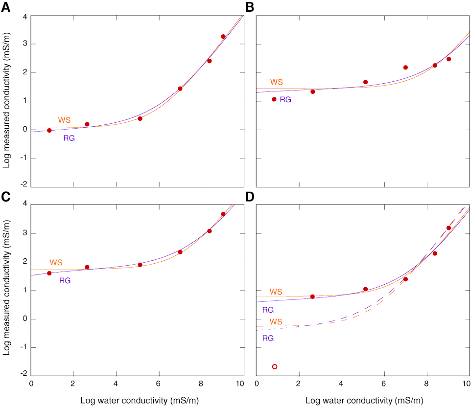
Figure F1. Examples of plots of core conductivities as a function of saturating fluid conductivities (log measured conductivity [C0] and log water conductivity [CW]). Best-fit curves are calculated using Waxman and Smits (1968) (WS, orange curve) and Revil and Glover (1998) (RG, purple curve) models. A. Good fit example. B. Bad fit example (higher errors on F and CS estimates, see Fig. F2). C. Good fit example with deflection of RG fit curve at low salinities, pointing to lower surface conductivities. D. Example of curve in which a good fit is obtained by removing a point (in this case, lowest salinity) that is several order of magnitudes out of range compared to adjacent point. See text for further explanations.

Close | Next | Top of page