Li, C.-F., Lin, J., Kulhanek, D.K., and the Expedition 349 Scientists, 2015
Proceedings of the International Ocean Discovery Program Volume 349
publications.iodp.org

doi:10.14379/iodp.proc.349.102.2015
Methods1
C.-F. Li, J. Lin, D.K. Kulhanek, T. Williams, R. Bao, A. Briais, E.A. Brown, Y. Chen, P.D. Clift, F.S. Colwell, K.A. Dadd, W.-W. Ding, I. Hernández-Almeida, X.-L. Huang, S. Hyun, T. Jiang, A.A.P. Koppers, Q. Li, C. Liu, Q. Liu, Z. Liu, R.H. Nagai, A. Peleo-Alampay, X. Su, Z. Sun, M.L.G. Tejada, H.S. Trinh, Y.-C. Yeh, C. Zhang, F. Zhang, G.-L. Zhang, and X. Zhao2
Keywords: International Ocean Discovery Program, IODP, JOIDES Resolution, Expedition 349, Site U1431, Site U1432, Site U1433, Site U1434, Site U1435, South China Sea, structural analysis, paleomagnetism, thermal demagnetization, igneous petrology, alteration, core description, microbial contamination tracers, microbiology, organic geochemistry, inorganic chemistry, physical properties, visual core description, ICP measurement, biostratigraphy, downhole measurements
MS 349-102: Published 30 March 2015
Introduction, background, and operations
Site locations
GPS coordinates from precruise site surveys were used to position the vessel at all International Ocean Discovery Program (IODP) Expedition 349 sites. A SyQuest Bathy 2010 CHIRP subbottom profiler was used to monitor seafloor depth on the approach to each site to reconfirm the depth profiles from precruise surveys. Once the vessel was positioned at a site, the thrusters were lowered, and a positioning beacon was dropped to the seafloor. The dynamic positioning control of the vessel used navigational input from the GPS and triangulation to the seafloor beacon, weighted by the estimated positional accuracy. The final hole position was the mean position calculated from the GPS data collected over a significant time interval.
Coring and drilling operations
All three standard coring systems, the advanced piston corer (APC), extended core barrel (XCB), and rotary core barrel (RCB), were used during Expedition 349. The APC was used in the upper portion of each hole to obtain high-quality core. The APC cuts soft-sediment cores with minimal coring disturbance relative to other IODP coring systems. After the APC core barrel is lowered through the drill pipe and lands near the bit, the drill pipe is pressured up until the two shear pins that hold the inner barrel attached to the outer barrel fail. The inner barrel then advances into the formation and cuts the core (Figure F1). The driller can detect a successful cut, or “full stroke,” from the pressure gauge on the rig floor.
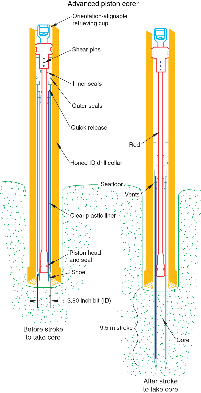
Figure F1. APC system schematic.
APC refusal is conventionally defined in two ways: (1) the piston fails to achieve a complete stroke (as determined from the pump pressure reading) because the formation is too hard or (2) excessive force (>60,000 lb; ~267 kN) is required to pull the core barrel out of the formation. When a full stroke cannot be achieved, additional attempts are typically made, and after each attempt the bit is advanced by the length of core recovered. The number of additional attempts is generally dictated by the length of recovery of the partial stroke core and the time available to advance the hole by piston coring. Note that this results in a nominal recovery of ~100% based on the assumption that the barrel penetrates the formation by the equivalent of the length of core recovered. When a full or partial stroke is achieved but excessive force cannot retrieve the barrel, the core barrel is sometimes “drilled over,” meaning after the inner core barrel is successfully shot into the formation, the drill bit is advanced to total depth to free the APC barrel.
Nonmagnetic core barrels were used during all conventional APC coring to a pull force of ~40,000 lb. Except for cores taken in Hole U1432C, APC cores recovered during Expedition 349 were oriented using the FlexIT tool (see Paleomagnetism). Formation temperature measurements were made to obtain temperature gradients and heat flow estimates (see Downhole measurements) for all APC sections.
The XCB was used to advance the hole when APC refusal occurred before the target depth was reached or when the formation became either too stiff for APC coring or hard substrate was encountered. The XCB is a rotary system with a small cutting shoe (bit) that extends below the large APC/XCB bit. The smaller bit can cut a semi-indurated core with less torque and fluid circulation than the main bit, optimizing recovery. The XCB cutting shoe extends ~30.5 cm ahead of the main bit in soft sediment but retracts into the main bit when hard formations are encountered (Figure F2). During Expedition 349, the XCB was only used at Site U1431. This system was not subsequently used because of poor core quality (the XCB cores collected at Site U1431 were highly biscuited) and the significant drilling-induced magnetic overprint resulting from the use of steel core barrels that are required for XCB coring. This overprint could not be removed by thermal demagnetization during shipboard analyses.
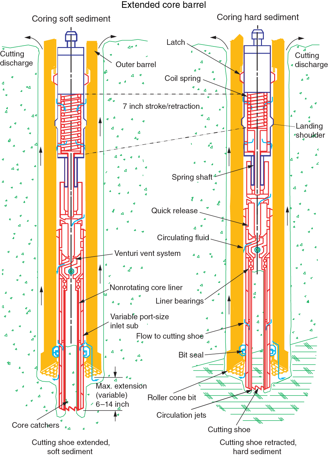
Figure F2. XCB system schematic.
The bottom-hole assembly (BHA) is the lowermost part of the drill string. The exact configuration of the BHA is reported in the operations section of each site chapter. A typical APC/XCB BHA consisted of a drill bit (outer diameter = 11⁷⁄₁₆ inch), a bit sub, a seal bore drill collar, a landing saver sub, a modified top sub, a modified head sub, a nonmagnetic drill collar (for APC/XCB), a number of 8 inch (~20.32 cm) drill collars, a tapered drill collar, six joints (two stands) of 5½ inch (~13.97 cm) drill pipe, and one crossover sub. A lockable float valve was used when downhole logging was planned so downhole logs could be collected through the bit.
The RCB was deployed when basement coring was expected (Figure F3). The RCB is the most conventional rotary drilling system and was used during Expedition 349 to drill and core into basement. The RCB requires a dedicated RCB BHA and a dedicated RCB drilling bit. The BHA used for RCB coring included a 9⅞ inch RCB drill bit, a mechanical bit release (if logging was considered), a modified head sub, an outer core barrel, a modified top sub, a modified head sub, and 7 to 10 control-length drill collars followed by a tapered drill collar to the two stands of 5½ inch drill pipe. Most cored intervals were ~9.7 m long, which is the length of a standard rotary core and approximately the length of a joint of drill pipe. In some cases, the drill string was drilled or “washed” ahead without recovering sediment to advance the drill bit to a target depth to resume core recovery. Such intervals were typically drilled using a center bit installed within the RCB bit. When coring basement, half-cores were sometimes collected to improve recovery and when rates of penetration decreased significantly.
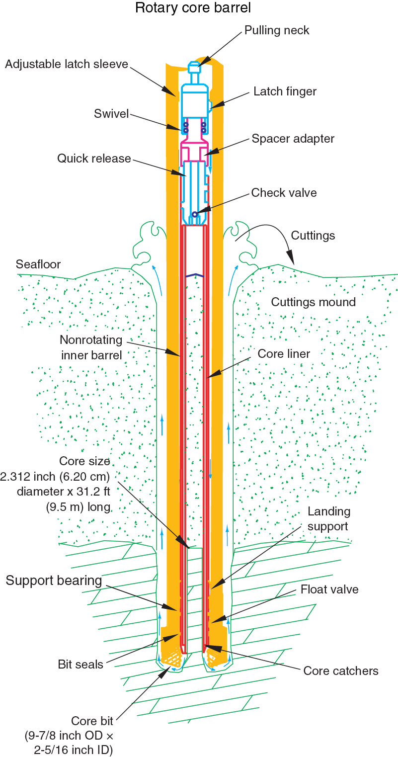
Figure F3. RCB system schematic.
IODP depth scales
Primary depth scale types are based on the measurement of drill string length (e.g., drilling depth below rig floor [DRF] and drilling depth below seafloor [DSF]), length of core recovered (e.g., core depth below seafloor [CSF]), and logging wireline (e.g., wireline log depth below rig floor [WRF] and wireline log depth below seafloor [WSF]). All units are in meters. The relationship between scales is defined either by protocol, such as the rules for computation of CSF from DSF, or by a combination of protocols with user-defined correlations. The distinction in nomenclature should keep the user aware that a nominal depth value at two different depth scales usually does not refer to exactly the same stratigraphic interval (see Curatorial procedures and sample depth calculations). For editorial convenience, we use meters below seafloor (mbsf) for the CSF-A depth scale throughout this volume.
Core handling and analysis
The coring strategy for Expedition 349 consisted of APC coring in one hole (Hole A) at each site to refusal, except at Site U1431, where five holes were cored with the APC. Multiple holes at this site allowed high-resolution sampling for specific objectives (e.g., microbiology, interstitial water measurements, and optically stimulated luminescence dating). APC refusal was followed by XCB coring at Site U1431 to ~617 mbsf. RCB coring was employed to reach and core into basement at all sites except Site U1432.
Cores recovered during Expedition 349 were extracted from the core barrel in 67 mm diameter plastic liners. These liners were carried from the rig floor to the core processing area on the catwalk outside the Core Laboratory, where they were split into ~1.5 m sections. Liner caps (blue = top, colorless = bottom, and yellow = whole-round sample taken) were glued with acetone onto liner sections on the catwalk by the Marine Technicians. The length of each section was entered into the database as “created length” using the Sample Master application. This number was used to calculate core recovery. Sections were cut into smaller lengths on cores taken from Holes U1431A and U1431B to allow for interstitial water whole rounds, microbiological whole rounds, and optically stimulated luminescence dating whole rounds to be taken at 50 cm resolution. A normal section length of 1.5 m was resumed following this high-resolution sampling in these two holes.
For sedimentary sections, as soon as cores arrived on deck, headspace samples were taken using a syringe for immediate hydrocarbon analysis as part of the shipboard safety and pollution prevention program. Core catcher samples were taken for biostratigraphic analysis. Whole-round samples were taken from some core sections for shipboard and postcruise interstitial water analyses. Rhizon interstitial water samples and syringe samples were taken from selected intervals in addition to whole rounds (see Geochemistry). In addition, whole-round and syringe samples were immediately taken from the ends of some cut sections for shore-based microbiological analysis.
Hard rock core pieces were slid out of the liners and placed in order in new, clean sections of core liner that had previously been split in half. Pieces having a vertical length greater than the internal (horizontal) diameter of the core liner are considered oriented pieces because they could have rotated only around their vertical axes. Those pieces were immediately marked on the bottom with a red wax pencil to preserve their vertical (upward) orientations. Pieces that were too small to be oriented with certainty were left unmarked. Adjacent but broken core pieces that could be fit together along fractures were curated as single pieces. The structural geologist or petrologist on shift confirmed the piece matches and corrected any errors. The structural geologist or petrologist also marked a split line on the pieces, which defined how the pieces should be cut into two equal halves. The aim was to maximize the expression of dipping structures on the cut face of the core while maintaining representative features in both archive and working halves. Whole-round microbiology samples were taken in the splitting room immediately after the core was slid from the liner. The petrologist on duty monitored the microbiology sampling to ensure that no critical petrographic interval was depleted. All microbiology whole-round samples were photographed and documented before being removed from the core. A foam spacer was used to mark where a microbiological sample was taken.
Core sections were then placed in core racks in the laboratory. When the cores reached equilibrium with laboratory temperature (typically after ~4 h), whole-round core sections were run through the Whole-Round Multisensor Logger (WRMSL; measuring P-wave velocity, density, and magnetic susceptibility) and the Natural Gamma Radiation Logger (NGRL). Thermal conductivity measurements were typically taken at a rate of one per core (see Physical properties). The core sections were then split lengthwise from bottom to top into working and archive halves. Investigators should note that older material may have been transported upward on the split face of each section during splitting. For hard rock sections, each piece of core was split with a diamond-impregnated saw into archive and working halves, with the positions of the plastic spacers between individual pieces maintained in both halves of the plastic liner. Pieces were numbered sequentially from the top of each section. Separate subpieces within a single piece were assigned the same number but were lettered consecutively (e.g., 1A, 1B, and 1C). Pieces were labeled only on the outer cylindrical surface of the core or on the core liner.
The working half of each sedimentary core was sampled for shipboard biostratigraphic, physical property, carbonate, paleomagnetic, and inductively coupled plasma–atomic emission spectroscopy (ICP-AES) analyses. The archive half of all cores was scanned on the Section Half Imaging Logger (SHIL) with a line scan camera at 20 pixels/mm and measured for color reflectance and magnetic susceptibility on the Section Half Multisensor Logger (SHMSL). At the same time, the archive halves were described visually and by means of smear slides and thin sections. All observations were recorded in the Laboratory Information Management System (LIMS) database using DESClogik, a descriptive data capture application. After visual description, the archive halves were run through the cryogenic magnetometer. Finally, digital color close-up images were taken of particular features of the archive or working halves, as requested by individual scientists. For hard rock cores, a sampling meeting was held at 1200 h to select key sampling intervals for shipboard analyses. Discrete samples were taken from working halves for physical property, paleomagnetic, thin section, and ICP-AES analyses. Records of all samples taken are kept by the IODP curator. Sampling for personal postcruise research was conducted immediately after splitting for sedimentary sequences and during several sampling parties over the course of the expedition for hard rock.
Both halves of the core were put into labeled plastic tubes that were sealed and transferred to cold storage space aboard the ship. At the end of the expedition, the cores were transported from the ship to permanent cold storage at the Kochi Core Center (KCC) at Kochi University in Kochi, Japan. The KCC houses cores collected from the western Pacific Ocean, Indian Ocean, Kerguelen Plateau, and Bering Sea.
Drilling disturbance
Cores may be significantly disturbed as a result of the drilling process and may contain extraneous material as a result of the coring and core handling process. In formations with loose sand layers, sand from intervals higher in the hole may be washed down by drilling circulation, accumulate at the bottom of the hole, and be sampled with the next core. The uppermost 10–50 cm of each core must therefore be examined critically during description for potential “fall-in.” Common coring-induced deformation includes the concave-downward appearance of originally horizontal bedding. Piston action may result in fluidization (flow-in) at the bottom of APC cores. Retrieval from depth to the surface may result in elastic rebound. Gas that is in solution at depth may become free and drive core segments within the liner apart. Both elastic rebound and gas pressure can result in a total length for each core that is longer than the interval that was cored and thus a calculated recovery of >100%. If gas expansion or other coring disturbance results in a void in any particular core section, the void can be closed by moving material if very large, stabilized by a foam insert if moderately large, or left as is. When gas content is high, pressure must be relieved for safety reasons before the cores are cut into segments. This is accomplished by drilling holes into the liner, which forces some sediment as well as gas out of the liner. These disturbances are described in the Lithostratigraphy sections in each site chapter and are graphically indicated on the core summary graphic reports (visual core descriptions [VCDs]). In extreme instances core material can be ejected from the core barrel, sometimes violently, onto the rig floor by high pressure in the core or other coring problems. This core material is replaced in the plastic core liner by hand and should not be considered to be in stratigraphic order. Core sections so affected are marked by a yellow label marked “disturbed,” and the nature of the disturbance is noted in the coring log.
Curatorial procedures and sample depth calculations
Numbering of sites, holes, cores, and samples follows standard IODP procedure (Figure F4). Drilling sites are numbered consecutively from the first site drilled by the D/V Glomar Challenger in 1968. Integrated Ocean Drilling Program Expedition 301 began using the prefix “U” to designate sites occupied by the United States Implementing Organization (USIO) platform, the R/V JOIDES Resolution. For all IODP drill sites, a letter suffix distinguishes each hole drilled at the same site. The first hole drilled is assigned the site number modified by the suffix “A,” the second hole the site number and the suffix “B,” and so on.
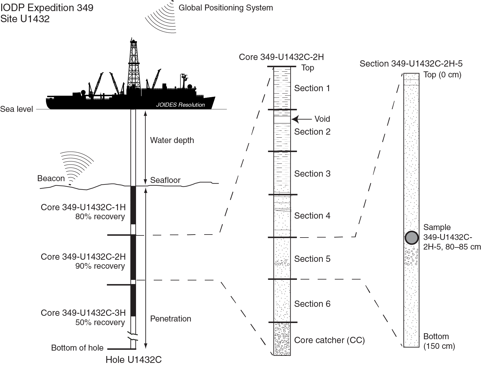
Figure F4. IODP sample naming convention.
Cored intervals are defined by the core top depth in DSF and the distance the driller advanced the bit and/or core barrel in meters. The length of the core is defined by the sum of lengths of the core sections. The CSF depth of a sample is calculated by adding the offset of the sample below the section top and the lengths of all higher sections in the core to the core top depth measured with the drill string (DSF). During Expedition 349, all core depths below seafloor were calculated according to the CSF, Method A (CSF-A), depth scale (see IODP Depth Scales Terminology, v.2, at www.iodp.org/program-policies). To more easily communicate shipboard results, CSF-A depths are reported in this volume as mbsf unless otherwise noted.
Cores taken from a hole are numbered sequentially from the top of the hole downward. When an interval is drilled down, this interval is also numbered sequentially and the drill down designated by a “1” instead of a letter that designates the coring method used (e.g., 349-U1431E-11). Cores taken with the APC system are designated with “H,” “X” designates XCB cores, and “R” designates RCB cores. “G” designates “ghost” cores that are collected while washing down through a previously drilled portion of a hole with a core barrel in place. The core barrel is then retrieved prior to coring the next interval. Core numbers and their associated cored intervals are unique in a given hole. Generally, maximum recovery for a single core is 9.5 m of sediment (APC) or 9.7 m of rock or sediment (XCB/RCB) contained in a plastic liner (6.6 cm internal diameter) plus an additional ~0.2 m in the core catcher, which is a device at the bottom of the core barrel that prevents the core from sliding out when the barrel is retrieved from the hole. In certain situations, recovery may exceed the 9.5 or 9.7 m maximum. In soft sediment, this is normally caused by core expansion resulting from depressurization. In hard rock cores, this typically occurs when a pedestal of rock fails to break off and is grabbed by the core barrel of the subsequent core. High heave, tidal changes, and overdrilling can also result in an advance that differs from the planned 9.5/9.7 m.
Recovered cores are divided into 1.5 m sections that are numbered serially from the top downward (except for Holes U1431A and U1431B, which were cut into sections 0.5 m long to accommodate high-resolution whole-round sampling). When full recovery is obtained, the sections are numbered 1–7, with the last section usually being <1.5 m. Rarely, an unusually long core may require more than seven sections. When the recovered core is shorter than the cored interval, by convention the top of the core is deemed to be located at the top of the cored interval for the purpose of calculating (consistent) depths. When coring hard rock, all pieces recovered are placed immediately adjacent to each other in the core tray. Samples and descriptions of cores are designated by distance, measured in centimeters, from the top of the section to the top and bottom of each sample or interval. By convention, hard rock material recovered from the core catcher is placed below the last section. In sedimentary cores, the core catcher section is treated as a separate section (“CC”). When the only recovered material is in the core catcher, it is placed at the top of the cored interval.
A full curatorial sample identifier consists of the following information: expedition, site, hole, core number, core type, section number, and interval in centimeters measured from the top of the core section. For example, a sample identification of “349-U1432C-2H-5, 80–85 cm,” represents a sample taken from the interval between 80 and 85 cm below the top of Section 5 of Core 2 (collected using the APC system) of Hole C of Site U1432 during Expedition 349 (Figure F4).
Authorship of site chapters
The separate sections of the site chapters and Methods chapter were written by the following shipboard scientists (authors are listed in alphabetical order; no seniority is implied):
- Background and objectives: D.K. Kulhanek, C.-F. Li, J. Lin
- Operations: D.K. Kulhanek, S. Midgley
- Lithostratigraphy: P.D. Clift, K.A. Dadd, S. Hyun, T. Jiang, Z. Liu
- Biostratigraphy: E.A. Brown, I. Hernández-Almeida, Q. Li, C. Liu, R.H. Nagai, A. Peleo-Alampay, X. Su
- Igneous petrology and alteration: A.A.P. Koppers, M.L.G. Tejada, G.-L. Zhang
- Structural geology: W.-W. Ding, Z. Sun
- Geochemistry: R. Bao, Y. Chen, X.-L. Huang
- Microbiology: F.S. Colwell, C. Zhang
- Paleomagnetism: Q. Liu, X. Zhao
- Physical properties: A. Briais, H.S. Trinh, Y.-C. Yeh, F. Zhang
- Downhole measurements: T. Williams
Lithostratigraphy
The lithology of sediment recovered during Expedition 349 was primarily determined using observations based on visual (macroscopic) core description, smear slides, and thin sections. In some cases, digital core imaging, color reflectance spectrophotometry, and magnetic susceptibility analysis provided complementary discriminative information. The methods employed during this expedition were similar to those used during Integrated Ocean Drilling Program Expeditions 330 and 339 (Expedition 330 Scientists, 2012; Expedition 339 Scientists, 2013). We used the DESClogik application to record and upload descriptive data into the LIMS database (see the DESClogik user guide at iodp.tamu.edu/labs/documentation). Spreadsheet templates were set up in DESClogik and customized for Expedition 349 before the first core on deck. The templates were used to record visual core descriptions as well as microscopic data from smear slides and thin sections, which were also used to quantify the texture and relative abundance of biogenic and nonbiogenic components. The locations of all smear slide and thin section samples taken from each core were recorded in the Sample Master application. Descriptive data uploaded to the LIMS database were also used to produce the VCD standard graphic reports.
Visual core descriptions
After descriptions of the cores were uploaded into the LIMS database, the data were used to produce VCDs, which include a simplified graphical representation of the core on a section-by-section basis with accompanying descriptions of the features observed (Figures F5, F6, F7). Depending on the type of material recovered, two VCDs were sometimes produced for the same section: one to describe sediments or sedimentary rocks and the other to describe igneous rocks.
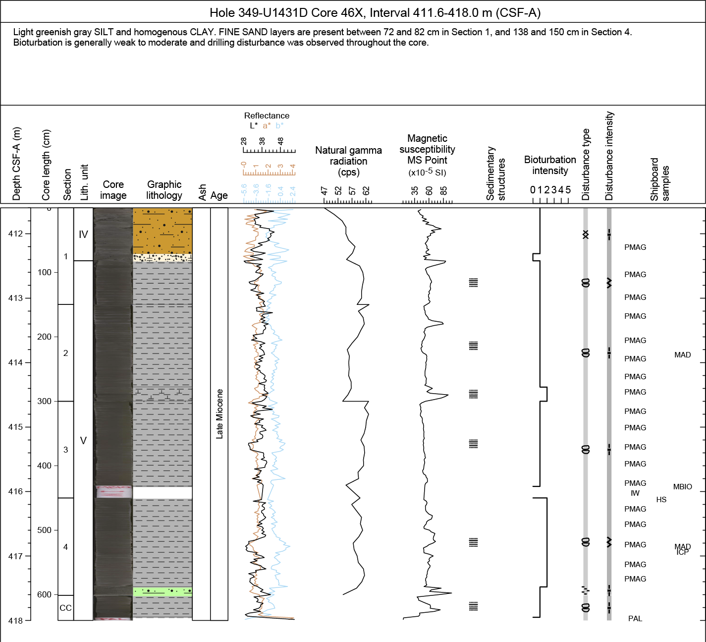
Figure F5. Example sedimentary VCD form.
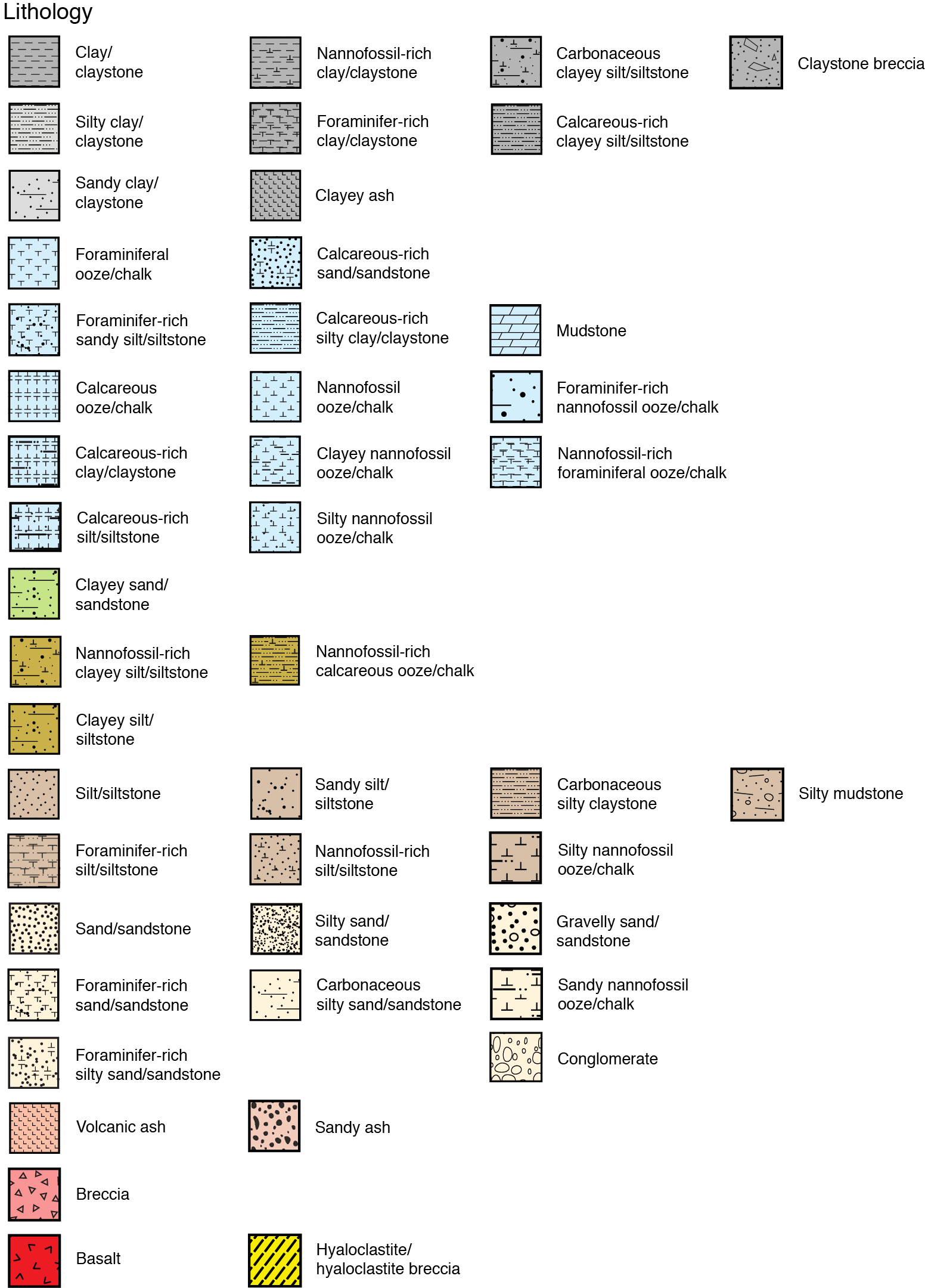
Figure F6. VCD lithology symbols.
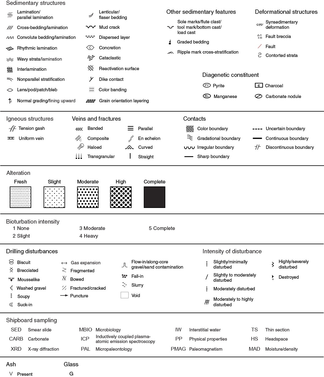
Figure F7. VCD symbols and nomenclature.
Site, hole, and depth in meters below seafloor, calculated according to the CSF-A depth scale, are given at the top of each VCD, with depth of core sections indicated along the left margin. Observations of the physical description of the core correspond to entries in DESClogik, including bioturbation intensity, fossils, ash layers, lithologic accessories, sedimentary structures, and drilling disturbance. Symbols used in the VCDs are given in Figures F6 and F7. Additionally, sedimentary VCDs display magnetic susceptibility, natural gamma radiation, color reflectance, and the locations of samples taken for shipboard measurements. Section summary text provides a generalized overview of the core section’s lithology and features. This summary text and individual columns shown on the VCDs are described below in greater detail, followed by an outline of the lithostratigraphic classification system used during Expedition 349.
Section summary
A brief overview of major and minor lithologies present in the section, as well as notable features (e.g., sedimentary structures), is presented in the section summary text field at the top of the VCDs. The summary includes sediment color determined qualitatively using Munsell soil color charts. Because sediment color may evolve during drying and subsequent oxidization, color was described shortly after the cores were split and imaged or measured by the SHIL and SHMSL.
Section-half image
The flat faces of the archive halves were scanned with the SHIL as soon as possible after splitting and scraping to avoid color changes caused by sediment oxidation and drying. The SHIL uses three pairs of advanced illumination high-current-focused LED line lights to illuminate large cracks and blocks in the core surface and sidewalls. Each LED pair has a color temperature of 6,500 K and emits 90,000 lx at 3 inches. A line-scan camera images 10 lines/mm to create a high-resolution TIFF file. The camera height was adjusted so that each pixel imaged a 0.1 mm2 section of the core. However, actual core width per pixel varied because of differences in section-half surface height. High- and low-resolution JPEG files were subsequently created from the high-resolution TIFF file. All image files include a gray scale and ruler. Section-half depths were recorded so that these images could be used for core description and analysis.
Graphic lithology
Lithologies of the core intervals recovered are represented on the VCD sheets by graphic patterns in the Graphic lithology column, using the symbols illustrated in Figure F6. The Graphic lithology column on each VCD plots to scale all beds that are at least 2 cm thick. A maximum of two different lithologies (for interbedded sediment) are shown within the same core interval for interlayers <2 cm thick. The major modifier of a primary lithology is shown using a modified version of the primary lithology pattern. Lithologic abundances are rounded to the nearest 10%; lithologies that constitute <10% of the core are generally not shown but are listed in the Description section. However, some distinctive secondary lithologies, such as ash layers, are included graphically in the Graphic lithology column as the primary lithology for a thin stratigraphic interval. Relative abundances of lithologies reported in this way are useful for general characterization of the sediment but do not constitute precise, quantitative observations.
Spectrophotometry and magnetic susceptibility of the archive section halves were measured with the SHMSL. The SHMSL takes measurements in empty intervals and over intervals where the core surface is well below the level of the core liner, but it cannot recognize relatively small cracks, disturbed areas of core, or plastic section dividers. Thus, SHMSL data may contain spurious measurements that have to be edited out of the data set by the user. Additional detailed information about measurement and interpretation of spectral data can be found in Balsam et al. (1997, 1998) and Balsam and Damuth (2000).
Spectrophotometry
Reflectance of visible light from the archive halves of sediment cores was measured using an Ocean Optics USB4000 spectrophotometer mounted on the automated SHMSL. Freshly split soft cores were covered with clear plastic wrap and placed on the SHMSL. Measurements were taken at 1.0 or 2.0 cm spacings to provide a high-resolution stratigraphic record of color variations for visible wavelengths. Each measurement was recorded in 2 nm wide spectral bands from 400 to 900 nm. Reflectance parameters of L*, a*, and b* were recorded.
Natural gamma radiation
Natural gamma radiation occurs primarily as a result of the decay of 238U, 232Th, and 40K isotopes. This radiation is measured using the NGRL (see Physical properties). Data generated from this instrument are used to augment geologic interpretations.
Magnetic susceptibility
Magnetic susceptibility was measured with a Bartington Instruments MS2E point sensor (high-resolution surface-scanning sensor) on the SHMSL. Because the SHMSL demands flush contact between the magnetic susceptibility point sensor and the split core, measurements were made on the archive halves of split cores that were covered with clear plastic wrap. Measurements were taken at 1.0 or 2.0 cm spacings. Measurement resolution was 1.0 SI, and each measurement integrated a volume of 10.5 mm × 3.8 mm × 4 mm, where 10.5 mm is the length perpendicular to the core axis, 3.8 mm is the width along the core axis, and 4 mm is the depth into the core. Only one measurement was taken at each measurement position.
Sedimentary structures
The locations and types of stratification and sedimentary structures visible on the prepared surfaces of the split cores are shown in the Sedimentary structures column of the VCD sheet. Symbols in this column indicate the locations and scales of interstratification, as well as the locations of individual bedding features and any other sedimentary features, such as sole marks, cross-lamination, and upward-fining intervals (Figure F7).
For Expedition 349, the following terminology (based on Stow, 2005) was used to describe the scale of stratification:
- Thin lamination = <3 mm thick.
- Medium lamination = 0.3–0.6 cm thick.
- Thick lamination = 0.6–1 cm thick.
- Very thin bed = 1–3 cm thick.
- Thin bed = 3–10 cm thick.
- Medium bed = 10–30 cm thick.
- Thick bed = 30–100 cm thick.
- Very thick bed = >100 cm thick.
Lithologic accessories
Some postdepositional features (e.g., concretions) and grains of special interest (e.g., pumice and coated grains) are recorded in the Lithologic accessories column.
Bioturbation intensity
Five levels of bioturbation are recognized using a scheme similar to that of Droser and Bottjer (1986). These levels are illustrated with a numeric scale in the Bioturbation intensity column. Any identifiable trace fossils (ichnofossils) are identified in the bioturbation comments in the core description.
- 1 = no bioturbation.
- 2 = slight bioturbation (<10%–30%).
- 3 = moderate bioturbation (30%–60%).
- 4 = heavy bioturbation (60%–90%).
- 5 = complete bioturbation (>90%).
Sediment disturbance
Drilling-related sediment disturbance is recorded in the Disturbance type column using the symbols shown in Figure F7. The style of drilling disturbance is described for soft and firm sediments using the following terms:
- Fall-in: out-of-place material at the top of a core has fallen downhole onto the cored surface.
- Bowed: bedding contacts are slightly to moderately deformed but still subhorizontal and continuous.
- Flow-in, coring/drilling slurry, along-core gravel/sand contamination: soft-sediment stretching and/or compressional shearing structures are severe and are attributed to coring/drilling. The particular type of deformation may also be noted (e.g., flow-in, gas expansion, etc.).
- Soupy or mousse-like: intervals are water saturated and have lost all aspects of original bedding.
- Biscuit: sediments of intermediate stiffness show vertical variations in the degree of disturbance. Softer intervals are washed and/or soupy, whereas firmer intervals are relatively undisturbed.
- Cracked or fractured: firm sediments are broken but not displaced or rotated significantly.
- Fragmented or brecciated: firm sediments are pervasively broken and may be displaced or rotated.
The degree of fracturing within indurated sediments is described using the following categories:
- Slightly fractured: core pieces are in place and broken.
- Moderately fractured: core pieces are in place or partly displaced, but original orientation is preserved or recognizable.
- Highly fractured: core pieces are probably in correct stratigraphic sequence, but original orientation is lost.
- Drilling breccia: core is crushed and broken into many small and angular pieces, with original orientation and stratigraphic position lost.
Age
The subepoch that defines the age of the sediments was provided by the shipboard biostratigraphers (see Biostratigraphy) and is listed in the Age column.
Samples
The exact positions of samples used for microscopic descriptions (i.e., smear slides and thin sections), biochronological determinations, and shipboard analysis of chemical and physical properties of sediment are recorded in the Shipboard samples column.
Sediment classification
The sediment recovered during Expedition 349 is composed of biogenic and siliciclastic components and is described using a classification scheme derived from Expedition 339 (Expedition 339 Scientists, 2013) and Stow (2005). The biogenic component is composed of the skeletal debris of open-marine calcareous and siliceous microfauna (e.g., foraminifers and radiolarians), microflora (e.g., calcareous nannofossils and diatoms), and macrofossil shell fragments. The siliciclastic component is composed of mineral and rock fragments derived from igneous, sedimentary, and metamorphic rocks. The relative proportion of these two components is used to define the major classes of sediment in this scheme (Figure F8).
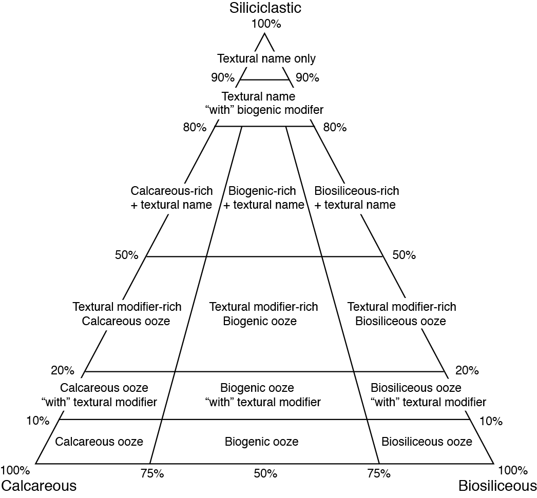
Figure F8. Sediment naming convention.
Naming conventions for Expedition 349 follow the general guidelines of the Ocean Drilling Program (ODP) sediment classification scheme (Mazzullo et al., 1988), with the exception that a separate “mixed sediment” category was not distinguished during Expedition 349. As a result, biogenic sediment is that which contains >50% biogenic grains and <50% siliciclastic grains, whereas siliciclastic sediment is that which contains >50% siliciclastic grains and <50% biogenic grains. Sediment containing >50% silt- and sand-sized primary volcanic grains is classified as an ash layer. We follow the naming scheme of Shepard (1954) for the classification of siliciclastic sediment and sedimentary rock depending on the relative proportion of sediment of different grain sizes (Figure F9). Sediment grain size divisions for both biogenic and siliciclastic components are based on Wentworth (1922), with eight major textural categories defined on the basis of the relative proportions of sand-, silt-, and clay-sized particles (Figure F10); however, distinguishing between some of these categories can be difficult (e.g., silty clay versus sandy clay) without accurate measurements of grain size abundances. The term “clay” is only used to describe particle size and is applied to both clay minerals and all other grains <4 µm in size.

Figure F9. Textural naming convention.
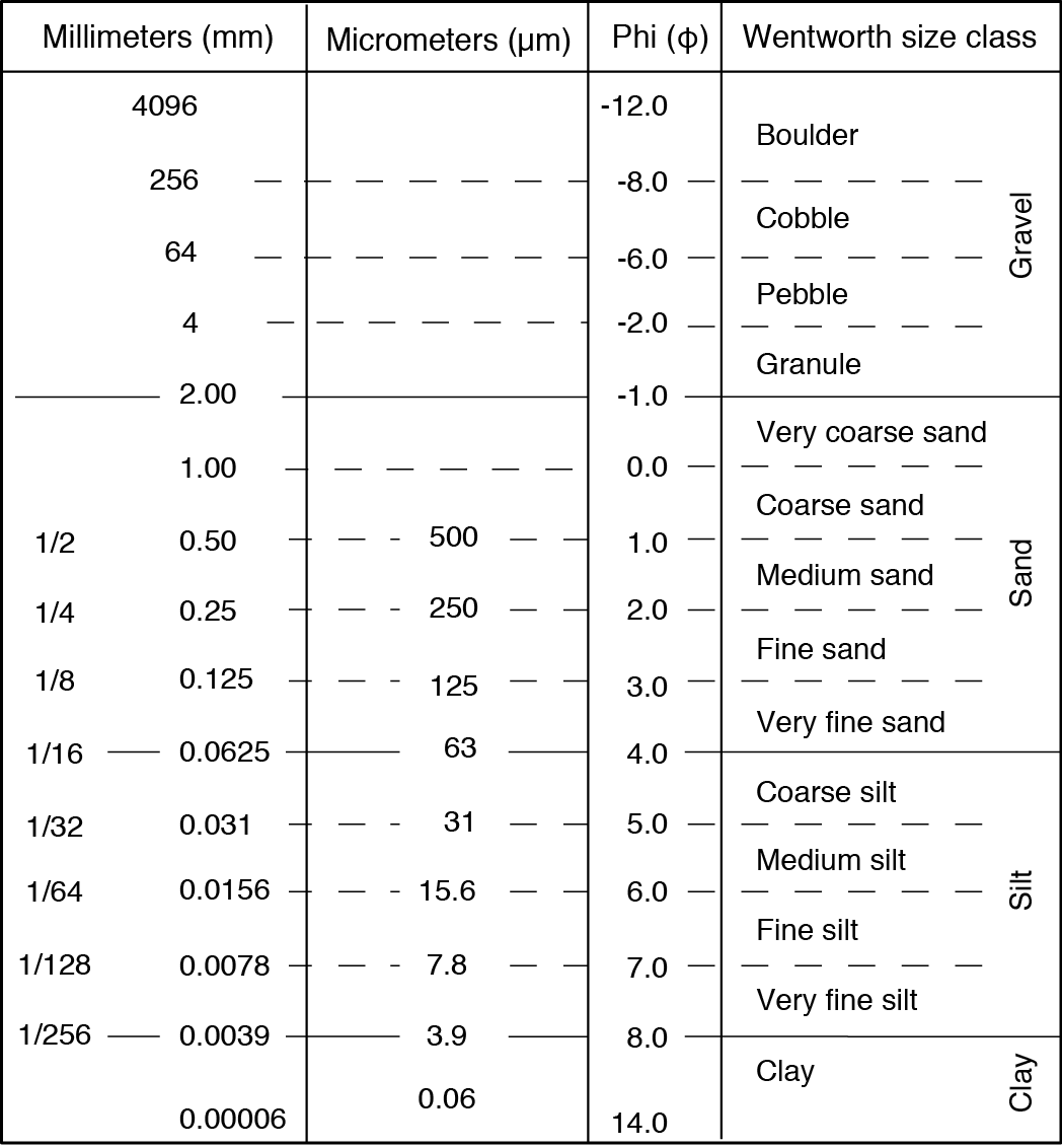
Figure F10. Grain-size classification.
The lithologic names assigned to sediment consists of a principal name and prefix based on composition and degree of lithification and/or texture as determined from visual description of the cores and from smear slide observations.
For a sediment that contains >90% of one component (either the siliciclastic or biogenic component), only the principal name is used. For sediments with >90% biogenic components, the name applied indicates the most common type of biogenic grain. For example, a sediment composed of >90% calcareous nannofossils is called a nannofossil ooze/chalk, and a sediment composed of 50% foraminifers and 45% calcareous nannofossils is called a calcareous ooze/chalk. For sediment with >90% siliciclastic grains, the principal name is based on the textural characteristics of all sediment particles (both siliciclastic and biogenic) (Figure F9).
For sediment that contains a significant mixture of siliciclastic and biogenic components (between 10% and 90% of both siliciclastic and biogenic components), the principal name is determined by the more abundant component. If the siliciclastic component is more abundant, the principal name is based on the textural characteristics of all sediment particles (both siliciclastic and biogenic) (Figure F9). If the biogenic component is more abundant, the principal name is based on the predominant biogenic component.
If a microfossil group composes 10%–50% of the sediment and this group is not included as part of the principal name, minor modifiers are used. When a microfossil group (e.g., diatom, nannofossil, or foraminifer) comprises 20%–50% of the sediment, a minor modifier consisting of the component name hyphenated with the suffix “‑rich” (e.g., diatom-rich clay) is used.
If one component forms 80%–90% of the sediment, the principal name is followed by a minor modifier (e.g., “with diatoms”), with the minor modifier based on the most abundant component that forms 10%–20% of the sediment. If the minor component is biogenic, then the modifier describes the group of biogenic grains that exceeds the 10% abundance threshold. If the minor component is siliciclastic, the minor modifier is based on the texture of the siliciclastic fraction.
If the primary lithology for an interval of core has a major modifier, then that major modifier is indicated in the Graphic lithology column of the VCD sheets using a modified version of the lithologic pattern for the primary lithology (Figure F5). The modified lithologic patterns are shown in Figure F6. The minor modifiers of sediment lithologies are not included in the Graphic lithology column.
The following terms describe lithification that varies depending on the dominant composition:
- Sediment composed predominantly of calcareous, pelagic organisms (e.g., calcareous nannofossils and foraminifers): the lithification terms “ooze” and “chalk” reflect whether the sediment can be deformed with a finger (ooze) or can be scratched easily by a fingernail (chalk).
- Sediment composed predominantly of siliceous microfossils (diatoms, radiolarians, and siliceous sponge spicules): the lithification terms “ooze” and “radiolarite/diatomite” reflect whether the sediment can be deformed with a finger (ooze) or cannot be easily deformed manually (radiolarite/diatomite).
- Sediment composed of a mixture of calcareous pelagic organisms and siliceous microfossils and sediment composed of a mixture of siliceous microfossils: the lithification terms “ooze” and “indurated sediment” reflect whether the sediment can be deformed with a finger (ooze) or cannot be easily deformed manually (indurated sediment).
- Sediment composed predominantly of siliciclastic material: if the sediment can be deformed easily with a finger, no lithification term is added and the sediment is named for the dominant grain size (i.e., sand, silt, or clay). For more consolidated material, the lithification suffix “-stone” is appended to the dominant size classification (e.g., claystone), except for gravel-sized sediment, when the terms conglomerate or breccia are used.
The subclassification of volcaniclastic sediments followed here differs from the standard ODP classification (Mazzullo et al., 1988) in that we adopted a descriptive (nongenetic) terminology similar to that employed during ODP Leg 197 (Shipboard Scientific Party, 2002) and Integrated Ocean Drilling Program Expedition 324 (Expedition 324 Scientists, 2010). Unless an unequivocally pyroclastic origin for volcanogenic particles could be determined, we simply described these deposits as for siliciclastic sediment (i.e., sand, silt, etc.).
Where evidence for a pyroclastic origin was compelling, we adopted the classification scheme of Fisher and Schmincke (1984). In these instances, we used the grain size terms “volcanic blocks” (>64 mm), “lapilli/lapillistone” (2–64 mm), and “ash/tuff” (<2 mm). The term “hyaloclastite” was used for vitroclastic (i.e., glassy) materials produced by the interaction of water and hot magma or lava (Fisher and Schmincke, 1984).
Smear slide observation
Two or more smear slide samples of the main lithologies were collected from the archive half of each core when the sediment was not lithified. Additional samples were collected from areas of interest (e.g., laminations, ash layers, and nodules). A small amount of sediment was taken with a wooden toothpick and put on a 2.5 cm × 7.5 cm glass slide. The sediment sample was homogenized with a drop of deionized water and evenly spread across the slide to create a very thin (about <50 µm) uniform layer of sediment grains for quantification. The dispersed sample was dried on a hot plate. A drop of Norland optical adhesive was added as a mounting medium to a coverslip, which was carefully placed on the dried sample to prevent air bubbles from being trapped in the adhesive. The smear slide was then cured in an ultraviolet light box.
Smear slides were examined with a transmitted-light petrographic microscope equipped with a standard eyepiece micrometer. The texture of siliciclastic grains (relative abundance of sand-, silt-, and clay-sized grains) and the proportions and presence of biogenic and mineral components were recorded and entered into DESClogik. Biogenic and mineral components were identified, and their percentage abundances were visually estimated using Rothwell (1989). The mineralogy of clay-sized grains could not be determined from smear slides. Note that smear slide analyses tend to underestimate the amount of sand-sized and larger grains because these grains are difficult to incorporate onto the slide.
X-ray diffraction analyses
Since the shipboard X-ray diffractometer was unavailable during Expedition 349, samples for X-ray diffraction (XRD) were analyzed onshore following the expedition. Quantitative mineralogy of shipboard samples was analyzed using a PANalytical X’Pert PRO XRD at the State Key Laboratory of Marine Geology, Tongji University (China). About 3 g of sample (bulk sediment or sedimentary rock) was first dried in an oven at 60°C for 24 h. The sample was then powdered in an agate mortar. A sample holder with a hole 20 mm in diameter and 2.5 mm depth was filled with a random orientation of grains. The analysis was processed from 3° to 85°2θ at 0.0334°2θ step size, with CuKα radiation and Ni filter, under a voltage of 45 kV and an intensity of 40 mA. The sample holder was rotated at 60 rotations/min during scanning. The X’Pert HighScore Plus (version 2.2.5) software was used for identification and semiquantitative calculation of individual minerals. The average accuracy error for most minerals using this method is ±5%. XRD data are available in XRD in Supplementary material.
Biostratigraphy
During Expedition 349, calcareous nannofossils, radiolarians, and planktonic foraminifers in core catcher samples were studied at all sites. Samples from core sections were also examined when a more refined age determination was necessary and when time permitted. Biostratigraphic events, mainly the first appearance datum (FAD; or base) and last appearance datum (LAD; or top) of the diagnostic species, are tied to the geomagnetic polarity timescale (GPTS) of Gradstein et al. (2012) (Figures F11, F12, F13).

Figure F11. Microfossil events and GPTS, 0–13 Ma.
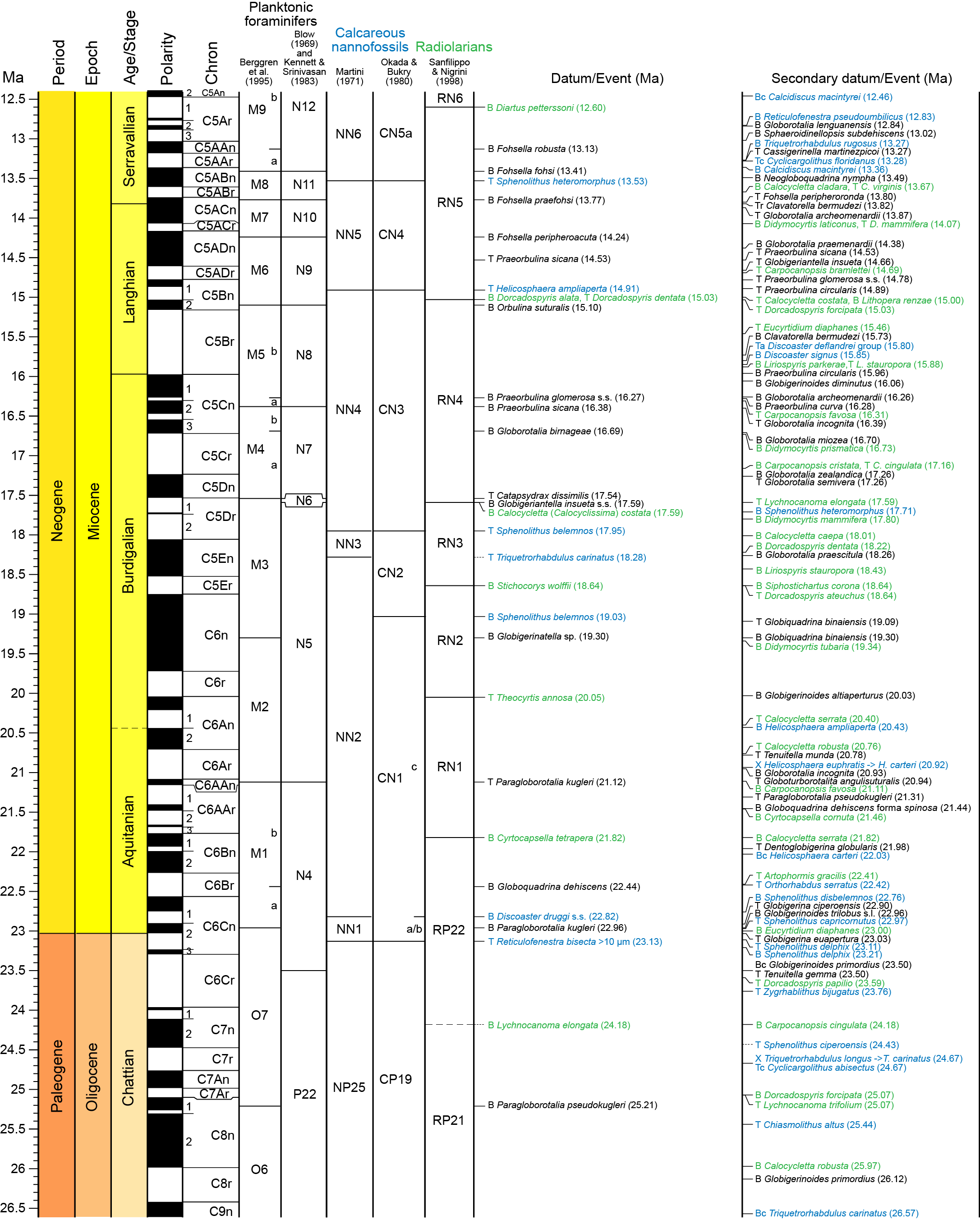
Figure F12. Microfossil events and GPTS, 12.5–26.5 Ma.
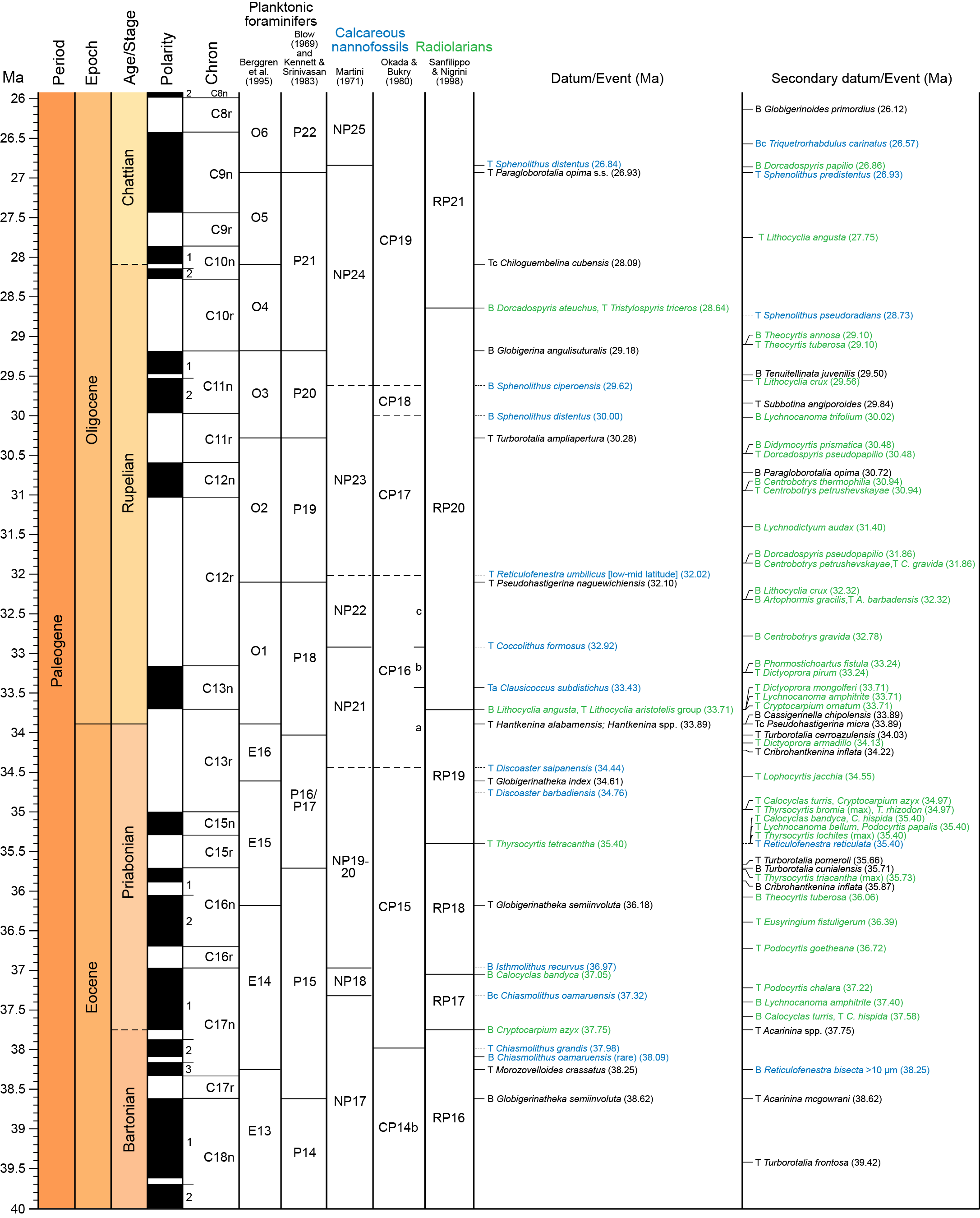
Figure F13. Microfossil events and GPTS, 26–40 Ma.
Calcareous nannofossils
Calcareous nannofossil zonation was based on the schemes of Okada and Bukry (1980) and Martini (1971). Calibrated ages for bioevents are from Gradstein et al. (2012) and given in Table T1. The timescale of Gradstein et al. (2012) assigns the Pleistocene/Pliocene boundary between the Gelasian and Piacenzian stages (2.59 Ma), the Pliocene/Miocene boundary between the Zanclean and Messinian stages (5.33 Ma), and the late/middle Miocene boundary at 11.63 Ma. For calcareous nannofossil biostratigraphy, the Pleistocene/Pliocene boundary now falls within Zone NN16 (Martini, 1971), between the LADs of Discoaster surculus (2.49 Ma) and Discoaster tamalis (2.8 Ma). The Pliocene/Miocene boundary falls within Zone NN12, between the LAD of Triquetrorhabdulus rugosus (5.28 Ma) and the FAD of Ceratolithus larrymayeri (5.34 Ma); however, C. larrymayeri was not noted in our samples, so we use the FAD of Ceratolithus acutus (5.35 Ma) as an alternative event. The late/middle Miocene boundary is placed within Zone NN7, between the last common appearance of Discoaster kugleri (11.58 Ma) and the first common appearance of D. kugleri (11.90 Ma). In this study, the identification of these geological time boundaries was mostly based on recognition of these nannofossil bioevents.
Table T1. Calcareous nannofossil events and ages (Gradstein et al., 2012 [GTS2012]) used during Expedition 349. Download table in .csv format.
Several species of the genus Gephyrocapsa, which are commonly used as Pleistocene biostratigraphic markers, often show a great range of variation in sizes and other morphological features, causing problems in identification (e.g., Samtleben, 1980; Su, 1996; Bollmann, 1997). Size-defined morphological groups of this genus (Young, 1998; Maiorano and Marino, 2004; Lourens et al., 2004; Raffi et al., 2006) were used as event markers during shipboard study, including the groups Gephyrocapsa sp. 3, medium Gephyrocapsa spp. (≥4 µm), large Gephyrocapsa spp. (≥5.5 µm), and small Gephyrocapsa spp. (<3.5 µm).
Several Reticulofenestra species with different coccolith and central opening sizes have been used as Neogene and Quaternary biostratigraphic markers; however, these parameters show considerable variations within and between “species,” making species differentiation difficult (e.g., Young, 1998; Su, 1996). In this study, we followed the definition of Reticulofenestra pseudoumbilicus by Young (1998) as having a maximum coccolith length >7 µm (similar to the size of its holotype), especially for specimens from its uppermost range in the early Pliocene. We distinguished Reticulofenestra asanoi from the similarly sized Pseudoemiliania lacunosa by the absence of slits on the shield (Su, 1996).
The LAD of Sphenolithus spp. (3.54 Ma) in Pliocene Zone NN16 was based on the LAD of Sphenolithus abies and Sphenolithus neoabies according to Raffi et al. (2006). Species concepts for other taxa mainly follow those of Perch-Nielsen (1985) and Bown (1998).
Methods
Calcareous nannofossil samples were prepared using standard smear slide techniques. For sandy sediment, suspended aliquots of the raw sample were utilized for analysis. Samples were examined with a Zeiss microscope under cross-polarized and plane-transmitted or phase contrast light at 1000× to 2000× magnification. A Hitachi TM3000 tabletop scanning electron microscope (SEM) was used to confirm the presence of small forms. Preservation of nannofossils was noted as follows:
- VG = very good (no evidence of dissolution and/or overgrowth).
- G = good (slight dissolution and/or overgrowth; specimens identifiable to the species level).
- M = moderate (some etching and/or overgrowth; most specimens identifiable to the species level).
- P = poor (severely etched or with overgrowth; most specimens cannot be identified at the species and/or generic level).
The relative abundance of calcareous nannofossils within the sediment was visually estimated at 500× magnification by referring to the particle abundance charts in Rothwell (1989) and reported using the following abundance categories:
- D = dominant (>90% of sediment particles).
- A = abundant (>50%–90% of sediment particles).
- C = common (>10%–50% of sediment particles).
- F = few (1%–10% of sediment particles).
- R = rare (<1% of sediment particles).
- B = barren (no nannofossils present in 100 fields of view [FOV]).
The relative abundance of individual calcareous nannofossil species or taxa groups was estimated at 1000× magnification:
- D = dominant (>50%, or 100 specimens per FOV).
- A = abundant (10%–50%, or 10–100 specimens per FOV).
- C = common (10%–10%, or 1–10 specimens per FOV).
- F = few (0.1%–1%, or 1 specimen per 1–10 FOV).
- R = rare (<0.1%, or <1 specimen per 10 FOV).
Planktonic foraminifers
The planktonic foraminiferal zonation schemes of Blow (1969, 1979) and Berggren et al. (1995), as modified by Wade et al. (2011), were used in this study. Calibrated ages for bioevents are from Gradstein et al. (2012), as given in Table T2. We also adopted the use of the LAD (0.12 Ma; Thompson et al., 1979) and FAD (0.40 Ma; Li, 1997) of Globigerinoides ruber (pink) as biostratigraphic indicators.
Table T2. Planktonic foraminiferal events and ages (Gradstein et al., 2012 [GTS2012]) used during Expedition 349. Download table in .csv format.
Taxonomic concepts for Neogene and Paleogene taxa mainly follow those of Kennett and Srinivasan (1983) and Bolli and Saunders (1985).
Methods
Core catcher samples (plus one sample per section, as needed) were soaked in distilled water or in a weak hydrogen peroxide solution when necessary, warmed on a hot plate, and washed over a 63 µm mesh sieve. Lithified material was crushed to pea size, heated in a hydrogen peroxide solution, and then sieved as above. All samples were dried in a <60°C oven. The dried samples were sieved over a 150 µm sieve, retaining the <150 µm size fraction for additional observation when necessary. The >150 µm size fraction specimens were examined under a Zeiss Discovery V8 microscope. The total abundance of planktonic foraminifers was defined as follows:
- A = abundant (>30% planktonic foraminifer specimens in total residue).
- C = common (10%–30% planktonic foraminifer specimens in total residue).
- R = rare (1%–10% planktonic foraminifer specimens in total residue).
- P = present (<1% planktonic foraminifer specimens in total residue).
- B = barren (no planktonic foraminifer specimens in total residue).
Individual planktonic foraminifers were recorded in qualitative terms based on an assessment of forms observed in a random sample of ~400 specimens from the >150 µm size fraction. Relative abundances were reported using the following categories:
- D = dominant (>30% of the assemblage).
- A = abundant (10%–30%).
- F = few (5%–10%).
- R = rare (1%–5%).
- P = present (<1%).
Planktonic foraminifer assemblage preservation was recorded as
- VG = very good (no evidence of breakage or dissolution).
- G = good (>80% of specimens unbroken with only minor evidence of diagenetic alteration).
- M = moderate (30%–80% of the specimens unbroken).
- P = poor (strongly recrystallized or dominated by fragments and broken or corroded specimens).
Radiolarians
Radiolarian biostratigraphy was mainly based on the zonation of Sanfilippo and Nigrini (1998), which uses the first and last appearances of key species. These datums are correlated to the timescale of Gradstein et al. (2012), as detailed in Figures F11, F12, and F13 and Table T3. For Pleistocene sections, we used the more specific radiolarian zonation for the South China Sea defined by Wang and Abelmann (1999). Taxonomic concepts for radiolarian species are mainly based on Moore (1995), Chen and Tan (1996), Sanfilippo and Nigrini (1998), Nigrini and Sanfilippo (2001), and Takahashi (1991).
Table T3. Radiolarian events, mainly from Sanfilippo and Nigrini (1998) with additional Quaternary bioevents from Wang and Abelmann (1999), and ages (Gradstein et al., 2012 [GTS2012]) used during Expedition 349. Download table in .csv format.
Methods
Core catcher samples were prepared following the procedures described in Sanfilippo and Riedel (1985). A sediment sample of ~5 cm3 was placed in a beaker with a 20% solution of hydrogen peroxide to remove organic matter and 15% hydrochloric acid to dissolve all calcareous components from the sediment. The solution was washed and sieved through a 63 µm mesh screen. If the sample was found to contain clays adhering to the tests, it was treated for as long as 1 min in a concentrated solution of NaOH, immersed briefly in an ultrasonic bath, and then resieved. An aliquot of the residue was randomly settled with a pipette onto a slide and mounted with a coverslip using a few drops of Norland optical adhesive. Slides were examined under plane-transmitted light on a Zeiss Axioskop microscope. Additional samples from selected split cores were prepared using the method described above for planktonic foraminifers, and then radiolarians were picked from the >63 µm size fraction, mounted on a holder with double-sided tape, and observed using a Hitachi TM3000 tabletop SEM.
Overall radiolarian abundances were determined based on strewn slide evaluation at 200× magnification using the following categories:
- A = abundant (>100 specimens/slide traverse).
- C = common (51–100 specimens/slide traverse).
- F = few (11–50 specimens/slide traverse).
- R = rare (1–10 specimens/slide traverse).
- B = barren (no radiolarians in sample).
The abundance of individual species was recorded relative to the fraction of the total assemblage at 500× as follows:
- A = abundant (>30% of the total sample).
- C = common (10%–30% of the total sample).
- F = few (5%–10% of the total sample).
- R = rare (<5% of the total sample).
Radiolarian preservation was defined as follows:
- G = good (majority of specimens complete, with minor dissolution, recrystallization, and/or breakage).
- M = moderate (minor but common dissolution, with a small amount of breakage).
- P = poor (strong dissolution, recrystallization, or breakage, many specimens unidentifiable).
Igneous petrology and alteration
The procedures for core description outlined here are adapted from Integrated Ocean Drilling Program Expedition 309/312 to the East Pacific Ridge flank (Expedition 309/312 Scientists, 2006), Expedition 324 to Shatsky Rise (Expedition 324 Scientists, 2010), Expedition 329 to the South Pacific Gyre (Expedition 329 Scientists, 2011), and Expedition 330 to the Louisville Seamount Trail (Expedition 330 Scientists, 2012). Our shipboard studies aimed to understand the nature of ocean crust in the South China Sea by systematically describing the petrology of the cored rocks and their alteration:
- Igneous lithologic unit boundaries were defined by visual identification of actual lithologic contacts, or by inference, using observed changes in phenocryst assemblages or volcanic characteristics.
- Lithology, phenocryst abundances and appearances, and characteristic igneous textures and vesicle distribution were described.
- Alteration as well as vein and vesicle infillings and halos were recorded.
- These macroscopic observations were combined with detailed thin section petrographic studies of key igneous units and alteration intervals.
Core description workflow
Before splitting into working and archive halves, each hard rock piece was labeled individually with unique piece/subpiece numbers from the top to the bottom of each section. If the top and bottom of a piece of rock could be determined, an arrow was added to the label to indicate uphole. These hard rock pieces were split with a diamond-impregnated saw along lines chosen by a petrologist so that important compositional and structural features were preserved in both the archive and working halves. The archive halves were imaged using the SHIL, which also records red, green, and blue spectral colors along the centerline of the core. After imaging, the archive halves were analyzed for color reflectance and magnetic susceptibility at 1–2.5 cm intervals using the SHMSL (see Physical properties). The working halves were sampled for shipboard physical properties, paleomagnetic studies, thin sections, and ICP-AES analysis.
Each section of core was first macroscopically examined and described for petrologic and alteration characteristics, followed by description of structures (see Structural geology). All descriptions during Expedition 349 were made on the archive halves of the cores except for thin sections, which were sampled from the working halves. For macroscopic observations and descriptions, the DESClogik program was used to record the primary igneous characteristics (e.g., lithologic unit division, groundmass and phenocryst mineralogy, and vesicle abundance and type) and alteration (e.g., color, vesicle filling, secondary minerals, and vein/fracture fillings). The amount of individual mineral modes and the sizes were estimated by examining the archive halves under a binocular microscope or using hand lenses with graticules of 0.1 mm. For microscopic observation, as many as 12 thin sections were made daily, and the descriptions were entered in DESClogik. Macroscopic features observed in the cores are summarized and presented in the VCD (see Macroscopic visual core description; Figures F7, F14).
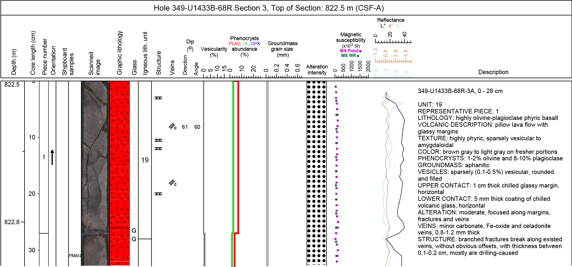
Figure F14. Example igneous VCD form.
Igneous petrology
Igneous lithologic and lithostratigraphic unit classifications
The first step in visual core description is the classification of the igneous lithologic units and subunits. These of volcanic rock unit boundaries are generally chosen to reflect different volcanic cooling units. The definition of an igneous lithologic unit is usually based on the presence of lava flow contacts, typically marked by chilled or glassy margins on the upper and lower contact or by the presence of intercalated volcaniclastic or sedimentary horizons. If no such boundaries were recovered (e.g., because of low recovery), we defined the igneous lithologic unit boundaries according to changes in the primary mineral assemblage (based on abundances of visible phenocryst and groundmass mineral phases), grain size, color, and structure or texture. Igneous lithologic units are given consecutive downhole Arabic numerals (e.g., igneous lithologic Units 1, 2, 3, etc.) irrespective of whether they are pillows, lobate or massive flows, volcaniclastic deposits, or igneous intrusions. Igneous lithologic subunits were used in cases where mineralogy remains similar but frequent changes in texture take place (e.g., igneous lithologic Subunits 1a, 1b, 1c, etc.).
Lithostratigraphic units, on the other hand, were defined where successions of consecutive cooling or depositional units with similar volcanic characteristics could be identified, usually based on phenocryst assemblages. In effect, these lithostratigraphic units combine similar igneous lithologic units and subunits, providing a first step toward considering volcanic stratigraphy and eruptive units. These successions are given consecutive downhole Roman numerals (e.g., lithostratigraphic Units III, IV, and V) that follow directly from the overlying sedimentary units (lithostratigraphic Units I and II in this example).
Lava flow types
Pillow lava flows
Pillow lavas are characterized by curved chilled margins oblique to the vertical axis of the core. When these margins are absent, we can potentially identify those boundaries by the presence of variolitic textures, curved fractures, and microcrystalline or cryptocrystalline grain sizes. Pillow lava flows consist of discrete subrounded units (or lobes) of relatively small size (0.2–1.0 m in diameter). Their exteriors are entirely bounded by glassy rinds as a result of rapid cooling. The outer zones typically show bands of vesicles, whereas their interiors typically display internally radiating vesicle trains and joint patterns. Pillow lava flows result from subaqueous eruptions that allow separation of lava pods from point sources along the advancing front.
Lobate lava flows
Lobate flows (~1–2 m in diameter) can develop by the same inflation process as pillow lava flows. Although these extrusions resemble pillow lavas, they differ in that they have massive, coarser grained, and sparsely vesicular flow interiors, often with pipe vesicle domains. These inflation units are characterized by more effective degassing and vesicle formation than pillow lava flows. Typically, vesicle zoning is concentrated in the upper regions of the inflation unit and often occurs as a series of vesicle bands that develop as a result of the inward migration of the cooling front, whereas the lower part of the inflation unit typically contains either sparse, poorly defined vesicle banding or teardrop-shaped vesicles at or just above the basal chilled zone. Recognizing lobate flows and distinguishing those from pillows in drill core is often difficult.
Sheet and massive lava flows
Sheet lava flows are defined as igneous lithologic units <3 m thick of the same rock type, with grain sizes increasing toward the center of flows. Massive lava flows are defined for continuous intervals that are >3 m of a similar lithology. Where recovered, these units are significantly thicker than the normal (~0.2–2 m) dimensions of pillow or lobate lava flows. Characterized by sparse vesicle layering, sheet and massive flows often have texturally uniform cores, as thick as several meters, and can have vertical vesicle pipes containing late-stage melt segregation material. Sheet-like and massive flows may result from particularly high effusion rates and/or increased local slopes.
Primary igneous lithologies and features
Phenocryst-based lithology names
Porphyritic basaltic rocks were named according to major phenocryst phase(s) when the total abundance of phenocrysts was >1%. The most abundant phenocryst appears last in the phenocryst-based lithology name. For example, olivine is the most abundant mineral in a plagioclase-olivine-phyric basalt. The term “phenocryst” was used for any crystal that was (1) significantly larger (typically at least five times) than the average size of the groundmass crystals, (2) >1 mm, and (3) euhedral or subhedral. The term “microphenocryst” was used for crystals larger than the modal groundmass grain size but smaller than 1 mm and is reported in the Microscopic (thin section) description template of DESClogik and in the lithologic unit summary under “Description” in the VCDs. A prefix was applied as a modifier to the primary lithology names to indicate the abundance of phenocrysts in the hand samples as follows:
- Aphyric (<1% phenocrysts),
- Sparsely phyric (1%–5% phenocrysts),
- Moderately phyric (5%–10% phenocrysts), and
- Highly phyric (>10% phenocrysts).
Aphyric rocks were not assigned any mineralogical modifier. Likewise, in coarser grained rocks with seriate to equigranular textures, we did not use modifiers unless there was a clear distinction in size between phenocrysts and groundmass crystals.
Groundmass
Groundmass is defined as the finer grained matrix (or the mesostasis) between the phenocryst phases, if the latter are present. Such groundmass is generally characterized by its texture (see below) and its grain size with the following standard notation:
- G = glassy.
- cx = cryptocrystalline (<0.1 mm).
- μx = microcrystalline (0.1–0.2 mm).
- fg = fine grained (>0.2–1 mm).
- mg = medium grained (>1–2 mm).
- cg = coarse grained (>2 mm).
An estimate of the average modal groundmass size (in millimeters) was included in the VCDs, whereas in the reports and description summaries we use descriptive terms (e.g., fine-grained or coarse-grained groundmass).
For volcanic rocks, the following terms were used to describe textures when microlites are present in the groundmass:
- Variolitic (fan-like arrangement of divergent microlites),
- Intergranular (olivine and pyroxene grains between plagioclase laths),
- Intersertal (glass between plagioclase laths),
- Subophitic (partial inclusion of plagioclase in clinopyroxene), and
- Ophitic (total inclusion of plagioclase in clinopyroxene).
Flow textures present in groundmass were described as follows:
- Trachytic (subparallel arrangement of plagioclase laths in the groundmass),
- Pilotaxitic (aligned plagioclase microlites embedded in a matrix of granular and usually smaller clinopyroxene grains), and
- Hyalopilitic (aligned plagioclase microlites with glassy matrix).
Description of habits for plagioclase and clinopyroxene groundmass crystals was adapted from those used during ODP Leg 206 (Shipboard Scientific Party, 2003) and Leg 148 (Shipboard Scientific Party, 1993). Four habit types were identified:
- Cryptocrystalline aggregates of fibrous crystals (fibrous),
- Comb-shaped or sheaf-like plumose crystals (fibrous),
- Granular-acicular subhedral to anhedral crystals, and
- Prismatic-stubby euhedral to subhedral crystals.
Rock color
Rock color was determined on a wet, cut surface of the archive half using Munsell color charts (Munsell Color Company, Inc., 1994) and converted to a more intuitive color name. Wetting of the rock was carried out using tap water and a sponge. Wetting was kept to a minimum because of adsorption of water by clay minerals (particularly saponite and celadonite) that are present throughout the core.
Volcanic textures and features
Various volcanic textures (e.g., glomerocrysts, coarser grained crystal aggregates, and xenoliths) were recorded, as were characteristic volcanic features such as chilled margins, baked contacts (with sediment), rubbly or brecciated flow tops, and so on. In particular, we noted the occurrence of vesicle banding, vesicle trains, pipe vesicles, and radiating cooling cracks.
Vesicles
An estimate of the percentage of vesicles and their average size was included in the VCDs. Vesicularity is described according to the abundance, size, and shape (sphericity and angularity) of the vesicles (Figure F15). Vesicle abundance was recorded as follows:
- Nonvesicular = <1% vesicles.
- Sparsely vesicular = 1%–5% vesicles.
- Moderately vesicular = 5%–20% vesicles.
- Highly vesicular = >20% vesicles.
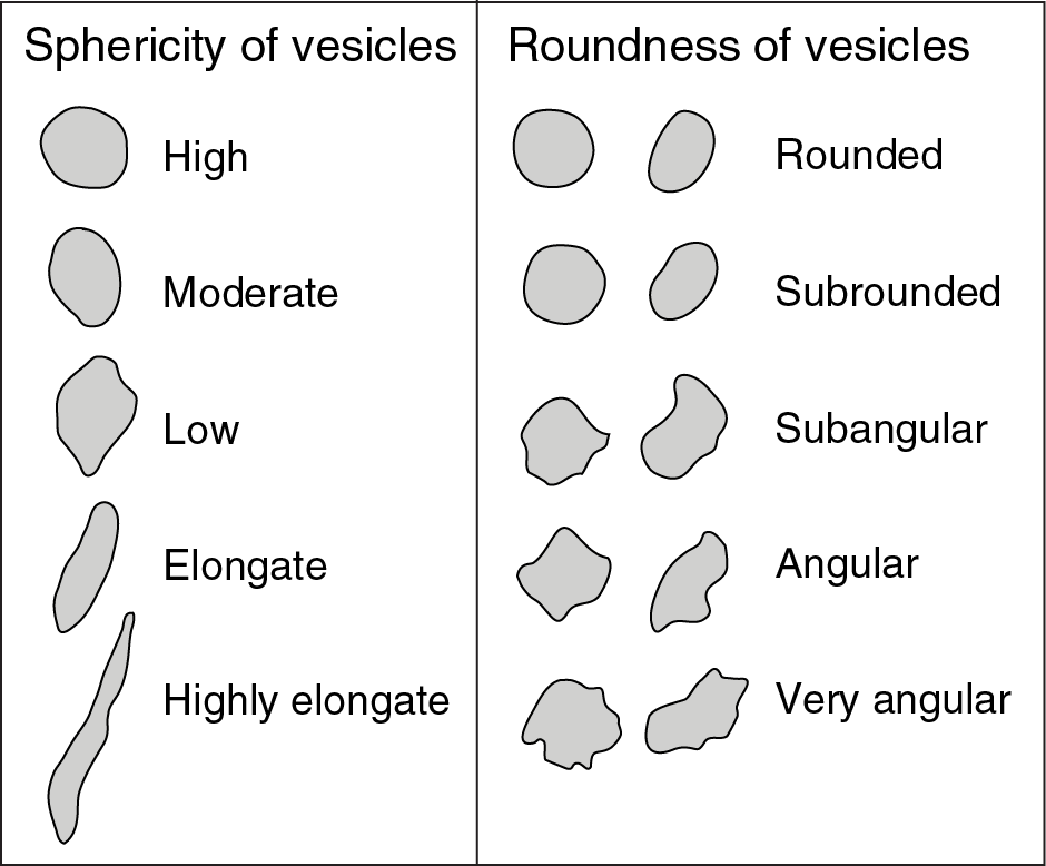
Figure F15. Vesicle shape comparison.
Alteration
Methods for describing alteration include hand sample descriptions and inspection of thin sections. These observations provided information on the alteration of primary igneous features, such as phenocrysts, groundmass minerals, and volcanic glass. In addition, the abundance of veins and vesicles and the succession of infilling materials were recorded to ascertain the order of mineral precipitation.
Alteration state and features
The alteration minerals were identified by color, habit and shape, association with primary minerals (if distinguishable), and hardness. Visual estimates of alteration degree, type, color, and textures (e.g., halos and patches) were recorded, as well as abundance (percentage) of minerals filling veins and vesicles, and the proportion of altered groundmass, volcanic glass, and all the different primary phenocryst phases. Complications arise in the identification of the secondary phases because many minerals produced during submarine alteration are visually similar, often being microcrystalline or amorphous, and are thus indistinguishable in the cores. Hence, identification of some alteration phases remains preliminary, pending detailed shore-based XRD studies and electron microprobe analyses.
Overall background alteration
The degree of the overall background alteration of groundmass and glass is defined and reported graphically on the VCDs according to various ranges of intensity in the alteration state. Different patterns are used to indicate slight, moderate, high, complete, or no (fresh) alteration (Figure F7) according to the following scale:
Vesicle fillings
Vesicles were first recorded for their shape, percentage abundance, size, and density, after which the infilling minerals were identified. Voids were described in terms of size, abundance, and partial infilling minerals, often lining the walls of irregular open spaces.
Veins
During Expedition 349, petrologists first recorded the location of veins and the mineralogy of the infilling materials and the halos surrounding those veins; after that, the structural geologists measured and recorded the orientation and width of the same veins (see Structural geology). Description of the veins included location, shape, crosscutting nature, width, color, and the amount (percentage) and nature of filling minerals. All features were recorded in DESClogik using a series of codes (Figure F7 for vein shape (straight, sigmoidal, irregular, pull-apart, and fault), connectivity (isolated, single, branched, and network), texture (massive, cross fiber, slip fiber, vuggy, and polycrystalline), structure (simple, composite, banded, haloed, and intravenous), and geometry (en echelon, ribbon, and cross fractures).
Alteration halos
Alteration halos commonly form around hydrothermal veins that allow for fluid flow of varying chemical composition. They can be different from the overall background alteration and vesicle filling in color, secondary mineral composition, and abundance. Color, thickness, and secondary minerals of alteration halos are recorded in the Veins-Halo tab of the DESClogik program.
Alteration color
Alteration color was defined using Munsell Soil Color Charts (Munsell Color Company, Inc., 1994) and converted to a more intuitive color name (very dark gray, greenish gray, etc.).
Volcanic glass
The presence of both unaltered and variably altered volcanic glass was also recorded in terms of the percentage of fresh material by volume. In addition, the composition and extent of replacement by secondary minerals were described.
Macroscopic visual core description
We used DESClogik to document each section of the igneous cores and their alteration by uploading our descriptions into the central LIMS database. These uploaded data were then used to produce VCDs, which include a simplified graphical representation of the core (for each section) with accompanying descriptions of the features observed. An example VCD for igneous rocks is shown in Figure F14, and the symbols used in these VCDs are given in Figure F7. The VCDs display the following items:
- Depth in mbsf;
- Scale for core section length (0–150 cm);
- Sample piece number;
- Upward-pointing arrow indicating oriented pieces of core;
- Sample type and position of intervals selected for different types of shipboard analytical studies, such as thin sections (TS), ICP-AES (ICP), paleomagnetism (PMAG), and physical properties (PP);
- Scanned digital image of the archive half;
- Graphical representation of lithology;
- Next to the graphical lithology, the symbol “G” indicates the presence of volcanic glass, either in the glassy rind of chilled margins or when encountered in hyaloclastite breccia;
- Igneous lithologic unit number;
- Symbolized structural information;
- Structural measurements of dip direction and dip angle;
- Line chart displaying the percent vesicularity;
- Stacked line chart displaying phenocryst percentage for plagioclase (pl: red line), olivine (ol: green line), and clinopyroxene (cpx: blue line);
- A chart displaying variation in crystal size of modal groundmass (in millimeters)
- Column with variable patterns depicting alteration intensity;
- Chart displaying both point source and whole-round magnetic susceptibility measurements;
- Chart displaying color reflectance, with total reflectance (L*), red (a*), and blue (b*) data arranged side by side; and
- Description summary for each igneous lithologic unit (see below for details).
The section summary text (displayed on the right side) provides a generalized overview of the core section’s lithology and features on a unit-by-unit basis. This summary includes the following:
- Expedition, site, hole, core and core type, section number, and the depth of the top of the core section in mbsf (measured according to the CSF-A depth scale) shown at the top of the VCD;
- Igneous lithologic unit or subunit number(s) (numbered consecutively downhole) and piece numbers belonging to unit (and on which piece, or pieces, the description was based);
- Lithology, rock description, and name;
- Volcanic description based on type of unit and igneous structure (e.g., pillow lava, massive flow);
- Texture based on total percentage of phenocrysts and microphenocrysts by volume: aphyric (<1%), sparsely phyric (1%–5%), moderately phyric (>5%–10%), or highly phyric (>10%);
- Color determined on wet rock surfaces;
- Phenocryst percentage and type based on minerals identifiable by eye, hand lens, or binocular microscope;
- Groundmass grain size and texture: glassy, aphanitic (crystalline but individual grains not discernible with a hand lens), fine grained (<1 mm), medium grained (1–2 mm), or coarse grained (>2 mm);
- Vesicle percentage by volume, including filled, partially filled, and open vesicles;
- Upper and lower unit contact relations and boundaries, based on physical changes observed in retrieved core material (e.g., presence of chilled margins, changes in vesicularity, and alteration), including information regarding their position within the section. The term “not recovered” was entered where no direct contact was recovered;
- Alteration of the rock material, veins, and vesicle infillings; and
- Structural features (see Structural geology).
Microscopic (thin section) description
Thin section analyses of sampled core intervals were used to complement and refine macroscopic core observations. Typically, one thin section was examined and logged per defined igneous lithologic unit. To maintain consistency, the same terminology and nomenclature are used for macroscopic and microscopic descriptions. Phenocryst assemblages (and their modal percentages, shapes, habits, and sizes), groundmass, and alteration phases were determined, and textural features were described. All observations were entered into the LIMS database with a special DESClogik thin section template. Downloaded tabular reports of all igneous thin section descriptions can be found in Core descriptions.
Thin section descriptions include both primary (igneous) and secondary (alteration) features, for example, textural features, grain size of phenocrysts and groundmass minerals, mineralogy, abundance (percentage), inclusions, alteration color, alteration extent (percentage) in the total rock, alteration veins (type and number), and vesicles (type and fillings). An example of a thin section description form is given in Figure F16.
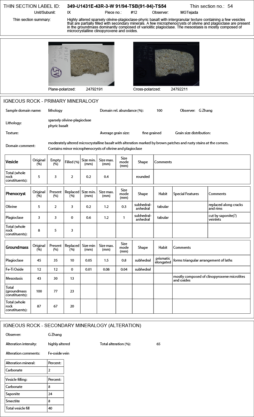
Figure F16. Igneous rock thin section description.
Textural terms used are those defined by MacKenzie et al. (1982) and include
- Heterogranular (different crystal sizes),
- Equigranular (similar crystal sizes),
- Seriate (continuous range in grain size),
- Porphyritic (increasing presence of phenocrysts),
- Glomeroporphyritic (containing clusters of phenocrysts),
- Holohyaline (100% glass),
- Hypo- or holocrystalline (100% crystals),
- Variolitic (fine, radiating fibers of plagioclase or pyroxene),
- Intergranular (olivine and pyroxene grains between plagioclase laths),
- Intersertal (groundmass fills the interstices between unoriented feldspar laths),
- Ophitic (lath-shaped euhedral crystals of plagioclase, grouped radially or in an irregular mesh, completely surrounded with large anhedral crystals of pyroxene), and
- Subophitic (partial inclusion of plagioclase in pyroxene).
Glass in basalts with more glassy groundmass are defined as
- Fresh glass (amber in transmitted polarized light and isotropic in transmitted cross-polarized light),
- Dark glass (darkness is caused by abundant crystallites; interstitial volcanic glass of basaltic composition is termed trachylytic),
- Glass with spherulites (spheroid aggregates of acicular crystals forming a nucleus), and
- Altered glass (partially or completely altered to clay minerals).
For alteration description, thin sections were examined to
- Confirm macroscopic identification of secondary minerals;
- Determine their mode of occurrence in terms of vesicle and void fillings, vein composition, and primary mineral replacement;
- Determine the chronological relationships between different secondary minerals;
- Establish the distribution, occurrences, and abundance of secondary minerals downhole;
- Quantify the overall amount of alteration in the basaltic rocks;
- Identify mineralogies of vein and vesicle infillings, as well as cement and voids present in basaltic breccia; and
- Calculate the total alteration (percentage) using the modal proportions of phenocrysts and groundmass minerals and their respective percentages of alteration.
Individual thin sections in some cases contain multiple domains that require separate description. In DESClogik, the user can enter multiple records for a single thin section, in the case where more than one domain can be recognized. We define the “domain” concept of DESClogik based on apparent observable differences in lithology, alteration, vesicle banding and grouping, and veining and when more than one clast type is present in volcaniclastic lithologies. Thin sections typically are taken so they represent a singular lithology, and thus by definition they encompass a single lithology domain (Figure F17A). In some cases, thin sections contain more than one lithology, with a sharp or diffuse boundary splitting the thin section into two lithology domains, whereby a diffuse (wider) boundary zone could be defined as a separate, third domain (Figure F17B). Alteration can result in many different domains in a rock, including the background alteration and various halos surrounding cracks and veins (Figure F17C). In pillow basalts, but also in thicker sheet and massive flows, different groupings or bands of vesicles may be apparent in thin section (Figure F17D). Multiple generations of veins with different filling patterns are often visible in thin section and should be assigned different domain names (Figure F17E). Heterolithic volcaniclastics often contain multiple clast types, as well as the matrix domain itself, that could be described separately (Figure F17F).
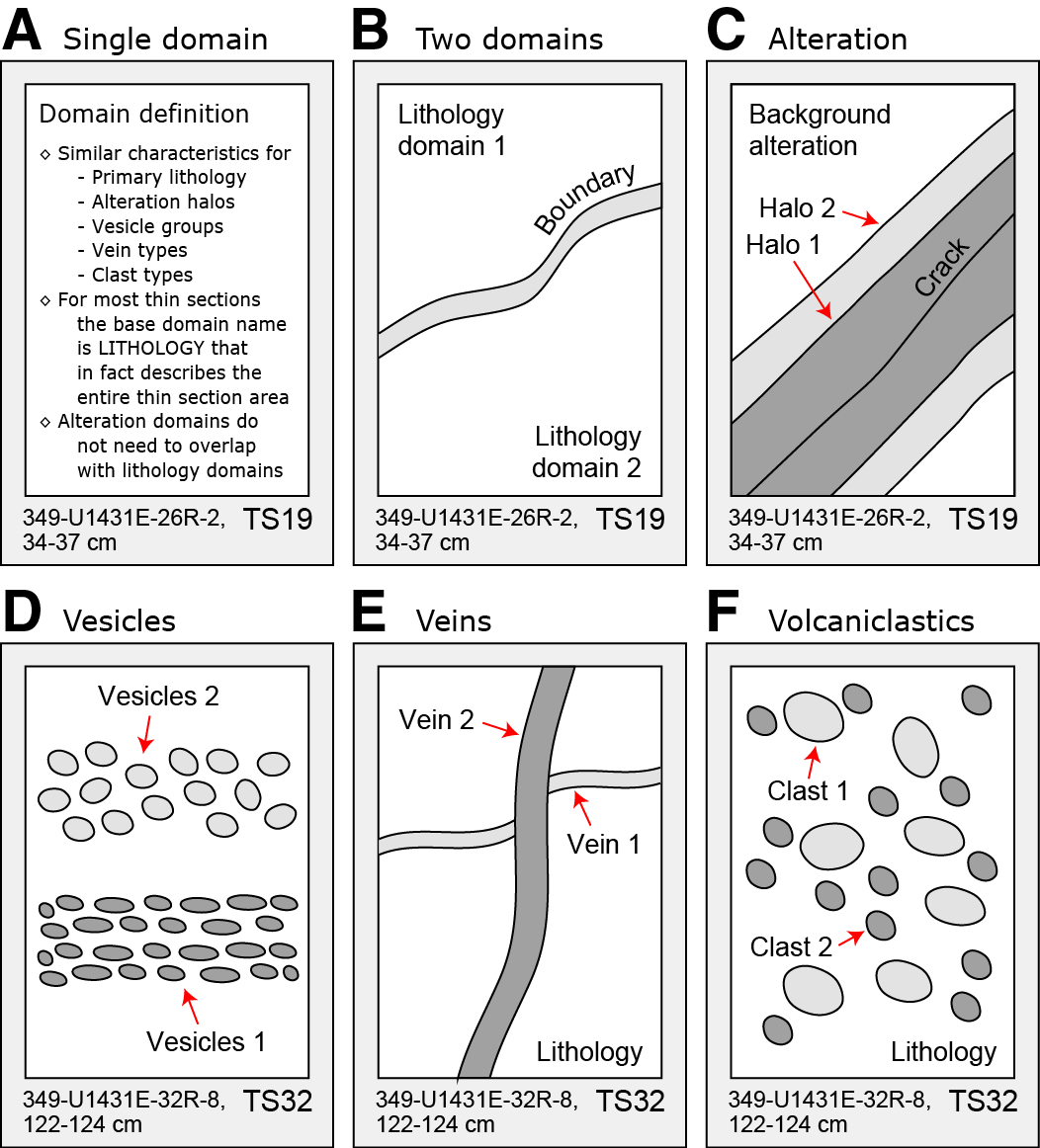
Figure F17. DESClogik thin section description types.
Finally, estimated volume percentages are required to quantify, for example, phenocryst and vesicle abundances. In DESClogik, the user is required to enter modal percentages of both whole-rock and groundmass constituents for extrusive and hypabyssal rocks. Using cartoons and example calculations, we define those modal percentages and explain how they add up to 100% in both cases. Figure F18A is a cartoon of an idealized porphyritic volcanic rock in a thin section with plagioclase and olivine phenocrysts, vesicles, and one crosscutting vein set in a finer grained groundmass matrix. The whole-rock constituents are the sum of all phenocrysts present, plus the vesicles and groundmass (Figure F18B). In this case, a total of 20% phenocrysts, 10% vesicles, and 70% groundmass matrix are present, equaling 100%. Veins and void spaces are ignored in this calculation. For the groundmass constituents, however, we examine the groundmass matrix as a whole (by ignoring the phenocrysts and vesicles), and we estimate the distribution of mineral phases, mesostasis, and fresh glass in it. In this case, the groundmass contains 40% plagioclase, 20% clinopyroxene, 10% olivine, 10% Fe-Ti oxides, and 20% mesostasis, equaling 100%. Fresh glass is not present in this example thin section, but if it were present, it would be considered a separate constituent from mesostasis. Mesostasis is the altered portion of the interstitial spaces between all the groundmass minerals present that originally often was volcanic glass. Figure F18C is a simplified view of a group of partially altered (replaced) olivine phenocrysts and partially filled vesicles. As explained above, in DESClogik the user at least records the percentage of the originally present phenocryst phases, groundmass mineral phases, and vesicles (Figure F18D). However, whenever possible, the user also should record how much of these constituents is still present (i.e., still fresh or not filled) and how much has been replaced (i.e., altered or filled) while taking into account that Original (%) = Present (%) + Replaced (%).
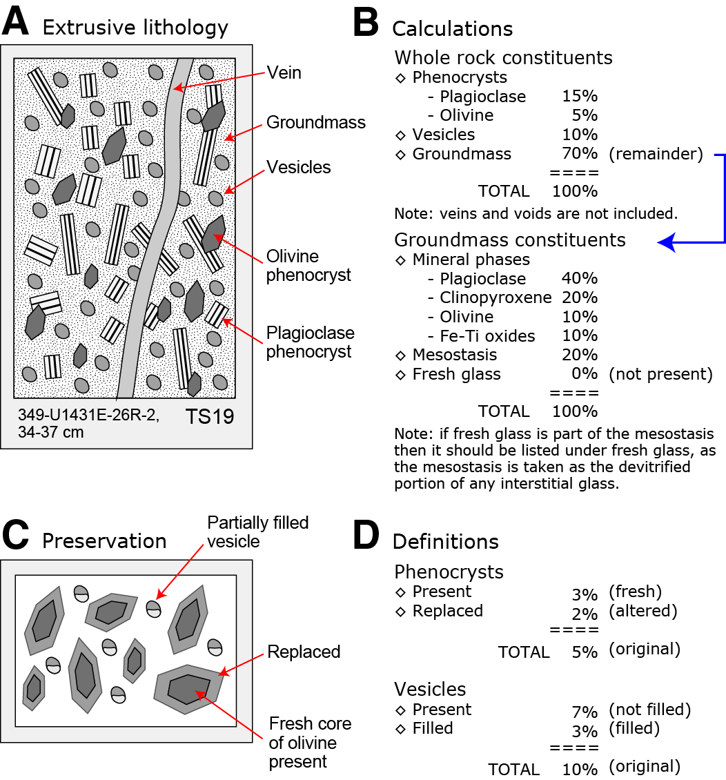
Figure F18. Thin section modal calculations.
Structural geology
This section outlines methods for documenting structural features observed in Expedition 349 cores, such as faults, fractures, breccia, and veins. After a core is split and described by sedimentologists or petrologists on shift, we documented structural features observed on the archive half by: (1) identifying structural features and classifying their structural types, (2) determining the top and bottom location of structural features in the core, (3) measuring the orientation of a structural feature where applicable, and (4) determining the sense of displacement on a structural feature where applicable. Our methods largely follow those used by structural geologists of Integrated Ocean Drilling Program Expedition 344 (Harris et al., 2013). The types of structural measurements and key parameters (either observed or calculated) are recorded on a spreadsheet (Figure F19). These data are then input into the LIMS database. Orientation data are corrected for rotation related to drilling using paleomagnetic declination and inclination information (see Paleomagnetism).

Figure F19. Structural geology observation sheet.
Graphic symbols and terminology
A predefined set of commonly observed structural features was used in the structural description of cores during Expedition 349. The terminology and graphic symbols used are presented in Figures F7 and F20. The major structural features identified include the following:
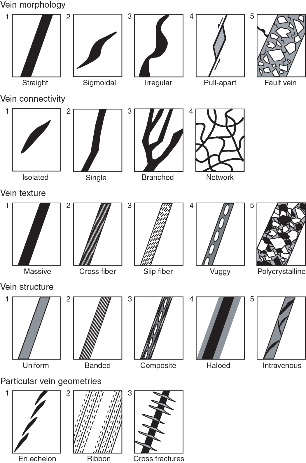
Figure F20. Vein description sheet.
- Fractures: brittle failure with unknown displacement and with no secondary infill minerals; however, breaks clearly resulting from drilling were not logged as fractures;
- Veins: fractures filled with secondary minerals;
- Igneous contacts: material contacts of extrusive or intrusive igneous rocks; and
- Magmatic fabrics: magmatic foliations defined by the preferred orientations of primary minerals with no evidence of crystal-plastic deformation.
Structural observation and description
Structural features were described from the top to bottom of each section of the core. For fractures, we examined and measured the following parameters:
- Location: where a fracture occurs in a core, measured in centimeters from the top of the section;
- Morphology: morphological shape of a fracture, e.g., straight, curved, banded, irregular, composite, isolated, single or branched;
- Displacement: lateral offset and/or opening of a fracture measured in centimeters; a closed fracture with no lateral offset is recorded as 0 cm of displacement;
- Orientation: dip angle and dipping orientation of a fracture measured in degrees; where applicable, reorientation of a fracture to geographic coordinates (i.e., relative to true north) was done to determine the real dip direction (see Orientation measurements and correction);
- Frequency: occurrence frequency of fractures per section; and
- Types: type of deformation of a fracture, e.g., normal, reverse, dextral, sinistral displacement, or a combination of the above.
For veins, we examined and measured several parameters:
- Location: where a vein occurs in a core, measured in centimeters from the top of the section;
- Morphology: morphological shape of a vein;
- Orientation: dip angle and dipping direction of a vein;
- Frequency: occurrence frequency of veins per section; and
- Mineral infill and alteration: these features are recorded as described by petrologists.
For igneous contacts, we described the following parameters:
- Location: where an igneous contact occurs in a core, measured in centimeters from the top of the section;
- Type of contacts: type of igneous contact boundary;
- Orientation: dip angle and dipping direction of an igneous contact;
- Frequency: occurrence frequency of igneous contacts per section; and
- Mineral infill and alteration: these features are recorded as described by petrologists.
For magmatic fabrics, we measured the following parameters:
- Location: where a magmatic fabric feature occurs in a core, measured in centimeters from the top of the section;
- Morphology: morphological shape of a magmatic fabric feature;
- Orientation: dip angle and dipping direction of a magmatic fabric feature; and
- Frequency: occurrence frequency of magmatic fabrics per section.
Orientation measurements and correction
Orientation measurements
We used a plastic goniometer for orientation measurements (Figure F21). Orientations of planar and linear features in a core section were determined relative to the core reference frame (Figure F22). The vertical axis of the core reference frame is aligned with the upcore direction of the core section, whereas the double line marked on the archive half of the core liner is defined as 180° in the cross-sectional plane perpendicular to the core vertical axis.
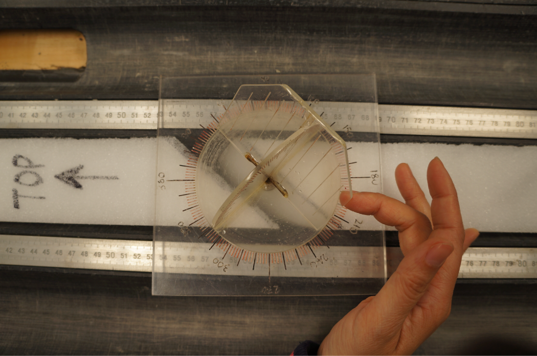
Figure F21. Expedition 349 goniometer.
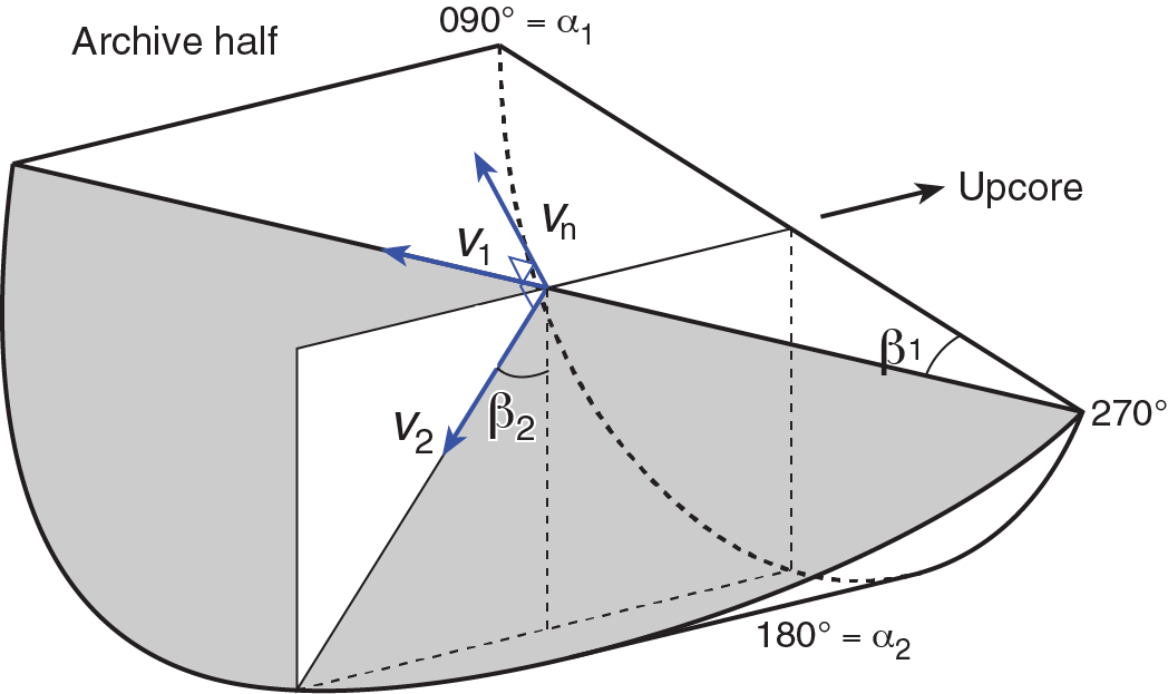
Figure F22. Core reference frame and coordinates.
To determine the orientation of a planar structural element (shaded plane in Figure F22), two apparent dips of the element were measured in the core reference frame. The first apparent dip measures the intersection angle between the planar structural element and the split face of the core (β1 in Figure F22); it is determined by measuring the dip direction and angle of the planar structural element in the core reference frame. A planar structural element could have a trend of 90° or 270° and a plunge angle ranging from 0° to 90°. The second apparent dip measures the intersection angle between the central line of the planar structural element and the split face of the core (β2 in Figure F22). In most cases, this was a plane either parallel or perpendicular to the core axis. In the former case, the apparent dip would trend 0° or 180° with plunge angle ranging from 0° to 90°; in the latter case, the trend would range from 0° to 360° with a plunge angle of 0°.
A linear feature observed in the surface of a split core is often associated with a planar structural element (e.g., a fault plane) in the core; the orientations of the planar structural element is determined by measuring either the rake (or pitch) of the associated plane or the trend and plunge of the planar element in the core reference frame. All measured data were manually typed into the log sheet together with the measured depths in the core section and descriptive information (Figure F19).
Plane orientation calculation
For a planar structural element (e.g., a bedding or fault plane), two apparent dips on two different surfaces (e.g., one being the split core surface, which is east–west vertical, and the other being horizontal or north–south vertical surface) were measured in the core reference frame. The two apparent dips are the azimuth (measured clockwise from north, looking down) and plunge. An x, y, z coordinate system was defined in such a way that the positive x, y, and z directions coincide with north, east, and vertical downward, respectively. If the azimuths and plunges of the two apparent dips are given as (α1, β1) and (α2, β2), respectively, as in Figure F22, the unit vectors representing these two lines, v1 and v2, are given by the following expression:
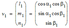 and
and .
.The unit vector normal to the planar structural element vn (Figure F23) is then defined as
 , where
 .
.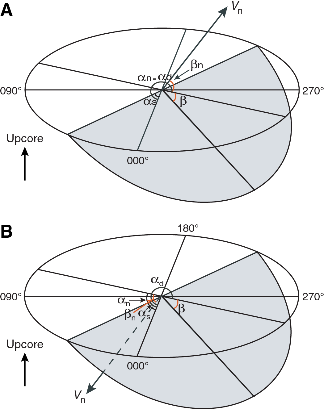
Figure F23. Dip direction and strike.
The azimuth αn and plunge βn of the vector vn are given by
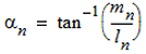 and
and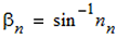 .
.The dip direction αd and dip angle β of this plane are αd = αn and β = 90° + βn, respectively, when βn < 0°; and αd = αn ± 180° and β = 90° − βn, respectively, when βn ≥ 0°. The strike of this plane αs according to the right-hand rule is then given by αs = αd − 90° (Figure F23).
Azimuth correction based on paleomagnetic data
Provided that a core is vertical, its magnetization is primary, and bedding is horizontal, its paleomagnetic declination αp indicates the magnetic north direction when its inclination βp ≥ 0° (Figure F24); in contrast, the angle αp indicates the magnetic south direction when βp < 0°. The dip direction and strike of a planar structural element in the geographic reference frame, αd* and αs*, are therefore αd* = αp − αd and αs* = αp − αs when βp ≥ 0°; or αd* = 180° + αp − αd and αs* = 180° + αp − αs when βp < 0°.
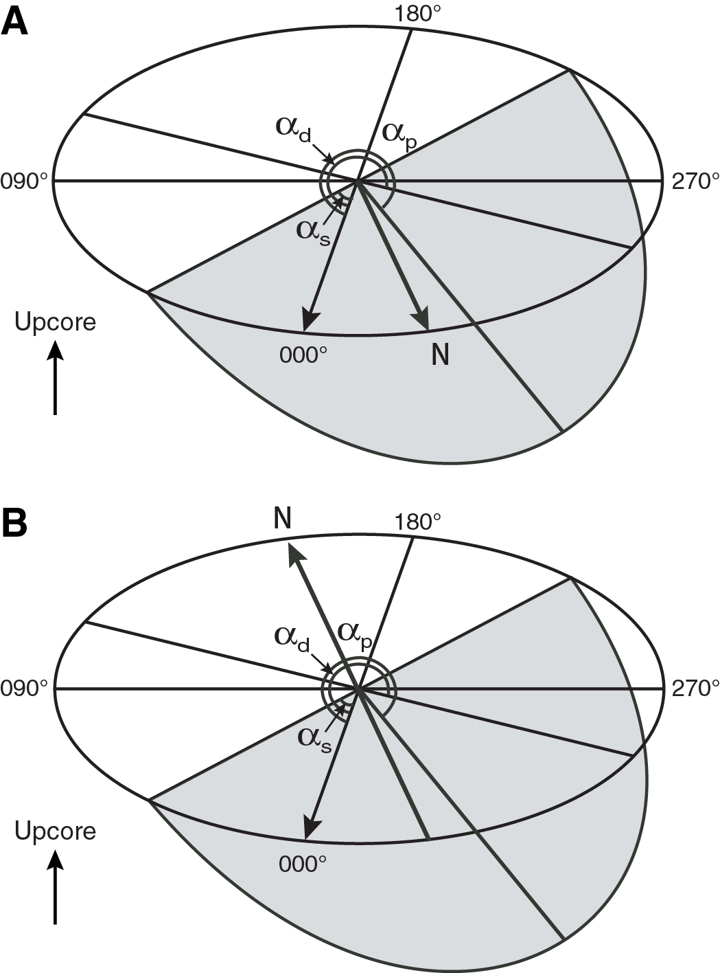
Figure F24. Azimuth correction.
If a core section was complete and continuous, one paleomagnetism sample per section (1.5 m) was deemed sufficient to determine the paleomagnetic orientation of the core section. If the core was discontinuous, one paleomagnetism sample for each subsection of the core that was continuous and structurally important was required. Paleomagnetism samples were taken as cubic or cylindrical samples close to a planar structural element of interest (usually within 5 cm) and from a coherent core interval that included the structural element of interest. In general, we avoided core fragments that were so small that potential spinning during drilling might cause significant deviation from the core axis (e.g., fragments of brecciated segments).
Geochemistry
The shipboard geochemistry program for Expedition 349 included measurements for
- Headspace gas content;
- Interstitial water composition;
- Sedimentary geochemistry including total inorganic carbon, total carbon, total nitrogen, and major and minor element content; and
- Igneous rock geochemistry (major and minor element content).
These analyses were carried out to satisfy routine shipboard safety and pollution prevention requirements; characterize interstitial water, sediment, and rock geochemistry for shipboard interpretation; and provide a basis for sampling for shore-based research.
Interstitial water chemistry
Interstitial water collection
Routine interstitial water samples were obtained by squeezing whole-round sections cut from cores. Standard whole-round samples were 5 cm long, but as water content decreased downhole, the size of the whole-round samples was increased up to 15 cm to enable extraction of the ~30 mL of water needed for shipboard and shore-based analyses. Whole-round samples were cut and capped as quickly as possible after the core arrived on deck and immediately moved to the chemistry laboratory for squeezing. Whole-round samples were typically collected at a frequency of up to 1 sample per section for the uppermost 20 m, 1–2 samples per core downhole to 100 mbsf, and then 1 sample per core until basement or until interstitial water extraction required a >15 cm whole-round section in order to preserve core for visual core description and other sampling. The exterior of the whole-round sample was carefully cleaned with a spatula to remove potential contamination from drilling fluid. For XCB cores, the intruded drilling mud between biscuits was also removed to eliminate contamination from drilling fluid. The cleaned sediment was placed into a 9 cm diameter titanium squeezer that was then placed in a Carver hydraulic press (Manheim and Sayles, 1974) and squeezed at pressures no higher than 25,000 lb (~17 MPa) to prevent the release of interlayer water from clay minerals during squeezing. The squeezed interstitial water was collected into a 60 mL deionized water-washed (18 MΩ/cm) high-density polyethylene syringe attached to the squeezing assembly and subsequently filtered through a 0.45 µm polyethersulfone membrane filter into various sample containers.
For Hole U1431A, interstitial waters were collected by both squeezing whole-round samples and Rhizon samplers. The whole-round samples were taken every 50 cm in order to obtain high-resolution interstitial water depth profiles for the upper 20 m of sediment. Rhizon sampling collected interstitial water at 5, 10, 20, and 50 cm intervals for sediment at 0–3, 3–9, 9–17, and 17–28 mbsf intervals, respectively. Rhizon sampling for interstitial water lasted for ~2–4 h to obtain ~20 mL water samples for shore-based analyses.
Sample allocation was determined based on the pore fluid volume obtained and analytical priorities based on the objectives of the expedition. Aliquots for analysis by ICP-AES were acidified by adding ~10 µL of trace metal–grade concentrated HNO3 and placed in 4 mL cryovials. Aliquots for titration and ion chromatography analyses were put in 10 mL high-density polyethylene vials. Aliquots for dissolved inorganic carbon (DIC) and dissolved organic carbon (DOC) and their δ13C were treated with 10 µL of a saturated HgCl2 solution and placed in 8 mL septum screw-lid glass vials. Aliquots for isotopic analyses of oxygen, hydrogen, and Sr ratios were also placed in 8 mL septum screw-lid glass vials. Aliquots for TH2S were placed in 2 mL septum screw-lid glass vials with 0.5 mL of 20% zinc acetate solution. The samples were stored at 4°C after collection.
Alkalinity, pH, and salinity were analyzed immediately after interstitial water was obtained. Other shipboard analyses were carried out in batches. Dissolved sodium, calcium, magnesium, chloride, bromide, and sulfate were analyzed by ion chromatography. Ammonium and phosphate were analyzed by spectrophotometry. Major and minor element concentrations were analyzed by ICP-AES.
After interstitial water extraction was complete, sediment squeeze cakes were divided and sealed in plastic bags for shipboard and shore-based analyses. Squeeze cake samples for shore-based organic analysis were stored at –80°C. All other squeeze cake samples were refrigerated at 4°C.
Shipboard interstitial water analysis
Interstitial water samples were analyzed on board following the protocols in Gieskes et al. (1991), Murray et al. (2000), and the Integrated Ocean Drilling Program user manual for shipboard instrumentation, which was updated during Integrated Ocean Drilling Program Expedition 344 (Harris et al., 2013).
Salinity, alkalinity, and pH
Salinity, alkalinity, and pH were measured immediately after squeezing, following the procedures in Gieskes et al. (1991). Salinity was measured using a Fisher temperature-compensated handheld refractometer. The pH was measured with a combined glass electrode, and alkalinity was determined by Gran titration with an autotitrator (Metrohm 794 basic Titrino) using 0.1 M HCl at 25°C. International Association for the Physical Sciences of the Oceans (IAPSO) standard seawater was used for calibration and was analyzed at the beginning and end of a set of samples for each site and after every 10 samples. Alkalinity titrations had a precision within 2% based on repeated analysis of IAPSO standard seawater. For sample volumes of ≤14 mL, alkalinity and pH were not measured because each alkalinity and pH analysis requires 3 mL of interstitial water.
Chloride by titration
High-precision chloride concentrations were acquired using a Metrohm 785 DMP autotitrator and silver nitrate (AgNO3) solution calibrated against repeated titrations of IAPSO standard. A 0.5 mL aliquot of sample was diluted with 30 mL of an 80 mM HNO3 solution and titrated with 0.1 N AgNO3. Repeated analyses of an IAPSO standard yielded a precision better than 0.05%; however, the chloride concentrations yielded by titration includes not only dissolved chloride but also all of the other halide elements and bisulfide. The JOIDES Resolution is equipped with Metrohm 850 Professional ion chromatograph (IC), which can analyze anions and cations simultaneously. The chloride concentration was analyzed by both titration and ion chromatography for Holes U1431A and U1431D. Chloride concentrations analyzed by ion chromatography were not greater than those by titration, indicating that ion chromatography can mostly provide reliable chloride data. As a result, chloride concentration was analyzed only by ion chromatography for the remaining sites.
Sulfate, chloride, bromide, calcium, magnesium, and sodium
Sulfate, chloride, bromide, calcium, magnesium, and sodium concentrations were analyzed by ion chromatography (Metrohm 850 Professional IC) using aliquots of 100 µL that were diluted 1:100 with deionized water (18 MΩ/cm). At the beginning and end of each run, different dilutions of IAPSO standard seawater were analyzed for quality control and to determine accuracy and precision. Analytical precision was within 0.9% for chloride, 4.0% for bromide, 1.0% for sulfate, 2.8% for calcium, 1.2% for magnesium, and 1.4% for sodium.
Ammonium and phosphate
Ammonium and phosphate concentrations were determined using an Agilent Technologies Cary Series 100 UV-Vis spectrophotometer with a sipper sample introduction system following the protocol in Gieskes et al. (1991). For ammonium concentration analysis, a 0.1 mL sample aliquot was diluted with 1 mL reagent water, to which 0.5 mL phenol ethanol, 0.5 mL sodium nitroprusside, and 1 mL oxidizing solution (trisodium citrate and sodium hydroxide) were added in a 5 mL capped glass vial (Gieskes et al., 1991). The solution was kept at room temperature for ~6.5 h to develop color. Ammonium concentrations were determined at an absorbance of 640 nm. Precision and accuracy of the ammonium analyses were within 2.5% and 3%, respectively.
For phosphate analysis, a 0.3 mL sample was diluted with 1 mL deionized water (18 MΩ/cm) in a 4 mL glass vial. Then 2 mL of mixed reagent (ammonium molybdate, sulfuric acid, ascorbic acid, and potassium antimonyl tartrate) was added to the vial (Gieskes et al., 1991), which was capped and kept at room temperature for at least several minutes to develop color. The phosphate concentration was determined at an absorbance of 885 nm ~30 min after adding the mixed reagent solution. Precision and accuracy of the phosphate analyses were better than 2% and 2%, respectively.
Major and minor elements
Dissolved major and minor elements were determined by Leeman ICP-AES. For major cation (Na+, K+, Ca2+, and Mg2+) analyses, dilutions of IAPSO standard seawater were used as calibration standards. Standards and acidified samples were diluted 1:100 (v/v) with a 2% HNO3 (by volume) solution (matrix) with Y at 10 ppm as an internal standard. Calibration for minor elements (Mn2+, Fe2+, B, Si, Sr2+, Ba2+, and Li+) was done with dilutions of a multielement synthetic standard solution (composed of single-element standards). Acidified samples measured for minor elements on the ICP-AES were diluted 1:20 (v/v) with the same matrix used for the major element analysis. Drift correction was made for both major and minor elements using the factor from a drift monitor solution (100% IAPSO for majors and 100% stock solution for minors) that was analyzed every eight samples. The ICP-AES autosampler and analysis chamber were rinsed with a 3% (by volume) HNO3 solution between samples. Major cations (Mg2+, Ca2+, K+, and Na+) were also determined by IC at 1:100 dilutions; however, these results yielded poor quality K+ data, whereas the ICP-AES yielded good quality data for K+.
Headspace gas geochemistry
One sediment sample (5 cm3) from each core, collected immediately after retrieval on deck, was placed in a 20 cm3 glass vial and sealed with a septum and a crimped metal cap. When consolidated or lithified samples were encountered, chips of material were placed in the vial and sealed. If an interstitial water sample was obtained, the headspace sample was taken from the top of the section immediately next to the interstitial water sample whenever possible. The vial was labeled with the core, section, and interval from which the sample was taken and then placed in an oven at 70°C for 30 min. A 5 cm3 volume of gas extracted through the septum was then injected with a gas-tight glass syringe into a gas chromatograph (GC).
The GC (Agilent 6890 equipped with a flame ionization detector [FID]) was set at 250°C and used to accurately and rapidly measure the concentrations of methane (C1), ethane (C2), ethylene (C2=), propane (C3), and propylene (C3=). A 2.4 m × 2.0 mm stainless steel column packed with 80/100 mesh HayeSep “R” is installed in the oven. The injector consists of a ¹⁄₁₆ inch Valco union with a 7 µm screen connected to a Valco-to-Luer lock syringe adaptor. This injector connects to a 10-port Valco valve that was switched pneumatically by a digital valve interface. The injector temperature was set at 120°C. Samples were introduced into the GC through a 0.25 cm3 sample loop connected to the Valco valve. The valve can be switched automatically to backflush the column. The oven temperature was programmed to start at 80°C for 8.25 min and then increased to 150°C for 5 min at a rate of 40°C/min. Helium was used as the carrier gas. Initial helium flow in the column was 30 mL/min. Flow was then ramped to 60 mL/min after 8.25 min to accelerate elution of C3 and C3=. The run time was 15 min. The GC was also equipped with an electronic pressure control module to control the overall flow into the GC.
Sediment geochemistry
Sedimentary inorganic and organic carbon content
Sediment samples were collected from the interstitial water squeeze cakes, with additional samples taken from intervals of distinct lithology. Samples were freeze-dried for ~24 h, crushed using an agate pestle and mortar, and then analyzed for total carbon, total inorganic carbon (TIC), and total nitrogen.
Total carbon and total nitrogen of the sediment samples were determined with a ThermoElectron Corporation FlashEA 1112 CHNS elemental analyzer equipped with a ThermoElectron packed column CHNS/NCS GC and a thermal conductivity detector (TCD). Approximately 10–15 mg of sediment was weighed into a tin cup and then combusted at 950°C in a stream of oxygen. The reaction gases were passed through a reduction chamber to reduce nitrogen oxides to nitrogen and were then separated by the GC before detection by TCD. All measurements were calibrated to a standard (Soil Reference Material NC [PN 33840025]), which was run every 10 samples. The peak areas from the TCD were calculated to determine the total carbon and total nitrogen of the samples.
TIC was determined using a Coulometrics 5015 CO2 coulometer. Approximately 10 mg of sediment was weighed into a glass vial and acidified with 2 M HCl. The liberated CO2 was titrated, and the corresponding change in light transmittance in the coulometric cell was monitored using a photodetection cell. The weight percent of calcium carbonate was calculated from the inorganic carbon content using the following equation:
CaCO3 (wt%) = TIC (wt%) × 100/12.
Standard CaCO3 (standard reference material) was used to confirm accuracy. Total organic carbon content was calculated by subtraction of inorganic carbon from the total carbon.
Elemental analysis of bulk sediment/sedimentary rock by ICP-AES
Elemental composition of bulk sediment was determined using a Leeman ICP-AES. Our analytical approach followed the general procedure outlined by Murray et al. (2000) and the constraints indicated by Quintin et al. (2002). Analytical blanks were prepared using 400 mg of lithium metaborate (LiBO2) flux to ensure matrix matching. Samples analyzed by ICP-AES were ignited before dissolution by heating 5 g of oven-dried (600°C for 12 h) ground sediment at 1025°C for 5 h to determine weight loss on ignition (LOI), to release volatile phases (H2O, CO2, and S), and to fully oxidize all iron to ferric iron.
Aliquots of 100 mg of ignited sediment and standards were mixed with 400 mg of LiBO2 flux. Subsequently, 10 µL of a wetting agent, 0.172 mM lithium bromide (LiBr), was added to the samples, standards, and blanks. This mixture was fused at 1050°C for 5 min in a Bead Sampler NT-4100 prior to dissolution in 50 mL of 10% HNO3. For complete dissolution, 1 h of shaking with a Burrell wrist-action shaker was required. Aliquots of 5 mL of the resulting solutions were filtered (0.45 µm) and diluted with 35 mL of 10% HNO3, resulting in a 4000× dilution of the original sediment.
A range of standards was selected to cover the entire range of expected sediment compositions, with their suitability monitored during the expedition. These standards were: STSD1, STSD2, STSD4, SO-1, SO-2, SO-3, SO-4, NBS-1c, JR-2, and BCR2. BHVO2 was also selected as both the drift and consistency standard. A range of major and trace elements was analyzed. Major elements included Si, Al, Fe, Mg, Ca, Na, K, Ti, Mn, and P, and trace elements included Ba, V, Cr, Ni, Cu, Zn, Rb, Sr, Y, Zr, Li, and Sc. Major elements were expressed as weight percent oxide and trace elements as parts per million. LOI values were determined routinely. Samples were analyzed in duplicate. The procedures used to process the data are outlined in Data reduction below.
The elemental compositions of sediment/sedimentary rock were only analyzed at Site U1431 due to time constraints.
Igneous rock geochemistry
Sample preparation
Representative samples of igneous rocks were analyzed for major and trace element concentrations during Expedition 349 using the Leeman ICP-AES.
Samples ranging in size from ~2 to ~8 cm3 were cut from the core with a diamond saw blade. A thin section billet was taken from the same or adjacent interval for petrographic analysis and alteration determination (see Igneous petrology and alteration). All outer surfaces were ground on a diamond-impregnated disk to remove altered rinds and surface contamination derived from the drill or saw. Each sample was then placed in a beaker containing acetone and washed ultrasonically for 15 min. The acetone was decanted, and the samples were sonicated in deionized water (18 MΩ/cm) twice for 10 min. The cleaned pieces were dried for 10–12 h at 110°C.
The cleaned, dried samples were crushed to <1 cm chips between two disks of Delrin plastic in a hydraulic press. The rock chips were then ground to a fine powder in tungsten carbide in a SPEX 8515 Shatter box. After grinding, a 5.0 ± 0.5 g aliquot of the sample powder was weighed on a Mettler Toledo balance and ignited at 1025°C for 4 h to determine LOI.
Murray et al. (2000) describes in detail the shipboard procedure for digestion of rocks and ICP-AES analysis of samples. The following protocol is an abbreviated form of this procedure with minor modifications. After determination of LOI, 100.0 ± 0.2 mg splits of the ignited whole-rock powders were weighed and mixed with 400.0 ± 0.5 mg of LiBO2 flux that had been preweighed on shore. Standard rock powders and full procedural blanks were included with unknowns in each ICP-AES run (note that among the elements analyzed, contamination from the tungsten carbide mills is negligible; Shipboard Scientific Party, 2003). All samples and standards were weighed on a microbalance with weighing errors estimated to be ±0.05 mg under relatively smooth sea-surface conditions.
To prevent the cooled bead from sticking to the crucible, 10 mL of 0.172 mM aqueous LiBr solution was added to the mixture of flux and rock powder as a nonwetting agent. Samples were then fused individually in Pt-Au (95:5) crucibles for ~12 min at a maximum temperature of 1050°C in an internally rotating induction furnace (Bead Sampler NT-4100).
After cooling, beads were transferred to high-density polypropylene bottles and dissolved in 50 mL of 10% (by volume) HNO3, aided by shaking with a Burrell wrist-action bottle shaker for 1 h. Following digestion of the bead, the solution was passed through a 0.45 µm filter into a clean 60 mL wide-mouth high-density polypropylene bottle. Next, 1.25 mL of this solution was transferred to a plastic vial and diluted with 10% HNO3 to a total volume of 10 mL. The final solution-to-sample dilution factor was ~4000×.
Analyses of igneous rocks
Major (Si, Ti, Al, Fe, Mn, Mg, Ca, Na, K, and P) and trace (Ba, Sr, Zr, Y, V, Sc, Zn, Co, Cr, Ni, Rb, and Nb) element concentrations of standards and samples were determined with a Leeman ICP-AES instrument. The plasma was ignited at least 30 min before each run of samples to allow the instrument to warm up and stabilize.
The ICP-AES data presented in the Geochemistry section of each Expedition 349 site chapter were acquired using the Gaussian mode of the Prodigy software. This mode fits a curve to points across a peak and integrates the area under the curve for each element measured. Each sample was analyzed four times from the same dilute solution (i.e., in quadruplicate) within a given sample run. For elements measured at more than one wavelength, we either used the wavelength giving the best calibration line in a given run or, if the calibration lines for more than one wavelength were of similar quality, used the data from all wavelengths and reported the average concentration.
- Certified rock standards (including AGV-1, BCR-2, BHVO-2, BIR-1, JA-3, JGb-1, JP-1, JR-2) analyzed twice during each run;
- Samples (unknowns) analyzed in quadruplicate;
- A drift-correcting standard (BHVO-2) analyzed in every eighth sample position and at the beginning and end of each run;
- A blank solution analyzed near the beginning;
- Two or three “check” standards (BHVO-2 and BCR-2) run as unknowns, each also analyzed in quadruplicate; and
- A 10% HNO3 wash solution run for 60 s between each analysis.
Data reduction
Following each run of the instrument, the measured raw-intensity values were transferred to a data file, corrected for instrument drift, and then corrected for the procedural blank. Drift correction was applied to each element by linear interpolation between the drift-monitoring solutions run in every eighth sample position.
After drift correction and blank subtraction, a calibration line for each element was calculated using the results for the certified rock standards. Element concentrations in the samples were then calculated from the relevant calibration lines.
Individual analyses of both standards and samples produced total volatile-free major element weight percentages that vary from 100 wt% by as much as several percent. Possible causes include some combination of errors in weighing the sample (particularly in rougher seas) and/or flux powders (although even when weighed on land, weighing errors are possible), variability in the dilutions (which were done volumetrically), and the duration and relatively low temperature of ignition. To facilitate comparison of Expedition 349 results with each other and with data from the literature, the measured major element values were normalized to 100 wt% totals.
Microbiology
During Expedition 349, samples for microbiological analysis collected from sediment and basement were preserved for determining the biomass, activity, and community structure of microbial communities. Relatively few analyses were performed shipboard because most measurements need to be made in shore-based laboratories. Accordingly, our effort was dedicated to collecting and preserving an adequate number of samples for subsequent shore-based studies. DNA and intact polar lipid analyses will be used to identify microbes in the samples. RNA determination will help to establish the activities of the communities. Single-cell genomics will provide detailed information about the functional potential of microbes in the samples, link those potentials to cellular identity, and provide clues related to the best ways to cultivate cells from the sediments. Fluorescence in situ hybridization (FISH) will allow key community members to be viewed microscopically and provide data related to cellular activity. Enrichment for specific groups of organisms will identify the unique physiological properties of the organisms. A considerable amount of time during the expedition was dedicated to collecting samples for quality assurance and quality control to allow determination of the microbiological quality of the samples. Some limited analyses of the tracers were also conducted.
Core handling and sampling
Microbiological sampling depends on careful sample handling techniques and the use of contamination tracers. Microorganisms collected from the seafloor are expected to be sensitive to chemical and physical changes that they encounter when brought to the surface. Changes in oxygen concentration and temperature are two important factors to be considered when bringing cells from cold, anoxic settings to the surface. Accordingly, the following procedures were followed in order to minimize harm to subsurface microbes without compromising the other objectives of the expedition.
Contamination testing
When obtaining deep sediment or rock samples for microbiological research, considerable potential exists for contamination by microbes from the surface. Accordingly, it has become common practice to add tracers to the drilling fluids and core catcher sub so that the extent of contamination from the drilling fluids or core recovery methods can be evaluated. To check for potential intrusion of drilling fluids from the outside to the center of cores and to confirm the suitability of core material for microbiological research, the following tracers were used:
- Perfluorocarbon tracers (PFT) were used during coring of sediment with the APC and XCB;
- Cell-sized fluorescent microspheres were used during coring of lithified sedimentary rock and basalt with the RCB; and
- Periodic sampling of the drilling fluids, seawater (used to mix the drilling fluids), and outer surface of core was conducted in order to obtain community data based on extracted DNA or lipids. Comparison of microbial community profiles derived from likely sources of contamination with profiles from the interior of cores should yield notable differences; otherwise, there is reason to believe that the interior of the samples has been compromised.
Perfluorocarbon tracer
As a group, PFTs are nontoxic, inert, insoluble in water, and easily detected in a gas chromatograph with an electron capture detector (ECD). Perfluoromethylcyclohexane was used on the JOIDES Resolution during Expedition 349. PFTs were introduced into the drilling fluids with a high-pressure liquid chromatography pump at a constant concentration of 1 mg/L. This compound serves as an imperfect tracer for potential contamination of core material by nonindigenous microbes in the drilling fluids because it is much smaller than microbes; however, it is a useful guide for qualitative estimates of contamination. PFTs are volatile and samples must be collected quickly or they will show evidence of PFT contamination even though such contamination may not have occurred during drilling, but instead during processing of the core.
Based on prior reports from Expedition 329 (Expedition 329 Scientists, 2011) and difficulties associated with release of PFTs from core material, we did not attempt to develop the PFT as a quantitative tracer. Instead, PFT samples were prepared according to previously established methods (Smith et al., 2000; Lever et al., 2006), slightly modified by taking 3 cm3 sediment samples on the catwalk immediately after core recovery (or soon thereafter) and placing them into GC vials. Each vial was quickly sealed and stored at 4°C for later analysis. The analyses were done on board using an Agilient 6890 GC with ECD. Samples for PFT characterization were obtained as shown in Figure F25.
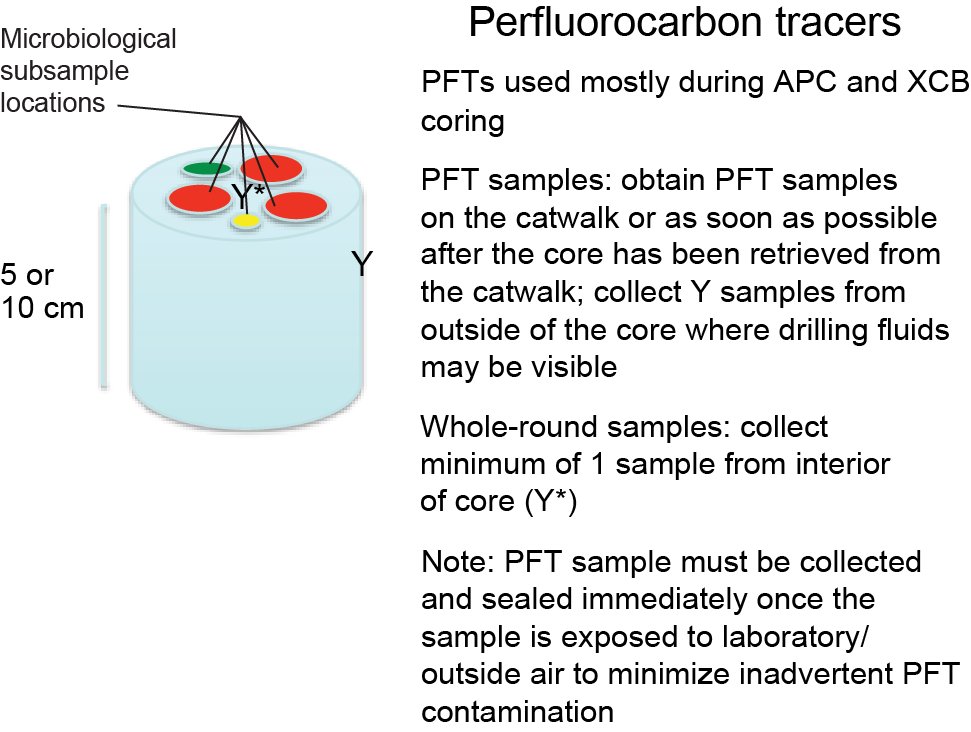
Figure F25. Whole-round sample and subsample locations.
Fluorescent microsphere tracers
Fluorescent microspheres, similar in size (0.5 µm in diameter) and charge to microorganisms, have been used in hydrology studies to determine dispersal and transport of microbe-sized objects (Harvey et al., 1989) and in drilling as tracers (Colwell et al., 1992). These microspheres (Fluoresbrite carboxylate microspheres; Polysciences, Inc.) appear bright green when observed by epifluorescence microscopy (458 nm excitation; 540 nm emission) and were used during Expedition 349 as a particulate tracer during coring of basalt and lithified sediment.
Microspheres were only deployed on cores acquired during RCB drilling when sampling was planned for microbiological cultivation and molecular biological analyses. The microspheres were deployed in plastic bags containing 40 mL of microsphere suspension in 18.2 MΩ water (1010 spheres/mL; 2 × 10¹¹ microspheres in a 40 mL bag according to Smith et al., 2000). The bag was then heat-sealed and placed into an additional plastic bag that was open at each end. By attaching the loose plastic ends with cord, the bag was wedged into a shim above the core catcher sub and stretched across the throat of the core barrel. The bags rupture and release the microspheres as the core enters the barrel. Samples for microsphere characterization were obtained as shown in Figure F26.
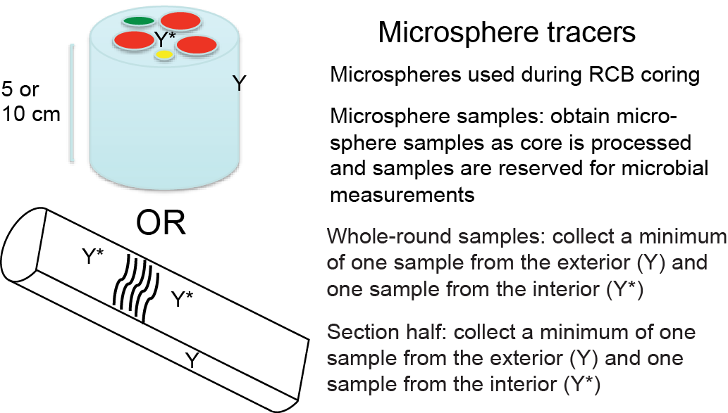
Figure F26. Microsphere sample locations.
Preliminary estimates of concentrations of fluorescent microspheres in core samples were quantified on board using a Zeiss Axioplan 2 epifluorescence microscope fitted with CoolLED pE-100 LED light sources, a blue filter set, and a 40× Plan-NEOFLUAR oil-immersion objective, as performed during Expedition 330 (Expedition 330 Scientists, 2012). For hard rock samples, aliquots (0.5 g) of the crushed rock were suspended in 1 mL of 0.2 µm filtered NaCl-saturated solution and filtered onto black, 25 mm diameter polycarbonate filters (0.2 µm pore size) in a filtration tower. The filters were then mounted on microscope slides with a drop of nonfluorescent immersion oil and covered with a coverslip. Microsphere abundance on the filter was determined by averaging the total number seen in at least 20 randomly selected fields of view. Quantitative estimates of the number of fluorescent beads in samples are difficult to achieve because microspheres are released from the bag at the beginning of RCB coring and the levels of fluorescent beads decrease during the coring of each section, such that the last sections to be cored may not have received a substantial microsphere dose.
Fluid community tracers
To further evaluate the extent to which contaminating cells may have penetrated a sample, contamination will be estimated by postcruise comparison of the microbial community diversity in basalt and sediment samples with the respective drilling fluid collected at the time of coring. This technique was first performed with deep continental samples (Lehman et al., 1995) but is common for studies of subseafloor samples, in which contamination is ubiquitous and genomic signatures of the contaminating material are subtracted from those of the subseafloor samples. The method can be accomplished by obtaining and preserving an adequate number of samples from the different sources of contamination (seawater, drilling fluid) and from the interior of the cores and then carrying out high-throughput sequencing of the 16S rRNA genes in the respective samples. Subsequent comparison of the community signatures can help to identify samples that significantly overlap in community structure with the drilling fluids (deeming them contaminated), as well as samples that have unique community structure when compared to the fluids (deeming them unlikely to be contaminated). This approach is especially important during RCB drilling because this method requires large amounts of surface seawater to be pumped into the borehole. This water is a major source of microbial contamination to cores collected for microbiological analyses.
For fluid community tracers, microorganisms were collected on 0.2 µm pore filters by filtering seawater or drilling fluid collected from the core liner or from the rig floor before the water was pumped into the drill string. The filters were frozen (–80°C) and will be analyzed postcruise in order to compare the microbial community structures in the drilling fluids with those in the core samples.
Microbiological sampling
Two distinct sampling strategies were adopted for microbiological samples. The respective approaches, (1) routine sampling of whole-round samples for microbiological measurements and (2) section half sampling for microbiological measurements across interfaces, are generally shown in Figure F27 and described in more detail below.
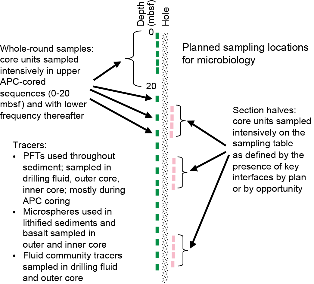
Figure F27. Microbiological sampling plan.
Whole-round samples
Once a core was retrieved, it was immediately transferred to the catwalk for labeling and cutting of sections. Cores were handled with care on the catwalk to prevent microbiological contamination. The core liner was cut by the standard IODP core cutter and with an ethanol-wiped spatula. Whole-round samples were provided to the microbiologist on duty as soon as possible on the catwalk. The core liner is not sterile, and the outer surface of the core is assumed to be contaminated during drilling. By subsampling the interior of the whole-round samples, the contaminated sediment or basalt that is next to the core liner can be avoided.
For routine microbiological sampling of whole-round samples, the upper sections close to the seafloor were sampled intensively, with whole-round samples taken as frequently as every 10 cm in the uppermost 1 mbsf. This sampling approach was followed when time permitted and when coring allowed a dedicated microbiology hole (e.g., Hole U1431B). Deeper than 1 mbsf, the sampling frequency decreased (see individual site reports), and the length of the whole-round samples collected was reduced to 5 cm. All whole-round samples were cut on the catwalk and capped on one end by an ethanol-rinsed plastic cap and by sterile foil on the other end. The whole-round samples were labeled and, with the foil covered ends held upright, transferred to the microbiology laboratory where they were stored in the cold room in an oxygen-free glove bag to minimize alteration of the microbial communities.
As soon as possible, the 5 or 10 cm long whole-round sample sections were subsampled into sterile 30 cm3 tip-cut syringes and then transferred into sterile 50 mL centrifuge tubes. For indurated materials, a hammer and an aseptically cleaned chisel were used to remove outer portions of the whole-round sample to obtain the inner, less altered portion of the core, which was then transferred into a sterile 50 mL centrifuge tube. In some cases, cores were hard enough that a SPEX 3624B X-Press hydraulic press was needed to crack the core to obtain material from the interior that was less likely to be contaminated by the drilling process. The pressure required to break the cores was usually <7 tons. Subsampling processes were carried out inside a N2-sparged glove bag unless a hammer and chisel or the hydraulic press were required.
Samples were then either stored in an ultralow-temperature freezer (−80°C) for molecular analyses or in a refrigerator (4°C) for cultivation-based analyses. After one ultralow-temperature freezer stopped functioning, some lipid samples were transferred to −20°C storage. The outer portions of the cores that remained after microbiological subsampling were returned to the core laboratory. In cores collected by XCB coring, we examined the split core for signs of drilling disturbance (e.g., biscuiting) to determine whether contamination might have occurred. Therefore, some of the samples were flagged as possibly or clearly contaminated.
Section-half samples
For microbiological sampling at lithologic interfaces on the working half of the core, a different approach was required. Important interfaces (e.g., turbidites and volcanic ash) can only be detected following the initial physical property evaluations and after the core has been split for direct observation. We recognize that some properties of the microbial communities may change with extended storage prior to core splitting, but well-preserved samples were accounted for in the aforementioned routine microbiological sampling. Section-half sampling for microbiology occurred after observation of the working halves of the core and at the point when discrete geological features could be identified and used as a guide for intensive sampling for microbiological properties. This required that the microbiologist on shift observe the cores immediately after splitting so that samples could rapidly and carefully be taken from the working halves and preserved for subsequent molecular analyses or cultivations. This procedure was also applied to four samples from Site U1433 where section-half samples were acquired from locations in the core within 1 cm of where the whole-round sample for microbiology was acquired several hours before when the core arrived on the catwalk. This will allow a direct comparison of microbial properties in nearly identical geological material that only differ based on the elapsed time before sample preservation.
Direct visual examination of the cores was applied to identify where drilling fluid intrusion might be a problem. Using sterile scalpels and putty knives, the working half was scraped to remove exposed material on the cut surface and then the contrasting features and the associated interface was subsampled into sterile 50 cm3 centrifuge tubes. These tubes were then transferred to ultralow-temperature freezers (−80°C), the −20°C freezer, or refrigeration (4°C) as noted above for the whole-round samples.
Paleomagnetism
During Expedition 349, we conducted paleomagnetic studies primarily to determine directions of remanence components. Routine measurements were completed on all archive halves with stepwise alternating field (AF) demagnetization. Discrete cube and minicore samples were taken from selected working halves and were measured with stepwise AF and thermal demagnetization. These data were used for core reorientation, magnetostratigraphic dating, and paleolatitude determination.
Magnetic measurements
Remanent magnetization was measured using a 2G superconducting rock magnetometer (SRM) (2G Enterprises model 760R) equipped with direct-current superconducting quantum interference devices (SQUIDs) and an in-line, automated AF demagnetizer capable of reaching a peak field of 80 mT. Ocean drilling cores generally carry secondary remanence components (overprints), including natural viscous remanence and a steep downward-pointing component attributed to the drill string. To separate the overprints from the characteristic remanence (ChRM), stepwise demagnetization experiments were performed, as described below.
Archive-half sections
Measurements of archive halves were conducted using the software SRM for section (version 1.0) with a nominal sample-area parameter of 15.59 cm2. The measurement interval and speed were 2.5 cm and 10 cm/s, respectively. The response functions of the pick-up coils of the SQUID sensors have a full width of 7–8 cm at half height (Parker and Gee, 2002). Therefore, data collected within ~4 cm of piece boundaries (or voids) are significantly affected by edge effects. Consequently, all data points within 4.5 cm of piece boundaries (as documented in the curatorial record) were filtered out prior to further processing. It should be noted that edge effects may also occur in a contiguous core piece if substantial heterogeneity (in intensity or direction) is present in the piece. It is more difficult to filter out such artifacts, but calculating the average direction (using Fisher statistics) for each core piece could provide a means of identifying these problems (Expedition 330 Scientists, 2012).
We performed successive AF demagnetization using the in-line AF demagnetizer of the SRM (2G Enterprises model 2G600) on all archive sections. The in-line AF demagnetizer applies a field to the x-, y-, and z-axes of the SRM in this fixed order. Previous reports suggest that higher AF demagnetization fields have produced significant anhysteretic remanent magnetization along the z-axis of the SRM. With this limitation, we used demagnetization steps up to 30 mT for demagnetizing sections. For most of the sediment sections, we performed steps from natural remanent magnetization to 30 mT demagnetization. The AF demagnetization results were plotted individually as vector plots (Zijderveld, 1967), as well as downhole variations with depth. We inspected the plots visually to judge whether the remanence after demagnetization at the highest AF step reflects the ChRM and geomagnetic polarity sequence.
Discrete samples
Oriented discrete samples representative of the lithology were collected from working-half sections. In soft sediment, discrete samples were taken in plastic “Japanese” Natsuhara-Giken sampling cubes (7 cm3 sample volume; Figure F28). Cubes were pushed by hand into the working half of the core with the “up” arrow on the cube pointing upsection in the core. For indurated intervals, cubes were cut with a table saw and trimmed to fit in the plastic containers. In lithified sediment and hard rock, oriented minicores (~11 cm3) were taken. Measurements of discrete samples were conducted using the software SRM for discrete samples (version 1.0). Discrete samples were also measured using a spinner magnetometer (AGICO model JR-6A) when the cryogenic magnetometer was in use for long core pass-through measurements.
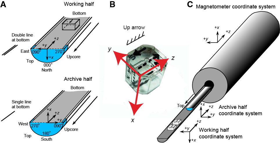
Figure F28. Paleomagnetic sample coordinates.
For discrete samples, we performed successive AF demagnetization with the DTech AF demagnetizer (model D-2000) for the spinner measurements to 120 mT (majority samples) and 200 mT (for several high-coercivity samples). We also performed successive thermal demagnetization using a thermal specimen demagnetizer (ASC Scientific model TD-48SC) for several selected discrete samples up to 675°C. Temperature increments of 25°–100°C were used depending on the unblocking temperature of each sample. We analyzed the stepwise demagnetization data of the discrete samples by principal component analysis to define the ChRM (Kirschvink, 1980). Section-half and discrete data collected on the pass-through SRM were uploaded to the LIMS database.
Low-field magnetic susceptibility of both whole rounds (see Physical properties) and split sections (see Lithostratigraphy and Physical properties) was routinely measured to roughly indicate the concentration of magnetic minerals. Anisotropy of magnetic susceptibility measurements were made on an AGICO KLY 4S Kappabridge instrument using the AMSSpin LabVIEW program designed by Gee et al. (2008) and adopted by the shipboard KLY 4S. The KLY 4S Kappabridge measures anisotropy of magnetic susceptibility by rotating the sample along three axes, stacking the data, and calculating the best-fit second-order tensor. It also measures the volume-normalized, calibrated bulk susceptibility (χ).
Coordinates
All magnetic data are reported relative to IODP orientation conventions: +x is into the face of the working half, +y points toward the left side of the face of the working half, and +z points downsection. The relationship between the SRM coordinates (X, Y, and Z) and the data coordinates (x, y, and z) is x = X, y = −Y, and z = Z for archive halves and x = −X, y = Y, and z = Z for working halves (Figure F28). The coordinate system for the spinner magnetometer (AGICO model JR-6A) and Natsuhara-Giken sampling cubes are indicated in Figure F29.
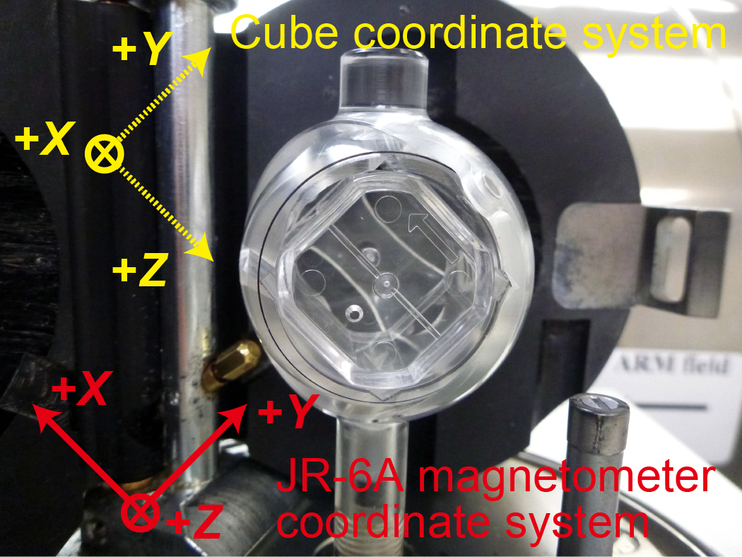
Figure F29. Magnetometer sample positions.
Core orientation
Core orientation of the APC cores was achieved with an orientation tool (FlexIT) mounted on the core barrel. The tool consists of three mutually perpendicular fluxgate magnetic sensors and two perpendicular gravity sensors. The information from both sets of sensors allows the azimuth and dip of the hole to be measured, as well as the azimuth of the APC core orientation. The orientation information contributed to paleomagnetic polarity determinations and magnetostratigraphic interpretations.
ChRM also provides a reference frame to reorient cores (see Structural geology). Provided that the reference magnetic pole is known, the orientation of the paleomagnetic vector is then used to restore the azimuth of the core: the horizontal component of the mean ChRM makes an angle with the reference line, which specifies the rotation of the core relative to the geographic coordinates (e.g., Fuller, 1969). The other assumptions for reorientation include whether
- The section has enough measurements to average out geomagnetic secular variation,
- The original bedding is horizontal,
- The core is vertical, and
- The sedimentary unit has not experienced any vertical axis rotation.
Assumptions 2 and 3 were verified by shipboard structural geologists, seismic profiles of the drill sites, and drilling operational records. Confirmation of 1 and 4 will be conducted postexpedition.
For intervals of particular interest for structural geology, we report the ChRMs defined from discrete samples. More detailed demagnetization steps for the discrete samples allowed more accurate determination of ChRMs than those from the archive halves.
Magnetostratigraphy
Magnetostratigraphy for each site was constructed by correlating observed polarity sequences with the geomagnetic polarity timescale in combination with biostratigraphic datums (Figures F11, F12, F13). We adopted the geomagnetic polarity timescale of Gradstein et al. (2012) (Table T4), in which boundary ages for Chrons C1n–C13n and C24n.1n–C34n are orbitally tuned, whereas those for Chrons C13r–C23r are spline fitted.
Table T4. Geomagnetic polarity timescale (Gradstein et al., 2012) used during Expedition 349. Download table in .csv format.
For azimuthally unoriented samples from sedimentary rock deposited at low latitudes, determining the polarity of sedimentary units may be difficult. The polarity ambiguity arises when the samples are azimuthally unoriented and the inclination is shallow near the Equator (the angular distance between reversed and normal polarity inclinations is small). Because paleomagnetic inclinations from any samples will have some degree of dispersion on their mean inclination, it is likely that when the mean inclination is shallow, the sign of the inclination will not be indicative of the polarity (e.g., McFadden and Reid, 1982; Cox and Gordon, 1984) and should be used with caution as a definitive estimate of magnetic polarity.
Whenever possible, we offer an interpretation of the magnetic polarity following the naming convention of correlative anomaly numbers prefaced by the letter C (Tauxe et al., 1984). Normal polarity subchrons are referred to by adding suffixes (n1, n2, etc.) that increase with age. For the younger part of the timescale (Pliocene–Pleistocene), we use traditional names to refer to the various chrons and subchrons (e.g., Brunhes, Jaramillo, Olduvai, etc.). In general, polarity reversals occurring at core section ends have been treated with extreme caution.
Physical properties
High-resolution physical property measurements were made during Expedition 349 mainly to aid lithostratigraphic characterization and to tie core descriptions to borehole data and seismic profiles. In particular, physical property data play a major role in hole-to-hole and site-to-site stratigraphic correlation, detection of discontinuities and inhomogeneities, obtaining information about differences in the composition and texture of sediment, identification of major seismic reflectors, and construction of synthetic seismic profiles. A variety of techniques and methods were used to characterize Expedition 349 cores on whole-round, split section-half, and discrete samples. Core sections are generally 1.5 m in length, so a typical coring length (stroke) of 9.5 m yields 6 sections plus a shorter seventh section. Procedures for measuring sediment or hard rock cores differ slightly.
Sedimentary cores
Recovered whole-round sections were first allowed to equilibrate to ambient room temperature (~20°C) and pressure for ~4 h. After thermally equilibrating, core sections were run through the WRMSL for measurement of density by gamma ray attenuation (GRA), magnetic susceptibility, and compressional wave velocity on the P-wave logger (PWL). Cores recovered with the XCB or the RCB are slightly smaller in diameter than those cored with the APC. As a result, sections cored with the XCB or RCB typically have gaps between the liner and the core, so P-wave velocity was not measured with WRMSL. Sections were then measured with the spectral NGRL. Thermal conductivity was measured on one whole-round section per sediment core (typically Section 3) by a needle probe inserted into the section through a small hole drilled through the plastic core liner close to the middle of the section. After that, cores were split longitudinally, with one half designated as archive and one as working half for sampling and analysis. The archive half of the core was passed through the SHMSL for measurement of point magnetic susceptibility and color reflectance. Compressional P-wave velocity measurements on split cores were typically made on the working halves that had been sampled for moisture and density (MAD), employing the transducers oriented in x-axis and z-axis directions. Discrete samples were collected from the working halves (every section for the first 15 cores and then every second section) to measure wet bulk density, dry bulk density, water content, porosity, and grain density with MAD procedures. For Hole U1431A, interstitial water was extracted by Rhizon samplers every 5, 10, or 20 cm before physical property measurements. P-wave velocity was expected to be higher in this hole compared to the others due to the extraction of water from the sediment, but the logs showed lower P-wave velocity, suggesting that the water in the liners was replaced by air.
Hard rock cores
Recovered hard rock sections were shaken onto sterile liners in the core splitting room for examination by a petrologist, who decided where the pieces should be split between working and archive halves. The pieces were then put back into liners and run through the WRMSL and NGRL. P-wave velocity was not measured, as the spaces between the liner and the rock core pieces make these measurements meaningless. After physical property measurements on whole-round cores, the core sections were split into working and archive halves and all rock pieces labeled. The archive half of the core was passed through the SHMSL for measurement of point magnetic susceptibility and color reflectance. Thermal conductivity was measured once per core using a contact probe on a piece of section half in a bath of seawater. Samples were taken from the working half of the core at a sampling interval of ~1 m depending on lithologic variability. Some of these samples were shared for both paleomagnetic and MAD measurements. Compressional P-wave velocity measurements were made on these discrete samples.
A full discussion of all methodologies and calculations used aboard the JOIDES Resolution in the Physical Properties Laboratory is available in Blum (1997). Details and procedures for each physical property measurement are described below.
WRMSL measurements
GRA-derived bulk density, P-wave velocity, and magnetic susceptibility were measured nondestructively with the WRMSL (Figure F30). To optimize the measurement process, sampling intervals and measurement integration times were the same for all sensors. Sampling intervals were set at 2.5 cm with an integration time of 5 s for each measurement. These sampling intervals are common denominators of the distances between the sensors installed on the WRMSL (30–50 cm), which allows sequential and simultaneous measurements. After every core, quality control and quality assurance (QC/QA) were monitored by passing a single core liner filled with deionized water through the WRMSL.
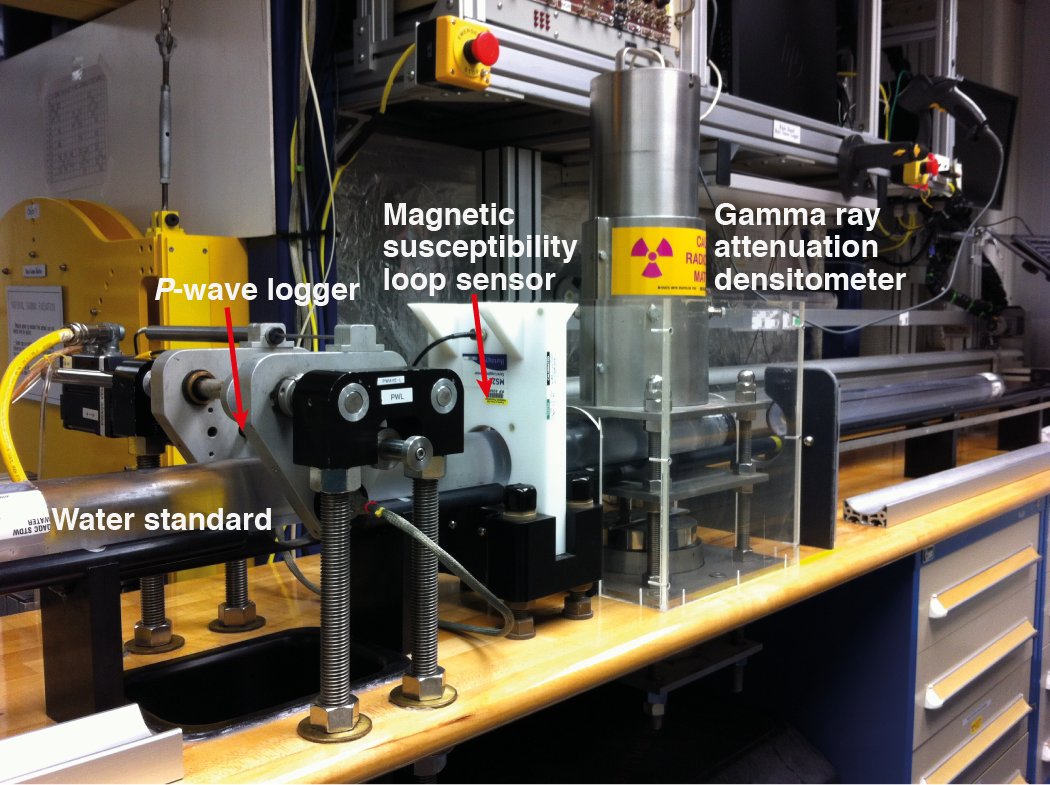
Figure F30. WRMSL measurements.
Gamma ray attenuation bulk density
Bulk density can be used to estimate the pore volume in sediment and evaluate the consolidation state of sediment. GRA density is an estimate of bulk density based on the attenuation of a gamma ray beam. The beam is produced by a 137Cs gamma ray source at a radiation level of 370 MBq within a lead shield with a 5 mm collimator, which is directed through the whole-round core. The gamma ray detector on the opposite side of the core from the source includes a scintillator and an integral photomultiplier tube to record the gamma radiation that passes through the core. The attenuation of gamma rays occurs primarily by Compton scattering, in which gamma rays are scattered by electrons in the formation; the degree of scattering is related to the material bulk density. Therefore, for a known thickness of sample, the density (ρ) is proportional to the intensity of the attenuated gamma rays and can be expressed as
- I = the measured intensity of gamma rays passing through the sample,
- I0 = gamma ray source intensity,
- μ = Compton attenuation coefficient, and
- d = sample diameter.
The μ and I0 are treated as constants, such that ρ can be calculated from I.
In general, WRMSL measurements are most accurate when taken on a completely filled core liner with minimal drilling disturbance; otherwise, measurements tend to underestimate true values. By default, the instrument reports measurements using the internal diameter of the core liner (66 mm) as the assumed sample diameter. This assumption is suitable for most sediment cores obtained by the APC; however, for sediment and/or hard rock cored by the XCB or RCB, core diameter is usually about 58 mm or less. Following Jarrard and Kerneklian (2007), the density measurements of cores obtained by XCB or RCB were corrected by multiplying the density values by ⁶⁶⁄₅₈ = 1.138 to account for this bias. The spatial resolution of the GRA densitometer is less than ±1 cm. The gamma ray detector is calibrated with sealed calibration cores (one standard core liner filled with distilled water and aluminum cylinders of various diameters). To establish the calibration curves, gamma ray counts were taken through each aluminum cylinder for 60 s. Each aluminum cylinder has a density of 2.7 g/cm3, and d is 1, 2, 3, 4, 5, or 6 cm. The relationship between I and µd is
where A, B, and C are coefficients determined from the calibration.
Recalibration was performed as needed when the deionized water QA/QC standard deviated significantly (more than a few percent) from 1 g/cm3.
Magnetic susceptibility
Magnetic susceptibility (χ) is a dimensionless measure of the degree to which a material can be magnetized by an external magnetic field:
where M is the magnetization induced in the material by an external field of strength H. Magnetic susceptibility is primarily sensitive to the concentration of ferrimagnetic minerals (e.g., magnetite and maghemite). It is also sensitive to magnetic mineralogy and can be related to the origin of the materials in the core and their subsequent diagenesis. Igneous materials typically have magnetic susceptibility a couple of orders of magnitude greater than their alteration products, such as clay.
The measurements were made using a Bartington MS2C loop sensor with a 9 cm diameter. An oscillator circuit in the sensor, which operates at a frequency of 0.565 kHz and an alternating field of ~140 A/m, produces a low-intensity, nonsaturating alternating magnetic field. Sediment or hard rock core sections going through the influence of this field cause a change in oscillator frequency. Frequency information returned in pulse form to the susceptometer is converted into magnetic susceptibility. The loop sensor has a spatial resolution of 23–27 mm, and it is accurate to within 2%.
P-wave velocity
P-wave velocity data can be used to evaluate small-strain moduli, correlate between downhole logging and core data, and evaluate porosity and cementation. P-wave (compressional) velocity (VP) is defined by the time required for a compressional wave to travel a specific distance
where d is the path length of the wave across the core and tcore is the traveltime through the core.
The PWL measures the traveltime of 500 kHz ultrasonic waves horizontally across the core at 2.5 cm intervals while it remains in the core liner. Waves are transmitted to the core by plastic transducer contacts connected to linear actuators. Pressure is applied to the actuators to ensure coupling between the transducers and the core liner. P-wave velocity transducers measure total traveltime of the compressional wave between transducers. The wave travels horizontally across the whole core and core liner. The total observed traveltime tcore is composed of
- tdelay = time delay related to transducer faces and electronic circuitry,
- tpulse = delay related to the peak detection procedure,
- tliner = transit time through the core liner, and
- tcore = traveltime through the sediment.
The system is calibrated using a core liner filled with distilled water, which provides control for tdelay, tpulse, and tliner. From these calibrations, VP can be calculated for the whole-round specimens in core liners as
VP = (dcl − 2dliner)/(to − tpulse − tdelay − 2tliner),
- dcl = measured diameter of core and liner,
- dliner = liner wall thickness, and
- to = measured total traveltime.
The above equation assumes that the core completely fills the core liner. The P-wave logger of the WRMSL was turned off for cores recovered with the XCB or RCB, which often do not fill the core liner.
NGRL measurements
Gamma radiation is emitted from the decay of mineral-hosted 238U, 232Th, and 40K. The NGRL measures this natural emission on whole-round cores using a system designed and built at the Integrated Ocean Drilling Program-US Implementing Organization (USIO) (Texas A&M University) (Vasiliev et al., 2011; Dunlea et al., 2013) (Figure F31). When 238U, 232Th, and 40K radioisotopes decay, they and their daughter products emit gamma radiation at specific energy levels unique to each isotope. NGR spectroscopy measures a wide energy spectrum that can be used to estimate the abundance of each isotope based on the strength of the signal at characteristic energies (Blum et al., 1997; Gilmore, 2008). Spectral data were collected and can be used for postcruise processing for U, Th, and K abundance but were not processed on board. Total counts were used on board, with high counts usually identifying fine-grained deposits containing K-rich clay minerals and their absorbed U and Th isotopes. NGR data thus reveal stratigraphic details that aid in core-to-core correlations. The system was installed on the renovated JOIDES Resolution in 2009 and has been used on every Integrated Ocean Drilling Program-USIO expedition starting with Expedition 320. The main NGR detector unit consists of 8 sodium iodide (NaI) detectors arranged along the core measurement axis at 20 cm intervals surrounding the lower half of the section (Figure F32). The detector array has passive (layers of lead) and active (plastic scintillators) shielding to reduce the background environmental and cosmic radiation. The overlying plastic scintillators detect incoming high-energy gamma and muon cosmic radiation and cancel this signal from the total counted by the NaI detectors.
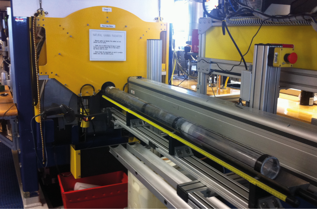
Figure F31. NGRL measurements.
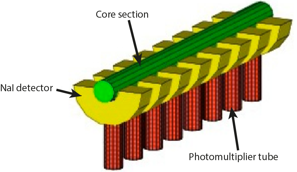
Figure F32. NGRL main elements.
A measurement run consisted of two sample positions, 10 cm apart, for a total of 16 measurements per 150 cm section. The quality of the energy spectrum measured in a core depends on the concentration of radionuclides in the sample but also on the counting time, with higher times yielding better spectra. Counting times were chosen as 5 min per position, or ~10 min per core, yielding statistically significant energy spectra (Vasiliev et al., 2011).
Thermal conductivity measurements
After NGR measurements were completed, thermal conductivity was measured with the TK04 (Teka Bolin) system using a needle-probe method in full-space configuration for whole-round sediment cores (Von Herzen and Maxwell, 1959) or a contact-probe method in half-space configuration on split cores for hard rock. The probes contain a heater wire and calibrated thermistor.
For soft sediment, the needle probe was inserted into a 2 mm diameter hole drilled through the liner along one of the lines that later guided core splitting. To avoid interference from air flow in the laboratory, the core was placed into an enclosed box outfitted with foam.
For hard rock cores, samples were selected from the working half and returned unaltered to the core liner upon completion of the tests. The contact probe embedded in the surface of an epoxy block with a low thermal conductivity (Vacquier, 1985) was maintained in contact with the sample and both were equilibrated together in a bath of seawater at room temperature in a cooler insulated with extruded polystyrene foam. The calibrated heat source of the probe was then turned on and the increase in temperature was recorded over 80 s. A heating power of 1.7 W/m was typically used in soft sediment and 1.9 W/m for indurated material. The solution to the heat conduction equation with a line source of heat was then fit to the temperature measurements to obtain the thermal conductivity. Because the probe is much more conductive than sediment or hard rock, the probe is assumed to be a perfect conductor. Under this assumption, the temperature of the superconductive probe has a linear relationship with the natural logarithm of the time after the initiation of the heat,
- T = temperature (K),
- q = heat input per unit length per unit time (J/m/s),
- k = thermal conductivity (W/[m·K]),
- t = time after the initiation of the heat (s), and
- C = instrumental constant.
Three measuring cycles were automatically performed to calculate average conductivity. A self-test, which included a drift study, was conducted at the beginning of each measurement cycle. Once the probe temperature stabilized, the heater circuit was closed and the temperature rise in the probe was recorded. Thermal conductivity was calculated from the rate of temperature rise while the heater current was flowing. Temperatures measured during the first 80 s of the heating cycle were fitted to an approximate solution of a constantly heated line source (for details, see Kristiansen, 1982; Blum, 1997). Measurement errors were 5%–10%. Thermal conductivity measurements were routinely taken in one section per core. Some cores retrieved by XCB yielded no results for thermal conductivity because cracks in the hard sediment caused bad coupling of the needle probe to the sediment.
SHMSL measurements
We measured color reflectance and magnetic susceptibility on archive section halves using the SHMSL. The archive half of the split core was placed on the core track, above which an electronic platform moves along a track, recording the height of the split-core surface with a laser sensor. The laser establishes the location of the bottom of the section, and then the platform reverses the direction of movement, moving from bottom to top making measurements of point magnetic susceptibility and color reflectance. All foam inserts were removed from the section-half cores before measurement, so the measured range of values represent that of the core material only. During Expedition 349, point magnetic susceptibility and color reflectance data were collected at constant intervals for each core but varied between 1 and 2.5 cm for different cores, depending on the available times for processing. These measurements have a sufficient resolution for comparing with the results obtained from the magnetic susceptibility loop of the WRMSL.
Color reflectance spectrometry
The color reflectance spectrometer uses an Ocean Optics 30 mm integrating sphere and both halogen and LED light source, which covers wavelengths from ultraviolet through visible to near infrared. The measurements were taken from 380 to 900 nm wavelengths at 2 nm intervals. The approximate 3 s data acquisition offset was applied for the entire scan of the archive section half. The data are reported using the L*a*b* color system, in which L* is lightness, a* is redness (positive) versus greenness (negative), and b* is yellowness (positive) versus blueness (negative) of the rock. The color reflectance spectrometer calibrates on two spectra, pure white (reference) and pure black (dark). Color calibration was conducted approximately once every 6 h (twice per shift).
Point magnetic susceptibility
Point magnetic susceptibility was measured with a Bartington MS2 meter and an MS2K contact probe with a flat 15 mm diameter round sensor with a field of influence of 25 mm and an operation frequency of 930 Hz. The instrument averages three measurements from the sensor for each offset, leading to an accuracy of ~5%. The spatial resolution of the point magnetic susceptibility instrument is ~3.8 mm, higher than that of the whole-round magnetic susceptibility for sections containing broken pieces <4 cm in length (the spatial resolution of whole-round magnetic susceptibility). As with whole-round measurements, the output displayed by the point magnetic susceptibility sensor must be converted to dimensionless SI units by multiplying by 10−5. The probe is zeroed in air before each measurement location to avoid influence from the metal track. The point magnetic susceptibility meter was calibrated by the manufacturer before installation on the ship and is quality checked every ~6 h at the same time as color reflectance sensor calibration.
SHMG measurements
For soft-sediment cores, P-wave velocity and shear strength measurements were performed on the working half of split cores before any samples were taken. P-wave velocity measurements used the x-axis caliper and z-axis bayonet contact probe transducers on the Section Half Measurement Gantry (SHMG) (Figure F33), with one analysis per section. Measurements were usually taken at ~75 cm in the section; however, if this interval provided no good sediment/transducer coupling (e.g., caused by high amounts of sand or cracks), different positions were chosen to generate viable data. Cores drilled with the XCB generally did not provide usable data because of bad sediment/liner contact and disturbed sediment. For hard rock cores, P-wave velocity was measured on the discrete samples chosen for both physical property and paleomagnetic measurements.
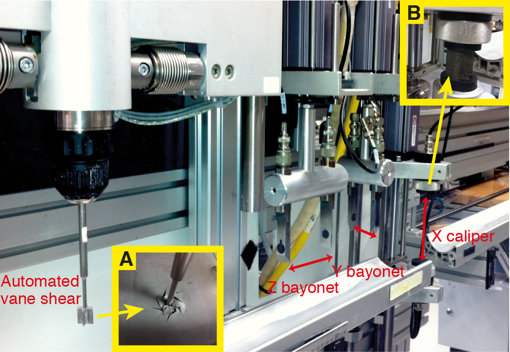
Figure F33. Section Half Multisensor Logger.
P-wave velocity
The P-wave velocity system uses Panametrics-NDT Microscan delay line transducers, which transmit at 0.5 MHz. The signal received through the section half or the discrete sample was recorded by the computer attached to the system, with the peak (P-wave arrival) usually chosen by autopicking software. In case of a weak signal, the first arrival was manually picked. During Expedition 349, we often manually picked the very base of the first arrival peak, leaving out the automatically picked points that usually fell along the ascending curve. The distance between transducers was measured with a built-in linear voltage displacement transformer. Calibration was performed with a series of acrylic cylinders of differing thicknesses and a known P-wave velocity of 2750 ± 20 m/s. The determined system time delay from calibration was subtracted from the picked arrival time to give a traveltime of the P-wave through the sample. The thickness of the sample (calculated by the linear voltage displacement transformer, in meters) was divided by the traveltime (in seconds) to calculate P-wave velocity in meters per second.
Shear strength
Shear strength is the resistance of a material to failure in shear. Shear stress in unconsolidated materials is resisted only by the network of solid particles. Shear strength (τf) can be expressed as a function of the effective normal stress at failure (σ′), the effective cohesion (c′), and friction angle (φ′),
where c2 and φ2 are the shear strength parameters that define a linear relationship between τf and φ2, according to the Mohr-Coulomb failure criterion.
Shear strength parameters can be determined by means of multiple laboratory tests. The c2 and φ2 are relevant in situations where field drainage conditions correspond to test conditions. The shear strength of a soil under undrained conditions (interstitial water drainage does not occur during failure) is different from that under drained conditions (interstitial water drainage occurs).
Undrained shear strength can be expressed in terms of total stress in the case of fully saturated materials of low permeability (e.g., clays), denoted by Su. The most common strength tests in shipboard laboratories are the vane shear and penetrometer tests, which provide measurement of undrained shear strength (Su) (Blum, 1997).
During Expedition 349, Su was measured in undisturbed fine-grained sediment using the automated vane shear (AVS) system in working-half cores (Figure F33). Using the AVS, undrained shear strength was determined by inserting a four-bladed vane into the split core and rotating it at a constant 90°/min to determine the torque required to cause a cylindrical surface to be sheared by the vane, which provides a measurement of the peak shear strength. The difference in rotational strain between the top and the bottom of a linear spring is measured using digital shaft encoders. Measurements were made with the vane rotation axis perpendicular to the split surface. The residual shear strength was taken to be the constant and lowest measured shear strength after reaching the peak value during the test cycle. Sampling rates were one per core unless the sediment was too firm for instrument penetration or was disturbed during coring.
Vane shear strength Su(v) (kPa) is calculated as
- T = torque required to induce material failure (N·m),
- Kv = constant, depending on vane dimensions (m3),
- Δ = maximum torque angle (°) at failure, and
- B = spring constant that relates the deflection angle to the torque (°/N·m) (Blum, 1997).
All measurements used a vane with a height and diameter of 12.7 mm. Failure torque (T) was determined by measuring the degrees of rotation of one of four torsional springs. A linear calibration equation (specified by the manufacturer) relates the rotation angle to the torque for the particular spring being used. Selection of the appropriate spring was based on the anticipated shear strength of the material. Vane shear results were generally considered reliable for shear strength values less than ~150–200 kPa, above which excessive cracking and separation of the core material occurred.
Discrete sample MAD measurements
Discrete samples were collected from the working halves to determine wet and dry bulk density, grain density, water content, and porosity. In soft sediment, ~10 cm3 samples were collected with a plastic syringe, the diameter of which fit that of the glass vials. An attempt was made to sample every section for the first 15 cores and every second section for deeper cores, depending on lithologic variability. In indurated sediment and hard rock, minicores were extracted from the working halves for physical property measurements, with some also shared for paleomagnetic measurements.
Sample preparation
Soft-sediment samples were placed in numbered, preweighed ~16 mL Wheaton glass vials for wet and dry sediment weighing, drying, and dry volume measurements. Determination of an accurate wet mass of the minicore samples of indurated sediment and hard rock first required that the pore space of the samples be completely saturated with seawater. To do this, we placed the samples in individual plastic vials filled with seawater and used a vacuum chamber. A vacuum pump removed the air from the chamber to a pressure of ~40–50 kPa below the atmospheric pressure, forcing seawater into the samples. The samples were kept under saturation for at least 24 h, with the vacuum maintained in the chamber by turning the pump on for 30 min every 5 h. After removal from the saturator, the minicores were patted dry with a paper towel and wet mass immediately determined using the dual balance system. P-wave velocities were then measured on the wet samples. Following the velocity measurements, the samples were dried in a convection oven for at least 24 h at 105° ± 5°C. Dried samples were then cooled in a desiccator for at least 60 min before the dry mass and the volume were measured.
Dual balance mass measurement
The weights of wet and dry sample masses were determined to a precision of 0.005 g using two Mettler Toledo electronic balances, with one acting as a reference. A standard weight of similar value to the sample was placed upon the reference balance to increase accuracy. A computer averaging system was used to compensate for the ship’s motion. The default setting of the balances is 300 measurements (taking ~1.5 min).
Pycnometer volume measurement
Dry sample volume was determined using a hexapycnometer system of a six-celled, custom-configured Micrometrics AccuPyc 1330TC helium-displacement pycnometer (Figure F34). The precision of each cell is 1% of the full-scale volume. Volume measurement was preceded by three purges of the sample chamber with helium warmed to ~28°C. Three measurement cycles were run for each sample. A reference volume (set of two calibration spheres) was placed sequentially in one of the chambers to check for instrument drift and systematic error. The volumes occupied by the numbered Wheaton vials were calculated before the cruise by multiplying each vial’s weight against the average density of the vial glass. Dry mass and volume were measured after samples were heated in an oven at 105° ± 5°C for 24 h and allowed to cool in a desiccator. The procedures for the determination of these physical properties comply with the American Society for Testing and Materials (ASTM) designation (D) 2216 (ASTM International, 1990). The fundamental relation and assumptions for the calculations of all physical property parameters are discussed by Blum (1997) and summarized below.
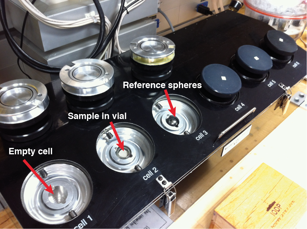
Figure F34. Pyncometer.
Mass and volume calculation
We measured wet mass (Mwet), dry mass (Mdry), and dry volume (Vdry). The ratio of mass (rm) is a computational constant of 0.965 (i.e., 0.965 g of freshwater per 1 g of seawater). Salt precipitated in sediment pores during the drying process is included in the Mdry and Vdry values. The mass of the evaporated water (Mwater) and salt (Msalt) in the sample are given by
where s is the assumed saltwater salinity (0.035%) corresponding to a pore water density (ρpw) of 1.024 g/cm3 and a salt density (ρsalt) of 2.22 g/cm3. The corrected mass of pore water (Mpw), volume of pore water (Vpw), mass of solids excluding salt (Msolid), volume of salt (Vsalt), volume of solids excluding salt (Vsolid), and wet volume (Vwet) are
Vwet = Vdry − Vsalt + Vpw, and
Calculation of bulk properties
For all sediment samples, water content (w) is expressed as the ratio of mass of pore water to wet sediment (total) mass,
Wet bulk density (ρwet), dry bulk density (ρdry), sediment grain density (ρsolid), porosity (φ), and void ratio (VR) are calculated as:
Moisture and density properties reported and plotted in the Physical properties sections of all site chapters were calculated with the MADMax shipboard program, set with “method C” calculation process.
Downhole measurements
Downhole logs are used to determine physical, chemical, and structural properties of the formation penetrated by a borehole. The data are rapidly collected, continuous with depth, and measured in situ; they can be interpreted in terms of the stratigraphy, lithology, mineralogy, magnetic characteristics, and geochemical composition of the penetrated formation. Where core recovery is incomplete or disturbed, log data may provide the only way to characterize the borehole section. Where core recovery is good, log and core data complement one another and may be interpreted jointly.
Downhole logs measure formation properties on a scale that is intermediate between those obtained from laboratory measurements on core samples and those from geophysical surveys. They are useful in calibrating the interpretation of geophysical survey data (e.g., through the use of synthetic seismograms) and provide a necessary link for the integrated understanding of physical and chemical properties on different scales.
During Expedition 349, downhole logging measurements were taken in Holes U1431E and U1433B. In addition, downhole temperature measurements were acquired using the advanced piston corer temperature tool (APCT-3) in Holes U1431D, U1432C, and U1433A.
Wireline logging
During wireline logging operations, logs are recorded with Schlumberger logging tools combined into several tool strings, which are lowered into the hole after completion of coring operations. Two main tool strings were used during Expedition 349. The first is a variant of the triple combination (triple combo) tool string, which measures, from top to bottom, borehole fluid temperature, NGR, porosity, density, electrical resistivity, and magnetic susceptibility. The second tool string is the Formation MicroScanner (FMS)-sonic, which measures NGR, sonic velocities, and FMS resistivity images of the borehole wall (Figure F35; Table T5). Each tool string also contains an Enhanced Digital Telemetry Cartridge (EDTC) for communicating through the wireline to the Schlumberger data acquisition system (MAXIS unit) on the drillship.

Figure F35. Wireline tool strings.
Table T5. Downhole measurements made by wireline tool strings during Expedition 349. For definitions of tool acronyms, see Table T6. Download table in .csv format.
In preparation for logging, the boreholes were reamed in their lower sections, flushed of debris by circulating drilling fluid, and filled with seawater-based logging gel (sepiolite mud mixed with seawater and weighted with barite; approximate density = 10.5 lb/gal) to help stabilize the borehole walls in sections where instability was expected from drilling and coring results. The BHA was pulled up to ~150 m wireline depth below seafloor (WSF) to cover the unstable upper part of Hole U1431E and to 100 m WSF in Hole U1433B. The tool strings were then lowered downhole on a seven-conductor wireline cable before being pulled up at constant speed, typically ~300 m/h for the triple combo and 600 m/h for the FMS-sonic, to provide continuous log measurements of several properties simultaneously.
Each tool string deployment is termed a logging “run.” During each run, tool strings can be lowered and pulled up in the hole several times to check repeatability and to increase coverage of the FMS borehole images. Each lowering or hauling-up of the tool string while collecting data constitutes a “pass.” Incoming data were recorded and monitored in real time on the MCM MAXIS logging computer. A wireline heave compensator (WHC) was used to minimize the effect of ship’s heave on the tool position in the borehole (see below).
Logged sediment properties and tool measurement principles
The logged properties and the principles used in the tools that measure them are briefly described below. The main logs are listed in Table T6. More detailed information on individual tools and their geological applications may be found in Serra (1984, 1986, 1989), Schlumberger (1989, 1994), Rider (1996), Goldberg (1997), Lovell et al. (1998), and Ellis and Singer (2007). A complete online list of acronyms for the Schlumberger tools and measurement curves is at www.apps.slb.com/cmd.
Table T6. Acronyms and units used for downhole wireline tools and measurements during Expedition 349. For the complete list of acronyms used in IODP and for additional information about tool physics, consult IODP-USIO Science Services, LDEO, at iodp.ldeo.columbia.edu/TOOLS_LABS/tools.html. Download table in .csv format.
Natural gamma radiation
The Hostile Environment Natural Gamma Ray Sonde (HNGS) was used on both the triple combo and FMS-sonic tool strings to measure NGR in the formation. The HNGS uses two bismuth germanate scintillation detectors and five-window spectroscopy to determine concentrations of potassium (in weight percent), thorium (in parts per million), and uranium (in parts per million) from the characteristic gamma ray energies of isotopes in the 40K, 232Th, and 238U radioactive decay series, which dominate the natural radiation spectrum. The computation of the elemental abundances uses a least-squares method of extracting U, Th, and K elemental concentrations from the spectral measurements. The HNGS filters out gamma ray energies below 500 keV, eliminating sensitivity to bentonite or KCl in the drilling mud and improving measurement accuracy. The HNGS also provides a measure of the total gamma ray emission (HSGR) and uranium-free or computed gamma ray emission (HCGR) that are measured in American Petroleum Institute units (gAPI). The HNGS response is influenced by the borehole diameter, and therefore the HNGS data are corrected for borehole diameter variations during acquisition.
An additional NGR sensor was housed in the EDTC, which was used primarily to communicate data to the surface. The sensor includes a sodium iodide scintillation detector that also measures the total NGR emission of the formation. It is not a spectral tool (does not provide U, Th, and K concentrations), but it provides total gamma radiation for each pass.
The inclusion of the HNGS in every tool string allows use of the gamma ray data for precise depth match processing between logging strings and passes and for core-log integration.
Density and photoelectric factor
Formation density was measured with the Hostile Environment Litho-Density Sonde (HLDS). The sonde contains a radioactive cesium (137Cs) gamma ray source (622 keV) and far and near gamma ray detectors mounted on a shielded skid, which is pressed against the borehole wall by a hydraulically activated decentralizing arm. Gamma radiation emitted by the source undergoes Compton scattering, in which gamma rays are scattered by electrons in the formation. The number of scattered gamma rays that reach the detectors is proportional to the density of electrons in the formation, which is in turn related to bulk density. Porosity may also be derived from this bulk density if the matrix (grain) density is known.
The HLDS also measures the photoelectric effect factor (PEF), a measure of the photoelectric absorption of low-energy gamma radiation. Photoelectric absorption occurs when their energy falls below 150 keV as a result of being repeatedly scattered by electrons in the formation. PEF is determined by comparing the counts from the far detector in the high-energy region, where only Compton scattering occurs, with those in the low-energy region, where count rates depend on both reactions. Because PEF depends on the atomic number of the elements in the formation (heavier elements have higher PEF), it also varies according to the chemical composition of the minerals present and can be used for the identification of the overall mineral make-up of the formation. For example, the PEF of calcite is 5.08 barn/e−, illite is 3.03 barn/e−, quartz is 1.81 barn/e−, and hematite is 21 barn/e−. Good contact between the tool and borehole wall is essential for good HLDS logs; poor contact results in underestimation of density values. Both the density correction and caliper measurement of the hole are used to check the contact quality. In the deeper parts of the hole, the PEF log should be used with caution, especially in washouts, because barium in the logging mud swamps the signal, despite correction for mud effect.
Electrical resistivity
The High-Resolution Laterolog Array (HRLA) tool provides six resistivity measurements with different depths of investigation (including the borehole, or mud, resistivity and five measurements of formation resistivity with increasing penetration into the formation). The tool sends a focused current into the formation and measures the intensity necessary to maintain a constant drop in voltage across a fixed interval, providing direct resistivity measurements. The array has one central (source) electrode and six electrodes above and below it, which serve alternatively as focusing and returning current electrodes. By rapidly changing the role of these electrodes, a simultaneous resistivity measurement at six penetration depths is achieved. The tool is designed to ensure that all signals are measured at exactly the same time and tool position and to reduce the sensitivity to “shoulder bed” effects when crossing sharp beds thinner than the electrode spacing. The design of the HRLA, which eliminates the need for a surface reference electrode, improves formation resistivity evaluation compared to traditional dual induction and allows the full range of resistivity to be measured, from low (e.g., in high-porosity sediments) to high (e.g., in basalt). The HRLA needs to be run centralized in the borehole for optimal results, so knuckle joints were used to centralize the HRLA while allowing the density and porosity tools to maintain good contact with the borehole wall (Figure F35).
Calcite, silica, and hydrocarbons are electrical insulators, whereas ionic solutions like interstitial water are conductors. Electrical resistivity, therefore, can be used to evaluate porosity for a given salinity and resistivity of the interstitial water. Clay surface conduction also contributes to the resistivity values, but at high porosities, this is a relatively minor effect.
Acoustic velocity
The Dipole Shear Sonic Imager (DSI) measures the transit times between sonic transmitters and an array of eight receivers. It combines replicate measurements, thus providing a direct measurement of sound velocity through formations that is relatively free from the effects of formation damage and an enlarged borehole (Schlumberger, 1989). Along with the monopole transmitters found on most sonic tools, it also has two crossed-dipole transmitters that allow the measurement of shear wave velocity in addition to compressional wave velocity. Dipole measurements are necessary to measure shear velocities in slow formations with shear velocity less than the velocity of sound in the borehole fluid. Such slow formations are typically encountered in deep-ocean drilling.
Formation MicroScanner
The FMS provides high-resolution electrical resistivity–based images of borehole walls. The tool has four orthogonal arms and pads, each containing 16 button electrodes that are pressed against the borehole wall during logging. The electrodes are arranged in two diagonally offset rows of 8 electrodes each. A focused current is emitted from the button electrodes into the formation, with a return electrode near the top of the tool. Resistivity of the formation at the button electrodes is derived from the intensity of current passing through the button electrodes.
Processing transforms the resistivity measurements into oriented high-resolution images that reveal geologic structures of the borehole wall. Features such as bedding, stratification, fracturing, slump folding, and bioturbation can be resolved (Luthi, 1990; Salimullah and Stow, 1992; Lovell et al., 1998). Because the images are oriented to magnetic north, further analysis can provide measurement of the dip and direction (azimuth) of planar features in the formation. In addition, when the corresponding planar features can be identified in the recovered core samples, individual core pieces can be reoriented with respect to true north.
Approximately 30% of a borehole with a diameter of 25 cm is imaged during a single pass. Standard procedure is to make two full uphole passes with the FMS to maximize the chance of getting full borehole coverage with the pads. The maximum extension of the caliper arms is 40.6 cm (16 inches). In holes with a diameter greater than this maximum, the pad contact at the end of the caliper arms will be inconsistent, and the FMS images may appear out of focus and too conductive. Irregular (rough) borehole walls will also adversely affect the images if contact with the wall is poor.
Magnetic Susceptibility Sonde
The Magnetic Susceptibility Sonde (MSS) is a nonstandard wireline tool designed by Lamont-Doherty Earth Observatory (LDEO). It measures the ease with which formations are magnetized when subjected to a magnetic field. The ease of magnetization is ultimately related to the concentration and composition (size, shape, and mineralogy) of magnetic minerals (principally magnetite) in the formation. These measurements provide one of the best methods for investigating stratigraphic changes in mineralogy and lithology because the measurement is quick, repeatable, and nondestructive and because different lithologies often have strongly contrasting susceptibilities.
The MSS dual-coil sensor provides ~40 cm resolution measurements, with ~20 cm depth of horizontal investigation. The MSS was run as the lowermost tool in the triple combo tool string, using a specially developed data translation cartridge to enable the MSS to be run in combination with the Schlumberger tools. The MSS also has an optional single-coil sensor to provide high-resolution measurements (~10 cm), but this was not used during Expedition 349 because it has a large bowspring that would require the MSS to be run higher up in the tool string and because it is very sensitive to separation from the borehole wall.
Magnetic susceptibility data from both the high-resolution and deep-reading sensors are plotted as uncalibrated units. The MSS reading responses are affected by temperature and borehole size (higher temperatures lead to higher susceptibility measurements). Preliminary processing was performed offshore to remove the temperature drift by calculating a least-squares polynomial fit to the data and subtracting the calculated trend from the data set. When the magnetic susceptibility signal in sediment is very low, the detection limits of the tool may be reached. For quality control and environmental correction, the MSS also measures internal tool temperature, z-axis acceleration, and low-resolution borehole conductivity.
Acceleration and inclinometry
The General Purpose Inclinometer Tool (GPIT) was included in the FMS-sonic tool string to calculate tool acceleration and orientation during logging. Tool orientation is defined by three parameters: tool deviation, tool azimuth, and relative bearing. The GPIT utilizes a three-axis inclinometer and a three-axis fluxgate magnetometer to record the orientation of the FMS as the magnetometer records the magnetic field components (Fx, Fy, and Fz). Thus, the FMS images can be corrected for irregular tool motion, and the dip and direction (azimuth) of features in the FMS image can be determined.
Log data quality
The main influence on log data quality is the condition of the borehole wall. Where the borehole diameter varies over short intervals because of washouts of softer material or ledges of harder material, the logs from tools that require good contact with the borehole wall (i.e., FMS, density, and porosity) may be degraded. Deep investigation measurements such as gamma radiation, resistivity, and sonic velocity, which do not require contact with the borehole wall, are generally less sensitive to borehole conditions. “Bridged” sections, where borehole diameter is much below the bit size, will also cause irregular log results. The quality of the borehole is improved by minimizing the circulation of drilling fluid while drilling, flushing the borehole to remove debris, and logging as soon as possible after drilling and conditioning are completed. During this expedition, the necessity of flushing dense basement rocks up and out of the borehole required heavy circulation.
The quality of the wireline depth determination depends on several factors. The depth of the logging measurements is determined from the length of the cable payed out from the winch on the ship. The seafloor is identified on the NGR log by the abrupt reduction in gamma ray count at the water/sediment interface (mudline). Discrepancies between the drilling depth and the wireline log depth may occur. For the case of drilling depth, discrepancies are due to core expansion, incomplete core recovery, or incomplete heave compensation. In the case of log depth, discrepancies between successive runs occur because of incomplete heave compensation, incomplete correction for cable stretch, and cable slip. Tidal changes in sea level affect both drilling and logging depths, although these were <1 m in the South China Sea.
Wireline heave compensator
During wireline logging operations, the up-and-down motion of the ship (heave) causes a similar motion of the downhole logging tools. If the amplitude of this motion is large, depth discrepancies can be introduced into the logging data. The risk of damaging downhole instruments is also increased. A WHC system was thus designed to compensate for the vertical motion of the ship and maintain a steady motion of the logging tools to ensure high-quality logging data acquisition (Liu et al., 2012; Iturrino et al., 2013). The WHC uses a vertical accelerometer (motion reference unit [MRU]) positioned under the rig floor near the ship’s center of gravity to calculate the vertical motion of the ship with respect to the seafloor. It then adjusts the length of the wireline by varying the distance between two sets of pulleys through which the cable passes in order to minimize downhole tool motion. Real-time measurements of uphole (surface) and downhole acceleration are made simultaneously by the MRU and the EDTC, respectively. An LDEO-developed software package allows these data to be analyzed and compared in real time, displaying the actual motion of the logging tool string and enabling monitoring of the efficiency of the compensator. The WHC was used for logging Hole U1431E but not for Hole U1433B because heave conditions were calm.
Logging data flow and log depth scales
Data for each wireline logging run were monitored in real time and recorded using the Schlumberger MAXIS 500 system. Initial logging data were referenced to the rig floor (wireline depth below rig floor [WRF]). After logging was completed, the data were shifted to a seafloor reference (WSF), which was based on the step in gamma radiation at the sediment/water interface.
Data were transferred onshore to LDEO, where standardized data processing took place. The main part of the processing is depth matching to remove depth offsets between logs from different logging runs, which results in a new depth scale: wireline log matched depth below seafloor (WMSF). Also, corrections are made to certain tools and logs (e.g., FMS imagery is corrected for tool acceleration, including “stick and slip”), documentation for the logs (with an assessment of log quality) is prepared, and the data are converted to ASCII for the conventional logs and GIF for the FMS images. The Schlumberger Geo-Quest’s GeoFrame software package is used for most of the processing of the collected wireline logging data. The data were transferred back to the ship within a few days of logging, and this processed data set was made available to the science party (in ASCII and DLIS formats) through the shipboard IODP logging database and shipboard servers.
In situ temperature measurements
During Expedition 349, in situ temperature measurements were made with the APCT-3 in Hole A at each site when the APC was deployed, except at Site U1431, where 4 in situ temperature measurements were made in Hole U1431D. The APCT-3 fits directly into the coring shoe of the APC and consists of a battery pack, data logger, and a platinum resistance-temperature device calibrated over a temperature range from 0° to 30°C. Before entering the borehole, the tool is first stopped at the mudline for 5 min to thermally equilibrate with bottom water. However, the lowest temperature recorded during the run was occasionally used instead of the average temperature at the mudline as an estimate of the bottom water temperature because (1) it was more repeatable and (2) the bottom water is expected to have the lowest temperature in the profile. When the APC is plunged into the formation, there is an instantaneous temperature rise from frictional heating. This heat gradually dissipates into the surrounding sediment as the temperature at the APCT-3 equilibrates toward the temperature of the sediment. After the APC penetrated the sediment, it was held in place for 5 min while the APCT-3 recorded the temperature of the cutting shoe every second.
The equilibrium temperature of the sediment was estimated by applying a mathematical heat-conduction model to the temperature decay record (Horai and Von Herzen, 1985). The synthetic thermal decay curve for the APCT-3 is a function of the geometry and thermal properties of the probe and the sediment (Bullard, 1954; Horai and Von Herzen, 1985). Equilibrium temperature was estimated by applying a fitting procedure (Pribnow et al., 2000). However, where the APC did not achieve a full stroke or where ship heave pulled the APC up from full penetration, the temperature equilibration curve is disturbed and temperature determination is less accurate. The nominal accuracy of the APCT-3 temperature measurements is ±0.05°C.
APCT-3 temperature data were combined with measurements of thermal conductivity (see Physical properties) obtained from whole-round core sections to obtain heat flow values. Heat flow was calculated according to the Bullard method, to be consistent with the synthesis of ODP heat flow data by Pribnow et al. (2000).
References
ASTM International, 1990. Standard method for laboratory determination of water (moisture) content of soil and rock (Standard D2216–90). In Annual Book of ASTM Standards for Soil and Rock (Vol. 04.08): Philadelphia (American Society for Testing Materials). [revision of D2216-63, D2216-80]
Balsam, W.L., and Damuth, J.E., 2000. Further investigations of shipboard vs. shore-based spectral data: implications for interpreting Leg 164 sediment composition. In Paull, C.K., Matsumoto, R., Wallace, P., and Dillon, W.P. (Eds.), Proceedings of the Ocean Drilling Program, Scientific Results, 164: College Station, TX (Ocean Drilling Program), 313–324. http://dx.doi.org/10.2973/odp.proc.sr.164.222.2000
Balsam, W.L., Damuth, J.E., and Schneider, R.R., 1997. Comparison of shipboard vs. shore-based spectral data from Amazon Fan cores: implications for interpreting sediment composition. Proceedings of the Ocean Drilling Program, Scientific Results, 155: College Station, TX (Ocean Drilling Program), 193–215. http://dx.doi.org/10.2973/odp.proc.sr.155.210.1997
Balsam, W.L., Deaton, B.C., and Damuth, J.E., 1998. The effects of water content on diffuse reflectance spectrophotometry studies of deep-sea sediment cores. Marine Geology, 149(1–4):177–189. http://dx.doi.org/10.1016/S0025-3227(98)00033-4
Berggren, W.A., Kent, D.V., Swisher, C.C., III, and Aubry, M.-P., 1995. A revised Cenozoic geochronology and chronostratigraphy. In Berggren, W.A., Kent, D.V., Aubry, M.-P., and Hardenbol, J. (Eds.), Geochronology, Time Scales and Global Stratigraphic Correlation. Special Publication - SEPM (Society for Sedimentary Geology), 54:129–212. http://dx.doi.org/10.2110/pec.95.04.0129
Blow, W.H., 1969. Late middle Eocene to Recent planktonic foraminiferal biostratigraphy. Proceedings of the International Conference on Planktonic Microfossils, 1:199–422.
Blow, W.H., 1979. The Cainozoic Foraminifera (Vols. 1–3): Leiden, The Netherlands (E.J. Brill).
Blum, P., 1997. Physical properties handbook: a guide to the shipboard measurement of physical properties of deep-sea cores. Ocean Drilling Program Technical Note, 26. http://dx.doi.org/10.2973/odp.tn.26.1997
Bolli, H.M., and Saunders, J.B., 1985. Oligocene to Holocene low latitude planktic foraminifera. In Bolli, H.M., Saunders, J.B., and Perch-Nielsen, K. (Eds.), Plankton Stratigraphy (Vol. 1): Planktic Foraminifera, Calcareous Nannofossils and Calpionellids: Cambridge, UK (Cambridge University Press), 155–262.
Bollmann, J., 1997. Morphology and biogeography of Gephyrocapsa coccoliths in Holocene sediments. Marine Micropaleontology, 29(3–4):319–350. http://dx.doi.org/10.1016/S0377-8398(96)00028-X
Bown, P.R. (Ed.), 1998. Calcareous Nannofossil Biostratigraphy: Dordrecht, The Netherlands (Kluwer Academic Publishing).
Bullard, E.C., 1954. The flow of heat through the floor of the Atlantic Ocean. Proceedings of the Royal Society of London, Series A: Mathematical, Physical and Engineering Sciences, 222(1150):408–429. http://dx.doi.org/10.1098/rspa.1954.0085
Chen, M.H., and Tan, Z.Y., 1996. Radiolaria from Surface Sediments of the Central and Northern South China Sea: Beijing (Science Press). (in Chinese with English summary)
Colwell, F.S., Stormberg, G.J., Phelps, T.J., Birnbaum, S.A., McKinley, J., Rawson, S.A., Veverka, C., Goodwin, S., Long, P.E., Russell, B.F., Garland, T., Thompson, D., Skinner, P., and Grover, S., 1992. Innovative techniques for collection of saturated and unsaturated subsurface basalts and sediments for microbiological characterization. Journal of Microbiological Methods, 15(4):279–292. http://dx.doi.org/10.1016/0167-7012(92)90047-8
Cox, A., and Gordon, R.G., 1984. Paleolatitudes determined from paleomagnetic data from vertical cores. Reviews of Geophysics and Space Physics, 22(1):47–71. http://dx.doi.org/10.1029/RG022i001p00047
Droser, M.L., and Bottjer, D.J., 1986. A semiquantitative field classification of ichnofabric. Journal of Sedimentary Research, 56(4):558–559. http://dx.doi.org/10.1306/212F89C2-2B24-11D7-8648000102C1865D
Dunlea, A.G., Murray, R.W., Harris, R.N., Vasiliev, M.A., Evans, H., Spivack, A.J., and D’Hondt, S., 2013. Assessment and use of NGR instrumentation on the JOIDES Resolution to quantify U, Th, and K concentrations in marine sediment. Scintific Drilling, 15:57–63. http://dx.doi.org/10.2204/iodp.sd.15.05.2013
Ellis, D.V., and Singer, J.M., 2007. Well Logging for Earth Scientists (2nd ed.): New York (Elsevier).
Expedition 309/312 Scientists, 2006. Methods. In Teagle, D.A.H., Alt, J.C., Umino, S., Miyashita, S., Banerjee, N.R., Wilson, D.S., and the Expedition 309/312 Scientists. Proceedings of the Integrated Ocean Drilling Program, 309/312: Washington, DC (Integrated Ocean Drilling Program Management International, Inc.). http://dx.doi.org/10.2204/iodp.proc.309312.102.2006
Expedition 324 Scientists, 2010. Methods. In Sager, W.W., Sano, T., Geldmacher, J., and the Expedition 324 Scientists, Proceedings of the Integrated Ocean Drilling Program, 324: Tokyo (Integrated Ocean Drilling Program Management International, Inc.). http://dx.doi.org/10.2204/iodp.proc.324.102.2010
Expedition 329 Scientists, 2011. Methods. In D’Hondt, S., Inagaki, F., Alvarez Zarikian, C.A., and the Expedition 329 Scientists, Proceedings of the Integrated Ocean Drilling Program, 329: Tokyo (Integrated Ocean Drilling Program Management International, Inc.). http://dx.doi.org/10.2204/iodp.proc.329.102.2011
Expedition 330 Scientists, 2012. Methods. In Koppers, A.A.P., Yamazaki, T., Geldmacher, J., and the Expedition 330 Scientists, Proceedings of the Integrated Ocean Drilling Program, 330: Tokyo (Integrated Ocean Drilling Program Management International, Inc.). http://dx.doi.org/10.2204/iodp.proc.330.102.2012
Expedition 339 Scientists, 2013. Methods. In Stow, D.A.V., Hernández-Molina, F.J., Alvarez Zarikian, C.A., and the Expedition 339 Scientists, Proceedings of the Integrated Ocean Drilling Program, 339: Tokyo (Integrated Ocean Drilling Program Management International, Inc.). http://dx.doi.org/10.2204/iodp.proc.339.102.2013
Fisher, R.V., and Schmincke, H.-U., 1984. Pyroclastic Rocks: Berlin (Springer-Verlag). http://dx.doi.org/10.1007/978-3-642-74864-6
Fuller, M., 1969. Magnetic orientation of borehole cores. Geophysics, 34(5):772–774. http://dx.doi.org/10.1190/1.1440047
Gee, J.S., Tauxe, L., and Constable, C., 2008. AMSSpin: a LabVIEW program for measuring the anisotropy of magnetic susceptibility with the Kappabridge KLY-4S. Geochemistry, Geophysics, Geosystems, 9(8):Q08Y02. http://dx.doi.org/10.1029/2008GC001976
Gieskes, J.M., Gamo, T., and Brumsack, H., 1991. Chemical methods for interstitial water analysis aboard JOIDES Resolution. Ocean Drilling Program Technical Note, 15. http://dx.doi.org/10.2973/odp.tn.15.1991
Gilmore, G.R., 2008. Practical Gamma-ray Spectrometry (2nd ed.): Hoboken, NJ (John Wiley & Sons). http://dx.doi.org/10.1002/9780470861981
Goldberg, D., 1997. The role of downhole measurements in marine geology and geophysics. Reviews of Geophysics, 35(3):315–342. http://dx.doi.org/10.1029/97RG00221
Gradstein, F.M., Ogg, J.G., Schmitz, M.D., and Ogg, G.M. (Eds.)., 2012. The Geological Time Scale 2012: Amsterdam (Elsevier).
Harris, R.N., Sakaguchi, A., Petronotis, K., Baxter, A.T., Berg, R., Burkett, A., Charpentier, D., Choi, J., Diz Ferreiro, P., Hamahashi, M., Hashimoto, Y., Heydolph, K., Jovane, L., Kastner, M., Kurz, W., Kutterolf, S.O., Li, Y., Malinverno, A., Martin, K.M., Millan, C., Nascimento, D.B., Saito, S., Sandoval Gutierrez, M.I., Screaton, E.J., Smith-Duque, C.E., Solomon, E.A., Straub, S.M., Tanikawa, W., Torres, M.E., Uchimura, H., Vannucchi, P., Yamamoto, Y., Yan, Q., and Zhao, X., 2013. Methods. In Harris, R.N., Sakaguchi, A., Petronotis, K., and the Expedition 344 Scientists, Proceedings of the Integrated Ocean Drilling Program, 344: College Station, TX (Integrated Ocean Drilling Program). http://dx.doi.org/10.2204/iodp.proc.344.102.2013
Harvey, R.W., George, L.H., Smith, R.L., and LeBlanc, D.R., 1989. Transport of microspheres and indigenous bacteria through a sandy aquifer: results of natural- and forced-gradient tracer experiments. Environmental Science & Technology, 23(1):51–56. http://dx.doi.org/10.1021/es00178a005
Horai, K., and Von Herzen, R.P., 1985. Measurement of heat flow on Leg 86 of the Deep Sea Drilling Project. In Heath, G.R., Burckle, L.H., et al., Initial Reports of the Deep Sea Drilling Project, 86: Washington, DC (U.S. Government Printing Office), 759–777. http://dx.doi.org/10.2973/dsdp.proc.86.135.1985
Iturrino, G., Liu, T., Goldberg, D., Anderson, L., Evans, H., Fehr, A., Guerin, G., Inwood, J., Lofi, J., Malinverno, A., Morgan, S., Mrozewski, S., Slagle, A., and Williams, T., 2013. Performance of the wireline heave compensation system onboard D/V JOIDES Resolution. Scientific Drilling, 15:46–50. http://dx.doi.org/10.2204/iodp.sd.15.08.2013
Jarrard, R.D., and Kerneklian, M.J., 2007. Data report: physical properties of the upper oceanic crust of ODP Site 1256: multisensor track and moisture and density measurements. In Teagle, D.A.H., Wilson, D.S., Acton, G.D., and Vanko, D.A. (Eds.), Proceedings of the Ocean Drilling Program, Scientific Results, 206: College Station, TX (Ocean Drilling Program), 1–11. http://dx.doi.org/10.2973/odp.proc.sr.206.011.2007
Kennett, J.P., and Srinivasan, M.S., 1983. Neogene Planktonic Foraminifera: A Phylogenetic Atlas: Stroudsburg, PA (Hutchinson Ross).
Kirschvink, J.L., 1980. The least-squares line and plane and the analysis of palaeomagnetic data. Geophysical Journal of the Royal Astronomical Society, 62(3):699–718. http://dx.doi.org/10.1111/j.1365-246X.1980.tb02601.x
Kristiansen, J.I., 1982. The transient cylindrical probe method for determination of thermal parameters of earth materials [Ph.D. dissert.]. Åarhus Univ., Åarhus, Denmark.
Lehman, R.M., Colwell, F.S., Ringelberg, D.B., and White, D.C., 1995. Combined microbial community-level analyses for quality assurance of terrestrial subsurface cores. Journal of Microbiological Methods, 22(3):263–281. http://dx.doi.org/10.1016/0167-7012(95)00012-A
Lever, M.A., Alperin, M., Engelen, B., Inagaki, F., Nakagawa, S., Steinsbu, B.O., Teske A., and IODP Expedition 301 Scientists, 2006. Trends in basalt and sediment core contamination during IODP Expedition 301. Geomicrobiology Journal, 23(7):517–530. http://dx.doi.org/10.1080/01490450600897245
Li, B., 1997. Paleoceanography of the Nansha Area, southern South China Sea since the last 700,000 years [Ph.D. dissert.]. Nanjing Institute of Geology and Paleontology, Academic Sinica, Nanjing, China. (in Chinese, with abstract in English)
Liu, T., Iturrino, G., Goldberg, D., Meissner, E., Swain, K., Furman, C., Fitzgerald, P., Frisbee, N., Chlimoun, J., Van Hyfte, J., and Beyer, R., 2013. Performance evaluation of active wireline heave compensation systems in marine well logging environments. Geo-Marine Letters, 33(1):83–93. http://dx.doi.org/10.1007/s00367-012-0309-8
Lourens, L.J., Hilgen, F.J., Laskar, J., Shackleton, N.J., and Wilson, D., 2004. The Neogene period. In Gradstein, F.M., Ogg, J., et al. (Eds.), A Geologic Time Scale 2004: Cambridge, UK (Cambridge University Press), 409–440.
Lovell, M.A., Harvey, P.K., Brewer, T.S., Williams, C., Jackson, P.D., and Williamson, G., 1998. Application of FMS images in the Ocean Drilling Program: an overview. In Cramp, A., MacLeod, C.J., Lee, S.V., and Jones, E.J.W. (Eds.), Geological Evolution of Ocean Basins: Results from the Ocean Drilling Program. Geological Society Special Publication, 131(1):287–303. http://dx.doi.org/10.1144/GSL.SP.1998.131.01.18
Luthi, S.M., 1990. Sedimentary structures of clastic rocks identified from electrical borehole images. In Hurst, A., Lovell, M.A., and Morton, A.C. (Eds.), Geological Applications of Wireline Logs. Geological Society Special Publication, 48(1):3–10. http://dx.doi.org/10.1144/GSL.SP.1990.048.01.02
MacKenzie, W.S., Donaldson, C.H., and Guilford, C., 1982. Atlas of Igneous Rocks and Their Textures: Essex, UK (Longman Group UK Limited).
Maiorano, P., and Marino, M., 2004. Calcareous nannofossil bioevents and environmental control on temporal and spatial patterns at the early–middle Pleistocene. Marine Micropaleontology, 53(3–4):405–422. http://dx.doi.org/10.1016/j.marmicro.2004.08.003
Manheim, F.T., and Sayles, F.L., 1974. Composition and origin of interstitial waters of marine sediments, based on deep sea drill cores. In Goldberg, E.D. (Ed.), The Sea (Vol. 5): Marine Chemistry: The Sedimentary Cycle: New York (Wiley), 527–568.
Martini, E., 1971. Standard Tertiary and Quaternary calcareous nannoplankton zonation. In Farinacci, A. (Ed.), Proceedings of the Second Planktonic Conference, Roma 1970: Rome (Edizioni Tecnoscienza), 2:739–785.
Mazzullo, J.M., Meyer, A., and Kidd, R.B., 1988. New sediment classification scheme for the Ocean Drilling Program. In Mazzullo, J., and Graham, A.G. (Eds.), Handbook for shipboard sedimentologists. Ocean Drilling Program Technical Note, 8:44–67. http://dx.doi.org/10.2973/odp.tn.8.1988
McFadden, P.L., and Reid, A.B., 1982. Analysis of paleomagnetic inclination data. Geophysical Journal of the Royal Astronomical Society, 69(2):307–319. http://dx.doi.org/10.1111/j.1365-246X.1982.tb04950.x
Moore, T.C., Jr., 1995. Radiolarian stratigraphy, Leg 138. In Pisias, N.G., Mayer, L.A., Janecek, T.R., Palmer-Julson, A., and van Andel, T.H. (Eds.), Proceedings of the Ocean Drilling Program, Scientific Results, 138: College Station, TX (Ocean Drilling Program), 191–232. http://dx.doi.org/10.2973/odp.proc.sr.138.111.1995
Munsell Color Company, Inc., 1994. Munsell Soil Color Chart (Revised ed.): Newburgh, MD (Munsell Color).
Murray, R.W., Miller, D.J., and Kryc, K.A., 2000. Analysis of major and trace elements in rocks, sediments, and interstitial waters by inductively coupled plasma–atomic emission spectrometry (ICP-AES). Ocean Drilling Program Technical Note, 29. http://dx.doi.org/10.2973/odp.tn.29.2000
Nigrini, C., and Sanfilippo, A., 2001. Cenozoic radiolarian stratigraphy for low and middle latitudes with descriptions of biomarkers and stratigraphically useful species. Ocean Drilling Program Technical Note, 27. http://dx.doi.org/10.2973/odp.tn.27.2001
Okada, H., and Bukry, D., 1980. Supplementary modification and introduction of code numbers to the low-latitude coccolith biostratigraphic zonation (Bukry, 1973; 1975). Marine Micropaleontology, 5:321–325. http://dx.doi.org/10.1016/0377-8398(80)90016-X
Parker, R.L., and Gee, J.S., 2002. Calibration of the pass-through magnetometer—II. Application. Geophysical Journal International, 150:140–152. http://dx.doi.org/10.1046/j.1365-246X.2002.01692.x
Perch-Nielsen, K., 1985. Cenozoic calcareous nannofossils. In Bolli, H.M., Saunders, J.B., and Perch-Nielsen, K. (Eds.), Plankton Stratigraphy: Cambridge, UK (Cambridge University Press), 427–554.
Pribnow, D., Kinoshita, M., and Stein, C., 2000. Thermal Data Collection and Heat Flow Recalculations for Ocean Drilling Program Legs 101–180: Hanover, Germany (Institute for Joint Geoscientific Research, Institut für Geowissenschaftliche Gemeinschaftsaufgaben [GGA]). http://www-odp.tamu.edu/publications/heatflow/ODPReprt.pdf
Quintin, L.L., Faul, K.L., Lear, C., Graham, D., Peng, C., Murray, R.W., and Shipboard Scientific Party, 2002. Geochemical analysis of bulk marine sediment by inductively coupled plasma–atomic emission spectroscopy on board the JOIDES Resolution. In Lyle, M., Wilson, P.A., Janecek, T.R., et al., Proceedings of the Ocean Drilling Program, Initial Reports, 199: College Station, TX (Ocean Drilling Program), 1–14. http://dx.doi.org/10.2973/odp.proc.ir.199.107.2002
Raffi, I., Backman, J., Fornaciari, E., Pälike, H., Rio, D., Lourens, L., and Hilgen, F., 2006. A review of calcareous nannofossil astrobiochronology encompassing the past 25 million years. Quaternary Science Reviews, 25(23–24):3113–3137. http://dx.doi.org/10.1016/j.quascirev.2006.07.007
Richter, C., Acton, G., Endris, C., and Radsted, M., 2007. Handbook for shipboard paleomagnetists. Ocean Drilling Program Technical Note, 34. http://dx.doi.org/10.2973/odp.tn.34.2007
Rider, M.H., 1996. The Geological Interpretation of Well Logs (2nd ed.): Caithness (Whittles Publishing).
Rothwell, R.G., 1989. Minerals and Mineraloids in Marine Sediments: An Optical Identification Guide: London (Elsevier).
Salimullah, A.R.M., and Stow, D.A.V., 1992. Application of FMS images in poorly recovered coring intervals: examples from ODP Leg 129. In Hurst, A., Griffiths, C.M., and Worthington, P.F. (Eds.), Geological Application of Wireline Logs II. Geological Society Special Publication, 65(1):71–86. http://dx.doi.org/10.1144/GSL.SP.1992.065.01.06
Samtleben, C., 1980. Die Evolution der Coccolithophoriden-Gattung Gephyrocapsa nach Befunden im Atlantik. Paläontologische Zeitschrift, 54(1–2):91–127. http://dx.doi.org/10.1007/BF02985885
Sanfilippo, A., and Nigrini, C., 1998. Code numbers for Cenozoic low latitude radiolarian biostratigraphic zones and GPTS conversion tables. Marine Micropaleontology, 33(1–2):109–117, 121–156. http://dx.doi.org/10.1016/S0377-8398(97)00030-3
Sanfilippo, A., and Riedel, W.R., 1985. Cenozoic radiolaria. In Bolli, H.M., Saunders, J.B., and Perch-Nielsen, K. (Eds.), Plankton Stratigraphy: Cambridge, UK (Cambridge Univ. Press), 631–712.
Schlumberger, 1989. Log Interpretation Principles/Applications: Houston (Schlumberger Education Services), SMP–7017.
Schlumberger, 1994. IPL Integrated Porosity Lithology: Houston (Schlumberger Wireline Testing), SMP-9270.
Serra, O., 1984. Fundamentals of Well-Log Interpretation (Vol. 1): The Acquisition of Logging Data: Amsterdam (Elsevier).
Serra, O., 1986. Fundamentals of Well-Log Interpretation (Vol. 2): The Interpretation of Logging Data. Amsterdam (Elsevier).
Serra, O., 1989. Formation MicroScanner Image Interpretation: Houston (Schlumberger Education Services), SMP-7028.
Shepard, F.P., 1954. Nomenclature based on sand-silt-clay ratios. Journal of Sedimentary Research, 24(3):151–158. http://dx.doi.org/10.1306/D4269774-2B26-11D7-8648000102C1865D
Shipboard Scientific Party, 1993. Explanatory notes. In Alt, J.C., Kinoshita, H., Stokking, L.B., et al., Proceedings of the Ocean Drilling Program, Initial Reports, 148: College Station, TX (Ocean Drilling Program), 5–24. http://dx.doi.org/10.2973/odp.proc.ir.148.101.1993
Shipboard Scientific Party, 2002. Explanatory notes. In Tarduno, J.A., Duncan, R.A., Scholl, D.W., et al., Proceedings of the Ocean Drilling Program, Initial Reports, 197: College Station, TX (Ocean Drilling Program), 1–89. http://dx.doi.org/10.2973/odp.proc.ir.197.102.2002
Shipboard Scientific Party, 2003. Explanatory notes. In Wilson, D.S., Teagle, D.A.H., Acton, G.D. et al., Proceedings of the Ocean Drilling Program, Initial Reports, 206: College Station, TX (Ocean Drilling Program), 1–94. http://dx.doi.org/10.2973/odp.proc.ir.206.102.2003
Smith, D.C., Spivack, A.J., Fisk, M.R., Haveman, S.A., and Staudigel, H., 2000. Tracer-based estimates of drilling-induced microbial contamination of deep sea crust. Geomicrobiology Journal, 17(3):207–219. http://dx.doi.org/10.1080/01490450050121170
Stow, D.A.V., 2005. Sedimentary Rocks in the Field: A Colour Guide: London (Manson Publishing).
Su, X., 1996. Development of late Tertiary and Quaternary coccolith assemblages in the northeast Atlantic. GEOMAR Report, 48.
Takahashi, K., 1991. Radiolaria: Flux, Ecology, and Taxonomy in the Pacific and Atlantic. Ocean Biocoenosis Series, 3. http://hdl.handle.net/1912/408
Tauxe, L., Tucker, P., Peterson, N.P., and LaBrecque, J.L., 1984. Magnetostratigraphy of Leg 73 sediments. In Hsü, K.J., LaBrecque, J.L., et al., Initial Reports of the Deep Sea Drilling Project, 73: Washington, DC (U.S. Government Printing Office), 609–621. http://dx.doi.org/10.2973/dsdp.proc.73.123.1984
Thompson, P.R., Bé, A.W.H., Duplessy, J.-C., and Shackleton, N.J., 1979. Disappearance of pink-pigmented Globigerinoides ruber at 120,000 yr BP in the Indian and Pacific oceans. Nature, 280(5723):554–558. http://dx.doi.org/10.1038/280554a0
Vacquier, V., 1985. The measurement of thermal conductivity of solids with a transient linear heat source on the plane surface of a poorly conducting body. Earth and Planetary Science Letters, 74(2–3):275–279. http://dx.doi.org/10.1016/0012-821X(85)90027-5
Vasiliev, M.A., Blum, P., Chubarian, G., Olsen, R., Bennight, C., Cobine, T., Fackler, D., Hastedt, M., Houpt, D., Mateo, Z., and Vasilieva, Y.B., 2011. A new natural gamma radiation measurement system for marine sediment and rock analysis. Journal of Applied Geophysics, 75:455–463. http://dx.doi.org/10.1016/j.jappgeo.2011.08.008
Von Herzen, R., and Maxwell, A.E., 1959. The measurement of thermal conductivity of deep-sea sediments by a needle-probe method. Journal of Geophysical Research, 64(10):1557–1563. http://dx.doi.org/10.1029/JZ064i010p01557
Wade, B.S., Pearson, P.N., Berggren, W.A., and Pälike, H., 2011. Review and revision of Cenozoic tropical planktonic foraminiferal biostratigraphy and calibration to the geomagnetic polarity and astronomical time scale. Earth-Science Reviews, 104(1–3):111–142. http://dx.doi.org/10.1016/j.earscirev.2010.09.003
Wang, R., and Abelmann, A., 1999. Pleistocene radiolarian biostratigraphy in the South China Sea. Science in China (Series D), 42(5):537–543.
Wentworth, C.K., 1922. A scale of grade and class terms for clastic sediments. Journal of Geology, 30(5):377–392. http://dx.doi.org/10.1086/622910
Young, J.R., 1998. Neogene. In Bown, P.R. (Ed.), Calcareous Nannofossil Biostratigraphy: Dordrecht, The Netherlands (Kluwer Academic Publishing), 225–265.
Zijderveld, J.D.A., 1967. AC demagnetization of rocks: analysis of results. In Collinson, D.W., Creer, K.M., and Runcorn, S.K. (Eds.), Methods in Palaeomagnetism: Amsterdam (Elsevier), 254–286.
1Li, C.-F., Lin, J., Kulhanek, D.K., Williams, T., Bao, R., Briais, A., Brown, E.A., Chen, Y., Clift, P.D., Colwell, F.S., Dadd, K.A., Ding, W., Hernández Almeida, I., Huang, X.-L., Hyun, S., Jiang, T., Koppers, A.A.P., Li, Q., Liu, C., Liu, Q., Liu, Z., Nagai, R.H., Peleo-Alampay, A., Su, X., Sun, Z., Tejada, M.L.G., Trinh, H.S., Yeh, Y.-C., Zhang, C., Zhang, F., Zhang, G.-L., and Zhao, X., 2015. Methods. In Li, C.-F., Lin, J., Kulhanek, D.K., and the Expedition 349 Scientists, Proceedings of the Integrated Ocean Discovery Program, 349: South China Sea Tectonics: College Station, TX (International Ocean Discovery Program). http://dx.doi.org/10.14379/iodp.proc.349.102.2015
2Expedition 349 Scientists’ addresses.
Figure F8. Siliciclastic-calcareous-biosiliceous ternary diagram used for sediment names of different compositions.
Figure F9. Lithologic classification for textural names. A. Shepard ternary classification diagram (Shepard, 1954). B. Biogenic classification. D = diatom.
Figure F11. GPTS (Gradstein et al., 2012), biostratigraphic zonations, and microfossil events from 0 to 13 Ma used during Expedition 349. B = base, T= top, Bc = base common, Tc = top common, Ba = base acme, Ta = top acme, Br = base regular, Tr = top regular, X = crossover in abundance.
Figure F12. GPTS (Gradstein et al., 2012), biostratigraphic zonations, and microfossil events from 12.5 to 26.5 Ma used during Expedition 349. B = base, T= top, Bc = base common, Tc = top common, Ba = base acme, Ta = top acme, Br = base regular, Tr = top regular, X = crossover in abundance.
Figure F13. GPTS (Gradstein et al., 2012), biostratigraphic zonations, and microfossil events from 26 to 40 Ma used during Expedition 349. B = base, T= top, Bc = base common, Tc = top common, Ba = base acme, Ta = top acme, Br = base regular, Tr = top regular, X = crossover in abundance.
Figure F15. Comparison charts for describing the shape of vesicles in volcanic rocks. Modal shape and sphericity of vesicle populations were adapted from the Wentworth (1922) scheme for describing grain shape in sedimentary rocks.
Figure F21. Goniometer used during Expedition 349 to measure dip and dip direction of planes in split cores.
Figure F22. Diagram of core reference frame and coordinates used in orientation data calculation during Expedition 349.
Figure F23. Diagram of dip direction (αd), right-hand rule strike (αs), and dip (β) of a plane deduced from its normal azimuth (αn) and dip (βn). Vn denotes the unit vector normal to plane. A. βn < 0°. B. βn ≥ 0°.
Figure F24. Diagrams of azimuth correction based on paleomagnetic data. αp = paleomagnetic declination, αd and αs = dip direction and right-hand rule strike of a plane. A. βp ≥ 0°. B. βp < 0°.
Figure F25. Diagram of whole-round sample with subsample locations and perfluorocarbon tracer (PFT) sample locations on the outside of the core (Y) and on the inside of the core (Y*).
Figure F26. Diagram of whole-round sample and section half showing recommended microsphere sample locations on the outside of the core (Y) and on the inside of the core (Y*).
Figure F27. Generalized plan for microbiological sampling of whole-round sections and section halves, as well as planned tracer sampling points. PFT = perfluorocarbon tracer.
Figure F28. A. Coordinates of paleomagnetic samples (after Richter et al., 2007). B. Natsuhara-Giken sampling cubes (7 cm3 volume) shown with the sample coordinate system. Hatched arrow is parallel to the “up” arrow on the sample cube and points in the –z sample direction. C. Coordinate system used for the superconducting rock magnetometer (SRM).
Figure F29. Positioning of discrete samples in the “automatic holder” of the JR-6A magnetometer. The cube and JR-6A magnetometer coordinate systems are indicated by yellow and red, respectively.
Figure F30. WRMSL, which measures GRA bulk density, magnetic susceptibility, and P-wave velocity. A water standard is measured at the end of each core for QA/QC purposes.
Figure F31. NGRL for whole-round cores, which conducts 8 measurements at a time in 2 positions, resulting in 16 measurements per core.
Figure F33. SHMG showing the x-axis caliper and y- and z-axis bayonets to measure P-wave velocity on split-core sections of soft sediment or discrete samples of indurated sediment or hard rock. AVS is used to measure shear strength. A. Deformation in the sediment after rotation of the vane. B. Measurement of P-wave velocity on a hard rock discrete sample using the x-axis caliper.
Figure F34. Pycnometer used to measure the volume of dry samples, either in small vials for soft sediment or as discrete samples.
Figure F35. Wireline tool strings used during Expedition 349. Numbers next to tool strings mark the height of the tool joints and sensors above the bottom of the tool string. For definitions of tool acronyms, see Table T6. LEH-QT = Logging Equipment Head (model QT).
Table T1. Calcareous nannofossil events and ages (Gradstein et al., 2012 [GTS2012]) used during Expedition 349. Download table in .csv format.
Table T2. Planktonic foraminiferal events and ages (Gradstein et al., 2012 [GTS2012]) used during Expedition 349. Download table in .csv format.
Table T3. Radiolarian events, mainly from Sanfilippo and Nigrini (1998) with additional Quaternary bioevents from Wang and Abelmann (1999), and ages (Gradstein et al., 2012 [GTS2012]) used during Expedition 349. Download table in .csv format.
Table T4. Geomagnetic polarity timescale (Gradstein et al., 2012) used during Expedition 349. Download table in .csv format. Download table in .csv format.
Table T5. Downhole measurements made by wireline tool strings during Expedition 349. For definitions of tool acronyms, see Table T6. Download table in .csv format.
Table T6. Acronyms and units used for downhole wireline tools and measurements during Expedition 349. For the complete list of acronyms used in IODP and for additional information about tool physics, consult IODP-USIO Science Services, LDEO, at iodp.ldeo.columbia.edu/TOOLS_LABS/tools.html. Download table in .csv format.