• IODP Publications /
• Proceedings /
• Volume 352 /
• Expedition 352 methods

Reagan, M.K., Pearce, J.A., Petronotis, K., and the Expedition 352 Scientists, 2015
Proceedings of the International Ocean Discovery Program Volume 352
publications.iodp.org

doi:10.14379/iodp.proc.352.102.2015

Expedition 352 methods¹

M.K. Reagan, J.A. Pearce, K. Petronotis, R. Almeev, A.A. Avery, C. Carvallo, T. Chapman, G.L. Christeson, E.C. Ferré, M. Godard, D.E. Heaton, M. Kirchenbaur, W. Kurz, S. Kutterolf, H.Y. Li, Y. Li, K. Michibayashi, S. Morgan, W.R. Nelson, J. Prytulak, M. Python, A.H.F. Robertson, J.G. Ryan, W.W. Sager, T. Sakuyama, J.W. Shervais, K. Shimizu, and S.A. Whattam²

MS 352-102: Published 29 September 2015

Introduction

This introduction provides an overview of operations, depth conventions, core handling, curatorial procedures, and analyses performed during International Ocean Discovery Program (IODP) Expedition 352. This information will help the reader understand the basis of our shipboard observations and preliminary interpretations. It will also enable interested investigators to identify data and select samples for further study.

Site locations

GPS coordinates from precruise site surveys were used to position the vessel at Expedition 352 sites. A SyQwest Bathy 2010 CHIRP subbottom profiler was used to monitor seafloor depth on the approach to each site to confirm the depth profiles from precruise surveys. Once the vessel was positioned at a site, the thrusters were lowered and a positioning beacon was dropped to the seafloor at all sites except Hole U1439A. Dynamic positioning control of the vessel uses navigational input from the GPS system and triangulation to the seafloor beacon, weighted by the estimated positional accuracy. The final hole position was the mean position calculated from the GPS data collected over a significant portion of the time during which the hole was occupied.

Drilling operations

The advanced piston corer (APC), extended core barrel (XCB), and rotary core barrel (RCB) systems were used during Expedition 352. The APC and XCB systems were used to recover the sedimentary sections at Sites U1439 and U1440, and the RCB system was used to recover the igneous basement sections at Sites U1439 and U1440 and the entire section at Sites U1441 and U1442.

The APC system cuts soft-sediment cores with minimal coring disturbance relative to other IODP coring systems. After the APC core barrel is lowered through the drill pipe and lands above the bit, the drill pipe is pressured up until the two shear pins that hold the inner barrel attached to the outer barrel fail. The inner barrel then advances into the formation and cuts the core. The driller can detect a successful cut, or “full stroke,” by observing the pressure gauge on the rig floor because the excess pressure accumulated prior to the stroke drops rapidly.

APC refusal is conventionally defined in one of two ways: (1) the piston fails to achieve a complete stroke (as determined from the pump pressure and recovery reading) because the formation is too hard, or (2) excessive force (>60,000 lb; ~267 kN) is required to pull the core barrel out of the formation. When a full or partial stroke can be achieved but excessive force cannot retrieve the barrel, the core barrel can be “drilled over” (i.e., after the inner core barrel is successfully shot into the formation, the drill bit is advanced to total depth to free the APC barrel).

The XCB system was used to advance the hole when APC refusal occurred before the target depth was reached or when drilling conditions required it. The XCB is a rotary system with a small cutting shoe that extends below the large rotary APC/XCB bit. The smaller bit can cut a semi-indurated core with less torque and fluid circulation than the main bit, potentially improving recovery. The XCB cutting shoe extends ~30.5 cm ahead of the main bit in soft sediments but is allowed to retract into the main bit when hard formations are encountered.

The bottom-hole assembly (BHA) used for APC and XCB coring was composed of an 11⁷⁄₁₆ inch (~29.05 cm) drill bit, a bit sub, a seal bore drill collar, a landing saver sub, a modified top sub, a modified head sub, five 8¼ inch control length drill collars, a tapered drill collar, two stands of 5½ inch transition drill pipe, and a crossover sub to the drill pipe that extended to the surface.

The RCB BHA included a 9⅞ inch drill bit, a bit sub, an outer core barrel, a modified top sub, a modified head sub, a variable number of 8¼ inch control length drill collars, a tapered drill collar, two stands of 5½ inch drill pipe, and a crossover sub to the drill pipe that extended to the surface.

Nonmagnetic core barrels were used in the APC and RCB sections. APC cores were oriented with the FlexIT tool when coring conditions allowed. Formation temperature measurements were taken with the advanced piston corer temperature tool (APCT-3) in APC sections (see Physical properties).

Most APC cored intervals were ~9.5 m long, and XCB cored intervals were ~9.7–9.8 m long, these distances being the length of a standard core barrel and the length of a joint of drill pipe, respectively. Depths of drilled intervals and recovered cores are provided in the Operations section of each site chapter.

IODP depth conventions

In previous phases of ocean drilling, publications used three primary designations to reference depth: meters below rig floor (mbrf), meters below seafloor (mbsf), and meters composite depth (mcd). These designations evolved over many years to meet the needs of individual science parties but, over the course of time, issues with the existing depth scale designations and the lack of a consistent framework became apparent. A new classification and nomenclature for depth scale types was defined in 2006–2007 to ensure that data acquisition, scale mapping, and the construction of composite splices are unequivocal (see IODP Depth Scales Terminology at www.iodp.org/program-policies).

The primary depth scales are measured by the length of drill string (e.g., drilling depth below rig floor [DRF] and drilling depth below seafloor [DSF]), the length of core recovered (e.g., core depth below seafloor [CSF]), and the logging wireline (e.g., wireline log depth below rig floor [WRF] and wireline log depth below seafloor [WSF]). In cases where multiple logging passes are made, wireline log depths are mapped to one reference pass, creating the wireline log matched depth below seafloor (WMSF). All units are in meters. The relationship between scales is defined either by protocol, such as the rules for computation of CSF from DSF, or by user-defined correlations, such as core-to-log correlation. The distinction in nomenclature should keep the reader aware that a nominal depth value in different depth scales usually does not refer to the exact same stratigraphic interval.

During Expedition 352, unless otherwise noted, depths below rig floor were calculated as DRF and are reported as meters, core depths below seafloor were calculated as CSF-A and are reported as mbsf, and all downhole wireline depths were calculated as WMSF and are reported as mbsf.

Curatorial procedures and sample depth calculations

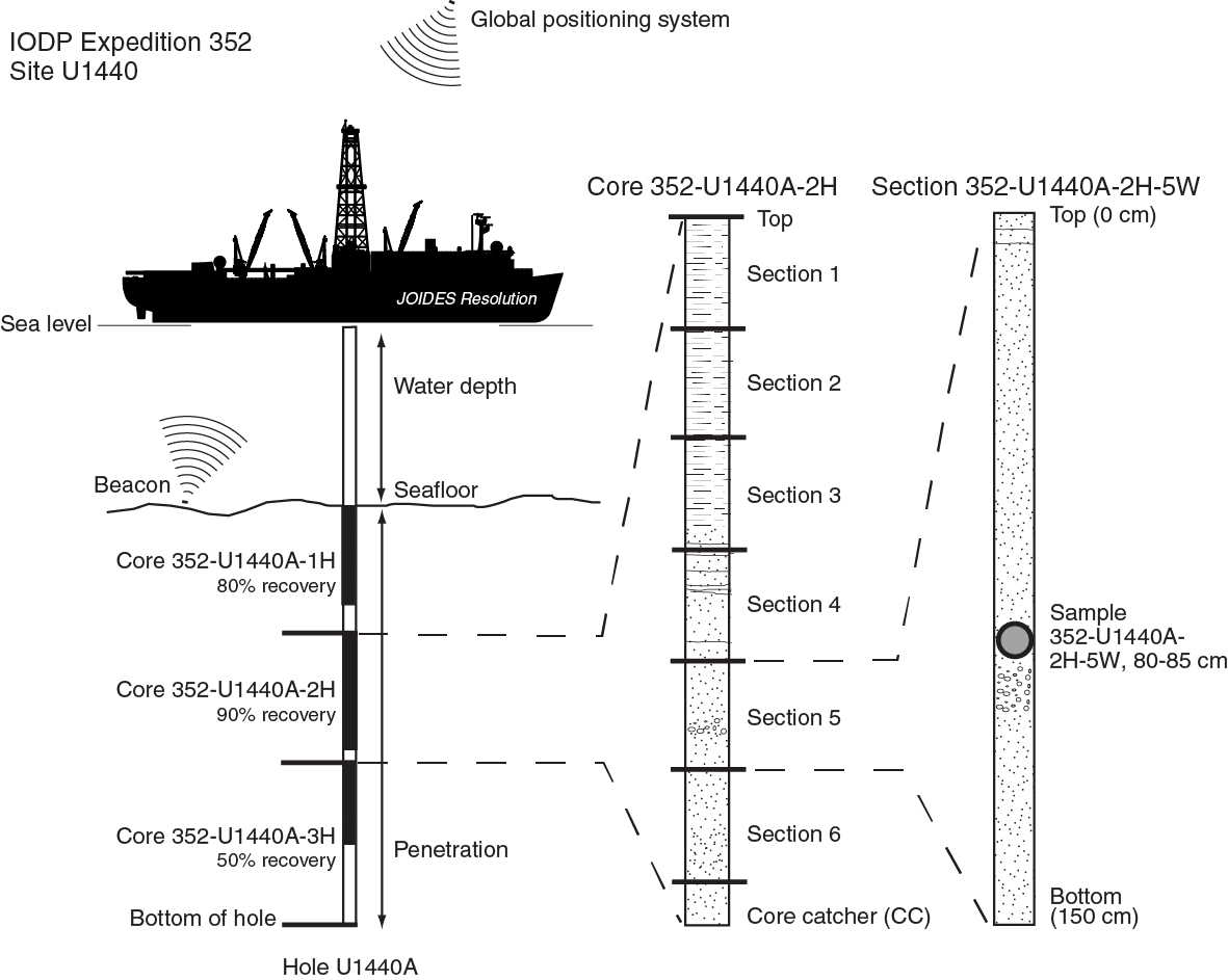
Numbering of sites, holes, cores, and samples followed standard IODP procedure. A full curatorial identifier for a sample consists of the following information: expedition, site, hole, core number, core type, section number, section half, piece number (hard rocks only), and interval in centimeters measured from the top of the core section. For example, a sample identification of “352-U1440A-2H-5W, 80–85 cm” indicates a 5 cm sample removed from the interval between 80 and 85 cm below the top of Section 5 (working half) of Core 2 (“H” designates that this core was taken with the APC system) of Hole A at Site U1440 during Expedition 352 (Figure F1). The “U” preceding the hole number indicates the hole was drilled by the US platform, the R/V JOIDES Resolution. The drilling system used to obtain a core is designated in the sample identifiers as follows: H for APC, X for XCB, and R for RCB.

Cored intervals are defined by the length of drill string, the seafloor depth, and the amount the driller advanced the core barrel. The length of the core is defined by the sum of the lengths of the core sections. The CSF depth of a sample is calculated by adding the offset of the sample below the section top and the lengths of all higher sections in the core to the core-top depth measured with the drill string (DSF). A soft to semisoft sediment core from less than a few hundred meters below seafloor expands upon recovery (typically a few percent to as much as 15%), so the recovered interval does not necessarily match the cored interval. In addition, a coring gap can occur between cores. Thus, a discrepancy between DSF and CSF depths can exist with regard to a stratigraphic interval.

Furthermore, when core recovery is >100% of the cored interval, a sample taken from the bottom of a core may have a CSF depth that is deeper than that of a sample from the top of the subsequent core (i.e., the data associated with the two core intervals will overlap on the CSF-A scale).

If a core has <100% recovery, for curation purposes all cored material is assumed to originate from the top of the drilled interval as a continuous section; the true depth interval within the cored interval is unknown. This should be considered a sampling uncertainty in age-depth analysis or in correlation of core data with downhole logging data.

Core handling and analysis

Sediment

Sediment cores were extracted from the core barrel in plastic liners. The liners were carried from the rig floor to the core processing area on the catwalk outside the core laboratory, where they were split into ~1.5 m sections. Blue (uphole direction) and clear (downhole direction) liner caps were glued with acetone onto the cut liner sections.

Once the cores were cut into sections, whole-round (WR) samples were taken for interstitial water analyses. When a WR sample was removed, a yellow cap was used to denote the missing interval. Syringe samples were taken for headspace gas analyses according to the IODP hydrocarbon safety monitoring protocol.

Core sections were placed in core racks in the laboratory. When the cores reached equilibrium with laboratory temperature (typically after 3 h), WR core sections were run through the Whole-Round Multisensor Logger (WRMSL) for P-wave velocity, magnetic susceptibility, and bulk density. The WR core sections were also run through the Natural Gamma Radiation Logger (NGRL), and thermal conductivity measurements were taken once per core (see Physical properties).

Sediment cores were then split lengthwise from bottom to top into working and archive halves. Investigators should note that older material can be transported upward on the split face of each section during splitting.

The working half of each core was described by the structural geologists. Samples were then taken, first for discrete physical properties and paleomagnetic analyses, followed by samples taken for shore-based studies based on the sampling plan agreed upon by the science party and shipboard curator. Finally samples were taken for remaining shipboard analyses such as bulk X-ray diffraction (XRD), carbonate, and inductively coupled plasma–atomic emission spectroscopy (ICP-AES) analyses.

The archive half of each core was scanned on the Section Half Imaging Logger (SHIL) and measured for color reflectance and point magnetic susceptibility on the Section Half Multisensor Logger (SHMSL). Labeled foam pieces were used in the place of missing WR intervals in the SHIL images. The archive halves were then described visually and by means of smear slides. Finally, the magnetization of archive halves and discrete pieces was measured with the cryogenic magnetometer and spinner magnetometer.

Hard rock

Pieces were extracted from the core liners on the catwalk or directly from the core barrel on the rig floor. The pieces were pushed to the bottom of 1.5 m liner sections, and the total rock length was measured. The length was entered into the database using the SampleMaster application as “created length.” This number was used to calculate recovery. The liner sections were then transferred to the core splitting room.

Oriented pieces of core were marked on the bottom with a wax pencil to preserve orientation. Adjacent but broken pieces that could be fit together along fractures were curated as single pieces. The structural geologist on shift confirmed piece matches and marked the split line on the pieces, which defined how the pieces were to be cut into two equal halves. The aim was to maximize the expression of dipping structures on the cut face of the core while maintaining representative features in both archive and working halves. A plastic spacer was secured with acetone to the split core liner between individual pieces or reconstructed contiguous groups of subpieces. These spacers can represent substantial intervals of no recovery. The length of each section of core, including spacers, was entered into the database as “curated length,” which commonly differs by several centimeters from the length measured on the catwalk. Finally, the depth of each piece in the database was recalculated based on the curated length.

Core sections were placed in core racks in the laboratory. When the cores reached equilibrium with laboratory temperature (typically after 1 h), the WR core sections were run through the WRMSL and the NGRL. Whole-round images of cylindrical oriented pieces were taken on the SHIL.

Each piece of core was split with a diamond-impregnated saw into an archive half and a working half, with the positions of plastic spacers between pieces maintained in both halves. Pieces were numbered sequentially from the top of each section, beginning with number 1. Separate subpieces within a single piece were assigned the same number but lettered consecutively (e.g., 1A, 1B, etc.). Pieces were labeled only on the outer cylindrical surfaces of the core. If it was evident that an individual piece had not rotated around a horizontal axis during drilling, an arrow pointing to the top of the section was added to the label. The piece’s oriented character was recorded in the database using the SampleMaster application.

The working half of each core was first described by the structural geologists. Samples were then taken for thin section preparation and shipboard geochemical, paleomagnetic, and physical properties analyses. The archive half of each core was scanned on the SHIL and measured for color reflectance and point magnetic susceptibility on the SHMSL. Thermal conductivity measurements were undertaken on selected archive-half samples (see Physical properties). The archive halves were then described visually, and selected pieces were analyzed by pXRF. Thin sections cut from the working half were also described. Finally, the magnetization of archive-half sections, archive-half pieces, and discrete samples taken from the working half was measured with the cryogenic magnetometer and spinner magnetometer.

Sampling for shore-based studies was delayed until the end of coring at each hole or at other appropriate times. Sampling was conducted based on the sampling plan agreed upon by the science party and shipboard curator.

When all steps were completed, cores were wrapped, sealed in plastic tubes, and transferred to cold storage space aboard the ship. At the end of the expedition the cores were kept on the ship and, following the transit to Subic Bay, Philippines, were sent to the IODP Kochi Core Center in Japan.

Core sample disturbance

Cores may be significantly disturbed and contain extraneous material as a result of the coring and core handling process (Jutzeler et al., 2014). In formations with loose sand layers, sand from intervals higher in the hole may be washed down by drilling circulation, accumulate at the bottom of the hole, and be sampled with the next core. The uppermost 10–50 cm of each core must therefore be examined critically during description for potential “fall-in.” Common coring-induced deformation includes the concave-downward appearance of originally horizontal bedding. Piston action can result in fluidization (“flow-in”) at the bottom of APC cores. Retrieval from depth to the surface can result in elastic rebound. Gas that is in solution at depth may become free and drive apart core segments within the liner. When gas content is high, pressure must be relieved for safety reasons before the cores are cut into segments. This is accomplished by drilling holes into the liner, which forces some sediment as well as gas out of the liner. These disturbances are described in each site chapter and graphically indicated on the visual core descriptions.

Authorship of chapters

The separate sections of the site chapters were written by the following scientists (authors are listed in alphabetical order; see Expedition 352 science party for contact information):

• Background and objectives: Pearce, Reagan, Petronotis
• Operations: Petronotis and Operations Superintendent Midgley
• Sedimentology: Kutterolf, Robertson
• Biostratigraphy: Avery
• Fluid geochemistry: Godard, Kirchenbaur, Y. Li, Ryan, Whattam
• Petrology: Chapman, Heaton, H.-Y. Li, Nelson, Prytulak, Shervais, Shimizu; Alteration: Python
• Sediment and rock geochemistry: Godard, Kirchenbaur, Y. Li, Ryan, Whattam
• Structural geology: Ferré, Kurz
• Physical properties: Almeev, Christeson, Michibayashi, Sakuyama
• Paleomagnetism: Carvallo, Sager
• Downhole logging: Morgan

Sedimentology

In this section we outline the procedures used to document the composition, texture, structures, and the level of core disturbance of the sediment and sedimentary rock recovered during Expedition 352. The procedures included visual core description, smear slide and petrographic thin section analysis, digital color imaging, color spectrophotometry, XRD, carbonate analysis, and ICP-AES.

Core sections from the archive halves were available for sedimentary and petrographic observation. Sections dominated by soft sediment were split using a thin wire held in high tension. Recovered hard rock was split with a diamond-impregnated saw. The split surface of the archive half was then assessed for quality (e.g., smearing or surface unevenness) and, if necessary, gently scraped with a glass slide. After splitting, the archive half was imaged by the SHIL and then analyzed for color reflectance and magnetic susceptibility using the SHMSL (see Physical properties). The archive-half section was occasionally reimaged when visibility of sedimentary structures or fabrics improved following treatment of the split core surface.

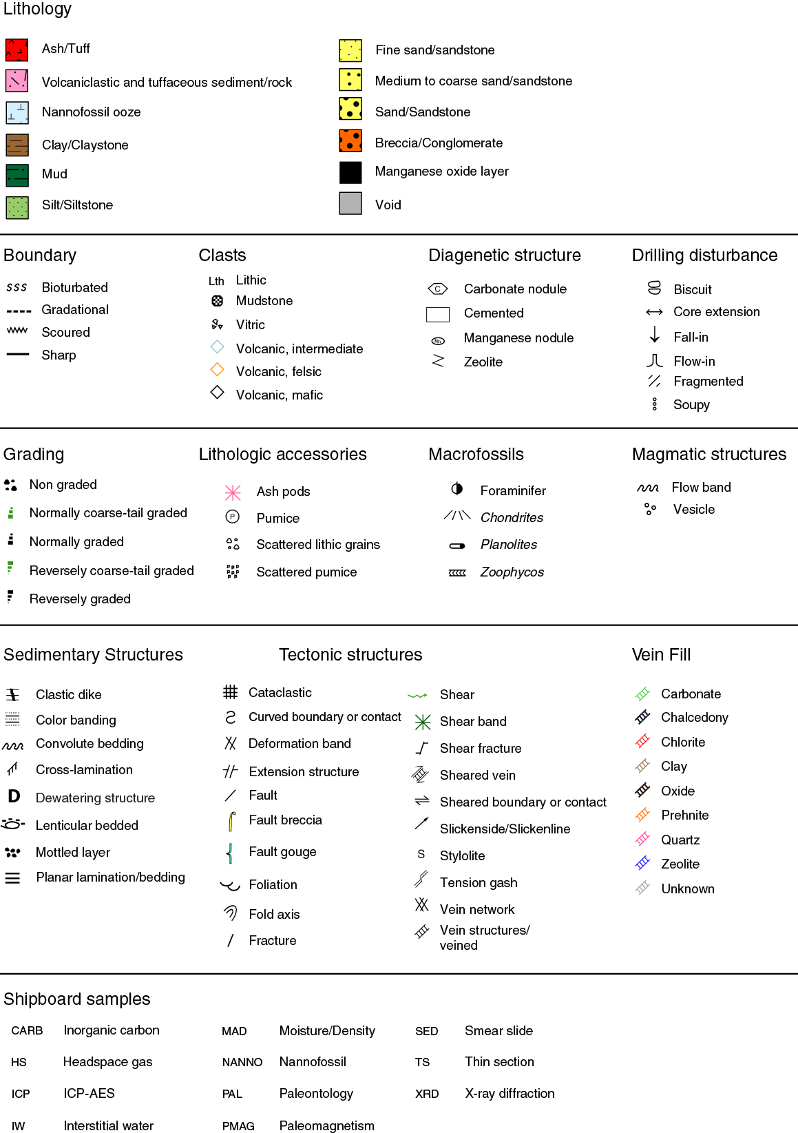
Following imaging, the archive-half sections of the sediment cores were macroscopically described for lithologic and sedimentary features (aided by use of a 20× wide-field hand lens and binocular microscope). Lithostratigraphic units were defined following visual inspection and smear slide analysis. Visual inspection yielded information particularly concerning lithologic variation, color, sedimentary structures, and drilling disturbance, whereas smear slide analysis was used to identify sedimentary constituents, including microfossils. All of the descriptive data were entered into DESClogik (see IODP use of DESClogik for details). Based on preliminary visual descriptions and physical property data, samples were taken from the working-half sections to make thin sections and to provide samples for XRD and ICP-AES. All descriptions and sample locations were recorded using curated depths (CSF-A) and documented on visual core description (VCD) graphic reports (Figure F2).

Visual core descriptions of sediment and sedimentary rock

Color and composition

Color was determined qualitatively for core intervals using Munsell Color Charts (Munsell Color Company, Inc., 2000). Visual inspections of the archive-half sections were used to identify compositional and textural elements of the sediment, including rock fragments, sedimentary structures, and diagenetic features such as color mottling and the results of element mobility (e.g., manganese oxide segregation).

Pelagic/hemipelagic and volcaniclastic sediment and sedimentary rock were the principal sedimentary materials recovered during Expedition 352. The sedimentary classification scheme that was employed emphasizes important descriptors for sediment and rock that could be quantified and recorded in the DESClogik database in the same time frame as shipboard core description.

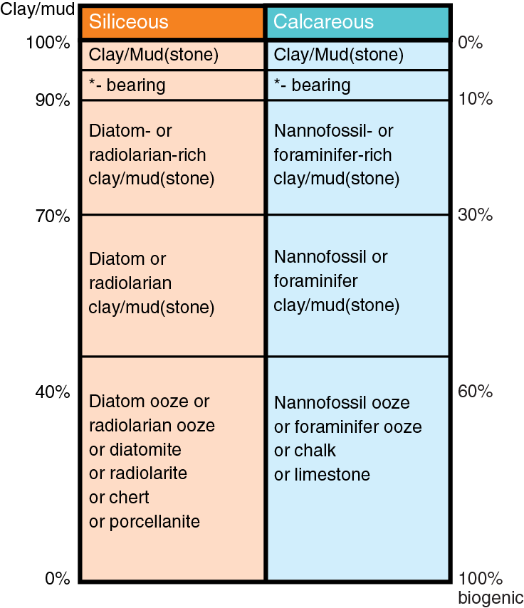
Sediment and sedimentary rock were classified using an approach that integrates the nature of volcanic particles into the sedimentary descriptive scheme typically used by IODP. In the scheme used here, sediment and sedimentary rock were divided into four lithologic classes based on composition (types of particles) (Figure F3):

1. Volcaniclastic sediment and rock of pyroclastic origin with >75% volcaniclastic or pyroclastic particles,
2. Tuffaceous/volcaniclastic sediment and rock of sedimentary origin (25%–75% volcaniclastic or pyroclastic particles),
3. Siliciclastic sediment and sedimentary rock with <25% volcaniclastic and tuffaceous particles and <5% biogenic particles, and
4. Pelagic to hemipelagic sediment (rock) with <25% volcaniclastic and tuffaceous particles and >5% biogenic particles.

Examples of each of the four lithologic classes were encountered during this expedition. Within each class, the principal lithology name is based on particle size. In addition, appropriate prefixes and suffixes were applied. For example, the prefix “tuffaceous” was used for the tuffaceous lithologic classes, and prefixes that indicate the dominant biogenic component as determined by microscopic examination were used for pelagic/hemipelagic sediments and sedimentary rocks. Suffixes were also used to indicate minor components within each principal lithologic type.

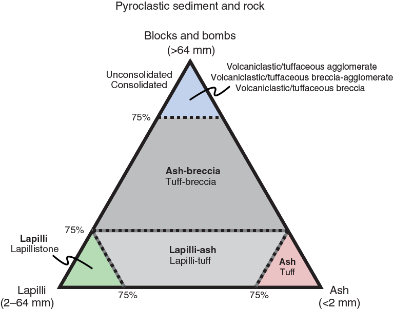
To emphasize the differences in the composition of the volcaniclastic sandstones recovered, the rocks were further classified using the scheme of Fisher and Schmincke (1984), which is well established and used worldwide. In general, coarser grained sedimentary rocks (63 µm to 2 mm average grain size) are designated as “sand(stone)” where the volcaniclastic components are <25% of the total clasts. Volcaniclastic rocks can be (1) reworked and commonly altered heterogeneous assemblages of volcanic material, including lava, tuff fragments, and compositionally different ash lenses/particles, or (2) fresh, or relatively unaltered, compositionally homogeneous, unconsolidated pyroclastic material directly resulting from explosive eruptions on land or effusive/explosive vents on the seafloor. Pyroclasts are composed of volcanogenic material (“pyro,” meaning fire; magma) that is fragmented (“clast,” meaning fragmented) during explosive eruption.

Where there are ≥25% volcaniclasts but <25% pyroclasts the sediment or sedimentary rock is designated as a “volcaniclastic sand(stone).” Where the clast composition is 25%–75% pyroclasts, the sediment/sedimentary rock is classified as “tuffaceous sand(stone).” However, if the clast composition is ≥75% pyroclasts, it is classified using the volcanological terms ash/tuff (<2 mm), lapilli/lapillistone (2–64 mm), and bombs, blocks/pyroclastic breccia/agglomerate (modified after Fischer and Schmincke, 1984).

A breccia-conglomerate is composed of predominantly rounded and/or subrounded clasts (>50 vol%) and subordinate angular/subangular clasts. A breccia is predominantly composed of angular and subangular clasts (>50 vol%). The description was refined by indicating whether the fabric is either clast supported or matrix supported (see below). For the equivalent pyroclastic lithologic class the term “agglomerate” or “pyroclastic breccia” is used in the place of conglomerate and breccia (Fisher and Schmincke, 1984) (Table T1; Figure F4). Depending on grain size, degree of compaction, and lithification, the nomenclature was adjusted accordingly.

Textures, structures, and sedimentary fabric

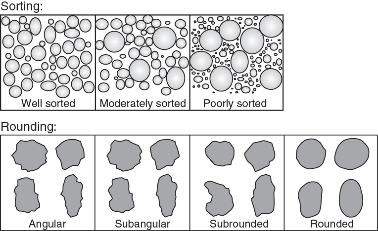
For relatively coarse grained material (coarse sand and above), sediment grain size, particle shape, and sorting were determined using the Wentworth scale (Wentworth, 1922). However, for finer grained sediments the textural analysis required inspection at high magnification, which was performed on smear slides and thin sections (see below). The classification of sorting and rounding that was used is shown in Figure F5.

Sedimentary structures observed in the recovered cores included bedding, grading (normal and reverse), soft-sediment deformation, bioturbation, and diagenetic effects. Bed thickness (see Ingram, 1954) was defined as the following units:

• Very thick bedded = >100 cm.
• Thick bedded = 30–100 cm.
• Medium bedded = 10–30 cm.
• Thin bedded = 3–10 cm.
• Very thin bedded = 1–3 cm.
• Laminae = <1 cm.

Estimations of abundances of the components (typically in smear slides) were made semiquantitatively using the following scheme:

• R = rare (<1 vol%).
• C = common (1–10 vol%).
• A = abundant (10–50 vol%).
• D = dominant (50–80 vol%).
• M = major (>80 vol%).

The abundance of bioturbation was estimated using the semiquantitative ichnofabric index, as described by Droser and Bottjer (1986, 1991), aided by visual comparative charts (Heard and Pickering, 2008). These charts exhibit the degree of biogenic disruption of primary fabric, such as lamination, ranging from nonbioturbated sediment to total homogenization:

• Nonbioturbated = no bioturbation recorded; all original sedimentary structures preserved.
• Slight bioturbation = discrete, isolated trace fossils; up to 10% of original bedding disturbed.
• Moderate bioturbation = approximately 10%–60% of original bedding disturbed; burrows largely overlap and are commonly poorly defined.
• Strong bioturbation = bedding is completely disturbed, but burrows can still be discerned in places; the fabric is not mixed although the bedding may be nearly or totally homogenized.

Smear slides, thin sections, XRD, and carbonate analysis

Smear slides and thin sections were used to identify basic textural and compositional features. The textures of the sediment were estimated with the help of a visual comparison chart (Rothwell, 1989). Smear slides were used to help identify lithology, texture, diagenesis, and composition and were also used to help define the boundaries of units and subunits. Particular attention was paid to the recognition of ash layers and mineral-rich sands, and these were sampled extensively. The results are summarized in the smear slide tables (see Core descriptions).

The qualitative abundance of major components was confirmed by XRD for selected samples (see X-ray diffraction). Also, the absolute weight percent of carbonate was determined by chemical analysis (see Sediment and rock geochemistry). Samples for whole-rock chemical and carbonate analysis were generally taken close together, in most cases from relatively fine-grained background sediment, typically nannofossil ooze or clay-rich sediment.

IODP use of DESClogik

Data for the macroscopic and microscopic descriptions of recovered cores were entered into the IODP Laboratory Information Management System (LIMS) database using the IODP data-entry software, DESClogik. Data were entered in the Sediment tab of the Macroscopic template. DESClogik is core description software used to store macroscopic and/or microscopic descriptions of cores. Core description data are available through the Descriptive Information LIMS Report (web.iodp.tamu.edu/DESCReport). A single row in DESClogik defines one descriptive interval, which is commonly one bed but may also be used, for example, to designate marked color variation that may be of diagenetic origin. In addition, the position of each smear slide or petrographic thin section is shown in the VCDs with a sample code of “SED” or “TS,” respectively. The VCDs were generated using the plotting software Strater.

X-ray diffraction

Routine XRD analysis was carried out on bulk powders using a Bruker D-4 Endeavor diffractometer mounted with a Vantec-1 detector using nickel-filtered Cu-Kα radiation. Our principal goal was to identify the different minerals that are present in the sediments of the different units, notably total phyllosilicate minerals, quartz, plagioclase, and calcite. Clay minerals either were not identified or only broadly categorized because advanced analytical techniques (e.g., differential thermal analysis and glycolation) were not available at sea.

Most of the samples were selected from typical “background” sediment intervals (e.g., nannofossil ooze and clay). As a result, not all of the minor lithologies were subjected to shipboard XRD. Tephra and mineral-rich sands were preferentially studied in smear slides in which minor mineral occurrences could be easily detected. Samples were freeze-dried, crushed using a mortar and pestle (along with powder for carbonate), and mounted as random bulk powders. Standard locked coupled scan conditions were

• Voltage = 40 kV,
• Current = 35 mA,
• Goniometer scan 2θ = 4°–70°,
• Step size = 0.0174°,
• Scan rate = 1 s/step, and
• Divergence slit = 0.6 mm.

The diffractograms of single samples were evaluated with the Bruker DiffracPlus Evaluation software package (EVA). All data files were uploaded into the LIMS database.

Biostratigraphy

Paleontological investigations and biostratigraphic determinations were carried out on calcareous nannofossils using the standard zonations of Martini (1971) and Okada and Bukry (1980). Identification of calcareous nannofossils during this expedition followed the taxonomy of Perch-Nielsen (1985), Varol (1998), and Young (1998).

The core catcher (CC) sample from each core was examined. Additional samples were taken from working-half sections as necessary to refine the biostratigraphy, preferentially sampling hemipelagic intervals.

Calcareous nannofossils

Calcareous nannofossils were examined in smear slides prepared directly from unprocessed samples using standard techniques. The slides were analyzed under plane-polarized light (PPL) and cross-polarized light (XPL) using a Zeiss Axiophot light microscope at a magnification of 1000×. One traverse (~100 fields of view [FOV]) was used to estimate relative abundance and to ensure rare species were recorded. For coarse material, the fine fraction was separated from the coarse fraction by settling through water before the smear slide was prepared. Photomicrographs were taken using a Spot RTS system with the IODP Image Capture and Spot commercial software.

The overall individual abundances were given the following letter codes:

• V = very abundant (>100 specimens per FOV).
• A = abundant (>10–100 specimens per FOV).
• C = common (>1–10) specimens per FOV).
• F = few (>1–10 specimens per 2–10 FOV).
• VF = very few (1 specimen per 2–10 FOV).
• R = rare (1 specimen per >10 FOV).
• B = barren (no nannofossils).
• * = reworked occurrence.

The following basic criteria were used qualitatively to provide a measure of preservation of the nannofossil assemblage:

• E = excellent (no dissolution seen, all specimens can be identified).
• G = good (little dissolution and/or overgrowth is observed, diagnostic characteristics are preserved and all specimens can be identified).
• M = moderate (dissolution and/or overgrowth are evident and a significant proportion—up to 25%—of the specimens cannot be identified to species level with absolute certainty).
• P = poor (severe dissolution, fragmentation and/or overgrowth has occurred, most primary features have been destroyed and many specimens cannot be identified at the species level).

Scanning electron microscope

All samples containing calcareous nannofossils were viewed using the TM3000 tabletop scanning electron microscope (SEM). This was very helpful in confirming the existence of many marker fossils with closely related taxa appearing in the same age range, which can sometimes make consistent identification difficult. It was especially useful in examining the youngest material recovered to confirm the presence or absence of recent and nearly recent taxa that are quite small, including Pseudoemiliania lacunosa, Pseudoemiliania ovata, Emiliania huxleyi, and many Gephyrocapsa species such as Gephyrocapsa oceanica.

Fluid geochemistry

Shipboard geochemical analyses were performed on fluids sampled in Holes U1439A and U1440A. These analyses comprised hydrocarbon measurements of headspace gas and inorganic chemical analysis of the interstitial water in the pores and fractures of the cored sediment and rock.

Headspace analysis of hydrocarbon gases

One sample per core was routinely subjected to headspace hydrocarbon gas analysis as part of standard shipboard safety monitoring procedures, as described in Kvenvolden and McDonald (1986) and Pimmel and Claypool (2001). This ensured that the sediments being drilled did not contain amounts of hydrocarbons above safety levels.

A ~3–5 cm³ sediment sample was collected from freshly exposed core directly after it was brought on deck. It was then placed in a 20 cm³ glass vial and sealed with a fluoropolymer/silicon septum and a crimped aluminum cap. During Expedition 352, the headspace sample was typically taken at the top of Section 4 (below the interstitial water [IW] sample). The sample was placed in the oven at 80°C for 30 min. A 5 cm³ aliquot of the evolved hydrocarbon gases was extracted from the headspace vial with a standard gas syringe and then manually injected into an Agilent/Hewlett Packard 6890 Series II gas chromatograph (GC) equipped with a flame ionization detector set at 250°C. The column (2 mm inner diameter; 6.3 mm outer diameter) was packed with 80/100 mesh HayeSep (Restek). The GC oven program was set to stay at 80°C for 8.25 min with a subsequent heat-up to 150°C at 40°C/min. The total run time was 15 min.

Results were collected using the Hewlett Packard 3365 ChemStation data processing software. The chromatographic response was calibrated using nine different gas standards and checked daily. The concentration of the analyzed hydrocarbon gases was reported as parts per million by volume.

Interstitial water analyses

Sampling

A whole-round core sample was taken immediately after core sectioning on deck, typically at the bottom of Section 3, for subsequent extraction of interstitial water. The length of the whole-round core taken for interstitial water analysis varied from 5 cm in the upper sediments to 10 cm in the deeper sediments where the volume of extracted interstitial water was more limited. Typically, one whole-round per core was selected in the upper 100 m and one every third core below that depth.

The whole-round samples collected were processed under atmospheric conditions. After extrusion from the core liner, contamination by seawater and sediment smearing was removed by scraping the core’s outer surface with a spatula. In APC cores, ~0.5 cm of material from the outer diameter and the top and bottom faces was removed, whereas in XCB cores, where borehole contamination is higher, as much as two-thirds of the sediment was removed from each whole-round sample. The remaining inner core (~150–300 cm³) was placed into a titanium squeezer (modified after Manheim and Sayles, 1974) and compressed using a laboratory hydraulic press to extract the interstitial water, using a total pressure <20 MPa.

The interstitial water extracted from the sediment sample was filtered through a prewashed Whatman Number 1 filter situated above a titanium mesh screen. Approximately 15 mL of interstitial water was collected in a precleaned plastic syringe attached to the squeezing assembly and then filtered through a Gelman polysulfone disposable filter (0.45 µm). After extraction, the squeezer parts were cleaned with shipboard water, rinsed with deionized water, and dried thoroughly prior to the next use. Shipboard analytical protocols are summarized in the following section.

Shipboard interstitial water analyses

The interstitial water samples were analyzed on board following the protocols of Gieskes et al. (1991), Murray et al. (2000), and, for newer shipboard instrumentation, those reported in the IODP user manuals. Precision and accuracy were tested using International Association for the Physical Sciences of the Oceans (IAPSO) standard seawater with the following composition, based on results in Gieskes et al. (1991):

• Alkalinity = 2.325 mM.
• Ca = 10.55 mM.
• Mg = 54.0 mM.
• K = 10.44 mM.
• Sr = 87 mM.
• Sulfate = 28.9 mM.
• Cl = 559 mM.
• Na = 480 mM.
• Li = 27 mM.

The interstitial water extracted from the compressed sediment sample was split into aliquots for the following analyses:

1. ~50 µL for salinity measurement with a refractometer,
2. 3 mL for pH and alkalinity,
3. 100 µL for ion chromatographic analysis of major anions and cations,
4. 500 µL for chloride titration,
5. 100 µL for ammonium analysis, and
6. 300 µL for phosphate analysis by spectrophotometry.

Salinity, alkalinity, and pH

Salinity, alkalinity, and pH were measured immediately after interstitial water extraction following the procedures in Gieskes et al. (1991). Salinity was measured using a Fisher temperature-compensated handheld refractometer (Fisher model S66366). A transfer pipette was used to transfer two drops of interstitial water to the salinity refractometer, and the corresponding salinity value, expressed in uncorrected permil (‰), was manually registered in the log book.

pH was measured with a combination glass electrode, and alkalinity was determined by Gran titration with an autotitrator (Metrohm 794 basic Titrino) using 0.1 M HCl at 20°C. Certified Reference Material 104 was used for calibration of the acid. IAPSO standard seawater was used for calibration and was analyzed at the beginning and end of the sample set for each site, as well as after every 10 samples. Repeated measurements of IAPSO standard seawater alkalinity yielded a precision <0.8%.

Chloride

Chloride concentrations in interstitial water samples were measured through titration using a Metrohm 785 DMP autotitrator and a silver nitrate (AgNO₃) solution, calibrated against repeated titrations of an IAPSO standard. Where fluid recovery was ample, a 0.5 mL sample aliquot was diluted with 30 mL of nitric acid (HNO₃) solution (92 ± 2 mM) and titrated with 0.1015 M AgNO₃. In all other cases, a 0.1 mL aliquot was diluted with 10 mL of 90 ± 2 mM HNO₃ and titrated with 0.1778 M AgNO₃. IAPSO standard solutions interspersed with the unknowns yielded a precision <0.5%.

Chloride, sulfate, bromide, sodium, magnesium, potassium, and calcium

Major ions in interstitial water samples were analyzed on a Metrohm 850 Professional II ion chromatograph (IC) equipped with a Metrohm 858 Professional sample processor, an MSM CO₂ suppressor, and a thermal conductivity detector. For anion (Cl^–, SO₄^2–, and Br^–) analyses, a Metrosep C6 column (100 mm length; 4 mm inner diameter) was used, with 3.2 mM Na₂CO₃ and 1.0 mM NaHCO₃ solutions used as the eluents. For cation (Na⁺, Mg²⁺, K⁺, and Ca²⁺) analyses, a Metrosep A supp 7 column (150 mm length; 4 mm inner diameter) was used, with 1.7 mM HNO₃ and 1.7 mM pyridine-2,6-dicarboxylic acid (CAS# 499-83-2) solutions used as eluents.

The calibration curve was established by diluting the IAPSO standard by 100×, 150×, 200×, 350×, and 500×. An aliquot of 100 µL interstitial water sample was diluted 1:100 with deionized water, using specifically designated pipettes. For every 10 samples, an IAPSO standard with specific dilution was run as an unknown to ensure accuracy. Repeated measurements of anion and cation concentrations in IAPSO standard seawater yielded a precision better than 1% for all the analyzed ions and an accuracy better than 2.5% for all elements except for Ca (8%).

Ammonium and phosphate

Concentrations of ammonium and phosphate in interstitial water were determined on an Agilent Technologies Cary Series 100 UV-Vis spectrophotometer equipped with a sipper sample introduction system, following the protocol in Gieskes et al. (1991). The determination of ammonium in 100 μL of interstitial water was based on diazotization of phenol and subsequent oxidation of the diazo compound by Chlorox bleach to yield a blue color, measured spectrophotometrically at 640 nm.

Determination of phosphate concentration was based on the reaction of orthophosphate with Mo(VI) and Sb(III) in an acidic solution that forms an antimony-phosphomolybdate complex subsequently reduced by ascorbic acid to form a blue color. The absorbance is measured spectrophotometrically at 885 nm (Gieskes et al., 1991). For phosphate analysis, 300 µL of interstitial water was diluted prior to color development so that the highest concentration was <1000 µM.

Petrology

Most igneous rock description procedures used during Expedition 352 were adapted from Integrated Ocean Drilling Program Expeditions 330 and 344 and IODP Expedition 350 (e.g., Expedition 330 Scientists, 2012; Harris et al., 2013; Tamura et al., 2015). Macroscopic observations were coordinated, where possible, with thin section petrographic observations and bulk rock chemical analyses of representative samples, including both ICP-AES and portable X-ray fluorescence (pXRF) (see Sediment and rock geochemistry). Data for the macroscopic and microscopic descriptions of recovered cores were entered into the Laboratory Information Management System (LIMS) database using DESClogik. Volcanic rock characteristics were entered into the Extrusive hypabyssal tab, and alteration assemblages were entered into the Alteration tab.

Our shipboard studies sought to systematically describe the petrology of the cored rocks, their physical occurrence, and their alteration. The first task was division of the recovered material into coherent units. Igneous lithologic unit boundaries were defined using complementary information, including petrography, chemical composition, and physical properties such as magnetic susceptibility. The ability to collect meaningful chemical data in real time with a pXRF spectrometer was particularly useful for rocks lacking distinguishing petrographic characteristics. Secondly, lithology, phenocryst abundances and appearances, and characteristic igneous textures and vesicle distribution were described macroscopically and investigated in more detail by thin section petrography. Finally, our petrographic observations were corroborated with numerous pXRF measurements taken on the archive half of the core.

Core description workflow

Before the core was split into working and archive halves, each hard rock piece was oriented (if possible) and archived into numbered bins. Whole-round images of large sections of core were taken at 0°, 90°, 180°, and 270°. Hard rock pieces were split with a diamond-impregnated saw along lines chosen by a structural geologist so that important compositional and structural features were preserved in both halves. Once split, each rock in both the working and the archive halves was labeled individually with unique piece/subpiece numbers from the top to the bottom of each section. If the top and bottom of a piece of rock could be determined, an arrow was added to the label to indicate the uphole direction. The archive halves were imaged using the SHIL, which also records red, green, and blue spectral colors along the centerline of the core. After imaging, the archive halves were analyzed for color reflectance and magnetic susceptibility at 1–2.5 cm intervals using the SHMSL (see Physical properties). Selected pieces from the archive half were analyzed by pXRF (see Sediment and rock geochemistry) in order to characterize the bulk chemistry of the core and then to refine the chemostratigraphy around suspected unit boundaries. The working halves were sampled for shipboard physical properties, paleomagnetic studies, thin sections, XRD, and geochemical analysis by ICP-AES analysis. All core that was sampled for shipboard ICP-AES analyses had complementary pXRF analyses performed on the archive half for comparative and data assessment purposes.

Each section of core was first macroscopically examined and described for petrologic and alteration characteristics. Igneous and alteration descriptions during Expedition 352 were made on the archive halves of the cores. Structural observations (see Structural geology) and thin section billets were made on the working halves. For macroscopic observations and descriptions, DESClogik was used to record the primary igneous characteristics (e.g., lithologic unit division, groundmass and phenocryst mineralogy, and vesicle abundance and type) and alteration (e.g., color, vesicle filling, secondary minerals, and vein/fracture fillings; see Secondary minerals in igneous rocks). Mineral modes and sizes were estimated by examining archive halves with a binocular microscope and/or hand lens. For microscopic observation, as many as 12 thin sections were requested daily, and their descriptions were entered in DESClogik. Macroscopic features observed in the cores are summarized and presented in the VCDs.

Volcanic and hypabyssal unit classifications

The definition of an igneous lithologic unit is usually based on the presence of lava flow contacts, typically marked by chilled or glassy margins on the upper and lower contact or by the presence of intercalated volcaniclastic or sedimentary horizons. In the absence of such boundaries, igneous lithologic units were defined according to changes in the primary mineral assemblage (based on abundance of visible phenocrysts and groundmass phases), grain size, color, or texture. Where these features were not diagnostic (as at Site U1440), we relied on a chemical lithostratigraphy defined by abrupt changes in diagnostic major or trace elements (e.g., Ti, Zr, Cr, or Sr). Preliminary chemical compositions were determined using the pXRF spectrometer, and the data were calibrated using working curves made from international rock standards (see Sediment and rock geochemistry).

Igneous lithologic units are given consecutive downhole Arabic numerals (igneous lithologic Units 1, 2, 3, etc.). The unit boundaries represent abrupt changes in chemical characteristics, phenocrysts, and groundmass assemblages. Igneous lithologic subunits were used to distinguish rocks in a single unit that differed in their textures, grain size, and thus emplacement mode (e.g., hyaloclastite, pillow lava, massive lava, or shallow intrusive) or had minor variations in chemical compositions.

Lava flow and hypabyssal unit types

Pillow lava flows

Pillow lava flows consist of discrete subrounded lobes of relatively small size (0.2–2.0 m in diameter). Their exteriors are entirely bounded by glassy rinds. The outer zones typically show bands of vesicles, whereas their interiors typically display internally radiating vesicle trains. Pillow lava flows result from subaqueous eruptions that allow separation of lava pods from point sources along the advancing front. Pillow lavas are characterized by curved chilled margins, oblique to the vertical axis of the core, radial fractures that emanate from a massive core, or outer surfaces coated with glass. Pillows may also be identified by the presence of variolitic textures, curved fractures, and microcrystalline or cryptocrystalline grain sizes.

Sheet and massive lava flows

Lava flows are defined as sheet flows if they comprise igneous lithologic units <1 m thick of the same rock type, with grain sizes increasing toward the flow center. Massive lava flows are defined for continuous intervals of >1 m with a similar lithology. Sheet-like and massive flows result from particularly high effusion rates and/or increased local slopes. They are texturally characterized by uniform cores as thick as several meters that are typically coarser grained than pillow lavas and may coarsen toward their interior. Sheet and massive flows often have vertical vesicle pipes that may contain late-stage melt segregation material. Glassy margins are thin and usually not preserved during coring.

Hyaloclastites

Hyaloclastites are fragmental igneous rocks that represent primary flow deposits (that is, they are not resedimented or epiclastic) formed by autofragmentation of lava during subaqueous eruption. They typically consist of glassy and/or lithic fragments <64 mm in diameter (hyaloclastite lapilli tuff) but may also include larger fragments (hyaloclastite breccia or tuff-breccia) or isolated pillows (hyaloclastite pillow breccia). These may be less than a meter to several meters thick and are commonly intercalated with pillow lava or sheet flows. Pillow lavas may contain an extensive matrix of intrapillow hyaloclastite, and hyaloclastite pillow breccias may grade into pillow lava flows as the proportion of pillows increases. The glassy ash portion of hyaloclastite pillow breccias typically consists of flat glass shards spalled off expanding pillows, with keystone-shaped fragments derived from the pillow rims. In contrast, hyaloclastites that represent submarine fire fountain deposits are characterized by rounded lapilli formed from quenched magma globules, along with angular glass shards formed by thermal shock fracturing of globules and shattered vesicle walls.

Intrusive sheets

Intrusive sheets include both dikes and sills. They are tabular bodies that are usually distinguished from lava flows by having relatively planar contacts and quenched margins on both their upper and lower contacts. Dikes are further distinguished by contacts that crosscut primary depositional layering. Intrusive sheets typically lack vesicles, are significantly coarser grained than lavas, and may have granular or doleritic textures (subophitic to ophitic or hypidiomorphic granular textures, seriate grain size distribution). Intrusive sheets may also contrast chemically with their volcanic wallrocks. In practice, it can be difficult to distinguish intrusive sheets from massive sheet flows.

Principal lithology name and descriptive parameters

The lithologic name comprises a principal name, a prefix, and optional suffix. The principal name is based upon the nature of the phenocrysts, when present, and/or the color of the groundmass. Seven rock categories are defined in DESClogik:

1. Basalt: black to dark gray rock containing plagioclase and pyroxene.
2. Dolerite: black to dark gray rock with basaltic or basaltic andesite composition, but typically coarser grained than basalt.
3. Andesite: dark to light gray rock containing pyroxenes and/or feldspar and/or amphibole, typically devoid of olivine and quartz.
4. Boninite: light gray rock with glassy matrix containing orthopyroxene or clinoenstatite and usually olivine. Used when the type of boninite is not known or is inferred, and for evolved members of boninite series.
5. Dacite: light gray to tan rock, usually plagioclase-phyric, and sometimes containing pyroxenes ± quartz ± hornblende.
6. Rhyolite: light gray to pale white rock, usually plagioclase-phyric, and sometimes containing quartz ± hornblende.
7. Hyaloclastite: as described in the preceding section; this term is typically used as a principal lithology when the lithic-rich and ash-rich portions of hyaloclastite pillow breccias or tuff breccias are described as separate domains.

Porphyritic rocks are named according to major phenocryst phase(s) when the total abundance of phenocrysts was >1%. The term “phenocryst” is used to describe any crystal significantly larger (typically 5× more) than the average size of groundmass and >1 mm in diameter. The term “microphenocryst” is used for crystals larger than the modal groundmass grain size but <1 mm. A prefix is applied as a modifier to the primary lithology names to indicate the phenocryst assemblage in the hand samples. “Glomerocryst” is used to describe clusters of intergrown phenocrysts that represent normal phenocryst assemblage.

The suffix in DESClogik indicates the nature of the volcanic body: glass, lava, pillow lava, intrusive sheet, hyaloclastite, breccia, or clast. The suffix hyaloclastite or breccia is used if the rock is in direct association with related lava. Other recorded descriptive parameters are rock texture (see below), grain size, phenocryst phase and abundance, vesicularity and vesicle shape, secondary minerals, and the nature of contacts between volcanic rock intervals.

Textures are described macroscopically for all igneous rock core sections and microscopically for the subset of intervals having thin sections. Grain size modal names are

• Coarse grained = >5 mm,
• Medium grained = >1–5 mm,
• Fine grained = 0.3–1 mm,
• Microcrystalline = <0.3 mm, and
• Cryptocrystalline = <0.1 mm.

Vesicularity is described according to proportions

• No vesicles = 0%,
• Sparsely vesicular = <5%,
• Moderately vesicular = 5%–20%, and
• Highly vesicular = >20%.

The modal size, sphericity, and roundness of vesicle populations are visually estimated, along with the amount and extent of vesicle filling phases (typically clays, zeolites, or calcite).

Microscopic descriptions are similar to macroscopic observations but are more detailed. Seven primary rock types are defined: basalt, boninite, dolerite, andesite, dacite, rhyolite, and glass (when composition is not known). A prefix indicates the phenocryst assemblage and total phenocryst abundances:

• Highly = >10%.
• Moderately = >5%–10%.
• Sparsely = 1%–5%.
• Aphyric = <1% phenocrysts.

Optional suffixes indicate the nature of the volcanic rock body. The modal abundance and size of all phenocryst phases are recorded together with other parameters including shape and habit of each phase.

Some core sections comprise two or more distinct domains. These domains may be described and named separately, with the proportion of each domain indicated in DESClogik. Domain names are based on the dominant characteristic of that domain. For Expedition 352 these include the following terms:

• Volcanic clast, mafic
• Mafic lava
• Leucocratic lava
• Melanocratic lava
• Pillow matrix
• Pillow top
• Glass
• Scoria
• Sediment matrix
• Vein matrix

The proportion of each domain is indicated in DESClogik, and each domain is given a lithologic name as described above.

pXRF measurements

The pXRF spectrometer provides real-time characterization of core for assessment of broad chemical variations and how they may (or may not) tie to petrographic observables. Measurements are calibrated using reference materials and correction factors applied for some elements (see Sediment and rock geochemistry). Some limits were imposed on the use of pXRF data to determine unit boundaries. First, only elements that should be little affected by alteration are targeted for igneous unit distinction (e.g., Cr, Ti, and Zr). Second, only large shifts (>30%) in the abundance of Cr, Ti, and Zr are interpreted as suggestive of unit breaks. Real-time pXRF measurements proved invaluable for characterization of extrusive rocks in Holes U1440B and U1441A, where rocks are dominantly aphyric and microcrystalline, thus hindering more traditional initial unit definition based on petrographic variation. Finally, the rapid nature of data acquisition in the core lab allowed pXRF characterization to aid in shipboard sampling.

Secondary minerals in igneous rocks

Alteration features in igneous rocks from Expedition 352 are based on macroscopic observations of core, aided by shipboard smear slide, thin section, and XRD and ICP-AES investigations. Secondary minerals in cores were recorded in DESClogik in the Macroscopic template under separate tabs for Alteration, Veins, and Halos as percentage of rock consisting of secondary materials (including devitrification). In chapter descriptions, levels of alteration in groundmass were recorded as

• High = >40%,
• Moderate = 15%–40%, and
• Slight = <15%.

Textures used to define groundmass alteration are patchy, corona, pseudomorphic, or recrystallized. Colors used to define alteration are black, brown, gray, green, white, or yellow. Groundmass, glass, and mineral replacement minerals and vesicle-filling minerals are classified as dominant, second, and third order. Alteration phases listed in DESClogik include clays, carbonate, zeolites, chlorite, feldspar (albite), quartz, chalcedony, oxides, sulfide, native copper, and amphibole. Vesicle-filling minerals (i.e., amygdules) include calcite, carbonate, chalcedony, zeolite, clay, chalcopyrite and other sulfides, chlorite, and prehnite. Microscopic observations of alteration minerals in igneous rocks are similar but more detailed. Percentages of individual replacement minerals are estimated for each phenocryst mineral, groundmass, and glass.

Descriptions of veins and halos record their mineralogy, geometry, contacts, and crosscutting relationships with the host rock. Vein texture selections are vuggy, cataclastic, saccharoidal, sutures, patchy, banded, comb structured, overgrowths, fibrous, or brecciated. Vein geometry selections are splayed, sinuous, irregular, planar, or curved. Vein contacts may be gradational, sharp-to-gradational, sharp, sutured, or diffuse. Vein connectivity is described as networked, anastomosing, branched, or isolated. Vein and halo minerals are described as dominant, second, or third order.

Petrologic classification of igneous rocks

The petrologic classification of igneous rocks recovered by ocean floor drilling is one of the most important tasks of the shipboard Petrology Team because this classification forms the first-order framework on which stratigraphic units and subunits are built. In general, the International Union of Geological Sciences (IUGS) classification parameters are used to arrive at conventional rock names. However, some of the rock series found in fore-arc settings have unusual fractionated compositions and mineral assemblages, rendering the IUGS conventions inadequate. Further, many of the rocks recovered by drilling are chemically altered, making the application of classification schemes based on major element compositions tenuous.

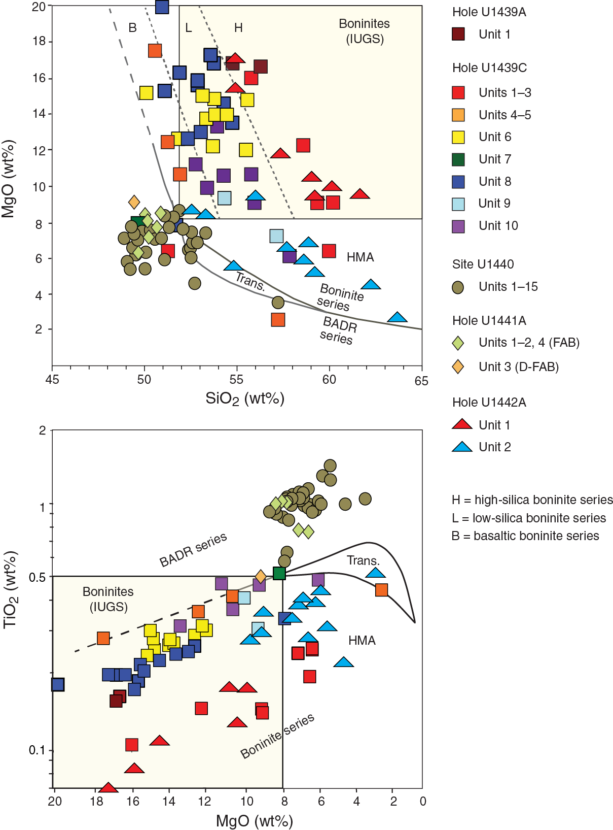
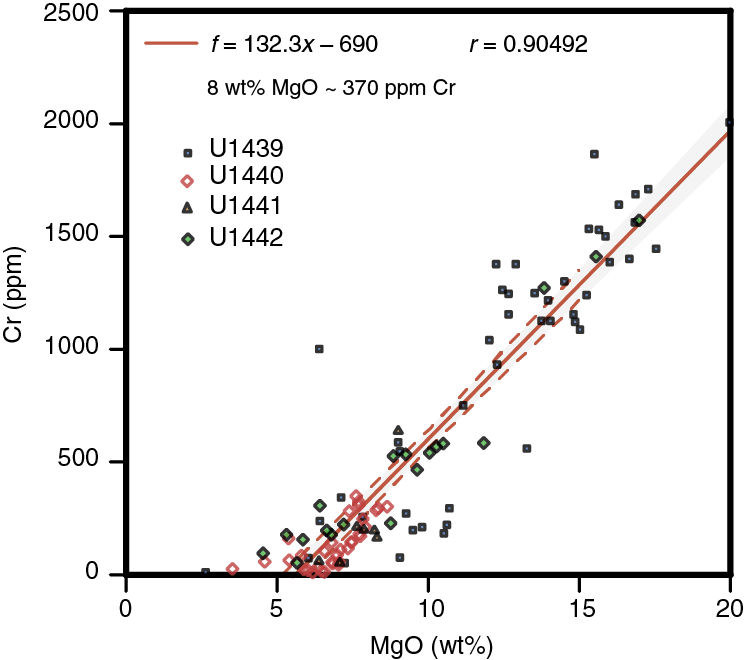
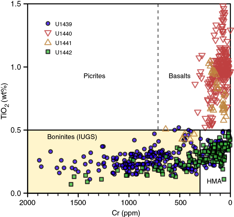
During Expedition 352, two primary rock groups were encountered: fundamentally basaltic rock at Sites U1440 and U1441 and fundamentally boninitic rock at Sites U1439 and U1442. Within each group, a range of magma series may be found, each with its distinct parent magma and each fractionating to form separate liquid lines of descent. Most rocks at Sites U1440 and U1441 are easily classified as basalt using the total alkali-silica diagram (TAS) or MgO-silica plot (Figure F6). Some have fractionated to basaltic andesite (SiO₂ = 52–57 wt%) and andesite (SiO₂ = 57–63 wt%). Their minor and trace element compositions mark them as distinct from mid-ocean-ridge basalt (MORB), arc tholeiite, and boninite.

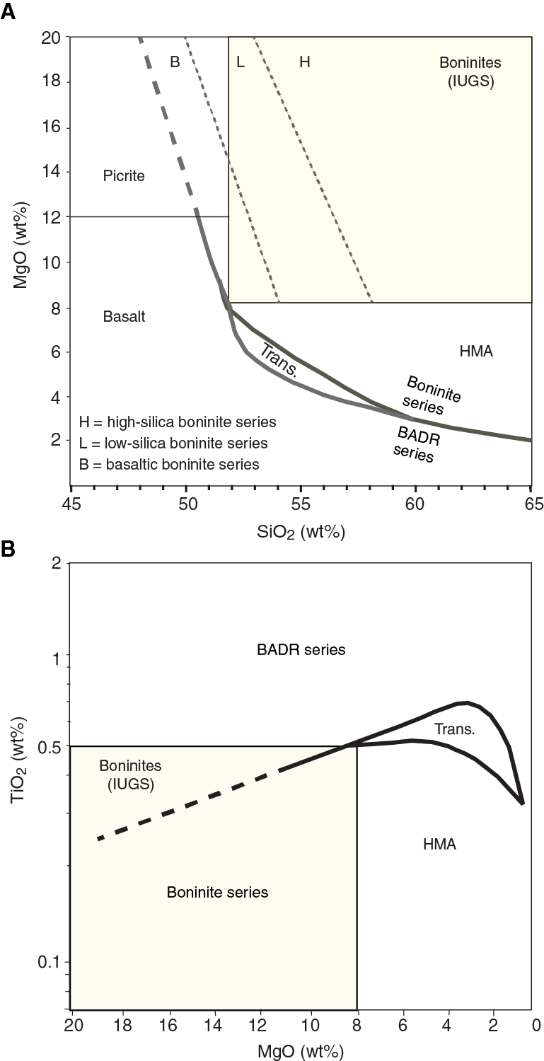
Boninites present special problems. First, the IUGS classification is based on major elements such as Si and Mg that are subject to disruption during low-temperature alteration. The IUGS MgO-TiO₂ parameters are somewhat more robust, but problems with mobility still persist (see Sediment and rock geochemistry). Second, the square boxes of the IUGS classification are not parallel to olivine or orthopyroxene control lines, so some rocks with boninitic trace elements plot outside the boninite field, as do evolved rocks that are part of the boninite series. Finally, the IUGS boninite classification does recognize divisions within the boninite group. These divisions reflect primary melts derived from mantle source regions that differ in their depletion and enrichment histories. These melts have distinct phenocryst assemblages, and their evolved products follow different paths through composition space.

Two improvements to the IUGS classification of boninites have recently been put forward. Pearce and Robinson (2010) proposed extending the low-silica limit for boninites parallel to an olivine control line that passes through the low-silica, low-magnesium corner of the boninite field: this would place rocks with basaltic silica contents into the boninite field, even though no such rocks have been described previously. Kanayama et al. (2013) proposed dividing the boninite field into high-silica boninites (HSBs) and low-silica boninites (LSBs), with a dividing line at SiO₂ = 55 wt% at MgO = 20 wt% and SiO₂ = 59 wt% at MgO = 8 wt%. Because boninite-series lavas with a wide range of compositions were recovered during Expedition 352, both of the changes above were adopted to facilitate a more detailed classification of the recovered lavas, although the Kanuyama et al. (2013) boundary was displaced to lower silica to better distinguish the boninitic suites from the expedition. In each case, the precise boundaries were amended slightly to optimize their application to the shipboard samples. As a result, three boninite families are recognized here (Figures F6, F7):

1. High-silica boninite, with lower boundary at SiO₂ = 53 wt% at MgO = 20 wt% and SiO₂ = 58 wt% at MgO = 8 wt%.
2. Low-silica boninite, with upper boundary at SiO₂ = 53 wt% at MgO = 20 wt% and SiO₂ = 58 wt% at MgO = 8 wt%, and lower boundary at SiO₂ = 50 wt% at MgO = 20 wt% and SiO₂ = 54 wt% at MgO = 8 wt%.
3. The newly recognized series, basaltic boninite, with upper boundary at SiO₂ = 50 wt% at MgO = 20 wt% and SiO₂ = 54 wt% at MgO = 8 wt%, and lower boundary at SiO₂ = 48 wt% at MgO = 20 wt% and SiO₂ = 52 wt% at MgO = 8 wt%.

In general, high-silica boninites have the lowest TiO₂, low-silica boninites have higher TiO₂, and basaltic boninites have the highest TiO₂ (Figure F6A). In addition, each of these suites can give rise to evolved rocks by low-pressure fractionation (typically high-Mg andesites). There is no IUGS convention for classifying boninite-series rocks with MgO contents less than their lower limit of 8 wt% MgO. We therefore use the boundary of Pearce and Robinson (2010) to separate high-magnesium andesite (HMA; the typical differentiation product of boninite) from basaltic andesites and andesites (the typical differentiation products of tholeiitic magmas).

Each suite is characterized by a distinct phenocryst assemblage:

• High-silica boninites have orthopyroxene ≥ olivine, with no clinopyroxene;
• Low-silica boninites have olivine >> orthopyroxene, with or without clinopyroxene ± spinel; and
• Basaltic boninites have olivine, orthopyroxene, and clinopyroxene together in subequal proportions.

Evolved boninites and their derivatives (e.g., high-magnesium andesites) have clinopyroxene phenocrysts (± plagioclase ± olivine), and may contain plagioclase in the groundmass.

However, as discussed above, major element data by ICP-AES were limited during shipboard analysis, making it impossible to classify most of the rocks recovered using the IUGS protocols. In addition, the problems with Si and Mg mobility further cloud the application of these data. As a result, we relied on data provided by the shipboard pXRF spectrometer to produce a detailed chemical stratigraphy while drilling in order to classify the rocks analyzed, group samples into units, and plan sample strategies for postcruise research. Protocols for producing calibrated data with the pXRF were established by the Geochemistry Team, as discussed above, so that several major and trace elements were available for use, including high-quality data for Ti. However, as the pXRF does not produce reliable data for lower atomic number elements, proxies were developed for Mg and Si concentrations from elements reliably analyzed by pXRF so we could classify all samples in a scheme that approximates the Si-Ti-Mg scheme developed above.

Chromium is a reliable proxy for MgO, which is substantiated for Expedition 352 samples using ICP-AES data. Figure F8 shows that a plot of MgO versus Cr produces a linear correlation with Cr = (132.3 × MgO) – 690, with a correlation coefficient of 0.90. Thus, the lower limit of the IUGS boninite field at MgO = 8 wt% corresponds to 370 ppm Cr. Some of the ICP-AES data fall above this correlation line, with extremely high Cr concentrations. Comparing the ICP-AES analyses with pXRF analyses of the same pieces shows that pXRF concentrations are about half the ICP-AES concentrations and fall on or near the linear correlation. This reflects the problems with ICP-AES Cr calibration at high concentrations that are noted in Sediment and rock geochemistry. As a result, the correlation line of Todd et al. (2012) for the global MORB database, PETDB, is used, which gives a concentration of 300 ppm Cr at 8 wt% MgO. Application of this correlation to the IUGS MgO-TiO₂ discrimination plot is shown in Figure F9.

Establishing a proxy for silica proved more difficult because it is buffered during melting at different values depending on extent of source depletion, pressure, and water vapor pressure, and is susceptible to enhancement by slab melt addition. Given the limited array of elements with reliable pXRF concentrations, two elements were used as indirect proxies for silica: Ti (reflecting both degree of melt and source depletion) and Zr (reflecting both source depletion and possible slab melt addition). Thus, depleted sources with higher melt addition have lower Ti and higher Zr, resulting in low Ti/Zr ratios. Less depleted sources with minor or no melt addition have higher Ti and lower Zr, resulting in high Ti/Zr ratios. Clearly, the variety of processes affecting Ti/Zr gives rise to considerable scatter and thus, unlike Cr versus MgO, a plot of silica versus Ti/Zr does not produce a linear correlation (Figure F10). However, the magnitude of variation in Ti/Zr is mirrored in the plot of SiO₂ versus MgO. Critically, the relative position of the primary boninite groups in both SiO₂ versus MgO and Ti/Zr versus SiO₂ suggests that Ti/Zr can be used as an indirect proxy for SiO₂ and is thus employed in the larger pXRF database for which no SiO₂ data are available.

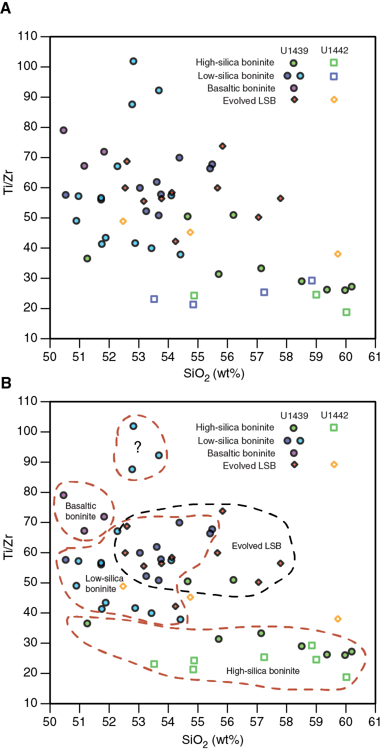
These proxies (Cr and Ti/Zr) are applied to the entire pXRF and ICP-AES data sets for Sites U1439 and U1442 in Figures F11A and F11B. Figure F11A emphasizes the wide range in Cr concentrations, part of which is real and part of which may reflect either analytical error or crystal accumulation (see individual site chapters). Much of the data >1300 ppm Cr are ICP-AES analyses that may be out of calibration range. Other data (pXRF and ICP-AES) >1300 ppm Cr may result from analyses of parts of lava flows rich in cumulus crystals. Evolved low-silica boninites have <300 ppm Cr and ranges in Ti/Zr ratios that form linear arrays that are probably controlled by crystal fractionation. Note that most evolved boninites (high-magnesium andesites) must be related to the low-silica boninite group, because they are both lower in silica and higher in Ti/Zr than the high-silica boninites. Evolved basaltic boninites are less common, and evolved high-silica boninites are least common.

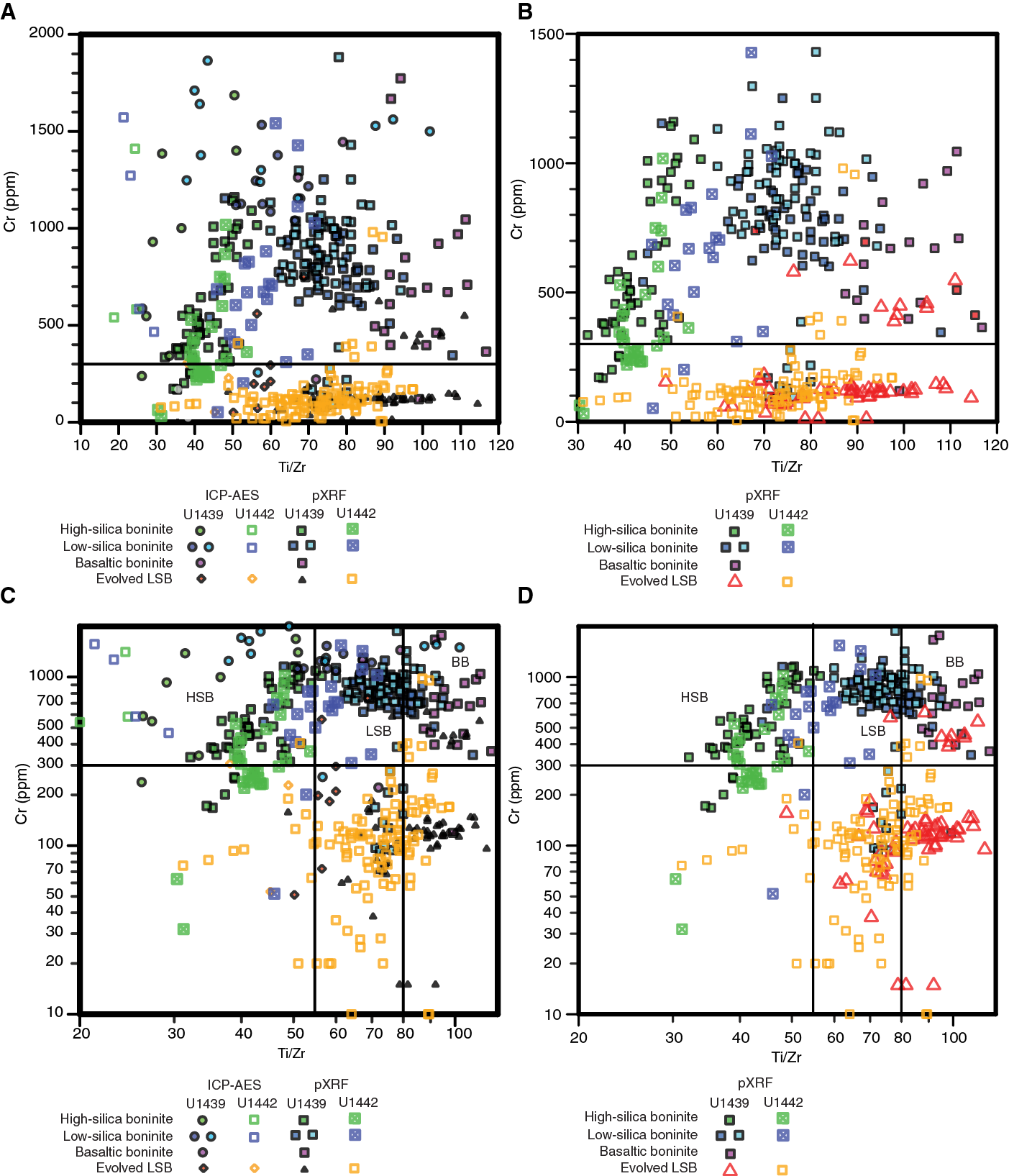
Figures F11C and F11D use a logarithmic transformation to reduce the variance at high concentrations and increase the variance at low concentrations. The Cr concentration of 300 ppm is again plotted as a horizontal line that separates evolved boninites (high-magnesium andesites) from boninites (sensu stricto). The boninites with >300 ppm Cr are divided into three groups based on their Ti/Zr ratios, which correspond to the three boninite suites discussed above:

• High-silica boninites, with Ti/Zr ratios of <55,
• Low-silica boninites with Ti/Zr ratios of 55–80, and
• Basaltic boninites with Ti/Zr ratios of 80–110.

Therefore, we arrive at a useful definition of the subgroups of the boninite series that can be based on elements for which pXRF measurements have been demonstrated to be robust (Cr-Ti-Zr; see Sediment and rock geochemistry) and for which we have high-resolution data for all igneous material recovered during Expedition 352.

Sediment and rock geochemistry

Shipboard geochemical analyses were performed on sediments and igneous rocks sampled at Sites U1439–U1442. These samples were selected as representative of the sediments and rocks recovered during Expedition 352 by the Shipboard Scientists. A thin section or XRD sample was located next to each of the chosen geochemical rock samples to precisely determine its modal composition and degree of alteration (see Sedimentology and Petrology in each site chapter for the characterization of the lithologic units). Selected sedimentary samples were analyzed for inorganic CO₂, total carbon, and total nitrogen, and igneous rocks were analyzed for carbon and hydrogen to assay their volatile contents. Site U1439 and U1440 sediments and all the igneous rock samples selected for geochemical study were analyzed for major and trace element concentrations using ICP-AES. A selection of sediments and most of these same igneous rock samples were analyzed for selected elemental abundances using pXRF.

Sample preparation

Sediment samples were taken from the interiors of cores with 10 cm³ tubes and then freeze-dried for ~24 h to remove water. Hard rock samples were prepared from 15–50 cm³ of rock. The solid rock samples were cut from cores using a diamond-blade rock saw. Outer surfaces of rock samples were ground on a diamond-impregnated grinding wheel to remove saw marks and altered rinds resulting from drilling. Each cleaned solid rock sample was placed in a beaker containing isopropanol and agitated in an ultrasonic bath for 15 min. The isopropanol was decanted, and the samples were then agitated twice in an ultrasonic bath in nanopure deionized water (18 MΩ) for 10 min. The cleaned pieces were then dried for 10–12 h at 110°C. After drying, the rock samples were crushed to <1 cm between two Delrin plastic disks in a hydraulic press. Where the collected sample was large enough, the coarse crush was split into two parts: one portion was stored for on-shore crushing and analyzed as part of a communal sampling strategy for geochemical analyses and the other portion was processed for shipboard measurements.

The freeze-dried samples and crushed chips of rock were ground to a fine powder using a SPEX 8515 Shatterbox powdering system with a tungsten carbide mill. A check on grinding contamination contributed by the tungsten carbide mills was performed during Leg 206 (Shipboard Scientific Party, 2003), and contamination was found to be negligible for major elements and most of the trace elements measured on board (Sc, V, Cr, Ni, Sr, Y, Zr, and Ba). A systematic analysis of the shipboard powders from Expedition 304/305 indicated possible Co contamination during powdering (Godard et al., 2009).

After powdering, a 5.00 ± 0.05 g aliquot of the sample powder was weighed on a Mettler Toledo balance and ignited for 4 h at 1025°C for igneous rocks and 700°C for sedimentary rocks to determine weight loss on ignition (LOI), with an estimated precision of 0.02 g (0.4%).

Volatile measurements

Volatile concentrations of sediments and rocks were measured on powder splits of ICP-AES samples.

Sediment

Carbonates

The inorganic carbon content was determined by acidifying ~11 mg of powder with 5 mL of 2 M HCl at 40°C and measuring the amount of CO₂ generated using a UIC 5011 CO₂ coulometer. Its volume was determined by trapping the CO₂ with ethanolamine and titrating coulometrically with hydroxyethylcarbamic acid. The end point of the titration was determined by a photodetector in which the change in light transmittance is proportional to the inorganic carbon content of the sample. The weight percent of carbonate was calculated from total inorganic carbon (IC) by

CaCO₃ (wt%) = IC (wt%) × 8.33.

All CO₂ was assumed to derive from dissolution of CaCO₃. No corrections were made for other carbonate minerals.

Total carbon, total organic carbon, and total nitrogen

Approximately 10 mg of bulk powder was weighed into a tin capsule to determine the total carbon and total nitrogen content. The powder was combusted in an oxygen gas stream at 900°C on a Flash EA-1112 Series Thermo Electron Corporation carbon-hydrogen-nitrogen-sulfur (CHNS) analyzer equipped with a Thermo Electron packed column (CHNS/NCS) and a thermal conductivity detector (TCD) for total carbon and total nitrogen. Reaction gases were passed through a reduction chamber to reduce nitrogen oxides to N₂, and the mixture of CO₂ and N₂ was separated by gas chromatography and detected by the TCD. Calibration was based on the Thermo Fisher Scientific NC Soil Reference Material standard that contains 2.29 wt% C and 0.21 wt% N. This standard was chosen because the elemental C and N compositions in the standard are close to those expected during Expedition 352. Total organic carbon was calculated by subtracting weight percent of inorganic carbon from total C obtained with the CHNS analyzer.

Igneous rocks

Volatile concentrations were measured by gas chromatographic separation on the Thermo CHNS analyzer. The calibration strategy for the analysis of H₂O, CO₂, and S in mafic rocks using the CHNS elemental analyzer was developed during Expedition 345 (Gillis et al., 2014). This calibration method involves measuring a series of international rock standards that approximate to the composition of the unknown samples. Because of the generally very low volatile content of the igneous samples, no S analyses were carried out on Expedition 352 igneous samples.

Analytical method

Powders were dried for 12 h at 110°C to ensure evaporation of possible adsorbed moisture and kept in a desiccator prior to measurements. Aliquots of powder, typically 10 mg, were weighed on a Cahn Microbalance Model 29 and packed into tin containers (Universal Tin Container “light”; Thermo Electron P/N 240-06400). A revolving autosampler dropped sample capsules into a 950°C resistance furnace, where they were combusted in a reactor. Tin from the capsule creates a violent flash combustion within an oxygen-enriched atmosphere. The oxidized and liberated volatiles were carried by a constant helium gas flow through a commercial glass column (Costech P/N 061110) packed with an oxidation catalyst of tungsten trioxide (WO₃) and a copper reducer. For separation, the liberated gases were transported by the helium carrier flow to a 2 m packed GC column (Costech P/N 0581080). During the measuring time of 1000 s, the millivoltage at the detector was continuously recorded. CO₂ and H₂O separated by the GC column arrived at the thermal conductivity detector at approximately 94 s (CO₂) and 250 s (H₂O) for the international gabbro Standard JGb-1.

Calibration, blanks, and standards

The routine method for quantitative chromatographic geochemical analyzes involves the preparation of a series of standard solutions (e.g., 80 mM L-(+)-cysteine hydrochloride). Because of the low volatile concentrations and different mineralogies in mafic rocks, an alternative method using a matrix-matched calibration strategy based on international geostandards for CO₂ and H₂O was used. Peak areas of the measured volatiles from the geostandard chromatographs were integrated and weight corrected. They were then plotted as a function of their reference concentrations, which were obtained from Expedition 345 Methods (Gillis et al., 2014) and/or downloaded from the GeoReM database (for the certified JP-1, MRG-1, and Cody shale SCO-1 standards). Procedural blanks were determined using empty tin capsules and were measured after 10 samples during each GC run, which included up to 20 samples and up to 9 reference material analyses. After weight correction, H₂O and CO₂ abundances were calculated using the function resulting from the linear or polygonal functions of the calibration lines.

Peridotite JP-1, gabbro MRG-1, and Cody shale SCO-1 standards were used for quality control to monitor analytical accuracy and reproducibility and to monitor instrument drift through replicate measurements. A typical gas chromatography run included a maximum of 20 unknown samples per session; this approach allowed the frequent restandardization required for high accuracy. Results of the GC analyses for the MRG-1, SCO-1, and JP-1 standards during Expedition 352 are presented in Table T2. Based on 18 runs of the JP-1, SCO-1, and MRG-1 standards, the reproducibility was better than 3% for CO₂ and H₂O when the concentrations of these elements were >1 wt% and 2 wt%, respectively. The obtained concentrations for these reference materials are in agreement with recommended values (Govindaraju, 1994) downloaded from the GeoReM database.

In comparing the GC volatile analyses with the LOI results, it is important to bear in mind that Fe²⁺ will change into Fe³⁺ during ignition of the sample in an atmospheric oxygen fugacity. This can result in a weight gain of as much as 11.1% of the proportion of ferrous Fe within the sample (e.g., a sample with 10% Fe²⁺ could increase in weight by >1 wt%). Also, ignition at or above 1000°C can result in the loss of K and Na, as these elements have vapor points below 1000°C (759°C for K and 883°C for Na) (Lide, 2000). These two issues lead to discrepancies between LOI analyses and volatile concentrations determined by GC analysis.

ICP-AES

The standard shipboard procedure for digestion of rocks and subsequent ICP-AES analysis is described in Murray et al. (2000). The following protocol is an abbreviated form of this procedure with minor changes and additions.

Digestion procedure

After determination of LOI, each sample and standard was weighed on a Cahn C-31 microbalance to 100.0 ± 0.2 mg splits; weighing errors are estimated to be ±0.05 mg under relatively smooth sea-surface conditions. Splits of ignited whole-rock powders were mixed with 400.0 ± 0.5 mg of LiBO₂ flux (preweighed on shore).

Aqueous LiBr solution (10 mL of 0.172 mM) was added to the flux and rock powder mixture as a nonwetting agent prior to sample fusion to prevent the fused bead from sticking to the crucible during cooling. Samples were fused individually in Pt-Au (95:5) crucibles for ~12 min at a maximum temperature of 1050°C in an internally rotating induction furnace (Bead Sampler NT-2100).

The beads were transferred into 125 mL high-density polypropylene bottles and dissolved in a 50 mL solution containing 10% HNO₃ and 10 ppm Ge. The solution bottle was placed in a Burrell wrist-action shaker for 1 h to aid dissolution. Next, 20 mL increments of the solution were passed through a 0.45 µm filter into a clean 60 mL wide-mouth high-density polypropylene bottle. From the filtered solution, 1.25 mL was pipetted into a scintillation vial and diluted with 8.75 mL of dissolution solution of 10% HNO₃, 10 ppm Ge, and 1000 ppm Li (added as a peak enhancer to improve sensitivity). The final solution-to-sample dilution factor was 4000; this solution was used to analyze both major and trace elements. For standards, stock standard solutions were placed in an ultrasonic bath for 1 h prior to final dilution to ensure a homogeneous solution.

Analysis

Major and trace element concentrations of standards and samples were determined using a Teledyne Leeman Labs Prodigy ICP-AES instrument. The analyzed elements and the wavelengths used for sample analysis during Expedition 352 are provided in Table T3. Certified international rock reference materials, calibration and drift solutions, and chemical procedure blanks were included with the unknown samples for each sample run. Detection limits were calculated as three times the standard deviation of the mean for blank solution measurements.

The ICP-AES plasma was ignited at least 30 min before each sample run to allow the instrument to warm up and stabilize. After the warm-up period, a zero-order search was performed to check the mechanical zero of the diffraction grating. After the zero-order search, the mechanical step positions of emission lines were tuned by automatically searching with a 0.002 nm window across each emission peak using two solutions containing 10 ppm concentrations of set elements prepared in 1% HNO₃. During the initial setup, an emission profile was selected for each peak using the multielement solutions to determine peak-to-background intensities and set the locations of background levels for each element. The Prodigy data acquisition software uses these background locations to calculate the net intensity for each emission line.

The ICP-AES data presented in the Sediment and rock geochemistry sections for each site were acquired using the Prodigy software. The intensity curve for each element is defined by 20 measurements within the designated wavelength window. The user selects the two background points that define the baseline. The Prodigy software integrates the area delineated by the baseline and the intensity curve. Each sample was analyzed four times from the same dilute solution within a given sample run. For several elements, measurements were made at two or more wavelengths (e.g., Si at 250.690, 251.611, and 288.158 nm; Table T3). For each run, the wavelength yielding the best calibration line was identified and used for determining concentrations.

A typical ICP-AES run includes

• A set of six certified rock standards, analyzed twice per run and chosen for their wide range of compositions in order to calibrate the analyses;
• Peridotite JP-1, basalts BIR-1 and BCR-2, gabbro MRG-1, andesite AGV-1, and granodiorite JG-1A for igneous rock and basalt BCR-2, andesite AGV-1, granodiorite JG-1A, shale SCO-1, sediment SO-3, and carbonate NBS-1C for sediment;
• As many as sixteen unknown samples;
• A drift-correction sample (basalt BHVO-2) analyzed every fifth sample position and at the beginning and end of each run;
• Procedural blank solutions run near the beginning and the end of each run; and
• Two to four “check” standards chosen for their composition similar to that of the analyzed material run as unknowns (e.g., basalt BHVO-2). Given that the igneous rocks encountered during Expedition 352 included boninite, three samples from the Chichijima Island boninite series (Samples X88, 40618, and 32108; J. Pearce, pers. comm., 2014) were regularly included as check samples for igneous rock analyses.

A 10% HNO₃ wash solution was run for 90 s between each sample analysis. Each sample analysis was the average of four measurements. The check standards were used to test analytical accuracy and reproducibility of the obtained data.

Data reduction

Following each sample run, concentrations were calculated off-line based on the measured raw intensities using the shipboard ICP Analyzer software. First, all analyses were corrected for drift. A drift correction was applied to each element by linear interpolation between drift-monitoring solutions run every fourth analysis. After drift correction and subtraction of procedural blank, a calibration line for each element was calculated using the results for the certified rock standards. Concentrations used for the calibrations were compiled values from the literature; they were recalculated on a volatile-free basis for samples having LOI values >2%. The compiled values were from Govindaraju (1994) and from the GeoRem website (georem.mpch-mainz.gwdg.de; September 2014; Jochum et al., 2005; Table T4). Element concentrations in the samples were then calculated from the relevant calibration lines.

Estimates of accuracy and precision of major and trace element analyses were based on replicate analyses of check standards (mainly BHVO-2) compared to values published in Govindaraju (1994) and/or downloaded from the GeoRem database and of three samples from the Chichijima Island boninite series (Samples X88, 40618, and 32108; J. Pearce, pers. comm., 2014). Results are presented in Table T5. During Expedition 352, run-to-run relative standard deviation by ICP-AES was generally ±1% for major elements except for MgO (±2%) and ±5%–10% for trace elements. Accuracy was better than 2% for major elements and better than 5% for most trace elements, with the exception of Ni and Co, for which accuracy was poor (20%–30%).

Rock and sample powder analysis using pXRF

During Expedition 352, we made extensive use of the Thermo Fisher Niton XL3t GOLDD+ pXRF, which had in the past been evaluated for use during Expeditions 330, 335, and 345 (see Supplementary material in the Expeditions 330, 335, and 345 Proceedings volumes) (Koppers, Yamazaki, Geldmacher, and the Expedition 330 Scientists, 2012; Teagle, Ildefonse, Blum, and the Expedition 335 Scientists, 2012; Gillis, Snow, Klaus, and the Expedition 345 Scientists, 2014). This instrument was used to conduct rapid analysis of both solid rock samples (thin section billets and surfaces of the archive core sections) and rock powders (both fresh and oxidized) prepared for ICP-AES analysis.

The Niton XL3t is a self-contained energy-dispersive XRF survey instrument that includes data correction packages tailored to a variety of applications (metals, plastics, soils and minerals, and consumer goods). Its data correction methods are based on the “fundamental parameters” methodology, which solves a series of nonlinear equations for each analyzed element. The parameters used in these equations comprise metrics for the X-ray source, fluorescence intensities, absorption coefficients, and absorption edge effects for each wavelength analyzed, together with parameters for sample geometry (e.g., van Sprang, 2000). In our use of the instrument, we primarily utilized the “soils” correction protocol within the “soils and minerals” submenu, which presumes a perpendicular sample geometry. The soils protocol analyzes for elements in three ranges (low = Cr, V, Ti, Sc, Ca, K, and S; main = Mo, Zr, Sr, U, Rb, Th, Pb, Au, Se, As, Hg, Zn, W, Cu, Ni, Co, Fe, and Mn; and high = Ba, Cs, Te, Sb, Sn, Cd, Ag, and Pd). In general, the high-range elements did not provide reliable results, but the main- and low-range groupings yielded results that were sufficiently precise and accurate when concentrations were above instrument detection limits (see Application and performance analysis).

Analytical protocols

For analysis, samples were either loaded into the Niton Field-Mate sample holder system provided with the equipment or placed in the specially made shielded sample analysis assembly (Figure F12). The Fisher Niton system includes both a specialized mount for round powdered samples (see below) and a general purpose mount for bagged or unusually shaped samples. In all cases, it was important that the geometry of the sample was consistent, with its surface parallel to and in a fixed, close proximity to the face of the analyzer, to minimize atmospheric absorption effects and geometry-related losses. The protocol for analysis was as follows:

1. Turn on the pXRF instrument with the on-off button on the instrument. Click “Yes” on the warning screen, and input the instrument password.
2. Open the NDTr software on the pXRF operating computer, and press “Connect” (ensure that the VGA cable to the pXRF instrument is connected before trying to enable the computer). This software images the pXRF operating screen, permitting mouse and keyboard operation.
3. Under “System,” check the detector temperature, which should settle to a value below –23°C within a few minutes of starting. The temperature should be monitored periodically during operation to ensure that it is not climbing, as values above –23°C prevent instrument operation and variations will impact instrument performance.
4. Run “System check” to optimize the system for analysis.
5. Select “Analyze” and ensure that “Soils” is the chosen sample type. Input sample names and locations (if needed) under “Data input.”
6. Click “Measurement” on the operating screen to begin the measurement, and click “Stop” on the screen when prompted by the instrument’s end-point sound (a double beep) to end collection.
7. When measurements are completed, click “Disconnect” on the NDTr screen on the computer, and open the NDT data transfer program to download results:
8. On the main NDT screen, click “Download.”
9. On the “Download” screen, click “Test” to ensure connectivity with the XRF instrument, and “Query results” to pull up the full list of XRF measurements made. Scroll to the most recent measurements and click the boxes next to those to be downloaded.
10. Click “Download,” and the selected XRF measurements will be downloaded as an NDT file to a computer directory called “Standard” and (if selected) as a Microsoft Excel file that can be saved into the shipboard file directory for easy access.

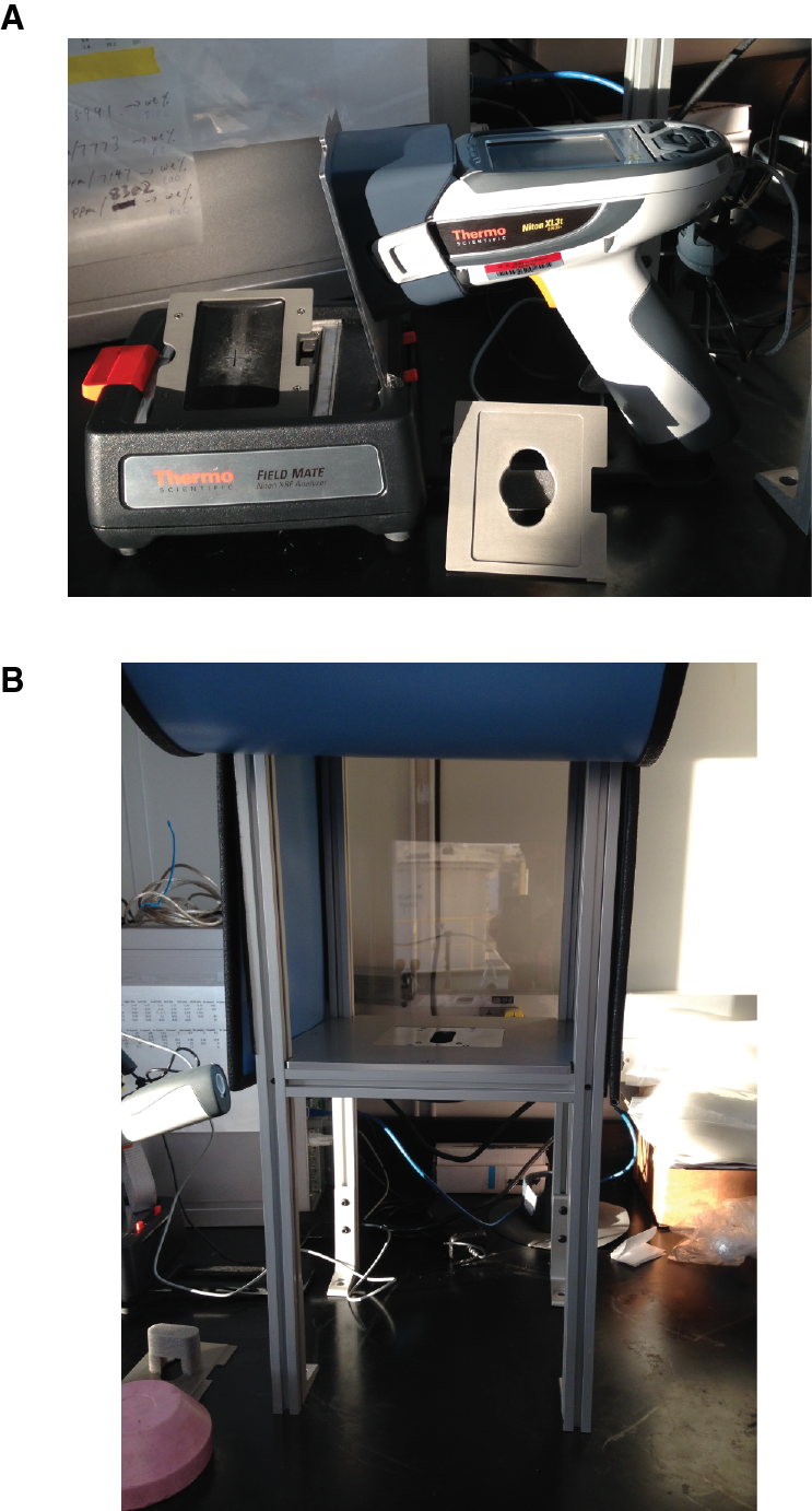
Samples were measured manually for 60 s, with three measurements per unknown constituting a single analysis. One powdered standard reference material (BHVO-2) was analyzed with each set of unknowns to track instrument performance (Table T6). The total variation among individual measurements of the same sample was always well within the measurement uncertainties reported by the instrument and was often ≤5%. Day-to-day variation in our results for reference material BHVO-2 indicated no more than ±3% variability for higher precision elements over the course of analytical work during this expedition.

Rock surface analyses

The primary use of the pXRF instrument was to conduct quick geochemical assessments of volcanic rocks and dikes encountered in the core, both through direct measurements of cut rock surfaces of archive-half core pieces and through the analysis of residual thin section billets for rock samples chosen for microscopic analysis. For these measurements, the Fisher Niton FieldMate sample holder system was used to position smaller samples, and a specially made, shielded XRF holder/mounting system first used during Expedition 330 (Expedition 330 Scientists, 2012) was used for longer core segments and any rock samples too large for the FieldMate holder (Figure F12). Both sample holder systems provide optimal geometry for quantitative use of the system. A built-in video camera showed the spot on the material that was to be analyzed.

An obvious concern regarding measurements with this instrument is the degree to which within-sample compositional variability complicates the interpretation of results. To evaluate this issue, a thin section billet from a previously analyzed basaltic rock sample (Sample 1090-20; Reagan et al., 2010), comparable in both composition and texture to materials drilled at Site U1440, was analyzed multiple times at a variety of different positions on the sample’s cut surface. The results of this test are presented in Table T7. The standard deviation of analyses varied by element as a function of overall abundance level and instrument performance: species that showed high standard deviation on the instrument showed similar variability among spots, with some elements showing as little as 3% overall variation. The resultant analyses were largely comparable to the published data for this sample, indicating that, for the very fine grained igneous rocks recovered at Site U1440 and similar igneous rock samples from the other Expedition 352 sites, within-sample variability is not a significant concern.

Analyses of sample powders

The pXRF system was also used to assess elemental abundances in powdered samples, both freshly produced shipboard rock powders and the oxidized powders produced during sample LOI determinations and subsequently used for ICP-AES analyses. Samples were prepared for analysis using plastic powder mount assemblies provided with the instrument. A short length of thin transparent film for XRF applications (Ultralene or an equivalent product) was stretched across one end of the mount base and held in place with a plastic ring-cap, producing a smooth, transparent surface for sample loading. Sample powder was loaded inside the mount base on the transparent film to a depth of 1–2 mm. A small circle of filter paper (Whatman 24 mm circles, grade 540) was placed on top of the sample and either a round 24 mm plastic foam spacer (similar to those used to fill gaps in sediment core left by sampling) or plastic floss was packed behind the filter paper to hold the sample powder in place, followed by a snap-on plastic sealing cap. The transparent surface of the mount was placed face-up in the XRF sample holder to permit analysis of the powder.

Calibration/correction curves for the different elements measured by pXRF were produced using powder mounts of international reference standards (BHVO-2; BCR-2, JB-2, JB-3, AGV-1, MRG-1, JP-1, and DTS-1). Additionally, previously analyzed Chichijima Island boninite samples (J. Pearce, pers. comm., 2014) were included in our working curves to provide additional calibration data for boninites, which have unusual compositional profiles. The standards correlation data was loaded into Microsoft Excel with the LINEST function to produce slope and intercept values that were used to correct the “raw” concentration data relative to accepted standard values.

Application and performance analysis

The elements found both to be reliably above instrument detection limits with precise and reproducible results were Ca, Ti, K, Rb, Sr, Zr, Cu, Zn, V, and Cr (see Table T6 for results on the BHVO-2 standard). Sc gave scattered results that were generally 3–10 times the actual abundances based on reference materials. Ni was above detection limits for high-abundance samples, which included some of the igneous rock examined during Expedition 352. However, Ni was too close to its detection limit in many of the reference materials examined to permit the development of reasonable working curves, resulting in spurious concentration values (Ni reported level of detection = 25 ppm) (see Expedition 335 Supplementary material [Teagle, Ildefonse, Blum, and the Expedition 335 Scientists, 2012]; see also Table T6). Sc and Ni were therefore not further considered for pXRF measurement during Expedition 352.

Correlation curves for Fe, Ca, Mn, Ti, K, Sr, Zr, Cu, Zn, V, and Cr (plots of pXRF abundances as per the soils correction protocol versus reported consensus values for reference materials) (Figure F13) were of varying quality, but many yielded correlation coefficient r = 0.96 or better, indicating high consistency in instrument performance over a large range of concentrations. Decisions to accept pXRF data for use in chemostratigraphic and other applications were based on quality of fit (correlation coefficient r = 0.95 or better), slopes approximating 1.0 (0.9–1.1), and y-intercepts approaching the origin within analytical uncertainties. y-intercept values were significantly offset from the origin for some elements (Figure F13), in particular Fe and Mn, and this is most likely related to the specifics of the soils correction protocol, which is preset in the instrument. Our correlation curve for V was relatively poor, but pXRF results for V were found to be highly reproducible and largely at the correct abundance levels for the samples examined during Expedition 352, suggesting that for V the pXRF is producing an internally consistent data set.

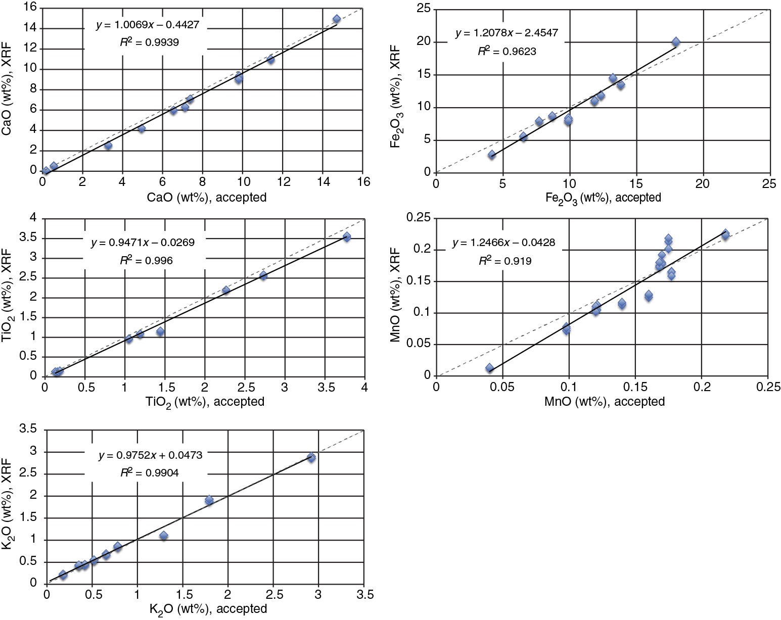
Data for elements with correlation curves showing substantial offsets in their y-intercepts and data for elements with correlation curve r < 0.95 were not utilized in our interpretations. For the remaining elements, the correlation curves in Figure F13 became the bases for working curves to calculate accurate elemental concentrations. These curves are reliable over the concentration ranges constrained by our reference materials.

We conducted a wide range of exploratory analyses with the pXRF on the different core sample materials available for study during Expedition 352. Measurement results from these studies are presented in Tables T8 (thin section billets from Sites U1440 and U1439), T9 (unoxidized rock powders from Hole U1440B), and T10 (oxidized sediment powders from Hole U1439A). In addition, results of pXRF measurements conducted on oxidized rock powders are presented and interpreted in Table T9 in the Site U1439 chapter, Table T9 in the Site U1440 chapter, T8 in the Site U1441 chapter, and Table T8 in the Site U1442 chapter (Reagan et al., 2015a, 2015b, 2015c, 2015d). Results for several key tests conducted on instrument performance and on comparisons with our ICP-AES results are presented below.

Comparisons of pXRF results for powdered igneous rock samples and adjacent thin section residues

To compare the performance of the pXRF instrument on solid rock samples versus powdered samples, we conducted measurements on a selection of sample powders from Hole U1440B that were prepared for ICP-AES analysis and on the cut surfaces of thin section billets taken from the same core sections. Our data for Hole U1440B thin section billets may be found in Table T8, and the data for the unoxidized igneous rock powders from Site U1440B are presented in Table T9. The comparison between pXRF analyses on powders and thin section billets is illustrated in Figure F14 in plots of elemental abundance versus SiO₂ concentrations.

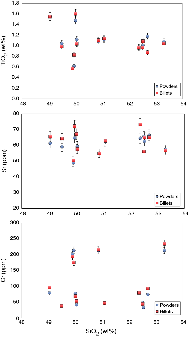
A first-order expectation for this comparison would be a broad similarity between the powder and billet results, with potentially significant variability due to mineralogical variations in the rock samples. In addition, an important concern regarding data quality is evidence of any systematic differences in abundance levels for all or some elements, indicating potential differences in pXRF performance on powders versus rocks. As shown in Figure F14, we see generally good correlations between pXRF data for unoxidized sample powders and the corresponding thin section billets from Hole U1440B, with variability at or within the measurement uncertainties of the elements. There appears to be no evidence of performance differences related to material type, and no “flyer” results on any of the selected thin sections that might indicate mineralogically controlled variations. Thus, the pXRF appears to able to provide equally good quantitative results for selected elements on both powdered and whole-rock versions of approximately the same sample material. Furthermore, in the very fine grained, nonporphyritic volcanic rocks encountered in Hole U1440B, direct pXRF measurements of the rock yielded data that were directly comparable to those from the powdered samples.

Comparisons of pXRF and ICP-AES data from sediment and igneous rock

To compare our pXRF data with results obtained using the shipboard ICP-AES, we conducted pXRF measurements on the rock powder aliquots that had undergone LOI determinations, as it was these oxidized rock powders that were digested to conduct ICP-AES measurements. Data acquired on Site U1439 sediments are presented in Table T10. The data acquired on the oxidized powders of Expedition 352 igneous rock are in Table T9 in the Site U1439 chapter, Table T9 in the Site U1440 chapter, T8 in the Site U1441 chapter, and Table T8 in the Site U1442 chapter (Reagan et al., 2015a, 2015b, 2015c, 2015d).

Site U1440 igneous rock pXRF results and the ICP-AES results on these same powders are plotted together for comparison in Figure F15. The first-order expectation for this comparison would be that the pXRF oxidized powder measurements should correlate well with our ICP-AES solution analysis results. As depicted in Figure F15, we find that pXRF and ICP-AES results for major elements and several of the higher abundance trace elements are similar within their respective uncertainties. TiO₂ shows a largely good correlation with a few outliers; this may be due to some segregation of Ti-rich grains (magnetite and/or ilmenite) in the powders.

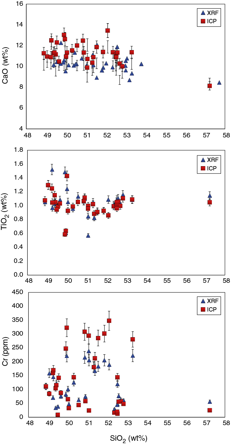
For one trace element (Cr), we found more systematic offsets within the data set, with the pXRF recording higher concentration values than ICP-AES up to ~100 ppm Cr and the ICP-AES producing similar higher values than pXRF above 200 ppm Cr. Investigation of this disagreement between the data sets indicates that, for Cr, the reason may lie in differences in the performance of the two instruments in conducting low-level Cr measurements. Both our ICP-AES and pXRF protocols appear to have similar lower limits of quantitative measurement: our calculated in-rock ICP-AES limit of determination is 8 ppm Cr, and the limit of quantification for Cr is 25 ppm (Table T5). The pXRF limit of quantification is also ~25 ppm Cr for basaltic materials (see Expedition 335 Supplementary material [Teagle, Ildefonse, Blum, and the Expedition 335 Scientists, 2012]). However, the determination of working curves on the two instruments differ. Cr shows extreme variation in abundance among available reference materials, so the slope of either an ICP-AES or pXRF calibration curve for Cr will be strongly impacted by the accuracy of measurements on the higher concentration reference materials used. pXRF results for Cr show substantial increases in measurement uncertainty approaching 25 ppm, and the working curve for Cr in Figure F13 excludes the lowest concentration reference samples, as these could not be reliably determined. These lower abundance reference samples are included in ICP-AES working curves when their measurements during runs are sufficiently precise. Thus, the disagreement between the Cr data sets relates to differences in their working curves and to lower-precision measurements at low concentration levels, though both data sets appear to be internally consistent.

pXRF data evaluation

Previous Integrated Ocean Drilling expeditions have found the shipboard pXRF instrument to be of limited, if any, use as a semiquantitative analysis tool (Koppers, Yamazaki, Geldmacher, and the Expedition 330 Scientists, 2012; Teagle, Ildefonse, Blum, and the Expedition 335 Scientists, 2012; Gillis, Snow, Klaus, and the Expedition 345 Scientists, 2014). During Expedition 352, the combination of amenable analytical targets (fine-grained homogeneous mafic igneous rock) and the need for chemical discriminators that happened to fall within the main range of pXRF analytes, resulted in this instrument becoming a highly valuable addition to the suite of tools for shipboard sample analysis. The limitations of this instrument’s capabilities (i.e., it cannot make reliable measurements on elements at lower atomic numbers than 19 [Koppers, Yamazaki, Geldmacher, and the Expedition 330 Scientists, 2012; Teagle, Ildefonse, Blum, and the Expedition 335 Scientists, 2012; Gillis, Snow, Klaus, and the Expedition 345 Scientists, 2014]) are such that it cannot replace other shipboard instrumentation, though it can augment overall at-sea capabilities for a few elements. The instrument’s most important attribute during Expedition 352 was its ability to provide immediate determinations on several key elements downhole (TiO₂, CaO, K₂O, Rb, Sr, Zn, Cu, Cr, Zr, and V), both to define and refine stratigraphic correlations and to guide our shipboard sampling decisions.

Structural geology

The methods for documenting structural features encountered in Expedition 352 cores largely followed those of Expeditions 334 and 344 (see Structural geology in the Expedition 334 and Expedition 344 Methods chapters [Expedition 334 Scientists, 2012; Harris et al., 2013]). Blenkinsop and Doyle (2010) also provided valuable information on measuring planar structures from core. Structures observed in the split cores were classified and quantified in terms of depth extent, orientation, and sense of displacement. Each structure was recorded manually on a description table sheet (Figure F16) at the core table and then typed into the DESClogik interface to the LIMS database and exported as an Excel file for calculations.

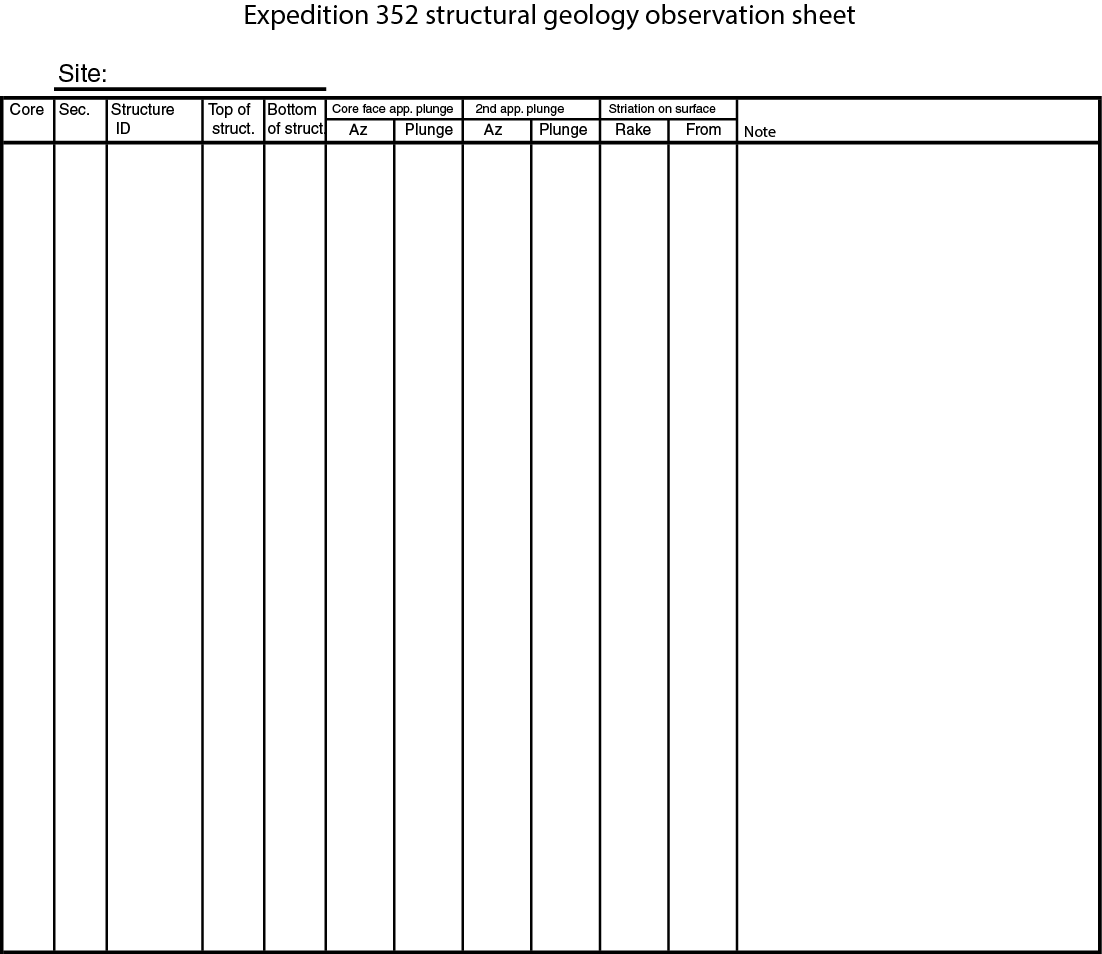
Structural data acquisition and orientation measurements

Core measurements followed the general procedures described in Introduction. In the following, we describe the specifics of structural measurements. We used a plastic protractor for orientation measurements (Figure F17), using the working half of the split core because it provided greater flexibility in removing—and cutting, if necessary—pieces of the core for structural measurements.

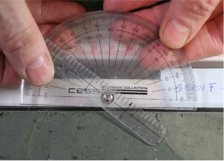
Orientations of planar and linear features in cores were determined relative to the core axis, which represents the vertical axis in the core reference frame, and the split line marked on the working half of the split core liner, which represents 0° (and 360°) in the plane perpendicular to the core axis (Figure F18). To determine the orientation of a planar structural element, two apparent dips of this fabric were measured in the core reference frame. These two apparent dips were then converted, using an Excel spreadsheet (see 352_Structure_Calculations.xls in STRUCTURE in Supplementary material), to a plane represented by dip angle and either a strike or dip direction (Figure F19). One apparent dip was usually represented by the intersection of the planar feature with the split face of the core and was quantified by measuring the dip direction and angle in the core reference frame (β₁; Figure F20). Typical apparent dip measurements had a trend of 90° or 270° and ranged in plunge from 0° to 90° (β₂; Figure F20). The second apparent dip was usually represented by the intersection of the planar feature and a cut or fractured surface at a high angle to the split face of the core. In most cases, this structure was a surface either parallel or perpendicular to the core axis. In the former, the apparent dip lineation trended 0° or 180° and plunged from 0° to 90°; in the latter, the trend would have ranged from 0° to 360° and plunged 0°. Linear features observed in the cores were systematically associated with planar structures (e.g., striation on a fault plane), and their orientations were determined by measuring either the rake on the associated plane or the trend and plunge in the core reference frame. During Expedition 352, we measured rake for striations on fault surfaces (Figure F21) and azimuth and plunge for other lineations.

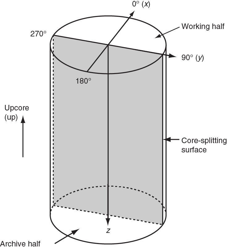
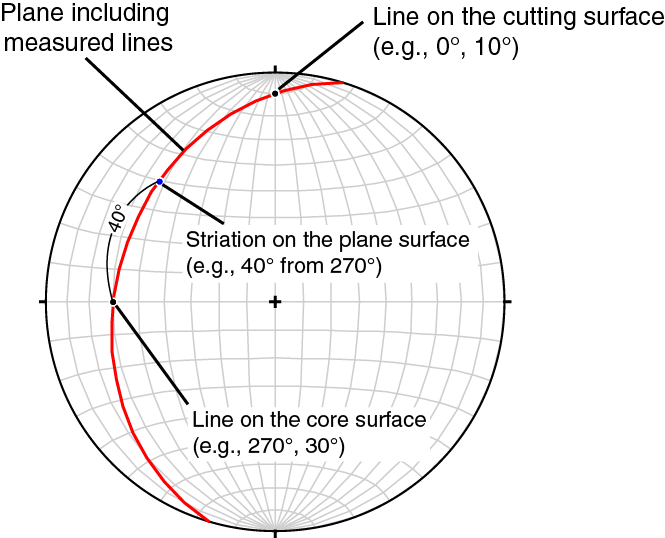
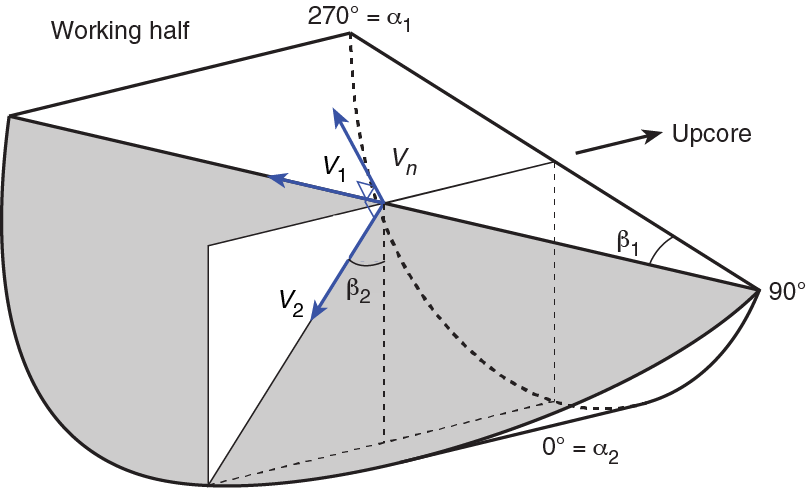
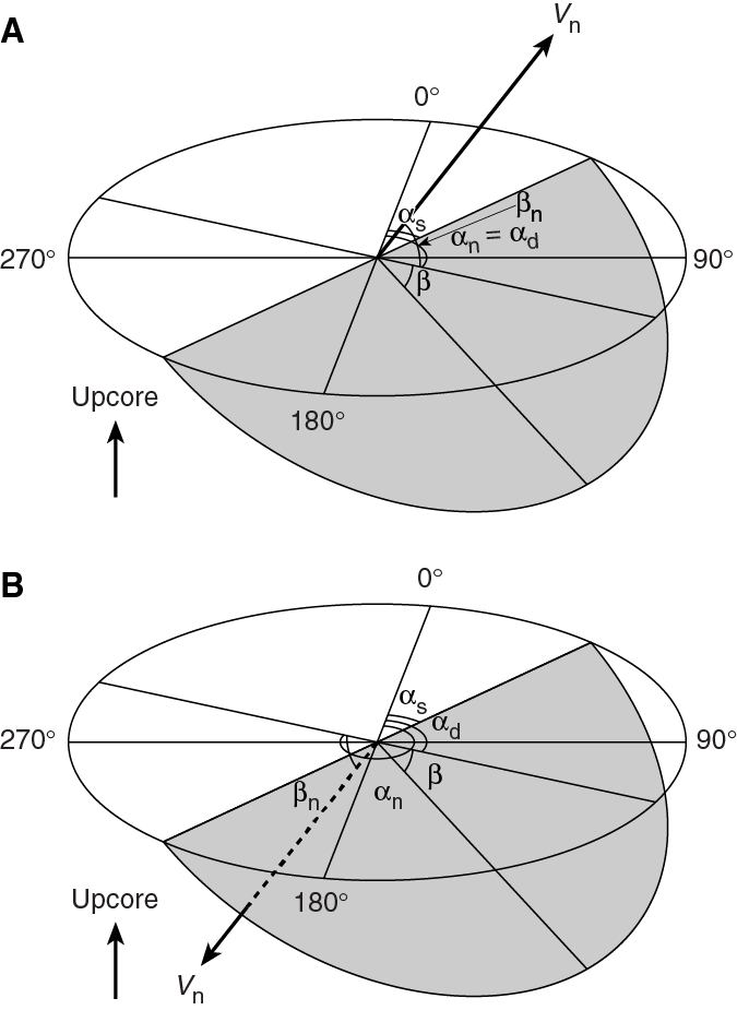
Description and classification of structures

We constructed a structural geology template for DESClogik that facilitates the description and classification of observed structures. We defined the terminology used to describe fault-related rocks, both for clarity and as the basis for differentiating natural structures from drilling-induced features.

Faults were classified into several categories based on the sense of fault slip and their structural characteristics. The sense of the fault slip was identified using offsets of markers (e.g., bedding and older faults) across the fault plane and predominantly by steps or mineral fibers on slickensides. A fault with cohesiveness across the fault zone was described as a healed fault. Zones of high fault density and intense deformation were respectively termed “brecciated zones” and “fractured zones.” Here, fractured zones are moderately deformed zones where the size of fragments is usually bigger than the width of the core; brecciated zones are intensely deformed zones fragmented into centimeter-size and smaller fragments, containing a few larger fragments. “Shear zone” is a zone of strong localized deformation delimited by material with lower finite deformation.

Veins were defined as extensional fractures healed with minerals precipitated from a fluid. The lithology of the host rock and the mineralogy of the vein minerals were described by the petrologists, whereas orientations of the veins, foliations, and other structural features in the igneous rocks were described by the structural geologists.

Structural data may, in places, be disturbed by drilling-induced structures such as flow-in structures in APC cores and biscuiting, fracturing, faulting, and rotation of fragments in XCB and RCB cores. In the case that structures had been disturbed by flow-in on >60% of the cross section of the core, we excluded measurements because of the intense disturbance (bending, rotation, etc.) of these structures. When multiple orientation measurements were plotted in stereographic projection, natural faults were expected to display preferred orientations that may be related to tectonic stress orientations, whereas drilling-induced faults were expected to yield random orientation distributions.

Calculation of plane orientation

For planar structures (e.g., bedding or faults), two apparent dips on two different surfaces (e.g., one being the split core surface, which is east–west vertical, and the other being the horizontal or north–south vertical surface), were measured in the core reference frame as azimuths (measured clockwise from north, looking down) and plunges (Figures F18, F19, F20). A coordinate system was defined in such a way that the positive x-, y-, and z-directions coincide with north, east, and vertical downward, respectively. If the azimuths and plunges of the two apparent dips are given as (α₁, β₁) and (α₂, β₂), respectively, as in Figure F20, then the unit vectors representing these two lines, v₁ and v₂, are

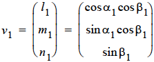and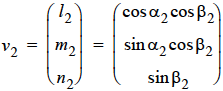

.

The unit vector normal to the plane, v_n (Figure F20), is then defined as

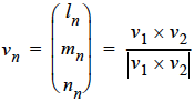, where

.

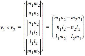The azimuth, α_n, and plunge, β_n, of v_n are given by

and

.

The dip direction, α_d, and dip angle, β, of this plane are α_n and 90° + β_n, respectively, when β_n is <0° (Figure F21A). They are α_n ± 180° and 90° – β_n, respectively, when β_n ≥ 0° (Figure F21B). The right-hand rule strike of this plane, α_s, is then given by α_d – 90°.

Calculation of slickenline rake

For a fault with striations, the apparent rake angle of the striation, φ_a, was measured on the fault surface from either the 90° or 270° direction of the split-core surface trace (Figures F19, F21). Fault orientation was measured as described above. Provided that v_n and v_c are unit vectors normal to the fault and split core surfaces, respectively, the unit vector of the intersection line, v_i, is perpendicular to both v_n and v_c (Figure F22) and is therefore defined as

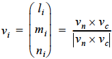, where

and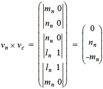

.

 

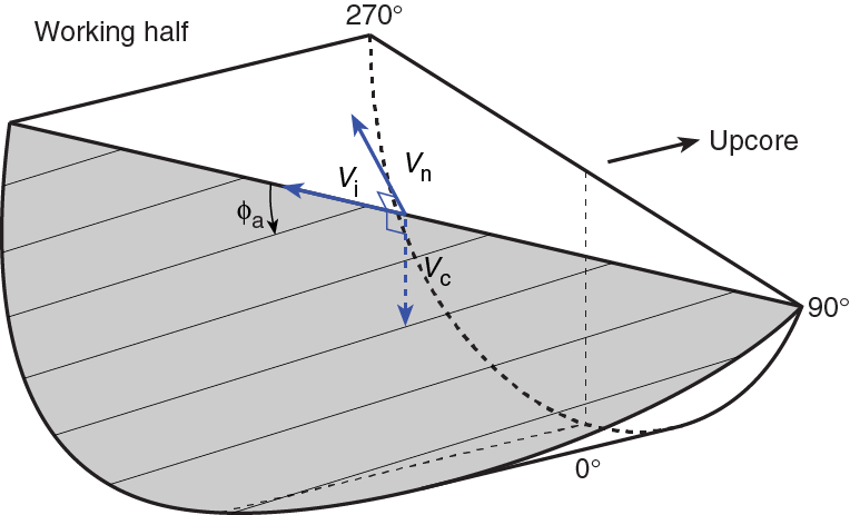
Knowing the right-hand rule strike of the fault plane, α_s, the unit vector, v_s, toward this direction is then

.

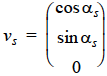The rake angle of the intersection line, φ_i, measured from the strike direction is given by

φ = cos^–1(v_s × v_i),

because

v_s × v_i = |v_s||v_i|cos φ_i = cos φ_i ∴ |v_s| = |v_i| = 1.

DESClogik structural database

The DESClogik database is a program used to store a visual (macroscopic and/or microscopic) description of core structures at a given depth. During this expedition, only the locations of structural features, calculated orientations in the core reference frame, and restored orientations based on the paleomagnetic data were input into DESClogik. Orientation data management and planar fabric analysis were made with a spreadsheet as described above.

Physical properties

Shipboard measurements of physical properties were undertaken to characterize recovered core material. These data are used to link the geological observations made on the core to the results of downhole logging and regional geophysical survey results.

Sediment cores were measured in the following sequence:

1. Cores were thermally equilibrated to ambient room temperature (~3 h) (Figure F23).
2. Whole-round cores were run on the WRMSL. The WRMSL includes a gamma ray attenuation (GRA) bulk densitometer, a magnetic susceptibility pass-through loop system (MSL), and a P-wave velocity logger (PWL). The sampling interval was set to 2.5 cm.
3. Whole-round cores were run on the NGRL when the length of an individual section was >50 cm.
4. Thermal conductivity (TCON) was measured on 1 section (typically Section 3) of each core.
5. Cores were split.
6. The archive half of the core was passed through the SHMSL for point magnetic susceptibility (MSP) and reflectance spectroscopy and colorimetry (RCS).
7. Shipboard samples for moisture and density (MAD) analyses were collected for every second section, typically at 50 cm, avoiding unique units such as ash beds.
8. Wet samples were measured for MAD.
9. Samples were heated in an oven for 24 h and then cooled to room temperature.
10. Dry samples were measured for MAD.
11. Volumes of samples were measured, and bulk density, dry density, grain density, and porosity were calculated.

For hard rock cores, a slightly different sequence was carried out, which included:

1. Thermal equilibration to ambient room temperature (~1 h).
2. Whole-round cores were run on the WRMSL with the PWL turned off. In contrast to sedimentary cores, the sampling interval was decreased to 0.5 cm to obtain more reliable data for individual hard rock pieces.
3. Whole-round cores were run on the NGRL when the length of an individual section was >50 cm.
4. Whole-round image scanning was conducted for large pieces.
5. Cores were split.
6. The archive half of the core was passed through the SHMSL for MSP and RCS.
7. Shipboard samples were collected from each section, with oriented discrete cube samples (2 cm³) taken from the working half for paleomagnetic (see Paleomagnetism), MAD, and P-wave velocity measurements. To remove air from pore spaces, cubes were soaked for 24 h in seawater at ambient temperature under vacuum before any measurements were acquired.
8. Archive-half pieces with a length >7 cm were selected, soaked for 24 h in seawater under vacuum to remove air from pore spaces, and measured for thermal conductivity.
9. MAD measurements were made on wet cube samples.
10. P-wave velocity was measured for wet cube samples in three orthogonal directions.
11. Samples were heated in an oven for 24 h and then cooled to room temperature.
12. MAD was measured on dry samples.
13. Volumes of samples were measured, and bulk density, dry density, grain density, and porosity were calculated. Samples were then returned to paleomagnetism group.

During Expedition 352, all raw data were uploaded to the LIMS database. A comprehensive discussion of methodologies and calculations used in the JOIDES Resolution Physical Properties Laboratory is presented in Blum (1997).

WRMSL measurements

The WRMSL was used to measure GRA density, bulk density, magnetic susceptibility, and P-wave velocity nondestructively. The sampling interval for WRMSL measurements was set at 2.5 cm for sediment cores. For hard rock cores, the PWL was turned off and the sampling interval was set at 0.5 cm to obtain more reliable data for individual hard rock pieces. Calibration was verified after each core measurement by passing a freshwater-filled calibration core through the WRSML. The nominal accuracy of the calibrated instruments was between 1% and 2%.

GRA bulk density

The GRA densitometer on the WRMSL operates by passing gamma rays from a ¹³⁷Cs source through a whole-round core and into a 75 mm³ sodium iodide (NaI) detector located directly below the core. The input gamma ray peak has a principal energy of 0.662 MeV and is attenuated as it passes through the core. Attenuation of gamma rays, mainly by Compton scattering, is related to electron density, and thereby related to material bulk density by

ρ_b = ρ_ew/2ΣN,

where

• ρ_b = bulk density,
• ρ_e = electron density,
• w = molecular weight, and
• N = atomic number of elements in the material.

For the majority of elements, and for rock-forming minerals, 2ΣN/w is ~1, whereas for hydrogen it is 1.9841. Therefore, for a known sample thickness the gamma ray count is proportional to density. Calibration of the GRA densitometer was performed using a core liner filled with freshwater and aluminum density standards. Recalibration was performed if the measured density of the freshwater standard was not 1.00 ± 0.02 g/cm³.

Magnetic susceptibility

Magnetic susceptibility, Κ, is a dimensionless measure of the degree to which a material can be magnetized by an external magnetic field: Κ = M/H (SI), where M is the magnetization induced in the material and H is strength of an external field, respectively. Magnetic susceptibility varies in response to the type and concentration of magnetic grains, making it useful for identifying compositional variations. Magnetic susceptibility responds to variations in the magnetic composition of the sediment that are commonly related to variations in mineralogical composition (e.g., terrigenous versus biogenic materials) and diagenetic overprinting. Materials such as clay generally have a magnetic susceptibility several orders of magnitude lower than magnetite and some other iron oxides that are common constituents of igneous and volcanogenic material. Water and plastics (such as the core liner) have a slightly negative low magnetic susceptibility.

The WRMSL measures volume magnetic susceptibility using a Bartington Instruments MS2 meter coupled to a MS2C sensor coil (88 mm diameter) and operates at an alternating field of 250 mT and frequency of 0.513 kHz. During Expedition 352, the instrument was set to record SI units with an integration period of ~1 s, which produced a sensitivity of 1 × 10^–5 SI. The instrument output (Κ_MEAS) depends on the diameter of the core (d) passing through the coil diameter (D). The core diameter is smaller than the sensor coil aperture, so a correction factor (Κ_REL) is necessary to convert the instrument output to true volume susceptibility (Κ in SI units), where Κ_REL = 3.45(d/D)³ (Bartington Instruments, Ltd., 2011). Κ_REL is 1 for d = 58 mm and D = 88 mm. Although d is typically 57 ± 1 mm for well-cut RCB hard rock cores, the size of small pieces and rollers varies in an unpredictable manner. Hence, because a single correction factor was not justified and therefore no correction was applied to WRSML magnetic susceptibility measurements, raw data were reported in instrument units (10^–5 SI).

The along-core response curve of the MS2C coil has a full width at half maximum of ~4 cm (Blum, 1997) and is consistent with the decay in magnetic intensity with distance from a dipole. Therefore, measurements of susceptibility from core pieces <8 cm long will significantly underestimate magnetic susceptibility by >10%.

P-wave velocity

P-wave velocity is the rate at which a (compressional) P-wave travels through a medium per unit time, expressed in meters per second. P-wave velocity is dependent on the composition, porosity, bulk density, fabric, and temperature of the material, which in turn are functions of consolidation and lithification, state of stress, and degree of fracturing. The PWL system on the WRMSL transmits a 500 kHz P-wave pulse across the core liner at a specified repetition rate. Pulser and receiver are mounted on a caliper-type device and are aligned in order to make wave propagation perpendicular to the section’s long axis. A linear variable differential transducer measures the P-wave travel distance between the pulse source and the receiver. Good coupling between transducers and core liner is facilitated with water dripping onto the contact from a peristaltic water pump system. Signal processing software picks the first arrival of the wave at the receiver and the processing routine also corrects for the thickness of the liner.

A series of acrylic cylinders of varying thicknesses are used to calibrate the PWL system. The regression of traveltime versus travel distance yields the P-wave velocity of the standard material, which should be 2750 ± 20 m/s. The thickness of the calibration samples, corrected for liner thickness, is divided by the traveltime to calculate P-wave velocity in meters per second. The calibration is verified by measuring a core liner filled with pure water, and the calibration passes if the velocity is within ±20 m/s of the expected value for water (1485 m/s).

NGRL measurements

Gamma radiation is emitted from rock primarily as a result of the radioactive decay of ⁴⁰K and the decay of isotopes in the ²³⁸U and ²³²Th series. Measurement of natural gamma radiation (NGR) from the recovered core provides an indication of the concentration of these elements and can also be used to correlate the core with the downhole gamma ray logs (e.g., Révillon et al., 2002). The NGRL installed on the JOIDES Resolution was designed and built by the Integrated Ocean Drilling Program-United States Implementing Organization at Texas A&M University (Vasilyev et al., 2011). The main NGR detector unit comprises 8 sodium iodide (NaI) scintillator detectors, 7 plastic scintillation detectors, 22 photomultipliers, and passive lead shielding. The eight NaI detectors are spaced every 20 cm in the logger; the detectors themselves are semicylindrical annuli around the lower half of the core (each crystal is ~13 cm wide along the core). Detectors are shielded by lead to reduce the measurement of external gamma radiation, and the NGRL also employs seven plastic scintillation detectors that detect and actively suppress the effect of high-energy gamma and muon components of cosmic radiation.

The NGRL was calibrated using ¹³⁷Cs and ⁶⁰Co sources to identify peaks at 662 and 1330 keV, respectively. Background measurements of an empty core liner counted for 6 h were made upon arrival at Site U1439 and for 12 h at Site U1440; background count variability between the two sites was <1%.

A single measurement run with the NGRL provides 16 measurements at 10 cm intervals over a 150 cm section of core. To achieve a 10 cm interval using the NGRL’s eight sensors spaced every 20 cm, the NGRL records two sets of measurements offset by 10 cm. Total counts are routinely summed over the range of 100–3000 keV. The quality of the energy spectrum measured depends on the concentration of radionuclides in the sample and on the counting time, with longer counting times providing better counting statistics. A live counting time of 5 min was set in each position for sediment samples and 20 min for hard rock samples (for a total live count time of about 10 min per section for sediments and 40 min for hard rocks).

SHMSL measurements

The SHMSL was used to measure spectral reflectance and point magnetic susceptibility on archive section halves. An electronic platform moves along a track above the section half, recording the sample height using a laser sensor. The laser establishes the location of the surface of the section and the presence of samples to measure by locating gaps and cracks between pieces. The platform then reverses direction, moving from bottom to top taking measurements of point magnetic susceptibility data at 2 cm intervals.

Reflectance spectrophotometry and colorimetry

Reflectance of visible light from the archive halves of sediment cores was measured using an Ocean Optics USB4000 spectrophotometer mounted on the SHMSL. For sediment and sedimentary rock, freshly split cores were covered with clear plastic wrap. Spectral data are routinely reduced to the L*a*b* color space for output and presentation, in which L* is lightness (greater value = lighter) in the range between 0 (black) and 100 (white), a* is the red–green value (greater value = redder) in the range between –60 (green) and 60 (red), and b* is the yellow–blue value (greater value = yellower) in the range between –60 (blue) and 60 (yellow). The color reflectance spectrophotometer calibrates on two spectra, pure white (reference) and pure black (dark). Each measurement was recorded in wide spectral bands from 400 to 900 nm in 2 nm steps. Each measurement took ~5 s.

Point magnetic susceptibility

MSP was measured on the SHMSL using a Bartington MS2K point sensor (high-resolution surface scanning sensor) operating at an alternating field of 250 mT and a frequency of 0.580 kHz, similar to the Bartington sensor MSL on the WRMSL. The sensor takes and averages three measurements at 1 s intervals to an accuracy of 5%. Measurements were made on the archive halves of split cores that were covered with clear plastic wrap. Measurements were taken at 2 cm spacing, integrating over a volume of 10.5 mm × 3.8 mm × 4 mm, where 10.5 mm is the length perpendicular to the core axis, 3.8 mm is the width in the core axis, and 4 mm is the depth. The probe was zeroed in air before each measurement point, and a background magnetic field was measured and removed from the data before being output.

Discrete measurements

P-wave velocity (for hard cores)

The P-wave velocity gantry measures ultrasonic sound speed between the transducers on discrete sample cubes (2 cm³). Before we measured the P-wave velocity of a sample, we used a vacuum pump system to ensure complete saturation of seawater in a sample. The system consists of a vacuum pump and a plastic chamber that contains the cubes submerged in seawater in small plastic vials. A vacuum pump then removes air from the chamber once an hour, essentially sucking air from pore spaces. Samples were kept under vacuum for at least 24 h. During this time, a gauge attached to the vacuum pump monitored the pressure in the chamber periodically to ensure a stable vacuum. After removal from the saturator, cubes were stored in sample containers to maintain saturation. All P-wave caliper (PWC) measurements were done on the same discrete cube samples taken from the working half for paleomagnetic (see Paleomagnetism) and MAD measurements.

The cubes were oriented following standard IODP conventions and placed on a gantry that measures P-wave velocity in all three directions (x-, y-, and z-directions). P-wave anisotropy between the average horizontal and vertical velocities (Anis_(xy)z) and horizontal anisotropy (Anis_xy) were calculated using

Anis_(xy)z (%) = 100 × [mean(V_x, V_y) – V_z]/mean(V_x, V_y, V_z)

and

Anis_xy (%) = 100 × (V_x – V_y)/mean(V_x, V_y),

respectively, where x, y, and z are the standard core coordinate axes, V_x and V_y are the transverse core velocities, and V_z is the longitudinal core velocity.

The measurement system used Panametrics-NDT Microscan delay line transducers (transmitting at 0.5 MHz). The IODP Velocity Gantry 2.0.5.0 software identifies the peak of the first arrival of P-wave automatically and/or manually. The complete waveform was stored with the data if reanalysis was deemed necessary. Shipboard visual checks of the picks appeared satisfactory. The distance between transducers was measured with a built-in linear voltage displacement transformer. Measurements on standards were conducted as frequently as necessary. A calibration was made daily with acrylic cylinders of different thicknesses (in which the standard with a 45 mm thickness was usually used) and a known P-wave velocity (2750 ± 20 m/s). We found that the measured values were more consistent and closer to the certified acrylic velocity (2750 ± 20 m/s) when a drop of water was added between the acrylic cylinder surfaces and the transducers.

Moisture and density

On average, a ~10 mL cylindrical sample was taken every second section of the sediment core. The sample was placed in a labeled glass vial, the mass of which had already been weighed on land. For hard rocks, the discrete cubes initially used for paleomagnetic (PMAG) and PWC measurements were further used for the MAD analyses. Mass and volume measurements were made to determine bulk density, dry density, and grain density and porosity. The shipboard MAD facility consists of a dual-balance system and a hexapycnometer.

Dual-balance system

A dual-balance system was used to measure both wet and dry masses. Two analytical balances (Mettler-Toledo XS204) compensate for ship motion; one acts as a reference and the other measures the unknown (i.e., a sample). A standard mass of similar value to that of the sample was placed on the reference balance to increase accuracy. An accuracy of 0.005 g was readily attainable by using a reference mass within ~10% of the sample mass. After wet mass determinations and P-wave measurements (for cube samples), samples were placed in an oven at 105° ± 5°C for at least 24 h and then allowed to cool in a desiccator for a minimum of 1 h prior to the determination of dry masses.

Hexapycnometer system

The hexapycnometer is an IODP custom-built system that uses six Micromeritics cell units, electronics, and control programs. The system measures dry sample volume using pressurized He-filled chambers with a precision of 0.02 cm³. At the start of the expedition, and whenever the helium gas tank was changed, shipboard technicians performed a calibration using stainless steel spheres of known volume. For each measurement, five unknown cells and one cell that contained two stainless steel calibration spheres (3 and 7 cm³) with a total volume of ~10 cm³ were run. Calibration spheres were cycled through the cells to identify any systematic error and/or instrument drift. Spheres were assumed known to within 1% of their total volume. If the volumes of the calibration spheres deviated by >1% from their known volume, then that pycnometer cell was recalibrated.

MAD calculations

For density calculations, both mass and volume are first corrected for the salt content of the pore fluid:

M_salt = M_water[s/(1 – s)],

where

• s = pore water salinity,
• M_salt = mass of salt, and
• M_water = mass of water.

Grain density (ρ_g) is determined from the dry mass (M_dry) and dry volume (V_dry) measurements:

ρ_g = (M_dry – M_salt)/[V_dry – (M_salt/ρ_s)],

where ρ_s is the density of salt (2.20 g/cm³; Blum, 1997) and M_salt is the mass of salt.

The salt-corrected mass of pore water (M_pw) is calculated as

M_pw = (M_wet – M_dry)/(1 – s),

where M_wet is wet mass of the sample. Then, the volume of pore water (V_pw) is

V_pw = M_pw /ρ_pw = (M_wet – M_dry)/[(1 – s)ρ_pw],

where we assume the density of the pore fluid (ρ_pw) to be 1.024 g/cm³ (seawater with salinity of 35 g/L; Blum, 1997). To calculate sample bulk density (ρ_b), we first computed bulk volume (V_b) as

V_b = V_dry + V_pw.

Then,

ρ_b = M_wet/V_b.

Porosity (φ) is calculated from the two volume parameters above:

φ = V_pw/V_b.

Thermal conductivity

Thermal conductivity (k, in W/[m·K]) is a measure of the rate at which heat is transported through a material and depends on temperature, pressure, types of saturating fluid, and the composition, distribution, and alignment of mineral phases. At steady state, thermal conductivity is the coefficient of heat transfer (q) across a steady-state temperature difference over a distance:

q = k(dT/dx).

The TK04 system measures thermal conductivity by transient heating of the sample with a known heating power and geometry. Changes in temperature with time during heating are recorded and used to calculate thermal conductivity. Heating power can be adjusted for each sample. Heating power (W/m) is typically set to be ~2 times the expected thermal conductivity (W/[m·K]). The TK04 device uses an approximation method to calculate conductivity and to assess the fit of the heating curve. This method fits discrete windows of the heating curve to the theoretical temperature (T) with time (t) function:

T(t) = A₁ + A₂ ln(t) + A₃ [ln(t)/t] + (A₄/t),

where A_1–4 are constants that are calculated by linear regression. A₁ is the initial temperature, whereas A₂, A₃, and A₄ are related to geometry and material properties surrounding the needle probe. Having defined these constants (and how well they fit the data), the apparent conductivity (k_a) for the fitted curve is time-dependent and given by

k_a (t) = q/4π{A₂ + A₃ [1 – ln(t)/t] – (A₄/t)},

where q is the input heat flux. The maximum value of k_a and the time (t_max) at which it occurs on the fitted curve are used to assess the validity of that time window for calculating the thermal conductivity. The best solutions are those where t_max is greatest, and these solutions are selected for output. Fits are considered good if k_a has a maximum value, t_max is large, and the standard deviation of the least-squares fit is low. For each heating cycle, several output values can be used to assess the quality of the data, including natural logarithm of extreme time t_max, which should be large; the number of solutions (N), which should also be large; and the contact value, which assesses contact resistance between the probe and the sample, should be small and uniform for repeat measurements.

For sediment core, we used a needle probe in which a 2 mm hole was first drilled into the plastic sheathing of the whole rounds, and a needle was inserted into the sediment. The temperature of the superconductive needle probe has a quasi-linear relationship with the natural logarithm of the time after the initiation of heating (Blum, 1997).

For hard rock core, half-space determinations of thermal conductivity were made with a needle probe embedded in the bottom of a Plexiglas block with a thermal conductivity of 0.184 W/(m·K). The Plexiglas block was placed against samples from the archive-half core. Heat is assumed to have transferred through the sample, and the TK04 documentation indicates that heat flow through the Plexiglas block itself is only significant for sample thermal conductivities <1 W/(m·K). The samples and the sensor needle were placed in an isolated Styrofoam-covered seawater bath (k = ~0.6 W/[m·K]) during measurement. Seawater is preferred to improve the needle/sample contact compared to silicone thermal contact gel in order to avoid contamination of the samples. Isolation of the seawater bath with the sample and sensor needle eliminated the effect of small but rapid temperature changes introduced by air currents in the laboratory, as well as the ship’s motion.

The instrument internally measures temperature drift and does not begin a heating run until sufficient thermal equilibrium is attained. Core pieces from the archive half were measured at irregular intervals downhole depending on the availability of homogeneous and relatively vein/crack free pieces long enough to be measured without edge effects (pieces >7 cm long; i.e., longer than the instrument needle). At least three measurements were performed on each sample to verify the consistency of the results and provide an average value. The probe was periodically checked using the MACOR ceramic standard.

Magnetic susceptibility

Magnetic susceptibility was measured on discrete cubes using the Bartington MS2K point sensor (see Point magnetic susceptibility). Measurements were taken on the 2 cm³ samples that were also used for MAD and PMAG measurements. The sensor was zeroed in air prior to each discrete measurement, and a background magnetic field measurement was taken and removed from these measurements before the final data were output.

Downhole temperature measurements

Downhole in situ temperature measurements were made in the sediment intervals cored using the APCT-3, which fits directly into the coring shoe of the APC. The APCT-3 is made up of three main components: electronics, coring hardware, and computer software. The temperature sensors were calibrated for a working range of 0°–45°C. The APCT-3 was held at the mudline for ~5 min to equilibrate with bottom water temperature before being deployed in a hole. The tool was then lowered in the hole to penetrate the formation. Frictional heating caused by the deployment of the APCT-3 into a formation causes a rise in temperature. Following this initial temperature rise, the temperature decreases along a decay curve to near equilibrium. During this decay phase, it is important that the temperature tool is not disturbed. A second rise in temperature occurs due to frictional heating caused by the tool being extracted from the formation. Temperatures were measured as a time series with a sampling rate of 1 s with the resulting data logged onto a microprocessor within the downhole tool. The data were retrieved when the tool was recovered to the ship. The formation equilibrium temperature was determined based on fitting the temperature decay curve using the MATLAB TP-Fit program (M. Heeseman et al., pers. comm., 2008).

If heat transfer is conductive and constant with depth through the sediment, the thermal gradient will be inversely proportional to thermal conductivity according to Fourier’s law. This relationship can be linearized by plotting temperature as a function of summed thermal resistance (Bullard, 1939),

 

T(z) = T₀ + Q = ,

where

• T = temperature,
• z = depth,
• T₀ = bottom water temperature,
• Q = heat flow, and
• = thermal resistance.

Where several reliable thermal conductivity data values were available throughout the borehole, the above equation was used to estimate the borehole temperature profile.

Paleomagnetism

During Expedition 352, routine shipboard paleomagnetic experiments were carried out on sedimentary and igneous cores recovered from Sites U1439–U1442. Remanent magnetization was measured on archive section halves and on discrete cube samples taken from the working-half cores. Continuous archive section halves from APC cores were demagnetized with an alternating field (AF), whereas discrete samples were subjected to stepwise AF demagnetization or thermal demagnetization to remove overprint magnetization(s) and reveal the primary magnetization. Because the azimuthal orientations of core samples recovered by rotary drilling are normally not constrained, all magnetic data are reported relative to the sample core coordinate system (Figure F24, F25). In this system, +x points into the section working half (i.e., toward the double line), +z is downcore, and +y is orthogonal to x and z in a right-hand sense.

Archive section half remanent magnetization data

Measurement

The compiled version of the LabView software (SRM Section) used during Expedition 352 was SRM version 318. In this version (Expedition 330 Scientists, 2011), the speed at which the archive section was moved when not measuring is set at 20 cm/s, and simultaneous sampling of the magnetometer axes was incorporated.

The response functions of the pick-up coils of the superconducting quantum interference device (SQUID) sensors have a full width of 7–8 cm at half height (Parker and Gee, 2002). As a result, data collected within ~4 cm of piece boundaries (or voids) are significantly affected by edge effects. Consequently, samples less than ~16 cm in length may yield measurements influenced by edge effects. Sedimentary core sections characterized by very coarse grained lithologies (i.e., conglomerates with clasts larger than 2 cm) or significantly disturbed lithologies were not measured. Where such intervals were present in part of a section, they were filtered out from the measured data prior to interpretation.

The remanent magnetization of sediment section archive halves was measured at 5 cm intervals using the automated pass-through direct-current SQUID (DC-SQUID) cryogenic rock magnetometer (2G Enterprises model 760R). An integrated, inline AF demagnetizer (2G model 600), capable of applying peak fields up to 80 mT, was used to progressively demagnetize the core. During Expedition 352, AF demagnetization was carried out at 15, 20, 25, and 30 mT steps for sediment cores. A magnetometer measuring track velocity of 10 cm/s was used to optimize the rate at which core could be processed. AF demagnetization at steps >40 mT was not attempted on sediment because of a well-documented problem with the cryogenic magnetometer demagnetization coils (e.g., see Expedition 335 Scientists, 2012), which results in a spurious anhysteretic remanent magnetization (ARM) along the z-axis of the core at higher applied fields.

Because of low recovery in igneous basement, larger oriented archive-half igneous rock pieces were measured to gain additional paleomagnetic data. Oriented pieces longer than 10 cm were selected for measurement because smaller pieces do not fill the sensing coil and may give spurious readings owing to perturbations of the sample magnetic field by edge effects. These pieces were measured using the discrete sample software. The core pieces were placed in the magnetometer sample boat at intervals of 32 cm in order to minimize the influence of a given piece on the adjacent pieces. AF demagnetization steps were run at 5, 10, 15, 20, 25, 30, 40, and sometimes 50 mT, the latter in the case of high-coercivity samples. This is a nonstandard measurement for the cryogenic magnetometer because the pieces are irregular in shape, which is not ideal for accurately measuring the magnetization. Furthermore, sample volumes are also much larger than the 8 cm³ of the normal discrete samples. For this reason, magnetization intensities in the LIMS database are incorrect and the directions must be treated with caution. Nevertheless, these measurements provided a routine evaluation of magnetic properties of the cores to guide sampling and analysis of the working-half cores.

Filtering and processing

For sediment cores, discrete sample AF demagnetization experiments were used to determine the AF demagnetization field that removed the drill string overprint (Roberts et al., 1996; Fuller et al., 1998; Acton et al., 2002) most completely. Because the drill string overprint usually has a low coercivity, this final step was usually 20–30 mT. Inclination and declination data were plotted downhole at the defined AF demagnetization step, and shifts in inclination and declination were used to determine polarity intervals, which were then correlated with the geomagnetic polarity timescale (GPTS; Gradstein et al., 2012). The sediment cored during Expedition 352 revealed a disappointing propensity to acquire an ARM at higher demagnetization steps, placing a limit on the amount of AF demagnetization that could be employed. Usually, the upper limit of the applied AF field before obtaining an ARM was only ~25–30 mT. It was noticed that, even after AF demagnetization at 30 mT, the average positive and negative inclinations often have different mean values, with positive inclinations being larger in average magnitude. This observation implies that the drill string overprint has not been completely removed from the AF demagnetized core measurements.

Characteristic remanent magnetization directions were determined from the archive-half core piece measurements using principal component analysis (PCA; Kirschvink, 1980). Data were reformatted and input into Remasoft version 3.1 software supplied by Agico for the JR-6A spinner magnetometer. The characteristic remanence direction was calculated using a minimum of three higher demagnetization steps that appeared to define univectorial decay toward the origin of an orthogonal vector plot. Typically, PCA calculations were done both with and without the origin as a point. In well-behaved samples, these different PCA solutions were not significantly different.

Discrete sample data

Measurement and instrumentation

All discrete samples taken from working-half core sections for shipboard magnetic analysis were 8 cm³ cubes. Although standard 2.5 cm diameter minicores are more commonly used, cubic samples were preferred, as they should have a more precisely determined vertical reference (based on a saw cut perpendicular to the core length) than the minicores, where the arrow on the split-core face must then be transferred to the long axis of the sample. Moreover, the use of cubes instead of minicores enabled sharing of the limited discrete samples for physical properties measurements.

Remanent magnetization of discrete samples was measured exclusively with the Agico JR-6A spinner magnetometer because tests of the reliability of small-sample discrete measurements from the 2G cryogenic magnetometer showed significant scatter for weakly magnetic samples (Expedition 335 Scientists, 2012). For samples measured on the spinner magnetometer, the automated sample holder was used. Measurements of the empty automatic sample holder, after subtracting the stored holder magnetization, yielded intensities on the order of 4.0 × 10^–6 A/m, representing the practical noise limit of the system.

It was intended that about half of the discrete samples would be subjected to stepwise AF demagnetization and the other half to thermal demagnetization. AF demagnetization is often preferred for routine exploratory sampling because it is done much more quickly than thermal demagnetization. Some sections did not respond well to AF demagnetization and there were problems with the AF demagnetization equipment, so the balance of the two techniques was biased toward thermal demagnetization, depending on the results of pilot studies using AF demagnetization on a particular lithology. AF demagnetization was performed using the D-Tech AF demagnetizer (model D-2000), capable of peak fields up to 200 mT. Demagnetization steps were adapted to the different magnetic mineralogies but, in general, each demagnetization run was composed of 10–12 steps. However, after demagnetization at 20–30 mT, the weakest samples acquired a spurious magnetization, probably an ARM caused by imperfectly balanced coils in the demagnetizer. Testing of sample demagnetizations suggests that this problem is linked to a glitch with one of the two amplifiers of the D-Tech demagnetizer. It was unclear whether this was also an effect of the sample mineralogies. This problem was particularly troublesome for weakly magnetized samples, where the magnetization was lower than a few hundreds of milliamperes per meter, and also for samples with a strong coercivity that required demagnetization in AF fields higher than 40 mT. These problems with the AF demagnetizing equipment severely limited the results and use of AF demagnetization during Expedition 352.

Discrete samples treated to thermal demagnetization were demagnetized using an ASC Scientific thermal demagnetizer (model TD-48 SC), capable of demagnetizing samples up to 700°C. The total magnetic field along the length of the TD-48 SC access tube has a maximum field in the sample chamber region of <50 nT from 30 cm onward (measured from the edge of the access opening). The large sample boat allowed samples to be spaced loosely, alleviating sample interaction, and orientations were varied at alternative steps to allow any interaction between adjacent samples or spurious axial field to be identified (but none were detected). Samples were held at the desired temperature for 30 min prior to cooling in the low-magnetic field chamber. Magnetic susceptibility was measured (using a Bartington MS2C magnetic susceptibility sensor) after every heating step to monitor thermal alteration of magnetic minerals during heating. Heating was carried out from 120° or 150°C until the samples were demagnetized, in steps of 25° or 50°C depending on the magnetic mineralogy. Thermal steps were typically at 50°C intervals up to 400° or 450°C and at 25°C intervals for higher temperatures up to 600°–625°C.

Discrete samples for which we suspected the presence of a possible large multidomain component based on the AF demagnetization spectra of the corresponding archive half were subjected to low-temperature demagnetization (LTD) (Merrill, 1970; Dunlop, 2003; Yu et al., 2003) prior to thermal demagnetization in order to remove substantial secondary drilling-related magnetization. LTD involves cooling samples in a liquid nitrogen bath (T = 77 K) and allowing them to warm back up to room temperature in a very low field environment. This procedure cools the samples to below the Verwey transition of magnetite (Dunlop, 2003), resulting in a loss of magnetic remanence by multidomain grains upon subsequent warming to ambient temperature. During shipboard experiments, a suitable low-field environment was provided by nesting the two available cylindrical mu-metal shields to produce a six-layer shield with an internal field of <10 nT. This was sufficiently low to allow LTD treatment to be performed successfully. This also allowed the removal of a spurious magnetization acquired during physical properties measurements by heating to 110°C without magnetic shielding.

As was done for the archive core pieces, discrete sample PCA was carried out using the Remasoft 3.1 software provided by Agico.

Anisotropy of low-field magnetic susceptibility

Measurements of the anisotropy of low-field magnetic susceptibility were not made during Expedition 352 because the Kappabridge instrument, which malfunctioned during the previous expedition, was unavailable.

Magnetostratigraphy

Expedition 352 sites are located at ~28.5°N, so the expected time-averaged geocentric axial dipole field inclination is ~47.4°. Because of this significant dip, reversals of the Earth’s magnetic field in more recent parts of the stratigraphy can be easily identified by distinct changes in inclination. For older parts of the stratigraphy (and underlying basement rocks), believed to have formed closer to the Equator (Salisbury et al., 2002), magnetic polarities are more difficult to determine using inclination data alone. Magnetozones identified from the shipboard data were correlated to the GPTS (Gradstein et al., 2012) with the aid of biostratigraphic datums. In this updated GPTS, Late Cretaceous through Neogene time has been calibrated with magnetostratigraphic, biostratigraphic, and cyclostratigraphic studies and selected radioisotopically dated levels. The chron terminology used in the figures is from Cande and Kent (1995).

Downhole logging

Downhole logging data are rapidly and continuously collected in situ at sampling intervals ranging from 2.5 mm to 15 cm. These data are used to determine the physical, chemical, and structural properties of the formation penetrated by a borehole and can be used to aid the interpretation of stratigraphy, lithology, mineralogy, and geochemical composition. Downhole logs also provide information about the status and size of a borehole including information about formation stress or deformations induced by drilling. In the event of incomplete core recovery, the continuous nature of this data set may provide the only means of characterizing the formation penetrated.

Downhole logs are intermediate in scale between laboratory measurements of core samples and geophysical surveys and are therefore particularly useful in calibrating and ground-truthing the interpretation of geophysical survey data. Overall, logs are an essential link in understanding physical properties across a range of scales.

Downhole measurements data were acquired using a variety of logging tools (manufactured by Schlumberger and Lamont-Doherty Earth Observatory [LDEO] that were combined into tool strings (Table T11; Figure F26) and run downhole on a wireline cable after coring operations were completed at each site. During Expedition 352, 3 tool strings were used:

1. Triple combo-Ultrasonic Borehole Imager (UBI) tool string, which recorded gamma radiation, density, resistivity, and oriented acoustic images;
2. Triple combo-Magnetic Susceptibility Sonde (MSS) tool string, which recorded gamma radiation, density, resistivity and magnetic susceptibility; and
3. Formation MicroScanner (FMS)-sonic tool string, which recorded gamma radiation, compressional and shear wave velocities, and oriented microresistivity images of the borehole wall.

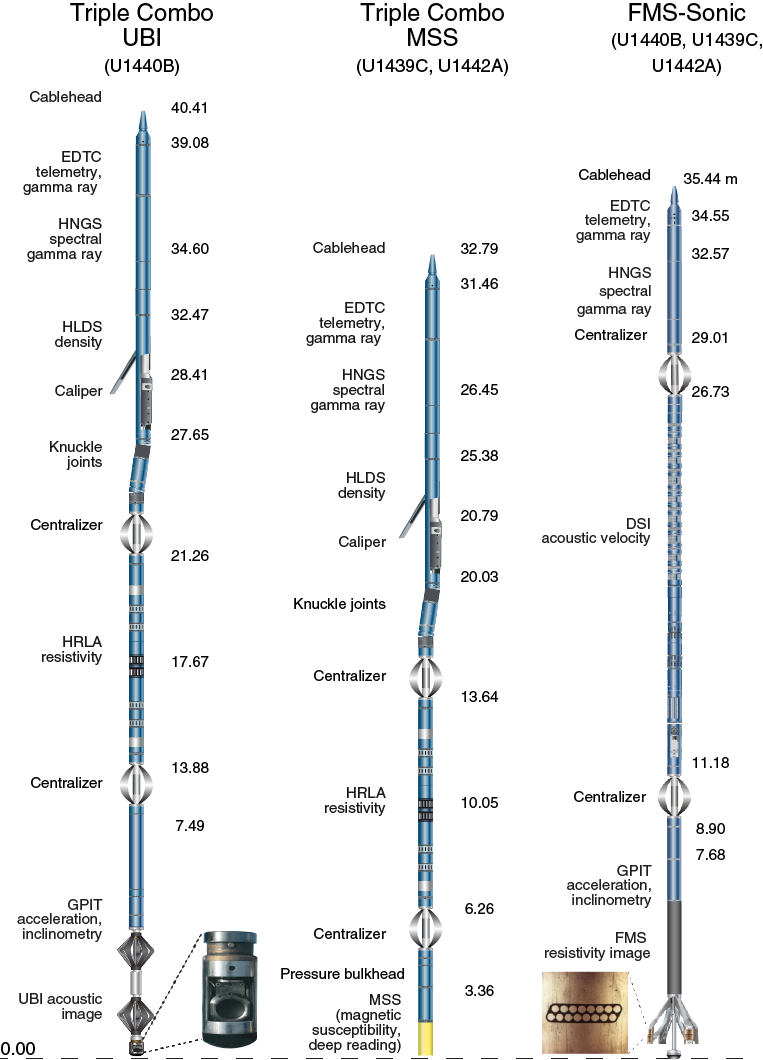
Each of these tool strings also contained a telemetry cartridge that facilitated communication between the tools and the Schlumberger data acquisition system (MAXIS unit) on the surface through the wireline cable.

In preparation for logging operations, a wiper trip was undertaken in each borehole to remove debris from the hole and optimize the hole conditions. At Site U1440, the bit was changed to a logging bit before tool string deployment, whereas at Site U1439, a mechanical bit release (MBR) was used to drop the tricone bit in the hole ahead of logging. The drill string was then pulled inside the casing and the tool strings were deployed through the drill string on a 7-conductor wireline cable in sequential runs. At Site U1442, an MBR was used to drop the rotary coring bit in the hole ahead of logging operations. Owing to the absence of a full reentry system at this site (free-fall funnel only), the drill pipe was raised to ~96.5 mbsf (~15 m below the sediment/basement interface), and the logging tools were deployed through the drill string. At all sites the tool strings were each pulled up at a constant speed, typically 120–550 m/h, to provide a continuous set of measurements in each logging run. To minimize the effect of the ship’s heave on the position of the tool string in the borehole, a wireline heave compensator (WHC) was employed as required (see below). During each logging run, real-time incoming data were recorded and monitored on the MCM MAXIS logging computer.

Logged formation properties and tool measurement principles

The properties of the formations logged and the methods by which they were measured are described below. The main logs recorded during Expedition 352 are listed in Table T12. Further information regarding individual tools and their applications is widely available (including Ellis and Singer, 2007; Goldberg, 1997; Lovell et al., 1998; Rider and Kennedy, 1996; Schlumberger, 1989; and Serra, 1984, 1986, 1989). In addition, a complete list of acronyms for Schlumberger tools and logs is available at www.glossary.oilfield.slb.com.

Natural gamma radiation

Total and spectral gamma ray measurements were acquired using a Hostile Environment Natural Gamma Ray Sonde (HNGS). This tool utilizes two bismuth germanate (BGO) scintillation detectors and five-window spectroscopy to determine concentrations of ⁴⁰K, ²³²Th, and ²³⁸U in the formation. Sensitivity to any additives in the drilling fluid (notably bentonite and KCl) is eliminated because the HNGS filters out gamma ray energies <500 keV, thus improving measurement accuracy. The inclusion of HNGS in all tool strings allows the use of gamma ray data for depth correlation between consecutive tool string runs and individual tool string passes.

Density

The Hostile Environment Litho-Density Sonde (HLDS) measures formation density utilizing a cesium (¹³⁷Cs) gamma ray source and far and near gamma ray detectors mounted on a shielded skid. This skid is pressed against the borehole wall using a hydraulically activated eccentering arm. The gamma particles emitted from the source are attenuated through the process of Compton scattering, which involves a partial energy loss resulting from elastic collision with electrons in the formation. The quantity of gamma radiation that reaches the detectors is directly related to the density of electrons in the formation, which in turn is related to the bulk density. Good tool/borehole contact is essential for good HLDS measurements, whereas poor contact results in an underestimation of formation density values.

Photoelectric effect

The HLDS also measures photoelectric absorption as the photoelectric effect (PEF). After repeated Compton scattering, as a result of collision with formation electrons, gamma radiation reaches a low enough energy (<150 keV) that it is photoelectrically absorbed. PEF is dependent on the atomic number of the elements in the formation and therefore varies according to the mineral makeup of the lithologies encountered. As such, PEF can be used to identify the presence of some minerals (Bartetzko et al., 2003).

Electrical resistivity

Six resistivity measurements with different depths of investigation (including one borehole fluid measurement and five formation measurements) were acquired with the High-Resolution Laterolog Array (HRLA). The array provides direct resistivity measurements by emitting a focused current into the formation and measuring the intensity necessary to maintain a constant drop in voltage across a fixed interval. The HRLA has one central (source) electrode and six electrodes above and below it, which alternate as transmitting and receiving current electrodes. Simultaneous resistivity measurement at six penetration depths is possible because of the rapid alternation in roles of these electrodes.

Typically, sulfide and oxide minerals, as well as ionic solutions like pore fluid, are conductors, whereas igneous minerals found in crustal rocks are electrical insulators. As a result, electrical conduction in most rocks will occur primarily by ion transport through pore fluids, and thus the resistivity measurement is largely dependent on porosity.

Porosity

A porosity measurement can be derived from the HLDS density measurement using average grain density and fluid density. Equally, a porosity measurement can be derived from the resistivity measurement using Archie’s law.

Acoustic images

Acoustic images of the borehole wall were generated from measurements taken by the UBI. The UBI features a high-resolution transducer, which emits ultrasonic pulses at a frequency of 250 kHz that are reflected by the borehole surface and then received by the same transducer recording the amplitude and traveltime of the reflected signal. Continuous rotation of the transducer combined with the upward motion of the tool result in a 360° image of the borehole wall. The amplitude of the signal depends on the reflection coefficient of the borehole fluid/borehole wall interface, the position of the UBI tool in the borehole, the shape of the borehole, and the roughness of the borehole wall. Modulation of the reflected signal is dependent on the borehole wall roughness. Therefore, fractures or other changes in the character of the drilled formation (e.g., grain size and texture) can be recognized in the amplitude image. The recorded traveltime image gives detailed information about the cross-sectional shape of the borehole, which allows calculation of 1 caliper value (radius) of the borehole from each traveltime measurement. These amplitude and traveltime measurements are recorded in combination with an azimuthal measurement (from the General Purpose Inclinometry Tool [GPIT]), permitting the orientation of these images. The full coverage of UBI measurements make the images a useful tool for core orientation and for stress analysis (Paillet and Kim, 1987).

Magnetic susceptibility

The MSS-B is a downhole logging tool designed by LDEO that measures the degree of magnetization of a material in response to an applied magnetic field. The ease with which a formation is magnetized is ultimately related to the concentration and composition (size, shape, and mineralogy) of the magnetizable material it contains. This measurement is extremely useful in investigating changes in mineralogy and lithology in a borehole because the measurement is not only quick, repeatable, and nondestructive, but also because different lithologies can have strongly contrasting magnetic susceptibilities.

The sensor used during Expedition 352 was the deep-reading cartridge of the MSS-B, deployed as part of the triple combo tool string by using a specially developed data transition module (EFTB Lamont Interface Cartridge). The deep-reading cartridge has a three-coil sensor that provides measurements with a vertical resolution of ~40 cm. For quality control and environmental correction, the MSS-B also measures internal tool temperature, z-axis acceleration, and low-resolution borehole conductivity.

Acoustic velocity

The Dipole Sonic Imager (DSI) measures the transit time of acoustic pulses between sonic transmitters and an array of 8 receivers. The resulting waveforms are used to calculate the sonic velocity of the formation. High-frequency (5–15 kHz) pulses emitted by the omnidirectional monopole transmitter are used to extract the compressional velocity (V_P) of the formation. It is possible to extract the shear wave velocity (V_S) from these data in the event that it is faster than the acoustic velocity in the borehole fluid. The monopole transmitter can also be fired in sequence at a lower frequency (0.5–1.0 kHz) to generate Stoneley waves, which are sensitive to fractures and variations in formation permeability. The DSI has two cross-dipole transmitters, which can facilitate the acquisition of shear wave velocity data in “slow” formations, where the formation V_S is less than that of the borehole fluid. In fast formations, such as the basement penetrated during Expedition 352, V_S measurements from the monopole waveforms are possible and have sharper arrivals and more accurate V_S estimates than the equivalent cross-dipole data. However, the cross-dipole-derived shear velocities can be useful in identifying any sonic anisotropy associated with the local stress regime.

Microresistivity images

High-resolution electrical resistivity images of the borehole walls were provided by the FMS. The tool has four orthogonal arms and pads, each with 16 button electrodes that are pressed against the borehole wall during recording. The electrodes are arranged in two diagonally offset rows with eight electrodes in each row. A focused current is emitted from these electrodes into the formation, with a return electrode near the top of the tool. Formation resistivity is derived from the intensity of the current passing through the button electrodes. Processing of these data, in combination with azimuthal data from the GPIT, transforms the measurements into oriented, high-resolution images that can reveal the geologic features exposed in the borehole wall. Features such as vesicles, veins, fractures, and volcaniclastic breccia can be resolved, and fabric analysis can be undertaken, in addition to quantitative analyzes of structural and stratigraphic features.

The FMS microresistivity images do not provide full coverage of the borehole wall with a single pass (~37% coverage in an 8.5 inch hole). To increase this coverage, it is standard practice to undertake two passes of the borehole in the hope that the tool will be oriented differently on the second pass.

Accelerometry and magnetic field measurement

The GPIT makes three-component acceleration and magnetic field measurements. The primary purpose of this tool is to determine the acceleration and orientation of the tool string in which it is deployed. The resulting data can be used to facilitate corrections for irregular tool motion and to provide oriented image data from the FMS and UBI tools. GPIT data are also used to provide real-time evaluation of the WHC (see Wireline heave compensator).

Log data quality

The condition of a borehole is the principal factor contributing to log data quality. The ideal conditions for logging include a consistent borehole diameter of the size of the bit, with no washouts or bridges. Oversized borehole diameters can have a significant impact on measurements, especially those that require tool eccentering (e.g., HLDS) or tool centralization (e.g., FMS and UBI). The measurement principles of the eccentered tools, as well as the centralized FMS, means that direct contact with the formation is essential for acquisition of high-quality data sets. The UBI is a noncontact measurement, but data quality is best when the tool is actively centered in the borehole. Beyond certain diameters, it is not possible to centralize/eccentralize these tools (Table T13). Certain measurements (notably, resistivity [HRLA] and acoustic velocity [DSI]) taken during Expedition 352 read deeper into the logged formations. These measurements are consequently less affected by borehole conditions, although data are optimized in boreholes where the tools can be centralized (up to ~20 inch diameter).

If the borehole diameter changes over short intervals as a consequence of washouts or ledges, logging results may be irregular. The quality of the borehole can be improved by minimizing the circulation of drilling fluid, flushing the borehole to remove debris prior to logging, performing a full wiper trip, and starting logging as soon after drilling and hole-conditioning as possible.

The length of wireline cable payed out is used to determine the depth of the logging measurements. The quality of this logging depth determination is dependent on a number of factors, including the ship’s heave, cable stretch, cable slip, and tidal changes. To minimize the effect of ship’s heave on logging depth, a hydraulic WHC is used to adjust the wireline length for rig motion during logging operations (see Wireline heave compensator). An important reference datum in wireline logging is the seafloor/mudline, which is determined from the gamma ray logs acquired in each logging run. Discrepancies between the drilling core depth and the wireline logging depth occur because of core expansion, incomplete core recovery, incomplete heave compensation, and drill pipe stretch. Reconciling the differences between the two data sets is possible through comparison of the common data sets acquired in situ and on core (e.g., magnetic susceptibility and natural gamma radiation).

Wireline heave compensator

The WHC, first used during Integrated Ocean Drilling Program Expedition 320T in 2009, is designed to compensate for the ship’s vertical motion to help maintain the steady movement of the logging tools in the borehole (Iturrino et al., 2013). Vertical acceleration measurements, made by the motion reference unit (MRU; located under the rig floor near the ship’s center of gravity), are used to calculate the vertical motion of the ship. The WHC then adjusts the length of the wireline by varying the distance between two sets of pulleys through which the cable passes. Simultaneous real-time measurements of surface and downhole acceleration are made by the MRU and by the Enhanced Digital Telemetry Cartridge/GPIT tool (see Accelerometry and magnetic field measurement), respectively. These data are then analyzed and compared in real time by a software package developed by LDEO. The actual motion of the tool string is displayed, thus enabling evaluation of the compensator’s efficiency.

The WHC was not used during logging operations at Site U1440 due to a very calm sea state (<1 m peak-to-peak heave). Sea conditions during logging at Site U1439 were more challenging because of Tropical Storm Fengshen, with a peak-to-peak heave of ~4 m. The WHC was therefore used and was very effective through the first tool string deployment, though was operating at its limits during the second deployment because of deteriorating weather conditions as logging progressed. At Site U1442, sea conditions were favorable for logging (<1 m peak-to-peak heave), though the forecast was for this to increase over the logging operations timeframe. On that basis, the WHC was used during logging at Site U1442.

Logging data flow and depth scales

Downhole data for each logging run were monitored in real time and recorded by the Schlumberger MAXIS 500 system. Initially, the logging data were referenced to the rig floor. After completion of logging operations, the data were shifted to a seafloor reference using the step in gamma ray data (acquired in all logging runs) at the sediment/water interface.

Downhole logging data were also transferred onshore to LDEO for standardized data processing. Processing primarily involves depth matching to provide consistency in the depth scale between the different logging runs. Similar to the depth shift to the seafloor datum, this depth matching was undertaken primarily by utilizing the gamma ray data. In addition, corrections were made to certain tools and logs (e.g., speed and voltage corrections to microresistivity images), documentation for the logs (including an assessment of log data quality) was prepared, and the data were converted to ASCII for the conventional logs and GIF for the images. The data were transferred back to the ship within a few days of logging and were made available (in ASCII and DLIS formats) through the shipboard IODP logging database. Schlumberger Geo-Quest’s GeoFrame software package was used for most of the processing.

References

Acton, G.D., Okada, M., Clement, B.M., Lund, S.P., and Williams, T., 2002. Paleomagnetic overprints in ocean sediment cores and their relationship to shear deformation caused by piston coring. Journal of Geophysical Research: Solid Earth, 107(B4):2067–2081. http://dx.doi.org/10.1029/2001JB000518

Bartetzko, A., Paulick, H., Iturrino, G., and Arnold, J., 2003. Facies reconstruction of a hydrothermally altered dacite extrusive sequence: evidence from geophysical downhole logging data (ODP Leg 193). Geochemistry, Geophysics, Geosystems, 4(10):1087. http://dx.doi.org/10.1029/2003GC000575

Bartington Instruments, Ltd., 2011. Operation Manual for MS2 Magnetic Susceptibility System: Oxford, UK (Bartington Instruments, Ltd.). http://www.bartington.com/Literaturepdf/Operation%20Manuals/om0408%20MS2.pdf

Blenkinsop, T.G., and Doyle, M.G., 2010. A method for measuring the orientations of planar structures in cut core. Journal of Structural Geology, 32(6):741–745. http://dx.doi.org/10.1016/j.jsg.2010.04.011

Blum, P., 1997. Technical Note 26: Physical Properties Handbook: A Guide to the Shipboard Measurement of Physical Properties of Deep-Sea Cores. Ocean Drilling Program. http://dx.doi.org/10.2973/odp.tn.26.1997

Bullard, E.C., 1939. Heat flow in South Africa. Proceedings of the Royal Society of London, Series A, 173(955):474–502. http://dx.doi.org/10.1098/rspa.1939.0159

Cande, S.C., and Kent, D.V., 1995. Revised calibration of the geomagnetic polarity timescale for the Late Cretaceous and Cenozoic. Journal of Geophysical Research: Solid Earth, 100(B4):6093–6095. http://dx.doi.org/10.1029/94JB03098

Droser, M.L., and Bottjer, D.J., 1986. A semiquantitative field classification of ichnofabric. Journal of Sedimentary Research, 56(4):558–559. http://dx.doi.org/10.1306/212F89C2-2B24-11D7-8648000102C1865D

Droser, M.L., and Bottjer, D.J., 1991. Trace fossils and ichnofabric in Leg 119 cores. In Barron, J., Larsen, B., et al., Proceedings of the Ocean Drilling Program, Scientific Results, 119: College Station, TX (Ocean Drilling Program), 635–641. http://dx.doi.org/10.2973/odp.proc.sr.119.206.1991

Dunlop, D.J., 2003. Stepwise and continuous low-temperature demagnetization. Geophysical Research Letters, 30(11):1582. http://dx.doi.org/10.1029/2003GL017268

Ellis, D.V., and Singer, J.M., 2007. Well Logging for Earth Scientists (2nd ed.): New York (Elsevier).

Expedition 330 Scientists, 2012. Methods. In Koppers, A.A.P., Yamazaki, T., Geldmacher, J., and the Expedition 330 Scientists, Proceedings of the Integrated Ocean Drilling Program, 330: Tokyo (Integrated Ocean Drilling Program Management International, Inc.). http://dx.doi.org/10.2204/iodp.proc.330.102.2012

Expedition 334 Scientists, 2012. Methods. In Vannucchi, P., Ujiie, K., Stroncik, N., Malinverno, A., and the Expedition 334 Scientists, Proceedings of the Integrated Ocean Driling Program, 334: Tokyo (Integrated Ocean Drilling Program Management International, Inc.). http://dx.doi.org/10.2204/iodp.proc.334.102.2012

Expedition 335 Scientists, 2012. Methods. In Teagle, D.A.H., Ildefonse, B., Blum, P., and the Expedition 335 Scientists. Proceedings of the Integrated Ocean Drilling Program, 335: Tokyo (Integrated Ocean Drilling Program Management International, Inc.). http://dx.doi.org/10.2204/iodp.proc.335.104.2012

Fisher, R.V., and Schmincke, H.-U., 1984. Pyroclastic Rocks: Berlin (Springer-Verlag). http://dx.doi.org/10.1007/978-3-642-74864-6

Fuller, M., Hastedt, M., and Herr, B., 1998. Coring-induced magnetization of recovered sediment. In Weaver, P.P.E., Schmincke, H.-U., Firth, J.V., and Duffield, W. (Eds.), Proceedings of the Ocean Drilling Program, Scientific Results, 157: College Station, TX (Ocean Drilling Program), 47–56. http://dx.doi.org/10.2973/odp.proc.sr.157.103.1998

Gieskes, J.M., Gamo, T., and Brumsack, H., 1991. Chemical methods for interstitial water analysis aboard JOIDES Resolution. Ocean Drilling Program Technical Note, 15. http://dx.doi.org/10.2973/odp.tn.15.1991

Gillis, K.M., Snow, J.E., Klaus, A., and the Expedition 345 Scientists, 2014. Proceedings of the Integrated Ocean Drilling Program, 345: College Station, TX (International Ocean Discovery Program). http://dx.doi.org/10.2204/iodp.proc.345.2014

Gillis, K.M., Snow, J.E., Klaus, A., Guerin, G., Abe, N., Akizawa, N., Ceuleneer, G., Cheadle, M.J., Adrião, Á., Faak, K., Falloon, T.J., Friedman, S.A., Godard, M.M., Harigane, Y., Horst, A.J., Hoshide, T., Ildefonse, B., Jean, M.M., John, B.E., Koepke, J.H., Machi, S., Maeda, J., Marks, N.E., McCaig, A.M., Meyer, R., Morris, A., Nozaka, T., Python, M., Saha, A., and Wintsch, R.P., 2014. Methods. In Gillis, K.M., Snow, J.E., Klaus, A., and the Expedition 345 Scientists, Proceedings of the Integrated Ocean Drilling Program, 345: College Station, TX (Integrated Ocean Drilling Program). http://dx.doi.org/10.2204/iodp.proc.345.102.2014

Godard, M., Awaji, S., Hansen, H., Hellebrand, E., Brunelli, D., Johnson, K., Yamasaki, T., Maeda, J., Abratis, M., Christie, D., Kato, Y., Mariet, C., and Rosner, M., 2009. Geochemistry of a long in-situ section of intrusive slow-spread oceanic lithosphere: results from IODP Site U1309 (Atlantis Massif, 30°N Mid-Atlantic-Ridge). Earth and Planetary Science Letters, 279(1–2):110–122. http://dx.doi.org/10.1016/j.epsl.2008.12.034

Goldberg, D., 1997. The role of downhole measurements in marine geology and geophysics. Reviews of Geophysics, 35(3):315–342. http://dx.doi.org/10.1029/97RG00221

Govindaraju, K., 1994. 1994 compilation of working values and sample description for 383 geostandards. Geostandards Newsletter, 18(1). http://dx.doi.org/10.1111/j.1751-908X.1994.tb00502.x

Gradstein, F.M., Ogg, J.G., Schmitz, M.D., and Ogg, G.M. (Eds.), 2012. The Geological Time Scale 2012: Amsterdam (Elsevier).

Harris, R.N., Sakaguchi, A., Petronotis, K., Baxter, A.T., Berg, R., Burkett, A., Charpentier, D., Choi, J., Diz Ferreiro, P., Hamahashi, M., Hashimoto, Y., Heydolph, K., Jovane, L., Kastner, M., Kurz, W., Kutterolf, S.O., Li, Y., Malinverno, A., Martin, K.M., Millan, C., Nascimento, D.B., Saito, S., Sandoval Gutierrez, M.I., Screaton, E.J., Smith-Duque, C.E., Solomon, E.A., Straub, S.M., Tanikawa, W., Torres, M.E., Uchimura, H., Vannucchi, P., Yamamoto, Y., Yan, Q., and Zhao, X., 2013. Methods. In Harris, R.N., Sakaguchi, A., Petronotis, K., and the Expedition 344 Scientists, Proceedings of the Integrated Ocean Drilling Program, 344: College Station, TX (Integrated Ocean Drilling Program). http://dx.doi.org/10.2204/iodp.proc.344.102.2013

Harris, R.N., Sakaguchi, A., Petronotis, K., and the Expedition 344 Scientists, 2013. Proceedings of the Integrated Ocean Drilling Program, 344: College Station, TX (Integrated Ocean Drilling Program). http://dx.doi.org/10.2204/iodp.proc.344.2013

Heard, T.G., and Pickering, K.T., 2008. Trace fossils as diagnostic indicators of deep-marine environments, middle Eocene Ainsa-Jaca Basin, Spanish Pyrenees. Sedimentology, 55(4):809–844. http://dx.doi.org/10.1111/j.1365-3091.2007.00922.x

Hyndman, R.D., Erickson, A.J., and Von Herzen, R.P., 1974. Geothermal measurements on DSDP Leg 26. In Davies, T.A., Luyendyk, B.P., et al., Initial Reports of the Deep Sea Drilling Project, 26: Washington, DC (U.S. Government Printing Office), 451–463. http://dx.doi.org/10.2973/dsdp.proc.26.113.1974

Ingram, R.L., 1954. Terminology for the thickness of stratification and parting units in sedimentary rocks. Geological Society of America Bulletin, 65(9):937–938. http://dx.doi.org/10.1130/0016-7606(1954)65[937:TFTTOS]2.0.CO;2

Iturrino, G., Liu, T., Goldberg, D., Anderson, L., Evans, H., Fehr, A., Guerin, G., Inwood, J., Lofi, J., Malinverno, A., Morgan, S., Mrozewski, S., Slagle, A., and Williams, T., 2013. Performance of the wireline heave compensation system onboard D/V JOIDES Resolution. Scientific Drilling, 15:46–50. http://dx.doi.org/10.2204/iodp.sd.15.08.2013

Jochum, K.P., Nohl, U., Herwig, K., Lammel, E., Stoll, B., and Hofmann, A.W., 2005. GeoRem: a new geochemical database for reference materials and isotopic standards. Geostandards and Geoanalytical Research, 29(3):333–338. http://dx.doi.org/10.1111/j.1751-908X.2005.tb00904.x

Jutzeler, M., White, J.D.L., Talling, P.J., McCanta, M., Morgan, S., Le Friant, A., and Ishizuka, O., 2014. Coring disturbances in IODP piston cores with implications for offshore record of volcanic events and the Missoula megafloods. Geochemistry, Geophysics, Geosystems, 15(9):3572–3590. http://dx.doi.org/10.1002/2014GC005447

Kanayama, K., Kitamura, K., and Umino, S., 2013. New geochemical classification of global boninites. IAVCEI 2013 Scientific Assembly Abstracts. (Poster 4W_1B-P13)

Kirschvink, J.L., 1980. The least-squares line and plane and the analysis of palaeomagnetic data. Geophysical Journal of the Royal Astronomical Society, 62(3):699–718. http://dx.doi.org/10.1111/j.1365-246X.1980.tb02601.x

Koppers, A.A.P., Yamazaki, T., Geldmacher, J., and the Expedition 330 Scientists, 2012. Proceedings of the Integrated Ocean Drilling Program, 330: Tokyo (Integrated Ocean Drilling Program Management International, Inc.). http://dx.doi.org/10.2204/iodp.proc.330.2012

Kvenvolden, K.A., and McDonald, T.J., 1986. Organic geochemistry on the JOIDES Resolution—an assay. Ocean Drilling Program Technical Note, 6: College Station, TX (Ocean Drilling Program). http://dx.doi.org/10.2973/odp.tn.6.1986

Le Bas, M.J., 2000. IUGS reclassification of the high-Mg and picritic volcanic rocks. Journal of Petrology, 41(10):1467–1470. http://dx.doi.org/10.1093/petrology/41.10.1467

Lide, D.R. (Ed.), 2000. Handbook of Chemistry and Physics (81st ed.): Boca Raton, Florida (Chemical Rubber Publishing Company).

Lovell, M.A., Harvey, P.K., Brewer, T.S., Williams, C., Jackson, P.D., and Williamson, G., 1998. Application of FMS images in the Ocean Drilling Program: an overview. In Cramp, A., MacLeod, C.J., Lee, S.V., and Jones, E.J.W. (Eds.), Geological Evolution of Ocean Basins: Results from the Ocean Drilling Program. Geological Society Special Publication, 131(1):287–303. http://dx.doi.org/10.1144/GSL.SP.1998.131.01.18

Manheim, F.T., and Sayles, F.L., 1974. Composition and origin of interstitial waters of marine sediments, based on deep sea drill cores. In Goldberg, E.D. (Ed.), The Sea (Volume 5): Marine Chemistry: The Sedimentary Cycle: New York (Wiley), 527–568.

Martini, E., 1971. Standard Tertiary and Quaternary calcareous nannoplankton zonation. In Farinacci, A. (Ed.), Proceedings of the Second Planktonic Conference, Roma 1970: Rome (Edizioni Tecnoscienza), 2:739–785.

Merrill, R.T., 1970. Low-temperature treatments of magnetite and magnetite-bearing rocks. Journal of Geophysical Research: Solid Earth, 75(17):3343–3349. http://dx.doi.org/10.1029/JB075i017p03343

Munsell Color Company, Inc., 2000. Munsell Soil Color Chart: New York (Gretag-Macbeth).

Murray, R.W., Miller, D.J., and Kryc, K.A., 2000. Technical Note, 29: Analysis of Major and Trace Elements in Rocks, Sediments, and Interstitial Waters by Inductively Coupled Plasma–Atomic Emission Spectrometry (ICP-AES). Ocean Drilling Program. http://dx.doi.org/10.2973/odp.tn.29.2000

Okada, H., and Bukry, D., 1980. Supplementary modification and introduction of code numbers to the low-latitude coccolith biostratigraphic zonation (Bukry, 1973; 1975). Marine Micropaleontology, 5:321–325. http://dx.doi.org/10.1016/0377-8398(80)90016-X

Paillet, F.L., and Kim, K., 1987. Character and distribution of borehole breakouts and their relationship to in situ stresses in deep Columbia River basalts. Journal of Geophysical Research: Solid Earth, 92(B7):6223–6234. http://dx.doi.org/10.1029/JB092iB07p06223

Parker, R.L., and Gee, J.S., 2002. Calibration of the pass-through magnetometer—II. Application. Geophysical Journal International, 150:140–152. http://dx.doi.org/10.1046/j.1365-246X.2002.01692.x

Pearce, J.A., and Robinson, P.T., 2010. The Troodos ophiolitic complex probably formed in a subduction initiation, slab edge setting. Gondwana Research, 18(1):60–81. http://dx.doi.org/10.1016/j.gr.2009.12.003

Perch-Nielsen, K., 1985. Cenozoic calcareous nannofossils. In Bolli, H.M., Saunders, J.B., and Perch-Nielsen, K. (Eds.), Plankton Stratigraphy: Cambridge, UK (Cambridge University Press), 427–554.

Pimmel, A., and Claypool, G., 2001. Technical Note, 30: Introduction to shipboard organic geochemistry on the JOIDES Resolution. Ocean Drilling Program. http://dx.doi.org/10.2973/odp.tn.30.2001

Puchelt, H., Malpas, J., Falloon, T., Pedersen, R., Eckhardt, J.-D., and Allan, J.F., 1996. Data report: ultramafic reference material from Core 147-895D-10W. In Mével, C., Gillis, K.M., Allan, J.F., and Meyer, P.S. (Eds.), Proceedings of the Ocean Drilling Program, Scientific Results, 147: College Station, TX (Ocean Drilling Program), 493–496. http://dx.doi.org/10.2973/odp.proc.sr.147.033.1996

Reagan, M.K., Ishizuka, O., Stern, R.J., Kelley, K.A., Ohara, Y., Blichert-Toft, J., Bloomer, S.H., Cash, J., Fryer, P., Hanan, B.B., Hickey-Vargas, R., Ishii, T., Kimura, J.-I., Peate, D.W., Rowe, M.C., and Woods, M., 2010. Fore-arc basalts and subduction initiation in the Izu-Bonin-Mariana system. Geochemistry, Geophysics, Geosystems, 11(3):Q03X12. http://dx.doi.org/10.1029/2009GC002871

Reagan, M.K., Pearce, J.A., Petronotis, K., Almeev, R., Avery, A.A., Carvallo, C., Chapman, T., Christeson, G.L., Ferré, E.C., Godard, M., Heaton, D.E., Kirchenbaur, M., Kurz, W., Kutterolf, S., Li, H.Y., Li, Y., Michibayashi, K., Morgan, S., Nelson, W.R., Prytulak, J., Python, M., Robertson, A.H.F., Ryan, J.G., Sager, W.W., Sakuyama, T., Shervais, J.W., Shimizu, K., and Whattam, S.A., 2015a. Site U1439. In Reagan, M.K., Pearce, J.A., Petronotis, K., and the Expedition 352 Scientists, Izu-Bonin-Mariana Fore Arc. Proceedings of the International Ocean Discovery Program, 352: College Station, TX (International Ocean Discovery Program). http://dx.doi.org/10.14379/iodp.proc.352.103.2015

Reagan, M.K., Pearce, J.A., Petronotis, K., Almeev, R., Avery, A.A., Carvallo, C., Chapman, T., Christeson, G.L., Ferré, E.C., Godard, M., Heaton, D.E., Kirchenbaur, M., Kurz, W., Kutterolf, S., Li, H.Y., Li, Y., Michibayashi, K., Morgan, S., Nelson, W.R., Prytulak, J., Python, M., Robertson, A.H.F., Ryan, J.G., Sager, W.W., Sakuyama, T., Shervais, J.W., Shimizu, K., and Whattam, S.A., 2015b. Site U1440. In Reagan, M.K., Pearce, J.A., Petronotis, K., and the Expedition 352 Scientists, Izu-Bonin-Mariana Fore Arc. Proceedings of the International Ocean Discovery Program, 352: College Station, TX (International Ocean Discovery Program). http://dx.doi.org/10.14379/iodp.proc.352.104.2015

Reagan, M.K., Pearce, J.A., Petronotis, K., Almeev, R., Avery, A.A., Carvallo, C., Chapman, T., Christeson, G.L., Ferré, E.C., Godard, M., Heaton, D.E., Kirchenbaur, M., Kurz, W., Kutterolf, S., Li, H.Y., Li, Y., Michibayashi, K., Morgan, S., Nelson, W.R., Prytulak, J., Python, M., Robertson, A.H.F., Ryan, J.G., Sager, W.W., Sakuyama, T., Shervais, J.W., Shimizu, K., and Whattam, S.A., 2015c. Site U1441. In Reagan, M.K., Pearce, J.A., Petronotis, K., and the Expedition 352 Scientists, Izu-Bonin-Mariana Fore Arc. Proceedings of the International Ocean Discovery Program, 352: College Station, TX (International Ocean Discovery Program). http://dx.doi.org/10.14379/iodp.proc.352.105.2015

Reagan, M.K., Pearce, J.A., Petronotis, K., Almeev, R., Avery, A.A., Carvallo, C., Chapman, T., Christeson, G.L., Ferré, E.C., Godard, M., Heaton, D.E., Kirchenbaur, M., Kurz, W., Kutterolf, S., Li, H.Y., Li, Y., Michibayashi, K., Morgan, S., Nelson, W.R., Prytulak, J., Python, M., Robertson, A.H.F., Ryan, J.G., Sager, W.W., Sakuyama, T., Shervais, J.W., Shimizu, K., and Whattam, S.A., 2015d. Site U1442. In Reagan, M.K., Pearce, J.A., Petronotis, K., and the Expedition 352 Scientists, Izu-Bonin-Mariana Fore Arc. Proceedings of the International Ocean Discovery Program, 352: College Station, TX (International Ocean Discovery Program). http://dx.doi.org/10.14379/iodp.proc.352.106.2015

Révillon, S., Barr, S.R., Brewer, T.S., Harvey, P.K., and Tarney, J., 2002. An alternative approach using integrated gamma-ray and geochemical data to estimate the inputs to subduction zones from ODP Leg 185, Site 801. Geochemistry, Geophysics, Geosystems, 3(12):8902. http://dx.doi.org10.1029/2002GC000344

Rider, M.H., and Kennedy, M., 2011. The Geological Interpretation of Well Logs (3rd edition): Sutherland, United Kingdom (Rider-French Consulting Limited).

Roberts, A.P., Stoner, J.S., and Richter, C., 1996. Coring-induced magnetic overprints and limitations of the long-core paleomagnetic measurement technique: some observations from Leg 160, eastern Mediterranean Sea. In Emeis, K.-C., Robertson, A.H.F., Richter, C., et al., Proceedings of the Ocean Drilling Program, Initial Reports, 160: College Station, TX (Ocean Drilling Program), 497–505. http://dx.doi.org/10.2973/odp.proc.ir.160.115.1996

Rothwell, R.G., 1989. Minerals and Mineraloids in Marine Sediments: An Optical Identification Guide: London (Elsevier).

Salisbury, M.H., Shinohara, M., Suetsugu, D., Arisaka, M., Diekmann, B., Januszczak, N., and Savov, I.P., 2006. Leg 195 synthesis: Site 1201—a geological and geophysical section in the West Philippine Basin from the 660-km discontinuity to the mudline. In Shinohara, M., Salisbury, M.H., and Richter, C. (Eds.), Proceedings of the Ocean Drilling Program, Scientific Results, 195: College Station, TX (Ocean Drilling Program), 1–27. http://dx.doi.org/10.2973/odp.proc.sr.195.113.2006

Schlumberger, 1989. Log Interpretation Principles/Applications: Houston (Schlumberger Education Services), SMP–7017.

Serra, O., 1984. Fundamentals of Well-Log Interpretation (Vol. 1): The Acquisition of Logging Data: Amsterdam (Elsevier).

Serra, O., 1986. Fundamentals of Well-Log Interpretation (Vol. 2): The Interpretation of Logging Data. Amsterdam (Elsevier).

Serra, O., 1989. Formation MicroScanner Image Interpretation: Houston (Schlumberger Education Services), SMP-7028.

Shipboard Scientific Party, 2003. Explanatory notes. In Wilson, D.S., Teagle, D.A.H., Acton, G.D., et al., Proceedings of the Ocean Drilling Program, Initial Reports, 206: College Station, TX (Ocean Drilling Program), 1–94. http://dx.doi.org/10.2973/odp.proc.ir.206.102.2003

Tamura, Y., Busby, C.J., Blum, P., Guèrin, G., Andrews, G.D.M., Barker, A.K., Berger, J.L.R., Bongiolo, E.M., Bordiga, M., DeBari, S.M., Gill, J.B., Hamelin, C., Jia, J., John, E.H., Jonas, A.-S., Jutzeler, M., Kars, M.A.C., Kita, Z.A., Konrad, K., Mahoney, S.H., Martini, M., Miyazaki, T., Musgrave, R.J., Nascimento, D.B., Nichols, A.R.L., Ribeiro, J.M., Sato, T., Schindlbeck, J.C., Schmitt, A.K., Straub, S.M., Vautravers, M.J., and Yang, Y., 2015. Expedition 350 methods. In Tamura, Y., Busby, C.J., Blum, P., and the Expedition 350 Scientists, Izu-Bonin-Mariana Rear Arc. Proceedings of the International Ocean Discovery Program, 350: College Station, TX (International Ocean Discovery Program). http://dx.doi.org/10.14379/iodp.proc.350.102.2015

Teagle, D.A.H., Ildefonse, B., Blum, P., and the Expedition 335 Scientists, 2012. Proceedings of the Integrated Ocean Drilling Program, 335: Tokyo (Integrated Ocean Drilling Program Management International, Inc.). http://dx.doi.org/10.2204/iodp.proc.335.2012

Todd, E., Gill, J.B., and Pearce, J.A., 2012. A variably enriched mantle wedge and contrasting melt types during arc stages following subduction initiation in Fiji and Tonga, southwest Pacific. Earth and Planetary Science Letters, 335–336:180–194. http://dx.doi.org/10.1016/j.epsl.2012.05.006

van Sprang, H.A., 2000. Fundamental parameter methods in XRF spectroscopy. Advances in X-ray Analysis, 42:1–10. http://www.icdd.com/resources/axa/vol42/v42_01.pdf

Varol, O., 1998. Paleogene. In Bown, P.R. (Ed.), Calcareous Nannofossil Biostratigraphy: London (Kluwer Academic Publishing), 201–224.

Vasiliev, M.A., Blum, P., Chubarian, G., Olsen, R., Bennight, C., Cobine, T., Fackler, D., Hastedt, M., Houpt, D., Mateo, Z., and Vasilieva, Y.B., 2011. A new natural gamma radiation measurement system for marine sediment and rock analysis. Journal of Applied Geophysics, 75:455–463. http://dx.doi.org/10.1016/j.jappgeo.2011.08.008

Wentworth, C.K., 1922. A scale of grade and class terms for clastic sediments. Journal of Geology, 30(5):377–392. http://dx.doi.org/10.1086/622910

Young, J.R., 1998. Neogene. In Bown, P.R. (Ed.), Calcareous Nannofossil Biostratigraphy: Dordrecht, The Netherlands (Kluwer Academic Publishing), 225–265.

Yu, Y., Dunlop, D.J., and Özdemir, Ö., 2003. On the resolution of multivectorial remanences. Earth and Planetary Science Letters, 208(1–2):13–26. http://dx.doi.org/10.1016/S0012-821X(02)01149-4

---

¹Reagan, M.K., Pearce, J.A., Petronotis, K., Almeev, R., Avery, A.A., Carvallo, C., Chapman, T., Christeson, G.L., Ferré, E.C., Godard, M., Heaton, D.E., Kirchenbaur, M., Kurz, W., Kutterolf, S., Li, H.Y., Li, Y., Michibayashi, K., Morgan, S., Nelson, W.R., Prytulak, J., Python, M., Robertson, A.H.F., Ryan, J.G., Sager, W.W., Sakuyama, T., Shervais, J.W., Shimizu, K., and Whattam, S.A., 2015. Expedition 352 methods. In Reagan, M.K., Pearce, J.A., Petronotis, K., and the Expedition 352 Scientists, Izu-Bonin-Mariana Fore Arc. Proceedings of the International Ocean Discovery Program, 352: College Station, TX (International Ocean Discovery Program). http://dx.doi.org/10.14379/iodp.proc.352.102.2015

²Expedition 352 Scientists’ addresses.