Clemens, S.C., Kuhnt, W., LeVay, L.J., and the Expedition 353 Scientists
Proceedings of the International Ocean Discovery Program Volume 353
publications.iodp.org
doi:10.14379/iodp.proc.353.103.2016

Site U14431
S.C. Clemens, W. Kuhnt, L.J. LeVay, P. Anand, T. Ando, M. Bartol, C.T. Bolton, X. Ding, K. Gariboldi, L. Giosan, E.C. Hathorne, Y. Huang, P. Jaiswal, S. Kim, J.B. Kirkpatrick, K. Littler, G. Marino, P. Martinez, D. Naik, A. Peketi, S.C. Phillips, M.M. Robinson, O.E. Romero, N. Sagar, K.B. Taladay, S.N. Taylor, K. Thirumalai, G. Uramoto, Y. Usui, J. Wang, M. Yamamoto, and L. Zhou2
Keywords: International Ocean Discovery Program, IODP, Expedition 353, JOIDES Resolution, Site U1443, Indian monsoon, monsoon, paleoclimate, paleoceanography, Miocene, Pliocene, Pleistocene, Holocene, Cretaceous, Paleogene, Ninetyeast Ridge, Indian Ocean, salinity, orbital, abrupt climate change
MS 353-103: Published 29 July 2016
Background and objectives
Structure and paleogeographic history of the northern Ninetyeast Ridge
International Ocean Discovery Program (IODP) Site U1443 is located ~100 m southeast of Ocean Drilling Program (ODP) Leg 121 Site 758 on the crest of the Ninetyeast Ridge and is a redrill of Site 758 (Figure F1). The Ninetyeast Ridge represents the trace of the Kerguelen/Ninetyeast hotspot prior to middle Eocene rifting (Shipboard Scientific Party, 1989a). As a result of northward movement, Site U1443 moved from temperate southern latitudes during the Campanian, to ~5°S near the Oligocene/Miocene boundary, and to its present location of 5°N in the southernmost Bay of Bengal. The site has been within 10° of the Equator for the past 35 My (Shipboard Scientific Party, 1989a). The ridge-top location has prevented the deposition of sedimentary sequences typically associated with fan transport processes.
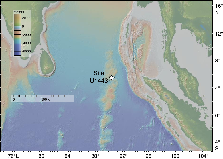
Figure F1. Location of Site U1443 on the northern Ninetyeast Ridge.
Site U1443 is situated on the southeast side of the easternmost tilted blocks that form the Ninetyeast Ridge north of the Equator. The proposed site location was picked at common midpoint (CMP) 4360 on Line ar55.0881.knox06rr of the seismic reflection survey carried out by the R/V Roger Revelle in 2007 (Shipboard Scientific Party, 2007) (Figure F2). Reflection seismics at this site exhibit a virtually identical seismic succession as at Site 758, and individual reflectors, which were dated at Site 758, can be easily compared (Figure F3).
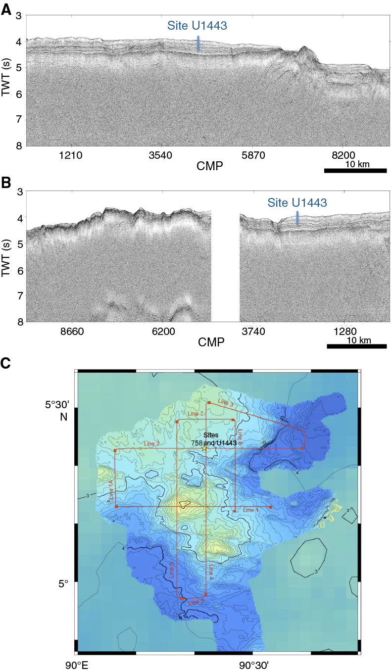
Figure F2. Seismic Lines ar55.0881.knox06rr and ar55.0885.knox06rr of the seismic reflection survey carried out by the Roger Revelle in 2007 with the position of Site U1443.
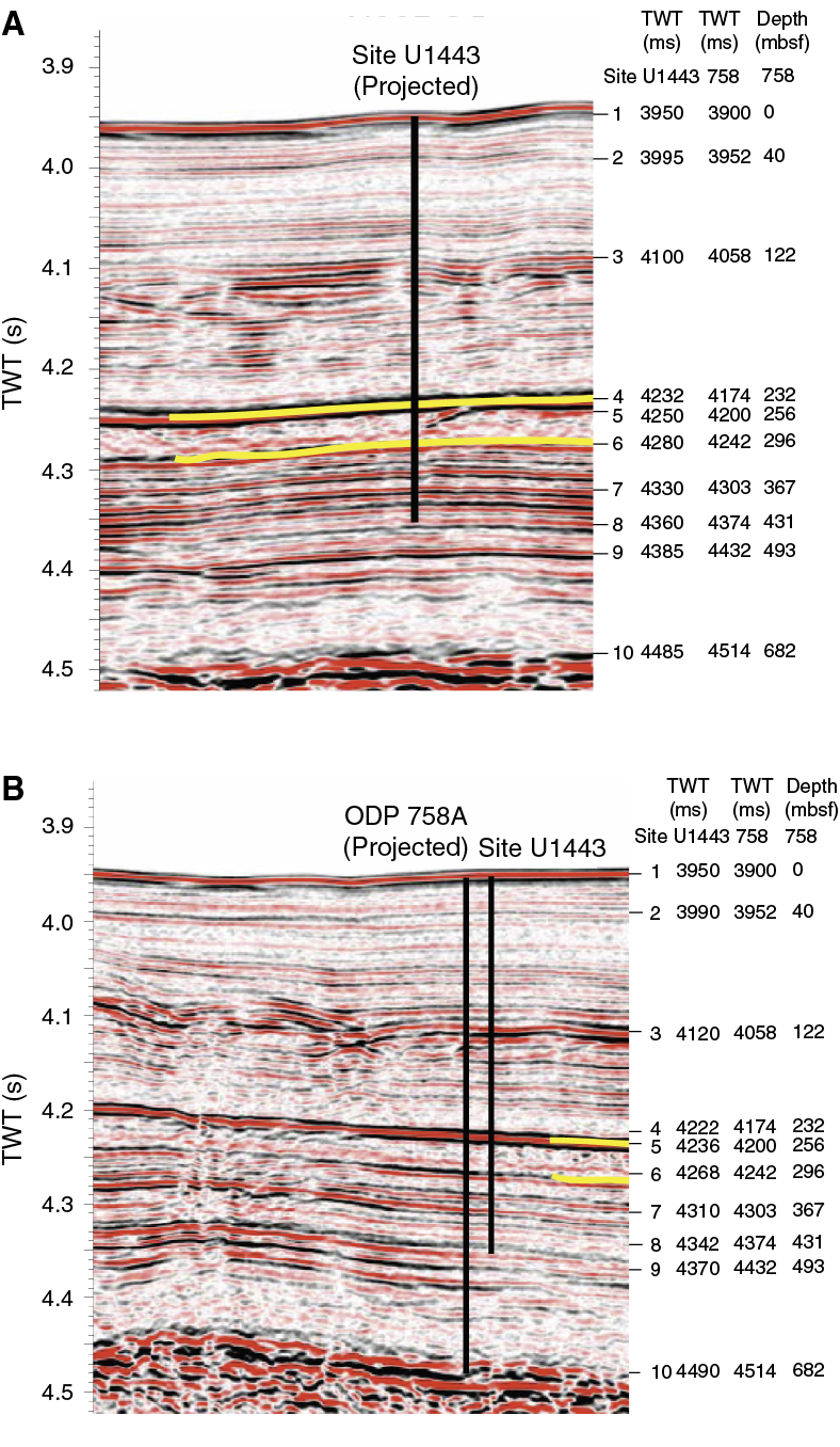
Figure F3. Position of Site U1443 on seismic Lines ar55.0881.knox06rr and ar55.0885.knox06rr with depth of reflectors at Sites U1443 and 758.
Neogene paleoclimatic records of the Indian monsoon
Previous drilling at this location included overlapping ODP holes (758A and 758B) over the top 92 m of the total 527 m of sediments drilled. This limited the resulting composite record to the past 7.3 My (Farrell and Janecek, 1991). In spite of these limitations, the IODP sample database shows that more than 16,000 sediment samples have been taken from Site 758 cores in the last ten years. Parts of the uppermost sections are almost entirely depleted, and sampling has moved to the archive half. Recent research using Site 758 sediments includes high-resolution (suborbital) Late Pleistocene reconstruction of changes in upper water column structure based on multispecies planktonic foraminifer records (Bolton et al., 2013), reconstruction of the Li isotope composition of seawater over the past 70 My (Misra and Froelich, 2012), Late Cretaceous to early Eocene reconstruction of seawater Nd (Le Houedec et al., 2012), and glacial–interglacial scale reconstruction of the Os isotopic composition of seawater (Burton et al., 2010).
One important paleoclimatic goal of Site U1443 was to recover sediment successions that would allow precise timing of onset and phases of intensification and weakening of the Indian monsoon system. In particular, the timing of the Miocene intensification of the Indian monsoon is still unresolved; suggestions for the initial intensification range between ~7–8, ~15, and ~22 Ma (Clift and Plumb, 2008; Clift et al., 2008), and indications of an active monsoon have been suggested for as early as ~45 Ma (Licht et al., 2014). One of the main setbacks in evaluating the southeast Asian monsoonal history on tectonic to orbital timescales is the lack of continuous high-resolution proxy records of either monsoonal upwelling (Kroon et al., 1991), changes in vegetation (Quade et al., 1989), continental runoff, or weathering indexes (Clift and Plumb, 2008) before ~12 Ma. Exceptions to date include ODP Sites 1146 and 1148 in the South China Sea and the fragmentary record of Site 758 in the southern Bay of Bengal. This location is specifically suited to record the long-term history of the Indian monsoon because it records the runoff from the Ganges-Brahmaputra and Irrawaddy Rivers, the largest river systems draining the Himalaya and the Tibetan Plateau in addition to local surface salinity and primary productivity changes in the southern Bay of Bengal. Drilling at Site 758 revealed that delivery of terrigenous material to the northern Ninetyeast Ridge increased at ~10 Ma with two subsequent pulses at ~7.0–5.6 and ~3.9–2.0 Ma, which were interpreted as increases in river runoff resulting from the uplift and erosion of the Himalaya (Hovan and Rea, 1992). The Nd isotope composition of the carbonate component of Bay of Bengal sediments has been used to investigate variations in the relative contribution of discharge from the Ganges-Brahmaputra, Irrawaddy, and Arkan Rivers (Burton and Vance, 2000; Stoll et al., 2007; Gourlan et al., 2008, 2010). These studies agree that input from the Ganges-Brahmaputra river complex decreased during glacial periods, probably as a result of a decrease in Indian monsoon strength or a shift in the location of the center of the monsoonal precipitation. Extension of these Nd isotope records into the Miocene indicates a complex relationship between global climate change, riverine discharge, and terrigenous input into the Bay of Bengal. However, the proxy records for river discharge are presently of insufficient time resolution to document the relation between global climate and the Indian monsoon throughout the Neogene. The complete Neogene sediment archive at Site U1443 will make such reconstructions possible.
Contribution of the Site U1443 record to the high-resolution stratigraphic framework of Indian Ocean deepwater sediments
The composite spliced section of advanced piston corer (APC) cores from Holes 758A and 758B provides a continuous undisturbed archive for the past 7.3 My (Farrell and Janecek, 1991). Radiogenic Sr isotopes measured on foraminifers from Site 758 were used to refine the global Pliocene Sr isotope stratigraphy (Clemens et al., 1993; Henderson et al., 1994; McArthur et al., 2006).
The stable isotope records from Site 758 are the only complete orbitally tuned Pliocene–Pleistocene records in the Indian Ocean (Hoogakker et al., 2006; Mudelsee and Raymo 2005) and the only tropical Indian Ocean record in the global benthic δ18O isotope stack (LR04-stack) of Lisiecki and Raymo (2005). The high-resolution stable isotope records for benthic foraminifers and the planktonic foraminifer Globigerinoides sacculifer back to 3.6 Ma demonstrate the potential of isotope records from the northern end of the Ninteyeast Ridge (Chen et al., 1995; Farrell and Janecek, 1991). The benthic foraminiferal isotope and assemblage records extending back to ~5.5 Ma have been used to infer strengthening of the Indian monsoon seasonality associated with the onset of the Northern Hemisphere glaciation (Gupta and Thomas 2003). However, because the complete spliced sediment archive at Site 758 ends at 7.3 Ma, it could not be used to verify the main period of monsoon intensification in the Arabian Sea around 8 Ma (Kroon et al., 1991; Gupta et al., 2004). The Site U1443 splice, which covers the entire Neogene, will close this gap.
Main objectives
Drilling of Site U1443 had the following main objectives:
- Establish a composite section for the entire Miocene–Oligocene sedimentary succession at the Ninetyeast Ridge, which would be the base for establishing the first orbitally tuned Indian Ocean isotope stratigraphy for this time interval;
- Recover a more complete record of the Cretaceous/Paleogene boundary interval, which was only incompletely retrieved at the base of the core catcher of Core 121-758A-31X;
- Correlate the onset of increased terrigenous clay component and sedimentation rates in the late Miocene to orbitally tuned isotope and magnetic reversal stratigraphy;
- Precisely determine the timing of intensifications of the Indian monsoon, as evident from increased freshwater input to the Bay of Bengal and northern end of the Ninetyeast Ridge, using salinity proxies based on Mg/Ca-temperature estimates and δ18O of surface-dwelling planktonic foraminifers;
- Investigate variability and the possible influence of orbital forcing on fluxes of terrigenous material to the northern Ninetyeast Ridge since the middle Miocene; in particular, relate terrigenous pulses at ~7.0–5.6 and ~3.9–2.0 Ma, which were interpreted to represent variations in the fluvial flux resulting from the uplift and erosion of the Himalaya (Hovan and Rea, 1992), to the variability of the Indian monsoon;
- Extend the Pliocene–Pleistocene stable isotope record for Site 758, which is the only “high-resolution” record across the initiation of the Northern Hemisphere glaciation in the Indian Ocean (Hoogakker et al., 2006; Mudelsee and Raymo, 2005), into the Miocene and Oligocene; and
- Use the Nd isotope composition of Ninetyeast Ridge sediments to extend reconstructions of the relative contribution of discharge from the Ganges-Brahmaputra, Irrawaddy, and Arkan Rivers as indicators of glacial–interglacial variability in monsoon strength into the Miocene (Burton and Vance 2000; Stoll et al., 2007; Gourlan et al., 2008, 2010); a complete Neogene sediment archive at Site U1443 opens the possibility to obtain proxy records for river discharge in sufficient time resolution to document the relation between global climate and the Indian monsoon throughout the Neogene.
Operations
Singapore port call
The R/V JOIDES Resolution’s first line ashore in Singapore was at 0936 h on 29 November 2014. The vessel was berthed at Loyang Jetty 2A for the duration of the port call. The JOIDES Resolution Science Operator staff plus the Co-Chief Scientists boarded the ship on 29 November. The science party boarded the ship the next day, 30 November. The Siem Offshore and subcontractor crews changed on 30 November.
Fuel was loaded by barge along with three tanks of lube oil. All outbound surface freight and airfreight were offloaded. The vessel was secured for sea with final maintenance checks performed prior to departure. The pilot arrived on board at 0948 h, and the last line was released at 1010 h on 4 December. The vessel began the 966 nmi passage to Site U1443 (primary Site N90E-2C).
Transit to Site U1443
After a 966 nmi transit from Singapore averaging 11.7 kt, the vessel arrived at Site U1443 at 2037 h (UTC + 8 h) on 7 December 2014. The thrusters were lowered, and dynamic positioning assumed control at 2105 h. The positioning beacon was deployed and the vessel positioned to the site coordinates.
Site U1443
Site U1443 consisted of four holes (Table T1), ranging in depth from 8.2 to 344.0 m drilling depth below seafloor (DSF). Overall, 118 cores were recorded for the site. A total of 444.06 m of core over a 471.7 m interval was recovered using the APC system (94% recovery). The half-length advanced piston corer (HLAPC) system was used to core a 156.4 m interval and 161.25 m of core was recovered (103%). The cored interval with the extended core barrel (XCB) system was 258.4 m with a core recovery of 220.35 m (85%). The overall recovery percentage for Site U1443 was 93%. The total time spent on Site U1443 was 7.1 days.
Table T1. Site U1443 core summary. Download table in .csv format. View PDF table.
Hole U1443A
Hole U1443A was spudded at 1735 h on 8 December 2014 after an approximately 8 h delay for repair of the iron roughneck, slipping and cutting rusted wireline, repair of fused relays at the top of the derrick, and a broken core barrel with zero recovery. The seafloor was calculated to be 2940.2 m drilling depth below rig floor (DRF) (2929.4 meters below sea level [mbsl]) based on the recovery of Core 353-U1443A-1H. However, this depth calculation is ~5 m greater than the other three holes drilled at Sites U1443 and 758; therefore, this depth calculation is likely incorrect because of loss of core out of the core barrel. Nonmagnetic core barrels were used for APC coring of Core 2H and Cores 4H through 15H. The FlexIT tool was used for core orientation on Cores 2H through 13H. Temperature measurements were taken with the third-generation advanced piston corer temperature tool (APCT-3) shoe on Cores 4H, 7H, 10H, and 13H with good results. The HLAPC system, using nonmagnetic core barrels, was deployed for Cores 14F through 29F. Cores 30X through 48X were cored using the XCB system. The total depth of Hole U1443A is 344.0 m DSF. The drill string was pulled out of the hole and cleared the seafloor at 0225 h on 11 December, ending Hole U1443A.
A total of 15 APC cores were taken over a 134.8 m interval with a total recovery of 137.43 m of core (102% core recovery). Fourteen HLAPC cores were retrieved over a 67.2 m interval with 69.64 m recovered (104%). The XCB system was used for 19 cores over a drilled interval of 142.0 m with 119.73 m recovered (84%). Total core recovery for Hole U1443A was 95%.
Hole U1443B
After clearing the seafloor, the vessel was offset 20 m north of Hole U1443A. Hole U1443B was spudded at 0530 h on 11 December 2014. The seafloor was calculated at 2935.5 m DRF (2924.8 mbsl). Nonmagnetic core barrels were used for APC coring from Cores 353-U1443B-1H through 18H. The FlexIT orientation tool was used for Cores 2H through 16H. The HLAPC coring system was deployed for Cores 19F through 28F. The XCB coring system was then used to take Cores 29X through 40X. The total depth of Hole U1443B is 326.4 m DSF. The drill string was pulled from the hole and cleared the seafloor at 2310 h on 12 December, ending Hole U1443B.
A total of 20 APC cores were taken over a 162.0 m interval with a total recovery of 158.35 m of core (98% core recovery). The HLAPC system was used for 10 cores over a 48 m interval with 49.54 m recovered (103%). The XCB system was used for 12 cores over a drilled interval of 116.4 m with 100.62 m recovered (86%). Total core recovery for Hole U1443B was 95%.
Hole U1443C
The vessel was offset 20 m west of Hole U1443B to initiate Hole U1443C. An APC core barrel was shot into the mudline and the core barrel broke. The vessel was offset 15 m to the north, and a second steel core barrel was shot, which also broke. Although part of the core barrel remained in the bottom-hole assembly (BHA), it was successfully fished out on the second attempt. The vessel was again offset 15 m to the north, and a third APC core barrel was broken during the initial shot. An XCB assembly was deployed to check the BHA components. After confirming that the BHA was clear, the HLAPC was used to spud Hole U1443C following a 50 m offset to the south (20 m west of Hole U1443A).
Hole U1443C was spudded at 1040 h on 13 December 2014 and Cores 353-U1443C-1F and 2F were retrieved. Coring continued with nonmagnetic full-length APC core barrels from Cores 3H through 24H. Two drilled intervals (353-U1443C-141 and 171; 1.0 and 0.5 m, respectively) were necessary to offset cores for stratigraphic correlation. The Icefield MI-5 tool was used for orientation on Cores 3H through 5H, and the FlexIT orientation tool was used for Cores 6H through 19H. The HLAPC was again deployed for Cores 25F through 30F. The total depth of Hole U1443C is 209.4 m DSF. The drill string was pulled from the hole and cleared the seafloor at 1325 h on 14 December, ending Hole U1443C.
A total of 20 APC cores were taken over a 174.9 m interval with a total core recovery of 148.28 m (85% core recovery). The HLAPC system was used for 8 cores over a 33 m interval with 34.59 m recovered (105%). Total core recovery for Hole U1443C was 88%.
Hole U1443D
The vessel was offset 20 m to the south of Hole U1443C. Hole U1443D was spudded at 1455 h on 14 December 2014, and two HLAPC cores (353-U1443D-1F and 2F) were taken to recover a complete mudline section. Hole U1443D was drilled to a total depth of 8.4 m DSF.
A total of two HLAPC cores were recovered over an 8.2 m interval with 7.48 m recovered (91% core recovery).
Following Hole U1443D, the drill pipe was tripped, and the bit cleared the drill floor at 0300 h on 15 December. The ship was then prepared for transit to Visakhapatnam, India.
Lithostratigraphy
Sediments recovered from Holes U1443A–U1443C reveal a range of pelagic and hemipelagic sediments of Late Pleistocene to Campanian age, comprising four distinct lithostratigraphic units (I–IV) (Figure F4). Unit I is 108 m thick and composed of Late Pleistocene to late Miocene light–dark gray nannofossil ooze with varying proportions of foraminifers, clay, and volcanic ash. Unit II is 135 m thick and composed of pale yellow to white nannofossil ooze and chalk with variable authigenic carbonate and foraminifer content. Unit III is late Paleocene to late Campanian in age and comprises a 66 m thick package of pale yellow and brown nannofossil chalk with varying proportions of authigenic carbonate and occasional chert and porcellanite nodules and thin beds. Only 31 m of Unit IV, comprising a succession of greenish gray marlstones with glauconite of late Campanian age, was recovered before Hole U1443A was terminated at 338 m core depth below seafloor, Method A (CSF-A), because of reduced recovery (5%) associated with chert horizons. Lithostratigraphic units are defined by changes in lithology (as identified by visual core description and smear slide observations), physical properties, and color reflectance (L*, a*, and b*) (Figures F5, F6, F7, F8, F9, F10). The observed lithologic differences between units are primarily the result of varying abundances of nannofossils, clay, and authigenic carbonate, with glauconite influencing the color and magnetic susceptibility (MS) properties in Unit IV (Figure F5). Lithologic descriptions are based primarily on sediments recovered from Hole U1443A, supplemented with observations from the two shorter holes (U1443B and U1443C). Where specific ash layers have been identified and named, these are with reference to ash previously identified in Dehn et al. (1991) (Figure F11; Table T2).
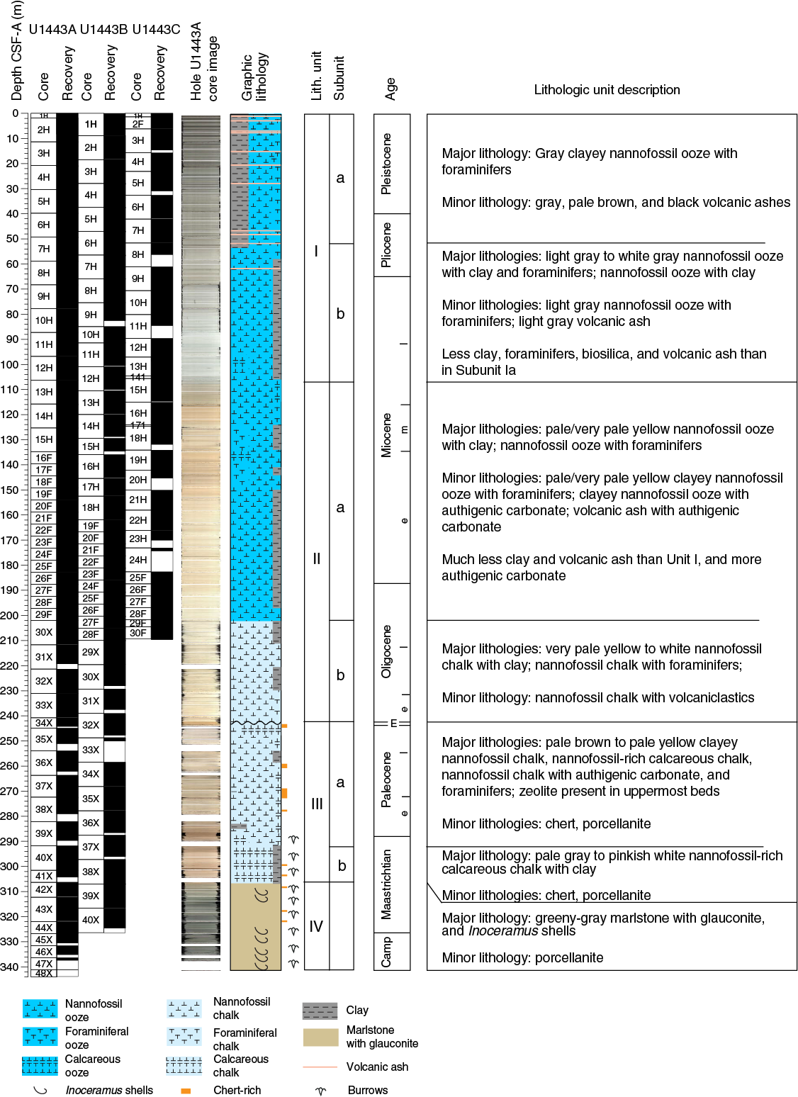
Figure F4. Lithostratigraphic summary, Site U1443.
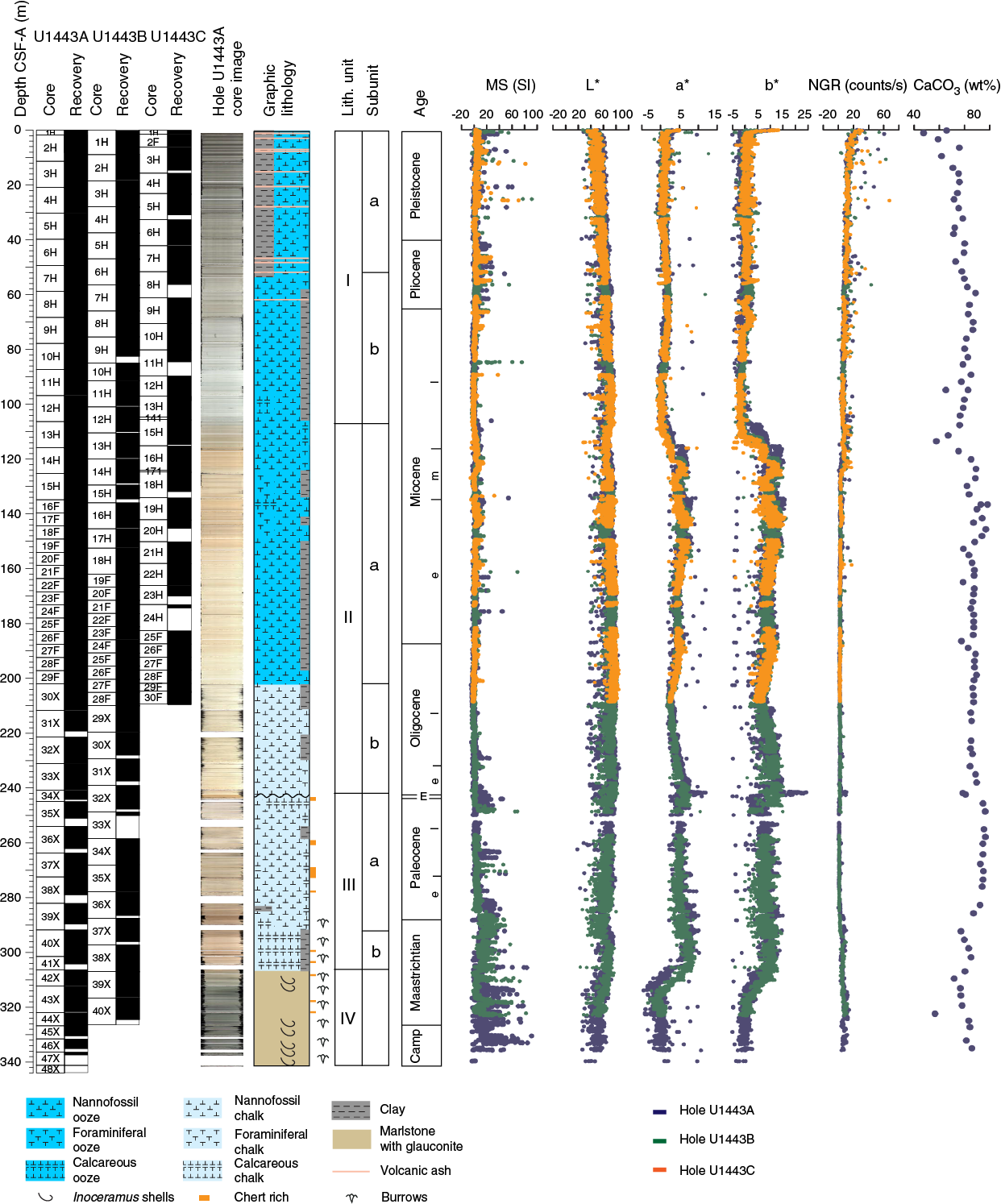
Figure F5. Lithostratigraphic summary with selected physical property and geochemical data from Holes U1443A–U1443C plotted against depth.
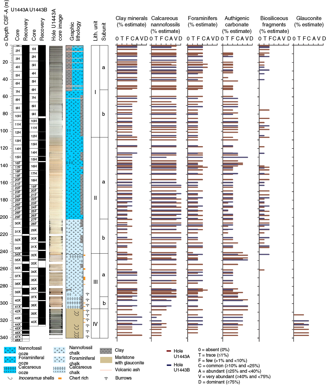
Figure F6. Smear slide data, Holes U1443A and U1443B.
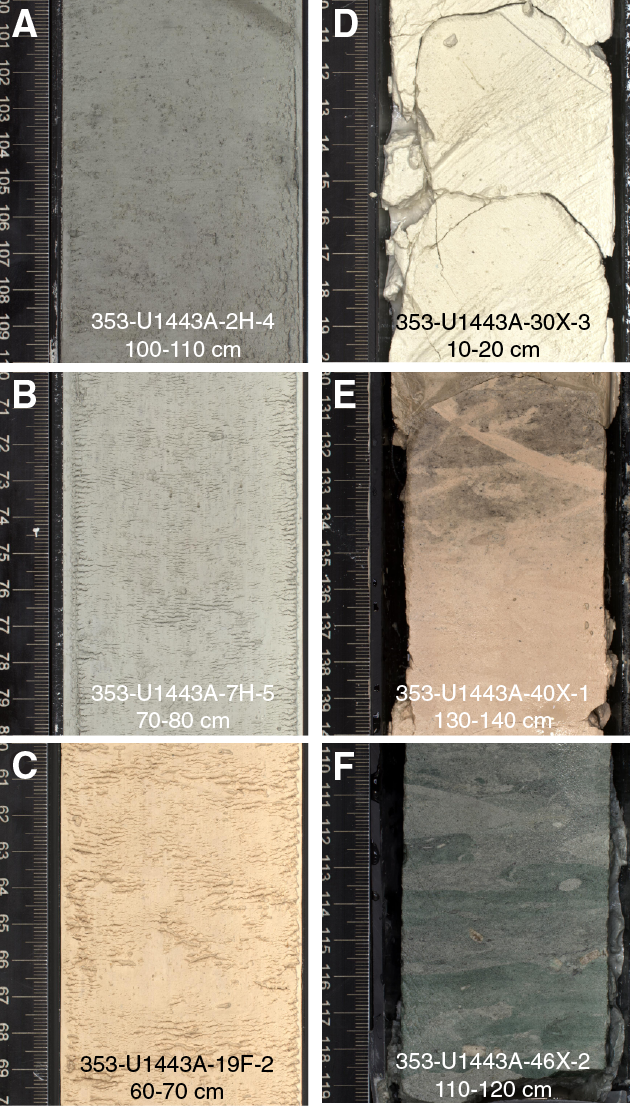
Figure F7. Major lithologies: A. Clayey nannofossil ooze. B. Nannofossil ooze with authigenic carbonate. C. Nannofossil ooze. D. Nannofossil chalk. E. Transition from clayey nannofossil chalk to authigenic carbonate-rich nannofossil chalk. F. Marlstone with glauconite.

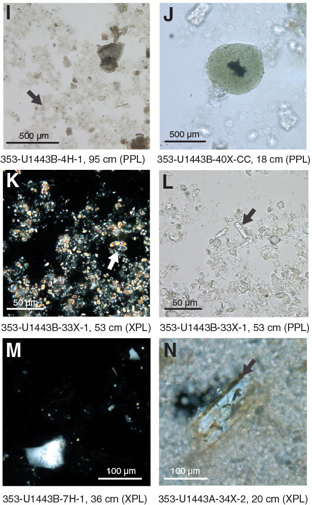
Figure F8. Biogenic sedimentary components: A, B. Nannofossils. C, D. Planktonic foraminifer fragments. E, F. Radiolarian fragment. G. Siliceous fragment. H. Diatom fragment in vitric ash. I. Clay. J. Glauconite clast. K. Authigenic carbonate. L. Small zeolites. M. Quartz grain in ash. N. Altered feldspar with Fe-oxide coating.
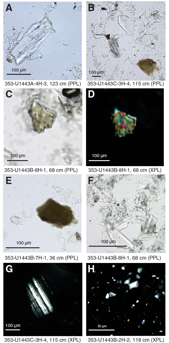
Figure F9. Ash layers, Unit I. A, B. Glass shards. C, D. Heavy mineral in black ash. E. Sand-sized biotite flake in ash shards. F. Glass shards with fine disseminated black opaques. G. Feldspar showing multiple twinning. H. Quartz and feldspar grains.

Figure F10. Minor lithologies. A. Light gray ash. B. Dark gray ash. C. Ash with authigenic carbonate. D. Porcellanite. E. Glauconite nodules. F. Dispersed Inoceramus shell fragments. G. Trace fossil (Zoophycos) filled with glauconite.
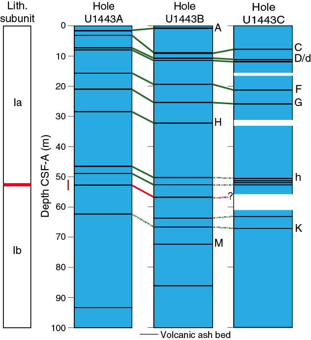
Figure F11. Correlation of major Pleistocene and Pliocene volcanic ash layers between Holes U1443A, U1443B, and U1443C.
Table T2. Depth information for major Pleistocene and Pliocene volcanic ash layers recovered in Holes U1443A–U1443C. Download table in .csv format.
Unit I
- Intervals: 353-U1443A-1H-1, 0 cm, through 13H-2, 0 cm; 353-U1443B-1H-1, 0 cm, through 13H-2, 40 cm; 353-U1443C-1H-1, 0 cm, through 15H-5, 70 cm
- Depths: Hole U1443A = 0–107.80 m CSF-A; Hole U1443B = 0–112.40 m CSF-A; Hole U1443C = 0–112.30 m CSF-A
- Age: Late Pleistocene to late Miocene
- Major lithology: clayey nannofossil ooze with foraminifers
- Minor lithology: volcanic ash
Unit I and its two Subunits Ia and Ib comprise a ~108 m thick succession of light gray–dark gray clayey nannofossil ooze with varying amounts of foraminifers and volcanic ash (Figures F4, F5). Unit I is characterized by a downhole decrease in both clay and volcanic ash content and a corresponding increase in calcareous nannofossil and authigenic carbonate content (Figure F6). These content changes are reflected in a color change from light gray (5Y 7/1) to paler whitish gray (GLEY 1 8/N) sediments. Trace amounts of detrital quartz and feldspar are found in the more clay-rich nannofossil ooze beds, particularly in Subunit Ia, the only such occurrence in pelagic sediments at Site U1443. Sediments are generally homogeneous with gradational color changes. Although Subunits Ia and Ib have definite lithologic differences, the change from Subunit Ia to Ib is gradational and, therefore, is nominally defined as the base of a prominent black ash bed at interval 353-U1443A-4H-1, 23 cm (21.03 m CSF-A), traceable in all three holes. The base of Unit I is defined by a change to pale yellow (2.5Y 8/4) nannofossil ooze with foraminifers, as evidenced by the first significant positive shift in b* and a* values (Figure F5).
Subunit Ia
- Intervals: 353-U1443A-1H-1, 0 cm, through 7H-3, 48.5 cm; 353-U1443B-1H-1, 0 cm, through 7H-1, 37 cm; 353-U1443C-1F-1, 0 cm, through 8H-CC, 22 cm
- Depths: Hole U1443A = 0–52.78 m CSF-A; Hole U1443B = 0–56.87 m CSF-A; Hole U1443C = 0–56.33 m CSF-A
- Age: Late Pleistocene to early Pliocene
- Major lithology: clayey nannofossil ooze with foraminifers
- Minor lithology: volcanic ash
Subunit Ia is a ~21 m thick succession of clayey nannofossil ooze with foraminifers, foraminifer-rich nannofossil ooze with clay, and nannofossil ooze with clay, with minor volcanic ash beds. Within the nannofossil ooze, gradational regular decimeter-scale alternations in color from light gray (5Y 7/1) to gray (5Y 5/1) occur, coinciding with changes in clay content and also visible in L* and MS data (Figures F5, F6). Some thin green bands with higher iron sulfide content occur in Subunit Ia, particularly between 0.5 and 9 m CSF-A. Foraminiferal content is moderate to high throughout, peaking in the uppermost 10 m CSF-A and at ~20 m CSF-A, and with decreasing downhole abundances (Figure F6). There is a persistent trace (<5%) contribution of biosilica, including radiolarian, sponge spicule, and silicoflagellate fragments, which decreases downhole. Volcanic ash layers, dominated by vitric grains with varying amounts of feldspar, quartz, and biotite, are a persistent minor lithology in this subunit (Figures F9, F10, F11; Table T2). The ash layers range in color from gray (10YR 5/1 and 10YR 6/1) to dark gray (GLEY 1/3N), with several horizons on the order of 5 cm thick or more. The thickest ash bed is correlated to the Late Pleistocene Toba ash event (intervals 353-U1443A-1H-2, 53 cm, through 1H-CC, 9 cm; 353-U1443B-1H-1, 69–88 cm; and 353-U1443D-1F-1, 140 cm, through 1F-2, 12 cm; not recovered in Hole U1443C). The base of Subunit Ia is defined as the base of an ash layer at 52.78 m CSF-A in Hole U1443A, as the change from Subunit Ia to Ib is gradational in terms of clay and foraminiferal content, color, MS, and reflectance (Figures F5, F6). There is no observable drilling disturbance in this subunit.
Subunit Ib
- Intervals: 353-U1443A-7H-3, 48.5 cm, through 13H-2, 0 cm; 353-U1443B-7H-1, 37 cm, through 13H-5, 40 cm; 353-U1443C-9H-1, 0 cm, through 15H-5, 70 cm
- Depths: Hole U1443A = 52.78–107.80 m CSF-A; Hole U1443B = 56.87–112.40 m CSF-A; Hole U1443C = 61.10–112.30 m CSF-A
- Age: early Pliocene to late Miocene
- Major lithology: clayey nannofossil ooze with foraminifers and nannofossil ooze with clay
- Minor lithology: nannofossil ooze with foraminifers and volcanic ash
Subunit Ib is an 86 m thick succession of light gray (5Y 7/1) to white gray (GLEY 1 8/N) nannofossil ooze. Foraminifers and clay make up a smaller proportion of the sediment than in Subunit Ia, with a slightly larger proportion of authigenic carbonate (Figure F6). The proportion of clay continues to decrease downhole, as reflected in the decreasing MS values (Figure F5). Subunit Ib has a higher CaCO3 content (~70–90 wt%) relative to Subunit Ia (60–75 wt%). The color of the ooze also becomes paler downhole, shifting from light gray and gray (5Y 6/1 and 5Y 7/1) to white gray (GLEY 1 8/N) at 68 m CSF-A, as reflected by a subtle shift in L*, b*, and a* values (Figure F5). The biosilica component is very low, with trace (1%) amounts between 27–40 and 93–105 m CSF-A, but is otherwise absent. Predominantly gray (10YR 6/1) and occasional black (GLEY 1 2.5/N) volcanic ash layers are less common in Subunit Ib and become less frequent downhole, with the last occurring at 62 m CSF-A. Drilling disturbance is minor with only occasional horizontal cracks or infrequent soupy intervals.
Unit II
- Intervals: 353-U1443A-13H-2, 0 cm, through 34X-2, 0 cm; 353-U1443B-13H-2, 40 cm, through 32X-CC, 34 cm; 353-U1443C-15H-5, 70 cm, through 30F-CC, 29 cm
- Depths: Hole U1443A = 107.80–242.36 m CSF-A; Hole U1443B = 112.40–247.85 m CSF-A; Hole U1443C = 112.30–209.62 m CSF-A (end of hole)
- Age: late Miocene to early Oligocene
- Major lithology: nannofossil ooze with clay, nannofossil ooze with foraminifers, nannofossil chalk with clay, and nannofossil chalk with foraminifers
- Minor lithology: clayey nannofossil ooze with foraminifers, clayey nannofossil ooze with authigenic carbonate, nannofossil chalk with volcaniclastics, and volcanic ash
Unit II and its two Subunits IIa and IIb comprise a 135 m thick succession of pale yellow (2.5Y 8/2) to white (2.5Y 8/1) nannofossil ooze and chalks with varying amounts of authigenic carbonate and foraminifers (Figures F4, F5, F6). Subunit IIa is characterized by nannofossil ooze, recovered using the HLAPC tool, whereas Subunit IIb is characterized by more lithified nannofossil chalk recovered using the XCB tool. Sediment throughout Unit II is highly homogeneous and likely heavily bioturbated, with no obvious stratification in grain size but with some occasional gray-colored mottling. Clay content is generally low (<20%) and decreases downhole (Figure F6). Authigenic carbonate generally comprises only 1%–10% of the sediment and also decreases downhole. Foraminifer content is variable but is generally 5%–15% throughout Unit II. The contribution from biosilica is low (<1%) throughout most of Unit II but increases downhole. The base of Unit II is defined as a change to a browner nannofossil chalk with more clay and the appearance of zeolites. This lithostratigraphic boundary coincides with the major hiatus between the early Oligocene and the late Paleocene.
Subunit IIa
- Intervals: 353-U1443A-13H-2, 0 cm, through 30X-1, 0 cm; 353-U1443B-13H-2, 40 cm, through 29X-1, 0 cm; 353-U1443C-15H-5, 70 cm, through 30F-CC, 29 cm
- Depths: Hole U1443A = 107.80–202.00 m CSF-A; Hole U1443B = 112.40–210.00 m CSF-A; Hole U1443C = 112.30–209.62 m CSF-A
- Age: late Miocene to late Oligocene
- Major lithology: nannofossil ooze with clay and nannofossil ooze with foraminifers
- Minor lithology: clayey nannofossil ooze with foraminifers, clayey nannofossil ooze with authigenic carbonate, and volcanic ash with authigenic carbonate
Subunit IIa is characterized by a 95 m thick succession of pale yellow to very pale yellow (2.5Y 8/2 to 2.5Y 9.5/2) and white (2.5Y 8/1) nannofossil ooze with varying amounts of clay, authigenic carbonate, and foraminifers (Figures F4, F5, F6). The b* and a* values are the highest observed at Site U1443, reflecting the light coloration of the sediment (Figure F5). The sediment is highly homogeneous, but some mottling with darker gray sediment occurs between 140 and 149 m CSF-A. Clay content decreases from ~25% at the top of the subunit to ~5% at the base (Figure F6). Calcareous nannofossils comprise >50% of the components in all samples, with the highest values of Site U1443 (>80%) occurring in the lower half of the subunit between 160 and 202 m CSF-A. Authigenic carbonate content is on the order of 2%–7%, with the exception of an anomalous interval between 125 and 140 m CSF-A, where values between 15% and 40% are observed. Foraminiferal content is variable but is generally 2%–10%. Biosilica content is very low (<1%) throughout most of Subunit IIa but increases to 1%–6% at the base of the subunit between 177 and 186 m CSF-A. One thin (10 cm) bed of gray (2.5Y 6/1) calcite-cemented volcanic ash occurs at 176.51 m CSF-A within interval 353-U1443A-24F-3, 31–42 cm. Although a general trend of increasing lithification is observed throughout Unit II, the base of Subunit IIa is defined by the first true chalk, which coincides with the first core recovered with the XCB tool. This step is also coincident with a sharp decrease in MS values (Figure F5). Drilling disturbance is generally minor and characterized by horizontal cracks and soupy intervals, which is particularly prevalent between 130 and 135 m CSF-A.
Subunit IIb
- Intervals: 353-U1443A-30X-1, 0 cm, through 34X-2, 0 cm; 353-U1443B-29X-1, 0 cm, through 32X-CC, 34 cm
- Depths: Hole U1443A = 202.00–242.36 m CSF-A; Hole U1443B = 210.00–247.85 m CSF-A
- Age: early to late Oligocene
- Major lithology: nannofossil chalk with clay and nannofossil chalk with foraminifers
- Minor lithology: nannofossil chalk with volcaniclastics
Subunit IIb is 40 m thick and characterized by the first occurrence of nannofossil chalk, with varying proportions of clay and foraminifers, and occasional volcaniclastic input (Figures F5, F6). The color ranges from very pale yellow (2.5Y 9/2) in the top of the unit to white (2.5Y 8.1) from 227 m CSF-A and deeper, reflected by a gradational increase in a* and b* values (Figure F5). The sediment is highly homogeneous, but some mottling with darker gray sediment is observed between 245 and 260 m CSF-A. Clay generally comprises <10% of the sediment in Subunit IIb, whereas nannofossils comprise between 50% and 75% with a decreasing downhole trend (Figure F6). Authigenic carbonate is generally low (<10%) but increases downhole to 10%–15% within the subunit. Biosiliceous content is low overall but is highest at the top of the subunit between 208 and 243 m CSF-A. Drilling disturbance is moderate to severe, coincident with the change to using the XCB tool, with frequent biscuiting and rare fall-in.
Unit III
- Intervals: 353-U1443A-34X-2, 0 cm, through 42X-1, 100 cm; 353-U1443B-32X-CC, 34 cm, through 39X-5, 70 cm
- Depths: Hole U1443A = 242.36–308.68 m CSF-A; Hole U1443B = 247.85–313.70 m CSF-A
- Age: late Paleocene to late Campanian
- Major lithology: calcareous chalk with clay, clayey nannofossil chalk, clayey nannofossil chalk with foraminifers, nannofossil chalk with authigenic carbonate, and nannofossil-rich calcareous chalk
- Minor lithology: chert and porcellanite
Unit III and its two Subunits IIIa and IIIb comprise a ~66 m thick succession of white to pale yellow (7.5Y 8/1 to 10YR 7/2 to 2.5Y 8/2) and brown nannofossil and calcareous chalks with varying proportions of clay and foraminifers. Occasional chert and porcellanite nodules and thin beds are observed, particularly in Subunit IIIa between 255 and 275 m CSF-A (Figure F4). The top of the unit is marked by an extensive hiatus between the late Paleocene and early Oligocene. Chalks are generally homogeneous and apparently heavily bioturbated, but color mottling is a common feature. Burrows become common in Subunit IIIb, just above the Cretaceous/Paleogene boundary.
Subunit IIIa
- Intervals: 353-U1443A-34X-2, 0 cm, through 40X-1, 135 cm; 353-U1443B-32X-CC, 34 cm, through 38X-1, 136 cm
- Depths: Hole U1443A = 242.36–291.80 m CSF-A; Hole U1443B = 247.85–298.66 m CSF-A
- Age: late Paleocene to Maastrichtian
- Major lithology: clayey nannofossil chalk, nannofossil-rich calcareous chalk, nannofossil chalk with authigenic carbonate, authigenic carbonate-rich nannofossil chalk with foraminifers, and clayey nannofossil chalk with foraminifers
- Minor lithology: chert and porcellanite
Subunit IIIa is 50 m thick interval of calcareous chalk and nannofossil chalk with foraminifers, and clay. Color most commonly varies from pale brown (10YR 8/2) to pale yellow (2.5Y 8/2). Thin to medium beds of dark reddish gray (5YR 4/2) chert occur in Subunit IIIa, particularly in the lower portion between 300 and 308 m CSF-A (Figures F4, F5). Clay mineral content increases with depth from ~10% to 30%, with a corresponding decrease in nannofossil content (Figure F6). The uppermost beds (240–248 m CSF-A), underlying the major unconformity, are characterized by an increase in authigenic carbonate and clay, as well as the presence of zeolites as a minor fine silt–sized component. Mottling and color banding were observed commonly throughout Subunit IIIa. Bioturbation is present throughout this interval, observed as burrows. Drilling disturbance is moderate to severe, most commonly present as biscuiting.
Subunit IIIb
- Intervals: 353-U1443A-40X-1, 135 cm, through 42X-1, 100 cm; 353-U1443B-38X-1, 136 cm, through 39X-5, 70 cm
- Depths: Hole U1443A = 291.80–308.68 m CSF-A; Hole U1443B = 298.66–313.70 m CSF-A
- Age: Maastrichtian
- Major lithology: nannofossil-rich calcareous chalk with clay
- Minor lithology: chert and porcellanite
Subunit IIIb is a 15 m thick interval of nannofossil-rich calcareous chalk with clay distinguished from Subunit IIIa by an increase in bioturbation starting from just above the Cretaceous/Paleogene boundary and continuing to the base of the unit. Color ranges from pale gray (2.5Y 7/1) to pinkish white (7.5YR 8.5/2) to very pale brown (10YR 8/3). Mottling is observed in this subunit. Clay mineral content decreases from ~30% in Subunit IIIa to ~20% in Subunit IIIb, whereas authigenic carbonate content increases from ~20% to ~60% across the same interval (Figure F6). Nannofossil content continues to decrease and only comprises around 10% of the sediment at the base of Subunit IIIb. Very thin to thin beds of porcellanite and chert occur, particularly between 300 and 308 m CSF-A.
Unit IV
- Intervals: 353-U1443A-42X-1, 100 cm, through 48X-CC, 15 cm; 353-U1443B-39X-5, 70 cm, through 40X-CC, 44 cm
- Depths: Hole U1443A = 308.68–341.35 m CSF-A; Hole U1443B = 313.70–324.69 m CSF-A
- Age: Maastrichtian to late Campanian
- Major lithology: marlstone with glauconite
- Minor lithology: bioclastic marlstone with glauconite
Unit IV is composed of 34 m of mottled greenish gray (GLEY 1 6/10GY to GLEY 1 8/10Y) marlstone with glauconite and locally high concentrations of Inoceramus shells and fragments (Figures F4, F5). Sediment is heavily bioturbated with a large number of burrows and tracks visible, including the inclined U-shaped burrows characteristic of the Zoophycos ichnofacies (Figure F10). Clay content is elevated relative to Units I and II, ranging from 20% to 50%, whereas nannofossil content is greatly reduced, averaging 1%–25% and decreasing sharply downhole (Figure F6). Authigenic carbonate ranges from 40%–60% at the top of the unit to 10%–20% at the base. Foraminifers are present in quantities of 2%–15%, and there is no obvious biosiliceous content. Glauconite is found throughout the unit, giving the characteristic greenish color and the increased MS values (Figures F5, F6). The darker color of the sediment is also reflected in the low L* and a* values as compared to Unit III (Figure F5). Dark green nodules present within this unit (Figure F10) are composed almost entirely of glauconite (Figure F12). Inoceramus shells are common and in places are numerous enough to classify the sediment as bioclastic. The shells are intact pieces visible as thick shell fragments several centimeters long and as fine disseminated calcite prisms throughout the sediment (Figure F10).
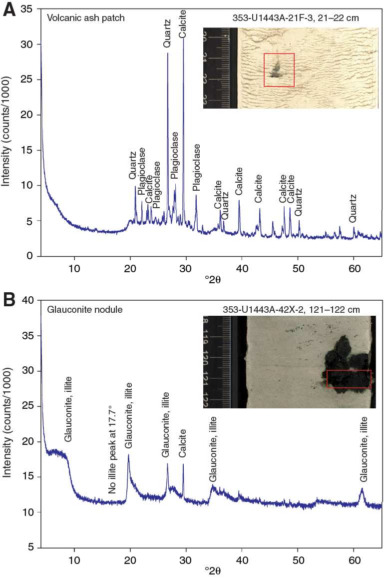
Figure F12. X-ray diffraction diffractograms from selected samples, Hole U1443A. A. Gray volcanic ash bleb in high calcium carbonate nannofossil ooze. B. Glauconite nodule.
Biostratigraphy
Abundances of different microfossil groups at Site U1443 have different downhole trends. In Hole U1443A, the upper 30.36 m is rich in both siliceous and calcareous microfossils. Within this interval, diatom abundances fluctuate between common and abundant, and preservation is generally moderate to good. Between 28 and 116.27 m CSF-A, the occurrence of siliceous microfossils is sporadic, but calcareous microfossils are consistently present (Figure F13). Deeper than 116.27 m CSF-A, sediments are barren of siliceous microfossils except for some isolated intervals. Calcareous nannofossils are abundant throughout the recovered sections and are well preserved in the upper 115 m; deeper than 115 m CSF-A, preservation is generally moderate and occasionally poor. Foraminifers are dominant to abundant in the upper 241 m in Hole U1443A. Abundance decreases deeper than 241 m CSF-A and falls to common to few deeper than 326 m CSF-A. Preservation is good to moderate throughout the Cenozoic with exceptions in the late Miocene (116.24 m CSF-A) and the early Oligocene to Paleocene (240.60 to 244.27 m CSF-A) where preservation is poor. Preservation in the Cretaceous (deeper than 273 m CSF-A) is moderate to poor. Note that in Hole U1443A, CSF-A depths for all cores deeper than Core 353-U1443A-1H should have ~5 m added to be consistent with CSF-A depths of the other three holes. This is because stratigraphic correlation indicates that approximately 5 m of sediment was lost from Core 1H (see Operations for further discussion).
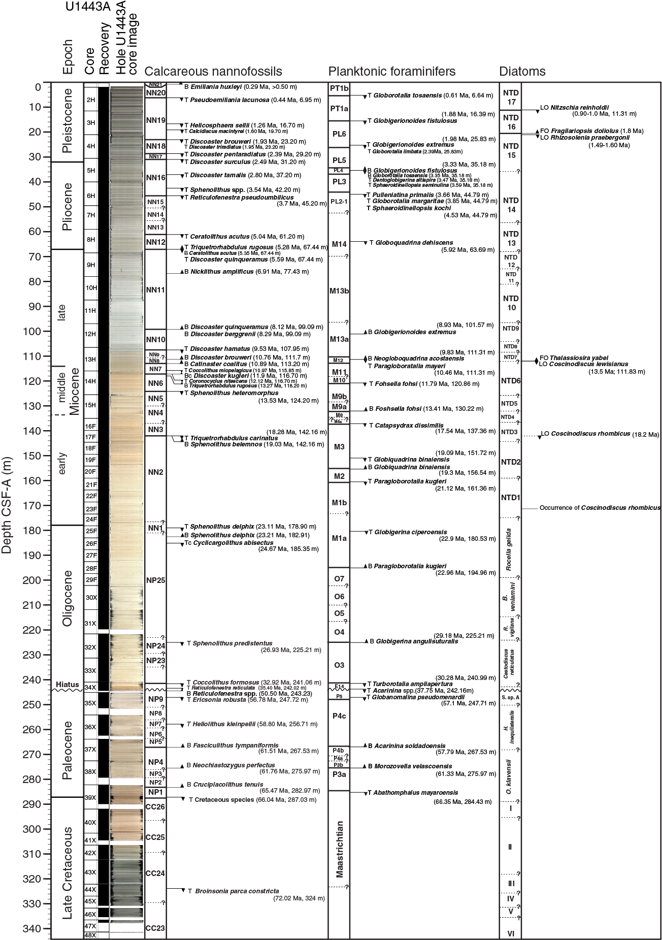
Figure F13. Summary of biostratigraphic events identified in Hole U1443A.
The biostratigraphic age model for Site U1443 was established by combining nannofossil and planktonic foraminifer datums with a few ages provided by diatoms (Figure F13; Tables T3, T4). The oldest planktonic foraminifer datum encountered is the last occurrence (LO) of Abathomphalus mayaroensis, which suggests that sediments in Sample 353-U1443A-39X-CC are of latest Maastrichtian age. The oldest calcareous nannofossil datum found is the LO of Broinsonia parca constricta, suggesting that sediments in Sample 44X-CC are close to the Maastrichtian/Campanian boundary (72.1 Ma).
Table T3. Calcareous nannofossil datums, Site U1443. Download table in .csv format.
Table T4. Planktonic foraminifer datums, Site U1443. Download table in .csv format.
Beyond the biostratigraphic schemes, microfossil assemblages provide a record of climatic shifts and may indicate changes in primary productivity and oceanography through time.
Calcareous nannofossils
Calcareous nannofossils were examined in all core catcher samples from Hole U1443A and the first core catcher of Hole U1443B. When time permitted, additional split core samples for Hole U1443A (and Core 353-U1443B-1H) were examined to refine the depth of biostratigraphic datums, with emphasis on the Quaternary, Neogene, and important boundaries. Semiquantitative species abundance estimates are divided into three periods (Quaternary and Neogene, Paleogene, and Cretaceous) and are shown in Tables T5, T6, and T7.
Table T5. Semiquantitative calcareous nannofossils abundance counts from Quaternary and Neogene core catcher samples, Site U1443. Download table in .csv format.
Table T6. Semiquantitative calcareous nannofossils abundance counts from Paleogene core catcher samples, Site U1443. Download table in .csv format.
Table T7. Semiquantitative calcareous nannofossils abundance counts from Cretaceous core catcher samples, Site U1443. Download table in .csv format.
Quaternary and Neogene
Abundant and well-preserved calcareous nannofossils were present throughout the Quaternary and Neogene sedimentary sections of Hole U1443A (approximately 0–178 m CSF-A), allowing us to define a relatively high-resolution Neogene stratigraphy using this fossil group (Table T3; Figure F13). The first downcore observation of significant diagenetic overgrowth (visible in the light microscope) of susceptible nannofossils (Discoaster and Sphenolithus) was noted in the middle to late Miocene around Core 353-U1443A-13H. This coincides with the top of lithostratigraphic Unit II, and nannofossil preservation (in terms of etching and overgrowth) deteriorates below this boundary. The good nannofossil preservation in Unit I could result from the enhanced clay content of these sediments relative to deeper lithostratigraphic units. This is because clay-rich sediments have low porosity and permeability; therefore, carbonate fossils are sealed in with their associated pore water fluids, and rapid chemical equilibration occurs (e.g., Pearson et al., 2001; Bown, 2005; Expedition 342 Scientists, 2012). Pleistocene to Miocene nannofossil assemblages are typically tropical/subtropical and included abundant Florisphaera profunda, Gephyrocapsa spp., Reticulofenestra spp., Sphenolithus spp., and Discoaster spp. Helicosphaera, Calcidiscus, and Umbilicosphaera spp. were also common.
Most Neogene marker species defined by Martini (1971) and Okada and Bukry (1980) (see Biostratigraphy in the Expedition 353 methods chapter [Clemens et al., 2016] for zonal schemes used) were found (Table T3), and all ages cited in the text and Figures are those of Gradstein et al. (2012). The presence of Emiliania huxleyi, which delineates the base of Zone NN21 (0.29 Ma), was confirmed shipboard by scanning electron microscope (SEM) in Samples 353-U1443A-1H-1W, 15 cm, 1H-1W, 50 cm, and 353-U1443B-1H-1W, 10 cm. However, the shift in dominance from Gephyrocapsa caribbeanica to E. huxleyi (dated at 0.09 Ma in tropical waters) was not encountered in Sample 353-U1443A-1H-1W, 15 cm, suggesting that the Holocene is unlikely to be completely recovered. These observations suggest a similar core top age at Site U1443 to Site 758, where the presence of E. huxleyi was noted in the upper 50 cm of Core 121-758C-1H. Further high-resolution SEM work will be needed to precisely define the first occurrence (FO) of this species and to estimate the age of the top of the recovered cores for Holes U1443A–U1443D. The LO of Pseudoemiliania lacunosa, dated at 0.44 Ma, occurs between Samples 353-U1443A-2H-1W, 15 cm, and 2H-2W, 15 cm, and between Samples 353-U1443B-1H-5W, 110 cm, and 1H-6W, 15 cm. The Pliocene/Pleistocene boundary (2.59 Ma) is bracketed by a number of Discoaster LOs that are dated between 2.39 and 2.8 Ma; we therefore place this boundary between Sections 353-U1443A-5H-2W and 5H-5W. The Miocene/Pliocene boundary (5.33 Ma) is estimated to be between Samples 353-U1443A-8H-6W, 15 cm, and 9H-1W, 15 cm, based on the LO of Triquetrorhabdulus rugosus (5.28 Ma) and the FO of Ceratolithus acutus (5.35 Ma). As also noted at Site 758, the early middle Miocene marker species Helicosphaera ampliaperta was not found. The Oligocene/Miocene boundary (23.03 Ma) is defined by the brief appearance of Sphenolithus delphix (23.11–23.21 Ma) between Samples 353-U1443A-25F-1W, 15 cm, and 26F-1W, 15 cm.
Paleogene and Cretaceous
Calcareous nannofossils are abundant in Paleogene (Cores 353-U1443A-34X through 38X) and Late Cretaceous (Cores 39X through 48X) sediments, but calcareous nannofossil preservation was moderate to poor, resulting in less robust biostratigraphic age control in these intervals relative to the Quaternary and Neogene (Table T3; Figure F13). A prominent hiatus spanning most of the Eocene and the uppermost Paleocene was identified, as anticipated based on recovery at Site 758, between Samples 33X-CC and 35X-CC. Sample 34X-CC contains a mixture of Eocene and Paleocene species. Two events were nevertheless identified in the likely discontinuous and highly condensed Eocene sediments that were recovered, namely the late Eocene LO of Reticulofenestra reticulata (35.40 Ma) between Samples 34X-1W, 68 cm, and 34X-2W, 25 cm, and the early Eocene FO of Reticulofenestra spp. (50.50 Ma) between Samples 34X-2W, 25 cm, and 34X-3W, 51 cm. The first event identified below the hiatus is the LO of Ericsonia robusta (56.78 Ma) between Samples 34X-CC and 35X-CC. The Cretaceous/Paleocene boundary (66.04 Ma) was identified between Samples 39X-4W, 40 cm, and 39X-5W, 60 cm. However, sediments in this interval are heavily bioturbated (containing burrows, blebs, patches, color banding, and mottles), and most samples studied within this interval contained a mixture of Cretaceous and Paleocene species. The interval below Section 39X-5W contains moderately to poorly preserved Cretaceous nannofossil assemblages. No latest Maastrichtian marker events were found, which is possibly the result of a minor hiatus. The LO of B. parca constricta just above the Maastrichtian/Campanian boundary (72.05 Ma) is found between Samples 43X-CC and 44X-CC. The presence of common Reinhardtites levis in the oldest recovered core (Sample 48X-CC) suggests that the sediment is not older than Zone CC23 in the late Campanian.
Planktonic foraminifers
Planktonic foraminifer biostratigraphy of the Pleistocene to Late Cretaceous section of Site U1443 was based on the shipboard study of core catcher samples from Hole U1443A and was supplemented by a small number of samples from Cores 353-U1443A-34X and 353-U1443B-1H to refine certain datums. Planktonic foraminifer distribution in Holes U1443A and U1443B is shown in Table T8. The absolute ages assigned to biostratigraphic datums listed in Table T4 follow the references given in Table T2 in the Expedition 353 methods chapter (Clemens et al., 2016). The planktonic/benthic ratio, reported as percentage planktonic foraminifers of the total foraminifer population, and the number of benthic foraminifers found in a 10 cm3 sample are based on examination of the >150 µm size fraction of core catcher samples.
Table T8. Semiquantitative planktonic foraminifer abundance counts from core catcher samples, Site U1443. Download table in .csv format.
Pleistocene
Pleistocene planktonic foraminifer assemblages were recovered from Samples 353-U1443A-1H-CC (1.80 m CSF-A) through 4H-CC (30.38 m CSF-A) and Samples 353-U1443B-1H-1W, 51 cm (0.53 m CSF-A), through 1H-6W, 51 cm (8.01 m CSF-A). Foraminiferal assemblages are abundant and generally well preserved. Planktonic assemblages are dominated by the tropical to warm subtropical species Pulleniatina obliquiloculata, Neogloboquadrina dutertrei, Globoquadrina conglomerata, Globigerinoides ruber, G. sacculifer, Globigerinoides trilobus, Globorotalia menardii, and Orbulina universa. The occurrences of Globorotalia flexuosa in Sample 353-U1443A-1H-CC (1.80 m CSF-A) and the top samples from Core 353-U1443B-1H confirm that these sediments are older than 0.07 Ma. G. ruber (pink) is also found in Samples 353-U1443A-1H-CC (1.80 m CSF-A) and 353-U1443B-1H-3W, 53 cm (3.53 m CSF-A), constraining the zone to PT1b. The top of Globigerinoides fistulosus in Sample 3H-CC marks the top of Zone PL6. Planktonic foraminifer percentage is >95%, and 250–700 benthic foraminifers are found in the >150 µm size fraction of a 10 cm3 Pleistocene sample.
Pliocene
Pliocene planktonic foraminifer assemblages were recovered from Samples 353-U1443A-5H-CC (39.97 m CSF-A) through 7H-CC (58.97 m CSF-A). Foraminiferal assemblages were abundant and moderately to well preserved regardless of extensive fragmentation. G. menardii, Globorotalia tumida, G. sacculifer, G. trilobus, Sphaeroidinella dehiscens, and Sphaeroidinellopsis seminulina dominate the assemblage. The top of Sphaeroidinellopsis kochi in Sample 6H-CC (49.61 m CSF-A) is the oldest Zone PL1 marker recorded in these sediments. Because some Pliocene samples are highly fragmented, planktonic foraminifer percentage is lower than in nonfragmented intervals (averaging 93%), and the number of benthic foraminifers per 10 cm3 sample is as high as 1100.
Miocene
Miocene sediments span Samples 353-U1443A-8H-CC (68.52 m CSF-A) through 27F-CC (192.54 m CSF-A). Planktonic foraminifers are abundant throughout the Miocene. Whereas poor preservation is evident in Sample 13H-CC (116.24 m CSF-A), all other samples are moderately to well preserved, showing moderate fragmentation and some evidence of dissolution. Dentoglobigerina altispira and Paragloborotalia mayeri are the most abundant species through the Miocene. Paragloborotalia kugleri and Globoquadrina tripartita are the most common species in the early Miocene. Globoquadrina venezuelana is the most common species in the middle Miocene. In the late Miocene, the most common species are S. seminulina, O. universa, Neogloboquadrina acostaensis, and Pulleniatina primalis. Most planktonic foraminifer zones were identified in Miocene sediments. Fohsella fohsi, marking the upper and lower limits of Zones 9b and 9a, respectively, occurs only in Sample 14H-CC. The top of Catapsydrax dissimilis in Sample 16F-CC marks the top of Zone M3. Zones M4a–M8 are not observed in core catcher sediments, however, suggesting that the interval between 125.50 and 139.73 m CSF-A is either highly compressed or contains a hiatus. The bottom of Zone M1a is marked by the base of P. kugleri in Sample 27F-CC (192.54 m CSF-A). Planktonic foraminifer percentages range from 73% to 99%, and the number of benthic foraminifers in a 10 cm3 sample ranges from 26 to 921, depending on the degree of fragmentation and dissolution of the sample.
Oligocene
Oligocene sediment was recovered in Samples 353-U1443A-28F-CC (197.39 m CSF-A) through 34X-1W, 56 cm (241.36 m CSF‑A). Though foraminifers are generally abundant, preservation ranges from good to poor. Assemblages are dominated by Paragloborotalia nana. Other common to abundant species include Globigerina angustiumbilicata, P. mayeri, and G. venezuelana. The base of Globigerina angulisuturalis in Sample 31X-CC marks the transition from Zone O4 to O3. Sample 32X-CC (231.115 m CSF-A) contains a few Acarinina spp. and Morozovella spp. of the Paleocene and Eocene, indicating some reworking. Planktonic foraminifer percentage is >92%, and the number of benthic foraminifers in a 10 cm3 sample ranges from 2 to 135, depending on the preservation of the sample.
Eocene
The Eocene is represented by Samples 353-U1443A-34X-2W, 65 cm (242.95 m CSF-A), and 34X-CC (244.25 m CSF-A). Foraminifers in these samples are highly fragmented and stained orange. Only poorly preserved Parasubbotina varianta, Acarinina soldadoensis, and Acarinina spp. are found. These samples contain many lithic fragments and several fish teeth. Planktonic foraminifer percentage is very low (59%), and the number of benthic foraminifers per 10 cm3 sample is 40.
Paleocene
Samples 353-U1443A-35X-CC (251.18 m CSF-A) through 38X-CC (279.12 m CSF-A) contain Paleocene assemblages dominated by Morozovella velascoensis and Globanomalina chapmani. Three Paleocene zones are identified in these four samples. Zone P4c is marked by the top of Globanomalina pseudomenardii in Sample 35X-CC. The bottom of A. soldadoensis in Sample 36X-CC marks the top of Zone P4b, and the bottom of M. velascoensis in Sample 37X-CC marks the top of Zone P3a. Foraminifers are abundant, and preservation is moderate to good throughout the Paleocene. Planktonic foraminifer percentage is 99% to 100%, and the number of benthic foraminifers per 10 cm3 sample ranges from 0 to 410.
Late Cretaceous
Cretaceous planktonic foraminifers were found in Samples 353-U1443A-39X-CC (289.74 m CSF-A) through 48X-CC (341.33 m CSF-A). Planktonic foraminifer abundance decreases downhole from dominant or abundant to few. Preservation is moderate to poor throughout the Cretaceous. The uppermost Maastrichtian is identified in Sample 39X-CC by the presence of A. mayaroensis. Sediments in older samples are characterized by a low-diversity assemblage consisting mainly of Globotruncana arca, Rugoglobigerina rugosa, Rugoglobigerina macrocephala, and Heterohelix spp. Inoceramid prisms are abundant to common in most Late Cretaceous samples. Planktonic foraminifer percentages range from 63% to 97%, and the number of benthic foraminifers in a 10 cm3 sample ranges from 76 to >1400, depending on the degree of dissolution of the sample.
Diatoms
In order to define the sediment age and paleoenvironmental conditions, core catcher samples and samples from selected split core sections from Hole U1443A were investigated (Table T9). For a detailed description of the diatom zonal scheme and taxonomy, see Biostratigraphy in the Expedition 353 methods chapter (Clemens et al., 2016). The sampling resolution for Hole U1443A was ~3 samples per core. However, 65 of the 99 samples investigated for Hole U1443A were barren of diatoms (Figure F13; Table T9). Diatom occurrence and valve preservation varies strongly throughout the sediment column of Site U1443. Diatoms occur more often in the uppermost 28 m, whereas their occurrence becomes sporadic downcore to 192 m CSF-A. Deeper sediments are barren of diatoms. This last observation strongly contradicts the results from Site 758 (Shipboard Scientific Party, 1989b). Moderately to well-preserved diatoms of Oligocene age were found in some short intervals at Site 758. Furthermore, Campanian age diatoms were found in core catcher samples at Site 758.
Table T9. Semiquantitative diatom abundance counts from core catcher samples, Site U1443. Download table in .csv format.
Diatom biostratigraphy
Diatoms were useful for age estimation only in the Pleistocene; the Fragilariopsis doliolus Zone (0 to 0.90–1 Ma) was recognized between Samples 353-U1443A-1H-1W, 16 cm, and 2H-CC. The LO of Nitzschia reinholdii in Sample 2H-CC defines the boundary between the F. doliolus and the N. reinholdii Zones. The Rhizosolenia praebergonii Zone (1.8–3.0 Ma) is easily identifiable by the presence of the corresponding species within Sample 4H-1W, 11–12 cm (Table T9).
Apart from Samples 353-U1443A-13H-5A, 40–41 cm, and 23F-2W, 85–86 cm, no other sample was useful for diatom biostratigraphy in the lower part of Hole U1443A. The former is particularly interesting because it coincides with a bloom of Thalassiothrix longissima. This sudden bloom (probably due to a rapid supply of nutrients) also contributed to the proliferation of stratigraphically useful species: both Coscinodiscus lewisianus and Thalassiosira yabei are observed in Sample 13H-5A, 40–41 cm. The LO of C. lewisianus coincides with the C. lewisianus/Coscinodiscus gigas var. diorama Zone boundary (~13.5 Ma), and the FO of T. yabei approximates this boundary (Figure F4B in the Expedition 353 methods chapter [Clemens et al., 2016]). The occurrence of Coscinodiscus rhombicus in Sample 23F-2W, 85–86 cm, suggests that this sample is older than 18.2 Ma (Figure F4B in the Expedition 353 methods chapter [Clemens et al., 2016]).
Our results for the Pleistocene, Pliocene, and Miocene generally agree with the results from Site 758 (Shipboard Scientific Party, 1989b). No diatoms, however, were found in Hole U1443A in the Paleogene and Cretaceous sediments; this lack of diatoms contrasts with the earlier results of Site 758. Indeed, although some biostratigraphically important diatoms were missing, a zonation for the Paleogene was possible at Site 758 and a few Cretaceous (Campanian) diatoms were observed.
Paleoenvironmental considerations (diatoms)
Valve preservation ranges from good to poor and tends to be better whenever abundance is higher. Strong variations in abundance and preservation and shifts in the species composition of the diatom assemblage will help to reconstruct paleoceanographic changes in the pelagic Eastern Indian Ocean.
The diatom community in the uppermost 28 m of Site U1443 is diverse and mainly consists of Pleistocene to Holocene species, mostly typical of warm to temperate, low-latitude ocean waters. Warm-water species, including F. doliolus, tend to dominate whenever total diatom abundance is higher than “few” (Table T9). Main contributors to the warm and temperate group include Alveus marinus, Azpeitia nodulifera, F. doliolus, Rhizosolenia bergonii, Shionodiscus oestrupii, Thalassionema nitzschioides var. parva, Thalassionema bacillaris, and Thalassiosira eccentrica (Hasle and Syvertsen, 1996). A certain degree of coastal water input above Site U1443 is revealed by the recurrent presence of coastal diatoms including Thalassionema nitzschioides var. nitzschioides, resting spores of Chaetoceros, and Actinocyclus spp. (Romero and Armand, 2010).
Sporadic increases of diatoms at Site U1443 in downcore sediments are associated with the occurrence of volcanic glass shards. This phenomenon is related to the release of nutrients from the volcanic ash layers and represents the photophysiological and biomass stimulation of phytoplankton communities following the supply of basaltic or rhyolitic volcanic ash (Langmann et al., 2010).
Radiolarians and silicoflagellates
Observations were also made on the presence of two other groups of siliceous microfossils: radiolarians and silicoflagellates. The distribution of silicoflagellates is similar to that of diatoms throughout the cores, whereas radiolarians can be common in levels completely barren of diatoms. Radiolarian-rich samples include Samples 353-U1443A-13H-1A, 35–36 cm, through 13H-5A, 40–41 cm; 21F-CC through 23F-2W, 85–86 cm; and 32X-5W, 107 cm, through 32X-6W, 57–58 cm (Table T9).
Sedimentation rates and age model
Age-depth relationships for Hole U1443A based on biostratigraphy for the three fossil groups studied (calcareous nannofossils, planktonic foraminifers, and diatoms) show good agreement for the Pleistocene where all three groups co-occur (Figure F14). Calcareous nannofossils and planktonic foraminifers show consistent age-depth relationships throughout the Cenozoic and Late Cretaceous with no major outliers. Paleomagnetic reversals were reliably determined in the upper 69 m for Hole U1443A and in most of the interval between 136 and 199 m CSF-A. In both intervals the match between biostratigraphic datums and the magnetochron boundary datums is very good. The combined biostratigraphic age model indicates a mean sedimentation rate of 1.20 cm/ky in the upper part of lithostratigraphic Unit I (0–85 m CSF-A), which covers the Pleistocene to late Miocene. The mean sedimentation rate then decreases to 0.41 cm/ky between 100 and 130 m CSF-A (the lower part of lithostratigraphic Unit I and the upper part of Subunit IIa), which covers the interval between the late and middle Miocene. The early to middle Miocene transitional interval appears to be condensed, and both foraminifer and calcareous nannofossil marker species are absent. Sedimentation rates between 135 and 200 m CSF-A in the lower half of lithostratigraphic Subunit IIa average 0.81 cm/ky (early Miocene to Oligocene). Finally, following a hiatus that spans the late Paleocene, Eocene, and early Oligocene, the mean sedimentation rate in the late Paleocene and Late Cretaceous (lithostratigraphic Units III and IV, 242.36–341.35 m CSF-A) is 0.36 cm/ky. These sedimentation rates and age estimates broadly agree with those published for Site 758.

Figure F14. Biostratigraphic and paleomagnetic reversal-based age-depth plot, Hole U1443A.
Geochemistry
The composition of the interstitial water and bulk sediment samples at Site U1443 reflects the variation in sediment composition and reactions that have occurred since deposition. The depositional environment changed as the site migrated from the Southern Hemisphere to the current location and as the collision of India with Asia delivered increasing amounts of terrigenous material to the location. In lithostratigraphic Unit I, ash deposition from the nearby Indonesian arc may also play an important role.
Sediment gas sampling and analysis
Headspace gas samples were taken at a frequency of one sample per core in Hole U1443A as part of the routine environmental protection and safety monitoring program (Table T10). All headspace samples had very low levels of methane (C1 < 5 ppmv), with no heavier hydrocarbons (Figure F15).
Table T10. Headspace gas concentrations, Hole U1443A. Download table in .csv format.
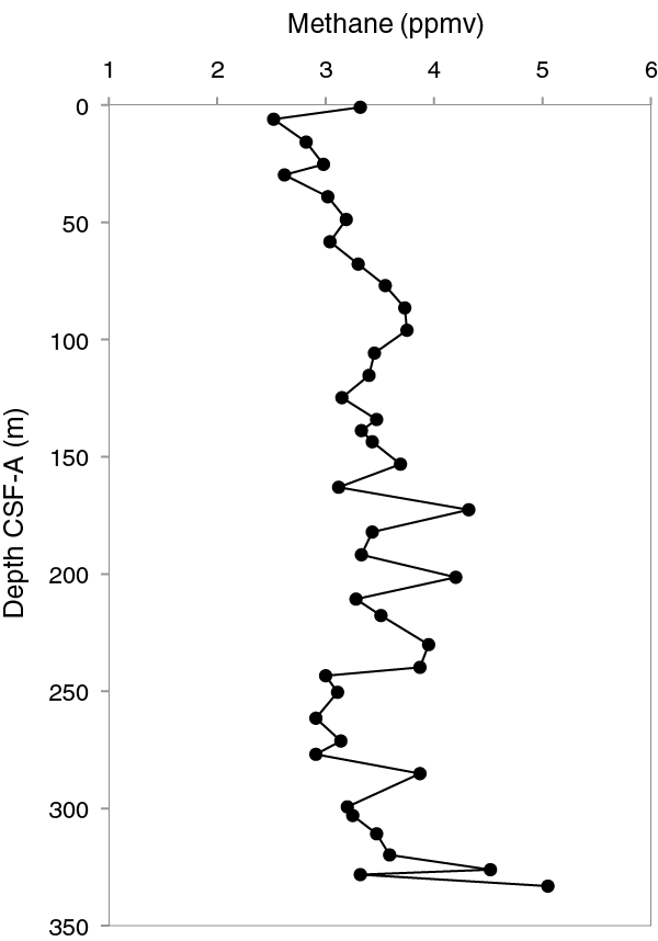
Figure F15. Headspace methane concentrations, Hole U1443A.
Bulk sediment geochemistry
Calcium carbonate and inorganic carbon contents were determined on sediment samples from Holes U1443A and U1443C (Table T11; Figure F16). CaCO3 values range between 54 and 97 wt%. In the uppermost 108 m, corresponding to lithostratigraphic Unit I, CaCO3 peaks at 89 wt% in the middle of the unit with the lowest values near the sediment surface and the lower unit boundary. Below the minimum (66 wt%) associated with the transition from Unit I to II, high carbonate values (maximum 89 wt%) are observed in Subunit IIa. Even higher values are found in Subunit IIIa (maximum 97 wt%) with moderately lower carbonate values in Subunit IIIb (maximum = 85 wt%) and Unit IV (maximum = 88 wt%).
Table T11. Calcium carbonate and organic carbon content, Holes U1443A and U1443C. Download table in .csv format.
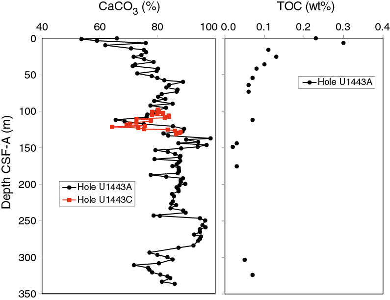
Figure F16. Calcium carbonate and TOC contents in sediments, Holes U1443A and U1443C.
In many samples, total organic carbon (TOC) was too low to determine via subtraction of CaCO3 from total carbon (TC) (see Geochemistry in the Expedition 353 methods chapter [Clemens et al., 2016]), and TC was measured after acidification for this site (a more direct measure of TOC). The acidification method determined TOC is low (<0.3 wt%) throughout the sampled sediment column and decreases with depth (Table T11; Figure F16).
Interstitial water sampling and chemistry
A total of 47 interstitial water samples were collected by whole-round squeezing from Hole U1443A (Table T12). For the first time on the JOIDES Resolution, whole-round samples were scraped and placed in the squeezer in a glove bag under a N2 atmosphere. The squeezer was then placed directly into the hydraulic press, also in a N2 atmosphere, and squeezed. This N2 handling was conducted for all but one of the samples taken from APC or HLAPC cores and the first XCB core section (353-U1443A-30X-6). One APC sample (6H-6, 145–150 cm; 48.75 m CSF-A) and all other XCB samples were prepared and squeezed in laboratory air.
Table T12. Interstitial water data, Hole U1443A. Download table in .csv format.
Pore water chloride concentration varies from ~538 mM in the shallowest sample to values around 575 mM in the bottom of the sampled sediment section (not shown). Generally, chloride values increase from ~560 mM in the uppermost core to ~570 mM around 250 m CSF-A. Deeper than 250 m CSF-A, there are two chloride peaks with values around 575 mM. Alkalinity increases from 2.92 mM in the uppermost sample to values >3.7 mM in the uppermost 20 m before gradually decreasing to ~3 mM around 200 m CSF-A (Figure F17). Deeper than 200 m CSF-A, alkalinity decreases gradually to around 2 mM at 280 m CSF-A before a pronounced decline to 0.5 mM at 320 m CSF-A and deeper. Sulfate concentration decreases with depth to values around 25 mM in the upper 100 m. Deeper than 100 m CSF-A, sulfate gradually decreases toward 24 mM in the bottom of the sampled section with one low value of 23.1 mM at 270 m CSF-A. Dissolved phosphate concentration was generally below detection, with a few detectable values, notably near the seafloor.

Figure F17. Interstitial water chemistry profiles, Hole U1443A.
Pore water Mg concentration decreases with depth from 53 to 39 mM with steeper changes in the uppermost and lowermost 40 m CSF-A (Figure F17). Calcium concentration increases linearly with depth from 10.8 to 32.5 mM with two small inflections at around 220 and 290 m CSF-A. Potassium concentration in the upper 25 m is scattered around 11 mM before steadily decreasing with depth to around 7.2 mM at the bottom of the sampled section. Alteration of basaltic basement exchanges K and Mg for Ca (e.g., Gieskes, 1981), and the gradients in these elements reflect diffusion between bottom seawater and basement. Superimposed on these overall gradients are structures likely to result from reactions with the sediments such as authigenic carbonate precipitation, alteration of volcanic ash layers in the uppermost 63 m, and the onset of chert and shell layers in lithostratigraphic Units III and IV (240–337 m CSF-A).
Lithium concentration decreases from ~26 µM in the uppermost sample to around 22 µM in the subsequent 20 m CSF-A (Figure F17). Deeper than 20 m CSF-A, Li concentration decreases to a minimum of ~19 µM near 100 m CSF-A before exhibiting three clear peaks and troughs while generally increasing to 23–24 µM in the bottom of the sampled section. These structures likely reflect variable uptake of Li by clay and possibly other mineral phases. A possible association with Mn oxide/hydroxide is suggested by the similar structure of the pore water Li and Mn profiles in the upper 150 m. Boron concentration peaks at 500 µM in the upper 40 m before stabilizing at ~450 µM from 50 to 300 m CSF-A. Deeper than 300 m CSF-A (Unit IV; Cretaceous age), B concentration drops to around 350 µM, and a similar sharp decrease in this unit is also observed for silicate and alkalinity profiles. Dissolved silicate concentration increases from 562 µM in the uppermost sample to between 700 and 800 µM from 10 to 240 m CSF-A. Deeper than 240 m CSF‑A, silicate decreases in two steps to around 600 µM between 250 and 300 m CSF-A and then to 350 µM deeper than 350 m CSF‑A. These silicate concentrations are much higher than seawater and most likely reflect the dissolution of biogenic silica. A general decline in silicate around 250 m CSF-A is associated with a transition from the fairly uniform ooze and chalk of Unit II to chert-banded Unit III. The decrease in silicate concentration at 310 m CSF-A is correlated to the onset of Unit IV (marlstone with glauconite).
Dissolved Mn concentration increases from 12.9 µM in the uppermost sample to peak above 20 µM in the upper 20 m (Figure F17). Deeper than 20 m CSF-A, Mn exhibits two troughs with values around 3–4 µM and two clear peaks with values >10 µM. One sample at approximately 200 m CSF-A has anomalously high Mn values, but this sample does not display anomalous concentrations of other elements. The peak in Mn at 144 m CSF-A is associated with extremely high CaCO3 concentration (up to 98 wt%), and both Mn peaks occur in intervals noted for the high abundance of authigenic carbonates (see Lithostratigraphy). The pattern of dissolved Mn deeper than 100 m CSF-A is also broadly coincident with the color reflectance a* and b* values, suggesting Mn phases influence the sediment color (see Physical properties). Dissolved iron is below detection in the uppermost sample but between 15 and 20 µM from 3 to 20 m CSF-A and between 10 and 22 µM from 20 to 80 m CSF-A (Figure F17). Deeper than 80 m CSF-A, dissolved Fe decreases to below detectable levels for the remaining sampled section except for a few small spikes. One noteworthy point is that the one APC recovered sample not squeezed in the N2 atmosphere (Section 353-U1443A-6H-6; 50 m CSF-A) appears to have anomalously low Fe concentration. This sample was sandwiched between ash layers (10 cm and 2 m away), and the low Fe values could also be related to the occurrence of ash, although ash layers are found throughout the upper 50 m where dissolved Fe is high. This suggests significant Fe oxide formation may have occurred when the sample was handled and squeezed in air, although further experiments are required to confirm this. The peaks of dissolved Mn and Fe co-occur, but the succession is consistent with the normal sequence of reductive diagenesis of Mn before Fe oxides. No sulfate reduction was observed in the sampled sediment section.
Strontium concentration increases from near seawater values (98 µm) in the shallowest sample to >400 µM by around 130 m CSF‑A before declining in steps to values around 370 µM at the base of the sampled sediment section (Figure F17). The Sr increase in pore waters reflects the release of Sr during carbonate recrystallization, as original biogenic calcite (mostly coccoliths) has a higher Sr content than secondary inorganic calcite (e.g., Baker et al., 1982). The Sr profile at Site U1443 suggests recrystallization is active at the site to maintain the gradient between seawater and the peak around 140 m CSF-A.
Despite the relatively high sulfate concentration, dissolved Ba concentration is above the detection limit in all samples, varying between 0.4 and 1.2 µM (Figure F17). The highest Ba values are found between 200 and 300 m CSF-A.
Paleomagnetism
Paleomagnetic measurements were conducted on all archive-half sections (Figures F18, F19, F20) and 127 discrete samples taken from the working halves of Holes U1443A–U1443C. Discrete samples were mostly taken from Hole U1443A (110 specimens). Discrete sample characteristic remanent magnetization (ChRM) was calculated using the principal component analysis (PCA) technique (Table T13). Some of the discrete samples were also treated in rock magnetic experiments. Magnetic polarity patterns were recovered for most of the APC and HLAPC cores, but pattern recognition was unsuccessful for XCB cores. Magnetostratigraphy was produced for 0–6 and 18–25 Ma (based on Hole U1443A). We divided the sediments into four intervals based on the success of pass-through measurements, which reflect lithology and drilling conditions, as summarized below.
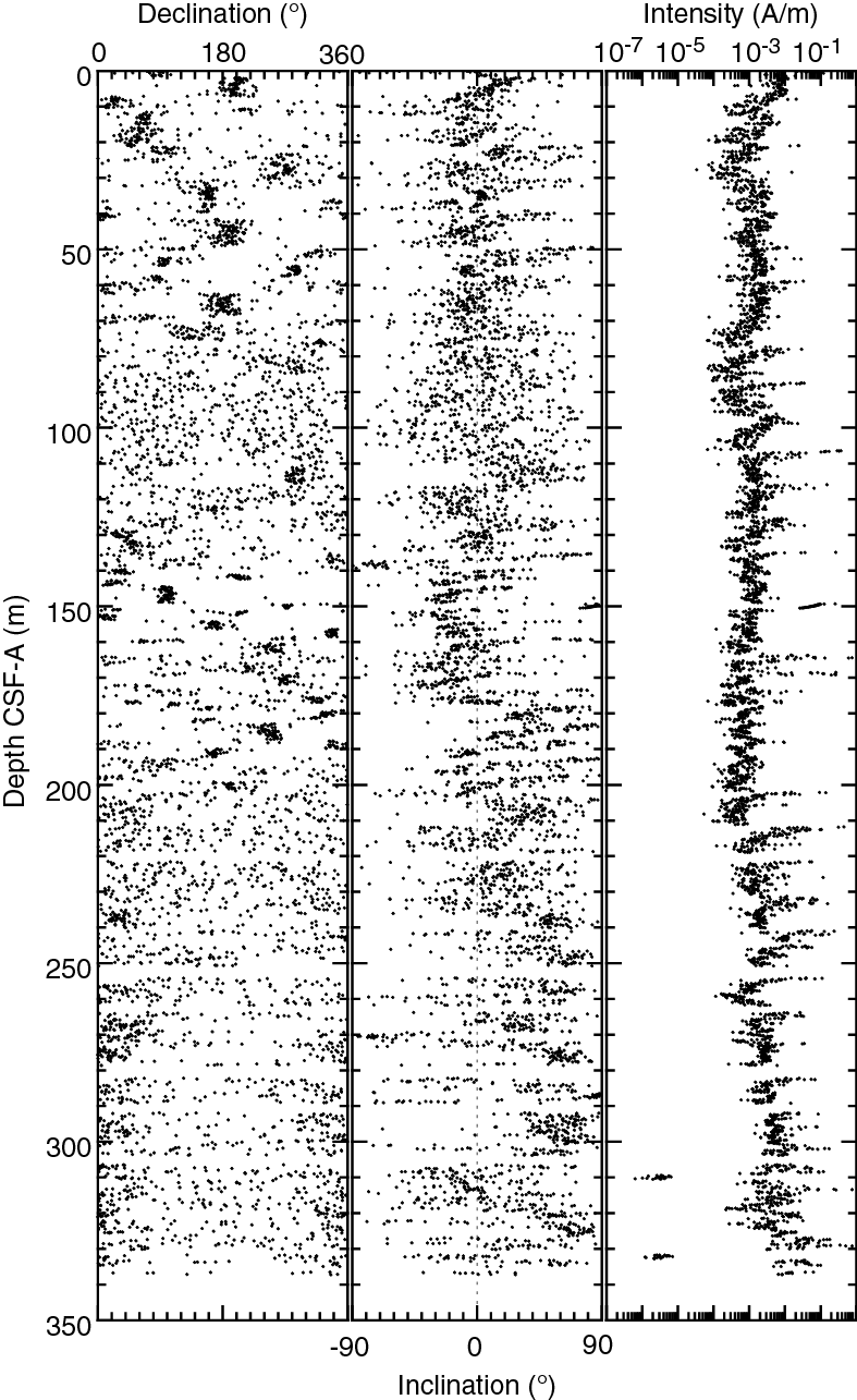
Figure F18. Archive-half paleomagnetic results, Hole U1443A after 15 mT AF demagnetization.

Figure F19. Archive-half paleomagnetic results, Hole U1443B after 10 mT AF demagnetization.
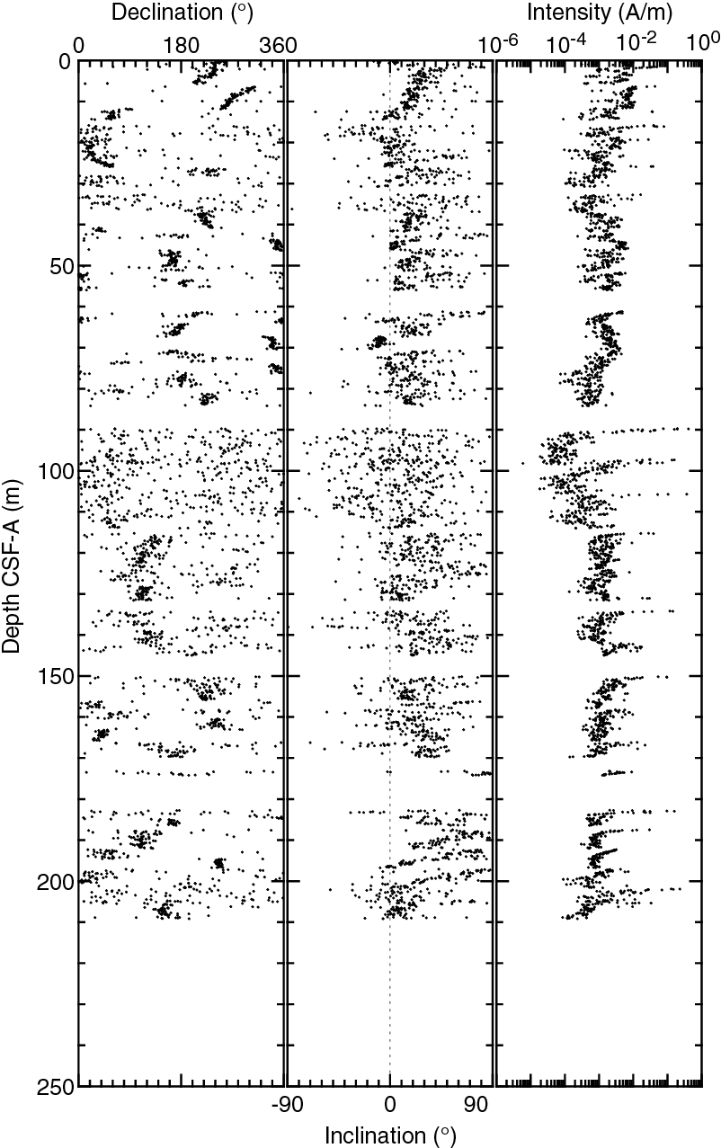
Figure F20. Archive-half paleomagnetic results, Hole U1443C after 10 mT AF demagnetization.
Table T13. Summary of ChRM for discrete samples, Hole U1443A. Download table in .csv format.
Interval 1
Sediments from the upper quarter of each hole (shallower than 70 m CSF-A for Hole U1443A, 80 m CSF-A for Hole U1443B, and 85 m CSF-A for Hole U1443C; or to Sections 353-U1443A-9H-3, 353-U1443B-9H-5, and 353-U1443C-12H-1), which covers lithostratigraphic Subunit Ia and the upper half of Subunit Ib (see Lithostratigraphy), revealed stable ChRM in both archive-half sections and discrete samples. The pass-through measurements after alternating field (AF) demagnetization to 10 or 15 mT showed declinations well grouped within any given core. Paleomagnetic polarity patterns were recovered as near-180° shifts in declination (Figures F18, F21). Orientation corrections in Holes U1443A and U1443C using data from the orientation tools successfully brought declinations into either 0° or 180°. This included the successful first run of the Icefield MI-5 tool in Cores 353-U1443C-3H through 5H. These “true” declinations were directly translated into polarity information (Figure F21). Discrete samples show clear ChRM (Figure F22), whereas the inclination of ChRM from each discrete sample also agrees with the inferred polarity patterns (Table T13).
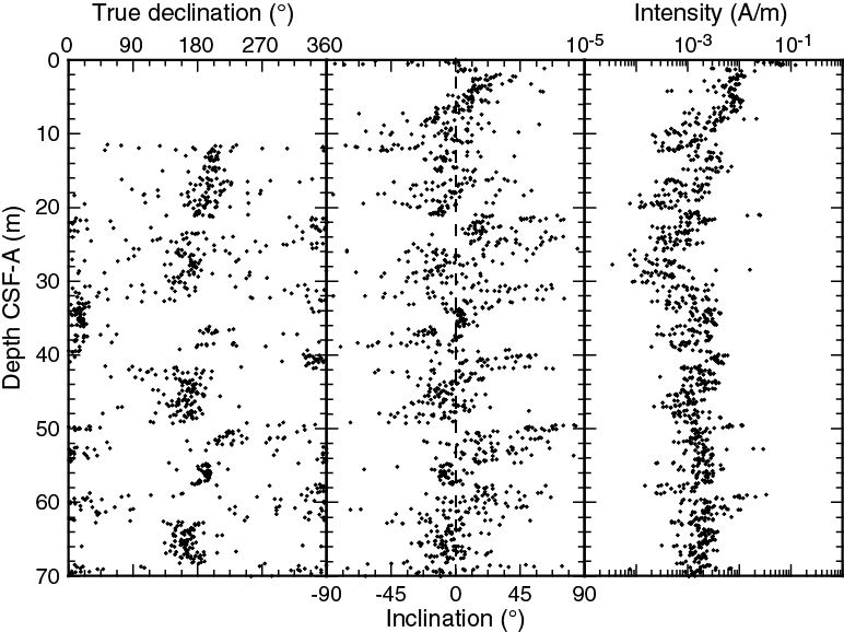
Figure F21. Archive-half paleomagnetic results for Interval 1, Hole U1443A after 15 mT AF demagnetization.
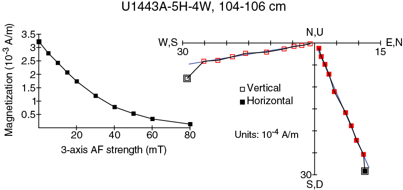
Figure F22. Representative demagnetization results of a discrete sample from Interval 1, Hole U1443A.
Interval 2
Sediments between 70 and 130 m CSF-A for Hole U1443A, 80 and 115 m CSF-A for Hole U1443B, and 85 and 115 m CSF-A for Hole U1443C (above Sections 353-U1443A-15H-4, 353-U1443B-13H-4, and 353-U1443C-16H-1), which include the lower half of the lithostratigraphic Subunit Ib and the top of Unit II, show scattered directional signals during pass-through remanence measurement (Figure F23). This scattering hinders any determination of polarity patterns within this depth or representative time interval across the whole site. Although pass-through data do not show significant changes in natural remanent magnetization (NRM) intensity, discrete sample measurements revealed low NRM intensities of <10−4 A/m. We suspect that these low intensities explain the scattered directional signals in pass-through measurements. A decrease in laboratory remanence parameters (see Rock magnetism) acquired on discrete samples in addition to high carbonate content (see Geochemistry) suggests either a decrease in the concentration of ferrimagnetic minerals and/or carbonate dilution. In contrast, however, some of the discrete samples revealed a reasonable ChRM (Figure F24). This indicates that on-shore measurements would be able to establish magnetostratigraphy for this interval. The relatively slow sedimentation rate during this interval inferred by biostratigraphy (see Biostratigraphy) suggests that high-resolution measurements (e.g., from continuous U-channel studies) would be necessary to achieve a robust magnetostratigraphy. A preceding study of Site 758 sediment could not achieve magnetostratigraphy using a measurement frequency of 2–10 discrete samples per core (Klootwijk et al., 1991).
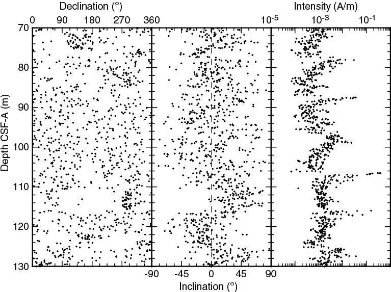
Figure F23. Archive-half paleomagnetic results for Interval 2, Hole U1443A after 15 mT AF demagnetization.
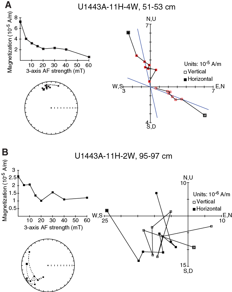
Figure F24. Representative demagnetization results of discrete samples from Interval 2, Hole U1443A.
Interval 3
Sediments between 130 and 200 m CSF-A for Hole U1443A and 115 and 215 m CSF-A for Holes U1443B and U1443C, which are within lithostratigraphic Unit II and prior to beginning XCB coring, show reasonable directional signals. Although orientation data are not available for this depth interval, declinations show near-180° shifts (Figure F25) and are interpreted as magnetic reversal records where magnetozones have been identified. Discrete samples revealed higher NRM intensities than the previous interval, and they revealed clear ChRMs (F26A) with many showing very high stability against AF demagnetization (F26B).

Figure F25. Archive-half paleomagnetic results for Interval 3, Hole U1443A after 15 mT AF demagnetization.
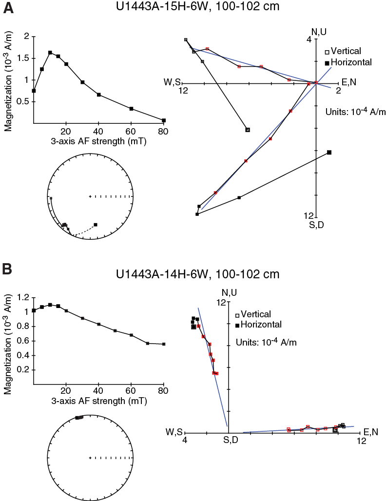
Figure F26. Representative demagnetization results of discrete samples from Interval 3, Hole U1443A.
Interval 4
All XCB cores (Holes U1443A and U1443B >200 and 210 m CSF-A, from Cores 353-U1443A-30X and 353-U1443B-29X, respectively) show either noisy or biased declinations toward 0° (360°), which was expected because of sediment disturbance caused by rotational drilling (Figure F27). Preliminary data from discrete samples indicate it may be possible to retrieve ChRM or some stable remanence component (Figure F28); however, further testing is needed to truly recover any signal.
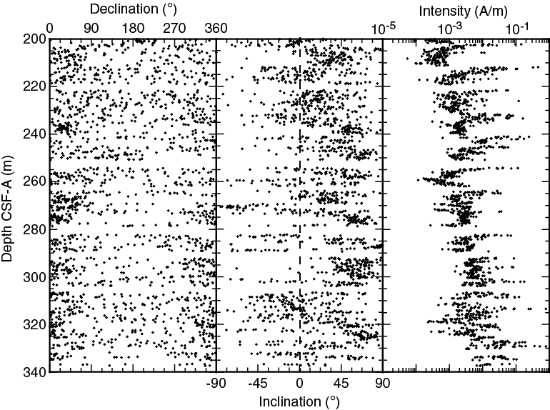
Figure F27. Archive-half paleomagnetic results for Interval 4, Hole U1443A after 15 mT AF demagnetization.
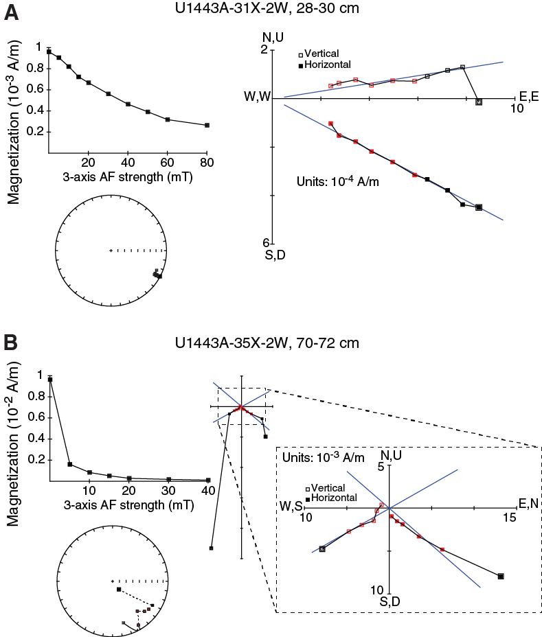
Figure F28. Representative demagnetization results of discrete samples from Interval 4, Hole U1443A.
In general, samples from Hole U1443B and parts of Hole U1443C show a larger overprint component than the samples from Hole U1443A. The overprint direction is near vertical, which is most likely due to drilling disturbance. In some cores, the topmost sections were severely disturbed during drilling, and we could not recover ChRM from those intervals.
Magnetostratigraphy
For Interval 1, we obtained continuous polarity patterns using true declination and inclination from Holes U1443A and U1443C (Figures F18, F21, F29). This polarity pattern is correlated with the geomagnetic polarity timescale (GPTS) (Gradstein et al., 2012) for the last 6 My without requiring significant change in the sedimentation rate (F29B; Table T14). For Hole U1443B, core orientation was not available and polarity was determined through correlation of magnetozone boundaries with Holes U1443A and U1443C. Hole U1443D does not show declination change; thus, the sediments were inferred to have deposited within the Brunhes Chron.
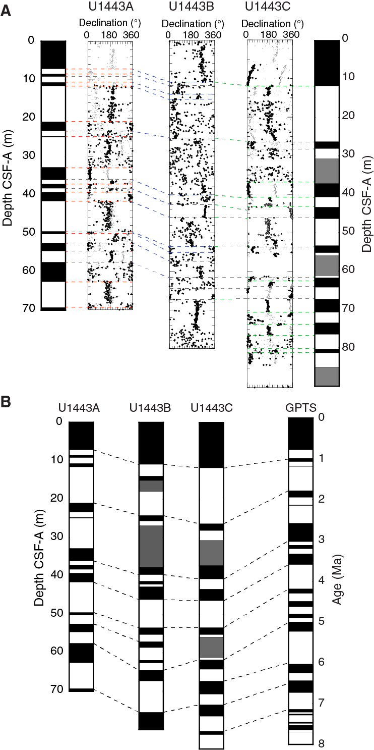
Figure F29. Magnetostratigraphy correlating magnetozones of Interval 1 to the GPTS, Site U1443.
Table T14. Summary of magnetostratigraphy for Interval 1, Holes U1443A–U1443C. Download table in .csv format.
Establishing magnetostratigraphy was more difficult within Interval 3 because of (1) the low latitude of the site, (2) the unavailability of core orientation, and (3) the short core length of HLAPC coring. We took the following steps to overcome this difficulty. First, we established magnetozones without polarity by observing the near-180° shifts in declination data from pass-through measurements on archive-half sections for Holes U1443A–U1443C using the composite depth scale provided by stratigraphic correlations (see Stratigraphic correlation). Taking the ChRM inclination from discrete samples and biostratigraphic age constraints into account, we visually correlated the inferred polarity pattern to the GPTS. Polarity chron intervals are more numerous than the biostratigraphic tie points, so ages within this depth interval are determined independently from the biostratigraphic ages (Figure F30; Table T15). However, note that there are multiple depth intervals with contradictory polarities among different holes. On-shore measurements are necessary to confirm the magnetostratigraphy proposed here.
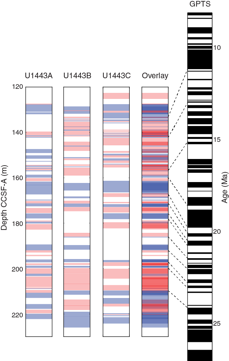
Figure F30. Magnetostratigraphy correlating magnetozones of Interval 3 to the GPTS, Site U1443.
Table T15. Summary of magnetostratigraphy for Interval 3, Holes U1443A–U1443C. Download table in .csv format.
Inclination trends and long-term motion of the Indian plate
ChRM inclinations from discrete samples in Hole U1443A are compiled in Figure F31. Inclination is close to 0° downhole to 230 m CSF-A with an occasional occurrence of large positive values, which is explained as a drilling-induced overprint. Deeper than 230 m CSF-A, inclination begins to increase and reaches around ±50° at 300 m CSF-A. Although the large positive inclination may be due to the drilling-induced overprint in XCB coring, the increasing trend of inclination magnitude with depth and the presence of negative inclinations do not fit with this explanation. Rather, the trend is best explained as recording northward motion of the Indian plate. In fact, the result is consistent with the inclination trend reported from Site 758 (Klootwijk et al., 1991).
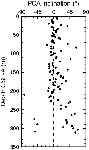
Figure F31. Downhole trend in ChRM inclination identified by discrete samples, Hole U1443A.
The correlation of our inclination trend with that of Klootwijk et al. (1991) gives an age estimate of ~53 Ma at ~230 m CSF-A and ~64 Ma at ~260 m CSF-A for sediments from Site U1443. The data scatter in both studies indicates that these numbers should be viewed as very rough estimates.
Brunhes/Matuyama boundary
The Brunhes/Matuyama (B/M) polarity boundary observed in pass-through measurements on the archive halves coincide with an ash layer situated at the bottom of light-colored sediment (Figure F32). A previous investigation using samples from Site 758 positioned the ash layer below the B/M boundary and very close to the older end of oxygen isotope Stage 19 (Hall and Farrell, 1995). On the other hand, the B/M boundary is inferred toward the young end of isotope Stage 19 based on sediment cores from elsewhere with high sedimentation rates (e.g., Channell et al., 2010). If the B/M boundary in Site U1443 is close to the ash layer, it is implied that processes such as delayed remanence lock-in have brought the apparent B/M boundary deeper than the true B/M boundary age. Because pass-through measurements suffer from signal blurring due to convolution, we examined discrete samples from Hole U1443C to better constrain the position of the B/M boundary in Site U1443.
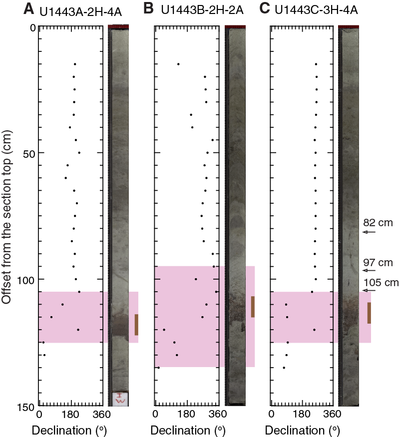
Figure F32. Section image and declination data for archive half surrounding the Brunhes/Matuyama boundary.
Discrete samples were taken from Section 353-U1443C-3H-4W at 82, 97, and 105 cm offsets (Figure F32). The upper boundary of the ash layer is found in Section 3H-4W between 108 and 118 cm offset. Stepwise AF demagnetization revealed clear ChRM for the upper two samples, with positive inclination and declination consistent with pass-through measurement of the archive-half section above the B/M boundary (Figure F33A–F33B). Sample 3H-4W, 105–107 cm offset, shows a rapid decrease in NRM intensity upon AF demagnetization. Although the sample did not yield a well-defined ChRM direction, after demagnetizing by 10 mT inclination became negative and the remanence direction moved toward a direction antiparallel to the ChRM of the other samples (Figure F33C). We interpret this observation as Sample 3H-4W, 105–107 cm, recording reversed polarity. It follows that the B/M boundary is between 97 and 105 cm of Section 3H-4W. The polarity record from discrete samples indicates that the distance between the ash layer and the B/M boundary is approximately 7–15 cm.
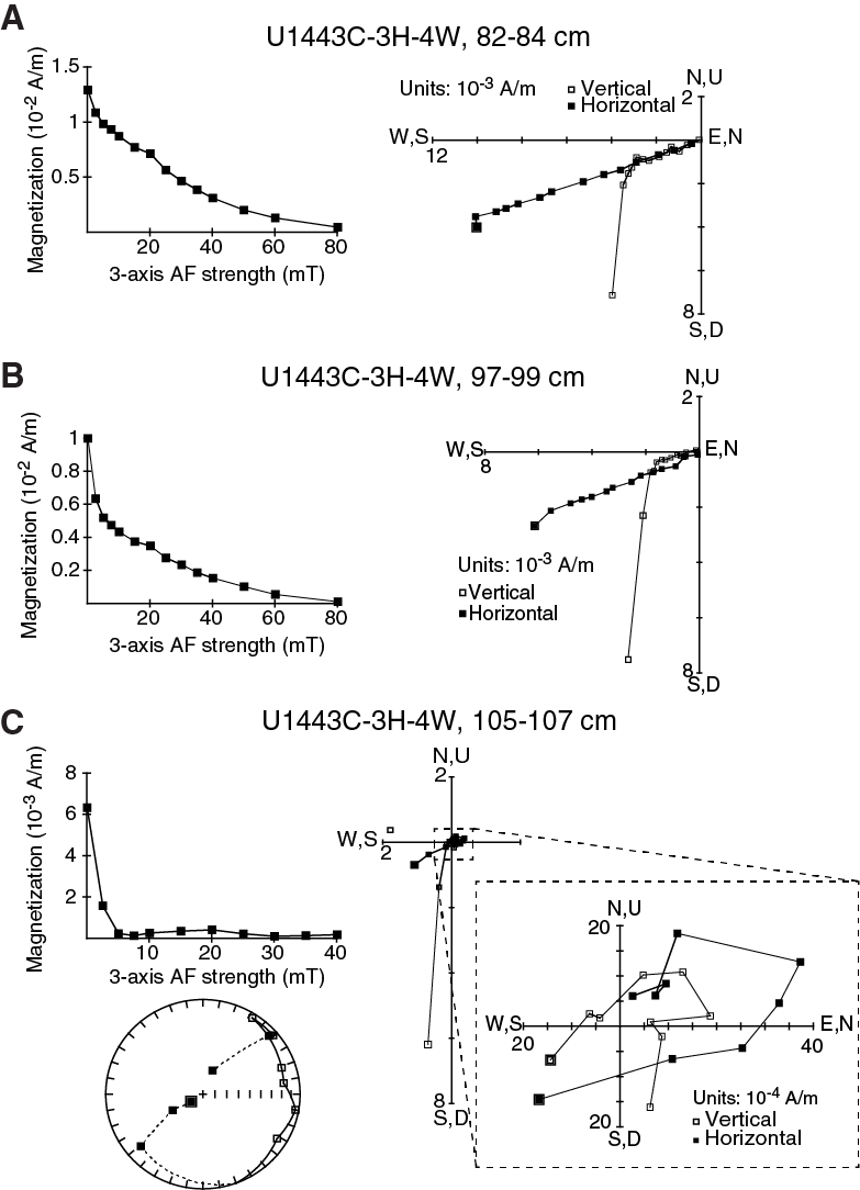
Figure F33. Demagnetization results of discrete samples, Hole U1443C.
Relative paleointensity proxy
NRM in sediments is not only related to the magnetic field strength during their deposition but also to the concentration, grain size, and mineralogy of the magnetic remanence carriers. Compensating for these variations, which are often linked to environment/climate forcing, developments have led to the construction of sedimentary relative paleomagnetic intensity (RPI) records by normalizing NRM with rock magnetic parameters. Even though the recovery of paleomagnetic information from sediments is in reality a complex problem, RPI as a proxy for paleomagnetic field change shows strong similarities across contrasting sedimentary environments (e.g., Peck et al., 1996; Guyodo and Valet, 1999; Valet et al., 2005; Yamazaki and Oda 2005). Adequate match of sediment RPI records with other independent paleomagnetic intensity reconstructions from marine magnetic anomalies (e.g., Gee et al., 2000), cosmogenic isotope records from ice cores (e.g., Muscheler et al., 2005), and sedimentary cores (Carcaillet et al., 2004) further support the validity of sedimentary RPI records. In addition, RPI records have been proven to greatly augment traditional polarity and oxygen isotope–based chronology (e.g., Channell et al., 2009), which typically provide good age constraints only at times of reversals or terminations. RPI records can potentially provide valuable high-resolution stratigraphic correlation constraints at timescales of a few millennia. For this reason, it may be possible to refine the depth/timing of particular polarity changes (which typically occur over a period of <5 ky) that may be missing or are difficult to interpret from magnetic declinations in Site U1443 sediment cores.
Because of time constraints on board the ship, preliminary tests were made only on the upper 70 m of Hole U1443A. The half-core point magnetic susceptibility (κ) (see Magnetic susceptibility) was chosen as a basic normalizing parameter. The magnetic susceptibility time series was resampled (piecewise linear interpolation) at 5 cm resolution to match the NRM measurement intervals. Figure F34 shows a selection of RPI plots with highlighted intervals where a polarity change was observed in the true declination data. We must note that the following observations/interpretations are speculative, as the method was very rudimentary due to time constraints during the expedition, and that further work is needed. A decrease in RPI is observed at these boundaries, which would be expected because the absolute field intensity during reversals often decreases to 10% of its original value. Curiously, the RPI scale here is able to show these boundaries quite clearly, although only as an initial and fairly basic construction. This suggests that the main remanence carrier is represented fairly well by magnetic susceptibility. Furthermore, constructing basic RPI timescales could be a useful method for identifying reversal boundaries and improving age determination for sedimentary successions during expeditions. For example, the B/M boundary based upon a decrease in relative paleointensity is located in Section 353-U1443A-2H-4, 105–125 cm (~7.2 m CSF-A).
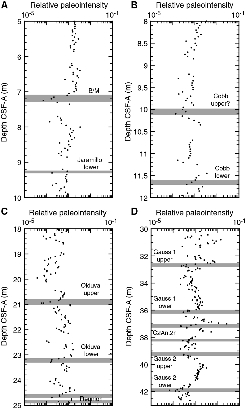
Figure F34. Relative paleointensity values across several polarity transitions, Hole U1443A sediments.
Rock magnetism
Several rock magnetic experiments were conducted on discrete samples taken from Hole U1443A (see Paleomagnetism in the Expedition 353 methods chapter [Clemens et al., 2016] for explanation). There are clear variations in the magnetic properties of sediment with depth that show some correlation to lithostratigraphy (Figure F35).
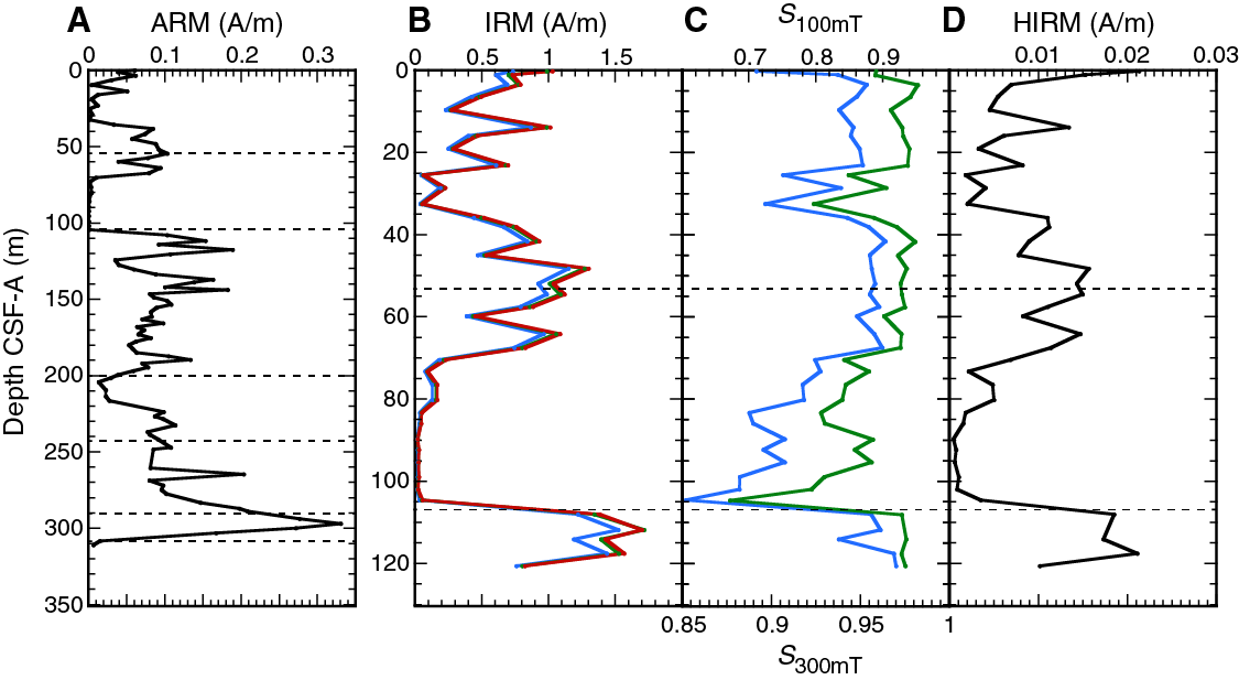
Figure F35. Depth variations in a selection of bulk magnetic parameters and ratios taken from discrete sample measurements, Hole U1443A.
Anhysteretic remanent magnetization (ARM) (Figure F35A) shows a clear minimum between ~100 and 70 m CSF-A (Subunit IB) and coincides with the most scattered magnetic declination found within Interval 2. This suggests a decrease in the relative concentration of fine-grained (single to pseudosingle domain) ferrimagnetic minerals (e.g., magnetite/maghemite) and, therefore, a weaker NRM signal. A steep peak in ARM (>0.2 A/m) is observed just deeper than ~290 m CSF-A, suggesting a significant increase in the relative concentration of fine-grained magnetite/maghemite. This peak occurs just before the Cretaceous/Paleocene boundary in the transition from clayey nannofossil chalk to calcareous chalk with clay (Subunit IIIb), and we speculate that this peak reflects an increase in terrigenous input.
Other rock magnetic parameters were measured between 0 and 120 m CSF-A, representing approximately the last ~11–12 My (see Biostratigraphy). Isothermal remanent magnetization (IRM) acquired at 100, 300, and 1000 mT (saturation isothermal remanent magnetization) (Figure F35B) all co-vary with ARM (correlation coefficient R2 = 0.84–0.87). These measurements suggest that the bulk IRM (up to 1000 mT) is largely controlled by the fine-grained magnetite/maghemite fraction. The S-ratio calculated with IRM100mT is slightly low (Figure F35C), averaging 0.84 ± 0.05 and implying that ~16% of remanence is acquired by minerals with coercivities between 100 and 1000 mT. The S-ratio calculated with IRM300mT is close to 1 (0.96 ± 0.01), meaning the bulk remanence acquired up to 1000 mT is controlled by the low-coercivity fraction, likely magnetite (representing IRM up to 100 mT) and maghemite (representing IRM between 100 and 300 mT). Therefore, the bulk magnetic properties of the mineral magnetic assemblage are principally controlled by changes in the concentration of (fine grained) magnetite/maghemite. The hard isothermal remanent magnetization (HIRM) (Figure F35D) correlates well with IRM and ARM (R2 = 0.85–0.88 and 0.73, respectively). HIRM tracks relative changes in the concentration of high-coercivity magnetic minerals (coercivities > 300 mT [e.g., hematite]). This correlation suggests that increases in both low- and high-coercivity minerals occur in tandem. However, because of near remanence saturation at 300 mT, it is probable that increases in HIRM reflect total increases in remanence rather than relative concentrations in higher coercivity minerals. Additional work is needed to decompose the true signal of any higher coercivity minerals, if they are present in significant amounts.
Generally, the variations in magnetic parameters and ratios follow the lithostratigraphic boundaries set for Hole U1443A (see Lithostratigraphy; Figure F35). Rock magnetic parameters suggest Unit I may be split into 3 “magnetic” subunits on the basis of remanence intensities. The first unit is between 69.0 and 107.8 m CSF-A where ARM and IRM intensities are low, the second unit is between 37.5 and 69.0 m CSF-A where remanence intensities are high, and the third interval is between 0 and 37.5 m CSF-A where remanence intensities are low. The remanence intensities reflect the concentrations of both magnetite/maghemite and any higher coercivity minerals present. This in turn is most likely related to the flux of terrigenous materials and levels of dissolution/alteration. With higher resolution measurements, and therefore removing any interval biasing/aliasing, the extents to which these variations relate to paleoclimate change are promising.
Physical properties
Physical property measurements were completed on whole-round sections and section halves from cores collected in Holes U1443A–U1443D. Gamma ray attenuation (GRA), MS, P-wave velocity (VP), and natural gamma radiation (NGR) measurements were made on all whole-round sections using the Special Task Multisensor Logger (STMSL), the Whole-Round Multisensor Logger (WRMSL), and the Natural Gamma Radiation Logger (NGRL). In Hole U1443A, the STMSL sampling resolution was set to 2.5 cm and WRMSL sampling resolution was set to 7.5 cm. Data duplication in Hole U1443A was done for cross-validation purposes. All sections were first logged using the STMSL (prior to thermal equilibration), generating a set of GRA and MS data. Following thermal equilibration (>19°C), the sections were logged using the WRMSL, generating VP and another set of GRA and MS data. Core sections from Holes U1443B–U1443D were run on the STMSL and WRMSL concurrently, without thermal equilibration, to speed up the acquisition of MS and GRA data for stratigraphic correlation. Sections 1, 3, 5, and 7 were run on the STMSL and Sections 2, 4, 6, and the core catchers were run on the WRMSL. After the sections thermally equilibrated to 19°–20°C, they were logged using the NGRL. Samples from the working-half sections were taken for moisture and density (MAD) measurements. In Hole U1443A, these samples were taken from Sections 2, 4, and 6. In Hole U1443C, the samples were taken from Section 2 between 0–100 and 150–209 m CSF-A. Between 100 and 150 m CSF-A, a sample was taken from every core section. Color reflectance and point MS were run on the archive-half sections using the Section Half Multisensor Logger (SHMSL). Red, green, and blue (RGB) were measured on the Section Half Imaging Logger (SHIL). Downhole temperature measurements were recorded in Hole U1443A.
Magnetic susceptibility
The MS values from the whole-round core (STMSL and WRMSL) analyses show low variability, reaching up to 40 instrument units (IU) downhole, after conditioning the data in order to remove outliers (Figure F36). The MS data from whole-round core measurements closely track point MS (SHMSL) fluctuations but with slightly lower absolute values when compared to whole-round core data. The bottom of Hole U1443A shows larger MS values reaching up to 40 IU with large variations between 242 and 341 m CSF-A with a minimum of ~2 IU at ~311 m CSF-A. This interval is overlain by an interval showing an overall decrease to lower values ranging from 0 to 12 IU between 107 and 242 m CSF-A with some intermittent large fluctuations up to 40 IU between 242 and 251 m CSF-A. We observe relatively moderate variations with a gradual increase in MS ranging from 0 to 10 IU from 0 to 107 m CSF-A. In general, higher MS values at this site are likely due to a relative increase in the concentration of strongly magnetic particles (i.e., iron-bearing minerals associated with ash layers) and/or due to a higher input of terrigenous material. Based on the MS data, we have divided Site U1443 into three physical property (PP) units (1–3). These units, as zones of distinct physical properties, can be found in all holes and in most of the physical property data sets (Table T16).
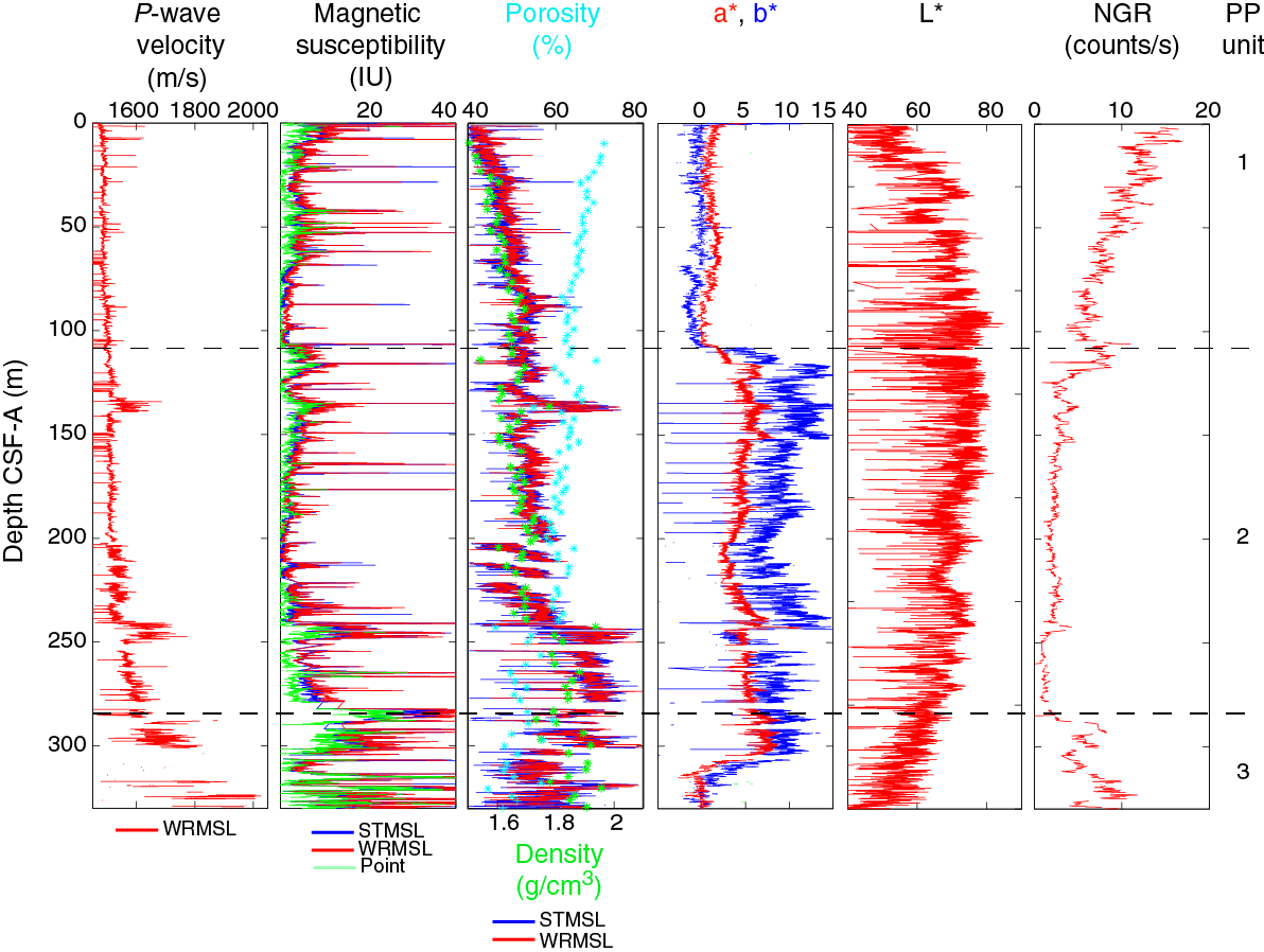
Figure F36. Physical properties including P-wave velocity, magnetic susceptibility, GRA bulk density, porosity, L*, a*, b*, and NGR, Hole U1443A.
Table T16. Physical properties units, Site U1443. Download table in .csv format.
Natural gamma radiation
NGR counts range from 0.001 to 20 counts/s and show large variations downhole (Figure F36). The variations in NGR counts represent total variation in the activity of the radioactive elements uranium, thorium, and potassium. There is generally higher total NGR counts between 291 and 341 m CSF-A ranging between 5 and 12 counts/s in PP Unit 3 followed by relatively lower NGR counts between 133 and 285 m CSF-A, ranging between 0.001 and 5 counts/s in PP Unit 2. The upper part of PP Unit 3 coincides with the lithostratigraphic Subunit IIIa/IIIb boundary (see Lithostratigraphy). PP Unit 2 follows a small peak in NGR counts between 107 and 133 m CSF-A, after which there is a gradual increase in NGR counts between 0 and 107 m CSF-A (PP Unit 1), reflecting potentially higher clay content in the sediment. The bottom of PP Unit 1 at 107 m CSF-A also coincides with the lithostratigraphic Unit I/II boundary (see Lithostratigraphy). The higher NGR counts in the bottom of the hole reflect relatively higher compaction followed by lower NGR counts because of the higher carbonate content of nannofossil ooze and chalk. The highest NGR counts at the top of Site U1443 are potentially due to the relatively higher clay content of the sediment, as is evident in the description of lithostratigraphic Unit I (see Lithostratigraphy). The NGR data set is fairly repeatable, in terms of finding three distinct units, in Holes U1443B–U1443D (Figures F37, F38, F39).

Figure F37. Physical properties including magnetic susceptibility, GRA bulk density, L*, a*, b*, and NGR, Hole U1443B.
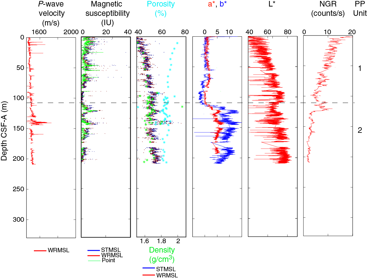
Figure F38. Physical properties including P-wave velocity, magnetic susceptibility, GRA bulk density, porosity, a*, b*, L*, and NGR, Hole U1443C.
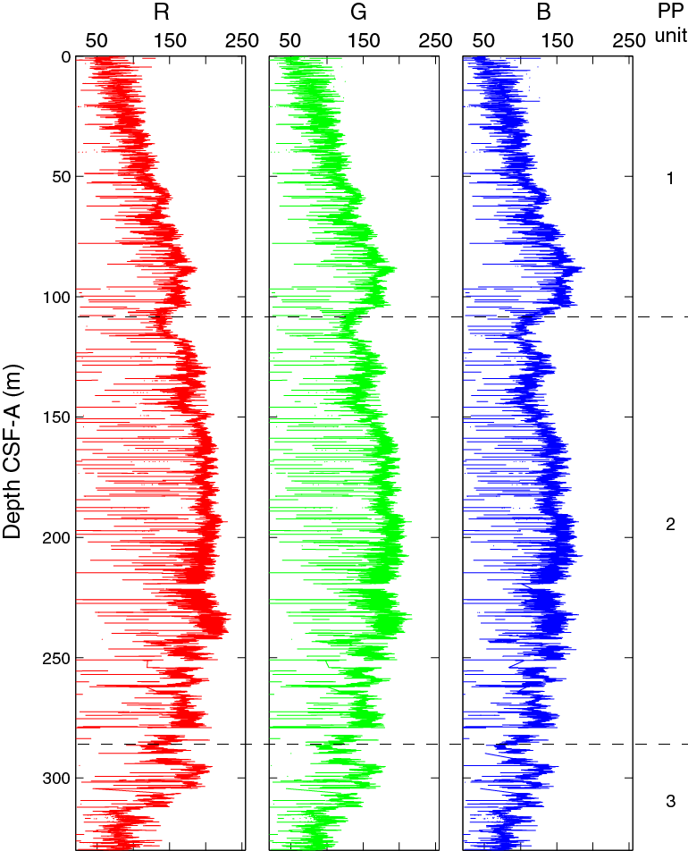
Figure F39. SHIL RGB color data, Hole U1443A.
Thermal conductivity
We attempted to collect thermal conductivity data from Sections 353-U1443A-2H-3, 3H-3, 4H-3, and 5H-3. However, we were unable to get a good reading from the instrument despite several attempts to adjust the settings. In order to save time, thermal conductivity measurements were ceased for the remainder of the expedition.
Moisture and density
Two methods were used to evaluate bulk density at Site U1443. The GRA method (described above) provided bulk density estimates from whole-round sections. MAD measurements on discrete samples provided a second, independent measure of bulk density and measurements of dry density, grain density, water content, and porosity. Changes in MAD and GRA bulk density values are well correlated throughout the sections (Figure F36). The mean MAD bulk density is 1.686 (bulk) and 2.716 g/cm3 (grain), similar to the GRA bulk density values that vary from 1.5 to 2.1 g/cm3. Grain density varies between 2.597 and 2.906 g/cm3. In general, density is higher with larger fluctuations between 242 and 341 m CSF-A, averaging 1.9 g/cm3 before decreasing sharply to 1.66 g/cm3 at ~238 m CSF-A. Values decrease gradually to 1.47–1.55 g/cm3 between 0 and 133 m CSF-A.
Overall, the porosity profile shows a gradually decreasing trend downhole with small intermittent variations (Figure F36). Porosity varies between 42.7% and 76.1%. The porosity data for Hole U1443C are also in good agreement with Hole U1443A (Figures F36, F38).
Compressional wave velocity
Compressional P-wave velocity measurements using the P-wave logger (PWL) were performed on whole-round sections for Holes U1443A and U1443C. Discrete compressional wave velocity measurements were conducted using the P-wave caliper (PWC) contact probe system on the working halves of selected core sections. The PWC data were found to be very unreliable because of the soft nature of the nannofossil ooze. The PWL data range between 1460 and 2000 m/s downhole (Figure F36). P-wave velocity values decrease from the highest value of ~2000 m/s at 341 m CSF-A to ~1530 m/s at 241 m CSF-A. We observe an increase in velocity between 241 and 249 m CSF-A, averaging ~1650 m/s. The P-wave velocity values gradually decrease, averaging ~1515 m/s between 133 and 241 m CSF-A, with intermittent smaller anomalies related to sediment compositional changes. PP Unit 1 between 0 and 107 m CSF-A shows a very slight decrease in P-wave velocity and coincides with the same unit from density at this site. P-wave velocity boundary units in Holes U1443A and U1443C are in good agreement with boundary units derived from density at this site (Figure F38).
Diffuse reflectance spectroscopy and digital color image
Spectral reflectance was measured on archive halves from all holes at Site U1443 using the SHMSL. L* ranges between 40 and 82 and is highly variable (Figure F36). Reflectance a* and b* values show ranges between −0.35 and 10 and −3 and 18, respectively. High-resolution cyclicities are observed in the color reflectance data, but they are not conformable with lithostratigraphic unit boundaries (see Lithostratigraphy). There is a step change in b* and a* data showing an increase at ~242 m CSF-A. The second step change is a decrease in b* and a* data at ~107 m CSF-A, which correlates with an increase in the L* data in Hole U1443A. The color reflectance change is due to compositional changes (e.g., at this site higher a*, b*, and L* data suggest increased concentration of nannofossil ooze, whereas lower values reflect relatively higher clay concentrations in PP Unit 1 and the presence of darker sediments in PP Unit 3). Spectral reflectance data from Holes U1443B–U1443C are very similar to data from Hole U1443A.
The SHIL obtained records of RGB color from the moist surface of the archive half. The RGB data have an average range of R = 78, G = 84, and B = 83 between 316 and 334 m CSF-A (Figure F39). The RGB index increases to a mean value of approximately R = 170, G = 168, and B = 130 between 115 and 296 m CSF-A with intermittent step variations within this interval. There is a gradual change in RGB data values from 0 to 90 m CSF-A with RGB data of approximately R = 160, G = 170, and B = 164 decreasing to R = 62, G = 55, and B = 40. The RGB data broadly correspond with the color reflectance data. The data for Holes U1443B and U1443C are plotted in Figures F40 and F41.
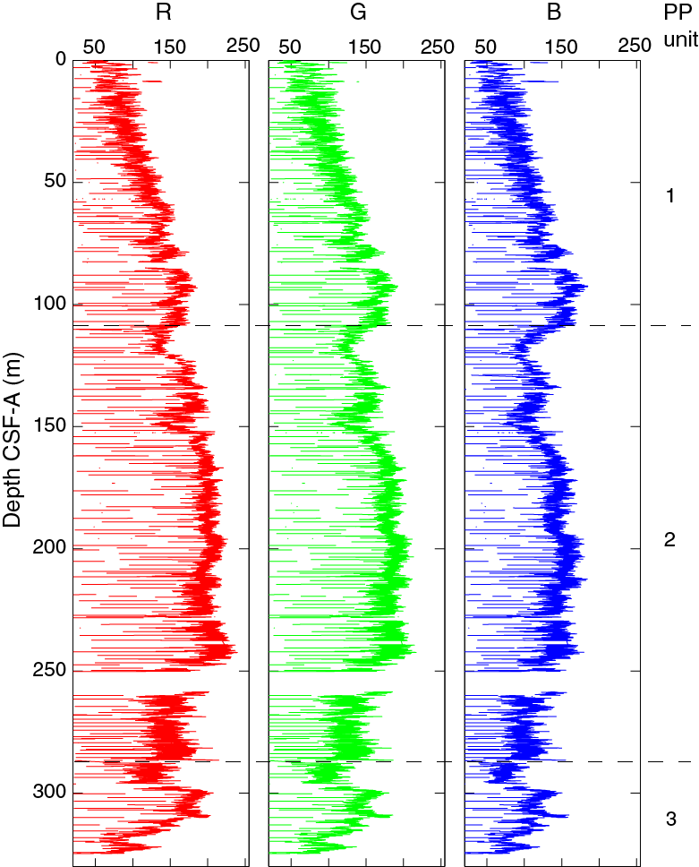
Figure F40. SHIL RGB color data, Hole U1443B.
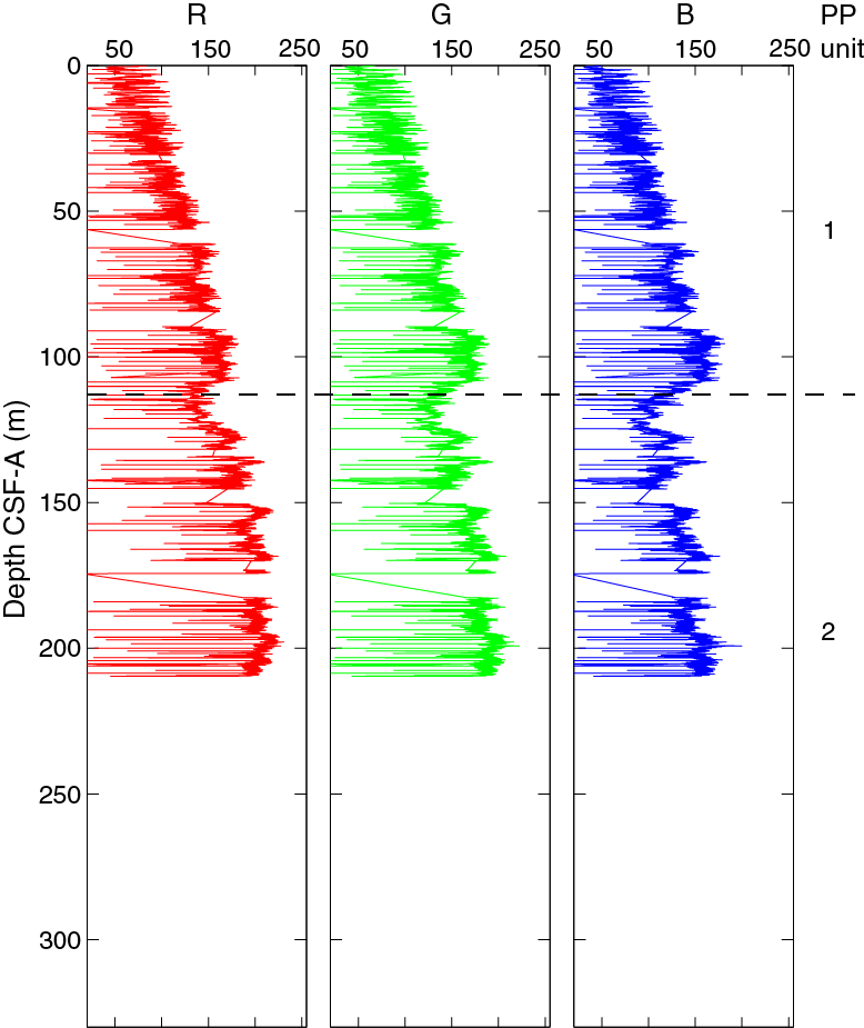
Figure F41. SHIL RGB color data, Hole U1443C.
Downhole temperature
In Hole U1443A, downhole temperature measurements were recorded for Cores 353-U1443A-4H, 7H, 10H, and 13H. The downhole temperature profile shows linear variation starting at 3.26°C at 30 m CSF-A to 7.36°C at 115.5 m CSF-A (Table T17). The overall geothermal gradient is 48.23°C/km (Figure F42).
Table T17. Downhole temperature measurements from the APCT-3, Site U1443. Download table in .csv format.
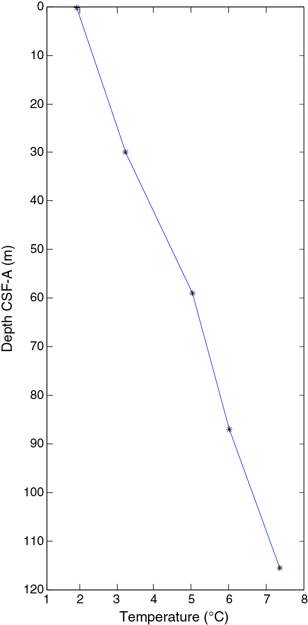
Figure F42. Downhole temperature measurements, Hole U1443A.
Summary
Overall, the physical property data collected at Site U1443 were found to be in good agreement with the lithostratigraphic data (see Lithostratigraphy). Data from the whole-round measurements are in good agreement with the split core measurements. The NGR counts and color reflectance data suggest the presence of darker and compacted sediments at the bottom of the hole, followed by the presence of lighter sediments (nannofossil ooze) in the middle section and sediments with higher clay content at the top of the section. The density, MS, and P-wave velocity data are in general agreement, displaying changes in sediment composition and/or depositional processes in the marine environment. In general, based on physical property characteristics, this site can be divided into three broad PP units, but their boundaries do not necessarily correspond with the lithostratigraphic boundaries. These differences in physical property boundaries are mainly due to the change in sediment lithology and/or secondary postdepositional processes at Site U1443. We observe an overall geothermal gradient in Hole U1443A of 48.23°C/km.
Stratigraphic correlation
A composite scale (CCSF-A) and a splice (CCSF-D) were constructed for Site U1443 using Holes U1443A–U1443C (as defined in Stratigraphic correlation in the Expedition 353 methods chapter [Clemens et al., 2016]). Splicing among these holes enabled us to construct a continuous stratigraphic sequence to ~195 m CCSF-D (Tables T18, T19; Figure F43).
Table T18. Vertical offsets applied to cores in order to align structure in adjacent holes, Site U1443. Download table in .csv format.
Table T19. Splice intervals, Site U1443. Download table in .csv format.
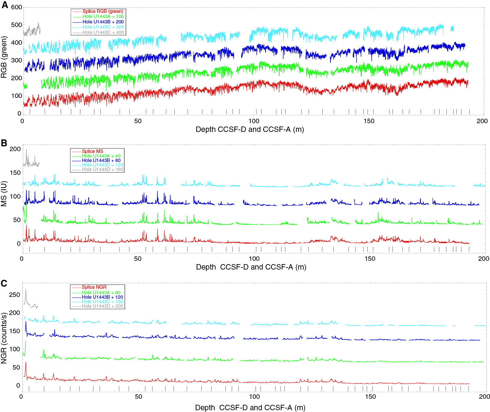
Figure F43. Core alignment exemplified using RGB green, NGR, and MS profiles, Holes U1443A–U1443C.
Construction of CCSF-A scale
We selected the core with the best mudline recovery (Core 353-U1443D-1F) to anchor the composite depth scale and defined the top as 0 m CCSF-A. The CCSF-A scale for Site U1443 (see Table T18) is based on correlation of RGB color data and secondarily on MS, NGR, and reflectance spectroscopy b* data. RGB green color was primarily used in correlations for Site U1443. MS and NGR were measured on whole-round sections, whereas green was measured on archive-half sections (see Physical properties for details). The remaining red and blue components of the RGB triplet are highly correlated to green and to each other because, on the first order, all are measures of the reflectivity of the sediment. The small differences between R, G, and B can be expressed as ratios such as red/green, red/blue, or green/blue. However, ratios were not employed in our correlation due to lack of time (see the Expedition 353 methods chapter [Clemens et al., 2016]).
Construction of CCSF-D scale
A combination of Holes U1443A, U1443B, U1443C, and U1443D cover the stratigraphic section to ~195 m CCSF-D. When constructing the splice, we tried to minimize inclusion of disturbed intervals and avoid whole-round sampling intervals (notably from Hole U1443A) as much as possible. Selected splice intervals are listed in Table T19. Postcruise, the splice interval tables were modified using the Splice-File-Fixer program to ensure that each depth has been assigned the correct sample ID. Both the affine and the corrected splice interval tables were uploaded into the Laboratory Information Management System (LIMS) database during the first postcruise meeting in June 2015. The core top depths in the affine tables were not corrected and hence may be slightly incorrect in a range of <2 cm. However, the offsets are correct.
Reliance on RGB, which sometimes has fuzzy character due to cracks and defects of the split core surface, precluded, in places, the definition of unique correlations. Features and general trends were used instead, reducing the accuracy of the splice to the decimeter range. As a result, correlation should be viewed with caution deeper than ~175 m CCSF-A, notably if high-resolution sampling is planned. Onshore X-ray fluorescence scanning, color reflectance rescanning, and bulk δ18O should provide better means of correlation.
References
Baker, P.A., Gieskes, J.M., and Elderfield, H., 1982. Diagenesis of carbonates in deep-sea sediments: evidence from Sr/Ca ratios and interstitial dissolved Sr2+ data. Journal of Sedimentary Research, 52(1):71–82. http://dx.doi.org/10.1306/212F7EE1-2B24-11D7-8648000102C1865D
Bolton, C.T., Chang, L., Clemens, S.C., Kodama, K., Ikehara, M., Medina-Elizalde, M., Paterson, G.A., Roberts, A.P., Rohling, E.J., Yamamoto, Y., and Zhao, X., 2013. A 500,000 year record of Indian summer monsoon dynamics recorded by eastern equatorial Indian Ocean upper water-column structure. Quaternary Science Reviews, 77:167–180. http://dx.doi.org/10.1016/j.quascirev.2013.07.031
Bown, P.R., 2005. Palaeogene calcareous microfossils from the Kilwa and Lindi areas of coastal Tanzania (Tanzania Drilling Project 2003–4). Journal of Nannoplankton Research, 27(1):21–95.
Burton, K.W., Gannoun, A., and Parkinson, I.J., 2010. Climate driven glacial–interglacial variations in the osmium isotope composition of seawater recorded by planktic foraminifera. Earth and Planetary Science Letters, 295(1–2):58–68. http://dx.doi.org/10.1016/j.epsl.2010.03.026
Burton, K.W., and Vance, D., 2000. Glacial–interglacial variations in the neodymium isotope composition of seawater in the Bay of Bengal recorded by planktonic foraminifera. Earth and Planetary Science Letters, 176(3–4):425–441. http://dx.doi.org/10.1016/S0012-821X(00)00011-X
Carcaillet, J., Bourlès. D.L., Thouveny, N., and Arnold, M., 2004. A high resolution authigenic 10Be/9Be record of geomagnetic moment variations over the last 300 ka from sedimentary cores of the Portuguese margin. Earth and Planetary Science Letters, 219(3–4):397–412. http://dx.doi.org/10.1016/S0012-821X(03)00702-7
Channell, J.E.T., Hodell, D.A., Singer, B.S., and Xuan, C., 2010. Reconciling astrochronological and 40Ar/39Ar ages for the Matuyama-Brunhes boundary and late Matuyama Chron. Geochemistry, Geophysics, Geosystems, 11(12):Q0AA12. http://dx.doi.org/10.1029/2010GC003203
Channell, J.E.T., Xuan, C., and Hodell, D.A., 2009. Stacking paleointensity and oxygen isotope data for the last 1.5 Myr (PISO-1500). Earth and Planetary Science Letters, 283(1–4):14–23. http://dx.doi.org/10.1016/j.epsl.2009.03.012
Chen, J., Farrell, J.W., Murray, D.W., and Prell, W.L., 1995. Timescale and paleoceanographic implications of a 3.6 m.y. oxygen isotope record from the northeast Indian Ocean (Ocean Drilling Program Site 758). Paleoceanography, 10(1):21–48. http://dx.doi.org/10.1029/94PA02290
Clemens, S.C., Farrell, J.W., and Gromet, L.P., 1993. Synchronous changes in seawater strontium isotope composition and global climate. Nature, 363(6430):607–610. http://dx.doi.org/10.1038/363607a0
Clemens, S.C., Kuhnt, W., LeVay, L.J., Anand, P., Ando, T., Bartol, M., Bolton, C.T., Ding, X., Gariboldi, K., Giosan, L., Hathorne, E.C., Huang, Y., Jaiswal, P., Kim, S., Kirkpatrick, J.B., Littler, K., Marino, G., Martinez, P., Naik, D., Peketi, A., Phillips, S.C., Robinson, M.M., Romero, O.E., Sagar, N., Taladay, K.B., Taylor, S.N., Thirumalai, K., Uramoto, G., Usui, Y., Wang, J., Yamamoto, M., and Zhou, L., 2016. Expedition 353 methods. In Clemens, S.C., Kuhnt, W., LeVay, L.J., and the Expedition 353 Scientists, Indian Monsoon Rainfall. Proceedings of the International Ocean Discovery Program, 353: College Station, TX (International Ocean Discovery Program). http://dx.doi.org/10.14379/iodp.proc.353.102.2016
Clift, P.D., Hodges, K.V., Heslop, D., Hannigan, R., Long, H.V., and Calves, G., 2008. Correlation of Himalayan exhumation rates and Asian monsoon intensity. Nature Geoscience, 1(12):875–880. http://dx.doi.org/10.1038/ngeo351
Clift, P.D., and Plumb, R.A., 2008. The Asian Monsoon: Causes, History and Effects: Cambridge, United Kingdom (Cambridge University Press). http://dx.doi.org/10.1017/CBO9780511535833
Dehn, J., Farrell, J.W., and Schmincke, H.-U., 1991. Neogene tephrochronology from Site 758 on northern Ninetyeast Ridge: Indonesian arc volcanism of the past 5 Ma. In Weissel, J., Peirce, J., Taylor, E., Alt, J., et al., Proceedings of the Ocean Drilling Program, Scientific Results, 121: College Station, TX (Ocean Drilling Program), 273–295. http://dx.doi.org/10.2973/odp.proc.sr.121.123.1991
Expedition 342 Scientists, 2012. Expedition 342 Preliminary Report: Paleogene Newfoundland Sediment Drifts. Integrated Ocean Drilling Program. http://dx.doi.org/10.2204/iodp.pr.342.2012
Farrell, J.W., and Janecek, T.R., 1991. Late Neogene paleoceanography and paleoclimatology of the northeast Indian Ocean (Site 758). In Weissel, J., Peirce, J., Taylor, E., Alt, J., et al., Proceedings of the Ocean Drilling Program, Scientific Results, 121: College Station, TX (Ocean Drilling Program), 297–355. http://dx.doi.org/10.2973/odp.proc.sr.121.124.1991
Gee, J.S., Cande, S.C., Hildebrand, J.A., Donnelly, K., and Parker, R.L., 2000. Geomagnetic intensity variations over the past 780 kyr obtained from near-seafloor magnetic anomalies. Nature, 408(6814):827–832. http://dx.doi.org/10.1038/35048513
Gieskes, J.M., 1981. Deep-sea drilling interstitial water studies: implications for chemical alteration of the oceanic crust, Layers I and II. In Warme, J.E., Douglas, R.G., and Winterer, E.L. (Eds.), The Deep Sea Drilling Project: A Decade of Progress. Special Publication - Society of Economic Paleontologists and Mineralogists, 32:149–167. http://archives.datapages.com/data/sepm_sp/SP32/Deep_Sea_Drilling_Interstitial_Water_Studies.html
Gourlan, A.T., Meynadier, L., and Allègre, C.J., 2008. Tectonically driven changes in the Indian Ocean circulation over the last 25 Ma: neodymium isotope evidence. Earth and Planetary Science Letters, 267(1–2):353–364. http://dx.doi.org/10.1016/j.epsl.2007.11.054
Gourlan, A.T., Meynadier, L., Allègre, C.J., Tapponnier, P., Birck, J.-L., and Joron, J.-L., 2010. Northern hemisphere climate control of the Bengali rivers discharge during the past 4 Ma. Quaternary Science Reviews, 29(19–20):2484–2498. http://dx.doi.org/10.1016/j.quascirev.2010.05.003
Gradstein, F.M., Ogg, J.G., Schmitz, M.D., and Ogg, G.M. (Eds.), 2012. The Geological Time Scale 2012: Amsterdam (Elsevier).
Gupta, A.K., Singh, R.K., Joseph, S., and Thomas, E., 2004. Indian Ocean high-productivity event (10–8 Ma): linked to global cooling or to the initiation of the Indian monsoons? Geology, 32(9):753–756. http://dx.doi.org/10.1130/G20662.1
Gupta, A.K., and Thomas, E., 2003. Initiation of Northern Hemisphere glaciation and strengthening of the northeast Indian monsoon: Ocean Drilling Program Site 758, eastern equatorial Indian Ocean. Geology, 31(1):47–50. http://dx.doi.org/10.1130/0091-7613(2003)031<0047:IONHGA>2.0.CO;2
Guyodo, Y., and Valet, J.-P., 1999. Global changes in intensity of the Earth’s magnetic field during the past 800 kyr. Nature, 399(6733):249–252. http://dx.doi.org/10.1038/20420
Hall, C.M., and Farrell, J.W., 1995. Laser 40Ar/39Ar ages of tephra from Indian Ocean deep-sea sediments: tie points for the astronomical and geomagnetic polarity time scales. Earth and Planetary Science Letters, 133(3–4):327–338. http://dx.doi.org/10.1016/0012-821X(95)00087-S
Hasle, G.R., and Syvertsen, E.E., 1996. Marine diatoms. In Tomas, C.R. (Ed.), Identifying Marine Diatoms and Dinoflagellates: San Diego (Academic Press), 5–385. http://dx.doi.org/10.1016/B978-012693015-3/50005-X
Henderson, G.M., Martel, D.J., O’Nions, R.K., and Shackleton, N.J., 1994. Evolution of seawater 87Sr/86Sr over the last 400 ka: the absence of glacial/interglacial cycles. Earth and Planetary Science Letters, 128(3–4):643–651. http://dx.doi.org/10.1016/0012-821X(94)90176-7
Hoogakker, B.A.A., Rohling, E.J., Palmer, M.R., Tyrrell, T., and Rothwell, R.G., 2006. Underlying causes for long-term global ocean δ13C fluctuations over the last 1.20 Myr. Earth and Planetary Science Letters, 248(1–2):15–29. http://dx.doi.org/10.1016/j.epsl.2006.05.007
Hovan, S., and Rea, D.K., 1992. The Cenozoic record of continental mineral deposition on Broken and Ninetyeast Ridges, Indian Ocean: southern African aridity and sediment delivery from the Himalayas. Paleoceanography, 7(6):833–860. http://dx.doi.org/10.1029/92PA02176
Klootwijk, C.T., Gee, J.S., Peirce, J.W., and Smith, G.M., 1991. Constraints on the India-Asia convergence: paleomagnetic results from Ninetyeast Ridge. In Weissel, J., Peirce, J., Taylor, E., Alt, J., et al., Proceedings of the Ocean Drilling Program, Scientific Results, 121: College Station, TX (Ocean Drilling Program), 777–882. http://dx.doi.org/10.2973/odp.proc.sr.121.121.1991
Kroon, D., Steens, T., and Troelstra, S.R., 1991. Onset of monsoonal related upwelling in the western Arabian Sea as revealed by planktonic foraminifers. In Prell, W.L., Niitsuma, N., et al., Proceedings of the Ocean Drilling Program, Scientific Results, 117: College Station, TX (Ocean Drilling Program), 257–263. http://dx.doi.org/10.2973/odp.proc.sr.117.126.1991
Langmann, B., Zakšek, K., Hort, M., and Duggen, S., 2010. Volcanic ash as fertiliser for the surface ocean. Atmospheric Chemistry and Physics, 10(8):3891–3899. http://dx.doi.org/10.5194/acp-10-3891-2010
Le Houedec, S., Meynadier, L., Cogné, J.-P., Allègre, C.J., and Gourlan, A.T., 2012. Oceanwide imprint of large tectonic and oceanic events on seawater Nd isotope composition in the Indian Ocean from 90 to 40 Ma. Geochemistry, Geophysics, Geosystems, 13(6):Q06008. http://dx.doi.org/10.1029/2011GC003963
Licht, A., van Cappelle, M., Abels, H.A., Ladant, J.-B., Trabucho-Alexandre, J., France-Lanord, C., Donnadieu, Y., Vandenberghe, J., Rigaudier, T., Lécuyer, C., Terry, D., Jr., Adriaens, R., Boura, A., Guo, Z., Soe, A.N., Quade, J., Dupont-Nivet, G., and Jaeger, J.-J., 2014. Asian monsoons in a late Eocene greenhouse world. Nature, 513(7519):501–506. http://dx.doi.org/10.1038/nature13704
Lisiecki, L.E., and Raymo, M.E., 2005. A Pliocene–Pleistocene stack of 57 globally distributed benthic δ18O records. Paleoceanography, 20(1):PA1003. http://dx.doi.org/10.1029/2004PA001071
Martini, E., 1971. Standard Tertiary and Quaternary calcareous nannoplankton zonation. In Farinacci, A. (Ed.), Proceedings of the Second Planktonic Conference, Roma 1970: Rome (Edizioni Tecnoscienza), 2:739–785.
McArthur, J.M., Rio, D., Massari, F., Castradori, D., Bailey, T.R., Thirlwall, M., and Houghton, S., 2006. A revised Pliocene record for marine-87Sr/86Sr used to date an interglacial event recorded in the Cockburn Island Formation, Antarctic Peninsula. Palaeogeography, Palaeoclimatology, Palaeoecology, 242(1–2):126–136. http://dx.doi.org/10.1016/j.palaeo.2006.06.004
Misra, S., and Froelich, P.N., 2012. Lithium isotope history of Cenozoic seawater: changes in silicate weathering and reverse weathering. Science, 335(6070):818–823. http://dx.doi.org/10.1126/science.1214697
Mudelsee , M., and Raymo, M.E., 2005. Slow dynamics of the Northern Hemisphere glaciation. Paleoceanography, 20(4):PA4022. http://dx.doi.org/10.1029/2005PA001153
Muscheler, R., Beer, J., Kubik, P.W., and Synal, H.-A., 2005. Geomagnetic field intensity during the last 60,000 years based on 10Be and 36Cl from the Summit ice cores and 14C. Quaternary Science Reviews, 24(16–17):1849–1860. http://dx.doi.org/10.1016/j.quascirev.2005.01.012
Okada, H., and Bukry, D., 1980. Supplementary modification and introduction of code numbers to the low-latitude coccolith biostratigraphic zonation (Bukry, 1973; 1975). Marine Micropaleontology, 5:321–325. http://dx.doi.org/10.1016/0377-8398(80)90016-X
Pearson, P.N., Ditchfield, P.W., Singano, J., Harcourt-Brown, K.G., Nicholas, C.J., Olsson, R.K., Shackleton, N.J., and Hall, M.A., 2001. Warm tropical sea surface temperatures in the Late Cretaceous and Eocene epochs. Nature, 413(6855):481–487. http://dx.doi.org/10.1038/35097000
Peck, J.A., King, J.W., Colman, S.M., and Kravchinsky, V.A., 1996. An 84-kyr paleomagnetic record from the sediments of Lake Baikal, Siberia. Journal of Geophysical Research: Solid Earth, 101(B5):11365–11385. http://dx.doi.org/10.1029/96JB00328
Quade, J., Cerling, T.E., and Bowman, J.R., 1989. Development of Asian monsoon revealed by marked ecological shift during the latest Miocene in northern Pakistan. Nature, 342(6246):163–166. http://dx.doi.org/10.1038/342163a0
Romero, O.E., and Armand, L.K., 2010. Marine diatoms as indicators of modern changes in oceanographic conditions. In Smol, J.P., and Stoermer, E.F. (Eds.), The Diatoms: Applications for the Environmental and Earth Sciences (2nd edition): Cambridge, United Kingdom (Cambridge University Press), 373–400.
Shipboard Scientific Party, 1989a. Leg 121 background and objectives. In Peirce, J., Weissel, J., et al., Proceedings of the Ocean Drilling Program, Initial Reports, 121: College Station, TX (Ocean Drilling Program), 5–31. http://dx.doi.org/:10.2973/odp.proc.ir.121.101.1989
Shipboard Scientific Party, 1989b. Site 758. In Peirce, J., Weissel, J., et al., Proceedings of the Ocean Drilling Program, Initial Reports, 121: College Station, TX (Ocean Drilling Program), 359–453. http://dx.doi.org/:10.2973/odp.proc.ir.121.112.1989
Shipboard Scientific Party, 2007. Cruise report KNOX06RR (R/V Roger Revelle, 6/18–8/06, Phuket to Singapore). http://www.marine-geo.org/link/data/field/Revelle/KNOX06RR/docs/KNOX06RR_CruiseRept.pdf
Sissingh, W. 1977. Biostratigraphy of Cretaceous calcareous nannoplankton. Geologie en Mijnbouw, 57:433–440.
Stoll, H.M., Vance, D., and Arevalos, A., 2007. Records of the Nd isotope composition of seawater from the Bay of Bengal: implications for the impact of Northern Hemisphere cooling on ITCZ movement. Earth and Planetary Science Letters, 255(1–2):213–228. http://dx.doi.org/10.1016/j.epsl.2006.12.016
Valet, J.-P., Meynadier, L., and Guyodo, Y., 2005. Geomagnetic dipole strength and reversal rate over the past two million years. Nature, 435(7043):802–805. http://dx.doi.org/10.1038/nature03674
Yamazaki, T., and Oda, H., 2005. A geomagnetic paleointensity stack between 0.8 and 3.0 Ma from equatorial Pacific sediment cores. Geochemistry, Geophysics, Geosystems, 6(11):Q11H20. http://dx.doi.org/10.1029/2005GC001001
1Clemens, S.C., Kuhnt, W., LeVay, L.J., Anand, P., Ando, T., Bartol, M., Bolton, C.T., Ding, X., Gariboldi, K., Giosan, L., Hathorne, E.C., Huang, Y., Jaiswal, P., Kim, S., Kirkpatrick, J.B., Littler, K., Marino, G., Martinez, P., Naik, D., Peketi, A., Phillips, S.C., Robinson, M.M., Romero, O.E., Sagar, N., Taladay, K.B., Taylor, S.N., Thirumalai, K., Uramoto, G., Usui, Y., Wang, J., Yamamoto, M., and Zhou, L., 2016. SiteU1443. In Clemens, S.C., Kuhnt, W., LeVay, L.J., and the Expedition 353 Scientists, Indian Monsoon Rainfall. Proceedings of the International Ocean Discovery Program, 353: College Station, TX (International Ocean Discovery Program). http://dx.doi.org/10.14379/iodp.proc.353.103.2016
- F1. Location of Site U1443 on the northern Ninetyeast Ridge.
- F2. Seismic Lines ar55.0881.knox06rr and ar55.0885.knox06rr of the seismic reflection survey carried out by the Roger Revelle in 2007 with the position of Site U1443.
- F3. Position of Site U1443 on seismic Lines ar55.0881.knox06rr and ar55.0885.knox06rr with depth of reflectors at Sites U1443 and 758.
- F4. Lithostratigraphic summary, Site U1443.
- F5. Lithostratigraphic summary with selected physical property and geochemical data from Holes U1443A–U1443C plotted against depth.
- F6. Smear slide data, Holes U1443A and U1443B.
- F7. Major lithologies: A. Clayey nannofossil ooze. B. Nannofossil ooze with authigenic carbonate. C. Nannofossil ooze. D. Nannofossil chalk. E. Transition from clayey nannofossil chalk to authigenic carbonate-rich nannofossil chalk. F. Marlstone with glauconite.
- F8. Biogenic sedimentary components: A, B. Nannofossils. C, D. Planktonic foraminifer fragments. E, F. Radiolarian fragment. G. Siliceous fragment. H. Diatom fragment in vitric ash. I. Clay. J. Glauconite clast. K. Authigenic carbonate. L. Small zeolites. M. Quartz grain in ash. N. Altered feldspar with Fe-oxide coating.
- F9. Ash layers, Unit I. A, B. Glass shards. C, D. Heavy mineral in black ash. E. Sand-sized biotite flake in ash shards. F. Glass shards with fine disseminated black opaques. G. Feldspar showing multiple twinning. H. Quartz and feldspar grains.
- F10. Minor lithologies. A. Light gray ash. B. Dark gray ash. C. Ash with authigenic carbonate. D. Porcellanite. E. Glauconite nodules. F. Dispersed Inoceramus shell fragments. G. Trace fossil (Zoophycos) filled with glauconite.
- F11. Correlation of major Pleistocene and Pliocene volcanic ash layers between Holes U1443A, U1443B, and U1443C.
- F12. X-ray diffraction diffractograms from selected samples, Hole U1443A. A. Gray volcanic ash bleb in high calcium carbonate nannofossil ooze. B. Glauconite nodule.
- F13. Summary of biostratigraphic events identified in Hole U1443A.
- F14. Biostratigraphic and paleomagnetic reversal-based age-depth plot, Hole U1443A.
- F15. Headspace methane concentrations, Hole U1443A.
- F16. Calcium carbonate and TOC contents in sediments, Holes U1443A and U1443C.
- F17. Interstitial water chemistry profiles, Hole U1443A.
- F18. Archive-half paleomagnetic results, Hole U1443A after 15 mT AF demagnetization.
- F19. Archive-half paleomagnetic results, Hole U1443B after 10 mT AF demagnetization.
- F20. Archive-half paleomagnetic results, Hole U1443C after 10 mT AF demagnetization.
- F21. Archive-half paleomagnetic results for Interval 1, Hole U1443A after 15 mT AF demagnetization.
- F22. Representative demagnetization results of a discrete sample from Interval 1, Hole U1443A.
- F23. Archive-half paleomagnetic results for Interval 2, Hole U1443A after 15 mT AF demagnetization.
- F24. Representative demagnetization results of discrete samples from Interval 2, Hole U1443A.
- F25. Archive-half paleomagnetic results for Interval 3, Hole U1443A after 15 mT AF demagnetization.
- F26. Representative demagnetization results of discrete samples from Interval 3, Hole U1443A.
- F27. Archive-half paleomagnetic results for Interval 4, Hole U1443A after 15 mT AF demagnetization.
- F28. Representative demagnetization results of discrete samples from Interval 4, Hole U1443A.
- F29. Magnetostratigraphy correlating magnetozones of Interval 1 to the GPTS, Site U1443.
- F30. Magnetostratigraphy correlating magnetozones of Interval 3 to the GPTS, Site U1443.
- F31. Downhole trend in ChRM inclination identified by discrete samples, Hole U1443A.
- F32. Section image and declination data for archive half surrounding the Brunhes/Matuyama boundary.
- F33. Demagnetization results of discrete samples, Hole U1443C.
- F34. Relative paleointensity values across several polarity transitions, Hole U1443A sediments.
- F35. Depth variations in a selection of bulk magnetic parameters and ratios taken from discrete sample measurements, Hole U1443A.
- F36. Physical properties including P-wave velocity, magnetic susceptibility, GRA bulk density, porosity, L*, a*, b*, and NGR, Hole U1443A.
- F37. Physical properties including magnetic susceptibility, GRA bulk density, L*, a*, b*, and NGR, Hole U1443B.
- F38. Physical properties including P-wave velocity, magnetic susceptibility, GRA bulk density, porosity, a*, b*, L*, and NGR, Hole U1443C.
- F39. SHIL RGB color data, Hole U1443A.
- F40. SHIL RGB color data, Hole U1443B.
- F41. SHIL RGB color data, Hole U1443C.
- F42. Downhole temperature measurements, Hole U1443A.
- F43. Core alignment exemplified using RGB green, NGR, and MS profiles, Holes U1443A–U1443C.
- T1. Site U1443 core summary.
- T2. Depth information for major Pleistocene and Pliocene volcanic ash layers recovered in Holes U1443A–U1443C.
- T3. Calcareous nannofossil datums, Site U1443.
- T4. Planktonic foraminifer datums, Site U1443.
- T5. Semiquantitative calcareous nannofossils abundance counts from Quaternary and Neogene core catcher samples, Site U1443.
- T6. Semiquantitative calcareous nannofossils abundance counts from Paleogene core catcher samples, Site U1443.
- T7. Semiquantitative calcareous nannofossils abundance counts from Cretaceous core catcher samples, Site U1443.
- T8. Semiquantitative planktonic foraminifer abundance counts from core catcher samples, Site U1443.
- T9. Semiquantitative diatom abundance counts from core catcher samples, Site U1443.
- T10. Headspace gas concentrations, Hole U1443A.
- T11. Calcium carbonate and organic carbon content, Holes U1443A and U1443C.
- T12. Interstitial water data, Hole U1443A.
- T13. Summary of ChRM for discrete samples, Hole U1443A.
- T14. Summary of magnetostratigraphy for Interval 1, Holes U1443A–U1443C.
- T15. Summary of magnetostratigraphy for Interval 3, Holes U1443A–U1443C.
- T16. Physical properties units, Site U1443.
- T17. Downhole temperature measurements from the APCT-3, Site U1443.
- T18. Vertical offsets applied to cores in order to align structure in adjacent holes, Site U1443.
- T19. Splice intervals, Site U1443.