Hall, I.R., Hemming, S.R., LeVay, L.J., and the Expedition 361 Scientists
Proceedings of the International Ocean Discovery Program Volume 361
publications.iodp.org
doi:10.14379/iodp.proc.361.102.2017

Expedition 361 methods1
I.R. Hall, S.R. Hemming, L.J. LeVay, S. Barker, M.A. Berke, L. Brentegani, T. Caley, A. Cartagena-Sierra, C.D. Charles, J.J. Coenen, J.G. Crespin, A.M. Franzese, J. Gruetzner, X. Han, S.K.V. Hines, F.J. Jimenez Espejo, J. Just, A. Koutsodendris, K. Kubota, N. Lathika, R.D. Norris, T. Periera dos Santos, R. Robinson, J.M. Rolinson, M.H. Simon, D. Tangunan, J.J.L. van der Lubbe, M. Yamane, and H. Zhang2
Keywords: International Ocean Discovery Program, IODP, JOIDES Resolution, Expedition 361, Site U1474, Site U1475, Site U1476, Site U1477, Site U1478, Site U1479, Agulhas Current, Agulhas Leakage, Agulhas Plateau, Agulhas Retroflection, Agulhas Return Current, Agulhas Rings, Agulhas Undercurrent, Atlantic Meridional Overturning Circulation, boundary current, Cape Basin, Circumpolar Deep Water, Congo Air Boundary, Delagoa Bight, East Madagascar Current, human evolution, Indian Ocean, Indonesian Throughflow, interocean exchange, Intertropical Convergence Zone, Last Glacial Maximum, Limpopo River, Middle Pleistocene Transition, Miocene, Mozambique Channel, Natal Valley, North Atlantic Deep Water, ocean circulation, paleoceanography, paleoclimate, Pleistocene, Pliocene, salinity, southern Africa, Southern Ocean, Subantarctic Zone, Subtropical Front, Subtropical Gyre, thermohaline circulation, Warm Water Route, Western Boundary Current, Zambezi River
MS 361-102: Published 30 September 2017
Introduction
This chapter documents the procedures and methods employed in the various shipboard laboratories of the drillship R/V JOIDES Resolution during International Ocean Discovery Program (IODP) Expedition 361. The information applies only to shipboard work described in the Expedition Reports section of the Expedition 361 Proceedings of the International Ocean Discovery Program volume. Methods used by investigators for shore-based analyses of Expedition 361 data will be described in separate, individual publications. This introductory section provides an overview of operations, curatorial conventions, depth scale terminology, and general core handling and analyses.
Authorship of the site chapters
All shipboard scientists contributed to this volume. However, certain sections were written by discipline-based groups of scientists as listed alphabetically below:
- Background and objectives: Ian Hall and Sidney Hemming
- Operations: Kevin Grigar and Leah LeVay
- Sedimentology: Thibaut Caley, Alejandra Cartagena-Sierra, Julien Crespin, Xibin Han, Andreas Koutsodendris, Kaoru Kubota, Masako Yamane, and Hucai Zhang
- Micropaleontology: Luna Brentegani, Jason Coenen, Richard Norris, Thiago Pereira dos Santos, Margit Simon, and Deborah Tangunan
- Geochemistry: Melissa Berke, Allison Franzese, Sophia Hines, Rebecca Robinson, and John Rolison
- Paleomagnetism: Janna Just and Jeroen van der Lubbe
- Physical properties: Jens Gruetzner, Francisco Jimenez-Espejo, and Lathika Nambiyathodi
- Stratigraphic correlation: Stephen Barker and Christopher Charles
Site locations
GPS coordinates from precruise site surveys were used to position the vessel at all Expedition 361 sites. A Syquest Bathy 2010 CHIRP subbottom profiler was used to monitor the seafloor depth on the approach to each site to reconfirm the depth profiles from precruise surveys. Once the vessel was positioned at a site, the thrusters were lowered and a positioning beacon was dropped to the seafloor. The dynamic positioning control of the vessel used navigational input from the GPS and triangulation to the seafloor beacon, weighted by the estimated positional accuracy. The final position for each hole of a given site was the mean position calculated from GPS data collected over a significant portion of the time the hole was occupied.
Coring and drilling operations
The advanced piston corer (APC), half-length advanced piston corer (HLAPC), and extended core barrel (XCB) systems were used during Expedition 361. At Sites U1474–U1479, multiple holes were drilled to build a composite depth scale and a stratigraphic splice for continuous subsampling after the cruise (see Sample depth calculations and Measurements and methods for correlation).
The APC and HLAPC cut soft-sediment cores with minimal coring disturbance relative to other IODP coring systems. After the APC core barrel is lowered through the drill pipe and lands near the bit, the drill pipe is pressured up until two shear pins that hold the inner barrel attached to the outer barrel fail. The inner barrel then advances into the formation and cuts the core. The driller can detect a successful cut, or “full stroke,” from the pressure gauge on the rig floor.
The depth limit of the APC, often referred to as APC refusal, is indicated in two ways: (1) the piston consistently fails to achieve a complete stroke (as determined from the pump pressure reading) because the formation is too hard and limited core recovery is achieved or (2) excessive force (>60,000 lb; ~267 kN) is required to pull the core barrel out of the formation. When a full stroke can not be achieved, one or more additional attempts are typically made, and each time the bit is advanced by the length of recovered core. Note that this results in a nominal recovery of ~100% based on the assumption that the barrel penetrated the formation by the length of core recovered. When a full or partial stroke is achieved but excessive force cannot retrieve the barrel, the core barrel is sometimes “drilled over,” meaning after the inner core barrel was shot into the formation, the drill bit is advanced to total depth to free the APC barrel.
The standard APC system contains a 9.5 m long core barrel; the HLAPC uses a 4.7 m long core barrel. In most instances, the HLAPC is deployed after the standard APC reaches refusal. During use of the HLAPC, the same criteria are applied in terms of refusal as for the full-length APC system. Use of the HLAPC allows for significantly greater APC sampling depths to be attained.
Nonmagnetic core barrels were used for all of the deployments of the APC and HLAPC. Steel core barrels were used for the XCB system. Orientation using the IceField MI-5 and FlexIt core orientation tools (see Paleomagnetism) was applied on standard APC cores taken in selected holes at each site. Formation temperature measurements were made at Site U1474 to obtain temperature gradients and heat flow estimates using the advanced piston corer temperature tool (APCT-3) (see Physical properties). The APCT-3 was not utilized at the other sites because it was noted that core quality was adversely affected when the core barrel remained in the sediment for the time required by the APCT-3 measurement.
The bottom-hole assembly (BHA) is the lowermost part of the drill string. A typical APC/XCB BHA consists of a drill bit (outer diameter = 11⁷⁄₁₆ inches [~29.05 cm]), bit sub, seal bore drill collar, landing saver sub, modified top sub, modified head sub, nonmagnetic drill collar (for APC/XCB), a number of 8¼ inch (~20.32 cm) drill collars, tapered drill collar, six joints (two stands) of 5½ inch (~13.97 cm) drill pipe, and one crossover sub.
Drilling disturbance
Cores may be significantly disturbed as a result of the drilling process and contain extraneous material as a result of the coring and core-handling processes. The uppermost 10–50 cm of each core must therefore be examined critically during description for potential “cave-in” and other disturbances (e.g., fluidization related to drill string heave in poor weather conditions). Common coring-induced deformation includes the concave-downward appearance of originally horizontal bedding. Piston action may result in fluidization (flow-in) at the bottom of APC cores. Retrieval from depth to the surface can result in core expansion caused by the decrease in pressure. Additionally, gas that was in solution at depth may exsolve and cause significant sediment gaps or extrusion of the sediment. When gas content is high, pressure must be relieved for safety reasons before the cores are cut into segments. This is accomplished by drilling holes into the liner, which forces some sediment as well as gas out of the liner. Drilling disturbances are described in the Sedimentology section of each site chapter and are graphically indicated on the visual core description summary reports.
Core handling and curatorial procedures
Cores recovered during Expedition 361 were extracted from the core barrel in plastic liners. These liners were carried from the rig floor to the core processing area on the catwalk outside the Core Laboratory and cut into ~1.5 m long sections. The exact section length was noted and later entered into the database as “curated length” using the Sample Master application. This number was used to calculate recovery compared to core length from drilling. Headspace samples were taken from selected section ends (typically one per core) using a syringe and immediately analyzed for hydrocarbon content as part of the shipboard safety and pollution prevention program. Whole-round samples for interstitial water were cut on the catwalk. Core catcher samples were taken for biostratigraphic analysis in the first hole and occasionally in subsequent holes if the penetration was deeper than in previous holes or to refine a biostratigraphic datum. When catwalk sampling was complete, liner caps (blue = top; colorless = bottom; yellow = bottom where whole-round cut was removed) were glued with acetone onto liner sections and the sections were placed in core racks in the laboratory for analysis.
The numbering of sites, holes, cores, and samples followed standard IODP procedure. A full curatorial sample identifier consists of the following information: expedition, site, hole, core number, core type, section number, and offset in centimeters measured from the top of a given section. For example, a sample identification of “361-U1474A-1H-2W, 10–12 cm” represents a sample taken from the interval between 10 and 12 cm below the top of Section 2 of Core 1 (“H” designates that this core was taken with the APC system) of Hole A at Site U1474 during Expedition 361. The “U” preceding the hole number indicates that the hole was drilled by the JOIDES Resolution. Other core types are designated by “F” for cores taken with the HLAPC system and “X” for cores taken by the XCB system. The letters “W” and “A” are used to denote the working half or the archive half of a split core section.
Shipboard core analysis
Whole-round core sections were immediately passed through the Special Task Multisensor Logger (STMSL), also called the “fast track,” or the Whole-Round Multisensor Logger (WRMSL). The STMSL measures density and magnetic susceptibility, and the WRMSL measures P-wave velocity, density, and magnetic susceptibility. Whole-round core sections were also scanned with the Natural Gamma Radiation Logger (NGRL).
In most cases, core sections were allowed to reach equilibrium with laboratory temperature (~4 h) prior to being passed through the WRMSL and NGRL. However, there were some cases for which it was necessary to run the core sections through the NGRL prior to thermal equilibrium to help guide stratigraphic correlation. Following the scanning of whole round sections, each section from a given core was split lengthwise from bottom to top into working (“W”) and archive (“A”) halves. Investigators should note that older material might have been transported upward on the split face of each section during splitting. The working half of each section was sampled for shipboard analysis (biostratigraphy, paleomagnetism, physical properties, geochemistry, and bulk X-ray diffraction [XRD] mineralogy). The archive half of each section for each core was scanned on the Section Half Image Logger (SHIL) and measured for color reflectance and magnetic susceptibility on the Section Half Multisensor Logger (SHMSL). The archive halves were also described macroscopically and smear slides were used for microscopic determination of composition. Following the sedimentological analysis, the archive halves were passed through the cryogenic magnetometer. Both halves of the core were then put into labeled plastic tubes that were sealed and transferred to cold storage space aboard the ship.
At the end of the expedition, all archive and working section halves were transported from the ship to the Gulf Coast Repository in College Station, Texas (USA), for the postcruise sampling party. After the sampling party and XRF scanning, the cores were shipped for permanent cold storage at the Kochi Core Center in Kochi, Japan.
Sample depth calculations
The primary depth scale types are based on the measurement of the drill string length deployed beneath the rig floor (drilling depth below rig floor [DRF] and drilling depth below seafloor [DSF]) and the length of each core recovered (core depth below seafloor [CSF-A] and core composite depth below seafloor [CCSF]). All depth scales are reported in meters. Depths of samples and measurements are calculated at the applicable depth scale either by fixed protocol (e.g., CSF-A) or by combinations of protocols with user-defined correlations (e.g., CCSF). The definition of these depth scale types, and the distinction in nomenclature, should keep the user aware that a nominal depth value at two different depth scale types would not usually refer to exactly the same stratigraphic interval in a hole.
Depths of cored intervals are measured from the drill floor based on the length of drill pipe deployed beneath the rig floor (DRF). The depth of the cored interval is referenced to the seafloor (DSF) by subtracting the seafloor depth estimated at the first hole from the DRF depth of the interval. In most cases, the seafloor depth is the length of pipe deployed minus the length of the mudline core recovered.
Standard depths of cores in meters below the seafloor (CSF-A scale) are determined based on the assumption that (1) the top depth of a recovered core corresponds to the top depth of its cored interval (at DSF scale), and (2) the recovered material is a contiguous section even if core segments are separated by voids when recovered. Voids in the core are closed by pushing core segments together, if possible, during core processing. This convention is also applied if a core has incomplete recovery, in which case the true position of the core within the cored interval is unknown and should be considered a sample depth uncertainty (with a magnitude as much as the length of the core barrel used) for any core data analysis. Standard depths of subsamples and associated measurements (CSF-A) are calculated by adding the offset of the subsample or measurement from the top of its section, and the lengths of all higher sections in the core, to the top depth of the cored interval.
A soft to semisoft sediment core from less than a few hundred meters below seafloor expands upon recovery (typically a few percent to as much as 15%), so the length of the recovered core may exceed that of the cored interval. Therefore, a stratigraphic interval may not have the same nominal depth at the DSF and CSF-A scales in the same hole. When core recovery (the ratio of recovered core to cored interval times 100%) is >100%, the CSF-A depth of a sample taken from the bottom of a core will be deeper than that of a sample from the top of the subsequent core (i.e., the data associated with the two core intervals overlap at the CSF-A scale).
Core composite depth scales (CCSF) are constructed for sites, whenever feasible, to mitigate the CSF-A core overlap problem as well as the coring gap problem and to create as continuous a stratigraphic record as possible. Using shipboard track-based physical property data verified with core photos, core depths in adjacent holes at a site are vertically shifted to correlate between cores recovered in adjacent holes. This process produces the CCSF-A depth scale. The correlation process results in affine tables, indicating the vertical shift of cores at the CCSF scale relative to the CSF-A scale. Once the CCSF scale is constructed, a splice can be defined that best represents the stratigraphy of a site by utilizing and splicing the best portions of individual sections and cores from each hole at a site. This process produces the CCSF-D depth scale, which is strictly correct only along the splice. For detailed depth scale definitions, see Stratigraphic correlation.
Sedimentology
The Expedition 361 sedimentary successions were divided into lithostratigraphic units on the basis of digital color imaging, visual core descriptions (VCDs), smear slides, physical property data (see Physical properties), shipboard measurements of total inorganic and organic carbon content (see Geochemistry), and shipboard XRD analyses.
The methods were adapted from the reports of Integrated Ocean Drilling Program Expeditions 339 (Expedition 339 Scientists, 2013), 342 (Norris et al., 2014), and IODP Expedition 353 (Clemens et al., 2016).
Preparation for core description
The cores were split using the standard method of pulling a wire lengthwise through their centers from bottom to top, which tends to smear their cut surfaces and obscure fine details of lithology and sedimentary structures. The archive core halves from Expedition 361 were gently scraped across, rather than along, the core section using a stainless steel scraper to prepare the surface for digital imaging and sedimentological examination. Scraping parallel to bedding with a freshly cleaned tool prevented cross-stratigraphic contamination.
Digital color image
The archive half of each section for each core was scanned on the SHIL. The SHIL imaged the flat face of the archive half of split cores using a line-scan camera. The archive halves were imaged as soon as possible after splitting to capture the core surface prior to drying and/or oxidation. Images were scanned at an interval of 10 lines/mm, with camera height allowing for square pixels. The imaging light was provided by three pairs of advanced illumination high-current-focused LED line lights with fully adjustable angles of the lens axis to illuminate large cracks and blocks in the core surface and sidewalls. Compression of line-scanned images on VCDs or summary figures may result in visual artifacts, primarily lamination that is not present in the actual sections. Red, green, and blue (RGB) data were also generated using the SHIL and used as a primary tool for stratigraphic correlation. Section-half depths were recorded together with the images and RGB data so that these images could be used for core description and analysis.
Visual core description
VCD sheets provide a summary of the data obtained during shipboard analysis of each sediment core including a simplified graphical representation of the core on a section-by-section basis with accompanying descriptions of the features and lithologies observed (Figures F1, F2). We used the DESClogik application (version 13.2.0.0) to record and upload descriptive data into the IODP Laboratory Information Management System (LIMS) database (see the DESClogik user guide at http://iodp.tamu.edu/labs/documentation). Spreadsheet templates were set up in DESClogik and customized for Expedition 361 ahead of the first core arriving on deck. A spreadsheet template with four tabs was customized, recording the following information:
- Drilling disturbance
- Sediment properties
- Core summary (written description of major lithologic information by core), and
- Unit summary
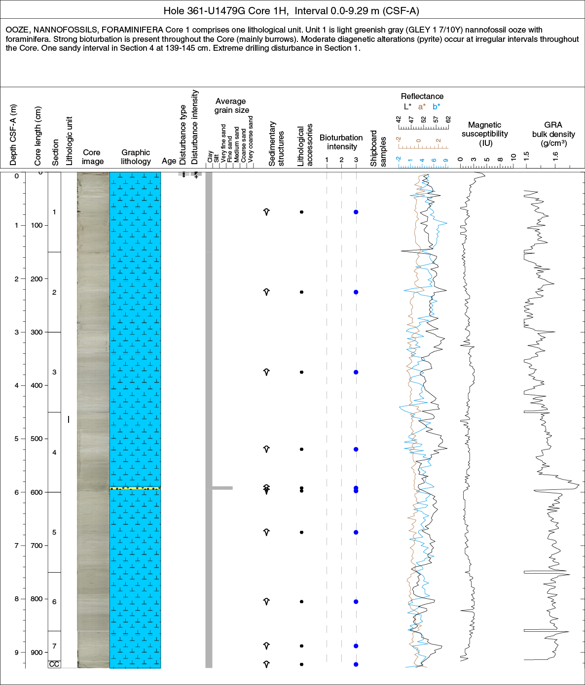
Figure F1. Example VCD.
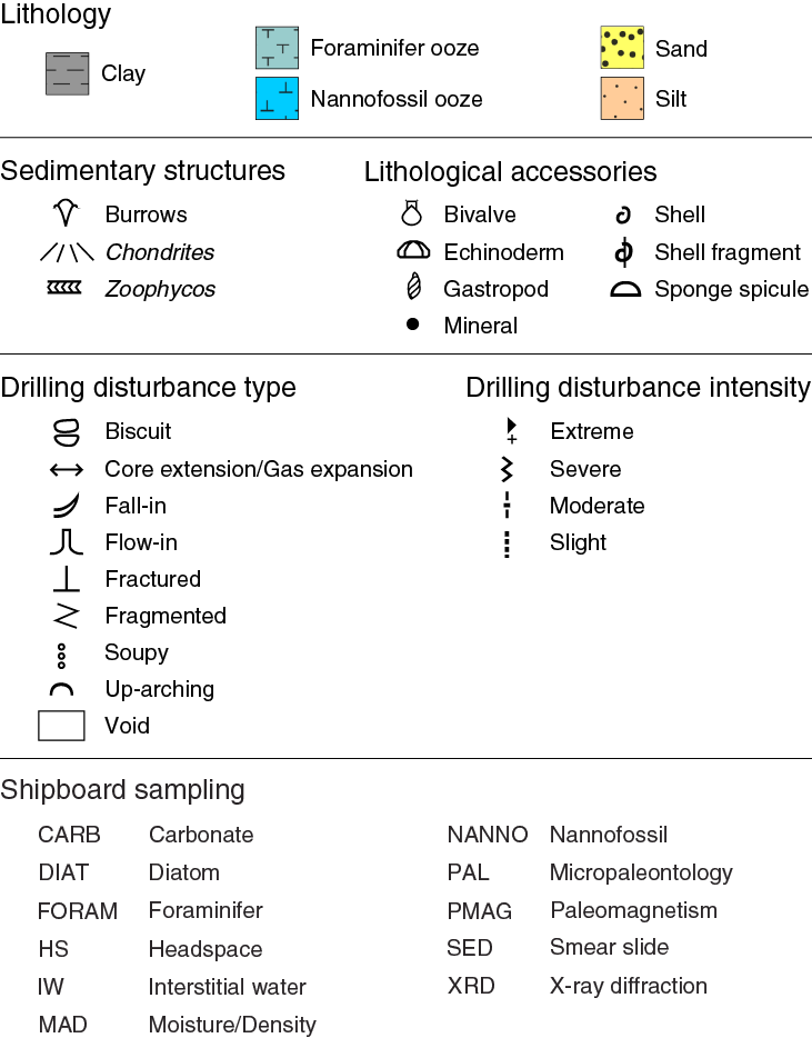
Figure F2. Symbols used for visual core description.
Smear slides were used to quantify the texture and relative abundance of biogenic and nonbiogenic components (see Smear slide descriptions). The locations of all smear slide samples taken from each core were recorded in the Sample Master application. DESClogik also includes a graphic display mode of digital images of section halves and physical property data to aid core description.
During Expedition 361, the Strater software package was used to compile the VCDs for each core. Site, hole, core number, and a core description summary are provided at the top of the VCD sheet (Figure F1). The written description for each core contains a concise summary of major and minor lithologies, sediment color based on the Munsell color classification, sedimentary structures, and drilling disturbances resulting from the coring process. Core depth (in meters), core length, section breaks, lithostratigraphic units, and age are indicated along the left side of the digital color image of the core and graphic lithology column. Columns to the right of the graphic lithology column include drilling disturbance (type and intensity), average grain size, sedimentary structures, lithologic accessories, bioturbation intensity, and shipboard sampling. Additional columns also show data collected by the WRMSL and SHMSL that include, from left to right, lightness (L*) and color (a* and b*) from color reflectance, magnetic susceptibility, and gamma ray attenuation (GRA) density. The graphic lithology column on the VCD sheet displays the dominant lithology of each section (Figure F1).
Sediment classification
Naming conventions follow the Ocean Drilling Program (ODP) sediment classification scheme from Mazzullo et al. (1988) (Figure F3). For a mixture of components, minor components representing between 10% and 25% of the sediment follow the principal name in order of increasing abundance. The principal name is preceded by major modifiers (in order of increasing abundance) referring to components making up ≥25% of the sediment. For example, unconsolidated sediment containing 50% foraminifers, 30% clay minerals, 10% nannofossils, and 10% diatoms would be described as a clayey foraminifer ooze with nannofossils and diatoms. The grain size scale used in descriptions is adapted from Wentworth (1922) (Figure F4).
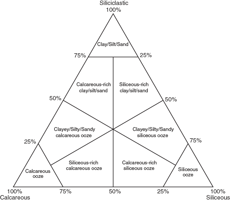
Figure F3. Siliciclastic-calcareous-siliceous ternary diagram used for lithologic classification.

Figure F4. Udden-Wentworth grain size classification of terrigenous sediment.
Description of lithification was based on the dominant composition (Figure F5):
- Sediment composed predominantly of calcareous pelagic organisms (e.g., calcareous nannofossils and foraminifers): the lithification terms “ooze,” “chalk,” and “limestone” reflect whether the sediment can be deformed with a finger (ooze), can be scratched easily by a fingernail (chalk), or cannot be scratched with a fingernail (limestone).
- Sediment composed predominantly of siliceous microfossils (diatoms, radiolarians, and siliceous sponge spicules): the lithification terms “ooze” and “radiolarite/spiculite/diatomite” reflect whether the sediment can be deformed with a finger (ooze) or cannot be easily deformed manually (radiolarite/spiculite/diatomite).
- Sediment composed predominantly of siliciclastic material: if the sediment can be deformed easily with a finger, no lithification term is added and the sediment is named for the dominant grain size. For more consolidated material, the lithification suffix “-stone” is appended to the dominant size classification (e.g., “clay” versus “claystone”).
- Consolidated sediment composed of an approximately equal mix of calcareous and fine siliciclastic material is described as “marlstone.”

Figure F5. Lithification classification.
Drilling-related sediment disturbance
Because cores may be significantly disturbed and contain extraneous material because of the drilling and core handling process (Jutzeler et al., 2014), the uppermost 10–50 cm of each core was examined during core description for such potential disturbances. Common coring-induced deformations were identified, including the concave-downward appearance of originally horizontal bedding as well as any fluidization (flow-in) at the bottom of APC cores resulting from the piston action. Because gas that is in solution at depth may become free, if gas content was high, pressure was relieved for safety reasons before the core was cut into segments. This was accomplished by drilling holes into the liner, which forces gas as well as some sediment out of the liner.
Drilling disturbances are described in the Sedimentology sections in each site chapter and are graphically indicated on the graphic core summary report VCDs using symbols shown in Figure F2). The style of drilling disturbance is described for soft and firm sediment using the following terms:
- Fall-in: out-of-place material at the top of a core has fallen downhole onto the cored surface.
- Flow-in: soft-sediment stretching and/or compressional shearing structures are severe and are attributed to coring/drilling. The particular type of deformation may also be noted (e.g., gas expansion etc.).
- Soupy or mousse-like: intervals are water saturated and have lost all aspects of original bedding.
- Biscuit: sediments of intermediate stiffness show vertical variations in the degree of disturbance. Softer intervals are washed and/or soupy, whereas firmer, disk- or biscuit-shaped intervals are relatively undisturbed.
- Cracked or fractured: firm sediments are broken but not displaced or rotated significantly.
- Fragmented or brecciated: firm sediments are pervasively broken and may be displaced or rotated.
Stratification and sedimentary structures
Sedimentary structures formed by physical and biological processes are represented with symbols in the sedimentary structures column on the VCDs.
Stratification
Layers and bedding thickness were described and classified following terminology based on Mazzullo et al. (1988) and Stow (2005):
- Thin lamination = < 0.3 cm thick
- Medium lamination = 0.3–0.6 cm thick
- Thick lamination = 0.6–1 cm thick
- Very thin bed = 1–3 cm thick
- Thin bed = 3–10 cm thick
- Medium bed = 10–30 cm thick
- Thick bed = 30–100 cm thick
- Very thick bed = >100 cm thick
The different contacts observed are described as follows:
- Gradational (normal/inverse): no horizontal line is drawn and there is a gradational curve between the two lithologies.
- Bioturbated: no horizontal line is drawn. Occasionally, a burrow is drawn at the right of the average grain size curve to show if the contact is sharp and bioturbated.
- Irregular: an irregular horizontal line is drawn between the two lithologies.
- Sharp: a ruled straight line is drawn between the two lithologies and a dash is shown to the right of the curve.
- Erosional/scoured: a wavy line is drawn between the two lithologies and a short wavy dash is shown to the right of the curve.
Bioturbation
Bioturbation was characterized using a three-level scheme. Bioturbation intensity was classified as strong (3), moderate (2), slight (1), and absent (none). These intensities are illustrated with a numeric scale in the bioturbation column on the VCDs.
Lithologic accessories
Lithologic, diagenetic, and paleontologic accessories, such as nodules, sulfides, and shells, are indicated on the VCDs using symbols (Figure F2).
Smear slide descriptions
Smear slide samples were taken from the archive halves during core description. For each sample, a small amount of sediment was removed with a wooden toothpick, dispersed evenly in deionized water on a 25 mm × 75 mm glass slide, and dried on a hot plate at a low setting. A drop of mounting medium was added and the slide was covered by a 22 mm × 30 mm glass and placed in an ultraviolet light box for ~15 min. Once fixed, each slide was investigated at 100–200× magnification with a transmitted light petrographic microscope using an eyepiece micrometer to assess grain size distributions in clay (<4 μm), silt (4–63 μm), and sand (>63 μm) fractions. The eyepiece micrometer was calibrated once for each magnification and combination of ocular and objective, using an inscribed stage micrometer. Relative proportions of each grain size and sediment components were estimated by microscopic examination. Note that smear slide analyses tend to underestimate the abundance of sand-sized and larger grains (e.g., foraminifers, radiolarians, and siliciclastic sand) because these are difficult to incorporate into the smear. Clay-sized biosilica, which is transparent and isotropic, is also very difficult to quantify. Clay minerals, micrite, and nannofossils can also be difficult to distinguish at the very finest (<4 μm) size range. After the general estimation of the grain-size distribution, several fields were examined at 200×–500× for mineral and microfossil identification. Standard petrographic techniques were employed to identify the commonly occurring minerals and biogenic groups, as well as important accessory minerals and microfossils. Smear slide analysis data tables are included in Core descriptions. These tables include information about the sample location, description of where the smear slide was taken, the estimated percentages of texture (i.e., sand, silt, and clay), and the estimated percentages of composition (i.e., detrital carbonate, biogenic carbonate, biogenic silica, and siliciclastics).
Shipboard samples
Samples were taken for shipboard sedimentological and chemical analyses to aid core description and consisted of interstitial water whole rounds, micropaleontology samples, smear slides, samples for physical properties (moisture and density [MAD]) and paleomagnetic studies, as well as selected samples for XRD and total inorganic carbon (TIC) and total organic carbon (TOC) analysis. Typically, three smear slides were made per core, but more samples were selected where high variability or minor lithologies were present. Interstitial water samples were taken at designated intervals, and micropaleontology samples were obtained from the core catchers in the first hole as well as further samples to refine the stratigraphy within the cores and in additional holes to extend the biostratigraphy or to address specific questions. Approximately three MAD samples were taken per core in the first hole. Discrete paleomagnetic samples were taken to verify the section-half paleomagnetic and susceptibility measurements and stratigraphy and to investigate changing magnetic mineral compositions. Discrete solid samples were taken for geochemical measurements (carbonate and in some cases bulk geochemical analyses). In a few cases, XRD samples were taken from selected intervals to characterize lithologic variability. TIC and organic carbon analyses were routinely taken from interstitial water squeeze cakes at the interval of one per core and at additional levels where requested (see Geochemistry). All shipboard samples are displayed in the VCDs.
X-ray diffraction
Samples for XRD analyses were taken from the working-half sections, selected based on visual core observations (e.g., color variability and visual changes in lithology and texture) and smear slides. Samples analyzed for bulk mineralogy were freeze-dried and ground by hand or in an agate ball mill, as necessary. Bulk sample XRD analyses were performed using a Bruker D-4 Endeavor X-ray diffractometer with a Vantec detector using Ni-filtered CuKα radiation (40 kV, 40 mA). Bulk powder samples were analyzed over a 2θ range of 4°–68° with a step size of 0.01°2θ. Scan speed was 1.2°2θ/min with a count time of 0.5 s. Samples analyzed for clay mineralogy were first treated with 10% acetic acid to remove carbonate minerals. The clay-sized fraction (<2 μm) was separated in a 1% sodium hexametaphosphate solution using a sonic dismembrator and centrifuge. The clay-sized suspension was allowed to dry on a glass slide to create an oriented grain mount. An additional split of the sample was treated with ethylene glycol. Oriented clay aggregates were analyzed over a 2θ range of 3°–30°. All XRD patterns were analyzed using Bruker AXS DIFFRAC.EVA software (version 3.0). Shipboard results yielded only qualitative results on the presence and relative abundances of the most common mineralogical components. Digital files with the diffraction patterns are available from the IODP LIMS database (http://iodp.tamu.edu/LORE/).
Physical properties
Physical property measurements were made during Expedition 361 to provide information on the bulk physical character and acoustic and elastic parameters of recovered sediment. Such data enhance our understanding of the physico-chemical context and history for oceanic deposits, augment lithologic characterization, and facilitate correlation of downhole logging data with discrete core measurements and core descriptions. Physical property data can be measured quickly at a high resolution and, as such, serve as important first-order proxies for determining changes in environmental conditions, geological processes, and/or depositional environments. Shipboard physical property data play a key role in the following:
- Hole-to-hole correlation for construction of composite stratigraphic sections;
- Detection of discontinuities and inhomogeneities, either caused naturally or by the drilling process;
- Identification of differences in the composition and texture of sediment;
- Time-series analysis for detection of orbital cycles and tuning to reference cores for stratigraphic purposes;
- Calculation of sedimentation and accumulation rates;
- Core-log-seismic integration; and
- Identification of major seismic reflectors and construction of synthetic seismic traces.
Initial nondestructive measurements of physical properties were undertaken on three whole-round core logging systems; sections were run in the Special Task Multisensor Logger (STMSL) immediately following cutting on the catwalk, and then through the WRMSL and Natural Gamma Ray Logger (NGRL) once core sections had warmed to ambient laboratory temperature (i.e., above 19°C). The linear track of the STMSL houses a GRA bulk densitometer and a magnetic susceptibility sensor loop. The WRMSL employs a GRA bulk densitometer, magnetic susceptibility sensor loop, and compressional P-wave velocity sensor. The NGRL records the natural gamma radiation (NGR) emitted from the cores. Discrete samples were collected from the working halves, primarily from one deep hole at each site, to measure wet bulk density, dry bulk density, water content, porosity, and grain density with moisture and density (MAD) procedures. Further holes were only occasionally sampled for MAD measurements to fill gaps in the sample series. To save as much material as possible for shore-based sampling, destructive shear strength measurements on split cores were not made during Expedition 361. For the same reason, compressional P-wave velocity measurements on split cores were only occasionally performed by using the x-axis caliper-type contact probe. Archive halves were measured with the SHMSL for color reflectance (with an Ocean Optics sensor) and magnetic susceptibility using a discrete point-source Bartington probe. A full discussion of all methodologies and calculations used aboard the JOIDES Resolution in the Physical Properties Laboratory is available in Blum (1997).
Whole-round core logging operation and sensors
Special Task Multisensor Logger
The purpose of STMSL logging operations during Expedition 361 was to rapidly record medium- to high-resolution GRA density and magnetic susceptibility data. This information is needed at multihole sites to ensure that drilling depth offsets are set at different stratigraphic depths in each hole so that a complete composite stratigraphic section can be constructed. The GRA bulk densitometer and magnetic susceptibility loop incorporated in the STMSL are effectively identical to those in the WRMSL (see below). The spacing distance between STMSL measurements was typically 2.5 cm for GRA density and magnetic susceptibility measurements. Scanning time averaged 8 s per sample with three repeats for the magnetic susceptibility measurements. A core can therefore be passed through the STMSL in ~25 min. Comments about structural integrity and incomplete filling of liners were recorded.
Whole-Round Multisensor Logger
High-resolution WRMSL data, especially GRA bulk density and magnetic susceptibility, were gathered to advance shipboard core-to-core correlation between drill holes and the construction of composite stratigraphic sections. WRMSL data assembly had to be completed within a reasonable time to not encumber downstream core processing and sample collection. The quality of WRMSL data is highly dependent on the structural integrity of the sediment (cracks, voids, biscuiting, etc.) and whether any gaps between the sediment and the core liner are present. GRA bulk density and magnetic susceptibility were measured nondestructively on all whole-round core sections. P-wave velocity was measured in sections undisturbed by gas expansion voids and cracks. To optimize WRMSL performance, the same sampling spacing was set for all sensors. Measurement time, although somewhat different for the different sensors, averaged ~8 s per data, with three repeats of the magnetic susceptibility measurements providing sufficient reproducibility. With handling and data initialization, a 1.5 m section took ~10 min to scan.
GRA bulk density
Bulk density varies with water-saturated porosity, grain density (dominant mineralogy), grain packing, and coring disturbance. To measure bulk density, the GRA densitometer uses a 10 mCi 137Cs capsule as a gamma ray source (with the principal energy peak at 0.662 MeV) and a scintillation detector. The narrow collimated peak is attenuated as it passes through the center of the core. Incident photons are scattered by the electrons of the sediment by Compton scattering.
The attenuation of the incident intensity (I0) is directly related to the electron density in the sediment core of diameter D that can be related to bulk density given the average attenuation coefficient (in micrometers) of the sediment (Evans, 1965; Harms and Choquette, 1965). Because the attenuation coefficient is similar for most common minerals and aluminum, bulk density is obtained through direct calibration of the densitometer using aluminum rods of different diameters mounted in a core liner filled with distilled water. The GRA densitometer has a spatial resolution of <1 cm.
Magnetic susceptibility
Magnetic susceptibility is a measure of the degree to which a material can be magnetized by an external magnetic field, providing information on the magnetic composition of the sediment that commonly can be related to mineralogical composition (e.g., terrigenous versus biogenic materials) and diagenetic overprinting. Magnetite and a few other iron oxides with ferromagnetic characteristics have a specific magnetic susceptibility several orders of magnitude higher than clay, which has paramagnetic properties. Carbonate layers, opal, water, and plastic (core liner) have small negative values of magnetic susceptibility. Calcareous and biogenic deposits with low clay and iron-bearing mineral debris content thus have values approaching the detection limit of magnetic susceptibility meters.
Magnetic susceptibility was measured on the WRMSL and STMSL with the Bartington Instruments MS2C system. The frequency at which the magnetic susceptibility loop operates is 565 Hz for the WRMSL and STMSL (Blum, 1997). We used a 1 s measurement cycle with three measurements averaged at each sample position. The unit switch on the instrument was set to SI units. In this report we present the raw output of the magnetic susceptibility sensors as instrument units (IU). To obtain dimensionless SI volume-specific magnetic susceptibility values, these instrument units, which are also stored in the IODP database, must be multiplied by a correction factor (0.68) to compensate for instrument scaling and the geometric ratio between core and loop dimensions.
Compressional P-wave velocity
P-wave velocity varies with the material’s lithology, porosity, and bulk density, as well as state of stress, temperature, and fabric or degree of fracturing. In sediment and rock, velocity is controlled by the degree of consolidation and lithification and fracturing, along with the occurrence and abundance of free gas and gas hydrate. Together with bulk density, velocity data are used to calculate acoustic impedance and reflection coefficients in order to construct synthetic seismic profiles and to estimate the depth of specific seismic horizons.
The P-wave velocity sensor measures the ultrasonic P-wave velocity of the whole-round sample residing in the core liner. The P-wave logger transmits a 500 kHz P-wave pulse across the core section at a specified repetition rate. Traveltime is determined by signal processing software that uses a series of mathematical and data manipulation techniques to suppress the noise relative to the peak of the first arrival and automatically detects the first arrival of the P-wave signal to a precision of 50 ns. Prior to coring at Site U1476, the algorithm for detecting the first arrival of the P-wave signal on the WRMSL was changed such that the signal-to-noise ratio enhancement process consisted of three steps: (1) smoothing, (2) first derivative, and 3) smoothing (see EXP 361 TECH RPT P-Wave.docx in PWVTECH in Supplementary material). With the new approach, the number of outliers in the P-wave data set was significantly reduced compared to the previous sites. Ultrasonic P-wave velocity is calculated after correcting for system propagation delay, liner thickness, and liner material velocity.
NGR core logging
The NGRL was designed and built at the Texas A&M University IODP facility and measures gamma radiation emitted from whole-round core sections (Vasiliev et al., 2011). Gamma radiation detected by the logger arises primarily from the decay of mineral-hosted uranium, thorium, and potassium isotopes. In general, high counts identify fine-grained deposits containing K-rich clay minerals and their absorbed U and Th atoms. The NGR data reveals stratigraphic details that aid in core-to-core correlations.
The main NGR detector unit consists of 8 sodium iodide (NaI) scintillator detectors surrounding the lower half of the section, 7 shielding plastic scintillator detectors, 22 photomultipliers, and passive lead shielding. The NaI detectors are covered by at least 8 cm of lead shielding. In addition, lead separators (~7 cm of low-background lead) are positioned between the NaI detectors. Half of the lead shielding closest to the NaI detectors is composed of low-background lead, whereas the outer half is composed of common (virgin) lead. In addition to this passive lead shielding, the overlying plastic scintillators detect incoming high-energy gamma and muon cosmic radiation and cancel this signal from the total counted by the NaI detectors.
A measurement run consisted of two core section positions. Gamma rays were counted for 5 min at each position. At position 1 the gamma ray signal was collected at 0, 20, 40, 60, 80, 100, 120, and 140 cm from the core-section top, and at position 2 the signal was collected at 10, 30, 50, 70, 90, 110, 130, and 150 cm from the core-section top, resulting in a total of 16 measurements (10 cm spacing) per section. Further information may be found in Vasiliev et al. (2011) and Dunlea et al. (2013).
Thermal conductivity
After NGR measurements were completed, thermal conductivity was measured with the TK04 (Teka Bolin) system using the needle-probe method in full-space configuration for whole-round sediment cores (Von Herzen and Maxwell, 1959). The needle probe contains a heater wire and calibrated thermistor. The probe was inserted into a 2 mm hole drilled through the liner along one of the lines that later guided the splitting of the core. To avoid interference from airflow in the laboratory, an insulating jacket of foam rubber was placed over the core section during measurement of thermal conductivity. Because the probe is much more conductive than unconsolidated sediment, the probe is assumed to be a perfect conductor. Under this assumption, the temperature of the superconductive probe has a linear relationship with the natural logarithm of the time after the initiation of the heat:
- T = temperature (K),
- q = heat input per unit length per unit time (J/m/s),
- k = thermal conductivity (W/[m·K]),
- t = time after the initiation of the heat (s), and
- C = instrumental constant.
Three measuring cycles were automatically performed at each probe location to calculate average conductivity. A self-test, which included a drift study, was conducted at the beginning of each measurement cycle. Once the probe temperature stabilized, the heater circuit was closed and the temperature rise in the probe was recorded. Thermal conductivity was calculated from the rate of temperature rise while the heater current was flowing. Temperatures measured during the first 150 s of the heating cycle were fitted to an approximate solution of a constantly heated line source (for details, see Kristiansen, 1982; Blum, 1997). Measurement errors were 5%–10%. Thermal conductivity measurements were routinely taken at a resolution of 10–20 m in one deep hole of each site.
Moisture and density
After completion of whole-round measurements, whole-round cores were split into working halves and archive halves. The working halves were placed on the sampling table for the collection of discrete samples to determine wet and dry bulk density, grain density, water content, salt content, and porosity. In soft sediment, ~12 cm3 samples were collected with a 2 cm diameter plastic syringe that fits into a glass vial of 10 cm3 volume so that the vial is completely filled with sediment. Samples were collected from every other section.
Samples were placed in prelabeled and preweighed 16 mL Wheaton glass vials for wet and dry sediment mass measurement. The samples were dried in a convective oven at 105° ± 5°C for 24 h and allowed to cool in a desiccator for ~3 h before taking the dry volume measurements. The weights of wet and dry sample masses were determined to a precision of 0.005 g using two Mettler Toledo electronic balances and a computer averaging system to compensate for the ship’s motion. Dry sample volume was determined using a hexapycnometer system of a six-celled, custom-configured Micromeritics AccuPyc 1330TC helium-displacement pycnometer. The precision of each cell is 1% of the full-scale volume. Volume measurement was preceded by three purges of the sample chamber with helium warmed to ~28°C. Three measurement cycles were run for each sample. A reference volume (calibration sphere) was placed sequentially in one of the chambers to check for instrument drift and systematic error. The volume of glass for each numbered Wheaton vial was calculated before the cruise by dividing the weight of each vial by the average density of the vial glass. Dry mass and volume were measured after samples were heated in an oven at 105° ± 5°C for 24 h and allowed to cool in a desiccator. The procedures for the determination of these physical properties comply with the American Society for Testing and Materials (ASTM) designation (D) 2216 (ASTM International, 1990). The fundamental relation and assumptions for the calculations of all physical property parameters are discussed by Blum (1997) and summarized below.
Mass and volume calculation
Wet mass (Mwet), dry mass (Mdry), and dry volume (Vdry) were measured in the laboratory. The ratio of mass (rm) is a computational constant of 0.965 (i.e., 0.965 g of freshwater per 1 g of seawater). Salt precipitated in sediment pores during the drying process is included in the Mdry and Vdry values. The mass of the evaporated water (Mwater) and salt (Msalt) in the sample are given by, respectively,
where s is the assumed saltwater salinity (0.035%) corresponding to a pore water density (ρpw) of 1.024 g/cm3 and a salt density (ρsalt) of 2.22 g/cm3. The corrected mass of pore water (Mpw), volume of pore water (Vpw), mass of solids excluding salt (Msolid), volume of salt (Vsalt), volume of solids excluding salt (Vsolid), and wet volume (Vwet) are
Vwet = Vdry – Vsalt + Vpw, and
Calculation of bulk properties
For all sediment samples, water content (w) is expressed as the ratio of mass of pore water to wet sediment (total) mass,
Wet bulk density (ρwet), dry bulk density (ρdry), sediment grain density (ρsolid), porosity (φ), and void ratio (VR) are calculated as
Moisture and density properties reported and plotted in the Physical properties sections of all site chapters were calculated with the MADMax shipboard program.
Discrete velocity measurements
Because of the generally quite good quality of the P-wave logging data from the WRMSL during the expedition, P-wave velocity measurements on split cores were performed only occasionally by using the x-axis caliper-type contact probe transducers on the Section Half Measurement Gantry. The system uses Panametrics-NDT Microscan delay line transducers, which transmit at 0.5 MHz. The signal, received through the sample, was recorded by the system computer and the peak (P-wave arrival) was chosen by an autopicking software. In case of a weak signal, the first arrival was manually picked. The distance between transducers was measured with a built-in linear voltage displacement transformer (LDVT).
Calibration was performed with a series of acrylic cylinders of differing thicknesses and a known P-wave velocity of 2750 ± 20 m/s. The determined system time delay from calibration was subtracted from the picked arrival time to give a travel time of the P-wave through the sample. The thickness of the sample (calculated by the LDVT in meters) was divided by the travel time (in seconds) to calculate P-wave velocity in meters per second.
Digital color image
The surfaces of the archive halves of split cores were digitally imaged using a 3-CCD (charge-coupled device) line-scan camera (JAI model CV107CL) with a macro lens (AF micro Nikkor 60 mm, 1:2.8). Mounted on the SHIL, the camera moves across the sample on a motorized gantry. Prior to imaging, and when necessary, the core face was prepared by scraping across, rather than along, the core section using a stainless steel or glass scraper. Scraping parallel to bedding with a freshly cleaned tool prevented cross-stratigraphic contamination. After splitting, the archive halves were imaged as soon as possible to capture the core surface prior to drying and/or oxidation. Images were scanned at an interval of 10 lines/mm, with camera height allowing for square pixels. The imaging light was provided by three pairs of advanced illumination high-current focused LED line lights with fully adjustable angles to the lens axis. Compression of line-scanned images on VCDs or summary figures may result in visual artifacts, primarily lamination that is not present in the actual sections. Along with the images the variations in the RGB color channels were also recorded by the SHIL and used as a primary tool for stratigraphic correlation.
Spectrophotometry and magnetic susceptibility point measurements
After imaging, spectrophotometry was measured on the archive halves with the SHMSL. Spurious measurements may occur from small cracks, drilling disturbance, plastic section dividers, or in cases where the instrument could not land the sensors flatly on the core surface, resulting in the leakage of ambient room light into the spectrophotometer readings.
Reflectance of visible light from the archive halves of sediment cores was measured using an Ocean Optics USB4000 spectrophotometer mounted on the automated SHMSL. A halogen light source, covering a wavelength range through the visible spectrum and slightly into the infrared domain, was used. Prior to Expedition 361, an additional blue light source was installed to enhance performance at the darker end of the spectrum. Freshly split cores were covered with clear plastic wrap and placed on the SHMSL. Measurements were taken at different spacing (0.5–8 cm, depending on need based on accumulation rate and available time) to provide high-resolution stratigraphic records of color variation for visible wavelengths. Each measurement was recorded in 2 nm wide spectral bands from 400 to 900 nm. Additional details regarding measurement and interpretation of spectral data can be found in Balsam et al. (1997), Balsam and Damuth (2000), and Giosan et al. (2001, 2002).
Magnetic susceptibility was measured with a Bartington Instruments MS2E point sensor (high-resolution surface-scanning sensor) on discrete points along the SHMSL track. Measurements (3 repeats) were taken at the same spacing as the reflectance measurements, integrating a volume of 10.5 mm × 3.8 mm × 4 mm, where 10.5 mm is the length perpendicular to the core axis, 3.8 mm is the width in the core axis, and 4 mm is the depth. For conversion of the instrument units stored in the IODP database, a correction factor (67/80) must be employed to correct for the relation of the sensor diameter and sediment thickness.
Micropaleontology
Paleontological studies were primarily based on semiquantitative analyses of calcareous nannofossil and planktonic foraminifer assemblages as well as benthic foraminifers, diatoms, radiolarians, and phytoliths. Preliminary ages were assigned based on core catcher samples for each site. Additional samples taken within the cores were examined when a more refined age determination was required. Calcareous nannofossil and foraminifer age events from the late Miocene to the recent were evaluated by correlation to the geomagnetic polarity timescale (GPTS) of Gradstein et al. (2012). The microfossils zonal scheme used during Expedition 361 is illustrated in Figure F6).
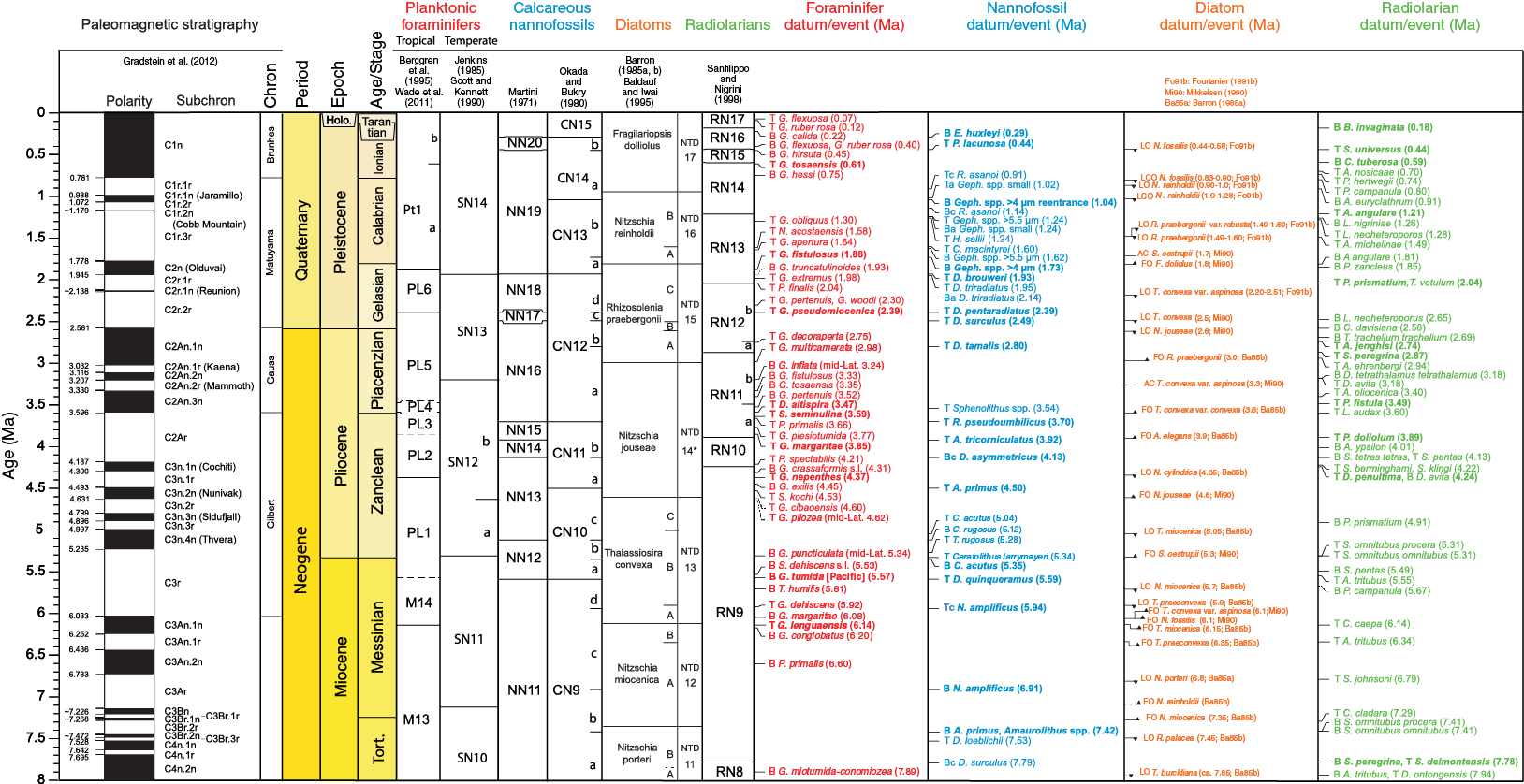
Figure F6. Microfossil zonal scheme.
Calcareous nannofossils
Zonal scheme and taxonomy
The nannofossil biostratigraphic zonation schemes of Martini (1971; codes NN) and Okada and Bukry (1980; codes CN) were adopted for this study. Age dates were calibrated following Lourens et al. (2004) and Gradstein et al. (2012) (Table T1). Biostratigraphic events were determined based on the occurrence of calcareous nannofossils (abundance, presence, or absence) in core catcher samples, in preselected intervals, and in additional split-core sections, when necessary. The taxonomy and identification mainly followed Perch-Nielsen (1985) and Bown (1998). Young et al. (2003) was adopted for the recent taxa.
Table T1. Age estimates of calcareous nannofossil datum events. Download table in .csv format.
Methods of study
Core samples for determining nannofossil assemblages and relative preservation were studied using the standard smear slide technique (Watkins and Bergen, 2003) and mounted with Norland Optical adhesive 61 (refractive index = 1.56). Calcareous nannofossil recognition was achieved with a Zeiss Axiophot light microscope under cross-polarized transmitted light and brightfield illumination at 1000× magnification. Selected samples were additionally analyzed under a scanning electron microscope (SEM; Hitachi tabletop microscope TM3000). Additionally, mudline samples from the water/seafloor interface were analyzed to assess preservation and biodiversity of recently deposited fossils. The mudline suspension was collected in a bucket from which subsamples were withdrawn by centrifuging the solution. Smear slides and stubs were then prepared for SEM analyses. Photographs were taken using the Spot FLEX system with Image Capture and Spot software as well as with the SEM.
Total abundance of calcareous nannofossils within the sediment record was categorized as
- A = abundant (>50% of sediment particles).
- C = common (>10%–50% of sediment particles).
- F = few (1%–10% of sediment particles).
- R = rare (≤1% of sediment particles).
- B = barren (none present).
Abundances of individual calcareous nannofossil taxa were categorized as
- A = abundant (>10 specimens per field of view [FOV]).
- C = common (>1–10 specimens per FOV).
- F = few (1 specimen per 1–10 FOV).
- R = rare (<1 specimen per 10 FOV).
Preservation of calcareous nannofossils, based on dissolution and overgrowth was classified as
- G = good (little or no evidence of dissolution and/or overgrowth; primary morphological characteristics appear unaltered; specimens identifiable to the species level).
- M = moderate (minor to moderate dissolution and/or overgrowth; primary morphological characteristics somewhat modified; most specimens identifiable to the species level).
- P = poor (severe dissolution, fragmentation and/or overgrowth; primary morphological characteristics and specimens mostly unidentifiable).
Planktonic and benthic foraminifers
Zonal scheme and taxonomy
For the Pliocene–Pleistocene, the biostratigraphy of Wade et al. (2011) was updated with specific age assignments for Indian Ocean sites based on the review of Vincent (1977). Age estimates for planktonic foraminifer datums follow Gradstein et al. (2012) (Table T2). Planktonic foraminifer taxonomic concepts in the Cenozoic selectively follow those of Jenkins (1971), Blow (1979), Kennett and Srinivasan (1983), Bolli et al. (1985), Toumarkine and Luterbacher (1985), Scott et al. (1990), Pearson (1995), Chaisson and Pearson (1997), and Olsson et al. (1999). A taxonomic list of planktonic foraminifer datum species is given in Table T3.
Table T2. Age estimates of planktonic foraminifer datum events. Download table in .csv format.
Table T3. Taxonomic species list for planktonic foraminifer datums. Download table in .csv format.
Benthic foraminifer taxonomy systematics for generic assignment follow Loeblich and Tappan (1988). Species identification was conducted following Holbourn et al. (2013) and Jones (1994). Ecological and paleobathymetric interpretations are based on a compilation of ecological data, including but not limited to van Morkhoven et al. (1986). Benthic foraminifers provide only limited biostratigraphic age control, but they are useful for paleobathymetric and paleoenvironmental interpretation.
Methods of study
Roughly 20–30 cm³ of sediment from the core catcher was washed to identify the main planktonic and benthic foraminifer datum events. At some sites we examined samples at a resolution of 1 per section in certain holes to refine preliminary biozones. Sediment was washed with tap water over a 63 µm mesh sieve. When time allowed, samples were dried in an oven and soaked in tap water and borax before washing. To avoid contamination of foraminifers between samples, the empty sieves were placed in an ultrasonic bath for several minutes and cleaned with compressed air. Washed residues were dried on 63 µm screens in a 90°C oven and transferred to sample vials. A subsample was examined under a binocular Zeiss Discovery V8 stereomicroscope.
Examination of planktonic foraminifers was carried out on the >150 µm size fraction, and examination of benthic foraminifers was conducted on the >63 µm fraction. The split sample was spread over a sample tray and examined for either planktonic or benthic foraminifers. Where possible, at least 150 specimens were picked, identified, and counted to determine the relative abundances of benthic foraminifers.
Photomicrographs were taken using a Spot RTS system with IODP Image Capture and commercial Spot software. We also used a Hitachi TM3000 tabletop SEM to create images for verification of our species assignments and to make photographic plates. The dried foraminifer residues were used to estimate the abundance of total planktonic and benthic foraminifers relative to other sedimentary components, as follows:
- A = abundant (>50% of the total sediment particles).
- C = common (>25%–50% of the total sediment particles).
- F = few (5%–25% of the total sediment particles).
- R = rare (<5% of the total particles).
- B = barren (no specimens in the whole sample).
Note that to save time, raw samples were not weighed prior to washing, so we can make only qualitative estimates of foraminifer abundance relative to other sedimentary components. The relative abundance of planktonic and benthic foraminifer species relative to other members of the foraminifer assemblage is indicated by
- D = dominant (>30% of the planktonic foraminifer assemblage).
- A = abundant (10%–30% of the planktonic foraminifer assemblage).
- F = few (5%–10% of the planktonic foraminifer assemblage).
- R = rare (1%–5% of the planktonic foraminifer assemblage).
- P = present (<1% of the planktonic foraminifer assemblage).
Preservation of planktonic and benthic foraminifers is recorded as
- G = good (>90% of specimens unbroken with only minor evidence of diagenetic alteration).
- M = moderate (30%–90% of specimens are unbroken).
- P = poor (strongly recrystallized or dominated by fragments and broken or corroded specimens).
Siliceous microfossils
Zonal scheme and taxonomy
The diatom zonal scheme used for the Indian Ocean mainly follows biostratigraphic studies by Barron (1985), Mikkelsen (1990), and Fourtanier (1991). Datums were modified following the updated GPTS (Gradstein et al., 2012). The biozones used for the Neogene are those described by Barron (1985) for the Pacific Ocean; however, some biozone boundaries were modified following bioevent ages calibrated for the Indian Ocean (Fourtanier, 1991; Mikkelsen, 1990) (Table T4).
Table T4. Neogene tropical diatom datum and age estimates. Download table in .csv format.
In the mid- to low-latitude Indian Ocean sites, we follow the tropical Pacific radiolarian zones (Sanfilippo and Nigrini, 1998; Nigrini and Sanfilippo, 2001; Kamikuri et al., 2009) (Table T5; Figure F6).
Table T5. North Pacific diatom datum and age estimates. Download table in .csv format.
For the Southern Ocean assemblages, the initial shipboard age assignment of individual samples for 0–18 Ma is mostly based on diatoms using the high-resolution quantitative diatom biochronology of Cody et al. (2008). Species ranges and age assignments are in Table T6. We primarily employed the constrained optimization (CONOP) average range model, drawing on the information from the CONOP total range model, where appropriate. The taxonomic concepts of marker species are comprehensively specified in appendixes 1a and 1b of Cody et al. (2008).
Table T6. Southern Ocean diatom datum and age estimates. Download table in .csv format.
Methods of study
Diatoms, radiolarians, silicoflagellates, ebridians, sponge spicules, and phytolith assemblages were analyzed from smear slides mounted with Norland optical adhesive 61 (refractive index = 1.56). Samples with rare to common overall abundance of siliceous microfossils were either disaggregated in distilled water or processed with hydrogen peroxide (H2O2) and/or 10% hydrochloric acid (HCl). Strewn slides were prepared from these samples, and, when necessary, the cleaned material was washed over a 20 µm sieve to improve viewing. Species identification was carried out with a Zeiss Axioplan microscope using brightfield illumination at 400×, 630× (oil), and 1000× (oil) magnification. The counting method of Schrader and Gersonde (1978) was utilized for all diatom specimens.
Abundances of individual taxa were quantified by a count tallied over two 22 mm traverses of a smear slide using 630× magnification. Photomicrographs were taken using a Spot FLEX system with IODP Image Capture and commercial Spot software. We also used a Hitachi TM3000 tabletop SEM. Qualitative siliceous microfossil group abundances were also determined from smear slides, using 630× magnification.
Abundance of groups and individual taxa are categorized as
- A = abundant (>10 valves per FOV).
- C = common (≥1–10 valves per FOV).
- F = few (≥1 valve every 10 FOV and <1 valve per FOV).
- R = rare (≥3 valves per traverse and <1 valve per 10 FOV).
- X = trace (<3 valves per traverse, including fragments).
- B = barren (no valves or fragments observed).
- ? = uncertain identification.
Preservation of individual siliceous microfossil groups was determined qualitatively using the following scale (Barron and Gladenkov, 1995):
- VG = very good (no breakage or dissolution).
- G = good (majority of specimens complete, with minor dissolution and/or breakage and no significant enlargement of the areolae or dissolution of frustule rims detected. The sample generally has a high number of diatoms per gram concentration).
- M = moderate (minor, but common areolae enlargement and dissolution of frustule rims, with a considerable amount of breakage of specimens).
- P = poor (strong dissolution or breakage, some specimens unidentifiable, strong dissolution of frustule rims and areolae enlargement. The sample generally has a lower number of diatoms per gram concentration).
Paleomagnetism
The main aim for shipboard magnetic measurements was identification of past reversals of the Earth’s magnetic field in order to establish the magnetostratigraphy for sediment cores recovered during Expedition 361. High-resolution, continuous paleomagnetic measurements were performed on archive halves using a superconducting rock magnetometer (SRM). Additionally, detailed paleo- and rock magnetic experiments were carried out on discrete samples to support the continuous SRM data and further characterize the magnetic inventory of the sediment.
Continuous measurements
Archive halves were analyzed using a 2G Enterprises Model-760R SRM equipped with three direct-current super conducting quantum interference devices (DC-SQUID) and an in-line alternating field (AF) demagnetizer equipped with two transverse and one axial AF degausser. Natural remanent magnetization (NRM) measurements were performed at 4 cm resolution, the first and last measurements taken 15 cm from the ends of the core sections. Subsequently, the core halves were AF demagnetized, and at the same intervals remanence measurements were taken after each demagnetization step. Past experiences of technical staff and scientists onboard the JOIDES Resolution have shown that at AF levels higher than 40 mT, a leaking field into the AF unit causes samples to acquire an anhysteretic remanent magnetization (ARM). To avoid this issue and to preserve core NRM for possible future demagnetization experiments, we used maximum AF fields of 15, 20, or 25 mT, which depended on the coercivity of the magnetic minerals present at each site.
Discrete samples
Discrete samples were taken from each or every other working-half section using 2.3 cm × 2.2 cm × 2.2 cm (7 cm3) “Japanese” sampling cubes with rounded corners. All samples were taken in the middle of sections where the influence of drilling disturbance was expected to be small. The magnetic susceptibility of each sample was measured by using a KYL-4S Kappabridge. On selected samples measurements of anisotropy of magnetic susceptibility (AMS) were conducted using the automated sample rotation of the KYL-4S. During the rotation along each of the three specimen axes, repetitive measurements were performed to allow identification of the anisotropy ellipsoid characterized by three susceptibility tensors, each normal to the others: Kmax, Kint, and Kmin. The data are represented by an equal-angle, lower hemisphere projection of the larger principal axis (Kmax) of the AMS tensor. On this lower hemisphere, each point is determined by the intersection of an axis passing by the center of the hemisphere and reflecting the alignment of para- and ferrimagnetic minerals (magnetic or sediment fabric). As the AMS fabric in marine sediment is acquired during deposition (i.e., the statistical common organization of the grains providing that the grains have an oblong shape), it may be indicative of bottom-current strengths (e.g., Ellwood and Ledbetter, 1977, 1979; Joseph et al., 1998; Hassold et al., 2006). Following the susceptibility measurements, all discrete samples were demagnetized in up to 7 steps between 5 and 100 mT using a manually operated AF demagnetizer (Model 2G600). The aim was to verify (1) if a stable characteristic remanent magnetization (ChRM) can be determined and (2) whether a potential coring or early diagenetic overprint biasing the primary directional record was sufficiently removed by the demagnetization level chosen for SRM measurements. Afterward, experiments of isothermal remanent magnetization (IRM) acquisition were performed at 100, 1200, and a backfield of 300 mT using an ASC IM10 impulse magnetizer. IRM acquisition remanence measurements are indicative of the magnetic mineralogy, which depends on the detrital magnetic mineral supply and/or diagenetic dissolution and neo-formation of ferrimagnetic minerals.
Based on these remanence parameters the saturation IRM (SIRM) was approximated by
the hard IRM (HIRM) was approximated by
HIRM = 0.5 × (SIRM – IRM – 300 mT),
and the S-ratio was calculated by
S = 0.5 × (1 + IRM – 300 mT/SIRM).
For both the NRM and IRM experiments, magnetic intensities were measured using a JR-6A spinner magnetometer.
Magnetostratigraphy
Based on directional changes of inclination and declination, magnetic polarity zones were defined for sediment sequences recovered during Expedition 361. Core orientation data were collected with the Icefield MI-5 and FlexIt core orientation tools for 5 min prior to the firing of each APC core. Where available, orientation data were used to correct the declination of each core. Normal and reversed polarity zones were assigned to the paleomagnetic (sub-)chrons reported by Gradstein et al. (2012) (Figure F6).
Stratigraphic correlation
As with any IODP paleoceanographic expedition, the scientific objectives of Expedition 361 demanded recovery of complete stratigraphic sections with continuity on the centimeter scale. Such recovery is impossible to achieve with a single IODP hole because coring gaps generally occur between successive cores during the APC process, despite 100% or greater recovery (e.g., Ruddiman, Kidd, Thomas, et al., 1987; Hagelberg et al., 1995; Acton et al., 2001). Furthermore, the top of any core might sample sediment that has fallen into the hole, resulting in stratigraphic noise. Thus, the reconstruction of a complete, continuous, and “representative” stratigraphic section requires combining stratigraphic intervals from two or more holes cored at the same site, where the depths of core gaps are staggered between holes. Given this primary objective, the shipboard work of the stratigraphic correlators during Expedition 361 was threefold: (1) to use the correlation of sediment physical properties among holes (that have been scanned rapidly upon retrieval of cores) as a guide while drilling to minimize gap alignment, (2) to construct a composite depth scale for all holes drilled, and (3) to reconstruct the most representative single continuous sedimentary section by splicing intervals from multiple holes.
The procedure for each of these activities involves consideration of several different depth scales (Figure F7). The depth scales used during Expedition 361 followed IODP conventions (see IODP Depth Scales Terminology at http://www.iodp.org/policies-and-guidelines) and are described in methodological order.

Figure F7. Relationships between cored material and the depth scales.
Core depth below seafloor (CSF-A) scale
The starting point for the process of building a composite section is to assign a depth to the top of each core, and this is based initially on the drilling depth below seafloor (DSF). DSF is a drill string measurement determined as the difference between (1) the length of the drill string below the rig floor to the top of the cored interval and (2) the length of the drill string from the rig floor to the mudline (assumed to be the seafloor). DSF error includes phenomena such as pipe and BHA stretch and compression, tides, and uncompensated heave. Tidal influence on this depth measurement might be significant (Hagelberg et al., 1995), and the prediction of tides is generally useful for guiding drilling to avoid gap alignment (Mix, Tiedemann, Blum, et al., 2003). However, during Expedition 361 the tidal range was small enough—at least relative to other sources of error (especially heave)—that it was not considered explicitly.
The depth to a given position within any core is then determined relative to the DSF core top depth. The CSF-A scale therefore combines the DSF core top depth with the curated depth within a core after retrieval. The CSF-A depth scale is equivalent to the historical Deep Sea Drilling Project, ODP, and Integrated Ocean Drilling Program meters below seafloor (mbsf) scale and is specific to each hole. It is important to note that the within-core position of any given sedimentary feature may change after recovery under various influences such as the relief of overburden, gas-induced expansion, or water loss. Thus, error in the CSF-A scale includes both drilling effects as well as core expansion effects, and, as one consequence, the CSF-A scale permits overlaps between successive cores (e.g., caused by expansion) that are stratigraphically impossible. In principle, the composite depth scale, described below, should rectify such artifacts.
Core composite depth below seafloor (CCSF-A)
The construction of a common, composite depth scale for a given IODP site involves identification of coeval, laterally continuous features in all drilled holes (which will generally occur at different depths on the CSF-A depth scales for each hole). Once correlative features were identified, then the depth of individual cores was offset relative to CSF-A in that hole such that the features align on a common depth scale. The resulting CCSF-A scale is equivalent to the historical ODP and Integrated Ocean Drilling Program meters composite depth (mcd) scale. In constructing the CCSF-A scale, the depths of each individual core were offset by a constant amount without stretching or squeezing within individual cores. This composite depth scale provides good estimates of the length of coring gaps and provides the basis for development of the spliced record (on the CCSF-D scale). The vertical depth offset of every core in every hole was tabulated in an affine table, one of the principal “deliverables” of the stratigraphic correlator.
In practice, the CCSF-A scale is built by correlating features downhole from the mudline. The mudline establishes the top of the stratigraphic section, anchoring the entire composite depth scale for all cores from all holes at a site. The compositing proceeds sequentially by establishing specific tie points among the various holes, working from the mudline (anchor) core to the bottom of the drilled section. The CCSF-A scale very rarely (if ever) results in alignment of all coeval features because of the differing effects of coring-induced stretching and squeezing among cores, as well as sedimentological differences between holes (Figure F7). Differential stretching proved to be problematic at some sites during Expedition 361, whereas it was essentially negligible in others (see individual site summary chapters for details).
In principle, if core gaps never come into alignment between all holes at a site and recovery is sufficiently high, then it should be possible to correlate each successive core in one hole to a core from an adjacent hole, all the way to the bottom of a drilled section. However, aligned coring gaps across all holes at a site are often difficult to avoid. In the case of an aligned core gap, cores below the gap are no longer tied to the anchor core. They can, however, still be tied to one another to produce correlated sections that are “floating” on the CCSF-A scale. Such floating ties were denoted in the affine table as “APPENDED” or “SET,” depending on whether the offset to the top of that section was estimated by inheriting the absolute offset of the core above or by assuming a constant growth rate (SCORS user guide, unpublished). The SET method is preferable because estimates of the expansion of cores from the same hole can be considered, thus leading to more realistic approximation of coring gaps.
During the process of constructing the composite section, the CCSF-A depth becomes systematically larger than that of the CSF-A depth for equivalent horizons. This expansion, typically as much as ~15%, results primarily from decompression of the cores as they are brought to the surface, gas expansion, stretching that occurs as part of the coring process, and curation of material that has fallen downhole (e.g., Hagelberg et al., 1995; Acton et al., 2001).
Splice core composite depth below seafloor (CCSF-D)
Once the CCSF-A scale was developed and the between-core gaps identified, a complete stratigraphic section (splice) was constructed by combining selected intervals between the previously established tie points. The depth scale is designated the CCSF-D scale. CCSF-D can be considered a subset of the CCSF-A depth scale, because this D designation applies only to intervals included in the splice. Intervals not included in the primary splice retain the CCSF-A scale. In the case of aligned core gaps across all holes, any spliced sections below the gap were appended to those above and designated as floating splice sections. In principle, the amount of missing section between anchored and floating sections can be assessed using downhole logs. However, no logging was done during Expedition 361. Therefore, the default practice was to use the CSF-A scale to estimate the length of the missing section in the splice.
Core composite depth below seafloor (CCSF-C)
Once the splice is constructed, it is usually desirable to map into the splice those intervals not included in the splice itself. This can be accomplished by treating the splice as a downhole log. The methodology is based on identification of correlative tie points at the highest possible resolution, with linear adjustments of depths between ties. This is designated as the CCSF-C scale and can be thought of as an “equivalent splice depth”. In the ideal case, the CCSF-C and CCSF-D scales are equivalent. In reality, they are only equivalent to the extent that the correlations are accurate. At core boundaries, where strong stretching and compression are prevalent, these detailed depth maps will be less accurate. Tables of “equivalent splice depth” were not generated shipboard during Expedition 361, but in most cases they should be straightforward to generate by using the shipboard affine tables as starting points. Further details and guidance may be found in the individual site summary chapters.
Measurements and methods for correlation
For the majority of sites, initial development of composite sections (CCSF-A scale) was based on the stratigraphic correlation of magnetic susceptibility data sets acquired from the WRMSL and the STMSL as soon as possible after core retrieval. This allowed stratigraphic correlation to take place in near–real time such that bit depth could be adjusted as necessary to avoid alignment of core gaps between holes. Real-time stratigraphic correlation was not possible at the carbonate-rich sites devoid of any appreciable magnetic susceptibility signal; in these cases, spot-coring strategies were designed for later holes upon identification of potential gap alignment in the holes drilled earlier. No single variable proved to be universally powerful at all sites for stratigraphic correlation or splice construction. Thus, at all sites, correlation proceeded through a combination of WRMSL, STMSL, and digitized color reflectance data (R, G, B, L*, a*, and b*). Color reflectance data were extracted from core images acquired from the SHIL and SHMSL. Magnetic susceptibility, GRA density, and L* (or a* and b*) were measured at 2.5 or 4 cm intervals, depending on the average sedimentation rate at the site, whereas R, G, and B values were calculated at 0.5 cm intervals in the form of 0.5 cm averages measured continuously along a 1.5 cm wide strip centered on digital color SHIL images. Details on instrument calibrations, settings, and measurement intervals for Expedition 361 are given in Physical properties.
Compositing and splicing were accomplished using Correlator software (version 2.1), from which standard affine tables (listings of the vertical offset in meters added to each core in order to generate the CCSF-A scales) and splice interval tables (listings of the specific core intervals used to construct the splice) were generated. These tables were uploaded into the IODP LIMS database, which then affixes the appropriate depth scale to any associated data set.
Geochemistry
The geochemistry program for Expedition 361 included characterization of headspace gases, interstitial water compositions, and sedimentary geochemistry. These analyses were carried out to satisfy routine shipboard safety and pollution prevention requirements, to characterize interstitial water for sediment geochemistry and shipboard interpretation, and to inform future researchers as to the nature of the sediment. In addition, high-resolution interstitial water sampling was performed at four of the six sites on cores from a dedicated hole to provide a large number of samples for shore-based research, as outlined in Ancillary Project Letter (APL) 845.
Sedimentary hydrocarbon gases
The shipboard organic geochemistry monitoring program consisted of determining the composition and concentrations of volatile hydrocarbons (C1–C6) in sediment in order to ensure that gas content did not exceed amounts safe for drilling operations. Typically, one headspace gas sample was measured at the top of Section 7 (Figure F8). The headspace gas sampling procedure involved placing ~5 cm3 of sediment into a glass serum vial immediately following core retrieval. The glass vial was sealed with a polytetrafluoroethylene/silicone septum and aluminum crimp cap and heated at 70°C for 30 min to encourage gas generation from the sediment. Following heating, a 5 cm3 volume of headspace gas from the headspace in the vial was removed with a gas-tight glass syringe for analysis by gas chromatography (GC).

Figure F8. Schematic of interstitial water sampling strategy for Hole A and APL Hole B.
Headspace gas samples were analyzed using an Agilent 6890 gas chromatograph equipped with a flame ionization detector (FID). A stainless steel GC column (2.4 m × 3.2 mm inner diameter) packed with 80/100 mesh HayeSep R was used. The oven program started with a temperature of 80°C and held for 8.25 min before ramping at 40°C/min to 150°C, with a final hold time of 5 min, for a total run time of 15 min per gas sample. Data were collected and evaluated with an Agilent Chemstation data-handling program. Specifically, the instrument measures concentrations of methane (C1), ethane (C2), ethene (C2=), propane (C3), and propene (C3=). Chromatographic response was calibrated against known standards at the beginning of the expedition to determine concentrations in sediment. Gas standards were measured routinely to monitor data quality.
Interstitial water sampling
Whole-round samples
Routine interstitial water was extracted from 5–10 cm long, whole-round sediment sections that were cut and capped immediately after core retrieval on deck. Samples were taken from the bottom of Section 6 in each core (Figure F8), with modifications as indicated (seethe Geochemistry sections in each site chapter). Samples from more than one hole were treated as constituting a single depth profile (“splice”) using CCSF-A as the depth reference, if possible.
High-resolution interstitial water sampling was done at Sites U1474–U1476 and U1478 in dedicated holes spanning a water depth range from 450 to 3040 m. High-resolution samples were taken either as 5–10 cm whole rounds or using Rhizon samplers (Rhizosphere Research Products) as shown in Figure F8. No acetone was used to seal the end caps of the cut cores until after all whole-round samples were removed from the catwalk.
In the shipboard laboratory, whole-round sediment samples were removed from the core liner, and the outside surfaces (~1 cm) of the sediment samples were carefully scraped off with spatulas to minimize potential contamination with drill fluid. Each scraped whole-round sediment sample was placed into a Manheim titanium squeezer and compressed at ambient temperature with a Carver hydraulic press (Manheim and Sayles, 1974). Interstitial water samples discharged from the squeezer were passed through 0.45 µm polyethersulfone membrane filters, collected in acid-cleaned plastic syringes, and stored in plastic sample tubes for shipboard analyses. Samples used for analysis by inductively coupled plasma–atomic emission spectrometry (ICP-AES) were acidified with HNO3 in order to prevent precipitation of element complexes. Time between squeezing and analysis ranged from 10 to 120 min.
Samples saved for shore-based analyses were split into aliquots as follows: for each whole round, two 5 mL samples were flame-sealed in glass ampules, one 10 mL sample was stored in a 15 mL Falcon tube that contained 500 µL of 1 M zinc acetate, and all remaining interstitial water was stored in trace metal–cleaned 30 mL high-density polyethylene (HDPE) Nalgene bottles, which were acidified with 50 µL of trace metal–clean HCl.
Rhizon samples
Rhizon samples were collected for shipboard nitrate analysis and shore-based sampling at Sites U1475 and U1476. Rhizon sampling extracts interstitial water from sediment by suction filtering into 10 mL plastic syringes through thin tubes of hydrophilic porous polymer that has a mean pore diameter of 0.1 µm. Rhizon samplers were inserted through holes drilled in the core liner along the line used to guide subsequent core splitting. Syringes were attached to each Rhizon sampler with a Luer-lock, pulled to generate vacuum, and held open with wooden spacers. Samplers were left in place during core temperature equilibration (~3 h). Syringes were emptied to repull the vacuum on the Rhizon samplers at intervals of ~30–60 min to increase yield. When necessary, Rhizon samplers were used in pairs to sample from both sides of the whole-round core in order to retrieve enough volume from a given depth. Water from both samplers was combined into one sample and shaken to mix before analysis and splitting. Samples were split into plastic sample tubes for shipboard and shore-based analyses and stored frozen.
Before deployment, new and previously used Rhizon samplers were soaked in 18.2 MΩ deionized water for several hours, followed by rinsing with 30 mL of 18.2 MΩ water that was suction-filtered through each Rhizon sampler. After washing, Rhizon samplers were left to dry on filter paper. Care was taken to only use completely dry Rhizon samplers. Blanks consisting of 18.2 MΩ water pulled through new and recycled Rhizon samplers analyzed for nitrate onboard, as described below, were all below detection limit.
Shipboard interstitial water analyses
Interstitial water samples were analyzed on board the ship following the protocols in Gieskes et al. (1991), Murray et al. (2000), and the IODP user manuals for shipboard instrumentation.
Salinity, alkalinity, and pH
Salinity, alkalinity, and pH were measured as soon as possible after squeezing, following the procedures in Gieskes et al. (1991). Salinity was measured using a Fisher temperature-compensated handheld refractometer, pH was measured with a combined glass electrode, and alkalinity was determined by Gran titration with an autotitrator (Metrohm 794 basic Titrino) using 0.1 M HCl at 20°C. International Association for the Physical Sciences of the Oceans (IAPSO) standard seawater was used for calibration and was analyzed, at least, at the beginning and end of a set of samples for each site. Repeated alkalinity analyses of an IAPSO standard yielded a precision better than 6%.
Chloride
Chloride concentrations were acquired using a Metrohm 785 DMP autotitrator and silver nitrate (AgNO3) solution calibrated against repeated titrations of an IAPSO standard. A 0.5 mL aliquot of sample was diluted with 10 mL of 90 ± 2 mM HNO3 and titrated with 0.1778 M AgNO3. Repeated analyses of an IAPSO standard yielded a precision better than 4%.
Ion chromatograph analysis of sulfate and major cations
Interstitial water SO4 concentrations were measured by ion chromatography using the Metrohm 850 Professional ion chromatograph and calibrated against an IAPSO standard. A large seawater sample collected at the start of the expedition was filtered, homogenized, and used as an internal standard, which was run every 5 samples.
Major cations (Mg2+, Ca2+, K+, and Na+) were also determined by ion chromatography on the same 1:200 dilutions used for sulfate determinations.
Nitrate
Nitrate concentrations were analyzed with a Metrohm 844 UV/VIS compact ion chromatograph (provided by the University of Rhode Island Geobiology Laboratory). A 150 mm × 4.0 mm Metrosep A SUPP 8 150 column was used. The column oven was set at 30°C. The eluent was a 10% NaCl solution filtered through a 0.45 µm filter. Approximately 0.8 mL of interstitial water was injected manually into a 250 µL sample loop. Absorption at the 215 nm channel was used for quantification. A dilution series of sodium nitrate/nitrite standard (Fluka, ion chromatography standard 1000 mg/L) was run after every fifth sample. Repeated analysis of a prepared potassium nitrate solution yielded a precision of better than 3%.
Phosphate
Phosphate concentrations were determined by spectrophotometry using an Agilent Technologies Cary Series 100 UV-visible spectrophotometer with a sipper sample introduction system following the protocol in Gieskes et al. (1991). In the phosphate method, orthophosphate reacts with Mo(VI) and Sb(III) in an acidic solution to form an antimony-phosphomolybdate complex. Ascorbic acid reduces this complex, forming a blue color that is measured at 880 nm. Potassium phosphate monobasic (KH2 PO4) dissolved in 18.2 MΩ water was used to produce a calibration curve with 1, 5, 10, 15, 20, 40, 60, 100, 200, and 300 µM concentrations to check for instrument linearity. The 10 µM standard was used to test accuracy and drift during the analytical runs. While measuring samples for Site U1479, the blank values were high and exceptionally variable. The flow cell was replaced, resulting in much lower (near zero) and reproducible blank measurements. Measurements prior to replacing the flow cell, in particular for Site U1478, may be less precise; however, we believe that the observed trends and the shapes of the downhole profiles are robust.
ICP-AES analysis of major and minor elements
A Teledyne Prodigy high-precision ICP-AES was used to analyze the concentrations of major and minor elements in interstitial water following the methods outlined in ODP Technical Note 29 (Murray et al., 2000). The ICP-AES was calibrated for major elements Mg2+, Ca2+, K+, and Na+ using sequential dilutions of IAPSO standard seawater. For the analysis of major elements, standards and samples were diluted 1:100 (v/v) with 2% HNO3 containing 10 ppm Y, which served as an internal standard. A multielement synthetic standard was prepared from single-element standards and was used to calibrate the ICP-AES for minor elements Mn2+, Fe2+, B, Si, Sr2+, Ba2+, and Li+. Calibrations were done with every run. Samples for the analysis of minor elements were diluted 1:10 (v/v) with the same 2% HNO3 containing 10 ppm Y solution as was used for the major element analysis. A drift-monitor solution containing all elements of interest was analyzed every 8 samples to provide a baseline for drift correction throughout the analytical run. The introduction system was rinsed with 3% HNO3 wash solution after each sample and standard. The calibrated concentration range for each element is given in Table T7. Typical internal precision was <3% (relative standard deviation [RSD]). External precision was generally <3% based on three replicates of a filtered seawater consistency standard. Blank values for the minor elements are given for each analytical session in Table T8.
Table T7. Calibrated concentration range for major and minor elements. Download table in .csv format.
Table T8. Blank values for minor elements. Download table in .csv format.
Multiple wavelengths were measured for each element, and the wavelengths used for the reporting of the elemental concentration data were selected based on possible interferences, the linearity of calibration curves, and the precision and accuracy of IAPSO seawater measurements.
Bulk sediment geochemistry
Inorganic carbon content
Total inorganic carbon concentrations were determined using a UIC 5011 CO2 coulometer. Samples of ~10 mg of freeze-dried, ground sediment were weighed and reacted with 5 mL 2 M HCl. The liberated CO2 was titrated, and a photodetector was used for end-point determination. Calcium carbonate content, expressed as weight percent, was calculated from the TIC content assuming that all inorganic carbon is present as calcium carbonate:
Accuracy and precision were monitored by replicate analyses of selected samples, as well as a pure CaCO3 standard (approximately every 10 samples). Typical precision was 1% for 5 replicate analyses of a carbonate sample.
Organic carbon content
Total organic carbon content was calculated as the difference between total carbon (TC) and TIC:
wt% TOC = (wt% TC) – (wt% TIC).
TC content was determined on aliquots of the same samples that were analyzed for TIC using a Thermo Electron Flash EA 1112 elemental analyzer equipped with a Thermo Electron packed GC column CHNS/NCS (polytetrafluoroethylene; length = 2 m; diameter = 6 mm × 5 mm) and thermal conductivity detector (TCD). Aliquots of ~10 mg of freeze-dried, ground sediment were weighed into tin cups and then combusted in the instrument reactor oven with a pulse of O2. Nitrogen oxides were reduced to N2, and the mixture of gases produced was separated by GC at 65°C and measured by the TCD. All TOC measurements were calibrated by comparison to a pure sulfanilamide standard, giving a reproducibility of TOC from ±0.03 to ±0.06 wt% (1σ; N = 5), with a typical detection limit of 0.03 wt%. Sulfanilamide check standards were run after every 10 samples.
Computing TOC by difference, the subtraction of inorganic carbon (IC) measured by coulometry from TC measured on the elemental analyzer, when TC and IC are both large numbers, results in small and variable estimates of TOC that are neither accurate nor precise. When deemed a potential problem, TOC was measured after removing the IC fraction by acidification. Approximately 10 mg of each sample was weighed into silver cups and 100 μL of nanopure water and 300 µL of 1 M HCl, in 50 μL aliquots, were added to each cup to remove carbonate. Complete removal was assessed visually with the addition of more acid. Samples were dried completely, folded, placed into tin cups to ensure complete combustion, and analyzed in the elemental analyzer.
Major and trace element concentrations
Major and trace element concentrations were measured for a subset of the freeze-dried, ground sediment sampled for percent carbonate analyses. Samples were processed using lithium metaborate (LiBO2 ) flux fusion according to the procedure outlined in ODP Technical Note 29 (Murray et al., 2000). A set of five to six rock and sediment standards was prepared with each batch of samples (Table T9). The standards were heated in an oven for 12 h at 100°C and then cooled before weighing. For analysis, 100 ± 0.5 mg of sample or standard was mixed with 400 ± 5 mg of LiBO2 flux, transferred into a Pt-Au crucible along with 10 μL of 0.172 mM LiBr wetting agent, and fused at 1050°C for 10–12 min. After cooling, the fused bead was dissolved in 50 mL of a 10% nitric acid solution and filtered through an Acrodisc. A 5 mL aliquot of the filtered sample solution was diluted with 35 mL of 10% HNO3 to give a total volume of 40 mL and a 4000× (nominal) dilution. With each batch of samples, 400 mg of LiBO2 was fused alone and processed as a procedural blank.
Table T9. Major and trace element concentrations for selected standard reference materials. Download table in .csv format.
Major and trace elements were analyzed simultaneously using a Teledyne Prodigy high-precision ICP-AES following a similar method as described for interstitial water. A calibration was performed for each run using the standard reference materials processed with each batch of samples. A mixture of several samples was used as a drift monitor solution and analyzed every 8 samples. Typical internal precision was ~3% RSD. Blank values for the major and minor elements are given for each analytical session in Table T10.
Table T10. Total procedural blank values for LiBO2 flux fusions. Download table in .csv format.
References
Abelmann, A., 1992. Early to middle Miocene radiolarian stratigraphy of the Kerguelen Plateau, Leg 120. In Wise, S.W., Jr., Schlich, R., et al., Proceedings of the Ocean Drilling Program, Scientific Results, 120: College Station, TX (Ocean Drilling Program), 757–783. http://dx.doi.org/10.2973/odp.proc.sr.120.165.1992
Acton, G.D., Borton, C.J., and the Leg 178 Shipboard Scientific Party, 2001. Palmer Deep composite depth scales for Leg 178 Sites 1098 and 1099. In Barker, P.F., Camerlenghi, A., Acton, G.D., and Ramsay, A.T.S. (Eds.), Proceedings of the Ocean Drilling Program, Scientific Results, 178: College Station, TX (Ocean Drilling Program), 1–35. http://dx.doi.org/10.2973/odp.proc.sr.178.202.2001
ASTM International, 1990. Standard method for laboratory determination of water (moisture) content of soil and rock (Standard D2216–90). In Annual Book of ASTM Standards for Soil and Rock (Volume 04.08): Philadelphia (American Society for Testing Materials). [revision of D2216-63, D2216-80]
Balsam, W.L., and Damuth, J.E., 2000. Further investigations of shipboard vs. shore-based spectral data: implications for interpreting Leg 164 sediment composition. In Paull, C.K., Matsumoto, R., Wallace, P., and Dillon, W.P. (Eds.), Proceedings of the Ocean Drilling Program, Scientific Results, 164: College Station, TX (Ocean Drilling Program), 313–324. http://dx.doi.org/10.2973/odp.proc.sr.164.222.2000
Balsam, W.L., Damuth, J.E., and Schneider, R.R., 1997. Comparison of shipboard vs. shore-based spectral data from Amazon Fan cores: implications for interpreting sediment composition. In Flood, R.D., Piper, D.J.W., Klaus, A., and Peterson, L.C. (Eds.), Proceedings of the Ocean Drilling Program, Scientific Results , 155: College Station, TX (Ocean Drilling Program), 193–215. http://dx.doi.org/10.2973/odp.proc.sr.155.210.1997
Balsam, W.L., Deaton, B.C., and Damuth, J.E., 1998. The effects of water content on diffuse reflectance spectrophotometry studies of deep-sea sediment cores. Marine Geology, 149(1–4):177–189. http://dx.doi.org/10.1016/S0025-3227(98)00033-4
Barron, J.A., 1985. Miocene to Holocene planktic diatoms. In Bolli, H.M., Saunders, J.B., and Perch-Nielsen, K. (Eds.), Plankton Stratigraphy: Cambridge, United Kingdom (Cambridge University Press), 763–809.
Barron, J.A., and Gladenkov, A.Y., 1995. Early Miocene to Pleistocene diatom stratigraphy of Leg 145. In Rea, D.K., Basov, I.A., Scholl, D.W., and Allan, J.F. (Eds.), Proceedings of the Ocean Drilling Program, Scientific Results, 145: College Station, TX (Ocean Drilling Program), 3–19. http://dx.doi.org/10.2973/odp.proc.sr.145.101.1995
Blow, W.H., 1979. The Cainozoic Globigerinida: A Study of the Morphology, Taxonomy, Evolutionary Relationships and the Stratigraphical Distribution of Some Globigerinida (mainly Globigerinacea): Leiden, The Netherlands (E.J. Brill).
Blum, P., 1997. Technical Note 26: Physical Properties Handbook—A Guide to the Shipboard Measurement of Physical Properties of Deep-Sea Cores. Ocean Drilling Program. http://dx.doi.org/10.2973/odp.tn.26.1997
Bolli, H.M., Saunders, J.B., and Perch-Nielsen, K. (Eds.), 1985. Plankton Stratigraphy (Volume 1): Planktic Foraminifera, Calcareous Nannofossils and Calpionellids: Cambridge, United Kingdom (Cambridge University Press).
Bown, P.R. (Ed.), 1998. Calcareous Nannofossil Biostratigraphy: Dordrecht, The Netherlands (Kluwer Academic Publishing).
Chaisson, W.P., and Pearson, P.N., 1997. Planktonic foraminifer biostratigraphy at Site 925: middle Miocene–Pleistocene. In Shackleton, N.J., Curry, W.B., Richter, C., and Bralower, T.J. (Eds.), Proceedings of the Ocean Drilling Program, Scientific Results, 154: College Station, TX (Ocean Drilling Program), 3–31. http://dx.doi.org/10.2973/odp.proc.sr.154.104.1997
Clemens, S.C., Kuhnt, W., LeVay, L.J., Anand, P., Ando, T., Bartol, M., Bolton, C.T., Ding, X., Gariboldi, K., Giosan, L., Hathorne, E.C., Huang, Y., Jaiswal, P., Kim, S., Kirkpatrick, J.B., Littler, K., Marino, G., Martinez, P., Naik, D., Peketi, A., Phillips, S.C., Robinson, M.M., Romero, O.E., Sagar, N., Taladay, K.B., Taylor, S.N., Thirumalai, K., Uramoto, G., Usui, Y., Wang, J., Yamamoto, M., and Zhou, L., 2016. Expedition 353 methods. In Clemens, S.C., Kuhnt, W., LeVay, L.J., and the Expedition 353 Scientists, Indian Monsoon Rainfall . Proceedings of the International Ocean Discovery Program, 353: College Station, TX (International Ocean Discovery Program). http://dx.doi.org/10.14379/iodp.proc.353.102.2016
Cody, R.D., Levy, R.H., Harwood, D.M., and Sadler, P.M., 2008. Thinking outside the zone: high-resolution quantitative diatom biochronology for the Antarctic Neogene. Palaeogeography, Palaeoclimatology, Palaeoecology , 260(1–2):92–121. http://dx.doi.org/10.1016/j.palaeo.2007.08.020
Dunlea, A.G., Murray, R.W., Harris, R.N., Vasiliev, M.A., Evans, H., Spivack, A.J., and D’Hondt, S., 2013. Assessment and use of NGR instrumentation on the JOIDES Resolution to quantify U, Th, and K concentrations in marine sediment. Scientific Drilling, 15:57–63. http://dx.doi.org/10.2204/iodp.sd.15.05.2013
Ellwood, B.B., and Ledbetter, M.T., 1977. Antarctic bottom water fluctuations in the Vema Channel: effects of velocity changes on particle alignment and size. Earth and Planetary Science Letters, 35(2):189–198. http://dx.doi.org/10.1016/0012-821X(77)90121-2
Ellwood, B.B., and Ledbetter, M.T., 1979. Paleocurrent indicators in deep-sea sediment. Science, 203(4387):837–839. http://dx.doi.org/10.1126/science.203.4387.1335
Evans, H.B., 1965. GRAPE—a device for continuous determination of material density and porosity. Transactions of the SPWLA Annual Logging Symposium: 6(2):B1–B25. https://www.spwla.org/SymposiumTransactions/grape-device-continuous-determination-material-density-and-porosity
Expedition 339 Scientists, 2013. Methods. In Stow, D.A.V., Hernández-Molina, F.J., Alvarez Zarikian, C.A., and the Expedition 339 Scientists, Proceedings of the Integrated Ocean Drilling Program, 339: Tokyo (Integrated Ocean Drilling Program Management International, Inc.). http://dx.doi.org/10.2204/iodp.proc.339.102.2013
Fourtanier, E., 1991. Diatom biostratigraphy of equatorial Indian Ocean Site 758. In Weissel, J., Peirce, J., Taylor, E., Alt, J., et al., Proceedings of the Ocean Drilling Program, Scientific Results, 121: College Station, TX (Ocean Drilling Program), 189–208. http://dx.doi.org/10.2973/odp.proc.sr.121.137.1991
Gieskes, J.M., Gamo, T., and Brumsack, H., 1991. Technical Note 15: Chemical Methods for Interstitial Water Analysis Aboard JOIDES Resolution. Ocean Drilling Program. http://dx.doi.org/10.2973/odp.tn.15.1991
Giosan, L., Flood, R.D., and Aller, R.C., 2002. Paleoceanographic significance of sediment color on western North Atlantic drifts: I. Origin of color. Marine Geology, 189(1–2):25–41. http://dx.doi.org/10.1016/S0025-3227(02)00321-3
Giosan, L., Flood, R.D., Grützner, J., Franz, S.-O., Poli, M.-S., and Hagen, S., 2001. High-resolution carbonate content estimated from diffuse spectral reflectance for Leg 172 sites. In Keigwin, L.D., Rio, D., Acton, G.D., and Arnold, E. (Eds.), Proceedings of the Ocean Drilling Program, Scientific Results, 172: College Station, TX (Ocean Drilling Program), 1–12. http://dx.doi.org/10.2973/odp.proc.sr.172.210.2001
Gradstein, F.M., Ogg, J.G., Schmitz, M.D., and Ogg, G.M. (Eds.), 2012. The Geological Time Scale 2012: Amsterdam (Elsevier).
Hagelberg, T.K., Pisias, N.G., Shackleton, N.J., Mix, A.C., and Harris, S., 1995. Refinement of a high-resolution, continuous sedimentary section for studying equatorial Pacific Ocean paleoceanography, Leg 138. In Pisias, N.G., Mayer, L.A., Janecek, T.R., Palmer-Julson, A., and van Andel, T.H. (Eds.), Proceedings of the Ocean Drilling Program, Scientific Results, 138: College Station, TX (Ocean Drilling Program), 31–46. http://dx.doi.org/10.2973/odp.proc.sr.138.103.1995
Harms, J.C., and Choquette, P.W., 1965. Geologic evaluation of a gamma-ray porosity device. Transactions of the SPWLA Annual Logging Symposium, 6(2):C1–C37.
Hassold, N.J.C., Rea, D.K., van der Pliujm, B.A., Parés, J.M., Gleason, J.D., and Ravelo, A.D., 2006. Late Miocene to Pleistocene paleoceanographic records from the Feni and Gardar Drifts: Pliocene reduction in abyssal flow. Paleogeography, Palaeoclimatology, Palaeoecology, 236(3–4):290–301. http://dx.doi.org/10.1016/j.palaeo.2005.11.011
Holbourn, A., Henderson, A.S., and MacLeod, N., 2013. Atlas of Benthic Foraminifera: Chichester, United Kingdom (John Wiley & Sons, Ltd.). http://dx.doi.org/10.1002/9781118452493
Jenkins, D.G., 1971. New Zealand Cenozoic planktonic foraminifera. New Zealand Geological Survey Paleontological Bulletin, 42.
Jones, R.W., 1994. The Challenger Foraminifera: New York (Oxford University Press USA).
Joseph, L.H., Rea, D.K., and van der Pluijm, B.A., 1998. Use of grain-size and magnetic fabric analyses to distinguish among depositional environments. Paleoceanography, 13(5):491–501. http://dx.doi.org/10.1029/98PA01939
Jutzeler, M., White, J.D.L., Talling, P.J., McCanta, M., Morgan, S., Le Friant, A., and Ishizuka, O., 2014. Coring disturbances in IODP piston cores with implications for offshore record of volcanic events and the Missoula megafloods. Geochemistry, Geophysics, Geosystems, 15(9):3572–3590. http://dx.doi.org/10.1002/2014GC005447
Kamikuri, S., Motoyama, I., Nishi, H., and Iwai, M., 2009. Neogene radiolarian biostratigraphy and faunal evolution rates in the eastern equatorial Pacific ODP Sites 845 and 1241. Acta Palaeontologica Polonica, 54(4):713–742. http://dx.doi.org/10.4202/app.2008.0076
Kennett, J.P., and Srinivasan, M.S., 1983. Neogene Planktonic Foraminifera: A Phylogenetic Atlas: Stroudsburg, PA (Hutchinson Ross).
Kristiansen, J.I., 1982. The transient cylindrical probe method for determination of thermal parameters of earth materials [Ph.D. dissertation]. Åarhus University, Åarhus, Denmark.
Lazarus, D., 1992. Antarctic Neogene radiolarians from the Kerguelen Plateau, Legs 119 and 120. In Wise, S.W., Jr., Schlich, R., et al., Proceedings of the Ocean Drilling Program, Scientific Results, 120: College Station, TX (Ocean Drilling Program), 785–809. http://dx.doi.org/10.2973/odp.proc.sr.120.192.1992
Loeblich, A.R., Jr., and Tappan, H., 1988. Foraminiferal Genera and Their Classification: New York (Van Nostrand Reinhold).
Lourens, L., Hilgen, F., Shackleton, N.J., Laskar, J., and Wilson, D., 2004. The Neogene period. In Gradstein, F.M., Ogg, J.G., and Smith, A. (Eds.), A Geologic Time Scale 2004: Cambridge, United Kingdom (Cambridge University Press), 409–440. http://dx.doi.org/10.1017/CBO9780511536045.022
Manheim, F.T., and Sayles, F.L., 1974. Composition and origin of interstitial waters of marine sediments, based on deep sea drill cores. In Goldberg, E.D. (Ed.), The Sea (Volume 5): Marine Chemistry: The Sedimentary Cycle: New York (Wiley), 527–568.
Martini, E., 1971. Standard Tertiary and Quaternary calcareous nannoplankton zonation. In Farinacci, A. (Ed.), Proceedings of the Second Planktonic Conference, Roma 1970: Rome (Edizioni Tecnoscienza), 2:739–785.
Mazzullo, J.M., Meyer, A., and Kidd, R.B., 1988. New sediment classification scheme for the Ocean Drilling Program. In Mazzullo, J., and Graham, A.G. (Eds.), Technical Note 8: Handbook for Shipboard Sedimentologists. Ocean Drilling Program, 44–67. http://dx.doi.org/10.2973/odp.tn.8.1988
Mikkelsen, N., 1990. Cenozoic diatom biostratigraphy and paleoceanography of the western equatorial Indian Ocean. In Duncan, R.A., Backman, J., Peterson, L.C., et al., Proceedings of the Ocean Drilling Program, Scientific Results, 115: College Station, TX (Ocean Drilling Program), 411–432. http://dx.doi.org/10.2973/odp.proc.sr.115.157.1990
Mix, A.C., Tiedemann, R., Blum, P., et al., 2003. Proceedings of the Ocean Drilling Program, Initial Reports, 202: College Station, TX (Ocean Drilling Program). http://dx.doi.org/10.2973/odp.proc.ir.202.2003
Murray, R.W., Miller, D.J., and Kryc, K.A., 2000. Technical Note 29: Analysis of Major and Trace Elements in Rocks, Sediments, and Interstitial Waters by Inductively Coupled Plasma–Atomic Emission Spectrometry (ICP-AES). Ocean Drilling Program. http://dx.doi.org/10.2973/odp.tn.29.2000
Nigrini, C., and Sanfilippo, A., 2001. Technical Note 27: Cenozoic Radiolarian Stratigraphy for Low and Middle Latitudes with Descriptions of Biomarkers and Stratigraphically Useful Species. Ocean Drilling Program. http://dx.doi.org/10.2973/odp.tn.27.2001
Norris, R.D., Wilson, P.A., Blum, P., Fehr, A., Agnini, C., Bornemann, A., Boulila, S., Bown, P.R., Cournede, C., Friedrich, O., Ghosh, A.K., Hollis, C.J., Hull, P.M., Jo, K., Junium, C.K., Kaneko, M., Liebrand, D., Lippert, P.C., Liu, Z., Matsui, H., Moriya, K., Nishi, H., Opdyke, B.N., Penman, D., Romans, B., Scher, H.D., Sexton, P., Takagi, H., Turner, S.K., Whiteside, J.H., Yamaguchi, T., and Yamamoto, Y., 2014. Methods. In Norris, R.D., Wilson, P.A., Blum, P., and the Expedition 342 Scientists, Proceedings of the Integrated Ocean Drilling Program, 342: College Station, TX (Integrated Ocean Drilling Program). http://dx.doi.org/10.2204/iodp.proc.342.102.2014
Okada, H., and Bukry, D., 1980. Supplementary modification and introduction of code numbers to the low-latitude coccolith biostratigraphic zonation (Bukry, 1973; 1975). Marine Micropaleontology, 5:321–325. http://dx.doi.org/10.1016/0377-8398(80)90016-X
Olsson, R.K., Hemleben, C., Berggren, W.A., and Huber, B.T. (Eds.), 1999. Atlas of Paleocene planktonic foraminifera. Smithsonian Contributions to Paleobiology, 85. http://dx.doi.org/10.5479/si.00810266.85.1
Pearson, P.N., 1995. Planktonic foraminifer biostratigraphy and the development of pelagic caps on guyots in the Marshall Islands group. In Haggerty, J.A., Premoli Silva, I., Rack, F., and McNutt, M.K. (Eds.), Proceedings of the Ocean Drilling Program, Scientific Results, 144: College Station, TX (Ocean Drilling Program), 21–59. http://dx.doi.org/10.2973/odp.proc.sr.144.013.1995
Perch-Nielsen, K., 1985. Cenozoic calcareous nannofossils. In Bolli, H.M., Saunders, J.B., and Perch-Nielsen, K. (Eds.), Plankton Stratigraphy: Cambridge, United Kingdom (Cambridge University Press), 427–554.
Ruddiman, W.F., Kidd, R.B., Thomas, E., et al., 1987. Initial Reports of the Deep Sea Drilling Project, 94: Washington, DC (U.S. Government Printing Office). http://dx.doi.org/10.2973/dsdp.proc.94.1987
Sanfilippo, A., and Nigrini, C., 1998. Code numbers for Cenozoic low latitude radiolarian biostratigraphic zones and GPTS conversion tables. Marine Micropaleontology, 33(1–2):109–117, 121–156. http://dx.doi.org/10.1016/S0377-8398(97)00030-3
Schrader, H.J., and Gersonde, R., 1978. Diatoms and silicoflagellates. In Zachariasse, W.J., et al. (Eds.), Micropaleontological Counting Methods and Techniques: An Exercise of an Eight Metres Section of the Lower Pliocene of Cap Rossello, Sicily. Utrecht Micropaleontology Bulletin, 17:129–176.
Scott, G.H., Bishop, S., and Burt, B.J., 1990. Guide to some Neogene Globotalids (Foraminiferida) from New Zealand. New Zealand Geological Survey Paleontological Bulletin, 61:1–135.
Stow, D.A.V., 2005. Sedimentary Rocks in the Field: A Colour Guide: London (Manson Publishing)
Toumarkine, M., and Luterbacher, H., 1985. Paleocene and Eocene planktic foraminifera. In Bolli, H.M., Saunders, J.B., and Perch-Nielsen, K. (Eds.), Plankton Stratigraphy: Cambridge, United Kingdom (Cambridge University Press), 87–154.
van Morkhoven, F.P.C.M., Berggren, W.A., Edwards, A.S.,and Oertli, H.J., 1986. Cenozoic cosmopolitan deep-water benthic foraminifera. Bulletin des Centres de Recherches Exploration-Production Elf-Aquitaine, 11.
Vasiliev, M.A., Blum, P., Chubarian, G., Olsen, R., Bennight, C., Cobine, T., Fackler, D., Hastedt, M., Houpt, D., Mateo, Z., and Vasilieva, Y.B., 2011. A new natural gamma radiation measurement system for marine sediment and rock analysis. Journal of Applied Geophysics, 75:455–463. http://dx.doi.org/10.1016/j.jappgeo.2011.08.008
Vincent, E., 1977. Indian Ocean Neogene planktonic foraminiferal biostratigraphy and its paleoceanographic implications. In Heirtzler, J.R., Bolli, H.M., Davies, T.A., Saunders, J.B., and Sclater, J.G. (Eds.), Indian Ocean Geology and Biostratigraphy. American Geophysical Union, 469–584. http://dx.doi.org/10.1029/SP009p0469
Von Herzen, R., and Maxwell, A.E., 1959. The measurement of thermal conductivity of deep-sea sediments by a needle-probe method. Journal of Geophysical Research, 64(10):1557–1563. http://dx.doi.org/10.1029/JZ064i010p01557
Wade, B.S., Pearson, P.N., Berggren, W.A., and Pälike, H., 2011. Review and revision of Cenozoic tropical planktonic foraminiferal biostratigraphy and calibration to the geomagnetic polarity and astronomical time scale. Earth-Science Reviews, 104(1–3):111–142. http://dx.doi.org/10.1016/j.earscirev.2010.09.003
Watkins, D.K., and Bergen, J.A., 2003. Late Albian adaptive radiation in the calcareous nannofossil genus Eiffellithus. Micropaleontology, 49(3):231–251. http://dx.doi.org/10.2113/49.3.231
Wentworth, C.K., 1922. A scale of grade and class terms for clastic sediments. Journal of Geology, 30(5):377–392. http://dx.doi.org/10.1086/622910
Young, J.R., Geisen, M., Gros, L., Kleyne, A., Sprengel, C., Probert, I., and Ostergard, J., 2003. A guide to extant coccolithosphore taxonomy. Journal of Nannoplankton Research, 1:1–125.
1 Hall, I.R., Hemming, S.R., LeVay, L.J., Barker, S., Berke, M.A., Brentegani, L., Caley, T., Cartagena-Sierra, A., Charles, C.D., Coenen, J.J., Crespin, J.G., Franzese, A.M., Gruetzner, J., Han, X., Hines, S.K.V., Jimenez Espejo, F.J., Just, J., Koutsodendris, A., Kubota, K., Lathika, N., Norris, R.D., Periera dos Santos, T., Robinson, R., Rolinson, J.M., Simon, M.H., Tangunan, D., van der Lubbe, J.J.L., Yamane, M., and Zhang, H., 2017. Expedition 361 methods. In Hall, I.R., Hemming, S.R., LeVay, L.J., and the Expedition 361 Scientists, South African Climates (Agulhas LGM Density Profile). Proceedings of the International Ocean Discovery Program, 361: College Station, TX (International Ocean Discovery Program). http://dx.doi.org/10.14379/iodp.proc.361.102.2017
2 Expedition 361 Scientists’ addresses.
This work is distributed under the Creative Commons Attribution 4.0 International (CC BY 4.0) license. 
- F1. Example VCD.
- F2. Symbols used for visual core description.
- F3. Siliciclastic-calcareous-siliceous ternary diagram used for lithologic classification.
- F4. Udden-Wentworth grain size classification of terrigenous sediment.
- F5. Lithification classification.
- F6. Microfossil zonal scheme.
- F7. Relationships between cored material and the depth scales.
- F8. Schematic of interstitial water sampling strategy for Hole A and APL Hole B.
- T1. Age estimates of calcareous nannofossil datum events.
- T2. Age estimates of planktonic foraminifer datum events.
- T3. Taxonomic species list for planktonic foraminifer datums.
- T4. Neogene tropical diatom datum and age estimates.
- T5. North Pacific diatom datum and age estimates.
- T6. Southern Ocean diatom datum and age estimates.
- T7. Calibrated concentration range for major and minor elements.
- T8. Blank values for minor elements.
- T9. Major and trace element concentrations for selected standard reference materials.
- T10. Total procedural blank values for LiBO2 flux fusions.