Morgan, J., Gulick, S., Mellett, C.L., Green, S.L., and the Expedition 364 Scientists
Proceedings of the International Ocean Discovery Program Volume 364
publications.iodp.org
https://doi.org/10.14379/iodp.proc.364.105.2017

Site M0077: Post-Impact Sedimentary Rocks1
S. Gulick, J. Morgan, C.L. Mellett, S.L. Green, T. Bralower, E. Chenot, G. Christeson, P. Claeys, C. Cockell, M.J.L. Coolen, L. Ferrière, C. Gebhardt, K. Goto, H. Jones, D. Kring, J. Lofi, C. Lowery, R. Ocampo-Torres, L. Perez-Cruz, A.E. Pickersgill, M. Poelchau, A. Rae, C. Rasmussen, M. Rebolledo-Vieyra, U. Riller, H. Sato, J. Smit, S. Tikoo, N. Tomioka, J. Urrutia-Fucugauchi, M. Whalen, A. Wittmann, K. Yamaguchi, L. Xiao, and W. Zylberman2
Keywords: International Ocean Discovery Program, IODP, International Continental Scientific Drilling Program, ICDP, L/B Myrtle, Mission Specific Platform, Expedition 364, Site M0077, Hole M0077A, Gulf of México, Yucatán shelf, Chicxulub, impact crater, crater modification, multi-ring basin, peak ring, uplifted continental crust, impact melt rock, planar deformation features, Cretaceous/Paleogene boundary, PETM, K-Pg boundary, Cretaceous-Paleogene mass extinction, shock metamorphism, carbon isotope excursions, hydrothermal, geomagnetic reversal, shatter cone, ejecta, suevite, granitoid, pelagic limestone, tsunamite
MS 364-105: Published 30 December 2017
Introduction
In the uppermost part of the cored interval in Hole M0077A, a succession of post-impact sedimentary rocks was recovered between 505.7 and 617.33 meters below seafloor (mbsf) (Core 1R to Section 40R-1, 109.4 cm). The following sections detail the data and measurements from this package.
Operations
At 1315 h on 19 April 2016, the coring assembly was prepared and running in of pipe recommenced to allow for the start of coring in Hole M0077A. At 2020 h, the bottom-hole assembly (BHA) was recovered for inspection due to the lack of advance and was then delatched and sent back to the bottom of the hole. No progress was made, so the string was again tripped out at 2043 h. A fabricated “stinger” was added to the BHA to guide it past the misaligned casing. This assembly was run in at 0345 h on 20 April. By 0655 h, the BHA had passed the misaligned casing and progressed to the base of the hole, where coring commenced. At 1055 h, the first core barrel was recovered to the deck. It contained debris material associated with the drilling process (metal and rubber). A second core barrel was deployed and rotated for approximately 30 min with no advance. On recovery to deck, this barrel was found to be empty. Following discussion, it was decided to fish for any additional pieces of metal (thought to be crowns from a damaged bit) that could be at the bottom of the hole. Attempts to remove debris and advance coring were made throughout the day.
On 21 April, attempts to remove debris continued until 1415 h, when essential maintenance to the rig was carried out. Rig maintenance continued until 0710 h on 22 April. For the remainder of the day, attempts to clear the borehole of debris continued. At 2330 h, after no advance, the pipe was tripped to change the bit.
Tripping of pipe continued until 1155 h, when the BHA was recovered on deck. A tricone bit was added to the BHA to drill open hole past the obstruction. Shortly afterward, the supply boat Linda F arrived to transfer personnel to the platform. Running in pipe continued, and at 1630 h, open-hole drilling commenced. By 2120 h, the hole advanced beyond the debris/obstruction to 505.70 m drilling depth below seafloor (DSF).
Tripping pipe commenced and continued until 0215 h on 24 April, when the BHA was recovered to deck and the bit was changed to allow coring. The pipe was run in and reached the base of the hole at 0730 h, when coring commenced. The first core, Core 1R, was recovered to deck at 0800 h. Coring then continued on 24 April with a total of nine runs, reaching 521.67 m DSF.
During the early hours of 25 April, it was necessary to carry out maintenance on the top drive motors, resulting in a break in coring until 0505 h. Cores 10R and 11R were recovered at 0650 h and 0900 h, respectively, before further rig maintenance was required. Following this, coring progressed smoothly on 25 April, reaching 546.09 m DSF by 2400 h.
The supply boat Linda F arrived at 1600 h on 26 April to deliver groceries and other supplies. Smooth coring operations continued on 26 and 27 April. Core 40R was recovered at 1715 h on 27 April. Within this core, the base of the Post-Impact Sedimentary Rocks interval was identified.
Lithology
This section outlines the general lithologies that characterize the Post-Impact Sedimentary Rocks interval in Hole M0077A. It describes seven preliminary lithostratigraphic subunits (1A–1G) (Table T1), which were designated based on changes in the distribution of lithologies throughout the core. Additionally, this section describes computed tomography (CT) facies and how they can be used to evaluate lithologic and diagenetic variations in the core. The cores in this interval were remarkably undisturbed, with the exception of some fractures.
Table T1. Lithostratigraphic unit boundaries. Download table in CSV format.
Lithologic descriptions
Lithologic descriptions were compiled from information summarized in the Expedition Drilling Information System (ExpeditionDIS) and from the visual core descriptions (VCDs). Descriptions systematically refer to color, bedding thickness and character, grain size, ichnofabric index (1–5), fossils, alteration features, interbedded and vertically adjacent facies, and the occurrence of a specific lithology in the core.
Claystone
Claystones are light to dark gray and bluish gray (gray colors vary between 2.5Y 3/1, 4/1, 5/2, and 6/1-2; bluish gray colors vary mainly between Gley 2 4/1, 5/1, 6/1, and 7/1) (Figure F1). Claystone occurs in relatively thin layers (between 0.5 and 15 cm thick) throughout the different lithostratigraphic subunits (except for Subunit 1G) and are interpreted to be volcanic ash beds. Upper and lower claystone contacts are commonly sharp but locally disrupted by burrowing. The grain size is dominantly clay, although local coarse grains (shell fragments or subangular clasts) are present within the claystone beds. Lamination and structures occur rarely, with disturbed lamination the most commonly observed structure. The ichnofabric index for most claystone units was described as 1, although burrowing is present locally at the top and bottom of individual claystone beds, indicating an ichnofabric index of 2–3. In addition, several units contain pyrite or chert nodules, whereas others appear to have a slurry-like texture.
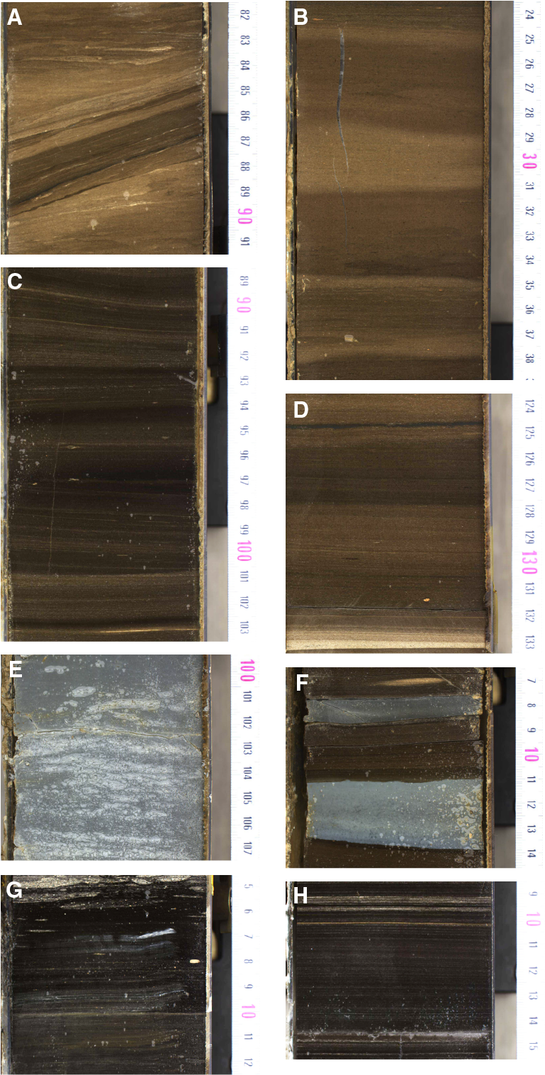
Figure F1. Marlstone/claystone lithologies.
Black shale
Black shales are dark gray to black (2.5Y 3/1, 2.5Y 2.5/1) and planar laminated at the submillimeter to millimeter scale (Figure F1). They comprise clay- to silt-sized grains with local fine sand–sized grains. They are locally burrowed with a maximum ichnofabric index of 2. Black shales contain thin interlaminations of dark marlstone/claystone and brown marlstone and grade upward into dark marlstone/claystone, marlstone, and/or limestone. Black shale occurs as thin millimeter- to centimeter-scale interbeds in Subunits 1A and 1D. It is also prominent in Subunit 1E, with decimeter-scale packages at the base and in the lower portion and as thin interbeds throughout the subunit.
Dark marlstone/claystone
Dark marlstone/claystone is olive-brown (2.5Y 4/3), very dark grayish brown (2.5Y 3/2), or very dark gray (2.5Y 3/1) with local light olive-brown interbeds (2.5Y 5/4) (Figure F1). Marlstone and claystone are lumped together in this facies because they are commonly interlaminated at the millimeter scale. Bedding ranges from millimeter to decimeter thick with millimeter- to centimeter-scale bedding most common. Beds are planar to wavy, and grain size is dominantly clay to silt sized with local sand-sized grains. The ichnofabric index ranges from 1 to 4 with local well-preserved individual burrows. Locally thin millimeter-scale light-colored packstones or grainstones are interbedded. Alteration features include soft-sediment deformation, pyrite, and carbonate nodules. Dark marlstone/claystone occurs in Subunits 1A–1E, locally overlies black shale, marlstone, wackestone, or packstone, and commonly grades upward into marlstone and/or wackestone or packstone.
Marlstone
Marlstones vary tremendously in color, including light gray (2.5Y 7/1), light brownish gray (2.5Y 6/2), grayish brown (2.5Y 5/2), olive-brown (2.5Y 4/3), very dark grayish brown (2.5Y 3/2), dark gray (2.5Y 4/1), light bluish gray (Gley 2 7-8/5PB or Gley 2 8/10B), and greenish gray (Gley 2 5/10G) (Figure F1). These lithologies exhibit a wide range of bedding morphologies and ichnofabrics. Bedding ranges from millimeter to decimeter thick with millimeter- to centimeter-scale bedding most common. Beds are planar to wavy and locally display wispy stylolites, especially in Subunit 1E (Figure F2). Grain size is dominantly clay to silt sized with local sand-sized grains and foraminifers (Figure F3). The ichnofabric index ranges from 1 to 4, and marlstones locally have well-preserved individual or crosscutting burrows. Marlstone commonly overlies dark marlstone/claystone, wackestone, or packstone and commonly grades upward into wackestone or packstone. Marlstone occurs in Subunits 1A–1F (Figures F2, F4, F5, F6, F7, F8, F9).
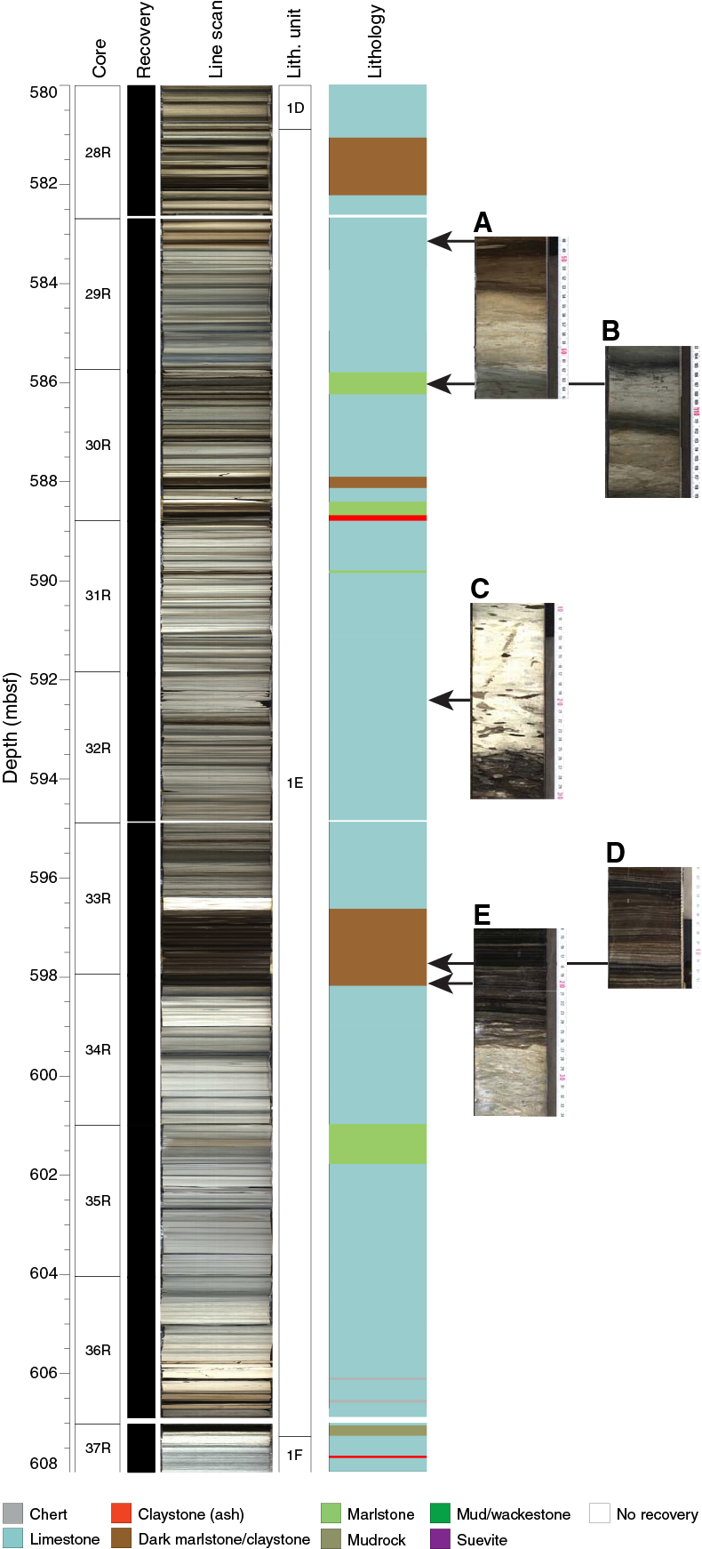
Figure F2. Subunit 1E lithologies.

Figure F3. Selected lithologies.

Figure F4. Subunit 1A lithologies.

Figure F5. Subunit 1B lithologies.
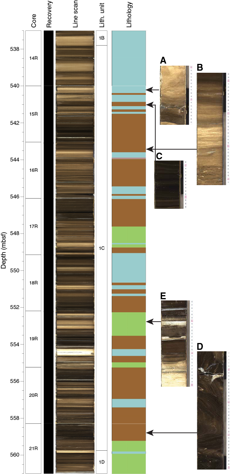
Figure F6. Subunit 1C lithologies.
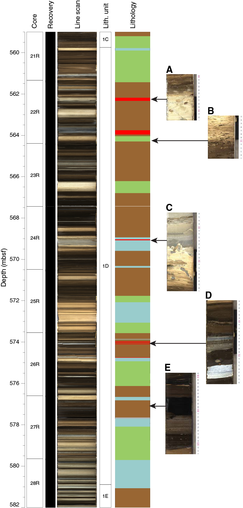
Figure F7. Subunit 1D lithologies.
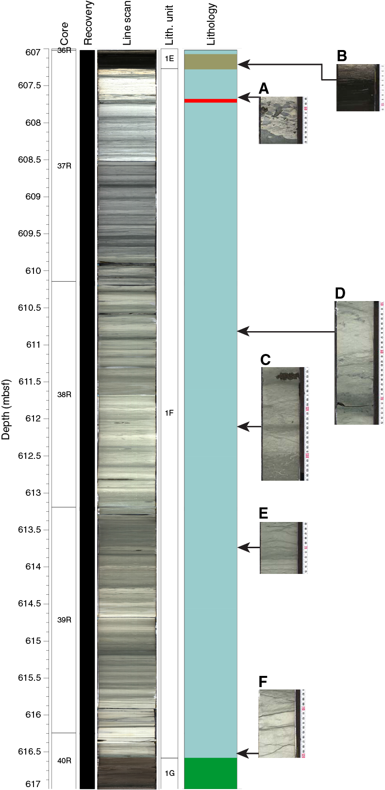
Figure F8. Subunit 1F lithologies.
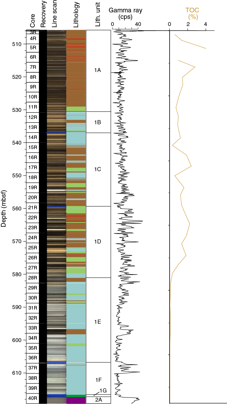
Figure F9. Lithostratigraphy, gamma ray, and TOC.
Wackestone
Limestones classified as wackestones are very diverse in color, including light gray (2.5Y 7/2), light olive-brown (2.5Y 5/3), light brownish gray (2.5Y 6/2), light yellowish brown (2.5Y 6/3), olive-brown (2.5Y 4/4), and very dark grayish brown (2.5Y 3/2) (Figure F10). Beds are millimeter thick and planar laminated to weakly laminated (ichnofabric index = 1–2) or centimeter to decimeter thick and bioturbated (ichnofabric index = 3–5). Foraminifers and radiolarians are rare to common (Figure F3). Wackestones are commonly gradational or interbedded with dark marlstone/claystone, marlstone, and packstone. Alteration features include soft-sediment deformation and wispy stylolites. Wackestone occurs in Subunits 1B–1E (Figures F2, F5, F6, F7).
Figure F10. Wackestone/packstone/grainstone/siltstone lithologies.
Packstone
Lime packstones vary in color, including very dark grayish brown (2.5Y 4/2), grayish brown (2.5Y 5/2), very dark gray (2.5Y 3/1), dark brownish gray (2.5Y 3/2), light brownish gray (2.5Y6/2), light olive-brown (2.5Y 5/3), light gray (2.5Y 7/2), gray (Gley 1 6/N), light bluish gray (Gley 2 7/10B), greenish gray (Gley 2 6/5GB), and light yellowish brown (2.5Y 6/3) (Figure F10). Beds are centimeter to decimeter thick and commonly bioturbated (ichnofabric index = 2–5) and locally contain well-preserved burrows (Figure F2). Grains are silt to sand sized, and foraminifers are rare to common. Alteration features include local glauconitic grains, chert, soft-sediment deformation, and wispy stylolites, especially in Subunit 1F. Packstones are gradational or intercalated with dark marlstone/claystone, marlstone, wackestone, or grainstone. Packstone occurs in Subunits 1B–1F (Figures F2, F5, F6, F7, F8). Rare, very thin beds of packstone with grains of impact glass and a variety of carbonate grains also occur at the bases of some fining-upward packages in Subunit 1G.
Grainstone
Grainstones are pale yellow (2.5Y 7/3), light yellowish brown (2.5Y 6/3), light bluish gray (Gley 2 7/10B), light gray (2.5Y 7/1), and dark gray (Gley 1 4/N) (Figure F10). Grainstones commonly occur as millimeter-scale laminated to cross-laminated interbeds with sharp contacts or infill burrows in dark marlstone/claystone and marlstone in Subunits 1A, 1D, and 1E. This lithology also occurs as centimeter- to decimeter-scale units with sharp basal contacts that commonly grade upward into wackestone or marlstone. Grains are silt to sand sized, including rare to common foraminifers and other unidentifiable carbonate grains. Grainstones thicker than 1 cm are scarce and occur only in Subunits 1D and 1E.
Lime mud/wackestone
Lime mud/wackestone is dark gray (10YR 4/1) to dark grayish brown (10YR 4/2) and displays submillimeter- to millimeter-scale planar laminations to centimeter-scale beds (Figures F10, F11). Locally, laminae are grayish green (Gley 1 4/5G) or mottled grayish green. The base of the mud/wackestone contains two 5–7 mm thick graded beds with silt- to medium sand–sized clasts similar to the underlying suevite. The package grades upward from submillimeter-scale dark grayish brown laminae to couplets that contain millimeter-scale dark grayish brown laminae and millimeter- to centimeter-scale dark gray laminae. Bedding is less distinct in the upper part of the mud/wackestone, which is gray (10YR 5/1) with a 2–3 mm thick, pale green (Gley 1 6/5G), laminated marly interval. The mud/wackestone is locally altered by displacive pyrite and soft-sediment deformation, with an approximately 10 cm thick soft-sediment fold with an axis at 616.86 mbsf, in Subunit 1G.
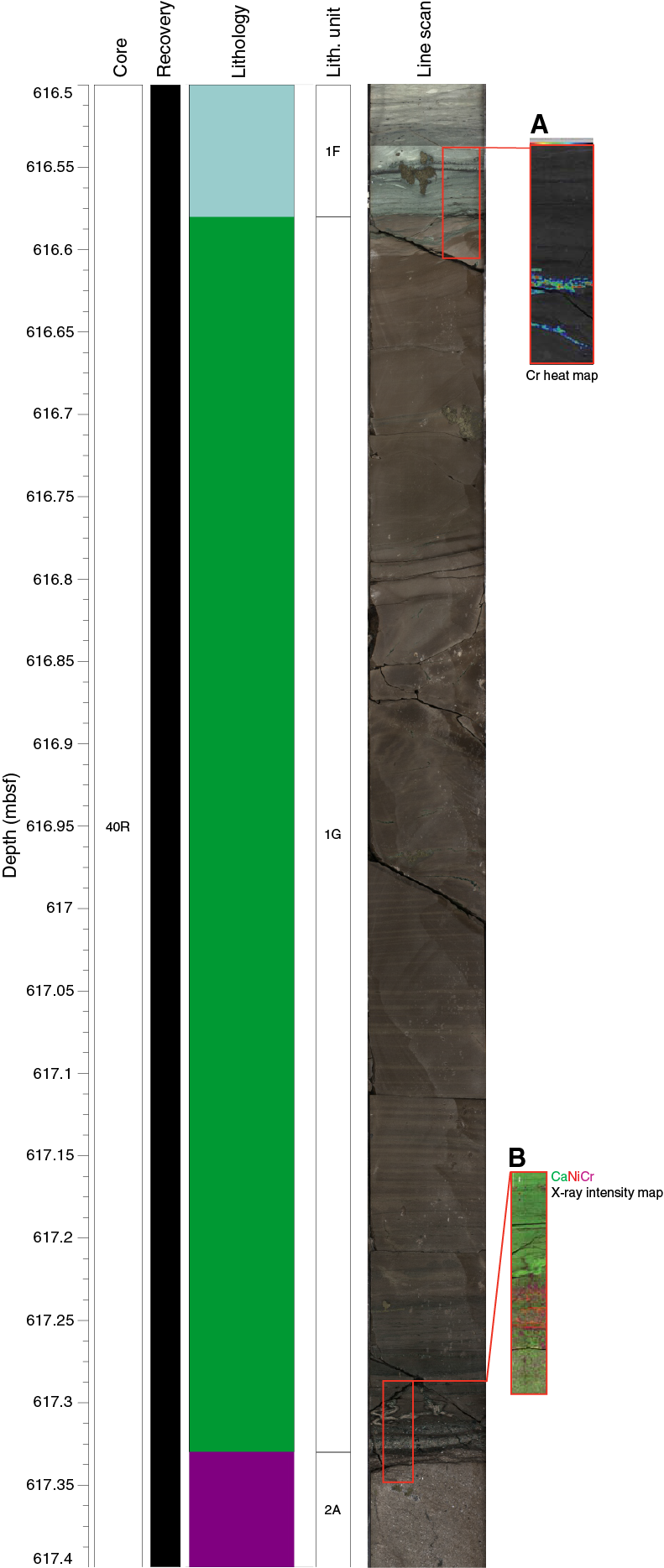
Figure F11. Upper and lower contacts of Subunit 1G.
Lithostratigraphic units
Lithostratigraphic units were defined based on significant changes in the distribution of the different lithologies described above. Contacts between units are usually sharp and either depositional or erosional but are locally gradational due to bioturbation (Table T1; Figures F2, F4, F5, F6, F7, F8, F11, F12, F13). The biostratigraphy of the cored interval provides age control (see Biostratigraphy) (Figure F12).

Figure F12. Lithostratigraphic summary.
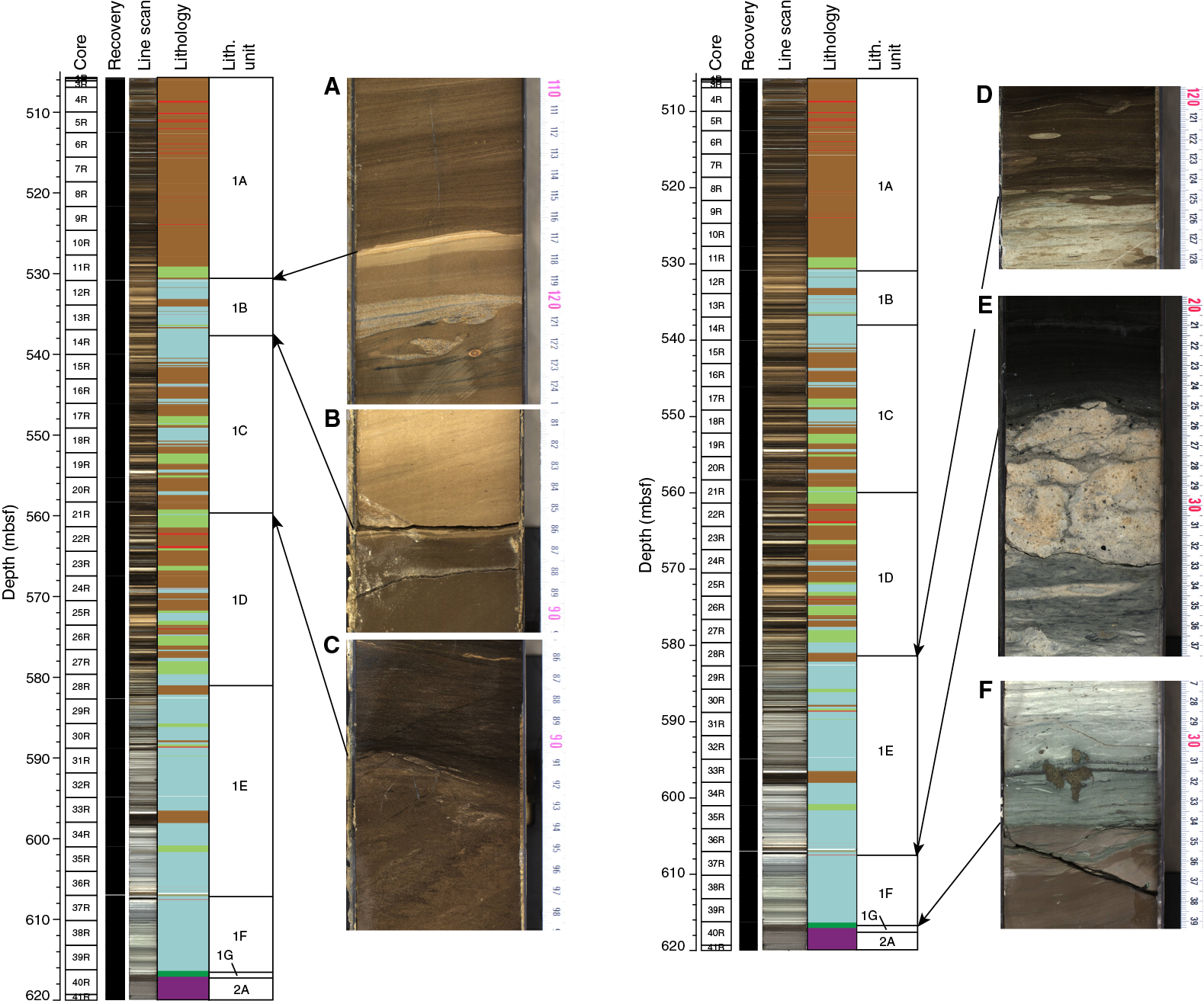
Figure F13. Basal contacts of Subunits 1A–1F.
Subunit 1A
Subunit 1A occurs from the top of the cored interval at 505.7 mbsf to 530.18 mbsf and consists of dark marlstone/claystone and marlstone that is laminated at the millimeter scale or centimeter- to decimeter-scale bedded (Figures F4, F13A). These lithologies include millimeter-scale interbeds of packstone or grainstone with foraminifers and radiolarians (Figure F3). Claystones occur sporadically through the subunit with several thick examples in the upper part. The contact with Subunit 1B is a sharp erosional contact that truncates an underlying thin grainstone in Section 11R-2, 116.8 cm (530.18 mbsf) (Table T1).
Subunit 1B
Subunit 1B continues from 530.18 to 537.80 mbsf and contains millimeter- to centimeter-scale bedded dark marlstone/claystone, centimeter- to decimeter-scale bedded marlstone, and centimeter- to decimeter-scale bedded wackestone and packstone with local claystone intervals (Figures F5, F13A). The base of the subunit is packstone that erosionally truncates the underlying dark marlstone/claystone at the top of Subunit 1C in Section 14R-1, 86.40 cm (537.89 mbsf) (Table T1).
Subunit 1C
Subunit 1C extends from 537.80 to 559.75 mbsf and consists of intercalated dark marlstone/claystone, marlstone, wackestone, packstone, and local claystone (Figures F6, F13A). Dark marlstone/claystones are laminated at the millimeter scale or centimeter-scale bedded. Claystones are centimeter-scale bedded, and other lithologies are centimeter- to decimeter-scale bedded. The subunit displays a centimeter-scale soft-sediment fold within a packstone in Section 14R-1, 100–107.5 cm. Soft-sediment deformation recurs in the lower part of Section 20R-2 and the upper part of Section 21R-1 with decimeter-scale soft-sediment folds in dark marlstone/claystone. The base of the subunit is a gradational contact designated as the last millimeter-scale dark marlstone/limestone overlying marlstone with thin light brown wackestone interbeds in Section 21R-1, 146.20 cm (559.75 mbsf) (Table T1).
Subunit 1D
Subunit 1D stretches from 559.75 to 580.89 mbsf and contains interbedded dark marlstone/claystone, claystone, marlstone, wackestone, and packstone intercalated at the centimeter to decimeter scale (Figures F5, F13B). Dark marlstone/claystone was observed mostly laminated at the millimeter scale, whereas marlstones are generally centimeter-scale bedded or bioturbated and decimeter-scale bedded. Claystones are mainly centimeter-scale bedded except for decimeter-thick claystones. One such claystone bed extends from the base of Section 22R-2 to the top of Section 22R-3, and another exists in Section 24R-2. Both are bioturbated with an ichnofabric index of 2–3. Wackestones and packstones are largely bioturbated and centimeter-scale bedded in the upper part of the subunit but become thicker downhole (>20 cm). Marlstones are brownish gray or grayish brown, and limestones are light brownish gray to light yellowish brown. The subunit appears largely cyclic, with lithologies that coarsen upward from dark marlstone/claystone to marlstone to wackestone and/or packstone. The base of the subunit is slightly gradational at the bottom of a dark marlstone/claystone with minor burrowing in Section 28R-1, 125.20 cm (580.89 mbsf) (Table T1). The contact was designated based on the change to bluish marlstones that occur in the core below.
Subunit 1E
Subunit 1E occurs from 580.89 to 607.27 mbsf and contains interbedded dark marlstone/claystone, lighter brown marlstone (ichnofabric index = 2–3), light brown to bluish wackestone and packstone (ichnofabric index = 2–4), and black shale (ichnofabric index = 1) (Figures F2, F13B). Facies other than black shale contain wispy stylolites. Units that contain black shale display elevated gamma ray signatures and the highest total organic carbon (TOC) contents in the core (Figure F8). The upper portion of the subunit is highly cyclic, with decimeter-thick dark marlstone/claystone or marlstone-based cycles that grade upward into wackestone or packstone. Contacts between lithologies are usually gradational due to burrowing. From the top of the subunit to the middle of Section 29R-1, marlstones are dominantly light brownish gray or grayish brown and limestones are light brownish gray to light yellowish brown, with all displaying some bluish intervals. Deeper marlstones are dominantly light bluish gray, and limestones are light gray to light bluish gray. In Section 33R-2, 25.5 cm (596.65 mbsf), cyclic bedding is replaced by a package of dark marlstone/claystone that is burrowed at the top (ichnofabric index = 3), parallel laminated below, and intercalated with thin planar-laminated black shale and dark brown wackestone. This package extends to Section 34R-1, 26.5 cm (598.21 mbsf). Downhole, the core once again records decimeter-scale cyclic alternations of dark gray to light bluish gray marlstones that grade upward into light gray to light bluish gray wackestone or packstone with foraminifers (Figure F3) and local black chert. In Section 36R-1, 58 cm, burrows take on a brownish hue and lithologies alternate between light brown and bluish colors. Contacts between lithologies are usually gradational due to burrowing. In Section 36R-2, 78 cm, is a 1.5 cm thick granule-pebble carbonate rudstone. Below the rudstone to Section 36R-4, 16 cm, is a package of light yellowish brown wackestone and packstone with centimeter-thick dark gray marl interbeds and black chert horizons. The lowermost package in the subunit is a burrowed packstone that grades downward into black shale at Section 37R-1, 0–25.5 cm. A gradational contact between the packstone and black shale occurs at Section 37R-1, 4.5 cm. The base of the subunit is the top of a prominent carbonate-cemented surface with about 1.5 cm of relief in Section 37R-1, 25.5 cm (607.27 mbsf) (Table T1).
Subunit 1F
Subunit 1F extends from 607.27 to 616.58 mbsf and consists of interbedded light gray to light bluish gray wackestone and packstone (ichnofabric index = 3–5) and light to dark bluish gray marlstone (ichnofabric index = 2) at the centimeter to decimeter scale (Figures F8, F13B). All lithologies contain wispy stylolites. The upper portion of the subunit, to Section 37R-1, 65.5 cm, is light yellowish brown packstone that is burrowed (ichnofabric index = 4) and intercalated with gray marlstone. The uppermost 7.5 cm, above the marlstone, is calcite cemented. Clasts are fine to coarse sand sized and include foraminifers. The lowermost part of this package has two black chert patches. From the base of this package to Section 37R-1, 72.5 cm, is bluish gray claystone. Downhole, bedding is cyclic at the centimeter to decimeter scale with light bluish marlstone bases grading upward into light gray or light bluish gray wackestone and packstone. Contacts between lithologies are usually gradational due to burrowing. Rocks take on a light greenish hue near the base of the subunit. Cycles thicken upward between 610.25 and 612.57 mbsf, thin upward between 612.57 and 613.87 mbsf, thicken upward from 613.87 to 615.06 mbsf, and thin upward from 615.06 to the base of subunit at 616.55 mbsf. The base of the subunit is a sharp contact below the base of the greenish claystone in Section 40R-1, 34.20 cm (616.58 mbsf) (Table T1).
Subunit 1G
Subunit 1G occurs from 616.58 to 617.33 mbsf and consists mainly of dark brown to dark grayish brown lime mudstone to wackestone (mud/wackestone) (Figure F11). The subunit is complex, with several different lithologies that generally fine upward. It contains postdepositional pyrite nodules that disrupt bedding. The upper portion of the subunit has two thin intervals that display Cr enrichment based on µXRF mapping (see Geochemistry and mineralogy). The uppermost Subunit 1G is slightly deformed, with one millimeter-scale greenish marlstone interbedded with the lightest gray mud/wackestone in Section 40R-1, 34.2–36.8 cm (616.58–616.60 mbsf). Bedding is indistinct in the upper mud/wackestone and is obscured by soft-sediment deformation in Section 40R-1, 57.5–67.5 cm (616.73–616.83 mbsf). In Section 40R-1, 78–100.04 cm (617.24 mbsf), Subunit 1G contains millimeter-bedded couplets of dark brown and dark grayish brown mud/wackestone that overlie centimeter-bedded mud/wackestone. In Section 40R-1, 100.04–109.4 cm (617.24 to 617.33 mbsf), are five thin intervals: (1) a 3 cm thick light gray mud/wackestone laminated at the submillimeter scale with local greenish laminae, (2) a 1.8 cm thick mud/wackestone that is slightly darker gray and has some greenish laminae and clasts, (3) a 3.1 cm thick light gray mud/wackestone laminated at the submillimeter scale (similar to 2) that also contains a calcite-filled convoluted feature that crosscuts itself, and (4 and 5) two normally graded beds of packstone with impact glass and a variety of carbonate grains, each less than 1 cm thick. Beds grade upward from packstone with greenish sand-sized clasts, similar to those in the underlying suevite, to dark gray millimeter-thick laminae similar to the overlying mud/wackestone. These two beds display enrichment of Ni and Cr based on X-ray intensity mapping (see Geochemistry and mineralogy). The base of the subunit is a sharp, stylolitized contact in Section 40R-1, 109.4 cm (617.33 mbsf) (Table T1), that overlies the upper suevite of Subunit 2A.
Computed tomography facies analysis
Post-impact sediments are classified according to their lithologic affiliation and divided into different units depending on their composition. Expedition 364 cores were CT scanned with two different energy levels (80 and 135 kV). The higher energy CT scan is more sensitive to density, and the lower energy scan is more sensitive to atomic number. For the purposes of observations made during the Onshore Science Party (OSP), the CT facies described are simply put in context of higher or lower CT values. Although a single CT value is returned for each 0.3 × 0.3 mm pixel within the scanned cores, areas of similar lithology generally return similar CT values. Hence, a clast of a single rock type will be recognizable because all pixels within the region of the clast are colored similarly. Within the post-impact succession, layers of similar lithology will display similar CT values represented by a grayscale color scheme. The X-Z slice images of bulk density (ρb) and effective atomic number (Zeff) are also discussed. One can therefore define a CT facies to describe sections of the cores that have similar patterns in the CT images and dual energy–derived products.
Computed tomography facies of individual rock types
The marlstone lithology is divided into marlstone and dark marlstone/claystone. CT scans associated with the former consist mainly of light gray to dark gray intervals. Both intervals correspond mainly to low ρb and high Zeff. In a few cases, ρb and Zeff vary between high and moderate values, complicating the recognition of a clear pattern. Bioturbated areas occur locally as black intervals. A few light gray to white intervals occur within the marlstones and are associated with high ρb and low Zeff.
The dark marlstone/claystone lithology consists of alternations of light gray, dark gray, and black intervals. The light gray intervals are mainly associated with low ρb and high Zeff. However, high ρb and high Zeff are also common within these intervals. The dark gray intervals correspond to high ρb and low Zeff, but moderate values for both properties are present. The black intervals are mainly associated with relatively moderate values for ρb and Zeff, but several areas also display relatively high or low values for either ρb or Zeff.
Generally, even if certain patterns can be associated with the two lithologies, variances are common, making a clear definition of the CT facies challenging without further detailed study.
The limestone lithology is divided into wackestone, packstone, and grainstone. CT scans of the wackestone and packstone intervals show alternations of variable thickness (from a few millimeters to an entire core section) of light to dark gray and black intervals. These intervals are associated with a broad spectrum of ρb and Zeff that vary between high, moderate, and low values. A pattern cannot be recognized. Within the wackestone, however, white intervals are locally present that are associated with relatively high Zeff compared with the darker intervals. In many cases, an increase in the ichnofabric index correlates with a lighter interval on the CT image interval (up to light gray), whereas density values drop compared to less bioturbated areas.
The grainstone lithology presents itself uniformly as a light interval, mainly light gray and in rare cases white. This lithology is associated with high ρb and high Zeff relative to the observed values of the other lithologies.
The claystone lithology is associated with a black CT interval that corresponds to relatively low ρb and low Zeff. In only a few cases are either moderate ρb or high Zeff present. An exception to this pattern was observed within a bioturbated claystone layer (Section 6R-1) where the recycling of sediment possibly caused a white CT interval (Figure F14). In areas where claystones experienced silicification, the CT interval still appears black and is associated with relatively low ρb but relatively moderate Zeff.
Recurring extraordinary features such as pyrite, chert layers or nodules, and mineral-filled cracks appear as pearly white features on the core surface and are always associated with relatively high ρb and Zeff (Figures F14, F15).
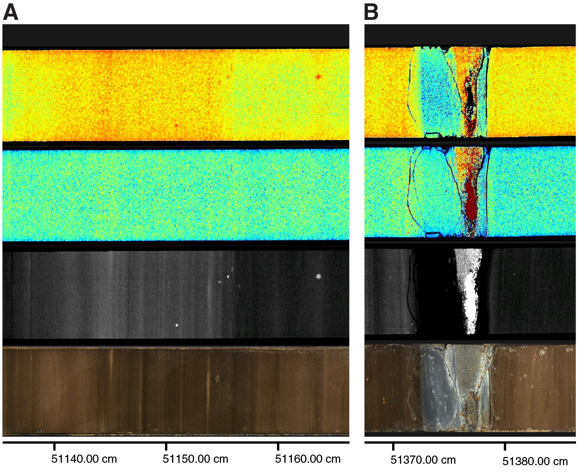
Figure F14. Line scan, CT scan, density, and atomic number, Hole M0077A.
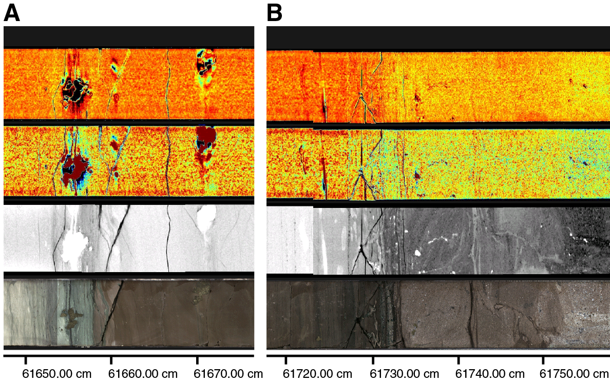
Figure F15. Line scan, CT scan, density, and atomic number, Section 40R-1.
CT facies of individual subunits
The Post-Impact Sedimentary Rocks interval is divided into seven subunits (1A–1G) (Table T1). Subunit 1A consists mainly of marlstone and dark marlstone/claystone layers that both appear as alternating sequences of light gray, dark gray, and black intervals on the CT scans (Figure F14). Overall, the subunit is associated with relatively low ρb and high Zeff. However, opposite patterns also occur throughout the subunit and seem to become more common toward the bottom.
Similarly, Subunit 1B is represented by alternating light gray, dark gray, and black intervals that appear relatively thicker than those in Subunit 1A. This subunit is also represented by relatively low ρb and high Zeff, but opposite patterns were also observed. The rarely occurring limestone packages at the bottom of the subunit are associated with light gray intervals on the CT scan and relatively high ρb and high Zeff.
Subunit 1C is also an alternating sequence of light gray, dark gray, and black intervals with relatively low ρb and high Zeff. Changes within the pattern of ρb and Zeff are common. The more frequently occurring limestone packages are associated with a light gray interval and relatively high ρb and high Zeff. In addition, the CT scans mirror the soft-sediment deformation that was observed within the interbedded marlstone lithologies.
Subunit 1D is also composed of light gray, dark gray, and black intervals. However, the black and very light gray (almost white) intervals have increased thickness compared to those in the upper three units. The black intervals are associated with (nonlaminated) marlstone and dark marlstone/claystone layers that have low ρb and high Zeff, although this association is variable. The light gray intervals are associated with the limestone packages that correspond to high ρb and high Zeff. Overall, the subunit shows more areas that are associated with low Zeff than Subunits 1A–1C. Even though these areas cannot be clearly associated with a lithology, they seem to correlate more with the occurrence of marlstone and claystone. Toward the bottom of the subunit, the alternating intervals of the CT scan decrease in thickness.
Subunit 1E consists predominantly of a light gray interval with some relatively thin intervals of dark gray and black. The light gray interval was correlated with high but also low Zeff and quite variable density values. The light gray interval corresponds with the presence of limestone, and the darker intervals are associated with marlstone and claystone.
This trend continues in Subunit 1F, which consists mainly of one light gray interval associated with high ρb and high Zeff that corresponds with the presence of limestone. Dark gray and black intervals become rare to nonexistent throughout the subunit and are only correlated with a few interbedded marlstones and core disturbance.
Subunit 1G (616.58–617.33 mbsf) was initially described as siltstone during visual core description but was later reclassified as lime mud/wackestone; it has an average CT number of 2314.6 ± 248.8 (2σ). It consists of light to dark gray intervals that are overall associated with relatively high ρb and high Zeff (Figure F15). At the top of the subunit, laminations of low–CT intensity material were observed; these correspond to green laminae seen in the VCDs. Throughout the subunit, intermittently developed irregular laminae were observed; these become particularly prominent in the lower third of the subunit (Figure F15). Besides rare occurrences of pyrite, which have high Zeff and ρb, the mud/wackestone has a very homogeneous Zeff and ρb distribution. Within the bottom 10 cm of the subunit, horizontally elongate bright spots were observed in CT data; these spots are interconnected, horizontally elongated regions with bulbous shapes. Below this zone, just above the lower contact, is a folded and crumpled layer of material with a slightly brighter CT number. Laminations seen in the CT data in the bottom 5 cm are associated with ρb variability. The contact with Subunit 2A marks an abrupt drop in CT number and a reduction in the homogeneity of the material (F15).
Biostratigraphy
Coring in Hole M0077A recovered ~110 m of post-impact Paleogene sediments, ranging from middle Eocene (Ypresian) to basal Paleocene (Danian). Biostratigraphic zones are summarized in Figure F16, and semiquantitative abundance counts are summarized in Tables T2 and T3 for foraminifers and nannoplankton, respectively. Preservation varies greatly from very poor to good and is strongly correlated to the induration of the rock, particularly silicified intervals. Planktic and benthic foraminifers and calcareous nannofossils are generally present throughout.
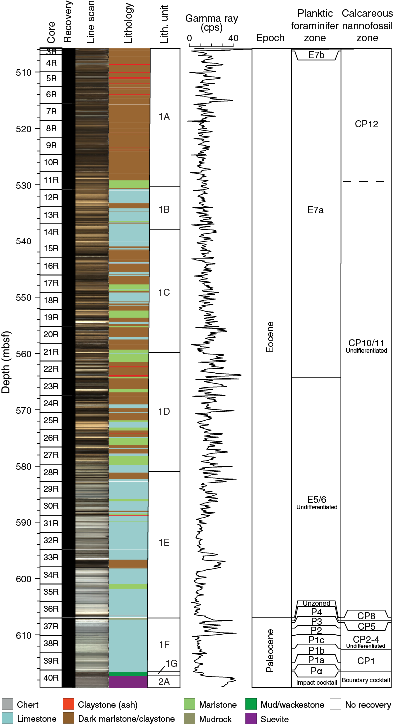
Figure F16. Biostratigraphic zones.
Table T2. Foraminifers. Download table in CSV format.
Table T3. Nannofossils. Download table in CSV format.
The Eocene section ranges from planktic foraminifer Zones E7b to E5 and calcareous nannofossil Zones CP12 to CP10. This interval is characterized by diverse but variable assemblages of both foraminifers and nannofossils and contains rare to dominant radiolarians, which are often associated with more organic-rich, laminated, and often indurated lithologies that can only be examined in thin section.
A set of stacked unconformities spanning Sections 36R-4 through 37R-1 (~606.5–607.5 mbsf) separate the Paleocene and Eocene sections and separate partial intervals of the uppermost Paleocene (including the Paleocene/Eocene Thermal Maximum [PETM]; nannofossil Zone CP8) and upper Paleocene (nannofossil Zone CP5 and planktic foraminifer Zone P4a). The lower Paleocene is complete, however, and ranges from planktic Zones P3b to Pα. Nannofossil zonation is difficult in this interval because the assemblage is dominated by bloom taxa (e.g., Braarudosphaera). Thoracosphaera, a calcareous dinoflagellate common in early Danian marine records, is very abundant in both thin section and sieved residues from the lower part of Section 39R-3 to the limestone in the upper portion of Section 40R-1 (~616.0–616.5 mbsf).
Below Zone Pα, a 75 cm thick brown mud/wackestone contains a number of Maastrichtian foraminifers and nannoplankton characterizing the “Boundary Cocktail” of Bralower et al. (1998).
Eocene
Planktic foraminifers
Variable preservation in the Eocene section (Cores 1R–36R; 505.70–606.51 mbsf) hampered shipboard biostratigraphy. During the OSP, core catcher samples collected aboard the L/B Myrtle were supplemented with additional samples from the middle of each core, selected from the least lithified intervals possible. Additionally, a number of thin sections were prepared and analyzed during the OSP to better constrain the assemblage in indurated intervals. Overall, the Eocene section contains a diverse (and variable) assemblage of planktic foraminifers, as well as a large number of radiolarians (Figure F17), particularly in the upper part of the section.

Figure F17. Upper Eocene radiolarians.
The base of Core 1R, in Sample 1R-1, 14–15 cm (505.85 mbsf), contains a middle Eocene assemblage of Zone E7b, indicated by the presence of Turborotalia frontosa. This taxon is not found below Sample 3R-1, 125–126 cm, whereas Acarinina cuneicamerata continues to Sample 21R-3, 0–2 cm (561.14 mbsf), defining the range of Zone E7a.The assemblage in this zone is characterized by Pseudohastigerina wilcoxensis, species of Acarinina and Subbotina, rare Astrorotalia palmerae (in Cores 15R and 16R), and common radiolarians. Morozovellids are very rare throughout Zone E7 and are not consistent components of the assemblage until nearly the base of the Eocene section. The lowest occurrence (LO) of A. cuneicamerata is followed by very poor preservation to Sample 23R-2, 88–91 cm (566.77 mbsf), which contains abundant foraminifers, including other Acarininids; the base of Zone E7a is therefore interpolated between these two well-preserved samples at 564.03 mbsf.
Zones E6 and E5 are undifferentiated. The base of Zone E6 is defined as the highest occurrence (HO) of Morozovella subbotinae, but the rarity of Morozovellids throughout the section suggests that the observed HO of M. subbotinae in Sample 32R-3, 58–59 cm (594.84 mbsf), may be ecologically controlled and thus not a robust biostratigraphic datum. Morozovellids generally become more common below Core 30R and include a typical early Eocene assemblage including Morozovella aragonensis, M. subbotinae, and Morozovella formosa (Figure F18). Additional typical early Eocene planktics, including Acarinina wilcoxensis, Acarinina soldadoensis, Igorina broedermanni, and Planorotalites pseudoscitula, are also present throughout this interval. P. wilcoxensis is less common than it is in Zone E7. Radiolarians also become a less prominent component of most samples in this interval. M. aragonensis, whose base defines the bottom of Zone E5, is present to Sample 36R-3, 6–7 cm (606.17 mbsf). Deeper samples are poorly preserved until the unconformity separating the Eocene and Paleocene sections, and we believe it is likely that Zone E5 extends to the base of the Eocene section.
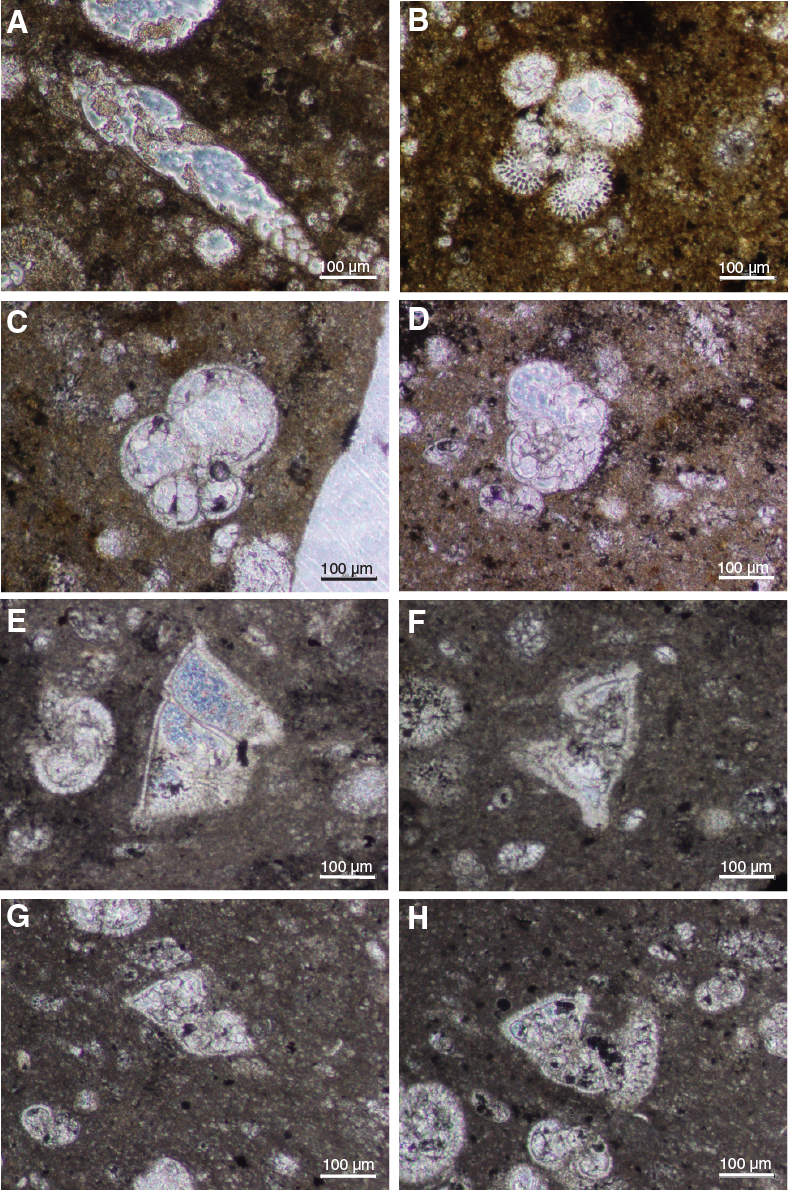
Figure F18. Eocene planktic foraminifers.
Calcareous nannofossils
In the Eocene section, nannofossils range from few to abundant and preservation is generally poor with some more well preserved intervals. Specimens are moderately etched and overgrown. Assemblages are relatively diverse with consistent occurrences of Discoaster barbadiensis, Discoaster lodoensis, Zygrhablithus bijugatus, Coccolithus pelagicus, Ericsonia formosa, Toweius gammation, small Toweius spp., Sphenolithus moriformis, and Sphenolithus radians throughout most of the interval. Reticulofenestra dictyoda and Discoaster sublodoensis are only present in the top part of the hole (Figure F19). Other species such as Discoaster kuepperi, Toweius crassus, Toweius callosus, Toweius pertusus, Chiasmolithus bidens, Chiasmolithus solitus, Chiasmolithus consuetus, Campylosphaera dela, Helicosphaera seminulum, Helicosphaera lophota, Pontosphaera spp., and Clausicoccus cribellum are rare or have more intermittent occurrences.
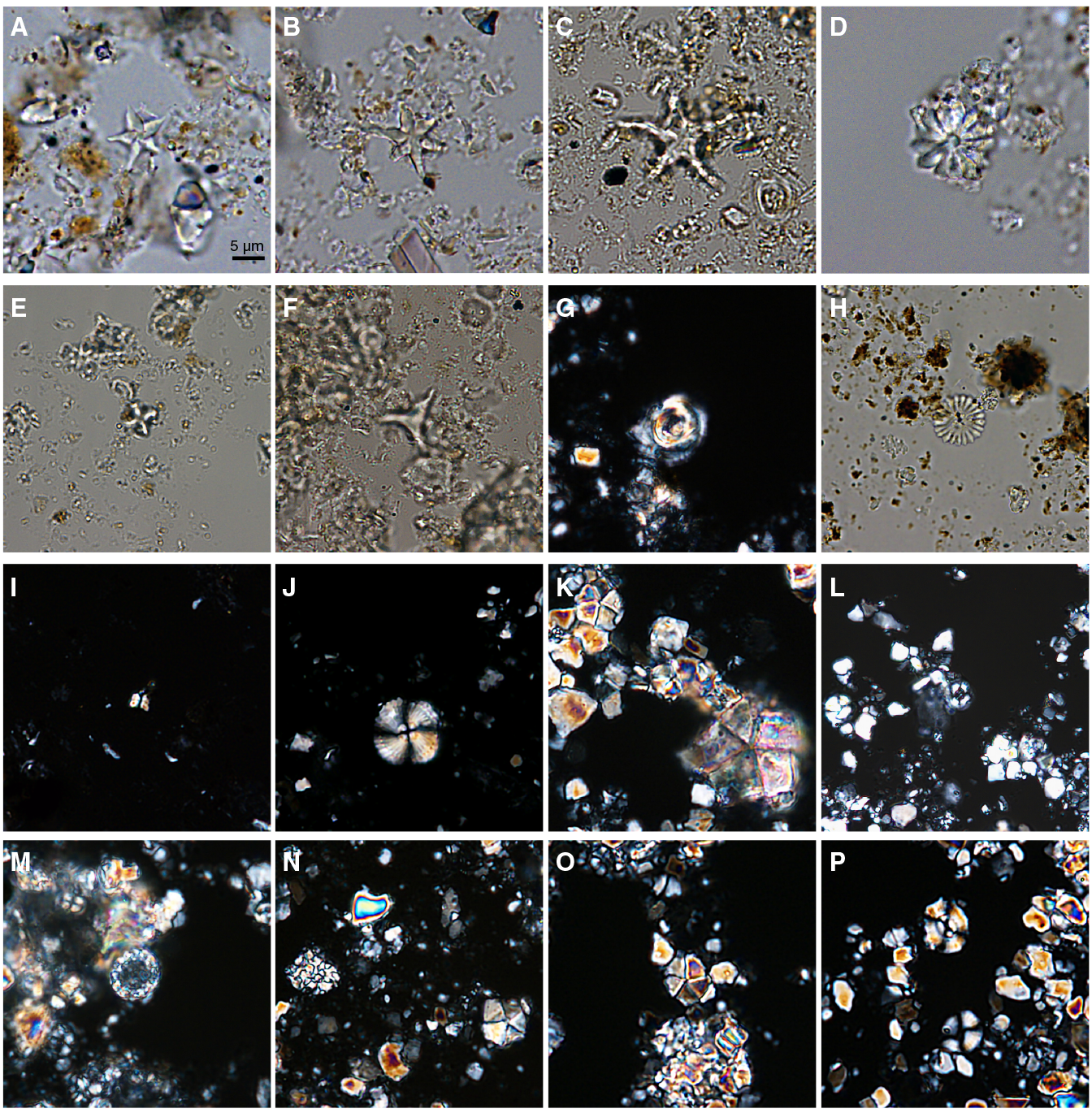
Figure F19. Typical and marker calcareous nannoplankton.
The interval from Sample 1R-1, 8–9 cm, to Sample 10R-1, 56–58.5 cm (505.78–525.2 mbsf), is assigned to Zone CP12 based on the sporadic occurrence of D. sublodoensis. However, it is often difficult to differentiate this species from five-rayed specimens of D. lodoensis, which appears morphologically similar in overgrown samples and is often abundant. There are two subsidiary markers that shed light on the placement of the base of Zone CP12: (1) D. sublodoensis co-occurs with an early form of Nannotetrina sp. within Sample 10R-1, 56–58.5 cm (525.2 mbsf). Nannotetrina sp. has a LO within Zone CP12 (Bralower and Muttterlose, 1995), which corroborates the assignment of this sample to this biozone. (2) Sample 10R-2, 93–94 cm (527.07 mbsf), contains several fragments of Tribrachiatus orthostylus, whose LO is at the top of Zone CP11 (Perch-Nielsen, 1985). Nonetheless, we do not view the proposed boundary between Zones CP11 and CP12 with confidence.
The interval from Sample 10R-2, 93–94 cm, to Sample 24R-1, 56–58.5 cm (527.07–568 mbsf), is assigned tentatively to Zone CP11. The base of Zone CP11 is defined by the LO of T. crassus. This species is rare and difficult to differentiate from its ancestor, T. callosus, near its base. In Sample 25R-2, 50–52.5 cm (572.27 mbsf), many specimens that are intermediate between T. crassus and T. callosus are present. However, because definitive T. crassus specimens were not observed below Sample 25R-2, 50–52.5 cm (572.27 mbsf), we tentatively assign this sample to Zone CP10. Other datums that can be determined with more confidence and allow correlation with other sequences include the LO of R. dictyoda between Samples 16R-1, 67–69 cm (543.71 mbsf), and 17R-2, 60–62 cm (548.2 mbsf); the LO of T. gammation between Samples 26R-1, 82.5–85 cm (574.365 mbsf), and 27R-2, 30–32 cm (578.39 mbsf); and the LO of C. cribellum between Samples 29R-2, 22–24 cm (583.96 mbsf), and 30R-2, 22–24 cm (587.39 mbsf).
The base of Zone CP10 is defined by the LO of D. lodoensis between Samples 36R-2, 19–20 cm (605.22 mbsf), and 36R-2, 40–42.5 cm (605.43 mbsf). This species occurs continuously through the upper part of the section, is distinct morphologically and was identified even in poorly preserved samples. From Sample 36R-2, 40–42.5 cm (605.43 mbsf), to Sample 37R-1, 0–1 cm (607.02 mbsf), samples are heavily recrystallized and nannofossils are rare. Several large, overgrown Discoaster spp. were observed in this interval, in addition to frequent, moderately preserved Discoaster multiradiatus specimens. The absence of robust D. lodoensis indicates that these samples can be assigned to Zone CP9.
Benthic foraminifers
Benthic foraminifer abundance varies significantly throughout the Eocene (Figure F20). Generally, they appear to be more common in the upper portion of the Eocene section than in the lower portion, and their abundance appears anticorrelated with radiolarians. They are almost always estimated to represent less than 5% of the total foraminiferal assemblage. Several intervals of higher benthic diversity are listed in the abundance table (Table T2). These intervals are, roughly, in Cores 1R–6R (505–514 mbsf), 14R–17R (537–548 mbsf), and 36R (604–606 mbsf). Many other samples, often dark and organic rich, are nearly devoid of benthic foraminifers, including samples in which the benthic population consists of a single specimen.
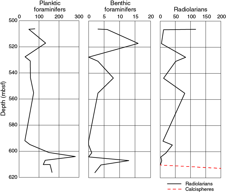
Figure F20. Abundance counts in thin section.
The benthic assemblage is characterized by species of Uvigerina, Gyroidina, Cibicidoides, Osangularia, Bulimina (especially Bulimina trinitatensis), Bolivina, and various uniserial taxa. Agglutinated foraminifers were only found in a few samples. Overall, this assemblage is characterized by deep-water benthics similar to that of the Velasco “fauna” (e.g., Alegret and Thomas, 2001), suggesting paleowater depths in the upper to middle bathyal range (~500–700 mbsf).
Paleocene
Planktic foraminifers
The stacked unconformities that characterize the bottom of Core 36R and the upper part of Core 37R are summarized in Figure F21. The bottom of Core 36R (Sample 36R-4, 1–17 cm) is characterized by a bioturbated interval containing abundant larger benthic foraminifers Discocyclina sp. and Asterocyclina, echinoid spines, fish debris, pyrite, and impact glass that has been altered to clay (including several examples with visible vesicles), all of which suggests extensive reworking. This reworked interval extends into the upper 4 cm of Section 37R-1, below which is a 21 cm thick interval (37R-1, 4–26 cm; 607.06–607.27 mbsf) of laminated black shale almost entirely barren of foraminifers. Calcareous nannofossils mark this interval as equivalent to the PETM. Sieved residues of this black shale, which disaggregates easily, contain carbonate debris (especially echinoid spines), fish teeth, and reworked impact glass, similar to the sandy interval above. One sample (37R-1, 5–5.5 cm; 607.06 mbsf) contains a few foraminifers that are discolored and abraded and therefore likely reworked. All samples within this black shale contain a component of volcanic glass (including biotite, angular glass shards, and euhedral sanidine crystals).
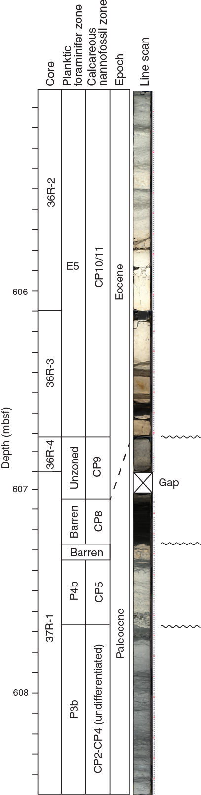
Figure F21. Biostratigraphic zones and unconformities, Sections 36R-3 through 37R-1.
The PETM black shale clearly unconformably overlies a hardground; the uppermost sample in the hardground (Sample 37R-1, 29–31 cm; 607.31 mbsf) is barren and entirely composed of sugary calcite. The next several samples (37R-1, 35–39 cm, and 37R-1, 50–52 cm; 607.37 and 607.52 mbsf) are better preserved and contain a diverse assemblage of late Paleocene planktic foraminifers assigned to Zone P4a based on the presence of Globanomalina pseudomenardii. Overall, these samples contain abundant Morozovellids, including Morozovella angulata, Morozovella acuta, abundant Subbotina spp., Acarinina spp., and few Igorina albeari. Section 37R-1, 58–65 cm, contains rip-up clasts, indicating another disconformity overlying a claystone with an erosionally scoured top. This interval was not sampled during the OSP, but we assume that Zone P4a extends to the base of the rip-up clast layer.
Sample 37R-1, 74–77 cm (607.76 mbsf), begins a long interval of poorly preserved microfossils in indurated limestone that extends to nearly Section 40R-1. Age-diagnostic taxa are present but rare and allow for a complete early Paleocene zonation from Zone P3 to Pα. The occurrence of Igorina pusilla in Samples 37R-1, 100–102 cm, and 37R-1, 135–137 cm (608.02 and 608.37 mbsf), places this interval in Zone P3. After this taxon disappears (interpolated datum depth at 608.83 mbsf), the continued presence of Praemurica uncinata downsection defines the extent of Zone P2 (interpolated datum depth at 610.37 mbsf). The LO of Globanomalina compressa, first found in Sample 38R-1, 65–68 cm (610.46 mbsf), indicates the base of Zone P1c (interpolated at 610.61 mbsf). The base of P1b is defined as the LO of Subbotina triloculinoides (interpolated datum at 611.75). Zone P1a extends to 616.29 mbsf, below which the HO of Parvularugoglobigerina eugubina in Sample 39R-3, 47–48 cm (616.24 mbsf), represents the first sample in Zone Pα (Figure F22). This zone extends to the base of the limestone section in Sample 40R-1, 34 cm (616.34 mbsf). Based on our sampling resolution (which was conservative to preserve core material through this critical interval), it is not clear if Zone P0 is present. The first sample observed in the limestone already contained an abundant, relatively well preserved assemblage of P. eugubina.
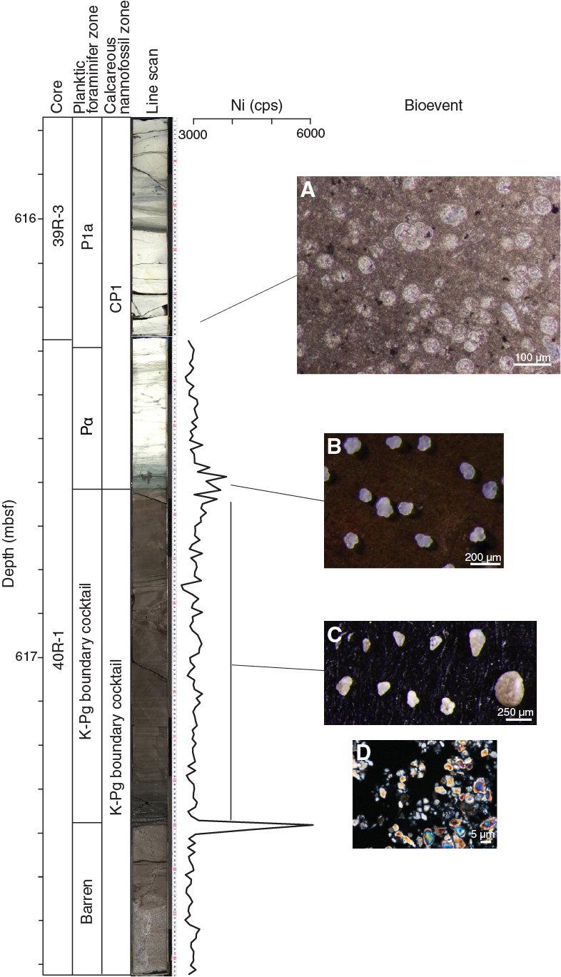
Figure F22. Biostratigraphic zones and major paleoecologic events.
Thin section analysis and sieved residues both yielded a large number of the calcareous dinoflagellate Thoracosphaera spp. in Zone Pα, a bloom event that is found in a large number of lower Danian sediments across the world (Figure F22).
Two samples were taken for paleontological analysis in the brown mud/wackestone interval 40R-1, 34–109 cm (Samples 40R-1, 42–43 cm [616.66 mbsf], and 40R-1, 97–98 cm [617.21 mbsf]). Both samples contain reworked Cretaceous planktic and benthic foraminifers, including members of the genera Heterohelix, Laeviheterohelix, and Rugoglobigerina (Figure F22).
Calcareous nannofossils
The interval from Sample 37R-1, 5.4 cm, to Sample 37R-1, 26.0 cm (607.074–607.28 mbsf), is characterized by black shale with abundant organic matter and pyrite observed in smear slide. Samples 37R-1, 6–7 cm (607.08 mbsf), and 37R-1, 11–13 cm (607.13 mbsf), contain frequent, moderately well preserved D. multiradiatus and Discoaster salisburgensis in addition to Discoaster falcatus, Sphenolithus primus, T. pertusus, and Toweius eminens. The crossover in occurrence of species of Fasciculithus (including Fasciculithus tympaniformis and members of the Fasciculithus schaubii and Fasciculithus alanii groups) and Z. bijugatus strongly suggests that the black shale interval represents the middle PETM within Zone CP8 (Raffi et al., 2009). This correlation is corroborated by the presence of rare excursion taxa (D. salisburgensis var. anartios) that are restricted to the PETM interval (Bybell and Self-Trail, 1995; Bralower and Self-Trail, 2016).
Two samples underneath the hardground at the base of the PETM (Samples 37R-1, 35–37 cm [607.37 mbsf], and 37R-1, 50–52 cm [607.52 mbsf]) contain common S. primus with F. tympaniformis, C. pelagicus, Ericsonia subpertusa, Ericsonia robusta, T. pertusus, T. eminens, Sphenolithus anarrhopus, Cruciplacolithus tenuis, and C. bidens. This typical late Paleocene assemblage was assigned to Zone CP5 based on the presence of Heliolithus kleinpellii and the absence of Discoaster mohleri (marker for the base of Zone CP6).
Samples in the interval from Sample 37R-1, 74–76 cm, to Sample 38R-2, 90–92 cm (607.76–612.5 mbsf), are often heavily recrystallized and contain poorly preserved nannofossils. Most samples are dominated by Braarudosphaera bigelowii with varying abundances of Coccolithus cavus, C. pelagicus, E. subpertusa, Cruciplacolithus primus, Cruciplacolithus intermedius, Placozygus sigmoides, and Neochiastozygus spp. The absence of F. tympaniformis, S. primus, and H. kleinpellii and the presence of Chiasmolithus danicus suggest that these samples correlate to Zones CP2–CP3. The age of this interval cannot be restricted further because Ellipsolithus macellus, the marker for the base of Zone CP3, has an inconsistent record throughout the hole, and its absence cannot be used reliably. The LO of C. danicus in Sample 38R-2, 90–92 cm (612.5 mbsf), marks the base of Zone CP2.
The interval from Sample 38R-2, 90–92 cm, to Sample 40R-1, 33.5–34 cm (612.5–616.575 mbsf), is assigned to Zone CP1 based on the presence of C. intermedius and C. primus and the absence of C. danicus. Between Samples 38R-1, 112–114 cm, and 39R-1, 30–32 cm (611.26–613.49 mbsf), the coccoliths and coccospheres of the bloom taxa Prinsius tenuiculus were observed, consistent with later recovery assemblages from Northern Hemisphere sites (e.g., Jiang et al., 2010; Schueth et al., 2015). Increased abundances of small, primitive Neochiastozygus spp. are also present in the same interval. Between Samples 39R-1, 80–82 cm, and 38R-2, 90–92 cm (612.5–613.99 mbsf), assemblages contain frequent B. bigelowii and Thoracosphaera spp. with frequent to common E. subpertusa and C. cavus and rare to few C. primus, C. intermedius, Neochiastozygus sp., and P. sigmoides. This biostratigraphy is consistent with early recovery assemblages observed at other global K-Pg boundary sites (e.g., Pospichal and Bralower, 1992; Bown, 2005). Samples between Samples 39R-1, 105–107 cm, and 40R-1, 10–11 cm (614.24–616.34 mbsf), are dominated by B. bigelowii and Thoracosphaera spp., with rare and/or intermittent C. cavus, C. primus, and C. intermedius. Some Cretaceous taxa (e.g., Watznaueria barnesiae, Retecapsa surirella, and Eiffellithus turriseiffelii) were also rarely observed. The lowermost fossiliferous Danian sample (40R-1, 32–33 cm; 616.56 mbsf) is completely recrystallized and contains very few Cretaceous taxa.
Two samples from the brown mud/wackestone layer (40R-1, 42–43 cm [616.66 mbsf], and 40R-1, 97–98 cm [617.21 mbsf]) underlying the lowest limestone contain very rare Cretaceous taxa including Prediscosphaera spp., W. barnesiae, P. sigmoides, and R. surirella.
Benthic foraminifers
Benthic foraminifers are relatively common in the Paleocene section. The PETM interval is barren. The lowermost sample of black shale (37R-1, 25–26 cm; 607.27 mbsf) contains several larger benthic foraminifers that appear to have been reworked from the underlying hardground in addition to the other reworked debris found throughout. The hardground contains a number of larger benthic foraminifers visible on the face of the core (see Lithology) that seem to indicate a shallow-water environment, but the large amount of reworked material in the upper portion of the hardground (including altered impact glass, pyrite, and fish debris) would instead suggest reworking from a shallow-water environment outside the crater.
The uppermost sample collected in the hardground was barren; the next two samples (37R-1, 35–39 cm [607.37 mbsf], and 37R-1, 50–52 cm [607.52 mbsf]), assigned to Zone P4a, contain a relatively abundant (estimated at 5%–10% benthics, greater than most of the Eocene section) benthic foraminiferal assemblage composed primarily of Bulimina spp., Gyroidina spp., and Cibicidoides spp. This assemblage is broadly indicative of an upper bathyal (300–400 m) depositional environment. Benthic foraminifers are generally rarer through the rest of the Paleocene section. Benthic foraminifer abundance is highest in a sample taken from a claystone (37R-2, 135–136 cm; 609.85 mbsf), which contains a well-preserved assemblage of mostly large Cibicidoides spp. and Gyroidina spp. Downhole, benthic abundance is generally very low. Thin section analysis also suggests a low-diversity, low-abundance assemblage of benthics through the base of Zone Pα. The lack of diversity precludes an assemblage-based water depth estimate, but the very high planktic:benthic ratio suggests relatively deep waters or seafloor conditions not conducive to benthic life.
Paleomagnetism
Discrete sample measurements
A total of 75 samples from the Post-Impact Sedimentary Rocks interval (Core 1R to Section 40R-1, 109.4 cm; 505.7–617.33 mbsf) were measured using a superconducting magnetometer. The majority of samples were acquired at a standard resolution of one sample per core. Cores 37R–39R were sampled at a higher resolution of one sample per ~25 cm. The natural remanent magnetization (NRM) was measured for all samples, as well as remanence following stepwise alternating field (AF) demagnetization (in increments of 5 mT) up to maximum applied fields of 15 or 20 mT, depending on the sample. To test whether the remanence present at 15 mT was an overprint, further AF demagnetization to 100 mT was conducted on two samples (34R-2, 44.0–46.5 cm, and 35R-2, 88.0–90.5 cm).
Remanent magnetization
The major components of the post-impact sedimentary rocks include marlstone, claystone, shale, and limestone (Figure F23A). The initial NRMs of these sedimentary rocks are on the order of 1 × 10⁻¹⁰ to 8 × 10⁻⁹ Am2 (for sample volumes of ~12.25 cm3) (Figure F23B). The NRMs of the packstone intervals near the base of the column are approximately one order of magnitude higher than those of the overlying sedimentary rocks. This observation is consistent with the multisensor core logger (MSCL) magnetic susceptibility data, which indicate the presence of more ferromagnetic material within the packstone when compared with the overlying sedimentary rocks.

Figure F23. Stratigraphic plots.
Following AF demagnetization to 15 mT, the remaining magnetizations within sedimentary rocks range between 3 × 10–11 and 4 × 10⁻⁹ Am2. These intensities are often comparable to the magnetic moment of the sample holder of the magnetometer sample handling system (10–11 to 10–10 Am2). Due to the typically weak nature of the NRM, the data for most samples are too noisy to determine clear magnetization directions via principal component analysis (Figure F24A). The magnetization in most of the sedimentary rocks appears to be dominated by a positive inclination (indicative of normal polarity) and low-coercivity component that is still present after AF demagnetization to 15 mT. At the 15 mT demagnetization step, the mean inclination of all samples exhibiting normal polarity was 50.9° (Figure F23B), essentially equivalent to the 50.7° inclination of the present local magnetic field (determined via the International Geomagnetic Reference Field calculator) at the drilling site within the Chicxulub crater. The two samples that were AF demagnetized to 100 mT changed magnetization directions from positive inclination to negative inclination midexperiment (Figure F24B). The prevalence of positive inclination data throughout the entire sedimentary column (despite the fact that much of the Post-Impact Sedimentary Rocks interval [Unit 1] was almost certainly lithified during periods of reversed polarity; see Biostratigraphy and Age model and mass accumulation rates) suggests that a pervasive normal polarity remagnetization of these sedimentary rocks likely occurred within the low-coercivity fraction of magnetic grains within the post-impact sedimentary rocks.
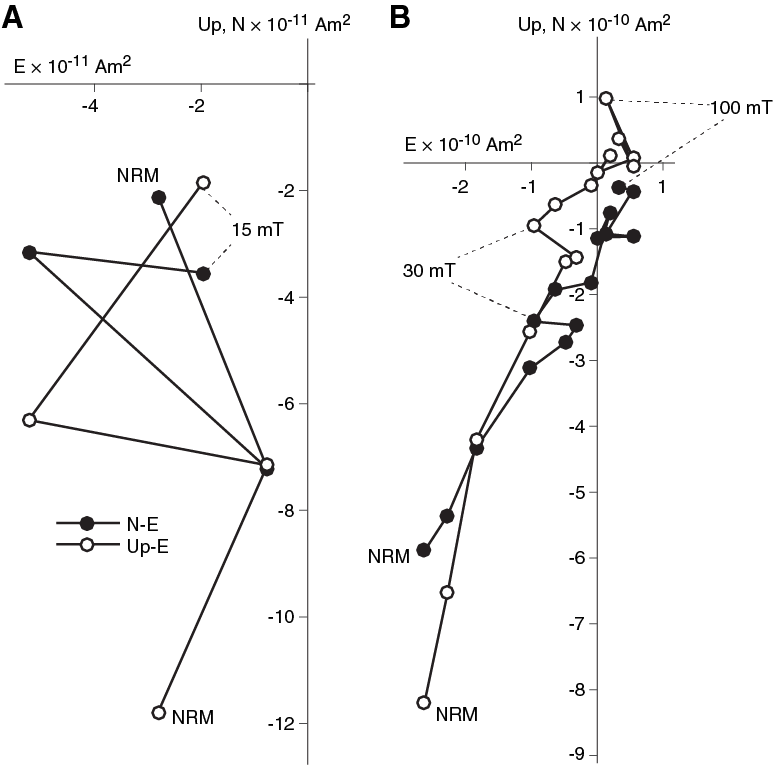
Figure F24. AF demagnetization.
The normal polarity overprint identified in Unit 1 may either be a viscous remanent magnetization acquired from long-term exposure to the geomagnetic field or a drilling-induced remanent magnetization (e.g., Jackson and Van der Voo, 1985). Both of these forms of remanence may be acquired in the direction of the ambient magnetic field at the time of drilling, so further characterization of rock magnetic properties is required to conclusively differentiate between the two mechanisms. However, as described in Downhole logging, the magnetic field within the borehole periodically (every ~15 m) varied between 35 and 50 µT. These sinusoidal fluctuations in field intensity coincided with fluctuations in borehole tilt and scraping patterns etched on the borehole walls seen in downhole images. The fact that such large variations in borehole magnetic field intensity correlate so well with drilling-related properties suggests that drilling-induced remagnetization has likely occurred within the core.
For applications such as magnetostratigraphy, it is important that original detrital remanent magnetizations are properly characterized. Because samples may not typically be demagnetized to >20 mT during OSP standard measurements, full characterization of the underlying primary detrital remanent magnetization components will be reserved for postexpedition research, when demagnetization to higher AF levels will be able to remove overprints. Therefore, a detailed magnetostratigraphy and age model will be developed postexpedition.
Age model and mass accumulation rates
The age model for Site M0077 was constructed using planktic foraminifer and nannoplankton age datums (Figure F25; Table T4). Paleomagnetic reversal datums are excluded because of pervasive magnetic overprinting and low confidence in the shipboard demagnetization data collected from the Post-Impact Sedimentary Rocks interval (see Paleomagnetism). Sedimentation rates vary widely throughout the interval. The Eocene is characterized by high sedimentation rates (average = 2.3 cm/ky), whereas the Paleocene is characterized by low sedimentation rates (average = 0.22 cm/ky).
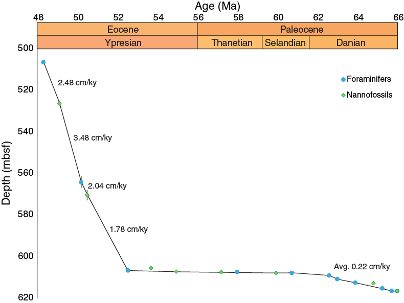
Figure F25. Biostratigraphic datums and LSR.
Table T4. Biostratigraphic datums. Download table in CSV format.
The age model was applied to dry bulk density data to generate mass accumulation rates (MARs), including rates for organic carbon and bulk carbonate (Figures F26, F27). In general, organic carbon accumulation is highest in the younger Eocene after rising from nearly zero at the base of the Eocene interval; the carbonate MAR is generally high throughout but also increases from the base of the Eocene interval to a peak at 50 ± 0.5 Ma. Geochemical data are not plotted for the Paleocene because (1) multiple unconformities in the upper Paleocene prevent the calculation of a sedimentation rate and (2) the low accumulation rate in the early Paleocene would not plot at the same scale (i.e., MAR averages 0.09 g/cm2/ky in the early Paleocene, two orders of magnitude lower than the Eocene average).
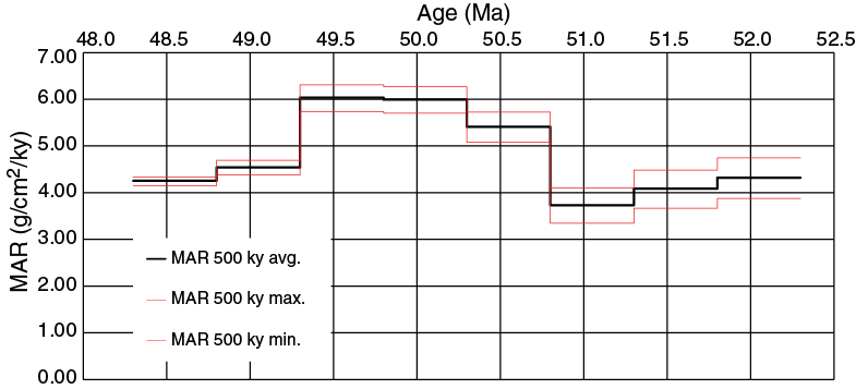
Figure F26. MAR for the Eocene.
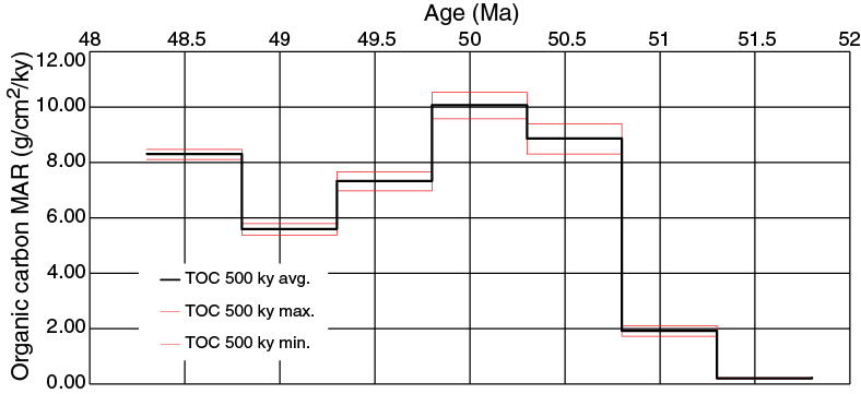
Figure F27. Organic carbon MAR for the Eocene.
Age model
Seventeen age-diagnostic planktic foraminifer and calcareous nannofossil datums were recognized, ranging from 48.3 to 66.03 Ma (following ages reported in Gradstein et al., 2012). These datums were used to construct an age-depth model (Figure F25). Datums are reported as the midpoint between the sample containing the datum and the adjacent sample. In most instances, this stratigraphic error is negligible. However, the lowest occurrences of two marker taxa (Acarinina cuneicamerata at the base of Zone E7a and Tribachiatus orthostylus at the base of Zone CP11) occur above a zone of very poor preservation and thus have a stratigraphic uncertainty of several meters (error bars on Figure F25).
Stacked highest and lowest occurrence datums at the base of Core 36R and in Section 37R-1 (~607 mbsf) indicate that several unconformities are stacked in a short interval. These occurrences are plotted as lowest occurrence datums on the age-depth plot, but they likely do not represent the “true” lowest occurrences of these taxa, and these intervals could fall anywhere within the total range of these species.
It was not possible to apply magnetostratigraphic constraints to the age model for the sedimentary column because the majority of sediment samples carried a pervasive normal polarity magnetic overprint that represents either viscous contamination from the geomagnetic field or drilling-induced magnetization. Because this overprint was not fully removed by AF demagnetization to the maximum applied field levels of 15–20 mT, the underlying detrital remanent magnetization (i.e., the characteristic component utilized for polarity magnetostratigraphy) could not be identified during the OSP.
Linear sedimentation rate
Biostratigraphic datums not interpreted to be truncated by unconformities were used to create a linear sedimentation rate curve (Figure F25). This curve shows very high sedimentation rates in the Eocene (Cores 1R–36R), averaging 2.3 cm/ky. In the Paleocene (Core 37R through Section 40R-1), sedimentation rates are much lower and average 0.22 cm/ky.
Mass accumulation rates
Linear sedimentation rates are multiplied by dry bulk density to obtain MARs of the bulk sediments. A 500 ky time step was selected for the MAR calculation for the Eocene (Cores 1R–36R) based on the sample spacing of the dry bulk density and geochemical measurements taken during the OSP (Figure F26). The MAR for the Eocene is plotted and ranges from 3.7 to 6.0 g/cm2/ky. Error envelopes are calculated for the MAR based on the stratigraphic uncertainty in position of the foraminiferal datums (and therefore uncertainty in the exact sedimentation rate). The MAR is not calculated for sediments between the unconformities spanning Core 36R and Section 37R-1.
Three dry bulk density measurements were taken in the Paleocene post-impact interval in Cores 37R–39R (the sample from Core 40R was below the top of the suevite and is therefore excluded). Obviously, a 500 ky time step is not appropriate for such broadly spaced data; the average MAR for these three cores is 0.09 ± 0.02 g/cm2/ky.
MARs are multiplied by percent abundance geochemical data to obtain MARs of specific components. MARs for organic carbon and bulk carbonate are plotted in Figures F27 and F28. MARs for Cores 37R–40R are not plotted on these figures due to scale changes; early Paleocene (Zones Pα–P3b) accumulation rates average 0.0045 ± 0.0010 g/cm2/ky for organic carbon and 0.89 ± 0.20 g/cm2/ky for carbonate, significantly lower than Eocene rates.
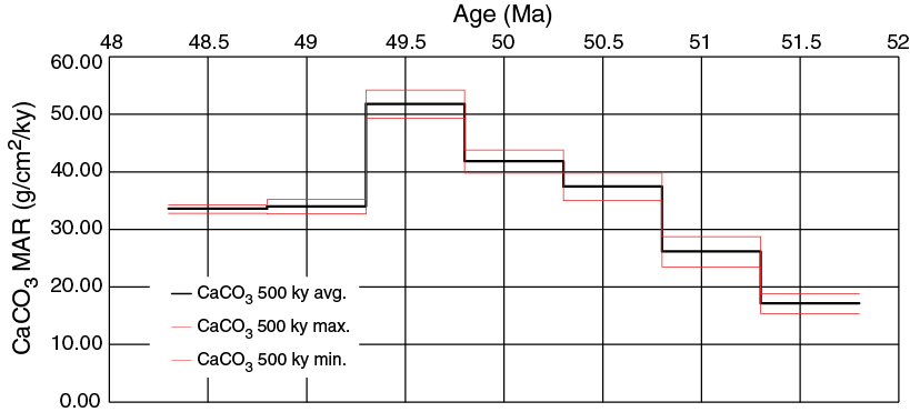
Figure F28. Bulk carbonate MAR for the Eocene.
Geochemistry and mineralogy
Discrete bulk X-ray fluorescence (XRF), total carbon, and X-ray diffraction data on Core 3R through Section 39R-2 (506.12–615.77 mbsf) provide a picture of bulk chemistry and mineralogy for the Post-Impact Sedimentary Rocks interval. Additional XRF linescan and µXRF mapping of Section 40R-1 provide a detailed examination of this key succession that represents the transition from the Upper Peak Ring interval to the Post-Impact Sedimentary Rocks interval.
Major and trace elements and carbon and sulfur content
Major elements
Major element compositions of the 37 samples from Core 3R (506.12 mbsf) through Section 39R-2 (614.91 mbsf) are presented in Table T5. Their depth profiles are shown in Figure F29. Reproducibility was 1.5% for SiO2, 1.2% for TiO2, 1% for Al2O3, 0.5% for K2O, 0.3% for FeO, and 0.1% for CaO. Poorer reproducibility was found for P2O5 (1.88%), MgO (3.3%), and Na2O (3.5%).
Table T5. Major element compositions. Download table in CSV format.
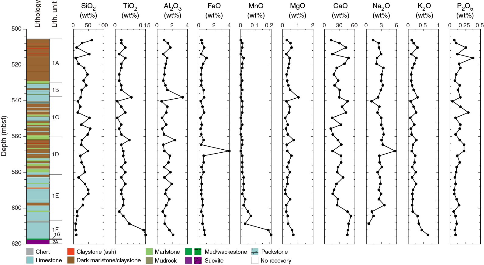
Figure F29. Major element compositions.
The majority of the samples have variable CaO contents (average ± 1σ = 30.06 ± 11.48 wt%), reflecting the abundance of marlstone and limestone as major lithologies in this section. The CaO content is negatively correlated with the SiO2 content and linearly correlated to the carbonate carbon (Ccarb) content with a slope reflecting the stoichiometry of CaCO3 (CaO:Ccarb = 1:1 in molar ratio or 56:12 in weight ratio) (Figure F30). Such abundant carbonate components lower the sum of major elements that are detectable by XRF to much less than 100% (average ± 1σ = 65.22 ± 4.98 wt%) (Table T5).

Figure F30. Ccarb and CaO contents.
Carbon and sulfur
Contents of total carbon (Ctotal), organic carbon (Corg), Ccarb, and sulfur in the 37 samples from Cores 3R–39R (506.17–614.91 mbsf) are presented in Table T6, and their depth profiles are shown in Figure F31. Reproducibility is within 0.7% for Ctotal and Corg and 1.3% for sulfur.
Table T6. Carbon and sulfur contents. Download table in CSV format.
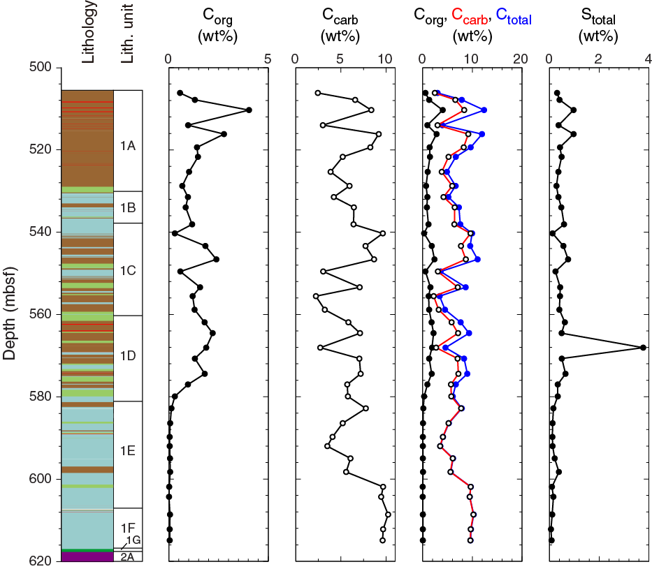
Figure F31. Carbon and sulfur contents.
The Ccarb contents are variable (average ± 1σ = 6.31 ± 2.36 wt%), which quantitatively translates to a total average CaCO3 content of ~50 wt%. The Corg contents (average ± 1σ = 1.01 ± 0.93 wt%) are also variably high. About 85% of the Ctotal contents (average ± 1σ = 7.32 ± 2.58 wt%) are dominated by Ccarb. Most samples have low sulfur contents (average ± 1σ = 0.38 ± 0.23 wt%), except for one sample at 568.07 mbsf (3.77 wt%). When this high-sulfur sample is included for calculation, the average content is 0.47 ± 0.60 wt% (Table T6). A positive correlation exists between the Corg and S contents, suggesting a cogenetic origin.
Trace elements
Trace element compositions of the 37 samples from Cores 3R–39R (506.17–614.91 mbsf) are presented in Table T7, and their depth profiles are shown in Figure F32. Reproducibility was 0.7% for Sr, 0.6% for Zr, and 1.3% for S. Other trace elements exhibit relative errors estimated to be on the order of 5%.
Table T7. Minor and trace element compositions. Download table in CSV format.
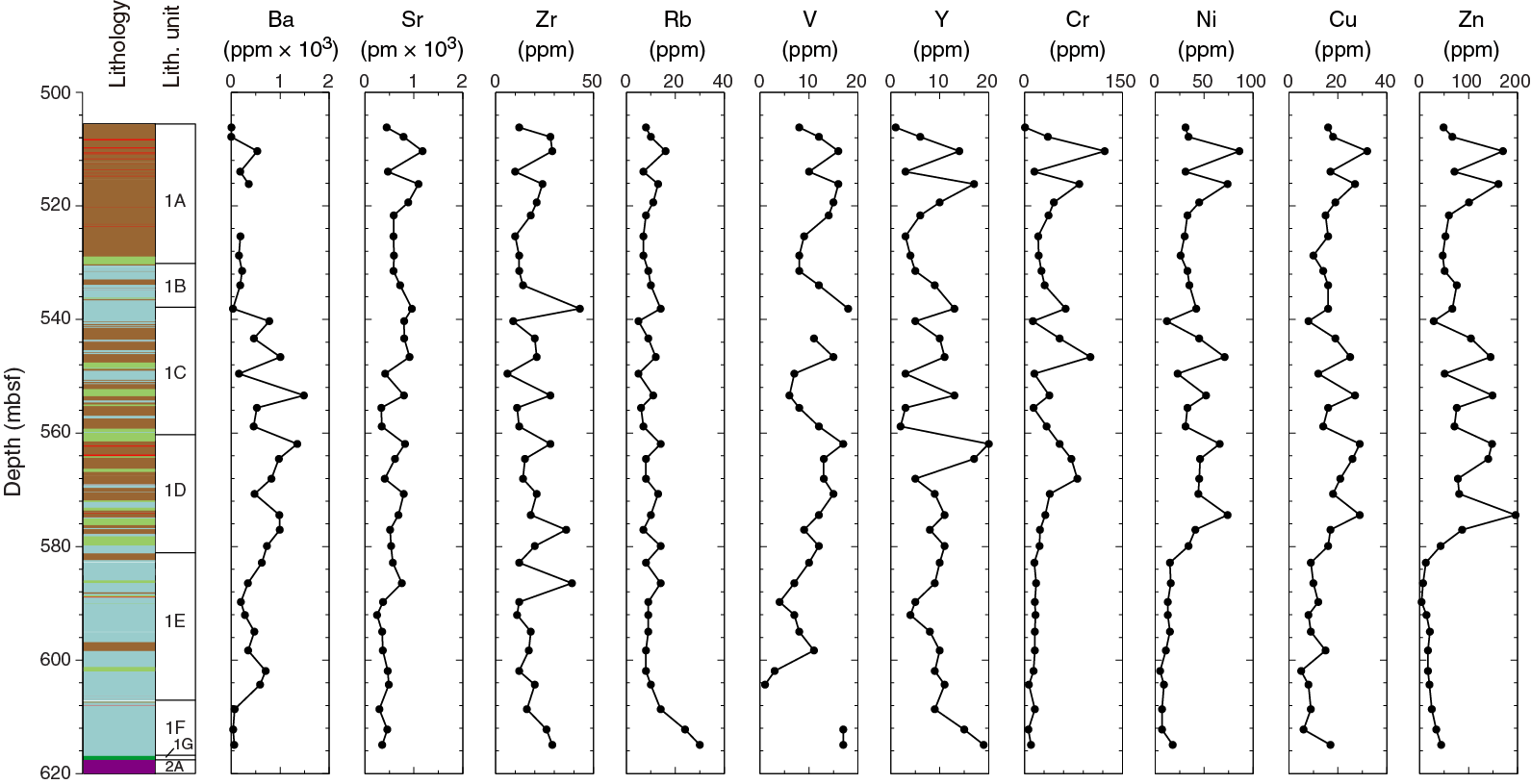
Figure F32. Trace element compositions.
These trace elements show coherent geochemical behaviors; the depth profiles appear to be similar to 535 mbsf. However, below that depth, differences among them become apparent. Trace elements such as Zn, Cr, Ni, and Cu show good positive correlations (R2 ≥ 0.76) with Corg concentrations (Figure F33).
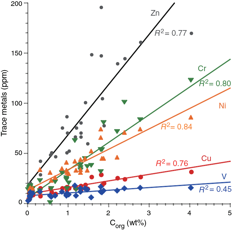
Figure F33. Selected trace metals and organic carbon.
Section 40R-1: linescan data
The XRF linescan of Section 40R-1 resulted in 140 spot analyses over 142 cm. Data from this scan are plotted as total count rate for the elements Ca, Fe, S, Ni, Pb, Zn, Br, Rb, Zr, K, Si, Al, Sr, Ti, Ba, and Mn versus depth alongside a linescan image and lithostratigraphic column in Figures F34, F35, and F36. This core section is divided into limestone (Subunit 1F) (see Lithology) at the top from 607.27 to 616.58 mbsf, mud/wackestone (Subunit 1G) in the center from 616.58 to 617.33 mbsf and in the interval where suevite begins (Subunit 2A; 617.33–617.66 mbsf).
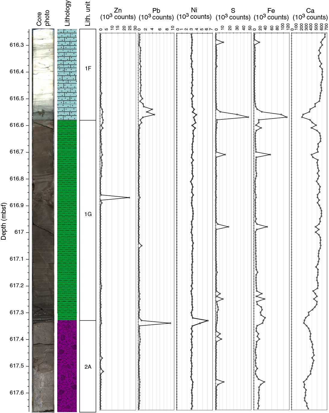
Figure F34. Zn, Pb, Ni, S, Fe, and Ca concentrations.
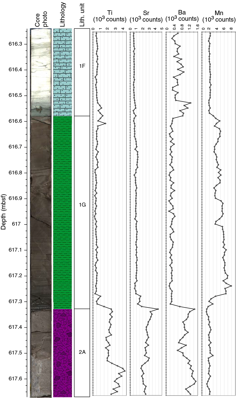
Figure F35. Ti, Sr, Ba, and Mn concentrations.

Figure F36. Zr, Rb, Br, Al, Si, and K concentrations.
Subunit 1F is dominated by Ca, with a small spike in S and Fe at 616.29 mbsf. Subunit 1G is also dominated by Ca, with localized enrichments in S and Fe that correlate with relative depletions in Ca. These data indicate that Subunits 1F and 1G are dominantly limestones that contain localized sulfide mineralization. These two limestone intervals are chemically distinct due to the relatively higher Mn, Fe, and Sr concentrations in the mud/wackestone (Subunit 1G) that contrast with relatively higher concentrations of Ba, Si, K, Rb, and Pb in Subunit 1F.
The contact between Subunits 1F and 1G is characterized by a relative increase in Zr, Rb, Br, S, K, Pb, S, Fe, Ti, and Ba and a significant relative decrease in Ca. Across a distance of 3 to 5 cm (616.54–616.59 mbsf), sulfide mineralization is evident through the spikes in Fe, S, Ba, and Pb concentrations. This is accompanied by a moderate relative enrichment in Rb, Zr, and Ti and a weak relative enrichment in Si, Al, Sr, Ni, and K.
The contact (~3–5 cm wide in Section 40R-1) between Subunit 1G and the silicate-enriched suevite (Subunit 2A) is characterized by depletion in Ca similar in magnitude to the drop in Ca at the boundary between Subunits 1F and 1G. In the same zone, Ba, Sr, and Pb appear relatively enriched. In this boundary interval, a conspicuous, localized relative Ni enrichment was detected that does not correspond to an S enrichment.
Relative Ca and Si abundances within Section 40R-1 clearly outline the depths that are dominated by CaCO3 (Figure F34) and silicate minerals (Figure F36). In addition, the abundance of S in this core section shows the occurrence of sulfide or sulfate mineralization. Generally, elements such as Fe, Ni, and Pb correlate with spikes in the S signal, suggesting that these are mostly sulfide mineralizations of pyrite and related assemblages. In contrast, Ca is distinctly anticorrelated with S, which suggests that Ca-sulfates such as gypsum and anhydrite are not the sources of the S excursions.
Section 40R-1: µXRF mapping
µ-XRF mapping of Section 40R-1 (616.24–617.68 mbsf) resulted in four subsection maps.
µXRF Interval 1 (616.54–616.60 mbsf)
The mapped areas (Figures F37, F38) capture a lithologic boundary between the brown mud/wackestone (Subunit 1G) at the bottom and the greenish to white marlstone, wackestone, and packstone (Subunit 1F) at the top. Subunit 1F is relatively enriched in Si and K compared to Subunit 1G, which has relatively larger concentrations of Mn and Mg. Iron sulfide mineralization occurs as 1 cm nodules and ~1 mm grains in 0.5 mm thick layers in Subunit 1F; Cr is enriched in some of these iron sulfide domains. Cr is also enriched in the boundary layer between Subunit 1G and the greenish transition layer at the bottom of Subunit 1F. A 0.5 mm thick, green marly layer inclined in the upper part of Subunit 1G displays relative enrichment in K, Si, and Cr.
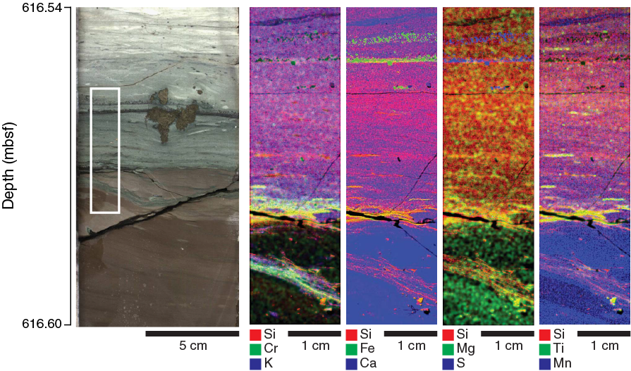
Figure F37. µX-ray intensity maps, Section 40R-1 (Subsection 1).
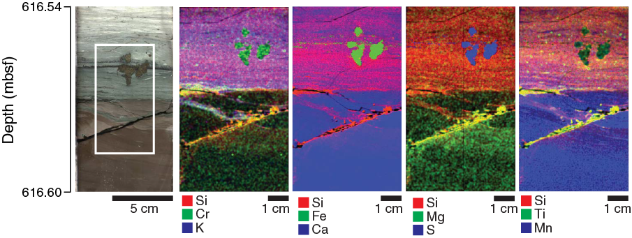
Figure F38. µX-ray intensity maps, Section 40R-1 (Subsection 1).
µXRF Interval 2 (~617.00–617.08 mbsf)
The second scanned µXRF interval comprises part of Subunit 1G. The mapped region (Figure F39) captures a carbonate rock that shows a pronounced Mn concentration and millimeter-thick layers enriched in Fe, Si, and Ti. Toward the top of the mapped region, a diffuse relative Si enrichment is apparent.
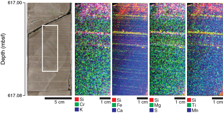
Figure F39. µX-ray intensity maps, Section 40R-1 (Subsection 2).
µXRF Interval 3 (617.27–617.36 mbsf)
The third scanned µXRF interval comprises the major lithologic transition between suevite (Subunit 2A) and mud/wackestone (Subunit 1G) (Figure F40). The mapped region captures the basal part of the brown mud/wackestone, which exhibits contorted pipe structures near the contact to 2.5 cm thick sandy layers (617.315–617.33 mbsf) that transition to cross-bedded, size-sorted suevite with sand-sized components.

Figure F40. µX-ray intensity maps, Section 40R-1 (Subsection 3).
In 0.5 cm thick layers in Subunit 1G and especially in the sandy transition layers, mineral components occur that are relatively enriched in Cr, Fe, Mg, Ti, and Ni. Ni is also enriched in millimeter-thick discontinuous layers in the sandy, suevitic transition zone. These Ni-enriched layers do not appear to be correlated with enrichments in any other elements that were mapped.
Subunit 1G also contains <0.5 mm layers that are enriched in Fe and S and some that are very thin and enriched in Si. The contorted pipe structures near the bottom of Subunit 1G are relatively enriched in Mn, whereas they appear relatively depleted in Si.
Our X-ray intensity maps show a relatively sharp boundary between Subunit 1G and the underlying suevite (Subunit 2A) that is characterized by a strong relative enrichment in Si and K and a relative depletion of Ca below, compared to the mud/wackestone (Subunit 1G) above.
µXRF Interval 4 (617.44–617.54 mbsf)
The fourth scanned µXRF interval comprises size-sorted suevite (Figure F41). The mapped region captures diffuse, subvertical structures that are a few millimeters to 3 cm wide. Compared to the host suevite, these vein networks are relatively depleted in Si and K and enriched in Ca, Mg, and Mn.
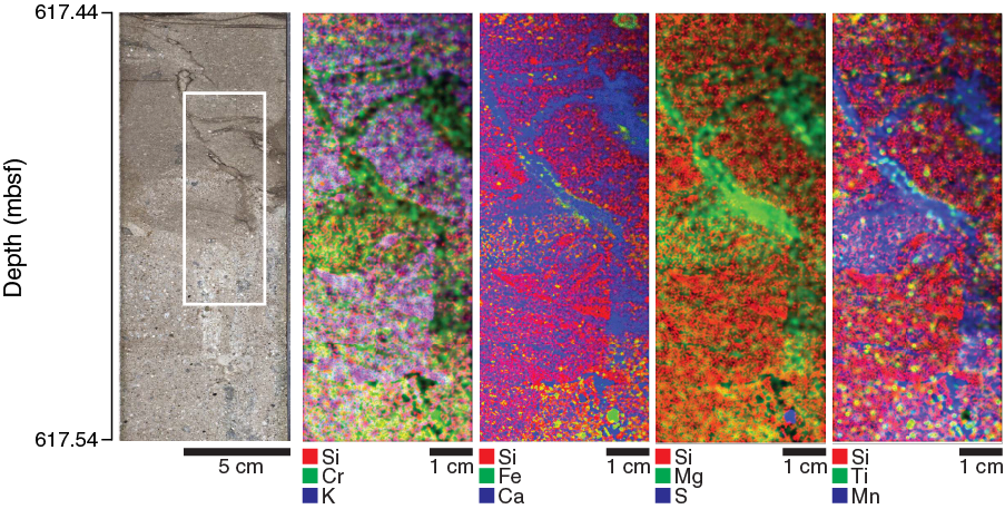
Figure F41. µX-ray intensity maps, Section 40R-1 (Subsection 4).
Mineralogy
The composition of the bulk mineralogy of 38 samples from Cores 3R–39R (506.2–614.91 mbsf) is presented in Table T8, and their depth profiles are shown in Figure F42. For a general description of the different minerals present in the Post-Impact Sedimentary Rocks interval, refer to Table T9.
Table T8. Abundance of all minerals. Download table in CSV format.
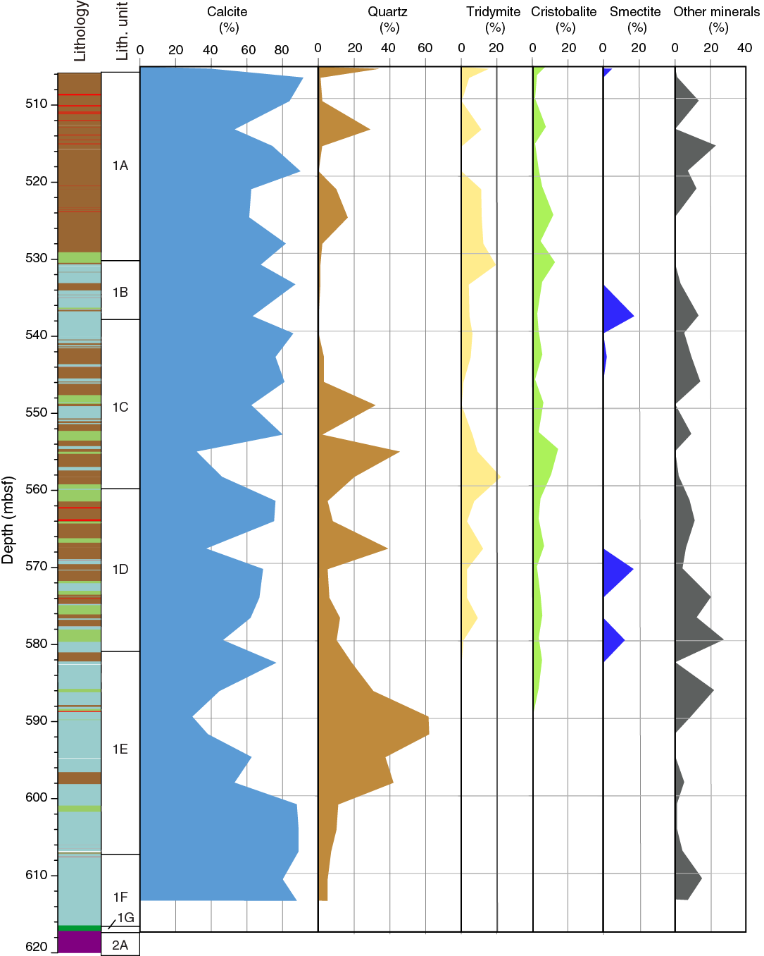
Figure F42. Bulk mineralogy.
Table T9. All minerals that occur in Cores 3R through 39R. Download table in CSV format.
The evolution of the mineral assemblage was divided into five main intervals:
- Cores 3R–11R (506.17–528.75 mbsf; Subunit 1A): associated with calcite (average = 60%), the three SiO2 polymorphs, quartz (average = 20%), tridymite, and cristobalite (average = 10%), occur in most samples. Accessory minerals (average = 10%), including feldspars (albite), oxides (hollandite and spinel), and sulfides (sphalerite and pyrite), occur in a few samples. The clay fraction is mostly composed of clinoptilolite associated with smectites (montmorillonite) or micas (tobelite) in a few samples.
- Cores 12R–15R (531.45–540.31 mbsf; parts of Subunits 1B and 1C): associated with calcite (70%), the SiO2 fraction is only represented by tridymite and cristobalite (average = 10%) in most samples. Few accessory minerals are recorded in this interval; among them are feldspars (albite), zeolites (heulandite and stibilite), oxides (hollandite), and sulfides (pyrite). The clay fraction is mainly composed of smectites (saponite and montmorillonite) in a few samples.
- Cores 16R–30R (543.36–586.45 mbsf; base of Subunits 1C and 1D and part of Subunit 1E): calcite (average = 60%) is associated with the three SiO2 polymorphs, quartz, tridymite, and cristobalite (average = 30%). Accessory minerals, including silicates (tobermorite), zeolites (faujasite, heulandite, and stibilite), oxides (perovskite), evaporites (halite), and sulfides (pyrite) occur in a few samples.
- Cores 31R–36R (589.77–604.34 mbsf; part of Subunit 1E): calcite (average = 60%) is associated with quartz (average = 30%, except in Cores 31R and 32R, which contain more than 60% quartz). Few accessory minerals including oxides (rutile) and sulfides (pyrite) occur in a few samples. With a few exceptions of clinoptilolite-bearing samples, samples in this subunit are poor in clay minerals.
- Cores 37R–39R (607.165–614.91 mbsf; base of Subunit 1E, Subunit 1F, and part of Subunit 1G): calcite (average = 80%) is associated with quartz. Accessory minerals are feldspars (anorthite and albite), silicates (almandine and sodalite), and oxides (wüstite and rutile). In Cores 32R and 33R, the clay fraction is contains traces of palygorskite.
Physical properties
P-wave velocity
P-wave velocities from discrete sample measurements in the Post-Impact Sedimentary Rocks interval (Unit 1) range from ~2500 to 4500 m/s (Figure F43). Mean velocities are ~3100 m/s to 585 mbsf, where the lithology is predominantly marlstone, and increase to 3500–4500 m/s lower in the interval, where the lithology is dominated by limestone. P-wave velocities decrease sharply to ~2900 m/s in the underlying suevite (Subunit 2A). P-wave velocity measurements on discrete samples are consistently higher than velocities obtained downhole but follow the general trend of the downhole sonic log and vertical seismic profile (VSP).
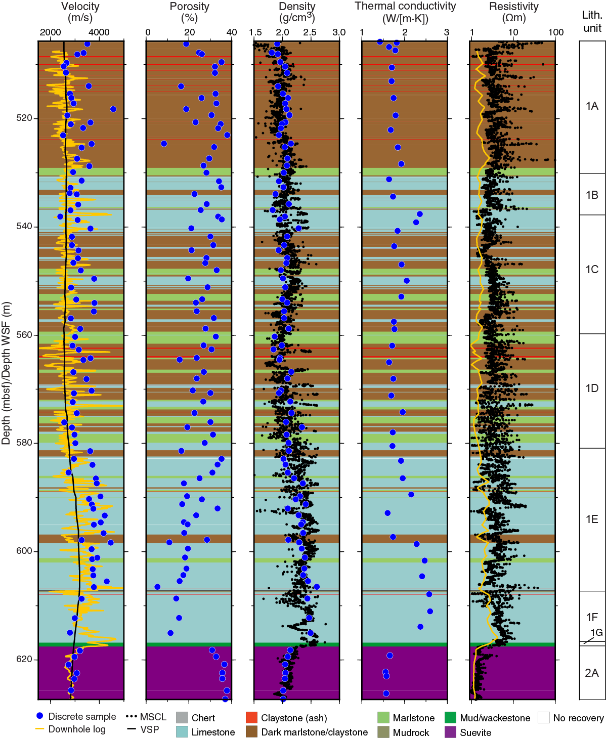
Figure F43. Physical properties.
Porosity
Porosities range from 5% to 38%. Porosities have a mean value of 27% to 581 mbsf (Subunits 1A–1D) and a mean value of 20% from 581 to 617 mbsf (Subunits 1E–1G) (Figure F43). In general, porosities are inversely correlated with velocities, with higher porosities corresponding to zones of lower velocity. There is a sharp increase to porosities of ~35% in the underlying suevite (Subunit 2A).
Density
Bulk densities range from 1.8 to 2.6 g/cm3 with a mean value of 2.0 g/cm3 to 581 mbsf (Subunits 1A–1D) and a mean value of 2.3 g/cm3 from 581 to 617 mbsf (Subunits 1E–1G) (Figure F43). In general, bulk densities follow the same trend as velocities. Densities decrease sharply to 2.0 g/cm3 in the underlying suevite (Subunit 2A). There is good correspondence between bulk densities measured on discrete samples and bulk densities measured using gamma ray attenuation using the MSCL, although more variation is observed in the MSCL values.
Thermal conductivity
Thermal conductivity values range from 1.4 to 2.6 W/(m·K) with a mean value of 1.8 W/(m·K) to 581 mbsf (Subunits 1A–1D) and a mean value of 2.2 W/(m·K) from 581 to 617 mbsf (Subunits 1E–1G) (Figure F43). There is a sharp decrease to 1.6 W/(m·K) in the underlying suevite (Subunit 2A). Thermal conductivity values follow the same trend as P-wave velocities and bulk densities.
Resistivity
In general, resistivities measured by the MSCL vary from 1 to 10 Ωm with a mean value of 5 Ωm (Figure F43). Unlike other physical property measurements, there is no obvious difference in values between Subunits 1A–1D and 1E–1G. Resistivities decrease sharply to 1.5 Ωm in the underlying suevite (Subunit 2A). MSCL resistivities are consistently higher but follow the same trend as that measured in the downhole log. This difference might be explained by the differences in the volume of rock investigated by each of the tools used (MSCL measures a smaller volume than wireline) or the invasion of borehole fluids into the surrounding rock.
Magnetic susceptibility
Magnetic susceptibility values measured by the MSCL are low (Figure F44). Values range from 0 to 1 × 10⁻⁵ SI to 604 mbsf and increase to a mean value of 1.5 × 10⁻⁵ SI below 604 mbsf. Values increase in the uppermost 10 m of the underlying suevite (Subunit 2A) from 2 × 10⁻⁵ to 37 × 10–5 SI. Magnetic susceptibility values measured by the MSCL are consistently lower than those measured by the wireline downhole log as a result of the difference in volume investigated between the tools used (MSCL measures a smaller volume than wireline) (e.g., Dubuisson et al., 1995). The MSCL and wireline log trends are similar (compare values in Subunit 2A) despite a malfunction of the logging tool (see Downhole logging in the Expedition 364 methods chapter [Gulick et al., 2017]).
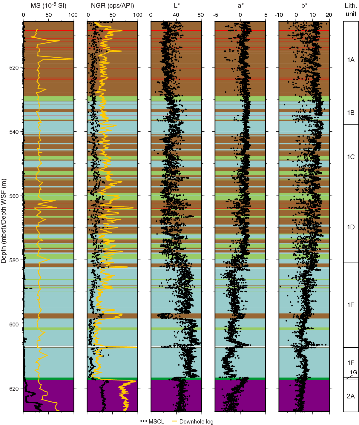
Figure F44. Magnetic susceptibility, NGR, and L*, a*, and b*.
Natural gamma radiation
In general, natural gamma radiation (NGR) values measured by the MSCL vary from 0 to 35 counts/s. The NGR mean value is 16.5 counts/s in the upper marlstone section to 581 mbsf (Subunits 1A–1D) and 11.5 counts/s in the lower limestone section from 581 to 617 mbsf (Subunits 1E–1G) (Figure F44). Some local changes in NGR values correspond to lithostratigraphic subunits (e.g., 597 mbsf). Values increase sharply to 25–40 counts/s in the underlying suevite (Subunit 2A). The trend of NGR values measured by the MSCL in counts per second is in good agreement with the one from the wireline downhole log in American Petroleum Institute (API) units.
Color reflectance
Similar to many other physical property measurements, there is a change in color reflectance values at ~581 mbsf, the Subunit 1D/1E boundary (Figure F44). L*, a*, and b* mean values are 32, 1, and 10, respectively, in Subunits 1A–1D and 55, –1, and 5, respectively, in Subunits 1E–1G. There is a sharp decrease in L* values, an increase in a* values, and a smaller decrease in b* values at the contact with the underlying suevite (Subunit 2A).
Downhole logging
Downhole logging measurements in the Post-Impact Sedimentary Rocks interval were conducted during the second logging session, from 697 m wireline log depth below seafloor (WSF) to the base of the casing at ~507 m WSF (see Figure F26 in the Expedition 364 methods chapter [Gulick et al., 2017]).
Wireline logs
From 507 to 697 m WSF, the hole was very stable, and borehole conditions were excellent. Wireline log data quality is very good (Figure F45), except for the conductivity and magnetic susceptibility measurements, which experienced technical problems during acquisition (see Downhole logging in the Expedition 364 methods chapter [Gulick et al., 2017]). The downhole logs are in agreement with the physical properties measurements performed on whole-round cores and discrete samples (see Physical properties). The gamma ray logs from the various tool strings and runs match well, and only a small number of minor postacquisition depth-shift adjustments (generally less than 5 cm) were required to align the various passes. The base of casing was located at 507.35 m WSF on the acoustic borehole image (ABI) (Figure F45). From 503 to 507 m WSF, gamma ray values are lower than those acquired from farther downhole due to attenuation of the signal through the pipe.
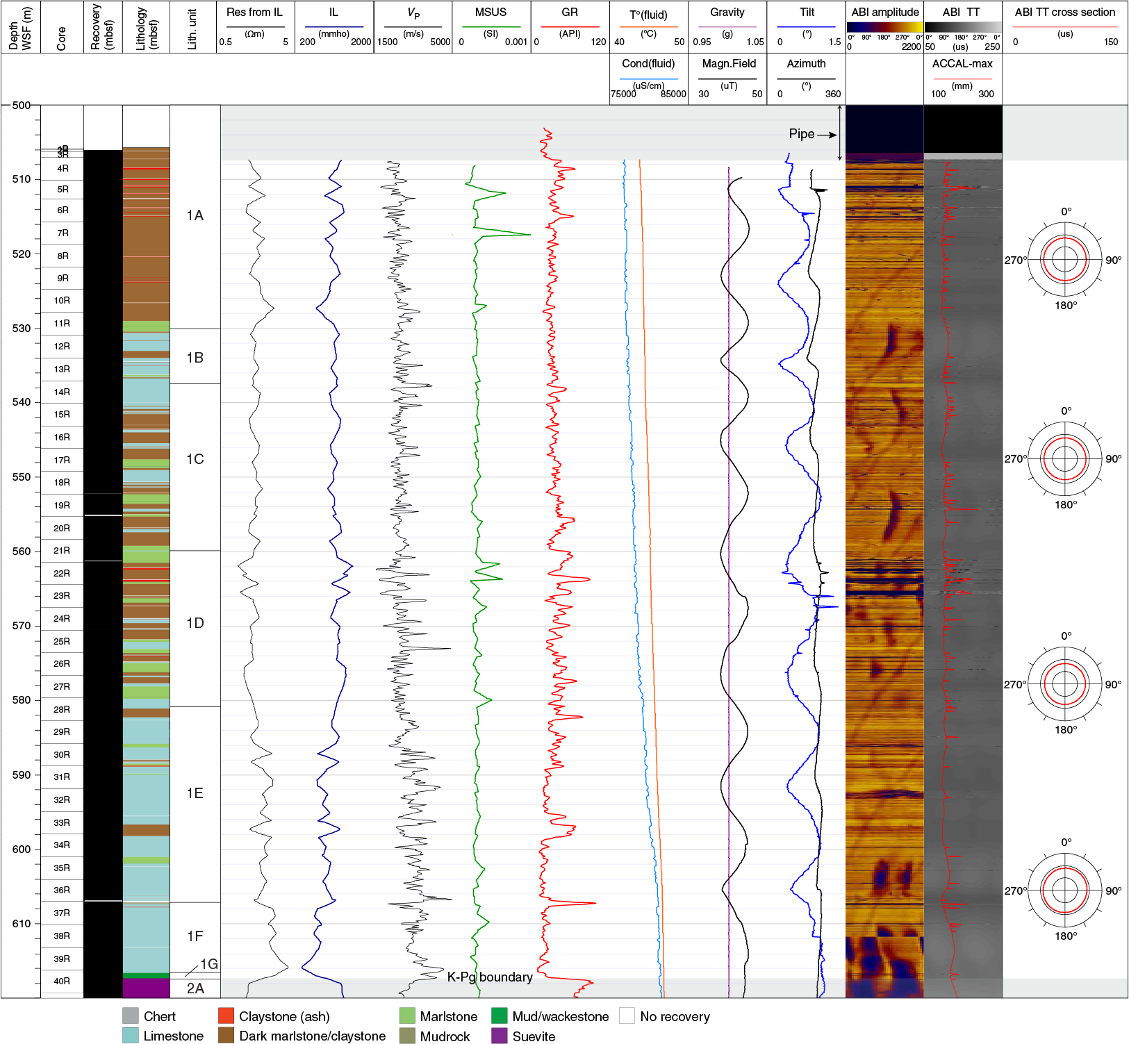
Figure F45. Wireline downhole log data.
Wireline logs are characterized by moderate to low variability as illustrated in Figure F45. Conductivity (IL) log values range between ~300 and 1080 mmho with an average conductivity of ~700 mmho. Conductivity and sonic logs are anticorrelated, although the conductivity log is of lower resolution. Sonic P-wave velocities range between 1400 and 5500 m/s with an average of ~2800 m/s. The maximum velocity was observed at ~607 m WSF, and it correlates with a high-amplitude interval (bright yellow) on the ABI and with chert layers in Core 36R (Figure F46C) (606.3–607 m WSF; 606.1–606.7 mbsf). Magnetic susceptibility is low throughout the Post-Impact Sedimentary Rocks interval, as expected for carbonate formations. The borehole fluid temperature (T°fluid) ranges from 43.6°C below the pipe to 47.2°C at the base of the interval. Borehole fluid conductivity (Condfluid) ranges between 76,800 and 81,800 µS/cm, gradually increasing downhole. The fluid parameter logs were acquired shortly after the drilling, so these measurements should only be used qualitatively. The borehole fluid temperature likely reflects a minimum value for the in situ temperature of the formation, whereas the borehole conductivity is affected by the recent drilling operations and the presence of drill mud and seawater in the hole.
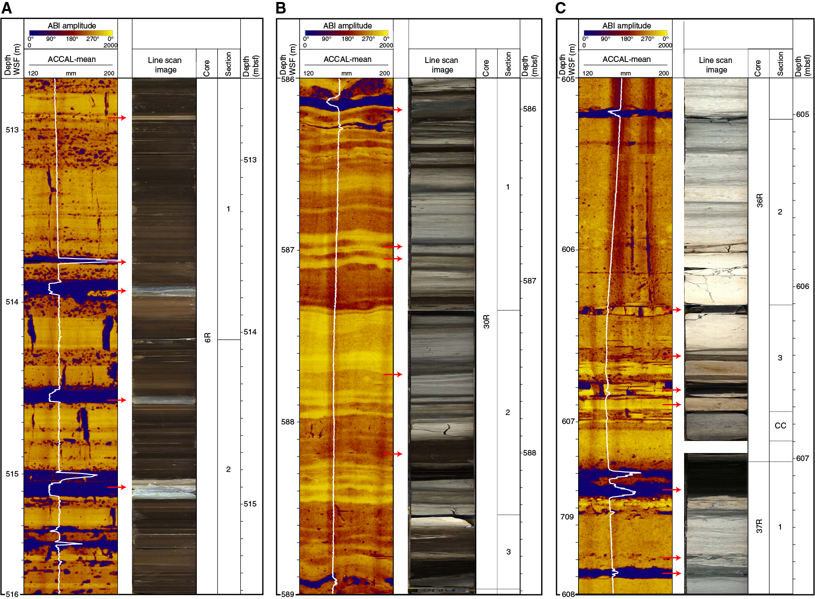
Figure F46. Core-log integration.
The ABIs are excellent quality (Figure F46) due to the high resolution and low logging speed at which the images were acquired and the regular width of the borehole, as shown by the maximum acoustic caliper (ACCAL-max), which gives a mean diameter around 15.6 cm. Traveltime cross sections at several depths indicate that the borehole shape is almost circular. Locally, borehole enlargements (spikes on the ACCAL-max) were observed and correlate in depth with low-amplitude intervals on the ABIs. These likely reflect softer sediments that have been washed out during coring (e.g., ~560–566 m WSF; Figure F45). The ABIs correlate well with the line-scan core data, although a small depth offset is observed between the two data sets (less than ~0.2 m in Figure F46). It should be noted that the ABIs do not necessarily correlate with changes in rock color but rather reflect changes in hardness or rugosity.
The character of the logs changes downhole. The sonic log shows larger changes in P-wave velocity values below ~583 m WSF with a slightly increasing trend downhole, whereas the conductivity of the formation decreases. A small decrease in mean gamma ray values was observed below ~590 m WSF. A spike in gamma ray values at ~607 m WSF correlates with a dark layer in Section 37R-1 (Figure F46C), which may correspond to the PETM (see Biostratigraphy).
From 507 to 697 m WSF, the tilt and azimuth given by the ABI tool display sinusoidal and oscillating downhole trends (with a wavelength of about ~15 m) (Figure F45). These trends may be drilling induced or an effect of a decentralized tool during wireline data acquisition. The magnetic field also follows this trend, and the cause of this oscillation remains to be determined.
Vertical seismic profile
The three-component VSP collected from 500.0 to 650.0 m WSF is generally good quality. The vertical component of the VSP shows a broad-spectrum waveform up to 350 Hz with dominant frequencies at 25 and 64 Hz (Figure F47A).
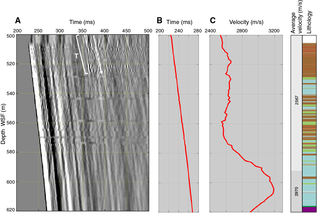
Figure F47. VSP vertical component.
First-arrival traveltimes were picked (Figure F47B), and a moving-window algorithm was used to determine the change in P-wave velocity with depth (Figure F47C). A high-velocity region lies between 590 and 610 m WSF. The signal between 500 and 507 m WSF is affected by the proximity of the pipe. Tube waves are secondary arrivals below 500 m WSF, terminating between 520 and 540 m WSF, and were likely produced by the casing. The radial and azimuthal horizontal component data are of reasonably good quality (Figure F48).
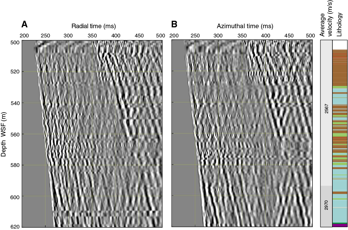
Figure F48. VSP horizontal component.
References
Alegret, L., and Thomas, E., 2001. Upper Cretaceous and lower Paleogene benthic foraminifera from northeastern Mexico. Micropaleontology, 47(4):269–316. https://doi.org/10.2113/47.4.269
Bown, P., 2005. Selective calcareous nannoplankton survivorship at the Cretaceous–Tertiary Boundary. Geology, 33(8):653–656. https://doi.org/10.1130/G21566.1
Bralower, T.J., and Mutterlose, J., 1995. Calcareous nannofossil biostratigraphy of Site 865, Allison Guyot, central Pacific Ocean: a tropical paleogene reference section. In Winterer, E.L., Sager, W.W., Firth, J.V., and Sinton, J.M. (Eds.), Proceedings of the Ocean Drilling Program, Scientific Results, 143: College Station, TX (Ocean Drilling Program), 31–74. https://doi.org/10.2973/odp.proc.sr.143.204.1995
Bralower, T.J., Paull, C.K., and Leckie, R.M., 1998. The Cretaceous–Tertiary boundary cocktail: Chicxulub impact triggers margin collapse and extensive sediment gravity flows. Geology, 26(4):331–334. https://doi.org/10.1130/0091-7613(1998)026<0331:TCTBCC>2.3.CO;2
Bralower, T.J., and Self-Trail, J.M., 2016. Nannoplankton malformation during the Paleocene-Eocene Thermal Maximum and its paleoecological and paleoceanographic significance. Paleoceanography, 31:1423–1439. https://doi.org/10.1002/2016PA002980
Bybell, L.M., and Self-Trail, J.M., 1995. Evolutionary, biostratigraphic, and taxonomic study of calcareous nannofossils from a continuous Paleocene-Eocene boundary section in New Jersey. U.S. Geological Survey Professional Paper, 1554. https://pubs.er.usgs.gov/publication/pp1554
Dubuisson, G., Thibal, J., Barthès, V., Pocachard, J., and Pozzi, J.-P., 1995. Downhole magnetic logging in sediments during Leg 145: usefulness and magnetostratigraphic interpretation of the logs at Site 884. In Rea, D.K., Basov, I.A., Scholl, D.W., and Allan, J.F. (Eds.), Proceedings of the Ocean Drilling Program, Scientific Results, 145: College Station, TX (Ocean Drilling Program), 455–468. https://doi.org/10.2973/odp.proc.sr.145.135.1995
Gradstein, F.M., Ogg, J.G., Schmitz, M.D., and Ogg, G.M. (Eds.), 2012. The Geological Time Scale 2012: Amsterdam (Elsevier).
Gulick, S., Morgan, J., Mellett, C.L., Green, S.L., Bralower, T., Chenot, E., Christeson, G., Claeys, P., Cockell, C., Coolen, M., Ferrière, L., Gebhardt, C., Goto, K., Jones, H., Kring, D., Lofi, J., Lowery, C., Ocampo-Torres, R., Perez-Cruz, L., Pickersgill, A.E., Poelchau, M., Rae, A., Rasmussen, C., Rebdolledo-Vieyra, M., Riller, U., Sato, H., Smit, J., Tikoo, S., Tomioka, N., Urrutia Fucugauchi, J., Whalen, M., Wittmann, A., Yamagachi, K., Xiao, L., and Zylberman, W., 2017. Expedition 364 methods. In Morgan, J., Gulick, S., Mellett, C.L., Green, S.L., and the Expedition 364 Scientists, Chicxulub: Drilling the K-Pg Impact Crater. Proceedings of the International Ocean Discovery Program, 364: College Station, TX (International Ocean Discovery Program). https://doi.org/10.14379/iodp.proc.364.102.2017
Jackson, M., and Van der Voo, R., 1985. Drilling-induced remanence in carbonate rocks: occurrence, stability and grain-size dependence. Geophysical Journal International, 81(1):75–87. https://doi.org/10.1111/j.1365-246X.1985.tb01351.x
Jiang, S., Bralower, T.J., Patzkowsky, M.E., Kump, L.R., and Schueth, J.D., 2010. Geographic controls on nannoplankton extinction across the Cretaceous/Palaeogene boundary. Nature Geoscience, 3(4):280–285. https://doi.org/10.1038/ngeo775
Perch-Nielsen, K., 1985. Cenozoic calcareous nannofossils. In Bolli, H.M., Saunders, J.B., and Perch-Nielsen, K. (Eds.), Plankton Stratigraphy: Cambridge, United Kingdom (Cambridge University Press), 427–554.
Pospichal, J.J., and Bralower, T.J., 1992. Calcareous nannofossils across the Cretaceous/Tertiary boundary, Site 761, northwest Australian margin. In von Rad, U., Haq, B.U., et al., Proceedings of the Ocean Drilling Program, Scientific Results, 122: College Station, TX (Ocean Drilling Program), 735–751. https://doi.org/10.2973/odp.proc.sr.122.187.1992
Raffi, I., Backman, J., Zachos, J.C., and Sluijs, A., 2009. The response of calcareous nannofossil assemblages to the Paleocene Eocene Thermal Maximum at the Walvis Ridge in the South Atlantic. Marine Micropaleontology, 70(3–4):201–212. https://doi.org/10.1016/j.marmicro.2008.12.005
Schueth, J.D., Bralower, T.J., Jiang, S., and Patzkowsky, M.E., 2015. The role of regional survivor incumbency in the evolutionary recovery of calcareous nannoplankton from the Cretaceous/Paleogene (K/Pg) mass extinction. Paleobiology, 41(4):661–679. https://doi.org/10.1017/pab.2015.28
1 Gulick, S., Morgan, J., Mellett, C.L., Green, S.L., Bralower, T., Chenot, E., Christeson, G., Claeys, P., Cockell, C., Coolen, M.J.L., Ferrière, L., Gebhardt, C., Goto, K., Jones, H., Kring, D., Lofi, J., Lowery, C., Ocampo-Torres, R., Perez-Cruz, L., Pickersgill, A.E., Poelchau, M., Rae, A., Rasmussen, C., Rebolledo-Vieyra, M., Riller, U., Sato, H., Smit, J., Tikoo, S., Tomioka, N., Urrutia- Fucugauchi, J., Whalen, M., Wittmann, A., Yamaguchi, K., Xiao, L., and Zylberman, W., 2017. Site M0077: Post-Impact Sedimentary Rocks. In Morgan, J., Gulick, S., Mellett, C.L., Green, S.L., and the Expedition 364 Scientists, Chicxulub: Drilling the K-Pg Impact Crater. Proceedings of the International Ocean Discovery Program, 364: College Station, TX (International Ocean Discovery Program). https://doi.org/10.14379/iodp.proc.364.105.2017
2 Expedition 364 Scientists’ addresses.
This work is distributed under the Creative Commons Attribution 4.0 International (CC BY 4.0) license. 
- F1. Marlstone/claystone lithologies.
- F2. Subunit 1E lithologies.
- F3. Selected lithologies.
- F4. Subunit 1A lithologies.
- F5. Subunit 1B lithologies.
- F6. Subunit 1C lithologies.
- F7. Subunit 1D lithologies.
- F8. Subunit 1F lithologies.
- F9. Lithostratigraphy, gamma ray, and TOC.
- F10. Wackestone/packstone/grainstone/siltstone lithologies.
- F11. Upper and lower contacts of Subunit 1G.
- F12. Lithostratigraphic summary.
- F13. Basal contacts of Subunits 1A–1F.
- F14. Line scan, CT scan, density, and atomic number, Hole M0077A.
- F15. Line scan, CT scan, density, and atomic number, Section 40R-1.
- F16. Biostratigraphic zones.
- F17. Upper Eocene radiolarians.
- F18. Eocene planktic foraminifers.
- F19. Typical and marker calcareous nannoplankton.
- F20. Abundance counts in thin section.
- F21. Biostratigraphic zones and unconformities, Sections 36R-3 through 37R-1.
- F22. Biostratigraphic zones and major paleoecologic events.
- F23. Stratigraphic plots.
- F24. AF demagnetization.
- F25. Biostratigraphic datums and LSR.
- F26. MAR for the Eocene.
- F27. Organic carbon MAR for the Eocene.
- F28. Bulk carbonate MAR for the Eocene.
- F29. Major element compositions.
- F30. Ccarb and CaO contents.
- F31. Carbon and sulfur contents.
- F32. Trace element compositions.
- F33. Selected trace metals and organic carbon.
- F34. Zn, Pb, Ni, S, Fe, and Ca concentrations.
- F35. Ti, Sr, Ba, and Mn concentrations.
- F36. Zr, Rb, Br, Al, Si, and K concentrations.
- F37. µX-ray intensity maps, Section 40R-1 (Subsection 1).
- F38. µX-ray intensity maps, Section 40R-1 (Subsection 1).
- F39. µX-ray intensity maps, Section 40R-1 (Subsection 2).
- F40. µX-ray intensity maps, Section 40R-1 (Subsection 3).
- F41. µX-ray intensity maps, Section 40R-1 (Subsection 4).
- F42. Bulk mineralogy.
- F43. Physical properties.
- F44. Magnetic susceptibility, NGR, and L*, a*, and b*.
- F45. Wireline downhole log data.
- F46. Core-log integration.
- F47. VSP vertical component.
- F48. VSP horizontal component.