Lamy, F., Winckler, G., Alvarez Zarikian, C.A., and the Expedition 383 Scientists
Proceedings of the International Ocean Discovery Program Volume 383
publications.iodp.org

https://doi.org/10.14379/iodp.proc.383.102.2021
Expedition 383 methods1
G. Winckler, F. Lamy, C.A. Alvarez Zarikian, H.W. Arz, C. Basak, A. Brombacher, O.M. Esper, J.R. Farmer, J. Gottschalk, L.C. Herbert, S. Iwasaki, V.J. Lawson, L. Lembke-Jene, L. Lo, E. Malinverno, E. Michel, J.L. Middleton, S. Moretti, C.M. Moy, A.C. Ravelo, C.R. Riesselman, M. Saavedra-Pellitero, I. Seo, R.K. Singh, R.A. Smith, A.L. Souza, J.S. Stoner, I.M. Venancio, S. Wan, X. Zhao, and N. Foucher McColl2
Keywords: International Ocean Discovery Program, IODP, JOIDES Resolution, Expedition 383, Dynamics of the Pacific Antarctic Circumpolar Current, Site U1539, Site U1540, Site U1541, Site U1542, Site U1543, Site U1544, Southern Ocean, South Pacific, Chilean margin, paleoceanography, Antarctic Circumpolar Current, oceanic fronts, Circumpolar Deep Water, Antarctic Intermediate Water, marine carbon cycle, dust, biological productivity, iron fertilization, southern westerly winds, Patagonian ice sheet, West Antarctic ice sheet
MS 383-102: Published 18 July 2021
Introduction
This introduction provides an overview of operations, depth conventions, core handling, curatorial procedures, and analyses performed on the R/V JOIDES Resolution during International Ocean Discovery Program (IODP) Expedition 383. The information applies only to shipboard work described in the Expedition Reports section of the Expedition 383 Proceedings of the International Ocean Discovery Program volume. Methods used by investigators for shore-based analyses of Expedition 383 data will be described in separate individual postcruise research publications.
Site locations
GPS coordinates (WGS84 datum) from precruise site surveys were used to position the vessel at Expedition 383 sites. A SyQwest Bathy 2010 CHIRP subbottom profiler was used to monitor seafloor depth on the approach to each site to confirm the seafloor depth once on site. Once the vessel was positioned at a site, the thrusters were lowered and a seafloor positioning beacon was prepared for deployment in case it was needed. Dynamic positioning control of the vessel primarily used navigational input from the GPS (Figure F1); we did not deploy seafloor beacons during this expedition. The final hole position was the mean position calculated from the GPS data collected over a significant portion of the time during which the hole was occupied.
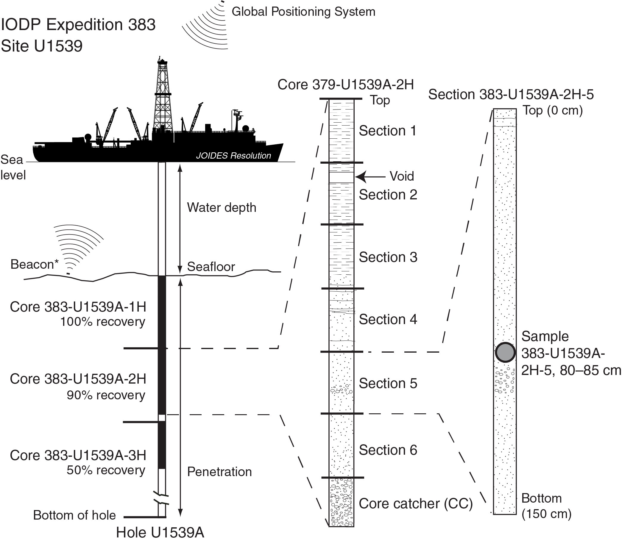
Figure F1. Sample naming convention.
Drilling operations
The advanced piston corer (APC), half-length APC (HLAPC), and extended core barrel (XCB) systems were used during Expedition 383 (Figures F2, F3). These tools and other drilling technology is documented in Graber et al. (2002).
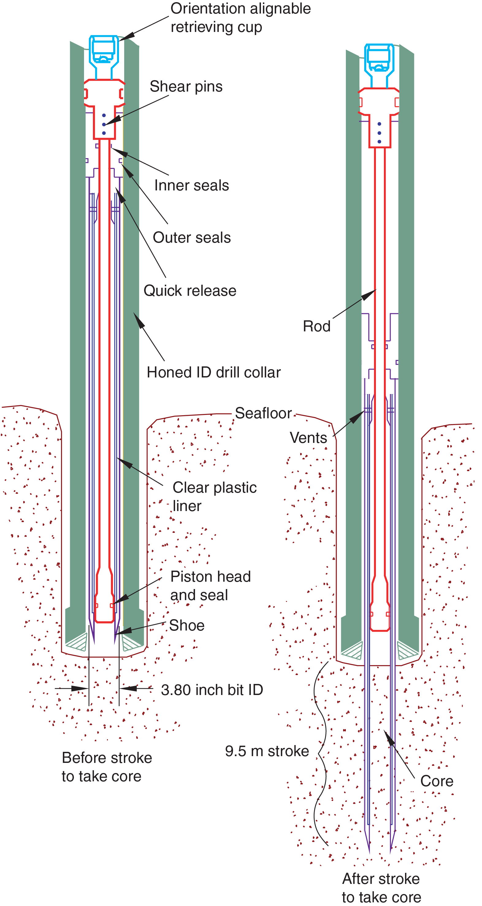
Figure F2. APC drilling system.
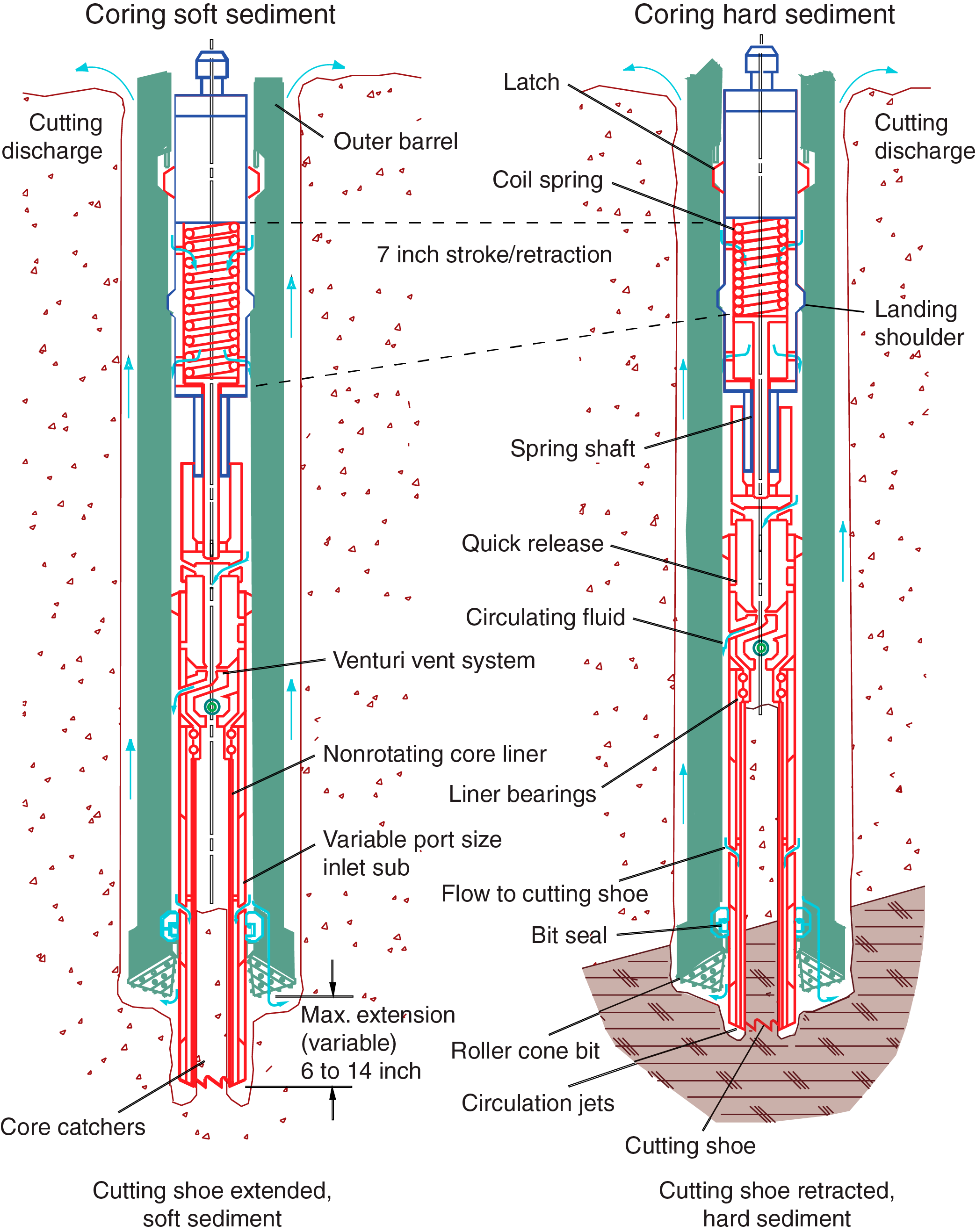
Figure F3. XCB drilling system.
The APC and HLAPC systems cut soft-sediment cores with minimal coring disturbance relative to other IODP coring systems. After the APC/HLAPC core barrel is lowered through the drill pipe and lands above the bit, the drill pipe is pressured up until the two shear pins that hold the inner barrel attached to the outer barrel fail. The inner barrel then advances into the formation and cuts the core (Figure F2). The driller can detect a successful cut, or “full stroke,” by observing the pressure gauge on the rig floor because the excess pressure accumulated prior to the stroke drops rapidly.
APC refusal is conventionally defined in one of two ways: (1) the piston fails to achieve a complete stroke (as determined from the pump pressure and recovery reading) because the formation is too hard, or (2) excessive force (>60,000 lb) is required to pull the core barrel out of the formation. For APC cores that do not achieve a full stroke, the next core can be taken after advancing to a depth determined by the recovery of the previous core (advance by recovery) or to a depth of a full APC core (typically 9.5 m). When a full stroke could not be achieved, one or more additional attempts were typically made, and each time the bit was advanced by the length of the core recovered (note that for these cores, this results in a nominal recovery of ~100%). When a full or partial stroke is achieved but excessive force is not able to retrieve the barrel, the core barrel can be “drilled over,” meaning that after the inner core barrel was successfully shot into the formation, the drill bit was advanced to total depth to free the APC barrel.
The standard APC system uses a 9.5 m long core barrel, whereas the HLAPC system uses a 4.7 m long core barrel. In most instances, the HLAPC was deployed after the standard APC had repeated partial strokes and the core liners were damaged. During use of the HLAPC system, the refusal criteria for the APC system were applied. Use of the HLAPC system allowed significantly greater APC sampling depths to be attained than would have otherwise been possible.
The XCB is a rotary system with a small cutting shoe that extends below the large rotary APC/XCB bit (Figure F3). The smaller bit can cut a semi-indurated core with less torque and fluid circulation than the main bit, potentially improving recovery. The XCB cutting shoe typically extends ~30.5 cm ahead of the main bit in soft sediments, but a spring allows it to retract into the main bit when hard formations are encountered. Shorter XCB cutting shoes can also be used. The XCB system is typically used when the APC/HLAPC system has difficulty penetrating the formation and/or damages the core liner or core. The XCB system can also be used to either initiate holes where the seafloor is not suitable for APC coring or interchanged with the APC/HLAPC system when dictated by changing formation conditions (e.g., Hole U1544A). The XCB system was used to advance holes when HLAPC refusal occurred before the target depth was reached or when drilling conditions required it (e.g., Holes U1540D and U1541B).
The bottom-hole assembly (BHA) used for APC and XCB coring is typically composed of an 11⁷⁄₁₆ inch (~29.05 cm) roller-cone drill bit, a bit sub, a seal bore drill collar, a landing saver sub, a modified top sub, a modified head sub, 8¼ inch control length drill collars, a tapered drill collar, two stands of 5½ inch transition drill pipe, and a crossover sub to the drill pipe that extends to the surface.
The RCB system is a rotary coring system designed to recover firm to hard sediments and basement rocks (Graber et al., 2002), and it was not used during Expedition 383.
Nonmagnetic core barrels were used for most APC and HLAPC coring. APC cores were oriented with the Icefield MI-5 core orientation tool when coring conditions allowed. Formation temperature measurements were taken with the advanced piston corer temperature (APCT-3) tool (see Downhole measurements). Information on recovered cores, drilled intervals, downhole tool deployments, and related information are provided in the Operations, Paleomagnetism, Physical properties, and Downhole measurements sections of each site chapter.
IODP depth conventions
Primary depth scale types are based on the measurement of drill string length deployed beneath the rig floor (drilling depth below rig floor [DRF] and drilling depth below seafloor [DSF]), the length of core recovered (core depth below seafloor [CSF] and core composite depth below seafloor [CCSF]), and the length of the logging wireline deployed (wireline log depth below rig floor [WRF], wireline log depth below seafloor [WSF], and wireline log matched depth below seafloor [WMSF]). All depth units are in meters. The relationship between scales is defined either by protocol, such as the rules for computation of CSF from DSF, or by combinations of protocols with user-defined correlations (e.g., CCSF). The distinction in nomenclature should keep the user aware that a nominal depth value at two different depth scales usually does not refer to exactly the same stratigraphic interval (see Curatorial procedures and sample depth calculations). For more information on depth scales, see “IODP Depth Scales Terminology” at http://www.iodp.org/policies-and-guidelines. To more easily communicate shipboard results, CSF-A depths are reported in this volume as meters below seafloor (mbsf) unless otherwise noted.
Depths of cored intervals are measured from the drill floor based on the length of drill pipe deployed beneath the rig floor (DRF scale; Figure F1). The depth of the cored interval is referenced to the seafloor (DSF scale) by subtracting the seafloor depth of the hole from the DRF depth of the interval. Standard depths of cores in meters below the seafloor (CSF, Method A [CSF-A] scale) are determined based on the assumption that the top depth of a recovered core corresponds to the top depth of its cored interval (at the DSF scale). Standard depths of samples and associated measurements (CSF-A scale) are calculated by adding the offset of the sample or measurement from the top of its section and the lengths of all higher sections in the core to the top depth of the core.
If a core has <100% recovery, for curation purposes all cored material is assumed to originate from the top of the drilled interval as a continuous section. In addition, voids in the core are closed by pushing core segments together, if possible, during core handling. If the core pieces can’t be pushed together to close the voids, then foam spacers are inserted and clearly labeled “void.” Therefore, the true depth interval within the cored interval is only partially constrained. This should be considered a sampling uncertainty in age-depth analysis or in correlation of core data with downhole logging data.
When core recovery is >100% (the length of the recovered core exceeds that of the cored interval), the CSF depth of a sample or measurement taken from the bottom of a core will be deeper than that of a sample or measurement taken from the top of the subsequent core (i.e., the data associated with the two core intervals overlap at the CSF-A scale). This can happen when a soft to semisoft sediment core recovered from a few hundred meters below the seafloor expands upon recovery (typically by a few percent to as much as 15%). Therefore, a stratigraphic interval may not have the same nominal depth at the DSF and CSF scales in the same hole.
During Expedition 383, all core depths below seafloor were initially calculated according to the CSF-A depth scale. Unless otherwise noted, all depths presented are core depths below seafloor calculated as CSF-A.
CCSF depth scales are constructed for sites with two or more holes to create a stratigraphic record as continuous as possible. This also helps mitigate the CSF-A core overlap problem and the coring gap problem. Using shipboard core logger–based physical property data verified with core photos, core depths in adjacent holes at a site are vertically shifted to correlate between cores recovered in adjacent holes. This process produces the CCSF depth scale. The correlation process results in affine tables, indicating the vertical shift of cores on the CCSF scale relative to the CSF-A scale. Once the CCSF scale is constructed, a splice can be defined that best represents the stratigraphy of a site by utilizing and splicing the best portions of individual sections and cores from each hole. Because of core expansion, the CCSF depths of stratigraphic intervals are typically 10%–15% deeper than their CSF-A depths. CCSF depth scale construction also reveals that coring gaps on the order of 1.0–1.5 m typically occur between two subsequent cores despite the apparent >100% recovery. For more details on construction of the CCSF depth scale, see Stratigraphic correlation.
Curatorial procedures and sample depth calculations
Numbering of sites, holes, cores, and samples followed standard IODP procedure (Figure F1). A full curatorial identifier for a sample consists of the following information: expedition, site, hole, core number, core type, section number, section half, piece number (hard rocks only), and interval in centimeters measured from the top of the core section. For example, a sample identification of “383-U1539A-2H-5W, 50–55 cm” indicates a 5 cm sample removed from the interval between 50 and 55 cm below the top of Section 5 (working half) of Core 2 (“H” designates that this core was taken with the APC system) of Hole A at Site U1539 during Expedition 383 (Figure F1). The “U” preceding the hole number indicates the hole was drilled by the United States IODP platform, JOIDES Resolution. The drilling system used to obtain a core is designated in the sample identifiers as follows: H = APC, F = HLAPC, and X = XCB. Integers are used to denote the “core” type of drilled intervals (e.g., a drilled interval between Cores 2H and 4H would be noted as Core 31).
Core handling and analysis
The overall flow of cores, sections, analyses, and sampling implemented during Expedition 383 is shown in Figure F4.
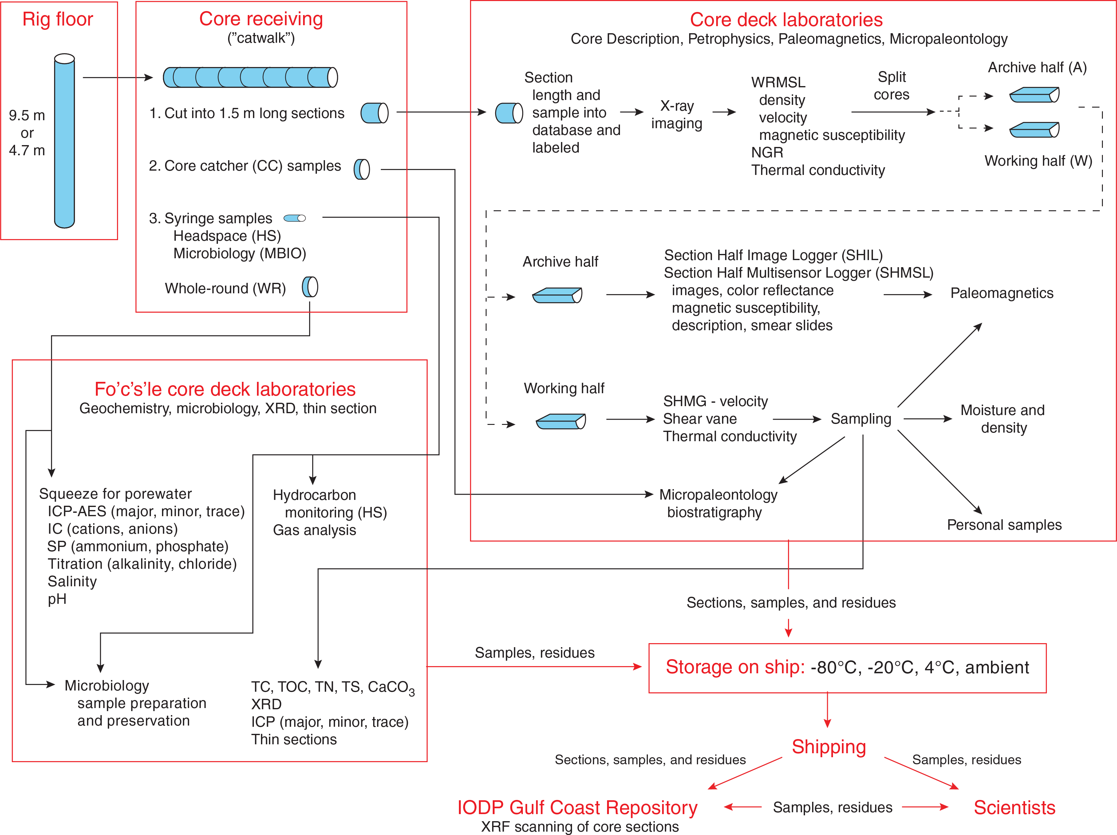
Figure F4. Shipboard core flow.
Sediment
When the core barrel reached the rig floor, the core catcher from the bottom of the core was removed and taken to the core receiving platform (“catwalk”), and a sample was extracted for paleontological (PAL) analysis. Next, the sediment core was extracted from the core barrel in its plastic liner. The liner was carried from the rig floor to the core processing area on the catwalk outside the core laboratory, where it was split into ~1.5 m sections. Blue (uphole direction) and clear (downhole direction) liner caps were glued with acetone onto the cut liner sections.
Once the core was cut into sections, whole-round samples were taken for interstitial water (IW) chemical analyses. When a whole-round sample was removed, a yellow cap was used identify a whole-round sample had been taken. Syringe samples were taken for gas analyses according to the IODP hydrocarbon safety monitoring protocol. Syringe and whole-round samples were taken for microbiology contamination testing and postcruise analyses. Toothpick samples for smear slides were taken from some of the section ends for additional paleontological analysis.
The core sections were placed in a core rack in the laboratory, core information was entered into the database, and the sections were labeled. When the core sections reached equilibrium with laboratory temperature (typically after 4 h), they were run through the Whole-Round Multisensor Logger (WRMSL) for P-wave velocity (PWL), magnetic susceptibility (MS), and gamma ray attenuation (GRA) bulk density (see Physical properties). The core sections were also run through the Natural Gamma Radiation Logger (NGRL), and thermal conductivity measurements were taken once per core when the material was suitable.
The core sections were then split lengthwise from bottom to top into working and archive halves. Investigators should note that older material can be transported upward on the split face of each section during splitting.
Discrete samples were then taken for moisture and density (MAD) and paleomagnetic (PMAG) analyses and for remaining shipboard analyses such as X-ray diffraction (XRD), carbonate (CARB), and inductively coupled plasma–atomic emission spectroscopy (ICP-AES). Samples were not collected when the lithology was a high-priority interval for expedition or postcruise research, when the core material was unsuitable, or when the core was severely deformed. During the expedition, samples for personal postcruise research were taken when they concerned ephemeral properties (e.g., IW and amino acid sampling). We also took a limited number of personal or shared “pilot” samples (mostly scrapes) for two reasons: (1) to find out if an analytical method works and yields interpretable results, and how much sample is needed, to guide postcruise sampling, and (2) to generate low spatial resolution pilot data sets that can be incorporated in proposals and potentially increase their chances of being funded.
The archive half of each core was scanned on the Section Half Imaging Logger (SHIL) to provide line-scan images and then measured for point magnetic susceptibility (MPS) and reflectance spectroscopy and colorimetry (RSC) on the Section Half Multisensor Logger (SHMSL). All of the archive-half core sections were X-ray imaged. Labeled foam pieces were used to denote missing whole-round intervals in the SHIL images. The archive-half sections were then described visually and by means of smear slides for sedimentology. Finally, the magnetization of archive-half sections and working-half discrete pieces was measured with the cryogenic magnetometer and spinner magnetometer.
When all steps were completed, cores were wrapped, sealed in plastic tubes, and transferred to cold storage space aboard the ship. At the end of the expedition, all the working- and archive-half sections of the cores were sent to the IODP Gulf Coast Repository (GCR) in College Station, Texas (USA), where a subset of the archive-half sections were scanned for X-ray fluorescence (XRF) and samples for postcruise research were taken.
Drilling and handling core disturbance
Cores may be significantly disturbed and contain extraneous material as a result of the coring and core handling process (Jutzeler et al., 2014). For example, in formations with loose gravel or pebble-sized clasts, the clasts from intervals higher in the hole may be washed down by drilling circulation, accumulate at the bottom of the hole, and be sampled with the next core. The uppermost 10–50 cm of each core must therefore be examined critically during description for potential “fall-in.” Common coring-induced deformation includes the concave-downward appearance of originally horizontal bedding. Piston action can result in fluidization (“flow-in”) at the bottom of APC cores. The rotation and fluid circulation used during XCB and RCB coring can also cause core pieces to rotate relative to each other as well as induce fluids into the core and/or cause fluidization and remobilization of poorly consolidated/cemented sediments. In addition, extending APC or HLAPC coring into a deeper, more firm formation can also induce core deformation. Retrieval from depth to the surface can result in elastic rebound. Gas that is in solution at depth may become free and drive apart core segments within the liner. When gas content is high, pressure must be relieved for safety reasons before the cores are cut into segments. This is accomplished by drilling holes into the liner, which forces some sediment as well as gas out of the liner. These disturbances are described in each site chapter and graphically indicated on the visual core descriptions (VCDs).
Sedimentology
This section outlines the general procedures for documenting the sedimentology of cores recovered during Expedition 383 including core description, sediment classification, smear slide preparation and description, X-ray imaging, X-ray diffraction (XRD) of bulk sediment and clay mineral assemblages, and X-ray fluorescence of section halves. All observations and data were uploaded directly into the IODP Laboratory Information Management System (LIMS) using the DESClogik application. DESClogik also includes a graphic display mode for core data (e.g., digital images of section halves and measurement data) that was used for quality control of the uploaded data sets.
Core preparation and digital color imaging
Prior to core description and high-resolution digital color imaging, the quality of the split-core surface of the archive half of each core was assessed and the surface was scraped lightly with a flexible metallic plate or glass microscopic slide. Cleaned core sections were then described in conjunction with images obtained using the Section Half Imaging Logger (SHIL), smear slide analyses, and measurements obtained using the Section Half Multisensor Logger (SHMSL) (see Physical properties).
The cleaned archive half was imaged with the SHIL as soon as possible to avoid sediment color changes caused by oxidation and drying. In cases of watery or soupy sediment, the surface was allowed to dry sufficiently to avoid light reflection prior to scanning. The SHIL uses three pairs of Advanced Illumination high-current focused LED line lights (model CS420) to illuminate the features of the core. Each of the LED pairs has a color temperature of 6,500 K and emits 200,000 lux at 3 inches. Digital images were taken by a JAI 3CCD line-scan camera (model CV107CL) with a Nikkor 60 mm AF 1:2.8 D lens at an interval of 10 lines/mm to create a high-resolution TIFF file. The camera height was set so that each pixel imaged a 0.1 mm2 section of the core surface; however, actual core width per pixel can vary because of slight differences in the section-half surface height. A high-resolution JPEG with grayscale and depth ruler and a low-resolution cropped JPEG showing only the core section surface were created from the high-resolution TIFF files. We observed that core sections with high carbonate content tended to overexpose during SHIL imaging. Such sections were reimaged using a lower gain setting only for the purpose of core photos. Note that all RGB data from Expedition 383 were collected using the original high gain setting to avoid any RGB data artifacts resulting from changing gain settings. After acquisition, raw SHIL data were processed for core edge and void effects arising from sediment gaps and styrofoam inserts for interstitial water and micropaleontology samples. RGB data compromised by nonsediment material were excluded from processed data products. Additional screening for core cracks and voids was performed, and RGB data compromised by cracks or voids were removed from processed data products. These “cleaned” data are used for graphical display only and are not available from the LIMS database but may be obtained from the Sedimentology team.
Visual core description
Macroscopic descriptions of each core section (nominally 0–150 cm long) were recorded by hand on log sheets that included an image of the core obtained using the SHIL. All logs were digitally preserved as PDF files. Sediment color was determined qualitatively for core intervals using Munsell Soil Color Charts (Munsell Color Company, Inc., 2010). Information from hand-annotated visual core descriptions (VCDs) for each core section was recorded directly into the Tabular Data Capture mode of the DESClogik program. A template was constructed, and tabs and columns were customized to include relevant descriptive information categories (lithology, sedimentary structures, bioturbation intensity, drilling disturbance, and clast abundance). A summary description was also entered for each core.
A simplified one-page graphical representation of each core (VCD) (Figure F5) was generated using the LIMS2Excel application and a commercial program (Strater, Golden Software). VCDs are presented with the core depth below seafloor, Method A (CSF-A), depth scale, split-core photographs, graphic lithology, and columns for core disturbance, sedimentary structures, bioturbation, shipboard samples, gamma ray attenuation (GRA) bulk density, magnetic susceptibility (MSP), RGB blue color intensity, and b* color reflectance. Graphic lithologies, sedimentary structures, and other visual observations are represented on the VCDs using graphic patterns and symbols (Figure F6). Each VCD also contains the summary description for the core. Only major lithologies are shown in the summary figure for each site chapter.
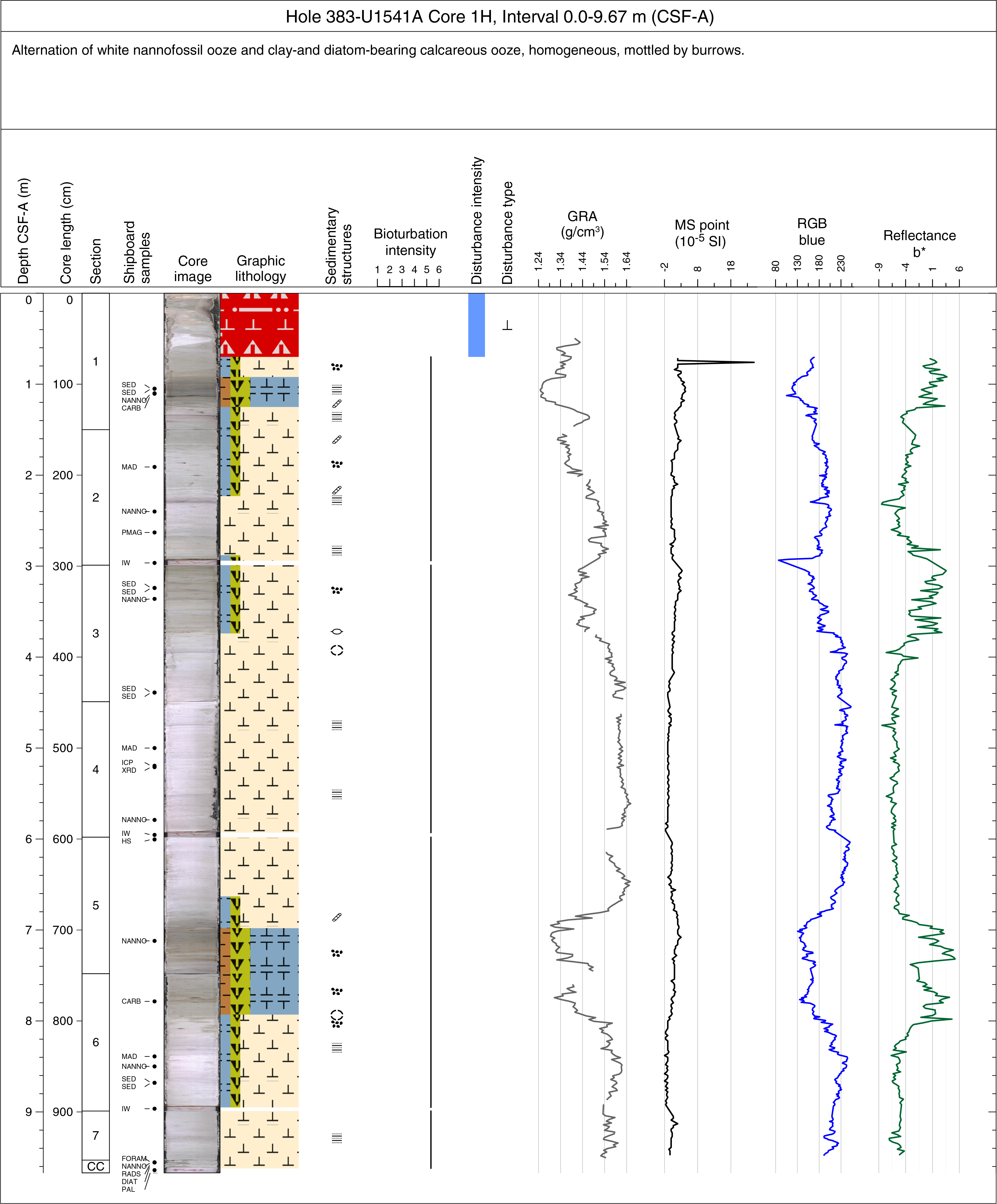
Figure F5. Example VCD.
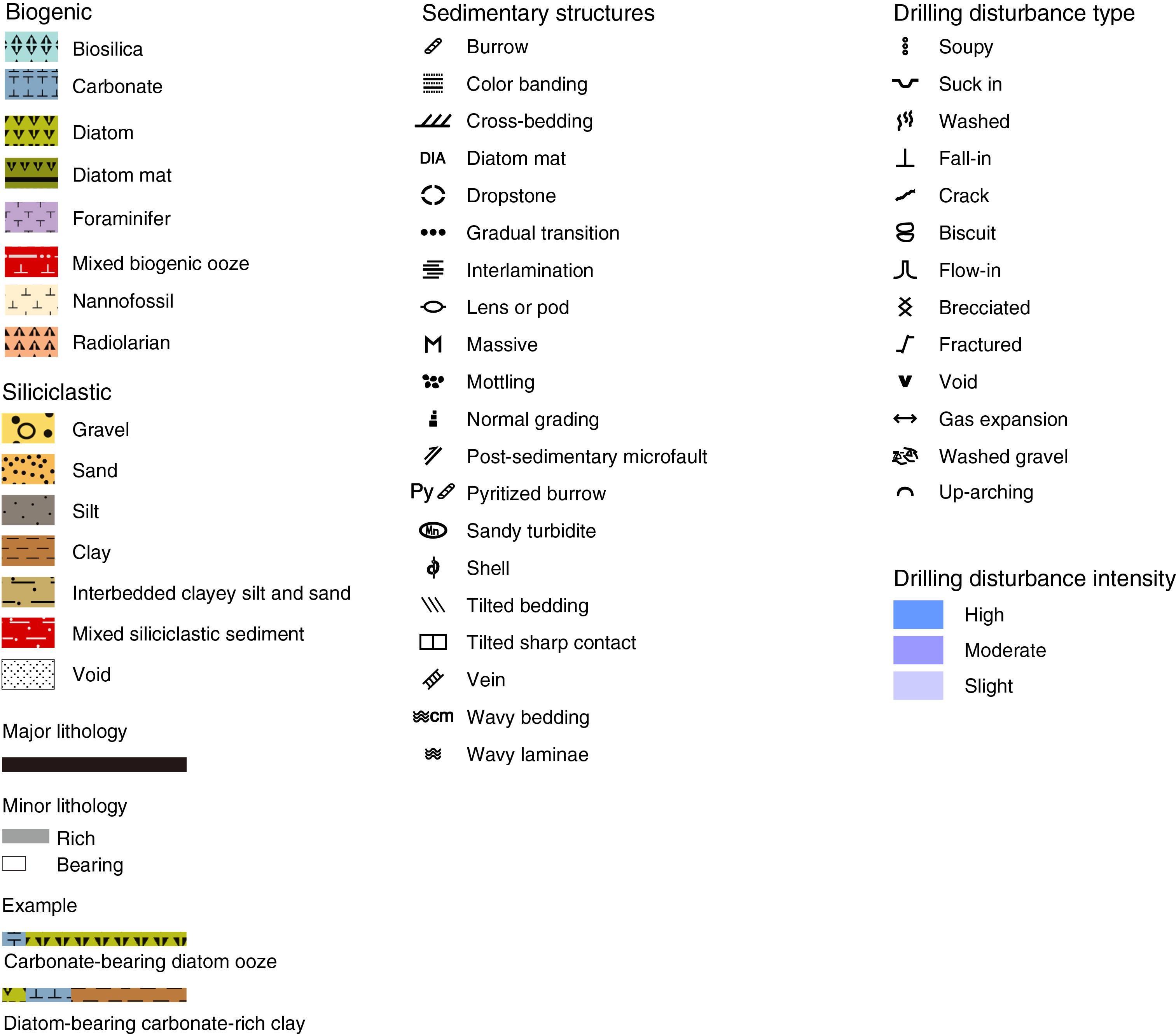
Figure F6. Lithologic key and symbols used for VCDs.
Smear slides and thin sections
Smear slide microscopic analysis was used to determine biogenic and terrigenous constituents and abundance to aid in lithologic classification. Toothpick samples were typically taken from each lithology at a frequency of at least two samples per core. For these preparations, the sediment was mixed with distilled water on a glass coverslip or glass slide and dried on a hot plate at 50°C. The dried sample was then mounted in Norland optical adhesive Number 61 and fixed in an ultraviolet light box. Smear slides were examined with a transmitted-light petrographic microscope equipped with a standard eyepiece micrometer. Biogenic and mineral components were identified following standard petrographic techniques as stated in Rothwell (1989) and Marsaglia et al. (2013, 2015). Several fields of view were examined at 100×, 200×, 400×, and 500× to assess the abundance of detrital, biogenic, and authigenic components. The relative abundance percentages of the sedimentary constituents were visually estimated using the techniques of Rothwell (1989). The texture of siliciclastic lithologies (e.g., relative abundance of sand-, silt-, and clay-sized grains) and the proportions and presence of biogenic and mineral components were recorded on the smear slide worksheet in the microscopic DESClogik template. Components observed in smear slides were categorized as follows:
- TR = trace (≤1%).
- R = rare (>1%–10%).
- C = common (>10%–25%).
- A = abundant (>25%–50%).
- D = dominant (>50%).
Smear slides provide only a rough estimate of the relative abundance of sediment constituents. Occasionally, the lithologic name assigned based on smear slide observation does not match the name in the macroscopic lithology description because a small sample may not represent the macroscopic description of a much larger sediment interval. Additionally, very fine and coarse grains are difficult to observe in smear slides, and their relative proportions in the sediment can be affected during slide preparation. Therefore, intervals dominated by sand and larger sized constituents were examined by macroscopic comparison to grain size reference charts. Photomicrographs of some smear slides were taken and uploaded to the LIMS database. Several thin sections of volcanic glass fragments were prepared and used to microscopically describe their texture and petrological properties. Photomicrographs of thin sections were taken and uploaded to the LIMS database.
Lithologic classification scheme
The principal lithologic name was assigned on the basis of the relative abundances of biogenic and terrigenous clastic grains:
- The principal name of a sediment with <50% biogenic grains was based on the grain size characteristics of the terrigenous clastic fraction. If the sediment contains no or minor amounts of gravel, then the principal name was determined by the relative abundances of sand, silt, and clay (Figure F7; after Mazzullo et al., 1988).
- The principal name of a sediment/rock with ≥50% biogenic grains was classified as an ooze and was modified by the most abundant specific biogenic grain type that forms 50% or more of the sediment (Figure F7). For example, if diatoms exceed 50%, then the sediment was classified as a “diatom ooze.” Optionally, similar biogenic grain types were grouped together to exceed this 50% abundance threshold (e.g., if diatoms are 40% of the sediment and sponge spicules are 20%, then the sediment was termed “biosiliceous ooze”).
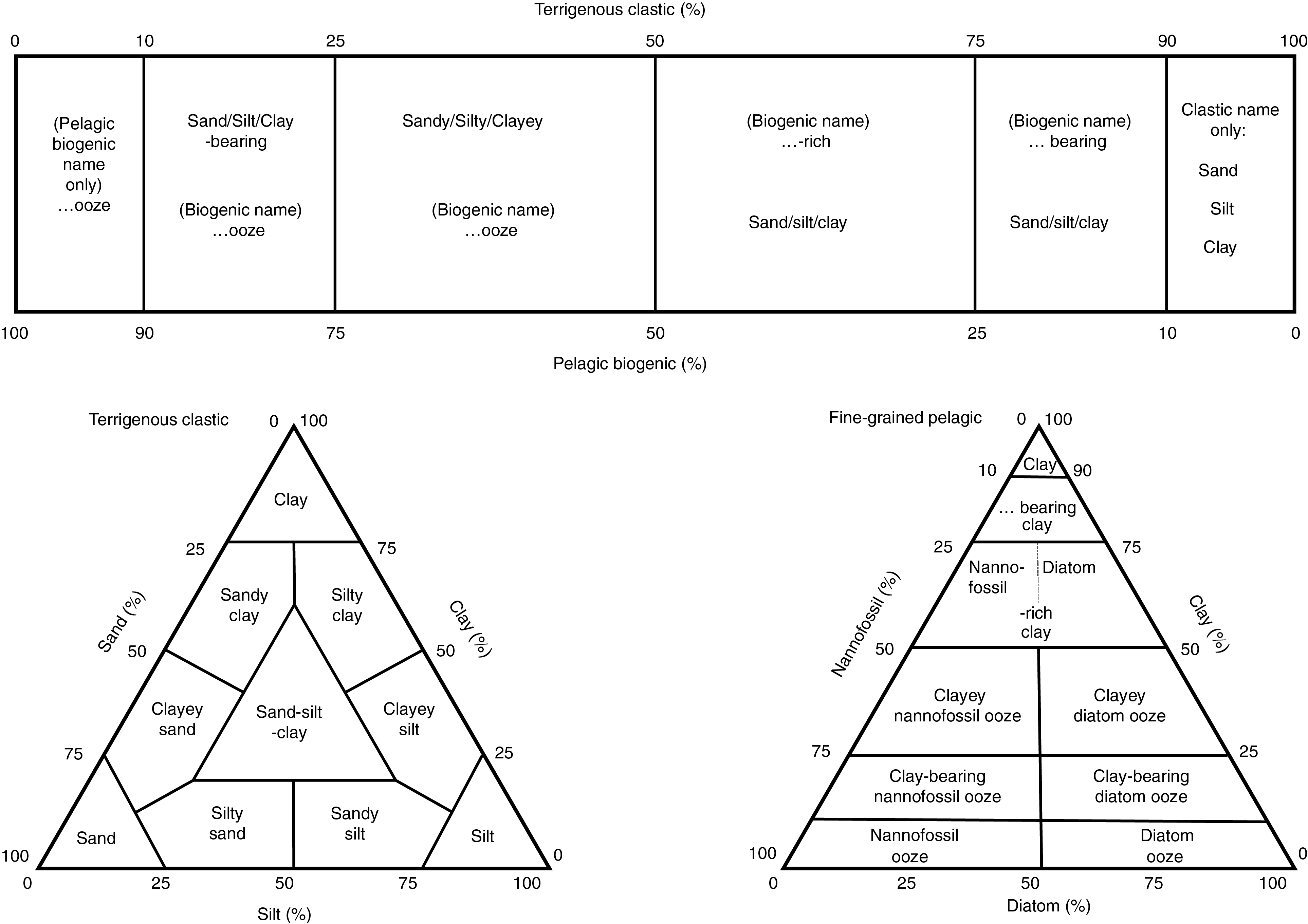
Figure F7. Lithology naming and classification schemes.
Major and minor modifiers were applied to any of the principal granular sediment/rock names. The use of major and minor modifiers follows the scheme of Integrated Ocean Drilling Program Expedition 318 (Expedition 318 Scientists, 2011):
- Minor modifiers (Figure F7) are components with abundances between 10% and <25% and are indicated by the suffix “-bearing” (e.g., diatom-bearing, silt-bearing).
- Major modifiers (Figure F7) are components with abundances between 25% and 49% and are indicated by the suffix “-rich” for the biogenic components (e.g., diatom-rich) and by “clayey,” “silty” or “sandy” according to the major terrigenous clastic modifier.
- If possible, modifiers were assigned based on the most abundant specific grain type (e.g., diatom-rich versus biosilica-rich).
- Components with abundances <10% were included in the comments column in DESClogik (e.g., “with sponge spicule” or “with radiolarians”).
The Wentworth (1922) scale was used to define grain size classes. The terms “mixed siliciclastic sediment” and “mixed biogenic ooze” were attributed to intervals of core that contained extreme drilling disturbance usually associated with fall-in and/or suck-in (see Core disturbance). The terms and associated lithologic symbols in the VCDs were used to avoid inclusion in the splice (where possible) and sampling.
Clast abundance
Dropstone observations were part of the sediment visual core description and provide a preliminary account of the presence and abundance record of ice-rafted debris (IRD) in the cores. We used the processed X-ray images to estimate dropstone abundance per X-ray image. Each image integrates 12 cm of core, and the dropstone concentration is obtained for the central depth of an image. We assume dropstones appear as dark gray to black very dense defined particles in the X-ray images and counted particles larger than ~0.5 mm. Some counting uncertainty may have been introduced by considering spot-like diagenetic iron sulfides as dropstones. Because of the very high abundance of dropstones at Site U1542 and the short period available to process all data, we elected to qualitatively assess abundance in each X-ray image using the categories dominant, abundant, common, rare, and trace and reported these categories in the VCDs for this site (see Core descriptions).
Bioturbation
Ichnofabric description analysis included evaluation of the extent of bioturbation and notation of distinctive biogenic structures. To assess the degree of bioturbation semiquantitatively, the ichnofabric index from Droser and O’Connell (1992) (from 1 to 5) was employed (e.g., 1 = bioturbation absent, 3 = moderate bioturbation [10%–40% of the surface], and 5 = total biogenic homogenization of sediment). This index is illustrated using the numerical scale in the Relative bioturbation column of the VCDs (Figure F8).
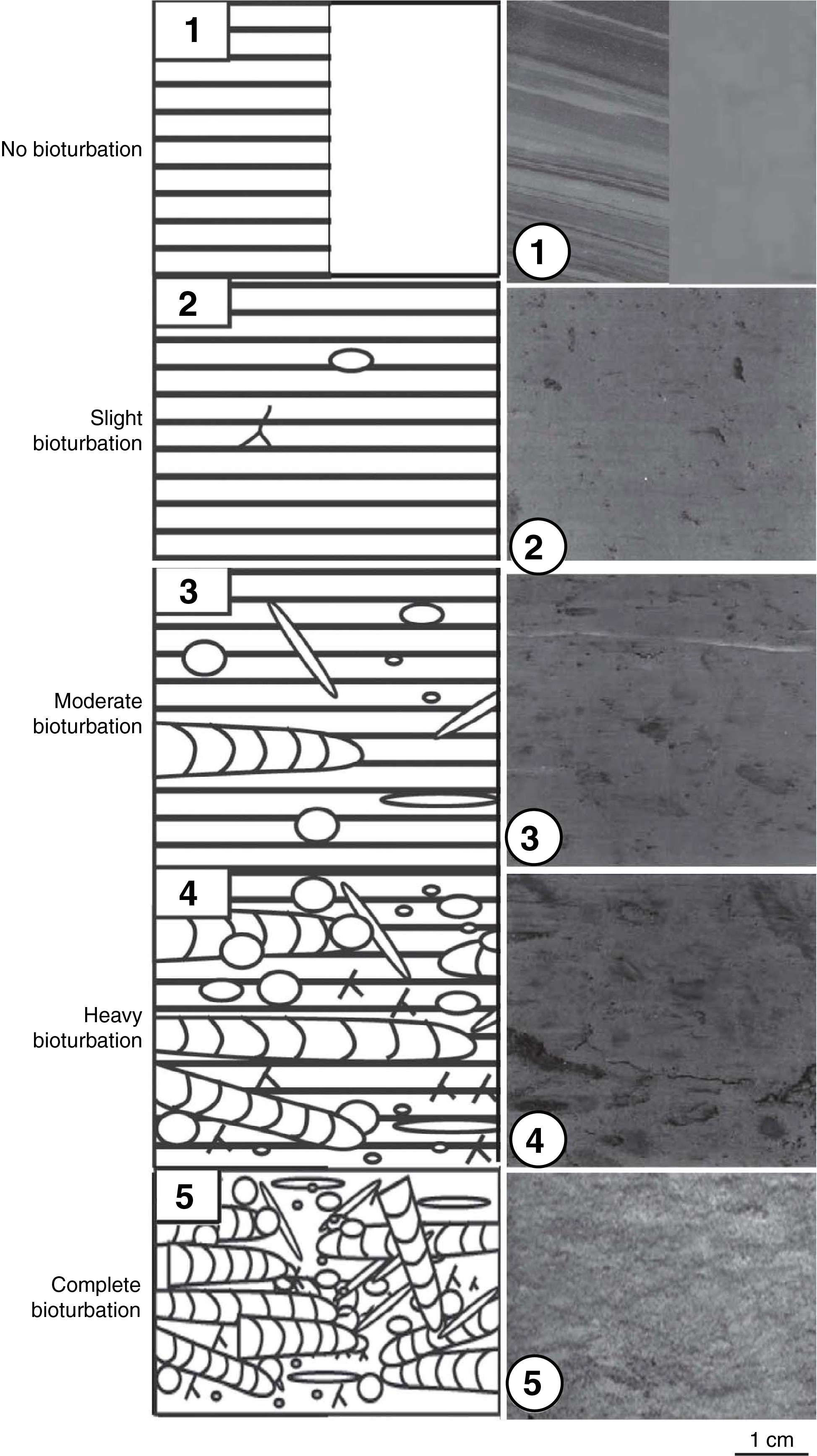
Figure F8. Bioturbation index.
Core disturbance
Drilling disturbance was classified into four categories:
- None.
- Slightly disturbed: bedding contacts are slightly bent.
- Moderately disturbed: bedding contacts are extremely bowed.
- Extremely disturbed: bedding is completely deformed and may show diapiric or minor flow structures or is soupy to the degree that the sediments are water saturated and show no traces of original bedding or structure.
When a specific type of drilling disturbance was identified, the nomenclature of Jutzeler et al. (2014) was used to characterize the drilling disturbance (Figure F9):
- Biscuit,
- Bowed,
- Brecciated,
- Crack,
- Fall-in,
- Flow-in,
- Fractured,
- Gas expansion,
- Soupy,
- Uparching,
- Washed, and
- Washed gravel.
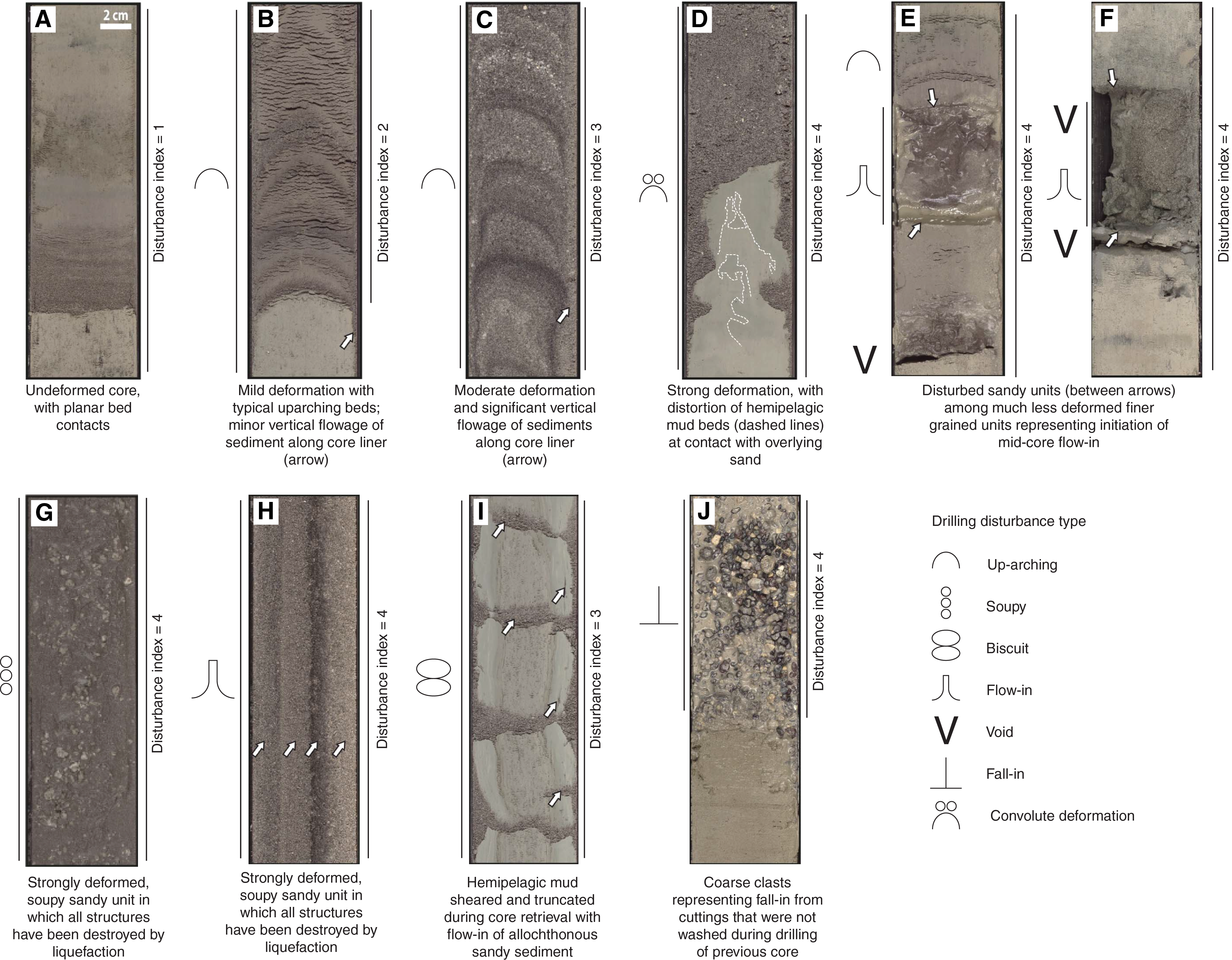
Figure F9. Coring disturbance index.
X-ray diffraction analysis of bulk sediment and clay fraction
Selected samples for XRD analysis were obtained from the working halves of the cores at an average spacing of one sample per core. When possible, samples were taken adjacent to the carbonate content and major element samples. XRD analysis was performed on the clay fraction in most samples. For these preparations, a ~2 g sample was placed in a 50 mL centrifuge tube with 10% acetic acid, sonicated for 15 min, and allowed to stand overnight to remove carbonate material. After centrifuging for 15 min at 1500 rpm, the acetic acid was decanted, 25 mL of distilled water was added, the sample was centrifuged again, and the water was decanted. This washing procedure was repeated two more times to remove both the acid and salts from the sample. After decanting the final wash, 25 mL of 1% sodium metaphosphate solution was added to the sample in a 50 mL beaker. The sample was then placed in an ultrasonic bath for 5 min to suspend the clays by ultrasonic disaggregation and then centrifuged for 5 min at 1000 rpm to settle the >2 µm particles. The clays that remained in suspension were removed from the uppermost ~1 cm of the centrifuge tube and pipetted onto two amorphous quartz sample discs. The sample discs were then left to air dry in a desiccator. After drying, one disc was analyzed and the other was solvated with ethylene glycol for ~8 h at 65°C and analyzed to determine the presence of expandable clays.
The prepared samples were mounted onto a sample holder and analyzed by XRD using a Bruker D-4 Endeavor diffractometer mounted with a Vantec-1 detector using nickel-filtered CuKα radiation. The standard locked coupled scan was as follows:
- Voltage = 35 kV.
- Current = 40 mA.
- Goniometer scan = 3.5°–30°2θ.
- Step size = ~0.0085°.
- Scan speed = 1 s/step.
- Divergence slit = 0.3°.
The diffractograms of single samples were evaluated with the Bruker Diffrac-Plus EVA software package. Relative abundances of the major clay mineral groups were established based on maximum peak intensity, preferentially from the glycolated analysis. Quantification of mineral contents was not possible because the samples were not spiked with a defined amount of a mineral standard for calibration. Therefore, the shipboard results were interpreted qualitatively based on relative occurrences and abundances of the most common clay mineralogical components.
A small number of selected samples were freeze-dried, ground, and mounted on aluminum holders for bulk XRD analysis. Scans of these samples were performed with the same instrument settings as the clay preparations and scanned over a goniometer range of 3.5°–70°2θ.
X-ray imaging
X-radiograph images were produced from all sites to evaluate bioturbation intensity, drilling disturbance, sedimentary structures, and clast abundance. Images were obtained from archive-half sections immediately after splitting and imaging. The onboard X-ray imager (XRI) is composed of a Teledyne ICM CP120B X-ray generator and a detector unit. The generator works with a maximum voltage of 120 kV and a tube current of 1 A and has a 0.8 mm × 0.5 mm focal spot. The generator produces a directional cone at a beam angle of 50° × 50°. The detector unit is located 65 cm from the source and consists of a Go-Scan 1510 HR system composed of an array of CMOS sensors arranged to offer an active area of 102 mm × 153 mm and a resolution of 99 µm. Core sections were run through the imaging area at 12 cm intervals, providing images of 15 cm onto the detector and allowing an overlap of 3 cm.
Tests were conducted on archive-half sections to obtain the best image resolution for determining the internal structure of cores. The XRI settings were then changed to adjust to the varying lithologies of the cores. The number of images stacked was 20, taken at exposure times of 300–350 ms. The voltage ranged between 60 and 70 kV, and the current varied from 0.7 to 0.8 mA.
The raw images were collected as 16 bit images and were processed with the IODP in-house processing utility in the Integrated Measurement System (IMS) software (v. 1.3). The software applies corrections for the detector (gain and offset corrections), compensates for core shape and thickness, and adjusts the image contrast. The Savitzky-Golay FIR filter was chosen to smooth images. The resulting processed images include a masked background, the depth scale of the section, and the acquisition parameters. The software applies different processing to APC or HLAPC cores and to rotary cores. Some sections where the processing utility did not give good results were reprocessed, first with the LeVay processing software and later with the processing utility.
Handheld X-ray fluorescence
Handheld X-ray fluorescence (XRF) scanning was performed on select sections from Site U1540 and U1541 to generate higher resolution element abundance and elemental ratios in bulk sediment. The Olympus Delta Premium handheld XRF device is adapted to measure K, Ca, Si, Fe, and Mn. Each measurement takes ~1 min and consists of two measurement steps performed with 10 kV and 30 s integration time for lighter elements and 40 kV and 30 s integration time for heavier elements. The relative intensity is calculated by internal standard calibrated concentrations. Handheld XRF measurements were conducted to test (1) the comparison bulk sediment K content derived from NGR and XRF and (2) the relative elemental content changes of Si, Ca, Mn, and Fe in potentially altered sediments from the bottom of Sites U1540 and U1541.
Biostratigraphy
Preliminary shipboard biostratigraphic and paleoenvironmental information for Expedition 383 was provided by fossil marine diatoms, radiolarians, silicoflagellates, calcareous nannofossils, planktonic and benthic foraminifers, and ostracods. Shipboard biostratigraphic age assignments were based on analysis of microfossils from mudline and core catcher samples from Hole A at each site. At sites with high recovery or where subsequent holes penetrated deeper strata than Hole A, core catcher samples from Holes B–E were analyzed as necessary to constrain the age of the sequence or as time allowed. Additional toothpick and cylinder samples from split-core sections were analyzed as necessary to refine biostratigraphic boundaries, examine critical intervals, or investigate assemblage composition above and below significant changes in lithology. At least one mudline sample was analyzed for every site to constrain the youngest possible age and to assess the presence of any living benthic microfauna on seafloor. Freeze-dried raw mudline material and <63 µm residue are stored at the IODP Gulf Coast Repository and are available upon request.
Diatoms, radiolarians, calcareous nannofossils, and planktonic foraminifers provide excellent primary biostratigraphic control for all hemipelagic sites (U1539–U1541 and U1543) and Chilean margin Site U1542, whereas the biostratigraphy of Chilean margin Site U1544 is based solely on diatom and nannofossil occurrences. All microfossil groups aided in characterizing paleoenvironmental conditions such as changes in water masses, water depth, and sea ice presence/absence and identifying intervals of varying marine productivity. Biostratigraphic zonations and the ages of first appearance datums (FADs) and last appearance datums (LADs) of diatoms, radiolarians, and planktonic foraminifers were guided by recent IODP expeditions to the Southern Ocean (e.g., Expeditions 374, 379, and 382) (McKay et al., 2019b; Gohl et al., 2021b; Weber et al., 2021b) and the 2015 site survey Cruise ANA-05B of the R/V Araon (Ohneiser et al., 2019). Calcareous nannofossil datums were adapted from the biostratigraphic scheme of Expedition 361 (Hall et al., 2017). Biostratigraphic events and biozone boundaries for all late Miocene to recent (~0–8 Ma) intervals cored during Expedition 383 are expressed relative to the geomagnetic polarity timescale (GPTS) of Gradstein et al. (2012). Biostratigraphic zonations for microfossil groups are presented individually in the representative sections below (Figure F10).
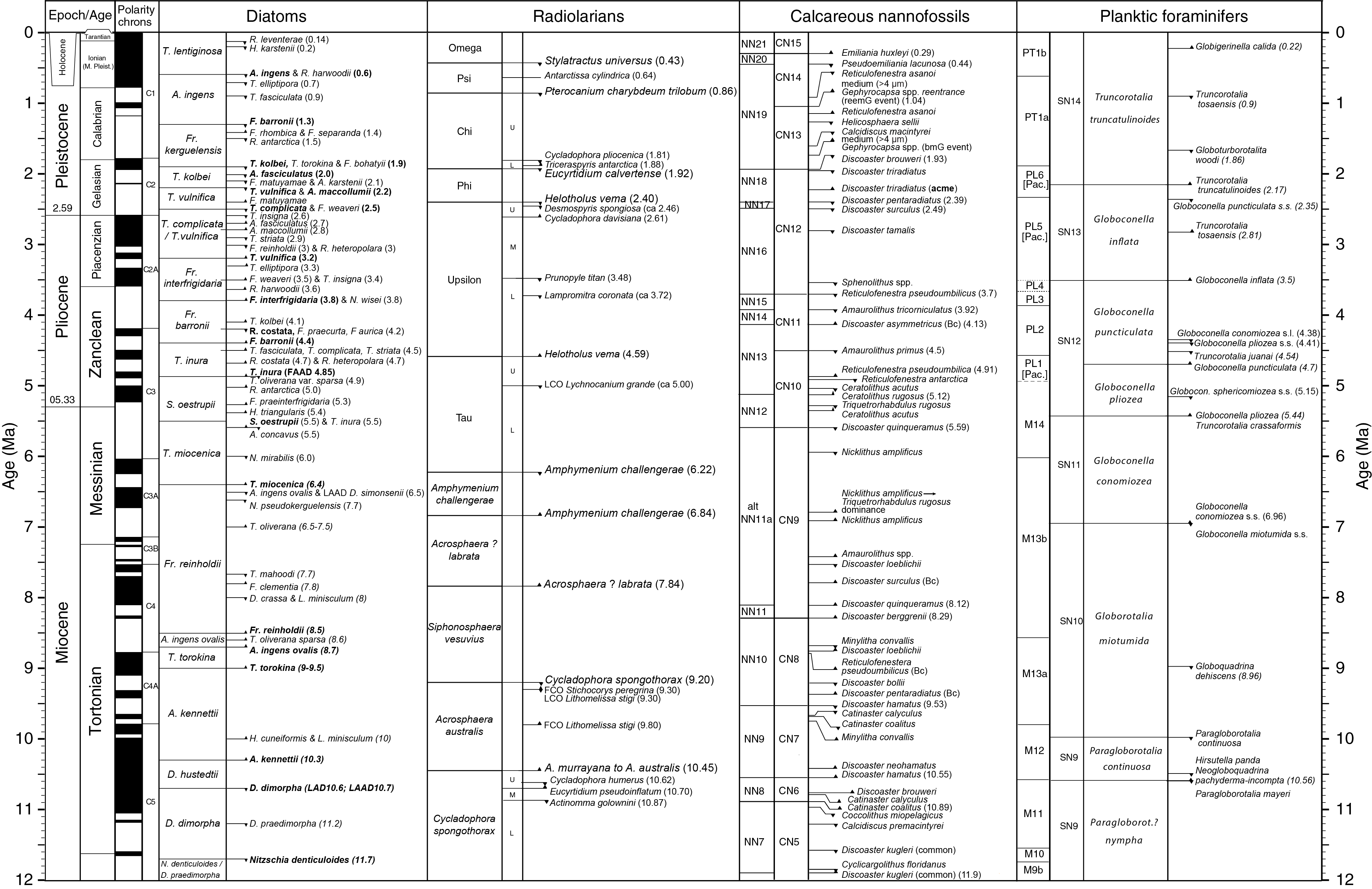
Figure F10. Biostratigraphic zonations and key datums for diatoms. This figure is also available in an oversized format.
Following the convention of recent expeditions (McKay et al., 2019a; Gohl et al., 2021a; Weber et al., 2021a), ages assigned to diatom and radiolarian datum levels were guided by the composite ordering of events and model age output from constrained optimization (CONOP) analysis of Southern Hemisphere data sets (Cody et al., 2008). Diatom datums follow the Expedition 374 event compilation (Table T1), and additional biostratigraphic information was taken from Harwood and Maruyama (1992), Censarek and Gersonde (2002), Zielinski and Gersonde (2002), Tauxe et al. (2012), Cody et al. (2012), Winter et al. (2012), and Ohneiser et al. (2019). Diatom zonations are adapted from the Miocene–early Pliocene subantarctic zonal scheme of Censarek and Gersonde (2002) and the Pliocene–Pleistocene subantarctic zonal scheme of Zielinski and Gersonde (2002). Radiolarian biostratigraphic zones for the middle Miocene to Pleistocene additionally follow Lazarus (1990, 1992), Florindo et al. (2013), and Ohneiser et al. (2019) (Table T2). Calcareous nannofossil zonation follows the standard schemes of Martini (1971) and Okada and Bukry (1980), and the calibration of events is primarily derived from Raffi et al. (2006) and Gradstein et al. (2012). Ages and calibration sources for calcareous nannofossil datums are presented in Table T3. Biostratigraphic zones of austral temperate and subantarctic planktonic foraminifers are based on Jenkins (1993) and Berggren (1992), and datum ages are derived from the New Zealand Geological Timescale (Crundwell et al. 2016) (Table T4). Correlation to the tropical–subtropical zonation and the Gradstein et al. (2012) geologic timescale (GTS2012) (Wade et al., 2011) is also provided in Table T4.
Data for each microfossil group are presented in the form of taxonomic distribution charts that record occurrences within each sample examined. Relative abundance and preservation data were entered using the DESClogik application into the IODP LIMS database for all identified microfossil taxa and all paleontological data gathered during shipboard investigations. These data are available from the LIMS database in accordance with IODP policy. Taxonomic occurrence charts also record suspected upsection reworking or otherwise out-of-place species. The first figure in each Biostratigraphy section in the site chapters presents a summary of biostratigraphic and paleoenvironmental information provided by each microfossil group. An age-depth chronostratigraphic composite figure incorporating paleomagnetic data and showing the locations of unconformities is also provided in each site chapter.
Distribution charts for microfossil groups presented in each site chapter are based on shipboard study only. Shipboard biostratigraphic studies focused primarily on the identification of biostratigraphic horizons (biohorizons) in the cores and are biased toward the reporting of age-diagnostic species and identifying intervals and ages of reworking. Events reported include the first occurrence (FO) and/or last occurrence (LO) of a given taxon at a given site and in some cases the first common occurrence (FCO) or last common occurrence (LCO), events that indicate a change in abundance within a taxon’s range and are sometimes more reliable for correlation. Identification of a sequence of biohorizons in stratigraphic order allowed the recognition of biostratigraphic zones and subzones using standard schemes. Tables in each site chapter present the depth and age of important bioevents for use in constructing age-depth plots in which biostratigraphic information is integrated with the magnetic polarity stratigraphy, if available, to produce an age model for each site. These age models are based on preliminary shipboard data and will be updated postcruise.
Diatoms
Diatom taxonomy
Taxonomic concepts for Neogene Antarctic diatoms, many of which are endemic to the southern high latitudes, have developed largely through the last 45 y of stratigraphic drilling by the Deep Sea Drilling Project (DSDP), Ocean Drilling Program (ODP), and Integrated Ocean Drilling Program in the Southern Ocean and Antarctic shelf (McCollum, 1975; Schrader, 1976; Gombos, 1976; Ciesielski, 1983; Gersonde and Burckle, 1990; Gersonde, 1990, 1991; Fenner, 1991; Baldauf and Barron, 1991; Harwood and Maruyama, 1992; Mahood and Barron, 1996; Gersonde and Bárcena, 1998; Iwai and Winter, 2002; Censarek and Gersonde, 2002; Zielinski and Gersonde, 2002; Arney et al., 2003; Bohaty et al., 2003; Whitehead and Bohaty, 2003, Taylor-Silva and Riesselman, 2018, Armbrecht et al., 2013). In parallel to the above efforts, ice platform drilling on the Antarctic margin recovered neritic diatom floras that serve as useful taxonomic references on the Antarctic shelf (Harwood 1986, 1989; Winter and Harwood, 1997; Bohaty et al., 1998; Scherer et al., 2000; Olney et al., 2007, 2009; Winter et al., 2012; Riesselman, 2012; Sjunneskog et al., 2012; Riesselman and Dunbar, 2013). Other useful taxonomic references for Neogene and modern Antarctic marine diatoms include Fenner et al. (1976), Akiba (1982), Harwood et al. (1989), Yanagisawa and Akiba (1990), Medlin and Priddle (1990), Cremer et al. (2003), and Scott and Thomas (2005).
Methods of study for diatoms
Diatoms and other siliceous and organic-walled microfossils (endoskeletal dinoflagellates, dinoflagellate cysts [dinocysts], ebridians, chrysophyte cysts, and sponge spicules) were analyzed from smear slides and sieved slides. To make smear slides, a toothpick sample of sediment from the core catcher or another interval was mixed with a drop of water and smeared across a 22 mm × 40 mm coverslip. Coverslips were dried on a slide warmer, mounted to glass microscope slides using Norland optical adhesive No. 61 (NOA 61; refractive index = 1.56), and cured under UV light.
At Site U1542, where lithology was dominated by silt and clay particles, diatom valves were diluted to such a degree that marker taxa were difficult to find in smear slides. At that site, sieved slides were therefore prepared for all samples with trace or higher diatom abundance to remove clay and concentrate larger valves. About 1 g of wet sediment was suspended in borax solution for 30 min and washed through a 15 µm mesh sieve. The residue was then transferred to a 15 mL centrifuge tube, topped off with 10 mL of deionized water, and left to settle for 1 h. After settling, each tube was decanted to 3 mL, resuspending the biogenic layer at the surface of the settled sediment column. To prepare slides, a dome of deionized water was pipetted onto a coverslip on a slide warmer, 1 mL of the suspended sediment was drawn into a pipette, and two or three drops of the suspension were added to the water on the coverslip, which was allowed to dry and mounted as described above.
Samples were examined using a Zeiss Axio Scope.A1 transmitted light microscope. Photomicrographs were taken using a Diagnostic Instruments, Inc., Spot digital camera and uploaded to the LIMS database. Qualitative siliceous microfossil group abundances were determined from smear slides using 630× magnification. Care was taken to ensure smear slides were prepared with similar amounts of sediment. For each sample, the abundance of diatoms was qualitatively estimated by light microscopic observations at 630× magnification with the examination of five random fields of view (FOVs) as follows:
- A = abundant (>5 identifiable valves per FOV).
- C = common (2–5 identifiable valves per FOV).
- F = few (1 identifiable valve in 1–5 FOVs).
- R = rare (1 identifiable valve in 6–30 FOVs).
- X = trace (very rare valves or diatom fragments).
- B = barren (no diatom valves or fragments observed).
Relative abundances of individual taxa were categorized in reference to their occurrence in FOVs or in reference to a traverse across a 30 mm wide coverslip (~55 FOVs) as follows:
- D = dominant (>10 valves per FOV).
- A = abundant (>5 and <10 valves FOV).
- C = common (1 to 5 valves per FOV).
- F = few (1 valve in every 10 FOV).
- R = rare (<5 valves per traverse).
- X = trace (<1 valve per traverse or fragments noted).
All semiquantitative diatom abundance data produced onboard were logged in DESClogik. Shipboard observations of diatom assemblages focused on the presence of age-diagnostic species, so the distribution data do not represent the full diatom assemblage.
Although the degree of siliceous microfossil fragmentation often mirrors dissolution, the two factors are not always directly correlated. Diatoms with well-preserved fine structures can be extensively fragmented resulting from mechanical disturbance such as compaction or glacial processes (Scherer et al., 2004). In contrast, dissolution is a wholly chemical process that can influence unbroken frustules (Warnock and Scherer, 2015). Therefore, the preservation of diatoms was assessed independently with regard to the degree of dissolution and the degree of fragmentation.
The degree of dissolution was assessed qualitatively as follows:
- L = low (slight to no apparent dissolution; fine structures preserved).
- L–M = low to moderate.
- M = moderate (fine structures may be lost).
- M–H = moderate to high.
- H = high (severe effects of dissolution, including widened areolae and fusion of neighboring areolae, relatively abundant margins and cingula compared with valves, and notably higher proportions of heavily silicified forms).
The degree of fragmentation was assessed as follows:
- L = low (<50% of identifiable diatoms are broken).
- L–M = low to moderate.
- M = moderate (>50% of diatom valves are broken, but most are identifiable).
- M–H = moderate to high.
- H = high (valves highly fragmented and very few complete valves present, hampering identification).
Age assignment
Initial shipboard age assignment of individual Neogene samples was based on diatom biostratigraphy by applying the biostratigraphic zonation for Southern Ocean sites compiled by David Harwood for Expedition 374 (Table T1), with subantarctic modifications from Zielinski and Gersonde (2002) and Censarek and Gersonde (2002). The Harwood compilation draws extensively from Harwood and Maruyama (1992) and Censarek and Gersonde (2002). A wealth of additional biostratigraphic information is available from the drill core–based studies listed in Diatom taxonomy, as well as the integrated biochronological syntheses in the associated volumes for each leg and expedition (e.g., Gersonde et al., 1990; Barron et al., 1991; Harwood et al., 1992). Ages applied to specific diatom events and zonal boundaries were guided by successive iterations of the diatom biochronology afforded by CONOP (Cody et al., 2008, 2012; Florindo et al., 2013) and are in general agreement with ages of appearance and extinction of Southern Ocean endemic planktonic diatoms presented in Barron (2003). Age assignments for diatom datum levels are presented in Figure F10 and Table T1.
Radiolarians
Radiolarian taxonomy and zonal schemes
Radiolarian taxonomic concepts for the late Cenozoic primarily follow those of Petrushevskaya (1975), Weaver (1983), Nigrini and Lombari (1984), Lombari and Lazarus (1988), Lazarus (1990, 1992), Caulet (1991), Abelmann (1992), Nigrini and Sanfilippo (2001), and Vigour and Lazarus (2002). The radiolarian zone scheme for the Southern Ocean introduced by Lazarus (1990, 1992) and Abelmann (1992) was applied herein, and the composite zonation is shown in Figure F10.
The original age estimates for late Cenozoic radiolarian datums are based on their calibration to magnetostratigraphy according to Hays and Opdyke (1967), Gersonde et al. (1990), Barron et al. (1991), Caulet (1991), Abelmann (1992), Lazarus (1992), Harwood et al. (1992), Shackleton et al. (1995), and Kamikuri et al. (2004). Age estimates for radiolarian datums were recalibrated to the GTS2012. Age estimates of radiolarian bioevents for the Southern Ocean are presented in Table T2.
Methods of study for radiolarians
A ~10 cm3 sediment sample was disaggregated in a beaker containing ~50 mL of water by gently warming it on a hot plate in a 10% solution of hydrogen peroxide together with an arbitrary amount of dilute borax. After effervescence subsided, calcareous components were dissolved by adding a 10% hydrochloric acid solution, and then the solution was washed through a 63 µm sieve. Strewn slides were prepared by pipetting the residue onto a 22 mm × 50 mm microscope coverslip that was dried on a hot plate. Twelve drops of NOA 61 mounting medium was applied to a 25 mm × 75 mm slide. The coverslip was then inverted and gently placed on the slide. The mounting medium was fixed by placing the slide under a UV lamp for ~15 min. Species were identified and their abundances estimated using a Zeiss Axioplan microscope with bright field illumination at 100× and 200× magnification. Photomicrographs were taken using a Spot digital camera and uploaded to the LIMS database. A Hitachi TM3000 tabletop scanning electron microscope (SEM) was used for higher magnification micrographs of selected specimens.
For each sample, the total abundance of radiolarians was qualitatively estimated by light microscopic observations at 100× magnification along one horizontal traverse of the slide and recorded as follows:
- A = abundant (>100 specimens/slide traverse).
- C = common (51–100 specimens/slide traverse).
- F = frequent (11–50 specimens/slide traverse).
- R = rare (1–10 specimens/slide traverse).
- Tr = trace (1–10 specimens per slide).
- B = barren (absent).
Shipboard observations of radiolarian assemblages logged in DESClogik focused on the presence of age-diagnostic species, so the distribution data do not represent the full radiolarian assemblage. Individual species were recorded as present (P); uncertain identifications were noted with a question mark (?).
Preservation of the radiolarian assemblages was recorded as follows:
- G = good (most specimens complete; fine structures preserved).
- M = moderate (minor dissolution and/or breakage).
- P = poor (common dissolution, recrystallization, and/or breakage).
Silicoflagellates
Silicoflagellate zonal scheme and taxonomy
Silicoflagellate taxonomy follows the systematic summary of Perch-Nielsen (1985) and updates by Jordan and McCartney (2015). Biozones follow the Southern Ocean silicoflagellate zonation of Ciesielsky (1975) tied to diatom biozones and paleomagnetic stratigraphy by Ciesielsky and Weaver (1983).
Methods of study for silicoflagellates
Samples were prepared following standard smear slide techniques and fixed with NOA 61. Silicoflagellate abundance was estimated with a Zeiss Axioskop.A1 polarizing transmitted light microscope at 200× magnification, and specimens were then examined at 1000× for fine-scale taxonomic identification.
The total silicoflagellate abundance within the sediment was recorded as follows:
- A = abundant (>5 specimens per FOV).
- C = common (2–5 specimens per FOV).
- F = few (1 specimen per FOV).
- R = rare (1 specimen in 6–30 FOVs).
- B = barren (no silicoflagellates observed).
Abundance of individual silicoflagellate taxa was recorded as follows:
- D = dominant (>10 specimens per FOV).
- A = abundant (>5 and <10 specimens per FOV).
- C = common (1–5 specimens per FOV).
- F = few (1 specimen in every 10 FOVs).
- R = rare (<5 specimens per traverse).
- X = trace (<1 specimen per traverse).
Calcareous nannofossils
Calcareous nannofossil zonal scheme and taxonomy
Nannofossil taxonomy follows Bown (1998) and Perch-Nielsen (1985) (Table T3). Bioevent ages were assigned based on the occurrence of calcareous nannofossils (dominant, present, or absent) in core catcher samples and in additional split core section samples when necessary.
Methods of study for calcareous nannofossils
Samples were prepared following standard smear slide techniques and fixed with NOA 61. Calcareous nannofossils were examined with a Zeiss Axiophot polarized light microscope at 1000× magnification. Selected samples were occasionally analyzed using a SEM (Hitachi tabletop TM3000). Additionally, mudline samples from the water/seafloor interface were analyzed to assess preservation and biodiversity of recently deposited nannofossils. The mudline suspension was collected in a bucket from which subsamples were taken. Smear slides and stubs were then prepared for SEM analyses. Photomicrographs were taken using the Spot system with Image Capture and Spot software as well as with the SEM.
The total calcareous nannofossil abundance within the sediment was recorded as follows:
- D = dominant (>90% of sediment particles).
- A = abundant (50%–90% of sediment particles).
- C = common (10%–50% of sediment particles).
- F = few (1%–10% of sediment particles).
- R = rare (<1% of sediment particles).
- B = barren (none present).
Abundance of individual calcareous nannofossil taxa was recorded as follows:
- D = dominant (>100 specimens per FOV).
- A = abundant (10–100 specimens per FOV).
- C = common (1–10 specimens per FOV).
- F = few (1 specimen per 1–10 FOVs).
- R = rare (≤1 specimen per 10 FOVs).
Preservation of calcareous nannofossils was recorded as follows:
- G = good preservation (little or no evidence of dissolution and/or recrystallization; primary morphological characteristics unaltered or only slightly altered; specimens were identifiable to the species level).
- M = moderate preservation (specimens exhibit some etching and/or recrystallization; primary morphological characteristics somewhat altered; however, most specimens were identifiable to the species level).
- P = poor preservation (specimens were severely etched or overgrown; primary morphological characteristics largely destroyed; fragmentation has occurred; specimens often could not be identified at the species and/or generic level).
Foraminifers
Planktonic and benthic foraminifer zonal scheme and taxonomy
Planktonic foraminifer taxonomic concepts in the Cenozoic selectively follow those of Jenkins (1971), Blow (1979), Kennett and Srinivasan (1983), Bolli et al. (1985), Toumarkine and Luterbacher (1985), Scott et al. (1990), Pearson (1995), Chaisson and Pearson (1997), and Olsson et al. (1999). Age estimates for planktonic foraminiferal datums following Gradstein et al. (2012) and additional basin-specific dates from Wade et al. (2011) are most appropriate for sediment intervals deposited under the influence of tropical–subtropical waters. Given the southern high latitude location of Expedition 383 sites, the subantarctic zonal scheme of Berggren (1992; ODP Leg 120, Kerguelen Plateau) and Austral temperate zonal scheme of Jenkins (1993) were preferentially utilized; ages were updated to the GTS2012, and datums by GNS Science (New Zealand) for planktonic foraminifer biostratigraphy (Crundwell et al., 2016) were used. The FAD for Truncorotalia crassaformis imbricata was added following Bylinskaya (2005), the LAD of Globoconella puncticulata puncticuloides is from Hornibrook (1981), and the FAD of Globoconella inflata follows the date provided by Wei (1994) converted to the modern zone. The FAD and LAD for Globorotalia puncticulata were added following Wei (1994) and Scott et al. (2007). Based on comparisons with the other fossil groups present at our sites, the LADs of Globoconella conomiozea and Hirsutella juanai at Site U1541 best match the dates given by Wei (1994) and Chaisson and Pearson (1997), respectively. Ages for planktonic foraminifer events used here are shown in Figure F10 and Table T4.
Benthic foraminifer taxonomy systematics for generic assignment follow Loeblich and Tappan (1988). Species identification was conducted following Holbourn et al. (2013), Jones and Brady (1994), Thomas (1990), and Nomura (1995). Ecological and paleobathymetric interpretations are based on a compilation of ecological data including but not limited to van Morkhoven et al., (1986), Singh and Gupta (2004, 2005, 2010), Singh et al. (2012), Verma et al. (2013), and Gupta et al. (2004, 2013). Benthic foraminifers provide only limited biostratigraphic age control, but they are useful for paleobathymetric and paleoenvironmental interpretation. It was assumed that the epifaunal benthic foraminifers that live on surface sediments or a few millimeters within the sediments may have generally planoconvex, biconvex, and rounded trochospiral tests or tubular, coiled flattened, milioline, and palmate tests. Infaunal foraminifers living in the deeper layers of sediment have cylindrical or flattened tapered, spherical, rounded planispiral, flattened ovoid, globular unilocular, or elongate multilocular tests. Further, the oxic, suboxic, and anoxic species conditions were inferred using the dominance of species listed in Das et al. (2017). Morphogroup analysis is also used as a proxy for combined oxygenation and food availability in the deep ocean (Jorissen et al., 2007; Das et al., 2017). Antarctic margin species depth information is based on Kennett (1968), Echols (1971; for agglutinated taxa), Fillon (1974), Anderson (1975), and Patterson and Ishman (2012). Benthic foraminifer species diversity fluctuates with depth at deeper sites and with glacial–interglacial cycles at shallow sites (Singh and Gupta, 2005; Gupta et al., 2013). The species diversity index H was calculated using the Shannon-Wiener Diversity Index (Shannon and Wiener, 1949) and given by the formula
- S = number of species in a given sample,
- pi = proportion of the ith species in the sample, and
- ln = natural logarithm.
Paleodepth estimates were based on van Morkhoven et al. (1986) using the following categories:
Methods of study for planktonic and benthic foraminifers
Roughly 20–30 cm3 of sediment from every core catcher was washed with tap water over a 63 µm mesh sieve to identify the main planktonic and benthic foraminifers and datum events. Samples collected from Chilean margin Site U1543 were first soaked in tap water and borax to aid washing. Additionally, mudline samples were taken from each hole and analyzed for planktonic and benthic foraminifers. Mudline samples were collected by emptying the sediment/water material from the top core liner of the hole into a bucket and then transferring it to a polyvinyl chloride bottle. A mixture of rose bengal and ethanol solution was added to determine which specimens had been alive immediately prior to sample collection. The samples were stained for 7–10 days, after which they were gently washed over a 63 µm wire mesh sieve, dried in a low-temperature oven at ~50°C, and examined under a Zeiss Discovery V8 stereomicroscope. To avoid contamination of foraminifers between samples, the empty sieves were placed in an ultrasonic bath for several minutes and cleaned with compressed air.
Samples were split and spread over a microfossil picking tray to be examined for either planktonic or benthic foraminifers. Planktonic foraminifers were analyzed on the >150 µm fraction, and benthic foraminifers were examined on the >125 µm size fraction. When time permitted, the 63–125 µm size fraction was scanned for rare species. Photomicrographs were taken using a Spot system with IODP Image Capture and commercial Spot software. We also used the Hitachi tabletop SEM to create images for verification of our species assignments and to make photographic plates.
The dried foraminifer residues were used to estimate the abundance of total planktonic and benthic foraminifers relative to other coarse fraction sedimentary components as follows:
- A = abundant (>50% of the total coarse fraction particles).
- C = common (>25%–50% of the total coarse fraction particles).
- F = few (5%–25% of the total coarse fraction particles).
- R = rare (<5% of the total coarse fraction particles).
- B = barren (no examples in the entire sieved sample).
Because of time constraints, raw samples were not dried and weighed prior to washing, so we can make only qualitative estimates of foraminifer abundance relative to other sedimentary components. The relative abundance of planktonic and benthic foraminifer species relative to other members of the foraminifer assemblage is indicated by the following:
- D = dominant (>30% of the planktonic/benthic foraminifer assemblage).
- A = abundant (>10%–30% of the planktonic/benthic foraminifer assemblage).
- F = few (>5%–10% of the planktonic/benthic foraminifer assemblage).
- R = rare (1%–5% of the planktonic/benthic foraminifer assemblage).
- P = present (<1% of the planktonic/benthic foraminifer assemblage).
Preservation of planktonic and benthic foraminifers is recorded as follows:
- G = good (>90% of specimens unbroken and only minor evidence of diagenetic alteration).
- M = moderate (30%–90% of specimens are unbroken).
- P = poor (strongly recrystallized or dominated by fragments and broken or corroded specimens).
Ostracods
Core catcher samples were examined for the presence of ostracods at all sites. Sample preparation and examination for ostracod assemblage characterization followed the same methods described above for foraminifers, and the same sample residues were used. Ostracods were examined from the >125 µm size fraction by spreading the dry sediment over a metal tray and then picking under a Zeiss Discovery V8 stereomicroscope for taxonomic characterization. Photomicrographs were taken using a Hitachi tabletop SEM to create images for verification of our species assignments and to make photographic plates. All ostracods present in the samples were picked and identified at all sites except Site U1544, where end-of-expedition time constraints did not permit species identification. Ostracod taxonomic assignments follow Whatley et al. (1986), Boomer (1999), Boomer and Whatley (1995), Yasuhara et al. (2013), Stepanova and Lyle (2014), and Alvarez Zarikian (2015).
Ostracod abundance was defined by the number of valves (counted as single individuals) per sample as follows:
- A = abundant (>50 valves).
- C = common (≥20–50 valves).
- F = few (5–20 valves).
- R = rare (<5 valves).
- B = barren (no specimens in the entire sample).
Ostracod preservation was estimated using the following definitions:
- VG = very good (valves translucent; no evidence of overgrowth, dissolution, or abrasion).
- G = good (valves semitranslucent; little evidence of overgrowth, dissolution, or abrasion).
- M = moderate (common but minor calcite overgrowth, dissolution, or abrasion).
- P = poor (substantial overgrowth, dissolution, or fragmentation of the valves).
Paleomagnetism
Paleomagnetic studies during Expedition 383 focused on measuring the natural remanent magnetization (NRM) before and after alternating field (AF) demagnetization using archive-half core sections and discrete cube samples (~7 cm3). Remanence measurements and AF demagnetization on archive-half sections were made using a computer-controlled (Instrument Measurement Properties, Version 10.2) 2G Enterprises Model-760R-4K superconducting rock magnetometer (SRM) equipped with direct-current superconducting quantum interference devices (DC-SQUIDs) and an in-line, automated AF demagnetizer capable of peak fields of 80 mT. The spatial resolution for archive-half section measurements is a function of the integrated response function (following Acton et al., 2017) with effective lengths of 7.30 cm for the X-axis, 7.30 cm for the Y-axis, and 9.00 cm for the Z-axis. The practical noise level of the SRM is ~2 × 10⁻⁹ Am2, and it is primarily controlled by the magnetization of the core liner and the background magnetization of the measurement tray.
NRM measurements of the archive-half sections were made at 2 cm intervals, along with a 14 cm leader and trailer to monitor the background magnetic moment. Data acquisition was set for no averaging and used fast 10 Hz data filtering with a 250 ms settling time, resulting in significant time savings. Experiments employed to compare these parameters with more standard approaches (averaging three independent measurements and slow 1 Hz data filtering with a 1000 ms settling time) showed little perceptible difference. We measured the initial NRM and the remanent magnetization remaining after AF demagnetization steps of 5, 10, 15, and occasionally 20 mT peak fields on the first core of each site and until core flow dictated faster processing. Low peak fields (<20 mT) were used at all sites to remove the drill string magnetic overprint and identify the characteristic remanence while maintaining core flow and preserving the NRM for higher resolution postcruise research. Based on those observations and needs, a two-step (0, 15, or 20 mT) or three-step (0, 10, 15, or 20 mT) demagnetization sequence was followed for the rest of the site.
Sample trays were cleaned with deionized water and window cleaner at the beginning of every shift, at the start of new holes, or as deemed necessary. The sample tray was then AF demagnetized with a peak field of 30 mT, and its remanence was measured using the “Section background” routine to update the background correction values for the empty sample tray.
One oriented discrete sample per core was collected from the first complete hole at each site. Discrete samples were collected by pushing plastic Natsuhara-Giken (“Japanese”) cubes (2 cm external edge length and internal volume of ~7 cm3) into working-half sections with the arrow marker on the cube pointing toward the stratigraphic up direction. When the sediment was more indurated, a hollow metal tube was pushed into the working half and a plunger was used to extrude the sample into the plastic cube. We typically sampled from the center of Section 2, adjusting the location based on lithology and core disturbance.
If initial NRM intensities were weak (<10−2 A/m), discrete samples were measured on the AGICO JR-6A spinner magnetometer before and after a manual three-axis AF demagnetization using a D-Tech AF demagnetizer (Model D-2000). Peak AFs were incremented at 5, 10, 15, 20, (25), 30, 40, (60), and (80) mT. Maximum peak AF was dependent upon sample behavior or the AF level at which the remanence intensity dropped below 10% of the NRM. The JR-6A spinner magnetometer was calibrated using the 7.99 A/m cube standard with an 8 cm3 volume. The instrument has a sensitivity of ~2 × 10⁻⁶ A/m using Remasoft 3.0 AGICO software control. A holder correction was determined by measuring an empty Japanese cube inside the rotating specimen holder. If samples had strong initial NRM intensities (>10−2 A/m), NRM was measured using the SRM on discrete sample mode with in-line AF demagnetization typically at steps of 0, 2, 4, 6, 8, 10, 15, 20, 25, 30, 35, 40, 45, 50, 55, 60, 65, 70, and 80 mT.
Rock-magnetic analyses
When time allowed, additional rock magnetic investigations were used to assess the remanence carriers of NRM. For this purpose, laboratory remanences such as anhysteretic remanent magnetization (ARM) were applied to discrete samples after NRM demagnetization. ARM was imparted using a peak AF of 80 mT, a decay rate of 0.005 mT/half-cycle, and a direct current (DC) bias field of 0.05 mT along the sample’s X-direction using the D-Tech AF demagnetizer.
Core collection and orientation
Cores were collected using nonmagnetic core barrels for the APC and HLAPC coring systems. The BHA included a Monel (nonmagnetic) drill collar that was required when the Icefield MI5 core orientation tool was used and was employed during all APC coring prior to Site U1544 because it potentially reduces the magnetic field near where the core is cut and within the core barrel.
The Icefield tool uses three orthogonally mounted fluxgate magnetometers to record the orientation of the magnetic tool face, which is colinear with the double lines scribed on the core liner with respect to magnetic north. The Icefield tool can only be used with full-length APC core barrels and was deployed when time constraints allowed.
Coordinates
All magnetic data are reported relative to IODP orientation conventions: +x points into the face of the working half (toward the “double line”), +y points toward the left side of the working half when looking downcore, and +z is downcore. The relationship between the SRM coordinates (X, Y, and Z) and the sample coordinates (x, y, and z) is +X = +x, +Y = +y, and +Z = −z for archive halves and +X = −x, +Y = −y, and +Z = −z for working halves. Data were stored using the standard IODP file format and automatically uploaded to the LIMS database using the IMS software for the SRM that was first used during IODP Expedition 362 (McNeill et al., 2017). For discrete samples, positioning in the SRM and the JR-6A spinner magnetometer can depend upon the collection method used (extruder or push-in), which may cause confusion during operation. For this expedition, +x points toward the lid of the cube, which is the same as the push-in method. For the JR-6A spinner magnetometer, azimuth = 0, dip = 90, P1 = 12, P2 = 0, P3 = 12, and P4 = 0. The −z arrow points northwest, and the +x arrow points away from the user (into the holder).
Editing archive measurements for coring disturbance
Sediment disturbance due to coring or geological processes (downslope processes, faulting, etc.) often leads to distorted and unreliable paleomagnetic records. The paleomagnetic data in these intervals were removed from consideration using evidence provided from visual core description, X-ray imaging, and other information, which can be automated using PmagPy in the Jupyter notebook and/or other methods. These data were systematically filtered as follows:
- Measurements within 4 cm of the section ends were filtered to remove edge effects inherent in all pass-through measurement systems such as the SRM.
- Data from intervals identified as disturbed during visual core description (see Sedimentology) and/or in the paleomagnetic logbook were excluded during interpretation. These intervals are provided in tables in the site chapters.
Magnetostratigraphy
Magnetic polarity zones were assigned based on changes in inclination after 15 (or 20) mT peak AF demagnetization. The polarity stratigraphy of each hole was correlated to the geomagnetic polarity timescale (GPTS) of the GTS2012 (Gradstein et al., 2012; summarized in Table T5). The GTS2012 includes orbitally tuned reversals between Chron C1n and the base of Subchron C5r.2n (0–11.657 Ma) and between the base of Chron C5ABn and Subchron C5Bn.1n (13.608–15.215 Ma). The intervals between Chrons C5r.2n and C5ABn and between C5Bn and C6Cn (11.657–13.608 and 15.215–23.030 Ma, respectively) are calibrated by spline fitting of marine magnetic anomaly profiles following Lourens et al. (2004) and Hilgen et al. (2012). We follow the chron terminology of Gradstein et al. (2012). Stratigraphic correlation enabled assessment of magnetostratigraphic results across holes at each site. Correlation to the GPTS was assisted by discussion with the shipboard biostratigraphy team.
Geochemistry
The Expedition 383 shipboard geochemistry program included analyses of headspace gases (hydrocarbons), interstitial water (IW) characteristics and composition (salinity, pH, alkalinity, ammonium, phosphate, silica, and major and minor cations and anions), and bulk sediment composition (total and organic carbon and nitrogen and bulk elemental analysis).
Headspace gas geochemistry
Hydrocarbon gases, namely methane, ethane, and propane, were measured upon retrieval of each core as part of the IODP shipboard hydrocarbon monitoring program to ensure safe drilling procedures. Headspace samples were collected from each core following the methods of Kvenvolden and McDonald (1986). Using a brass boring tool, ~5 cm3 of sediment was collected from Hole A immediately after retrieval of each core on deck, and other holes were sampled when depths surpassed those previously drilled. Sediment was then placed in a 21.5 cm3 glass serum vial, sealed with an aluminum crimp cap fitted with a fluoropolymer septum, and transported to the geochemistry laboratory for headspace gas analyses. The glass serum vial was labeled with the core, section, and interval from which the sample was collected and placed in an oven at 70°C for ~30 min to release hydrocarbon gases from the sediment plug.
After heating the glass serum sample vial, a gas-tight glass syringe was used to extract headspace gases from the sample. Within the headspace, light hydrocarbons including methane, ethane, ethylene, propane, and propylene were quantified by injecting contents of the syringe into an Agilent/HP 6890 Series II gas chromatograph (GC) equipped with a 2.4 m × 2.00 mm stainless steel column packed with 80/100 mesh HayeSep “R” and a flame ionization detector (FID). The FID was set to 250°C. Samples were introduced into the GC through a 0.25 cm3 sample loop connected to the Valco valve. The valve can be switched automatically to backflush the column. The GC oven temperature was programmed to start at 80°C for 8.25 min, increase to 150°C for 5 min at a rate of 40°C/min, and return to 100°C postrun for 15 min. Helium was used as a carrier gas; it initially flowed into the column at a rate of 30 mL/min and subsequently ramped to 60 mL/min after 8.25 min to accelerate elution of propane and propylene. Data were collected and evaluated using the Agilent Chemstation software (2001–2006), and chromatographic responses were calibrated against different preanalyzed gas standards with variable quantities of low-molecular weight hydrocarbons produced by Scott Specialty Gases (Air Liquide). Concentrations of hydrocarbon gases are reported in parts per million by volume (ppmv).
Interstitial water chemistry
IW samples for shipboard determination of salinity, alkalinity, pH, chlorinity, phosphate (PO43−), silica, ammonium (NH4+), and major and minor elements were obtained by squeezing 5–10 cm whole-round sections cut from cores immediately after core retrieval. Whole-round samples were typically collected at a frequency of three samples per core (i.e., Sections 2, 4, and 6) between 0 and 120 m CSF-A, two samples per core (i.e., Sections 2 and 5) between 120 and 150 m CSF-A, and one sample per core (i.e., Section 4) from 150 m CSF-A to the bottom of the site. At two sites, whole-round samples were collected at a higher resolution of one per section in the top two or three cores. After collection, whole-round samples were stored at 4°C in bags filled with N2 gas until they could be processed. In a nitrogen-filled glove bag, whole rounds were carefully trimmed with a plastic spatula to remove potential contamination from drilling fluid as well as any sediment that was exposed to oxygen. Still in the glove bag, the cleaned sediment rounds were transferred into 8 cm inner diameter titanium squeezers that were then placed into Carver hydraulic presses (Manheim and Sayles, 1974) and squeezed at pressures ranging from 3,000 to 25,000 force pounds (1.335 × 10⁶ N) depending on the water content of the sediment and IW retrieval. The squeezed IW was filtered through a 0.45 µm syringe-tip filter and collected in a 60 mL acid-washed high-density polyethylene syringe attached to the squeezing assembly. Sample volume permitting, the IW samples were split as outlined in the analytical workflow below. Sample volume was generally >20 mL, but if volume was between 20 and 6 mL, some of the shore-based samples were omitted on a case-by-case basis. Any sample volume <6 mL was subjected only to shipboard analyses.
The priority list for shipboard analyses and shore-based samples from IW (from high to low priority) was as follows:
- Salinity (~100 µL) was determined using optical refractometry immediately after squeezing.
- pH and alkalinity (~3 mL) were titrated/determined immediately after squeezing.
- Anions and cations (~100 µL), namely sodium (Na+), potassium (K+), calcium (Ca2+), magnesium (Mg2+), chloride (Cl−), bromide (Br−), and sulfate (SO42−) were determined using ion chromatography (IC).
- Silica (~200 µL), PO43− (~600 µL), and NH4+ (~200 µL) were determined using spectrophotometry.
- Major and trace element analyses (~2 mL), namely boron (B), barium (Ba), Ca, copper (Cu), iron (Fe), K, lanthanum (La), lithium (Li), Mg, manganese (Mn), molybdenum (Mo), Na, nickel (Ni), rubidium (Rb), sulfur (S), scandium (Sc), silicon (Si), strontium (Sr), titanium (Ti), uranium (U), vanadium (V), yttrium (Y), zinc (Zn), and zirconium (Zr) were determined using inductively coupled plasma–optical emission spectroscopy (ICP-OES). (Data produced on the Agilent 5110 ICP-OES were collected in atomic emission spectroscopy [AES] mode and are referred to as “ICP-AES” in the LIMS/LIMS Reports [LORE] database and in this volume.) Samples were preserved by adding 30 µL concentrated, trace metal clean nitric acid (HNO3).
- For shore-based δ56Fe and dissolved sulfide (total ~5 mL), Fe isotope samples were preserved in acid-cleaned plastic vials and acidified with trace metal grade HNO3 to pH ~2. Dissolved sulfide samples were preserved by adding 800 µL of zinc acetate (ZnAc).
- Shore-based samples for chlorinity (5 mL) and δ18O (5 mL) were collected in glass vials and subsequently flame sealed.
- Shore-based samples for dissolved rare earth element (REE) analyses (~8 mL) were stored in acid-cleaned plastic vials and acidified with optima grade HCl to pH ~2.
Shipboard analysis
Alkalinity, pH, salinity, and chloride
Salinity of the IW was measured using a Fisher Model S66366 refractometer that was calibrated with 18 MΩ deionized water and standardized using International Association of Physical Sciences of the Ocean (IAPSO) standard seawater of known salinity.
A Metrohm Model 794 Basic Titrino autotitrator was used to measure alkalinity and pH in the same IW aliquots. The pH was first measured with a glass electrode immersed in 3 mL of constantly stirred IW. Then alkalinity was analyzed by titrating the same IW sample with 0.1 M HCl to an end point pH of 4.2. Both measurements were standardized using an IAPSO standard seawater solution. This standard was analyzed multiple times with ~2% reproducibility. Here and throughout, reproducibility is given as the percent relative standard deviation of repeated measurements of a relevant standard material.
Chloride concentrations were acquired using a Metrohm 785 DMP autotitrator and silver nitrate (AgNO3) solution calibrated against repeated titrations of an IAPSO standard. A 0.1 mL aliquot of sample was diluted with 30 mL of 0.09 M HNO3 and titrated with 0.015 M silver nitrate (AgNO3). Repeated analyses of an IAPSO standard yielded a precision of ~1%.
Ion chromatography
Concentrations of Na+, K+, Ca2+, Mg2+, Cl−, Br−, and SO42− in the IW were analyzed by IC using a Metrohm 85 Professional ion chromatograph. Samples were first diluted 1:100 with deionized water. The calibration curve was generated using various dilutions of IAPSO standard seawater, which was also analyzed several times during each run for data quality control. As part of quality control, standards were analyzed every 10 samples for each batch run. These standards, analyzed for the entire duration of the expedition, were used to calculate reproducibility of the measured ions. The reproducibility was <1.5% for Cl−, Br−, and SO42− and < 3.5% for Na+, K+, Mg2+, and Ca2+.
Spectrophotometry (ammonium, phosphate, and silica)
NH4+, PO43−, and dissolved silica were analyzed using an Agilent Cary 100 UV-Vis spectrophotometer. Analyses of NH4+ were conducted by phenol diazotization and subsequent oxidization by sodium hypochlorite (NaClO) to yield a blue color, measured spectrophotometrically at a wavelength of 640 nm. Ammonium chloride (NH4Cl) was used for calibration and standardization. Reproducibility of NH4+ standards was ~6%.
PO43− was measured using the ammonium molybdate method described by Gieskes et al. (1991) with commensurate dilutions. Approximately 30 min following the addition of the mixed reagent, PO43− concentration was determined at an absorbance of 885 nm wavelength. The reproducibility for shipboard measurement of PO43− was ~3%.
Dissolved silica was measured by reacting samples with ammonium molybdate tetrahydrate solution acidified with HCl to form molybdosilicic acid. The complex was reduced by ascorbic acid to form molybdenum blue, which was measured at a wavelength of 812 nm. Solutions of sodium silicofluoride (Na2SiF6) at concentrations of 240 µm were used as standards with a reproducibility of ~4%.
Inductively coupled plasma–atomic emission spectroscopy
Dissolved major (Ca, K, Mg, and Na) and minor (B, Ba, Fe, Li, Mn, P, Si, Sr, and S) elemental concentrations were determined using an Agilent 5110 ICP-OES with a SPS4 autosampler. IW samples were diluted 1:10 in 2% HNO3 (v/v) and mixed with an internal standard to correct for drift as well as atomic and ionic interferences. In detail, 100 µL of internal standard solution containing 100 ppm beryllium (Be), indium (In), and Sc and 200 ppm antimony (Sb) was added to 500 µL of IW sample and 4.4 mL of 2% HNO3. For calibration, serial dilutions of IAPSO standard seawater (0%, 1%, 5%, 10%, 25%, 50%, 75%, 100%, and 200%) were prepared to cover IW concentrations smaller than or equal to normal seawater. Additional calibration solutions for major and minor element concentrations exceeding that of seawater were prepared with 3.5% sodium chloride (NaCl) as a matrix. Calibration solutions for B, Ba, Ca, Fe, K, Li, Mg, Mn, P, Si, and Sr were mixed with the internal standard in the same manner as IW samples.
During each ICP-AES batch run, a complete set of in-house and IAPSO dilutions were analyzed at the beginning and the end, bracketing sample analyses. Known solutions of in-house standards were run every 8–10 samples to monitor instrumental drift, and the IAPSO standard was run at a similar frequency to monitor accuracy. Reproducibility was better than 1.5% for all elements.
Comparative analysis of analytical methodologies for interstitial water
The sampling plan for this expedition generates multiple measurements of the same elements using different methods. Ca, K, Na, and Mg were measured independently using IC and ICP-AES, Si was measured using spectrophotometry and ICP-AES, and Cl− was measured using titration and IC. Generally, these data sets are in good agreement. Average percent difference between IC and ICP-AES was <4% for K and Na and <12% for Mg and Ca. Average percent difference between spectrophotometry and ICP-AES for Si was ~5%. Average percent difference between titration and IC for Cl− was ~1%.
Sedimentary geochemistry
Sedimentary inorganic and organic carbon, nitrogen, and carbonate content
Sediment samples (each about 5 cm3) were collected from the working halves of the split cores following identification of major lithologies by sedimentologists for on-board bulk sediment analyses. Each sample was freeze-dried for ~12 h, crushed to a fine powder using solvent-cleaned agate pestle and mortar, and sampled for individual analyses. Average sample resolution was 2–3 samples per core.
Total carbon (TC) and total nitrogen (TN) contents of the sediment samples were determined with a ThermoElectron Corporation FlashEA 1112 CHNS elemental analyzer equipped with a ThermoElectron packed column CHNS/NCS GC and a thermal conductivity detector (TCD). Approximately 15–25 mg of freeze-dried ground sediment was weighed into a tin cup, but the weighing method varied slightly between sites. At Sites U1539 and U1540, 15 mg of sediment was weighed per sample. At Site U1541, TN concentrations declined below detection limit of the CHNS analyzer, so a higher mass of 25 mg was weighed for all samples except for 10 that were weighed at 15 mg.
Six of the ten samples that were analyzed with a mass of 15 mg at Site U1541 were remeasured with a higher mass of 25 mg. At Sites U1542–U1544, 25 mg of sediment was weighed per sample (see Meth-T1.csv in GEOCHEM in Supplementary material).
To reduce weighing error in high seas, a counterweight of 25 mg was placed on the tare balance at Sites U1541–U1543 to decrease the net difference between tare weight and sample weight. Samples weighed using the counterbalance had a notable reduction in instantaneous standard deviation for a given measurement. Samples were weighed without a counterbalance at Sites U1539, U1540, U1544, and part of U1541. At Site U1541, 21 samples were run without a counterbalance, and 8 of these samples were remeasured with a counterbalance. A comparison between duplicates is recorded in Meth-T2.csv in GEOCHEM in Supplementary material.
This difference in methodology at Site U1541 incurs <1% error between measurements, and instrumental error accounts for remaining differences in TC/TN between duplicates. Across all sites, standard deviation of internal standards was ±0.007 wt% for TN and ±0.07 wt% for TC, corresponding to a relative standard deviation of 3.9% for TN and 2% TC.
Once weighed, samples were introduced automatically in the system after being loaded into a carousel with a 15 sample capacity. In the system, nitrogen oxides were reduced to N2 and the mixture of N2 and CO2 gases was separated by gas chromatography and measured using a TCD. All measurements were calibrated to the NIST 2704 Buffalo Mountain sediment standard material, which was run every 5–10 samples.
Total inorganic carbon (TIC) concentrations were determined using a UIC Inc. CM 5011 CO2 coulometer coupled with a UIC Inc. CM 5130 acidification module. An aliquot of around 12 mg was transferred to weighing paper, which was then introduced at the bottom of a glass tube. For Sites U1542 and U1543, around 20 mg of material was weighed to compensate for the low carbonate content. The glass tube containing the sample capsule was connected to the acidification module, and 2M HCl was subsequently injected into the tube, where it reacted with the carbonate fraction of the sediment. Produced CO2 gas continuously flowed from the acidification module to the coulometer, where it was absorbed by a solution containing a colorimetric pH indicator. As CO2 was quantitatively and cumulatively absorbed by the pH-sensitive solution, the color of the solution started to fade. A photodetector measured the increase in transmissivity through the solution. As soon as a change in transmissivity was detected, an electric titration current was proportionally generated to electrochemically produce a base in the solution that neutralized the acidity induced by the constantly added sample CO2.
Calcium carbonate (CaCO3) content, expressed as weight percent, was calculated from the TIC content, assuming that all evolved CO2 was derived from dissolution of CaCO3, using the following equation:
Standard CaCO3 (>99.9% CaCO3; Fisher Scientific) was run every 10 samples to check for instrumental accuracy and drift before, during, and after each run. No correction was made for the presence of other carbonate minerals. Relative standard deviation of internal standards was 3.28% for carbonate analyses.
Total organic carbon (TOC) content was calculated as the difference between TC and TIC:
Major and minor elemental analysis
Major (Al, Ca, Fe, K, Mg, Mn, Na, Si, Ti, P, and S) and several minor (Ba, Sr, Zr, Cu, Rb, Mo, Co, Cr, Ni, V, and Zn) elements were analyzed in the bulk sediment using an Agilent 5110 ICP-OES with an SPS4 autosampler. Several sediment reference materials were analyzed in parallel with the samples to detect sample handling artifacts.
Homogenized, dried, and ground sediment (100 ± 0.5 mg) was placed in a vial and mixed with lithium metaborate (LiBO2) in a 1:4 sample to LiBO2 ratio (400 mg LiBO2). This mixture was transferred to a platinum-gold (Pt-Au) crucible along with 10 µL of 0.172 M LiBr. Each sample was individually heated for 12 min at 1050°C in a Bead Sampler NT-2100 internal-rotating induction furnace. Following fusion, the resulting bead was allowed to cool to room temperature, transferred to an acid-washed high-density polypropylene (HDPE) Nalgene wide-mouth bottle, and then dissolved in 50 mL of 10% trace metal grade HNO3. The bottles were agitated for 90 min on a Burrell wrist-action shaker, and then 500 µL aliquots were diluted in 4.4 mL 2% trace metal grade HNO3. Finally, 100 µL of an internal standard solution (100 ppm Be−, In, and Sc and 200 ppm Sb) was added and the samples were analyzed on the ICP-AES. Reproducibility for this method, based on repeated measurement of standard reference materials, was <2% for Al, Ba, Ca, Fe, Mg, Mn, Na, Si, Ti, and V and <13% for Cr, Sr, P, Rb, and S. Co, Cu, and Ni had reproducibility between 13% and 48%, and the reproducibility for Mo could not be calculated because it was not present in the check standard.
Physical properties
Physical property measurements were made during Expedition 383 for lithostratigraphic characterization, stratigraphic correlation, and connection of core descriptions to downhole data and primary seismic reflectors. GRA, magnetic susceptibility (MS), P-wave velocity, and natural gamma radiation (NGR) data were key to generating the first high-resolution continuous data sets for hole-to-hole and site-to-site stratigraphic correlation, detecting discontinuities and inhomogeneities, obtaining information about differences in the composition and texture of sediment, and identifying major seismic reflectors. Discrete measurements for moisture, density, and P-wave velocity were made to check the calibration of these data sets. Thermal properties of the recovered material were also measured and combined with downhole temperature measurements to estimate geothermal heat flow. Specific techniques and methods used to characterize Expedition 383 cores on whole-round, section half, and discrete samples are described below. Detailed descriptions of methodologies and procedures can be found in Blum (1997) and in shipboard user guides available online.
General sampling and measurement sequence
Cores measuring ~9.5 m in length were collected and cut into 1.5 m sections (see Drilling operations and Core handling and analysis). A core with ~100% recovery yields six 1.5 m sections plus an additional shorter seventh section. All whole-round sections were analyzed with the WRMSL and the NGRL. In addition, for holes drilled after Hole A and as requested by the stratigraphic correlators, as soon as catwalk processing and core section sample registration was complete, the Special Task Multisensor Logger (STMSL) was used at a 3 cm resolution to quickly retrieve GRA (1 s acquisition time) and MS (one measurement) data for stratigraphic correlation. These data were stored as STMSL files to distinguish between the two different logging data sets. The new 2-D X-ray Imager (XRI) was used later in the core flow to image archive section halves (see X-ray imaging), but priority was given to using the STMSL for newly retrieved cores. Usually whole-round sections were equilibrated to 17°C to ensure thermal and barometric homogeneity, protect sensors from damage, and minimize temperature effects on MS and P-wave velocity. The warming rate over 17°C decreased to <1°C per hour. This core sequence was adjusted only when gas expansion of the sediment was moving sediment within the whole-round sections in a way that affected depth-in-section measurements, formed voids, and compromised the integrity of the sediment as it oozed out the end caps and drilled holes (see Core handling and analysis).
The WRMSL includes a GRA bulk densitometer, an MS loop sensor, and a compressional P-wave logger (PWL). Whole-round sections were typically sampled at a 2.0 cm resolution on the WRMSL with a 3 s acquisition time for GRA and three measurements for MS. As WRMSL processing proceeded, the condition of each whole-round section was noted in the log sheet. Comments were later entered into the GRA, MS, and PWL data tables using the following flags:
- 1 = coring disturbances such as sediment cracks, and crushed or patched liners;
- 2 = liners not filled with sediment, soupy sediment, and/or water or air bubbles present; and
- 3 = edge effects such as caused by end caps.
These flags aided in processing GRA, MS, and PWL data and can alert future users to potential problems with the data. When cores needed to be split as soon as possible to allow for a larger surface area for gas expansion, the WRMSL resolution was increased to 3 cm with one MS measurement and a 1 s GRA acquisition time. (see Core handling and analysis).
After they were run on the WRMSL, all whole-round sections from all holes were run through the NGRL to collect spectral gamma radiation data at 10 cm resolution unless core flow time required reducing the resolution to 20 cm. When reduced time for NGR measurements was required at a site with high terrigenous input, the acquisition time was reduced to 200 s. Thermal conductivity was measured on at least one whole-round section per core (typically Section 3) after NGRL processing. Sections and/or offsets were chosen that were not watery or soupy, had good contact with the liner, and had few cracks. A needle probe was inserted into the section through a small hole drilled along the split line of the plastic core liner. Heating powers from 0.3 to 3.0 W/m were tested in the first hole. A power of 0.5 W/m was used for the deep central southern Pacific sites, and a power of 0.7 W/m was used for the eastern southern Pacific site. For each of the three measurements in a test, the last exponential term and number of solutions was logged. When required by the core flow, thermal conductivity measurements were taken before NGR and the probe hole in the section was taped to protect the NGRL.
Once all whole-round measurements were completed, core sections were split longitudinally. One half was designated as an archive section half; the other half was designated as a working section half for sampling and physical properties purposes. X-ray imaging was performed on the archive section half to determine the internal structure of the sediments and locate drilling disturbances (see X-ray imaging). Archive section halves were used for measuring MSP, color reflectance, and colorimetry on the SHMSL, the Bartington MS2 point sensor, and an Ocean Optics spectrophotometer, respectively, at a 2 cm resolution. Working section halves underwent P-wave velocity measurements employing the P-wave caliper (PWC) on the Section Half Measurement Gantry (SHMG). Measurements were made at a resolution of two per core in a variety of lithologies. Discrete samples were taken for moisture and density (MAD) measurements on every section in Hole A at the first site and were not taken in subsequent holes at the same site unless the core depth was not previously sampled. Wet and dry mass, wet and dry bulk density, water content, porosity, and grain density were quantified using the MADMax software. The goal of the MAD sampling distribution was to obtain a representation of all different lithologies and transitions between lithologies at various depths throughout the entire site. At subsequent sites, sampling was reduced to two to four measurements per core on the first hole and subsequently at the same resolution when the core depth was not previously sampled.
Whole-Round Multisensor Logger measurements
The WRMSL measures GRA bulk density, MS (on the MSL), and compressional P-wave velocity logging (on the PWL) (Figure F11). The selected WRMSL sampling intervals were common denominators of the distances between the used sensors (30–50 cm) to allow sequential and simultaneous measurements.
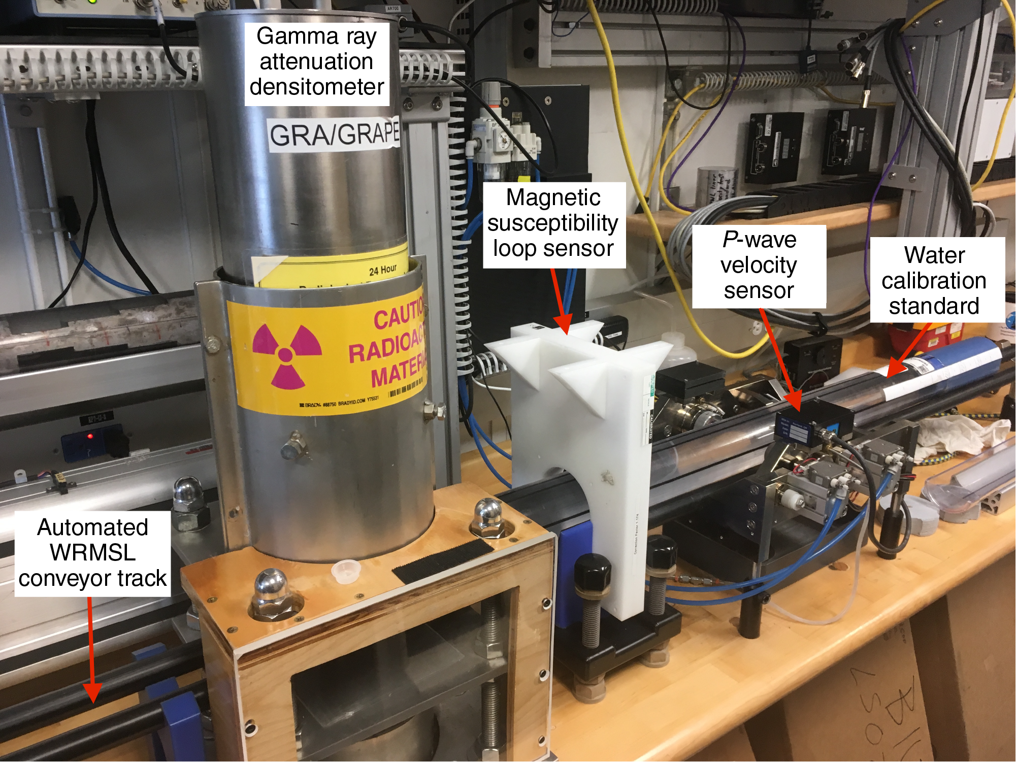
Figure F11. Whole-Round Multisensor Logger.
WRMSL measurements were completed on all whole-round sections during Expedition 383. Typically, the cores were temperature equilibrated. To optimize the measurement procedure and provide consistency, the sampling intervals and measurement times were the same for all sensors on each instrument. In this way, all sensors measure simultaneously and idle periods are avoided. A sampling resolution of 2 cm was generally considered appropriate for stratigraphic correlation and integration with seismic profiles and allowed for efficient core flow. A 3 cm resolution was used when faster core flow was required. Once the measurements were finalized for the last section of the core, a deionized water standard was run through all instruments to keep them calibrated and assure quality assurance/quality control (QA/QC). The instruments underwent recalibration if the measured standard values deviated from the range of published tolerances (Blum, 1997).
Gamma ray attenuation bulk density
The GRA bulk density instrument is used to measure the whole-round section at discrete and equidistant intervals to provide an average density value. It measures the attenuation of a directed gamma ray beam through the core. This beam is produced by a 137Cs gamma ray source at 370 MBq of radiation and an energy level of 660 KeV. The source is mounted directly above the whole-round core track in a lead shield with a 5 mm collimator at the bottom. The beam is directed downward toward the core section during measurement. A scintillation detector with an integrated photomultiplier tube is mounted underneath the core track (and opposite the 137Cs source) and measures the gamma radiation that passes through the core sections. The GRA bulk density instrument operates with medium-energy gamma rays (0.1–1 MeV) that interact with the material of the formation using Compton scattering. The measured electron density of the scattering is then used to estimate the bulk density of the material. For a known thickness of sample, the density (ρ) is proportional to the intensity of the attenuated gamma rays:
- I = measured intensity of gamma rays passing through the sample,
- I0 = gamma ray source intensity,
- µ = Compton attenuation coefficient, and
- d = sample diameter.
µ and I0 are constants, and ρ is then calculated from I. The bulk density provided by the GRA is related to the porosity, grain size, consolidation state, mineral composition, and any disturbances or contrasts present in the formation.
Generally, GRA bulk density measurements are most accurate when the core liner is completely filled and has minimal drilling disturbance, cracks, voids, or double liners. Otherwise, measurements tend to underestimate the true values. The GRA instrument estimates bulk density values based on an internal core diameter of 66 mm, which is appropriate for most sediment cores obtained using the APC and HLAPC systems. The GRA densitometer is calibrated with specific calibration cores, one standard core liner filled with distilled water, and aluminum cylinders of various diameters (Blum, 1997). The spatial resolution is less than ±1 cm. The instrument was recalibrated when the deionized water QA/QC standard deviated significantly (>2%) from 1 g/cm3. Additional postprocessing of the GRA measurements was needed to remove edge effects and single data spikes caused by voids or cracks in the core liner. Any values <1.12 g/cm3 were also removed. Unreliable measurements that result when the sediment does not fill the core along several to tens of centimeters, as often occurs in the first section of a core, were also removed. We flagged the data as indicated above in General sampling and measurement sequence.
Magnetic susceptibility
MS was acquired for all whole-round sections using a pass-through loop on the WRMSL. MS (χ) is a dimensionless parameter in the metric system that indicates the degree to which a material can be magnetized by an external magnetic field. χ is a relative indicator for changes in the formation composition that can also be related to paleoclimate-controlled depositional events or processes. MS is acquired at very low fields generally not exceeding 0.5 mT. Volume susceptibility is defined as
where M is the magnetization induced in the material by the external field of strength H. Accordingly, MS is most sensitive to formations containing high concentrations of ferromagnetic minerals such as magnetite, pyrite, hematite, and various other iron oxides. In addition, χ can also be related to the origin of the materials in the core and their subsequent diagenesis. Ferromagnetic minerals are characterized by MS values several orders of magnitude higher than their alteration products. Paramagnetic and diamagnetic minerals (e.g., calcite, halite, water, quartz, and plastic) present very small or even negative MS values. Therefore, calcareous and siliceous biogenic deposits often have values close to the detection limit of the instrument itself.
All MS measurements on the WRMSL were taken by a Bartington MS2C loop sensor with a 90 mm diameter. An oscillator circuit in the sensor operates at a frequency of 565 Hz to avoid any potential interference between instruments, with an automatic software correction factor of 1.174 and a ~140 A/m alternating field. This alternating field is responsible for a low-intensity, nonsaturated alternating magnetic field. Sediment core sections passing through the influence of this field cause a change in oscillator frequency. Frequency information is returned in pulse form to the susceptometer, and the MS value is estimated. The spatial resolution of the sensor is 20 mm with an accuracy of 2% (Blum, 1997). The output provided by the sensor is dimensionless in instrument units (IU), equivalent to 10−5 SI units. Estimated values are computed as the mean of three discrete measurements in the same location. MS values in text and figures in this volume are expressed in instrument units unless otherwise noted. Instrument drift should be considered because it can occur during the period of a core section scan. The instrument was automatically zeroed at the beginning of each run, and a zero-background measurement was taken at the end of each core section to correct for this drift. All acquired MS data needed postprocessing to remove edge effects and single data spikes caused by large voids and metal drill fragments, among others. We then flagged the data as indicated in General sampling and measurement sequence.
Compressional P-wave velocity
Compressional P-wave velocity was acquired for each whole-round section using the PWL. P-wave velocity depends on the lithology, porosity, and bulk density of the formation, as well as the state of stress, lithostatic pressure, and/or fabric or degree of fracturing within the material. The degree of consolidation and lithification and the occurrence and abundance of free gas also control the velocity. The acoustic impedance and reflection coefficients are obtained using the P-wave velocity together with the density values. These parameters can be used to derive synthetic seismograms, which in turn can be used estimate the depth of the main reflectors observed in seismic profiles. P-wave velocity (VP) is defined by the time required for a compressional wave to travel a specific distance,
where d is the length that the wave crosses (i.e., the core section) and tcore is the traveltime through the core.
For P-wave velocity measurements using the PWL, the core section is placed between two piezoelectric transducers (a transmitter and a receiver) mounted in stainless-steel housings. Acoustic coupling through an epoxy resin surface is enhanced by a water film supplied by an automated drip system. A 500-kHz pulse (2 µs wave period; 120 V) is produced at a frequency of 1 kHz and sent to the transmitter transducer, which generates an ultrasonic compressional pulse at about 500 kHz (pulse timing is measured with a resolution of 50 ns). Pressure is applied to the actuators to ensure coupling between the transducers and the core liner, and the automated drip system maintains wet contacts on the transducers to ensure a reliable coupling is always established. The compressional P-wave propagates horizontally through the core and is received by the receiver transducer on the opposite side. Velocity is amplified by an automatic gain control amplifier to produce the received signal. P-wave velocity transducers measure total traveltime of the compressional wave between transducers. A calibration of the PWL accounts for errors in the total distance (dtotal) and the total traveltime (ttotal). Errors in dtotal were assumed to be related to the laser distance. The obtained discrete data is the average of 100 discrete measurements at the set interval.
A core liner of assumed thickness (L) covered each core section for all measurements. The traveltime through the core liner (tliner) was determined by measuring the total traveltime through a core liner filled with distilled water with velocity of ~1480 m/s. A correction (tdelay; system delay) was measured using the traveltime through a standard block of aluminum with a known thickness and a published velocity of 6295 m/s. Arrival time picks were chosen at the inflection point of the second lobe of the waveform, giving a second correction (tpulse) from the first arrival. Then, tpulse and tdelay were combined and named ttotal_delay. Therefore, the velocity is computed as
- VP = core velocity (k/s),
- dtotal = measured diameter of the core and the liner (mm),
- L = wall thickness of the liner (mm),
- ttotal = total time for the pulse to travel through the core and the liner (µs),
- tliner = traveltime through the liner (µs), and
- ttotal_delay = delay related to the combined transducer faces, electronic circuitry, and peak detection procedures (µs).
The VP equation above assumes that the core completely fills the core liner and that there are no gaps or air present. Any measured P-wave signal can degenerate because of an incompletely filled core liner, any present voids or cracks, or attenuation caused by microcracks that formed during core recovery. This degeneration is partly reflected in the gain (signal strength) factor applied to the original signal by the automated gain control. However, signal strength can also be affected by the grain size of the sediment, so low-strength signals cannot simply be interpreted as proportional to attenuation. Additional postprocessing of the P-wave measurements was needed to remove edge effects. Single data spikes caused by voids or cracks in the core liner and any values <1460 were also removed. The upper measurement limit was adjusted according to the site. We then flagged the data as indicated in General sampling and measurement sequence.
Natural Gamma Radiation Logger measurements
The NGRL measures NGR on whole-round sections using a system designed by the Integrated Ocean Drilling Program US Implementing Organization (USIO) at Texas A&M University, USA (Vasiliev et al., 2011). This instrument measures the cumulative radiation emitted during natural decay of three long-lived radioisotopes, potassium (40K), thorium (232Th), and uranium (238U), which have half-lives of 1.3 × 10⁹, 1.4 × 10¹⁰, and 4.4 × 10⁹ y, respectively. These isotopes and their daughter products emit gamma radiation at specific energy levels unique to each isotope. NGR is used to estimate the abundance of each isotope based on the strength of the signal at characteristic energies (Blum, 1997; Gilmore, 2008). In sediments and sedimentary rocks, Th and K are usually associated with particular clay minerals, whereas U is often encountered in either clay minerals or organic-rich material (Dunlea et al., 2013). High counts generally reflect the presence of fine-grained deposits, and relative changes are indicative of stratigraphic details and aid in core-to-core, core-to-wireline log data, and/or borehole correlations between holes.
The NGR system consists of eight sodium iodide (NaI) detectors arranged along the core measurement axis at 20 cm intervals surrounding the lower half of the section (Figure F12). The detector array is fit with both passive (layers of lead) and active (plastic scintillators) shielding to reduce the background environmental and cosmic radiation. The overlying plastic scintillators detect incoming high-energy gamma and muon cosmic radiation above 3 MeV and cancel this signal from the total counted by the NaI detectors.
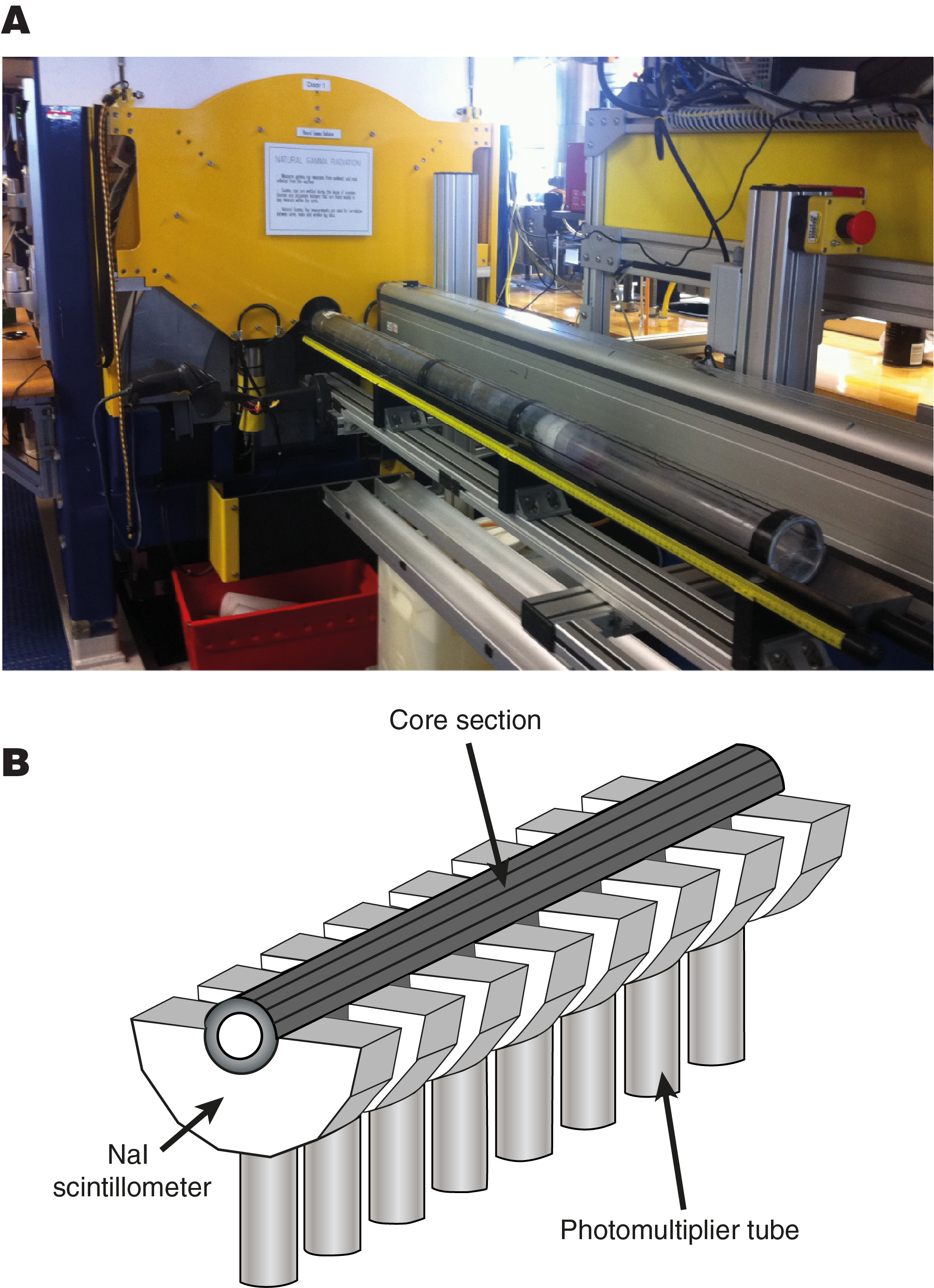
Figure F12. Natural Gamma Radiation Logger.
The quality of the core measurements depends on the concentration of radionuclides and the counting time. For Expedition 383, the measurement run began with two sample positions 10 cm apart and a counting period of 300 s. After 300 s, the position was advanced downcore by 10 cm and counted again for 300 s. This run yielded a total of 16 measurements (10 cm apart) per 150 cm core section. Total acquisition times were ~5 min per measurement cycle, or ~10 min per core section. This measurement procedure yielded statistically significant total counts. To accommodate a faster core flow when the terrigenous component of the sediment was high, the acquisition time could be reduced to 200 s.
The NGR data were then deconvolved to calculate the concentration of potassium (K), uranium (U), and Thorium (Th) (expressed as a fraction of the total weight of the sediment) using a Matlab script by De Vleeschouwer et al. (2017) that was updated to the current IODP LIMS extended NGR data files. This calculation requires normalizing/correcting for density changes. Density-normalized NGR data help reduce biases that may reflect variability in parameters such as sediment compaction, porosity, and missing sediment at some depth in or throughout all of a section liner (Walczak et al., 2015). Density-normalized NGR was calculated using the GRA density, to which a Gaussian smoothing was applied within a range of 20 cm on either side of the NGR measurement positions. If density-normalized NGR is shown, the units are cps/g/cm3.
As a way to validate the K (wt%) values, shipboard measurements of K were made via ICP-AES and XRF. However, because the ICP-AES measurements were made on dried discrete samples, the NGR-derived K values for those discrete samples needed to be recalculated by normalizing the NGR data relative to dry density rather than wet density. Dry density was calculated from the GRA wet density data using a site-specific transfer function, relating dry to wet density measurements of the MAD discrete samples. These estimated dry density values were then used to normalize the NGR data, which was then deconvolved to extract K wt% data that could be directly compared to the ICP-AES K wt% data.
Thermal conductivity measurements
Thermal conductivity is an intrinsic property of the materials; hence, it depends on the chemical composition, porosity, density, structure, and fabric composing them (Jumikis, 1966). Thermal conductivity is the capacity of a material to transfer heat by conduction. Measurements of this parameter in sediments and rock sections combined with in situ temperature measurements (see Downhole measurements) are used to estimate local geothermal heat flow. This parameter is an indicator of type and age of oceanic crust, and of geodynamics and tectonic processes of oceanic and continental lithosphere (Martos et al., 2017, 2018).
Thermal conductivity was measured immediately after NGR analysis in the case of soft sediments (whole-round sections) and when reliable measurements were yielded by the probe. One to two acquisitions per core were taken, generally in the third section, using the TK04 (Teka Bolin) system. When measuring whole-round sections, the needle-probe method in full space configuration was used (Von Herzen and Maxwell, 1959). The needle probe was inserted into a 2 mm diameter hole drilled through the core liner along a split line. Measurement locations were chosen based on the least amount of fracturing and most homogeneous portions of core sections. The core was placed in an enclosed box with insulating foam (Figure F13) to avoid interference with airflow in the laboratory and allow for stable thermal conditions during measurements. The calibrated probe heat source was turned on, and the increase in temperature was recorded over 80 s for the needle probe. The heating power ranged between 0.3 and 0.7 W/m. The heat equation solution for a line source of heat was then fit to the temperature measurements to obtain the thermal conductivity. The probe is assumed to be a perfect conductor because it conducts heat more efficiently than sediment or hard rock. Following this assumption, the linear relationship between the superconductive probe temperature and the natural logarithm of time after initiation of the heat is expressed as
- T = temperature (K),
- q = heat input per unit length per unit time (J/m/s),
- k = thermal conductivity (W/[m·K]),
- t = time after the initiation of heat (s), and
- C = an instrumental constant.
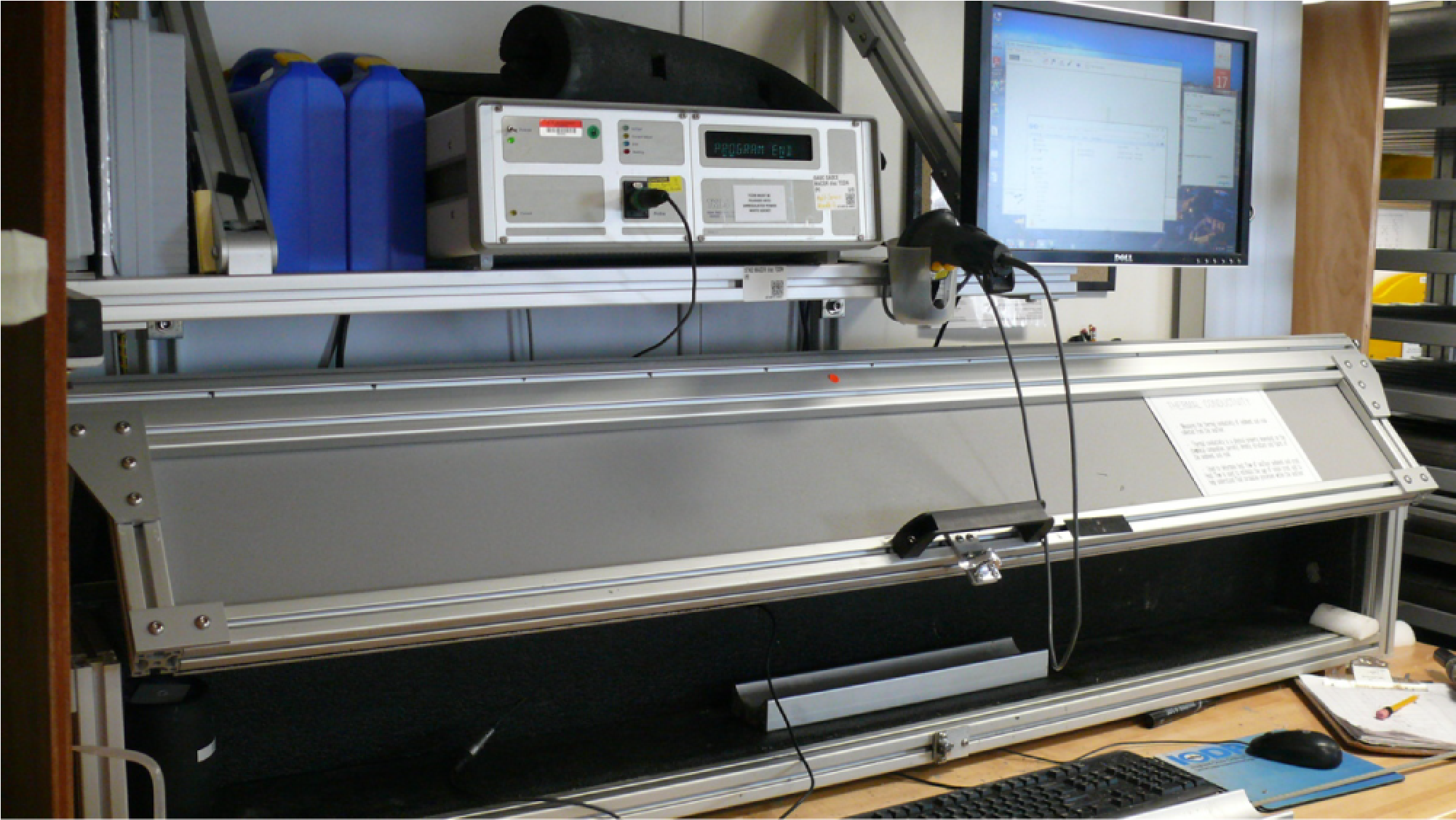
Figure F13. Thermal conductivity instrument.
To calculate the average thermal conductivity, three measurement cycles were performed separated by 10 min. A self-test, which included a drift study, was carried out at the beginning of each measurement cycle. The heater circuit was closed after the probe temperature stabilized, and the temperature increase in the probe was recorded. Thermal conductivity was estimated from the temperature increase rate while the heater current was flowing. Temperatures measured during the first 80 s of the needle probe heating cycle were fit to an approximate solution of a constantly heated line source (Kristiansen, 1982; Blum, 1997). Measurement errors were 5%–10%.
Section Half Multisensor Logger measurements
The SHMSL employs multiple sensors to measure bulk physical properties reflectance spectroscopy and colorimetry, magnetic susceptibility, and a laser surface analyzer (Figure F14). Archive section halves were covered with plastic wrap and placed on the SHMSL track, above which an electronic platform moves along a track and records the height of the core surface. The laser sensor detects the location of the bottom of the archive section half, and then the instrument progresses along the core making measurements of MSP and color reflectance. Color reflectance and MSP data were collected at a 2 cm resolution.
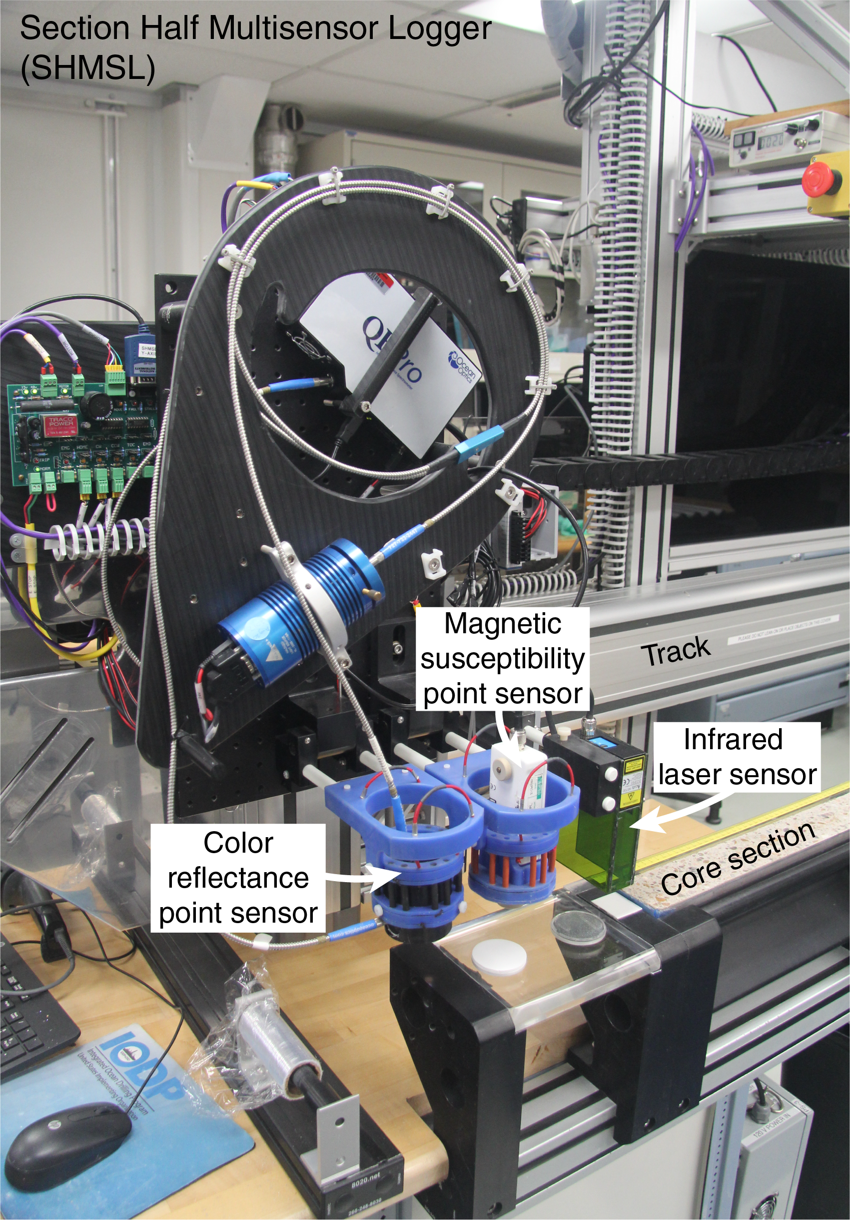
Figure F14. Section Half Multisensor Logger.
After acquisition, raw SHMSL data were processed for core edge and void effects principally arising from sediment gaps and styrofoam inserts for interstitial water and micropaleontology samples. Reflectance and MSP measurements compromised by non-sediment material were excluded from processed data products. Additional screening for core cracks and voids was performed, and reflectance and point magnetic susceptibility measurements compromised by cracks or voids were additionally removed from processed data products.
Color reflectance spectrometry
The color reflectance spectrophotometry of the archive section halves was measured using an Ocean Optics USB4000 spectrophotometer, with an Ocean Optics QE Pro detector integrating sphere and associated light sources, covering wavelengths from the ultraviolet to near-infrared range. Each measurement was taken in 2 nm wide spectral bands from 390 to 732 nm. Data are reported using the L*a*b* color space system, which expresses color as a function of lightness (L*) and color values a* and b*, where a* reflects the balance between red (positive a*) and green (negative a*) and b* reflects the balance between yellow (positive b*) and blue (negative b*). When a* and b* are 0, there is no color and L* determines grayscale. Two spectra, pure white (reference) and pure black (dark), were used to calibrate the color reflectance spectrometer. Color calibration was conducted approximately once every 6 h (twice per shift). Accurate spectrophotometry using the SHMSL demands a direct and level contact between the instrument sensors and the split core surface. A built-in laser surface analyzer aids the recognition of irregularities in the split core surface (e.g., cracks and voids), and data from this tool were recorded to provide an independent check on the fidelity of SHMSL measurements.
Additional details regarding measurement and interpretation of spectral data can be found in Balsam et al. (1997), Balsam and Damuth (2000) and Giosan et al. (2002).
Point magnetic susceptibility
MSP was measured with a Bartington MS2 meter and an MS2K contact probe with a flat 15 mm diameter round sensor that has a field of influence of 25 mm and an operation frequency of 930 Hz. The instrument averages three measurements from the sensor for each offset with an accuracy of ~5%. The spatial resolution of the MSP sensor is ~3.8 mm and reports values in instrument units (IU), which can be converted to dimensionless SI units by multiplying by 10−5. The instrument was calibrated by the manufacturer before installation on JOIDES Resolution and is quality checked every 6 h at the same time as color reflectance sensor calibration.
Digital color imaging
The Section Half Imaging Logger (SHIL) captures continuous high-resolution images of the archive section half surface for analysis and description. The instrument was used shortly after core splitting in an effort to avoid time-dependent color changes resulting from sediment drying and oxidation. The shipboard system uses a commercial linescan camera lens (AF Micro Nikon; 60 mm; 1:2.8 D), and illumination is provided by a custom assembly of three pairs of LED strip lights that provide constant illumination over a range of surface elevations. Each pair of lights has a color temperature of 6,500 K and emits 90,000 lux at 3 inches. The resolution of the linescan camera was set at 10 pixels/mm. Users set a crop rectangle for each image to remove extraneous information. Images were saved as high-resolution TIFF files. Available files include the original high-resolution image with grayscale and ruler as well as reduced JPEG images cropped to show only the section-half surfaces.
Section Half Measurement Gantry measurements
P-wave velocity measurements were performed on working section halves using the SHMG. Two to three measurements were typically made on one section of each core. The number of x-caliper measurements was increased when the WRMSL PWL was not able to estimate accurate velocity measurements, for example due to internal cracks in the cores. Measurements were taken at varying section intervals to accommodate lithologic variations, drilling disturbance, fractures, larger clasts, general core quality, and MAD samples.
P-wave velocity
P-wave velocity values on working section halves were measured with the PWC, which measures the P-wave velocity vertical to the sectional plane of the section (x-axis) (Figure F15). The system uses Panametrics-NDT Microscan delay line transducers, which transmit at 500 kHz. During measurement, the signal transmitted through the core was recorded by the attached computer system, which then used an automated algorithm in the processing software to choose peak (P-wave) arrival. In cases of poor contact or weak signal, the instrument operator manually picked the first arrival. The distance between transducers was measured with a built-in linear voltage displacement transformer (LDVT). Calibrations were performed with an acrylic standard of known thickness and a published velocity of 2730 m/s, whereas an aluminum standard of 6295 m/s was used for compressional P-wave measurements on the WRMSL. The system time delay determined from the calibration was subtracted from the chosen arrival time to calculate a P-wave traveltime through the sample. Sample thickness (calculated by LDVT in meters) was divided by the traveltime (in seconds) to calculate P-wave velocity in m/s.
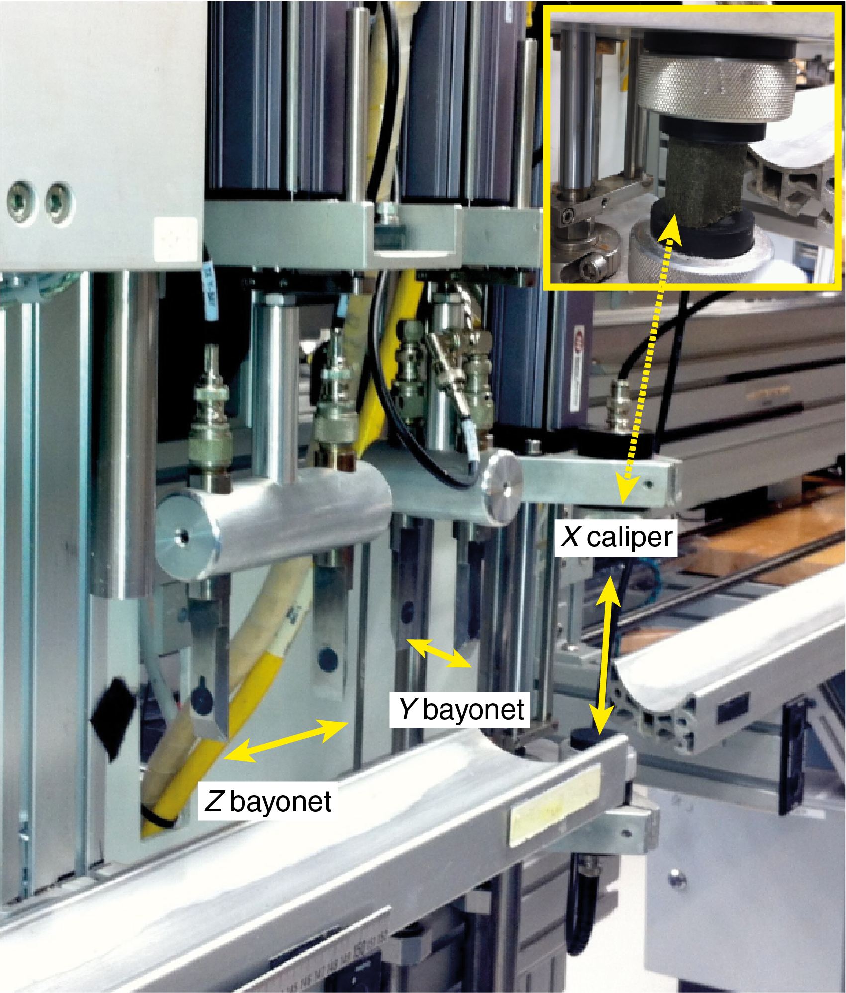
Figure F15. Section Half Measurement Gantry.
Moisture and density measurements
Discrete samples from working section halves were selected to carry out MAD measurements to determine wet and dry bulk density, grain density, water content, and porosity. For soft-sediment cores, 10 cm3 samples were collected with a plastic syringe.
Sediment samples were placed in numbered, preweighed ~16 mL Wheaton glass vials to obtain wet and dry sediment mass and dry volume measurements. Wet sample mass was first measured on each vial before placing it in a convection oven for ~24 h at 105˚ ± 5˚C to dry. Once samples were dried, they were cooled in a desiccator for at least 3 h before measuring dry mass and volume. Wet and dry sample masses were determined to an accuracy of 0.005 g using two Mettler Toledo electronic balances, with one balance acting as a reference and one acting as an unknown. A standard mass of similar value to the sample mass was placed upon the reference balance to increase the accuracy of the unknown sample measurement (Figure F16). An averaging algorithm in the MADMax software was used to correct for the motion of the ship. The default measurement setting of the two balances was 300 measurements over an interval of ~1.5 min.
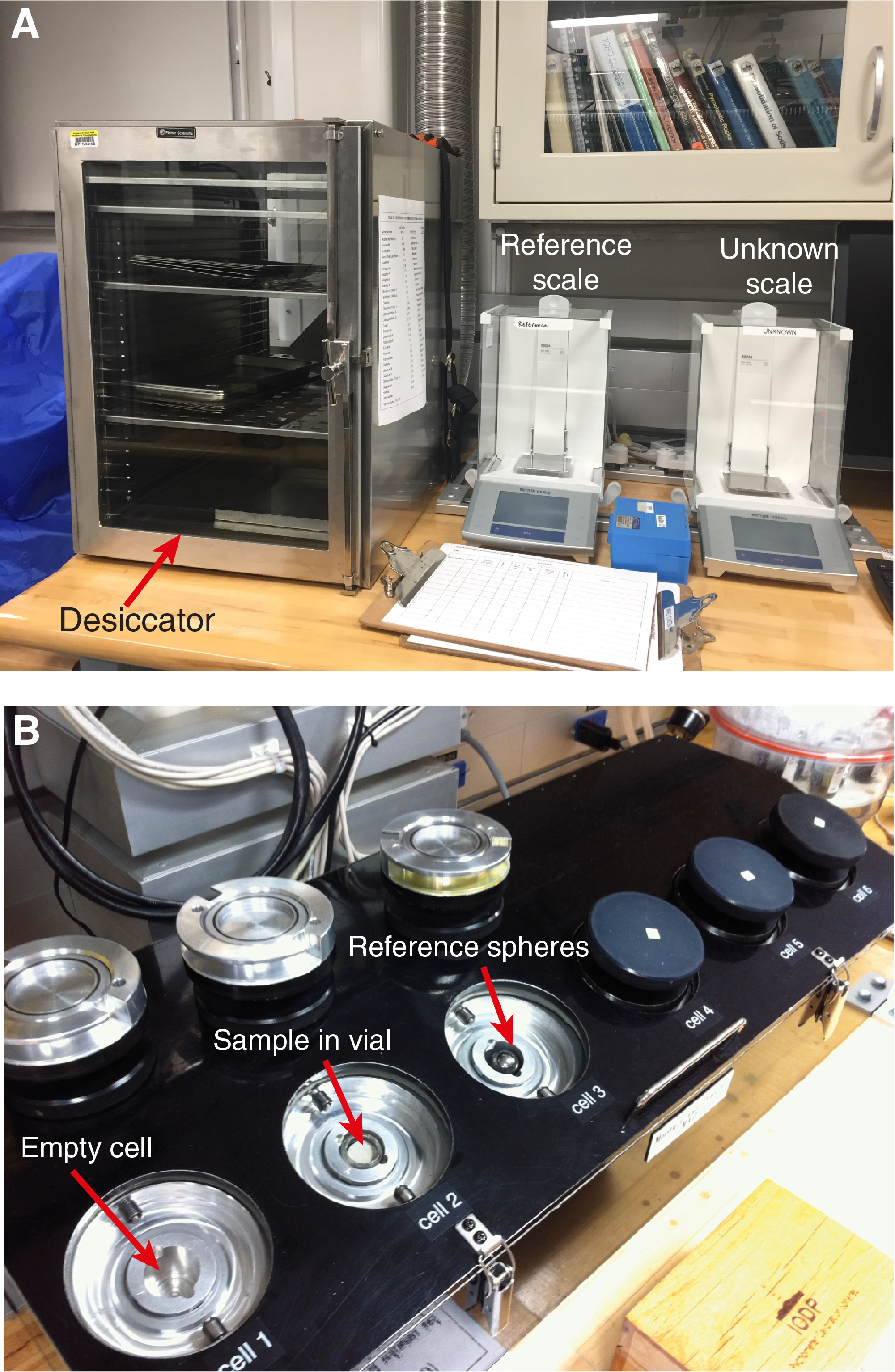
Figure F16. MAD instrumentation.
Dry sample volume was determined using a six-celled, custom-configured Micrometrics AccuPyc 1330TC helium-displacement pycnometer (Figure F16). The precision of each cell is 1% of the full-scale volume. Volume measurements are preceded by three purges of the sample chamber with helium warmed to ~28°C. Three measurement cycles were run for each sample. Calibration was done for the six chambers between sites. A set of two calibration spheres was placed in one of the chambers with each set of five samples to check for instrument drift and systematic error. When the results were not within 1%, the chamber was calibrated again and two calibration spheres measured after calibration. The volumes occupied by the numbered Wheaton vials were calculated before the expedition by multiplying the weight of each vial against the average density of the vial glass. The procedures for the determination of these physical properties comply with the American Society for Testing and Materials (ASTM) designation 2216 (ASTM International, 1990). The relationships and assumptions for the calculations of the physical properties parameters are discussed in detail in Blum (1997) and summarized below. The shipboard program MADMax was used for computing the displayed MAD properties.
Mass and volume calculation
Wet mass (Mwet), dry mass (Mdry), and dry volume (Vdry) were measured in the laboratory as detailed in the previous section. The ratio of mass (rm) is a computational constant of 0.965 (i.e., 0.965 g of freshwater per 1 g of seawater). Salt precipitated in sediment pores during the drying process is included in the Mdry and Vdry values. The mass of the evaporated water (Mwater) and salt (Msalt) in the sample are given by Mwater = Mwet − Mdry, and Msalt = Mwater[s/(1 − s)], respectively, where s is the assumed saltwater salinity (0.035%) corresponding to a pore water density (ρpw) of 1.024 g/cm3 (from experimental and empirical relations between salinity and density at laboratory conditions; Blum, 1997) and a salt density (ρsalt) of 2.22 g/cm3. The corrected mass of pore water (Mpw), volume of pore water (Vpw), mass of solids excluding salt (Msolid), volume of salt (Vsalt), volume of solids excluding salt (Vsolid), and wet volume (Vwet) are defined as follows:
Wet (or total) volume (Vt), dry mass (Mdry), and dry volume (Vdry) were measured in the laboratory. Total mass, including the freshwater of the pore water, is calculated using a water density of 1 g/cm3:
Assuming a pore water density of 1.024 g/cm3, the volume of the pore water is calculated as
Finally, the mass of the pore water is estimated as
Calculation of bulk properties
Water content (w) is expressed as the ratio of the mass of pore water to wet sediment (total) mass,
Wet bulk density (ρwet), dry bulk density (ρdry), sediment grain density (ρsolid), porosity (φ), and void ratio (VR) are calculated using the following expressions:
Downhole measurements
Advanced piston corer temperature tool
During APC coring operations and generally above 200 m drilling depth below seafloor (DSF), the formation temperature was measured with an APCT-3 tool that is housed in a specially designed coring shoe that replaces the standard cutting shoe (Heesemann et al., 2006). Normally, these measurements were made while coring Hole A at a site; however, if obtained temperature measurements were considered to be unreliable, additional APCT-3 measurements were made in one or more subsequent holes.
The APCT-3 tool comprises a battery pack, a data logger unit, and a platinum resistance-temperature device calibrated over a temperature range of 0°–30°C. This instrument is fitted to be used in an APC coring shoe (Figures F17, F18). Upon deployment, the APCT-3 tool first stops at the mudline for 5–10 min to thermally equilibrate with bottom water before entering the borehole. Frictional heating occurs as the APCT-3 tool moves into the formation. This heat gradually dissipates into the surrounding sediment as the APCT-3 tool equilibrates to formation temperature while being held in place for 15 min, acquiring data every second.
Figure F17. APCT-3 insert.
Figure F18. APCT-3 downhole tool.
After retrieval and readout of the data, the equilibrium temperature of the sediment is estimated by applying a mathematical heat-conduction model to the temperature decay record (Horai and Von Herzen, 1985). The synthetic thermal decay curve for the APCT-3 tool is a function of the geometry and thermal properties of the probe and the sediment (Bullard, 1954; Horai and Von Herzen, 1985). Equilibrium temperature was estimated by applying a fitting procedure (Pribnow et al., 2000). The nominal accuracy of the APCT-3 temperature measurements is ±0.05°C.
Wireline logging
Wireline logging was planned for Chilean margin Sites U1542–U1544, but downhole measurements were canceled because of rough weather, high seas, and the resulting lack of sufficient time to conduct these operations.
Stratigraphic correlation
Continuous sedimentary sections cannot be collected from a single borehole because core recovery gaps occur between successive APC and XCB cores despite 100% (or greater) nominal recovery (Ruddiman et al., 1987; Hagelberg et al., 1995). Consequently, to meet the scientific objectives of Expedition 383 it was necessary to drill more than one hole at each site. The construction of a continuous sedimentary section, referred to as a splice, requires the combination of stratigraphic intervals from two or more holes cored at the same site. To maximize the probability of bridging gaps between successive cores in individual holes, the starting depths below seafloor from which cores are recovered are offset between holes. This practice ensures that most missing sedimentary sections from intercore gaps within a given hole are recovered in one or more adjacent holes. Usually at least two complete holes and a third partial hole must be cored to recover a complete section in the interval cored with the APC system at a site. Additional complete holes are cored to allow construction of alternate and secondary splices where possible. During Expedition 383, inclement weather conditions often limited the number of overlapping intervals drilled in multiple holes at each site. As a result, each splice contains at least one short gap. Only a single hole could be drilled at Site U1544, so no splice is available for this site.
The composite section and splice construction methodology employed during Expedition 383 follows the basic strategy originally developed during ODP Leg 138 (e.g., Hagelberg et al., 1995) and refined during subsequent legs. This strategy is now common practice for all high-resolution paleoceanographic expeditions. Our approach used initial MS and GRA bulk density data from the STMSL as soon as possible after core retrieval to construct initial composites to inform drilling decisions; subsequently a more refined composite scale and splice was developed as more detailed information became available from the WRMSL and NGRL, the digitized RGB color data from core images acquired with the SHIL, and color reflectance and MSP data from the SHMSL.
The goals for stratigraphic correlation, in order of priority, were to
- Guide drilling to ensure recovery of a complete stratigraphic section;
- Establish a composite depth scale;
- Define a stratigraphically complete and representative sampling splice; and
- Evaluate and, if possible, refine shipboard stratigraphic age models by synthesizing all available age information, including the potential for tuning lithologic variations to reference records.
The procedure for these activities involved consideration of several different depth scales (Figure F17). The depth scales used during Expedition 383 followed IODP convention (http://www.iodp.org/policies-and-guidelines) and are described in methodological order (Figure F19).
Figure F19. Measured, calculated, and constructed depth scales.
Core depth below seafloor (CSF-A) scale
We began the process of building a composite section by assigning a depth to the top of each core, based initially on the drilling depth below seafloor (DSF). DSF is a drill string measurement determined as the difference between the length of the drill string below the rig floor to the top of the cored interval and the length of the drill string from the rig floor to the mudline (assumed to be the seafloor). DSF error includes phenomena such as pipe and BHA stretch and compression, tides, and uncompensated heave. Tidal influence on this depth measurement might be significant (Hagelberg et al., 1995), and the prediction of tides is generally useful for guiding drilling to avoid gap alignment (Mix, Tiedemann, Blum, et al., 2003).
During Expedition 383, ship heave (typically 1–4 m) contributed a significant source of error to bit position on the DSF scale. This effect appeared to impact the relative depths of obvious stratigraphic markers between multiple adjacent holes. Significant ship heave also appears to have increased the occurrence of misfired cores, which often resulted in short, disturbed, or poorly aligned sediment recovery that complicated splice construction. Because heave magnitude and direction is unpredictable for the moment a core is fired, we did not explicitly adjust drilling targets to compensate for heave conditions.
Tidal influence was minimal during Expedition 383, with the exception of Site U1542 and, presumably, Site U1544. At these sites, the tidal range was at times as high as 1.5 m, and this appeared to impact the size of the core gaps. We did not adjust drilling explicitly to compensate for changing tide height; instead, we used it to help us anticipate whether core gaps would migrate relative to other holes that were drilled during a different phase of the tide and adjusted with drill-ahead intervals or short cores (cores fired above the bit/sediment interface) when needed.
The depth to a given position within any core was then determined relative to the DSF core top depth. The CSF-A depth, therefore, combined the DSF core-top depth with the curated length of the core after retrieval. The CSF-A depth scale is equivalent to the historical DSDP, ODP, and Integrated Ocean Drilling Program meters below seafloor (mbsf) scale and is specific to each hole. It is important to note that the “within-core” position, on the CSF-A depth scale, of any given sedimentary feature may change after recovery due to various influences such overburden relief, gas-induced expansion, and water loss. Therefore, hole-to-hole differences in the position of a stratigraphic feature on the CSF-A scale includes both drilling effects and core expansion effects. For example, the CSF-A scale permits stratigraphically impossible overlaps between successive cores caused by gas-induced expansion. In principle, the composite depth scale, described below, should rectify such artifacts.
Core composite depth below seafloor
(CCSF-A) scale
The construction of a common, composite depth scale for a given site involves identification of coeval, laterally continuous features in all drilled holes (which will generally occur at different depths on the CSF-A depth scale for each hole). Once correlative features were identified during Expedition 383, the depth of individual cores was offset relative to the CSF-A depth scale in that hole so that the features aligned on a common depth scale, which is the core composite depth below seafloor, Method A (CCSF-A), scale. The CCSF-A scale is equivalent to the historical ODP and Integrated Ocean Drilling Program meters composite depth (mcd) scale. In constructing the CCSF-A scale, the depths of individual cores were offset by a constant amount (without stretching or squeezing in individual cores). This composite depth scale provided good estimates of the length of coring gaps and formed the basis for developing the spliced record (on the CCSF-A scale). The vertical depth offset of every core in every hole was tabulated in an affine table, one of the principal deliverables of the stratigraphic correlator.
The CCSF-A scale was built by correlating features downhole from the mudline. The mudline at one hole was established as the top of the stratigraphic section, anchoring the entire composite depth scale for all cores from all holes at a single site. Compositing proceeded sequentially by establishing specific tie points between the various holes, working from the mudline (anchor) core to the bottom of the drilled section. The CCSF-A scale very rarely (if ever) resulted in alignment of all coeval features because of the contrasting effects of coring-induced stretching and squeezing among cores, as well as stratigraphic differences between holes.
In principle, if core gaps never come into alignment between all holes at a site and if recovery is sufficiently high, then it should be possible to correlate each successive core in one hole to a core from an adjacent hole all the way to the bottom of a drilled section. However, aligned coring gaps across all holes at a site are often difficult to avoid. In the case of aligned core gaps, cores below the gap are no longer tied to the anchor core. They can, however, still be tied to one another to produce correlated sections that are “floating” on the CCSF-A scale. Such floating ties were denoted in the affine table as “APPENDED” or “SET” depending on whether the offset to the top of that section was estimated by inheriting the absolute offset of the core above (APPEND) or by assuming a constant growth rate (SET). The second method (SET) is preferable because it produces a more realistic estimate of the core gap based on estimates of the expansion of overlying cores from the same hole.
During the process of constructing the composite section, the CCSF-A depth becomes systematically larger than the CSF-A depth for equivalent horizons. This expansion, which typically averaged 7%–10% during Expedition 383, has four main causes: (1) decompression of the sediment as it is brought to atmospheric pressure; (2) pore-space gases coming out of solution, warming, and expanding; (3) stretching that occurs as part of the coring process; and (4) curation of borehole wall sediment that fell downhole and was re-cored (e.g., Hagelberg et al., 1995; Acton et al., 2001).
The splice
Once the CCSF-A scale was developed and the between-core gaps were identified, a complete stratigraphic section (splice) was constructed by combining selected intervals between the previously established tie points. In the case of aligned core gaps across all holes, any spliced sections below the gap were appended to those above and designated as floating splice sections, with the length of the missing sections in the splice gap estimated based on the percent expansion observed where we had a continuous splice.
Intervals outside of splice
Once the splice was constructed, we mapped into the splice those intervals not included in the splice itself by treating the splice as a downhole log. The methodology is based on identifying correlative tie points and using these tie points to make linear adjustments of these cores not used in the splice. This was used to put cores not used in the splice on the CCSF-A depth scale. In reality, the CCSF-A depth scale at adjacent holes are equivalent only to the extent that the correlations are accurate. At core boundaries, where evidence of stretching and compression was most prevalent, the detailed depth maps are considered less accurate. Thus, the CCSF-A scale is not precisely the same at all holes at a site except exactly where the splice tie points were made. See the individual site chapters for additional details and guidance.
Measurements and methods for correlation
For the majority of sites, initial development of composite sections (CCSF-A scale) was based on the stratigraphic correlation of GRA density or magnetic susceptibility data sets acquired from the WRMSL and the STMSL as soon as possible after core retrieval. In many cases, this allowed stratigraphic correlation to take place in near real time so that bit depth could be adjusted as necessary to avoid alignment of core gaps between holes. More details about the effectiveness of real-time stratigraphic correlation are provided in the site chapters. At all sites, no single variable proved to be universally powerful for stratigraphic correlation or splice construction; thus, correlation proceeded through a combination of WRMSL, STMSL, and NGR data as well as section-half digitized color reflectance (RGB and L*a*b*) and MSP data. Color reflectance data were extracted from core images acquired from the SHIL (RGB) and the SHMSL (L*a*b*). Magnetic susceptibility, GRA, and L* (or a* and b*) were measured at 2 or 3 cm intervals, and RGB values were calculated at 1 cm intervals in the form of 0.5 cm averages measured continuously along a 1.5 cm wide strip centered on digital color SHIL images. Details on instrument calibrations, settings, and measurement intervals are given in Physical properties.
Compositing and splicing were accomplished using Correlator software (version 3.0), from which standard affine tables (listings of the vertical offset [m] added to each core to generate the CCSF-A scale) and splice interval tables (listings of the specific core intervals used to construct the splice) were generated. These tables were uploaded into the LIMS database, which then linked the appropriate depth scale to any associated data set.
References
Abelmann, A., 1992. Early to middle Miocene radiolarian stratigraphy of the Kerguelen Plateau, Leg 120. In Wise, S.W., Jr., Schlich, R., et al., Proceedings of the Ocean Drilling Program, Scientific Results, 120: College Station, TX (Ocean Drilling Program), 757–783. https://doi.org/
Acton, G., Morris, A., Musgrave, R., Zhao, X., and IODP SRM Personnel, 2017. Assessment of the New Superconducting Rock Magnetometer (SRM) on the JOIDES Resolution. http://iodp.tamu.edu/
Acton, G.D., Borton, C.J., and the Leg 178 Shipboard Scientific Party, 2001. Palmer Deep composite depth scales for Leg 178 Sites 1098 and 1099. In Barker, P.F., Camerlenghi, A., Acton, G.D., and Ramsay, A.T.S. (Eds.), Proceedings of the Ocean Drilling Program, Scientific Results, 178: College Station, TX (Ocean Drilling Program), 1–35. https://doi.org/
Akiba, F., 1982. Late Quaternary diatom biostratigraphy of the Bellingshausen Sea, Antarctic Ocean. Report of the Technology Research Center, Japan National Oil Corporation, 16:31–74.
Alvarez Zarikian, C.A., 2015. Cenozoic bathyal and abyssal ostracods beneath the South Pacific Gyre (IODP Expedition 329 Sites U1367, U1368 and U1370). Palaeogeography, Palaeoclimatology, Palaeoecology, 419:115–142. https://doi.org/
Anderson, J.B., 1975. Ecology and distribution of foraminifera in the Weddell Sea of Antarctica. Micropaleontology, 21(1):69–96. https://doi.org/
Armbrecht, L.H., Lowe, V., Escutia, C., Iwai, M., McKay, R., and Armand, L. 2018. Variability in diatom and silicoflagellate assemblages during mid-Pliocene glacial-interglacial cycles determined in Hole U1361A of IODP Expedition 318, Antarctic Wilkes Land Margin. Marine Micropaleontology, 139:28–41. https://doi.org/
Arney, J.E., McGonigal, K.L., Ladner, B.C., and Wise, S.W., Jr., 2003. Lower Oligocene to middle Miocene diatom biostratigraphy of ODP Site 1140, Kerguelen Plateau. In Frey, F.A., Coffin, M.F., Wallace, P.J., and Quilty, P.G. (Eds.), Proceedings of the Ocean Drilling Program, Scientific Results, 183: College Station, TX (Ocean Drilling Program), 1–21. https://doi.org/
ASTM International, 1990. Standard method for laboratory determination of water (moisture) content of soil and rock (Standard D2216–90). In Annual Book of ASTM Standards for Soil and Rock (Volume 04.08): Philadelphia (American Society for Testing Materials). [revision of D2216-63, D2216-80]
Baldauf, J.G., and Barron, J.A., 1991. Diatom biostratigraphy: Kerguelen Plateau and Prydz Bay regions of the Southern Ocean. In Barron, J., Larsen, B., et al., Proceedings of the Ocean Drilling Program, Scientific Results, 119: College Station, TX (Ocean Drilling Program), 547–598. https://doi.org/
Balsam, W.L., and Damuth, J.E., 2000. Further investigations of shipboard vs. shore-based spectral data: implications for interpreting Leg 164 sediment composition. In Paull, C.K., Matsumoto, R., Wallace, P., and Dillon, W.P. (Eds.), Proceedings of the Ocean Drilling Program, Scientific Results, 164: College Station, TX (Ocean Drilling Program), 313–324. https://doi.org/
Balsam, W.L., Damuth, J.E., and Schneider, R.R., 1997. Comparison of shipboard vs. shore-based spectral data from Amazon Fan cores: implications for interpreting sediment composition. In Flood, R.D., Piper, D.J.W., Klaus, A., and Peterson, L.C. (Eds.), Proceedings of the Ocean Drilling Program, Scientific Results, 155: College Station, TX (Ocean Drilling Program), 193–215. https://doi.org/
Barron, J.A., 2003. Planktonic marine diatom record of the past 18 m.y.: appearances and extinctions in the Pacific and Southern Oceans. Diatom Research, 18(2):203–224. https://doi.org/
Barron, J.A., Baldauf, J.G., Barrera, E., Caulet, J.-P., Huber, B.T., Keating, B.H., Lazarus, D., Sakai, H., Thierstein, H.R., and Wei, W., 1991. Biochronologic and magnetochronologic synthesis of Leg 119 sediments from the Kerguelen Plateau and Prydz Bay, Antarctica. In Barron, J., Larsen, B., et al., Proceedings of the Ocean Drilling Program, Scientific Results, 119: College Station, TX (Ocean Drilling Program), 813–847. https://doi.org/
Berggren, W.A., 1992. Neogene planktonic foraminifer magnetobiostratigraphy of the southern Kerguelen Plateau (Sites 747, 748, and 751). In Wise, S.W., Jr., Schlich, R., et al., Proceedings of the Ocean Drilling Program, Scientific Results, 120: College Station, TX (Ocean Drilling Program), 631–647. https://doi.org/
Blow, W.H., 1979. The Cainozoic Globigerinida: A Study of the Morphology, Taxonomy, Evolutionary Relationships and the Stratigraphical Distribution of Some Globigerinida (mainly Globigerinacea): Leiden, The Netherlands (E.J. Brill).
Blum, P., 1997. Technical Note 26: Physical Properties Handbook—A Guide to the Shipboard Measurement of Physical Properties of Deep-Sea Cores. Ocean Drilling Program. https://doi.org/
Bohaty, S.M., Scherer, R.P., and Harwood, D.M., 1998. Quaternary diatom biostratigraphy and palaeoenvironments of the CRP-1 drillcore, Ross Sea, Antarctica. Terra Antartica, 5(3):431–453. http://epic.awi.de/
Bohaty, S.M., Wise, S.W., Jr., Duncan, R.A., Moore, C.L., and Wallace, P.J., 2003. Neogene diatom biostratigraphy, tephra stratigraphy, and chronology of ODP Hole 1138A, Kerguelen Plateau. In Frey, F.A., Coffin, M.F., Wallace, P.J., and Quilty, P.G. (Eds.), Proceedings of the Ocean Drilling Program, Scientific Results, 183: College Station, TX (Ocean Drilling Program), 1–53. https://doi.org/
Bolli, H.M., Saunders, J.B., and Perch-Nielsen, K. (Eds.), 1985. Plankton Stratigraphy (Volume 1): Planktic Foraminifera, Calcareous Nannofossils and Calpionellids: Cambridge, United Kingdom (Cambridge University Press).
Boomer, I., 1999. Late Cretaceous and Cainozoic bathyal Ostracoda from the Central Pacific (DSDP Site 463). Marine Micropaleontology, 37(2):131–147. https://doi.org/
Boomer, I., Whatley, R.C., 1995. Cainozoic Ostracoda from guyots in the western Pacific: Leg 143, Holes 865B and 866B. In Winterer, E.L., Sager, W.W., Firth, J.V., and Sinton, J.M. (Eds), Proceedings of the Ocean Drilling Program, Scientific Results, 143:75–86. https://doi.org/
Bown, P.R. (Ed.), 1998. Calcareous Nannofossil Biostratigraphy: Dordrecht, The Netherlands (Kluwer Academic Publishing).
Bullard, E.C., 1954. The flow of heat through the floor of the Atlantic Ocean. Proceedings of the Royal Society of London, Series A: Mathematical, Physical and Engineering Sciences, 222(1150):408–429. https://doi.org/
Bylinskaya, M.E., 2005. Range and stratigraphic signicance of the Globorotalia crassaformis plexus. Journal of Iberian Geology, 31(1):51–63.
Caulet, J.-P., 1991. Radiolarians from the Kerguelen Plateau, Leg 119. In Barron, J., Larsen, B., et al., Proceedings of the Ocean Drilling Program, Scientific Results, 119: College Station, TX (Ocean Drilling Program), 513–546. https://doi.org/
Censarek, B., and Gersonde, R., 2002. Miocene diatom biostratigraphy at ODP Sites 689, 690, 1088, 1092 (Atlantic sector of the Southern Ocean). Marine Micropaleontology, 45(3–4):309–356. https://doi.org/
Chaisson, W.P., and Pearson, P.N., 1997. Planktonic foraminifer biostratigraphy at Site 925: middle Miocene–Pleistocene. In Shackleton, N.J., Curry, W.B., Richter, C., and Bralower, T.J. (Eds.), Proceedings of the Ocean Drilling Program, Scientific Results, 154: College Station, TX (Ocean Drilling Program), 3–31. https://doi.org/
Channell, J.E.T., Hodell, D.A., and Curtis, J.H., 2016. Relative paleointensity (RPI) and oxygen isotope stratigraphy at IODP Site U1308: North Atlantic RPI stack for 1.2–2.2 Ma (NARPI-2200) and age of the Olduvai Subchron. Quaternary Science Reviews, 131(A):1–19. https://doi.org/
Ciesielski, P.F., 1983. The Neogene and Quaternary diatom biostratigraphy of subantarctic sediments, Deep Sea Drilling Project Leg 71. In Ludwig, W.J., Krasheninnikov, V.A., et al., Initial Reports of the Deep Sea Drilling Project, 71 (Part 2): Washington (U.S. Government Printing Office), 635–666. https://doi.org/
Cody, R., Levy, R., Crampton, J., Naish, T., Wilson, G., and Harwood, D., 2012. Selection and stability of quantitative stratigraphic age models: Plio–Pleistocene glaciomarine sediments in the ANDRILL 1B drillcore, McMurdo Ice Shelf. Global and Planetary Change, 96–97:143–156. https://doi.org/
Cody, R.D., Levy, R.H., Harwood, D.M., and Sadler, P.M., 2008. Thinking outside the zone: high-resolution quantitative diatom biochronology for the Antarctic Neogene. Palaeogeography, Palaeoclimatology, Palaeoecology, 260(1–2):92–121. https://doi.org/
Cremer, H., Roberts, D., McMinn, A., Gore, D., and Melles, M., 2003. The Holocene diatom flora of Marine Bays in the Windmill Islands, East Antarctica. Botanica Marina, 46(1):82–106. https://doi.org/
Crundwell, M.P., Morgans, H.E.G., and Hollis, C.J., 2016. Micropaleontological report on dredge samples collected during the 2015 VESPA (Volcanic Evolution of South Pacific Arcs) expedition. GNS Science Internal Report.
Das, M., Singh, R.K., Gupta, A.K., and Bhaumik, A.K., 2017. Holocene strengthening of the oxygen minimum zone in the northwestern Arabian Sea linked to changes in intermediate water circulation or Indian monsoon intensity? Palaeogeography, Palaeoclimatology, Palaeoecology, 483:125–135. https://doi.org/
Dean, W.E., Leinen, M., and Stow, D.A.V., 1985. Classification of deep-sea, fine-grained sediments. Journal of Sedimentary Research, 55(2):250–256. https://doi.org/
De Vleeschouwer, D., Dunlea, A.G., Auer, G., Anderson, C.H., Brumsack, H., de Loach, A., Gurnis, M., et al., 2017. Quantifying K, U, and Th contents of marine sediments using shipboard natural gamma radiation spectra measured on DV JOIDES Resolution. Geochemistry, Geophysics, Geosystems, 18(3):1053–1064. https://doi.org/
Droser, M.L., and O’Connell, S., 1992. Trace fossils and ichnofabric in Triassic sediments from cores recovered on Ocean Drilling Program Leg 122. In von Rad, U., Haq, B.U., et al., Proceedings of the Ocean Drilling Program, Scientific Results,122: College Station, TX (Ocean Drilling Program), 475–486. https://doi.org/
Dunlea, A.G., Murray, R.W., Harris, R.N., Vasiliev, M.A., Evans, H., Spivack, A.J., and D’Hondt, S., 2013. Assessment and use of NGR instrumentation on the JOIDES Resolution to quantify U, Th, and K concentrations in marine sediment. Scientific Drilling, 15:57–63. https://doi.org/
Echols, R.J., 1971. Distribution of foraminifera in sediments of the Scotia Sea area, Antarctic waters. In Reid, J.L. (Ed.), Antarctic Oceanology I. Antarctic Research Series, 15:93–168. https://agupubs.onlinelibrary.wiley.com/
Expedition 318 Scientists, 2011. Methods. In Escutia, C., Brinkhuis, H., Klaus, A., and the Expedition 318 Scientists, Proceedings of the Integrated Ocean Drilling Program, 318: Tokyo (Integrated Ocean Drilling Program Management International, Inc.). https://doi.org/
Fenner, J., 1991. Late Pliocene–Quaternary diatom stratigraphy in the Atlantic sector of the Southern Ocean. In Ciesielski, P.F., Kristoffersen, Y., et al., Proceedings of the Ocean Drilling Program, Scientific Results, 114: College Station, TX (Ocean Drilling Program), 97–121. https://doi.org/
Fenner, J., Schrader, H.-J., and Wienigk, H., 1976. Diatom phytoplankton studies in the southern Pacific Ocean: composition and correlation to the Antarctic Convergence and its paleoecological significance. In Hollister, C.D., Craddock, C., et al., Initial Reports of the Deep Sea Drilling Project, 35: Washington, DC (U.S. Government Printing Office), 757–813. https://doi.org/
Fillon, R.H., 1974. Late Cenozoic foraminiferal paleoecology of the Ross Sea, Antarctica. Micropaleontology, 20(2):129–151. https://doi.org/
Florindo, F., Farmer, R.K., Harwood, D.M., Cody, R.D., Levy, R., Bohaty, S.M., Carter, L., and Winkler, A., 2013. Paleomagnetism and biostratigraphy of sediments from Southern Ocean ODP Site 744 (southern Kerguelen Plateau): implications for early-to-middle Miocene climate in Antarctica. Global and Planetary Change, 110(C):434–454. https://doi.org/
Gersonde, R., 1990. Taxonomy and morphostructure of Neogene diatoms from the Southern Ocean, ODP Leg 113. In Barker, P.F., Kennett, J.P., et al., Proceedings of the Ocean Drilling Program, Scientific Results, 113: College Station, TX (Ocean Drilling Program), 791–802. https://doi.org/
Gersonde, R., 1991. Taxonomy and morphostructure of late Neogene diatoms from the Maude Rise (Antarctic Ocean). Polarforschung, 59(3):141–171. http://epic.awi.de/
Gersonde, R., Abelmann, A., Burckle, L.H., Hamilton, N., Lazarus, D., McCartney, K., O’Brien, P., Spieß, V., and Wise, S.W., Jr., 1990. Biostratigraphic synthesis of Neogene siliceous microfossils from the Antarctic Ocean, ODP Leg 113 (Weddell Sea). In Barker, P.F., Kennett, J.P., et al., Proceedings of the Ocean Drilling Program, Scientific Results, 113: College Station, TX (Ocean Drilling Program), 915–936. https://doi.org/
Gersonde, R., and Bárcena, M.A., 1998. Revision of the upper Pliocene: Pleistocene diatom biostratigraphy for the northern belt of the Southern Ocean. Micropaleontology, 44(1):84–98. https://doi.org/
Gersonde, R., and Burckle, L.H., 1990. Neogene diatom biostratigraphy of ODP Leg 113, Weddell Sea (Antarctic Ocean). In Barker, P.F., Kennett, J.P., et al., Proceedings of the Ocean Drilling Program, Scientific Results, 113: College Station, TX (Ocean Drilling Program), 761–789. https://doi.org/
Gieskes, J.M., Gamo, T., and Brumsack, H., 1991. Technical Note 15: Chemical Methods for Interstitial Water Analysis Aboard JOIDES Resolution. Ocean Drilling Program. https://doi.org/
Gilmore, G.R., 2008. Practical Gamma-ray Spectrometry (2nd edition): Hoboken, NJ (John Wiley & Sons). https://doi.org/
Giosan, L., Flood, R.D., and Aller, R.C., 2002. Paleoceanographic significance of sediment color on western North Atlantic drifts: I. Origin of color. Marine Geology, 189(1–2):25–41. https://doi.org/
Gohl, K., Wellner, J.S., Klaus, A., Bauersachs, T., Bohaty, S.M., Courtillat, M., Cowan, E.A., Esteves, M.S.R., De Lira Mota, M.A., Fegyveresi, J.M., Frederichs, T., Gao, L., Halberstadt, A.R., Hillenbrand, C.-D., Horikawa, K., Iwai, M., Kim, J.-H., King, T.M., Klages, J.P., Passchier, S., Penkrot, M.L., Prebble, J.G., Rahaman, W., Reinardy, B.T.I., Renaudie, J., Robinson, D.E., Scherer, R.P., Siddoway, C.S., Wu, L., and Yamane, M., 2021a. Expedition 379 methods. In Gohl, K., Wellner, J.S., Klaus, A., and the Expedition 379 Scientists, Amundsen Sea West Antarctic Ice Sheet History. Proceedings of the International Ocean Discovery Program, 379: College Station, TX (International Ocean Discovery Program). https://doi.org/
Gohl, K., Wellner, J.S., Klaus, A., Bauersachs, T., Bohaty, S.M., Courtillat, M., Cowan, E.A., Esteves, M.S.R., De Lira Mota, M.A., Fegyveresi, J.M., Frederichs, T., Gao, L., Halberstadt, A.R., Hillenbrand, C.-D., Horikawa, K., Iwai, M., Kim, J.-H., King, T.M., Klages, J.P., Passchier, S., Penkrot, M.L., Prebble, J.G., Rahaman, W., Reinardy, B.T.I., Renaudie, J., Robinson, D.E., Scherer, R.P., Siddoway, C.S., Wu, L., and Yamane, M., 2021b. Expedition 379 summary. In Gohl, K., Wellner, J.S., Klaus, A., and the Expedition 379 Scientists, Amundsen Sea West Antarctic Ice Sheet History. Proceedings of the International Ocean Discovery Program, 379: College Station, TX (International Ocean Discovery Program). https://doi.org/
Gombos, A.M., Jr., 1976. Paleogene and Neogene diatoms from the Falkland Plateau and Malvinas Outer Basin: Leg 36, Deep Sea Drilling Project. In Barker, P.F., Dalziel, I.W.D. et al., Initial Reports of the Deep Sea Drilling Project, 36: Washington, DC (U.S. Government Printing Office), 575–687. https://doi.org/
Graber, K.K., Pollard, E., Jonasson, B., and Schulte, E. (Eds.), 2002. Technical Note 31: Overview of Ocean Drilling Program Engineering Tools and Hardware. Ocean Drilling Program. https://doi.org/
Gradstein, F.M., Ogg, J.G., Schmitz, M.D., and Ogg, G.M. (Eds.), 2012. The Geological Time Scale 2012: Amsterdam (Elsevier). https://doi.org/
Gupta, A.K., Singh, R.K., Joseph, S., and Thomas, E., 2004. Indian Ocean high-productivity event (10–8 Ma): linked to global cooling or to the initiation of the Indian monsoons? Geology, 32(9):753–756. http://dx.doi.org/
Gupta, A.K., Singh, R.K., and Verma, S., 2013. Deep-sea palaeoceanographic evolution of the eastern Indian Ocean during the late Oligocene–Pleistocene: species diversity trends in benthic foraminifera. Current Science, 104(7):904–910. http://www.currentscience.ac.in/
Hagelberg, T.K., Pisias, N.G., Shackleton, N.J., Mix, A.C., and Harris, S., 1995. Refinement of a high-resolution, continuous sedimentary section for studying equatorial Pacific Ocean paleoceanography, Leg 138. In Pisias, N.G., Mayer, L.A., Janecek, T.R., Palmer-Julson, A., and van Andel, T.H. (Eds.), Proceedings of the Ocean Drilling Program, Scientific Results, 138: College Station, TX (Ocean Drilling Program), 31–46. https://doi.org/
Hall, I.R., Hemming, S.R., LeVay, L.J., Barker, S., Berke, M.A., Brentegani, L., Caley, T., Cartagena-Sierra, A., Charles, C.D., Coenen, J.J., Crespin, J.G., Franzese, A.M., Gruetzner, J., Han, X., Hines, S.K.V., Jimenez Espejo, F.J., Just, J., Koutsodendris, A., Kubota, K., Lathika, N., Norris, R.D., Periera dos Santos, T., Robinson, R., Rolinson, J.M., Simon, M.H., Tangunan, D., van der Lubbe, J.J.L., Yamane, M., and Zhang, H., 2017. Expedition 361 methods. In Hall, I.R., Hemming, S.R., LeVay, L.J., and the Expedition 361 Scientists, South African Climates (Agulhas LGM Density Profile). Proceedings of the International Ocean Discovery Program, 361: College Station, TX (International Ocean Discovery Program). http://dx.doi.org/
Harwood, D.M., 1986. Diatoms. In Barrett, P.J. (Ed.), Antarctic Cenozoic History from the MSSTS-1 Drillhole, McMurdo Sound. DSIR Bulletin (New Zealand), 237:69–107.
Harwood, D.M., 1989. Siliceous microfossils. In Barrett, P.J. (Ed.), Antarctic Cenozoic History from the CIROS-1 Drillhole, McMurdo Sound. DSIR Bulletin (New Zealand), 245:67–97.
Harwood, D.M., Bohaty, S.M., and Scherer, R.P., 1998. Lower Miocene diatom biostratigraphy of the CRP-1 drillcore, McMurdo Sound, Antarctica. Terra Antartica, 5(3):499–514. https://epic.awi.de/
Harwood, D.M., Lazarus, D.B., Abelmann, A., Aubry, M.-P., Berggren, W.A., Heider, F., Inokuchi, H., Maruyama, T., McCartney, K., Wei, W., and Wise, S.W., Jr., 1992. Neogene integrated magnetobiostratigraphy of the central Kerguelen Plateau, Leg 120. In Wise, S.W., Jr., Schlich, R., et al., Proceedings of the Ocean Drilling Program, Scientific Results, 120: College Station, TX (Ocean Drilling Program), 1031–1052. https://doi.org/
Harwood, D.M., and Maruyama, T., 1992. Middle Eocene to Pleistocene diatom biostratigraphy of Southern Ocean sediments from the Kerguelen Plateau, Leg 120. In Wise, S.W., Jr., Schlich, R., et al., Proceedings of the Ocean Drilling Program, Scientific Results, 120: College Station, TX (Ocean Drilling Program), 683–733. https://doi.org/
Harwood, D.M., Scherer, R.P., and Webb, P.-N., 1989. Multiple Miocene marine productivity events in West Antarctica as recorded in upper Miocene sediments beneath the Ross Ice Shelf (Site J-9). Marine Micropaleontology, 15(1–2):91–115. https://doi.org/
Hays, J.D., and Opdyke, N.D., 1967. Antarctic radiolaria, magnetic reversals, and climate change. Science, 158(3804):1001–1011. https://www.jstor.org/
Heesemann, M., Villinger, H., Fisher, A.T., Tréhu, A.M., and White, S., 2006. Data report: testing and deployment of the new APCT-3 tool to determine in situ temperatures while piston coring. In Riedel, M., Collett, T.S., Malone, M.J., and the Expedition 311 Scientists. Proceedings of the Integrated Ocean Drilling Program, 311: Washington, DC (Integrated Ocean Drilling Program Management International, Inc.). https://doi.org/
Hilgen, F.J., Lourens, L.J., and Van Dam, J.A., 2012. The Neogene period. With contributions by A.G. Beu, A.F. Boyes, R.A. Cooper, W. Krijgsman, J.G. Ogg, W.E. Piller, and D.S. Wilson. In Gradstein, F.M., Ogg, J.G., Schmitz, M.D., and Ogg, G.M. (Eds.), The Geologic Time Scale: Oxford, United Kingdom (Elsevier), 923–978. https://doi.org/
Holbourn, A., Henderson, A.S., and MacLeod, N., 2013. Atlas of Benthic Foraminifera: Chichester, United Kingdom (John Wiley & Sons, Ltd.). https://doi.org/
Horai, K., and Von Herzen, R.P., 1985. Measurement of heat flow on Leg 86 of the Deep Sea Drilling Project. In Heath, G.R., Burckle, L.H., et al., Initial Reports of the Deep Sea Drilling Project, 86: Washington, DC (U.S. Government Printing Office), 759–777. https://doi.org/
Hornibrook, N.d.B., 1981. Globorotalia (planktic Foraminiferida) in the late Pliocene and early Pleistocene of New Zealand. New Zealand Journal of Geology and Geophysics, 24(2):263–292. https://doi.org/
Iwai, M., and Winter, D., 2002. Data report: taxonomic notes of Neogene diatoms from the western Antarctic peninsula: Ocean Drilling Program Leg 178. In Barker, P.F., Camerlenghi, A., Acton, G.D., and Ramsay, A.T.S. (Eds.), Proceedings of the Ocean Drilling Program, Scientific Results, 178: College Station, TX (Ocean Drilling Program), 1–57. https://doi.org/
Jenkins, D.G., 1971. New Zealand Cenozoic planktonic foraminifera. New Zealand Geological Survey Paleontological Bulletin, 42.
Jenkins, D.G., 1993. Cenozoic southern mid- and high-latitude biostratigraphy and chronostratigraphy based on planktonic foraminifera. In Kennett, J.P., and Warnke, D.A. (Eds.), The Antarctic Paleoenvironment: A Perspective on Global Change: Part Two. Antarctic Research Series, 60:125–144. https://agupubs.onlinelibrary.wiley.com/
Jones, R.W. and Brady, H.B., 1994. The Challenger Foraminifera: New York (Oxford University Press USA).
Jordan, R.W., and McCartney, K., 2015. Stephanocha nom. nov., a replacement name for the illegitimate silicoflagellate genus Distephanus (Dictyochophyceae). Phytotaxa, 201(3):177–187. https://doi.org/
Jorissen, F.J., Fontanier, C., and Thomas, E., 2007. Paleoceanographical proxies based on deep-sea benthic foraminiferal assemblage characteristics. In Hillaire-Marcel, C., and De Vernal, A. (Eds.), Developments in Marine Geology (Volume 1): Proxies in Late Cenozoic Paleoceanography: Amsterdam (Elsevier), 263–325. https://doi.org/
Jumikis, A.R., 1966. Thermal Soil Mechanics: New Brunswick, N.J. (Rutgers University Press).
Jutzeler, M., White, J.D.L., Talling, P.J., McCanta, M., Morgan, S., Le Friant, A., and Ishizuka, O., 2014. Coring disturbances in IODP piston cores with implications for offshore record of volcanic events and the Missoula megafloods. Geochemistry, Geophysics, Geosystems, 15(9):3572–3590. https://doi.org/
Kamikuri, S., Nishi, H., Motoyama, I., and Saito, S., 2004. Middle Miocene to Pleistocene radiolarian biostratigraphy in the northwest Pacific Ocean, ODP Leg 186. Island Arc, 13(1):191–226. https://doi.org/
Kennett, J.P., 1968. The fauna of the Ross Sea. Part 6: Ecology and distribution of foraminifera. New Zealand Department of Scientific and Industrial Research Bulletin, 186. http://docs.niwa.co.nz/
Kennett, J.P., and Srinivasan, M.S., 1983. Neogene Planktonic Foraminifera: A Phylogenetic Atlas: Stroudsburg, PA (Hutchinson Ross).
Kristiansen, J.I., 1982. The transient cylindrical probe method for determination of thermal parameters of earth materials [Ph.D. dissertation]. Åarhus University, Denmark. http://digitallib.oit.edu/
Kvenvolden, K.A., and McDonald, T.J., 1986. Technical Note 6: Organic Geochemistry on the JOIDES Resolution—An Assay. Ocean Drilling Program. https://doi.org/
Lamy, F., Winckler, G., Alvarez Zarikian, C.A., and the Expedition 383 Scientists, 2021. Supplementary material, https://doi.org/
Lazarus, D., 1990. Middle Miocene to Recent radiolarians from the Weddell Sea, Antarctica, ODP Leg 113. In Barker, P.F., Kennett, J.P., et al., Proceedings of the Ocean Drilling Program, Scientific Results, 113: College Station, TX (Ocean Drilling Program), 709–727. https://doi.org/
Lazarus, D., 1992. Antarctic Neogene radiolarians from the Kerguelen Plateau, Legs 119 and 120. In Wise, S.W., Jr., Schlich, R., et al., Proceedings of the Ocean Drilling Program, Scientific Results, 120: College Station, TX (Ocean Drilling Program), 785–809. https://doi.org/
Lisiecki, L.E., and Raymo, M.E., 2005. A Pliocene–Pleistocene stack of 57 globally distributed benthic δ18O records. Paleoceanography, 20(1):PA1003. https://doi.org/
Loeblich, A.R., Jr., and Tappan, H., 1988. Foraminiferal Genera and Their Classification: New York (Van Nostrand Reinhold).
Lombari, G., and Lazarus, D.B., 1988. Neogene cycladophorid radiolarians from North Atlantic, Antarctic, and North Pacific deep-sea sediments. Micropaleontology, 34(2):97–135. https://doi.org/
Lourens, L., Hilgen, F., Shackleton, N.J., Laskar, J., and Wilson, D., 2004. The Neogene period. In Gradstein, F.M., Ogg, J.G., and Smith, A. (Eds.), A Geologic Time Scale 2004: Cambridge, United Kingdom (Cambridge University Press), 409–440. https://doi.org/
Mahood, A.D., and Barron, J.A., 1996. Late Pliocene diatoms in a diatomite from Prydz Bay, East Antarctica. Micropaleontology, 42(3):285–302. https://doi.org/
Manheim, F.T., and Sayles, F.L., 1974. Composition and origin of interstitial waters of marine sediments, based on deep sea drill cores. In Goldberg, E.D. (Ed.), The Sea (Volume 5): Marine Chemistry: The Sedimentary Cycle: New York (Wiley), 527–568.
Marsaglia, K., Milliken, K., and Doran, L., 2013. Technical Note 1: IODP Digital Reference for Smear Slide Analysis of Marine Mud—Part 1: Methodology and Atlas of Siliciclastic and Volcanogenic Components. Integrated Ocean Drilling Program. https://doi.org/
Marsaglia, K., Milliken, K., Leckie, R.M., Tentori, D., and Doran, L., 2015. Technical Note 2: IODP Smear Slide Digital Reference for Sediment Analysis of Marine Mud, Part 2: Methodology and Atlas of Biogenic Components. International Ocean Discovery Program. https://doi.org/
Martini, E., 1971. Standard Tertiary and Quaternary calcareous nannoplankton zonation. In Farinacci, A. (Ed.), Proceedings of the Second Planktonic Conference, Roma 1970: Rome (Edizioni Tecnoscienza), 2:739–785.
Martos, Y.M., Catalán, M., Jordan, T.A., Golynsky, A., Golynsky, D., Eagles, G., and Vaughan, D.G., 2017. Heat flux distribution of Antarctica unveiled. Geophysical Research Letters, 44(22):11417–11426. https://doi.org/
Martos, Y.M., Jordan, T.A., Catalán, M., Jordan, T.M., Bamber, J.L., and Vaughan, D.G., 2018. Geothermal heat flux reveals the Iceland hotspot track underneath Greenland. Geophysical Research Letters, 45(16):8214–8222. https://doi.org/
Mazzullo, J.M., Meyer, A., and Kidd, R.B., 1988. New sediment classification scheme for the Ocean Drilling Program. In Mazzullo, J., and Graham, A.G. (Eds.), Technical Note 8: Handbook for Shipboard Sedimentologists. Ocean Drilling Program, 44–67. https://doi.org/
McCollum, D.W., 1975. Diatom stratigraphy of the Southern Ocean. In Hayes, D.E., Frakes, L.A., et al., Initial Reports of the Deep Sea Drilling Project, 28: Washington, DC (U.S. Government Printing Office), 515–571. https://doi.org/
McKay, R.M., De Santis, L., Kulhanek, D.K., Ash, J.L., Beny, F., Browne, I.M., Cortese, G., Cordeiro de Sousa, I.M., Dodd, J.P., Esper, O.M., Gales, J.A., Harwood, D.M., Ishino, S., Keisling, B.A., Kim, S., Kim, S., Laberg, J.S., Leckie, R.M., Müller, J., Patterson, M.O., Romans, B.W., Romero, O.E., Sangiorgi, F., Seki, O., Shevenell, A.E., Singh, S.M., Sugisaki, S.T., van de Flierdt, T., van Peer, T.E., Xiao, W., and Xiong, Z., 2019. Expedition 374 methods. In McKay, R.M., De Santis, L., Kulhanek, D.K., and the Expedition 374 Scientists, Ross Sea West Antarctic Ice Sheet History. Proceedings of the International Ocean Discovery Program, 374: College Station, TX (International Ocean Discovery Program). https://doi.org/
McNeill, L.C., Dugan, B., Petronotis, K.E., and the Expedition 362 Scientists, 2017. Sumatra Subduction Zone. Proceedings of the International Ocean Discovery Program, 362: College Station, TX (International Ocean Discovery Program). https://doi.org/
Medlin, L.K., and Priddle, J. (Eds.), 1990. Polar Marine Diatoms: Cambridge, United Kingdom (British Antarctic Survey).
Mix, A.C., Tiedemann, R., Blum, P., et al., 2003. Proceedings of the Ocean Drilling Program, Initial Reports, 202: College Station, TX (Ocean Drilling Program). https://doi.org/
Munsell Color Company, Inc., 2010. Munsell Soil Color Chart: with genuine Munsell color chips: Grand Rapids, MI (Munsell Color Company, Inc.).
Nigrini, C., and Lombari, G., 1984. A Guide to Miocene Radiolaria. Special Publication - Cushman Foundation for Foraminiferal Research, 22.
Nigrini, C., and Sanfilippo, A., 2001. Technical Note 27: Cenozoic Radiolarian Stratigraphy for Low and Middle Latitudes with Descriptions of Biomarkers and Stratigraphically Useful Species. Ocean Drilling Program. https://doi.org/
Nomura, R., 1995. Paleogene to Neogene deep-sea paleoceanography in the eastern Indian Ocean: benthic foraminifera from ODP Sites 747, 757 and 758. Micropaleontology, 41(3):251–290. https://doi.org/
Ohneiser, C., Yoo, K.-C., Albot, O.B., Cortese, G., Riesselman, C., Lee, J.I., McKay, R., et al., 2019. Magneto-biostratigraphic age models for Pleistocene sedimentary records from the Ross Sea. Global and Planetary Change, 176:36–49. https://doi.org/
Okada, H., and Bukry, D., 1980. Supplementary modification and introduction of code numbers to the low-latitude coccolith biostratigraphic zonation (Bukry, 1973; 1975). Marine Micropaleontology, 5:321–325. https://doi.org/
Olney, M.P., Bohaty, S.M., Harwood, D.M., and Scherer, R.P., 2009. Creania lacyae gen. nov. et sp. nov. and Synedropsis cheethamii sp. nov., fossil indicators of Antarctic sea ice? Diatom Research, 24(2):357–375. https://doi.org/
Olney, M.P., Scherer, R.P., Harwood, D.M., and Bohaty, S.M., 2007. Oligocene–early Miocene Antarctic nearshore diatom biostratigraphy. Deep Sea Research, Part II: Topical Studies in Oceanography, 54(21–22):2325–2349. https://doi.org/
Olsson, R.K., Hemleben, C., Berggren, W.A., and Huber, B.T. (Eds.), 1999. Atlas of Paleocene planktonic foraminifera. Smithsonian Contributions to Paleobiology, 85. https://doi.org/
Patterson, M.O., and Ishman, S.E., 2012. Neogene benthic foraminiferal assemblages and paleoenvironmental record for McMurdo Sound, Antarctica. Geosphere, 8(6):1331–1341. https://doi.org/
Pearson, P.N., 1995. Planktonic foraminifer biostratigraphy and the development of pelagic caps on guyots in the Marshall Islands group. In Haggerty, J.A., Premoli Silva, I., Rack, F., and McNutt, M.K. (Eds.), Proceedings of the Ocean Drilling Program, Scientific Results, 144: College Station, TX (Ocean Drilling Program), 21–59. https://doi.org/
Perch-Nielsen, K., 1985. Cenozoic calcareous nannofossils. In Bolli, H.M., Saunders, J.B., and Perch-Nielsen, K. (Eds.), Plankton Stratigraphy: Cambridge, United Kingdom (Cambridge University Press), 427–554.
Petrushevskaya, M.G., 1975. Cenozoic radiolarians of the Antarctic, Leg 29, DSDP. In Kennett, J.P., Houtz, R.E., et al., Initial Reports of the Deep Sea Drilling Project, 29: Washington, DC (U.S. Government Printing Office), 541–675. https://doi.org/
Pribnow, D., Kinoshita, M., and Stein, C., 2000. Thermal Data Collection and Heat Flow Recalculations for Ocean Drilling Program Legs 101–180: Hanover, Germany (Institute for Joint Geoscientific Research, Institut für Geowissenschaftliche Gemeinschaftsaufgaben [GGA]). http://www-odp.tamu.edu/
Raffi, I., Backman, J., Fornaciari, E., Pälike, H., Rio, D., Lourens, L., and Hilgen, F., 2006. A review of calcareous nannofossil astrobiochronology encompassing the past 25 million years. Quaternary Science Reviews, 25(23–24):3113–3137. https://doi.org/
Riesselman, C.R., 2012. Fragilariopsis tigris sp. nov., a new late Pliocene Antarctic continental shelf diatom with biostratigraphic promise. Micropaleontology, 58(4):367–376. https://www.jstor.org/
Riesselman, C.R., and Dunbar, R.B., 2013. Diatom evidence for the onset of Pliocene cooling from AND-1B, McMurdo Sound, Antarctica. Palaeogeography, Palaeoclimatology, Palaeoecology, 369:136–153. https://doi.org/
Rothwell, R.G., 1989. Minerals and Mineraloids in Marine Sediments: An Optical Identification Guide: London (Elsevier). https://doi.org/
Ruddiman, W.F., Kidd, R.B., Thomas, E., et al., 1987. Initial Reports of the Deep Sea Drilling Project, 94: Washington, DC (U.S. Government Printing Office). https://doi.org/
Scherer, R.P., Bohaty, S.M., and Harwood, D.M., 2000. Oligocene and lower Miocene siliceous microfossil biostratigraphy of Cape Roberts Project core CRP-2/2A, Victoria Land Basin, Antarctica. Terra Antartica, 7(4):417–442. http://epic.awi.de/
Scherer, R.P., Sjunneskog, C.M., Iverson, N.R., and Hooyer, T.S., 2004. Assessing subglacial processes from diatom fragmentation patterns. Geology, 32(7):557–560. https://doi.org/
Schrader, H.-J., 1976. Cenozoic planktonic diatom biostratigraphy of the Southern Pacific Ocean. In Hollister, C.D., Craddock, C., et al., Initial Reports of the Deep Sea Drilling Project, 35: Washington, DC (U.S. Government Printing Office), 605–671. https://doi.org/
Scott, F.J., and Thomas, D.P., 2005. Diatoms. In Scott, F.J., and Marchant, H.J. (Eds.), Antarctic Marine Protists: Canberra, ACT (Australian Biological Resources Study/Australian Antarctic Division), 13–201.
Scott, G.H., Bishop, S., and Burt, B.J., 1990. Guide to some Neogene Globotalids (Foraminiferida) from New Zealand. New Zealand Geological Survey Paleontological Bulletin, 61:1–135.
Scott, G.H., Kennett, J.P., Wilson, K.J., and Hayward, B.W., 2007. Globorotalia puncticulata: population divergence, dispersal and extinction related to Pliocene–Quaternary water masses. Marine Micropaleontology, 62(4):235–253. https://doi.org/
Shackleton, N.J., Baldauf, J.G., Flores, J.-A., Iwai, M., Moore, T.C., Jr., Raffi, I., and Vincent, E., 1995. Biostratigraphic summary for Leg 138. In Pisias, N.G., Mayer, L.A., Janecek, T.R., Palmer-Julson, A., and van Andel, T.H. (Eds.), Proceedings of the Ocean Drilling Program, Scientific Results, 138: College Station, TX (Ocean Drilling Program), 517–536. https://doi.org/
Shannon, C.E., and Wiener, W., 1949. The Mathematical Theory of Communication: Urbana, IL (The University of Illinois Press).
Singh, R.K. and Gupta, A.K., 2004. Late Oligocene–Miocene paleoceanographic evolution of the southeastern Indian Ocean: evidence from deep-sea benthic foraminifera (ODP Site 757). Marine Micropaleontology, 51(1–2):153–170. https://doi.org/
Singh, R.K., and Gupta, A.K., 2005. Systematic decline in benthic foraminiferal species diversity linked to productivity increases over the last 26 Ma in the Indian Ocean. Journal of Foraminiferal Research, 35(3):219–227. http://dx.doi.org/
Singh, R.K., and Gupta, A.K., 2010. Deep-sea benthic foraminiferal changes in the eastern Indian Ocean (ODP Hole 757B): their links to deep Indonesian (Pacific) flow and high latitude glaciation during the Neogene. Episodes, 33(2):74–82. http://www.episodes.co.in/
Singh, R.K., Gupta, A.K., and Das M., 2012. Paleoceanographic significance of deep-sea benthic foraminiferal species diversity at southeastern Indian Ocean Hole 752A during the Neogene. Palaeogeography, Palaeoclimatology, Palaeoecology, 361–362:94–103. https://doi.org/
Sjunneskog, C., Riesselman, C., Winter, D., and Scherer, R., 2012. Fragilariopsis diatom evolution in Pliocene and Pleistocene Antarctic shelf sediments. Micropaleontology, 58(3):273–289. http://www.micropress.org/
Stepanova, A., and Lyle, M., 2014. Deep-sea Ostracoda from the eastern equatorial Pacific (ODP Site 1238) over the last 460 ka. Marine Micropaleontology, 111:100–107. https://doi.org/
Tauxe, L., Stickley, C.E., Sugisaki, S., Bijl, P.K., Bohaty, S.M., Brinkhuis, H., Escutia, C., et al., 2012. Chronostratigraphic framework for the IODP Expedition 318 cores from the Wilkes Land Margin: constraints for paleoceanographic reconstruction. Paleoceanography, 27(2):PA2214. https://doi.org/
Taylor-Silva, B.I., and Riesselman, C.R., 2018. Polar frontal migration in the warm late Pliocene: diatom evidence from the Wilkes Land margin, East Antarctica. Paleoceanography and Paleoclimatology, 33(1):76–92. https://doi.org/
Thomas, E., 1990. Late Cretaceous through Neogene deep-sea benthic foraminifers (Maud Rise, Weddell Sea, Antarctica). In Barker, P.F., Kennett, J.P., et al., Proceedings of the Ocean Drilling Program, Scientific Results, 113: College Station, TX (Integrated Ocean Drilling Program), 571–594. https://doi.org/
Toumarkine, M., and Luterbacher, H., 1985. Paleocene and Eocene planktic foraminifera. In Bolli, H.M., Saunders, J.B., and Perch-Nielsen, K. (Eds.), Plankton Stratigraphy: Cambridge, United Kingdom (Cambridge University Press), 87–154.
van Morkhoven, F.P.C.M., Berggren, W.A., Edwards, A.S.,and Oertli, H.J., 1986. Cenozoic cosmopolitan deep-water benthic foraminifera. Bulletin des Centres de Recherches Exploration-Production Elf-Aquitaine: Mémoire, 11.
Vasiliev, M.A., Blum, P., Chubarian, G., Olsen, R., Bennight, C., Cobine, T., Fackler, D., Hastedt, M., Houpt, D., Mateo, Z., and Vasilieva, Y.B., 2011. A new natural gamma radiation measurement system for marine sediment and rock analysis. Journal of Applied Geophysics, 75:455–463. https://doi.org/
Verma, S., Gupta, A.K., and Singh, R.K., 2013. Variations in deep-sea benthic foraminifera at ODP Hole 756B, southeastern Indian Ocean: evidence for changes in deep ocean circulation. Palaeogeography, Palaeoclimatology, Palaeoecology, 376:172–183. https://doi.org/
Vigour, R., and Lazarus, D., 2002. Biostratigraphy of late Miocene–early Pliocene radiolarians from ODP Leg 183 Site 1138. In Frey, F.A., Coffin, M.F., Wallace, P.J., and Quilty, P.G. (Eds.), Proceedings of the Ocean Drilling Program, Scientific Results, 183: College Station, TX (Ocean Drilling Program), 1–17. https://doi.org/
Von Herzen, R., and Maxwell, A.E., 1959. The measurement of thermal conductivity of deep-sea sediments by a needle-probe method. Journal of Geophysical Research, 64(10):1557–1563. https://doi.org/
Wade, B.S., Pearson, P.N., Berggren, W.A., and Pälike, H., 2011. Review and revision of Cenozoic tropical planktonic foraminiferal biostratigraphy and calibration to the geomagnetic polarity and astronomical time scale. Earth-Science Reviews, 104(1–3):111–142. https://doi.org/
Warnock, J.P., and Scherer, R.P., 2015. Diatom species abundance and morphologically-based dissolution proxies in coastal Southern Ocean assemblages. Continental Shelf Research, 102:1–8. https://doi.org/
Weaver, F.M., 1983. Cenozoic radiolarians from the southwest Atlantic, Falkland Plateau region, Deep Sea Drilling Project Leg 71. In Ludwig, W.J., Krasheninnikov, V.A., et al., Initial Reports of the Deep Sea Drilling Project, 71 (Part 2): Washington (U.S. Government Printing Office), 667–686. https://doi.org/
Weber, M.E., Raymo, M.E., Peck, V.L., Williams, T., Armbrecht, L.H., Bailey, I., Brachfeld, S.A., Cardillo, F.G., Du, Z., Fauth, G., García, M., Glüder, A., Guitard, M.E., Gutjahr, M., Hemming, S.R., Hernández-Almeida, I., Hoem, F.S., Hwang, J.-H., Iizuka, M., Kato, Y., Kenlee, B., Martos, Y.M., O’Connell, S., Pérez, L.F., Reilly, B.T., Ronge, T.A., Seki, O., Tauxe, L., Tripathi, S., Warnock, J.P., and Zheng, X., 2021a. Expedition 382 methods. In Weber, M.E., Raymo, M.E., Peck, V.L., Williams, T., and the Expedition 382 Scientists, Iceberg Alley and Subantarctic Ice and Ocean Dynamics. Proceedings of the International Ocean Discovery Program, 382: College Station, TX (International Ocean Discovery Program). https://doi.org/
Weber, M.E., Raymo, M.E., Peck, V.L., Williams, T., Armbrecht, L.H., Bailey, I., Brachfeld, S.A., Cardillo, F.G., Du, Z., Fauth, G., García, M., Glüder, A., Guitard, M.E., Gutjahr, M., Hemming, S.R., Hernández-Almeida, I., Hoem, F.S., Hwang, J.-H., Iizuka, M., Kato, Y., Kenlee, B., Martos, Y.M., O’Connell, S., Pérez, L.F., Reilly, B.T., Ronge, T.A., Seki, O., Tauxe, L., Tripathi, S., Warnock, J.P., and Zheng, X., 2021b. Expedition 382 summary. In Weber, M.E., Raymo, M.E., Peck, V.L., Williams, T., and the Expedition 382 Scientists, Iceberg Alley and Subantarctic Ice and Ocean Dynamics. Proceedings of the International Ocean Discovery Program, 382: College Station, TX (International Ocean Discovery Program). https://doi.org/
Wei, K.-Y., 1994. Stratophenetic tracing of phylogeny using SIMCA pattern recognition technique: a case study of the late Neogene planktonic foraminifera Globoconella clade. Paleobiology, 20(1):52–65. https://doi.org/
Wentworth, C.K., 1922. A scale of grade and class terms for clastic sediments. Journal of Geology, 30(5):377–392. https://doi.org/
Whatley, R.C., Downing, S.E., Kesler, K., and Harlow, C.J., 1986. The ostracod genus Poseidonamicus from the Cainozoic of D.S.D.P. sites in the S.W. Pacific. Revista Española de Micropaleontology, 18:387–400.
Whitehead, J.M., and Bohaty, S.M., 2003. Data report: Quaternary–Pliocene diatom biostratigraphy of ODP Sites 1165 and 1166, Cooperation Sea and Prydz Bay. In Cooper, A.K., O'Brien, P.E., and Richter, C. (Eds.), Proceedings of the Ocean Drilling Program, Scientific Results, 188: College Station, TX (Ocean Drilling Program), 1–25. https://doi.org/
Winter, D., Sjunneskog, C., Scherer, R., Maffioli, P., and Harwood, D., 2012. Pliocene–Pleistocene diatom biostratigraphy of nearshore Antarctica from the AND-1B drillcore, McMurdo Sound. Global and Planetary Change, 96–97:59–74. https://doi.org/
Winter, D.M., and Harwood, D.M., 1997. Integrated diatom biostratigraphy of late Neogene drillholes in Southern Victoria Land and correlation to Southern Ocean records. In Ricci, C.A. (Ed.), The Antarctic Region: Geological Evolution and Processes. Terra Antartica Publication, 985–992.
Yanagisawa, T., and Akiba, F., 1990. Taxonomy and phylogeny of the three marine diatom genera, Crucidenticula, Denticulopsis, and Neodenticula. Bulletin of the Geological Survey of Japan, 41(5):197–301. https://www.gsj.jp/
Yasuhara, M., Hunt, G., Okahashi, H., and Brandão, S.N., 2013. The ‘Oxycythereis’ problem: taxonomy and paleobiogeography of deep-sea ostracod genera Pennyella and Rugocythereis. Palaeontology, 56(5):1045–1080. https:/doi.org/
Zielinski, U., and Gersonde, R., 2002. Plio–Pleistocene diatom biostratigraphy from ODP Leg 177, Atlantic sector of the Southern Ocean. Marine Micropaleontology, 45(3–4):225–268. https://doi.org/
1 Winckler, G., Lamy, F., Alvarez Zarikian, C.A., Arz, H.W., Basak, C., Brombacher, A., Esper, O.M., Farmer, J.R., Gottschalk, J., Herbert, L.C., Iwasaki, S., Lawson, V.J., Lembke-Jene, L., Lo, L., Malinverno, E., Michel, E., Middleton, J.L., Moretti, S., Moy, C.M., Ravelo, A.C., Riesselman, C.R., Saavedra-Pellitero, M., Seo, I., Singh, R.K., Smith, R.A., Souza, A.L., Stoner, J.S., Venancio, I.M., Wan, S., Zhao, X., and Foucher McColl, N., 2021. Expedition 383 methods. In Lamy, F., Winckler, G., Alvarez Zarikian, C.A., and the Expedition 383 Scientists, Dynamics of the Pacific Antarctic Circumpolar Current. Proceedings of the International Ocean Discovery Program, 383: College Station, TX (International Ocean Discovery Program). https://doi.org/10.14379/iodp.proc.383.102.2021
2 Expedition 383 Scientists’ affiliations.
This work is distributed under the Creative Commons Attribution 4.0 International (CC BY 4.0) license. 