Uenzelmann-Neben, G., Bohaty, S.M., Childress, L.B., and the Expedition 392 Scientists
Proceedings of the International Ocean Discovery Program Volume 392
publications.iodp.org
https://doi.org/10.14379/iodp.proc.392.103.2023
Site U15791
![]() S.M. Bohaty,
S.M. Bohaty,
![]() G. Uenzelmann-Neben,
G. Uenzelmann-Neben,
![]() L.B. Childress,
L.B. Childress,
![]() O.A. Archontikis,
O.A. Archontikis,
![]() S.J. Batenburg,
S.J. Batenburg,
![]() P.K. Bijl,
P.K. Bijl,
![]() A.M. Burkett,
A.M. Burkett,
![]() H.C. Cawthra,
P. Chanda,
H.C. Cawthra,
P. Chanda,
![]() J.J. Coenen,
J.J. Coenen,
![]() E. Dallanave,
P.C. Davidson,
E. Dallanave,
P.C. Davidson,
![]() K.E. Doiron,
K.E. Doiron,
![]() J. Geldmacher,
J. Geldmacher,
![]() D. Gürer,
D. Gürer,
![]() S.J. Haynes,
S.J. Haynes,
![]() J.O. Herrle,
Y. Ichiyama,
J.O. Herrle,
Y. Ichiyama,
![]() D. Jana,
D. Jana,
![]() M.M. Jones,
M.M. Jones,
![]() C. Kato,
C. Kato,
![]() D.K. Kulhanek,
J. Li,
J. Liu,
D.K. Kulhanek,
J. Li,
J. Liu,
![]() J. McManus,
J. McManus,
![]() A.N. Minakov,
A.N. Minakov,
![]() D.E. Penman,
C.J. Sprain,
D.E. Penman,
C.J. Sprain,
![]() A.C. Tessin,
A.C. Tessin,
![]() T. Wagner, and
T. Wagner, and
![]() T. Westerhold
2
T. Westerhold
2
1 Bohaty, S.M., Uenzelmann-Neben, G., Childress, L.B., Archontikis, O.A., Batenburg, S.J., Bijl, P.K., Burkett, A.M., Cawthra, H.C., Chanda, P., Coenen, J.J., Dallanave, E., Davidson, P.C., Doiron, K.E., Geldmacher, J., Gürer, D., Haynes, S.J., Herrle, J.O., Ichiyama, Y., Jana, D., Jones, M.M., Kato, C., Kulhanek, D.K., Li, J., Liu, J., McManus, J., Minakov, A.N., Penman, D.E., Sprain, C.J., Tessin, A.C., Wagner, T., and Westerhold, T., 2023. Site U1579. In Uenzelmann-Neben, G., Bohaty, S.M., Childress, L.B., and the Expedition 392 Scientists, Agulhas Plateau Cretaceous Climate. Proceedings of the International Ocean Discovery Program, 392: College Station, TX (International Ocean Discovery Program). https://doi.org/10.14379/iodp.proc.392.103.2023
2 Expedition 392 Scientists’ affiliations.
1. Background and objectives
Site U1579 is located on the shallowest part of the central Agulhas Plateau (39°57.0725′S, 26°14.1793′E) at 2492 m water depth. The Agulhas Plateau rises up to 2200 m above the surrounding seafloor, with the shallowest central area rising to ~1800 m on average. The central and southern parts of the plateau have a smoother topography, whereas the northern plateau is characterized by a rough topography. The sedimentary column is thicker on the central and southern Agulhas Plateau, and the northern plateau shows a very thin or no sedimentary cover. Basement highs characterize the plateau and have been interpreted to represent magmatic edifices. The plateau has been subject to erosion that resulted in wedge-out of sequences and the formation of unconformities, which are interpreted to have resulted from oceanic currents flowing across and past the plateau since the Paleogene. Seismic data show that Site U1579 is positioned between two basement highs in a small sediment-filled depression. The seismostratigraphic model developed prior to drilling (see Background in the Expedition 392 summary chapter [Uenzelmann-Neben et al., 2023b]) provides a framework for interpreting the drill core results. The deepest interpreted horizon is characterized by a rugged topography and has been interpreted as the top of basement (purple line, Figure F1). Below this horizon, reflections have been observed dipping away from the basement highs. The sedimentary column shows a chaotic layer (ZS) with a strong top reflection immediately above basement. Two further strong seismic horizons can be observed separating layers of potentially Campanian, Maastrichtian, and Paleocene age, which will be confirmed in postcruise analysis. These reflections and the Campanian and Maastrichtian sequences follow the basement topography. The younger sequences show continuous reflections of weaker amplitude. The youngest part of the sedimentary column is affected by strong erosion at the seafloor (Figure F1).
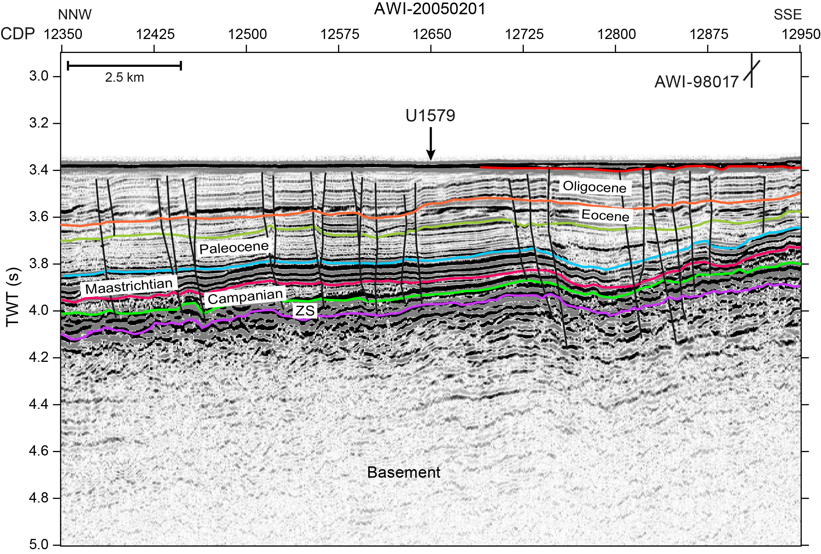
Figure F1. Seismic Line AWI-20050201.
Site U1579 was chosen to recover both Cretaceous and Paleogene sedimentary records and basement. Integration of seismic profiles with the drilling results allows for direct dating of the observed seismic Unconformities M, LE, and LO (green, magenta, and blue in Figure F1) and interpretation of their causes. Recovery of the sediment/basement interface will provide information on the age of the oldest sediments above the basement, as well as the water depth and environment at the time of deposition. At this site, records spanning the transition from the Cretaceous supergreenhouse and through the Paleogene were drilled. Based on precruise seismostratigraphic interpretations, critical intervals of ocean–climate transitions such as the Eocene–Oligocene transition (EOT), Paleocene/Eocene Thermal Maximum (PETM), Cretaceous/Paleogene (K/Pg) boundary, and Oceanic Anoxic Events (OAEs) 2 and 3 were expected to be documented in the sedimentary record. The nature and age of the basement would also be unraveled by drilling at this site.
2. Operations
Hole locations, water depths, and the number of cores recovered are listed in Table T1. All times are provided in local ship time (UTC + 2 h).
2.1. Port call
Expedition 392 began in Cape Town, South Africa, at Repair Quay 3 at 0918 h on 5 February 2022. Because of the COVID-19 quarantine (7 days), oncoming JOIDES Resolution Science Operator (JRSO) technical staff and crew did not board until 7 February, and the previous expedition’s staff and crew remained on board until then. During hotel quarantine, COVID-19 tests were conducted on Days 4 and 6. For the JRSO, 44 scientists and staff joined the vessel on 7 February. They were joined by three more personnel on 8 February and the final participant on 9 February.
The majority of incoming International Ocean Discovery Program (IODP) freight was loaded by the previous crew, which included two core liner boxes, two free-fall funnel kits, and the Ultrasonic Borehole Imager (UBI). On 8 February, the offgoing core and surface freight was loaded into two reefers, and a special air shipment left via World Courier. Fuel bunkering was completed via barge on 8 and 9 February, with the vessel taking on 1002 mt. The vessel also took on a load of fresh/frozen produce to top off stores on 8 and 9 February. The final installation, testing, and commissioning of the new 50 kVA uninterruptible power supply (UPS) for the JRSO network was done on 8 and 9 February, requiring temporary blackouts of shipboard IT services. The UPS was deemed fully operational. COVID-19 rapid antigen testing was conducted for all shipboard personnel on 8 February, and PCR testing was conducted on 9 February. All tests were negative. Schedules were established for staggered meal times in the mess hall to follow COVID-19 mitigation procedures.
On 10 February, the pilot boarded at 0942 h. The vessel began the transit to the first site (U1579) with the first line away at 1024 h. The pilot was away at 1045 h, and the start of the sea passage was recorded as 1048 h. Within minutes of the vessel reaching full throttle, the newly commissioned UPS began rejecting the ship’s power and started to run off the batteries. The vessel was throttled back to half speed at 1116 h. The UPS returned to normal operating mode. This reaction was verified several more times to diagnose the problem, and it was decided to take the UPS offline. Beginning at 1245 h, JRSO IT services were taken offline. The UPS was bypassed, and regulated power was restored at 1445 h. The vessel returned to full throttle at 1448 h, and the sea voyage continued at full speed. JRSO IT services were fully restored at 1715 h. During the transit, daily COVID-19 antigen testing was conducted in the conference room for the science party and JRSO staff and in the ship’s medical office for the crew. The testing continued daily for 8 days out of port and every other day after that until the end of the 2 week mitigation period.
2.2. Hole U1579A
Site U1579 was the first site occupied during Expedition 392. The ship arrived at Site U1579 on 12 February 2022 after a transit of 2.2 days (52.8 h) from Cape Town, covering a distance of 557 nmi at an average speed of 10.8 kt. The vessel came on site, ending the sea passage at 1430 h, and the thrusters were lowered and secured at 1451 h. The vessel was switched from cruise mode to dynamic positioning (DP) mode at 1452 h. The rig floor was given the all clear at 1500 h. The precision depth recorder (PDR) was used to get a sounding of the seafloor, which was calculated to be 2512.4 meters below rig floor (mbrf). On the rig floor, the crew commenced assembling the bottom-hole assembly (BHA) and preparing drill collars for the rotary core barrel (RCB) system to be used in subsequent holes at Site U1579. The advanced piston corer/extended core barrel (APC/XCB) BHA was assembled and run down to 2476.1 mbrf. At that point, the top drive was picked up and swung into place and preparations were made to spud the hole. The APC core barrel was picked up and run-in on the coring line while the vessel was offset a final 20 m to be directly over the desired coordinates. Hole U1579A was spudded at 0440 h from a bit depth of 2508 mbrf, and Core 1H was on deck at 0500 h. Recovery was 8.07 m, resulting in a calculated seafloor depth of 2498.4 meters below sea level (mbsl). APC coring continued through Core 8H at 65.1 m core depth below seafloor, Method A (CSF-A). The advanced piston corer temperature (APCT-3) tool was run on Cores 4H and 7H, resulting in poor data from Core 4H and acceptable data from Core 7H.
At 1330 h, after firing Core 392-U1579A-9H at 74.6 m CSF-A, the core barrel became stuck, and an overpull of ~70,000 lb was made with no success. The APC barrel was drilled over for ~3 m, which was the maximum possible advance due to the block position. Overpull was again applied, and the pipe came free, quickly rising 1–2 m. The core barrel was retrieved; however, all that was recovered was a sheared overshot and the sinker bars. The reaction force had sheared the overshot and released it. An attempt was made to fish out the core barrel, but despite landing out several times in the top of the BHA, the barrel was not retrieved. The decision was made to abandon the hole, trip the pipe, clear the BHA, and start a new hole. The final bit depth of Hole U1579A was 74.6 m CSF-A, with the bottom of the lost Core 9H cutting shoe likely at 84.1 m CSF-A. The drill string was raised, and the pipe was tripped back to the rig floor. The bit cleared the seafloor at 1735 h. A total of nine cores were taken in Hole U1579A over an 84.1 m interval with 87% recovery. Total time on Hole U1579A was 33.12 h (1.38 days).
2.3. Hole U1579B
On 14 February 2022, the coring bit was checked and the BHA was reassembled. The BHA was picked up and run-in on the drill pipe to 2476.1 mbrf at 0630 h. Meanwhile, the vessel was offset 20 m north of Hole U1579A. Hole U1579B was spudded at 0910 h. Based on the full recovery of Core 1H, the seafloor was calculated at 2492.9 mbsl. APC coring continued with Cores 2H–6H (9.5–57.0 m CSF-A). The APCT-3 tool was run on Core 4H, and the data were good, but it took 70,000 lb of overpull to free the barrel.
At 1515 h, coring was switched from the APC to the half-length APC (HLAPC) system for Core 392-U1579B-7F at 57 m CSF-A. This was just above the zone where the APC barrel became stuck in Hole U1579A. HLAPC coring continued into 15 February through Core 392-U1579B-24F at 136.9 m CSF-A. Cores 23F and 24F both saw overpull, and each core was drilled over approximately 2–2.5 m. Coring was then switched to the XCB system for Cores 25X–27X, and Hole U1579B reached a final depth of 167.2 m CSF-A. The XCB system was taking 50–55 min to core, which was too slow to reach the deeper targets in a reasonable time. The decision was made to terminate the hole, offset, and repeat the HLAPC section just completed.
At 1500 h on 15 February, the pipe was tripped up out of the hole, and the bit cleared the seafloor at 1643 h, ending Hole U1579B. A total of 27 cores were taken in Hole U1579B over a 167.08 m interval with 99% recovery. The rate of penetration (ROP) for the three XCB cores averaged 11 m/h. Total time on Hole U1579B was 40.56 h (1.69 days).
2.4. Hole U1579C
The vessel was offset 10 m east and 10 m south. The drill string was spaced out, Hole U1579C was spudded at 1720 h on 15 February 2022, and the water depth from the previous hole (2492.9 mbsl) was used as the depth for Hole U1579C. The hole was drilled down with a center bit to 56.5 m CSF-A. The center bit was retrieved, and HLAPC coring began with Core 2F and continued, with five small (0.5–1.5 m) advances without recovery for stratigraphic correlation, through Core 21F to 130.5 m CSF-A, just above the zone where the limiting overpulls occurred in Hole U1579B. The decision was made to drill down 31.5 m and switch to XCB coring. The drill string drilled to 162.0 m CSF-A, the center bit was retrieved, and an XCB core barrel was dropped. Core 392-U1579C-23X, a 5.50 m advance to correct the space-out, was cored in 25 min. Once on deck, however, the core barrel was found to be empty. The XCB cutting shoe had material on it, and its jets were clogged, evidence it had been into the formation but that the material had balled up in front of the drill bit. The pumps were increased from 50 to 65 strokes/min (about ~75 gal/min more).
Recovery of Cores 392-U1579C-24X and 25X was poor (less than 25%) because heave was making it difficult to keep the bit on bottom, and the decision was made to terminate coring at the final depth of 186.9 m CSF-A. The bit cleared the seafloor at 1815 h on 16 February. During the subsequent pipe trip, the wind and seas began picking up. At 2330 h, the pipe trip was completed, but it was too rough to handle the BHA. The BHA was at the rig floor at 2400 h on 16 February to wait on weather. On 17 February, the wait on weather period ended at 0930 h, and we were able to start disassembling the APC/XCB BHA. The bit cleared the rig floor at 1055 h, ending Hole U1579C. A total of 18 cores were taken in Hole U1579C over a 93.4 m interval with 80% recovery. The ROP for the three XCB cores averaged 9.6 m/h. Total time on Hole U1579C was 42.24 h (1.76 days).
2.5. Hole U1579D
The remainder of the four-stand RCB BHA was made up, and the pipe trip began at 1345 h on 17 February 2022. Upon completion of the pipe trip at 1800 h, the crew slipped and cut the drilling line. This was done to move the points where the drilling line wraps around the block to avoid fatigue failures. Hole U1579D was spudded at 2124 h using a water depth of 2492.9 mbsl. Hole U1579D was drilled to 130 m CSF-A by 0200 h on 18 February. Cores 2R–65R advanced from 130 to 727.2 m CSF-A. Sepiolite mud sweeps of 30 bbl were pumped every third core in Cores 31R–57R and in Cores 59R, 62R, 64R, and 65R.
On 24 February, the bit was released at the bottom of the hole at 0310 h and the hole was displaced with heavy mud. The pipe was tripped back to 70.7 m CSF-A, and the 48 m long quadruple combination (quad combo) tool string was prepared. It consisted of the Hostile Environment Litho-Density Sonde (HLDS), Dipole Shear Sonic Imager (DSI), Hostile Environment Natural Gamma Ray Sonde (HNGS), High-Resolution Laterolog Array (HRLA), and Magnetic Susceptibility Sonde (MSS). The logging tool string was run in the hole, pausing every 500 m to allow the new logging line to “season” (i.e., detorque). The downlog was paused to conduct a high-resolution uplog from 450 to 250 m wireline log depth below seafloor (WSF). After resuming the downlog, the tool tagged 727.7 m WSF, and a high-resolution uplog was done. We began pulling up the logging tools at 2040 h, and the quad combo was back at the rig floor by the end of the day. On 25 February 2022, the pipe was tripped out of Hole U1579D, clearing the seafloor at 0110 h. We continued tripping the pipe back to the rig floor, and Hole U1579D ended at 0735 h. The rig floor was secured for transit, the thrusters were raised, and at 0740 h we began our sea passage to the next site. A total of 64 cores were taken in Hole U1579D over a 597.2 m interval with 73.8% recovery. The ROP for RCB coring averaged just under 20 m/h in sediment to 2.0 m/h in basalt (average = 8.2 m/h). Total time on Hole U1579D was 188.4 h (7.85 days).
3. Lithostratigraphy
A 727 m thick sequence of sediments and basalts was recovered at Site U1579. The main sedimentary succession extends to 697 m CSF-A and is divided into Lithostratigraphic Units I–III (Table T2). Calcareous sediments of Pleistocene–Santonian age extend to ~635 m CSF-A (Lithostratigraphic Units I and II) and overlie zeolitic siliciclastic sediments of Lithostratigraphic Unit III between ~635 and 697 m CSF-A (Figures F2, F3; Table T2). Below Lithostratigraphic Unit III, a ~24 m interval of basalt is designated as Lithostratigraphic Unit IV (697.00–720.77 m CSF-A) (see Igneous petrology), which overlies another ~5 m of zeolitic siliciclastic sediments (Lithostratigraphic Unit V; 720.77–725.47 m CSF-A) and ~2 m of basalt (Lithostratigraphic Unit VI; 725.47–727.29 m CSF-A) (see Igneous petrology) in the lowermost part of the drilled sequence.
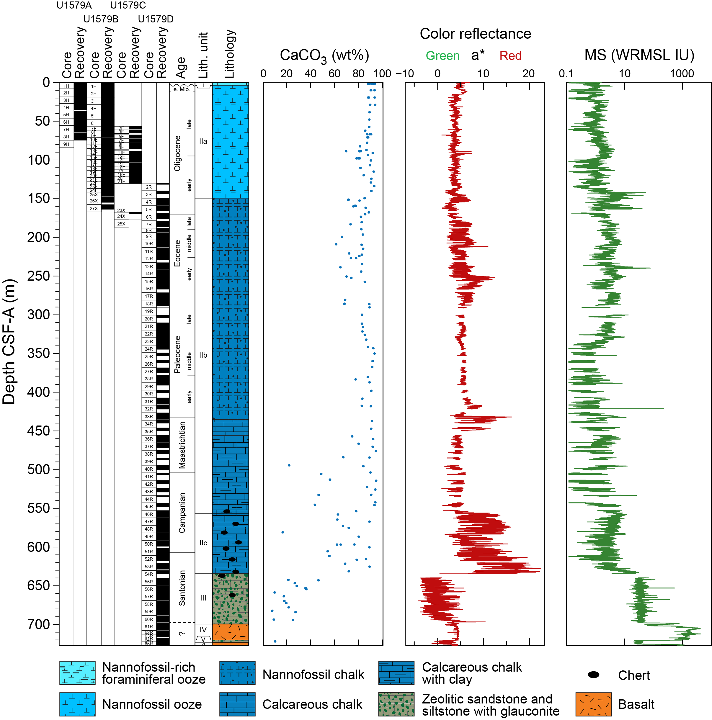
Figure F2. Lithostratigraphic summary.
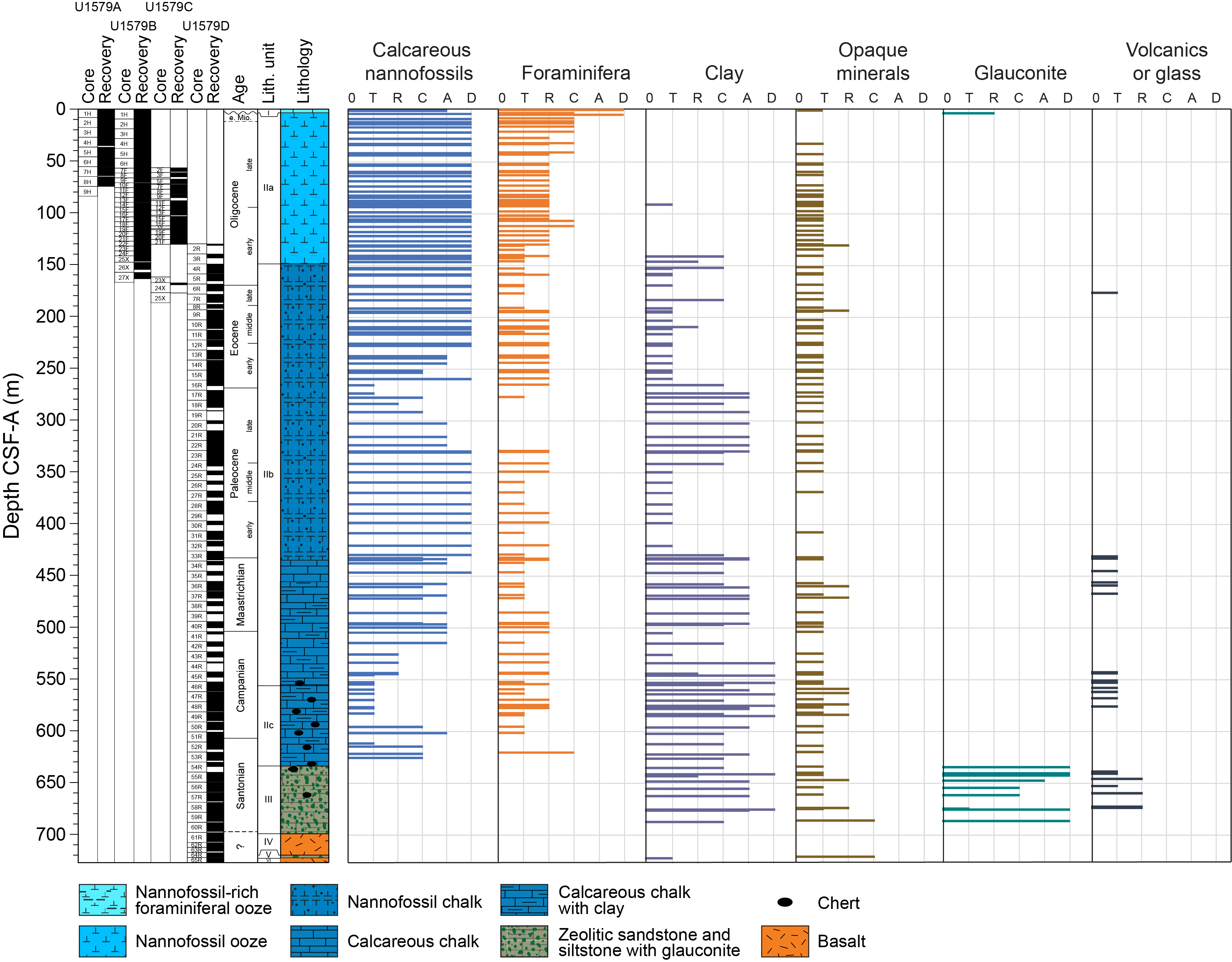
Figure F3. Smear slide components.
3.1. Lithostratigraphic Unit I
- Intervals: 392-U1579A-1H-1, 0 cm, to 1H-1, 131 cm; 392-U1579B-1H-1, 0 cm, to 1H-5, 8 cm
- Depths: Hole U1579A = 0–1.31 m CSF-A; Hole U1579B = 0–6.13 m CSF-A
- Age: upper Pleistocene
- Major lithology: nannofossil-rich foraminiferal ooze
Lithostratigraphic Unit I consists of light gray nannofossil-rich foraminiferal ooze (Figures F3, F4, F5) with ~90 wt% CaCO3 (see Geochemistry). Lithostratigraphic Unit I is differentiated from Lithostratigraphic Unit II based on a greater abundance of foraminifera and a darker light gray color than the underlying white nannofossil ooze of Lithostratigraphic Subunit IIa. The light gray color reflects a greater abundance of sand-sized glauconite grains, disseminated pyrite, and clay. The upper contact is placed at the seafloor, and the bottom contact is a bioturbated boundary with the white nannofossil ooze of Lithostratigraphic Unit II. The uppermost several decimeters of Lithostratigraphic Unit I are modified by soupy drilling disturbance. The thickness of Lithostratigraphic Unit I (i.e., the depth of the Lithostratigraphic Unit I/II boundary) differs significantly between Hole U1579A (1.31 m CSF-A) and Hole U1579B (6.13 m CSF-A), and the correlative interval was drilled without recovery in Holes U1579C and U1579D.
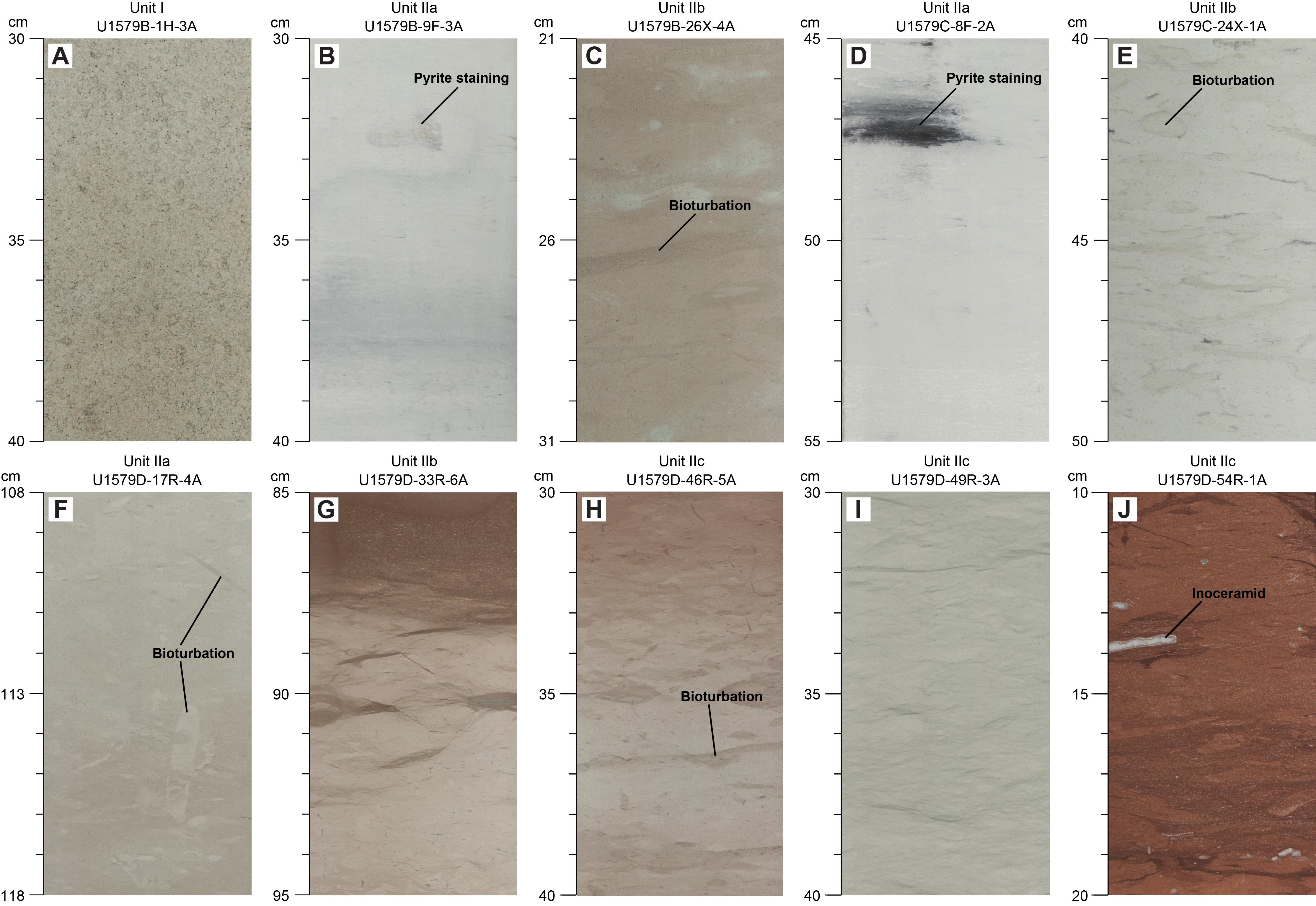
Figure F4. Lithostratigraphic Unit I and II major lithologies.
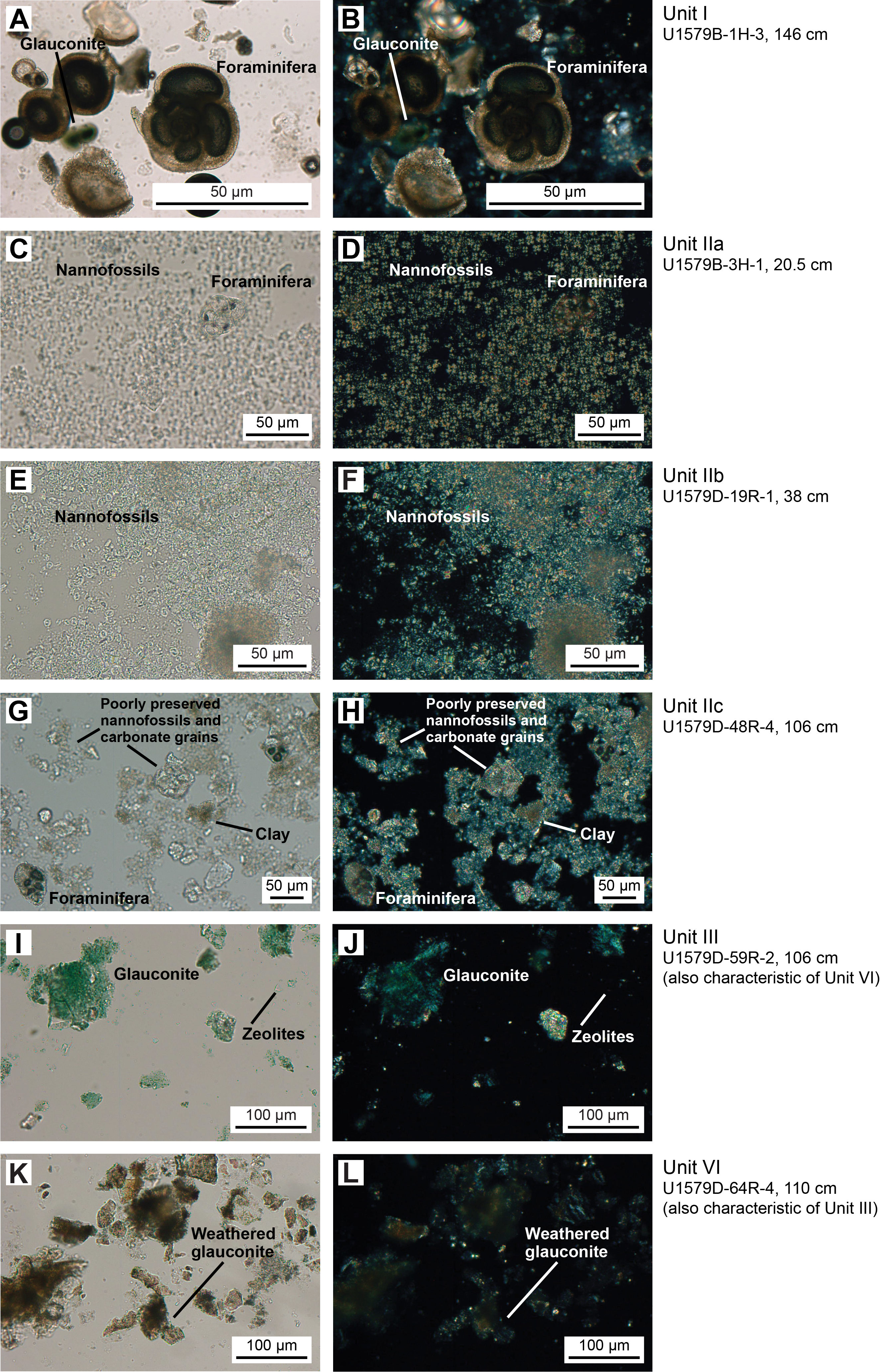
Figure F5. Major sedimentary lithologies.
3.2. Lithostratigraphic Unit II
- Intervals: 392-U1579A-1H-1, 131 cm, to 8H-CC, 16 cm; 392-U1579B-1H-5, 8 cm, to 27X-CC, 37 cm; 392-U1579C-2F-1, 0 cm, to 25X-CC, 5 cm; 392-U1579D-2R-1, 0 cm to 54R-CC, 21 cm
- Depths: Hole U1579A = 1.31–74.78 m; Hole U1579B = 6.13–163.96 m CSF-A; Hole U1579C = 56.50–177.70 m CSF-A; Hole U1579D = 130.00–634.72 m CSF-A
- Age: lower Miocene to Santonian
- Major lithology: nannofossil ooze and chalk
Lithostratigraphic Unit II consists of ~630 m of Miocene–Santonian carbonate ooze and chalk, mostly consisting of calcareous nannofossils and recrystallized calcite with varying abundance of foraminifera and clay. Lithostratigraphic Unit II is divided into Lithostratigraphic Subunits IIa–IIc based on lithification (ooze versus chalk), color, and the occurrence of thin silicified horizons. Only the top of Lithostratigraphic Unit II (Lithostratigraphic Subunit IIa and the top of Lithostratigraphic Subunit IIb) was recovered in Holes U1579A–U1579C, and the lower part of the unit (Lithostratigraphic Subunits IIb and IIc) was recovered in Hole U1579D.
3.2.1. Lithostratigraphic Subunit IIa
- Intervals: 392-U1579A-1H-1, 131 cm, to 8H-CC, 16 cm; 392-U1579B-1H-5, 8 cm, to 25X-CC, 35 cm; 392-U1579C-2F-1, 0 cm, to 21F-CC, 20 cm; 392-U1579D-2R-1, 0 cm, to 3R-CC, 13 cm
- Depths: Hole U1579A = 1.31–74.78 m CSF-A (bottom of hole); Hole U1579B = 6.13–147.10 m CSF-A; Hole U1579C = 56.50–130.68 m CSF-A; Hole U1579D = 130.00–143.87 m CSF-A
- Age: lower Miocene to lower Oligocene
- Major lithology: nannofossil ooze
Lithostratigraphic Subunit IIa consists of white and occasionally light gray or light greenish gray nannofossil ooze that contains rare and occasionally common foraminifera (Figures F3, F4, F5). Gray mottles and centimeter-scale darker banding are common throughout the subunit. Smear slides from the dark gray to black patches contain a higher abundance of subspherical, silt-sized opaque grains that were confirmed by scanning electron microscope (SEM) imaging to be framboidal pyrite (Figure F6). Carbonate content generally ranges 80–95 wt% CaCO3 (Figure F2; see Geochemistry), with lower values in the darker light gray intervals. The contact between Lithostratigraphic Subunits IIa and IIb represents the gradational ooze-to-chalk transition, which is defined at the top of Core 392-U1579B-26X (147.80 m CSF-A) and also identified at the top of Cores 392-U1579C-24X (167.50 m CSF-A) and 392-U1579D-4R (149.40 m CSF-A). This boundary also roughly corresponds to a change in porosity (Figure F48).
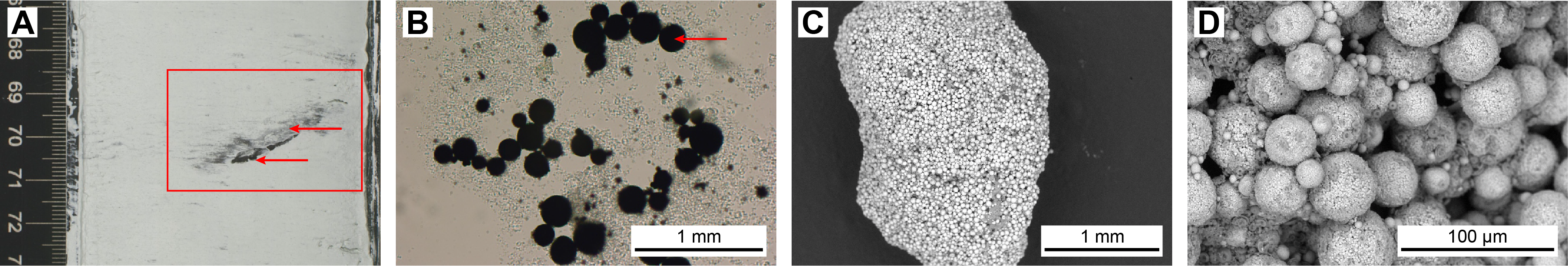
Figure F6. Pyrite mottles and framboids.
3.2.2. Lithostratigraphic Subunit IIb
- Intervals: 392-U1579B-26X-1, 0 cm, to 27X-CC, 37 cm; 392-U1579C-24X-1, 0 cm, to 25X-CC, 5 cm; 392-U1579D-4R-1, 0 cm, to 46R-3, 88 cm
- Depths: Hole U1579B = 147.80–163.96 m CSF-A (bottom of hole); Hole U1579C = 167.50–177.70 m CSF-A (bottom of hole); Hole U1579D = 149.40–556.31 m CSF-A
- Age: lower Oligocene to Campanian
- Major lithology: nannofossil chalk
Lithostratigraphic Subunit IIb consists of ~407 m of nannofossil chalk with varying clay content and trace to rare foraminifera. The uppermost ~20 m of Lithostratigraphic Subunit IIb was recovered using XCB coring in Holes U1579B and U1579C, and the entire subunit was recovered using RCB coring in Hole U1579D. This subunit differs from Lithostratigraphic Subunit IIa by degree of lithification (chalk rather than ooze). The dominant color is white to light greenish gray, but frequent decimeter-scale intervals of slightly darker colors reflect locally higher clay content. Carbonate content is generally 65–95 wt% CaCO3, with lower values coinciding with darker colors and higher clay content. Specks of dark gray pyrite are common, occasionally localized into centimeter-scale intervals and mottles. Recovery was variable across the subunit, and many cores are slightly to severely fractured or biscuited due to drilling disturbance.
Nannofossils are the dominant lithologic component throughout Lithostratigraphic Subunit IIb. However, the preservation of nannofossils is variable and in some intervals so poor that individual nannofossils cannot be recognized in smear slides. Intervals with fine-grained carbonate of indeterminate origin are therefore described as calcareous chalk. Clay content is rare to common, and likely represents most of the noncarbonate fraction. Foraminifera were observed in trace to rare abundance in most smear slides from this subunit (Figure F3). Trace siliceous microfossils (radiolarians, silicoflagellates, and sponge spicules) were noted in smear slides from ~160 to 180 m CSF-A. Bioturbation is common throughout the subunit, with intensity ranging from absent to intense, and includes clear examples of Zoophycos and Planolites burrows. In the lowermost intervals of Lithostratigraphic Subunit IIb (from Core 392-U1579D-33R at 430.6 m CSF-A to the bottom of the subunit), rare centimeter-scale gray silicified nodules and intervals are observed that increase in frequency downsection.
Throughout the subunit, there are faint decimeter- to meter-scale alternations between the dominant light-colored (white or light greenish gray) clay-poor nannofossil chalk and intervals of darker, more clay-rich sediment. The color of the more clayey intervals varies across the subunit and includes greenish gray, pinkish gray, yellowish brown, and reddish brown.
In addition to the meter-scale cycles in clay content, subtle larger scale trends are noted in clay content across Lithostratigraphic Subunit IIb. The upper part of the subunit (~150–330 m CSF-A) has generally higher and more variable clay content, with carbonate concentration ranging 60–90 wt% CaCO3. This interval coincides with slightly elevated natural gamma radiation (NGR) and magnetic susceptibility (MS) values (see Physical properties). Below this interval (~330–450 m CSF-A), the sediments are characterized by lower clay content and more consistent carbonate content ranging 80–95 wt% CaCO3 and very low NGR and MS values. The lowermost interval of Lithostratigraphic Subunit IIb (~450–556 m CSF-A) is characterized by higher and more variable clay content, with carbonate content generally ranging 50–95 wt% CaCO3. There is meter-scale variability in clay/CaCO3 content throughout the subunit, and the minimum reported weight percent CaCO3 values occur only in the darkest intervals.
The K/Pg boundary occurs in Section 392-U1579D-33R-6, 98.5 cm (433.255 m CSF-A) (Figure F7; see Chronostratigraphy). White nannofossil chalk at the top and bottom of this core is interrupted by a complex sequence of more clay-rich lithologies. Beginning in Section 33R-4, white nannofossil chalk gradually darkens downcore across a ~2 m interval (spanning Section 33R-5 and the upper part of Section 33R-6) to reddish brown clayey calcareous chalk, followed downcore by ~8 cm (interval 33R-6, 87–95 cm) of white calcareous chalk and then ~3 cm (interval 33R-6, 95–97.5 cm) of reddish brown clayey calcareous chalk. Immediately underlying that interval, a ~1 cm layer of greenish gray clayey calcareous ooze is present (interval 33R-6, 97.5–98.5 cm), which is significantly softer than the over- and underlying sediments and is deformed by drilling disturbance. The greenish gray clayey calcareous ooze transitions abruptly to white nannofossil chalk in Section 33R-6, 98.5 cm.
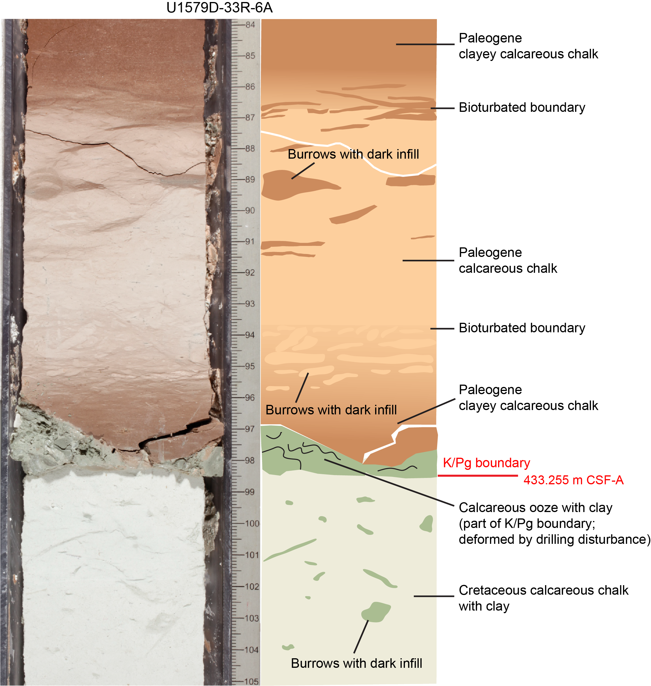
Figure F7. K/Pg boundary schematic.
The Lithostratigraphic Subunit IIb/IIc contact is gradational, reflecting a downhole increase in three distinct properties over several cores: more pronounced and rhythmically occurring centimeter-scale clay-rich layers, an increase in abundance and thickness of silicified intervals, and a change to reddish brown color. The Lithostratigraphic Subunit IIb/IIc boundary is defined at the first appearance of reddish brown chalk in Section 392-U1579D-46R-3, 88 cm (556.31 m CSF-A).
3.2.3. Lithostratigraphic Subunit IIc
- Interval: 392-U1579D-46R-3, 88 cm, to 54R-CC, 21 cm
- Depth: 556.31–634.72 m CSF-A
- Age: Campanian–Santonian
- Major lithology: nannofossil chalk with clay and occasional chert
Lithostratigraphic Subunit IIc consists of ~80 m of nannofossil chalk and calcareous chalk characterized by a reddish color that alternates with very light greenish gray bands. Throughout the subunit, there are cyclic occurrences of brownish gray clayey chalk and both gray and reddish brown cherts that range 0.5–12 cm in thickness. The recurrence of clay-rich layers is generally shorter (on the order of centimeters to decimeters) than that of the silicified layers (on the order of meters). Recrystallized inoceramid bivalves are present and preserved either in clusters of fragments or as larger discrete fragments throughout the subunit.
Carbonate content is variable in Lithostratigraphic Subunit IIc, with low values (down to 16 wt% CaCO3) measured on cherty intervals and discrete centimeter-scale clayey intervals. Carbonate content in the calcareous chalk intervals ranges 54–89 wt% CaCO3. In thin section (TS) Sample 392-U1579D-52R-2, 56–60 cm (TS01) (Figure F8), the more lithified reddish layers of Lithostratigraphic Subunit IIc contain calcite, possible shell fragments, and microcrystalline to cryptocrystalline calcite in a matrix of clay minerals. Zoophycos burrows and other trace fossils observed in Lithostratigraphic Subunit IIc have modified the sedimentary deposits, and there is remarkable clarity of internal trace fossil structures.
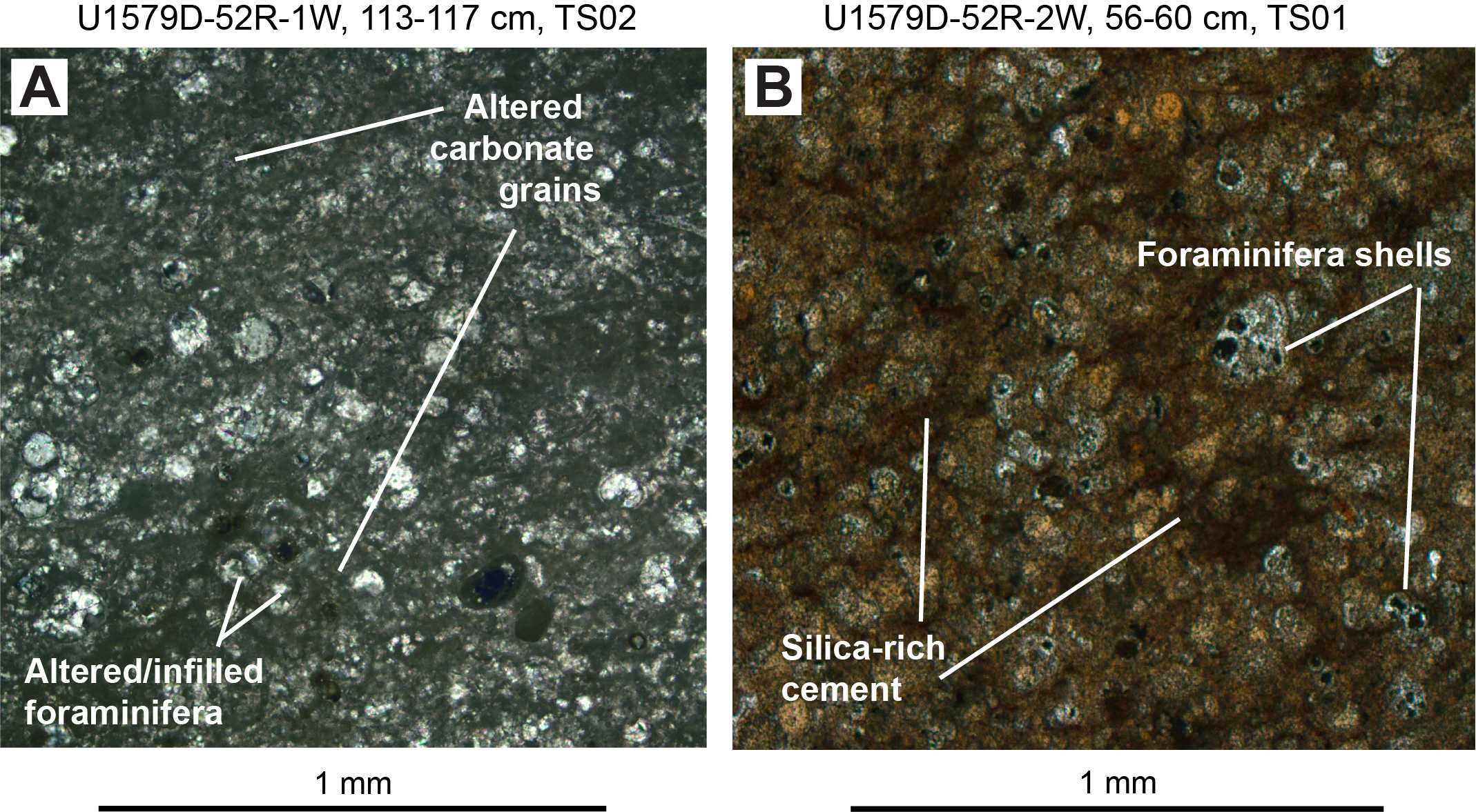
Figure F8. Lithostratigraphic Unit II thin sections.
The boundary between Lithostratigraphic Subunit IIc and Lithostratigraphic Unit III is marked by a sharp contact in Section 392-U1579D-54R-CC, 21 cm (634.72 m CSF-A).
3.3. Lithostratigraphic Unit III
- Interval: 392-U1579D-54R-CC, 21 cm, to 60R-7, 91 cm
- Depth: 634.72–697.00 m CSF-A
- Age: Santonian
- Major lithologies: zeolitic sandstone, siltstone, and claystone with glauconite
Lithostratigraphic Unit III consists of ~60 m of greenish gray well-lithified zeolitic siliciclastic sediments (sandstone, siltstone, and claystone) with glauconite. Most individual clasts, when identifiable, are silicate minerals, and there is rare glass that is likely of volcanic origin that has undergone significant alteration to clay minerals and zeolites (Figure F3) with carbonate cementation. Rare carbonate bioclasts and foraminifera suggest marine deposition. The variety of processes influencing the composition of Lithostratigraphic Unit III (volcanism, siliciclastic sedimentation, and alteration) suggests a complex history and challenges traditional sedimentological categorization schemes.
Lithostratigraphic Unit III sediments were described and classified principally based on grain size (ranging from claystone to coarse sandstone) and sedimentary structures. These structures include centimeter- to decimeter-scale sorted beds, often normally graded (Figure F9). Beds typically have a sharp planar base, sometimes irregular (e.g., scoured), and sometimes include intraclasts (e.g., rip-up clasts) of finer grained underlying sedimentary material. These features imply deposition in a hydraulically energetic (and variable) environment, presumably in shallow water.
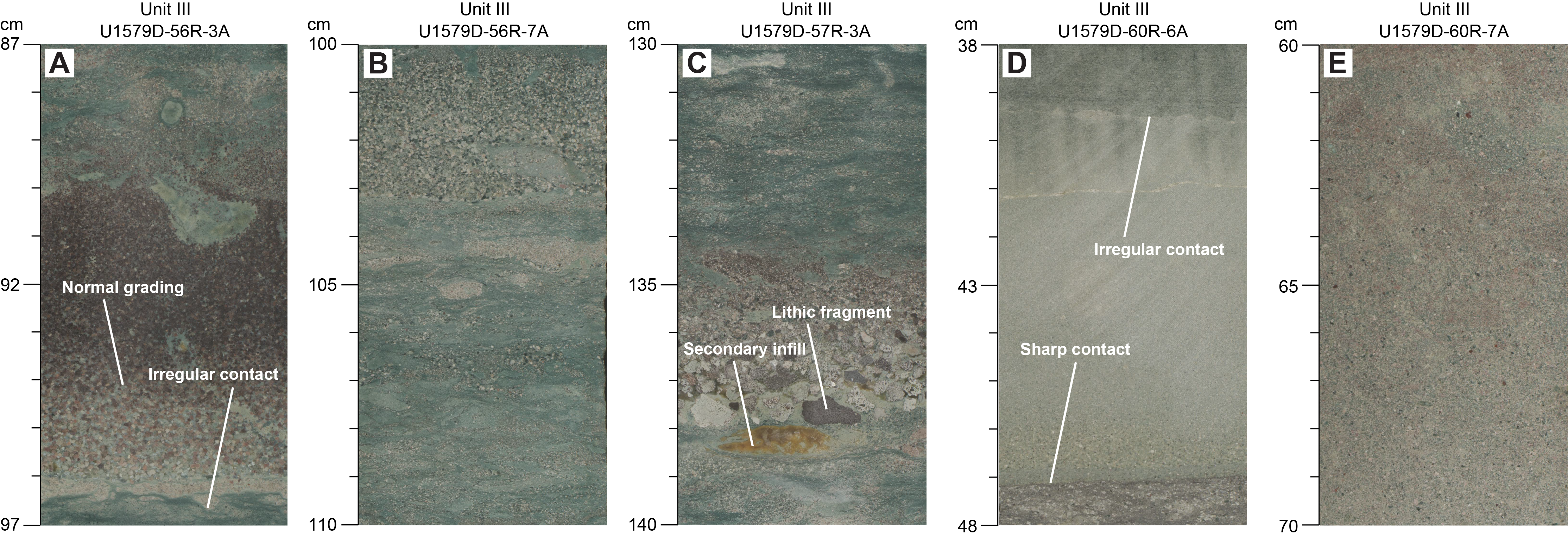
Figure F9. Lithostratigraphic Unit III major lithologies.
Where identifiable by hand lens and thin section (Figure F10), sand-sized clasts within coarser beds include lithic fragments, microvesicular pumice (heavily altered), and other likely volcanogenic silicate rocks, minerals, and glass. However, most grains are altered or replaced by zeolites, clays, and other alteration products. Rare subspherical sand-sized glauconite grains were observed in thin sections and likely contribute to the overall greenish gray color of the unit. Discrete centimeter-scale dark green intervals were scraped for smear slides and also appear to be glauconitic. However, disseminated fine-grained green material, either a different morphology of glauconite or another alteration mineral, is also widely observed in thin sections.
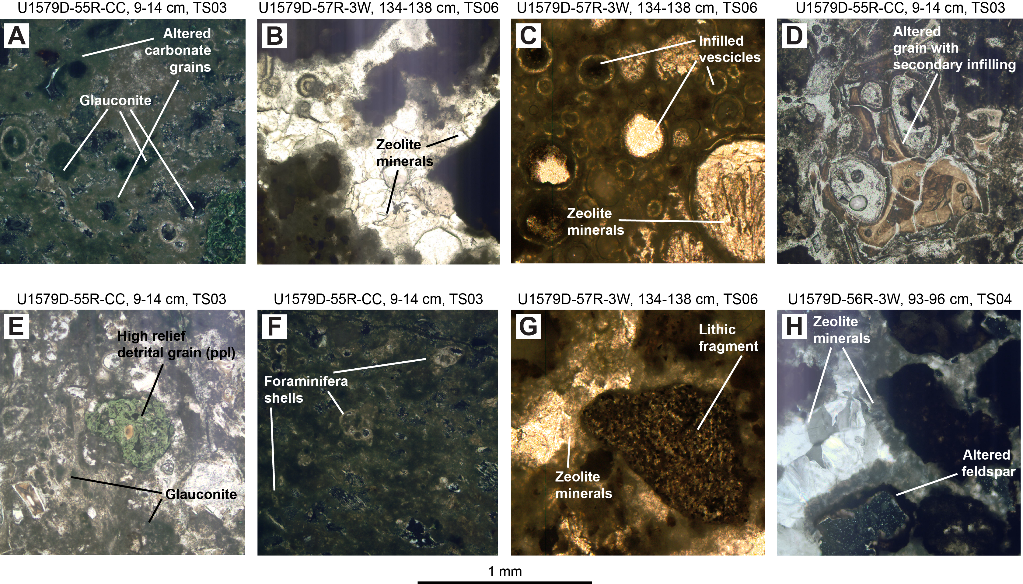
Figure F10. Lithostratigraphic Unit III thin sections.
Carbonate content in Lithostratigraphic Unit III generally ranges 18–35 wt% CaCO3, which likely is present as siderite and dolomite cements and infills in addition to calcite bioclasts. Thin sections (Figure F10) of the finer grained facies of Lithostratigraphic Unit III also include rare bioclasts such as shell fragments and foraminifera.
Bulk and clay-fraction X-ray diffraction (XRD) analysis of sediments from Lithostratigraphic Unit III (Figure F11) shows a high abundance of analcime and chabazite, which are zeolites that can be formed by the alteration of basaltic glass (Moberly and Jenkyns, 1981; Vitali et al., 1995). Other mineral phases present include siderite and dolomite (which likely comprise most of the carbonate content in Lithostratigraphic Unit III, instead of calcite), and glauconite, which likely contributes to the characteristic greenish gray color of Lithostratigraphic Unit III.
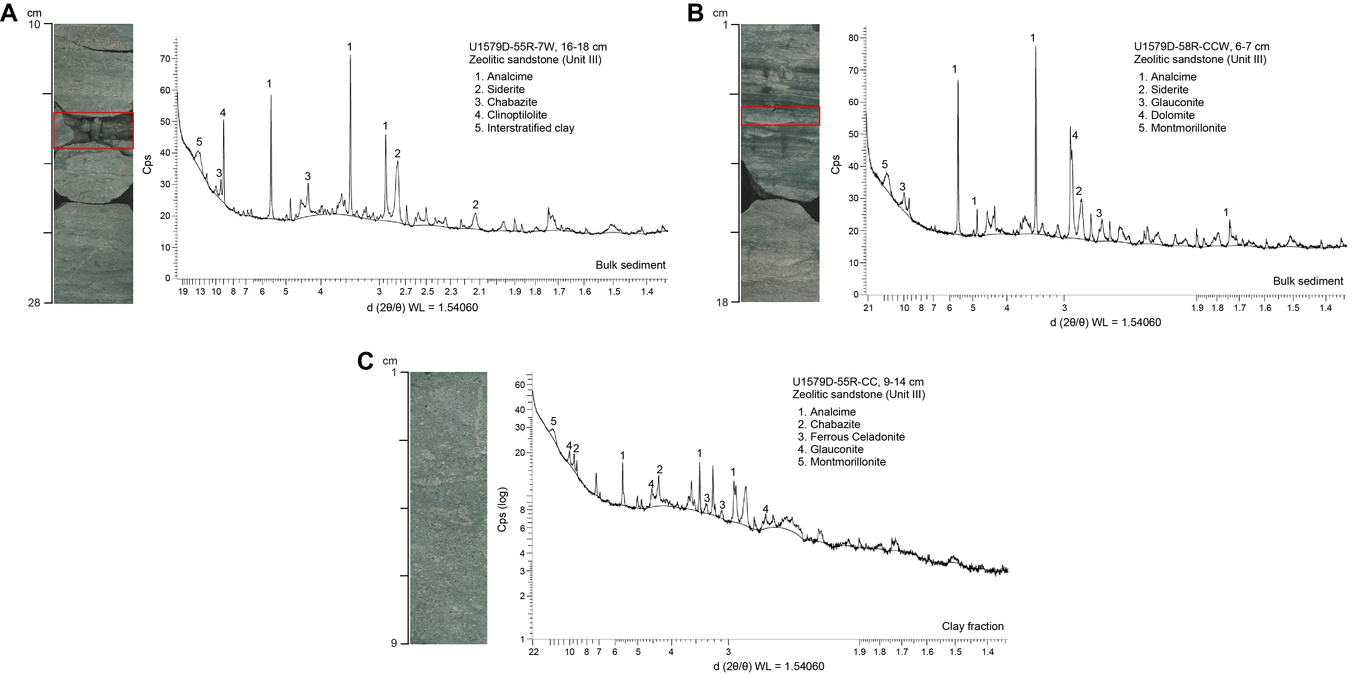
Figure F11. XRD.
3.4. Lithostratigraphic Unit IV
Lithostratigraphic Unit IV (Igneous Unit 1) consists of plagioclase-clinopyroxene phyric basalt (see Igneous petrology).
3.5. Lithostratigraphic Unit V
- Interval: 392-U1579D-64R-4, 0 cm, to 65R-3, 97 cm
- Depth: 720.77–725.47 m CSF-A
- Age: Santonian or older
- Major lithology: zeolitic sandstone and siltstone with glauconite
Lithostratigraphic Unit V consists of a ~5 m interval of greenish gray sediments similar to those described in Lithostratigraphic Unit III. Lithostratigraphic Unit V is physically separated from Lithostratigraphic Unit III by the interlayered basalts of Lithostratigraphic Unit IV, but the sedimentological description of Lithostratigraphic Unit III applies equally to Lithostratigraphic Unit V. Like Lithostratigraphic Unit III, Lithostratigraphic Unit V consists of well-lithified greenish gray zeolitic sandstone and siltstone with glauconite.
The lower contact of Lithostratigraphic Unit V with Lithostratigraphic Unit VI (Igneous Unit 2) occurs in Section 392-U1579D-65R-3, 97 cm (725.47 m CSF-A). In the lower 50 cm of Lithostratigraphic Unit V, color gradually lightens downcore from greenish gray to light greenish gray and individual grains and sedimentary structures become less distinct. This change in sedimentary character is interpreted as evidence for contact metamorphism in the sediment due to heating following intrusion of Lithostratigraphic Unit VI (Igneous Unit 2).
3.6. Lithostratigraphic Unit VI
Lithostratigraphic Unit VI (Igneous Unit 2) consists of ~1.8 m of aphyric basalt (see Igneous petrology).
4. Igneous petrology
Igneous rocks were reached at 697.00 m CSF-A in Hole U1579D below sedimentary Lithostratigraphic Unit III (Figure F12). A 23.77 m massive interval (Lithostratigraphic Unit IV) was cored (697.00–720.77 m CSF-A), below which a 4.7 m sedimentary sequence (Lithostratigraphic Unit V) was encountered (720.77–725.47 m CSF-A). This sequence was underlain by another massive igneous unit (Lithostratigraphic Unit VI; 725.47–727.29 m CSF-A), of which 1.82 m was recovered before drilling in Hole U1579D was terminated at a final depth of 727.29 m drilling depth below seafloor (DSF).
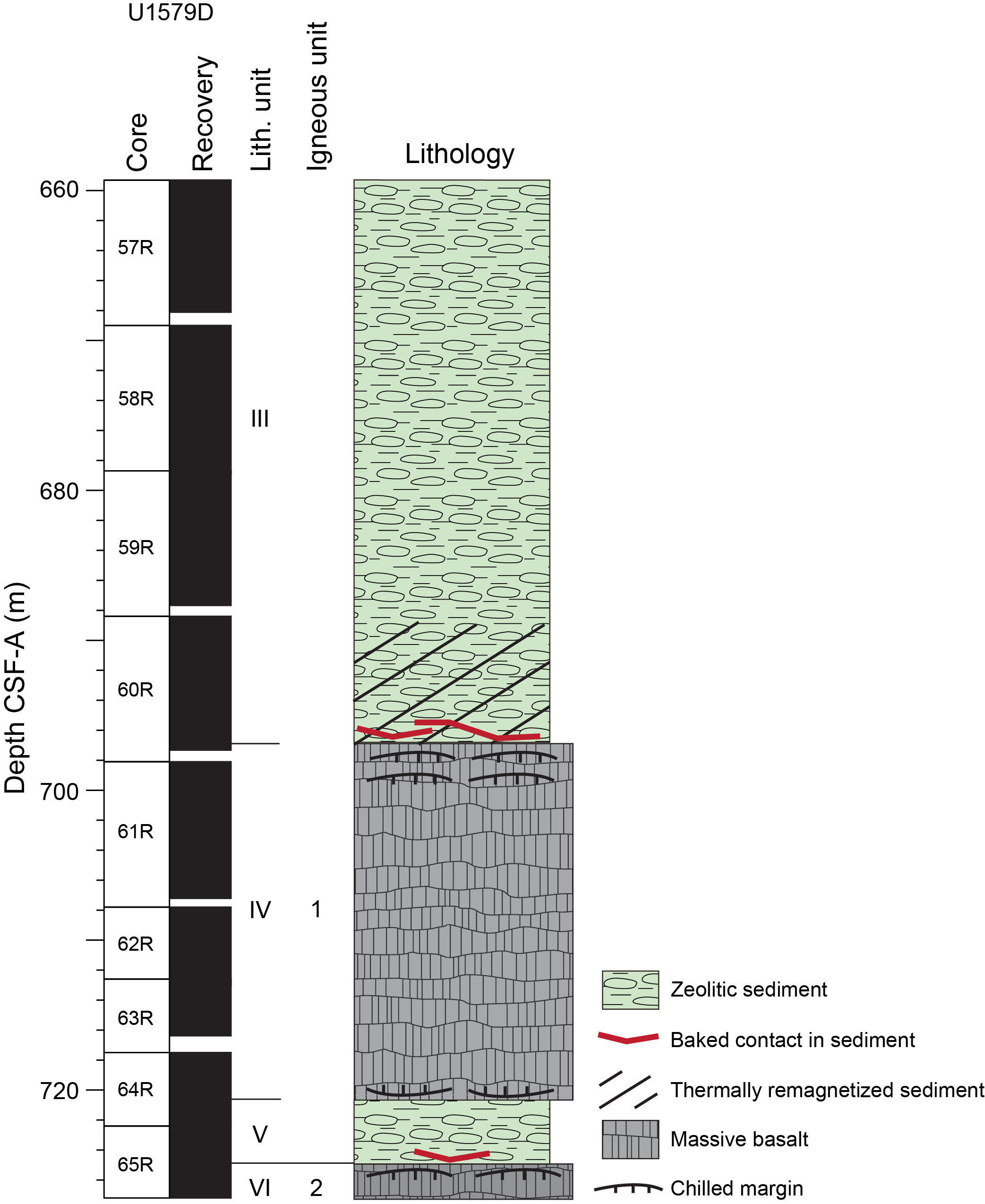
Figure F12. Stratigraphic summary.
4.1. Lithostratigraphic and igneous units
4.1.1. Lithostratigraphic Unit IV
- Interval: 392-U1579D-60R-7, 91 cm, to 64R-3, 52 cm
- Depth: 697.00–720.77 m CSF-A
- Lithology: Plagioclase-clinopyroxene phyric basalt
- Igneous unit: 1
Lithostratigraphic Unit IV is composed of plagioclase-clinopyroxene phyric basalt. Although the contact with the overlying sediment (Lithostratigraphic Unit III) was not recovered, the uppermost few meters of basalt are more altered and vesicular and have a finer groundmass grain size compared to the remaining portion of Lithostratigraphic Unit IV. A highly vesicular zone occurs between Sections 392-U1579D-61R-1, 52 cm, and 61R-2, 150 cm (698.62–700.87 m CSF-A). The rock grades downsection toward less vesicular and more coarse-grained textures until a near-absence of vesicles and a medium-sized groundmass grain size is reached in Section 61R-4, which continues downward to Section 64R-2. This central portion of the unit is well crystallized and medium grained. From the base of Section 64R-2, the groundmass grain size decreases downsection again to fine grained and eventually aphanitic at the base of Section 64R-3 (Piece 4). The contact with the underlying sediments of Lithostratigraphic Unit V was not recovered. Plagioclase phenocrysts are ubiquitous throughout and have an average abundance of ~5% and average size of 2 mm. Clinopyroxene phenocrysts are also present throughout Lithostratigraphic Unit IV in variable abundance, also averaging around 5%, but are smaller in size (~1 mm) and only a little larger than the groundmass in the interior of the unit. The groundmass consists of plagioclase, clinopyroxene, and olivine in roughly equal proportions, as well as metal oxides, with alteration predominantly affecting olivine and clinopyroxene (Figure F13A–F13C). The center of the unit is very well preserved (classified as fresh to slightly altered), and only the boundary zone to the upper sediments (interval 60R-7, 91 cm, to 61R-1, 2 cm; 697.0–698.12 m CSF-A) shows distinct signs of overprinting (highly altered). No abrupt or significant lithologic changes (e.g., different mineralogy or multiple cooling units) could be recognized in the ~23.8 m igneous succession, and therefore Lithostratigraphic Unit IV was not further divided and is designated as only one igneous unit (Igneous Unit 1). The recovered 22.01 m (curated length) of core material corresponds to an excellent recovery rate of 93%.
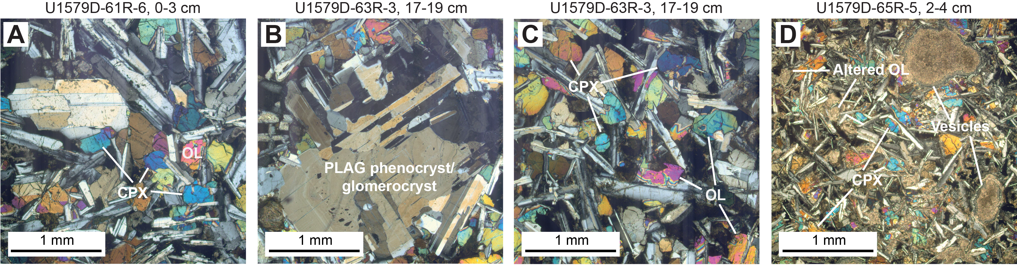
Figure F13. Igneous rock.
4.1.2. Lithostratigraphic Unit VI
- Interval: 392-U1579D-65R-3, 97 cm, to 65R-5, 52.5 cm
- Depth: 725.47–727.29 m CSF-A
- Lithology: aphyric basalt
- Igneous unit: 2
Lithostratigraphic Unit VI is composed of nearly aphyric basalt. The top of this unit is distinctly more altered in the uppermost 25 cm compared to the remainder of the unit. The contact with the overlying sediment is partially recovered in interval 392-U1579D-65R-3, 96–105 cm (~725.50 m CSF-A), although it is unoriented (Figure F14). This contact is sharp, and the basalt is completely altered and aphanitic, indicating a chilled margin. The recovered 1.82 m of this unit is moderately vesicular (and all vesicles are filled with alteration minerals) and shows a fine-grained groundmass (except for the uppermost aphanitic margin). Small plagioclase phenocrysts are present throughout but are not abundant (<1%) and are generally only 1.5–2 mm. The groundmass consists of plagioclase, clinopyroxene, and olivine in roughly equal proportions, as well as trace metal oxides, with alteration predominantly affecting the olivine and clinopyroxene, although plagioclase is also variably affected (Figure F13D). The overall degree of alteration is moderate except for the uppermost portion, where it is heavily altered. No abrupt or significant lithologic changes (e.g., different mineralogy or multiple cooling units) could be recognized in the igneous succession, and therefore Lithostratigraphic Unit VI is designated as only one igneous unit (Igneous Unit 2). The recovery rate for the interval comprising Lithostratigraphic Unit VI was 100%.
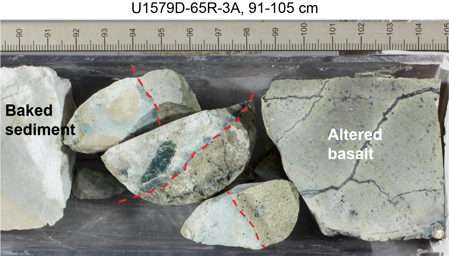
Figure F14. Lithostratigraphic Unit V/VI contact.
4.2. Interpretation of the igneous units
The two igneous units encountered in Hole U1579D are tentatively interpreted as sills based on systematic lithologic variations toward their upper and lower (only for Lithostratigraphic Unit IV) margins and the characteristics of the sediments at the contact zones.
The distinction of lava flows and intrusive sheets (sills) is often not easy in drill core samples (Koppers et al., 2010). Lava flows are generally characterized by finer grained tops and bases and highly fractured and brecciated flow tops. Chilled margins are usually thin or absent. In contrast, sill intrusions often show chilled margins and slow gradational changes in crystallinity toward coarsely crystalline interiors.
Both igneous units at Site U1579 show relatively wide (>20 cm) chilled (and altered) zones but without (recovered) significant brecciation. Lithostratigraphic Unit IV (which was completely penetrated) also shows a spatial increase in groundmass grain size toward its center. Accordingly, both units comprise more characteristics of sills than of lava flows. More importantly, the sediments at the contact zones above both the upper and lower igneous bodies show alteration reactions such as brick-red streaks characteristic of thermal baking (interval 392-U1579D-60R-7, 80–90 cm) or bleaching and recrystallization (interval 65R-3, 54–96 cm) (see Lithostratigraphy; Figure F14). If these sediments were deposited on top of a lava flow, no evidence of baking or other thermal alteration would be expected.
Additional evidence for the interpretation of these igneous units as sills comes from other laboratory groups. For instance, an organic matter–rich horizon recovered ~23 m above the upper sill contact (interval 392-U1579-58R-4, 107–117 cm) contains microfossils that are thermally altered beyond grades expected from the sedimentary overburden alone (see Micropaleontology). Likewise, the transition from an indistinct to a more distinct polarity signal in the paleomagnetic record of the sediments to ~7 m above the upper sill contact could have been caused by thermal remagnetization (see Paleomagnetism). In conclusion, we interpret both igneous units as sill injections into an already existing sedimentary succession in accordance with both our observations and the preliminary results from other laboratory groups.
The presence of basalts at relatively shallow depths (compared to the bulk of the plateau basement) and a micropaleontologically constrained age of 86 ± 8 Ma for the sediments in which the upper sill was injected (see Micropaleontology) suggest that these intrusions reflect late-stage volcanism of the Agulhas Plateau. Late-stage (or posterosional or rejuvenated) volcanism was recognized at other volcanic oceanic plateaus such as Walvis Ridge, Shatsky Rise, and Manihiki/Hikurangi (Homrighausen et al., 2018; Tejada et al., 2016; Hoernle et al., 2010) and is often characterized by alkaline composition. Petrographically, however, Site U1579 basalts show no indication of an alkaline character (e.g., predominance of olivine over plagioclase phenocrysts). These observations are confirmed by the preliminary shipboard chemical analyses (see Geochemistry), which reveal a tholeiitic composition of the basalt (Figure F44).
5. Micropaleontology
The 727.285 m succession cored at Site U1579 contains calcareous nannofossils, foraminifera, siliceous microfossils, and palynomorphs in varying numbers. The sedimentary succession consists of a thin veneer (~1–6 m) of Pleistocene sediment overlying ~697 m of Oligocene to Upper Cretaceous sediment. The lowermost part of the cored succession (697.00–727.285 m CSF-A) includes two intervals of igneous rock (Lithostratigraphic Units IV and VI; see Lithostratigraphy) with a short interval of sediment in between (Lithostratigraphic Unit V). Figure F15 provides a comprehensive overview of the occurrence and preservation of the microfossil groups found in the Site U1579 sediment. Calcareous nannofossils are generally abundant and moderately to well preserved above 635 m CSF-A (Lithostratigraphic Units I and II) and provide very good biostratigraphic resolution, especially for the Paleogene. Planktonic foraminifera are also generally abundant and moderately to well preserved above 635 m CSF-A. Benthic foraminifera are present below this interval but in significantly fewer numbers. Radiolarians, together with sparse silicoflagellates and diatoms, are present across the EOT interval. Palynomorphs, including dinoflagellate cysts (dinocysts), pollen, and spores, found in discrete dark siltstone layers below 635 m CSF-A in Lithostratigraphic Unit III provide important age control in the lower part of the sedimentary succession, which is nearly devoid of carbonate and siliceous microfossils.
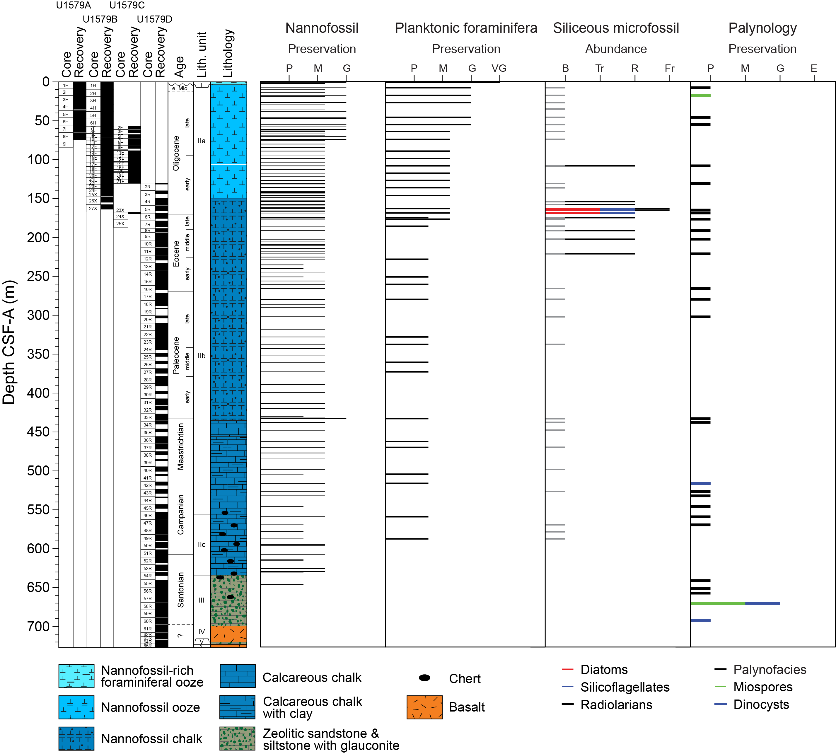
Figure F15. Calcareous nannofossils, planktonic foraminifera, palynomorphs, and siliceous microfossils.
5.1. Calcareous nannofossils
We examined all APC, HLAPC, and XCB core catcher samples from Holes U1579A and U1579B, all XCB core catcher samples from Hole U1579C, and most RCB core catcher samples from Hole U1579D to establish a calcareous nannofossil biostratigraphy (Figure F16; Table T3). Additional samples from split core sections were used to refine ages for selected intervals. Calcareous nannofossil assemblage distribution data are based on shipboard observations, which focused on identification and tabulation of species that are age diagnostic; therefore, the recorded assemblage may not be fully representative of the entire nannofossil assemblage (Tables T4, T5, T6, T7). Photomicrographs of selected nannofossils are shown in Figures F17 and F18.
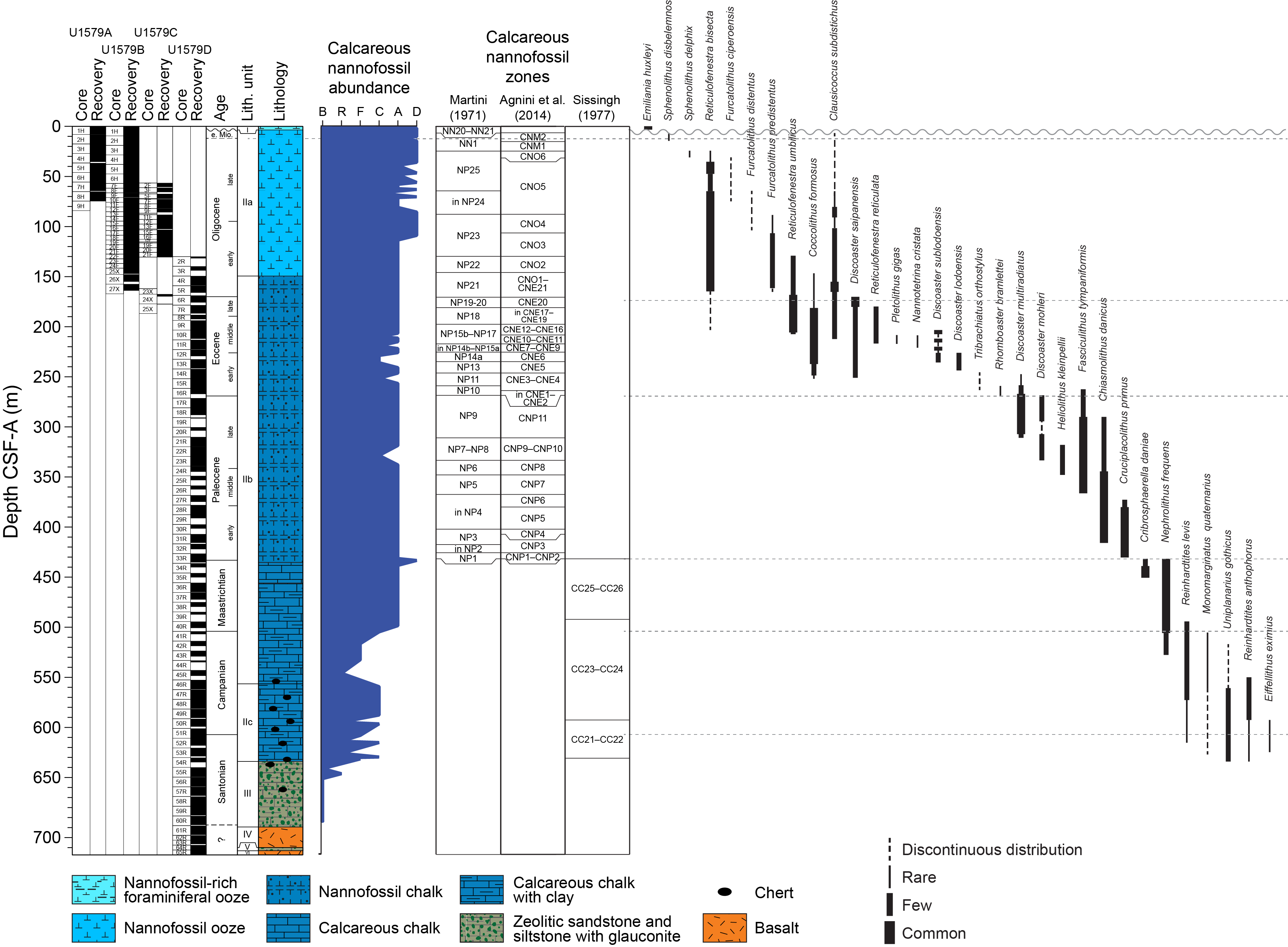
Figure F16. Calcareous nannofossil abundance, zones, and distribution of biostratigraphically important taxa.
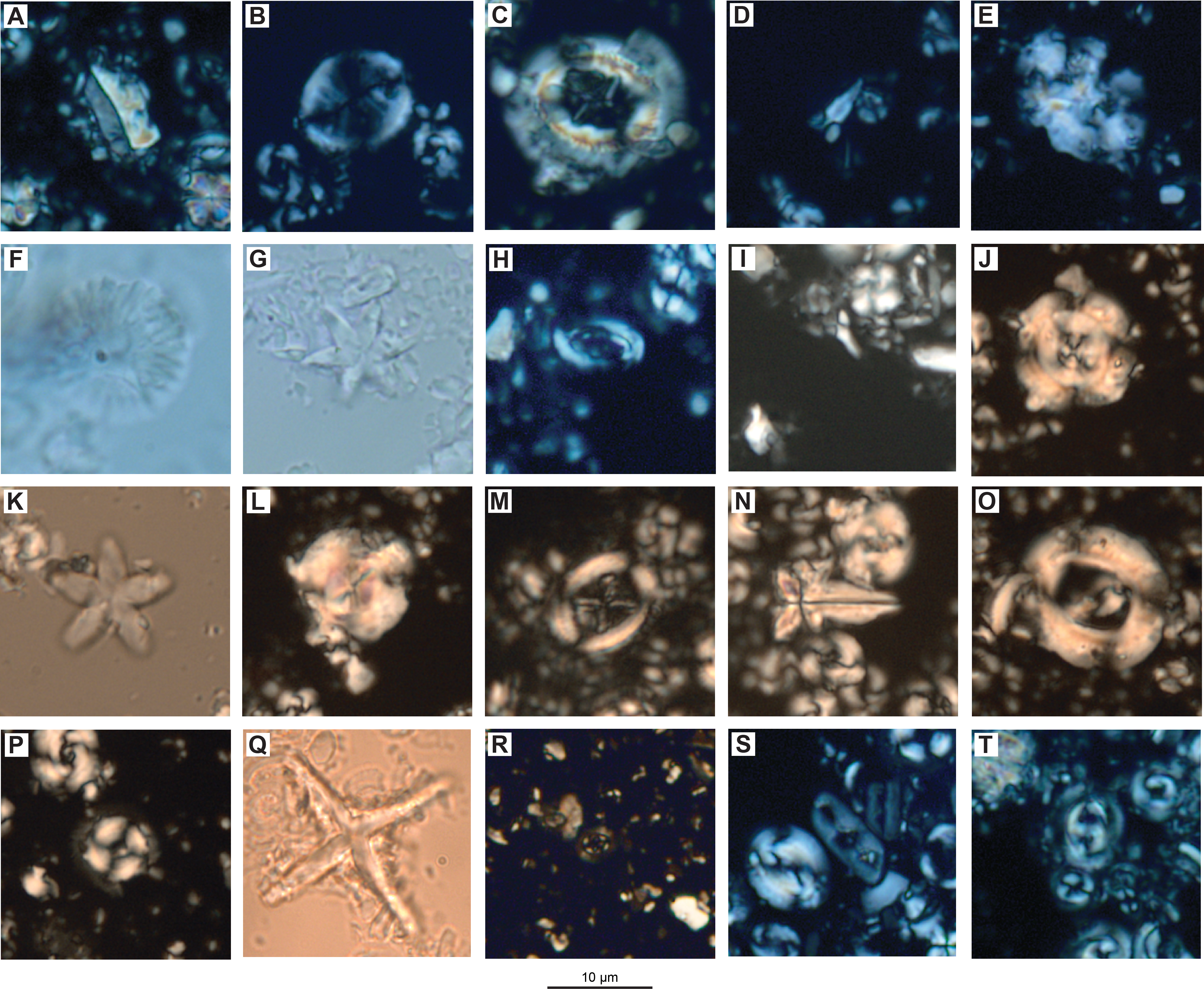
Figure F17. Paleogene calcareous nannofossils.
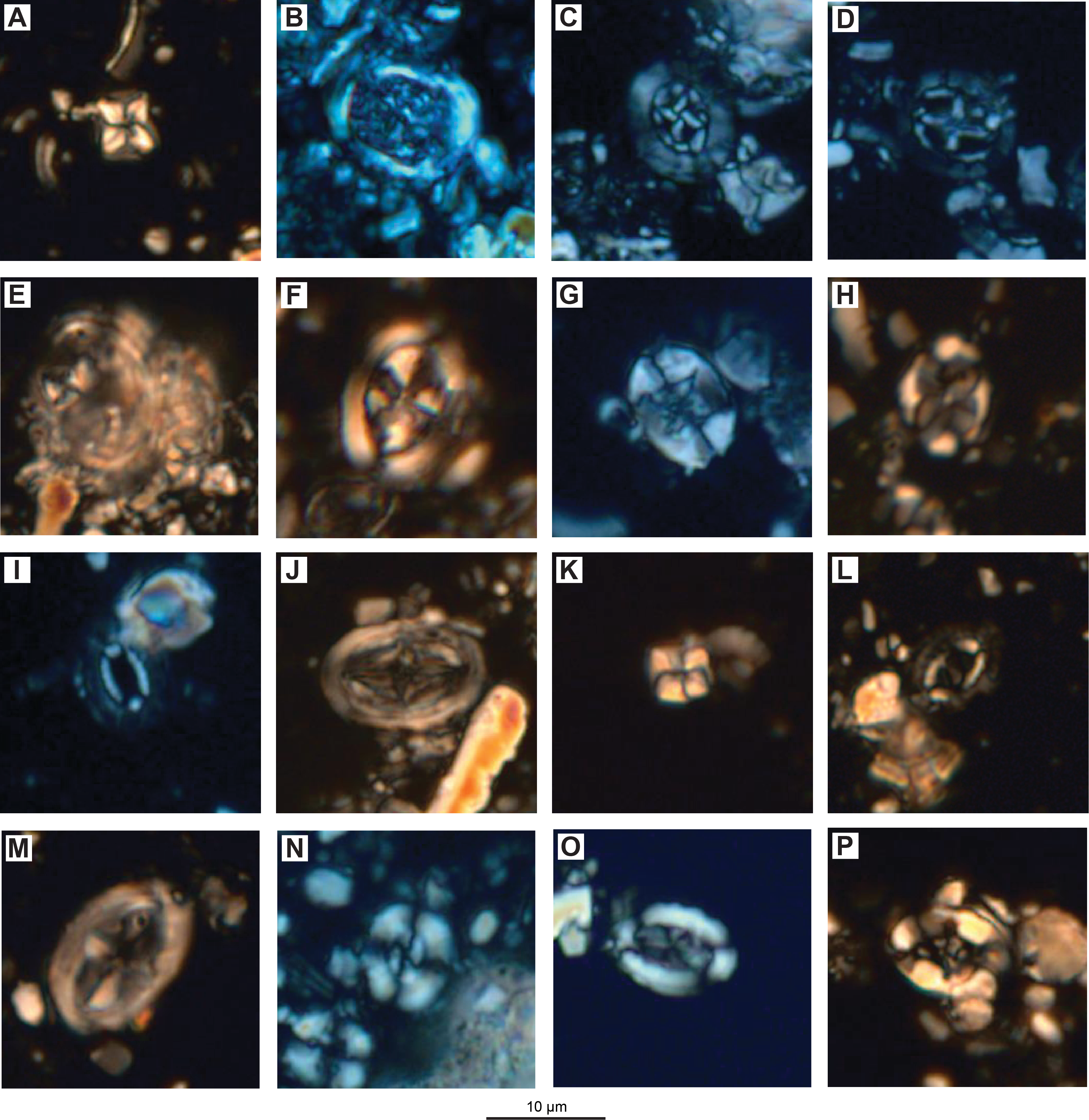
Figure F18. Cretaceous calcareous nannofossils.
Beneath a thin Pleistocene–recent veneer (~1–6 m thick), the sediment recovered in Holes U1579A (1.31–74.78 m CSF-A), U1579B (6.19–163.96 m CSF-A), and U1579C (56.50–177.70 m CSF-A) is predominantly Oligocene to early Miocene in age (Figure F16; Tables T3, T4, T5, T6). Coring in Hole U1579D was initiated at 130.00 m CSF-A in lower Oligocene sediments, and the oldest sediment containing calcareous nannofossils, recovered in Sample 392-U1579D-55R-CC, 9–14 cm (649.38 m CSF-A), is dated to the Late Cretaceous (likely early Campanian) (Figures F16, F18; Tables T3, T7). Calcareous nannofossil assemblages are generally abundant, diverse, and moderately to well preserved in Paleogene sediments (~8–433 m CSF-A) (Figure F17), although the Eocene (~168–267 m CSF-A) contains some intervals with lower abundances and poorer preservation. Maastrichtian sediments (~433–505 m CSF-A) also contain abundant and moderately to well-preserved nannofossils, although diversity is reduced compared to lower latitude sites. Overall abundance and preservation decrease downhole through the Campanian to Santonian (~510–649 m CSF-A), with very sparse and poorly preserved assemblages in some samples.
5.1.1. Pleistocene
The uppermost sediments at Site U1579 consist of Pleistocene nannofossil ooze with foraminifera. Hole U1579A recovered 1.31 m of Pleistocene ooze, and Sample 1H-1, 118 cm (1.18 m CSF-A), contains a Middle Pleistocene nannofossil assemblage with abundant Gephyrocapsa spp., Coccolithus pelagicus, Calcidiscus leptoporus, Helicosphaera carteri, and Florisphaera profunda. The presence of common numbers of Pseudoemiliania lacunosa (biohorizon top = 430 ka) allows placement of this sample within Zone NN20 (Martini, 1971) (Figure F16; Table T3). In Hole U1579B, the Pleistocene drape is 6.13 m thick. Sample 1H-1, 100 cm (1.00 m CSF-A), contains a Late Pleistocene nannofossil assemblage based on the presence of Emiliania huxleyi (biohorizon base = 290 ka) and is assigned to Zone NN21 (Martini, 1971). Both samples also contain numerous reworked Oligocene specimens.
5.1.2. Oligocene–Early Miocene
The Oligocene to lowermost Miocene stratigraphy at Site U1579 is well constrained by 14 nannofossil datums. The samples generally contain abundant and moderately well preserved nannofossils, with assemblages dominated by Cyclicargolithus floridanus, Reticulofenestra spp., including Reticulofenestra bisecta >10 µm (biohorizon top = 23.13 Ma; n2 in Figure F37 and Table T3), C. pelagicus, and Zygrhablithus bijugatus. The presence of diverse sphenolith assemblages, which are a warm-water indicator (e.g., Aubry, 1988; Kalb and Bralower, 2012), suggests that this site was located in the southern middle latitudes during the Oligocene because this group was mostly absent at southern high latitudes at that time (e.g., Wei and Wise, 1990; Wei et al., 1992; Persico and Villa, 2004).
Sediment beneath the Pleistocene veneer is dated to approximately the Oligocene/Miocene boundary. Biohorizon base Sphenolithus disbelemnos (22.90 Ma; n1 in Figure F37) in Sample 392-U1579B-1H-CC, 8–9 cm (9.96 m CSF-A), indicates an earliest Miocene age (Zone NN1/Zone CNM2) (Agnini et al., 2014) for the sediment underlying the disconformity in Hole U1579B. A similar nannofossil assemblage (without S. disbelemnos) in Sample 392-U1579A-1H-CC, 8–13 cm (8.02 m CSF-A), indicates that the sediment underlying the disconformity in Hole U1579A is slightly older, spanning the Oligocene/Miocene boundary. Biohorizon top Sphenolithus delphix (23.11 Ma; n2 in Figure F37) and top Sphenolithus capricornutus (23.11 Ma), identified in Samples 2H-2, 10 cm (9.76 m CSF-A), and 392-U1579B-3H-CC, 14–15 cm (29.14 m CSF-A), indicate a latest Oligocene age within Zones NP25/CNO6. These samples also contain R. bisecta >10 µm (biohorizon top = 23.13 Ma), which also denotes a latest Oligocene age. Biohorizon top Z. bijugatus (23.81 Ma; n3 in Figure F37) is found in Sample 4H-CC, 23–24 cm (38.55 m CSF-A). Biohorizon top Furcatolithus ciperoensis (24.36 Ma; n4 in Figure F37) in Sample 392-U1579A-4H-CC, 31–36 cm (35.43 m CSF-A), indicates the top of Zone CNO5. Biohorizon top Chiasmolithus altus (25.44 Ma; n5 in Figure F37) together with the presence of Cyclicargolithus abisectus in Samples 5H-CC, 13–18 cm (46.12 m CSF-A), and 392-U1579B-5H-CC, 9–14 cm (47.81 m CSF-A), indicate the lower part of Zones NP25/CNO5.
Biohorizon top Furcatolithus distentus (26.81 Ma; n6 in Figure F37) is recognized in Samples 392-U1579A-6H-CC, 8–13 cm (55.67 m CSF-A), and 392-U1579B-8F-CC, 18–19 cm (66.49 m CSF-A). This event marks the top of Zone NP24 and is within Zone CNO5. Biohorizon top Furcatolithus predistentus (26.93 Ma; n7 in Figure F37) falls within Zone NP24 and indicates the top of Zone CNO4. This event is identified in Samples 392-U1579A-8H-4, 40 cm (70.02 m CSF-A), and 392-U1579B-13F-CC, 9–14 cm (89.85 m CSF-A). Additional postcruise research will identify the positions of the Furcatolithus biohorizons on the core composite depth below seafloor (CCSF) depth scale, which should help to resolve discrepancies in their positions between the two holes. Biohorizon base F. distentus (30.0 Ma; n8 in Figure F37) is found in Sample 16F-CC, 0–5 cm (104.11 m CSF-A). This event marks the top of Zone CNO3 and is within Zone NP23.
Biohorizon top Reticulofenestra umbilicus >14 µm (32.02 Ma; n9 in Figure F37) marks the top of Zones NP22 and CNO2. This event is recognized in Sample 392-U1579B-22F-CC, 0–5 cm (132.25 m CSF-A). Biohorizon top Coccolithus formosus (n10 in Figure F37) in Sample 25X-CC, 35–40 cm (147.10 m CSF-A), indicates the top of Zones NP21 and CNO1. This event is also identified in Sample 392-U1579D-2R-CC, 10–15 cm (131.72 CSF-A); however, the interval above this was drilled without coring, so it is unclear if this represents the true biohorizon top of this species in Hole U1579D. Biohorizon top Isthmolithus recurvus (33.06 Ma; n11 in Figure F37) falls within Zones NP21 and CNO1. This event is found in Sample 392-U1579B-26X-2, 57 cm (149.87 m CSF-A).
An interval of increased abundance of Clausicoccus subdistichus (n12 in Figure F37) occurs just above the Eocene/Oligocene boundary; the top of this interval is dated to 33.47 Ma and the base to 33.88 Ma. This event is easily identified at Site U1579: the biohorizon top is found in Samples 392-U1579B-26X-CC, 45–50 cm (154.95 m CSF-A), and 392-U1579D-4R-CC, 11–16 cm (158.82 m CSF-A). Hole U1579B terminated within the C. subdistichus abundant occurrence interval in Sample 392-U1579B-27X-CC, 32–37 cm (163.91 m CSF-A). Coring in Hole U1579C resumed within this interval below a drilled interval between 130.50 and 162.00 m CSF-A, and Sample 24X-CC, 29–34 cm (169.73 m CSF-A), contains common numbers of C. subdistichus and Reticulofenestra daviesii. The latter species also exhibits increased numbers in the Southern Ocean beginning at 33.71 Ma following the Eocene/Oligocene boundary (Fioroni et al., 2012). Biohorizon base abundant C. subdistichus is found in Sample 392-U1579D-5R-CC, 10–15 cm (165.97 m CSF-A). This event marks the base of Zone CNO1 just above the Eocene/Oligocene boundary (33.90 Ma).
5.1.3. Eocene
Based on calcareous nannofossil biostratigraphy, the Eocene/Oligocene boundary in Hole U1579C is identified between Samples 392-U1579C-24X-CC, 29–34 cm (169.73 m CSF-A), and 25X-1, 13 cm (177.3 m CSF-A). In Hole U1579D, the Eocene/Oligocene boundary is located between Samples 5R-CC, 10–15 cm (165.97 m CSF-A), and 6R-CC, 11–16 cm (175.74 m CSF-A). This boundary is marked by a distinct change in sedimentation rate—lower rates in the Eocene and an increase above the Eocene/Oligocene boundary (see Chronostratigraphy). Nannofossil preservation decreases downhole in the Eocene, and several intervals show significant decreases in diversity and increased fragmentation of nannofossil assemblages between 203.60 m CSF-A (middle Eocene) and 222.45 m CSF-A (lower Eocene). This interval is also marked by the lowest sedimentation rates for the entire site and may include one or more hiatuses. Additional postcruise research will help to elucidate whether this interval is highly condensed and whether there are hiatuses present. Despite these challenges, stratigraphy of the Eocene sediment is well resolved with 18 biostratigraphic events. Eocene assemblages are generally dominated by members of Reticulofenestra, following this group’s evolution in the early Eocene at ~52 Ma in the southern high latitudes (Schneider et al., 2011).
Biohorizon top Discoaster saipanensis (34.44 Ma; n14 in Figure F37 and Table T3) is indicative of the latest Eocene, marking the top of Zones NP21 and CNE21 in Sample 392-U1579C-25X-1, 13 cm (177.33 m CSF-A). In Hole U1579D, this event co-occurs with biohorizon top Discoaster barbadiensis (34.77 Ma) in Sample 6R-CC, 11–16 cm (175.74 m CSF-A). Biohorizon top Reticulofenestra reticulata (35.24 Ma; n15 in Figure F37) marks the top of Zone CNE20 in Samples 392-U1579C-25X-CC, 0–5 cm (177.65 m CSF-A), and 392-U1579D-7R-CC, 0–5 cm (186.74 m CSF-A). Biohorizon top Chiasmolithus grandis (37.77 Ma; n16 in Figure F37) and biohorizon base common Chiasmolithus oamaruensis (37.84 Ma; base of Zone NP18) co-occur in Sample 392-U1579D-8R-CC, 0–7 cm (192.46 m CSF-A).
Deeper than the base of Core 392-U1579D-9R (203.65 m CSF-A), sedimentation rates slow significantly, and Cores 10R and 11R represent ~8 My (Table T3) (see Chronostratigraphy). This interval is also marked by poorer preservation and significant fragmentation of the nannofossil assemblage. Biohorizon base R. bisecta >10 µm (40.25 Ma; n18 in Figure F37), found in Sample 9R-CC, 15–20 cm (203.60 m CSF-A), occurs within Zone NP17 and marks the base of Zone CNE15. Biohorizon base common R. umbilicus >14 µm (42.72 Ma; n19 in Figure F37) in Sample 10R-3, 66 cm (207.08 m CSF-A), is within lowermost Zone NP16 and marks the base of Zone CNE13. Pletolithus gigas has a relatively short range in the early middle Eocene. Its biohorizon top (43.64 Ma; n20 in Figure F37), marking the top of Subzone NP15b and Zone CNE11, is identified in Sample 10R-5, 92 cm (210.36 m CSF-A). Biohorizon base P. gigas (n21 in Figure F37), marking the base of Subzone NP15b and Zone CNE10, is found in Sample 11R-2, 105 cm (215.61 m CSF-A). Biohorizon base Nannotetrina cristata (47.85 Ma; n22 in Figure F37), which falls within Subzone NP14b and marks the base of Zone CNE8, is identified in Sample 11R-CC, 0–5 cm (222.42 m CSF-A).
Biohorizon top Discoaster lodoensis (48.22 Ma; n23 in Figure F37), found in Sample 392-U1579D-12R-3, 80 cm (226.61 m CSF-A), is within Subzone NP14a and marks the top of Zone CNE6. Biohorizon base common Discoaster sublodoensis (48.80 Ma; n24 in Figure F37), which marks the base of Zones NP14 and CNE6, is identified in Sample 12R-CC, 19–24 cm (229.35 m CSF-A). Two events dated to 50.65 Ma are identified in Sample 13R-CC, 0–5 cm (241.58 m CSF-A): (1) biohorizon top Tribrachiatus orthostylus (n25 in Figure F37), which marks the top of Zones NP12 and CNE4, and (2) the crossover in abundance from predominantly Toweius to predominantly Reticulofenestra (n25 in Figure F37). The latter event marks a significant change in nannofossil assemblages worldwide, with Reticulofenestra dominating assemblages for the remainder of the Paleogene and Neogene.
Sedimentation rates increase below Core 392-U1579D-13R (241.63 m CSF-A) (see Chronostratigraphy). Biohorizon base Toweius gammation (53.67 Ma; n26 in Figure F37) is found in Sample 14R-CC, 23–28 cm (252.21 m CSF-A). Biohorizon base T. orthostylus (54.3 Ma; n28 in Figure F37), which falls within Zone NP10 and marks the base of Zone CNE3, is identified in Sample 15R-CC, 12–17 cm (261.78 m CSF-A). Because of minor but pervasive reworking of Cretaceous and Paleocene species, we are unable to identify the biohorizon top of Fasciculithus spp. (55.60 Ma), which occurs after the PETM. Sample 16R-CC, 15–20 cm (267.14 m CSF-A), includes two markers for the PETM, biohorizon base Rhomboaster bramlettei (56.0 Ma; base of Zone NP10; n29 in Figure F37) and biohorizon base Campylosphaera eodela (56.0 Ma). These species are absent in Sample 17R-1, 20 cm (271.5 m CSF-A). Core 16R contains no visual indication of carbonate dissolution that would typically mark the PETM, and, unfortunately, poor recovery in Core 16R (58%) suggests that the Paleocene/Eocene boundary (and the base of the PETM) is likely within the core gap below Core 16R. Therefore, only some of the PETM recovery phase may be present within the sediments recovered at Site U1579.
5.1.4. Paleocene
Nannofossil preservation is variable throughout the Paleocene; samples contain moderately preserved abundant nannofossils in the upper Paleocene and poor to moderate preservation with common numbers of nannofossils in the lowermost Paleocene sediments. The upper Paleocene assemblages are characterized by common to abundant Toweius pertusus, Toweius callosus, Toweius eminens, Prinsius martinii, and Prinsius bisulcus. Other species that are consistently present include C. pelagicus, Chiasmolithus bidens, and Sphenolithus moriformis. The lower Paleocene sediments are marked by a significant decrease in diversity and increased fragmentation of nannofossils, including a prominent increase in calcispheres downhole. Paleocene stratigraphy at Site U1579 is defined using 13 nannofossil datums.
Biohorizon top Ericsonia robusta (57.11 Ma; n30 in Figure F37 and Table T3), which falls within Zones NP9 and CNP11, is found in Sample 392-U1579D-19R-CC, 10–15 cm (291.55 m CSF-A). Biohorizon base Discoaster multiradiatus (57.32 Ma; n31 in Figure F37), which marks the base of Zones NP9 and CNP11, is recognized in Sample 20R-CC, 13–18 cm (303.75 m CSF-A). Despite persistent reworking in the lower Eocene (Table T7), biohorizon top Heliolithus kleinpellii (58.80 Ma; n32 in Figure F37) is identified at the top of its consistent presence in Sample 21R-CC, 5–10 cm (319.84 m CSF-A). This event is within Zones NP7 and CNP9. Biohorizon base Discoaster mohleri (58.97 Ma; n33 in Figure F37), which also represents the evolution of this genus and marks the base of Zones NP7 and CNP9, is recognized in Sample 22R-CC, 16–21 cm (329.76 m CSF-A). Biohorizon base H. kleinpellii (59.36 Ma; n34 in Figure F37), which marks the base of Zone NP6 and is within Zone CNP8, and biohorizon base Heliolithus cantabriae (59.60 Ma; n35 in Figure F37), which marks the base of Zone CNP8, are recorded together in Sample 24R-CC, 15–20 cm (344.76 m CSF-A). There is a notable change in assemblage at about this depth (~345 m CSF-A), with more diverse Toweius above, including T. eminens and Toweius tovae, whereas in deeper samples, members of Prinsius are more abundant and Toweius is represented by only T. pertusus and a few related taxa.
Biohorizon base Fasciculithus tympaniformis (61.27 Ma; n36 in Figure F37), which is documented in Sample 392-U1579D-26R-CC, 19–24 cm (362.38 m CSF-A), marks the base of Zone NP5 and is located within the lower part of Zone CNP7. Biohorizon base S. moriformis (62.10 Ma; n37 in Figure F37), which also represents the evolution of this genus, is recorded in Sample 27R-CC, 19–24 cm (374.80 m CSF-A). This event is located within upper Zone NP4 and also marks the base of Zone CNP6. Biohorizon base common T. pertusus (63.15 Ma; n38 in Figure F37), which marks the base of Zone CNP5, is identified in Sample 29R-CC, 18–23 cm (391.15 m CSF-A). Biohorizon base P. martinii (63.66 Ma; n39 in Figure F37), within Zone NP3 and marking the base of Zone CNP4, is identified in Sample 30R-CC, 14–19 cm (401.41 m CSF-A). The base of Zone NP3 is defined by biohorizon base Chiasmolithus danicus (64.53 Ma; n40 in Figure F37), which is identified in Sample 31R-CC, 28–33 cm (415.70 m CSF-A). Biohorizon base Cruciplacolithus intermedius (65.45 Ma; n41 in Figure F37) is documented in Sample 32R-CC, 13–18 cm (422.05 m CSF-A), and is located within Zones NP2 and CNP2. Biohorizon base Cruciplacolithus primus (65.77 Ma; n42 in Figure F37) is identified in Sample 33R-5, 70–71 cm (432.26 m CSF-A), and coincides with a considerable increase in the numbers of calcispheres and reworked Cretaceous specimens. This event occurs within Zones NP1 and CNP1.
5.1.5. Cretaceous
The K/Pg boundary, recovered in Section 392-U1579D-33R-6, 98.5 cm (433.255 m CSF-A), is marked by a pronounced sediment color change from white to red (see Lithostratigraphy). We examined samples from just above and below the boundary to confirm the age of the sediment. Sample 33R-6, 95 cm (433.22 m CSF-A), contains mostly broken pieces of calcite and common numbers of reworked Cretaceous species (including Micula staurophora, Micula murus, Biscutum constans, Nephrolithus frequens, and Arkhangelskiella cymbiformis). Rare to few numbers of known survivor taxa are also present, including Biscutum harrisonii, Cyclagelosphaera reinhardtii, Markalius inversus, and Zeugrhabdotus sigmoides. Neither Neobiscutum parvulum nor C. primus were observed, suggesting that this sediment represents deposition soon after the mass extinction event. Sample 33R-6, 102 cm (433.29 m CSF-A), immediately below the boundary, contains a reasonably well preserved late Maastrichtian assemblage characterized by abundant N. frequens, common Prediscosphaera cretacea, Micula spp., and Kamptnerius magnificus (n43 in Figure F37). Other typical Late Cretaceous taxa include Eiffellithus turriseiffelii and Watznaueria barnesiae.
Cores 392-U1579D-34R through 46R (436.20–562.00 m CSF-A) are dated to the Maastrichtian to early Campanian. The Maastrichtian is characterized by diverse and moderately preserved calcareous nannofossil assemblages that include common numbers of N. frequens, K. magnificus, M. murus, A. cymbiformis, M. staurophora, Prediscosphaera spp., Cribrosphaerella daniae, and Cribrosphaerella ehrenbergii. These assemblages are similar to southern high-latitude assemblages sampled on Maud Rise (Pospichal and Wise, 1990), Northeast Georgia Rise (Crux, 1991), and Kerguelen Plateau (Watkins, 1992). These and other studies (e.g., Wise, 1988) demonstrated that the Maastrichtian is marked by provincialism in nannoplankton, with some taxa, such as Nephrolithus, appearing significantly earlier in the southern high latitudes. Watkins et al. (1996) and Guerra et al. (2016) built on prior zonations from earlier studies to develop a Late Cretaceous southern high-latitude zonation. We see a similar distribution of taxa in the upper Campanian and Maastrichtian intervals at Site U1579, suggesting that this site was located in the southern high-latitude province at that time. This is particularly true for the abundant occurrences of K. magnificus and M. murus in the upper Maastrichtian (Samples 34R-CC, 10–15 cm, to 39R-CC, 16–21 cm [440.14–487.32 m CSF-A]) and upper Campanian (Samples 45R-CC, 15–20 cm, to 48R-CC, 0–5 cm [548.50–581.23 m CSF-A]). Due to a paucity of magnetostratigraphic records from many of these high-latitude sites, the zones and datums are not well dated. Therefore, we report the Gradstein et al. (2020) ages for Cretaceous events but caution that these represent Tethyan ages and may not be valid for the southern high latitudes.
Biohorizon top Reinhardtites levis (70.14 Ma; n44 in Figure F37 and Table T3), identified in Sample 392-U1579D-40R-CC, 17–22 cm (500.76 m CSF-A), marks the top of Zone CC24 (Sissingh, 1977; Perch-Nielsen, 1985) and indicates that the interval above comprises Zones CC25–CC26. This event is accompanied by a decline in N. frequens abundance, and its biohorizon base is observed in Sample 43R-CC, 15–20 cm (529.10 m CSF-A), similar to the succession observed at Maud Rise (Pospichal and Wise, 1990). Because the Gradstein et al. (2020) age for this event is from the Tethyan region, we do not include it in our age-depth model (Table T3) (see Chronostratigraphy). Many of the markers for the early Maastrichtian are absent at Site U1579 or are only present well below their dated extinction level from the Tethyan region, including Uniplanarius trifidus, Broinsonia parca constricta, and Tortolithus caistorensis; therefore, we also exclude these from the age-depth model. Biohorizon top Monomarginatus quaternarius (72.10 Ma; n45 in Figure F37), in Zone CC23 and located just above the Campanian/Maastrichtian boundary, is recorded in Sample 41R-CC, 16–21 cm (506.89 m CSF-A). Biohorizon top Uniplanarius gothicus (72.48 Ma; n46 in Figure F37), also within Zone CC23 and located just below the Campanian/Maastrichtian boundary, is identified in Sample 42R-CC, 18–23 cm (518.76 m CSF-A), suggesting that the Campanian/Maastrichtian boundary is located within Core 42R. However, nannofossils in samples from the Campanian and lower Maastrichtian are generally sparse and poorly to moderately preserved, so additional postcruise research may result in refinement of these datum positions.
Deeper than the base of Core 392-U1579D-44R (534.96 m CSF-A), nannofossil abundance decreases even further, and many samples contain only rare to few numbers of nannofossils. Despite this, we were able to identify biohorizon top Reinhardtites anthophorus (74.47 Ma; n47 in Figure F37) in Sample 45R-CC, 15–20 cm (548.50 m CSF-A). This event falls within Zone CC23. Biohorizon top Eiffellithus eximius (75.85 Ma; n48 in Figure F37), which marks the top of Zone CC22, is identified in Sample 50R-CC, 9–14 cm (599.24 m CSF-A); however, this is likely not the true top of this taxon, as it should occur within a normal polarity interval (Chron C33n), whereas this sample is within a reversed polarity interval assigned to Chron C33r (see Paleomagnetism). Sparse nannofossil assemblages are sporadically present in Cores 51R–54R (601.10–634.76 m CSF-A) and are consistent with an early Campanian age; however, no additional marker taxa were identified. A significant transition in sediment color from red above to green below is present in Section 54R-CC, 21 cm (634.72 m CSF-A); nannofossils are extremely rare or absent in this green sediment (Lithostratigraphic Unit III).
5.2. Foraminifera
Core catcher samples from the APC, HLAPC, XCB, and RCB cores retrieved from the mudline of Hole U1579A to the bottom of Core 392-U1579D-49R (0–590.5 m CSF-A) were processed and examined for planktonic and benthic foraminifera in the >45 µm size fraction. Assemblages in the 45–63 and 63–150 µm fractions were similar, whereas assemblages in the >150 µm size fraction were not necessarily representative of small foraminifera, especially the biserial planktonic assemblages. Samples from Hole U1579A and most of Holes U1579B and U1579C (within Lithostratigraphic Unit I and Lithostratigraphic Subunit IIa; see Lithostratigraphy) were easily disaggregated. Core catcher samples from the upper part of Lithostratigraphic Subunit IIb (Cores 392-U1579D-6R–26R; 168.80–362.43 m CSF-A) required soaking and stirring for disaggregation. The sediments from deeper than Core 26R are more lithified, and acetic acid or H2O2 was used to help disaggregate these samples as well as remove fine particles (including nannofossils and clay) from foraminiferal specimens, which would otherwise obscure diagnostic features.
Foraminiferal preservation decreases downhole at Site U1579 from very good to poor (Figure F15). Preservation degrades significantly in Samples 392-U1579D-12R-CC, 19–24 cm, to 14R-CC, 23–28 cm (229.35–252.21 m CSF-A), returns to moderate in Sample 15R-CC, 12–17 cm (261.78 m CSF-A), and then degrades again to poor in Sample 22R-CC, 16–21 cm (329.76 m CSF-A). Foraminiferal preservation remains poor deeper than Core 22R (329.81 m CSF-A) until the extraction of foraminifera was no longer feasible, which was below Sample 49R-CC, 25–30 cm (590.45 m CSF-A). Slight to moderate dissolution is visible on small delicate planktonic foraminifera such as Globorotaloides quadrocameratus in Sample 392-U1579A-1H-CC, 8–13 cm (8.02 m CSF-A) (Figure F19A). Recrystallization of foraminiferal tests was observed in Samples 7H-CC, 9–14 cm (64.41 m CSF-A) (slight; Figure F19B), and 392-U1579B-13F-CC, 9–14 (89.85 m CSF-A) (severe; Figure F19C). Recrystallization is apparent in samples below Sample 392-U1579D-26R-CC (362.43 m CSF-A) and common below Sample 46R-CC (562.00 m CSF-A). However, there is considerable variability in the extent of recrystallization between specimens within core catcher samples, and individual foraminifera tests may appear clear to semitransparent under light microscopy, whereas SEM reveals that this is likely the result of remineralization. We therefore highly recommend SEM imaging for any samples to be used for geochemical analyses in postcruise studies. Benthic foraminifera are often better preserved, less fragmented, and much less abundant than the planktonic foraminifera throughout the sedimentary succession at Site U1579. Planktonic foraminifera abundances and distribution are documented in Table T8, which also includes information about the state of preservation and other biogenic and microscopic materials noted during examination. Benthic foraminifera abundances and distribution are documented in Table T9.
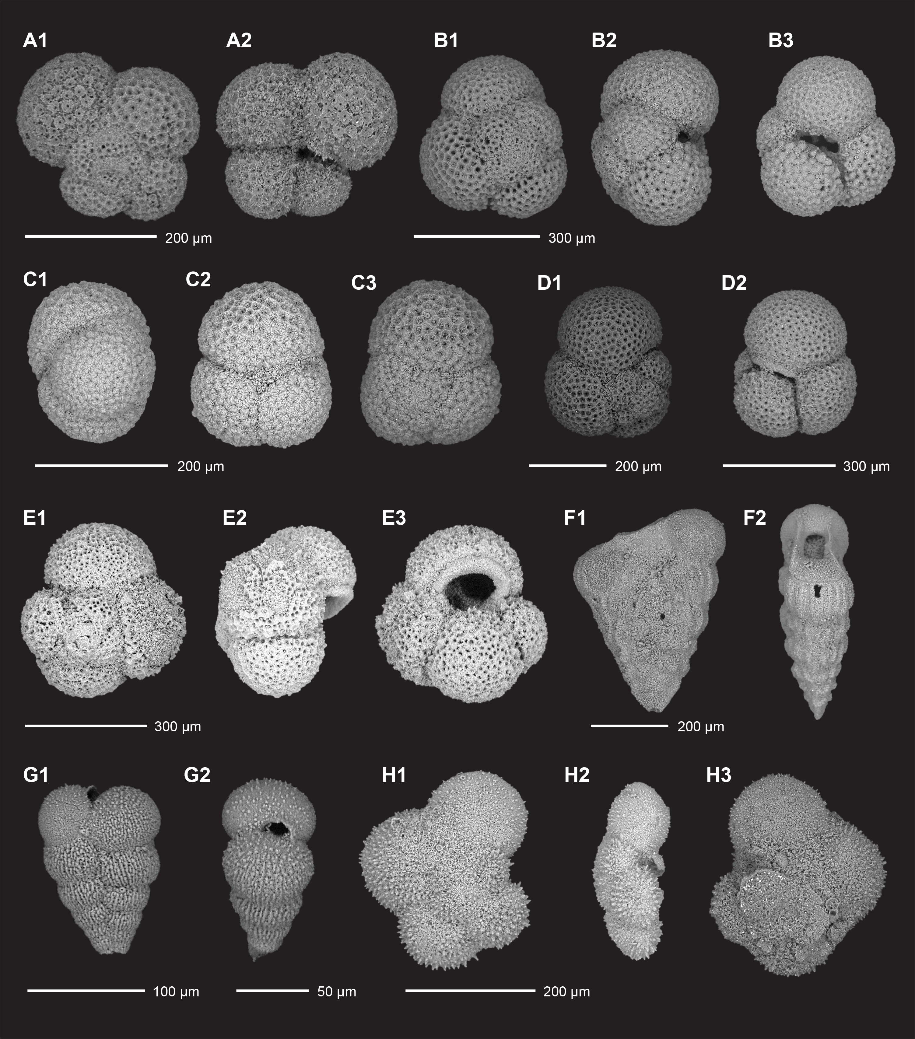
Figure F19. Planktonic foraminifera.
Overall, benthic foraminifera from all Site U1579 samples are much less abundant than planktonic foraminifera and consist mostly of Cibicidoides, Gyroidinoides, Bolivina, Bulimina, Uvigerina, Lenticulina, Siphonodosaria, and Nodosaria species. When possible, specimens were identified to species level, but lineages and/or morphologic changes will be further examined during postcruise research. Although benthic foraminifera are typically less useful for biostratigraphy than planktonic foraminifera, we were able to identify several useful datums.
Foraminifera collected from the mudline and Sample 392-U1579B-1H-3, 67–68 cm (3.71 m CSF-A), have very similar assemblages that indicate a Pleistocene to recent age. The mid-Pleistocene extinction event, commonly referred to as the Stilostomella extinction, includes extinction and die-back of several species well documented in Deep Sea Drilling Project (DSDP) and Ocean Drilling Program (ODP) sites in the southwest Pacific. It has been noted that in the southwest Pacific, extinction and die-back groups began to decline in the Late Pliocene with greater extinction rates between 0.7 and 1.2 Ma (Hayward, 2002). One of these benthic foraminifera, Pleurostomella (range = Eocene to mid-Pleistocene), is consistently present from Sample 392-U1579A-2H-CC, 8–13 cm (17.77 m CSF-A), to at least Sample 392-U1579B-25X-CC, 35–40 cm (147.10 m CSF-A). The presence of Aragonia velascoensis (range = Campanian to early Eocene) in Sample 392-U1579D-14R-CC, 23–28 cm (252.21 m CSF-A), indicates an Eocene age, and the biohorizon top Bolivinoides draco (66.04 Ma; f4 in Figure F37 and Table T3) in Sample 33R-CC, 15–20 (435.23 m CSF-A), is indicative of a latest Cretaceous age (Figure F20D). Most if not all benthic foraminiferal assemblages are indicative of bathyal water depths.
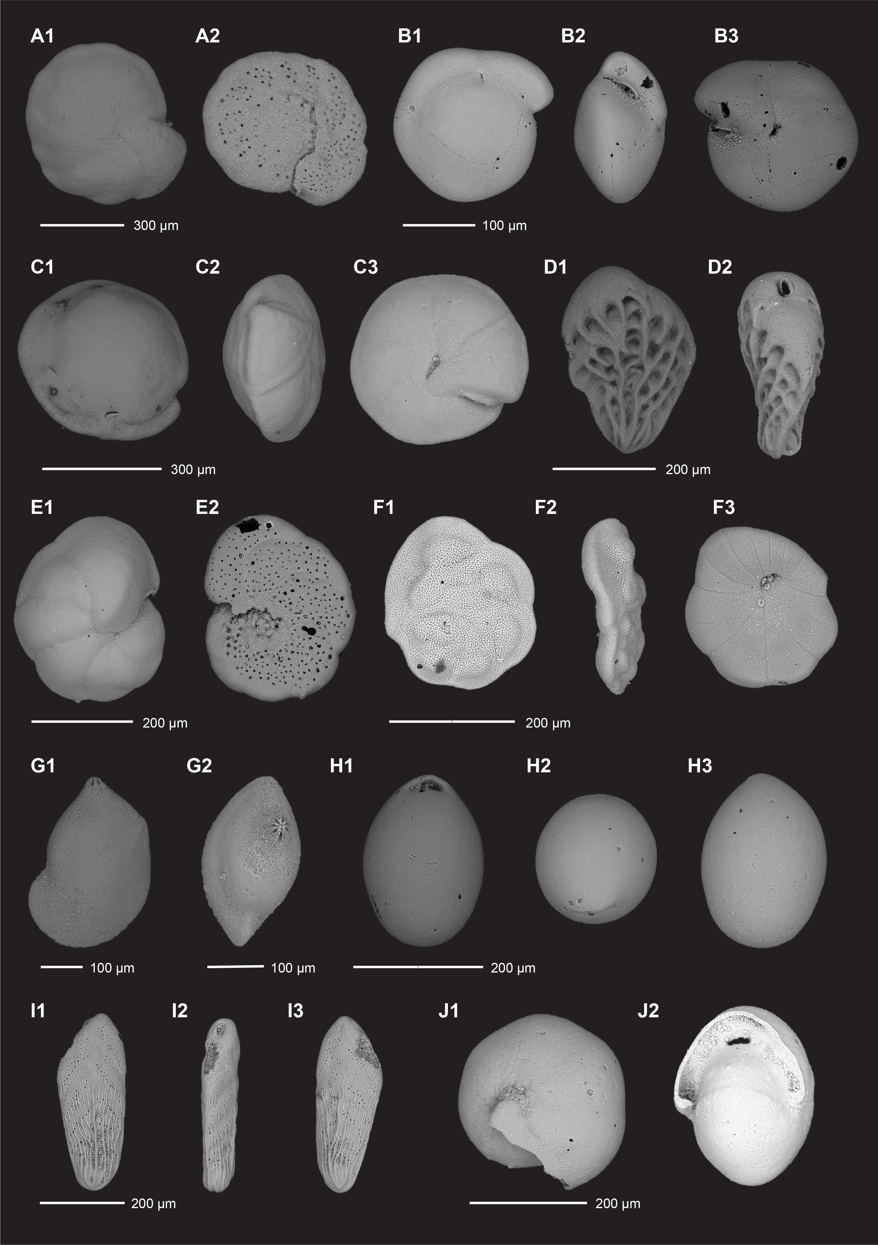
Figure F20. Benthic foraminifera.
Planktonic foraminifera are generally abundant in all samples examined, allowing identification of several planktonic foraminifera biohorizons (Table T3). These datums correlate well with both the nannofossil biostratigraphy and magnetostratigraphy (see Paleomagnetism and Chronostratigraphy). Subbotina dominates most planktonic foraminiferal assemblages in Samples 392-U1579A-7H-CC, 9–14 cm (64.41 m CSF-A; upper Oligocene), to 392-U1579D-26R-CC, 19–24 cm (362.38 m CSF-A; middle Paleocene), although preservation was very poor and identification difficult in samples from Cores 22R (329.76 m CSF-A) and 23R (339.23 m CSF-A). Biohorizon top Subbotina eocaena (within Zone O6 [Wade et al., 2011]; 25.21–26.93 Ma) and biohorizon top Subbotina angiporoides (within Zone O3; 29.18–30.28 Ma; f2 in Figure F37) are both identified in Sample 392-U1579B-13F-CC, 9–14 cm (89.85 m CSF-A). However, Subbotina with infilled apertures that could not be identified to species level are present above this depth in Samples 392-U1579A-7H-CC, 9–14 cm (64.41 m CSF-A), and 8H-CC (74.73 m CSF-A), and the true top of S. eocaena may therefore be well above 89.95 m CSF-A. Biohorizon top common Chiloguembelina cubensis (27.29 Ma; f1 in Figure F37) marks the top of Zone O4, very near the early/late Oligocene boundary. C. cubensis is present, although not abundantly, in Sample 392-U1579B-13F-CC, 9–14 cm (89.85 m CSF-A), in the 63–150 µm size fraction (absent in the >150 µm size fraction), is absent in Sample 15F-CC, 12–17 cm (99.49 m CSF-A), and dominates the assemblage in Sample 17F-CC, 8–13 cm (108.85 m CSF-A). We tentatively identify the biohorizon top of C. cubensis in Sample 13F-CC, 9–14 cm (89.85 m CSF-A).
Subbotina utilisindex (biohorizon top in Zone O3; 29.18–30.28 Ma; f3 in Figure F37) is present in Sample 392-U1579B-21F-CC, 5–10 cm (127.64 m CSF-A). The biohorizon top of Chiloguembelina ototara is within Zone O2 (32.10–30.28 Ma) and is identified in Sample 27X-CC, 32–37 cm (163.91 m CSF-A). This sample also contains larger specimens and higher abundances of benthic foraminifera than samples from shallower depths. Assemblages are similar in Sample 392-U1579D-12R-CC, 19–24 cm (229.35 m CSF-A), indicating an Oligocene age for this interval. A transition from the Oligocene to Eocene can be inferred in Sample 14R-CC, 23–28 cm (252.21 m CSF-A), based on the presence of the benthic foraminifera A. velascoensis and the planktonic foraminifera Planorotalites capdevilensis and Acarinina collactea. Within this sample, preservation is poor, with recrystallization, infilling of apertures, and red coloration in most tests.
Globotruncanella havanensis, Planohedbergella aspera, Gublerina rajagopalani, and Gublerina cuvillieri (top within the Abathomphalus mayaroensis Zone of Gradstein et al., 2012, and references therein; 67.30–69.18 Ma; f5 in Figure F37), as well as the benthic foraminifera B. draco (biohorizon top at the end of the Cretaceous), are present in Sample 392-U1579D-33R-CC, 15–20 cm (435.23 m CSF-A), demarcating the transition from the Paleocene above into the Cretaceous below. Specimens from this sample show recrystallization but can be easily cleaned of fine particles (including calcareous nannofossils and clay) with light ultrasonification. Specimens from Hole U1579D were extracted with acetic acid and using only water. The best specimens came from agitation in water as even momentary exposure to acetic acid appeared to remove significant amounts of test material. Large agglutinated benthic foraminifera, such as Cribrostomoides subglobosus, were present in Sample 41R-CC, 16–21 cm (506.89 m CSF-A), whereas biserial species of Planoheterohelix dominate in Sample 42R-CC, 18–23 cm (518.76 m CSF-A). Planohedbergella impensa, P. aspera, and Planohedbergella prairiehillensis have biohorizon tops in the G. havanensis Zone (74.00–75.71 Ma; f6 in Figure F37) and are present in Sample 46R-CC, 9–14 cm (561.95 m CSF-A). Similar species are present down to Sample 49R-CC, 25–30 cm (590.45 m CSF-A), below which shipboard processing of samples ceased due to the indurated sediment and poor preservation of extracted foraminifera. Additionally, sparse foraminifera were noted in some thin sections from Lithostratigraphic Unit III (see Lithostratigraphy).
Other biogenic materials observed in core catcher residues included abundant ostracods (Cores 392-U1579A-1H, 2H, 3H, 5H, 7H, and 8H and 392-U1579B-13F, 15F, 17F, 19F, 21F, and 23F), a single fish tooth (Sample 392-U1579D-33R-CC, 15–20 cm [435.23 m CSF-A]), radiolarians, and the calcisphere Pithonella ovalis in Samples 42R-CC, 18–23 cm (518.76 m CSF-A), and 46R-CC, 9–14 (561.95 m CSF-A). Interestingly, P. ovalis calcisphere specimens have been noted in Maastrichtian-age materials when present in abundance (Banner, 1972). In core catcher samples, these calcispheres were abundant in both the 63–150 and >150 µm size fractions. The preservation state was also different between Samples 42R-CC, 18–23 cm (518.76 m CSF-A), and 46R-CC, 9–14 cm (561.95 m CSF-A), with the former being more delicate and lattice-like and the latter heavily recrystallized.
5.3. Siliceous microfossils
Smear slides were routinely made from APC, HLAPC, XCB, and RCB core catcher samples from Holes U1579A–U1579D and checked for the presence of siliceous microfossils. Additionally, 36 core catcher samples were decalcified in an attempt to detect rare occurrences of diatoms, silicoflagellates, and radiolarians (Table T10). The mudline from Hole U1579A (Sample 392-U1579A-1H-1, 0 cm) only contained rare radiolarian fragments and sponge spicules, making age assignment difficult. Most samples from Holes U1579A–U1579D were barren of siliceous microfossils; however, an interval spanning the EOT (Samples 392-U1579B-17F-CC, 8–13 cm, to 27X-CC, 32–37 cm [108.85–163.91 m CSF-A]; 392-U1579C-24X-CC, 29–34 cm [169.73 m CSF-A]; and 392-U1579D-4R-CC, 11–16 cm, to 5R-CC, 0–5 cm [158.82–165.97 m CSF-A]) contains an assemblage of radiolarians and silicoflagellates that are age diagnostic, whereas diatoms are poorly preserved and present only in trace amounts.
5.3.1. Oligocene
Sample 392-U1579B-27X-CC, 32–37 cm (163.91 m CSF-A), contains rare Coscinodiscus spp. fragments and Liostephania stage diatoms (see Schrader [1974] for a discussion of Liostephania stage diatom preservation) (Figure F21A, F21D, F21E). Additionally, this sample contains the age-diagnostic silicoflagellates Naviculopsis biapiculata and Distephanus crux, suggesting an Oligocene age (Figure F21B, F21C, F21G, F21H). Sample 392-U1579D-5R-CC, 10–15 cm (165.97 m CSF-A), has a similar silicoflagellate assemblage to that observed in Sample 392-U1579B-27X-CC, 32–37 cm (163.91 m CSF-A). The diatom assemblage is fragmented and exhibits poor preservation and contains Cestodiscus spp. and Coscinodiscus spp. fragments and a dissolved Hemiaulus spp., which also indicate an Oligocene or Eocene age depending on species level identification that was not possible due to poor preservation (Figure F21F). This sample also contains Liostephania stage diatoms similar to those observed in Sample 392-U1579D-5R-CC, 10–15 cm (165.97 m CSF-A). Sample 392-U1579C-24X-CC, 29–34 cm (169.73 m CSF-A), contains Liostephania stage diatoms and the silicoflagellate N. biapiculata (Figure F21B, F21C). All other samples from Holes U1579B and U1579D are barren of diatoms and silicoflagellates.
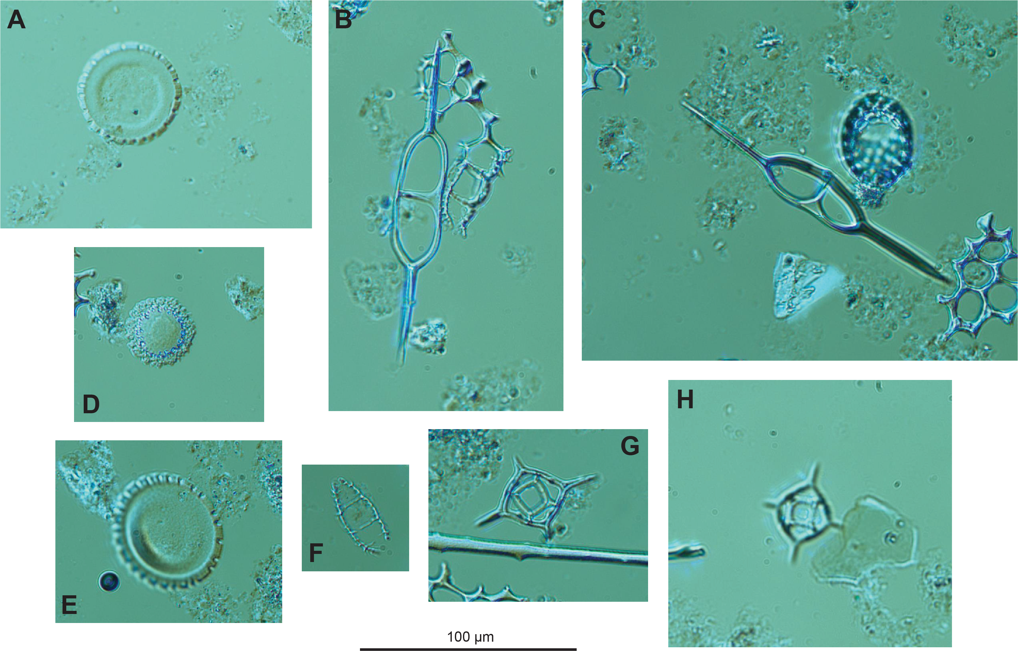
Figure F21. Siliceous microfossils.
Sample 392-U1579B-27X-CC, 32–37 cm (163.91 m CSF-A), contains common radiolarians. The radiolarian assemblage is also consistent with the Oligocene to EOT interval (Christopher Hollis, pers. comm., 2022). Samples 392-U1579D-5R-CC, 10–15 cm (165.97 m CSF-A), and 392-U1579C-24X-CC, 29–34 cm (169.73 m CSF-A), have a similar radiolarian assemblage to what was observed in Sample 392-U1579B-27X-CC, 32–37 cm (163.91 m CSF-A). Rare radiolarian fragments were observed in Samples 17F-CC, 8–13 cm (108.85 m CSF-A), and 26X-CC, 45–50 cm (154.95 m CSF-A), and in Samples 392-U1579D-4R-CC, 11–16 cm (158.82 m CSF-A); 6R-CC, 11–16 cm (175.74 m CSF-A); and 8R-CC, 0–7 cm, to 11R-CC, 0–5 cm (192.46–222.40 m CSF-A). The remaining samples from Holes U1579A–U1579D were barren of radiolarians.
5.3.2. Paleoenvironment, preservation, and depositional setting
The presence of diatoms and silicoflagellates in three samples and the rare occurrences of radiolarians in nine samples from the EOT to lower Oligocene interval of Site U1579 may suggest the influence of cool/intermediate waters over the site at that time, likely from Antarctic Intermediate Water (AAIW) input, which would support diatom and radiolarian productivity. The absence of siliceous microfossils throughout the rest of the sedimentary sequence recovered at Site U1579 may be a result of both low siliceous microfossil sedimentation at the site and postdepositional diagenesis. The dissolution of biogenic opal is facilitated by high-alkalinity interstitial water (IW) in carbonate-rich sediments (Flower, 1993), which is consistent with the carbonate-rich sequence observed for Site U1579 (see Lithostratigraphy). The presence of Liostephania stage (internal casts of diatom frustules) diatoms indicates enhanced dissolution (Hanna and Brigger, 1970), which was observed together with fragments of diatoms in Samples 392-U1579B-27X-CC, 32–37 cm (163.91 m CSF-A); 392-U1579C-24X-CC, 29–34 cm (169.73 m CSF-A); and 392-U1579D-5R-CC, 10–15 cm (165.97 m CSF-A). These observations are consistent with elevated alkalinity and Si within IW samples from Site U1579 (Figure F39; Table T11).
5.4. Palynology
Sixteen core catcher samples from Holes U1579A–U1579C were decalcified for analysis of biogenic organic content (Table T12). The mudline sample of Hole U1579A contains common amorphous organic matter and rare brown phytoclasts. Other decalcified samples contain trace amounts of amorphous organic matter and brown phytoclasts.
Twenty samples from Hole U1579D were decalcified for analysis of noncarbonate biogenic content (Table T12). Almost all of the samples are barren of palynomorphs apart from trace amounts of brown phytoclasts and amorphous organic matter. Core catcher samples from Cores 42R–47R (518.76–572.31 m CSF-A) and split-core samples from Cores 55R–60R (644.26–695.68 m CSF-A) were processed with hydrofluoric acid (HF) to extract palynomorphs. Two of these samples yielded palynofacies. Sample 42R-CC, 18–23 cm (518.76 m CSF-A), contains frequent amorphous organic matter and brown phytoclasts and trace amounts of marine palynomorphs. The sample from a dark brown zeolitic silty claystone in Lithostratigraphic Unit III (Sample 58R-4, 109–111 cm; 673.74 m CSF-A) contains abundant dark brown amorphous organic matter, frequent dark brown phytoclasts, common and well-preserved dinocysts, frequent well-preserved miospores, and rare prasinophytes (Figure F22).
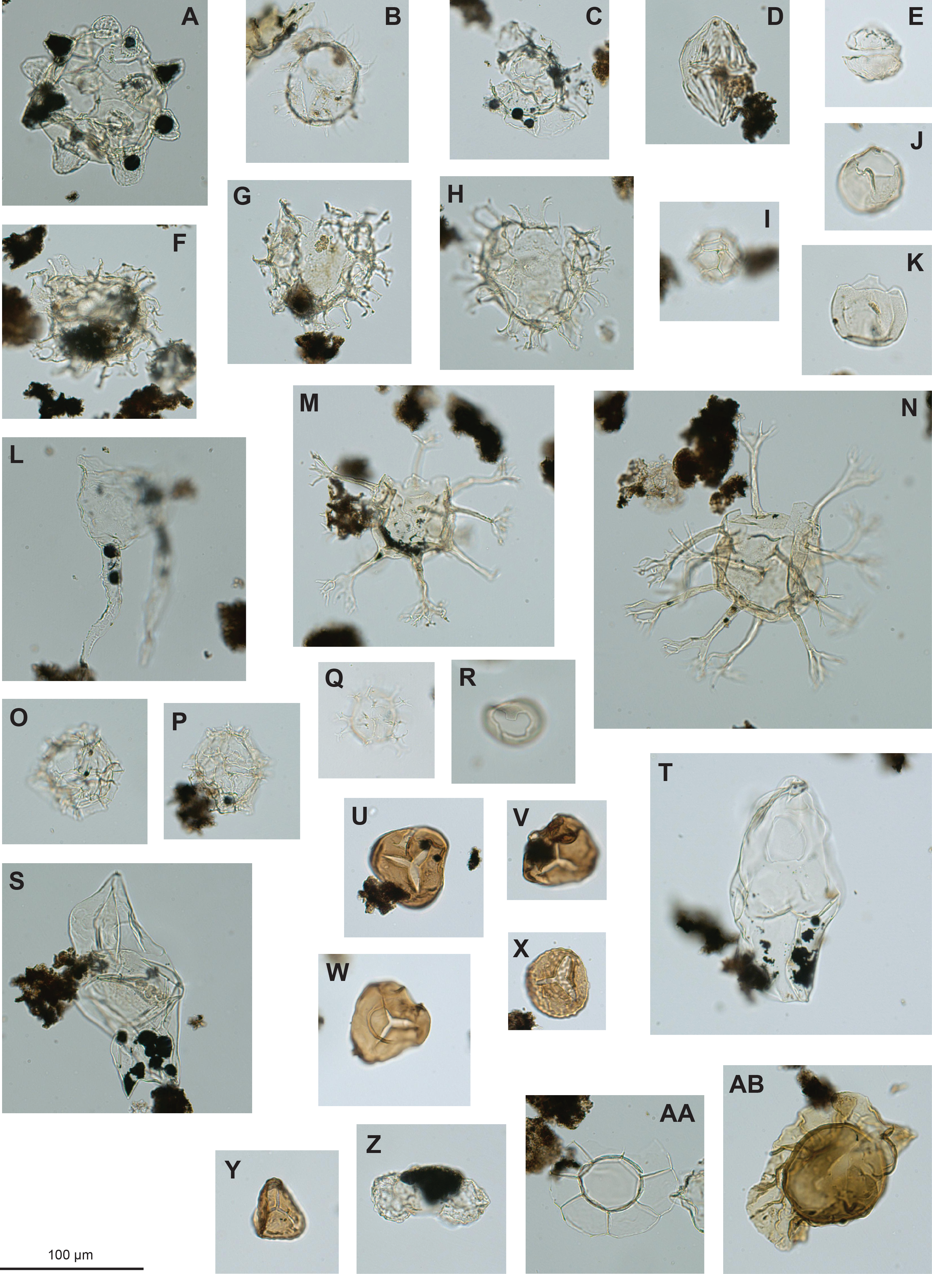
Figure F22. Palynomorphs.
5.4.1. Dinocysts
Sample 392-U1579B-17F-CC, 14–19 cm (108.85 m CSF-A), contains single specimens of Impagidinium patulum, Spiniferites ramosus, and Operculodinium centrocarpum. Three poorly preserved dinocyst specimens from Sample 392-U1579D-42R-CC, 18–23 cm (518.76 m CSF-A), could not be identified to genus level. Sample 58R-4, 109–111 cm (673.74 m CSF-A), contains a rich, moderately preserved, and diverse dinocyst assemblage containing, among others, abundant Trithyrodinium suspectum; frequent Oligosphaeridium complex, Conosphaeridium striatoconus, and Satyrodinium haumuriense; and rare Odontochitina cribropoda, Cassiculosphaeridia reticulata, Dinogymnium denticulatum, Dinogymnium euclaense, and Heterosphaeridium spinaconjunctum. The coexistence of these species, specifically O. cribropoda and C. striatoconus, indicate a late Coniacian–early Santonian age (89.6–85.2 Ma; dc1 in Figure F37 and Table T3). If the common occurrence of T. suspectum in this sample stratigraphically correlates to that in the Norfolk Chalks, UK (Pearce, 2000; as Trithyrodinium sp. B.), the age of this sample can be more tightly constrained to 85.2–86.8 Ma, early Santonian. This would also be consistent with the absence of Cyclonephelium filoreticulatum, which has a top below that time interval in the Norfolk Chalk (Pearce, 2000). S. haumuriense, known from the Maastrichtian of Maud Rise and Georgia Rise (Mohr and Mao, 1997). Based on this and the results from Site U1579, we extend its stratigraphic range into the Santonian.
5.4.2. Miospores
Sample 392-U1579D-58R-4, 109–111 cm (673.74 m CSF-A), contains moderately preserved miospores with low diversity, dominated by trilete spores (Deltoidospora/Cyathidites), which are pteridophytes (fern spores). Rare bisaccate pollen of conifers were also recorded.
5.4.3. Paleoenvironments and depositional setting
The near-absence of palynofacies in the samples from almost the entire sedimentary record recovered at Site U1579 can be interpreted to reflect well-ventilated (oxygenated) conditions on the ocean floor during sedimentation or postdepositional oxidation. The low detrital clay/silt content in calcareous oozes and chalks recovered at Site U1579 (see Lithostratigraphy) likely further contributed to the poor preservation of organic matter in these sediments.
The depositional environment of the dark brown zeolitic silty claystone (Lithostratigraphic Unit III) from Sample 392-U1579D-58R-4, 109–111 cm (673.74 m CSF-A), is interpreted to be shallow-marine based on the palynological association. Bisaccate pollen are wind-dispersed and therefore could have been transported to the site from afar (African continent). The pteridophyte spores, however, typically have a much more local source area. As a preliminary explanation, their presence at this site would imply subaerial exposure of parts of the Agulhas Plateau, acting as a terrestrial source for these spores. The darkness of the amorphous organic matter suggests an unquantifiable degree of postdepositional maturation of the organic matter, which requires higher pressure/temperature than can be expected to result from the overburden of 674 m of sediment.
6. Paleomagnetism
Paleomagnetic measurements were performed on all archive-half sections from Site U1579 (Cores 392-U1579A-1H through 8H [0–74.78 m CSF-A], 392-U1579B-1H through 27X [0–163.96 m CSF-A], 392-U1579C-2F through 25X [56.5–177.7 m CSF-A], and 392-U1579D-2R through 65R [130–727.285 m CSF-A]) and on 131 discrete samples from Cores 392-U1579A-1H through 8H, 392-U1579B-10F through 27X, and 392-U1579D-3R through 65R (Figures F23, F24, F25, F26). The primary purpose of these measurements was to determine magnetic polarity stratigraphy. However, additional rock magnetic experiments (anisotropy of magnetic susceptibility [AMS] and isothermal remanent magnetization [IRM] acquisition) were performed to further inform the reliability of magnetic signals, magnetic fabric, and environmental and postdepositional processes.
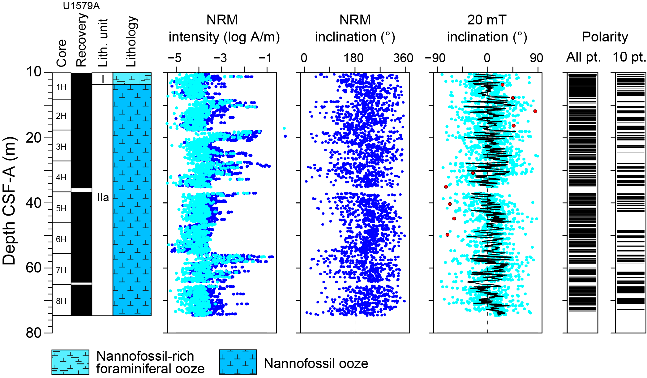
Figure F23. Magnetostratigraphic results, Hole U1579A.
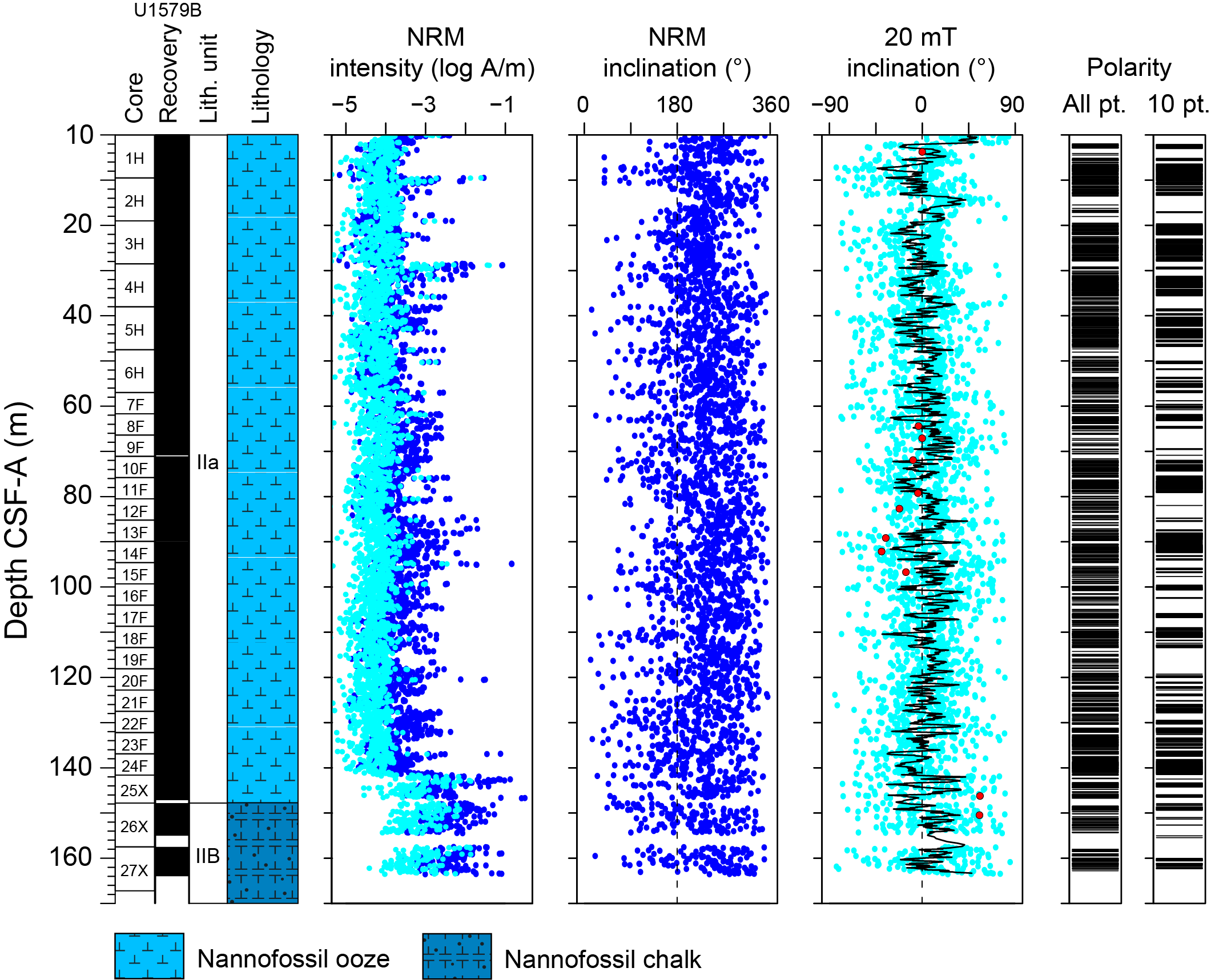
Figure F24. Magnetostratigraphic results, Hole U1579B.
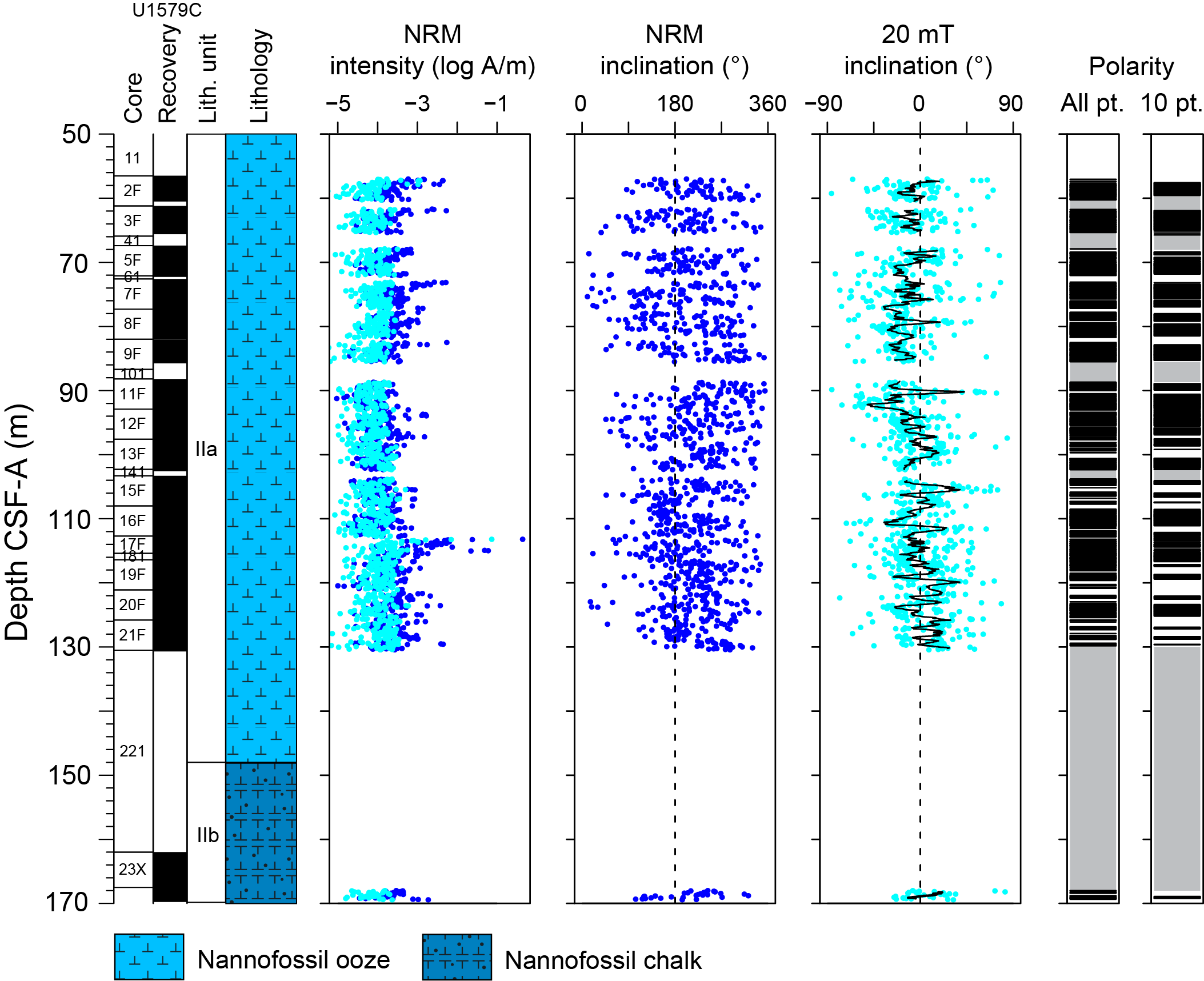
Figure F25. Magnetostratigraphic results, Hole U1579C.
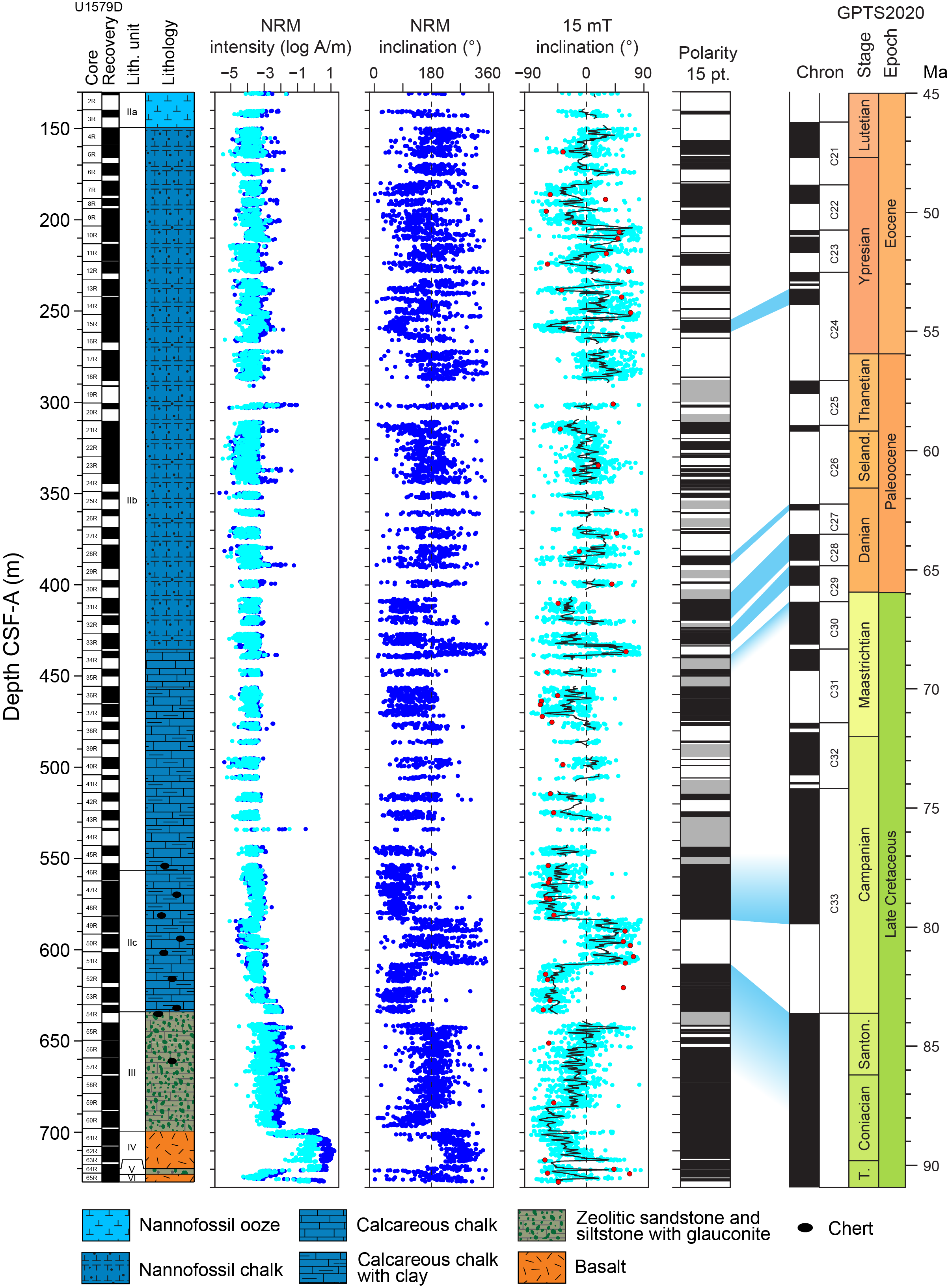
Figure F26. Magnetostratigraphic results, Hole U1579D.
6.1. Summary
Paleomagnetic measurements were undertaken on all archive halves from Holes U1579A–U1579D and on 131 discrete samples from Holes U1579A, U1579B, and U1579D. Rock magnetic analyses and demagnetization experiments were performed to constrain the magnetic mineralogy and magnetic polarity of both the sedimentary and igneous units collected at Site U1579. Paleomagnetic results indicate that some of the units sampled at Site U1579 are reliable recorders of magnetic field direction. No magnetic reversals were identified in Holes U1579A–U1579C. In Hole U1579D, a total of 11 magnetic reversals (m1–m11 in Figure F37 and Table T13) were identified, and normal and reversed polarity intervals were correlated to chrons in the geomagnetic polarity timescale (GPTS) from GTS2020 (Ogg, 2020; Gradstein et al., 2020). These include Chrons C24.2r through C34n. Results from rock magnetic analyses indicate that the dominant magnetic minerals include both ferrimagnetic and antiferromagnetic minerals, likely magnetite and hematite with greigite occurring in Lithostratigraphic Unit III (zeolitic sandstone, siltstone, and claystone with glauconite) and Unit V (zeolitic sandstone and siltstone with glauconite). AMS measurements indicate that all samples analyzed from Site U1579 have a very low anisotropy degree (excluding three measurement outliers) and shape parameter values, indicating the absence of a well-defined magnetic fabric (Figure F27).
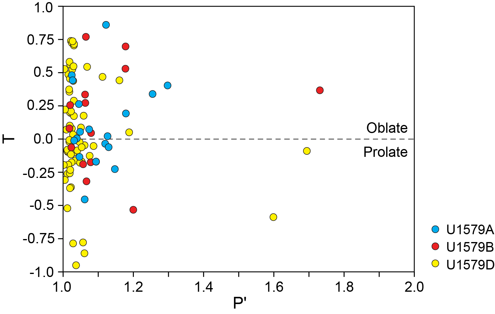
Figure F27. AMS data.
6.2. Discrete samples
Discrete sediment and igneous rock samples were analyzed from Cores 392-U1579A-1H through 8H (3.71–73.17 m CSF-A), 392-U1579B-10F through 27X (71.93–161.14 m CSF-A), and 392-U1579D-3R through 65R (140.2–388.99 m CSF-A), with the exception of Cores 16R and 17R (261.6–267.19 m CSF-A), which span the Paleocene/Eocene boundary, and Core 33R (426.5–435.28 m CSF-A), which contains the K/Pg boundary. All samples underwent demagnetization experiments including both alternating field (AF) demagnetization and thermal demagnetization (on selected cubes from Cores 61R–65R). Samples from sedimentary units were analyzed for MS and AMS, which gives information on the possible drilling-induced deformation of the sediments. This was followed by IRM acquisition experiments to monitor the variation in magnetic mineralogy through the record.
MS measurements (Figure F28), normalized to volume, are consistent with measurements of whole cores. AMS data were inspected using anisotropy degree (P′) and shape parameter (T) defined by Jelinek (1981), where P′ = 1.0 indicates the absence of magnetic fabric and T > 0 (T < 0) indicates a oblate (prolate) ellipsoid. All samples analyzed from Site U1579 are characterized by a very low P′ (excluding three measurement outliers) and low T values, indicating the overall absence of a well-defined magnetic fabric (Figure F27).
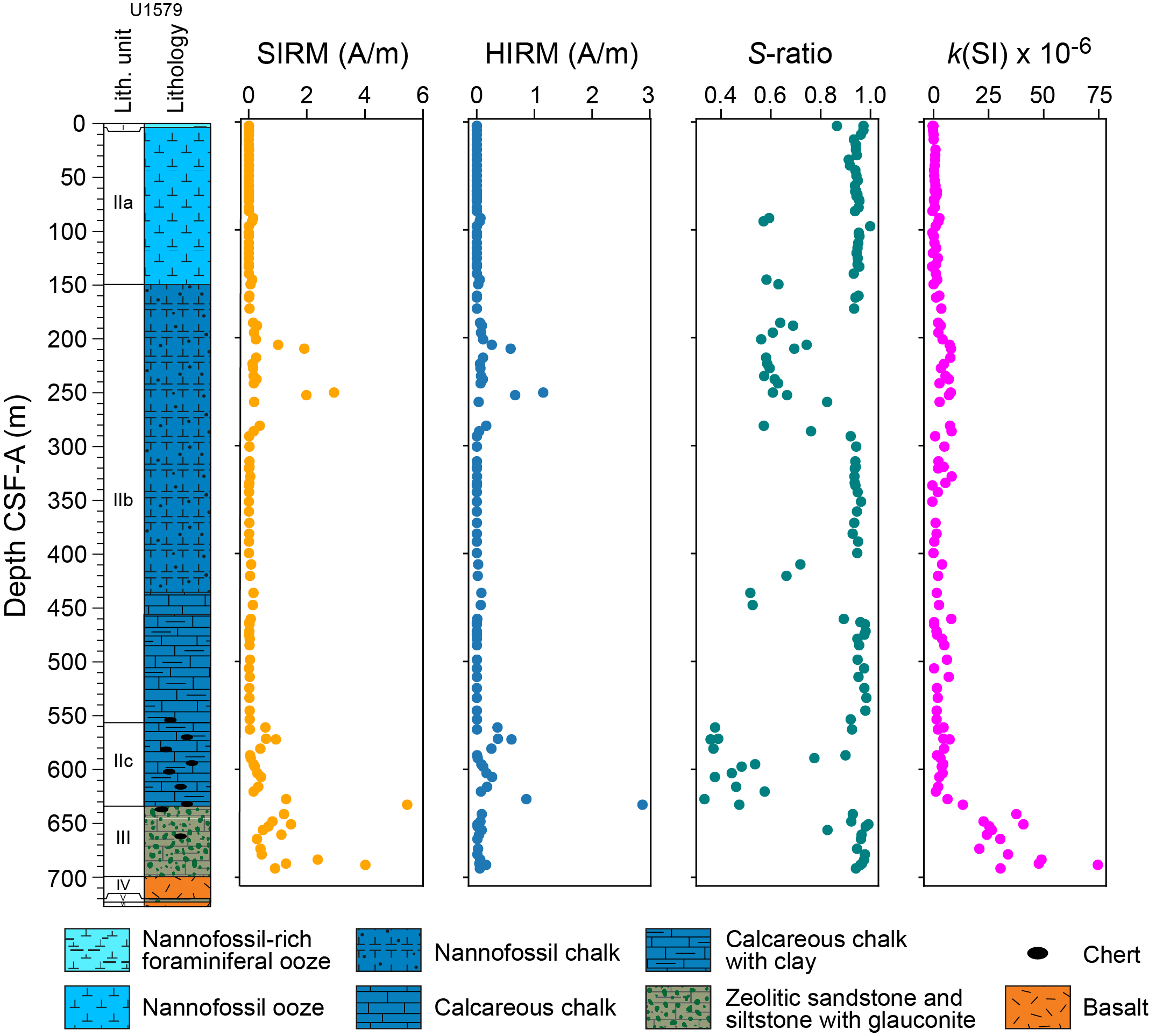
Figure F28. SIRM, HIRM, S -ratio, and MS.
From IRM acquisition experiments, we assessed hard IRM (HIRM), saturation IRM (SIRM), and S-ratios versus depth (see Paleomagnetism in the Expedition 392 methods chapter [Uenzelmann-Neben et al., 2023a]). In general, we observe low SIRM and HIRM values for 90% of the measured samples (values < 0.5 A/m) (Figure F28). However, we do observe spikes in both SIRM and HIRM in sedimentary intervals that have red banding (~200–300, 400–500, and 550–650 m CSF-A), which is indicative of the presence of hematite. S-ratios nicely mimic the observed red banding (~200–300, 400–500, and 550–650 m CSF-A), with S-ratios dropping where red banding occurs (Figure F28). Regions without red bands (~0–200, 300–400, 500–550, and deeper than 650 m CSF-A) have high S-ratios, which indicates that the main magnetic carrier is likely magnetite, with the exception of cores from Lithostratigraphic Unit III (zeolitic sandstone, siltstone, and claystone with glauconite) (see Lithostratigraphy). In Lithostratigraphic Units III and V, the main magnetic carrier is likely greigite, based on AF experiments where a gyroremanent magnetization was acquired (Figure F29C).
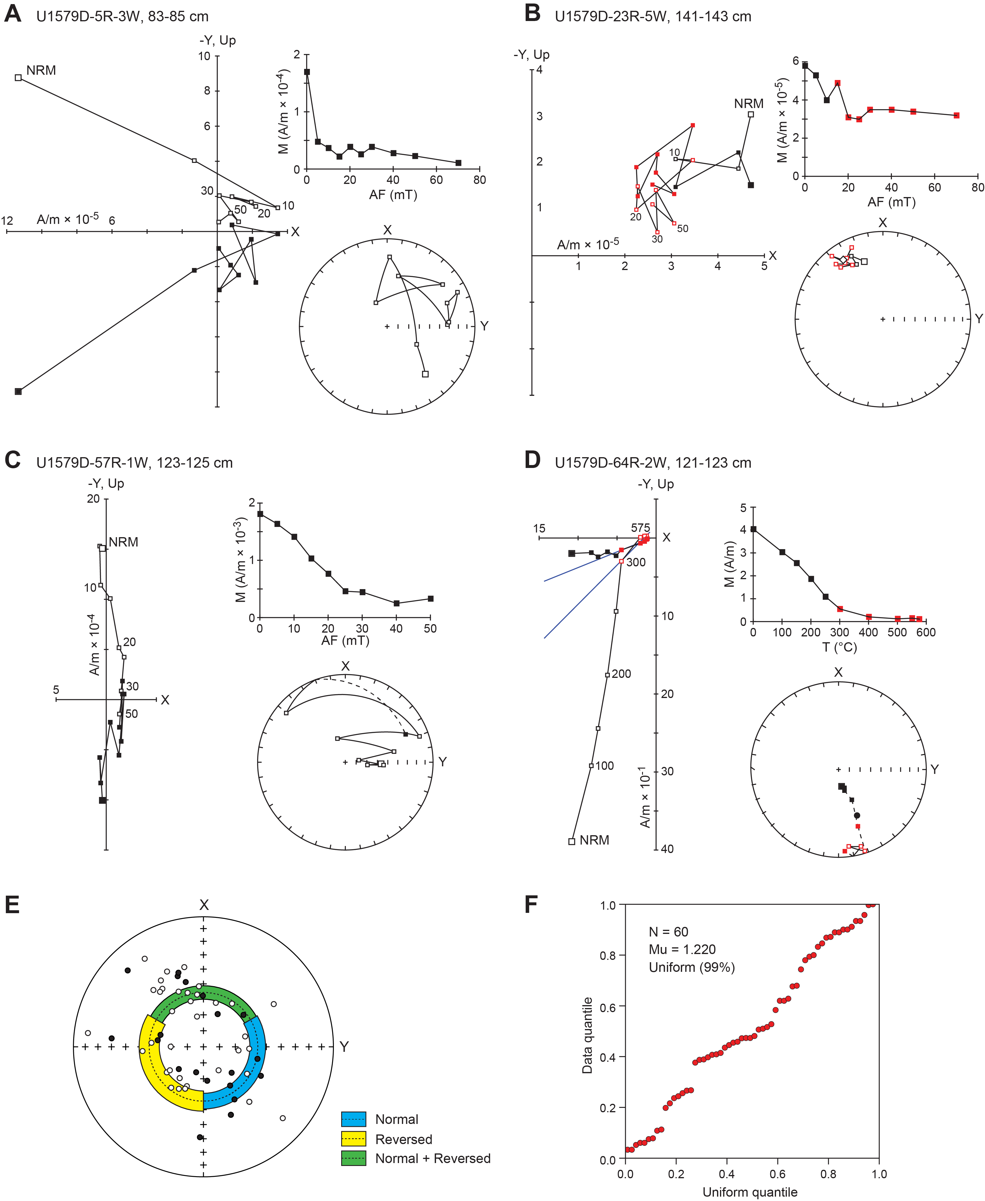
Figure F29. Demagnetization.
Demagnetization experiments on discrete samples were moderately successful, with the identification of a characteristic remanent magnetization (ChRM) largely dependent on lithology and age. Samples from Lithostratigraphic Unit I (foraminiferal ooze), Lithostratigraphic Subunit IIa (nannofossil ooze), and Lithostratigraphic Subunit IIb (nannofossil chalk) are characterized by very weak magnetizations (average = ~1 × 10⁻⁴ A/m). Using demagnetization steps of ~10 mT, these samples reached the noise level of the spinner magnetometer, and ChRM could not be determined (Figure F29A). For those samples from Lithostratigraphic Subunit IIb that were characterized by red banding (~200–300 and 400–500 m CSF-A), ChRM directions could be determined. However, magnetizations are still low, and principal component analysis (PCA) (Kirschvink, 1980) could not be used (Figure F29B). Instead, Fisher statistics (Fisher, 1953) on at least the last five demagnetization steps were used to determine directions using PuffinPlot software (Lurcock and Wilson, 2012). An analogous approach was used with the discrete samples from Lithostratigraphic Subunit IIc (nannofossil chalk with clay and occasional chert), which possess higher natural remanent magnetization (NRM) intensities and yield more reliable paleomagnetic data (Figure F26). Vector endpoint demagnetization diagrams from Lithostratigraphic Units III and V show anomalous magnetization acquisition during the AF demagnetization protocol (Figure F29C), which is a phenomenon called gyroremanent magnetization acquisition that may indicate the presence of greigite (Fe3S4) (Snowball, 1997). The inclinations for sediment samples that yielded ChRM directions alternate between positive (down-pointing) and negative (up-pointing) values, indicating reversed and normal polarities, respectively. Discrete samples from igneous units are excellent magnetic recorders, and PCA analysis (Kirschvink, 1980) was used for directional interpretation of these samples (Figure F29D). Average ChRM inclination measurements, calculated using the inclination-only protocol of McFadden and Reid (1982), for discrete samples from Hole U1579D are reported in Table T14.
6.3. Archive-half measurements
Downhole paleomagnetic data are variable in quality and correlate strongly with lithostratigraphic units (see Lithostratigraphy). This correlation is clearly displayed by comparing NRM intensity, inclination, and inclination after application of a 15 or 20 mT AF step versus depth (Figures F23, F24, F25, F26). Correlation between downhole paleomagnetic data and lithology is further evident in Figure F30, which shows histograms of inclination values after the 20 mT step for magnetic data from each hole (Holes U1579A–U1579D). In ideal samples with strong magnetic signals, two peaks in the inclination data would be expected, one with positive inclination and the other with roughly the same inclination values but negative, indicating the presence of opposite polarities. However, the pooled data from each hole at Site U1579 have marked peaks around ±30°, which match the background noise on the superconducting rock magnetometer (SRM). For Holes U1579A–U1579C, only these two peaks are discernible, but for Hole U1579D, which contains lithologies with more reliable magnetic signals, there is an additional peak in inclination of about ±55° (Figure F30).
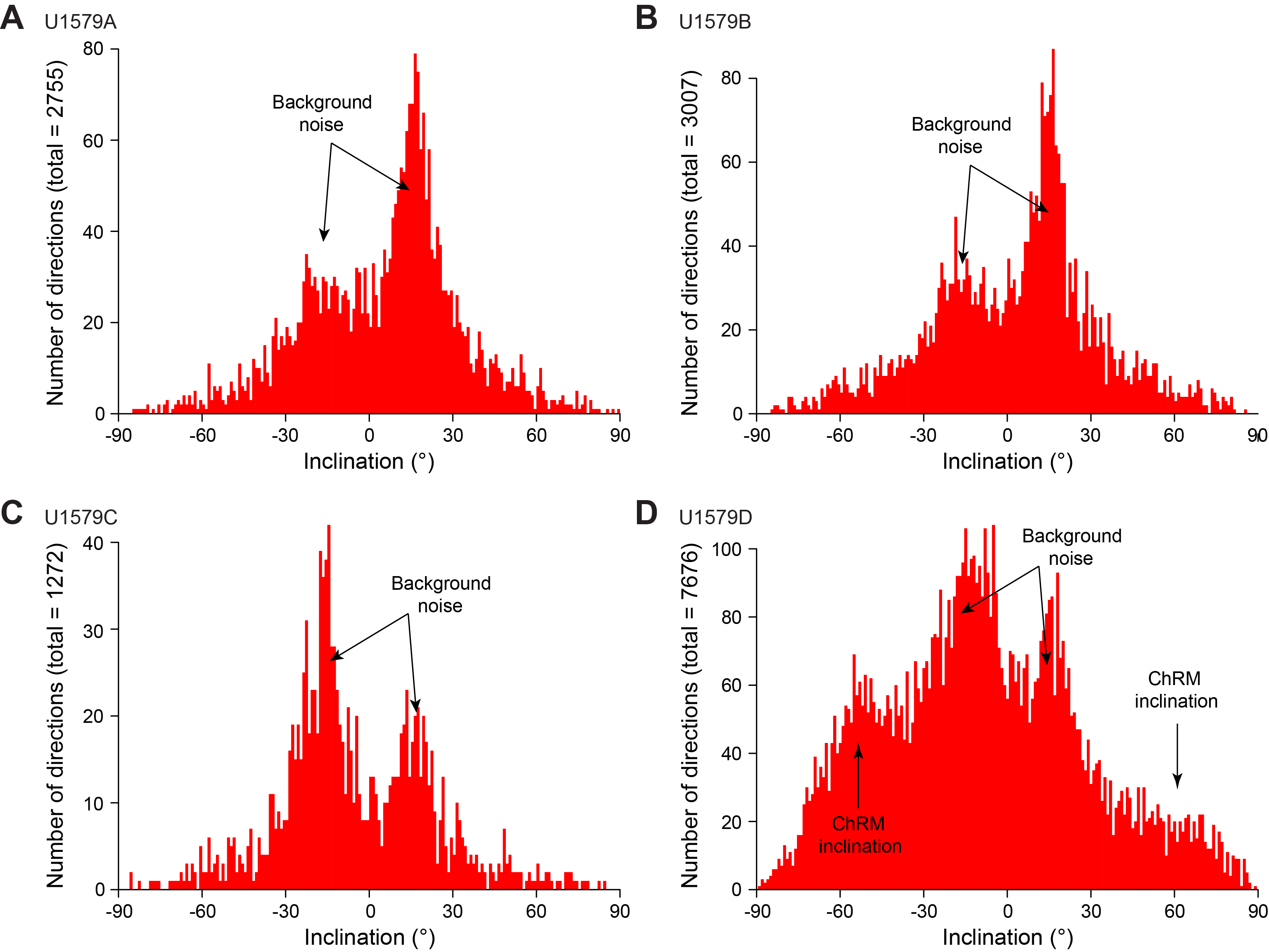
Figure F30. Magnetic inclination data.
In Lithostratigraphic Unit I (foraminiferal ooze) and Lithostratigraphic Subunit IIa (nannofossil ooze), magnetization intensity is low (~1 × 10⁻⁴ A/m) and interpretation of magnetic polarity is difficult. In Lithostratigraphic Subunits IIb (nannofossil chalk) and IIc (nannofossil chalk with clay and occasional chert), magnetization intensity is similarly low and interpretation of polarity is also difficult. However, in intervals with red banding in Lithostratigraphic Subunits IIb and IIc (~200–300, 400–500, and 550–650 m CSF-A) (Figure F26), magnetization increases and polarity can be determined. In these intervals, ChRM directions contain both positive and negative inclination values, indicating the presence of both reversed and normal polarity intervals.
In Lithostratigraphic Unit III (zeolitic sandstone, siltstone, and claystone with glauconite), magnetization intensity increases to ~1 × 10⁻³ A/m and polarity determination is possible. However, based on demagnetization results of discrete samples, it appears that the primary carrier of magnetic remanence in this unit is greigite, which tends to be a secondary mineral that can form during diagenesis (Roberts et al., 2011) and also acquires a gyroremanent magnetization upon AF demagnetization (Figure F29C). In the archive halves, however, it does not appear that a gyroremanent magnetization was acquired by the 15 mT AF step, and ChRM directions could therefore be determined. ChRM directions of cores from Lithostratigraphic Unit III predominantly show shallow negative inclination values, indicative of normal polarity (Figure F26).
Lithostratigraphic Units IV and VI (basalt) have significantly higher magnetization intensities (~1 × 10⁻¹ A/m) and yield stable magnetic signals after AF demagnetization to 15 mT. All cores from the basalt units have strong secondary overprints that for the most part are removed by 15 mT. However, a few intervals (intervals 392-U1579D-61R-2, 5–15 cm, and 61R-2, 80–85 cm; Section 62R-2, 65 cm; and intervals 62R-2, 110–115 cm; 63R-2, 115–120 cm; 64R-2, 125–135 cm; and 63R-3, 10–35 cm) maintain this overprint even after the 15 mT step. Based on discrete sample results, the overprint is eventually removed at slightly higher AF steps (~25 mT) and thermal demagnetization to 300°C. ChRM directions from the basalt units are steep and negative, indicating normal polarity. In Lithostratigraphic Unit V (zeolitic sandstone and siltstone with glauconite), results are similar to those in Lithostratigraphic Unit III, with a drop in magnetization to ~1 × 10⁻³ A/m, but polarity determination is still possible. Additionally, ChRM directions from the zeolitic siltstone and sandstone with glauconite in Lithostratigraphic Units III and V in close contact with basalt show steeper negative inclinations, which is suggestive of baked contact zones (Figure F26).
6.3.1. Magnetostratigraphy
In Lithostratigraphic Unit I and Lithostratigraphic Subunit IIa, no reliable magnetostratigraphy can be determined because of the low magnetization intensities of the samples. In Lithostratigraphic Subunit IIb (nannofossil chalk), the determination of a coherent magnetostratigraphy is also not possible, again because of the low magnetization of the samples. However, using biostratigraphic constraints, we are able to determine distinct polarities in some intervals of Hole U1579D with red banding in Lithostratigraphic Subunit IIb (~200–300, 400–500, and 550–650 m CSF-A) and to correlate these to chrons in the GPTS from the GTS2020 (Ogg, 2020; Gradstein et al., 2020). These include Chrons C24n.3n, C27 through C29, C33r, and the top of C34n. All of the zeolitic sandstone and siltstone with glauconite and the basalt units (Lithostratigraphic Units III–VI) have normal polarity that we assign to Chron C34n. Determined positions of chron boundaries (m1–m11) and their ascribed ages are shown in Table T13 and Figure F37.
7. Stratigraphic correlation
At Site U1579, three holes were cored using the APC, HLAPC, and XCB systems. Hole U1579A was piston cored to 84.1 m DSF (bottom recovered depth = 74.78 m CSF-A), Hole U1579B was piston cored to 141.6 m DSF (bottom recovered depth = 141.90 m CSF-A), and Hole U1579C was piston cored from 56.5 to 130.5 m DSF (bottom recovered depth = 130.68 m CSF-A). Differences in DSF drilled depths and CSF-A depths of the recovered intervals are due to incomplete recovery and core expansion. The XCB system was used in Holes U1579B and U1579C to continue coring. In Hole U1579B, XCB coring continued to 167.2 m DSF (bottom recovered depth = 163.96 m CSF-A). Following piston coring between 56.5 and 130.5 m DSF, Hole U1579C was drilled from 130.5 to 162 m DSF and then XCB cored to 186.9 m DSF (bottom recovered depth = 177.7 m CSF-A). Hole U1579D was drilled to 130 m DSF and then cored to 727.2 m DSF using the RCB system (bottom recovered depth = 727.285 m CSF-A; Core 392-U1579D-65R).
7.1. Guidance for coring
Before and during coring in Hole U1579B, target depths for each piston core advancement were recommended to recover cores across recovery gaps, core breaks, and disturbed intervals in Hole U1579A based on comparison of NGR data. The first core from Hole U1579B spanned a different stratigraphy than that observed in Core 392-U1579A-1H, hampering a direct correlation to cover the gap between Cores 392-U1579A-1H and 2H. A correlation was established between Cores 392-U1579B-2H and 392-U1579A-2H and continued downward.
Coring in Hole U1579C was guided to recover material across core breaks in Holes U1579A and U1579B by comparison of MS data obtained from unequilibrated cores from Hole U1579C using the Special Task Multisensor Logger (STMSL) and NGR data. Drilling in Hole U1579C was successfully guided to recover stratigraphy from remaining core gaps between Cores 392-U1579A-6H, 7H, and 8H and between Cores 392-U1579B-7F and 22F. Most core breaks in Hole U1579B were spanned by cores in Hole U1579C, and only three minor stratigraphic gaps remain. Intervals of stratigraphy not recovered in Cores 392-U1579B-25X through 27X, 392-U1579C-24X, and 25X were further recovered in Cores 392-U1579D-3R through 6R.
7.2. Correlation of cores
7.2.1. Holes U1579A–U1579D
The physical property records of Holes U1579A–U1579D were compared, and correlated where possible, to establish a common depth scale. Tie points were identified using NGR, MS from the Whole-Round Multisensor Logger (WRMSL), color reflectance data, high-resolution digital core images, and red-green-blue (RGB) color space data extracted from the digital core images obtained using the Section Half Imaging Logger (SHIL). Across all four holes, the most complete and least disturbed intervals of cores were selected, avoiding locations of IW samples (5 or 10 cm whole round intervals) where possible. A composite record was spliced for the upper 147 m CCSF of the recovered stratigraphic succession (Figures F31, F32, F33; Tables T15, T16). Small recovery gaps in the composite record exist at 66.42–67.02 m CCSF between Cores 392-U1579A-6H and 7H, between Cores 392-U1579B-7F and 8F, and between Cores 392-U1579C-2F and 3F. Another small 14 cm gap is located between Cores 392-U1579C-9F and 392-U1579B-13F at 94.00–94.13 m CCSF. Uncertainty in placing tie points between cores only occurs between Cores 392-U1579A-2H and 392-U1579B-3H and between Cores 392-U1579B-21F and 392-U1579C-20F. These correlations need to be evaluated using shore-based X-ray fluorescence (XRF) core scanning.
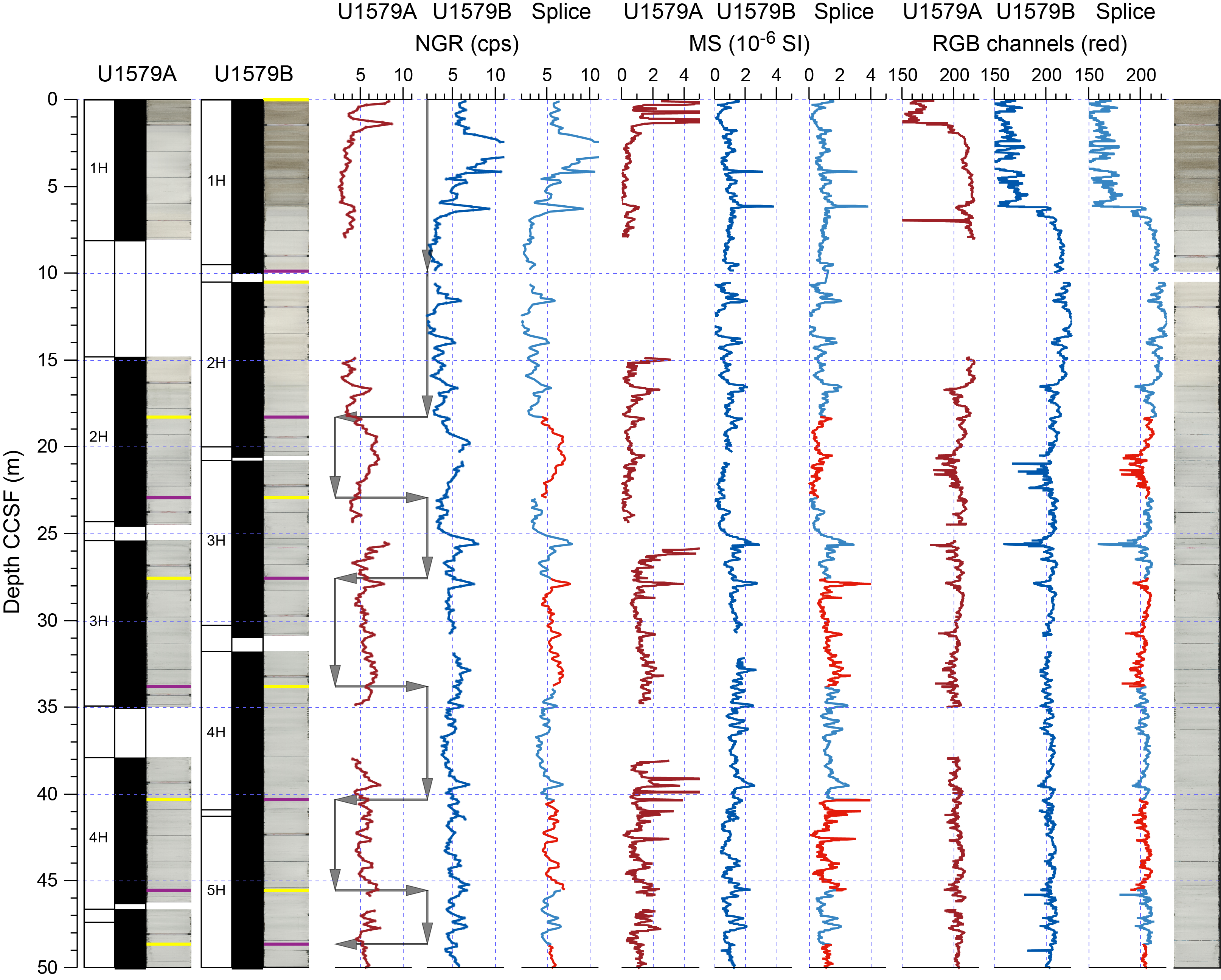
Figure F31. Composite record, 0–50 m CSF-A.
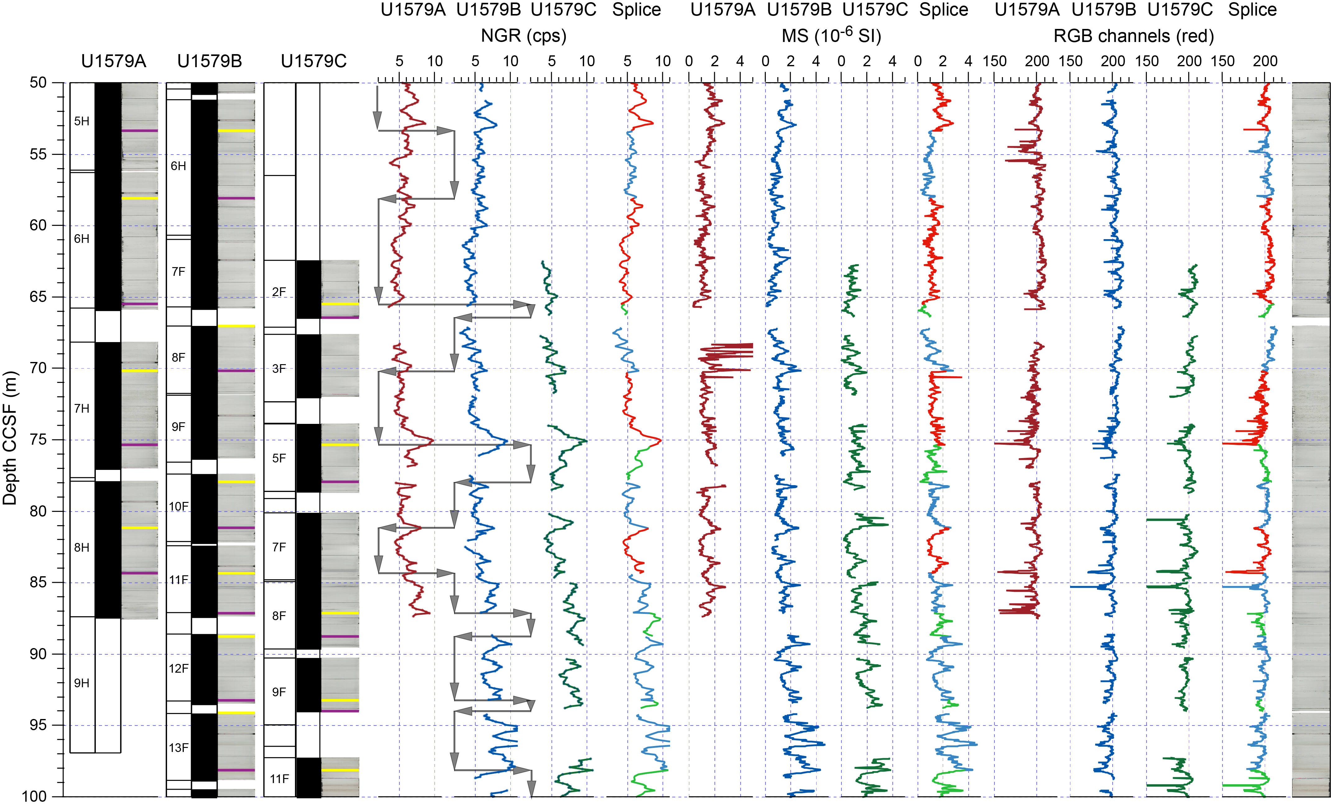
Figure F32. Composite record, 50–100 m CSF-A.
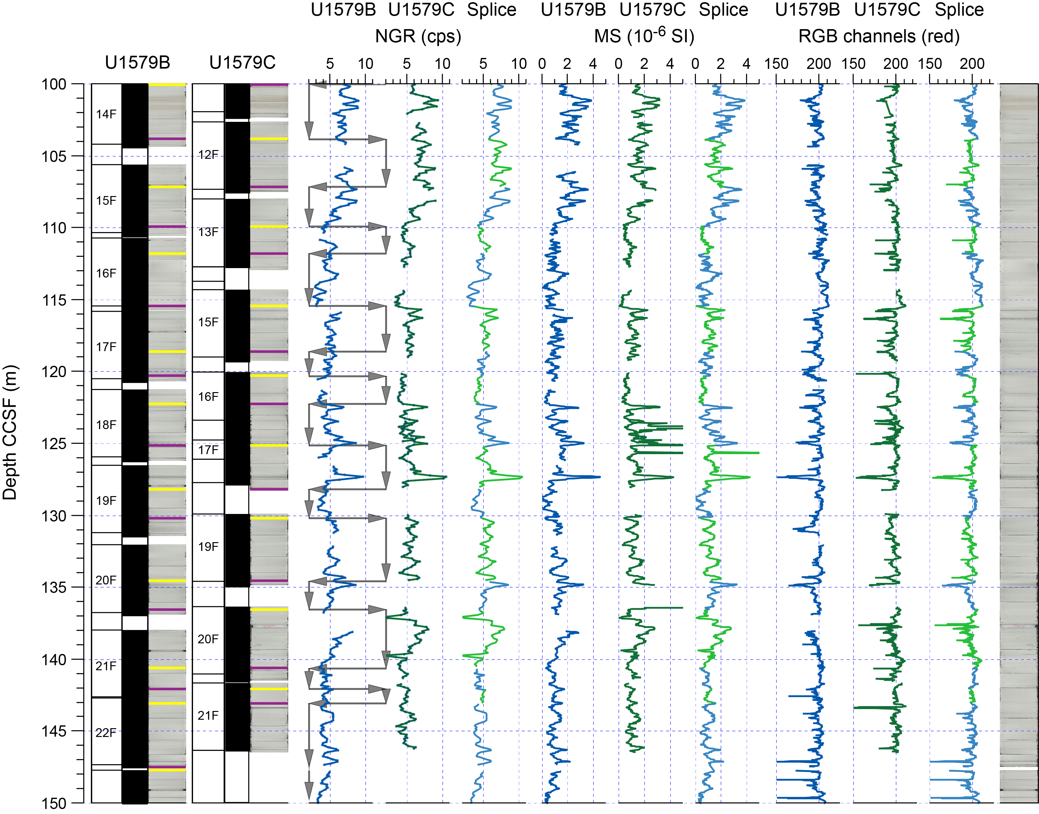
Figure F33. Composite record, 100–150 m CSF-A.
From 147.49 to 164.32 m CCSF (Figure F34), a complete composite record could not be established because no overlapping cores were recovered from parallel holes. From 164.32 to 182.52 m CCSF, a composite record was made by stitching cores together from Holes U1579B and U1579D. Below 182.52 m CCSF, cores from Hole U1579D do not have parallel drilled sections. Because of expansion of the cored material, the CCSF depth scale has growing offsets from the CSF-A scale for individual cores and an average growth factor of ~1.14 (Figure F35).
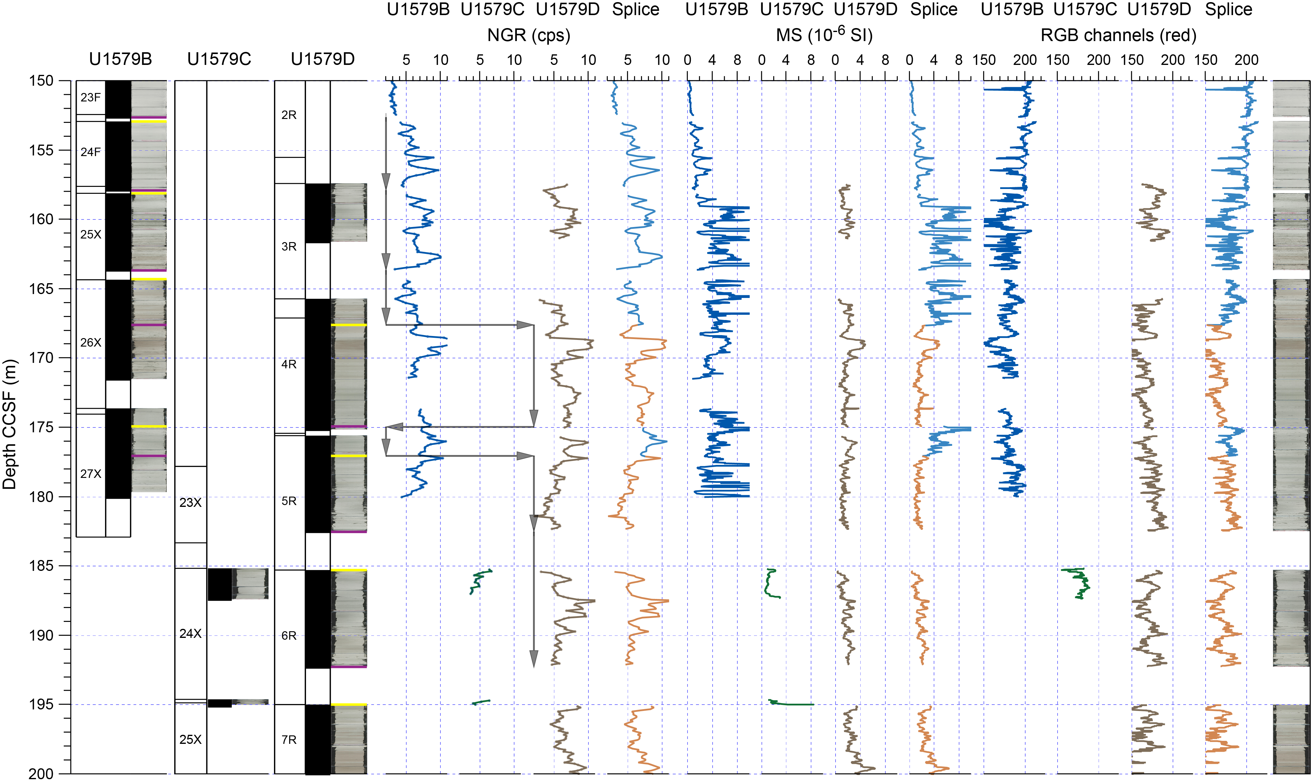
Figure F34. Composite record, 150–200 m CSF-A.
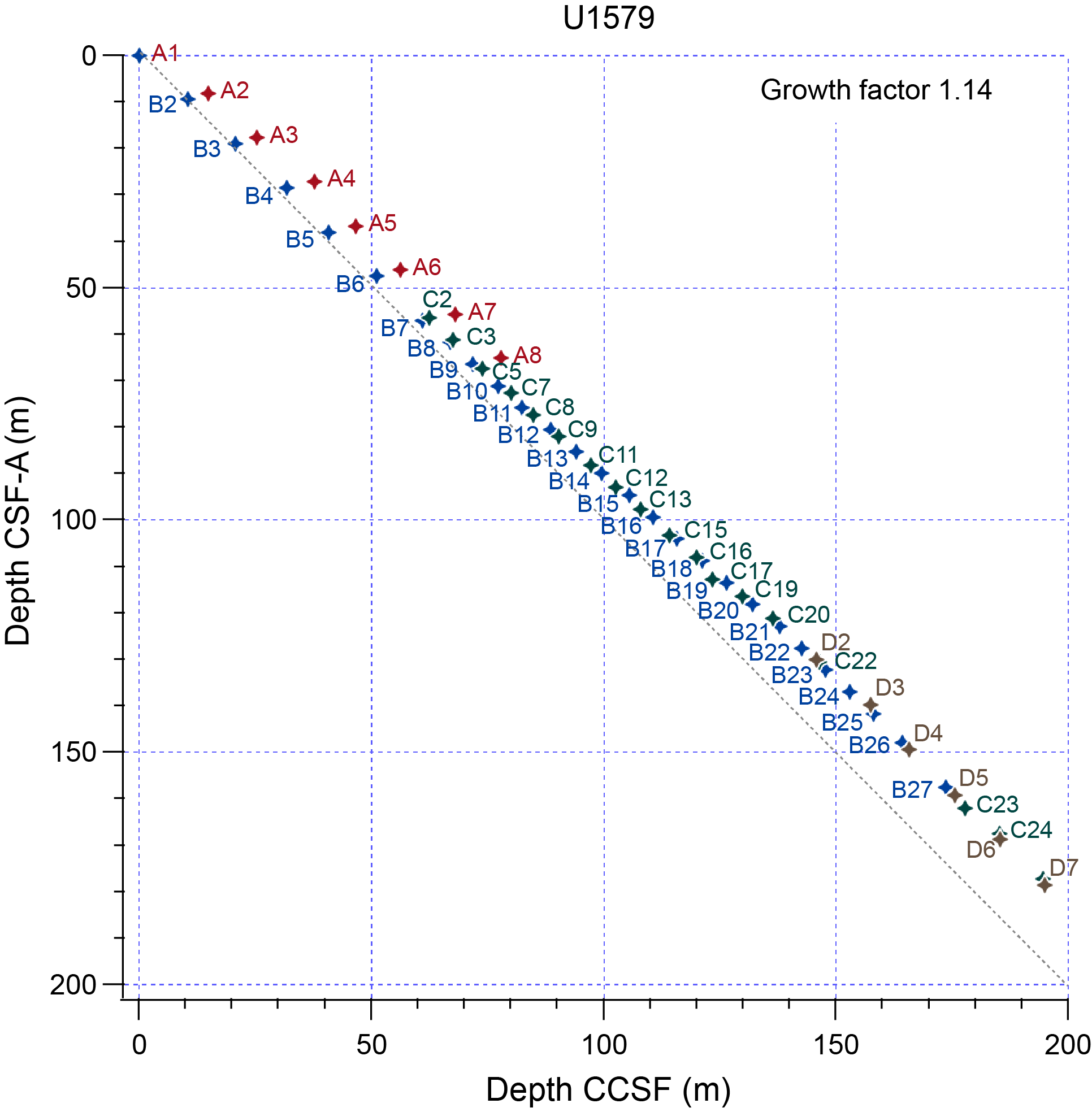
Figure F35. CSF-A vs. CCSF depths for the tops of cores.
7.2.2. Correlation of core to wireline
Recognition of matching patterns in NGR records from cores and total spectral gamma ray (HSGR) data from wireline logging with the HNGS in Hole U1579D permitted translation of core depth scales from the CSF-A scale to the wireline log matched depth below seafloor (WMSF) scale (Figure F36; see Downhole measurements). The average recommended offset for individual cores is −1.8 m between the depth scales. Prominent peaks in HSGR in downhole logging data at 200–203 WMSF (~203.5 m CSF-A) and 266–269 WMSF (~270 m CSF-A) are not identified in the core data and likely coincide with nonrecovery at core breaks at ~203.5 and ~270 m CSF-A, respectively. These two intervals not recovered by drilling likely represent carbonate dissolution horizons associated with the Middle Eocene Climatic Optimum (MECO) and PETM events, respectively (see Micropaleontology and Chronostratigraphy).
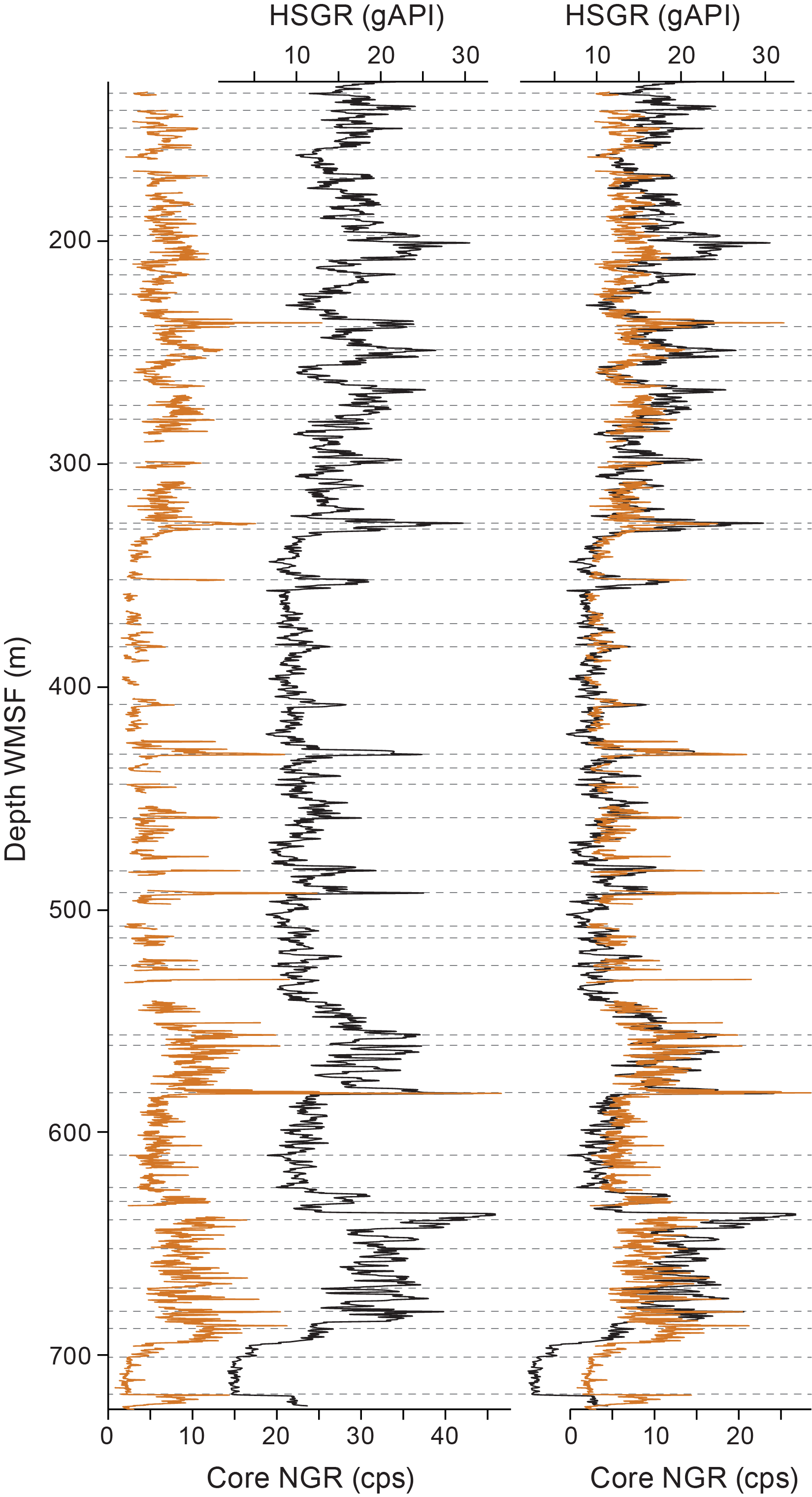
Figure F36. NGR to HSGR correlation.
In the green zeolitic clastic sediments of Lithostratigraphic Unit III (634.72–697.00 m CSF-A), the NGR data from cores and HSGR data from downhole logging behave differently and correlation of patterns is tentative.
7.3. Summary
Compiled records of the cored intervals at Site U1579 demonstrate good coverage, spanning from the lower Miocene to the lower Campanian, with composite records established for the uppermost 147 m CCSF of the cored succession spanning the lower Miocene to the lower Oligocene, as well as from 164.32 to 182.52 m CCSF in the lowermost Oligocene to the uppermost Eocene. Correlation between retrieved sediment cores and borehole logging using NGR data is excellent.
8. Chronostratigraphy
Calcareous nannofossils, planktonic and benthic foraminifera, dinocysts, and magnetostratigraphy provide age control for the Santonian–lower Miocene record recovered at Site U1579 (see Micropaleontology and Paleomagnetism). Biostratigraphic datums (Table T3) guided the interpretation of magnetic polarity reversals (Table T13), which are tied to the GPTS (Ogg, 2020) for the Campanian–Eocene sediments from Hole U1579D. The ages and sedimentation rates of the sedimentary succession (Figure F37) are described in stratigraphic order (i.e., oldest to youngest).
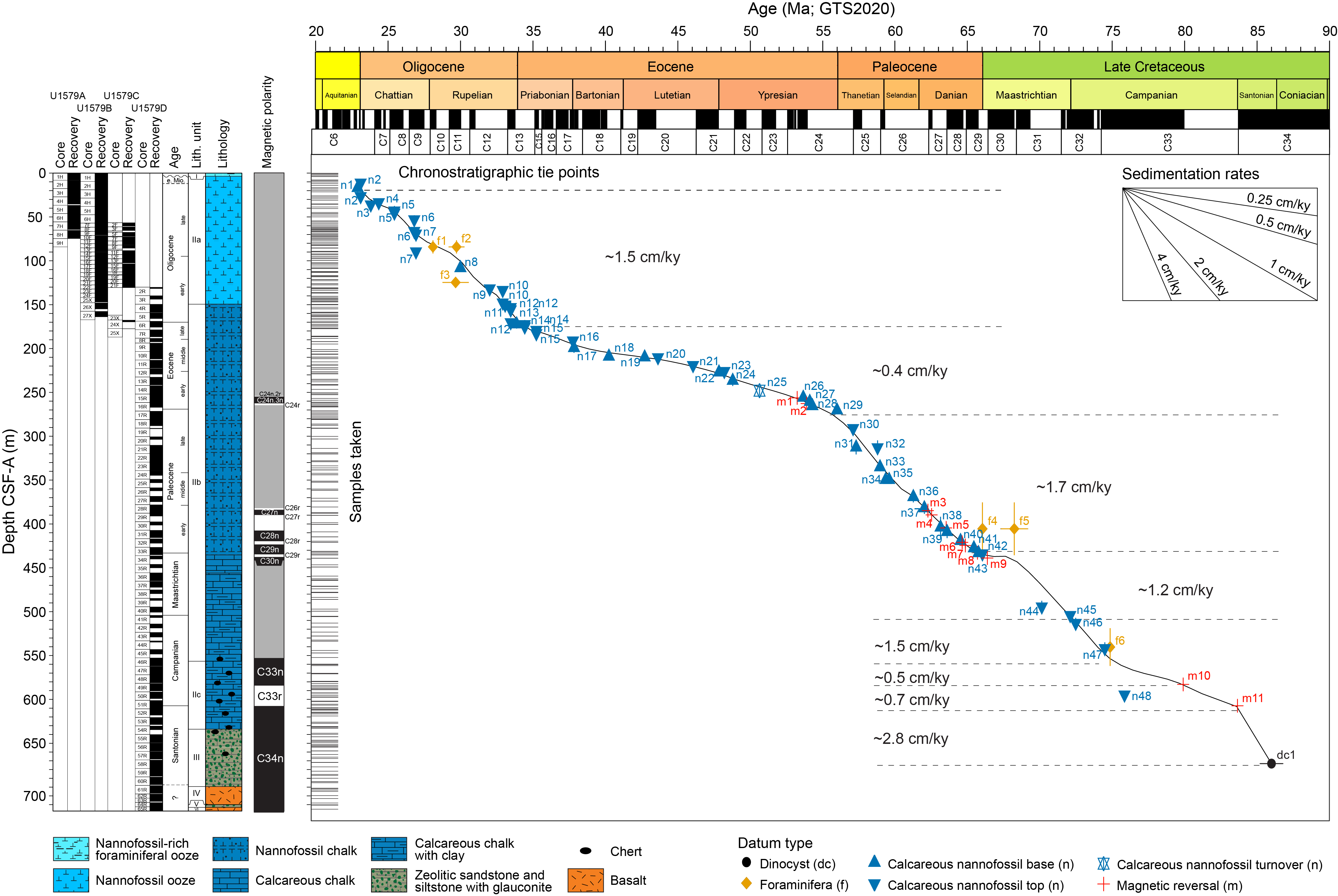
Figure F37. Age-depth model and average sedimentation rates.
8.1. Santonian and older (older than 83.7 Ma; 725.47–607.59 m CSF-A)
There are few age constraints for the sediments recovered below ~607 m CSF-A in Hole U1579D, which include Lithostratigraphic Unit V (725.47–720.77 m CSF-A) and the sediment below the top of Chron C34n in Lithostratigraphic Unit III (679.00–607.59 m CSF-A). An early Santonian age (86.8–85.2 Ma) is indicated for the lowermost part of Lithostratigraphic Unit III by the dinocyst assemblage in a single sample at 673.75 m CSF-A, which is consistent with the interpretation of the persistent normal polarity in this interval within Chron C34n (the Cretaceous Normal Superchron). The dinocyst-based age toward the base of Lithostratigraphic Unit III (dc1 in Figure F37 and Table T3), together with paleomagnetic age constraints farther uphole (m11 in Table T13), suggest average sedimentation rates of 2.8 cm/ky for Lithostratigraphic Unit III. However, the sediment in Lithostratigraphic Unit III ranges from claystone to coarse sandstone, with discrete graded beds suggesting intervals of rapid deposition (see Lithostratigraphy), which precludes use of an average sedimentation rate to assign ages through this unit. Postcruise research, such as careful sampling of carbonate-bearing intervals for nannofossil and foraminifera biostratigraphy, is needed to resolve the age of the lowermost sediments recovered at Site U1579 (Lithostratigraphic Unit V).
8.2. Campanian (83.7–72.2 Ma; 607.59 to ~505 m CSF-A)
The biohorizon top of the calcareous nannofossil U. gothicus (n46 in Figure F37 and Table T3) in Sample 392-U1579D-42R-CC, 18–23 cm (518.76 m CSF-A), and the biohorizon top of planktonic foraminifera P. prairiehillensis (f6 in Figure F37) in Sample 46R-CC, 9–14 cm (561.95 m CSF-A), indicate a late Campanian age for the lower part of Lithostratigraphic Unit II. Thus, the reversed polarity interval identified between 607.59 (m11 in Figure F37 and Table T13) and 583.11 m CSF-A (m10 in Figure F37) is identified as Chron C33r, and the persistent normal polarity interval farther downhole is identified as Chron C34n. The Santonian/Campanian boundary is defined as the base of Chron C33r at 607.59 m CSF-A in Hole U1579D (m11 in Figure F37). Sedimentation rates in the Campanian (607.59 to ~505 m CSF-A) are constrained by two magnetic reversals and four biostratigraphic datums. Between 607.59 and 583 m CSF-A, sedimentation rates average 0.7 cm/ky; they then decrease slightly to ~0.5 cm/ky between 583 and 555 m CSF-A. Above 555 m CSF-A, sedimentation rates increase to ~1.5 cm/ky for the remainder of the Campanian. These sedimentation rates for the Campanian are supported by estimates assuming an orbitally forced origin of rhythmic sedimentary banding patterns.
8.3. Maastrichtian (72.2–66.04 Ma; ~507–433.255 m CSF-A)
The age-depth model for the Maastrichtian (~507–433.255 m CSF-A) is constrained by five biostratigraphic datums and one magnetic reversal. The lowermost Maastrichtian is identified by the biohorizon top of calcareous nannofossil M. quaternarius (n45 in Figure F37 and Table T3) (72.10 Ma) in Sample 392-U1579D-41R-CC, 16–21 cm (506.89 m CSF-A). The K/Pg boundary was recovered in Section 33R-6, and the base of the Paleocene was identified in a thin greenish gray clay with its base in Section 33R-6, 98.5 cm (433.255 m CSF-A). This placement was confirmed by the biohorizon top of benthic foraminifera B. draco (f4 in Figure F37; 66.04 Ma) in Sample 33R-CC, 15–20 cm (435.23 m CSF-A), as well as the top of Cretaceous nannoflora (n43 in Figure F37) in Sample 33R-6, 102 cm (433.29 m CSF-A), demarcating the end of the Cretaceous. The identification of the top of Chron C30n at 438.46 m CSF-A (m9 in Figure F37 and Table T13) supports this interpretation. Average sedimentation rates for the Maastrichtian are ~1.2 cm/ky, which is broadly consistent with the rhythmicity in the sedimentary color banding of the cores.
8.4. Paleocene (66.04–56.0 Ma; 433.255–267.14 m CSF-A)
The K/Pg boundary identified in Section 392-U1579D-33R-6, 98.5 cm (433.255 m CSF-A), marks the base of the Paleocene. The basal Eocene (~56.0 Ma) was identified using the biohorizon bases of C. eodela and R. bramlettei (n29 in Figure F37 and Table T3) in Sample 16R-CC, 15–20 cm (267.14 m CSF-A). Between the K/Pg boundary and basal Eocene, 13 nannofossil biohorizons and 6 paleomagnetic reversals provide good age control for the Paleocene sediments (m3–m8 in Figure F37 and Table T13). The Paleocene interval has average sedimentation rates of 1.7 cm/ky and excellent consistency between nannofossil biohorizons and magnetostratigraphy based on the identification of Chrons C29r to C26r. Sedimentation rates show little variability at the resolution of the tie points and suggest a continuous Paleocene section, although the Paleocene/Eocene boundary is missing in the recovered sedimentary sequence, specifically in the core gap between Cores 17R and 16R (271.30–267.19 m CSF-A) (see Micropaleontology, Physical properties, and Stratigraphic correlation).
8.5. Eocene (56.0–33.9 Ma; 267.14 to ~168 m CSF-A)
The lack of visible change in sediment color and physical properties between the top of Core 392-U1579D-17R and the base of Core 16R suggests that the Paleocene/Eocene boundary is not represented in the recovered sedimentary section at Site U1579, although the presence of calcareous nannofossil R. bramlettei in Sample 16R-CC, 15–20 cm (267.14 m CSF-A), suggests that some of the PETM recovery interval may be present at this site (see Micropaleontology). The Eocene/Oligocene boundary (33.9 Ma) is identified between the biohorizon top of D. saipanensis (n14 in Figure F37 and Table T3; 34.44 Ma) in Sample 6R-CC, 11–16 cm (175.74 m CSF-A), and the biohorizon base of abundant C. subdistichus (n13 in Figure F37; 33.88 Ma) in Sample 5R-CC, 10–15 cm (165.97 m CSF-A). Between the basal Eocene and Eocene/Oligocene boundary, 18 nannofossil biohorizons and 2 paleomagnetic reversals (C24n.3n/C24r and C24n.2r/C24n.3n; m1 and m2 in Figure F37 and Table T13) provide good age control for the Eocene sediments. Sedimentation rates average 0.4 cm/ky and are consistently lower than those in the Paleocene and overlying Oligocene. Between 223 and 203 m CSF-A in the lower and middle Eocene (~48–40 Ma), the section is either strongly condensed or there may be one or more hiatuses.
8.6. Oligocene–early Miocene (33.9–22.9 Ma; ~168 to 1–6 m CSF-A)
The shipboard age model suggests the potential for continuous sedimentation across the EOT; however, XCB and RCB coring precluded collection of a complete composite section across this interval (see Stratigraphic correlation). Near the top of the recovered sedimentary section, a disconformity separates a thin veneer (~1–6 m thick) of Pleistocene sediments from the underlying sediments, which are dated to approximately the Oligocene/Miocene boundary (23.04 Ma) based on the presence of the calcareous nannofossil S. disbelemnos (biohorizon base = 22.90 Ma; n1 in Figure F37 and Table T3) in Sample 392-U1579B-1H-CC, 8–9 cm (9.96 m CSF-A). In Hole U1579A, sediment immediately underlying the disconformity is slightly older because S. disbelemnos is absent. The presence of S. delphix (biohorizon top = 23.11 Ma; n2 in Figure F37) in Samples 392-U1579A-2H-2, 10 cm (9.76 m CSF-A), and 392-U1579B-3H-CC, 14–15 cm (29.14 m CSF-A), confirms the Oligocene/Miocene boundary above these depths in each hole. No magnetic reversals could be identified from shipboard paleomagnetic results because of the low natural magnetization intensity of the samples, but 13 calcareous nannofossil datums and 3 foraminifera datums provide good age control for the Oligocene to lower Miocene sediments. Sedimentation rates for this interval average 1.5 cm/ky.
9. Geochemistry
The geochemistry program at Site U1579 was designed to characterize the composition of bulk sediment and IW and report on the presence and abundance of volatile hydrocarbons for routine safety monitoring. In addition, major and certain trace elements of selected igneous rock samples were measured. A sedimentary sequence spanning the lowermost Miocene to Upper Cretaceous was recovered at Site U1579 (see Lithostratigraphy and Chronostratigraphy). Sediments were analyzed for carbon and nitrogen concentrations in Holes U1579A–U1579D to Section 392-U1579D-64R-4 (720.84 m CSF-A). Interstitial samples were analyzed in Holes U1579A, U1579B, and U1579D through Section 392-U1579D-40R-2 (496.98 m CSF-A), below which pore water was not extractable.
9.1. Headspace hydrocarbon gases
In total, 73 headspace samples were taken and analyzed for routine safety monitoring. The samples typically were taken from the top of the deepest section above the core catcher in each core, with the exception of lithified cores where sediment was taken from the section breaks of the core for convenience. Methane is above the detection limit in 46 samples. Methane concentrations are overall very low throughout Site U1579 and generally range 0–12.4 ppmv, with the highest methane concentration of 21.2 ppmv in Section 392-U1579D-28R-7 (386.92 m CSF-A; Figure F38; Table T17). Higher hydrocarbons are not detected except in Section 32R-4 (421 m CSF-A), where traces of iso-pentane (<0.2 ppmv) are detected. Because no other hydrocarbons were detected, those values are not presented in Table T17 and Figure F38.
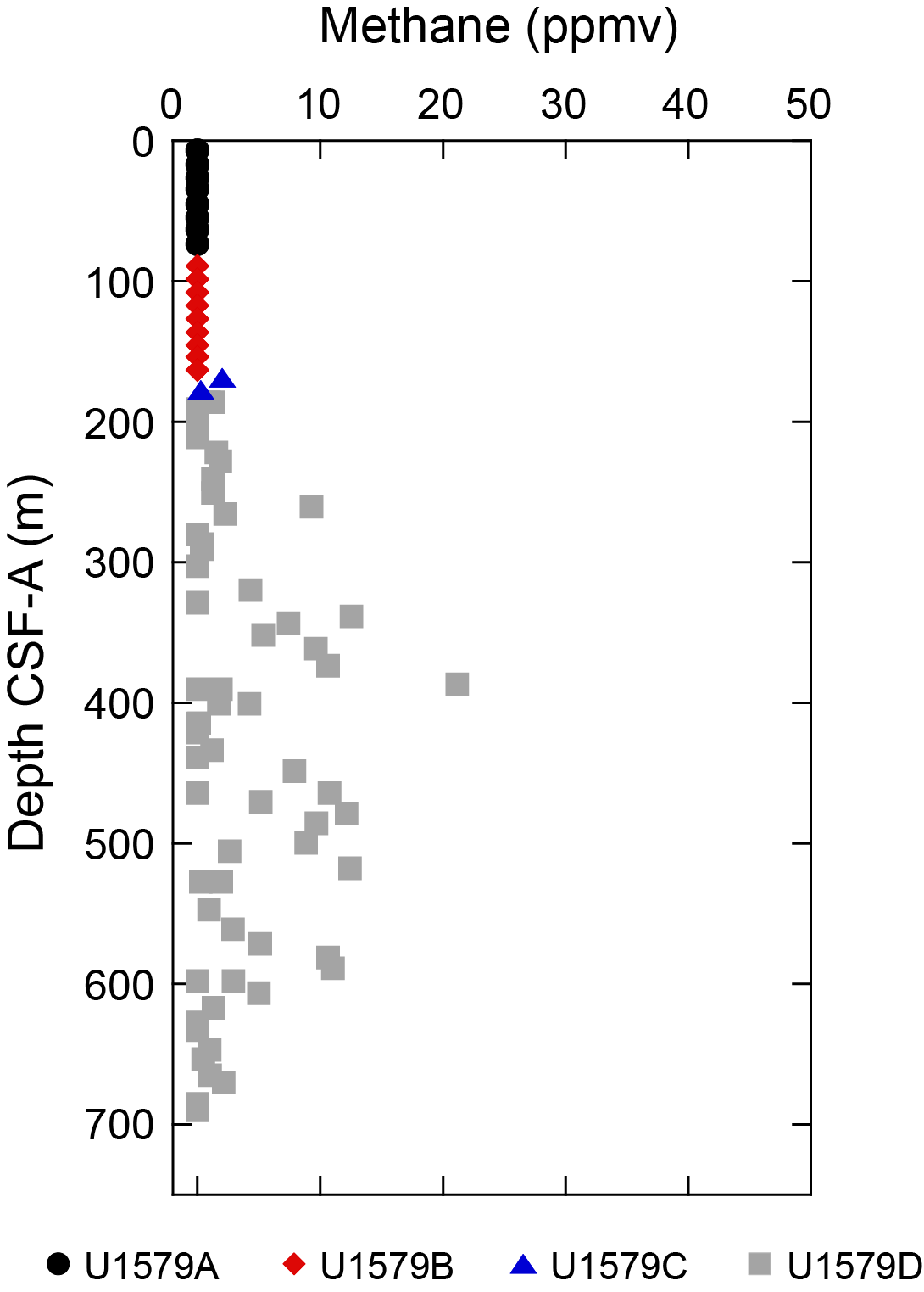
Figure F38. Methane concentration.
9.2. Interstitial water geochemistry
Samples for IW were collected downcore until no water was retrieved in three consecutive samples from Hole U1579D (42R-3, 113–123 cm [517.56 m CSF-A]; 45R-2, 131–141 cm [545.68 m CSF-A]; and 47R-5, 142–152 cm [569.73 m CSF-A]). IW samples were largely taken from intervals dominated by carbonate. Note that although Table T11 presents both inductively coupled plasma–atomic emission spectroscopy (ICP-AES) data and ion chromatography data for many of the major elements, we focus on the ion chromatography results for sulfate, chloride, and sodium and the ICP-AES data for the balance of the major cations. When discussing specific depths of samples for Geochemistry, this chapter references the Top depth CSF-A (m) value. Finally, we select the reference depth to anchor our results presentation as either from Hole U1579A, where the shallowest sample is from 1.45 m CSF-A, or Hole U1579B, where the shallowest sample is from 1.42 m CSF-A, depending on which sample provides the particular site minimum or maximum in relation to the other data in the profile.
Alkalinity increases from 2.9 mM in the shallowest sample (392-U1579B-1H-1, 142–152 cm; 1.42 m CSF-A) to 15.4 mM in Sample 392-U1579D-40R-2, 138–148 cm (496.98 m CSF-A) (Figure F39; Table T11). There is an overall decrease in pH from 7.7 at 1.42 m CSF-A to 7.0 at 496.98 m CSF-A (Figure F39; Table T11). Of the major anions, sulfate decreases at Site U1579 from 29.0 mM at 1.45 m CSF-A to 22.7 mM at ~280 m CSF-A and then remains relatively constant to nearly 500 m CSF-A (Figure F40). Chloride increases downhole over its seawater value (557 mM) to ~610 mM at ~497 m CSF-A at Site U1579 (Figure F40). The major cation sodium increases over its seawater value (481 mM) to 511 mM at 497 m CSF-A (Sample 1H-1, 142–152 cm; 1.42 m CSF-A) (Figure F40). Magnesium (ICP-AES) decreases from 51.6 mM at 1.45 m CSF-A to 43.0 mM at ~279 m CSF-A before increasing to 47.1 mM at the base of the record (Figure F40). Calcium (ICP-AES) increases from 10.7 mM at 1.42 m CSF-A to 27.5 mM at 497 m CSF-A. Potassium declines throughout the site from 10.9 to 7.0 mM (Figure F40). The minor elements Li and Sr both increase deeper at the site and are heavily enriched relative to seawater values (Lisw = 26.5 µM; Srsw = 91 µM) with maximum concentrations of 169.3 µM for Li and 727.3 µM for Sr. Boron concentrations are relatively invariant throughout the site at ~450 µM with the exception of an enrichment in the upper 100 m of the site where the maximum value exceeds 575.5 µM at 28.5 m CSF-A. Iron shows a broad range of 0–72.1 µM throughout the site (Figure F41).
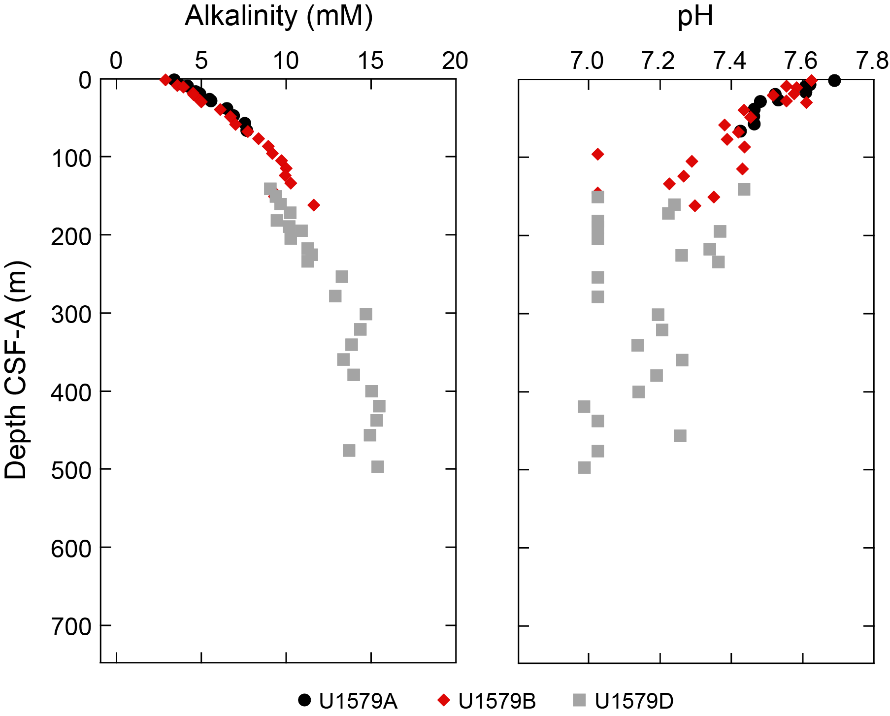
Figure F39. Alkalinity and pH.
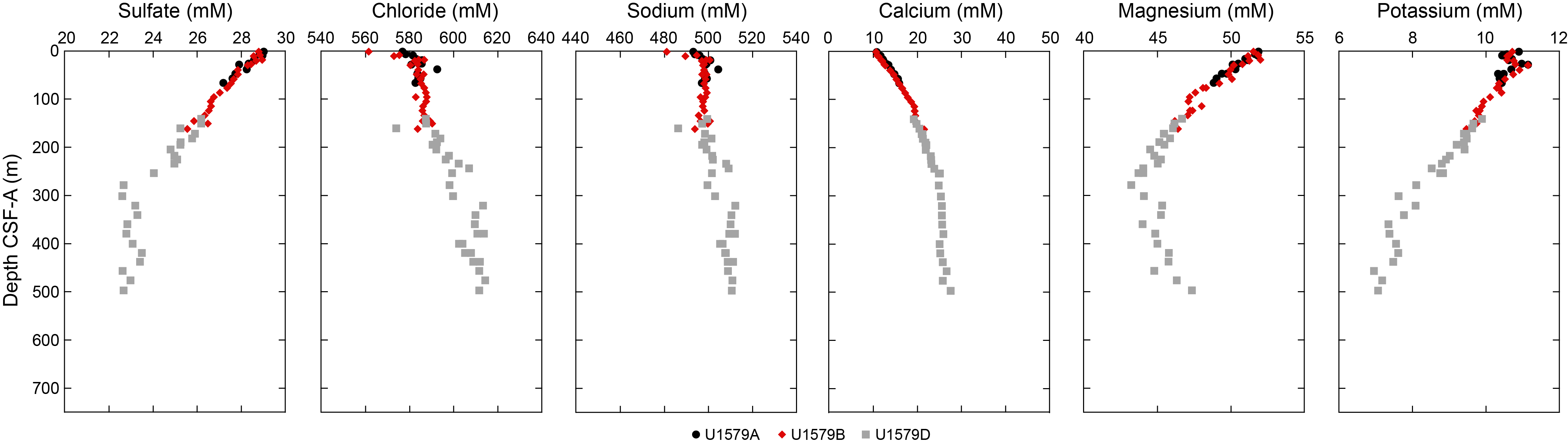
Figure F40. IW sulfate, chloride, sodium, calcium, magnesium, and potassium.
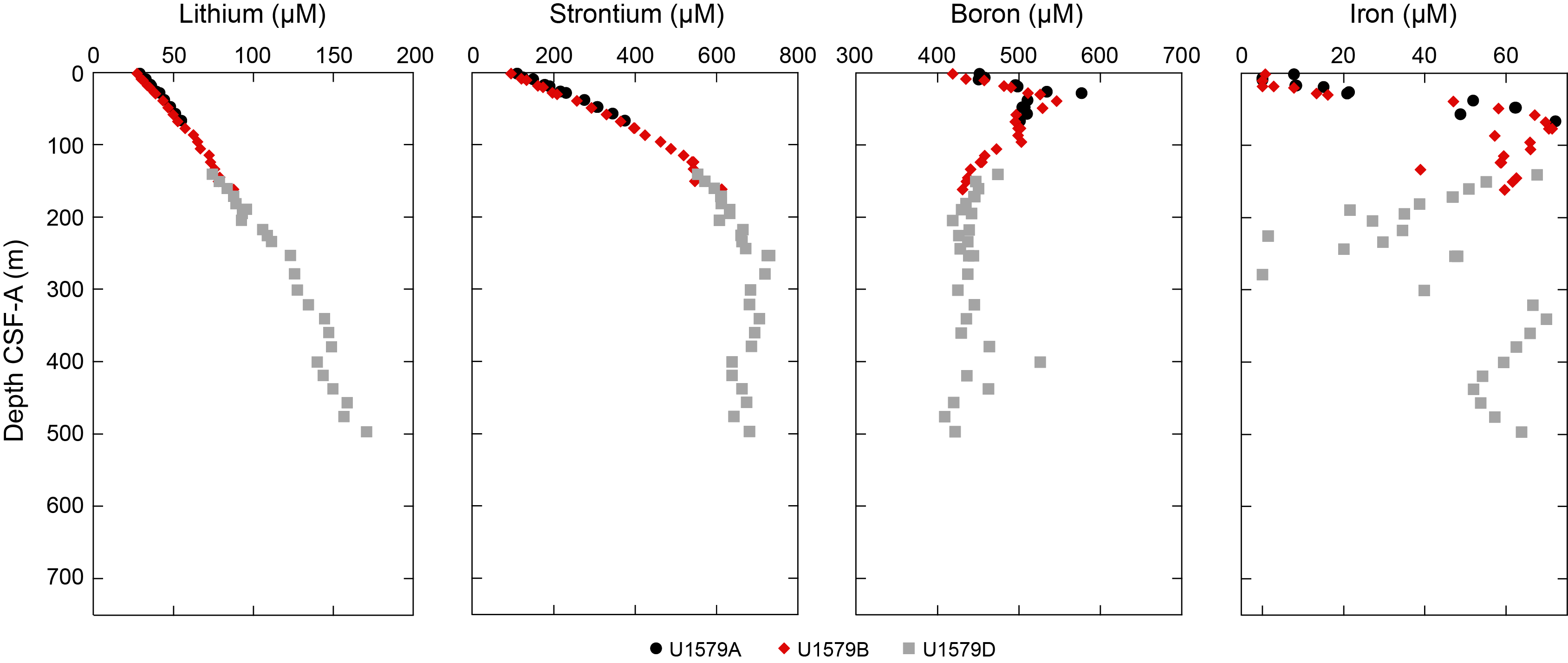
Figure F41. IW lithium, strontium, boron, and iron.
9.3. Bulk sediment geochemistry
In total, 135 sediment samples were obtained for bulk carbon and nitrogen analyses. One or two samples were routinely taken from the working half sections and more frequently in some cores to capture specific intervals of interest (i.e., lithologic variability).
Total carbon and CaCO3 range 1.0–12.2 wt% and 8.0–94.9 wt% at Site U1579, respectively, which is consistent with the deposition of largely pelagic nannofossil oozes (see Lithostratigraphy) (Figure F42; Tables T18, T19). We observe more variability in CaCO3 content between ~150 to 300 m CSF-A and generally lower concentrations of carbonate below ~450 m CSF-A. Below 630 m CSF-A, inorganic carbon and CaCO3 decrease to averages of 2.8 and 23.0 wt%, respectively. As a note of caution for the interpretation of these inorganic carbon records, we emphasize that the main carbonate mineral phase is likely CaCO3 for most parts of the nannofossil and foraminiferal ooze and chalk lithologies (Lithostratigraphic Units I and II; see Lithostratigraphy for smear slide data). However, in the green zeolitic siltstones and sandstones below ~640 m CSF-A (Lithostratigraphic Unit III), the carbonate content may include other carbonate minerals, including siderite, dolomite, and possibly others (see Lithostratigraphy). Despite these uncertainties, it is worth noting that carbonate carbon persists to the bottom of the analyzed sedimentary section (~695 m CSF-A).
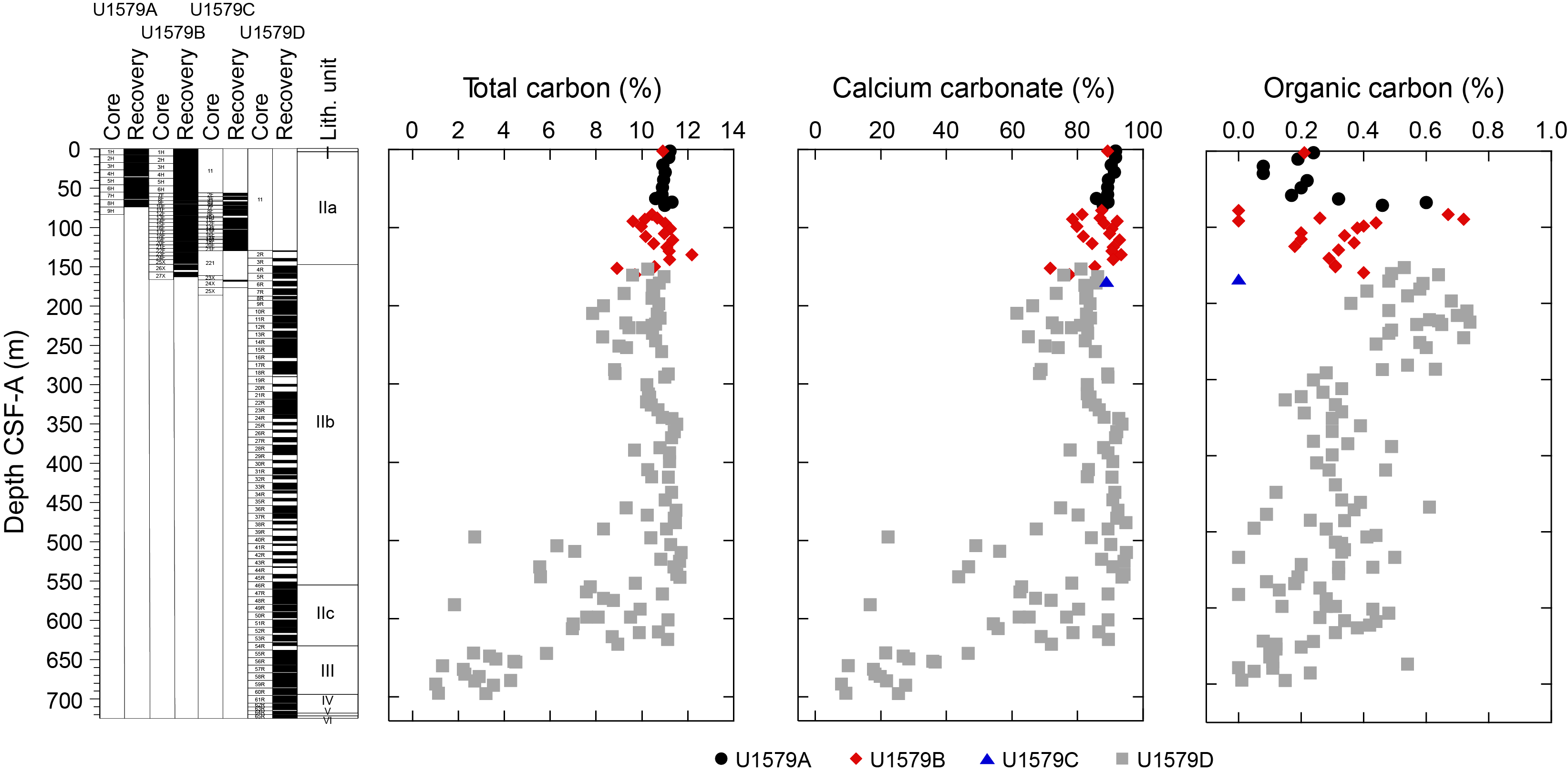
Figure F42. Carbon.
Organic carbon contents are calculated as the difference between total carbon (elemental analyzer measurement) and inorganic carbon (coulometer measurement). All organic carbon values are reported in Table T19, but three values that exceed 1 wt% organic carbon are excluded from Figure F42 for the purposes of plotting and are not included in the calculation of statistical data. Excluding these outliers, the average total organic carbon is 0.3 wt% ± 0.2% with minimum and maximum concentrations of 0.0 and 1.0 wt%, respectively. The uncertainty in the organic carbon estimation is ±0.3 wt% and is based on the average uncertainties in the carbonate carbon and total carbon measurements. Concentrations at or close to 0 are scattered throughout the sedimentary sequence, reflecting the prominent calcareous ooze and chalk character of large parts of the site and supporting the overall low methane concentrations. These results emphasize the need to determine organic carbon directly using an elemental analyzer in shore-based analysis, using decalcified samples.
Total nitrogen was measured but remains below detection limit for most samples analyzed from Site U1579. Where quantified, the results are likely related to the presence of inorganic nitrogen due to low organic carbon concentrations in these samples. The data are presented in Table T19 but are not discussed here further.
9.4. Sediment and igneous rock geochemistry
All major element concentrations for sediments are calculated and discussed as elemental weight percentages, and all minor and trace elements are presented in parts per million (Figure F43; Table T20). Aluminum concentrations are <3 wt% from 1.42 to 603.55 m CSF-A. Below 650.96 m CSF-A, Al concentrations increase abruptly and range 4.7–6.3 wt% in the remaining sediments. Silicon concentrations similarly are relatively low (1.5–7.7 wt%) in the upper ~600 m CSF-A and elevated below ~650 m CSF-A (18.4–24.6 wt%). Calcium concentrations likely represent calcium carbonate due to the similarity between the Ca concentrations and CaCO3 records. The Ca record mirrors the Al and Si records, with elevated concentrations (~26–35 wt%) in the upper 600 m CSF-A and lower concentrations (<4 wt%) from 600 to 683.63 m CSF-A. Potassium concentrations broadly follow Al and Si; however, the increase in K concentrations is more gradual and begins at 569.73 m CSF-A, almost 80 m above the changes in Al and Si. Iron and sulfur have opposite trends at Site U1579. Iron concentrations are relatively low in the upper 600 m CSF-A (<2 wt%) and elevated below ~650 m CSF-A, with a maximum concentration of 7.8 wt% in Sample 392-U1579D-56R-2, 3–5 cm (650.96 m CSF-A). Sulfur concentrations range 0.42–0.55 wt% between 1.42 and 603.55 m CSF-A. Below ~650 m CSF-A, S concentrations remain below 0.15 wt%.
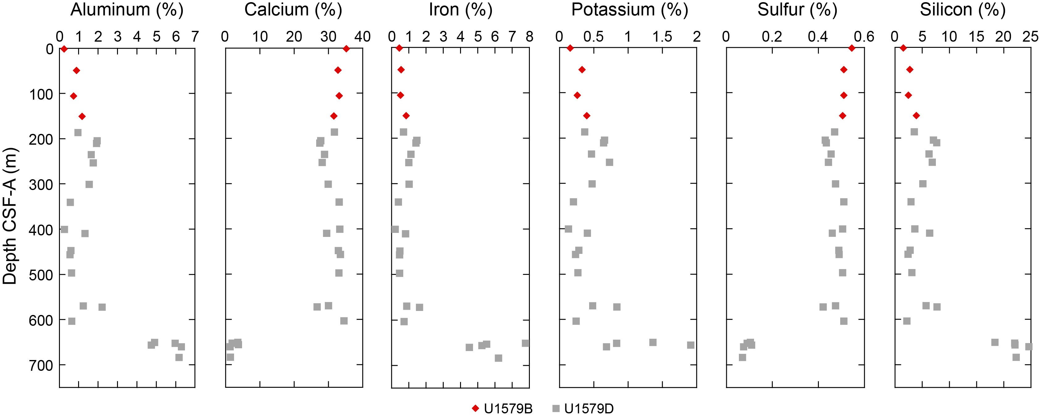
Figure F43. Sediment aluminum, calcium, iron, potassium, sulfur, and silicon.
All major element concentrations for igneous rock are calculated and discussed as oxide weight percentages, and all minor and trace elements are presented in parts per million. Two igneous rock intervals (Lithostratigraphic Unit IV, Igneous Unit 1; Lithostratigraphic Unit VI, Igneous Unit 2) were cored at the bottom of Hole U1579D, separated by sediments of Lithostratigraphic Unit V (see Igneous petrology). Two samples from the upper igneous interval (61R-6, 0–3 cm, and 63R-3, 17–19 cm; Igneous Unit 1) and one sample from the lower igneous interval (65R-5, 2–4 cm; Igneous Unit 2) were analyzed using ICP-AES (Table T21). Based on classic discrimination diagrams for igneous rocks (Figure F44) all three samples classify as tholeiitic basalts, plotting along with tholeiitic lavas from the neighboring Mozambique Ridge.
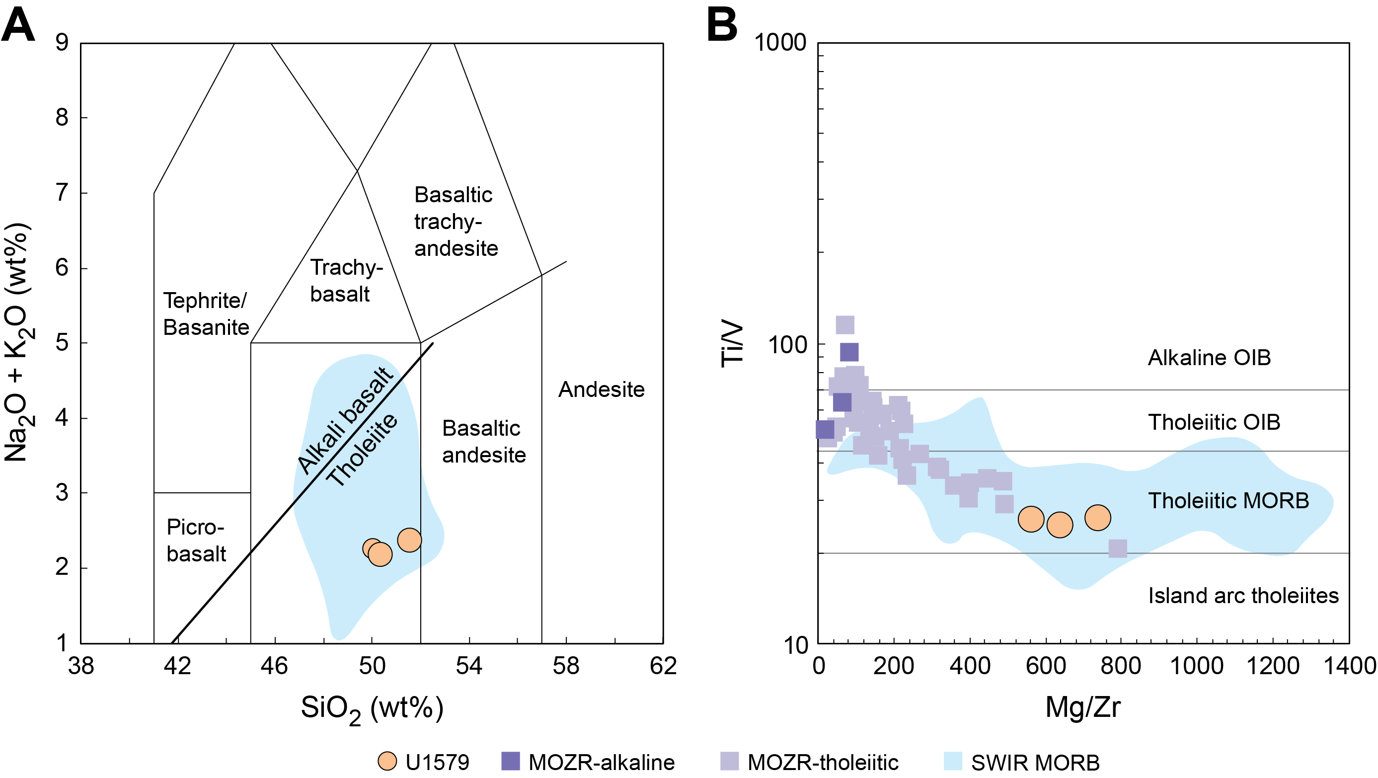
Figure F44. Total alkali vs. silica and Mg/Zr vs. Ti/V.
10. Physical properties
Physical properties of sediments and igneous rocks recovered at Site U1579 were measured on whole-round core sections, split-half core sections, and discrete samples from each hole at the site to the total recovered depth of 727.29 m CSF-A. In the upper 182 m of the site, the holes overlap stratigraphically and physical properties data were used to construct a composite splice (see Stratigraphic correlation). Downhole logging was also performed in Hole U1579D (see Downhole measurements).
10.1. Natural gamma radiation
NGR at Site U1579 varies between the lithostratigraphic units (Figure F45). The nannofossil-rich foraminiferal ooze of Lithostratigraphic Unit I is characterized by relatively high NGR values, as high as 27.3 counts/s in Core 392-U1579B-1H (2.82 m CSF-A). The nannofossil ooze of Lithostratigraphic Subunit IIa (Hole U1579B = 6.13–147.10 m CSF-A) has lower NGR values (average = 6.1 counts/s), which is consistent with high carbonate content in the interval. Lithostratigraphic Subunits IIb and IIc (Hole U1579D = 149.40–634.72 m CSF-A) have greater variability in NGR, although most values remain below 15 counts/s. Peaks above 15 counts/s coincide with intervals of distinct lithologies, including green clay-rich bands of chalk around 329, 496, 553, and 584 m CSF-A and intervals of chalks with red coloration around 433, 458, 558, 564, and 583 m CSF-A. In Lithostratigraphic Unit III at 639.90–697.09 m CSF-A, NGR values average 9.5 counts/s. In the basalts of Lithostratigraphic Units IV (697.00–720.77 m CSF-A) and VI (725.47–727.29 m CSF-A), NGR values are lower (average = 2.7 counts/s) and delineate the contacts with sedimentary Lithostratigraphic Unit V from 720.90 to 725.47 m CSF-A, which has NGR values of around 8 counts/s.
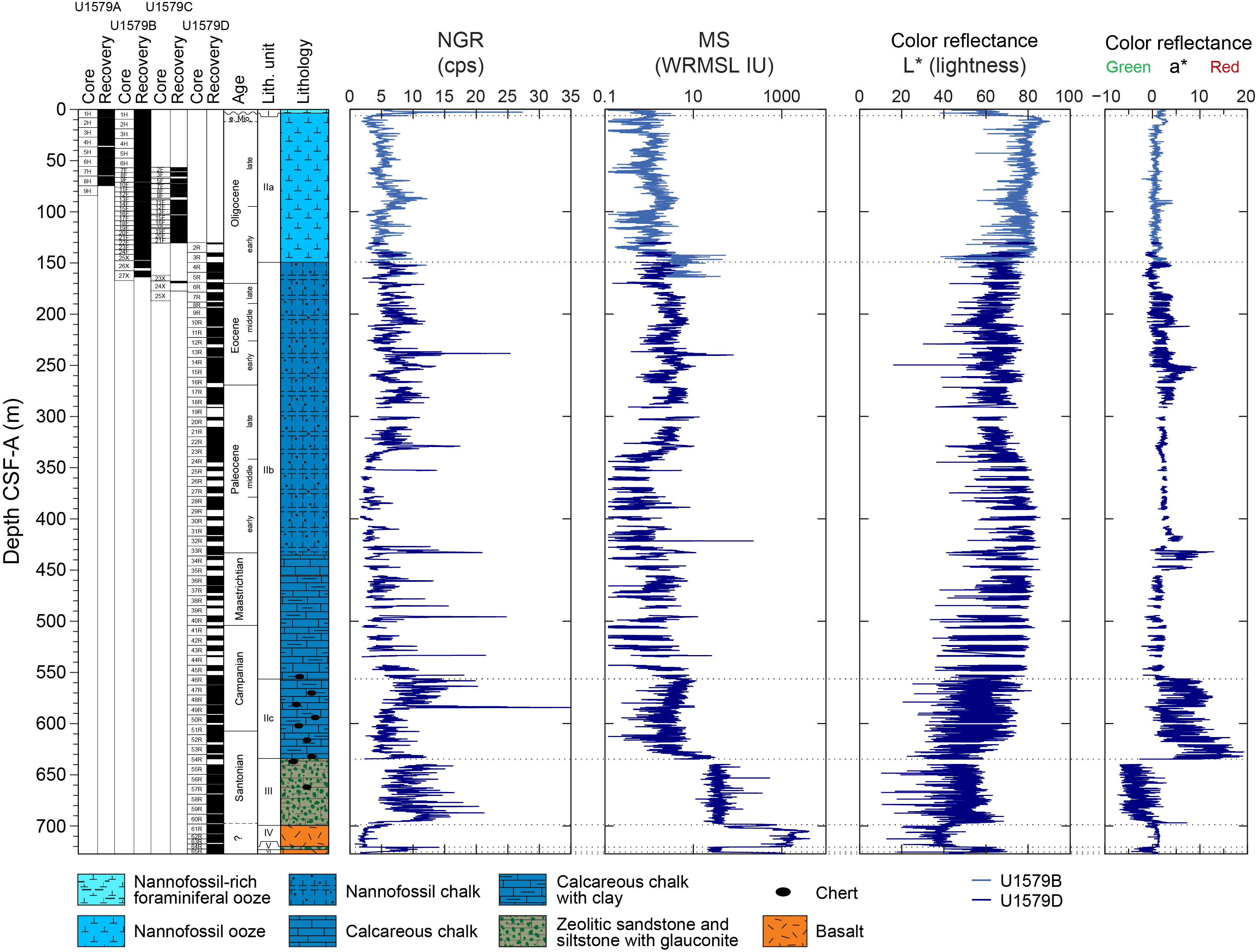
Figure F45. Physical properties.
Elemental abundances of K, U, and Th were deconvolved from the Natural Gamma Radiation Logger (NGRL) spectral data (see Physical properties in the Expedition 392 methods chapter [Uenzelmann-Neben et al., 2023a]) and provide additional insights into trends of the full NGR profile, along with geochemical and lithologic information for Site U1579 (Figures F46, F47). The main trends in K, Th, and U abundances generally follow broader trends in the NGR profile. For example, total NGR values and abundances of K, Th, and U all decrease downcore in the chert-rich nannofossil chalk of Lithostratigraphic Subunit IIc from 556 to 634 m CSF-A (Figure F47). In some intervals, abundance trends among the gamma ray–emitting elements diverge. In the uppermost ~6.2 m of Hole U1579B (Lithostratigraphic Unit I), U contents in the foraminiferal ooze sediments reach 3 ppm and are enriched compared to elsewhere in the hole (Figure F46). The abundance of K is particularly elevated, as high as ~2 wt%, in relation to U and Th in the green zeolitic siltstones and sandstones of Lithostratigraphic Units III and V in Hole U1579D (~635–697 and ~721–725 m CSF-A, respectively) (see Lithostratigraphy) (Figure F47).
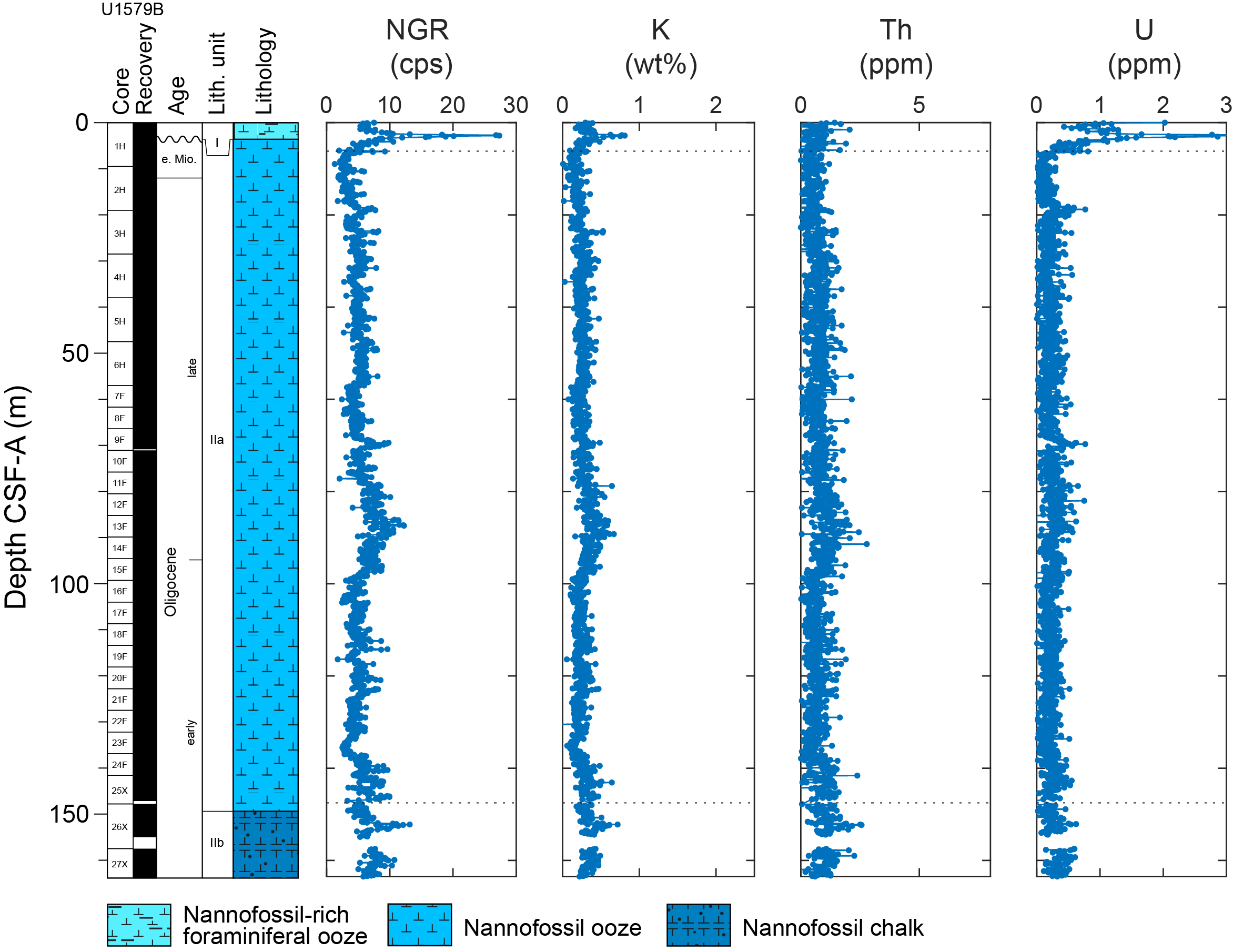
Figure F46. NGR and K, Th, and U, Hole U1579B.
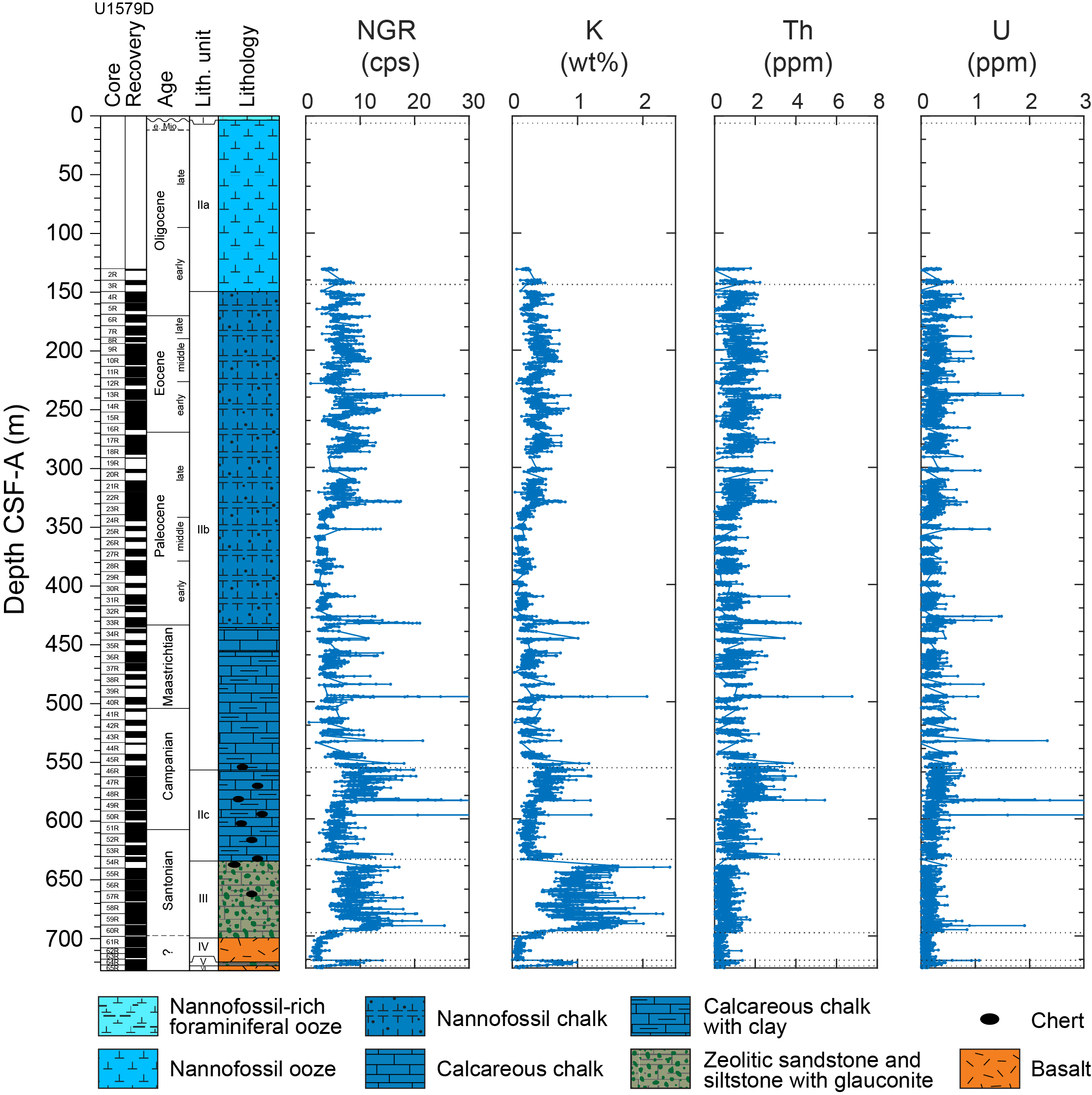
Figure F47. NGR and K, Th, and U, Hole U1579D.
10.2. X-ray images
X-ray imaging was performed on whole-round sections from Holes U1579A and U1579B and on Cores 392-U1579C-24X and 392-U1579D-5R, 6R, 7R, 23R, and 33R. Initial analysis of the X-ray images from Holes U1579A and U1579B did not show any distinct features caused by changes in density, so the decision was made to not routinely collect X-ray images for Holes U1579C and U1579D. For Hole U1579D, X-ray imaging was performed on selected sections and only minor drilling disturbance features could be imaged, with no trace of large ice-rafted clasts observed. Features related to bioturbation were observed, however, and are comparable to those documented in visual observation.
10.3. Color reflectance
Color reflectance parameters are distinctive among the lithostratigraphic units at Site U1579 (Figure F45). The nannofossil oozes and chalks of Lithostratigraphic Subunits IIa and IIb (~6 to 556 m CSF-A) have high L* values (lightness) that are mostly above 50, consistent with high carbonate content in this interval (see Geochemistry). In the red-hued chert-rich nannofossil chalks of Lithostratigraphic Subunit IIc (~556 to 634 m CSF-A), values of a* (red to green) are as high as ~20 and L* values decrease downcore. The potassium-rich and green-hued zeolitic siltstones and sandstones of Lithostratigraphic Units III (~635–697 m CSF-A) and V (~721–725 m CSF-A) have the lowest a* values for the site, approaching −9.
10.4. Magnetic susceptibility
MS was measured on all whole-round sections at Site U1579 using the WRMSL and on archive-half sections using the point MS (MSP) instrument on the Section Half Multisensor Logger (SHMSL). Trends in the data sets from the two instruments are comparable, although data from the SHMSL are noisier. The following report thus refers to the values measured with the WRMSL (Figure F45).
In Lithostratigraphic Unit I and Lithostratigraphic Subunit IIa (Hole U1579B = 0–147.10 m CSF-A), MS values are generally low (average = ~1 instrument unit [IU]) with the exception of peaks in Core 392-U1579C-17F between 113 and 115 m CSF-A that coincide with an interval of coring disturbance. MS values in nannofossil chalks of Lithostratigraphic Subunit IIb (149.40–556.31 m CSF-A) average 3.0 IU to 345 m CSF-A and 1.3 IU to the base of the subunit (Figure F45). In Lithostratigraphic Subunit IIc, MS values average 3.3 IU. The highest values of MS in Lithostratigraphic Subunits IIb and IIc coincide with intervals of red sedimentary banding. In the green zeolitic siltstones and sandstones of Lithostratigraphic Unit III, MS values are considerably higher (average = 38 IU) (Figure F45). MS values in the upper part of the basalt of Lithostratigraphic Unit IV are variable, averaging 408 IU at 698.15–700.24 m CSF-A and 76 IU at 700.24–701.97 m CSF-A. The highest MS of the entire sequence recovered at Site U1579 occurs between 701.97 and 720.60 m CSF-A in the basalts of Lithostratigraphic Unit IV (average = ~1700 IU) (Figure F45). MS values average 31 IU from 720.90 to 725.47 m CSF-A, coinciding with the zeolitic siltstones and sandstones of Lithostratigraphic Unit V, and ~600 IU from 725.47 m CSF-A to the base of the cored interval at 727.285 m CSF-A in the basalt of Lithostratigraphic Unit VI (Figure F45).
10.5. Bulk density, grain density, and porosity
Moisture and density (MAD) analyses were performed on 139 discrete samples (2 per full core; 1 per half core). Bulk density increases downcore from ~1.7 g/cm3 near the seafloor to about ~2.0 g/cm3 at 140 m CSF-A, following a general trend of porosity reduction from 58% near the seafloor to ~43% at the transition from nannofossil ooze (Lithostratigraphic Subunit IIa) to nannofossil chalk (Lithostratigraphic Subunit IIb) at ~140 m CSF-A (Figure F48). This trend is consistent with mechanical compaction of the ooze. In the underlying nannofossil chalk of Lithostratigraphic Subunit IIb (~140–550 m CSF-A), porosity and bulk density values vary in a narrow range of ~40%–45% and ~1.9–2.1 g/cm3, respectively. Bulk density values are higher in the chert-bearing interval of Lithostratigraphic Subunit IIc (~550–630 m CSF-A) and reach ~2.5 g/cm3, indicating pore cementation (porosity = ~15%). The altered zeolitic siltstones and sandstones of Lithostratigraphic Unit III are characterized by variable but on average very high porosity (40%–50%) and low bulk density (1.8–1.9 g/cm3) (Figure F48). Grain density values in Lithostratigraphic Unit III drop below 2.5 g/cm3, which is beyond standard deviation and cannot be attributed to a random fluctuation with respect to the mean grain density obtained for all MAD samples at Site U1579 (2.71 ± 0.06 g/cm3; values typical for calcite). This low grain density may indicate the presence of low-density clay minerals such as glauconite (2.3 g/cm3) and zeolites (chabazite = 2.09 g/cm3; analcime = 2.3 g/cm3). The bulk and grain density values measured in the basalt lithologies are 2.6–3.0 g/cm3.
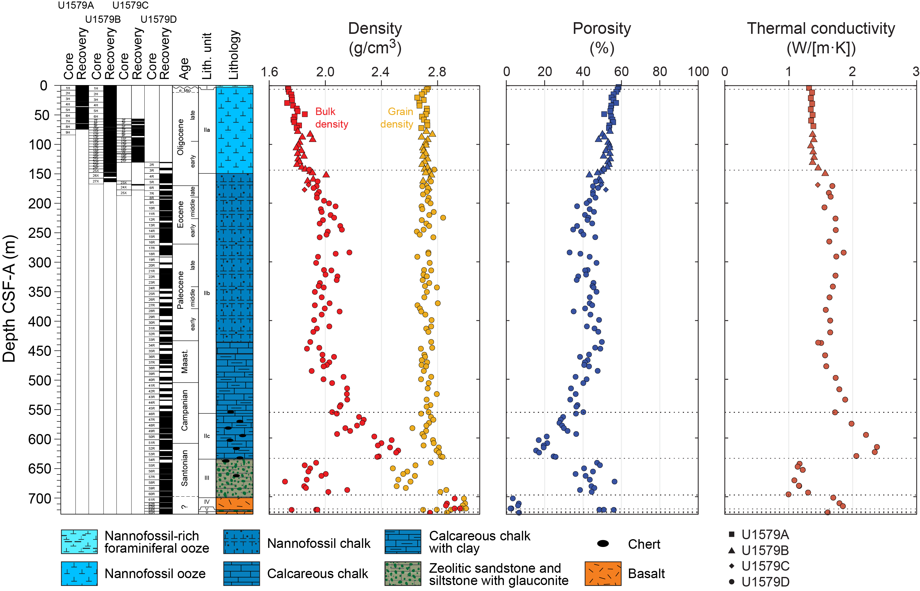
Figure F48. MAD and thermal conductivity.
In the sedimentary lithologies at Site U1579, the WRMSL gamma ray attenuation (GRA) bulk density values vary between 1.5 and 2.3 g/cm3, with frequent lower outliers at locations of cracks or other core disturbances that were cleaned from the data set (Figure F49). The general MAD density trend is consistent with GRA bulk density data (Figure F50). However, the absolute values obtained in the core samples using the two methods exhibit systematic offsets. In the oozes at shallow depths, the MAD bulk density values are lower than GRA bulk densities by 0.05–0.10 g/cm3. This is likely an artifact of the measurement process caused by a silicon standard used for calibration of the GRA instrument (B. Mills, pers. comm., 2022). In Hole U1579D, GRA bulk density data are lower than MAD values, likely because of voids between the core liner and rock in RCB cores. Despite this, GRA bulk density data from Hole U1579D correlate with MAD bulk density data (Figure F50).
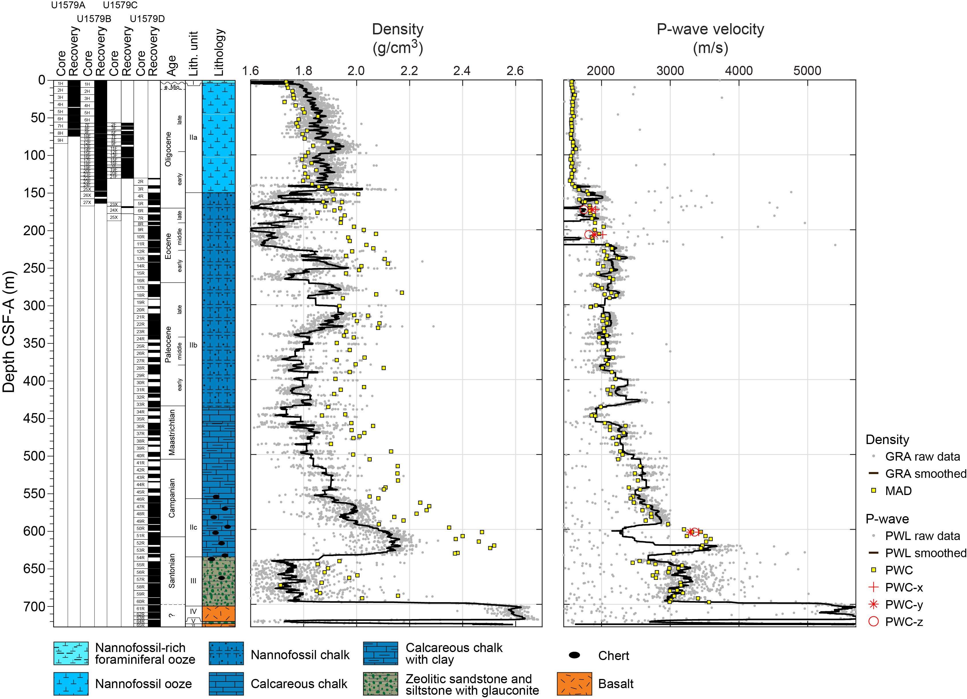
Figure F49. Density and P-wave velocity.
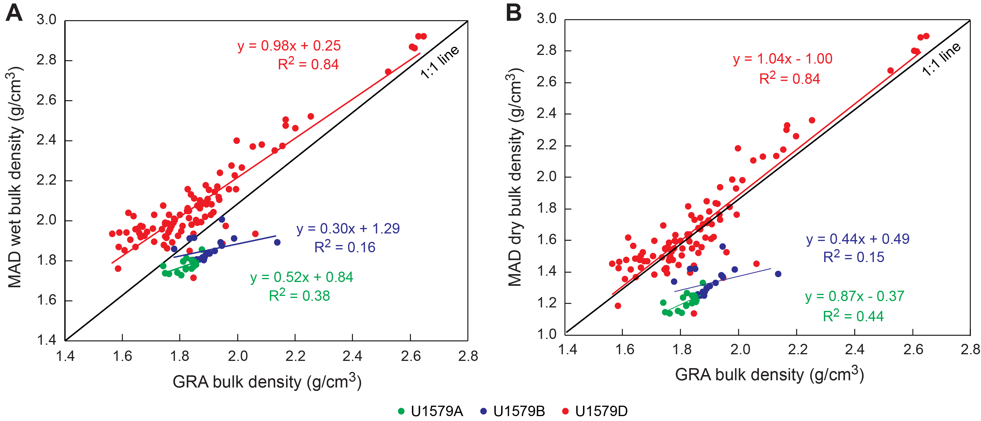
Figure F50. Bulk density.
10.6. P-wave velocity
Contact P-wave velocity data were measured using the P-wave caliper (PWC) system on working-half sections (1–2 per core; total = 163) and 3 discrete cubic samples (9 measurements) (Figure F49). In the foraminiferal and nannofossil oozes of Lithostratigraphic Unit I and Lithostratigraphic Subunit IIa (0–147.10 m CSF-A), P-wave velocities vary in a narrow range of 1560–1600 m/s. PWC P-wave velocity increases notably from ~1800 to 2000 m/s below ~148 m CSF-A across the contact of the poorly cemented nannofossil ooze (Lithostratigraphic Subunit IIa) and the stiffer underlying nannofossil chalk (Lithostratigraphic Subunit IIb). Values of about 2000–2150 m/s characterize the nannofossil chalk of Lithostratigraphic Subunit IIb to ~500 m CSF-A. In the chert-rich nannofossil chalk of Lithostratigraphic Subunit IIc, the velocity significantly increases to 2500–3500 km/s between 556 and 635 m CSF-A. Average P-wave velocities in the underlying altered zeolitic siltstones and sandstones (Lithostratigraphic Units III and V) and basalts (Lithostratigraphic Units IV and VI) are 2500–3000 and 4500–5600 km/s, respectively.
PWC velocity data are generally consistent with the WRMSL P-wave logger (PWL) data, which average 1585 m/s in Holes U1579A and U1579C and Cores 392-U1579B-1H through 23X. For Cores 25X–27X (141.6–163.96 m CSF-A), PWL velocity data scatter relates to poor contact between core and liner. For subsequent measurements of P-wave velocity on XCB or RCB cores, which generally have smaller diameters than APC cores, the P-wave velocity logger was adjusted to improve contact with the core. Because of an error in instrumental settings for Cores 392-U1579D-50R through 52R (591.4–618.16 m CSF-A), P-wave values above 3000 m/s were cut off, resulting in an incomplete record. The amplitude threshold settings on the PWL were corrected for more reliable measurements in subsequent cores. In these intervals (Cores 50R–52R; 591.4–618.16 m CSF-A), we performed 3–5 repeated caliper measurements on half-core sections at different sample points and additional P-wave velocity measurements on discrete samples (2 cm3) in the x-, y-, and z-(downhole) directions.
10.7. Thermal conductivity
Thermal conductivity was measured on soft-sediment whole-round sections using a needle probe in Cores 392-U1579A-1H through 8H (0–69 m CSF-A) and a puck probe on underlying material (Figure F48). Thermal conductivity generally increases downcore from ~1.4 W/(m·K) in the nannofossil ooze of Lithostratigraphic Subunit IIa (~6–144 m CSF-A) to ~1.7 W/(m·K) in the nannofossil chalk of Lithostratigraphic Subunit IIb (~144–556 m CSF-A) and to 2.2–2.5 W/(m·K) in the chert-rich nannofossil chalk of Lithostratigraphic Subunit IIc (~556–635 m CSF-A). Lithostratigraphic Unit III (~635–697 m CSF-A) exhibits a very low thermal conductivity of 1.2–1.3 W/(m·K). Thermal conductivity measured in the basalt of Lithostratigraphic Unit IV (~700–720 m CSF-A) is 1.8–1.9 W/(m·K), with lower values in this range reflecting more vesicular texture (see Igneous petrology). Overall, thermal conductivity values at the site inversely correlate with porosity and positively correlate with both bulk density and P-wave velocity data.
11. Downhole measurements
Downhole measurements at Site U1579 included formation temperature measurements in Holes U1579A and U1579B and wireline logging in Hole U1579D. Downhole data are available through the Lamont-Doherty Earth Observatory (LDEO) logging database.
11.1. Wireline downhole logging
The quad combo tool string was deployed in Hole U1579D following the completion of RCB drilling. The borehole was first swept with sepiolite and stabilized with barite. The BHA of the drill string was then retracted to 70.7 m DSF (see Operations). From bottom to top, the main tools on the 48.4 m long quad combo string consisted of the MSS, HNGS, HRLA, DSI, and HLDS (see Downhole measurements in the Expedition 392 methods chapter [Uenzelmann-Neben et al., 2023a]). The downhole logging run consisted of multiple passes. The main pass spanned from ~728 m WMSF to the seafloor (Figure F51) and was preceded by a high-resolution repeat pass from 460 to 240.5 m WMSF (Figure F52). Logging speed was 550 m/h for the main pass and 275 m/h for the high-resolution repeat pass. For standard logging speeds on the main pass, the HLDS (density), DSI (seismic velocities), HRLA (resistivity), and HNGS (gamma ray) logs had a sampling resolution of 15.24 cm (6 inches). For high-resolution logging speeds on the repeat pass, the HRLA, HLDS, and HNGS logs had a sampling resolution of 5.08 cm (2 inches). Dual-coil MSS data were acquired with a depth sampling resolution of 2.54 cm (1 inch).
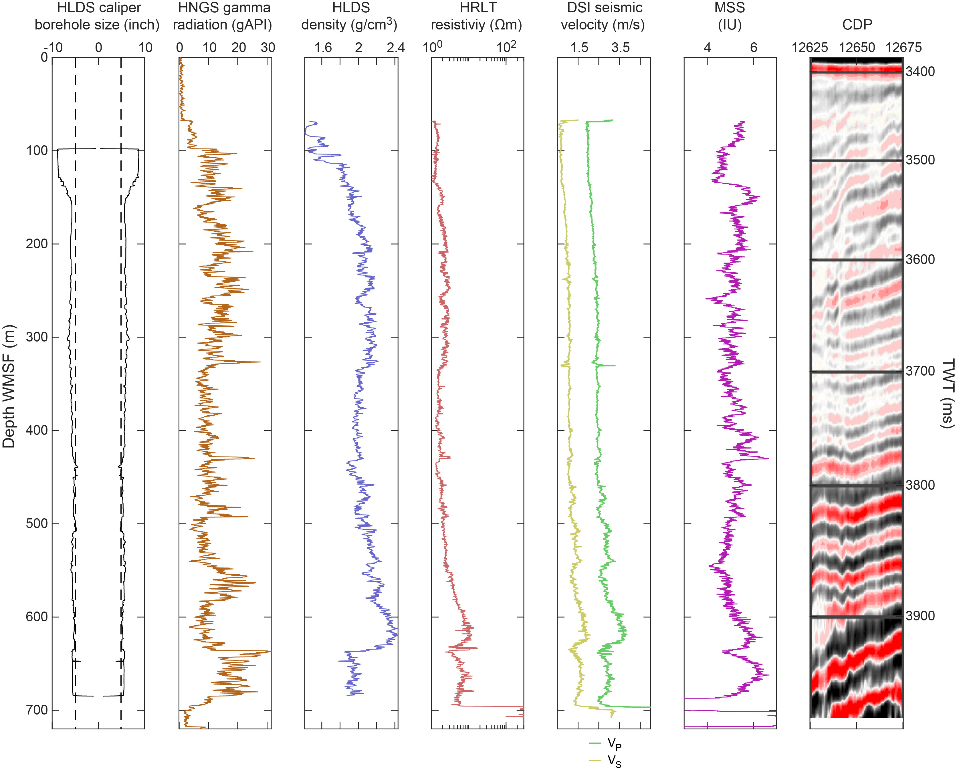
Figure F51. Downhole logging.
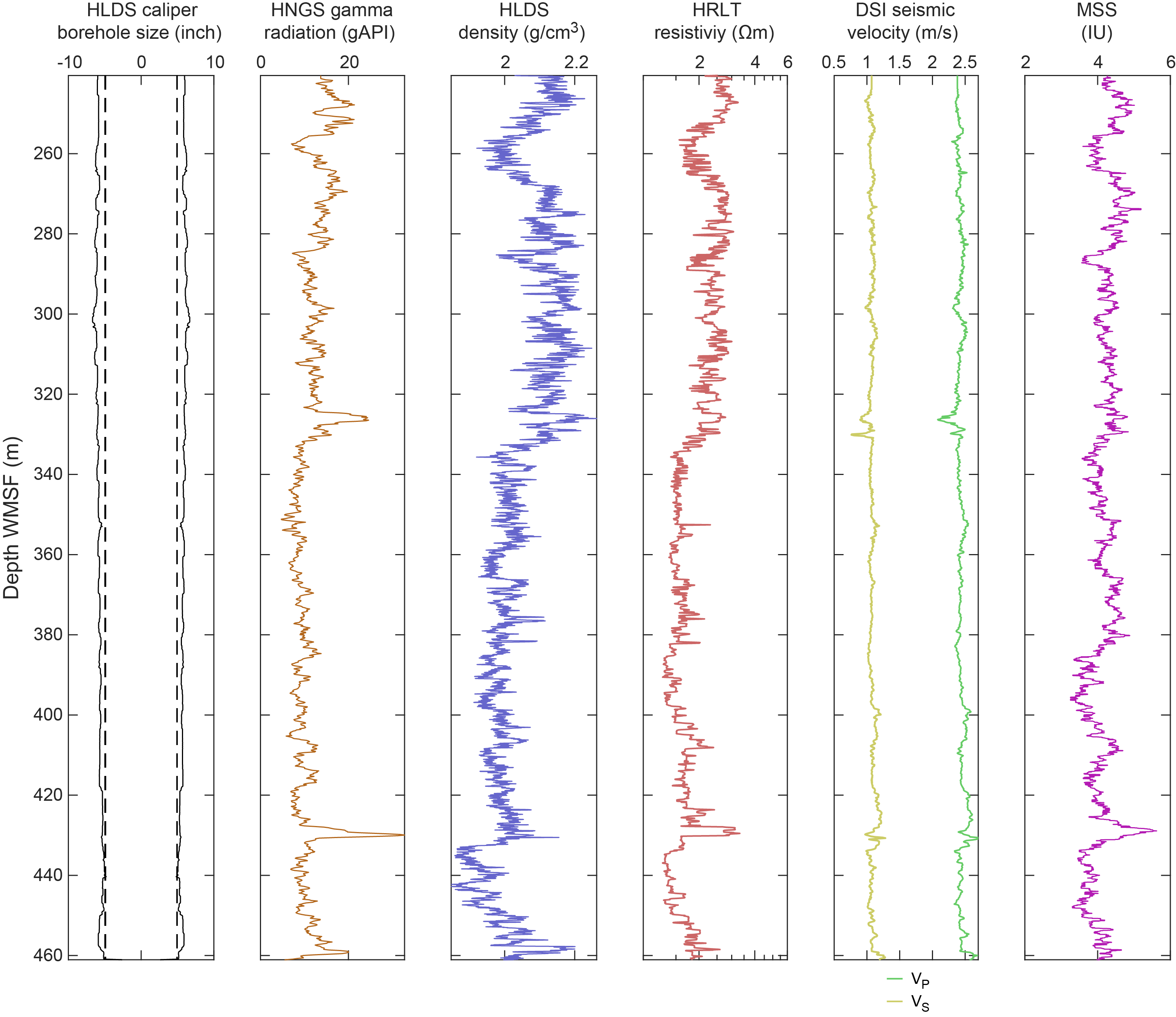
Figure F52. High-resolution downhole logging.
Logging data were corrected for variations in the borehole diameter in Hole U1579D, which were measured using a hydraulic caliper on the HLDS during each main pass. The quality of the borehole was good to excellent for downhole logging. Caliper measurements indicated a median borehole diameter of 29.0 cm (11.4 inches) for the main pass, which is close to the diameter of the RCB drill bit (25.1 cm; 9.875 inches). Shallower than ~160 m WMSF, the borehole diameter exceeded the 43.2 cm (17 inch) measurement limit of the caliper, suggesting extensive washout of the borehole wall. Measurements using logging tools such as the HLDS and HRLA, which require contact with the borehole wall, can be affected by wide (>30.5 cm; 12 inches) or irregular borehole size. As a result, logging data shallower than ~160 m WMSF from Hole U1579D should be interpreted with caution.
After logging, the preprocessed logs were sent to the LDEO Borehole Research Group (LDEO-BRG), where the logs were processed and then sent back to the ship during the expedition. One aspect of this processing involved shifting the wireline logs to a depth scale referenced to the seafloor, which was determined by steps in HSGR (standard total NGR) and resistivity observed on the downpass of the quad combo at 2504 m wireline log depth below rig floor (WRF) in Hole U1579D. The high-resolution logging pass from 460 to 240.5 m WMSF measured detailed density and NGR records important for stratigraphic correlation across geologic events at Site U1579 spanning the Maastrichtian to the lower Eocene in Lithostratigraphic Subunit IIb (see Lithostratigraphy and Chronostratigraphy). Downhole variations in NGR, density, electrical resistivity, and seismic velocities logs for Hole U1579D are shown in Figures F51 and F52 (high-resolution run).
11.1.1. Natural gamma radiation
The HNGS measured lithology-dependent NGR from the borehole wall in Hole U1579D. HSGR ranges 5–30 American Petroleum Institute gamma radiation units (gAPI) between 100 and 720 m WMSF. Prominent peaks and trends in the HSGR downhole profile can be readily correlated to NGR data measured from the cores on the NGRL (see Stratigraphic correlation; Figure F36). The nannofossil ooze of Lithostratigraphic Subunits IIa and IIb (~130–330 m CSF-A) is characterized by HSGR of about 20 gAPI on average (Figures F51, F52). In Lithostratigraphic Subunits IIb and IIc (~330–635 m CSF-A), HSGR records a less uniform signal of 10–30 gAPI. From ~360 to 540 m WMSF (Lithostratigraphic Subunit IIb), the average HSGR is lower (about 10 gAPI), with distinct spikes generally corresponding to increased clay content (such as at 329 and 430 m WMSF). HSGR increases to about 20 gAPI in the silicified chalk of Lithostratigraphic Subunit IIc (~540–590 m CSF-A) and is more variable than in Lithostratigraphic Subunit IIb. HSGR is greatest (20–30 gAPI) in the zeolitic siliciclastic sediments of Lithostratigraphic Unit III (~630–697 m CSF-A), whereas values are lowest (~5 gAPI) below 697 m WMSF in the basalt of Lithostratigraphic Unit IV. However, there is no information on the borehole size in this interval because the caliper arm was closed.
The HNGS measured the approximate elemental abundance of U, Th, and K based on downhole spectral HSGR data. The abundance of gamma ray emitting elements measured during downhole logging in Hole U1579D are equivalent to spectral deconvolution results from the NGRL data. The downhole K and Th abundances follow the HSGR trend in Hole U1579D except for several peaks in U abundance, such as at about 580 m WMSF in the mid-Campanian strata of Lithostratigraphic Subunit IIc.
A crossplot diagram of thorium versus potassium abundances can be used for discrimination of clay mineralogy using downhole gamma ray spectroscopy data. The measured Th/K ratios for 100 to ~630 m CSF-A (Lithostratigraphic Units I and II) fall between lines Th/K = 2 and Th/K = 12 (Figure F53). This range of elemental ratios is characteristic for illite and montmorillonite clays (Quirein et al., 1982). Th/K ratios between ~630 and 700 m WMSF form a distinct cluster between the Th/K = 0.5 and Th/K = 2 lines. This indicates the presence of more potassium-rich clay minerals (e.g., glauconite, micas) in the zeolitic siliciclastic sediments of Lithostratigraphic Unit III.
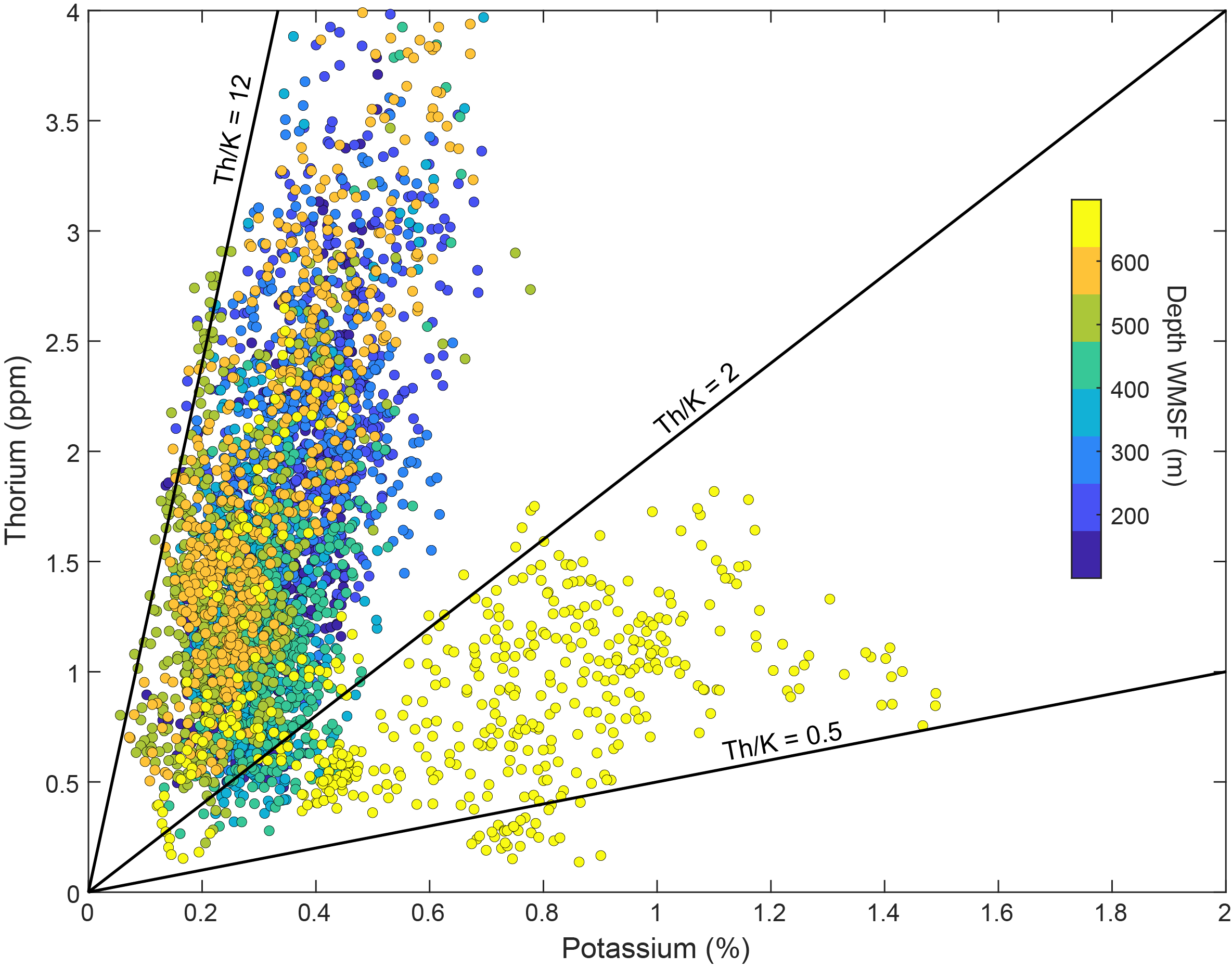
Figure F53. K vs. Th abundance data.
11.1.2. Resistivity
Electrical resistivity was measured in Hole U1579D using the HRLA (Figures F51, F52). In the nannofossil oozes and chalks of Lithostratigraphic Subunits IIa and IIb logged between ~80 and 550 m WMSF, resistivity is very low (between 1 and 2 Ωm). Resistivity increases from 2 to about 10 Ωm between ~556 and 635 m WMSF in the lower porosity Lithostratigraphic Subunit IIc (Figure F48), which consists of chalk with claystone and chert (see Lithostratigraphy). Resistivity in the zeolitic siliciclastic sediments (Lithostratigraphic Unit III; ~635–697 m CSF-A) is 5–6 Ωm on average, indicative of more conductive lithologies than in the lower part of Lithostratigraphic Subunit IIc. The highest resistivity values (100–300 Ωm) were recorded in the basalt of Lithostratigraphic Unit IV below ~697 m WMSF.
11.1.3. Seismic velocity
Downhole P-wave velocity (VP) data from the DSI are biased by borehole washout from ~70 to 160 m WMSF. Below ~160 m WMSF, DSI P-wave velocity data generally follow the same trends as P-wave velocities measured from the cores using the PWC (Figure F49). However, the two data sets show a systematic offset in Lithostratigraphic Subunit IIb (200–556 m WMSF), where the DSI P-wave velocity is about 300 m/s higher than PWC data from the equivalent depth interval. This can be explained by sediment decompaction that occurs during core recovery when confinement pressure drops. After applying a correction to the PWC data following Urmos and Wilkens (1993), the velocities are equivalent with data from the DSI (Figures F51, F52). Velocities in Lithostratigraphic Subunit IIc (VP = 2500–3200 m/s; S-wave velocity [VS] = 1800–2000 m/s) correlate with increased electrical resistivity and HSGR values. The variation of shear wave velocity in this subunit is similar to variations in P-wave velocity. A distinct peak in HSGR values at ~330 m WMSF is also observed in P-wave and S-wave velocities obtained using the DSI.
11.1.4. Density
The density profile of the borehole wall in Hole U1579D was measured using the HLDS during logging (Figures F51, F52). In the nannofossil chalk of Lithostratigraphic Subunit IIb, density averages ~2.0 g/cm3 (~160 and 500 m WMSF). Density increases from 2.0 to 2.4 g/cm3 toward the bottom of Lithostratigraphic Subunit IIc (chalk with claystone) at ~635 m WMSF, below which it drops significantly to less than 1.8 g/cm3 in the zeolitic siliciclastic sediments of Lithostratigraphic Unit III (~635 to 697 m CSF-A). The porosity and density determined by MAD analysis (see Physical properties) are in good agreement with the downhole HLDS density logs data.
11.1.5. Magnetic susceptibility
MS was measured downhole using the MSS. Subsequent data processing included removing a nonlinear trend related to the thermal sensitivity of the MSS and estimated temperature changes with depth in the borehole during logging. This baseline correction was performed with a high-order polynomial (Degree 5 to 11), providing the highest correlation with WRMSL MS data. A polynomial of Degree 9 was found to be optimal, and this trend was subtracted from the raw data. In Figures F51 and F52, a 30 point median filter was applied to smooth the raw data.The downhole MSS data provide more detailed information on the depth intervals of partial core recovery, such as from ~200 to 550 m WMSF (Figure F52). Changes in downhole MS can be correlated with lithologic changes and with discontinuities in P-wave velocity and density.
11.2. Formation temperature
Borehole formation temperatures were measured in Holes U1579A (Cores 4H, 35.0 m CSF-A, and 7H, 55.6 m CSF-A) and U1579B (Core 4H, 38.0 m CSF-A) using the APCT-3 tool (see Downhole measurements in the Expedition 392 methods chapter [Uenzelmann-Neben et al., 2023a]). The temperature measurement from Core 392-U1579A-4H (35.0 m CSF-A) was of poor quality, likely due to a heave of the drill string during measurement. As a result, that data point is not recorded in the LIMS database. Based on the two higher quality equilibrium borehole temperatures (4.4° ± 0.01°C at 38.0 m CSF-A and 5.9° ± 0.01°C at 55.6 m CSF-A), a geothermal gradient of ~55°C/km and heat flow of ~70 mW/m2 were calculated using the TP-Fit software. These preliminary results are consistent with prior measurements for the Agulhas Plateau published in the global heat flow database by Fuchs et al. (2021) but require further postcruise analysis and uncertainty estimation.
References
Agnini, C., Fornaciari, E., Raffi, I., Catanzariti, R., Pälike, H., Backman, J., and Rio, D., 2014. Biozonation and biochronology of Paleogene calcareous nannofossils from low and middle latitudes. Newsletters on Stratigraphy, 47(2):131–181. https://doi.org/
Aubry, M.-P., 1988. Handbook of Calcareous Nannoplankton (Book 2): Ortholithae (Catinasters, Ceratoliths, Rhabdoliths). New York (Micropaleontology Press).
Banner, F.T., 1972. Pithonella ovalis from the early Cenomanian of England. Micropaleontology, 18(3):278–284. https://doi.org/
Crux, J.A., 1991. Calcareous nannofossils recovered by Leg 114 in the subantarctic South Atlantic Ocean. In Ciesielski, P.F., Kristoffersen, Y., et al., Proceedings of the Ocean Drilling Program, Scientific Results. 114: College Station, TX (Ocean Drilling Program), 155–177. https://doi.org/
Fioroni, C., Villa, G., Persico, D., Wise, S.W., and Pea, L., 2012. Revised middle Eocene-upper Oligocene calcareous nannofossil biozonation for the Southern Ocean. Revue de Micropaléontologie, 55(2):53–70. https://doi.org/
Fisher, N.I., Lewis, T., and Embleton, B.J.J., 1987. Statistical Analysis of Spherical Data: Cambridge, United Kingdom (Cambridge University Press). https://doi.org/
Fisher, R.A., 1953. Dispersion on a sphere. Proceedings of the Royal Society A: Mathematical, Physical and Engineering Sciences, 217(1130):295–305. https://doi.org/
Flower, R.J., 1993. Diatom preservation: experiments and observations on dissolution and breakage in modern and fossil material. Hydrobiologia, 269(1):473–484. https://doi.org/
Fuchs, S., Norden, B., and the International Heat Flow Commission, 2021. The Global Heat Flow Database. GFZ Data Services. https://doi.org/
Gradstein, F.M., Ogg, J.G., Schmitz, M.D., and Ogg, G.M. (Eds.), 2012. The Geologic Time Scale 2012: Amsterdam (Elsevier). https://doi.org/
Gradstein, F.M., Ogg, J.G., Schmitz, M.D., and Ogg, G.M. (Eds.), 2020. The Geologic Time Scale 2020: Amsterdam (Elsevier BV). https://doi.org/
Guerra, R.d.M., Concheyro, A., Wise, S.W., Kender, S., and Fauth, G., 2016. New latitude-based nannofossil zonations for the Campanian–Maastrichtian of the South Atlantic Ocean and their paleoceanographic implications. Palaeogeography, Palaeoclimatology, Palaeoecology, 452:55–67. https://doi.org/
Hanna, G.D., and Brigger, A.L., 1970. Observations on Liostephania. Nova Hedwigia, Beihefte, 31:89–100. https://doi.org/
Hayward, B.W., 2002. Late Pliocene to middle Pleistocene extinctions of deep-sea benthic Foraminifera (“Stilostomella extinction”) in the Southwest Pacific. Journal of Foraminiferal Research, 32(3):274–307. https://doi.org/
Hoernle, K., Hauff, F., van den Bogaard, P., Werner, R., Mortimer, N., Geldmacher, J., Garbe-Schönberg, D., and Davy, B., 2010. Age and geochemistry of volcanic rocks from the Hikurangi and Manihiki oceanic plateaus. Geochimica et Cosmochimica Acta, 74(24):7196–7219. https://doi.org/
Homrighausen, S., Hoernle, K., Hauff, F., Geldmacher, J., Wartho, J.-A., van den Bogaard, P., and Garbe-Schönberg, D., 2018. Global distribution of the HIMU end member: formation through Archean plume-lid tectonics. Earth-Science Reviews, 182:85–101. https://doi.org/
Jacques, G., Hauff, F., Hoernle, K., Werner, R., Uenzelmann-Neben, G., Garbe-Schönberg, D., and Fischer, M., 2019. Nature and origin of the Mozambique Ridge, SW Indian Ocean. Chemical Geology, 507:9–22. https://doi.org/
Jelinek, V., 1981. Characterization of the magnetic fabric of rocks. Tectonophysics, 79(3–4):T63–T67. https://doi.org/
Kalb, A.L., and Bralower, T.J., 2012. Nannoplankton origination events and environmental changes in the late Paleocene and early Eocene. Marine Micropaleontology, 92-93:1–15. https://doi.org/
Kirschvink, J.L., 1980. The least-squares line and plane and the analysis of palaeomagnetic data. Geophysical Journal International, 62(3):699–718. https://doi.org/
Koppers, A.A.P., Sano, T., Natland, J.H., Widdowson, M., Almeev, R., Greene, A.R., Murphy, D.T., Delacour, A., Miyoshi, M., Shimizu, K., Li, S., Hirano, N., Geldmacher, J., and the Expedition 324 Scientists, 2010. Massive basalt flows on the southern flank of Tamu Massif, Shatsky Rise: a reappraisal of ODP Site 1213 basement units. In Sager, W.W., Sano, T., Geldmacher, J., and the Expedition 324 Scientists, Proceedings of the Integrated Ocean Drilling Program. 324: Tokyo (Integrated Ocean Drilling Program Management International, Inc.). https://doi.org/
Le Voyer, M., Hauri, E.H., Cottrell, E., Kelley, K.A., Salters, V.J.M., Langmuir, C.H., Hilton, D.R., Barry, P.H., and Füri, E., 2019. Carbon fluxes and primary magma CO2 contents along the global mid-ocean ridge system. Geochemistry, Geophysics, Geosystems, 20(3):1387–1424. https://doi.org/
Lurcock, P.C., and Wilson, G.S., 2012. PuffinPlot: a versatile, user-friendly program for paleomagnetic analysis. Geochemistry, Geophysics, Geosystems, 13(6):Q06Z45. https://doi.org/
MacDonald, G.A., and Katsura, T., 1964. Chemical composition of Hawaiian lavas. Journal of Petrology, 5(1):82–133. https://doi.org/
Martini, E., 1971. Standard Tertiary and Quaternary calcareous nannoplankton zonation. Proceedings of the Second Planktonic Conference, Roma, 1970:739–785.
McFadden, P.L., and Reid, A.B., 1982. Analysis of palaeomagnetic inclination data. Geophysical Journal International, 69(2):307–319. https://doi.org/
Moberly, R., and Jenkyns, H.C., 1981. Cretaceous volcanogenic sediments of the Nauru Basin, Deep Sea Drilling Project Leg 61. In Larson, R.L., Schlanger, S.O., et al., Initial Reports of the Deep Sea Drilling Project. 61: Washington, DC (US Government Printing Office), 533–548. https://doi.org/
Mohr, B.A.R., and Mao, S., 1997. Maastrichtian dinocyst floras from Maud Rise and Georgia Basin (Southern Ocean): their stratigraphic and paleoenvironmental implications. Palynology, 21(1):41–65. https://doi.org/
Ogg, J.G., 2020. Geomagnetic Polarity Time Scale. In Gradstein, F.M., Ogg, J.G., Schmitz, M., and Ogg, G. (Eds.), Geologic Time Scale 2020. Amsterdam (Elsevier), 159–192. https://doi.org/
Pearce, M.A., 2000. Palynology and chemostratigraphy of the Cenomanian to lower Campanian chalk of southern and eastern England [PhD dissertation]. Kingston University, London.
https://eprints.kingston.ac.uk/
Perch-Nielsen, K., 1985. Mesozoic calcareous nannofossils. In Bolli, H.M., Saunders, J.B., and Perch-Nielsen, K., Plankton Stratigraphy (Volume 1). Cambridge, UK (Cambridge University Press), 329–426.
Persico, D., and Villa, G., 2004. Eocene–Oligocene calcareous nannofossils from Maud Rise and Kerguelen Plateau (Antarctica): paleoecological and paleoceanographic implications. Marine Micropaleontology, 52(1–4):153–179. https://doi.org/
Pospichal, J.J., and Wise, S.W., Jr., 1990. Maestrichtian calcareous nannofossil biostratigraphy of Maud Rise, ODP Leg 113 Sites 689 and 690, Weddell Sea. In Barker, P.F., Kennett, J. P., et al., Proceedings of the Ocean Drilling Program, Scientific Results. 113: College Station, TX (Ocean Drilling Program), 465–487. https://doi.org/
Quirein, J.A., Gardner, J.S., and Watson, J.T., 1982. Combined natural gamma ray spectral/litho-density measurements applied to complex lithologies. Presented at the SPE Annual Technical Conference and Exhibition, New Orleans, LA, 26–29 September 1982. https://doi.org/
Roberts, A.P., Chang, L., Rowan, C.J., Horng, C.-S., and Florindo, F., 2011. Magnetic properties of sedimentary greigite (Fe3S4): an update. Reviews of Geophysics, 49(1):RG1002. https://doi.org/
Schneider, L.J., Bralower, T.J., and Kump, L.R., 2011. Response of nannoplankton to early Eocene ocean destratification. Palaeogeography, Palaeoclimatology, Palaeoecology, 310(3):152–162. https://doi.org/
Schrader, H.J., 1974. Cenozoic marine planktonic diatom stratigraphy of the tropical Indian Ocean. In Fisher, R.L., Bunce, E. T., et al., Initial Reports of the Deep Sea Drilling Project. 24: Washington, DC (US Government Printing Office), 887–967. https://doi.org/
Shervais, J.W., 2022. The petrogenesis of modern and ophiolitic lavas reconsidered: Ti-V and Nb-Th. Geoscience Frontiers, 13(2):101319. https://doi.org/
Sissingh, W., 1977. Biostratigraphy of Cretaceous calcareous nannoplankton. Geologie en Mijnbouw, 56:37–65.
Snowball, I.F., 1997. Gyroremanent magnetization and the magnetic properties of greigite-bearing clays in southern Sweden. Geophysical Journal International, 129(3):624–636.
https://doi.org/
Tauxe, L., 2010. Essentials of Paleomagnetism: Oakland, CA (University of California Press).
Tejada, M.L.G., Geldmacher, J., Hauff, F., Heaton, D., Koppers, A.A.P., Garbe-Schönberg, D., Hoernle, K., Heydolph, K., and Sager, W.W., 2016. Geochemistry and age of Shatsky, Hess, and Ojin Rise seamounts: implications for a connection between the Shatsky and Hess Rises. Geochimica et Cosmochimica Acta, 185:302–327. https://doi.org/
Uenzelmann-Neben, G., Bohaty, S.M., Childress, L.B., Archontikis, O.A., Batenburg, S.J., Bijl, P.K., Burkett, A.M., Cawthra, H.C., Chanda, P., Coenen, J.J., Dallanave, E., Davidson, P.C., Doiron, K.E., Geldmacher, J., Gürer, D., Haynes, S.J., Herrle, J.O., Ichiyama, Y., Jana, D., Jones, M.M., Kato, C., Kulhanek, D.K., Li, J., Liu, J., McManus, J., Minakov, A.N., Penman, D.E., Sprain, C.J., Tessin, A.C., Wagner, T., and Westerhold, T., 2023a. Expedition 392 methods. In Uenzelmann-Neben, G., Bohaty, S.M., Childress, L.B., and the Expedition 392 Scientists, Agulhas Plateau Cretaceous Climate. Proceedings of the International Ocean Discovery Program, 392: College Station, TX (International Ocean Discovery Program). https://doi.org/
Uenzelmann-Neben, G., Bohaty, S.M., Childress, L.B., Archontikis, O.A., Batenburg, S.J., Bijl, P.K., Burkett, A.M., Cawthra, H.C., Chanda, P., Coenen, J.J., Dallanave, E., Davidson, P.C., Doiron, K.E., Geldmacher, J., Gürer, D., Haynes, S.J., Herrle, J.O., Ichiyama, Y., Jana, D., Jones, M.M., Kato, C., Kulhanek, D.K., Li, J., Liu, J., McManus, J., Minakov, A.N., Penman, D.E., Sprain, C.J., Tessin, A.C., Wagner, T., and Westerhold, T., 2023b. Expedition 392 summary. In Uenzelmann-Neben, G., Bohaty, S.M., Childress, L.B., and the Expedition 392 Scientists, Agulhas Plateau Cretaceous Climate. Proceedings of the International Ocean Discovery Program, 392: College Station, TX (International Ocean Discovery Program). https://doi.org/
Urmos, J., and Wilkens, R.H., 1993. In situ velocities in pelagic carbonates: new insights from Ocean Drilling Program Leg 130, Ontong Java Plateau. Journal of Geophysical Research: Solid Earth, 98(B5):7903–7920. https://doi.org/
Vitali, F., Blanc, G., and Larqué, P., 1995. Zeolite distribution in volcaniclastic deep-sea sediments from the Tonga Trench margin (SW Pacific). Clays and Clay Minerals, 43(1):92–104. https://doi.org/
Wade, B.S., Pearson, P.N., Berggren, W.A., and Pälike, H., 2011. Review and revision of Cenozoic tropical planktonic foraminiferal biostratigraphy and calibration to the geomagnetic polarity and astronomical time scale. Earth-Science Reviews, 104(1–3):111–142. https://doi.org/
Watkins, D.K., 1992. Upper Cretaceous nannofossils from Leg 120, Kerguelen Plateau, Southern Ocean. In Wise, S.W., Jr., Schlich, R., et al., Proceedings of the Ocean Drilling Program, Scientific Results. 120: College Station, TX (Ocean Drilling Program), 343–370. https://doi.org/
Watkins, D.K., Wise, S.W., Jr., Popsichal, J.J., and Crux, J., 1996. Upper Cretaceous calcareous nannofossil biostratigraphy and paleoceanography of the Southern Ocean. Presented at the Microfossils and Oceanic Environments, Aberstwyth, Wales, 19–21 April 1994.
Wei, W., Villa, G., and Wise, S.W., Jr., 1992. Paleoceanographic implications of Eocene-Oligocene calcareous nannofossils from Sites 711 and 748 in the Indian Ocean. In Wise, S.W., Jr., Schlich, R., et al., Proceedings of the Ocean Drilling Program, Scientific Results. 120: College Station, TX (Ocean Drilling Program), 979–999. https://doi.org/
Wei, W., and Wise, S.W., Jr., 1990. Biogeographic gradients of middle Eocene-Oligocene calcareous nannoplankton in the South Atlantic Ocean. Palaeogeography, Palaeoclimatology, Palaeoecology, 79(1–2):29–61.
https://doi.org/
Wise, S.W., Jr., 1988. Mesozoic-Cenozoic history of calcareous nannofossils in the region of the Southern Ocean. Palaeogeography, Palaeoclimatology, Palaeoecology, 67(1–2):157–179.
https://doi.org/