Knutz, P.C., Jennings, A.E., Childress, L.B., and the Expedition 400 Scientists
Proceedings of the International Ocean Discovery Program Volume 400
publications.iodp.org
https://doi.org/10.14379/iodp.proc.400.102.2025
Expedition 400 methods1
![]() P.C. Knutz,
P.C. Knutz,
![]() A.E. Jennings,
A.E. Jennings,
![]() L.B. Childress,
L.B. Childress,
![]() R. Bryant,
R. Bryant,
![]() S.K. Cargill,
S.K. Cargill,
![]() H.K. Coxall,
H.K. Coxall,
![]() T.D. Frank,
T.D. Frank,
![]() G.R. Grant,
G.R. Grant,
![]() R.E. Gray,
R.E. Gray,
![]() L. Ives,
L. Ives,
![]() V. Kumar,
V. Kumar,
![]() S. Le Houedec,
S. Le Houedec,
![]() J. Martens,
J. Martens,
![]() F. Naim,
F. Naim,
![]() M. Nelissen,
M. Nelissen,
![]() V. Özen,
V. Özen,
![]() S. Passchier,
S. Passchier,
![]() L.F. Pérez,
L.F. Pérez,
![]() J. Ren,
J. Ren,
![]() B.W. Romans,
B.W. Romans,
![]() O. Seki,
O. Seki,
![]() P. Staudigel,
P. Staudigel,
![]() L. Tauxe,
L. Tauxe,
![]() E.J. Tibbett,
E.J. Tibbett,
![]() Y. Yokoyama,
Y. Yokoyama,
![]() Y. Zhang, and
Y. Zhang, and
![]() H. Zimmermann2
H. Zimmermann2
1 Knutz, P.C., Jennings, A.E., Childress, L.B., Bryant, R., Cargill, S.K., Coxall, H.K., Frank, T.D., Grant, G.R., Gray, R.E., Ives, L., Kumar, V., Le Houedec, S., Martens, J., Naim, F., Nelissen, M., Özen, V., Passchier, S., Pérez, L.F., Ren, J., Romans, B.W., Seki, O., Staudigel, P., Tauxe, L., Tibbett, E.J., Yokoyama, Y., Zhang, Y., and Zimmermann, H., 2025. Expedition 400 methods. In Knutz, P.C., Jennings, A.E., Childress, L.B., and the Expedition 400 Scientists, NW Greenland Glaciated Margin. Proceedings of the International Ocean Discovery Program, 400: College Station, TX (International Ocean Discovery Program). https://doi.org/10.14379/iodp.proc.400.102.2025
2 Expedition 400 Scientists’ affiliations.
1. Introduction
The procedures and tools employed in coring operations and in the various shipboard laboratories of the R/V JOIDES Resolution are documented here for International Ocean Discovery Program (IODP) Expedition 400. This information applies only to shipboard work described in the Expedition reports section of the Expedition 400 Proceedings of the International Ocean Discovery Program volume. Methods for shore-based analyses of Expedition 400 samples and data will be described in separate individual publications. This introductory chapter describes the procedures and equipment used for drilling, coring, core handling, and sample registration; the computation of depth for samples and measurements; and the sequence of shipboard analyses. Subsequent sections describe laboratory procedures and instruments in more detail.
Unless otherwise noted, all depths in this volume refer to the core depth below seafloor, Method A (CSF-A), scale (in meters), which is equivalent to the meters below seafloor (mbsf) scale.
1.1. Operations
1.1.1. Site location and holes
GPS coordinates (WGS84 coordinate system) from precruise site surveys were used to position the vessel at each site. A Knudsen CHIRP 3260 subbottom profiler (12 kHz) was used to monitor the seafloor depth on the approach to each site. When the vessel was positioned at the site, the thrusters were lowered. Dynamic positioning control of the vessel used navigational input from the GPS, weighted by the estimated positional accuracy. The final hole position was the mean position calculated from GPS data collected over a significant portion of the time the hole was occupied.
Drill sites are numbered according to the series that began with the first site drilled by Glomar Challenger in 1968. Starting with Integrated Ocean Drilling Program Expedition 301, the prefix “U” designates sites occupied by JOIDES Resolution.
When multiple holes are drilled at a site, hole locations are typically offset from each other by ~20 m. A letter suffix distinguishes each hole drilled at the same site. The first hole drilled is assigned the site number modified by the suffix “A,” the second hole takes the site number and the suffix “B,” and so forth. During Expedition 400, 15 holes were drilled at 6 sites (U1603–U1608).
1.1.2. Coring and drilling strategy
The primary coring strategy for Expedition 400 was to core single or stratigraphically overlapping holes to provide a composite stratigraphic succession that includes preglacial conditions, a record of first growth of the northern Greenland ice sheet, and glacial and interglacial cycles. Based on the original operations plan, at the two lower slope sites we planned to use the advanced piston corer (APC) system and possibly the half-length APC (HLAPC) system in the uppermost ~250 m, followed by the extended core barrel (XCB) system to ~400 m CSF-A. At the two outer shelf sites, we planned to use the rotary core barrel (RCB) system in the first hole of each site to ~300 m CSF-A, followed by the APC/XCB systems in a second hole as permitted by the lithology. At the two Pliocene middle shelf sites, we planned to RCB core to ~400–560 m CSF-A. At the middle shelf site closest to land, we planned to RCB core in the first hole to 620 m CSF-A. The second hole was planned to begin with the installation of a hydraulic release tool (HRT) reentry system with 600 m of casing, followed by RCB coring from 600 to 978 m CSF-A. Logging was planned at all seven primary sites, including the use of the Versatile Seismic Imager (VSI) at five sites.
The coring and drilling strategy was adapted throughout the expedition to accommodate ice, recovery, and the scientific objectives. This includes RCB coring the deeper intervals of one lower slope site, deploying free-fall funnels at the lower slope sites, abandoning the second outer shelf site based on poor recovery at the first, and coring the middle shelf site closest to land without casing, among other operational changes (see Operations in each site chapter for further details).
1.1.3. JOIDES Resolution standard coring systems
The APC and HLAPC coring systems cut soft-sediment cores with minimal coring disturbance relative to the other coring systems and are typically ideal for the upper portion of each hole (Figure F1). After the APC core barrel is lowered through the drill pipe and lands near the bit, the inside of the drill pipe is pressurized until failure of the two shear pins holding the inner barrel to the piston rod. The inner barrel then advances into the formation at high speed and cuts a core with a diameter of 66 mm (2.6 inches). The driller can detect a successful cut, or full stroke, from the pressure gauge on the rig floor. The assumption is that the barrel penetrated the formation by the length of core recovered (nominal recovery of ~100%), so the bit is advanced by that length before cutting the next core. The maximum subbottom depth that can be achieved with the APC system (often referred to as APC refusal) is limited by the formation stiffness or cohesion and is indicated in two ways: (1) the piston fails to achieve a complete stroke (as determined from the pump pressure reading) because the formation is too hard, or (2) excessive force (>100,000 lb; ~267 kN) is required to pull the core barrel out of the formation. Typically, several attempts are made when a full stroke is not achieved. When a full or partial stroke is achieved but excessive force cannot retrieve the barrel, the core barrel is drilled over. This means that after the inner core barrel is successfully shot into the formation, the drill bit is advanced by the length of the APC barrel (~9.6 m), thereby drilling it free from the sediment.
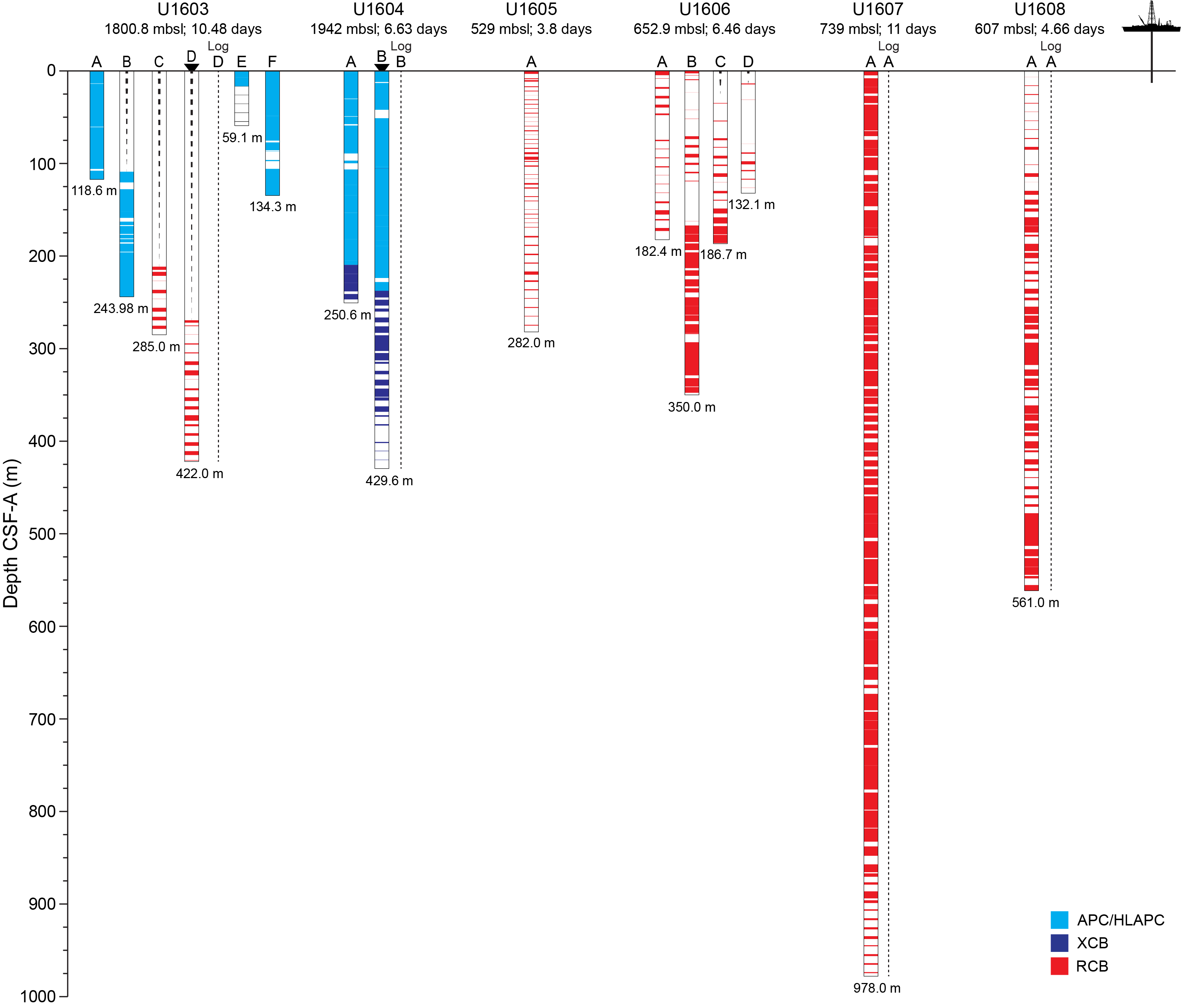
Figure F1. Holes drilled, coring systems used, and recovery.
We deployed nonmagnetic core barrels for all APC and HLAPC cores. The downhole orientation tool was generally not deployed due to the latitude of Expedition 400 sites; however, testing of the tool was conducted in Holes U1603F and U1604B. We obtained 10 formation temperature measurements with the APC temperature (APCT-3) tool embedded in the APC coring shoe while coring Hole U1603A (Cores 4H, 7H, 10H, and 13H), Hole U1603F (Cores 4H and 10H), and Hole U1604A (Cores 4H, 7H, 10H, and 13H). These measurements are applied to calculations of the downhole temperature gradient and heat flow estimates.
The XCB corer is a rotary system with a small cutting shoe that extends below the large rotary APC/XCB bit (Figure F1). The XCB bit is able to cut a semi-indurated core with less torque and fluid circulation than the larger main bit, optimizing recovery. The XCB cutting shoe (bit) extends ~30.5 cm ahead of the main bit in soft sediment but retracts into the main bit when hard formations are encountered. The resulting cores have a nominal diameter of 5.87 cm (2.312 inches), slightly less than the 6.6 cm diameter of APC cores. XCB cores are often broken (torqued) into biscuits, which are disc-shaped pieces a few to several centimeters long with remolded sediment (including some drilling slurry) interlayering the discs in a horizontal direction and packing the space between the discs and the core liner in a vertical direction. This type of drilling disturbance may give the impression that the XCB cores have the same thickness (66 mm) as the APC cores. Although both XCB and RCB core recovery generally lead to drilling disturbance in similar sedimentary material, switching from an APC/XCB bottom-hole assembly (BHA) to an RCB BHA requires a pipe trip, adding significant time to the coring operations on site. Thus, we opted to attempt recovery with the XCB coring system as deep as possible prior to terminating operations in Holes U1604A and U1604B.
The RCB system is the most conventional rotary coring system and is suitable for lithified rock material (Figure F1). During Expedition 400, we used the RCB system exclusively for the four shelf sites (U1605–U1608). We also used the RCB system in Holes U1603C and U1603D to penetrate the deepest intervals and provide a more stable logging hole. Like the XCB system, the RCB system cuts a core with a nominal diameter of 5.87 cm. RCB coring can be done with or without the core liners used routinely with the APC/XCB soft-sediment systems.
The BHA is the lowermost part of the drill string and is typically ~130–170 m long, depending on the coring system used and total drill string length. A typical APC/XCB BHA consists of a drill bit (outside diameter = 11⁷⁄₁₆ inches), a bit sub, a seal bore drill collar, a landing saver sub, a modified top sub, a modified head sub, a nonmagnetic drill collar (for APC/XCB drilling), a number of 8¼ inch (~20.32 cm) drill collars, a tapered drill collar, six joints (two stands) of 5½ inch (~13.97 cm) drill pipe, and one crossover sub. A typical RCB BHA consists of a drill bit, a bit sub, a head sub, an outer core barrel, a top sub, a head sub, eight joints of 8¼ inch drill collars, a tapered drill collar, two stands of standard 5½ inch drill pipe, and a crossover sub to the regular 5 inch drill pipe.
Cored intervals may not be contiguous if they are separated by intervals that are drilled but not cored. During Expedition 400, we drilled ahead without coring to accelerate penetration because an interval had already been cored in an adjacent hole (Hole U1603B = 109.1 m; Hole U1603C = 211.5 m; Hole U1603D = 269.4 m; Hole U1606C = 25.0 m; Hole U1606D = 13.6 m). Holes thus consist of a sequence of cored and drilled intervals, or advancements. These advancements are numbered sequentially from the top of the hole downward. Numbers assigned to physical cores correspond to advancements and may not be consecutive.
1.1.4. Drilling disturbance
Cores may be significantly disturbed by the drilling process as well as contain extraneous material as a result of the coring and core handling process. In formations with loose granular layers (sand, ash, foraminifera ooze, chert fragments, shell hash, etc.), drilling circulation may allow granular material from intervals higher in the hole to settle and accumulate in the bottom of the hole. Such material could be sampled by the next core; thus, the uppermost 10–50 cm of each core must be assessed for potential “fall-in.”
Common coring-induced deformation includes the concave-downward appearance of originally horizontal bedding. Piston action may result in fluidization (flow-in) at the bottom of, or sometimes in, APC cores. Retrieval of unconsolidated (APC) cores from depth to the surface typically results, to some degree, in elastic rebound, and gas that is in solution at depth may become free and drive apart core segments in the liner. When gas content is high, pressure must be relieved for safety reasons before the cores are cut into segments. Holes are drilled into the liner, which forces some sediment and gas out of the liner. As noted above, XCB coring typically results in biscuits mixed with drilling slurry. RCB coring typically homogenizes unlithified core material and often fractures lithified core material.
Drilling disturbances are described in the Lithostratigraphy section of each site chapter and are indicated on the graphic core summary reports (visual core descriptions [VCDs]) in Core descriptions.
1.2. Core and section handling
1.2.1. Whole-core handling
All APC, HLAPC, XCB, and RCB cores recovered during Expedition 400 were extracted from the core barrel in plastic liners. All cores were then cut into ~1.5 m sections. The exact section length was noted and entered into the database as “created length” using the Sample Master application. This number was used to calculate recovery. Subsequent processing differed for soft-sediment and lithified material.
1.2.1.1. Sediment section handling
Headspace samples were taken from selected section ends (typically one per core) using a syringe for immediate hydrocarbon analysis as part of the shipboard safety and pollution prevention program. Whole-round samples for interstitial water (IW) analysis also were taken immediately after the core was sectioned. Sedimentary ancient DNA (sedaDNA) samples were taken from section ends following a scraping procedure to generate a clean surface (see Biostratigraphy). Core catcher samples (PAL) were taken for biostratigraphic analysis. When catwalk sampling was complete, liner caps (blue = top, colorless = bottom, and yellow = top of a whole-round sample removed from the section) were glued with acetone onto liner sections, and sections were placed in core racks for analysis.
For sediment cores, the curated length was set equal to the created length and was updated very rarely (e.g., in cases of errors or when the section length kept expanding by more than ~2 cm). Depth in hole calculations are based on the curated section length (see Depth calculations).
After completion of whole-round section analyses, the sections were split lengthwise from bottom to top into working and archive halves. Softer cores were split using a wire, and harder cores were split using a diamond saw. It is important to note that older material can be transported upward on the split face of a section during splitting.
1.3. Sample naming
1.3.1. Editorial practice
Sample naming in this volume follows standard IODP procedure. A full sample identifier consists of the following information: expedition, site, hole, core number, core type, section number, section half, and offset in centimeters measured from the top of the core section. For example, a sample identification of “400-U1603A-1H-2W, 10–12 cm,” represents a sample taken from the interval between 10 and 12 cm below the top of the working half of Section 2 of Core 1 (“H” designates that this core was taken with the APC system) of Hole U1603A during Expedition 400.
When working with data downloaded from the Laboratory Information Management System (LIMS) database or physical samples that were labeled on the ship, three additional sample naming concepts may be encountered: text ID, label ID, and printed labels.
1.3.2. Text ID
Samples taken aboard JOIDES Resolution are uniquely identified for use by software applications using the text ID, which combines two elements:
- The sample type designation (e.g., SHLF for section half) and
- A unique sequential number for any sample and sample type added to the sample type code (e.g., SHLF12641501).
The text ID is not particularly helpful to most users but is critical for machine reading and troubleshooting.
1.3.3. Label ID
The label ID is used throughout the JOIDES Resolution workflows as a convenient, human-readable sample identity. However, a label ID is not necessarily unique. The label ID is made up of two parts: the primary sample identifier and the sample name.
1.3.3.1. Primary sample identifier
The primary sample identifier is very similar to the editorial sample name described above, with two notable exceptions:
- Section halves always carry the appropriate identifier (400-U1608A-35R-2-A versus 400-U1608A-35R-2-W for archive and working halves, respectively).
- Sample top and bottom offsets relative to the parent section are indicated as “35/37” rather than “35–37 cm.”
Specific rules were set for printing the offset/offset at the end of the primary sample identifier:
- For samples taken out of the hole, core, or section, top offset/bottom offset is not added to the label ID. This has implications for the common process of taking samples out of the core catcher (CC), which technically is a section (relevant primarily for paleontology samples).
- For samples taken out of the section half, top offset/bottom offset is always added to the label ID. The rule is triggered when an update to the sample name, offset, or length occurs.
- The offsets are always rounded to the nearest centimeter before insertion into the label ID (even though the database stores higher precisions and reports offsets to millimeter precision).
1.3.3.2. Sample name
Sample name is a free text parameter for subsamples taken from a primary sample or from subsamples thereof. It is always added to the primary sample identifier following a hyphen (-NAME) and is populated from one of the following prioritized user entries in the Sample Master application:
- Entering a sample type (-TYPE) is mandatory (same sample type code used as part of the text ID; see above). By default, -NAME = -TYPE (examples include SHLF, CUBE, CYL, PWDR, etc.).
- If the user selects a test code (-TEST), the test code replaces the sample type and -NAME = -TEST. The test code indicates the purpose of taking the sample but does not guarantee that the test was actually completed on the sample (examples include PAL, TSB, ICP, PMAG, MAD, etc.).
- If the user selects a requester code (-REQ), it replaces -TYPE or -TEST and -NAME = -REQ. The requester code represents the name of the requester of the sample who will conduct postexpedition analysis.
- If the user types any kind of value (-VALUE) in the -NAME field, perhaps to add critical sample information for postexpedition handling, the value replaces -TYPE, -TEST, or -REQ and -NAME = -VALUE (e.g., SYL-80deg, DAL-40mT, etc.).
In summary, and given the examples above, the same subsample may have the following label IDs based on the priority rule -VALUE > -REQ > -TEST > -TYPE:
- 400-U1608A-35R-2-W 35/37-CYL.
- 400-U1608A-35R-2-W 35/37-PMAG.
- 400-U1608A-35R-2-W 35/37-DAL.
- 400-U1608A-35R-2-W 35/37-DAL-40mT.
When subsamples are taken out of subsamples, the -NAME of the first subsample becomes part of the parent sample ID and another -NAME is added to that parent sample label ID:
For example, a thin section billet (sample type = TSB) taken from the working half at 2–4 cm offset from the section top might result in a label ID of 400-U1608A-20R-1-W 2/4-TSB. After the thin section was prepared (~48 h later), a subsample of the billet might receive an additional designation of TS49, which would be the forty-ninth thin section made during the expedition. A resulting thin section label ID might therefore be 400-U1608A-20R-1-W 2/4-TSB-TS_49.
1.4. Depth calculations
Sample and measurement depth calculations were based on the methods described in IODP Depth Scales Terminology (version 2.0) at https://www.iodp.org/policies-and-guidelines/142-iodp-depth-scales-terminology-april-2011/file (Table T1). The definition of multiple depth scale types and their distinction in nomenclature should alert the user that a nominal depth value on two different depth scale types (and even two different depth scales of the same type) generally does not refer to exactly the same stratigraphic interval in a hole. The SI unit for all depth scales is meters (m).
Depths of cored intervals were measured from the drill floor based on the length of drill pipe deployed beneath the rig floor and referred to as drilling depth below rig floor (DRF), traditionally referred to as meters below rig floor (mbrf). The depth of each cored interval, measured on the DRF scale, can be referenced to the seafloor by subtracting the seafloor depth measurement (DRF) from the cored interval (DRF). This seafloor-referenced depth of the cored interval is referred to as the drilling depth below seafloor (DSF), traditionally mbsf. In the case of APC coring, the seafloor depth was the length of pipe deployed minus the length of the mudline core recovered. In the case of RCB coring, the seafloor depth was adopted from a previous hole drilled at the site or by tagging the seafloor.
Depths of samples and measurements in each core were computed based on a set of rules that result in a depth scale type referred to as CSF-A. The two fundamental rules are that (1) the top depth of a recovered core corresponds to the top depth of its cored interval (top DSF = top CSF-A), regardless of type of material recovered or drilling disturbance observed, and (2) the recovered material is a contiguous stratigraphic representation even when core segments are separated by voids when recovered, the core is shorter than the cored interval, or the amount of material missing between core pieces is unknown. When voids were present in the core on the catwalk, they were closed by pushing core segments together whenever possible. The length of missing core should be considered a depth uncertainty when analyzing data associated with core material.
When core sections were given their curated lengths, they were also given a top and a bottom depth based on the core top depth and the section length. Depths of samples and measurements on the CSF-A scale were calculated by adding the offset of the sample (or measurement from the top of its section) to the top depth of the section.
Per IODP policy established after the introduction of IODP Depth Scales Terminology version 2.0, sample and measurement depths on the CSF-A depth scale type are commonly referred to with the custom unit mbsf, just like depths on the DSF scale type. The reader should be aware, though, that the use of mbsf for different depth scales can cause confusion in specific cases because different “mbsf depths” may be assigned to the same stratigraphic interval. For example, a soft-sediment core from less than a few hundred meters below seafloor often expands upon recovery (typically by a few percent to as much as 15%), and the length of the recovered core exceeds that of the cored interval. Therefore, a stratigraphic interval in a particular hole may not have the same depth on the DSF and CSF-A scales; thus, throughout this volume the CSF-A depth scale is used unless otherwise noted. When recovery in a core exceeds 100%, the CSF-A depth of a sample taken from the bottom of the core will be deeper than that of a sample from the top of the subsequent core (i.e., some data associated with the two cores overlap on the CSF-A scale). To overcome the overlap problem, core intervals can be placed on the core depth below seafloor, Method B (CSF-B), depth scale. The Method B approach scales the recovered core length back into the interval cored, from >100% to exactly 100% recovery. If cores had <100% recovery to begin with, they are not scaled. When downloading data using the JOIDES Resolution Science Operator (JRSO) LIMS Reports pages (http://web.iodp.tamu.edu/LORE), depths for samples and measurements are by default presented on both the CSF-A and CSF-B scales. The CSF-B depth scale can be useful for data analysis and presentations at sites with a single hole.
A core composite depth below seafloor (CCSF) scale can be constructed to mitigate inadequacies of the CSF-A scale for scientific analysis and data presentation (see Stratigraphic correlation). The most common application is the construction of a CCSF scale from multiple holes drilled at a site using depth shifting of correlative features across holes. This method not only eliminates the CSF-A core overlap problem but also allows splicing of core intervals such that gaps in core recovery, which are inevitable in coring a single hole, are essentially eliminated and a continuous stratigraphic representation is established. This depth scale type was used at Sites U1603, U1604, U1607, and U1608 during Expedition 400.
A CCSF scale and stratigraphic splice are accomplished by downloading correlation data from the expedition (LIMS) database using the Correlation Downloader application, correlating stratigraphic features across holes using Correlator or any other application, depth-shifting cores to create an affine table with an offset for each core relative to the CSF-A scale, and creating a splice interval table that defines which core intervals from the participating holes make up the stratigraphic splice. Affine and splice interval tables can be uploaded to the LIMS database, where internal computations create a CCSF depth scale. The CCSF depth can then be added to all subsequent data downloads from the LIMS database, and data can be downloaded for a splice.
1.5. Shipboard core analysis
Whole-round core sections were immediately run through the Whole-Round Multisensor Logger (WRMSL), which measures P-wave velocity, density, and magnetic susceptibility (MS), and the Natural Gamma Radiation Logger (NGRL). After letting cores thermally equilibrate for at least 4 h, thermal conductivity measurements were also taken before the cores were split lengthwise into working and archive halves. In select holes, Rhizon samples were collected in the upper ~20 m CSF-A from whole-round core sections (see Geochemistry). The working half of each core was sampled for shipboard analysis, routinely for paleomagnetism and physical properties and more irregularly for geochemistry and biostratigraphy. The archive half of each core was scanned on the Section Half Imaging Logger (SHIL) and the X-Ray Linescan Logger (XSCAN). Archive halves were also measured for color reflectance and MS on the Section Half Multisensor Logger (SHMSL). The archive halves were described macroscopically and microscopically in smear slides. Finally, the archive halves were run through the cryogenic magnetometer. Both halves of the core were wrapped and then put into labeled plastic tubes that were sealed and transferred to cold storage space aboard the ship.
A total of 5882 samples were taken for shipboard analysis. At the end of Expedition 400, all archive section halves of the cores were shipped to the Gulf Coast Repository in preparation for X-ray fluorescence (XRF) core scanning. Working section halves and all other residues were shipped to the Bremen Core Repository for a shore-based sampling party in March 2024. All sections and samples will be permanently stored in the Bremen Core Repository.
2. Lithostratigraphy
Sediments and rocks recovered during Expedition 400 were described macroscopically from core archive section halves and microscopically from smear slides and thin sections. Observations were recorded in separate macroscopic and microscopic GEODESC templates. X-ray diffraction (XRD) analyses of both clay mineral and bulk preparations were done from the working half of the section. Color spectrophotometry, point-source MS (MSP) measurements, and X-ray and linescan camera imaging of core archive section halves were also carried out by the lithostratigraphy group. Methods associated with X-ray imaging are described in Physical properties. Methods associated with shipboard measurements of carbonate and organic matter (carbon-hydrogen-nitrogen-sulfur [CHNS]) of sediment samples selected by the lithostratigraphy group are described in Geochemistry.
2.1. Section-half images
The technique used for splitting cores into working and archive halves (either using a piano wire or a saw from the bottom to the top; see Introduction) affects the appearance of the split core surface. Before core description and high-resolution digital color imaging, the quality of the split core surface of the archive half of each core was assessed. When necessary (e.g., if the surface was irregular or smeared), the split core surface was scraped lightly with a glass microscope slide or stainless steel plate to even the surface.
2.1.1. Photography and color imaging
The surface of the cleaned archive half was imaged using the SHIL. Imaging was conducted as soon as possible after splitting to avoid sediment color changes caused by oxidation and drying. In cases of watery or soupy sediment, the surface was allowed to dry sufficiently prior to scanning to avoid excessive light reflection and overexposure. The SHIL captures continuous high-resolution images for analysis and description, using three pairs of advanced illumination, high-current, focused light-emitting diode (LED) line lights to illuminate the core. Each of the LED pairs has a color temperature of 6,500 K and emits 200,000 lux at 7.6 cm. Digital images were taken using a linescan camera (manufactured by JAI) at an interval of 10 lines/mm to create a high-resolution image file. The camera height was set such that each pixel imaged a 0.1 mm2 section of the core surface, but the actual core width per pixel can vary because of slight differences in the section-half surface height. Low-resolution cropped raster files of the core section surface and high-resolution raster files with a grayscale and depth ruler were created from the image files.
2.1.2. Spectrophotometry and colorimetry
The SHMSL employs multiple sensors to measure bulk physical properties in a motorized and computer-controlled instrument track. The sensors included in the SHMSL are a spectrophotometer, an MSP sensor, and a laser surface analyzer. During this expedition, the point measurement interval for the spectrophotometer and the MSP sensor measurements was 2 cm for all sections. To achieve a flush contact between point sensors and the split core surface and to avoid sediment transfer to the instrument surfaces, archive halves were covered with clear plastic wrap prior to measurement. The laser surface analyzer helps recognize irregularities in the split core surface (e.g., cracks and voids), whereas data from this tool were recorded to provide an independent check on SHMSL measurement fidelity. MS was measured using a Bartington Instruments MS2 meter and an MS2K contact probe (see Physical properties). Reflectance spectroscopy (spectrophotometry) was carried out using an Ocean Optics QE Pro detector, which measures the reflectance spectra of the split core from the ultraviolet to near-infrared range. Each measurement was recorded in 2 nm spectral bands from 390 to 732 nm. The data were converted to the L*a*b* color space system, which expresses color as a function of lightness (L*; grayscale, where more white is positive and more black is negative) and color values a* and b*, where a* reflects the balance between red (positive a*) and green (negative a*) and b* reflects the balance between yellow (positive b*) and blue (negative b*).
2.2. Sedimentological core description
Macroscopic descriptions of each section (nominally 0–150 cm long) were recorded on handwritten core description forms (barrel sheets) that include color images collected using the SHIL (Figure F2). All handwritten sheets were scanned and digitally preserved (see LITH in Supplementary material). Standard sedimentological observations of lithology, primary and secondary (i.e., syn- and postsedimentary deformation) sedimentary structures, bioturbation intensity, macroscopic biogenic remains (e.g., shell fragments and plant matter), diagenetic features, drilling disturbance type and intensity, clast counts (>5 mm diameter), character of the lower contact, and shipboard archive-half sample types and depths were recorded in individual columns on the barrel sheets. Color (Munsell Color Company, 2010), shape, and compositional characteristics of coarse clasts (>2 cm) were recorded as comments. The identification of distinct sedimentary features or core intervals was supported by inspection of physical property data, including whole-round core measurements of MS and natural gamma radiation (NGR) (see Physical properties), as well as split core MSP and color reflectance. As an example, reduced MS and lower density could be used to delineate biogenic-rich intervals.
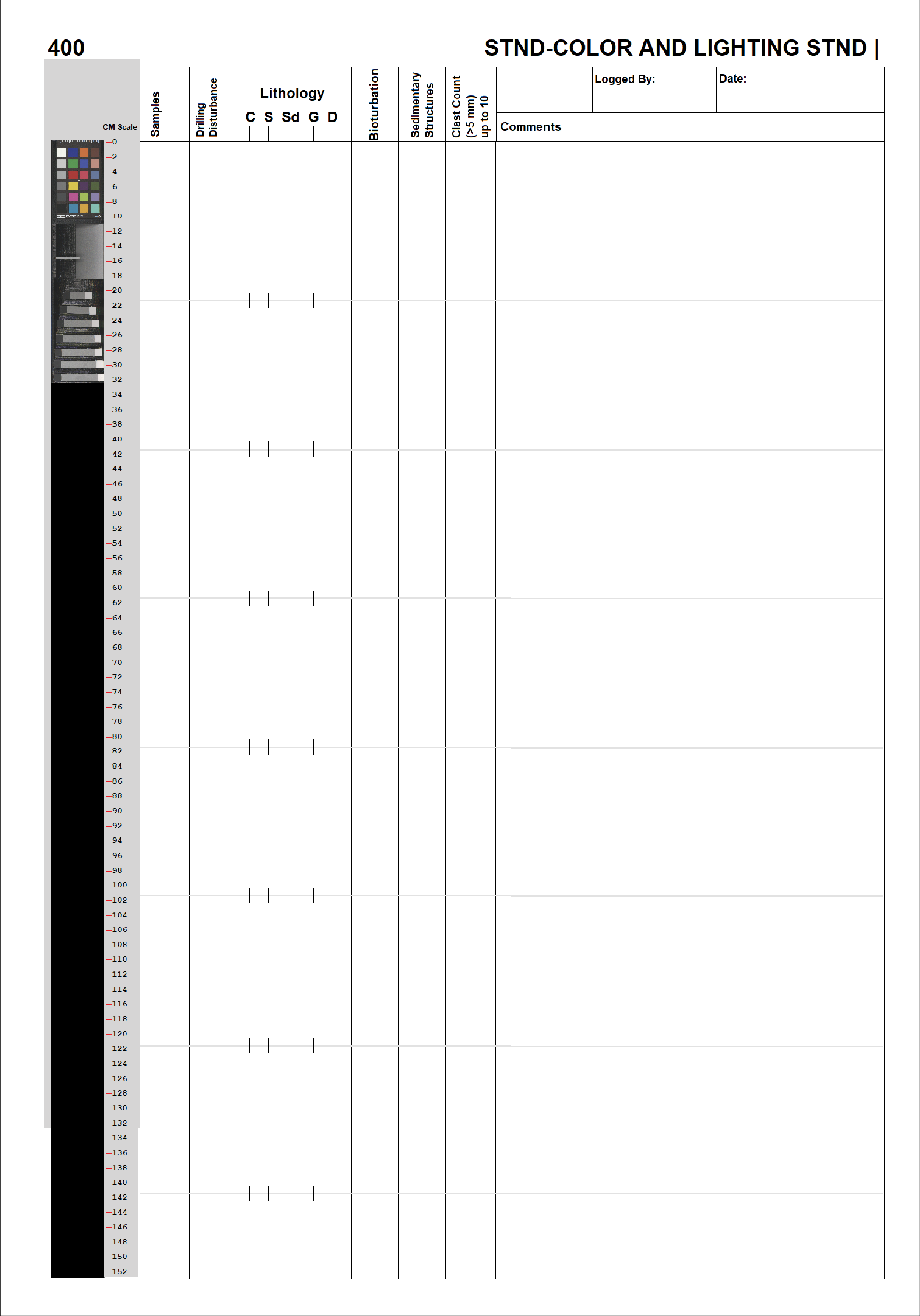
Figure F2. Barrel sheet template.
2.2.1. GEODESC data capture software
Data from the handwritten core description sheets were compiled and entered into the LIMS database using GEODESC software. A macroscopic template was developed in GEODESC Template Manager for Expedition 400 and includes the following categories:
- Drilling disturbance (type and intensity),
- Lithology (major lithology, with prefix and suffix modifiers indicating variable biogenic content, matrix grain size, clast abundance, degree of consolidation, and other characteristics),
- Strata thickness (if stratification is present),
- Sedimentary structures,
- Bioturbation intensity,
- Macrofossils,
- Diagenetic constituents/composition,
- Clast counts (number of lithic clasts >5 mm and characteristics of clasts >2 cm), and
- Lower contact (shape, definition, and attitude).
A separate template was made to capture clast counts per 10 cm interval for clasts with diameters >5 mm. Four additional GEODESC templates were constructed for (1) hole/site summary (lithostratigraphic units and age), (2) core summary (written description of major lithologic findings by core), and two microscopic templates for (3) smear slides and (4) thin sections. The microscopic templates describe the relative abundance of major lithogenic and/or biogenic components and minor constituents. The thin section template provides a summary overview and links to images. All information entered into GEODESC was subsequently uploaded to the LIMS database (accessible via GEODESC Data Access) and was used as input to a simplified one-page VCD graphical report for each core.
2.2.2. Drilling disturbance
Core disturbance from the drilling process was characterized and modified from the nomenclature of Jutzeler et al. (2014) and entered into GEODESC (Table T2). The intensity of drilling disturbance was also entered into GEODESC and displayed graphically on the VCDs. The intensity of drilling disturbance of unconsolidated and consolidated sediments was classified into five categories: undisturbed, slightly, moderately, strongly, and severely.
In unconsolidated sediments, the five categories imply the following:
- 0 = undisturbed.
- 1 = slightly disturbed: bedding contacts are slightly bent or bowed in a concave-downward appearance.
- 2 = moderately disturbed: bedding contacts are bent or bowed in a concave-downward appearance but are still visible and in the correct stratigraphic order.
- 3 = strongly disturbed: core has some portions that are completely deformed and may not maintain stratigraphic order.
- 4 = severely disturbed: bedding is completely deformed and may show diapiric or flow structures.
In harder sediments (i.e., consolidated by compaction or cementation), the five categories are defined as follows:
- 0 = undisturbed.
- 1 = slightly fractured: core pieces are in place and have very little drilling slurry or brecciation.
- 2 = moderately fractured or biscuited: core pieces are in the correct stratigraphic sequence (although the entire section may not be represented); on occasion, intact core pieces are broken into rotated discs (or biscuits) as a result of the drilling process, and drilling mud has possibly flowed in.
- 3 = strongly fractured: core pieces are probably in correct stratigraphic sequence (although the entire section may not be represented); frequently, intact core pieces are broken into rotated discs (or biscuits) as a result of the drilling process, and drilling mud has possibly flowed in.
- 4 = severely fractured or brecciated: pieces are from the cored interval but may not occur in the correct stratigraphic sequence within the core.
2.3. Lithologic classification scheme
Lithologic descriptions were based on the classification schemes described in the Methods chapters for other high-latitude, glaciated-margin drilling expeditions such as Ocean Drilling Program (ODP) Leg 178 (Shipboard Scientific Party, 1999), the Cape Roberts Project (Hambrey et al., 1997), the Antarctic Drilling Project (ANDRILL; Naish et al., 2006), Integrated Ocean Drilling Program Expeditions 318 (Expedition 318 Scientists, 2011) and 341 (Jaeger et al., 2014), and IODP Expeditions 374 (McKay et al., 2019) and 379 (Gohl et al., 2021).
2.3.1. Principal names and modifiers
The principal lithologic name was assigned based on the relative abundances of nonbiogenic (i.e., terrigenous, detrital carbonate) and biogenic grains (Figure F3). The principal name is purely descriptive and does not include interpretive classifications relating to fragmentation, transport, deposition, or alteration processes. The principal name entered into GEODESC of a sediment/rock with >50% terrigenous grains is based on an estimate of the grain sizes present (Figure F3A). The Wentworth (1922) scale was used to define size classes of clay, silt, sand, and gravel.
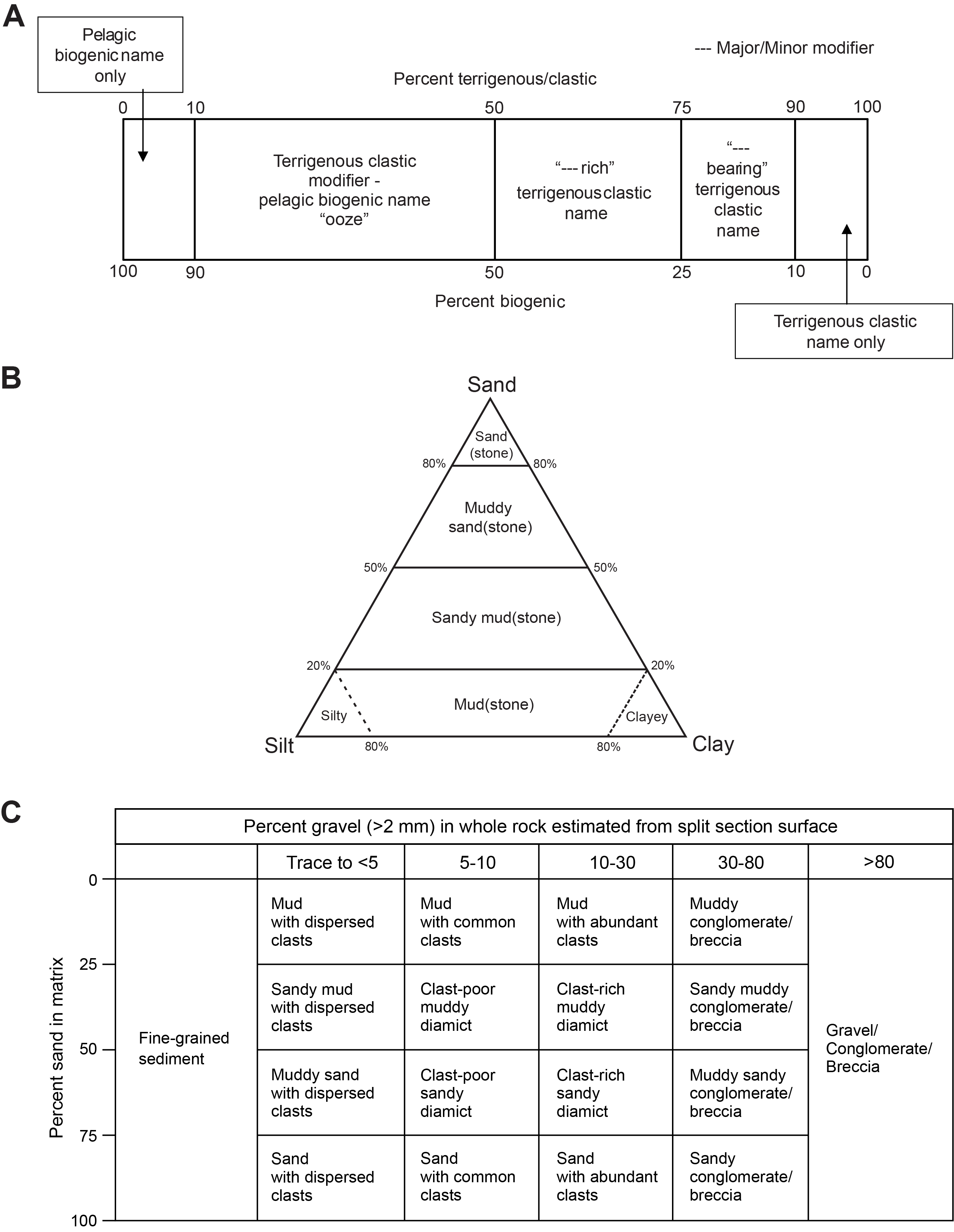
Figure F3. Lithology classification scheme.
If no gravel is present, the principal sediment/rock name was determined based on the relative abundances of sand, silt, and clay. The term “mud” is used to define sediments containing a mixture of silt and clay that could not be reliably differentiated using visual macroscopic inspection (e.g., silty mud, clayey mud, or sandy mud) (Mazzullo et al., 1988; Shepard, 1954) (Figure F3B). Sandy mud to muddy sand describes sediment composed of a mixture of at least 20% each of sand, silt, and clay (Figure F3B). The prefix was determined by the percentage >50% of sand versus mud in the matrix (Figure F3B).
If the sediment/rock contains siliciclastic gravel, then the principal name was determined from the relative abundance of gravel (>2 mm; also referred to as “clasts”) and sand/mud ratio of the matrix following a modified version of the textural classifications of Moncrieff (1989) as outlined in Marsaglia and Milliken (2023), with gravel percent estimated using the comparison chart of Terry and Chilingar (1955) (Figure F3C). The term “diamicton/diamictite” is used as a nongenetic term for unsorted to poorly sorted terrigenous sediment that contains a wide range of particle sizes. The name “diamicton” is used for unlithified, poorly sorted sediment, whereas “diamictite” is used for the lithified type. Accordingly, a clast-poor muddy diamicton includes 5%–10% gravel (>2 mm) and 25%–50% sand in matrix, whereas a clast-rich muddy diamicton includes 10%–30% gravel and 25%–50% sand in matrix. A clast-poor sandy diamicton has 5%–10% gravel and 50%–75% sand in matrix. For a clast-rich sandy diamicton, gravel content is 10%–30%, sand content is 50%–75%, and the remainder is mud. The terms “gravel/conglomerate/breccia” are used when the matrix includes >30% gravel, with conglomerate describing a sediment with dominantly (well) rounded gravel grains and breccia describing a sediment with dominantly (very) angular gravel grains (Figure F3). If clasts (>2 mm) are present but less than 5% in abundance, the term “dispersed clasts” is used as a lithology suffix, following the principal lithology name. If there is 25% or less sand or mud (combined clay and silt) with clasts (>2 mm) present, the principal lithology is named for the siliciclastic component with common clasts (5%–10%) or abundant clasts (10%–30%) (e.g., sandy mud with common clasts).
The principal name of sediment with >50% biogenic grains is ooze, modified by the most abundant biogenic grain type (Figure F3A). For example, if diatoms exceed 50%, then the sediment is called diatom ooze. However, if the sediment is a mixture of biogenic siliceous material (e.g., diatoms, spicules, radiolaria, etc.) with none of the biogenic component exceeding 50% in abundance, then the sediment is termed biosiliceous ooze. The same principle applies to calcareous microfossils (e.g., foraminifera ooze versus calcareous ooze).
The prefix “calcareous” is used for sediments dominated by detrital carbonate. In all instances for this expedition, calcareous lithologies are composed of abiogenic silt-sized crystalline or micrite grains. Where no material is present, the type (void, whole round, gas expansion, or other) and depth range is recorded in GEODESC.
For all lithologies, we applied major and minor modifiers to the principal sediment/rock names modified from the biogenic-pelagic scheme in the Expedition 379 methods (Gohl et al., 2021) (Figure F3A):
- Minor biogenic modifiers are those components with abundances of 10%–25% and are indicated by the suffix “-bearing” (e.g., diatom-bearing).
- Major biogenic modifiers are those components that comprise 25%–50% of the grains and are indicated by the suffix “-rich” (e.g., diatom-rich).
- Siliciclastic modifiers in biogenic oozes are those components with abundances of 10%–50% and are indicated by the terrigenous modifier “-y” (e.g., silty, muddy, or sandy).
2.3.2. Sedimentary structures
The locations and types of sedimentary structures visible on the prepared surfaces of the archive section halves were entered into the macroscopic GEODESC template under strata thickness, sedimentary structures (syndeposition), and deformational structures (postdeposition). Lower contacts (basal boundaries) between different lithologies are classified as curved, irregular, straight, and wavy. Bedding and lamination are defined following Mazzullo et al. (1988) as follows:
- Thinly laminated (≤3 mm thick),
- Lainated (3 mm to 1 cm thick),
- Very thinly bedded (1–3 cm),
- Thinly bedded (3–10 cm),
- Medium bedded (10–30 cm),
- Thickly bedded (30–100 cm), and
- Very thickly bedded (>100 cm).
For units in which two lithologies are interbedded or interlaminated (i.e., where individual beds [layers >1 cm thick] or laminae [layers <1 cm thick] alternate between one lithology and another), the terms “interbedded” or “interlaminated” were added before the lithology names and are considered a primary lithology (e.g., interbedded sand and mud and interbedded mud and diamicton). This terminology is for ease of data entry and graphic log display purposes. When discrete beds of one lithology occur within a thicker interval of another lithology (e.g., centimeter- to decimeter-thick sand beds within a mud bed), those discrete beds were logged individually, and the associated bed thickness and grain size ranges were described.
Grading within beds and laminae was also described. Normal grading corresponds to layers with an upward decrease in grain size, whereas inverse/reverse grading corresponds to layers with an upward increase in grain size.
Deformational features that are unrelated to drilling disturbance were recorded in notes on the barrel sheets, in GEODESC, and as symbols on the VCDs. Symbols include both synsedimentary deformation structures (e.g., flame structures) and postdepositional features (e.g., faults). When possible, to determine apparent motion sense for faults with certainty, the direction of displacement (i.e., reverse or normal) was recorded in GEODESC and on the barrel sheets but is not displayed systematically on the VCDs.
Where sediments are diagenetically altered (e.g., mottling or the presence of pyrite, concretions, or cement), the diagenetic feature was selected from a predefined list in the Diagenetic constituent column of the GEODESC template. We define mottles (millimeter to centimeter scale) as spots or smears where material has a different color than the surrounding sediment.
Interval thickness is recorded from the uppermost to the lowermost extent of the described feature, as well as in the Comments column of the core barrel sheet.
2.3.3. Bioturbation
Ichnofabric description included the extent of bioturbation and notation of distinctive biogenic structures. To assess the degree of bioturbation semiquantitatively, we used the Droser and Bottjer (1986) ichnofabric index (0–6):
- 0 = bioturbation absent.
- 1 = sparse bioturbation (bedding distinct, few discrete traces).
- 2 = uncommon bioturbation (bedding distinct, low trace density).
- 3 = moderate bioturbation (bedding boundaries sharp, traces discrete with rare overlap).
- 4 = common bioturbation (bedding boundaries indistinct, high trace density with common overlap).
- 5 = abundant bioturbation (bedding just visible though completely disturbed).
- 6 = complete bioturbation (total biogenic homogenization of sediment).
The ichnofabric index is graphed using the numerical scale in the Bioturbation column of the graphical logs. Descriptions of the bioturbation were made in the Bioturbation comments column in the GEODESC template. When identifiable, ichnofacies (Ekdale et al., 1984) were noted and logged in the Interval comment column of the macroscopic GEODESC template.
2.3.4. Macroscopic biogenic components and diagenetic features
Paleontologic and diagenetic features other than those delineated above were recorded on the barrel sheets, and descriptions were entered in the corresponding columns of the GEODESC template. These features include, for example, macroscopic biogenic remains (e.g., skeletal and organic debris) and concretions. When possible, concretions were described by composition.
2.3.5. Clast abundance and characteristics
Coarse gravel abundance was determined by counting the clasts >5 mm in diameter visible on the surface of the archive half in 10 cm depth intervals. Where only holes or depressions caused by lithic clasts were observed, the working half was also examined to determine pebble abundance. If between one and nine individual clasts were counted per 10 cm depth interval, the number of clasts per interval was entered into GEODESC in the Clast count column. If 10 or more clasts were present in a 10 cm interval, the number 10 was entered in the Clast column.
Details on lithology, size, shape, rounding, and surface texture (e.g., striae or faceted faces) on clasts with a long axis >2 mm are provided in the core description sheets and in the Interval comments column in GEODESC.
2.4. Microscopic descriptions
2.4.1. Smear slides
To aid in lithologic classification, the size, composition, and abundance of sediment constituents were estimated microscopically using smear slides (Figure F4). For each smear slide, a small amount of sediment was removed from the archive section half using a wooden toothpick and put on glass. The sediment was mixed with deionized water and evenly spread. To reduce the water droplet tension and aid in disaggregating clays, soap or saliva was used. The dispersed sample was dried on a hot plate at a moderate setting (150°C). A drop of Norland Optical Adhesive Number 61 was used to glue a coverslip to the slide. The smear slide was then placed in an ultraviolet light box for at least 15 minutes to cure the adhesive.
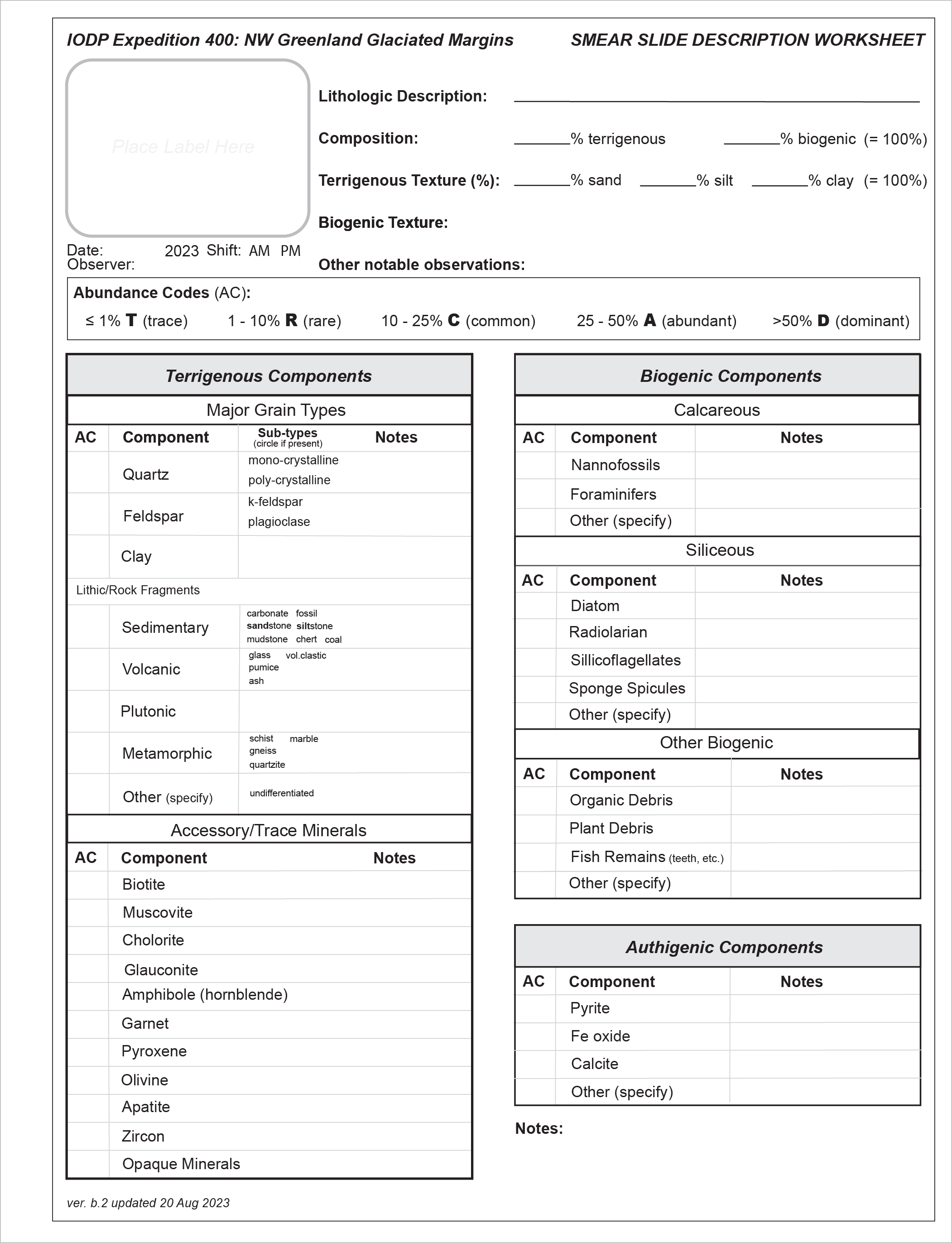
Figure F4. Smear slide description worksheet.
Smear slides were examined with a transmitted-light petrographic microscope equipped with a standard eyepiece micrometer. Biogenic and mineral components were identified following standard petrographic techniques as stated in Rothwell (1989), Marsaglia et al. (2013), and Marsaglia et al. (2015). Several fields of view (FOVs) were examined at 50×, 100×, 200×, 400×, and 500× magnification to assess the abundance of detrital, biogenic, and authigenic components. The relative abundance percentages of the sedimentary constituents were visually estimated using the techniques of Rothwell (1989). The texture of siliciclastic lithologies (e.g., the relative abundance of sand-, silt-, and clay-sized grains) and the proportions and presence of biogenic and mineral components were recorded in the smear slide worksheet and entered into the microscopic GEODESC template.
Components observed in smear slides are categorized as follows:
- T = trace (≤1%).
- R = rare (>1%–10%).
- C = common (>10%–25%).
- A = abundant (>25%–50%).
- D = dominant (>50%).
Very fine and coarse grains are difficult to observe in smear slides, and their relative proportions in the sediment can be affected during slide preparation. Therefore, intervals dominated by sand-sized and larger constituents were examined by macroscopic comparison to grain size reference charts. Photomicrographs of some smear slides (e.g., representative lithologies) were acquired and uploaded to the LIMS database.
2.4.2. Thin sections
The descriptions of sediments and rocks were complemented with thin section analysis (Figure F5). Standard thin section billets were cut from selected intervals or features as needed, and thin sections prepared on board were examined with a transmitted-light petrographic microscope equipped with a standard eyepiece micrometer. Data were entered into the Thin section summary template for GEODESC. Photomicrographs of thin sections were acquired and uploaded to the LIMS database.
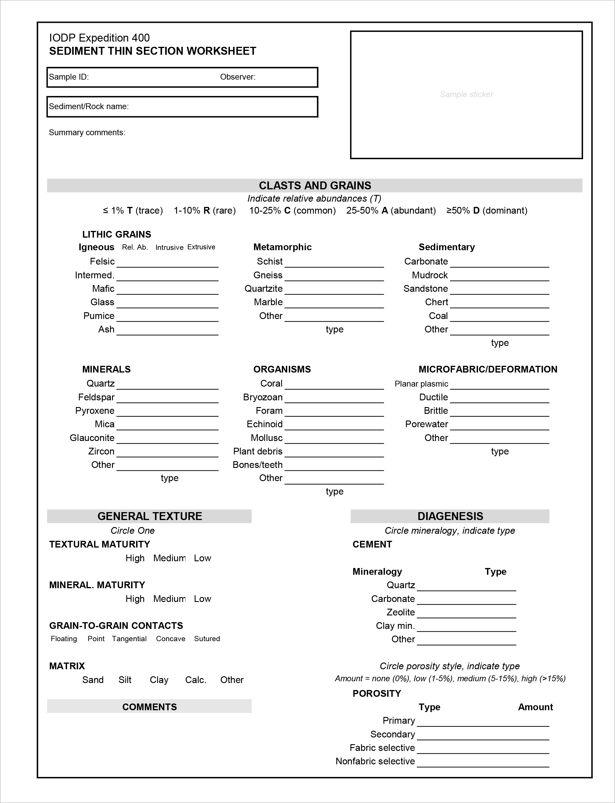
Figure F5. Thin section description worksheet.
2.5. X-ray diffraction analysis
XRD analysis was performed on both bulk sediment and clay (<4 µm) separates to determine their mineralogy. A 5 cm3 sample was taken from the working section halves at variable intervals, depending on the site. Sample positions for bulk and clay fraction XRD were selected based on visual core observations (e.g., color variability, visual changes in lithology and texture, etc.) and smear slide investigations. The sampling objective was to characterize the mineralogy for distinct lithologic units (or subunits) or detect changes above and below transitions and unconformities.
For bulk sediment analysis, samples were freeze-dried and stored in a desiccator to prevent reabsorption of moisture. Freeze-dried samples were finely ground using an appropriate mortar and pestle size.
Clay fractions were prepared according to procedures outlined in the Expedition 318 methods (Expedition 318 Scientists, 2011). For these preparations, a ~2 g sample was placed in a 50 mL centrifuge tube with 10% acetic acid, sonicated for 15 min, and allowed to stand for 1 h to remove carbonate material. After centrifuging for 15 min at 1500 rpm, the acetic acid was decanted, 25 mL of distilled water was added, the sample was centrifuged again, and the water was decanted. This washing procedure was repeated two more times to remove both the acid and salts from the sample. After decanting the final wash, 25 mL of 1% sodium hexametaphosphate solution was added to the sample in a 50 mL centrifuge tube. The sample was then placed in a dismembrator for 5 min to suspend the clays and then centrifuged for 4 min at 750 rpm twice to settle the >4 µm particles. The clays that remained in suspension were removed from the top ~1 cm of the centrifuge tube and centrifuged for 1 h at 3000 rpm. Three subsamples were pipetted directly onto amorphous quartz sample discs. These sample discs were then left to air dry in a desiccator. After drying, one disc was analyzed and the other was solvated with ethylene glycol for ~12 h and reanalyzed to determine the presence of expandable clays. The third subsample was heated in a muffle furnace at 550°C over 4 h before being analyzed to check for the presence of kaolinite.
Prepared samples were top-mounted onto a sample holder and analyzed using a Malvern Panalytical AERIS X-ray diffractometer mounted with a PIXcel1D-Medipix3 detector using nickel-filtered CuKα radiation. XRD instrument settings for clay samples were as follows:
- Voltage = 40 kV.
- Current = 40 mA.
- Goniometer scan = air dried, 5°–15.5°2θ (step size = 0.016599°2θ); glycolyzed, 1.5°–34.5°2θ (step size = 0.016599°2θ) and 24°–45.01°2θ (step size = 0.0085°2θ) for resolving the (002) peak of kaolinite from the (004) peak of chlorite; and heated, 1.5°–34.5°2θ (step size = 0.0108664°2θ).
- Scan speed = 109.65 s/step.
- Divergence slit = ⅛°.
XRD instrument settings for bulk samples were as follows:
- Voltage = 40 kV.
- Current = 40 mA.
- Goniometer scan = 5°–90°2θ (step size = 0.0108664°2θ).
- Scan speed = 80.3255 s/step.
- Divergence slit = ¼°.
Diffractograms of bulk samples were evaluated with the HighScore Plus software package (version 4.8), which allowed for mineral identification and basic peak characterization (e.g., baseline removal and maximum peak intensity). Files were created that contained d-spacings, diffraction angles, and peak intensities with the background removed. These files were screened for d-spacings characteristic of a limited range of minerals that were expected to be present in the sediments (Table T3). Peak intensities from those selected minerals were reported to provide a semiquantitative measure of their variations downhole. The semiquantitative results were calculated from the peak intensities expressed as a percentage of the sum of all primary peak intensities of the targeted minerals. These percentages were qualified as follows:
Secondary diffraction peaks were not checked to ensure that there were no false identifications. Thus, if the peak of a rare mineral fell within the detection window of a mineral to be identified, then the identification of the mineral will be wrong. Also, there were peaks on the XRD patterns that did not match the minerals being searched, and the materials responsible for those peaks have not yet been identified. Digital files with the diffraction patterns as well as raw XRD files are available in the LIMS database.
Relative abundances of the major clay mineral groups (smectite, chlorite, illite, and kaolinite) were established on the basis of the main peak intensity from the glycolated analysis. The air-dried and heated spectra were not interpreted on board but are available in the LIMS database. The shipboard results were interpreted semiqualitatively based on the relative peak intensities of the most common clay components. The ratio of the peak intensity of identified clay is presented as a first estimation of the clay ratio in the sediments.
2.6. Core description
2.6.1. Lithostratigraphic units
At each site, units were assigned to packages of reoccurring lithologies to highlight major lithologic changes downhole. Units were established where a prominent change in recurring sediment lithology, clast abundance, sedimentary structures, color, or macroscopic constituents was observed, generally on the scale of tens of meters. Lithostratigraphic units are numbered beginning at the top of the stratigraphic succession using Roman numerals. When notable but more subtle changes were observed, units were divided into subunits. Subunits are distinguished from the main lithologic units by adding a letter to the unit number (e.g., Subunit IA).
2.6.2. Standard graphical report
VCDs are generated for each core using the Strater software package (Golden Software) (Figure F6). Sample identification (expedition, hole, core, and section) is included at the top of each VCD, along with a summary core description. To the left of the graphic in the Lithology column, VCDs display the depth CSF-A (in meters), core length (in centimeters), section, location of shipboard samples, and the SHIL digital color image. Columns to the right of Lithology provide the type and intensity of drilling disturbance, bioturbation intensity, sedimentary structures, lower contact descriptions, and clast abundance (when appropriate for a given site), and may include physical property data (MS, gamma ray attenuation [GRA], and NGR) collected using the WRMSL and SHMSL (see Physical properties) (Figure F6). Graphic lithologies, sedimentary structures, and other visual observations shown on the VCDs by graphic patterns and symbols are explained in Figure F7. Lithologic symbols are simplified for hole and site summary graphic logs, for which individual legends are provided.
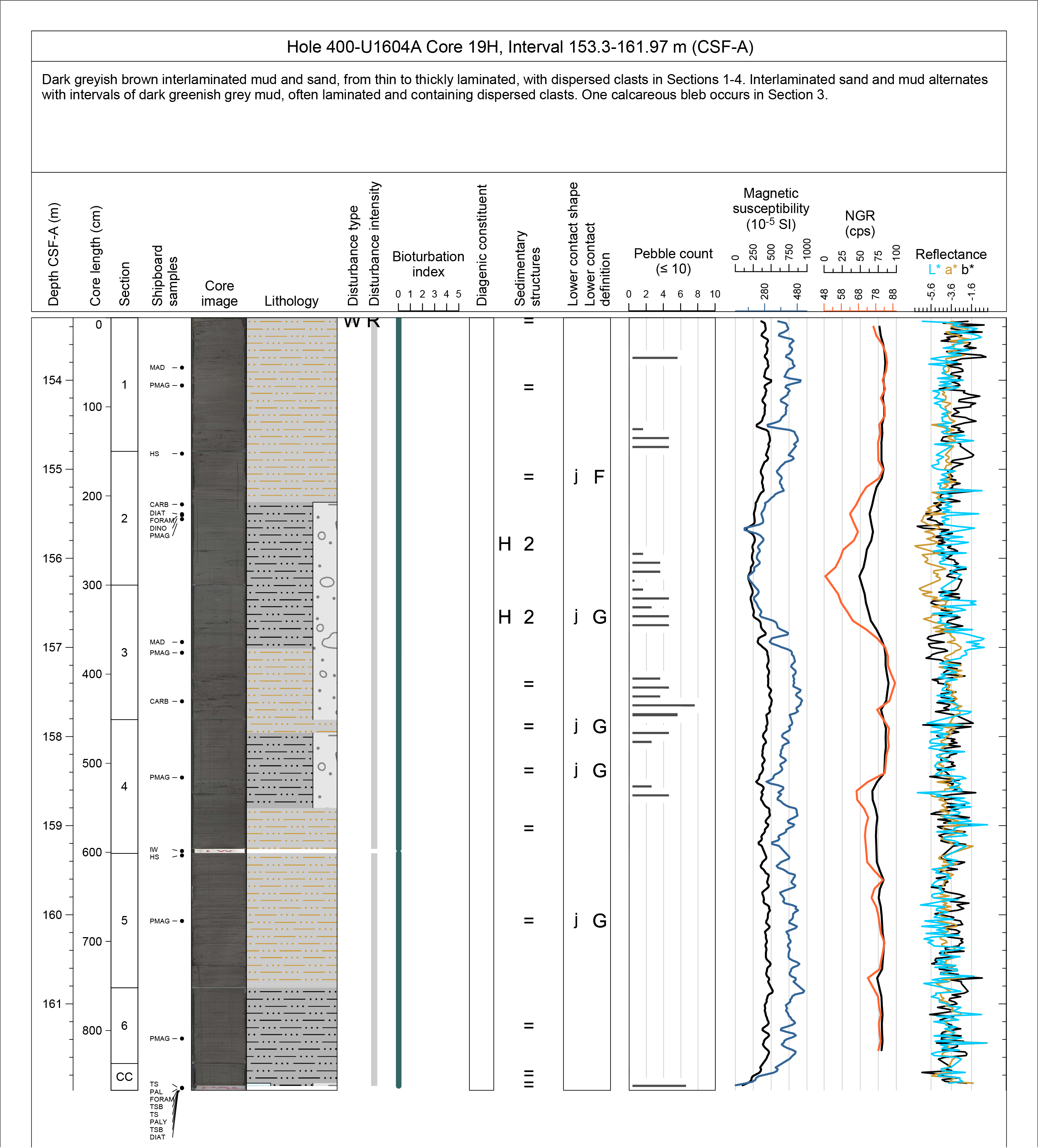
Figure F6. Example VCD.
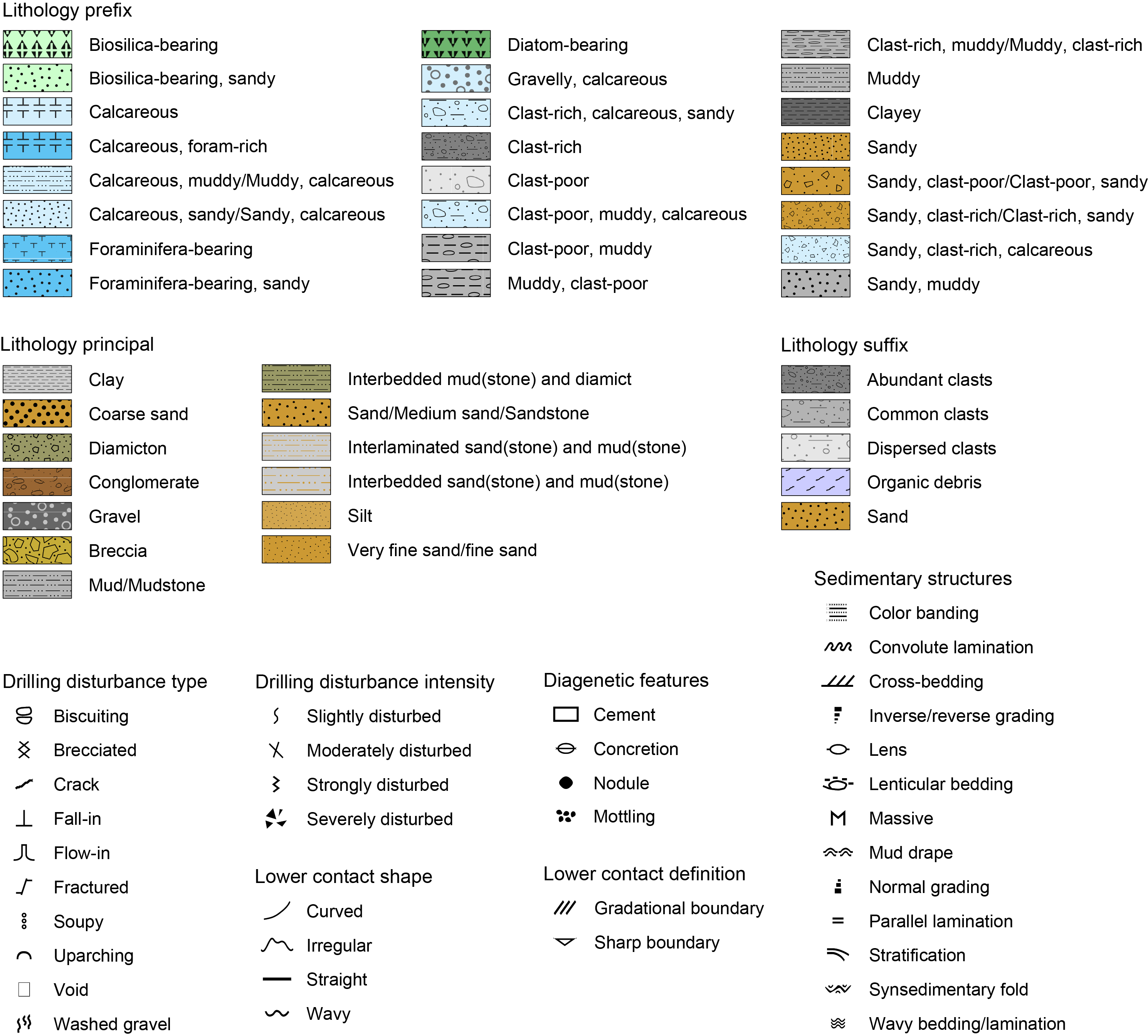
Figure F7. Key for VCDs and graphic logs.
3. Biostratigraphy
Biostratigraphy is based on planktonic foraminifera, benthic foraminifera, diatoms, and dinoflagellate cysts (dinocysts), which were studied in core catcher samples from all sites. Additional samples were taken from split core sections at some sites, targeting lithofacies variations suggestive of improved microfossil preservation (e.g., where color and/or physical properties data suggest calcareous, biosilica-rich, or organic-rich intervals). Samples from Expedition 400 were processed and analyzed for microfossil content shipboard during the expedition. Core catcher dinocyst assessments will be updated as part of initial shore-based work using hydrofluoric acid digestion approaches to concentrate palynomorphs, a method that was not available during this expedition. At high latitudes, where standard zonal markers are often absent, integration of microfossil groups is crucial for even the coarsest of chronological frameworks.
Biostratigraphy is aimed at identification of biostratigraphic horizons (biohorizons) in the cores, which might delimit established biozones. Ideally, the bioevents involve the first occurrence (FO) or last occurrence (LO) of a species and/or the first or last common occurrence (FCO or LCO) of a species. In reality, because of highly discontinuous microfossil occurrences at Expedition 400 sites, as a consequence of preservation and environmental factors influencing the Greenland margin, often only fragmentary perspectives on species ranges are available, especially in the case of foraminifera and diatoms. Therefore, during Expedition 400, we were unable to apply established biozone schemes, even regional versions constructed for the northern high latitudes. We were, however, able to recognize some biohorizons, including a selection of primary and accessory markers that have been defined in existing zonation schemes. Biohorizons are assumed to result from biological events (bioevents) in the past, such as migrations, extinctions, and evolutionary transitions. These bioevents have been previously assigned absolute ages, ideally referenced to the paleomagnetic reversal sequence. However, few Cenozoic bioevents recognized in the northern polar latitudes are well calibrated. Moreover, listed bioevent ages may not be accurate for the cored sites because of diachrony and/or imprecise calibration at the Arctic latitudes of Baffin Bay, for which no detailed and tested zonation schemes exist. Nevertheless, identification of biohorizons in stratigraphic order allowed us to contribute to age-depth modeling. Details of the biostratigraphic schemes and markers used for the various groups are outlined in their respective sections below and compiled in Figure F8.

Figure F8. Pleistocene to Oligocene biostratigraphic framework.
There were no dedicated calcareous nannofossil or benthic foraminifera biostratigraphy specialists on board during Expedition 400. However, because planktonic foraminifera are extremely scarce, benthic foraminifera became a primary chronostratigraphic guide and, thus, an overview of the benthic foraminifera was attempted. Similarly, where relevant, general observations of calcareous nannofossil presence/absence in smear slides was recorded by the Expedition 400 diatom team in consultation with sedimentologists during smear slide description. These slides and observations could be of future interest to a calcareous nannofossil specialist. Bolboformids, which are useful for biostratigraphy in other regions of the northern North Atlantic, are not found in the studied samples recovered during Expedition 400.
Where possible, for each site and each fossil group a list of identified biohorizons was prepared. These age constraints are plotted against depth in the accompanying age-depth plots where appropriate. Biohorizon lists and age-depth plots were not produced for Sites U1603–U1605 due to the scarcity of microfossils and limited time coverage at those sites. Because we never captured actual bioevents (e.g., LOs or FOs), constraints in the age-depth plots involve bars or boxes representing the total age range of a key taxon recognized at the stated depth. The biostratigraphic age information was used in conjunction with the paleomagnetic reversal records to construct integrated biomagneto age-depth models for each site. For each site, the paleomagnetic and biostratigraphic data were collated on a common geological timescale. The timescale used for Expedition 400 is mostly taken from Ogg (2020), which was published as part of the Geologic Time Scale 2020 (Gradstein et al., 2020). For subdivision of the formal series of the timescales and their geochronologic equivalent epochs, we use capitalized subseries (e.g., Lower Pleistocene) and subepochs (e.g., Early Pliocene) according to Aubry et al. (2024). Lowercase is used when referring to strata (e.g., lower Pliocene) and time (e.g., late Miocene) when a stage/age has not been constrained. The lowercase modifier emphasizes their informal status. All semiquantitative microfossil abundance data produced shipboard were input to GEODESC and are available for each site (https://iodp.tamu.edu/DataAccess/).
3.1. Planktonic foraminifera
3.1.1. Taxonomy and zonal scheme
Previous drilling of Miocene age to recent sediments of the high-latitude North Atlantic and the Subarctic and central Arctic Oceans tells us that few of the planktonic foraminifera marker species that are used in the standard global tropical to subtropical biozonation would be present at Expedition 400 sites, which lie along a continental shelf to slope transect at ~74°N. If present, they are likely only occasional immigrants; thus, their appearance may not represent a truly global evolutionary event. The possibility of lower latitude species making appearances is considered more likely for the Oligocene–Pliocene epochs, when latitudinal climatic gradients were weaker than in the Pleistocene. Nevertheless, we referred to existing high northern latitude planktonic biostratigraphic frameworks that have been developed over the past 50 years.
There have been repeated efforts to develop regionally applicable planktonic foraminifera biostratigraphic schemes for the North Atlantic, the Nordic Seas, and the North Sea based on endemic cold-water–tolerant taxa (Poore and Berggren, 1975; Poore, 1979; Weaver and Clement, 1986; King, 1989; Spiegler and Jansen, 1989; Gradstein and Backstrom, 1996; Spiegler, 1996; Flower, 1999; Anthonissen, 2009, 2012; Sierro et al., 2009). For Expedition 400, the biostratigraphic challenges were a general paucity of calcareous microfossils combined with low species diversity, consistent with the few previous long-term Cenozoic Arctic coring attempts at northern high latitudes. ODP Leg 151, which reached 80°N on the Yermak Plateau, found common planktonic foraminifera only in the Pleistocene, in the form of Neogloboquadrina pachyderma–dominated assemblages, with strong abundance variability over glacial cycles (Spiegler, 1996). Calcareous fossils disappeared rapidly downsection during the Pliocene and were almost entirely absent in the Miocene to Eocene (Spiegler, 1996), a pattern exaggerated in the central Arctic Ocean, where calcareous microfossils were found only in the Holocene to mid-Pleistocene of the central Arctic Ocean during IODP Expedition 302 (Expedition 302 Scientists, 2006). The North and Norwegian Seas have been the subject of various biostratigraphic studies through the petroleum industry and scientific ocean drilling. A series of foraminifera zonation schemes exist for this region, most notably those of King (1989), Gradstein and Backstrom (1996), Laursen and Kristoffersen (1999), and Anthonissen (2009, 2012). Calibration of the utilized biohorizons in these schemes has generally improved over the years, although the challenges of diachroneity at high latitudes, due to both climate gradients as well as local basinal tectonic processes affecting bathymetry, remain. The integrated foraminifera, bolboformid, dinocyst, and diatom zonations defined from IODP and industry boreholes through the North and Nordic Seas of Anthonissen (2009, 2012) provide the most up-to-date biostratigraphic frameworks for the northeastern North Atlantic for the Pliocene and Miocene. ODP Leg 105 Site 645 on the southwestern side of Baffin Bay (70°N) is the nearest drilled site to Expedition 400 targets. Foraminifera studies at Site 645 found planktonic foraminifera-bearing sediments in the Pleistocene, but the Pliocene and Miocene were barren (Aksu and Kaminski, 1989; Kaminski et al., 1989). Likewise, Expedition 400 found only a few horizons containing planktonic foraminifera; thus, a minimal set of bioevents could be used. Shipboard observations allowed only a skeletal foraminifera biostratigraphic framework, involving sparse, tentatively calibrated planktonic and benthic events and broad, informal benthic assemblage zones inspired by Kaminski et al. (1989) (Figure F8).
3.1.2. Preparation and examination methods
Planktonic foraminifera were examined from core catcher samples, selected samples taken from split cores, and mudline samples from the top of selected holes. Sample volumes between 5 and 20 cm3 were washed over 63 µm sieves. Before sieving, samples were agitated in deionized water on a shaker table in Erlenmeyer flasks to aid clay disaggregation. Harder, more lithified samples were mechanically fractured before agitation using a mortar and pestle and then soaked in solutions of Borax and sometimes Liquinox while they were agitated on the shaker table. Empty sieves were soaked in methylene blue and cleaned in an ultrasonic bath between samples to identify sieve contaminants and minimize cross contamination between samples. Dried residues (>63 µm) were transferred to labeled glass vials. All or parts of the prepared sand residues were examined on metal picking trays using a Zeiss Discovery V8 stereomicroscope. Because the >63 µm residues are so variable in their terrigenous and other fossil contents, a representative view of the picking tray was commonly photographed using the QImaging Image Capture system coupled to the Zeiss light microscope (images uploaded to the LIMS database). These images are included with broader descriptions of sand fractions, including qualitative observations on the clast composition, size, shape, sorting, and other fossil remains.
To aid species identification, scanning electron microscope (SEM) imaging was carried out for selected samples. This involved choosing candidate specimens, mounting them on a steel stub, and then applying a gold coating using a Leica EM ACE200 sputter coater. The specimens were imaged using a Hitachi TM3000 benchtop SEM. Routinely, whole specimen images were taken followed by close-ups of the apertural region or test wall to document wall textures and preservation quality.
Apart from planktonic foraminifera, the following particle categories were recorded: siliceous plankton; spicules; quartz; rock fragments; glauconite; pyrite; organic material (plant and wood fragments); volcanic ash; icthyoliths (including fish teeth, scales, etc.); and other fossiliferous materials, such as echinoid spines, mollusk fragments, and bryozoans. Planktonic foraminifera taxonomy follows Brummer and Kučera (2022) for the Pleistocene, with perspectives on morphotypes of N. pachyderma from El Bani Altuna et al. (2018) and Wade et al. (2018) for the Oligocene, with support from Mikrotax (https://www.mikrotax.org/pforams/). In practice, we tended to sieve samples into 63–125 µm and >125 µm fractions for our standard microscope observations. However, because of the low numbers of foraminifera encountered, abundances are pooled and reported as the relative numbers of specimens in the dried sample in the >63 µm fraction. The following abundance categories relative to total sediment particles were visually estimated:
- D = dominant (>50% of sediment particles).
- C = common (5%–50% of sediment particles).
- R = rare (<5% of sediment particles).
- Tr = trace (few individuals).
- B = barren.
Planktonic foraminifera preservation as viewed under the light microscope was recorded as follows:
- E = excellent, with most specimens having a glassy appearance indicating very little recrystallization and very little evidence of overgrowth or dissolution, as well as little abrasion.
- VG = very good, with some specimens showing minor evidence of diagenetic overgrowth, dissolution, or abrasion; recrystallization may or may not have occurred.
- G = good, with some specimens showing signs of significant overgrowth, dissolution, or abrasion and possibly some infilling with cement or indurated sediment.
- M = moderate, with most specimens showing evidence of overgrowth, dissolution, and abrasion; tests are generally infilled with cement or indurated sediment obscuring apertures.
- P = poor, with substantial diagenetic overgrowth, dissolution, and abrasion; foraminifera can be fragmented and difficult to identify because of major overgrowth and/or dissolution.
Planktonic foraminifera fragmentation as viewed under the light microscope was recorded as follows:
Where N. pachyderma was encountered, coiling ratios were utilized to investigate whether populations contained only N. pachyderma (a left:right coiling ratio of 5%:95% is expected) or a combination of N. pachyderma and Neogloboquadrina incompta (>5% right coiling is expected) (Darling et al., 2006).
3.2. Benthic foraminifera
No dedicated benthic foraminifera biostratigrapher sailed as a part of the Expedition 400 scientific party. However, the relative abundance of benthic species, including calcareous versus agglutinated species in the >63 µm size fractions, was routinely recorded and the presence of key marker species was noted. We anticipated several calcareous benthic foraminifera biostratigraphic markers in the sediments acquired during Expedition 400 (Figure F8). Seidenkrantz (1995) erected a new species, Cassidulina neoteretis, from its presumed direct ancestor, Cassidulina teretis Tappan (1951), on the basis of slight morphological changes (especially to the apertural plate) and differences in the species distributions. The LO of C. teretis Tappan (1951) has been placed between ~2.3 and 0.7 Ma in the North Atlantic and the Nordic Seas (Seidenkrantz, 1995). These species have been found commingled until the late Pleistocene in the Arctic Ocean (Lazar et al., 2016), suggesting that extinction of C. teretis was time transgressive (Cage et al., 2021). C. neoteretis is a common modern species in the Arctic Ocean and the northern North Atlantic, particularly around the Greenland margin, in areas occupied by chilled Atlantic water (c.f. Cage et al., 2021), making it important for paleoceanographic reconstructions in Baffin Bay and one of the few markers featured in our coarse biostratigraphic scheme (Figure F8).
Benthic foraminifera in the Pliocene/Pleistocene Clyde Foreland Formation of eastern Baffin Island (Feyling-Hanssen, 1976) and the Kap København Formation (Feyling-Hanssen, 1990; Funder et al., 2001) of northern Greenland contain taxa that do not occur in Baffin Bay today. In particular, Cibicides grossus Ten Dam and Reinhold, 1941, and Nonion tallahattensis Bandy, 1949, are taxa that were found only in sections considered to be of Pliocene age by Feyling-Hanssen in the Clyde Foreland Formation; they do not occur in the Arctic today. Recent attempts to use amino acid racemization and cosmogenic radionuclide dating of the Clyde Foreland Formation confirm latest Pliocene to early Pleistocene ages for the oldest units (Refsnider et al., 2013), reinforcing their utility for Expedition 400 biostratigraphy. The taxonomy of recognized benthic species follows Feyling-Hanssen (1976, 1990), Kaminski et al. (1989), and Cage et al. (2021). Although, as found at ODP Site 645 (Kaminski et al., 1989), agglutinated benthic species are present in Expedition 400 cores, we have not attempted to use agglutinated benthic species for biostratigraphic purposes. We anticipate that doing so, especially for Site U1607, could be a fruitful path for future work.
Benthic foraminifera abundance based on observations of the dried sample in the >63 µm fraction was recorded using the following scheme:
- D = dominant (>50% of the foraminifera assemblage).
- C = common (5%–50% of the foraminifera assemblage).
- R = rare (<5% of the foraminifera assemblage).
- Tr = trace (few individuals).
- B = barren.
The relative abundance of calcareous and agglutinated benthic species, respectively, were recorded using the following scheme:
- D = dominant (>50% of the foraminifera assemblage).
- C = common (5%–50% of the foraminifera assemblage).
- R = rare (<5% of the foraminifera assemblage).
- Tr = trace (few individuals).
- B = barren.
3.3. Diatoms
3.3.1. Taxonomy and zonal scheme
The Neogene and Quaternary diatom biostratigraphy principally follows the previous works carried out in the North Atlantic by Baldauf (1984, 1987) (Deep Sea Drilling Project [DSDP] Legs 81 and 94), Koç and Scherer (1996) (ODP Leg 151), and Koç et al. (1999) (ODP Leg 162). The North Pacific diatom zonation, developed by Barron (1985) (DSDP Leg 85), Akiba (1986) (DSDP Leg 87), Barron and Gladenkov (1995) (ODP Leg 145), and Yanagisawa and Akiba (1998), was also used when diatom species from the North Pacific were encountered. Although the Oligocene and Eocene diatom zonation from the Norwegian Sea Cenozoic diatom biostratigraphy by Schrader and Fenner (1976) (DSDP Leg 38), Dzinoridze et al. (1978) (DSDP Leg 38), and Fenner (1985) and Scherer and Koç (1996) (ODP Leg 151) was not applied due to the lack of specific diatom biostratigraphic markers, diatom descriptions and photomicrographs therein were used to identify certain species. Furthermore, diatom resting spores are an integral part of diatom biostratigraphy (e.g., Suto, 2005). Therefore, the North Atlantic biostratigraphic schemes of diatom resting spore genera (e.g., Goniothecium, Dicladia, Monocladia, and Syndendrium) were also employed to provide age control (Suto, 2005; Suto et al., 2008). Diatom biostratigraphic age constraints were also obtained from data sets from the Janus database (http://www-odp.tamu.edu/database) and then calibrated to the 2020 geomagnetic polarity timescale (GPTS2020; Gradstein et al., 2020) using the Neptune database (https://www.museumfuernaturkunde.berlin/en/science/nsb-database) (Figure F8). The recognized diatom biohorizons involve the FOs and LOs of key species.
Diatoms were identified to species level where possible. Key stratigraphic markers were identified according to previous work by Schrader and Fenner (1976), Baldauf (1984), Akiba (1986), Monjanel and Baldauf (1989), Baldauf and Monjanel (1989), Koç and Scherer (1996), and Koç et al. (1999).
Although the shipboard micropaleontology work mainly focuses on the identification of biostratigraphically useful events, additional biosiliceous microfossil groups of specific environmental indications were also identified and recorded from the same sample. This was done for additional age control and included sea ice and marine diatoms, freshwater diatoms, silicoflagellates, ebridians, and siliceous spicules of endoskeletal dinoflagellates. These microfossils were identified based on previous studies in the northern high latitudes by Sancetta (1982), Koç Karpuz and Schrader (1990), Pearce et al. (2014), Tsoy and Obrezkova (2017), and Oksman et al. (2019).
3.3.2. Preparation and analysis methods
Smear slides from the core catcher samples were examined on a routine basis for stratigraphic markers and paleoenvironmentally sensitive taxa. A toothpick sample of sediment was placed on a 22 mm × 40 mm coverslip and wetted with deionized water and a small amount of regular soap to break the surface tension and ensure a relatively homogeneous spread of sediment over the coverslip. The coverslips were allowed to dry on a hot plate. Once dried, a few drops of Norland Optical Adhesive Number 61 (refractive index = 1.56) were added and covered with coverslips. The microscope slides were then placed under the ultraviolet lamp and cured for ~10 min.
For samples of low diatom concentration but with critical stratigraphic and paleoenvironmental implications, slides were prepared from core catcher and section half samples using the following procedures. A ~2 cm3 sediment sample was placed in a 250 mL beaker with 30% hydrogen peroxide (H2O2) and sodium borate (Borax) to remove organic material and to disaggregate clay-sized sediments. Carbonate was generally rare in most samples; thus, hydrochloric acid (HCl) was not used. When the reaction was complete, the sample was diluted with distilled water until the residue was neutralized. The diatoms were then concentrated by using a 10 µm mesh sieve. A few aliquots of the sieved sample residue were evenly dropped on a 22 mm × 40 mm coverslip and mounted with Norland Optical Adhesive Number 61 (refractive index = 1.56) under the ultraviolet lamp. The sieved slide method may bias the total diatom abundance, but it is practical to observe diatoms in low concentration samples.
Samples prepared for diatom analysis were examined using a Zeiss Axioskop transmitted light microscope. For photomicrographs, a SPOT Flex 64 Mp digital camera was used. A Hitachi TM3000 tabletop SEM was used for further taxonomic assessments when needed. Qualitative siliceous microfossil group abundances were determined from smear slides using 630× magnification. Additionally, samples were routinely examined under 1000× magnification for detailed taxonomic observations. Care was taken to ensure smear slides were prepared with similar amounts of sediments to produce consistent abundance estimates.
For each sample, the total abundance of diatoms was qualitatively estimated by light microscopic observations with the examination of five random FOVs, following the classification listed below:
- M = mass abundance (>60% diatoms).
- A = abundant (>20% diatoms).
- C = common (10%–20% diatoms).
- F = few (5%–10% diatoms).
- R = rare (2%–5% diatoms).
- Tr = trace (trace quantities <2%).
- B = barren (no diatom debris).
Trace amounts (<2%) could contain very rare, unrecognizable fragments, maybe comprising diatoms that have undergone processes like pyritization, recrystallization, or partial dissolution. These diatom elements might only retain traces of their original form due to the effects of significant dissolution or diagenesis and therefore do not provide valuable information for biostratigraphic applications. Visual estimates of percentages adopted standard guidelines (e.g., Rothwell, 1989).
The following relative abundances of individual taxa were categorized in reference to their occurrence in FOVs or to a traverse across a 40 mm wide coverslip (~100 FOVs at 630× magnification):
- D = dominant (the taxon represents >50% of all diatoms in diatom-rich samples).
- A = abundant (2 or more specimens per FOV).
- C = common (1–5 specimens per ~5 FOVs).
- F = few (1–5 specimens per transect).
- R = rare (1 specimen within 1–5 transects).
- Tr = trace (<1 specimen per 5 average horizontal transects [40 mm]).
The counting approach adopts Schrader and Gersonde (1978) and Zielinski (1993) frameworks for the above categorization. Diatom occurrence data were logged in GEODESC and primarily focused on the presence of biostratigraphically and paleoenvironmentally critical species. Therefore, the logged data probably do not reflect the underlying diatom diversity Expedition 400 materials might possess. Care was taken to track changes of both occurrence and abundance of diatom assemblages indicating sea surface environment.
Diatom preservation was qualitatively assessed as a function of the degrees of dissolution and fragmentation. Although diatom fragmentation and dissolution in some settings are related, the mechanistic links between these two factors are not always directly correlated. Furthermore, dissolution is a wholly chemical/diagenetic process (Warnock and Scherer, 2015), whereas fragmentation can be dominantly or entirely due to mechanical processes (Scherer et al., 2004).
Shipboard data collection integrated fragmentation and dissolution observations into overall diatom preservation and categorized it using the following levels:
3.4. Organic-walled dinoflagellate cysts
3.4.1. Taxonomy and zonal scheme
Dinocyst zonation schemes for the subarctic region suffer from the same lack of local zonal development and calibration as the other biostratigraphic groups, thus requiring some ad hoc customization. In the absence of a paleomagnetic record to match biostratigraphic data from the more southerly Baffin Bay ODP Site 645 (Baldauf et al., 1989), the distribution pattern of dinocyst index taxa in Expedition 400 sites is more broadly compared to the various zonation schemes of the North Atlantic Ocean and Nordic Seas, where some paleomagnetic data do exist. These include (palyno)stratigraphic schemes and bioevents from the Arctic covering the Quaternary (Matthiessen et al., 2018) to Neogene (Mudie et al., 1990); from Baffin Bay covering the late Neogene (Aubry et al., 2021) and Miocene (Head et al., 1989); and from the North Atlantic covering the Pliocene and Pleistocene (de Schepper and Head, 2009), Neogene (de Schepper et al., 2017; Piasecki, 2003), and Oligocene (Egger et al., 2016). An overview of zonation schemes and existing relevant calibrated dinocyst biohorizon ages is provided in Figure F8. Diachronism of dinocyst bioevents (de Schepper et al., 2015; Matthiessen et al., 2018) complicates the potential for regional correlation between sites and development of consistent chronologic frameworks, emphasizing the need for renewed efforts to integrate perspectives from various microfossil groups as well as new interpretations of the relationship of dinocyst events to the magnetic reversal stratigraphy.
Aside from biochronostratigraphic purposes, shipboard quantitative marine palynological analysis included preliminary palynofacies assemblage characterization in terms of paleoenvironment.
3.4.2. Preparation methods
Several processing methods may be employed depending on, for example, biogenic or detrital silica concentrations, the presence of carbonates, and the degree of cementation. For safety reasons, no hydrofluoric acid was used on this expedition, so some samples yielded large amounts of diatoms and/or clay minerals, which compromises dinocyst analysis.
For shipboard sample preparation, approximately 20 cm3 (~20 g) of soft, clay-rich material was treated with a warm 1% Liquinox solution and left overnight to disaggregate (as described by Riding and Kyffin-Hughes [2011], who used Liquinox for the strong detergent). Carbonate-rich samples were first treated with 30% HCl to dissolve the bulk of the carbonate. To further disaggregate the samples, Borax flakes were added and the beaker with the sample was placed on a hotplate and stirred. Borax replaces the sodium hexametaphosphate used by Riding and Kyffin-Hughes (2011). The organic residues were then sieved over 15–250 µm nylon sieves to remove large phytoclasts and palynodebris (>250 µm) and small particles (amorphous organic matter and minor amounts of clays, usually phyllosilicates), followed by rinsing with demineralized (or deionized or tap) water to remove the Liquinox and Borax. This step was followed by an ultrasonic bath to separate heavy from light material. The light material was collected, and a few drops of the sieved sample residue were evenly distributed on a 22 mm × 40 mm coverslip and mounted with Norland Optical Adhesive Number 61 (refractive index = 1.56) under the ultraviolet lamp.
3.4.3. Marine palynological associations (palynofacies)
The palynological residues resulting from the processing method described above allow analysis of palynofacies. Observed particles fall into two categories: (1) palynodebris, specifically, fragments of larger multicellular entities or related elements (e.g., from fragments of plant tissue to small resin droplets), and (2) palynomorphs, identifiable (semi)complete elements, or remains of uni- or multicellular biota. The latter are composed of both aquatic elements (freshwater and/or marine derived) and terrestrial components such as elements related to higher plants (spores, gymnosperm pollen, and angiosperm pollen), sometimes including remnants of freshwater plants (Grímsson et al., 2015), various fungal remains, or even invertebrate-derived elements (e.g., the jaws of marine annelids, so-called scolecodonts, and various insect remains) (Whitlock and Dawson, 1990). The aquatic fresh-to-brackish water elements may include single-celled palynomorphs such as Cymatiosphaera, Pterospermella, and Tasmanites spp.; cysts of freshwater dinoflagellates; and multicellular (colonial) forms such as Pediastrum and Botryococcus spp. The marine portion typically consists of organic-walled dinocysts of either gonyaulacoid or (proto)peridinioid dinoflagellates and various organic-walled microfossils of unknown affinity (so-called Acritarchs), but it may also yield remains of many other marine microbiota, including, but not limited to, the inner linings of benthic foraminifera and tintinnid loricae.
3.4.4. (Semi)quantitative palynofacies analysis
Palynofacies analysis and data collection were carried out using a Zeiss Axiophot microscope with brightfield illumination at 400×, 630× (oil), and 1000× (oil) magnification. For each sample, one 22 mm × 40 mm slide was scanned semiquantitatively and characterized for palynodebris categories (see below). For each of the palynodebris categories, the percent of coverage per slide was estimated and indicated in the table (0%–100%). Photomicrography was conducted using a SPOT Flex digital camera, and images were uploaded to the LIMS database.
The following broad palynodebris categories were employed:
- Black phytoclasts and opaque elements of unknown affinity,
- Brown phytoclasts,
- Plant tissue general,
- Leaf/cuticle remains,
- Amorphous organic matter (aggregates),
- Amorphous organic matter (filaments),
- Transparent filaments/fungal affinity,
- Pyritized microfossils,
- Indeterminable elements (palynomorphs), and
- Clay mineral aggregates.
The following palynomorph categories were employed:
- In situ dinocysts (≥0.5 cyst) (determined to group or species level),
- Indeterminable (likely) remains of dinocysts (fragments),
- Reworked marine dinocysts (and ages),
- Organic linings of (benthic) foraminifera,
- Acritarchs (various groups),
- In situ pollen and spores,
- Reworked pollen and spores,
- Single-celled brackish/freshwater palynomorphs,
- Multicelled brackish/freshwater palynomorphs, and
- Indeterminable elements (palynomorphs).
For each of the palynomorph categories, the following relative abundances were categorized in reference to their occurrence:
- p = present (1 or 2 individual specimens per slide).
- c = common (more than 2 individual specimens per slide).
- a = abundant (more than 10 individual specimens per slide).
- A = acme (dominant species/group).
3.4.5. Environmental reconstructions using dinocysts and palynofacies
Both dinocysts and the general composition of the palynofacies present useful insights for reconstruction of paleoenvironments (e.g., Batten, 1996). Organic-walled cyst-producing dinoflagellates are sensitive to even minor changes in their physical and biochemical environment, and assemblage characteristics can be used to qualitatively and semiquantitatively reconstruct a range of ancient environmental parameters and conditions, including salinity, shore proximity (paleodepth), productivity, upwelling, and temperature. Ecological preferences of extant species are well documented using modern core-top data (Zonneveld et al., 2013; Marret et al., 2020), whereas, for extinct species, researchers have utilized independent proxy data and field observations to assign groups of taxa (ecogroups) to specific paleoenvironmental conditions including high-latitude, potentially glacially influenced locations (e.g., Schreck et al., 2017; de Schepper et al., 2011; Rochon et al., 1999). These studies allowed us to make coarse, low-resolution, environmental reconstructions for all cores that yielded sufficiently well-preserved dinocyst assemblages and palynofacies.
3.5. Marine sedimentary ancient DNA sampling
3.5.1. Summary
The shipboard program for marine sedaDNA sampling included collecting samples and applying chemical tracers to assess potential core contamination. Most sample preparation and analyses will be conducted onshore at the facilities of the Center for GeoGenetics, University of Copenhagen (Denmark) and the Geological Survey of Denmark and Greenland (GEUS). We aim to address fundamental questions about DNA preservation in Arctic marine sediments. By using a combination of targeted (DNA metabarcoding and hybridization capture) and untargeted (metagenomic shotgun sequencing) genetic approaches, we investigate how far back in time we can use DNA to uncover interactions between climate, the ocean, and the biosphere. We will further investigate the effect of climate on marine ecosystem structure and function and test the influence of increased freshwater runoff from Greenland ice sheet melting during interglacials (trace runoff via terrestrial plant-derived DNA), thereby contributing to the scientific objectives of Expedition 400. Sampling for marine sedaDNA was conducted immediately after core recovery to prevent DNA degradation due to sediment exposure to oxygen, elevated temperatures, and/or irradiation. Samples were collected from sediments acquired using the APC system at Sites U1603 and U1604 and the RCB system at Sites U1608 and U1606. Sampling followed either (1) the catwalk sampling; (2) split core section sampling; or (3) whole-round core intervals procedures (see below), which were partly adapted from the sedaDNA sampling procedures established during IODP Expedition 382 (Weber et al., 2021).
Of the coring systems available on board, the APC system produced the least amount of sediment disturbance and was thus the least susceptible to contamination (House et al., 2003; Lever et al., 2006). Therefore, we limited the sampling to cores acquired by the APC system and extended our record with four samples acquired by RCB drilling (Figure F9).
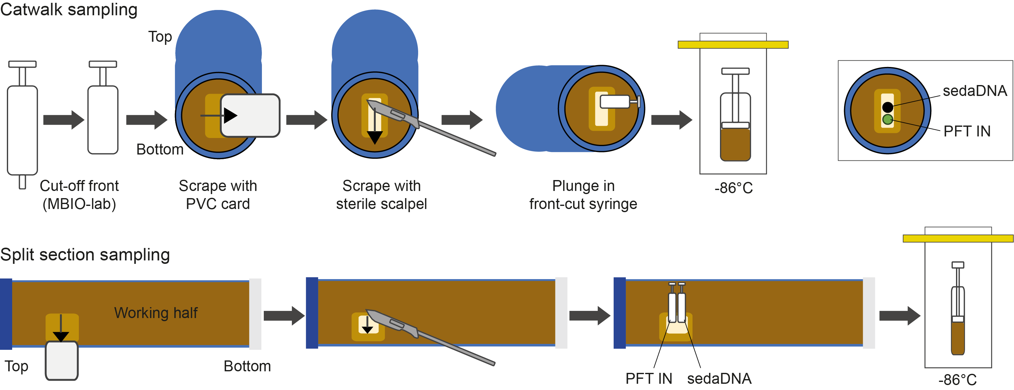
Figure F9. Workflows for collecting sedaDNA and PFTIN samples.
3.5.2. Catwalk sampling
Throughout sedaDNA sampling on the catwalk, personal protective equipment (PPE; Tyvek overall, face mask, hairnet, safety goggles, and two pairs of disposable gloves) was worn by the analyst and technicians, and the outer gloves were changed immediately if they were contaminated with any sediment material. After core sectioning, approximately 2 mm of the exposed sediment in the center were scraped off with a bleach- and ethanol-treated polyvinyl chloride (PVC) card (Figure F9). Then, using a sterile scalpel, about 1 mm of the freshly scraped area was removed. The clean center was subsampled for sedaDNA with a sterile 10 mL syringe of which the front was cut off (cut-tip syringe). The syringe was placed immediately into a sterile WhirlPak bag, labeled, and stored frozen at −86°C. We took three samples per core, usually at the bottom of Sections 1, 3, and 5. To monitor potential contamination of sediments by drill fluids, perfluorodecalin (PFD) tracer was added to the drill water. Directly next to the sample in the scraped area, a sample for tracer analysis was taken using a 3 mL cut-tip syringe. The tracer sample was then placed into a headspace vial, covered with the lid, labeled, and placed in the refrigerator until the analysis was run. To validate tracer arrival at the sediment core, one positive control was taken for each core where the sediment is in contact with the core liner.
The mudline (sediment/seawater interface) was collected directly from the liner with a sterile scoop into a sterile WhirlPak bag (approximately 10 g) and frozen at −86°C. This sample was expected to provide an overview of recent communities and/or potential contamination downcore if tracer was detected in the sediments.
3.5.3. Sampling on split core sections
For splitting core sections, technicians wore a laboratory coat, hairnet, safety goggles, face mask, and gloves that were changed between samples, and the microbiologist wore a Tyvek overall, bleached arm sleeves, double layer of gloves, hairnet, safety goggles, and face mask. The sections were generally split into halves from bottom to top; however, if a targeted interval was close to the top, we split from top to bottom to avoid the interval being destroyed by a rock. Access to the closed-off splitting room was restricted to the technicians and the microbiologist. Liner caps in core sections chosen for sedaDNA sampling were sonically sealed instead of using the standard acetone technique. To separate the working half from the archive half after core section splitting, cleaned spatulas were used instead of distilled water. The cutting procedure likely transported contaminated sediments from the core liner to the inner part of the core. Therefore, the surface layer (~1 mm) of the working half was scraped off perpendicular to the length of the working half at each anticipated sampling depth using bleach- and ethanol-treated PVC scrapers. The surface was scraped a second time (~1–2 mm) using a sterile scalpel. A sterile front-cut 3 mL syringe (~1 cm3) was plunged into the freshly scraped area, immediately placed into a sterile WhirlPak bag, and stored frozen (−86°C) (Figure F9).
3.5.4. Sampling on whole-round core intervals
Rotary drilling led to the recovery of compacted sediments in longer (>10 cm) and shorter (~5–10 cm) intact intervals. To avoid contamination by splitting the core using the saw, the whole rounds of 5 cm long intact intervals were collected into sterile WhirlPak bags at the catwalk immediately after the core was on deck and taken into the microbiology laboratory for cleaning. All steps were carried out within the KOACH T 500-F Table Clean Bench to keep the environment as clean as possible during the cleaning procedure. The KOACH system consists of two air filtration boxes that can locally produce the cleanliness level of International Organization for Standardization (ISO) Class 1 in an environment where the cleanliness level is between ISO Classes 1 and 8 by creating a coherent, colliding airflow (Figure F10B). Potential contamination by the laboratory air was monitored with an Extech VPC300 Particle Counter (<700 particles of 0.3 µm during sampling of Sections 400-U1608A-13R-1 and 14R-1; <200 particles of 0.3 µm size during sampling of Section 29R-2; and <1000 particles of 0.3 µm during sampling of Hole U1606B), while a sterile 50 mL tube was open during the procedure (air blank to which 2 mL DNA/RNA Shield [Zymo Research, USA] were added). The microbiologist wore PPE (Tyvek overall, bleached arm sleeves, double layer of gloves, hairnet, plastic socks, and face mask) at all times, and gloves were changed whenever they came into contact with sediment.
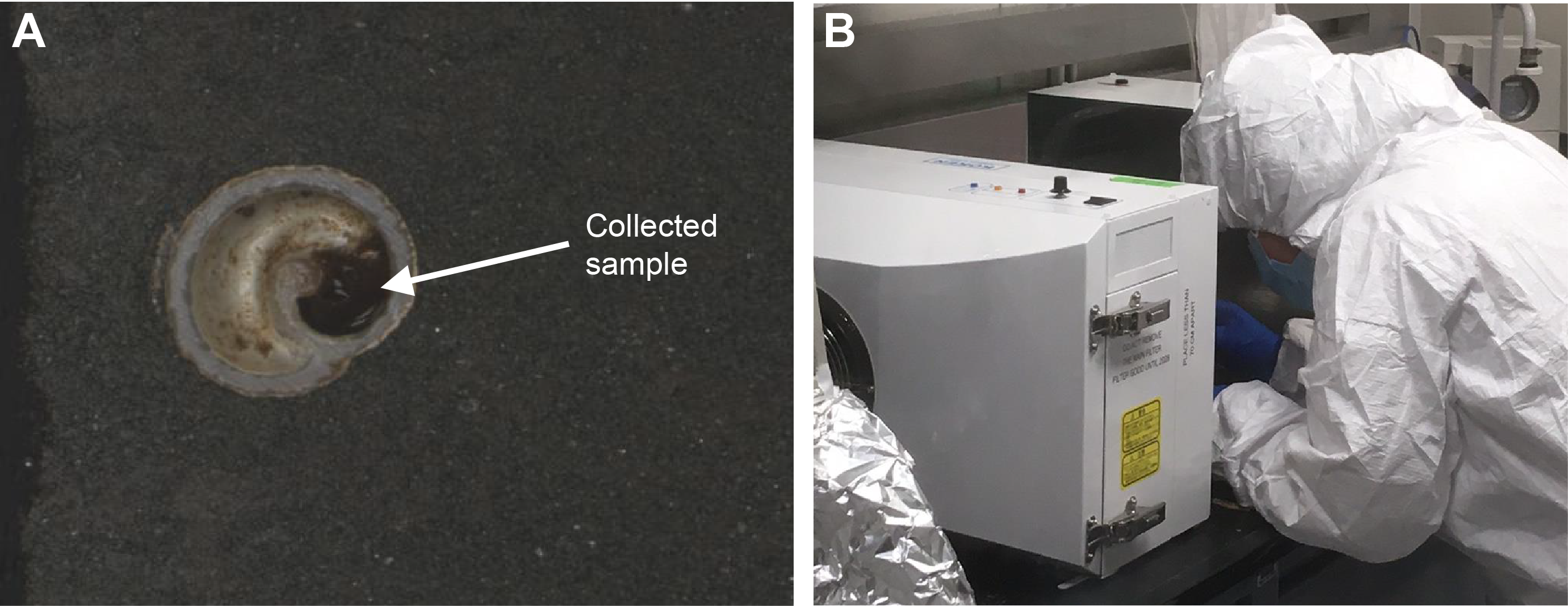
Figure F10. Sampling a gastropod shell.
All surfaces were cleaned with 3% bleach, which was rinsed off using 70% ethanol. A WhirlPak bag was opened and unfolded to create a sterile work area onto which the sediment piece was placed. Using a stainless steel chisel and hammer (both soaked in 3% bleach, which was rinsed off using 70% ethanol), about 2 mm of the surface were taken off and collected for external tracer analysis (see Contamination control). After each application on the sediment piece, the chisels were cleaned (3% bleach; 70% ethanol). The cleaned sediment piece was placed into a WhirlPak bag while the workbench was cleaned. A second round of cleaning was carried out on a freshly opened WhirlPak bag using sterile scalpels as chisels. Thereafter, the sediment piece was stored again in a WhirlPak bag while the workbench was cleaned (3% bleach; 70% ethanol). Finally, the sample was placed on a combusted aluminum foil (see Sampling the organic remains of a gastropod shell), and a sediment piece was taken off for internal tracer analysis. The freshly exposed part, which was not in contact with any plastic, was sampled for biomarker analysis (only Sections 400-U1608A-13R-1 and 29R-2) into a combusted glass vial covered by aluminum foil between the sample and lid (see Sampling the organic remains of a gastropod shell) and stored at −20°C. Finally, a piece of the interior of the sediment piece was collected into a sterile 50 mL tube and submerged in DNA/RNA Shield for RNA preservation and coupled DNA and RNA extraction. DNA/RNA Shield is a buffer to preserve RNA if continuous storage in liquid nitrogen until RNA extraction cannot be guaranteed. This will allow us to test which part of the taxonomic composition can be attributed to the metabolically active assemblage (represented by DNA and RNA) and which part is either inactive or dead, ancient communities (only represented by DNA). The cleaned, interior part of the sediment piece was carefully placed into a WhirlPak bag and stored frozen at −86°C. All sediment residues were collected during the cleaning process for microfossil and other analyses and stored at 4°C; therefore, they contain the tracer.
3.5.5. Contamination control
After sampling for sedaDNA from each hole, at least one air control sample was taken on the catwalk or in the core splitting room to test for potential airborne contamination. For this control, a sterile 15 mL tube was waved through the air 10 times in the sampling area and then transferred into a sterile WhirlPak bag and frozen (−86°C).
To assess the potential for contamination during coring and the sectioning of cores on the catwalk, a perfluorocarbon tracer (PFT) was added to the drilling fluid for Holes U1603E, U1603F, U1604B, U1608A, and U1606B. The tracer compound PFD (C10F18) is a commonly available contamination tracer because others are either extremely volatile (e.g., perfluoromethylcyclohexane [PFMCH]; MacLeod et al., 2017) or much bigger than DNA fragments (e.g., particulate fluorescent microspheres; 0.5–1 mm) and thus either difficult to measure or not informative.
PFD tracer was initially injected at a flow rate of 0.4 mL/min, starting about 1 h before the coring process to guarantee tracer arrival at the drill bit (adapted after Smith et al., 2000). The tracer flow rate was increased to 0.8 mL/min after the first tracer samples were evaluated and kept at this rate for all sampled holes. We collected two types of sediment samples for tracer analysis. The first type was taken to confirm the delivery of the tracer to the drill bit (exterior sample [PFTEX]; one per core) by taking a sample where the sediment is in contact with the core liner. Because only trace amounts of PFD tracer were retrieved, liquid from the top of the core was taken (PFTLIQ) instead to confirm tracer arrival. The second type was collected next to a sedaDNA sample in the scraped sediment area (interior sample [PFTIN]). Approximately 3 cm3 of sediment were taken for PFTIN catwalk sampling, and about 1 cm3 of sediment was taken during split core sampling using disposable, 3 mL cut-tip syringes, which were immediately placed into a sterile WhirlPak bag. For PFTEX sampling, about 3 cm3 were taken with a spatula and placed into a 20 mL headspace vial with metal caps and polytetrafluoroethylene (PTFE) seals.
Samples were stored at 4°C and analyzed as soon as possible after collection. We tested sediment samples from the periphery of the core by transferring ~3 cm3 of sediment using a disposable, 5 mL cut-tip syringe into a 20 mL headspace vial (combusted at 500°C for 5 h) with metal caps and PTFE seals prior to any scraping/cleaning of surface sediments. The sample from the center was collected in the same way after scraping and right next to the location of the sedaDNA sample to minimize differences between material tested for sedaDNA and chemical tracers.
Samples were analyzed using a GC2-Agilent 6890N gas chromatograph (GC) with a microelectron capture detector (HP G1223A) using an injection volume of 2500 µL, a fill speed of 100 µL/s, a 500 ms pre- and postinjection delay, a 10 s flush time, an incubation and syringe temperature of 70°C, and an incubation time of 10 min (total GC run time = 60 min) (MacLeod et al., 2017). The oven temperature program included a 3 min equilibration, a maximum temperature set to 200°C, an increase from an initial 50°C (6 min) in 15°C steps until reaching a final temperature of 200°C (21.5 min), and then a decrease to 100°C (total run time = 37.5 min). The front inlet was used in splitless mode with an initial pressure of 28.1 psi and a total flow of 36.6 mL/min, a gas saver flow of 20.0 mL/min, and a saver time of 2.00 min, using helium. The front detector was set to a constant makeup flow (20 mL/min) using nitrogen as the makeup gas type and without applying temperature. A capillary column with the following parameters was used:
- Maximum temperature = 260°C.
- Nominal length = 50.0 m.
- Nominal diameter = 530.00 µm.
- Nominal film thickness = 10.00 µm.
- Constant flow mode, initial flow = 33.6 mL/min.
- Nominal initial pressure = 27.9 psi.
- Average velocity = 141 cm/s.
- Inlet = front.
- Outlet = front detector.
- Outlet pressure = ambient.
The GC was calibrated using 0.1, 0.2, 0.3, 0.5, 1, 5, 10, and 20 ng/µL PFD tracer (adapted from IODP Expedition 399; Lang et al., 2025). The retention time of PFD tracer was 10.6 min.
In addition to the sediment samples, we collected a sample of the tracer-infused drilling fluid directly from the injection pipe on the rig floor (wearing gloves). Approximately 10 mL of the drilling fluid was transferred to a 15 mL centrifuge tube, placed into a sterile WhirlPak bag, and stored at −86°C. The drilling fluid samples will be processed and analyzed in the same way as the sediment samples. Any organisms detected in both sediments and drilling fluid after sequencing and data filtering will be carefully investigated and interpreted and then either removed from our analysis or processed using bioinformatic software.
3.5.6. Sampling the organic remains of a gastropod shell
During the splitting of Section 400-U1607-60R-CC, a gastropod shell was split in half and a notable black filling in the archive half was interpreted as organic (Figure F10A). Sampling proceeded for potential future analysis. Until preparations for the sampling were completed, the core section was stored refrigerated at 4°C. The laboratory bench in the microbiology room (including the wall and cupboard) was cleaned with 3% bleach, which was rinsed off with 70% ethanol. Stainless steel tweezers and spatulas were soaked in 3% bleach for 10 minutes, rinsed with 70% ethanol, and then flamed. Furthermore, the screw cap lids of clean glass vials were collected into a sterile WhirlPak bag that was frozen at −86°C until sampling was carried out, and the openings of the glass vials were covered by a small piece of aluminum foil. Each item was separately wrapped in aluminum foil, placed into a muffle oven, and combusted at 500°C for 5 h to remove any organic material. The oven remained closed until temperatures reached 125°C.
To keep the laboratory environment as clean as possible during the sampling procedure, each core section was processed in between the KOACH T 500-F Table Clean Bench (see Sampling on whole-round core intervals; Figure F10B). Using the Extech VPC300 Particle Counter, we monitored the abundance of particles in different size classes reaching the bottom of the clean environment. Outside the clean environment, up to 14,000 particles of the 0.3 µm size class were counted; inside the clean environment, the amount was reduced to fewer than 700 particles. All equipment and the section half that was sampled were placed in the clean environment. The scientists carrying out the sampling wore the same PPE as required for sedaDNA sample collection (Figure F10B). The combusted tweezers were used to remove any organic material from both the working and archive halves without damaging the gastropod shell. Once removed, it was collected into separate glass vials for the working and archive halves, which were immediately covered by the combusted tin foil and closed by screwing the cap on top. The dark infilling of the archive half shattered, unfortunately, and the small pieces were carefully collected. The vials were then frozen at −86°C for future analysis.
4. Paleomagnetism
Paleomagnetic investigations during Expedition 400 focused on measuring the natural remanent magnetization (NRM) and alternating field (AF) demagnetization of the NRM of archive section halves and discrete samples from the working half. In general, we used low peak fields (20 mT) for the purposes of removing the drill string overprint and identifying a direction of the characteristic remanent magnetization (ChRM) that can be matched to the magnetic polarity intervals given in the geomagnetic polarity timescale (GPTS) of Ogg (2020) (Table T4). Low AF values were selected as necessary to balance the competing goals of timely core processing, identification/removal of any drilling overprints, and preservation of the NRM for high-resolution measurements using U-channels postcruise, if necessary.
Discrete cube samples (~7 cm3 plastic “Japanese” Natsuhara-Giken cubes [J-cubes] or 8 cm3 sawed cubes) were taken from most working section halves recovered from the first hole at each site, avoiding sections and intervals that were visually disturbed. These cubes were supplemented by select intervals from additional holes at each site to complete coverage. The NRM of nearly all the cube samples was measured, and then the cubes were subjected to low peak fields (5, 10, 15, and 20 mT) for the purposes of removing the drill string overprint. Detailed AF demagnetization of the NRM (up to 80 mT) was investigated on most of the discrete samples to evaluate the fidelity of the archive-half measurements and assess the feasibility of shore-based studies (e.g., environmental magnetism and relative paleointensity).
4.1. Preoperations instrumentation tests
Prior to the start of coring operations, we used standard samples to cross-check sample coordinate schemes on the superconducting rock magnetometer (SRM; see Core collection and coordinates), on the AGICO JR-6A spinner magnetometer, and in shore-based laboratories. This also allowed us to ensure that both the SRM and the JR-6A yielded similar directional and intensity data. To do this, we measured a set of five standard samples with a range of intensities and directions. All had previously been measured in the laboratory at Scripps Institution of Oceanography (SIO). Measurement data are provided in Table T5, and a comparison of the directional measurements is shown in Figure F11A; a comparison of the intensity is shown in Figure F11B.
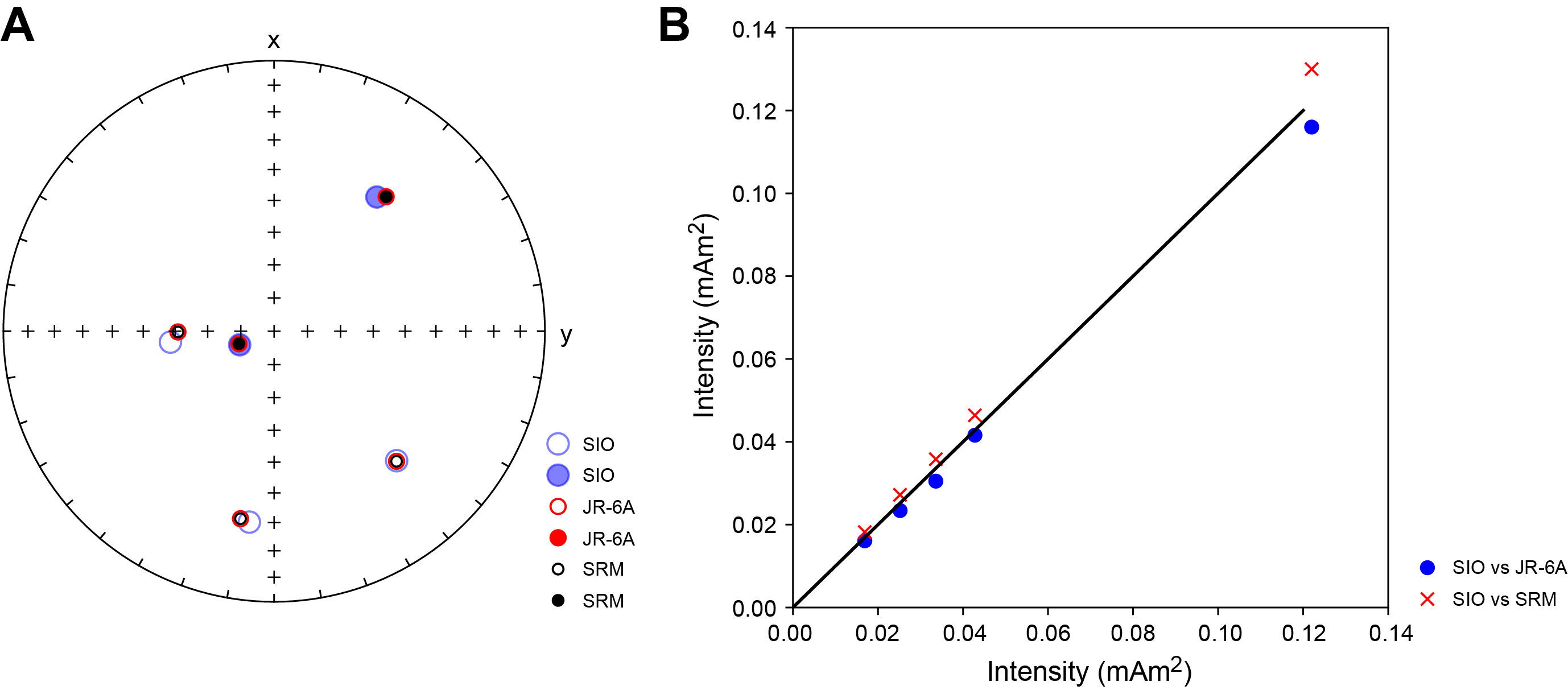
Figure F11. Comparison of SIO and shipboard standard sample vectors.
4.2. Core collection and coordinates
Cores were collected using nonmagnetic core barrels for the APC and HLAPC systems. These nonmagnetic core barrels are more brittle and cannot be used in conjunction with the XCB or RCB coring systems (see Coring and drilling operations in each site chapter). The BHA included a Monel (nonmagnetic) drill collar, which was used for all APC and XCB cores. This collar can potentially reduce the magnetic field near where the core is cut and within the core barrel.
All magnetic data are reported relative to IODP orientation conventions: +x points into the face of the working half (toward the double line), +y points toward the left side of the working half when looking downcore, and +z points downcore. The hatched arrows on the discrete cube samples point upcore (in the −z-direction). The relationship between the SRM coordinates (X, Y, and Z) and the sample coordinates (x, y, and z) is +X = +x, +Y = −y, and +Z = +z for archive halves and +X = −x, +Y = +y, and +Z = +z for working halves (Figure F12A, F12B). Note that the orientation of the SRM axes forms a left-handed coordinate system (Figure F12C). This is converted to a right-handed system within the Integrated Measurement System (IMS) software by multiplying the calibration constant for the y-axis by −1.
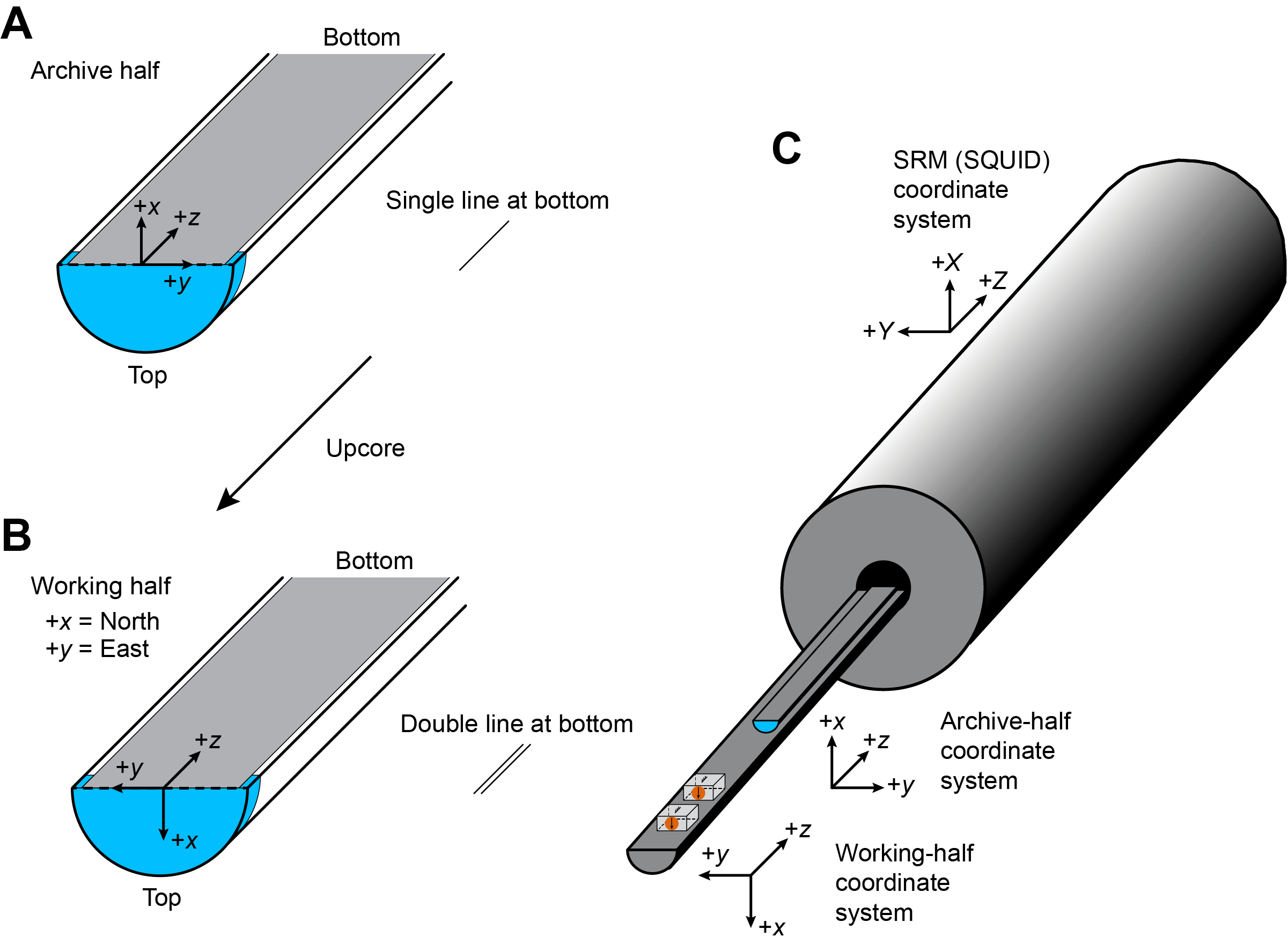
Figure F12. Coordinate systems.
Discrete sample labeling is shown in Figure F13A. For the SRM, we measured the samples using the following orientation settings:
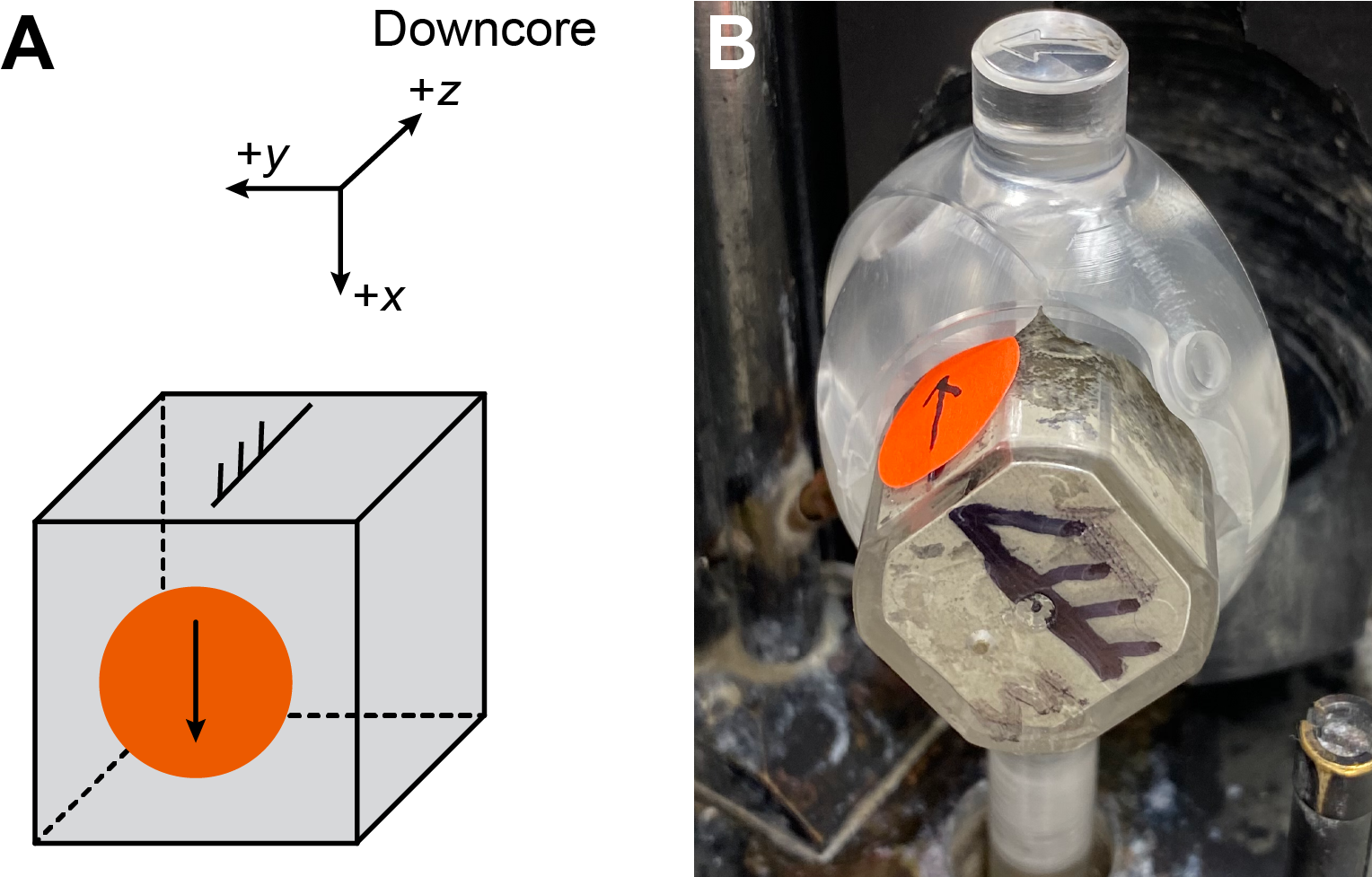
Figure F13. Discrete cube sample coordinate system and JR-6A orientation.
For the JR-6A, we used the following settings:
The −z (hatched) arrow pointed northwest, and the x arrow pointed away from the user (into the holder) (Figure F13B). Note that the SIO standard samples were treated as archive-half samples and were inserted with the x arrow pointing toward the user and the face with the hatched up arrow toward the back.
4.3. Samples and measurements
4.3.1. Archive section halves
Remanence measurements on archive section halves were made using a 2G Enterprises Model 760R-4K SRM equipped with direct-current superconducting quantum interference devices (DC-SQUIDs) and a three-axis, in-line, automated AF demagnetizer capable of peak fields of 80 mT. The spatial resolution for archive section half measurements is a function of the integrated response function (following Acton et al., 2017) with effective lengths of 7.30 cm for the X-axis, 7.30 cm for the Y-axis, and 9.00 cm for the Z-axis. The practical noise level of the SRM is ~2 × 10⁻⁹ Am2 and is primarily controlled by the magnetization of the core liner and the background magnetization of the measurement tray.
We cleaned the sample tray with soapy water daily or more often if deemed necessary. The sample tray was then AF demagnetized with a peak field of 80 mT, and its remanence was measured using the Section background routine to update the background correction values for the empty sample tray. The empty sample tray was subsequently measured with the updated background correction values subtracted for QA/QC purposes.
NRM measurements of the archive section halves were made at 2 cm intervals, along with a 5 cm trailer and leader to monitor the background magnetic moment. We began by measuring the initial NRM and the remanent magnetization remaining after AF demagnetization steps of 5, 10, 15, and 20 mT peak fields. After we were confident that fewer steps were adequate, we adopted a protocol whereby the NRM was followed by 10 and 20 mT AF demagnetization steps.
4.3.2. Discrete samples
We collected one oriented discrete sample per section from the working section half of the first hole for each site, as well as some additional samples from other holes to fill gaps in recovery as required. We sampled from the center of each section, modifying the exact location based on lithologic observations or core disturbance observations. Discrete samples were collected by pushing plastic J-cubes (2 cm external edge length and internal volume of ~7 cm3) into working section halves with the hatched arrow marker on the cube pointing toward the stratigraphic up direction (Figure F12A) and the flags pointing to +y. When the sediment was more indurated, a hollow metal tube (shaped to match the plastic cubes) was pushed into the working half and a plunger was used to extrude the sample onto a clean surface. The plastic cube was then placed over the sampled sediment, again with the hatched arrow marker pointing toward stratigraphic up, allowing for an orientation frame of reference identical to the pushed samples. For very indurated sediments, we used the parallel saw to cut 8 cm3 specimens from the core, with arrows etched onto the cube in the same sense as for the J-cubes (upcore with flags to +y).
The JR-6A and the D-Tech Model D-2000 AF demagnetizer were used for many cube measurements, including AF demagnetization, and the SRM with inline AF demagnetizer was used as time permitted. The sample measurement protocol for the JR-6A included calibrating the instrument using the 7.99 A/m cube standard with an 8 cm3 volume. A holder correction was determined by measuring the empty specimen holder. Data acquisition settings were as follows:
- Holder = automatic (sample is automatically rotated around three mutually perpendicular axes).
- Specimen type = cube.
- Acquisition time = normal.
- Speed of rotation = low (16.7 revolutions/s), to avoid deforming water-rich sediment.
- Specimen volume = 7 cm3 for J-cubes.
- Orientation parameters P1–P4 = 12, 0, 12, 0 (see Core collection and coordinates).
- Azimuth = 0.
- Dip = 90 (see Core collection and coordinates).
The P1–P4 orientation parameters, azimuth, and dip allow the AGICO software to convert the declination and inclination measured in the specimen coordinate system to geographic declination and inclination, which are the data reported in this volume.
We used the JR-6A to implement a gyroscopic remanent magnetization (GRM) protocol at intervals where we suspected the presence of the iron sulfide greigite. This protocol (after Stephenson, 1993) was applied to a subset of cubes in an attempt to separate the GRM from the primary detrital remanent magnetization (DRM). The GRM protocol consisted of the following sequence of steps at each AF step:
- Three-axis AF demagnetization using the D-Tech D-2000 in the +x-, +y-, and −z-directions, followed by measurement on the JR-6A.
- Single-axis AF demagnetization using the D-Tech D-2000 in the −x-direction, followed by measurement on the JR-6A.
- Single-axis AF demagnetization using the D-Tech D-2000 in the −y-direction, followed by measurement on the JR-6A.
The three measurements were then averaged to yield the GRM-free vector. The circular standard deviation of the three measurements can be a useful proxy for the presence of sulfides.
4.3.3. Rock magnetic analyses
As time permitted, discrete samples were analyzed for bulk MS as part of the measurement of anisotropy of MS (AMS) using an AGICO MFK2 Kappabridge. AMS characterizes the orientation of the paramagnetic (mainly phyllosilicates) and ferromagnetic minerals in sediments and can be interpreted in terms of depositional processes (e.g., Rees and Woodall, 1975; Ellwood, 1980; Taira, 1989; Schwehr and Tauxe, 2003; Tauxe et al., 2015). Settling of particles produces an oblate magnetic fabric with the minimum susceptibility clustered around the pole of the depositional plane. Ideally, the maximum and intermediate susceptibility axes are uniformly dispersed, defining a planar, near horizontal, gravity- or compaction-induced settling fabric. The magnetic fabric of sediments deposited by flowing water is typified by current-oriented magnetic foliation that can be either horizontal or tilted (imbricated) and/or clustering of the maximum susceptibility parallel to the flow direction. Disturbance by slumping or other deformation generally yields triaxial fabrics. We used the Hext (1963) method to assess the degree and type of anisotropy at the specimen level and the bootstrap method to estimate confidence bounds on AMS eigenparameters for multiple specimens (Constable and Tauxe, 1990; Tauxe et al., 2010).
For AMS measurements, the MFK2 Kappabridge was calibrated prior to each session using the AGICO cylindrical standard, which has maximum susceptibility along the axis of the cylinder and minimum susceptibility in the transverse direction. Each analysis consists of measuring the specimen along the three axes while it rotates within the applied field, followed by a bulk susceptibility measurement. For sawed cubes, we used a method in which each specimen is measured along the three axes separately, with the user rotating the specimen between each step.
4.4. Editing of archive measurements for coring disturbance
Sediment disturbance resulting from coring or geological processes (slumping, faulting, etc.) often leads to distorted and unreliable paleomagnetic directional records and largely altered sediment fabric. The paleomagnetic data were therefore filtered to remove these intervals. Editing of the measurements from the archive sections was automated using Jupyter notebooks. The SRM data were systematically filtered as follows:
- Deletion of all measurements within 10 cm of the section ends to remove the edge effects inherent in all pass-through measurement systems, such as the SRM, as well as potential accumulation of fall-in material from the top of the cores, and
- Deletion of all data from intervals that were assigned moderate and greater drilling disturbance during visual core description (see Lithostratigraphy) to remove data in intervals affected by coring-induced disturbance.
In some cases, we inspected core composite photographs and X-radiographs for evidence of coring or sedimentary disturbance. X-radiographs for all APC and HLAPC sections were used to identify additional features that might adversely affect the NRM but that may not be readily apparent during visual description. Examples include large dropstones beneath the core surface or centimeter-scale deformation of the sediment that would not be considered highly disturbed in a macroscopic sense but whose presence is sufficient to disrupt the microfabric of the NRM. Such features could lead to false identification of geomagnetic excursions. X-radiographs and paleomagnetic data are collected from the archive section half; thus, features observed in X-radiographs are directly relevant to paleomagnetic data.
We also note that filtering 10 cm from the ends of each core section served to remove intervals of sediment disturbed by insertion of the temperature probe into the top of each section prior to commencing physical properties measurements of whole rounds and syringe scars, in which a syringe was inserted into a section end to extract sediment for headspace gas measurements or sedaDNA analysis.
4.5. Magnetostratigraphy
Magnetic polarity intervals were assigned based on changes in inclination after 20 mT peak AF demagnetization. Once a polarity stratigraphy was established for a given hole, we correlated the pattern with the GPTS (Ogg et al., 2020) summarized in Table T4. Correlation with the GPTS was assisted by discussion with the shipboard biostratigraphy team when needed.
5. Physical properties
During Expedition 400, physical property measurements were conducted for lithostratigraphic characterization, for stratigraphic correlation, and to tie core descriptions to downhole data and main seismic reflections. Physical property data were key to generating high-resolution and continuous data sets for hole-to-hole and site-to-site stratigraphic correlation. The key objectives were to detect coring discontinuities and/or inhomogeneities, detect differences in sediment composition and texture, identify seismic discontinuities, and construct synthetic seismograms. The thermal properties of the recovered material were measured and combined with downhole temperature measurements to estimate geothermal heat flow. Different techniques and methods were used to characterize Expedition 400 cores on whole-round, split section half, and discrete samples.
5.1. General sampling and measurement sequence
Cores measuring ~9.6 m in length were collected and then split into ~1.5 m sections (see Operations and Core and section handling). A core with ~100% recovery yields six 1.5 m sections, an additional shorter seventh section, and possibly a core catcher that is usually shorter than 0.5 m. The resolution of physical property measurements made during Expedition 400 was hole dependent and was set to complete the core analyses without impacting workflow in the different laboratories.
Different measuring procedures were used for soft sediments versus semilithified and lithified sediments. The methodologies differ slightly and are explained for each instrument/property below. Whole-round core sections were equilibrated to ambient room temperature (~19°–22°C) over ~4 h to ensure thermal and barometric homogeneity, which minimizes any effects on physical property measurements, especially P-wave velocity, and protects the sensors from damage.
Prior to splitting, whole-round sections were analyzed with three whole-round physical property core logging systems: the WRMSL, the NGRL, and the thermal conductivity meter (wherever possible). The WRMSL includes a GRA bulk densitometer, an MS loop (MSL) sensor, and a compressional P-wave logger (PWL). The whole-round sections from all sites were measured at a 2 cm resolution on the WRMSL. A consistent and unbroken contact between the sediment and core liner is required to make accurate measurements with the PWL. This was generally fulfilled for the APC and HLAPC systems but not for narrower cores obtained with the XCB or RCB systems. For the XCB and RCB systems, gaps between the recovered material and the core liner lead to velocities outside the probabilistic range (1450–4500 m/s). PWL values from these cores need to be correlated to caliper P-wave velocities. All whole-round sections from all holes were also run on the NGRL to collect spectral gamma ray data at a 10 cm resolution before the cores were equilibrated to ambient room temperature because the temperature variation does not affect NGR measurements. Thermal conductivity was measured on at least one whole-round section per core (wherever possible). A needle probe was inserted into the section through a small hole drilled along the split line of the plastic core liner near the central part of the section. When the needle did not provide measurements due to poor contact or lithified sediments, the measurements were conducted using a contact puck on the working section half (see Thermal conductivity measurements).
In Holes U1603E, U1603F, and U1604B, whole-round sections were logged on the WRMSL on fast track mode (Special Task Multisensor Logger [STMSL]) at a 5 cm resolution upon arrival in the laboratory to allow stratigraphic correlation between cores and thus fill the recovery gaps on the previous holes of the site. Only the MSL sensor was logged because the GRA source was turned off to avoid any potential detrimental effects to sedaDNA samples planned for these holes. Because temperature equilibration was not reached, the PWL was not run.
5.2. Whole-Round Multisensor Logger measurements
The WRMSL (Figure F14) is a logging system for GRA densitometry, MS, and compressional P-wave velocity. The sampling intervals for the WRMSL were common denominators of the distances between the participating sensors (30–50 cm) to allow sequential and simultaneous measurements (Table T6).
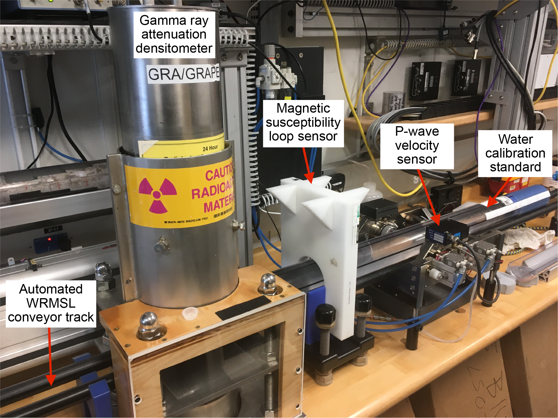
Figure F14. WRMSL.
WRMSL measurements were applied to all whole-round core sections during Expedition 400. Before measuring, the cores were equilibrated to room temperature. To optimize the measurement procedure and provide consistency, sampling intervals and measurement times were the same for all sensors on each instrument. This way, all sensors measure simultaneously and idle periods are avoided. A sampling resolution of 2 cm was considered appropriate for stratigraphic correlation and integration with seismic profiles, which also allowed efficient core flow. After the measurements were finalized for the last section of each core, a deionized water standard was run through all the instruments to keep them calibrated and to assure QA/QC. The instruments underwent recalibration when the measured standard values deviated from the range of published tolerances (Blum, 1997).
5.2.1. Gamma ray attenuation bulk density
The GRA bulk density instrument is used to measure the whole-round core at discrete and equidistant intervals to provide an average density value. The GRA instrument measures the attenuation of a directed gamma ray beam through the core. This beam is produced by a 137Cs gamma ray source at 370 MBq radiation and 660 keV energy levels. The source is mounted directly above the whole-round core track within a lead shield with a 5 mm collimator at the bottom. The beam is directed downward toward the core section during measurement. A scintillation detector with an integrated photomultiplier tube is mounted underneath the core track (and opposite the 137Cs source) and measures the gamma radiation that passes through the core sections. The GRA bulk density instrument operates with medium-energy gamma rays (0.1–1 MeV) that interact with the material of a formation by Compton scattering. The measured electron density of the scattering is then used to estimate the bulk density of the material. For a sample of known thickness, the density (ρ) is proportional to the intensity of the attenuated gamma rays as
- I = measured intensity of gamma rays passing through the sample,
- I0 = gamma ray source intensity,
- μ = Compton attenuation coefficient, and
- d = sample diameter.
The parameters μ and I0 are constants, and ρ is then calculated from I. The bulk density provided by the GRA instrument is related to the porosity, grain size, consolidation state, mineral composition, and any disturbances or contrasts present in a formation.
Generally, GRA bulk density measurements are most accurate when the core liner is completely filled and has minimal drilling disturbance, gaps, or liner patches. Otherwise, measurements tend to underestimate true values. The GRA instrument estimates bulk density based on an internal core diameter of 66 mm, which is appropriate for most sediment cores obtained by the APC and HLAPC systems; for material recovered by the XCB or RCB systems, the core diameter is usually smaller (≤58 mm) but no correction was applied. The GRA densitometer is calibrated with specific calibration cores (one standard core liner filled with distilled water and aluminum cylinders of various diameters; Blum, 1997). The spatial resolution is less than ±1 cm. The instrument was recalibrated when the deionized water QA/QC standard deviated significantly (>2%) from 1 g/cm3. The sampling interval on the GRA instrument is 2 cm by default, and the integration time was set to 3 s. Additional postprocessing of the GRA bulk density measurements was needed to remove edge effects. Single data spikes caused by voids, cracks in the core liner, metal drill fragments, and other various defects in the core, as well as any values <0.5 g/cm3, were also removed.
5.2.2. Magnetic susceptibility
MS was acquired for all whole-round core sections using a pass-through loop on the WRMSL. MS (χ) is a dimensionless parameter in the metric system that indicates the degree to which a material can be magnetized by an external magnetic field. χ is a relative indicator for changes in formation composition that may be related to paleoclimate-controlled depositional events or processes. MS is acquired at very low fields that generally do not exceed 0.5 mT. The volume susceptibility is defined as
where M is the magnetization induced in the material by the external field of strength, H. Accordingly, MS is most sensitive to formations containing high concentrations of ferromagnetic minerals such as magnetite, pyrite, hematite, and various other iron oxides. In addition, χ can be related to the origin of the materials in the core and their subsequent diagenesis. Ferromagnetic minerals are characterized by MS values several orders of magnitude higher than their alteration products. Other minerals, such as paramagnetic and diamagnetic (e.g., calcite, halite, water, and plastic) minerals, present very small or even negative values of MS. Therefore, calcareous and siliceous biogenic deposits often have values close to the detection limit of the instrument itself.
All MS measurements on the WRMSL were taken by a Bartington Instruments MS2C loop sensor with a 90 mm diameter and volume integration of ~18 cm and 1σ (Weber et al., 1997). An oscillator circuit in the sensor operates at a frequency of 565 Hz to avoid any potential interference between instruments using an automatic software correction factor of 1.174 and a ~140 A/m AF. This AF is responsible for a low-intensity, nonsaturating alternating magnetic field. Sediment core sections passing through the influence of this field cause a change in oscillator frequency. Frequency information is returned in pulse form to the susceptometer, and the MS value is estimated. The spatial resolution of the sensor is 20 mm with an accuracy of 2% (Blum, 1997). The output provided by the sensor is dimensionless instrument units (IU) and is equivalent to 10−5 SI units. The estimated values are computed as the mean of three discrete measurements in the same location. In the site chapters, MS values are expressed in the text in SI units and in the figures in IU, unless otherwise noted. Instrument drift should be taken into account because it can occur during the period of a core section scan. The instrument was automatically zeroed at the beginning of each run, and a zero-background measurement was taken at the end of a core section to correct for this drift. The sampling resolution was set to 2 cm, as it was for the GRA and PWL measurements. All the acquired MS data needed postprocessing to remove edge effects and single data spikes caused by voids, cracks in the core liner, and metal drill fragments, among other causes.
5.2.3. Compressional P-wave velocity
Compressional P-wave velocity was acquired for each whole-round core section using the PWL. P-wave velocity depends on the lithology, porosity, and bulk density of the formation, as well as the state of stress, lithostatic pressure, and/or fabric or degree of fracturing within the material. The degree of consolidation and lithification and the occurrence and abundance of free gas also control the velocity. The acoustic impedance and reflection coefficients are obtained using the P-wave velocity together with the density values. These parameters can be used to derive synthetic seismograms, which in turn can be used to estimate the depth of the main reflections observed in the seismic profiles. P-wave velocity (VP) is defined by the time required for a compressional wave to travel a specific distance:
where d is the length that the wave crosses (i.e., the core diameter) and tcore is the traveltime through the core.
For P-wave velocity measurement with the PWL, the core section is placed between two piezoelectric transducers (a transmitter and a receiver) mounted in stainless steel housings. Acoustic coupling is through an epoxy resin surface and is enhanced by a water film supplied by an automated drip system. A 500 kHz pulse (2 µs wave period; 120 V) is produced at a frequency of 1 kHz and sent to the transmitter transducer, which generates an ultrasonic compressional pulse at about 500 kHz (pulse timing is measured with a resolution of 50 ns). Pressure is applied to the actuators to ensure coupling between the transducers and the core liner, and the automated drip system maintains wet contacts on the transducers to ensure a reliable coupling is always established. The compressional P-wave propagates horizontally through the core and is received by the receiver transducer on the opposite side. Velocity is amplified by an automatic gain control amplifier to produce the received signal. P-wave velocity transducers measure total traveltime of the compressional wave between transducers. Calibration of the PWL accounts for errors in the total distance (dtotal) and the total traveltime (ttotal). Errors in dtotal were assumed to be related to the laser distance. The obtained discrete data are the average of 100 discrete measurements at the set interval.
A core liner of assumed thickness (L) covered each core section for all measurements. The traveltime through the core liner (tliner) was determined by measuring the total traveltime through a core liner filled with distilled water with a velocity of ~1480 m/s. A correction (tdelay; system delay) was measured using the traveltime through a standard block of aluminum with a known thickness and a published velocity of 6295 m/s. Arrival time picks were chosen at the inflection point of the second lobe of the waveform, giving a second correction (tpulse) from the first arrival. Then, tpulse and tdelay were combined and named ttotal_delay. Therefore, the velocity is computed as
- VP = core velocity (km/s);
- dtotal = measured diameter of the core and the liner (mm);
- L = wall thickness of the liner (mm);
- ttotal = total time for the pulse to travel through the core and liner (µs);
- tliner = traveltime through the liner (µs); and
- ttotal_delay = delay related to the combined transducer faces, electronic circuitry, and peak detection procedures (µs).
This VP equation assumes that the core completely fills the core liner and gaps or air are not present. P-wave velocity was measured for cores recovered with the XCB or RCB systems. However, these cores are ~5 mm (diameter) smaller than the core liner, generating an air gap that results in unreliable data. The P-wave signal can also be attenuated because of voids and microcracks that formed during core recovery. This degeneration is partly reflected in the gain (signal strength) factor applied to the original signal by the automated gain control. However, signal strength also represents the grain size of the sediment, and thus low-strength signals are not simply proportional to attenuation. The sampling resolution was set at 2 cm for the PWL, as it was for the other WRMSL instruments.
5.3. Natural Gamma Radiation Logger measurements
The NGRL measures NGR on whole-round cores using a system designed by the Integrated Ocean Drilling Program US Implementing Organization (USIO) (Texas A&M University, USA) (Vasiliev et al., 2011; Dunlea et al., 2013). This instrument measures the cumulative radiation emitted during natural decay of three long-lived radioisotopes—potassium (40K), thorium (232Th), and uranium (238U)—that have half-lives of 1.3 × 10⁹, 1.4 × 10¹⁰, and 4.5 × 10⁹ y, respectively. These isotopes and their daughter products emit gamma radiation at specific energy levels unique to each isotope. NGR is used to estimate the abundance of each isotope based on the strength of the signal at characteristic energies (Blum, 1997; Gilmore, 2008). In sediments and sedimentary rocks, Th and K are usually associated with specific clay minerals, whereas U is often encountered in either clay minerals or organic-rich material. High counts generally reflect the presence of fine-grained deposits, whereas relative changes are indicative of detailed stratigraphic variations. NGR measurements are a strong aid in core-to-core, core-to-wireline log data, as well as borehole correlations between holes.
The NGRL system consists of eight sodium iodide (NaI) detectors arranged along the core measurement axis at 20 cm intervals surrounding the lower half of the section (Figure F15). The detector array is fitted with both passive (layers of lead) and active (plastic scintillators) shielding to reduce the background environmental and cosmic radiation. The overlying plastic scintillators detect incoming high-energy gamma and muon cosmic radiation above 3 MeV and cancel this signal from the total counted by the NaI detectors.
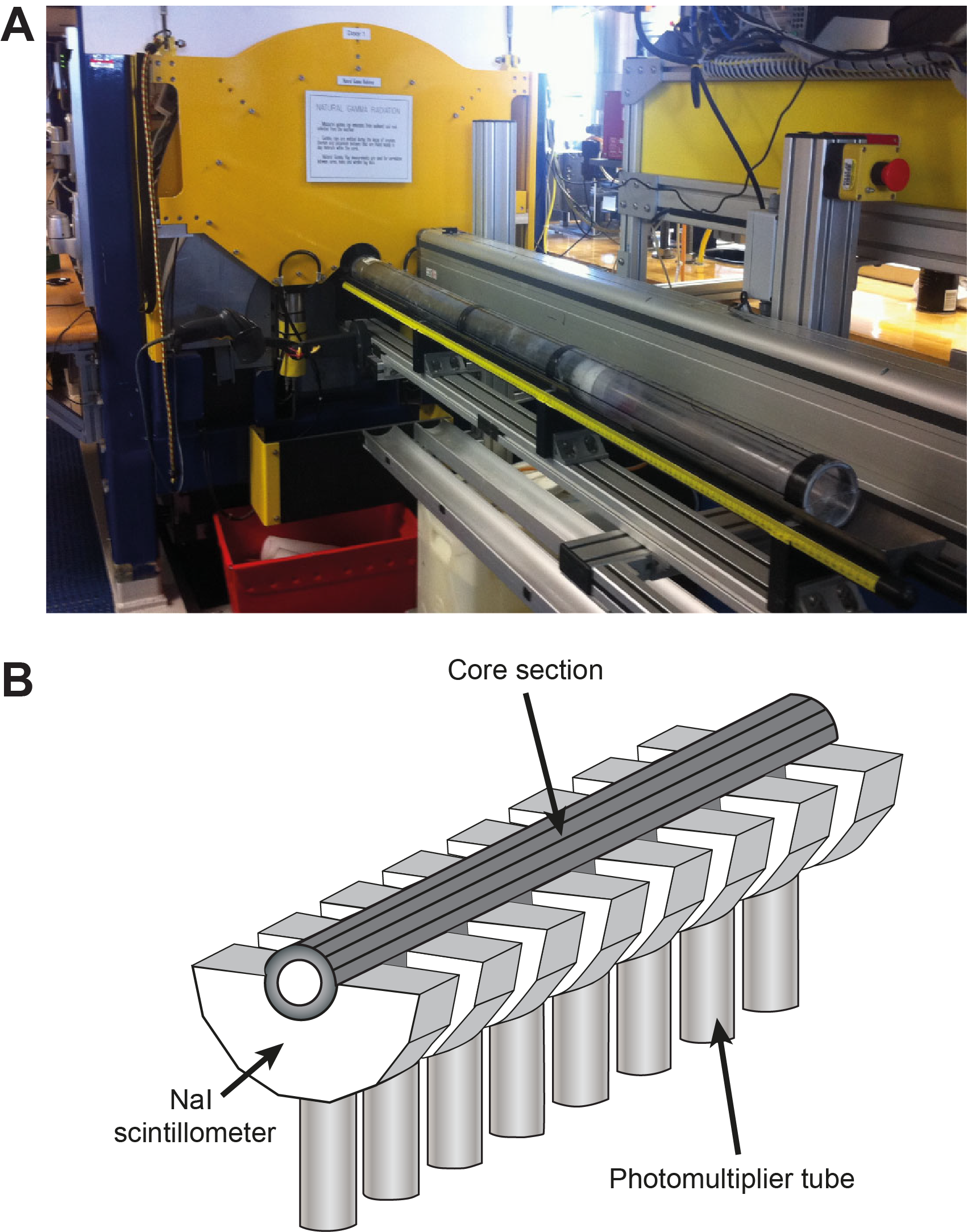
Figure F15. Equipment used to measure NGR.
The quality of the core measurements depends on the concentration of radionuclides and the counting time. For Expedition 400, a measurement run began with two sample positions 10 cm apart and a counting period of 300 s. After 300 s, the position was advanced downcore by 10 cm and counted again for 300 s (Table T6). This run yielded a total of 16 measurements (10 cm apart) per 150 cm core section. The NGR was measured in the core sections as they were obtained (i.e., before the sections equilibrated to ambient room temperature). Sections less than 50 cm length were not measured on the NGRL. Total acquisition times were ~5 min per measurement cycle or ~10 min per 150 cm long core section. This measurement procedure yielded statistically significant total counts. The collected data were of very good quality but needed postprocessing to remove single data spikes due to cracks in the core liner and metal drill fragments, among other causes.
5.4. Thermal conductivity measurements
Thermal conductivity is an intrinsic property of materials; it depends on the chemical and fabric composition, porosity, density, and structure (Jumikis, 1966). Thermal conductivity is the capacity of the material to transfer heat by conduction. Measurements of this parameter in sediments and rock sections combined with in situ temperature measurements (see Downhole measurements) are used to estimate local geothermal heat flow. Geothermal heat flow is an indicator of the type and age of oceanic crust and the geodynamics and tectonic processes of the oceanic and continental lithospheres (Pollack et al., 1993; Stein and Stein, 1994).
Thermal conductivity was measured immediately after WRMSL logging in soft sediments (whole-round) and when reliable measurements were yielded by the probe. A single measurement per core was generally taken in the central section using the TK04 (Teka Bolin) system (Table T6). For whole-round cores, the needle probe method in full-space configuration was used (Von Herzen and Maxwell, 1959). The needle probe was inserted into a 2 mm diameter hole drilled through the core liner along a split line. The core was placed in an enclosed box with insulating foam to avoid interference with airflow in the laboratory (Figure F16).
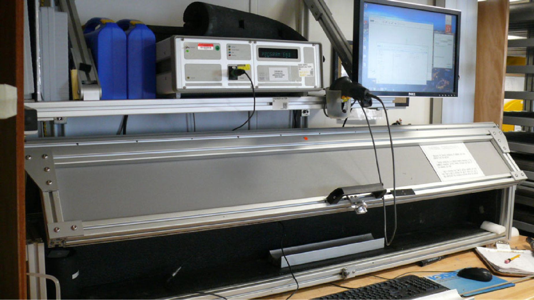
Figure F16. Shipboard station for measuring thermal conductivity.
For lithified sediments or rocks and soft sediments in which the needle probe did not yield reliable results, a contact probe (or puck) method was used for half-space configurations on split cores. The probes consist of a heater wire and a calibrated thermistor. The measurement locations were chosen based on the least amount of fracturing and most homogeneous portions of the core sections. The sections were prepared for a puck-style contact probe by applying distilled water onto the sediment surface. This procedure was applied to ensure good contact between the sediment and the probe. The puck probe was placed directly on the sediments and secured in place with a rubber strap or wooden tool to ensure proper contact pressure. The section half was then placed in the insulated box to stabilize thermal conditions during measurements.
After whole rounds or section halves were prepared for measurements and placed in the insulated box, the calibrated heat source of the probe was turned on and the increase in temperature was recorded over 80 s for the needle probe (soft sediments) and 60 s for the contact probe (hard or lithified sediments). The heating power ranged 0.8–4 W/m for needle measurements and 0.8–3.5 W/m for contact probe measurements. The heat equation solution for a line source of heat was then fit to the temperature measurements to obtain the thermal conductivity. The probe is assumed to be a perfect conductor because it conducts heat more efficiently than sediment or hard rock. Following this assumption, the linear relationship between the superconductive probe temperature and the natural logarithm of the time after initiation of the heat is expressed as
- T = temperature (K),
- q = heat input per unit length per unit time (J/m/s),
- k = thermal conductivity (W/[m·K]),
- t = time after the initiation of the heat (s), and
- C = instrumental constant.
To calculate the average thermal conductivity, three measurement cycles were performed separated by 10 min. A self-test, which included a drift study, was carried out at the beginning of each measurement cycle. The heater circuit was closed after the probe temperature stabilized, and the temperature increase in the probe was recorded. Thermal conductivity was estimated from the temperature increase rate while the heater current was flowing. Temperatures measured during the first 80 s of the needle probe heating cycle and 60 s of the contact probe heating cycle were fit to an approximate solution of a constantly heated line source (Kristiansen, 1982; Blum, 1997). Measurement errors were below 5%.
5.5. X-ray imager
The XSCAN collects linescan X-radiographs from whole-round cores or split core halves. The XSCAN source and detector can be rotated around the core material to produce line scans with different view angles to create pseudo-computed tomography (CT) scans of the core (Figure F17). During Expedition 400, continuous linescan X-radiographs were obtained solely in plane view on the archive section halves. The XSCAN comprises an X-ray scanner with a 210 W, 160 kV, 1.3 mA constant potential X-ray source and linescan detector. The source is a Spellman XRBD 160PN210 Monoblock X-ray generator with a 0.5 mm focal spot. The beam angle is 9° × 12°, which is located ~36 cm from the source. The detector is a Hamamatsu C12300-321, composed of a charge-coupled device sensor with a ~22 cm FOV utilizing time-delayed integration and a resolution of 48 µm per pixel. Imaging acquisition and processing was completed within the IMS system (version 14). Processing of images during Expedition 400 was limited to black and white correction and image cropping. XSCAN images can facilitate the identification of sedimentary structures and objects such as fractures, ice-rafted detritus, and materials with distinct densities (e.g., alteration zones and oxide and sulfide concentrations). Core sections were measured using energies between 90 and 100 kV and 0.80 and 0.90 mA. The XSCAN was calibrated for the used measuring energies before core measurements were obtained.

Figure F17. XSCAN.
5.6. Section Half Multisensor Logger measurements
Color reflectance and MS were measured on archive halves using the SHMSL (Figure F18). Archive halves were covered with plastic wrap and placed on the SHMSL track, above which an electronic platform moves along a track and records the height of the core surface. The laser sensor detects the location of the bottom of the section, and then the instrument progresses along the core, making measurements of MSP and color reflectance. Color reflectance and MSP data were collected at a 2 cm resolution during Expedition 400 (Table T6).
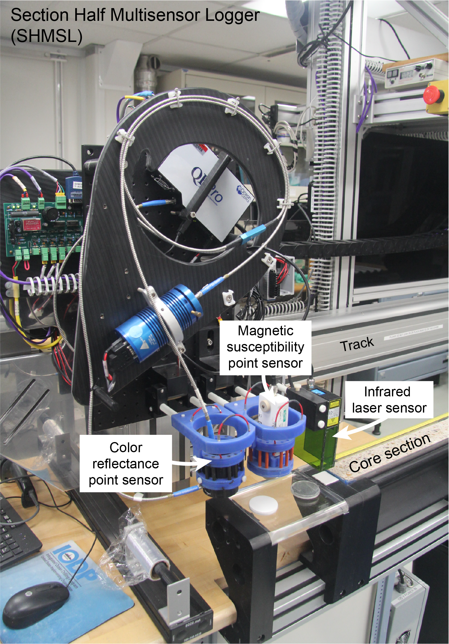
Figure F18. SHMSL.
5.6.1. Color reflectance spectrophotometry
The color reflectance spectrometry of the archive halves was measured using an Ocean Optics QE Pro detector integrating sphere and associated light sources covering wavelengths from UV through visible to near infrared. Each measurement was taken in 2 nm wide spectral bands from 390 to 732 nm. The data are reported using the L*a*b* color system. L*a*b* color reflectance measurements describe coordinates in a spherical system with 16.8 million possible variations (Weber, 1998; Blum, 1997). The L* axis measures the black–white color component, known as lightness or gray value. It is a reliable tracer for the content of biogenic carbonate in marine sediment (Weber, 1998). The a* axis is the green–red component, redness (positive) versus greenness (negative), and is commonly used to trace changing redox conditions in the sediments or sediment provenance. The b* axis is the yellow–blue component, yellowness (positive) versus blueness (negative), with more positive values (yellower colors) often corresponding to a higher content of biogenic material (e.g., biosiliceous or carbonate) contents. Two spectra, pure white (reference) and pure black (dark), were used for calibration of the color reflectance spectrometer. Color calibration was conducted approximately once every 6 h (twice per shift). Additional details regarding measurement and interpretation of spectral data can be found in Balsam et al. (1997), Balsam and Damuth (2000), and Giosan et al. (2002).
5.6.2. Point magnetic susceptibility
MSP was measured with a Bartington MS2 meter and an MS2K contact probe with a flat 15 mm diameter round sensor with a field of influence of 25 mm and an operation frequency of 930 Hz. The instrument averages three measurements from the sensor for each offset with an accuracy of ~5%. The spatial resolution of the MSP sensor is ~3.8 mm, and it reports values in IU, which can also be converted to dimensionless SI units by multiplying by 10−5. The volume integration of the sensor is ~1 cm and 1σ (Weber et al., 1997). The instrument was calibrated by the manufacturer before installation on JOIDES Resolution and is quality checked every 6 h at the same time as the color reflectance sensor.
5.6.3. Color imaging
The SHIL captures continuous high-resolution images of the archive-half surface for analysis and description. The instrument was used shortly after core splitting in an effort to avoid time-dependent color changes resulting from sediment drying and oxidation. However, some sections were intentionally measured after drying to image features not apparent when the section was wet; in these cases, a wet and a dry image are available in the LIMS database. The shipboard system uses a commercial linescan camera lens (AF Micro Nikon; 60 mm; 1:2.8 D), and illumination is provided by a custom assembly of three pairs of LED strip lights that provide constant illumination over a range of surface elevations. Each pair of lights has a color temperature of 6,500 K and emits 90,000 lux at 3 inches. The resolution of the linescan camera was set at 10 pixels/mm. Users set a crop rectangle for each image to remove extraneous information. Images were saved as high-resolution TIFF files. Available files include the original high-resolution image with a gray scale and ruler and reduced JPEG images cropped to show only the section-half surfaces.
5.7. Section Half Measurement Gantry
P-wave velocity measurements were performed on working halves using the Section Half Measurement Gantry (SHMG). Measurements were typically made using the x-caliper on three points per core (Table T6). However, on cores where PWL velocity was missing, x-caliper measurements were done on every section of every core. Shear strength on selected working halves was measured on board with the automated vane shear (AVS) system. A total of five AVS measurements were done, all on sections from Hole U1603B. Measurements were taken at varying section intervals to accommodate lithologic variations, drilling disturbance, fractures, larger clasts, general core quality, and moisture and density (MAD) samples.
5.7.1. Discrete P-wave velocity measurements
P-wave velocities on working halves were measured with the P-wave caliper (PWC). The PWC measures the P-wave velocity perpendicular to the split face of the section (along the x-axis) (Figure F19). The system uses Panametrics-NDT Microscan delay line transducers that transmit at 500 kHz. During measurement, the signal transmitted through the core was recorded by the attached computer system, which then used an automated algorithm in the processing software to choose the peak (P-wave) arrival. In cases of poor contact or a weak signal, the instrument operator manually picked the first arrival. The distance between transducers was measured with a built-in linear voltage displacement transformer (LVDT). Calibrations were performed with an acrylic standard with a known thickness and a published velocity of 2730 m/s. The system time delay determined from the calibration was subtracted from the chosen arrival time to calculate a P-wave traveltime through the sample. Sample thickness (calculated by the LVDT in meters) was divided by the traveltime (in seconds) to calculate P-wave velocity (in meters/second).
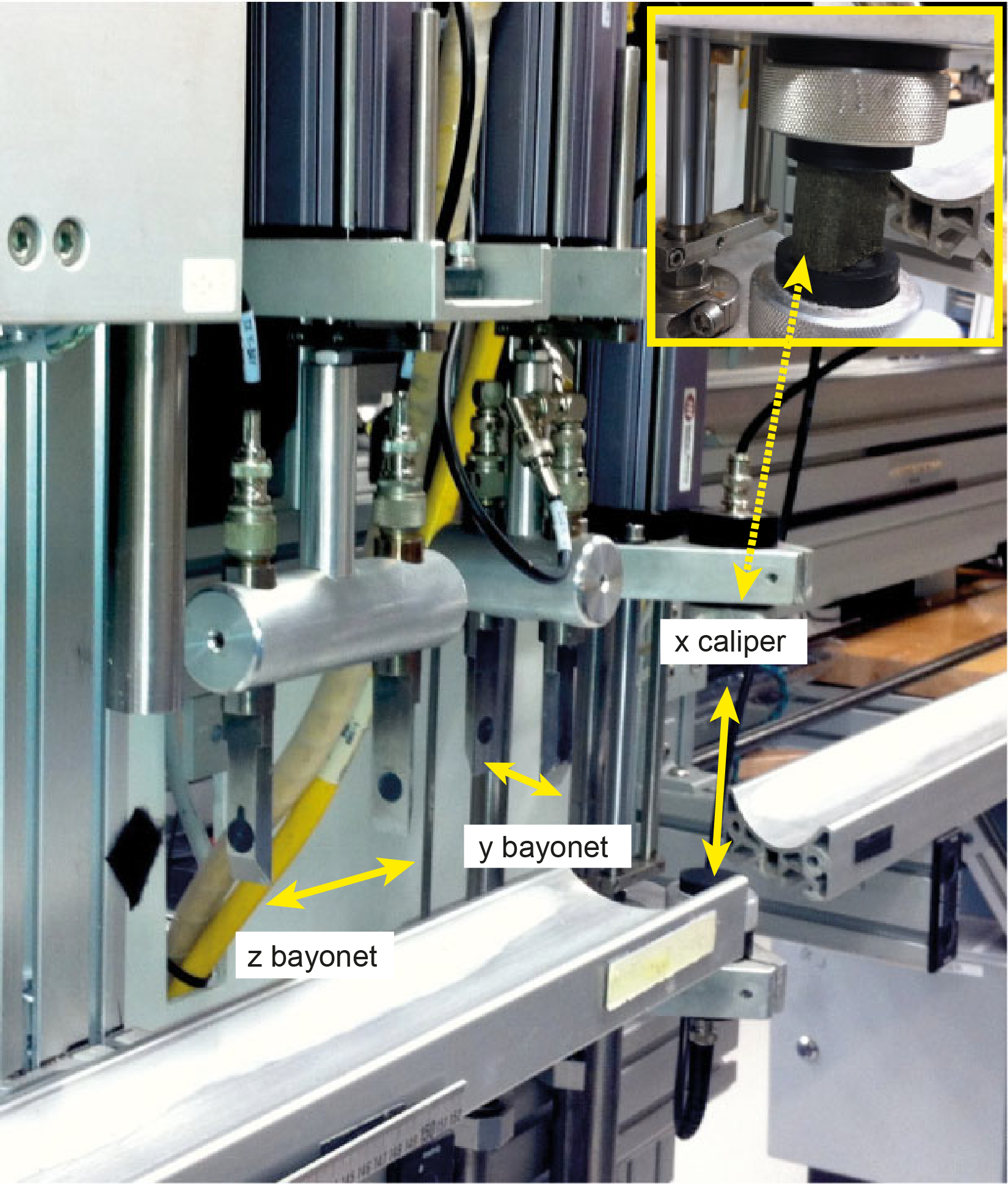
Figure F19. SHMG for measuring P-wave velocity.
5.7.2. Shear strength with automated vane shear system
Shear strength on selected working halves was measured on board with the AVS system (Figure F20). The AVS provides in situ determination of the undrained strength of intact, fully saturated clays (undrained strengths < 100 kN/m2). The test is not suitable for other types of sediments or if the clay contains sand or silt laminations. Thus, measurements were limited to the suitable sediments of three cores from Hole U1603B. A four-bladed vane was inserted into the working section half of the core and rotated at a constant rate to determine the torque required to cause a cylindrical surface (with a diameter equal to the overall width of the vane) to be sheared by the vane. The rotation axis of the vane was parallel to the bedding plane and the rotation rate was between 6° and 12° per minute. The torque required to shear the sediment along the vertical and horizontal edges of the vane is a relatively direct measure of the shear strength. When the sediment became too firm for insertion of the vane, the measurements were discontinued. The shear stress was calculated by the GeoLab software that controls the AVS as

Figure F20. SHMG for measuring shear strength.
5.8. Moisture and density measurements
Discrete samples from working halves were selected to carry out MAD measurements to determine wet and dry bulk density, grain density, water content, and porosity. For soft-sediment cores, ~10 cm3 samples were collected with a plastic syringe. Generally, two samples per core were collected with the aim of representing the complete core lithology (Table T6). For harder sediments or rocks, samples were taken with a metallic syringe or a chisel, or they were taken adjacent to the samples that were cut and prepared for other laboratories, such as paleomagnetism. On cores with large lithologic variability, three or more MAD samples were measured to obtain representative values.
Sediment samples were placed in numbered, preweighed ~16 mL Wheaton glass vials to obtain wet and dry sediment mass and dry volume measurements. Wet sample mass was first measured on each vial before placing it in a convection oven for approximately 24 h at 105° ± 5°C to dry. Wet and dry sample masses were determined to an accuracy of 0.005 g using two Mettler Toledo electronic balances, with one balance acting as a reference and one as an unknown. A standard mass of similar value to the sample mass was placed on the reference balance to increase the accuracy of the unknown sample measurement (Figure F21). An averaging algorithm in the MADMax software was used to correct for the motion of the ship. The default measurement setting of the two balances was 300 measurements over an interval of ~1.5 min. In the case of heavy seas resulting in ship heave and roll affecting the balances, 600–800 measurements were taken.
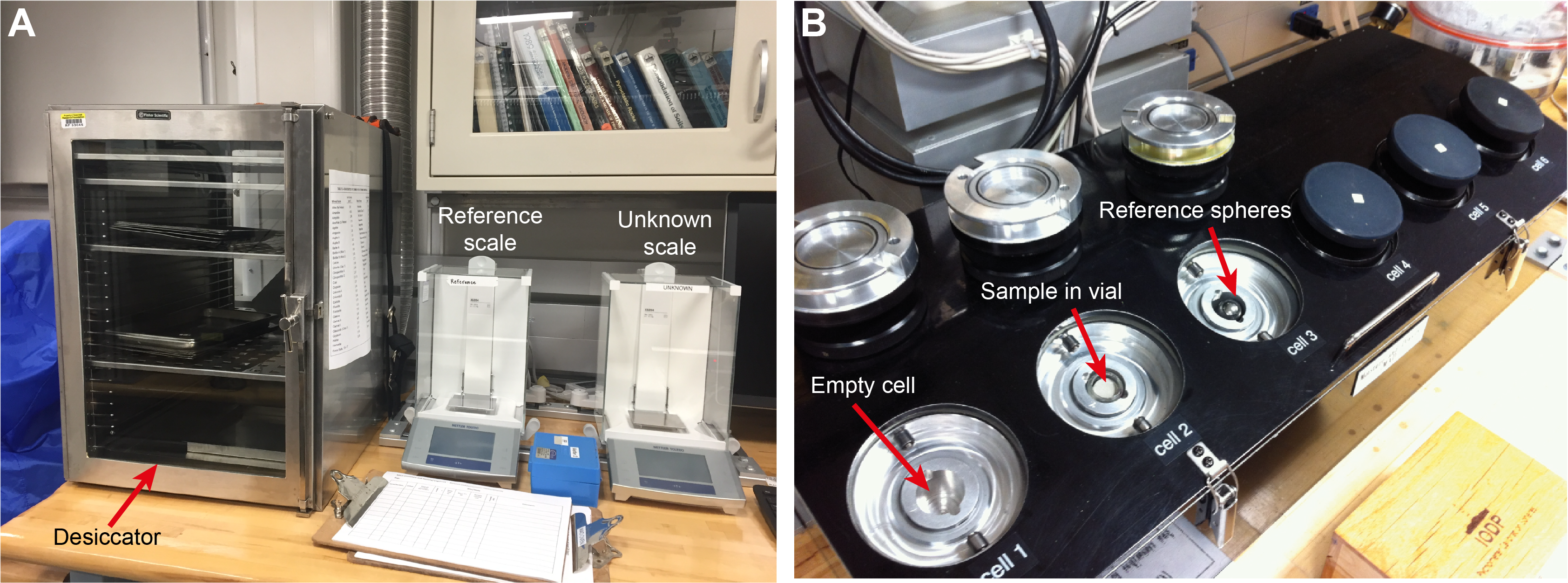
Figure F21. Equipment used for MAD analyses.
Dry sample volume was determined using a six-celled, custom-configured Micromeritics AccuPyc 1330TC helium-displacement pycnometer (Figure F21). The precision of each cell is 1% of the full-scale volume. Volume measurements were preceded by three purges of the sample chamber with helium warmed to ~28°C. Three measurement cycles were run for each sample. A set of two calibration spheres was periodically placed in each chamber to check for instrument drift and systematic error. The volumes occupied by the numbered Wheaton vials were calculated before the expedition by multiplying the weight of each vial against the average density of the vial glass. The procedures for the determination of these physical properties comply with American Society for Testing and Materials (ASTM) standard D2216 (ASTM International, 1990). The relationships and assumptions for the calculations of the physical property parameters are discussed in detail in Blum (1997) and Weber et al. (1997) and summarized below. The MADMax shipboard program was used for computing the displayed MAD properties.
5.8.1. Mass and volume calculation
Wet mass (Mwet), dry mass (Mdry), and dry volume (Vdry) were measured in the laboratory as detailed above. The mass ratio (rm) is a computational constant of 0.965 (i.e., 0.965 g of freshwater per 1 g of seawater). Salt precipitated in sediment pores during the drying process is included in the Mdry and Vdry values. The mass of the evaporated water (Mwater) and salt (Msalt) in the sample are given by
where s is the assumed saltwater salinity (35 ppt) corresponding to a pore water density (ρpw) of 1.024 g/cm3 (from experimental and empirical relations between salinity and density at laboratory conditions; Blum, 1997) and a salt density (ρsalt) of 2.22 g/cm3. The corrected mass of pore water (Mpw), volume of pore water (Vpw), mass of solids excluding salt (Msolid), volume of salt (Vsalt), volume of solids excluding salt (Vsolid), and wet volume (Vwet) are defined as
Wet (or total) volume (Vt), dry mass (Mdry), and dry volume (Vdry) were measured in the laboratory. Total mass, including the freshwater of the pore water, is calculated using a water density of 1 g/cm3 by
Assuming a pore water density of 1.024 g/cm3, the volume of the pore water is calculated as
Finally, the mass of the pore water is estimated as
5.8.2. Calculation of bulk properties
Water content (w) is expressed as the ratio of the mass of pore water to wet sediment (total) mass:
Wet bulk density (ρwet), dry bulk density (ρdry), sediment grain density (ρsolid), porosity (ϕ), and void ratio (VR) are calculated using the following expressions:
6. Geochemistry
The shipboard geochemistry program for Expedition 400 included measurements of headspace gas content (hydrocarbons), IW composition, and bulk sediment geochemical parameters.
6.1. Headspace gas geochemistry
Routine analysis of hydrocarbon gases in sediment cores is part of the standard IODP shipboard monitoring to ensure safe drilling operations. During Expedition 400, hydrocarbon monitoring was carried out by headspace analysis (gas obtained from sediment samples). One or two sediment samples (~5 cm3) were collected from each core from Hole A at each site for headspace gas analyses immediately after retrieval on deck. Additional samples were collected from other holes when depths exceeded those previously drilled. Headspace samples were collected from the top of a section near the middle of the core, immediately adjacent to the IW sample whenever possible. For soft sediments, plug samples were collected using a graduated syringe and extruded into a 21.5 cm3 glass serum vial with a crimped seal metal cap and a PTFE septum. For consolidated or lithified samples, chips of sediment were placed in the vial and sealed. Samples were not weighed, and sample volume varied largely (estimated up to 50%) depending on the availability of sediment and sampling method. The vial was labeled with the core, section, and interval from which the sample was taken and then placed in an oven at 70°C for at least 30 min.
Headspace gas (5 cm3) was sampled from the glass vial with a gas-tight glass syringe and then injected into an Agilent 7890A GC equipped with a flame ionization detector (FID; 250°C) to quantify concentrations of methane (C1), ethane (C2), ethene (C2=), propane (C3), iso-butane (C4), n-butane (C4), and iso-pentane (C5). The GC was equipped with a 2.4 m × 2.0 mm stainless steel column packed with 80/100 mesh HayeSep R. The injector consists of a ¹⁄₁₆ inch Valco union with a 7 µm screen connected to a Valco-to-Luer lock syringe adapter. This injector connects to a 10-port Valco valve that was switched pneumatically by a digital valve interface. The injector temperature was set at 120°C. Gas samples were introduced into the GC through a 0.25 cm3 sample loop connected to the Valco valve. The valve can be switched automatically to backflush the column. The oven temperature program started at 80°C, which was held for 8.25 min and then increased to 150°C for 5 min at a rate of 40°C/min. Helium was used as the carrier gas, with an initial column flow of 30 mL/min. Flow was then increased to 60 mL/min after 8.25 min to accelerate elution of longer chained hydrocarbons. The GC run time was 15 min. The GC was also equipped with an electronic pressure control module to control the overall flow into the GC. Chromatograms were collected and automatically evaluated using the Agilent Chemstation software. The integrated peak areas of low molecular weight hydrocarbon gases were quantified using a nine-point calibration of gas standards with known gas concentrations, as provided by Scott Specialty Gases (Air Liquide). In addition to the calibration sequence, gas standards at concentrations comparable to headspace gas samples were run daily alongside regular blank air injections to monitor accuracy of the GC system. Concentrations of hydrocarbon gases are reported in parts per million by volume (ppmv).
6.2. Interstitial water chemistry
IW samples were obtained by squeezing 5 or 10 cm whole-round core samples that were cut from cores immediately after core retrieval. The recovered water was split for shipboard determination of salinity, alkalinity, pH, anions and cations, and major and trace elements, as well as for shore-based water isotope and dissolved inorganic carbon (DIC) analyses. Whole-round samples were typically collected at a frequency of one sample per core of previously unsampled material (to avoid duplicate sampling of identical stratigraphic sections) to the bottom of the site where sufficient material was available (i.e., >1.5 sections recovered) or until IW extraction produced <2 mL of IW after 3 h of squeezing at 30,000 lb force (only the lowermost samples at Site U1607 failed to yield water at this pressure). When using the HLAPC system or when cutting half-cores with rotary coring systems, samples were taken every other core maintaining the same sample frequency. The exterior of the whole-round sample was carefully cleaned in a glove bag under a nitrogen atmosphere with a spatula to remove potential contamination from drilling fluid. For XCB and RCB cores, the intruded drilling mud between biscuits was also removed to eliminate contamination from drilling fluid. The cleaned sediment was transferred into a titanium squeezer (8 cm diameter) that was then placed in a Carver hydraulic press (Manheim and Sayles, 1974) and squeezed with slowly increasing pressures up to 30,000 lb (1.335 × 10⁶ N). The initial drops were discarded to avoid contamination. The IW was then collected in a 60 mL acid-washed (10% HCl) high-density polyethylene syringe attached to the squeezing assembly. If sample volume permitted, the IW samples were split as outlined in the analytical workflow below. If IW volume was limited (i.e., <20 but >2 mL), shore-based samples or shipboard alkalinity/inductively coupled plasma–optical emission spectroscopy (ICP-OES) analyses were omitted on a case-by-case basis. Data produced on the Agilent 5110 ICP-OES instrument were collected in atomic emission spectroscopy (AES) mode and are referred to as ICP-AES in the LIMS database. Hereafter in this volume, ICP-AES is used to refer to these data.
Additional IW samples were obtained with higher spatial resolution (~1 m) using Rhizon samplers (Rhizosphere Research Products). Rhizon sampling was initially planned for the uppermost 20 m of sediment at each site. At most sites, only the first core was sampled with this method. For Rhizon IW sampling, 2 mm diameter holes were drilled into the split line of the core during core temperature equilibration. Rhizon samplers, which consist of a 5 cm long, 2.5 mm outer diameter membrane-coated cylinder, were inserted into the sediment and attached to a syringe via a Luer lock connection. The syringe was drawn back and locked in place with a wooden spacer to generate a vacuum, drawing IW from the sediment. Rhizons were inserted into the sediments on the working half, to not disrupt the archive half. Up to 12 mL of water was obtained and measured using ion chromatography (IC) and ICP-AES, and additional 2 mL samples were set aside for shore-based water isotope and DIC isotope analyses following the methods stated for whole-round analyses.
The priority list and sample amount needed for shipboard analyses and shore-based samples from IW was as follows (order from high to low priority):
- Salinity (~100 µL): determined by optical refractometry immediately after squeezing.
- Anions and cations (~100 µL; Na+, K+, Ca2+, Mg2+, Cl−, Br−, and SO42−): determined by IC.
- Phosphate (PO43−) (~1.2 mL) and ammonium (NH4+) (200 µL): determined by spectrophotometry.
- Major and trace element analyses (~2 mL; B, Ba, Ca, Fe, K, Li, Mg, Mn, Na, S, Si, and Sr): determined by ICP-AES; addition of 10 µL concentrated trace metal clean HNO3.
- Water isotope analysis (shore-based) (δ18O, δ2H, and δ17O) (2 mL): no headspace; stored at 4°C.
- Carbon isotope and DIC analysis (shore-based) (δ13C and DIC) (2 mL): addition of 10 µL saturated HgCl solution (prepoisoned); stored at 4°C.
- pH and alkalinity (~3 mL): titrated/determined immediately after squeezing.
- Additional water for shore-based chemical or isotopic analyses: addition of 10–50 µL trace metal clean HNO3.
For all analyses, IW was filtered through a 0.45 µm polysulfone disposable filter (Whatman) into 15 mL centrifuge tubes, except for aliquots for ICP-AES analysis. Aliquots for shore-based isotope and DIC analyses were collected in 2 mL vials with no headspace. Samples for DIC analyses were treated with 10 µL of saturated HgCl. Alkalinity, pH, and salinity were measured immediately after squeezing. All other shipboard analyses were carried out in batches.
6.2.1. Shipboard analyses
IW samples were analyzed on board following the protocols in Gieskes et al. (1991), Murray et al. (2000), and the IODP user manuals for shipboard instrumentation.
6.2.1.1. Alkalinity, pH, and salinity
Alkalinity and pH were measured using a Metrohm autotitrator (Model 794 Basic Titrino) equipped with a pH glass electrode and a stirrer (Model 728 Stirrer). The pH readings were directly obtained from the LabVIEW Alkalinity program, and alkalinity was measured by titrating 3 mL of sample with 0.1 N HCl until reaching an end point of pH = 4.2. Standardization for both measurements was achieved using the International Association for the Physical Sciences of the Oceans (IAPSO) seawater standard, which was analyzed repeatedly during the expedition and reproduced within 2%. Salinity was analyzed using a Fisher Model S66366 refractometer calibrated using 18 MΩ millipore deionized water. The known salinity of the IAPSO seawater was used for data quality control.
6.2.1.2. Ion chromatography
Aliquots of IW were diluted at 1:100 with deionized water (18 MΩ millipore water) for analysis of Na+, K+, Ca2+, Mg2+, Cl−, Br−, and SO42− using a Metrohm 850 Professional ion chromatograph. The IAPSO seawater standard was used for standardization of measurements.
6.2.1.3. Spectrophotometry
Aliquots of IW samples were diluted with deionized water for analysis of ammonium and phosphate using an Agilent Cary 100 UV-Vis spectrophotometer. Ammonium analysis was conducted using phenol diazotization and subsequent oxidization by sodium hypochlorite to yield a blue color, measured spectrophotometrically at a wavelength of 640 nm. Ammonium chloride (NH4Cl) was used for calibration and standardization. Phosphate concentrations were determined following the protocol in Gieskes et al. (1991). Briefly, orthophosphate reacts with Mo(VI) and Sb(III) in an acidic solution to form an antimony-phosphomolybdate complex. Ascorbic acid reduces this complex, forming a blue color that is measured at 880 nm. Potassium phosphate monobasic (KH2O4) dissolved in deionized water was used to produce a calibration curve at concentrations 1, 5, 10, 15, 20, 40, 60, 80, 100, 200, and 300 µM to monitor instrument linearity.
6.2.1.4. Inductively coupled plasma–atomic emission spectroscopy
Dissolved major (Ca, K, Mg, and Na) and minor (B, Ba, Fe, Li, Mn, S, Si, and Sr) element concentrations were determined using an Agilent 5110 ICP-AES with an SPS4 autosampler. IW samples were diluted 1:10 in 2% HNO3, with an internal standard added to correct for atomic and ionic interferences. In detail, 100 µL of internal standard solution containing 100 ppm beryllium (Be), indium (In), and scandium (Sc), and 200 ppm antimony (Sb) was added to 500 µL of IW sample and 4.4 mL of 2% HNO3. For calibration, serial dilutions of the IAPSO seawater standard (0%, 1%, 5%, 10%, 25%, 50%, 75%, and 100%) were prepared to cover IW concentrations smaller than or equal to normal seawater. Additional calibration solutions for major and minor element concentrations exceeding that of seawater were prepared using water with 3.5% NaCl as a dilution matrix. Calibration solutions for B, Ba, Ca, Fe, K, Li, Mg, Mn, P, Si, and Sr were treated in the same way as IW samples, with the internal standard added.
During each ICP-AES run, a complete set of in-house and IAPSO dilutions were analyzed at the beginning and the end. Additionally, known solutions of in-house standards were run every 8–10 samples to monitor instrumental drift, and the IAPSO standard was run at a similar frequency to monitor accuracy. The elemental concentrations reported for each sample are average values from three replicate measurements for each sample. Reproducibility of all elements was typically in the 1%–3% range, and not higher than 5%. Sulfur and phosphorus concentrations for the IAPSO (S) and in-house check standards (P) showed greater variability for some instrumental runs, with uncertainties of up to 6%.
6.2.1.5. Comparative analysis of analytical methodologies for interstitial waters
IODP standard shipboard analytical protocols produce overlapping measurements for a number of elements. For ICP-AES, Ba, Ca, Fe, K, Mg, Mn, Na, S, Si, and Sr were measured using two or more wavelengths. Results for each wavelength were analyzed by evaluating the shape and size of peak intensities as well as interferences to archive the best possible measurement. Final wavelengths chosen are reported in Table T7. In addition to measurements by ICP-AES, Ca, Mg, K, Na, and SO42− were also measured by IC.
6.3. Sedimentary geochemistry
For analyses of carbon, nitrogen, and CaCO3 content of bulk sediments, two to four 5 cm3 samples were taken from the working halves of split cores following identification of major lithologies by sedimentologists. The 5 cm3 samples were freeze-dried for ~12 h and then crushed using an agate pestle and mortar, when possible, or ground using an SPEX 8000 Mixer Mill equipped with tungsten carbide cups filled with freeze-dried sediment and a tungsten carbide bead.
6.3.1. Sedimentary inorganic and organic carbon, nitrogen, and carbonate content
Total carbon and total nitrogen contents of sediment samples were determined with a Thermo Electron Corporation FlashSmart CHNS elemental analyzer equipped with a Thermo Electron packed column CHNS/NCS GC and a thermal conductivity detector (TCD). Approximately 14–16 mg of sediment was weighed into a tin cup and then combusted at 950°C in a stream of oxygen. The reaction gases were passed through a reduction chamber to reduce nitrogen oxides to nitrogen and were then separated by the GC before detection by the TCD. Peak areas from the TCD were calculated to determine the total carbon and total nitrogen of the samples. All measurements were calibrated to the National Institute of Standards and Technology (NIST) Reference Material (RM) 8704 (Buffalo River Sediment) standard (3.35 wt% carbon; 0.17 wt% nitrogen) at seven concentrations (3, 6, 10, 15, 20, 40, and 60 mg). A check standard of 15 mg NIST RM 8704 was run every 10 samples throughout each analytical session to monitor analytical accuracy, with concentrations of 3.38 ± 0.17 wt% (mean ±2σ; n = 53 for the whole expedition) for carbon and 0.17 ± 0.02 wt% for nitrogen indicating an overall analytical accuracy of 4.9% for carbon and 12% for nitrogen.
Calcium carbonate content (CaCO3) was determined using a Coulometrics 5017 CO2 coulometer. Approximately 12 mg of sediment was weighed into a glass vial and acidified with 2 N HCl. The liberated CO2 was titrated, and the corresponding change in light transmittance in the coulometric cell was monitored using a photodetection cell and automatically converted to total inorganic carbon (TIC) content. The weight percent of CaCO3 was automatically calculated from the TIC using
Standard CaCO3 (>99.9% calcium carbonate; Fisher Scientific) was used to confirm accuracy, and instrument performance was monitored by repeat analysis of the standard before, during (after every 10 samples), and after each run. With an overall average of 99.2 ± 1.3 wt% (mean ±2σ; n = 55 for the whole expedition), the repeat measurements of the CaCO3 standard suggest a method accuracy of 1.3%.
Total organic carbon (TOC) content was calculated by subtraction of inorganic carbon derived by coulometry from the total carbon derived by the CHNS elemental analyzer such that
7. Stratigraphic correlation
The accomplishment of Expedition 400 scientific objectives relies on the recovery of complete stratigraphic sections to the extent possible. A continuous sedimentary sequence cannot be recovered from a single borehole because of gaps in recovery between successive cores, even if recovery for each individual core exceeds 100% (Ruddiman et al., 1987; Hagelberg et al., 1995). Assessing the precise magnitude of gaps in recovery is often difficult. A complete (synthetic) stratigraphic section, referred to as a splice, is constructed by combining stratigraphic sections from two or more holes recovered at a single site to produce a composite and continuous record. To bridge the stratigraphic gaps between cores from holes with incomplete recovery and to document the magnitude of “missing” intervals, all site-specific holes are intercorrelated using core physical properties. To this end, one hole with a clear mudline is used as the depth anchor. Then the initially recorded core depths for the other holes are offset by amounts required to align them with correlation tie points on the anchor hole. At least two holes, or in many cases more holes, are needed to generate a complete (primary) splice from cores recovered using the APC system. Typically, cores from four or more holes must be recovered to construct a complete alternate (or secondary) splice, although selected intervals from the primary splice might be used on the secondary splice if needed.
Our methodology for developing splices follows a basic strategy that is common practice for high-resolution paleoceanographic IODP expeditions, limited by time demands and weather/iceberg situations. We used the initial analyses of core petrophysical data run on the WRMSL to develop preliminary composite depths for the purposes of making real-time drilling decisions (Shipboard Scientific Party, 2003). In most cases, we were not able to change the drilling decisions because of competing pressures, and in some cases core gaps were subsequently lined up on all the holes of the site for long intervals.
Our goals for stratigraphic correlation, in priority order, were as follows:
- To establish a composite depth scale,
- To define a sampling splice where possible, and
- To guide drilling in real time for enhancing the chance of recovering a complete stratigraphic section.
To meet these goals, several depth scales were generated (Figure F22). A detailed discussion of the definitions of these depth scales and the processes by which they were created are outlined below.
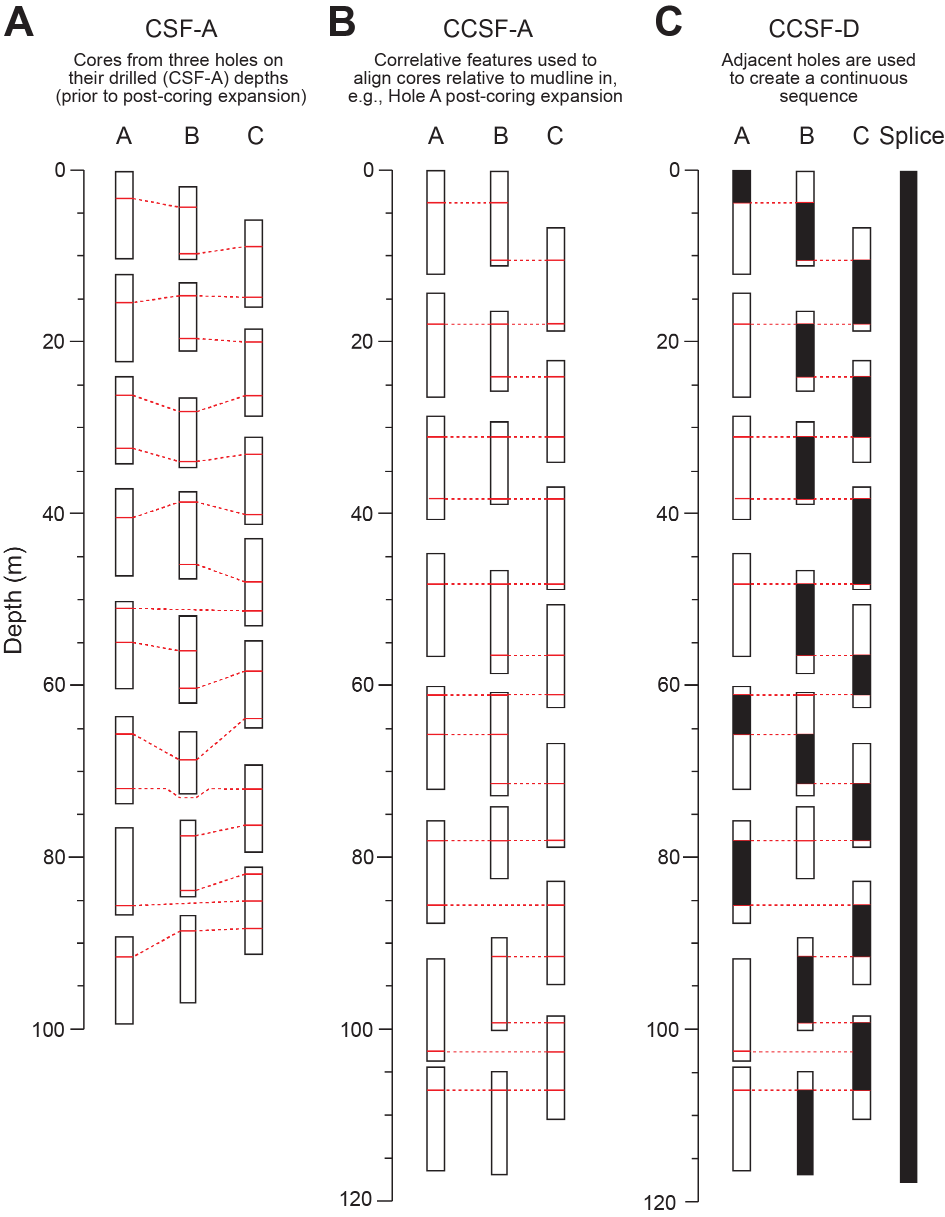
Figure F22. Depth scales.
7.1. Composite depth scale
The initial depth scale produced during IODP coring is called the CSF-A scale (Figure F22A). This depth scale is defined as the length that the drill string is advanced core by core. The CSF-A scale is often inaccurate because of the ship’s heave (which exceeds the limits of the ship’s heave compensator), tidal variations at sea level, core expansion, and other sources of error. Unlike CSF-A, the CSF-B depth scale considers a compression algorithm if recovery is above 100%. Thus, the curated length is used for the calculation of CSF-B depths.
Before a splice can be constructed, cores from multiple holes must be stratigraphically correlated with each other. Such correlation transfers the CSF-A scale to a composite depth scale, referred to as CCSF, Method A (CCSF-A) (Figure F22B). The splice that is generated from a subset of CCSF-A depths results in a depth scale termed CCSF, Method D (CCSF-D) (Figure F22C). Importantly, differences between these depth scales occur because features may be slightly offset between individual holes on their own CCSF-A scales and the splice on the CCSF-D scale.
The CCSF-A scale is built by assuming that the sediment surface in the first core from one of the holes is the sediment/water interface (commonly referred to as the mudline). This selected core becomes the anchor in the composite depth scale. From this anchor, core petrophysical data are correlated between the top sections of the other cores. Stratigraphic tie points, known as affine values, are chosen for each core to best align the observed physical property feature to the equivalent cores in adjacent holes. The affine values produce single depth offsets that are added to the CSF-A depth in sequence down the holes. It is noted that the affine value depths may differ from true depths due to the potential for relative stretching or thinning of core during recovery.
During Expedition 400, affine ties were typically established using 2 or 10 cm resolution MS or NGR data measured on the WRMSL and the NGRL, respectively. These ties were then confirmed using core photographs and other physical property data, such as GRA density. Specific methods for WRMSL, SHMSL, SHIL, and other physical properties measurements are described in Physical properties. Most WRMSL and SHMSL logging data were collected at 2 or 5 cm intervals, whereas SHIL data are pixel based.
7.2. Composite depth scale construction
The core logging data were imported into the specialized shipboard software Correlator (version 4; Windows). Correlator enables the construction of a composite depth scale for each hole at a given site by shifting depths of individual cores to maximize the correlation of reproducible features in the core petrophysical data. For hole-to-hole correlations and plotting results, data were cropped to avoid incorporating anomalous data influenced by edge effects. Such effects (e.g., soupy drilling disturbance) may influence the instrument response function at section boundaries, at core tops, or in voids where no sediment is present. All original data are retained in the LIMS database.
Correlations between cores from adjacent holes are evaluated visually and statistically (by windowed cross correlation). The depth offsets for each core that are used to convert CSF-A depths to the CCSF-A scale are included in an affine table specifying tie points for each site. The CCSF-A depth for any point in a core equals the CSF-A depth plus the affine offset. Correlation at a finer resolution between cores is not possible within Correlator because depth adjustments are applied linearly to individual cores. Hence, no adjustments are made in the length of each core, such as numerical squeezing and stretching within cores. Finer scale adjustments of individual depths within cores relative to splice depths (Hagelberg et al., 1995; Pälike et al., 2006) or relative to logging data (Harris et al., 1995) may be done at a later stage.
As a result of imperfect core recovery and/or disturbance, not all cores can be tied to the CCSF-A scale. Therefore, the base of the continuous CCSF-A scale does not always correspond to the bottom of the deepest core recovered from the deepest hole. The CSF-A depths of cores that cannot be tied directly to the overlying continuous CCSF-A scale are appended to it. Their CCSF-A depths are determined by adding a constant offset to the CSF-A depths, which is usually the average affine value used to establish the continuous CCSF-A for that site. An exception to this procedure occurs when cores from two or more holes recovered from depths greater than the base of the CCSF-A and CCSF-D splice can be correlated with each other. In this scenario, it is possible to generate a “floating” CCSF-A scale and CCSF-D splice for an interval deeper than the continuous CCSF-A scale.
When logging was conducted (see Downhole measurements), the log provides a continuous record that may allow better interpretation of the lithologies encountered. Downhole NGR and MS data were imported into Correlator in an effort to improve our understanding of the positions of the cores relative to the downhole log. This exercise has some significant uncertainties due to the presence of large-scale features that are unlike the pattern of NGR and MS variation found in the cores. However, the overall cyclicity is well matched between the log and the cores. This information was used to confidently place depth constraints on the cores in sites with a single hole and logging data.
7.3. Splice
The splice is a composite stratigraphic section that represents the complete record at a site or a certain interval at a site. It is composed of core sections from adjacent holes such that coring gaps in one hole are filled with core from an adjacent hole. In constructing the splice, an effort is made to minimize the inclusion of disturbed sections or intervals of sediment fall-in (typically the top 10–100 cm of a core) or flow-in. Disturbed sections are identified by VCD, core photographs, and X-ray images. Ultimately, the splice should guide the core sampling process for high-resolution studies. Tables and figures in each site chapter summarize the intervals from each hole used to construct the splice. The portion of the CCSF-A depth scale used to construct the splice is referred to as the CCSF-D depth scale. Within the splice sections, CCSF-D depths are identical to CCSF-A depths.
In generating a splice, depth intervals within cores are not squeezed or stretched by Correlator. It is therefore not possible to align all the correlative features in each core using affine values. Depth differences between features in different holes on the CCSF-A scale may reflect small-scale differences in sedimentation and/or distortion caused by the coring and archiving processes. For example, the tops of APC cores may be stretched and the bottoms may be compressed, although it depends on lithology and the extent of lithification. Even though all samples have CCSF-A depths, the final composite depth scale (CCSF-D) is only formally defined within the primary splice. Accordingly, affine values should not be used to assign CCSF-D values to samples taken from cores not used to construct the primary (or secondary) splice without further stratigraphic correlations (Figure F23).

Figure F23. Illustration of how to assign splice depths.
To minimize subjectivity when generating splice tie points, we followed three rules:
- Where possible, tie points were defined by a peak or trough in the data to avoid splice jumps at important climate transitions documented by later research.
- Where possible, first and last sections of cores were left out of the splice to avoid disturbance due to drilling artifacts (even if not apparent in core logging data).
- We attempted to incorporate those parts of the stratigraphic sequence that in our judgment were most representative of the holes recovered and appeared to be the least disturbed.
8. Downhole measurements
Downhole logs are crucial for determining the physical, chemical, and structural properties of the geological formations penetrated by a borehole. The data are measured continuously in situ and can be interpreted in terms of stratigraphy, lithology, mineralogy, and geochemical composition of the penetrated formation. Where core recovery is incomplete or disturbed, log data may provide the only characterization of the borehole section. For high recovery intervals, downhole logging data are complementary to core data and may be interpreted jointly. The downhole formation properties constitute an intermediary between geophysical surveys and laboratory measurements obtained from core samples. The logging information is often used to evaluate formation velocities and facilitate the interpretation of seismic data, thereby integrating physical properties and spatial (2D or 3D) seismic information. In addition, formation temperature alongside depth can be measured using the APCT-3 tool, which is solely deployed with the APC system for targeted depths. The obtained temperature gradient combined with thermal conductivity measurements allow an estimation of the local geothermal heat flux.
8.1. Wireline logging
During wireline logging operations, logs are recorded with a variety of Schlumberger logging tools combined into several tool strings that are lowered into the hole after the completion of the coring/drilling operations (Figure F24; Table T8). The tool strings are lowered downhole on a seven-conductor wireline cable before being pulled up at a constant speed, typically 250–550 m/h, to provide continuous measurements of several properties simultaneously. Three tool strings were used during Expedition 400. The first downhole logging run was typically done with the modified triple combination (triple combo) tool string, thus referred to as the quad combo tool string. It included the Magnetic Susceptibility Sonde (MSS), Hostile Environment Litho-Density Sonde (HLDS), Hostile Environment Natural Gamma Ray Sonde (HNGS), Enhanced Digital Telemetry Cartridge (EDTC-B), High-Resolution Laterolog Array (HRLA) tool, and Dipole Sonic Imager (DSI). Each tool string contains a telemetry cartridge for communicating through the wireline with the Schlumberger data multitasking acquisition and imaging system (MAXIS) on the drillship. These tools measure gamma radiation, density, resistivity, and P- and S-wave velocity. During Expedition 400, downhole velocity data were obtained from the DSI on the quad combo, a priority choice for obtaining robust core-log-seismic correlations. A second run typically included the Formation MicroScanner (FMS), which provides the reflection of the microresistivity variations of the formation. The VSI constituted the second or third run on sites where the time-to-depth correlation was a priority. VSI obtains check shot measurements that constrain the time-to-depth conversion between core and seismic data. Downhole logging data with the quad combo tool string were collected in Holes U1603D, U1604B, U1607A, and U1608A. FMS images were obtained in Holes U1603D, U1604B, and U1608A. In addition, the VSI was run in Holes U1603D, U1607A, and U1608A.

Figure F24. Downhole logging tool strings.
Before logging, the borehole was flushed of debris by circulating viscous drilling fluid and then filled with a seawater-based logging gel (sepiolite mud mixed with seawater and weighted with barite; approximate density = 10.5 lb/gal) to help stabilize the borehole walls. The BHA was pulled up to 50–90 m wireline log depth below seafloor (WSF) to cover the upper part of the open hole. The wireline heave compensator (WHC) corrected for heave during logging operations. During the logging run, incoming data were recorded and monitored in real time on the Schlumberger Minimum Configuration (MCM) MAXIS logging computer.
8.1.1. Logged sediment properties and tool measurement principles
The logged properties and the principles used for the measurement tools are described below. More detailed information on individual tools and their geological applications can be found in Serra (1984, 1986, 1989), Schlumberger (1989, 1994), Rider (1996), Goldberg (1997), Lovell et al. (1998), and Ellis and Singer (2007). A complete online list of acronyms for the Schlumberger tools and measurement curves is available at https://www.apps.slb.com/cmd.
8.1.2. Natural gamma radiation
The HNGS uses two bismuth germanate scintillation detectors and five-window spectroscopy to determine concentrations of potassium (in weight percent), thorium, and uranium (both in parts per million) from the characteristic gamma ray energies of isotopes in the 40K, 232Th, and 238U radioactive decay series, which dominate the natural radiation spectrum. The computation of the elemental abundances uses a least-squares method of extracting U, Th, and K elemental concentrations from the spectral measurements. The HNGS filters out gamma ray energies below 500 keV, eliminating sensitivity to bentonite or KCl in the drilling mud and thus improving measurement accuracy. The HNGS also provides a measure of the total spectral gamma ray (HSGR) emission and uranium-free or computed gamma ray (HCGR) emission, which are both measured in American Petroleum Institute units (gAPI). HNGS data are corrected for borehole diameter variations during acquisition.
An additional gamma ray sensor housed in the EDTC-B primarily communicates data to the surface. It includes a sodium iodide scintillation detector that measures the total natural gamma ray emissions of the formation. It is not a spectral tool, but it provides total gamma radiation for each pass. The data provided by the HNGS are valuable for precise depth-match processing between logging measurements and for core-log integration.
8.1.3. Density and photoelectric factor
Formation density was measured with the HLDS, requiring a certain level of borehole stability. The HLDS contains a cesium (137Cs) gamma ray source (662 keV) and far and near gamma ray detectors mounted on a shielded skid that is pressed against the borehole wall by a hydraulically activated decentralizing arm. Gamma rays emitted from the source are subject to Compton scattering, whereby gamma rays are scattered by electrons contained in the drilled formation. The number of scattered gamma rays that reach the detectors is proportional to the density of electrons in the formation, which translates to bulk density and porosity (the latter requires that matrix or grain density is known).
The HLDS also computes the photoelectric effect (PEF), a measure of the photoelectric absorption of low-energy gamma radiation. Photoelectric absorption of gamma rays occurs when their energy falls below 150 keV as a result of being repeatedly scattered by electrons in the formation. PEF is determined by comparing the counts from the far detector in the high-energy region, where only Compton scattering occurs, with those in the low-energy region, where count rates depend on both reactions. PEF varies according to the chemical composition of the minerals present and can be used to identify the overall mineral makeup of the formation (Serra, 1984; Schlumberger, 1989).
Good contact between the tool and borehole wall is essential for good HLDS logs; poor contact results in underestimation of density values. The density correction and caliper measurement of the hole are used to check the contact quality. In the deeper parts of the hole, the PEF log should be used with caution, especially in washouts, because barium in the logging mud tends to swamp the signal despite correction for drilling mud influence.
8.1.4. Electrical resistivity
Resistivity is measured to aid in identifying poorly recovered sections of the hole because different materials have different electrical conductivities. It can be used to evaluate porosity for a given salinity and resistivity of IW.
The HRLA tool provides six resistivity measurements across different depths of investigation, including borehole (mud) resistivity and five measurements of formation resistivity with increasing penetration into the formation. The tool sends a focused current into the formation and measures the intensity necessary to maintain a constant drop in voltage across a fixed interval, providing direct resistivity measurements. The array has one central (source) electrode and six electrodes above and below it that serve alternately as focusing and returning current electrodes. By rapidly changing the roles of these electrodes, a simultaneous resistivity measurement at six penetration depths is achieved. The tool is designed to ensure that all signals are measured at exact times and tool positions. This reduces the sensitivity to “shoulder bed” effects when crossing sharp beds that are thinner than the electrode spacing. The design of the HRLA tool eliminates the need for a surface reference electrode, which improves formation resistivity evaluation compared to traditional dual induction and allows the full range of resistivity to be measured from low (e.g., in high-porosity sediments) to high (e.g., in basalt). The HRLA tool needs to be run centralized in the borehole for optimal results, so knuckle joints were used to centralize the HRLA tool while allowing the density and porosity tools to maintain good contact with the borehole wall.
8.1.5. Acoustic velocity
The sound velocity through formations is measured using the DSI, which measures the transit times between sonic transmitters and an array of eight receivers. The direct measurement is a combination of replicate measurements and therefore is relatively free from the effects of formation damage and an enlarged borehole (Schlumberger, 1989). In addition to compressional wave velocity, the DSI has two crossed-dipole transmitters that measure shear wave velocity. Dipole measurements are necessary to resolve shear velocity in slow formations with shear velocity values below the sound velocity values in the borehole fluid.
8.1.6. Formation MicroScanner
The FMS provides high-resolution electrical resistivity–based images of borehole walls (Figure F24). The tool has four orthogonal arms and pads, each containing 16 microelectrodes that are pressed against the borehole wall during logging. The electrodes are arranged in two diagonally offset rows of eight electrodes each. A focused current is emitted from the button electrodes into the formation, and a return electrode is located near the top of the tool. Resistivity of the formation at the button electrodes is derived from the intensity of current passing through the button electrodes.
Processing of the resistivity measurements generates oriented high-resolution images that reveal geologic structures of the borehole wall. Features such as bedding, stratification, fracturing, slump-related folding, and bioturbation can be resolved (Luthi, 1990; Salimullah and Stow, 1992; Lovell et al., 1998). Because the images are oriented to magnetic north, further analysis can provide measurement of the dip and direction (azimuth) of planar features in the formation. In addition, when the corresponding planar features can be identified in the recovered core samples, individual core pieces can be reoriented with respect to true north.
The maximum extension of the caliper arms is 40.6 cm (16 inches). In holes or sections of holes with a diameter greater than this maximum, the pad contact at the end of the caliper arms will be inconsistent, and the FMS images may appear out of focus and too conductive. Irregular (rough) borehole walls will also adversely affect the images if contact with the wall is poor. Approximately 30% of a borehole with a diameter of 25 cm is imaged during a single pass. The standard procedure is to make two full uphole passes with the FMS to maximize the chance of getting full borehole coverage with the pads.
8.1.7. Versatile Seismic Imager
In a vertical seismic profile (VSP) experiment, the VSI is anchored against the borehole wall at regularly spaced intervals (20–50 m during Expedition 400) to record the full waveform of elastic waves generated by a seismic source positioned just below the sea surface (Figure F25). These check shot measurements relate depth in the hole to traveltime in seismic reflection profiles. The VSI used here contains a three-axis geophone and was anchored against the borehole wall at approximately 20–50 m spacing between stations (depending on borehole conditions), with 3–5 air gun shots typically taken at each station. The recorded waveforms were stacked, and one-way traveltime was determined from the median of the first breaks for each station.

Figure F25. General layout of VSI source during VSP experiment.
The seismic sources used were two 250 inch3 Sercel G guns in parallel clusters separated by 1 m and fired at 2000 psi. The source was positioned on the port side of JOIDES Resolution at ~3–5 meters below sea level with a horizontal borehole offset of ~46–47.5 m (Figure F25). Precautions were taken to protect marine mammals and diving birds following the restrictions in place for seismic surveys in Greenland waters. If there were no such fauna in or approaching the safety radius (940 m for water depths over 1000 m and 1850 m for water depths between 100 and 1000 m), air gun operations commenced using a ramp-up or soft start procedure (gradually increasing the operational pressure and air gun firing interval) to guarantee enough time for undetected fauna to respond to the sounds and vacate the area. Once the guns were at full power, the check shot survey proceeded. Observations for relevant wildlife continued during the check shot survey, and the survey was suspended if marine mammals or diving birds entered the safety radius or if visibility conditions decreased.
8.1.8. Wireline heave compensator
A WHC system compensates for the vertical motion of the ship (heave) and maintains a steady motion of the logging tools to ensure the acquisition of high-quality logging data (Liu et al., 2013; Iturrino et al., 2013). The WHC uses a vertical accelerometer (motion reference unit [MRU]) positioned under the rig floor near the ship’s center of gravity to calculate the vertical motion of the ship with respect to the seafloor. It then adjusts the length of the wireline by varying the distance between two sets of pulleys through which the cable passes to minimize downhole tool motion. Real-time measurements of uphole (surface) and downhole acceleration are made simultaneously by the MRU and the EDTC-B, respectively. A Lamont-Doherty Earth Observatory (LDEO)–developed software package allows these data to be analyzed and compared in real time, displaying the actual motion of the logging tool string and enabling monitoring of the efficiency of the compensator.
8.1.9. Logging data flow, data quality, and log processing
Data for each wireline logging run were monitored in real time and recorded using the Schlumberger MAXIS 500 system. Logging measurement depth is determined from the length of the cable payout from the winch on the ship, and the depth scale is referred to as wireline log depth below rig floor (WRF) (or mbrf). The seafloor is usually identified on the HSGR log by the abrupt upward reduction in gamma ray count at the water/sediment interface (mudline), and the seafloor depth is subtracted to give the WSF depth. Discrepancies between the DSF and WSF depth scales may occur because of incomplete heave compensation, incomplete correction for cable stretch, and cable slip. The correlation among different properties, including MSS measurements and HSGR, was used to determine the correct seafloor depth.
The most determining factors influencing the log data quality are the condition of the borehole wall and the vertical movement of the ship. Where the borehole diameter varies over short intervals because of washouts of softer material or ledges of harder material, the logs from tools that require good contact with the borehole wall may be degraded. Bridged sections, where borehole diameter is significantly below the bit size, will also cause irregular log results. The quality of the borehole is improved by minimizing the circulation of drilling fluid while drilling, flushing the borehole to remove debris, and logging as soon as possible after drilling and conditioning are completed.
The downhole log data were transferred on shore to LDEO for standardized data processing. Schlumberger Geo-Quest’s GeoFrame software package was used for most of the processing, which mainly includes depth matching that removes depth offsets between different logging runs. Additional processing includes corrections to certain tools and logs; log documentation, including assessment of log quality; and data format conversion to ASCII and GIF.
The data were transferred back to the ship within a few days of logging and made available to the science party.
8.2. Core-log-seismic correlation
A depth-traveltime relationship must be established at the site to correlate log and core data acquired on a depth scale with seismic reflection profiles in two-way traveltime. A calibrated depth to traveltime relationship allows for correlation of the borehole stratigraphy with seismic reflection features. VSI and sonic data from the downhole runs as well as core data (PWC measurements) were used to convert to seismic traveltime, create synthetic seismograms using Schlumberger’s Petrel software package, and select the best fit for the time-depth model (see Physical properties in each site chapter).
For sites where downhole sonic logs and VSI data were acquired, a direct measurement of the depth-traveltime relationship is given by the first arrival times in the zero-offset VSP (see above). These initial depth-traveltime results are useful for a preliminary borehole-seismic tie and serve as the foundation for postcruise analysis.
8.3. Downhole formation temperature
In situ temperature measurements were made with the APCT-3 (Heesemann et al., 2006) in Holes U1603A, U1603F, and U1604A between ~30 and 120 m CSF-A. The APCT-3 tool is composed of a battery pack, data logger, and platinum resistance-temperature device calibrated over a temperature range of 0°–30°C. This instrument perfectly fits into the coring shoe of the APC system. Upon deployment, the APCT-3 tool is halted at the mudline for 5 min to thermally equilibrate with bottom water before entering the borehole. Frictional heating is created as the APCT-3 tool moves into the formation, causing instantaneous temperature increases. This heat gradually dissipates into the surrounding sediment as the APCT-3 tool equilibrates to the temperature of the formation. The APCT-3 tool is then held in place for ~10 min while it acquires the temperature of the cutting shoe every second.
The equilibrium temperature of the sediment is estimated by applying a mathematical heat-conduction model to the temperature decay record (Horai and Von Herzen, 1985). The synthetic thermal decay curve for the APCT-3 tool is a function of the geometry and thermal properties of the probe and the sediment (Bullard, 1954; Horai and Von Herzen, 1985). Equilibrium temperature is estimated according to a fitting procedure (Pribnow et al., 2000). However, if the APC system does not achieve a full stroke or if the ship pulls it up from full penetration, the temperature equilibration curve is disturbed and the temperature determination is thus not accurate. The nominal accuracy of APCT-3 temperature measurements is ±0.05°C.
APCT-3 downhole temperature data are finally combined with thermal conductivity measurements (see Physical properties) obtained from the central section of each individual core. Heat flow is estimated according to the Bullard method to be consistent with the synthesis of ODP heat flow data by Pribnow et al. (2000).
References
Acton, G., Morris, A., Musgrave, R., Zhao, X., and IODP SRM Personnel, 2017. Assessment of the New Superconducting Rock Magnetometer (SRM) on the JOIDES Resolution. http://iodp.tamu.edu/publications/JRSO/SRM_Workshop_2017.pdf
Akiba, F., 1986. Middle Miocene to Quaternary diatom biostratigraphy in the Nankai Trough and Japan Trench, and modified lower Miocene through Quaternary diatom zones for middle-to-high latitudes of the North Pacific. In Kagami, H., Karig, D.E., Coulbourn, W.T., et al., Initial Reports of the Deep Sea Drilling Project. 87: Washington, DC (US Government Printing Office), 393–481. https://doi.org/10.2973/dsdp.proc.87.106.1986
Aksu, A.E., and Kaminski, M.A., 1989. Neogene and Quaternary planktonic foraminifer biostratigraphy and biochronology in Baffin Bay and the Labrador Sea. In Srivastava, S.P., Arthur, M., Clement, B., et al., Proceedings of the Ocean Drilling Program, Scientific Results. 105: College Station, TX (Ocean Drilling Program), 287–304. https://?/10.2973/odp.proc.sr.105.122.1989
Anthonissen, E.D., 2009. A new Pliocene biostratigraphy for the northeastern North Atlantic. Newsletters on Stratigraphy, 43/2:91–126. https://doi.org/10.1127/0078-0421/2009/0043-0091
Anthonissen, E.D., 2012. A new Miocene biostratigraphy for the northeastern North Atlantic: an integrated foraminiferal, bolboformid, dinoflagellate and diatom zonation. Newsletters on Stratigraphy, 45(3):281–307. https://doi.org/10.1127/0078-0421/2012/0025
ASTM International, 1990. Standard method for laboratory determination of water (moisture) content of soil and rock (Standard D2216–90). In Annual Book of ASTM Standards for Soil and Rock Philadelphia (American Society for Testing Materials).
Aubry, A.M.R., de Vernal, A., and Knutz, P.C., 2021. Baffin Bay late Neogene palynostratigraphy at Ocean Drilling Program Site 645. Canadian Journal of Earth Sciences, 58(1):67–83. https://doi.org/10.1139/cjes-2019-0227
Aubry, M.-P., Piller, W.E., Van Couvering, J.A., Berggren, W.A., Flynn, J.J., Head, M.J., Hilgen, F., Jun, T., Kent, D.V., and Miller, K.G., 2024. Unifying Cenozoic chronostratigraphy and geochronology: applying the rules. Newsletters on Stratigraphy, 57(1):25–36. https://doi.org/10.1127/nos/2023/0767
Baldauf, J.G., 1984. Cenozoic diatom biostratigraphy and paleoceanography of the Rockall Plateau region, North Atlantic, Deep Sea Drilling Project Leg 81. In Roberts, D.G., Schnitker, D., et al., Initial Reports of the Deep Sea Drilling Project. 81: Washington, DC (US Government Printing Office), 439–478. https://doi.org/10.2973/dsdp.proc.81.107.1984
Baldauf, J.G., 1987. Diatom biostratigraphy of the middle- and high-latitude North Atlantic Ocean, Deep Sea Drilling Project Leg 94. In Ruddiman, W.E., Kidd, R. B., Thomas, E., et al., Initial Reports of the Deep Sea Drilling Project. 94: Washington, DC (US Government Printing Office), 729–762. http://hdl.handle.net/10.2973/dsdp.proc.94.115.1987
Baldauf, J.G., Clement, B.M., Aksu, A.E., de Vernal, A., Firth, J.V., Hall, F.R., Head, M.J., Jarrard, R.D., Kaminski, M.A., Lazarus, D., Monjanel, A.-L., Berggren, W.A., Gradstein, F.M., Knüttel, S., Mudie, P.J., and Russell, M.D., Jr., 1989. Magnetostratigraphic and biostratigraphic synthesis of Ocean Drilling Program Leg 105: Labrador Sea and Baffin Bay. In Srivastava, S.P., Arthur, M., Clement, B., et al., Proceedings of the Ocean Drilling Program, Scientific Results. 105: College Station, TX (Ocean Drilling Program), 935–956. https://doi.org/10.2973/odp.proc.sr.105.165.1989
Baldauf, J.G., and Monjanel, A.-L., 1989. An Oligocene diatom biostratigraphy for the Labrador Sea: DSDP Site 112 and ODP Hole 647A. In Srivastava, S.P., Arthur, M., Clement, B., et al., Proceedings of the Ocean Drilling Program, Scientific Results. 105: College Station, TX (Ocean Drilling Program), 323–347. https://doi.org/10.2973/odp.proc.sr.105.129.1989
Balsam, W.L., and Damuth, J.E., 2000. Further investigations of shipboard vs. shore-based spectral data: implications for interpreting Leg 164 sediment composition. In Paull, C.K., Matsumoto, R., Wallace, P.J., Dillon, W.P. (Eds.), Proceedings of the Ocean Drilling Program, Scientific Results. 164: College Station, TX (Ocean Drilling Program), 314–324. https://doi.org/10.2973/odp.proc.sr.164.222.2000
Balsam, W.L., Damuth, J.E., and Schneider, R.R., 1997. Comparison of shipboard vs. shore-based spectral data from Amazon Fan cores: implications for interpreting sediment composition. In Flood, R.D., Piper, D.J.W., Klaus, A., and Peterson, L.C. (Eds.), Proceedings of the Ocean Drilling Program, Scientific Results. 155: College Station, TX (Ocean Drilling Program), 193–215. https://doi.org/10.2973/odp.proc.sr.155.210.1997
Barron, J.A., 1985. Late Eocene to Holocene diatom biostratigraphy of the equatorial Pacific Ocean, Deep Sea Drilling Project Leg 85. In Mayer, L., Theyer, E., et al., Initial Reports of the Deep Sea Drilling Project. 85: Washington, DC (US Government Printing Office), 413–456. https://doi.org/10.2973/dsdp.proc.85.108.1985
Barron, J.A., and Gladenkov, A.Y., 1995. Early Miocene to Pleistocene diatom stratigraphy of Leg 145. In Rea, D.K., Basov, I.A., Scholl, D.W., and Allan, J.F. (Eds.), Proceedings of the Ocean Drilling Program, Scientific Results. 145: College Station, TX (Ocean Drilling Program), 3–19. https://doi.org/10.2973/odp.proc.sr.145.101.1995
Batten, D.J., 1996. Palynofacies and paleoenvironmental interpretation. In Jansonius, J., and McGregor, D.C. (Eds.), Palynology: Principles and Applications. Dallas, TX (American Association of Stratigraphic Palynologists Foundation).
Blum, P., 1997. Physical properties handbook: a guide to the shipboard measurement of physical properties of deep-sea cores. Ocean Drilling Program Technical Note, 26. https://doi.org/10.2973/odp.tn.26.1997
Brummer, G.-J.A., and Kučera, M., 2022. Taxonomic review of living planktonic foraminifera. Micropaleontology, 41(1):29–74. https://doi.org/10.5194/jm-41-29-2022
Bullard, E.C., 1954. The flow of heat through the floor of the Atlantic Ocean. Proceedings of the Royal Society of London, A: Mathematical and Physical Sciences, 222(1150):408–429. https://doi.org/10.1098/rspa.1954.0085
Cage, A.G., Pieńkowski, A.J., Jennings, A., Knudsen, K.L., and Seidenkrantz, M.S., 2021. Comparative analysis of six common foraminiferal species of the genera Cassidulina, Paracassidulina, and Islandiella from the Arctic–North Atlantic domain. Journal of Micropalaeontology, 40(1):37–60. https://doi.org/10.5194/jm-40-37-2021
Constable, C., and Tauxe, L., 1990. The bootstrap for magnetic susceptibility tensors. Journal of Geophysical Research: Solid Earth, 95(B6):8383–8395. https://doi.org/10.1029/JB095iB06p08383
Darling, K.F., Kucera, M., Kroon, D., and Wade, C.M., 2006. A resolution for the coiling direction paradox in Neogloboquadrina pachyderma. Paleoceanography, 21(2):PA2011. https://doi.org/10.1029/2005PA001189
De Schepper, S., Beck, K.M., and Mangerud, G., 2017. Late Neogene dinoflagellate cyst and acritarch biostratigraphy for Ocean Drilling Program Hole 642B, Norwegian Sea. Review of Palaeobotany and Palynology, 236:12–32. https://doi.org/10.1016/j.revpalbo.2016.08.005
De Schepper, S., Fischer, E.I., Groeneveld, J., Head, M.J., and Matthiessen, J., 2011. Deciphering the palaeoecology of Late Pliocene and Early Pleistocene dinoflagellate cysts. Palaeogeography, Palaeoclimatology, Palaeoecology, 309(1):17–32. https://doi.org/10.1016/j.palaeo.2011.04.020
De Schepper, S., and Head, M.J., 2009. Pliocene and Pleistocene dinoflagellate cyst and acritarch zonation of DSDP Hole 610A, eastern North Atlantic. Palynology, 33(1):179–218. https://doi.org/10.2113/gspalynol.33.1.179
De Schepper, S., Schreck, M., Beck, K.M., Matthiessen, J., Fahl, K., and Mangerud, G., 2015. Early Pliocene onset of modern Nordic Seas circulation related to ocean gateway changes. Nature Communications, 6(1):8659. https://doi.org/10.1038/ncomms9659
de Vernal, A., and Mudie, P.J., 1989. Pliocene and Pleistocene palynostratigraphy at ODP Sites 646 and 647, eastern and southern Labrador Sea. In Srivastava, S.P., Arthur, M., Clement, B., et al., Proceedings of the Ocean Drilling Program, Scientific Results, 105: College Station, TX (Ocean Drilling Program), 401–422. https://doi.org/10.2973/odp.proc.sr.105.134.1989
Droser, M.L., and Bottjer, D.J., 1986. A semiquantitative field classification of ichnofabric. Journal of Sedimentary Research, 56(4):558–559. https://doi.org/10.1306/212F89C2-2B24-11D7-8648000102C1865D
Dunlea, A.G., Murray, R.W., Harris, R.N., Vasiliev, M.A., Evans, H., Spivack, A.J., and D’Hondt, S., 2013. Assessment and use of NGR instrumentation on the JOIDES Resolution to quantify U, Th, and K concentrations in marine sediment. Scientific Drilling, 15:57–63. https://doi.org/10.2204/iodp.sd.15.05.2013
Dzinoridze, R.N., Jouse, A.P., Koroleva-Golikova, G.S., Kozlova, G.E., Nagaeva, G.S., Petrushevskaya, M.G., and Strelnikova, N.I., 1978. Diatom and radiolarian Cenozoic stratigraphy, Norwegian Basin: DSDP Leg 38. In Talwani, M., Udintsev, G., et al., Initial Reports of the Deep Sea Drilling Project. 38: Washington, DC (US Government Printing Office), 289–427. https://doi.org/10.2973/dsdp.proc.38394041s.119.1978
Egger, L.M., Sliwinska, K.K., van Peer, T.E., Liebrand, D., Lippert, P.C., Friedrich, O., Wilson, P.A., Norris, R.D., and Pross, J., 2016. Magnetostratigraphically-calibrated dinoflagellate cyst bioevents for the uppermost Eocene to lowermost Miocene of the western North Atlantic (IODP Expedition 342, Paleogene Newfoundland sediment drifts). Review of Palaeobotany and Palynology, 234:159–185. https://doi.org/10.1016/j.revpalbo.2016.08.002
Ekdale, A.A., Bromley, R.G., and Pemberton, S.G., 1984. Ichnology: The Use of Trace Fossils in Sedimentology and Stratigraphy. SEPM Short Course Notes, 15. https://doi.org/10.2110/scn.84.15
El Bani Altuna, N., Pieńkowski, A.J., Eynaud, F., and Thiessen, R., 2018. The morphotypes of Neogloboquadrina pachyderma: isotopic signature and distribution patterns in the Canadian Arctic Archipelago and adjacent regions. Marine Micropaleontology, 142:13–24. https://doi.org/10.1016/j.marmicro.2018.05.004
Ellis, D.V., and Singer, J.M., 2007. Well Logging for Earth Scientists (2nd edition): New York (Elsevier). https://doi.org/10.1007/978-1-4020-4602-5
Ellwood, B.B., 1980. Induced and remanent magnetic properties of marine sediments as indicators of depositional processes. Marine Geology, 38(1):233–244. https://doi.org/10.1016/0025-3227(80)90061-4
Expedition 302 Scientists, 2006. Expedition 302 summary. In Backman, J., Moran, K., McInroy, D.B., Mayer, L.A., and the Expedition 302 Scientists, Proceedings of the Integrated Ocean Drilling Program. 302: Edinburgh (Integrated Ocean Drilling Program Management International, Inc.). https://doi.org/10.2204/iodp.proc.302.101.20060
Expedition 318 Scientists, 2011. Methods. In Escutia, C., Brinkhuis, H., Klaus, A., and the Expedition 318 Scientists, Proceedings of the Integrated Ocean Drilling Program. 318: Tokyo (Integrated Ocean Drilling Program Management International, Inc.). https://doi.org/10.2204/iodp.proc.318.102.2011
Fenner, J., 1985. Late Cretaceous to Oligocene planktonic diatoms. In Bolli, H.M., Saunders, J.B., and Perch-Nielsen, K. (Eds.), Plankton stratigraphy. Cambridge (Cambridge University Press), 713–762.
Feyling-Hanssen, R.W., 1976. The Clyde Foreland Formation: a micropaleontological study of Quaternary stratigraphy. Maritime Sediments Special Publication, 1.
Feyling-Hanssen, R.W., 1990. Foraminiferal stratigraphy in the Plio-Pleistocene Kap Kobenhavn Formation, North Greenland. Geosciences, 24.
Flower, B.P., 1999. Data report: planktonic foraminifers from the subpolar North Atlantic and Nordic Seas: Sites 980–987 and 907. In Raymo, M.E., Jansen, E., Blum, P., and Herbert, T.D. (Eds.), Proceedings of the Ocean Drilling Program, Scientific Results. 162: College Station, TX (Ocean Drilling Program). https://doi.org/10.2973/odp.proc.sr.162.038.1999
Funder, S., Bennike, O., Böcher, J., Israelson, C., Petersen, K.S., and Símonarson, L.A., 2001. Late Pliocene Greenland – the Kap København Formation in North Greenland. Bulletin of the Geological Society of Denmark, 48:117–134. https://doi.org/10.37570/bgsd-2001-48-06
Gieskes, J.M., Gamo, T., and Brumsack, H.J., 1991. Chemical methods for interstitial water analysis aboard JOIDES Resolution. Ocean Drilling Program Technical Note, 15. https://doi.org/10.2973/odp.tn.15.1991
Gilmore, G.R., 2008. Practical Gamma-Ray Spectrometry, 2nd Edition: New York (Wiley). https://doi.org/10.1002/9780470861981
Giosan, L., Flood, R.D., and Aller, R.C., 2002. Paleoceanographic significance of sediment color on western North Atlantic drifts, I. Origin of color. Marine Geology, 189(1–2):25–41. https://doi.org/10.1016/S0025-3227(02)00321-3
Gohl, K., Wellner, J.S., Klaus, A., Bauersachs, T., Bohaty, S.M., Courtillat, M., Cowan, E.A., De Lira Mota, M.A., Esteves, M.S.R., Fegyveresi, J.M., Frederichs, T., Gao, L., Halberstadt, A.R., Hillenbrand, C.-D., Horikawa, K., Iwai, M., Kim, J.-H., King, T.M., Klages, J.P., Passchier, S., Penkrot, M.L., Prebble, J.G., Rahaman, W., Reinardy, B.T.I., Renaudie, J., Robinson, D.E., Scherer, R.P., Siddoway, C.S., Wu, L., and Yamane, M., 2021. Expedition 379 methods. In Gohl, K., Wellner, J.S., Klaus, A., and the Expedition 379 Scientists, Amundsen Sea West Antarctic Ice Sheet History. Proceedings of the International Ocean Discovery Program, 379: College Station, TX (International Ocean Discovery Program). https://doi.org/10.14379/iodp.proc.379.102.2021
Goldberg, D., 1997. The role of downhole measurements in marine geology and geophysics. Reviews of Geophysics, 35(3):315–342. https://doi.org/10.1029/97RG00221
Gradstein, F., and Backstrom, S., 1996. Cainozoic biostratigraphy and palaeobathymetry, northern North Sea and Haltenbanken Norsk Geologisk Tidsskrift, 76:3–32.
Gradstein, F.M., Ogg, J.G., Schmitz, M.D., and Ogg, G.M. (Eds.), 2020. Geologic Time Scale 2020: Amsterdam (Elsevier BV). https://doi.org/10.1016/C2020-1-02369-3
Grímsson, F., Zetter, R., Grimm, G.W., Pedersen, G.K., Pedersen, A.K., and Denk, T., 2015. Fagaceae pollen from the early Cenozoic of West Greenland: revisiting Engler’s and Chaney’s Arcto-Tertiary hypotheses. Plant Systematics and Evolution, 301(2):809–832. https://doi.org/10.1007/s00606-014-1118-5
Hagelberg, T.K., Pisias, N.G., Shackleton, N.J., Mix, A.C., and Harris, S., 1995. Refinement of a high-resolution, continuous sedimentary section for studying equatorial Pacific Ocean paleoceanography, Leg 138. In Pisias, N.G., Mayer, L.A., Janecek, T.R., Palmer-Julson, A., and van Andel, T.H. (Eds.), Proceedings of the Ocean Drilling Program, Scientific Results, 138: College Station, TX (Ocean Drilling Program). https://doi.org/10.2973/odp.proc.sr.138.103.1995
Hambrey, M.J., 1997. Cape Roberts Project: Core Logging Manual: Wellington, NZ (Victoria University of Wellington).
Harris, S., Hagelberg, T., Mix, A., Pisias, N.G., and Shackleton, N.J., 1995. Sediment depths determined by comparisons of GRAPE and logging density data during Leg 138. In Pisias, N.G., Mayer, L.A., Janecek, T.R., Palmer-Julson, A., and van Andel, T.H. (Eds.), Proceedings of the Ocean Drilling Program, Scientific Results, 138: College Station, TX (Ocean Drilling Program), 47–57. https://doi.org/10.2973/odp.proc.sr.138.104.1995
Head, M.J., Norris, G., and Mudie, P.J., 1989. Palynology and dinocyst stratigraphy of the Miocene in ODP Leg 105, Hole 645E, Baffin Bay. In Srivastava, S.P., Arthur, M., Clement, B., et al., Proceedings of the Ocean Drilling Program, Scientific Results, 105: College Station, TX (Ocean Drilling Program), 467–514. https://doi.org/10.2973/odp.proc.sr.105.137.1989
Heesemann, M., Villinger, H.W., Tréhu, A.T.F.M., and White, S., 2006. Data report: testing and deployment of the new APCT-3 tool to determine in situ temperatures while piston coring. In Riedel, M., Collett, T.S., Malone, M.J., and the Expedition 311 Scientists, Proceedings of the Integrated Ocean Drilling Program, 311: Washington, DC (Integrated Ocean Drilling Program Management International, Inc.). https://doi.org/10.2204/iodp.proc.311.108.2006
Hext, G.R., 1963. The estimation of second-order tensors, with related tests and designs. Biometrika, 50(3–4):353–373. https://doi.org/10.1093/biomet/50.3-4.353
Horai, K., and Von Herzen, R.P., 1985. Measurement of heat flow on Leg 86 of the Deep Sea Drilling Project. In Heath, G.R., Burckle, L. H., et al., Initial Reports of the Deep Sea Drilling Project, 86: Washington, DC (US Government Printing Office), 759–777. https://doi.org/10.2973/dsdp.proc.86.135.1985
House, C.H., Cragg, B.A., Teske, A., and the Leg 201 Scientific Party, 2003. Drilling contamination tests during ODP Leg 201 using chemical and particulate tracers. In D’Hondt, S.L., Jørgensen, B.B., Miller, D.J., et al., Proceedings of the Ocean Drilling Program, Initial Reports, 201: College Station, TX (Ocean Drilling Program). https://doi.org/10.2973/odp.proc.ir.201.102.2003
Iturrino, G., Liu, T., Goldberg, D., Anderson, L., Evans, H., Fehr, A., Guerin, G., Inwood, J., Lofi, J., Malinverno, A., Morgan, S., Mrozewski, S., Slagle, A., and Williams, T., 2013. Performance of the wireline heave compensation system onboard D/V JOIDES Resolution. Scientific Drilling, 15:46–50. https://doi.org/10.2204/iodp.sd.15.08.2013
Jaeger, J.M., Gulick, S.P.S., LeVay, L.J., Asahi, H., Bahlburg, H., Belanger, C.L., Berbel, G.B.B., Childress, L.B., Cowan, E.A., Drab, L., Forwick, M., Fukumura, A., Ge, S., Gupta, S.M., Kioka, A., Konno, S., März, C.E., Matsuzaki, K.M., McClymont, E.L., Mix, A.C., Moy, C.M., Müller, J., Nakamura, A., Ojima, T., Ridgway, K.D., Rodrigues Ribeiro, F., Romero, O.E., Slagle, A.L., Stoner, J.S., St-Onge, G., Suto, I., Walczak, M.H., and Worthington, L.L., 2014. Methods. In Jaeger, J.M., Gulick, S.P.S., LeVay, L.J., and the Expedition 341 Scientists, Proceedings of the Integrated Ocean Drilling Program, 341: College Station, TX (Integrated Ocean Drilling Program). https://doi.org/10.2204/iodp.proc.341.102.2014
Jumikis, A.R., 1966. Thermal Soil Mechanics: New Brunswick, NJ (Rutgers University Press).
Jutzeler, M., White, J.D.L., Talling, P.J., McCanta, M., Morgan, S., Le Friant, A., and Ishizuka, O., 2014. Coring disturbances in IODP piston cores with implications for offshore record of volcanic events and the Missoula megafloods. Geochemistry, Geophysics, Geosystems, 15(9):3572–3590. https://doi.org/10.1002/2014GC005447
Kaminski, M.A., Gradstein, F.M., Scott, D.B., and MacKinnon, K.D., 1989. Neogene benthic foraminifer biostratigraphy and deep-water history of Sites 645, 646, and 647, Baffin Bay and Labrador Sea. In Srivastava, S.P., Arthur, M., Clement, B., et al., Proceedings of the Ocean Drilling Program, Scientific Results. 105: College Station, TX (Ocean Drilling Program), 731–756. https://doi.org/10.2973/odp.proc.sr.105.123.1989
King, C., 1989. Cenozoic of the North Sea. In Jenkins, D.G., and Murray, J.W. (Eds.), Stratigraphical Atlas of Fossil Foraminifera Chichester, England (Ellis Horwood).
Knutz, P.C., Jennings, A.E., Childress, L.B., and the Expedition 400 Scientists, 2025. Supplementary material, https://doi.org/10.14379/iodp.proc.400supp.2025. In Knutz, P.C., Jennings, A.E., Childress, L.B., and the Expedition 400 Scientists, NW Greenland Glaciated Margin. Proceedings of the International Ocean Discovery Program, 400: College Station, TX (International Ocean Discovery Program).
Koç, N., Hodell, D.A., Kleiven, H.F., and Labeyrie, L., 1999. High-resolution Pleistocene diatom biostratigraphy of Site 983 and correlations with isotope stratigraphy. In Raymo, M.E., Jansen, E., Blum, P., and Herbert, T.D. (Eds.), Proceedings of the Ocean Drilling Program, Scientific Results, 162: College Station, TX (Ocean Drilling Program). https://doi.org/10.2973/odp.proc.sr.162.035.1999
Koç, N., and Scherer, R.P., 1996. Neogene diatom biostratigraphy of the Iceland Sea Site 907. In Thiede, J., Myhre, A.M., Firth, J.V., Johnson, G.L., and Ruddiman, W.F. (Eds.), Proceedings of the Ocean Drilling Program, Scientific Results, 151: College Station, TX (Ocean Drilling Program), 61–74. https://doi.org/10.2973/odp.proc.sr.151.108.1996
Koç Karpuz, N., and Schrader, H., 1990. Surface sediment diatom distribution and Holocene paleotemperature variations in the Greenland, Iceland and Norwegian Sea. Paleoceanography, 5(4):557–580. https://doi.org/10.1029/PA005i004p00557
Kristiansen, J.I., 1982. The transient cylindrical probe method for determination of thermal parameters of earth materials [PhD dissertation]. Åarhus University, Åarhus, Denmark. http://digitallib.oit.edu/digital/collection/geoheat/id/2103/
Lang, S.Q., McCaig, A.M, Blum, P., Abe, N., Brazelton, W., Coltat, R., Deans, J.R., Dickerson, K.L., Godard, M., John, B.E., Klein, F., Kuehn, R., Lin, K.-Y., Lissenberg, C.J., Liu, H., Lopes, E.L., Nozaka, T., Parsons, A.J., Pathak, V., Reagan, M.K., Robare, J.A., Savov, I.P., Schwarzenbach, E., Sissmann, O.J., Southam, G., Wang, F., and Wheat, C.G., 2025. Expedition 399 methods. In McCaig, A.M., Lang, S.Q., Blum, P., and the Expedition 399 Scientists, Building Blocks of Life, Atlantis Massif. Proceedings of the International Ocean Discovery Program, 399: College Station, TX (International Ocean Discovery Program). https://doi.org/10.14379/iodp.proc.399.102.2025
Laursen, G.V., and Kristoffersen, F.N., 1999. Detailed foraminiferal biostratigraphy of Miocene formations in Denmark. Mededelingen van de Werkgroep voor Tertiaire en Kwartaire Geologie, 36(1–4):73–107. https://natuurtijdschriften.nl/pub/521645
Lazar, K.B., Polyak, L., and Dipre, G.R., 2016. Re-examination of the use of Cassidulina neoteretis as a Pleistocene biostratigraphic marker in the Arctic Ocean. Journal of Foraminiferal Research, 46(2):115–123. https://doi.org/10.2113/gsjfr.46.2.115
Lever, M.A., Alperin, M., Engelen, B., Inagaki, F., Nakagawa, S., Steinsbu, B.O., and Teske, A., 2006. Trends in basalt and sediment core contamination during IODP Expedition 301. Geomicrobiology Journal, 23(7):517–530. https://doi.org/10.1080/01490450600897245
Liu, T., Iturrino, G., Goldberg, D., Meissner, E., Swain, K., Furman, C., Fitzgerald, P., Frisbee, N., Chlimoun, J., Van Hyfte, J., and Beyer, R., 2013. Performance evaluation of active wireline heave compensation systems in marine well logging environments. Geo-Marine Letters, 33(1):83–93. https://doi.org/10.1007/s00367-012-0309-8
Lovell, M.A., Harvey, P.K., Brewer, T.S., Williams, C., Jackson, P.D., and Williamson, G., 1998. Application of FMS images in the Ocean Drilling Program: an overview. In Cramp, A., MacLeod, C.J., Lee, S.V., and Jones, E.J.W. (Eds.), Geological Evolution of Ocean Basins: Results from the Ocean Drilling Program. Geological Society, London, Special Publication, 131: 287–303. https://doi.org/10.1144/GSL.SP.1998.131.01.18
Luthi, S.M., 1990. Sedimentary structures of clastic rocks identified from electrical borehole images. In Hurst, A., Lovell, M.A., and Morton, A.C. (Eds.), Geological Applications of Wireline Logs. Geological Society Special Publication, 48: 3–10. https://doi.org/10.1144/GSL.SP.1990.048.01.02
MacLeod, C.J., Dick, H.J.B., Blum, P., Abe, N., Blackman, D.K., Bowles, J.A., Cheadle, M.J., Cho, K., Ciazela, J., Deans, J.R., Edgcomb, V.P., Ferrando, C., France, L., Ghosh, B., Ildefonse, B.M., Kendrick, M.A., Koepke, J.H., Leong, J.A.M., Chuanzhou, L., Qiang, M., Morishita, T., Morris, A., Natland, J.H., Nozaka, T., Pluemper, O., Sanfilippo, A., Sylvan, J.B., Tivey, M.A., Tribuzio, R., and Viegas, L.G.F., 2017. Expedition 360 methods. In MacLeod, C.J., Dick, H.J.B., Blum, P., and the Expedition 360 Scientists, Southwest Indian Ridge Lower Crust and Moho. Proceedings of the International Ocean Discovery Program, 360: College Station, TX (International Ocean Discovery Program). https://doi.org/10.14379/iodp.proc.360.102.2017
Manheim, F.T., and Sayles, F.L., 1974. Composition and origin of interstitial waters of marine sediments, based on deep sea drill cores. In Goldberg, E.D., The Sea (Volume 5): Marine Chemistry: The Sedimentary Cycle. New York (Wiley), 527–568. http://pubs.er.usgs.gov/publication/70207491
Marret, F., Bradley, L., de Vernal, A., Hardy, W., Kim, S.-Y., Mudie, P., Penaud, A., Pospelova, V., Price, A.M., Radi, T., and Rochon, A., 2020. From bi-polar to regional distribution of modern dinoflagellate cysts, an overview of their biogeography. Marine Micropaleontology, 159:101753. https://doi.org/10.1016/j.marmicro.2019.101753
Marsaglia, K., Milliken, K., and Doran, L., 2013. IODP digital reference for smear slide analysis of marine mud, Part 1: Methodology and atlas of siliciclastic and volcanogenic components. Integrated Ocean Drilling Program Technical Note, 1. https://doi.org/10.2204/iodp.tn.1.2013
Marsaglia, K., Milliken, K., Leckie, R., Tentori, D., and Doran, L., 2015. IODP smear slide digital reference for sediment analysis of marine mud, Part 2: Methodology and atlas of biogenic components. Integrated Ocean Drilling Program Technical Note, 2. https://doi.org/10.2204/iodp.tn.2.2015
Marsaglia, K.M., and Milliken, K.L., 2023. Technical Note 5: Handbook for Sedimentological Core Description: Shipboard and Shorebased. International Ocean Discovery Program. https://doi.org/10.14379/iodp.tn.5.2023
Matthiessen, J., Schreck, M., De Schepper, S., Zorzi, C., and de Vernal, A., 2018. Quaternary dinoflagellate cysts in the Arctic Ocean: potential and limitations for stratigraphy and paleoenvironmental reconstructions. Quaternary Science Reviews, 192:1–26. https://doi.org/10.1016/j.quascirev.2017.12.020
Mazzullo, J., Meyer, A., and Kidd, R., 1988. Appendix I: New sediment classification scheme for the Ocean Drilling Program. In Mazzullo, J., and Graham, A.G., Handbook for shipboard sedimentologists. Ocean Drilling Program Technical Note. 8:44–67. https://doi.org/10.2973/odp.tn.8.1988
McKay, R.M., De Santis, L., Kulhanek, D.K., Ash, J.L., Beny, F., Browne, I.M., Cortese, G., Cordeiro de Sousa, I.M., Dodd, J.P., Esper, O.M., Gales, J.A., Harwood, D.M., Ishino, S., Keisling, B.A., Kim, S., Kim, S., Laberg, J.S., Leckie, R.M., Müller, J., Patterson, M.O., Romans, B.W., Romero, O.E., Sangiorgi, F., Seki, O., Shevenell, A.E., Singh, S.M., Sugisaki, S.T., van de Flierdt, T., van Peer, T.E., Xiao, W., and Xiong, Z., 2019. Expedition 374 methods. In McKay, R.M., De Santis, L., Kulhanek, D.K., and the Expedition 374 Scientists, Ross Sea West Antarctic Ice Sheet History. Proceedings of the International Ocean Discovery Program, 374: College Station, TX (International Ocean Discovery Program). https://doi.org/10.14379/iodp.proc.374.102.2019
Moncrieff, A.C.M., 1989. Classification of poorly-sorted sedimentary rocks. Sedimentary Geology, 65(1–2):191–194. https://doi.org/10.1016/0037-0738(89)90015-8
Monjanel, A.-L., and Baldauf, J.G., 1989. Miocene to Holocene diatom biostratigraphy from Baffin Bay and Labrador Sea, Ocean Drilling Program Sites 645 and 646. In Srivastava, S.P., Arthur, M.A., Clement, B., et al., Proceedings of the Ocean Drilling Program, Scientific Results. 105: College Station, TX (Ocean Drilling Program), 305–322. https://doi.org/10.2973/odp.proc.sr.105.127.1989
Mudie, P.J., De Vernal, A., and Head, M.J., 1990. Neogene to Recent palynostratigraphy of Circum-Arctic basins: results of ODP Leg 104, Norwegian Sea, Leg 105, Baffin Bay, and DSDP Site 611, Irminger Sea. In Bleil, U., and Thiede, J. (Eds.), Geological History of the Polar Oceans: Arctic versus Antarctic. Dordrecht (Springer Netherlands), 609–646. https://doi.org/10.1007/978-94-009-2029-3_33
Munsell Color Company, 2010. Munsell soil color charts: with genuine Munsell color chips: Grand Rapids, MI (Munsell Color). https://search.library.wisc.edu/catalog/9910109259802121
Murray, R.W., Miller, D.J., and Kryc, K.A., 2000. Analysis of major and trace elements in rocks, sediments, and interstitial waters by inductively coupled plasma–atomic emission spectrometry (ICP-AES). Ocean Drilling Program Technical Note, 29. https://doi.org/10.2973/odp.tn.29.2000
Naish, T.R., Levy, R.H., and Powell, R.D., 2006. Scientific Logistics Implementation Plan for the ANDRILL McMurdo Ice Shelf Project. https://digitalcommons.unl.edu/andrillinfo/5/
Ogg, J.G., 2020. Geomagnetic Polarity Time Scale. In Gradstein, F.M., Ogg, J.G., Schmitz, M., and Ogg, G. (Eds.), Geologic Time Scale 2020. Amsterdam (Elsevier), 159–192. https://doi.org/10.1016/B978-0-12-824360-2.00005-X
Oksman, M., Juggins, S., Miettinen, A., Witkowski, A., and Weckström, K., 2019. The biogeography and ecology of common diatom species in the northern North Atlantic, and their implications for paleoceanographic reconstructions. Marine Micropaleontology, 148:1–28. https://doi.org/10.1016/j.marmicro.2019.02.002
Pälike, H., Moore, T., Backman, J., Raffi, I., Lanci, L., Parés, J.M., and Janecek, T., 2006. Integrated stratigraphic correlation and improved composite depth scales for ODP Sites 1218 and 1219. In Wilson, P.A., Lyle, M., and Firth, J.V. (Eds.), Proceedings of the Ocean Drilling Program, Scientific Results, 199: College Station, TX (Ocean Drilling Program). https://doi.org/10.2973/odp.proc.sr.199.213.2005
Pearce, C., Weckström, K., Sha, L., Miettinen, A., and Seidenkrantz, M.-S., 2014. The Holocene marine diatom flora of Eastern Newfoundland bays. Diatom Research, 29(4):441–454. https://doi.org/10.1080/0269249X.2014.925508
Piasecki, S., 2003. Neogene dinoflagellate cysts from Davis Strait, offshore West Greenland. Marine and Petroleum Geology, 20(9):1075–1088. https://doi.org/10.1016/S0264-8172(02)00089-2
Pollack, H.N., Hurter, S.J., and Johnson, J.R., 1993. Heat flow from the Earth’s interior: analysis of the global data set. Reviews of Geophysics, 31(3):267–280. https://doi.org/10.1029/93RG01249
Poore, R.Z., 1979. Oligocene through Quaternary planktonic foraminiferal biostratigraphy of the North Atlantic: DSDP Leg 49. In Luyendyk, B.P., Cann, J.R., et al., Initial Reports of the Deep Sea Drilling Project, 49: Washington, DC (US Government Printing Office), 447–517. https://doi.org/10.2973/dsdp.proc.49.115.1979
Poore, R.Z., and Berggren, W.A., 1975. Late Cenozoic planktonic foraminiferal biostratigraphy and paleoclimatology of Hatton-Rockall Basin; DSDP Site 116. Journal of Foraminiferal Research, 5(4):270–293. https://doi.org/10.2113/gsjfr.5.4.270
Pribnow, D.F.C., Kinoshita, M., and Stein, C.A., 2000. Thermal data collection and heat flow recalculations for ODP Legs 101–180: Hannover, Germany (Institute for Joint Geoscientific Research, GGA). http://www-odp.tamu.edu/publications/heatflow/
Rees, A.I., and Woodall, W.A., 1975. The magnetic fabric of some laboratory-deposited sediments. Earth and Planetary Science Letters, 25(2):121–130. https://doi.org/10.1016/0012-821X(75)90188-0
Refsnider, K.A., Miller, G.H., Fréchette, B., and Rood, D.H., 2013. A chronological framework for the Clyde Foreland Formation, eastern Canadian Arctic, derived from amino acid racemization and cosmogenic radionuclides. Quaternary Geochronology, 16:21–34. https://doi.org/10.1016/j.quageo.2012.05.009
Rider, M.H., 1996. The Geological Interpretation of Well Logs (2nd edition): Caithness, Scotland (Whittles Publishing).
Riding, J.B., and Kyffin-Hughes, J.E., 2011. A direct comparison of three palynological preparation techniques. Review of Palaeobotany and Palynology, 167(3–4):212–221. https://doi.org/10.1016/j.revpalbo.2011.07.008
Rochon, A., de Vernal, A., Turon, J.-L., Mattießen, J., and Head, M.J., 1999. Distribution of recent dinoflagellate cysts in surface sediments from the North Atlantic Ocean and adjacent seas in relation to sea-surface parameters. American Association of Stratigraphic Palynologists Contribution Series, 35. https://epic.awi.de/id/eprint/3706/
Rothwell, R.G., 1989. Minerals and Mineraloids in Marine Sediments: An Optical Identification Guide: London (Elsevier). https://doi.org/10.1007/978-94-009-1133-8
Ruddiman, W.F., Cameron, D., and Clement, B.M., 1987. Sediment disturbance and correlation of offset holes drilled with the hydraulic piston corer - Leg 94. In Ruddiman, W.F., Kidd, R. B., Thomas, E., et al., Initial Reports of the Deep Sea Drilling Project, 94: Washington, DC (US Government Printing Office), 615–634. https://doi.org/10.2973/dsdp.proc.94.111.1987
Salimullah, A.R.M., and Stow, D.A.V., 1992. Application of FMS images in poorly recovered coring intervals; examples from ODP Leg 129. In Hurst, A., Griffiths, C.M., and Worthington, P.F. (Eds.), Geological Applications of Wireline Logs II. Geological Society Special Publication, 65: 71–86. https://doi.org/10.1144/GSL.SP.1992.065.01.06
Sancetta, C., 1982. Distribution of diatom species in surface sediments of the Bering and Okhotsk Seas. Micropaleontology, 28(3):221–257. https://doi.org/10.2307/1485181
Scherer, R.P., and Koç, N., 1996. Late Paleogene diatom biostratigraphy and paleoenvironments of the northern Norwegian-Greenland Sea. In Thiede, J., Myhre, A.M., Firth, J.V., Johnson, G.L., and Ruddiman, W.F., Proceedings of the Ocean Drilling Program, Scientific Results, 151. College Station, TX (Ocean Drilling Program), 75–99. https://doi.org/10.2973/odp.proc.sr.151.155.1996
Scherer, R.P., Sjunneskog, C.M., Iverson, N.R., and Hooyer, T.S., 2004. Assessing subglacial processes from diatom fragmentation patterns. Geology, 32(7):557–560. https://doi.org/10.1130/G20423.1
Schlumberger, 1989. Log Interpretation Principles/Applications, SMP-7017: Houston (Schlumberger Education Services).
Schlumberger, 1994. IPL Integrated Porosity Lithology, SMP-9270: Houston (Schlumberger Education Services).
Schrader, H., and Gersonde, R., 1978. Diatoms and silicoflagellates. In Zachariasse, W.J., Riedel, W.R., Sanfilippo, A., Schmidt, R.R., Brolsma, M.J., Schrader, H.J., Gersonde, R., Drooger, M.M., and Broekman, J.A. (Eds.), Micropaleontological Counting Methods and Techniques: an Exercise on an Eight Metres Section of the Lower Pliocene of Capo Rossello, Sicily. Utrecht Micropaleontological Bulletin, 17: 129–176.
Schrader, H.-J., and Fenner, J., 1976. Norwegian Sea Cenozoic diatom biostratigraphy and taxonomy: Part I: Norwegian Sea Cenozoic diatom biostratigraphy. In Andrews, J.E., Packham, G. et al., Initial Reports of the Deep Sea Drilling Project. 38: Washington, DC (US Government Printing Office), 921–1099. https://doi.org/10.2973/dsdp.proc.38.130.1976
Schreck, M., Matthiessen, J., and Head, M.J., 2012. A magnetostratigraphic calibration of Middle Miocene through Pliocene dinoflagellate cyst and acritarch events in the Iceland Sea (Ocean Drilling Program Hole 907A). Review of Palaeobotany and Palynology, 187:66–94. https://doi.org/10.1016/j.revpalbo.2012.08.006
Schreck, M., Nam, S.-I., Clotten, C., Fahl, K., De Schepper, S., Forwick, M., and Matthiessen, J., 2017. Neogene dinoflagellate cysts and acritarchs from the high northern latitudes and their relation to sea surface temperature. Marine Micropaleontology, 136:51–65. https://doi.org/10.1016/j.marmicro.2017.09.003
Schwehr, K., and Tauxe, L., 2003. Characterization of soft-sediment deformation: detection of cryptoslumps using magnetic methods. Geology, 31(3):203–206. https://doi.org/10.1130/0091-7613(2003)031<0203:COSSDD>2.0.CO;2
Seidenkrantz, M.S., 1995. Cassidulina teretis Tappan and Cassidulina neoteretis new species (Foraminifera): stratigraphic markers for deep sea and outer shelf areas. Journal of Micropalaeontology, 14(2):145–157. https://doi.org/10.1144/jm.14.2.145
Serra, O., 1984. Fundamentals of Well-log Interpretation (Volume 1): The Acquisition of Logging Data: Amsterdam (Elsevier).
Serra, O., 1986. Fundamentals of Well-Log Interpretation (Volume 2): The Interpretation of Logging Data: Amsterdam (Elsevier).
Serra, O., 1989. Formation MicroScanner Image Interpretation, SMP-7028: Houston (Schlumberger Education Services).
Shepard, F.P., 1954. Nomenclature based on sand-silt-clay ratios. Journal of Sedimentary Research, 24(3):151–158. https://doi.org/10.1306/D4269774-2B26-11D7-8648000102C1865D
Shipboard Scientific Party, 1999. Explanatory notes. In Barker, P.F., Camerlenghi, A., Acton, G.D., et al., Proceedings of the Ocean Drilling Program, Initial Reports, 178. College Station, TX (Ocean Drilling Program), 1–66. https://doi.org/10.2973/odp.proc.ir.178.104.1999
Shipboard Scientific Party, 2003. Explanatory notes. In Mix, A.C., Tiedemann, R., Blum, P., et al., Proceedings of the Ocean Drilling Program, Initial Reports, 202. College Station, TX (Ocean Drilling Program), 1–76. https://doi.org/10.2973/odp.proc.ir.202.102.2003
Sierro, F.J., Hernandez-Almeida, I., Alonso-Garcia, M., and Flores, J.A., 2009. Data report: Pliocene-Pleistocene planktonic foraminifer bioevents at IODP Site U1313. In Channell, J.E.T., Kanamatsu, T., Sato, T., Stein, R., Alvarez Zarikian, C.A., Malone, M.J., and the Expedition 303/306 Scientists, Proceedings of the Integrated Ocean Drilling Program, 303/306: College Station, TX (Integrated Ocean Drilling Program Management International, Inc.). https://doi.org/10.2204/iodp.proc.303306.205.2009
Smith, D.C., Spivack, A.J., Fisk, M.R., Haveman, S.A., and Staudigel, H., 2000. Tracer-based estimates of drilling-induced microbial contamination of deep sea crust. Geomicrobiology Journal, 17(3):207–219. https://doi.org/10.1080/01490450050121170
Spiegler, D., 1996. Planktonic foraminifer Cenozoic biostratigraphy of the Arctic Ocean, Fram Strait (Sites 908–909), Yermak Plateau (Sites 910-912), and East Greenland Margin (Site 913). In Thiede, J., Myhre, A.M., Firth, J.V., Johnson, G.L., and Ruddiman, W.F. (Eds.), Proceedings of the Ocean Drilling Program, Scientific Results, 151: College Station, TX (Ocean Drilling Program), 153–167. https://doi.org/10.2973/odp.proc.sr.151.104.1996
Spiegler, D., and Jansen, E., 1989. Planktonic foraminifer biostratigraphy of Norwegian Sea sediments: ODP Leg 104. In Eldholm, O., Thiede, J., Taylor, E., et al., Proceedings of the Ocean Drilling Program, Scientific Results, 104: College Station, TX (Ocean Drilling Program), 681–696. https://doi.org/10.2973/odp.proc.sr.104.157.1989
Stein, C.A., and Stein, S., 1994. Constraints on hydrothermal heat flux through the oceanic lithosphere from global heat flow. Journal of Geophysical Research: Solid Earth, 99(B2):3081–3095. https://doi.org/10.1029/93JB02222
Stephenson, A., 1993. Three-axis static alternating field demagnetization of rocks and the identification of natural remanent magnetization, gyroremanent magnetization, and anisotropy. Journal of Geophysical Research: Solid Earth, 98(B1):373–381. https://doi.org/10.1029/92JB01849
Suto, I., 2005. Taxonomy and biostratigraphy of the fossil marine diatom resting spore general Dicladia Ehrenberg, Monocladia Suto and Syndendrium Ehrenberg in the North Pacific and Norwegian Sea. Diatom Research, 20(2):351–374. https://doi.org/10.1080/0269249X.2005.9705642
Suto, I., Jordan, R.W., and Watanabe, M., 2008. Taxonomy of the fossil marine diatom resting spore genus Goniothecium Ehrenberg and its allied species. Diatom Research, 23(2):445–469. https://doi.org/10.1080/0269249X.2008.9705769
Taira, A., 1989. Magnetic fabrics and depositional processes. In Taira, A., and Masuda, F. (Eds.) Sedimentary Facies in the Active Plate Margin. Tokyo (Terra Scientific Publication Company).
Tauxe, L., 2010. Essentials of Paleomagnetism: Oakland, CA (University of California Press).
Tauxe, L., Sugisaki, S., Jiménez-Espejo, F., Escutia, C., Cook, C.P., van de Flierdt, T., and Iwai, M., 2015. Geology of the Wilkes Land sub-basin and stability of the East Antarctic ice sheet: insights from rock magnetism at IODP Site U1361. Earth and Planetary Science Letters, 412:61–69. https://doi.org/10.1016/j.epsl.2014.12.034
Terry, R.D., and Chilingar, G.V., 1955. Summary of “Concerning some additional aids in studying sedimentary formations,” by M. S. Shvetsov. Journal of Sedimentary Research, 25(3):229–234. https://doi.org/10.1306/74D70466-2B21-11D7-8648000102C1865D
Tsoy, I., and Obrezkova, M., 2017. Atlas of Diatom Algae and Silicoflagellates from Holocene Sediments of the Russian East Arctic Seas: Vladivostok, Russia (Russian Academy of Sciences).
Vasiliev, M.A., Blum, P., Chubarian, G., Olsen, R., Bennight, C., Cobine, T., Fackler, D., Hastedt, M., Houpt, D., Mateo, Z., and Vasilieva, Y.B., 2011. A new natural gamma radiation measurement system for marine sediment and rock analysis. Journal of Applied Geophysics, 75(3):455–463. https://doi.org/10.1016/j.jappgeo.2011.08.008
Von Herzen, R., and Maxwell, A.E., 1959. The measurement of thermal conductivity of deep-sea sediments by a needle-probe method. Journal of Geophysical Research, 64(10):1557–1563. https://doi.org/10.1029/JZ064i010p01557
Wade, B.S., Olsson, R.K., Pearson, P.N., Huber, B.T., and Berggren, W.A., 2018. Atlas of Oligocene Planktonic Foraminifera. Special Publication - Cushman Foundation for Foraminiferal Research, 46.
Wade, B.S., Pearson, P.N., Berggren, W.A., and Pälike, H., 2011. Review and revision of Cenozoic tropical planktonic foraminiferal biostratigraphy and calibration to the geomagnetic polarity and astronomical time scale. Earth-Science Reviews, 104(1-3):111-142. https://doi.org/10.1016/j.earscirev.2010.09.003
Warnock, J.P., and Scherer, R.P., 2015. Diatom species abundance and morphologically-based dissolution proxies in coastal Southern Ocean assemblages. Continental Shelf Research, 102:1–8. https://doi.org/10.1016/j.csr.2015.04.012
Weaver, P.P.E., and Clement, B.M., 1986. Synchroneity of Pliocene planktonic foraminiferal datums in the North Atlantic. Marine Micropaleontology, 10(4):295–307. https://doi.org/10.1016/0377-8398(86)90033-2
Weber, M.E., 1998. Estimation of biogenic carbonate and opal by continuous non-destructive measurements in deep-sea sediments: application to the eastern equatorial Pacific. Deep Sea Research, Part I: Oceanographic Research Papers, 45(11):1955–1975. https://doi.org/10.1016/S0967-0637(98)00028-4
Weber, M.E., Niessen, F., Kuhn, G., and Wiedicke, M., 1997. Calibration and application of marine sedimentary physical properties using a multi-sensor core logger. Marine Geology, 136(3–4):151–172. https://doi.org/10.1016/S0025-3227(96)00071-0
Weber, M.E., Raymo, M.E., Peck, V.L., Williams, T., Armbrecht, L.H., Bailey, I., Brachfeld, S.A., Cardillo, F.G., Du, Z., Fauth, G., García, M., Glüder, A., Guitard, M.E., Gutjahr, M., Hemming, S.R., Hernández-Almeida, I., Hoem, F.S., Hwang, J.-H., Iizuka, M., Kato, Y., Kenlee, B., Martos, Y.M., O’Connell, S., Pérez, L.F., Reilly, B.T., Ronge, T.A., Seki, O., Tauxe, L., Tripathi, S., Warnock, J.P., and Zheng, X., 2021. Expedition 382 methods. In Weber, M.E., Raymo, M.E., Peck, V.L., Williams, T., and the Expedition 382 Scientists, Iceberg Alley and Subantarctic Ice and Ocean Dynamics. Proceedings of the International Ocean Discovery Program, 382: College Station, TX (International Ocean Discovery Program). https://doi.org/10.14379/iodp.proc.382.102.2021
Wentworth, C.K., 1922. A scale of grade and class terms for clastic sediments. The Journal of Geology, 30(5):377–392. https://doi.org/10.1086/622910
Whitlock, C., and Dawson, M.R., 1990. Pollen and vertebrates of the early Neogene Haughton Formation, Devon Island, Arctic Canada. Arctic, 43(4):324–330. http://www.jstor.org/stable/40510958
Yanagisawa, Y., and Akiba, F., 1998. Refined Neogene diatom biostratigraphy for the Northwest Pacific around Japan, with an introduction of code numbers for selected diatom biohorizons. Chishitsugaku Zasshi, 104(6):395–414. https://doi.org/10.5575/geosoc.104.395
Zielinski, U., 1993. Quantitative estimation of paleoenvironmental parameters of the Antarctic Surface Water in the late Quaternary using transfer functions with diatoms. Reports on Polar Research, 126.
Zonneveld, K.A.F., Marret, F., Versteegh, G.J.M., Bogus, K., Bonnet, S., Bouimetarhan, I., Crouch, E., de Vernal, A., Elshanawany, R., Edwards, L., Esper, O., Forke, S., Grøsfjeld, K., Henry, M., Holzwarth, U., Kielt, J.-F., Kim, S.-Y., Ladouceur, S., Ledu, D., Chen, L., Limoges, A., Londeix, L., Lu, S.H., Mahmoud, M.S., Marino, G., Matsouka, K., Matthiessen, J., Mildenhal, D.C., Mudie, P., Neil, H.L., Pospelova, V., Qi, Y., Radi, T., Richerol, T., Rochon, A., Sangiorgi, F., Solignac, S., Turon, J.-L., Verleye, T., Wang, Y., Wang, Z., and Young, M., 2013. Atlas of modern dinoflagellate cyst distribution based on 2405 data points. Review of Palaeobotany and Palynology, 191:1–197. https://doi.org/10.1016/j.revpalbo.2012.08.003