Lucchi, R.G., St. John, K.E.K., Ronge, T.A., and the Expedition 403 Scientists
Proceedings of the International Ocean Discovery Program Volume 403
publications.iodp.org
https://doi.org/10.14379/iodp.proc.403.102.2026
Expedition 403 methods1
![]() R.G. Lucchi,
R.G. Lucchi,
![]() K.E.K. St. John,
K.E.K. St. John,
![]() T.A. Ronge,
T.A. Ronge,
![]() M.A. Barcena,
M.A. Barcena,
![]() S. De Schepper,
S. De Schepper,
![]() L.C. Duxbury,
L.C. Duxbury,
![]() A.C. Gebhardt,
A.C. Gebhardt,
![]() A. González-Lanchas,
A. González-Lanchas,
![]() G. Goss,
G. Goss,
![]() N.M. Greco,
N.M. Greco,
![]() J. Gruetzner,
J. Gruetzner,
![]() L. Haygood,
L. Haygood,
![]() K. Husum,
K. Husum,
![]() M. Iizuka,
M. Iizuka,
![]() A.K.I.U. Kapuge,
A.K.I.U. Kapuge,
![]() A.R. Lam,
A.R. Lam,
![]() O. Libman-Roshal,
O. Libman-Roshal,
![]() Y. Liu,
Y. Liu,
![]() L.R. Monito,
L.R. Monito,
![]() B.T. Reilly,
B.T. Reilly,
![]() Y. Rosenthal,
Y. Rosenthal,
![]() Y. Sakai,
Y. Sakai,
![]() A.V. Sijinkumar,
A.V. Sijinkumar,
![]() Y. Suganuma, and
Y. Suganuma, and
![]() Y. Zhong2
Y. Zhong2
1 Lucchi, R.G., St. John, K.E.K., Ronge, T.A., Barcena, M.A., De Schepper, S., Duxbury, L.C., Gebhardt, A.C., Gonzalez-Lanchas, A., Goss, G., Greco, N.M., Gruetzner, J., Haygood, L., Husum, K., Iizuka, M., Kapuge, A.K.I.U., Lam, A.R., Libman-Roshal, O., Liu, Y., Monito, L.R., Reilly, B.T., Rosenthal, Y., Sakai, Y., Sijinkumar, A.V., Suganuma, Y., and Zhong, Y., 2026. Expedition 403 methods. In Lucchi, R.G., St. John, K.E.K., Ronge, T.A., and the Expedition 403 Scientists, Eastern Fram Strait Paleo-Archive. Proceedings of the International Ocean Discovery Program, 403: College Station, TX (International Ocean Discovery Program). https://doi.org/10.14379/iodp.proc.403.102.2026
2 Expedition 403 Scientists' affiliations.
1. Operations
This section provides an overview of operations, depth conventions, core handling, curatorial procedures, and analyses performed on board the R/V JOIDES Resolution during International Ocean Discovery Program (IODP) Expedition 403, Eastern Fram Strait Paleo-Archive. This information applies only to shipboard work described in the Expedition reports section of the Expedition 403 Proceedings volume. Methods used by investigators for shore-based analyses of Expedition 403 data will be described in separate individual postexpedition research publications. Methods for Expedition 403 generally follow long-standing established practices used during IODP; therefore, the terminologies and methodologies described here are aligned to those from other IODP expeditions. Citations are used in cases when the methods of a prior expedition or technical report particularly informed the method used during Expedition 403.
1.1. Site locations
GPS coordinates (WGS84 datum) from precruise site surveys were used to position the vessel at Expedition 403 sites. A SyQwest Bathy 2010 CHIRP subbottom profiler was used to monitor seafloor depth during the approach to each site and to confirm the seafloor depth upon arrival on site. After the vessel was positioned at a site, the thrusters were lowered. Dynamic positioning control of the vessel primarily used navigational input from the GPS (Figure F1). The final hole position was the mean position calculated from the GPS data collected over a significant portion of the time that the hole was occupied.
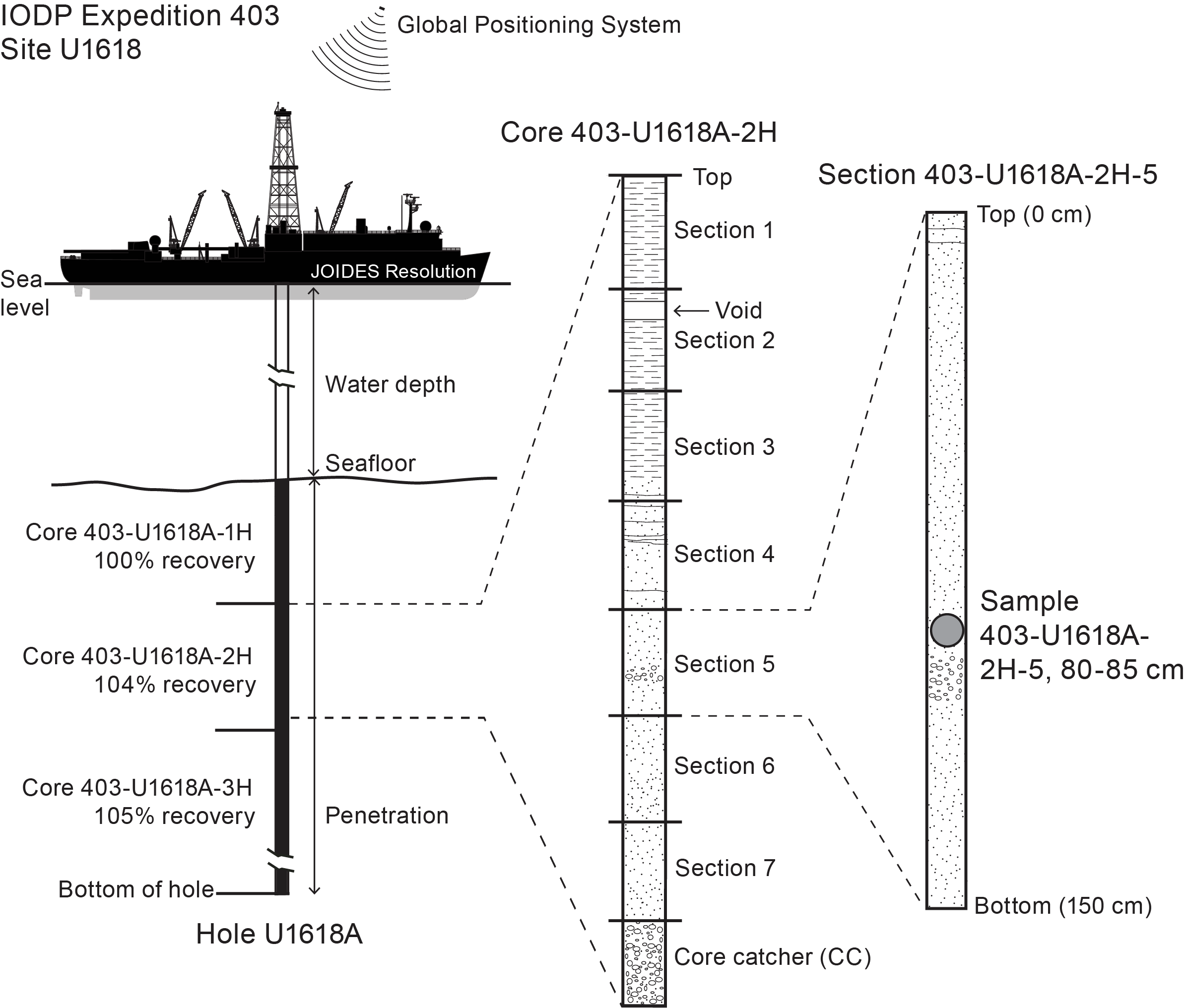
Figure F1. IODP naming convention.
1.2. Drilling operations
The advanced piston corer (APC), half-length APC (HLAPC), and extended core barrel (XCB) systems were used during Expedition 403 (Figures F2, F3). These tools and other drilling technology are documented in Graber et al. (2002). The APC and HLAPC systems cut soft-sediment cores with minimal coring disturbance relative to other IODP coring systems. After the APC/HLAPC core barrel is lowered through the drill pipe and lands above the bit, the drill pipe is pressured up until the two shear pins that hold the inner barrel attached to the outer barrel fail. The inner barrel then advances into the sediments and cuts the core. The driller can detect a successful cut, or full stroke, by observing the pressure gauge on the rig floor because the excess pressure accumulated prior to the stroke drops rapidly.
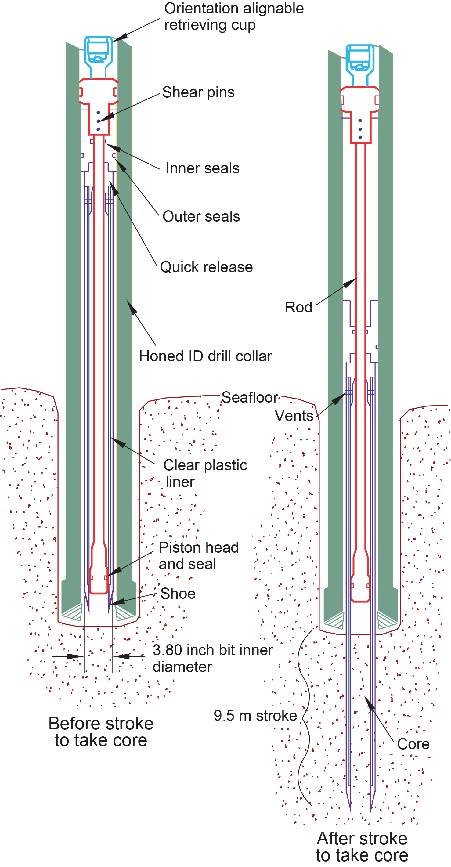
Figure F2. APC system.
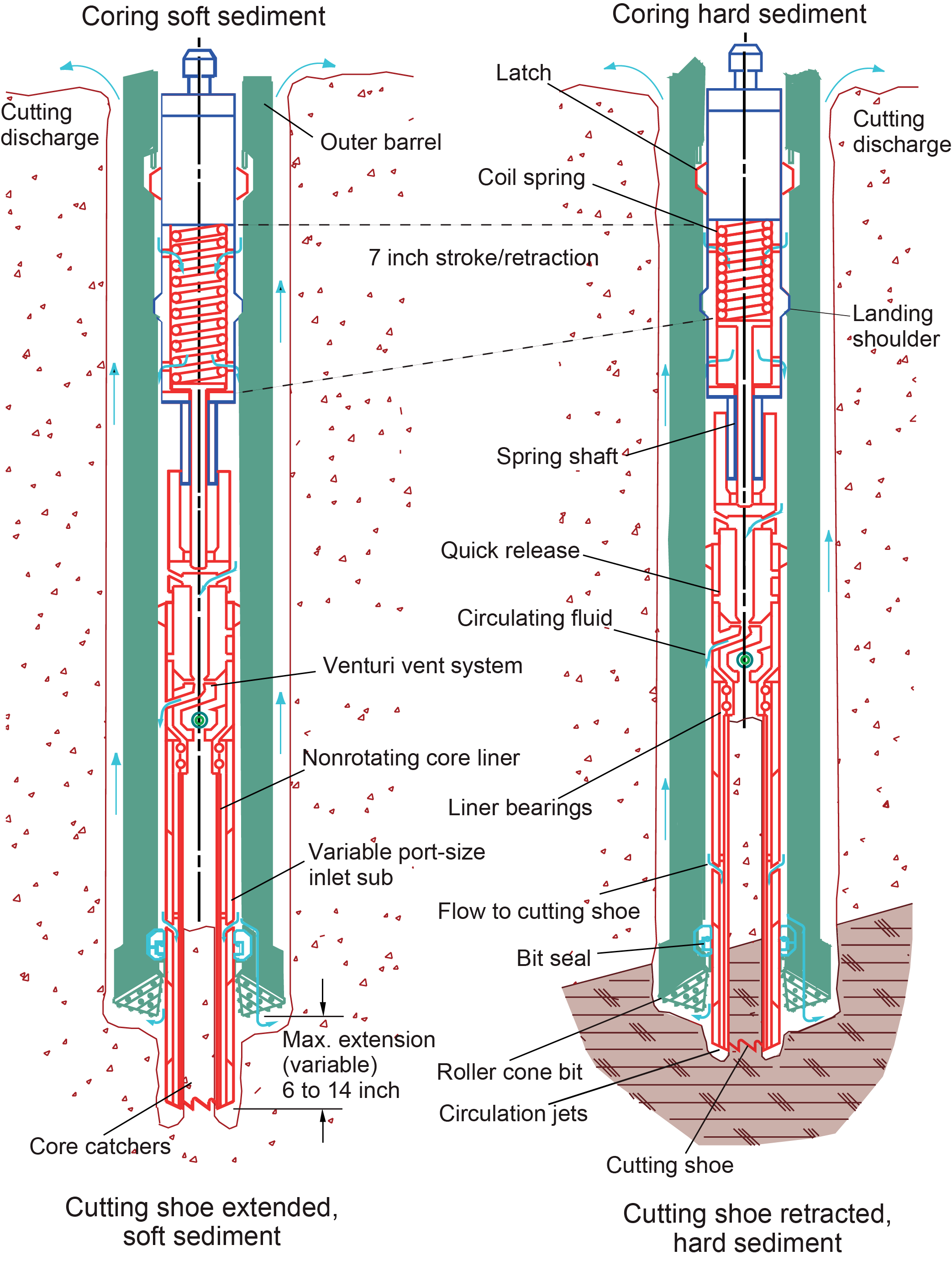
Figure F3. XCB system.
APC refusal is conventionally defined in one of two ways: (1) the piston fails to achieve a complete stroke (as determined from the pump pressure and recovery reading) because the formation is too hard or (2) excessive force overpull (>60,000 lb) is required to pull the core barrel out of the formation. For APC cores that do not achieve a full stroke, the next core can be taken after advancing to a depth determined by the recovery of the previous core (advance by recovery) or to the depth of a full APC core (typically 9.5 m). When a full stroke is not achieved, one or more additional attempts are typically made, and each time the bit is advanced by the length of the core recovered (note that for these cores, this results in a nominal recovery of ~100%). When a full or partial stroke is achieved but excessive force is not able to retrieve the barrel, the core barrel can be drilled over, meaning that after the inner core barrel is successfully shot into the sediments, the drill bit is advanced to the total depth to free the APC barrel.
The standard APC system uses a 9.5 m long core barrel, whereas the HLAPC system uses a 4.7 m long core barrel. In most instances, the HLAPC system is deployed after the standard APC system has repeated partial strokes and/or the core liners are damaged. During use of the HLAPC system, the same criteria are applied in terms of refusal as for the APC system. Use of the HLAPC system allowed for significantly greater APC sampling depths to be attained than would have otherwise been possible.
The XCB system is typically used when the APC/HLAPC system has difficulty penetrating the formation and/or damages the core liner or core. The XCB system can also either be used to initiate holes where the seafloor is not suitable for APC coring or be interchanged with the APC/HLAPC system when dictated by changing sediment conditions (highly compacted or lithified). The XCB system is used to advance the hole when HLAPC refusal occurs before the target depth is reached or when drilling conditions require it. The XCB system is a rotary system with a small cutting shoe that extends below the large rotary APC/XCB bit (Figure F3). The smaller bit can cut a semi-indurated core with less torque and fluid circulation than the main bit, potentially improving recovery. The XCB cutting shoe typically extends ~30.5 cm ahead of the main bit in soft sediments, but a spring allows it to retract into the main bit when hard formations are encountered. Because the core diameter for the XCB system (5.87 cm) is slightly smaller than for the APC/HLAPC system (6.6 cm), drilling slurry can emplace between the liner and the core as well as between biscuits of sediment, a common type of drilling disturbance during XCB drilling.
The bottom-hole assembly (BHA) used for APC/XCB coring is typically composed of an 11⁷⁄₁₆ inch (~29.05 cm) roller cone drill bit, a bit sub, a seal bore drill collar, a landing saver sub, a modified top sub, a modified head sub, 8¼ inch control length drill collars, a tapered nonmagnetic drill collar, two stands of 5½ inch transition drill pipe, and a crossover sub to the drill pipe that extends to the surface.
Nonmagnetic core barrels were used for APC and HLAPC coring. APC cores were not oriented because at the high latitude of Expedition 403 sites the paleomagnetic inclination is near vertical, and therefore azimuth direction is not useful to determine paleomagnetic polarity changes. Formation temperature measurements were taken with the advanced piston corer temperature (APCT-3) tool (see Downhole measurements). Information on recovered cores, drilled intervals, downhole tool deployments, and related information are provided in the Operations, Paleomagnetism, and Downhole measurements sections of each site chapter.
1.3. IODP depth conventions
The primary depth scales used by IODP are based on the measurement of the drill string length deployed beneath the rig floor (drilling depth below rig floor [DRF] and drilling depth below seafloor [DSF]), the length of core recovered (core depth below seafloor [CSF] and core composite depth below seafloor [CCSF]), and the length of logging wireline deployed (wireline log depth below rig floor [WRF], wireline log depth below seafloor [WSF], and wireline log matched depth below seafloor [WMSF]). All depths are in meters. The relationship between scales is defined either by protocol, such as the rules for computation of CSF depths from DSF depths, or by combinations of protocols with user-defined correlations (e.g., CCSF scale). The CCSF scale provides a site-specific common depth scale that is accomplished by correlating downhole data across multiple holes at a single site. The distinction in nomenclature should keep the user aware that a nominal depth value in two different depth scales usually does not refer to the same stratigraphic interval (see Curatorial procedures and sample depth calculations). For more information on depth scales, see IODP Depth Scales Terminology (http://www.iodp.org/policies-and-guidelines). To more easily communicate shipboard results, core depth below seafloor, Method A (CSF-A), depths in this volume are reported as meters below seafloor (mbsf) unless otherwise noted.
Depths of cored intervals are measured from the drill floor based on the length of drill pipe deployed beneath the rig floor (DRF scale) (Figure F1). The depth of the cored interval is referenced to the seafloor (DSF scale) by subtracting the seafloor depth of the hole from the DRF depth of the interval. Standard depths of cores in meters below seafloor (CSF-A scale) are determined based on the assumption that the top depth of a recovered core corresponds to the top depth of its cored interval (DSF scale). Standard depths of samples and associated measurements (CSF-A scale) are calculated by adding the offset of the sample or measurement from the top of its section and the lengths of all higher sections in the core to the top depth of the core.
If a core has <100% recovery, for curation purposes all cored material is assumed to originate from the top of the drilled interval as a continuous section. In addition, voids in the core are closed by pushing core segments together, if possible, during core handling. If the core pieces cannot be pushed together to get rid of the voids, then foam spacers are inserted and clearly labeled "void." Therefore, the true depth interval within the cored interval is only partially constrained. This should be considered a sampling uncertainty in age-depth analysis or correlation of core data with downhole logging data.
When core recovery is >100% (the length of the recovered core exceeds that of the cored interval), the CSF-A depth of a sample or measurement taken from the bottom of a core will be deeper than that of a sample or measurement taken from the top of the subsequent core (i.e., the data associated with the two core intervals overlap on the CSF-A scale). This overlap can happen when a soft to semisoft sediment core recovered from a few hundred meters below seafloor expands upon recovery and/or when the sediment is gas rich. In the case of Expedition 403, core expansion from gas escape resulted in core recoveries of up to 182%, but core recovery for all holes was 95% on average. Therefore, stratigraphic intervals often do not have the same nominal depth on the DSF and CSF-A scales in the same hole.
During Expedition 403, all core depths below seafloor were initially calculated according to the CSF-A depth scale. CCSF depth scales are constructed for sites with two or more holes to create as continuous a stratigraphic record as possible (see Stratigraphic correlation). They also help mitigate the CSF-A core overlap problem and the coring gap problem. Using shipboard core logger–based physical property data (verified with core photos as needed), core depths in adjacent holes at a site are vertically shifted to correlate between cores recovered in adjacent holes. This process produces the CCSF depth scale. The correlation process results in affine tables that indicate the vertical shift of cores on the CCSF scale relative to the CSF-A scale. After the CCSF scale is constructed, a splice can be defined that best represents the stratigraphy of a site by utilizing and splicing the best portions of individual sections and cores from each hole. Because of core expansion, the CCSF depths of stratigraphic intervals are up to 15% (Hole U1619A) deeper than their CSF-A depths. CCSF depth scale construction also reveals that coring gaps on the order of 1.0–1.5 m often occur between two subsequent cores despite the apparent >100% recovery. For more details on the construction of the CCSF depth scale, see Stratigraphic correlation.
1.4. Curatorial procedures and sample depth calculations
Numbering of sites, holes, cores, and samples followed standard IODP procedure (Figure F1). A full curatorial identifier for a sample consists of the following information: expedition, site, hole, core number, core type (APC, HLAPC, or XCB), section number, section half type (working or archive), piece number (hard rocks only), and interval in centimeters measured from the top of the core section. For example, a sample identification of "403-U1618A-2H-5W, 80–85 cm," indicates a 5 cm sample removed from the interval between 80 and 85 cm below the top of Section 5 (working half) of Core 2 ("H" designates that this core was taken with the APC system) of Hole A at Site U1618 during Expedition 403. The "U" preceding the hole number indicates the hole was drilled by the U.S. IODP platform, JOIDES Resolution. The drilling system used to obtain a core is designated in the sample identifiers as follows: H = APC, F = HLAPC, and X = XCB. Integers are used to denote the core type of drilled intervals (e.g., a drilled interval between Cores 2H and 4H would be denoted as Core 31). A drilled interval refers to an interval where the drill string advances without recovery.
1.5. Core handling and analysis
The overall flow of cores, sections, analyses, and sampling implemented during Expedition 403 is shown in Figure F4.
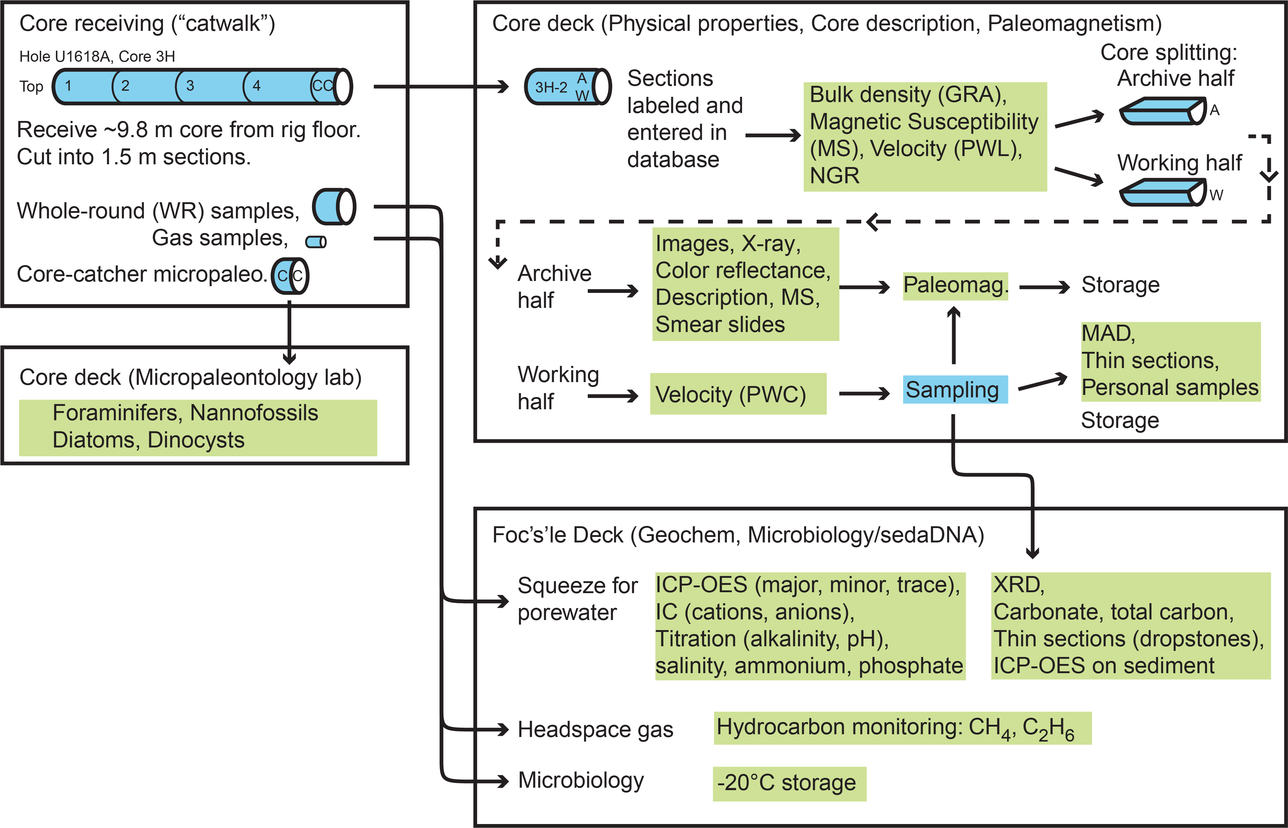
Figure F4. Expedition 403 workflows.
1.6. Sediment workflow
When the core barrel reached the rig floor, the core catcher from the bottom of the core was removed and taken to the core receiving platform (i.e., catwalk), and a sample was extracted for paleontological (PAL) analysis. For the first core of each site, mudline samples were taken for micropaleontology and sometimes for microbiological sampling. Next, the sediment core was extracted from the core barrel in its plastic liner. The liner was carried from the rig floor to the core processing area on the catwalk outside the core laboratory, where it was split into ~1.5 m sections. Blue (uphole direction) and gray (downhole direction) liner caps were glued with acetone onto the cut liner sections.
After the core was cut into sections, time-sensitive samples were taken. Whole-round samples were taken for interstitial water (IW) chemical and microbiological analyses. When a whole-round sample was removed, a yellow end cap was used to indicate the location it was taken. Syringe samples were taken for gas analyses according to the IODP hydrocarbon safety monitoring protocol. Syringe and whole-round samples were taken for sedimentary ancient DNA (sedaDNA) postexpedition analyses.
The core sections were placed in a core rack in the laboratory, core information was entered into the database, and the sections were labeled and laser engraved before being run through the Special Task Multisensor Logger (STMSL). When the core sections reached equilibrium with laboratory temperature (typically after 4 h), they were run through the Whole-Round Multisensor Logger (WRMSL) to measure P-wave velocity, magnetic susceptibility (MS), and gamma ray attenuation (GRA) bulk density (see Physical properties). The core sections were also run through the Natural Gamma Radiation Logger (NGRL), often prior to temperature equilibration because that does not affect the natural gamma radiation (NGR) data.
The core sections were then split lengthwise from bottom to top into working and archive halves. Investigators should note that older material can be transported upward on the split face of each section during splitting.
Discrete samples were then taken for moisture and density (MAD), paleomagnetic (PMAG) analyses, and the remaining shipboard analyses such as X-ray diffraction (XRD), carbonate (CARB), and inductively coupled plasma–atomic emission spectroscopy (ICP-AES) and ion chromatography (IC). Samples were not collected when the lithology was a high-priority interval for expedition or postexpedition research, the core material was unsuitable, or the core was severely deformed. During the expedition, samples for personal postexpedition research were taken only in special circumstances. A limited number of personal or shared pilot samples were taken for five reasons: (1) to find out whether an analytical method works and yields interpretable results and how much sample is needed to guide postexpedition sampling, (2) to generate low spatial resolution pilot data sets that can be incorporated in proposals and potentially increase their chances of being funded, (3) to collect DNA samples that would otherwise decay until the sampling party, (4) to take whole-round samples for anelastic strain recovery (ASR) experiments that would not be possible later than 6 h after recovery, and (5) to get early results to help with high-impact publications before the Expedition 403 sampling party.
The archive half of each core was scanned on the Section Half Imaging Logger (SHIL) to provide linescan images. The X-Ray Linescan Logger (XSCAN) was used to provide X-ray images of the archive halves. Point magnetic susceptibility (MSP) and reflectance spectroscopy and colorimetry were measured for all archive halves on the Section Half Multisensor Logger (SHMSL). Labeled foam pieces were used to denote missing whole-round intervals in the SHIL images. The archive halves were then described visually and by means of smear slides for sedimentology. Finally, the magnetization of archive halves and working-half discrete pieces was measured with the cryogenic magnetometer and spinner magnetometer.
When all steps were completed, cores were wrapped, sealed in plastic tubes, and transferred to cold storage space aboard the ship. At the end of the expedition, the working halves of the cores were sent to the IODP Bremen Core Repository (Center for Marine Environmental Sciences [MARUM]; Bremen, Germany), where samples for postexpedition research were taken in January 2025. The archive halves of the cores were first sent to the IODP Gulf Coast Repository (Texas A&M University; College Station, Texas [USA]), where a subset was scanned for X-ray fluorescence (XRF), before being forwarded to the Bremen Core Repository for long-term archive.
1.7. Drilling and handling core disturbance
Cores may be significantly disturbed and contain extraneous material as a result of the coring and core handling process (Jutzeler et al., 2014, 2025). For example, in formations with high amounts of ice-rafted debris, clasts from intervals higher in the hole may be washed down by drilling circulation, accumulate at the bottom of the hole, and be sampled with the next core. The uppermost 10–50 cm of each core must therefore be examined critically during description for potential fall-in. Common coring-induced deformation includes the concave-downward appearance of originally horizontal bedding. Piston action can result in fluidization (flow-in) at the bottom of APC cores. The rotation and fluid circulation used during XCB coring can also cause core pieces to rotate relative to each other (resulting in biscuiting) as well as induce fluids into the core and/or cause fluidization and remobilization of poorly consolidated/cemented sediments. In addition, extending APC or HLAPC coring into deeper, firmer formation can also induce core deformation. Retrieval from depth to the surface can result in elastic rebound. Gas that is in solution at depth may become free and drive apart core segments in the liner. When gas content is high, pressure must be relieved for safety reasons before the cores are cut into segments. This is accomplished by drilling holes into the liner, which forces some sediment as well as gas out of the liner. These disturbances are described in each site chapter and graphically indicated on the visual core descriptions (VCDs).
2. Lithostratigraphy
The lithostratigraphy of sediments recovered during Expedition 403 was primarily determined through visual (macroscopic) core description of the split core surface of the archive halves and by microscopic analysis of smear slides taken from the archive halves. All observations were directly entered into the according GEODESC templates. An additional suite of data was collected to supplement these fundamental observations to aid in the characterization of the sediment lithologies. These approaches included: X-ray imaging, digital linescan imaging, SHMSL MS measurements, and color spectrophotometry on the archive halves, as well as select XRD measurements of the bulk and/or clay fraction from the working half and occasional thin section characterization and mineralogical analysis using energy dispersive spectrometry mineral analysis. Each of these analytical procedures is described below. Additionally, physical property data such as density, NGR, and whole-round MS were used for further core characterization (see Physical properties). The latter are displayed along with the lithologic data in the Lithostratigraphy section in the site chapters.
2.1. Split core surface preparation
Visual core description was carried out on the split core surface of the archive halves. Depending on sediment induration, core sections were split using either a piano wire or saw from bottom to top. These splitting techniques can affect the appearance of the split core surface. Thus, prior to any step in the workflow of visual core description, the quality of the split core surface was assessed and the surface was carefully scraped with stainless steel scrapers as needed. Often, cores split using the piano wire were subjected to scraping, whereas firmer sediments cut with the saw generally did not need to be scraped. Cleaning was performed parallel to bedding to avoid cross-lithology contamination.
2.2. Visual core description
Visual core descriptions of each section were recorded using the GEODESC template. Although handwritten visual core description is common practice, due to the high core recovery, visual core description observations were entered directly into GEODESC.
2.3. GEODESC software
Visual core descriptions were recorded using the GEODESC software (version 1.0.30) and were directly uploaded into the Laboratory Information Management System (LIMS) database. A macroscopic template was created in GEODESC Template Manager for Expedition 403 and includes the following categories:
- Lithology (prefix, principal name, suffix, and comments);
- Munsell color name (color codes were input instead of the full name);
- Interval contacts (lower contact type and shape);
- Sedimentary structures, strata thickness, and comments;
- Bioturbation index;
- Induration;
- Macrofossils; and
- Any additional notes related to core description.
Four additional GEODESC templates were constructed for (1) core summaries, (2) smear slides, (3) thin sections, and (4) drilling disturbance. GEODESC is continually uploaded to the LIMS database (accessible via GEODESC Data Access) and was used to generate a one-page VCD graphical figure for each core (Figure F5). For each site, an additional VCD figure was developed to further highlight features important to defining lithostratigraphic units and subunits (Figure F6).
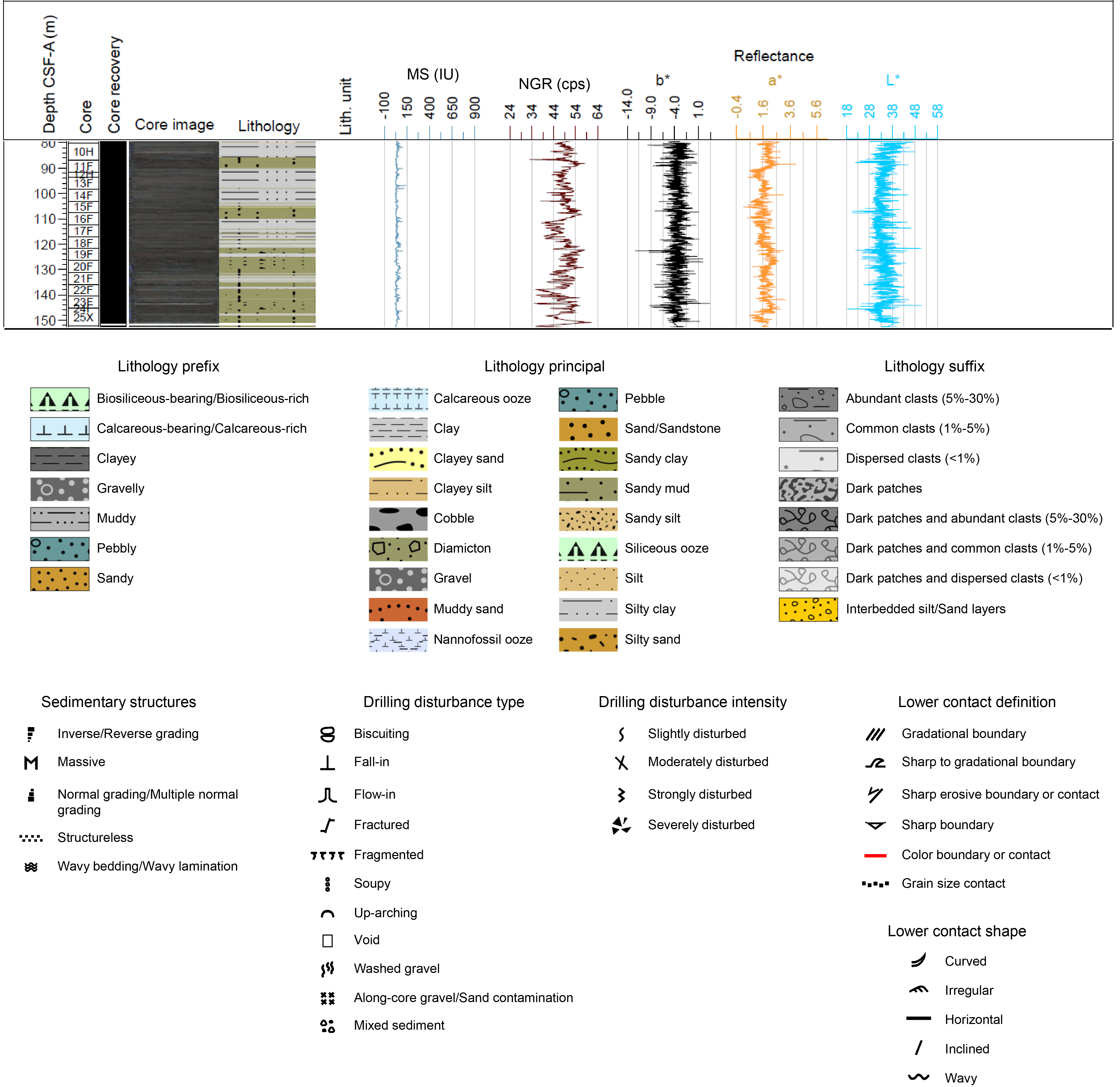
Figure F5. Example VCD.
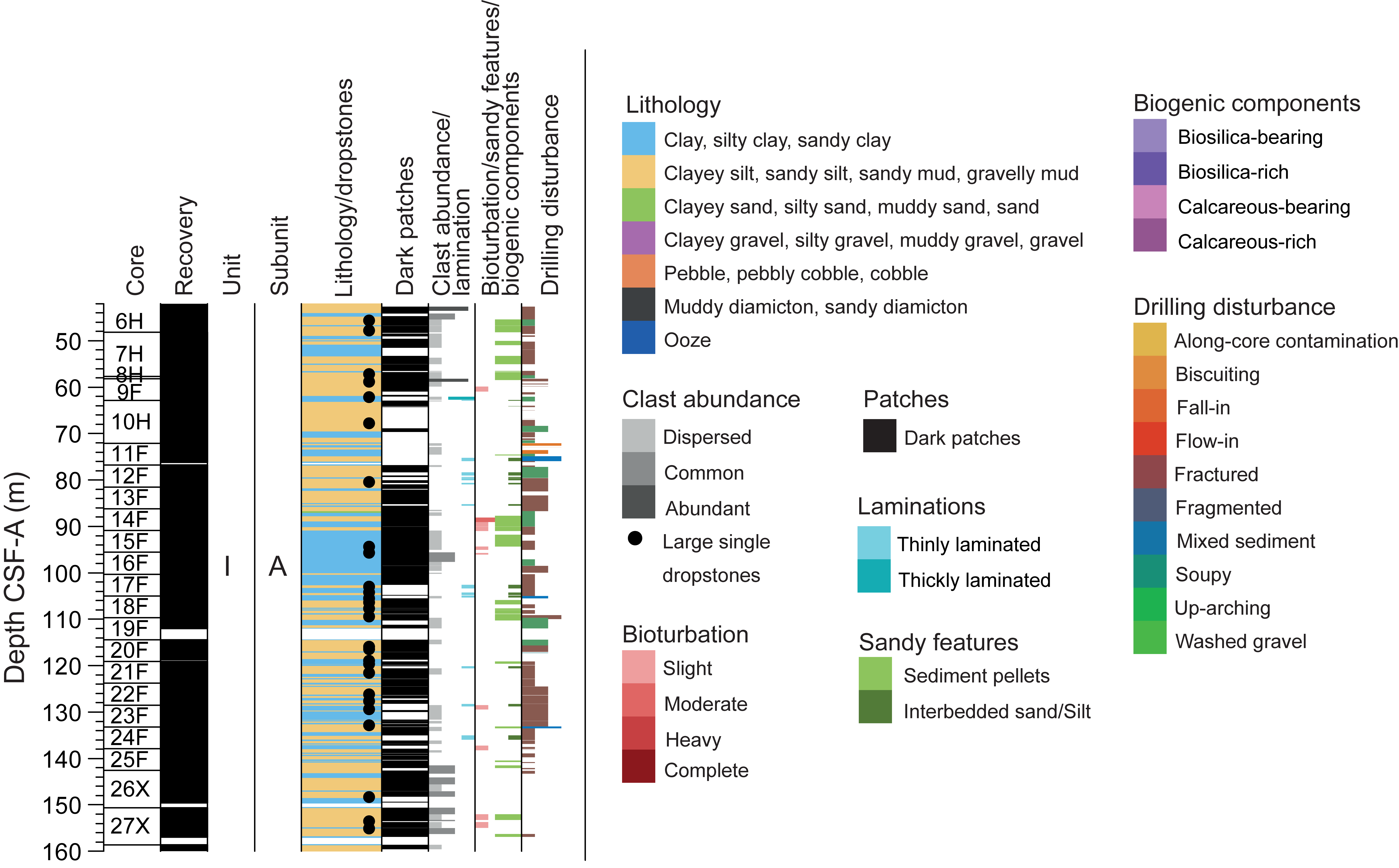
Figure F6. Key VCD features.
2.4. Evaluation of drilling disturbance
Drilling operations can alter the cores to varying degrees. Slight disturbances may result in bent or bowed contacts, whereas moderate to strong disturbances can result in displaced parts in the stratigraphic sequence or near-destruction of the core (examples are given in Jutzeler et al. [2014, 2025]). Drilling disturbances were described from the archive halves and directly noted into GEODESC, distinguishing different classes and severeness of disturbance in soft to hard sediments.
Classes of drilling disturbance include the following:
- Up-arching: sediment contacts are slightly to moderately bent but still subhorizontal and continuous.
- Fractured: sediment is broken into angular pieces that are still in their original place and not rotated significantly.
- Fragmented: firm parts of sediments are broken into angular pieces that are often displaced, rotated, and possibly mixed with drilling slurry.
- Biscuited: sediments have variations in the degree of disturbance, with softer intervals washed and/or soupy, whereas stiffer intervals are often relatively undisturbed or exhibit sections of material between a slurry of mixed sediments.
- Along-core contamination: coarse material was dragged or washed up between the in situ core material and the core liner.
- Fall-in: sediment originating from the formations above the actual core fell into the subsequent barrel upon coring.
- Soupy: sediment intervals are water saturated and have lost their initial structures.
- Washed gravel: fine material was possibly lost during the drilling process, and only coarse materials (mostly gravel or pebbles) remain. This often occurs when coring unsorted to poorly sorted, unconsolidated sediments with a high content of coarse grains.
- Void: interval has no core material due to drilling operations or expansion of gas that resulted in the partitioning of pieces.
- Mixed sediment: sediment was visually mixed during the coring process.
- Flow-in: material was pulled in at the core bottom due to the lack of separation from the remaining formation.
In addition to the nature of core disturbance, the severity of disturbance was categorized as slight, moderate, or strong.
2.5. Lithologic classification scheme
Lithologic descriptions were based on a classification scheme modified from one used during IODP Expedition 379 (Wellner et al., 2021). Lithologic names were assigned based on composition and texture, as outlined in the flow chart (Figure F7). The principal name is purely descriptive and does not include interpretive classifications relating to fragmentation, transport, deposition, or alteration processes.
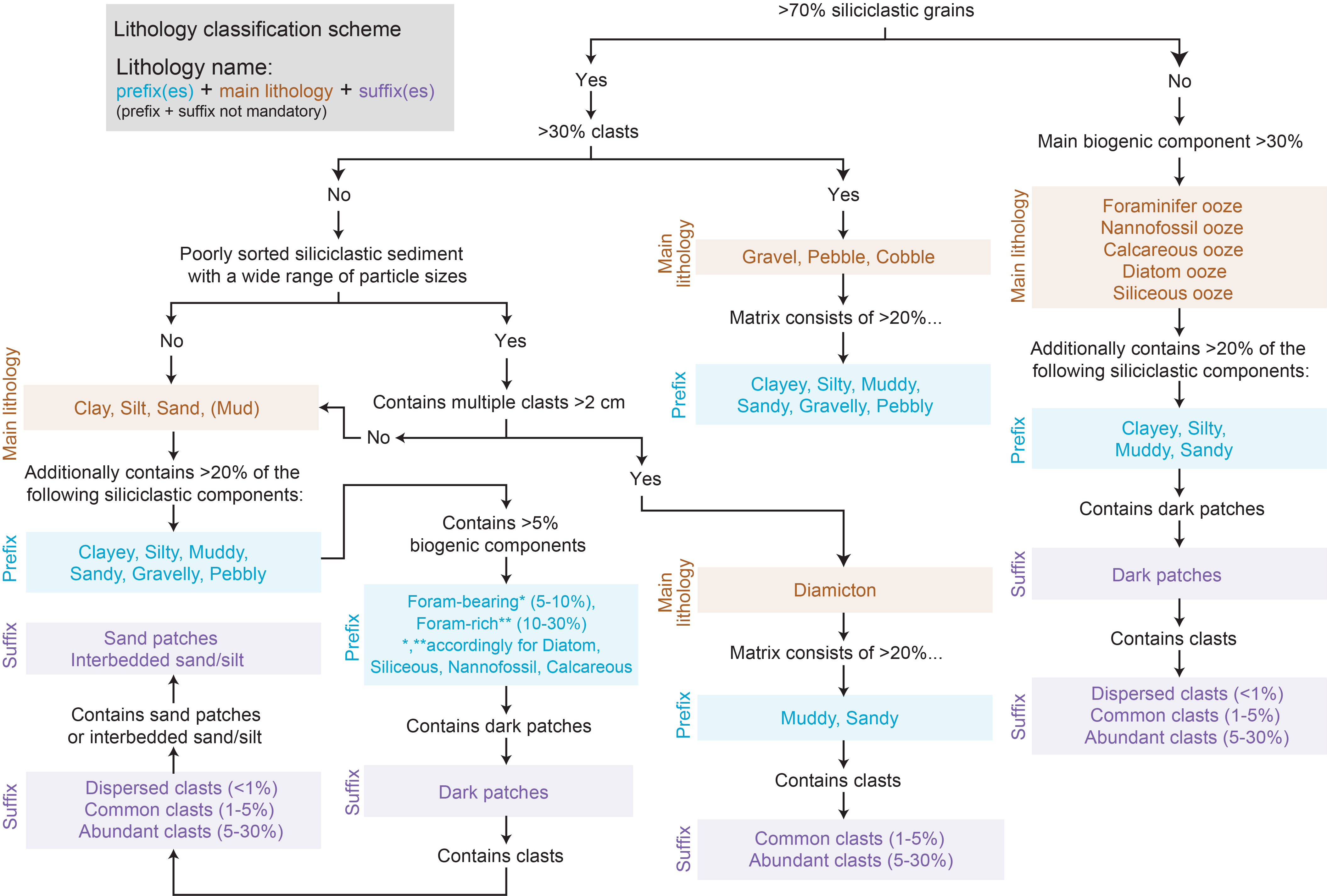
Figure F7. Lithology classification scheme.
2.5.1. Principal names and modifiers
The principal name of a sediment/rock with >70% siliciclastic grains is based on an estimate of the grain sizes present (Figure F7). The definition of clay, silt, sand, and gravel/pebble/cobble size classes for Expedition 403 was modified from the Wentworth (1922) scale. In the absence of grains larger than gravel (>2 mm), the principal sediment name was determined based on the relative abundances of sand, silt, and clay (e.g., silt, sandy silt, silty sand, etc.) (Naish et al., 2006, after Shepard, 1954, and Mazzullo et al., 1988) (Figure F8). For example, if any one of these components exceeds 80%, then the lithology is defined by the primary grain size class (e.g., sand). Sediments composed of a mixture of at least 20% each of sand, silt, and clay are classified as sandy mud to muddy sand. In cases where a sediment consists of two grain size fractions that each exceed 20% (e.g., 40% clay and 60% silt), the prefix is determined by the fraction with the lower percentage (e.g., clayey silt).
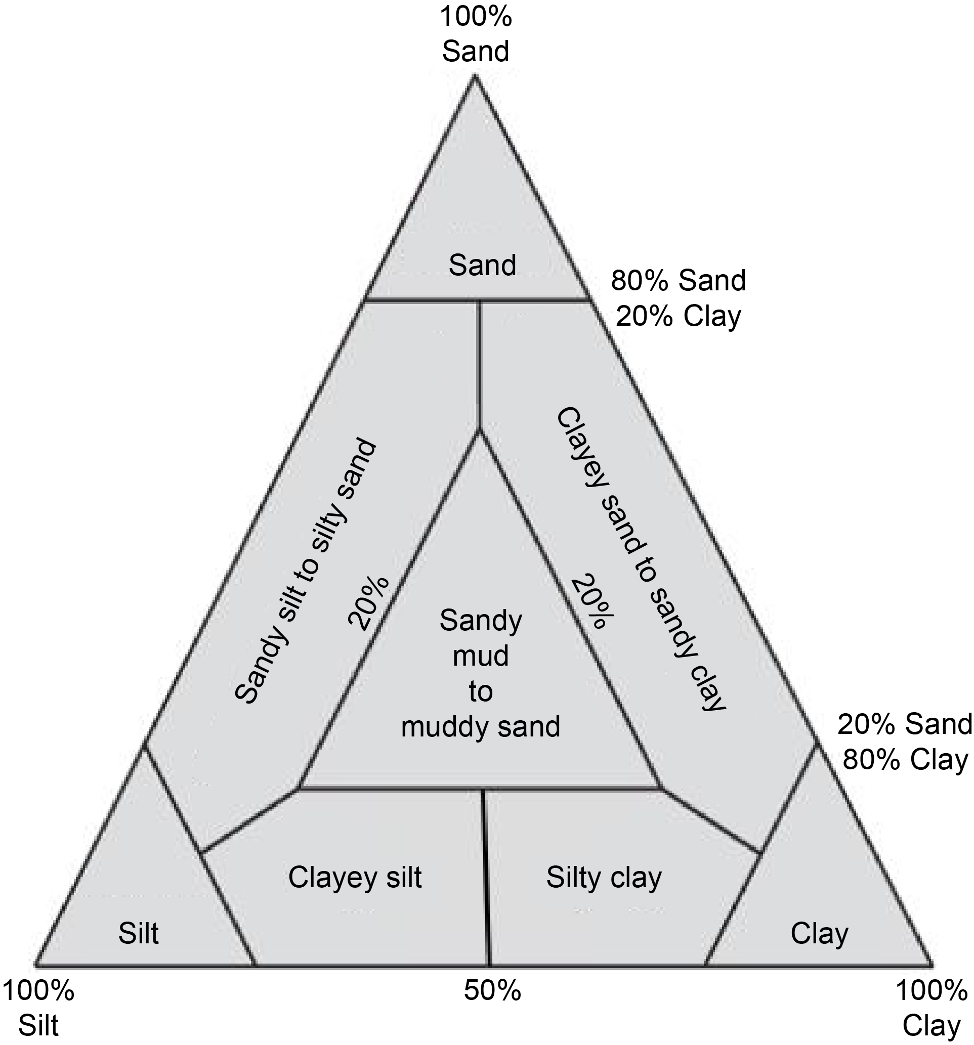
Figure F8. Ternary diagram for terrigenous clastic sediments.
When the sediment contains siliciclastic gravel (2–4 mm)/pebble (4–64 mm)/cobble (>64 mm), the principal name is determined by analyzing their relative abundance and the sand/mud ratio of the clastic matrix (Figure F7). For Expedition 403, the definition of diamicton was slightly modified from Moncrieff (1989). We employed the term "diamicton" as a nongenetic term for unsorted to poorly sorted terrigenous unconsolidated sediment containing between 1% and 30% of clasts, with more than one clast >2 cm. A muddy diamicton comprises 1%–30% gravel/pebble/cobble and >50% mud in matrix, whereas a sandy diamicton comprises 1%–30% gravel/pebble/cobble and >50% sand in matrix. In addition, lithology suffixes of "common clasts (1%–5%)" and "abundant clasts (5%–30%)" were utilized in the Lithology suffix column in the macroscopic sediments GEODESC template to describe the clast abundance within diamictons, instead of characterizing them as "clast poor" or "clast rich." The term "gravel/pebble/cobble" was employed when the sediment contained >30% of grains larger than 2 mm.
The principal name of sediment with >30% biogenic grains is "ooze," modified by the most abundant specific biogenic grain type (Figure F9).
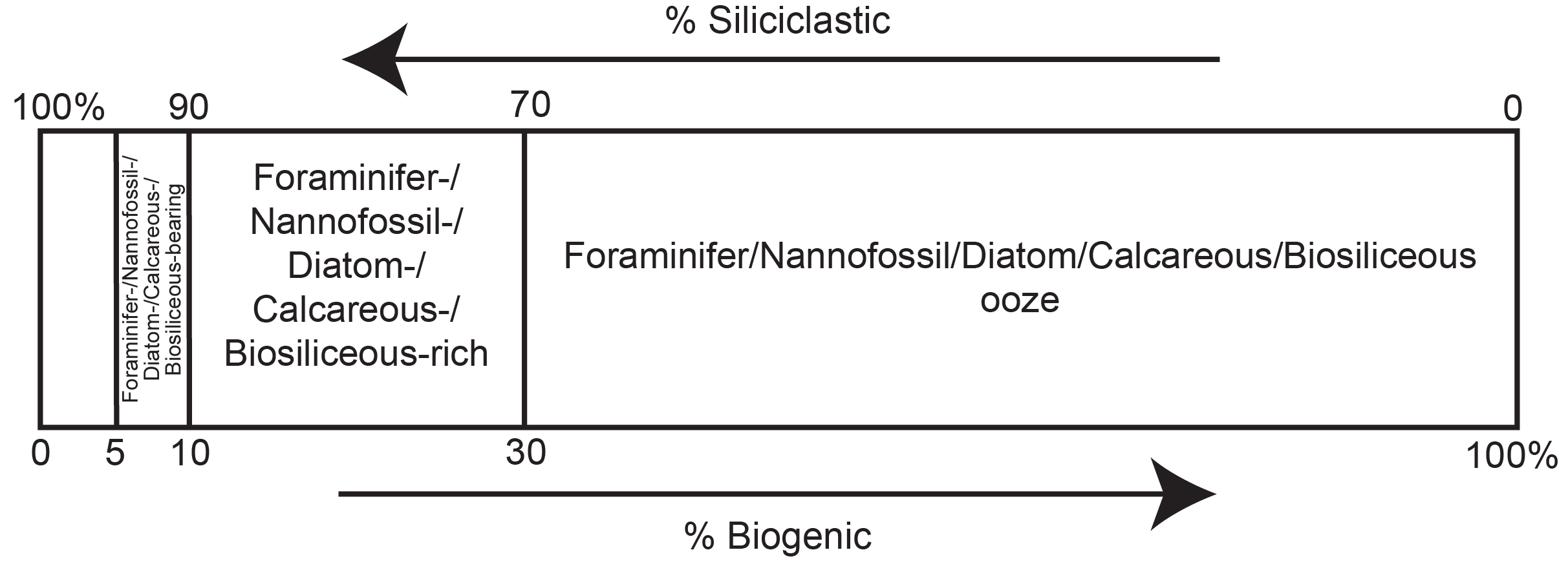
Figure F9. Sediment classification scheme.
For all lithologies, major and minor modifiers were applied to the principal sediment names using the following modified scheme from Expedition 318 (Expedition 318 Scientists, 2011) (Figures F7, F9):
- Minor biogenic modifiers are those components with abundances of 5%–10% and are indicated by the suffix "-bearing" (e.g., diatom-bearing).
- Major biogenic modifiers are those that comprise 10%–30% of the grains and are indicated by the suffix "-rich" (e.g., diatom-rich).
- Siliciclastic modifiers in biogenic oozes are those components with abundances of >20% and are indicated by the suffix "-y" (e.g., silty, muddy, or sandy).
In the case of intervals in which two lithologies are interbedded or interlaminated (i.e., individual beds or laminated intervals that are <15 cm thick and alternate between one lithology and another), the term "interbedded" or "interlaminated" is recorded under the Lithology suffix tab as "interbedded silt/sand layers" in the macroscopic GEODESC template and further described under Comments on the Lithology tab.
2.5.2. Color
Sediment color was determined using Munsell soil color charts and further recorded in GEODESC comment sections when necessary. Each interval color was described with the color code (e.g., 5Y 4/1) instead of the color name.
2.5.3. Induration
Induration or sediment stiffness was assessed and recorded in GEODESC as "soft," "firm," or "hard." Quick induration tests involved using the end of a toothpick and gently scraping the end of it into the sediment. Soft sediment easily deforms under very little pressure and can be easily scraped with a toothpick or metal tool, firm sediment is still able to be scraped with a toothpick or metal tool but requires more pressure, and hard sediment undergoes little to no deformation under pressure and needs a saw to cut.
2.5.4. Sedimentary structures
Sedimentary structures were classified as structureless, massive, wavy bedding, normal grading, multiple normal grading, inverse grading, and multiple inverse/reverse grading. "Normal grading" refers to layers with a fining upward grain size, whereas "reverse grading" refers to layers with a coarsening upward trend. The lamination and bedding thickness classification used to describe the cores comes from Mazzullo et al. (1988):
- Thinly laminated (≤3 mm thick),
- Thickly laminated (3 mm to 1 cm),
- Very thinly bedded (1–3 cm),
- Thinly bedded (3–10 cm),
- Medium bedded (10–30 cm),
- Thickly bedded (30–100 cm), and
- Very thickly bedded (>100 cm).
Lower contacts between lithologies are classified as sharp, gradational, sharp to gradational, sharp erosive, grain size, or color boundaries and can be horizontal, inclined, irregular, curved, or wavy.
2.5.5. Bioturbation
Ichnofabric description included the extent of bioturbation of the sediments. The degree of bioturbation was assessed semiquantitatively using the ichnofabric index (0–4) of Droser and Bottjer (1986) and as modified by Savrda et al. (2001) (Figure F10):
- 0 = no apparent bioturbation (≤10%).
- 1 = slight bioturbation (>10%–30%).
- 2 = moderate bioturbation (>30%–60%).
- 3 = heavy bioturbation (>60%–90%).
- 4 = complete bioturbation (>90%).
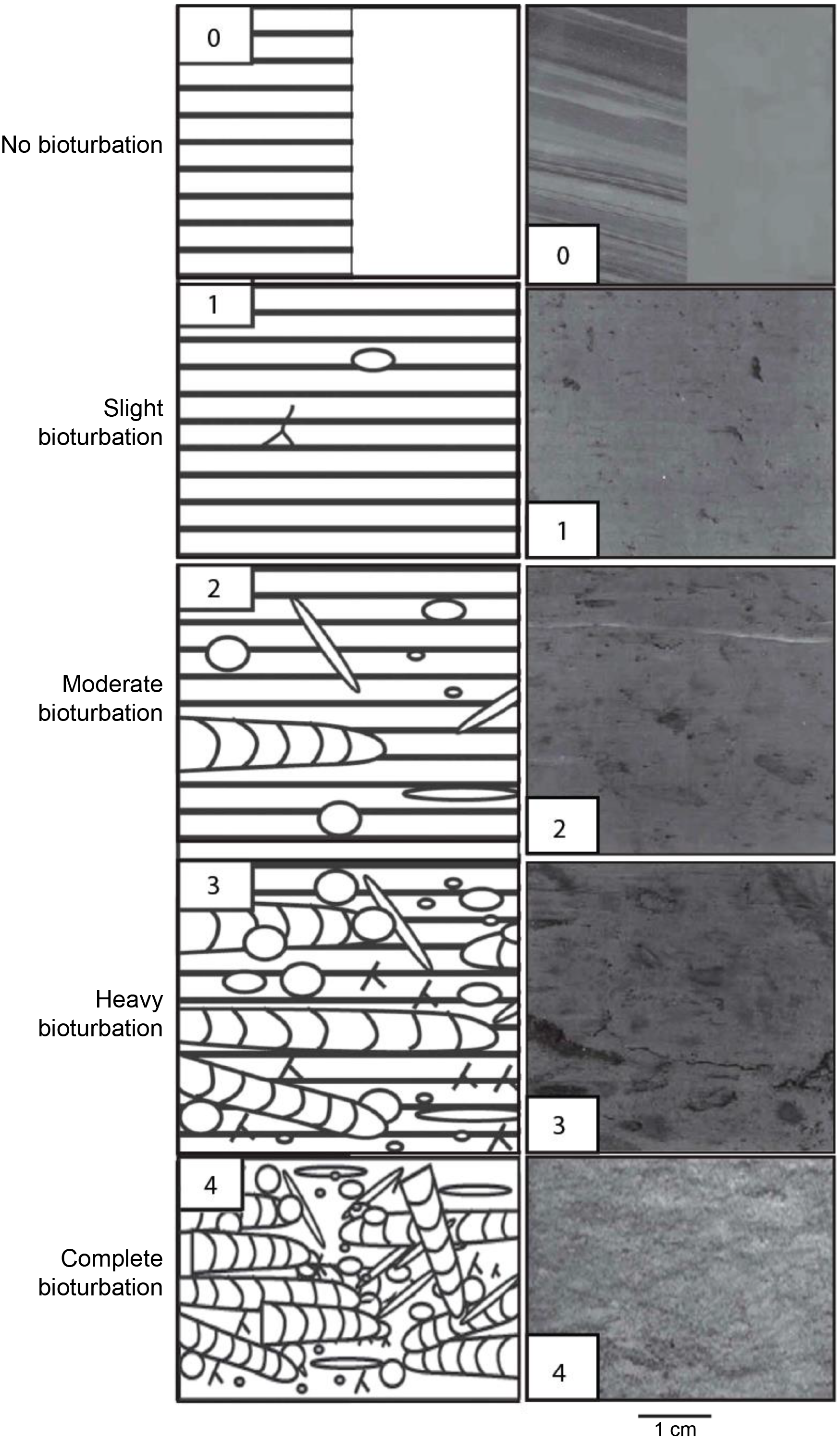
Figure F10. Ichnofabric index legend.
2.5.6. Smear slides
To aid in lithologic classification, the grain size, composition, and abundance of the sediment constituents were estimated for primary lithologies microscopically using smear slides. For each smear slide, a small amount of sediment was removed from the archive half using a wooden toothpick. This sediment was then placed on a 22 mm × 30 mm glass microscope slide, and two to four drops of deionized (DI) water were placed atop the sediment. After the sediment and water were homogenized, the sample was smeared evenly over the glass slide until a thin layer remained, which was dried on a hotplate for a few minutes at ~150°C. Upon completely drying, a few drops of Norland Optical Adhesive Number 61 were placed atop the sediment. A cover glass was carefully placed on the dried sample, which was then placed in an ultraviolet light box for approximately 10 min to cure the adhesive.
Smear slides were examined with a transmitted light petrographic microscope equipped with a standard eyepiece micrometer. Biogenic and mineral components were identified following the petrographic techniques from Marsaglia et al. (2013, 2015). Because of time constraints, only 2–3 fields of view (FOVs) were examined at 10×, 20×, and 40× magnification to assess the abundance of detrital, biogenic, and authigenic components. The relative abundance of each constituent was visually estimated using the techniques of Rothwell (1989). The texture of siliciclastic lithologies and the proportions and presence of biogenic and mineral components were recorded in the smear slide worksheet of the microscopic GEODESC template as percentages.
Smear slides provide only a rough estimate of the relative abundance of sediment constituents. Occasionally, smear slides were collected for minor lithologies and are noted in the GEODESC Smear slide template. Very fine and coarse grain constituents are difficult to observe in smear slides, and their relative proportions in the sediment can be affected during smear slide preparation. Therefore, intervals dominated by sand-sized and larger constituents were examined by macroscopic comparison to grain size reference charts. Photomicrographs of select smear slides were uploaded to the LIMS database.
2.6. Thin sections
Occasionally, thin sections of selected clasts (>2 cm), authigenic carbonate nodules, and epoxy-impregnated laminated intervals were made to further assess composition and/or texture. Thin section preparation was completed on board through a semiautomated process using primarily a Buehler Petrothin for cutoffs and lapping, as well as a glass plate and silicon carbide slurry for finer lapping. Certain samples required freeze-drying to create a more consolidated billet for easier processing or epoxy impregnation to stabilize the sample while being processed and allow for successful lapping, mounting, and polishing. Epo-Tek petrographic epoxy was used for impregnation and mounting. One sample was dyed with blue porosity dye, and one was stained with Alizarin Red S and potassium ferricyanide for carbonate studies. Final reflective polishing was achieved by using a diamond paste on fiber cloth, fitted to a rotating wheel of a Buehler MetaServ. Thin sections were examined with a transmitted and reflected light petrographic microscope.
Data were entered into the Thin section tab of the GEODESC microscopic template.
2.7. X-ray diffraction analysis
XRD analysis was performed on clay and bulk fractions of select samples. Sample frequency varied; they were chosen to characterize different lithologic intervals and facies and were selected based on visual core observations (e.g., color variability, visual changes in lithology, texture, etc.) and smear slide investigations.
For clay mineral XRD analysis, the <2 µm (clay) fraction was separated from the bulk sample and treated to remove nonmineralogical material. To remove carbonate content (e.g., biogenic material), 25 mL of 10% acetic acid was added to ~2 cm3 undried sample in a centrifuge tube, mixed well, and let sit for at least 1 h to decarbonate. The centrifuge tube was placed in the shaker for at least 30 s and observed for any bubble release to ensure the reaction had stopped. Samples were centrifuged for 15 min at 1500 rpm, and then the supernatant (acetic acid solution) was decanted. A total of 25 mL of DI (nanopure) water was added to the centrifuge tube and put in the shaker to mix well with any residual acetic acid. The solution was then centrifuged again for 15 min at 1500 rpm. The supernatant (clear water) was decanted, and the wash cycle was repeated at least three times to remove all acetic acid. A series of centrifuging or gravity settling is required to separate the clay fraction (<2 µm) from the coarser material. Approximately 25 mL of 1% borax solution was added to the clay plug in the centrifuge tube. The sample was dismembrated/sonicated for at least 1 min to remove >2 µm coarser fraction and then allowed to settle for 12 h. The solution was centrifuged for 4 min at 750 rpm. The supernatant liquid was decanted into a separate centrifuge, where the suspended clay was separated from the liquid. This step was repeated for the centrifuge tube with the coarser fraction at least three times to validate that all the <2 µm clay fraction had been removed. The <2 µm clay fraction was centrifuged for 15 min at 1500 rpm to remove the borax solution. The supernatant was decanted, and 25 mL of DI water was added, shaken, and centrifuged for 60 min at 3000 rpm. The supernatant was decanted, and the residue left was a <2 µm clay fraction. A zero-background silicon (quartz) disk was then heated to 550°C and put in a sample holder. The <2 µm clay fraction was removed using a dropper and by spreading the concentrated slurry on the silicon disk to cover the area. After drying the sample in a desiccator, the clay particles oriented themselves as the solution dried on the disk. To expand swelling clays and aid in mineral identification, ethylene glycol was used. Samples on disks were subjected to the vapor treatment method of glycolation because it provides less disturbance to the sample and minimizes amorphous scattering of X-rays by excess liquid. The glycolator was filled with a ~1 cm layer of ethylene glycol at the bottom, and the samples on disks were placed on a rack inside the glycolator. Subsequently, the glycolator was placed in the oven (60°–70°C) for approximately 12 h. Finally, the glycolated sample on the disk was analyzed using XRD on the Benchtop Malvern Panalytical AERIS Research Edition X-ray diffractometer aboard JOIDES Resolution. The HighScore Plus software (version 4.8) was utilized to identify significant peaks and calculate the basal peak areas (counts ×°2θ). A semiquantitative approach based on the Biscaye (1964) method was used to estimate clay mineral relative abundances of smectite (S), illite (I), chlorite (C), and kaolinite (K) based on peak area weighed by empirical estimate factors and then summed to 100% according to the Biscaye (1965) method:
Bulk sediment samples were prepared for XRD analysis by freeze-drying them for at least 12 h, followed by grinding using an agate mortar and pestle. If the texture of the sample resembled talc powder and appeared homogeneous, it was then packed into a sample holder and placed in the Benchtop Malvern Panalytical AERIS Research Edition X-ray diffractometer sample area. The HighScore Plus software (version 4.8) was employed to identify and quantify the bulk mineral composition and percentages.
2.8. Digital core imaging
After the split core surface was cleaned, the archive half was imaged using the SHIL. On the SHIL, three pairs of advanced illumination high-current, focused light-emitting diodes, each pair with a color temperature of 6,500 K and 200,000 lux at 7.6 cm, were used to illuminate the core surface. The SHIL contains a linescan camera manufactured by JAI with a Nikon 60 mm macro lens and a resolution of 20 lines/mm (50 µm) used to generate a high-resolution TIFF image. The camera height was set to image 0.1 mm2 per pixel, but the actual pixel size might vary due to slight irregularities in split section height.
Archive sections were imaged as soon as possible to avoid color changes due to oxidation or drying of the sediment. When sections were soupy or watery, they were allowed to dry sufficiently to avoid excessive light reflection and overexposure before imaging. Some very soupy intervals were covered with Kimwipes to absorb moisture prior to imaging.
2.9. Colorimetry and point-sensor magnetic susceptibility
The SHMSL is a point-sensor logger that measures the bulk physical properties of the sediment surface. These include a laser surface analyzer, a point sensor to measure MS, and a spectrophotometer. The measurement interval was typically set to 5.0 cm. Because both MS and spectrophotometer measurements require contact between the sensor and sediment surface, the archive halves were covered by a thin, clear plastic wrap. Before measurements were carried out, a laser surface analyzer scanned the sediment surface for irregularities (e.g., cracks or voids), providing quality control for MS and spectrophotometer measurements. Color calibration was conducted once every 6 h.
MS was measured using a Bartington Instrument MS2 meter with an MS2K contact probe, a flat 15 mm diameter round sensor, a field influence of 25 mm, and an operational frequency of 930 Hz. The spatial resolution of the MS sensor is ~3.8 mm, and it reports values in instrument units (IU). Spectrophotometry was carried out with an Ocean Optics QE Pro detector that measures the reflectance spectra of the split core surface between the ultraviolet and the near-infrared range (recorded in 2 nm spectral bands from 390 to 732 nm). Color information was converted to the CIELAB color space (L*a*b*), which displays colors as a function of lightness (L* = perceptional lightness; grayscale white to black = 0–100) and color values (a* ranges green [negative] to red [positive]; b* ranges blue [negative] to yellow [positive]) (Balsam et al., 1997, 1998).
2.10. Acquisition of X-radiographs
X-radiographs were collected using an XSCAN from archive section halves. The IODP X-ray system is composed of a 120 kV, 1 mA constant potential X-ray source and a detector unit. The X-ray source is a Teledyne ICM CP120B portable X-ray generator with a 0.8 mm × 0.5 mm focal spot. The beam angle is 50° × 50° and generates a directional cone onto the detector, which is 65 cm from the source. The detector is a Go-Scan 1510 H unit composed of an array of complementary metal-oxide semiconductor (CMOS) sensors with an active area of 102 mm × 153 mm and a resolution of 99 μm. Raw X-ray images were collected as 16 bit images using the Integrated Measurement System (IMS) software (version 14). Images were processed using an IODP software that allows for high and low calibration, adjustment of image contrast, sharpness, and crop; additionally, the software accounts for the differential thickness across the half-round core diameter. X-ray images were frequently used to aid the lithologic description and were especially helpful in showing sedimentary features (e.g., laminations, bioturbation, and authigenic mineral formations) that could not always be observed on the split core surface.
2.11. Lithostratigraphic units
At each site, sedimentary units were designated to highlight the major lithologic changes downhole. Lithostratigraphic units were established based on prominent changes in lithology, clast abundance, bioturbation, and presence/absence of sedimentary features including laminations, dark patches, and sand patches. Physical properties were also sometimes used to make decisions on lithologic unit/subunit boundaries. Units are numbered from the top of the stratigraphic sequence downhole using Roman numerals. When more subtle lithostratigraphic changes were identified, units were divided into subunits. Subunits are identified from the main lithostratigraphic units by adding a letter designation after the Roman numeral from the top of the stratigraphic sequence downhole (e.g., Subunit IIA would indicate Subunit A of Unit II).
3. Biostratigraphy and paleoenvironment
Calcareous nannofossils, diatoms, dinoflagellate cysts (dinocysts), planktonic foraminifers, and occasionally silicoflagellates were used to develop a preliminary shipboard biostratigraphy and assessment of the paleoenvironment. The overall objective was to develop age-depth models for all Expedition 403 sites, integrating biostratigraphic and magnetostratigraphic data.
Samples were collected from core catchers over the length of the first drilled hole at each site. When subsequent drill holes went deeper, we analyzed core catcher samples from the stratigraphic record that was not recovered by the first hole. Where appropriate, additional samples were taken from split cores to better define the position of bioevents and zonal boundaries.
Age constraints and zonations were distinguished primarily based on lowest occurrence (LO) and highest occurrence (HO) and/or the lowest or highest common occurrence (LCO or HCO) of a taxon. Biostratigraphic events and biozone boundaries are given in Tables T1, T2, T3, and T4.
Establishing a continuous calcareous nannofossil chronological characterization in Arctic environments could be challenging due to the overall environmental limitation of calcareous phytoplankton species in high latitudes, which results in low diversity of the calcareous nannofossil record and absence of some relevant biomarkers, as well as diachroneity of some of the globally tuned bioevents. The higher continuity of the records recovered during Expedition 403 and the comparatively southernmost position of some of the sites, which is more intensely affected by the warm influence of North Atlantic Water through time, contribute to partially overcoming this limitation.
Following the common procedure, the global standard calcareous nannofossil zonation by Martini (1971) was primarily adopted. The standard calibrations of calcareous nannofossil bioevents from the Pliocene to the Quaternary by Sato et al. (1991), Sato and Kameo (1996), Sato et al. (1999), Lourens et al. (2004), Raffi et al. (2006), and Thierstein et al. (1977) were adopted. The revised Quaternary biochronology of Arctic Ocean sediments by Razmjooei et al. (2023) was considered complementary. The Neogene and Quaternary diatom zonation used for the high-latitude sites of Expedition 403 follows previous North Atlantic and high-latitude Deep Sea Drilling Project (DSDP) Legs 81 and 94, Ocean Drilling Program (ODP) Legs 151 and 162, and Integrated Ocean Drilling Program Expedition 303/306 proposed by Baldauf (1984, 1987), Koç and Scherer (1996), and Koç et al. (1999), respectively, and compiled by Romero (2009). The planktonic foraminiferal biozonation follows previous high-latitude DSDP and ODP legs (Weaver and Clement, 1986; Spiegler and Jansen, 1989). Additionally, datums based on silicoflagellates were used following Locker (1996). There is no standard dinocyst biozonation for the Neogene to Quaternary of the Arctic and Nordic Seas. We used biostratigraphic events identified in the Miocene and Pliocene of the Fram Strait (Matthiessen and Brenner, 1996), the Nordic Seas (De Schepper et al., 2015, 2017), the Iceland Sea (Schreck et al., 2012), the Arctic Ocean (Matthiessen et al., 2018), and the wider North Atlantic (Aubry et al., 2020, 2021; De Schepper and Head, 2008, 2009).
3.1. Calcareous nannofossils
3.1.1. Calcareous nannofossil taxonomy and biozonation scheme
The taxonomy of the taxa considered in the shipboard analysis of calcareous nannofossils during Expedition 403 is referenced in the global catalogs by Perch-Nielsen (1985), Bown (1998), and Young et al. (2003). Relevant information is also available from the Nannotax3 website (Young et al., 2024). According to the common approach for the biostratigraphic characterization of the Gephyrocapsa and Reticulofenestra genera during the Miocene to Quaternary (Raffi et al., 1993; Wei, 1993), a size classification is applied, as detailed below.
Gephyrocapsa specimens <3 μm, mainly constituted by Gephyrocapsa ericsonii and Gephyrocapsa aperta, are classified as small Gephyrocapsa. The species Gephyrocapsa muellerae and Gephyrocapsa margerelii, as well as other Gephyrocapsa specimens in the 3–5.5 μm size range, are clustered together as medium Gephyrocapsa. The large Gephyrocapsa group includes all Gephyrocapsa specimens with sizes >5.5 μm. In addition, the determination Gephyrocapsa caribbeanica is used to refer to those Gephyrocapsa specimens with sizes between 3 and 5 μm and a closed central area (González-Lanchas et al., 2023). Reticulofenestra specimens with sizes <3 μm, mostly constituted by Reticulofenestra minuta, are considered small Reticulofenestra. Reticulofenestra ampla, Reticulofenestra minutula, and Reticulofenestra haqii, ranging 3–5 μm, are determined to be medium Reticulofenestra. Consistent with the traditional definition and biostratigraphic application (Raffi et al., 1993; Wei, 1993), the species Reticulofenestra pseudoumbilicus and Reticulofenestra asanoi are separately identified and are correspondent to those specimens with sizes >7 and >6 μm, respectively.
The identified bioevents are based on the LO and HO of calcareous nannofossil marker species. The concept of acme (dominance interval) is also applied (Table T1).
The global standard calcareous nannofossil zonations by Martini (1971) were adopted and complemented by the recently revised Quaternary biochronology of Arctic Ocean sediments by Razmjooei et al. (2023). The standard calibration of calcareous nannofossil bioevents from the Pliocene to the Quaternary follows Sato et al. (1991), Wei (1993), Sato and Kameo (1996), Sato et al. (1999), Raffi (2002), Lourens et al. (2004), Raffi et al. (2006), and Thierstein et al. (1977).
Correspondence to regionally revised datums and biochronological schemes resulting from North Atlantic and high-latitude Integrated Ocean Drilling Program Expedition 303/306 and ODP Legs 104, 151, and 162 by Takayama and Sato (1987), Sato and Kameo (1996), and Sato et al. (2009) is additionally discussed.
3.1.2. Calcareous nannofossil sampling, sample preparation, and analysis
The standard smear slide method (Bown, 1998) was followed for the preparation of samples for calcareous nannofossil analysis using Norland optical adhesive as mounting medium. Samples were examined with standard transmitted light microscope techniques using a Zeiss Axio microscope with cross-polarization and phase contrast at 1000× magnification.
Preservation includes the effect of dissolution and crystal overgrowth. The preservation of calcareous nannofossils in samples was assessed and categorized as follows:
- G = good (little or no evidence of dissolution and/or overgrowth; specimens are identifiable to the species level).
- M = moderate (minor dissolution and/or overgrowth; most of the specimens are identifiable to species level).
- P = poor (strong dissolution and/or crystal overgrowth).
The total abundance of calcareous nannofossils in samples and the abundance of individual taxa, or groups of calcareous nannofossils, was estimated for each sample and categorized as follows:
- VA = very abundant (>100 specimens per FOV).
- A = abundant (>10–100 specimens per FOV).
- C = common (1–10 specimens per FOV).
- F = few (1 specimen per 1–10 FOVs).
- R = rare (1 specimen in >10 FOVs).
- B = barren (no nannofossil present).
3.2. Diatoms and silicoflagellates
3.2.1. Diatom and silicoflagellate taxonomy and biozonation scheme
Diatom biostratigraphy for Expedition 403 follows the previous work of Baldauf (1987; DSDP Leg 94), Koç and Scherer (1996; ODP Leg 151) and Koç et al. (1999; ODP Leg 162). According to Koç and Scherer (1996), most of the fossil diatom species of the Norwegian-Greenland Sea are endemic to the area. Therefore, it is problematic to use high-latitude Southern Ocean and Pacific Ocean diatom biostratigraphies. The taxonomy of most of the diatom and silicoflagellate taxa considered here are referenced in Barron (1981), Baldauf (1984, 1987), Sundström (1986), Hasle et al. (1996), Koç and Scherer (1996), Locker (1996), Koç et al. (1999), Lundholm and Hasle (2010), and Andrade et al. (2019), among others. A list of the most significant species of diatoms and silicoflagellates identified during Expedition 403 is presented in Table T2, including ecological significance and biostratigraphic markers. In addition, a taxonomic list is included with the most significant identified taxa, the author's name, date of the original publication, published figures, and the work used for its identification.
3.2.2. Diatom and silicoflagellate sampling, sample preparation, and analysis
Diatom observations are based on smear slides from the core catcher samples. Smear slides are made by picking a small amount of unprocessed sediment with a disposable wood toothpick, spreading it on a slide, and diluting it with some drops of distilled water. The slide is then placed until total evaporation on a hot plate (30°–35°C). Norland optical adhesive is used as a mounting medium. For biostratigraphic markers and paleoenvironmentally sensitive taxa, slides were examined using a standard transmitted light microscope on a Zeiss Axio microscope at 1000× magnification.
Preliminary ages were assigned primarily on core catcher samples. Samples for a more refined age determination were taken from within the cores when necessary.
The counting convention of Schrader and Gersonde (1978) was adopted. Overall diatom abundance and species-relative abundances were determined based on smear slide evaluation using the following conventions:
- A = abundant (>100 valves per traverse).
- C = common (40–100 valves per traverse).
- F = few (20–40 valves per traverse).
- R = rare (10–20 valves per traverse).
- T = trace (<10 valves per traverse).
- B = barren.
For computing purposes, a number was assigned to each abundance category (0 = B, 1 = T, 2 = R, 3 = F, 4 = C, and 5 = A).
Preservation of diatoms was determined qualitatively as follows:
- G = good (weakly silicified forms present; no alteration of frustules observed).
- M = moderate (weakly silicified forms present but with some alteration).
- P = poor (weakly silicified forms absent or rare and fragmented; the assemblage is dominated by robust forms).
A number was assigned to each category (1 = P, 2 = M, and 3 = G).
3.3. Dinocysts and acritarchs
3.3.1. Dinocyst and acritarch taxonomy and biozonation scheme
Dinocyst taxonomy and nomenclature generally follows Williams et al. (2017). For dinocyst species described after 2017 and all acritarchs, we used taxonomy as described in the original paper. A list of the dinocysts, acritarchs, and freshwater algae encountered during this expedition is presented in Table T3 with a photographic plate of dinocyst and acritarch biostratigraphic markers and ecologically significant species (Figure F11). Currently, there is no standard dinocyst biozonation for the Neogene–Quaternary of the Fram Strait. Smelror (1999) analyzed the palynology of the western Svalbard margin (ODP Site 986) and reported several biostratigraphic events as well as substantial reworking. De Schepper et al. (2017) refined the Late Miocene to Late Pliocene dinocyst zonation of the Vøring Plateau. There is no Quaternary biozonation for the wider Arctic region, where instead ecozonations are applied (e.g., Matthiessen et al., 2018). Matthiessen and Brenner (1996) made an ecostratigraphy for the Pliocene and Pleistocene of ODP Site 911 on the Yermak Plateau. To establish a dinocyst-based age model for Expedition 403, we relied on magnetostratigraphically calibrated stratigraphic events of the Late Miocene to Pliocene Norwegian Sea (De Schepper et al., 2015, 2017), the Miocene of the Iceland Sea (Schreck et al., 2012), and the Quaternary of the wider Arctic region (Matthiessen et al., 2018). Calibrated events and zonations from the northern North Atlantic (De Schepper and Head, 2008, 2009; Louwye et al., 2008) and the Labrador Sea (de Vernal and Mudie, 1989a, 1989b; Head et al., 1989a, 1989b; Aubry et al., 2021) were used to support age assignments. When using biostratigraphic events established outside of the Arctic, one should take into consideration that bioevents can be diachronous (e.g., even up to 500,000 y between the North Atlantic and Nordic Seas; De Schepper et al., 2015, 2017).
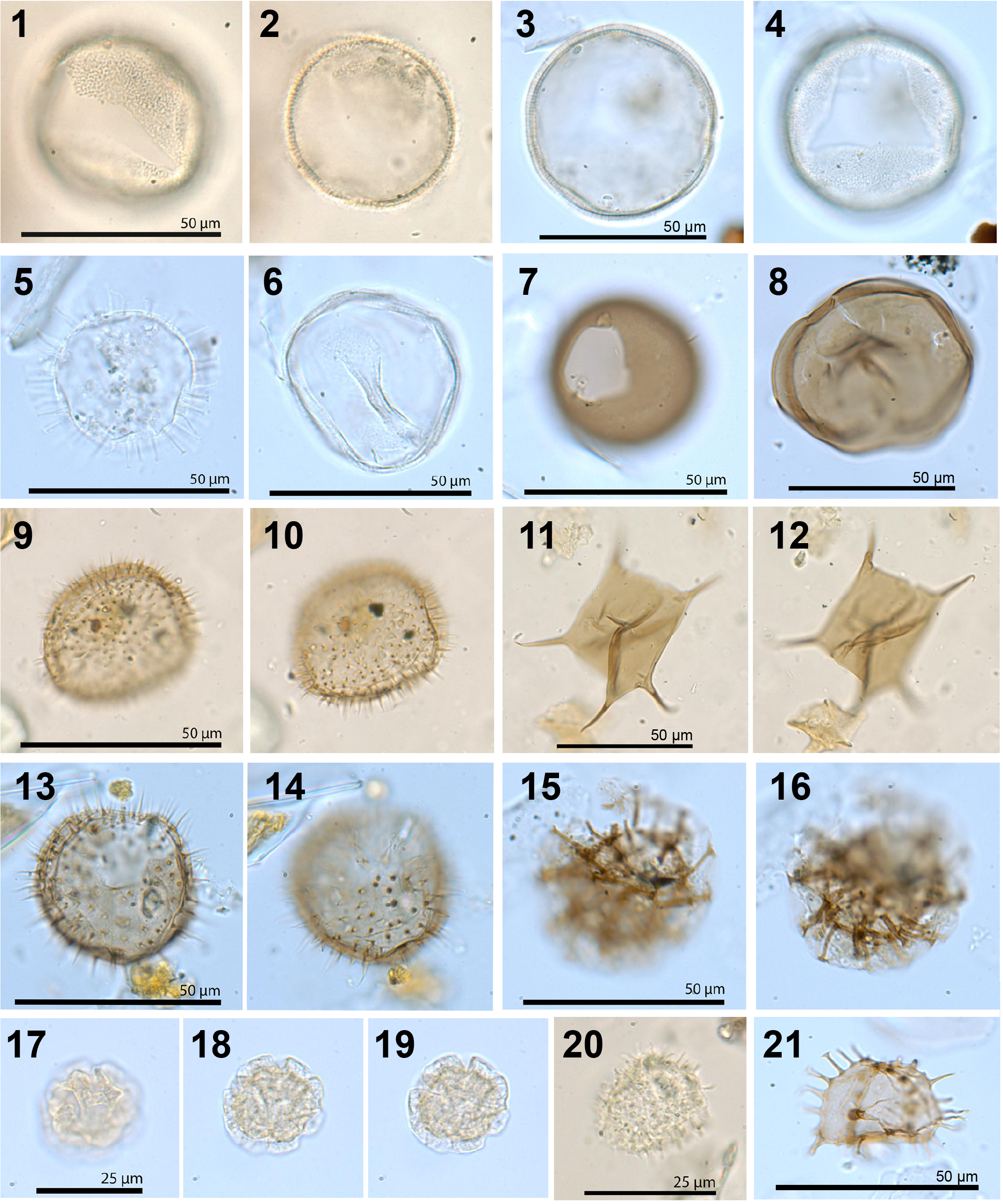
Figure F11. Dinocysts and acritarchs.
3.3.2. Dinocyst and acritarch sampling, sample preparation, and analysis
Samples were collected from selected core catchers over the entire depth of the first hole at each site. In addition, core catcher samples were analyzed for the deepest hole from the stratigraphic record that was not recovered by the first hole. Targeted samples from non–core catcher intervals were occasionally collected and analyzed for dinocysts to refine age estimates and the biostratigraphy.
For safety reasons, the sampling preparation aboard JOIDES Resolution did not include the use of acids, in particular hydrofluoric acid. The preparation was based on the nonacid protocol of Riding and Kyffin-Hughes (2006) and IODP Expedition 400 (Knutz et al., 2025b). The nonacid preparation could not fully remove clay particles and/or diatoms, which sometimes made dinocyst analysis difficult. Therefore, core catcher samples from some sites (U1618–U1620) were collected for onshore acid-based preparation following the expedition.
The shipboard palynological preparation protocol was as follows. About 5–15 g of sediment sample was placed into a 2 L glass beaker, and ~200 mL of distilled water and ~1% Liquinox were added. The samples were put on a shaker and left for a minimum of 4 h and often overnight. The beaker was transferred to a magnetic hotplate at medium heat (~50°C), and the mixture was agitated using a plastic-coated magnetic stirrer before adding ~30 mL of borax powder ((NaPO3)6 flakes). The sample was left on the magnetic hotplate for a minimum of 20 min while stirring. The sample was sieved at 125 µm to remove larger particles and biogenic content and at 10 µm to retain small dinocysts and acritarchs. All detergent and borax was washed out, and the >10 µm fraction was retained. The residue was transferred to a watch glass that floated in a sonicator. The sonicator was switched on for 5–10 s to separate the fines from heavier particles using a pipette. The fine residue was returned to the sieve and then the watch glass for up to three sonicator treatments, which removed most of the larger particles. The residue was finally transferred to a centrifuge vial and spun at 3000 rpm for 4 min. When needed, the residue was sieved one more time at 10 µm and then returned to the centrifuge. After removing most supernatant, the concentrated residue was put on microscopic slides and mounted with glycerine jelly.
Marine palynomorphs were analyzed using a Zeiss Axioskop microscope with brightfield illumination at 100×, 200×, 400×, 630×, and 1000× (oil) magnification. For each sample, one 22 mm × 40 mm slide was scanned along nonoverlapping traverses. In situ dinocysts and acritarchs, organic linings of foraminifers, pollen and spores, and freshwater palynomorphs were identified, and the amount of reworked marine and terrestrial palynomorphs was estimated. Most dinocysts were identified to species level. Spiniferate cysts were often grouped in Spiniferites, except for Spiniferites elongatus, Spiniferites mirabilis, and Spiniferites ramosus. All round, brown heterotrophic cysts with no clear archeopyle were classified as round brown cysts. When an archeopyle was visible, those were classified as Brigantedinium and Brigantedinium simplex.
The abundance of dinocysts per sample was estimated as follows:
- A = abundant (>50 specimens per 10 traverses).
- C = common (20–50 specimens per 10 traverses).
- R = rare (10–20 specimens per 10 traverses).
- B = barren (<10 specimens per 10 traverses).
For each dinocyst species in the assemblage, the following categories were used:
- D = dominant (>30% of total assemblage).
- A = abundant (10%–30% of total assemblage).
- C = common (5%–10% of total assemblage).
- R = rare (<5% of total assemblage).
When a sample was barren or had <20 specimens counted, all categories were set to rare (R). For acritarchs, the same categories were used, but the acritarch abundance is relative to the total number of dinocysts.
3.4. Planktonic foraminifers
3.4.1. Planktonic foraminiferal taxonomy and biozonation scheme
Planktonic foraminiferal taxonomy largely follows that of Kennett and Srinivasan (1983). Identification of left- and right-coiling Neogloboquadrina pachyderma was done following Darling et al. (2006). If the right-coiling forms constituted less than 3%, they were referred to as N. pachyderma (aberrant forms). In assemblages where the right-coiling forms constituted between 3% and 97%, they were counted as Neogloboquadrina incompta (Table T4).
High-latitude planktonic foraminiferal assemblages are of low diversity, and, as such, biostratigraphic datums are infrequent. However, preliminary ages were assigned using Neogene planktonic biostratigraphic zonations from the North Atlantic (Weaver and Clement, 1986; Spiegler and Jansen, 1989). During analysis, it was also registered if benthic foraminifers were present. Species identification of benthic foraminifers was only carried out if they held any potential biostratigraphic information (i.e., Cibicides grossa [cf. Anthonissen, 2008] and Cassidulina teretis [cf. Seidenkrantz, 1995]) (Figure F12).
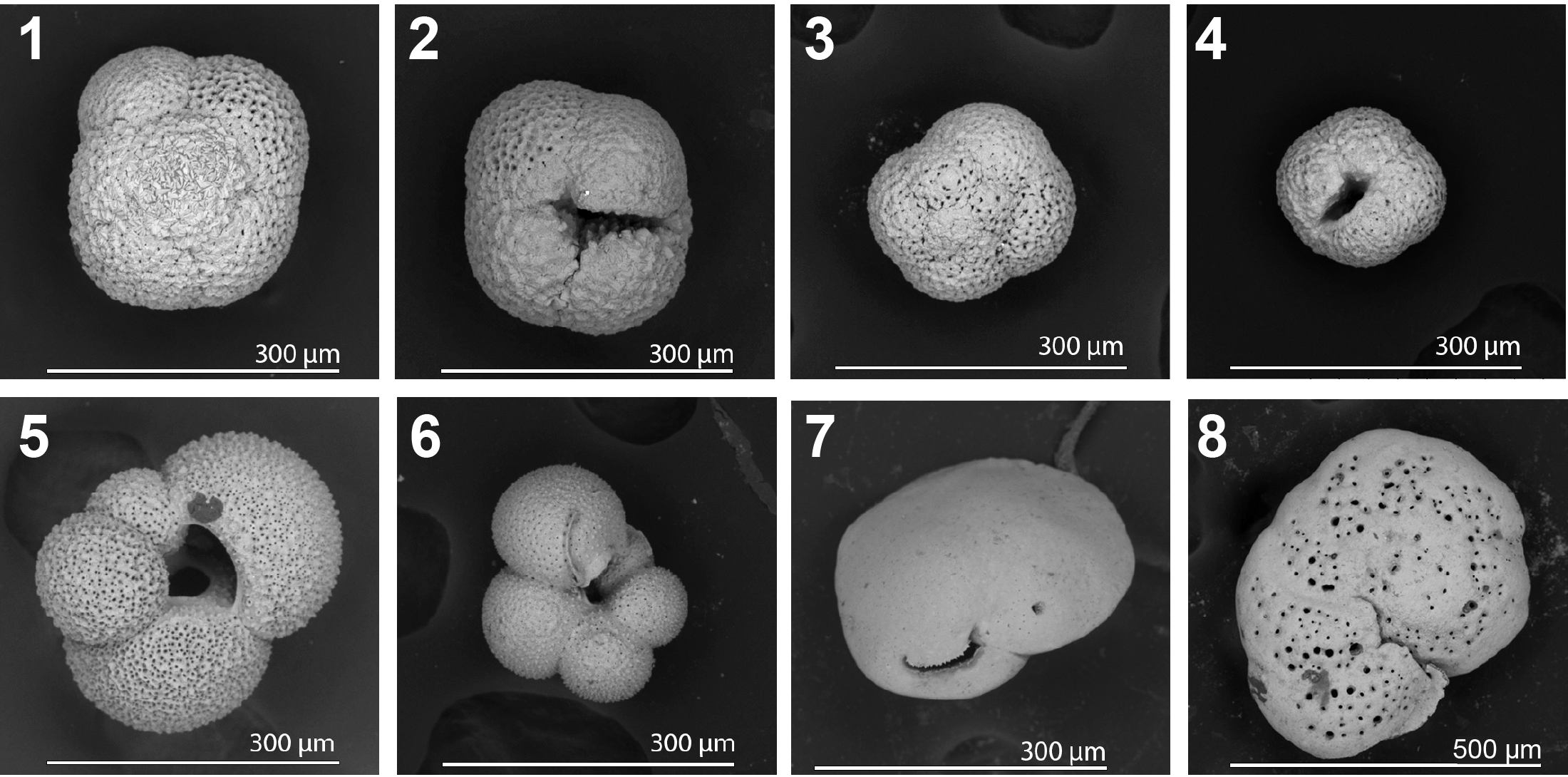
Figure F12. Foraminifers.
3.4.2. Planktonic foraminiferal sampling, sample preparation, and analysis
Shipboard identification of planktonic foraminifers was carried out on core catcher samples. Sample volumes of 20 cm3 were disintegrated by soaking in reverse osmosis (RO) water and washing through a 63 µm sieve using an Easy Washer Apparatus developed by Fabricio Ferreira (JOIDES Resolution Science Operator [JRSO]). Samples consisting of more consolidated sediments were disintegrated by soaking in RO water for 2–6 h before wet sieving. Even more consolidated sediments were left soaking in hydrogen peroxide (5%) for 20–30 min before wet sieving at the 63 µm size fraction. All samples were rinsed in RO water before drying in a thermostatically controlled drying cabinet at ~45°C. After drying, samples were dry sieved at 125 µm. To minimize contamination of foraminifers between samples, the sieve was thoroughly rinsed with water and placed into a sonicator for 5–10 min and then systematically checked. The faunal analysis was carried out using a Zeiss Discovery V8 stereo microscope. The >125 µm size fraction was analyzed with regard to foraminiferal fauna composition and abundance in addition to preservation and fragmentation. Images of specimens representing the observed species were taken using a camera mounted on the microscope. Scanning electron micrographs of planktonic foraminiferal species were acquired by mounting the specimens on a stub and acquiring images with a Hitachi TM3000 tabletop microscope. Selected foraminifers are illustrated in Figure F12.
The abundance of planktonic foraminifers as a group relative to the total sieved residue was categorized as follows:
- A = abundant (>50%).
- C = common (25%–50%).
- F = frequent (10%–25%).
- R = rare (<5% of the residue).
- B = barren (no specimens in sample).
Preservation of the foraminiferal tests includes any effects of abrasion, encrustation, and/or dissolution. The degree of these degrading effects on the foraminifers was categorized as follows:
- H = high (a high degree of abrasion, encrustation, and/or dissolution).
- M = moderate (abrasion, encrustation, and/or dissolution effects are common).
- L = low (abrasion, encrustation, and/or dissolution effects are rare).
Foraminifer fragmentation was categorized as follows:
- H = high (fragments are more common than whole tests).
- M = moderate (partially broken tests or fragments are common).
- L = low (fragmentation is observed in a minority of specimens).
4. Paleomagnetism
Paleomagnetic investigation during Expedition 403 focused on measuring the natural remanent magnetization (NRM) and alternating field (AF) demagnetization of the NRM on archive-half sections and a limited number of discrete cube samples. AF demagnetization of APC/HLAPC archive-half sections was limited to 20 mT (Site U1619) or 15 mT (all other sites) peak fields to remove the drill string overprint (Richter et al., 2007) and identify a characteristic remanent magnetization (ChRM) that could be matched to the magnetic polarity intervals of the geomagnetic polarity timescale (GPTS) (Gradstein et al., 2020). These low AF values were selected to balance the competing goals of timely core processing, identifying/removing drilling overprints, and preserving the NRM for more detailed shore-based analysis. Because XCB cores do not use nonmagnetic core barrels and are more susceptible to the viscous isothermal remanent magnetization (VIRM) drill string overprint (Richter et al., 2007), XCB archive-half sections required higher AF demagnetization steps to remove this overprint and were measured before and after 15 and 30 mT peak AF demagnetization.
In general, one to two discrete cube samples (~7 cm3) per core were taken from the working-half sections recovered from the first hole at each site, avoiding sections and intervals that were visually disturbed. In some cases, extra cubes were taken from intervals that needed additional investigation because the cube samples often appeared to provide more reliable results in XCB cores and allowed for initial assessment of the magnetic mineralogy. Cube sample NRMs were studied with more detailed AF demagnetization at 5–10 mT increments to assess the reliability of archive-half measurements. A ChRM was identified using principal component analysis and assessed using the maximum angular deviation parameter (Kirschvink, 1980). All cube samples were measured for MS and given an anhysteretic remanent magnetization (ARM). A subset were given isothermal remanent magnetizations (IRMs) to provide an additional initial assessment of the magnetic mineralogy.
4.1. Core recovery and coordinates
Cores collected using the APC and HLAPC coring systems used nonmagnetic core barrels; however, they are more brittle than standard core barrels and could not be used with the XCB system (see Operations). The BHA included a Monel (nonmagnetic) drill collar for all holes because it could potentially reduce the magnetic field near where the core is cut and in the core barrel. The field inclination expected from a geocentric axial dipole (GAD) is quite steep at the latitudes drilled during Expedition 403 (expected GAD inclinations are 83.1°–84.5°), and in 2024 magnetic inclination ranges 81.6°–82.8° (Table T5). Recent high-latitude expeditions have found that the orientation tool does not have the precision or reliability necessary to orient cores at these steep inclinations (e.g., McKay et al., 2019; Weber et al., 2021a) and polarity can confidently be interpreted using inclination alone. Therefore, use of the magnetic orientation tool was not considered necessary.
All magnetic data are reported relative to IODP orientation conventions: +x points toward the double line at the bottom of the working half, +y points toward the left side of the working half when looking downcore, and +z is downcore (Figure F13). This coordinate system differs from that of the superconducting rock magnetometer (SRM) (Figure F13), but the appropriate transformations are made in the IODP IMS software. Cube samples from the working half were taken by either pushing the plastic cube into the core surface or by using a hollow metal extruder and then transferring the sediment into the plastic cube. In both cases, the −z (upcore) direction was aligned with the inscribed arrow on the base of the box and the +x face (toward the double line; into the face of the working half) was covered with the plastic lid (Figure F14).
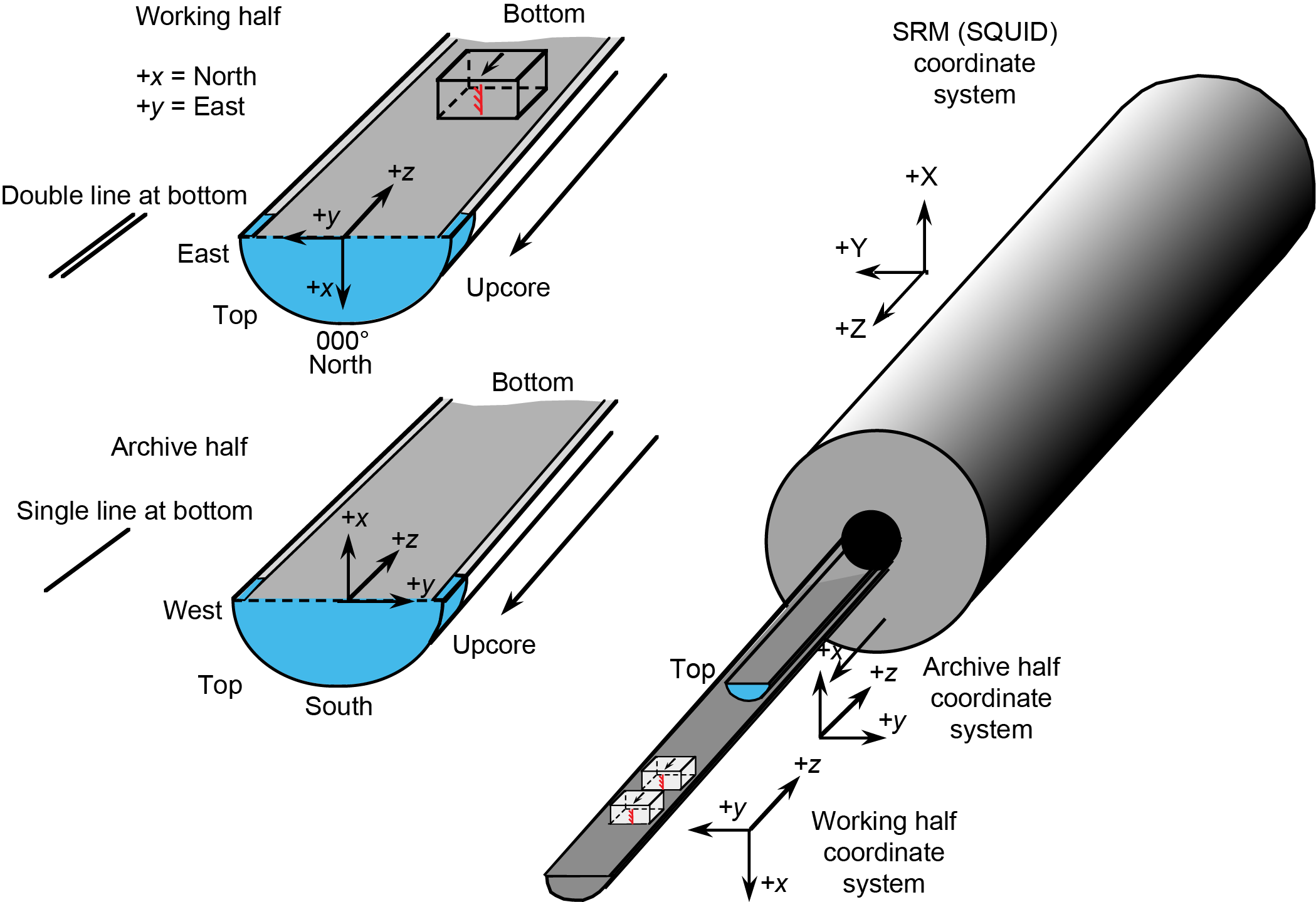
Figure F13. Coordinate systems, orientation of archive-half sections and discrete cube samples, and SRM.
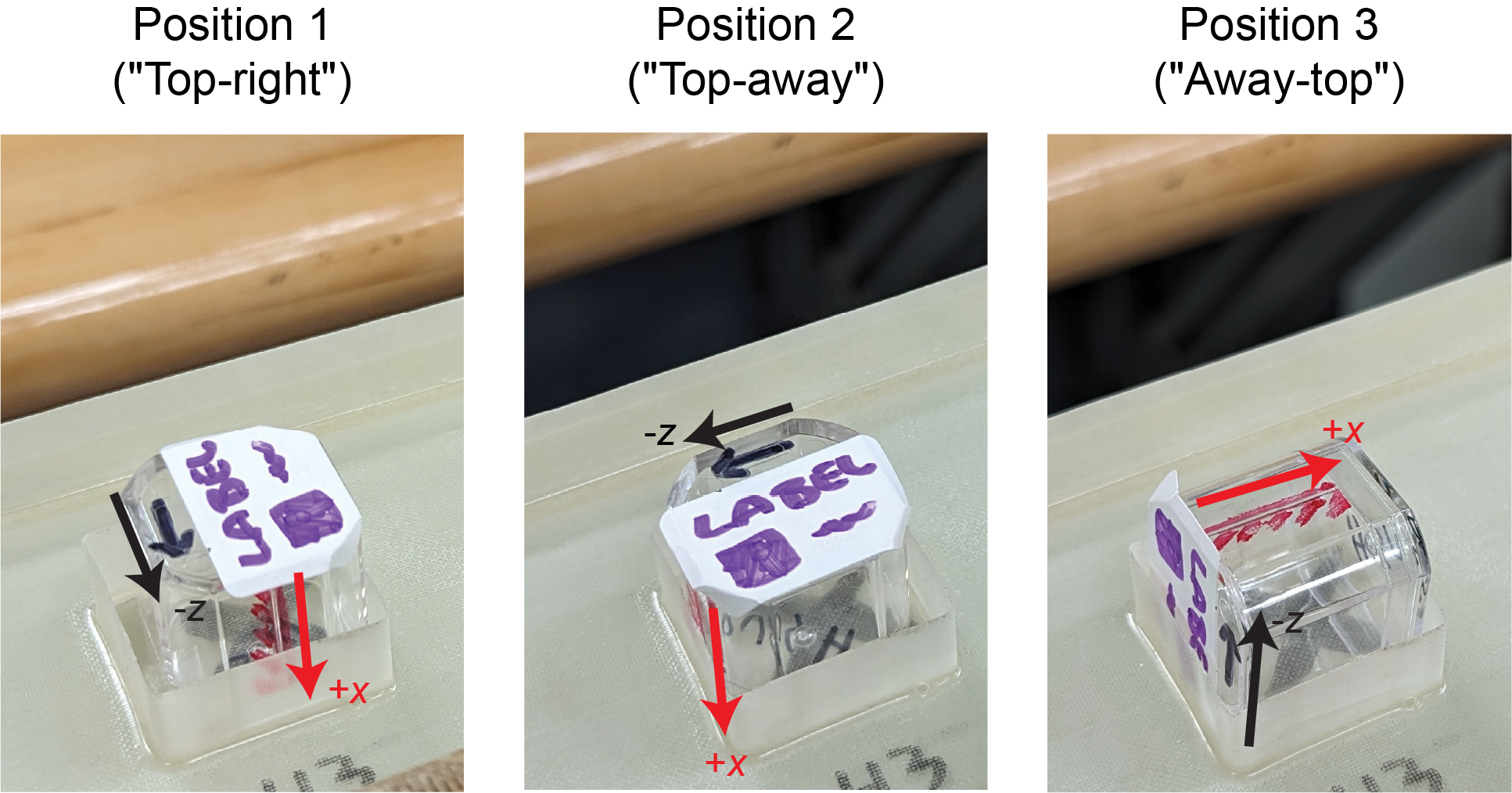
Figure F14. Discrete sample orientation.
4.2. Natural remanent magnetization
All remanence measurements on archive section halves and most on discrete samples were made using a 2G Enterprises Model 760-4K SRM optimized for measuring IODP half cores equipped with direct-current superconducting quantum interference devices (DC-SQUIDs) and an in-line AF demagnetizer capable of fields up to 80 mT. The IODP-recommended peak AF field for routine analysis is 50 mT, which was the maximum field used on discrete cube samples except in a few circumstances where a 60 mT peak field was used. The effective resolution for archive-half measurements is a function of the integrated response function, determined to be 7.4, 7.2, and 9.1 cm for the X-, Y-, and Z-axes, respectively (Acton et al., 2017).
The sample tray was cleaned with DI water as often as deemed necessary and at least once per hole. The sample tray was then AF demagnetized with a peak field of 50 mT, and its remanence was measured using the section background routine to update the background correction values for the empty sample tray. Archive-half measurements were made at 2.5–5 cm intervals with a 15 cm trailer and leader to monitor the background magnetic moment. In general, for APC/HLAPC cores we measured the initial NRM and the remanent magnetization remaining after 10 and 15 mT peak AF demagnetization. The one exception was at Site U1619, where we used 10 and 20 mT steps. For XCB-cored intervals, we measured the initial NRM and the remanent magnetization remaining after 15 and 30 mT peak AF demagnetization. In Hole U1624C, we modified this to only use the 30 mT step to keep up with core flow.
Generally, one to two oriented discrete samples per core were sampled near the center of the core to avoid disturbed sediments near the core liner, with locations chosen to avoid coring disturbance and capture representative lithofacies. In XCB cores, we sampled from larger intact biscuits whenever possible; however, in some cores where large biscuits were not obvious or present, we sampled where there was less visible deformation, often in consultation with the shipboard sedimentologists. Additional samples were taken in some cases to better define polarity intervals. At some sites, we preferentially sampled intervals from low MS intervals because these intervals appeared to yield more reliable paleomagnetic results. Discrete samples were collected by pushing plastic Japanese-style cubes (external edge length = 2 cm; internal volume = ~7 cm3) into the working halves with the inscribed arrow marker on the cube pointing toward the stratigraphic up (−z) direction. When the sediment was more indurated, a hollow metal tube was pushed into the working half and a plunger was used to extrude the sample, first onto a clean cutting board and then into the plastic cube to preserve the same relative −z and +x orientation as the pushed cubes.
Discrete cube samples were measured and subjected to detailed demagnetization up to 100 mT peak AF, with the maximum peak field dependent on sample behavior, when the remanence intensity drops below 10% of the NRM, core flow time constraint, or the instrument being used. The majority of samples were measured on the SRM using the in-line AF demagnetization system and discrete sample tray, with cubes placed 20 cm apart in the top away position (Figure F14) and a combination of 5, 10, 15, 20, 25, 30, 35, 40, 45, 50, and 60 mT peak AF. Some samples were measured on the AGICO JR-6 spinner magnetometer and demagnetized using the ASC DTECH D-2000 AF demagnetizer, allowing for additional higher AF steps of between 60 and 100 mT.
4.3. Laboratory magnetizations
Discrete samples were analyzed for bulk MS and anisotropy of magnetic susceptibility (AMS) using the MFK2-FA Kappabridge. Measurements were made using the 3D rotator at 425 A/m field intensity at 976 Hz. ARMs were applied to all samples following demagnetization of the NRM in a 100 mT peak AF and 0.05 mT bias field using the ASC DTECH D-2000 demagnetizer. The majority of the ARMs were measured on the SRM before and after 30 mT peak AF demagnetization, although some samples of interest were subject to additional AF demagnetization. A subset were measured and demagnetized on the AGICO JR-6 spinner magnetometer and the ASC D-TECH D-2000 demagnetizer. IRMs were applied to select samples at 100, 300, and 1000 mT using an ASC IM-10 impulse magnetizer. All IRMs were measured on the AGICO JR-6 spinner magnetometer because some of these IRMs might be too strong to measure on the SRM.
MS, ARM, and IRM data were used to construct parameters sensitive to magnetic grain size and mineralogy. These included the ratio of ARM to MS (Banerjee et al., 1981; King et al., 1982), ratios of the ARM after demagnetization to the initial ARM (e.g., Peters and Thompson, 1998), and the S-ratio (Stober and Thompson, 1979).
In a few cases, we sampled targeted authigenic iron sulfide nodules. Small amounts of this material were removed from the core and mounted in cyanoacrylate glue within a paleomagnetic cube. These samples were measured for their bulk MS using the same settings as the normal sediment cubes: frequency-dependent MS at 200 A/m and 976/15616 Hz; ARM; and IRMs imparted at 100, 300, and 1000 mT. ARM imparted with a 0.05 mT bias field and 100 mT peak AF and IRM imparted at 300 mT were subject to detailed AF demagnetization up to 100 mT peak AF. When the nodule could be removed as an intact piece, we measured the NRM of the sample before and after AF demagnetization at 10, 20, 30, 40, 50, 60, 70, 80, 90, and 100 mT before imparting any laboratory magnetizations.
4.4. Magnetometer standards
On the initial transit, the IODP SRM standards 5, 6, 7, 8, 10, 11, and 12, created at the Scripps Institution of Oceanography (SIO), were measured to test the software's treatment of the three discrete positions and to compare to values determined at SIO in November 2019 and aboard JOIDES Resolution in November 2022. First, the samples were run three times using the Archive Section Half setting at 1 cm resolution with the +x arrow facing up and the −z arrow facing away from the SRM (as the archive half would be oriented). This demonstrated consistency in measurements (all circular standard deviations for the three measurements were <0.25°) and confirmed the position of the discrete samples relative to the tray. Next, the standards were measured three times in the three perpendicular orientations described above (Figure F14). Circular standard deviations of the three measurements at each position were higher than when the cubes were run as an archive half but were generally <0.5° and always <2°. Circular standard deviations of the measurements from the three perpendicular orientations range 5.4°–7.6°. The higher circular standard deviation could be explained in part by imperfect placement of the standards on the tray when rotated to the three positions, some rotation of the round tray on the SRM track between runs, and/or slight differences in the X-, Y-, and Z-SQUIDs. All results indicate that the software is making the correct rotations for each orientation (Figure F15).
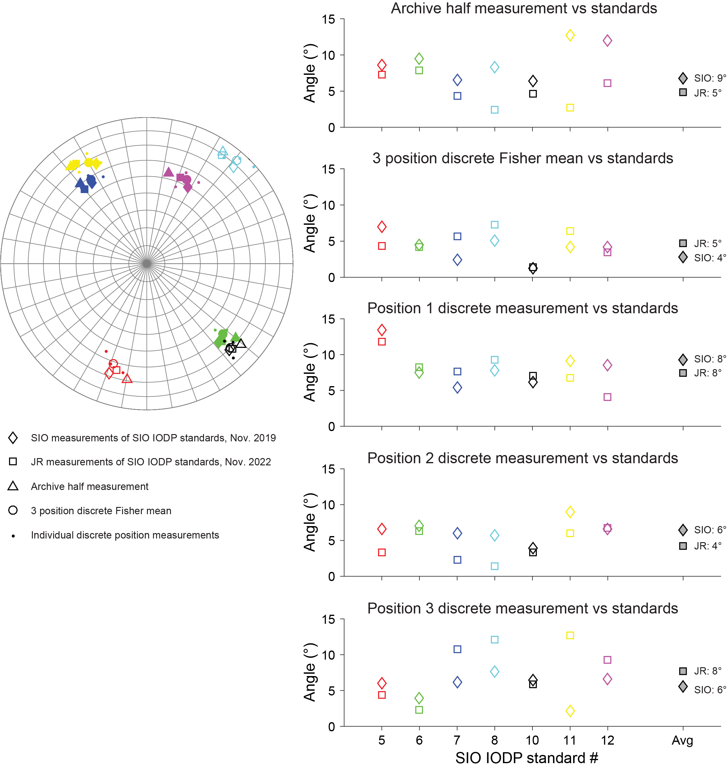
Figure F15. SRM and software assessment.
Figure F15 illustrates the comparison of these new measurements with the previous SIO and IODP documentation of each standard's inclination and declination. The spread in values is largely in the horizontal plane (X- and Y-directions in the SRM coordinates), which may in part reflect rotation of the tray by a few degrees while making measurements on the JOIDES Resolution SRM. When the standards were run as an archive half or in discrete position 2 (with the −z-axis facing away from the magnetometer), our results were most similar to the prior measurements aboard JOIDES Resolution in November 2022 (the date in the IODP documentation for which these comparisons can be made) (a difference of 4° or 5°) that were run with a similar orientation. We found values most similar to the SIO values measured in November 2019 when we took the Fisher mean (Fisher, 1953) of the three perpendicular discrete measurements (a difference of 4°), with the individual positions and archive-half setting showing a larger difference to these previously measured values (difference of 6°–9°). Overall, we find this uncertainty reasonable for our work while on board, noting that archive-half measurements appear to be very internally consistent between runs and that more accurate results can be achieved through measuring discrete samples in multiple positions and averaging.
4.5. Magnetostratigraphy
Magnetic polarity zones were assigned based on changes in inclination after the maximum AF demagnetization step (i.e., either 15, 20, or 30 mT) with careful consideration of the results from cube samples. During XCB coring, polarity assignment was sometimes made only using the discrete cube samples because these often seemed to provide more consistent results, had inclinations that were more consistent with expected values for a GAD, and had initial data to characterize their magnetic mineral assemblage. After a polarity stratigraphy was established for a given hole, we correlated the pattern with the GPTS (Gradstein et al., 2020) (Table T6). Correlation to the GPTS was informed by discussions with the shipboard biostratigraphy team when needed. Pleistocene (C1n–C2r) ages for magnetic reversals in the 2020 geologic timescale (GTS2020; Gradstein et al., 2020) were updated from the 2012 geologic timescale (GTS2012) based on the review of Channell et al. (2020), which considered geographically distributed sediment records that could be directly intercalibrated with benthic δ18O and the LR04 timescale of Lisiecki and Raymo (2005). GTS2020 Pliocene (C2An–C3n) reversal ages are the same as those in the GTS2012, derived from orbital tuning of Mediterranean sections described by Lourens et al. (1996, 2004). Late Miocene (C3r–C4r.1r) reversal ages have been updated to the timescale of Drury et al. (2017) based on orbital tuning of benthic stable isotopes from Integrated Ocean Drilling Program Site U1337 in the equatorial Pacific Ocean.
5. Physical properties
Physical properties measured on whole-round sections and split core halves are fast, continuous, high-resolution measurements that are used for lithostratigraphic characterization and stratigraphic correlation. Physical properties measured shipboard during Expedition 403 yielded information for identifying coring discontinuities, changes in sediment density, porosity, and inferred composition. Shipboard physical property data also provided essential information for determining hole-to-hole correlations, constructing stratigraphic splices, and making site-to-site correlations. Techniques and methods for obtaining physical properties in whole-round, split half, and discrete samples are adapted from previous IODP expeditions and shipboard user guides.
5.1. Sampling and measurement sequence
After cores were cut into ~1.5 m sections on the core receiving platform (see Operations), they were labeled and laser engraved. These whole-round sections were then run through the STMSL, which measured GRA bulk density and MS for initial hole-to-hole correlations (see Sediment workflow). STMSL measurements were made with a 2.5 cm step or at a 5 cm step where high core recovery necessitated a faster processing time. Cores were then allowed to warm to room temperature for 4 h to ensure thermal and barometric homogeneity, protect sensors from damage, and minimize temperature effects on P-wave velocity. After temperature equilibration, whole-round sections were run through two physical property core logging systems: the WRMSL and the NGRL. The WRMSL measured GRA bulk density, MS, and P-wave velocity at 2.5 cm intervals. NGR measurements were performed at 10 cm intervals. In addition, several 10 cm interval samples were selected for ASR analysis and taken within 2–4 h of core recovery. ASR intervals were measured on the STMSL and NGRL but were excluded from WRMSL measurements.
After the core sections were split into halves, one or two discrete samples targeting representative lithologies were collected for MAD analyses from working halves in every core from Hole A and deeper cores of subsequent holes. One working-half section per core was used to measure P-wave velocities with the Section Half Measurement Gantry (SHMG) and thermal conductivity with the TeKa TK04 thermal conductivity meter where sediment quality permitted. Archive halves were run on the SHIL and the SHMSL to capture a core image and to measure color reflectance and point MS (see Lithostratigraphy). An overview of the sampling strategies for physical properties measured during Expedition 403 is provided in Table T7. Detailed procedures for each physical property measurement are described below.
5.2. Whole-round logger measurements
5.2.1. Gamma ray attenuation bulk density
GRA bulk density was acquired on both the STMSL and the WRMSL for all whole-round sections (Figure F16) except cores selected for studies of sedaDNA (see Microbiology). The GRA instrument on the STMSL and the WRMSL measures the attenuation of a directed gamma ray beam through the core, which is related to sediment density. The beam is produced by a 137Cs capsule with a principal energy peak of 660 KeV and radiation level of 370 MBq. The radiation is contained within a lead (Pb) shield with a 5 mm collimator. The 137Cs source is situated directly above the core track, and a scintillation detector with an integrated photomultiplier is mounted on the underside of the core opposite the source. The scintillation detector measures the attenuated gamma radiation that passes through the core. As the incident gamma rays (photons) travel through the core, they are scattered by electrons in the formation due to Compton scattering. The degree of scattering depends on the material, with higher density material leading to lower intensity of gamma rays reaching the detector. This is used to estimate the bulk density (ρ) of the sediment:
- Io = gamma ray source intensity,
- I = intensity of gamma rays passing through the sample,
- µ = Compton attenuation coefficient, and
- d = sample diameter (Evans, 1965; Harms and Choquette, 1965).
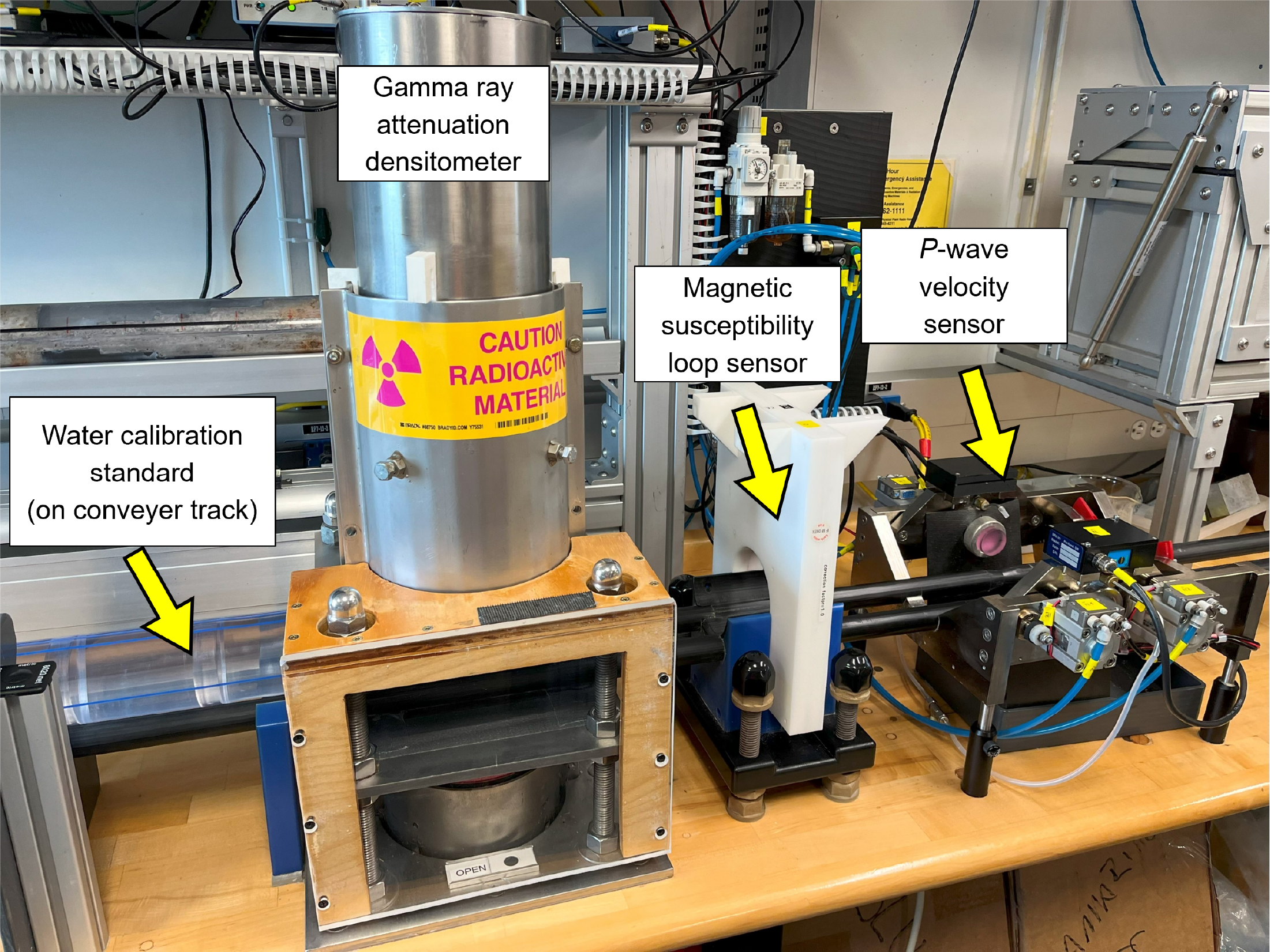
Figure F16. WRMSL.
GRA bulk density depends on sample composition and is influenced by sample porosity, grain density and consolidation, and core disturbance. GRA bulk density measurements are most accurate when made on a completely filled liner with minimal gaps and core disturbance; otherwise, measurements underestimate density values. GRA instrument calculations are based on a 66 mm internal core diameter, appropriate for the APC and HLAPC systems.
The instrument was calibrated using sealed aluminum and water calibration tubes of different diameters (after Blum, 1997) and recalibrated with DI water when the DI water standard deviated significantly (>2%) from 1 g/cm3. Measurements were performed at 2.5 cm increments (5 cm step on the STMSL for intervals where high core recovery necessitated a faster processing time).
5.2.2. Magnetic susceptibility (loop)
MS was acquired on the STMSL and the WRMSL (Figure F16). MS (χ) is a dimensionless parameter that indicates how much material is magnetized by an external magnetic field. χ is defined as
where M is the magnetization induced in the material by an external field with strength (H). MS is acquired at low fields, typically <0.5 mT. Ferromagnetic materials (e.g., magnetite and titanomagnetite) have high χ values, several orders of magnitude higher than paramagnetic and diamagnetic minerals (e.g., carbonate, opal, water, and plastic), which have very small or negative χ values. Siliceous and biogenic clays may have χ values close to the limit of detection. MS indicates the concentration of magnetic material in a volume of sediment, which can be used to interpret mineralogy and diagenesis.
MS measurements on the STMSL and WRMSL were made with a Bartington MS2C loop sensor with a 90 mm loop diameter at a frequency of 565 Hz, using an automatic software correction factor of 1.174 and a ~140 A/m AF to adjust for a change in oscillator frequency caused by sediment cores passing through the instrument. The loop measurement resolution is 20 mm and accuracy is 2%, as stated in Barrington specifications (Blum, 1997). The loop automatically zeroed in air before each run, and a measurement was taken at the end of a core section to correct for instrument drift. The output for χ values is reported in dimensionless instrument units. Measurements were performed at an interval of 2.5 cm steps (5 cm steps on the STMSL for intervals where high core recovery necessitated a faster processing time).
5.2.3. Compressional P-wave velocity
Compressional P-wave velocities were acquired using the WRMSL P-wave logger (PWL) track for all cores (Figure F16) except those sampled for ASR analysis. P-wave velocity is affected by sample lithology, porosity, bulk density, lithostatic pressure and temperature, sediment fabric and degree of consolidation, degree of fracturing within the material, and abundance of free gas. P-wave velocities combined with density values are used to obtain acoustic impedance and downhole reflection coefficients and estimate the depth of reflector layers in seismic profiles. P-wave velocity (VP) is defined as
where d is the length of the core section and tcore is the traveltime through the core.
For P-wave velocity measurement, the core was pushed along the track between two transducers (a transmitter and a receiver) mounted on stainless steel holders on either side of the track. Acoustic coupling through the epoxy was improved by water sprayed on the liner surface by an automated drip system during measurements. A transmitter sent a pulse equivalent to 2 µs wave periods at 120 V and frequency of 1 kHz, generating an ultrasonic compressional pulse of ~500 kHz. Pulse timing was measured with a resolution of 50 ns. The compressional P-wave that propagated horizontally was amplified by an automatic gain control amplifier and registered by the receiver on the opposite side. Total traveltime (ttotal) of the compressional wave between the transducers was measured. A calibration of the PWL accounts for errors in ttotal and total distance (dtotal). To correct for the core liner, a traveltime through a core liner (tliner) of known thickness (L) was measured for a section filled with distilled water, which had a velocity of ~1480 m/s. Additionally, traveltime was measured through a standard block of aluminum with a known velocity of 6295 m/s and used for a system delay correction (tdelay). Arrival times at the inflection point of the second lobe of the waveform gave a second correction (tpulse), which was incorporated into a total delay correction (ttotal_delay) to account for combined delay related to transducer, electronic circuitry, and peak detection procedures delay. Accordingly, VP was calculated as
This equation does not account for gaps in the core or voids where the core does not completely fill the liner. Therefore, signal strength at low values cannot always be attributed to attenuation. Measurements were performed at 2.5 cm increments.
5.2.4. Natural gamma radiation
The NGR measurements were acquired using the NGRL system built by IODP (Vasiliev et al., 2011; Dunlea et al., 2013) (Figure F17). The NGRL measures the gamma radiation emitted during the decay of mineral-hosted 238U, 232Th, and 40K (respective half-lives: 4.4 × 10⁹, 1.4 × 10¹⁰, and 1.3 × 10⁹ y). Parent isotopes and their daughter products emit gamma radiation at characteristic energy levels unique to each isotope. Measurements of NGR energy spectra can be used to estimate the concentration of each isotope (Blum, 1997; Gilmore, 2008). Th and K are typically associated with clays, whereas U is associated with organic-rich materials. High NGR counts identify fine-grained K-rich clay deposits and their absorbed U and Th atoms. NGR data can be utilized in downcore geochemical interpretations, as well as for core-to-core and core-to-wireline log data, and hole-to-hole correlations.
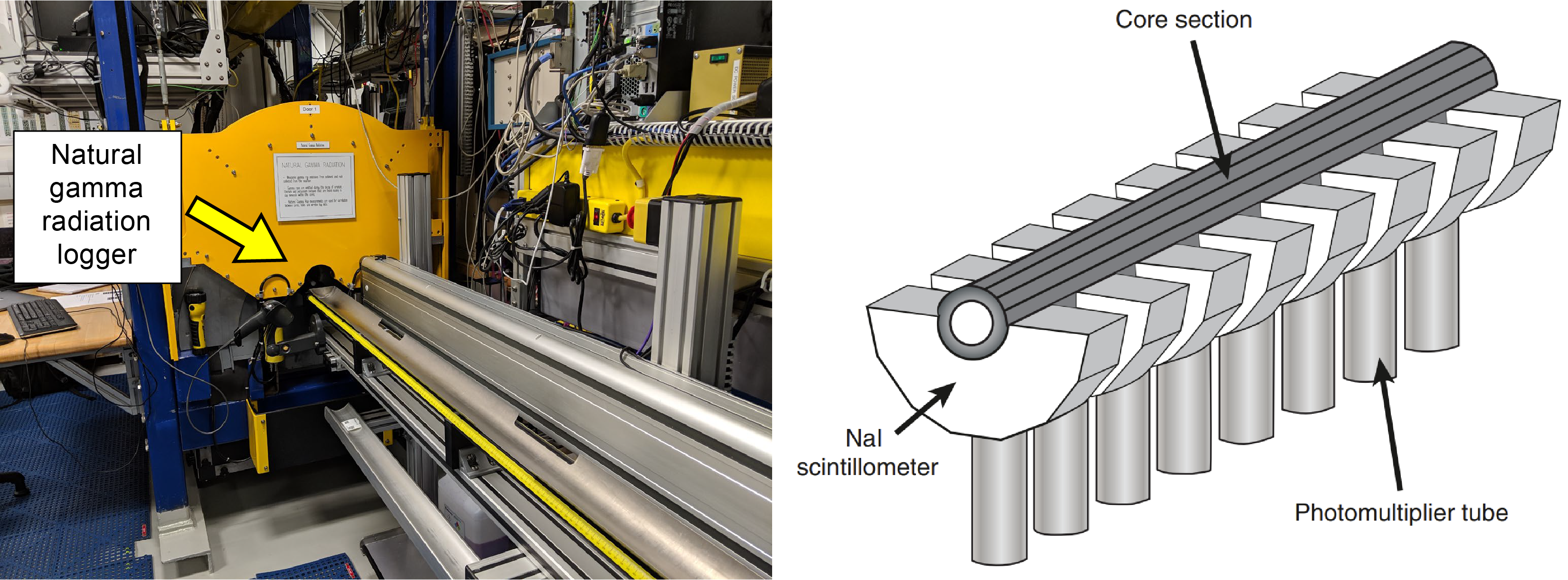
Figure F17. NGRL.
The NGRL system consists of eight sodium iodide (NaI) scintillator detectors surrounding the lower half of the section, placed along the core axis at 20 cm intervals. The NaI detector array is shielded to reduce background environmental and cosmic radiation. Detectors are surrounded with layers of passive lead shielding; in addition, active plastic scintillators detect high incoming high-energy gamma and muon radiation and subtract the background signal from the total counts.
The quality of NGR data depends on sample radionuclide concentration and on counting times, with higher times yielding better spectra. NGR counts were measured for 300 s at two sample positions 10 cm apart, with 8 measurements per position resulting in 16 measurements per section.
5.3. Anelastic strain recovery
The ASR technique is a core-based stress measurement that can evaluate both orientation and magnitude of 3D present-day principal stress on rock. The ASR approach was used to measure the anelastic strain change by releasing the stress soon after core recovery. The methodology used for ASR measurement during Expedition 403 is based on Matsuki (1991), following the guidelines described in Lin et al. (2007). A ~10 cm long undisturbed whole-round section was selected for ASR measurement on the catwalk. STMSL and NGR measurements were performed on the ASR samples but not WRMSL measurements because those are time sensitive and require instrumentation as soon as the core is retrieved to capture early strain recovery. Samples were selected for ASR measurement based on the hardness and/or density measurements from STMSL scans. Those samples were then pushed out of their core liners, and the outer surface was immediately removed by sanding with 160 or finer mesh sandpapers to remove drilling mud and make a flat surface prior to analysis.
The anelastic strains, shown by the elliptical shape of the specimens in nine directions, including six independent directions, were measured using 18-wire strain gauges (six cross and six single gauges). In cases where a few fractures had developed in the specimen, the fractures were glued or fixed with tape to prevent the sample from splitting into pieces. It took 1–2 h to mount 18 strain gauges, and the total elapsed time from core on deck was 2–4 h before starting to record the strain recovery. The core samples were triple bagged (with plastic and aluminum) and submerged in a thermostatic water bath where temperature changes were kept controlled at 17° ± 0.1°C for the duration of the measurement. Strain values were collected every 10 min for at least 6 days.
The ASR protocol was sometimes supplemented with headspace gas measurements (see Geochemistry) to evaluate if sediment degassing was affecting ASR measurements.
5.4. Thermal conductivity
After the cores were split, thermal conductivity was measured on the split face of the working-half section for each core (Figure F18). Thermal conductivity is a material property that depends on density, composition, and sedimentary fabric. Heat flow calculated from thermal conductivity profiles can be an indicator of fluid circulation processes. Cores were thermally equilibrated for at least 4 h and then split. Measuring points were chosen to avoid cracks, fractures, and any coring disturbances. Thermal conductivity was measured with the TK04 instrument using the puck method (Von Herzen and Maxwell, 1959). The puck, containing a heater rod and a calibrated thermistor, was placed on top of the core section. A small amount of DI water was used on the measuring point to ensure good contact with the probe. The measurement was performed in a thermally insulated container to minimize thermal interference from the laboratory surroundings.
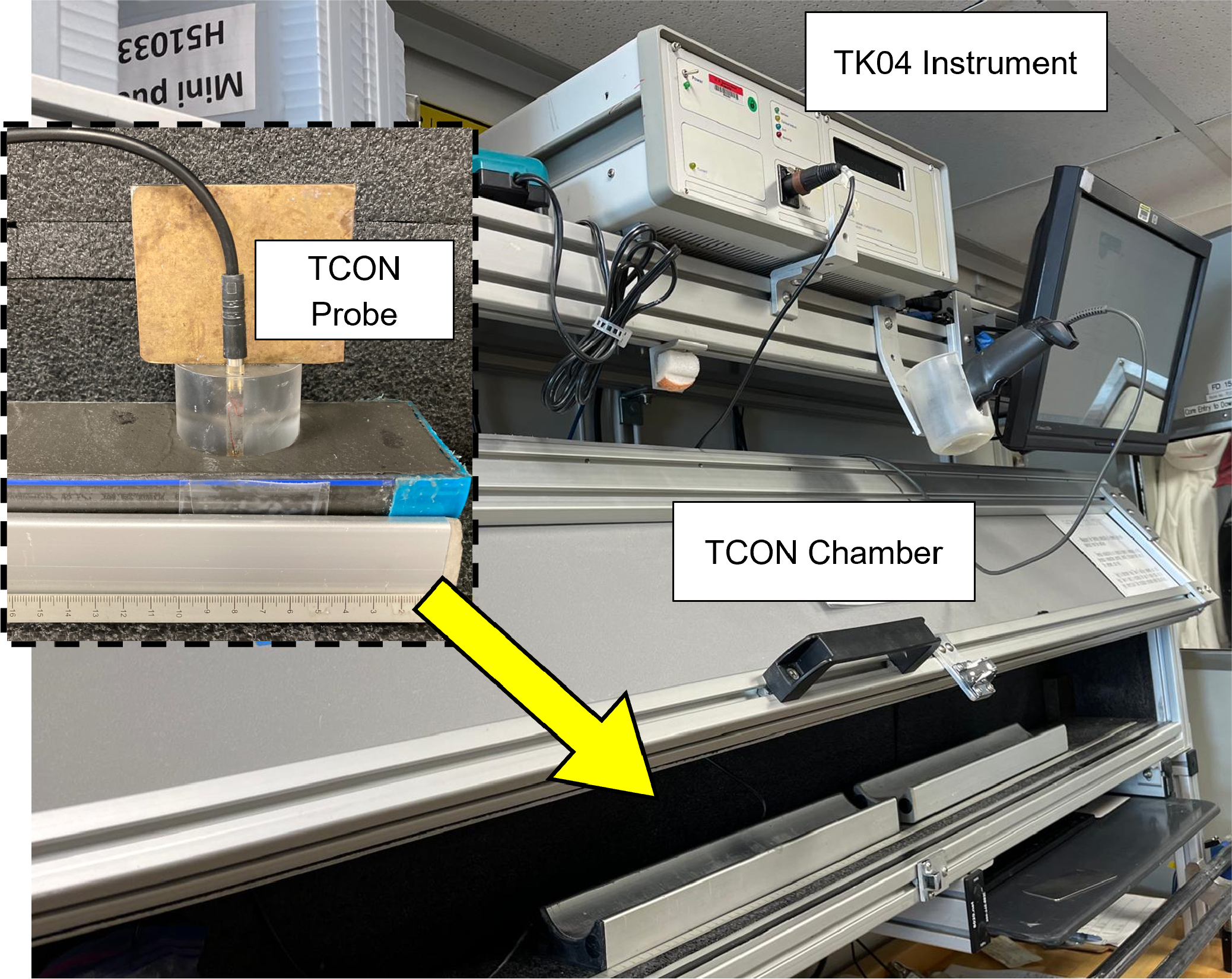
Figure F18. Thermal conductivity station.
The puck acts as a perfect conductor because its thermal conductivity is much higher than that of the sediment. The temperature of the probe is related to the time after heat initiation:
- T = temperature (K),
- q = heat input per unit length per unit time (J/m/s),
- k = thermal conductivity (W/[m∙K]),
- t = time after the initiation of the heat (s), and
- C = instrumental constant.
After the puck temperature stabilized, the rate of temperature rise in the sample was used to determine the thermal conductivity of the sample (Kristiansen, 1982; Blum, 1997). Measurements were made in triplicate to obtain an average thermal conductivity at each sampling horizon. The TK04 instrument performed a self-test and a drift correction at the beginning of each measurement cycle.
5.5. Section Half Measurement Gantry
Discrete P-wave velocity measurements were performed on the working half of split cores using the SHMG. Measurements were typically made once per core in the first complete hole of each site where sediment allowed and a signal was detectable. The y- and z-bayonets were used for softer sediments, and the x-caliper was used for all sediments (Figure F19). When using the P-wave caliper for the x-axis (vertical to the split surface of the section), plastic film was placed on the core surface with a small amount of DI water to ensure an even contact and reduce disturbance. Section intervals for measurements were selected to accommodate lithologic variations, drilling disturbances, fractures, larger clasts, general core quality, and MAD samples (see Sampling and measurement sequence).
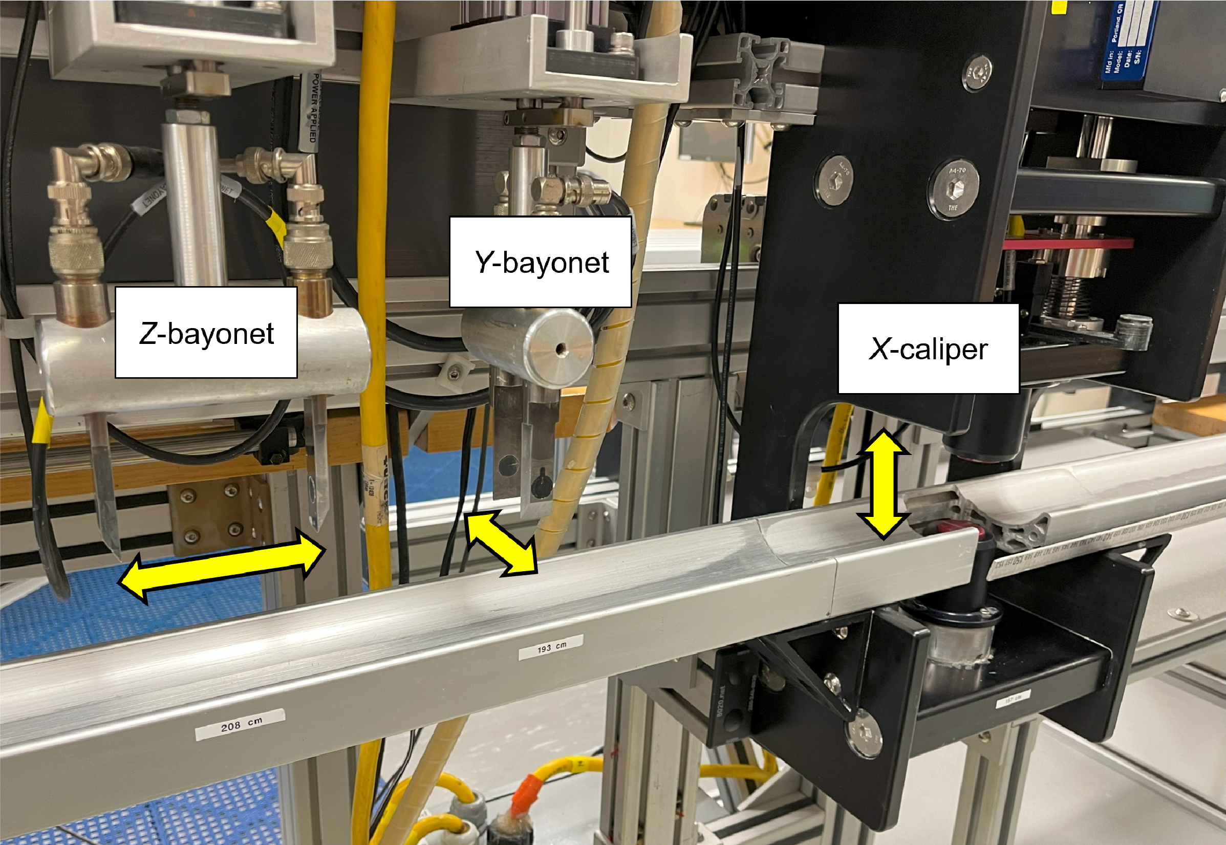
Figure F19. SHMG.
The SHMG uses Panametrics-NDT Microscan delay line transducers, which transmit at 0.5 MHz. The signal received through the sample was recorded by the computer attached to the system, and the peak (P-wave arrival) was chosen with an autopicking software. In the case of a weak signal or poor contact with the core, the first arrival was manually picked by the instrument operator. The distance between transducers was measured with a built-in linear voltage displacement transformer (LDVT). Calibrations were performed with a series of acrylic cylinders of differing, known thicknesses and a published P-wave velocity of 2750 ± 20 m/s. The system time delay determined from calibration was subtracted from the chosen arrival time to calculate a traveltime of the P-wave through the sample. Sample thickness (calculated by the LDVT in meters) was divided by the traveltime (in seconds) to calculate the P-wave velocity (in meters/second).
5.6. Moisture and density
Discrete samples from working halves were selected for MAD measurements to determine wet and dry bulk density, grain density, water content, salt content, and porosity. Samples (~10 cm3) were collected with a 2 cm diameter plastic syringe or metal extruder, depending on sediment hardness, and placed in a 12 cm3 glass vial. Two samples were collected per core for MAD measurements; if the core was shorter (three sections or less), only one sample was collected. Intervals for MAD samples were selected to capture representative lithologies and to avoid disturbances, cracks, voids, large clasts, and conflict with other sampling priorities (e.g., paleomagnetic cubes).
Samples were placed in prelabeled, preweighed 16 mL Wheaton glass vials to measure wet and dry sediment mass (Figure F20). The wet sample mass of each sample was first measured, and then samples were placed in a convection oven at 105.5° ± 5°C for a minimum of 24 h to dry. After drying, samples were placed in a desiccator to cool for at least 3 h and then measured for dry mass and volume. The weights of wet and dry sample masses were determined to a precision of 0.005 g using two Mettler Toledo electronic balances, with one balance acting as a reference and one as an unknown. A standard weight value similar to that of the sample (within ~5 g) was placed on the reference balance to increase accuracy of the unknown sample measurement. An averaging algorithm in the MADMax software was used to correct for the motion of the ship. The default measurement setting of the two balances was 300 measurements over an interval of ~1.5 min for each sample.
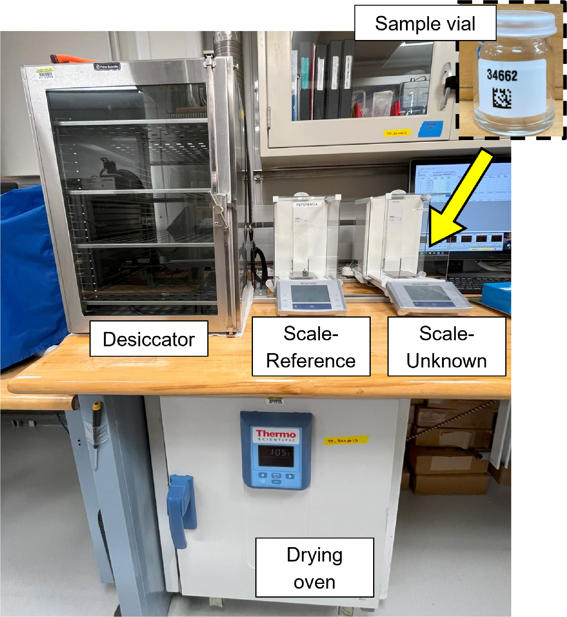
Figure F20. MAD sample preparation materials.
Dry sample volume was determined using a six-celled, custom-configured Micromeritics AccuPyc 1330TC helium-displacement pycnometer (Figure F21). The precision of each cell is 1% of the full-scale volume. Volume measurements were preceded by three purges of the sample chamber with helium warmed to ~28°C. Three measurement cycles were run for each sample. For every measurement, a reference volume (calibration spheres) was sequentially placed in one of the six chambers to check for instrument drift and systematic error. The volumes of the numbered Wheaton vials were calculated before the expedition by multiplying the weight of each vial against the average density of the vial glass. The procedures for the determination of these physical properties comply with the American Society for Testing and Materials (ASTM) designation D2216 (ASTM International, 1990). The fundamental relation and assumptions for the calculations of all physical property parameters are discussed by Blum (1997) and summarized below.
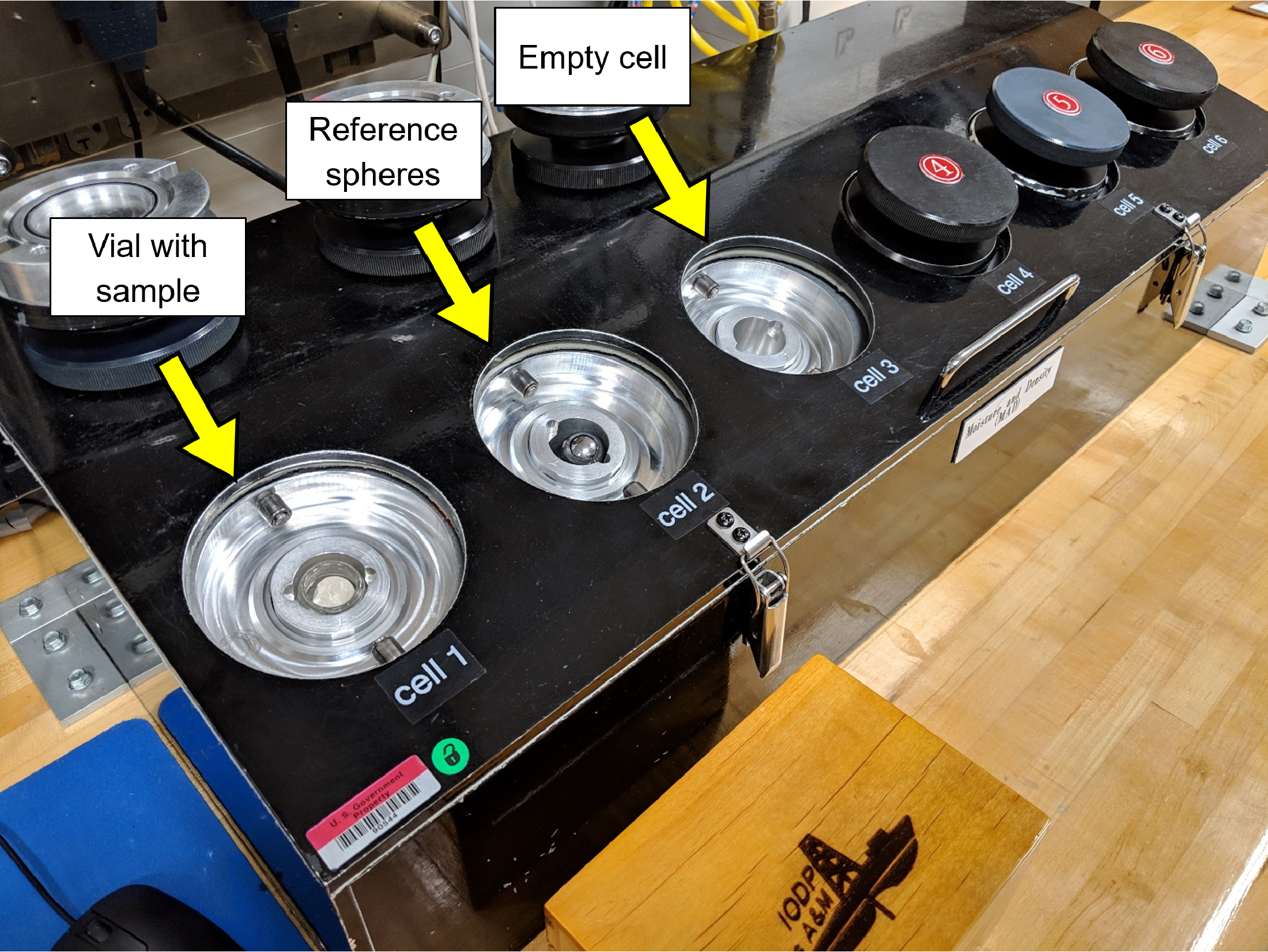
Figure F21. Pycnometer.
5.6.1. Mass and volume calculations
Wet mass (Mwet), dry mass (Mdry), and dry volume (Vdry) were measured in the laboratory as detailed above and used to calculate several parameters related to the mass and volume of water and salt in each sample. The ratio of mass (rm) is a computational constant of 0.965 g of freshwater per 1 g of seawater. Salt precipitated in sediment pores during the drying process is included in the Mdry and Vdry values. The mass of the evaporated water (Mwater) and salt (Msalt) in the sample are given by
where s is the assumed saltwater salinity (0.035%) corresponding to a pore water density (ρpw) of 1.024 g/cm3 (from experimental and empirical relations between salinity and density at laboratory conditions; Blum, 1997) and a salt density (ρsalt) of 2.22 g/cm3. The corrected mass of pore water (Mpw), volume of pore water (Vpw), mass of solids excluding salt (Msolid), Msalt, volume of salt (Vsalt), volume of solids excluding salt (Vsolid), and wet volume (Vwet) are
5.6.2. Calculation of bulk properties
For all sediment samples, water content (w) is expressed as the ratio of mass of IW to wet sediment (total) mass:
Wet bulk density (ρwet), dry bulk density (ρdry), sediment grain density (ρsolid), porosity (ϕ), and void ratio (VR) were calculated as
All MAD properties reported and plotted in the Physical properties sections of each site chapter were calculated with the MADMax shipboard program, which was set with the Method C calculation process (Blum, 1997).
6. Stratigraphic correlation
Cores were recovered during Expedition 403 using a combination of APC and XCB technologies. The stratigraphic correlation for the expedition followed the practices and protocols of previous IODP expeditions. As with any IODP paleoceanographic expedition, the scientific objectives of Expedition 403 demanded recovery of complete stratigraphic sections to generate continuous records that allow the reconstruction of climate and ocean variability with high temporal resolution. Such recovery is difficult to achieve with a single hole because coring gaps generally occur between successive cores during the APC coring process, despite 100% or greater recovery (e.g., Ruddiman et al., 1987; Hagelberg et al., 1995; Acton et al., 2001). Furthermore, the top of any core might sample sediment that has fallen into the hole, resulting in stratigraphic noise. Thus, the reconstruction of a complete, continuous, and representative stratigraphic section, referred to as a splice, requires the combination of stratigraphic intervals from two or more holes cored at the same site, where the depths of core gaps are staggered between holes. Given this context, the primary objectives of the shipboard work of the stratigraphic correlators were fourfold:
- To correlate sediment physical properties data (e.g., MS, GRA bulk density, NGR, and color) among holes;
- To use this correlation as a guide while drilling to minimize gap alignment;
- To construct composite depth scales for all holes drilled and corresponding tables of vertical depth offsets from the composite depth scale of each hole; and
- To construct the most representative single continuous sedimentary section for each site by splicing intervals from multiple holes.
The procedure for each of these activities involves consideration of several depth scales (Figure F22). The depth scales used during Expedition 403 followed IODP conventions (see IODP Depth Scales Terminology at http://www.iodp.org/policies-and-guidelines) and are described in methodological order.
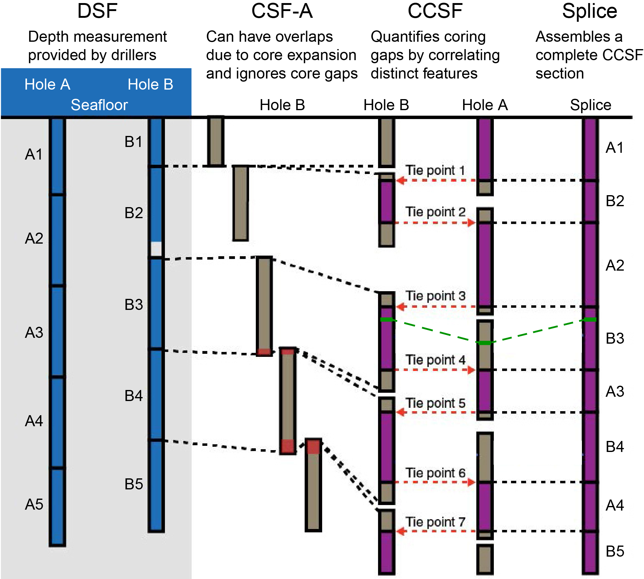
Figure F22. Relationships between cored material and depth scales.
6.1. Measurement and method for correlation
For most sites, initial correlations to inform the development of a composite depth scale were based on the stratigraphic correlation of MS and GRA density data sets acquired from the STMSL as soon as possible after core retrieval. This allowed stratigraphic correlation to take place in near–real time such that bit depth could be adjusted as necessary to avoid alignment of core gaps between holes. No single variable proved to be universally useful at all sites for stratigraphic correlation or splice construction. Thus, at all sites, correlation proceeded through a combination of measurements obtained with the WRMSL, the NGRL, the SHMSL, and the SHIL. Parameters primarily used were MS and GRA density measured with the WRMSL at 2.5 cm resolution, NGR measured with the NGRL at 10 cm resolution, a* and L* measured with the SHMSL at 2.5 cm resolution, and R value (red) extracted at 1 cm resolution from core images acquired with the SHIL. Details on instrument calibrations, settings, and measurement intervals for Expedition 403 are given in Lithostratigraphy and Physical properties.
This first-order ship-based correlation is expected to be verified and secured on shore after the expedition with the generation of adjusted or revised composite depth scales based on XRF scanning data, which can be used to refine linkages between core and logging depths at sites where logging was done.
6.1.1. Using correlation to minimize gaps while drilling
To maximize the probability of bridging gaps between successive cores in individual holes, the starting depths below seafloor from which cores are recovered are offset between holes. This practice ensures that most missing sedimentary sections due to coring gaps and onboard sampling (e.g., IW and paleontology [PAL] samples) in a given hole are recovered in one or more adjacent holes.
6.2. Construction of composite depth scales
The construction of composite depth scales depends first on understanding the depth scale for individual holes, which is the CSF-A scale. This is followed by describing and differentiating among the different types of composite depth scales.
6.2.1. Core depth below seafloor (CSF-A) scale
The depth to the top of each core is based on a drill string measurement (DSF scale), which is determined by the length of drill string below the rig floor to the top of the cored interval minus the length of drill string from the rig floor to the mudline (assumed to be the seafloor). The depth to a point along the core is determined by adding the position at which the point occurs to the core top depth. This CSF-A depth scale is equivalent to the historical (DSDP, ODP, and Integrated Ocean Drilling Program) mbsf scale and is specific to each hole. The zero-depth point of the CSF-A scale is defined by the mudline in the first core of each hole. However, it is often difficult to tell whether this empirical mudline recovers the true sediment/water interface. Some holes are inadvertently (or purposely) started below the sediment/water interface. In this case, the zero-depth point on the CSF-A scale may be substantially offset from the zero-depth point in adjacent holes that successfully recover the sediment/water interface. The CSF-A scale may also be inaccurate because of ship heave, tidal variations in sea level, and other sources of error. DSF scale errors are due to phenomena such as pipe and BHA stretch and compression, tides, and uncompensated ship heave. Tidal influence on this depth measurement can sometimes be significant (Hagelberg et al., 1995), and the prediction of tides is generally useful for guiding drilling to avoid gap alignment (Mix et al., 2003). The maximum tidal range during Expedition 403 was typically <1.5 m, and therefore it was on par with other sources of error (especially heave).
The depth to a given position within any core is then determined relative to the DSF core top depth. The CSF-A scale therefore combines the DSF core top depth with the curated depth within a core after retrieval. It is important to note that the within-core position of any given sedimentary feature may change after recovery under various influences such as the relief of overburden, gas-induced expansion, or water loss. Thus, error in the CSF-A scale includes both drilling effects and core expansion effects, and, as one consequence, the CSF-A scale permits overlap between successive cores (e.g., caused by expansion) that are stratigraphically impossible. In principle, the composite depth scale, described below, should rectify such artifacts.
6.2.2. Core composite depth below seafloor (CCSF-A) scale
The composite section and splice construction methodology employed during Expedition 403 followed the basic strategy originally developed during ODP Leg 138 (e.g., Hagelberg et al., 1992, 1995) and later refined during many other ODP legs and IODP expeditions, specifically Expedition 397 (Abrantes et al., 2024). This strategy is now common practice on all high-resolution paleoceanographic expeditions. Assembly and verification of a complete composite stratigraphic section requires construction of a composite depth scale, referred to as the core composite depth below seafloor, Method A (CCSF-A), depth scale. The composite depth scale provides a common depth scale for the holes at a site that is different from the original mbsf or CSF-A scale, which has drilling measurement as the top and curated length as the bottom depth. It is also different from the DSF scale due to deviations in the length of core recovery resulting from sediment expansion (common), compression, and core loss. The DSF, CSF-A, and CCSF-A scales are unique to each hole.
The construction of a common, composite depth scale for a given site involves identification of coeval, laterally continuous features in all drilled holes at an individual site (which will generally occur at different depths on the CSF-A depth scales for each hole). After correlative features are identified, the depth of individual cores are offset relative to CSF-A in that hole such that the features align on a common depth scale. The resulting CCSF-A scale is equivalent to the historical (ODP and Integrated Ocean Drilling Program) mcd scale. In constructing the CCSF-A scale, the depths of each individual core are offset by a constant amount, using a single tie point in each core, which therefore does not compensate for stretching or squeezing within individual cores. This composite depth scale provides good estimates of the length of coring gaps and provides the basis for development of the spliced record (on the core composite depth below seafloor, Method D [CCSF-D], scale). The vertical depth offset of every core in every hole is tabulated in an affine table, one of the principal deliverables of the stratigraphic correlator. The growth rate, also listed in the affine table, describes the vertical depth offset as a quotient; at each core top level, the growth rate is calculated by dividing the core top depth in meters CCSF-A by the core top depth in meters CSF-A. A growth rate of 1.1 means that the CCSF scale is expanded by 10% relative to the CSF scale.
In practice, the CCSF-A scale is built by correlating features downhole from the mudline. The mudline establishes the top of the stratigraphic section, anchoring the entire composite depth scale for all cores from all holes at a site. The compositing proceeds sequentially by establishing specific tie points among the various holes, working from the mudline (anchor) in the backbone core to the bottom of the drilled section. The CCSF-A scale very rarely (if ever) results in alignment of all coeval features because of the differing effects of coring-induced stretching and squeezing among cores, as well as sedimentologic differences between holes (Figure F22). Gas expansion due to the abundant methane hydrates proved to be problematic at most sites cored during Expedition 403 and resulted in high growth rates, mostly below 100 mbsf (see the site chapters for details).
In principle, if core gaps never come into alignment between all holes at a site and recovery is sufficiently high, then it should be possible to correlate each successive core in one hole to a core from an adjacent hole all the way to the bottom of a drilled section. However, aligned coring gaps across all holes at a site are often difficult to avoid. In the case of an aligned core gap, cores below the gap are no longer tied to the anchor core. They can, however, still be tied to one another to produce correlated sections that are floating on the CCSF-A scale. Such floating ties were denoted in the affine table as APPENDED or SET, depending on whether the offset to the top of that section was estimated by inheriting the absolute offset of the core above (APPENDED) or by assuming a constant growth rate (SET). The SET method is preferable because estimates of the expansion of cores from the same hole can be considered, thus leading to more realistic approximation of coring gaps.
During the process of constructing the composite section, the CCSF-A depth becomes systematically larger than that of the CSF-A depth for equivalent horizons. This expansion, typically as much as ~15%–30% at our sites, results primarily from decompression of the cores as they are brought to the surface, gas expansion, stretching that occurs as part of the coring process, and curation of material that has fallen downhole (e.g., Hagelberg et al., 1995; Acton et al., 2001).
6.2.3. Splice core composite depth below seafloor (CCSF-D) scale
After the CCSF-A scale is developed and the between-core gaps are identified, a complete stratigraphic section (splice) is constructed by combining selected intervals between the previously established tie points. The depth scale is designated the CCSF-D scale, which can be considered a subset of the CCSF-A depth scale because this D designation applies only to intervals included in the splice. Intervals not included in the primary splice retain the CCSF-A scale. In the case of aligned core gaps across all holes, any spliced sections below the gap are offset relative to those above by either APPEND or SET and designated as floating splice sections. In principle, the amount of missing section between anchored and floating sections can be assessed using downhole logs.
6.2.4. Core composite depth below seafloor (CCSF-C) scale
After the splice is constructed, it is usually desirable to map into the splice those intervals not included in the splice itself. This can be accomplished by treating the splice as a downhole log. The methodology is based on identification of correlative tie points at the highest possible resolution, with linear adjustments of depths between ties. This is designated as the core composite depth below seafloor, Method C (CCSF-C), scale and can be thought of as an equivalent splice depth. In the ideal case, the CCSF-C and CCSF-D scales are equivalent. In reality, they are only equivalent to the extent that the correlations are accurate. At core boundaries, where strong stretching and compression are prevalent, these detailed depth maps will be less accurate. Tables of equivalent splice depth were not generated shipboard during Expedition 403, but in most cases they should be straightforward to generate by using the shipboard affine tables as starting points.
6.3. The splice
The splice is a composite stratigraphic section that represents the complete record through intervals at a site. It is composed of core sections from adjacent holes such that coring gaps in one hole are filled with core from an adjacent hole. An effort is also made to minimize the inclusion of disturbed sections or intervals of sediment fall-in (typically the top ~10–50 cm of a core) or flow-in. Disturbed sections are identified by examining the cores and their photographs and X-radiographs. The splice ultimately should guide core sampling for high-resolution studies.
In generating the splices, we tried to adhere to the following guiding principles:
- We defined tie points, where possible, close to stratigraphic intervals that had reduced variability to minimize the possibility that splice jumps occur during important climate transitions.
- Where possible, we avoided using the first and last sections of cores, where disturbance due to drilling artifacts (even if not apparent in core logging data) is most likely.
- We attempted to incorporate those parts of the stratigraphic sequence that in our judgment were most representative of the holes recovered and appeared to be the least disturbed.
Composite splicing was accomplished using Correlator software (version 4.5.4), from which standard affine tables (listings of the vertical offset in meters added to each core to generate the CCSF-A scales) and splice interval tables (listings of the specific core intervals used to construct the splice) were generated. These tables were uploaded into the IODP LIMS database, which then affixes the appropriate depth scale to any associated data set.
7. Geochemistry
The shipboard geochemistry program for Expedition 403 included measurements of headspace gas content (hydrocarbons), IW composition, and bulk sediment geochemical parameters.
7.1. Headspace gas geochemistry
Headspace sampling (HS) geochemical analysis is used to measure hydrocarbon gases in seafloor sediments and is essential to determine the safe continuation of drilling. These measurements are required for drilling to any depth, and thus the analyses are predominantly carried out on Hole A at each site. If, in any subsequent hole, the drilled depth exceeds the depth of Hole A, headspace gas analysis resumes.
During Expedition 403, hydrocarbon gas measurements were performed on ~5 cm3 samples from each core. The samples were collected on the catwalk from the top of a section near the middle of a core, adjacent to the IW sample, and immediately taken to the chemistry laboratory for analysis. In soft sediments, plug samples were taken using a syringe and extruded into a 21.5 cm3 glass serum vial with a crimped metal cap and a polytetrafluoroethylene (PTFE) septum. For harder sediments, fragments of sediment were transferred into the vial instead. The vial was then heated in the oven at 60°C for 30 min. While recovering cores with the APC, HLAPC, and XCB systems, expansion of entrapped gases can form voids in the sediments. When such voids were observed, the length was recorded before sampling on the core retrieval platform. Select void gas samples (VACs) were collected by piercing the core liner with a custom piercing tool that allows the gas to expand into a 50–60 mL gas-tight syringe connected to the tool.
A total of 5 cm3 of HS and VAC samples were extracted through the septum with a gas-tight glass syringe and injected into an Agilent 7890A gas chromatograph (GC) fitted with a flame ionization detector (FID) at 250°C to quantify concentrations of methane (C1), ethane (C2), ethene (C2=), propane (C3), iso-butane (iC4), n-butane (nC4), and iso-pentane (C5). The GC was equipped with a 2.4 m × 2.0 mm stainless steel column packed with 80/100 mesh HayeSep R. The injector consisted of a ¹⁄₁₆ inch Valco union with a 7 µm screen connected to a Valco-to-Luer lock syringe adapter. This injector connected to a 10-port Valco valve that was switched pneumatically by a digital valve interface. The injector temperature was set at 120°C. Gas samples were introduced into the GC through a 0.25 cm3 sample loop connected to the Valco valve. The valve can be switched automatically to backflush the column. The oven temperature program started at 80°C, maintained this temperature for 8.25 min, and then increased to 150°C at a rate of 40°C/min for a period of 5 min. Helium was used as the carrier gas, with an initial column flow of 30 mL/min. Flow was increased to 60 mL/min after 8.25 min to accelerate the elution of longer chained hydrocarbons. The run time was 15 min. The GC was also equipped with an electronic pressure control module to manage the overall flow into the GC. Chromatograms were collected and automatically evaluated using the Agilent Chemstation software. The integrated peak areas of low molecular weight hydrocarbons were quantified to parts per million by volume (ppmv) using a nine-point calibration with gas standards of known concentrations, as provided by Scott Specialty Gases (Air Liquide).
For all sites, methane concentrations were very high at specific sediment intervals and subsequently were plotted using a logarithmic scale to better show data trends. Heavier hydrocarbons (e.g., ethane) at some sites (e.g., U1618–U1620) were also very high and therefore were plotted using a logarithmic scale to better represent the data. At other sites (e.g., U1621–U1624), heavy hydrocarbons were relatively low in concentration, and therefore a logarithmic scale was not necessary for showing data trends.
7.2. Interstitial water chemistry
IW samples were obtained by squeezing 5 or 10 cm3 whole-round samples that were cut from cores immediately after core retrieval. For extremely low IW content sediment, 15 cm3 samples were used. The recovered IW was split for shipboard determination of salinity, alkalinity, pH, anions and cations, and major and trace elements, as well as for postexpedition IW research. Whole-round samples were typically collected at a frequency of one sample per core of previously unsampled material to avoid duplicate sampling of identical stratigraphic sections, to the bottom of the hole where sufficient material was available (i.e., >1.5 sections recovered) or until IW extraction produced <2 mL of IW after 3 h of squeezing at 30,000 force lb. The sampling frequency was reduced by half when using the HLAPC system or when cutting half cores with rotary coring systems. The exterior of the whole-round sample was carefully cleaned with a spatula to remove potential contamination from the drilling fluid. For XCB cores, the intruded drilling material between biscuits was also removed to eliminate contamination from the drilling fluid. The cleaned sediment was transferred into an 8 cm inner diameter titanium squeezer that was then placed in a Carver hydraulic press (Manheim and Sayles, 1974) and squeezed with slowly increasing pressure up to 30,000 force lb (1.335 × 10⁶ N). After discarding the initial drops to avoid contamination, the squeezed IW was collected into a 60 mL acid-washed (10% HCl) high-density polyethylene syringe attached to the squeezing assembly. If sample volume permitted, the IW samples were split as outlined in the analytical workflow below. If IW volume was limited (i.e., <20 mL but >2 mL), postexpedition samples or shipboard alkalinity/ICP-AES analyses were omitted on a case-by-case basis. Data produced on the Agilent 5110 inductively coupled plasma–optical emission spectroscope (ICP-OES) were collected in atomic emission spectroscopy (AES) mode and are referred to as ICP-AES in the LIMS Online Reports (LORE) database. Hereafter in this document, ICP is used to refer to these data.
The priority list for shipboard analyses and postexpedition samples from IW was as follows (from high to low priority):
- Salinity (~100 µL): determined by optical refractometry immediately after squeezing.
- pH and alkalinity (~3 mL): titrated/determined immediately after squeezing.
- Anions and cations (~100 µL) (Na+, K+, Ca2+, Mg2+, Cl−, Br−, and SO42−): determined using IC.
- Phosphate (~0.6 mL) and ammonium (50 µL): determined by spectrophotometry.
- Major and trace element analyses (~0.5 mL) (B, Ba, Ca, Fe, K, Li, Mg, Mn, Na, Si, and Sr): determined by ICP; addition of 10 µL concentrated trace metal clean HNO3.
For all analyses, IW was filtered through a 0.45 µm polysulfone disposable filter (Whatman) into 15 mL centrifuge tubes, except for aliquots for ICP analysis. Alkalinity, pH, and salinity were measured immediately after squeezing. All other shipboard analyses were carried out in batches.
7.2.1. Shipboard analyses
IW samples were analyzed on board following the protocols in Gieskes et al. (1991), Murray et al. (2000), and the JRSO user manuals for shipboard instrumentation.
7.2.1.1. Alkalinity, pH, and salinity
Alkalinity and pH were measured using a Metrohm autotitrator (Model 794 Basic Titrino) equipped with a pH glass electrode and a stirrer (Model 728). The pH readings were obtained directly from the LabVIEW Alkalinity program, where alkalinity was measured by titrating 3 mL of sample with 0.1 M HCl until reaching an end point of pH = 4.2. Standardization for both measurements was achieved using the International Association for the Physical Sciences of the Oceans (IAPSO) seawater standard, which was analyzed repeatedly during the expedition and reproduced within 2%. Salinity was analyzed using a Fisher Model S66366 refractometer calibrated using 18 MΩ Millipore DI water. The known salinity of the IAPSO seawater was used for data quality control.
7.2.1.2. Ion chromatography
Aliquots of IW were diluted at 1:100 with DI water for analysis of Na+, K+, Ca2+, Mg2+, Cl−, Br−, and SO42− using a Metrohm 850 Professional ion chromatograph. IAPSO seawater standard was used for standardization of measurements.
7.2.1.3. Spectrophotometry
Aliquots of IW samples were diluted with 18 MΩ Millipore water for analysis of ammonium and phosphate using an Agilent Cary 100 UV-Vis spectrophotometer. Ammonium analyses were conducted using phenol diazotization and subsequent oxidation by sodium hypochlorite (NaOCl) to yield a blue color, measured spectrophotometrically at a wavelength of 640 nm. Ammonium chloride (NH4Cl) was used for calibration and standardization. Phosphate concentrations were determined following the protocol in Gieskes et al. (1991). In the phosphate method, orthophosphate reacts with Mo(VI) and Sb(III) in an acidic solution to form an antimony-phosphomolybdate complex. Ascorbic acid reduces this complex, forming a blue color that is measured at 880 nm. Potassium phosphate monobasic (KH2PO4) dissolved in 18.2 MΩ water was used to produce a calibration curve with 1, 5, 10, 15, 20, 40, 60, 80, and 100 µM concentrations to check for instrument linearity.
7.2.1.4. Inductively coupled plasma spectrometry
Dissolved major (Ca, K, Mg, and Na) and minor (B, Ba, Fe, Li, Mn, Si, and Sr) element concentrations were determined using an Agilent 5110 ICP-OES with an SPS4 autosampler. IW samples were diluted 1:10 in 2% HNO3 and spiked with an internal standard added to correct for atomic and ionic interferences. In detail, 100 µL of spike solution containing 100 ppm beryllium (Be), indium (In), and scandium (Sc), and 200 ppm antimony (Sb) was added to 500 µL of IW sample and 4.4 mL of 2% HNO3. For calibration, serial dilutions of IAPSO seawater standard (0%, 1%, 5%, 10%, 25%, 50%, 75%, and 100%) were prepared to cover IW concentrations smaller than or equal to normal seawater. Additional calibration solutions for major and minor element concentrations exceeding that of seawater were prepared with 3.5% NaCl as a matrix. Calibration solutions for B, Ba, Ca, Fe, K, Li, Mg, Mn, P, Si, and Sr were spiked in the same way as the IW samples.
During each ICP batch run, a complete set of in-house and IAPSO standard dilutions were analyzed at the beginning and the end of each run. Known solutions of in-house standards were run every 8–10 samples to monitor instrumental drift, and the IAPSO standard was run at a similar frequency to monitor accuracy. The elemental concentrations (major elements = percent; trace elements = ppm) reported for each sample are average values from three replicate integrations for each sample. Reproducibility was typically better than 5% for all elements, mostly around 1%–3%.
7.2.1.5. Comparative analysis of analytical methodologies for interstitial waters
IODP standard shipboard analytical protocols produce multiple data sets for several elements. For example, Ba, Ca, Fe, K, Mg, Mn, Na, Si, and Sr were measured using two or more wavelengths by ICP. Results for each wavelength were analyzed by evaluating the shape and size of intensity peaks, as well as interferences. Although K and Na were measured via both IC and ICP, the ICP-measured K and Na are variable compared to IC-measured K and Na, and therefore IC-measured concentrations are described in the site chapters. There are more analytical steps for analysis via ICP compared to IC, which is likely the cause of variability of K and Na.
7.3. Sedimentary geochemistry
For the shipboard analyses of carbon, nitrogen, calcium carbonate (CaCO3), and sulfur content of bulk sediments, two to four 5 cm3 samples were taken from the working halves of split cores following the identification of major lithologies by sedimentologists. The 5 cm3 samples were freeze-dried for ~12 h and then crushed using an agate pestle and mortar, when possible, or ground using a SPEX 8000 mixer mill equipped with tungsten carbide cups filled with freeze-dried sediment and a tungsten carbide bead.
7.3.1. Sedimentary inorganic and organic carbon, nitrogen, carbonate, and sulfur content
Total carbon (TC), total nitrogen (TN), and total sulfur (TS) contents of sediment samples were determined using a Thermo Electron Corporation FlashSmart carbon-hydrogen-nitrogen-sulfur (CHNS) elemental analyzer equipped with a Thermo Electron packed column CHNS/NCS GC and a thermal conductivity detector (TCD). Approximately 14–16 mg of sediment was weighed into a tin cup and then combusted at 950°C in a stream of oxygen. The reaction gases were passed through a reduction chamber to reduce nitrogen oxides to nitrogen and were then separated by the GC before detection by the TCD. Peak areas from the TCD were used to calculate the TC, TN, and TS contents of the samples. All measurements were calibrated to the National Institute of Standards and Technology (NIST) Reference Material (RM) 8704 (Buffalo River Sediment) standard (3.35 wt% carbon; 0.18 wt% nitrogen) at seven different quantities (3, 6, 10, 15, 20, 40, and 60 mg). A check standard of 15 mg NIST 8704 was run every 10 samples throughout each analytical session to monitor instrument drift.
Total inorganic carbon (TIC) was determined using a Coulometrics 5017 CO2 coulometer. Approximately 12 mg of sediment was weighed into a glass vial and acidified with 2 M HCl. The liberated CO2 was titrated, and the corresponding change in light transmittance in the coulometric cell was monitored using a photodetection cell. The weight percent of CaCO3 was calculated from the TIC content using the following equation:
Standard CaCO3 (>99.9% CaCO3; Fisher Scientific) was used to confirm accuracy, and instrument performance was monitored by repeat analysis of the standard before and after every 10 samples, as well as at the end of each run.
Total organic carbon (TOC) content was calculated as the difference between TC and TIC such that
8. Microbiology
To date, very few sedaDNA studies have been conducted on marine sediments older than the late Quaternary because most marine studies use sediments collected from gravity cores and piston cores (e.g., Grant et al., 2024; Pawłowska et al., 2016; Zimmermann et al., 2021). JOIDES Resolution can reach much greater depths compared to these shallow coring techniques and can open a time window extending from thousands to millions of years for studies of past ecosystems, paleoceanography, and paleoclimate.
Prior to Expedition 403, sedaDNA samples had only been collected twice on JOIDES Resolution, during Expedition 382 (Weber et al., 2021b) and Expedition 400 (Knutz et al., 2025b). Samples collected during Expedition 382 yielded a sedaDNA record dating back to ~1 Ma, which is currently the oldest record of sedaDNA in the ocean (Armbrecht et al., 2022). The sampling of sedaDNA aboard JOIDES Resolution requires extensive coordination between drillers, technicians, and scientists to minimize the risk that collected samples are contaminated with modern DNA and to successfully retrieve the targeted intervals of interest. This involves adapting the standard drilling and shipboard laboratory workflow: cores cannot be scanned for density measurements because the radioactive cesium source may damage the sedaDNA, and core splitting must be carried out in a sealed room where contamination can be carefully controlled. To achieve the sampling of targeted intervals, a preliminary age model must also be established prior to sampling.
The microbiology shipboard sampling plan of Expedition 403 was designed to retrieve sedaDNA from Holocene to Pliocene sediments. Metabarcoding, shotgun metagenomics, and transcriptomic analysis will be conducted postexpedition in shore-based clean laboratories at the Institute of Marine and Antarctic Studies (Australia) and the Norwegian Research Centre (NORCE) (Norway). During Expedition 403, samples were collected at five of seven drilled sites (U1618–U1621 and U1623) to (1) reconstruct past marine ecosystems, paleoceanography, and sea ice history on long timescales and during targeted climatic intervals; (2) understand sedaDNA preservation in the Eastern Fram Strait paleoarchive; and (3) investigate the potential preservation of sedimentary RNA (sedaRNA).
For the successful recovery of sedaDNA from ocean scientific drilling campaigns, it was important to emphasize communication, logistics, and dynamic decision-making procedures that allow for the adjustment of sampling plans in accordance with evolving scientific understanding of the sediment retrieved. These considerations were especially crucial because Expedition 403 was a high-recovery expedition and sedaDNA sampling needed to be balanced with the maintenance of efficient shipboard laboratory workflows. The methods applied during Expedition 403 derive mainly from the experience built upon two previous IODP expeditions during which sedaDNA sampling was performed: Expedition 382 (Weber et al., 2021a) and Expedition 400 (Knutz et al., 2025a).
8.1. Sampling
Different sampling strategies were followed to achieve the science objectives. The muddy water at the sediment/water interface (mudline) was sampled at all microbiology sites. Low-resolution sampling on the catwalk was done to address questions about long-term ecosystem change and sedaDNA preservation (Sites U1618 and U1620). Split cores were sampled to target glacial and interglacial climate intervals and their transitions (primarily the Last Glacial Maximum and Marine Isotope Stages [MISs] 5, 11, and 31), test the preservation limitations of sedaDNA (Sites U1619 and U1620), and test new methods of sedaRNA analysis (Sites U1618, U1620, U1621, and U1623). To further test the sedaDNA preservation limits, two whole-round samples were collected from some of the oldest sections of Site U1620.
8.1.1. Mudline sampling
Mudline sampling occurred at all sites where sedaDNA was sampled to capture the biological community at the sediment/water interface, except Site U1619, where a small concentrated volume of mudline was retrieved and only one hole was drilled, hampering the possibility to sample another hole's mudline. The DNA mudline sample was usually taken from Hole A to allow direct comparison with a suite of other proxy data collected from the same mudline (e.g., microfossil identification). To avoid the risk of contamination, the DNA mudline sample was the first sample taken of the mudline samples. A technician wearing gloves, a face mask, and safety goggles tilted the core liner downward to allow the sediment/water interface to pour into a ~600 mL plastic bottle held by the microbiologist wearing a Tyvek suit, gloves, safety goggles, and a face mask. The plastic bottle was precleaned with bleach and rinsed with DI water. The plastic bottle was capped and transported to the microbiology laboratory, where the bottle was decanted into four to six 50 mL centrifuge tubes. Samples were frozen at −20°C. No tracer or air control were collected here. Samples will be analyzed for DNA postexpedition at the Institute for Marine and Antarctic Studies (Australia).
8.1.2. Catwalk sampling
Two long records were collected from the entirety of Hole U1618B and from Hole U1620C on the catwalk at a resolution of one sample per core (~10 m intervals). The main aim is to assess how far back in time sedaDNA can be retrieved and used for documenting long-term patterns of ecosystem change. Catwalk sampling involved sampling material from the bottom of a freshly cut core section in the middle of the core. We collected catwalk samples from both the APC and XCB systems.
Prior to sampling, a plastic box with sampling consumables and equipment was prepared and stored on the catwalk. The box contained sterilized PVC scrapers, sterile syringes of various sizes (3, 5, and 10 mL) with cut-off ends in WhirlPak bags, sterilized permanent markers, and sterilized metal spatulas. Before each sample was taken, the core liner cutting tool was sterilized with 3% bleach, washed with DI water, wiped with 70% ethanol, and wrapped in aluminum foil.
The microbiologist who directly collected the sample wore a Tyvek suit, face mask, safety goggles (cleaned with 3% bleach and 70% ethanol), and double gloves. Assisting technicians wore face masks, clean laboratory coats, safety goggles, double gloves, and beanies or hairnets to cover their hair. The outer pair of gloves was changed if they became contaminated. Gloves were either changed or wiped with 3% bleach between samples.
Immediately prior to cutting the core liner, a technician wiped the core liner with 3% bleach and then with DI water. The core liner was then cut with the sterilized core liner cutting tool, and the sediment was sliced with a sterilized metal spatula. At the exposed bottom of the section, ~3 mm was scraped off the surface with a sterile PVC card by the microbiologist. A sterile precut syringe (5 or 10 mL) was used to collect 3–4 cm3 of sediment from the center of the working half. The syringe was immediately packed in a WhirlPak bag and frozen at −20°C.
8.1.3. Split core sampling
Split core sections were sampled at Sites U1618–U1621 and U1623, primarily to capture target glacial–interglacial cycles. Split core sampling was generally carried out for the last hole at each site to allow preliminary shipboard stratigraphic constraints to guide the sampling strategy.
On the catwalk, core liners were capped with presterilized end caps or extender caps (treated with 3% bleach and DI water). Instead of standard acetone sealing, end caps were sonic-welded to avoid potential contamination of the sediment with acetone. The core sections were then laser-engraved and scanned for NGR and whole-round MS. These measurements allowed us to correlate the sections with previous holes and adjust our sampling horizons accordingly. Core sections were left to reach room temperature and run through physical properties loggers with the gamma ray aperture closed. At the end of the scanning procedures and prior to bringing the core sections into the splitting room, core liners were wiped down with 3% bleach.
Sampling for sedaDNA was conducted in the shipboard splitting room. The core splitting room was closed off from the other laboratory spaces, and the ventilation was blocked to reduce introduction of potential outside contamination. Benches and other surfaces in this space were routinely cleaned with 3% bleach, DI water, and 70% ethanol. Only designated scientists and technicians with full PPE (Tyvek suit, double gloves [the outer pair of which was changed or bleached between samples], mask, and goggles) were present. Two technicians cut open the core, one helped clean utensils, and the microbiologist was charged with sampling directly from the split core. Before APC/HLAPC core sections were split, the cutting wire and blades were cleaned with 3% bleach and 70% ethanol and an air control was opened on a nearby bench. XCB core sections were split with the super saw, which was also cleaned with 3% bleach and 70% ethanol. After the core was split, it was moved to the core sink and pried open with sterilized spatulas. For XCB core sections, the core was rinsed with ship water (sterilized and remineralized seawater) to remove the outer layer of disturbed sediment from sawing. Between section processing, the core sink was cleaned with ship water and then with 3% bleach and 70% ethanol.
Samples were taken from the working-half sections of the split cores as follows. The sample depth was identified, and then the top few millimeters of sediment were scraped off with a sterile PVC card. Two consecutive sterile syringes with a cut-off tip were subsequently used to collect ~3–4 cm3 of sediment each. When lithology prevented the use of syringes, sterilized metal spatulas were used to scoop sediment into the syringe. Samples were then put in a WhirlPak bag and frozen at −20°C.
8.1.4. Whole-round sampling
Two whole-round sections of 10 cm length were taken from older sections at Site U1620 to test the limitations of sedaDNA preservation. The core section was taken to the catwalk, which was free of personnel except one technician and the microbiologist, who were each wearing gloves, a facemask, and safety goggles. The liner was cut with a clean core liner cutting tool (same procedure as outlined above). The sediment was cut with a sterile spatula and immediately capped with a precleaned end cap (bleached and dried). The capped whole-round sample was then placed in a plastic bag, which was flushed with nitrogen gas and vacuum sealed. The samples were stored at 4°C. The whole-round samples will be opened in specialized clean laboratories on shore.
8.2. Controls and chemical tracers
A major consideration for sedaDNA sampling is controlling contamination from intact modern DNA, which can easily overprint the damaged and fragmented ancient signal. During standard scientific drilling operations, core sediment risks being contaminated with modern environmental and human DNA during standard core handling and description. In ideal conditions, ancient DNA samples are collected under sterile surroundings in a clean laboratory. However, this is not entirely possible during scientific drilling operations. For this reason, stringent controls are required.
When core sediment is exposed to the air, the sample is at risk of contamination from airborne environmental or human DNA. Air controls were used to track sources of airborne contamination by opening a 15 mL sample tube in the vicinity of the sediment during sampling. The air controls are processed alongside sedaDNA samples in shore-based laboratories. Contaminants detected in these controls can then be subtracted from sample taxa lists. Air controls were opened at the beginning of each sample session, either on the catwalk or when splitting in the sealed-off splitting room. One air control per sampling session or site was collected. A control of the ship water used to wash down the XCB split core sections was also taken for the same reason.
Another pathway for contamination is through the drill fluid used to pressurize the drill string to fire core barrels, cool the drill bit, and clear cuttings from the hole during APC and XCB drilling. The primary drill fluid is seawater, with occasional sweeps of clay sepiolite to help clear cuttings at depth. The drill fluid therefore risks contaminating the sample with modern environmental DNA present in seawater. Normally, the center of the core where the sedaDNA samples are taken should be free from drill fluid contamination; however, drilling disturbance can allow the drill fluid to penetrate the core interior. To track drill fluid contamination of the core interior, the drill fluid was infused with the chemical tracer perfluorodecalin (PFD) at a flow rate of 0.4 mL/min. Control samples were taken to (1) validate the correct dispersal of the chemical tracer into the drill fluid (positive controls) and (2) monitor whether the drill fluid had penetrated to the core interior where the sedaDNA sample was taken (negative controls). For each core where sedaDNA was analyzed, a positive chemical tracer control to detect the tracer in the drill fluid was taken from the top of the core where the drill fluid is reliably found. If no fluid was present, sediment was scraped from the top of the core. A chemical tracer control of ~1–2 cm3 of sediment was also collected with a 3 mL precut syringe immediately adjacent to each catwalk and split core sedaDNA sample. All chemical tracer samples were immediately extruded into a headspace vial, capped, and taken to the chemistry laboratory for further analysis. Chemical tracer controls were run on an Agilent 6890 GC with a micro-electron capture detector (micro-ECD) and Gerstel headspace autosampler to determine the concentration of PFD parts per billion. Sampling horizons where negative chemical tracer controls indicated drill fluid contamination can be omitted from further sedaDNA analysis. As an additional layer of redundancy, a sample of the drill fluid (seawater mixed with sepiolite) was taken to analyze alongside the sedaDNA samples in shore-based laboratories. This way, potential drill fluid contamination can also be assessed by comparing the taxonomic composition of the drill fluid to our sedaDNA samples.
9. Downhole measurements
Downhole logs determine various in situ physical, chemical, and structural properties of the formation penetrated by a borehole. The data are collected when all coring operations at a given hole are finished and are most often monitored in real time as the downhole tool is raised up the borehole. The data are available for incorporating into science operations shortly after all logging is completed at that site. Where core recovery is incomplete or disturbed, downhole log data may provide the only reliable characterization of the formation. Where core recovery is good, certain log measurements provide a direct tie to core data and lead to highly reliable joint interpretations.
Downhole logs measure formation properties at scales between those obtained from laboratory measurements on core samples and those from conventional geophysical surveys. They are useful in calibrating the interpretation of seismic survey data (e.g., through the use of synthetic seismograms) and provide a necessary link for the integrated understanding of physical and chemical properties on different scales.
During Expedition 403, wireline logging measurements were conducted in Holes U1618B, U1620D, and U1623D. Note that borehole seismics were canceled because the z-axis accelerometers to correct the vertical position of data were out of order due to electronic failures before deployment in Hole U1618B. Downhole temperature measurements were acquired while coring with the APC system, using the APCT-3 tool, and while coring with the XCB system with the Sediment Temperature 2 (SET2) tool. Formation temperature was measured for at least one hole at every site.
9.1. Wireline logging
Logs were recorded during Expedition 403 with standard Schlumberger tools lowered into the hole when coring was finished. Three tool strings were used in separate log deployments. Each string contained a telemetry cartridge for communicating via wireline to the Schlumberger data acquisition system (multi-tasking acquisition and imaging system [MAXIS]) on the drillship.
The first logging tool string (Figure F23; Tables T8, T9), the triple combo, recorded natural gamma ray using the Hostile Environment Natural Gamma Ray Sonde (HNGS) tool, porosity with the Accelerator Porosity Sonde (APS), formation density using the Hostile Environment Litho-Density Sonde (HLDS), and electrical resistivity using the High-Resolution Laterolog Array/Phasor Dual Induction-Spherically Focused Resistivity Tool (HRLA/DIT). We also recorded MS using the Magnetic Susceptibility Sonde (MSS), a nonstandard wireline tool designed by the Lamont-Doherty Earth Observatory (LDEO). In addition, a caliper tool measured borehole diameter to provide information about borehole integrity and log data quality.
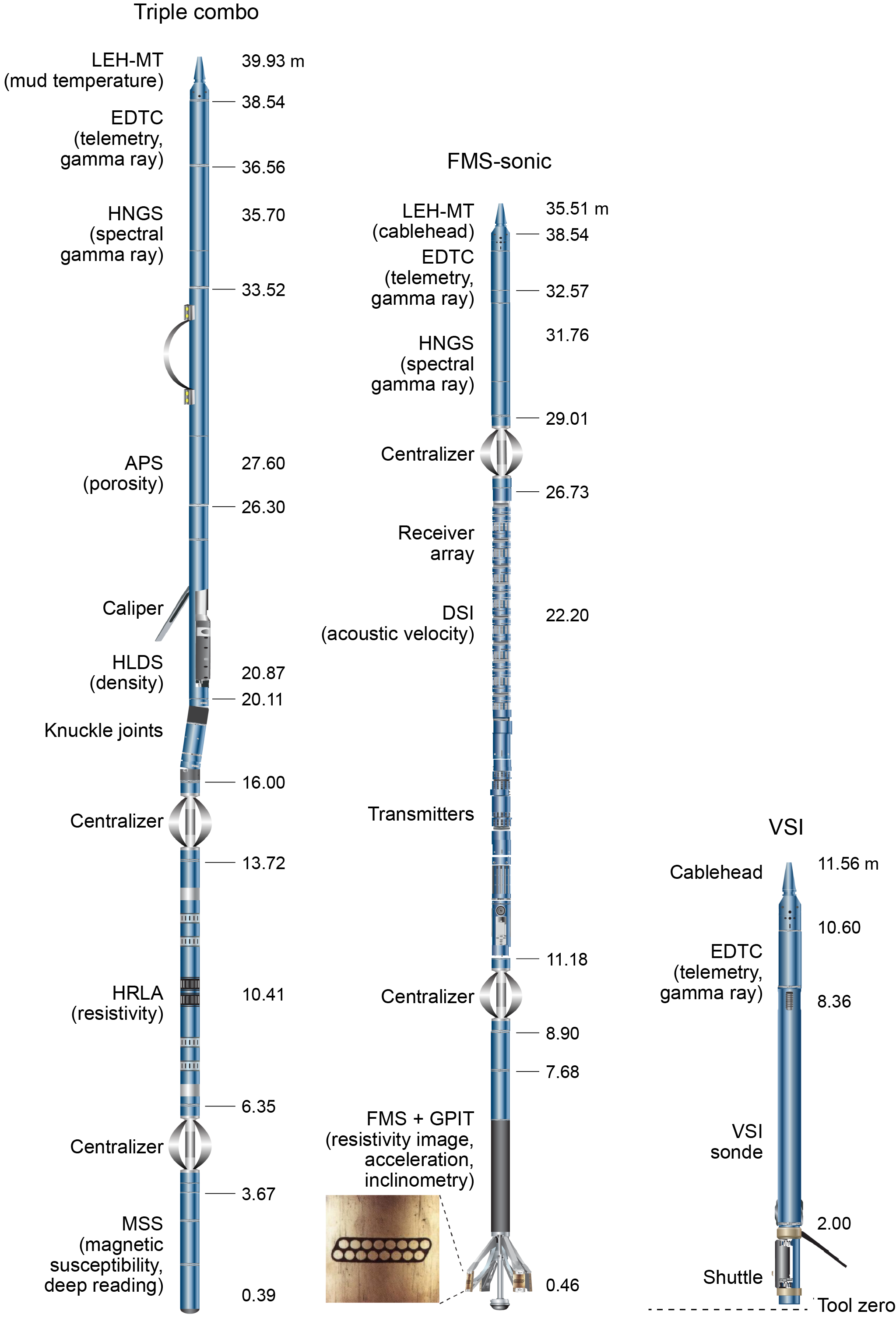
Figure F23. Triple combo, FMS-sonic, and VSI tool strings.
The second logging deployment used the Formation MicroScanner (FMS)-sonic tool string (Figure F23; Tables T8, T9) to provide an oriented resistivity image of the borehole wall plus P- and S-wave acoustic velocity of the formation using the Dipole Shear Sonic Imager (DSI). Magnetometry was measured with a fluxgate magnetometer in the General Purpose Inclinometry Tool (GPIT) that simultaneously measured any borehole deviation from vertical. The HNGS tool was included to record natural gamma ray to depth-match features between the logging runs, and a caliper again measured borehole diameter to indicate hole and data quality.
To prepare for logging, the hole was cleared of drilling cuttings with a mud sweep, followed by flushing with seawater. Depending on the hole conditions, the BHA was set between 68 and 104.5 m DSF to cover the most unstable upper part of the hole. Tool strings were lowered downhole on a seven-conductor wireline cable before being pulled up at constant speed, typically ~550 m/h for the triple combo and 500–550 m/h for the FMS-sonic tool string.
Each tool string deployment is termed a logging "run." During each run, tool strings were lowered and pulled up in the hole several times to check repeatability and to increase coverage of the FMS-sonic borehole images. Each lowering or hauling up of the tool string while collecting data constitutes a pass. Incoming data were recorded and monitored in real time on the Schlumberger Minimum Configuration MAXIS (MCM) logging computer. Ship heave was 0.3–1.0 m during logging. The wireline heave compensator (WHC) was utilized for all logging during this expedition.
9.2. Logged sediment properties and tool measurement principles
Logged properties and the principles used in the tools that measure them are briefly described below. All logs collected during this expedition are listed in Table T8. More detailed information on individual tools and their geologic applications may be found in Serra (1984, 1986, 1989), Schlumberger (1989, 1994), Rider (1996), Goldberg (1997), Lovell et al. (1998), and Ellis and Singer (2007). A complete list of acronyms for the Schlumberger tools and measurement curves is available at http://iodp.tamu.edu/tools/logging/index.html.
9.2.1. Natural gamma ray
The HNGS was used on both the triple combo and FMS-sonic tool strings to measure natural gamma ray in the formation. The HNGS uses two bismuth germanate scintillation detectors and five-window spectroscopy to determine concentrations of potassium (in weight percent), thorium (in parts per million), and uranium (in parts per million) from the characteristic gamma ray energies of isotopes in the 40K, 232Th, and 238U radioactive decay series, which dominate the natural radiation spectrum. The computation of the elemental abundances uses a least-squares method of extracting U, Th, and K elemental concentrations (weight percent, parts per million, and parts per million, respectively) from the spectral measurements. The HNGS filters out gamma ray energies below 500 keV, eliminating sensitivity to bentonite or KCl in the drilling mud and improving measurement accuracy. The HNGS also provides a measure of the total spectral gamma ray (HSGR) and uranium-free or computed gamma ray (HCGR) emissions, which are measured in American Petroleum Institute gamma radiation units (gAPI). The HNGS response is influenced by the borehole diameter, and HNGS data are corrected for borehole diameter variations during acquisition.
An additional natural gamma ray sensor was housed in the Enhanced Digital Telemetry Cartridge (EDTC), which was used primarily to communicate data to the surface. This sensor includes a sodium iodide scintillation detector, which also measures the total natural gamma ray emission of the formation. It is not a spectral tool (i.e., it does not provide U, Th, and K concentrations), but it provides total gamma radiation for each pass.
Including the HNGS in both tool strings enabled us to use the gamma ray data for precise depth match processing between logging strings and provided a reliable means of core-log integration.
9.2.2. Density and photoelectric factor
Formation density was measured with the HLDS. The sonde contains a radioactive cesium (137Cs) gamma ray source (622 keV) and both far and near gamma ray detectors mounted on a shielded skid, which is pressed against the borehole wall by a hydraulically activated decentralizing arm. Gamma rays emitted by the source undergo Compton scattering, in which gamma rays are scattered by electrons in the formation. The number of scattered gamma rays that reach the detectors is proportional to the density of electrons in the formation, which is in turn related to bulk density. Porosity may also be derived from this bulk density if the matrix (grain) density is known.
The HLDS also measures the photoelectric effect (PEF), a measure of the photoelectric absorption of low-energy gamma radiation. Photoelectric absorption occurs when gamma radiation energy falls below 150 keV as a result of being repeatedly scattered by electrons in the formation. The PEF is determined by comparing the counts from the far detector in the high-energy region, where only Compton scattering occurs, with those in the low-energy region, where count rates depend on both Compton scattering and photoelectric absorption. Because PEF depends on the atomic number of the elements in the formation (heavier elements have higher PEF), it also varies according to the chemical composition of the minerals present and can be used for the identification of the overall mineral makeup of the formation. For example, the PEF of calcite is 5.08 barn/e−, illite is 3.03 barn/e−, quartz is 1.81 barn/e−, and hematite is 21 barn/e− (Serra, 1984; Schlumberger, 1989).
Good contact between the tool and borehole wall is essential for good HLDS logs; poor contact results in underestimation of density values. Both the density correction and caliper measurement of the hole are used to check the contact quality. The PEF log should be used with caution when multiple mud sweeps are used to stabilize the borehole and especially in washouts, because barium in the logging mud swamps the signal, regardless of attempts to correct for the mud effect.
9.2.3. Porosity
Formation porosity was measured with the APS. The sonde includes a minitron neutron generator that produces fast (14.4 MeV) neutrons and five neutron detectors (four epithermal and one thermal) positioned at different distances from the minitron. The tool's detectors count neutrons that arrive at the detectors after being scattered and slowed by collisions with atomic nuclei in the formation.
The highest energy loss occurs when neutrons collide with hydrogen nuclei, which have practically the same mass as the neutron (the neutrons bounce off heavier elements without losing much energy). If the hydrogen (i.e., water) concentration is low, as in low-porosity formations, neutrons can travel farther before being captured and the count rates increase at the detector. The opposite effect occurs in high-porosity formations where the water content is high. However, because hydrogen bound to minerals, such as clays, or that forms part of hydrocarbon molecules also contributes to the measurement, the raw porosity value is often an overestimate and should be checked against laboratory-derived values from core when possible.
Upon reaching thermal energies (0.025 eV), neutrons are captured by the nuclei of Cl, Si, B, and other elements, resulting in a gamma ray emission. This neutron-capture cross section (Σf) is also measured by the tool.
9.2.4. Electrical resistivity
The HRLA tool provides six resistivity measurements with different depths of investigation throughout the logged interval (including the borehole mud resistivity and five measurements of formation resistivity with increasing penetration into the formation). The tool sends a focused current into the formation and measures the intensity necessary to maintain a constant drop in voltage across a fixed interval, providing direct resistivity measurements. The array has one central (source) electrode and six electrodes above and below it, which serve alternatively as focusing and returning current electrodes. By rapidly changing the role of these electrodes, a simultaneous resistivity measurement at six penetration depths is achieved. The tool is designed to ensure that all signals are measured at the same time and tool position and to reduce the sensitivity to shoulder bed effects when crossing sharply defined beds thinner than the electrode spacing. The design of the HRLA tool, which eliminates the need for a surface reference electrode, improves formation resistivity evaluation compared to traditional dual induction resistivity methods and allows the full range of resistivity to be measured, from low (e.g., in high-porosity sediment) to high (e.g., in basalt). The HRLA tool needs to be run centralized in the borehole for optimal results, so bowspring centralizers were used to keep it in the center of the borehole. Knuckle joints above the HRLA tool allowed the density tool to be centralized and maintain good contact with the borehole wall (Figure F23).
Calcite, silica, and hydrocarbons are electrical insulators, whereas ionic solutions, like IW, are conductors. Electrical resistivity, therefore, can be used to evaluate porosity for a given salinity and resistivity of the IW (Schlumberger, 1989). Clay surface conduction also contributes to the resistivity values, but at high porosities, this is a relatively minor effect.
9.2.5. Magnetic Susceptibility Sonde
The MSS is a nonstandard wireline tool designed by LDEO. It measures the ease with which formations are magnetized when subjected to a magnetic field. The ease of magnetization is ultimately related to the concentration and composition (size, shape, and mineralogy) of magnetic minerals (principally magnetite) in the formation. These measurements provide one of the best methods for investigating stratigraphic changes in mineralogy and lithology because the measurement is quick, repeatable, and nondestructive and because different lithologies often have strongly contrasting susceptibilities.
The MSS dual-coil sensor provides ~40 cm resolution measurements with ~20 cm horizontal penetration. The MSS was run as the lowermost tool in the triple combo tool string, using a specially developed data translation cartridge to enable the MSS to be run in combination with the Schlumberger tools. The MSS also has an optional single-coil sensor to provide high-resolution measurements (~10 cm), but this was not used during Expedition 403 because it requires a large bowspring to achieve adequate contact with the borehole wall. This would mean that the MSS would have to be run higher up in the tool string so it could be centralized and ultimately would require an additional log run.
MS data from the deep-reading sensor are plotted as uncalibrated units. The MSS reading responses are affected by temperature and borehole size (higher temperatures lead to higher susceptibility measurements). No apparent temperature drift was seen in the data, so no corrections were made offshore. When the MS signal in sediment is very low, the detection limits of the tool may be reached. For quality control and environmental correction, the MSS also measures internal tool temperature and low-resolution borehole conductivity.
9.2.6. Acoustic velocity
The DSI measures the transit times between sonic transmitters and an array of eight receivers. It combines replicate measurements, thus providing a direct measurement of P- and S-wave sound velocity through formations that is relatively free from the effects of formation damage and an enlarged borehole (Schlumberger, 1989). Acoustic velocity results from multiple physical properties of the borehole wall, including lithology, porosity, and Poisson's ratio, which helps stratigraphic correlation even if other logging data are not high quality. Along with the monopole transmitters found on most sonic tools, the DSI has two crossed-dipole transmitters that allow measurement of shear wave velocity, in addition to compressional wave velocity. Dipole measurements are necessary to measure shear wave velocities in slow formations where shear wave velocity is less than the velocity of sound in the borehole fluid. Such slow formations are often encountered in deep ocean drilling.
9.2.7. Formation MicroScanner
The FMS provides high-resolution electrical resistivity–based images of borehole walls. The tool has four orthogonal arms and pads, each containing 16 button electrodes that are pressed against the borehole wall during logging (Figure F23). The electrodes are arranged in two diagonally offset rows of eight electrodes each. A focused current is emitted from the button electrodes into the formation, with a return electrode near the top of the tool. Resistivity of the formation at the button electrodes is derived from the intensity of current passing through the button electrodes.
Processing transforms the resistivity measurements into oriented high-resolution images that reveal geologic structures of the borehole wall. Features such as bedding, stratification, fracturing, slump folding, and bioturbation can be resolved (Luthi, 1990; Salimullah and Stow, 1992; Lovell et al., 1998). Because the images are oriented to magnetic north, further analysis can provide measurement of the dip and direction (azimuth) of planar features in the formation. In addition, when the corresponding planar features can be identified in the recovered core samples, individual core pieces can be reoriented with respect to true north.
Approximately 30% of a borehole with a diameter of 25 cm (9.8 inches) is imaged during an uplog. Standard procedure is to make two uphole passes with the FMS to maximize the chance of getting full borehole coverage with the pads. The maximum extension of the caliper arms is 40.6 cm (16 inches). In holes with a diameter greater than this maximum, the pad contact at the end of the caliper arms will be inconsistent, and the FMS images may appear out of focus and too conductive. Irregular (rough) borehole walls will also adversely affect the images if contact with the wall is poor.
9.2.8. Acceleration and inclinometry
Three-component acceleration and magnetic field measurements were made with the GPIT. The primary purpose of this tool, which incorporates a three-component accelerometer and a three-component magnetometer, is to determine the acceleration and orientation of the FMS-sonic tool string during logging. This information allows the FMS-sonic images to be corrected for irregular tool motion and the dip and direction (azimuth) of features in the images to be determined. The GPIT is run with other tools on the FMS-sonic tool string that can carry remanent or induced magnetization; therefore, its magnetic measurements can be affected by the other tools as well as the rocks in the borehole wall and magnetization of the casing and/or drill pipe. However, on the FMS-sonic tool string, the GPIT has greater nonmagnetic insulation from the other tools, which greatly reduces the effects on its magnetic measurements.
9.3. Log data quality
The main influence on log data quality is the condition of the borehole wall. Where the borehole diameter varies over short intervals because of washouts (wide borehole) of softer material or ledges of harder material, the logs from tools that require good contact with the borehole wall (i.e., FMS, density, and porosity) may be degraded. Deep investigation measurements, such as gamma radiation, resistivity, and sonic velocity, which do not require contact with the borehole wall, are generally less sensitive to borehole conditions. Bridged sections, where borehole diameter is much lower than the bit size, will also cause irregular log results. The quality of the borehole is improved by minimizing the circulation of drilling fluid while drilling, flushing the borehole to remove debris, and logging as soon as possible after drilling and conditioning are completed.
The quality of the wireline depth determination depends on several factors. The depth of the logging measurements is determined by the length of the cable laid out from the winch on the ship. The seafloor is identified on the natural gamma ray log by the abrupt reduction in gamma ray count at the water/sediment interface (mudline). Discrepancies between the drilling depth and the wireline log depth may occur. In the case of drilling depth, discrepancies are caused by core expansion, incomplete core recovery, or incomplete heave compensation. In contrast to log depth, discrepancies between successive runs occur because of incomplete heave compensation, incomplete correction for cable stretch, and cable slip. Tidal changes in sea level and unaccounted-for changes in trim of the drillship affect both drilling and logging depths.
9.4. Logging data flow and log depth scales
Data for each wireline logging run were monitored in real time and recorded using the Schlumberger MAXIS 500 system. Initial logging data were referenced to the rig floor (WRF depth scale). After logging was completed, the data were shifted to a seafloor reference (WSF depth scale) based on the step in logged gamma radiation at the sediment/water interface.
Data were transferred onshore to LDEO, where standardized data processing took place. A main part of the processing was depth matching to remove depth offsets between logs from different logging runs. This resulted in a new depth scale: WMSF. Also, corrections were made to certain tools and logs (e.g., FMS imagery was corrected for tool acceleration, including stick and slip motion), documentation for the logs (with an assessment of log quality) was prepared, and the data were converted to ASCII for the conventional logs and to GIF for the FMS images. The Schlumberger GeoQuest's GeoFrame software package was used for most of the processing of the collected wireline logging data. The data were transferred back to the ship within a few days after logging, and the processed data set was made available to the science party.
9.5. In situ temperature measurements and heat flow calculation
In situ temperature measurements were made with the APCT-3 tool (Figure F24) at each site when the APC system was deployed and with the SET2 tool when XCB coring occurred.
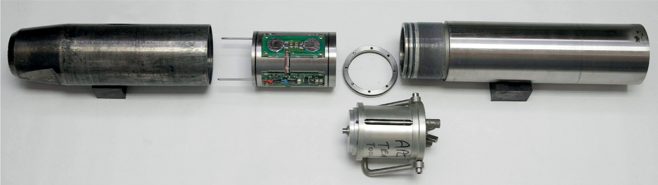
Figure F24. APCT-3.
The APCT-3 tool fits directly into the coring shoe of the APC system and consists of a battery pack, data logger, and platinum resistance-temperature device calibrated over a temperature range of −5° to +50°C with an accuracy of ±0.02°C. Before entering the borehole, the tool is first stopped at the mudline for 5 min to thermally equilibrate with the bottom water. When the APC system is inserted into the formation, frictional heat causes rapid temperature rise. This heat gradually conducts the surrounding formation, so the temperature of the probe equilibrates toward in situ formation temperature. After the APC system penetrates the sediment, it is held for 5 min while the APCT-3 tool records the temperature of the cutting shoe every second.
The equilibrium temperature of the sediment is estimated by applying a mathematical heat-conduction model to the temperature decay record (Horai and Von Herzen, 1985). The synthetic thermal decay curve for the APCT-3 tool is a function of the geometry and thermal properties of the probe and the sediment (Bullard, 1954; Horai and Von Herzen, 1985). Equilibrium temperature is estimated by applying a fitting procedure (Pribnow et al., 2000). However, where the APC system does not achieve a full stroke or where ship heave pulls it up from full penetration, the temperature equilibration curve is disturbed and temperature determination is less accurate. The nominal accuracy of the APCT-3 tool's temperature measurements is ±0.05°C.
Using the SET2 tool (Figure F25), the actual in situ temperature was measured while XCB coring. The SET2 tool consists of a battery, data logger, extended logger tip, bumper seal, thermistor, and its string wrapped by probe tip. The thermistor is calibrated for a temperature range of −2° to 50°C with an accuracy of ±0.002°C. The probe tip is designed to enter the sediment with minimal disturbance. Features of the probe tip design include the following:
- High-strength stainless steel construction survives penetration into consolidated sediment.
- The 8 mm spherical probe tip tapers upward at an included angle of 5° to minimize mechanical disturbance of the sediment and the tendency to crack the formation upon penetration by the tool.
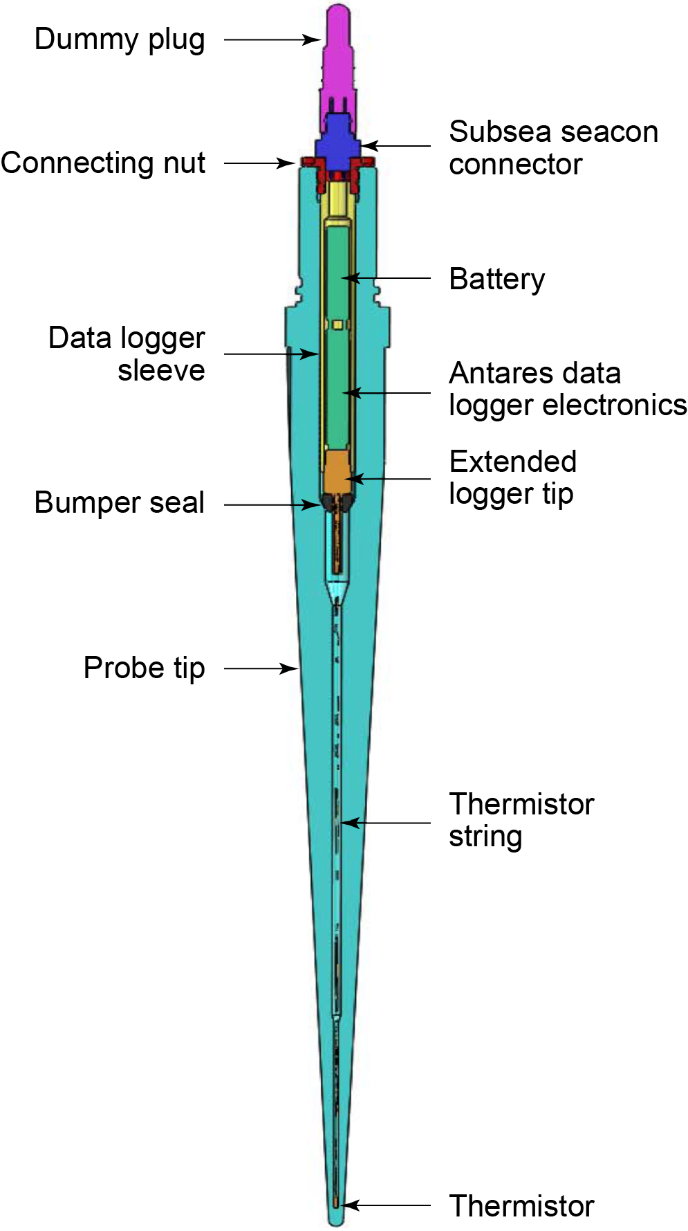
Figure F25. SET2.
APCT-3 and SET2 temperature data are combined with thermal conductivity measurements, and heat flow and geothermal gradient are calculated according to the Bullard (1939) method to be consistent with the synthesis of the ODP heat flow data by Pribnow et al. (2000). This methodology assumes a linear relationship between temperature, T, and thermal resistance of the sediments, Ω(z):
Thermal resistance is expressed as
with zi and zi−1 as bottom and top depths, respectively, of a horizontal layer with thermal conductivity, λi, and i as the number of layers between the surface and depth z. Because of the data frequency, thermal conductivity is assumed to be constant in the whole core.
Plotting Ω(z) as a function of T(z), the Bullard plot allows estimation of the surface temperature (T0) from the intercept with z = 0 and of the heat flow (Q) from the slope. The conditions for the linearity of the plot are affected by conductive conditions, steady state, and absence of internal heat source.
To obtain the thermal conductivity at the depth of the temperature measurements, we estimated a continuous profile of λ(z), assuming that there is a linear variation of thermal conductivity with depth (Pribnow et al., 2000):
The linear trend was confirmed at each site. The thermal resistance ΩLIN,j for the depth (zT,j) of the jth temperature value (Tj) was calculated using the results of the linear regression, λ0 and Γ (slope) with
which allows the calculation of the heat flow.
References
Abrantes, F., Hodell, D.A., Alvarez Zarikian, C.A., Brooks, H.L., Clark, W.B., Dauchy-Tric, L.F.B., dos Santos Rocha, V., Flores, J.-A., Herbert, T.D., Hines, S.K.V., Huang, H.-H.M., Ikeda, H., Kaboth-Bahr, S., Kuroda, J., Link, J.M., McManus, J.F., Mitsunaga, B.A., Nana Yobo, L., Pallone, C.T., Pang, X., Peral, M.Y., Salgueiro, E., Sanchez, S., Verma, K., Wu, J., Xuan, C., and Yu, J., 2024. Expedition 397 methods. In Hodell, D.A., Abrantes, F., Alvarez Zarikian, C.A., and the Expedition 397 Scientists, Iberian Margin Paleoclimate. Proceedings of the International Ocean Discovery Program, 397: College Station, TX (International Ocean Discovery Program). https://doi.org/10.14379/iodp.proc.397.102.2024
Acton, G., Borton, C.J., and the Leg 178 Shipboard Scientific Party, 2001. Palmer Deep composite depth scales for Leg 178 sites 1098 and 1099. In Barker, P.F., Camerlenghi, A., Acton, G.D., and Ramsay, A.T.S. (Eds.), Proceedings of the Ocean Drilling Program, Scientific Results, 178: College Station, TX (Ocean Drilling Program), 1–35. https://doi.org/10.2973/odp.proc.sr.178.202.2001
Acton, G., Morris, A., Musgrave, R., Zhao, X., and IODP SRM Personnel, 2017. Assessment of the New Superconducting Rock Magnetometer (SRM) on the JOIDES Resolution. http://iodp.tamu.edu/publications/JRSO/SRM_Workshop_2017.pdf
Alken, P., Thébault, E., Beggan, C.D., Amit, H., Aubert, J., Baerenzung, J., Bondar, T.N., Brown, W.J., Califf, S., Chambodut, A., Chulliat, A., Cox, G.A., Finlay, C.C., Fournier, A., Gillet, N., Grayver, A., Hammer, M.D., Holschneider, M., Huder, L., Hulot, G., Jager, T., Kloss, C., Korte, M., Kuang, W., Kuvshinov, A., Langlais, B., Léger, J.M., Lesur, V., Livermore, P.W., Lowes, F.J., Macmillan, S., Magnes, W., Mandea, M., Marsal, S., Matzka, J., Metman, M.C., Minami, T., Morschhauser, A., Mound, J.E., Nair, M., Nakano, S., Olsen, N., Pavón-Carrasco, F.J., Petrov, V.G., Ropp, G., Rother, M., Sabaka, T.J., Sanchez, S., Saturnino, D., Schnepf, N.R., Shen, X., Stolle, C., Tangborn, A., Tøffner-Clausen, L., Toh, H., Torta, J.M., Varner, J., Vervelidou, F., Vigneron, P., Wardinski, I., Wicht, J., Woods, A., Yang, Y., Zeren, Z., and Zhou, B., 2021. International Geomagnetic Reference Field: the thirteenth generation. Earth, Planets and Space, 73(1):49. https://doi.org/10.1186/s40623-020-01288-x
Andrade, J., Legoinha, P., Stroynowski, Z., and Abrantes, F., 2019. Morphology, biostratigraphy, and evolution of Pliocene-Pleistocene diatoms Proboscia barboi and Proboscia curvirostris. Geological Acta, 17(9):1–17. https://doi.org/10.1344/GeologicaActa2019.17.9
Anthonissen, E.D., 2008. Late Pliocene and Pleistocene biostratigraphy of the Nordic Atlantic region. Newsletters on Stratigraphy, 43(1):33–48. https://doi.org/10.1127/0078-0421/2008/0043-0033
Armbrecht, L., Weber, M.E., Raymo, M.E., Peck, V.L., Williams, T., Warnock, J., Kato, Y., Hernández-Almeida, I., Hoem, F., Reilly, B., Hemming, S., Bailey, I., Martos, Y.M., Gutjahr, M., Percuoco, V., Allen, C., Brachfeld, S., Cardillo, F.G., Du, Z., Fauth, G., Fogwill, C., Garcia, M., Glüder, A., Guitard, M., Hwang, J.-H., Iizuka, M., Kenlee, B., O'Connell, S., Pérez, L.F., Ronge, T.A., Seki, O., Tauxe, L., Tripathi, S., and Zheng, X., 2022. Ancient marine sediment DNA reveals diatom transition in Antarctica. Nature Communications, 13(1):5787. https://doi.org/10.1038/s41467-022-33494-4
ASTM International, 1990. Standard method for laboratory determination of water (moisture) content of soil and rock (Standard D2216–90). In Annual Book of ASTM Standards for Soil and Rock. Philadelphia (American Society for Testing Materials).
Aubry, A.M.R., De Schepper, S., and de Vernal, A., 2020. Dinocyst and acritarch biostratigraphy of the Late Pliocene to Early Pleistocene at Integrated Ocean Drilling Program Site U1307 in the Labrador Sea. Journal of Micropalaeontology, 39(1):41–60. https://doi.org/10.5194/jm-39-41-2020
Aubry, A.M.R., de Vernal, A., and Knutz, P.C., 2021. Baffin Bay late Neogene palynostratigraphy at Ocean Drilling Program Site 645. Canadian Journal of Earth Sciences, 58(1):67–83. https://doi.org/10.1139/cjes-2019-0227
Backman, J., Raffi, I., Rio, D., Fornaciari, E., and Pälike, H., 2012. Biozonation and biochronology of Miocene through Pleistocene calcareous nannofossils from low and middle latitudes. Newsletters on Stratigraphy, 45(3):221–244. https://doi.org/10.1127/0078-0421/2012/0022
Baldauf, J.G., 1984. Cenozoic diatom biostratigraphy and paleoceanography of the Rockall Plateau region, North Atlantic, Deep Sea Drilling Project Leg 81. In Roberts, D.G., Schnitker, D., et al., Initial Reports of the Deep Sea Drilling Project, 81: Washington, DC (U.S. Government Printing Office), 439–478. https://doi.org/10.2973/dsdp.proc.81.107.1984
Baldauf, J.G., 1987. Diatom biostratigraphy of the middle- and high-latitude North Atlantic Ocean, Deep Sea Drilling Project Leg 94. In Ruddiman, W.E., Kidd, R. B., Thomas, E., et al., Initial Reports of the Deep Sea Drilling Project, 94: Washington, DC (U.S. Government Printing Office), 729–762. http://doi.org/10.2973/dsdp.proc.94.115.1987
Balsam, W.L., Damuth, J.E., and Schneider, R.R., 1997. Comparison of shipboard vs. shore-based spectral data from Amazon Fan cores: implications for interpreting sediment composition. In Flood, R.D., Piper, D.J.W., Klaus, A., and Peterson, L.C. (Eds.), Proceedings of the Ocean Drilling Program, Scientific Results, 155: College Station, TX (Ocean Drilling Program), 193–215. https://doi.org/10.2973/odp.proc.sr.155.210.1997
Balsam, W.L., Deaton, B.C., and Damuth, J.E., 1998. The effects of water content on diffuse reflectance spectrophotometry studies of deep-sea sediment cores. Marine Geology, 149(1):177–189. https://doi.org/10.1016/S0025-3227(98)00033-4
Banerjee, S.K., King, J., and Marvin, J., 1981. A rapid method for magnetic granulometry with applications to environmental studies. Geophysical Research Letters, 8(4):333–336. https://doi.org/10.1029/GL008i004p00333
Barron, J.A., 1981. Late Cenozoic diatom biostratigraphy and paleoceanography of the middle-latitude eastern North Pacific, Deep Sea Drilling Project Leg 63. In Yeats, R.S., Haq, B.U., et al., Initial Reports of the Deep Sea Drilling Project, 63: Washington, DC (U.S. Government Printing Office), 507–538. http://doi.org/10.2973/dsdp.proc.63.113.1981
Barron, J.A., Bukry, D., Addison, J.A., and Ager, T.A., 2016. Holocene evolution of diatom and silicoflagellate paleoceanography in Slocum Arm, a fjord in southeastern Alaska. Marine Micropaleontology, 126:1–18. https://doi.org/10.1016/j.marmicro.2016.05.002
Biscaye, P.E., 1964. Distinction between kaolinite and chlorite in recent sediments by X-ray diffraction. American Mineralogist, 49(9–10):1281–1289.
Biscaye, P.E., 1965. Mineralogy and sedimentation of recent deep-sea clay in the Atlantic Ocean and adjacent seas and oceans. Geological Society of America Bulletin, 76(7):803–832. https://doi.org/10.1130/0016-7606(1965)76[803:MASORD]2.0.CO;2
Blum, P., 1997. Technical Note 26: Physical properties handbook. Ocean Drilling Program. https://doi.org/10.2973/odp.tn.26.1997
Bown, P.R., 1998. Calcareous Nannofossil Biostratigraphy: Dordrect, Netherlands (Kluwer Academic Publishing).
Bullard, E.C., 1939. Heat flow in South Africa. Proceedings of the Royal Society of London, A: Mathematical and Physical Sciences, 173(955):474–502. https://doi.org/10.1098/rspa.1939.0159
Bullard, E.C., 1954. The flow of heat through the floor of the Atlantic Ocean. Proceedings of the Royal Society of London, A: Mathematical and Physical Sciences, 222(1150):408–429. https://doi.org/10.1098/rspa.1954.0085
Chaisson, W.P., and Pearson, P.N., 1997. Planktonic foraminifer biostratigraphy at Site 925: middle Miocene-Pleistocene. In Shackleton, N.J., Curry, W.B., Richter, C., and Bralower, T.J. (Eds.), Proceedings of the Ocean Drilling Program, Scientific Results, 154: College Station, TX (Ocean Drilling Program), 3–31. https://doi.org/10.2973/odp.proc.sr.154.104.1997
Channell, J.E.T., Hodell, D.A., and Curtis, J.H., 2016. Relative paleointensity (RPI) and oxygen isotope stratigraphy at IODP Site U1308: North Atlantic RPI stack for 1.2-2.2 Ma (NARPI-2200) and age of the Olduvai Subchron. Quaternary Science Reviews, 131(A):1–19. https://doi.org/10.1016/j.quascirev.2015.10.011
Channell, J.E.T., Singer, B.S., and Jicha, B.R., 2020. Timing of Quaternary geomagnetic reversals and excursions in volcanic and sedimentary archives. Quaternary Science Reviews, 228:106114. https://doi.org/10.1016/j.quascirev.2019.106114
Darling, K.F., Kucera, M., Kroon, D., and Wade, C.M., 2006. A resolution for the coiling direction paradox in Neogloboquadrina pachyderma. Paleoceanography, 21(2):PA2011. https://doi.org/10.1029/2005PA001189
De Schepper, S., Beck, K.M., and Mangerud, G., 2017. Late Neogene dinoflagellate cyst and acritarch biostratigraphy for Ocean Drilling Program Hole 642B, Norwegian Sea. Review of Palaeobotany and Palynology, 236:12–32. https://doi.org/10.1016/j.revpalbo.2016.08.005
De Schepper, S., and Head, M.J., 2008. Age calibration of dinoflagellate cyst and acritarch events in the Pliocene–Pleistocene of the eastern North Atlantic (DSDP Hole 610A). Stratigraphy, 5(2):137–162. https://doi.org/10.29041/strat.05.2.02
De Schepper, S., and Head, M.J., 2009. Pliocene and Pleistocene dinoflagellate cyst and acritarch zonation of DSDP Hole 610A, eastern North Atlantic. Palynology, 33(1):179–218. https://doi.org/10.2113/gspalynol.33.1.179
De Schepper, S., and Mangerud, G., 2017. Age and palaeoenvironment of the Utsira Formation in the northern North Sea based on marine palynology. Norwegian Journal of Geology, 97(4):305–325. https://doi.org/10.17850/njg97-4-04
De Schepper, S., and Head, M.J., 2014. New late Cenozoic acritarchs: evolution, palaeoecology and correlation potential in high latitude oceans. Journal of Systematic Palaeontology, 12(4):493–519. https://doi.org/10.1080/14772019.2013.783883
De Schepper, S., Schreck, M., Beck, K.M., Matthiessen, J., Fahl, K., and Mangerud, G., 2015. Early Pliocene onset of modern Nordic Seas circulation related to ocean gateway changes. Nature Communications, 6(1):8659. https://doi.org/10.1038/ncomms9659
de Vernal, A., and Mudie, P.J., 1989a. Late Pliocene to Holocene palynostratigraphy at ODP Site 645, Baffin Bay. In Srivastava, S.P., Arthur, M., and Clement, B. (Eds.), Proceedings of the Ocean Drilling Program, Scientific Results, 105: College Station, TX (Ocean Drilling Program), 387–399. https://doi.org/10.2973/odp.proc.sr.105.133.1989
de Vernal, A., and Mudie, P.J., 1989b. Pliocene and Pleistocene palynostratigraphy at ODP Sites 646 and 647, eastern and southern Labrador Sea. In Srivastava, S.P., Arthur, M., and Clement, B. (Eds.), Proceedings of the Ocean Drilling Program, Scientific Results, 105: College Station, TX (Ocean Drilling Program), 401–422. https://doi.org/10.2973/odp.proc.sr.105.134.1989
de Vernal, A., Radi, T., Zaragosi, S., Van Nieuwenhove, N., Rochon, A., Allan, E., De Schepper, S., Eynaud, F., Head, M.J., Limoges, A., Londeix, L., Marret, F., Matthiessen, J., Penaud, A., Pospelova, V., Price, A., and Richerol, T., 2020. Distribution of common modern dinoflagellate cyst taxa in surface sediments of the Northern Hemisphere in relation to environmental parameters: The new n=1968 database. Marine Micropaleontology, 159:101796. https://doi.org/10.1016/j.marmicro.2019.101796
Droser, M.L., and Bottjer, D.J., 1986. A semiquantitative field classification of ichnofabric. Journal of Sedimentary Research, 56(4):558–559. https://doi.org/10.1306/212F89C2-2B24-11D7-8648000102C1865D
Drury, A.J., Westerhold, T., Frederichs, T., Tian, J., Wilkens, R., Channell, J.E.T., Evans, H., John, C.M., Lyle, M., and Röhl, U., 2017. Late Miocene climate and time scale reconciliation; accurate orbital calibration from a deep-sea perspective. Earth and Planetary Science Letters, 475:254–266. https://doi.org/10.1016/j.epsl.2017.07.038
Dunlea, A.G., Murray, R.W., Harris, R.N., Vasiliev, M.A., Evans, H., Spivack, A.J., and D'Hondt, S., 2013. Assessment and use of NGR instrumentation on the JOIDES Resolution to quantify U, Th, and K concentrations in marine sediment. Scientific Drilling, 15:57–63. https://doi.org/10.2204/iodp.sd.15.05.2013
Ellis, D.V., and Singer, J.M., 2007. Well Logging for Earth Scientists (2nd edition): New York (Elsevier). https://doi.org/10.1007/978-1-4020-4602-5
Evans, H.B., 1965. GRAPE* - A Device For Continuous Determination Of Material Density And Porosity. Presented at the SPWLA 6th Annual Logging Symposium (Volume II), Dallas, TX. https://onepetro.org/SPWLAALS/proceedings/SPWLA-1965-II/All-SPWLA-1965-II/SPWLA-1965-2B/18331
Expedition 318 Scientists, 2011. Methods. In Escutia, C., Brinkhuis, H., Klaus, A., and the Expedition 318 Scientists, Proceedings of the Integrated Ocean Drilling Program, 318: Tokyo (Integrated Ocean Drilling Program Management International, Inc.). https://doi.org/10.2204/iodp.proc.318.102.2011
Fisher, R.A., 1953. Dispersion on a sphere. Proceedings of the Royal Society A: Mathematical, Physical and Engineering Sciences, 217(1130):295–305. https://doi.org/10.1098/rspa.1953.0064
Gieskes, J.M., Gamo, T., and Brumsack, H.J., 1991. Technical Note 15: Chemical methods for interstitial water analysis aboard JOIDES Resolution. Ocean Drilling Program. https://doi.org/10.2973/odp.tn.15.1991
Gilmore, G.R., 2008. Practical Gamma-Ray Spectrometry, 2nd Edition: New York (Wiley). https://doi.org/10.1002/9780470861981
Goldberg, D., 1997. The role of downhole measurements in marine geology and geophysics. Reviews of Geophysics, 35(3):315–342. https://doi.org/10.1029/97RG00221
González-Lanchas, A., Rickaby, R.E.M., Sierro, F.J., Rigual-Hernández, A.S., Alonso-García, M., and Flores, J.A., 2023. Globally enhanced calcification across the coccolithophore Gephyrocapsa complex during the mid-Brunhes interval. Quaternary Science Reviews, 321:108375. https://doi.org/10.1016/j.quascirev.2023.108375
Graber, K.K., Pollard, E., Jonasson, B., and Schulte, E. (Eds.), 2002. Technical Note 31: Overview of Ocean Drilling Program engineering tools and hardware. Ocean Drilling Program. https://doi.org/10.2973/odp.tn.31.2002
Gradstein, F.M., Ogg, J.G., Schmitz, M.D., and Ogg, G.M. (Eds.), 2020. Geologic Time Scale 2020: Amsterdam (Elsevier BV). https://doi.org/10.1016/C2020-1-02369-3
Grant, D.M., Steinsland, K., Cordier, T., Ninnemann, U.S., Ijaz, U.Z., Dahle, H., De Schepper, S., and Ray, J.L., 2024. Sedimentary ancient DNA sequences reveal marine ecosystem shifts and indicator taxa for glacial-interglacial sea ice conditions. Quaternary Science Reviews, 339:108619. https://doi.org/10.1016/j.quascirev.2024.108619
Hagelberg, T.K., Pisias, N.G., Shackleton, N.J., Mix, A.C., and Harris, S., 1995. Refinement of a high-resolution, continuous sedimentary section for studying equatorial Pacific Ocean paleoceanography, Leg 138. In Pisias, N.G., Mayer, L.A., Janecek, T.R., Palmer-Julson, A., and van Andel, T.H. (Eds.), Proceedings of the Ocean Drilling Program, Scientific Results, 138: College Station, TX (Ocean Drilling Program). https://doi.org/10.2973/odp.proc.sr.138.103.1995
Hagelberg, T., Shackleton, N., Pisias, N., and the Shipboard Scientific Party, 1992. Development of composite depth sections for Sites 844 through 854. In Mayer, L., Pisias, N., Janecek, T., et al., Proceedings of the Ocean Drilling Program, Initial Reports, 138: College Station, TX (Ocean Drilling Program), 79–85. https://doi.org/10.2973/odp.proc.ir.138.105.1992
Hall, J.R., Allison, M.S., Papadopoulos, M.T., Barfod, D.N., and Jones, S.M., 2023. Timing and Consequences of Bering Strait Opening: New Insights From 40Ar/39Ar Dating of the Barmur Group (Tjörnes Beds), Northern Iceland. Paleoceanography and Paleoclimatology, 38(4):e2022PA004539. https://doi.org/10.1029/2022PA004539
Harms, J.C., and Choquette, P.W., 1965. Geologic evaluation of a gamma-ray porosity device. Presented at the SPWLA 6th Annual Logging Symposium, Dallas, TX, May 1965.
Hasle, G.R., Syvertsen, E.E., Steidinger, K.A., Tangen, K., and Tomas, C.R., 1996. Identifying Marine Diatoms and Dinoflagellates: (Academic Press). https://doi.org/10.1016/B978-0-12-693015-3.X5000-1
Head, M.J., 1996. Late Cenozoic Dinoflagellates from the Royal Society Borehole at Ludham, Norfolk, Eastern England. Journal of Paleontology, 70(4):543–570. https://doi.org/10.1017/S0022336000023532
Head, M.J., Norris, G., and Mudie, P.J., 1989a. Palynology and dinocyst stratigraphy of the Miocene in ODP Leg 105, Hole 645E, Baffin Bay. In Srivastava, S.P., Arthur, M., Clement, B., et al., Proceedings of the Ocean Drilling Program, Scientific Results, 105: College Station, TX (Ocean Drilling Program), 467–514. https://doi.org/10.2973/odp.proc.sr.105.137.1989
Head, M.J., Norris, G., and Mudie, P.J., 1989b. Palynology and dinocyst stratigraphy of the upper Miocene and lowermost Pliocene, ODP Leg 105, Site 646, Labrador Sea. In Srivastava, S.P., Arthur, M., Clement, B., et al., Proceedings of the Ocean Drilling Program, Scientific Results, 105: College Station, TX (Ocean Drilling Program), 423–452. https://doi.org//10.2973/odp.proc.sr.105.135.1989
Head, M.J., Riding, J.B., Eidvin, T., and Chadwick, R.A., 2004. Palynological and foraminiferal biostratigraphy of (Upper Pliocene) Nordland Group mudstones at Sleipner, northern North Sea. Marine and Petroleum Geology, 21(3):277–297. https://doi.org/10.1016/j.marpetgeo.2003.12.002
Hennissen, J.A.I., Head, M.J., de Schepper, S., and Groeneveld, J., 2014. Palynological evidence for a southward shift of the North Atlantic Current at ∼2.6 Ma during the intensification of late Cenozoic Northern Hemisphere glaciation. Paleoceanography and Paleoclimatology, 29(6):564–580. https://doi.org/10.1002/2013PA002543
Horai, K., and Von Herzen, R.P., 1985. Measurement of heat flow on Leg 86 of the Deep Sea Drilling Project. In Heath, G.R., Burckle, L. H., et al., Initial Reports of the Deep Sea Drilling Project, 86: Washington, DC (U.S. Government Printing Office), 759–777. https://doi.org/10.2973/dsdp.proc.86.135.1985
Husum, K., and Hald, M., 2012. Arctic planktic foraminiferal assemblages: Implications for subsurface temperature reconstructions. Marine Micropaleontology, 96-97:38–47. https://doi.org/10.1016/j.marmicro.2012.07.001
Jutzeler, M., Clark, A.S., Manga, M., McIntosh, I., Druitt, T., Kutterolf, S., and Ronge, T.A., 2025. Data report: coring disturbances in advanced piston cores from IODP Expedition 398, Hellenic Arc Volcanic Field. In Druitt, T.H., Kutterolf, S., Ronge, T.A., and the Expedition 398 Scientists, Hellenic Arc Volcanic Field. Proceedings of the International Ocean Discovery Program, 398: College Station, TX (International Ocean Discovery Program). https://doi.org/10.14379/iodp.proc.398.203.2025
Jutzeler, M., White, J.D.L., Talling, P.J., McCanta, M., Morgan, S., Le Friant, A., and Ishizuka, O., 2014. Coring disturbances in IODP piston cores with implications for offshore record of volcanic events and the Missoula megafloods. Geochemistry, Geophysics, Geosystems, 15(9):3572–3590. https://doi.org/10.1002/2014GC005447
Kennett, J.P., and Srinivasan, M.S., 1983. Neogene Planktonic Foraminifera: A Phylogenetic Atlas: London (Hutchinson Ross).
King, J., Banerjee, S.K., Marvin, J., and Özdemir, Ö., 1982. A comparison of different magnetic methods for determining the relative grain size of magnetite in natural materials: Some results from lake sediments. Earth and Planetary Science Letters, 59(2):404–419. https://doi.org/10.1016/0012-821X(82)90142-X
Kirschvink, J.L., 1980. The least-squares line and plane and the analysis of palaeomagnetic data. Geophysical Journal International, 62(3):699–718. https://doi.org/10.1111/j.1365-246X.1980.tb02601.x
Knutz, P.C., Jennings, A.E., Childress, L.B., Bryant, R., Cargill, S.K., Coxall, H.K., Frank, T.D., Grant, G.R., Gray, R.E., Ives, L., Kumar, V., Le Houedec, S., Martens, J., Naim, F., Nelissen, M., Özen, V., Passchier, S., Pérez, L.F., Ren, J., Romans, B.W., Seki, O., Staudigel, P., Tauxe, L., Tibbett, E.J., Yokoyama, Y., Zhang, Y., and Zimmermann, H., 2025a. Expedition 400 methods. In Knutz, P.C., Jennings, A.E., Childress, L.B., and the Expedition 400 Scientists, NW Greenland Glaciated Margin. Proceedings of the International Ocean Discovery Program, 400: College Station, TX (International Ocean Discovery Program). https://doi.org/10.14379/iodp.proc.400.102.2025
Knutz, P.C., Jennings, A.E., Childress, L.B., Bryant, R., Cargill, S.K., Coxall, H.K., Frank, T.D., Grant, G.R., Gray, R.E., Ives, L., Kumar, V., Le Houedec, S., Martens, J., Naim, F., Nelissen, M., Özen, V., Passchier, S., Pérez, L.F., Ren, J., Romans, B.W., Seki, O., Staudigel, P., Tauxe, L., Tibbett, E.J., Yokoyama, Y., Zhang, Y., and Zimmermann, H., 2025b. Expedition 400 summary. In Knutz, P.C., Jennings, A.E., Childress, L.B., and the Expedition 400 Scientists, NW Greenland Glaciated Margin. Proceedings of the International Ocean Discovery Program, 400: College Station, TX (International Ocean Discovery Program). https://doi.org/10.14379/iodp.proc.400.101.2025
Koç, N., Hodell, D.A., Kleiven, H.F., and Labeyrie, L., 1999. High-resolution Pleistocene diatom biostratigraphy of Site 983 and correlations with isotope stratigraphy. In Raymo, M.E., Jansen, E., Blum, P., and Herbert, T.D. (Eds.), Proceedings of the Ocean Drilling Program, Scientific Results, 162: College Station, TX (Ocean Drilling Program), 51–62. https://doi.org/10.2973/odp.proc.sr.162.035.1999
Koç, N., and Scherer, R.P., 1996. Neogene diatom biostratigraphy of the Iceland Sea Site 907. In Thiede, J., Myhre, A.M., Firth, J.V., Johnson, G.L., and Ruddiman, W.F. (Eds.), Proceedings of the Ocean Drilling Program, Scientific Results, 151: College Station, TX (Ocean Drilling Program), 61–74. https://doi.org/10.2973/odp.proc.sr.151.108.1996
Kristiansen, J.I., 1982. The transient cylindrical probe method for determination of thermal parameters of earth materials [PhD dissertation]. Åarhus University, Åarhus, Denmark. http://digitallib.oit.edu/digital/collection/geoheat/id/2103/
Lam, A.R., Crundwell, M.P., Leckie, R.M., Albanese, J., and Uzel, J.P., 2022. Diachroneity rules the mid-latitudes: a test case using Late Neogene planktic foraminifera across the Western Pacific. Geosciences, 12(5):190. https://doi.org/10.3390/geosciences12050190
Lin, W., Yeh, E., Ito, H., Hirono, T., Soh, W., Wang, C., Ma, K., Hung, J., and Song, S.-R., 2007. Preliminary results of stress measurement using drill cores of TCDP Hole-A: an application of anelastic strain recovery method to three-dimensional in-situ stress determination. Terrestrial Atmospheric and Oceanic Sciences, 18:379–393. http://doi.org/10.3319/TAO.2007.18.2.379(TCDP)
Lisiecki, L.E., and Raymo, M.E., 2005. A Pliocene-Pleistocene stack of 57 globally distributed benthic δ18O records. Paleoceanography, 20(1):PA1003. https://doi.org/10.1029/2004PA001071
Locker, S., 1996. Cenozoic siliceous flagellates from the Fram Strait and the East Greenland margin: biostratigraphic and paleoceanographic results. In Thiede, J., Myhre, A.M., Firth, J.V., Johnson, G.L., and Ruddiman, W.F. (Eds.), Proceedings of the Ocean Drilling Program; Scientific Results, 151: College Station, TX (Ocean Drilling Program), 101–124. https://doi.org/10.2973/odp.proc.sr.151.102.1996
Lourens, L., Antonarakou, A., Hilgen, F.J., Van Hoof, A.A.M., Vergnaud-Grazzini, C., and Zachariasse, W.J., 1996. Evaluation of the Plio-Pleistocene astronomical timescale. Paleoceanography, 11(4):391–413. https://doi.org/10.1029/96PA01125
Lourens, L., Hilgen, F., Shackleton, N.J., Laskar, J., and Wilson, D., 2004. The Neogene period. In Smith, A.G., Gradstein, F.M. and Ogg, J.G., A Geologic Time Scale 2004. Cambridge, UK (Cambridge University Press), 409–440. https://doi.org/10.1017/CBO9780511536045.022
Louwye, S., Foubert, A., Mertens, K., and van Rooij, D., 2008. Integrated stratigraphy and palaeoecology of the lower and middle Miocene of the Porcupine Basin. Geological Magazine, 145(3):321–344. https://doi.org/10.1017/S0016756807004244
Lovell, M.A., Harvey, P.K., Brewer, T.S., Williams, C., Jackson, P.D., and Williamson, G., 1998. Application of FMS images in the Ocean Drilling Program: an overview. In Cramp, A., MacLeod, C.J., Lee, S.V., and Jones, E.J.W. (Eds.), Geological Evolution of Ocean Basins: Results from the Ocean Drilling Program. Geological Society, London, Special Publication, 131: 287–303. https://doi.org/10.1144/GSL.SP.1998.131.01.18
Lundholm, N., and Hasle, G.R., 2010. Fragilariopsis (Bacillariophyceae) of the Northern Hemisphere – morphology, taxonomy, phylogeny and distribution, with a description of F. pacifica sp. nov. Phycologia, 49(5):438–460. https://doi.org/10.2216/09-97.1
Luthi, S.M., 1990. Sedimentary structures of clastic rocks identified from electrical borehole images. In Hurst, A., Lovell, M.A., and Morton, A.C. (Eds.), Geological Applications of Wireline Logs. Geological Society Special Publication, 48: 3–10. https://doi.org/10.1144/GSL.SP.1990.048.01.02
Manheim, F.T., and Sayles, F.L., 1974. Composition and origin of interstitial waters of marine sediments, based on deep sea drill cores. In Goldberg, E.D., The Sea (Volume 5): Marine Chemistry: The Sedimentary Cycle. New York (Wiley), 527–568. https://pubs.usgs.gov/publication/70207491
Marsaglia, K., Milliken, K., and Doran, L., 2013. Technical Note 1: IODP digital reference for smear slide analysis of marine mud, Part 1: Methodology and atlas of siliciclastic and volcanogenic components. Integrated Ocean Drilling Program. https://doi.org/10.2204/iodp.tn.1.2013
Marsaglia, K., Milliken, K., Leckie, R., Tentori, D., and Doran, L., 2015. Technical Note 2: IODP smear slide digital reference for sediment analysis of marine mud, Part 2: Methodology and atlas of biogenic components. International Ocean Discovery Program. https://doi.org/10.2204/iodp.tn.2.2015
Martini, E., 1971. Standard Tertiary and Quaternary calcareous nannoplankton zonation. Proceedings of the Second Planktonic Conference, Roma, 1970:739–785.
Matsuki, K., 1991. Three-dimensional in-situ stress measurement with anelastic strain recovery of a rock core. Presented at the 7th ISRM Congress.
Matthiessen, J., and Brenner, W., 1996. Dinoflagellate cyst ecostratigraphy of Pliocene-Pleistocene sediments from the Yermak Plateau (Arctic Ocean, Hole 911A). In Thiede, J., Myhre, A.M., Firth, J.V., Johnson, G.L., and Ruddiman, W.F. (Eds.), Proceedings of the Ocean Drilling Program, Scientific Results, 151: 243–253. https://doi.org/10.2973/odp.proc.sr.151.109.1996
Matthiessen, J., and Knies, J., 2001. Dinoflagellate cyst evidence for warm interglacial conditions at the northern Barents Sea margin during marine oxygen isotope stage 5. Journal of Quaternary Science, 16(7):727–737. https://doi.org/10.1002/jqs.656
Matthiessen, J., Schreck, M., De Schepper, S., Zorzi, C., and de Vernal, A., 2018. Quaternary dinoflagellate cysts in the Arctic Ocean: potential and limitations for stratigraphy and paleoenvironmental reconstructions. Quaternary Science Reviews, 192:1–26. https://doi.org/10.1016/j.quascirev.2017.12.020
Mazzullo, J., Meyer, A., and Kidd, R., 1988. Appendix I: New sediment classification scheme for the Ocean Drilling Program. In Mazzullo, J., and Graham, A.G., Technical Note 8: Handbook for shipboard sedimentologists. (Ocean Drilling Program), 44–67. https://doi.org/10.2973/odp.tn.8.1988
McKay, R.M., De Santis, L., Kulhanek, D.K., Ash, J.L., Beny, F., Browne, I.M., Cortese, G., Cordeiro de Sousa, I.M., Dodd, J.P., Esper, O.M., Gales, J.A., Harwood, D.M., Ishino, S., Keisling, B.A., Kim, S., Kim, S., Laberg, J.S., Leckie, R.M., Müller, J., Patterson, M.O., Romans, B.W., Romero, O.E., Sangiorgi, F., Seki, O., Shevenell, A.E., Singh, S.M., Sugisaki, S.T., van de Flierdt, T., van Peer, T.E., Xiao, W., and Xiong, Z., 2019. Expedition 374 methods. In McKay, R.M., De Santis, L., Kulhanek, D.K., and the Expedition 374 Scientists, Ross Sea West Antarctic Ice Sheet History. Proceedings of the International Ocean Discovery Program, 374: College Station, TX (International Ocean Discovery Program). https://doi.org/10.14379/iodp.proc.374.102.2019
Mix, A.C., Tiedemann, R., Blum, P., et al., 2003. Proceedings of the Ocean Drilling Program, Initial Reports, 202: College Station, TX (Ocean Drilling Program). https://doi.org/10.2973/odp.proc.ir.202.2003
Moncrieff, A.C.M., 1989. Classification of poorly-sorted sedimentary rocks. Sedimentary Geology, 65(1–2):191–194. https://doi.org/10.1016/0037-0738(89)90015-8
Murray, R.W., Miller, D.J., and Kryc, K.A., 2000. Technical Note 29: Analysis of major and trace elements in rocks, sediments, and interstitial waters by inductively coupled plasma–atomic emission spectrometry (ICP-AES). Ocean Drilling Program. https://doi.org/10.2973/odp.tn.29.2000
Naish, T.R., Levy, R.H., Powell, R.D., and MIS Science and Operations Team Members, 2006. Scientific Logistics Implementation Plan for the ANDRILL McMurdo Ice Shelf Project. https://digitalcommons.unl.edu/andrillinfo/5/
Oksman, M., Juggins, S., Miettinen, A., Witkowski, A., and Weckström, K., 2019. The biogeography and ecology of common diatom species in the northern North Atlantic, and their implications for paleoceanographic reconstructions. Marine Micropaleontology, 148:1–28. https://doi.org/10.1016/j.marmicro.2019.02.002
Pawłowska, J., Zajączkowski, M., Łącka, M., Lejzerowicz, F., Esling, P., and Pawlowski, J., 2016. Palaeoceanographic changes in Hornsund Fjord (Spitsbergen, Svalbard) over the last millennium: new insights from ancient DNA. Climate of the Past, 12(7):1459–1472. https://doi.org/10.5194/cp-12-1459-2016
Pearson, P.N., and Kučera, M., 2018. Taxonomy, biostratigraphy, and phylogeny of Oligocene Turborotalita. In Wade, B.S., Olsson, R.K., Pearson, P.N., Huber, B.T. and Berggren, W.A., Atlas of Oligocene Planktonic Foraminifera. Cushman Foundation Special Publication, 46: (Cushman Foundation for Foraminiferal Research), 385–392. https://pubs.geoscienceworld.org/cushmanfoundation/books/edited-volume/2271/chapter-abstract/126275377/TAXONOMY-BIOSTRATIGRAPHY-AND-PHYLOGENY-OF
Pearson, P.N., Wade, B.S., and Huber, B.T., 2018. Taxonomy, biostratigraphy, and phylogeny of Oligocene Globigerinitidae (Dipsidripella, Globigerinita, and Tenuitella). In Wade, B.S., Olsson, R.K., Pearson, P.N., Huber, B.T. and Berggren, W.A., Atlas of Oligocene Planktonic Foraminifera. Cushman Foundation Special Publication, 46: (Cushman Foundation for Foraminiferal Research), 429–458. https://pubs.geoscienceworld.org/cushmanfoundation/books/edited-volume/2271/chapter-abstract/126275385/TAXONOMY-BIOSTRATIGRAPHY-AND-PHYLOGENY-OF
Perch-Nielsen, K., 1985. Cenozoic calcareous nannofossils. In Bolli, H.M., Saunders, J.B., and Perch-Nielsen, K. (Eds.), Plankton Stratigraphy (Volume 1). Cambridge, UK (Cambridge University Press), 427–554.
Peters, C., and Thompson, R., 1998. Magnetic identification of selected natural iron oxides and sulphides. Journal of Magnetism and Magnetic Materials, 183(3):365–374. https://doi.org/10.1016/S0304-8853(97)01097-4
Pribnow, D.F.C., Kinoshita, M., and Stein, C.A., 2000. Thermal data collection and heat flow recalculations for ODP Legs 101–180: Hannover, Germany (Institute for Joint Geoscientific Research, GGA). http://www-odp.tamu.edu/publications/heatflow/
Raffi, I., 2002. Revision of the Early-Middle Pleistocene calcareous nannofossil biochronology (1.75–0.85 Ma). Marine Micropaleontology, 45(1):25–55. https://doi.org/10.1016/S0377-8398(01)00044-5
Raffi, I., Backman, J., Fornaciari, E., Pälike, H., Rio, D., Lourens, L., and Hilgen, F., 2006. A review of calcareous nannofossil astrobiochronology encompassing the past 25 million years. Quaternary Science Reviews, 25(23):3113–3137. https://doi.org/10.1016/j.quascirev.2006.07.007
Raffi, I., Backman, J., Rio, D., and Shackleton, N.J., 1993. Plio-Pleistocene nannofossil biostratigraphy and calibration to oxygen isotope stratigraphies from Deep Sea Drilling Project Site 607 and Ocean Drilling Program Site 677. Paleoceanography and Paleoclimatology, 8(3):387–408. https://doi.org/10.1029/93PA00755
Razmjooei, M.J., Henderiks, J., Coxall, H.K., Baumann, K.-H., Vermassen, F., Jakobsson, M., Niessen, F., and O'Regan, M., 2023. Revision of the Quaternary calcareous nannofossil biochronology of Arctic Ocean sediments. Quaternary Science Reviews, 321:108382. https://doi.org/10.1016/j.quascirev.2023.108382
Ren, J., Gersonde, R., Esper, O., and Sancetta, C., 2014. Diatom distributions in northern North Pacific surface sediments and their relationship to modern environmental variables. Palaeogeography, Palaeoclimatology, Palaeoecology, 402:81–103. https://doi.org/10.1016/j.palaeo.2014.03.008
Richter, C., Acton, G., Endris, C., and Radsted, M., 2007. Technical Note 34: Handbook for shipboard paleomagnetists. Ocean Drilling Program. https://doi.org/10.2973/odp.tn.34.2007
Rider, M.H., 1996. The Geological Interpretation of Well Logs (Second edition): Houston, TX (Gulf Publishing Company).
Riding, J.B., and Kyffin-Hughes, J.E., 2006. Further testing of a non-acid palynological preparation procedure. Palynology, 30(1): 69–87. https://doi.org/10.1080/01916122.2006.9989619
Romero, O.E., 2009. Data report: Pleistocene diatoms from Sites U1302 and U1303, Orphan Knoll, northwestern Atlantic Ocean. In Channell, J.E.T., Kanamatsu, T., Sato, T., Stein, R., Alvarez Zarikian, C.A., Malone, M.J., and the Expedition 303/306 Scientists, Proceedings of the Integrated Ocean Drilling Program, 303/306: College Station, TX (Integrated Ocean Drilling Program Management International, Inc.). https://doi.org/10.2204/iodp.proc.303306.203.2009
Rothwell, R.G., 1989. Minerals and Mineraloids in Marine Sediments: An Optical Identification Guide: London (Elsevier). https://doi.org/10.1007/978-94-009-1133-8
Ruddiman, W.F., Kidd, R.B., Thomas, E., et al., 1987. Initial Reports of the Deep Sea Drilling Project, 94: Washington, DC (U.S. Government Printing Office). https://doi.org/10.2973/dsdp.proc.94.1987
Salimullah, A.R.M., and Stow, D.A.V., 1992. Application of FMS images in poorly recovered coring intervals; examples from ODP Leg 129. In Hurst, A., Griffiths, C.M., and Worthington, P.F. (Eds.), Geological Applications of Wireline Logs II. Geological Society Special Publication, 65: 71–86. https://doi.org/10.1144/GSL.SP.1992.065.01.06
Sato, T., Chiyonobu, S., and Hodell, D.A., 2009. Data report: Quaternary calcareous nannofossil datums and biochronology in the North Atlantic Ocean, IODP Site U1308. In Channell, J.E.T., Kanamatsu, T., Sato, T., Stein, R., Alvarez Zarikian, C.A., Malone, M.J., and the Expedition 303/306 Scientists, Proceedings of the Integrated Ocean Drilling Program, 303/306: College Station, TX (Integrated Ocean Drilling Program Management International, Inc.). https://doi.org/10.2204/iodp.proc.303306.210.2009
Sato, T., and Kameo, K., 1996. Pliocene to Quaternary calcareous nannofossil biostratigraphy of the Arctic Ocean, with reference to late Pliocene glaciation. In Thiede, J., Myhre, A.M., Firth, J.V., Johnson, G.L., and Ruddiman, W.F. (Eds.), Proceedings of the Ocean Drilling Program, Scientific Results, 151: College Station, TX (Ocean Drilling Program), 39–59. https://doi.org/10.2973/odp.proc.sr.151.112.1996
Sato, T., Kameo, K., and Mita, I., 1999. Validity of the latest Cenozoic calcareous nannofossil datums and its application to the tephrochronology. Earth Science (Chikyu Kagaku), 53(4):265–274. https://doi.org/10.15080/agcjchikyukagaku.53.4_265
Sato, T., Kameo, K., and Takayama, T., 1991. Coccolith biostratigraphy of the Arabian Sea. In Prell, W.L., Niitsuma, N., et al., Proceedings of the Ocean Drilling Program, Scientific Results, 117: College Station, TX (Ocean Drilling Program), 37–54. https://doi.org/10.2973/odp.proc.sr.117.133.1991
Savrda, C.E., Krawinkel, H., McCarthy, F.M.G., McHugh, C.M.G., Olson, H.C., and Mountain, G., 2001. Ichnofabrics of a Pleistocene slope succession, New Jersey margin: relations to climate and sea-level dynamics. Palaeogeography, Palaeoclimatology, Palaeoecology, 171(1):41–61. https://doi.org/10.1016/S0031-0182(01)00266-8
Schiebel, R., and Hemleben, C., 2017. Planktic Foraminifers in the Modern Ocean: Berlin (Springer). https://doi.org/10.1007/978-3-662-50297-6
Schlumberger, 1989. Log Interpretation Principles/Applications, SMP-7017: Houston (Schlumberger Education Services).
Schlumberger, 1994. IPL Integrated Porosity Lithology, SMP-9270: Houston (Schlumberger Education Services).
Schrader, H., and Gersonde, R., 1978. Diatoms and silicoflagellates. In Zachariasse, W.J., Riedel, W.R., Sanfilippo, A., Schmidt, R.R., Brolsma, M.J., Schrader, H.J., Gersonde, R., Drooger, M.M., and Broekman, J.A. (Eds.), Micropaleontological Counting Methods and Techniques: an Exercise on an Eight Metres Section of the Lower Pliocene of Capo Rossello, Sicily. Utrecht Micropaleontological Bulletin, 17: 129–176.
Schreck, M., Matthiessen, J., and Head, M.J., 2012. A magnetostratigraphic calibration of Middle Miocene through Pliocene dinoflagellate cyst and acritarch events in the Iceland Sea (Ocean Drilling Program Hole 907A). Review of Palaeobotany and Palynology, 187:66–94. https://doi.org/10.1016/j.revpalbo.2012.08.006
Seidenkrantz, M.S., 1995. Cassidulina teretis Tappan and Cassidulina neoteretis new species (Foraminifera): stratigraphic markers for deep sea and outer shelf areas. Journal of Micropalaeontology, 14(2):145–157. https://doi.org/10.1144/jm.14.2.145
Serra, O., 1984. Fundamentals of Well-log Interpretation (Volume 1): The Acquisition of Logging Data: Amsterdam (Elsevier).
Serra, O., 1986. Fundamentals of Well-Log Interpretation (Volume 2): The Interpretation of Logging Data: Amsterdam (Elsevier).
Serra, O., 1989. Formation MicroScanner Image Interpretation, SMP-7028: Houston (Schlumberger Education Services).
Shepard, F.P., 1954. Nomenclature based on sand-silt-clay ratios. Journal of Sedimentary Research, 24(3):151–158. https://doi.org/10.1306/D4269774-2B26-11D7-8648000102C1865D
Smelror, M., 1999. Pliocene-Pleistocene and redeposited dinoflagellate cysts from the western Svalbard margin (Site 986); biostratigraphy, paleoenvironments, and sediment provenance. In Raymo, M.E., Jansen, E., Blum, P., and Herbert, T.D. (Eds.), Proceedings of the Ocean Drilling Program, Scientific Results, 162: College Station, TX (Ocean Drilling Program), 83–97. https://doi.org/10.2973/odp.proc.sr.162.011.1999
Spezzaferri, S., Coxall, H.K., Olsson, R.K., and Hemleben, C., 2018. Taxonomy, biostratigraphy, and phylogeny of Oligocene Globigerina, Globigerinella, and Quiltyella n. gen. In Wade, B.S., Olsson, R.K., Pearson, P.N., Huber, B.T. and Berggren, W.A., Atlas of Oligocene Planktonic Foraminifera. Cushman Foundation Special Publication, 46: (Cushman Foundation for Foraminiferal Research), 179–214. https://pubs.geoscienceworld.org/cushmanfoundation/books/edited-volume/2271/chapter-abstract/126275365/TAXONOMY-BIOSTRATIGRAPHY-AND-PHYLOGENY-OF
Spiegler, D., and Jansen, E., 1989. Planktonic foraminifer biostratigraphy of Norwegian Sea sediments: ODP Leg 104. In Eldholm, O., Thiede, J., Taylor, E., et al., Proceedings of the Ocean Drilling Program, Scientific Results, 104: College Station, TX (Ocean Drilling Program), 681–696. https://doi.org/10.2973/odp.proc.sr.104.157.1989
Stober, J.C., and Thompson, R., 1979. An investigation into the source of magnetic minerals in some Finnish lake sediments. Earth and Planetary Science Letters, 45(2):464–474. https://doi.org/10.1016/0012-821X(79)90145-6
Sundström, B.G., 1986. The marine diatom genus rhizosolenia: A new approach to the taxonomy [PhD Dissertation]. Lund University, Sweden.
Takayama, T., and Sato, T., 1987. Coccolith biostratigraphy of the North Atlantic Ocean, Deep Sea Drilling Project Leg 94. In Ruddiman, W.E., Kidd, R. B., Thomas, E., et al., Initial Reports of the Deep Sea Drilling Project, 94: Washington, DC (U.S. Government Printing Office), 651–702. https://doi.org/10.2973/dsdp.proc.94.113.1987
Thierstein, H.R., Geitzenauer, K.R., Molfino, B., and Shackleton, N.J., 1977. Global synchroneity of late Quaternary coccolith datum levels validation by oxygen isotopes. Geology, 5(7):400–404. https://doi.org/10.1130/0091-7613(1977)5<400:GSOLQC>2.0.CO;2
Vasiliev, M.A., Blum, P., Chubarian, G., Olsen, R., Bennight, C., Cobine, T., Fackler, D., Hastedt, M., Houpt, D., Mateo, Z., and Vasilieva, Y.B., 2011. A new natural gamma radiation measurement system for marine sediment and rock analysis. Journal of Applied Geophysics, 75(3):455–463. https://doi.org/10.1016/j.jappgeo.2011.08.008
Verhoeven, K., and Louwye, S., 2012. Selenopemphix islandensis sp. nov.: a new organic-walled dinoflagellate cyst from the Lower Pliocene Tjörnes beds, northern Iceland. Palynology, 36(1):10–25. https://doi.org/10.1080/01916122.2011.593573
Von Herzen, R., and Maxwell, A.E., 1959. The measurement of thermal conductivity of deep-sea sediments by a needle-probe method. Journal of Geophysical Research, 64(10):1557–1563. https://doi.org/10.1029/JZ064i010p01557
Wade, B.S., Pearson, P.N., Berggren, W.A., and Pälike, H., 2011. Review and revision of Cenozoic tropical planktonic foraminiferal biostratigraphy and calibration to the geomagnetic polarity and astronomical time scale. Earth-Science Reviews, 104(1–3):111–142. https://doi.org/10.1016/j.earscirev.2010.09.003
Weaver, P.P.E., and Clement, B.M., 1986. Synchroneity of Pliocene planktonic foraminiferal datums in the North Atlantic. Marine Micropaleontology, 10(4):295–307. https://doi.org/10.1016/0377-8398(86)90033-2
Weber, M.E., Raymo, M.E., Peck, V.L., Williams, T., Armbrecht, L.H., Bailey, I., Brachfeld, S.A., Cardillo, F.G., Du, Z., Fauth, G., García, M., Glüder, A., Guitard, M.E., Gutjahr, M., Hemming, S.R., Hernández-Almeida, I., Hoem, F.S., Hwang, J.-H., Iizuka, M., Kato, Y., Kenlee, B., Martos, Y.M., O'Connell, S., Pérez, L.F., Reilly, B.T., Ronge, T.A., Seki, O., Tauxe, L., Tripathi, S., Warnock, J.P., and Zheng, X., 2021a. Expedition 382 methods. In Weber, M.E., Raymo, M.E., Peck, V.L., Williams, T., and the Expedition 382 Scientists, Iceberg Alley and Subantarctic Ice and Ocean Dynamics. Proceedings of the International Ocean Discovery Program, 382: College Station, TX (International Ocean Discovery Program). https://doi.org/10.14379/iodp.proc.382.102.2021
Weber, M.E., Raymo, M.E., Peck, V.L., Williams, T., Armbrecht, L.H., Bailey, I., Brachfeld, S.A., Cardillo, F.G., Du, Z., Fauth, G., García, M., Glüder, A., Guitard, M.E., Gutjahr, M., Hemming, S.R., Hernández-Almeida, I., Hoem, F.S., Hwang, J.-H., Iizuka, M., Kato, Y., Kenlee, B., Martos, Y.M., O'Connell, S., Pérez, L.F., Reilly, B.T., Ronge, T.A., Seki, O., Tauxe, L., Tripathi, S., Warnock, J.P., and Zheng, X., 2021b. Expedition 382 summary. In Weber, M.E., Raymo, M.E., Peck, V.L., Williams, T., and the Expedition 382 Scientists, Iceberg Alley and Subantarctic Ice and Ocean Dynamics. Proceedings of the International Ocean Discovery Program, 382: College Station, TX (International Ocean Discovery Program). https://doi.org/10.14379/iodp.proc.382.101.2021
Wei, K.-Y., 1994. Stratophenetic tracing of phylogeny using SIMCA pattern recognition technique: a case study of the late Neogene planktic foraminifera Globoconella clade. Paleobiology, 20(1):52–65. https://doi.org/10.1017/S0094837300011131
Wei, W., 1993. Calibration of Upper Pliocene-Lower Pleistocene nannofossil events with oxygen isotope stratigraphy. Paleoceanography and Paleoclimatology, 8(1):85–99. https://doi.org/10.1029/92PA02504
Wellner, J.S., Gohl, K., Klaus, A., Bauersachs, T., Bohaty, S.M., Courtillat, M., Cowan, E.A., De Lira Mota, M.A., Esteves, M.S.R., Fegyveresi, J.M., Frederichs, T., Gao, L., Halberstadt, A.R., Hillenbrand, C.-D., Horikawa, K., Iwai, M., Kim, J.-H., King, T.M., Klages, J.P., Passchier, S., Penkrot, M.L., Prebble, J.G., Rahaman, W., Reinardy, B.T.I., Renaudie, J., Robinson, D.E., Scherer, R.P., Siddoway, C.S., Wu, L., and Yamane, M., 2021. Site U1532. In Gohl, K., Wellner, J.S., Klaus, A., and the Expedition 379 Scientists, Amundsen Sea West Antarctic Ice Sheet History. Proceedings of the International Ocean Discovery Program, 379: College Station, TX (International Ocean Discovery Program). https://doi.org/10.14379/iodp.proc.379.103.2021
Wentworth, C.K., 1922. A scale of grade and class terms for clastic sediments. The Journal of Geology, 30(5):377–392. https://doi.org/10.1086/622910
Williams, G.L., Fensome, R.A., and MacRae, R.A., 2017. The Lentin and Williams Index of Fossil Dinoflagellates 2017 Edition. AASP Contributions Series, 48. https://palynology.org/wp-content/uploads/2017/01/AASP-Contribution-Series-No.48.pdf
Young, J.R., 1998. Neogene. In Bown, P.R., Calcareous Nannofossil Biostratigraphy. Dordrecht, Netherlands (Kluwer Academic Publishing), 225–265.
Young, J.R., Bown, P.R., and Lees, J.A., 2024. Nannotax3 website. International Nannoplankton Association. https://www.mikrotax.org/Nannotax3
Young, J.R., Geisen, M., Gros, L., Kleyne, A., Sprengel, C., Probert, I., and Østergard, J., 2003. A guide to extant coccolithophore taxonomy. In Journal of Nannoplankton Research. Special Issue 1. https://ina.tmsoc.org/books/coccoguide.html
Zimmermann, H.H., Stoof-Leichsenring, K.R., Kruse, S., Nürnberg, D., Tiedemann, R., and Herzschuh, U., 2021. Sedimentary Ancient DNA From the Subarctic North Pacific: How Sea Ice, Salinity, and Insolation Dynamics Have Shaped Diatom Composition and Richness Over the Past 20,000 Years. Paleoceanography and Paleoclimatology, 36(4):e2020PA004091. https://doi.org/10.1029/2020PA004091