Previous   |   Next

doi:10.2204/iodp.proc.319.102.2010

Physical properties

Physical property measurements provide basic information to assess rock and sediment properties, to characterize lithologic units and states of consolidation and deformation, and to correlate core, cuttings, and downhole measurement and logging data. For the cored intervals, X-ray CT images were first taken of core sections. Then, gamma ray attenuation (GRA) density, magnetic susceptibility, natural gamma radiation, P-wave velocity, and electrical resistivity were measured for whole-round core sections (MSCL-W) using the multisensor core logger (MSCL) system (Geotek Ltd., London, United Kingdom) after 3 h of thermal equilibration at room temperature. After MSCL-W measurements, thermal conductivity measurements were carried out on the working half of split cores using the half-space method. Digital photo image scanning was carried out on the cut surfaces of archive halves using the MSCL-I. MAD were measured on discrete samples collected from core working halves. P-wave velocity was measured in three orthogonal directions on 20 mm cubic samples. For cuttings samples (700–1605 m MSF) of Hole C0009A, GRA was measured by MSCL-W, MAD measurements were conducted, and magnetic susceptibility was measured using the Kappabridge system. Details about each measurement are given in the following sections.

MSCL-W (cores and cuttings)

Gamma ray attenuation density

A thin gamma ray beam was produced by a ¹³⁷Cs gamma ray source at a radiation level of 370 MBq within a lead shield with a 5 mm collimator. The gamma ray detector is composed of a scintillator and an integral photomultiplier tube. Bulk density was computed from GRA as follows:

where

• ρ = sediment bulk density,

• η = Compton attenuation coefficient,

• d = sample diameter,

• I₀ = gamma source intensity, and

• I = measured intensity of gamma rays passing through the sample.

Because η and I₀ are treated as constants, ρ can be calculated from I. For calibration, we used a set of aligned aluminum cylinders of various diameters, surrounded by distilled water in a sealed core liner. Gamma ray counts were taken through each cylinder for a period of 4 s, and ln(I) was plotted against ηd. For the calibration cylinders, ρ was 2.71 g/cm³ and d was 1, 2, 3, 4, 5, or 6 cm. The relationship between I and ηd can be expressed as follows:

where A, B, and C are coefficients determined during calibration. For cores and cuttings, density measurements were conducted every 4 cm. The spatial resolution was 5 mm (collimator diameter), so each data point reflects the properties of the surrounding 5 mm interval.

P-wave velocity

P-wave velocity (V_P) was measured for discrete core samples in a time-of-flight mode, by measuring sonde length and traveltime:

where

• d = distance traveled through the core, and

• t = traveltime though the core.

P-wave velocity transducers are mounted on the MSCL system and measure d and t perpendicular to core axis at each measurement point. Total traveltime measured between the transducers includes three types of correctable delays:

• t_delay = delay related to transducer contact faces and electronic circuitry,

• t_pulse = delay related to the peak detection procedure, and

• t_liner = transit time through the core liner.

The effects of delays are calibrated using a core liner filled with pure water. For routine measurements on whole-round cores in core liners, the corrected core velocity can be expressed by

where

• V_Pcore = corrected velocity through core (m/s),

• d′_core = measured diameter of core and liner (mm),

• d_liner = liner wall thickness (mm), and

• t_total = measured total travel time (µs).

Electrical resistivity

The bulk electrical resistivity (R_e) of a core of length (L) and cross-section area (S) at constant temperature can be expressed as

where R is electrical resistance. The bulk resistivity of sediments and rocks is lower than that of its solid parts (the rock matrix) because of the presence of relatively high conductivity fluids. The effect of pore fluid on bulk resistivity depends on whether the fluid-filled pores are connected. The bulk electrical resistivity of a fluid-filled sediment relative to that of the pore fluid alone is described by an apparent formation factor F_a (Archie, 1947),

where R_f is the resistivity of the pore fluid. Values of F_a include the effect of grain-surface conductivity and thus do not represent the true formation factor, F = τ²/ϕ_c, where τ is the true tortuosity of the fluid flow path, and ϕ_c is the connected porosity.

The noncontact resistivity sensor on the MSCL system operates by inducing a high-frequency magnetic field in the core with a transmitter coil, which in turn induces electrical currents in the core that are inversely proportional to the resistivity. Very small magnetic fields regenerated by the electrical current are measured by a receiver coil. To measure these small magnetic fields accurately, a technique has been developed that compares readings generated from the measuring coils to readings from an identical set of coils operating in air. Electrical resistivity data were obtained at 4 cm intervals along each core section.

Magnetic susceptibility

Magnetic susceptibility is the degree to which a material can be magnetized by an external magnetic field. A Barrington loop sensor (MS2C) with an 8 cm loop diameter was used for magnetic susceptibility measurements. An oscillator circuit in the sensor produces a low-intensity (8.0 × 10^–4 mA/m RMS), nonsaturating, alternating magnetic field (0.565 kHz). Any material near the sensor that has a magnetic susceptibility causes a change in the oscillator frequency. This pulse frequency is then converted into a magnetic susceptibility value. The spatial resolution of the loop sensor is ~4 cm, and its accuracy is 5%. Magnetic susceptibility data were obtained at 4 cm intervals with an acquisition time of 1 s.

Natural gamma radiation

NGR emissions were recorded from all core sections and all unwashed cuttings samples to determine variations in the radioactive counts of the samples and for correlation with the downhole NGR measurements from logs. Unwashed bulk cuttings were packed into a 15 cm long core tube, producing a volume of 350 cm³. A lead-shielded counter, optically coupled to a photomultiplier tube and connected to a bias base that supplied high-voltage power and a signal preamplifier, was used. Two horizontal and two vertical sensors were mounted in a lead cube-shaped housing. Most NGR emissions from rocks and sediment are produced by the decay of ⁴⁰K, ²³²Th, and ²³⁸U, which are three long-period isotopes. Spatial resolution for this measurement was ~160 mm, and NGR was measured every 16 cm for 30 s. Background radiation noise was 35 cps, measured using a blank filled with distilled water, and this value was subtracted from the raw data to obtain NGR data for the samples.

Moisture and density (cores and cuttings)

Sampling and handling procedures

Core samples

Approximately 5 cm³ of material was taken from the working half of the core for each MAD measurement, at a spacing of one sample per core section. In addition, MAD samples were routinely taken from "cluster" slices adjacent to interstitial water whole-round samples. If the whole-round sampling location overlapped the regular MAD sampling intervals, no additional MAD sample was taken from the working half. Care was taken to sample undisturbed parts of the core and avoid drilling mud. Hard sediment and rock samples were cut with a parallel saw and soaked for 6 h in a 35‰ NaCl solution.

Cuttings

For cuttings, a volume of ~50 cm³ taken from the 1–4 mm size fraction was used for analysis. In sections of specific interest (1200–1400 m MSF in Hole C0009A), cuttings from the >4 mm size fraction were also used for analysis and comparison with the 1–4 mm fraction to assess the effects of sample fraction size on MAD measurements. Cuttings were rinsed three times with a 35‰ NaCl solution and then soaked for 6 h in a 35‰ NaCl solution. Cuttings were separated from the solution using a funnel and then were wiped dry and placed into a glass cell.

Moisture and density measurements

The wet sample mass (M_wet) was measured, and dry mass (M_dry) and volume (v_dry) were measured after drying the samples in a convection oven for >24 h at 105° ± 5°C. Dried samples were then cooled in a desiccator for at least 1 h before the dry mass was measured. Wet and dry masses were determined using a paired electronic balance system, which is designed to compensate for the ship's heave. Dry volume was measured using a helium-displacement Quantachrome penta-pycnometer with a nominal precision of ±0.04 cm³. Each reported value consists of an average of five measurements.

For calculation of bulk density, dry density, grain density, porosity, and void ratio, IODP Method C (Blum, 1997) was used. Water content, porosity, and void ratio are defined by the mass or volume of extracted water before and after removal of all water present in the sample through the drying process. This includes interstitial water (inside the pores) and water bound in hydrous minerals. Standard seawater density (ρ_w = 1.024 g/cm³) was assumed for the density of pore water.

Water mass, salt mass, water volume, and water content

Pore water mass (M_w) salt mass (M_s) pore water volume (v_pw) and salt volume (v_s) can be calculated by

where

• M_t = total mass of the saturated sample,

• M_d = mass of the dried sample,

• s = salinity (35‰),

• ρ_w = density of pore fluid, and

• ρ_salt = density of salt (2.22 g/cm³).

Water content (W_c) was determined following the methods of the American Society for Testing and Materials (ASTM) designation D2216 (ASTM International, 1990). Corrections are required for salt when measuring the water content of marine samples. In addition to the recommended water content calculation in ASTM D2216 (i.e., the ratio of pore fluid mass to dry sediment mass [percent dry weight]), we also calculated the ratio of pore fluid mass to total sample mass (percent wet weight). The equations for water content are

Bulk density

Bulk density (ρ_b) is the density of the saturated samples defined as ρ_b = M_t/v_t, where total wet mass (M_t) was measured using the balance, and total volume (v_t) was determined from the pycnometer measurements of dry volume (v_d) and the calculated volumes of the pore fluid and salt (v_t = v_pw + v_d – v_s).

Porosity

Porosity (ϕ) was calculated by

Grain density

Grain density (ρ_g) was determined from measurements of dry mass and dry volume. Mass and volume were corrected for salt by

Thermal conductivity (cores)

Thermal conductivity measurements were conducted on split cores at a frequency of 1 per core using a half-space line source probe (HLQ probe) and high-precision thermal conductivity meter (TeKa TK04 unit). At the beginning of each measurement, a ~10 cm long split core piece was taken from the working half and placed in seawater at ambient temperature (20°C) for 15 min. The sample and probe were then wrapped in stretchable plastic wrap to maintain contact between the probe and sample face. Care was taken to remove any visible air bubbles and extra water between the plastic wrap and the sample surface. The HLQ probe was placed on a flat surface of the sample with the line probe oriented parallel to the core axis, and heating and measurements were conducted automatically. During each 24 h period, a standard block with thermal conductivity of 1.652 ± 2 W/(m·K) was measured. The requirement for data quality control was that the measured conductivity of the standard sample was in the range of 1.62–1.68 W/(m·K).

MSCL-I: photo image logger (cores)

The MSCL-I scans the surface of archive-half cores and creates a digital image. The line-scan camera is equipped with three charge-coupled devices; each charge-coupled device has 2048 arrays. Light reflected from the sample surface passes through the lens and is split into three paths (red, green, and blue) by a beam splitter inside the line-scan camera. Then, each reflection is detected by the corresponding charge-coupled device. Finally, the signals are combined and the digital image is produced. Optical distortion downcore is avoided by precise movement of the camera. Spatial resolution is 100 pixels/cm.

Discrete P-wave measurement for P-wave velocity and anisotropy (cores)

P-wave velocity was measured on discrete samples taken from cores at the same locations as MAD samples, at a sample spacing of 1 per core section. Core pieces were cut with a rock saw into ~20 mm cubes. This sample preparation enables measurement of P-wave velocity in three orthogonal directions. All cubes were cut with faces orthogonal to the x-, y-, and z-axes of the core reference, respectively, and were soaked in a NaCl 35‰ solution for 6 h. Orientation of the axes is defined as z- pointing downward along the core axis, x- pointing into the working half, and y- along the core face.

A newly installed P-wave logger for discrete samples (PWL-D) was used (Geotek LTD London, UK). Its basic measurement principle is to measure P-wave traveltime and sample length, respectively, and then to calculate P-wave velocity. To measure P-wave velocity in a given direction, the sample is held by two 1.5 kg weights with a force of ~30 N (corresponding to a pressure of 75 kPa) between two transducers covered with rubber spacers to ensure good contact between the sample and the transducers. Both transmitter and receiver are a type of piezocomposite transducer, and the frequency of the compressional wave (P-wave) generated by the transmitter is 230 kHz. The transmitter is connected to a pulse generator, the receiver is connected to an amplifier, and the received signal is processed through an analog-to-digital (A/D) converter and then displayed on a PC. Traveltime is picked and logged automatically based on a threshold set by the operator. The sample dimension for the P-wave path is automatically measured at the same time as the traveltime measurement by a distance laser sensor mounted in the apparatus.

Calibration of traveltime and laser distance sensor correction was conducted daily. The traveltime offset was determined by placing the transmitter and receiver in direct contact and measuring traveltime. This setup provides a time offset of ~9.8 µs, which is subtracted from the total traveltime to obtain the true traveltime trough the sample. Velocity along a given direction is simply given by sample dimension divided by traveltime. Laser distance calibration was conducted by placing the transmitter and receiver in direct contact and then separating them using a reference box 2.5 cm high.

We defined two parameters to evaluate the degree of anisotropy in the three orthogonal directions:

where

• α_I = apparent anisotropy in the horizontal plane,

• α_T = apparent transverse anisotropy,

• V_Px = x-direction P-wave velocity,

• V_Py = y-direction P-wave velocity, and

• V_Pz = z-direction P-wave velocity.

Magnetic susceptibility (cuttings)

Approximately 10 cm³ of cuttings material (taken from material previously used for MAD measurements) was used for measuring magnetic susceptibility by Kappabridge, of which 7 cm³ was placed in a pmag cube for testing. The Kappabridge has a sensitive sensor so it can measure samples with a magnetic susceptibility as low as 3 × 10^–8 m³/kg. Cubes were weighed empty and then filled with the washed cuttings material. A standard was measured daily to ensure proper calibration of equipment, and a blank empty cube was measured with each batch of samples to obtain a background measurement. Samples were then measured using standard test procedures for the Kappabridge (Blum, 1997).

Logging

Wireline logging provides information on a wide range of in situ physical properties at scales of tens of centimeters to tens of meters, including compressional, shear, and surface wave velocities; electrical resistivity; NGR intensity; bulk density; and porosity. This section describes methods for obtaining (1) porosity from density and resistivity logs, (2) thermal conductivities from density logs, (3) downhole temperature profile based on thermal conductivity estimations, and (4) gas saturation from compressional and shear velocity logs.

Estimation of porosity from the density log

Porosity is calculated from bulk density log data by assuming a constant grain density (ρ_g) of 2.65 g/cm³ and a constant water density (ρ_w) of 1.024 g/cm³ using equation 3 in Blum (1997).

Estimation of thermal conductivity and temperature profile

The depth-dependent thermal conductivity (K) is estimated from porosity using a geometric mean model:

where

• K_g = grain thermal conductivity (2.85 W/[m·K] from Ocean Drilling Program Leg 190 Site 1173; Moore, Taira, Klaus, et al., 2001), and

• K_w = water thermal conductivity (0.60 W/[m·K]).

A 2°C surface (seafloor) temperature is assumed in the calculation. The temperature gradient is integrated from the seafloor downward using the estimated thermal conductivity profile and a measured or assumed heat flow at each site.

Estimation of porosity from resistivity

Archie's law is used to estimate porosity from resistivity:

where

• F = formation factor,

• a = a constant, and

• m = "cementation factor."

The value of m depends on rock type and is more closely related to texture than to cementation. The definition of a and m for each site is described in the site chapters.

The formation factor is calculated as

where

• R_e = bulk resistivity of the formation, and

• R_f = fluid resistivity.

We assumed that the pore fluid is similar to seawater. The formula used to calculate the resistivity of seawater (R_f) as a function of temperature (T) (°C) is (Shipley, Ogawa, Blum, et al., 1995)

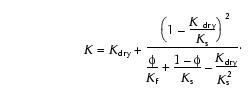
Estimation of gas saturation from the compressional velocity log

Brie et al. (1995) developed a model for the dependence of sonic velocities on pores and their fluid content that can be applied to clay-rich formations. It is based on the Gassmann equation for porous media and connects the bulk modulus of the fluid-filled material (K) to the modulus of the dry porous medium (K_dry), the modulus of the material (K_s), and the modulus of the fluid (K_f):

(30)

Elastic moduli are obtained from compressional wave velocity (V_P) and shear wave velocity (V_S), both of which are obtained from the sonic log:

where G is the shear modulus of the material. The ratio K/G is assumed to be the same for a nonporous material and for a porous material filled by very compressible fluid (Brie et al., 1995):

Under this assumption, an empirical relationship can be developed to estimate G for clays:

Using the known velocities for the matrix, the shear modulus (G_s), and hence the shear modulus of the dry porous material (G_dry) can be computed from Equation 33. By combining Equations 31 and 32, V_P/V_S can be plotted versus slowness (1/V_P) for a given porosity (in the case of a fully water-saturated fluid). In case of partial saturation (water saturation [S_w] <100%, as would be the case if gas is present), fluid moduli are computed by

where

• K_g = gas modulus, and

• K_w = water modulus.

For an ideal gas, the modulus is equal to its pressure and is assumed to be hydrostatic. The gas saturation can then be determined by fitting computed values of 1/V_P and V_P/V_S, which depend on ϕ and S_w, to V_P and V_S measurements from wireline logging.

Poisson's ratio (ν) is related to the ratio of V_P and V_S by

Top of page   |   Previous   |   Next