Tamura, Y., Busby, C.J., Blum, P., and the Expedition 350 Scientists, 2015
Proceedings of the International Ocean Discovery Program Volume 350
publications.iodp.org

doi:10.14379/iodp.proc.350.102.2015
Expedition 350 methods1
Y. Tamura, C.J. Busby, P. Blum, G. Guèrin, G.D.M. Andrews, A.K. Barker, J.L.R. Berger, E.M. Bongiolo, M. Bordiga, S.M. DeBari, J.B. Gill, C. Hamelin, J. Jia, E.H. John, A.-S. Jonas, M. Jutzeler, M.A.C. Kars, Z.A. Kita, K. Konrad, S.H. Mahony, M. Martini, T. Miyazaki, R.J. Musgrave, D.B. Nascimento, A.R.L. Nichols, J.M. Ribeiro, T. Sato, J.C. Schindlbeck, A.K. Schmitt, S.M. Straub, M.J. Vautravers, and Y. Yang2
Keywords: International Ocean Discovery Program, IODP, JOIDES Resolution, Expedition 350, Site U1436, Site U1437, Izu-Bonin-Mariana, IBM, prehnite, rear arc, seamount, Manji, tuffaceous mud, volcaniclastic, hyaloclastite, zircon, Neogene, ash, pumice, tuff, lapilli, Quaternary, breccia, peperite, rhyolite, intrusive, subduction, glass, continental crust, fore arc, density current, turbidite, fall deposit, tephra, greigite, volcano-bounded basin, VBB, hemipelagic mud, caldera, andesite, pXRF, ICP-AES, bioturbation, hydrothermal alteration, smectite, hornblende, sulfide reduction, fiamme, diagenesis, Aogashima, Kuroshio, explosive volcanism, submarine volcanism
MS 350-102: Published 30 May 2015
Introduction
This chapter of the International Ocean Discovery Program (IODP) Expedition 350 Proceedings volume documents the procedures and tools employed in the various shipboard laboratories of the R/V JOIDES Resolution during Expedition 350. This information applies only to shipboard work described in the Expedition Reports section of this volume. Methods for shore-based analyses of Expedition 350 samples and data will be described in the individual scientific contributions to be published in the open literature or in the Expedition Research Results section of this volume.
This section describes procedures and equipment used for drilling, coring, and hole completion; core handling; computation of depth for samples and measurements; and sequence of shipboard analyses. Subsequent sections describe specific laboratory procedures and instruments in more details.
Operations
Site locations
GPS coordinates from precruise site surveys were used to position the vessel at all Expedition 350 sites. A SyQuest Bathy 2010 CHIRP subbottom profiler was used to monitor the seafloor depth on the approach to each site to reconfirm the depth profiles from precruise surveys. Once the vessel was positioned at a site, the thrusters were lowered and a positioning beacon was dropped to the seafloor. The dynamic positioning control of the vessel used navigational input from the GPS and triangulation to the seafloor beacon, weighted by the estimated positional accuracy. The final hole position was the mean position calculated from the GPS data collected over a significant portion of the time the hole was occupied.
Coring and drilling operations
The coring strategy for Expedition 350 consisted primarily of obtaining as deep a penetration as possible at one site. The first hole would consist of a jet-in test to establish that a 16 inch casing, deployed with the reentry cone, could be washed in to ~25 meters below seafloor (mbsf). The second hole would be cored with the full-length advanced piston corer (APC) and the half-length APC (HLAPC) systems to refusal and deepened with the extended core barrel (XCB) system to ~400–600 mbsf. A third hole would be cored with the rotary core barrel (RCB) system from the maximum depth of the APC/XCB hole and penetrate as deep as possible. The fourth hole would be drilled without coring to the maximum depth of the existing RCB hole, then be cased, and then extended as deep as time permitted. A secondary component was to drill a 150 m APC hole at the beginning of the cruise to provide geotechnical information for a potential ultradeep riser hole to be drilled with the D/V Chikyu.
The APC and HLAPC cut soft-sediment cores with minimal coring disturbance relative to other IODP coring systems and are suitable for the upper portion of each hole. After the APC core barrel is lowered through the drill pipe and lands near the bit, the drill pipe is pressured up until one or two shear pins that hold the inner barrel attached to the outer barrel fail. The inner barrel then advances into the formation at high speed and cuts the core with a diameter of 66 mm (2.6 inches). The driller can detect a successful cut, or “full stroke,” from the pressure gauge on the rig floor.
The depth limit of the APC, often referred to as APC refusal, is indicated in two ways: (1) the piston fails to achieve a complete stroke (as determined from the pump pressure reading) because the formation is too hard, or (2) excessive force (>60,000 lb; ~267 kN) is required to pull the core barrel out of the formation. When a full stroke could not be achieved, additional attempts were typically made. The assumption is made that the barrel penetrated the formation by the length of core recovered (nominal recovery of ~100%), and the bit was advanced by that length before cutting the next core. When a full or partial stroke was achieved but excessive force could not retrieve the barrel, the core barrel was sometimes “drilled over,” meaning after the inner core barrel was successfully shot into the formation, the drill bit was advanced to total depth to free the APC barrel.
Nonmagnetic core barrels were used during all APC deployments, except during the return to Site U1436 at the end of the expedition, when no paleomagnetic measurements were needed. Most APC cores recovered during Expedition 350 were oriented using the FlexIT tool (see Paleomagnetism). Formation temperature measurements were made to obtain temperature gradients and heat flow estimates (see Downhole measurements).
The XCB is a rotary system with a small cutting shoe that extends below the large rotary APC/XCB bit. The smaller bit can cut a semi-indurated core with less torque and fluid circulation than the main bit, optimizing recovery. The XCB cutting shoe (bit) extends ~30.5 cm ahead of the main bit in soft sediment but retracts into the main bit when hard formations are encountered. It cuts a core with nominal diameter of 5.87 cm (2.312 inches), slightly less than the 6.6 cm diameter of the APC cores.
The RCB is the most conventional rotary coring system and is suitable for lithified rock material. It cuts a core with nominal diameter of 5.87 cm, just as the XCB system does. RCB coring can be done with or without the core liners used routinely with the APC/XCB soft sediment systems. We chose to core without the liner in the deeper parts of Hole U1437E because core pieces seemed to get caught at the edge of the liner, leading to jamming and reduced recovery.
The bottom-hole assembly (BHA) is the lowermost part of the drill string. A typical APC/XCB BHA consists of a drill bit (outer diameter = 11 inches), a bit sub, a seal bore drill collar, a landing saver sub, a modified top sub, a modified head sub, a nonmagnetic drill collar (for APC/XCB), a number of 8 inch (~20.32 cm) drill collars, a tapered drill collar, 6 joints (two stands) of 5½ inch (~13.97 cm) drill pipe, and 1 crossover sub. A lockable flapper valve was used to collect downhole logs without dropping the bit when APC/XCB coring.
A typical RCB BHA consists of a drill bit, a bit sub, an outer core barrel, a top sub, a head sub, 8 joints of 8¼ inch drill collars, a tapered drill collar, 2 joints of standard 5½ inch drill pipe, and a crossover sub to the regular 5 inch drill pipe.
The typical casing installation consists of 20 inch casing, about 25 m long, attached to a reentry cone, with a casing hanger that receives a 16 inch casing string a few hundred meters long, and finally a 10¾ inch string of several hundred meters length. Installation of the casing in Hole U1437E, which represents a record length for the JOIDES Resolution (1085.6 m), is described in Operations in the Site U1437 chapter (Tamura et al., 2015).
Drilling disturbance
Cores may be significantly disturbed as a result of the drilling process and contain extraneous material as a result of the coring and core handling process. In formations with loose granular layers (sand, ash, shell hash, ice-rafted debris, etc.), granular material from intervals higher in the hole may settle and accumulate in the bottom of the hole as a result of drilling circulation and be sampled with the next core. The uppermost 10–50 cm of each core must therefore be examined critically during description for potential “fall-in.” Common coring-induced deformation includes the concave-downward appearance of originally horizontal bedding. Piston action may result in fluidization (flow-in) at the bottom of, or even within, APC cores. Retrieval of unconsolidated (APC) cores from depth to the surface typically results to some degree in elastic rebound, and gas that is in solution at depth may become free and drive core segments within the liner apart. When gas content is high, pressure must be relieved for safety reasons before the cores are cut into segments. This is accomplished by drilling holes into the liner, which forces some sediment as well as gas out of the liner. XCB coring typically affects torquing of the indurated core, resulting in fractured disc-shaped pieces packed with sheared and remolded core material, mixed with drill slurry, resembling resembled soft cream between brittle “biscuits.”
Drilling disturbances are described in the Lithostratigraphy sections in each site chapter and are graphically indicated on the graphic core summary reports, also referred to as visual core descriptions (VCDs), in Core descriptions.
Core handling and analysis
All APC and XCB cores and some of the RCB cores recovered during Expedition 350 were extracted from the core barrel in plastic liners. These liners were carried from the rig floor to the core processing area on the catwalk outside the Core Laboratory and cut into ~1.5 m sections. The exact section length was noted and later entered into the database as “created length” using the Sample Master application. This number was used to calculate recovery. The curated length was set equal to the created length and very rarely had to be modified. Depth in hole calculations are based on the curated length.
When the core liners seemed to cause jams, preventing pieces to enter the barrel, liners were not used. Instead, the recovered core was slid and shaken out of the barrel and carefully arrange in the order retrieved in a prepared half-liner. The core pieces were then filled into a full liner for the purpose of splitting. We did not perform any “hard rock curation” whereby pieces are separated with dividers and logged separately.
Headspace samples were taken from selected section ends (typically 1 per core) using a syringe for immediate hydrocarbon analysis as part of the shipboard safety and pollution prevention program. Similarly, whole-round samples for interstitial water analysis and microbiology samples were taken immediately after the core was sectioned. Core catcher samples were taken for biostratigraphic analysis. When catwalk sampling was complete, liner caps (blue = top, colorless = bottom) were glued with acetone onto liner sections, and the sections were placed in core racks in the laboratory for analysis.
After completion of whole-round section analyses (see below), the sections were split lengthwise from bottom to top into working and archive halves. The softer cores were split with a wire, and harder cores were split with a diamond saw. Investigators should note that older material may have been transported upward on the split face of each section during splitting.
The numbering of sites, holes, cores, and samples followed standard IODP procedure. A full curatorial sample identifier consists of the following information: expedition, site, hole, core number, core type, section number, section half, and offset in centimeters measured from the top of the core section. For example, a sample identification of “350-U1436A-1H-2W, 10–12 cm” represents a sample taken from the interval between 10 and 12 cm below the top of the working half of Section 2 of Core 1 (“H” designates that this core was taken with the APC system) of Hole U1436A during Expedition 350. The “U” preceding the site number indicates that the hole was drilled by the United States Implementing Organization (USIO) platform, the JOIDES Resolution.
Sample depth calculations
Sample depth calculations are based on the methods described in IODP Depth Scales Terminology v.2 at www.iodp.org/program-policies/procedures/guidelines. Depths of samples and measurements were calculated at the applicable depth scale as summarized below. The definition of these depth scale types, and the distinction in nomenclature, should keep the user aware that a nominal depth value at two different depth scale types usually does not refer to exactly the same stratigraphic interval in a hole.
Depths of cored intervals were measured from the drill floor based on the length of drill pipe deployed beneath the rig floor and referred to as drilling depth below rig floor (DRF), with a commonly used custom unit designation of meters below rig floor (mbrf). The depth of the cored interval was referenced to the seafloor by subtracting the seafloor depth from the DRF depth of the interval. The seafloor referenced depth of the cored interval is referred to as the drilling depth below seafloor (DSF), with a commonly used custom unit designation of meters below seafloor (mbsf). In most cases, the seafloor depth was the length of pipe deployed minus the length of the mudline core recovered. In some cases, the seafloor depth was adopted from a previous hole drilled at the site.
Depths of samples and measurements in each core are computed based on a set of rules that result in a depth scale type referred to as the core depth below seafloor, Method A (CSF-A). The two most fundamental rules are that (1) the top depth of a recovered core corresponds to the top depth of its cored interval (top DSF = top CSF-A), even if the core includes fall-in material at the top (see Drilling disturbance); and (2) the recovered material is a contiguous stratigraphic representation, even if core segments are separated by voids when recovered and if the core is shorter than the cored interval. When voids were present in the core on the catwalk, they were closed by pushing core segments together whenever possible. When a core had incomplete recovery (i.e., the true position of the core within the cored interval was unknown), the top of the recovered interval was assigned to the top of the cored interval. The length of missing core should be considered a sample depth uncertainty when analyzing data associated with the core material. Depths of subsamples and associated measurements at the CSF-A scale were calculated by adding the offset of the subsample or measurement from the top of its section, and the lengths of all higher sections in the core, to the top depth of the cored interval (top DSF = top CSF-A).
Per IODP policy established after the introduction of the IODP Depth Scales Terminology v.2, sample and measurement depths at the CSF-A depth scale type are commonly referred to with the custom unit mbsf, just as depths at the DSF scale type. The reader should be aware that the use of mbsf for different depth scale types is inconsistent with the more rigorous definition of depth types and may be misleading in specific cases because different “mbsf depths” may be assigned to the same stratigraphic interval. One example is described below.
A soft to semisoft sediment core from less than a few hundred meters below seafloor expands upon recovery (typically a few percent to as much as 15%), so the length of the recovered core exceeds that of the cored interval. Therefore, a stratigraphic interval may not have the same nominal depth at the DSF and CSF-A scales in the same hole. When core recovery (the ratio of recovered core to cored interval times 100%) is >100%, the CSF-A depth of a sample taken from the bottom of a core will be deeper than that of a sample from the top of the subsequent core (i.e., the data associated with the two core intervals overlap at the CSF-A scale). The core depth below seafloor, Method B (CSF-B), depth scale is a solution to the overlap problem. This method scales the recovered core length back into the interval cored, from >100% to exactly 100% recovery. If cores had <100% recovery to begin with, they were not scaled. When downloading data using the IODP-USIO Laboratory Information Management System (LIMS) Reports pages at web.iodp.tamu.edu/UWQ, depths for samples and measurements are by default presented at both CSF-A and CSF-B scales. The CSF ‑B depth scale is primarily useful for data analysis and presentations in single-hole situations.
Another major depth scale type is the core composite depth below seafloor (CCSF) scale, typically constructed from multiple holes for each site, whenever feasible, to mitigate the CSF-A core overlap problem as well as the coring gap problem and to create as continuous a stratigraphic record as possible. This depth scale type was not used during Expedition 350 and is therefore not further described here.
Shipboard core analysis
After letting the cores thermally equilibrate for at least 1 h, whole-round core sections were run through the Whole-Round Multisensor Logger (WRMSL), which measures P-wave velocity, density, and magnetic susceptibility, and the Natural Gamma Radiation Logger (NGRL). Thermal conductivity measurements were also taken before the cores were split lengthwise into working and archive halves. The working half of each core was sampled for shipboard analysis, routinely for paleomagnetism and physical properties, and more irregularly for thin sections, geochemistry, and biostratigraphy. The archive half of each core was scanned on the Section Half Imaging Logger (SHIL) and measured for color reflectance and magnetic susceptibility on the Section Half Multisensor Logger (SHMSL). The archive halves were described macroscopically as well as microscopically in smear slides, and the working halves were sampled for thin section microscopic examination. Finally, the archive halves were run through the cryogenic magnetometer. Both halves of the core were then put into labeled plastic tubes that were sealed and transferred to cold storage space aboard the ship.
Samples for postcruise analysis were taken for individual investigators from the working halves of cores, based on requests approved by the Sample Allocation Committee (SAC). Up to 17 cores were laid out in 13 sampling parties lasting 2–3 days each, from planning to execution. Scientists viewed the cores, flagged sampling locations, and submitted detailed lists of requested samples. The SAC reviewed the flagged samples and resolved rare conflicts as needed. Shipboard staff cut, registered, and packed the samples. A total of 6372 samples were taken for shore-based analyses, in addition to 3211 samples taken for shipboard analysis.
All core sections remained on the ship until the end of Expedition 351 because of ongoing construction at the Kochi Core Center (KCC). At the end of Expedition 351, all core sections and thin sections were trucked to the KCC for permanent storage.
Lithostratigraphy
Lithologic description
The lithologic classification of sedimentary, volcaniclastic, and igneous rocks recovered during Expedition 350 uses a new scheme for describing volcaniclastic and nonvolcaniclastic sediment (Figure F1) but uses generally established (International Union of Geological Sciences [IUGS]) schemes for igneous rocks. This new scheme was devised to improve description of volcaniclastic sediment and the mixtures with nonvolcanic (siliciclastic and chemical and biogenic) sediment while maintaining the usefulness of prior schemes for describing nonvolcanic sediment. The new scheme follows the recommendations of a dedicated core description workshop held in January 2014 in College Station (TX, USA) prior to the cruise and attended by participants of IODP Expeditions 349, 350, 351, and 352 and was tested and finalized during Expedition 350. The new scheme was devised for use in a spreadsheet-based descriptive information capture program designed by IODP (DESClogik), and the spreadsheet configurations were modified to use this scheme. Also during Expedition 350, the new scheme was applied to microscopic description of core samples, and the DESClogik microscope spreadsheet configurations were modified to use this scheme.
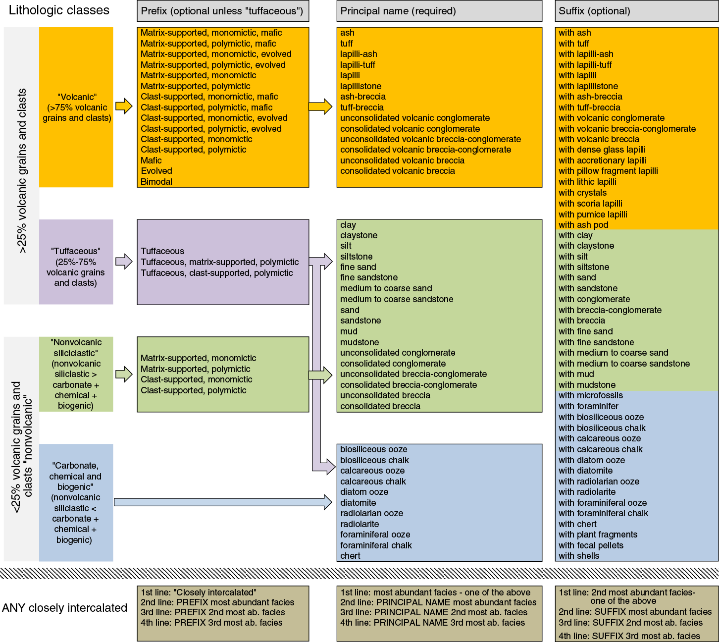
Figure F1. Sedimentary and volcaniclastic lithology naming conventions.
During Expedition 350, all sediment and rock types were described by a team of core describers with backgrounds principally in physical volcanology, volcaniclastic sedimentation, and igneous petrology. Macroscopic descriptions were made at dedicated tables where the split core sections were laid out. Each core section was described in two steps: (1) hand-written observations were recorded onto 11 inch × 17 inch printouts of high-resolution SHIL images, and (2) data were entered into the DESClogik software (see below). This method provides two description records of each core, one physical and one digital, and minimizes data entry mistakes in DESClogik. Smear slides and petrographic thin sections were investigated with binocular and petrographic microscopes (transmitted and reflected light) and described in DESClogik. Because of the delay (about 24 h) required in producing petrographic thin sections, only smear slides could be used to contribute to macroscopic descriptions at the time the cores were described. Thin section descriptions were used later to refine the initial macroscopic observations.
IODP use of DESClogik
Data for the macroscopic and microscopic descriptions of recovered cores were entered into the LIMS database, using the IODP data-entry software DESClogik. DESClogik is a core description software interface used to enter macroscopic and/or microscopic descriptions of cores. Core description data are available through the Descriptive Information LIMS Report (web.iodp.tamu.edu/DESCReport). A single row in DESClogik defines one descriptive interval, which is commonly (but not necessarily) one bed (Table T1).
Table T1. Lithostratigraphic and lithologic units, descriptive intervals, and domains. Download table in .csv format.
Core disturbances
IODP coring induces various types of disturbances in recovered cores. Core disturbances are recorded in DESClogik. Core disturbances are diverse (Jutzeler et al., 2014), and some of them are only associated with specific coring techniques.
- Core extension (APC) preferentially occurs in granular (noncohesive) sediment. This disturbance is obvious where sediment does not entirely fill the core liner and soupy textures occur. Stratification is commonly destroyed, and bed thickness is artificially increased.
- Sediment flowage disturbance (APC) is the result of material displacement along the margins of the core liner. This results in horizontal superposition of the original stratigraphy enveloped in allochthonous material.
- Mid-core flow-in (APC) is injection of material within the original stratigraphy. Developing from sediment flowage, allochthonous sediment is intruded into the genuine stratigraphy, creating false beds. This disturbance type is rare and is commonly associated with strong shearing and sediment flowage along the margin of the core liner.
- Basal flow-in (APC) is associated with partial strokes in sediment and occurs where cohesive, muddy beds are absent from the bottom of the core. Basal flow-in results from the sucking-in of granular material from the surrounding sediment through the cutting shoe during retrieval of the core barrel. It creates a false stratigraphy, commonly composed of soupy, polymictic, density-graded sediment that generally lacks horizontal laminations (indicating homogenization). Basal flow-in disturbances can affect more than half of the core.
- Fall-in (APC, XCB, and RCB) disturbances result from collapse of the unstable borehole or fall-back of waste cuttings that could not be evacuated to the seafloor during washing with drilling water. Fall-in disturbances occur at the very top of the core (i.e., usually most prevalent in Section 1 and rarely continues into the lower core sections) and often follow a core that was a partial stroke. Fall-in disturbances commonly consist of polymictic, millimeter to centimeter clasts and can be clast or matrix supported. The length of a fall-in interval is typically on the order of 10–40 cm but can exceed 1 m. A fall-in interval is recognized by being distinctly different from the other facies types in the lower part of the same core, displaying chaotic or massive bedding, and containing constituents encountered further up in the hole.
- Fractured rocks (XCB and RCB) occur over three fracturing intensities (slight, moderate, and severe), but do not show clast rotation (Figure F2).
- Brecciated and randomly oriented fragmented rocks (XCB and RCB) occur where rock fracturing was followed by remobilization and reorientation of the fragments into a disordered pseudostratigraphy (Figure F2).
- Biscuited disturbances (XCB and RCB) consist of intervals of mud and brecciated rock. They are produced by fragmentation of the core in multiple disc-shaped pieces (biscuits) that rotate against each other at different rates, inducing abrasion and comminution. Biscuiting commonly increases in intensity toward the base of a core (Figure F2). Interstitial mud is either the original lithology and/or a product of the abrasion. Comminuted rock produces mud-sized gouges that can lithify and become indistinguishable from fine-grained beds (Piper, 1975).
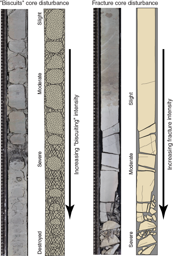
Figure F2. Core disturbances.
Sediments and sedimentary rocks
Rationale
Sediments and sedimentary rocks are classified using a rigorously nongenetic approach that integrates volcanic particles into the sedimentary descriptive scheme typically used by IODP (Figure F1). This is necessary because volcanic particles are the most abundant particle type in arc settings like those drilled during the Izu-Bonin-Mariana (IBM) expeditions. The methodology developed allows, for the first time, comprehensive description of volcanogenic and nonvolcanogenic sediment and sedimentary rock and integrates with descriptions of coherent volcanic and igneous rock (i.e., lava and intrusions) and the coarse clastic material derived from them. This classification allows expansion to bioclastic and nonvolcanogenic detrital realms.
The purpose of the new classification scheme (Figure F1) is to include volcanic particles in the assessment of sediment and rock recovered in cores, be accessible to scientists with diverse research backgrounds and experiences, allow relatively quick and smooth data entry, and display data seamlessly in graphical presentations. The new classification scheme is based entirely on observations that can be made by any scientist at the macroscopic and microscopic level, with no genetic inferences, making the data more reproducible from user to user.
Classification and nomenclature of deposits with volcanogenic clasts has varied considerably throughout the last 50 y (Fisher, 1961; Fisher and Schmincke, 1984; Cas and Wright, 1987; McPhie et al., 1993; White and Houghton, 2006), and no consensus has yet been reached. Moreover, even the most basic descriptions and characterizations of mixed volcanogenic and nonvolcanogenic sediment are fraught with competing philosophies and imperfectly applied terminology. Volcaniclastic classification schemes are all too often overly based on inferred modes of genesis, including inferred fragmentation processes or inferred transport and depositional processes and environments. However, submarine-erupted and deposited volcanic sediments are typically much more difficult to interpret than their subaerial counterparts, partly because of more complex density-settling patterns through water relative to air and the ease with which very fine grained sediment is reworked by water. Soft-sediment deformation, bioturbation, and low-temperature alteration are also more significant in the marine realm relative to the terrestrial realm.
In our new classification scheme, some common lithologic parameters are broader (i.e., less narrowly or strictly applied) than those used in the published literature; this has been done (1) to reduce unnecessary detail that is in the realm of specialist sedimentology and physical volcanology and make the descriptive process more accessible, intuitive, and comprehensible to nonspecialists and (2) to make the descriptive process as linear and as “database ready” as possible.
Description workflow
The following workflow was used:
- Initial determination of intervals in a core section was conducted by a pair of core describers (typically a physical volcanologist and an igneous petrologist). Macroscopic analyses were performed on all intervals for a first-order assessment of their main characteristics: particle sizes, compositions, and heterogeneity, as well as sedimentary structures and petrofabrics. If an interval described in the macroscopic sediment data sheet had igneous clasts larger than 2 cm, the clasts were described in detail on the extrusive/hypabyssal data sheet (e.g., crystallinity, mineralogy, etc.) because clasts of that size are large enough to be described macroscopically.
- Microscopic analyses were performed for each new facies using (i) discrete samples diluted in water (not curated), (ii) sediment glued into a smear slide, or (iii) petrographic thin sections of sediment or sedimentary rock. Consistency was regularly checked for reoccurring facies. Thin sections and smear slides varied in quantity and proportion, depending on the firmness of the material, the repetitiveness of the facies, and the time available during core description. Microscopic observations allow detailed descriptions of smaller particles than is possible with macroscopic observation, so if a thin section described in the microscopic sediment data sheet had igneous clasts larger than 2 mm (the cutoff between sand/ash and granules/lapilli, see definitions below), the clasts were described in detail on the igneous microscopic data sheet.
- The sediment or sedimentary rock was named (Figure F1).
- A single lithologic summary sentence was written for each core.
Units
Sediment and sedimentary rock, including volcaniclastic, siliciclastic, and bioclastic, are described at the level of (1) the descriptive interval (a single descriptive line in the DESClogik spreadsheet) and (2) the lithostratigraphic unit.
Descriptive intervals
A descriptive interval (Table T1) is unique to a specific depth interval and typically consists of a single lithofacies distinct from those immediately above and below (e.g., an ash interval intercalated between mud intervals). Descriptive intervals are, therefore, typically analogous to beds, and thicknesses can be classified in the same way (e.g., Ingram, 1954). Because cores are individually described per core section, a stratigraphically continuous bed may be divided into two (or more) intervals if it is cut by a core/core section boundary.
In the case of closely intercalated, monotonous, repetitive successions (e.g., alternating thin sand and mud beds), lithofacies may be grouped within the descriptive interval. This is done by using the lithology prefix “closely intercalated,” followed by the principal name, which represents the most abundant facies, followed by suffixes for the subordinate facies, in order of abundance (Figure F1). Using the domain classifier in the DESClogik software, the closely intercalated interval is identified as Domain 0 and the subordinate parts are identified as Domains 1, 2, and 3, respectively, and their relative abundances noted. Each subordinate domain is described beneath the composite descriptive interval as if it were its own descriptive interval, but each subordinate facies is described only once, allowing simplified data entry and graphical output. This allows for each subordinate domain to be assigned its own prefix, principal name, and suffix (e.g., a closely intercalated tuff with mudstone can be expanded to evolved tuff with lapilli [Domain 1, 80%] and tuffaceous mudstone with shell fragments [Domain 2, 20%]).
Lithostratigraphic units
Lithostratigraphic units, not to be confused with lithologic units used with igneous rocks (see below), are meters to hundreds of meters thick assemblages of multiple descriptive intervals containing similar facies (Table T1). They are numbered sequentially (Unit I, Unit II, etc.) from top to bottom. Lithostratigraphic units should be clearly distinguishable from each other by several characteristics (e.g., composition, bed thickness, grain size class, and internal homogeneity). Lithostratigraphic units are, therefore, analogous to formations but are strictly informal. Furthermore, they are not defined by age, geochemistry, physical properties, or paleontology, although changes in these parameters may coincide with boundaries between lithostratigraphic units.
Descriptive scheme for sediment and sedimentary rocks
The newly devised descriptive scheme (Figure F1) is divided into four main sedimentary lithologic classes, based on composition: volcanic, nonvolcanic siliciclastic, chemical and biogenic, and mixed volcanic-siliciclastic or volcanic-biogenic, with mixed referred to as the tuffaceous lithologic class. Within those lithologic classes, a principal name must be chosen; the principal name is based on particle size for the volcanic, nonvolcanic siliciclastic, and tuffaceous nonvolcanic siliciclastic lithologic classes. In addition, appropriate prefixes and suffixes may be chosen, but this is optional, except for the prefix “tuffaceous” for the tuffaceous lithologic class, as described below.
Sedimentary lithologic classes
In this section, we describe lithologic classes and principal names; this is followed by a description of a new scheme where we divide all particles into two size classes: grains (<2 mm) and clasts (>2 mm). Then we describe prefixes and suffixes used in our new scheme and describe other parameters. Volcaniclastic, nonvolcanic siliciclastic, and chemical and biogenic sediment and rock can all be described with equal precision in the new scheme presented here (Figure F1). The sedimentary lithologic classes, based on types of particles, are
- Volcanic lithologic class, defined as >75% volcanic particles;
- Tuffaceous lithologic class, containing 75%–25% volcanic-derived particles mixed with nonvolcanic particles (either or both nonvolcanic siliciclastic and chemical and biogenic);
- Nonvolcanic siliciclastic lithologic class, containing <25% volcanic siliciclastic particles and nonvolcanic siliciclastic particles dominate chemical and biogenic; and
- Biogenic lithologic class, containing <25% volcanic siliciclastic particles and nonvolcanic siliciclastic particles are subordinate to chemical and biogenic particles.
The definition of the term tuffaceous (25%–75% volcanic particles) is modified from Fisher and Schmincke (1984) (Table T2).
Table T2. Relative abundances of volcanogenic material. Download table in .csv format.
Principal names
Principal names for sediment and sedimentary rock of the nonvolcanic siliciclastic and tuffaceous lithologic classes are adapted from the grain size classes of Wentworth (1922), whereas principal names for sediment and sedimentary rock of the volcanic lithologic class are adapted from the grain size classes of Fisher and Schmincke (1984) (Table T3; Figure F3). Thus, the Wentworth (1922) and Fisher and Schmincke (1984) classifications are used to refer to particle type (nonvolcanic versus volcanic, respectively) and the size of the particles (Figure F1). The principal name is thus purely descriptive and does not depend on interpretations of fragmentation, transport, depositional, or alteration processes. For each grain size class, both a consolidated (i.e., semilithified to lithified) and a nonconsolidated term exists; they are mutually exclusive (e.g., mud or mudstone; ash or tuff). For simplicity, Wentworth’s clay and silt sizes are combined in a “mud” class; similarly, fine, medium, and coarse sand are combined in a “sand” class.
Table T3. Particle size nomenclature and classifications. Download table in .csv format.
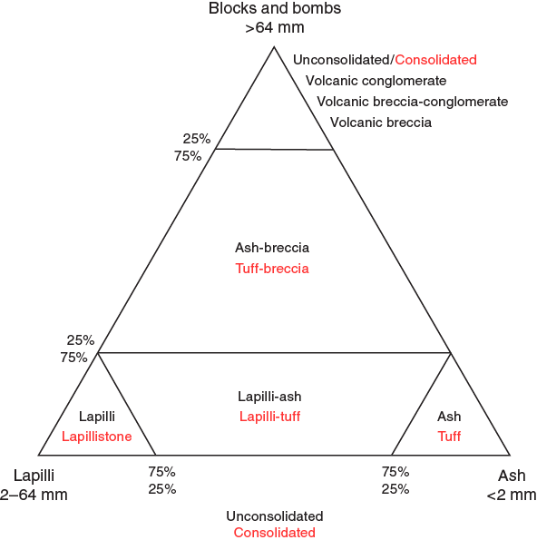
Figure F3. Volcaniclastic grain size terms.
New definition of principal name: conglomerate, breccia-conglomerate, and breccia
The grain size terms granule, pebble, and cobble (Wentworth, 1922) are replaced by breccia, conglomerate, or breccia-conglomerate in order to include critical information on the angularity of fragments larger than 2 mm (the sand/granule boundary of Wentworth, 1922). A conglomerate is defined as a deposit where the fragments are >2 mm and are exclusively (>95 vol%) rounded and subrounded (Table T3; Figure F4). A breccia-conglomerate is composed of predominantly rounded and/or subrounded clasts (>50 vol%) and subordinate angular clasts. A breccia is predominantly composed of angular clasts (>50 vol%). Breccia, conglomerates, and breccia-conglomerates may be consolidated (i.e., lithified) or unconsolidated. Clast sphericity is not evaluated.
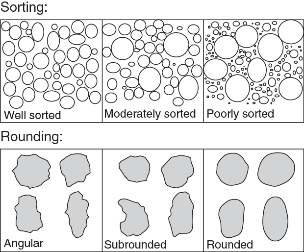
Figure F4. Sorting and rounding classifications.
Definition of grains versus clasts and detailed grain sizes
We use the general term “particles” to refer to the fragments that make up volcanic, tuffaceous, and nonvolcanic siliciclastic sediment and sedimentary rock, regardless of the size of the fragments. However, for reasons that are both meaningful and convenient, we employ a much stricter use of the terms “grain” and “clast” for the description of these particles. We refer to particles larger than 2 mm as clasts and particles smaller than 2 mm as grains. This cut-off size (2 mm) corresponds to the sand/granule grain size division of Wentworth (1922) and the ash/lapilli grain size divisions of Fisher (1961), Fisher and Schmincke (1984), Cas and Wright (1987), McPhie et al. (1993), and White and Houghton (2006) (Table T3). This size division has stood the test of time because it is meaningful: particles larger than 2 mm are much easier to see and describe macroscopically (in core or on outcrop) than particles smaller than 2 mm. Additionally, volcanic particles <2 mm in size commonly include volcanic crystals, whereas volcanic crystals are virtually never >2 mm in size. As examples using our definition, an ash or tuff is made entirely of grains, a lapilli-tuff or tuff-breccia has a mixture of clasts and grains, and a lapillistone is made entirely of clasts.
Irrespective of the sediment or rock composition, detailed average and maximum grain size follows Wentworth (1922). For example, an ash can be further described as sand-sized ash or silt-sized ash; a lapilli-tuff can be described as coarse sand sized or pebble sized.
Definition of prefix: monomict versus polymict
The term mono- (one) when applied to clast compositions refers to a single type, and poly- (many) when applied to clast compositions refers to multiple types. These terms have been most widely applied to clasts (>2 mm in size; e.g., conglomerates) because these can be described macroscopically. We thus restrict our use of the terms monomict or polymict to particles >2 mm in size (referred to as clasts in our scheme) and do not use the term for particles <2 mm in size (referred to as grains in our scheme).
Variations within a single volcanic parent rock (e.g., a collapsing lava dome) may produce clasts referred to as monomict, which are all of the same composition.
Definition of prefix: clast supported versus matrix supported
“Matrix supported” is used where smaller particles visibly envelop each of the larger particles. The larger particles must be >2 mm in size; that is, they are clasts, using our definition of the word. However, the word “matrix” is not defined by a specific grain size cutoff (i.e., it is not restricted to grains, which are <2 mm in size). For example, a matrix-supported volcanic breccia could have blocks supported in a matrix of lapilli-tuff. “Clast supported” is used where clasts (>2 mm in diameter) form the sediment framework; in this case, porosity and small volumes of matrix or cement are interstitial. These definitions apply to both macroscopic and microscopic observations.
Definition of prefix: mafic versus evolved versus bimodal
In the scheme shown in Figure F1, the compositional range of volcanic grains and clasts is represented by only three entries: “mafic,” “bimodal,” and “evolved.” In macroscopic analysis, mafic versus evolved intervals are defined by the grayscale index of the main particle component, with unaltered mafic grains and clasts usually ranging from black to dark gray and unaltered evolved grains and clasts ranging from dark gray to white. Microscopic examination may further aid in assigning the prefix mafic or evolved, using glass shard color and mineralogy, but precise determination of bulk composition requires chemical analysis. In general, intervals described as mafic are inferred to be basalt and basaltic andesite, whereas intervals described as evolved are inferred to be intermediate and silicic in composition, but again, geochemical analysis is needed to confirm this. Bimodal may be used where both mafic and evolved constituents are mixed in the same descriptive interval. Compositional prefixes (e.g., mafic, evolved, and bimodal) are optional and may be impossible to assign in altered rocks.
In microscopic description, a more specific compositional name can be assigned to an interval if the necessary index minerals are identified. Following the procedures defined for igneous rocks (see below), the presence of olivine identifies the deposit as “basaltic,” the presence of quartz identifies the deposit as “rhyolite-dacite,” and the absence of both identifies the deposit as “andesitic.”
Suffixes
The suffix is used for a subordinate component that deserves to be highlighted. It is restricted to a single term or phrase to maintain a short and effective lithology name containing the most important information only. It is always in the form “with ash,” “with clay,” “with foraminifer,” etc.
Other parameters
Bed thicknesses (Table T4) follow the terminology of Ingram (1954), but we group together thin and thick laminations into “lamina” for all beds <1 cm thick; the term “extremely thick” is added for >10 m thick beds. Sorting and clast roundness values are restricted to three terms: well, moderately, and poor and rounded, subrounded, and angular, respectively (Figure F4), for simplicity and consistency between core describers.
Table T4. Bed thickness classifications. Download table in .csv format.
Intensity of bioturbation is qualified in four degrees: none, slight, moderate, and strong, corresponding to the degradation of otherwise visible sedimentary structures (e.g., planar lamination) and inclusion of grains from nearby intervals.
Macrofossil abundance is estimated in six degrees, with dominant (>50%), abundant (2%–50%), common (5%–20%), rare (1%–5%), trace (<1%), and absent (Table T5), following common IODP practice for smear slide, stereomicroscopic, and microscopic observations. The dominant macrofossil type is selected from an established IODP list.
Table T5. Macrofossil abundance classifications. Download table in .csv format.
Quantification of the grain and clast componentry differs from most previous Integrated Ocean Drilling Program (and equivalent) expeditions. An assessment of grain and clast componentry includes up to three major volcanic components (vitric, crystal, and lithic), which are sorted by their abundance (“dominant,” “second order,” and “third order”). The different types of grains and clasts occurring within each component type are listed below.
Vitric grains (<2 mm) and clasts (>2 mm) can be angular, subrounded, or rounded and of the following types:
- Pumice
- Scoria
- Shards
- Glass, dense
- Pillow fragment
- Accretionary lapilli
- Fiamme
- Limu o Pele
- Pele’s hair (microscopic only)
Crystals can be euhedral, subhedral, or anhedral and are always described as grains regardless of size (i.e., they are not clasts); they are of the following types:
Lithic grains (<2 mm) and clasts (>2 mm) can be angular, subrounded, or rounded and of the following types (igneous plutonic grains do not occur):
- Igneous clast/grain, mafic (unknown if volcanic or plutonic)
- Igneous clast/grain, evolved (unknown if volcanic or plutonic)
- Volcanic clast/grain, evolved
- Volcanic clast/grain, mafic
- Plutonic clast/grain, mafic
- Plutonic clast/grain, evolved
- Metamorphic clast/grain
- Sandstone clast/grain
- Carbonate clast/grain (shells and carbonate rocks)
- Mudstone clast/grain
- Plant remains
In macroscopic description, matrix can be well, moderately, or poorly sorted based on visible grain size (Figure F3) and of the following types:
Summary
We have devised a new scheme to improve description of volcaniclastic sediments and their mixtures with nonvolcanic (siliciclastic, chemogenic, and biogenic) particles, while maintaining the usefulness of prior schemes for describing nonvolcanic sediments. In this scheme, inferred fragmentation, transport, and alteration processes are not part of the lithologic name. Therefore, volcanic grains inferred to have formed by a variety of processes (i.e., pyroclasts, autoclasts, epiclasts, and reworked volcanic clasts; Fisher and Schmincke, 1984; Cas and Wright, 1987; McPhie et al., 1993) are grouped under a common grain size term that allows for a more descriptive (i.e., nongenetic) approach than proposed by previous authors. However, interpretations can be entered as comments in the database; these may include inferences regarding fragmentation processes, eruptive environments, mixing processes, transport and depositional processes, alteration, and so on.
Igneous rocks
Igneous rock description procedures during Expedition 350 generally followed those used during previous Integrated Ocean Drilling Program expeditions that encountered volcaniclastic deposits (e.g., Expedition 330 Scientists, 2012; Expedition 336 Scientists, 2012; Expedition 340 Scientists, 2013) with modifications in order to describe multiple clast types at any given interval. Macroscopic observations were coordinated with thin section or smear slide petrographic observations and bulk-rock chemical analyses of representative samples. Data for the macroscopic and microscopic descriptions of recovered cores were entered into the LIMS database using the DESClogik program.
During Expedition 350, we recovered volcaniclastic sediments that contain igneous particles of various sizes, as well as an igneous unit classified as an intrusive sheet. Therefore, we describe igneous rocks as either a coherent igneous body or as large igneous clasts in volcaniclastic sediment. If igneous particles are sufficiently large to be described individually at the macroscopic scale (>2 cm), they are described for lithology with prefix and suffix, texture, grain size, and contact relationships in the extrusive_hypabyssal and intrusive_mantle tabs in DESClogik. In thin section, particles >2 mm in size are described as individual clasts or as a population of clasts, using the 2 mm size cutoff between grains and clasts described above; this is a suitable size at the scale of thin section observation (Figure F5).
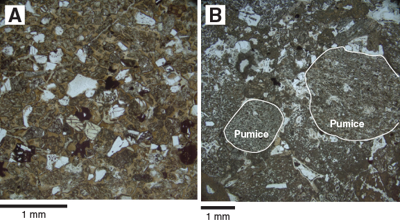
Figure F5. Tuff and lapilli-tuff.
Plutonic rocks are holocrystalline (100% crystals with all crystals >1.0 mm) with crystals visible to the naked eye. Volcanic rocks are composed of a glassy or microcrystalline groundmass (crystals <1.0 mm) and can contain various proportions of phenocrysts (typically 5 times larger than groundmass, usually >0.1 mm) and/or vesicles.
Units
Igneous rocks are described at the level of the descriptive interval (the individual descriptive line in DESClogik), the lithologic unit, and ultimately at the level of the lithostratigraphic unit. A descriptive interval consists of variations in rock characteristics, such as vesicle distribution, igneous textures, mineral modes, and chilled margins. Rarely, a descriptive interval may comprise multiple domains, for example in the case of mingled magmas. Lithologic units in coherent igneous bodies are defined either by visual identification of actual lithologic contacts (e.g., chilled margins) or by inference of the position of such contacts using observed changes in lithology (e.g., different phenocryst assemblage or volcanic features). These lithologic units can include multiple descriptive intervals. The relationship between multiple lithologic units is then used to define an overall lithostratigraphic interval.
Volcanic rocks
Samples within the volcanic category are massive lava, pillow lava, intrusive sheets (i.e., dikes and sills), volcanic breccia intimately associated with lava flows, and volcanic clasts in sediment and sedimentary rock (Table T6). Volcanic breccia not associated with lava flows and hyaloclastites not associated with pillow lava are described in the sediment tab in DESClogik. Monolithic volcanic breccia with clast sizes <6.4 cm (−6φ) first encountered beneath any other rock type are automatically described in the sediment tab in order to avoid confusion. A massive lava is defined as a coherent volcanic body with a massive core and vesiculated (sometimes brecciated or glassy) flow top and bottom. When possible, we identify pillow lava on the basis of being subrounded massive volcanic bodies (0.2–1 m in diameter) with glassy margins (and/or broken glassy fragments hereby described as hyaloclastite) that commonly show radiating fractures and decreasing mineral abundances and grain size toward the glassy rims. The pillow lava category therefore includes multiple seafloor lava flow morphologies (e.g., sheet, lobate, hackly, etc.). Intrusive sheets are defined as dikes or sills cutting across other lithologic units. They consist of a massive core with a holocrystalline groundmass and nonvesiculated chilled margins along their boundaries. Their size varies from several millimeters to several meters in thickness. Clasts in sediment include both lithic (dense) and vitric (inflated scoria and pumice) varieties.
Table T6. Nomenclature for extrusive and hypabyssal volcanic rocks. Download table in .csv format.
Lithology
Volcanic rocks are usually classified on the basis of their alkali and silica contents. A simplified classification scheme based on visual characteristics is used for macroscopic and microscopic determinations. The lithology name consists of a main principal name and optional prefix and suffix (Table T6). The main lithologic name depends on the nature of phenocryst minerals and/or the color of the groundmass. Three rock types are defined for phyric samples:
- Basalt: black to dark gray, typically olivine-bearing volcanic rock;
- Andesite: dark to light gray, containing pyroxenes and/or feldspar and/or amphibole; typically devoid of olivine and quartz; and
- Rhyolite-dacite: light gray to pale white, usually plagioclase-phyric, and sometimes containing quartz ± biotite; this macroscopic category may extend to SiO2 contents <70% and therefore may include dacite.
Volcanic clasts smaller than the cutoff defined for macroscopic (2 cm) and microscopic (2 mm) observations are described only as mafic (dark-colored) or evolved (light-colored) in the sediment tab. Dark aphyric rocks are considered to be basalt, whereas light-colored aphyric samples are considered to be rhyolite-dacite, with the exception of obsidian (generally dark colored but rhyolitic in composition).
The prefix provides information on the proportion and the nature of phenocrysts. Phenocrysts are defined as crystals significantly larger (typically 5 times) than the average size of the groundmass crystals. Divisions in the prefix are based on total phenocryst proportions:
- Aphyric (<1% phenocrysts)
- Sparsely phyric (≥1%–5% phenocrysts)
- Moderately phyric (>5%–20% phenocrysts)
- Highly phyric (>20% phenocrysts)
The prefix also includes the major phenocryst phase(s) (i.e., those that have a total abundance ≥1%) in order of increasing abundance left to right, so the dominant phase is listed last. Macroscopically, pyroxene and feldspar subtypes are not distinguished, but microscopically, they are identified as orthopyroxene and clinopyroxene, and plagioclase and K-feldspar, respectively. Aphyric rocks are not given any mineralogical identifier.
The suffix indicates the nature of the volcanic body: massive lava, pillow lava, intrusive sheet, or clast. In rare cases, the suffix hyaloclastite or breccia is used if the rock occurs in direct association with a related, in situ lava (Table T6). As mentioned above, thick sections of hyaloclastite or breccia unrelated to lava are described in the sediment tab.
Plutonic rocks
Plutonic rocks are classified according to the IUGS classification of Le Maitre et al. (2002). The nature and proportion of minerals are used to give a root name to the sample (see Figure F6 for the root names used). A prefix can be added to indicate the presence of a mineral not present in the definition of the main name (e.g., hornblende-tonalite) or to emphasize a special textural feature (e.g., layered gabbro). Mineral prefixes are listed in order of increasing abundance left to right.
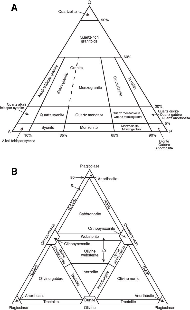
Figure F6. Classification of plutonic rocks.
Leucocratic rocks dominated by quartz and feldspar are named using the quartz–alkali feldspar–plagioclase (Q-A-P) diagram of Le Maitre et al. (2002) (Figure F6A). For example, rocks dominated by plagioclase with minor amounts of quartz, K-feldspar, and ferromagnesian silicates are diorite; tonalites are plagioclase-quartz-rich assemblages; whereas granites contain quartz, K-feldspar, and plagioclase in similar proportions. For melanocratic plutonic rocks, we used the plagioclase-clinopyroxene-orthopyroxene triangular plots and the olivine-pyroxenes-plagioclase triangle (Le Maitre et al., 2002) (Figure F6B).
Textures
Textures are described macroscopically for all igneous rock core samples, but a smaller subset is described microscopically in thin sections or grain mounts. Textures are discriminated by average grain size (groundmass for porphyritic rocks), grain size distribution, shape and mutual relations of grains, and shape-preferred orientation. The distinctions are based on MacKenzie et al. (1982).
Textures based on groundmass grain size of igneous rocks are defined as
- Coarse grained (>5–30 mm)
- Medium grained (>1–5 mm)
- Fine grained (>0.5–1 mm)
- Microcrystalline (0.1–0.5 mm)
In addition, for microscopic descriptions cryptocrystalline (<0.1 mm) is used. The modal grain size of each phenocryst phase is described individually.
For extrusive and hypabyssal categories, rock is described as holocrystalline, glassy (holohyaline), or porphyritic. Porphyritic texture refers to phenocrysts or microphenocrysts surrounded by groundmass of smaller crystals (microlites ≤ 0.1 mm; Lofgren, 1974) or glass. Aphanitic texture signifies a fine-grained, nonglassy rock that lacks phenocrysts. Glomeroporphyritic texture refers to clusters of phenocrysts. Magmatic flow textures are described as trachytic when plagioclase laths are subparallel. Spherulitic textures describe devitrification features in glass, whereas perlite describes rounded hydration fractures in glass. Quench margin texture describes a glassy or microcrystalline margin to an otherwise coarser grained interior. Individual mineral percentages and sizes are also recorded.
Particular attention is paid to vesicles, as they might be a major component of some volcanic rocks. However, they are not included in the rock-normalized mineral abundances. Divisions are made according to proportions:
- Not vesicular (≤1% vesicles)
- Sparsely vesicular (>1%–10% vesicles)
- Moderately vesicular (>10%–40% vesicles)
- Highly vesicular (>40% vesicles)
The modal shape and sphericity of vesicle populations are estimated using appropriate comparison charts, following Expedition 330 Scientists (2012) (Figure F7).
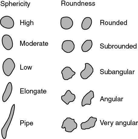
Figure F7. Classification of vesicle sphericity and roundness.
For intrusive rocks (all grains >1 mm), macroscopic textures are divided into equigranular (principal minerals have the same range in size) and inequigranular (the principal minerals have different grain sizes). Porphyritic texture is as described above for extrusive rocks. Poikilitic texture is used to describe larger crystals that enclose smaller grains. We also use the terms ophitic (olivine or pyroxene partially enclose plagioclase) and subophitic (plagioclase partially enclose olivine or pyroxene). Crystal shapes are described as euhedral (the characteristic crystal shape is clear), subhedral (crystal has some of its characteristic faces), or anhedral (crystal lacks any characteristic faces).
Alteration
Submarine samples are likely to have been variably influenced by alteration processes such as low-temperature seawater alteration; therefore, the cores and thin sections are visually inspected for alteration.
Macroscopic core description
The influence of alteration is determined during core description. Descriptions span alteration of minerals, groundmass, or equivalent matrix, volcanic glass, pumice, scoria, rock fragments, and vesicle fill. The color is used as a first-order indicator of alteration, based on a simple color scheme (brown, green, black, gray, white, and yellow). The average extent of secondary replacement of the original groundmass or matrix is used to indicate the alteration intensity for a descriptive interval, per established IODP values:
The alteration assemblages are described as dominant, second-order, and third-order phases replacing the original minerals within the groundmass or matrix. Alteration of glass at the macroscopic level is described in terms of the dominant phase replacing the glass. Groundmass or matrix alteration texture is described as pseudomorphic, corona, patchy, and recrystallized. For patchy alteration, the definition of a patch is a circular or highly elongate area of alteration, described in terms of shape as elongate, irregular, lensoidal, lobate, or rounded and the dominant phase of alteration in the patches. The most common vesicle fill compositions are reported as dominant, second-order, and third-order phases.
Vein fill and halo mineralogy are described with the dominant, second-order, and third-order hierarchy. Halo alteration intensity is expressed by the same scale as for groundmass alteration intensity. For veins and halos, it is noted that the alteration mineralogy of halos surrounding the veins can affect both the original minerals or overprint previous alteration stages. Veins and halos are also recorded as density over a 10 cm core interval:
Microscopic description
Core descriptions of alteration are followed by thin section petrography. The intensity of replacement of original rock components is based on visual estimations of proportions relative to total area of the thin section. Descriptions are made in terms of dominant, second-order, and third-order replacing phases for minerals, groundmass/matrix, clasts, glass, and patches of alteration, whereas vesicle and void fill refer to new mineral phases filling the spaces. Descriptive terms used for alteration extent are
Alteration of the original minerals and groundmass or matrix is described in terms of the percentage of the original phase replaced and a breakdown of the replacement products by percentage of the alteration. Comments are used to provide further specific information where available. Accurate identification of very fine-grained minerals is limited by the lack of X-ray diffraction during Expedition 350; therefore, undetermined clay mineralogy is reported as clay minerals.
VCD standard graphic summary reports
Standard graphic reports were generated from data downloaded from the LIMS database to summarize each core (typical for sediments) or section half (typical for igneous rocks). An example VCD for lithostratigraphy is shown in Figure F8. Patterns and symbols used in VCDs are shown in Figures F9 and F10.
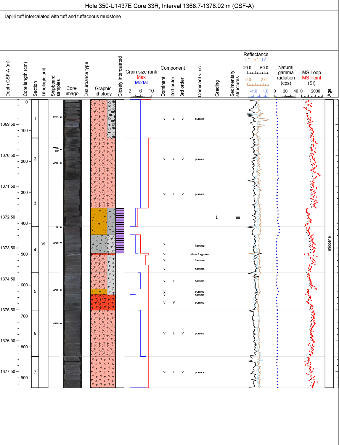
Figure F8. Lithostratigraphic graphic summary.
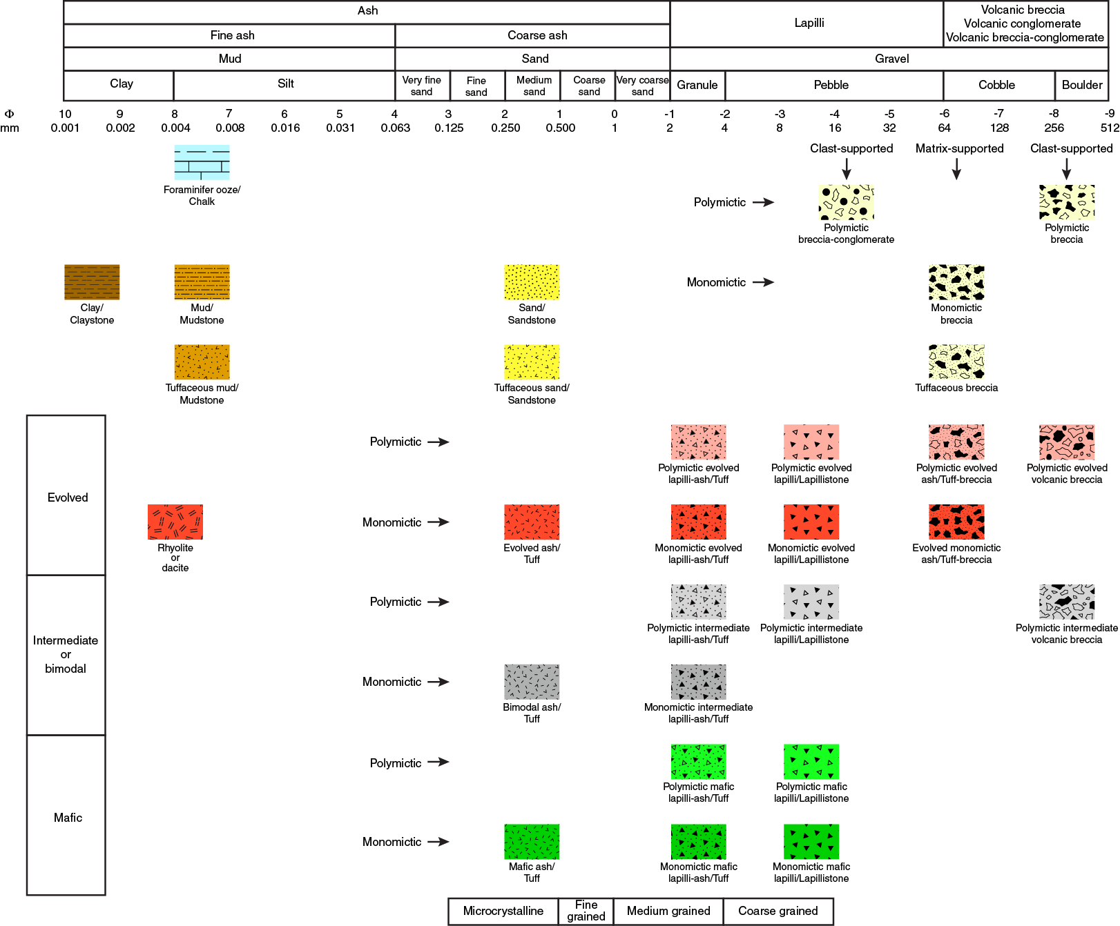
Figure F9. Lithology patterns and definitions.
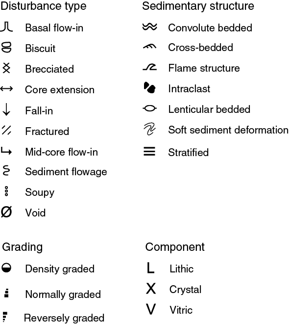
Figure F10. Graphic summary symbols.
Geochemistry
Headspace analysis of hydrocarbon gases
One sample per core was routinely subjected to headspace hydrocarbon gas analysis as part of the standard shipboard safety monitoring procedure as described in Kvenvolden and McDonald (1986), to ensure that the sediments being drilled do not contain greater than the amount of hydrocarbons that is safe to operate with. Therefore, ~3–5 cm3 of sediment was collected from freshly exposed core (typically at the end of Section 1 of each core) directly after it was brought on deck. The extracted sediment sample was transferred into a 20 mL headspace glass vial, which was sealed with an aluminum crimp cap with a teflon/silicon septum, and subsequently put in an oven at 70°C for 30 min, allowing the diffusion of hydrocarbon gases from the sediment. For subsequent gas chromatography (GC) analysis, an aliquot of 5 cm3 of the evolved hydrocarbon gases was extracted from the headspace vial with a standard gas syringe and then manually injected into the Agilent/Hewlett Packard 6890 Series II gas chromatograph (GC3) equipped with a flame ionization detector set at 250°C. The column used for the described analysis was a 2.4 m long (2 mm inner diameter; 6.3 mm outer diameter) column packed with 80/100 mesh HayeSep (Restek). The GC3 oven program was set to hold at 80°C for 8.25 min with subsequent heat-up to 150°C at 40°C/min. The total run time was 15 min.
Results were collected using the Hewlett Packard 3365 ChemStation data processing software. The chromatographic response was calibrated to nine different analysis gas standards and checked on a daily basis. The concentration of the analyzed hydrocarbon gases is expressed as parts per million by volume (ppmv).
Pore fluid analysis
Pore fluid collection
Whole-round core samples, generally 5 cm long, and in some cases 10 cm long (RCB cores) were cut immediately after the core was brought on deck, capped, and taken to the laboratory for pore fluid processing. Samples collected during Expedition 350 were processed under atmospheric conditions. After extrusion from the core liner, contamination from seawater and sediment smearing was removed by scraping the core surface with a spatula. In APC cores, ~0.5 cm of material from the outer diameter and the top and bottom faces was removed, whereas in XCB and RCB cores, where borehole contamination is higher, as much as two-thirds of the sediment was removed from each whole round. The remaining ~150–300 cm3 inner core was placed into a titanium squeezer (modified after Manheim and Sayles, 1974) and compressed using a laboratory hydraulic press. The squeezed pore fluids were filtered through a prewashed Whatman No. 1 filter placed in the squeezers above a titanium mesh screen. Approximately 20 mL of pore fluid was collected in precleaned plastic syringes attached to the squeezing assembly and subsequently filtered through a 0.45 µm Gelman polysulfone disposable filter. In deeper sections, fluid recovery was as low as 5 mL after squeezing the sediment for as long as ~2 h. After the fluids were extracted, the squeezer parts were cleaned with shipboard water and rinsed with deionized (DI) water. Parts were dried thoroughly prior to reuse.
Sample allocation was determined based on the pore fluid volume recovered and analytical priorities based on the objectives of the expedition. Shipboard analytical protocols are summarized below.
Shipboard pore fluid analyses
Pore fluid samples were analyzed on board the ship following the protocols in Gieskes et al. (1991), Murray et al. (2000), and the IODP user manuals for newer shipboard instrumentation. Precision and accuracy was tested using International Association for the Physical Science of the Ocean (IAPSO) standard seawater with the following reported compositions: alkalinity = 2.353 mM, Cl = 559.6 mM, sulfate = 28.94 mM, Na = 480.7 mM, Mg = 54.1 mM, K = 10.46 mM, Ca = 10.54 mM, Li = 26.4 µM, B = 450 µM, and Sr = 93 µM (Gieskes et al., 1991; Millero et al., 2008; Summerhayes and Thorpe, 1996). Pore fluid components reported here that have low abundances in seawater (ammonium, phosphate, Mn, Fe, Ba, and Si) are based on calibrations using stock solutions (Gieskes et al., 1991).
Alkalinity, pH, and salinity
Alkalinity and pH were measured immediately after squeezing, following the procedures in Gieskes et al. (1991). pH was measured with a combination glass electrode, and alkalinity was determined by Gran titration with an autotitrator (Metrohm 794 basic Titrino) using 0.1 M HCl at 20°C. Certified Reference Material 104 obtained from the laboratory of Andrew Dickson (Marine Physical Laboratory, Scripps Institution of Oceanography, USA) was used for calibration of the acid. IAPSO standard seawater was used for calibration and was analyzed at the beginning and end of a set of samples for each site and after every 10 samples. Salinity was subsequently measured using a Fisher temperature-compensated handheld refractometer.
Chloride
Chloride concentrations were acquired directly after pore fluid squeezing using a Metrohm 785 DMP autotitrator and silver nitrate (AgNO3) solutions that were calibrated against repeated titrations of IAPSO standard. Where fluid recovery was ample, a 0.5 mL aliquot of sample was diluted with 30 mL of HNO3 solution (92 ± 2 mM) and titrated with 0.1015 M AgNO3. In all other cases, a 0.1 mL aliquot of sample was diluted with 10 mL of 90 ± 2 mM HNO3 and titrated with 0.1778 M AgNO3. IAPSO standard solutions analyzed interspersed with the unknowns are accurate and precise to <5%.
Sulfate, bromide, sodium, magnesium, potassium, and calcium
Anion (sulfate and Br) and cation (Na, Mg, K, and Ca) abundances were analyzed using a Metrohm 850 ion chromatograph equipped with a Metrohm 858 Professional Sample Processor as an autosampler. Cl concentrations were also determined in the ion chromatography (IC) analyses but are only considered here for comparison because the titration values are generally more reliable. The eluent solutions used were diluted 1:100 with DI water, using specifically designated pipettes. The analytical protocol was to establish a seawater standard calibration curve using IAPSO dilutions of 100×, 150×, 200×, 350×, and 500×. Reproducibility for IAPSO analyses by IC interspersed with the unknowns are Br = 2.9%, Cl = 0.5%, sulfate = 0.6%, Ca = 4.9%, Mg = 1.2%, K = 22.3%, and Na = 0.5% (n = 10). The deviations of the average concentrations measured here relative to those in Gieskes et al. (1991) are Br = 0.8%, Cl = 0.1%, sulfate = 0.3%, Ca = 4.1%, Mg = 0.8%, K = −0.8%, and Na = 0.3%.
Ammonium and phosphate
Ammonium concentrations were determined by spectrophotometry using an Agilent Technologies Cary Series 100 ultraviolet-visible spectrophotometer with a sipper sample introduction system following the protocol in Gieskes et al. (1991). Samples were diluted prior to color development so that the highest concentration was <1000 µM. Phosphate was measured using the ammonium molybdate method described in Gieskes et al. (1991), using appropriate dilutions. Relative uncertainties of ammonium and phosphate determinations are estimated at 0.5%–2% and 0.8%, respectively (Expedition 323 Scientists, 2011).
Major and minor elements (ICP-AES)
Major and minor elements were analyzed by inductively coupled plasma–atomic emission spectroscopy (ICP-AES) with a Teledyne Prodigy high-dispersion ICP spectrometer. The general method for shipboard ICP-AES analysis of samples is described in Ocean Drilling Program (ODP) Technical Note 29 (Murray et al., 2000) and the user manuals for new shipboard instrumentation, with modifications as indicated (Table T7). Samples and standards were diluted 1:20 using 2% HNO3 spiked with 10 ppm Y for trace element analyses (Li, B, Mn, Fe, Sr, Ba, and Si) and 1:100 for major constituent analyses (Na, K, Mg, and Ca). Each batch of samples run on the ICP spectrometer contains blanks and solutions of known concentrations. Each item aspirated into the ICP spectrometer was counted four times from the same dilute solution within a given sample run. Following each instrument run, the measured raw intensity values were transferred to a data file and corrected for instrument drift and blank. If necessary, a drift correction was applied to each element by linear interpolation between the drift-monitoring solutions.
Table T7. Primary, secondary, and tertiary wavelengths, ICP-AES. Download table in .csv format.
Standardization of major cations was achieved by successive dilution of IAPSO standard seawater to 120%, 100%, 75%, 50%, 25%, 10%, 5%, and 2.5% relative to the 1:100 primary dilution ratio. Replicate analyses of 100% IAPSO run as an unknown throughout each batch of analyses yielded estimates for precision and accuracy.
For minor element concentration analyses, the interstitial water sample aliquot was diluted by a factor of 20 (0.5 mL sample added to 9.5 mL of a 10 ppm Y solution). Because of the high concentration of matrix salts in the interstitial water samples at a 1:20 dilution, matrix matching of the calibration standards is necessary to achieve accurate results by ICP-AES. A matrix solution that approximated IAPSO standard seawater major ion concentrations was prepared according to Murray et al. (2000). A stock standard solution was prepared from ultrapure primary standards (SPC Science PlasmaCAL) in 2% nitric acid solution. The stock solution was then diluted in the same 2% ultrapure nitric acid solution to concentrations of 100%, 75%, 50%, 25%, 10%, 5%, and 1%. The calibration standards were then diluted using the same method as for the samples for consistency. All calibration standards were analyzed in triplicate with a reproducibility of Li = 0.83%, B = 1.25%, Si = 0.91%, and Sr = 0.83%. IAPSO standard seawater was also analyzed as an unknown during the same analytical session to check for accuracy. Relative deviations are Li = +1.8%, B = 4.0%, Si = 4.1%, and Sr = −1.8%. Because values of Ba, Mn, and Fe in IAPSO standard seawater are close to or below detection limits, the accuracy of the ICP-AES determinations cannot be quantified, and reported values should be regarded as preliminary.
Sediment bulk geochemistry
For shipboard bulk geochemistry analysis, sediment samples comprising 5 cm3 were taken from the interiors of cores with autoclaved cut-tip syringes, freeze-dried for ~24 h to remove water, and powdered to ensure homogenization. Carbonate content was determined by acidifying approximately 10 mg of bulk powder with 2 M HCl and measuring the CO2 evolved, all of which was assumed to be derived from CaCO3, using a UIC 5011 CO2 coulometer. The amounts of liberated CO2 were determined by trapping the CO2 with ethanolamine and titrating coulometrically the hydroxyethylcarbamic acid that is formed. The end-point of the titration was determined by a photodetector. The weight percent of total inorganic carbon was calculated by dividing the CaCO3 content in weight percent by 8.33, the stoichiometric factor of C in CaCO3.
Total carbon (TC) and total nitrogen (TN) contents were determined by an aliquot of the same sample material by combustion at >900°C in a Thermo Electron FlashEA 1112 elemental analyzer equipped with a Thermo Electron packed column and a thermal conductivity detector (TCD). Approximately 10 mg powder was weighed into a tin cup and subsequently combusted in an oxygen gas stream at 900°C for TC and TN analysis. The reaction gases were passed through a reduction chamber to reduce nitrogen oxides to N2, and the mixture of CO2 and N2 was separated by GC and detected by the TCD. Calibration was based on the Thermo Fisher Scientific NC Soil Reference Material standard, which contains 2.29 wt% C and 0.21 wt% N. The standard was chosen because its elemental concentrations are equivalent to those encountered at Site U1437. Relative uncertainties are 1% and 2% for TC and TN determinations, respectively (Expedition 323 Scientists, 2011). Total organic carbon content was calculated by subtracting weight percent of inorganic carbon derived from the carbonate measured by coulometric analysis from total C obtained with the elemental analyzer.
Sampling and analysis of igneous and volcaniclastic rocks
Reconnaissance analysis by portable X-ray fluorescence spectrometer
Volcanic rocks encountered during Expedition 350 show a wide range of compositions from basalt to rhyolite, and the desire to rapidly identify compositions in addition to the visual classification led to the development of reconnaissance analysis by portable X-ray fluorescence (pXRF) spectrometry. For this analysis, a Thermo-Niton XL3t GOLDD+ instrument equipped with an Ag anode and a large-area drift detector for energy-dispersive X-ray analysis was used. The detector is nominally Peltier cooled to −27°C, which is achieved within 1–2 min after powering up. During operation, however, the detector temperature gradually increased to −21°C over run periods of 15–30 min, after which the instrument needed to be shut down for at least 30 min. This faulty behavior limited sample throughput but did not affect precision and accuracy of the data. The 8 mm diameter analysis window on the spectrometer is covered by 3M thin transparent film and can be purged with He gas to enhance transmission of low-energy X-rays. X-ray ranges and corresponding filters are preselected by the instrument software as “light” (e.g., Mg, Al, and Si), “low” (e.g., Ca, K, Ti, Mn, and Fe), “main” (e.g., Rb, Sr, Y, and Zr), and “high” (e.g., Ba and Th). Analyses were performed on a custom-built shielded stand located in the JOIDES Resolution chemistry lab and not in portable mode because of radiation safety concerns and better analytical reproducibility for powdered samples.
Two factory-set modes for spectrum quantification are available for rock samples: “soil” and “mining.” Mining uses a fundamental parameter calibration taking into account the matrix effects from all identified elements in the analyzed spectrum (Zurfluh et al., 2011). In soil mode, quantification is performed after dividing the baseline- and interference-corrected intensities for the peaks of interest to those of the Compton scatter peak, and then comparing these normalized intensities to those of a suitable standard measured in the factory (Zurfluh et al., 2011). Precision and accuracy of both modes were assessed by analyzing volcanic reference materials (Govindaraju, 1994). In mining mode, light elements can be analyzed when using the He purge, but the results obtained during Expedition 350 were generally deemed unreliable. The inability to detect abundant light elements (mainly Na) and the difficulty in generating reproducible packing of the powders presumably biases the fundamental parameter calibration. This was found to be particularly detrimental to the quantification of light elements Mg, Al, and Si. The soil mode was therefore used for pXRF analysis of core samples.
Spectrum acquisition was limited to the main and low-energy range (30 s integration time each) because elements measured in the high mode were generally near the limit of detection or unreliable. No differences in performance were observed for main and low wavelengths with or without He purge, and therefore analyses were performed in air for ease of operation. For all elements the factory-set soil calibration was used, except for Y, which is not reported by default. To calculate Y abundances, the main energy spectrum was exported, and background-subtracted peak intensities for Y Kα were normalized to the Ag Compton peak offline. The Rb Kβ interference on Y Kα was then subtracted using the approach in Gásquez et al. (1997) with a Rb Kβ/Rb Kα factor of 0.11 determined from regression of Standards JB-2, JB-3, BHVO-2, and BCR-2 (basalts); AGV-1 and JA-2 (andesites); JR-1 and JR-2 (rhyolite); and JG-2 (granite). A working curve determined by regression of interference-corrected Y Kα intensities versus Y concentration was established using the same rock standards (Figure F11).
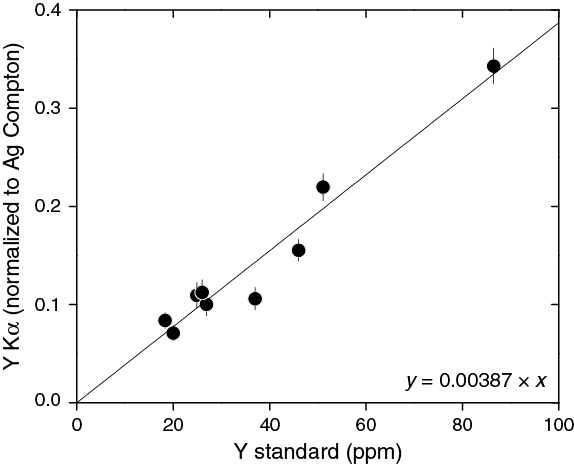
Figure F11. Working curve for shipboard pXRF analysis of Y.
Reproducibility was estimated from replicate analyses of JB-2 standard (n = 131) and was found to be <5% (1σ relative error) for indicator elements K, Ca, Sr, Y, and Zr over an ~7 week period (Figure F12; Table T8). No instrumental drift was observed over this period. Accuracy was evaluated by analyzing Standards JB-2, JB-3, BHVO-2, BCR-2, AGV-1, JA-2, and JR-1 in replicate. Relative deviations from the certified values (Figure F13) are generally within 20% (relative). For some elements, deviations correlate with changes in the matrix composition (e.g., from basalt to rhyolite deviations range from Ca +2% to −22%), but for others (e.g., K and Zr) systematic trends with increasing SiO2 are absent. Zr abundances appear to be overestimated in high-Sr samples likely because of the factory-calibrated correction incompletely subtracting the Sr interference on the Zr line. For the range of Sr abundances tested here, this bias in Zr was always <20% (relative).
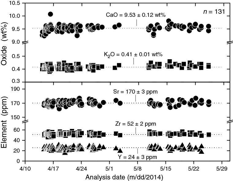
Figure F12. Reproducibility of shipboard pXRF analysis of JB-2 powder.
Table T8. pXRF and true values for standards. Download table in .csv format.

Figure F13. Accuracy of shipboard pXRF analyses.
Dry and wet sample powders were analyzed to assess matrix effects arising from the presence of H2O. A wet sample of JB-2 yielded concentrations that were on average ~20% lower compared to bracketing analyses from a dry JB-2 sample. Packing standard powders in the sample cups to different heights did not show any significant differences for these elements, but thick (to several millimeters) packing is critical for light elements. Based on these initial tests, samples were prepared as follows:
- Collect several grams of core sample.
- Freeze-dry sample for ~30 min.
- Grind sample to a fine powder using a corundum mortar or a shatterbox for hard samples.
- Transfer sample powder into the plastic sample cell and evenly distribute it on the tightly seated polypropylene X-ray film held in place by a plastic ring.
- Cover sample powder with a 2.4 cm diameter filter paper.
- Stuff the remaining space with polyester fiber to prevent sample movement.
- Close the sample cup with lid and attach sample label.
Prior to analyzing unknowns, a software-controlled system calibration was performed. JB-2 (basalt from Izu-Oshima Volcano, Japan) was preferentially analyzed, bracketing batches of 4–6 unknowns to monitor instrument performance because its composition is very similar to mafic tephra encountered during Expedition 350. Data are reported as calculated in the factory-calibrated soil mode (except for Y, which was calculated offline using a working curve from analysis of rock standards), regardless of potential systematic deviations observed on the standards. Results should only be considered as absolute abundances within the limits of the systematic uncertainties constrained by the analysis of rock standards, which are generally <20% (Figure F13).
ICP-AES
Sample preparation
Selected samples of igneous and volcaniclastic rocks were analyzed for major and trace element concentrations using ICP-AES. For unconsolidated volcaniclastic rock, ash was sampled by scooping, whereas lapilli-sized juvenile clasts were hand-picked, targeting a total sample volume of ~5 cm3. Consolidated (hard rock) igneous and volcaniclastic samples ranging in size from ~2 to ~8 cm3 were cut from the core with a diamond saw blade. A thin section billet was always taken from the same or adjacent interval to microscopically check for alteration. All cutting surfaces were ground on a diamond-impregnated disk to remove altered rinds and surface contamination derived from the drill bit or the saw. Hard rock blocks were individually placed in a beaker containing trace-metal-grade methanol and washed ultrasonically for 15 min. The methanol was decanted, and the samples were washed in Barnstead DI water (~18 MΩ·cm) for 10 min in an ultrasonic bath. The cleaned pieces were dried for 10–12 h at 110°C.
The cleaned, dried samples were crushed to <1 cm chips between two disks of Delrin plastic in a hydraulic press. Some samples containing obvious alteration were hand-picked under a binocular microscope to separate material as free of alteration phases as possible. The chips were then ground to a fine powder in a SPEX 8515 shatterbox with a tungsten carbide lining. After grinding, an aliquot of the sample powder was weighed to 1000.0 ± 0.5 mg and ignited at 700°C for 4 h to determine weight loss on ignition (LOI). Estimated relative uncertainties for LOI determinations are ~14% on the basis of duplicate measurements.
The ICP-AES analysis protocol follows the procedure in Murray et al. (2000). After determination of LOI, 100.0 ± 0.2 mg splits of the ignited whole-rock powders were weighed and mixed with 400.0 ± 0.5 mg of LiBO2 flux that had been preweighed on shore. Standard rock powders and full procedural blanks were included with unknowns in each ICP-AES run (note that among the elements reported, contamination from the tungsten carbide mills is negligible; Shipboard Scientific Party, 2003). All samples and standards were weighed on a Cahn C-31 microbalance (designed to measure at sea) with weighing errors estimated to be ±0.05 mg under relatively smooth sea-surface conditions.
To prevent the cooled bead from sticking to the crucible, 10 mL of 0.172 mM aqueous LiBr solution was added to the mixture of flux and rock powder as a nonwetting agent. Samples were then fused individually in Pt-Au (95:5) crucibles for ~12 min at a maximum temperature of 1050°C in an internally rotating induction furnace (Bead Sampler NT-2100).
After cooling, beads were transferred to high-density polypropylene bottles and dissolved in 50 mL of 10% (by volume) HNO3, aided by shaking with a Burrell wrist-action bottle shaker for 1 h. Following digestion of the bead, the solution was passed through a 0.45 µm filter into a clean 60 mL wide-mouth high-density polypropylene bottle. Next, 2.5 mL of this solution was transferred to a plastic vial and diluted with 17.5 mL of 10% HNO3 to bring the total volume to 20 mL. The final solution-to-sample dilution factor was ~4000. For standards, stock standard solutions were placed in an ultrasonic bath for 1 h prior to final dilution to ensure a homogeneous solution.
Analysis and data reduction
Major (Si, Ti, Al, Fe, Mn, Mg, Ca, Na, K, and P) and trace (Sc, V, Cr, Co, Ni, Cu, Zn, Rb, Sr, Y, Zr, Nb, Ba, and Th) element concentrations of standards and samples were analyzed with a Teledyne Leeman Labs Prodigy ICP-AES instrument (Table T7). For several elements, measurements were performed at more than one wavelength (e.g., Si at 250.690 and 251.611 nm), and data with the least scatter and smallest deviations from the check standard values were selected.
The plasma was ignited at least 30 min before each run of samples to allow the instrument to warm up and stabilize. A zero-order search was then performed to check the mechanical zero of the diffraction grating. After the zero-order search, the mechanical step positions of emission lines were tuned by automatically searching with a 0.002 nm window across each emission peak using single-element solutions.
The ICP-AES data presented in the Geochemistry section of each site chapter were acquired using the Gaussian mode of the instrument software. This mode fits a curve to points across a peak and integrates the area under the curve for each element measured. Each sample was analyzed four times from the same dilute solution (i.e., in quadruplicate) within a given sample run. For elements measured at more than one wavelength, we either used the wavelength giving the best calibration line in a given run or, if the calibration lines for more than one wavelength were of similar quality, used the data for each and reported the average concentration.
A typical ICP-AES run (Table T9) included a set of 9 or 10 certified rock standards (JP-1, JB-2, AGV, STM-1, GSP-2, JR-1, JR-2, BHVO-2, BCR-2, and JG-3) analyzed together with the unknowns in quadruplicate. A 10% HNO3 wash solution was introduced for 90 s between each analysis, and a solution for drift correction was analyzed interspersed with the unknowns and at the beginning and end of each run. Blank solutions aspirated during each run were below detection for the elements reported here. JB-2 was also analyzed as an unknown because it is from the Bonin arc, and its composition matches closely the Expedition 350 unknowns (Table T10).
Table T9. Sequence of analyses in ICP-AES run. Download table in .csv format.
Table T10. JB-2 standard major and trace element data. Download table in .csv format.
Measured raw intensities were corrected offline for instrument drift using the shipboard ICP Analyzer software. A linear calibration line for each element was calculated using the results for the certified rock standards. Element concentrations in the samples were then calculated from the relevant calibration lines. Data were rejected if total volatile-free major element weight percentages totals were outside 100 ± 5 wt%. Sources of error include weighing (particularly in rougher seas), sample and standard dilution, and instrumental instabilities. To facilitate comparison of Expedition 350 results with each other and with data from the literature, major element data are reported normalized to 100 wt% total. Total iron is stated as total FeO* or Fe2O3*. Precision and accuracy based on replicate analyses of JB-2 range between ~1% and 2% (relative) for major oxides and between ~1% and 13% (relative) for minor and trace components (Table T10).
Physical properties
Shipboard physical properties measurements were undertaken to provide a general and systematic characterization of the recovered core material, detect trends and features related to the development and alteration of the formations, and infer causal processes and depositional settings. Physical properties are also used to link geological observations made on the core to downhole logging data and regional geophysical survey results. The measurement program included the use of several core logging and discrete sample measurement systems designed and built at IODP (College Station, Texas) for specific shipboard workflow requirements.
After cores were cut into 1.5 m (or shorter) sections and had warmed to ambient laboratory temperature (~20°C), all core sections were run through two core logger systems, the WRMSL and the NGRL. The WRMSL includes a gamma ray attenuation (GRA) bulk densitometer, a magnetic susceptibility logger (MSL), and a P-wave logger (PWL). Thermal conductivity measurements were carried out using the needle probe technique if the material was soft enough. For lithified sediment and rocks, thermal conductivity was measured on split cores using the half-space technique.
After the sections were split into working and archive halves, the archive half was processed through the SHIL to acquire high-resolution images of split core, followed by the SHMSL for color reflectance and point magnetic susceptibility (MSP) measurements with a contact probe. The working half was placed on the Section Half Measurement Gantry (SHMG), where P-wave velocity was measured using a P-wave caliper (PWC) and, if the material was soft enough, a P-wave bayonet (PWB), each equipped with a pulser-receiver system. P-wave measurements on section halves are often of superior quality to those on whole-round sections because of better coupling between the sensors and the sediment. PWL measurements on the whole-round logger have the advantage of being of much higher spatial resolution than those produced by the PWC. Shear strength was measured using the automated vane shear (AVS) apparatus where the recovered material was soft enough.
Discrete samples were collected from the working halves for moisture and density (MAD) analysis.
The following sections describe the measurement methods and systems in more detail. A full discussion of all methodologies and calculations used aboard the JOIDES Resolution in the Physical Properties Laboratory is available in Blum (1997).
Gamma ray attenuation bulk density
Sediment bulk density can be directly derived from the measurement of GRA (Evans, 1965). The GRA densitometer on the WRMSL operates by passing gamma radiation from a Cesium-137 source through a whole-round section into a 75 mm sodium iodide detector situated vertically under the source and core section. The gamma ray (principal energy = 662 keV) is attenuated by Compton scattering as it passes through the core section. The attenuation is a function of the electron density, and electron density is related to the bulk density via the mass attenuation coefficient. For the majority of elements and for anhydrous rock-forming minerals, the mass attenuation coefficient is ~0.48, whereas for hydrogen it is 0.99. For a two-phase system including minerals and water and a constant absorber thickness (the core diameter), the gamma ray count is proportional to the mixing ratio of solids with water, and thus the bulk density.
The spatial resolution of the GRA densitometer measurements is <1 cm. The quality of GRA data is highly dependent on the structural integrity of the core because of the high resolution (i.e., the measurements are significantly affected by cracks, voids, and remolded sediment). The absolute values will be lower if the sediment does not completely fill the core liner (i.e., if gas, seawater, or slurry fill the gap between the sediment and the core liner).
GRA precision is proportional to the square root of the counts measured, as gamma ray emission is subject to Poisson statistics. Currently, GRA measurements have typical count rates of 10,000 (dense rock) to 20,000 counts/s (soft mud). If measured for 4 s, the statistical error of a single measurement is ~0.5%. Calibration of the densitometer was performed using a core liner filled with distilled water and aluminum segments of variable thickness. Recalibration was performed if the measured density of the freshwater standard deviated by ±0.02 g/cm3 (2%). GRA density was measured at the interval set on the WRMSL for the entire expedition (i.e., 5 cm).
Magnetic susceptibility
Low-field magnetic susceptibility (MS) is the degree to which a material can be magnetized in an external low-magnetization (≤0.5 mT) field. Magnetic susceptibility of rocks varies in response to the magnetic properties of their constituents, making it useful for the identification of mineralogical variations. Materials such as clay generally have a magnetic susceptibility several orders of magnitude lower than magnetite and some other iron oxides that are common constituents of igneous material. Water and plastics (core liner) have a slightly negative magnetic susceptibility.
On the WRMSL, volume magnetic susceptibility was measured using a Bartington Instruments MS2 meter coupled to a MS2C sensor coil with a 90 mm diameter, operating at a frequency of 0.565 kHz. We refer to these measurements as MSL. MSL was measured at the interval set on the WRMSL for the entire expedition (i.e., 5 cm).
On the SHMSL, volume magnetic susceptibility was measured using a Bartington Instruments MS2K meter and contact probe, which is a high-resolution surface scanning sensor with an operating frequency of 0.93 kHz. The sensor has a 25 mm diameter response pattern (full width and half maximum). The response reduction is ~50% at 3 mm depth and 10% at 8 mm depth. We refer to these as MSP measurements. Because the MS2K demands flush contact between the probe and the section-half surface, the archive halves were covered with clear plastic wrap to avoid contamination. Measurements were generally taken at 2.5 cm intervals; the interval was decreased to 1 cm when time permitted.
Magnetic susceptibility from both instruments is reported in instrument units. To obtain results in dimensionless SI units, the instrument units need to be multiplied by a geometric correction factor that is a function of the probe type, core diameter, and loop size. Because we are not measuring the core diameter, application of a correction factor has no benefit over reporting instrument units.
P-wave velocity
P-wave velocity is the distance traveled by a compressional P-wave through a medium per unit of time, expressed in meters per second. P-wave velocity is dependent on the composition, mechanical properties, porosity, bulk density, fabric, and temperature of the material, which in turn are functions of consolidation and lithification, state of stress, and degree of fracturing. Occurrence and abundance of free gas in soft sediment reduces or completely attenuates P-wave velocity, whereas gas hydrates may increase P-wave velocity. P-wave velocity, along with bulk density data, can be used to calculate acoustic impedances and reflection coefficients, which are needed to construct synthetic seismic profiles and estimate the depth of specific seismic horizons.
Three instrument systems described here were used to measure P-wave velocity.
The PWL system on the WRMSL transmits a 500 kHz P-wave pulse across the core liner at a specified repetition rate. The pulser and receiver are mounted on a caliper-type device and are aligned in order to make wave propagation perpendicular to the section’s long axis. A linear variable differential transducer measures the P-wave travel distance between the pulse source and the receiver. Good coupling between transducers and core liner is facilitated with water dripping onto the contact from a peristaltic water pump system. Signal processing software picks the first arrival of the wave at the receiver, and the processing routine also corrects for the thickness of the liner. As for all measurements with the WRMSL, the measurement intervals were 5 cm.
The PWC system on the SHMG also uses a caliper-type configuration for the pulser and receiver. The system uses Panametrics-NDT Microscan delay line transducers, which transmit an ultrasonic pulse at 500 kHz. The distance between transducers is measured with a built-in linear voltage displacement transformer. One measurement was in general performed on each section, with exceptions as warranted.
A series of acrylic cylinders of varying thicknesses are used to calibrate both the PWL and the PWC systems. The regression of traveltime versus travel distance yields the P-wave velocity of the standard material, which should be within 2750 ± 20 m/s. The thickness of the samples, corrected for liner thickness, is divided by the traveltime to calculate P-wave velocity in meters per second. On the PWL system, the calibration is verified by measuring a core liner filled with pure water, and the calibration passes if the measured velocity is within ±20 m/s of the expected value for water at room temperature (1485 m/s). On the PWC system, the calibration is verified by measuring the acrylic material used for calibration.
The PWB system on the SHMG uses transducers built into bayonet-style blades that can be inserted into soft sediment. The distance between the pulser and receiver is fixed, and the traveltime is measured. Calibration is performed with a split liner half filled with pure water, using a known velocity of 1485 m/s at 22°C.
On both the PWC and the PWB systems, the user has the option to override the automated pulse arrival, particularly in the case of a weak signal, and pick the first arrival manually.
Natural gamma radiation
Natural gamma radiation (NGR) is emitted from Earth materials as a result of the radioactive decay of 238U, 232Th, and 40K isotopes. Measurement of NGR from the recovered core provides an indication of the concentration of these elements and can be compared directly against downhole NGR logs for core-log integration.
NGR was measured using the NGRL. The main NGR detector unit consists of 8 sodium iodide (NaI) scintillation detectors spaced at ~20 cm intervals along the core axis, 7 active shield plastic scintillation detectors, 22 photomultipliers, and passive lead shielding (Vasiliev et al., 2011).
A single measurement run with the NGRL provides 8 measurements at 20 cm intervals over a 150 cm section of core. To achieve a 10 cm measurement interval, the NGRL automatically records two sets of measurements, offset by 10 cm. The quality of the energy spectrum measured depends on the concentration of radionuclides in the sample and on the counting time. A live counting time of 5 min was set in each position (total live count time of 10 min per section).
Thermal conductivity
Thermal conductivity (k; in W/[m·K]) is the rate at which heat is conducted through a material. At steady state, thermal conductivity is the coefficient of heat transfer (q) across a steady-state temperature (T) difference over a distance (x):
Thermal conductivity of Earth materials depends on many factors. At high porosities such as those typically encountered in soft sediment, porosity (or bulk density, water content), the type of saturating fluid, and temperature are the most important factors affecting thermal conductivity. For low-porosity materials, composition and texture of the mineral phases are more important.
A TeKa TK04 system measures and records the changes in temperature with time after an initial heating pulse emitted from a superconductive probe. A needle probe inserted into a small hole drilled through the plastic core liner is used for soft-sediment sections, whereas hard rock samples are measured by positioning a flat needle probe embedded into a plastic puck holder onto the flat surfaces of split core pieces. The TK04 system measures thermal conductivity by transient heating of the sample with a known heating power and geometry. Changes in temperature with time during heating are recorded and used to calculate thermal conductivity. Heating power can be adjusted for each sample; as a rule of thumb, heating power (W/m) is set to be ~2 times the expected thermal conductivity (i.e., ~1.2–2 W/[m·K]). The temperature of the superconductive probe has a quasilinear relationship with the natural logarithm of the time after heating initiation. The TK04 device uses a special approximation method to calculate conductivity and to assess the fit of the heating curve. This method fits discrete windows of the heating curve to the theoretical temperature (T) with time (t) function:
T(t) = A1 + A2 ln(t) + A3 [ln(t)/t] + (A4/t),
where A1–A4 are constants that are calculated by linear regression. A1 is the initial temperature, whereas A2, A3, and A4 are related to geometry and material properties surrounding the needle probe. Having defined these constants (and how well they fit the data), the apparent conductivity (ka) for the fitted curve is time dependent and given by
ka(t) = q/4π{A2 + A3[1 − ln(t)/t] − (A4/t)},
where q is the input heat flux. The maximum value of ka and the time (tmax) at which it occurs on the fitted curve are used to assess the validity of that time window for calculating thermal conductivity. The best solutions are those where tmax is greatest, and these solutions are selected for output. Fits are considered good if ka has a maximum value, tmax is large, and the standard deviation of the least-squares fit is low. For each heating cycle, several output values can be used to assess the quality of the data, including natural logarithm of extreme time tmax, which should be large; the number of solutions (N), which should also be large; and the contact value, which assesses contact resistance between the probe and the sample and should be small and uniform for repeat measurements.
Thermal conductivity values can be multiplied with downhole temperature gradients at corresponding depths to produce estimates of heat flow in the formation (see Downhole measurements).
Moisture and density
In soft to moderately indurated sediments, working section halves were sampled for MAD analysis using plastic syringes with a diameter only slightly less than the diameter of the preweighed 16 mL Wheaton glass vials used to process and store the samples of ~10 cm3 volume. Typically, 1 sample per section was collected. Samples were taken at irregular intervals, depending on the availability of material homogeneous and continuous enough for measurement.
In indurated sediments and rocks, cubes of ~8 cm3 were cut from working halves and were saturated with a vacuum pump system. The system consists of a plastic chamber filled with seawater. A vacuum pump then removes air from the chamber, essentially sucking air from pore spaces. Samples were kept under vacuum for at least 24 h. During this time, pressure in the chamber was monitored periodically by a gauge attached to the vacuum pump to ensure a stable vacuum. After removal from the saturator, cubes were stored in sample containers filled with seawater to maintain saturation.
The mass of wet samples was determined to a precision of 0.005 g using two Mettler-Toledo electronic balances and a computer averaging system to compensate for the ship’s motion. The samples were then heated in an oven at 105° ± 5°C for 24 h and allowed to cool in a desiccator for 1 h. The mass of the dry sample was determined with the same balance system. Dry sample volume was determined using a 6-celled, custom-configured Micromeritics AccuPyc 1330TC helium-displacement pycnometer system. The precision of each cell volume is 1% of the full-scale volume. Volume measurement was preceded by three purges of the sample chamber with helium warmed to ~28°C. Three measurement cycles were run for each sample. A reference volume (calibration sphere) was placed sequentially in one of the six chambers to check for instrument drift and systematic error. The volumes of the numbered Wheaton vials were calculated before the cruise by multiplying each vial’s mass against the average density of the vial glass.
The procedures for the determination of the MAD phase relationships comply with the American Society for Testing and Materials (ASTM International, 1990) and are discussed in detail by Blum (1997). The method applicable to saturated, fine-grained sediments is called “Method C.” Method C is based on the measurement of wet mass, dry mass, and volume. It is not reliable or adapted for unconsolidated coarse-grained sediments in which water can be easily lost during the sampling (e.g., in foraminifer sands often found at the top of the hole).
Wet mass (Mwet), dry mass (Mdry), and dry volume (Vdry) were measured in the laboratory. Wet bulk density (ρwet), dry bulk density (ρdry), sediment grain density (ρsolid), porosity (φ), and void ratio (VR) were calculated as follows:
where the volume of pore water (Vpw), mass of solids excluding salt (Msolid), volume of solids excluding salt (Vsolid), and wet volume (Vwet) were calculated using the following parameters (Blum, 1997; ASTM International, 1990):
- Mass ratio (rm) = 0.965 (i.e., 0.965 g of freshwater per 1 g of seawater).
- Salinity (s) = 0.035.
- Pore water density (ρpw) = 1.024 g/cm3.
- Salt density (ρsalt) = 2.22 g/cm3.
An accuracy and precision of MAD measurements of ~0.5% can be achieved with the shipboard devices. The largest source of potential error is the loss of material or moisture during the ~30–48 h long procedure for each sample.
Sediment strength
Shear strength of soft sedimentary samples was measured using the AVS by Giesa. The Giesa system consists of a controller and a gantry for shear vane insertion. A four-bladed miniature vane (diameter = height = 12.7 mm) was pushed carefully into the sediment of the working halves until the top of the vane was level with the sediment surface. The vane was then rotated at a constant rate of 90°/min to determine the torque required to cause a cylindrical surface to be sheared by the vane. This destructive measurement was done with the rotation axis parallel to the bedding plane. The torque required to shear the sediment along the vertical and horizontal edges of the vane is a relatively direct measurement of shear strength. Undrained shear strength (su) is given as a function of pressure in SI units of pascals (kPa = kN/m2).
Strength tests were performed on working halves from APC cores at a resolution of 1 measurement per section.
Color reflectance
Reflectance of ultraviolet to near-infrared light (171–1100 nm wavelength at 2 nm intervals) was measured on archive half surfaces using an Ocean Optics USB4000 spectrophotometer mounted on the SHMSL. Spectral data are routinely reduced to the L*a*b* color space parameters for output and presentation, in which L* is luminescence, a* is the green–red value, and b* is the blue–yellow value. The color reflectance spectrometer calibrates on two spectra, pure white (reference) and pure black (dark). Measurements were taken at 2.5 cm intervals and rarely at 1 cm intervals.
Because the reflectance integration sphere requires flush contact with the section-half surface, the archive halves were covered with clear plastic wrap to avoid contamination. The plastic film adds ~1%–5% error to the measurements. Spurious measurements with larger errors can result from small cracks or sediment disturbance caused by the drilling process.
Paleomagnetism
Samples, instruments, and measurements
Paleomagnetic studies during Expedition 350 principally focused on measuring the natural remanent magnetization (NRM) of archive section halves on the superconducting rock magnetometer (SRM) before and after alternating field (AF) demagnetization. Our aim was to produce a magnetostratigraphy to merge with paleontological datums to yield the age model for each of the two sites (see Age model). Analysis of the archive halves was complemented by stepwise demagnetization and measurement of discrete cube specimens taken from the working half; these samples were demagnetized to higher AF levels and at closer AF intervals than was the case for sections measured on the SRM. Some discrete samples were thermally demagnetized.
Demagnetization was conducted with the aim of removing magnetic overprints. These arise both naturally, particularly by the acquisition of viscous remanent magnetization (VRM), and as a result of drilling, coring, and sample preparation. Intense, usually steeply inclined overprinting has been routinely described from ODP and Integrated Ocean Drilling Program cores and results from exposure of the cores to strong magnetic fields because of magnetization of the core barrel and elements of the BHA and drill string (Stokking et al., 1993; Richter et al., 2007). The use of nonmagnetic stainless steel core barrels during APC coring during Expedition 350 reduced the severity of this drilling-induced overprint (Lund et al., 2003).
Discrete cube samples for paleomagnetic analysis were collected both when the core sections were relatively continuous and undisturbed (usually the case in APC-cored intervals) and where discontinuous recovery or core disturbance made use of continuous sections unreliable (in which case, the discrete samples became the sole basis for magnetostratigraphy). We collected one discrete sample per section through all cores at both sites. A subset of these samples, after completion of stepwise AF demagnetization and measurement of the demagnetized NRM, were subjected to further rock-magnetic analysis. These analyses comprised partial anhysteretic remanent magnetization (pARM) acquisition and isothermal remanent magnetization (IRM) acquisition and demagnetization, which helped us to assess the nature of magnetic carriers and the degree to which these may have been affected by postdepositional processes, both during early diagenesis and later alteration. This allowed us to investigate the lock-in depth (the depth below seafloor at which postdepositional processes ceased to alter the NRM) and to adjust AF demagnetization levels to appropriately isolate the depositional (or early postdepositional) characteristic remanent magnetization (ChRM). We also examined the downhole variation in rock-magnetic parameters as a proxy for alteration processes and compared them with the physical properties and lithologic profiles.
Archive section half measurements
Measurements of remanence and stepwise AF demagnetization were conducted on archive section halves with the SRM, driven with the SRM software (Version 318). The SRM is a 2G Enterprises Model 760R equipped with direct-current superconducting quantum interference devices and an in-line, automated 3-axis AF demagnetizer capable of reaching a peak field of 80 mT. The spatial resolution measured by the width at half-height of the pick-up coils response is <10 cm for all three axes, although they sense a magnetization over a core length up to 30 cm. The magnetic moment noise level of the cryogenic magnetometer is ~2 × 10⁻¹⁰ Am2. The practical noise level, however, is affected by the magnetization of the core liner and the background magnetization of the measurement tray, resulting in a lower limit of magnetization of ~2 × 10⁻⁵ A/m that can be reliably measured.
We measured the archive halves at 2.5 cm intervals, and they were passed through the sensor at a speed of 10 cm/s. Two additional, 15 cm long intervals in front of and behind the core section, respectively, were also measured. These header and trailer measurements serve the dual functions of monitoring background magnetic moment and allowing for future deconvolution analysis. After an initial measurement of undemagnetized NRM, we proceeded to demagnetize the archive halves over a series of 10 mT steps from 10 to 40 mT. We chose the upper demagnetization limit to avoid contamination by a machine-induced anhysteretic remanent magnetization (ARM), which was reported during some previous Integrated Ocean Drilling Program expeditions (Expedition 324 Scientists, 2010). In some cores, we found that the final (40 mT) step did not improve the definition of the magnetic polarity, so to improve the rate of core flow through the lab we discontinued the 40 mT demagnetization step in these intervals. NRM after AF demagnetization was plotted for individual sample points as vector plots (Zijderveld, 1967) to assess the effectiveness of overprint removal, as well as plots showing variations with depth at individual demagnetization levels. We inspected the plots visually to judge whether the remanence after demagnetization at the highest AF step reflected the ChRM and geomagnetic polarity sequence.
Discrete samples
Where the sediment was sufficiently soft, we collected discrete samples in plastic “Japanese” Natsuhara-Giken sampling boxes (with a sample volume of 7 cm3). In soft sediment, these boxes were pushed into the working half of the core by hand with the up arrow on the box pointing upsection in the core. As the sediment became stiffer, we extracted samples from the section with a stainless steel sample extruder; we then extruded the sample onto a clean plate and carefully placed a Japanese box over it. Note that this method retained the same orientation relative to the split core face of push-in samples. In more indurated sediment, we cut cubes with orthogonal passes of a tile saw with 2 parallel blades spaced 2 cm apart. Where the resulting samples were friable, we fitted the resulting sample into an “ODP” plastic cube. For lithified intervals, we simply marked an upcore orientation arrow on the split core face of the cut cube sample. These lithified samples, without a plastic liner, were available for both AF and thermal demagnetization.
Remanence measurements
We measured the NRM of discrete samples before and after demagnetization on an Agico JR-6A dual-speed spinner magnetometer (sensitivity = ~2 × 10⁻⁶ A/m). We used the automatic sample holder for measuring the Japanese cubes and lithified cubes without a plastic liner. For semilithified samples in ODP plastic cubes, which are too large to fit the automatic holder, we used the manual holder in 4 positions. Although we initially used high-speed rotation, we found that this resulted in destruction of many fragile samples and in slippage and rotation failure in many of the Japanese boxes, so we changed to slow rotation speed, until we again encountered sufficiently lithified samples. Progressive AF demagnetization of the discrete samples was achieved with a DTech D-2000 AF demagnetizer at 5 mT intervals from 5 to 50 mT, followed by steps at 60, 80, and 100 mT. Most samples were not demagnetized through the full number of steps; rather, routine demagnetization for determining magnetic polarity was carried out only until the sign of the magnetic inclination was clearly defined (15–20 mT in most samples). Some selected samples were demagnetized to higher levels to test the efficiency of the demagnetization scheme.
We thermally demagnetized a subset of the lithified cube samples, as an alternative, more effective method of demagnetizing high-coercivity materials (e.g., hematite) that is also efficient at removing the magnetization of magnetic sulfides, particularly greigite, which thermally decomposes during heating in air at temperatures of 300°–400°C (Roberts and Turner, 1993; Musgrave et al., 1995). Difficulties in thermally demagnetizing samples in plastic boxes discouraged us from applying this method to softer samples. We demagnetized these samples in a Schonstedt TSD-1 thermal demagnetizer at 50°C temperature steps from 100° to 400°C and then 25°C steps up to a maximum of 600°C and measured demagnetized NRM after each step on the spinner magnetometer. As with AF demagnetization, we limited routine thermal demagnetization to the point where only a single component appeared to remain and magnetic inclination was clearly established. A subset of samples was continued through the entire demagnetization program. Because thermal demagnetization can lead to generation of new magnetic minerals capable of acquiring spurious magnetizations, we monitored such alteration by routine measurements of the magnetic susceptibility following remanence measurement after each thermal demagnetization step. We measured magnetic susceptibility of discrete samples with a Bartington MS2 susceptibility meter, using an MS2C loop sensor.
Sample sharing with physical properties
In order to expedite sample flow at Site U1437, some paleomagnetic analysis was conducted on physical properties samples already subjected to MAD measurement. MAD processing involves water saturation of the samples, followed by drying at 105°C for 24 h in an environment exposed to the ambient magnetic field. Consequently, these samples acquired a laboratory-induced overprint, which we termed the “MAD overprint.” We measured the remanence of these samples after they returned from the physical properties team and again after thermal demagnetization at 110°C before continuing with further AF or thermal demagnetization.
Liquid nitrogen treatment
Multidomain magnetite, with grain sizes typically greater than ~1 µm, does not exhibit the simple relationship between acquisition and unblocking temperatures predicted by Néel (1949) for single-domain grains; low-temperature overprints carried by multidomain grains may require very high demagnetization temperatures to remove, and in fact it may prove impossible to isolate the ChRM through thermal demagnetization. Similar considerations apply to AF demagnetization. For this reason, when we had evidence that overprints in multidomain grains were obscuring the magnetostratigraphic signal, we instituted a program of liquid nitrogen cooling of the discrete samples in field-free space (see Dunlop et al., 1997). This comprised inserting the samples (after first drying them during thermal demagnetization at 110°–150°C) into a bath of liquid nitrogen held in a Styrofoam container, which was then placed in a triple-layer mu-metal cylindrical can, to provide a (near) zero-field environment. We allowed the nitrogen to boil off and the samples to warm. Cooling of the samples to the boiling point of nitrogen (−196°C) forces the magnetite to acquire a temperature below the Verwey transition (Walz, 2002) at about −153°C. Warming within field-free space above the transition allows remanence to recover in single-domain grains but randomizes remanence in multidomain grains (Dunlop, 2003). Once at room temperature, the samples were transferred to a smaller mu-metal can until measurement to avoid acquisition of VRM. The remanence of these samples was measured, and then routine thermal or AF demagnetization continued.
Rock-magnetic analysis
After completion of AF demagnetization, we selected two subsets of discrete samples for rock-magnetic analysis to identify magnetic carriers by their distribution of coercivity. High-coercivity, antiferromagnetic minerals (e.g, hematite), which magnetically saturate at fields in excess of 300 mT, can be distinguished from ferromagnetic minerals (e.g., magnetite) by the imposition of IRM. On the first subset of discrete samples, we used an ASC Scientific IM-10 impulse magnetometer to impose an IRM in a field of 1 T in the +z (downcore)-direction, and we measured the IRM (IRM1T) with the spinner magnetometer. We subsequently imposed a second IRM at 300 mT in the opposite, −z-direction and measured the resultant IRM (“backfield IRM” [IRM−03T]). The ratio S−0.3T = [(IRM−0.3T/IRM1T) + 1]/2 is a measure of the relative contribution of the ferrimagnetic and antiferromagnetic populations to the total magnetic mineralogy (Bloemendal et al., 1992).
We subjected the second subset of discrete samples to acquisition of pARM over a series of coercivity intervals, using the pARM capability of the DTech AF demagnetizer. This technique, which involves applying a bias field during part of the AF demagnetization cycle when the demagnetizing field is decreasing, allows recognition of different coercivity spectra in the ferromagnetic mineralogy, corresponding to different sizes or shapes of grains (e.g., Jackson et al., 1988) or differing mineralogy or chemistry (e.g., varying Ti substitution in titanomagnetite). We imparted pARM using a 0.1 mT bias field aligned along the +z-axis and a peak demagnetization field of 100 mT over a series of 10 mT coercivity windows up to 100 mT.
Anisotropy of magnetic susceptibility
At Site U1437 we carried out magnetic fabric analysis in the form of anisotropy of magnetic susceptibility (AMS) measurements, both as a measure of sediment compaction and to determine the compaction correction needed to determine paleolatitudes from magnetic inclination. We carried this out on a subset of discrete samples using an Agico KLY 4 magnetic susceptibility meter. We calculated anisotropy as the foliation (F) = K2/K3, and the lineation (L) = K1/K2, where K1, K2, and K3 are the maximum, intermediate, and minimum eigenvalues of the anisotropy tensor, respectively.
Sample coordinates
All magnetic data are reported relative to IODP orientation conventions: +x is into the face of the working half, +y points toward the right side of the face of the working half (facing upsection), and +z points downsection. The relationship of the SRM coordinates (x ‑, y-, and z-axes) to the data coordinates (x-, y-, and z-directions) is as follows: for archive halves x-direction = x-axis, y-direction = −y-axis, and z-direction = z-axis; for working halves x-direction = −x-axis, y-direction = y-axis, and z-direction = z-axis (Figure F14). Discrete cubes are marked with an arrow on the split face (or the corresponding face of the plastic box) in the upsection (i.e., −z-direction).
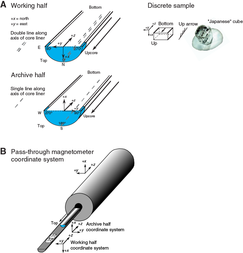
Figure F14. Paleomagnetic sample and SRM coordinate systems.
Core orientation
With the exception of the first two or three APC cores (where the BHA is not stabilized in the surrounding sediment), full-length APC cores taken during Expedition 350 were oriented by means of the FlexIT orientation tool. The FlexIT tool comprises three mutually perpendicular fluxgate magnetic sensors and two perpendicular gravity sensors, allowing the azimuth (and plunge) of the fiducial lines on the core barrel to be determined. Nonmagnetic (Monel) APC barrels and a nonmagnetic drill collar were used during APC coring (with the exception of Holes U1436B, U1436C, and U1436D) to allow accurate registration against magnetic north.
Magnetostratigraphy
Expedition 350 drill sites are located at ~32°N, a sufficiently high latitude to allow magnetostratigraphy to be readily identified by changes in inclination alone. By considering the mean state of the Earth’s magnetic field to be a geocentric axial dipole, it is possible to calculate the field inclination (I) by tan I = 2tan(lat), where lat is the latitude. Therefore, the time-averaged normal field at the present-day positions of Sites U1436 and U1437 has a positive (downward) inclination of 51.76° and 51.11°, respectively. Negative inclinations indicate reversed polarity. Magnetozones identified from the shipboard data were correlated to the geomagnetic polarity timescale (GPTS) (GPTS2012; Gradstein et al., 2012) with the aid of biostratigraphic datums (Table T11). In this updated GPTS version, the Late Cretaceous through Neogene time has been calibrated with magnetostratigraphic, biostratigraphic, and cyclostratigraphic studies and selected radioisotopically dated datums. The chron terminology is from Cande and Kent (1995).
Table T11. Age estimates for timescale of magnetostratigraphic chrons. Download table in .csv format.
Biostratigraphy
Paleontology and biostratigraphy
Paleontological investigations carried out during Expedition 350 focused on calcareous nannofossils and planktonic and benthic foraminifers. Preliminary biostratigraphic determinations were based on nannofossils and planktonic foraminifers. Biostratigraphic interpretations of planktonic foraminifers and biozones are based on Wade et al. (2011) with the exception of the bioevents associated with Globigerinoides ruber, for which we refer to Li (1997). Benthic foraminifer species determination was mostly carried out with reference to ODP Leg 126 records by Kaiho (1992). The standard nannofossil zonations of Martini (1971) and Okada and Bukry (1980) were used to interpret calcareous nannofossils. The Nannotax website (http://ina.tmsoc.org/Nannotax3/) was consulted to find updated nannofossil genera and species ranges. The identified bioevents for both fossil groups were calibrated to the GPTS (Gradstein et al., 2012) for consistency with the methods described in Paleomagnetism (see Age model; Figure F17; Tables T12, T13). All data were recorded in the DESClogik spreadsheet program and uploaded into the LIMS database.
Table T12. Calcareous nannofossil datum events. Download table in .csv format.
Table T13. Planktonic foraminifer datum events. Download table in .csv format.
The core catcher (CC) sample of each core was examined. Additional samples were taken from the working halves as necessary to refine the biostratigraphy, preferentially sampling tuffaceous mud/mudstone intervals.
As the core catcher is 5 cm long and neither the orientation nor the precise position of a studied sample within is available, the mean depth for any identified bioevent (i.e., T = top, and B = bottom) is calculated following the scheme in Figure F15.
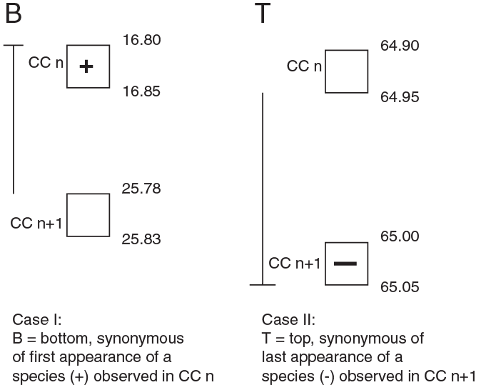
Figure F15. Foraminifer and nannofossil bioevent mean depth calculation.
Foraminifers
Sediment volumes of 10 cm3 were taken. Generally, this volume yielded sufficient numbers of foraminifers (~300 specimens per sample), with the exception of those from the volcaniclastic-rich intervals where intense dilution occurred. All samples were washed over a 63 µm mesh sieve, rinsed with DI water, and dried in an oven at 50°C. Samples that were more lithified were soaked in water and disaggregated using a shaking table for several hours. If necessary, the samples were soaked in warm (70°C) dilute hydrogen peroxide (20%) for several hours prior to wet sieving. For the most lithified samples, we used a kerosene bath to saturate the pores of each dried sample following the method presented by Hermann (1992) for similar material recovered during Leg 126. All dry coarse fractions were placed in a labeled vial ready for micropaleontological examination. Cross contamination between samples was avoided by ultrasonically cleaning sieves between samples. Where coarse fractions were large, relative abundance estimates were made on split samples obtained using a microsplitter as appropriate.
Examination of foraminifers was carried out on the >150 µm size fraction following dry sieving. The sample was spread on a sample tray and examined for planktonic foraminifer datum diagnostic species. We made a visual assessment of group and species relative abundances as well as their preservation according to the categories defined below. Micropaleontological reference slides were assembled for some samples, where appropriate for the planktonic fauna samples, and for all benthic fauna samples. These are marked by an asterisk next to the sample name in the results table. Photomicrographs were taken using a Spot RTS system with IODP Image Capture and commercial Spot software.
The proportion of planktonic foraminifers in the >150 µm fraction (i.e., including lithogenic particles) was estimated as follows:
The proportion of benthic foraminifers in the biogenic fraction >150 µm was estimated as follows:
- B = barren (no foraminifers present).
- R = rare (<1%).
- F = few (1%–5%).
- C = common (>5%–10%).
- A = abundant (>10%–30%).
- D = dominant (>30%).
The relative abundance of foraminifer species in either the planktonic or benthic foraminifer assemblages (>150 µm) were estimated as follows:
- T = trace (<0.1% of species in the total planktonic/benthic foraminifer assemblage >150 µm).
- P = present (<1%).
- R = rare (1%–5%).
- F = few (>5%–10%).
- A = abundant (>10%–30%).
- D = dominant (>30%).
The degree of fragmentation of the planktonic foraminifers (>150 µm), where a fragment was defined as part of a planktonic foraminifer shell representing less than half of a whole test was estimated as follows:
- N = none (no planktonic foraminifer fragment observed in the >150 µm fraction).
- L = light (0%–10%).
- M = moderate (>10%–30%).
- S = severe (>30%–50%).
- VS = very severe (> 50%).
A record of the preservation of the samples was made using comments on the aspect of the whole planktonic foraminifer shells (>150 µm) examined:
- E = etched (>30% of planktonic foraminifer assemblage shows etching).
- G = glassy (>50% of planktonic foraminifers are translucent).
- F = frosty (>50% of planktonic foraminifers are not translucent).
As much as possible we tried to give a qualitative estimate of the extent of reworking and/or downhole contamination using the following scale:
Calcareous nannofossils
Calcareous nannofossil assemblages were examined and described from smear slides made from core catcher samples of each recovered core. Standard smear slide techniques were utilized for immediate biostratigraphic examination. For coarse material, the fine fraction was separated from the coarse fraction by settling through water before the smear slide was prepared. All samples were examined using a Zeiss Axiophot light microscope with an oil immersion lens under a magnification of 1000×. The semiquantitative abundances of all species encountered were described (see below). Additional observations with the scanning electron microscope (SEM) were used to identify Emiliania huxleyi. Photomicrographs were taken using a Spot RTS system with Image Capture and Spot software.
The Nannotax website (http://ina.tmsoc.org/Nannotax3/) was consulted to find up-to-date nannofossil genera and species ranges. The genus Gephyrocapsa has been divided into species; however, in addition as the genus shows high variations in size, it has also been divided into three major morphogroups based on maximum coccolith length following the biometric subdivision by Raffi et al. (1993) and Raffi et al. (2006): small Gephyrocapsa (<4 µm), medium Gephyrocapsa (4–5.5 µm), and large Gephyrocapsa spp. (>5.5 µm).
Species abundances were determined using the criteria defined below:
- V = very abundant (>100 specimens per field of view).
- A = abundant (>10–100 specimens per field of view).
- C = common (>1–10 specimens per field of view).
- F = few (>1–10 specimens per 2–10 fields of view).
- VF = very few (1 specimen per 2–10 fields of view).
- R = rare (1 specimen per >10 fields of view).
- B = barren (no nannofossils).
- * (reworked) = reworked occurrence.
The following basic criteria were used to qualitatively provide a measure of preservation of the nannofossil assemblage:
- E = excellent (no dissolution is seen, all specimens can be identified).
- G = good (little dissolution and/or overgrowth is observed, diagnostic characteristics are preserved, and all specimens can be identified).
- M = moderate (dissolution and/or overgrowth are evident; a significant proportion [up to 25%] of the specimens cannot be identified to species level with absolute certainty).
- P = poor (severe dissolution, fragmentation, and/or overgrowth has occurred; most primary features have been destroyed and many specimens cannot be identified at the species level).
For each sample a comment on the presence or absence of diatoms and siliceous plankton is recorded.
Age model
One of the main goals of Expedition 350 was to establish an accurate age model for Sites U1436 and U1437 in order to understand the temporal evolution of the Izu arc. Both biostratigraphers and paleomagnetists worked closely to deliver a suitable shipboard age model.
Timescale
The polarity stratigraphy established onboard was correlated with the GPTS of Gradstein et al. (2012). The biozones for planktonic foraminifers and calcareous nannofossils and the paleomagnetic chrons were calibrated according to this GPTS (Figure F16; Tables T11, T12, T13). Because of calibration uncertainties in the GPTS, the age model is based on a selection of tie points rather than using all biostratigraphic datums. This approach minimizes spurious variations in estimating sedimentation rates. Ages and depth range for the biostratigraphic and magnetostratigraphic datums are shown in Tables T11, T12, and T13.
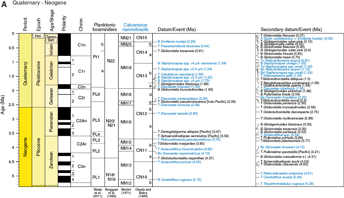
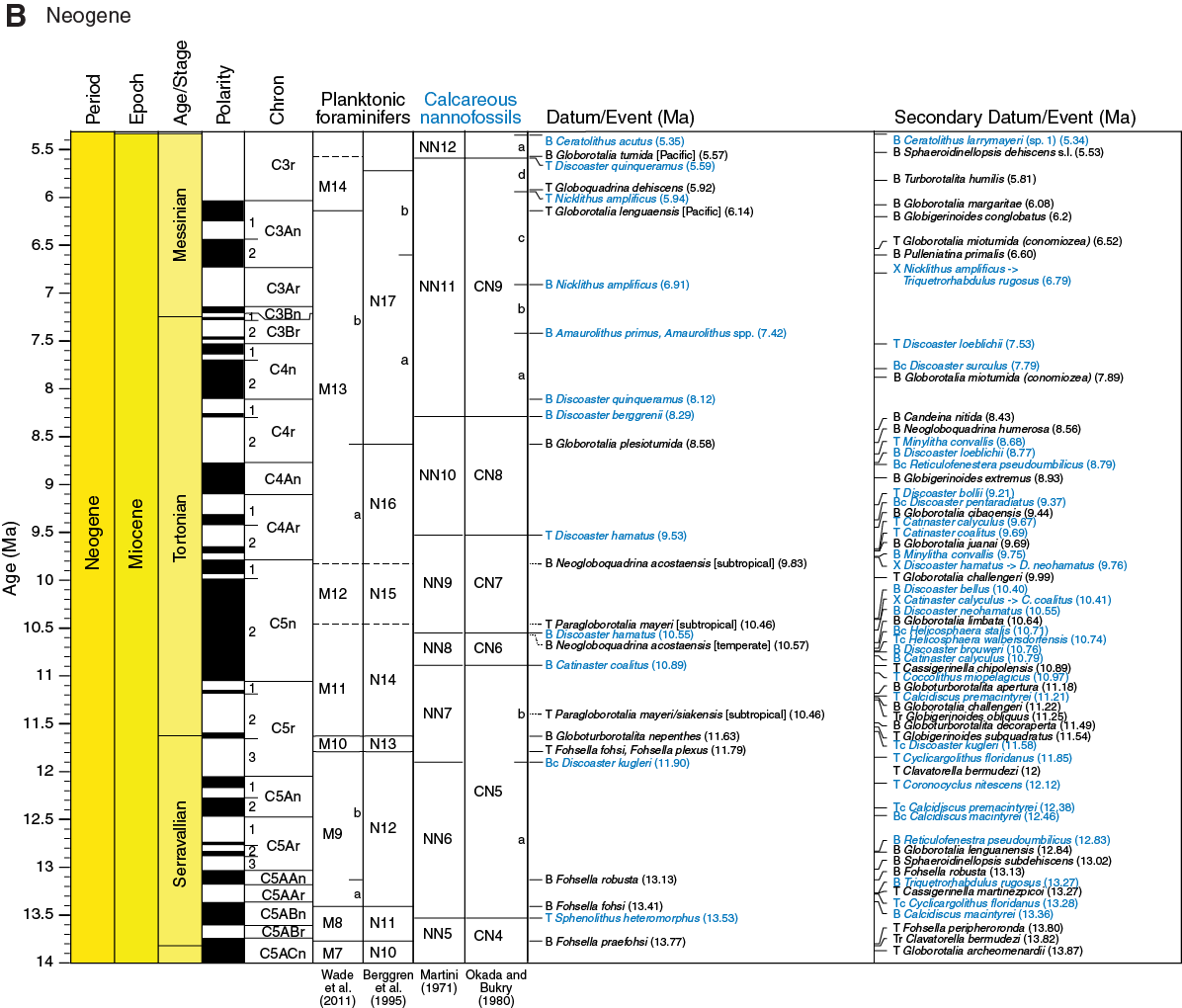
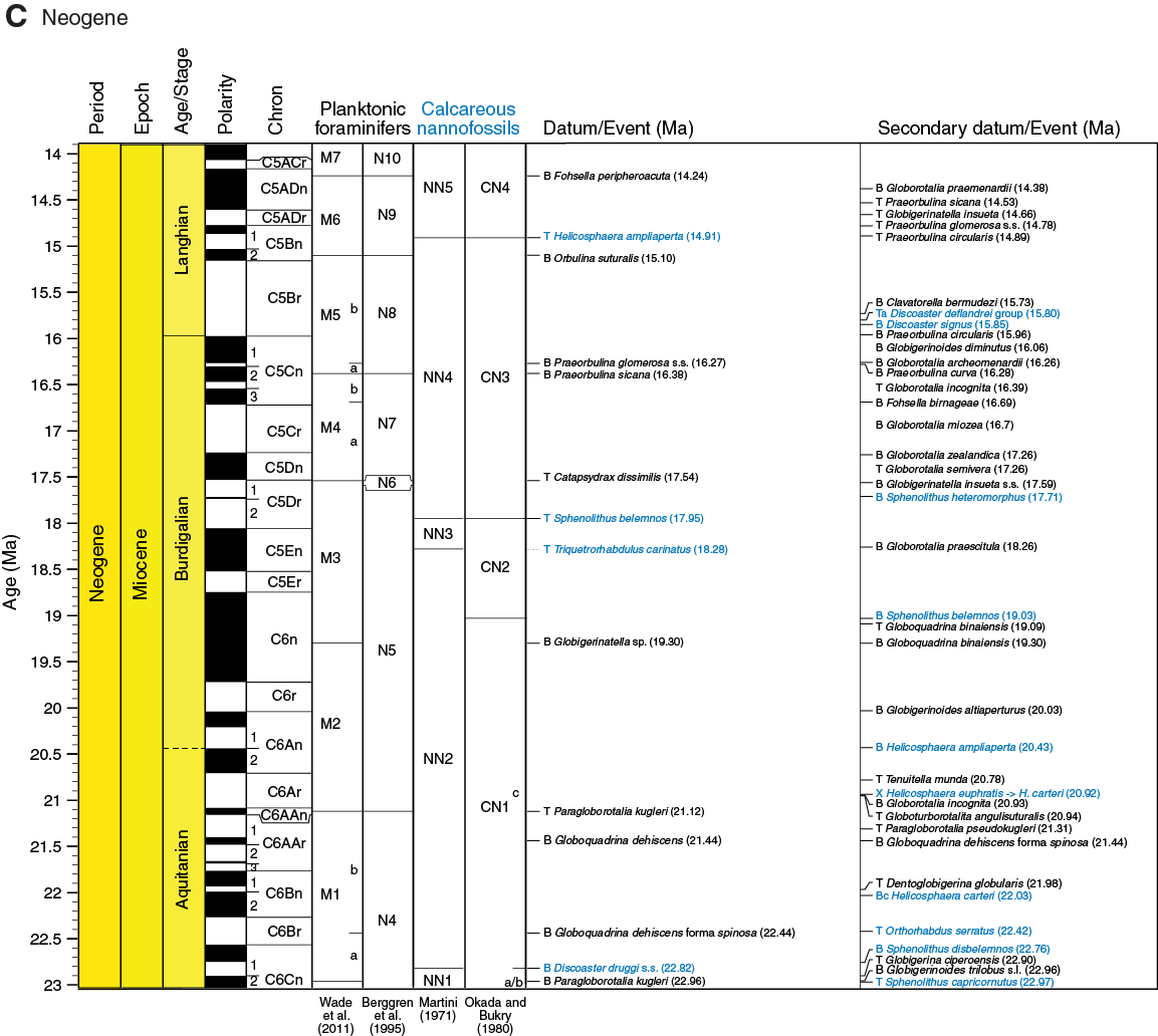
Figure F16. Timescale.
Depth scale
Several depth scale types are defined by IODP based on tools and computation procedures used to estimate and correlate the depth of core samples (see Operations). Because only one hole was cored at Site U1436, the three holes cored at Site U1437 did not overlap by more than a few meters, and instances of >100% recovery were very few at both sites, we used the standard CSF-A depth scale, referred to as mbsf in this volume.
Constructing the age-depth model
If well-constrained by biostratigraphic data, the paleomagnetic data were given first priority to construct the age model. The next priority was given to calcareous nannofossils, followed by planktonic foraminifers. In cases of conflicting microfossil datums, we took into account the reliability of individual datums as global dating tools in the context of the IBM rear arc, as follows:
- The reliability of fossil groups as stratigraphic indicators varies according to the sampling interval and nature of the material collected (i.e., certain intervals had poor microfossil recovery).
- Different datums can contradict each other because of contrasting abundances, preservation, localized reworking during sedimentation, or even downhole contamination during drilling. The quality of each datum was assessed by the biostratigraphers.
- The uncertainties associated with bottom or top datums were considered. Bottom datums are generally preferred as they are considered to be more reliable to secure good calibrations to GPTS 2012.
The precision of the shipboard Expedition 350 site-specific age-depth models is limited by the generally low biostratigraphic sampling resolution (4.5–9 m). The procedure applied here resulted in conservative shipboard age models, satisfying as many constraints as possible without introducing artifacts. Construction of the age-depth curve for each site started with a plot of all biostratigraphic and paleomagnetic control points. Age and depth uncertainties were represented by error bars. Obvious outliers and conflicting datums were then masked until the line connecting the remaining control points was contiguous (i.e., without age-depth inversions) in order to have linear correlation. Next, an interpolation curve was applied that passed through all control points. Linear interpolation is used for the simple age-depth relationships.
Linear sedimentation rates
Based on the age-depth model, linear sedimentation rates (LSRs) were calculated and plotted based on a subjective selection of time slices along the age-depth model. Keeping in mind the arbitrary nature of the interval selection, only the most realistic and conservative segments were used. Hiatuses were inferred when the shipboard magnetostratigraphy and biostratigraphy could not be continuously correlated. LSRs are expressed in meters per million years.
Mass accumulation rates
Mass accumulation rate (MAR) is obtained by simple calculation based on LSR and dry bulk density (DBD) averaged over the LSR defined. DBD is derived from shipboard MAD measurements (see Physical properties). Average values for DBD, carbonate accumulation rate (CAR), and noncarbonate accumulation rate (nCAR) were calculated for the intervals selected for the LSRs. CAR and nCAR are expressed in g/cm2/ky and calculated as follows:
MAR (g/cm2/ky) = LSR (cm/ky) × DBD (g/cm3),
A step plot of LSR, total MAR, CAR, and nCAR is presented in each site chapter.
Downhole measurements
Wireline logging
Wireline logs are measurements of physical, chemical, and structural properties of the formation surrounding a borehole that are made by lowering probes with an electrical wireline in the hole after completion of drilling. The data are continuous with depth (at vertical sampling intervals ranging from 2.5 mm to 15 cm) and are measured in situ. The sampling and depth of investigation are intermediate between laboratory measurements on core samples and geophysical surveys and provide a link for the integrated understanding of physical properties on all scales.
Logs can be interpreted in terms of stratigraphy, lithology, mineralogy, and geochemical composition. They provide also information on the status and size of the borehole and on possible deformations induced by drilling or formation stress. When core recovery is incomplete, which is common in the volcaniclastic sediments drilled during Expedition 350, log data may provide the only way to characterize the formation in some intervals. They can be used to determine the actual thickness of individual units or lithologies when contacts are not recovered, to pinpoint the actual depth of features in cores with incomplete recovery, or to identify intervals that were not recovered. Where core recovery is good, log and core data complement one another and may be interpreted jointly. In particular, the imaging tools provide oriented images of the borehole wall that can help reorient the recovered core within the geographic reference frame.
Operations
Logs are recorded with a variety of tools combined into strings. Three tool strings were used during Expedition 350 (see Figure F17; Tables T14, T15):
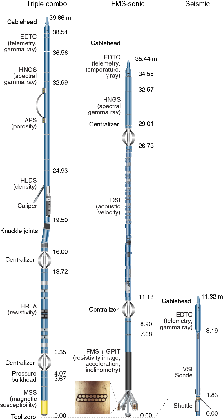
Figure F17. Wireline tool strings.
Table T14. Downhole measurements. Download table in .csv format.
Table T15. Downhole wireline tool acronyms and units. Download table in .csv format.
- Triple combo with magnetic susceptibility (measuring spectral gamma ray, porosity, density, resistivity, and magnetic susceptibility);
- Formation MicroScanner (FMS)-sonic (measuring spectral gamma ray, sonic velocity, and electrical images); and
- Seismic (measuring gamma ray and seismic transit times).
After completion of coring, the bottom of the drill string is set at some depth inside the hole (to a maximum of about 100 mbsf) to prevent collapse of unstable shallow material. In cased holes, the bottom of the drill string is set high enough above the bottom of the casing for the longest tool string to fit inside the casing. The main data are recorded in the open hole section. The spectral and total gamma ray logs (see below) provide the only meaningful data inside the pipe to identify the depth of the seafloor.
Each deployment of a tool string is a logging “run,” starting with the assembly of the tools and the necessary calibrations. The tool string is then sent to the bottom of the hole while recording a partial set of data and pulled back up at a constant speed, typically 250–500 m/h to record the main data. During each run, tool strings can be lowered down and pulled up the hole several times for control of repeatability or to try to improve the quality or coverage of the data. Each lowering or hauling up of the tool string while collecting data constitutes a “pass.” During each pass, the incoming data are recorded and monitored in real time on the surface system. A logging run is complete once the tool string has been brought to the rig floor and disassembled.
Logged properties and tool measurement principles
The main logs recorded during Expedition 350 are listed in Table T14. More detailed information on individual tools and their geological applications may be found in Ellis and Singer (2007), Goldberg (1997), Lovell et al. (1998), Rider (1996), Schlumberger (1989), and Serra (1984, 1986, 1989).
Natural radioactivity
The Hostile Environment Natural Gamma Ray Sonde (HNGS) was used on all tool strings to measure natural radioactivity in the formation. It uses two bismuth germanate scintillation detectors and 5-window spectroscopy to determine concentrations of K, Th, and U, whose radioactive isotopes dominate the natural radiation spectrum.
The Enhanced Digital Telemetry Cartridge (EDTC, see below), which is used primarily to communicate data to the surface, includes a sodium iodide scintillation detector to measure the total natural gamma ray emission. It is not a spectral tool but it provides an additional high-resolution total gamma ray for each pass.
Porosity
Formation porosity was measured with the Accelerator Porosity Sonde (APS). The sonde includes a minitron neutron generator that produces fast neutrons and 5 detectors positioned at different spacings from the minitron. The tool’s detectors count neutrons that arrive after being scattered and slowed by collisions with atomic nuclei in the formation.
The highest energy loss occurs when neutrons collide with hydrogen nuclei, which have practically the same mass as the neutron. Therefore, the tool provides a measure of hydrogen content, which is most commonly found in water in the pore fluid and can be directly related to porosity. However, hydrogen may be present in sedimentary, igneous and, alteration minerals, which can result in an overestimation of actual porosity.
Upon reaching thermal energies (0.025 eV), the neutrons are captured by the nuclei of Cl, Si, B, and other elements, resulting in a gamma ray emission. This neutron capture cross section (Σf) is also measured by the tool and can be used to identify such elements (Broglia and Ellis, 1990; Brewer et al., 1996).
Density
Formation density was measured with the Hostile Environment Litho-Density Sonde (HLDS). The sonde contains a radioactive cesium (137Cs) gamma ray source and far and near gamma ray detectors mounted on a shielded skid, which is pressed against the borehole wall by an eccentralizing arm. Gamma rays emitted by the source undergo Compton scattering, where gamma rays are scattered by electrons in the formation. The number of scattered gamma rays that reach the detectors is proportional to the density of electrons in the formation, which is in turn related to bulk density. Porosity may be derived from this bulk density if the matrix (grain) density is known.
The HLDS also measures photoelectric absorption as the photoelectric effect (PEF). Photoelectric absorption of the gamma rays occurs when their energy is reduced below 150 keV after being repeatedly scattered by electrons in the formation. Because PEF depends on the atomic number of the elements encountered, it varies with the chemical composition of the minerals present and can be used for the identification of some minerals (Bartetzko et al., 2003; Expedition 304/305 Scientists, 2006).
Electrical resistivity
The High-Resolution Laterolog Array (HRLA) tool provides six resistivity measurements with different depths of investigation (including the borehole fluid or mud resistivity and five measurements of formation resistivity with increasing penetration into the formation). The sonde sends a focused current beam into the formation and measures the current intensity necessary to maintain a constant drop in voltage across a fixed interval, providing direct resistivity measurement. The array has one central source electrode and six electrodes above and below it, which serve alternately as focusing and returning current electrodes. By rapidly changing the role of these electrodes, a simultaneous resistivity measurement is achieved at six penetration depths.
Typically, minerals found in sedimentary and igneous rocks are electrical insulators, whereas ionic solutions like pore water are conductors. In most rocks, electrical conduction occurs primarily by ion transport through pore fluids and thus is strongly dependent on porosity. Electrical resistivity can therefore be used to estimate porosity, alteration, and fluid salinity.
Acoustic velocity
The Dipole Shear Sonic Imager (DSI) generates acoustic pulses from various sonic transmitters and records the waveforms with an array of 8 receivers. The waveforms are then used to calculate the sonic velocity in the formation. The omnidirectional monopole transmitter emits high frequency (5–15 kHz) pulses to extract the compressional velocity (VP) of the formation, as well as the shear velocity (VS) when it is faster than the sound velocity in the borehole fluid. The same transmitter can be fired in sequence at a lower frequency (0.5–1 kHz) to generate Stoneley waves that are sensitive to fractures and variations in permeability. The DSI also has two cross dipole transmitters, which allow an additional measurement of shear wave velocity in “slow” formations, where VS is slower than the velocity in the borehole fluid. The waveforms produced by the two orthogonal dipole transducers can be used to identify sonic anisotropy that can be associated with the local stress regime.
Formation MicroScanner
The FMS provides high-resolution electrical resistivity images of the borehole walls. The tool has four orthogonal arms and pads, each containing 16 button electrodes that are pressed against the borehole wall during the recording. The electrodes are arranged in two diagonally offset rows of eight electrodes each. A focused current is emitted from the button electrodes into the formation with a return electrode near the top of the tool. Resistivity of the formation at the button electrodes is derived from the intensity of current passing through the button electrodes. Processing transforms these measurements into oriented high-resolution images that reveal the structures of the borehole wall. Features such as flows, breccia, fractures, folding, or alteration can be resolved. The images are oriented to magnetic north so that the dip and direction (azimuth) of planar features in the formation can be estimated.
Accelerometry and magnetic field measurements
Acceleration and magnetic field measurements are made with the General Purpose Inclinometry Tool (GPIT). The primary purpose of this tool, which incorporates a 3-component accelerometer and a 3-component magnetometer, is to determine the acceleration and orientation of the FMS-sonic tool string during logging. Thus, the FMS images can be corrected for irregular tool motion, and the dip and direction (azimuth) of features in the FMS image can be determined.
Magnetic susceptibility
The magnetic susceptibility sonde (MSS), a tool designed by Lamont-Doherty Earth Observatory (LDEO), measures the ease with which formations are magnetized when subjected to Earth’s magnetic field. This is ultimately related to the concentration and composition (size, shape, and mineralogy) of magnetizable material within the formation. These measurements provide one of the best methods for investigating stratigraphic changes in mineralogy and lithology because the measurement is quick and repeatable and because different lithologies often have strongly contrasting susceptibilities. In particular, volcaniclastic deposits can have a very distinct magnetic susceptibility signature compared to hemipelagic mud/mudstone. The sensor used during Expedition 350 was a dual-coil sensor providing deep-reading measurements with a vertical resolution of ~40 cm. The MSS was run as an addition to the triple combo tool string, using a specially developed data translation cartridge.
Auxiliary logging equipment
Cablehead
The Schlumberger logging equipment head (or cablehead) measures tension at the very top of the wireline tool string to diagnose difficulties in running the tool string up or down the borehole or when exiting or entering the drill string or casing.
Telemetry cartridges
Telemetry cartridges are used in each tool string to transmit the data from the tools to the surface in real time. The EDTC also includes a sodium iodide scintillation detector to measure the total natural gamma ray emission of the formation, which can be used to match the depths between the different passes and runs.
Joints and adapters
Because the tool strings combine tools of different generations and with various designs, they include several adapters and joints between individual tools to allow communication, provide isolation, avoid interferences (mechanical or acoustic), terminate wirings, or position the tool properly in the borehole. Knuckle joints in particular were used to allow some of the tools such as the HRLA to remain centralized in the borehole, whereas the overlying HLDS was pressed against the borehole wall.
All these additions are included and contribute to the total length of the tool strings in Figure F17.
Log data quality
The principal factor in the quality of log data is the condition of the borehole wall. If the borehole diameter varies over short intervals because of washouts or ledges, the logs from tools that require good contact with the borehole wall may be degraded. Deep investigation measurements such as gamma ray, resistivity, and sonic velocity, which do not require contact with the borehole wall, are generally less sensitive to borehole conditions. Very narrow (“bridged”) sections will also cause irregular log results.
The accuracy of the logging depth depends on several factors. The depth of the logging measurements is determined from the length of the cable played out from the winch on the ship. Uncertainties in logging depth occur because of ship heave, cable stretch, cable slip, or even tidal changes. Similarly, uncertainties in the depth of the core samples occur because of incomplete core recovery or incomplete heave compensation. All these factors generate some discrepancy between core sample depths, logs, and individual logging passes. To minimize the effect of ship heave, a hydraulic wireline heave compensator (WHC) was used to adjust the wireline length for rig motion during wireline logging operations.
Wireline heave compensator
The WHC system is designed to compensate for the vertical motion of the ship and maintain a steady motion of the logging tools. It uses vertical acceleration measurements made by a motion reference unit, located under the rig floor near the center of gravity of the ship, to calculate the vertical motion of the ship. It then adjusts the length of the wireline by varying the distance between two sets of pulleys through which the wireline passes.
Logging data flow and processing
Data from each logging run were monitored in real time and recorded using the Schlumberger MAXIS 500 system. They were then copied to the shipboard workstations for processing. The main pass of the triple combo was commonly used as a reference to which other passes were interactively depth matched. After depth matching, all the logging depths were shifted to the seafloor after identifying the seafloor from a step in the gamma ray profile. The electrical images were processed by using data from the GPIT to correct for irregular tool motion, and the image gains were equalized to enhance the representation of the borehole wall. All the processed data were made available to the science party within a day of their acquisition in ASCII format for most logs and in GIF format for the images.
The data were also transferred onshore to LDEO for a standardized implementation of the same data processing, formatting for the online logging database, and for archiving.
In situ temperature measurements
In situ temperature measurements were made at each site using the advanced piston corer temperature tool (APCT-3). The APCT-3 fits directly into the coring shoe of the APC and consists of a battery pack, data logger, and platinum resistance-temperature device calibrated over a temperature range from 0° to 30°C. Before entering the borehole, the tool is first stopped at the seafloor for 5 min to thermally equilibrate with bottom water. However, the lowest temperature recorded during the run down was preferred to the average temperature at the seafloor as an estimate of the bottom water temperature because it is more repeatable and the bottom water is expected to have the lowest temperature in the profile. After the APC penetrated the sediment, it was held in place for 5–10 min as the APCT-3 recorded the temperature of the cutting shoe every second. Shooting the APC into the formation generates an instantaneous temperature rise from frictional heating. This heat gradually dissipates into the surrounding sediments as the temperature at the APCT-3 equilibrates toward the temperature of the sediments.
The equilibrium temperature of the sediments was estimated by applying a mathematical heat-conduction model to the temperature decay record (Horai and Von Herzen, 1985). The synthetic thermal decay curve for the APCT-3 tool is a function of the geometry and thermal properties of the probe and the sediments (Bullard, 1954; Horai and Von Herzen, 1985). The equilibrium temperature is estimated by applying an appropriate curve fitting procedure (Pribnow et al., 2000). However, when the APCT-3 does not achieve a full stroke, or when ship heave pulls up the APC from full penetration, the temperature equilibration curve is disturbed and temperature determination is more difficult. The nominal accuracy of the APCT-3 temperature measurement is ±0.1°C.
The APCT-3 temperature data were combined with measurements of thermal conductivity (see Physical properties) obtained from core samples to obtain heat flow values using to the method designed by Bullard (1954).
References
ASTM International, 1990. Standard method for laboratory determination of water (moisture) content of soil and rock (Standard D2216–90). In Annual Book of ASTM Standards for Soil and Rock (Vol. 04.08): Philadelphia (American Society for Testing Materials). [revision of D2216-63, D2216-80]
Bartetzko, A., Paulick, H., Iturrino, G., and Arnold, J., 2003. Facies reconstruction of a hydrothermally altered dacite extrusive sequence: evidence from geophysical downhole logging data (ODP Leg 193). Geochemistry, Geophysics, Geosystems, 4(10):1087. http://dx.doi.org/10.1029/2003GC000575
Berggren, W.A., Kent, D.V., Swisher, C.C., III, and Aubry, M.-P., 1995. A revised Cenozoic geochronology and chronostratigraphy. In Berggren, W.A., Kent, D.V., Aubry, M.-P., and Hardenbol, J. (Eds.), Geochronology, Time Scales and Global Stratigraphic Correlation. Special Publication - SEPM (Society for Sedimentary Geology), 54:129–212. http://dx.doi.org/10.2110/pec.95.04.0129
Bloemendal, J., King, J.W., Hall, F.R., and Doh, S.-J., 1992. Rock magnetism of late Neogene and Pleistocene deep-sea sediments: relationship to sediment source, diagenetic processes, and sediment lithology. Journal of Geophysical Research: Solid Earth, 97(B4):4361–4375. http://dx.doi.org/10.1029/91JB03068
Blum, P., 1997. Physical properties handbook: a guide to the shipboard measurement of physical properties of deep-sea cores. Ocean Drilling Program Technical Note, 26. http://dx.doi.org/10.2973/odp.tn.26.1997
Brewer, T.S., Harvey, P.K., Locke, J., and Lovell, M.A., 1996. Neutron absorption cross section (Σ) of basaltic basement samples from Hole 896A, Costa Rica rift. In Alt, J.C., Kinoshita, H., Stokking, L.B., and Michael, P.J. (Eds.), Proceedings of the Ocean Drilling Program, Scientific Results, 148: College Station, TX (Ocean Drilling Program), 389–394. http://dx.doi.org/10.2973/odp.proc.sr.148.154.1996
Broglia, C., and Ellis, D., 1990. Effect of alteration, formation absorption, and standoff on the response of the thermal neutron porosity log in gabbros and basalts: examples from Deep Sea Drilling Project-Ocean Drilling Program sites. Journal of Geophysical Research: Solid Earth, 95(B6):9171–9188. http://dx.doi.org/10.1029/JB095iB06p09171
Bullard, E.C., 1954. The flow of heat through the floor of the Atlantic Ocean. Proceedings of the Royal Society of London, Series A: Mathematical, Physical and Engineering Sciences, 222(1150):408–429. http://dx.doi.org/10.1098/rspa.1954.0085
Cande, S.C., and Kent, D.V., 1995. Revised calibration of the geomagnetic polarity timescale for the Late Cretaceous and Cenozoic. Journal of Geophysical Research: Solid Earth, 100(B4):6093–6095. http://dx.doi.org/10.1029/94JB03098
Cas, R.A.F., and Wright, J.V., 1987. Volcanic Successions, Modern and Ancient: a Geological Approach to Processes, Products and Successions: London (Allen and Unwin).
Chaisson, W.P., and Pearson, P.N., 1997. Planktonic foraminifer biostratigraphy at Site 925: middle Miocene–Pleistocene. In Shackleton, N.J., Curry, W.B., Richter, C., and Bralower, T.J. (Eds.), Proceedings of the Ocean Drilling Program, Scientific Results, 154: College Station, TX (Ocean Drilling Program), 3–31. http://dx.doi.org/10.2973/odp.proc.sr.154.104.1997
Dunlop, D.J., 2003. Stepwise and continuous low-temperature demagnetization. Geophysical Research Letters, 30(11):1582. http://dx.doi.org/10.1029/2003GL017268
Dunlop, D.J., Özdemir, Ö., and Schmidt, P.W., 1997. Paleomagnetism and paleothermometry of the Sydney Basin 2. Origin of anomalously high unblocking temperatures. Journal of Geophysical Research: Solid Earth, 102(B12):27285–27295. http://dx.doi.org/10.1029/97JB02478
Ellis, D.V., and Singer, J.M., 2007. Well Logging for Earth Scientists (2nd ed.): New York (Elsevier).
Evans, H.B., 1965. GRAPE—a device for continuous determination of material density and porosity. Transactions of the SPWLA Annual Logging Symposium: 6(2):B1–B25. https://www.spwla.org/SymposiumTransactions/grape-device-continuous-determination-material-density-and-porosity
Expedition 304/305 Scientists, 2006. Methods. In Blackman, D.K., Ildefonse, B., John, B.E., Ohara, Y., Miller, D.J., MacLeod, C.J., and the Expedition 304/305 Scientists, Proceedings of the Integrated Ocean Drilling Program, 304/305: College Station, TX (Integrated Ocean Drilling Program Management International, Inc.). http://dx.doi.org/10.2204/iodp.proc.304305.102.2006
Expedition 323 Scientists, 2011. Methods. In Takahashi, K., Ravelo, A.C., Alvarez Zarikian, C.A., and the Expedition 323 Scientists, Proceedings of the Integrated Ocean Drilling Program, 323: Tokyo (Integrated Ocean Drilling Program Management International, Inc.). http://dx.doi.org/10.2204/iodp.proc.323.102.2011
Expedition 324 Scientists, 2010. Methods. In Sager, W.W., Sano, T., Geldmacher, J., and the Expedition 324 Scientists, Proceedings of the Integrated Ocean Drilling Program, 324: Tokyo (Integrated Ocean Drilling Program Management International, Inc.). http://dx.doi.org/10.2204/iodp.proc.324.102.2010
Expedition 330 Scientists, 2012. Methods. In Koppers, A.A.P., Yamazaki, T., Geldmacher, J., and the Expedition 330 Scientists, Proceedings of the Integrated Ocean Drilling Program, 330: Tokyo (Integrated Ocean Drilling Program Management International, Inc.). http://dx.doi.org/10.2204/iodp.proc.330.102.2012
Expedition 336 Scientists, 2012. Methods. In Edwards, K.J., Bach, W., Klaus, A., and the Expedition 336 Scientists, Proceedings of the Integrated Ocean Drilling Program, 336: Tokyo (Integrated Ocean Drilling Program Management International, Inc.). http://dx.doi.org/10.2204/iodp.proc.336.102.2012
Expedition 340 Scientists, 2013. Methods. In Le Friant, A., Ishizuka, O., Stroncik, N.A., and the Expedition 340 Scientists, Proceedings of the Integrated Ocean Drilling Program, 340: Tokyo (Integrated Ocean Drilling Program Management International, Inc.). http://dx.doi.org/10.2204/iodp.proc.340.102.2013
Fisher, R.V., 1961. Proposed classification of volcaniclastic sediments and rocks. Geological Society of America Bulletin, 72(9):1409–1414. http://dx.doi.org/10.1130/0016-7606(1961)72[1409:PCOVSA]2.0.CO;2
Fisher, R.V., and Schmincke, H.-U., 1984. Pyroclastic Rocks: Berlin (Springer-Verlag). http://dx.doi.org/10.1007/978-3-642-74864-6
Gásquez, J.A., Perino, E., Marchevsky, E., Olsina, R., and Riveros, A., 1997. Correction of line interference in X-ray fluorescence trace analysis. Application to yttrium determination in silicate rocks. X-Ray Spectrometry, 26(5):272–274.
Gieskes, J.M., Gamo, T., and Brumsack, H., 1991. Chemical methods for interstitial water analysis aboard JOIDES Resolution. Ocean Drilling Program Technical Note, 15. http://dx.doi.org/10.2973/odp.tn.15.1991
Goldberg, D., 1997. The role of downhole measurements in marine geology and geophysics. Reviews of Geophysics, 35(3):315–342. http://dx.doi.org/10.1029/97RG00221
Govindaraju, K., 1989. 1989 compilation of working values and sample description for 272 geostandards. Geostandards Newsletter, 13(S1). http://dx.doi.org/10.1111/j.1751-908X.1989.tb00476.x
Govindaraju, K., 1994. 1994 compilation of working values and sample description for 383 geostandards. Geostandards Newsletter, 18(1). http://dx.doi.org/10.1111/j.1751-908X.1994.tb00526.x
Gradstein, F.M., Ogg, J.G., Schmitz, M.D., and Ogg, G.M. (Eds.)., 2012. The Geological Time Scale 2012: Amsterdam (Elsevier).
Harris, R.N., Sakaguchi, A., Petronotis, K., Baxter, A.T., Berg, R., Burkett, A., Charpentier, D., Choi, J., Diz Ferreiro, P., Hamahashi, M., Hashimoto, Y., Heydolph, K., Jovane, L., Kastner, M., Kurz, W., Kutterolf, S.O., Li, Y., Malinverno, A., Martin, K.M., Millan, C., Nascimento, D.B., Saito, S., Sandoval Gutierrez, M.I., Screaton, E.J., Smith-Duque, C.E., Solomon, E.A., Straub, S.M., Tanikawa, W., Torres, M.E., Uchimura, H., Vannucchi, P., Yamamoto, Y., Yan, Q., and Zhao, X., 2013. Methods. In Harris, R.N., Sakaguchi, A., Petronotis, K., and the Expedition 344 Scientists, Proceedings of the Integrated Ocean Drilling Program, 344: College Station, TX (Integrated Ocean Drilling Program). http://dx.doi.org/10.2204/iodp.proc.344.102.2013
Hermann, Y., 1992. Eocene through Quaternary planktonic foraminifers from the northwest Pacific, Leg 126. In Taylor, B., Fujioka, K., et al., Proceedings of the Ocean Drilling Program, Scientific Results, 126: College Station, TX (Ocean Drilling Program), 271–284. http://dx.doi.org/10.2973/odp.proc.sr.126.133.1992
Horai, K., and Von Herzen, R.P., 1985. Measurement of heat flow on Leg 86 of the Deep Sea Drilling Project. In Heath, G.R., Burckle, L.H., et al., Initial Reports of the Deep Sea Drilling Project, 86: Washington, DC (U.S. Government Printing Office), 759–777. http://dx.doi.org/10.2973/dsdp.proc.86.135.1985
Ingram, R.L., 1954. Terminology for the thickness of stratification and parting units in sedimentary rocks. Geological Society of America Bulletin, 65(9):937–938. http://dx.doi.org/10.1130/0016-7606(1954)65[937:TFTTOS]2.0.CO;2
Jackson, M., Gruber, W., Marvin, J., and Banerjee, S.K., 1988. Partial anhysteretic remanence and its anisotropy: applications and grainsize-dependence. Geophysical Research Letters, 15(5):440–443. http://dx.doi.org/10.1029/GL015i005p00440
Jutzeler, M., White, J.D.L., Talling, P.J., McCanta, M., Morgan, S., Le Friant, A., and Ishizuka, O., 2014. Coring disturbances in IODP piston cores with implications for offshore record of volcanic events and the Missoula megafloods. Geochemistry, Geophysics, Geosystems, 15(9):3572–3590. http://dx.doi.org/10.1002/2014GC005447
Kaiho, K., 1992. Eocene to Quaternary benthic foraminifers and paleobathymetry of the Izu-Bonin arc, Legs 125 and 126. In Taylor, B., Fujioka, K., et al., Proceedings of the Ocean Drilling Program, Scientific Results, 126: College Station, TX (Ocean Drilling Program), 285–310. http://dx.doi.org/10.2973/odp.proc.sr.126.137.1992
Kvenvolden, K.A., and McDonald, T.J., 1986. Organic geochemistry on the JOIDES Resolution—an assay. Ocean Drilling Program Technical Note, 6: College Station, TX (Ocean Drilling Program). http://dx.doi.org/10.2973/odp.tn.6.1986
Le Maitre, R.W., Steckeisen, A., Zanettin, B., Le Bas, M.J., Bonin, B., and Bateman, P. (Eds.), 2002. Igneous rocks: A Classification and Glossary of Terms (2nd ed.): Cambridge, UK (Cambridge University Press).
Li, B., 1997. Paleoceanography of the Nansha Area, southern South China Sea since the last 700,000 years [Ph.D. dissert.]. Nanjing Institute of Geology and Paleontology, Academic Sinica, Nanjing, China. (in Chinese, with abstract in English)
Lofgren, G., 1974. An experimental study of plagioclase crystal morphology: isothermal crystallization. American Journal of Science, 274:243–273.
Lourens, L.J., Hilgen, F.J., Laskar, J., Shackleton, N.J., and Wilson, D., 2004. The Neogene period. In Gradstein, F.M., Ogg, J., et al. (Eds.), A Geologic Time Scale 2004: Cambridge, UK (Cambridge University Press), 409–440.
Lovell, M.A., Harvey, P.K., Brewer, T.S., Williams, C., Jackson, P.D., and Williamson, G., 1998. Application of FMS images in the Ocean Drilling Program: an overview. In Cramp, A., MacLeod, C.J., Lee, S.V., and Jones, E.J.W. (Eds.), Geological Evolution of Ocean Basins: Results from the Ocean Drilling Program. Geological Society Special Publication, 131(1):287–303. http://dx.doi.org/10.1144/GSL.SP.1998.131.01.18
Lund, S.P., Stoner, J.S., Mix., A.C., Tiedemann, R., Blum, P., and the Leg 202 Shipboard Scientific Party, 2003. Appendix: observations on the effect of a nonmagnetic core barrel on shipboard paleomagnetic data: results from ODP Leg 202. In Mix, A.C., Tiedemann, R., Blum, P., et al., Proceedings of the Ocean Drilling Program, Initial Reports, 202: College Station, TX (Ocean Drilling Program), 1–10. http://dx.doi.org/10.2973/odp.proc.ir.202.114.2003
MacKenzie, W.S., Donaldson, C.H., and Guilford, C., 1982. Atlas of Igneous Rocks and Their Textures: Essex, UK (Longman Group UK Limited).
Manheim, F.T., and Sayles, F.L., 1974. Composition and origin of interstitial waters of marine sediments, based on deep sea drill cores. In Goldberg, E.D. (Ed.), The Sea (Vol. 5): Marine Chemistry: The Sedimentary Cycle: New York (Wiley), 527–568.
Martini, E., 1971. Standard Tertiary and Quaternary calcareous nannoplankton zonation. In Farinacci, A. (Ed.), Proceedings of the Second Planktonic Conference, Roma 1970: Rome (Edizioni Tecnoscienza), 2:739–785.
McPhie, J., Doyle, M., and Allen, R., 1993. Volcanic Textures: A Guide to the Interpretation of Textures in Volcanic Rocks: Hobart (Tasmanian Government Printing Office).
Millero, F.J., Feistel, R., Wright, D.G., and McDougall, T.J., 2008. The composition of Standard Seawater and the definition of the reference-composition salinity scale. Deep-Sea Research, Part I, 55(1):50–72. http://dx.doi.org/10.1016/j.dsr.2007.10.001
Murray, R.W., Miller, D.J., and Kryc, K.A., 2000. Analysis of major and trace elements in rocks, sediments, and interstitial waters by inductively coupled plasma–atomic emission spectrometry (ICP-AES). Ocean Drilling Program Technical Note, 29. http://dx.doi.org/10.2973/odp.tn.29.2000
Musgrave, R.J., Collombat, H., and Didenko, A.N., 1995. Magnetic sulfide diagenesis, thermal overprinting, and paleomagnetism of accretionary wedge and convergent margin sediments from the Chile triple junction region. In Lewis, S.D., Behrmann, J.H., Musgrave, R.J., and Cande, S.C. (Eds.), Proceedings of the Ocean Drilling Program, Scientific Results, 141: College Station, TX (Ocean Drilling Program), 59–76. http://dx.doi.org/10.2973/odp.proc.sr.141.015.1995
Néel, L., 1949. Théorie du traînage magnétique des ferromagnétiques en grains fins avec applications aux terres cuites. Annales de Geophysique (Centre National de la Recherche Scientifique), 5:99–136.
Okada, H., and Bukry, D., 1980. Supplementary modification and introduction of code numbers to the low-latitude coccolith biostratigraphic zonation (Bukry, 1973; 1975). Marine Micropaleontology, 5:321–325. http://dx.doi.org/10.1016/0377-8398(80)90016-X
Piper, D.J.W., 1975. Deformation of stiff and semilithified cores from Legs 18 and 28. Initial Reports of the Deep Sea Drilling Project, 28: Washington, DC (U.S. Government Printing Office), 977–979. http://dx.doi.org/10.2973/dsdp.proc.28.app2.1975
Pribnow, D., Kinoshita, M., and Stein, C., 2000. Thermal Data Collection and Heat Flow Recalculations for Ocean Drilling Program Legs 101–180: Hanover, Germany (Institute for Joint Geoscientific Research, Institut für Geowissenschaftliche Gemeinschaftsaufgaben [GGA]). http://www-odp.tamu.edu/publications/heatflow/ODPReprt.pdf
Raffi, I., Backman, J., Fornaciari, E., Pälike, H., Rio, D., Lourens, L., and Hilgen, F., 2006. A review of calcareous nannofossil astrobiochronology encompassing the past 25 million years. Quaternary Science Reviews, 25(23–24):3113–3137. http://dx.doi.org/10.1016/j.quascirev.2006.07.007
Raffi, I., Backman, J., Rio, D., and Shackleton, N.J., 1993. Plio–Pleistocene nannofossil biostratigraphy and calibration to oxygen isotope stratigraphies from Deep Sea Drilling Project Site 607 and Ocean Drilling Program Site 677. Paleoceanography, 8(3):387–408. http://dx.doi.org/10.1029/93PA00755
Richter, C., Acton, G., Endris, C., and Radsted, M., 2007. Handbook for shipboard paleomagnetists. Ocean Drilling Program Technical Note, 34. http://dx.doi.org/10.2973/odp.tn.34.2007
Rider, M.H., 1996. The Geological Interpretation of Well Logs (2nd ed.): Caithness, Scotland (Whittles Publishing).
Roberts, A.P., and Turner, G.M., 1993. Diagenetic formation of ferrimagnetic iron sulphide minerals in rapidly deposited marine sediments, South Island, New Zealand. Earth and Planetary Science Letters, 115(1–4):257–273. http://dx.doi.org/10.1016/0012-821X(93)90226-Y
Schlumberger, 1989. Log Interpretation Principles/Applications: Houston (Schlumberger Education Services), SMP–7017
Serra, O., 1984. Fundamentals of Well-Log Interpretation (Vol. 1): The Acquisition of Logging Data: Amsterdam (Elsevier).
Serra, O., 1986. Fundamentals of Well-Log Interpretation (Vol. 2): The Interpretation of Logging Data. Amsterdam (Elsevier).
Serra, O., 1989. Formation MicroScanner Image Interpretation: Houston (Schlumberger Education Services), SMP-7028.
Shipboard Scientific Party, 2003. Explanatory notes. In Wilson, D.S., Teagle, D.A.H., Acton, G.D. et al., Proceedings of the Ocean Drilling Program, Initial Reports, 206: College Station, TX (Ocean Drilling Program), 1–94. http://dx.doi.org/10.2973/odp.proc.ir.206.102.2003
Stokking, L., Musgrave, R., Bontempo, D., Autio, W., Rabinowitz, P.D., Baldauf, J., and Francis, T.J.G., 1993. Handbook for shipboard paleomagnetists. Ocean Drilling Program Technical Note, 18. http://dx.doi.org/10.2973/odp.tn.18.1993
Summerhayes, C.P., and Thorpe, S.A., 1996. Oceanography: An Illustrated Guide: Hoboken, NJ (John Wiley & Sons), 165–181.
Tamura, Y., Busby, C.J., Blum, P., Guèrin, G., Andrews, G.D.M., Barker, A.K., Berger, J.L.R., Bongiolo, E.M., Bordiga, M., DeBari, S.M., Gill, J.B., Hamelin, C., Jia, J., John, E.H., Jonas, A.-S., Jutzeler, M., Kars, M.A.C., Kita, Z.A., Konrad, K., Mahony, S.H., Martini, M., Miyazaki, T., Musgrave, R.J., Nascimento, D.B., Nichols, A.R.L., Ribeiro, J.M., Sato, T., Schindlbeck, J.C., Schmitt, A.K., Straub, S.M., Vautravers, M.J., and Yang, Y., 2015. Site U1437. In Tamura, Y., Busby, C.J., Blum, P., and the Expedition 350 Scientists, Proceedings of the International Ocean Discovery Program, Expedition 350: Izu-Bonin-Mariana Rear Arc: College Station, TX (International Ocean Discovery Program). http://dx.doi.org/10.14379/iodp.proc.350.104.2015
Vasiliev, M.A., Blum, P., Chubarian, G., Olsen, R., Bennight, C., Cobine, T., Fackler, D., Hastedt, M., Houpt, D., Mateo, Z., and Vasilieva, Y.B., 2011. A new natural gamma radiation measurement system for marine sediment and rock analysis. Journal of Applied Geophysics, 75:455–463. http://dx.doi.org/10.1016/j.jappgeo.2011.08.008
Wade, B.S., Pearson, P.N., Berggren, W.A., and Pälike, H., 2011. Review and revision of Cenozoic tropical planktonic foraminiferal biostratigraphy and calibration to the geomagnetic polarity and astronomical time scale. Earth-Science Reviews, 104(1–3):111–142. http://dx.doi.org/10.1016/j.earscirev.2010.09.003
Walz, F., 2002. The Verwey transition—a topical review. Journal of Physics: Condensed Matter, 14(12):R285–R340. http://dx.doi.org/10.1088/0953-8984/14/12/203
Wentworth, C.K., 1922. A scale of grade and class terms for clastic sediments. Journal of Geology, 30(5):377–392. http://dx.doi.org/10.1086/622910
White, J.D.L., and Houghton, B.F., 2006. Primary volcaniclastic rocks. Geology 34(8):677–680. http://dx.doi.org/10.1130/G22346.1
Zijderveld, J.D.A., 1967. AC demagnetization of rocks: analysis of results. In Collinson, D.W., Creer, K.M., and Runcorn, S.K. (Eds.), Methods in Palaeomagnetism: Amsterdam (Elsevier), 254–286.
Zurfluh, F.J., Hofmann, B.A., Gnos, E., and Eggenberger, U., 2011. Evaluation of the utility of handheld XRF in meteoritics. X-Ray Spectrometry, 40(6):449–463. http://dx.doi.org/10.1002/xrs.1369
1Tamura, Y., Busby, C.J., Blum, P., Guèrin, G., Andrews, G.D.M., Barker, A.K., Berger, J.L.R., Bongiolo, E.M., Bordiga, M., DeBari, S.M., Gill, J.B., Hamelin, C., Jia, J., John, E.H., Jonas, A.-S., Jutzeler, M., Kars, M.A.C., Kita, Z.A., Konrad, K., Mahony, S.H., Martini, M., Miyazaki, T., Musgrave, R.J., Nascimento, D.B., Nichols, A.R.L., Ribeiro, J.M., Sato, T., Schindlbeck, J.C., Schmitt, A.K., Straub, S.M., Vautravers, M.J., and Yang, Y., 2015. Expedition 350 methods. In Tamura, Y., Busby, C.J., Blum, P., and the Expedition 350 Scientists, Proceedings of the International Ocean Discovery Program, Expedition 350: Izu-Bonin-Mariana Rear Arc: College Station, TX (International Ocean Discovery Program). http://dx.doi.org/10.14379/iodp.proc.350.102.2015
2Expedition 350 Scientists’ addresses.
Figure F1. New sedimentary and volcaniclastic lithology naming conventions based on relative abundances of grain and clast types. Principal lithology names are compulsory for all intervals. Prefixes are optional except for tuffaceous lithologies. Suffixes are optional and can be combined with any combination of prefix/principal name. First-order division is based on abundance of volcanic-derived grains and clasts: >25% volcanic grains is of either “volcanic” (>75% volcanic grains; named from grain size classification of Fisher and Schmincke, 1984 [orange]) or “tuffaceous” (25%–75% volcanic grains). Tuffaceous lithologies: if dominant nonvolcanic grain component is siliciclastic, the grain size classification of Wentworth (1922; green) was used; if not siliciclastic, it is named by the dominant type of carbonate, chemical, or biogenic grain (blue). Lithologies with 0%–25% volcanic grains are classified as “nonvolcanic” and treated similarly to tuffaceous lithologies: when nonvolcanic siliciclastic sediment dominates, the grain size classification of Wentworth (1922; green) is used; when the combined carbonate, other chemical, and biogeneic sediment dominate, the principal lithology is taken from the dominant component type (blue). Closely intercalated intervals can be grouped as domains to avoid repetitive entry at the small-scale level.
Figure F2. Visual interpretation of core disturbances in semilithified and lithified rocks in 350-U1437B-43X-1A, 50–128 cm (left), and 350-U1437D-12R-6A, 34–112 cm (right).
Figure F3. Ternary diagram of volcaniclastic grain size terms and their associated sediment and rock types (modified from Fisher and Schmincke, 1984).
Figure F4. Visual representations of sorting and rounding classifications.
Figure F5. A. Tuff composed of glass shards and crystals described as sediment in DESClogik (350-U1437D-38R-2; TS20). B. Lapilli-tuff containing pumice clasts in a glass and crystal matrix (29R; TS10). The matrix and clasts are described as sediment, and the vitric and lithic clasts (>2 mm) are additionally described as extrusive or intrusive as appropriate. Individual clasts or a population of clasts can be described together.
Figure F6. Classification of plutonic rocks following Le Maitre et al. (2002). A. Q-A-P diagram for leucocratic rocks. B. Plagioclase-clinopyroxene-orthopyroxene triangular plots and olivine-pyroxenes-plagioclase triangle for melanocratic rocks.
Figure F7. Classification of vesicle sphericity and roundness (adapted from the Wentworth [1922] classification scheme for sediment grains).
Figure F8. Example of a standard graphic summary showing lithostratigraphic information.
Figure F9. Lithology patterns and definitions for standard graphic summaries.
Figure F10. Symbols used on standard graphic summaries.
Figure F11. Working curve for shipboard pXRF analysis of Y. Standards include JB-2, JB-3, BHVO-2, BCR-2, AGV-1, JA-2, JR-1, JR-2, and JG-2 with Y abundances between 18.3 and 86.5 ppm. Intensities of Y Kα were peak-stripped for Rb Kβ using the approach of Gásquez et al. (1997). All characteristic peak intensities were normalized to the Ag Compton intensity. Counting errors are reported as 1σ.
Figure F12. Reproducibility of shipboard pXRF analysis of JB-2 powder over an ~7 week period in 2014. Errors are reported as 1σ equivalent to the observed standard deviation.
Figure F13. Accuracy of shipboard pXRF analyses relative to international geochemical rock standards (solid circles; Govindaraju, 1994) and shipboard ICP-AES analyses of samples collected and analyzed during Expedition 350.
Figure F14. A. Paleomagnetic sample coordinate systems. B. SRM coordinate system on the JOIDES Resolution (after Harris et al., 2013).
Figure F15. Scheme adopted to calculate the mean depth for foraminifer and nannofossil bioevents.
Figure F16. Expedition 350 timescale based on calcareous nannofossil and planktonic foraminifer zones and datums. B = bottom, T = top, Bc = bottom common, Tc = top common, Bd = bottom dominance, Td = top dominance, Ba = bottom acme, Ta = top acme, X = crossover in nannofossils. A. Quaternary to Pliocene (0–5.3 Ma). (Continued on next three pages.)
Figure F16 (continued). B. Late to Middle Miocene (5.3–14 Ma). (Continued on next page).
Figure F16 (continued). C. Middle to Early Miocene (14–23 Ma). (Continued on next page).
Figure F16 (continued). D. Paleogene (23–40 Ma).
Figure F17. Wireline tool strings, Expedition 350. See Table T15 for tool acronyms. Height from the bottom is in meters. VSI = Versatile Seismic Imager.
- F1. Sedimentary and volcaniclastic lithology naming conventions.
- F2. Core disturbances.
- F3. Volcaniclastic grain size terms.
- F4. Sorting and rounding classifications.
- F5. Tuff and lapilli-tuff.
- F6. Classification of plutonic rocks.
- F7. Classification of vesicle sphericity and roundness.
- F8. Lithostratigraphic graphic summary.
- F9. Lithology patterns and definitions.
- F10. Graphic summary symbols.
- F11. Working curve for shipboard pXRF analysis of Y.
- F12. Reproducibility of shipboard pXRF analysis of JB-2 powder.
- F13. Accuracy of shipboard pXRF analyses.
- F14. Paleomagnetic sample and SRM coordinate systems.
- F15. Foraminifer and nannofossil bioevent mean depth calculation.
- F16. Timescale.
- F17. Wireline tool strings.
- Table T1. Definition of lithostratigraphic and lithologic units, descriptive intervals, and domains.
- Table T2. Relative abundances of volcanogenic material.
- Table T3. Particle size nomenclature and classifications.
- Table T4. Bed thickness classifications.
- Table T5. Macrofossil abundance classifications.
- Table T6. Explanation of nomenclature for extrusive and hypabyssal volcanic rocks.
- Table T7. Primary, secondary, and tertiary wavelengths used for rock and interstitial water measurements by ICP-AES, Expedition 350.
- Table T8. Values for standards measured by pXRF (averages) and true (reference) values.
- Table T9. Selected sequence of analyses in ICP-AES run, Expedition 350.
- Table T10. JB-2 check standard major and trace element data for ICP-AES analysis, Expedition 350.
- Table T11. Age estimates for timescale of magnetostratigraphic chrons.
- Table T12. Calcareous nannofossil datum events used for age estimates.
- Table T13. Planktonic foraminifer datum events used for age estimates.
- Table T14. Downhole measurements made by wireline logging tool strings.
- Table T15. Acronyms and units used for downhole wireline tools, data, and measurements.