Clemens, S.C., Kuhnt, W., LeVay, L.J., and the Expedition 353 Scientists
Proceedings of the International Ocean Discovery Program Volume 353
publications.iodp.org
doi:10.14379/iodp.proc.353.105.2016

Site U14451
S.C. Clemens, W. Kuhnt, L.J. LeVay, P. Anand, T. Ando, M. Bartol, C.T. Bolton, X. Ding, K. Gariboldi, L. Giosan, E.C. Hathorne, Y. Huang, P. Jaiswal, S. Kim, J.B. Kirkpatrick, K. Littler, G. Marino, P. Martinez, D. Naik, A. Peketi, S.C. Phillips, M.M. Robinson, O.E. Romero, N. Sagar, K.B. Taladay, S.N. Taylor, K. Thirumalai, G. Uramoto, Y. Usui, J. Wang, M. Yamamoto, and L. Zhou2
Keywords: International Ocean Discovery Program, IODP, Expedition 353, JOIDES Resolution, Site U1445, Indian monsoon, monsoon, Bay of Bengal, paleoclimate, paleoceanography, Miocene, Pliocene, Pleistocene, Holocene, Indian Ocean, salinity, orbital, millennial, centennial, abrupt climate change
MS 353-105: Published 29 July 2016
Background and objectives
International Ocean Discovery Program (IODP) Site U1445 is located near the southern end of the Mahanadi basin, on the eastern margin of India (Figure F1). This sedimentary basin extends both onshore and offshore and was formed during the late Jurassic rifting of Gondwana (Sastri et al., 1981; Subrahmanyam et al., 2008). Today, the Mahanadi River basin (19°21′ to 23°35′N, 80°30′ to 86°50′E; ~1.42 × 10⁵ km2) drains a catchment composed of late Archaean and early Proterozoic granite batholiths and gneisses from the Eastern Ghats (~56%); Gondwana-age limestones, shales, and sandstones (~39%); and recent alluvium (~5%) (Mazumdar et al., 2015; Rickers et al., 2001), including one of the richest mineral belts on the Indian subcontinent. This mineralization results in higher concentrations of trace metals such as Fe, Cu, Zn, and Pb in suspended river sediments compared to other rivers in peninsular India (Chakrapani and Subramanian, 1990b). Kaolinite, chlorite, quartz, dolomite, and minor montmorillonite and illite are characteristic components of suspended sediments discharged by the Mahanadi River into the Bay of Bengal (Subramanian, 1980; Chakrapani and Subramanian, 1990b).
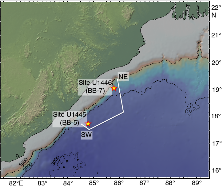
Figure F1. Mahanadi basin with locations of Sites U1445 and U1446 and the approximate track of the “regional” seismic line.
The summer monsoon is the primary control on present-day sediment discharge from the Mahanadi basin with 90% of the annual sediment delivery into the Bay of Bengal (15 × 106 metric tons) occurring between July and September (Chakrapani and Subramanian, 1990a). The exceptionally narrow (25–50 km) continental shelf promotes rapid transit of particulates to the continental slope and rise. Direct summer monsoon precipitation and runoff from rivers surrounding the Bay of Bengal yield a net positive water flux (precipitation + runoff − evaporation) of 152 × 1010 m3/y (Varkey et al. 1996). In particular, the Ganges/Brahmaputra and other Indian peninsular rivers provide 63.5 × 10¹⁰ m3/y of runoff directly to coastal regions of the northern and western Bay of Bengal. Much of this freshwater is entrained within the East Indian Coastal Current (EICC), maintaining a low-salinity region extending ~100 km offshore eastern India (Antonov et al., 2010; Chatterjee et al., 2012; Chaitanya et al., 2014).
Site U1445 is located 2502 meters below sea level (mbsl) in a flat-lying region of the upper continental rise, ~94 km from the Indian coastline. The seismic profile (proprietary, not shown) to the 680 m target depth is characterized by parallel, flat-lying reflectors minimally interrupted by small-scale dewatering faults that extend upward from depth, terminating ~80 m below the seafloor, presumably in the less consolidated sediments. This location on the upper rise is not protected from turbidite deposition, but the target depth offers the possibility to reach Miocene sediments as indicated in the regional seismic profile (Figure F2) (Dangwal et al., 2008).
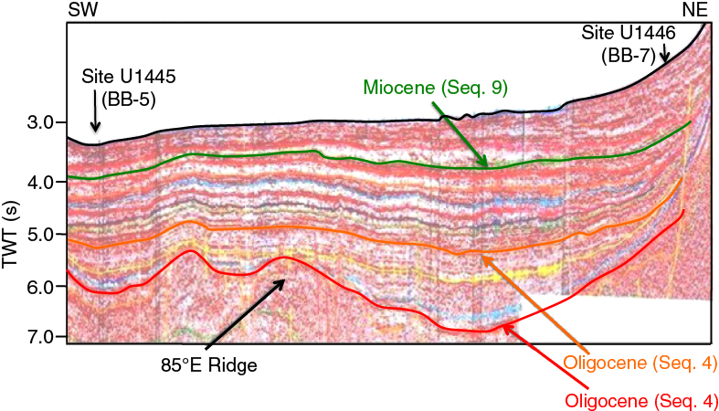
Figure F2. Interpreted “regional” seismic section passing through the 85°E Ridge in the Mahanadi deepwater basin to the shelf edge in the north.
The objective at Site U1445 is to recover Miocene to Holocene sediments at three or more holes in order to construct a composite section and splice from which to make continuous time-series reconstructions of changing monsoon precipitation and runoff at suborbital to orbital timescales. Sites U1445 and U1446 will constitute the northern end of a meridional salinity transect that includes sites in the Andaman Sea and is anchored by IODP Site U1443 at 5°N.
Operations
Site U1445 consisted of three holes (Table T1) ranging in depth from 33.0 to 672.6 m drilling depth below seafloor (DSF). Overall, 117 cores were recorded for the site. A total of 487.34 m of core over a 476.3 m cored interval was recovered using the advanced piston corer (APC) system (102% recovery). The cored interval with the extended core barrel (XCB) system was 534.5 m with a core recovery of 518.02 m (97%). The overall recovery at Site U1445 was 99%. The total time spent on Site U1445 was 9.3 days.
Table T1. Site U1445 core summary. Download table in .csv format. View PDF table.
Port Visakhapatnam
The R/V JOIDES Resolution transited 235 nmi from Site U1444 to Visakhapatnam, India, for an inspection by the Indian Navy, to board three Indian Scientists, and to gain permission to core the remaining primary sites for Expedition 353. The vessel was tied up at the Fertilizer Pier in Port Visakhapatnam with the first line ashore at 0720 h (UTC + 8 h) on 29 December 2014. The naval inspection took place on 30 December and was completed by 1630 h. Three scientists from Indian institutions boarded the vessel at 2130 h on 30 December. A diplomatic note from the Indian Ministry of External Affairs granting clearance to operate within the Indian exclusive economic zone was received at 2145 h.
Transit to Site U1445
The vessel departed Visakhapatnam for Site U1445 (proposed primary Site BB-5) on 31 December 2014 with the last line ashore at 0306 h. After an 87 nmi transit, the ship arrived at Site U1445. The thrusters were lowered and dynamic positioning assumed control of the vessel at 1942 h.
Site U1445
Winds of 35 kt and heave up to 4.5 m forced operations to wait on weather until 0245 h on 1 January 2015. At that time, an APC/XCB bottom-hole assembly (BHA) was made and deployed to the seafloor by 1015 h. High heave conditions caused spudding of Hole U1445A to be delayed.
Hole U1445A
Hole U1445A was spudded at 1900 h on 1 January. The seafloor was estimated at 2502 mbsl. Cores 353-U1445A-1H through 24H (0–225.1 m DSF) were retrieved using the APC system. Temperature measurements were taken on Cores 4H, 7H, 10H, and 13H. Core orientation data were obtained from Cores 3H through 24H using the Icefield MI-5 tool. The XCB system was deployed for Cores 25X through 77X (225.1–672.6 m DSF). Coring advances of 8 m were utilized for Cores 33X, 34X, and 38X through 66X to allow for core expansion within the core liner.
After completion of coring operations in Hole U1445A, the hole was swept with 50 bbl of high-viscosity mud and then displaced with heavy weight (10.6 lb/gal) mud in preparation for downhole logging operations. The hole was then logged using the triple combo tool string, including the magnetic susceptibility sonde (MSS), and the Formation MicroScanner (FMS)-sonic tool string. Each tool string was run twice from 85 to 444 m DSF. Neither tool string was able to pass below a bridge at 444 m DSF. Downhole logging operations were completed at 0630 h on 7 January. The drill string was pulled from the hole with the bit clearing the seafloor at 0711 h, ending Hole U1445A.
A total of 24 APC cores were taken over a 225.1 m interval with a total core recovery of 234.31 m (104% core recovery). The XCB system was used for 53 cores over a cored interval of 447.5 m with 432.09 m recovered (97%). Total core recovery for Hole U1445A was 99%.
Hole U1445B
The vessel was offset 20 m south, and Hole U1445B was spudded at 1010 h on 7 January. Hole U1445B was dedicated for high-resolution pore water sampling. Cores 353-U1445B-1H through 4H were retrieved with 101% recovery. The bit cleared the seafloor at 1320 h, ending Hole U1445B.
Four APC cores were taken over a 33.0 m interval with a total core recovery of 33.36 m (101% core recovery).
Hole U1445C
The vessel was offset 20 m west, and Hole U1445C was spudded at 1415 h on 7 January. Cores 353-U1445C-1H through 24H were retrieved using the APC system. Temperature measurements were taken with the advanced piston corer temperature tool (APCT-3) on Cores 20H and 22H. Cores 3H through 24H were oriented using the Icefield MI-5 tool. The XCB system was deployed for Cores 25X through 36X (218.2–305.2 m DSF). Cores 26X through 36X used 8 m advances to allow for core expansion within the core liner.
A total of 24 APC cores were taken over a 218.2 m interval with a total core recovery of 219.67 m (101% core recovery). The XCB system was used for 12 cores over a cored interval of 87.0 m with 85.93 m recovered (99%). Total core recovery for Hole U1445C was 100%.
After coring operations were completed, the hole was displaced with heavy mud. The pipe trip out of the hole was delayed for 3 h while a hydraulic dump valve was replaced on the iron roughneck power unit. The bit cleared the rig floor at 0430 h on 10 January. The rig was secured for transit, and the sea voyage to Site U1446 (proposed Site BB-7) began at 0548 h on 10 January.
Lithostratigraphy
Sediments recovered from Holes U1445A–U1445C are principally composed of hemipelagic clays with a significant biogenic component, as well as occasional thin turbidites, of Late Pleistocene (Holocene?) to late Miocene age. Lithostratigraphic units are defined predominantly by changes in lithology (as identified by visual core description and smear slide observations), with supporting information from physical property and X-ray diffraction (XRD) data (Figures F3, F4, F5, F6, F7, F8). The observed lithologic differences between units are mainly the result of the varying abundance of biosilica, principally diatoms, which influences the physical property data primarily through the dilution of the lithogenic components, particularly in Subunit Ib (Figure F4). Lithologic descriptions are based primarily on sediments recovered from Hole U1445A, supplemented with observations from Hole U1445C.
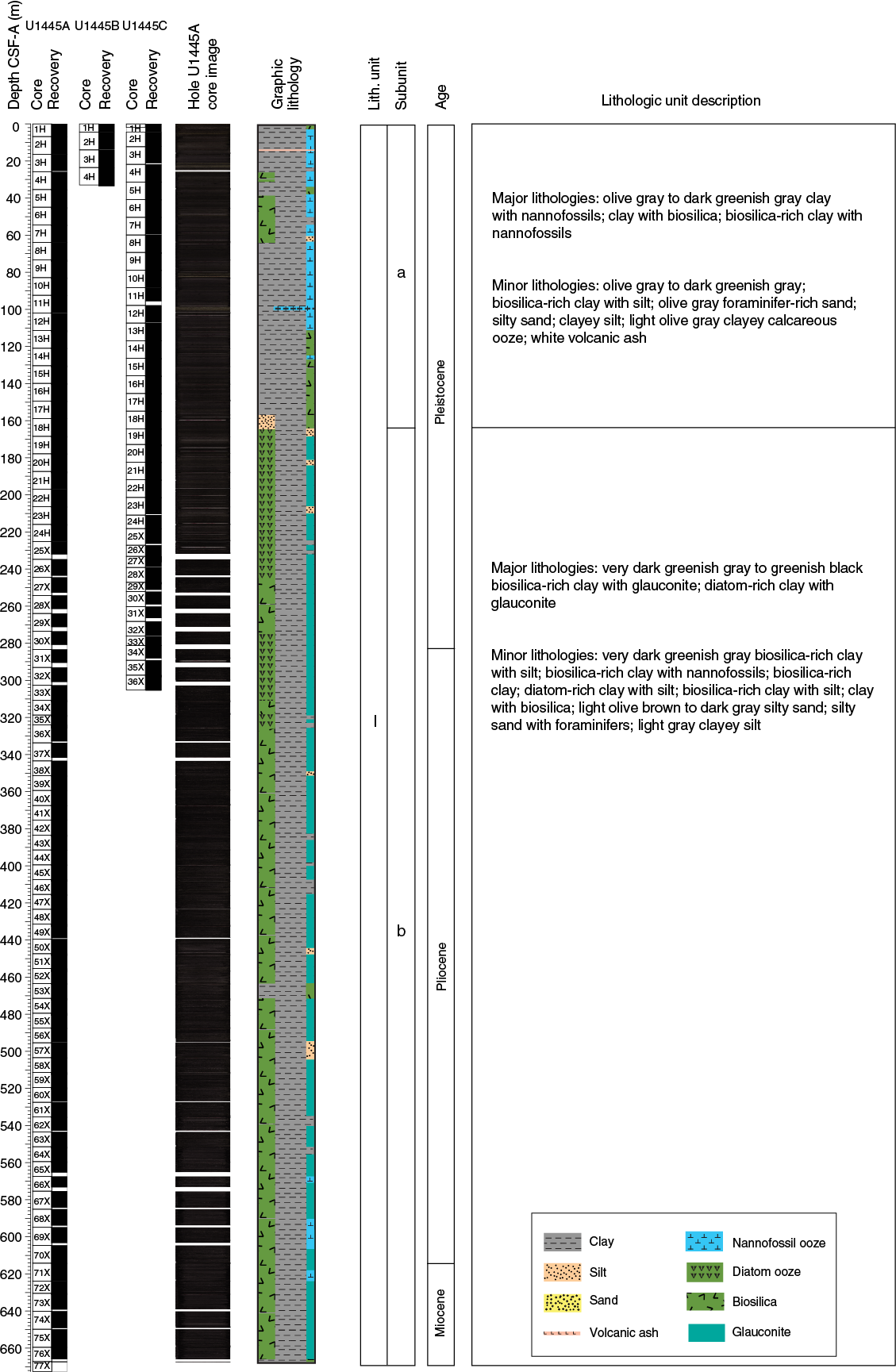
Figure F3. Lithostratigraphic summary, Site U1445.
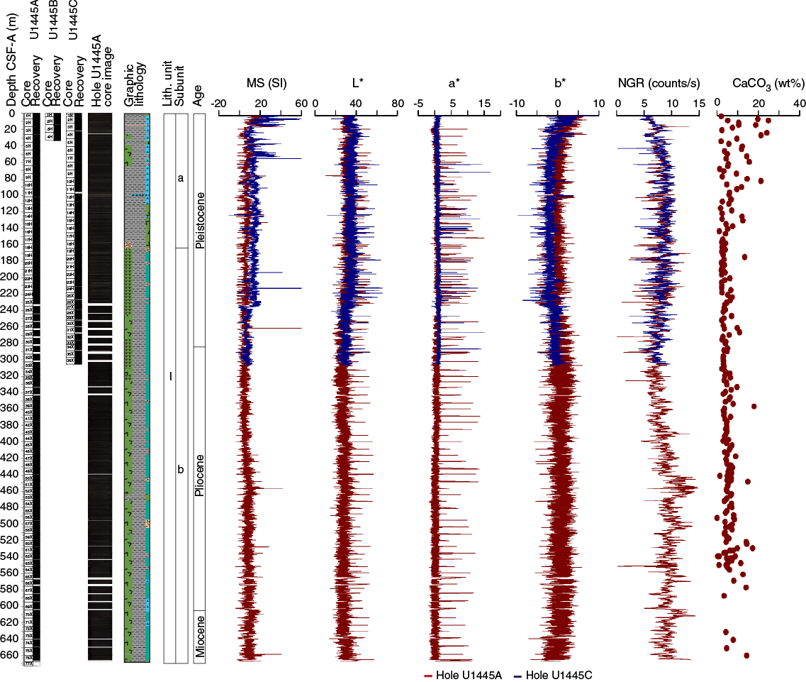
Figure F4. Lithostratigraphic summary with selected physical property and geochemical data from Holes U1445A–U1445C.
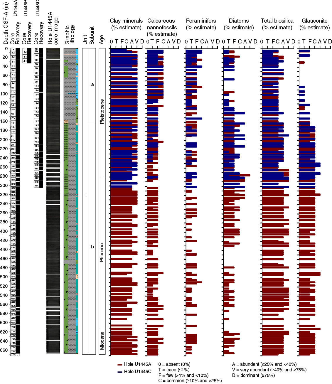
Figure F5. Smear slide data, Holes U1445A and U1445C.
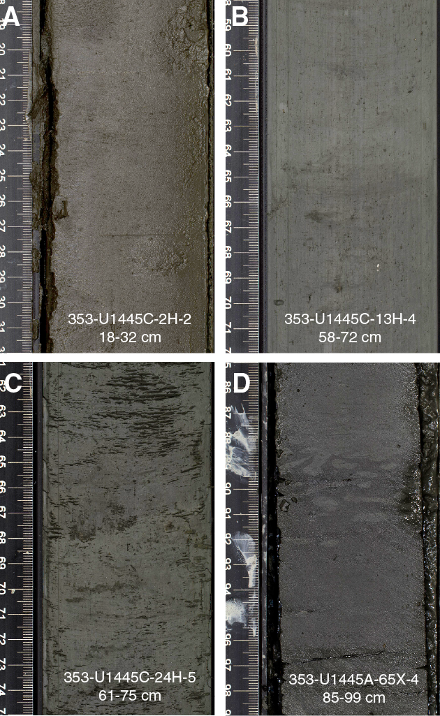
Figure F6. Main lithologies, Site U1445. A. Clay with nannofossils. B. Clay with biosilica. C. Diatom-rich clay. D. Biosilica-rich clay.
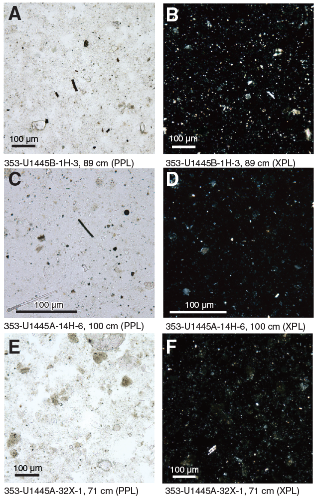
Figure F7. Main lithologic types, Site U1445. A, B. Clay with nannofossils. C, D. Clay with biosilica. E, F. Diatom-rich clay with glauconite.
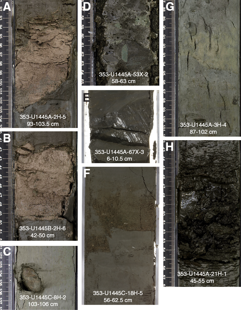
Figure F8. Site U1445 features. A, B. Volcanic ash. C. Authigenic pyrite nodule. D. Nannofossil ooze clasts. E. Lineation from possible fault fracture. F. Minor fault. G. Severe core disturbance. H. Severe mousselike core disturbance.
Because of the homogeneous nature of the sediments, only one stratigraphic unit is recognized, divided into two subunits (Ia and Ib) primarily based on nannofossil and biosilica content (Figure F3). Subunit Ia is a 165 m thick sequence of Late Pleistocene (Holocene?) to Middle Pleistocene olive-gray to dark greenish gray clay with biosilica, as well as clay with nannofossils, with occasional beds of biosilica-rich clay. Foraminifers are a persistent but variable component of the smear slides in Subunit Ia. Subunit Ib is a 502 m thick sequence, the top of which is defined by the first downcore occurrence of biosilica-rich clays in Hole U1445A. Subunit Ib is dominated by very dark greenish gray biosilica-rich clay with glauconite, with significant intervals of increased diatom content between 160 and 330 m core depth below seafloor, Method A (CSF-A). Foraminifers and nannofossils are much less common in Subunit Ib than in Subunit Ia but are present in small numbers throughout, particularly between ~570 and 670 m CSF-A where an increase in calcareous nannofossils is observed. Thin (~2–20 cm thick) turbidites are present in sediments from both Subunits Ia and Ib, varying in composition from silt-sized quartz-rich silt/sands to foraminifer-rich sands, with occasional bioclastic-rich sands. Occasional soupy or mousselike intervals, characteristic of gas hydrate dissociation, were identified in sediments recovered using the APC system in Holes U1445A–U1445C from both Subunits Ia and Ib. Overall, cores from Hole U1445C were considerably less disturbed by drilling disturbance and gas expansion than those recovered from Hole U1445A at equivalent depths, possibly due to reduced heave during Hole U1445C operations.
Subunit Ia
- Intervals: 353-U1445A-1H-1, 0 cm, through 18H-5, 141 cm; 353-U1445B-1H-1, 0 cm, through 4H-CC, 22 cm; 353-U1445C-1H-1, 0 cm, through 19H-1, 88 cm
- Depths: Hole U1445A = 0–165.28 m CSF-A; Hole U1445B = 0–33.56 m CSF-A; Hole U1445C = 0–164.82 m CSF-A
- Age: Late Pleistocene (Holocene?) to Middle Pleistocene
- Major lithology: clay with biosilica and clay with nannofossils
- Minor lithology: biosilica-rich clay, foraminifer-rich sand, foraminifer-rich silt, silt with sand, and volcanic ash
Subunit Ia comprises a ~165 m thick succession of olive-gray (5Y 5/2) to dark greenish gray (GLEY 1 4/10Y) clay with biosilica and clay with nannofossils (Figures F3, F4). There is a persistent foraminiferal component throughout Subunit Ia that peaks at around 3%–15% in the uppermost 100 m (Figure F5). Calcareous nannofossils make up ~5%–15% of the sediments in the top 100 m, gradually decreasing to ~5% by 165 m CSF-A at the base of the subunit. Biosilica, a common component of this sequence, is predominantly composed of whole and fragmented diatoms with occasional radiolarians, sponge spicules, and rare silicoflagellates. The biosilica content first decreases from ~15%–25% at the top of the subunit to 5%–15% at 100 m CSF-A before beginning to rise again, becoming consistently >35% of the sediment at the base of the subunit at 165 m CSF-A (Figure F5). Readily identifiable diatoms generally comprise <5% of the sedimentary components in Subunit Ia. Clay mineral content has an opposite downcore trend to that of biosilica, ranging from 30% to 65% throughout. Fine-grained quartz is systematically found as a minor component within the clay lithologies, generally ranging from 1% to 7% but peaking at 10%–15% between 140 and 165 m CSF-A near the base of the subunit. The biosilica-rich clays are generally homogeneous in terms of both texture and color, with few sedimentary or biogenic structures visible.
Thin turbidites, ~3–15 cm thick, are visible throughout Subunit Ia and fall into three main types: light gray well-sorted quartz-rich silt; olive-brown silty sand, including foraminifer-rich sand, with silt; and quartz-dominated medium to coarse sand with shelly bioclasts and foraminifers (Figures F9, F10, F11). More turbidites were observed in the upper 80 m of the sequence (~10–15 per core) than between 80 and 165 m CSF-A (~5 per core). The proportion of fine quartz turbidites increased between 0 and 100 m CSF-A, whereas the number of foraminifer-rich turbidites decreased, with the trend reversing between 100 and 165 m CSF-A (Figure F11). Authigenic pyrite, as framboids and octahedral individual crystals or as aggregates, is commonly observed in both types of turbidites but is less common in the foraminifer-rich turbidites (Figure F12).
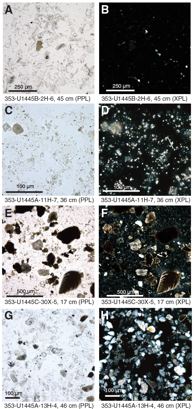
Figure F9. Minor sedimentary components, Site U1445. A, B. Volcanic ash. C, D. Clayey authigenic carbonate–rich ooze. E, F. Foraminifer-rich sand with quartz. G, H. Quartz-rich well-sorted silt with feldspar.
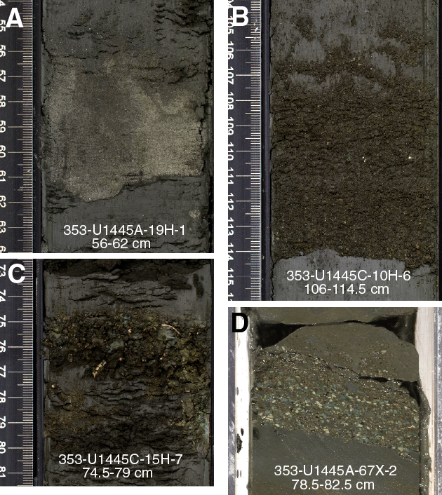
Figure F10. Representative turbidite compositions, Site U1445. A. Quartz-rich turbidite. B. Coarse-grained turbidite with foraminifers. C. Turbidite with shell fragments. D. Turbidite with gray and green clasts.
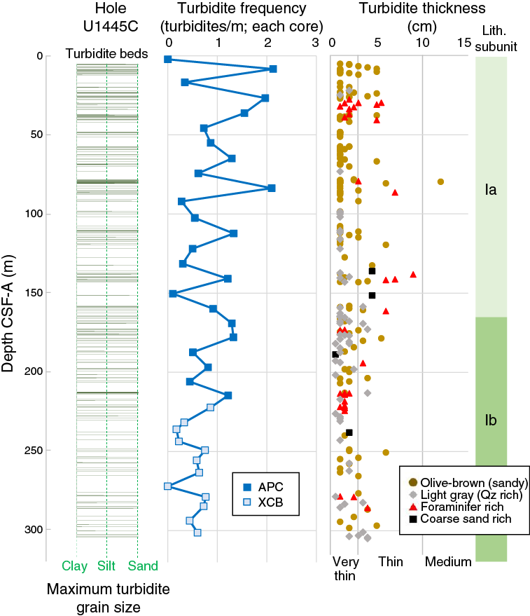
Figure F11. Turbidite abundance and thicknesses, Hole U1445C.
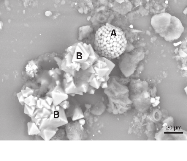
Figure F12. SEM image of a turbidite sample showing (A) a pyrite framboid and (B) octahedral crystal aggregates of authigenic pyrite.
One vitric ash, ~10 cm thick and likely to be the latest Toba eruption of ~75 ka, was identified in both Holes U1445A and U1445B at 13.83–13.93 m CSF-A but was not recovered in Hole U1445C (Figures F3, F8). One interval of clayey calcareous ooze, rich in fine-grained authigenic carbonate, was correlated between Holes U1445A and U1445C at ~100 m CSF-A (Figure F3).
Drilling disturbance is generally slight to moderate in the sections recovered using the APC system (Cores 353-U1445A-1H through 24H, 353-U1445C-1H through 4H, and 353-U1445C-1H through 24H), characterized by voids, gas expansion cracks, and occasional mousselike and soupy intervals related to gas hydrate dissociation (Figure F8). Disturbance is noticeably less prominent in Holes U1445B and U1445C than in Hole U1445A, with fewer voids and cracks observed.
Subunit Ib
- Intervals: 353-U1445A-18H-5, 141 cm, through 77X-CC, 36 cm; 353-U1445C-19H-1, 88 cm, through 36X-CC, 44 cm
- Depths: Hole U1445A = 165.28–667.56 m CSF-A; Hole U1445C = 164.82–305.48 m CSF-A
- Age: Middle Pleistocene to late Miocene
- Major lithology: biosilica-rich clay with glauconite and diatom-rich clay with glauconite
- Minor lithology: biosilica-rich clay with silt, biosilica-rich clay with nannofossils, biosilica-rich clay, diatom-rich clay with silt, biosilica-rich clay with silt, clay with biosilica, silty sand, silty sand with foraminifers, and clayey silt
Subunit Ib is a ~502 m thick succession of very dark gray (GLEY 1 3/N) to very dark greenish gray (GLEY 1 3/10GY) to greenish black (GLEY 1 2.5/10Y) biosilica-rich clay with glauconite. Calcareous nannofossil content is low throughout, averaging 1%–5%, but increasing to 15% between 590 and 640 m CSF-A (Figure F5). Foraminifers are present throughout but in low numbers, averaging 1%–3% of the sediment. Biosilica is a constant, and in some cases, dominant component of Subunit Ib, increasing from 20%–30% of the sediment at 165 m CSF-A to 40%–55% at 275–320 m CSF-A and remaining >20% for the remainder of the subunit downhole. Several intervals show a large increase in diatom abundance, particularly between 165–175 and 275–424 m CSF-A, where well-preserved and diverse assemblages of diatoms often comprise >25% of the sediment. Clay mineral content varies between 20% and 65%, reaching a low between 260 and 295 m CSF-A due to dilution by the increased biosilica content. Fine-grained quartz is a persistent minor component of the clays, generally ranging from 2% to 7% and peaking at >10% between 165–208 and 540–560 m CSF-A.
Although generally homogeneous, the biosilica-rich clays in Subunit Ib show more mottling and bioturbation than those in Subunit Ia, ranging from centimeter-sized Planolites to smaller Chondrites and Zoophycos trace fossils. The bioturbation is made more visible by the increased proportion of browner clay as a minor lithology, which appears as infilled burrows or irregularly shaped thin beds. XRD and smear slide data reveal that the browner sediment is more carbonate rich (up to 10% nannofossils) (Figure F9). The primary observed variability within bulk XRD samples is in the relative intensity of the calcite peak, corresponding to changes in abundance of calcareous fossil components (Figure F13). Illite is the most prominent peak in XRD analyses of oriented clay aggregates, with smectite, chlorite, and kaolinite peaks present as more minor components (Figure F14). Occasional rip-up clasts of pale greenish gray nannofossil ooze are found in Subunit Ib, dated as Miocene and Oligocene age (see Biostratigraphy).

Figure F13. XRD diffractograms showing the difference in calcite content between the main dark gray lithology and the more nannofossil-rich browner minor lithology.
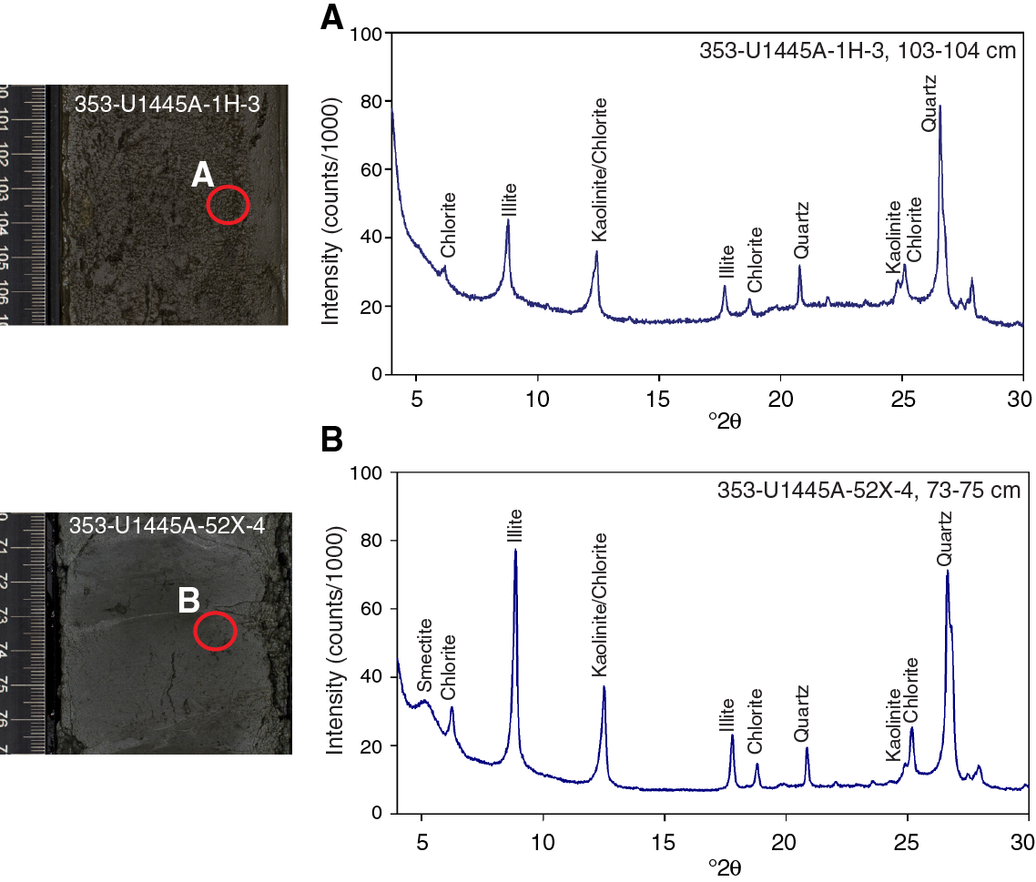
Figure F14. XRD diffractograms showing clay mineralogy from selected samples, Hole U1445A.
Thin turbidites are present in Subunit Ib, with the same mixture of compositions from quartz silt to foraminifer-rich sand as was seen in Subunit Ia (Figures F9, F10, F11). The apparent decrease in the number of turbidites per core between 220 and 270 m CSF-A may be an artifact of the poorer recovery obtained during XCB drilling in Hole U1445A, as this decrease is less pronounced at equivalent depths in Hole U1445C where recovery is improved. Turbidite thickness increases between 550 and 650 m CSF-A. Notably, some of the coarser sandy turbidites in Subunit Ib contain large bioclastics, including fragments of corals and bivalves, indicative of transport and reworking of sediments from very shallow water.
Many cores in Subunit Ib were recovered using the XCB system, so the drilling disturbance is more severe than for Subunit Ia. Moderate to severe biscuiting is present throughout with occasional soupy or mousselike intervals indicative of the presence of gas hydrates.
Biostratigraphy
Calcareous and siliceous microfossils are present in Hole U1445A with variable downcore abundance trends. Calcareous nannofossils are present throughout the recovered sections, and their preservation is good to moderate. Abundances vary between rare (<1% of sediment particles) and abundant (>50% of sediment particles), although in most samples nannofossils represent around 10% of sediment particles. Abundances of carbonate microfossils are generally higher in lithostratigraphic Subunit Ia (0–165.28 m CSF-A).
Foraminifers are dominant to abundant in the upper 188 m in Hole U1445A. Abundance decreases rapidly deeper than 188 m CSF-A and falls to few or rare deeper than 290 m CSF-A. Samples 353-U1445A-48X-CC (432.70 m CSF-A) and 77X-CC (667.43 m CSF-A) are barren of foraminifers. Preservation is good to moderate with three exceptions: Samples 29X-CC (271.20 m CSF-A) and 30X-CC (280.83 m CSF-A) of the late Pliocene and Sample 75X-CC (659.66 m CSF-A) of the late Miocene show poor preservation.
Strong variations in abundance and shifts in the diatom assemblage species composition will help to reconstruct paleoceanographic changes in the Mahanadi basin. Diatom valve preservation ranges from good to poor and tends to be better when abundance is higher.
The age model for Site U1445 was established by combining calcareous nannofossil, planktonic foraminifer, and diatom datums with paleomagnetic reversal datums. The oldest calcareous nannofossil sample studied (Sample 353-U1445A-77X-CC) contains Discoaster quinqueramus and Discoaster berggrenii, suggesting an age between 5.59 and 7.53 Ma. The oldest planktonic foraminifer datum encountered is the first occurrence (FO) of Globorotalia margaritae (5.57 Ma) in Sample 71X-CC. Globigerinoides conglobatus is found in the deepest nonbarren sample (76X-CC), suggesting that the basal age of Hole U1445A is between 5.57 and 6.20 Ma. The oldest diatom datum is the last occurrence (LO) of Nitzschia miocenica (5.7 Ma), which is found between Samples 71X-1W, 76–77 cm, and 71X-3W, 75 cm (614.96 and 617.96 m CSF-A).
Calcareous nannofossils
Calcareous nannofossils were examined in all core catcher samples from Hole U1445A. Additional split core samples from Hole U1445A were examined to refine the depth of biostratigraphic datums once they were defined between two core catcher samples. Semiquantitative species abundance estimates for all core catcher samples are shown in Table T2. Pleistocene to late Miocene nannofossil assemblages are typical of tropical/subtropical paleoenvironments and include common Florisphaera profunda, Gephyrocapsa spp., Reticulofenestra spp., Sphenolithus spp., Discoaster spp., Helicosphaera spp., Calcidiscus spp., and Umbilicosphaera spp. This permitted the construction of a relatively high resolution stratigraphy using this fossil group (Table T3; Figure F15). Although etching and fragmentation of coccoliths is apparent in certain samples, no significant diagenetic overgrowth of susceptible nannofossils (e.g., Discoaster and Sphenolithus) is observed under the light microscope.
Table T2. Semiquantitative calcareous nannofossils abundance counts from core catcher samples, Site U1445. Download table in .csv format.
Table T3. Calcareous nannofossil datums, Site U1445. Download table in .csv format.
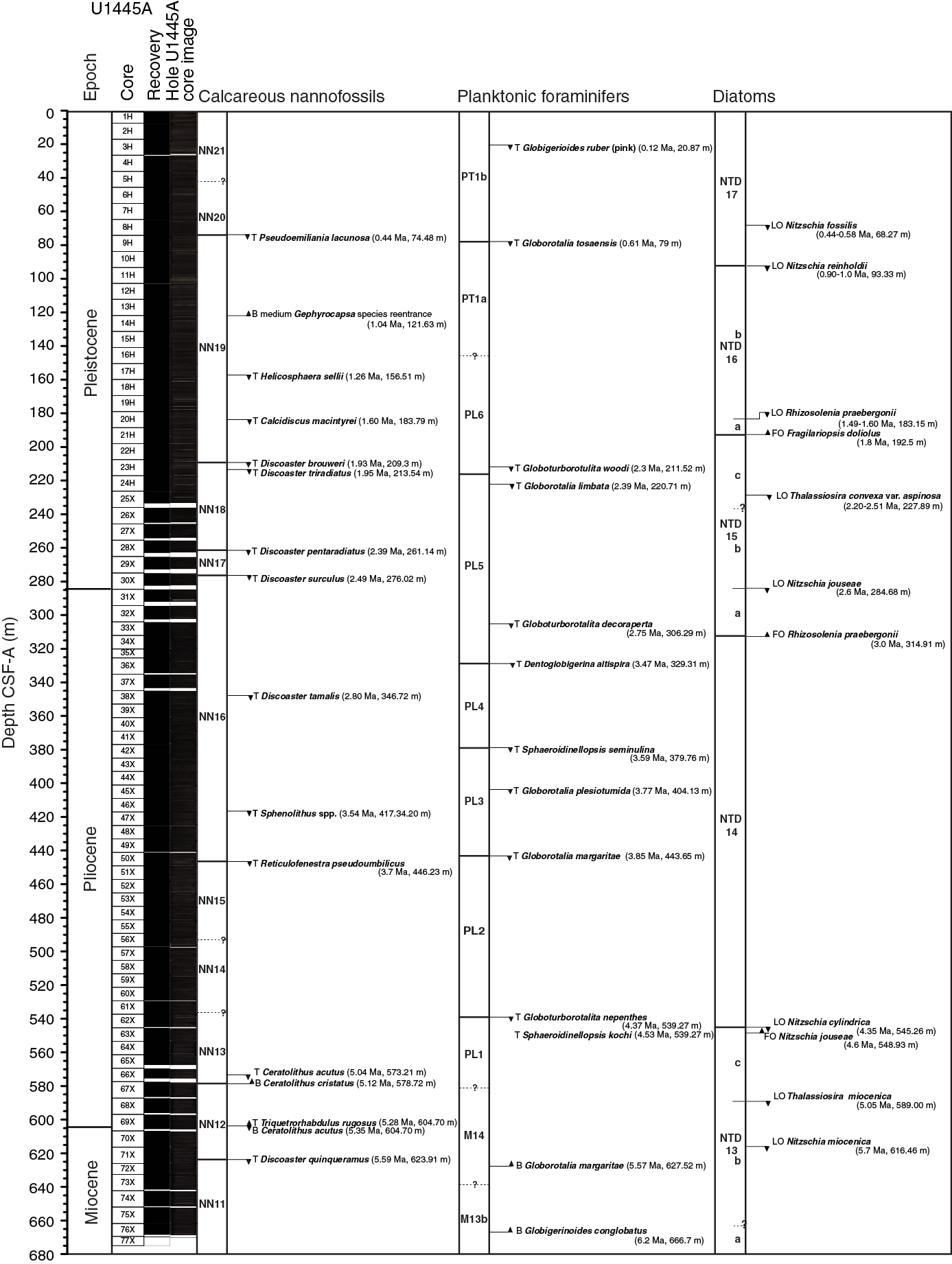
Figure F15. Summary of biostratigraphic events identified in Hole U1445A.
Pleistocene
Well-preserved calcareous nannofossils are present throughout the Pleistocene sedimentary section of Hole U1445A (~0–290 m CSF-A). Nannofossils are mostly common and sometimes abundant or rare. All Pleistocene marker species defined by Martini (1971) and Okada and Bukry (1980) were found (Table T3), with the exception of Reticulofenestra asanoi (see Biostratigraphy in the Expedition 353 methods chapter [Clemens et al., 2016] for zonal schemes used; all ages cited in the text and figures are those of Gradstein et al., 2012). Emiliania huxleyi, which delineates the base of Zone NN21 (0.29 Ma), is present in Sample 353-U1445A-7H-CC and all shallower core catcher samples based on light microscope identification. However, subsequent shipboard scanning electron microscope (SEM) work could only confirm the presence of E. huxleyi in Sample 2H-6W, 15 cm, and shallower; therefore, we do not use this event in the construction of the age model. SEM work on Samples 1H-CC through 7H-CC indicates that small placoliths belonging to the genus Reticulofenestra (probably Reticulofenestra parvula) are common in these Late Pleistocene samples. We speculate that at Site U1445 small Reticulofenestra species may dominate over E. huxleyi in some Late Pleistocene intervals, as documented in sediments offshore Western Australia (Okada and Wells, 1997).
The onset of the dominance of E. huxleyi among the Noelaerhabdaceae, which perhaps is synchronous with the crossover of dominance between E. huxleyi and Gephyrocapsa caribbeanica dated at 0.09 Ma in tropical waters, is recorded between Samples 353-U1445A-2H-6W, 15 cm, and 2H-4W, 15 cm. The LO of Pseudoemiliania lacunosa, dated at 0.44 Ma, occurs between Samples 8H-CC and 9H-2W, 90 cm (74.34 and 83.66 m CSF-A). Although large (>5.5 µm) Gephyrocapsa oceanica coccoliths are present in a few Late and late Middle Pleistocene samples between core catcher Samples 1H-CC and 17H-CC, no large (>5.5 µm) Gephyrocapsa specimens were found in deeper Middle Pleistocene samples, where their LO is expected to occur. Other well-defined Pleistocene events are the reentrance of medium-sized (4–5.5 µm) Gephyrocapsa species and the FOs of Helicosphaera sellii, Calcidiscus macintyrei, Discoaster brouweri, Discoaster triradiatus, Discoaster pentaradiatus, and Discoaster surculus (Table T3; Figure F15). We note that at Site U1445, D. triradiatus and D. surculus are usually rare where present; therefore, limited confidence can be placed in the exact depths of their LOs at 1.95 and 2.49 Ma, respectively.
Pliocene
The Pliocene/Pleistocene boundary (2.59 Ma) is bracketed by a number of Discoaster LOs that are dated between 2.39 and 2.8 Ma; we therefore place this boundary between Cores 353-U1445A-31X and 38X. The LO of Sphenolithus species (3.54 Ma) occurs between Samples 43X-CC and 44X-CC (391.67 and 399.87 m CSF-A). However, because only very few, possibly reworked, Sphenolithus specimens were found in samples shallower than Sample 47X-3W, 22 cm (418.61 m CSF-A), we place the LO datum between Samples 46X-CC and 47X-3W, 22 cm (Figure F15). Discoaster asymmetricus was almost entirely absent from the assemblage at Site U1445.
Miocene
The Miocene/Pliocene boundary (5.33 Ma) is well constrained between Samples 353-U1445A-69X-CC and 70X-2W, 145 cm (603.22 and 606.19 m CSF-A), based on the LO of Triquetrorhabdulus rugosus (5.28 Ma) and the FO of Ceratolithus acutus (5.35 Ma) in this interval. The LO of D. quinqueramus (5.59 Ma) occurs between Samples 71X-4W, 144 cm, and 71X-CC (620.15 and 623.91 m CSF‑A). Rare specimens of the nannofossil Orthorhabdus finifer, which has a narrow range spanning the Miocene/Pliocene boundary, are found in Sample 70X-CC. The oldest calcareous nannofossil sample studied (Sample 77X-CC; 447.46 m CSF-A), contains D. quinqueramus and D. berggrenii, suggesting an age between 5.59 and 7.53 Ma.
Rip-up clasts
Rip-up clasts, brown and green in color and ranging in size from a few millimeters to a few centimeters, are found in several horizons within two intervals in Hole U1445A (42–70 and 324–664 m CSF‑A) and corresponding depths in Hole U1445C (Figure F16). Sedimentological analyses suggest high abundances of nannofossils in some rip-up clasts, whereas in others they are comparable to those characterizing the surrounding sediment. We collected toothpick samples from several clasts (from Holes U1445A and U1445C) rich in nannofossils and examined the assemblages to determine their age. We also sampled and examined the matrix immediately surrounding the rip-up clasts. Within the constraints of the time resolution attainable by nannofossil biostratigraphy, the matrix surrounding the clasts was of the same age as the sediment above and below the horizons containing the clasts.
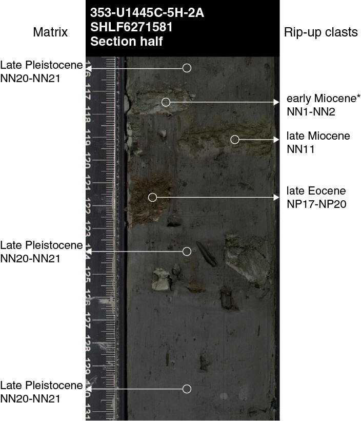
Figure F16. Horizon containing rip-up clasts of nannofossil-rich sediment of different ages, Hole U1445C.
The rip-up clasts were rich in well-preserved nannofossils, and nannofossil abundance was much higher than in sediments sampled throughout the cores in Site U1445. This suggests that the rip-up clasts originate from an environment characterized by a much lower rate of siliciclastic input than the late Miocene to recent sediments recovered from Site U1445.
A brown rip-up clast (Sample 353-U1445-67X-3W, 80 cm) contained an assemblage that was very similar to that in the core catcher of the same core, including the rare marker species C. acutus that has a short stratigraphic range between 5.04 and 5.35 Ma. The ages of other rip-up clasts examined range between late Eocene and late Miocene. We were able to assign ages to clasts with variable precision, depending on the presence or absence of marker species. Ages of rip-up clast samples and their stratigraphic positions are summarized in Table T4.
Table T4. Stratigraphic position and approximate ages of rip-up clasts based on nannofossil assemblages, Site U1445. Download table in .csv format.
Planktonic foraminifers
Planktonic foraminifer biostratigraphy of the Pleistocene to late Miocene section of Site U1445 is based on the shipboard study of core catcher samples from Hole U1445A. Planktonic foraminifer distribution in Hole U1445A is shown in Table T5. The absolute ages assigned to biostratigraphic datums listed in Table T6 follow the references given in Table T2 in the Expedition 353 methods chapter (Clemens et al., 2016).
Table T5. Semiquantitative planktonic foraminifer abundance counts from core catcher samples, Hole U1445A. Download table in .csv format.
Table T6. Planktonic foraminifer datums, Hole U1445A. Download table in .csv format.
Planktonic foraminifer percentages are high (mean = 86.4%) in the upper 158.97 m CSF-A but lower (mean = 59.9%) through the remaining Hole U1445A core catcher samples. The total number of foraminifers per 10 cm3 raw sediment is highly variable, ranging from 0 to more than 24,000, with a marked decrease deeper than 180 m CSF-A. The number of benthic foraminifers per 10 cm3 raw sediment follows the same pattern, averaging 1667 in the uppermost 180 m and 129 in deeper samples. The planktonic/benthic ratio, reported as percentage planktonic foraminifers of the total foraminifer assemblage, and the number of benthic foraminifers and total foraminifers found in a 10 cm3 sample are based on examination of the >150 µm size fraction of core catcher samples.
Reworking is apparent in many late Miocene through Pleistocene samples. Commonly, reworking is evidenced by a range of preservation or by a collection of species from different time periods within a single sample. In some Pleistocene samples, however, reworking is indicated only by the artificially extended ranges of some index species. It is possible that some reworked specimens of similar age and preservation to the nonreworked specimens were not identified. The presence of small turbidites and rip-up clasts throughout Hole U1445A, in combination with the large sample size (100 cm3) utilized for foraminiferal study, may explain the commonness of reworked species at this site.
Pleistocene
Pleistocene planktonic foraminifer assemblages were recovered from Samples 353-U1445A-1H-CC through 28X-CC (6.90–261.49 m CSF-A). Foraminiferal assemblages are dominant and generally well preserved. Planktonic assemblages are dominated by the tropical to warm subtropical species Pulleniatina obliquiloculata, Globigerinoides ruber, Globigerinoides sacculifer, Globigerinoides trilobus, Globigerinita glutinata, and Neogloboquadrina dutertrei as well as the temperate species Globigerina bulloides. G. glutinata and N. dutertrei, species commonly associated with upwelling zones, are common to abundant throughout Samples 1H-CC through 20H-CC (6.93–188.17 m CSF-A), indicating some degree of vertical mixing of intermediate and deep waters during this period.
The LO of G. ruber (pink) in Sample 353-U1445A-3H-CC (25.29 m CSF-A) confirms that these sediments are older than 0.12 Ma, in Zone PT1b. The top of Zone PT1a is placed at the LO of Globorotalia tosaensis in Sample 9H-CC (83.66 m CSF-A). The LO of Globorotalia limbata is found in Sample 24H-CC (225.05 m CSF-A), marking the top of Zone PL5.
Species of markedly different last appearance ages, Globigerinoides obliquus (1.30 Ma), Globigerinoides fistulosus (1.88 Ma), Globigerinoides extremus (1.98 Ma), Globoturborotalita woodi (2.3 Ma), Globoturborotalita decoraperta (2.75 Ma), and Miocene species Paragloborotalia mayeri (10.62 Ma) and Paragloborotalia kugleri (21.12 Ma) are found in Samples 353-U1445A-9H-CC through 18H-CC (83.66–168.98 m CSF-A), which identifies this interval as a zone of reworking. This interpretation is supported by the presence of reworked calcareous nannofossils (Table T2) and mottled sedimentary structures (see Core descriptions) in the upper 197 m. The last appearances of G. obliquus, G. fistulosus, and G. extremus occur either within or just below the reworking zone, making the placement of these LO datums uncertain. These uncertainties are shown as vertical error bars on Figure F17.
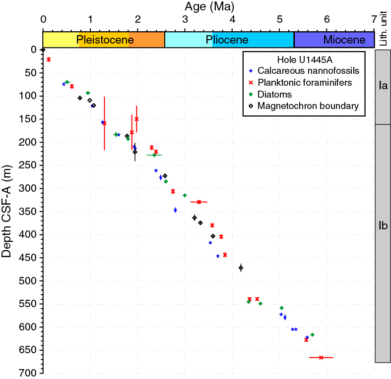
Figure F17. Biostratigraphic- and paleomagnetic reversal-based age-depth plot, Hole U1445A.
Pliocene
Pliocene planktonic foraminifer assemblages are recovered from Samples 353-U1445A-29X-CC through 68X-CC (271.21–593.81 m CSF-A). With few exceptions, preservation of planktonic foraminifers is moderate to good. Abundance is highly variable, ranging from dominant to barren. G. trilobus, G. bulloides, Dentoglobigerina altispira, G. extremus, G. sacculifer, and G. ruber occur commonly to abundantly in Pliocene samples.
The LO of D. altispira in Sample 353-U1445A-36X-CC (332.78 m CSF-A) defines the upper boundary of Zone PL4. This event is diachronous, occurring at different times in the Atlantic (3.13 Ma) and Pacific (3.47 Ma) Oceans. A younger age for this event is a better fit to our age model. A horizontal error bar denotes this age range on Figure F17. The LO of Sphaeroidinellopsis seminulina in Sample 62X-CC (542.76 m CSF-A) marks top of Zone PL3, and the LO of Globorotalia plesiotumida occurs within this zone in Sample 45X-CC (408.40 m CSF-A). The upper boundary of Zone PL2 is marked by the LO of G. margaritae in Sample 50X-CC (448.44 m CSF-A). The LO of Sphaeroidinellopsis kochi appears together with the LO of Globoturborotalita nepenthes in Sample 62X-CC (542.76 m CSF-A) to mark the top of Zone PL1.
Miocene
Miocene sediments span Samples 353-U1445A-69X-CC through 77X-CC (603.22–667.44 m CSF-A). Preservation is generally good, though planktonic foraminifers are rare. The planktonic foraminifer assemblage is dominated by Neogloboquadrina pachyderma (dextral), the artificial Neogloboquadrina “dupac” intergrade, and G. trilobus. The FO of G. margaritae in Sample 71X-CC (623.91 m CSF-A) marks the base of Zone PL1. The occurrence of G. conglobatus in Sample 76X-CC suggests a maximum age of 6.20 Ma.
Diatoms
In order to define the sediment age and paleoenvironmental conditions, core catchers and numerous samples from selected split core sections from Hole U1445A were investigated (Table T7). The absolute ages assigned to biostratigraphic datums listed in Table T8 follow the references given in Table T3 in the Expedition 353 methods chapter (Clemens et al., 2016). Figure F15 shows the age/depth graph for Site U1445 (also shown are calcareous nannofossils and foraminifer datums).
Table T7. Semiquantitative diatom abundance counts from core catcher and split core samples, Site U1445. Download table in .csv format.
Table T8. Diatom datums, Site U1445. Download table in .csv format.
Diatom abundance varies between abundant and few with only a few barren samples. Strong variations in abundance and shifts in the species composition of the diatom assemblage will help to reconstruct paleoceanographic changes in the eastern Bay of Bengal between the late Miocene and the Late Pleistocene. Valve preservation is mostly good to moderate. The highly diverse diatom community mainly consists of species typical of warm to temperate, low- to mid-latitude ocean waters. High-productivity species, including the coastal species Thalassionema nitzschioides var. nitzschioides, resting spores of Chaetoceros, Actinocyclus curvatulus, and Cyclotella striata, tend to dominate when total diatom abundance is higher than “few” (Table T7). Accompanying components of the diatom assemblage are warm and temperate species, including Alveus marinus, several species of Azpeitia, Rhizosolenia praebergonii, Shionodiscus oestrupii, Thalassionema bacillare, and Thalassiosira eccentrica. A certain degree of freshwater/land input (through winds or river runoff) above Site U1445 is revealed by the recurrent presence of numerous phytoliths and several taxa of freshwater diatoms (Aulacoseira spp., Epithemia spp., Navicula spp., Pinnularia spp., and Stephanodiscus spp.).
Diatom biostratigraphy
Diatoms are useful for age estimation throughout the entire sedimentary column of Hole U1445A. The Fragilariopsis doliolus Zone (from 0 to 0.90–1 Ma) is recognized between Samples 353-U1445A-1H-1W, 102 cm (1.02 m CSF-A), and 10H-CC (92.60 m CSF-A). Within this zone the LO of Nitzschia fossilis (0.44–0.58 Ma) is recognized between Samples 8H-3W, 123–124 cm, and 8H-5W, 75 cm (67.09–69.44 m CSF-A).
The LO of Nitzschia reinholdii (0.90–1.0 Ma) between Samples 353-U1445A-10H-CC and 11H-2W, 29 cm (92.60 and 94.09 m CSF‑A), defines the boundary between the F. doliolus and N. reinholdii Zones. Within this latter zone the LO of R. praebergonii (1.49–1.60 Ma) is observed between Samples 19H-CC and 20H-CC (178.14 and 188.17 m CSF-A); this event divides the N. reinholdii Zone into Subzones a and b.
The FO of F. doliolus occurs at the bottom of the N. reinholdii zone (between Samples 353-U1445A-21H-1W, 75 cm, and 21H-CC [188.94 and 196.83 m CSF-A], respectively), defining the boundary between this and the R. praebergonii Zone. Within the R. praebergonii Zone we found two biostratigraphic events: the LO of Thalassiosira convexa var. aspinosa (2.20–2.51 Ma) between Samples 25X-2W, 54–55 cm, and 25X-4W, 52–53 cm (226.41 and 229.36 m CSF‑A), and the LO of Nitzschia jouseae (2.6 Ma) between Samples 30X-CC and 31X-6W, 33 cm (280.83 and 288.56 m CSF-A). The latter event coincides with the Pliocene/Pleistocene boundary (Figure F15).
The FO of R. praebergonii (3.0 Ma) occurs between Samples 353-U1445A-34X-3W, 50–51 cm, and 34X-4W, 74–75 cm (314.07 and 315.75 m CSF-A). This event marks the boundary between the R. praebergonii and the N. jouseae Zones (Figure F15). Two diatom events were identified within the N. jouseae Zone (middle to early Pliocene): the LO of Nitzschia cyclindrica (4.35 Ma) between Samples 62X-CC and 63X-4W, 71 cm (542.76 and 547.79 m CSF-A), and the FO of N. jouseae (4.6 Ma) between Samples 63X-4W, 71 cm, and 63X-6W, 47 cm (547.79 and 550.06 m CSF-A). This latter event marks the boundary between the N. jouseae and the Thalassiosira convexa Zones. Two diatom events were recognized within the T. convexa Zone: the LO of Thalassiosira miocenica (5.05 Ma) was identified between Samples 67X-CC and 68X-CC (584.24 and 593.81 m CSF-A) and marks the boundary between Subzone b and c of the T. convexa Zone.
The oldest diatom datum identified in Hole U1445A is the LO of N. miocenica; this is dated at 5.7 Ma and was identified between Samples 353-U1445A-71X-1W, 76–77 cm, and 71X-3W, 75 cm (614.96 and 617.96 m CSF-A), suggesting that the bottom of Hole U1445A is older than 5.7 Ma.
Sedimentation rates and age model
Age-depth relationships for Hole U1445A based on biostratigraphy for the three fossil groups studied (calcareous nannofossils, planktonic foraminifers, and diatoms) show good agreement (Figure F17). A number of paleomagnetic reversals were reliably determined at Site U1445 (see Magnetostratigraphy). The match between biostratigraphic datums and magnetochron boundary datums is very good. Sedimentation rates in Hole U1445A are remarkably constant over the last 6 My. The combined biostratigraphic/magnetostratigraphic age model indicates a mean sedimentation rate of 11.4 cm/ky, assuming a linear fit of all data. A number of possible interpretations of minor sedimentation rate changes are possible based on Figure F17; however, these changes cannot be reliably resolved until an orbital-resolution isotope stratigraphy has been generated.
Geochemistry
The geochemistry of Site U1445 strongly reflects the processes of sulfate reduction and methanogenesis associated with microbial degradation of organic matter. Headspace and void space gas samples have high methane concentrations and high methane/ethane ratios, suggesting that the methane is mostly of biogenic origin. Organic carbon content is as high as 3 wt% and higher carbonate content is associated with intervals of more abundant calcareous microfossils. The interstitial water chemistry of Site U1445 reflects reducing conditions with pore water sulfate depleted at around 18 m CSF-A. Other examples are alkalinity peaking at around 30 mM near 50 m CSF-A and dissolved Ba increasing downhole. The influence of seawater and oxygen contamination during XCB coring is noticeable in the profiles of some elements, most notably sulfate, phosphate, and Fe.
Sediment gas sampling and analysis
Headspace gas samples were taken at a frequency of one sample per core in Hole U1445A as part of the routine environmental protection and safety-monitoring program (Table T9). Headspace methane concentration increases from 2 parts per million (ppm) at 6.0 m CSF-A, to a peak of 12,463 ppm at 23.9 m CSF-A, and decreases to several hundreds of parts per million by 71.6 m CSF-A. Deeper than 71.6 m CSF-A, four methane concentration maxima exceed 1000 ppm around 190, 370, 590, and 660 m CSF-A (Figure F18). However, methane concentration tends to be lower in cores that spent more time on deck before sampling, suggesting that core processing time is a factor affecting headspace methane concentration. Ethane was detected at trace levels and shows a similar variation with methane deeper than 150 m CSF-A. Ethene was also detected at 186.6 m CSF-A (Table T9). The methane/ethane ratio exceeded 10,000 at 23.9 m CSF-A, decreased to about 1,000 around 250 m CSF-A, and was constant around 1,000 deeper than 250 m CSF-A (Figure F18). The higher methane/ethane ratio suggests that the methane is mostly of biogenic rather than thermogenic origin.
Table T9. Headspace gas concentrations and methane/ethane ratios, Hole U1445A. Download table in .csv format.
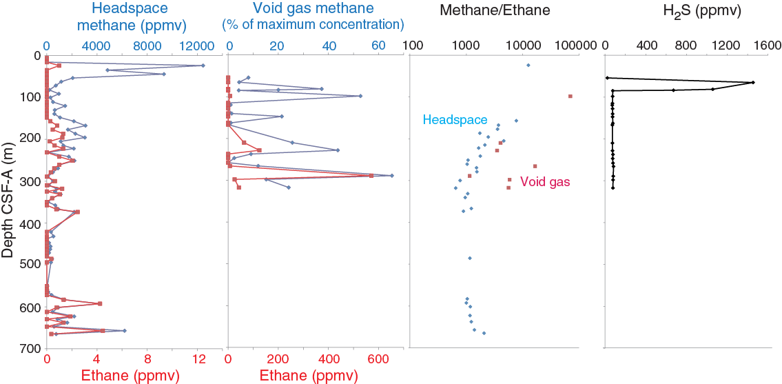
Figure F18. Methane and ethane concentrations, methane/ethane ratio, and hydrogen sulfide gas concentrations, Hole U1445A.
Syringe gas samples were taken from gas voids from 54.3 to 317.3 m CSF-A in Hole U1445A (Table T10). Methane concentration ranges from 0% to 65% and shows maxima around 100, 200, and 280 m CSF-A (Figure F18). Ethane concentration ranges from 0 to 571 ppm and is highest at 289 m CSF-A. The methane/ethane ratio shows a decreasing trend with depth.
Table T10. Void gas concentrations and methane/ethane ratios, Hole U1445A. Download table in .csv format.
In Hole U1445B, headspace gas samples were taken at a frequency of one sample per section as part of high-resolution geochemical studies (Table T11). Methane concentration is constantly low (<22 ppm) from 1.5 to 15.5 m CSF-A, abruptly increases from 17.1 m CSF-A, and shows three concentration maxima at 20.0 (1357 ppm), 28.1 (826 ppm), and 31.1 m CSF-A (4051 ppm) (Figure F19). The abrupt increase in methane coincides with the absence of sulfate ion (see Interstitial water sampling and chemistry).
Table T11. Headspace gas concentrations, Hole U1445B. Download table in .csv format.
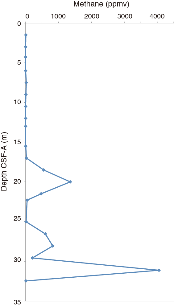
Figure F19. Headspace gas methane concentration, Hole U1445B.
Bulk sediment geochemistry
Calcium carbonate, inorganic carbon, total organic carbon (TOC), and total nitrogen (TN) contents were determined on sediment samples from Hole U1445A (Table T12; Figure F20). CaCO3 concentration ranges between 1 and 51 wt% and tends to be higher in lithostratigraphic Subunit Ia than in Subunit Ib (Figure F20). The variation in CaCO3 is consistent with coccolith and planktonic foraminifer abundances (see Lithostratigraphy). TOC ranges between 0.8 and 3.2 wt%. TOC tends to be higher in the upper part of lithostratigraphic Subunit Ib than in the other intervals (Figure F20). TN ranges between 0.15 and 0.55 wt%. TN shows a similar stratigraphic pattern to that of TOC. The TOC/TN ratio is lower than 6, suggesting that the organic matter is mostly of marine origin.
Table T12. Calcium carbonate, TOC, and TN contents and TOC/TN ratio, Hole U1445A. Download table in .csv format.

Figure F20. Calcium carbonate, TOC, and TN contents and TOC/TN ratio, Hole U1445A.
Interstitial water sampling and chemistry
Hole U1445A was analyzed for pore water chemistry at a relatively coarse resolution of one sample per core for the uppermost 46 cores and every other core thereafter. Hole U1445B was sampled for high-resolution geochemistry at a resolution of one sample per section (150 cm resolution) for four cores (i.e., the top 32 m). Site U1445 is broadly characterized geochemically by remineralization of organic matter supporting a reducing, methanogenic sediment column (Table T13). The upper 220 m in Hole U1445A was cored with the APC system, and whole rounds for pore water squeezing were kept under N2 during extraction of interstitial waters. After the switch to XCB coring, whole rounds were treated under ambient air.
Table T13. Interstitial water chemistry, Holes U1445A and U1445B. Download table in .csv format.
Concomitant with a sharp drawdown of sulfate are increases in alkalinity and nutrients (Figures F21, F22). Sulfate is <1 mM by 18.5 m CSF-A, absent downcore to 220 m CSF-A, and has an abrupt and sustained reappearance deeper than 220 m CSF-A, coincident with XCB drilling. These values, ~1–2 mM, would represent a mixing ratio of 3%–6% seawater with a pure sulfate-free end-member (likely pore water sulfate concentration). Barium concentration increases from zero to 150 µM at 220 m CSF-A. Deeper than 220 m CSF-A, in XCB cores, Ba values become more variable. Alkalinity continues to increase below the sulfate–methane transition to a peak >35 mM around 50 m CSF-A. Deeper than 50 m CSF-A, alkalinity decreases rapidly between 50 and 100 m CSF-A, after which it decreases gradually downcore to a minimum value of 5 mM in the bottom of Hole U1445A. Silicate and ammonium increase more gradually, reaching broad maxima around 200–300 m CSF-A, below which both gradually decrease. Maximum silicate values are 1.8 mM and ammonium reaches 7 mM. Bromine shows a similar profile, increasing from 1 mM near the surface to 1.4 mM between 180 and 380 m CSF-A. Phosphate also increases to a maximum value of 160 µM at 150 m CSF-A but, unlike the other nutrients, decreases sharply starting around 250 m CSF-A. The phosphate profile at depth mirrors that of Fe. Iron initially increases in the uppermost 100 m to values >30 µM but sharply decreases and then disappears deeper than 250 m CSF-A. This may be related to the switch from sample processing under N2 to air. Pore water Mn is initially quite high in the uppermost core (Figures F21, F22A), with the highest value (138 µM) in the shallowest sample (1.48 m CSF-A). Deeper than 1.48 m CSF-A, Mn rapidly decreases to <10 µM before increasing again to a secondary maximum at about 60 m CSF-A. From 100 m CSF-A to the bottom of the hole, Mn is generally <10 µM.
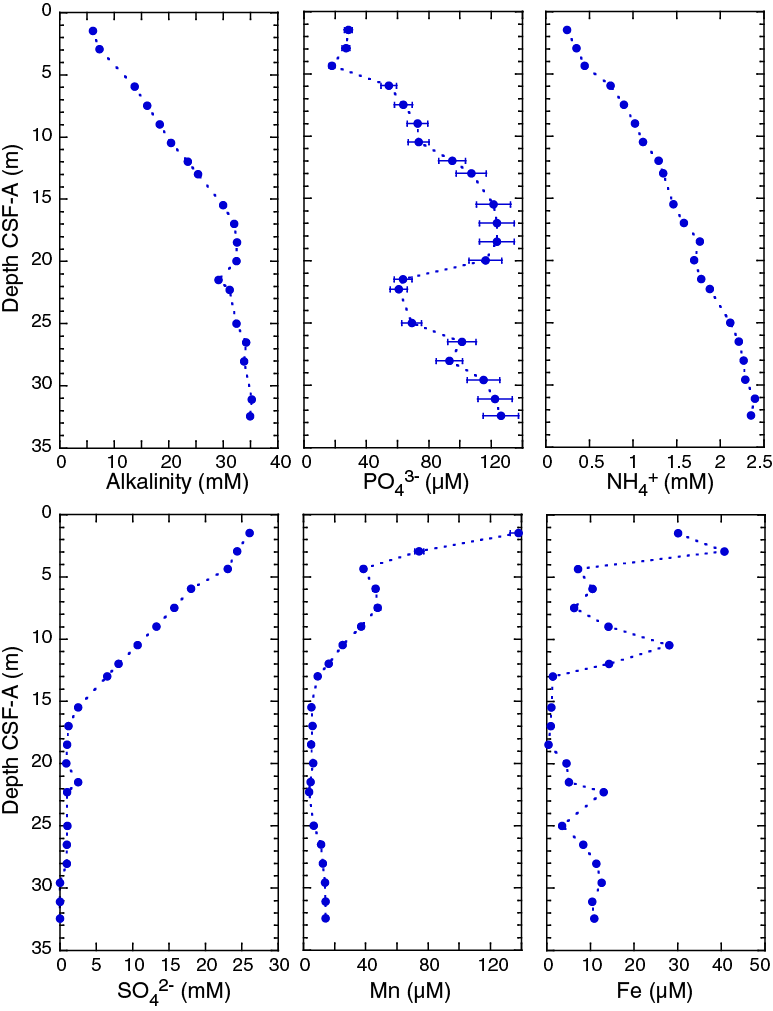
Figure F21. Interstitial water chemistry profiles, Hole U1445B.

Figure F22. Interstitial water chemistry profiles, Site U1445.
Anions and cations generally show a few sharp changes in the near surface (meter scale) with gradual and consistent trends downcore. Calcium sharply decreases in the uppermost three cores to a minimum of ~3 mM. Starting around 200 m CSF-A, Ca increases steadily to >14 mM in the bottom of Hole U1445A (680 m CSF-A). Potassium and Na show a small initial decrease, followed by decreasing values downcore. Potassium is >10 mM near the surface but reaches <3 mM at 680 m CSF-A. Magnesium shows a similar, consistent trend, decreasing from around 50 mM near the sediment/water interface to 12.8 mM at depth. This mirrors the trend in Cl, where considerable freshening is observed (Figure F23), albeit of a lesser magnitude than Mg or K. Therefore, part of the trend in Mg and K is likely due to dewatering of methane hydrates during core retrieval (see below), but the majority of the trend potentially reflects reactions with basement.

Figure F23. Chloride concentrations of hydrate-associated interstitial water compared to routinely sampled interstitial water, Site U1445.
Finally, similar to many of the cations, B gradually decreases downcore from 550 to <200 mM at 460 m CSF-A. However, deeper than 460 m CSF-A, B shows a notable increase to the bottom of Hole U1445A with values >300 µM. Lithium is low throughout Subunit Ia but increases from 20 to 200 mM throughout Subunit Ib, reflecting a strong input at depth.
Sampling interstitial water related to gas hydrate
A total of 31 interstitial water (IW) samples were collected for shipboard chloride measurements to test for a freshening signature related to gas hydrate dissociation within the cores (Table T14). Gas hydrate stability is pressure-temperature (P-T) dependent, and when removed from their P-T stability zone via the coring process, gas hydrates dissociate, drawing in heat from the surrounding environment while releasing freshwater and expanding gas into the system. Thus, cold thermal anomalies and low Cl values are indicative of gas hydrate occurrence. The IW samples were selected based on thermal infrared anomalies (see Physical properties) or mousselike/soupy textures identified in split-core halves by the sedimentologists. To preserve sediments for the splice efforts, most IW samples were collected using Rhizons inserted into the cold spots from whole-round sections or into the soupy sediments of the working half of split-core sections. Three samples were measured via whole-round squeezing. Most samples were found to exhibit low Cl values (105–400 mM). These low Cl anomalies show a gradual increase downhole and are most concentrated between Cores 353-U1445C-18H and 353-U1445C-30H (~160–260 m CSF-A) (Figure F23). Much of the hydrate-related sampling was limited to Hole U1445C, which extends only to 305.5 m CSF-A. Few cold spots were identified in Hole U1445A deeper than 305.5 m CSF-A, and drilling disturbances related to biscuiting made split-core identification of hydrate structures in Hole U1445A cores impossible.
Table T14. Gas hydrate associated interstitial water and shipboard measurements of chloride and alkalinity, Site U1445. Download table in .csv format.
Paleomagnetism
Paleomagnetic measurements were conducted on archive-half sections (Figures F24, F25) for all three holes at Site U1445, with alternating field (AF) demagnetization typically up to 10 mT. Discrete samples (N = 219) taken from working-half sections were also analyzed, with AF demagnetization typically up to 30 mT. Characteristic remanent magnetization (ChRM) of discrete samples was calculated using the principal component analysis (PCA) technique (Table T15). Additionally, the bulk magnetic properties of the discrete samples were assessed.
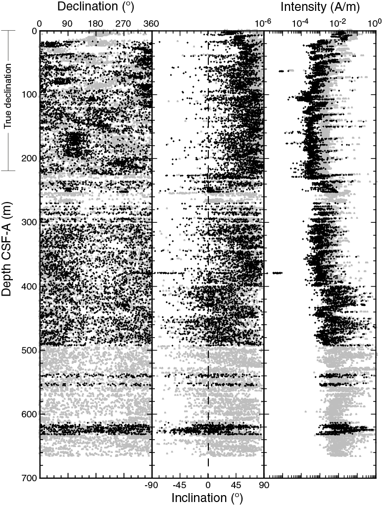
Figure F24. Downhole variations in declination, inclination, and intensity, Hole U1445A.
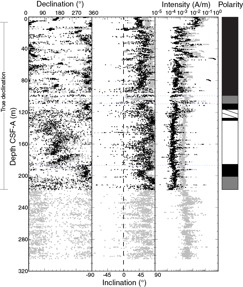
Figure F25. Downhole variations in declination, inclination, and intensity, Hole U1445C.
Table T15. Summary of discrete sample measurements, Hole U1445A. Download table in .csv format.
Remanence intensities drop significantly in the uppermost 10–20 m due to diagenetic reduction (see Bulk magnetic properties; Figure F26). Nonetheless, we successfully produced a magnetic polarity stratigraphy, except for the lower part of Hole U1445A (deeper than ~470 m CSF-A). Rock magnetic measurements on discrete samples provided promising variations in the bulk magnetic properties over the last 6 My. The significance of these trends is yet to be evaluated; however, a periodicity, possibly on the order of 400–600 ky, may indicate astronomical-scale cyclicity.
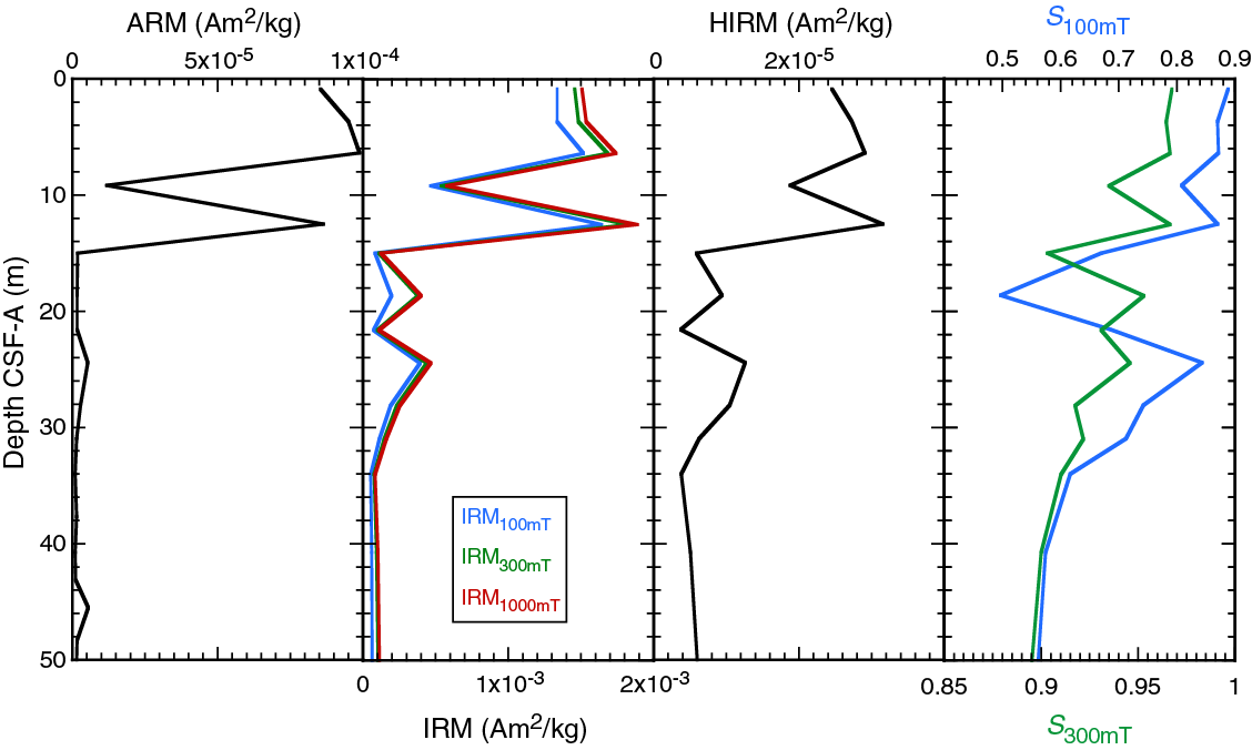
Figure F26. Variations in a selection of bulk magnetic parameters and ratios in the upper 50 m, Hole U1445A.
Magnetostratigraphy
For Hole U1445A (Figure F24), Cores 353-U1445A-3H through 24H were oriented using the Icefield MI-5 tool, so we have obtained “true” declinations between 16 and 225 m CSF-A. The declination data after demagnetization concentrate either around 0° (360°) or 180° downhole to 149.6 m CSF-A (Core 16H) indicating magnetozones. Unexpectedly, the data below this depth concentrate around 110° or 290°. As this tendency is persistent from Core 17H through 24H, we interpret this as a constant offset, although we could not identify the cause. Inclination data from discrete samples (see below) indicate that 110° and 290° declinations correspond to reversed and normal polarity respectively (i.e., the apparent offset is around −70°). Inclination data from the archive halves were uniformly positive at generally steep angles, and they do not show changes corresponding to the near-180° shifts in declination, indicating a strong drilling-related overprint. Most of the discrete samples revealed a reasonable ChRM (Figure F27). For the interval with orientation information, both ChRM declinations and inclinations match the polarity inferred by section measurements (Figure F28). As the section measurements were relatively noisy, the end depths of magnetozones were often defined on the basis of discrete sample ChRM. For XCB cores, magnetostratigraphy was solely based on ChRM inclination from discrete samples.
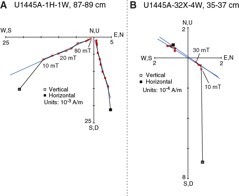
Figure F27. Representative stepwise AF demagnetization results displayed by orthogonal vector plots.
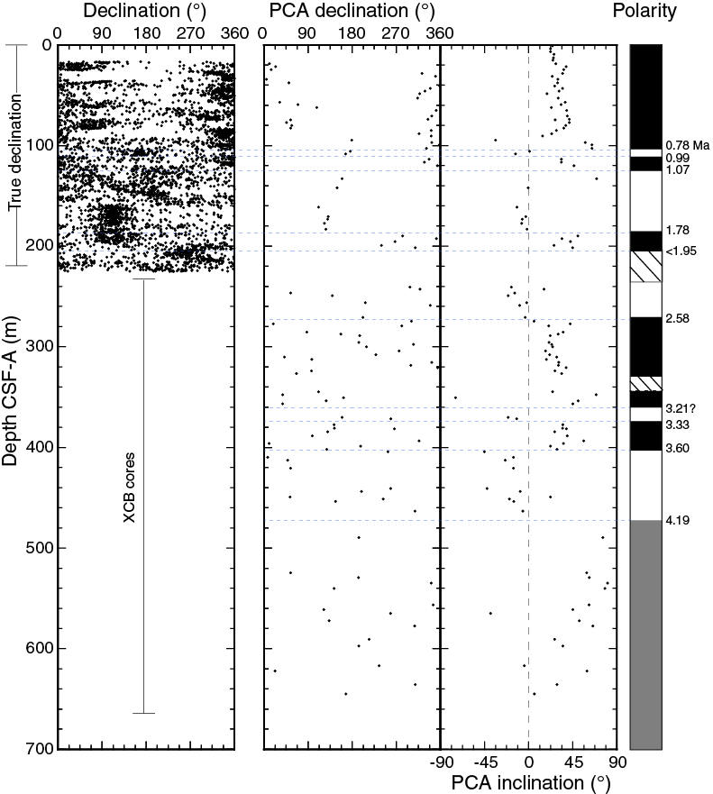
Figure F28. Downhole variations in magnetic parameters used to define magnetostratigraphy, Hole U1445A. True declination from archive halves, discrete sample ChRM declination and inclination, and inferred polarity pattern.
Throughout Hole U1445A, correlations to polarity chrons are straightforward: we simply assume that all the major subchrons except for very short ones (i.e., C1r.2n and C1r.1n) are resolved. Ages for each chron boundary (Table T16) were determined by correlating to the geomagnetic polarity timescale (GPTS) (Gradstein et al., 2012). There is some ambiguity in assigning Chron C2An.2r to a reversed magnetozone deeper than ~360 m CSF-A. Although we did not identify Chron C2An.1r, the close position of this magnetozone to the Gauss/Gilbert boundary together with a short duration of Chron C2An.1r (~80 ky) suggest that we missed Chron C2An.1r. A supporting observation is that Sample 353-U1445A-37X-4W, 91–93 cm (338.4 m CSF-A), although not revealing a well-defined ChRM in PCA, shows remanence migrating to a negative inclination after 30 mT demagnetization (Figure F29). This potentially reflects Chron C2An.1r.
Table T16. Summary of magnetostratigraphy, Site U1445. Download table in .csv format.
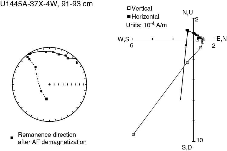
Figure F29. Stepwise AF demagnetization results, 338.4 m CSF-A.
For Hole U1445C (Figure F25), Cores 353-U1445C-2H through 24H were oriented (4.4–217.67 m CSF-A). No discrete samples were taken from this hole, and magnetostratigraphy is based entirely on the archive-half measurements. Similarly to Hole U1445A, declinations concentrate around 0° (360°) and 180° or 110° and 290°, whereas inclination does not show systematic variability. Although major magnetozones were clearly resolved, the position of the Brunhes/Matuyama boundary and Subchron C1r.1n (Jaramillo) are ambiguous. Although a major near-180° declination cluster in the 10 mT AF demagnetized data appear at ~85 m CSF-A, we consider this as an experimental error for the following two reasons: (1) natural remanent magnetization (NRM) before demagnetization in this interval clusters around 0° (360°), whereas NRM deeper than ~120 m CSF-A clusters around 180°, and (2) it is much shallower (20 m) than in Hole U1445A. A normal polarity magnetozone between ~109 and 116.5 m CSF-A is likely to be the Jaramillo on the basis of the depth comparison to Hole U1445A. Unfortunately, 10 mT AF demagnetization data are missing between 100.71 and 104.98 m CSF-A due to a flux jump in the y-axis superconducting quantum interference device (SQUID) in the cryogenic magnetometer and scattered data between ~105 and 109 m CSF-A, prevent identification of the top of Chron C1r.1r and Jaramillo. The top of Chron C2n (Olduvai) is well resolved to 186.0–186.7 m CSF-A.
Hole U1445B is too short to reach any polarity transition. Nonetheless, remanence intensities (Figure F30) show variability similar to Holes U1445A and U1445C. Note that this variability is likely to reflect diagenetic reactions and does not necessarily indicate the depositional age of the sediment.
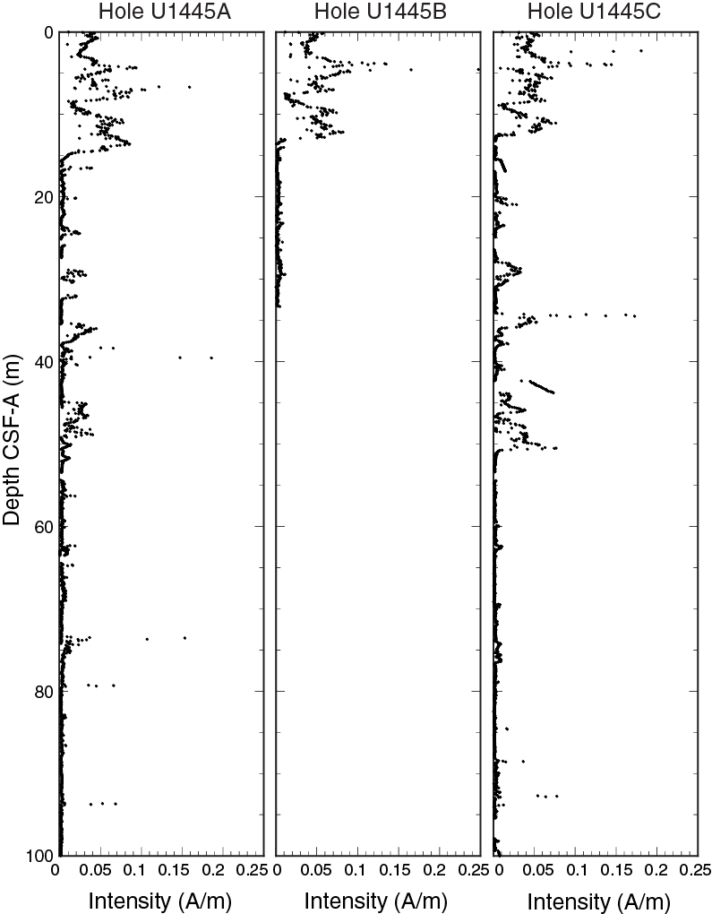
Figure F30. Downhole comparison of NRM intensity, Site U1445.
Bulk magnetic properties
Anhysteretic remanent magnetization (ARM) (0.05 mT direct current field, 80 mT AF), isothermal remanent magnetization (IRM) (100, 300, and 1000 mT), and their related magnetic parameters (hard isothermal remanent magnetization [HIRM] and S-ratio; see Paleomagnetism in the Expedition 353 methods chapter [Clemens et al., 2016] for further information) were acquired on a selection of discrete samples taken from the working halves of Hole U1445A. ARM broadly measures relative changes in the concentration of ferrimagnetic minerals, where increases in the concentration of finer grained particles will increase ARM values much greater than an equivalent change in coarser grained particles. IRM is a measure of remanence acquired up to a certain applied field and therefore depends on the mineralogy, concentration, and grain size of ferromagnetic (sensu stricto), ferrimagnetic, and nonperfect antiferromagnetic minerals. However, there is a bias toward minerals such as magnetite, maghemite, and greigite, which have magnetizations an order of magnitude or more than other minerals.
In addition to the whole-round and point magnetic susceptibility measurements (see Physical properties), clear signs of early diagenesis are recorded by the bulk magnetic parameters (Figure F26). A significant decrease in ARM and IRM from 0 to 15 m CSF-A suggests a large decrease in the concentration of ferrimagnetic minerals (magnetite, maghemite, and greigite). HIRM equally shows a decrease in the upper 15 m, suggesting a decrease in the concentrations of higher coercivity minerals, such as hematite and goethite. However, unlike the low-coercivity fraction, the higher coercivity fraction interpreted from HIRM does not display as strong a decrease, and this suggests a higher resistance to diagenesis. This observation strengthens the need to exploit trends in higher coercivity iron oxides/hydroxides within sedimentary sequences, which are often ignored or missed because of their weak magnetization. The S-ratio depth trends also decrease, showing a “hardening” (increase in the relative concentration of higher coercivity minerals to low-coercivity minerals) of the bulk magnetic assemblage. The decrease to near zero in ARM and IRM corresponds to the lower value (<0.7) in S100mT. As a note, the increase in magnetization at ~11 m CSF-A observed through each parameter is yet to be explained.
Bulk magnetic parameters were further measured to ~660 m CSF-A (Figure F31). A downhole decrease is observed for values of ARM, IRM, and S-ratio (excluding the clear high in S-ratio between 130 and 220 m CSF-A). This is likely due to continual diagenesis. Generally, an increase in IRM corresponds to an increase in ARM and a decrease in ARM/IRM (proxy for mean ferrimagnetic grain size). These relationships indicate that bulk IRM is controlled by coarser grained ferrimagnetic minerals.

Figure F31. Variations in a selection of bulk magnetic parameters and ratios for the entirety of Hole U1445A.
The S-ratio calculated with an IRM acquired at 100 mT (S100mT) is fairly low (<0.75) and indicates that at least 25% of the remanence up to 1000 mT (approximate saturation magnetization) is acquired by minerals with coercivities greater than 100 mT. However, the S-ratio calculated with an IRM at 300 mT (S300mT) is generally above 0.9, suggesting the magnetization is close to saturation by 300 mT. Therefore, we can assume the bulk magnetic assemblage primarily comprises minerals with coercivities up to 300 mT, such as (titano)magnetite, oxidized magnetite, maghemite, and possibly greigite. This conclusion does not exclude the presence of higher coercivity minerals, just that their concentrations are not significantly impacting the bulk magnetic properties (such as IRM and magnetic susceptibility values). HIRM, as mentioned, tracks the relative changes in higher coercivity mineral concentration and shows an increasing trend with depth. This trend could be due to more resistance against early diagenesis, some mineralization due to burial diagenesis or oxidation, or a relative increase in the detrital input of higher coercivity minerals.
Clear peaks are observed in IRM and HIRM that appear more prominent deeper than ~300 m CSF-A. These peaks are less prominent in ARM, the S-ratio, and the ratio of ARM/IRM. These observations suggest that the bulk magnetic assemblage (coarse-grained ferrimagnetic minerals and some higher coercivity minerals) are reacting to astronomical-scale cyclicity. These results are encouraging for any on-shore research into the links between mineral magnetic variations and paleoclimate.
Physical properties
Standard physical property measurements were collected at Site U1445 from Holes U1445A–U1445C, with the addition of thermal infrared (IR) scanning of cores on the catwalk for the detection of temperature anomalies related to gas hydrate dissociation. Data from Hole U1445B are presented but not discussed in this report because this short hole was drilled for high-resolution geochemistry sampling. Based on measurements from Holes U1445A and U1445C, we have defined three physical property (PP) units independent of the lithostratigraphic units, based on clear diversions in the physical property data: Unit 1 (0–235 m CSF-A), Unit 2 (235–408 m CSF-A), and Unit 3 (408–665 m CSF-A) (Table T17). Hole U1445C ends at 304.26 m CSF-A. The trends up to that point show excellent correlation with Hole U1445A data and we could define the Unit 1/2 boundary in Hole U1445C.
Table T17. Physical property units, Site U1445. Download table in .csv format.
Gamma ray attenuation (GRA), magnetic susceptibility (MS), P-wave velocity (VP), and natural gamma radiation (NGR) measurements were acquired on all whole-round sections using the Special Task Multisensor Logger (STMSL), the Whole-Round Multisensor Logger (WRMSL), and the Natural Gamma Radiation Logger (NGRL). Whole-round sections from Hole U1445A were first run through the STMSL (2.5 cm resolution) and WRMSL (5 cm resolution) before being taken to the core rack for thermal equilibration to ~19°C. For Hole U1445C, alternate sections were run on the STMSL (Sections 1, 3, 5, and 7) and WRMSL (Sections 2, 4, 6, 8, and CC) at a 2.5 cm sampling interval in order to provide the stratigraphic correlators with near real-time hole-to-hole correlation data. P-wave data were found to be unreliable following Core 353-U1445A-4H because the transducer malfunctioned and was disabled for the remainder of Hole U1445C. Following thermal equilibration, sections were logged on the NGRL. Approximately 10 cm3 sediment samples were collected from the working halves of Sections 2, 4, and 6 for moisture and density (MAD) analyses. The archive-half sections were used to collect color reflectance and point MS data on the Section Half Multisensor Logger (SHMSL) and red, green, and blue (RGB) data on the Section Half Imaging Logger (SHIL). The data presented here were conditioned to remove outliers (see Physical properties in the Expedition 353 methods chapter [Clemens et al., 2016]). We present the minimum, maximum, and mean values of all measured parameters downhole for hole-to-hole comparison (Table T18). Downhole wireline logging was completed at this site, and the core logger data will likely serve as a critical bridge to connect the downhole log and core data.
Table T18. Minimum, maximum, and mean statistics of measured physical properties data, Holes U1445A–U1445C. Download table in .csv format.
Magnetic susceptibility
STMSL and WRMSL MS values recorded for Hole U1445A showed minor variability generally between 1.33 and 33 instrument units (IU) (Figure F32). Occasional values >33 IU are recorded. Unit 1 is characterized by higher average MS values than Unit 2 but comparable values to Unit 3, although there is less variability in Unit 1 than Unit 3. Lower average MS values in Unit 2 correspond with anomalously high porosity. The STMSL and WRMSL track measurements agree nicely with the SHMSL point measurements. A slight offset exists between the STMSL MS data between Holes U1445A and U1445C; however, the WRMSL data from Holes U1445A and U1445C match up well. There is a large discrepancy between the SHMSL MS data from Holes U1445A and U1445C (Figures F32, F33) where the offset is constant with depth. It is likely that the low MS values recorded in Unit 2 are from dilution of the lithogenic fractions via an increase in biogenic silica, which is further supported by the NGR data showing a similar decreasing to increasing trend.
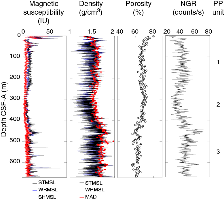
Figure F32. Physical properties showing downhole variability in magnetic susceptibility, density, porosity, and NGR, Hole U1445A.
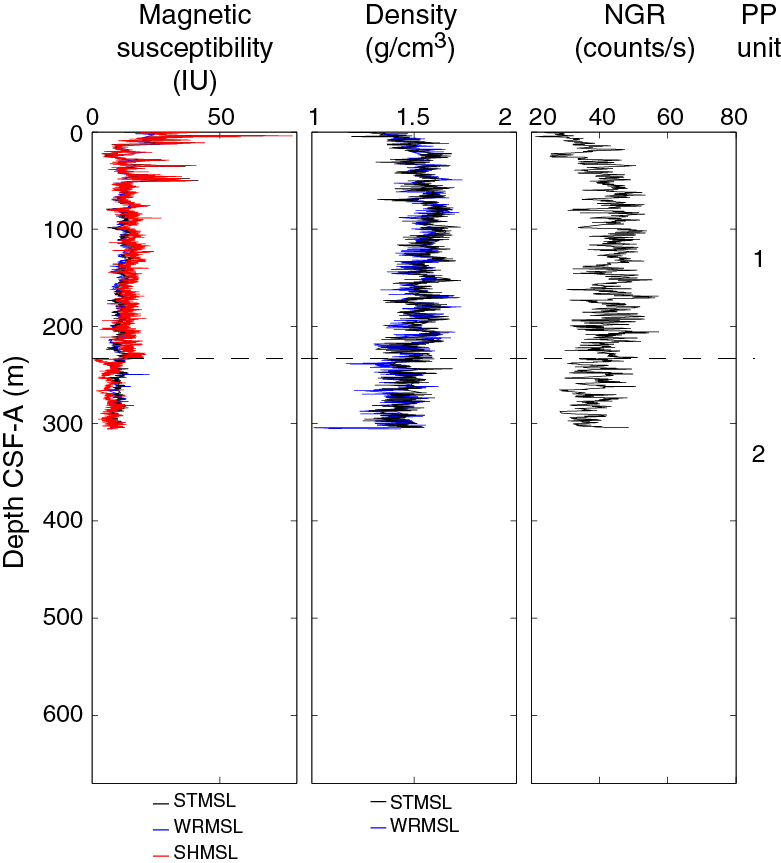
Figure F33. Whole-round physical properties showing downhole variability in magnetic susceptibility, density, and NGR, Hole U1445C.
Natural gamma radiation
The NGR and MS long-term downhole variations follow similar trends. There is low variability in Unit 1 with an overall decrease in counts marking the top of Unit 2 and a return to higher counts with higher variability in Unit 3 (Figures F32, F33, F34). Generally, clay minerals containing K, Th, and U are the principal source of high NGR counts. Most of Site U1445 is composed of clay, and the variations in NGR at this site are inversely related to the CaCO3 content (see Geochemistry). Therefore, the lower NGR values in Unit 2 likely reflect a higher proportion of diatoms and biogenic silica relative to the lithogenic fractions downhole, meaning that the NGR drop in Unit 2 represents a dilution to lithogenic clay material rather than a flux of lithogenic material in Units 1 and 3. Because NGR counts are sensitive to material volume, an increase in variability in Unit 3 could be related to biscuiting and an increase in gas expansion cracks, with low measurements associated with less volume and voids. Several flakes of what appeared to be rust were visibly observed within the core liner between the sediment/liner contact in the deeper section of Hole U1445A, which likely resulted in correspondingly high NGR and MS peaks. NGR counts in Hole U1445C Units 1 and 2 show an analogous trend to Hole U1445A (Figures F32, F33).
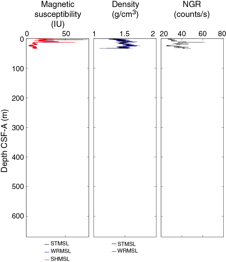
Figure F34. Whole-round physical properties showing downhole variability in magnetic susceptibility, density, and NGR, Hole U1445B.
GRA and MAD bulk density
Bulk density at Site U1445 was measured using (1) the GRA method using the STMSL that provides bulk density estimates from whole-round sections for both Holes U1445A and U1445C (Figures F32, F33) and (2) MAD measurements on discrete samples that provide a second, independent measure of bulk density and the dry density, grain density, water content, and porosity from Hole U1445A only (Figure F32). The MAD and GRA data show excellent agreement, and because the GRA data between Holes U1445A and U1445C are also in excellent agreement, we discuss the data from Hole U1445A only (Figures F32, F33, F34).
The GRA bulk density values range from ~1.01 to 1.99 g/cm3, whereas the MAD bulk density comparably ranges between 1.328 and 1.979 g/cm3. The mean MAD bulk density is 1.619 (bulk) and 2.766 g/cm3 (grain) with a minimum dry density of 0.477 g/cm3 and a maximum dry density of 1.413 g/cm3. The porosity values vary significantly downhole and range between 53.6% and 83.1%, whereas the volume of the pore water content per 10 cm3 sample is between 1.346 and 8.125 cm3 (Figure F32).
The density data are divided into three units that agree with the MS and NGR unit depths. Density commonly increases with a corresponding decrease in porosity with depth, related to sediment compaction. However, we observe a decrease in density with an increase in porosity in Unit 2 possibly related to more abundant biosiliceous material in Unit 2. There is an abrupt return to high density with low porosity between Units 2 and 3.
Compressional wave velocity
Compressional P-wave velocity measurements using the P-wave logger (PWL) were performed on whole-round sections for Cores 353-U1445A-1H through 19F (0–167 m CSF-A). The P-wave values were found to be unreliable, and we ceased taking measurements on the remainder of the cores in Hole U1445A. P-wave data collection was not attempted on cores from Hole U1445C.
Diffuse reflectance spectroscopy and digital color image
Spectral reflectance was measured on all archive halves using the SHMSL. There are slight color variations downhole, with the most noticeable change occurring at the Unit 1/2 boundary. L* values range from 17.2 to 40 with an average of 29.4. Reflectance a* and b* values range between −1.9 and 3 (average = 0.45) and −5.2 to 7 (average = 0.68), respectively (Table T18). There is a stepwise change to lower L* values at the Unit 1/2 boundary and an increase in L* at the Unit 2/3 boundary. The Unit 1/2 boundary is not as distinct in the a* and b* plots. However, there is a broadening of the count range in both Units 2 and 3 compared to Unit 1 (Figure F35). Changes in color reflectance are directly related to compositional changes and could reflect variations in clay mineralogy and water content downhole. Biscuiting is prevalent in Cores 353-U1445A-40X through 73X, and the increase in water content from the sawing procedure used to split these cores likely increased sediment darkness. Downhole variability in L*, a*, and b* from Holes U1445B and U1445C are also shown (Figures F36, F37).

Figure F35. L*, a*, and b* data, Hole U1445A.
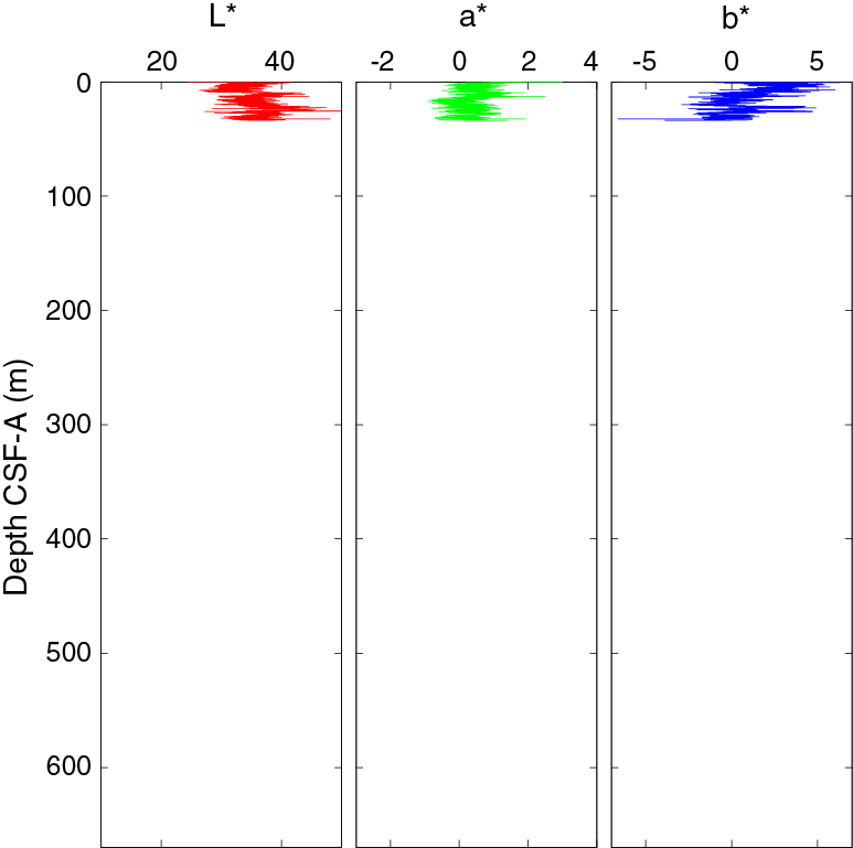
Figure F36. L*, a*, and b* data, Hole U1445B.
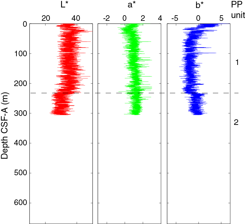
Figure F37. L*, a*, and b* data, Hole U1445C.
The SHIL data (RGB) were recorded from the surface of the split archive halves prior to drying. The raw RGB data averages are R = 31.11, G = 30.45, and B = 28.82. A marked decrease in R, G, and B counts occur at the Unit 1/2 boundary, which steadily increase through Unit 3. Unit 3 has a wider color range than Units 1 or 2. The higher G counts in Unit 3 reflect an increase in glauconite-rich clay in Cores 353-U1445A-40X through 76X (Figure F38). Downcore variability in RGB is also shown for Holes U1445B and U1445C (Figures F39, F40).
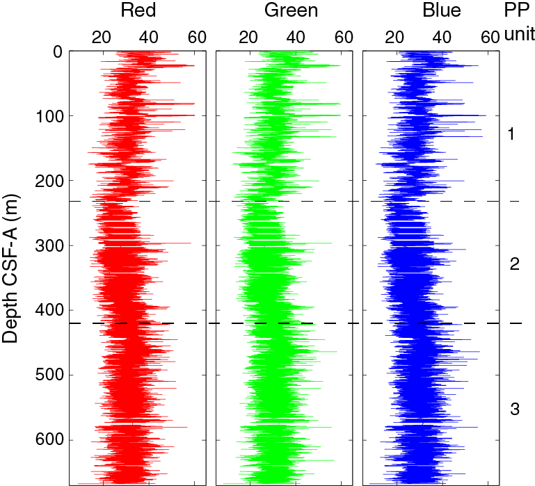
Figure F38. SHIL RGB color data, Hole U1445A.
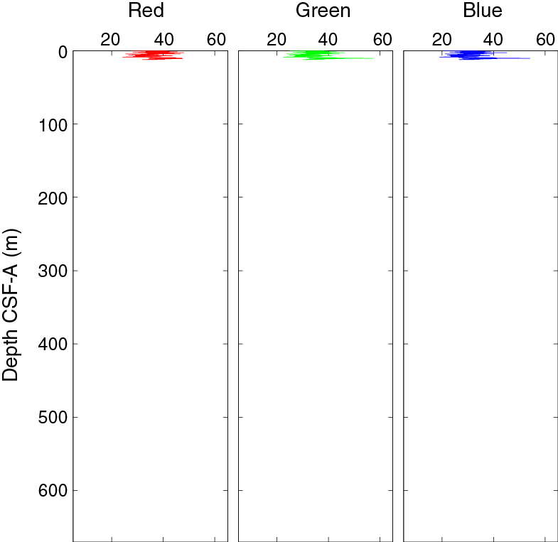
Figure F39. SHIL RGB color data, Hole U1445B.
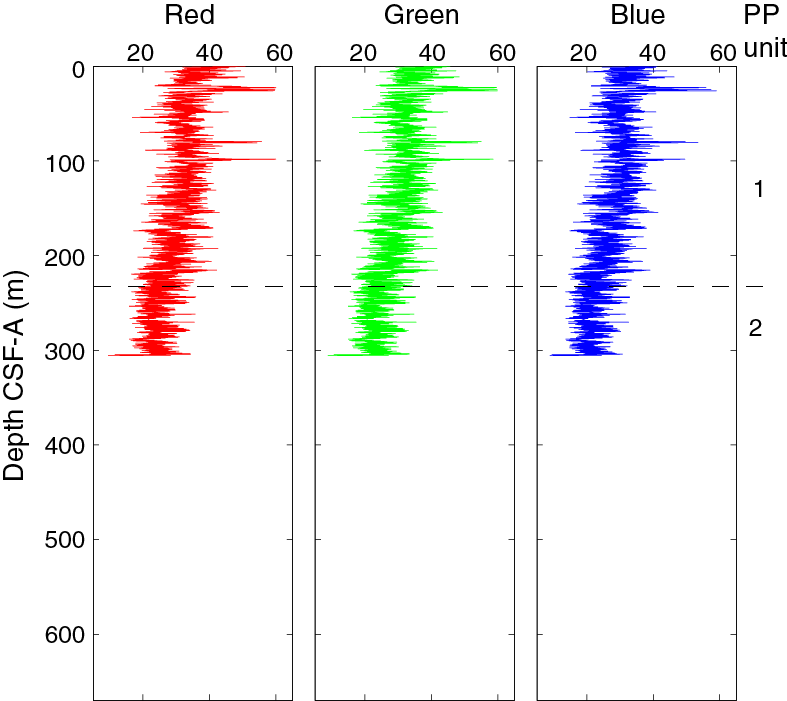
Figure F40. SHIL RGB color data, Hole U1445C.
Downhole temperature
Standard downhole temperature measurements were made on Cores 353-U1445A-4H, 7H, 10H, and 13H using the APCT-3 (Table T19). Two additional temperature measurements were taken on Cores 353-U1445C-20H and 22H to better constrain the geothermal gradient, which is calculated to be ~50°C/km (Figure F41).
Table T19. Downhole temperature data from the APCT-3, Holes U1445A–U1445C. Download table in .csv format.
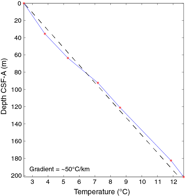
Figure F41. Downhole temperature data, Holes U1445A and U1445C.
Thermal infrared temperature
A FLIR thermal IR camera was used for thermal imaging of cores on the catwalk to detect IR cold spot anomalies related to gas hydrate dissociation. Numerous IR cold anomalies ranging from 1 to 15 cm in width were found downhole, beginning with Core 353-U1445C-4H (Figure F42). These cold spots were used to guide pore water sampling to test for the Cl− freshening signature of gas hydrate dissociation (see Geochemistry). Cold spots were mostly concentrated between Cores 18F and 30X (144.4 and 202 m CSF-A).

Figure F42. IR cold spot anomalies, Hole U1445C. A. Anomaly is ~4.7°C cooler than surrounding sediments. B. Anomaly is ~5.0°C cooler than surrounding sediments. C. Anomaly is ~6.0°C cooler than surrounding sediments.
Summary
Physical property data between Holes U1445A and U1445C correlate well. Change between Units 1 and 2 is likely related to a transition to a more biosilica-rich clay that began at the boundary of these two units (see Lithostratigraphy). The MS, density, and NGR values are lower, whereas the porosity values are high in the more diatom-rich clay of Unit 2. The NGR data are inversely related to the CaCO3 content found in CARB analyses (see Geochemistry) and likely reflect a dilution to the background clay content. Changes in color reflectance could be a result of a change from APC to XCB coring. There is a zone of high NGR peaks in Unit 3 that could be related to biscuiting, where peaks correspond to biscuits and troughs correspond to the less dense, washed out zones. Numerous cold-spot thermal anomalies indicating gas hydrate dissociation were found in Hole U1445C.
Downhole logging
On 6 January 2015, Hole U1445A was circulated and displaced with 10 lb/gal mud with barite. No major problem was reported during coring/drilling operations. The drill pipe was brought to logging depth (2597.9 meters below rig floor [mbrf]; 84.8 meters below seafloor [mbsf]). Rig-up for downhole logging started at 1100 h (UTC + 8 h), and ship heave was less than 0.2 m peak to peak. The driller’s seafloor depth at the Mahanadi logging site was 2509 mbrf. Total penetration at Hole U1445A (APC coring) was 672.6 mbsf. Two passes were made with both the triple combo and the FMS-sonic tool strings for better data comparison of repeatability.
Triple combo string (MSS/HRLA/HLDS/APS/HNGS/EDTC/LEQT/SP)
During tool checks, the Accelerator Porosity Sonde (APS) and related hardware, including the inline eccentralizer and the required adapters, were unable to communicate with the wireline telemetry. After some discussion with the Co-Chief Scientists and Logging Staff Scientist, the backup set was put in place and checked. Fortunately, this combination worked, and the gamma source was loaded following the standard protocol. The tools started down the pipe at 1400 h. The triple combo tool string was run in the hole at 1420 h and reached seafloor depth at 1535 h. A downlog was started approximately 50 m above seafloor, and the tool was run at a speed of 1800 ft/h (548 m/h) while acquiring Hostile Environment Natural Gamma Ray Sonde (HNGS) data near the seafloor. No problems were seen running the tool string through the pipe or the bottom-hole assembly (BHA), and the tools descended out the drill bit uneventfully. After passing the seafloor, the downlog was run at a logging speed of 3000 ft/h (914 m/h). The triple combo tool string reached 2957 mbrf (444 mbsf) at 1615 h. The downlog did not utilize the caliper or APS porosity because neither can be operated for the downlog without serious operational problems. The first uplog started at 1700 h at a logging speed of 1800 ft/h (548 m/h) up to approximately 2645 mbrf. The borehole shape was in relatively good condition, ranging from 12 to 14 inches (30.5 to 35.5 cm) deeper than 237 mbsf; at shallower depths, the range increased to 14–17 inches (35.5 to 43 cm). At some point before reaching 2645 mbrf (the turnaround depth for the second uplog), the active heave compensator (AHC) stroked to the full upward position, creating a depth change in the log file of nearly 5–6 m. The first uplog was stopped, and the AHC was recentered and locked. Because the heave was 40 cm or less, the compensator was not needed, and locking the AHC avoided any possible depth issues with the second uplog until the problem could be addressed. The tool string was back at the bottom of the hole at 2957 mbrf at 1802 h. The second uplog started at this time from the bottom of the hole at a logging speed of 1800 ft/h (548 m/h). The caliper was opened at 426 mbsf and closed at 95 mbsf. The pipe was found at 2593 mbrf. The seafloor was found at 2509 mbrf at 1850 h. The triple combo tool string was back to the surface at 2000 h.
FMS-sonic string (FMS/DSST/HNGS/EDTC/LEQT)
The FMS-sonic string, including the FMS, the Dipole Shear Sonic Imager, and the HNGS, was deployed at 2230 h. A downlog was taken at ~1800 ft/h (548 m/h) near the seafloor then sped up to 3000 ft/h (914 m/h). The tool string passed the seafloor at 0000 h on 7 January 2015 (2513 mbrf). Again, no problems were encountered running down through the drill pipe or BHA. The FMS-sonic tool string reached the bottom of the hole (bridged depth as before from the triple combo tool string at 2957 mbrf [444 mbsf]) at 0100 h. The sonic tool was run with SAMX (BCR both crossed dipole) and SAM4 P&S compressional modes at a speed of 1800 ft/h (548 m/h). The SAMX will require processing in BestDT in Geoframe or similar software to provide the anisotropy analysis. The compressional data (Delta-T Receiver Array Compressional [DTRP]) required playbacks to adjust the starting window for the compressional labeling, so the original logs do not have the correctly labeled compressional curve. The first uplog was started at 0100 h with the calipers opened at 447 mbsf and closed at 110 mbsf. The log was stopped at 126 mbsf to avoid reentering the drill bit and then run in the hole again to the bridge depth. The second uplog was started at 0212 h again at 2957 mbrf with calipers opened at 446 mbsf and closed at 126 mbsf. While entering the drill pipe, the tool became stuck and unable to pass 2603 mbrf. Fortunately, the tool could still be lowered down without problem. After several attempts and delicate pulling at no more than about 500 lb of overpull, it appeared that the lower mechanical caliper device (MCD; used as a centralizer only) was catching the flapper valve above the bit. Because small rocks can prevent the springs from closing against the tool, rig personnel hooked up the circulating hose in attempt to circulate seawater over this area and clean any potential debris from the MCD. During circulating hose setup, tool tension dropped off and the tool released. The tool was then pulled up to continue logging to seafloor at 1800 ft/h (548 m/h). The pipe was found at 2593 mbrf, and the seafloor was found at 2509 mbrf. The tool was pulled from the hole and arrived on the surface at 0430 h. Final rigdown was completed at 0630 h. This concluded the wireline logging operations for Hole U1445A.
Caliper
Hole U1445A is divided into three distinct caliper units based on the deviation from the bit size as recorded in the caliper log: Unit 1 (100–237 m CSF-A) is highly irregular with large washed out zones, Unit 2 (237–380 m CSF-A) is close to the bit size, and Unit 3 (380–440 m CSF-A) has minor but frequent washouts (Figure F43A). Based on the caliper reading, data are less reliable in Units 1 and 3.

Figure F43. Downhole logs: (A) caliper, (B) total NGR, and (C, D) spectral gamma curves for potassium, uranium, and thorium, Site U1445.
Natural gamma radioactivity
Measured wireline (WL) gamma ray values are less than the natural radioactivity values measured on core sections, likely because of attenuation from the logging mud. To bring the WL gamma ray data to within range of whole-core values, they were scaled by 40%. A comparison of the scaled WL gamma ray log and the whole-round NGRL logs from Holes U1445A and U1445C is shown in Figure F43B. Caliper Unit 1 has a low gamma ray count, most likely due to an anomalously expanded hole. In Unit 2, the magnitude of the WL gamma log is comparable to the shipboard NGRL log, further attesting to the reliability of this unit. The high potassium to uranium and thorium ratios from the WL spectral log suggest a dominance of micaceous clays (illite) (Figure F43C–F43D). Where the borehole quality in caliper Unit 3 is poor, variability increases and the total WL NGR counts decrease, suggesting the diameter of the borehole is influencing the NGR log response.
Density
Figure F44B shows a plot of the WL density log against the whole-round core bulk density measurements and MAD bulk density results (see Physical properties) for hole-log comparison. Log density is highly variable in the upper unit, likely because of poor borehole conditions. Log density is in good agreement with MAD measurements in caliper Unit 2. Although borehole conditions were not ideal in Unit 3, the log density data have the same trend and magnitude as the MAD density measurements. On a related note, density data from the STMSL appear to underestimate the true formation density, which could be due to volume effect intensified from core expansion and opening of new cracks (Figure F44).
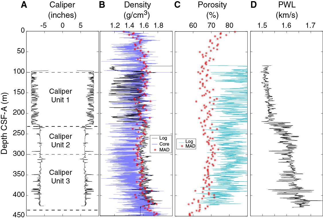
Figure F44. Downhole logs: (A) caliper, (B) density, (C) porosity, and (D) P-wave velocity, Site U1445.
Porosity
We plotted the porosity WL curve from the neutron tool against the core-derived MAD porosity measurements for comparison (Figure F44C). On all accounts, WL log porosity is ~10%–20% higher than correlative MAD measurements, suggesting a high content of bound water in the clay-dominated sediments.
P-wave velocity
In caliper Unit 1, sonic velocity remains relatively constant, suggesting poor penetration into the formation related to poor borehole conditions (Figure F44D). Deeper than 237 m CSF-A, there is more variability in the P-wave data, which we believe is reliable data based on the caliper measurements. Many points throughout caliper Units 2 and 3 display a combination of low density, high porosity, and a high P-wave velocity indicative of gas hydrates. However, the resistivity log data (Figure F45) do not show high spikes, suggesting that the gas hydrate morphology at this site is disperse in the sediments rather than nodular or massive. Unfortunately, core-based P-wave data are not available for comparison with the WL log because of the malfunctioning of the WRMSL P-wave transducer.
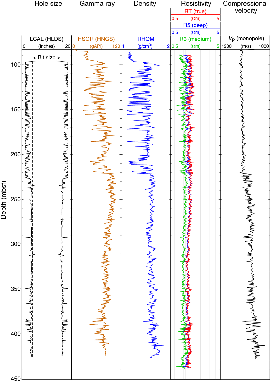
Figure F45. Triple combo tool summary logs, Hole U1445A.
Formation MicroScanner
The FMS images the borehole based on its electrical properties. The nonlinear display of the static and dynamic FMS logs suggests that the tool was rotating within the borehole, and periodic intervals showing tool-drag related artifacts are evident (e.g., 144–154 mbsf in Figure F46). As shown in Figure F46, the WL-derived resistivity-at-the-bit (RAB) images of borehole resistivity reveal numerous high-resistivity intervals (light yellow to white) throughout the stratigraphic column. Throughout caliper Unit 2, these highly resistive layers could be hydrate-rich layers. Most of the very dark bands correspond to washouts as a function of the tool having a moderate to shallow depth of investigation.
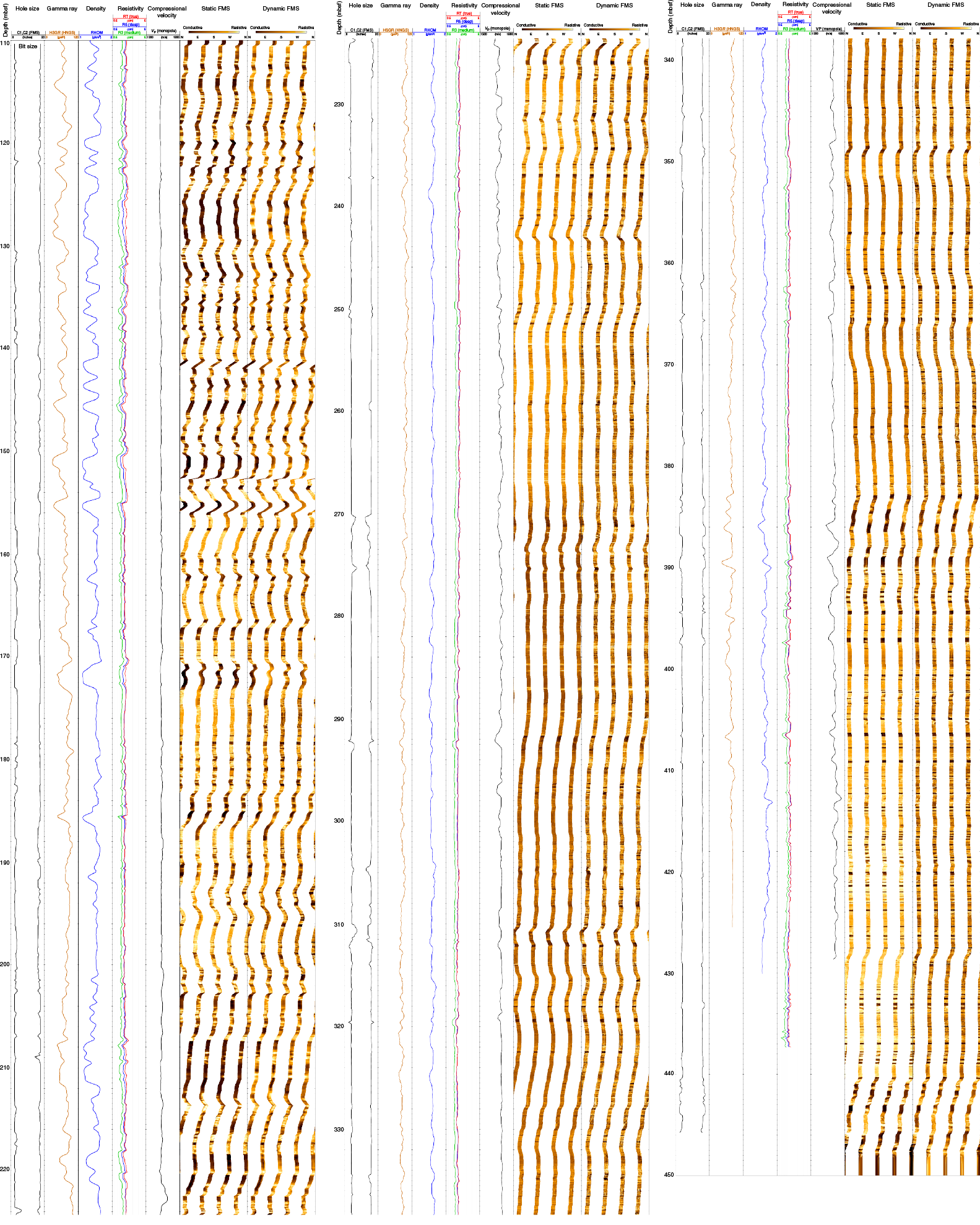
Figure F46. FMS summary log images (static and dynamic normalization), Hole U1445A.
Magnetic susceptibility
Magnetic susceptibility data were not reliable and are therefore excluded from the discussion.
Summary
Hole U1445A was conditioned for logging with a heavyweight, water-based mud. Barite was added as a thickener and likely affected the quality of data collected by several tools, including the gamma ray and photoelectric effect. Two passes of the triple combo and FMS-sonic tool strings were made. Each tool run through the hole proceeded smoothly until an unpassable bridge was met at ~440 m CSF-A. For the purpose of discussion, the WL logging suites are divided into three units based on the caliper data. The diameter of the hole at caliper Unit 2 is close to that of the drill bit and provides reliable data, whereas any interpretations of caliper Units 1 and 3 should proceed cautiously because of poor borehole conditions. The WL density measurements agree with the bulk density values provided by MAD measurements where borehole conditions are good. However, the density log from the WRMSL and STMSL appears to consistently underestimate the true density of the formation. The WL porosity curve shows high apparent porosity as a result of water bound in the structure of the clays that dominate the downhole lithology. There are no significantly high resistivity peaks in the resistivity log; however, there are many high-resistivity bands in FMS logs, suggesting that gas hydrates are present in disseminated form. Magnetic susceptibility data were not reliable and were excluded from interpretation.
Stratigraphic correlation
A composite scale (CCSF-A) and a splice (CCSF-D) were constructed for Site U1445 using Holes U1445A and U1445C (as defined in Stratigraphic correlation in the Expedition 353 methods chapter [Clemens et al., 2016]). Splicing among these holes enabled us to construct a continuous stratigraphic sequence to ~252 m CCSF-D (Tables T20, T21; Figure F47). Hole U1445B, dedicated to geochemical sampling on board the ship, was short and not used in splicing. However, we tied it to the same composite scale as Holes U1445A and U1445C.
Table T20. Vertical offsets applied to cores in order to align structure in adjacent holes, Site U1445. Download table in .csv format.
Table T21. Splice intervals, Site U1445. Download table in .csv format.
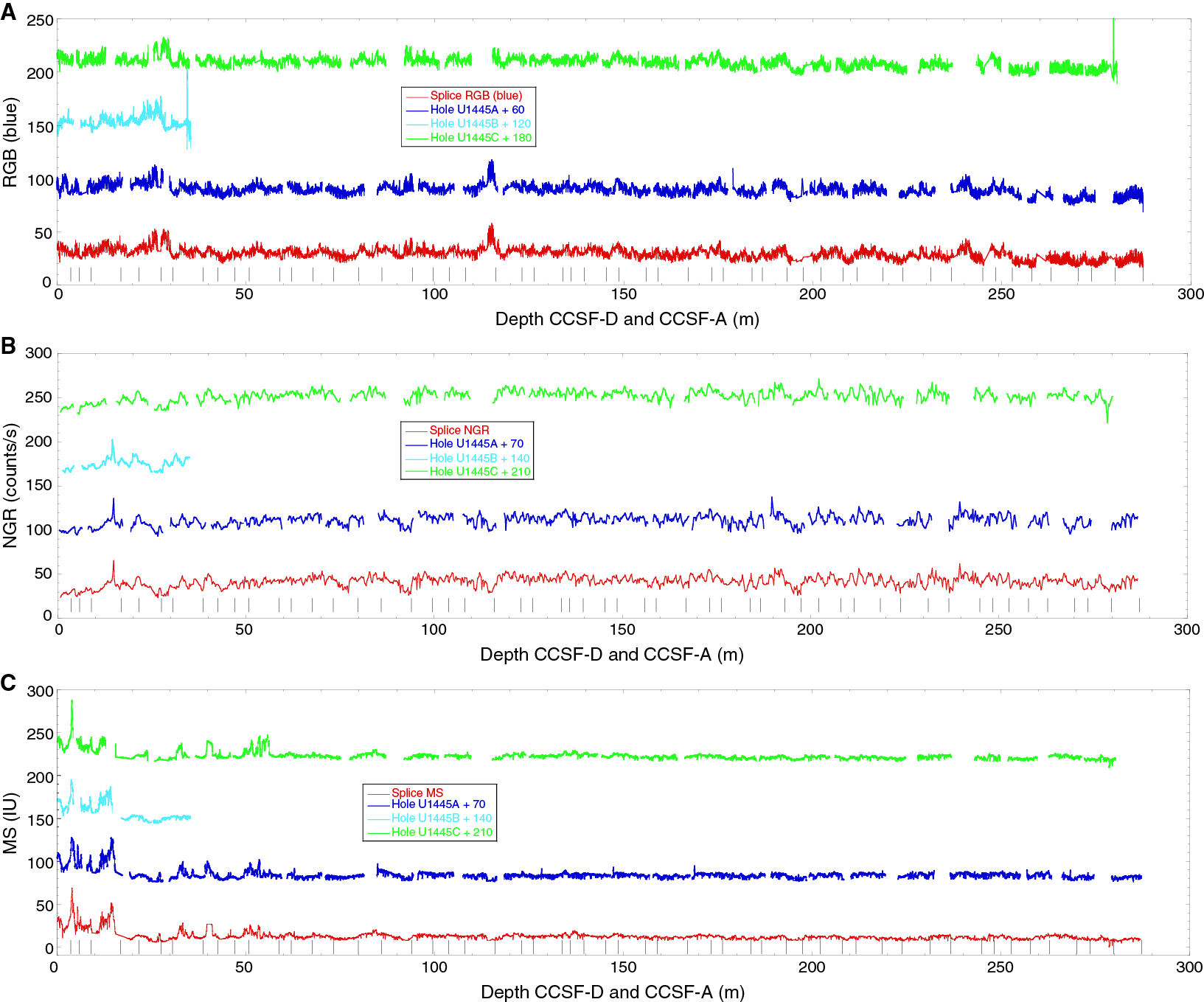
Figure F47. Core alignment exemplified using (A) RGB blue, (B) NGR, and (C) MS profiles, Holes U1445A–U1445C.
Construction of CCSF-A scale
We selected the core with the best mudline recovery (Core 353-U1445C-1H) to anchor the composite depth scale and defined the top as 0 m CCSF-A. The CCSF-A scale for Site U1445 (see Table T20) is based on correlation of primarily RGB color data, which are aided at times by MS and NGR data. MS and NGR were measured on whole-round sections, whereas RGB was measured on archive-half sections (see Physical properties for details). The R, G, and B components of the RGB triplet are highly correlated to each other because, on the first order, all are measures of the reflectivity of the sediment. The small differences between R, G, and B can be expressed as ratios such as red/green, red/blue, or green/blue. However, ratios were not employed in our correlation due to lack of time (see the Expedition 353 methods chapter [Clemens et al., 2016]). Reflectance spectroscopy data (i.e., L*, a*, and b*), which can produce information similar to RGB ratios, were not used for correlation due to inconsistent variability from hole to hole resulting from low-quality wavelength spectra collected by the Ocean Optics USB4000 spectrophotometer on the monotonously dark sediments of Site U1445.
Deeper than ~50 m CCSF-A, where MS values are low and erratic, RGB was effectively the only parameter available to use for correlation. NGR, which was measured at lower resolution than RGB (see Physical properties) was employed in several instances where RGB did not provide a reasonably good tie (see Table T20).
Construction of CCSF-D scale
A combination of Holes U1445A and U1445C cover the stratigraphic section to ~252 m CCSF-D. When constructing the splice, we tried to minimize the inclusion of disturbed intervals and avoided whole-round sampling intervals (notably from Hole U1445A) as much as possible. Selected splice intervals are listed in Table T21. Postcruise, the splice interval tables were modified using the Splice-File-Fixer program to ensure that each depth has been assigned the correct sample ID. Both the affine and the corrected splice interval tables were uploaded into the Laboratory Information Management System (LIMS) database during the first postcruise meeting in June 2015. The core top depths in the affine tables were not corrected and hence may be slightly incorrect in a range of <2 cm. However, the offsets are correct.
Reliance on a single correlation parameter (i.e., RGB) and its sometimes fuzzy character precluded, in places, the definition of unique features for correlation, so general trends were used instead, reducing the accuracy of the splice to the decimeter range. As a result, correlation should be viewed with caution deeper than ~50 m CCSF-A and especially deeper than ~236 m CCSF-A, notably if high-resolution sampling is planned. Onshore X-ray fluorescence scanning, color reflectance rescanning, and bulk δ18O should provide better means of correlation.
References
Antonov, J.I., Seidov, D., Boyer, T.P., Locarnini, R.A., Mishonov, A.V., Garcia, H.E., Baranova, O.K., Zweng, M.M., and Johnson, D.R., 2010. World Ocean Atlas 2009 (Volume 2): Salinity. In Levitus, S. (Ed.), NOAA Atlas NESDIS 69: Washington D.C. (U.S. Government Printing Office). ftp://ftp.nodc.noaa.gov/pub/WOA09/DOC/woa09_vol2_text_figures.pdf
Barron, J.A., 1985. Miocene to Holocene planktic diatoms. In Bolli, H.M., Saunders, J.B., and Perch-Nielsen, K. (Eds.), Plankton Stratigraphy: Cambridge, United Kingdom (Cambridge University Press), 763–809.
Chaitanya, A.V.S., Lengaigne, M., Vialard, J., Gopalakrishna, V.V., Durand, F., Kranthikumar, C., Amritash, S., Suneel, V., Papa, F., and Ravichandran, M., 2014. Salinity measurements collected by fishermen reveal a “river in the sea” flowing along the eastern coast of India. Bulletin of the American Meteorological Society, 95(12):1897–1908. http://dx.doi.org/10.1175/BAMS-D-12-00243.1
Chakrapani, G.J., and Subramanian, V., 1990a. Factors controlling sediment discharge in the Mahanadi River basin, India. Journal of Hydrology, 117(1–4):169–185. http://dx.doi.org/10.1016/0022-1694(90)90091-B
Chakrapani, G.J., and Subramanian, V., 1990b. Preliminary studies on the geochemistry of the Mahanadi River basin, India. Chemical Geology, 81(3):241–253. http://dx.doi.org/10.1016/0009-2541(90)90118-Q
Chatterjee, A., Shankar, D., Shenoi, S.S.C., Reddy, G.V., Michael, G.S., Ravichandran, M., Gopalkrishna, V.V., Rama Rao, E.P., Udaya Bhaskar, T.V.S., and Sanjeevan, V.N., 2012. A new atlas of temperature and salinity for the North Indian Ocean. Journal of Earth System Science, 121(3):559–593. http://dx.doi.org/10.1007/s12040-012-0191-9
Clemens, S.C., Kuhnt, W., LeVay, L.J., Anand, P., Ando, T., Bartol, M., Bolton, C.T., Ding, X., Gariboldi, K., Giosan, L., Hathorne, E.C., Huang, Y., Jaiswal, P., Kim, S., Kirkpatrick, J.B., Littler, K., Marino, G., Martinez, P., Naik, D., Peketi, A., Phillips, S.C., Robinson, M.M., Romero, O.E., Sagar, N., Taladay, K.B., Taylor, S.N., Thirumalai, K., Uramoto, G., Usui, Y., Wang, J., Yamamoto, M., and Zhou, L., 2016. Expedition 353 methods. In Clemens, S.C., Kuhnt, W., LeVay, L.J., and the Expedition 353 Scientists, Indian Monsoon Rainfall. Proceedings of the International Ocean Discovery Program, 353: College Station, TX (International Ocean Discovery Program). http://dx.doi.org/10.14379/iodp.proc.353.102.2016
Dangwal, V., Sengupta, S., and Desai A.G., 2008. Speculated petroleum systems in deep offshore Mahanadi Basin in Bay of Bengal, India [paper presented at the 7th International Conference and Exposition on Petroleum Geophysics, Hyderabad, India, 14–16 January, 2008]. http://www.spgindia.org/2008/001.pdf
Gradstein, F.M., Ogg, J.G., Schmitz, M.D., and Ogg, G.M. (Eds.), 2012. The Geological Time Scale 2012: Amsterdam (Elsevier).
Martini, E., 1971. Standard Tertiary and Quaternary calcareous nannoplankton zonation. In Farinacci, A. (Ed.), Proceedings of the Second Planktonic Conference, Roma 1970: Rome (Edizioni Tecnoscienza), 2:739–785.
Mazumdar, A., Kocherla, M., Carvalho, M.A., Peketi, A., Joshi, R.K., Mahalaxmi, P., Joao, H.M., and Jisha, R., 2015. Geochemical characterization of the Krishna–Godavari and Mahanadi offshore basin (Bay of Bengal) sediments: a comparative study of provenance. Marine and Petroleum Geology, 60:18–33. http://dx.doi.org/10.1016/j.marpetgeo.2014.09.005
Okada, H., and Bukry, D., 1980. Supplementary modification and introduction of code numbers to the low-latitude coccolith biostratigraphic zonation (Bukry, 1973; 1975). Marine Micropaleontology, 5:321–325. http://dx.doi.org/10.1016/0377-8398(80)90016-X
Okada, H., and Wells, P., 1997. Late Quaternary nannofossil indicators of climate change in two deep-sea cores associated with the Leeuwin Current off Western Australia. Palaeogeography, Palaeoclimatology, Palaeoecology, 131(3–4):413–432. http://dx.doi.org/10.1016/S0031-0182(97)00014-X
Rickers, K., Mezger, K., and Raith, M.M., 2001. Evolution of the continental crust in the Proterozoic Eastern Ghats Belt, India and new constraints for Rodinia reconstruction: implications from Sm-Nd, Rb-Sr and Pb-Pb isotopes. Precambrian Research, 112(3–4):183–210. http://dx.doi.org/10.1016/S0301-9268(01)00146-2
Sastri, V.V., Venkatachala, B.S., and Narayanan, V., 1981. The evolution of the east coast of India. Palaeogeography, Palaeoclimatology, Palaeoecology, 36(1–2):23–54. http://dx.doi.org/10.1016/0031-0182(81)90047-X
Subrahmanyam, V., Subrahmanyam, A.S., Murty, G.P.S., and Murthy, K.S.R., 2008. Morphology and tectonics of Mahanadi basin, northeastern continental margin of India from geophysical studies. Marine Geology, 253(1–2):63–72. http://dx.doi.org/10.1016/j.margeo.2008.04.007
Subramanian, V., 1980. Mineralogical input of suspended matter by Indian rivers into the adjacent areas of the Indian Ocean. Marine Geology, 36(3–4):29–34. http://dx.doi.org/10.1016/0025-3227(80)90084-5
Varkey, M.J., Murty, V.S.N., and Suryanarayana, A., 1996. Physical oceanography of the Bay of Bengal and Andaman Sea. Oceanography and Marine Biology, 34:1–70. http://drs.nio.org/drs/handle/2264/2276
1Clemens, S.C., Kuhnt, W., LeVay, L.J., Anand, P., Ando, T., Bartol, M., Bolton, C.T., Ding, X., Gariboldi, K., Giosan, L., Hathorne, E.C., Huang, Y., Jaiswal, P., Kim, S., Kirkpatrick, J.B., Littler, K., Marino, G., Martinez, P., Naik, D., Peketi, A., Phillips, S.C., Robinson, M.M., Romero, O.E., Sagar, N., Taladay, K.B., Taylor, S.N., Thirumalai, K., Uramoto, G., Usui, Y., Wang, J., Yamamoto, M., and Zhou, L., 2016. Site U1445. In Clemens, S.C., Kuhnt, W., LeVay, L.J., and the Expedition 353 Scientists, Indian Monsoon Rainfall. Proceedings of the International Ocean Discovery Program, 353: College Station, TX (International Ocean Discovery Program). http://dx.doi.org/10.14379/iodp.proc.353.105.2016
- F1. Mahanadi basin with locations of Sites U1445 and U1446 and the approximate track of the “regional” seismic line.
- F2. Interpreted “regional” seismic section passing through the 85°E Ridge in the Mahanadi deepwater basin to the shelf edge in the north.
- F3. Lithostratigraphic summary, Site U1445.
- F4. Lithostratigraphic summary with selected physical property and geochemical data from Holes U1445A–U1445C.
- F5. Smear slide data, Holes U1445A and U1445C.
- F6. Main lithologies, Site U1445. A. Clay with nannofossils. B. Clay with biosilica. C. Diatom-rich clay. D. Biosilica-rich clay.
- F7. Main lithologic types, Site U1445. A, B. Clay with nannofossils. C, D. Clay with biosilica. E, F. Diatom-rich clay with glauconite.
- F8. Site U1445 features. A, B. Volcanic ash. C. Authigenic pyrite nodule. D. Nannofossil ooze clasts. E. Lineation from possible fault fracture. F. Minor fault. G. Severe core disturbance. H. Severe mousselike core disturbance.
- F9. Minor sedimentary components, Site U1445. A, B. Volcanic ash. C, D. Clayey authigenic carbonate–rich ooze. E, F. Foraminifer-rich sand with quartz. G, H. Quartz-rich well-sorted silt with feldspar.
- F10. Representative turbidite compositions, Site U1445. A. Quartz-rich turbidite. B. Coarse-grained turbidite with foraminifers. C. Turbidite with shell fragments. D. Turbidite with gray and green clasts.
- F11. Turbidite abundance and thicknesses, Hole U1445C.
- F12. SEM image of a turbidite sample showing (A) a pyrite framboid and (B) octahedral crystal aggregates of authigenic pyrite.
- F13. XRD diffractograms showing the difference in calcite content between the main dark gray lithology and the more nannofossil-rich browner minor lithology.
- F14. XRD diffractograms showing clay mineralogy from selected samples, Hole U1445A.
- F15. Summary of biostratigraphic events identified in Hole U1445A.
- F16. Horizon containing rip-up clasts of nannofossil-rich sediment of different ages, Hole U1445C.
- F17. Biostratigraphic- and paleomagnetic reversal-based age-depth plot, Hole U1445A.
- F18. Methane and ethane concentrations, methane/ethane ratio, and hydrogen sulfide gas concentrations, Hole U1445A.
- F19. Headspace gas methane concentration, Hole U1445B.
- F20. Calcium carbonate, TOC, and TN contents and TOC/TN ratio, Hole U1445A.
- F21. Interstitial water chemistry profiles, Hole U1445B.
- F22. Interstitial water chemistry profiles, Site U1445.
- F23. Chloride concentrations of hydrate-associated interstitial water compared to routinely sampled interstitial water, Site U1445.
- F24. Downhole variations in declination, inclination, and intensity, Hole U1445A.
- F25. Downhole variations in declination, inclination, and intensity, Hole U1445C.
- F26. Variations in a selection of bulk magnetic parameters and ratios in the upper 50 m, Hole U1445A.
- F27. Representative stepwise AF demagnetization results displayed by orthogonal vector plots.
- F28. Downhole variations in magnetic parameters used to define magnetostratigraphy, Hole U1445A. True declination from archive halves, discrete sample ChRM declination and inclination, and inferred polarity pattern.
- F29. Stepwise AF demagnetization results, 338.4 m CSF-A.
- F30. Downhole comparison of NRM intensity, Site U1445.
- F31. Variations in a selection of bulk magnetic parameters and ratios for the entirety of Hole U1445A.
- F32. Physical properties showing downhole variability in magnetic susceptibility, density, porosity, and NGR, Hole U1445A.
- F33. Whole-round physical properties showing downhole variability in magnetic susceptibility, density, and NGR, Hole U1445C.
- F34. Whole-round physical properties showing downhole variability in magnetic susceptibility, density, and NGR, Hole U1445B.
- F35. L*, a*, and b* data, Hole U1445A.
- F36. L*, a*, and b* data, Hole U1445B.
- F37. L*, a*, and b* data, Hole U1445C.
- F38. SHIL RGB color data, Hole U1445A.
- F39. SHIL RGB color data, Hole U1445B.
- F40. SHIL RGB color data, Hole U1445C.
- F41. Downhole temperature data, Holes U1445A and U1445C.
- F42. IR cold spot anomalies, Hole U1445C. A. Anomaly is ~4.7°C cooler than surrounding sediments. B. Anomaly is ~5.0°C cooler than surrounding sediments. C. Anomaly is ~6.0°C cooler than surrounding sediments.
- F43. Downhole logs: (A) caliper, (B) total NGR, and (C, D) spectral gamma curves for potassium, uranium, and thorium, Site U1445.
- F44. Downhole logs: (A) caliper, (B) density, (C) porosity, and (D) P-wave velocity, Site U1445.
- F45. Triple combo tool summary logs, Hole U1445A.
- F46. FMS summary log images (static and dynamic normalization), Hole U1445A.
- F47. Core alignment exemplified using (A) RGB blue, (B) NGR, and (C) MS profiles, Holes U1445A–U1445C.
- T1. Site U1445 core summary.
- T2. Semiquantitative calcareous nannofossils abundance counts from core catcher samples, Site U1445.
- T3. Calcareous nannofossil datums, Site U1445.
- T4. Stratigraphic position and approximate ages of rip-up clasts based on nannofossil assemblages, Site U1445.
- T5. Semiquantitative planktonic foraminifer abundance counts from core catcher samples, Hole U1445A.
- T6. Planktonic foraminifer datums, Hole U1445A.
- T7. Semiquantitative diatom abundance counts from core catcher and split core samples, Site U1445.
- T8. Diatom datums, Site U1445.
- T9. Headspace gas concentrations and methane/ethane ratios, Hole U1445A.
- T10. Void gas concentrations and methane/ethane ratios, Hole U1445A.
- T11. Headspace gas concentrations, Hole U1445B.
- T12. Calcium carbonate, TOC, and TN contents and TOC/TN ratio, Hole U1445A.
- T13. Interstitial water chemistry, Holes U1445A and U1445B.
- T14. Gas hydrate associated interstitial water and shipboard measurements of chloride and alkalinity, Site U1445.
- T15. Summary of discrete sample measurements, Hole U1445A.
- T16. Summary of magnetostratigraphy, Site U1445.
- T17. Physical property units, Site U1445.
- T18. Minimum, maximum, and mean statistics of measured physical properties data, Holes U1445A–U1445C.
- T19. Downhole temperature data from the APCT-3, Holes U1445A–U1445C.
- T20. Vertical offsets applied to cores in order to align structure in adjacent holes, Site U1445.
- T21. Splice intervals, Site U1445.