Pandey, D.K., Clift, P.D., Kulhanek, D.K., and the Expedition 355 Scientists
Proceedings of the International Ocean Discovery Program Volume 355
publications.iodp.org
doi:10.14379/iodp.proc.355.103.2016

Site U14561
D.K. Pandey, P.D. Clift, D.K. Kulhanek, S. Andò, J.A.P. Bendle, S. Bratenkov, E.M. Griffith, G.P. Gurumurthy, A. Hahn, M. Iwai, B.-K. Khim, A. Kumar, A.G. Kumar, H.M. Liddy, H. Lu, M.W. Lyle, R. Mishra, T. Radhakrishna, C.M. Routledge, R. Saraswat, R. Saxena, G. Scardia, G.K. Sharma, A.D. Singh, S. Steinke, K. Suzuki, L. Tauxe, M. Tiwari, Z. Xu, and Z. Yu2
Keywords: International Ocean Discovery Program, IODP, JOIDES Resolution, Expedition 355, Site U1456, Laxmi Basin, turbidite, mica, pyrite, breccia, hypersthene, glaucophane, actinolite, faulting, hiatus, Formation MicroScanner, calcarenite, mass transport deposit, methanogenesis, submarine fan, dehydration of clay minerals, sulfate, chlorinity, foraminifers, calcareous nannofossils, Neogene, Pleistocene
MS 355-103: Published 29 August 2016
Background and objectives
International Ocean Discovery Program (IODP) Site U1456 lies offshore the western margin of India, ~475 km from the Indian coast and ~820 km from the modern mouth of the Indus River, which is presumed to be the primary source of sediment to the area (Figure F1). Site U1456 is within Laxmi Basin, which is flanked by Laxmi Ridge to the west and the Indian continental shelf to the east. Laxmi Ridge separates the Eastern Arabian Basin to the east and Western Arabian Basin to the west. Gop Rift lies northeast of Laxmi Ridge and is an along-strike equivalent of Laxmi Basin. Laxmi Basin is a 200–250 km wide depression that runs in a northwest–southeast direction parallel to the west coast of India. A series of isolated seamounts (e.g., Panikkar and Raman Seamounts, together with Wadia Guyot) occur along the axial part of Laxmi Basin, which are collectively referred to as Panikkar Ridge (Krishna et al., 2006) (Figure F2). Site U1456 was positioned in order to core through the Cenozoic sedimentary cover and penetrate into igneous basement to understand the long-term development of the regional tectonics, climate, and erosional history.
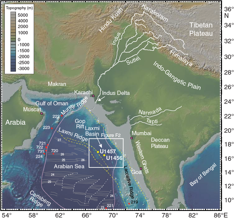
Figure F1. Bathymetric map of the Arabian Sea and surrounding landmasses.
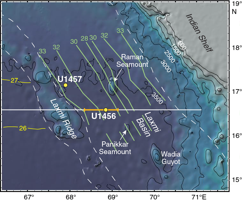
Figure F2. Bathymetric map of the region around Laxmi Basin with locations of Sites U1456 and U1457 in relation to other major bathymetric features.
Paleogeographic reconstructions of the northern Indian Ocean suggest that rifting between the India-Seychelles continental block and Madagascar initiated in Mascarene Basin and continued until Chron C27, ~62 Ma (Bernard and Munschy, 2000; Müller et al., 2000). Rifting of the Seychelles Block from India did not occur until 64–62 Ma (Miles and Roest, 1993; Chaubey et al., 1998; Collier et al., 2008). The final phase of rifting along this margin is linked to the emplacement of Deccan Traps Flood Basalts, supposedly at the initiation of Réunion mantle plume activity (Mahoney, 1988; White and McKenzie, 1989); however, the temporal and spatial relationships between Deccan Traps Flood Basalts and rifting between the Seychelles and India are yet to be resolved.
The nature of the crust in Laxmi Basin is highly enigmatic. Laxmi Ridge, which is a structural and topographic high exhibiting a negative free-air gravity anomaly of 25–50 mGal, is usually interpreted as a continental fragment of India (Naini and Talwani, 1982; Talwani and Reif, 1998; Minshull et al., 2008). In contrast, identification of the oldest seafloor-spreading magnetic anomalies in the Arabian Sea is a matter of long-standing debate. The oldest identified anomalies vary from Chron 27n (62.1 Ma; Miles et al., 1998) west of Laxmi Ridge in the Arabian Basin to Chron 33n (~79.5 Ma; Bhattacharya et al., 1994) to the east of Laxmi Ridge (Figure F2). In contrast, Todal and Edholm (1998) suggested that Laxmi Ridge has oceanic affinity and interpreted the magnetic anomalies in Laxmi Basin as a continuation (Chrons 28n–31n) of anomalies in the Arabian Sea. However, Miles et al. (1998) and Krishna et al. (2006) argue that both Laxmi Ridge and Gop Rift are underlain by stretched continental crust and attribute the observed magnetic anomalies to strongly magnetized magmatic intrusions unrelated to seafloor spreading.
Thus, to test these hypotheses we needed to directly sample the basement underlying Laxmi Basin, which will have significant implications for the break-up history of India and the Seychelles. The operations plan for Site U1456 included coring through the ~1490 m of sediment overlying the basement and then penetrating at least 50 m into basement. Regional seismic profiles were used to choose a location where drilling would penetrate through major reflectors thought to be Paleogene and younger in age (Figure F3). The Miocene and younger reflectors have been identified based on regional correlation from industrial drilling sites on the Indus shelf in the north (Clift et al., 2001), as well as on the Indian shelf to the east (http://www.dghindia.gov.in). Dating these reflectors through direct sampling of the sedimentary section in Laxmi Basin is necessary to generate meaningful and robust sediment budgets for this region. In turn, these are required if we are to attempt a mass balance between erosion in the Himalayan source mountains and sedimentation in the Arabian Sea. In addition, we interpret the Paleogene reflector to represent the base of the Indus submarine fan and coring through it will offer much needed constraint on estimating the Indus Fan sediment budget, as well as dating the base of the fan, which can act as a minimum estimate for India/Eurasia collision.
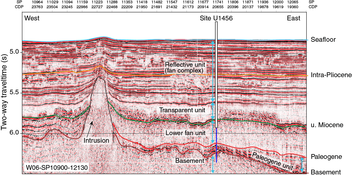
Figure F3. Seismic reflection profile Line W06 with location of Site U1456 and main seismically defined horizons.
Much of the shallower part of sediment section is dominated by a seismically reflective, largely flat-lying sequence interpreted as distal turbidite deposits related to the Indus Fan Megasequence of Droz and Bellaiche (1991) (Figure F3). The location of the site is relatively distal from the sediment source, which is also evident from the lack of well-developed channel-levee complexes that are observed on the upper fan (Kolla and Coumes, 1987; Clift et al., 2002). Normark et al. (1993) interpreted this type of reflective unit as a product of fan lobe sedimentation, and we anticipated that it would be largely composed of silty and muddy turbidites. Channel features are rare and generally shallow in form, although there is an onlapping of stacked channel-levee bodies against one another in the upper parts of the stratigraphy (Figure F3), as well as clear onlap against the steep sides of the Laxmi Ridge (Figure F4).
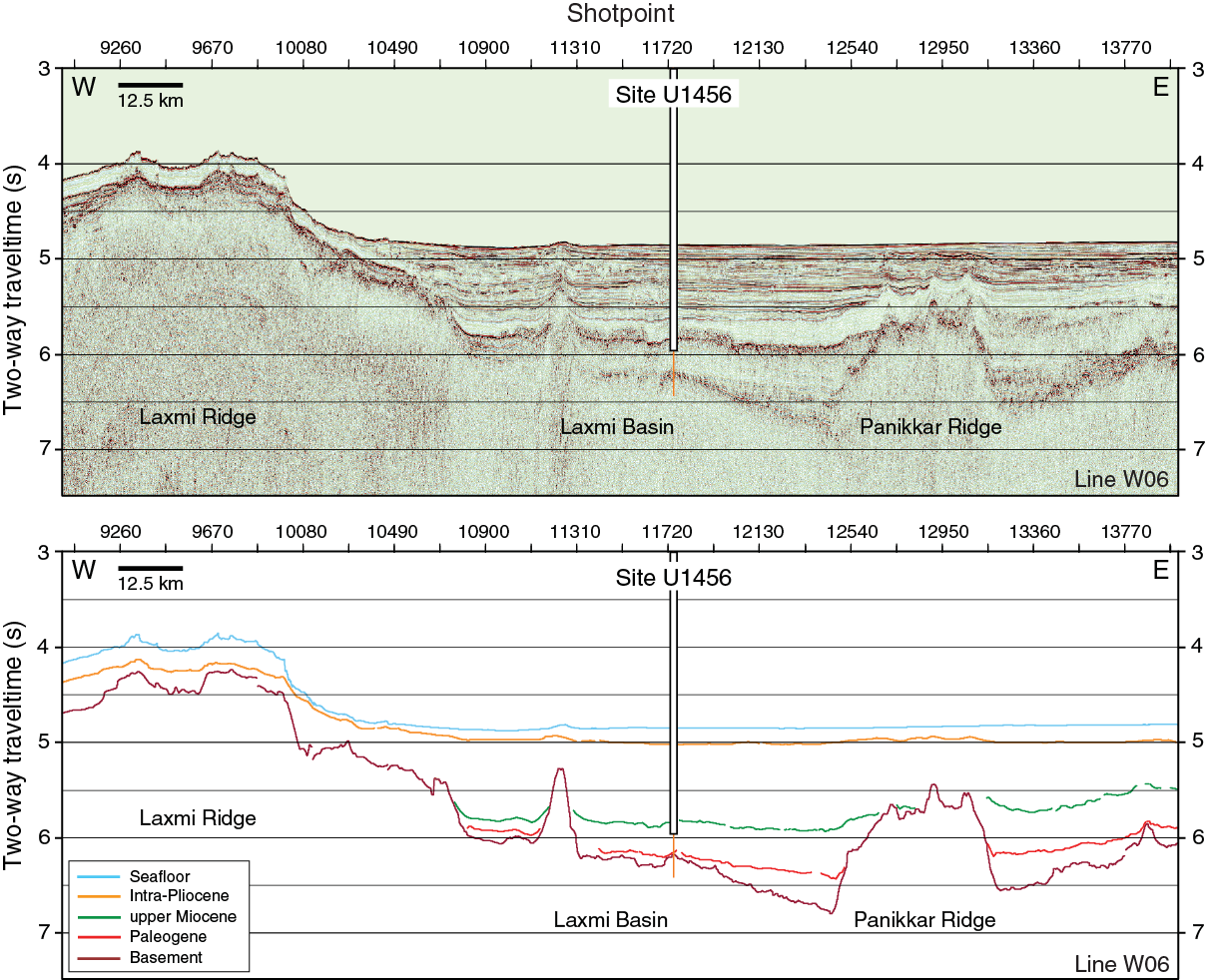
Figure F4. Uninterpreted seismic reflection profile Line W06 and interpreted seismic sections with location of Site U1456.
The bright reflective unit overlies an acoustically transparent unit that thins across the basin from east to west and is ~0.2 s two-way traveltime (TWT) thick at Site U1456 (Figures F3, F4). The transparent unit drapes Panikkar Ridge in the center of Laxmi Basin. The top of this unit slopes down westward into the basin, whereas the upper reflective unit lies disconformably above the transparent unit. The origin of this transparent unit is not well understood, but its geometry and seismic character suggest that the unit may be a large mass transport deposit, likely derived from the western Indian continental margin, rather than directly adjacent to the drilling site. Our original interpretation suggested that the top of the transparent unit lay close to the base of the Miocene.
A very bright reflector underlies this transparent unit, and below this level the sediment is less well bedded or clearly reflective. Below the transparent unit is the highly variable, weakly bedded Lower Fan unit. The lowermost Paleogene unit underlies this, thins from east to west, and is close to 0.1 s TWT thick at Site U1456, compared to a maximum of 0.4 s TWT in the central basin adjacent to Panikkar Ridge (Figure F4). Further west, this unit is disrupted by a late-stage intrusion that penetrates high into the Miocene section before the Paleogene disappears entirely against the side of Laxmi Ridge (Figures F3, F4). This Paleogene unit is believed to predate fan sedimentation and probably the onset of India/Eurasia collision. The source of sediment in the Paleogene is thus inferred to be dominantly from peninsular India to the east.
Scientific objectives
Site U1456 is the focus of a number of scientific objectives central to the success of Expedition 355. We planned to core at least 50 m of basement to find out the nature of the crust in Laxmi Basin, which would in turn determine whether it is true oceanic crust or some sort of transitional crust, such as intruded continental crust, or even exposed serpentinized upper mantle, such as that which characterizes the continent/ocean boundary offshore Iberia and Newfoundland in the North Atlantic (Boillot et al., 1988; Kusznir and Karner, 2007). Additionally, analyses of sediment retrieved from the basin will allow us to constrain depositional environments during the syn- and postrift periods that can be used to examine vertical motions and thus the tectonics of extension, particularly the timing and nature of strain accommodation.
Sampling and dating the base of the Indus Fan is a primary expedition objective because this has only been inferred elsewhere in the northern Arabian Sea based on the occurrence of Himalayan material in 45 Ma sandstone on Owen Ridge at Deep Sea Drilling Project (DSDP) Site 224 (Clift et al., 2001) and by the transition from pelagic biogenic sediment in the Eocene to more muddy hemipelagic sediment in the upper Eocene and Oligocene at DSDP Sites 220 and 221 at the southern tip of the fan (Shipboard Scientific Party, 1974a, 1974b).
Another primary objective is to recover a continuous Eocene and Oligocene sequence to aid in reconstructing patterns and rates of erosion, as well as continental environmental conditions (e.g., humidity and vegetation patterns) in the Indus drainage during the earliest phases of India/Eurasia collision. Although a muddy Eocene unit is found in the Himalayan foreland basin, called the Gazij, Subathu, and Bhainskati Formations, respectively, in Pakistan (northwest India) and Nepal (Raiverman, 1979; Najman, 2006), it is widely recognized that there is no Oligocene–lower Miocene known through most of the foreland basin. This gap precedes the exhumation of the Greater Himalaya and hampers understanding of the conditions that led to the major change in Himalayan tectonics as the Main Central Thrust became active around 23 Ma (Catlos et al., 2007; Searle et al., 2008). This site is designed to provide a continuous record through this missing, mostly Oligocene section, which should allow us to understand how the monsoonal climate evolved during this critical tectonic and climatic transition and to determine erosion patterns and rates at the time of the onset of Greater Himalayan exhumation. In particular, we will test the hypothesis that the start of the exhumation process was driven by an intensification of summer monsoon precipitation and increased erosion along the southern flank of the Tibetan Plateau (Clift et al., 2008b). Direct coupling of erosion rates and exhumation is a prediction of the channel flow model for Himalayan evolution (Beaumont et al., 2001; Hodges, 2006), although it might also be applicable to some tectonic wedge models for structural evolution (Robinson et al., 2006).
Although the Neogene history of the Himalaya is better known than the Paleogene, coring at Site U1456 is designed to provide a continuous record of erosion, weathering, and environmental history from the western Himalaya in order to complement records already compiled from the foreland basin (Quade et al., 1995; Burbank et al., 1996; Sanyal et al., 2004; Singh et al., 2012) and Bay of Bengal, cored during IODP Expedition 354 (France-Lanord et al., 2015). Because the source regions of the Indus Fan are quite different from those in the Ganges-Brahmaputra system and the monsoon is anticipated to be weaker in the western Himalaya and Karakoram compared to the eastern Himalaya, the response to climate change through the Neogene is unknown. Dating the seismic reflectors in the Neogene part of the section will allow us to derive a relatively high resolution sediment budget that can be compared in detail with climatic and environmental reconstructions.
Over this part of the section we will leverage existing climate records derived from earlier drilling along the Oman continental margin (Kroon et al., 1991; Prell et al., 1992) and at the same time generate a continental environmental record using a combination of chemical weathering proxies, organic geochemistry, and palynological data to constrain how continental conditions evolved in the Indus Basin over this time period. Critical issues that need to be addressed include the nature of the climatic transition at 8 Ma, which is traditionally thought to be a time of summer monsoon intensification, but which has recently been reinterpreted as a time at which drier conditions became established (Hoorn et al., 2000; Dettman et al., 2001; Singh et al., 2012). We will also examine whether this change in climate is accompanied by faster or slower erosion of the mountains themselves. Although sedimentation records preserved onshore in the Siwalik Group seem to show coarser and presumably faster erosion toward the end of the Miocene (Johnson et al., 1985; Ghosh and Kumar, 2000; Bernet et al., 2006; van der Beek et al., 2006), some reconstructions of marine sedimentation instead suggest that this was a time of slower erosion (Clift, 2006), although others argue for faster sediment supply to the Indian Ocean at that time (Rea, 1992; Métivier et al., 1999). We will attempt to resolve this debate through coring at this location.
Site U1456 also includes Pliocene–Pleistocene objectives. This time period is generally reconstructed as a time of stronger than average monsoon, albeit with rapid intensity transitions over relatively short timescales, probably driven by the same solar insolation that controls Northern Hemisphere ice sheet development (Clemens and Prell, 1991; Clemens et al., 2010). Early attempts to derive sediment budgets from the Indian Ocean indicate that this was a time of increased clastic sedimentation (Rea, 1992; Métivier et al., 1999), as recognized globally and presumed to be driven by rapid changes of climate over this time period (Zhang et al., 2001). More recently, cosmogenic isotope work suggests that the apparent increase in sedimentation rate is in fact an aberration derived from considering shorter and shorter time intervals, rather than being an actual response of the continents to changing climate (Willenbring and von Blanckenburg, 2010). Our detailed age model coupled with high-quality seismic profiling should allow us to address this issue.
We will also be able to study at relatively high resolution how erosion and chemical weathering patterns change in the fan source regions over glacial cycles. We can test the hypothesis that erosion was more centered in the Karakoram during glacial times but switched to become faster overall and focused more on the Lesser Himalaya during interglacial periods when the summer monsoon was stronger (Bookhagen et al., 2005; Clift et al., 2008a). Moreover, chemical weathering indexes will allow us to understand whether chemical weathering fluxes increase or decrease in the system during glacial cycles. Because chemical weathering itself helps to draw down atmospheric CO2 concentration, a well-known greenhouse gas, it is possible that the chemical weathering response to glacial cycles may either intensify or moderate the solar-driven cycles (Berner and Berner, 1997). Although this has been ruled out at high latitudes (Foster and Vance, 2006), the response of low latitudes is still uncertain. As the largest orogenic belt on Earth, the weathering response of the Himalaya to climate forcing may also be a primary control to global climatic conditions (Raymo and Ruddiman, 1992).
Operations
Summary
The original operations plan for Site U1456 (proposed Site IND-03C) called for three holes: the first to advanced piston corer (APC) refusal, followed by a second APC hole with extended core barrel (XCB) coring to ~650 m below seafloor (mbsf). The third hole was a planned reentry hole including 650 m of casing followed by coring to a total depth of ~1590 mbsf, which included 100 m of basement. The plan was modified to include a short APC hole for high-resolution microbiological and geochemical sampling of the upper ~30 m. We ultimately cored five holes at Site U1456 (Table T1).
Table T1. Site U1456 core summary. Download table in .csv format. View PDF table.
When APC refusal was reached at a much shallower depth than anticipated (~140 mbsf), we opted to deepen Hole U1456A using the half-length advanced piston corer (HLAPC). Because of good hole conditions, we continued coring in Hole U1456A with the XCB to 426.6 mbsf, at which point the XCB cutting shoe detached and was left in the hole, forcing us to abandon the hole. Hole U1456B was cored with the APC to 29.1 mbsf. We then cored Hole U1456C with the APC and HLAPC to 221.6 mbsf, drilled ahead without coring to 408.0 mbsf, and then continued coring with the XCB to 465.2 mbsf. We terminated coring operations in Hole U1456C when we determined that the lithology at 465.2 mbsf would be ideal for the base of the casing for our deep hole. After conditioning the hole for logging, we conducted three logging runs in Hole U1456C. The triple combo tool string was run first without the radioactive source to 465 m wireline depth below seafloor (WSF), and then the Formation MicroScanner (FMS)-sonic tool string was run to 465 m WSF with two upward passes. The last logging run was made with the triple combo tool suite with the radioactive source after the hole was determined to be in good condition.
In Hole U1456D, we drilled-in a 10¾ inch casing string to 458.8 mbsf and then began coring with the rotary core barrel (RCB) coring assembly. When we reached 1024.4 mbsf, we pulled out of the hole for a bit change; however, we encountered difficulties reentering the hole. The drill string became stuck in the open hole below the casing and ultimately had to be severed, effectively terminating the hole. We then decided to install a longer 10¾ inch casing string to 748.2 mbsf in Hole U1456E, drilled without coring to 970 mbsf, and then continued to RCB core to 1109.4 mbsf. We pulled out of the hole for a bit change and again encountered difficulties trying to trip the drill string back to the bottom of the hole. After little progress was made to advance the bit over a 12 h period and several instances of the drill string getting temporarily stuck, we decided to terminate the hole and end operations at Site U1456. The total time spent on Site U1456 was 885 h (36.9 days).
A total of 197 cores were collected at this site. The APC coring system was deployed 35 times, recovering 276.91 m of core over 301.9 m of penetration (92% recovery). The HLAPC system was deployed 72 times, recovering 287.55 m of core over 334.8 m of penetration (86% recovery). The XCB coring system was deployed 13 times, recovering 44.58 m of core over 94.3 m of penetration (47% recovery). The RCB coring system was deployed 77 times, recovering 401.63 m of core over 705.0 m of penetration (57% recovery).
Transit to Site U1456
After a 941 nmi transit from Colombo, Sri Lanka, averaging 11.1 kt, the vessel arrived at the first expedition site, U1456. A prespud meeting was held prior to arrival to review operations at the first site. The vessel stabilized and switched from cruise mode to dynamic positioning at 1054 h (all times are local; UTC + 5.5 h) on 9 April 2015. The positioning beacon was deployed at 1108 h. The position reference was a combination of GPS signals and a single acoustic beacon.
Hole U1456A
After arriving and deploying the acoustic positioning beacon, initial operations in Hole U1456A included picking up drill collars from the forward main deck pipe rack, spacing out the APC/XCB coring systems, and measuring (strapping) and verifying the internal diameter (drifting) of all tubulars during the first pipe trip of the expedition. The bottom-hole assembly (BHA) included two stands of 5½ inch drill pipe, a tapered drill collar, five 8¼ inch control length drill collars, a nonmagnetic drill collar, head sub, top sub, latch sub, seal bore drill collar (which serves as the outer core barrel for the coring system), bit sub with a lockable float valve, and a “used” 9⅞ inch Russian polycrystalline diamond compact (PDC) APC/XCB core bit.
After pumping a drill string wiper plug, we deployed the APC coring system, spudding Hole U1456A at 0210 h on 10 April after offsetting the ship 15 m to the west of the original prospectus coordinates for the drill site. We positioned the bit at a depth of 3645.0 m below rig floor (mbrf), and the first APC core was on deck at 0235 h, recovering 4.54 m of sediment and establishing a seafloor depth to the rig floor of 3650.0 mbrf. This hole was originally planned as an APC/XCB hole to ~250 mbsf; however, because the hole conditions were better than anticipated we elected to continue drilling to ~600 mbsf as planned initially for Hole U1456C.
Oriented APC coring using nonmagnetic core barrels and plastic bags containing fluorescent microspheres for microbiology contamination testing continued through Core 355-U1456A-16H to 139.3 mbsf. The advanced piston corer temperature tool (APCT-3) was deployed for Cores 4H (33.0 mbsf), 7H (61.5 mbsf), 10H (90.0 mbsf), and 13H (118.5 mbsf). The first deployment was unsuccessful due to flooding of the APC shoe pressure case. After two successive partial strokes on Cores 15H and 16H, with the latter returning only a small amount of sediment in the core catcher, we decided to switch to the HLAPC. Coring continued using the HLAPC coring system from Core 17F through 40F to 249.3 mbsf. Although we originally planned to end Hole U1456A at 250 mbsf, we opted to continue coring due to good hole conditions and good recovery.
Coring with the HLAPC continued in Hole U1456A through Core 70F to 389.5 mbsf. The coring system was changed to the XCB system and at 0615 h on 13 April 2015, the first XCB core (71X) was on deck, recovering 7.10 m. Coring continued through Core 74X. When that core barrel was retrieved on deck, the XCB cutting shoe was missing. Further examination revealed that it had broken off at the last engaged thread of the inner barrel connection, terminating Hole U1456A at 426.6 mbsf. Although short of the planned depth of ~600 mbsf, discussions had been under way to possibly terminate the hole at 450–460 mbsf due to the consistently fine grained lithologies encountered below 400 mbsf. We decided to defer wireline logging in Hole U1456A in favor of logging Hole U1456C, which would likely be deeper and open for a shorter period of time. The drill string was tripped back to the seafloor with the top drive in place in case any problems were encountered in the hole due to the unconsolidated sands. Although a fair amount of sand was evident in the cores, the driller did not experience any difficulty recovering the drill string. The bit cleared the seafloor at 1805 h, ending Hole U1456A and beginning Hole U1456B. A total of 4.3 days were spent in Hole U1456A.
Hole U1456A consisted of 16 APC cores recovering 121.18 m of core over 139.3 m of penetration (87% recovery), 54 HLAPC cores recovering 216.22 m of core over 250.2 m of penetration (86% recovery), and four XCB cores recovering 27.85 m of core over 37.1 m of penetration (75% recovery). The total depth of the hole was 426.6 mbsf.
Hole U1456B
The ship was offset 15 m to the east of the original site coordinates, with the bit positioned at 3647 mbrf, 2 m lower than for Hole U1456A. Hole U1456B was started at 1955 h on 13 April 2015. A seafloor depth of 3655.8 mbrf (3645.0 m below sea level [mbsl]) was established based on APC core recovery, which was ~7 m deeper than the previous hole located 30 m to the west. Based on discussions with the coring technician on watch, we determined that a significant amount of material was lost due to the soupy nature of the core, which led to an inaccurate seafloor depth. This hole was planned as a dedicated microbiology hole to consist of three cores; however, because the recovery was only 0.69 m in Core 355-U1456B-1H, we decided to take one additional core. APC coring continued through Core 4H to 29.1 mbsf where the hole was terminated. The bit was pulled clear of the seafloor at 2355 h on 13 April 2015, ending Hole U1456B and beginning Hole U1456C. We spent 0.3 days on Hole U1456B, which consisted of four APC cores recovering 28.79 m of core over 29.1 m of penetration (99% recovery). The total depth of Hole U1456B was 29.1 mbsf.
Hole U1456C
The ship was offset 15 m north of the original site coordinates, with the bit positioned at 3647 mbrf. Hole U1456C was started at 0050 h on 14 April 2015. The seafloor depth for this hole was established based upon APC core recovery as 3649.2 mbrf (3638.4 mbsl). Oriented APC coring continued through Core 355-U1456C-17H to 134.3 mbsf. Core 18H achieved only a partial stroke advancing to 137.0 mbsf with limited recovery of 2.72 m, apparently hitting a significant sand layer. The bit was advanced by recovery and the coring system was changed to the HLAPC. Cores 19F through 36F were recovered to a depth of 221.6 mbsf with Core 36F on deck at 1155 h on 15 April 2015. During HLAPC coring, each interval was advanced 4.7 m regardless of recovery. After Core 36F was retrieved, coring was suspended, and an XCB center bit assembly deployed to drill to 408.0 mbsf. Drilling of the 186.4 m interval required 12.25 h to complete. We suspect that bit balling of the PDC bit in the soft clay formation slowed the drilling. In addition, hard layers were occasionally encountered, requiring a longer amount of time to penetrate because of the limited weight-on-bit that could be applied due to the presence of the XCB center bit. The net rate of penetration (ROP) achieved (including connection time, mud sweeps, etc.) was 15.2 m/h. Thirty-barrel sea gel mud sweeps were pumped every 30 m to proactively avoid sand build-up in the annulus and to help prevent any recurrences of the stuck wireline barrels that occurred in Hole U1456A.
After reaching 408.0 mbsf, the center bit was recovered and an XCB core barrel deployed. At 0230 h on 16 April 2015, XCB coring resumed in Hole U1456C. Cores 355-U1456C-38X and 39X were cut and recovered to 418.0 mbsf. Core 39X was on deck at 0745 h. While Core 39X was being recovered, a notification came from the bridge (at ~0700 h) that they were observing an unknown vessel located ~3.5 nmi away from the drill site. Soon after, the bridge instructed the drill floor to suspend coring operations and begin pulling out of the hole to near the seafloor when the vessel began to approach. The vessel began deploying fishing line in the vicinity of the R/V JOIDES Resolution and also motioned to personnel onboard that they wanted food. After being instructed that we were a research vessel and that they needed to standoff a minimum of 3 nmi from our drilling location, the vessel departed. At 0845 h, the drill crew began tripping pipe back to the bottom of the hole and XCB coring resumed, with Cores 40X through 46X cut and recovered to 465.2 mbsf. At this point we determined that this depth would make a reasonable casing point and that the material being cored was recoverable with the RCB coring system. Coring operations were terminated in Hole U1456C and we began to prepare the hole for wireline logging operations.
A 40 bbl sea gel mud sweep was circulated out of the hole and at 0215 h on 17 April 2015, a wiper trip was conducted to 56.3 mbsf. The driller detected no overpull, excessive drag, or fill on the bottom. At 0645 h on 17 April, the lockable float valve (LFV) go-devil was deployed, another 40 bbl sea gel mud sweep pumped, and after chasing the sweep with 500 strokes of seawater, the hole was displaced with 171 bbl of 10.5 lb/gal heavy mud. The drill string was then positioned with the end-of-pipe at a logging depth of 81.1 mbsf. We started assembling the first wireline logging tool string (triple combo without the source), and it was deployed at 1155 h on 17 April. This suite of logging tools reached the total borehole depth of 465.2 mbsf, and after an up-log was collected, the tool string was retrieved to the rig floor at 1740 h. The second suite of tools, the FMS-sonic tool string, was deployed at 1810 h and also was able to reach bottom. Two up-passes were collected with the FMS-sonic, and the tool string was retrieved to the surface at 0315 h on 18 April. The third and final logging run was made with the triple combo tool suite, this time with the source after the hole was determined to be in good condition. The tool string was deployed at 0445 h, reached the total depth of the hole, and was then retrieved to the rig floor at 1150 h on 18 April. After rigging down from logging the subsea camera was deployed, and the drill string was pulled out of the hole, clearing the seafloor at 1440 h on 18 April. The vessel was offset in dynamic positioning mode to 15 m south of the original site coordinates. A drill string tag of the seafloor was observed on the subsea camera, establishing a seafloor depth adjusted to the rig floor dual elevator stool of 3648.0 mbrf for the next hole (U1456D). The subsea camera was then returned to the surface while we began to trip the drill string back to the vessel. We completed the pipe trip out of Hole U1456C, racked the drill collars back in the derrick, and laid out the seal bore and nonmagnetic collars to the forward pipe rack. The bit cleared the rig floor at 0220 h on 19 April, officially ending Hole U1456C and beginning Hole U1456D.
Hole U1456C consisted of 15 APC cores recovering 126.94 m of core over 133.5 m of penetration (95.1% recovery), 18 HLAPC cores recovering 71.33 m of core over 84.6 m of penetration (84.3% recovery), and nine XCB cores recovering 16.73 m of core over 57.2 m of penetration (29.2% recovery). The total depth of the hole was 465.2 mbsf. Total time spent on Hole U1456C was 5.1 days.
Hole U1456D
The vessel was offset 15 m south of the original site coordinates and the seafloor tag depth of 3648.0 mbrf (3637.1 mbsl) used as the official seafloor depth for the hole. After laying out the upper guide horn, preparations began for installing the reentry cone and 10¾ inch casing string. The 16 inch casing hanger assembly was made up and racked back in the derrick. We then assembled and tested the 458.83 m long drilling assembly, which consisted of the 9⅞ inch tricone drilling bit, 8 inch mud motor, and underreamer with arms set to 12¾ inches. The preassembled standard reentry cone was positioned over the moonpool doors. We began to run casing at 1200 h on 19 April 2015. The casing string, made-up of a Texas-pattern casing shoe, shoe joint, 33 joints of 10¾ inch casing, a 16 inch × 10¾ inch casing crossover (swage), 16 inch casing pup joint, and a 16 inch casing hanger, totaled 455.11 m in length. This assembly was lowered into the reentry cone using the casing running tool. At 2045 h, the driller lowered the drilling assembly into the reentry cone and latch-in was completed at 0035 h on 20 April. At 0100 h we began tripping the assembly toward the seafloor. During the pipe trip, the subsea camera was deployed, and the drill pipe filled with seawater every 15 stands.
After picking up the top drive, Hole U1456D was spudded at 1035 h on 20 April. It required a total of 20.75 h to drill in the 455 m of casing. The reentry cone base landed on the seafloor at 0710 h on 21 April, positioning the casing shoe at a depth of 455.1 mbsf. The driller rotated the drill string 3½ turns to the right to release the casing running tool; however, the drilling assembly was unable to pull free of the reentry cone and casing. We attempted to free the assembly over the next 4.25 h by offsetting the ship in a grid pattern away from the hole location. After this did not free the assembly, it became clear that the running tool was released, but the underreamer arms had not fully retracted. At 1135 h on 21 April, the drilling assembly was pulled free with 15,000 lb of overpull. While pulling the drill string, the underreamer continued to drag intermittently inside the casing, predominantly when passing through casing couplings. The top drive was set back, the subsea camera retrieved to the ship, and the bit pulled clear of the seafloor at 1540 h. After tripping the assembly back to the ship, the running tool was de-torqued, the drill collars racked back in the derrick, the mud motor and underreamer assemblies flushed with freshwater, and at 0140 h on 22 April, the bit cleared the rotary table. From start to finish, using a mud motor and underreamer assembly, we required only a total of 3 days to make up and install a standard reentry cone with 455 m of 10¾ inch casing in 3637 m water depth using the drill-in casing approach.
With the reentry cone and casing installed, the drill crew requested time to investigate a noise they had heard on multiple occasions that emanated from the drilling package. During operations they were unable to determine whether the source of the noise was the top drive itself or the swivel assembly. A total of 9 h of “downtime” were taken to separate the swivel from the top drive and thoroughly investigate the issue. Ultimately the gear was all reassembled without identifying the original source of the noise. Once everything was reassembled, the noise was no longer heard.
We then made up the RCB BHA assembly and, after slipping and cutting the drilling line, began tripping toward the seafloor. The subsea camera was deployed during the pipe trip; however, after there was a problem with the video feed, the camera was brought back aboard, repaired, and redeployed. At 0245 h on 23 April we reentered Hole U1456D after maneuvering the ship for only 20 min. The drill string was lowered into the casing string to a depth of 416.0 mbsf (39.1 m above the casing shoe) when soft fill was tagged. We picked up the top drive, deployed a wash barrel, and began to slowly circulate. The fill was cleared by 0800 h on 23 April. A 40 bbl sea gel mud sweep was circulated out and the wash barrel recovered. At 1000 h on 23 April, a core barrel was deployed and continuous RCB coring using nonmagnetic core barrels initiated. RCB coring continued with 30 bbl sea gel mud sweeps pumped every third core. Although we encountered no fill on bottom between cores, rapid penetration rates, low recovery, and evidence of sand in the recovered core material indicated there was still some sand in the formation. We therefore initiated preventative measures in order to preserve the integrity of the hole as much as possible.
RCB coring continued without incident through Core 355-U1456D-43R to 866.2 mbsf. Hole conditioning consisted of pumping 40 bbl sea gel mud sweeps every third core. While cutting Core 44R, the driller noted erratic changes in pump pressure and excessive torque. After pumping a 40 bbl mud sweep, the core barrel landed with a 200 psi pressure loss. After advancing 2.0 m the lost pressure was regained; however, after advancing another 1.0 m the hole apparently began to collapse around the drill string. Pump pressure increased by 600 psi, top drive torque increased by 200 amps, and there was a 20,000 lb weight loss. We spent 2.25 h circulating and working the pipe back to 821.0 mbsf. We then recovered Core 44R and completed a wiper trip to just inside the 10¾ inch casing shoe at 442.6 mbsf. The wiper trip was uneventful, with no apparent issues with the upper portion of the hole. After taking a short period of time to service the rig and grease the traveling block, the pipe was tripped back in the hole. The pipe was lowered to 821.0 mbsf, with the driller noting 10,000–15,000 lb of drag from 722.0 to 753.0 mbsf. We picked up the top drive at 0930 h on 27 April, and after beginning circulation we noted a 400 psi pump pressure excess, indicating that the annulus of the hole was filled with drill cuttings. We pulled the pipe back to 791.9 mbsf and deployed a wash barrel. At 1100 h the pipe was washed/reamed back to the original total depth of 869.2 mbsf, encountering 12 m of fill at the bottom of the hole. We circulated a 50 bbl sea gel mud sweep and then spent an additional 2.5 h circulating a series of mud sweeps (two 50 bbl sweeps at 110 viscosity, a 50 bbl sweep at 120 viscosity, and a 60 bbl sweep at 130 viscosity) before regaining normal drilling parameters.
With the hole stabilized, we recovered the wash barrel and deployed an RCB core barrel. At 1830 h on 27 April, RCB coring recommenced. As a preventative measure, the drillers pumped 50 bbl high-viscosity mud sweeps every other core to help prevent any recurrence of cuttings build-up in the hole annulus. Coring continued without incident through Core 54R to 966.2 mbsf. While cutting Core 55R, an abrupt change in ROP occurred at ~970 mbsf. ROP dropped to 2.9 m/h. We recovered Core 55R after only a 6.0 m advance and found that the core barrel had been jammed, resulting in poor recovery (3%). We recovered Core 56R after a 6.0 m advance (125 min at 2.9 m/h) because of concerns that the barrel may have jammed again; however, the core barrel was full (111% recovery), and the slow ROP was found to be due to the hard sandstone lithology encountered. We picked up a knobby drilling joint for cutting Core 57R to 987.4 mbsf. This 9.2 m advance required 270 min of rotating time (2.0 m/h). At this point, hole conditions became problematic with high torque (600 amps) and pump pressure elevated by 400 psi. We spent >8 h working the pipe, circulating multiple 50 bbl high-viscosity mud sweeps, and conditioning the hole before coring could resume. At 1830 h on 29 April, we resumed coring. Core 58R was cut to 996.6 mbsf (9.2 m advance) in 160 min at 3.5 m/h. After recovering this core and deploying the next core barrel, hole conditions again deteriorated. Top drive torque increased, and when the core barrel landed the driller noted that he had lost the ability to rotate the pipe. The pipe was freed in <1 h; however, this required 900 amps of top drive torque and 55,000 lb of overpull. Core 59R was cut to 1005.8 mbsf with a slightly higher ROP. Coring continued through Core 61R to 1024.4 mbsf at an average ROP of 6.0 m/h. Because of the accumulated bit rotating hours plus the intangible unrecorded reaming hours, we decided to cut one additional core and then round trip the drill string for a bit change. When the core barrel landed for the final core, the WKM valve on the top drive failed and would not seal properly. Because replacing the valve required tripping the pipe up inside the casing shoe at 455 mbsf, we decided instead to recover the entire drill string to change the bit and also repair the WKM valve.
We displaced the hole with heavy mud, recovered the empty core barrel, and pulled the drill string clear of the seafloor at 1900 h on 30 April. We offset the vessel 50 m from the reentry cone, serviced the rig, and removed the WKM valve to expedite the required repairs. The drill string was recovered back to the surface with the bit clearing the rotary table at 0355 h on 1 May. We checked all outer core barrel subs, inspected the RCB latch sleeve, and prepared a new CC-4 RCB bit. The BHA was reassembled, and by 1045 h the drill string was deployed to 3274.4 mbrf when the 5½ inch pipe racker developed a problem. We spent 45 min troubleshooting and fixing the pipe racker. The pipe trip resumed to 3624 mbrf, and then the subsea camera was deployed and lowered toward the seafloor for reentry. While the camera was being deployed, the spare WKM valve was installed on the top drive in preparation for coring operations. We began maneuvering the ship at 1440 h on 1 May and reentered Hole U1456D in 35 min. We recovered the subsea camera to the ship and continued tripping the pipe inside the 10¾ inch casing to 442.6 mbsf, where we encountered unexpected resistance. We pulled back the pipe, deployed a wash barrel, and picked up the top drive. Using very slow rotation and minimal pump pressure, the bit was lowered through the obstructed area with no discernable indication of resistance. We lowered the drill string below the casing shoe to 529.9 mbsf, recovered the wash barrel, and racked back the top drive.
We continued to lower the drill string without incident to a tag depth of 995.8 mbsf with a maximum drag of 10,000 lb. We picked up the drill string to 966.6 mbsf and picked up the top drive. At 0100 h on 2 May, the driller attempted to break circulation and realized that he could not rotate the string or circulate fluid. The driller picked up the drill string to 937.5 mbsf with no overpull. We picked up a knobby joint and the top drive and worked the drill string for 2.75 h. Circulation was reestablished; however, 900 amps of maximum torque and 150,000 lb of overpull failed to free the drill string. At 0600 h on 2 May, we offset the ship 185 m (5% of water depth) to the south to set a drill pipe tool joint at the rig floor. The sinker bars were installed with a core barrel attached, and this assembly was lowered into the drill string to determine if there were any mechanical issues with the integrity of the drill string or if hole instability and stuck pipe was the sole issue. The core barrel would not pass a depth approximately equal to the seafloor depth (hard tag at ~3668 mbrf), indicating that there were other issues in addition to hole conditions. The vessel was offset to allow recovery of the wireline assembly, the upper guide horn pulled, and the subsea camera deployed to determine if there was a problem at the seafloor. The subsea camera showed that the reentry cone was buried in cuttings; however, the drill pipe appeared to be extending straight up from the reentry cone/cuttings pile. We observed no identifiable problem with the drill pipe or the seafloor installation. We recovered the subsea camera on deck at 1240 h on 2 May.
At this point we decided to sever the drill string and abandon Hole U1456D. We hoped to sever in the first joint of 5½ inch drill pipe (transition joint) above the tapered drill collar (TDC) at the top of the BHA; however, there was some concern that (1) the wireline severing tool may not be able to pass the seafloor and (2) if the pipe was severed above the BHA the drill pipe above may still remain firmly stuck in the hole. We held a safety meeting at the rig floor and preparations began for rigging up the Schlumberger wireline drill pipe severing tool. After securing radio silence and shutting down all wireless devices, the severing tool was deployed at 1800 h on 2 May. There was no problem passing through the transition zone at the seafloor, and the tools reached all the way to the bit. The system was then recovered and positioned at the approximate midpoint (~4.5 m) of the first joint of 5½ inch drill pipe above the TDC. We applied a slight amount of torque and overpull to the drill string before the charge was fired; however, no voltage was sent. The Schlumberger computer used to control the system was rebooted and the second attempt to fire the charge was successful. The driller was then able to pull the drill string back to the next tool joint and rotate, indicating that the string was successfully severed at the location desired and freed from the formation.
While pulling the Schlumberger wireline severing tools, the Schlumberger engineer indicated that a weak link on the Schlumberger cable head had failed and the severing tool assembly was lost in the hole. With the top drive in, the drill string was pulled back to 756.6 mbsf. Overpull was 10,000–15,000 lb. The top drive was set back and the drill string pulled clear of the seafloor at 0425 h on 3 May. When the drill string reached 753.9 mbrf it became apparent why the core barrel deployed earlier via wireline would not pass the seafloor depth. Several joints of 5 inch drill pipe that had extended from just below the seafloor and deeper into the hole were recovered severely bent. The next 13 h were spent removing the joints from the drill string and laying them out with the pipe racker to the port-side inboard bay of the riser hold. In total, there were 39 joints (~377 m) of bent 5 inch drill pipe. The four-stand RCB BHA that was lost in the hole included 11 control length drill collars, one TDC, a new CC-4 RCB core bit, a complete mechanical bit release assembly (MBR), two modified head subs, and one modified top sub. A detailed list of lost hardware was prepared along with an incident report. The remainder of the drill string was intact, and the severed end of the last joint of 5 inch drill pipe cleared the rig floor at 2200 h on 3 May. This officially ended Hole U1456D and began Hole U1456E.
Hole U1456D consisted of 60 RCB cores recovering 319.18 m of core over 656.6 m of penetration (56% recovery). Including the initial drilled interval, the total depth of the hole was 1024.4 mbsf. Total time spent on Hole U1456D was 14.8 days.
Hole U1456E
Because we had not achieved our objectives at Site U1456, we decided to install a new casing string to ~750 mbsf to stabilize the unconsolidated sands above this depth. The drill crew cleared the rig floor of all remnants of the bent pipe recovery (cut-off tool joints, etc.) and serviced the rig. At 2245 h on 3 May 2015 the drill crew began picking up the 11 additional control length drill collars and TDC required to make up the BHA for drilling operations in Hole U1456E. The drill collars were made up into stands and racked back in the derrick. The upper guide horn was laid out to the forward main deck pipe rack, and the casing running tools, subs, and equipment were picked up. At 0700 h on 4 May, we began to assemble the drilling stinger. This included a 9⅞ inch R2 tricone drill bit, a bit sub with LFV, an underreamer with the mill tooth arms/cutters set to 12¾ inch diameter, and a positive displacement mud motor. This assembly was deck tested with the motor beginning rotation at ~25 strokes/min of the mud pumps, and with the underreamer arms fully opening at 30–35 strokes/min. After testing, the assembly was laid out on the pipe racker. The Hole U1456E reentry cone was moved over the center of the moonpool doors and a 16 inch casing hanger with pup joint was lowered and latched into the reentry cone using the 16 inch casing running tool. A 10¾ inch casing hanger assembly was made up with the 10¾ inch casing running tool and the power tongs and casing running equipment rigged up. At 1430 h on 4 May we began making up the 10¾ inch casing string. The first five joints were welded together and the casing hanger was also welded to the last casing collar. Including the shoe joint, 55 joints of casing were made up in 8.5 h, and by 2400 h on 4 May, the 10¾ inch casing hanger was landed and latched into the reentry cone assembly. The drilling stinger assembly was then picked up, along with 23 stands and one single of 5 inch drill pipe, run inside the casing string, and the casing running tool was attached to the 10¾ inch casing hanger. Three hours were spent working on the 5½ inch pipe racker jacking assembly before beginning the pipe trip toward the seafloor.
At 0700 h on 5 May, with the drilling stinger assembly (bit) extending 4.82 m ahead of the casing shoe, the reentry cone, casing, and drilling stinger assembly were deployed. This space-out assembly placed the underreamer arms 2.61 m below the 10¾ inch casing shoe. While lowering the casing toward the seafloor, the pipe was filled with seawater every 15 stands, the drilling line was slipped and cut, and the subsea camera deployed for reentry. The drilling assembly reached the seafloor by 2045 h on 5 May. We then picked up the top drive, and the drill string was spaced out. At 2130 h, Hole U1456E was spudded. We spent the next day drilling in the casing to 743.4 mbsf. The reentry cone landed at the seafloor (3648 mbrf) at 0100 h on 7 May. We then released the casing string and retracted the underreamer assembly back up inside the casing. After setting back the top drive, the subsea camera and drill string were recovered to the ship. After the drilling assembly cleared the seafloor at 0410 h on 7 May, the vessel was offset 50 m east of the reentry installation as a precaution. After spending 1 h repairing a ruptured hose on the iron roughneck, the pipe trip was completed by 1415 h. We then washed and laid out the mud motor/underreamer assembly.
At 1615 h on 7 May, we began making up the new RCB drilling/coring BHA. The drill string was once again tripped to the seafloor, and the subsea camera deployed. After maneuvering the ship for 36 min, we reentered Hole U1456E. The subsea camera was recovered, the pipe advanced to 706.1 mbsf (still inside the casing string), the top drive picked up, and a RCB core barrel dressed with a center bit was deployed. The bit was advanced to 748.2 mbsf before tagging the bottom of the hole. This was the depth the drilling “stinger” assembly reached when drilling in the 10¾ inch casing shoe, indicating that there was no fill at the bottom of the hole. We pumped a 30 bbl high-viscosity mud sweep and at 0830 h on 8 May began drilling without coring with the RCB center bit. A total of 26.5 h were required to advance the 9⅞ inch diameter hole to 970.0 mbsf, and at 1100 h on 9 May, the drill ahead was completed. The overall average rate of penetration for the 221.8 m interval drilled was 10.9 m/h. We pumped a 40 bbl mud sweep and recovered the RCB center bit; however, before a core barrel could be dropped the driller noted that he had 4 m of fill on bottom. Therefore, instead of dropping a RCB core barrel, we deployed a wash barrel and pumped two 50 bbl high-viscosity mud sweeps out of the hole at a circulating rate of 130 strokes/min. Once the hole was considered to be clean the wash barrel was recovered, and at 1545 h on 9 May we deployed a core barrel and coring initiated in Hole U1456E from 970.0 mbsf. For reference, it required 5.6 days to drill in a new reentry cone and 10¾ inch casing assembly to 743.4 mbsf and then drill a 9⅞ inch hole to 970.0 mbsf. Prior to that, another 1.8 days had been spent severing the drill string and recovering the bent string of drill pipe. Total lost time due to the loss of Hole U1456D was 7.4 days.
We continued RCB coring in Hole U1456E through Core 355-U1456E-19R to 1109.4 mbsf with the rate of penetration varying from 2.9 to 7.0 m/h. To enhance hole cleaning the drillers pumped 40 bbl high-viscosity mud sweeps after each core. These were pumped at high annular velocity all the way to the surface prior to recovering the core barrel so that the cuttings from the entire cored interval would be flushed from the hole. After recovering Core 19R, we decided to recover the drill string, inspect the outer core barrel assembly, and change the bit because the present bit was approaching 60 h of use. We pumped a final mud sweep from the total depth of the hole and then displaced the open hole section with 125 bbl of heavy mud. We began to pull out of the hole but had to wait until the drill bit was inside the 10¾ inch casing shoe at 735.2 mbsf before we could set back the top drive, indicating that the formation was beginning to impinge on the open hole below the casing. Once the top drive was set back, the drill string was pulled up to 36.6 mbsf, the circulating head picked up, and the reentry cone thoroughly flushed with seawater to remove any remnant cuttings or drilling mud that might inhibit the reentry attempt. The drill bit cleared the seafloor at 2330 h on 12 May, and the remaining drill string was recovered to the ship. The BHA was racked back in the derrick, and the MBR and coring bit were removed, clearing the rotary table at 0740 h on 13 May.
Coincident with the decision to trip the drill string for a bit change, we were approached and contacted by an Indian Navy vessel, which informed us that we would have to move because the Indian military was planning to conduct a live-fire weapons exercise the following morning (13 May) between 0800 and 1200 h. We informed the boarding officer (1) that we were in international waters conducting scientific research under IODP in collaboration with the Indian government and (2) that our drill string was >1100 m below the seafloor and it would take many hours to recover our drill string and prepare to get under way, making it impossible for us to vacate the zone of operation before their deadline. After a number of shore-based entities were contacted (Siem, IODP management, and Indian Ministry of Earth Sciences), the situation was ultimately resolved when the military moved the prohibited zone away from our location.
On 13 May, we prepared a new RCB CC-4 core bit and new MBR and deployed the new BHA. We lowered the drill string to 3597.6 mbrf and deployed the subsea camera for reentry. Shortly after deployment, the camera had to be recovered because of a network communication problem. The issue was resolved quickly, and at 1630 h the camera was again deployed. While running to bottom, the drilling line was slipped and cut and the RigWatch drawworks encoder recalibrated. At 1900 h, the ship began maneuvering for reentry. Picture quality was poor, primarily as a result of the seafloor around the reentry cone being covered with white drilling mud. The backscatter became worse as the camera got closer to the seafloor and that, coupled with particles in the water column, created a severe glare. Attempts to reenter Hole U1456E continued for >18 h until 1315 h on 14 May when the camera failed completely and had to be recovered to the ship. During this time, multiple unsuccessful stab attempts were made, which further reduced visibility. After recovering the subsea camera, we attempted to disconnect the camera iris autoadjust feature; however, this was unsuccessful. The spare black and white camera was installed and this camera provided a better picture, although the other lighting and visibility issues remained. The subsea camera was redeployed and reached the seafloor by 1615 h on 14 May, and attempts at reentering Hole U1456E resumed. With the improved picture quality and elapsed time for some of the particles to settle out of the water column, we finally reentered Hole U1456E at 1900 h after an additional 2.75 h of maneuvering.
We positioned the bit just inside the throat of the reentry cone to thoroughly flush it with seawater in an attempt to remove the veneer of cuttings and drilling mud that masked all of the cone markings. The top drive was set back, and the subsea camera recovered to the ship. At 0000 h on 15 May, we began lowering the pipe inside the casing until we encountered an obstruction at 725.6 mbsf while the bit was still within the casing near the casing shoe. Just as in Hole U1456D, the obstruction was easily passed after picking up the top drive, deploying an RCB wash barrel, and circulating through the obstruction. The pipe was advanced to 822.7 mbsf with minimal rotation or weight on bit. The next 12 h were spent unsuccessfully washing and reaming the hole in an attempt to reach to the total depth of the hole (1109.4 mbsf) to resume RCB coring. The deepest the bit could be advanced was 936.0 mbsf, and several momentary episodes of stuck pipe were experienced during these attempts. We decided to abandon Hole U1456E and concentrate on achieving at least some of the remaining expedition objectives at another location. After reviewing the sites available, the collective science decision was to proceed to alternate proposed Site IND-06B (Site U1457), core two shallow APC holes, and then attempt to reach basement in the third hole using the RCB coring system. At 1530 h on 15 May, we began to pull the pipe out of the hole. Just as in the previous hole, the top drive was required in order to pull the bit back into the casing shoe, and drag continued even while pulling the bit up inside the casing. We speculate that this was as a result of a clay ball on the core bit being dragged into the casing from the open hole. The pipe trip into the casing was interrupted briefly (30 min) to repair a ruptured hydraulic line on the iron roughneck. Ultimately the bit was pulled clear of the seafloor at 2350 h on 15 May, and by 0800 h on 16 May, the ship was secured and under way for Site U1457.
Hole U1456E consisted of 17 RCB cores recovering 82.45 m of core over 139.4 m of penetration (59% recovery). Including the two drilled intervals, the total depth of the hole was 1109.4 mbsf. Total time spent on Hole U1456E was 12.4 days.
Lithostratigraphy
Four lithologic units are defined at Site U1456. The lithologic summaries of Holes U1456A–U1456E are shown in Figure F5, and the composite lithology of these five holes is summarized schematically in Figure F6. Lithologic units are defined on the basis of a combination of visual core description, microscopic examination of smear slides and thin sections, magnetic susceptibility and color spectral observations (see Lithostratigraphy and Physical properties in the Expedition 355 methods chapter [Pandey et al., 2016a]). A composite lithostratigraphy for Site U1456 was derived from a combination of cores from Holes U1456A (0–419.38 mbsf), U1456B (0–29.03 mbsf), U1456C (0–463.73 mbsf), U1456D (458.80–1024.4 mbsf), and U1456E (970.0–1104.52 mbsf), which were drilled to investigate the Pleistocene–Miocene stratigraphy of Laxmi Basin.
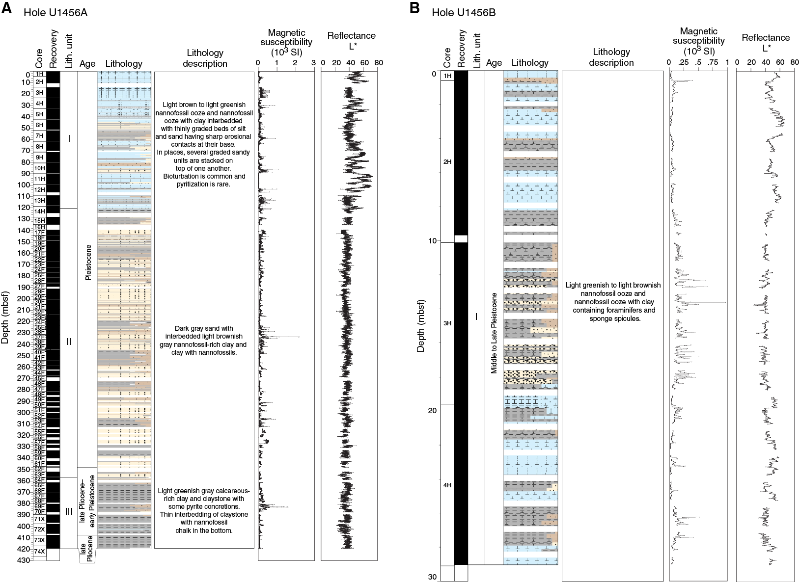

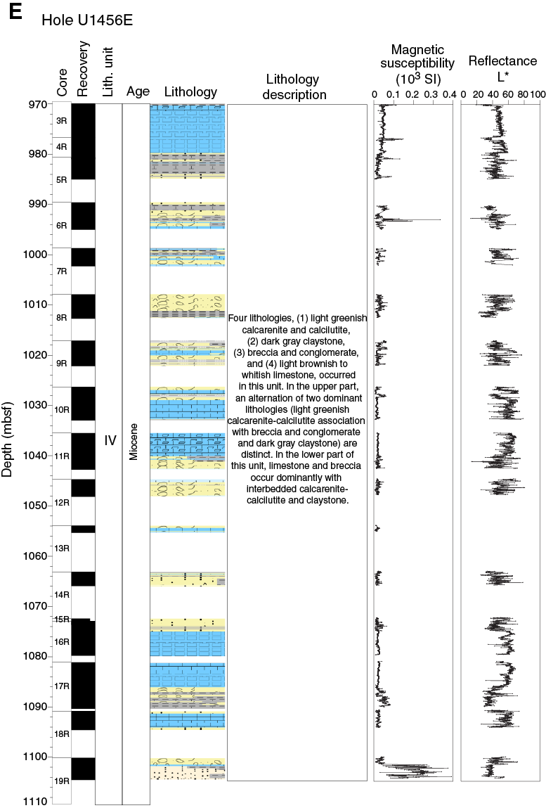
Figure F5. Lithostratigraphic summary.
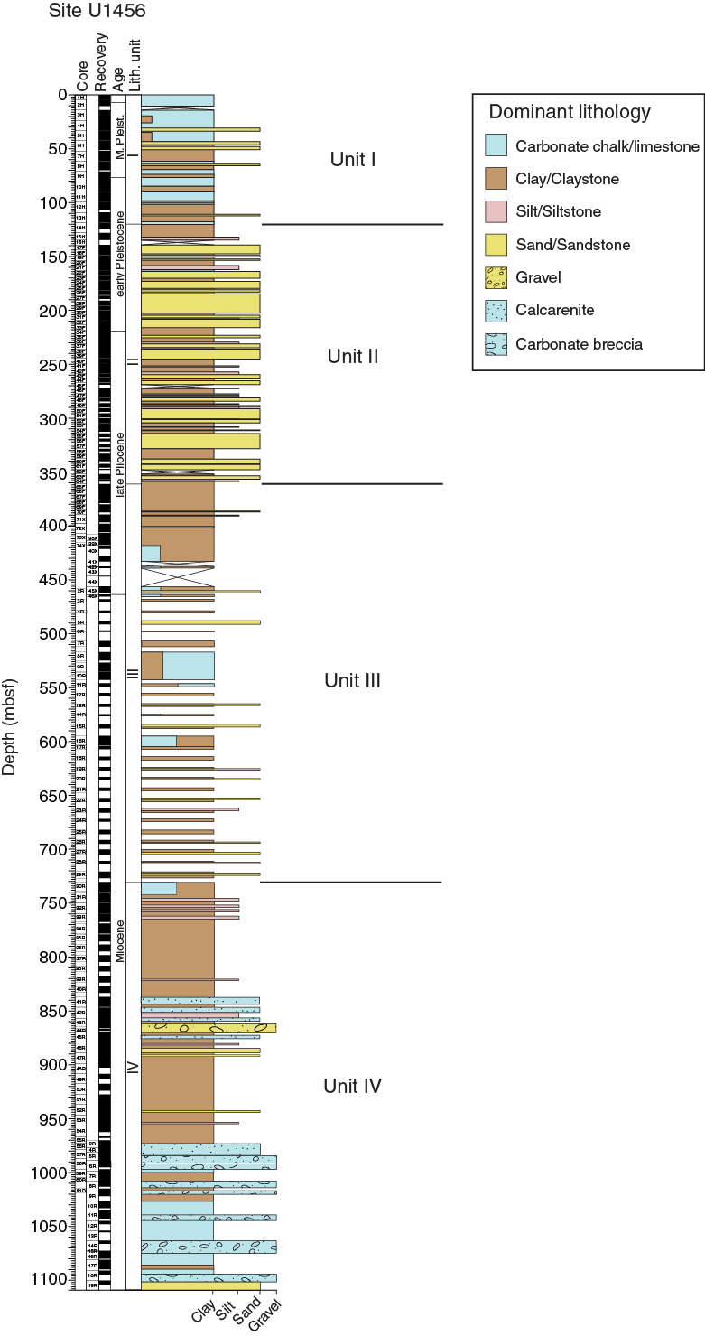
Figure F6. Synthesis lithostratigraphic log for Site U1456 showing combined recovery in Holes U1456A–U1456E.
Lithologic Unit I is composed of light brown to light greenish nannofossil ooze or foraminifer-rich nannofossil ooze interbedded with clay, silt, and sand, in addition to smaller amounts of whitish calcareous ooze and nannofossil-rich clay. Unit II consists mainly of dark gray to black sand, silt, and clay interbedded with thin-bedded nannofossil-rich clay and is interpreted as a series of turbidites. The main lithologies of Unit III are light brown to dark green clay/claystone, light brown to dark gray sand/sandstone, light greenish nannofossil chalk, and light to dark greenish gray nannofossil-rich claystone. Unit IV consists primarily of an alternation of dark gray claystone and light greenish calcarenite and calcilutite interbedded with other lithologies such as carbonate breccia and light brownish to whitish limestone.
Unit descriptions
Unit I
- Intervals: 355-U1456A-1H-1, 0 cm, through 14H-2, 136 cm; 355-U1456B-1H-1, 0 cm, through 4H-CC, 16 cm; 355-U1456C-1H-1, 0 cm, through 16H-5, 27 cm
- Depths: Hole U1456A = 0–121.36 mbsf, Hole U1456B = 0–29.03 mbsf (total depth), Hole U1456C = 0–121.30 mbsf
- Thickness: Hole U1456A = 121.36 m, Hole U1456C = 121.30 m
- Age: Pleistocene to recent
- Lithology: nannofossil ooze, foraminifer-rich nannofossil ooze, calcareous ooze, clay with nannofossil ooze, nannofossil-rich clay, clay, silt, and sand
Unit I is composed of light brown to light greenish nannofossil ooze or foraminifer-rich nannofossil ooze interbedded with clay, silt, and sand, in addition to whitish calcareous ooze and nannofossil-rich clay (Figure F7). Nannofossil ooze often contains abundant foraminifers, occasionally in high enough numbers that the sediment is a foraminifer-rich nannofossil ooze. Medium- to thick-bedded (<100 cm) nannofossil ooze layers are generally interbedded with thin and very thin (<5 cm) silt and sandy silt beds that contain abundant foraminifers in the upper part of Unit I. In contrast, nannofossil ooze layers are rare in the lower part of this unit. The nannofossil ooze in Unit I is often very thick bedded (>100 cm), comprises >50% of the entire unit, and is sparsely interbedded with thin to very thin clayey silt and sandy silt layers. Clay is generally interbedded with thin- to medium-bedded (<15 cm) sand or silty sand and generally comprises <25% of the entire section. Occasionally, sand is found in beds as thick as 40 cm, and over limited depth intervals it can comprise >50% of the entire section.
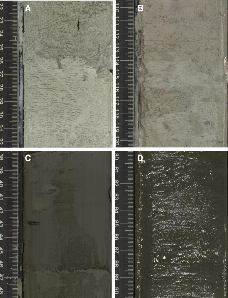
Figure F7. Dominant lithologies in Unit I, Hole U1456A.
Thin sand or silty sand layers overlie relatively thick nannofossil ooze or clay layers in Unit I (Figure F8A, F8B). The coarser grained sediment shows normal grading, which is interpreted as evidence for deposition from turbidity currents. In places, several turbidites are stacked on top of one another. In general, the tops of the nannofossil ooze or clay beds are sharply eroded or scoured (Figure F8C, F8D). These sharp contacts represent erosion and scouring interpreted as formed during passage of turbidity currents. The very thin (<2 cm) light blackish gray silt and sand layer observed above the erosional contact is typically enriched in foraminifers. Burrows and bioturbation are very common in greenish clay and silty clay (Figure F8E). Ichnofacies are dominated by Planolites and composite burrows. Shells and shell fragments (<0.5 cm) are rare, but they are observed in some calcareous ooze and sand beds (Figure F8F). Black spots of pyrite, sometimes present as concretions, are common in Unit I and, particularly, in calcareous and nannofossil ooze.
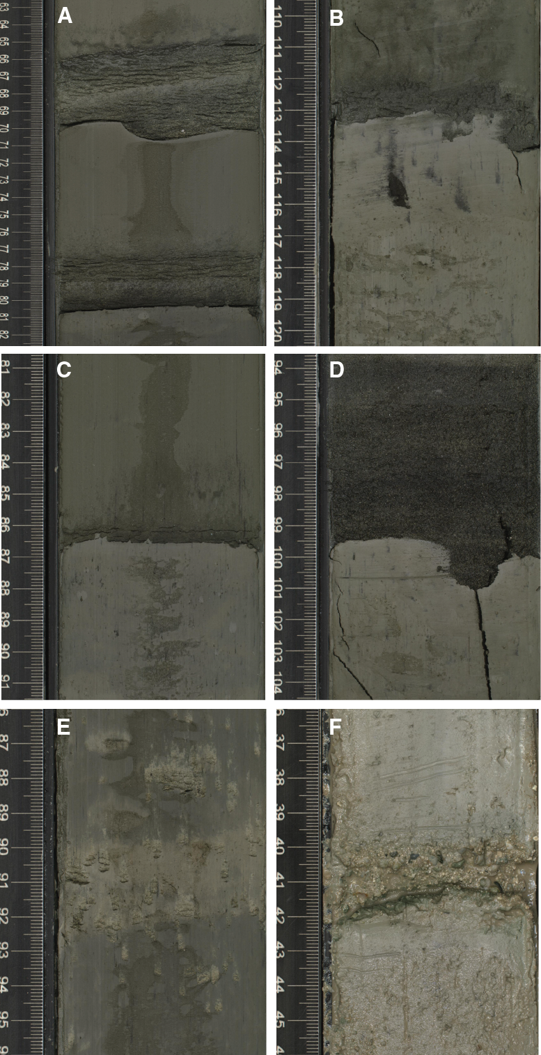
Figure F8. Sedimentary structures and other features, Hole U1456A.
Based on microscopic observation, the most common minerals in the silt- to sand-sized sediment of Unit I are quartz, feldspar, and mica (Figure F9). In these lithologies, heavy minerals are comparatively rare (Figure F10). Blue-green calcic amphiboles are common, tourmaline and epidote are rare, and kyanite, zircon, and fibrolitic sillimanite are present only in trace amounts. Unit I also contains distinctive but rare volcanic augitic clinopyroxenes with deeply etched outlines and subrounded grains of bluish green glauconite. Nannofossils together with foraminifers are abundant, and sponge spicules rare (Figure F9).
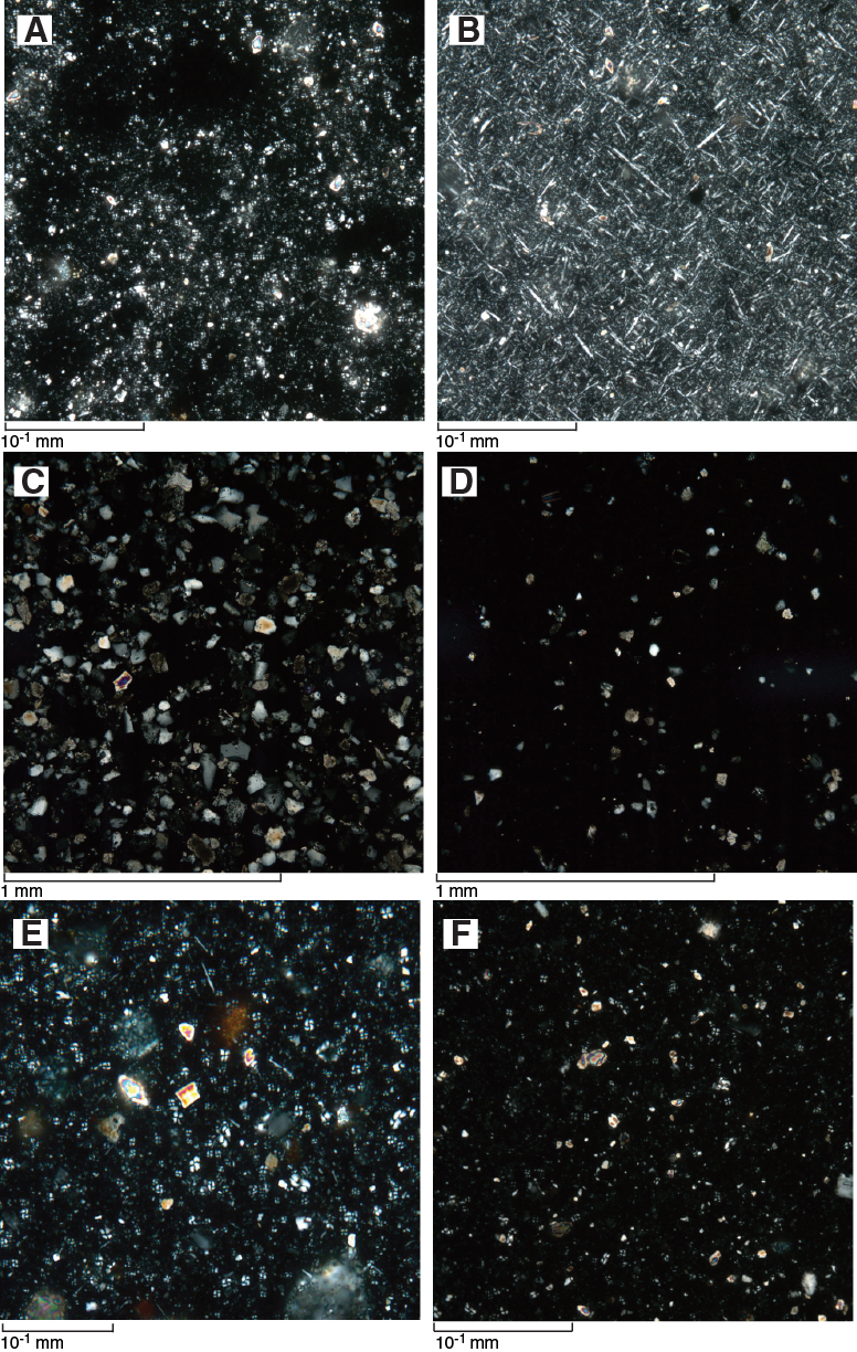
Figure F9. Microscopic observation of smear slides in Unit I, Hole U1456A.
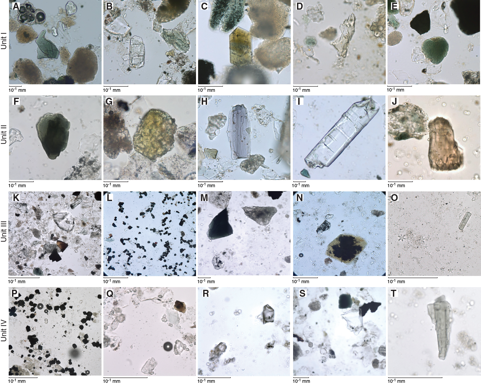
Figure F10. Heavy-mineral assemblages, Holes U1456A and U1456D.
X-ray diffraction (XRD) analysis was conducted on selected sediment samples from Hole U1456A. XRD data were obtained from the bulk sediment and clay fractions. XRD data of bulk sediment in Unit I show that the mineral assemblage is dominated by quartz, muscovite, chlorite, anorthite, albite, and calcite (Figure F11). Generally, the peak intensities of minerals in Unit I are not as high as seen in Unit II; however, the strong calcite peak typical of Unit I indicates dilution by carbonate minerals. According to XRD data from the clay-sized fraction, chlorite, illite, quartz, and feldspar are present (Figure F12). A small amount of smectite was detected in the glycol-treated samples in Unit I.
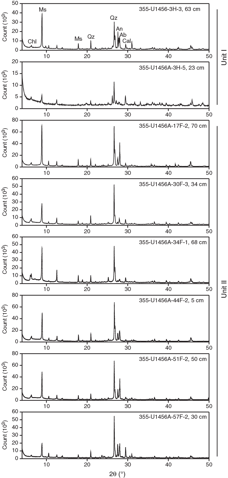
Figure F11. XRD patterns of bulk sediment from Units I and II, Hole U1456A.
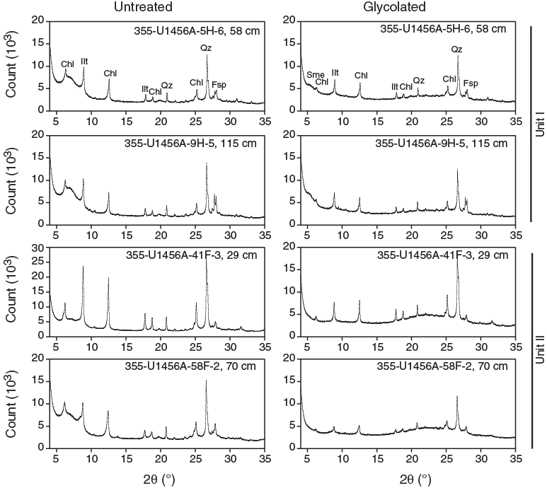
Figure F12. XRD patterns of clay fraction from Units I and II, Hole U1456A.
The lithologic unit boundary between Units I and II is located at Sections 355-U1456A-14H-2, 136 cm (121.36 mbsf), and 355-U1456C-16H-5, 27 cm (121.30 mbsf). All of the cored interval in Hole U1456B belongs to Unit I. The unit boundary is distinguished by the abundance of calcareous and nannofossil ooze in Unit I and the appearance of common sand and silty sand in Unit II. This division is also seen in magnetic susceptibility and color spectral data (Figure F5; see also Physical properties), as well as carbonate content (see Geochemistry).
Unit II
- Intervals: 355-U1456A-14H-2, 136 cm, through 65F-1, 19 cm; 355-U1456C-16H-5, 27 cm, through 36F-CC, 14 cm
- Depths: Hole U1456A = 121.36–361.49 mbsf, Hole U1456C = 121.30–220.22 mbsf
- Thickness: Hole U1456A = 240.13 m, Hole U1456C = 98.92 m (minimum thickness)
- Age: late Pliocene to early Pleistocene
- Lithology: sand, silt, clay, and nannofossil-rich clay
Dark grayish to blackish sand and silt and light brown nannofossil-rich clay are the dominant lithologies in Unit II (Figures F5, F13), but most of this unit is composed of dark grayish to blackish sand (Figure F13A). Thick sand layers are typically massive and lack structures. Most of the sand is medium to fine grained. The sand is enriched in medium- to coarse-grained mica. Clay color varies from light greenish gray to light brown, depending on the nannofossil content (Figure F13B) and is interbedded with very thin (~1 cm) blackish silt and sand layers. Thin clay with silt layers are intercalated within thick-bedded sand and show a gradational change upward from coarse to fine sediment. Such a transition suggests deposition from turbidity currents. Oxidized pyrite is frequently observed in the thin sandy layers, as are foraminifers. Nannofossil-rich clay and nannofossil-rich clay with silt beds are also seen in this unit, but they constitute only a small proportion (Figure F13C, F13D). Flow-in of clay, which is a form of drilling-induced disturbance, is often observed toward the base of the cores taken with the HLAPC.
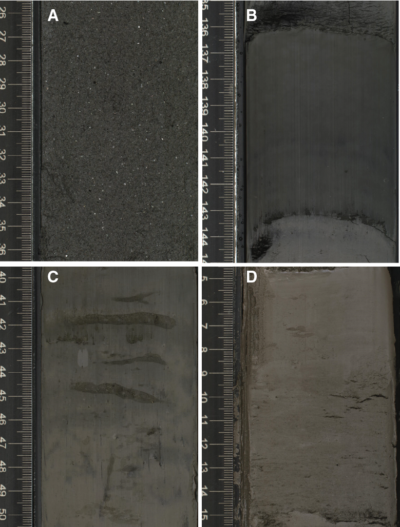
Figure F13. Dominant lithologies in Unit II, Hole U1456A.
In Unit II, the most abundant minerals are quartz, feldspar, and mica, together with lithic fragments (metamorphic rock fragments) (Figure F14). Heavy minerals are common in Unit II (Figure F10). The suite of heavy minerals is consistent throughout the unit, consisting of common blue-green calcic amphiboles, epidote, garnet, kyanite, and clinopyroxene, with rare zircon, tourmaline, and apatite. The presence of very rare high-pressure sodic-amphiboles (glaucophane) and pink-green hypersthene is distinctive of this unit. Amphiboles are angular or have only incipient corrosion features, whereas clinopyroxenes show commonly corroded or etched outlines. Foraminifers and other bioclastic fragments are very rare in all sand- and silt-sized layers. Nannofossils are present in low abundances in the interbedded nannofossil-rich clay layers.
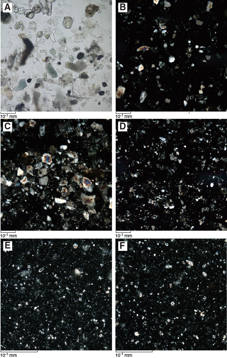
Figure F14. Microscopic observation of smear slides in Unit II, Hole U1456A.
XRD data from bulk sediment in Unit II show that the mineral compositions are similar to Unit I, containing quartz, muscovite, chlorite, anorthite, albite, and calcite (Figure F11). However, the peak intensities of these minerals, except for calcite, are much stronger than those seen in Unit I, which implies that the concentrations of these minerals are much higher in Unit II. XRD analysis of the clay-sized fraction in Unit II is also similar to that in Unit I (Figure F12); however, smectite seems to be absent in Unit II based on analysis of the glycolated samples.
The lithologic unit boundary between Units II and III was recovered only from Hole U1456A. The lithologic unit boundary is defined at Section 355-U1456A-65F-1, 19 cm (361.49 mbsf). The appearance of common light brown to dark green clay/claystone defines the top of Unit III, as compared to dark gray to black sand and silty sand found in Unit II. The Unit II/III boundary is also apparent in magnetic susceptibility and color spectral data (Figure F5; see also Physical properties), as well as carbonate content (see Geochemistry). This lithologic unit boundary is presumed to be within the interval drilled without coring from 221.6 to 408.0 mbsf in Hole U1456C. Hole U1456D was also drilled without coring to 458.80 mbsf, and the boundary is presumed to fall above that depth.
Unit III
- Intervals: 355-U1456A-65F-1, 19 cm, through 74X-CC, 23 cm; 355-U1456C-38X-1, 0 cm, through 46X-1, 43 cm; 355-U1456D-2R-1, 0 cm, through 30R-1, 30 cm
- Depths: Hole U1456A = 361.49–419.38 mbsf (total depth), Hole U1456C = 408.0–463.73 mbsf (total depth), Hole U1456D = 458.80–730.70 mbsf
- Thickness: Hole U1456A = 57.89 m (minimum thickness), Hole U1456C = 55.73 m (minimum thickness), Hole U1456D = 271.90 m
- Age: late Miocene to late Pliocene
- Lithology: clay/claystone, sand/sandstone, nannofossil chalk, and nannofossil-rich claystone
The major lithologies of Unit III consist of light brown to dark green clay/claystone, light brown to dark gray sand/sandstone, light greenish nannofossil chalk, and light to dark greenish gray nannofossil-rich claystone (Figures F5, F15). Varying carbonate content, mostly in the form of nannofossils, causes the color difference between different clay layers. Some of the sediment is indurated, but most of the recovered sediment is lithified. Sediment becomes noticeably more lithified deeper than 394.34 mbsf (Section 355-U1456A-71X-4). The corresponding interval was not sampled again; it was drilled without coring in Holes U1456C (drilled interval 355-U1456C-371) and U1456D (drilled interval 355-U1456D-11). Deeper than 394 mbsf, whitish calcareous chalk, light greenish gray claystone, claystone with nannofossils, and nannofossil chalk are prevalent. It is noteworthy that among these lithologies clay/claystone and sand/sandstone occur together, separated clearly from nannofossil chalk and nannofossil-rich claystone layers. Such differentiation is also reflected in physical properties such as magnetic susceptibility and lightness of sediment color (Figure F5).

Figure F15. Dominant lithologies in Unit III, Hole U1456D.
The light gray and light brown sand and clay layers are interbedded with sharp erosive boundaries at the base of the sand and show normal grading between the layers (Figure F15A). Sand layers include common mica grains. In addition, thin silty laminae are intercalated within clayey layers (Figure F15B). Abundances of deformed clay/claystone patches (i.e., rip-up clasts) are common within sandstones. These may suggest deposition by turbidity currents, as observed in Units I and II. The light gray sand in the upper part of Unit III is different from that of the lower part and includes thin (~1 cm) wood fragment-rich laminae (Figure F15C). These tiny fibrous wooden particles form very thin (a few millimeters) laminae, which are intercalated within mostly dark greenish gray claystone (Figure F15D). These sedimentary features imply that the sediment may have been transported from a terrestrial environment. Another remarkable feature of this unit is the black staining in claystone (Figure F15D), which seems to be a result of chemical reaction within the sediment. The dark gray claystone with silt is almost devoid of bioturbation. Light greenish nannofossil chalk and light to dark greenish gray nannofossil-rich claystone represent other dominant lithologies from this unit (Figure F15E, F15F). The chalk and claystone are characterized by intensive bioturbation, which is similar to that observed in Unit I. The ichnofacies are dominated by Planolites, Chondrites, and Zoophycos, as well as complex composite burrows (Figure F15E), typical of a deep-water clastic setting. Pyrite nodules frequently occur in this lithology (Figure F15F).
In Unit III, the most common minerals observed are quartz, feldspar, and mica, with rare heavy minerals (Figures F10, F16). Heavy mineral concentration changes with grain size, with a greater abundance in the coarser silty and sandy fraction. Different abundances and assemblages of dense minerals characterize each lithology. In silty sandstone, heavy minerals are common. In that lithology, the assemblage is characterized by abundant blue-green hornblende, pale green clinopyroxene, and epidote with rare garnet and trace amounts of kyanite, apatite, zircon, tourmaline, and rutile. Nannofossil chalk contains only rare or traces of heavy minerals, with common blue-green hornblende and epidote, rare garnet, sillimanite, and bluish gray chloritoid, together with traces of apatite, zircon, tourmaline, and rutile. Nannofossil-rich claystone contains only traces of green tourmaline (Figure F10). Amphiboles show well-developed corrosion features, and etched outlines are common. Euhedral authigenic Ti oxides and platy flakes of Fe oxides are also present in trace concentrations in claystone and nannofossil-rich claystone.
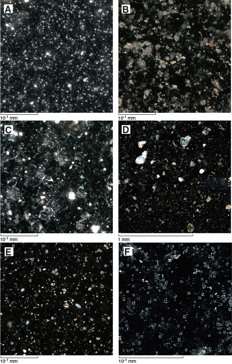
Figure F16. Microscopic observation of smear slides in Unit III, Site U1456.
The lithologic unit boundary between Units III and IV was cored only in Hole U1456D and is defined at Section 355-U1456D-30R-1, 30 cm (730.70 mbsf) (Figure F17A). The lithologic unit boundary in Hole U1456E is presumed to be within the interval drilled without coring down to 970 mbsf. The unit boundary is marked by brownish gray silty claystone along with silty sandstone at the base of Unit III overlying the greenish gray nannofossil chalk and dark gray claystone of Unit IV. There is a clear color change between Units III and IV, which is also paralleled in physical properties such as magnetic susceptibility (Figure F5; see also Physical properties).
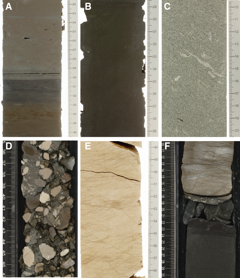
Figure F17. Dominant lithologies of Unit IV, Holes U1456D and U1456E.
Unit IV
- Intervals: 355-U1456D-30R-1, 30 cm, through 61R-CC, 16 cm (total depth); 355-U1456E-3R-1, 0 cm, through 19R-CC, 19 cm (total depth)
- Depths: Hole U1456D = 730.70–1018.46 mbsf (total depth), Hole U1456E = 970.0-1104.52 mbsf (minimum)
- Thickness: Hole U1456D = 287.76 m, Hole U1456E = 134.52 m (minimum thickness)
- Age: Miocene
- Lithology: calcarenite, calcilutite, claystone, siltstone, breccia, conglomerate, and limestone
Unit IV consists mainly of four lithologies (Figures F5, F17):
- Light greenish calcarenite and calcilutite,
- Dark gray claystone,
- Breccia and conglomerate, and
- Light brownish to whitish limestone.
Dark gray massive claystone, light greenish calcarenite and calcilutite, and breccia/conglomerate are dominant in the upper part of Unit IV. In the lower part of this unit, limestone and breccia are most abundant, with interbedded calcarenite, calcilutite, and claystone. Similar lithologic changes are also discernible in magnetic susceptibility and sediment color measurements (Figure F5).
The dark gray claystone is mostly massive (Figure F17B) and is marked by light brownish to light greenish interbeds of nannofossil-rich claystone, nannofossil chalk, and siltstone. Various colors of claystone, including dark brown, light blue, and pale blue, occur between 1011.15 and 1012.49 mbsf (Sections 355-U1456E-8R-3, 61 cm, through 8R-4, 94 cm). The bluish claystone is very rich in smectite as determined by XRD analysis, although smear slide examination finds only brownish volcanic glass in the clay. The bed appears to be a thick, altered tephra. Thick to very thick beds of fine- to medium-grained calcarenite and calcilutite with nannofossils and foraminifers occur only below 837.10 mbsf (Section 41R-1). The light grayish green calcarenite and calcilutite can be easily distinguished from dark gray claystone (Figure F17C). The calcarenite is often interbedded with foraminifer-rich claystone patches and granule-sized intraclasts of carbonate, with abundance increasing with depth. Calcarenite and calcilutite also show reverse grading from medium-grained calcarenite at the top of a given bed and very fine grained calcilutite at the bottom (Section 42R-1 through 43R-3). Normal grading with fine calcarenite at the top of a bed and coarse calcarenite at the bottom was also observed at 871.60 mbsf (Section 45R-2). The boundary between calcarenite or calcilutite and dark gray claystone is normally sharp and erosive. Breccia is dominated by subangular to subrounded carbonate (<3 cm) clasts, small clasts of claystone, and weathered volcanic material (Figure F17D). Small breccia clasts are matrix supported, mostly by clay or clay and carbonate mixtures. Coarser grained breccias have matrixes that are not strongly cemented. The size of breccia limestone clasts increases with depth. Light brownish to whitish limestone (Figure F17E) is found in the lower part of this unit only below 981.79 mbsf (Sections 355-U1456D-59R-1, 0 cm, and 355-U1456E-5R-1, 119 cm). This light brownish limestone is deposited with calcarenite and calcilutite along with breccia and conglomerate.
Unit IV shows diverse structural features such as microfaults, folds, slickensides, and inclined to vertical bedding (Figure F18). High-angle faults and slickensides are observed in silty claystone and calcarenite (Figure F18A, F18B). Soft-sediment folds are common in claystone and limestone (Figure F18C, F18D). In addition, vertical bedding indicates larger scale folding or tilting (Figure F18E). Pressure-induced sedimentary structures (i.e., stylolites) are observed within limestone (Figure F18F). Sedimentary structures caused by loading pressure are also observed as clast (typically calcite fragments) loading into the claystone, as exhibited by the solitary clast in Figure F18G. Limestones are often highly bioturbated, showing Zoophycos, Planolites, and Skolithos burrows (Figure F18H). Most of these sedimentary structures indicate that Unit IV was formed as a result of mass transport (Pickering and Hiscott, 2015).
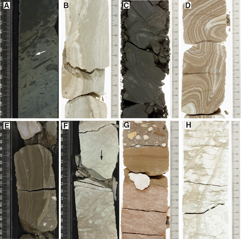
Figure F18. Main sediment features of Unit IV, Holes U1456D and U1456E.
In Unit IV, the most common minerals are quartz and mica, with very rare or trace amounts of heavy minerals (Figures F10, F19. Heavy mineral suites are common in sandstone, and their relative contribution to the total assemblage in siltstone and claystone decreases with the reduction of grain size. Heavy minerals are absent in nannofossil-rich calcarenite and calcilutite. Silty sandstone displays common heavy minerals with common blue-green hornblende and epidote, rare garnet, and traces of apatite, zircon, and tourmaline (Figure F19). Silty claystone and claystone contain trace or rare heavy minerals with rare hornblende, actinolite, epidote, and garnet and traces of zircon, tourmaline, spinel, and rutile. Nannofossil-rich claystone contains only trace amounts of heavy minerals with rare zircon, tourmaline, and rutile and traces of hornblende, apatite, and garnet. A thin section of a clast from one of the breccias shows oriented plagioclase feldspar crystals within a basaltic groundmass (Figure F19E).
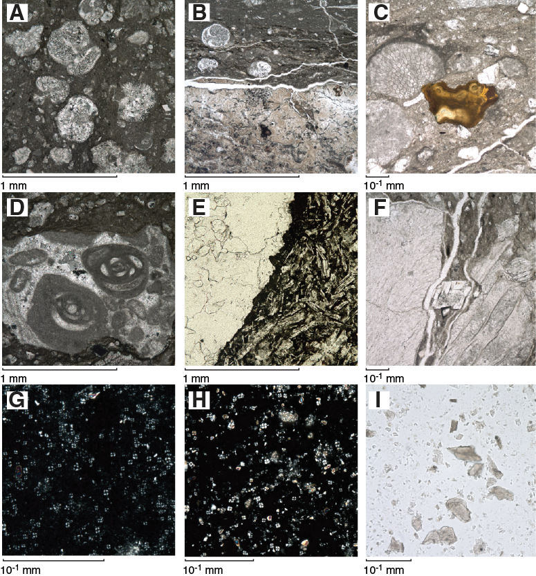
Figure F19. Microscopic observation of thin sections and smear slides, Holes U1456D and U1456E.
Dark gray sandstone interbedded with silty claystone and overlain by dark gray silty sandstone is observed at the bottom of Unit IV (Sections 355-U1456E-19R-2, 19 cm, through 19R-CC, 17 cm) at the base of Hole U1456E, just below a thin layer of breccia (Figure F17F). The sandstone is much darker in color and has subhorizontal bedding. This change in lithology is also paralleled by changes in physical properties such as magnetic susceptibility and natural gamma radiation. This sandstone may represent the last in situ deposit below the mass transport deposit, or it may be a different lithology within the slump. The sandstone is found between 1101.67 mbsf (Section 19R-2, 19 cm) and the base of Hole U1456E at 1104.52 mbsf.
Discussion
Depositional environments
Trace fossils preserved in deep-sea sediment represent the last burrows that are imposed on a sediment, mostly within the uppermost 5–7 cm of the seafloor (Ekdale et al., 1984). The assemblages seen in fine-grained sediment within our cores are typical of intermediate to very deepwater sedimentary environments in distal clastic settings and mostly correspond to the Nereites ichnofacies. This ichnofacies indicates sedimentation in abyssal or equivalent deep-sea environments and it is associated with pelagic deposits and distal turbidites (Seilacher, 1967). We conclude that water depths have not changed appreciably since ~10 Ma at Site U1456 and have remained deep since that time.
Burrows are mostly observed in hemipelagic nannofossil-rich clay and claystone as well as nannofossil ooze and chalk that dominate Units I and III. Such nannofossil-rich claystone and nannofossil chalk are also observed interbedded in the lower part of Unit IV. Planolites is dominant in Unit I, whereas pelagic/hemipelagic sediment in Units II and III show strong bioturbation dominated by fodinichnia (traces of infaunal deposit feeders), such as Planolites, Zoophycos, Chondrites, and various composite burrows (Figure F15E). This indicates that sedimentation in this region took place in the presence of highly oxic conditions at the seawater/sediment interface and within the sediment mixed layer (see Geochemistry). Vertical burrows, such as Skolithos, are commonly associated with low sedimentation–rate environments with extremely depleted organic content (Kemp, 1995) and are almost absent in our cores, which is unsurprising given the submarine fan setting.
Clastic sedimentation dominates the drilled stratigraphy, yet several biogenic intervals are known, which is perhaps to be expected given the clastic hiatus associated with the current Holocene highstand (Kolla and Coumes, 1984; Prins et al., 2000). Biogenic carbonate (nannofossil ooze/chalk, nannofossil-rich clay/claystone) is more common in Unit I and part of Units III and IV. These pelagic deposits formed during periods of increased surface water productivity and/or decreased clastic influx, but all units show some evidence for the long-term influx of clastic sediment.
The commonly muddy and carbonate-rich character of Unit I indicates that this site has been in a distal location in relation to active depocenters throughout the Middle to Late Pleistocene climatic fluctuations (since ~1.2 Ma). Changes in clastic content and magnetic susceptibility are noted, but their cause is presently unknown (see Paleomagnetism and rock magnetism). The muddy character suggests sedimentation in a lower fan, distal plain setting for Unit I (Mutti and Johns, 1978; Walker, 1978). There is no suggestion that the muddy character of this unit reflects slow erosion onshore and reduced sediment delivery in the Indus at this time. Indeed, regional sediment mass flux budgets here and across Asia generally point to fast sedimentation through the Pleistocene (Métivier et al., 1999; Clift, 2006). Slow sedimentation at Site U1456 is the result of active lobe avulsion and autocyclic processes within the fan. Although sinuous channels are recognized at the modern seafloor within Laxmi Basin (Mishra et al., 2015), they do not appear to be supplying much coarse sediment to Site U1456.
Terrigenous sediment, such as dark grayish to blackish sand, dominates Unit II and is interpreted as turbidites (Figure F13). The sequence is mostly sandy but with intervening muddy intervals. Consideration of the seismic profiling, together with the lack of stacked sand beds in the cores, rules out a channel setting for Unit II but rather favors sheet-like turbidite sedimentation within an active lobe (Mutti, 1992; Normark et al., 1993). The lack of coarse sand or gravel also argues for this being a sheet-type lobe in a mid- or lower fan setting supplied by sediment from an incised channel upslope. Rapid accumulation of sediment in a short period is indicated by the bio- and magnetostratigraphic age model (Figure F20), consistent with a lobe setting. Unit III is characterized mostly by terrigenous sediment and sequences of hemipelagic sediment (Figure F15). The graded and erosive cycles of clay and sand found within Unit III are interpreted as distal turbidity current deposits. Because of the low recovery it is not entirely clear how the sandy layers in Unit III are organized. If much of the missing section is rich in sand, as might be inferred given that poorly consolidated sands are notoriously difficult to recover, particularly with rotary coring, then it is possible that this unit represents another, slightly more distal lobe, similar to Unit II and separated from it by a hemipelagic sequence assigned to the top of Unit II spanning ~360–460 mbsf. If the recovery is really representative of the entire unit, then this sequence would represent sedimentation on the distal edge of a suprafan lobe in its transition into basin plain turbidites (Normark, 1978). It is clearly more distal that the thick sand of Unit II.
Mass transport
Unit IV is >350 m thick and consists of claystone and a mixture of light gray calcarenite/calcilutite and gray breccia with conglomerate (Figure F17). The lower part of the unit is a repetition of the upper part with more intense brecciation, interpreted as the product of mass transport. Calcarenite and calcilutite are composed mostly of detrital carbonate grains transported from land and deposited in the area of the drill site. These are concentrated toward the base of the unit at >970 mbsf. Various deformation structures (e.g., microfaults, slickensides, soft-sediment folds, vertical bedding, stylolites, and load structures; Figure F18) are mostly found in claystone and limestone within this unit. The breccia includes clasts ranging at least to 10 cm across and possibly much greater, which cannot be assessed in a narrow core. The clasts are composed of calcite and limestone and are poorly sorted, ungraded, and subangular to subrounded. The clasts are suspended in a clay mixed with carbonate matrix typical of debris flow emplacement. The deformation structures and breccia indicate that deposition in the lower part of Unit IV was a result of debris flows processes. Unit IV correlates closely with the Nataraja slide identified from seismic reflection profiles and which is seen along much of the length of the Laxmi Basin as far north as ~21°N (Calvès et al., 2015).
Sediment at Site U1456 indicates three primary types of deposition:
- Pelagic sediment such as nannofossil ooze/chalk and nannofossil-rich clay, which are highly bioturbated and present in Units I, II, and III;
- Turbidites composed of silty sand/sandstone and clay/claystone with a clear Indus provenance; and
- Mass transport deposits comprising conglomerate and breccia eroded from the Indian continental shelf.
Carbonate intervals composed of calcarenite/calcilutite were also derived from the Indian shelf. Although neighboring submarine ridges and seamounts (e.g., Laxmi Ridge or Panikkar Ridge) could supply some carbonate debris, the scale of the deposit recovered in Unit IV clearly points to the Indian continental margin as the primary source. This interpretation is consistent with evidence for recently active mass wasting from the Indian margin offshore Ratnagiri and Goa (Rao and Wagle, 1997).
Provenance
The location of Site U1456 and the mineralogy of the cored sediment require derivation of material from the western margin of the Indian subcontinent, mainly from the Indus River, which drains the high-relief topography of the western Tibetan Plateau, Karakoram, and Himalaya (Milliman et al., 1984; Garzanti et al., 2005). The relative input from those rivers draining the Himalaya through the Punjab (currently the Ravi, Jhellum, Chenab, and Sutlej Rivers but previously involving the Yamuna and Ghaggar-Hakra Rivers [Saini et al., 2009; Clift et al., 2012]) and from the trunk Indus coming from the Karakoram and western Tibet varies depending on climate zoning and drainage reorganization (Clift et al., 2008a). The Indian peninsula is likely a much less important source because the wide continental shelf acts as a major sediment buffer (Rao and Wagle, 1997), and smear slide descriptions of sediment at Site U1456 confirm that peninsular sources are only intermittently important, at least in Units I–III. Sediment flux from the major rivers draining the peninsula, such as the Narmada and Tapti Rivers, is less than the Indus but may have been significant at times. Milliman and Syvitski (1992) recorded a sediment load for the pre-recent Narmada River at around half that of the Indus, ~125 × 106 versus 250 × 106 tons/y. Mineralogy evidence from our cores strongly supports a dominant Indus signature and suggests significant sequestration of Narmada/Tapti sediment on the shelf, or that the relative discharges of the Indus and Narmada Rivers were more asymmetric in the past.
Biostratigraphy
Samples from core catchers and additional samples from split core sections from Holes U1456A–U1456E were examined to define calcareous nannofossil, planktonic foraminifer, radiolarian, and diatom biostratigraphies for Site U1456. The chronologic framework for Site U1456 is based on the identification of a series of calcareous nannofossil and planktonic foraminifer events (Table T2; Figure F20) and paleomagnetic events (Table T21; Figure F20). Nannofossils are generally abundant and moderately to well preserved in most samples examined (Tables T3, T4, T5, T6). Planktonic foraminifers are abundant and well preserved in most samples but are absent in the coarser grained intervals of lithologic Units II and III (see Lithostratigraphy). Planktonic foraminifer preservation is poor in some core catcher samples toward the bottom of Hole U1456A (Tables T7, T8). Diatoms were observed in the mudline samples collected and in the uppermost samples of Holes U1456A and U1456C (Table T9). Radiolarians are only present in very low abundance in the topmost sections of Holes U1456A and U1456C (Table T10), below which samples are barren of both radiolarians and diatoms (Tables T11, T12).
Table T2. Biostratigraphic datums for Holes U1456A–U1456E. Download table in .csv format.
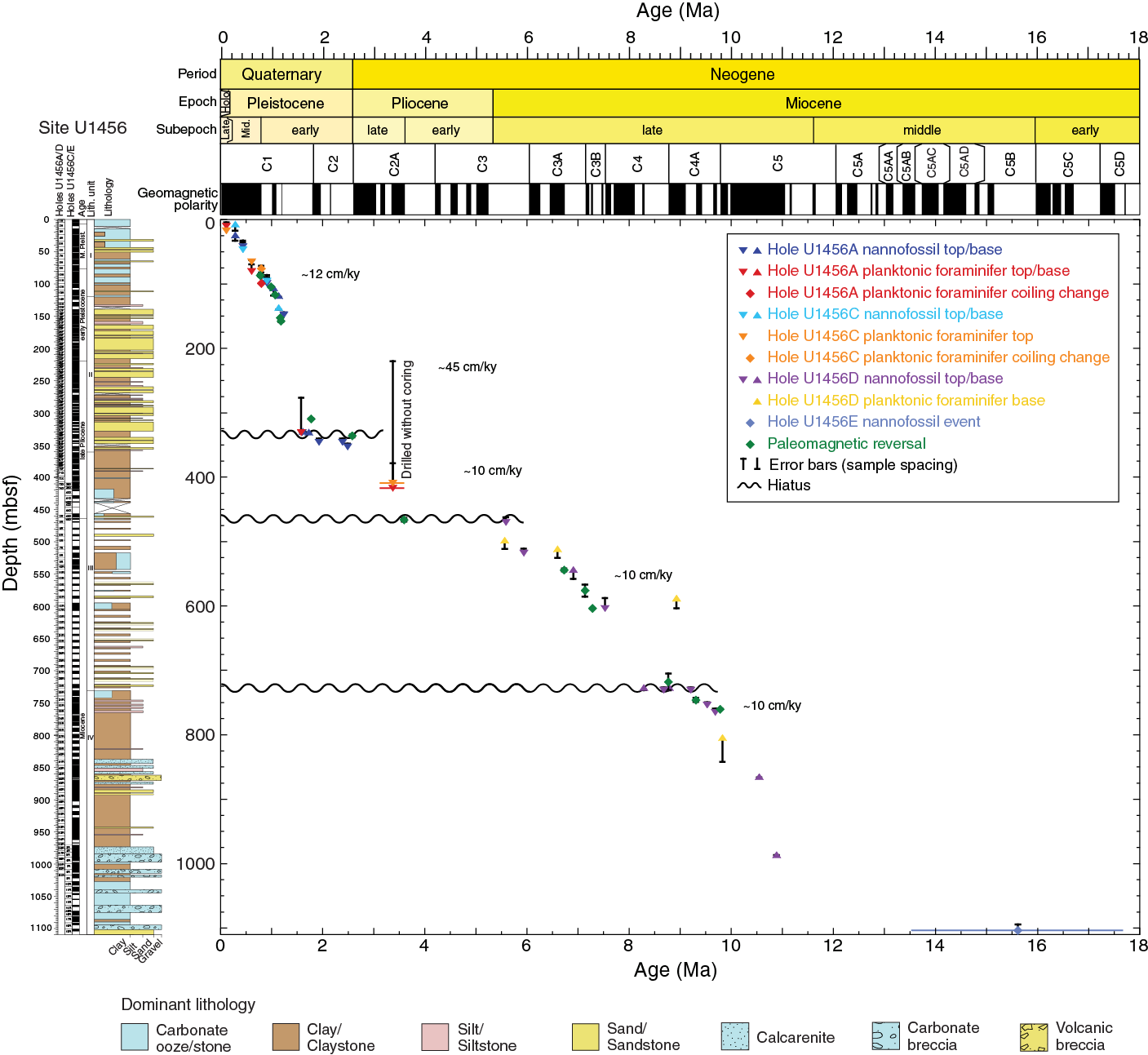
Figure F20. Age-depth plot, Site U1456.
Table T3. Distribution of calcareous nannofossils, Hole U1456A. Download table in .csv format.
Table T4. Distribution of calcareous nannofossils, Hole U1456C. Download table in .csv format.
Table T5. Distribution of calcareous nannofossils, Hole U1456D. Download table in .csv format.
Table T6. Distribution of calcareous nannofossils, Hole U1456E. Download table in .csv format.
Table T7. Distribution of planktonic foraminifers, Holes U1456A and U1456C. Download table in .csv format.
Table T8. Distribution of planktonic foraminifers, Holes U1456D and U1456E. Download table in .csv format.
Table T9. Distribution of diatoms, Holes U1456A and U1456C. Download table in .csv format.
Table T10. Distribution of radiolarians, Holes U1456A and U1456C. Download table in .csv format.
Table T11. Samples containing no diatoms. Download table in .csv format.
Table T12. Samples containing no radiolarians. Download table in .csv format.
The succession of calcareous nannofossil and planktonic foraminifer events indicates that Site U1456 spans the Miocene through recent. The biostratigraphic framework established at Site U1456 enabled the identification of three unconformities and an interval of mass transport deposition. Calculated sedimentation rates at Site U1456 suggest that the sedimentation rate appears to have been relatively consistent in the late Miocene at ~10 cm/ky, although deposition was interrupted for ~0.5 million years between ~8.1 and 8.6 Ma. Another unconformity spanning ~2.0 million years and encompassing the Miocene/Pliocene boundary (5.33 Ma) was identified at ~470 mbsf in the upper part of lithologic Unit III. The sedimentation rate in the late Pliocene to early Pleistocene was again ~10 cm/ky. After a 0.45 million year hiatus, sedimentation rates in the early Pleistocene are much higher (~45 cm/ky) during deposition of Unit II. The sedimentation rate slowed down from the late early Pleistocene to recent, averaging ~12 cm/ky (Figure F20).
Calcareous nannofossils
All advanced piston corer (APC), extended core barrel (XCB), and rotary core barrel (RCB) core catcher samples were examined from Holes U1456A–U1456E in order to establish a calcareous nannofossil biostratigraphy (Table T2; Figure F20). When the half-length advanced piston corer (HLAPC) was used, at minimum every second core catcher (1 sample/~9.5 m) was examined. Additional samples were taken from the split core sections of Holes U1456A–U1456E to constrain biohorizons. The section sampled in Holes U1456A and U1456C spans the Pliocene to recent, whereas those in Hole U1456D and U1456E are predominantly late Miocene in age (Tables T3, T4, T5, T6).
Calcareous nannofossil assemblages are generally abundant and diverse and are well preserved through lithologic Unit I (see Lithostratigraphy). Within Unit II, nannofossils are scarce in the dominantly sandy lithologies but abundant through the fine-grained interbedded clays. Unit III is dominated by finer grained lithologies with common to abundant nannofossils. Nannofossils in Units II and III show moderate to good preservation. Nannofossil abundance in Unit IV varies from absent to abundant, and preservation also varies significantly from poor to good. There is common reworking of Cretaceous and Paleogene forms in Units I–III, whereas Unit IV includes Paleogene and early Neogene reworking, with only very sparse Cretaceous forms. Some individual horizons in Unit IV contain reworked assemblages with no in situ taxa, suggesting that deposition of the reworked material was so rapid that the normal background pelagic sedimentation was not included before the reworked sediments were further buried.
Pleistocene
Emiliania huxleyi is present in Samples 355-U1456A-1H-CC through 3H-CC (4.49–23.34 mbsf), as well as Sample 355-U1456C-1H-CC (7.33 mbsf), dating the samples to <0.290 Ma within Zone NN21 of Martini (1971). The absence of E. huxleyi and Pseudoemiliania lacunosa in Samples 355-U1456A-4H-CC (32.86 mbsf) and 355-U1456C-3H-CC through 5H-CC (17.7–35.84 mbsf) indicates Zone NN20, which is assigned to 0.29–0.44 Ma. The last occurrence (LO) of P. lacunosa is a globally synchronous event (Thierstein et al., 1977) that is used to mark the top of Zone NN19 (0.44 Ma). This species is first noted in Samples 355-U1456A-5H-CC (42.25 mbsf) and 355-U1456C-6H-CC (46.77 mbsf). Reticulofenestra asanoi has a last common and first common appearance at 0.91 and 1.14 Ma, respectively. This species occurs in Samples 355-U1456A-11H-CC through 13H-CC (99.24–118.01 mbsf) and 355-U1456C-13H-CC through 18H-CC (95.64–136.97 mbsf), indicating an age of 0.91–1.14 Ma for this interval. The base of the reappearance of Gephyrocapsa spp. >4 µm (1.04 Ma) occurs in Sample 355-U1456A-12H-CC (106.23 mbsf).
Samples 355-U1456A-24F-1, 94 cm, through 58F-1, 74 cm (173.14–329.14 mbsf), are dated at 1.24–1.62 Ma based on the presence of large gephyrocapsids (Gephyrocapsa oceanica >5.5 µm and Gephyrocapsa caribbeanica >5.5 µm). The first occurrence (FO) of Gephyrocapsa spp. >4 µm, dated to 1.73 Ma, occurs in Sample 58F-CC (330.63 mbsf). No other nannofossil bioevents are noted throughout the interval between 173.14 and 329.14 mbsf within lithologic Unit II in Hole U1456A. This is likely in part because of the coarse-grained sediment that dominates this interval (see Lithostratigraphy). Helicosphaera sellii (LO at 1.26 Ma) is not observed in this section, probably because of the sparse nature of the assemblages. This species is found together with Calcidiscus macintyrei (LO at 1.60 Ma) in Sample 58F-1, 31 cm (328.71 mbsf), just above the FO of Gephyrocapsa >5.5 µm (1.62 Ma). The sedimentation rate is very high (~45 cm/ky) throughout Unit II (Figure F20), resulting in incorporation of less pelagic sediment (see Lithostratigraphy) and therefore diluted nannofossil assemblages.
We interpret the LOs of Discoaster brouweri (1.93 Ma; top of Zone NN18) and Discoaster pentaradiatus (2.39 Ma; top of Zone NN17) in Sample 355-U1456A-61F-CC (345.84 mbsf) to indicate a hiatus of at least 0.45 million years between Samples 60F-CC and 61F-CC (Figure F20), with all of Zone NN18 missing. The few specimens of these species found in Sample 59F-2, 83 cm (335.43 mbsf), are attributed to reworking because discoasters are absent below that depth until Sample 61F-CC (345.84 mbsf), despite the abundant nature of the assemblages through that interval. D. brouweri is found sporadically downhole to Sample 66F-CC (370.36 mbsf), below which it occurs more consistently and with higher abundance. Discoaster surculus also occurs only sporadically near its LO in Sample 63F-1, 116 cm (353.06 mbsf). This event indicates the top of Zone NN16 and is dated to 2.49 Ma, just above the Pliocene/Pleistocene boundary at 2.588 Ma (Gradstein et al., 2012).
Pliocene
The base of Hole U1456A (Section 355-U1456A-74X-CC; 419.33 mbsf) correlates to Section 355-U1456C-41X-CC (see Stratigraphic correlation) and is assigned a late Pliocene age (>2.49 Ma) based on the presence of D. surculus. Samples from Sections 355-U1456C-41X-CC through 46X-1 (432.69–463.75 mbsf) yield a characteristic late Pliocene assemblage with D. surculus, D. pentaradiatus, D. brouweri, Reticulofenestra haqii, Reticulofenestra minuta, and Reticulofenestra pseudoumbilicus 5–7 µm. The LO of Sphenolithus abies is difficult to identify as a result of reworking; however, it is commonly present below Sample 355-U1456C-38X-CC, which indicates an age older than its LO at 3.54 Ma if at least some of the specimens are in situ. The base of Hole U1456C (Samples 44X-1, 40–45 cm, and 45X-CC; 446.5–463.75 mbsf) contains rare R. pseudoumbilicus >7 µm and, together with the absence of Amaurolithus tricorniculatus in these samples and Sample 46X-1, 45–50 cm (463.75 mbsf), suggests an age of 3.70–3.92 Ma (within Zone NN15).
Miocene
The LO of Discoaster quinqueramus (5.59 Ma) is found in Sample 355-U1456D-3R-CC (470.26 mbsf), which marks the top of Zone NN11. The absence of the index species Ceratolithus acutus (5.04–5.35 Ma) together with the absence of Amaurolithus species (LO at 4.50 Ma) above Sample 3R-CC suggests an unconformity that encompasses the Miocene/Pliocene boundary (5.33 Ma) (Figure F20). The presence of Nicklithus amplificus in Samples 8R-1A, 81 cm, through 10R-CC (517.8–543.76 mbsf) constrains the age of this interval to between 5.94 and 6.91 Ma.
The section becomes sandier below Core 355-U1456D-11R, with sparser nannofossil assemblages. Amauroliths and discoasters are rare through this interval. Nevertheless, a single specimen of Discoaster loeblichii was identified in Sample 355-U1456D-16R-CC (603.90 mbsf), which has a LO at 7.53 Ma, within the lower part of Zone NN11. Additional work is necessary to determine if this single specimen represents an in situ occurrence. The base of Discoaster berggrenii (FO at 8.29 Ma) is found in Sample 29R-CC (726.55 mbsf), which marks the top of Zone NN10. D. berggrenii occurs only sporadically in samples between 607.45 and 684.19 mbsf as a result of dilution caused by the dominance of sandy lithologies through Unit III (see Lithostratigraphy). Sample 30R-1, 41 cm (730.81 mbsf), contains the LOs of Minylitha convallis (8.68 Ma) and Discoaster bollii (9.21 Ma), as well as the base of common R. pseudoumbilicus >7 µm (8.79 Ma). The co-occurrence of these species, together with the presence of D. berggrenii just above in Sample 29R-CC, indicates a hiatus of at least 500 ky between 726.55 and 730.81 mbsf (Figure F20).
Sample 355-U1456D-32R-3, 85 cm (753.65 mbsf), yields the LO of Discoaster hamatus, which is dated to 9.53 Ma, and this event also marks the top of Zone NN9. A few barren samples were found within the interval between the FO of D. berggrenii and the LO of D. hamatus. With the exception of one barren sample in Hole U1456C (Sample 355-U1456C-40X-CC; 421.01 mbsf); these are the shallowest barren samples examined from this site. Barren samples become more common toward the base of Hole U1456D. The LOs of Catinaster coalitus (9.69 Ma) and Catinaster calyculus (9.67 Ma) are found in Sample 355-U1456D-33R-4, 144 cm (765.25 mbsf). The FO of D. hamatus (10.55 Ma) marks the top of Zone NN8 and is identified in Sample 37R-CC (804.51 mbsf).
We see a distinct change in the nannofossil assemblages below Section 355-U1456D-38R-CC. Much of the interval from Core 355-U1456D-38R to the base of the hole in Core 61R contains a mixture of different lithologies that sometimes displays chaotic bedding and small faults (see Lithostratigraphy), as well as abundant reworked Paleogene to early Neogene microfossil assemblages. This interval is interpreted as a mass transport deposit. Short intervals of normal pelagic sedimentation are observed within the mass transport deposit based on the occurrence of late Miocene nannofossils, as well as coherent paleomagnetics results (see Paleomagnetism and rock magnetism) within horizontally bedded deposits. Samples 355-U1456D-51R-5, 12 cm, through 52R-3, 100 cm (933.52–941.10 mbsf), and Sample 57R-7, 80 cm (986.65 mbsf), contain few to common C. coalitus, and the latter sample also contains rare C. calyculus. These species also occur in samples in which reworking is rare or absent, further suggesting that these intervals represent upper Miocene sediment deposited between individual mass transport events.
The first core from Hole U1456E (Core 355-U1456E-3R) overlaps with the base of Hole U1456D and appears similar to Core 355-U1456D-56R, although it is impossible to make firm correlations between the two holes (see Stratigraphic correlation). Samples 355-U1456E-3R-1, 74 cm, through 18R-CC (970.74–1094.54 mbsf) continue to display mixed Paleogene and early Neogene nannofossil assemblages. A change of lithology in Core 19R suggests normally deposited sediment underlying the mass transport deposit of lithologic Unit IV (see Lithostratigraphy). Samples 19R-4, 46 cm, through 19R-4, 61 cm (1103.76–1103.88 mbsf), show common reworking of Cretaceous forms, similar to what was noted in Units I–III. Other indicators suggesting a period of normal pelagic sedimentation below the mass transport deposit include heavy mineral assemblages indicative of Himalayan provenance, as well as horizontal bedding noted in core descriptions that contrast with steep dips and soft-sediment folds seen within the mass transport deposit itself (see Lithostratigraphy). Nannofossil assemblages are sparse in samples from Core 19R but contain a background assemblage consistent with a Miocene age that includes Helicosphaera carteri and Calcidiscus leptoporus, together with reticulofenestrids. A single specimen of Sphenolithus heteromorphus was identified in Sample 19R-4, 46 cm (1103.73 mbsf), which constrains the age to the early to middle Miocene between 17.71 and 13.53 Ma or younger if the specimen is reworked.
Planktonic foraminifers
Core catcher samples from Holes U1456A and U1456C–U1456E were examined for planktonic foraminifer biostratigraphy. Additional samples from within cores were analyzed to better constrain biohorizons (Tables T7, T8). No samples were taken from Hole U1456B. Planktonic foraminifers are abundant in Cores 355-U1456A-1H to 14H (4.49–124.53 mbsf), which corresponds to lithologic Unit I. Foraminifers are generally absent in Cores 15H through 52F (134.63–304.58 mbsf) of Unit II, except for Samples 355-U1456A-20F-CC (158.15 mbsf); 24F-1, 94–96 cm (173.14 mbsf); 26F-2, 65–67 cm (183.75 mbsf); 36F-CC (231.34 mbsf); 40F-CC (249.51 mbsf); and 46F-CC (277.05 mbsf), which contain rare to abundant planktonic foraminifers (Table T7). Planktonic foraminifers are rare to abundant in the clayey layers of Unit III, including Samples 58F-CC (330.77 mbsf); 59F-CC (337.90 mbsf); 64F-CC (358.92 mbsf); 65F-CC (366.30 mbsf); 66F-CC (370.36 mbsf); 67F-2, 6–8 cm (372.26 mbsf); 68F-CC (378.86 mbsf); 71X-CC (396.55 mbsf); 72X-CC (406.26 mbsf); and 73X-CC (417.21 mbsf). The sandy intervals of Unit III are barren of planktonic foraminifers. Planktonic foraminifers from Hole U1456A are moderately to well preserved, except for those in Samples 26F-2, 65–67 cm (183.75 mbsf); 72X-3, 135–137 cm (402.15 mbsf); 72X-CC (406.26 mbsf); and 73X-CC (417.21 mbsf), which show poor preservation (Table T7).
Abundant and moderately to well-preserved planktonic foraminifers are found in Samples 355-U1456C-1H-CC to 23F-CC (7.33–160.41 mbsf), except for Sample 21F-CC (150.78 mbsf). As in Hole U1456A, samples mainly composed of sand are devoid of planktonic foraminifers (Samples 355-U1456C-21F-CC [150.78 mbsf], 25F-CC [169.78 mbsf], 27F-CC [178.30 mbsf], 32F-CC [201.07 mbsf], and 40X-CC through 46X-CC [421.01–463.75 mbsf]). Rare to abundant planktonic foraminifers were recovered from Samples 33F-CC (207.07 mbsf), 36F-CC (220.17 mbsf), 38F-CC (409.05 mbsf), and 39F-CC (414.86 mbsf) (Table T7).
The planktonic foraminifer assemblages identified in Holes U1456A and U1456C are typical for subtropical to tropical water masses. Globigerinoides ruber, Globigerinoides sacculifer, Globigerinita glutinata, and Neogloboquadrina dutertrei are the most abundant species in samples from Cores 355-U1456A-1H through 14H (4.49–124.53 mbsf) and 355-U1456C-1H through 23F (7.33–160.41 mbsf). Sphaeroidinella dehiscens, Globorotalia menardii, Orbulina universa, and Pulleniatina obliquiloculata are also frequently present in many of the samples examined (Table T7). The significant occurrences of G. glutinata, N. dutertrei, and Globigerina bulloides in the eastern Arabian Sea have been associated with upwelling and high surface productivity conditions (Ivanova et al., 2003; Singh et al., 2011).
In Hole U1456D, samples barren of planktonic foraminifers alternate with samples in which they are common (Table T8). Samples from Cores 355-U1456D-44R through 53R (866.37–956.77) and Samples 355-U1456D-55R-CC (966.20 mbsf), 59R-CC (1004.59 mbsf), and 60R-CC (1008.42 mbsf) are barren of planktonic foraminifers, whereas other samples contain few to common specimens. When present, planktonic foraminifers are generally moderately to well preserved in lithologic Unit III, except Sample 9R-7, 59–64 cm (536.27 mbsf), which has poorly preserved specimens (Table T8). Planktonic foraminifers are poorly preserved in many samples from lithologic Unit IV, including Samples 41R-4, 111–112 cm (842.11 mbsf), 54R-CC (962.12 mbsf), 56R-6, 49–54 cm (978.78 mbsf), 58R-CC (990.00 mbsf), and 61R-CC (1018.51 mbsf).
Planktonic foraminifers are rare to abundant in Samples from Cores 355-U1456E-3R through 19R (977.45–1104.47 mbsf), except for Samples 355-U1456E-4R-CC (980.930 mbsf), 8R-4, 40–42 cm (1012.35 mbsf), 19R-4, 45–47 cm (1104.17 mbsf), and 19R-CC (1104.77 mbsf), where they are absent (Table T8). The tests of planktonic foraminifers are generally moderately preserved, but they are poorly preserved in calcarenite samples from Unit IV because of intense recrystallization (e.g., Samples 16R-6, 73–78 cm [1079.75 mbsf], and 18R-CC [1094.54 mbsf]).
Ages and biozones were assigned based on the presence, absence, and LO of planktonic foraminifer marker taxa and also changes in morphology (e.g., coiling shift in Pulleniatina). Important marker species in sediments from Holes U1456A and U1456C are Neogloboquadrina acostaensis, Dentoglobigerina altispira, Sphaeroidinellopsis seminulina, and Globorotalia tosaensis. The occurrences of Globigerinoides fistulosus in Samples 355-U1456A-64F-CC (358.92 mbsf) and 355-U1456C-23F-CC (160.41 mbsf) are too rare and sporadic to define the LO of this species as a biohorizon.
Holes U1456A and U1456C
The LO of Globigerinoides ruber (pink variety) is reported in Samples 355-U1456A-2H-CC (10.35 mbsf) and 355-U1456C-3H-CC (17.7 mbsf). The disappearance of the pink variety of G. ruber from the Indo-Pacific occurred at 0.12 Ma, and this event is considered to be an important biostratigraphic datum for the Late Pleistocene within the Indo-Pacific (Thompson, 1981).
Although G. tosaensis, because of its association with subtropical to temperate water masses, occurs sporadically in the examined samples, its LO was recorded in Samples 355-U1456A-9H-CC (80.28 mbsf) and 355-U1456C-8H-5, 85–87 cm (63.15 mbsf). The age of the LO of G. tosaensis has been assigned to ~0.61 Ma by Wade et al. (2011).
The coiling shift in Pulleniatina has been found to be a useful biostratigraphic datum in the tropical Indian Ocean (Singh and Srinivasan, 1993) and equatorial Pacific (Wade et al., 2011) sedimentary records. The shift in prominent coiling is dated at ~0.80 Ma. This shift is recorded in Samples 355-U1456A-11H-CC (99.24 mbsf) and 355-U1456C-10H-CC (76.22 mbsf).
The LO of N. acostaensis is identified in Sample 355-U1456A-58F-CC (330.77 mbsf). In Hole U1456C, the last occurrence of N. acostaensis is in Sample 355-U1456C-38X-CC (409.05 mbsf); however, the interval above this core was drilled without coring (Figure F20), so the true LO of this species may be present within this unrecovered interval. The age of this event is estimated as 1.58 Ma.
The LOs of both D. altispira and S. seminulina are recorded together in Samples 355-U1456A-73X-CC (417.21 mbsf) and 355-U1456C-38X-CC (409.05 mbsf). The ages of the LOs of D. altispira and S. seminulina are estimated as 3.13 and 3.16 Ma, respectively, in the South Atlantic and as 3.47 and 3.59 Ma in the equatorial Pacific (Wade et al., 2011). At DSDP Site 219, a younger age for the LO of D. altispira compared to the LO of S. seminulina in the late Pliocene was also recorded previously (Srinivasan and Singh, 1992). Therefore, the co-occurrence of these datums at Site U1456 suggests the possible presence of a hiatus above this level (see discussion below).
Based on the recorded stratigraphic ranges of biostratigraphically important taxa, we tentatively identify four biostratigraphic zones in the sediment section of Holes U1456A and U1456C: Subzones PT1b, PT1a, and PT1a–Zone PL6 and Zones PL4–PL3. The boundary between Subzones PT1b and PT1a is defined by the LO of G. tosaensis. The Subzone PT1a/PL6 boundary could not be clearly identified because G. fistulosus only occurs in Samples 355-U1456A-64F-CC (358.92 mbsf) and 355-U1456C-23F-CC (160.41 mbsf). Zone PL5 could not be defined because marker taxa for this zone were not observed in samples from Holes U1456A and U1456C. The co-occurrence of marker species for the Zone PL5/PL4 (LO of D. altispira) and PL4/PL3 (LO of S. seminulina) boundaries suggests the presence of Zones PL4–PL3. Based on the planktonic foraminifer record from Holes U1456A and U1456C, we suggest that a hiatus exists between Zone PL4 and Subzone PT1a (~3.46–1.88 Ma), which is consistent with the nannofossil biostratigraphy (Figure F20).
Holes U1456D and U1456E
Important marker species for the chronologic interpretation of Hole U1456D are Globorotalia tumida, Pulleniatina primalis, Globigerinoides extremus, and N. acostaensis. The FO of G. tumida is recorded in Sample 355-U1456D-6R-CC (497.86 mbsf). The FO of G. tumida in the Pacific has been reported to occur at ~5.51 Ma (Wade et al., 2011). The FO of P. primalis (6.40 Ma [Wade et al., 2011] or 6.60 Ma [Gradstein et al., 2012]) is recorded in Sample 7R-CC (511.39 mbsf). Although the FO of G. extremus is noted in Sample 15R-CC (587.9 mbsf), the presence of this species is too rare to define its first appearance in Hole U1456D. The FO of N. acostaensis is observed in Sample 37R-CC (804.51 mbsf) and the age of this event has been assigned as 9.83 Ma (Gradstein et al., 2012). The FO of N. acostaensis in Sample 37R-CC (804.51 mbsf) is found to co-occur with the LOs of other marker species of the early late Miocene (Paragloborotalia mayeri) and late early Miocene (Praeorbulina sicana and Praeorbulina glomerosa). The co-occurrence of these marker species suggests mixing of older taxa with a younger assemblage. Based on the planktonic foraminifer assemblages observed in Hole U1456D, two planktonic foraminifer biozones can be assigned: the late Miocene Zone M14 and the early Pliocene Zone PL1. The boundary between the planktonic foraminifer Zones M14 and PL1 is marked by the FO of G. tumida in Sample 6R-CC (497.86 mbsf).
Planktonic foraminifer assemblages identified in samples from Cores 355-U1456D-37R through 61R (804.51–1018.51 mbsf) of lithologic Unit IV represent mixed assemblages of species of late Eocene, Oligocene, and early–middle Miocene age. Because of considerable reworking of early Neogene and Paleogene planktonic foraminifers, no biozones can be assigned, and the mixed planktonic foraminifer assemblages preclude a biostratigraphic interpretation of Hole U1456D below 805 mbsf. Only Sample 355-U1456D-59R, 106–108 cm (1002.50 mbsf), contains an assemblage of late Oligocene planktonic foraminifers without any admixtures of older and younger forms.
Based on a semiquantitative analysis of the reworked planktonic foraminifers present in samples from Unit IV, reworking is more prevalent in Cores 355-U1456D-37R to 58R (804.51–990.00 mbsf) within Unit IV. This might be attributed to enhanced mass transport activity during the late Miocene. Sample 355-U1456D-59R, 106–108 cm (1002.50 mbsf), does not contain any characteristic Miocene taxa; however, late Oligocene planktonic foraminifers in this sample are mixed with taxa of late Eocene age.
Planktonic foraminifer assemblages identified in samples from Cores 355-U1456E-3R through 19R (977.45–1104.47 mbsf) of Unit IV represent mixed assemblages of species of the middle–late Eocene (e.g., Morozovella aragonensis, Hantkenina alabamensis, Turborotalia cerroazulensis, and Globigerinatheka sp.), Oligocene (e.g., Turborotalia ampliapertura, Paragloborotalia opima, and Tenuitella gemma), and early Miocene (e.g., Catapsydrax dissimilis and Paragloborotalia kugleri) age. No biozones can be assigned to Hole U1456E because of intense reworking of early Neogene and Paleogene planktonic foraminifers. Without any admixtures of older and younger reworked planktonic foraminifers, the occurrence of P. kugleri in Sample 355-U1456E-17R-CC (1090.32 mbsf) suggests an early Miocene age (Subzones M1a and M1b [23.73–21.81 Ma]; Wade et al., 2011).
Benthic foraminifers
In addition to planktonic foraminifers, benthic foraminifers were examined in samples from core catchers and additional samples from split core sections of Holes U1456A and U1456C–U1456E. As compared to planktonic foraminifers, benthic foraminifers are conspicuously low in numbers. Benthic foraminifers are generally rare in the examined samples at Site U1456, except in samples from Cores 355-U1456A-1H through 14H (4.49–99.24 mbsf) where benthic foraminifers are relatively more frequent. Benthic foraminifers are also common in the early Miocene samples of Holes U1456D and U1456E.
The constituent taxa of benthic foraminifer assemblages belong to the rotaliid, miliolid, buliminid, bolivinid, uvigerinid, nodosarid, textularid, and cassidulinid groups. The assemblages examined are generally composed of deep-water species. A distinct variation in benthic assemblage is noticed in Holes U1456D and U1456E in terms of morphological characteristics of the constituent species. Species with planispiral and trochospiral tests are common in Samples 355-U1456D-9R-5, 97–100 cm (533.56 mbsf), 9R-7, 59–64 cm (536.27 mbsf), and 10R-CC (543.76 mbsf), whereas tapered, cylindrical, and rectilinear tests are common in Samples 31R-CC (749.7 mbsf), 34R-CC (778.16 mbsf), and 36R-CC (794.49 mbsf). Reworked shallow-water benthic foraminifers including larger foraminifers were encountered in some samples such as Samples 41R, 111–112 cm (846.21 mbsf), and 42R-CC (856.61 mbsf) from the calcarenite of lithologic Unit IV.
Diatoms
A mudline water sample from Hole U1456A and core catcher samples from Holes U1456A and U1456C–U1456E were examined for diatom biostratigraphy at Site U1456. Additional toothpick samples of fine-grained sediment from split core sections were also examined (Tables T9, T11).
Sample 355-U1456A-1H-1, 0 cm (mudline water sample), contains well-preserved diatoms. Diatom abundance is low in smear and acid-processed slides, but common in sieved slides. The diatom assemblage is dominated by typical modern tropical ocean diatoms such as Alveus marinus, Azpeitia africana, Azpeitia nodulifera s.l., and Thalassiosira spp. and also contains neritic species such as Paralia sulcata.
Samples from core catcher and split cores examined for diatoms at Site U1456 were mostly barren, except for the upper parts of lithologic Unit I. Samples 355-U1456A-1H-CC (4.49 mbsf) and 355-U1456C-1H-CC (7.33 mbsf) contain rare neritic meroplanktonic diatoms such as P. sulcata, Triceratium favus, and Actinoptycus splendens. Also, a freshwater planktonic diatom, Aulacoseira sp., was found in Sample 355-U1456C-1H-CC (7.33 mbsf). Resting spores of Chaetoceros, a proximal species indicative of coastal upwelling, were found with benthic species such as Diploneis bombus and Navicula spp. in Samples 355-U1456C-1H-3A, 12 cm (3.12 mbsf), and 1H-CC (7.33 mbsf). Below Cores 355-U1456A-2H and 355-U1456C-2H, all samples examined are barren of diatoms, except Samples 355-U1456A-7H-CC (61.10 mbsf; >20 µm) and 355-U1456C-10H-3A, 30 cm (70.10 mbsf), in which a resting spore of Chaetoceros was found, together with poorly preserved sponge spicules. Samples from Holes U1456D and U1456E are completely barren of diatoms. No age-diagnostic species were observed at this site.
The neritic diatom P. sulcata occurs in the mudline sample and topmost cores of all holes. P. sulcata is a benthic neritic species that lives on coarse sediment and requires relatively low salinity and a shallow-water environment. It can easily be transported into deep-water environments by current-driven sediment transport or by an increased influx of relatively low salinity water from the shelf (e.g., Tanimura, 1981; McQuoid and Nordberg, 2003). The sporadic presence of the delicate benthic diatoms Diploneis spp., Navicula spp., and/or freshwater diatom Aulacoseira sp. over the same interval suggests sediment transport from shallow-water environments.
The interstitial water silica profile suggests a relatively high concentration of source material for silica in the top ~130 mbsf compared to the deeper section at Site U1456 (see Geochemistry). Biogenic opal, including diatoms, radiolarians, and sponge spicules, has the potential to be a source of silica in the interstitial waters. Radiolarians and sponge spicules are rare but sporadically present within this interval; however, diatoms occur only as traces of heavily silicified taxa. The rough surface structure of a sponge spicule found in Sample 355-U1456A-7H-CC (61.10 mbsf) also suggests silica dissolution. Compared to radiolarians and sponge spicules, diatoms have less resistance to silica dissolution in which dilution by clay and biogenic carbonate can accelerate diatom dissolution. The rapid decrease in abundance, especially of delicate diatoms, as well as a decrease in species diversity within the uppermost ~10 mbsf, also supports silica dissolution during early diagenesis.
Radiolarians
A total of 43 samples were examined for radiolarian assemblages from Holes U1456A–U1456D. Twelve species were identified and their distribution is documented in Table T10. Radiolarians are absent in all samples examined from Holes U1456B and U1456D (Table T12) and in some samples from Holes U1456A and U1456C. Radiolarians occur in low abundance in Samples 355-U1456A-1H-CC (4.49 mbsf) and 2H-CC (10.35 mbsf), and also show sporadic occurrence in Samples 355-U1456C-1H-CC (7.33 mbsf), 12H-CC (86.62 mbsf), 14H-CC (105.27 mbsf), and 16H-CC (122.19 mbsf). The preservation is poor in all samples where radiolarians occur. This observation is consistent with the high silica concentration in the interstitial water in the upper part of the hole, which decreases below 120 mbsf in Unit I, suggesting dissolution during diagenesis (see Geochemistry).
Because the radiolarians are rare and sporadic at Site U1456, it is difficult to record stratigraphic ranges of zonal marker taxa or to confidently demarcate biozones. However, the occurrence of characteristic taxa does suggest the presence of two zones: RN17 and RN16. The presence of Buccinosphaera invaginata in Sample 355-U1456A-1H-CC (4.54 mbsf) indicates Zone RN17, which is defined by the total range of this species. The FO of this species is dated as 0.18 Ma. This suggests that the age of Sample 355-U1456A-1H-CC should be <0.18 Ma. The base of Zone RN16 is defined by the LO of Stylatractus universus (0.44 Ma). This species is present in Sample 355-U1456C-2H-CC (10.35 mbsf), suggesting an age of 0.44 Ma or older for this sample.
The radiolarian assemblage is typical of low latitudes and includes B. invaginata, Amphirhopalum ypsilon, Anthocyrtidium ophirense, Lithelius minor, Collosphaera tuberosa, and Collosphaera macropora. In Sample 355-U1456A-1H-CC (4.54 mbsf) we also found two reworked species (Spongatractus balbis and Cenosphaera cristata) of Miocene and Eocene age, respectively, as well as one upwelling species (A. ypsilon).
Stratigraphic correlation
Sampling splice
A spliced sediment section for Site U1456 was constructed from the surface to a depth of ~142 m core composite depth below seafloor (CCSF) using sediment cores recovered from Holes U1456A and U1456C. Whole-Round Multisensor Logger (WRMSL) track records and core images from Hole U1456B (the dedicated microbiology hole) were useful to confirm correlations between Holes U1456A and U1456C, despite heavy whole-round sampling of Hole U1456B. Two tie points in the splice are tentative because of poor overlap between the cores from the two holes, but the ties are supported by core-log correlations. Below 142 m CCSF (base of Core 355-U1456A-15H), correlation between the two holes was lost because of extensive core disturbance and poor core recovery in the sands of lithologic Unit II (see Lithostratigraphy). Nevertheless, an unambiguous correlation between 4 cores each from Holes U1456A and U1456C was found in a more clay-rich interval in Unit II between 156 and 177 m CCSF. Between 177 m CCSF and the end of the overlapping cored section, other correlations between the holes could not be firmly established. Poor core recovery at the base of Hole U1456C precluded correlations between these cores and the deepest cores from Hole U1456A.
The initial correlation was done using Correlator 2.0.1 software and is based on gamma ray attenuation (GRA) bulk density and magnetic susceptibility measured on the Special Task Multisensor Logger (STMSL) and the WRMSL. The initial splice was revised using depth-registered core images along with the WRMSL physical property data to confirm and refine physical property correlations between the holes. The revised correlation was achieved with Igor 6.3.6 software using the software routines written by Dr. Roy Wilkens for IODP stratigraphic correlation. Based upon the correlations between holes, the CCSF depth scale grew by 6.2% relative to the CSF-A scale over the spliced interval (Figure F21). The affine table (Table T13) summarizes the individual depth offsets needed to convert core depths from CSF-A to CCSF.
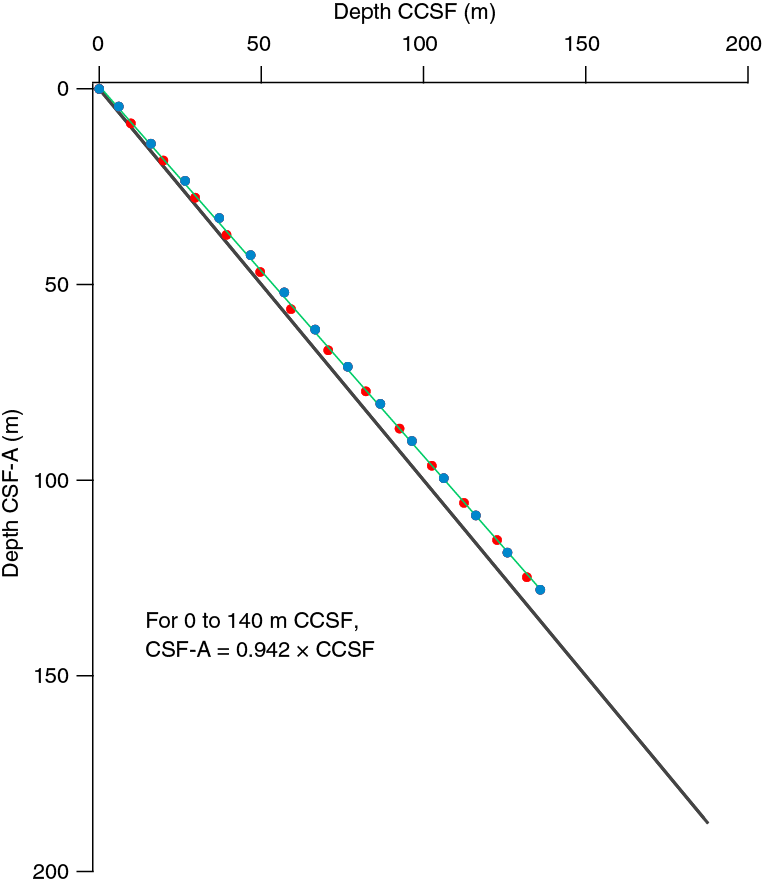
Figure F21. CCSF depth scale growth rate with respect to CSF-A depth, Site U1456.
Table T13. Affine table, Holes U1456A–U1456C. Download table in .csv format.
Although the CCSF scale is useful to put cores and intervals in a detailed stratigraphic sequence, CCSF depth is typically greater than the drilled depth to the same interval because of core expansion. Compressing the scale is important in order to calculate sedimentation rates and to construct detailed synthetic seismic reflection profiles in the upper part of the drilled section. In order to compress the CCSF scale back to CSF-A, the CCSF depth should be multiplied by a compression factor of 0.942 (Figure F21).
Correlation during drilling operations
Near-real-time assessment of the alignment of coring gaps was done during drilling of Hole U1456C by quickly measuring GRA bulk density and magnetic susceptibility on cores from Hole U1456C on the STMSL immediately after the cores were curated on the catwalk. The first 13 cores from Hole U1456C were scanned at 2 cm spacing, whereas subsequent cores were scanned at 5 cm intervals to speed up core flow. We found that the depths of Hole U1456C core breaks were drifting closer to those of Hole U1456A during coring. Therefore, we drilled ahead without coring for short intervals in Hole U1456C in order to provide a complete splice and reduce or eliminate unrecovered intervals. The hole was advanced by 1.5 m at 7.3 mbsf (drilled interval 355-U1456C-21), by 1 m at 65.8 mbsf (drilled interval 91), and by 1.0 m at 76.3 mbsf (drilled interval 111). The offset was maintained between holes from that depth onward, allowing good correlation between the two holes as long as full recovery was achieved. At Core 355-U1456A-12H, where only 6.8 m of core was recovered, the large gap between cores in Hole U1456A proved impossible to unambiguously bridge with cores from Hole U1456C. However, correlation between logs and cores verifies that little or no section is missing from the splice at this depth.
Composite section and splice construction
Stratigraphic correlation and splice construction were based on WRMSL magnetic susceptibility and GRA bulk density data from Holes U1456A–U1456C collected after cores equilibrated to the laboratory temperature. Initial correlations were then adjusted using depth-referenced core images from the Section Half Image Logger (SHIL) (see Lithostratigraphy in the Expedition 355 methods chapter [Pandey et al., 2016a]). SHIL images from each core section were combined to form a complete core image typically 9.5 m long, and the core images were depth-shifted by the initial CCSF offsets based upon the WRMSL data. Comparisons between depth-shifted core images from different holes were used to make finer scale matches and revise the offsets.
GRA bulk density data were useful for hole-to-hole correlation where magnetic susceptibility was weak. Median magnetic susceptibility is ~75 × 10 –5 SI in the upper 420 mbsf of Site U1456 and ranged from –5 × 10⁻⁵ to 1470 × 10–5 SI (see Physical properties). Magnetic susceptibility is typically low (or negative) in the nannofossil-rich sediment and higher in the clay- and sand-rich sections. As such, these measurements are useful for correlating between thin silts and graded beds interpreted as turbidites in the spliced section. GRA bulk density data complemented the magnetic susceptibility data because it exhibited the highest variability in the nannofossil-rich portions of the spliced section, where magnetic susceptibility was low and displayed less variation.
Figures F22, F23, F24, and F25 illustrate the correlations between cores from Holes U1456A–U1456C. Each figure shows a 50 m long section of the composited and spliced data. Only the magnetic susceptibility data are plotted on the line-scan images to reduce the complexity of the profiles.
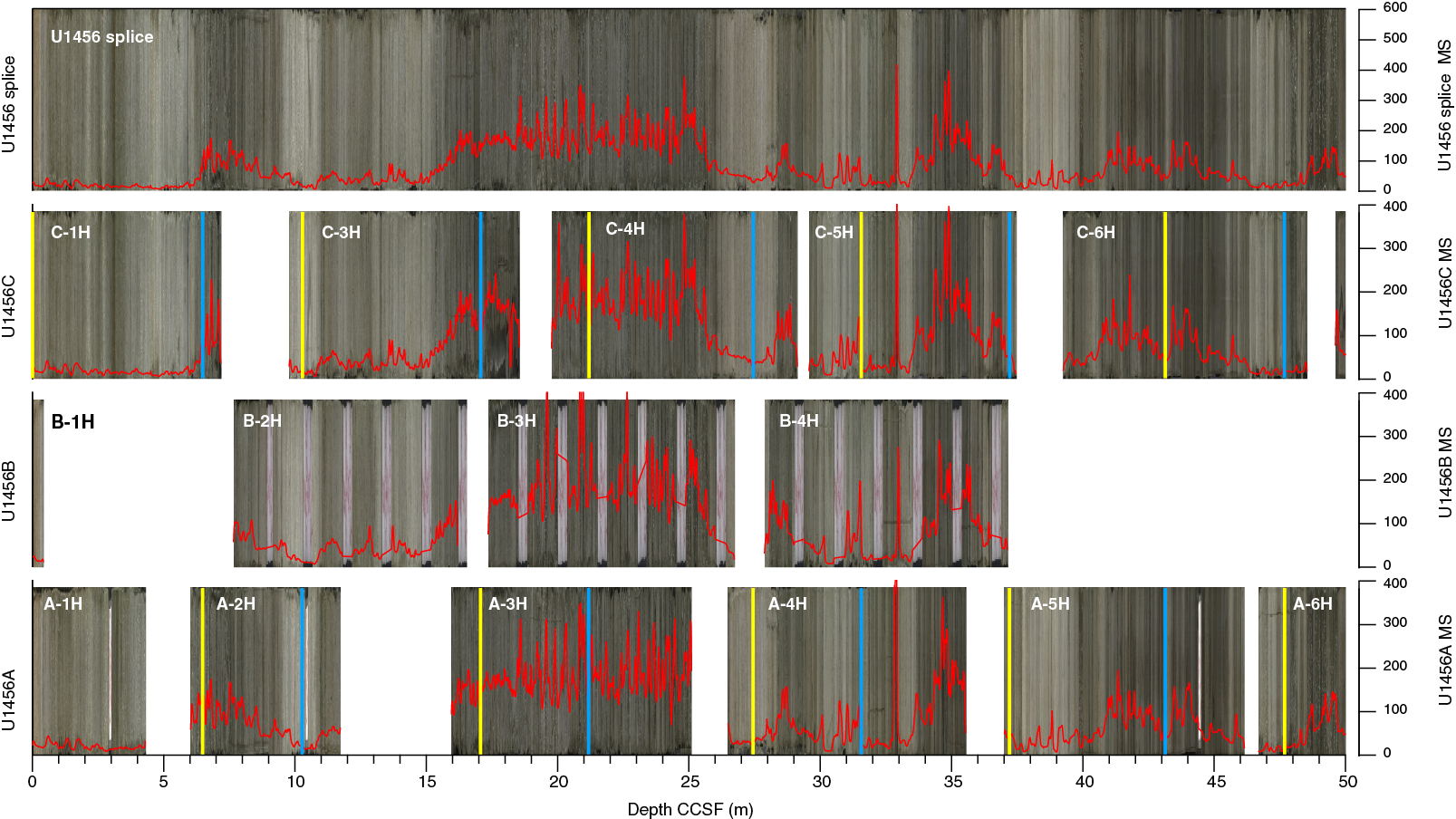
Figure F22. Core images and MS for 0–50 m CCSF in Holes U1456A–U1456C.
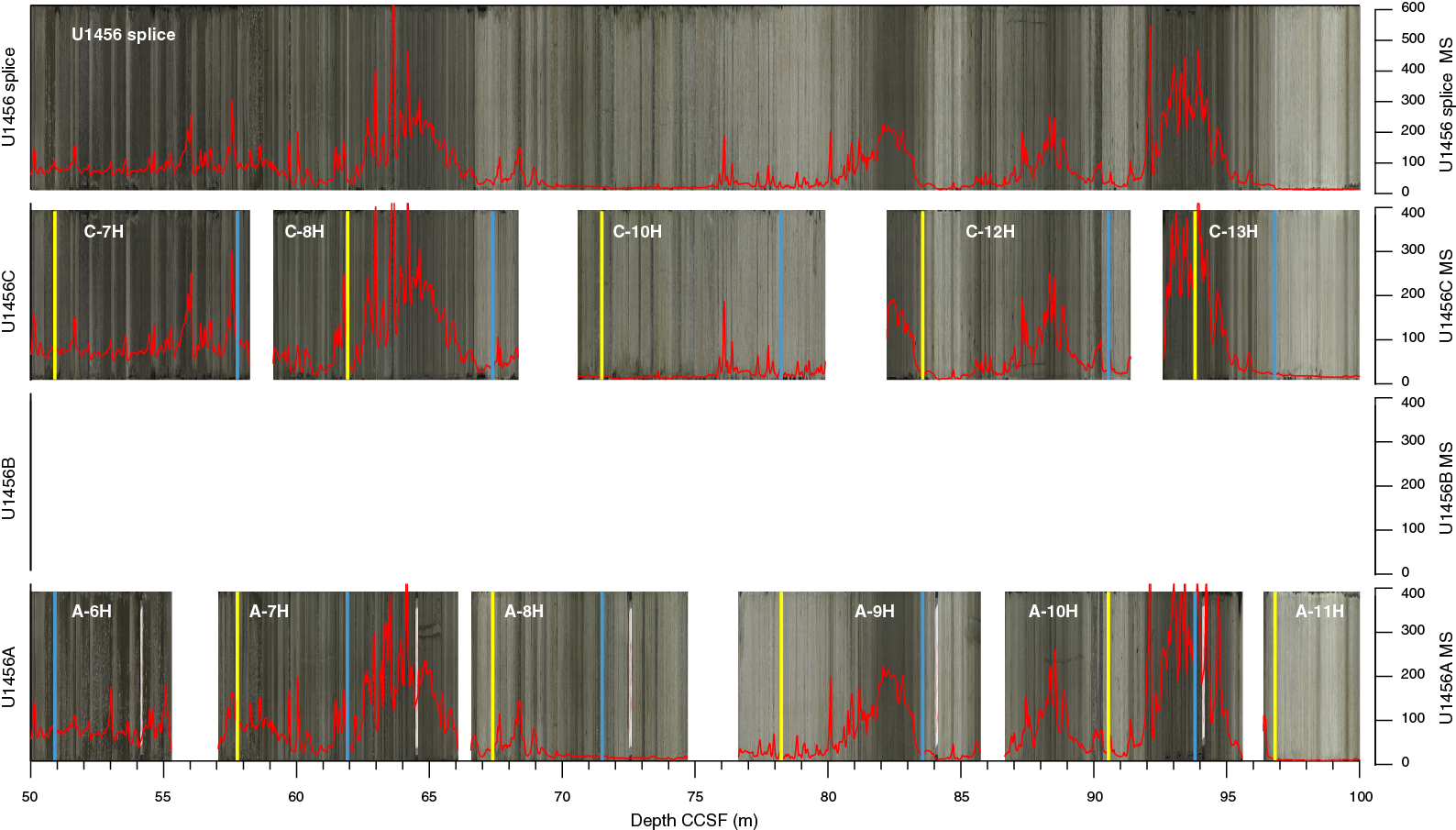
Figure F23. Core images and MS for 50–100 m CCSF in Holes U1456A and U1456C.
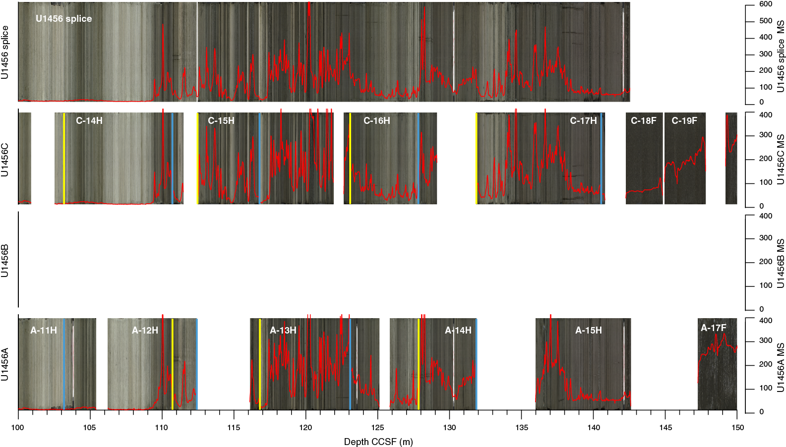
Figure F24. Core images and MS for 100–150 m CCSF in Holes U1456A and U1456C.
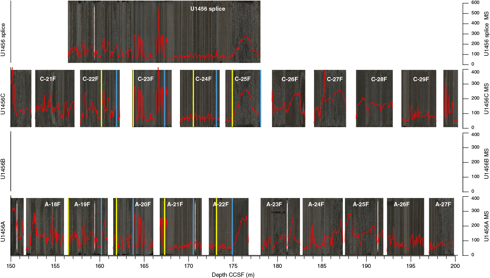
Figure F25. Core images and MS for 150–200 m CCSF in Holes U1456A and U1456C.
Holes U1456A, U1456B, and U1456C were all cored from the seafloor; however, Core 355-U1456B-1H recovered <1 m of sediment, despite the bit being positioned so that the base of the core should have been about 6 mbsf. Because Core 2H clearly correlates to a depth deeper than 6 mbsf in the other holes, much of Core 1H appears to have been lost during core recovery (Figure F22; 0–50 m CCSF) (see Operations).
Good correlations are found among cores from all holes until the base of Core 355-U1456C-5H, which barely overlapped with Core 355-U1456A-5H. Offsets improved when Hole U1456C was drilled ahead without coring (drilled intervals 355-U1456C-91 and 111) (Figure F23). Offset of the coring gaps was lost again when Core 355-U1456A-12H was shorter than normal, recovering only 6.8 m (Figure F24). The missing section was similar in length to the offset that was maintained between the two holes and left no overlap to Core 355-U1456C-15H. The top of Core 355-U1456C-15H was appended to the base of Core 355-U1456A-12H, leaving an unknown but likely small interval not recovered. After logging Hole U1456C (see Downhole measurements), we checked the offset between the two cores by comparing natural gamma radiation (NGR) and magnetic susceptibility records from the cores to the logs and found that the gap was small or nonexistent (see Core-log correlation).
Cores with poor recovery (Cores 355-U1456A-14H and 355-U1456C-16H) occurred at a similar CCSF depth, and Core 355-U1456A-14H failed to bridge the large coring gap to Core 355-U1456C-17H. Core 17H was therefore appended to the base of Core 355-U1456A-14H. Core-log correlation establishes that there is little or no gap between these cores, as discussed in the next section.
Thick sands first appear at the base of Core 355-U1456A-15H, marking the end of the spliced section (Figure F24; 100–150 m CCSF). Coring disturbance in sand and poor core recovery prevented consistent hole-to-hole correlations from being established below this depth as needed to continue the splice.
Although continuity was lost at 142.6 m CCSF because of poor recovery in sands, we found four HLAPC cores from Hole U1456A that have good overlaps with four HLAPC cores from U1456C and can be correlated to each other (Figure F25; 150–200 m CCSF). Good offsets were achieved between Cores 355-U1456A-19F through 22F and 355-U1456C-22F through 25F, making a composite section between 156.7 and 177.5 m CCSF. These eight cores were spliced, and the sampling splice intervals can be found in Table T14. Distinct features found in both Cores 355-U1456A-26F and 355-U1456C-29F allowed one further tie between the two holes at these cores. No further ties could be unambiguously identified between 197 and 229 m CCSF, the base at which Holes U1456A and U1456C overlap before the long drill-ahead section in Hole U1456C. Once coring recommenced below 416 m CCSF in Hole U1456C, poor core recovery precluded correlation.
Table T14. Splice interval table. Download table in .csv format.
From Core 355-U1456A-30F and deeper (>215.3 m CCSF), the CCSF offsets were occasionally increased in order to develop a sequence without core overlaps in the CCSF scale for cores from the same hole (Table T13). In the CSF-A scale, core overlaps often occur because core recovery may be larger than the cored interval (see Stratigraphic correlation in the Expedition 355 methods chapter [Pandey et al., 2016a]), but these overlaps are eliminated in the CCSF scale.
Core-log correlation
Logging data from Hole U1456C were compared with GRA, NGR, and magnetic susceptibility data on recovered core as another way to correlate between the cores and the original sediment column (Figure F26). The wireline log matched depths below seafloor (WMSF) for cores established by this correlation are also included in Table T13. The assigned WMSF depths are not as precise as the CCSF depths because log data are recorded only every 15 cm versus 2 cm for the core data. Also, we occasionally found that different offsets are required to match the magnetic susceptibility versus the NGR logs, presumably because the tools are offset on the logging string and minor winch variations cause variability in depth measured by the wireline tool. Based on repeated attempts at correlation, the assigned WMSF depths are probably only accurate to ±30 cm.
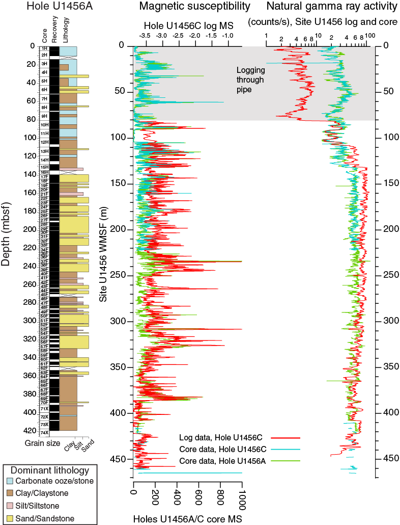
Figure F26. Lithologic summary and comparison of NGR wireline logs to core NGR data and MS wireline logs to core MS data.
Through-pipe NGR allowed a very good correlation from cores to logs in the upper sediment section from the seafloor to base of pipe at 81 m drilling depth below seafloor (DSF) (the low-NGR section shown in Figure F26). The correlation was continued using both magnetic susceptibility and NGR logs from 81 m WMSF to the bases of Holes U1456A and U1456C.
The continuity of the logs allowed a match of the general patterns of magnetic susceptibility and NGR change between a succession of cores and allowed for a good correlation to be made to ~220 m WMSF, where Hole U1456C was drilled ahead. Below 220 m WMSF, a fair to good correlation could be made between Hole U1456A and the wireline logs. The different character of the magnetic susceptibility and the NGR logs for the most part allowed for unambiguous matches despite the short cores and coring disturbance in the recovered core sections.
Correlations between core data and log data within the spliced section provide an alternative way to determine the length of missing section at the depth where Core 355-U1456C-15H is appended to Core 355-U1456A-12H (see Composite section and splice construction). Although the determination is independent, the correlation between cores and logs is not very precise. Nevertheless, there is no evidence of missing section or overlap based upon the logging correlation. The splice intervals given in Table T14 are the best description of a complete section that can be made with the available data.
There are offsets between relative depths assigned by correlating to either the NGR log or to the magnetic susceptibility log, especially in the interval near the base of pipe. For example, the magnetic susceptibility signal from the cores is well aligned with the magnetic susceptibility log in the interval between 80 and 90 m WMSF on Figure F26, but an additional downward shift of ~1 m is needed to match the NGR log. We speculate that offsets between the logs occur because of minor errors in wireline depth if the logs are from separate logging runs, or because winch-related errors in the WMSF scale occur at different depths in the respective logs because of the tool offset.
Geochemistry
Organic geochemistry
Shipboard organic geochemical analysis of sediment from Site U1456 included monitoring of hydrocarbon gases and bulk sediment measurements of total carbon, total inorganic carbon (TIC), total sulfur, and total nitrogen (TN). We used these analyses to calculate the CaCO3 and total organic carbon (TOC) content (see Geochemistry in the Expedition 355 methods chapter [Pandey et al., 2016a]). In total, 140 samples were analyzed for hydrocarbon gas monitoring (Table T15; Figure F27). For bulk sediment measurements, 82 samples were analyzed from Hole U1456A, 7 samples from Hole U1456C, 101 samples from Hole U1456D, and 29 samples from Hole U1456E (Table T16; Figures F28, F29).
Table T15. Headspace gas composition of sediment. Download table in .csv format.
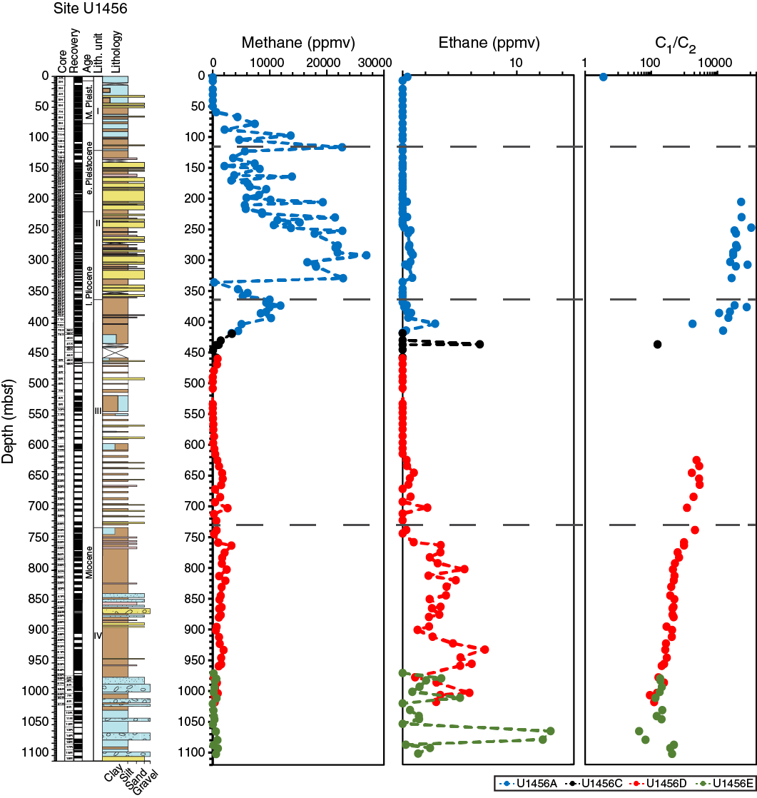
Figure F27. Methane, ethane, and C1/C2 ratios.
Table T16. Carbon, nitrogen, and sulfur analyses of sediment. Download table in .csv format.
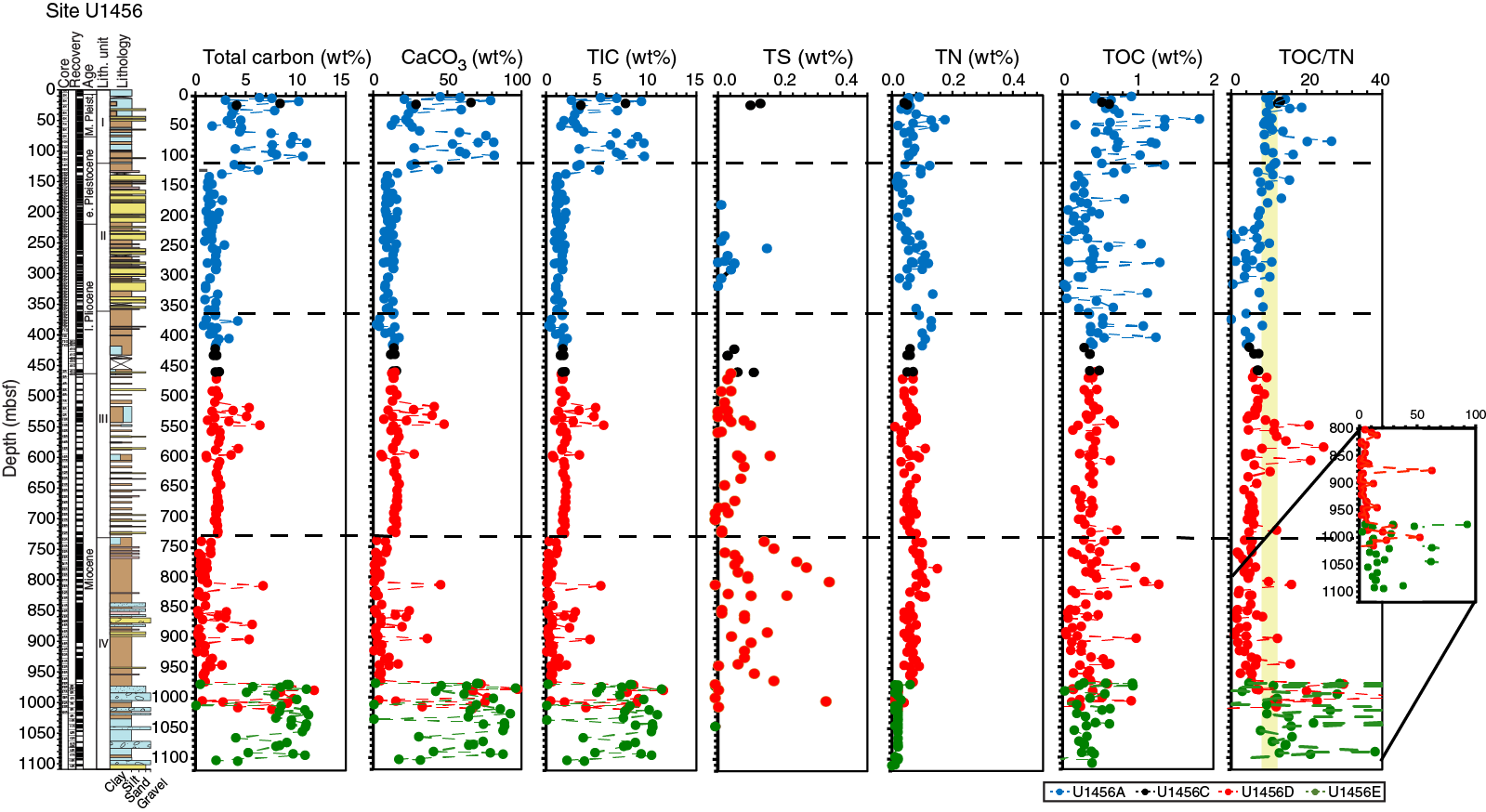
Figure F28. Total carbon, CaCO3, total inorganic carbon, total sulfur, total nitrogen, total organic carbon, and TOC/TN.
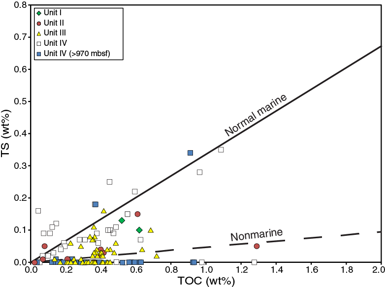
Figure F29. TOC vs. TS with samples plotted by lithologic units.
Volatile gases
Headspace gas analysis was performed typically once per core, or once per ~9.5 m interval (except for Hole U1456B and Hole U1456C above Core 355-U1456C-40X, which overlapped with Hole U1456A) (Table T15; Figure F27). Headspace methane content represents residual gas in cores (with some gas lost during core retrieval and sampling). Methane concentrations vary by four orders of magnitude at this site. Methane levels are low (<1,000 ppmv) between 0 and 60 mbsf. Below 60 mbsf, methane values start to increase and reach a value of 22,680 ppmv by 116 mbsf. This increase in methane corresponds to a reduction in sulfate concentrations in the interstitial water profile (Figure F30), suggesting a transition from sulfate reduction to methanogenesis. Methane concentrations decrease to ~2,000 ppmv at 147 mbsf and then increase again to 26,933 ppmv at 292 mbsf. The relatively high methane levels encountered between 100 and 330 mbsf suggest a lithologic control (i.e., the accumulation of gases in relatively porous silty sand and silt with sand layers). Methane drops to 257 ppmv at 336 mbsf and then increases to 11,858 ppmv at 373 mbsf. In Holes U1456C–U1456E, measured methane levels are relatively low and do not exceed 2,606 ppmv.
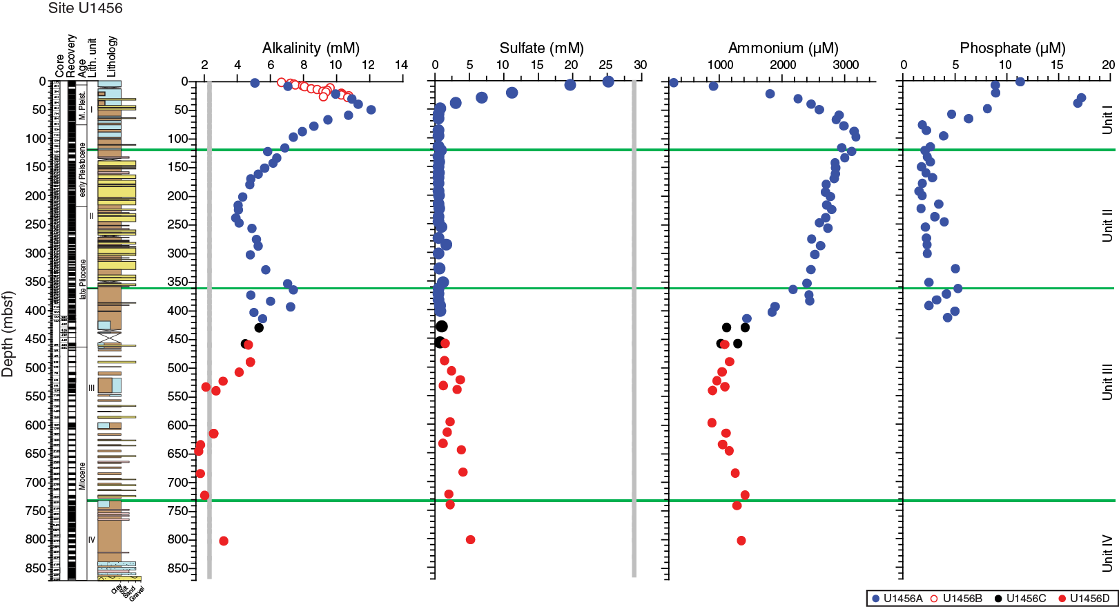
Figure F30. Interstitial water alkalinity, sulfate, ammonium, and phosphate variations.
Ethane levels were low for all intervals recovered from Site U1456 and did not exceed 15 ppmv. Methane/ethane (C1/C2) ratios were calculated only for those samples where ethane was detected (Figure F27). C1/C2 ratios are high throughout the cored interval in Hole U1456A (from >11,000 to >100,000) and are at least an order of magnitude higher than levels associated with thermogenic production and thus posed no threat to drilling operations.
Sedimentary geochemistry
In lithologic Unit I, total carbon values are high and variable (1.6–10.8 wt%). CaCO3 values are also variable (14.7–81.6 wt%) and follow the same trend as total carbon, indicating that most of the total carbon is present as CaCO3 (Figure F28). TOC varies between 0.16 and 1.8 wt%. High TOC values correspond to layers of silty sand with nannofossils and silt with sand (Figure F28).
In the upper part of lithologic Unit II, from ~140 to 240 mbsf, total carbon values are low (<2 wt%). CaCO3 and TOC values fall within 8–15 wt% and 0.1–0.4 wt%, respectively. Below 240 mbsf, total carbon and CaCO3 values remain low, whereas TOC varies significantly between 0.37 and 1.24 wt% (Figure F28), with lower TOC values found in sandy layers.
Lithologic Unit III (~362–730 mbsf) is characterized by low total carbon (<3.54 wt%) and low CaCO3 (<27.59 wt%), with the exception of the interval between 517 and 596 mbsf where total carbon and CaCO3 increase to as much as 6.42 and 47.79 wt%, respectively (Figure F28). TOC values range between 0.14 and 1.29 wt% throughout the unit. Poor sediment recovery in Unit III limits comparison between chemical variability and specific lithology.
Lithologic Unit IV can be divided into two intervals based on the total carbon, TIC, and CaCO3 results (Figure F28). On the other hand, TOC ranges between 0.1 and 1.27 wt% throughout Unit IV, with no distinct differences between the upper and lower parts of the unit. From 740 to 978 mbsf generally low values of total carbon (<2 wt%) and CaCO3 (<10 wt%) prevail. This interval is characterized by silty claystone and sandstone lithologies (see Lithostratigraphy) with generally lower nannofossil and foraminifer abundance (see Biostratigraphy). Within this interval there are a number of samples with notably higher total carbon and CaCO3, for example CaCO3 spikes to 45.4, 22.2 and 36.4 wt% at 813, 866, and 902 mbsf, respectively, coincident with calcareous lithologies. The interval between 978 and 1102 mbsf contains the highest percentages of total carbon (up to 11.8 wt%) and CaCO3 (up to 97.4 wt%) recorded at this site. Such high values are associated with nannofossil-rich claystone and calcarenite together with sandstone lithologies. Overall, the interval exhibits a mixture of different lithologies that sometimes displays chaotic bedding and small faults (see Lithostratigraphy), as well as abundant reworked Paleogene to early Neogene microfossil assemblages (see Biostratigraphy). This interval is interpreted as a mass transport deposit (see Lithostratigraphy).
We report TOC/TN ratios as a preliminary estimate for the source of organic material (Figure F28). Müller and Mathesius (1999) proposed that the TOC/TN ratio can be used to constrain predominantly marine (TOC/TN < 8) from predominantly terrestrial (TOC/TN > 12) organic inputs (yellow box in Figure F28). However, a simple model of the factors influencing TOC/TN ratios is not always applicable. High TOC/TN ratios atypical for marine algal source organic carbon have been measured in organic carbon–rich Mediterranean sapropel layers, upper Neogene sediment from the Benguella upwelling region, Eocene horizons from the Arctic Ocean, and Cenomanian–Turonian black shales (Meyers, 1990; Stein and Macdonald, 2004; Stein et al., 2006; Twichell et al., 2002).
In Unit I in Hole U1456A, TOC/TN values are generally >8, suggesting some terrestrial input. Three distinct intervals with high TOC/TN (>15) at 22.4, 78.5, and 100.3 mbsf suggest increased terrestrial input and correspond to beds of silty sand with nannofossils and silt with sand (Figure F28). A background of low to intermediate TOC/TN values in Units II and III (~1–10) suggests that mixed terrestrial and marine organic matter inputs prevail. Similar ratios for Unit IV suggest mixed inputs between 740 and 978 mbsf. Superimposed on the low to intermediate background values in Unit III, high TOC/TN values (>20) occur at 549.1, 585.4, and 607.4 mbsf. The samples at 549.1 and 585.4 mbsf are extracted from sandy turbidite horizons, confirming a terrestrial source. Notably, the sample at 585.4 mbsf contains lignite-like wood fragments. In Unit IV TOC/TN spikes above background values to 16 and 63 at 813.3 and 877.4 mbsf, respectively. Very high values (up to 92) occur within the 978–1018 mbsf interval (a large mass transport deposit, see Lithostratigraphy) suggesting strong terrestrial input of organic matter.
To further estimate the source of organic material to the sediment, correlation between TOC and total sulfur may provide a basic estimation of the source of organic matter to marine sediments (Berner and Raiswell, 1983). In general, normal marine sediment contains higher sulfur concentrations and has lower TOC content than sediment deposited in freshwater environments. Therefore, following the approach of Gregor et al. (1988), we plotted TS (wt%) versus TOC (wt%) in order to better constrain the sources of organic matter in the different units (Figure F29). Intermediate values of total sulfur relative to downhole variations in Unit I suggest a mixed input of terrestrial and marine organic matter into the sediment. Units II and III indicate a mixed input of the organic matter with a slight predominance of nonmarine input in Unit III. The Unit IV data suggest stronger normal marine input of organic matter, with some strong terrestrial input over the 978–1102 mbsf interval. The approximations of source based on the TOC/total sulfur scatter plot are broadly consistent with the TOC/TN downhole interpretations.
Total lipid extractions
Organic solvent extractions were performed (see Geochemistry in the Expedition 355 methods chapter [Pandey et al., 2016a]) on 96 sediment samples. Aliquots of ~1.5 g were taken from interstitial water squeeze cake and core catcher samples. Total lipid extracts (TLE) varied between 0 and 19.4 mg/g dry sediment. The TLE samples were archived for shore-based biomarker assays and analyses.
Inorganic geochemistry
Whole-round samples (5 cm long from 0 to 303 mbsf, 10 cm long from 303 to 597 mbsf, and 15 cm thereafter) were collected for interstitial water extraction at regular intervals throughout Hole U1456A (one sample per core or every other core when using HLAPC), Hole U1456B (one sample per section), and Holes U1456C and U1456D (one sample per 9.5 m core). The volume of the interstitial water recovered decreased with depth from 35 to 3 mL. Interstitial water sample collection was discontinued below 863 mbsf in Hole U1456D when interstitial water volume was no longer sufficient for analysis. Specific aliquots were used for shipboard analyses and the remaining fluid was sampled for shore-based analyses or archived.
Salinity, pH, chloride, sodium, and bromide
Downhole profiles of salinity, pH, chloride, sodium, and bromide concentrations at Site U1456 are shown in Figure F31, with the data given in Table T17. From the seafloor to 22 mbsf, interstitial water salinity remains close to the average seawater value. Salinity decreases to 32 at 59 mbsf and then remains more or less uniform with depth in Holes U1456A, U1456C, and U1456D. This decrease in salinity may be caused by clay mineral dehydration with increasing depth (Jaeger et al., 2014). The pH of the interstitial water is observed to be slightly lower than that of modern seawater. This lower pH could be driven by the release of organic acids in the initial stages of anaerobic organic matter degradation (Soetaert et al., 2007). Overall, pH increases slightly with depth to ~700 mbsf in Hole U1456D. Chloride is a conservative ion and its concentration is controlled by diffusion and compaction-driven advection in interstitial water (Jaeger et al., 2014). The chlorinity of the interstitial waters is similar to modern seawater values (559 mM) downhole to ~270 mbsf and then increases from that depth to ~825 mbsf in Hole U1456D. Bromide is incorporated in marine organic matter and can be released during microbial degradation of organic matter. Bromide increases from ~0.83 mM near the top of Hole U1456A to ~1 mM until the base of Unit II and stays fairly uniform thereafter. The concentration of sodium in interstitial water is close to that of seawater (480 mM) in the upper 276 mbsf of Hole U1456A and then increases gradually to its maximum concentration (502 mM) at ~725 mbsf in Hole U1456D. Variations in sodium concentrations in interstitial water closely mimic the concentration profile of chlorinity, with a molar ratio of Na/Cl close to modern seawater (~0.86).
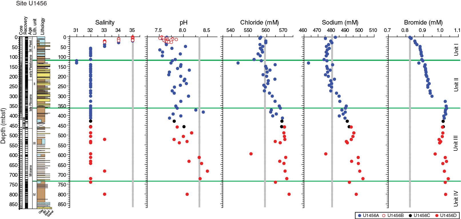
Figure F31. Interstitial water salinity, pH, chloride, sodium, and bromide variations.
Table T17. Cations and anions in interstitial water. Download table in .csv format.
Alkalinity, sulfate, phosphate, and ammonium
Downhole variations in alkalinity, sulfate, ammonium, and phosphate at Site U1456 are shown in Figure F30, and the data are given in Table T17. From the seafloor to 50 mbsf, alkalinity increases steadily from 5 to 12 mM and then decreases to a concentration of 3.9 mM at 238 mbsf. Alkalinity increases further to 7 mM by 350 mbsf and decreases steadily to ~550 mbsf below which point it remains low to the end of interstitial water sampling in Hole U1456D. We suggest the alkalinity increases are a byproduct of microbial degradation of organic matter, and its increase in the top 50 mbsf reflects the action of anaerobic sulfate reduction, which in turn is reflected in the sulfate profile. The concentration of sulfate decreases from 25 to 0.6 mM in the uppermost 50 mbsf, indicating anaerobic sulfate reduction, and then remains low throughout the remainder of sampling in Hole U1456D with a slight increase after 500 mbsf. Ammonium increases from 285 µM near the surface to 3193 µM at 100 mbsf and decreases thereafter until ~500 mbsf, where it has a value of ~900 µM. Ammonium concentrations remain uniform below that depth throughout the remainder of sampling in Hole U1456D. Phosphate decreases from 17 to 1.5 mM in Hole U1456A at ~100 mbsf. It remains low until 415 mbsf, but then falls below the detection limit deeper than 420 mbsf in Holes U1456C and U1456D. Ammonium is a byproduct of microbial degradation of organic material, and its concentration increases in the sulfate reduction zone (~0–100 mbsf). Below the sulfate reduction zone, methanogenesis becomes an important process, which is reflected in the increase in methane concentrations below 50 mbsf (Figure F27).
Calcium, strontium, lithium, magnesium, and potassium
Downhole variations of calcium, strontium, lithium, magnesium, and potassium at Site U1456 are shown in Figure F32, and the data are given in Table T18. Calcium concentrations in interstitial water at Site U1456 range from 3 to 15 mM. Calcium concentrations remain below modern seawater values above 550 mbsf, below which depth they increase to maximum value in Hole U1456D. The calcium profile is generally anticorrelated with alkalinity, suggesting that whenever the alkalinity is high, calcium is precipitated as carbonate, decreasing the concentration of calcium in the interstitial water. The concentrations of strontium and lithium range from 74 to 587 µM and 0.4 to 138 µM, respectively. Strontium concentration increases in the uppermost 100 mbsf corresponding to Unit I, possibly due to dissolution and recrystallization of biogenic carbonate, which is relatively enriched in strontium (Sayles and Manheim, 1975). Strontium then decreases with depth until ~200 mbsf as carbonate within the sediment decreases as a result of a change to a more sand- and clay-based lithology (see Lithostratigraphy). A dramatic increase in strontium concentrations is observed from 550 to 850 mbsf, possibly due to carbonate dissolution, which also corresponds to an increase in the calcium profile. A major sink of lithium is caused by adsorption of lithium onto clay minerals like kaolinite, vermiculite, and smectite, as well as onto other terrigenous sediment (Scholz et al., 2010; Millot et al., 2010, and references therein). The concentration of lithium is less than the average modern seawater value above 500 mbsf, likely indicating its adsorption onto clay minerals and other terrigenous sediment. Lithium increases dramatically deeper than 700 mbsf, possibly due to diagenetic release from clay minerals and other terrigenous sediment. The concentrations of magnesium and potassium range from 23 to 53 mM and 2 to 12 mM, respectively, and decrease with depth. Magnesium and potassium concentrations are lower than the average seawater values measured below the top of Hole U1456A, likely because of removal into newly formed clay minerals.
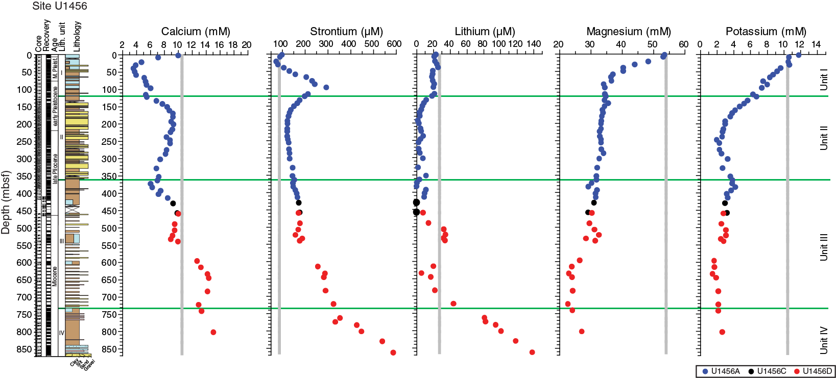
Figure F32. Interstitial water calcium, strontium, lithium, magnesium, and potassium variations.
Table T18. Major and trace element concentrations in interstitial water. Download table in .csv format.
Silicon, barium, manganese, boron, and iron
Downhole variations of silicon, barium, manganese, boron, and iron at Site U1456 are shown in Figure F33 and the data are given in Table T18. Dissolved silicon concentrations are between 93 and 555 µM at Site U1456. Silicon concentrations are highest in the uppermost 120 mbsf of Hole U1456A (Unit I), which may be caused by release of silicon during the dissolution of biogenic silica (diatoms, radiolarian, sponge spicules, etc.). Silicon decreases below 120 mbsf and stays low throughout Holes U1456A, U1456C, and U1456D, suggesting that the biogenic source of silica seen at shallower depths is absent or expended. Barium concentration in interstitial water ranges from 0.1 to 288 µM, with a dramatic increase in concentration between 250 and 400 mbsf. Anaerobic degradation of organic matter (Schenau et al., 2001) and dissolution of feldspar are potential sources of barium in interstitial water. Alternatively, barium can also be released by in situ barite dissolution in low-sulfate fluids (Li et al., 2015).

Figure F33. Interstitial water silicon, barium, manganese, boron, and iron variations.
Manganese and iron concentrations range from 0.3 to 5.6 µM and 0 to 16 µM, respectively. Manganese concentrations decline sharply in the uppermost ~50 mbsf of Hole U1456A, which corresponds to the sulfate reduction zone. Manganese is a terminal electron acceptor in the organic oxidation reaction. The oxidation and reduction of manganese during organic matter degradation leads to redistribution of manganese between dissolved and particulate phases, which could explain the observed manganese profile. Except for two values at ~9 and 80 mbsf, iron shows consistently low concentrations, indicating its removal, probably by metal sulfide formation under anaerobic conditions. The concentration of boron in interstitial water ranges from 266 to 620 µM. Boron concentrations decrease from ~550 µM at 3 mbsf to ~260 µM near 220 mbsf and then generally increase to high values by 350 mbsf. Below this depth there is a slight decline over the remainder of the drilled interval to values ~300 µM (Figure F33).
Microbiology
The primary objectives of microbiological studies at Site U1456 were contamination assessment of samples, shipboard characterization of subsurface microbes, and preservation of samples for detailed shore-based investigation.
Microbial sampling
Thirty-six whole-round core samples were taken at a frequency of one per ~9.5 m of cored interval downhole to 414 mbsf in Hole U1456A. Hole U1456B was cored as a dedicated microbiology hole, and 36 whole-round core samples (eighteen 5 cm long whole rounds and eighteen 10 cm long whole rounds) were taken at a frequency of one per ~1.5 m from Cores 355-U1456B-2H through 4H (0.6–29.03 mbsf). Sampling was completed on the catwalk, and the samples were immediately moved to the cold room in the microbiology laboratory for further subsampling. Subsampling procedures were completed within a short time of the core arriving on deck. Subsamples for total microbial counts and molecular marker analyses were immediately collected using sterile syringes (one 50 mL and two 5 mL). All whole-round samples for microbial and interstitial water chemistry measurements were taken next to each other for comparison purposes. The whole-round microbiology samples were preserved at –80°C for shore-based characterization of microbial communities using DNA/RNA, at –20°C for microbial lipid analysis, and at 4°C for cultivation-based studies. We also collected and preserved 100 mL of drilling mud fluid and seawater for contamination analysis. The microbial communities, DNA, and lipids present in these samples will be compared to those inside the cores in order to determine if microbes in the drilling fluid have contaminated subsurface samples.
Contamination assessment
We used a fluorescent microsphere–based contamination testing method during APC coring at Site U1456.
Fluorescent microspheres
Fluorescent microspheres were added to the core catcher sub for Cores 355-U1456A-1H through 70F, as well as Cores 355-U1456B-1H through 4H. Three samples were collected from each core for analysis of microspheres. These samples were taken from (1) the interior of the core, (2) the exterior of the core, and (3) an intermediate position in between the exterior and interior.
Samples taken for microsphere-based contamination testing were analyzed during the expedition. In samples from Hole U1456B, no microspheres were observed in the interior of any of the core samples (Figure F34; Table T19). All exterior samples contained microspheres, and most intermediate samples contained a low concentration of microspheres, demonstrating that contamination significantly decreases from the exterior toward the interior of the core.
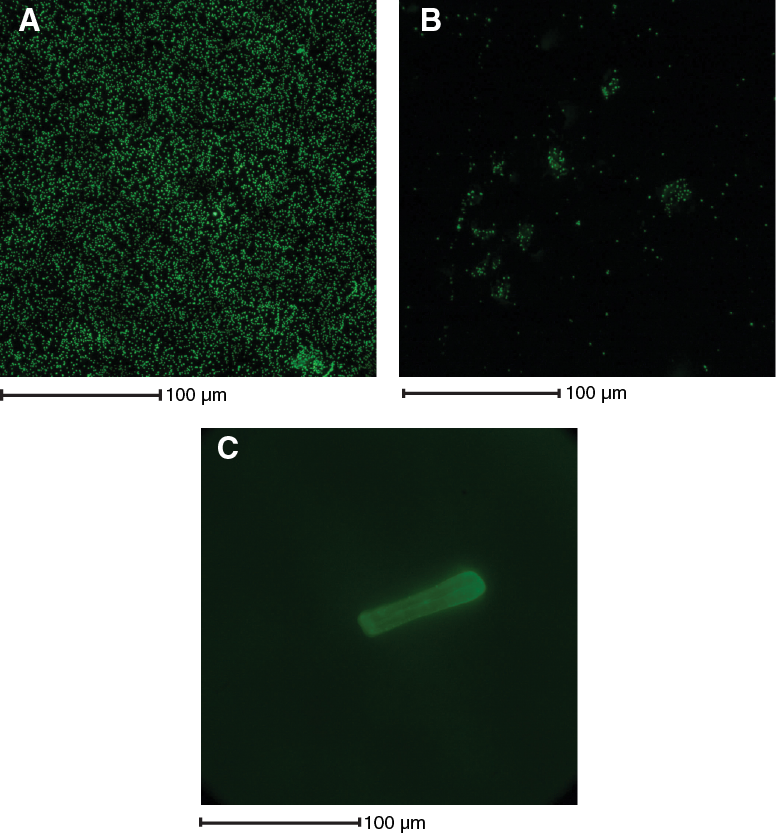
Figure F34. Results of fluorescent microsphere contamination testing for whole-round Sample 355-U1456B-3H-1, 130–140 cm.
Table T19. Fluorescent microsphere contamination test results, Hole U1456B. Download table in .csv format.
Drilling fluid and seawater samples
Samples of drilling mud and core liner water samples for shore-based characterization of microbial communities were taken at daily intervals. These samples are used to estimate the number of cells introduced into the core samples during drilling.
Microbiological shipboard analyses
Samples from Hole U1456B were analyzed for new microbial community structures. The subsurface sediment (0–27 mbsf) in Hole U1456B contains some species of eukaryotic fungi (Figure F35) and meiofauna (Kinorhynchs sp.) (Figure F36). Initial shipboard observations find that these two different taxonomic groups sometimes co-occur in the same habitat, such as in Sections 355-U1456B-2H-4 and 4H-1 (Table T20). Interestingly, we observed the meiofauna at ~6 mbsf (Figure F36).The exact phylogenetic positions of the new taxa will be addressed during postcruise research by advanced molecular techniques. Despite an increasing number of studies on deep-sea microorganisms and meiobenthos, the mechanisms of their interactions, such as their response to organic matter availability, is still unclear.
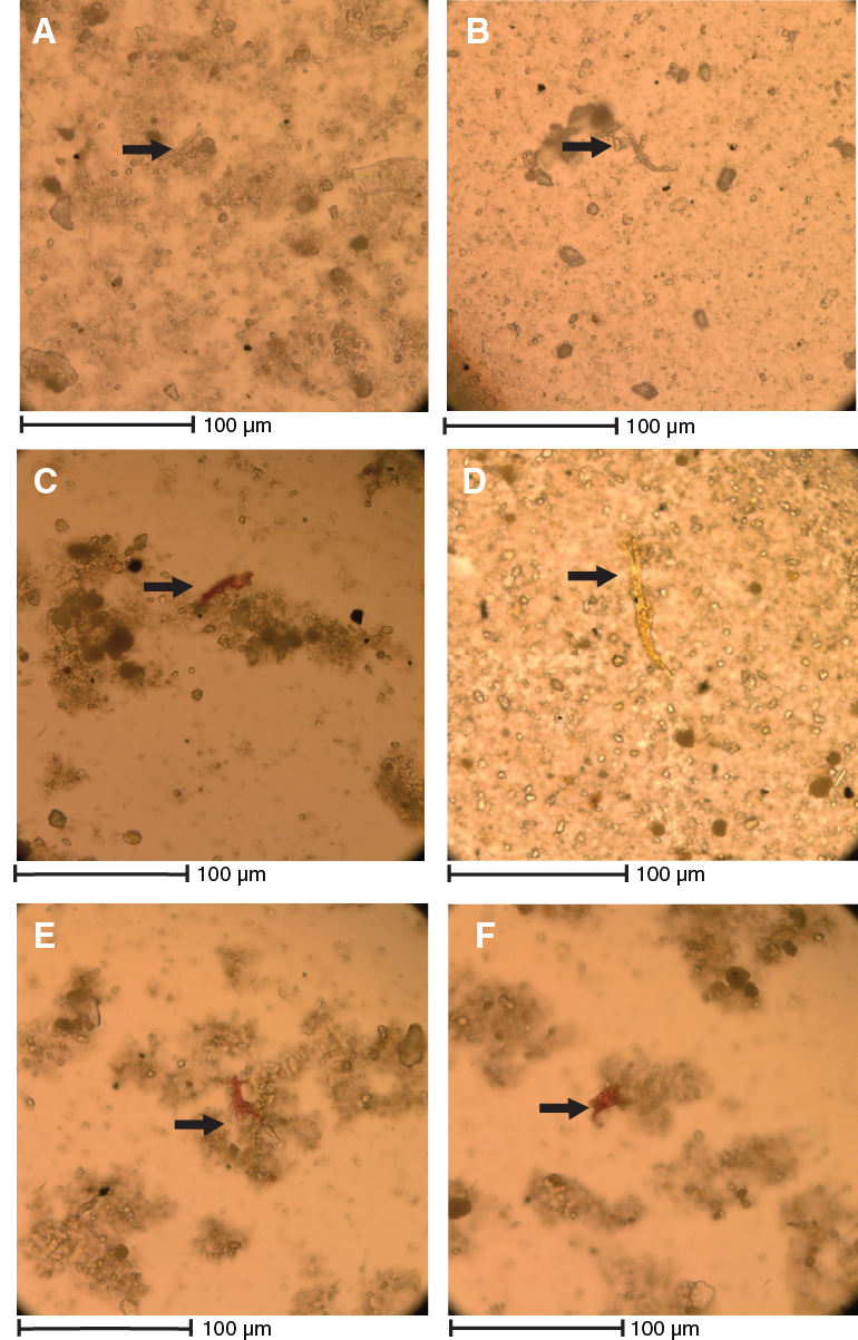
Figure F35. Fungal assemblages observed at 500× magnification, Hole U1456B.
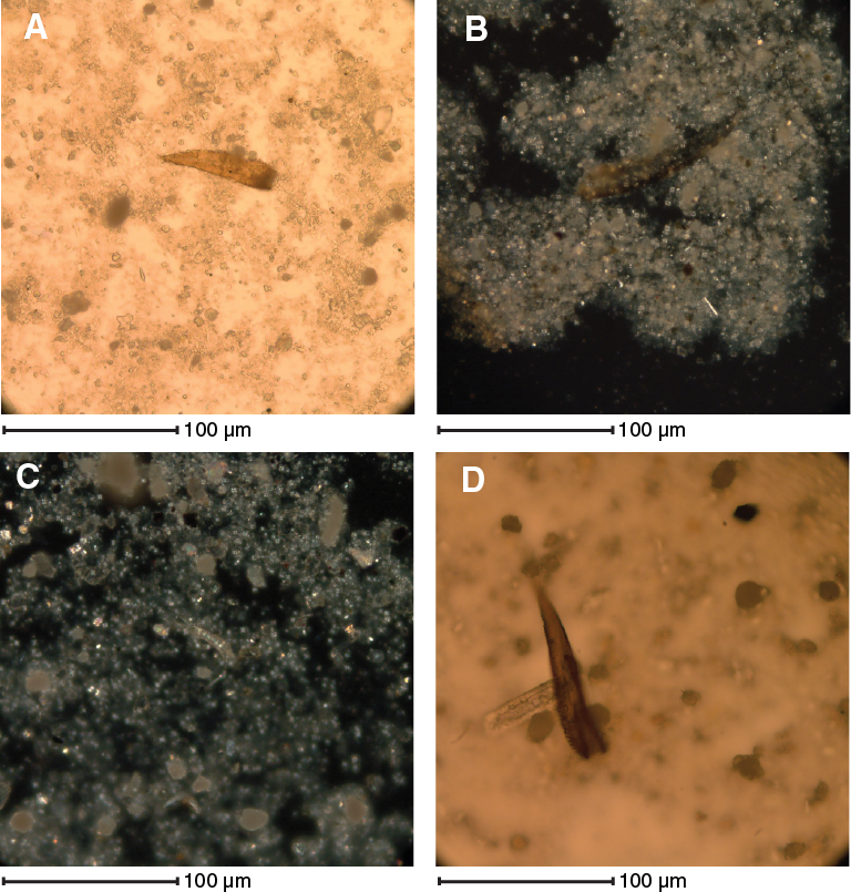
Figure F36. Meiofaunal organisms observed at 500× magnification, Hole U1456B.
Table T20. Presence of fungi and meiofauna, Hole U1456B. Download table in .csv format.
Paleomagnetism and rock magnetism
Measurements
We measured the magnetic properties of archive halves from Cores 355-U1456A-1H through 21F at 5 cm intervals through step-wise demagnetization to a maximum of 20 mT and Cores 355-U1456D-2R through 67R with step-wise demagnetization to 25 mT. To aid in interpretation of the data, we took discrete samples at a rate of one per section from Holes U1456A, U1456C, and U1456D. Archive halves from intervals deemed to be not in situ (e.g., mass wasting events) were not measured, and these intervals were only sparsely sampled. We measured the anisotropy of magnetic susceptibility (AMS) and performed step-wise demagnetization on discrete samples from all holes. In order to characterize the rock magnetic mineralogy, we subjected many samples to anhysteretic remanent magnetization (ARM) and isothermal remanent magnetization (IRM) acquisition experiments, and a selected few were subjected to the full 3D-IRM thermal demagnetization experiment (see Paleomagnetism and rock magnetism in the Expedition 355 methods chapter [Pandey et al., 2016a]).
Interpretation
Archive-half data
We plotted all of the measurements from the archive halves of Hole U1456A as blue symbols in Figure F37. Declinations within each core are reasonably consistent, but the cores appear to be randomly oriented, an indication that they were not completely remagnetized during coring and splitting. The upper 10 cores have inclinations consistent with the expected normal polarity average of ~30° for the latitude of the site. However, although there are some negative inclinations in and below Core 355-U1456A-11H, the polarity log does not reflect the expected pattern for reversals, whereby entire intervals would be uniformly negative or positive, but appear to have many more positive inclinations than expected.
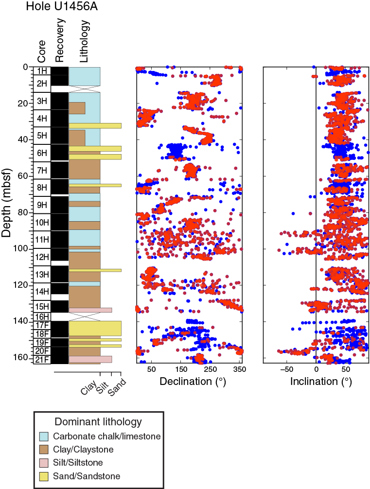
Figure F37. Results of pass-through magnetometer measurements of archive halves, Hole U1456A.
Ends of core sections measured in the pass-through system, coring disturbance (soupy layers and flow-in), and the presence of sand layers likely affected the results because these are less likely to preserve the original magnetization. Therefore, we removed data from
- Within 10 cm of each core section end because these would be biased by the wide response function of the instrument’s sensor;
- Unconsolidated sandy intervals, as these are not expected to preserve a reliable magnetization; and
- Layers described as “soupy” or “flow-in” (see Lithostratigraphy).
Tables taken from lithostratigraphic descriptions were used to edit the data. The edited magnetic results are illustrated in Figure F37 as red dots and show that there was little to no reduction in scatter in the data. As a result, we ceased measurement of archive halves below Core 355-U1456A-21F and focused our efforts on the discrete samples.
The results are similar for Hole U1456D (Figure F38). The original data at the 25 mT step are plotted in blue. Magnetic stability is grain size dependent and, generally speaking, sand-sized magnetite is unstable. Therefore, all horizons marked “sandy” or “sandstone” in either the major or minor descriptions were deleted, as were all data within 10 cm of the section ends and with disturbance intensities of 2 or greater. The edited data set is plotted in red. Although there are fewer data points after applying the filtering criteria listed above, any magnetostratigraphic interpretation based on these data would be questionable.
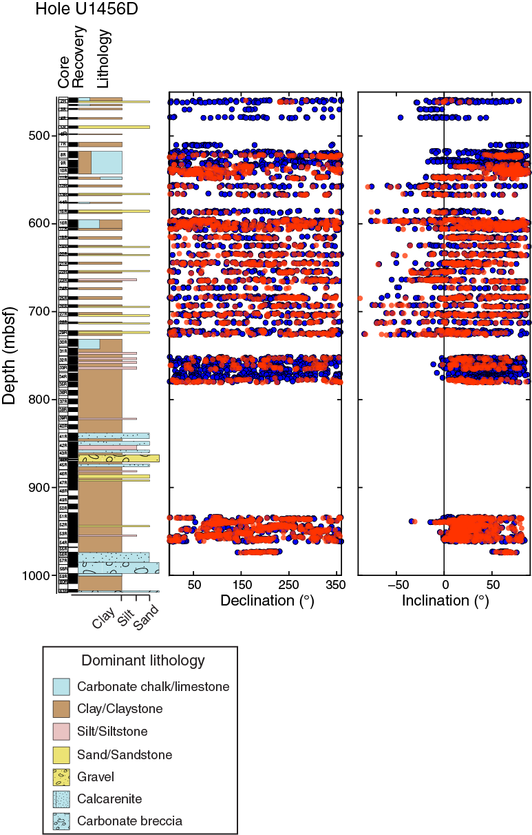
Figure F38. Results of pass-through magnetometer measurements of archive halves, Hole U1456D.
Discrete samples
Step-wise demagnetization of discrete samples produced a wide variety of behavior. Representative examples are plotted in Figure F39. The behavior shown in Figure F39A and F39B is straightforward in that the remanence decays quasilinearly to the origin with largely constant directions after removal of a soft, steeply dipping, coring-induced remanence at demagnetization step 15 or 20 mT. These we classify as Type I and interpret by fitting a line through at least four consecutive measurements. Two statistics are helpful in quantitatively assessing the quality of the fit: the maximum angle of deviation (Kirschvink, 1980), which is a measure of the scatter about the best fit line, and the deviation angle (Tauxe, 2010), which measures the deviation of the fitted line from the origin. We used a cut-off of 15° and 10° for the maximum angle of deviation and the deviation angle, respectively, and rejected data that exceeded these bounds. As core orientation is basically random in azimuth (see discussion below), we based our interpretation on the inclination values of the magnetization vector: downward-directed (positive) remanences (e.g., Figure F39A) are interpreted as being “normal,” whereas upward-directed (negative) remanences (Figure F39B) are interpreted as “reverse.”
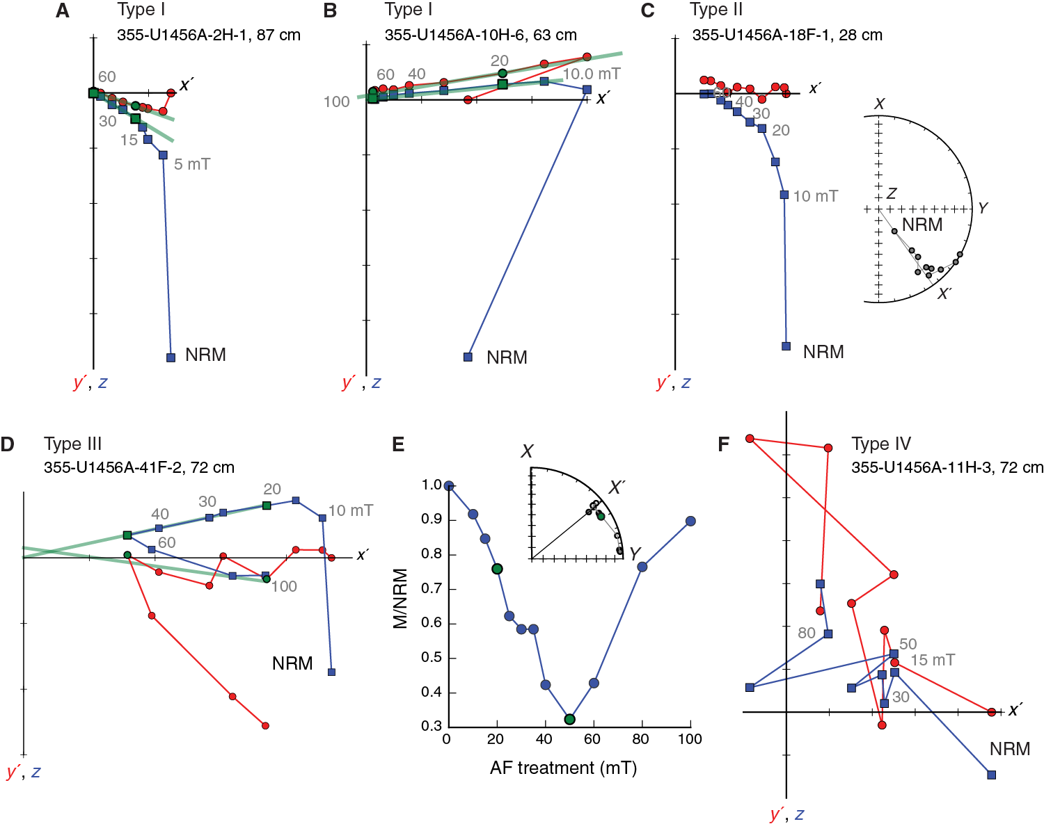
Figure F39. Representative results of step-wise demagnetization data during AF demagnetization.
Type II behavior (Figure F39C) fails the criteria for Type I in that the data do not go to the origin. The deviation angle exceeds 10°, and the polarity is uncertain. On the equal area projection, data are initially spread along a great circle suggesting that the characteristic magnetization is upward directed but never reached. It is also possible that the characteristic magnetization is downward directed and is being deflected by the acquisition of a laboratory remanence. We therefore reject this type of behavior.
The examples shown in Figures F39D and F39E illustrate the problem of unintended laboratory-acquired remanences suspected in the Type II behavior. The demagnetization data in Figure F39D (Type III) initially trend toward the origin but then begin to deviate strongly away from the origin, growing in magnetization (Figure F39E). On the equal area projection (inset to Figure F39E) they are spread along a great circle deviating toward the specimen’s y-axis. This fact suggests laboratory remagnetization starting at ~40 or 50 mT. This magnetization is perpendicular to the last axis demagnetized (in this case, the specimen’s z-axis) and is interpreted as a gyroremanent magnetization (GRM), frequently associated with the authigenic (diagenetic or biogenic) iron sulfide greigite (Fe3 S4). These data were treated as a special case. We calculated a GRM index (Fu et al., 2008), which is the remanence after demagnetization to 60 mT minus the minimum value, and normalized by the vector difference sum of the portion of demagnetization data prior to the minimum value minus the minimum value. This index quantifies the tendency to gain remanence after the 40 or 50 mT step (as shown in Figure F39D, F39E). GRM ranges from 0 to >1, and the specimen shown in Figure F39D and F39E has a value of 0.47. Interpretation of GRM associated with the occurrence of greigite is not straightforward, as many studies have shown that it can grow significantly during diagenesis after initial shallow burial (e.g., Sagnotti et al., 2005). The systematic use of the GRM index throughout all cores allowed us to log the potential occurrence of greigite and to easily identify stratigraphic intervals that may have experienced a diagenetic remagnetization. The data in Figure F39F (Type IV) are completely noisy (termed “spaghetti plots”). These are also ignored.
The criteria used in this study are admittedly somewhat arbitrary, and the reliability of these interpretations must be established by some means. In a typical land-based study, directions are plotted in equal area projections and the data are tested using a “reversals test” (e.g., Tauxe, 2010) to establish that there are two antipodal modes that can be reasonably assigned to normal and reverse groups. Because the cores from Holes U1456A and U1456C were nominally oriented using the Icefield MI-5 orientation device, we can attempt a “reversal” test for the data from Site U1456 in those intervals. We plot all the Type I specimen directions in equal area projection in Figure F40A. The outer rim is the horizontal plane and the central cross is the vertical direction (±90°). Declinations of directions can be read by finding the azimuth of each data point along the outer rim (tick marks are at 10° intervals). Inclinations go from the outer rim (0°) to the center. The declinations are randomly oriented, as might be expected, but the inclinations appear, except for a few cases, limited to within 60° of horizontal and are both upward (open symbols) and downward (solid symbols) directed.
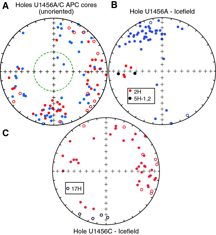
Figure F40. Equal area projections of specimen directions from APC cores, Holes U1456A and U1456C.
Cores 355-U1456A-1H through 16H and 355-U1456C-1H through 18H were “oriented” using two of the three Icefield orientation devices available on board. Devices are swapped out regularly to prevent depletion of the batteries. The first device was used to orient Cores 355-U1456A-1H through 11H and 355-U1456C-16H through 18H, and the second was used to orient the rest. After applying the core’s azimuth obtained from the Icefield device, the directions are shown in Figure F40B and F40C for Holes U1456A and U1456C, respectively. The uppermost two cores in Hole U1456A (1H and 2H) were quite soupy, and the orientation adjustment clearly was unsuccessful (note that no usable data were obtained from Core 1H). In addition, the Icefield tool data for Core 355-U1456A-5H showed a spiraling pattern during penetration, and the uppermost two sections of this core are also apparently twisted. Apart from these exceptions, there are two distinct directional groups, one with a northwesterly and downward average direction and the other southeasterly and upward. It is unclear why there is an anticlockwise bias in the directions, as the magnetic declination at the site is nearly zero; however, there are very few reverse data points, which are insufficient to carry out a meaningful reversals test.
In contrast to the relative success of the data from Hole U1456A, the oriented data for Hole U1456C (Figure F40C) are in no way oriented, with the exception of the deepest core collected (Core 355-U1456C-17H), which was oriented after switching back to the first Icefield tool. Just before retrieval of Core 17H, it was noticed that the screw that ties the orientation device to the core barrel was loose and had to be tightened. A possible explanation for the pattern of failure apparently beginning near the lowermost Icefield measurements in Hole U1456A and continuing until near the last Icefield measurements in Hole U1456C is that the screw became loose just above Core 355-U1456A-14H and then was tightened above Core 355-U1456C-17H. Alternatively, it might be possible to attribute the “bad” orientations to the second Icefield tool, which was used to orient Cores 355-U1456A-12H through 16H and 355-U1456C-1H through 15H, although there is not a perfect match between the failure of orientation and the use of the orientation tool.
A second method of assessing the reliability in an unoriented drill core relies on the behavior of the inclination data. Here we employ the TK03 statistical model for paleosecular variation (Tauxe and Kent, 2004) in order to predict the distribution of inclinations expected from the latitude of the site. We drew 1000 realizations of the model for a latitude of 16°N and plotted the resulting inclinations as a histogram in Figure F41A. These data are for a uniformly normal field direction, but although most of the data are indeed downward directed, ~6% are upward directed. By ignoring data dipping within 5° of the horizontal, we can achieve a 95% confidence in the polarity interpretation from the inclination data. If one also takes the additional precaution of placing little weight on polarity intervals represented by single specimens, one can be reasonably confident in the polarity assignments, if the data behave as the model predicts.
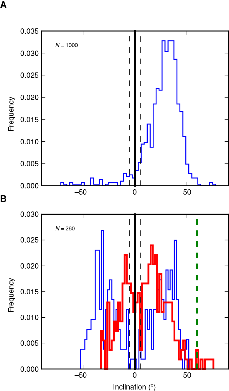
Figure F41. Histograms of predicted and observed inclinations from the TK03 paleosecular variation model and specimen inclinations.
We show the distribution of inclinations for Type I specimens from Holes U1456A, U1456C, and U1456D plotted as a histogram (red) in Figure F41B. We anticipate that there are both polarities present in our cores, so we also show the same number of realizations of the TK03 model with both polarities as a blue line. These show two distinct peaks, the normal (positive) and reverse (negative) polarities in the model. The data from Site U1456 (red line) also have two peaks but appear to be biased toward shallower directions, particularly for those specimens with negative inclinations (which come from deeper in the sedimentary section, making the polarity determination more difficult). There is also a minor peak with inclinations steeper than ~60° (not seen in the negative inclination data), which may be an unremoved coring-induced remanence. Nonetheless, if nearly horizontal data, polarity zones based on single specimens, and inclinations steeper than 60° are given little weight, then a reasonable interpretation of the polarity can be made.
We plot the inclination data versus depth for Holes U1456A, U1456C, and U1456D in Figure F42. The lithologic log is shifted downward by 12.1 m below 425 mbsf to make the log compatible with the composite depths used for the inclinations. Inclinations within 5° of horizontal and those steeper than 60° are marked with dashed lines and a yellow shaded box, respectively (Figure F42C), and should be given little weight, as should polarity zones based on a single specimen (indicated by short bars on Figure F42D). There are clear zones of dominant normal and reverse polarity (shown in the polarity logs as black and white intervals, respectively). Where the two holes overlap, the agreement is excellent. We plot the GRM index in Figure F42B. The greigite-bearing samples are of both polarities.
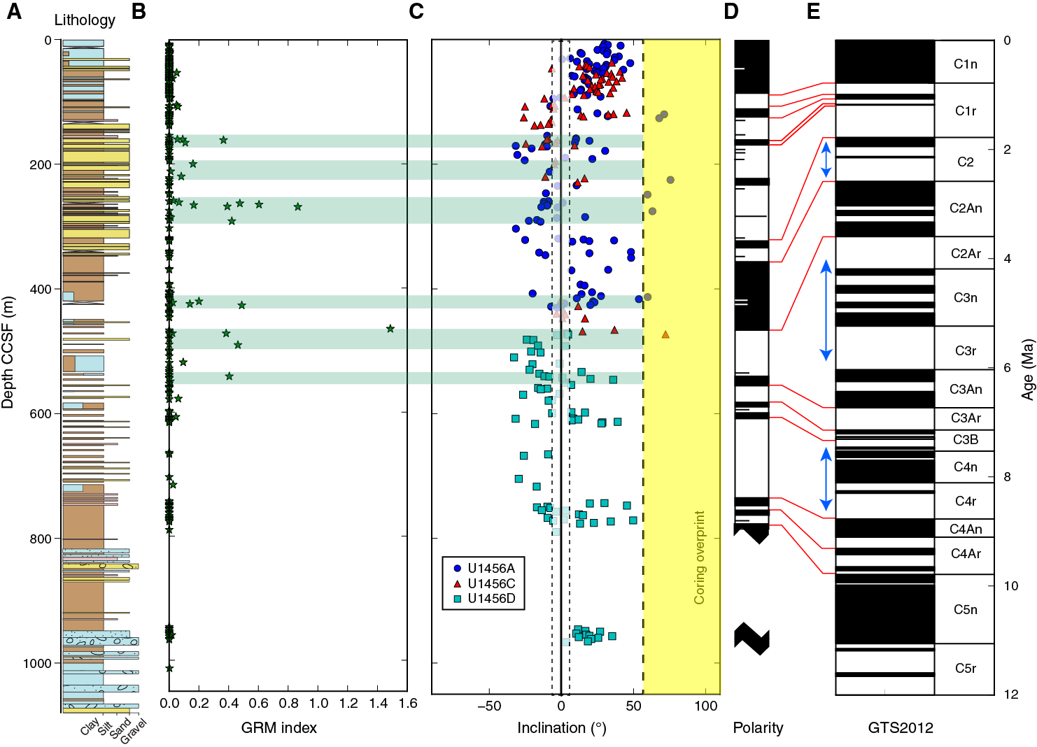
Figure F42. Lithology, GRM index, and inclinations from Type I specimen directions with polarity and GPTS.
Our magnetostratigraphic interpretation is based on polarity zones in the composite log (Figure F42D). Many of these zones can be correlated to the geomagnetic polarity timescale of Gradstein et al. (2012), and our tie points are shown as solid red lines in Figure F42. These ties are also listed in Table T21 and plotted on the Site U1456 age-depth plot (Figure F20). Intervals with significant hiatuses are indicated by the blue arrows next to the timescale in Figure F42E.
Table T21. Magnetic polarity tie points. Download table in .csv format.
Rock magnetic experiments
Basic rock magnetic experiments were carried out on representative samples from Hole U1456D. In our preliminary study, we relied on step-wise IRM acquisition and successive thermal decay of a three-component IRM (see Paleomagnetism and rock magnetism in the Expedition 355 methods chapter [Pandey et al., 2016a]). IRM acquisition was carried out in 14 steps up to 1 T (the maximum field available in the shipboard laboratory) with a direct-current field strong enough to saturate low- to medium-coercivity magnetic minerals, such as magnetite and Fe sulfides, and to interpret acquisition behavior of hematite and goethite. We show the acquisition curves in Figure F43.
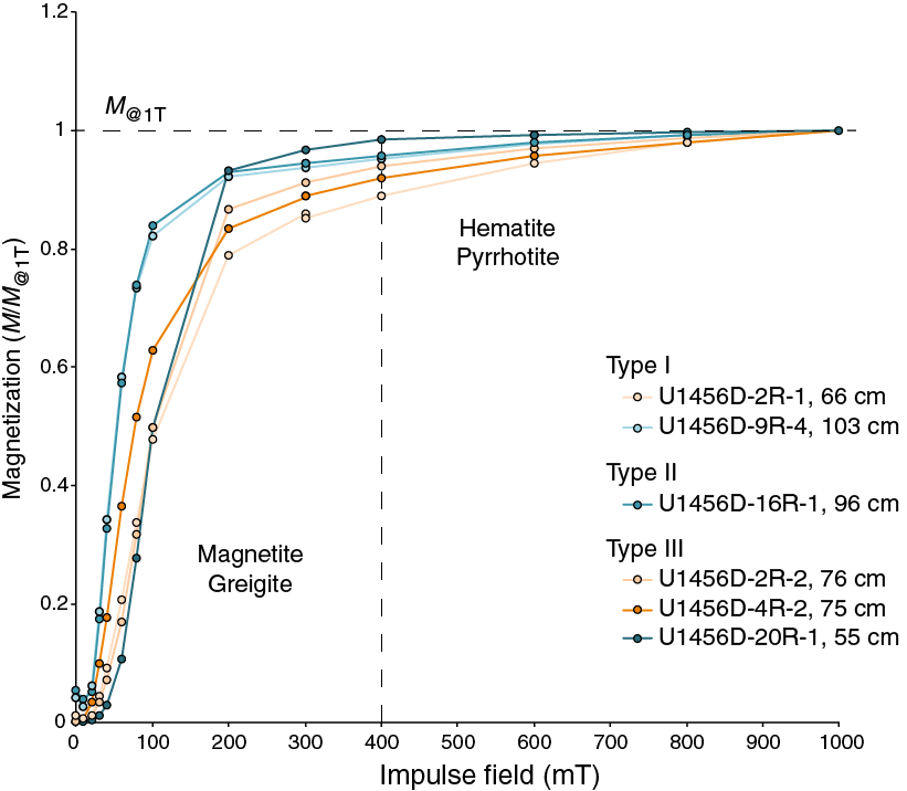
Figure F43. IRM acquisition curves for representative samples from Hole U1456D.
All samples show a general behavior characterized by steep acquisition at low field strengths, usually associated with magnetite and greigite, followed by a gradual approach to saturation. Lack of saturation is generally associated with the presence of goethite, hematite, or pyrrhotite. Interestingly, two of the three Type III (GRM) specimens (Samples 355-U1456D-2R-2, 76 cm, and 4R-2, 75 cm) do not saturate, and we suspect that the usual interpretation of GRM as indicating greigite may be oversimplified in this sediment. Either there is the co-occurrence of iron sulfide (greigite) with the most highly oxidized form of iron oxide (hematite), or certain forms of hematite (specularite) may also exhibit the GRM behavior.
After imparting a 1 T field along the specimens’ z-axes, the specimens were then subjected to a second IRM in a 0.3 T field parallel to the y-axes, and finally a third IRM in a field of 0.12 T along the specimens’ x-axes. Thermal demagnetization of the three-component IRM in Sample 355-U1456D-2R-1, 66 cm (Figure F44A; Type I), shows the distinctive behavior associated with hematite in that the hard fraction does not demagnetize until well above 600°C. In contrast, Sample 9R-4, 103 cm (Figure F44B; Type I), has an insignificant hard fraction and is fully demagnetized at just over 600°C. This sample also shows a sharp decrease in intensity at 300°–320°C in the soft fraction and a more gradual decrease of intensity in the medium fraction between 200° and 350°C. These observations together point to a maghemite-dominated magnetic mineralogy (Lowrie, 1990). Sample 16R-1, 96 cm (Figure F44C; Type II), is similar to that shown in Figure F44B but is fully demagnetized by 600°C, indicating that magnetite is the main magnetic carrier. Samples 20R-1, 55 cm, 2R-2, 76 cm (Figure F44E), and 4R-2, 75 cm (Figure F44D–F44F), are all Type III yet have different behavior in the 3D-IRM demagnetization experiments. Figure F44D shows a sharp decrease in intensity at 300°–320°C within the soft fraction, and the sample is fully demagnetized by 400°C, consistent with a pyrrothite or greigite remanence. Figure F44E also demonstrates a steep decline in the soft fraction, as well as in the medium fraction, but retains significant remanence in the medium and hard fractions above 600°C, as does the sample shown in Figure F44F. These observations suggest the presence of hematite and another mineral with either a Curie temperature near 350°C (e.g., greigite) or one that is metastable at that temperature (e.g., maghemite). No behavior indicative of goethite, which has a Curie temperature of ~125°C and a very high coercivity, is observed. On the whole, our experiments confirm the occurrence of magnetite, maghemite, and hematite as the main magnetic carriers, as well as Fe sulfide (greigite). However, the common interpretation of GRM (Type III behavior) does not seem to be uniquely associated with greigite.
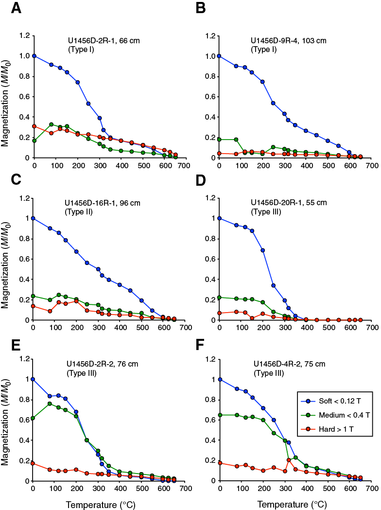
Figure F44. Thermal decay of the 3D-IRM experiments for representative samples, Hole U1456D.
Physical properties
Physical properties were measured on whole-round cores, split cores, and discrete samples from each of the five holes drilled at Site U1456 to provide basic information for characterizing the drilled section. All core sections were measured with the gamma ray attenuation (GRA) bulk densitometer, magnetic susceptibility loop, and P-wave logger on the WRMSL. Additionally, GRA bulk density and magnetic susceptibility were measured on all core sections from Holes U1456B and U1456C and the upper few cores from Hole U1456D (Cores 355-U1456D-2R through 7R) with the STMSL immediately after the cores were brought onboard. Core disturbances associated with poorly consolidated sand layers between ~135 and ~360 mbsf compromised the collection of core logger compressional wave (P-wave) velocity data during APC coring. After WRMSL scanning, whole-round sections were logged for NGR before splitting. Point-sensor magnetic susceptibility and color spectrometry (color reflectance) were measured on split core sections using the SHMSL. Discrete P-wave and shear strength measurements were made on cores from Holes U1456A and U1456E and from selected sections from Holes U1456C and U1456D on the Section Half Measurement Gantry. Moisture and density (MAD) measurements were made on discrete samples from Holes U1456A, U1456D, and U1456E and selected sections of Hole U1456C. Data from Hole U1456B are not plotted because they replicate the uppermost ~30 m of both Holes U1456A and U1456C.
GRA bulk density
Bulk density values measured from GRA on the WRMSL were corrected for the erroneously low or high values arising from measurements made toward the beginning or the end of the core sections, which are caused by the core liner cap. Additionally, values lower than the density of water were also removed. Core 355-U1456A-52X data were removed from the profile because of erroneous measurements generated while logging and confirmed with erroneous measurements of the water standard measurements taken at the same time.
Bulk density is low in lithologic Unit I (see Lithostratigraphy) when compared to both Units II and III (Figure F45A, F45B). Within Unit I, bulk density increases from ~1.4 g/cm3 near the seafloor to ~1.8 g/cm3 at ~50 mbsf and then decreases to ~1.6 g/cm3 between ~50 and ~75 mbsf. Subsequently, the bulk density increases back to ~1.8 g/cm3 until ~130 mbsf, which is slightly deeper than the base of Unit I. In addition to these major trends, periodic and pronounced changes in bulk density occur throughout Unit I at an interval of ~10 m in the uppermost 75 m and ~5 m below 75 mbsf until the base of Unit I (Figure F46). When examined in detail, these periodic changes are gradual and do not correlate to the core breaks.
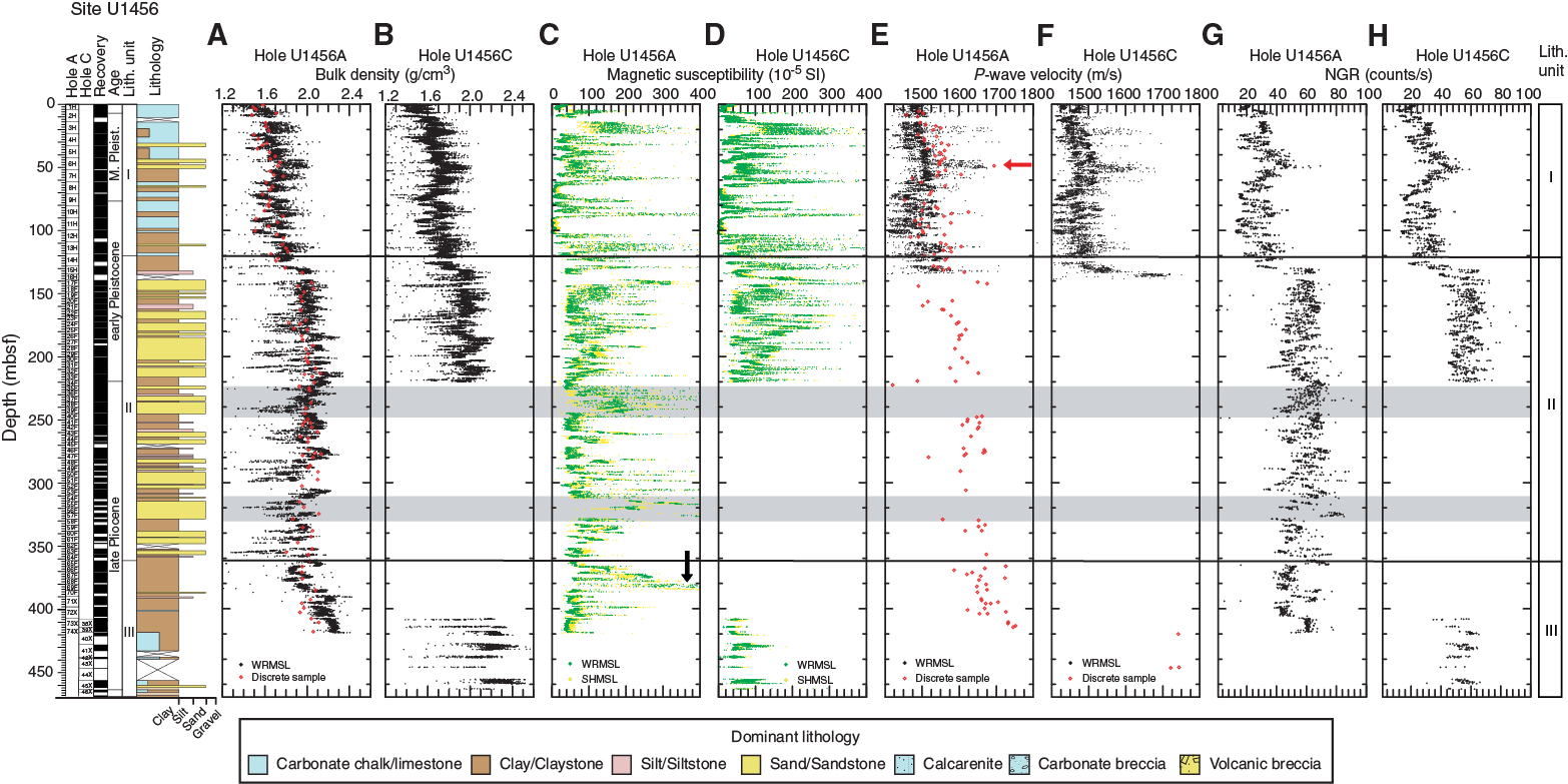
Figure F45. A–H. Physical properties measurements, Holes U1456A and U1456C.

Figure F46. Periodic changes in GRA bulk density, NGR, and MS in lithologic Unit I, Hole U1456A.
A distinct shift in bulk density to ~2.0 g/cm3 occurs at ~135 mbsf, roughly 15 m below the Unit I/II boundary defined based on visual core description (see Lithostratigraphy). Higher bulk density in Unit II is attributed to the dominance of sand, as opposed to the carbonate-rich, soft, clayey sediment in Unit I, which has a lower bulk density. Within Unit II, bulk density generally increases downhole to ~2.2 g/cm3 at ~210 mbsf, followed by a net decrease in bulk density to ~1.9 g/cm3 at the base of Unit II (~360 mbsf). Fluctuations in bulk density within Unit II probably correspond either to graded beds, interpreted as turbidite deposits, or occasional clay-silt layers (Figure F45A, F45B). Bulk density in both Holes U1456B and U1456C matches well with that of Hole U1456A for both Units I and II.
Bulk density is relatively high in Unit III, with values varying from 2.0 to 2.5 g/cm3 (Figures F45, F47). The increase in bulk density in Unit III is attributed to the dominance of indurated claystone. Within Unit III, distinct decreases in bulk density to ~1.8 g/cm3 are observed between 510 and 550 mbsf and from 595 to 605 mbsf (upper two gray boxes in Figure F47). The first interval of low bulk density is dominated by nannofossil-rich chalk, whereas nannofossil-rich claystone and clayey nannofossil chalk are abundant in the second interval. Bulk density then decreases again in the upper part of Unit IV to close to 2.0 g/cm3 until ~835 mbsf. The slight decrease in bulk density over this interval is attributed to the dominance of indurated claystone intercalated with sandy siltstone. A distinct increase in bulk density is observed from 835 to 965 mbsf, but values still vary between 2.0 and 2.4 g/cm3. A further shift in bulk density with values ranging dramatically from 1.8 to 2.6 g/cm3 is observed toward the base of both Holes U1456D and U1456E (Figure F47). The shift in bulk density toward the base of Unit IV is attributed to the dominance of calcarenite and carbonate breccia.
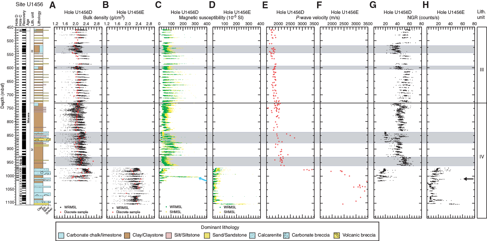
Figure F47. Physical properties measurements, Holes U1456D and U1456E, in the lower part of the U1456 sediment section.
Magnetic susceptibility
In general, magnetic susceptibility varies from 0 to 400 × 10–5 SI (Figures F45C, F45D, F47C, F47D). Intervals with high amounts of carbonate (e.g., Core 355-U1456A-11H) generally have very low magnetic susceptibility, whereas those with coarser/terrigenous material have higher magnetic susceptibility. A distinct increase in the lowest values or baseline of magnetic susceptibility is noted at the base of lithologic Unit I and is attributed to the common presence of sand that begins here and continues in Unit II. Considerable fluctuations are noted in magnetic susceptibility within Unit I. Magnetic susceptibility is somewhat less variable in the upper part of Unit II, between ~140 and ~220 mbsf. An abrupt increase in values is observed between ~220 and ~250 mbsf, which corresponds to dark-colored sand with silt, and again between ~310 and ~330 mbsf (shaded areas in Figure F45), which is attributed to the abundance of mica in these sand-dominated intervals. Subsequently, a decrease in magnetic susceptibility is noted from~330 to ~360 mbsf at the base of Unit II, followed by an overall increase within Unit III to a peak at ~380 mbsf (black arrow in Figure F45C), which is attributed to the presence of concretions within the clay. A distinct decrease in magnetic susceptibility is observed between 510 and 540 mbsf and is attributed to an abundance of biogenic material (upper gray box in Figure F47). From 550 mbsf downward, magnetic susceptibility is comparatively higher, except for a brief decrease between 595 and 605 mbsf, which is also attributed to the presence of nannofossil-rich claystone and clayey nannofossil chalk. Magnetic susceptibility decreases in the upper part of Unit IV down to ~835 mbsf. A distinct increase in magnetic susceptibility is observed from 845 to 925 mbsf. Subsequently, magnetic susceptibility decreases at 925 mbsf and then slowly rises to 955 mbsf. Values show less scatter in this interval than those above. The decrease in magnetic susceptibility is attributed to the abundance of biogenic material (nannofossil-rich claystone and claystone with nannofossils). A further drop in magnetic susceptibility is observed below 975 mbsf, which continues until the base of Unit IV in both Holes U1456D and U1456E, except for a distinct peak centered at 1003 mbsf within nannofossil-rich claystone (Core 355-U1456D-59R; blue arrow in Figure F47C). The drop in magnetic susceptibility is attributed to the presence of calcarenite rich in biogenic material. Point magnetic susceptibility measured on section halves using the SHMSL is comparable to the whole-round data from the WRMSL (Figures F45C, F45D, F47C, F47D).
P-wave velocity
The P-wave velocity values measured with the P-wave logger (PWL) on the WRMSL were erratic at times because of poor acoustic coupling in some of the cores, especially those with predominantly sand-sized grains, which were partially saturated with water. All values >1800 m/s were removed from Figure F45E and F45F. Within Unit I, P-wave velocity increases from ~1500 m/s at the seafloor to 1700 m/s at ~50 mbsf before decreasing again to ~1500 m/s at ~75 mbsf. Subsequently, P-wave velocity increases to greater than 1600 m/s at ~130 mbsf. P-wave velocity could not be measured for Units III and IV by the PWL because of the sandy nature of the sediment and the narrow diameter of RCB cores, as compared to that of the liner. WRMSL P-wave velocities of the cores from both Holes U1456B and U1456C are similar to those from Unit I in Hole U1456A (Figure F45E, F45F).
P-wave measurements (x- and z-axis) using the P-wave caliper (PWC) tool were taken from Site U1456 at ~1.5 m resolution or when recovery and lithology allowed. Because of poor data quality in soft sandy sections or unsaturated indurated sections, fewer x-axis and no z-axis PWC measurements were taken below ~135 mbsf. Comparison of PWL and PWC x-axis measurements in overlapping intervals of Holes U1456A and U1456C reveal overall good correspondence (Figure F45E, F45F).
PWC values vary widely, sometimes within the same section, likely because of varying lithology. Values generally range from ~1400 to ~1700 m/s in Hole U1456A to 420 mbsf. The overall trend shows lower values (average = ~1400–1600 m/s) in the clay of Unit I, with a peak at ~50 mbsf (red arrow in Figure F45E). Higher values (up to 1700 m/s) are observed in Units II and III, probably related to an increase in grain size and compaction of the sediment. This trend continues in Hole U1456D, where velocity increases downhole from ~1700 to ~2200 m/s at 965 mbsf. High values of >3000 m/s were reached in a calcarenite at ~975 mbsf in Core 355-U1456D-56R (Figure F47E), possibly corresponding to a strong seismic reflector (see Background and objectives). Hole U1456E, which cored through the mid- and lower part of Unit IV, has high seismic velocities up to 3500 m/s (Figure F47F).
Natural gamma radiation
NGR varies from ~12 to ~50 counts/s between the seafloor and ~130 mbsf (Figure F45G, F45H), which corresponds to lithologic Unit I. Variations in NGR in Unit I also exhibit a periodicity of ~10 m in the upper part and ~5 m in the lower part, similar to that seen in the bulk density record (Figure F46). A distinct increase in NGR to ~45–75 counts/s is recorded at ~130 mbsf near the top of Unit II, and NGR remains high until the base of Unit II at ~360 mbsf. The increase in NGR in Unit II is attributed to the higher percentage of clastic material in this unit, contrasting with the predominance of biogenic carbonate in Unit I.
NGR fluctuates regularly between intervals of low and high values within Unit III (Figures F45G, F45H, F47G, F47H). A distinct interval with low values of NGR can be found in the upper part of Unit III, between 510 and 545 mbsf, with values ranging from 25 to 45 counts/s (upper gray box in Figure F47). The drop matches very well with the drop in bulk density and is attributed to an abundance of nannofossil chalk. Subsequently, NGR values are higher (40–70 counts/s) until the base of Unit III, except for a short decrease between 595 and 605 mbsf (second upper gray box in Figure F47). High NGR is attributed to the dominance of claystone in this interval. The drop in NGR between 595 and 605 mbsf is driven by the abundance of biogenic material (nannofossil-rich claystone) within this interval.
A dramatic (but variable) decrease in NGR between 835 and 925 mbsf within Unit IV is attributed to the presence of biogenic carbonate–rich sediment (nannofossil-rich calcarenite). NGR is distinctly high between 930 and 960 mbsf, and interestingly, unlike the previous intervals with elevated NGR values, this interval is in a nannofossil-rich claystone. The claystone within this interval is possibly responsible for the uniform high NGR values. A significant drop in NGR, which is attributed to higher carbonate content (calcarenite), marks the lower part of Unit IV in both Holes U1456D and U1456E. An extremely high peak of 112 counts/s was seen within Unit IV in Hole U1456E at 1011.5 mbsf (depth of high value falling off the figure indicated by black arrow in Figure F47H). This peak occurs near the top of multicolored claystone composed of deeply weathered volcanic glass (see Lithostratigraphy) and could be the result of a concentration of uranium related to extreme leaching of volcanic glass (e.g., Leventhal, 1983). This lithology was only recovered in Hole U1456E. The sandstone recovered at the bottom of Hole U1456E has higher NGR values, similar to previous low-carbonate intervals. The NGR activity in the units recovered in both Holes U1456B and U1456C matches well with that in Hole U1456A (Figure F45G, F45H).
Moisture and density
Bulk density, dry density, grain density, porosity, and void ratios in Holes U1456A and U1456C–U1456E were calculated from mass and volume measurements on discrete samples taken from the working halves of split cores (see Physical properties in the Expedition 355 methods chapter [Pandey et al., 2016a]). Most samples were obtained from Holes U1456A, U1456D, and U1456E, whereas Hole U1456C served to fill in gaps in the uppermost 464 mbsf. MAD values correspond well with WRMSL GRA bulk densities after correcting for density differences in GRA density during XCB and RCB coring (see Physical properties in the Expedition 355 methods chapter [Pandey et al., 2016a]; Figures F45, F46, F47).
MAD dry densities increase downhole from ~0.8 g/cm3 at the seafloor to ~1.4 g/cm3 at the base of Unit I. Deeper than ~135 mbsf, density stays high and increases up to 1.8 g/cm3 by ~460 mbsf (Figure F48). Values around 1.6–1.8 g/cm3 are maintained throughout most of Hole U1456D, with some high values up to 2.4 g/cm3 in the lower half of Unit IV (Figure F49). Porosity (percent pore space in the wet sediment volume) measured on discrete samples generally decreases with depth. Discrete porosity values decrease rapidly from >80% at the surface to ~40%–44% at ~130 mbsf, consistent with compaction in the upper part of the sediment column (Figure F48). Below ~130 mbsf, porosity values continue to decrease gradually to ~35% at ~925 mbsf (Figures F48, F49); more strongly lithified sections in the 925–1100 mbsf interval show porosities as low as 10% (Figure F49). Co-varying downhole trends in dry density, porosity, and void ratio are most likely related to compaction, as well as shifts in lithology. Carbonate-rich, soft, fine-grained sediment in Unit I has lower dry densities and higher porosity and void ratios than the thick sand beds in Unit II. Because sediment becomes more lithified downhole, density continues to increase in Units III and IV. However, Unit IV has higher variability as a result of measurements on a range of lithologies that were transported by mass wasting to the site. Grain density varies between 2.6 and 3.0 g/cm3 with no visible downhole trend, although at the bottom of Unit IV the carbonate conglomerates have the lowest grain densities (Figure F49). The relatively high average grain density values may be related to the presence of recrystallized carbonates, clays, and/or heavy minerals in the sediment.
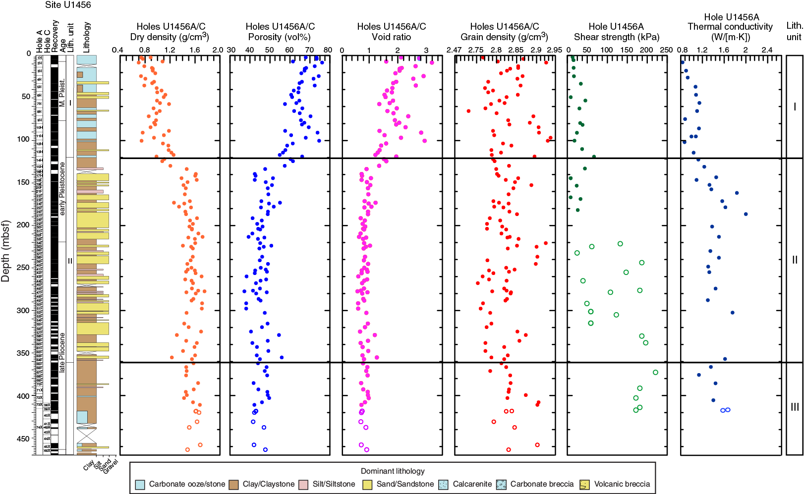
Figure F48. MAD discrete sample, density, porosity, and void ratios and thermal conductivity, Holes U1456A and U1456C.
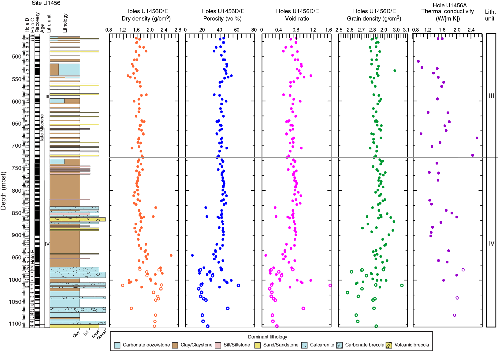
Figure F49. MAD discrete sample density, porosity, and void ratios and thermal conductivity, Holes U1456D and U1456E.
Shear strength
Shear strength measurements were performed on sediment from Hole U1456A using the automated vane shear (AVS) through Core 355-U1456A-26F (~185 mbsf). Below this depth, sediment became too compacted for this method, so a penetrometer was used and shear strength was calculated from compressional strength (see Physical properties in the Expedition 355 methods chapter [Pandey et al., 2016a]). Sediment was too compacted for the penetrometer at and below Core 355-U1456A-74X (Figure F48). Shear strength indicates that sediment ranges from soft (0–50 kPa) above 200 mbsf to stiff (150–220 kPa) below 325 mbsf. The soft carbonate ooze in the upper part of the sediment sequence is reflected in the very low shear strength values in Unit I. Sediment becomes harder with compaction downhole; however, values are variable throughout Unit II, probably due to alternating layers of sand and compacted clay layers.
Thermal conductivity
A thermal conductivity profile was obtained (resolution of ~10 m) using a thermal conductivity needle until the recovered material was too hard for penetration at ~360 mbsf (base of Unit II), below which a puck was used on split core sections. Thermal conductivity measurements show a shift from low values in Unit I (0.8–1.2 W/[m·K]) to higher values (1.2–2.0 W/[m·K]) within sand-rich sections characteristic of Unit II (Figure F48). With increasing lithification downhole, values increase up to 2.4 W/(m·K) (Figure F49).
Downhole measurements
Logging operations
Logging operations began after completion of coring operations in Hole U1456C at 1000 h (all times are local; UTC + 5.5 h) on 17 April 2015 to a total depth of 465.2 m DSF. Preparation for logging included a wiper trip, which found no fill; locking open the LFV; and then running a 40 bbl sepiolite mud sweep, after which the pipe was raised to a logging depth of 81 m DSF. Two tool strings were initially deployed in Hole U1456C during logging operations: the triple combo and the FMS-sonic tool strings (Figure F50; see Downhole measurements in the Expedition 355 methods chapter [Pandey et al., 2016a]). Because of the possibility of unstable borehole conditions caused by the presence of unconsolidated, fluidized sands, the radioactive gamma ray source was left out of the first logging run with the triple combo tool string. After the borehole was found to be in good condition during two logging runs with no obvious tight spots, we decided to deploy the triple combo tool string with the radioactive gamma ray source as a third logging run after the FMS-sonic tool string.
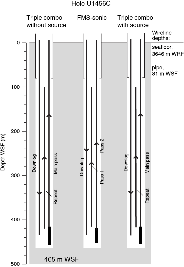
Figure F50. Logging operations summary diagram showing wireline depths reached during different logging passes and borehole depth.
The first deployment was the triple combo tool string, made up of gamma ray, density, resistivity, and magnetic susceptibility tools. The tool string was lowered into the hole at 1155 h on 17 April. When the tool string was just below the end of the pipe, the wireline heave compensator settings were optimized to minimize downhole tool motion. A downlog proceeded at a speed of ~550 m/h to a total depth of ~465 m WSF, and two uplogs (main and repeat) were collected at a speed of ~550 m/h. The main pass was logged upward from total depth through the drill string to record seafloor with the gamma ray tool. The tool string was recovered to the rig floor at 1740 h on 17 April.
The second logging run was performed with the FMS-sonic tool string. The tool string was rigged up and run into the hole at 1810 h on 17 April. A downlog was recorded at 550 m/h, reaching a total depth of ~465 m WSF. Two passes of the hole were made: the first at a speed of 550 m/h while recording all Dipole Shear Sonic Imager (DSI) modes (monopole compressional, upper dipole shear, lower dipole shear, and Stoneley) and the second at 520 m/h while recording only standard DSI modes (crossed dipole, Stoneley, and monopole compressional). The FMS-sonic tool string was retrieved to the rig floor and rigged down by 0315 h on 18 April.
The second deployment of the triple combo tool string with the radioactive gamma ray source constituted the third logging run in Hole U1456C. The tool string was lowered into the hole at 0445 h on 18 April. A downlog proceeded at a speed of ~550 m/h to a total depth of ~465 m WSF. The hole was logged upward at a speed of ~550 m/h, recording data from ~465 m WSF uphole in three passes. The tool string was recovered to the rig floor at 1150 h on 18 April.
Sea state was relatively calm for the duration of logging operations. There was an average heave of 0.5 to 0.75 m (peak to peak). All logging operations in Hole U1456C were completed by 1300 h on 18 April.
Data processing and quality assessment
The Borehole Research Group of Lamont-Doherty Earth Observatory (LDEO) provided processed depths for the logs. This includes a depth shift to the seafloor and depth matching between passes leading to the WMSF depth scale. The triple combo main pass identified the seafloor at 3649.2 m water depth based on a shift in gamma ray values from the main pass of the FMS-sonic tool string, which was first shifted to the seafloor (3646 m wireline depth below rig floor). All other logs have been depth-matched to this gamma ray log.
The quality of the downhole logs was affected by variations in borehole diameter, estimated by the hydraulic caliper on the Hostile Environment Litho-Density Sonde (HLDS) and by the FMS calipers (Figures F51, F52, F53). The caliper logs show an irregular shape through much of the open borehole. Borehole diameter was enlarged >38 cm (15 inches) in the uppermost 204 m (purple shading in Figures F51, F53) but decreased to 33–36 cm (13–14 inches) below 204 m WMSF and was mostly in-gauge between ~370 and 425 m WMSF. All tool strings deployed in Hole U1456C reached the total depth of the drilled hole without any issues.
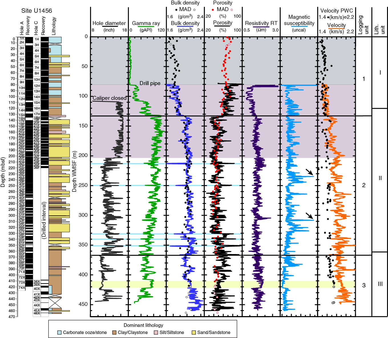
Figure F51. Summary of logs from the triple combo and FMS-sonic tool strings with lithologic and logging units
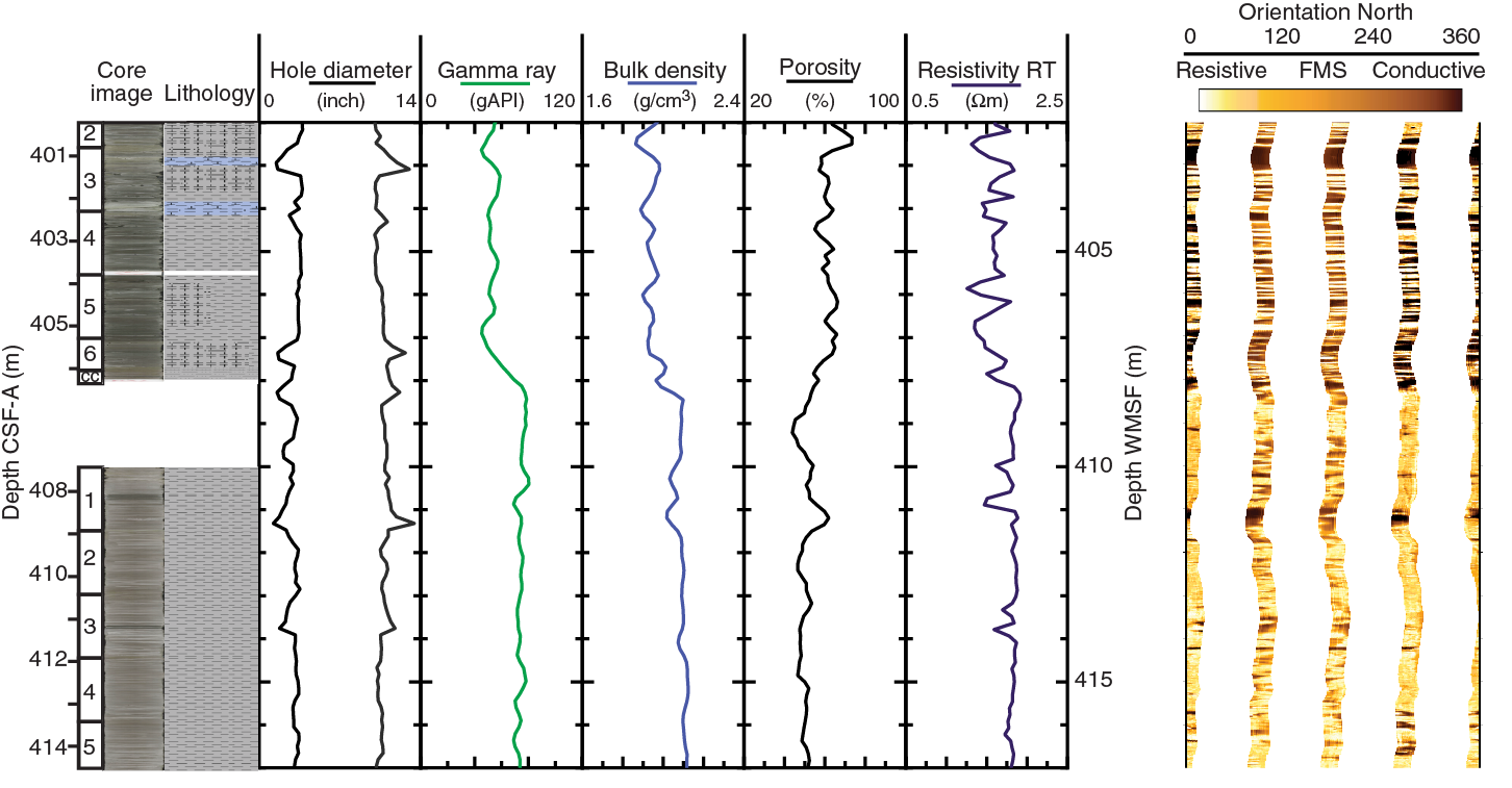
Figure F52. FMS images from 402–417 m WMSF in Hole U1456C and corresponding logs.

Figure F53. Downhole logs dependent on the geochemistry and mineralogy of the formation.
As a result of varying borehole conditions associated with rugosity and borehole diameter, logging data vary in quality, particularly for those that require eccentralization and good contact with the borehole wall (density, porosity, and FMS). In general, gamma ray, resistivity, magnetic susceptibility, and P-wave velocity values were the measurements least affected by the variable hole diameter. Features in gamma ray data associated with very wide or very narrow borehole diameters should be treated with caution; fewer gamma rays reach the detector in a wider borehole and more reach the detector where the borehole is narrower. Density and porosity were affected at points within Hole U1456C where density values approached water density and anomalously high porosity (close to 100%; blue shaded intervals in Figure F51). Magnetic susceptibility logs show reasonable responses throughout the borehole with no significant downhole temperature drift in Hole U1456C (Figures F51, F53).
The quality of the logs can also be assessed by comparison with measurements made on cores from the same site (Figure F51). Density and porosity logs were acquired in three separate passes, but no single pass covered the entire open hole interval due to loss of communication with the tool string during the main pass. Porosity and density measurements are plotted from a combination or splice of Passes 2 and 3 and show generally very good correspondence with the core-based MAD data (Figure F51). Some intervals, however, show elevated porosity values from the logs compared to discrete measurements (e.g., above 140 m WMSF and below 370 m WMSF). Magnetic susceptibility logs also show good correlation with data from cores, and measurements were repeatable between the downlog and uplog passes of the triple combo tool string (Run 1; data not shown). Total natural gamma radiation (HSGR) values from the triple combo tool string show generally good agreement with total NGR core data (Figure F53).
FMS data quality relies on a number of factors, including an in-gauge hole, smooth borehole walls, and good contact between the tool’s pads and the borehole wall. Processing of the FMS image data allows a speed correction to be applied that takes into account variations in the speed of the tool, including stick and slip, measured by the General Purpose Inclinometry Tool (GPIT) incorporated into the tool string. Two processing methods were applied to the speed-corrected images. Static processing normalizes the entire measured resistivity range for the full depth of the borehole to allow for assessment of large-scale resistivity variations. Dynamic processing re-scales the color intensity over a sliding 2 m depth window to highlight local features. Detailed data processing was carried out by LDEO.
Despite borehole conditions, FMS images are generally of good quality, with the pads making contact with the borehole walls through much of the logged interval. However, the FMS resistivity images also show poor contact with the borehole wall in the wide, washed-out intervals of the logged section (seen as darker bands that correspond to large-diameter intervals) and what may be inadequate compensation for downhole tool motion (evidenced by blurry images).
The sonic tool acoustic velocities are generally of good quality, with the exception of the shear velocities acquired in the first uplog. Additional processing of the sonic waveforms may improve the data quality.
Logging stratigraphy
Downhole logging data for Hole U1456C are summarized in Figures F51, F52, and F53. The logged interval is divided into three logging units, primarily on the basis of gamma radiation, density, magnetic susceptibility, sonic logs, hole conditions, and lithology.
Logging Unit 1: base of drill pipe (81 m WMSF) to 132 m WMSF
Logging Unit 1 is characterized by high porosity, averaging 70%. Total gamma ray, density, and resistivity values are relatively low, averaging ~60 gAPI, 1.7 g/cm3, and 1.4 Ωm, respectively. Magnetic susceptibility exhibits some high-frequency variations, varying between –3500 and –2000 (uncalibrated units), with two peaks up to –1500. P-wave (compressional) velocity is between 1.5 and 1.6 km/s with traveltime (∆t) between 185 and 205 µs/ft. This logging unit corresponds to lithologic Unit I (see Lithostratigraphy), but the base is defined ~12 m deeper based on the responses seen in the logging measurements that clearly define the beginning of coarser grain sized sediment in logging Unit 2 (Figure F51).
Logging Unit 2: 132–368 m WMSF
At the top of logging Unit 2, total gamma ray, density, and resistivity values increase to levels averaging ~80 gAPI, 2.0 g/cm3, and 1.5 Ωm, respectively. Porosity decreases to an average of 48%. These properties exhibit regular fluctuations (Figure F51). Spikes in porosity to high values (>80%) and density measurements to low values (near that of water) are evident and are the result of poor borehole conditions (blue boxes in Figure F51). Magnetic susceptibility varies between –3500 and –2500, with peak values of –2000, but much higher peak values of –500 occur at ~240 and ~310 m WMSF (arrows on Figure F51). These peaks correlate well with core magnetic susceptibility data and correspond to an interval of dark sand with silt and graded bedding with common lithic grains and heavy minerals in Section 355-U1456A-37F-1 and a nannofossil-rich clay with silt showing some bioturbation and color banding with common iron (hydr)oxides in Section 53F-1. P-wave velocity increases from 1.5 to 2.0 km/s with peaks of >2.2 km/s, equivalent to ∆t of 130–200 µs/ft. An increase in sonic velocity reflects compaction with depth. Mudcake was observed over some intervals, indicative of permeable zones. This logging unit corresponds to lithologic Unit II (see Lithostratigraphy), which is dominated by sands and silts.
Logging Unit 3: 368–460 m WMSF
This section of the hole is primarily in-gauge except at the bottom of the hole (>425 m WMSF), which has a larger diameter. The characteristics are somewhat more uniform within this unit. Resistivities and densities are similar to those seen in logging Unit 2, averaging ~1.5 Ωm and 2.0 g/cm, respectively. Porosities continue to decrease to an average of 43% (Figure F51). Total gamma ray values decrease to an average of 40 gAPI, with a resolvable increase in uranium content (Figure F53). Magnetic susceptibilities decrease to an average of approximately –4000. P-wave velocity is between 1.8 and 2.2 km/s with ∆t of 150–175 µs/ft. The largest single resistive unit is found in this logging unit between 408 and 425 m WMSF, as seen in the FMS logs, and corresponding to a particularly uniform interval of claystone (yellow shaded box in Figure F51). This logging unit corresponds to part of lithologic Unit III (see Lithostratigraphy), which comprises primarily claystone.
FMS images
Despite the variability in borehole size and the presence of washed-out intervals, the FMS resistivity images reveal some local transitions between alternating resistive and conductive intervals at the meter to submeter scale not obviously apparent in the depth matched cores (Figure F52). These alternations may reflect changes in sediment electrical properties related to subtle changes in lithology, for example claystone interbedded with claystone with nannofossils (see Lithostratigraphy). A transition from interbedded nannofossil-rich claystone with abundant burrows at 408 WMSF to claystone with higher gamma radiation, bulk density, and resistivity and lower porosity below can clearly be seen in logging Unit 3 (Figure F52). This higher resistivity claystone has particularly uniform characteristics within all logs (yellow shaded box in Figure F51).
Downhole temperature and heat flow
Three downhole temperature measurements were conducted using the APCT-3 during coring in Hole U1456A. An exponential decrease in temperature is expected for the time interval highlighted in Figure F54 (between 210 and 540 s after penetration) and was used to estimate ambient temperature. The data yielded values from 6.01°C at 62.5 m DSF to 9.25°C at 118.5 m DSF (Figure F54), giving a geothermal gradient of 57°C/km for the upper ~120 m DSF shown in Figure F55. Bottom water temperature was determined to be 1.80°C.
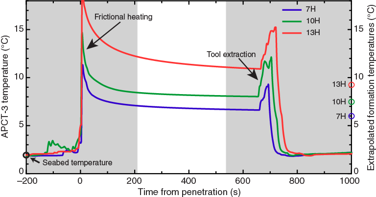
Figure F54. APCT-3 temperature-time series, Hole U1456A.

Figure F55. Plots of heat flow calculations, Hole U1456A.
We estimated a thermal conductivity profile (resolution ~10 m) using laboratory-determined thermal conductivity data (see Physical properties in the Expedition 355 methods chapter [Pandey et al., 2016a]). Thermal resistance was calculated using the “average approach” outlined in Pribnow et al. (2000) using an average thermal conductivity of 1.0 W/(m·K) measured in the upper 120 mbsf (Figure F55). The slope of the linear fit between temperature and thermal resistance indicates heat flow of 57 mW/m2 (Pribnow et al., 2000). This estimate of heat flow is equivalent to 84 Ma ocean crust according to the model of Stein and Stein (1992), slightly older than the anticipated age of Laxmi Basin at ~65 Ma (Bhattacharya et al., 1994). Using the calculated heat flow value and the higher average thermal conductivity measured deeper than 120 m DSF (average 1.6 W/[m·K]), a geothermal gradient of 35°C/km is calculated for depths between 120 and 1000 m DSF.
References
Beaumont, C., Jamieson, R.A., Nguyen, M.H., and Lee, B., 2001. Himalayan tectonics explained by extrusion of a low-viscosity crustal channel coupled to focused surface denudation. Nature, 414(6865):738–742. http://dx.doi.org/10.1038/414738a
Bernard, A., and Munschy, M., 2000. Were the Mascarene and Laxmi Basins (western Indian Ocean) formed at the same spreading centre? Comptes Rendus de l’Academie des Sciences, Serie IIa: Sciences de la Terre et des Planetes, 330(11):777–783. [French with English abstract] http://dx.doi.org/10.1016/S1251-8050(00)00221-4
Berner, R.A., and Berner, E.K., 1997. Silicate weathering and climate. In Ruddiman, W.F. (Ed.), Tectonic Uplift and Climate Change: New York (Springer), 353–365. http://dx.doi.org/10.1007/978-1-4615-5935-1_15
Berner, R.A., and Raiswell, R., 1983. Burial of organic carbon and pyrite sulfur in sediments over Phanerozoic time: a new theory. Geochimica et Cosmochimica Acta, 47(5):855–862. http://dx.doi.org/10.1016/0016-7037(83)90151-5
Bernet, M., van der Beek, P., Pik, R., Huyghe, P., Mugnier, J.-L., Labrin, E., and Szulc, A., 2006. Miocene to recent exhumation of the central Himalaya determined from combined detrital zircon fission-track and U/Pb analysis of Siwalik sediments, western Nepal. Basin Research, 18(4):393–412. http://dx.doi.org/10.1111/j.1365-2117.2006.00303.x
Bhattacharya, G.C., Chaubey, A.K., Murty, G.P.S., Srinivas, K., Sarma, K.V.L.N.S., Subrahmanyam, V., and Krishna, K.S., 1994. Evidence for seafloor spreading in the Laxmi Basin, northeastern Arabian Sea. Earth and Planetary Science Letters, 125(1–4):211–220. http://dx.doi.org/10.1016/0012-821X(94)90216-X
Boillot, G., Girardeau, J., and Kornprobst, J., 1988. Rifting of the Galicia margin: crustal thinning and emplacement of mantle rocks on the seafloor. In Boillot, G., Winterer, E.L., et al., Proceedings of the Ocean Drilling Program, Scientific Results, 103: College Station, TX (Ocean Drilling Program), 741–756. http://dx.doi.org/10.2973/odp.proc.sr.103.179.1988
Bookhagen, B., Thiede, R.C., and Strecker, M.R., 2005. Late Quaternary intensified monsoon phases control landscape evolution in the northwest Himalaya. Geology, 33(2):149–152. http://dx.doi.org/10.1130/G20982.1
Burbank, D.W., Beck, R.A., and Mulder, T., 1996. The Himalayan foreland basin. In Yin, A., and Harrison, T.M. (Eds.), The Tectonic Evolution of Asia: Cambridge, United Kingdom (Cambridge University Press), 149–188.
Calvès, G., Huuse, M., Clift, P.D., and Brusset, S., 2015. Giant fossil mass wasting off the coast of West India: the Nataraja submarine slide. Earth and Planetary Science Letters, 432:265–272. http://dx.doi.org/10.1016/j.epsl.2015.10.022
Catlos, E.J., Dubey, C.S., Marston, R.A., and Harrison, T.M., 2007. Geochronologic constraints across the Main Central Thrust shear zone, Bhagirathi River (NW India): implications for Himalayan tectonics. In Cloos, M., Carlson, W.D., Gilbert, M.C., Liou, J.G., and Sorensen, S.S. (Eds.), Convergent Margin Terranes and Associated Regions: A Tribute to W.G. Ernst. Special Paper - Geological Society of America, 419: 35–151. http://dx.doi.org/10.1130/2006.2419(07)
Chaubey, A.K., Bhattacharya, G.C., Murty, G.P.S., Srinivas, K., Ramprasad, T., and Gopala Rao, D., 1998. Early Tertiary seafloor spreading magnetic anomalies and paleo-propagators in the northern Arabian Sea. Earth and Planetary Science Letters, 154(1–4):41–52. http://dx.doi.org/10.1016/S0012-821X(97)00178-7
Clemens, S.C., and Prell, W.L., 1991. Late Quaternary forcing of Indian Ocean summer-monsoon winds: a comparison of Fourier model and general circulation model results. Journal of Geophysical Research: Atmospheres, 96(D12):22683–22700. http://dx.doi.org/10.1029/91JD02205
Clemens, S.C., Prell, W.L., and Sun, Y., 2010. Orbital-scale timing and mechanisms driving Late Pleistocene Indo-Asian summer monsoons: reinterpreting cave speleothem δ18O. Paleoceanography, 25(4):PA4207 http://dx.doi.org/10.1029/2010PA001926
Clift, P., Gaedicke, C., Edwards, R., Lee, J.I., Hildebrand, P., Amjad, S., White, R.S., and Schlüter, H.-U., 2002. The stratigraphic evolution of the Indus Fan and the history of sedimentation in the Arabian Sea. Marine Geophysical Research, 23(3):223–245. http://dx.doi.org/10.1023/A:1023627123093
Clift, P.D., 2006. Controls on the erosion of Cenozoic Asia and the flux of clastic sediment to the ocean. Earth and Planetary Science Letters, 241(3–4):571–580. http://dx.doi.org/10.1016/j.epsl.2005.11.028
Clift, P.D., Carter, A., Giosan, L., Durcan, J., Duller, G.A.T., Macklin, M.G., Alizai, A., Tabrez, A.R., Danish, M., VanLaningham, S., and Fuller, D.Q., 2012. U-Pb zircon dating evidence for a Pleistocene Sarasvati River and capture of the Yamuna River. Geology, 40(3):211–214. http://dx.doi.org/10.1130/G32840.1
Clift, P.D., Giosan, L., Blusztajn, J., Campbell, I.H., Allen, C., Pringle, M., Tabrez, A.R., Danish, M., Rabbani, M.M., Alizai, A., Carter, A., and Lückge, A., 2008a. Holocene erosion of the Lesser Himalaya triggered by intensified summer monsoon. Geology, 36(1):79–82. http://dx.doi.org/10.1130/G24315A.1
Clift, P.D., Hodges, K.V., Heslop, D., Hannigan, R., Long, H.V., and Calves, G., 2008b. Correlation of Himalayan exhumation rates and Asian monsoon intensity. Nature Geoscience, 1(12):875–880. http://dx.doi.org/10.1038/ngeo351
Clift, P.D., Shimizu, N., Layne, G.D., Blusztajn, J.S., Gaedicke, C., Schlüter, H.U., Clark, M.K., and Amjad, S., 2001. Development of the Indus Fan and its significance for the erosional history of the western Himalaya and Karakoram. Geological Society of America Bulletin, 113(8):1039–1051. http://dx.doi.org/10.1130/0016-7606(2001)113<1039:DOTIFA>2.0.CO;2
Collier, J.S., Sansom, V., Ishizuka, O., Taylor, R.N., Minshull, T.A., and Whitmarsh, R.B., 2008. Age of Seychelles–India break-up. Earth and Planetary Science Letters, 272(1–2):264–277. http://dx.doi.org/10.1016/j.epsl.2008.04.045
Dettman, D.L., Kohn, M.J., Quade, J., Ryerson, F.J., Ojha, T.P., and Hamidullah, S., 2001. Seasonal stable isotope evidence for a strong Asian monsoon throughout the past 10.7 m.y. Geology, 29(1):31–34. http://dx.doi.org/10.1130/0091-7613(2001)029<0031:SSIEFA>2.0.CO;2
Droz, L., and Bellaiche, G., 1991. Seismic facies and geologic evolution of the central portion of the Indus Fan. In Weimer, P., and Link, M.H. (Eds.), Frontiers in Sedimentary Geology (Volume 4): Seismic Facies and Sedimentary Processes of Submarine Fans and Turbidite Systems. Bouma, A.H. (Series Ed.): New York (Springer-Verlag), 383–402. http://dx.doi.org/10.1007/978-1-4684-8276-8_21
Ekdale, A.A., Bromley, R.G., and Pemberton, S.G. (Eds.), 1984. Ichnology: The Use of Trace Fossils in Sedimentology and Stratigraphy. SEPM Short Course, 15.
Foster, G.L., and Vance, D., 2006. Negligible glacial–interglacial variation in continental chemical weathering rates. Nature, 444(7121):918–921. http://dx.doi.org/10.1038/nature05365
France-Lanord, C., Spiess, V., Klaus, A., and the Expedition 354 Scientists, 2015. Expedition 354 Preliminary Report: Bengal Fan. International Ocean Discovery Program. http://dx.doi.org/10.14379/iodp.pr.354.2015
Fu, Y., von Dobeneck, T., Franke, C., Heslop, D., and Kasten, S., 2008. Rock magnetic identification and geochemical process models of greigite formation in Quaternary marine sediments from the Gulf of Mexico (IODP Hole U1319A). Earth and Planetary Science Letters, 275(3–4):233–245. http://dx.doi.org/10.1016/j.epsl.2008.07.034
Garzanti, E., Vezzoli, G., Andò, S., Paparella, P., and Clift, P.D., 2005. Petrology of Indus River sands: a key to interpret erosion history of the Western Himalayan syntaxis. Earth and Planetary Science Letters, 229(3–4):287–302. http://dx.doi.org/10.1016/j.epsl.2004.11.008
Ghosh, S.K., and Kumar, R., 2000. Petrography of Neogene Siwalik sandstone of the Himalayan foreland basin, Garhwal Himalaya: implications for source-area tectonics and climate. Journal of the Geological Society of India, 55(1):1–15. http://www.geosocindia.org/index.php/jgsi/article/view/69230
Gradstein, F.M., Ogg, J.G., Schmitz, M.D., and Ogg, G.M. (Eds.), 2012. The Geological Time Scale 2012: Amsterdam (Elsevier).
Gregor, C.B., Garrels, R.M., Mackenzie, F.T., and Maynard, J.B. (Eds.), 1988. Chemical Cycles in the Evolution of the Earth: New York (John Wiley & Sons).
Hodges, K.V., 2006. A synthesis of the channel flow-extrusion hypothesis as developed for the Himalayan-Tibetan orogenic system. In Law, R.D., Searle, M.P., and Godin, L. (Eds.), Channel Flow, Ductile Extrusion and Exhumation in Continental Collision Zones. Geological Society Special Publication, 268:71–90. http://dx.doi.org/10.1144/GSL.SP.2006.268.01.04
Hoorn, C., Ohja, T., and Quade, J., 2000. Palynological evidence for vegetation development and climatic change in the sub-Himalayan zone (Neogene, Central Nepal). Palaeogeography, Palaeoclimatology, Palaeoecology, 163(3–4):133–161. http://dx.doi.org/10.1016/S0031-0182(00)00149-8
Ivanova, E., Schiebel, R., Singh, A.D., Schmiedl, G., Niebler, H.-S., and Hemleben, C., 2003. Primary production in the Arabian Sea during the last 135 000 years. Palaeogeography, Palaeoclimatology, Palaeoecology, 197(1–2):61–82. http://dx.doi.org/10.1016/S0031-0182(03)00386-9
Jaeger, J.M., Gulick, S.P.S., LeVay, L.J., Asahi, H., Bahlburg, H., Belanger, C.L., Berbel, G.B.B., Childress, L.B., Cowan, E.A., Drab, L., Forwick, M., Fukumura, A., Ge, S., Gupta, S.M., Kioka, A., Konno, S., März, C.E., Matsuzaki, K.M., McClymont, E.L., Mix, A.C., Moy, C.M., Müller, J., Nakamura, A., Ojima, T., Ridgway, K.D., Rodrigues Ribeiro, F., Romero, O.E., Slagle, A.L., Stoner, J.S., St-Onge, G., Suto, I., Walczak, M.H., and Worthington, L.L., 2014. Expedition 341 summary. In Jaeger, J.M., Gulick, S.P.S., LeVay, L.J., and the Expedition 341 Scientists, Proceedings of the Integrated Ocean Drilling Program, 341: College Station, TX (Integrated Ocean Drilling Program). http://dx.doi.org/10.2204/iodp.proc.341.101.2014
Johnson, N.M., Stix, J., Tauxe, L., Cerveny, P.F., and Tahirkheli, R.A.K., 1985. Paleomagnetic chronology, fluvial processes, and tectonic implications of the Siwalik deposits near Chinji village, Pakistan. The Journal of Geology, 93(1):27–40. http://dx.doi.org/10.1086/628917
Kemp, A.E.S., 1995. Variation of trace fossils and ichnofacies in Neogene and Quaternary pelagic sediments from the eastern equatorial Pacific Ocean (Leg 138). In Pisias, N.G., Mayer, L.A., Janecek, T.R., Palmer-Julson, A., and van Andel, T.H. (Eds.), Proceedings of the Ocean Drilling Program, Scientific Results, 138: College Station, TX (Ocean Drilling Program), 177–190. http://dx.doi.org/10.2973/odp.proc.sr.138.110.1995
Kirschvink, J.L., 1980. The least-squares line and plane and the analysis of palaeomagnetic data. Geophysical Journal of the Royal Astronomical Society, 62(3):699–718. http://dx.doi.org/10.1111/j.1365-246X.1980.tb02601.x
Kolla, V., and Coumes, F., 1984. Morpho-acoustic and sedimentologic characteristics of the Indus Fan. Geo-Marine Letters, 3(2–4):133–139. http://dx.doi.org/10.1007/BF02462458
Kolla, V., and Coumes, F., 1987. Morphology, internal structure, seismic stratigraphy, and sedimentation of Indus Fan. AAPG Bulletin, 71(6):650–677. http://archives.datapages.com/data/bulletns/1986-87/images/pg/00710006/0650/06500.pdf
Krishna, K.S., Gopala Rao, D., and Sar, D., 2006. Nature of the crust in the Laxmi Basin (14°–20°N), western continental margin of India. Tectonics, 25(1):TC1006. http://dx.doi.org/10.1029/2004TC001747
Kroon, D., Steens, T., and Troelstra, S.R., 1991. Onset of monsoonal related upwelling in the western Arabian Sea as revealed by planktonic foraminifers. In Prell, W.L., Niitsuma, N., et al., Proceedings of the Ocean Drilling Program, Scientific Results, 117: College Station, TX (Ocean Drilling Program), 257–263. http://dx.doi.org/10.2973/odp.proc.sr.117.126.1991
Kusznir, N.J., and Karner, G.D., 2007. Continental lithospheric thinning and breakup in response to upwelling divergent mantle flow: application to the Woodlark, Newfoundland and Iberia margins. In Karner, G.D., Manatschal, G., and Pinheiro, L.M. (Eds.), Imaging, Mapping and Modelling Continental Lithosphere Extension and Breakup. Geological Society Special Publication, 282:389–419. http://dx.doi.org/10.1144/SP282.16
Leventhal, J.S., 1983. Organic carbon, sulfur, and iron relationships as an aid to understanding depositional environments and syngenetic metals in recent and ancient sediments. In Cronin, T.M., Cannon, W.F., and Poore, R.Z. (Eds.), Paleoclimate and Mineral Deposits. Geological Survey Circular, 822:34–36. http://pbadupws.nrc.gov/docs/ML0331/ML033140310.pdf
Li, C.-F., Lin, J., Kulhanek, D.K., Williams, T., Bao, R., Briais, A., Brown, E.A., Chen, Y., Clift, P.D., Colwell, F.S., Dadd, K.A., Ding, W., Hernández-Almeida, I., Huang, X.-L., Hyun, S., Jiang, T., Koppers, A.A.P., Li, Q., Liu, C., Liu, Q., Liu, Z., Nagai, R.H., Peleo-Alampay, A., Su, X., Sun, Z., Tejada, M.L.G., Trinh, H.S., Yeh, Y.-C., Zhang, C., Zhang, F., Zhang, G.-L., and Zhao, X., 2015. Site U1433. In Li, C.-F., Lin, J., Kulhanek, D.K., and the Expedition 349 Scientists, South China Sea Tectonics. Proceedings of the International Ocean Discovery Program, 349: College Station, TX (International Ocean Discovery Program). http://dx.doi.org/10.14379/iodp.proc.349.105.2015
Lowrie, W., 1990. Identification of ferromagnetic minerals in a rock by coercivity and unblocking temperature properties. Geophysical Research Letters, 17(2):159–162. http://dx.doi.org/10.1029/GL017i002p00159
Mahoney, J.J., 1988. Deccan Traps. In MacDougall, J.D. (Ed.), Continental Flood Basalts: Dordrecht, The Netherlands (Kluwer Academic), 151–194.
Martini, E., 1971. Standard Tertiary and Quaternary calcareous nannoplankton zonation. In Farinacci, A. (Ed.), Proceedings of the Second Planktonic Conference, Roma 1970: Rome (Edizioni Tecnoscienza), 2:739–785.
McQuoid, M.R., and Nordberg, K., 2003. The diatom Paralia sulcata as an environmental indicator species in coastal sediments. Estuarine, Coastal and Shelf Science, 56(2):339–354. http://dx.doi.org/10.1016/S0272-7714(02)00187-7
Métivier, F., Gaudemer, Y., Tapponnier, P., and Klein, M., 1999. Mass accumulation rates in Asia during the Cenozoic. Geophysical Journal International, 137(2):280–318. http://dx.doi.org/10.1046/j.1365-246X.1999.00802.x
Meyers, P.A., 1990. Impacts of late Quaternary fluctuations in water level on the accumulation of sedimentary organic matter in Walker Lake, Nevada. Palaeogeography, Palaeoclimatology, Palaeoecology, 78(3–4):229–240. http://dx.doi.org/10.1016/0031-0182(90)90216-T
Miles, P.R., Munschy, M., and Ségoufin, J., 1998. Structure and early evolution of the Arabian Sea and East Somali Basin. Geophysical Journal International, 134(3):876–888. http://dx.doi.org/10.1046/j.1365-246x.1998.00625.x
Miles, P.R., and Roest, W.R., 1993. Earliest sea-floor spreading magnetic anomalies in the north Arabian Sea and the ocean–continent transition. Geophysical Journal International, 115(3):1025–1031. http://dx.doi.org/10.1111/j.1365-246X.1993.tb01507.x
Milliman, J.D., Quraishee, G.S., and Beg, M.A.A., 1984. Sediment discharge from the Indus River to the ocean: past, present and future. In Haq, B.U., and Milliman, J.D. (Eds.), Marine Geology and Oceanography of Arabian Sea and Coastal Pakistan: New York (Van Nostrand Reinhold), 65–70.
Milliman, J.D., and Syvitski, J.P.M., 1992. Geomorphic/tectonic control of sediment discharge to the ocean: the importance of small mountainous rivers. The Journal of Geology, 100(5):525–544. http://dx.doi.org/10.1086/629606
Millot, R., Vigier, N., and Gaillardet, J., 2010. Behaviour of lithium and its isotopes during weathering in the Mackenzie Basin, Canada. Geochimica et Cosmochimica Acta, 74(14):3897–3912. http://dx.doi.org/10.1016/j.gca.2010.04.025
Minshull, T.A., Lane, C.I., Collier, J.S., and Whitmarsh, R.B., 2008. The relationship between rifting and magmatism in the northeastern Arabian Sea. Nature Geoscience, 1(7):463–467. http://dx.doi.org/10.1038/ngeo228
Mishra, R., Pandey, D.K., Ramesh, P., and Shipboard Scientific Party SK-306, 2015. Active channel system in the middle Indus fan: results from high-resolution bathymetry surveys. Current Science, 108(3):409–412. http://www.currentscience.ac.in/Volumes/108/03/0409.pdf
Müller, A., and Mathesius, U., 1999. The palaeoenvironments of coastal lagoons in the southern Baltic Sea, I. The application of sedimentary Corg/N ratios as source indicators of organic matter. Palaeogeography, Palaeoclimatology, Palaeoecology, 145(1–3):1–16. http://dx.doi.org/10.1016/S0031-0182(98)00094-7
Müller, R.D., Gaina, C., and Clarke, S., 2000. Seafloor spreading around Australia. In Veevers, J.J. (Ed.), Billion-Year Earth History of Australia and Neighbours in Gondwanaland: Sydney (GEMOC Press), 18–28.
Mutti, E., 1992. Turbidite Sandstones: Milan (Agip S.p.A., S. Donato Milanese).
Mutti, E., and Johns, D.R., 1978. The role of sedimentary by-passing in the genesis of fan fringe and basin plain turbidites in the Hecho Group system (south-central Pyrenees). Memorie della Societa Geologica Italiana, 18:15–22.
Naini, B.R., and Talwani, M., 1982. Structural framework and the evolutionary history of the continental margin of Western India. In Watkins, J.S., and Drake, C.L. (Eds.), Studies in Continental Margin Geology. AAPG Memoir, 167–191.
Najman, Y., 2006. The detrital record of orogenesis: a review of approaches and techniques used in the Himalayan sedimentary basins. Earth-Science Reviews, 74(1–2):1–72. http://dx.doi.org/10.1016/j.earscirev.2005.04.004
Normark, W.R., 1978. Fan valleys, channels, and depositional lobes on modern submarine fans: characters for recognition of sandy turbidite environments. AAPG Bulletin, 62(6):912–931. http://archives.datapages.com/data/bulletns/1977-79/images/pg/00620006/0900/09120.pdf
Normark, W.R., Posamentier, H., and Mutti, E., 1993. Turbidite systems: state of the art and future directions. Reviews of Geophysics, 31(2):91–116. http://dx.doi.org/10.1029/93RG02832
Pandey, D.K., Clift, P.D., Kulhanek, D.K., Andò, S., Bendle, J.A.P., Bratenkov, S., Griffith, E.M., Gurumurthy, G.P., Hahn, A., Iwai, M., Khim, B.-K., Kumar, A., Kumar, A.G., Liddy, H.M., Lu, H., Lyle, M.W., Mishra, R., Radhakrishna, T., Routledge, C.M., Saraswat, R., Saxena, R., Scardia, G., Sharma, G.K., Singh, A.D., Steinke, S., Suzuki, K., Tauxe, L., Tiwari, M., Xu, Z., and Yu, Z., 2016a. Expedition 355 methods. In Pandey, D.K., Clift, P.D., Kulhanek, D.K., and the Expedition 355 Scientists, Arabian Sea Monsoon. Proceedings of the International Ocean Discovery Program, 355: College Station, TX (International Ocean Discovery Program). http://dx.doi.org/10.14379/iodp.proc.355.102.2016
Pandey, D.K., Clift, P.D., Kulhanek, D.K., Andò, S., Bendle, J.A.P., Bratenkov, S., Griffith, E.M., Gurumurthy, G.P., Hahn, A., Iwai, M., Khim, B.-K., Kumar, A., Kumar, A.G., Liddy, H.M., Lu, H., Lyle, M.W., Mishra, R., Radhakrishna, T., Routledge, C.M., Saraswat, R., Saxena, R., Scardia, G., Sharma, G.K., Singh, A.D., Steinke, S., Suzuki, K., Tauxe, L., Tiwari, M., Xu, Z., and Yu, Z., 2016b. Expedition 355 summary. In Pandey, D.K., Clift, P.D., Kulhanek, D.K., and the Expedition 355 Scientists, Arabian Sea Monsoon. Proceedings of the International Ocean Discovery Program, 355: College Station, TX (International Ocean Discovery Program). http://dx.doi.org/10.14379/iodp.proc.355.101.2016
Pickering, K.T., and Hiscott, R.N., 2015. Deep Marine Systems: Processes, Deposits, Environments, Tectonics and Sedimentation: Chichester, United Kingdom (Wiley-Blackwell).
Prell, W.L., Murray, D.W., Clemens, S.C., and Anderson, D.M., 1992. Evolution and variability of the Indian Ocean summer monsoon: evidence from the western Arabian Sea drilling program. In Duncan, R.A., Rea, D.K., Kidd, R.B., von Rad, U., and Weissel, J.K. (Eds.), Synthesis of Results from Scientific Drilling in the Indian Ocean. Geophysical Monograph, 70:447–469. http://dx.doi.org/10.1029/GM070p0447
Pribnow, D., Kinoshita, M., and Stein, C., 2000. Thermal Data Collection and Heat Flow Recalculations for Ocean Drilling Program Legs 101–180: Hanover, Germany (Institute for Joint Geoscientific Research, Institut für Geowissenschaftliche Gemeinschaftsaufgaben [GGA]). http://www-odp.tamu.edu/publications/heatflow/ODPReprt.pdf
Prins, M.A., Postma, G., Cleveringa, J., Cramp, A., and Kenyon, N.H., 2000. Controls on terrigenous sediment supply to the Arabian Sea during the late Quaternary: the Indus Fan. Marine Geology, 169(3–4):327–349. http://dx.doi.org/10.1016/S0025-3227(00)00086-4
Quade, J., Cater, J.M.L., Ojha, T.P., Adam, J., and Harrison, T.M., 1995. Late Miocene environmental change in Nepal and the northern Indian subcontinent: stable isotopic evidence from paleosols. Geological Society of America Bulletin, 107(12):1381–1397. http://dx.doi.org/10.1130/0016-7606(1995)107<1381:LMECIN>2.3.CO;2
Raiverman, V., 1979. Stratigraphy and facies distribution, Subathu sediments, Simla Hills, northwestern Himalaya. Geological Survey of India, Miscellaneous Publication, 41:111–125.
Rao, V.P., and Wagle, B.G., 1997. Geomorphology and surficial geology of the western continental shelf and slope of India: a review. Current Science, 73(4):330–340. http://www.currentscience.ac.in/Downloads/article_id_073_04_0330_0350_0.pdf
Raymo, M.E., and Ruddiman, W.F., 1992. Tectonic forcing of late Cenozoic climate. Nature, 359(6391):117–122. http://dx.doi.org/10.1038/359117a0
Rea, D.K., 1992. Delivery of Himalayan sediment to the northern Indian Ocean and its relation to global climate, sea level, uplift, and seawater strontium. In Duncan, R.A., Rea, D.K., Kidd, R.B., von Rad, U., and Weissel, J.K. (Eds.), Synthesis of Results from Scientific Drilling in the Indian Ocean. Geophysical Monograph, 70:387–402. http://dx.doi.org/10.1029/GM070p0387
Robinson, D.M., DeCelles, P.G., and Copeland, P., 2006. Tectonic evolution of the Himalayan thrust belt in western Nepal: implications for channel flow models. Geological Society of America Bulletin, 118(7–8):865–885. http://dx.doi.org/10.1130/B25911.1
Royer, J.-Y., Chaubey, A.K., Dyment, J., Bhattacharya, G.C., Srinivas, K., Yatheesh, V., and Ramprasad, T., 2002. Paleogene plate tectonic evolution of the Arabian and eastern Somali basins. In Clift, P.D., Kroon, D., Gaedicke, C., and Craig, J. (Eds.), The Tectonic and Climatic Evolution of the Arabian Sea Region. Geological Society Special Publication, 195(1):7–23. http://dx.doi.org/10.1144/GSL.SP.2002.195.01.02
Ryan, W.B.F., Carbotte, S.M., Coplan, J.O., O’Hara, S., Melkonian, A., Arko, R., Weissel, R.A., Ferrini, V., Goodwillie, A., Nitsche, F., Bonczkowski, J., and Zemsky, R., 2009. Global multi-resolution topography synthesis. Geochemistry, Geophysics, Geosystems, 10(3):Q03014. http://dx.doi.org/10.1029/2008GC002332
Sagnotti, L., Roberts, A.P., Weaver, R., Verosub, K.L., Florindo, F., Pike, C.R., Clayton, T., and Wilson, G.S., 2005. Apparent magnetic polarity reversals due to remagnetization resulting from late diagenetic growth of greigite from siderite. Geophysical Journal International, 160(1):89–100. http://dx.doi.org/10.1111/j.1365-246X.2005.02485.x
Saini, H.S., Tandon, S.K., Mujtaba, S.A.I., Pant, N.C., and Khorana, R.K., 2009. Reconstruction of buried channel-floodplain systems of the northwestern Haryana Plains and their relation to the ‘Vedic’ Saraswati. Current Science, 97(11):1634–1643. http://repository.ias.ac.in/75090/
Sanyal, P., Bhattacharya, S.K., Kumar, R., Ghosh, S.K., and Sangode, S.J., 2004. Mio–Pliocene monsoonal record from Himalayan foreland basin (Indian Siwalik) and its relation to vegetational change. Palaeogeography, Palaeoclimatology, Palaeoecology, 205(1–2):23-41. http://dx.doi.org/10.1016/j.palaeo.2003.11.013
Sayles, F.L., and Manheim, F., 1975. Interstitial solutions and diagenesis in deeply buried marine sediments: results from the Deep Sea Drilling Project. Geochimica et Cosmochimica Acta, 39(2):103–127. http://dx.doi.org/10.1016/0016-7037(75)90165-9
Schenau, S.J., Prins, M.A., De Lange, G.J., Monnin, C., 2001. Barium accumulation in the Arabian Sea: controls on barite preservation in marine sediments. Geochimica et Cosmochimica Acta, 65(10):1545–1556. http://dx.doi.org/10.1016/S0016-7037(01)00547-6
Scholz, F., Hensen, C., De Lange, G.J., Haeckel, M., Liebetrau, V., Meixner, A., Reitz, A., and Romer, R.L., 2010. Lithium isotope geochemistry of marine pore waters—insights from cold seep fluids. Geochimica et Cosmochimica Acta, 74(12):3459–3475. http://dx.doi.org/10.1016/j.gca.2010.03.026
Searle, M.P., Law, R.D., Godin, L., Larson, K.P., Streule, M.J., Cottle, J.M., and Jessup, M.J., 2008. Defining the Himalayan Main Central Thrust in Nepal. Journal of the Geological Society, 165(2):523–534. http://dx.doi.org/10.1144/0016-76492007-081
Seilacher, A., 1967. Bathymetry of trace fossils. Marine Geology, 5(5–6):413–428. http://dx.doi.org/10.1016/0025-3227(67)90051-5
Shipboard Scientific Party, 1974a. Site 220. With contribution by R.E. Coleman and N. Hamilton. In Whitmarsh, R.B., Weser, O.E., Ross, D.A., et al., Initial Reports of the Deep Sea Drilling Project, 23: Washington, DC (U.S. Government Printing Office), 117–166. http://dx.doi.org/10.2973/dsdp.proc.23.104.1974
Shipboard Scientific Party, 1974b. Site 221. With contribution by R.E. Coleman and N. Hamilton. In Whitmarsh, R.B., Weser, O.E., Ross, D.A., et al., Initial Reports of the Deep Sea Drilling Project, 23: Washington, DC (U.S. Government Printing Office), 167–210. http://dx.doi.org/10.2973/dsdp.proc.23.105.1974
Singh, A.D., Jung, S.J.A., Darling, K., Ganeshram, R., Ivanochko, T., and Kroon, D., 2011. Productivity collapses in the Arabian Sea during glacial cold phases. Paleoceanography, 26(3):PA3210. http://dx.doi.org/10.1029/2009PA001923
Singh, A.D., and Srinivasan, M.S., 1993. Quaternary climatic changes indicated by planktonic foraminifera of Northern Indian Ocean. Current Science, 64(11–12):908–915. http://repository.ias.ac.in/77408/1/77408.pdf
Singh, S., Parkash, B., Awasthi, A.K., and Singh, T., 2012. Palaeoprecipitation record using O-isotope studies of the Himalayan foreland basin sediments, NW India. Palaeogeography, Palaeoclimatology, Palaeoecology, 331–332:39–49. http://dx.doi.org/10.1016/j.palaeo.2012.02.031
Soetaert, K., Hofmann, A.F., Middelburg, J.J., Meysman, F.J.R., and Greenwood, J., 2007. The effect of biogeochemical processes on pH. Marine Chemistry, 106(1–2):380–401. (Reprint) http://dx.doi.org/10.1016/j.marchem.2007.06.008
Srinivasan, M.S., and Singh, A.D., 1992. Neogene planktonic foraminiferal biochronology of DSDP Site 219 (Chagos-Laccadive Ridge), Arabian Sea. Proceedings of the Indian National Science Academy, 58(4):335–354. http://www.dli.gov.in/data_copy/upload/INSA/INSA_2/200059fc_335.pdf
Stein, C.A., and Stein, S., 1992. A model for the global variation in oceanic depth and heat flow with lithospheric age. Nature, 359(6391):123–129. http://dx.doi.org/10.1038/359123a0
Stein, R., Boucsein, B., and Meyer, H., 2006. Anoxia and high primary production in the Paleogene Central Arctic Ocean: first detailed records from Lomonosov Ridge. Geophysical Research Letters, 33(18):L18606. http://dx.doi.org/10.1029/2006GL026776
Stein, R., and Macdonald, R.W., 2004. Geochemical proxies used for organic carbon source identification in Arctic Ocean sediments. In Stein, R., and Macdonald, R.W. (Eds.), The Organic Carbon Cycle in the Arctic Ocean: Berlin (Springer), 24–32.
Talwani, M., and Reif, C., 1998. Laxmi Ridge—a continental sliver in the Arabian Sea. Marine Geophysical Research, 20(4):259–271. http://dx.doi.org/10.1023/A:1004674909280
Tanimura, Y., 1981. Late Quaternary diatoms of the Sea of Japan. Science Reports of the Tohoku University, Series 2: Geology, 51:1–36.
Tauxe, L., 2010. Essentials of Paleomagnetism: Berkeley, California (University of California Press).
Tauxe, L., and Kent, D.V., 2004. A simplified statistical model for the geomagnetic field and the detection of shallow bias in paleomagnetic inclinations: was the ancient magnetic field dipolar? In Channell, J.E.T., Kent, D.V., Lowrie, W., and Meert, J.G. (Eds.), Timescales of the Paleomagnetic Field. Geophysical Monograph, 145:101–115. http://dx.doi.org/10.1029/145GM08
Thierstein, H.R., Geitzenauer, K.R., Molfino, B., and Shackleton, N.J., 1977. Global synchroneity of late Quaternary coccolith datum levels validation by oxygen isotopes. Geology, 5(7):400–404. http://dx.doi.org/10.1130/0091-7613(1977)5<400:GSOLQC>2.0.CO;2
Thompson, P.R., 1981. Planktonic foraminifera in the western North Pacific during the past 150,000 years: comparison of modern and fossil assemblages. Palaeogeography, Palaeoclimatology, Palaeoecology, 35:241–279. http://dx.doi.org/10.1016/0031-0182(81)90099-7
Todal, A., and Edholm, O., 1998. Continental margin off western India and Deccan Large Igneous Province. Marine and Geophysical Research, 20(4):273–291. http://dx.doi.org/10.1023/A:1004640508371
Twichell, S.C., Meyers, P.A., and Diester-Haass, L., 2002. Significance of high C/N ratios in organic-carbon-rich Neogene sediments under the Benguela Current upwelling system. Organic Geochemistry, 33(7):715–722. http://dx.doi.org/10.1016/S0146-6380(02)00042-6
van der Beek, P., Robert, X., Mugnier, J.-L., Bernet, M., Huyghe, P., and Labrin, E., 2006. Late Miocene–recent exhumation of the central Himalaya and recycling in the foreland basin assessed by apatite fission-track thermochronology of Siwalik sediments, Nepal. Basin Research, 18(4):413–434. http://dx.doi.org/10.1111/j.1365-2117.2006.00305.x
Wade, B.S., Pearson, P.N., Berggren, W.A., and Pälike, H., 2011. Review and revision of Cenozoic tropical planktonic foraminiferal biostratigraphy and calibration to the geomagnetic polarity and astronomical time scale. Earth-Science Reviews, 104(1–3):111–142. http://dx.doi.org/10.1016/j.earscirev.2010.09.003
Walker, R.G., 1978. Deep-water sandstone facies and ancient submarine fans: models for exploration of stratigraphic traps. AAPG Bulletin, 62:932–966.
White, R., and McKenzie, D., 1989. Magmatism at rift zones: the generation of volcanic continental margins and flood basalts. Journal of Geophysical Reasearch: Solid Earth, 94(B6):7685–7729. http://dx.doi.org/10.1029/JB094iB06p07685
Willenbring, J.K., and von Blanckenburg, F., 2010. Long-term stability of global erosion rates and weathering during late-Cenozoic cooling. Nature, 465(7295):211–214. http://dx.doi.org/10.1038/nature09044
Zhang, P., Molnar, P., and Downs, W.R., 2001. Increased sedimentation rates and grain sizes 2–4 Myr ago due to the influence of climate change on erosion rates. Nature, 410(6831):891–897. http://dx.doi.org/10.1038/35073504
1Pandey, D.K., Clift, P.D., Kulhanek, D.K., Andò, S., Bendle, J.A.P., Bratenkov, S., Griffith, E.M., Gurumurthy, G.P., Hahn, A., Iwai, M., Khim, B.-K., Kumar, A., Kumar, A.G., Liddy, H.M., Lu, H., Lyle, M.W., Mishra, R., Radhakrishna, T., Routledge, C.M., Saraswat, R., Saxena, R., Scardia, G., Sharma, G.K., Singh, A.D., Steinke, S., Suzuki, K., Tauxe, L., Tiwari, M., Xu, Z., and Yu, Z., 2016. Site U1456. In Pandey, D.K., Clift, P.D., Kulhanek, D.K., and the Expedition 355 Scientists, Arabian Sea Monsoon. Proceedings of the International Ocean Discovery Program, 355: College Station, TX (International Ocean Discovery Program). http://dx.doi.org/10.14379/iodp.proc.355.103.2016