Pandey, D.K., Clift, P.D., Kulhanek, D.K., and the Expedition 355 Scientists
Proceedings of the International Ocean Discovery Program Volume 355
publications.iodp.org
doi:10.14379/iodp.proc.355.102.2016

Expedition 355 methods 1
D.K. Pandey, P.D. Clift, D.K. Kulhanek, S. Andò, J.A.P. Bendle, S. Bratenkov, E.M. Griffith, G.P. Gurumurthy, A. Hahn, M. Iwai, B.-K. Khim, A. Kumar, A.G. Kumar, H.M. Liddy, H. Lu, M.W. Lyle, R. Mishra, T. Radhakrishna, C.M. Routledge, R. Saraswat, R. Saxena, G. Scardia, G.K. Sharma, A.D. Singh, S. Steinke, K. Suzuki, L. Tauxe, M. Tiwari, Z. Xu, and Z. Yu2
Keywords: International Ocean Discovery Program, IODP, JOIDES Resolution, Expedition 355, Site U1456, Site U1457, Arabian Sea, igneous petrology, biostratigraphy, XRD, XRF, logging, natural gamma radiation, seismic velocity, heat flow, downhole measurements, physical properties, microbiology, microbial contamination tracers, paleomagnetism, organic geochemistry, inorganic geochemistry
MS 355-102: Published 29 August 2016
Introduction, background, and operations
In this chapter we document the procedures and methods employed in the shipboard laboratories on the drillship R/V JOIDES Resolution during International Ocean Discovery Program (IODP) Expedition 355. This information applies to the shipboard work described in the Expedition Reports section of the Expedition 355 Proceedings of the International Ocean Discovery Program volume. This introductory section provides an overview of operations, curatorial conventions, depth scale terminology, and general core handling and analyses.
Site locations
GPS coordinates from precruise site surveys were used to position the vessel at all Expedition 355 sites. A SyQuest Bathy 2010 CHIRP subbottom profiler was used to monitor seafloor depth on the approach to each site to confirm the depth profiles derived from precruise surveys. Once the vessel was positioned at a site, the thrusters were lowered and a positioning beacon was dropped to the seafloor. The dynamic positioning control of the vessel used navigational input from the GPS and triangulation to the seafloor beacon, weighted by the estimated positional accuracy. The final hole position was the mean position calculated from the GPS data collected over a significant time interval.
Coring and drilling operations
All four standard coring systems, the advanced piston corer (APC), the half-length advanced piston corer (HLAPC), the extended core barrel (XCB), and the rotary core barrel (RCB), were used during Expedition 355. The APC was used in the upper portion of each hole to obtain high-quality cores. The APC cuts soft-sediment cores with minimal coring disturbance relative to other IODP coring systems. After the APC core barrel is lowered through the drill pipe and lands near the bit, the drill pipe is pressured up until the two shear pins that keep the inner barrel attached to the outer barrel fail. The inner barrel then advances into the formation and cuts the core (Figure F1). The driller can detect a successful cut, or “full stroke,” from the pressure gauge on the rig floor.
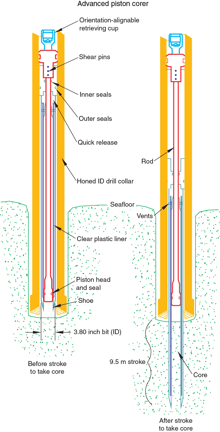
Figure F1. Schematic of the APC system used during Expedition 355.
APC refusal is conventionally defined in two ways: (1) the piston fails to achieve a complete stroke (as determined from the pump pressure reading) because the formation is too hard or (2) excessive force (>60,000 lb; ~267 kN) is required to pull the core barrel out of the formation. When a full stroke cannot be achieved, additional attempts are typically made and after each attempt the bit is advanced by the length of recovered core. The number of additional attempts is generally dictated by the length of recovery of the partial stroke core and the time available to advance the hole by piston coring. Note that this results in a nominal recovery of ~100% based on the assumption that the barrel penetrates the formation by the equivalent of the length of core recovered. When a full or partial stroke is achieved but excessive force cannot retrieve the barrel, the core barrel is sometimes “drilled over,” meaning after the inner core barrel is successfully shot into the formation, the drill bit is advanced to total depth to free the APC barrel.
The standard (full length) APC system contains a 9.5 m long core barrel, whereas the HLAPC system uses a 4.7 m core barrel. In most cases, the HLAPC was deployed after the full APC reached refusal. During the use of the HLAPC, we applied the same criteria for refusal as with the APC system. Use of this new technology allowed for significantly deeper continuous piston coring than would have otherwise been possible with the standard APC.
Nonmagnetic core barrels were used during all APC coring to a pull force of ~40,000 lb. In addition, full-length APC cores recovered during Expedition 355 were oriented using the Icefield MI-5 orientation tool (see Paleomagnetism and rock magnetism). We also used the advanced piston corer temperature tool (APCT-3) to obtain in situ formation temperatures in the first hole at each site to determine the geothermal gradient and estimate heat flow (see Downhole measurements).
The XCB system was used to advance the hole when APC or HLAPC refusal occurred before the target depth was reached or when the formation became either too stiff for APC coring or hard substrate was encountered. The XCB is a rotary system with a small cutting shoe that extends below the large rotary APC/XCB bit. The smaller bit can cut a semi-indurated core with less torque and fluid circulation than the main bit, optimizing recovery. The XCB cutting shoe (bit) extends ~30.5 cm ahead of the main bit in soft sediments but retracts into the main bit when hard formations are encountered (Figure F2).
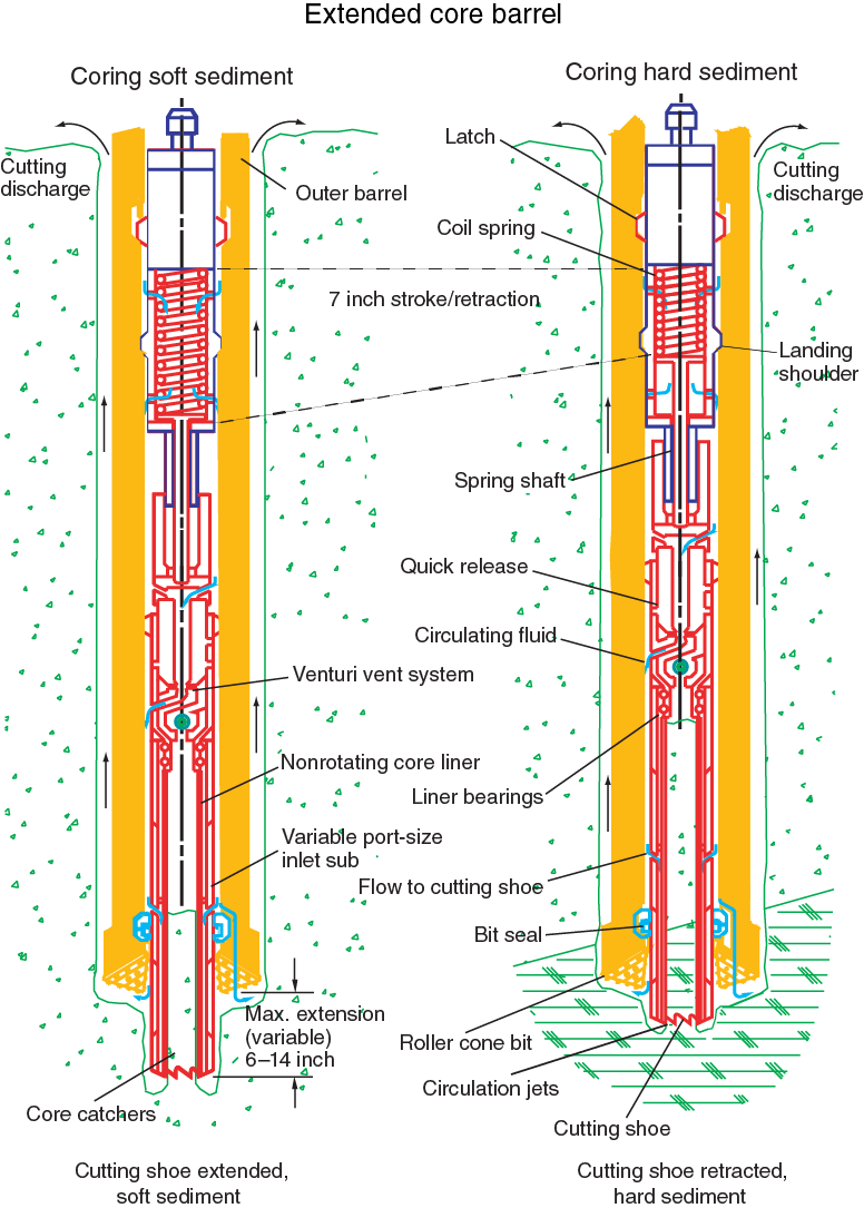
Figure F2. Schematic of the XCB system used during Expedition 355.
The bottom-hole assembly (BHA) is the lowermost part of the drill string. The configuration of the BHA is reported in the operations section in each site chapter. A typical APC/XCB BHA consists of a drill bit (outer diameter = 11⁷⁄₁₆ inches), a bit sub, a seal bore drill collar, a landing saver sub, a modified top sub, a modified head sub, a nonmagnetic drill collar (for APC/XCB), a number of 8 inch (~20.32 cm) drill collars, a tapered drill collar, six joints (two stands) of 5½ inch (~13.97 cm) drill pipe, and one crossover sub. A lockable float valve was used when downhole logging was planned so that downhole logs could be collected through the bit.
The RCB system was deployed when basement coring was expected or when the formation had become too hard for XCB coring to continue. The RCB is the most conventional rotary drilling system and was used during Expedition 355 to drill and core into hard sedimentary and igneous rocks (Figure F3). The RCB requires a dedicated RCB BHA and a dedicated RCB drilling bit. The BHA used for RCB coring included a 9⅞ inch RCB drill bit, a mechanical bit release (when logging was planned), a modified head sub, an outer core barrel, a modified top sub, a modified head sub, and 7–10 control-length drill collars followed by a tapered drill collar to two stands of 5½ inch drill pipe. Most cored intervals were ~9.7 m long, which is the length of a standard rotary core and approximately the length of a joint of drill pipe. In some cases, the drill string was drilled or “washed” ahead without recovering sediments to advance the drill bit to a target depth to resume core recovery. Such intervals were typically drilled using a center bit installed within the RCB bit. When coring basement, half-length cores were sometimes collected to improve recovery and when rates of penetration decreased significantly.
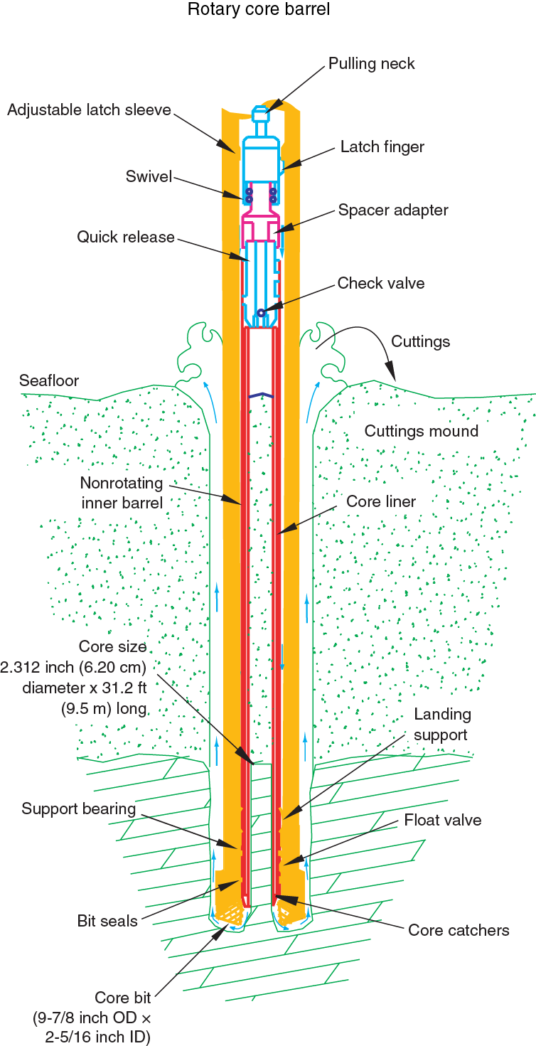
Figure F3. Schematic of the RCB system used during Expedition 355.
IODP depth scales
Primary depth scale types are based on the measurement of drill string length deployed beneath the rig floor (drilling depth below rig floor [DRF] and drilling depth below seafloor [DSF]), the length of core recovered (core depth below seafloor [CSF] and core composite depth below seafloor [CCSF]), and the length of the logging wireline deployed (wireline log depth below rig floor [WRF], wireline log depth below seafloor [WSF], and wireline log matched depth below seafloor [WMSF]). All units are in meters. The relationship between scales is defined either by protocol, such as the rules for computation of CSF from DSF, or by combinations of protocols with user-defined correlations (e.g., CCSF). The distinction in nomenclature should keep the user aware that a nominal depth value at two different depth scales usually does not refer to exactly the same stratigraphic interval (see Curatorial procedures and sample depth calculations). For more information on depth scales, see “IODP Depth Scales Terminology v2” at http://www.iodp.org/policies-and-guidelines/142-iodp-depth-scales-terminology-april-2011/file. To more easily communicate shipboard results, CSF-A depths are reported in this volume as meters below seafloor (mbsf) unless otherwise noted.
Depths of cored intervals are measured from the drill floor based on the length of drill pipe deployed beneath the rig floor (DRF scale). The depth of the cored interval is referenced to the seafloor (DSF scale) by subtracting the seafloor depth at the time of the first hole from the DRF depth of the interval. In most cases, the seafloor depth is the length of pipe deployed minus the length of the mudline core recovered. However, some of the seafloor depths were determined by offset or by tagging the seafloor with the camera system in place.
Standard depths of cores on the CSF-A scale are determined based on the assumptions that (1) the top depth of a recovered core corresponds to the top depth of its cored interval (DSF scale) and (2) the recovered material is a contiguous section even if core segments are separated by voids when recovered. Voids in the core are closed by pushing core segments together, if possible, during core handling. This convention is also applied if a core has incomplete recovery, in which case the true position of the core within the cored interval is unknown and should be considered a sample depth uncertainty, up to the length of the core barrel used, when analyzing data associated with the core material. Standard depths of subsamples and associated measurements (CSF-A scale) are calculated by adding the offset of the subsample or measurement from the top of its section, as well as the lengths of all higher sections in the core, to the top depth of the cored interval.
A soft to semisoft sediment core from less than a few hundred meters below seafloor expands upon recovery (typically a few percent to as much as 15%), so the length of the recovered core can exceed that of the cored interval. Therefore, a stratigraphic interval may not have the same nominal depth at the DSF and CSF scales in the same hole. When core recovery (the ratio of recovered core to cored interval) is >100%, the CSF depth of a sample taken from the bottom of a core will be deeper than that of a sample from the top of the subsequent core (i.e., the data associated with the two core intervals overlap on the CSF-A scale).
Core composite depth scales (CCSF) are constructed for sites, whenever feasible, to mitigate the CSF-A core overlap problem, as well as the coring gap problem, and to create as continuous a stratigraphic record as possible. Using shipboard core logger–based physical property data and verified with core photos, core depths in adjacent holes at a site are vertically shifted to correlate between cores recovered in adjacent holes. This process produces the CCSF depth scale. The correlation process results in “affine tables,” indicating the vertical shift of cores on the CCSF scale relative to the CSF-A scale. Once the CCSF scale is constructed, a splice can be defined that best represents the stratigraphy of a site by utilizing and splicing the best portions of individual sections and cores from each hole. Because of core expansion, the CCSF depths of stratigraphic intervals are typically 10%–15% deeper than their CSF-A depths. CCSF depth scale construction also reveals that coring gaps on the order of 1.0–1.5 m typically occur between two subsequent cores, despite apparent >100% recovery. For more details on construction of the CCSF depth scale, see Stratigraphic correlation.
Core handling and analysis
The initial coring strategy for Expedition 355 consisted of APC coring in two holes (A and B) to refusal. However, three holes were cored at Site U1456 with the APC. The extra APC hole at Site U1456 allowed for high-resolution sampling for specific objectives (e.g., microbiology and interstitial water measurements). APC refusal was followed by HLAPC coring at both sites, with XCB coring once we reached HLAPC refusal at Site U1456. RCB coring was employed to attempt to reach and core into basement at Sites U1456 and U1457.
Cores recovered during Expedition 355 were extracted from the core barrel in 67 mm diameter plastic liners. These liners were carried from the rig floor to the core processing area on the catwalk outside the Core Laboratory, where they were split into ~1.5 m sections. Liner caps (blue = top, colorless = bottom, and yellow = whole-round sample taken) were glued with acetone onto liner sections on the catwalk by the Marine Technicians. The length of each section was entered into the database as “curated length” using the Sample Master application. This number was used to calculate core recovery.
For sedimentary sections, as soon as cores arrived on deck, headspace samples were taken using a syringe for immediate hydrocarbon analysis as part of the shipboard safety and pollution prevention program. Core catcher samples were taken for biostratigraphic analysis. Whole-round samples were taken from some core sections for shipboard and postcruise interstitial water analyses. In addition, whole-round and syringe samples were immediately taken from the ends of cut sections for shore-based microbiological analysis.
Igneous rock core pieces were slid out of the liners and placed in order in new, clean sections of core liner that had previously been split in half. Pieces having a vertical length greater than the internal (horizontal) diameter of the core liner are considered oriented pieces because they could have rotated only around their vertical axes. Those pieces were immediately marked on the bottom with a red wax pencil to preserve their vertical (upward) orientations. Pieces that were too small to be oriented with certainty were left unmarked. Adjacent but broken core pieces that could be fit together along fractures were curated as single pieces. The core describers on shift confirmed the piece matches and corrected any errors. The core describers also marked a split line on the pieces, which defined how the pieces should be cut into two equal halves. The aim was to maximize the expression of dipping structures on the cut face of the core while maintaining representative features in both archive and working halves.
Whole-round core sections were immediately run through the Special Task Multisensor Logger (STMSL) when necessary for stratigraphic correlation after being cut on the catwalk. The STMSL measures gamma ray attenuation (GRA) bulk density and magnetic susceptibility that were used to aid in real-time stratigraphic correlation. After measurement, these cores were placed on the core racks in the laboratory. Cores not run through the STMSL were immediately placed in core racks after being cut on the catwalk. When the cores reached equilibrium with laboratory temperature (typically after ~4 h), whole-round core sections were run through the Whole-Round Multisensor Logger (WRMSL; measuring P-wave velocity, density, and magnetic susceptibility) and the Natural Gamma Radiation Logger (NGRL). Thermal conductivity measurements were typically taken at a rate of one per core (see Physical properties). The core sections were then split lengthwise from bottom to top into working and archive halves. Investigators should note that older material may have been transported upward on the split face of each section during splitting. For hard rock sections, each piece of core was split with a diamond-impregnated saw into an archive (A) and working half (W), with the positions of the plastic spacers between individual pieces maintained in both halves of the plastic liner. Pieces were numbered sequentially from the top of each section. Separate subpieces within a single piece were assigned the same number but were lettered consecutively (e.g., 1a, 1b, 1c). Pieces were labeled only on the outer cylindrical surfaces of the core or on the core liner.
The working half of each sedimentary core was sampled for shipboard (biostratigraphy, physical properties, carbonate, paleomagnetism, and X-ray diffraction [XRD]) analyses. The archive half of all cores was scanned on the Section Half Imaging Logger (SHIL) with a line-scan camera at 20 pixels/mm and measured for color reflectance and magnetic susceptibility on the Section Half Multisensor Logger (SHMSL). At the same time, the archive halves were described visually and by means of smear slides and thin sections. All observations were recorded in the Laboratory Information Management System (LIMS) using the descriptive data capture application DESClogik. After visual description, the archive halves were run through the cryogenic magnetometer. Finally, digital color close-up images were taken of particular features of the archive or working halves, as requested by individual scientists. For igneous rocks, discrete samples were taken from working halves for shore-based thin section and geochemical analyses because of the lack of time for such analyses during the expedition. Records of all samples taken are kept by the IODP curator. Sampling for personal postexpedition research was deferred until a postcruise sampling meeting; however, shipboard residues were made available for scientists to request for postcruise analyses to assist with personal sampling during the sampling meeting.
In preparation for storage, soft-sediment section-half cores were wrapped in plastic wrap, whereas lithified sedimentary and igneous rock section half cores were shrink-wrapped. After wrapping, both halves of the core were put into labeled plastic tubes that were sealed and transferred to cold storage space aboard the ship. At the end of the expedition, the cores were transported from the ship to cold storage at the Gulf Coast Repository (GCR) at Texas A&M University in College Station, Texas, USA. Shore-based sampling of the cores took place while the cores were stored at the GCR. Following sampling, the cores were shipped to permanent cold storage at the Kochi Core Center (KCC) at Kochi University in Kochi, Japan. The KCC houses cores collected from the western Pacific Ocean, Indian Ocean, and Bering Sea.
Drilling disturbance
Cores may be significantly disturbed as a result of the drilling process and contain extraneous material as a result of the coring and core handling process. In formations with loose sand layers, sand from intervals higher in the hole may be washed down by drilling circulation, accumulate at the bottom of the hole, and be sampled with the next core. The uppermost 10–50 cm of each core must therefore be examined critically during description for potential “fall-in.” Common coring-induced deformation includes the concave-downward appearance of originally horizontal bedding. Piston action may result in fluidization (flow-in) at the bottom of APC cores. Retrieval from depth to the surface may result in elastic rebound. Gas that is in solution at depth may become free and drive core segments within the liner apart. Both elastic rebound and gas pressure can result in a total length for each core that is longer than the interval that was cored and thus a calculated recovery of >100%. If gas expansion or other coring disturbance results in a void in any particular core section, the void can be either closed by moving material if very large, stabilized by a foam insert if moderately large, or left as is. When gas content is high, pressure must be relieved for safety reasons before the cores are cut into segments. This is accomplished by drilling holes into the liner, which forces some sediment as well as gas out of the liner. These disturbances are described in the Lithostratigraphy section in each site chapter and are graphically indicated on the core summary graphic reports (visual core descriptions [VCDs]). In extreme instances core material can be ejected from the core barrel, sometimes violently, onto the rig floor by high pressure in the core or other coring problems. This core material was replaced in the plastic core liner by hand and should not be considered to be in stratigraphic order. Core sections so affected are marked by a yellow label marked “disturbed,” and the nature of the disturbance is noted in the coring log.
Curatorial procedures and sample depth calculations
Numbering of sites, holes, cores, and samples follows standard IODP procedure (Figure F4). Drilling sites are numbered consecutively from the first site drilled by the D/V Glomar Challenger in 1968. Integrated Ocean Drilling Program Expedition 301 began using the prefix “U” to designate sites occupied by the United States Implementing Organization (USIO) platform, the JOIDES Resolution. For all IODP drill sites, a letter suffix distinguishes each hole drilled at the same site. The first hole drilled is assigned the site number modified by the suffix “A,” the second hole the site number and the suffix “B,” and so on.
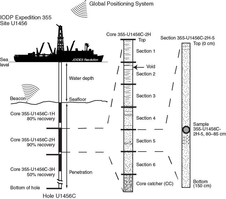
Figure F4. IODP conventions for naming sites, holes, cores, and samples.
Cores taken from a hole are numbered sequentially from the top of the hole downward. When an interval is drilled down, this interval is also numbered sequentially and the drill down designated by a “1” instead of a letter that designates the coring method used (e.g., Core 355-U1456D-11). Cores taken with the APC system are designated with “H,” “F” designates HLAPC cores, “X” designates XCB cores, and “R” designates RCB cores. Core numbers and their associated cored intervals are unique in a given hole. Generally, maximum recovery for a single core is 9.5 m of sediment (APC) or 9.7 m of rock or sediment (XCB/RCB) contained in a plastic liner (6.6 cm internal diameter) plus an additional ~0.2 m in the core catcher, which is a device at the bottom of the core barrel that prevents the core from sliding out when the barrel is retrieved from the hole. In certain situations, recovery may exceed the 9.5 or 9.7 m maximum. In soft sediment this excess core recovery is normally caused by core expansion resulting from depressurization. In hard rock cores this typically occurs when a pedestal of rock fails to break off and is grabbed by the core barrel of the subsequent core. High heave, tidal changes, and overdrilling can also result in an advance that differs from the expected 9.5/9.7 m.
Recovered cores are divided into 1.5 m sections that are numbered serially from the top downward. When full recovery is obtained, the sections are numbered 1–7, with the last section usually being <1.5 m. Rarely, an unusually long core may require more than seven sections. When the recovered core is shorter than the cored interval, by convention the top of the core is deemed to be located at the top of the cored interval for the purpose of calculating (consistent) depths. When coring hard rocks, all pieces recovered are placed immediately adjacent to each other in the core tray. Samples and descriptions of cores are designated by distance, measured in centimeters, from the top of the section to the top and bottom of each sample or interval. By convention, hard rock material recovered from the core catcher is placed below the last section. In sedimentary cores, the core catcher section is treated as a separate section (CC). When the only recovered material is in the core catcher, it is placed at the top of the cored interval.
A full curatorial sample identifier consists of the following information: expedition, site, hole, core number, core type, section number, and interval in centimeters measured from the top of the core section. For example, a sample identification of “355-U1456C-2H-5, 80–85 cm,” represents a sample taken from the interval between 80 and 85 cm below the top of Section 5 of Core 2 (collected using the APC system) of Hole C of Site U1456 during Expedition 355 (Figure F4).
Authorship of site chapters
The separate sections of the site chapters and Expedition 355 methods chapter were written by the following shipboard scientists (authors are listed in alphabetical order; no seniority is implied):
- Background and objectives: P.D. Clift, D.K. Kulhanek, D.K. Pandey
- Operations: D.K. Kulhanek, M. Storms
- Lithostratigraphy: S. Andò, P.D. Clift, B.K. Khim, A. Kumar, H. Lu, M.W. Lyle, R. Mishra, K. Suzuki, Z. Xu
- Biostratigraphy: M. Iwai, D.K. Kulhanek, C.M. Routledge, G.K. Sharma, A.D. Singh, S. Steinke
- Stratigraphic correlation: M.W. Lyle, G. Scardia
- Igneous petrology and alteration: D.K. Pandey, T. Radhakrishna
- Geochemistry: J.A.P. Bendle, S. Bratenkov, G.P. Gurumurthy, H.M. Liddy, M. Tiwari, Z. Yu
- Microbiology: A.G. Kumar
- Paleomagnetism: G. Scardia, L. Tauxe
- Physical properties: E.M. Griffith, A. Hahn, R. Saraswat, R. Saxena
- Downhole measurements: E.M. Griffith, R. Saxena
Lithostratigraphy
Expedition 355 sediment descriptions are primarily based on visual (macroscopic) core description, microscopic examination of smear slides and thin sections, and split-core imaging, color spectrophotometry, XRD, and magnetic susceptibility analysis. The methods adopted for this expedition are similar to those used during Integrated Ocean Drilling Program Expeditions 320/321 and 342 (Expedition 320/321 Scientists, 2010; Norris et al., 2014). The DESClogik application (version 8.0.0.0) was used to record and upload descriptive data into the LIMS database (see the DESClogik user guide at http://iodp.tamu.edu/labs/documentation). The customized Expedition 355 spreadsheet templates in DESClogik were used to record the macroscopic and microscopic data.
The standard method of splitting cores into working and archive halves (either using piano wire or a saw) can affect the appearance of the split core surface and obscure fine details of lithology and sedimentary structure. When necessary, the archive halves of cores were gently scraped across, rather than along, the core section using a stainless steel or glass scraper to prepare the surface for sedimentological examination and digital imaging. Scraping parallel to bedding with a freshly cleaned tool prevents up or downcore contamination. Cleaned sections were then described in conjunction with measurements using the SHIL and SHMSL.
Visual core descriptions
The visual core description (VCD) standard graphic reports were produced from the archive half descriptive core data uploaded into the LIMS database. VCDs include a simplified graphical representation of the core on a section-by-section basis along with visual description (Figures F5, F6). Depending on the type of material recovered, two VCDs were prepared: one to describe sediment or sedimentary rock and the other to describe igneous rock. Site, hole, and depth in meters below seafloor, calculated according to the core depth below seafloor (CSF-A) depth scale, are given at the top of each VCD. Both the CSF-A depth in meters and the length of the core in centimeters are displayed along the left margin, together with the lithologic unit defined by the core description team and the age based on biostratigraphy and magnetostratigraphy. VCDs display the physical description of the core as recorded in DESClogik, including lithologic accessories (sedimentary structures, diagenesis, and macrofossils), presence of graded beds, bioturbation intensity, and drilling disturbance. Symbols used in the VCDs are given in Figure F6. Additionally, VCDs display magnetic susceptibility, natural gamma radiation, and color reflectance from core scans and the locations of samples taken for shipboard measurements. The summary text and individual columns shown on the VCDs are described below in greater detail, followed by an outline of the lithostratigraphic classification system used during Expedition 355.
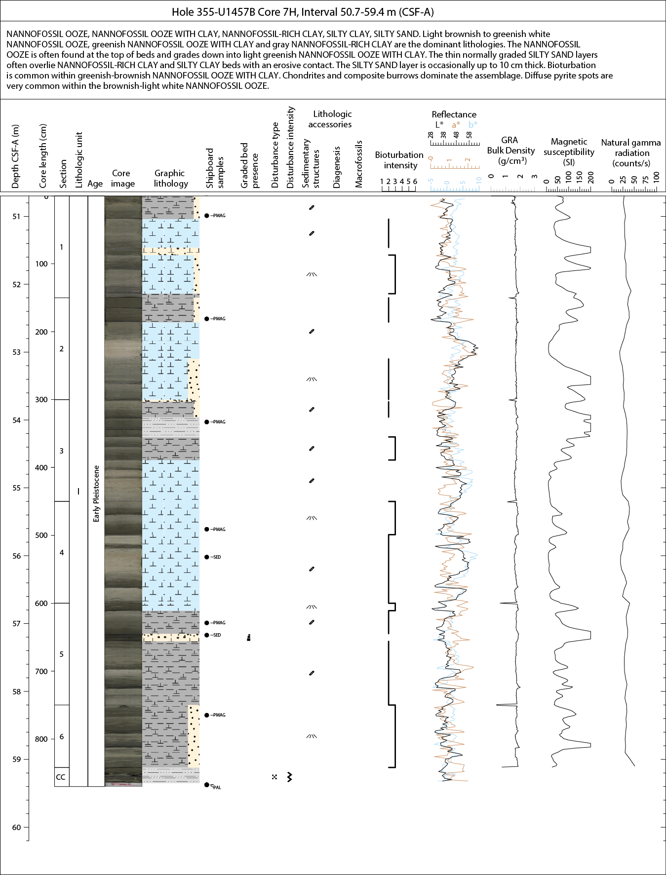
Figure F5. Example of a graphic VCD form for Expedition 355.
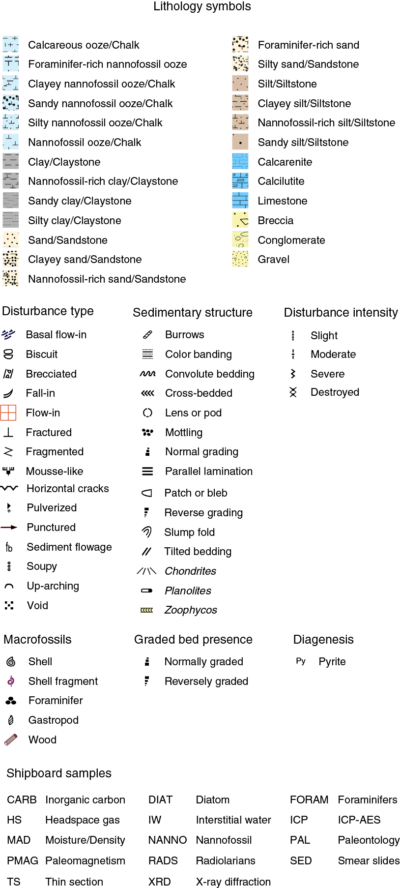
Figure F6. Symbols and nomenclature used for VCDs, Expedition 355.
Section summary
A brief overview of the core section is presented at the top of the VCD report in the section summary. The summary describes the major and minor lithologies present in the section, the visual sediment color, as well as notable features that are not readily recorded in the defined columns by symbols (e.g., sedimentary structures, fossils, etc.).
Section-half image
The archive halves were scanned with the SHIL as soon as possible after splitting and scraping to avoid color changes caused by sediment oxidation and drying. The SHIL uses three pairs of advanced illumination high-current, focused LED line lights to illuminate large cracks and blocks in the core surface and sidewalls. Each LED pair has a color temperature of 6,500 K and emits 90,000 lx at 3 inches. The line-scan camera images 10 lines/mm to create a high-resolution TIFF file. The camera height is adjusted so that each pixel images a 0.1 mm2 section of the core. High- and low-resolution JPEG files are subsequently created from the high-resolution TIFF files. All image files include a grayscale and ruler. Section-half depths were recorded so that these images can be used for core description and analysis. These images are displayed on the VCD in the Core image column.
Graphic lithology
Lithologies of the core intervals are represented on the VCDs by graphic patterns in the Graphic lithology column, using the symbols illustrated in Figure F6. The Graphic lithology column on each VCD plots to scale all beds that are at least 10 cm thick. A maximum of two different lithologies (for interbedded sediment) are shown within the same cored interval for interbeds <10 cm thick. The major modifier of a primary lithology is shown using a modified version of the primary lithology pattern. Lithologic abundances are rounded to the nearest 10%; lithologies that constitute <10% of the core are generally not shown but are listed in the DESClogik template. Relative abundances of lithologies reported in this way are useful for general characterization of the sediment but do not constitute precise quantitative observations.
Graded bed presence
The presence of graded beds is noted on the VCDs in the Graded bed presence column, separately from other sedimentary structures. Most graded bed intervals show sharp scoured bases, cross- and planar laminations, and flame structures, which we interpret as turbidite deposits.
Lithologic accessories
Sedimentary structures
The locations and types of stratification and sedimentary structures visible on the split core surfaces are shown in the Sedimentary structures column on the VCD and also entered into DESClogik with their respective location and depth. Symbols in this column indicate the locations and scales of interstratification (bedding), as well as the locations of individual bedding features and any other sedimentary features, such as cross-bedding, convolute bedding, and types of burrows. The symbolic representations of identified sedimentary structures are shown in Figure F6.
For Expedition 355, we used the following terminology (based on Stow, 2005) to describe the scale of stratification:
- Thin lamination = <3 mm thick.
- Medium lamination = 0.3–0.6 cm thick.
- Thick lamination = 0.6–1 cm thick.
- Very thin bed = 1–3 cm thick.
- Thin bed = 3–10 cm thick.
- Medium bed = 10–30 cm thick.
- Thick bed = 30–100 cm thick.
- Very thick bed = >100 cm thick.
Changes in sedimentary structures, such as lamination or bed boundaries (gradual, sharp, irregular, or erosive), presence of biogenic structures (e.g., burrows), and other structures related to the depositional environment (normal/reverse grading, parallel bedding, cross-bedding, etc.), were entered into DESClogik. Cross-bedding describes a bed that contains thin horizontal or inclined laminations <1 cm in thickness with inclined internal foresets. Vertical/tilted/inclined bedding describes a bed that exhibits the angle from the horizontal plane as inclined bedding (<10°) to vertical bedding (>70°). Structureless beds are not specifically entered, but beds that are homogeneous in lithology and color and exhibit no bedding, cross-bedding, grading, bioturbation, or bed disturbance are described as massive or structureless in the core description. For Expedition 355, we used various terminologies for sedimentary structures. When identifiable, folds, slump folds, microfaults, and ichnofossils such as Zoophycos, Chondrites, Skolithos, and Planolites burrows (Ekdale et al., 1984) were reported in the Sedimentary structures column as well as in core summary.
Diagenesis
Select postdepositional features (e.g., pyrite nodules) are recorded in the diagenesis column.
Macrofossils
The archive half of each core section was carefully examined for macrofossil shell fragments and other biogenic components consisting of the skeletal debris of marine calcareous and siliceous fossils. The presence of these fossils is recorded in the Macrofossils column on the VCD, and the symbols used to designate these features are shown in Figure F6.
Bioturbation intensity
We distinguished five levels of bioturbation intensity, which are illustrated with the following numeric scale in the Bioturbation intensity column:
- 1 = no bioturbation (<10%).
- 2 = slight bioturbation (<10%–30%).
- 3 = moderate bioturbation (30%–60%).
- 4 = heavy bioturbation (60%–90%).
- 5 = complete bioturbation (>90%).
Drilling disturbance
Drilling-related sediment disturbance is recorded in the Disturbance type column using the symbols shown in Figure F6. The type of drilling disturbance is described for soft and firm sediment using the following terms:
- Fall-in: out of place material at the top of a core that has fallen downhole onto the cored surface.
- Bowed: bedding contacts are slightly to moderately deformed but still subhorizontal and continuous.
- Up-arching: material retains its coherency, with material closest to the core liner bent downward. Most apparent when horizontal features are distorted.
- Void: empty space within the cored material (e.g., caused by gas expansion during core retrieval). Voids may also be related to partial strokes during the coring process, although these voids are curated on the catwalk and do not appear in any core description.
- Flow-in, coring/drilling slurry, along-core gravel/sand contamination: soft-sediment stretching and/or compressional shearing structures are severe and are attributed to coring/drilling. The particular type of deformation may also be noted (e.g., flow-in, gas expansion, etc.).
- Soupy or mousse-like: intervals are water saturated and have lost all aspects of original bedding.
- Biscuit: sediment of intermediate stiffness shows vertical variations in the degree of disturbance. Softer intervals are washed and/or soupy, whereas firmer intervals are relatively undisturbed.
- Cracked or fractured: firm sediment is broken during drilling but not displaced or rotated significantly.
- Fragmented, brecciated, or pulverized: firm sediment that is pervasively broken by drilling and may be displaced or rotated.
The categories of fracturing in indurated sediment include the following:
- Slight (core pieces are in place but broken),
- Moderate (core pieces are in place or partly displaced, but original orientation is preserved or recognizable),
- Severe (core pieces are probably in correct stratigraphic sequence, but original orientation is lost),
- Destroyed (core pieces are in incorrect stratigraphic sequence, and original orientation is lost),
- Drilling breccia (core is crushed and broken into many small and angular pieces, with original orientation and stratigraphic position lost).
Disturbance intensity is described in the Disturbance intensity column of the VCD using the following subjective scheme illustrated by the symbols shown in Figure F6:
Lithologic unit and age
Lithologic units are numbered in order from the top using Roman numerals (Figure F5) and shown in the Lithologic unit column of the VCD. Sediment age was provided by the shipboard biostratigraphers (see Biostratigraphy) and paleomagnetists (see Paleomagnetism and rock magnetism) and is listed in the Age column of the VCD.
Shipboard samples
The exact positions of samples used for microscopic descriptions (i.e., smear slides), biostratigraphic determinations, and shipboard analysis of chemical and physical properties of the sediment are recorded in the Shipboard samples column (Figure F5).
Spectrophotometry
Reflectance of visible light from the archive halves of sediment cores was measured using an Ocean Optics USB4000 spectrophotometer mounted on the automated SHMSL. Measurements were taken at 2.0 cm spacing to provide a high-resolution stratigraphic record of color variations for visible wavelengths (see Physical properties). Additional detailed information about measurement and interpretation of spectral data can be found in Balsam et al. (1997, 1998) and Balsam and Damuth (2000).
Reflectance of visible light from the archive halves of sediment cores was also measured using a portable Minolta CM-2002 spectrophotometer, according to the Minolta CM-2002 user’s manual (Minolta Camera Co., 1991). Measurements were taken at 2.0 cm spacing to provide another high-resolution stratigraphic record of color variations for visible wavelengths. Each measurement was recorded in 10 nm wide spectral bands from 400 to 700 nm. Data are converted to L*, a*, b* and X, Y, Z color reflectance parameters for efficient archival and display. Both zero and white calibrations were conducted before measurement on each core.
Natural gamma radiation
Natural gamma radiation occurs primarily as a result of the decay of naturally occurring 238U, 232Th, and 40K isotopes in geologic samples. This radiation is measured using the NGRL (see Physical properties). Data generated from this instrument are used to augment geologic interpretations.
Magnetic susceptibility
Magnetic susceptibility is measured first on the WRMSL (see Physical properties) but is measured again at higher resolution on the split-core archive half on the SHMSL with a Bartington Instruments MS2E point sensor (high-resolution surface-scanning sensor). Because the SHMSL demands flush contact between the magnetic susceptibility point sensor and the split core, measurements were made on the archive halves of split cores that were covered with clear plastic wrap. Measurements were taken at 2.0 cm spacing. Measurement resolution was 1.0 SI, and each measurement integrated a volume of 10.5 mm × 3.8 mm × 4 mm, where 10.5 mm is the length perpendicular to the core axis, 3.8 mm is the width along the core axis, and 4 mm is the depth into the core. Only one measurement was taken at each measurement position.
Sediment classification
Macroscopic observation
The lithologic description for sediment was based on the classification schemes used during Ocean Drilling Program (ODP) Leg 178 (Shipboard Scientific Party, 1999). Lithologic names consist of a principal name based on composition, degree of lithification, and/or texture as determined from visual examination and smear slide or thin section observations. The Wentworth (1922) scale was used to define sediment size classes (Figure F7). If no gravel was present, the principal sediment/rock name was determined based on the relative abundances of sand, silt, and clay (modified after Shepard, 1954). Sediment classification systems used during Expedition 355 are illustrated in Figure F8. The principal name of sediment with >50% siliciclastic grains was based on an estimate of the grain sizes present. For a mixture of components, the principal name is preceded by major modifiers (in order of increasing abundance) that refer to components making up ≥25% of the sediment. Minor components that represent between 10% and 25% of the sediment follow the principal name in order of increasing abundance.
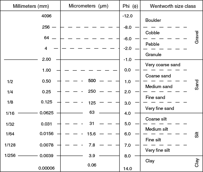
Figure F7. Udden-Wentworth grain-size classification of terrigenous sediment.
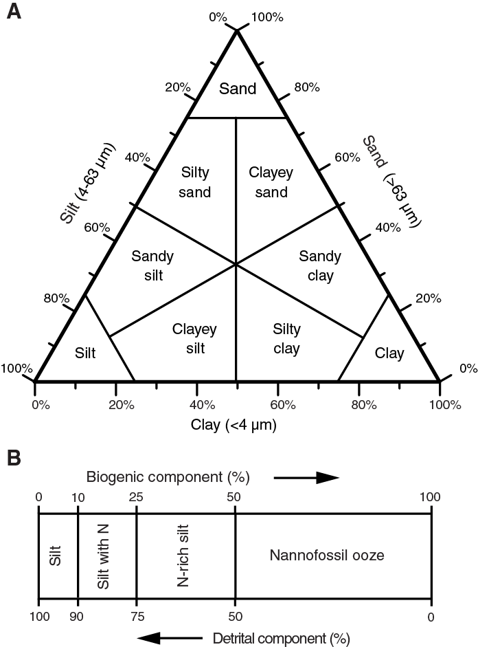
Figure F8. Sediment classification and lithology naming schemes.
The principal name of sediment that appears to contain <10% carbonate is based on the textural characteristic of the dominant detrital component (i.e., sand, silt, or clay). The second most abundant component defines the prefix (e.g., clayey, silty, and sandy); any additional component is described using a suffix after the main descriptors (e.g., with clay, with silt, with sand, with foraminifers, with nannofossils). However, distinguishing between some of these categories can be difficult (e.g., silty clay versus clayey silt) without accurate measurements of grain size abundances.
The primary name for sediment with >50% biogenic grains is “ooze,” modified by the most abundant specific biogenic grain type that forms 50% or more of the sediment. For example, if foraminifers exceed 50%, then the sediment is called “foraminiferal ooze.” However, if the sediment is composed of 40% diatoms and 15% radiolarians, then the sediment is termed “siliceous ooze.” This scheme is also applied to carbonate biogenic grains.
Major and minor modifiers for biogenic components are also applied to the principal sediment names:
- Major modifiers are those components with abundances between 25% and 50% and are indicated by the suffix “rich” (e.g., “nannofossil-rich”).
- Minor modifiers are those components with abundances of 10%–25% and are indicated by the suffix “with” (e.g., “with nannofossils”).
Description of lithification is dependent on the dominant composition, as described below:
- Sediment derived predominantly from siliciclastic material: if the sediment can be deformed easily with a finger, then no lithification term is added and the sediment is named for the dominant grain size. For more consolidated material, the lithification suffix “-stone” is appended to the dominant size classification (e.g., “clay” versus “claystone”).
- Sediment derived predominantly from calcareous pelagic organisms (e.g., calcareous nannofossils and foraminifers): the lithification terms “ooze,” “chalk,” and “limestone” reflect whether the sediment can be deformed with a finger (ooze), can be scratched easily by a fingernail (chalk), or cannot be scratched with a fingernail (limestone).
- “Pelagic” turbidites with calcareous components have a different classification and nomenclature. We distinguish a coarse sand-sized calcareous sediment called calcarenite and a finer silt- to clay-sized calcareous sediment termed calcilutite, following the original definition of Grabau (1903), later modified by Folk (1974) and Carozzi (1989). In cases of very coarse grained deposits, we use the terms “conglomerate” and “breccia,” following the definitions of Bates and Jackson (1987).
Microscopic observation
The microscopic descriptions were produced in smear slide and thin section templates customized for Expedition 355. Smear slide samples of the main lithologies were collected from the archive half of each core when the sediment was not lithified. Additional samples were collected from areas of interest (e.g., laminations, clasts, and nodules). We generated tables summarizing the relative abundance of minerals, texture, and sedimentary components from the smear slides.
For each smear slide, a small amount of sediment was removed from the core section using a wooden toothpick and placed directly on a 25 mm × 75 mm glass slide. A drop of deionized water was added, and the sediment was evenly spread across the glass slide using a toothpick. The glass slide was then dried on a hot plate at a low setting (50°C). A drop of adhesive (Norland Optical Adhesive Number 61) was added to mount a 22 mm × 30 mm coverslip to the glass slide. The slide with mounted coverslip was then placed in an ultraviolet light box for 5 min to cure the adhesive.
Once the mounts were fixed, each slide was scanned at 10×, 20×, 40×, 50×, or 63× with a transmitted-light petrographic microscope using an eyepiece micrometer to assess grain size distributions of clay (<4 µm), silt (4–63 µm), and sand (>63 µm) fractions. Several fields of view were examined at 10×, 20×, 40×, or 50× for detrital (e.g., quartz, feldspar, clay minerals, mica, and heavy minerals), biogenic (e.g., nannofossils, other calcareous bioclasts, diatoms, foraminifers, and radiolarians), and authigenic (e.g., carbonate, iron sulfide, iron [hydro]oxide, and glauconite) identification. Standard petrographic techniques were employed to identify the commonly occurring minerals and biogenic groups, as well as important accessory minerals and microfossils. Relative abundances of identified components such as mineral grains, microfossils, and biogenic fragments were described on a semiquantitative basis by percentage estimation. Most of the minerals and biogenic groups present were carefully detected and photographed.
Components observed in the smear slides were quantified using the following categories:
- Tr = trace (<1%).
- R = rare (1%–5%).
- C = common (>5%–25%).
- A = abundant (>25%–50%).
- D = dominant (>50%).
The heavy mineral assemblage was thoroughly studied to identify possible sources of detritus following the methods of Mange and Wright (2007). We included categories for each heavy mineral encountered in our smear slides and their relative abundance (Andò et al., 2012) in DESClogik. Identification with polarizing microscopy was applied using classical optical observation as stated in the reference manuals of Mange and Maurer (1992) and Deer et al. (1991).
Relative abundance among minor amounts of heavy minerals was quantified following a simplified ranking:
It should be noted that, on occasion, the lithologic name assigned based on smear slide observation does not match the name in the macroscopic lithology description. This is because the smear slide data refer to a smaller area sampled, which may not be representative of the entire described interval from which it was taken. In addition to this, very fine and coarse grains are difficult to observe in smear slides, and their relative proportions in the sediment can be affected during slide preparation.
Short descriptions and representative photomicrographs of thin sections were added in the customized template in DESClogik. The maximum size of biogenic and clastic constituents, minerals, surficial textures, and nomenclature (Andò et al., 2012) were also described.
X-ray diffraction analyses
Samples were prepared for XRD analysis in order to qualitatively identify bulk minerals and clay minerals. The XRD results combined with smear slide estimates and visual descriptions were used to assist in lithologic classification. In general, one 5 cm3 sample was taken from every second core over the interval cored by the APC. Additional limited samples were taken and analyzed based on visual core observations (e.g., color variability and visual changes in lithology and texture) and smear slides. Samples analyzed for bulk mineralogy were freeze-dried and ground to a homogeneous consistency in a metal ball mill. Prepared samples were top-mounted onto a sample holder and analyzed using a Bruker D-4 Endeavor diffractometer mounted with a Vantec-1 detector using nickel-filtered CuKα radiation. The standard locked coupled scan was as follows:
- Voltage = 40 kV.
- Current = 40 mA.
- Goniometer scan = 4°–70°2θ.
- Step size = 0.0087°2θ.
- Scan speed = 0.2 s/step.
- Divergence slit = 0.3 mm.
Shipboard results yielded only qualitative results of the presence of the most common mineral components.
Diffractograms of bulk samples were evaluated with the aid of the EVA software package, which allowed for mineral identification and basic peak characterization (e.g., maximum peak intensity). Files were created that contained d-spacing values, diffraction angles, and peak intensities. These files were scanned by the EVA software to find d-spacing values characteristic of a limited range of minerals.
Samples analyzed for clay mineralogy were first treated with 10% acetic acid to remove carbonate before separation. Excess acid was removed by repeated centrifuging followed by homogenization. The <2 μm fraction was separated by centrifuge and used to make oriented aggregates on glass slides. When required, lithified samples were dispersed with Calgon solution. All samples were air-dried and glycolated (12 h under vacuum in ethylene glycol at 60°–70°C) and analyzed at 3°–30°2θ scan under the same operation conditions of bulk sediment analysis, as described above. Shipboard results yielded only qualitative results for the presence of the most common clay mineral components.
Biostratigraphy
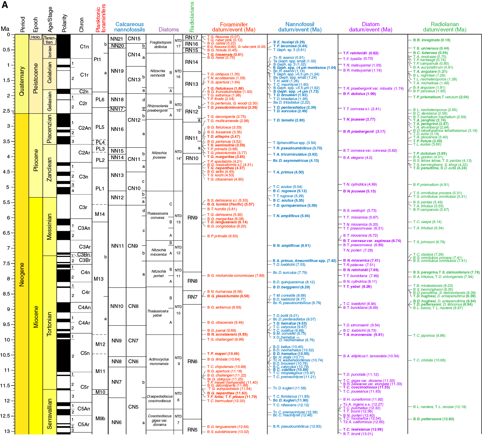
Calcareous nannofossils, planktonic foraminifers, radiolarians, and diatoms in core catcher samples were studied at all sites for preliminary biostratigraphic age assessment. Samples from split core sections were also examined when a more refined age determination was necessary and when time permitted. Biostratigraphic events, mainly the first occurrence (or base) and last occurrence (or top) of the diagnostic species, are tied to the geomagnetic polarity timescale of Gradstein et al. (2012).
Calcareous nannofossils
Calcareous nannofossil zonation was based on the schemes of Martini (1971) (codes NN and NP) and Okada and Bukry (1980) (codes CN and CP). Calibrated ages for bioevents are from Gradstein et al. (2012) as given in Table T1 and illustrated in Figure F9.
Table T1. Calcareous nannofossil events and GTS2012 ages used during Expedition 355. Download table in .csv format.

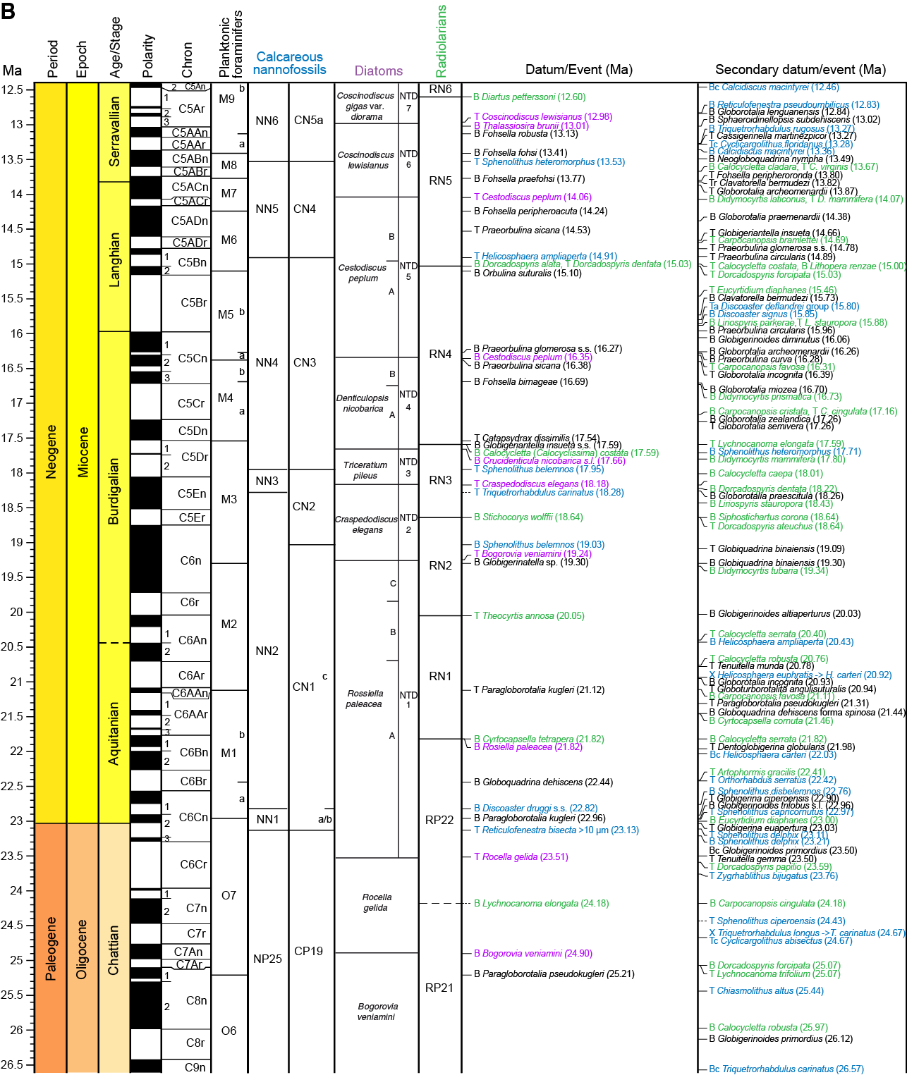
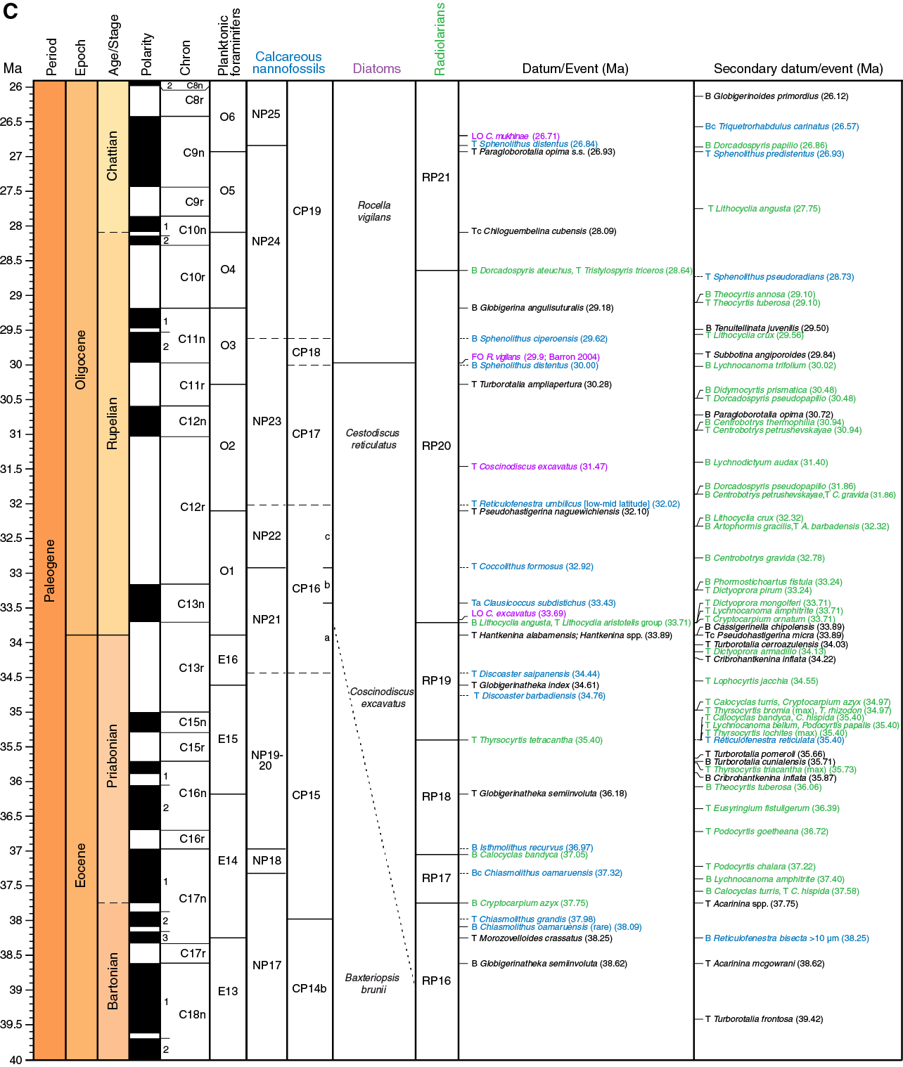
Figure F9. Geomagnetic polarity timescale, biostratigraphic zonation, and microfossil events used during Expedition 355.
Several species of the genus Gephyrocapsa, which are commonly used as Pleistocene biostratigraphic markers, show a great range of variation in size and other morphological features, causing problems in identification (e.g., Samtleben, 1980; Su, 1996; Bollmann, 1997). Size-defined morphological groups of this genus are used as biostratigraphic markers (e.g., Young, 1998; Maiorano and Marino, 2004; Lourens et al., 2004; Raffi et al., 2006). Thus, shipboard identification concentrated on identifying different size fractions within the overall Gephyrocapsa assemblage, including those <3, 3–4, 4–5.5, and >5.5 µm. In addition, specimens >3 µm were broadly divided into the following species based on the size of the central area: Gephyrocapsa oceanica (large central area with bridge angle <90° to the major axis) and Gephyrocapsa caribbeanica (small central area nearly filled by a bridge). Other forms, such as Gephyrocapsa muellerae, were included with G. oceanica.
Several Reticulofenestra species with different coccolith and central opening sizes are used as Cenozoic biostratigraphic markers; however, these parameters show considerable variations within and between “species,” making species differentiation difficult (e.g., Backman, 1980; Su, 1996; Young, 1998). In this study, we followed the definition of Reticulofenestra pseudoumbilicus by Young (1998) as having a maximum coccolith length >7 µm (similar to the size of its holotype), especially for specimens from its uppermost range in the early Pliocene. Smaller forms were categorized separately as R. pseudoumbilicus 5–7 µm. We distinguished Reticulofenestra asanoi from the similar sized Pseudoemiliania lacunosa by the absence of slits on the shield (Su, 1996).
Methods
We prepared samples from core catchers at ~9.5 m intervals from all holes at each site, with additional samples taken from split core sections to refine the biostratigraphy or to sample finer grained lithologies when the core catcher was predominantly sand. When holes at a site sampled the same stratigraphy, we prepared samples from core catchers of both holes but examined those from the second hole primarily to fill in gaps or refine the biostratigraphy. Calcareous nannofossil samples were usually prepared using standard smear slide techniques. For sandy sediment, we made strewn slides by thoroughly mixing a small amount of sediment in ~50–100 mL of deionized water buffered to a pH of ~8.5 with ammonium hydroxide. After mixing, the sample was allowed to sit for 10–15 s for larger particles to settle out. We used a pipette to transfer the remaining suspended sediment to a coverslip on a warming plate. After drying, the coverslip was affixed to a glass microscope slide using Norland Optical Adhesive Number 61, and the slide was cured under ultraviolet light. Slides were examined on a Zeiss Axiophot microscope equipped with oil immersion objectives under cross-polarized and plane-transmitted or phase contrast light at 400× to 1600× magnification. Photomicrographs were taken using a SPOT Flex 64 Mp digital camera. A Hitachi TM3000 tabletop scanning electron microscope was sometimes used to confirm the presence of small forms, such as Emiliania huxleyi.
Total calcareous nannofossil abundance within the sediment was visually estimated at 1000× magnification and reported using the following abundance categories:
- V = very abundant (>90% of sediment particles).
- A = abundant (>50%−90% of sediment particles).
- C = common (>10%−50% of sediment particles).
- F = few (1%−10% of sediment particles).
- R = rare (<1% of sediment particles).
- B = barren (no nannofossils present in 100 fields of view [FOV]).
The relative abundance of individual calcareous nannofossil species or taxa groups was estimated at 1000× magnification as
- VA = very abundant (>100 specimens per FOV).
- A = abundant (>10–100 specimens per FOV).
- C = common (1–10 specimens per FOV).
- F = few (1 specimen per 2–10 FOV).
- R = rare (<1 specimen per 10 FOV).
- * = reworked (presence of species interpreted as reworked).
- ? = questionable (questionable specimen of that taxon).
Preservation of nannofossils was categorized as
- E = excellent (no evidence of dissolution and/or overgrowth, no alteration of primary morphological features, all specimens were identifiable to the species level).
- G = good (little dissolution and/or overgrowth was observed, primary morphological features are slightly altered, and specimens were identifiable to the species level).
- M = moderate (dissolution and/or overgrowth was evident, primary morphological features somewhat altered, but most specimens were identifiable to the species level).
- P = poor (severe dissolution, fragmentation and/or overgrowth was observed, primary morphological features have largely been destroyed, and most specimens cannot be identified at the species and/or generic level).
Planktonic foraminifers
The planktonic foraminiferal biochronology and biostratigraphic zonal scheme of Berggren and Pearson (2005) as modified by Wade et al. (2011) was used for the Paleogene (codes P, E, and O), and the scheme of Berggren et al. (1995) as modified by Wade et al. (2011) was used for the Neogene (codes M, PL, and PT). The planktonic foraminifer zonal scheme used during Expedition 355 is illustrated in Figure F9. Age estimates for planktonic foraminiferal datums follow Gradstein et al. (2012), which are given in Table T2 and shown in Figure F9. The taxonomy of planktonic foraminifers for the Neogene follows the concepts of Kennett and Srinivasan (1983), Srinivasan (1989), Singh and Srinivasan (1995), and Chaisson and Pearson (1997) and for the Paleogene those of Bolli and Saunders (1985), Toumarkine and Luterbacher (1985), Spezzaferri (1994), and Olsson et al. (1999). Although the base of the Pliocene/Pleistocene boundary was changed to 2.58 Ma by The International Commission on Stratigraphy (Gibbard et al., 2010), we follow the biostratigraphic zonal nomenclature of Wade et al. (2011) because a modified zonation for the early Pleistocene and late Pliocene is not yet available.
Table T2. Planktonic foraminiferal events and GTS2012 ages used during Expedition 355. Download table in .csv format.
Methods
Core catcher samples were soaked in tap water or in a weak Calgon/hydrogen peroxide (H2O2) solution when necessary and washed over a 63 µm mesh sieve. Lithified material was crushed to pea size, heated in a Calgon/H2O2 solution, and then sieved as above. All samples were dried on filter paper in a low-temperature oven (~50°C). The dried samples were sieved over a 150 µm sieve, retaining the 63–150 µm size fraction for additional observation when necessary. In order to avoid contamination between successive samples, sieves used for wet sieving were cleaned in an ultrasonic bath for several minutes, and those used for dry sieving were cleaned with compressed air. Samples with abundant planktonic foraminifers (>150 µm size fraction) were split using a microsplitter into representative aliquots containing ~400 specimens of planktonic foraminifers. The entire sample was examined when containing fewer planktonic foraminifer specimens. The >150 µm size fraction was examined under a Zeiss Discovery V8 microscope equipped with a SPOT Idea 3.1 Mp digital camera for species identification. All age-diagnostic species of planktonic foraminifers were picked and mounted onto faunal slides.
The following planktonic foraminifer abundance categories relative to total sediment particles were estimated from visual examination of the dried sample in the >150 µm size fraction as
- A = abundant (>50% of the total sediment particles).
- C = common (>25%–50% of the total sediment particles).
- F = few (>5%–25% of the total sediment particles).
- R = rare (≤5% of the total sediment particles).
- B = barren.
The abundance of individual planktonic foraminifer species from the >150 µm size fraction was estimated semiquantitatively based on an assessment of specimens present in a sample:
- D = dominant (>30% of the total planktonic foraminifer assemblage).
- A = abundant (10%–30% of the total planktonic foraminifer assemblage).
- F = few (5%–10% of the total planktonic foraminifer assemblage).
- R = rare (1%–5% of the total planktonic foraminifer assemblage).
- P = present (<1% of the total planktonic foraminifer assemblage).
The preservation status of planktonic foraminifers was estimated as
- G = good (>90% of specimens unbroken with only minor evidence of diagenetic alteration).
- M = moderate (30%–90% of specimens are unbroken).
- P = poor (strongly recrystallized or dominated by fragments and broken or corroded specimens).
Additionally, benthic foraminifer abundance relative to the total sediment particles (>150 µm) was estimated from visual examination of the samples that were used for planktonic foraminifer identification as
- A = abundant (>50% of the total sediment particles).
- C = common (>25%–50% of the total sediment particles).
- F = few (>5%–25% of the total sediment particles).
- R = rare (≤5% of the total sediment particles).
- B = barren.
Radiolarians
Radiolarian biostratigraphy was primarily based on the tropical radiolarian zonation proposed by Sanfilippo and Nigrini (1998), which is based on the first and last appearance of taxa and evolutionary transition species. The datum levels are correlated with the timescale of Gradstein et al. (2012) as illustrated in Figure F9 and shown in Table T3. The taxonomic concepts for radiolarian species are primarily based on Riedel (1967), Moore (1995), Sanfilippo and Nigrini (1998), and Nigrini and Sanfilippo (2001).
Table T3. Radiolarian events and GTS2012 ages used during Expedition 355. Download table in .csv format.
Methods
A sediment sample of about 5 cm3 was placed in a beaker with a 20% solution of H2O2 in which 5 mg of Calgon had been dissolved. After effervescence subsided, calcareous components were dissolved by adding a 10% solution of hydrochloric acid (HCl). The solution was boiled for ~30 min and then washed through a 63 µm sieve. The washed residue was collected in a vial and strewn slides were prepared by pipetting the residue onto a microscope coverslip and then drying on a warming plate. Norland Optical Adhesive Number 61 was used as a mounting medium, which was applied to the coverslip (3–4 drops) while the coverslip was still warm. The coverslip was then inverted and gently placed on the slide, after which it was put under an ultraviolet lamp for 5–10 min to cure. The slides were inspected with a Zeiss AxioScope microscope equipped with a SPOT Flex 64 Mp digital camera. In addition, selected specimens were imaged with a Hitachi TM3000 tabletop scanning electron microscope.
For each sample, the total abundance of radiolarians was qualitatively estimated as
- A = abundant (>100 specimens/slide traverse).
- C = common (51−100 specimens/slide traverse).
- F = few (11−50 specimens/slide traverse).
- R = rare (1−10 specimens/slide traverse).
- B = barren (absent).
The abundance of individual species was recorded relative to the fraction of the total assemblage at 500× as
- A = abundant (>30% of the total sample).
- C= common (>10%−30% of the total sample).
- F = few (>5%−10% of the total sample).
- R = rare (≤5% of the total sample).
The preservation of radiolarians was recorded as
- G = good (majority of specimens complete, with minor dissolution, recrystallization, and/or breakage).
- M = moderate (minor but common dissolution, with a small amount of breakage).
- P = poor (strong dissolution, recrystallization, or breakage, many specimens unidentifiable).
Diatoms
During Expedition 355 we used the diatom zonal scheme of Barron (1985a, 1985b) with modifications by Baldauf and Iwai (1995) (Figure F9). All preexisting diatom bioevents (e.g., Barron, 1985a, 1992; Shackleton et al., 1995) tied to older geomagnetic polarity timescales (e.g., Cande and Kent, 1992, 1995; Shackleton et al., 1995) were recalibrated to the Gradstein et al. (2012) geochronologic timescale, which is based on astronomical tuning for the Neogene and Quaternary (astronomically tuned Neogene timescale of Hilgen et al., 2012). Primary biostratigraphic events (zonal indicators) and secondary biostratigraphic events for the Neogene and Quaternary are listed in Table T4.
Table T4. Diatom events and ages correlated to the GTS2012 timescale used during Expedition 355. Download table in .csv format.
Methods
We prepared smear slides by picking a small amount of unprocessed sediment with a disposable wooden toothpick, spreading the sediment on a 22 mm × 40 mm (thickness Number 1) coverslip and diluting with 1 or 2 drops of distilled water. When required (because of low concentration of specimens), samples were disaggregated in distilled water or processed with 10% H2O2 and/or 3% HCl, and strewn slides were prepared. Acid-processed samples were centrifuged (at 1500 rotations/min for 2–3 min) (Eppendorf Centrifuge 5810) before slide preparation following the procedures of Baldauf (1984). For coarse-grained sediment, we used a decantation technique. For this technique, 0.2 cm3 of sediment was placed in a 50 cm3 centrifuge tube and hot water was added. After allowing coarse sediment to settle, the decanted residue was placed on a coverslip. Norland Optical Adhesive Number 61 (refractive index = 1.56) was used as the mounting media for both smear slides and processed slides. A few drops were placed on a 25 mm × 75 mm × 1 mm glass slide, and the coverslip was then affixed to the slide. The adhesive was cured by placing it under an ultraviolet lamp for 10 min.
Microscope slides were examined with a Zeiss Axioplan microscope equipped with differential interference contrast/Normarski interference contrast at 400× magnification to identify biostratigraphic marker species. Where necessary, taxonomic identification was aided at 630× and 1000× magnification.
Diatom abundance was determined by the number of specimens observed per field of view (FOV) at 400× magnification. The abundance estimates were categorized as
- A = abundant (>10 valves per FOV).
- C = common (1–10 valves per FOV).
- F = few (≥1 valve every 10 FOV and <1 valve per FOV).
- R = rare (≥3 valves per traverse and <1 valve per 10 FOV).
- X = trace (<3 valves per traverse, including fragments).
- B = barren (no valves or fragments observed).
At least three traverses were observed at 200× magnification to confirm the absence of diatoms.
Preservation of diatoms was determined qualitatively and recorded as
- G = good (both thinly and heavily silicified forms present; robust forms are present and no alteration of the frustules was observed).
- M = moderate (thinly silicified forms are present but exhibit some alteration).
- P = poor (thinly silicified forms are rare or absent; robust forms dominate the assemblage).
Stratigraphic correlation
The functions of stratigraphic correlation are (1) to provide information to drillers on the completeness of sedimentary packages recovered during coring so that sediment from coring gaps can be recovered in successive holes at each site and (2) to construct complete stratigraphic sections at each site using information from multiple holes so that shipboard or shore-based measurements/data can be discussed in a common depth scale reference system.
Complete stratigraphic sections cannot be constructed from a single drilled hole because core-recovery gaps of 20–50 cm occur between successive cores despite 100% or more nominal recovery (e.g., Ruddiman, Kidd, Thomas, et al., 1987; Hagelberg et al., 1995; Acton et al., 2001). The construction of a complete stratigraphic section, referred to as a splice, requires combining stratigraphic intervals from two or more holes at the same site where core gaps have been offset from each other.
Depth scales
Depth within a section and depth in a particular drill hole are both measured by multiple means. In order to maintain a record about how the depth scale was established, different depth scales have been established by IODP. Core depth below seafloor (CSF-A; equivalent to meters below seafloor [mbsf] used by Ocean Drilling Program [ODP]) and core composite depth below seafloor (CCSF; equivalent to meters composite depth [mcd]) are used by IODP and maintained in the Laboratory Information Management System (LIMS) database. Additional informal depth scales also can be used when comparing the spliced sediment section to logs and seismic profiles, such as the compressed composite depth scale. To avoid confusion with the formal scales, the compressed scale will be referred to as cmcd (compressed mcd) if used.
Core depth below seafloor (CSF-A)
By definition, the depth to the top of each core is based on the drilling depth (in meters) below seafloor (DSF) scale. DSF is defined as the length of drill string below the rig floor to the top of the cored interval minus the length of drill string from the rig floor to the mudline, which is assumed to be the seafloor. Adding the DSF of the top of each core to the curated distance measured to any given sample or data point in that core provides the depth of that sample/data point. The resulting depth scale is referred to as CSF-A scale (Figure F10). The CSF-A scale is equivalent to the historical mbsf scale of the Deep Sea Drilling Project (DSDP), ODP, and the Integrated Ocean Drilling Program (see “IODP Depth Scales Terminology v2” at http://www.iodp.org/policies-and-guidelines/142-iodp-depth-scales-terminology-april-2011/file). Errors in the CSF-A depth scale result from pipe and bottom-hole assembly stretch and compression, tides, and uncompensated heave, as well as incomplete recovery and core expansion. Commonly, there are core gaps between sequential cores because of ship heave.
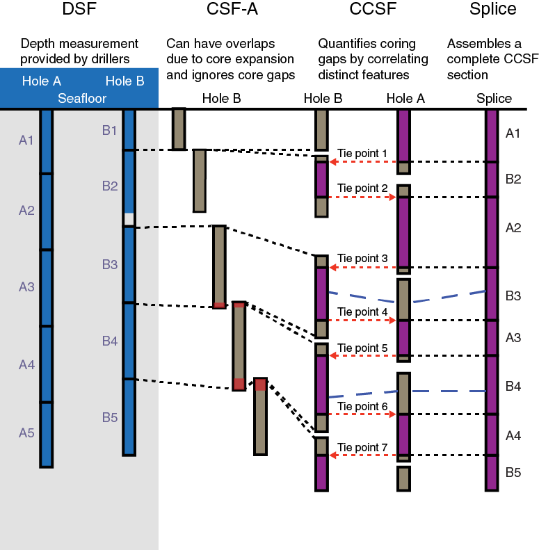
Figure F10. Depth scales used during Expedition 355.
Sediment cores often expand from relief of overburden, drilling disturbance, and gas expansion as the cores are brought up from great depths to shipboard atmospheric pressure and temperature. For this reason, the base of one core may overlap with the top of the succeeding core in the CSF-A depth scale.
Core composite depth below seafloor (CCSF)
Constructing a composite depth scale is done to create a common depth frame for all holes at a site. Stratigraphic features at each drill site are assumed to be laterally continuous over the small distances that separate successive holes. A new depth scale is then formed by shifting the depth of each individual core in the CSF-A scale until marker stratigraphic features align (Figure F10). The resulting CCSF scale is equivalent to the ODP and Integrated Ocean Drilling Program mcd scale. In constructing the CCSF scale from the CSF-A scale, the depths of the individual cores are shifted by a core-specific constant offset from CSF-A (i.e., no stretching or squeezing within an individual core is employed). The CCSF scale provides good first-order correlation between cores from different holes, as well as estimates of the length of coring gaps and a basis upon which the sediment splices are constructed.
The mudline is not merely taken as the top of the first core in a given hole but is the top of the first core at the site with the best-preserved sediment/water interface. This core anchors the entire composite depth scale for all holes at a site. The anchor mudline core is typically the only core in which the depths are the same for both the CSF-A and CCSF scales. Each core downhole is then tied to the composite section by adding or subtracting a depth offset (a constant) that best aligns an observed lithologic feature among adjacent cores from different holes. Because of the differing effects of coring-induced stretching and squeezing among cores, as well as hole-to-hole sedimentological differences, this approach very rarely aligns all core features (Figure F10). The depth offset of every core is tabulated in an affine table (a list of the linear depth offsets added to each core to place it in the CCSF scale), and the table is uploaded into the LIMS database so that depths of samples from different holes can easily be recalculated in the CCSF scale.
In the case that drilling gaps between cores never align among all holes at a site and recovery is sufficiently high, it is possible to correlate (or tie) each successive core in one hole to a core from an adjacent hole to the bottom of a drilled section. However, if coring gaps align across all holes at a site or if cores at a certain depth are badly disturbed, it becomes impossible to tie the cores to those above. Cores below such a gap will be appended to the composite section. Although the cores below the gap are no longer tied to the mudline core they can often still be tied to one another.
When constructing the composite section, the total CCSF depth is typically 5%–15% longer than the CSF-A scale. This expansion is mostly caused by decompression of the cores as they are brought to the surface, gas expansion, stretching that occurs as part of the coring process, and/or from curation of material that has fallen downhole or gas expansion voids that are curated as part of the core (e.g., Hagelberg et al., 1995; Acton et al., 2001)
Core-log correlation: CSF-A depth scale to WMSF depth scale
Initial wireline logging data are referenced to the rig floor and based on the length of wireline paid out during logging. These depths are then shifted to a seafloor reference to produce a wireline log depth below seafloor (WSF) depth scale (see Downhole measurements). After data processing, logs from successive runs are matched to remove depth offsets between successive runs, producing the WMSF depth scale. The WMSF depth scale can be linked to the CSF-A depth scale through common physical properties data measured by both wireline logging and the shipboard WRMSL. When a site has been logged, stratigraphic features from individual cores can be offset to match stratigraphic features in the wireline logs. These offsets are included in the affine table when available.
Sampling splice
The sampling splice is a composite core section from all the holes at a site that is the best available representation of a complete stratigraphic column at a site. It is often used for high-resolution sampling of the continuous sediment section or for reconstructing cyclic sediment deposition for time series analysis.
After the CCSF scale has been developed and the gaps between cores identified, a complete stratigraphic section is spliced from among holes by combining selected intervals that best avoid gaps, overlaps, and disturbed sections. The depth scale for the splice is in CCSF; the splice itself is the combination of sediments from different holes that are stacked into a complete section (Figure F10). Intervals included in the splice are listed in the splice interval table that tabulates sections from each core to be included in the splice.
If coring gaps aligned across all holes drilled at a site do occur, the spliced sections below are “appended” to those above and referred to as “floating splice sections” (i.e., not tied to the mudline). The amount of missing material between floating splices can be measured using downhole logs. Where no logs are available, the CSF-A scale provides an estimate of the length of the missing section that is reasonably accurate when coring in calm seas, such as experienced during Expedition 355.
Compressed splice
The splice, because it has been constructed using the CCSF scale, is typically longer than the drilled interval by 5%–15%. For some applications, it is necessary to compress the splice (e.g., for estimating sedimentation rates [meters of sediment accumulated per million years] across core boundaries or to join physical properties from the cores to log data). The difference in depth in CCSF versus CSF-A is typically linear, and the linear correlation can be used to generate a compression factor for each sampling splice to convert the CCSF depths to similar depths in the CSF-A depth scale. We refer to the compressed CCSF scale as compressed mcd (cmcd) because the acronym CCCSF is unwieldy.
Measurements and methods specific to Expedition 355
Compositing and splicing were accomplished using Correlator software (version 2.01; http://corewall.org/downloads.html) to generate standard affine tables and splice interval tables. During the expedition we used specific applications (i.e., Correlation Downloader version 6 and SCORS Uploader) for downloading and uploading data to and from Correlator. These tables were uploaded into the LIMS database, from which all users are able to attach the appropriate depth scale to any data set.
Multiple affine tables were made during the expedition for each site. A fast “init” affine table was generated and uploaded to the LIMS database so that shipboard scientists could align their measurements as soon as possible into a CCSF scale, and a second “revised” table was generated after the splice was further edited and checked for quality control. The init affine table was removed from the database before completion of the expedition.
The composite sections and splices are initially based on the stratigraphic correlation of data sets acquired from the WRMSL and the NGRL, as well as from digitized color data (from the red-green-blue [RGB] triplet), or extracted from core images acquired with the SHIL or color data from the Section Half Multisensor Logger SHMSL spectrophotometer. Details on the instrument calibrations, settings, and measurement intervals for Expedition 355 are given in Physical properties.
For the revised splice, we also visually compare the sediment section between holes using depth-referenced core section images collected on the SHIL. We used software routines developed for Igor 6.36 by Dr. Roy Wilkens for use on IODP cores to depth-reference SHIL line scan images in the CCSF depth scale and track data from each hole to make detailed comparisons. The images were offset by the constant offset added to each core to place them in the initial CCSF scale. Offsetting the core images allows for visually matching stratigraphic features in addition to using physical properties in order to best refine and revise the CCSF scale and sampling splice.
Igneous petrology
Igneous rock description procedures during Expedition 355 followed those used during Integrated Ocean Drilling Program Expeditions 309/312, 335, and 345 and IODP Expedition 349 (Expedition 309/312 Scientists, 2006; Expedition 335 Scientists, 2012; Gillis et al., 2014; Li et al., 2015). Because coring into the igneous basement took place on the last day of coring operations during Expedition 355, shipboard descriptions were completed under significant time constraints, limiting the amount of data that could be collected. During this expedition, only macroscopic core descriptions were carried out on board; these characteristics were entered into the LIMS database through the DESClogik portal. Shipboard studies aimed to characterize the nature of igneous basement by systematically describing the petrology of the cored rocks and their alteration through the following procedures:
- Definition of igneous units by visual identification of actual lithologic contacts or by inference using observed changes in phenocryst assemblages, mineral composition, or grain size variations;
- Description of lithology, phenocryst abundances, igneous textures, and vesicle distribution; and
- Description of alteration, as well as vein and vesicle infillings.
Shore-based thin section petrographic studies and geochemical (major and trace element) analyses were carried out after the end of the expedition and the results incorporated into the Proceedings volume.
Core description workflow
Before splitting into working and archive halves, each hard rock piece was labeled individually with unique piece/subpiece numbers from the top to the bottom of each section. These hard rock pieces were split with a diamond-impregnated saw along carefully chosen lines so that important compositional and structural features were preserved in both the archive and working halves. The working halves were sampled for shore-based analysis of thin section petrography and bulk geochemical analyses using XRF, which was performed at the National Centre for Earth Science Studies (CESS) in Trivandrum, India.
Each section of core was first examined macroscopically and described for petrologic and alteration characteristics. Characterization was based on the description of individual pieces from a recovered section of a core. If adjacent pieces were homogeneous with respect to their magmatic features, they were combined into one igneous interval. Lithologically and texturally similar pieces from consecutive core sections were described as belonging to the same igneous subunit. The upper and lower ends of each piece were directly taken from the curated piece log available within DESClogik. All descriptions during Expedition 355 were made on the archive halves. For macroscopic observations and descriptions, the DESClogik program was used to record the primary igneous characteristics (e.g., igneous unit, groundmass and phenocryst mineralogy, and vesicle presence and type) and alteration (e.g., color, vesicle filling, secondary minerals, and vein/fracture fillings). Shore-based microscopic analysis of the thin sections was carried out after the end of the expedition and the data uploaded into the database on shore.
The first step in visual core description (VCD) is the classification of the igneous lithologic units, which we divided into units and subunits. The igneous units are generally chosen to reflect downcore macroscopic variations in the cored sections. We defined the igneous lithologic units according to changes in the primary mineral assemblage (based on abundances of visible phenocrysts and groundmass mineral phases), grain size, color, and structure or texture that could be seen with the naked eye on the core description table. Igneous units are numbered consecutively downhole with Arabic numerals (igneous Units 1, 2, 3, etc.) irrespective of flow type.
Macroscopic description
Macroscopic descriptions included the standard categories applied to igneous petrology description listed below.
Lithology
For volcanic and hypabyssal rocks, we defined basalt as igneous rocks of basaltic composition with a grain size range of glassy to fine grained.
Lava flow types
Volcanic flows occur in different types:
- Pillow lavas are characterized by curved chilled margins, oblique to the vertical axis of the core. When such margins are absent, we can potentially identify these boundaries by the presence of variolitic textures, curved fractures, and microcrystalline or cryptocrystalline grain sizes. Characteristically, their exteriors are entirely bounded by glassy rinds as a result of rapid cooling and their interiors typically display internally radiating vesicles and joint patterns. Pillows are small in size, typically ~0.2–1.0 m in diameter, and result from subaqueous eruptions.
- Lobate lava flows have massive, coarser grained, and sparsely vesicular flow interiors and are ~1–2 m in diameter. Recognizing lobate flows and distinguishing those from pillows in drill cores is often difficult.
- Sheet flows are defined as <3 m of the same rock type with grain sizes increasing toward the center of the flows. This term implies a lateral extent that cannot be determined from core alone, but its size distinguishes it from the pillow and lobe type eruptions.
- Massive lava flows are defined as continuous intervals >3 m of a similar lithology. Both sheet and massive flows are characterized by sparse vesicle layering, often have texturally uniform cores as thick as several meters, and can have vertical vesicle pipes containing late-stage melt segregation material. Sheet-like and massive flows may result from particularly high effusion rates and/or increased local slopes.
Phenocrysts
Volcanic rocks were categorized according to the major phenocryst phase(s) when the total abundance of phenocrysts was >1%. The term “phenocryst” was used for any crystal that was (1) significantly larger (typically at least five times) than the average size of the groundmass crystals, (2) >1 mm, and (3) euhedral or subhedral. A prefix was applied as a modifier to the primary lithology names to indicate the abundance of phenocrysts in the hand samples:
- Aphyric (<1% phenocrysts).
- Sparsely phyric (1%–5% phenocrysts).
- Moderately phyric (5%–10% phenocrysts.
- Highly phyric (>10% phenocrysts).
Aphyric rocks were not assigned any mineralogical modifier.
Groundmass
Volcanic rocks contain groundmass, which is defined in terms of the finer grained matrix (or the mesostasis) surrounding various phenocryst phases if the latter are present. Such groundmass is generally characterized by its texture and grain size with the following standard notation:
- G = glassy.
- cx = cryptocrystalline (<0.1 mm).
- μx = microcrystalline (0.1–0.2 mm).
- fg = fine grained (>0.2–1 mm).
- mg = medium grained (>1–2 mm).
- cg = coarse grained (>2 mm).
For volcanic rocks, the following terms were used to describe textures when microlites are present in the groundmass:
- Intersertal (glassy between plagioclase laths),
- Trachytic (subparallel arrangement of plagioclase laths in the groundmass),
- Pilotaxitic (aligned plagioclase microlites embedded in a matrix of granular and usually smaller clinopyroxene grains),
- Hyalopilitic (aligned plagioclase microlites with glassy matrix), and
- Subophitic (partial inclusion of plagioclase in pyroxene).
Rock color
Rock color was determined on a wet, cut surface of the archive half using Munsell color charts (Munsell Color Company, Inc., 1994) and converted to a more intuitive color name. Wetting of the rock was carried out using a spray bottle. Wetting was kept to a minimum because of adsorption of water by clay minerals that may be present throughout the core.
Vesicles
For volcanic rocks, an estimate of the percentage of vesicles and their average size was included in the descriptions. Vesicularity was described according to the abundance, size, and shape (sphericity and angularity) of the vesicles. The infilling minerals in the vesicles were also identified. Vesicle abundance was recorded as
- Nonvesicular (<1% vesicles),
- Sparsely vesicular (1%–5% vesicles),
- Moderately vesicular (5%–20% vesicles), and
- Highly vesicular (>20% vesicles).
Alteration
Alteration was observed through visual macroscopic and microscopic description. These observations provided information on the alteration of primary igneous features such as phenocrysts, groundmass minerals, and volcanic glass.
Overall background alteration
The degree of the overall background alteration of groundmass and glass was defined and reported. An alteration summary description was entered in DESClogik and uploaded to the LIMS database to provide information on the extent of alteration in terms of the following scale:
Veins and alteration halos
Description of the veins included location, shape, crosscutting nature, width, color, and the amount (percentage) and nature of filling minerals. Alteration halos commonly form around hydrothermal veins that allow fluid flow of varying chemical composition. They can be different from the overall background alteration and vesicle filling in color, secondary mineral composition, and abundance.
Igneous visual core description sheets
We used DESClogik to document each section of the igneous cores by uploading our descriptions into the LIMS database. These uploaded data were then used to produce VCDs, which include a simplified graphical representation of the core (for each section) with accompanying descriptions of the features observed. An example VCD for igneous rocks is shown in Figure F11. The symbols and nomenclature used for VCDs are shown in Figure F6. The VCDs display the following items:
- Depth in mbsf (based on CSF-A);
- Scale for core section length (in centimeters measured from the top of each section);
- Sample piece number;
- Igneous unit number;
- Upward-pointing arrow indicating oriented pieces of core;
- Scanned digital image of the archive half;
- Graphical representation of lithology;
- Location of samples taken for shore-based thin section and geochemical characterization (XRF) of the basement;
- Stacked line chart displaying phenocryst percentage for plagioclase (PLAG; blue line), olivine (OL; red line), and clinopyroxene (CPX; green line);
- Line chart depicting alteration intensity; and
- Summary description for each igneous lithologic unit (see below for details).
The section summary text (displayed on the right side) provides a generalized overview of the core section’s lithology and features on a unit-by-unit basis. This includes
- Expedition, site, hole, core and core type, section number, and depth of the top of the core section in mbsf (measured according to the CSF-A depth scale) shown at the top of the VCD;
- Igneous unit and subunit (numbered consecutively downhole) and piece numbers belonging to the unit (and on which piece, or pieces, the description was based);
- Lithology;
- Description of the flow type based on igneous structures (e.g., pillow lava, massive flow);
- Texture;
- Color determined on wet rock surfaces;
- Phenocryst percentage and type based on minerals identifiable through macroscopic or microscopic description;
- Groundmass grain size and texture: glassy, aphanitic (crystalline but individual grains not discernible with a hand lens [cryptocrystalline or microcrystalline]), fine grained (<1 mm), medium grained (1–2 mm), or coarse grained (>2 mm);
- Vesicle percentage by volume, including filled, partially filled, and open vesicles;
- Upper and lower unit contact relations and boundaries based on physical changes observed in retrieved core material (e.g., presence of chilled margins, changes in vesicularity, and alteration), including information regarding their position within the section. The term “not recovered” was entered where no direct contact was recovered; and
- Alteration of the rock material, veins, and vesicle infillings.
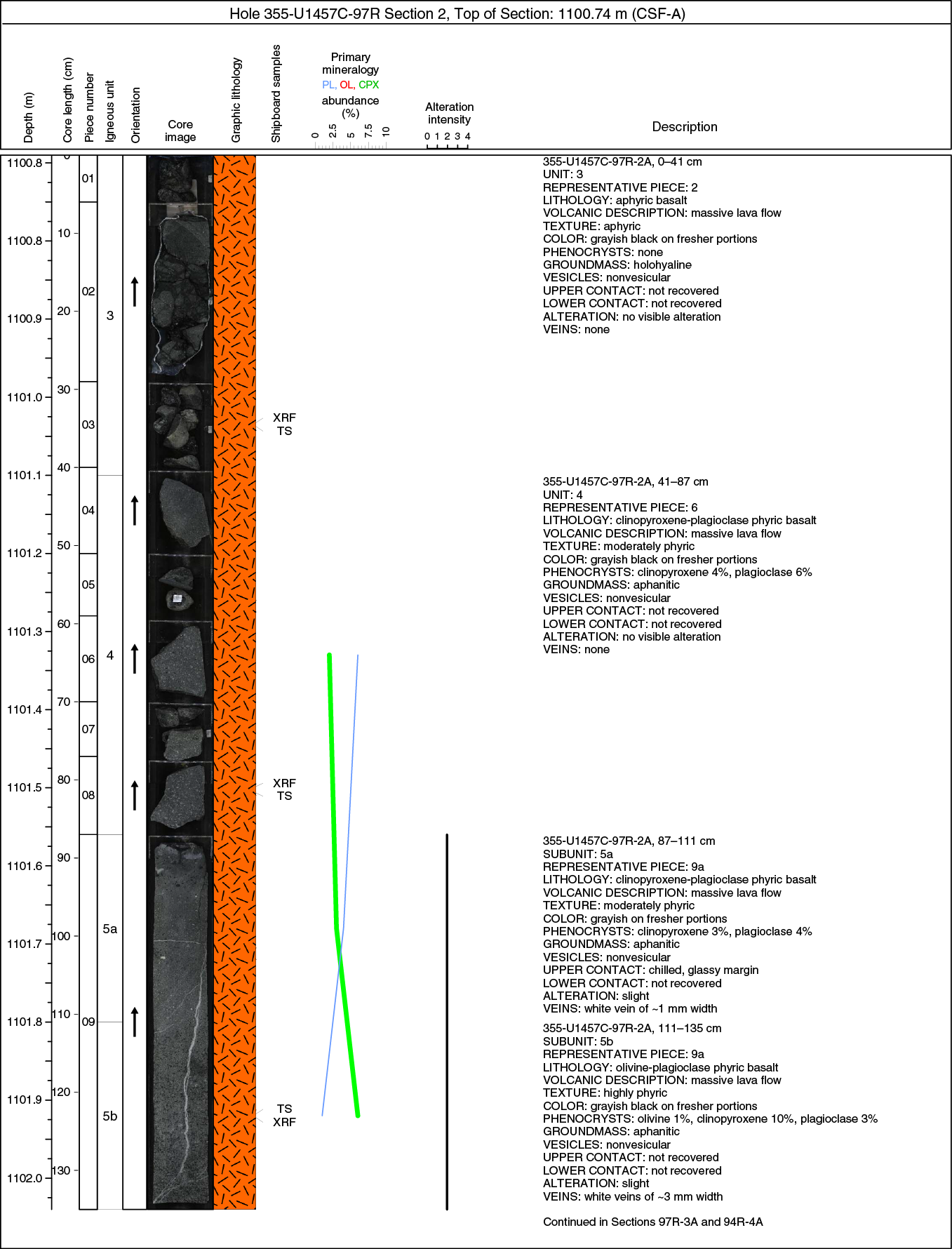
Figure F11. Example of an igneous basement VCD standard graphic report, Expedition 355.
Microscopic description
Thin section analyses of sampled core intervals were completed after the end of the expedition at the National Centre for Earth Science Studies, Trivandrum. These analyses were used to complement and refine the macroscopic core observations completed during the expedition. To maintain consistency, the same terminology and nomenclature are used for macroscopic and microscopic descriptions. Phenocryst assemblages (and modal percentages, shapes, habits, and sizes), groundmass, and alteration phases were described. All observations were uploaded into the LIMS database with a dedicated DESClogik thin section template. Downloaded tabular reports of all igneous thin section descriptions can be found in Core descriptions.
Thin section descriptions include both primary (igneous) and secondary (alteration) features (e.g., textural features; grain size of phenocrysts; and groundmass minerals, mineralogy, alteration extent, vesicles, etc.). An example of a thin section description form is given in Figure F12.
Textural terms used are those defined by MacKenzie et al. (1982) and include
- Holohyaline (100% glass) and
- Intersertal (groundmass fills the interstices between unoriented feldspar laths).
For alteration description, thin sections were examined to
- Confirm macroscopic identification of secondary minerals;
- Determine their mode of occurrence in terms of vesicle and void fillings, vein composition, and primary mineral replacement;
- Identify mineralogies of vein and vesicle infillings; and
- Calculate the total alteration (percentage) using the modal proportions of phenocrysts and groundmass minerals and their respective percentages of alteration.
Estimated volume percentages are required to quantify phenocryst and vesicle abundances. In DESClogik, the user records the percentage of the originally present phenocryst phases, groundmass mineral phases, and vesicles. When possible, the user also records how much of these constituents are still present (i.e., still fresh or not filled) and how much has been replaced (i.e., altered or filled) while taking into account that Original (%) = Present (%) + Replaced (%).
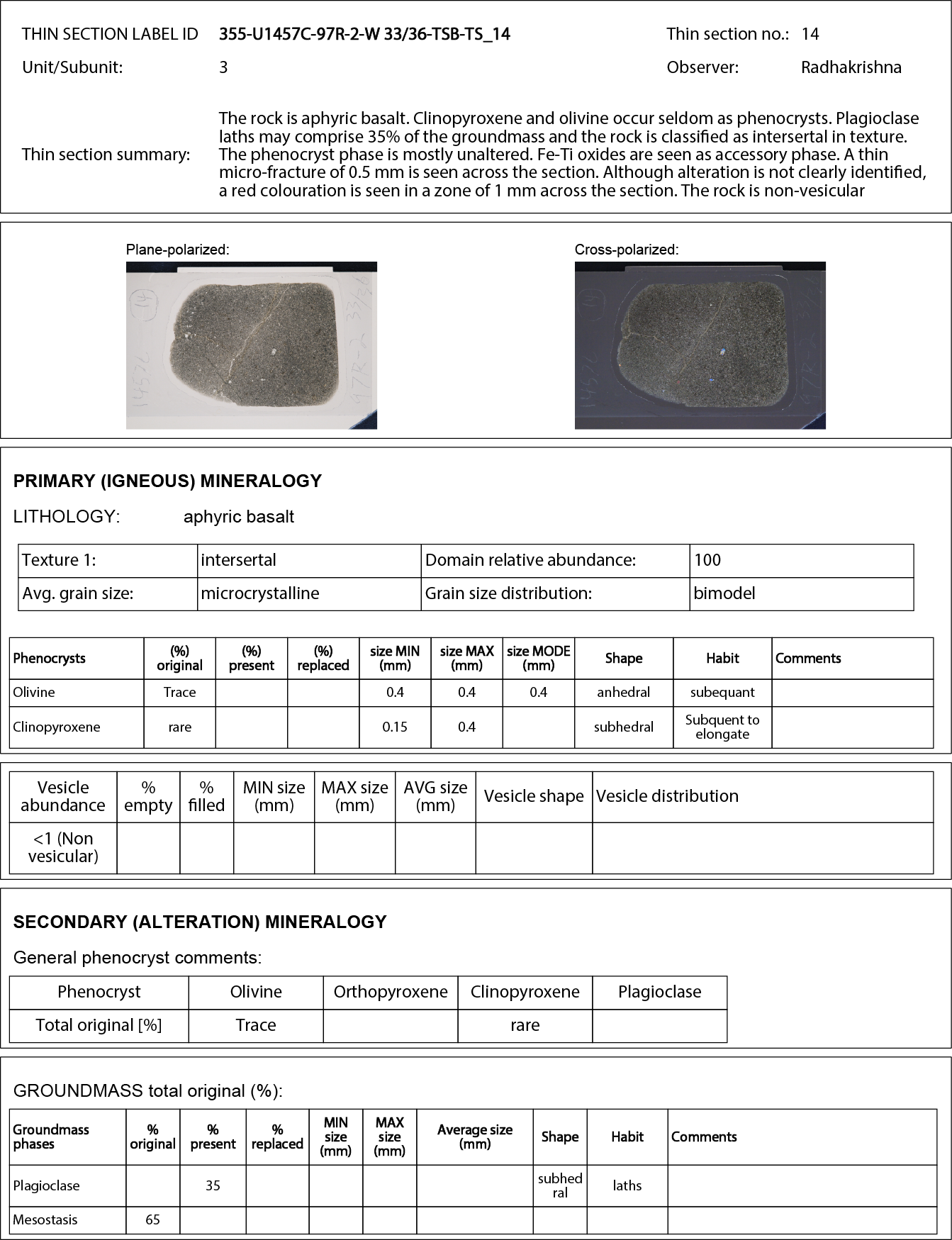
Figure F12. Example of thin section form.
Igneous geochemistry
Nine representative samples of igneous basement rock were selected for postcruise thin section and geochemistry studies because there was not enough time to complete these on board before the end of the expedition. These samples were analyzed for major oxides (SiO2, TiO2, Al2O3, Fe2O3, MgO, CaO, Na2O, K 2O, P2O5, MnO) and trace element (Cr, Ni, V, Cu, Zn, Ga, Rb, Sr, Y, Zr, Ba, La, Ce) concentrations using the Bruker S4 Pioneer sequential wavelength dispersive X-ray fluorescence (WD-XRF) spectrometer at the National Centre for Earth Science Studies, Trivandrum.
Each sample was cleaned thoroughly to remove drilling-related impurities. The cleaned rock chips were dried and then ground to a fine powder in a pulverizer (Pulverisset-9) using chrome-nickel disks. Approximately 5 g of the sample powder was weighed and ignited at 900°C for 4 h to determine loss on ignition (LOI). All samples were weighed on a microbalance (Sartorins model CP225D). Weighing errors were estimated to be ±0.05 mg.
After determination of LOI, ~1 g splits of the ignited whole-rock powders were weighed, and pressed pellets were prepared using 40 mm aluminum cups filled with boric acid crystals as binder. Finely powdered sample (–250 mesh size) was sprinkled over boric acid and pressed in a 40 ton hydraulic press (Insmart Systems, Ltd.) to produce the circular 40 mm disks.
Pressed powder pellets were used for both major oxide and trace element analysis. An analytical program using >15 international standards of basaltic matrix was employed for calibration. SPECTRAplus software supplied by the company was used for quantitative determination of elements. Three international rock standards (W2, JB3, and DNC-1) were analyzed with the samples to monitor accuracy. The data obtained from two international rock standards over one month during the sample analysis was used to evaluate precision. The data on these standards is given in Table T5. The major element accuracy was generally better than 10% (<2% for SiO2; <5% for TiO2, MnO, Fe2O3, CaO, P2O5 and K2O; <8% for Al2O3 and Na2O; and mostly <10% for MgO). The precision calculated using five determinations during the period is better than ±5% for all oxides. For trace elements, the accuracy was generally better than ±15% except for La and Ce, for which the error may be as high as 35%. Among the elements analyzed, contamination from the chrome-nickel disks is negligible.
Table T5. Major and trace element XRF analyses for international basalt rock standards. Download table in .csv format.
The XRF data presented in Igneous petrology in the Site U1457 chapter (Pandey et al., 2016b) are the average of measurements acquired at two different times within approximately four months.
Geochemistry
The shipboard geochemistry research program for Expedition 355 included measurements for
- Headspace gas content;
- Sedimentary geochemistry including total inorganic carbon (TIC), CaCO3, total carbon, total nitrogen, total sulfur, and total organic carbon (TOC);
- Organic geochemical extractions; and
- Interstitial water composition.
These analyses were carried out to
- Satisfy routine shipboard safety and pollution prevention requirements;
- Characterize interstitial water, sediment, and rock geochemistry for shipboard interpretation; and
- Provide a basis for shore-based sampling and research.
Headspace gas geochemistry
Sediment gas composition was typically determined once per core. After core retrieval on deck, 5 cm3 of sediment was sampled using a cork borer, put into a headspace vial, and crimp-sealed for standard IODP hydrocarbon safety monitoring. When the sediment became too lithified to extract using a cork borer, fragments of core were chiseled out of the core and placed in the vial. Headspace samples for onboard analyses were heated in an oven at 70°C for 30 min. A 5 cm3 gas sample was extracted through the septum using a gas-tight 5 mL PTFE Luer lock glass syringe and injected into the gas chromatograph.
An Agilent 6890 gas chromatograph (GC) equipped with a flame ionization detector (FID) was used to measure concentrations of methane (C 1), ethane (C2), ethylene (C2=), propane (C3), and propylene (C3=). The GC oven was fitted with a 2.4 m × 2.0 mm stainless steel column packed with 80/100 mesh HayeSep “R”. The 5 cm3 gas sample was introduced via an injector assembly consisting of a Valco-to-Luer lock syringe adaptor, a 0.25 cm3 sample loop, ¹⁄₁₆ inch Valco union with a 7 μm screen and 10-port Valco valve that was switched pneumatically by a digital valve interface. The valve can be switched automatically to backflush the column. The injector temperature was set at 120°C. The oven temperature was programmed to start at 80°C for 8.25 min and then increased to 150°C for 5 min, ramping up at a rate of 40°C/min. Helium was used as the carrier gas. The FID temperature was 250°C. Initial helium flow in the column was 30 mL/min. Flow was ramped to 60 mL/min after 8.25 min to accelerate the elution of C3 and C3=. Total run time was 15 min.
Data were collected and evaluated with an Agilent ChemStation data-handling program. The chromatographic response was calibrated to different gas standards with variable quantities of low molecular weight hydrocarbons. Gas components are reported as parts per million by volume (ppmv) of the injected sample. Methane in the uppermost headspace samples is also expressed as millimoles per liter per volume (mM), assuming a porosity of 0.45 (volume fraction), a sample volume of 5 cm3, and a vial volume of 21.5 cm3:
C1 (mM) = ppmv C1 × [(21.5 – 5)/(22,400 × 5 × 0.45)] = ppmv C1 × 0.0003.
Sediment geochemistry
Sample preparation for carbonate and elemental analysis
We routinely took ~3–5 g dry mass 5 cm3 samples of sediment for bulk geochemistry from the working half of each core. The samples were selected in collaboration with the sedimentologists to represent the major lithologic units recovered or any layer of special interest. Bulk geochemistry subsamples were also extracted from either the interstitial water (IW) squeeze cake or from the moisture and density (MAD) sample residues at an average of two samples per core. Samples for geochemistry were freeze-dried for at least 24 h and crushed to a homogeneous powder using a pestle and agate mortar. Geochemical analyses carried out included percent carbonate and elemental analyses of carbon, nitrogen, and sulfur.
Carbonate and elemental analysis
Total carbon, total nitrogen, and total sulfur of the sediment samples were determined with a ThermoElectron Corporation FlashEA 1112 CHNS elemental analyzer equipped with a ThermoElectron packed column CHNS/NCS gas chromatograph and a thermal conductivity detector (TCD). Approximately 15 mg of sediment and ~2 mg (a level scoop) of vanadium pentoxide catalyst (to facilitate sulfur analysis) were weighed into a tin cup and then combusted at 950°C in a stream of oxygen. The reaction gases were passed through a reduction chamber to reduce nitrogen oxides to nitrogen and were then separated by the gas chromatograph before detection by TCD. The peak areas from the TCD were integrated to determine the total carbon and total nitrogen of the samples.
All measurements were calibrated to a Soil CNS Reference Material PDWR [PN 3472541] (carbon = 3.496 wt%, nitrogen = 0.365 wt%, and sulfur = 0.063 wt%) that was run every eight samples. Based on the drift of C, N, and S in the reference material in typical batches, S content varies more than that of C and N. Therefore, analyses were only continued if standard data varied by <5% for C, <8.5% for N, and <12% for S. Duplicate measurements of C and N were made on ~20% of the samples, and the average difference between duplicates was 0.07 wt% for total carbon, 0.01 wt% for total nitrogen, and 0.05 wt% for TOC (see Table T17 in the Site U1456 chapter [Pandey et al., 2016a]), further confirming the reliability of the onboard analyses.
TIC was determined using a Coulometrics CM 5015 CO2 coulometer. Approximately 12 mg of sediment was weighed into a glass vial and acidified with 5 mL of 2 M HCl. The liberated CO2 was titrated, and the corresponding change in light transmittance in the coulometric cell was monitored using a photodetection cell. The weight percent of calcium carbonate was calculated from the TIC content using
CaCO3 (wt%) = TIC (wt%) × 100/12.
An external standard of 100% CaCO3 (standard reference material) was used to confirm accuracy. TOC content was calculated as the difference between total carbon (TC) and TIC from coulometry by the formula:
Total lipid extraction
Sediment samples from squeeze cakes and core catchers were sampled for total lipid extraction (TLE). A subsample of freeze-dried sediment from either an IW squeeze cake residue or a core catcher sample was homogenized using an agate mortar and pestle. Aliquots of 1.5 g were extracted with 7 mL of a 1:1 dichloromethane:methanol solution by Fisher Mini Vortexer, ultrasonicated for 20 min, and heated at 45°C for 1 h. Samples were centrifuged for 3 min at 3300 rotations/min, and the supernatant was pipetted into 50 or 250 mL round-bottomed flasks. This process was repeated two more times without heating for a total of three extractions. The combined extracts were then concentrated using a rotary evaporator under vacuum and water bath of 42°C. The TLEs were transferred to preweighed vials, dried under N2, weighed, and archived for shore-based biomarker assays and analyses.
Interstitial water chemistry
Interstitial water collection
Interstitial water analyses were carried out on samples taken from Sites U1456 and U1457 in conjunction with sampling for microbiology studies. Interstitial water was extracted from 5 to 15 cm long whole-round sections that were cut and capped immediately after core retrieval on deck. Whole-round sections were taken at a frequency of one sample per core or every other core when using the HLAPC, usually from the bottom of the second to last section of the core. This strategy was used to avoid removing whole rounds from the middle of cores, thereby preserving material integral to the splicing process. In Hole U1456B, which was drilled as a dedicated hole for microbiological sampling, one sample per section was taken. Before squeezing, samples were removed from the core liner and the outer surface was carefully scraped with a spatula to minimize potential contamination by the coring process. Whole rounds were placed into a titanium and steel squeezing device modified after the stainless steel squeezer of Manheim and Sayles (1974) and squeezed at ambient temperature with a hydraulic press at pressures of up to ~30,000 psi. The interstitial water squeezed out of the sediment was extruded into a prewashed (in 10% HCl) 60 mL plastic syringe attached to the bottom of the squeezer assembly. The solution was subsequently filtered through a 0.45 µm polysulfone disposable filter (Whatman) into separate vials for routine shipboard analyses (salinity, pH, alkalinity, chloride, sulfate, bromide, sodium, potassium, calcium, magnesium, phosphate, ammonium, and minor elements including lithium, boron, manganese, iron, strontium, barium, silicon, and phosphate) and for later shore-based analyses. The shipboard analyses was carried out following the protocols of Gieskes et al. (1991), Murray et al. (2000), and the IODP user manuals for shipboard instrumentation. The remaining interstitial water was archived. Following interstitial water removal, squeeze cakes were removed from the squeezing device, placed in sterile bags, and were further divided for different shipboard and shore-based analyses (any residual was archived).
Salinity, alkalinity, and pH analyses
Salinity, alkalinity, and pH were measured immediately after squeezing, following the procedures in Gieskes et al. (1991). Salinity was measured using a Fisher temperature-compensated handheld refractometer. The pH was measured with a combined glass electrode, and alkalinity was determined by Gran titration with an autotitrator (Metrohm 794 basic Titrino) using 0.1 M HCl at 25°C. International Association for the Physical Sciences of the Oceans (IAPSO) standard seawater was used for calibration and was analyzed at the beginning and end of a set of samples for each site and after every 10 samples. The accuracy of the salinity measurement is ±0.5. Measurements of pH and alkalinity have a percent error within 2% based on repeated analysis of the IAPSO standard seawater.
Sulfate, chloride, bromide, calcium, magnesium, potassium, and sodium
Sulfate, chloride, bromide, calcium, magnesium, potassium, and sodium concentrations were analyzed by ion chromatography (Metrohm 850 Professional IC) using aliquots of 100 μL that were diluted 1:100 with deionized water (18 MΩ/cm). At the beginning and end of each run, different dilutions of IAPSO standard seawater were analyzed for quality control and to determine accuracy and precision. Analytical percent error was within 0.1% for chloride, 1.3% for bromide, 0.6% for sulfate, 1.2% for calcium, 0.4% for magnesium, 2.5% for potassium, and 0.1% for sodium.
Ammonium and phosphate
Ammonium and phosphate concentrations were measured using an Agilent Technologies Cary Series 100 UV-Vis spectrophotometer with a sipper sample introduction system following the protocol provided by Gieskes et al. (1991). For ammonium concentration measurements, a 0.1 mL sample aliquot was diluted with 1 mL reagent water to which 0.5 mL phenol ethanol, 0.5 mL sodium nitroprusside, and 1 mL oxidizing solution (trisodium citrate and sodium hydroxide) were added in a 5 mL capped glass vial (Gieskes et al., 1991). The solution was kept at room temperature for ~6.5 h to develop color. Ammonium concentrations were determined at 640 nm wavelength absorption spectrophotometry. Uncertainties in the ammonium analyses were within 3%.
For phosphate analysis, a 0.3 mL sample was diluted with 1 mL nannopure water (18 MΩ/cm) in a 4 mL glass vial. Subsequently 2 mL of mixed reagent (ammonium molybdate, sulfuric acid, ascorbic acid, and potassium antimonyl tartrate) was added to the vial (Gieskes et al., 1991), which was capped and kept at room temperature for at least several minutes to develop color. The phosphate concentration was determined at an absorbance of 885 nm ~30 min after adding the mixed reagent solution. Percent error of the phosphate analyses was better than 2%.
Major and minor elements
The method developed for shipboard inductively coupled plasma–atomic emission spectroscopy (ICP-AES) analysis of bulk rock samples was described in detail in ODP Technical Note 29 (Murray et al., 2000). Subsequent minor updates have been incorporated, and a current, detailed methodology is described in the ICP User Guide (available from http://iodp.tamu.edu/labs/documentation/). Dissolved major and minor elements were determined by Leeman ICP-AES. For major cation (Na+, K+, Ca2+, and Mg2+) analyses, dilutions of IAPSO standard seawater were used as calibration standards. Standards and acidified samples were diluted 1:100 (v/v) with a 2% HNO3 (by volume) solution (matrix) with Y at 10 ppm as an internal standard. Calibration for minor elements (Mn2+, Fe2+, B, Si, Sr2+, Ba2+, and Li+) was achieved with dilutions of a multielement synthetic standard solution (composed of single-element standards). Acidified samples measured for minor elements on the ICP-AES were diluted 1:20 (v/v) with the same matrix used for the major element analysis. Drift correction was made for both major and minor elements using the factor from a drift monitor solution (100% IAPSO for majors and 100% stock solution for minors) that was analyzed every eight samples. The ICP-AES autosampler and analysis chamber were rinsed with a 3% (by volume) HNO3 solution between samples. The analytical percent error in the measurement is better than 0.7% for Ca2+, 1.4% for Mg2+, 2.5% for K+, 1.1% for Na+, 0.9% for B, 1.7% for Ba2+, 1.5% for Fe2+, 1.0% for Li+, 1.8% for Mn2+, 0.7% for Si, and 1% for Sr2+. At Site U1456, percent errors were lower for major elements using ion chromatography compared to ICP-AES. Therefore, at Site U1457 major elements (Ca2+, Mg2+, K+, and Na+) were measured only using ion chromatography.
Microbiology
During Expedition 355, samples were collected and preserved for shore-based analyses of the biomass, activity, and community structure of microbial communities. Relatively few shipboard analyses were performed because most measurements must be made in specialized shore-based laboratories in sterile conditions. Accordingly, our efforts were dedicated to collecting and preserving an adequate number of samples for subsequent shore-based studies, and a considerable amount of time during the expedition was dedicated to quality control and limited analysis of contamination tracers (see Contamination testing ).
Planned shore-based work includes
- Analysis of intact polar membrane lipids of microorganisms to estimate total microbial biomass;
- Metagenomics and single-cell genomics to provide detailed information about the composition and function of microbial communities in the samples and to provide clues related to the best ways to cultivate cells from the sediments; and
- Fluorescence in situ hybridization to identify key microbial community members microscopically and provide data related to cellular activity. Enrichment for specific groups of organisms will help to identify the unique physiological properties of these specific organisms.
Core handling and sampling
Microbiological sampling for postcruise work depends on aseptic handling techniques and the use of contamination tracers. Microorganisms collected from the seafloor are expected to be sensitive to the chemical and physical changes they encounter when brought to the surface. Changes in oxygen concentration and temperature are two important factors to be considered when bringing cells from cold, possibly anoxic settings deep below the seafloor to the surface. Accordingly, the following procedures were followed in order to minimize harm to subsurface microbes without compromising the other objectives of the expedition.
Contamination testing
When obtaining subseafloor sediment samples for microbiological research, considerable potential exists for contamination by microbes from the surface realm. Accordingly, it has become common practice to add tracers to the drilling fluids and the core catcher sub so that the extent of contamination by the drilling fluids or core recovery methods can be evaluated (e.g., Smith et al., 2000). To check for potential intrusion of drilling fluids from the exterior to the interior of cores and to confirm the suitability of core material for microbiological research, cell-sized fluorescent microspheres were used during coring with the advanced piston corer (APC). Sampling of the drilling fluids and seawater (used to mix the drilling fluids) was also conducted for subsequent shore-based analyses. Comparison of microbial community profiles (based on extracted DNA or lipids) derived from likely sources of contamination with profiles from the interior of cores should yield notable differences; otherwise, there would be reason to believe that the interior of the samples were compromised.
Fluorescent microsphere tracers
Fluorescent microspheres of near uniform size (0.5 ± 0.01 µm; Fluoresbrite carboxylate microspheres, Polysciences, Inc.) appear bright green when observed by epifluorescence microscopy (458 nm excitation; 540 nm emission) and were used during Expedition 355 as a particulate tracer during APC coring. Microspheres were only deployed when sampling was planned for microbiological cultivation and molecular biological analyses. The microspheres were deployed in plastic bags containing 40 mL of microsphere suspension in 18.2 MΩ water (1010 spheres/mL; 2 × 10¹¹ microspheres in a 40 mL bag according to Smith et al., 2000). The plastic bag was heat-sealed and placed into an additional plastic bag that was open at each end. By attaching the loose plastic ends with cord, the bag was wedged into a shim above the core catcher sub and stretched across the throat of the core barrel. The bags then rupture and release the microspheres as the core enters the barrel.
Preliminary estimates of concentrations of fluorescent microspheres in core samples were quantified on board using a Zeiss Axioplan 2 epifluorescence microscope fitted with CoolLED pE-100 LED light sources, a blue filter set, and a 50× objective. Three samples were collected from each core for analysis of microspheres: (1) interior of the core, (2) exterior of the core, and (3) an intermediate position between the exterior and interior. Microsphere abundance was determined by averaging the total number seen in at least 20 randomly selected fields of view.
Fluid community tracers
Postcruise comparisons of the microbial community diversity in sediment samples with the respective drilling fluid collected at the time of coring will be used to further evaluate the extent to which contaminating cells may have penetrated a sample. This approach is accomplished by obtaining and preserving samples from the different possible sources of contamination (i.e., seawater and drilling fluid) and from the interior of the cores. Subsequently, high-throughput sequencing of the 16S rRNA genes in the respective samples will be carried out. Comparison of the community signatures can help to identify samples that significantly overlap in community structure with the drilling fluids (deeming them contaminated), as well as samples that have unique community structure when compared to the fluids (deeming them unlikely to be contaminated). For fluid community tracers, microorganisms were collected on 0.2 µm pore filters by filtering seawater or drilling fluid collected from the core liner or from the rig floor before the water was pumped into the drill string. The filters were frozen at –80°C and stored for postcruise analysis.
Microbiological sampling
Sampling for microbiological and contamination analyses must be processed quickly and the samples transported to the cold room in the microbiology laboratory to minimize changes in the microbial population. Cores were handled with care on the catwalk. The core liner was cut by the standard IODP core cutter and with an ethanol-wiped spatula. Whole-round samples (5 or 10 cm in length) were provided to the microbiologist on duty as soon as possible on the catwalk. The core liner is not sterile, and the outer surface of the core is thus assumed to be contaminated during drilling. By subsampling the interior of the whole-round samples, the contaminated sediment proximal to the core liner can be avoided.
All whole-round samples were cut on the catwalk and capped on one end by an ethanol-rinsed plastic cap and by sterile foil on the other end. The whole-round samples were labeled and, with the foil covered ends held upright, transferred to the microbiology laboratory where they were stored in the cold room in an oxygen-free glove bag to minimize alteration of the microbial communities.
The 5 or 10 cm long whole-round samples were subsampled into sterile tip-cut syringes and then transferred to N 2 -filled packs as soon as possible after recovery. Samples were then either stored in an ultralow-temperature freezer (–80°C) for molecular analyses or in a refrigerator at 4°C for cultivation-based analyses. Subsamples for lipid biomarker analysis were stored in a –20°C freezer.
Analysis for fungal population
In order to analyze for the presence of fungal populations in the sediment, 0.1–1.0 g of sediment or rock sample was added into 9.0 mL of 4% paraformaldehyde/phosphate-buffered saline (PBS) solution (10% w/v) and kept overnight for fixing at 4°C. Subsequently, the samples were washed in PBS and added to a PBS/ethanol (50:50) solution. Finally, the fixed microbes in the sample were analyzed by epifluorescence microscopy.
Paleomagnetism and rock magnetism
Shipboard measurements included both measurements of natural remanence and rock magnetic parameters. We investigated the natural remanent magnetization (NRM) on archive-half sections and discrete samples by treating with alternating field (AF) demagnetization. Discrete samples underwent an additional set of measurements, which included anisotropy of magnetic susceptibility (AMS), anhysteretic remanent magnetization (ARM), and isothermal remanent magnetization (IRM). Selected specimens were also subjected to “3D-IRM” acquisition followed by thermal demagnetization to further constrain the magnetic mineralogy.
Instruments
The remanent magnetization of archive-half sections was measured using a pass-through, three-axis cryogenic magnetometer (SRM; 2G-Enterprises, model 760R) equipped with direct-current superconducting quantum interference devices (SQUIDs) and the 2G in-line AF demagnetizer with maximum peak field of 80 mT. Discrete samples were measured on both the SRM and a spinner magnetometer (Agico, model JR-6A). These were subjected to AF demagnetization treatments using both the 2G in-line AF demagnetizer and the DTECH (model D-2000) AF demagnetizer. ARM was imparted using the DTECH and IRM with an impulse magnetizer (ASC, model IM-10). AMS and bulk magnetic susceptibility were measured with a spinning magnetic susceptibility meter (AGICO, model KLY4-S). Selected specimens were dried, wrapped in aluminum foil, and subjected to a three-component IRM experiment (fields of 1.0, 0.3, and 0.12 T along three orthogonal axes; Lowrie, 1990) followed by thermal demagnetization by an ASC TD48-SC.
Measurement protocols
NRM measurement of archive-half sections was carried out on the SRM at 5 cm intervals at a speed of 10 cm/s. The software assumes a nominal area of 15.59 cm2 for conversion to volume-normalized magnetization units (A/m). In order to remove undesired magnetic overprints (e.g., drilling-induced or viscous), we performed step-wise AF demagnetization at 5 mT increments up to 20 or 25 mT, measuring the remanence after each treatment step. As the response functions of the pick-up coils of the SQUID sensors have a full width of 7–8 cm at half height, data collected within 10 cm of section boundaries (or voids) were filtered out prior to further processing. We also edited out obviously disturbed intervals based on core descriptions and photos. The coordinate system of the archive-half measurements is shown in Figure F13.
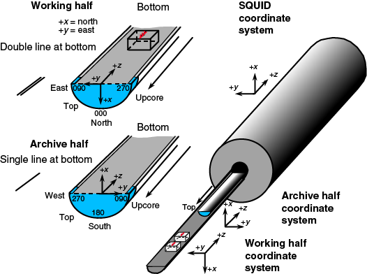
Figure F13. Coordinate systems used for archive and working-half sections and SQUID during Expedition 355.
We collected discrete samples from working-half sections with a target frequency of one sample per core section, except for those sections not suitable for paleomagnetic analysis because of pervasive geological (slumping) or drilling-induced disturbance. In these cases, discrete samples were collected from the working half at intervals necessary to define a reliable magnetostratigraphy. For soft sediment, we used Natsuhara-Giken (“Japanese”) cubes with a nominal volume of 7 cm3. For harder intervals, we collected samples by sawing ~7–8 cm3 cubes, depending on lithology. The coordinate system for all specimens is the same, regardless of sampling and measuring technique, whereby the red flag is the “up” arrow and is directed upcore, and the x-direction is directed toward the double line on the core liner (Figures F13, F14).
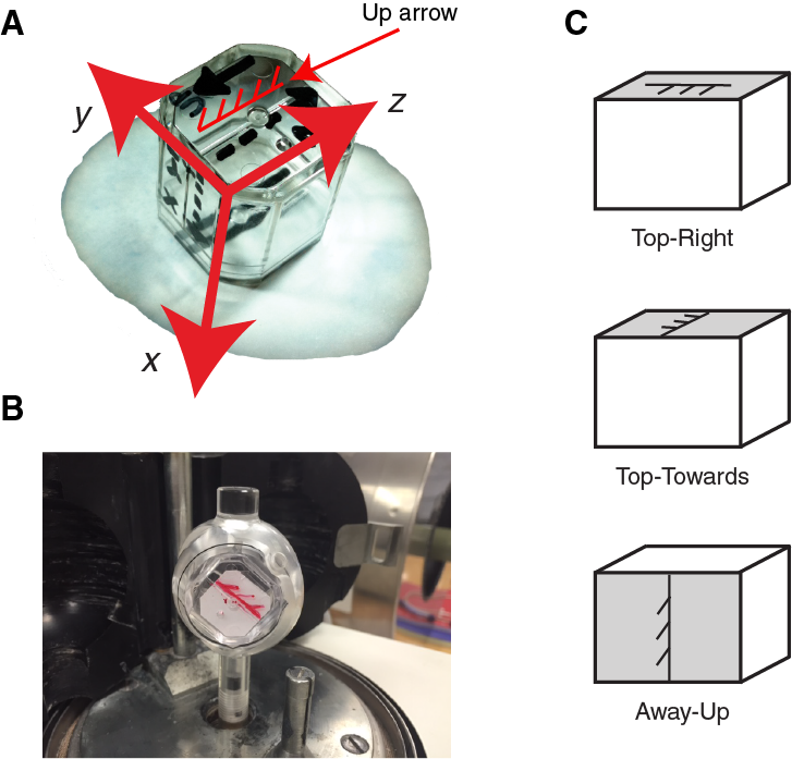
Figure F14. Japanese sampling cube, measurement positions in the JR-6 spinner magnetometer, and three positions for SRM measurements.
Analyses of discrete samples were performed in order to provide a comprehensive check on reliability and calibration of paleomagnetic and magnetic susceptibility data from SRM and core logger measurements, respectively, and to perform preliminary investigations on magnetic fabric and mineralogy. To achieve these goals, the measurement protocol for discrete samples was:
- AMS and bulk susceptibility measurement using the Agico KLY 4S susceptibility instrument. This step was performed as time permitted (either before or after Step 2).
- NRM and step-wise triaxial static AF demagnetization up to at least 50 mT (5 mT increments in the 0–20 mT range, 10 mT in the 20–50 mT). Time permitting, samples were demagnetized up to 60 mT and in many cases to 100 mT. We employed the DTECH or the 2G demagnetizer according to the availability, but the 2G AF demagnetizer was never used above 60 mT because of the tendency to acquire an unintended ARM along the z-axis (see discussion below).
- We imparted the ARM in the DTECH using a peak alternating field of 100 mT and direct-current bias field of 0.05 mT along the sample’s z-direction.
- We carried out three-step IRM acquisition experiments by first subjecting the specimen to an impulse field at 100 mT and at 1000 mT along the specimen’s –z-direction followed by backfield acquisition (along +z) at 300 mT. Specimens selected for the 3D-IRM experiment were subjected to a more detailed IRM acquisition, with additional steps for a total of 14. After step-wise IRM acquisition, these were given an IRM at 1000 mT along the z-direction followed by an IRM at 300 mT along the y-direction and then an IRM at 120 mT along the x-direction. Specimens, already dried, were wrapped in aluminum foil. We thermally demagnetized them at 25°C intervals from 50° to 150°C, followed by 50°C intervals to 500°C, and then 25°C intervals up to 675°C.
On the whole, measurements on the archive-half section did not provide very good results because of the prevalence of sandy layers (not suitable for paleomagnetic analysis) or the occurrence of a strong normal overprint that could not be resolved at 20 mT. We ceased routine measurement of the archive halves and focused on analysis of discrete specimens. For reasons of efficiency, discrete samples from Cores 355-U1456A-8H through 74X were measured on the SRM instead of the JR-6A. The measurement protocol was in a single position (top-toward measurement position; see Sample coordinate systems) for the NRM up to 15 mT. Thereafter, we adopted the three-position strategy from Expedition 318 (top-toward, top-to-right, and away-up) for demagnetization and measurement from 20 to 60 mT.
AMS characterizes the orientation of the paramagnetic (mainly phyllosilicates) and ferromagnetic minerals in sediment and can be interpreted in terms of depositional processes (e.g., Rees and Woodall, 1975; Ellwood, 1980; Taira, 1989; Schwehr and Tauxe, 2003). Settling of particles produces an oblate magnetic fabric with the minimum susceptibility clustered around the pole of the depositional plane. Ideally, the maximum and intermediate susceptibility axes are uniformly dispersed, defining a planar, near-horizontal, gravity-induced settling fabric. The magnetic fabric of sediment deposited by flowing water is typified by current-oriented magnetic foliation that can be either horizontal or tilted (imbricated) and/or clustering of the maximum susceptibility parallel to the flow direction. Disturbance by slumping or other deformation generally yields triaxial fabrics. We use the Hext (1963) method to assess the degree and type of anisotropy at the specimen level and the bootstrap method to estimate confidence bounds on AMS eigenparameters for multiple specimens (Constable and Tauxe, 1990; Tauxe et al., 2010). Unfortunately, we found a systematic pattern in all the Japanese cube samples in which the AMS was triaxial, with maximum susceptibility either parallel to x or to y. It is likely that coring disturbance has modified the fabric to the extent that interpretation of the AMS data is ambiguous. Therefore, no routine measurements of AMS were made at Site U1457.
ARM acquisition in peak AFs of 100 mT in the presence of a direct-current bias field of 0.05 mT is commonly used to estimate the presence of fine-grained (~0.03–0.1 μm) single-domain magnetite (King et al., 1982), whereas IRM acquisition at 100 mT is more sensitive to the occurrence of coarse-grained (>0.1 μm) multidomain magnetite (Frederichs et al., 1999). Thus the ratio ARM@100 mT/IRM@100 mT can be used to track the grain size variation of magnetite downcore. Contributions of high-coercivity minerals (hematite + goethite) are estimated by the difference of IRM@–300 mT, which should saturate soft-coercivity minerals such as magnetite and IRM acquired in higher fields (e.g., King and Channell, 1991). In our case, the maximum field available is constrained to 1000 mT by shipboard facilities. The difference between the IRM@1000 mT and the backfield step at 300 mT is useful for detecting the presence of hematite, which generally does not saturate by 1000 mT.
Sample coordinate systems
The instrument coordinate systems for the SRM and split core sections are shown in Figure F13. Whereas the instrument itself is “left-handed”, the measurement software converts the data into a right-handed coordinate system, such that if +x is along the direction of the thumb, +y is along the index finger and +z is along the middle finger. The “up” arrow is in the –z direction by paleomagnetic convention (in which z is positive down). In order to maintain a consistent reference frame between the two halves of the core, +x is always toward the double lines predrawn onto the core liner. The core is split such that the double lines are on the working half, so +x is into the core surface for the working half (including discrete samples taken from the working half) and out of the core in the archive half. In the coordinate system defined in the magnetometer software (labeled “SQUID coordinate system”), +z is into the machine and +x is up.
The discrete sample coordinate system is shown in Figure F14A. The upcore direction is marked by the red flag and is along the –z-direction in geographic coordinates. +x is toward the double line at the bottom of the cube. Sawed samples (not shown) are treated in the same fashion as the cubes. Samples are placed in the JR-6A spinner magnetometer in the orientation shown in Figure F14B, and the IODP_jr6_magic.py program (see Data processing) performs the conversion to specimen coordinates. The three positions used for SRM measurements refer to the direction of the “up” arrow with respect to a user facing the magnetometer in the sample loading area and the direction of the “up” arrow with respect to the magnetometer +z-axis (Figure F14C); therefore, for example, top-toward means that samples are put into the measurement tray with the “up” arrow face on top and the arrow facing in the magnetometer +z direction.
As the JR-6A software only saves eight characters of the specimen name in the .jr6 output files and performs no transformations from sample coordinates to geographic coordinates (in which +z is “down” and +x is toward the double line), we used the following convention: the first column of the output file is the last seven characters of the IODP “text id” from SampleMaster (e.g., CUBE1234567) with an underscore (“_”) prepended. The second column is a “treatment” code, where “ADxxx” is AF demagnetization at xxx mT, “TDxxx” is thermal demagnetization at xxx°C, IRMxxx is isothermal remanence imparted in a pulse field of xxx mT, and ARMxxx is imparted in a peak AF of xxx mT. The sixth column is an exponent for scaling the components. –z is in the third column (col3), +y is in the fourth column, and +x is in the fifth column. So, z would be –col3 × 10exp. These components are in units of A/m assuming a volume entered by the user, which must be identical to the volume assigned by SampleMaster and stored in the LIMS database. It is important to note that the actual volume entered is not saved anywhere by the JR-6A software. We used a nominal volume of 7 cm3 for all shipboard analyses with the JR-6A. Components are converted to declination, inclination, and intensity by the data uploaded using the usual transformations (see chapter 2 in Tauxe et al., 2010).
APC cores can be oriented using the Icefield MI-5 core orientation system, whereby an azimuth can be estimated for the core liner’s double line. This azimuth has been used with varying success to transform the sample coordinate systems into geographic coordinates by adding it to the declination referenced to the double line. Unfortunately during Expedition 355 the directions retrieved by the Icefield system were of uncertain reliability and were not helpful in the data interpretation.
Data processing
Data from archive-half sections and discrete samples are saved in .srm and .jr6 file formats. We uploaded the former to the LIMS database. We worked with the shipboard IT team in order to record core and discrete sample output data in compatible formats, but the .jr6 data format is not yet supported. Output datasheets exported from the LIMS database and the .jr6 files can be converted to the Magnetics Information Consortium (MagIC) standard format with a set of programs included in the PmagPy software package, available for download following the instructions in the online PmagPy cookbook (http://earthref.org/PmagPy/cookbook). Data downloaded from the LIMS database in the SRM archive and discrete sample formats can be converted to MagIC format using IODP_srm_magic.py and IODP_dscr_magic.py for data from the split halves and discrete sample measurements, respectively. Data from the JR-6A can be converted to the MagIC format with IODP_jr6_magic.py. These programs have been bundled together into the graphical user interface program QuickMagIC. PmagPy also allows analysis of demagnetization diagrams, equal area projections, and various plots versus depth or age.
Data interpretation
From previous shipboard science reports, we know that a drilling-induced magnetic remanence generally overprints the NRM with a magnetization subparallel to the core’s vertical axis (Roberts et al., 1996; Fuller et al., 1998). This overprint is usually removed by AF treatment at 10–15 mT and is distinguished from the original remanent magnetization because of its very steep inclination. Full demagnetization of discrete samples can allow us to detect other possible magnetic overprints, such as viscous remanent magnetization or overprints borne by postdepositional formation of authigenic magnetic minerals, such as greigite (Fe3S4) (e.g., Sagnotti et al., 2005).
Greigite, which is very common in marine sediment subjected to reducing conditions (Berner, 1984), can be recognized by its distinctive behavior during AF demagnetization. It frequently acquires a laboratory-induced magnetization at AF steps >40–60 mT, known as gyroremanent magnetization (GRM). GRM can be distinguished from ARM because it is acquired perpendicular to (instead of parallel to) the last axis along which a static AF was applied (in our case the z-axis) (Tauxe et al., 2010). Because greigite grows in the postdepositional environment, we used the GRM effect to track the occurrence of greigite-bearing intervals along the cores by calculating a GRM index from demagnetization data, defined as the ratio of the difference between the intensity value at the highest demagnetization level (mostly 60 mT) and the minimum intensity reached during demagnetization and the difference between the initial value and the same minimum in intensity (Fu et al., 2008). For the initial value, we use the vector difference sum (Tauxe et al., 2010).
We plot demagnetization data of the discrete samples on Zijderveld diagrams (Zijderveld, 1967) and equal area projections using demag_gui.py in the PmagPy software distribution. This allows calculation of the characteristic component using standard least-squares analysis (Kirschvink, 1980) or Fisher statistics (Fisher, 1953), with the former providing a more robust estimate of the direction than the latter.
Discrete samples measured on the 2G in-line AF demagnetizer and cryogenic magnetometer system showed a complex NRM structure, characterized by three components. The directions of the magnetic vector resulting during AF demagnetization were not constant, as expected if a single component has been isolated. Frequently, they were distributed on equal area projections along two great circles, converging toward the direction of the presumed original magnetization. The lower coercivity component (<10–15 mT) was very steep and downward directed, and we interpret it as a coring-induced remanence. In demagnetization data from the DTECH instrument, the higher coercivity component was directed toward the y-axis of the specimen and could be interpreted as a GRM. However, the higher coercivity component of specimens demagnetized in the 2G AF demagnetizer was more complex and not ascribable to GRM. After careful scrutiny of all the SRM data, we found a constant direct-current bias along +z that was likely an ARM induced in the specimens, increasing in intensity with the intensity of the applied AF field. The origin of the unwanted ARM is likely to be leakage of the ambient field into the 2G magnetic shields through the open bore.
Because samples measured in the SRM underwent a three-step measurement protocol above 20 mT, we could remove the ARM effect. Measurements in the three positions (top-toward, top-to-right, and away-up) were decomposed into their three (x, y, and z) specimen components. For each step, the component parallel to the instrument z-axis (Figure F13) was eliminated from the three measurements, and the remaining specimen x, y, and z components were recombined into two independent estimates for each measurement step. These were averaged to calculate a new estimate for the remanence vector.
Figure F15 shows representative samples of both polarities, before and after recalculation. In this way, we were able to recover data for many specimens in Hole U1456A that otherwise had been rejected because of the large circular standard deviation derived from averaging the three different measurements.
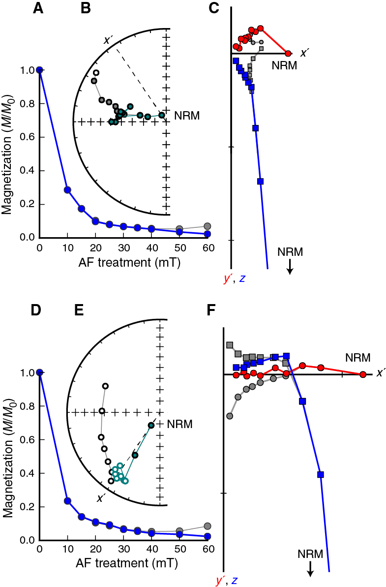
Figure F15. Demagnetization data exhibiting unwanted acquisition of ARM in the 2G AF demagnetizer.
Because core orientation using the Icefield MI-5 system was largely unsuccessful, the cores could not be independently oriented with respect to geographical north. Fortunately, the geocentric axial dipole inclination at the latitude of the expedition sites for Neogene deposits is large enough (~30°) to provide an unambiguous magnetic polarity, also taking into account possible biases caused by inclination shallowing by depositional inclination error or postdepositional compaction of the sediment (Tauxe et al., 2010). In the site chapters, we plot histograms of inclinations to establish that there are two unambiguous modes. Downward-directed inclinations are “normally magnetized,” whereas upward-directed inclinations are “reverse” for the Neogene. In the Eocene, the site paleolatitudes were equatorial (horizontal inclinations), and in the Paleocene the site paleolatitude was ~15°S (Cande et al., 2010), so downward-directed inclinations would be reverse. As the reliability of the data has been established in this way, cores can be reoriented such that the average normal direction for each core is set to zero. This may help to azimuthally orient sedimentary structures detected in the core for flux direction estimates.
Once a polarity stratigraphy was established for a given site, we correlated the pattern to the geomagnetic polarity timescale (Figure F9) in close collaboration with the shipboard biostratigraphy team. We use the chron terminology and numerical ages from Gradstein et al. (2012), listed in Table T6.
Table T6. Geomagnetic polarity timescale used during Expedition 355. Download table in .csv format.
Physical properties
Shipboard high-resolution physical property measurements are made to rapidly characterize lithologic units to aid hole-to-hole and site-to-site stratigraphic correlation that in turn guide drilling efforts to recover complete stratigraphic sequences at each site. The data are also used to tie core descriptions to borehole data and seismic profiles. In addition, physical property data play a major role in detection of stratigraphic discontinuities and inhomogeneities, obtaining information about differences in the composition and texture of sediment, identification of major seismic reflectors, and construction of synthetic seismic profiles. A variety of techniques and methods were used to characterize Expedition 355 cores on whole-round, split section-half, and discrete samples. Core sections are generally 1.5 m in length, so a typical coring length (stroke) of 9.5 m yields six sections plus a shorter seventh section. Procedures for measuring indurated sediment or igneous rock cores differ slightly, as described below.
Sediment cores
Recovered whole-round sections were usually allowed to equilibrate to ambient room temperature (~20°C) and pressure for ~4 h after being brought onboard, except when rapid measurement was necessary for stratigraphic correlation purposes. In those instances, the STMSL was run for rapid measurement of GRA bulk density and magnetic susceptibility. STMSL measurements were carried out at 2 or 5 cm resolution immediately after the whole-round cores were brought on board to assist in hole-to-hole stratigraphic correlation to guide drilling efforts to recover complete stratigraphic sequences at each site. After measurement on the STMSL, those cores were returned to the holding rack and allowed to equilibrate to room temperature.
After thermally equilibrating, core sections were run through the WRMSL for measurement of GRA bulk density, magnetic susceptibility, and compressional wave velocity by P-wave logger (PWL). Cores recovered with the XCB or RCB are slightly smaller in diameter than those cored with the APC. As a result, sections cored with the XCB or RCB typically have gaps between the liner and the core; therefore, P-wave velocity was not measured with the WRMSL on those cores. Sections were then run through the spectral NGRL. Thermal conductivity was measured on one whole-round section per sediment core (typically the last section of the core) by a needle probe inserted into the section through a small hole drilled through the plastic core liner close to the middle of the section. After that, cores were split longitudinally, with one half designated as archive half and the other as working half for sampling and discrete analysis. The archive half of the core was passed through the SHMSL to measure point magnetic susceptibility and color reflectance. Discrete physical property samples were typically collected from every other section of the working halves (~3 per core) to measure wet bulk density, dry bulk density, water content, porosity, and grain density. P-wave velocity and shear strength measurements on split cores were also performed on the working halves. P-wave velocity measurements employed transducers oriented in the x- and z-axis directions on the Section Half Measurement Gantry (SHMG), with typically one analysis per section. Vane shear strength was also measured on working half core sections using the automated vane shear (AVS) system on the SHMG.
Modifications of the method above were made for indurated sediment. Thermal conductivity was measured once per core on a split core section using a contact probe. A mini/half-size puck was used if the indurated sediment could be measured in the section liner. If the indurated sediment required saturation in seawater, this was done on a sediment piece from the section half in a bath of seawater. Compressional P-wave velocity measurements were made on this saturated section half. Samples from indurated sediments were taken using a parallel saw from the working half of the core for MAD measurements at a sampling interval of up to 3 samples per core (every ~3 m) depending on lithologic variability.
Igneous rock samples
Recovered igneous rock sections were shaken onto sterile liners in the core splitting room for examination by a core describer, who decided where the pieces should be split between working and archive halves. The pieces were then put back into liners and run through the WRMSL and NGRL. P-wave velocity was not measured because the spaces between the liner and the rock core pieces make these measurements meaningless. After physical property measurements were taken on whole-round sections, the core sections were split into working and archive halves and all rock pieces were labeled. The archive half of the core was passed through the SHMSL for measurement of point magnetic susceptibility and color reflectance. Compressional P-wave velocity measurements were made on these samples.
A full discussion of all methodologies and calculations used aboard the JOIDES Resolution in the Physical Properties Laboratory is available in Blum (1997). Details and procedures for each physical property measurement are described below.
Whole-Round Multisensor Logger measurements
GRA-derived bulk density, P-wave velocity, and magnetic susceptibility were measured nondestructively with the WRMSL (Figure F16). To optimize the measurement process, sampling intervals and measurement integration times were the same for all sensors. Sampling intervals were set at 2.0 cm with an integration time of 5 s for each measurement. After every core, quality control and quality assurance (QA/QC) were monitored by passing a single core liner filled with deionized water through the WRMSL.
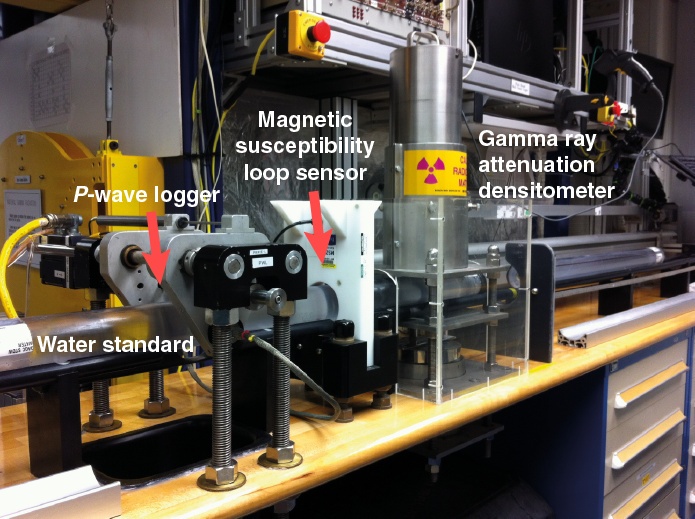
Figure F16. Onboard WRMSL, which measures GRA bulk density, magnetic susceptibility, and P-wave velocity.
GRA bulk density
Bulk density can be used to estimate the pore volume in sediment and evaluate the consolidation state of sediment. GRA density is an estimate of bulk density based on the attenuation of a gamma ray beam. The beam is produced by a 137Cs gamma ray source at a radiation level of 370 MBq within a lead shield with a 5 mm collimator, which is directed through the whole-round core. The gamma ray detector on the opposite side of the core from the source includes a scintillator and an integral photomultiplier tube to record the gamma radiation that passes through the core. The attenuation of gamma rays occurs primarily by Compton scattering, in which gamma rays are scattered by electrons in the formation; the degree of scattering is related to the material bulk density. Therefore, for a known sample thickness, the density (ρ) is proportional to the intensity of the attenuated gamma rays and can be expressed as
- I = the measured intensity of gamma rays passing through the sample,
- I0 = gamma ray source intensity,
- μ = Compton attenuation coefficient, and
- d = sample diameter.
The μ and I0 are treated as constants, such that ρ can be calculated from I.
In general, WRMSL measurements are most accurate when taken on a completely filled core liner with minimal drilling disturbance; otherwise, measurements tend to underestimate true values. By default, the instrument reports measurements using the internal diameter of the core liner (66 mm) as the assumed sample diameter. This assumption is suitable for most sediment cores obtained by the APC; however, for sediment and/or igneous rock cored by the XCB or RCB, core diameter is usually ~58 mm or less. Following Jarrard and Kerneklian (2007), the density measurements of cores obtained by XCB or RCB were corrected by multiplying the density values by 66/58 = 1.138 to account for this bias. Irregularly filled core liners will also influence GRA measurements and should be considered when interpreting the data. The spatial resolution of the GRA densitometer is less than ±1 cm. The gamma ray detector is calibrated with sealed calibration cores (one standard core liner filled with distilled water and aluminum cylinders of various diameters). To establish the calibration curves, gamma ray counts were taken through each aluminum cylinder for 60 s. Each aluminum cylinder has a density of 2.7 g/cm3, and d is 1, 2, 3, 4, 5, or 6 cm. The relationship between I and µd is
where A, B, and C are coefficients determined from the calibration.
Recalibration was performed as needed when the deionized water QA/QC standard deviated significantly (more than a few percent) from 1 g/cm3.
Magnetic susceptibility
Magnetic susceptibility (χ) is a dimensionless measure of the degree to which a material can be magnetized by an external magnetic field:
where M is the magnetization induced in the material by an external field of strength H. Magnetic susceptibility is primarily sensitive to the concentration of ferrimagnetic minerals (e.g., magnetite and maghemite). It is also sensitive to magnetic mineralogy and can be related to the origin of the materials in the core and their subsequent diagenesis. Igneous materials typically have magnetic susceptibility around 2 orders of magnitude greater than their alteration products, such as clay.
The measurements were made using a Bartington MS2C loop sensor with a 90 mm diameter. An oscillator circuit in the sensor, which operates at a frequency of 0.565 kHz and an alternating field of ~140 A/m, produces a low-intensity, nonsaturating alternating magnetic field. Sediment or igneous rock core sections going through the influence of this field cause a change in oscillator frequency. Frequency information returned in pulse form to the susceptometer is converted into magnetic susceptibility. The loop sensor has a spatial resolution of 20 mm and is accurate to within 5% as indicated in Bartington specifications (see Blum, 1997).
P-wave velocity
P-wave velocity data can be used to evaluate small-strain moduli, correlate between downhole logging and core data, and evaluate porosity and cementation. P-wave (compressional) velocity (VP) is defined by the time required for a compressional wave to travel a specific distance
where d is the path length of the wave across the core and tcore is the traveltime through the core.
The PWL measures the traveltime of 500 kHz ultrasonic waves horizontally across the core at 2.0 cm intervals. Waves are transmitted to the core by plastic transducer contacts connected to linear actuators. Pressure is applied to the actuators to ensure coupling between the transducers and the core liner. P-wave velocity transducers measure total traveltime of the compressional wave between transducers. The wave travels horizontally across the whole core and core liner. The total observed traveltime tcore is composed of
- tdelay = time delay related to transducer faces and electronic circuitry,
- tpulse = delay related to the peak detection procedure,
- tliner = transit time through the core liner, and
- tcore = traveltime through the sediment.
The system is calibrated using a core liner filled with distilled water, which provides control for tdelay, tpulse, and tliner. From these calibrations, VP can be calculated for the whole-round specimens in core liners as
VP = (dcl – 2dliner)/(to – tpulse – tdelay – 2tliner),
- dcl = measured diameter of core and liner,
- dliner = liner wall thickness, and
- to = measured total traveltime.
This equation assumes that the core completely fills the core liner. The WRMSL PWL was turned off for cores recovered with the XCB or RCB, which typically do not fill the core liner.
Special Task Multisensor Logger measurements
STMSL measurements were used to acquire GRA bulk density and magnetic susceptibility data, usually at a lower spatial resolution than on the WRMSL and prior to temperature equilibration. The purpose of these measurements is to allow rapid correlation between the different holes at each site in order to guide drilling operations and ensure complete sediment column recovery. The GRA bulk densitometer and magnetic susceptibility loop on the STMSL are similar to those on the WRMSL (see Whole-Round Multisensor Logger measurements), although warming of the core over the course of measurement produces drift of up to ~5 × 10⁻⁵ SI in magnetic susceptibility measurements. The along-section spacing distance between STMSL measurements varied between 2.0 and 5.0 cm, depending on the time available to process each new core through the shipboard laboratories.
Natural Gamma Radiation Logger measurements
Gamma radiation is emitted from the decay of mineral-hosted 238-uranium (238U), 232-thorium (232Th), and 40-potassium (40K). The NGRL measures this natural emission on whole-round cores using a system designed and built by the Integrated Ocean Drilling Program-US Implementing Organization (Texas A&M University, USA) (Vasiliev et al., 2011; Dunlea et al., 2013) (Figure F17). As 238U, 232Th, and 40K radioisotopes decay, they and their daughter products emit gamma radiation at specific energy levels unique to each isotope. NGR spectroscopy measures a wide energy spectrum that can be used to estimate the abundance of each isotope based on the strength of the signal at characteristic energies (Blum, 1997). Spectral data were collected but were not processed on board and can be used for postcruise processing for U, Th, and K abundance. Total counts were used on board, with high counts usually identifying fine-grained deposits containing K-rich clay minerals and their absorbed U and Th isotopes. NGR data thus reveal stratigraphic details that aid in core-to-core correlations. The main NGR detector unit consists of eight sodium iodide (thallium) (NaI[Tl]) detectors arranged along the core measurement axis at 20 cm intervals surrounding the lower half of the section (Figure F18). The detector array has passive (layers of lead) and active (plastic scintillators) shielding to reduce the background environmental and cosmic radiation. The overlying plastic scintillators detect incoming high-energy gamma and muon cosmic radiation and cancel this signal from the total counted by the NaI(Tl) detectors.
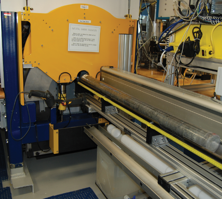
Figure F17. NGRL on board for whole-round cores.
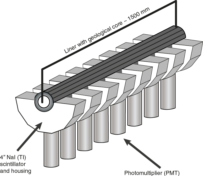
Figure F18. Main elements of the NGRL.
A measurement run consisted of two sample positions, 10 cm apart, for a total of 16 measurements per 150 cm section. The quality of the energy spectrum measured in a core depends on the concentration of radionuclides in the sample but also on the counting time, with higher times yielding better spectra. Counting times were chosen as 5 min per position, or around 10 min per core, yielding statistically significant energy spectra (Vasiliev et al., 2011).
Thermal conductivity measurements
Thermal conductivity was typically measured on the last section of each core with the TK04 (Teka Bolin) system using a needle probe in full-space configuration for whole-round soft-sediment cores (Von Herzen and Maxwell, 1959), a contact miniprobe in half-space configuration on split cores, or a contact probe on saturated sediment for indurated sediment cores. The probes contain a heater wire and calibrated thermistor.
For soft sediment, the needle probe was inserted into a 2 mm diameter hole drilled approximately midway through the liner along one of the lines that later guided core splitting. To avoid interference from airflow in the laboratory, the core was placed into an enclosed box insulated with foam.
For indurated sedimentary cores, samples were selected from the working half and returned unaltered to the core liner upon completion of the tests. The contact probe embedded in the surface of an epoxy block with a low thermal conductivity (Vacquier, 1985) was maintained in contact with the sample. For very lithified sedimentary sections, the samples were saturated in a bath of seawater at room temperature for 24 h under vacuum. Afterward, the probe was attached to the sample and placed in a cooler insulated with extruded polystyrene foam. The calibrated heat source of the probe was then turned on and the increase in temperature was recorded over 60 or 80 s. A heating power of 0.5 to 2 W/m was typically used in soft sediment and indurated material. The solution to the heat conduction equation with a line source of heat was then fit to the temperature measurements to obtain the thermal conductivity. Because the probe is much more conductive than sediment or igneous rock, the probe is assumed to be a perfect conductor. Under this assumption, the temperature of the superconductive probe has a linear relationship with the natural logarithm of the time after the initiation of the heat,
- T = temperature (K),
- q = heat input per unit length per unit time (J/m/s),
- k = thermal conductivity (W/[m·K]),
- t = time after the initiation of the heat (s), and
- C = instrumental constant.
Three to five measuring cycles were automatically performed to calculate average conductivity. A self-test, which included a drift study, was conducted at the beginning of each measurement cycle. Once the probe temperature stabilized, the heater circuit was closed and the temperature rise in the probe was recorded. Thermal conductivity was calculated from the rate of temperature rise while the heater current was flowing. Temperatures measured during the first 60 to 80 s of the heating cycle were fitted to an approximate solution of a constantly heated line source (for details, see Kristiansen, 1982; Blum, 1997). Measurement errors were 5%–10%.
Section Half Multisensor Logger measurements
Color reflectance and magnetic susceptibility were measured on archive section halves using the SHMSL. The archive half of the split core was placed on the core track, above which an electronic platform moves along a track recording the height of the split-core surface with a laser sensor. The laser establishes the location of the bottom of the section, and then the platform reverses the direction of movement, moving from bottom to top making measurements of point magnetic susceptibility and color reflectance. Intervals containing foam inserts were excluded from measurement, so the measured range of values represents that of the core material only. During Expedition 355, point magnetic susceptibility and color reflectance data were collected at constant intervals for each core (2 cm). These measurements integrate over a smaller depth than the magnetic susceptibility loop of the WRMSL.
Color reflectance spectrometry
The color reflectance spectrometer uses an Ocean Optics 30 mm integrating sphere and both halogen and LED light sources that cover wavelengths from ultraviolet through visible to near infrared. The measurements were taken from 380 to 900 nm wavelengths at 2 nm intervals. The ~3 s data acquisition offset was applied for the entire scan of the archive section half. The data are reported using the L*a*b* color system, in which L* is lightness, a* is redness (positive) versus greenness (negative), and b* is yellowness (positive) versus blueness (negative) of the rock. The color reflectance spectrometer calibrates on two spectra, pure white (reference) and pure black (dark). Color calibration was conducted approximately once every 6 h (twice per shift).
Point magnetic susceptibility
Point magnetic susceptibility was measured with a Bartington MS2 meter and an MS2K contact probe with a flat 15 mm diameter round sensor with a field of influence of 25 mm and an operation frequency of 930 Hz. The instrument averages three measurements from the sensor for each offset, leading to an accuracy of ~5%. The spatial resolution of the point magnetic susceptibility instrument is ~3 mm, higher than that of the whole-round magnetic susceptibility measurement (20 mm). As with whole-round measurements, the output displayed by the point magnetic susceptibility sensor must be converted to dimensionless SI units by multiplying by 10–5. The probe is zeroed in air before each measurement location in order to avoid influence from the metal track. The point magnetic susceptibility meter was calibrated by the manufacturer before installation on the ship and is quality checked every ~6 h at the same time as color reflectance sensor calibration.
Section Half Measurement Gantry measurements
For soft-sediment cores, P-wave velocity and shear strength measurements were performed on the working half of split cores after sampling for MAD and paleomagnetic measurements. P-wave velocity measurements used the x-axis caliper and z-axis bayonet contact probe transducers on the SHMG (Figure F19), with one analysis every section coinciding with or adjacent to the paleomagnetic discrete sample locations. However, if this interval provided no good sediment/transducer coupling (e.g., caused by high amounts of sand or cracks), different positions were chosen to generate viable data. For igneous rock samples, P-wave velocity was measured on discrete samples.
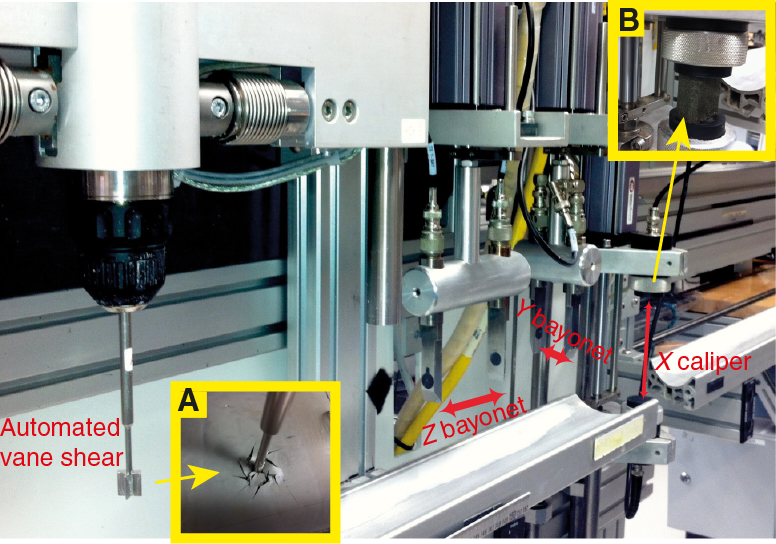
Figure F19. SHMG showing the x-axis caliper and y- and z-axis bayonets to measure P-wave velocity.
P-wave velocity
The P-wave velocity system uses Panametrics-NDT Microscan delay line transducers that transmit at 0.5 MHz. The signal received through the section half of the discrete sample was recorded by the computer attached to the system, with the peak (P-wave arrival) chosen by autopicking software when the signal was strong. In case of a weak signal, the first arrival was manually picked. Frequently, we manually picked the very base of the first arrival peak, leaving out the automatically picked points that fell along the ascending curve. The distance between transducers was measured with a built-in linear voltage displacement transformer. Calibration was performed with a series of acrylic cylinders of differing thicknesses and a known P-wave velocity of 2750 ± 20 m/s. The determined system time delay derived from the calibration was subtracted from the picked arrival time to give a traveltime of the P-wave through the sample. The thickness of the sample (calculated by the linear voltage displacement transformer, in meters) was divided by the traveltime (in seconds) to calculate P-wave velocity in meters per second.
Shear strength
Shear strength is the resistance of a material to failure in shear. Only the network of solid particles resists shear stress in unconsolidated materials. Shear strength (τf) can be expressed as a function of the effective normal stress at failure (σ′), the effective cohesion (c′), and friction angle (φ′),
where c′ and φ′ are the shear strength parameters that define a linear relationship between τf and φ′, according to the Mohr-Coulomb failure criterion.
Shear strength parameters can be determined by means of multiple laboratory tests. The c and φ are relevant in situations where field drainage conditions correspond to test conditions. The shear strength of a soil under undrained conditions (interstitial water drainage does not occur during failure) is different from that under drained conditions (interstitial water drainage occurs).
Undrained shear strength can be expressed in terms of total stress in the case of fully saturated materials of low permeability (e.g., clays), denoted by Su. The most common strength tests in shipboard laboratories are the vane shear and penetrometer tests, which provide measurement of undrained shear strength (Su) (Blum, 1997). Both tests were used during Expedition 355.
Vane shear strength was measured in undisturbed fine-grained sediment using the AVS system in working-half core sections (Figure F20). Using the AVS, undrained shear strength was determined by inserting a four-bladed vane into the split core and rotating it at a constant 90°/min to determine the torque required to cause a cylindrical surface to be sheared by the vane, which provides a measurement of the peak shear strength. The difference in rotational strain between the top and the bottom of a linear spring is measured using digital shaft encoders. Measurements were made with the vane rotation axis perpendicular to the split surface. The residual shear strength was taken to be the constant and lowest measured shear strength after reaching the peak value during the test cycle. Measurements were taken once per core, unless the sediment was too firm for instrument penetration or was disturbed during coring.
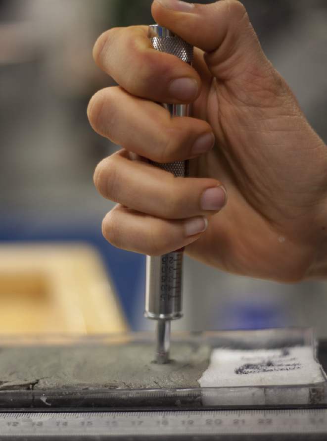
Figure F20. Pocket penetrometer for measuring (unconfined) compressive strength.
Vane shear strength Su(v) (kPa) is calculated as
- T = torque required to induce material failure (N·m),
- Kv = constant, depending on vane dimensions (m3),
- Δ = maximum torque angle (°) at failure, and
- B = spring constant that relates the deflection angle to the torque (°/N·m) (Blum, 1997).
All measurements used a vane with a height and diameter of 12.7 mm. Failure torque (T) was determined by measuring the degrees of rotation of one of four torsional springs. A linear calibration equation (specified by the manufacturer) relates the rotation angle to the torque for the particular spring being used. Selection of the appropriate spring was based on the anticipated shear strength of the material. Vane shear results were generally considered reliable for shear strength values less than ~150–200 kPa, above which excessive cracking and separation of the core material occurred.
AVS measurements cannot be performed on sediment where the vane is not able to penetrate. A handheld penetrometer was then used in order to determine (unconfined) compressional strength (Figure F20). Failure is defined as the maximum principal stress difference, which is the same as the (unconfined) compressive strength of the material (Blum, 1997). The penetrometer is a flat-footed, spring-operated device used to measure compressive strength by pushing a 6.4 mm diameter probe 6.4 mm deep below the split-core surface. The mechanical scale is in units of kilograms per square centimeter, which are converted into units of kilopascals for reporting as
2τf (kPa) = 98.1 × 2τf (kg/cm2).
If the compressive strength is determined by reading the vertical strain directly off the pocket penetrometer, the value must be divided by 2 to calculate the shear strength at a prescribed strain (Blum, 1997). The maximum shear strength that can be measured with the pocket penetrometer is 220 kPa (Blum, 1997).
Discrete sample measurements of moisture and density
Discrete samples were collected from the working halves to determine wet and dry bulk density, grain density, water content, and porosity. In soft sediment, ~10 cm3 samples were collected with a plastic syringe, the diameter of which fits that of the glass vials. Samples for MAD analysis were collected from every other section (~3 per core). In indurated sedimentary and igneous rock, wedges were sawed from the working halves for physical property measurements.
Sample preparation
Soft-sediment samples were placed in numbered, preweighed vials for wet and dry sediment weighing, drying, and dry volume measurements. Determination of an accurate wet mass of the wedge samples of indurated sediment and igneous rock first required that the pore space of the samples be completely saturated with seawater. To do this, we placed the samples in individual plastic vials filled with seawater within a vacuum chamber. A vacuum pump removed the air from the chamber to a pressure of ~40–50 kPa below the atmospheric pressure, forcing seawater into the samples. The samples were kept under saturation for at least 24 h, with the vacuum maintained in the chamber by turning the pump on for 5–10 min every 5 h as needed. After removal from the vacuum chamber, the samples were patted dry with a paper towel and wet mass immediately determined using the dual balance system (described below). P-wave velocities were then measured on the wet samples if appropriate. The samples were then dried in a convection oven for at least 24 h at 105° ± 5°C. Dried samples were then cooled in a desiccator for at least 60 min before the dry mass and the volume were measured.
Dual balance mass measurement
The weights of wet and dry sample masses were determined to a precision of 0.005 g using two Mettler Toledo electronic balances, with one acting as a reference. A standard weight similar to that of the sample was placed upon the reference balance to increase accuracy. A computer averaging system was used to compensate for the ship’s motion. The default setting of the balances is 300 measurements (taking ~1.5 min).
Pycnometer volume measurement
Dry sample volume was determined using a hexapycnometer system of a six-celled, custom-configured Micrometrics AccuPyc 1330TC helium-displacement pycnometer (Figure F21). The precision of each cell is 1% of the full-scale volume. Volume measurement was preceded by three purges of the sample chamber with helium warmed to ~28°C. Three measurement cycles were run for each sample. A reference volume (set of two calibration spheres) was placed sequentially in one of the chambers to check for instrument drift and systematic error. The volumes occupied by the numbered vials were calculated before the cruise by multiplying each vial’s weight against the average density of the vial material. Dry mass and volume were measured after samples were heated in an oven at 105° ± 5°C for 24 h and allowed to cool in a desiccator for ~60 min. The procedures for the determination of these physical properties comply with the American Society for Testing and Materials (ASTM) designation (D) 2216 (ASTM, 1990). The fundamental relations and assumptions for the calculations of all physical property parameters are discussed by Blum (1997) and are summarized below.
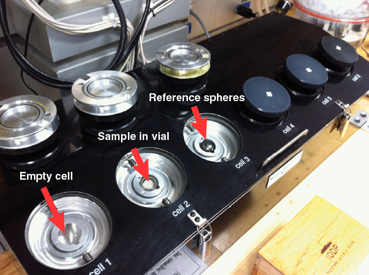
Figure F21. Pycnometer used to measure volume of dry samples.
Mass and volume calculation
We measured wet mass (Mwet), dry mass (Mdry), and dry volume (Vdry). The ratio of mass (rm) is a computational constant of 0.965 (i.e., 0.965 g of freshwater per 1 g of seawater). Salt precipitated in sediment pores during the drying process is included in the Mdry and Vdry values. The mass of the evaporated water (Mwater) and salt (Msalt) in the sample are given by
where s is the assumed saltwater salinity (0.035%) corresponding to an interstitial water density (ρpw) of 1.024 g/cm3 and a salt density (ρsalt) of 2.22 g/cm3. The corrected mass of interstitial water (Mpw), volume of interstitial water (Vpw), mass of solids excluding salt ( Msolid), volume of salt (Vsalt), volume of solids excluding salt (Vsolid), and wet volume (Vwet) are
Vwet = Vdry – Vsalt + Vpw, and
Calculation of bulk properties
For all sediment samples, water content (w) is expressed as the ratio of mass of pore water to wet sediment (total) mass,
Wet bulk density (ρwet), dry bulk density (ρdry), sediment grain density (ρsolid), porosity (φ), and void ratio (VR) are calculated as
MAD properties reported and plotted in the Physical properties sections of both site chapters were calculated with the MADMax shipboard program set with the “Method C” calculation process.
Downhole measurements
Downhole logs are used to determine physical, chemical, and structural properties of the formation penetrated by a borehole. The data are rapidly collected, continuous with depth and measured in situ; they can be interpreted in terms of the stratigraphy, lithology, mineralogy, magnetic characteristics, and geochemical composition of the penetrated section. Where core recovery is incomplete or disturbed, log data may provide the only way to characterize the borehole section. Where core recovery is good, log and core data complement one another and may be interpreted jointly, providing ground-truthing for the remote geophysical measurements.
Downhole logs measure formation properties on a scale that is intermediate between those obtained from laboratory measurements on core samples and those from conventional geophysical surveys. They are useful in calibrating the interpretation of geophysical survey data (e.g., through the use of synthetic seismograms) and provide a necessary link for the integrated understanding of physical and chemical properties on different scales.
During Expedition 355, downhole logging measurements were taken in Hole U1456C. In addition, downhole temperature measurements were acquired using the APCT-3 in Holes U1456A and U1457A.
Wireline logging
During wireline logging operations, logs were recorded with Schlumberger logging tools combined into tool strings, which were lowered into the hole after completion of coring operations. Two tool strings were used during Expedition 355: the triple combo, which measures NGR, porosity, density, and resistivity, and the Formation MicroScanner (FMS)-sonic, which provides FMS resistivity images of the borehole wall and sonic velocities (Figure F22; Table T7). Each tool string also contains a telemetry cartridge for communicating through the wireline to the Schlumberger data acquisition system (MultiAcquisition and Imaging System or “MAXIS” unit) on the drillship. When unstable hole conditions were anticipated as a result of unconsolidated sand or other difficulties encountered while drilling, the radioactive source was left out and the Hostile Environment Litho-Density Sonde (HLDS) functioned solely as a caliper tool to measure the borehole diameter.
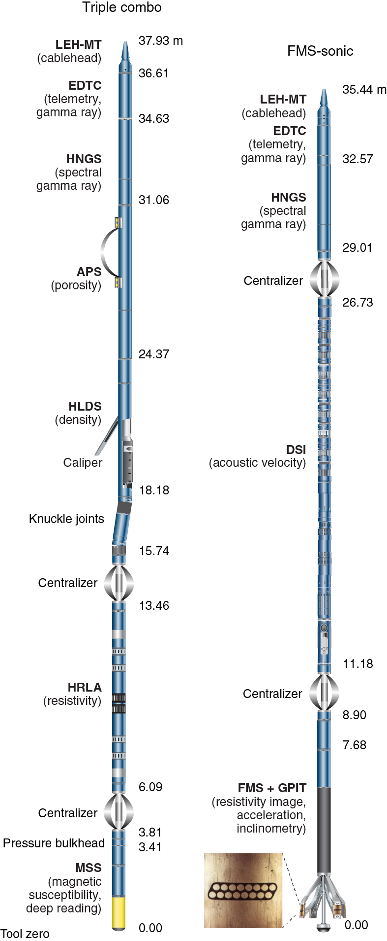
Figure F22. Wireline tool strings used during Expedition 355.
Table T7. Downhole measurements made by wireline tool strings during Expedition 355. Download table in .csv format.
In preparation for logging, the borehole was reamed in its lower sections, flushed of debris by circulating drilling fluid, and filled with seawater-based logging gel (sepiolite mud mixed with seawater and weighted with barite; approximate density = 10.5 lb/gal) to help stabilize the borehole walls in sections where instability was expected from the drilling and coring results. When logging in an uncased hole, the BHA was pulled up to ~80 m DSF to cover the most unstable upper part of the hole. The tool strings were then lowered downhole on a seven-conductor wireline cable before being pulled up at constant speed, typically ~550 m/h for the triple combo and 500–550 m/h for the FMS-sonic, to provide continuous log measurements of several properties simultaneously.
Each tool string deployment is termed a logging “run.” During each run, tool strings can be lowered and pulled up in the hole several times to check repeatability and to increase coverage of the FMS borehole images. Each lowering or hauling-up of the tool string while collecting data constitutes a “pass.” Incoming data were recorded and monitored in real time on the Modular Configuration MAXIS (MCM) logging computer. A wireline heave compensator (WHC) was used when necessary to minimize the effect of ship’s heave on the tool position in the borehole (see below).
Logged sediment properties and tool measurement principles
Logged properties and the principles used in the tools that measure them are briefly described below. The main logs collected during this expedition are listed in Table T8. More detailed information on individual tools and their geological applications may be found in Serra (1984, 1986, 1989), Schlumberger (1989, 1994), Rider (1996), Goldberg (1997), Lovell et al. (1998), and Ellis and Singer (2007). A complete online list of acronyms for the Schlumberger tools and measurement curves is at http://iodp.tamu.edu/tools/logging/index.html.
Table T8. Acronyms and units used for downhole wireline tools and measurements during Expedition 355. Download table in .csv format.
Natural gamma radiation
The Hostile Environment Natural Gamma Ray Sonde (HNGS) was used on both the triple combo and FMS-sonic tool strings to measure NGR in the formation. The HNGS uses two bismuth germanate scintillation detectors and five-window spectroscopy to determine concentrations of potassium (in weight percent), thorium (in parts per million), and uranium (in parts per million) from the characteristic gamma ray energies of isotopes in the 40K, 232Th, and 238U radioactive decay series, which dominate the natural radiation spectrum. The computation of the elemental abundances uses a least-squares method of extracting U, Th, and K elemental concentrations from the spectral measurements. The HNGS filters out gamma ray energies below 500 keV, eliminating sensitivity to bentonite or KCl in the drilling mud and improving measurement accuracy. The HNGS also provides a measure of the total gamma ray emission (HSGR) and uranium-free or computed gamma ray emission (HCGR) that are measured in American Petroleum Institute units (gAPI). The HNGS response is influenced by the borehole diameter, and therefore the HNGS data are corrected for borehole diameter variations during acquisition.
An additional NGR sensor was housed in the Enhanced Digital Telemetry Cartridge (EDTC), which was used primarily to communicate data to the surface. The sensor includes a sodium iodide scintillation detector that also measures the total NGR emission of the formation. It is not a spectral tool (does not provide U, Th, and K concentrations), but it provides total gamma radiation for each pass.
The inclusion of the HNGS in every tool string allows use of the gamma ray data for precise depth match processing between logging strings and passes and for core-log integration.
Density and photoelectric factor
Formation density was measured with the HLDS. The sonde contains a radioactive cesium (137Cs) gamma ray source (622 keV) and both far and near gamma ray detectors mounted on a shielded skid, which is pressed against the borehole wall by a hydraulically activated decentralizing arm. Gamma rays emitted by the source undergo Compton scattering, in which gamma rays are scattered by electrons in the formation. The number of scattered gamma rays that reach the detectors is proportional to the density of electrons in the formation, which is in turn related to bulk density. Porosity may also be derived from this bulk density if the matrix (grain) density is known.
The HLDS also measures the photoelectric effect factor (PEF), a measure of the photoelectric absorption of low-energy gamma radiation. Photoelectric absorption occurs when gamma radiation energy falls below 150 keV as a result of being repeatedly scattered by electrons in the formation. The PEF is determined by comparing the counts from the far detector in the high-energy region, where only Compton scattering occurs, with those in the low-energy region, where count rates depend on both reactions. Because PEF depends on the atomic number of the elements in the formation (heavier elements have higher PEF), it also varies according to the chemical composition of the minerals present and can be used for the identification of the overall mineral make-up of the formation. For example, the PEF of calcite is 5.08 barn/e–, illite is 3.03 barn/e–, quartz is 1.81 barn/e–, and hematite is 21 barn/e– (Serra, 1984; Schlumberger, 1989). Good contact between the tool and borehole wall is essential for good HLDS logs; poor contact results in underestimation of density values. Both the density correction and caliper measurement of the hole are used to check the contact quality. The PEF log should be used with caution when multiple mud sweeps are used to stabilize the borehole and especially in washouts, because barium in the logging mud swamps the signal, regardless of attempts to correct for the mud effect.
Porosity
Formation porosity was measured with the Accelerator Porosity Sonde (APS). The sonde includes a minitron neutron generator that produces fast (14.4 MeV) neutrons and five neutron detectors (four epithermal and one thermal) positioned at different distances from the minitron. The tool’s detectors count neutrons that arrive at the detectors after being scattered and slowed by collisions with atomic nuclei in the formation.
The highest energy loss occurs when neutrons collide with hydrogen nuclei, which have practically the same mass as the neutron (the neutrons bounce off heavier elements without losing much energy). If the hydrogen (i.e., water) concentration is low, as in low-porosity formations, neutrons can travel farther before being captured and the count rates increase at the detector. The opposite effect occurs in high-porosity formations where the water content is high. However, because hydrogen bound to minerals such as clays or that forms part of hydrocarbon molecules also contributes to the measurement, the raw porosity value is often an overestimate and should be checked against laboratory-derived values from core when possible.
Upon reaching thermal energies (0.025 eV), neutrons are captured by the nuclei of Cl, Si, B, and other elements, resulting in a gamma ray emission. This neutron capture cross section (Σf) is also measured by the tool.
Electrical resistivity
The High-Resolution Laterolog Array (HRLA) tool provides six resistivity measurements with different depths of investigation throughout the logged interval (including the borehole mud resistivity and five measurements of formation resistivity with increasing penetration into the formation). The tool sends a focused current into the formation and measures the intensity necessary to maintain a constant drop in voltage across a fixed interval, providing direct resistivity measurements. The array has one central (source) electrode and six electrodes above and below it, which serve alternatively as focusing and returning current electrodes. By rapidly changing the role of these electrodes, a simultaneous resistivity measurement at six penetration depths is achieved. The tool is designed to ensure that all signals are measured at exactly the same time and tool position and to reduce the sensitivity to “shoulder bed” effects when crossing sharp beds thinner than the electrode spacing. The design of the HRLA, which eliminates the need for a surface reference electrode, improves formation resistivity evaluation compared to traditional dual induction resistivity methods and allows the full range of resistivity to be measured, from low (e.g., in high-porosity sediment) to high (e.g., in basalt). The HRLA tool needs to be run centralized in the borehole for optimal results, so bow-spring centralizers were used to keep the HRLA in the center of the borehole. Knuckle joints above the HRLA allowed the density tool to be eccentralized and maintain good contact with the borehole wall (Figure F22).
Calcite, silica, and hydrocarbons are electrical insulators, whereas ionic solutions like interstitial water are conductors. Electrical resistivity, therefore, can be used to evaluate porosity for a given salinity and resistivity of the interstitial water (Schlumberger, 1989). Clay surface conduction also contributes to the resistivity values, but at high porosities, this is a relatively minor effect.
Acoustic velocity
The Dipole Shear Sonic Imager (DSI) measures the transit times between sonic transmitters and an array of eight receivers. It combines replicate measurements, thus providing a direct measurement of sound velocity through formations that is relatively free from the effects of formation damage and an enlarged borehole (Schlumberger, 1989). Along with the monopole transmitters found on most sonic tools, it also has two crossed-dipole transmitters that allow measurement of shear wave velocity in addition to compressional wave velocity. Dipole measurements are necessary to measure shear wave velocities in slow formations where shear wave velocity is less than the velocity of sound in the borehole fluid. Such slow formations are often encountered in deep-ocean drilling.
Formation MicroScanner
The FMS provides high-resolution electrical resistivity–based images of borehole walls. The tool has four orthogonal arms and pads, each containing 16 button electrodes that are pressed against the borehole wall during logging. The electrodes are arranged in two diagonally offset rows of eight electrodes each. A focused current is emitted from the button electrodes into the formation, with a return electrode near the top of the tool. Resistivity of the formation at the button electrodes is derived from the intensity of current passing through the button electrodes.
Processing transforms the resistivity measurements into oriented high-resolution images that reveal geologic structures of the borehole wall. Features such as bedding, stratification, fracturing, slump folding, and bioturbation can be resolved (Luthi, 1990; Salimullah and Stow, 1992; Lovell et al., 1998). Because the images are oriented to magnetic north, further analysis can provide measurement of the dip and direction (azimuth) of planar features in the formation. In addition, when the corresponding planar features can be identified in the recovered core samples, individual core pieces can be reoriented with respect to true north.
Approximately 30% of a borehole with a diameter of 25 cm (9.8 inches) is imaged during a single pass. Standard procedure is to make two full uphole passes with the FMS to maximize the chance of getting full borehole coverage with the pads. The maximum extension of the caliper arms is 40.6 cm (16 inches). In holes with a diameter greater than this maximum, the pad contact at the end of the caliper arms will be inconsistent, and the FMS images may appear out of focus and too conductive. Irregular (rough) borehole walls will also adversely affect the images if contact with the wall is poor.
Magnetic Susceptibility Sonde
The Magnetic Susceptibility Sonde (MSS) is a nonstandard wireline tool designed by Lamont-Doherty Earth Observatory (LDEO). It measures the ease with which formations are magnetized when subjected to a magnetic field. The ease of magnetization is ultimately related to the concentration and composition (size, shape, and mineralogy) of magnetic minerals (principally magnetite) in the formation. These measurements provide one of the best methods for investigating stratigraphic changes in mineralogy and lithology because the measurement is quick, repeatable, and nondestructive and because different lithologies often have strongly contrasting susceptibilities.
The MSS dual-coil sensor provides ~40 cm resolution measurements, with ~20 cm horizontal penetration. The MSS was run as the lowermost tool in the triple combo tool string, using a specially developed data translation cartridge to enable the MSS to be run in combination with the Schlumberger tools. The MSS also has an optional single-coil sensor to provide high-resolution measurements (~10 cm), but this was not used during Expedition 355 because it has a large bow-spring that is required because the tool is very sensitive to separation from the borehole wall. This would mean that the MSS would have to be run higher up in the tool string so it could be eccentralized and ultimately would require an additional log run.
Magnetic susceptibility data from the deep-reading sensor are plotted as uncalibrated units. The MSS reading responses are affected by temperature and borehole size (higher temperatures lead to higher susceptibility measurements). No apparent temperature drift was seen in the data and therefore no corrections were made offshore. When the magnetic susceptibility signal in sediment is very low, the detection limits of the tool may be reached. For quality control and environmental correction, the MSS also measures internal tool temperature, z-axis acceleration, and low-resolution borehole conductivity.
Acceleration and inclinometry
Three-component acceleration and magnetic field measurements were made with the General Purpose Inclinometry Tool (GPIT). The primary purpose of this tool, which incorporates a three-component accelerometer and a three-component magnetometer, is to determine the acceleration and orientation of the FMS-sonic tool string during logging. This information allows the FMS images to be corrected for irregular tool motion and the dip and direction (azimuth) of features in the images to be determined. The GPIT is run with other tools on the FMS-sonic tool string that can carry remanent or induced magnetization; therefore, its magnetic measurements can be affected by the other tools as well as the rocks in the borehole wall and magnetization of the casing and/or drill pipe. However, on the FMS-sonic tool string the GPIT has greater nonmagnetic insulation from the other tools, which greatly reduces the effects on its magnetic measurements.
Log data quality
The main influence on log data quality is the condition of the borehole wall. Where the borehole diameter varies over short intervals because of washouts (wide borehole) of softer material or ledges of harder material, the logs from tools that require good contact with the borehole wall (i.e., FMS, density, and porosity) may be degraded. Deep investigation measurements, such as gamma radiation, resistivity, and sonic velocity, which do not require contact with the borehole wall, are generally less sensitive to borehole conditions. “Bridged” sections, where borehole diameter is much lower than the bit size, will also cause irregular log results. The quality of the borehole is improved by minimizing the circulation of drilling fluid while drilling, flushing the borehole to remove debris, and logging as soon as possible after drilling and conditioning are completed.
The quality of the wireline depth determination depends on several factors. The depth of the logging measurements is determined from the length of the cable payed out from the winch on the ship. The seafloor is identified on the NGR log by the abrupt reduction in gamma ray count at the water/sediment interface (mudline). Discrepancies between the drilling depth and the wireline log depth may occur. In the case of drilling depth, discrepancies are caused by core expansion, incomplete core recovery, or incomplete heave compensation. In contrast for log depth, discrepancies between successive runs occur because of incomplete heave compensation, incomplete correction for cable stretch, and cable slip. Tidal changes in sea level affect both drilling and logging depths.
Wireline heave compensator
During wireline logging operations, the up-and-down motion of the ship (heave) causes a similar motion of the downhole logging tools. If the amplitude of this motion is large, depth discrepancies can be introduced into the logging data. The risk of damaging downhole instruments is also increased. A WHC system was thus designed to compensate for the vertical motion of the ship and maintain steady motion of the logging tools to ensure high-quality logging data acquisition (Iturrino et al., 2013; Liu et al., 2013). The WHC uses a vertical accelerometer (motion reference unit [MRU]) positioned under the rig floor near the ship’s center of gravity to calculate the vertical motion of the ship with respect to the seafloor. The WHC then adjusts the length of the wireline by varying the distance between two sets of pulleys through which the cable passes in order to minimize downhole tool motion. Real-time measurements of uphole (surface) and downhole acceleration are made simultaneously by the MRU and the EDTC, respectively.
Logging data flow and log depth scales
Data for each wireline logging run were monitored in real time and recorded using the Schlumberger MAXIS 500 system. Initial logging data were referenced to the rig floor (m WRF). After logging was completed, the data were shifted to a seafloor reference (m WSF) based on the step in gamma radiation at the sediment/water interface.
Data were transferred onshore to LDEO, where standardized data processing took place. The main part of the processing is depth matching to remove depth offsets between logs from different logging runs, which results in a new depth scale: WMSF. Also, corrections are made to certain tools and logs (e.g., FMS imagery is corrected for tool acceleration, including “stick and slip” motion), documentation for the logs (with an assessment of log quality) is prepared, and the data are converted to ASCII for the conventional logs and to GIF for the FMS images. The Schlumberger Geo-Quest’s GeoFrame software package is used for most of the processing of the collected wireline logging data. The data were transferred back to the ship within a few days after logging, and this processed data set was made available to the science party.
In situ temperature measurements
During Expedition 355, in situ temperature measurements were made with the APCT-3 in Hole A at each site when the APC was deployed. The APCT-3 fits directly into the coring shoe of the APC and consists of a battery pack, data logger, and a platinum resistance-temperature device calibrated over a temperature range from 0° to 30°C. Before entering the borehole, the tool is first stopped at the mudline for 5 min to thermally equilibrate with bottom water. However, the lowest temperature recorded during the run was occasionally used instead of the average temperature at the mudline as an estimate of the bottom water temperature because (1) it was more repeatable, and (2) the bottom water is expected to have the lowest temperature in the profile. When the APC is plunged into the formation, there is an instantaneous temperature rise from frictional heating. This heat gradually dissipates into the surrounding sediment as the temperature at the APCT-3 equilibrates toward the temperature of the sediment. After the APC penetrated the sediment, it was held in place for 10 min while the APCT-3 recorded the temperature of the cutting shoe every second.
The equilibrium temperature of the sediment was estimated by applying a mathematical heat-conduction model to the temperature decay record (Horai and Von Herzen, 1985). The synthetic thermal decay curve for the APCT-3 is a function of the geometry and thermal properties of the probe and the sediment (Bullard, 1954; Horai and Von Herzen, 1985). Equilibrium temperature was estimated by applying a fitting procedure (Pribnow et al., 2000). However, where the APC did not achieve a full stroke or where ship heave pulled the APC up from full penetration, the temperature equilibration curve is disturbed and temperature determination is less accurate. The nominal accuracy of the APCT-3 temperature measurements is ±0.05°C.
APCT-3 temperature data were combined with measurements of thermal conductivity (see Physical properties) obtained from core sections to obtain heat flow values. Heat flow was calculated according to the Bullard method, to be consistent with the synthesis of Ocean Drilling Program (ODP) heat flow data by Pribnow et al. (2000).
References
Acton, G.D., Borton, C.J., and the Leg 178 Shipboard Scientific Party, 2001. Palmer Deep composite depth scales for Leg 178 Sites 1098 and 1099. In Barker, P.F., Camerlenghi, A., Acton, G.D., and Ramsay, A.T.S. (Eds.), Proceedings of the Ocean Drilling Program, Scientific Results, 178: College Station, TX (Ocean Drilling Program), 1–35. http://dx.doi.org/10.2973/odp.proc.sr.178.202.2001
Andò, S., Garzanti, E., Padoan, M., and Limonta, M., 2012. Corrosion of heavy minerals during weathering and diagenesis: a catalog for optical analysis. Sedimentary Geology, 280:165–178. http://dx.doi.org/10.1016/j.sedgeo.2012.03.023
ASTM International, 1990. Standard method for laboratory determination of water (moisture) content of soil and rock (Standard D2216–90). In Annual Book of ASTM Standards for Soil and Rock (Volume 04.08): Philadelphia (American Society for Testing Materials). [revision of D2216-63, D2216-80]
Backman, J., 1980. Miocene–Pliocene nannofossils and sedimentation rates in the Hatton-Rockall Basin, NE Atlantic Ocean. Acta Universitatis Stockholmiensis: Stockholm Contributions in Geology, 36(1):1–91.
Baldauf, J.G., 1984. Cenozoic diatom biostratigraphy and paleoceanography of the Rockall Plateau region, North Atlantic, Deep Sea Drilling Project Leg 81. In Roberts, D.G., Schnitker, D., et al., Initial Reports of the Deep Sea Drilling Project, 81: Washington, DC (U.S. Government Printing Office), 439–478. http://dx.doi.org/10.2973/dsdp.proc.81.107.1984
Baldauf, J.G., and Iwai, M., 1995. Neogene diatom biostratigraphy for the eastern equatorial Pacific Ocean, Leg 138. In Pisias, N.G., Mayer, L.A., Janecek, T.R., Palmer-Julson, A., and van Andel, T.H. (Eds.), Proceedings of the Ocean Drilling Program, Scientific Results, 138: College Station, TX (Ocean Drilling Program), 105–128. http://dx.doi.org/10.2973/odp.proc.sr.138.107.1995
Balsam, W.L., and Damuth, J.E., 2000. Further investigations of shipboard vs. shore-based spectral data: implications for interpreting Leg 164 sediment composition. In Paull, C.K., Matsumoto, R., Wallace, P., and Dillon, W.P. (Eds.), Proceedings of the Ocean Drilling Program, Scientific Results, 164: College Station, TX (Ocean Drilling Program), 313–324. http://dx.doi.org/10.2973/odp.proc.sr.164.222.2000
Balsam, W.L., Damuth, J.E., and Schneider, R.R., 1997. Comparison of shipboard vs. shore-based spectral data from Amazon Fan cores: implications for interpreting sediment composition. In Flood, R.D., Piper, D.J.W., Klaus, A., and Peterson, L.C. (Eds.), Proceedings of the Ocean Drilling Program, Scientific Results, 155: College Station, TX (Ocean Drilling Program), 193–215. http://dx.doi.org/10.2973/odp.proc.sr.155.210.1997
Balsam, W.L., Deaton, B.C., and Damuth, J.E., 1998. The effects of water content on diffuse reflectance spectrophotometry studies of deep-sea sediment cores. Marine Geology, 149(1–4):177–189. http://dx.doi.org/10.1016/S0025-3227(98)00033-4
Barron, J.A., 1985a. Late Eocene to Holocene diatom biostratigraphy of the equatorial Pacific Ocean, Deep Sea Drilling Project Leg 85. In Mayer, L., Theyer, F., Thomas, E., et al., Initial Reports of the Deep Sea Drilling Project, 85: Washington, DC (U.S. Government Printing Office), 413–456. http://dx.doi.org/10.2973/dsdp.proc.85.108.1985
Barron, J.A., 1985b. Miocene to Holocene planktic diatoms. In Bolli, H.M., Saunders, J.B., and Perch-Nielsen, K. (Eds.), Plankton Stratigraphy: Cambridge, United Kingdom (Cambridge University Press), 763–809.
Barron, J.A., 1992. Neogene diatom datum levels in the equatorial and North Pacific. In Ishizaki, K., and Saito, T. (Eds.), Centenary of Japanese Micropaleontology: Tokyo (Terra Scientific Publishing Company), 413–425. http://www.terrapub.co.jp/e-library/cjm/pdf/0413.pdf
Bates, R.L., and Jackson, J.A. (Eds.), 1987. Glossary of Geology (3rd edition): Alexandria, VA (American Geological Institute).
Berggren, W.A., Kent, D.V., Swisher, C.C., III, and Aubry, M.-P., 1995. A revised Cenozoic geochronology and chronostratigraphy. In Berggren, W.A., Kent, D.V., Aubry, M.-P., and Hardenbol, J. (Eds.), Geochronology, Time Scales and Global Stratigraphic Correlation. Special Publication - SEPM (Society for Sedimentary Geology), 54:129–212. http://dx.doi.org/10.2110/pec.95.04.0129
Berggren, W.A., and Pearson, P.N., 2005. A revised tropical to subtropical Paleogene planktonic foraminiferal zonation. Journal of Foraminiferal Research, 35(4):279–298. http://dx.doi.org/10.2113/35.4.279
Berner, R.A., 1984. Sedimentary pyrite formation: an update. Geochimica et Cosmochimica Acta, 48(4):605–615. http://dx.doi.org/10.1016/0016-7037(84)90089-9
Blum, P., 1997. Technical Note 26: Physical Properties Handbook—A guide to the Shipboard Measurement of Physical Properties of Seep-sea Cores. Ocean Drilling Program. http://dx.doi.org/10.2973/odp.tn.26.1997
Bolli, H.M., and Saunders, J.B., 1985. Oligocene to Holocene low latitude planktic foraminifera. In Bolli, H.M., Saunders, J.B., and Perch-Nielsen, K. (Eds.), Plankton Stratigraphy (Volume 1): Planktic Foraminifera, Calcareous Nannofossils and Calpionellids: Cambridge, United Kingdom (Cambridge University Press), 155–262.
Bollmann, J., 1997. Morphology and biogeography of Gephyrocapsa coccoliths in Holocene sediments. Marine Micropaleontology, 29(3–4):319–350. http://dx.doi.org/10.1016/S0377-8398(96)00028-X
Bullard, E.C., 1954. The flow of heat through the floor of the Atlantic Ocean. Proceedings of the Royal Society of London, Series A: Mathematical, Physical and Engineering Sciences, 222(1150):408–429. http://dx.doi.org/10.1098/rspa.1954.0085
Cande, S.C., and Kent, D.V., 1992. A new geomagnetic polarity time scale for the Late Cretaceous and Cenozoic. Journal of Geophysical Research: Solid Earth, 97(B10):13917–13951. http://dx.doi.org/10.1029/92JB01202
Cande, S.C., and Kent, D.V., 1995. Revised calibration of the geomagnetic polarity timescale for the Late Cretaceous and Cenozoic. Journal of Geophysical Research: Solid Earth, 100(B4):6093–6095. http://dx.doi.org/10.1029/94JB03098
Cande, S.C., Patriat, P., and Dyment, J., 2010. Motion between the Indian, Antarctic and African plates in the early Cenozoic. Geophysical Journal International, 183(1):127–149. http://dx.doi.org/10.1111/j.1365-246X.2010.04737.x
Carozzi, A.V., 1989. Carbonate Rock Depositional Models: A Microfacies Approach: Englewood Cliffs, NJ (Prentice Hall).
Chaisson, W.P., and Pearson, P.N., 1997. Planktonic foraminifer biostratigraphy at Site 925: middle Miocene–Pleistocene. In Shackleton, N.J., Curry, W.B., Richter, C., and Bralower, T.J. (Eds.), Proceedings of the Ocean Drilling Program, Scientific Results, 154: College Station, TX (Ocean Drilling Program), 3–31. http://dx.doi.org/10.2973/odp.proc.sr.154.104.1997
Coccioni, R., Marsili, A., Montanari, A., Bellanca, A., Neri, R., Bice, D.M., Brinkhuis, H., Church, N., Macalady, A., McDaniel, A., Deino, A., Lirer, F., Sprovieri, M., Maiorano, P., Monechi, S., Nini, C., Nocchi, M., Pross, J., Rochette, P., Sagnotti, L., Tateo, F., Touchard, Y., Van Simaeys, S., and Williams, G.L., 2008. Integrated stratigraphy of the Oligocene pelagic sequence in the Umbria-Marche Basin (northeastern Apennines, Italy): a potential Global Stratotype Section and Point (GSSP) for the Rupelian/Chattian boundary. Geological Society of America Bulletin, 120(3–4):487–511. http://dx.doi.org/10.1130/B25988.1
Constable, C., and Tauxe, L., 1990. The bootstrap for magnetic susceptibility tensors. Journal of Geophysical Research: Solid Earth, 95(B6):8383–8395. http://dx.doi.org/10.1029/JB095iB06p08383
Deer, W.A., Howie, R.A., and Zussman, J., 1986. Rock-forming Minerals (Volume 1B): Disilicates and Ring Silicates (2nd edition): Harlow, United Kingdom (Longman Scientific Technical).
Dunlea, A.G., Murray, R.W., Harris, R.N., Vasiliev, M.A., Evans, H., Spivack, A.J., and D’Hondt, S., 2013. Assessment and use of NGR instrumentation on the JOIDES Resolution to quantify U, Th, and K concentrations in marine sediment. Scientific Drilling, 15:57–63. http://dx.doi.org/10.2204/iodp.sd.15.05.2013
Ekdale, A.A., Bromley, R.G., and Pemberton, S.G. (Eds.), 1984. Ichnology: The Use of Trace Fossils in Sedimentology and Stratigraphy. SEPM Short Course, 15.
Ellis, D.V., and Singer, J.M., 2007. Well Logging for Earth Scientists (2nd edition): New York (Elsevier).
Ellwood, B.B., 1980. Induced and remanent magnetic properties of marine sediments as indicators of depositional processes. Marine Geology, 38(1–3):233–244. http://dx.doi.org/10.1016/0025-3227(80)90061-4
Expedition 309/312 Scientists, 2006. Methods. In Teagle, D.A.H., Alt, J.C., Umino, S., Miyashita, S., Banerjee, N.R., Wilson, D.S., and the Expedition 309/312 Scientists. Proceedings of the Integrated Ocean Drilling Program, 309/312: Washington, DC (Integrated Ocean Drilling Program Management International, Inc.). http://dx.doi.org/10.2204/iodp.proc.309312.102.2006
Expedition 320/321 Scientists, 2010. Methods. In Pälike, H., Lyle, M., Nishi, H., Raffi, I., Gamage, K., Klaus, A., and the Expedition 320/321 Scientists. Proceedings of the Integrated Ocean Drilling Program, 320/321: Tokyo (Integrated Ocean Drilling Program Management International, Inc.). http://dx.doi.org/10.2204/iodp.proc.320321.102.2010
Expedition 335 Scientists, 2012. Methods. In Teagle, D.A.H., Ildefonse, B., Blum, P., and the Expedition 335 Scientists, Proceedings of the Integrated Ocean Drilling Program, 335: Tokyo (Integrated Ocean Drilling Program Management International, Inc.). http://dx.doi.org/10.2204/iodp.proc.335.102.2012
Fenner, J., 1984. Eocene-Oligocene planktic diatom stratigraphy in the low latitudes and the high southern latitudes. Micropaleontology, 30(4):319–342. http://dx.doi.org/10.2307/1485708
Fenner, J., 1985. Late Cretaceous to Oligocene planktic diatoms. In Bolli, H.M., Saunders, J.B., and Perch-Nielsen, K. (Eds.), Plankton Stratigraphy: Cambridge, United Kingdom (Cambridge University Press), 713–762.
Fisher, R.A., 1953. Dispersion on a sphere. Proceedings of the Royal Society of London, Series A, 217:295–305.
Folk, R.L., 1974. Petrology of Sedimentary Rocks: Austin, TX (University of Texas).
Frederichs, T., Bleil, U., Däumler, K., von Dobeneck, T., and Schmidt, A.M., 1999. The magnetic view on the marine paleoenvironment: parameters, techniques, and potentials of rock magnetic studies as a key to paleoclimatic and paleoceanographic changes. In Fischer, G., and Wefer, G. (Eds.), Use of Proxies in Paleoceanography: Examples from the South Atlantic: Berlin (Springer-Verlag), 575–599.
Fu, Y., von Dobeneck, T., Franke, C., Heslop, D., and Kasten, S., 2008. Rock magnetic identification and geochemical process models of greigite formation in Quaternary marine sediments from the Gulf of Mexico (IODP Hole U1319A). Earth and Planetary Science Letters, 275(3–4):233–245. http://dx.doi.org/10.1016/j.epsl.2008.07.034
Fuller, M., Hastedt, M., and Herr, B., 1998. Coring-induced magnetization of recovered sediment. In Weaver, P.P.E., Schmincke, H.-U., Firth, J.V., and Duffield, W. (Eds.), Proceedings of the Ocean Drilling Program, Scientific Results, 157: College Station, TX (Ocean Drilling Program), 47–56. http://dx.doi.org/10.2973/odp.proc.sr.157.103.1998
Gibbard, P.L., Head, M.J., and Walker, M.J.C., 2010. Formal ratification of the Quaternary system/period and the Pleistocene series/epoch with a base at 2.58 Ma. Journal of Quaternary Science, 25(2):96–102. http://dx.doi.org/10.1002/jqs.1338
Gieskes, J.M., Gamo, T., and Brumsack, H., 1991. Technical Note 15: Chemical Methods for Interstitial Water Analysis Aboard JOIDES Resolution. Ocean Drilling Program. http://dx.doi.org/10.2973/odp.tn.15.1991
Gillis, K.M., Snow, J.E., Klaus, A., Guerin, G., Abe, N., Akizawa, N., Ceuleneer, G., Cheadle, M.J., Adrião, Á., Faak, K., Falloon, T.J., Friedman, S.A., Godard, M.M., Harigane, Y., Horst, A.J., Hoshide, T., Ildefonse, B., Jean, M.M., John, B.E., Koepke, J.H., Machi, S., Maeda, J., Marks, N.E., McCaig, A.M., Meyer, R., Morris, A., Nozaka, T., Python, M., Saha, A., and Wintsch, R.P., 2014. Methods. In Gillis, K.M., Snow, J.E., Klaus, A., and the Expedition 345 Scientists, Proceedings of the Integrated Ocean Drilling Program, 345: College Station, TX (Integrated Ocean Drilling Program). http://dx.doi.org/10.2204/iodp.proc.345.102.2014
Goldberg, D., 1997. The role of downhole measurements in marine geology and geophysics. Reviews of Geophysics, 35(3):315–342. http://dx.doi.org/10.1029/97RG00221
Grabau, A.W., 1903. Paleozoic coral reefs. Geological Society of America Bulletin, 14(1):337–352. http://dx.doi.org/10.1130/GSAB-14-337
Gradstein, F.M., Ogg, J.G., Schmitz, M.D., and Ogg, G.M. (Eds.), 2012. The Geological Time Scale 2012: Amsterdam (Elsevier).
Hagelberg, T.K., Pisias, N.G., Shackleton, N.J., Mix, A.C., and Harris, S., 1995. Refinement of a high-resolution, continuous sedimentary section for studying equatorial Pacific Ocean paleoceanography, Leg 138. In Pisias, N.G., Mayer, L.A., Janecek, T.R., Palmer-Julson, A., and van Andel, T.H. (Eds.), Proceedings of the Ocean Drilling Program, Scientific Results, 138: College Station, TX (Ocean Drilling Program), 31–46. http://dx.doi.org/10.2973/odp.proc.sr.138.103.1995
Hext, G.R., 1963. The estimation of second-order tensors, with related tests and designs. Biometrika, 50(3–4):353–373. http://dx.doi.org/10.1093/biomet/50.3-4.353
Hilgen, F.J., Lourens, L.J., and Van Dam, J.A., 2012. The Neogene period. In Gradstein, F.M., Ogg, J.G., Schmitz, M.D., and Ogg, G.M. (Eds.), The Geologic Time Scale: Oxford, United Kingdom (Elsevier), 923–978. http://dx.doi.org/10.1016/B978-0-444-59425-9.00029-9
Horai, K., and Von Herzen, R.P., 1985. Measurement of heat flow on Leg 86 of the Deep Sea Drilling Project. In Heath, G.R., Burckle, L.H., et al., Initial Reports of the Deep Sea Drilling Project, 86: Washington, DC (U.S. Government Printing Office), 759–777. http://dx.doi.org/10.2973/dsdp.proc.86.135.1985
Iturrino, G., Liu, T., Goldberg, D., Anderson, L., Evans, H., Fehr, A., Guerin, G., Inwood, J., Lofi, J., Malinverno, A., Morgan, S., Mrozewski, S., Slagle, A., and Williams, T., 2013. Performance of the wireline heave compensation system onboard D/V JOIDES Resolution. Scientific Drilling, 15:46–50. http://dx.doi.org/10.2204/iodp.sd.15.08.2013
Jarrard, R.D., and Kerneklian, M.J., 2007. Data report: physical properties of the upper oceanic crust of ODP Site 1256: multisensor track and moisture and density measurements. In Teagle, D.A.H., Wilson, D.S., Acton, G.D., and Vanko, D.A. (Eds.), Proceedings of the Ocean Drilling Program, Scientific Results, 206: College Station, TX (Ocean Drilling Program), 1–11. http://dx.doi.org/10.2973/odp.proc.sr.206.011.2007
Kennett, J.P., and Srinivasan, M.S., 1983. Neogene Planktonic Foraminifera: A Phylogenetic Atlas: Stroudsburg, PA (Hutchinson Ross).
King, J., Banerjee, S.K., Marvin, J., and Özdemir, Ö., 1982. A comparison of different magnetic methods for determining the relative grain size of magnetite in natural materials: some results from lake sediments. Earth and Planetary Science Letters, 59(2):404–419. http://dx.doi.org/10.1016/0012-821X(82)90142-X
King, J.W., and Channell, J.E.T., 1991. Sedimentary magnetism, environmental magnetism, and magnetostratigraphy. Reviews Of Geophysics, Supplemental, 29:358–370.
Kirschvink, J.L., 1980. The least-squares line and plane and the analysis of palaeomagnetic data. Geophysical Journal of the Royal Astronomical Society, 62(3):699–718. http://dx.doi.org/10.1111/j.1365-246X.1980.tb02601.x
Kristiansen, J.I., 1982. The transient cylindrical probe method for determination of thermal parameters of earth materials [Ph.D. dissertation]. Åarhus University, Åarhus, Denmark.
Li, C.-F., Lin, J., Kulhanek, D.K., Williams, T., Bao, R., Briais, A., Brown, E.A., Chen, Y., Clift, P.D., Colwell, F.S., Dadd, K.A., Ding, W., Hernández-Almeida, I., Huang, X.-L., Hyun, S., Jiang, T., Koppers, A.A.P., Li, Q., Liu, C., Liu, Q., Liu, Z., Nagai, R.H., Peleo-Alampay, A., Su, X., Sun, Z., Tejada, M.L.G., Trinh, H.S., Yeh, Y.-C., Zhang, C., Zhang, F., Zhang, G.-L., and Zhao, X., 2015. Methods. In Li, C.-F., Lin, J., Kulhanek, D.K., and the Expedition 349 Scientists, South China Sea Tectonics. Proceedings of the International Ocean Discovery Program, 349: College Station, TX (International Ocean Discovery Program). http://dx.doi.org/10.14379/iodp.proc.349.102.2015
Liu, T., Iturrino, G., Goldberg, D., Meissner, E., Swain, K., Furman, C., Fitzgerald, P., Frisbee, N., Chlimoun, J., Van Hyfte, J., and Beyer, R., 2013. Performance evaluation of active wireline heave compensation systems in marine well logging environments. Geo-Marine Letters, 33(1):83–93. http://dx.doi.org/10.1007/s00367-012-0309-8
Lourens, L.J., Hilgen, F.J., Laskar, J., Shackleton, N.J., and Wilson, D., 2004. The Neogene period. In Gradstein, F.M., Ogg, J., et al. (Eds.), A Geologic Time Scale 2004: Cambridge, United Kingdom (Cambridge University Press), 409–440.
Lovell, M.A., Harvey, P.K., Brewer, T.S., Williams, C., Jackson, P.D., and Williamson, G., 1998. Application of FMS images in the Ocean Drilling Program: an overview. In Cramp, A., MacLeod, C.J., Lee, S.V., and Jones, E.J.W. (Eds.), Geological Evolution of Ocean Basins: Results from the Ocean Drilling Program. Geological Society Special Publication, 131(1):287–303. http://dx.doi.org/10.1144/GSL.SP.1998.131.01.18
Lowrie, W., 1990. Identification of ferromagnetic minerals in a rock by coercivity and unblocking temperature properties. Geophysical Research Letters, 17(2):159–162. http://dx.doi.org/10.1029/GL017i002p00159
Luthi, S.M., 1990. Sedimentary structures of clastic rocks identified from electrical borehole images. In Hurst, A., Lovell, M.A., and Morton, A.C. (Eds.), Geological Applications of Wireline Logs. Geological Society Special Publication, 48:3–10. http://dx.doi.org/10.1144/GSL.SP.1990.048.01.02
Maiorano, P., and Marino, M., 2004. Calcareous nannofossil bioevents and environmental control on temporal and spatial patterns at the early–middle Pleistocene. Marine Micropaleontology, 53(3–4):405–422. http://dx.doi.org/10.1016/j.marmicro.2004.08.003
Mange, M.A., and Maurer, H.F.W., 1992. Heavy Minerals in Colour: London (Chapman and Hall).
Mange, M.A., and Wright, D.T. (Eds.), 2007. Developments in Sedimentology (Volume 58): Heavy Minerals in Use: Amsterdam (Elsevier). http://www.sciencedirect.com/science/bookseries/00704571/58
Manheim, F.T., and Sayles, F.L., 1974. Composition and origin of interstitial waters of marine sediments, based on deep sea drill cores. In Goldberg, E.D. (Ed.), The Sea (Volume 5): Marine Chemistry: The Sedimentary Cycle: New York (Wiley), 527–568.
Martini, E., 1971. Standard Tertiary and Quaternary calcareous nannoplankton zonation. In Farinacci, A. (Ed.), Proceedings of the Second Planktonic Conference, Roma 1970: Rome (Edizioni Tecnoscienza), 2:739–785.
Minolta Camera Co., 1991. Spectrophotometer CM-2002 Instruction Manual: Osaka, Japan (Minolta Camera Co.).
Moore, T.C., Jr., 1995. Radiolarian stratigraphy, Leg 138. In Pisias, N.G., Mayer, L.A., Janecek, T.R., Palmer-Julson, A., and van Andel, T.H. (Eds.), Proceedings of the Ocean Drilling Program, Scientific Results, 138: College Station, TX (Ocean Drilling Program), 191–232. http://dx.doi.org/10.2973/odp.proc.sr.138.111.1995
Munsell Color Company, Inc., 1994. Munsell Soil Color Chart (revised edition): Newburgh, MD (Munsell Color).
Murray, R.W., Miller, D.J., and Kryc, K.A., 2000. Technical Note 29: Analysis of Major and Trace Elements in Rocks, Sediments, and Interstitial Waters by Inductively Coupled Plasma–Atomic Emission Spectrometry (ICP-AES). Ocean Drilling Program. http://dx.doi.org/10.2973/odp.tn.29.2000
Nigrini, C., and Sanfilippo, A., 2001. Technical Note 27: Cenozoic Radiolarian Stratigraphy for Low and Middle Latitudes with Descriptions of Biomarkers and Stratigraphically Useful Species. Ocean Drilling Program. http://dx.doi.org/10.2973/odp.tn.27.2001
Norris, R.D., Wilson, P.A., Blum, P., Fehr, A., Agnini, C., Bornemann, A., Boulila, S., Bown, P.R., Cournede, C., Friedrich, O., Ghosh, A.K., Hollis, C.J., Hull, P.M., Jo, K., Junium, C.K., Kaneko, M., Liebrand, D., Lippert, P.C., Liu, Z., Matsui, H., Moriya, K., Nishi, H., Opdyke, B.N., Penman, D., Romans, B., Scher, H.D., Sexton, P., Takagi, H., Turner, S.K., Whiteside, J.H., Yamaguchi, T., and Yamamoto, Y., 2014. Methods. In Norris, R.D., Wilson, P.A., Blum, P., and the Expedition 342 Scientists, Proceedings of the Integrated Ocean Drilling Program, 342: College Station, TX (Integrated Ocean Drilling Program). http://dx.doi.org/10.2204/iodp.proc.342.102.2014
Okada, H., and Bukry, D., 1980. Supplementary modification and introduction of code numbers to the low-latitude coccolith biostratigraphic zonation (Bukry, 1973; 1975). Marine Micropaleontology, 5:321–325. http://dx.doi.org/10.1016/0377-8398(80)90016-X
Olsson, R.K., Hemleben, C., Berggren, W.A., and Huber, B.T. (Eds.), 1999. Atlas of Paleocene planktonic foraminifera. Smithsonian Contributions to Paleobiology, 85. http://dx.doi.org/10.5479/si.00810266.85.1
Pandey, D.K., Clift, P.D., Kulhanek, D.K., Andó, S., Bendle, J.A.P., Bratenkov, S., Griffith, E.M., Gurumurthy, G.P., Hahn, A., Iwai, M., Khim, B.-K., Kumar, A., Kumar, A.G., Liddy, H.M., Lu, H., Lyle, M.W., Mishra, R., Radhakrishna, T., Routledge, C.M., Saraswat, R., Saxena, R., Scardia, G., Sharma, G.K., Singh, A.D., Steinke, S., Suzuki, K., Tauxe, L., Tiwari, M., Xu, Z., and Yu, Z., 2016a. Site U1456. In Pandey, D.K., Clift, P.D., Kulhanek, D.K., and the Expedition 355 Scientists, Arabian Sea Monsoon. Proceedings of the International Ocean Discovery Program, 355: College Station, TX (International Ocean Discovery Program). http://dx.doi.org/10.14379/iodp.proc.355.103.2016
Pandey, D.K., Clift, P.D., Kulhanek, D.K., Andó, S., Bendle, J.A.P., Bratenkov, S., Griffith, E.M., Gurumurthy, G.P., Hahn, A., Iwai, M., Khim, B.-K., Kumar, A., Kumar, A.G., Liddy, H.M., Lu, H., Lyle, M.W., Mishra, R., Radhakrishna, T., Routledge, C.M., Saraswat, R., Saxena, R., Scardia, G., Sharma, G.K., Singh, A.D., Steinke, S., Suzuki, K., Tauxe, L., Tiwari, M., Xu, Z., and Yu, Z., 2016b. Site U1457. In Pandey, D.K., Clift, P.D., Kulhanek, D.K., and the Expedition 355 Scientists, Arabian Sea Monsoon. Proceedings of the International Ocean Discovery Program, 355: College Station, TX (International Ocean Discovery Program). http://dx.doi.org/10.14379/iodp.proc.355.104.2016
Pribnow, D., Kinoshita, M., and Stein, C., 2000. Thermal Data Collection and Heat Flow Recalculations for Ocean Drilling Program Legs 101–180: Hanover, Germany (Institute for Joint Geoscientific Research, Institut für Geowissenschaftliche Gemeinschaftsaufgaben [GGA]). http://www-odp.tamu.edu/publications/heatflow/ODPReprt.pdf
Raffi, I., Backman, J., Fornaciari, E., Pälike, H., Rio, D., Lourens, L., and Hilgen, F., 2006. A review of calcareous nannofossil astrobiochronology encompassing the past 25 million years. Quaternary Science Reviews, 25(23–24):3113–3137. http://dx.doi.org/10.1016/j.quascirev.2006.07.007
Rees, A.I., and Woodall, W.A., 1975. The magnetic fabric of some laboratory-deposited sediments. Earth and Planetary Science Letters, 25(2):121–130. http://dx.doi.org/10.1016/0012-821X(75)90188-0
Rider, M.H., 1996. The Geological Interpretation of Well Logs (2nd edition): Caithness, Scotland (Whittles Publishing).
Riedel, W.R., 1967. Subclass radiolaria. In Harland, W.B., Holland, C.H., House, M.R., Hughes, N.F., Reynolds, A.B., Rudwick, M.J.S., Satterthwaite, G.E., Tarlo, L.B.H., and Willey, E.C. (Eds.), The Fossil Record. Journal of the Geological Society (London, United Kingdom), 291–298.
Roberts, A.P., Stoner, J.S., and Richter, C., 1996. Coring-induced magnetic overprints and limitations of the long-core paleomagnetic measurement technique: some observations from Leg 160, eastern Mediterranean Sea. In Emeis, K.-C., Robertson, A.H.F., Richter, C., et al., Proceedings of the Ocean Drilling Program, Initial Reports, 160: College Station, TX (Ocean Drilling Program), 497–505. http://dx.doi.org/10.2973/odp.proc.ir.160.115.1996
Ruddiman, W.F., Kidd, R.B., Thomas, E., et al., 1987. Initial Reports of the Deep Sea Drilling Project, 94: Washington, DC (U.S. Government Printing Office). http://dx.doi.org/10.2973/dsdp.proc.94.1987
Sagnotti, L., Roberts, A.P., Weaver, R., Verosub, K.L., Florindo, F., Pike, C.R., Clayton, T., and Wilson, G.S., 2005. Apparent magnetic polarity reversals due to remagnetization resulting from late diagenetic growth of greigite from siderite. Geophysical Journal International, 160(1):89–100. http://dx.doi.org/10.1111/j.1365-246X.2005.02485.x
Salimullah, A.R.M., and Stow, D.A.V., 1992. Application of FMS images in poorly recovered coring intervals: examples from ODP Leg 129. In Hurst, A., Griffiths, C.M., and Worthington, P.F. (Eds.), Geological Application of Wireline Logs II. Geological Society Special Publication, 65(1):71–86. http://dx.doi.org/10.1144/GSL.SP.1992.065.01.06
Samtleben, C., 1980. Die Evolution der Coccolithophoriden-Gattung Gephyrocapsa nach Befunden im Atlantik. Paläontologische Zeitschrift, 54(1–2):91–127. http://dx.doi.org/10.1007/BF02985885
Sanfilippo, A., and Nigrini, C., 1998. Code numbers for Cenozoic low latitude radiolarian biostratigraphic zones and GPTS conversion tables. Marine Micropaleontology, 33(1–2):109–117, 121–156. http://dx.doi.org/10.1016/S0377-8398(97)00030-3
Schlumberger, 1989. Log Interpretation Principles/Applications: Houston (Schlumberger Education Services), SMP–7017.
Schlumberger, 1994. IPL Integrated Porosity Lithology: Houston (Schlumberger Wireline Testing), SMP-9270.
Schwehr, K., and Tauxe, L., 2003. Characterization of soft-sediment deformation: detection of cryptoslumps using magnetic methods. Geology, 31(3):203–206. http://dx.doi.org/10.1130/0091-7613(2003)031<0203:COSSDD>2.0.CO;2
Serra, O., 1984. Fundamentals of Well-Log Interpretation (Volume 1): The Acquisition of Logging Data: Amsterdam (Elsevier).
Serra, O., 1986. Fundamentals of Well-Log Interpretation (Volume 2): The Interpretation of Logging Data: Amsterdam (Elsevier).
Serra, O., 1989. Formation MicroScanner Image Interpretation: Houston (Schlumberger Education Services), SMP-7028.
Shackleton, N.J., Baldauf, J.G., Flores, J.-A., Iwai, M., Moore, T.C., Jr., Raffi, I., and Vincent, E., 1995. Biostratigraphic summary for Leg 138. In Pisias, N.G., Mayer, L.A., Janecek, T.R., Palmer-Julson, A., and van Andel, T.H. (Eds.), Proceedings of the Ocean Drilling Program, Scientific Results, 138: College Station, TX (Ocean Drilling Program), 517–536. http://dx.doi.org/10.2973/odp.proc.sr.138.127.1995
Shepard, F.P., 1954. Nomenclature based on sand-silt-clay ratios. Journal of Sedimentary Research, 24(3):151–158. http://dx.doi.org/10.1306/D4269774-2B26-11D7-8648000102C1865D
Shipboard Scientific Party, 1999. Explanatory notes. In Barker, P.F., Camerlenghi, A., Acton, G.D., et al., Proceedings of the Ocean Drilling Program, Initial Reports, 178: College Station, TX (Ocean Drilling Program), 1–66. http://dx.doi.org/10.2973/odp.proc.ir.178.104.1999
Singh, A.D., and Srinivasan, M.S., 1995. Neogene planktic foraminiferal biochronology of the Central Indian Ocean DSDP Sites 237 and 238. Journal of Geological Society of India, 45:445–462. http://www.geosocindia.org/index.php/jgsi/article/view/67913
Smith, D.C., Spivack, A.J., Fisk, M.R., Haveman, S.A., and Staudigel, H., 2000. Tracer-based estimates of drilling-induced microbial contamination of deep sea crust. Geomicrobiology Journal, 17(3):207–219. http://dx.doi.org/10.1080/01490450050121170
Spezzaferri, S., 1994. Planktonic foraminiferal biostratigraphy and taxonomy of the Oligocene and lower Miocene in the oceanic record: an overview. Palaeontographica Italica, 81.
Srinivasan, M.S., 1989. Recent advances in Neogene planktonic foraminiferal biostratigraphy, chemostratigraphy and paleoceanography: northern Indian Ocean. Journal of the Paleontological Society of India, 34:1–18. http://palaeontologicalsociety.in/vol34/v1.pdf
Stow, D.A.V., 2005. Sedimentary Rocks in the Field: A Colour Guide: London (Manson Publishing)
Su, X., 1996. Development of late Tertiary and Quaternary coccolith assemblages in the northeast Atlantic. GEOMAR Report, 48.
Taira, A., 1989. Magnetic fabrics and depositional processes. In Taira, A., and Masuda, F. (Eds.), Sedimentary Facies in the Active Plate Margin. Advances in Earth and Planetary Sciences, 43–77.
Tauxe, L., 2010. Essentials of Paleomagnetism: Berkeley, California (University of California Press).
Toumarkine, M., and Luterbacher, H., 1985. Paleocene and Eocene planktic foraminifera. In Bolli, H.M., Saunders, J.B., and Perch-Nielsen, K. (Eds.), Plankton Stratigraphy: Cambridge, United Kingdom (Cambridge University Press), 87–154.
Vacquier, V., 1985. The measurement of thermal conductivity of solids with a transient linear heat source on the plane surface of a poorly conducting body. Earth and Planetary Science Letters, 74(2–3):275–279. http://dx.doi.org/10.1016/0012-821X(85)90027-5
Vasiliev, M.A., Blum, P., Chubarian, G., Olsen, R., Bennight, C., Cobine, T., Fackler, D., Hastedt, M., Houpt, D., Mateo, Z., and Vasilieva, Y.B., 2011. A new natural gamma radiation measurement system for marine sediment and rock analysis. Journal of Applied Geophysics, 75:455–463. http://dx.doi.org/10.1016/j.jappgeo.2011.08.008
Von Herzen, R., and Maxwell, A.E., 1959. The measurement of thermal conductivity of deep-sea sediments by a needle-probe method. Journal of Geophysical Research, 64(10):1557–1563. http://dx.doi.org/10.1029/JZ064i010p01557
Wade, B.S., Pearson, P.N., Berggren, W.A., and Pälike, H., 2011. Review and revision of Cenozoic tropical planktonic foraminiferal biostratigraphy and calibration to the geomagnetic polarity and astronomical time scale. Earth-Science Reviews, 104(1–3):111–142. http://dx.doi.org/10.1016/j.earscirev.2010.09.003
Wentworth, C.K., 1922. A scale of grade and class terms for clastic sediments. Journal of Geology, 30(5):377–392. http://dx.doi.org/10.1086/622910
Young, J.R., 1998. Neogene. In Bown, P.R. (Ed.), Calcareous Nannofossil Biostratigraphy: Dordrecht, The Netherlands (Kluwer Academic Publishing), 225–265.
Zijderveld, J.D.A., 1967. AC demagnetization of rocks: analysis of results. In Collinson, D.W., Creer, K.M., and Runcorn, S.K. (Eds.), Methods in Palaeomagnetism: Amsterdam (Elsevier), 254–286.
1Pandey, D.K., Clift, P.D., Kulhanek, D.K., Andò, S., Bendle, J.A.P., Bratenkov, S., Griffith, E.M., Gurumurthy, G.P., Hahn, A., Iwai, M., Khim, B.-K., Kumar, A., Kumar, A.G., Liddy, H.M., Lu, H., Lyle, M.W., Mishra, R., Radhakrishna, T., Routledge, C.M., Saraswat, R., Saxena, R., Scardia, G., Sharma, G.K., Singh, A.D., Steinke, S., Suzuki, K., Tauxe, L., Tiwari, M., Xu, Z., and Yu, Z., 2016. Expedition 355 methods. In Pandey, D.K., Clift, P.D., Kulhanek, D.K., and the Expedition 355 Scientists, Arabian Sea Monsoon. Proceedings of the International Ocean Discovery Program, 355: College Station, TX (International Ocean Discovery Program). http://dx.doi.org/10.14379/iodp.proc.355.102.2016