Tobin, H., Hirose, T., Ikari, M., Kanagawa, K., Kimura, G., Kinoshita, M., Kitajima, H., Saffer, D., Yamaguchi, A., Eguchi, N., Maeda, L., Toczko, S., and the Expedition 358 Scientists
Proceedings of the International Ocean Discovery Program Volume 358
publications.iodp.org

https://doi.org/10.14379/iodp.proc.358.102.2020
Expedition 358 methods1
T. Hirose, M. Ikari, K. Kanagawa, G. Kimura, M. Kinoshita, H. Kitajima, D. Saffer, H. Tobin, A. Yamaguchi, N. Eguchi, L. Maeda, S. Toczko, J. Bedford, S. Chiyonobu, T.A. Colson, M. Conin, P.H. Cornard, A. Dielforder, M.-L. Doan, J. Dutilleul, D.R. Faulkner, R. Fukuchi, G. Guérin, Y. Hamada, M. Hamahashi, W.-L. Hong, A. Ijiri, D. Jaeger, T. Jeppson, Z. Jin, B.E. John, M. Kitamura, A. Kopf, H. Masuda, A. Matsuoka, G.F. Moore, M. Otsubo, C. Regalla, A. Sakaguchi, J. Sample, A. Schleicher, H. Sone, K. Stanislowski, M. Strasser, T. Toki, T. Tsuji, K. Ujiie, M.B. Underwood, S. Yabe, Y. Yamamoto, J. Zhang, Y. Sanada, Y. Kido, E. Le Ber, and S. Saito with contributions by T. Kanamatsu2
Keywords: International Ocean Discovery Program, IODP, Chikyu, Expedition 358, NanTroSEIZE Plate Boundary Deep Riser 4: Nankai Seismogenic/Slow Slip Megathrust, Site C0002, Site C0024, Site C0025, Kumano Basin, Nankai accretionary prism, frontal thrust, cuttings, core, logging while drilling, LWD
MS 358-102: Published 18 July 2020
Introduction and operations
This chapter documents the methods used for shipboard measurements and analyses during International Ocean Discovery Program (IODP) Expedition 358. We conducted riser drilling from 2887.3 to 3262.5 meters below seafloor (mbsf) at Site C0002 (see Table T1 in the Expedition 358 summary chapter [Tobin et al., 2020a]) as a continuation of riser drilling in Hole C0002F begun during Integrated Ocean Drilling Program Expedition 326 (Expedition 326 Scientists, 2011) and deepened during Integrated Ocean Drilling Program Expeditions 338 and 348 (Strasser et al., 2014b; Tobin et al., 2015b). Please note that the top of Hole C0002Q begins from the top of the window cut into the Hole C0002P casing. Previous Integrated Ocean Drilling Program work at Site C0002 included logging and coring during Integrated Ocean Drilling Program Expeditions 314 (logging while drilling [LWD]), 315 (riserless coring), 332 (LWD and long-term monitoring observatory installation), 338 (riser drilling and riserless coring), and 348 (riser drilling) (Expedition 314 Scientists, 2009; Expedition 315 Scientists, 2009b; Expedition 332 Scientists, 2011; Strasser et al., 2014b; Tobin et al., 2015b).
Riserless contingency drilling was also conducted at Site C0024 (LWD and coring) near the deformation front of the Nankai accretionary prism off the Kii Peninsula and at Site C0025 (coring only) in the Kumano fore-arc basin.
Riser operations began with connection of the riser to the Hole C0002F wellhead, sidetrack drilling out the cement shoes from 2798 to 2966 mbsf to establish a new hole, and then running a cement bond log to check the integrity of the Hole C0002P casing-formation bonding. A new sidetrack was established parallel to previous Hole C0002P drilling and designated as Hole C0002Q to distinguish it from the overlapping interval in Hole C0002P. Several new kick offs were established (Holes C0002R–C0002T) in attempts to overcome problems drilling to the target depth and then, in the end, to collect core samples.
During riser operations, we collected drilling mud, mud gas, cuttings, downhole logs, core samples, and drilling parameters (including mud flow rate, weight on bit [WOB], torque on bit, and downhole pressure, among others). Gas from drilling mud was analyzed in near–real time in a special mud-gas monitoring laboratory (MGML) and was sampled for further postcruise research. Continuous LWD data were transmitted on board and displayed in real time for QC and for initial assessment of borehole environment and formation properties. Recorded-mode LWD data provided higher spatial sampling of downhole parameters and conditions. Cuttings were sampled for standard shipboard analyses and shore-based research. Small-diameter rotary core barrel (SD-RCB; 8½ inch) coring in Hole C0002T provided only minimal core. Riserless coring at Sites C0024 and C0025 with a 10⅝ inch rotary core barrel (RCB) and hydraulic piston coring system (HPCS)/extended punch coring system (EPCS)/extended shoe coring system (ESCS) bottom-hole assembly (BHA) provided most of the core used for standard shipboard and shore-based research.
Site C0002 drilling operations
Operations at Site C0002 were strictly riser drilling. With the riser attached to the wellhead, drilling mud was circulated to clean the hole of cuttings, prevent wellbore failure, and maintain borehole pressure to balance stresses and pore pressure in the formation. IODP riser-based drilling on the D/V Chikyu differs from riserless drilling in ways that impact science, most notably in that cuttings can be collected continuously whenever the drill bit is advancing and core physical properties and chemistry may be affected by the invasion of components of drilling mud (e.g., Expedition 319 Scientists, 2010a).
Continuous monitoring of mud weight, annular pressure, mud losses, and other circulation data during riser drilling can provide useful constraints on formation pore fluid pressure and state of stress (e.g., Zoback, 2007). Problems related to mud weight or hole collapse may impact successful drilling or casing of the borehole itself, as well as the ability to conduct downhole measurements or to achieve postdrilling scientific objectives, including observatory installations and active source seismic experiments. Because riser drilling remains relatively new to IODP, we followed recent proceedings from Integrated Ocean Drilling Program Expeditions 319, 338, and 348 to describe key observations related to downhole (borehole) pressure, mud weight, and hole conditions while drilling Holes C0002Q–C0002T.
Site C0024 and C0025 contingency drilling operations
Riserless drilling at Sites C0024 and C0025 followed standard IODP protocols and procedures. LWD and coring were performed at Site C0024, and only coring was performed at Site C0025.
Reference depths
Depths of each measurement or sample are reported referenced to the drilling vessel rig floor (rotary table) in meters below rotary table (BRT) and the seafloor (mbsf) (Table T1). These depths are determined by drill pipe and wireline lengths and are correlated to each other by the use of distinct reference points. Drilling engineers refer to pipe length when reporting depth and report it as drilling depth below rig floor (DRF) in meters. Core depths are based on drilling depth below rig floor to the top of the cored interval and curated length of the recovered core. During Expedition 358, core depths are converted to core depth below seafloor, Method B (CSF-B), using a compression algorithm that is incapable of overlap relative to the cored interval and section boundaries in cases of >100% core recovery due to expansion after coring (Table T1) (see IODP Depth Scales Terminology at http://www.iodp.org/policies-and-guidelines). Cuttings and mud depths are reported as mud depth below rig floor (MRF) or mud depth below seafloor (MSF) and are based on drilling depth (DRF) and the calculated lag depth of the cuttings (see below for further details).
In referring to LWD results, depth was measured as LWD depth below rig floor (LRF) and sometimes reported as LWD depth below seafloor (LSF) (see Logging). Depths reported in depth below rig floor (DRF and MRF) are converted to depth below seafloor (drilling depth below seafloor [DSF] or CSF and MSF, respectively) by subtracting water depth and the height of the rig floor from the sea surface (28.5 m) and making corrections relative to drilling depth where appropriate. These depths below seafloor (DSF, CSF, MSF, and LSF) are therefore all referenced to an equivalent datum. Seismic data are presented in either time (seconds) or depth (meters). For time sections, a two-way traveltime (TWT; seconds) scale is used. For depth sections, seismic depth below seafloor (SSF) or seismic depth below sea level (SSL) are used.
Because Holes C0002Q–C0002T are sidetracked holes (see Site C0002 drilling operations), there is a ~1–2 m difference in total between the true vertical depth (TVD) and the measured depth (MD) along the hole that is used for all shipboard measurements. Therefore, a measured depth (MD-m BRT and MD-mbsf) and a true vertical depth (TVD-m BRT and TVD-mbsf) are defined for any position along the boreholes. Because the difference is small, we used measured depth rather than true vertical depth for all measurements reported in this volume unless otherwise explicitly noted (i.e., in this volume "mbsf" refers to MD-mbsf).
Cuttings and mud depths
During riser drilling, drilling mud circulates down the drilling pipe, out at the drill bit, up the borehole annulus into the riser pipe, and back up to the drillship. As the drill bit cuts through the formation, cuttings are suspended in the drilling mud and carried with the drilling mud, formation fluid, and formation gas back to the ship. A cuttings sample is assumed to be a mixture of rock fragments, sediments, and drilling fluid from the sampled interval. The time between when the formation is cut by the drill bit and when these cuttings arrive at the ship is known as the "lag time," which is a function of drilling mud pumping rate and annular mud volume and is used to calculate the "lag depth." Lag time and lag depth values for cuttings samples were provided by Geoservices engineers. At a constant pump rate, lag time and lag depth increase as the hole is deepened and the volume of circulating mud increases. All of the depths reported for cuttings and mud gas in Holes C0002Q–C0002T have been corrected for this calculated lag (see MUDGAS in Supplementary material). Because cuttings disperse and mix as they are carried to the surface, any given cuttings sample is believed to be representative of a depth-averaged volume; the precision of their depth of origin is assumed to be ~5 m under normal conditions, and it is always possible that cavings and material from higher positions in the hole can be present at misleading lag depth.
Bit depth samples (SDBs) are defined as samples collected from any of the blades or cutting surfaces of any of the drilling or milling BHAs deployed. Depth assignment to each bit sample is defined with the window top as the top depth and the deepest advance of that BHA as the bottom depth.
Sampling and classification of material transported by drilling mud
A total of 155 cuttings samples were collected between 2887.3 and 3262.5 mbsf while drilling Holes C0002Q–C0002T. Cuttings were collected every 5 m from the shale shakers. Drilling mud and mud gases were also regularly sampled during drilling (see Geochemistry). Mud-gas, fluid, and cuttings samples were classified by drill site and hole using a sequential material number followed by an abbreviation describing the type of material:
- SMW = solid taken from drilling mud (cuttings).
- LMW = liquid taken from drilling mud.
- GMW = gas taken from drilling mud.
Additional information for individual samples (e.g., cuttings size fraction) is provided in the comments section of the J-CORES database system and reported as, for example, "358-C0002Q-123-SMW, 1–4 mm" (1–4 mm size fraction aliquot of cuttings from the 123rd cuttings sample recovered from Hole C0002Q during Expedition 358).
Influence of drilling mud composition on cuttings
Because of the recirculation of drilling mud and continuous production of formation cuttings and fluids, cuttings samples are contaminated. Expedition 319 Scientists (2010b) discussed the possible effects of contamination on different types of measurements. New observations of contamination and artifacts induced by riser drilling operations and further QA/QC analysis were performed during Expedition 358 and are reported in the individual methods and site chapters.
Cuttings handling
In Holes C0002Q–C0002T, we routinely collected 5000 cm3 of cuttings from the shale shaker every 5 m for shipboard analysis, long-term archiving, and personal samples for shore-based postcruise research. In addition, we collected 20,000 cm3 of cuttings every 100 m for personal samples for shore-based postcruise research. Analyses and descriptions of cuttings were made, however, every 10 m. Samples of all processed cuttings samples were sent to the Kochi Core Center (KCC; Japan) for permanent archiving.
The standard cuttings laboratory flow is summarized in Figure F1. Unwashed cuttings samples were taken in the core-processing laboratory for the following objectives:
- 400 cm3 for measuring natural gamma radiation (NGR) (see Physical properties) and archiving at the KCC,
- 200 cm3 for lithology description,
- 5 cm3 for hydrocarbon analyses,
- 10 cm3 for hydrogen and carbon monoxide analyses, and
- 50 cm3 for micropaleontology (calcareous nannofossils and radiolarians).
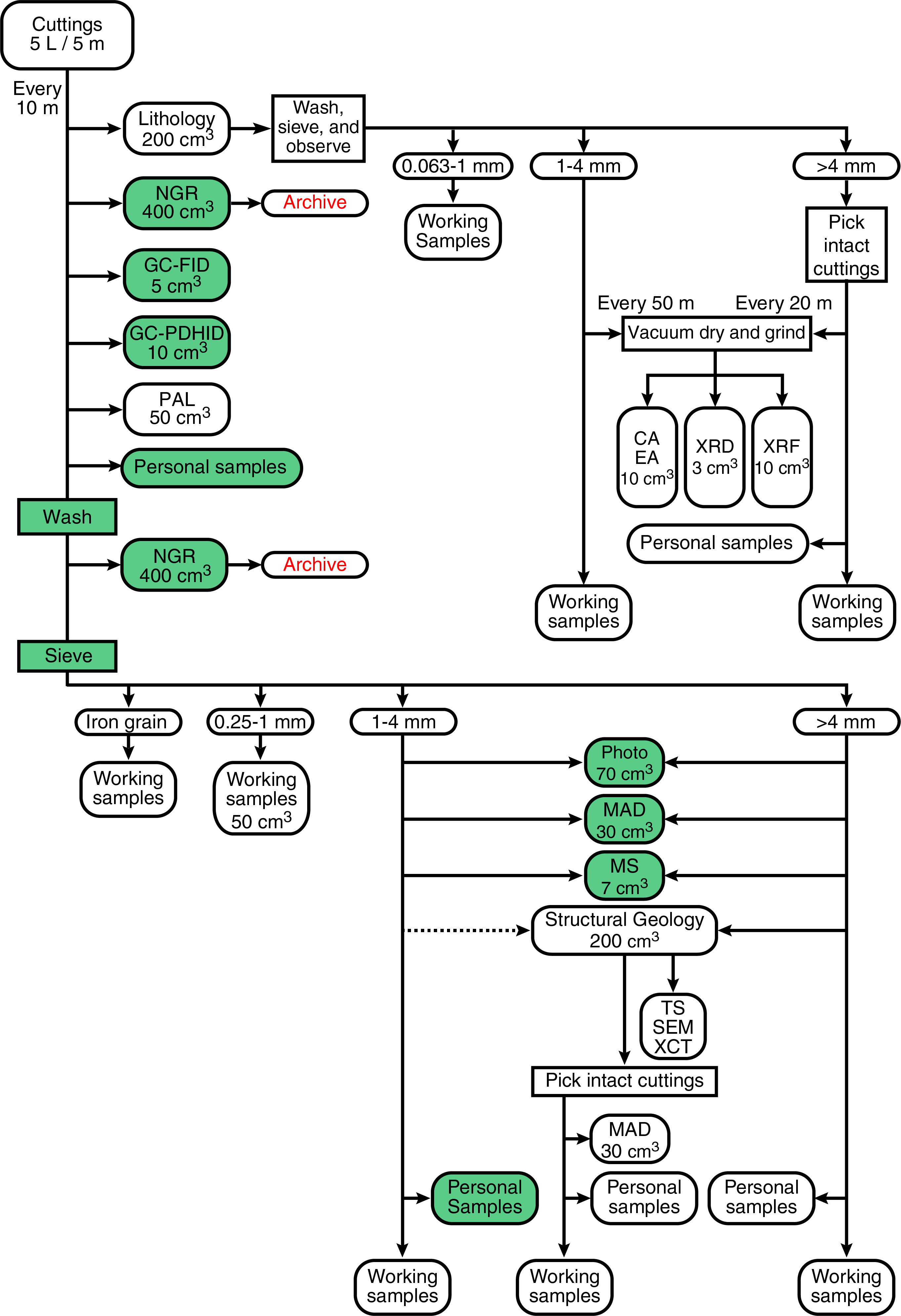
Figure F1. Cuttings analysis flow.
After lithology description and removing iron contaminants originating from drilling tools and casing, aliquots (23 cm3) of >4 mm intact washed cuttings handpicked by the lithology group were vacuum dried and ground for X-ray diffraction (XRD), X-ray fluorescence (XRF), and organic geochemistry analyses (total organic carbon [TOC], total carbon [TC], and total nitrogen [TN]).
The remaining unwashed cuttings were washed gently with seawater in a 250 µm sieve from which a 400 cm3 sample was taken for another NGR measurement for comparison and archiving at the KCC. The remaining gently washed cuttings were further washed and sieved with seawater using 0.25, 1, and 4 mm mesh and separated into size fractions of <1, 1–4, and >4 mm. During sieving, a hand magnet was used to remove iron contaminants. These iron grains and a <1 mm fraction were kept for archiving at the KCC. The 1–4 and >4 mm fractions were then used or taken for the following objectives:
- Both fractions for photographing,
- >4 mm fraction for X-ray computed tomography (CT),
- 200 cm3 from each fraction for structural description and selected cuttings for microscopy-based observations of thin sections,
- 30 cm3 from each fraction and 30 cm3 from intact cuttings after the structure description for bulk moisture and density (MAD) measurements,
- 7 cm3 from each fraction for magnetic susceptibility measurements, and
- Creating a cuttings composite section (CCS) for each hole.
The CCS is designed to create a stratigraphic model using a split core liner. Two CCSs were created from each cuttings fraction for each hole. Each CCS includes 3 cm wide pockets, and each pocket is filled with 50 cm3 of washed cuttings collected every 10 m of drilling advance. Thus, a 150 cm long CCS corresponds to a 500 m drilling interval.
Intact cuttings are considered to represent the formation and were collected by handpicking by each group from washed cuttings. Types of cuttings used for shipboard description and standard measurements are summarized in Table T2.
Drilling mud handling
Drilling mud samples were collected at two locations: mud tanks and the mud return ditch. Sampling was carried out regularly every 2–3 days. Drilling mud samples were used for measuring background and contamination effects for NGR and TOC analysis (see Physical properties and Geochemistry). Additional mud samples were collected once every 12 h (100 mL each) for archiving as reference material.
Mud-gas handling
Mud gas was extracted from drilling mud immediately after the mud returned from the borehole. A constant-volume degasser with a self-cleaning agitator was installed in the mud trough just before the shale shakers, and the gas extracted in the degasser chamber was pumped to the MGML using a PVC tube. Tests comparing the gas extraction volumes and gas species detected showed that there was no difference in position either in the "Gumbo" location in the bypass valve or when placed in the return mud trench before the shakers. Therefore, the degasser unit was moved to the mud return ditch just "upstream" of the shale shakers based primarily on the ease of clearing the mud return trench when compared to the Gumbo location. Analysis in the unit is described in Geochemistry.
Core handling
An 8½ inch SD-RCB coring tool with 7.3 cm inside diameter plastic core liner was used in Hole C0002T. Only minimal core was collected. A 10⅝ inch RCB system and HPCS/EPCS/ESCS was used at Sites C0024 and C0025. Cores from Sites C0024 and C0025 were typically cut into ~1.4 m sections at the core cutting area and logged and labeled by the shipboard curator. Site C0025 cores were preserved for a port call "core description party" to sample and perform shipboard measurements on board Chikyu from 13 to 18 July 2019.
Figure F2 shows the basic core processing flow chart. A small volume (~5–10 cm3) of sample was taken for micropaleontology from the core catcher section. Potential core sections for time-sensitive whole-round (WR) samples for anelastic strain recovery (ASR) were first run through the X-ray CT scanner. Core watchdogs then ensured that the samples could be used and did not contain any evident key features that should be preserved. Once approved, these WR samples were identified as core sections. ASR samples were approximately 10 cm long. All other core sections were taken to the core processing deck for standard X-ray CT scanning and core logging with the whole-round multisensor core logger (MSCL-W).
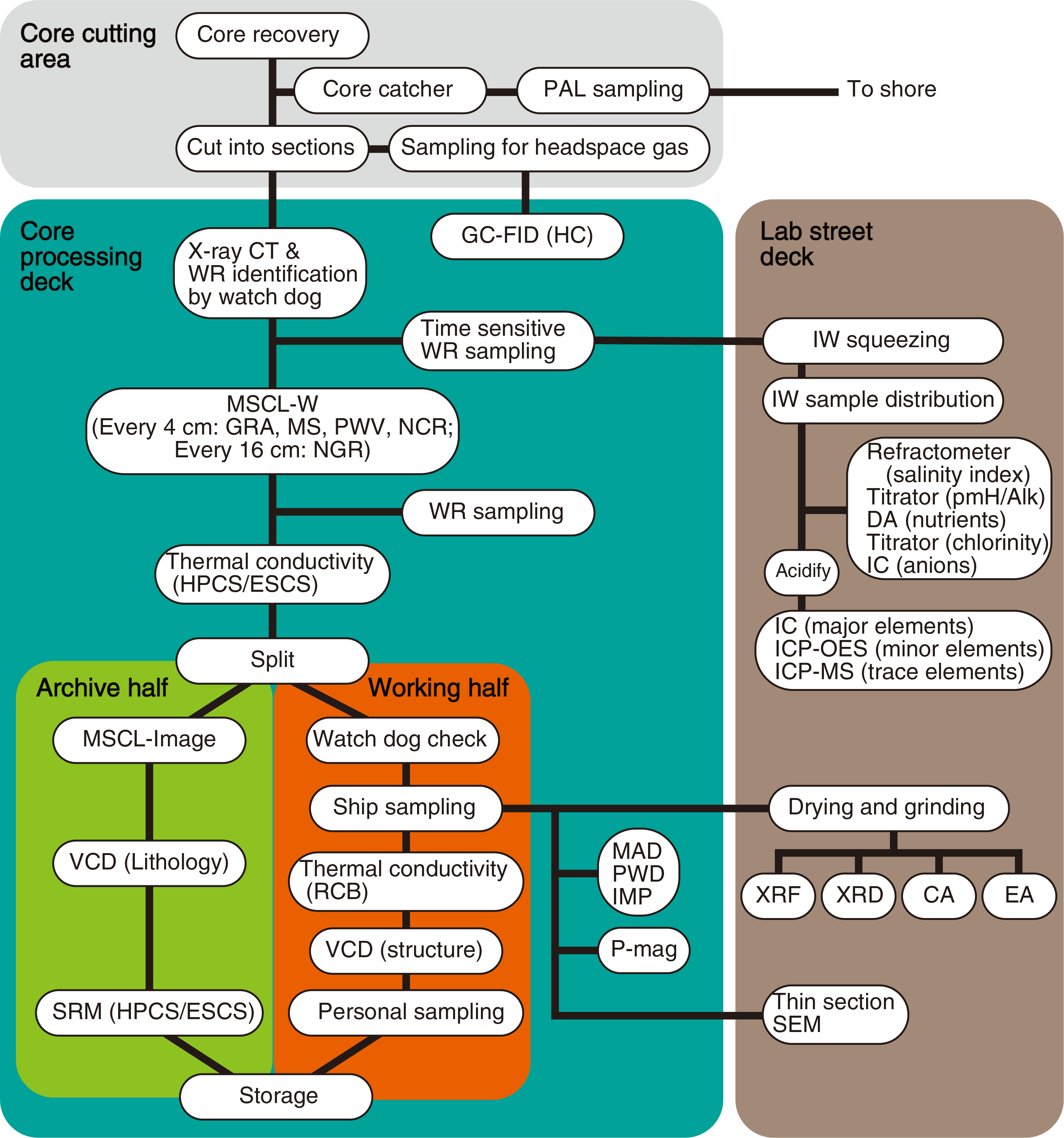
Figure F2. Core analysis flow.
After X-ray CT scanning and MSCL-W logging, community and approved personal WR samples as long as ~20 cm were taken where intact, relatively homogeneous sections could be identified. The number of community WRs was limited by core recovery and core quality. All WRs were stored at 4°C. Adjacent to WR samples (including the time-sensitive, community, and personal WRs), a cluster sample was taken at least once per section. The cluster sample was used for routine MAD, XRD, XRF, carbonate, and nitrogen analyses shipboard. Some cluster samples were used for shore-based research on clay-fraction XRD analysis.
The core sections remaining after WR core sampling were split into working and archive halves. Digital images of archive-half sections were taken with the photo image logger (MSCL-I) before visual core description by sedimentologists. Thermal conductivity measurements were performed on samples from the working halves using the half-space mode and on samples from WRs using the full-space mode. Discrete cubes for P-wave velocity measurement were sampled from the working half. Additional samples were taken for MAD, XRD, XRF, and carbon analyses. After the expedition, all cores were transported under cool temperature for archiving at the KCC.
Authorship of site chapters
The separate sections of the site and methods chapters were written by the following shipboard scientists (authors are listed in alphabetical order):
- Lithology: Underwood (Team Leader), Cornard, Dielforder, Fukuchi, Hamahashi, Jaeger, Sakaguchi, Schleicher, Strasser
- Structural geology: Yamamoto (Team Leader), Dielforder, Dutilleul, Faulkner, John, Otsubo, Regalla, Ujiie
- Biostratigraphy/Paleomagnetism: Matsuoka (Team Leader), Chiyonobu, Kanamatsu
- Geochemistry/Mud gas: Kopf (Team Leader), Hong, Ijiri, Masuda, Sample, Toki, Zhang,
- Physical properties: Sone (Team Leader), Bedford, Jin, Kitamura, Stanislowski
- Downhole: Hamada
- Logging: Moore (Team Leader), Conin, Doan, Guérin, Hamada, Jeppson, Tsuji, Yabe
Lithology
We made macroscopic observations using the archive halves of split cores from Sites C0002 (Hole C0002T) and C0024 and followed standard IODP protocols for visual core description. These data were supplemented by X-ray CT images, smear slide and thin section microscopy, bulk powder XRD, and bulk powder elemental XRF. Depths for core descriptions and samples are on the CSF-B depth scale (Table T1).
We described cuttings from Holes C0002Q–C0002T following methods that were modified from the methodology of previous riser drilling expeditions (Expedition 319 Scientists, 2010b; Strasser et al., 2014a; Tobin et al., 2015a). We made the modifications because most of the cuttings from Expedition 358 are lithified, which enhanced our ability to segregate lithologies. Specific tasks during cuttings analysis included visual (macroscopic) description, observation of X-ray CT images, smear slide and thin section microscopy, bulk powder XRD, and bulk powder elemental XRF. Depths for cuttings are on the MSF depth scale (Table T1), and data are plotted at the base of a given cuttings interval.
Visual core description
We first recorded sedimentologic information for cores on visual core description (VCD) forms on a section-by-section (150 cm) scale (Mazzullo and Graham, 1988). Scanned copies of the VCDs are archived in VCDSCAN in Supplementary material. Data on the VCDs were transferred to section-scale templates using J-CORES software and then converted to core-scale graphical depictions using Strater (Golden Software). Only discrete bed thicknesses >10 cm were entered into the J-CORES database. Repetitive thin interbeds (e.g., silty clay and silt or sand) are depicted with both graphic patterns side by side. The dominant of the two lithologies is shown on the left. We cataloged the base interval and thickness of all discrete event beds (e.g., inferred turbidites and volcanic ash layers) on a separate spreadsheet (see EVENTBED in Supplementary material).
Texture (defined by the relative proportions of sand-, silt-, and clay-sized grains) follows the classification of Shepard (1954). It is difficult to discriminate accurately when a specimen's grain size distribution is close to the 50:50 dividing line between two textural categories (e.g., between silty claystone and clayey siltstone) without quantitative grain size analysis. Therefore, that entire range of textures (i.e., silty claystone to clayey siltstone) is usually described in the site reports as "silty clay(stone)" for simplicity. The classification scheme for siliciclastic lithologies follows Mazzullo et al. (1988). Volcaniclastic and pyroclastic lithologies were divided only on the basis of their texture (ash, lapilli, etc.) rather than by proportions of clast type (e.g., glass shards, volcanic rock fragments, and primary crystals). Contacts between interbedded lithologies were described as sharp, erosional, or gradational. Categories of core disturbance for unconsolidated sediment include slightly disturbed, moderately disturbed, heavily disturbed, soupy, and gas expansion. Categories of drilling-induced core disturbance for lithified sedimentary rock include biscuit, slightly fractured, moderately fractured, highly fractured, and drilling brecciated.
Except for Hole C0002T, we used the same graphic patterns for unconsolidated and indurated examples of the same lithologies (Figure F3). For Hole C0002T, the lithology patterns for core are the same as the patterns for cuttings. As an operational guide, lithologies recovered by the HPCS are "unconsolidated" sediment (e.g., silty clay or volcanic ash), whereas the same lithologies recovered by the RCB system are "lithified" sedimentary rocks (e.g., silty claystone or tuff). The graphic lithology column on each VCD plots to scale only beds that are thicker than 10 cm. Thinner interbeds (e.g., silty clay and silt) are depicted using composite graphic patterns. VCDs also include symbols for common internal sedimentary structures (e.g., normal grading, planar lamination, cross-lamination, etc.), soft-sediment deformation, severity of core disturbance, and intensity of bioturbation (slight, moderate, or heavy).
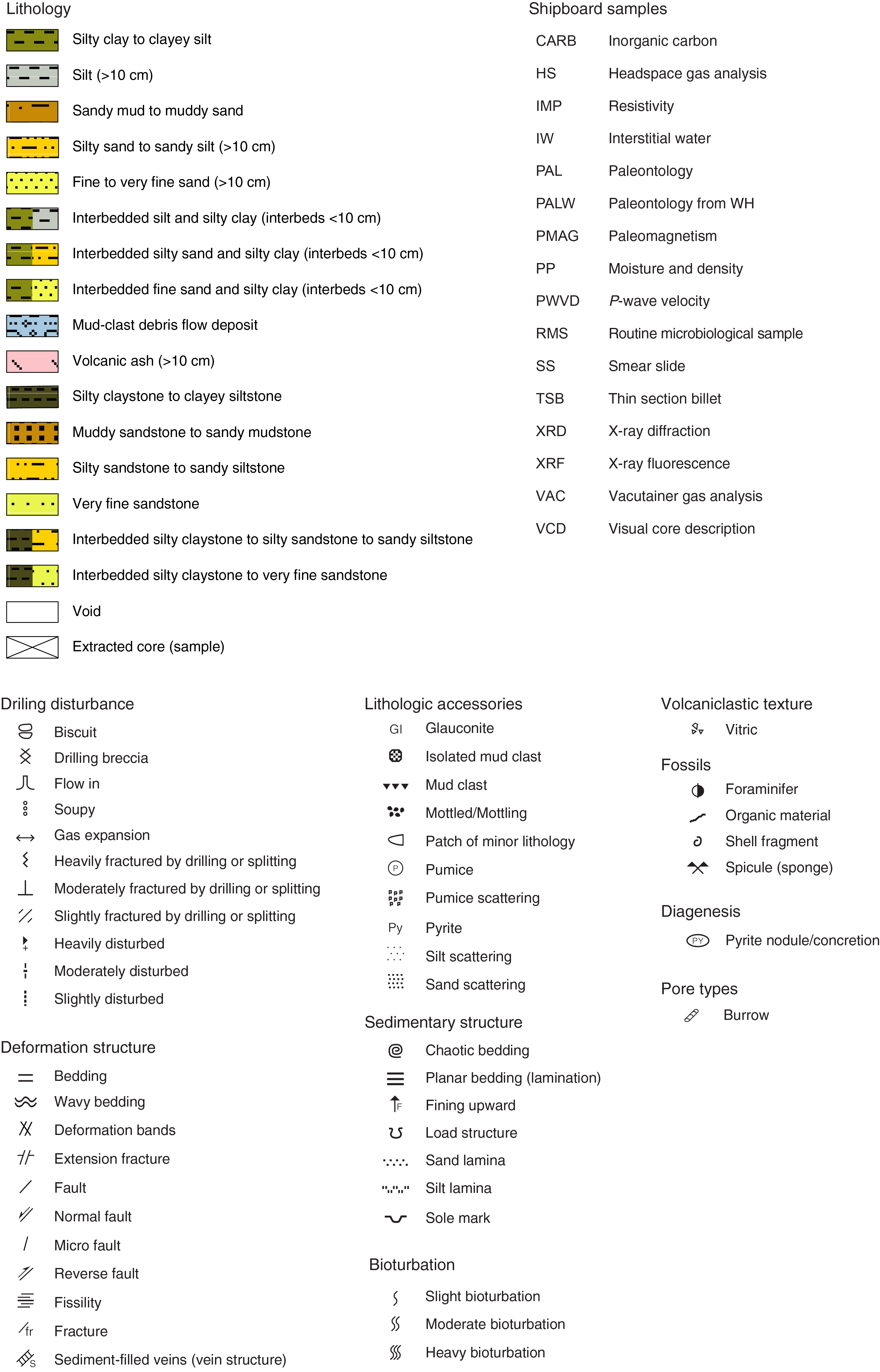
Figure F3. Graphic patterns and symbols for visual descriptions of cores.
Macroscopic observations of cuttings
Cuttings typically occur as small fragments of sedimentary rock ranging from 0.25 to 8 mm in size. Cuttings were routinely collected from the shale shaker at 5 m intervals, and samples were selected for detailed description every 10 m. Sample processing started with a 100–200 cm3 aliquot of bulk cuttings that was separated by wet sieving into four size fractions (>4 mm, 1–4 mm, 63–125 µm, and <63 µm). Solid fragments from the formation are usually coated in drilling mud and mixed with clay-bearing drilling additives (e.g., bentonite). Most of the drilling mud can be removed by washing gently with seawater for 30–60 s, but separation is not always complete, especially with soft cuttings. This artifact hampers quantification of the true clay mineral content and may cause chemical contamination (see X-ray fluorescence).
Descriptive information recorded for each cuttings VCD includes lithology, color, induration (soft, semilithified, hard, or loose), shape (angular, subangular, round, or platy), texture (crumbly, sticky, or fissile), sedimentary structures (lamination or size grading), organic matter (wood fragments or lignite), and fossils (Figure F4). We segregated the different lithologies according to the siliciclastic classification scheme of Mazzullo et al. (1988) and counted their proportions in a population of 200 fragments. The four common categories of lithology are fine silty claystone, silty claystone, siltstone, and very fine sandstone. All of the macroscopic observations were recorded on VCD forms and summarized in VCDSCAN in Supplementary material. Photographs of all cuttings samples, partitioned into the four common lithology categories (Figure F5), are also available in CUTTINGS in Supplementary material. To evaluate reproducibility of the modified methods (compared to Expeditions 338 and 348), we reprocessed some samples from the lower part of Hole C0002P (2600–2985 mbsf). Those tests showed no systematic artifacts or biases.
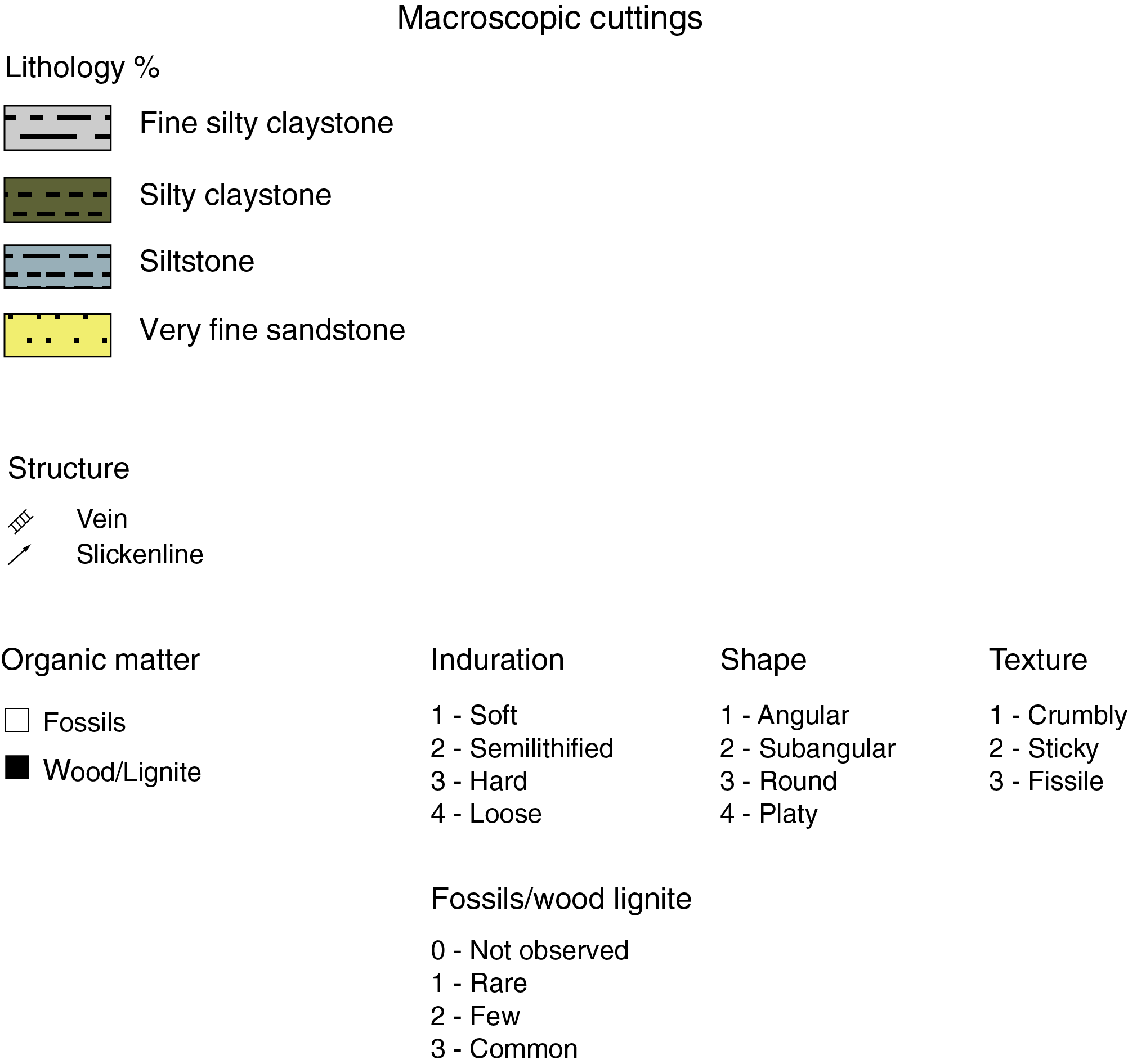
Figure F4. Graphic patterns and symbols for visual descriptions of cuttings.

Figure F5. Cuttings segregated by lithology.
Identification of cement (concrete) cuttings
Unfortunately, ambiguity exists in visual discrimination between artificial cement (concrete) cuttings and some types of fragments from the formation (Figure F6). Cement cuttings are most likely mistaken for coarse siltstone or sandstone. Compared to natural sedimentary rocks, however, framework grains in cement cuttings consistently fall within a narrower range of sizes (coarse silt to sand) and grain sorting is significantly better. Confirmation by XRD shows typical cement phases (e.g., alite, belite, and portlandite), and XRF verifies high concentrations of CaO. However, these tools are not practical to use on a routine basis, so some judgment is still required during visual analysis of cuttings.
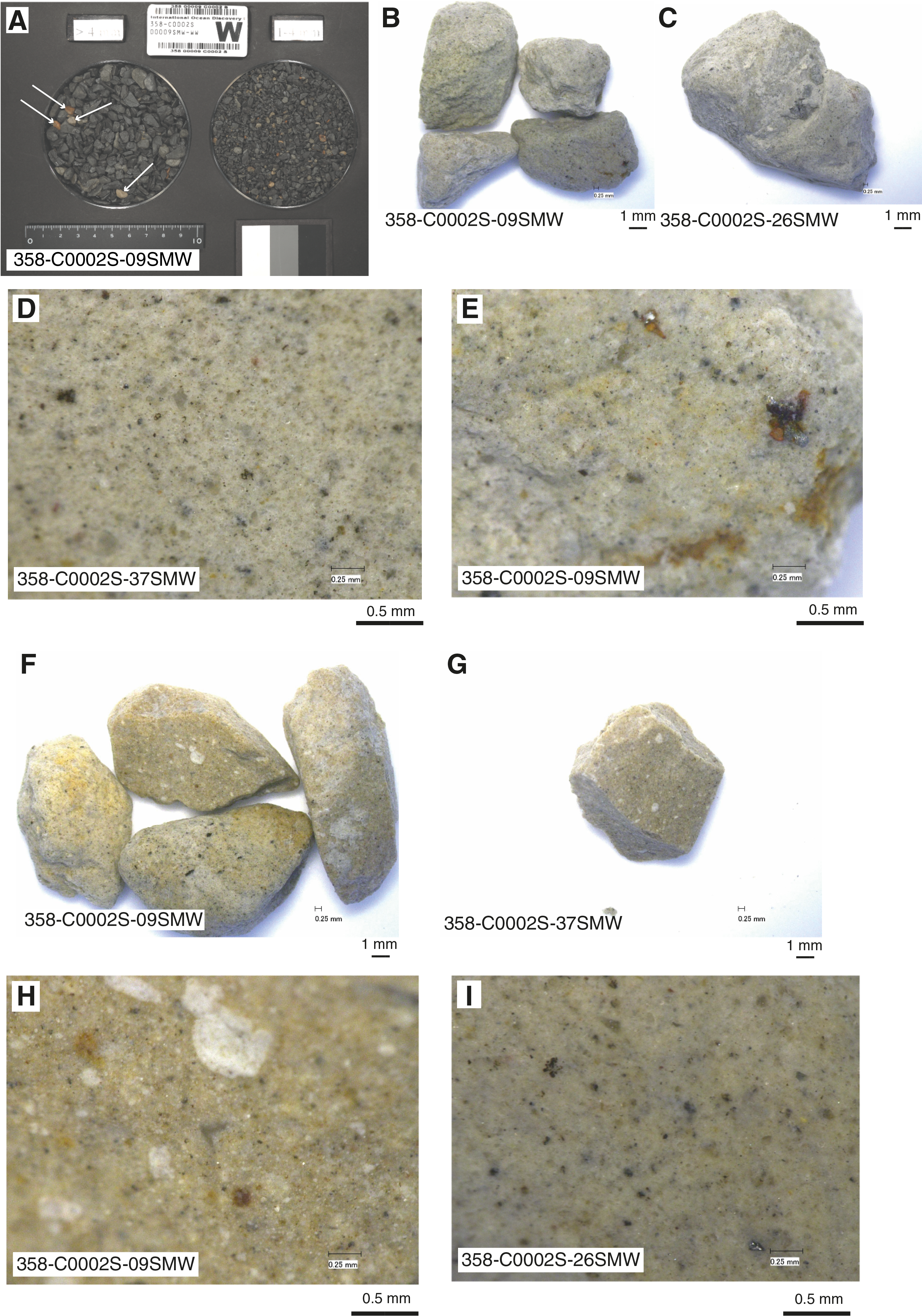
Figure F6. Cement/concrete examples.
After closer examination, we recognized two confirmed types of cement (concrete) cuttings during Expedition 358. Type 1 cuttings are gray in color and subangular in shape (Figure F6). Some of the Type 1 cuttings envelop lithified fragments of silty claystone. Crystalline matrix content is usually >70%, and its color varies from light gray to yellow. The fabric is matrix-supported. Crystals in the binding agent are not visible at 100× magnification under a binocular microscope. Approximately 10% of the constituents in Type 1 concrete fragments are dark-colored, subangular silt- and sand-sized minerals, and roughly 10% consist of transparent to light gray or yellow silt grains. Scattered reddish grains coexist with the subangular black minerals. The overall texture has a salt-and-pepper appearance. Yellow material (probable drilling mud) also occurs as an infilling to small depressions.
Type 2 cement (concrete) cuttings are yellow to light orange with shapes ranging from subangular to well rounded (Figure F6). Crystalline matrix content ranges from 50% to 80% of the mass, and its color is lighter with a yellow to orange tint. The fabric is matrix-supported. Silt-sized minerals are dominant and compose ~15% of the cuttings. Well-rounded to subangular black minerals and angular yellow to brown minerals are the main silt-sized components. Sand grains are milky white (probable quartz) and well rounded. Scattered reddish silt grains are the only sign of oxidation.
Smear slide and thin section petrography
Smear slides are very useful for routine identification of sediment texture and composition. The method is effective for petrographic examination of soft and semi-indurated sediments when disaggregation can be achieved using a toothpick or spatula (Marsaglia et al., 2013). Thin sections are more suitable than smear slides for examining lithified sedimentary rocks.
The sample location for each smear slide was entered into the J-CORES database with a sample code of SS. We examined the smear slides in transmitted and cross-polarized light using an Axioskop 40A polarizing microscope (Carl Zeiss) equipped with a Nikon DS-Fi1 digital camera. Abundances of biogenic, volcaniclastic, and siliciclastic constituents were estimated using a visual comparison chart (Rothwell, 1989). For cores, estimates of sand-, silt-, and clay-sized percentages were entered into the J-CORES samples database along with abundance ranges for the identifiable grain types. Results from visual estimates are grouped into the following range categories:
- D = dominant (>50%).
- A = abundant (>10%–50%).
- C = common (>1%–10%).
- F = few (0.1%–1%).
- R = rare (<0.1%).
The proportions of major components (clay minerals, quartz, and feldspar) were also validated by XRD (see X-ray diffraction), and the absolute weight percent of carbonate was verified by coulometric analysis (see Geochemistry). Photomicrographs and scanned smear slide forms are presented in SMEARSLD in Supplementary material.
Individual cuttings pieces were chosen for smear slide production based on the dominant lithology identified in a given interval, with a spacing of 20 m, and the slides were produced by scraping off the surface of a representative fragment with a spatula. Sometimes an additional smear slide was made for a distinctive minor lithology. The errors in visual estimates for cuttings are larger than for softer sediments because harder rock fragments do not disaggregate completely.
To improve petrographic accuracy for lithified sedimentary rocks, thin sections were produced from cuttings of the dominant lithology every 20–40 m. Minor lithologies were picked every 50 m. The cuttings were first freeze-dried and impregnated under a vacuum (Epovac) with epoxy (Epofix) prior to mounting. Multiple cuttings fragments were attached to a glass slide with Petropoxy 154, and the thin section was prepared as a 0.03 mm thick slice. Before microscopic observation, some thin sections were covered by a cover glass using index oil. Thin sections were observed and analyzed for mode composition analysis using an Axio Imager Alm POL-2 polarized microscope (Carl Zeiss).
Figure F7 shows a comparison between visual estimates for different lithologies in cuttings using smear slides and thin sections. The differences are small. For more quantitative point counts, we used a microscope equipped with a Micro Topper automatic sample stage and Medical Imaging Toolkit (MITO) software. Point counts of grain size and mineralogy (or rock-fragment type) were completed on 200 points per sample using an automated step size of 300 µm. Based on that population size, the estimated error for normalized relative percentages of particle size (clay, silt, and sand) and composition (10 constituent categories) is 6.8%. Minor occurrences were noted as "rare" on the description sheet. Thin section photomicrographs and scanned description sheets are included in THINSECT in Supplementary material.
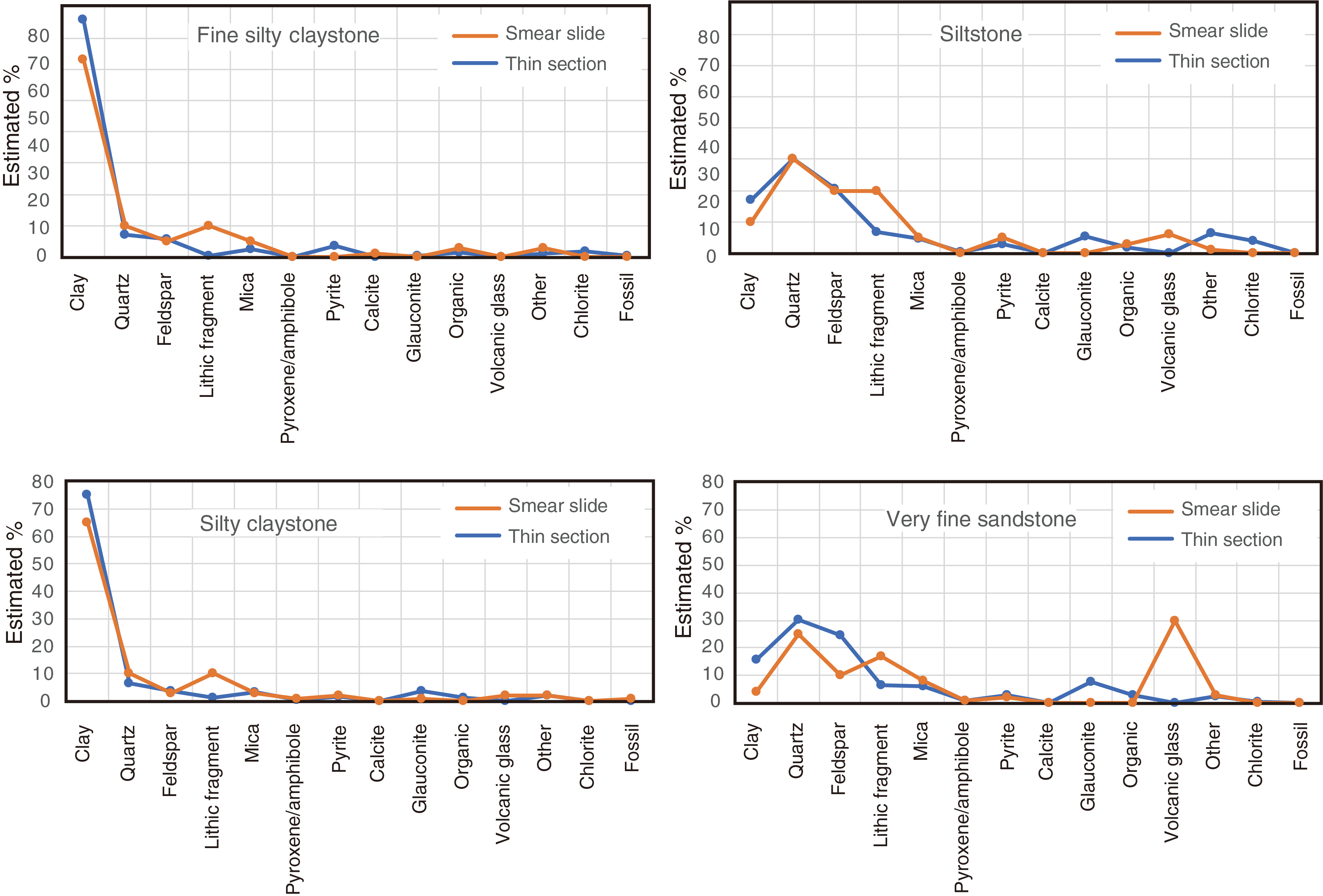
Figure F7. Mineral composition for different lithologies.
X-ray diffraction
The principal goal of XRD analysis during Expedition 358 was to estimate the relative weight percentages of total clay minerals, quartz, feldspar, and calcite in both cuttings and core samples. Most of the specimens from cores were positioned in "clusters" next to WR sample intervals (e.g., for interstitial water [IW] and personal WRs). For cuttings, XRD specimens were selected from 3 cm3 samples of the bulk cuttings using two size fractions. Bulk mix cuttings (1–4 mm) were picked every 50 m. The dominant lithology was handpicked from intact cuttings of the >4 mm size fraction every 20 m. For comparison, measurements were also made on handpicked samples from minor lithologies (siltstone and fine sandstone) every 100 m. All samples were washed in an ultrasonic bath to remove drilling mud, freeze-dried, crushed for 5 min with a ball mill, and mounted as randomly oriented powders.
The randomly oriented bulk powders were analyzed using a PANalytical CubiX3 (PW3800) diffractometer. The scanning parameters were set as follows:
- Generator = 45 kV.
- Current = 40 mA.
- Tube anode = Cu.
- Wavelength = 1.54060 Å (Kα1) and 1.54443 Å (Kα2).
- Step spacing = 0.005°2θ.
- Scan step time = 0.635 s.
- Divergent slit = 0.25°.
- Irradiated length = 10 mm.
- Scanning range = 2°–60°2θ.
- Spinning = yes.
To maintain as much consistency as possible with previous Nankai Trough Seismogenic Zone Experiment (NanTroSEIZE) results, we used MacDiff 4.2.5 software to process the digital XRD data (http://www.ccp14.ac.uk/ccp/ccp14/ftp-mirror/krumm/Software/macintosh/macdiff/MacDiff.html). Data reduction included creating a smooth baseline, smoothing counts, and shifting peak positions using the stable quartz (101) reflection for reference. Before determining peak area values, we also adjusted the upper and lower limit for each diagnostic peak following the guidelines shown in Table T3.
Calculations of relative mineral abundance utilized a matrix of normalization factors derived by singular value decomposition (SVD). The guiding principle is that X-ray counts for any particular mineral will depend not only on the abundance of that mineral but also on the abundances of other minerals in the mix (Fisher and Underwood, 1995). Calibration of SVD factors requires analysis of mineral standards using mixtures with known weight percentages; to be reliable, the mixtures must be close matches to the natural sediments of interest. We analyzed 13 bulk powder mixtures representative of deposits in the Nankai Trough study area (Table T4), as first reported by Underwood et al. (2003): quartz (Saint Peter sandstone), feldspar (Ca-rich albite), calcite (Cyprus chalk), smectite (Ca-montmorillonite), illite (Clay Mineral Society IMt-2, 2M1 polytype), and chlorite (Clay Mineral Society CCa-2). Refinements to corrections for impurities in the illite and calcite standards were based on iterative analyses completed at New Mexico Tech (USA). Figure F8 shows diffractograms for three of the mixtures along with designations of the diagnostic peaks. The new matrix of SVD factors (Table T5) was computed using average peak area values (total counts) for the four diagnostic peaks after the standards were rerun three times (Table T4).
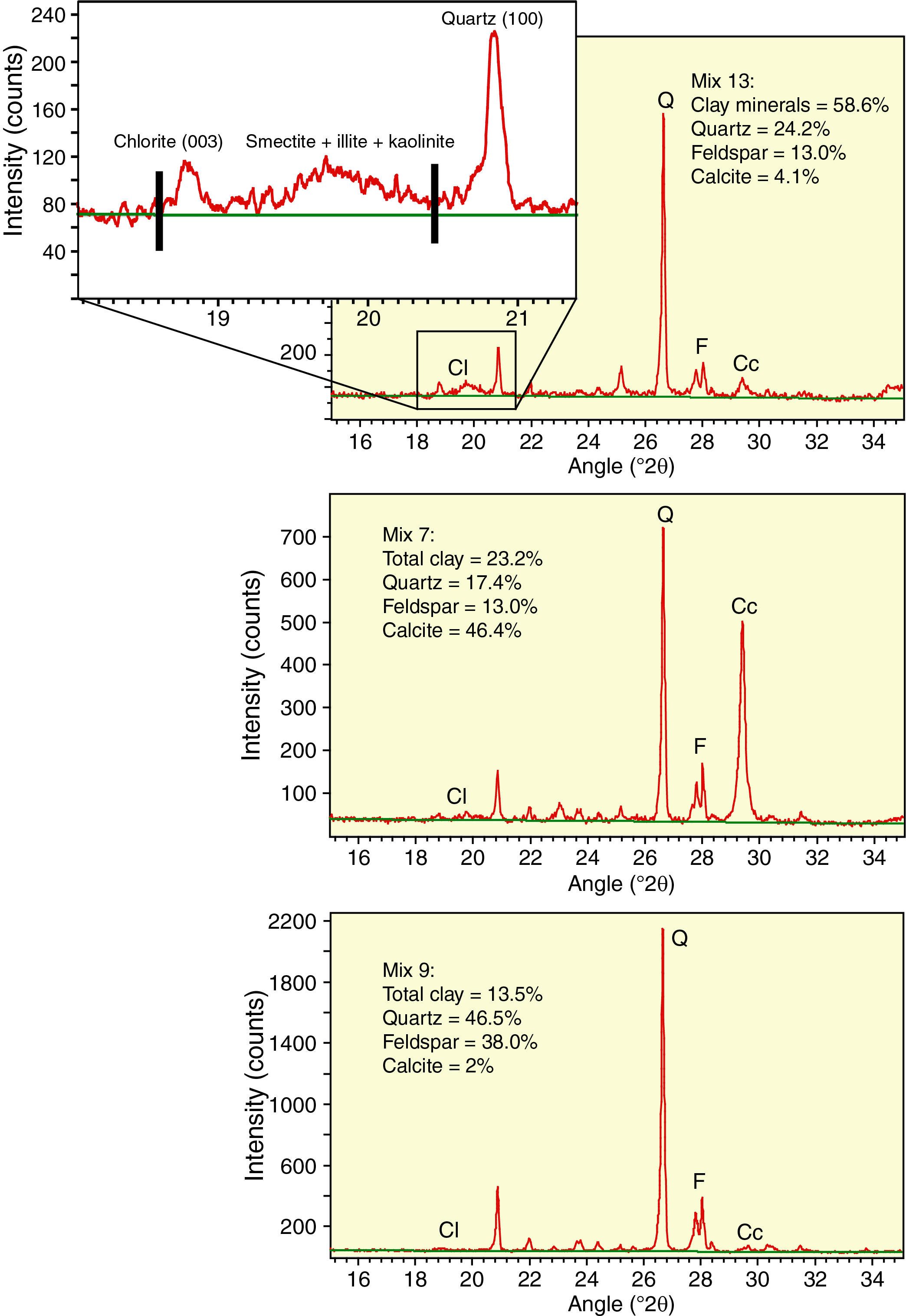
Figure F8. Random bulk powder X-ray diffractograms.
Average errors (SVD-derived weight percent versus true weight percent) for the standard mineral mixtures are small (Table T4):
Despite its precision with the standard mixtures, the SVD method remains semiquantitative for a variety of reasons. Assessments of precision (reproducibility) with previous results from NanTroSEIZE expeditions, for example, need to consider the influences of replacing the X-ray diffractometer on Chikyu prior to Expedition 358, X-ray tube fatigue (which results in systematically lower peak intensities), use of different sets of SVD normalization factors, and operator bias.
Several additional details contribute to inaccuracy. As with any bulk powder XRD method, peak response differs between poorly crystalline minerals at low diffraction angles (e.g., clay minerals) and highly crystalline minerals at higher diffraction angles (e.g., quartz and plagioclase). To determine abundance for the total clay mineral assemblage, one option is to measure one peak for each mineral and add the estimates together (thereby propagating the error). That error is enlarged further by overlap between the smectite (001) and chlorite (001) peaks. Instead, our preferred method is to measure a single composite peak that spans from approximately 18.6° to 20.4°2θ (Figure F8). That range of angles captures the counts from all of the common clay minerals, including the chlorite (003) peak. Additional sources of error include unaccounted for impurities in the mineral standards and inconsistencies in crystallinity between standards and natural minerals as burial depths and diagenesis increase. For cuttings, drilling mud contamination is also possible. Another glitch arises in computations when quantities of calcite are zero or barely above the XRD detection limit (~1.5 wt%). The use of negative SVD normalization factors (Table T5) then translates into negative values of absolute weight percent for calcite. In such cases, we adopted a value of 0.1 wt% as a proxy for "trace."
For the specimens analyzed during Expedition 358, calculated mineral abundances should be regarded as nothing more than relative percentages within a four-component system of total clay minerals (smectite, illite, chlorite, and kaolinite) + quartz + feldspar (plagioclase and K-feldspar) + calcite. We tabulated the "absolute" SVD-derived abundances on spreadsheets, but weight percent values have been normalized to 100% for graphical plots. Larger discrepancies between the absolute and normalized abundances indicate larger mismatches between the standard mineral mixtures and natural specimens. Such differences, however, provide a useful measure of the total amount of all other minerals (e.g., pyroxene, halite, and pyrite) and amorphous solids (e.g., biogenic silica and volcanic glass) within the total solids. For most natural samples, those differences add up to between 5% and 10%.
X-ray fluorescence
XRF spectrometry was performed to quantify major element abundances in cuttings and core samples. As for XRD analysis, most of the specimens from cores were positioned in clusters next to WR sample intervals (e.g., for IW and personal WRs). For cuttings, these analyses were conducted on 10 cm3 samples of the dominant lithology handpicked from intact cuttings of the > 4 mm size fraction every 20 m. Bulk mix cuttings were analyzed every 50 m. Additionally, measurements were also made on samples from minor lithologies (siltstones, sandstone, and tuff) every 100 m or upon prominent occurrence. All samples were first washed in an ultrasonic bath to remove drilling mud, vacuum-dried, and crushed with a ball mill.
Major elements in bulk sediment samples were measured on fused glass beads and reported as weight percent oxide proportions (Na2O, MgO, Al2O3, SiO2, P2O5, K2O, CaO, TiO2, MnO, and Fe2O3). An aliquot of 0.9 g of ignited sample powder was fused with 4.5 g of SmeltA12 flux for 7 min at 1150°C to create glass beads. Loss on ignition was measured using weight changes on heating at 105°C for 1 h and then at 1000°C for 3 h. Analyses were performed on a wavelength-dispersive XRF spectrometer Supermini (Rigaku) equipped with a 200 W Pd anode X-ray tube at 50 kV and 4 mA. Analytical details and measuring conditions for each component are given in Table T6. Starting with specimens from Hole C0002R, the analyses were performed without spinning the sample mounting table; QA/QC analyses on standards reveal no effects on the reported results. Rock standards of the National Institute of Advanced Industrial Science and Technology (Geological Survey of Japan) were used as the reference materials for quantitative analysis. Table T7 lists the results for selected standard samples. A calibration curve was created with matrix corrections provided by the operating software using the average content of each component.
Designation of lithologic units
Following conventional IODP strategies, divisions among lithologic units, subunits, and their boundaries are based mostly on macroscopic and microscopic attributes at the facies scale (e.g., ratio of dominant to minor lithologies, composition of minor lithologies, ranges of bed thickness, and inferred processes of deposition). We also considered XRD and XRF data together with LWD and physical property data (see Logging and Physical properties). Contrasts in grain density and porosity are relevant because they tend to change consistently with grain size and mineralogy. For cuttings, however, caveats need to be applied when discriminating between true formation variations and mechanical artifacts caused by preferential preservation of more resistant versus less resistant lithologies, differences in cutting tools among BHAs, drilling parameters, types of drill bits, changes in drilling mud composition, and pumping of cement into the borehole.
Structural geology
During Expedition 358, two types of sample material were used for structural geology analyses: cuttings (>4 and 1–4 mm size fractions) and cores. Cuttings were sampled during riser drilling at 10 m intervals between 2887.3 and 3262.5 mbsf in Hole C0002Q, between 2789.5 and 3084.5 mbsf in Hole C0002R, between 2842.5 and 2933.5 mbsf in Hole C0002S, and between 2817.5 and 2848.5 mbsf in Hole C0002T. Cores were recovered from 2836.5 to 2843.8 mbsf in Hole C0002T, between 0 and 319.5 mbsf and between 510 and 621.5 mbsf at Site C0024, and between 400 and 580.5 mbsf at Site C0025 (see Table T1 for depth scales). The methods used to document the structural geology data of Expedition 358 cores and cuttings are largely based on those used by the Integrated Ocean Drilling Program Expedition 315, 319, 338, 343, and 348 structural geologists (Expedition 315 Scientists, 2009a; Expedition 319 Scientists, 2010b; Expedition 343/343T Scientists, 2013; Strasser et al., 2014a; Tobin et al., 2015a).
Description and data collection
Cuttings
Structural descriptions were made on sieved and washed (see cuttings workflow in Figure F1) cuttings collected at 20 m intervals at 2887.3–3262.5 mbsf in Hole C0002Q, 2789.5–3082.5 mbsf in Hole C0002R, 2842.5–2933.5 mbsf in Hole C0002S, and 2817.5–2848.5 mbsf in Hole C0002T, as well as on cuttings collected at <20 m intervals for regions of interest (e.g., fault zones and the first occurrence of a specific structure). Cuttings from each bag were sieved using a stack of 4 mm and 1 mm mesh sieves and washed thoroughly with seawater for several minutes on the core processing deck to reduce the amount of drilling-induced cohesive aggregate (DICA) and pillowed cuttings. The cuttings samples were then sonicated in seawater for 3 min to remove drilling mud adhered to cuttings clasts. Subsequent washing and sieving continued until the large majority of the drilling mud, pillowed cuttings, and DICAs were removed. Sieving with 4 and 1 mm meshes allowed extraction of both >4 and 1–4 mm sized intact cuttings for structural analysis. In some samples collected during Expedition 348, >50% of the total initial cuttings disaggregated entirely. This potentially induced a bias toward more indurated rock types (silty sandstone and siltstone) in less consolidated deposits. However, at the depths drilled during Expedition 358, this bias is less of a concern.
A subset of ~100–600 grains from each cuttings bag was selected for visual description under a binocular or digital microscope. For each >4 and 1–4 mm sample, we noted the occurrence of bedding, carbonate, pyrite and/or quartz veins, slickenlined surfaces (or slickensides), cataclastic bands, deformation bands (Maltman et al., 1993), web structures (Byrne, 1984), and scaly fabric (Moore et al., 1986). We also noted the occurrence of open fractures, fresh drilling-induced striae, or other drilling-induced structures and the occurrence of thin or flat splintery cuttings that may actually be caving indicative of borehole breakouts. Exceptional examples of other features recovered in the cuttings were picked and saved (well-preserved fossils, etc.). A tally of the number of deformation features by type and host lithology was compiled in an Excel spreadsheet, and percent abundance of each feature was calculated for each depth interval (Figure F9). Thin sections were made and observed under the optical microscope and scanning electron microscope (SEM) to describe representative or particularly interesting structural elements.

Figure F9. Structural geology observation sheet for cuttings.
Following visual description, X-ray CT scanning (see X-ray computed tomography) was performed on both the described subset of >4 mm cuttings and bulk undescribed 1–4 mm cuttings. Cuttings from the >4 mm subset were divided into separate bags labeled (a) veins, (b) striae/scaly fabric, (c) no deformation, or (d) other, and cuttings from the 1–4 mm samples were labeled (e) not described. In addition, as many as three individual cuttings with interesting deformation features were bagged separately and labeled 1–3. These bags were placed in the X-ray CT scanner in order 1–3 and a–e. X-ray CT scans were used to examine the 3-D geometry of observed deformation features, especially veins and fault fabrics, to identify other deformational features internal to cuttings that may not have been observed during visual description, and to preserve a digital archive of cuttings samples.
Cores
Structures preserved in the cores were documented on split cores (working half) and on X-ray CT images of unsplit cores (see X-ray computed tomography). Observations on split cores were entered on the structural geology observation sheet by hand (Figure F10) and then transferred to a calculation sheet and the J-CORES database (see Data processing). Core observations and measurements followed procedures of previous Ocean Drilling Program (ODP) and Integrated Ocean Drilling Program expeditions in the Nankai and Costa Rica subduction zones (e.g., ODP Legs 131, 170, and 190 and Integrated Ocean Drilling Program Expeditions 315, 316, 319, 322, 333, 334, 338, 343, and 348). We measured the orientations of all structures observed in cores using a modified plastic protractor (Figure F11) and noted the measurements on the structural geology observation sheet with descriptions and sketches of structures. The orientations of planar or linear features in cores were defined with respect to the core reference frame, for which the core axis is defined as "vertical" and the double line marked on the working half of the core liner is arbitrarily called "north," 0° or 360° (Figure F12; in unoriented core, this does not correspond to true north) following techniques developed during Leg 131 (Shipboard Scientific Party, 1991) and later refined during NanTroSEIZE expeditions on Chikyu (Expedition 315 Scientists, 2009a; Expedition 316 Scientists, 2009; Expedition 319 Scientists, 2010b; Expedition 322 Scientists, 2010; Expedition 333 Scientists, 2012; Expedition Scientists 343/343T Scientists, 2013; Strasser et al., 2014a; Tobin et al., 2015a).
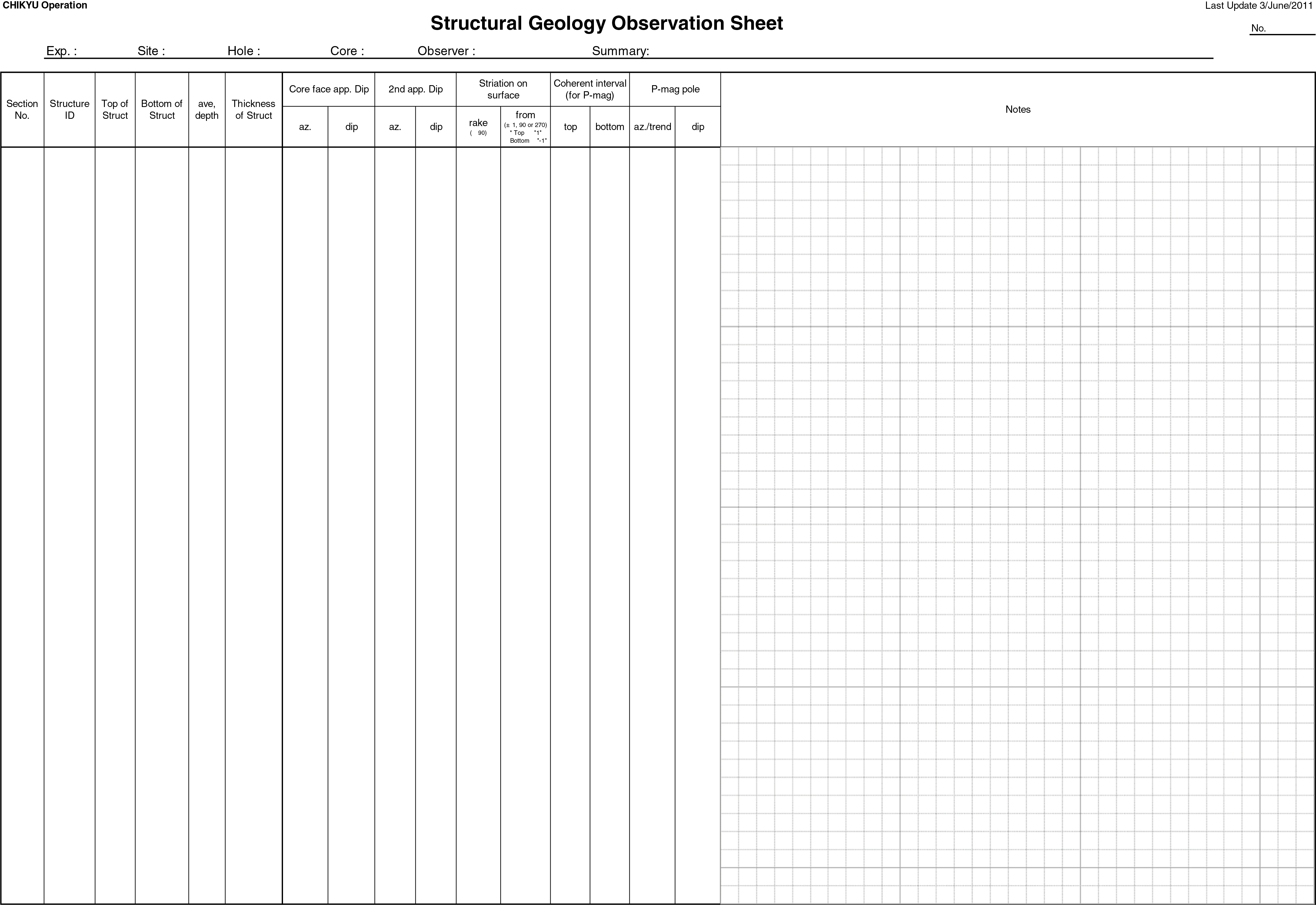
Figure F10. Structural geology observation sheet for working halves.
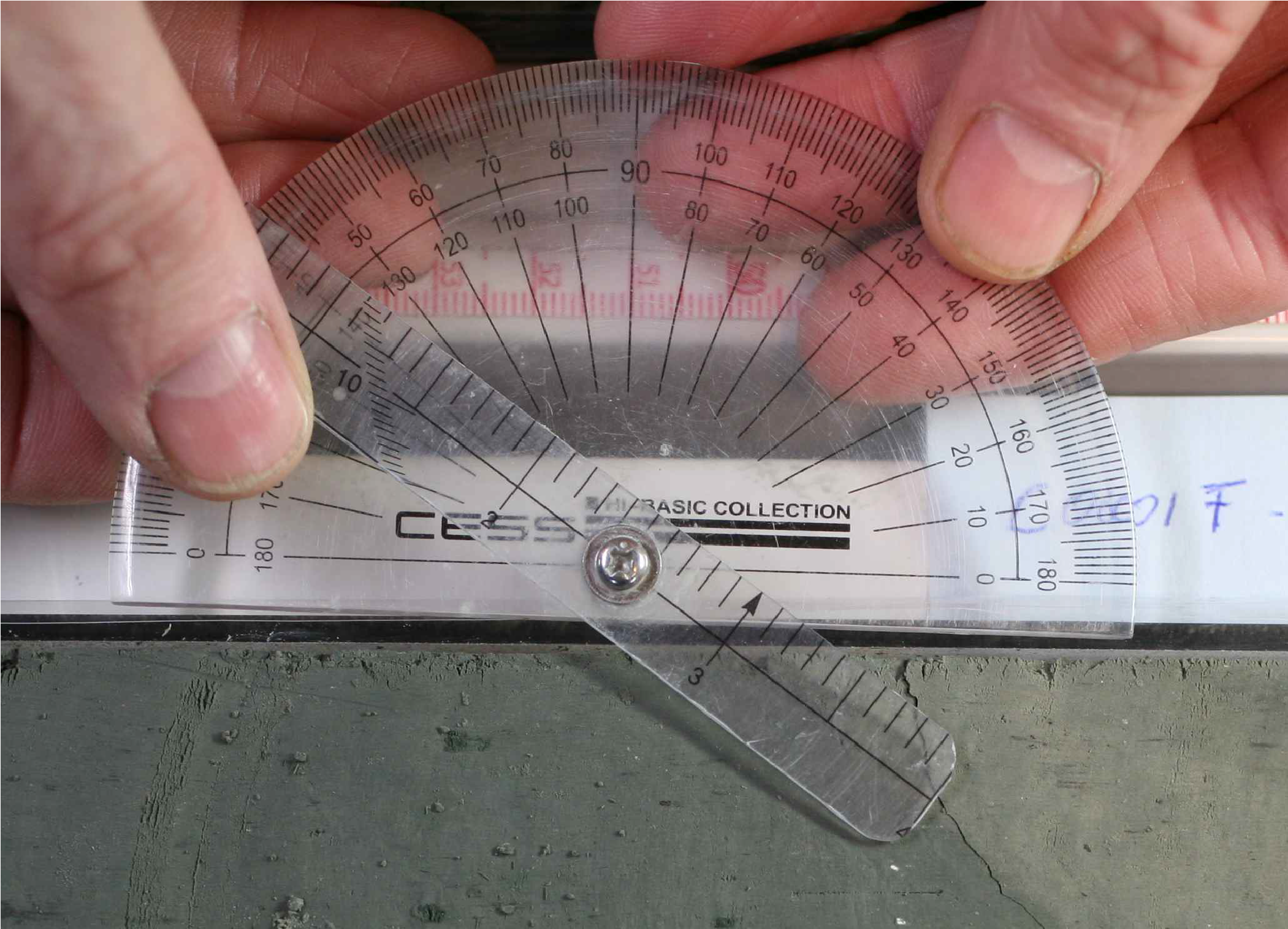
Figure F11. Modified protractor.
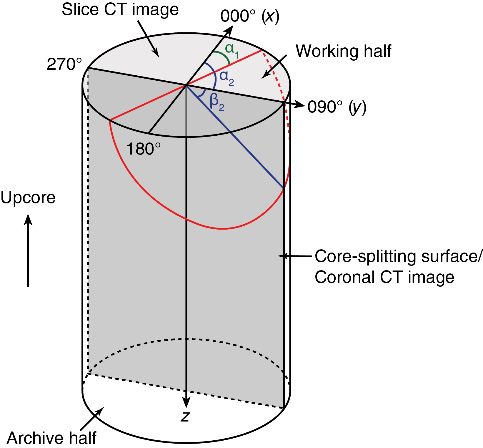
Figure F12. Core reference frame.
To determine the orientations of planes in the core reference frame (Figure F12), the apparent dip angle of any planar feature was measured in two independent sections parallel to the core axis (Figure F13A), and the true strike and dip in the core reference frame were determined using a calculation sheet (see Data processing). In practice, one section is typically the split surface of the core, on which the trace of the plane has a bearing (α1) and a plunge angle (β1). α1 is either 90° or 270°. The other section is typically a cut or fractured surface at a high angle to the split core surface, on which the bearing (α2) and plunge angle (β2) of the trace of the plane are measured. In the case where the second measurement surface is perpendicular to the core split surface, bearing α2 is either 0° or 180° (Figure F13A). Both β1 and β2 are between 0° and 90°. Similar measurements were made for planar features visible in X-ray CT images.
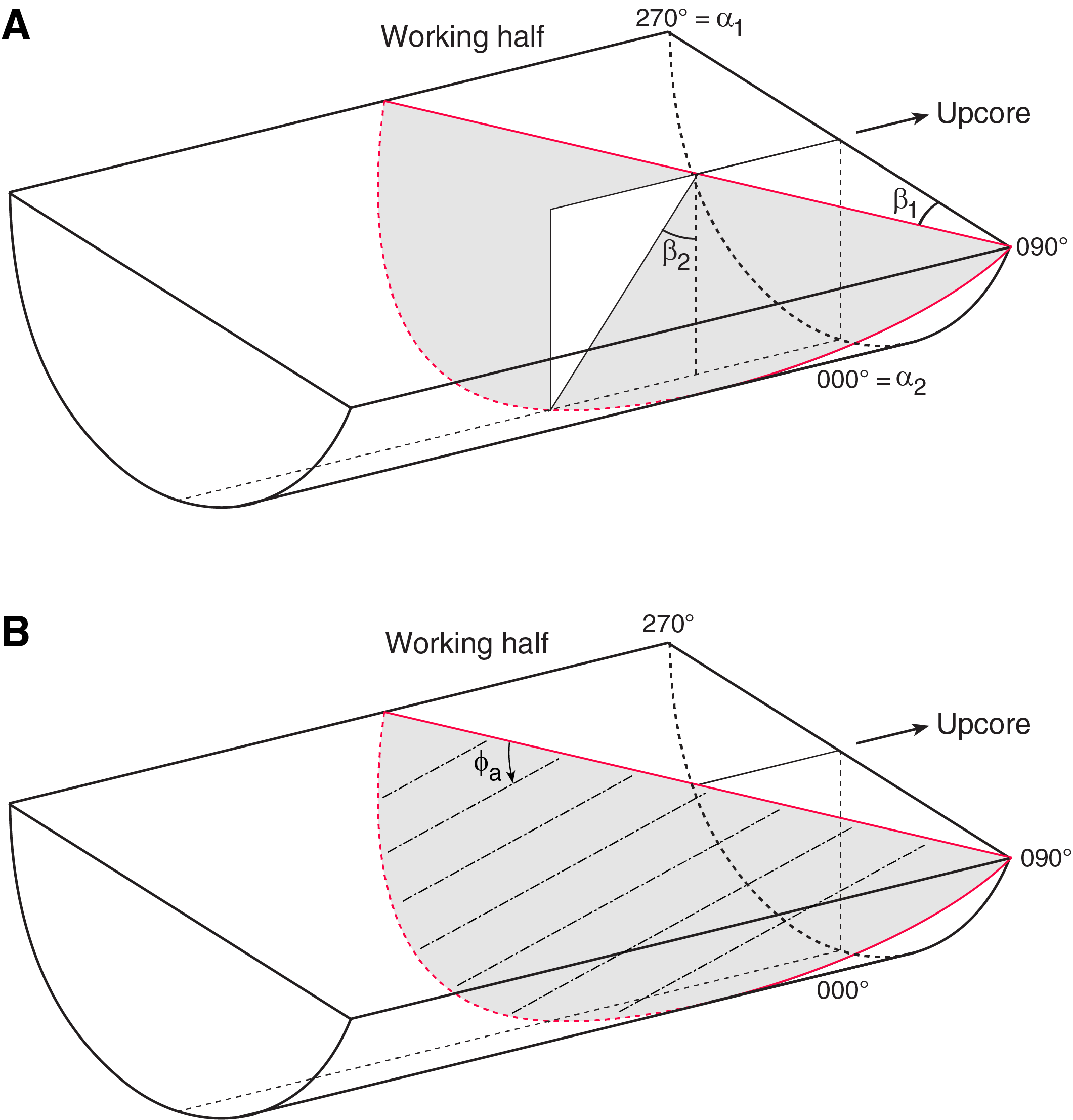
Figure F13. Plane orientation and rake.
Linear features (e.g., slickenlines) were observed on planar structures (typically fault or shear zone surfaces). Their orientations were determined in the core reference frame by measuring either their bearing and plunge or their rakes (or pitches) (ϕa) on the planes (Figure F13B).
Descriptive information for individual structures was recorded with the orientation data described above on the structural geology observation sheet based on mesoscopic and microscopic observations using a binocular microscope, thin sections, and SEM as necessary.
Data processing
Orientation data calculation and true north correction in cores
Measured orientation data were used to determine strike and dip in the core reference frame using an Excel spreadsheet developed during Integrated Ocean Drilling Program Expeditions 315, 316, 319, 322, 333, 334, 338, 344, and 348 (see StructureMeasurementSheet_C0024_C0025.xls in CORE in STRUCTURE in Supplementary material; Figure F14) (Expedition 315 Scientists, 2009a; Expedition 316 Scientists, 2009; Expedition 319 Scientists, 2010b; Expedition 322 Scientists, 2010; Expedition 333 Scientists, 2012; Expedition 334 Scientists, 2012; Harris et al., 2013; Strasser et al., 2014a; Tobin et al., 2015a). Based on the measured bearings (α1 and α2) and plunge angles (β1 and β2), this spreadsheet determines the strikes and dip angles of the planar features in the core reference frame. Because of drilling-induced core fragmentation (e.g., biscuiting) and ensuing core recovery and core preparation, the orientation of the core with respect to the present-day magnetic north is lost. A correction routine is therefore required to rotate orientations measured in the core reference frame back to the magnetic reference frame. Paleomagnetic data measured using the long-core cryogenic magnetometer on Chikyu (see Paleomagnetism) were used to correct drilling-induced rotations of cored sediments whenever there was a paleomagnetic datum point within the same coherent interval. If discrete sample paleomagnetic data are available, the Excel spreadsheet further converts the core reference data to geographic coordinates. The component inclinations, declinations, and maximum angular deviation values were calculated (see Paleomagnetism). For QC of paleomagnetic correction, a stable maximum angular deviation component less than 15° is used for orienting the structural directions.
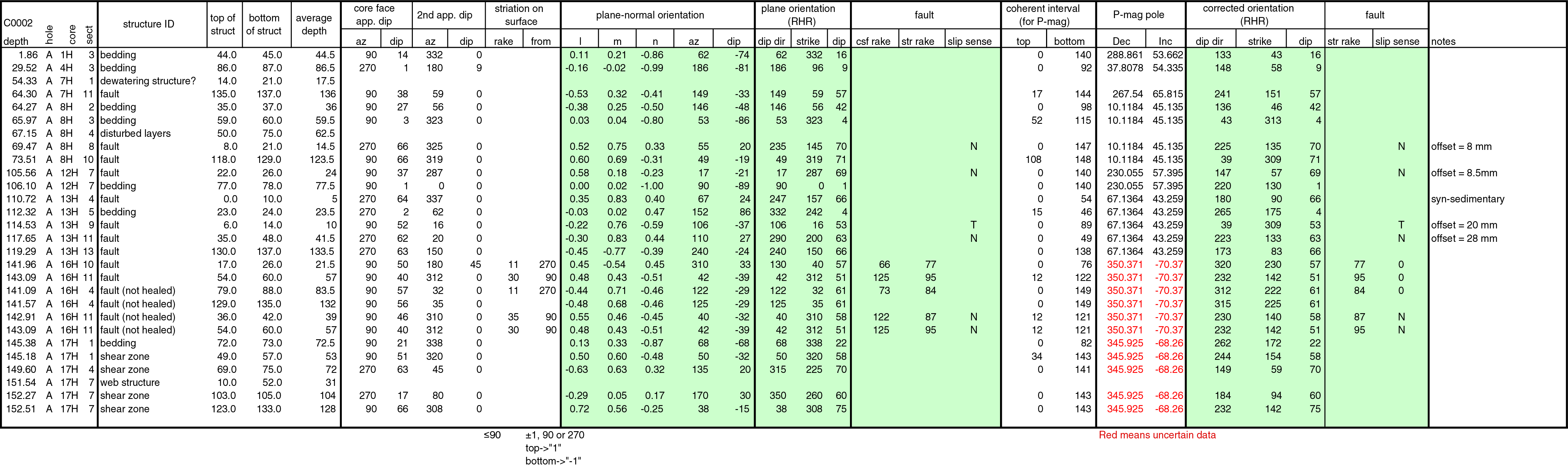
Figure F14. Orientation data spreadsheet.
J-CORES structural database
The J-CORES database has a VCD program to store visual (macroscopic and/or microscopic) descriptions of core structures at a given section index and a record of planar structures in the core coordinate system. The orientations of such features are saved as commentary notes but do not appear on the plots from the Composite Log Viewer. During Expedition 358, only the locations of structural features were entered in the J-CORES database, and orientation data management and analyses were performed with the Excel spreadsheet as described above. For final publication, structural elements were converted to core-scale depictions using Strater software.
X-ray computed tomography
X-ray CT imaging provides information about structural and sedimentary features in cores and cuttings and helps assess sample locations and quality for WR samples. X-ray CT scanning methods followed those in the measurement manual prepared for the Center for Deep Earth Exploration by laboratory technicians from Marine Works Japan (3D X-ray CT Scanning, Version 3.00, 24 March 2015; based on GE Healthcare, 2013a, 2013b, 2013c; Mees et al., 2003; Nakano et al., 2000) and are the same as those followed during previous expeditions (e.g., Strasser et al., 2014a). The X-ray CT scanner on Chikyu is a GE Yokogawa Medical Systems Discovery CT 750HD. This instrument scans a 1.4 m core section in 10 min: 5 min to scan and then 5 min to create, or "reformat," a coronal image. Images are core-axis-normal planes of X-ray attenuation values with dimensions of 512 × 512 pixels. Each axial scan of a 140 cm core section consists of approximately 2200 slice images, and each slice is 0.625 mm thick. Further analysis with a micro-X-ray CT scanner (ZEISS Xradia 410 Versa, Carl Zeiss Ltd.) was performed on selected cuttings samples at the KCC during Expedition 358. Reconstruction data generated by the Xradia consist of 1000 images with 1024 × 1000 (height × width) pixels. The pixel size and slice thickness corresponded to 15 µm. All data generated by both X-ray CT scanners are stored as Digital Imaging and Communication in Medicine (DICOM) formatted files.
Background
The theory behind X-ray CT is well established in medical research and the earth and planetary sciences (Carlson, 2006) and is only briefly outlined here. X-ray intensity varies as a function of X-ray path length and a linear attenuation coefficient (LAC) of the target material:
- I = transmitted X-ray intensity,
- I0 = initial X-ray intensity,
- η = LAC of the target material, and
- L = X-ray path length through the material.
LAC is a function of the chemical composition and density of the target material. The basic measure of attenuation, or radiodensity, is the CT number given in Hounsfield units (HU):
The distribution of raw attenuation values in a given slice is then used for image processing. Successive 2-D slices yield a representation of attenuation values in 3-D pixels (voxels).
During Expedition 358, an acrylic three-layer core liner section mock-up (calibration "standard") was run to calibrate the X-ray CT once every 24 h during coring operations. This QC standard is used to calibrate the CT numbers of air (CT number = −1000), water (CT number = 0), and aluminum (2477 < CT number < 2487) when the "Fast Cal" CT numbers for these three references fall out of normal range. For each standard analysis, the CT number was determined for a 24.85 mm2 area at fixed coordinates near the center of the cylinder. A color scale of CT values ranges between −1500 and +5500. The scale was fixed for all X-ray CT scans during Expedition 358.
X-ray CT scan data usage
X-ray CT scans were used for the following during Expedition 358:
- To provide an assessment of core recovery and liner integrity for drilling operations,
- To provide a data archive of core sections that were taken for WR samples prior to VCD preparation,
- To determine appropriate locations for WR core samples by avoiding important structural and sedimentological features,
- To identify the location of subtle features in cuttings or core that warrant detailed study or special handling during visual core description and sampling,
- To support visual core descriptions and cuttings descriptions in real time through display on computers in the core description laboratory,
- To distinguish between tectonic and drilling-induced structures, and
- To determine the 3-D geometry, orientation, and crosscutting relationships of sedimentary, tectonic, and drilling-induced structures.
X-ray CT scanning was done immediately after core cutting for time-sensitive samples to finalize their selection. All whole-round sections were screened to avoid destructive testing on intervals that may contain interesting structural or sedimentological features. This scanning also facilitated identifying intervals with minimal drilling disturbance for WR sampling and for assessing heterogeneity (essential for postcruise studies of frictional, geotechnical, and hydrogeological properties).
Fractures and other planar features identified in the X-ray CT scans were oriented directly from the imagery by measuring strike in the slice view (perpendicular to the core axis) and one or more apparent dips in axial sections (e.g., coronal and sagittal) (Figure F12). X-ray CT scanning helped reveal features that were cryptic or indistinguishable during visual core description.
X-ray CT scans can be used to identify sedimentary and tectonic features prior to visual core description. 3-D structure orientation in the core reference frame could easily be determined from X-ray CT scan sections, whereas performing the same measurement on the cores generally requires cutting orthogonal faces. Furthermore, structures such as shear zones could be classified by contrast in CT number, which is likely related to porosity changes or chemical alteration within shear zones. Structural and stratigraphic observations are incorporated into the structural geology and lithostratigraphy sections.
X-ray CT scan data have multiple uses, from early assessment of cores to description and synthesis. For this reason, several hundred gigabytes of scan data (~825 Mb/m) were stored on a local database at the OsiriX interpretation station. These data were later archived to tape and stored on terabyte disks.
Biostratigraphy and paleomagnetism
Biostratigraphy
Calcareous nannofossils and radiolarian ages were determined from 100 mL samples of unwashed cuttings collected at 20 m intervals from Holes C0002Q (2907.5–3257.5 mbsf), C0002R (2817.5–3077.5 mbsf), C0002S (2847.5–2933.5 mbsf), and C0002T (2836.5–2847.5 mbsf). Nannofossil analysis was performed on WR core samples (5 cm) collected from core catchers in Holes C0002T (2837.6–2843.7 mbsf), C0024B (7.1 mbsf), C0024C (7.3 mbsf), C0024D (11.8–119.3 mbsf), C0024E (512.4–618.8 mbsf), C0024G (106.3–318.9 mbsf), and C0025A (406.2–574.8 mbsf).
Calcareous nannofossils
Cuttings samples (2–3 cm3 volume) were washed gently with freshwater using 1 and 4 mm mesh sieves, and the fractions (1–4 mm) were dried for 2–3 h in an oven at 50°C. Four grains were selected from the 1–4 mm size fraction of each sample for study of calcareous nannofossils. Each selected grain was cut into two pieces using a razor or diagonal cutting pliers. One of the pieces was used to prepare a simple smear slide following Bown and Young (1998), and the remaining pieces were preserved in plastic bags. A smear slide was also made from core catcher samples following standard procedures and analyzed in the same manner as the cuttings samples.
Calcareous nannofossils were examined at 1500× magnification under a Nikon E600 polarizing light microscope. Nannofossil preservation was recorded as follows:
- G = good (little or no evidence of dissolution and/or overgrowth; specimens are identifiable to the species level).
- M = moderate (minor dissolution or crystal overgrowth; most specimens are identifiable to the species level).
- P = poor (strong dissolution or crystal overgrowth; many specimens are unidentifiable at the species and/or generic level).
The abundance of total calcareous nannofossils and individual taxa for each sample was estimated as follows:
- A = abundant (11 or more specimens per field of view).
- C = common (1–10 specimens per field of view).
- F = few (1 specimen per 2–10 fields of view).
- R = rare (1 specimen per 11–50 fields of view).
- VR = very rare (1 specimen per 51 or more fields of view).
- B = barren.
Results were correlated with the calcareous nannofossil biostratigraphic NN zones of Martini (1971), CN zones of Okada and Bukry (1980), and/or intervals by Young (1998). Furthermore, absolute ages for datums and additional biostratigraphic events were assigned based on Raffi et al. (2006) and/or Backman et al. (2012) whenever possible.
Radiolarians and foraminifers
Dried cuttings samples (3–6 g of the 1–4 mm size fraction) were soaked in a saturated sodium tetraphenylborate (C24H20BNa) solution with sodium chloride (NaCl) for 16–20 h at room temperature. Disaggregated particles were wet sieved using 63 and 500 µm mesh sieves. Wet residues were spread on one or two glass slides and dried on a hot plate. The dried residues on the glass slides were mounted with Entellan, a new, rapid mounting medium for microscopy. All of the slides were examined with a transmitted light microscope at 100× to 400× magnification.
Estimates of total radiolarian and foraminifer abundance in a slide were based on the following categories:
- A = abundant (>500 specimens in a slide).
- C = common (100–500 specimens in a slide).
- R = rare (10–99 specimens in a slide).
- VR = very rare (1–9 specimens in a slide).
Preservation of the radiolarian and foraminifer specimens was based on the following categories:
- G = good (tests show no sign of dissolution with only minor fragmentation).
- M = moderate (tests show evidence of moderate dissolution with obvious fragmentation).
- P = poor (tests show signs of a high degree of dissolution with very little intact nature).
Paleomagnetism
Paleomagnetic and rock magnetic analyses were conducted to determine the characteristic remanence directions for use in magnetostratigraphic and structural studies. Archive halves and discrete samples were measured with the superconducting rock magnetometer (SRM). Anisotropy of magnetic susceptibility (AMS) in discrete samples was measured with a magnetic susceptibility meter.
Laboratory instruments
The paleomagnetism laboratory on Chikyu houses a large (7.3 m × 2.8 m × 1.9 m) magnetically shielded room with its long axis athwartship. The total magnetic field inside the room is ~1% of Earth's magnetic field. The room is large enough to comfortably handle standard IODP core sections (~1.5 m). The shielded room houses all the equipment and instruments described in this section.
Superconducting rock magnetometer
The long-core SRM is a liquid helium–free cooling system (4 K SRM; WSGI); the 4 K SRM uses a Cryomech pulse tube cryocooler to achieve the required 4 K operating temperatures without the use of any liquid helium. The differences between the pulse tube cooled system and the liquid helium cooled magnetometers significantly impact the system in terms of ease of use, convenience, safety, and long-term reliability. The SRM system is ~6 m long with an 8.1 cm diameter access bore. A 1.5 m split core liner can pass through the magnetometer, alternating field demagnetizer, and anhysteretic remanent magnetizer. The system includes three sets of superconducting pickup coils: two for transverse moment measurement (x- and y-axes) and one for axial moment measurement (z-axis). The noise level of the magnetometer is <10−7 A/m for a 10 cm3 volume rock. An automated sample handler system (2G800) included in the magnetometer consists of aluminum and fiberglass channels designated to support and guide long-core movement. The core itself is positioned in a nonmagnetic fiberglass carriage that is pulled through the channels by a rope attached to a geared high-torque stepper motor. A 2G600 sample degaussing system is coupled to the SRM to allow automatic demagnetization of samples up to 100 mT. The system is controlled by an external computer and allows programming of a complete sequence of measurements and degauss cycles without removing the long core from the holder.
Anisotropy of magnetic susceptibility
The Kappabridge KLY 3S (AGICO, Inc.), which measures AMS, is also available on Chikyu. Data are acquired from spinning measurements around three axes perpendicular to each other. Deviatoric susceptibility tensor can then be computed, and an additional measurement for bulk susceptibility completes the sequence. Sensitivity for AMS measurement is 2 × 10⁻⁸ SI. Intensity and frequency of the field applied are 300 mA/m and 875 Hz, respectively. This system also includes a temperature control unit (CS-3/CS-L) for temperature variation of low-field magnetic susceptibility of samples.
Discrete samples and sampling coordinates
Because demagnetization levels on archive halves are limited to the lower level (~20 mT), one cubic sample (~7 cm3) was taken per 1–3 sections from coherent intervals of the working halves to confirm the results of paleomagnetic analysis on archive halves at higher and closer demagnetization levels. The relation between the orientation of archive section and that of a cube sample is shown in Figure F15.
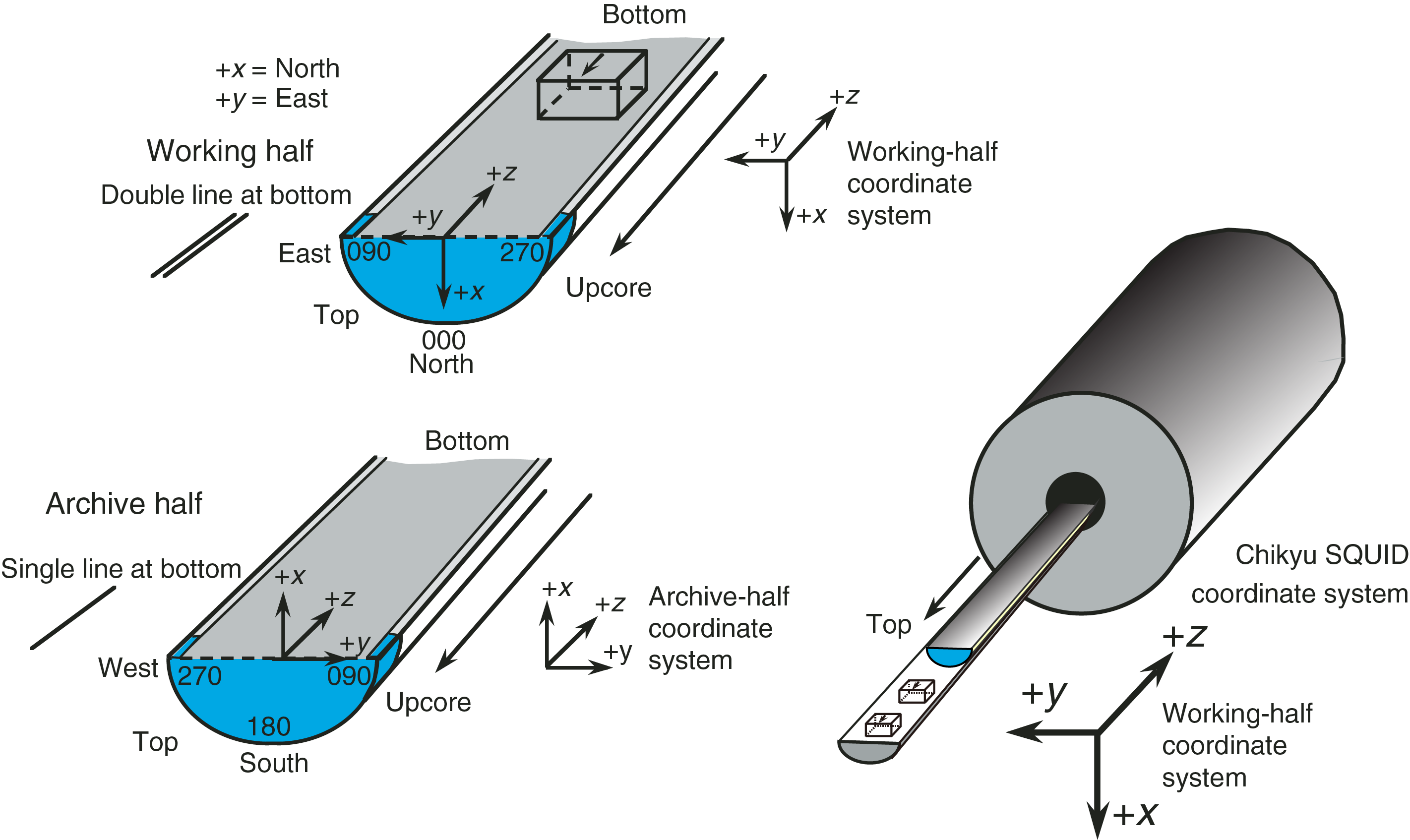
Figure F15. Archive half and cube sample orientation.
Magnetic reversal stratigraphy
Whenever possible, magnetic polarity interpretations are provided using the naming convention following that of correlative anomaly numbers prefaced by the letter C (Tauxe et al., 1984). Normal polarity subchrons are referred to by adding suffixes (e.g., n1, n2, etc.) that increase with age. For the younger part of the timescale (Pliocene–Pleistocene), we often use traditional names to refer to the various chrons and subchrons (e.g., Brunhes, Jaramillo, Olduvai, etc.). In general, polarity reversals occurring at core ends were treated with extreme caution. The ages of the polarity intervals used during Expedition 358 are a composite of four previous magnetic polarity timescales (magnetostratigraphic timescale for Neogene by Lourens et al. [2004]).
Geochemistry
Shipboard mud-gas monitoring system
Mud-gas monitoring system
The real-time mud-gas monitoring system is a powerful tool used to quantify in situ gaseous components, especially during superdeep drilling operations. In the framework of IODP, mud-gas monitoring was carried out during Expedition 319 (Expedition 319 Scientists, 2010a, 2010b) using third-party tools, as well as during Integrated Ocean Drilling Program Expeditions 337, 338, and 348 with shipboard instruments (Expedition 337 Scientists, 2013; Hammerschmidt et al., 2014; Strasser et al., 2014a; Tobin et al., 2015a).
Formation gas is liberated when the drill bit crushes sediment or rock. In a riser system, the liberated gas flows up to the ship with the drilling mud water (Figure F16), which is fed along a recycling system to a degasser.
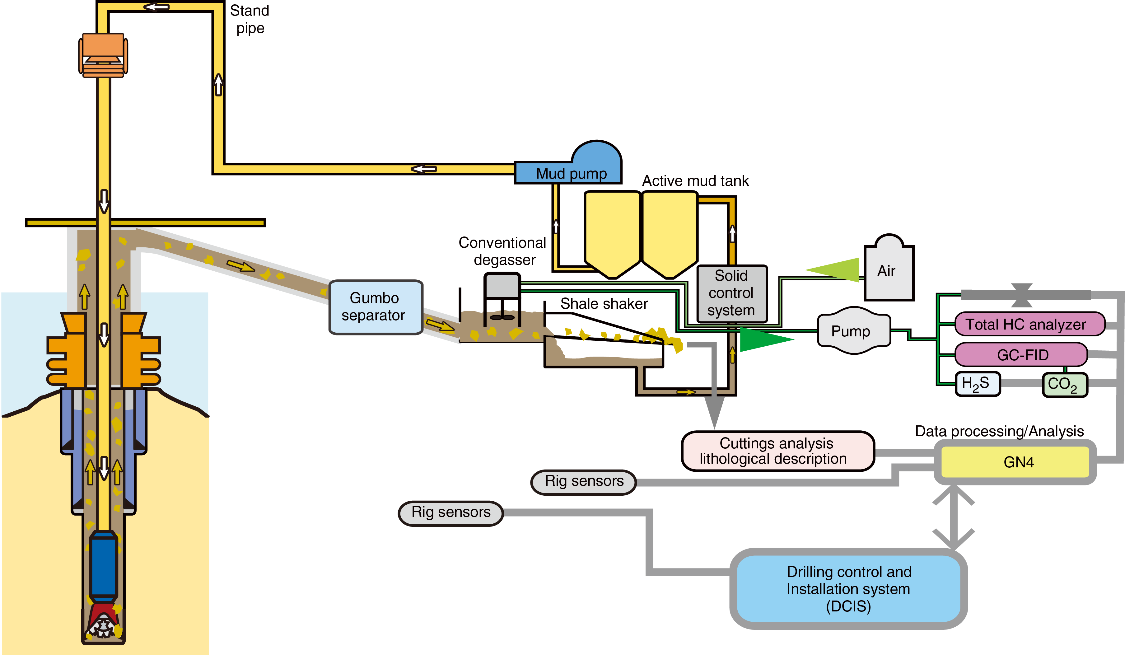
Figure F16. Mud-gas monitoring system.
Improvement of the degasser system
During previous expeditions, a degasser ("Standard Traps"; Geoservices) was placed downstream from a flow splitter connected to the Gumbo separator (Gumbo degasser; Figure F17). The system had major problems with cuttings jamming at the inlet of the degasser, which resulted in poor quality data (e.g., causing flood trapping and air contamination). The Gumbo degasser jammed several times during the previous expeditions. It was difficult not only to promptly find the jam but also to remove the cuttings from the Gumbo degasser. To resolve this problem, the degasser, which was replaced with a new one (constant-volume degasser provided by Geoservices), was relocated to the mud chamber downstream from the Gumbo separator (Trough degasser; Figure F17). The new degasser has a sealed degassing tank (Figure F18). Mud water was pumped into the degassing tank at a constant rate (1.5 L/min) via the mud suction probe, and "zero air" was pumped into the tank at a rate of ~500 mL/min through a PVC tube to generate bubbles in the mud water at the same time. Zero air was made by a zero gas generator (GC-1500; LNI Schmidlin SA), which was set up in the MGML (Figure F19). The zero gas generator removed hydrocarbons and carbon monoxide from the air supplied by an onboard air compressor. An agitator in the degasser tank stirred the bubbles to stimulate degassing from the mud water. The liberated gas from the crushed sediment/rock along with the zero air filled the headspace of the degassing tank. The gas in the headspace was pumped into the MGML via a PVC tube at ~500 mL/min. It takes 4 min and 50 s to transport the mud gas from the degasser to the MGML. On the way to the MGML, the gas passed through mud and water traps that prevent invasion of mud and water into the MGML system (Figures F18, F19). If the mud trap or PVC tube was jammed with cuttings, the inflow rate of mud gas to the MGML would change. Therefore, it is important to closely monitor the flow rate and pressure of mud gas to notice jamming as soon as possible. In addition, the inlet of the zero air into the degassing tank is routinely cleaned using a stick every ~24 h (Figure F18).
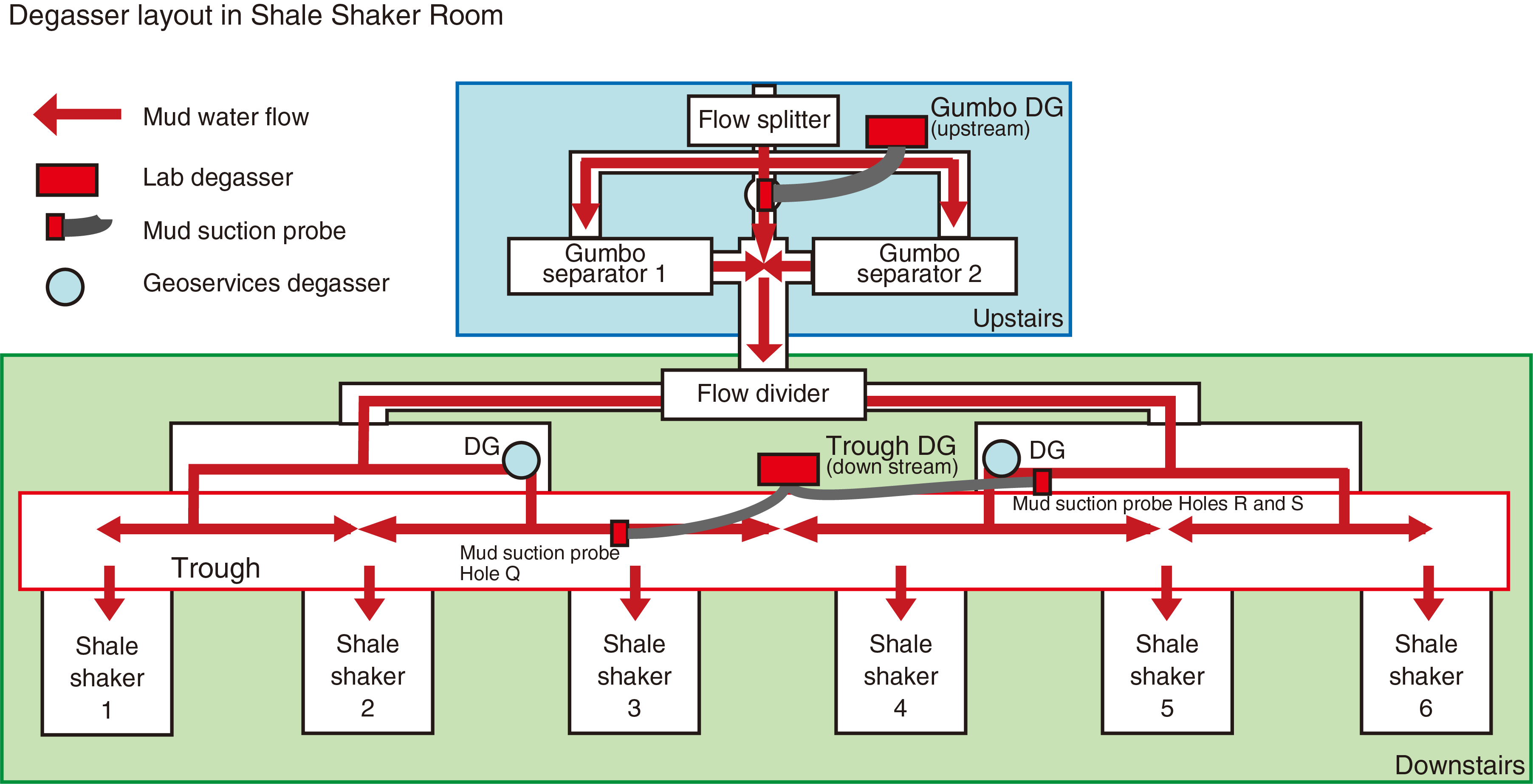
Figure F17. Degasser around shale shaker.
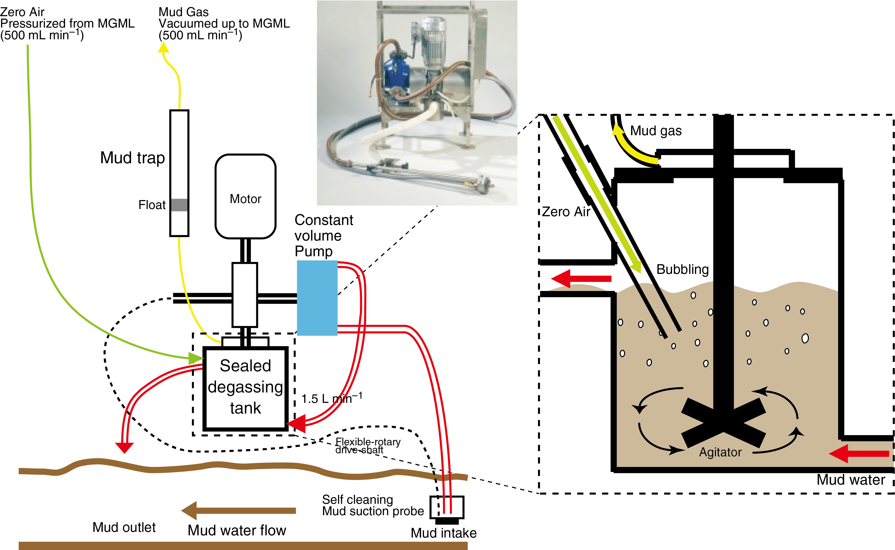
Figure F18. Newly installed degasser.
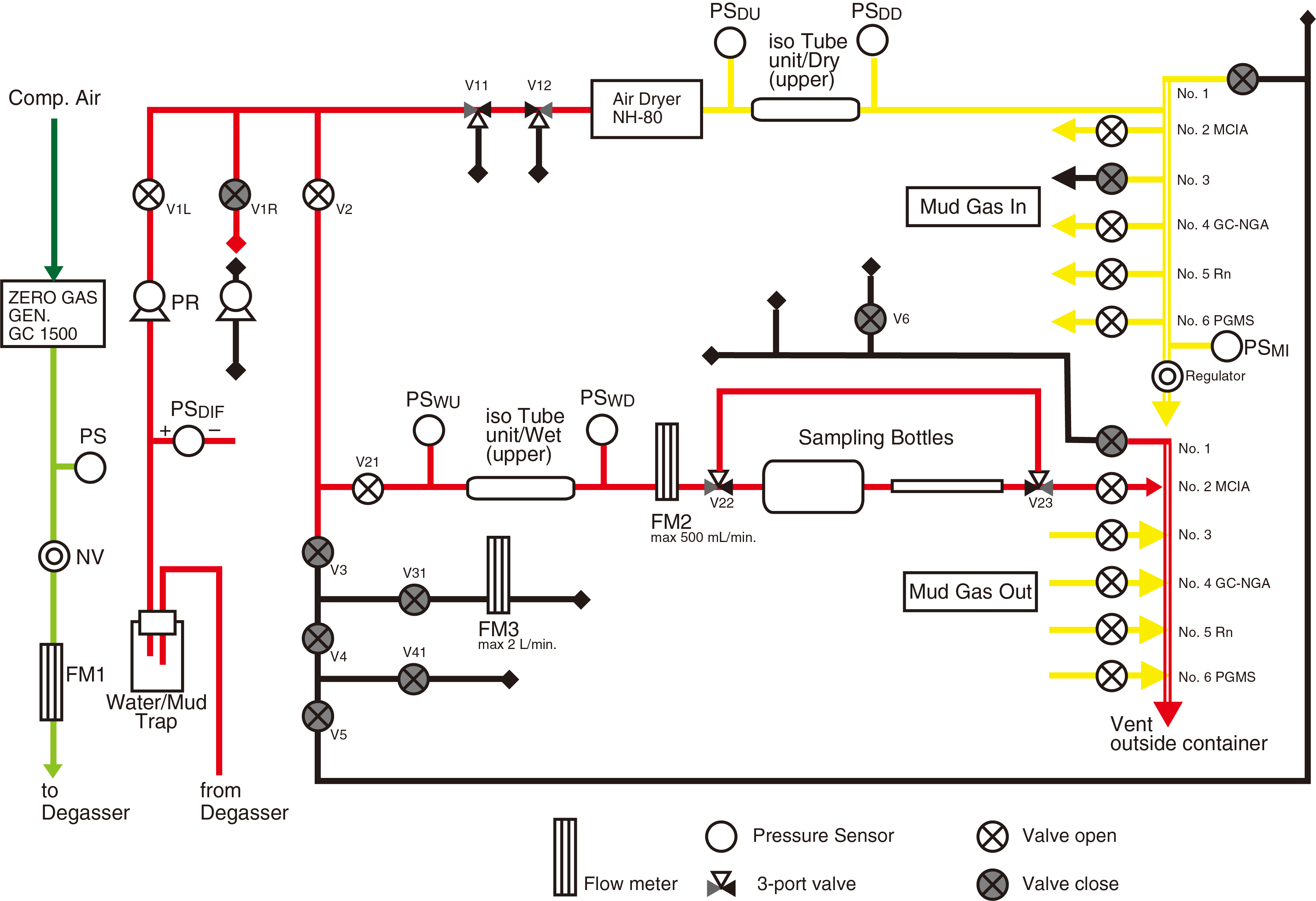
Figure F19. Gas flow in MGML.
In the previous degasser system used during Expeditions 337, 338, and 348, the degassing chamber was equipped with an agitator directly sunk into the mud stream, and the depth of the chamber from the mud flow surface was manually adjusted. This configuration resulted in variable gas sampling volumes. In addition, mud gas was pumped from the chamber without the zero air flow; as a result, mud condition often affected degassing efficiency. To solve these issues, in the new system installed for this expedition, mud water is pumped into the degasser tank via a mud suction probe at a constant rate independent from the drilling conditions such as the variable rig pump rates and mud level in the mud return circuit. In addition, the new degasser, in which sample gas is purged by zero air, allows constant degassing efficiency independent of mud parameters (density, viscosity, solids content, etc.).
However, it should be noted that the dilution by zero air lowers the apparent total mud-gas concentrations from those obtained by the previous degasser systems. Such a dilution effect is likely responsible for the low methane concentration observed in Hole C0002Q. To enhance the apparent gas concentration (i.e., degassing efficiency) before drilling operations in Hole C0002R started, the mud suction probe was moved to a more downstream position toward where the Geoservices degasser was installed (Figure F17).
Analysis and sampling flow in MGML
After the arrival of mud gas in the MGML, the gas flow was separated into two lines (Figure F19). One line was fed into a dehydrator (NH-80; Niscon) and then the dried gas was carried to the shipboard analyzing apparatus: methane carbon isotope ratio analyzer (MCIA), gas chromatograph (GC)–natural gas analyzer (NGA), radon meter, and process gas mass spectrometer (PGMS). The other line was used for personal sampling without desiccation.
Shipboard mud-gas analysis
Methane carbon isotope ratio by cavity ring-down spectrometer
The first instrument to analyze the gas in the MGML is an MCIA (Los Gatos Research, Model 908-0005), which measures methane concentrations and methane carbon isotope ratios at a sampling frequency of 1 Hz by cavity ring-down spectroscopy. The stable carbon isotopic composition of methane is reported in δ13CCH4 notation relative to the Vienna Peedee belemnite (VPDB) standard as expressed in parts per thousand (permil):
Calibration was carried out prior to the expedition using standard gas (Liso-1; [CH4]: 2500 ppm in atmospheric air, δ13CCH4: −66.5‰ ± 0.3‰ VPDB). Analytical condition was checked once a day by manually injecting the same standard gas. Methane concentrations and methane carbon isotope ratios were continuously monitored at a gas flow rate of ~110 mL/min.
The MCIA is able to analyze methane concentrations from 500 to 10,000 ppm (Range 2) with a built-in dynamic dilution system that can extend the upper detection limit to 100 times higher (https://www.et.co.uk/assets/resources/datasheets/Methane%20Carbon%20Isotope%20Analyser%20MCIA%20Product%20Datasheet.pdf). Methane carbon isotope ratios cannot be reliably determined when the concentration is lower than ~500 ppm, which was the threshold used during Expedition 337 (Expedition 337 Scientists, 2013) and this expedition (see next paragraph for details). Therefore, it is recommended not to use or rely on the methane carbon isotope data when the concentration is lower than ~500 ppm. Some methane concentrations measured during Expedition 358 were below this value, especially gases from Hole C0002R. We included all the methane carbon isotope data in the report even when methane concentrations are lower than 500 ppm, but the δ13CCH4 data with concentrations lower than 500 ppm were excluded from the figures. Extreme caution is needed when interpreting methane carbon isotope data of the samples including methane less than 500 ppm.
To evaluate the precision and accuracy of the isotopic measurements, especially when methane concentration is low, the carbon isotopic composition of standard gas concentrations was measured under two setup conditions. In the first setup, the evaluation was carried out by batch analysis for the standard gas (Liso-1) that was used for the daily condition check. δ13CCH4 was measured on one batch of undiluted standard gas (2500 ppm) and batches of N2-diluted standard gases with methane concentrations of 500 and 250 ppm. During the batch analysis, the sample gas was manually introduced by syringe and analyzed in the closed cell of the MCIA for 2 min (Figure F20A–F20C). The standard deviation of the 2 min measurement (120 data points) is seven times larger for the 250 ppm batch compared to the 2500 ppm batch (Figure F20A–F20C). The average δ13C values of the 2500 ppm batch (−67.4‰) was consistent with the known δ13C value of Liso-1 (−66.5), which varies by ±0.6‰ (1σ) during the daily condition check. However, those of the 500 and 250 ppm batches (−68.9‰ and −72.6‰, respectively) were consistently lower than the known value.
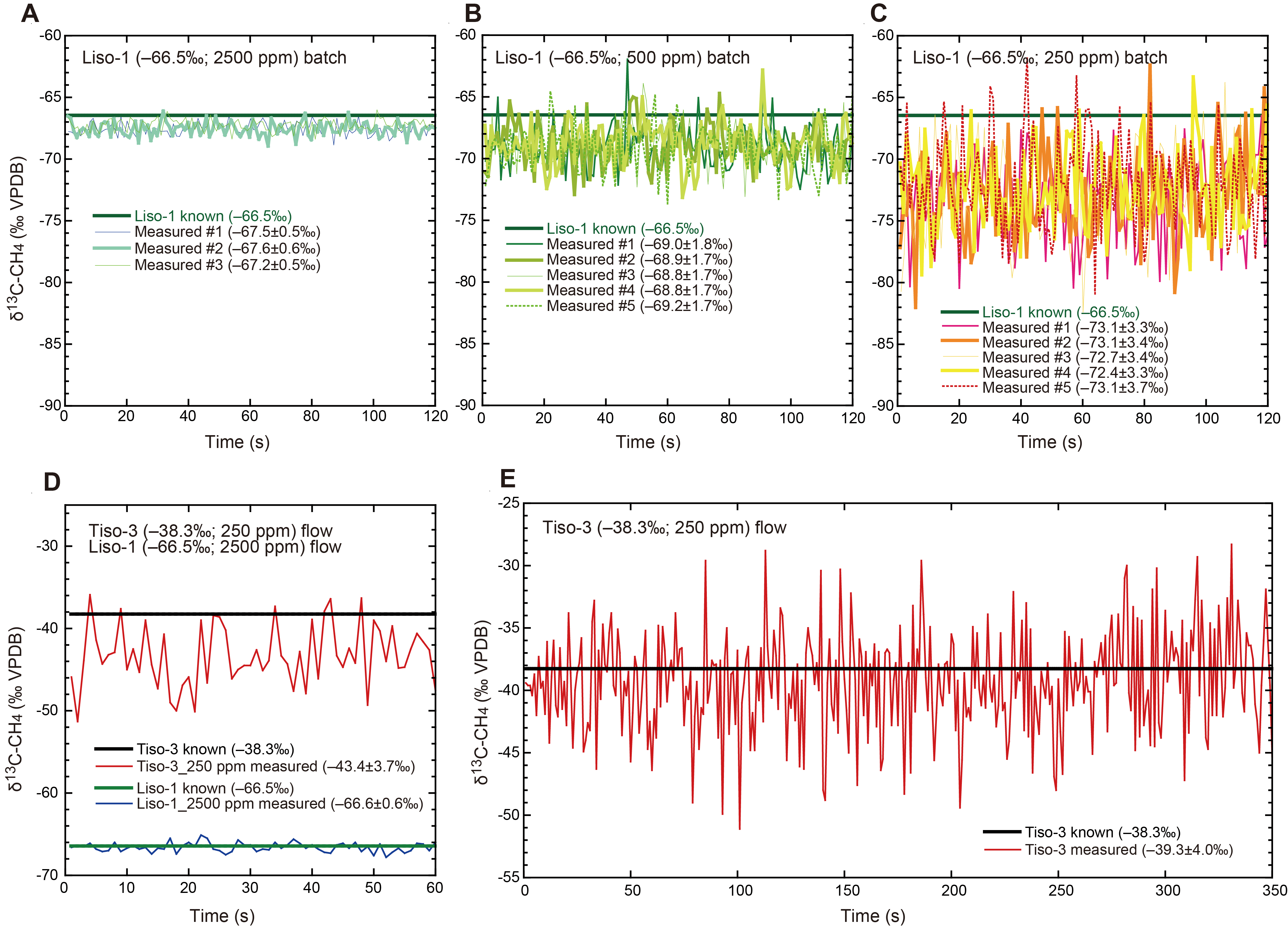
Figure F20. Precision and accuracy for carbon isotope analyses using MCIA.
The other setup was conducted for continuously flowing gas to simulate the routine mud-gas analysis. Both Liso-1 and Tiso-3 ([CH4]: 250 ppm, δ13C: −38.5‰ ± 0.2‰) were used for calibration. The 60 s flow analyses of both gases showed worse precision and accuracy for the low-concentration gas compared to the high-concentration gas (Figure F20D). The average δ13C value of the low-concentration Tiso-3 was 5.1‰ lower than the reported value with a standard deviation of 3.7‰. On the contrary, the average δ13C value of the high-concentration Liso-1 is only 0.1‰ higher than the reported value with a relatively small standard deviation of 0.6‰. The accuracy of the analytical results for the low-concentration gas improved when the duration of the analyses was increased to 350 s; the average δ13C value of the Tiso-3 was only 1‰ lower than the known value (Figure F20E). The precision, however, did not change much (3.7‰ vs. 4.0‰; Figure F20D, F20E). A deviation as high as ~5‰ from the known value was observed in the test on 250 ppm gas. These results revealed that both the precision and accuracy of the analyses significantly deteriorated when the methane concentration was too low.
Inorganic and organic gases by gas chromatography
The second instrument along the gas flow line in the MGML is a GC-NGA (Agilent Technologies 6890N Network GC system) equipped with a gas sampling port that has a multiposition valve (Wasson ECE instrumentation). In principle, the GC-NGA can analyze hydrocarbon gases (methane, ethane, propane, iso-/n-butane, and pentane [i.e., C1–C5]) with a flame ionization detector (FID) and nonhydrocarbon gases (H2, He, O2, N2, CO, and CO2) with a thermal conductivity detector (TCD). During Expeditions 338 and 348, nitrogen was used as the carrier gas so that He could be quantified (Strasser et al., 2014a; Tobin et al., 2015a). However, the nitrogen carrier decreased the instrument sensitivity to He. Thus, Ar was used as the carrier gas during Expedition 358 to detect He at a higher sensitivity than using nitrogen as a carrier gas because Ar has a larger contrast in thermal conductivity to He compared to nitrogen. In addition, oxygen concentrations could also be determined using Ar as a carrier. As a result, we were not able to detect Ar in our samples using the GC-NGA.
After flowing into the GC-NGA, the gas is introduced separately into the two sample loops with volumes of 1 and 0.1 mL. The 1 mL sample loop flows through an 8 ft capillary column (Wasson ECE Instrumentation, column 8 ft KM1 Slico) to roughly separate the different fractions of gaseous components. When the fractions of gas, except for CO2, exit this capillary column, they are diverted with a valve and introduced into another 50 m capillary column (Wasson Column 4 KC126 50 m × 0.53 mm, 22473), in which the gas fractions are separately eluted according to their retention times in sequence of He, H2, O2, N2, and CO. The gas concentrations are then quantified by TCD. The sampled gas in the 0.1 mL loop flows through a 50 cm capillary column (Wasson ECE Instrumentation, column Code 2378) that retains pentane. Upon turning a valve, the sample gas including methane, ethane, propane, and iso-/n-butane flows into another 49 m capillary column (Wasson ECE Instrumentation, column Code 2378). The gas fractions are separately eluted based on their retention times, and the concentrations are quantified by FID. The retained gas fraction in the previous 50 cm column was backflushed and introduced directly into the FID to reduce the analysis time of pentane.
The GC-NGA was more frequently used during Expedition 358 because of the successful reduction of measurement time from 27 min per sample during previous expeditions to 12 min per sample during this expedition by GC method improvements (i.e., changed temperature program and column). The continuous gas flow rate was 50 mL/min. Calibration was conducted at the beginning of the expedition by using two standard gas samples. The mixture of standard permanent gases for the calibration contained 1% of Ar, CO, O2, H2, CO2, and He in N2. The hydrocarbon standard gas mixture contained 1% each of C1–C5 in N2 (95%). During the expedition, the same standard gases were used to check the analytical condition every 24 h. If the measured concentrations of the daily condition check deviated >5% from the reported values, the calibration was conducted again. Despite daily calibration checks, during the drilling of Hole C0002Q N2 and O2 concentrations were not precisely calibrated because of the large difference between the concentrations in the mud gas and standard gas. To avoid the same issue, another standard gas containing 78% N2, 21% O2, 0.9% Ar, and 305 ppm CO2 was used to calibrate N2, O2, and CO2 when drilling started in Hole C0002R.
The detection limits of H2 and CO2 for the GC-NGA were estimated by analyzing the atmospheric air in the MGML, which has ~17 ppm H2 and ~700 ppm CO2, significantly higher values than those in open atmospheric air (500 ppb H2 and 400 ppm CO2). The higher concentrations of these gases are likely due to H2 and CO2 production by instruments such as the H2 generator, gas pumps, GC oven, and so on. The detection limits were estimated to be 12 ppm for H2 and 160 ppm for CO2. We could not estimate the detection limits for the other trace gases such as Xe, He, and CO because the TCD attached to the GC-NGA could not detect these gases in the atmospheric air sample.
Online radon analysis
Radon (Rn) concentration was measured by an Rn meter (Saphymo GmbH; AlphaGUARD Professional), which measures the ionized Rn concentration in a 650 mL ionization chamber (effective volume is ~500 mL). Measurements were carried out continuously, and the concentration was expressed as counts per minute averaged over a 10 min period. Analytical error calculated from repeated measurements was 100 Bq/m3 in the concentration range of 2 to 2 × 10⁶ Bq/m3. Temperature, pressure, and relative humidity of the air in the chamber were monitored and used to calculate the ionization efficiency to correct the Rn concentration. Calibration was conducted in the factory, and no further calibration was required on the ship.
Online gas analysis by process gas mass spectrometer
Helium, O2, Ar, Xe, N2, CO, CO2, and CH4 were continuously monitored by a PGMS (AMETEK Process Instruments Dycor ProLine). The PGMS includes a quadruple mass filter that identifies molecular masses of the targeted gases. Similar to Expeditions 338 and 348 (Strasser et al., 2014a; Tobin et al., 2015a), reduction of dwell time to 120 ms allowed a sampling interval of 4 s.
To obtain high-quality data, the following five-step calibration was conducted every 24 h:
- Pure Ar and N2 gases were used to check the background noise level of the PGMS.
- Standard cylinder air was used as a standard gas for calibrating O2, N2, and CO2.
- A mixture of inorganic gases was used as a standard gas for calibration of Ar, CO, Xe, O2, CO2, and He.
- Standard organic gas, which included C1–C4 hydrocarbon gases, was used to calibrate methane concentrations.
- CH4 standard gas diluted with CO2 was also used for calibration of methane.
The measured concentrations (or intensities) of N2, O2, Ar, CO2, CH4, CO, and He were normalized to the total amount of these seven gases assuming that only these gases were present. Therefore, the resulting concentrations may be overestimated if there was another significant gas component present.
Data processing for mud-gas monitoring
All the data determined by the MCIA, GC-NGA, PGMS, and Rn meter were recorded in a data storage system (SSX database) together with other drilling parameters at a recording frequency of 1 Hz. It should be noted that the SSX database continuously recorded data even when the drilling and/or mud flow pumps were disrupted. Data collected during such times were invalid for further scientific interpretation. We therefore selected only data obtained during increasing lag depth (i.e., normal drilling conditions). After this preliminary screening, the data were visually checked to find anomalies, which would be subject to further examination. Daily checks of the instrument condition in the MGML and disruptions in drilling operations were recorded as events by shipboard scientists. Data collected during the time of these events are not included in the final results.
Gas analysis
Sampling cored sediment for headspace gas analysis
For headspace analysis, ~5 cm3 sediment was sampled from the bottom of Section 1 in each core (or from the top of Section 2 when the sediment was disturbed at the bottom of Section 1) using a cut-off disposable plastic syringe (volume = 3 cm3) or a stainless steel cork borer when the sediment became too hard for the plastic syringe. When drilling progressed to deeper layers, sediment became too hard for the cork borer. Such sediment was crushed using a chisel, and several pieces of the crushed sediment totaling ~5 cm3 were picked. The sediment sample was placed in a glass vial (20 cm3) sterilized by baking at 450°C for 4 h prior to its use. The vial was then immediately capped by a butyl rubber septum coated with polytetrafluoroethylene (PTFE) and an aluminum cap. The butyl rubber septa were also sterilized at 100°C for 4 h before use. The precise mass of the wet sample was determined after gas analysis was finished.
Sampling sediment from cuttings for headspace gas analysis
Two ~5 cm3 sediment samples were taken from unwashed cuttings using a 3 cm3 cut-off disposable plastic syringe to analyze the headspace gas by GC-FID and GC–pulsed discharge helium ionization detector (PDHID). The sediment samples were placed in 20 cm3 glass vials, which were sterilized at 450°C for 4 h before use. The vials were then immediately sealed with a butyl rubber septum and an aluminum cap. The butyl rubber septa were also sterilized at 100°C for 4 h prior to the use.
Sampling gas for void gas analysis
When gas-rich sediment was recovered as a core on deck, dissolved gases in IW formed bubbles at atmospheric low pressure and high temperature compared to that from deep-sea environments. As a result, the sediment expanded and formed voids that contain free gas. Gas samples were taken from these voids through a needle attached to a gas-tight syringe (SGE Analytical Science; 100MR-VLLMA-GT) filled with Milli-Q water. The void gas was isolated by closing the stopcock of the gas-tight syringe and transferred to two sealed 20 cm3 vials under vacuum using a diaphragm pump (ULVAC; DTC-22). Because the pressure of the void gas sample is usually higher than the ambient atmospheric pressure, the concentrations of hydrocarbon gases will be overestimated when analyzing these pressurized samples. To avoid this, the septa of the void gas sample vials were pierced by a needle to reduce the inner pressure to one atmosphere pressure (1 atm).
GC-FID hydrocarbon concentrations
Low–molecular weight hydrocarbons (i.e., methane, ethane, propane, and iso-/n-butane) were analyzed by GC-FID (Agilent 7890B) equipped with an autosampler (Agilent Technologies 7697A headspace sampler). Before analysis of headspace gas, the vial containing sample sediment was heated at 70°C for 30 min. For both headspace and vacuum-sampled gases, the sample gas in the vial was replaced by pressurized He at 15 psi and transferred to a 1 mL sample loop through a needle. The sample gas was then injected into a capillary column (HP-PLOT Q; 30 m length, 0.53 mm outside diameter, 40 µm film) of the GC-FID. The flow rate of the He carrier gas was 5 mL/min. The GC oven was programmed to increase the temperature from an initial temperature of 60°C at a rate of 10°C/min to 150°C (run time: 9 min) after sample injection to elute the different gas fractions at different temperatures. Calibration was conducted once at the beginning of the expedition using standard gases containing 1% CH4 and standard hydrocarbons (1.02% ethane, 1.00% propane, 1.02% propylene, 1.02% n-butane, 1.01% iso-butane, and 1.03% ethylene) in N2 gas. Condition check measurements were carried out every day using 1% CH4 in N2 gas. The reproducibility of the analytical results was within 2.10%, 2.16%, 2.20%, 2.23%, and 2.14% for methane, ethane, propane, iso-butane, and n-butane, respectively (N = 38).
GC-PDHID hydrogen and carbon monoxide concentrations
Hydrogen gas and CO concentrations were determined using the GC-PDHID (Agilent 7890B) equipped with a capillary column (HP-PLOT Molesieve; 30 m × 0.53 mm × 50 µm film). The gas introduction system was similar to that of the GC-FID. A 20 cm3 vial containing a sediment sample was placed in a headspace sampler (Agilent Technologies 7697A headspace sampler), and the headspace gas was automatically injected into the GC-PDHID after heating the samples at 70°C for 30 min with He carrier gas at a flow rate of 3 mL/min. The GC oven temperature was programmed so that the initial temperature was 40°C, held for 7 min, and then increased to 180°C in 15 min. The temperature of the PDHID was 200°C. A standard gas containing 4020 ppm H2 and 99.7 ppm CO in N2 was used for both calibration and condition check measurements. Calibration was conducted once at the beginning of the expedition with repeated checks carried out every day. The analytical errors were 2.0% for H2 and 3.0% for CO (N = 77).
Chemical analysis of interstitial water
Interstitial water collection
IW samples were collected from sediments from Sites C0024 and C0025 for a range of shipboard and shore-based analyses. The methods summarized below are based on those reported for IODP Expedition 370 (Morono et al., 2017). When sufficient cored sediment was recovered, two WR IW samples per section were collected from the first three cores from Holes C0024B and C0024D to better define the location of the sulfate–methane transition, and one WR sediment sample was collected from each core thereafter for IW analyses. A summary of core length and IW recovery is shown in Table T8.
A total of 66 WRs were taken from 63 cores (Table T8) on the core processing deck with approval from the Science Leader on duty. Whole-round core sediments with lengths of 13–36 cm were selected to provide enough fluid to meet the minimum needs for shipboard and personal IW analyses (ideally ≥22 mL) while maximizing the core available for other research purposes. Each whole-round section for IW sampling was curated and delivered for scanning by X-ray CT to examine drilling disturbance or areas of interest for sedimentology or structural geology. After approval by the Science Leader, the sample was delivered to the sample preparation room for further treatment. The cored sediment was taken out of the core liner, cleaned by scraping off drilling-contaminated rinds along the outer edges and/or fractures of the cores, put in a modified 9 cm diameter Manheim titanium squeezer (Manheim and Sayles, 1974) on top of a filter paper rinsed by deionized water (18.2 MΩ Millipore water), and placed on top of two 320 mesh stainless steel screens. This part of the processing was done in a N2-filled glove bag to minimize oxidation of highly reactive materials including Fe2+ and reduced sulfur compounds. The sample sediments were squeezed at room temperature and pressures not exceeding 25,000 psi to avoid extracting interlayer clay waters. The IW was collected in a 60 mL acid-washed plastic syringe.
Aliquots of IW were distributed into glass and plastic vials after filtering through a 0.45 µm disposable PTFE filter for further analyses. Aliquots for shipboard major, minor, and trace component analyses and some personal samples were stored in acid-washed 4 mL plastic vials. The plastic vials, made of high-density polyethylene (HDPE), were used after cleaning by immersion for 24 h in 10% trace metal grade 12 M HCl and subsequently rinsed in Milli-Q water in a class 100 laminar flow clean hood. The samples for minor and trace element analysis by inductively coupled plasma–mass spectrometry (ICP-MS) or inductively coupled plasma–optical emission spectroscopy (ICP-OES) and some personal samples were acidified with a drop of 6 M HCl (TAMAPURE-100 grade) within 24 h after IW sampling. The collected samples were stored at 4°C. Some aliquots for personal requests were stored in 2 mL glass vials sealed with PTFE crimp caps. The glass vials and PTFE crimp caps were baked at 450° and 100°C, respectively, for 4 h before use. Some other personal request samples were also stored in the glass vials in which 2 µL of HgCl was added to 0.5 mL sample before sealing. Collected personal samples were stored at 4° or −20°C, depending on instructions from the individual scientists.
After IW was extracted, each sediment squeeze cake was divided for archive (stored at 4°C) and shore-based research (stored at −20°, 4°C, or room temperature).
IW analyses
The salinity of IW was routinely analyzed using a RX-5000i refractometer (Atago), which reports the refractive index of IW, immediately after the extraction. The refractive index was converted to salinity by referral to the repeated analytical results of International Association of Physical Sciences of the Oceans (IAPSO) standard seawater (salinity = 34.993). The standard deviation of the daily measurements of IAPSO standard seawater is equivalent to 0.04 kg/kg salinity.
Immediately after IW extraction, pH and alkalinity were analyzed by Gran titration using a Metrohm 888 Titrando. An aliquot of 1.0–3.0 mL IW adjusted to 3.0 mL with 0.7 M KCl solution was titrated with nominal 0.1 M HCl at 25°C. A 100 mM Na2CO3 solution was used for calibration of the acid each week. Quality checks were conducted twice per day using a 50 mM solution of NaHCO3 and 0.1 M HCl. When the sample volume was small, pH was analyzed using a compact pH meter (Horiba LAQUAtwin). The reproducibility of pH is ±0.1.
Sulfate and Br− concentrations in IW were analyzed by ion chromatography (Thermo Fisher Scientific ICS-2100) after diluting 1:100 with Milli-Q water. The column oven was set at 30°C. The eluent solution was 40 mM potassium hydroxide. A calibration curve was prepared for every measurement batch by using a series of diluted IAPSO standard seawater (0.01:100, 0.05:100, 0.1:100, 0.5:100, 1:100, and 1:50 diluted with Milli-Q water). IAPSO standard seawater (1:100 diluted) was also measured after every ~10 sample measurements as a condition check reference. Reproducibility of Br and SO4 is 3.7% and 0.18%, respectively.
Chlorinity was determined via titration of 100 µL water with silver nitrate (AgNO3). Here, the term "chlorinity" means the total concentration of reacting components with the titrant. The Metrohm 888 Titrando with a Metrohm Ag electrode was used for the analysis. The AgNO3 titrant was nominally 0.01 M. Standardization was based on replicate analyses of IAPSO Batch P162 (salinity = 34.993; chlorinity = 559.47 mM at the typical ambient laboratory temperature of 21.5°C). The precision of the chlorinity titrations expressed as the relative standard deviation (RSD) of IAPSO standard seawater was ±0.36%.
Ammonium and PO43− concentrations were measured by colorimetry using an automated spectrophotometer (SEAL Analytical AQ2 discrete analyzer) within 24 h after IW sampling. The AQ2 is equipped with a stepper motor–driven syringe for sampling, a quartz-halogen lamp, a flow-through cuvette (50 µL), and a photodiode. The analytical procedure is based on absorption spectroscopy of indophenol blue for NH4+ measurement and that of ammonium molybdate for PO43− measurement. Indophenol blue is formed by reaction of ammonium with the diazotization of phenol and subsequent oxidation of the diazo compound by sodium hypochlorite. Samples and reagents were taken into reaction segments with the sampling probe and warmed to 37°C for 8 min to enhance color development. Then the colored solution was transferred to the cuvette and absorbance at 620 nm was measured. Ammonium molybdate and potassium antimonyl tartrate reacted with orthophosphate in an acid medium to form an antimony-phosphomolybdate complex, which, on reduction with ascorbic acid, yielded an intense blue color suitable for photometric measurement at 880 nm. All operations, including sample dilution, color development, measurement, and calculation, were automated and controlled by operation software. Concentrations were calculated based on a standard calibration curve determined before each analytical run. The standard solution was measured after every five samples to check the analytical precision (QC). The RSDs of replicate analyses of the 0.071 µM QC NH4+ and 16.13 µM PO43− standards were ±1.9% and ±4.4%, respectively.
Concentrations of major cations (Na+, K+, Mg2+, and Ca2+) were measured using a Thermo Fisher Scientific ICS-2100 ion chromatograph equipped with an IONPAC CS12 analytical column (4 mm × 250 mm; part number 46073) with methanesulfonic acid eluent. Concentrations were determined based on calibration curves prepared with diluted solutions of IAPSO standard. Samples were diluted 1:200 with ultrapure water. IAPSO standard diluted to 1:200 was measured for QC after every 10 analyses. The relationship between peak area and Na+ concentration of the standard was linear within the measurement range; however, peak areas of K+, Mg2+, and Ca2+ overlapped with that of Na+, and the sensitivities of these elements were dependent on the Na+ concentration of each sample. This effect was reduced by creating calibration lines of K+, Mg2+, and Ca2+ as a function of Na+. RSDs obtained from drawing calibration lines were 0.37%, 0.45%, 0.32%, and 0.33% for Na+, K+, Mg2+, and Ca2+, respectively.
Minor elements (B, Ba, Fe, Li, Mn, Si, and Sr) were analyzed by ICP-OES (Thermo Scientific iCAP 7600 Series). An aliquot of acidified IW sample was diluted by a factor of 10 with 0.15 M HNO3. A multielement stock solution was prepared from the ultrapure primary standards (SPC Science PlasmaCAL) to match the matrix of samples and diluted by factors of 100, 50, and 25 with 0.15 M HNO3 and 30 g/L NaCl. Finally, these working standards were diluted 1:10 before each sequence using the Y-containing 0.15 M HNO3 solution. A second multielement solution prepared separately from the calibration stock solution was used for QC. The QC sample was measured after the analyses of each five IW samples.
V, Cu, Zn, Ar, Mo, Rb, Cs, Pb, and U were analyzed by ICP-MS (Agilent 7500ce ICP-MS) equipped with an octopole reaction system to reduce polyatomic and double-charge interferences. To calibrate for interferences by high concentration of matrix Na+, NaCl solution was added into the standard solutions and concentrations were adjusted to those of IAPSO standard seawater. The standard solutions were analyzed at the beginning of each run to produce calibration lines based on the average counts per second of the specific mass of elements. A 100 µL aliquot of 500 ppb indium standard was added to the empty vials before dilution. Sample aliquots were then diluted with 1% nitric acid solution to 10% in these vials (500 µL sample with 4 mL of 1% HNO3 solution and 500 µL of internal standard solution) based on previously determined detection limits and concentrations of the elements of interest. A primary standard solution matching the maximum range of predicted concentrations was made based on published results of deep-sea IW compositions in a variety of settings. Composition of the primary standard solution was as follows: V = 20 ppb; Cs, Cu, V, As, Mo, Pb, and U = 40 ppb; Zn = 140 ppb; and Rb = 500 ppb. This primary standard was diluted with the 1% nitric acid solution to relative concentrations of 50%, 25%, 10%, 5%, and 1%. These standards were then diluted to 10% with the addition of 500 µL of 560 mM NaCl and 3.5 mL of the 1% HNO3 solution to compensate matrix suppression of the plasma ionization efficiency and 500 µL internal standard solution. The 25% standard solution was diluted accordingly and analyzed between every eight samples throughout the series of analysis to evaluate precision and to keep consistent among the results in the different dates of analyses. Blank solution was also analyzed every eight samples, and the detection limits were determined from the standard deviation of five replicate analyses of a procedural blank of Milli-Q water acidified with 4 mL of optima-grade 6 M HCl. The average precisions of multiple determinations of the 25% ICP-MS standard was V < 6.4%, Cu < 10%, Zn < 10%, As < 5.4%, Mo < 2.0%, Rb < 0.71%, Cs < 0.31%, Pb < 1.8%, and U < 4.0%.
Chemical analysis of solid samples
Carbonate, nitrogen, carbon, sulfur, and total organic carbon
TC and TN concentrations were determined for cuttings and cored sediments. Two types of cuttings from Holes C0002Q and C0002R were analyzed: (1) bulk cuttings from the 1–4 mm size fraction that were gently washed by seawater (see Lithology), and (2) intact cuttings handpicked from the >4 mm size fraction and further washed by seawater in a sonicator. The cuttings were dried under vacuum and ground to powder before analysis. TC and TN concentrations were determined using a Thermo Finnigan Flash elemental analysis (EA) 1112 carbon-hydrogen-nitrogen-sulfur (CHNS) analyzer. Synthetic standard sulfanilamide, which contains 41.78 wt% C and 16.30 wt% N, was used for calibration. About 40 mg of sediment powder was weighed, placed in a tin container, and combusted in an oxygen stream at 900°C to liberate the carbon and nitrogen as oxide gases from the molten sample. The combustion-produced CO2 and NO2 were transported by a constant flow of carrier gas. Then, the NO2 was reduced to N2, which was separated from CO2 using a GC, and these gas concentrations were quantified with a TCD. The accuracy of the analysis was determined using a soil NCS reference material (Thermo Scientific, Milan, Italy) and a sulfanilamide standard (Thermo Scientific). The range of the blank values, measured for 10 empty tin containers in the same manner as the samples, was between 0.0004 and 0.0012 mg. Thus, the 3σ of these values (~0.0005 mg) should be considered the detection limit of TC. The quantitative detection limit of TN was estimated from the error of the intercept of the calibration curve determined prior to every analytical sequence. The detection limit varied in each sequence and was mostly <0.02 mg, roughly equal to 0.05 wt% for the analysis of about 40 mg of cuttings. Because the TN concentrations of cuttings sampled during Expedition 358 were mostly close to or lower than the detection limit, caution is advised when interpreting concentrations less than ~0.05 wt%.
In addition to TC and TN, total sulfur (TS) was measured using a Thermo Finnigan Flash EA for cored samples. Approximately 20 mg of sediment powder was weighed into a tin cup and mixed with an equivalent mass of V2O5 catalyst. For TS measurements, the same calibration standard sulfanilamide (18.65 wt% S) and JMS-1 reference material was used, whereas combustion temperature was set at 980°C.
Inorganic carbon (IC) was determined from the same set of samples used for elemental analysis. Approximately 15–25 mg of sediment powder was weighed and acidified with 2 M HCl at room temperature to convert carbonate to CO2. The released CO2 was titrated, and the change in light transmittance was measured with a photodetection cell (CM5012 CO2 coulometer; UIC Inc. Coulometrics). The weight percentage of carbonate was calculated from the IC content, assuming that all the evolved CO2 was derived from dissolution of calcium carbonate:
The presence of other carbonate minerals was not accounted for. Standard deviation of the analysis was less than ±0.05 wt%. Two standard materials (NIST-SRM 88b and JSD-2) were used to evaluate method accuracy. The detection limit of IC was assumed to be 3σ of the blank values of ~1 µg C.
TOC concentration was determined from the difference between the concentrations of TC and IC.
Physical properties
Physical property measurements provide valuable constraints on bulk sediment and rock characteristics to augment lithologic unit characterization and to facilitate correlation of seismic reflection data with discrete core and cuttings measurements and descriptions. Thus, these data provide information necessary for reliable cuttings-core-log-seismic integration. Expedition 358 employed multiple approaches and methods to characterize the physical properties of cuttings and cores.
Prior to core physical property measurements, X-ray CT images were collected for all cores, and cores were equilibrated to room temperature (~20°C). After temperature equilibration, whole-round core sections were run through the MSCL-W to measure gamma ray attenuation (GRA) bulk density, magnetic susceptibility, NGR, P-wave (compressional) velocity, and electrical resistivity. After cores were split into archive and working halves, MAD, electrical resistivity, and P-wave velocity measurements were performed on discrete samples of cores from working halves. Thermal conductivity measurements were made on either working halves using the TeKa thermal conductivity meter in half-space mode (mini-HLQ) or whole-round cores using the TeKa thermal conductivity meter in full-space mode (needle). High-resolution digital image photography was performed on archive halves using a MSCL-I. No color reflectance measurements were made during Expedition 358 because the color spectroscopy logger (MSCL-C) was not functioning properly.
For cuttings recovered from Holes C0002Q, C0002R, C0002S, and C0002T (2917.5–3257.5, 2817.5–3077.5, 2847.5–2933.5, and 2836.5–2847.5 mbsf, respectively), limited measurements were conducted because of the size of the available material. Unwashed and washed cuttings were analyzed for NGR employing the MSCL-W to determine variations in the radioactive counts of the samples and for correlation with LWD gamma ray measurements. Cuttings were rinsed with seawater to remove contamination from drilling mud and sieved into <1, 1–4, and >4 mm size fractions. Washed cuttings samples (~40 cm3 each) were taken from the 1–4 and >4 mm size fractions for physical property measurements, including MAD and magnetic susceptibility. Handpicked intact cuttings were also used for MAD measurements to avoid the inclusion of any DICAs, pillow cuttings, artificial cement, and drilling mud additives such as Fracseal or Barolift (see Introduction and operations). Washed cuttings of each size fraction collected every 10 m were also packed in plastic liners in 3 cm intervals to form a CCS for each hole. The CCS was then scanned by the MSCL-I to obtain high-resolution digital image photography.
On several occasions during the expedition, large intact rock fragments were collected from drill bits that were competent enough for physical property measurements. In such cases, the rock fragments (bit samples) were saw cut to produce parallel surfaces and used for electrical resistivity and P-wave velocity measurements followed by MAD measurements.
MSCL-W
Whole-round cores were scanned by the MSCL-W. Butyrate core liners were used in Holes C0024B–C0024D and C0024G, whereas polycarbonate liners were used in Holes C0024E, C0024F, and C0025A. Based on repeated measurements on standard materials placed inside both types of liners, no statistically significant differences were found in the measured GRA bulk density, P-wave velocity, or resistivity values. In addition to the whole-round cores, a 12 cm long core liner packed with either unwashed or gently washed bulk cuttings was scanned using the MSCL-W NGR unit only.
Gamma ray attenuation bulk density
Bulk density can be used to evaluate pore volume, which provides information on the consolidation state. GRA bulk density is based on the detection of a gamma ray beam directed through whole-round cores. The beam is produced by a 137Cs gamma ray source at a radiation level of 370 MBq within a lead shield with a 5 mm collimator. The gamma ray detector includes a scintillator and an integral photomultiplier tube to record the gamma rays that pass through the whole-round core. GRA bulk density (ρb) is calculated as
- I0 = gamma ray source intensity,
- I = measured intensity of gamma rays passing through the sample,
- µ = Compton attenuation coefficient, and
- d = sample diameter.
The Compton attenuation coefficient (µ) and source intensity (I0) are treated as constants, so ρb can be calculated from I. The system is calibrated with a special sealed calibration "core section" composed of a set of aligned aluminum cylinders of various diameters (e.g., 1–6 cm) surrounded by distilled water in a sealed core liner. Density depends on the diameter of the aluminum cylinder and spans from ρ = 1 (water only) to 2.71 g/cm3 (aluminum only). To calibrate the instrument, gamma ray counts were taken for each aluminum cylinder for a count time of 60 s. The resulting ln(I) was plotted against the product of the known parameters ρ and d of the calibration core section and fitted with a regression line of the following type:
where d is the internal diameter of the core liner (e.g., 7.3 cm) and A, B, and C are coefficients determined from the polynomial equation fit. Density measurements on core samples were conducted perpendicular to the core axis every 4 cm along the core.
Magnetic susceptibility
Magnetic susceptibility is the degree to which a material can be magnetized by an external magnetic field. Therefore, magnetic susceptibility provides information on sediment mineral composition but is more generally used for correlation between boreholes drilled in the same formation. A Bartington loop sensor of 8 cm diameter was used to measure magnetic susceptibility. An oscillator circuit in the sensor produces a low-intensity (~80 A/m root mean square [RMS]), nonsaturating alternating magnetic field (0.565 kHz). This pulse frequency is converted into magnetic susceptibility. The spatial resolution of the loop sensor is 23–27 mm, and it is accurate to within 5%. Magnetic susceptibility data were collected every 4 cm along the core.
Natural gamma radiation (whole-round cores and cuttings)
NGR measurements provide insights into sediment composition, which can be used to identify lithology. Whole-round cores as well as washed and unwashed cuttings packed into a 400 cm3 core liner were monitored for natural gamma ray emissions to obtain spatial variability in radioactivity and establish gamma ray data from cuttings for comparison with downhole gamma ray logs. A lead-shielded counter is optically coupled to a photomultiplier tube and connected to a bias base that supplies high-voltage power and a signal preamplifier. Two horizontal and two vertical sensors are mounted in a lead, cube-shaped housing. The NGR system records radioactive decay of long-period isotopes 40K, 232Th, and 238U. NGR has a spatial resolution of 120–170 mm and was measured every 16 cm with a count time of 30 s. The background radiation level was determined at the beginning of the expedition by taking measurements on core liners filled with deionized water; this background level was then subtracted from each measurement. Also, for QC purposes during the expedition, measurements on a water-filled liner and a standard granite core were conducted each day to check for fluctuations in detector sensitivity.
For cuttings measurements, variations in packing density may arise that affect the measured values. Thus, the mass of the cuttings and drilling mud that was packed in the liner was determined from the difference between empty and filled cylinder masses. These values were used later to normalize the measured NGR values by cuttings volume to facilitate comparison with logging data and data from other expeditions.
P-wave velocity
P-wave velocity data can be used to evaluate small-strain moduli; to correlate among log, core, and seismic data; and to evaluate pore structure and cementation. P-wave velocity (VP) is defined by the time required for a compressional wave to travel a set distance:
where d is the path length of the wave across the core, and tcore is traveltime through the core.
P-wave velocity transducers on the MSCL-W system measure total traveltime of the compressional wave between transducers. The wave travels horizontally across the whole core and core liner. The total traveltime observed is composed of the following:
- tdelay = time delay related to transducer faces and electronic circuitry,
- tpulse = delay related to the peak detection procedure,
- tliner = transit time through the core liner, and
- tcore = traveltime through the sediment or rock.
The system is calibrated using a core liner filled with distilled water, which provides control for tdelay, tpulse, and tliner. With these calibrations, core velocity (VP) can be calculated on whole-round specimens in core liners as follows:
- dcl = measured diameter of core and liner,
- dliner = liner wall thickness, and
- to = measured total traveltime.
The calculation assumes that the core completely fills the core liner. P-wave velocity data were collected every 4 cm along the core.
Electrical resistivity
Electrical resistivity may be useful for estimating other sediment physical properties, including porosity, tortuosity, permeability, and thermal conductivity, although resistivity data must be used with caution because the value is sensitive to all these parameters as well as to the salinity of pore fluid and mineralogy. Bulk electrical resistivity is controlled by solid grain resistivity, IW resistivity, pore space distribution, and pore connectivity. The noncontact resistivity sensor on the MSCL-W system induces a high-frequency magnetic field in the core with a transmitter coil. This generates an electrical current in the bulk sediment that is inversely proportional to its resistivity. The secondary magnetic field generated by this induced electrical current is measured by a receiver coil. To measure this smaller magnetic field accurately, a differencing technique has been developed that compares readings from the sample core to readings from an identical set of coils operating in air. Electrical resistivity is estimated from an empirical equation,
where R is the electrical resistivity (Ωm) and E is the sensor response (mV). The coefficients a and b are obtained by the calibration measurements on five reference core liners filled with different concentrations of NaCl solution (0.35, 1.75, 3.5, 17.5, and 35 g/L). Electrical resistivity data were obtained at 4 cm intervals on the MSCL-W.
Magnetic susceptibility (cuttings)
For magnetic susceptibility analysis, ~10 cm3 of seawater-rinsed cuttings material was taken from vacuum-dried cuttings from the 1–4 and >4 mm size fractions and placed into a paleomagnetic (pmag) cube. The mass of the cube was measured both empty and then filled with the washed cuttings material. The prepared cube, with a volume of 7 cm3, was then analyzed with the Kappabridge KLY 3S system (AGICO, Inc.). Sensitivity for the measurement is 3 × 10⁻⁸ SI, and intensity and frequency of the field applied are 300 mA/m and 875 Hz, respectively. A standard was measured once a day to ensure long-term consistency of the system calibration. A blank empty cube was measured to determine the background before each sample measurement. Using the mass of the samples and the measured raw magnetic susceptibility (bulk susceptibility), we calculate the mass magnetic susceptibility (MMS) by
Moisture and density measurements
The purpose of MAD measurements is to determine bulk wet density, bulk dry density, grain density, water content, porosity, and void ratio. All of these properties can be calculated using phase relations in marine sediment from the direct measurements of the wet sample mass (Mwet), the dry sample mass (Mdry), and the dry sample volume (Vdry) (Noorany, 1984). Standard ODP/IODP practices, which include a salt correction, were used to determine IW mass and volume, salt mass and volume, and solid grain mass and volume (Blum, 1997). Standard seawater density (1.024 g/cm3) and salinity (35‰) and a constant salt density (2.22 g/cm3) were assumed for all calculations. MAD measurements were conducted on both cuttings and cores; there is no difference in measurements and calculations between the two sample types, only sample preparation.
Sample preparation
For cores from Hole C0002T, two discrete samples (~8 cm3 each) were collected from 2836.75 and 2840.64 mbsf (Sections 358-C0002T-1K-1 and 2K-1, respectively) for determination of physical properties. For cores from Sites C0024 and C0025, two discrete samples were collected per section for determination of physical properties, except when core sections were shorter than half of a full section length (full section length is approximately 1.5 m), in which case only one discrete sample was taken from a section. Some of the samples were taken as a part of cluster samples next to WR samples. Sample intervals were chosen at minimally disturbed, homogeneous locations. Special care was taken to avoid drilling mud in MAD samples.
Cuttings samples were taken at 10 m depth intervals of drilling progress for MAD measurements. After being rinsed with seawater, the cuttings of the working portion were segregated into two size fractions (1–4 and >4 mm) by sieving. A volume of ~30 cm3 of each size fraction was used for MAD measurements. In addition, ~20 cm3 of handpicked intact pieces from the >4 mm size fraction were used to investigate the difference between stiffer formation cuttings and bulk cuttings that may also include DICAs, pillow cuttings, and drilling mud additives. For Hole C0002R, intact cuttings were also cleaned in an ultrasonic water bath for 3 min to further remove mud contamination prior to handpicking. This process was added to match the procedure of the structural geology group and helped with lithologic identification of the cuttings when necessary. Results show that this additional procedure did not affect the measured porosity values (see Physical properties in the Site C0002 chapter [Kitajima et al., 2020]). Wet cuttings were gently wiped with absorbent paper until no visible water films were observed on the surfaces. The samples were then immediately placed into a glass jar of known mass for wet mass measurement.
Measurements
The wet sample mass (Mwet) was measured using a paired electronic balance system designed to compensate for the ship's heave (Figure F21A). The sample mass was counterbalanced with a precisely known mass (40 g for sediment) and determined to a precision of ±0.01 g. The balance system was calibrated twice a day or more frequently during poor weather conditions. After measurement, the wet samples were placed in a convection oven for >24 h at 105° ± 5°C to dry. The dry samples were then cooled in a desiccator for at least 1 h to equilibrate to room temperature (~20°C) and then the dry mass and volume were measured. The dry mass (Mdry) was determined using the same counterbalanced measuring system. Dry volume (Vdry) was measured using a helium-displacement Quantachrome pentapycnometer (Figure F21B) with a precision of ±0.04 cm3. The five-chamber system allows the measurement of four sample volumes and one calibration sphere, which was rotated between all measurement chambers to monitor errors in each chamber. The pycnometer was calibrated at least once per 24 h. An average of five measurements was reported for each sample.
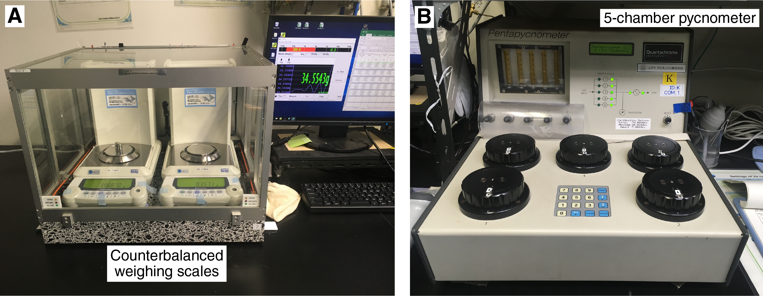
Figure F21. Counterbalanced weighing scale system.
Some repeat measurements were conducted on several cuttings samples from Hole C0002Q to check if drying time and method affected the results. For intact cuttings, additional drying time beyond 24 h has no effect on the results, whereas for bulk samples, porosity increased by 2%–6% with additional drying time. The drying time was fixed at 24 h, however, to remain consistent with previous expeditions. A vacuum chamber was also used to dry some cuttings samples to assess whether heating in the oven influenced the final porosity. Results showed that porosity values were generally consistent within 0.3% between oven-dried and vacuum-dried samples.
Phase relations in marine sediments
From the direct measurements of Mwet, Mdry, and Vdry, pore fluid mass (Mf), salt mass (Msalt), mass of solids excluding salt (Ms), pore fluid volume (Vf), salt volume (Vsalt), and volume of solids excluding salt (Vs) can be obtained by
- Mwet = total mass of the wet sample,
- Mdry = mass of the dried sample,
- s = salinity (3.5%),
- ρf = density of pore fluid (1.024 g/cm3), and
- ρsalt = density of salt (2.220 g/cm3).
Calculations of physical properties
Water content (Wc) was determined following the methods of the American Society for Testing and Materials (ASTM) Designation D2216 (ASTM International, 1990). Corrections are required for salt when measuring the water content of marine samples. In addition to the water content calculation in ASTM D2216 (i.e., the ratio of pore fluid mass to dry sediment mass as percent dry weight), we also calculated the ratio of pore fluid mass to total sample mass (percent wet weight). The equations for water content are
Bulk density (ρb), dry density (ρd), and grain density (ρg) are defined as
where Vwet is the bulk volume of wet sample determined from the dry volume (Vdry), pore fluid volume (Vf), and salt volume (Vsalt).
Porosity (ϕ) is the ratio of the volume of pores to the total sample volume; void ratio (e) is the ratio of the pore volume to the volume of the solid grains. They are calculated as
P-wave velocity (discrete samples)
P-wave velocity measurement was performed on discrete cubic samples (~20 mm × 20 mm × 20 mm) prepared from cores and bit samples. The samples were cut with either a single or a parallel diamond blade saw, and their two parallel surfaces were ground with 220 grit sandpaper if needed. When preparation of the cubic samples was difficult, the discrete samples with parallel surfaces in one or two directions were prepared and used for P-wave and resistivity measurements. For cores, samples were cut with faces orthogonal to the x-, y-, and z-axes of the core reference (see Structural geology). This three-component measurement plan enables first-order estimation of P-wave velocity anisotropy. For bit samples, the first measurement direction is recorded as the x-axis direction, the second as the y-axis, and the third as the z-axis because orientations of these bit samples were unknown.
A P-wave logger for discrete samples (PWL-D) was used to measure P-wave velocity (Figure F22). The sample is held between two transducers acting as transmitter and receiver. The PWL-D stand has a laser distance sensor and two interchangeable sets of transducers with resonant frequencies at 230 and 500 kHz. The transmitting transducer was connected to a pulse generator, and the receiving transducer was connected to an oscilloscope synchronized with the pulse generator. The oscilloscope signal was displayed digitally and the P-wave total traveltime (t) for the first arrival was picked and recorded. The laser distance sensor provided the sample length (L). The velocity in any direction (e.g., VPx) was defined by the sample length (e.g., Lx), total traveltime (tx), and system-calibrated delay time (tdelay):
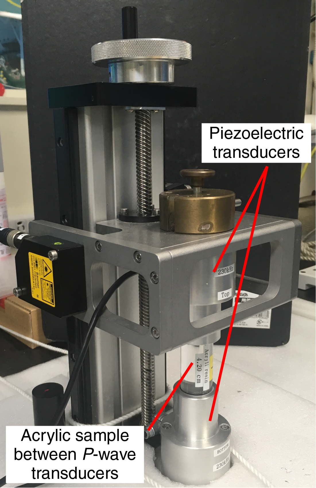
Figure F22. P-wave measuring unit.
Traveltime delay was determined by placing the transmitter and receiver in direct contact and measuring the traveltime. The laser distance sensor was calibrated by placing the transmitter and receiver in direct contact and then spacing them using a 2.5 cm long reference specimen. QC measurements were made daily by measuring velocity on acrylic and glass standards with known lengths and acoustic velocity values.
Measurements on discrete core samples were performed with the 500 kHz transducers, whereas those on bit samples from Holes C0002Q and C0002R were performed with both the 230 and 500 kHz transducers. Waveforms from heterogeneous or attenuating samples, as well as some samples with irregular shapes, exhibited significant distortion of the wave train. Because the automated pick was on the second zero crossing (rather than on the first arrival), these measurements were discarded as unreliable.
Because P-wave velocity was measured in the x-, y-, and z-directions for cores from Sites C0024 and C0025, the anisotropy was calculated following the approach of Carlson and Christensen (1977). Some sources of anisotropy include (1) alignment of pores during consolidation, (2) fabric development due to alignment of mineral grains, and (3) microstructures such as microfractures and microcracks. Calculation of the horizontal-plane anisotropy (αVPhor) and vertical-plane anisotropy (αVPvert) of P-wave velocity compares the horizontal (x and y) and vertical (z) components of P-wave velocity expressed as a percentage of the mean:
Electrical resistivity (discrete samples)
Resistivity was measured on the same discrete samples used for P-wave velocity measurements for relatively consolidated materials. The parallel faces of the samples were held between two electrodes, and their complex impedance was measured with a 40 Hz to 110 MHz frequency sweep with the Agilent 4294A impedance analyzer (Figure F23). Sample dimensions were obtained during P-wave velocity measurement. Coupling between the sample and each stainless steel electrode was obtained through a paper filter soaked in either 35 g/L NaCl solution or seawater. The impedance of the sample for each configuration was obtained by subtracting the impedance of the coupling layers from the measured impedance. The impedance of the coupling layers was evaluated by stacking the two filters between the electrodes immediately after measuring the impedance of the sample. Sample resistivity (Rx) in the x-direction was computed from the amplitude (|Zx|) and phase angle (θx) of the measured impedance by
where Lx, Ly, and Lz are the lengths of cubic discrete samples in the x-, y-, and z-direction, respectively, and |Z0| and θ0 refer to the amplitude and phase angle of the filter impedance. Resistivities in the y- and z-directions were obtained similarly.
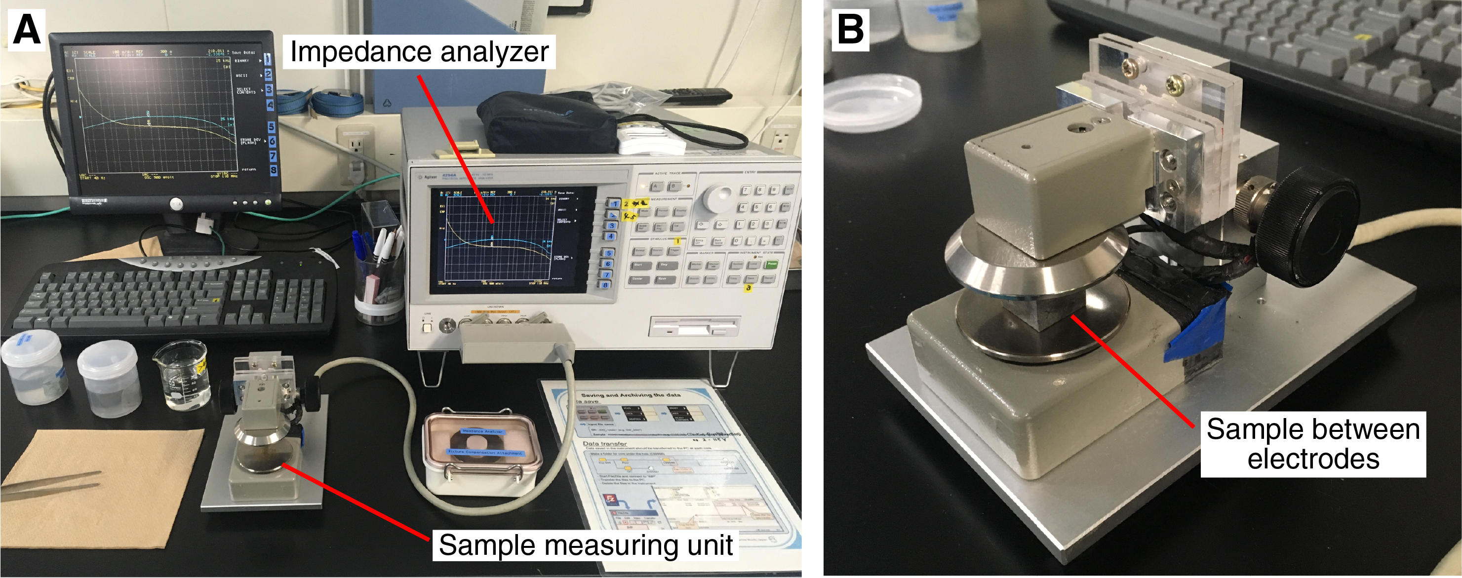
Figure F23. Impedance measurement system.
In the case of discrete core samples and bit samples from Site C0002, Ly and Lz are not known precisely because the shapes of the discrete samples were generally irregular. In such cases, the pycnometer was used to measure the wet rock volume so that the effective cross-sectional area (equivalent to Ly × Lz) could be estimated by dividing the volume by the thickness (Lx).
Resistivity is calculated as the inverse of the real conductivity. To minimize electrode polarization effects on conductance and to remain consistent with Expedition 348 data and reports, the values of conductivity and resistivity at 10 kHz were reported. The laboratory temperature was also reported for each measurement to allow correction to in situ temperature and for comparison with logging data. Similar to the P-wave velocity anisotropy, when oriented cubic samples were available from Site C0024 cores, the horizontal-plane anisotropy (αRhor) and vertical-plane anisotropy (αRvert) of electrical resistivity were calculated by comparing the horizontal (x and y) and vertical (z) components of resistivity expressed as a percentage of the mean:
For soft-sediment cores, the complex impedance (i.e., equivalent resistivity) was measured using the Agilent 4294A analyzer and a four-pin array consisting of four electrodes spaced 7.5 mm apart. The array was inserted into the working half and measured the complex impedance, from which the electrical resistivity in the y-direction was calculated:
where dr is a constant dependent on the geometry of the electrode array and Z and θ are the magnitude and phase, respectively, of the complex impedance. dr was determined every 24 h by comparing the measured impedance with an IAPSO standard seawater solution (35 g/L NaCl) of known electrical impedance.
Thermal conductivity
In an infinite homogeneous media, a line heat source with a constant heat power will cause a temperature increase after initiation of heating as expressed by
- T(t) = temperature as a function of time,
- q = constant line heat input per unit length per unit time,
- k = thermal conductivity,
- t = time after the start of heating, and
- C = a constant depending on thermal diffusivity, etc.
By applying a known heat power q for a certain time interval, the value of k can be determined through a least-squares fitting of the temperature versus time record.
Thermal conductivity was measured on core working halves at a spacing of at least 1 measurement per core using a half-space line source probe (mini-HLQ probe) (Vacquier, 1985), which approximates an infinite line source, for consolidated cores from Holes C0002T, C0024E, C0024F, and C0025A. Samples were placed in a seawater bath at ambient temperature (20°C) for at least 15 min before measurement. The half-space probe was placed directly on the split core parallel to the core axis. For soft-sediment cores from Holes C0024B, C0024D, C0024G, and C0025A, a full-space needle probe was inserted into whole-round sections through a hole drilled through the working-half side of the core liner.
Using the TK04 (TeKa Berlin) thermal conductivity measurement system (Blum, 1997), all thermal conductivity measurements were made after cores equilibrated to room temperature. At the beginning of each measurement, temperature in the sample was monitored to ensure that thermal drift was <0.4 mK/min (typically within 1–2 min). After it was established that the temperature was near equilibrium, a calibrated heat source was applied, and the rise in temperature was recorded for ~60 s. For optimal measurement conditions, the heat source power was adjusted as a function of the thermal conductivity of the sample. Thermal conductivity values were based on the observed rise in temperature for a given quantity of heat. The probe was calibrated at least once every 24 h. The calibration was performed on standard Macor blocks of known thermal conductivity, which is 1.652 W/(m·K) ± 2% for a half-space line source probe and 1.623 W/(m·K) ± 2% for a full-space needle probe. The TK04 software fitted a theoretical prediction of the temperature rise versus time curve to various segments of the data (typically segments within 20–80 s since start time of heating) yielding multiple estimates of the thermal conductivity. Each estimation was evaluated according to an index logarithm of extreme time (LET) that helps to evaluate at what point the boundary conditions assumed in the theoretical prediction appear to become invalid. We disregarded any conductivity estimates derived from those with LET values <4 for a half-space probe or <3 for a full-space needle probe. Also, the conductivity estimate associated with the greatest LET was taken as the best estimate (as suggested by the manufacturer). Measurements were repeated 5 times automatically by the TK04 system, and the average value of the conductivity estimates were reported.
Shear strength measurements
The shear strength of soft-sediment core working halves at Site C0024 was measured with an analog vane shear (Wykeham Farrance WF23544) and a pocket penetrometer (Geotest E-284B). One measurement per core was taken, avoiding disturbed and heterogeneous sections. The shear strength of cores from Site C0025 was measured using only the pocket penetrometer. At least one but occasionally two measurements were made per section for Site C0025. Measurements were made with the vane rotation axis and the penetrometer penetration direction aligned with the x-axis of the core.
Undrained shear stress (Su[vane]) is determined by the torque (T) at failure and a constant (Kv) dependent on the geometry of the vane:
All measurements were made with a 12.7 mm long vane and a 6.35 mm wide blade. Pocket penetrometer measurements provide an estimate of unconfined compressive strength (qu), which is related to the undrained shear stress (Su[penetrometer]) by
where g = gravitational acceleration. Penetrometer measurements were conducted by pushing a 6.5 mm diameter cylindrical probe into the working half and recording the penetration resistance. Shear strength was reported as undrained shear strength to allow comparison between different methods.
Anelastic strain recovery analysis
ASR is a core-based measurement technique that can evaluate both orientation and magnitude of 3-D present-day principal stresses, with several assumptions. The ASR approach is to measure the anelastic strain change due to release of the stress soon after core recovery. The methodology used for the ASR measurement during Expedition 358 is based on Matsuki (1991), following the guideline described in Lin et al. (2007). A 15 cm long undisturbed whole-round core was selected and sampled directly from the core in the core cutting area and then X-ray CT scanning was carried out to screen for potential important structural sections. We did not perform MSCL-W measurements on these samples because the ASR measurement is time sensitive and requires instrumentation as soon as possible after core is extracted from the subsurface to capture early strain recovery. Core samples were pushed out of their core liners, and the outer surface was washed in seawater to remove drilling mud.
Before starting the ASR measurement, the dimensions of an elliptical section of core sample were measured by a 2-D measurement sensor (Keyence Corporation; TM-065) while rotating the core samples on the rotary table (Figure F24). This measurement was carried out to capture initial elastic strain recovery.
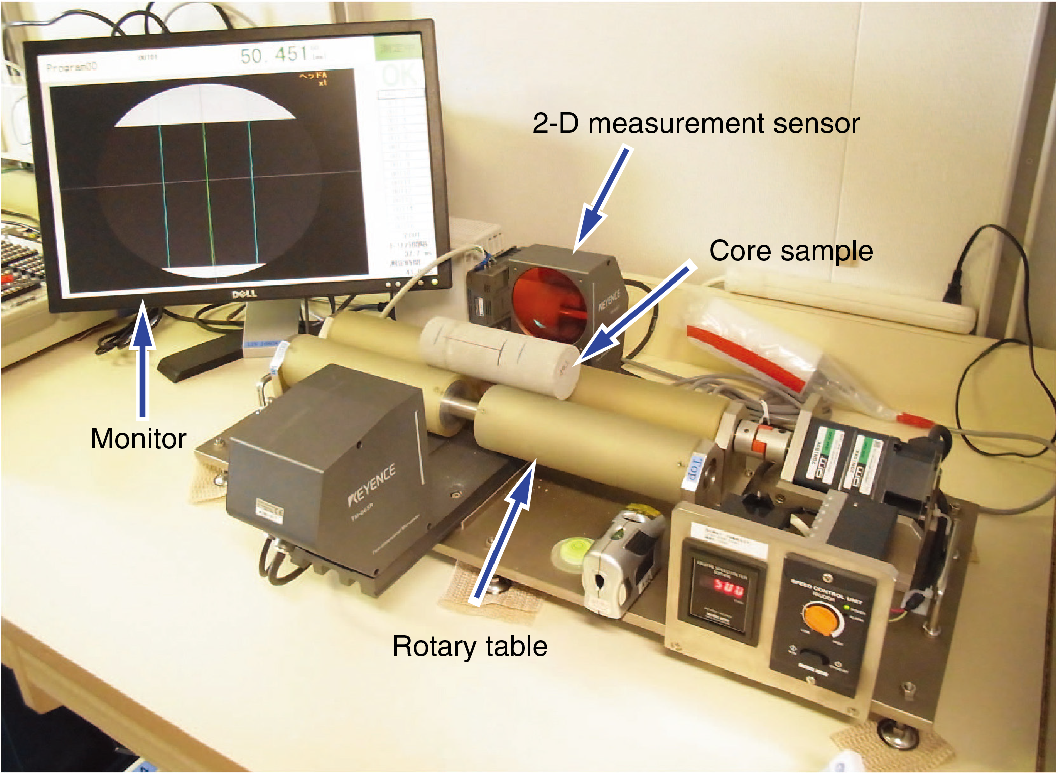
Figure F24. 2-D measurement system.
The anelastic strains in nine directions, including six independent directions, were measured using 18-wire strain gauges (6 cross- and 6 single gauges; 120 Ω; Figure F25). In cases where a few fractures had developed in the specimen, the fractures were glued to prevent the sample from splitting into pieces. It took 1–2 h to mount 18 strain gauges, and the total elapsed time just after core on deck was 1–2 h before starting to record the strain recovery. The core samples were double-bagged (with plastic and aluminum) and submerged in a thermostatic water bath where temperature changes were kept controlled at 22° ± 0.1°C for the duration of the measurement. Strain values were collected every 10 min for a maximum of 15 days.
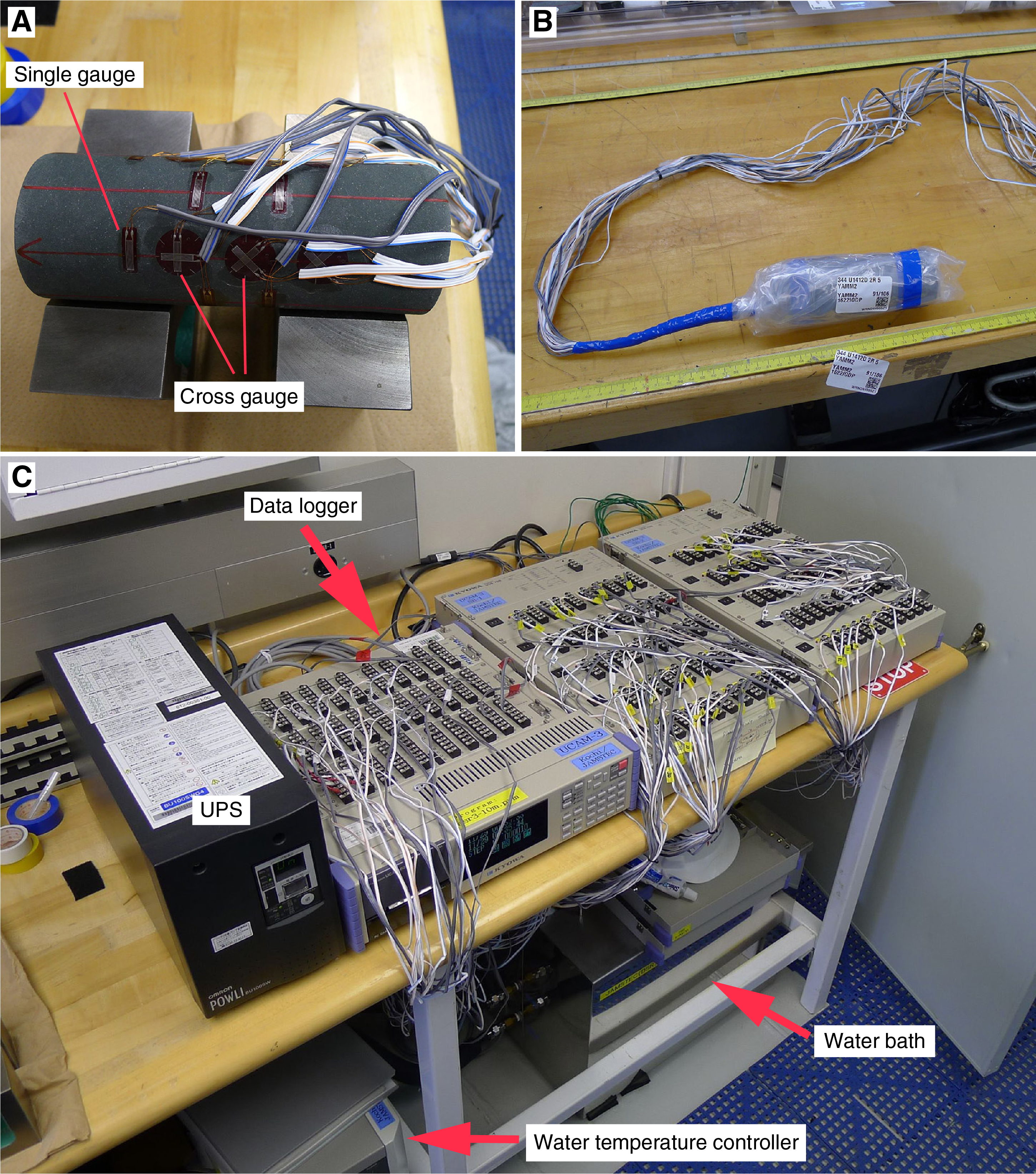
Figure F25. ASR procedures and equipment.
MSCL-I: photo image logger
Digital images of archive-half cores and CCSs were acquired by a linescan camera equipped with three charge-coupled devices. Each charge-coupled device has 2048 arrays. The reflected light from the core surface is split into three channels (red, green, and blue [RGB]) by a beam splitter inside the linescan camera and detected by the corresponding charge-coupled device. The signals were combined, and the digital image was reconstructed. A correction was made for any minor mechanical differences among the charge-coupled device responses. A calibration was conducted before scanning each core to compensate for pixel-to-pixel response variation, uneven lighting, and lens effects. After colors of black (RGB = 0) and white (RGB = 255) were calibrated at f-stop = f/16, the light was adjusted to have an adequate grayscale of RGB = 137 at f-stop = f/11. Optical distortion was avoided by precise movement of the camera. Spatial resolution is 100 pixels/cm.
Downhole measurements
In situ temperature measurements
In situ temperature measurements were carried out at Site C0024 using the advanced piston corer temperature (APCT-3) tool (Heesemann, et al., 2006), which is installed in the HPCS assembly to measure in situ formation temperatures. The APCT-3 shoe consists of the electronics and the coring hardware. During this expedition, an in situ temperature measurement was performed every two cores during HPCS coring. The sensor was calibrated for a working range of 0°–45°C. Prior to entering the hole, the instrument was held at the mudline for 5–10 min to equilibrate with bottom water temperature. The coring barrel was then lowered down the hole and penetrated the formation as part of the coring assembly. It was then left in position for at least 10 min to record temperature after penetration. The penetration of the tool into the formation causes a rise in temperature due to frictional heating. Following the initial rise in temperature, temperature decreases with time along a decay curve toward an equilibrium value. A second rise in temperature from frictional heating can also be seen when the tool is pulled out of the formation. Temperature was measured as a time series sampled every 1 s and logged on a microprocessor in the downhole tool; when the tool was retrieved, data were downloaded for processing. The formation equilibrium temperature is determined based on regression of a theoretical temperature decay curve to the data using the MATLAB script TP-Fit.
Logging
LWD and measurement-while-drilling (MWD) tools measure in situ physical properties and downhole drilling parameters that can be analyzed both in real time using mud-pulse telemetry and after recovering the BHA and downloading the memory data. For Expedition 358, LWD/MWD acquisition was performed under contract by Schlumberger Drilling and Measurements Services.
Because LWD/MWD data are recorded soon after initial drilling, depending on the BHA configuration and drilling rate of penetration (ROP), these measurements are less affected by drilling mud formation invasion and disturbance when compared to wireline logging. LWD/MWD tools used during Expedition 358 included Schlumberger's arcVISION, TeleScope, MicroScope, SonicScope, and seismicVISION. The types of data recorded include NGR, downhole WOB and torque, annular pressure and mud temperature, resistivity, azimuthal resistivity images, compressional and shear wave sonic velocities, and vertical seismic traveltime data. Although the original plan was to acquire a full suite of measurements over each section, depending on borehole diameter and tool availability, the actual tools and BHA configurations used in each section were eventually dictated by hole conditions and operational circumstances.
LWD acquisition systems and tools
The LWD/MWD assembly includes a memory module and uses batteries and a mud turbine for power. Real-time monitoring of data acquired downhole while drilling is possible by transmission from the tool string to the ship using a modulated pressure wave in the drilling mud (mud-pulse telemetry). Only a subset of LWD/MWD data was sent because of the bandwidth limitations of mud pulsing. Based on the relevance for drilling parameters and formation characterization, specific channels were chosen for real-time transmission. MWD data on drilling parameters such as drilling speed, ROP, and stick-slip indicators were transmitted (for some but not all BHA configurations) together with subsampled geophysical logs for hazard monitoring, formation information, and log quality checks during the acquisition. Full-resolution logs from each tool's memory chips only became available after the BHA was recovered on deck and data were downloaded.
Data processing included environmental corrections to raw data, image construction in depth, and waveform analysis, as detailed below. Depth values reported in the processed logs are corrected to true sensor location rather than bit depth. The individual tools that were used during Expedition 358 are described below. All tool specifications, names, and acronyms of the recorded logs are listed in Tables T9 and T10. Figure F26 shows the different LWD tool BHAs used during Expedition 358. Additional BHAs included only an MWD tool to record deviation surveys. A more complete description of the tools is available from Schlumberger Logging While Drilling Services (https://www.slb.com/drilling/surface-and-downhole-logging/logging-while-drilling-services).
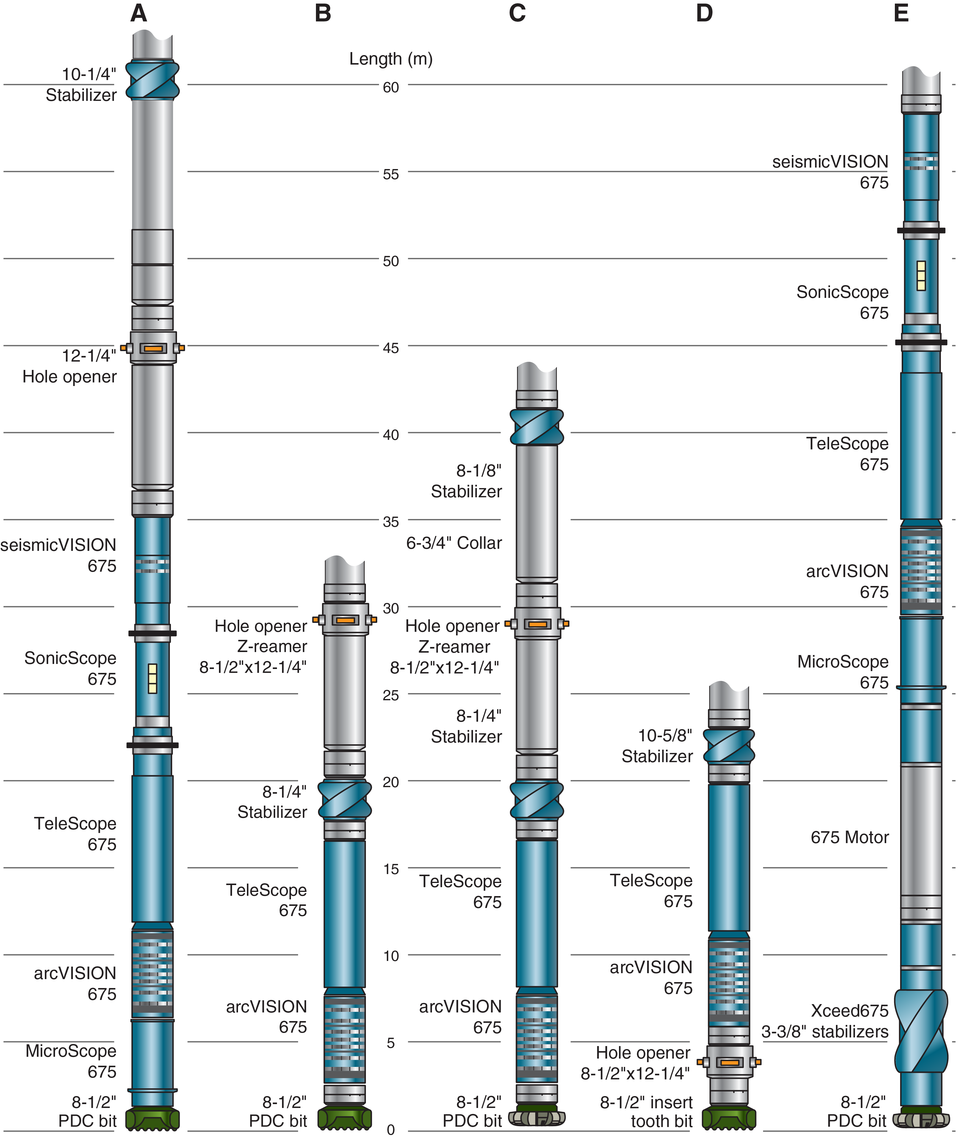
Figure F26. MWD/LWD BHA configurations.
arcVISION
Schlumberger's arcVISION tool measures gamma ray, propagation resistivity, and pressure and temperature in the borehole annulus. Annular pressure data were used to calculate the equivalent circulating density, which is the apparent density of the drilling fluid during pumping. Downhole pressure is also crucial for detecting any inflow from the formation into the borehole or obstruction of the borehole due to collapse of the borehole walls, signaled by an increase in pressure. Monitoring of downhole pressure also allows us to detect pressure decreases associated with loss of circulation due to permeable formations, faults, or unintended hydraulic fractures.
The arcVISION tool measures natural gamma ray and propagation resistivity. For propagation resistivity, phase shift and attenuation are measured using five transmitters and two receivers at two frequencies (400 kHz and 2 MHz). In total, 20 resistivity curves are acquired at different depths of investigation and axial resolutions. The depth of investigation ranges from 13 to 38 inches, and the axial resolution ranges from 0.7 to 3.0 inches (all resolutions and depths of investigation are detailed in Table T11). These resistivity data at various depths of penetration enable an estimation of the borehole size (electromagnetic caliper [e-caliper]) that Schlumberger can compute on demand using internal software. The e-caliper can also be processed shipboard by scientists using a nondocumented proprietary module from Schlumberger's Techlog software platform.
Processing of the gamma ray log includes corrections for four environmental factors: bit size, collar thickness, mud weight, and potassium content in the drilling mud. If the borehole is enlarged compared to the bit size, the processed gamma ray log values will be underestimated. If the mud has higher potassium content, the processed gamma ray values will be overestimated. The data are processed on site by Schlumberger prior to data delivery.
seismicVISION
The seismicVISION tool produces data that can be interpreted to be a check shot survey, providing a traveltime–depth function for seismic/well calibration, interval velocity, and a vertical seismic profile. The seismicVISION tool records seismograms using a hydrophone and a three-component geophone in the tool and a surface source and hydrophone. The source used during Expedition 358 in Hole C0024A consisted of an array of three 250 inch3 air guns and three 150 inch3 air guns (a total of 1200 inch3) that were suspended by crane ~57 m from the rotary table (Figure F27) and fired from 5.4 m below sea level (mbsl) at 2500 psi. Time correlations of the shots are ensured using high-precision clocks at both the surface and downhole hydrophones. The surface hydrophone was suspended 1.27 m below the air guns (total of 6.67 m below mean sea level) and the zero times of the waveforms were corrected to mean sea level. seismicVISION data were acquired while the pipe was being recovered. The first data were acquired at 752 mbsf, and the rest of the data were acquired every ~19 m at the connection and the middle of each standpipe above 575 mbsf.
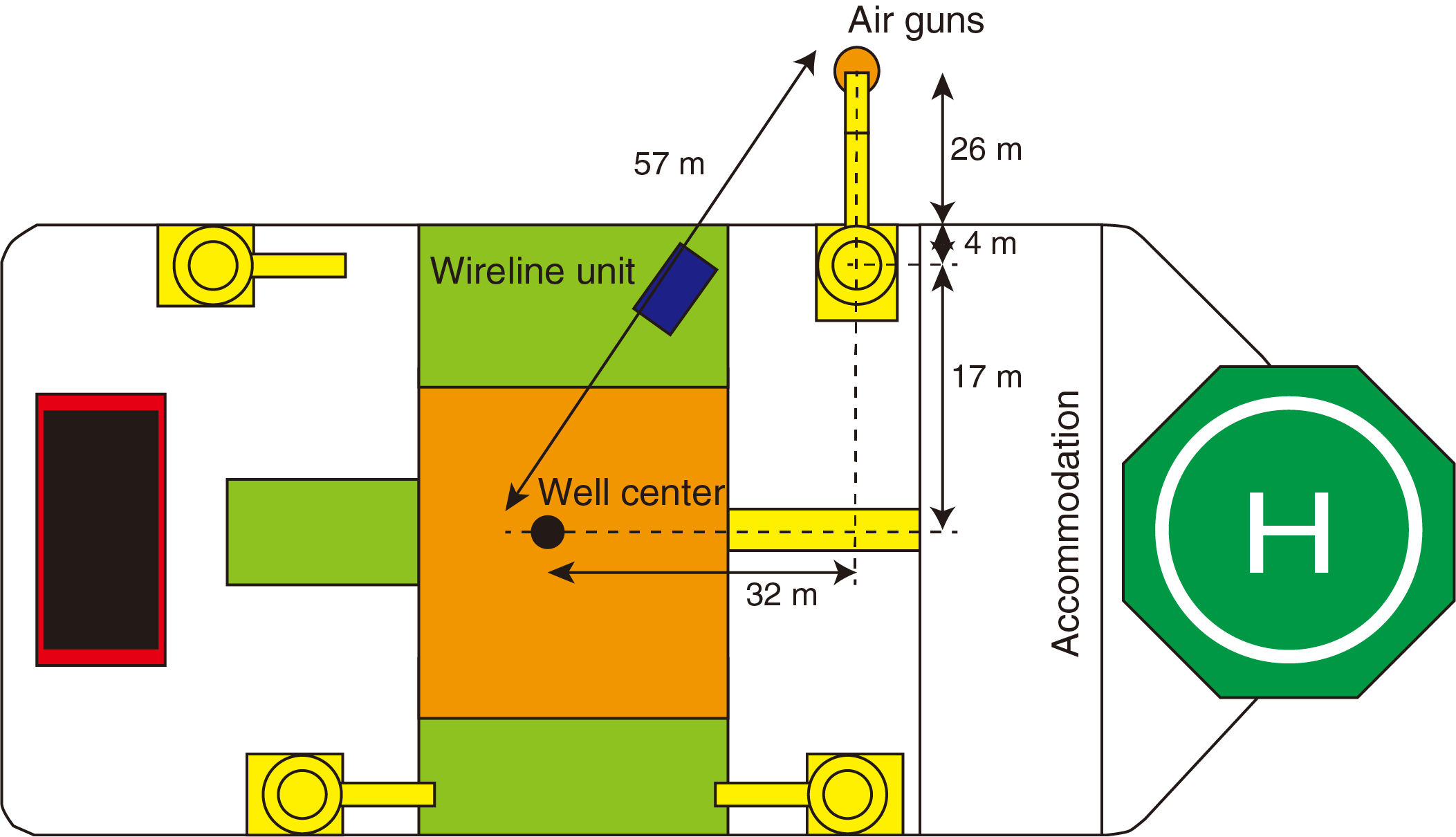
Figure F27. seismicVISION acquisition geometry.
At each data acquisition level, 10 shots were fired by the surface source at 15 s intervals. The tool records the pressure (hydrophone) and acceleration (three-component geophones) seismograms obtained for each shot and calculates and records a vertical stack of the shots. In practice, because our holes were near vertical and the tool was centered and unclamped, the geophone data yielded little useful information. The tool also automatically picks and records the P-wave arrival time in the stacked seismogram. The stacked seismogram and the picked P-wave arrival times from the instrument are transmitted to the ship by the MWD system and thus could be used soon after acquisition at each level or as the primary data in case the tool fails to record or loses data.
MicroScope
Schlumberger's MicroScope tool provides measurements of laterolog-type formation resistivity and high-resolution electrical resistivity images of the borehole wall. The tool provides several resistivity measurements: button resistivity at various depths of investigation (shallow, medium, deep, and extradeep), toroid (ring) resistivity, and bit resistivity.
Bit resistivity uses the lower portion of the tool and the bit as a measuring electrode. The lower transmitter coil generates a current that flows through the bit and into the formation, returning to the drill collar farther up the tool string. By measuring the axial current through the bit for a given voltage, resistivity near the bit is determined by Ohm's law. The axial resolution is 48 inches.
For the toroid/ring resistivity, upper and lower transmitter toroids produce currents that flow out of the tool approximately perpendicular to the formation and provide lateral resistivity measurements at two depths of investigation (5 and 6 inches) and an axial resolution of 15 inches.
Button resistivity is similar to toroid resistivity except that electrodes are used instead of toroids. Four button electrodes, each 0.4 inches in diameter, measure resistivity at four depths of investigation into the borehole wall: ~1.5, 3, 5, and 6 inches. The tool acquires azimuthal readings as it rotates and determines its orientation referenced to Earth's magnetic field using accelerometers and magnetometers. After downloading the tool memory data, the service company generated 360° images of the borehole wall, sampled azimuthally at ~6.4° (56 "bins") and sampled vertically at 0.3 inches (vertical resolution of 0.6 inches).
A two-button electrode design ensures better borehole wall coverage and provides ultrahigh-resolution images, sampled azimuthally at ~1.7° (208 bins) and sampled vertically at 0.2 inches (vertical resolution of 0.4 inches).
SonicScope
Schlumberger's SonicScope tool acquires both monopole and quadrupole waveforms using a single transmitter that excites both modes over a frequency range from 1 to 20 kHz. Transmitted sonic waves are detected by four arrays of azimuthal receivers; each array has 12 receivers. The received waveforms are stored in the tool memory, and the tool also automatically picks arrival times, generating an estimate of the slowness (Δt; traveltime over distance, or the reciprocal of velocity) for waves transmitted through the formation, and those picks are transmitted uphole for real-time slowness logs. Later processing of the full waveforms, stored in the memory data, is used to generate the final sonic logs.
In monopole mode, the transmitter generates a compressional wave that refracts at the borehole wall, generating critically refracted compressional and shear waves that travel along the borehole wall. The shear waves are only observed if the formation's shear slowness is less than the slowness of the borehole fluid (i.e., in a fast formation). If the formation shear slowness is greater than the fluid slowness (i.e., in a slow formation), the shear wave is refracted away from the borehole and no shear wave returns to the tool. Quadrupole sources generate waves that are highly dispersive (velocity is frequency dependent), but which at the lower end of the frequency range travel close to the shear wave velocity of the formation (Alford et al., 2012). The most accurate estimation of the shear velocity requires an inversion of the waveforms. The maximum recording rate of the SonicScope is 10 s when both real-time data and memory data are acquired.
TeleScope
Schlumberger's TeleScope MWD tool measures downhole WOB and torque, provides direction and inclination measurements, and transfers drilling data and select formation data to the ship in real time using mud-pulse telemetry (https://www.slb.com/-/media/files/drilling/brochure/telescope-br). The TeleScope provides critical real-time two-way communication between LWD tools and the surface. This communication enables both scientists and operators to monitor drilling operations, estimate borehole conditions, and detect geologic features while drilling. The mud-pulse telemetry process utilizes a modulator to generate a continuous 12 Hz pressure wave in the drilling fluid and changes the phase of the signal (continuous phase modulation) to transmit the data to the surface. The transmission rate ranges from 0.5 to 12 bps and is primarily dependent on water depth and fluid density. A pulse rate of 6 bps was used during Expedition 358. Various models of the TeleScope 675 were used during this expedition, and the main difference between them was the ability or lack thereof to measure downhole WOB.
During Expedition 358, various combinations of data from the TeleScope, arcVISION, MicroScope, and SonicScope were transferred to the ship in real time, depending on which tools were in the drill string BHA for a given run (Figure F26). Because of the limited bandwidth of mud-pulse telemetry, those data were downsampled for real-time transfer.
Onboard data flow
The LWD tools recorded data at a preset frequency based on logging speed and the tool-optimized resolution, providing measurements as a function of time. The depth information for the LWD and MWD data was recorded on the LSF depth scale) but reported as depth below seafloor (mbsf) for reporting purposes to allow standard interpretation and correlation with shipboard sample measurements. Schlumberger's integrated logging and drilling surface system, which was installed on Chikyu, was used to record and control the ROP and depth of the drill string at any given time while logging. This was determined using the length of the drill string and derrick top drive position. A crown-mounted heave compensator at the top of the derrick helped reduce errors from heave and improved WOB accuracy.
The real-time data were displayed on a monitor in the laboratory in real time and uploaded to the server every 12 h for an initial interpretation by shipboard scientists. Recovery of the memory data occurred after each BHA run. In both cases, data referenced in time were converted to BRT depth. The depth reference was then converted to the LSF depth scale. Data were then distributed in digital log information standard (DLIS) format, and the main scalar logs were extracted and converted into log ASCII standard (LAS) files.
Data quality assessment
Cross-correlating LWD/MWD data for primary quality assessment included the use of downhole drilling parameters, drilling control logs, and geophysical control logs. The Logging Staff Scientists (LSSs) documented the LWD/MWD operations and converted the raw data received from the Schlumberger engineer to the LSF depth scale. Resistivity and e-caliper logs were used for data quality assessment, permitting analysis of borehole conditions (e.g., caving, washout, bridges, and invasion) for potential effects on logging data. Borehole images were also used to assess borehole conditions. Regions of high stick-slip also affect image quality. Time elapsed after passage of the drill bit for the main geophysical measurements was also monitored as a quality check along with drilling operations. Because of variations in sampling time, all measurements may have insufficient heave compensation and/or unaccounted movements, including bending, shocks, and vibrations of the BHA, creating errors in local depth measurements as much as tens of centimeters.
Real-time quality control and real-time geomechanics
Logging scientists and the LSSs continuously observed the real-time data feed and closed-circuit television feed from the rig floor. This provided an initial quality check on the data and tracking of events (e.g., time off bottom) that could affect the log response. The parameters monitored included sonic logs, resistivity, gamma ray, annular pressures, torque, WOB, ROP, and mud volume.
When electric images were recorded, logging scientists provided rapid interpretation of structures and borehole breakouts using the real-time resistivity image data as part of the real-time geomechanics (RTG) workflow. Screenshots of the real-time data were printed out every 3 h, and manual picking of structures (bedding, resistive fractures, conductive fractures, borehole breakouts, and tensile fractures) was performed. PDFs of the real-time image data were uploaded to the server every 12 h and were used to double check the initial interpretations. Picked structures and their orientations were reported to the Science Leaders and RTG watch leads, who then used these data as part of a larger data set to examine borehole stability and downhole stress and provide recommendations for mud weight. Daily geomechanics reports are available in RTG in Supplementary material.
Log and image interpretation
Changes in the log response are usually related to variation of the composition and/or texture of sediment and rock, and they were used to define and characterize formation properties. Logging units were characterized through both qualitative and quantitative methods.
Lithologic logging unit characterization
The depths of logging unit boundaries, physical properties of the logging units, and bedding information were defined based on LWD logs and borehole images. Trends and variations in all available LWD/MWD logs were examined to define distinct logging units and allowed for the following:
- Defining and characterizing each logging unit, subunit, and unit boundary;
- Categorizing composition and trends in each unit; and
- Interpreting geological features based on log data.
Lithology, from unit scale to bed scale, was primarily determined from gamma ray logs along with resistivity and sonic logs when available. High or low gamma radiation was used as the primary indicator for the interpretation of clay- or sand-rich intervals, respectively. Sonic and resistivity logs aided textural interpretation. Borehole images helped in characterizing geological features such as bedding orientation, faults, fractures, sedimentary structures, bed boundaries, and unconformities. Logging units were correlated with core, cuttings, and seismic data at Site C0002 from previous Integrated Ocean Drilling Program expeditions (Expedition 314 Scientists, 2009; Expedition 315 Scientists, 2009b; Strasser et al., 2014b; Tobin et al., 2015b) to further refine the interpretations (see Lithology).
Structural interpretation from logs
Structural analysis was performed on the memory data resistivity image logs using Schlumberger's Techlog software. The azimuthal button resistivity data were displayed as unwrapped 360° north-oriented images of the borehole wall for interpretation and dip measurements. As part of the workflow for image analysis, dynamic and static normalization were performed on the resistivity images. Static normalization shows overall change in resistivity in a single borehole or a logging run because it displays a color scale covering the entire range of resistivity throughout the run. Dynamic normalization recalculates the color scale range over a "sliding" depth interval and is thus useful for bringing out subtle details in a log such as changes in facies or lithology, natural and drilling-induced fracture, or borehole breakout width.
Resistivity contrasts in the rock are the basis for the identification and interpretation of geological features in the resistivity images. Dipping planar surfaces are identified as sinusoidal curves of similar contrast in unwrapped resistivity images (Luthi, 2001). The dip and azimuth of fractures, faults, and bedding were determined by fitting sinusoids to the image data. Artifacts can appear in the processed data because of stick-slip and insufficient heave corrections (Lofts and Bourke, 1999). Borehole diameter was obtained from the e-caliper. The borehole size was set to the bit size (8½ inches for all runs, except 12¼ inches for the lowermost section of Hole C0002R) to calculate dip when a caliper measurement was missing. This assumption may cause dip to be overestimated in regions with a large borehole diameter, introducing small dip angle errors. This means the reported dips should be viewed as maximum values. Depth of resistivity investigation was also one of the parameters used for dip angle calculation.
Using the background resistivity as a base, we classified fractures as conductive or resistive but only for unambiguous examples. Clear crosscutting or dramatic variation in bedding dip formed the basis for fracture classification in addition to azimuth orientation and fracture density.
Borehole wall analysis
Stress orientation in the borehole can be determined by using both borehole breakouts and drilling-induced tensile fractures (DITFs). The vertical stress (Sv), two horizontal principal stresses (Shmin and SHMAX), fluid pressures, and mud weight are considered to control the circumferential stress azimuth around the borehole (Jaeger and Cook, 1979; Zoback, 2007). Borehole breakouts form when the maximum circumferential stress exceeds the unconfined compressive strength of the formation, assuming an isotropic formation. In a vertical well, breakouts appear in resistivity images (obtained with the MicroScope tool) as parallel and vertical conductive features oriented 180° apart from each other in the direction of Shmin. The minimum circumferential stress arises in the direction of SHMAX where DITFs form if the effective circumferential stress becomes negative (tensional) enough to overcome the tensile strength of the formation (typically less than 10 MPa). DITFs appear as vertical pairs of cracks 180° apart if the borehole axis is aligned with the vertical stress but could form en echelon patterns of inclined cracks if the borehole axis is deviated from vertical (Zoback, 2007).
Interpretation of the various resistivity images provided the orientation of breakouts and DITFs. Resistivity images were oriented to convert the measured azimuths and widths of breakouts along with DITFs into true azimuth for the estimation of horizontal principal stress direction.
Integration with lithologic interpretations helped interpret variations in the formation strength, stress, and/or pore pressure. MWD drilling parameters assisted in the analysis of borehole stability, mud pressure surges, and formation strength.
Estimation of porosity from resistivity
In the absence of an LWD tool to directly measure in situ porosity, we used Archie's law to derive a porosity (ϕ) log from the measured resistivity log:
where F is the formation factor, and a and m are known as the tortuosity and cementation factor, respectively. The formation factor is calculated from the resistivity log as
where R is the LWD-measured resistivity and Rf is the resistivity of the pore fluid. We used the deep resistivity measurement to minimize the effects of fluid invasion into the formation. The fluid resistivity can be estimated from assumptions on the pressure, temperature, and salinity of the pore fluid. The cementation factor depends on rock type and was calibrated using the shipboard measurements of porosity and resistivity on cuttings and core samples.
References
Alford, J., Blyth, M., Tollefsen, E., Crowe, J., Loreto, J., Mohammed, S., Pistre, V., and Rodriguez-Herrera, A., 2012. Sonic logging while drilling – shear answers. Oilfield Review, 24(1).
ASTM International, 1990. Standard method for laboratory determination of water (moisture) content of soil and rock (Standard D2216–90). In Annual Book of ASTM Standards for Soil and Rock (Volume 04.08): Philadelphia (American Society for Testing Materials). [revision of D2216-63, D2216-80]
Backman, J., Raffi, I., Rio, D., Fornaciari, E., and Pälike, H., 2012. Biozonation and biochronology of Miocene through Pleistocene calcareous nannofossils from low and middle latitudes. Newsletters on Stratigraphy, 45(3):221–244. https://doi.org/10.1127/0078-0421/2012/0022
Blum, P., 1997. Technical Note 26: Physical Properties Handbook—A Guide to the Shipboard Measurement of Physical Properties of Deep-Sea Cores. Ocean Drilling Program. https://doi.org/10.2973/odp.tn.26.1997
Bown, P.R., and Young, J.R., 1998. Techniques. In Bown, P.R. (Ed.), Calcareous Nannofossil Biostratigraphy: Dordrecht, The Netherlands (Kluwer Academic Publishing), 16–28.
Byrne, T., 1984. Early deformation in mélange terranes of the Ghost Rocks Formation, Kodiak Islands, Alaska. Special Paper - Geological Society of America, 198:21–52. https://doi.org/10.1130/SPE198-p21
Carlson, R.L., and Christensen, N.I., 1977. Velocity anisotropy and physical properties of deep-sea sediments from the western South Atlantic. In Supko, P.R., Perch-Nielsen, K., et al., Initial Reports of the Deep Sea Drilling Project, 39: Washington, DC (U.S. Government Printing Office), 555–559. https://doi.org/10.2973/dsdp.proc.39.124.1977
Carlson, W.D., 2006. Three-dimensional imaging of earth and planetary materials. Earth and Planetary Science Letters, 249(3–4):133–147. https://doi.org/10.1016/j.epsl.2006.06.020
Expedition 314 Scientists, 2009. Expedition 314 Site C0002. In Kinoshita, M., Tobin, H., Ashi, J., Kimura, G., Lallemant, S., Screaton, E.J., Curewitz, D., Masago, H., Moe, K.T., and the Expedition 314/315/316 Scientists, Proceedings of the Integrated Ocean Drilling Program, 314/315/316: Washington, DC (Integrated Ocean Drilling Program Management International, Inc.). https://doi.org/10.2204/iodp.proc.314315316.114.2009
Expedition 315 Scientists, 2009a. Expedition 315 methods. In Kinoshita, M., Tobin, H., Ashi, J., Kimura, G., Lallemant, S., Screaton, E.J., Curewitz, D., Masago, H., Moe, K.T., and the Expedition 314/315/316 Scientists, Proceedings of the Integrated Ocean Drilling Program, 314/315/316: Washington, DC (Integrated Ocean Drilling Program Management International, Inc.). https://doi.org/10.2204/iodp.proc.314315316.122.2009
Expedition 315 Scientists, 2009b. Expedition 315 Site C0002. In Kinoshita, M., Tobin, H., Ashi, J., Kimura, G., Lallemant, S., Screaton, E.J., Curewitz, D., Masago, H., Moe, K.T., and the Expedition 314/315/316 Scientists, Proceedings of the Integrated Ocean Drilling Program, 314/315/316: Washington, DC (Integrated Ocean Drilling Program Management International, Inc.). https://doi.org/10.2204/iodp.proc.314315316.124.2009
Expedition 316 Scientists, 2009. Expedition 316 methods. In Kinoshita, M., Tobin, H., Ashi, J., Kimura, G., Lallemant, S., Screaton, E.J., Curewitz, D., Masago, H., Moe, K.T., and the Expedition 314/315/316 Scientists, Proceedings of the Integrated Ocean Drilling Program, 314/315/316: Washington, DC (Integrated Ocean Drilling Program Management International, Inc.). https://doi.org/10.2204/iodp.proc.314315316.132.2009
Expedition 319 Scientists, 2010a. Expedition 319 summary. In Saffer, D., McNeill, L., Byrne, T., Araki, E., Toczko, S., Eguchi, N., Takahashi, K., and the Expedition 319 Scientists, Proceedings of the Integrated Ocean Drilling Program, 319: Tokyo (Integrated Ocean Drilling Program Management International, Inc.). https://doi.org/10.2204/iodp.proc.319.101.2010
Expedition 319 Scientists, 2010b. Methods. In Saffer, D., McNeill, L., Byrne, T., Araki, E., Toczko, S., Eguchi, N., Takahashi, K., and the Expedition 319 Scientists, Proceedings of the Integrated Ocean Drilling Program, 319: Tokyo (Integrated Ocean Drilling Program Management International, Inc.). https://doi.org/10.2204/iodp.proc.319.102.2010
Expedition 322 Scientists, 2010. Methods. In Saito, S., Underwood, M.B., Kubo, Y., and the Expedition 322 Scientists, Proceedings of the Integrated Ocean Drilling Program, 322: Tokyo (Integrated Ocean Drilling Program Management International, Inc.). https://doi.org/10.2204/iodp.proc.322.102.2010
Expedition 326 Scientists, 2011. Expedition 326 Preliminary Report: NanTroSEIZE Stage 3: Plate Boundary Deep Riser: Top Hole Engineering. Integrated Ocean Drilling Program. https://doi.org/10.2204/iodp.pr.326.2011
Expedition 332 Scientists, 2011. Site C0002. In Kopf, A., Araki, E., Toczko, S., and the Expedition 332 Scientists, Proceedings of the Integrated Ocean Drilling Program, 332: Tokyo (Integrated Ocean Drilling Program Management International, Inc.). https://doi.org/10.2204/iodp.proc.332.104.2011
Expedition 333 Scientists, 2012. Methods. In Henry, P., Kanamatsu, T., Moe, K., and the Expedition 333 Scientists, Proceedings of the Integrated Ocean Drilling Program, 333: Tokyo (Integrated Ocean Drilling Program Management International, Inc.). https://doi.org/10.2204/iodp.proc.333.102.2012
Expedition 334 Scientists, 2012. Methods. In Vannucchi, P., Ujiie, K., Stroncik, N., Malinverno, A., and the Expedition 334 Scientists, Proceedings of the Integrated Ocean Drilling Program, 334: Tokyo (Integrated Ocean Drilling Program Management International, Inc.). https://doi.org/10.2204/iodp.proc.334.102.2012
Expedition 337 Scientists, 2013. Methods. In Inagaki, F., Hinrichs, K.-U., Kubo, Y., and the Expedition 337 Scientists, Proceedings of the Integrated Ocean Drilling Program, 337: Tokyo (Integrated Ocean Drilling Program Management International, Inc.). https://doi.org/10.2204/iodp.proc.337.102.2013
Expedition 343/343T Scientists, 2013. Methods. In Chester, F.M., Mori, J., Eguchi, N., Toczko, S., and the Expedition 343/343T Scientists, Proceedings of the Integrated Ocean Drilling Program, 343/343T: Tokyo (Integrated Ocean Drilling Program Management International, Inc.). https://doi.org/10.2204/iodp.proc.343343T.102.2013
Fisher, A.T., and Underwood, M.B., 1995. Calibration of an X-ray diffraction method to determine relative mineral abundances in bulk powders using matrix singular value decomposition: a test from the Barbados accretionary complex. In Shipley, T.H., Ogawa, Y., Blum, P., et al., Proceedings of the Ocean Drilling Program, Initial Reports, 156: College Station, TX (Ocean Drilling Program), 29–37. https://doi.org/10.2973/odp.proc.ir.156.103.1995
GE Healthcare, 2013a. Discovery CT750 HD User Manual (revision 1): Waukesha, Wisconsin (GE Healthcare).
GE Healthcare, 2013b. Technical Reference Manual (revision 1): Waukesha, Wisconsin (GE Healthcare).
GE Healthcare, 2013c. Discovery CT Series Service Methods (revision 15): Waukesha, Wisconsin (GE Healthcare).
Hammerschmidt, S.B., Wiersberg, T., Heuer, V.B., Wendt, J., Erzinger, J., and Kopf, A., 2014. Real-time drilling mud gas monitoring for qualitative evaluation of hydrocarbon gas composition during deep sea drilling in the Nankai Trough Kumano Basin. Geochemical Transactions, 15(1):15. https://doi.org/10.1186/s12932-014-0015-8
Harris, R.N., Sakaguchi, A., Petronotis, K., Baxter, A.T., Berg, R., Burkett, A., Charpentier, D., Choi, J., Diz Ferreiro, P., Hamahashi, M., Hashimoto, Y., Heydolph, K., Jovane, L., Kastner, M., Kurz, W., Kutterolf, S.O., Li, Y., Malinverno, A., Martin, K.M., Millan, C., Nascimento, D.B., Saito, S., Sandoval Gutierrez, M.I., Screaton, E.J., Smith-Duque, C.E., Solomon, E.A., Straub, S.M., Tanikawa, W., Torres, M.E., Uchimura, H., Vannucchi, P., Yamamoto, Y., Yan, Q., and Zhao, X., 2013. Methods. In Harris, R.N., Sakaguchi, A., Petronotis, K., and the Expedition 344 Scientists, Proceedings of the Integrated Ocean Drilling Program, 344: College Station, TX (Integrated Ocean Drilling Program). https://doi.org/10.2204/iodp.proc.344.102.2013
Heesemann, M., Villinger, H., Fisher, A.T., Tréhu, A.M., and White, S., 2006. Data report: testing and deployment of the new APCT-3 tool to determine in situ temperatures while piston coring. In Riedel, M., Collett, T.S., Malone, M.J., and the Expedition 311 Scientists. Proceedings of the Integrated Ocean Drilling Program, 311: Washington, DC (Integrated Ocean Drilling Program Management International, Inc.). https://doi.org/10.2204/iodp.proc.311.108.2006
Jaeger, J.C., and Cook, N.G.W., 1979. Fundamentals of Rock Mechanics (2nd edition: New York (Chapman and Hall).
Kitajima, H., Hirose, T., Ikari, M., Kanagawa, K., Kimura, G., Kinoshita, M., Saffer, D., Tobin, H., Yamaguchi, A., Eguchi, N., Maeda, L., Toczko, S., Bedford, J., Chiyonobu, S., Colson, T.A., Conin, M., Cornard, P.H., Dielforder, A., Doan, M.-L., Dutilleul, J., Faulkner, D.R., Fukuchi, R., Guérin, G., Hamada, Y., Hamahashi, M., Hong, W.-L., Ijiri, A., Jaeger, D., Jeppson, T., Jin, Z., John, B.E., Kitamura, M., Kopf, A., Masuda, H., Matsuoka, A., Moore, G.F., Otsubo, M., Regalla, C., Sakaguchi, A., Sample, J., Schleicher, A., Sone, H., Stanislowski, K., Strasser, M., Toki, T., Tsuji, T., Ujiie, K., Underwood, M.B., Yabe, S., Yamamoto, Y., Zhang, J., Sanada, Y., Kido, Y., Le Ber, E., and Saito, S., 2020. Site C0002. With contributions by T. Kanamatsu. In Tobin, H., Hirose, T., Ikari, M., Kanagawa, K., Kimura, G., Kinoshita, M., Kitajima, H., Saffer, D., Yamaguchi, A. Eguchi, N., Maeda, L., Toczko, S., and the Expedition 358 Scientists, NanTroSEIZE Plate Boundary Deep Riser 4: Nankai Seismogenic/Slow Slip Megathrust. Proceedings of the International Ocean Discovery Program, 358: College Station, TX (International Ocean Discovery Program). https://doi.org/10.14379/iodp.proc.358.103.2020
Lin, W., Yeh, E.-C., Ito, H., Hirono, T., Soh, W., Wang, C.-Y., Ma, K.-F., Hung, J.-H., and Song, S.-R., 2007. Preliminary results of stress measurements using drill cores of TCDP Hole-A: an application of anelastic strain recovery method to three-dimensional in-situ stress determination. Terrestrial, Atmospheric and Oceanic Sciences, 18(2):379. https://doi.org/10.3319/TAO.2007.18.2.379(TCDP)
Lofts, J.C., and Bourke, L.T., 1999. The recognition of artefacts from acoustic and resistivity borehole imaging devices. In Lovell, M., Williamson, G., and Harvey, P., (Eds.), Borehole Imaging: Applications and Case Histories. Special Publications - Geological Society of London, 159:59–76. https://doi.org/10.1144/GSL.SP.1999.159.01.03
Lourens, L., Hilgen, F., Shackleton, N.J., Laskar, J., and Wilson, D., 2004. The Neogene period. In Gradstein, F.M., Ogg, J.G., and Smith, A. (Eds.), A Geologic Time Scale 2004: Cambridge, United Kingdom (Cambridge University Press), 409–440. https://doi.org/10.1017/CBO9780511536045.022
Luthi, S., 2001. Geological Well Logs: Their Use in Reservoir Modeling: Berlin (Springer-Verlag)
Maltman, A.J., Byrne, T., Karig, D.E., and Lallement, S., 1993. Deformation at the toe of an active accretionary prism: synopsis of results from ODP Leg 131, Nankai, SW Japan. Journal of Structural Geology, 15(8):949–964. https://doi.org/10.1016/0191-8141(93)90169-B
Manheim, F.T., and Sayles, F.L., 1974. Composition and origin of interstitial waters of marine sediments, based on deep sea drill cores. In Goldberg, E.D. (Ed.), The Sea (Volume 5): Marine Chemistry: The Sedimentary Cycle: New York (Wiley), 527–568.
Marsaglia, K., Milliken, K., and Doran, L., 2013. Technical Note 1: IODP Digital Reference for Smear Slide Analysis of Marine Mud—Part 1: Methodology and Atlas of Siliciclastic and Volcanogenic Components. Integrated Ocean Drilling Program. https://doi.org/10.2204/iodp.tn.1.2013
Martini, E., 1971. Standard Tertiary and Quaternary calcareous nannoplankton zonation. In Farinacci, A. (Ed.), Proceedings of the Second Planktonic Conference, Roma 1970: Rome (Edizioni Tecnoscienza), 2:739–785.
Matsuki, K., 1991. Three-dimensional in situ stress measurement with anelastic strain recovery of a rock core. Proceedings - International Congress on Rock Mechanics, 7:557–560.
Mazzullo, J., and Graham, A.G. (Eds.), 1988. Technical Note 8: Handbook for shipboard sedimentologists. Ocean Drilling Program. https://doi.org/10.2973/odp.tn.8.1988
Mazzullo, J.M., Meyer, A., and Kidd, R.B., 1988. New sediment classification scheme for the Ocean Drilling Program. In Mazzullo, J., and Graham, A.G. (Eds.), Technical Note 8: Handbook for Shipboard Sedimentologists. Ocean Drilling Program, 44–67. https://doi.org/10.2973/odp.tn.8.1988
Mees, F., Swennen, R., Van Geet, M., and Jacobs, P., 2003. Applications of X-ray computed tomography in the geosciences. Special Publication - Geological Society of London, 215(1):1–6. https://doi.org/10.1144/GSL.SP.2003.215.01.01
Moore, J.C., Roeske, S., Cowan, D.S., Lundberg, N., Gonzales, E., Schoonmaker, J., and Lucas, S.E., 1986. Scaly fabrics from Deep Sea Drilling Project cores from forearcs. In Moore J.C. (Ed.), Structural Fabrics in Deep Sea Drilling Project Cores from foearcs. Memoir - Geological Society of America, 166:55–74. https://doi.org/10.1130/MEM166-p55
Morono, Y., Inagaki, F., Heuer, V.B., Kubo, Y., Maeda, L., Bowden, S., Cramm, M., Henkel, S., Hirose, T., Homola, K., Hoshino, T., Ijiri, A., Imachi, H., Kamiya, N., Kaneko, M., Lagostina, L., Manners, H., McClelland, H.-L., Metcalfe, K., Okutsu, N., Pan, D., Raudsepp, M.J., Sauvage, J., Schubotz, F., Spivack, A., Tonai, S., Treude, T., Tsang, M.-Y., Viehweger, B., Wang, D.T., Whitaker, E., Yamamoto, Y., and Yang, K., 2017. Expedition 370 methods. In Heuer, V.B., Inagaki, F., Morono, Y., Kubo, Y., Maeda, L., and the Expedition 370 Scientists, Temperature Limit of the Deep Biosphere off Muroto. Proceedings of the International Ocean Discovery Program, 370: College Station, TX (International Ocean Discovery Program). https://doi.org/10.14379/iodp.proc.370.102.2017
Nakano, T., Nakashima, Y., Nakamura, K., and Ikeda, S., 2000. Observation and analysis of internal structure of rock using X-ray CT. Chishitsugaku Zasshi, 106(5):363–378. https://doi.org/10.5575/geosoc.106.363
Noorany, I., 1984. Phase relations in marine soils. Journal of Geotechnical Engineering, 110:539–543. https://doi.org/10.1061/(ASCE)0733-9410(1984)110:4(539)
Okada, H., and Bukry, D., 1980. Supplementary modification and introduction of code numbers to the low-latitude coccolith biostratigraphic zonation (Bukry, 1973; 1975). Marine Micropaleontology, 5:321–325. https://doi.org/10.1016/0377-8398(80)90016-X
Raffi, I., Backman, J., Fornaciari, E., Pälike, H., Rio, D., Lourens, L., and Hilgen, F., 2006. A review of calcareous nannofossil astrobiochronology encompassing the past 25 million years. Quaternary Science Reviews, 25(23–24):3113–3137. https://doi.org/10.1016/j.quascirev.2006.07.007
Rothwell, R.G., 1989. Minerals and Mineraloids in Marine Sediments: An Optical Identification Guide: London (Elsevier). https://doi.org/10.1007/978-94-009-1133-8
Shepard, F.P., 1954. Nomenclature based on sand-silt-clay ratios. Journal of Sedimentary Research, 24(3):151–158. https://doi.org/10.1306/D4269774-2B26-11D7-8648000102C1865D
Shipboard Scientific Party, 1991. Explanatory notes. In Taira, A., Hill, I., Firth, J.V., et al., Proceedings of the Ocean Drilling Program, Initial Reports, 131: College Station, TX (Ocean Drilling Program), 25–60. https://doi.org/10.2973/odp.proc.ir.131.104.1991
Strasser, M., Dugan, B., Kanagawa, K., Moore, G.F., Toczko, S., Maeda, L., Kido, Y., Moe, K.T., Sanada, Y., Esteban, L., Fabbri, O., Geersen, J., Hammerschmidt, S., Hayashi, H., Heirman, K., Hüpers, A., Jurado Rodriguez, M.J., Kameo, K., Kanamatsu, T., Kitajima, H., Masuda, H., Milliken, K., Mishra, R., Motoyama, I., Olcott, K., Oohashi, K., Pickering, K.T., Ramirez, S.G., Rashid, H., Sawyer, D., Schleicher, A., Shan, Y., Skarbek, R., Song, I., Takeshita, T., Toki, T., Tudge, J., Webb, S., Wilson, D.J., Wu, H.-Y., and Yamaguchi, A., 2014a. Methods. In Strasser, M., Dugan, B., Kanagawa, K., Moore, G.F., Toczko, S., Maeda, L., and the Expedition 338 Scientists, Proceedings of the Integrated Ocean Drilling Program, 338: Yokohama, Japan (Integrated Ocean Drilling Program). https://doi.org/10.2204/iodp.proc.338.102.2014
Strasser, M., Dugan, B., Kanagawa, K., Moore, G.F., Toczko, S., Maeda, L., Kido, Y., Moe, K.T., Sanada, Y., Esteban, L., Fabbri, O., Geersen, J., Hammerschmidt, S., Hayashi, H., Heirman, K., Hüpers, A., Jurado Rodriguez, M.J., Kameo, K., Kanamatsu, T., Kitajima, H., Masuda, H., Milliken, K., Mishra, R., Motoyama, I., Olcott, K., Oohashi, K., Pickering, K.T., Ramirez, S.G., Rashid, H., Sawyer, D., Schleicher, A., Shan, Y., Skarbek, R., Song, I., Takeshita, T., Toki, T., Tudge, J., Webb, S., Wilson, D.J., Wu, H.-Y., and Yamaguchi, A., 2014b. Site C0002. In Strasser, M., Dugan, B., Kanagawa, K., Moore, G.F., Toczko, S., Maeda, L., and the Expedition 338 Scientists, Proceedings of the Integrated Ocean Drilling Program, 338: Yokohama (Integrated Ocean Drilling Program). https://doi.org/10.2204/iodp.proc.338.103.2014
Tauxe, L., Tucker, P., Peterson, N.P., and LaBrecque, J.L., 1984. Magnetostratigraphy of Leg 73 sediments. In Hsü, K.J., LaBrecque, J.L., et al., Initial Reports of the Deep Sea Drilling Project, 73: Washington, DC (U.S. Government Printing Office), 609–621. https://doi.org/10.2973/dsdp.proc.73.123.1984
Tobin, H., Hirose, T., Ikari, M., Kanagawa, K., Kimura, G., Kinoshita, M., Kitajima, H., Saffer, D., Yamaguchi, A., Eguchi, N., Maeda, L., Toczko, S., Bedford, J., Chiyonobu, S., Colson, T.A., Conin, M., Cornard, P.H., Dielforder, A., Doan, M.-L., Dutilleul, J., Faulkner, D.R., Fukuchi, R., Guérin, G., Hamada, Y., Hamahashi, M., Hong, W.-L., Ijiri, A., Jaeger, D., Jeppson, T., Jin, Z., John, B.E., Kitamura, M., Kopf, A., Masuda, H., Matsuoka, A., Moore, G.F., Otsubo, M., Regalla, C., Sakaguchi, A., Sample, J., Schleicher, A., Sone, H., Stanislowski, K., Strasser, M., Toki, T., Tsuji, T., Ujiie, K., Underwood, M.B., Yabe, S., Yamamoto, Y., Zhang, J., Sanada, Y., Kido, Y., Le Ber, E., and Saito, S., 2020a. Expedition 358 summary. With contributions by T. Kanamatsu. In Tobin, H., Hirose, T., Ikari, M., Kanagawa, K., Kimura, G., Kinoshita, M., Kitajima, H., Saffer, D., Yamaguchi, A. Eguchi, N., Maeda, L., Toczko, S., and the Expedition 358 Scientists, NanTroSEIZE Plate Boundary Deep Riser 4: Nankai Seismogenic/Slow Slip Megathrust. Proceedings of the International Ocean Discovery Program, 358: College Station, TX (International Ocean Discovery Program). https://doi.org/10.14379/iodp.proc.358.101.2020
Tobin, H., Hirose, T., Ikari, M., Kanagawa, K., Kimura, G., Kinoshita, M., Kitajima, H., Saffer, D., Yamaguchi, A. Eguchi, N., Maeda, L., Toczko, S., and the Expedition 358 Scientists, 2020b. Supplementary material, https://doi.org/10.14379/iodp.proc.358supp.2020. Supplement to Tobin, H., Hirose, T., Ikari, M., Kanagawa, K., Kimura, G., Kinoshita, M., Kitajima, H., Saffer, D., Yamaguchi, A. Eguchi, N., Maeda, L., Toczko, S., and the Expedition 358 Scientists, NanTroSEIZE Plate Boundary Deep Riser 4: Nankai Seismogenic/Slow Slip Megathrust. Proceedings of the International Ocean Discovery Program, 358: College Station, TX (International Ocean Discovery Program). https://doi.org/10.14379/iodp.proc.358.2020
Tobin, H., Hirose, T., Saffer, D., Toczko, S., Maeda, L., Kubo, Y., Boston, B., Broderick, A., Brown, K., Crespo-Blanc, A., Even, E., Fuchida, S., Fukuchi, R., Hammerschmidt, S., Henry, P., Josh, M., Jurado, M.J., Kitajima, H., Kitamura, M., Maia, A., Otsubo, M., Sample, J., Schleicher, A., Sone, H., Song, C., Valdez, R., Yamamoto, Y., Yang, K., Sanada, Y., Kido, Y., and Hamada, Y., 2015a. Methods. In Tobin, H., Hirose, T., Saffer, D., Toczko, S., Maeda, L., Kubo, Y., and the Expedition 348 Scientists, Proceedings of the Integrated Ocean Drilling Program, 348: College Station, TX (Integrated Ocean Drilling Program). https://doi.org/10.2204/iodp.proc.348.102.2015
Tobin, H., Hirose, T., Saffer, D., Toczko, S., Maeda, L., Kubo, Y., Boston, B., Broderick, A., Brown, K., Crespo-Blanc, A., Even, E., Fuchida, S., Fukuchi, R., Hammerschmidt, S., Henry, P., Josh, M., Jurado, M.J., Kitajima, H., Kitamura, M., Maia, A., Otsubo, M., Sample, J., Schleicher, A., Sone, H., Song, C., Valdez, R., Yamamoto, Y., Yang, K., Sanada, Y., Kido, Y., and Hamada, Y., 2015b. Site C0002. In Tobin, H., Hirose, T., Saffer, D., Toczko, S., Maeda, L., Kubo, Y., and the Expedition 348 Scientists, Proceedings of the Integrated Ocean Drilling Program, 348: College Station, TX (Integrated Ocean Drilling Program). https://doi.org/10.2204/iodp.proc.348.103.2015
Underwood, M.B., Basu, N., Steurer, J., and Udas, S., 2003. Data report: normalization factors for semiquantitative X-ray diffraction analysis, with application to DSDP Site 297, Shikoku Basin. In Mikada, H., Moore, G.F., Taira, A., Becker, K., Moore, J.C., and Klaus, A. (Eds.), Proceedings of the Ocean Drilling Program, Scientific Results, 190/196: College Station, TX (Ocean Drilling Program), 1–28. https://doi.org/10.2973/odp.proc.sr.190196.203.2003
Vacquier, V., 1985. The measurement of thermal conductivity of solids with a transient linear heat source on the plane surface of a poorly conducting body. Earth and Planetary Science Letters, 74(2–3):275–279. https://doi.org/10.1016/0012-821X(85)90027-5
Young, J.R., 1998. Neogene. In Bown, P.R. (Ed.), Calcareous Nannofossil Biostratigraphy: Dordrecht, The Netherlands (Kluwer Academic Publishing), 225–265.
Zoback, M.D., 2007. Reservoir Geomechanics: Cambridge, United Kingdom (Cambridge University Press). https://doi.org/10.1017/CBO9780511586477
1 Hirose, T., Ikari, M., Kanagawa, K., Kimura, G., Kinoshita, M., Kitajima, H., Saffer, D., Tobin, H., Yamaguchi, A., Eguchi, N., Maeda, L., Toczko, S., Bedford, J., Chiyonobu, S., Colson, T.A., Conin, M., Cornard, P.H., Dielforder, A., Doan, M.-L., Dutilleul, J., Faulkner, D.R., Fukuchi, R., Guérin, G., Hamada, Y., Hamahashi, M., Hong, W.-L., Ijiri, A., Jaeger, D., Jeppson, T., Jin, Z., John, B.E., Kitamura, M., Kopf, A., Masuda, H., Matsuoka, A., Moore, G.F., Otsubo, M., Regalla, C., Sakaguchi, A., Sample, J., Schleicher, A., Sone, H., Stanislowski, K., Strasser, M., Toki, T., Tsuji, T., Ujiie, K., Underwood, M.B., Yabe, S., Yamamoto, Y., Zhang, J., Sanada, Y., Kido, Y., Le Ber, E., and Saito, S., 2020. Expedition 358 methods. With contributions by T. Kanamatsu. In Tobin, H., Hirose, T., Ikari, M., Kanagawa, K., Kimura, G., Kinoshita, M., Kitajima, H., Saffer, D., Yamaguchi, A. Eguchi, N., Maeda, L., Toczko, S., and the Expedition 358 Scientists, NanTroSEIZE Plate Boundary Deep Riser 4: Nankai Seismogenic/Slow Slip Megathrust. Proceedings of the International Ocean Discovery Program, 358: College Station, TX (International Ocean Discovery Program). https://doi.org/10.14379/iodp.proc.358.102.2020
2 Expedition 358 Scientists' affiliations.
This work is distributed under the Creative Commons Attribution 4.0 International (CC BY 4.0) license. 