Tobin, H., Hirose, T., Ikari, M., Kanagawa, K., Kimura, G., Kinoshita, M., Kitajima, H., Saffer, D., Yamaguchi, A., Eguchi, N., Maeda, L., Toczko, S., and the Expedition 358 Scientists
Proceedings of the International Ocean Discovery Program Volume 358
publications.iodp.org

https://doi.org/10.14379/iodp.proc.358.103.2020
Site C00021
H. Kitajima, T. Hirose, M. Ikari, K. Kanagawa, G. Kimura, M. Kinoshita, D. Saffer, H. Tobin, A. Yamaguchi, N. Eguchi, L. Maeda, S. Toczko, J. Bedford, S. Chiyonobu, T.A. Colson, M. Conin, P.H. Cornard, A. Dielforder, M.-L. Doan, J. Dutilleul, D.R. Faulkner, R. Fukuchi, G. Guérin, Y. Hamada, M. Hamahashi, W.-L. Hong, A. Ijiri, D. Jaeger, T. Jeppson, Z. Jin, B.E. John, M. Kitamura, A. Kopf, H. Masuda, A. Matsuoka, G.F. Moore, M. Otsubo, C. Regalla, A. Sakaguchi, J. Sample, A. Schleicher, H. Sone, K. Stanislowski, M. Strasser, T. Toki, T. Tsuji, K. Ujiie, M.B. Underwood, S. Yabe, Y. Yamamoto, J. Zhang, Y. Sanada, Y. Kido, E. Le Ber, and S. Saito with contributions by T. Kanamatsu2
Keywords: International Ocean Discovery Program, IODP, Chikyu, Expedition 358, NanTroSEIZE Plate Boundary Deep Riser 4: Nankai Seismogenic/Slow Slip Megathrust, Site C0002, Kumano Basin, Nankai accretionary prism, cuttings, riser drilling, logging while drilling, LWD
MS 358-103: Published 18 July 2020
Introduction and operations
Transit from Shimizu, Japan
International Ocean Discovery Program (IODP) Expedition 358 began on 7 October 2018 in the port of Shimizu, Japan, and the D/V Chikyu left on 10 October en route for Site C0002. Chikyu paused 2.5 days at the entrance of Suruga Bay to test the small-diameter rotary core barrel (SD-RCB) and rotary core barrel (RCB) assembly (see Table T2 in the Expedition 358 summary chapter [Tobin et al., 2020a]). After completion, Chikyu continued on to Site C0002, arriving on 13 October (see OPERATION in Supplementary material for the daily morning reports).
Site C0002
Upon return to Site C0002 (Figure F1), the ship was set in dynamic positioning mode and the remotely operated vehicle (ROV) dove to perform a seabed survey and deploy transponders. Four of the eight transponders were deployed before the ROV removed the corrosion cap from the wellhead. After waiting on weather for about 8 h, the remaining four transponders were set. Blowout preventer (BOP) running began at 2400 h Japan Standard Time [JST]) on 14 October 2018 to 60 m below rotary table (BRT). Troubleshooting found problems with the blue pod, so the BOP was recovered to the surface for troubleshooting and repairs. After all the pressure switches in the blue pod were replaced, BOP running began again on 19 October. The BOP landed on the wellhead on 23 October without any more issues, and BOP pressure and function tests were completed by 1800 h on 25 October.
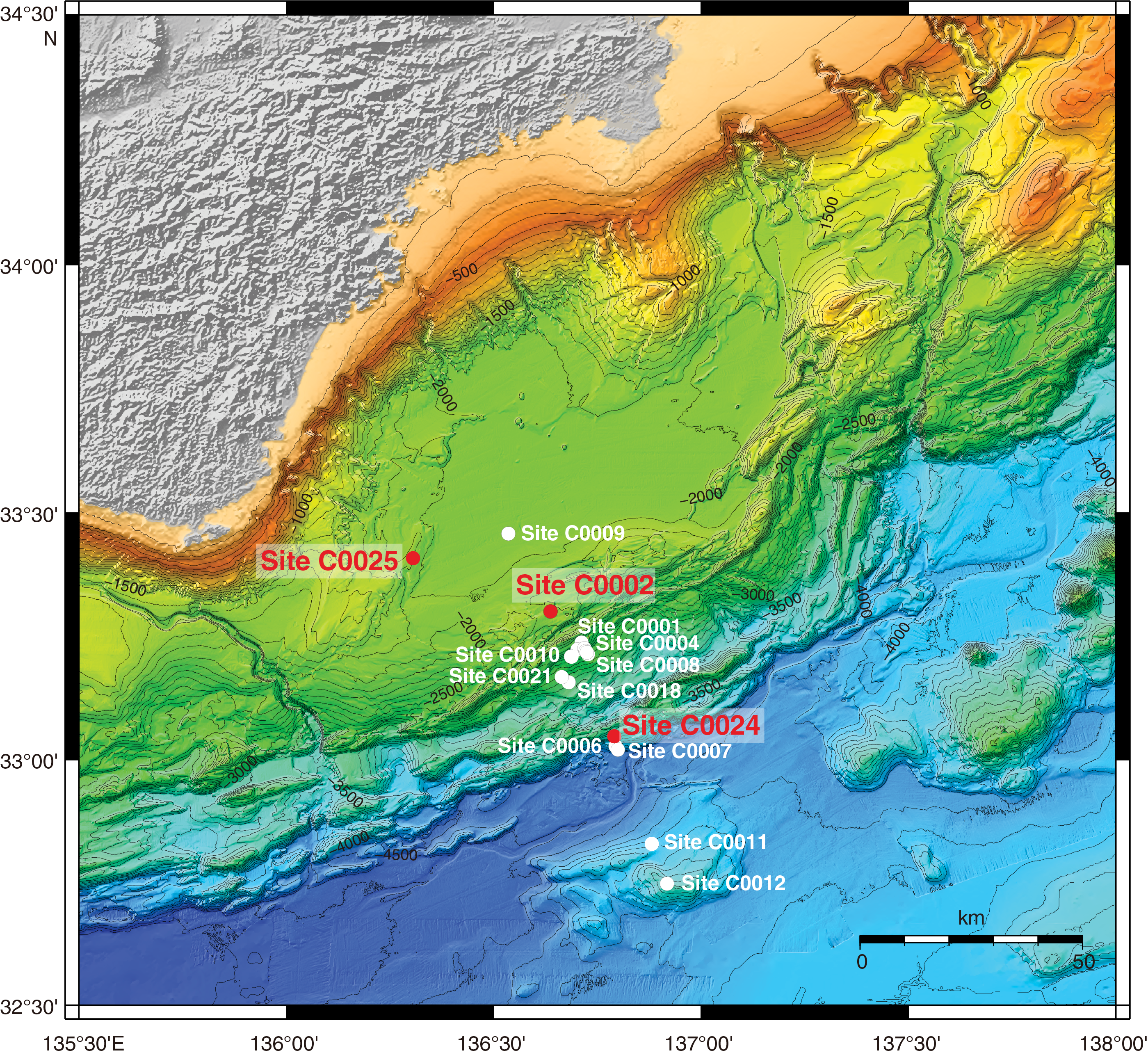
Figure F1. NanTroSEIZE project area.
The 12¼ inch drill-out cement (DOC) bottom-hole assembly (BHA) (Table T1) was made up and run in the hole, drilled out the cement plug from 3471 to 3530 m BRT, was washed down from 3530 to 3646 m BRT, and tagged the top of the 11¾ inch liner at 3884.2 m BRT at 0700 h on 29 October. The 10⅝ inch DOC BHA was run in the hole on 30 October. A pressure test of the 11¾ inch liner and 13⅜ inch casing was good. The cement plug from 4734 to 4902 m BRT was drilled out by 2400 h on 31 October. Three shoe bond tests were run before the DOC BHA was pulled out of the hole for a scraper run from 4325 to 4882 m BRT. The wireline cement bond log tool was made up and run on 3 November, logging between 2125 and 4878 m BRT to check the condition of the casing-cement-formation bonding.
After the wireline tools were rigged down at 1130 h on 4 November, preparations to run the easy drill sliding sleeve valve (EZSV) with the plug setting tool began. The EZSV was set at 4869 m BRT, and the setting tool was recovered to the surface. The 11¾ inch whipstock assembly was made up on 5 November and run to tag the top of the bridge plug (EZSV) at 4869 m BRT. The gyro assembly was run to ensure that the whipstock was facing the proper azimuth (N90E) for window cutting to avoid intersecting Integrated Ocean Drilling Program Hole C0002P. However, the whipstock failed to set, so it was recovered to the surface and a new whipstock assembly was made up and run in the hole on 8 November at 1000 h. The whipstock tagged the EZSV at 4869 m BRT, and the gyro wireline tool was rigged up and run again. Orientation surveys confirmed whipstock orientation was between 88.2° and 86.5°, so the wireline tool was recovered and then the whipstock was set by 1500 h on 9 November.
Sidetracking preparation began, and milling to 4862 m BRT was finished by 0600 h on 10 November. The Tri-Mill assembly was pulled out of the hole after drilling advance stopped but was run in the hole again to complete milling to 4867 m BRT, dress the window, and perform a formation integrity test (FIT) at the window on 12 November. The FIT was good, showing an equivalent mud weight of 1.450 specific gravity (SG), so the second scheduled FIT was canceled. The Tri-Mill assembly was pulled out of the hole, and a 10⅝ inch window mill assembly was run in the hole on 13 November. After reaching 4894 m BRT, the mill had trouble passing through the window; therefore, it was pulled out of the hole to the rig floor so that the string mill and window mill could be ground to reduce the outside diameter (OD) to 10⅝ inches. The milling assembly was run in the hole and worked from 4850 to 4864 m BRT by 2400 h on 15 November. The BHA was pulled out of the hole with a delay to replace the traveling block dolly cylinder, which had burst. The 8½ inch kick-off BHA was run in the hole to start drilling the pilot hole past the window.
Drilling in Holes C0002Q and C0002R was extremely complicated, with multiple tracks in each hole (Figure F2) because it was difficult to keep the BHAs in the same kick-off holes outside the windows in the Hole C0002P casing. Because the exact configurations of the holes/tracks were unknown, logging-while-drilling (LWD) run numbers were used to distinguish the data collected during each "run" with different BHAs. Details on BHAs and LWD run numbers are given in Table T1 (also see Table T32). Collection and shipboard analysis of LWD, mud gas, and cuttings for each run at Site C0002 are summarized in Tables T2 and T3.
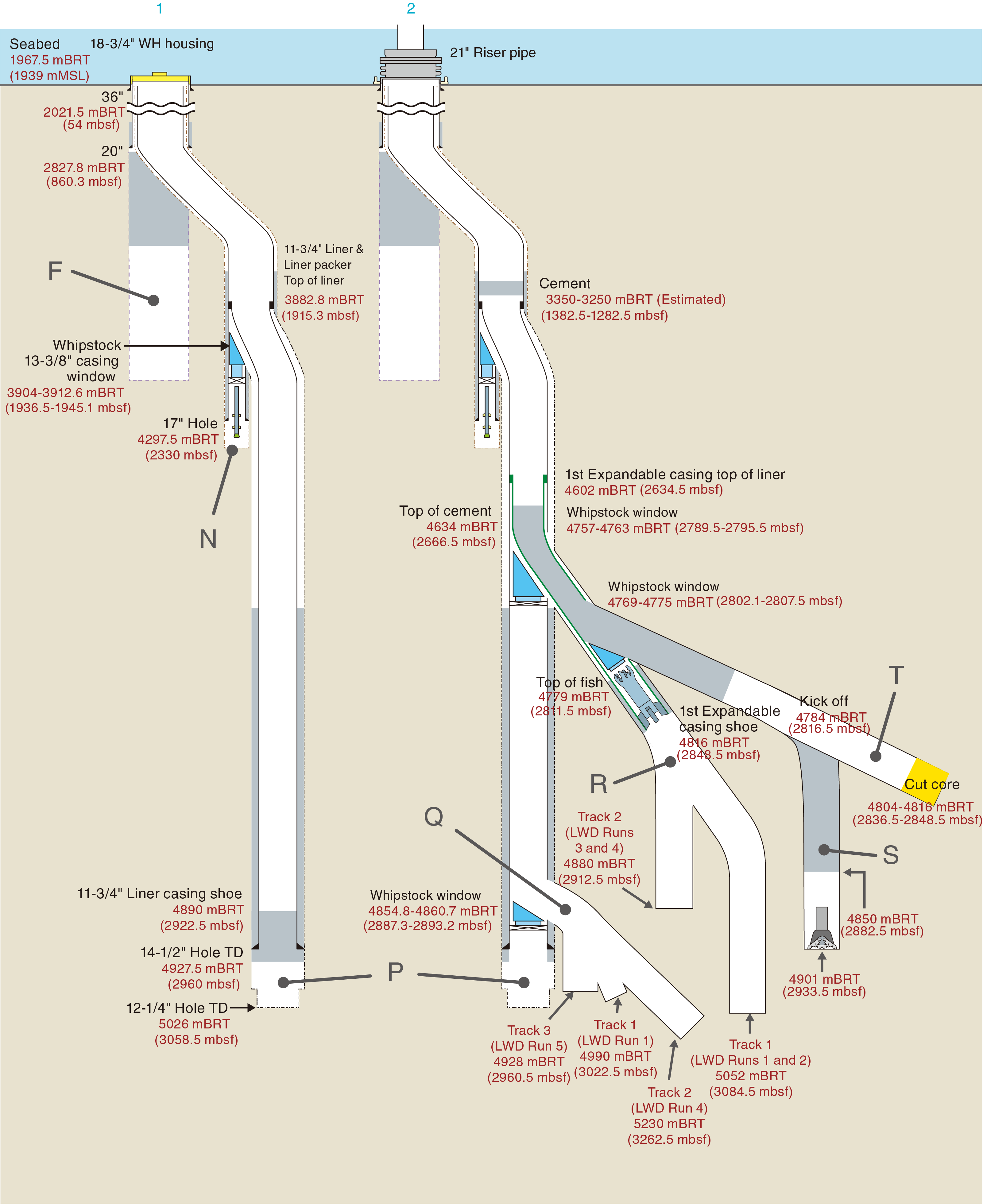
Figure F2. Final hole configuration.
Hole C0002Q
Hole C0002Q began at 0645 h on 18 November 2018 when the kick-off BHA began opening a new hole from 4867 m BRT. A number of stalls and overpulls occurred while drilling ahead, but the drill string was always recovered (see Table T1 in the Expedition 358 summary chapter [Tobin et al., 2020a]). At 1145 h on 18 November, a series of surveys to track azimuth and inclination started at 4879 m BRT. The pilot hole reached 4990 m BRT by 1400 h on 20 November (Hole C0002Q Track 1; LWD Run 1 in Figure F2). The kick-off BHA was pulled out of the hole to the surface by 2230 h on 21 November. After servicing the hydraulic power swivel (HPS) and traveling block, the Z-Reamer and well commander test assembly was made up and run in the hole before the 8½ inch × 12¼ inch LWD BHA with Z-Reamer was made up and run in the hole (Hole C0002Q LWD Run 2). The LWD BHA reached the window and began reaming from 4888 to 4909 m BRT; however, multiple stalls and overpulls were noted. Getting the BHA through the window proved difficult, so it was pulled out of the hole to run a hole-opening BHA at 0930 h on 25 November.
The hole-opening BHA, which included the arcVISION and TeleScope tools, was made up and run in the hole to 4778 m BRT (Hole C0002Q LWD Run 3). Before passing through the 4800 m BRT window, the BHA was pulled up to 4047 m BRT for a Z-Reamer function test when HPS stalls and other checks confirmed that the reamer ball seat had sheared. The BHA was pulled out of the hole to replace the Z-Reamer, reaching the rig floor by 0500 h on 27 November. The replacement hole-opening BHA was made up and run in the hole at 0815 h, reaching 4845 m BRT by 28 November. LWD function tests confirmed all tools were working well, so washing/reaming down began. At 0730 h on 29 November at 4941 m BRT, the BHA packed off but was soon released; reaming reached 4955 m BRT before pulling up to 4894 m BRT to activate the Z-Reamer. Opening the 8½ inch × 12¼ inch hole from 4894 to 4990 m BRT commenced; at 4990 m BRT, drilling ahead started. By 0100 h on 3 December, 4995 m BRT was achieved with the average rate of penetration (ROP) never exceeding 3.3 m/h. A short ream up to 4910 m BRT was completed early on 3 December, running back to 4995 m BRT before drilling ahead and reaching 5230 m BRT by 1445 h on 7 December (Hole C0002Q Track 2; LWD Run 4 in Figure F2). Because of the poor ROP (<5 m/h), the BHA was pulled out of the hole and laid out by 0530 h on 9 December, and memory data were recovered from the arcVISION and TeleScope tools. Running back into the hole with a new LWD BHA including an underreamer began at 1345 h. A short pause occurred after the bit reached 4880 m BRT so the internal BOP on the HPS could be replaced. While washing down from 4845 to 4910 m BRT, a series of surveys to check inclination and azimuth were taken on the BHA. Washing and reaming down to 4920 m BRT while checking surveys and conducting wiper trips aimed to confirm that the BHA was in the same hole. The underreamer was activated at a reamer depth of 4916 m BRT at 1445 h on 12 December, and the hole was opened to 4928 m BRT (Hole C0002Q Track 3; LWD Run 5 in Figure F2). Progress was unimpressive, and hole conditions continued to deteriorate, so the BHA was pulled out of the hole and laid down by 2115 h on 14 December to inspect the Z-Reamer underreamer. Chipped blades and other damage to the underreamer showed that the tool needed replacement. To escape from the poor hole conditions in Hole C0002Q, a new kick-off was planned.
Hole C0002R
On 15 December 2018, preparations to run in the hole with a new whipstock began. The EZSV bridge plug was run in by wireline and set at 4783.5 m BRT by 0645 h on 16 December (see Table T2 in the Expedition 358 summary chapter [Tobin et al., 2020a]). After successfully conducting a casing pressure test, the new whipstock was run in the hole at 1030 h on 16 December and was set at 4766 m BRT by 0945 h on 17 December. Milling out was completed by 20 December, with multiple milling BHAs and reciprocation through the window to ensure that the hole was clean. The new window cut from Hole C0002P was located at 4757–4763 m BRT (Figure F2). Another FIT (1.46 SG) was conducted in the new window, and the milling BHA was pulled out of the hole and laid down by 1700 h on 20 December. Another window dressing BHA was run in the hole at 1800 h and reamed down to 4767 m BRT. After circulation and bottoms up, the dressing BHA was pulled out of the hole for the next run with the kick-off BHA. The kick-off BHA ran in the hole at 1930 h on 22 December from 4755 to 4807.9 m BRT, reaming down and drilling before the sliding and drilling commenced (Hole C0002R LWD Run 1). Drilling mud weight was increased from 1.37 to 1.39 SG on 24 December before drilling and sliding continued. At 1630 h on 25 December, drilling from 4811.5 m BRT began, reaching 4843 m BRT by 0330 h on 26 December. Here, a pack-off interrupted drilling for about 45 min before drilling ahead resumed. The kick-off BHA finally reached 4963 m BRT by 0230 h on 29 December. Again, issues with poor borehole conditions and multiple overpulls while drilling combined with low ROP resulted in reaming out of the hole to confirm hole conditions. Reaming out encountered multiple overpulls and pressure spikes. Pulling out of the hole to the surface began so that the BHA could be laid out on 30 December. TeleScope data were downloaded while a new kick-off BHA was made up and run in the hole at 0215 h on 30 December.
At 2230 h on 31 December, the new kick-off BHA started drilling a new kick-off hole from 4963 m BRT before reaching 5052 m BRT on 3 January 2019 (Hole C0002R Track 1; LWD Run 2 in Figure F2). Reaming up and down commenced before the decision was made to return the BHA to the surface to examine why the mud motor started showing signs of failure. Once on deck, the top connection of the motor was found to be overtorqued into the crossover sub, and the motor itself had backed off, exposing the interior parts. A new LWD BHA, including the arcVISION and TeleScope tools and a Z-Reamer underreamer, was made up and run in the hole at 0200 h on 6 January. Washing and reaming down from 4744 m BRT began on 7 January; the Z-Reamer was activated at 1945 h at 4834 m BRT (bit depth). Reaming out the borehole and drilling a new hole from 8 January reached 4880 m BRT by 1700 h (Hole C0002R Track 2; LWD Run 3 in Figure F2). Hole cleaning and reaming were carried out until 0300 h on 9 January. The top drive torque started fluctuating and showing other signs of poor hole conditions; therefore, the BHA was pulled out of the hole to the surface to avoid over-enlarging the hole. Examination of the bit and underreamer showed extensive damage to both; cutters were severely damaged. A new LWD BHA with a new underreamer was made up and run in the hole from 0100 h on 10 January (Hole C0002R LWD Run 4). Because many tight spots were found while reaming down to 4745 m BRT, the decision was made to set 9⅝ inch × 11¾ inch expandable casing (ESET) at this depth at 2030 h on 11 January. The LWD BHA was pulled out of the hole to the surface by 1400 h on 12 January, and preparation for 9⅝ inch ESET installation was started. Running 9⅝ inch × 11¾ inch ESET began at 0000 h on 13 January and reached 4818 m BRT by 0730 h on 14 January. Expanding the 9⅝ inch × 11¾ inch ESET was conducted from 1615 to 1830 h after cementing, and the ESET launcher assembly was pulled out of the hole to the surface by 1200 h on 15 January. The launcher tool showed no sign of damage. A 9.851 inch DOC BHA was made up and run to 1403 m BRT from 1400 h on 15 January. A pressure test of the 11¾ inch liner and 9⅝ inch × 11¾ inch ESET was conducted and indicated that the casing was set and cemented properly by 2000 h on 15 January. The 9.851 inch DOC BHA reached 4791 m BRT at 0630 h on 16 January and started drilling out the 9⅝ inch × 11¾ inch ESET casing shoe. However, a drilling break, a sudden pressure increase (from 21.6 to 24.8 MPa), and stall (>38 kN) were observed from 4815 to 4816 m BRT, resulting in a stuck pipe at 1345 h on 16 January. Working the pipe started immediately and continued until 1445 h on 18 January with no sign that the drill string could be freed. Therefore, to back off the stuck BHA, a free point indicator tool was run and took a survey from 2000 h on 18 January to 0230 h 19 January. A back-off tool assembly was run to 4793.75 m BRT and successfully backed off the drill pipe between the 6¾ inch drill Collars 2 and 3 at 4793.75 m BRT at 1730 h on 19 January. A fishing BHA was run down onto Collar 2 at 4778 m BRT. Working the pipe at 4816 m BRT until 1800 h 23 January while jarring more than 400 times failed to free the drill string. An attempt to collide the stuck drill string began by running a 58.5 mm OD gauge cutter to check the inside of the drill pipe for obstructions. Several attempts to run the cutter failed to pass, even after modification. A blind back-off operation was conducted at 0415 h on 27 January, but the drill string was reconnected because the estimated back-off depth was 3450 m BRT. A colliding tool was run and severed the stuck drill string at 4782 m BRT at 0115 h on 28 January. The collided drill pipe was pulled out of the hole and recovered to the surface by 0545 h on 29 January.
Hole C0002S
Preparations to kick off with the third whipstock above the fish in Hole C0002R began at 1630 h on 30 January 2019 after rig repair and maintenance work. A 10¾ inch whipstock and 9¾ inch Tri-Mill assembly were made up and run in the hole from 0345 h on 31 January. The whipstock was set at 4779 m BRT (above the fish) and the tool face orientation was set at ~73° (as measured by the gyro assembly) by 2045 h on 1 February. Milling and dressing the casing was completed by 0130 h on 3 February with the window opened at 4769–4775 m BRT (Figure F2), and an 8½ inch kick-off BHA (bent angle 1.5°) was made up and run into the hole from 0215 h on 3 February.
The 8½ inch kick-off BHA reamed and drilled down Hole C0002S to 4788.5 m BRT by 2345 h on 3 February, and then the BHA was pulled out of the hole to 4766 m BRT (Hole C0002S LWD Run 1). A gyro assembly was run to 4115 m BRT (wireline [WL] depth) after drilling mud was conditioned to 1.35 SG while waiting on weather. The BHA tool face was oriented to ~215° at 1145 h on 4 February. Washing and reaming down with the BHA was conducted to 4788 m BRT, and then the BHA was recovered to the surface by 1315 h on 5 February. A full suite of tools on the 8½ inch LWD BHA was made up and run into the hole to 4747 m BRT (Hole C0002S LWD Run 2). Several communication tests for the LWD tools were conducted by 1015 h on 6 February, and then the LWD BHA was washed down to 4780.5 m BRT. Drilling down began from 4780.5 m BRT at 1045 h on 6 February and continued to 4900 m BRT by 1330 h on 8 February while taking surveys (Figure F2). Several stalls occurred at 4798, 4801.5, 4803.3, and 4805 m BRT while drilling. Drilling resumed after activating the rotary steerable system (RSS) to reduce inclination at 1730 h on 8 February, but miscommunication between the RSS and the lower C-Link and abnormal on/off bottom torque and pressure occurred. The decision to pull the 8½ inch RSS LWD BHA out of the hole was made at 1830 h on 8 February. Upon recovery of the BHA to the surface at 1315 h on 9 February, it was discovered that the bottom part of the BHA, the C-Link, and RSS were lost in the hole. Fishing operations were attempted three times but failed. The decision to kick off and core began with conducting another kick-off cementing job at 4850 m BRT at 2130 h on 13 February (Figure F2). An 8½ inch kick-off BHA was run and tagged the top of cement at 4748 m BRT 2145 h on 15 February and then started to drill out cement.
Hole C0002T
A wireline gyro assembly was run to 4724 m BRT (WL depth), and the orientation of the kick-off BHA was set to ~211° by 0300 h on 16 February 2019. The kick-off BHA drilled with sliding from 4784 to 4800 m BRT and then drilled to 4804 m BRT by 2245 h on 16 February. After 10 m3 of 30 lb/gal Fracseal was spotted at the hole bottom and the hole was reamed from 4804 to 4790 m BRT, the kick-off BHA was pulled out of the hole to the surface by 1815 h on 17 February. A 8½ inch SD-RCB BHA was run to 4752 m BRT by 1545 h on 18 February. From 4752 to 4804 m BRT, the BHA washed and reamed down with the center bit. The center bit was recovered to the surface at 2030 h on 18 February, and then core cutting began at 4804 m BRT at 2130 h on 18 February. Three cores were cut and retrieved from 4804 to 4816 m BRT by 0300 h on 20 February (Table T4; Figure F2). However, stalling and pack offs occurred at 4816 m BRT while reaming down at 0430 h on 20 February. The poor hole conditions required abandoning the hole, and the BHA was pulled out of the hole from 1230 h on 20 February. The BHA was recovered to the surface at 0800 h on 21 February.
The diverter BHA was run in the hole and washed down to 4788 m BRT so that cement could be spotted for a plug-back at 4780 m BRT at 0245 h on 22 February. This attempt failed, so a second plug-back cementing attempt was conducted at 4780 m BRT on 23 February, but it also failed. The third and final attempt to set the plug back with 1.36 SG cement was conducted at 4769 m BRT at 1030 h on 24 February. This cement plug passed a pressure test at 1330 h on 25 February. A fourth plug-back cementing job was set at 3350 m BRT at 2330 h on 25 February. The diverter assembly was pulled out of the hole, and inhibited mud was spotted. A short pause for rig servicing occurred before the wear bushing and wear bushing running/retrieving tool were recovered to the surface. The riser mud was displaced with seawater before operations to recover the riser, and BOP commenced from 27 February. The riser was laid out, and the BOP was recovered in the moonpool by 2315 h on 2 March.
Lithology
We described the lithologic character of cuttings from four overlapping holes (C0002Q–C0002T) and three cores from Hole C0002T (2789.5–3262.5 meters below seafloor [mbsf]) (Tables T5, T4). The sedimentary rocks collectively correlate with Unit V as defined by Tobin et al. (2015) (Figure F3). We did not define any subunits. Characterization of each lithology is based on observations with binocular microscopes, thin section and smear slide petrography, bulk powder X-ray diffraction (XRD), bulk powder X-ray fluorescence (XRF), and micro-X-ray computed tomography (CT) (see Lithology in the Expedition 358 methods chapter [Hirose et al., 2020]).
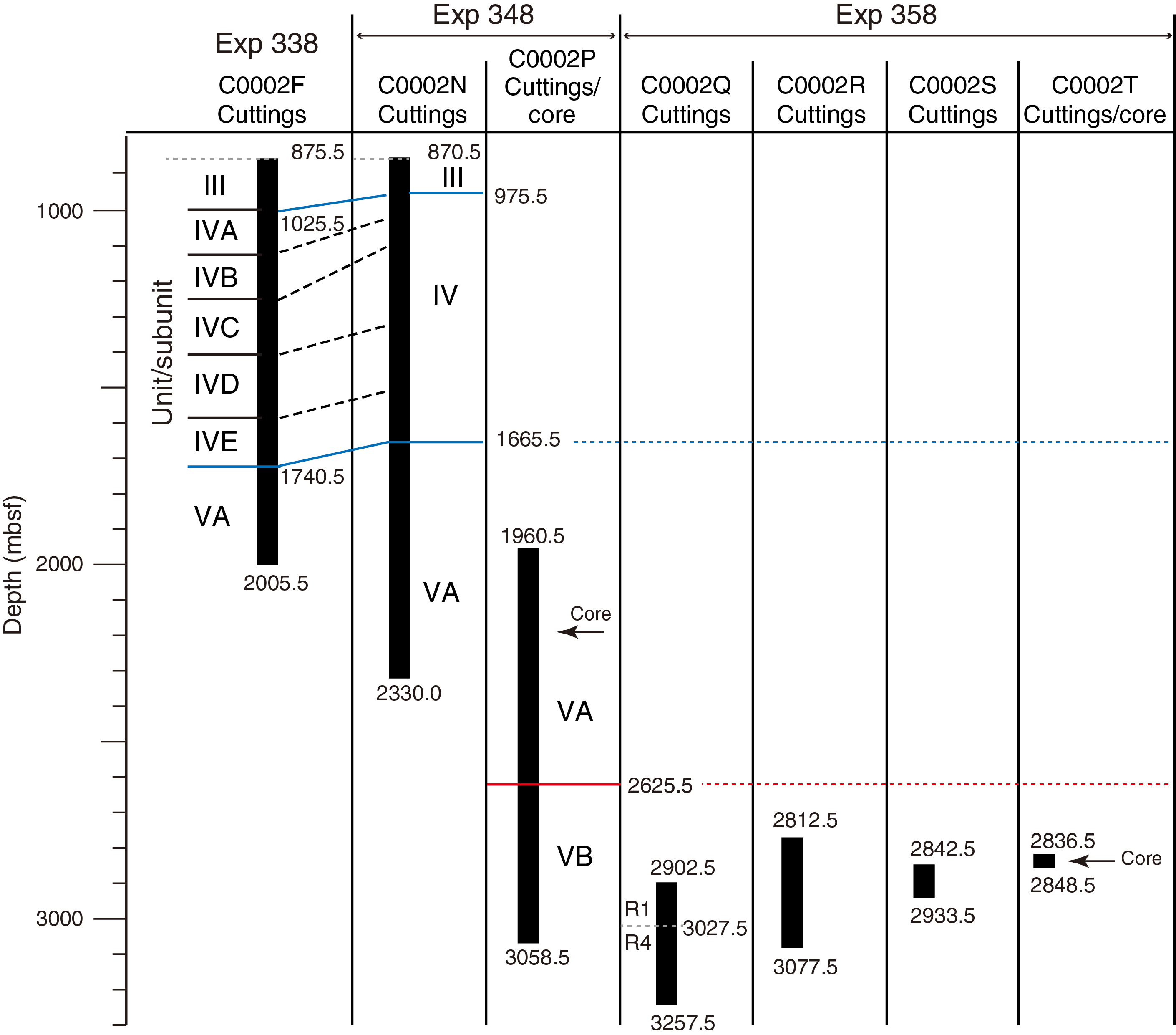
Figure F3. Depths cores and cuttings were recovered from.
Operational parameters
Cuttings from Hole C0002Q (2902.5–3257.5 mbsf) were produced during two runs using different BHA configurations (Figure F3). Samples 358-C0002Q-30-SMW to 57-SMW (2907.5–3017.5 mbsf) were obtained from Hole C0002Q during Run 1 without an underreamer. An underreamer was used in Hole C0002Q during Run 4 (3027.5–3257.5 mbsf), yielding Samples 365-SMW to 633-SMW. In these depth ranges, cuttings were mixed over an interval of at least 38 m (see Introduction and operations).
Cuttings from Hole C0002R (Samples 358-C0002R-89-SMW to 334-SMW) were obtained from 2812.5 to 3077.5 mbsf (Figure F3). This hole was drilled during two runs using different BHA configurations, but neither run included an underreamer (see Introduction and operations). Most of the cuttings, therefore, were produced at the drill bit. The interval of mixing in the borehole was at least 20 m because of the circulation of cuttings and cavings in the drilling mud.
Cuttings analysis for Hole C0002S utilized Samples 358-C0002S-9-SMW to 37-SMW (2842.5–2933.5 mbsf) (Figure F3). This interval was drilled without an underreamer (same configuration as Hole C0002R and Hole C0002Q Run 1), so we infer that intact cuttings were cut by the drill bit within ~20 m of their archived depth (see Introduction and operations).
Cuttings recovered from Hole C0002T were analyzed from only two samples (358-C0002T-6-SMW and 14-SMW) with base depths of 2836.5 and 2847.5 mbsf. In addition, three cores were taken from 2836.5 to 2848.5 mbsf (Figure F3; Table T4). Core recovery was poor (13%–32%), and drilling-induced deformation of the core is extensive. Most of the material is thoroughly fragmented with scattered preservation of primary stratigraphic layering and trace fossils.
Description of lithologies
Lithologic Unit V at Site C0002 is composed of four rock types with gradational lithologic attributes. Fine silty claystone is light gray to gray and contains variable proportions of clay- and silt-sized grains (Figure F4A, F4B). This lithology is poorly consolidated, and the cuttings are typically rounded and sticky. Rare sedimentary structures include parallel lamination. Micro-X-ray CT images show millimeter-scale layers with low X-ray attenuation and layers with small pyrite grains. Burrows are characterized by larger pyrite grains that penetrate the lamination.
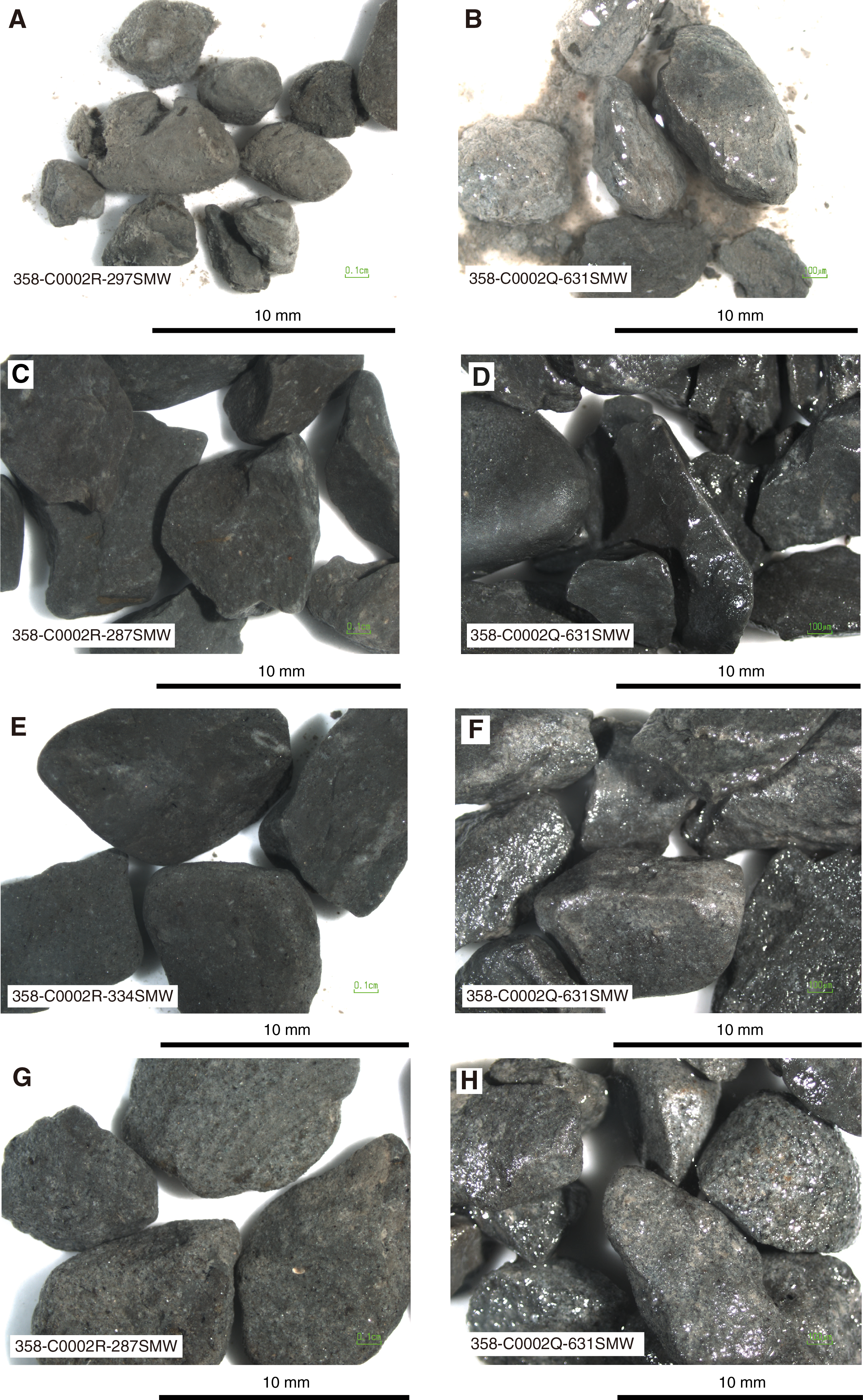
Figure F4. Dominant and minor lithologies, Holes C0002Q and C0002R.
The second common lithology, silty claystone, is gray to olive-black (Figure F4C, F4D). Silty claystone cuttings are more lithified, angular, and fissile. Typical sedimentary structures include bioturbation (Figure F5E, F5F) and lamination. We also observed carbonate fossils (Figure F5D) and contacts with probable interbeds of siltstone and sandstone (Figure F6A, F6B).

Figure F5. Characteristic features of fine silty claystone and silty claystone, Hole C0002R.
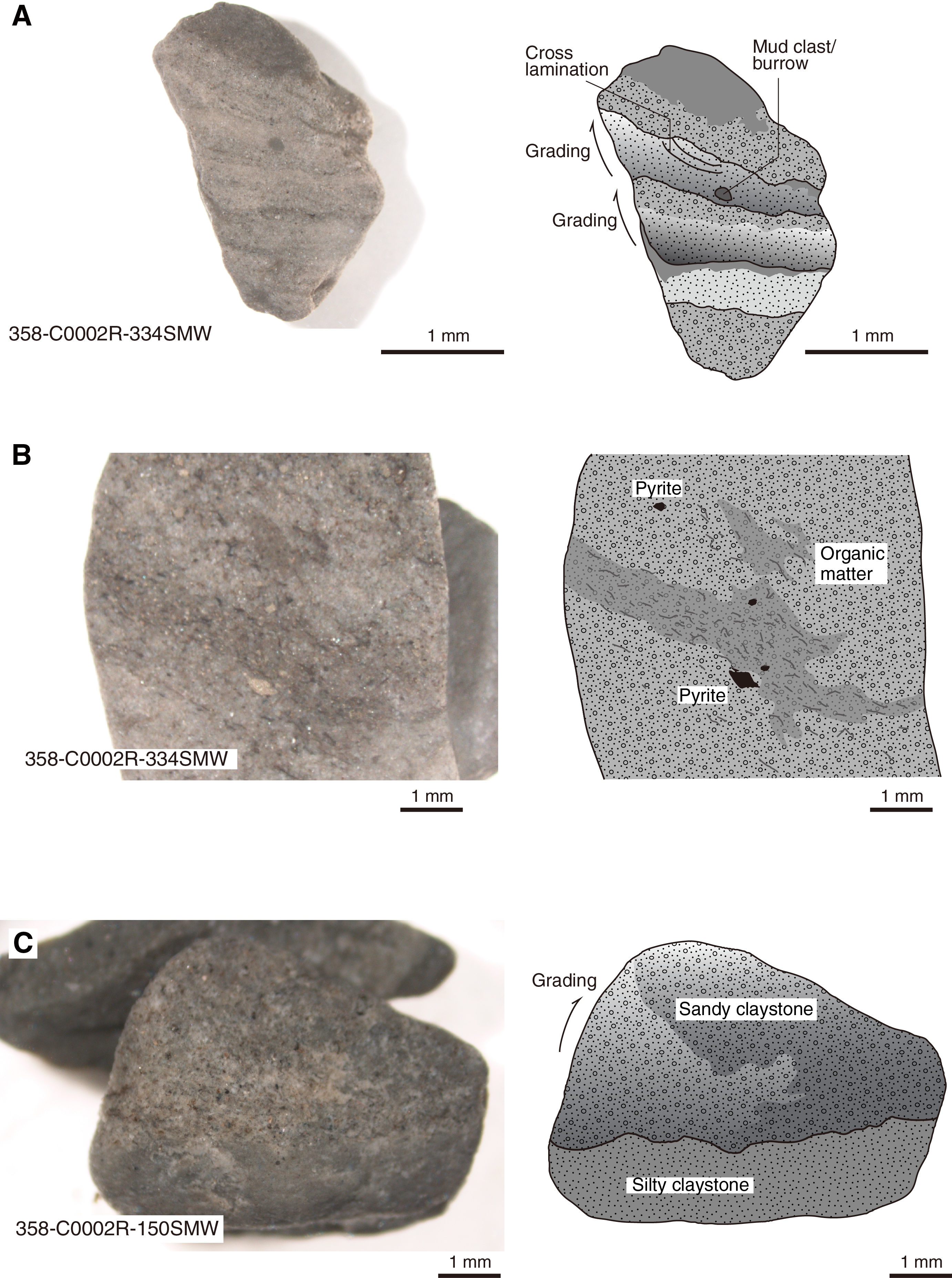
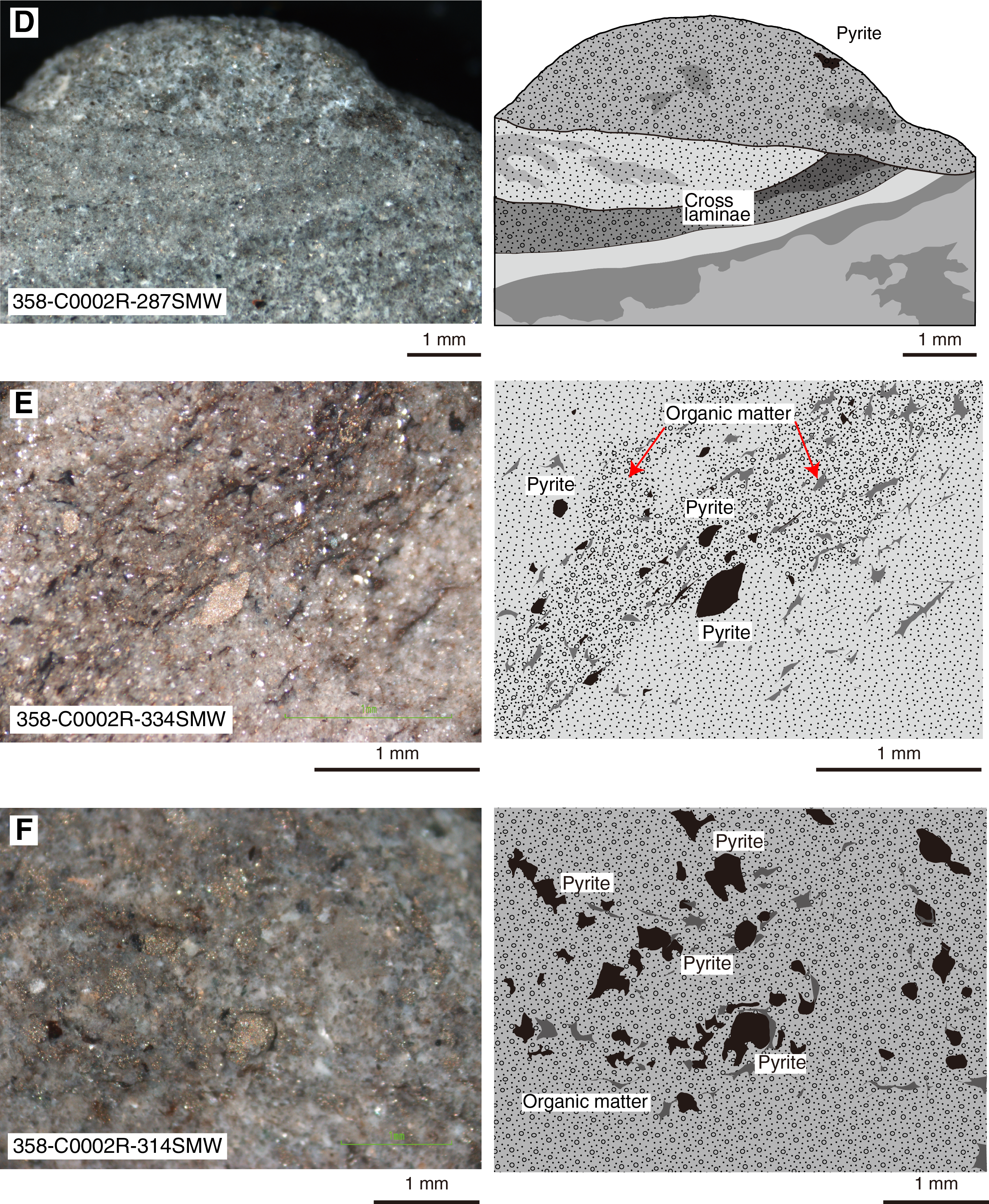
Figure F6. Sandstone and siltstone fragments from cuttings, Hole C0002R.
Siltstone is lighter colored and coarser grained than silty claystone, but the two lithologies are hard to distinguish without a binocular microscope. Compared to silty claystone, siltstone fragments show a higher degree of consolidation and cuttings are more angular in shape (Figure F4E, F4F). Sedimentary structures include size grading, planar lamination, cross-lamination (Figure F6), thin layers of organic matter, and pyrite nodules (Figure F6E, F6F).
We found two varieties of sandstone in cuttings. The more common type is gray and very fine grained. Those cuttings are subangular in shape, typically with a fissile texture and moderate degree of consolidation (Figure F4G, F4H). A light gray, fine-grained variety of sandstone is less abundant (present only in Hole C0002Q Run 4). Those cuttings show a lower degree of consolidation and a higher degree of roundness than the darker gray sandstone. Cuttings of both sandstone types display size grading, planar lamination, and cross-lamination (Figure F6D).
Silty claystone is the dominant lithology in the three cores from Hole C0002T, similar to what we observed in cuttings. Intense fragmentation of the cores, however, obscures the centimeter-scale details of primary stratification. Some of the larger intact pieces display lamination and trace fossils. We also found large pieces of pale yellow artificial drilling cement (concrete) and what appears to be a thin layer of matrix-supported shale-pebble conglomerate with rounded clasts.
Proportions of lithologies
We determined the relative proportions of each lithology using two sizes of cuttings: >4 and 1–4 mm. No significant difference exists between the two sizes. To be consistent with other data sets (see Structural geology and Physical properties), we quantified the lithologic proportions using the >4 mm cuttings.
Hole C0002Q
Cuttings from the upper part of Hole C0002Q Run 1 include a high content of artificial cement chips (concrete), as much as 66% of the total at 2907.5 mbsf (Sample 358-C0002Q-30-SMW) (Table T6). Cement content decreases progressively with depth to reach values between 0% and 9% from 2947.5 to 3017.5 mbsf (Samples 40-SMW to 57-SMW) (Figure F7). Fine silty claystone is the dominant lithology throughout Hole C0002Q Run 1, ranging from 36% at 2937.5 mbsf to 55% at 3017.5 mbsf. Over the same depth interval, the proportion of silty claystone is 20%–40%, siltstone is 5%–10%, and fine to very fine sandstone is 8%–28% (Figure F7).
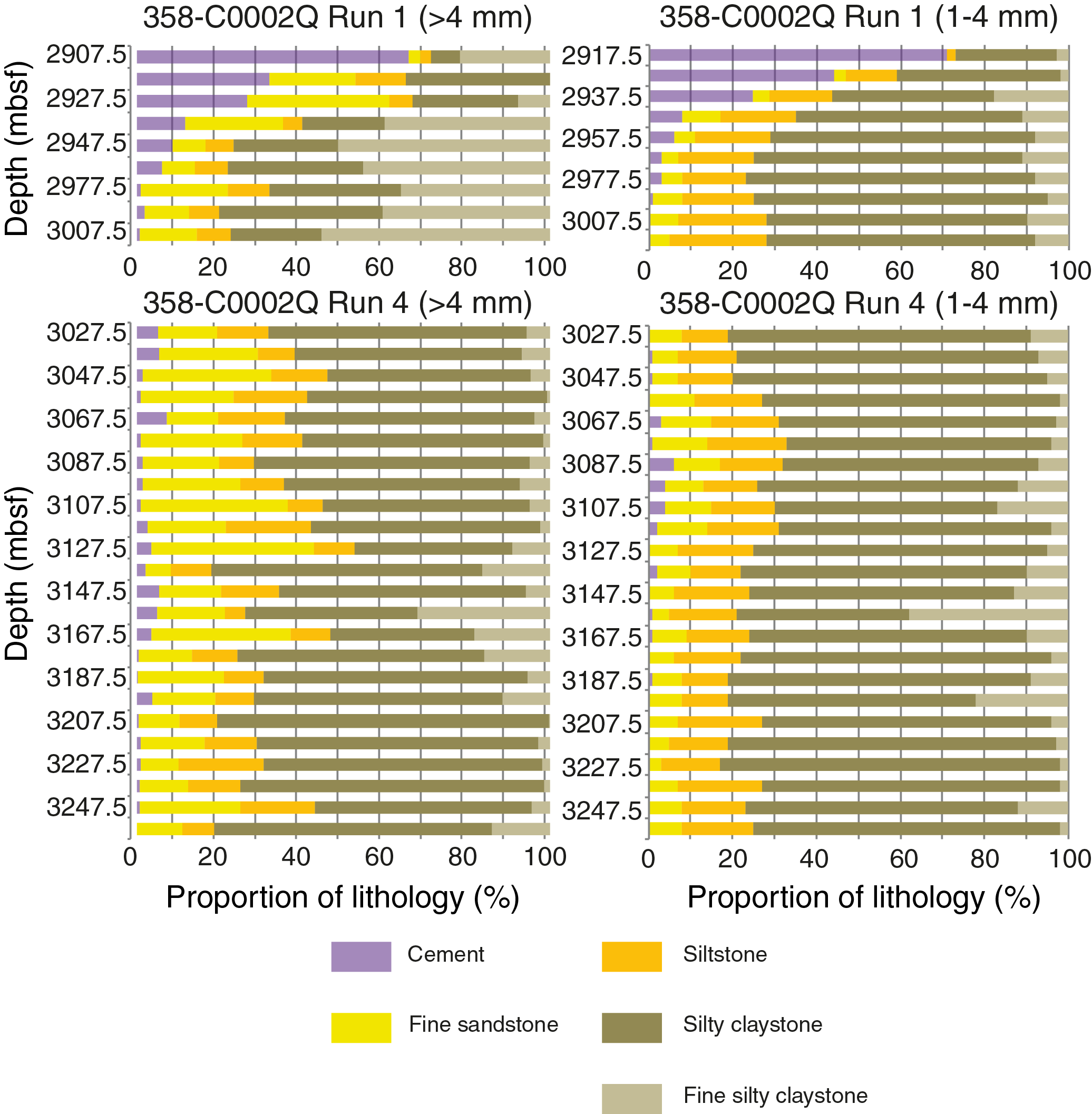
Figure F7. Distribution of different lithologies, Hole C0002Q.
The proportion of drilling cement (concrete) fragments in Hole C0002Q Run 4 ranges between 0% and 8%. Silty claystone is the dominant lithology, composing 35%–80% of the total cuttings (Figure F7). Percentages of siltstone and fine sandstone are 8%–21% and 6%–39%, respectively. Fine silty claystone content is generally 0%–7%, with amounts as high as 30% in one sample.
Hole C0002R
Silty claystone composes about 60%–65% of the formation drilled in Hole C0002R (Table T6). Estimates for siltstone and fine sandstone are approximately 18% and 14%, respectively (Figure F8). Fine silty claystone constitutes between 0% and 15% (mean value of 4%) of the cuttings recovered from Hole C0002R. We observed mixtures of harder dark gray silty claystone and softer light gray fine silty claystone at 2947.5 mbsf (Figure F5C), and locally >25% of the cuttings are actually composed of both lithologies (mixed type; Figure F5A, F5B). One fragment of pale brownish yellow muddy limestone (~74% high-Mg calcite) was also recovered from the drill bit (Sample 358-C0002R-72-SDB); its stratigraphic context remains unclear.

Figure F8. Distribution of different lithologies, Hole C0002R.
Hole C0002S
As found in Hole C0002R and Hole C0002Q Run 4, silty claystone is the dominant lithology in Hole C0002S with proportions ranging from 57% to 73% (Table T6). The percentage of silty claystone decreases progressively from 73% at 2847.5 mbsf to 57% at 2937.5 mbsf (Samples 358-C0002S-9-SMW to 37-SMW) (Figure F9). We also note an increase in the proportion of sandstone from 6% at the top of the hole to 24% at the bottom of the hole (2847.5–2937.5 mbsf). The proportion of siltstone remains relatively constant with percentages ranging from 12% to 22%. Fine silty claystone is present only between 2847.5 and 2917.5 mbsf (Figure F9). We also found two types of artificial cement (concrete) in the cuttings (see Lithology in the Expedition 358 methods chapter [Hirose et al., 2020]) between 2847.5 and 2907.5 mbsf; such fragments remain in low proportions (<4%).
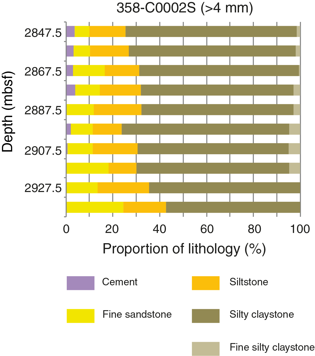
Figure F9. Distribution of different lithologies, Hole C0002S.
Hole C0002T
Recovery of both cores and cuttings from Hole C0002T was not extensive enough for us to complete meaningful analyses of lithologic proportions. Only two cuttings samples were recovered from Hole C0002T. The dominant lithology is silty claystone with proportions of 37% and 64% for Samples 358-C0002T-6-SMW and 14-SMW, respectively. Compared to Holes C0002Q–C0002S, a relatively high proportion of sandstone (23%) occurs in Sample 358-C0002T-6-SMW (Table T6).
Core recovery was very poor (Cores 358-C0002T-1K through 3K). All cores display a high degree of deformation induced by drilling (drilling breccia and ubiquitous fractures) and high drilling mud content. Several centimeter-sized clasts of artificial cement (concrete) are mixed with the rubble. Silty claystone is the dominant lithology. The degree of bioturbation in larger intact fragments ranges from low to moderate. Most of the silty claystone chips are structureless, but a few of the larger fragments retain millimeter-scale lamination or contacts between silty claystone and siltstone.
Petrography
Hole C0002Q
Smear slides were used to record the mineral composition and texture of cuttings from Hole C0002Q (see Site C0002 smear slides in Core descriptions; also see SMEARSLD in Supplementary material). Representative photomicrographs are shown in Figure F10. Quartz and plagioclase are common throughout the cuttings. Grains of mica and heavy minerals are few to common. Clusters of clay minerals are dominant to abundant. Shards of volcanic glass are few to common but more abundant from 3057.5 to 3117.5 mbsf (Samples 358-C0002Q-402-SMW to 480-SMW). Sedimentary lithic fragments are abundant to dominant from Samples 30-SMW to 57-SMW. Sedimentary lithic fragments decrease slightly with depth from 3027.5 to 3257.5 mbsf (Samples 365-SMW to 480-SMW). Volcanic lithic fragments are rare to few and found mainly in Samples 449-SMW to 507-SMW. Nannofossils, foraminifers, and fragments of terrestrial organic matter are also few.
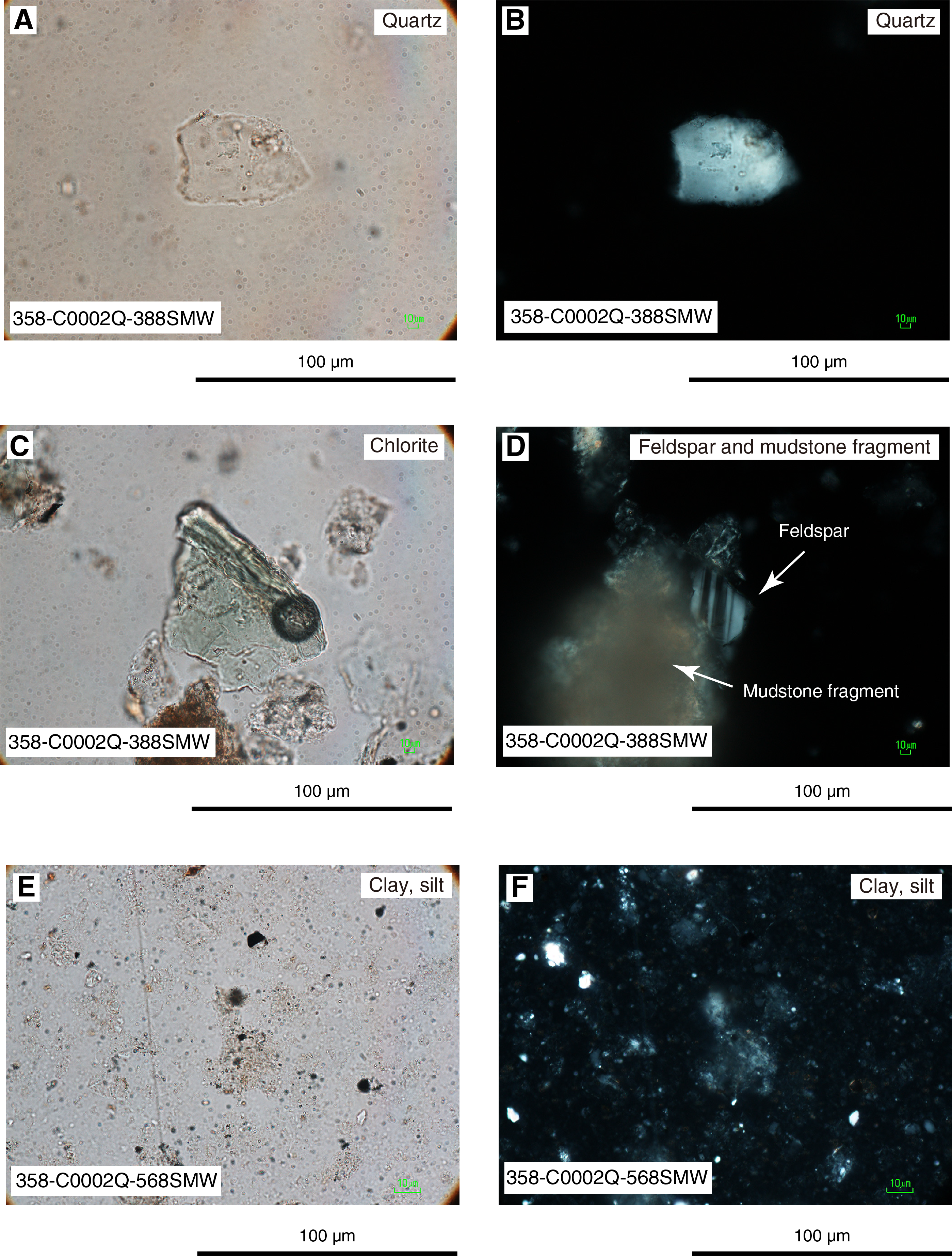
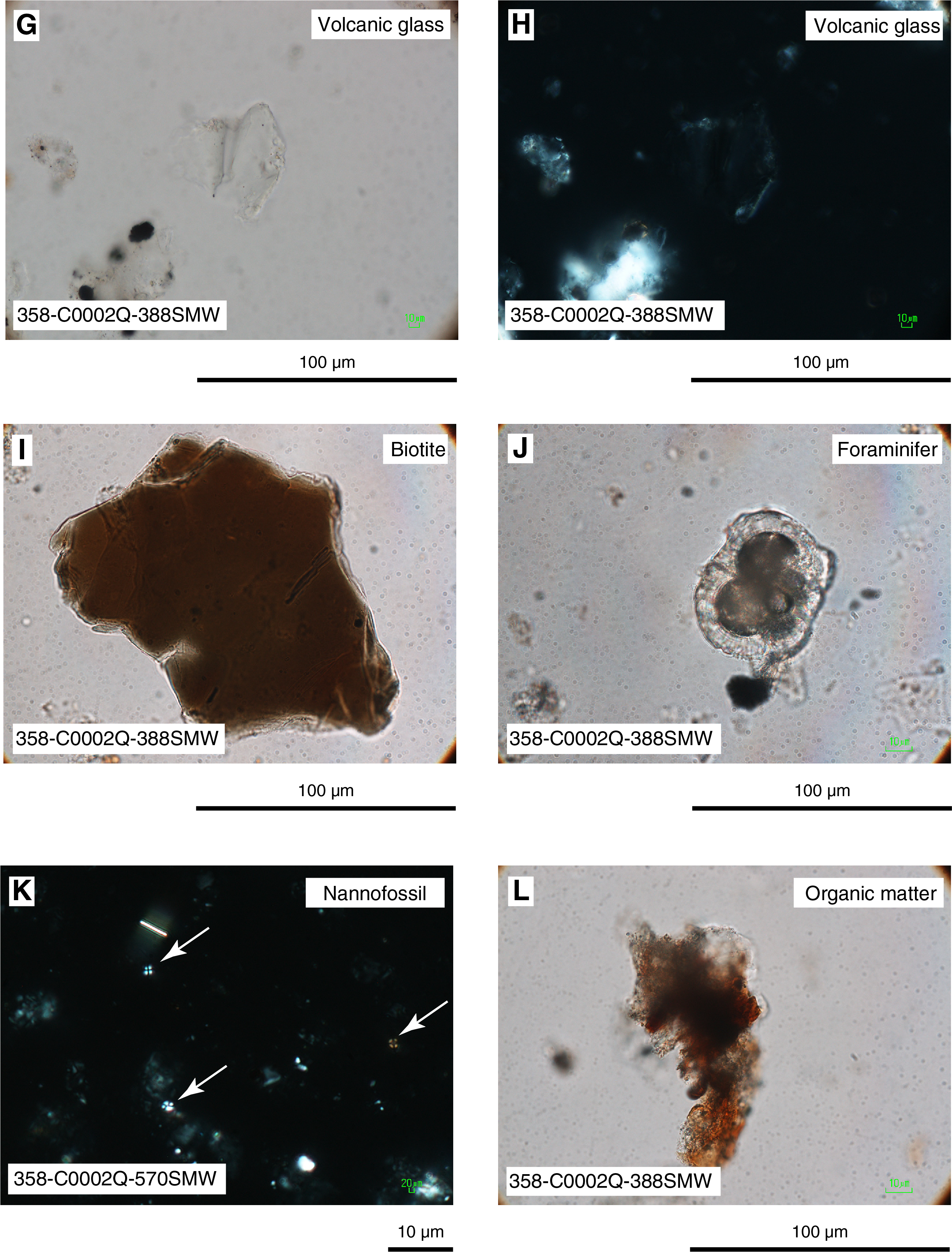
Figure F10. Cuttings samples, Hole C0002Q.
Hole C0002R
Cuttings from Hole C0002R were examined as both smear slides and thin sections (see Site C0002 thin sections in Core descriptions). Examination of silty claystone reveals that clay minerals are dominant (Figures F11, F12, F13) (see SMEARSLD and THINSECT in Supplementary material); they usually appear as partially disaggregated claystone fragments in smear slides (Figure F11). Quartz is abundant and feldspar grains are common throughout Hole C0002R. Grains of mica are common to few, and heavy minerals are few (locally rare). Common to rare sedimentary lithic fragments, volcanic lithic fragments, and organic matter are observed at certain depths (Figure F11), whereas pyrite is present throughout the hole (see Site C0002 smear slides and thin sections in Core descriptions). With the exception of scattered calcareous nannofossils (Figure F11) and a single broken foraminifer test, we did not observe any biogenic pelagic particles.
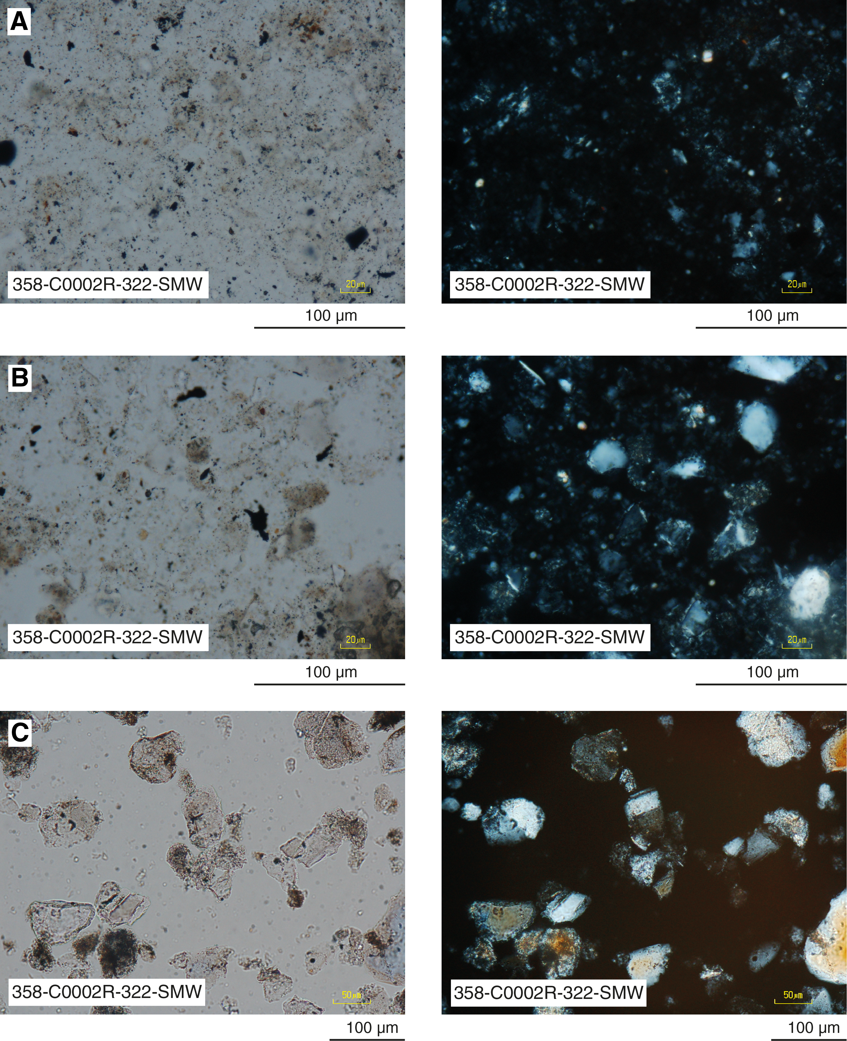
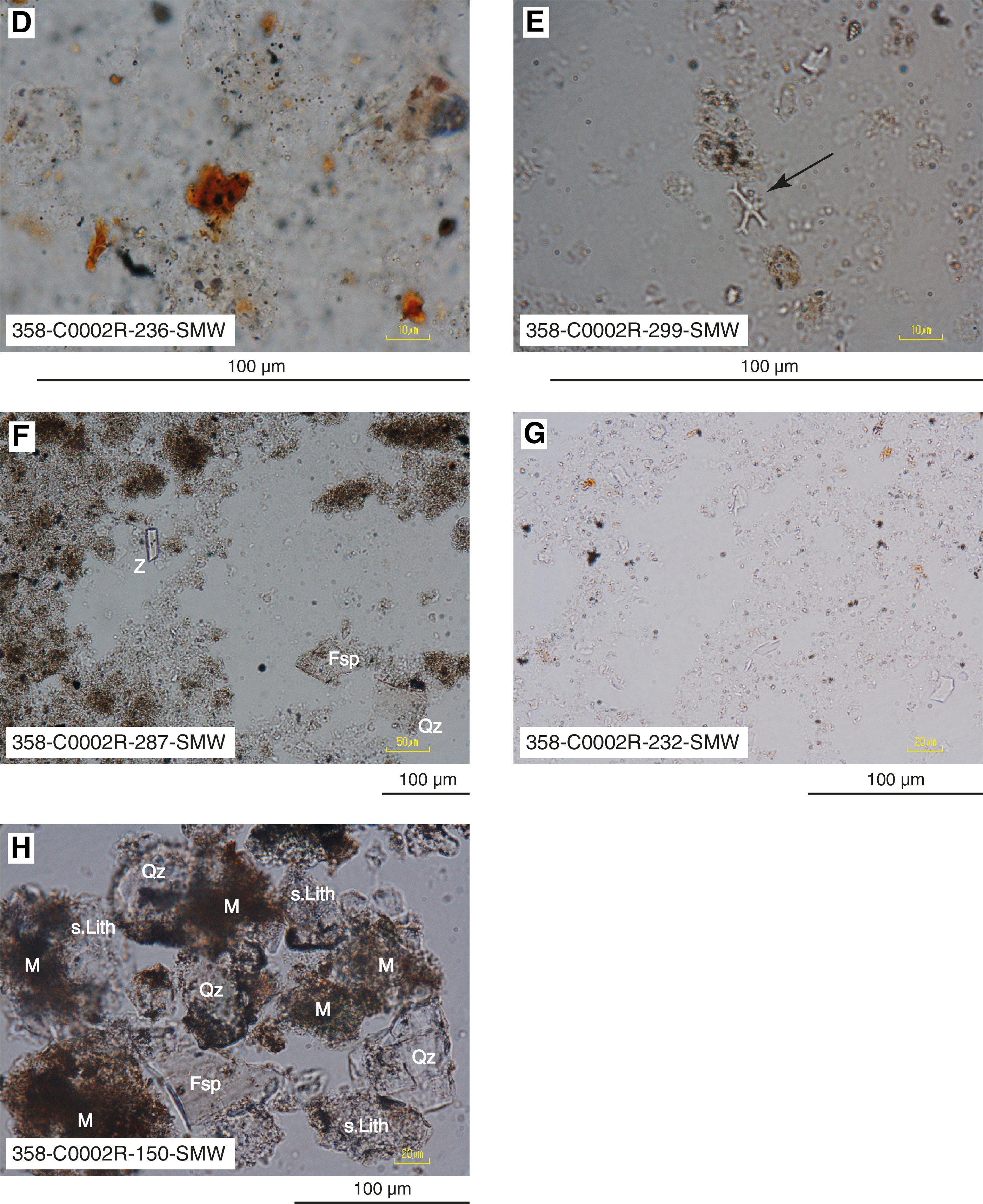
Figure F11. Cuttings samples, Hole C0002R.

Figure F12. Cuttings samples, Hole C0002R.

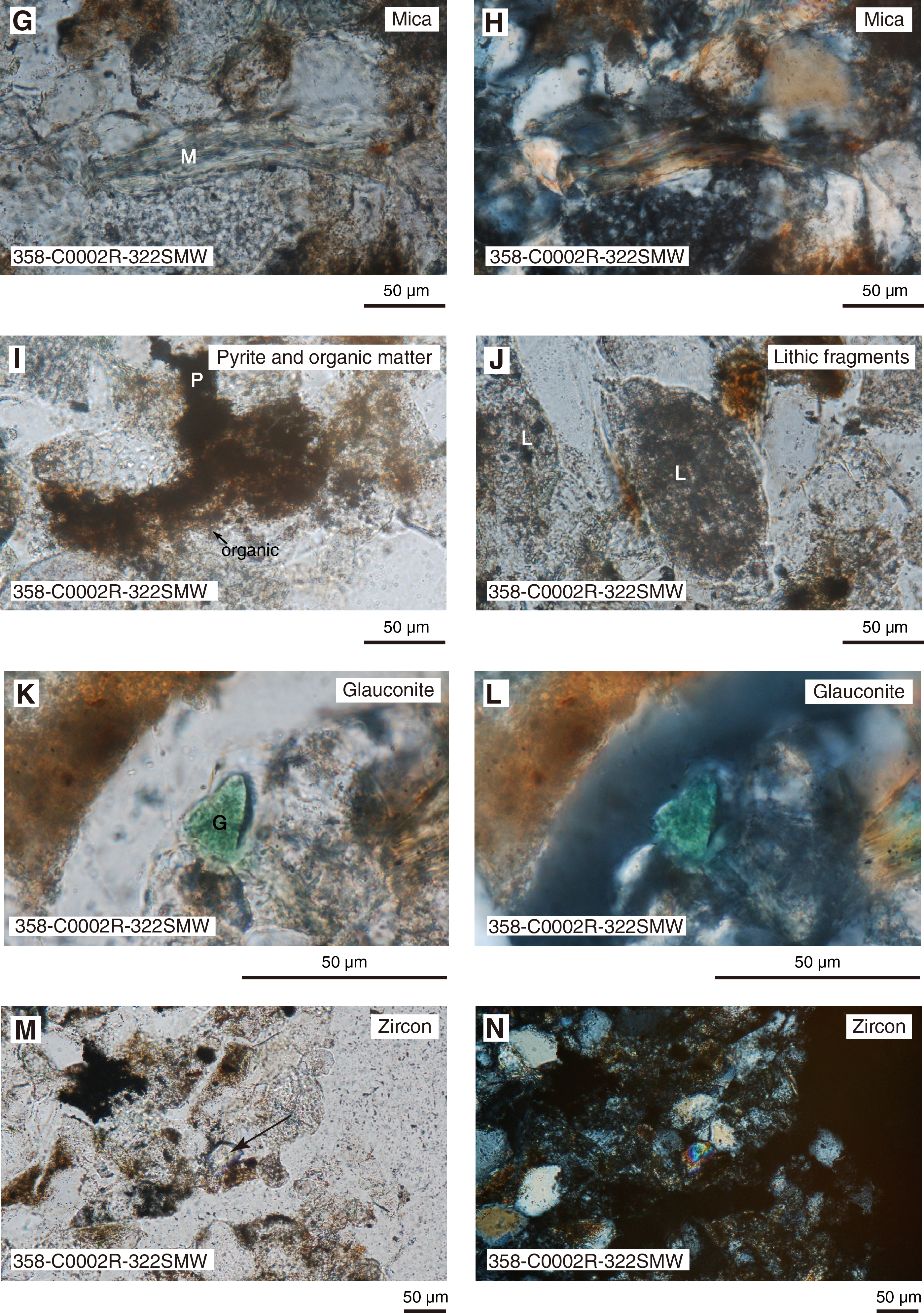
Figure F13. Silty claystone and sandstone, Hole C0002R.
Semiquantitative estimations reveal no distinct difference in mineralogy between fine silty claystone and silty claystone (Figure F12). However, aligned clay minerals and other clay-sized particles are more pronounced in the silty claystone (Figure F13).
Coarser grained granular lithologies include quartz-feldspar–rich sandstone and siltstone with abundant sedimentary lithic fragments (Figure F11). Quartz and feldspar are abundant, and sedimentary lithic grains commonly include mudstone, siltstone, and chert (Figures F12, F13). Grains of mica, pyrite, and organic matter are common to rare (Figure F13). A few grains of volcanic lithic fragments, heavy minerals, and glauconite are observed (Figure F13). Clay minerals are common to abundant and occupy the pore spaces in chips of grain-supported sandstone and sandy siltstone as well as the matrix in clay siltstone (Figure F13).
X-ray fluorescence geochemistry
To characterize compositional trends with depth and/or lithologic characteristics of sediments, XRF analysis was undertaken for cuttings samples (Figure F14; Table T7). The handpicked >4 mm dominant lithology was routinely measured every 20 m. For comparison, the 1–4 mm bulk cuttings were routinely measured every 10 m interval in Hole C0002Q and at least every 50 m in other holes. Spot sampling of minor lithologies was limited to >4 mm cuttings. The results provide contents of major and minor element oxides (SiO2, Al2O3, CaO, K2O, Na2O, Fe2O3, MgO, TiO2, P2O5, and MnO) complemented by loss on ignition (LOI) measurements.
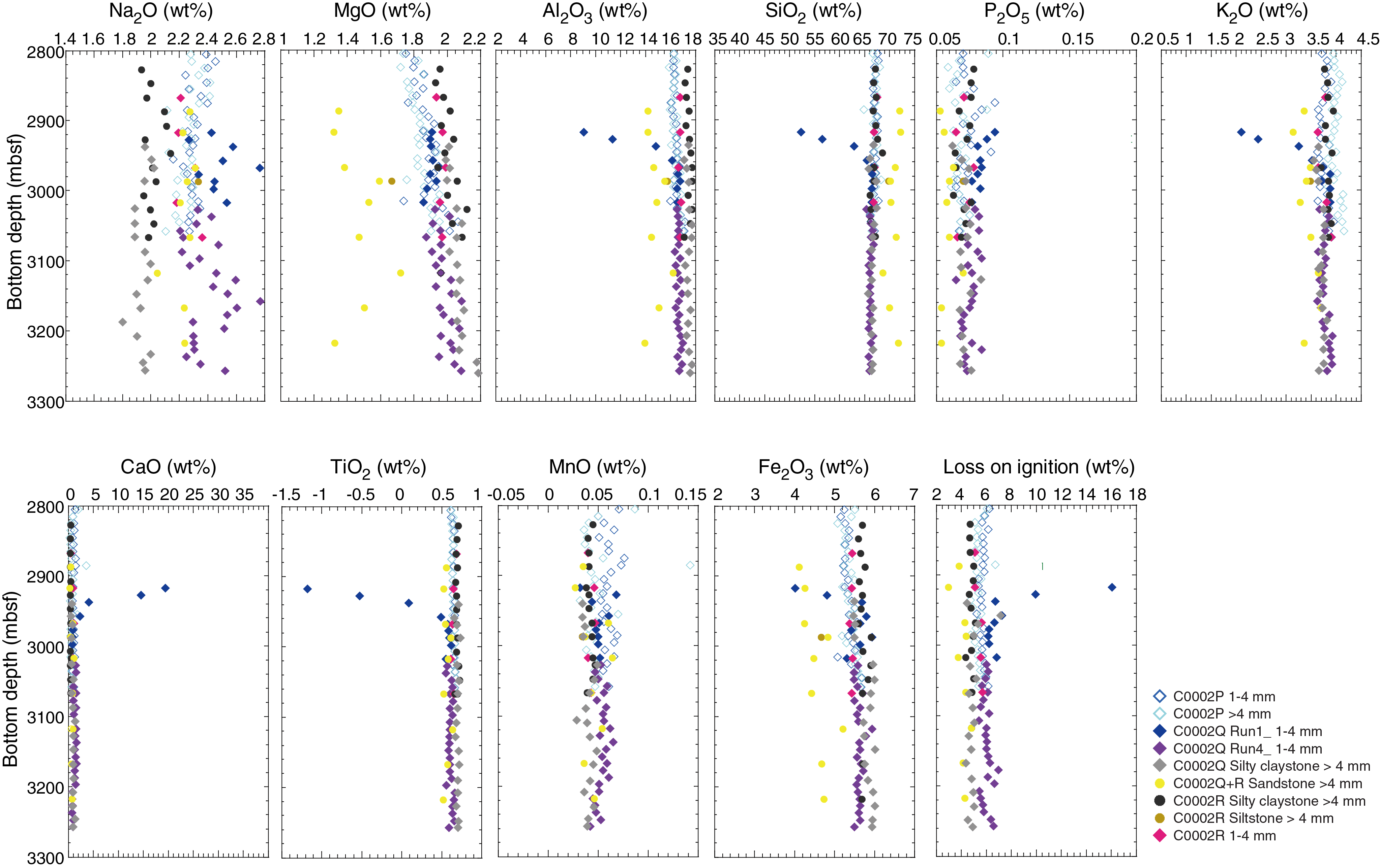
Figure F14. XRF chemical compositions, Hole C0002Q and C0002R cuttings.
The compositional spikes observed in the upper part of Hole C0002Q Run 1 in the 1–4 mm bulk rock are mainly due to contamination by cement near the kick-off section. CaO content indicates cement contamination between 2917.5 and 2957.5 mbsf (Samples 358-C0002Q-32-SMW to 43-SMW). LOI values in the cement contamination interval range as high as 16 wt%. Below the zone of cement contamination, CaO remains consistently <2.0 wt%. SiO2 is the dominant oxide, consistently greater than 60 wt%. Al2O3 and K2O have nearly constant values of approximately 16 and 3.5 wt%, respectively.
Overall, we do not recognize any significant depth-dependent trends in bulk sediment geochemistry except for a slight increase in MgO with depth. Na2O shows relatively strong scattering throughout the data; one reason for this could be contamination by drilling mud and/or seawater. The absence of significant downhole trends in and among the individual holes is consistent with relatively homogeneous proportions of rock types. Sandstone and siltstone lithologies show higher SiO2 values and lower MgO, Al2O3, P2O5, K2O, and Fe2O3 values compared to silty claystone, probably due to a slight decrease in feldspar and an increase in quartz grains. Comparing the >4 mm silty claystone and the 1–4 mm bulk cuttings, only slight changes in the amounts of various elements can be observed. This is likely due to the incorporation of siltstone and fine sandstone fragments in the 1–4 mm cuttings.
Figure F15 shows a compilation of values from measurements of all bulk powder XRF samples from core and cuttings, including results from Integrated Ocean Drilling Program Expeditions 338 and 348 (Strasser et al., 2014; Tobin et al., 2015). We cannot detect any significant shifts or consistent geochemical trends with depth aside from the contamination by cement (seen as perturbations of Na2O, CaO, LOI, SiO2, Al2O3, K2O, and Fe2O3). These geochemical data point to lithologic homogeneity in Unit V and are broadly consistent with the results from XRD analyses.
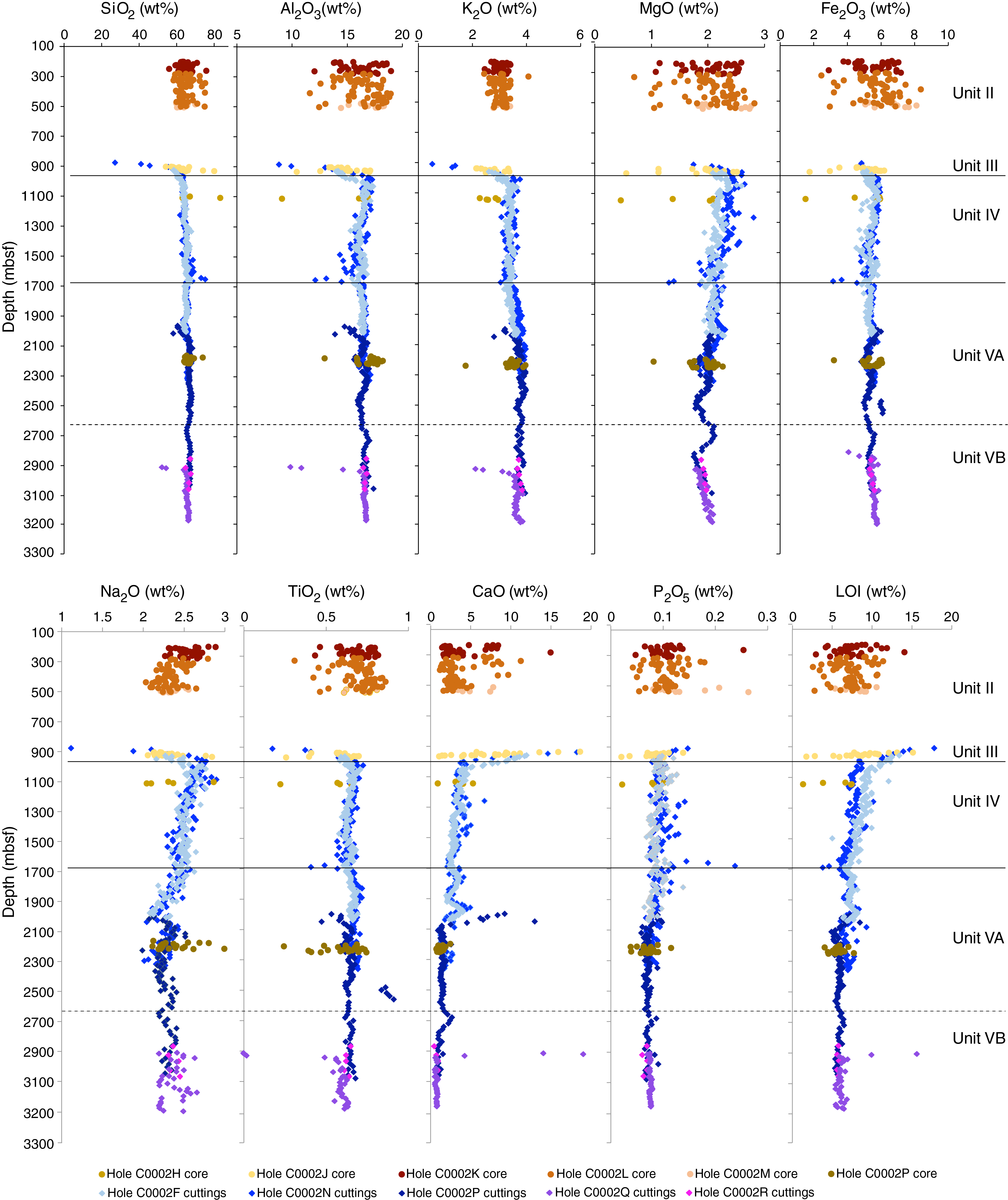
Figure F15. XRF chemical compositions, Site C0002 core and cuttings.
X-ray diffraction mineralogy
We routinely used XRD to measure the mineralogy in handpicked >4 mm cuttings every 20 m in all four holes. The 1–4 mm bulk cuttings were routinely measured every 10 m interval in Hole C0002Q and every 50 m in other holes. Representative handpicked samples of minor lithologies (>4 mm) were also analyzed to verify their compositions.
Hole C0002Q
Hole C0002Q results are displayed in Figure F16 and tabulated in Table T8. Calcite is below the detection limit in most samples from both cuttings size fractions; this result correlates well with coulometric data (see Geochemistry). In Hole C0002Q Run 1, the average total clay mineral content for handpicked silty claystone is 47.1 wt%; average quartz and feldspar values are 35.3 and 16.5 wt%, respectively. In Hole C0002Q Run 4, the comparable values are 43.7 wt% for total clay minerals, 28.7 wt% for quartz, and 13.7 wt% for feldspar. The absence of downhole trends in XRD data is consistent with relatively homogeneous visual core description results. Data from the 1–4 mm bulk cuttings show consistent contamination by cement (concrete) chips between 2917.5 and 2957.5 mbsf. Artificial cement is scattered in Hole C0002Q Run 4. The average total clay mineral content is 43 wt%; quartz content averages 41.7 wt%, and feldspar averages 15 wt%. In Hole C0002Q Run 4, the average values are 42.8 wt% total clay minerals, 36.3 wt% quartz, and 18.6 wt% feldspar. As expected, handpicked silty claystone samples from the >4 mm size fraction contain more total clay minerals (by 2–4 wt%) than bulk samples from the 1–4 mm cuttings (Figure F16; Table T8).
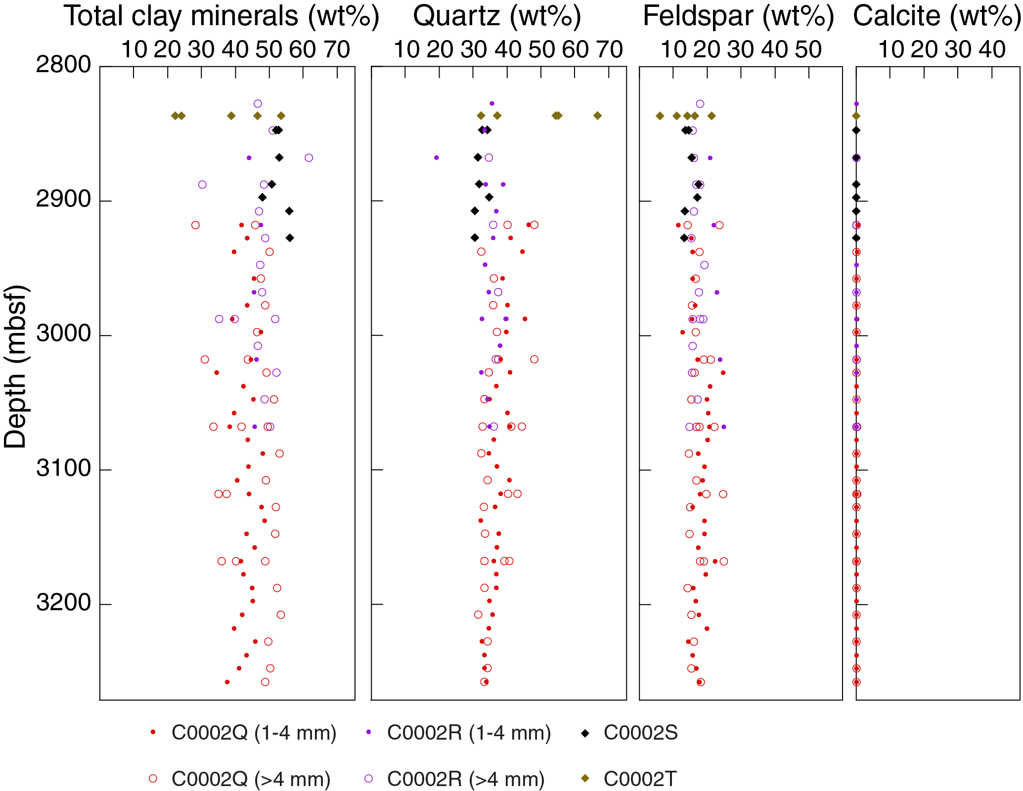
Figure F16. Random bulk powder XRD mineral composition.
Hole C0002R
Following the same procedure as for Hole C0002Q, we routinely analyzed handpicked silty claystone cuttings from the >4 mm fraction every 20 m between 2827.5 and 3067 mbsf in Hole C0002R. The 1–4 mm bulk samples were measured every 50 m (Figure F16; Table T8). Additionally, a few sandstone and siltstone samples (>4 mm) were analyzed for comparison. In silty claystone, the XRD patterns show an average clay mineral content of 49.8 wt%; quartz content is 33.4 wt%, and feldspar content is 16.4 wt%. Relative proportions of quartz and feldspar are about 5–10 wt% larger in handpicked sandstone and siltstone samples, and clay mineral abundances are smaller by about 10–20 wt%. We attribute the small compositional difference between bulk mix cuttings and silty claystone to the fact that proportions of siltstone and sandstone in bulk mix cuttings typically reach 20%–30% (Table T6).
Holes C0002S and C0002T
Bulk powder XRD results for specimens from Holes C0002S and C0002T are tabulated in Table T8 and plotted in Figure F16. We see no significant differences between those results relative to comparable lithologies from Holes C0002Q and C0002R.
Integration of XRD data among holes
Figure F17 provides a compilation of bulk powder XRD results from Expeditions 338, 348, and 358. Several caveats need to be considered when interpreting these results. First, some differences may have been imparted during washing and sieving of cuttings. Softer cuttings of sandstone and siltstone at shallower depths are more likely to disaggregate and pass through the 1 mm screen during sieving, but less vigorous washing could result in more of the bentonite-bearing drilling mud being retained. Second, the X-ray diffractometer on Chikyu was replaced before Expedition 358, and we used a different matrix of singular value decomposition normalization factors for calculations of mineral abundance (see Lithology in the Expedition 358 methods chapter [Hirose et al., 2020]). Third, all of the cuttings specimens analyzed from Integrated Ocean Drilling Program Holes C0002N and C0002P are from bulk mix cuttings. Incorporation of three or four lithologies into the bulk mix was responsible for homogenization of calculated mineral abundances toward the overall average of the lithologic assemblage. That effect is obvious if one compares the spread of values over the cored interval of Hole C0002P with data from bulk mix cuttings over the same depth interval (Figure F17). The effects of dispersing cuttings in the circulating drilling mud, together with the incorporation of cavings from above, over relatively extensive depth intervals of 50 m or more is also evident. We suggest that the long-wavelength oscillations of values from Holes C0002N and C0002P (Figure F17) are largely a manifestation of mixing in the borehole.
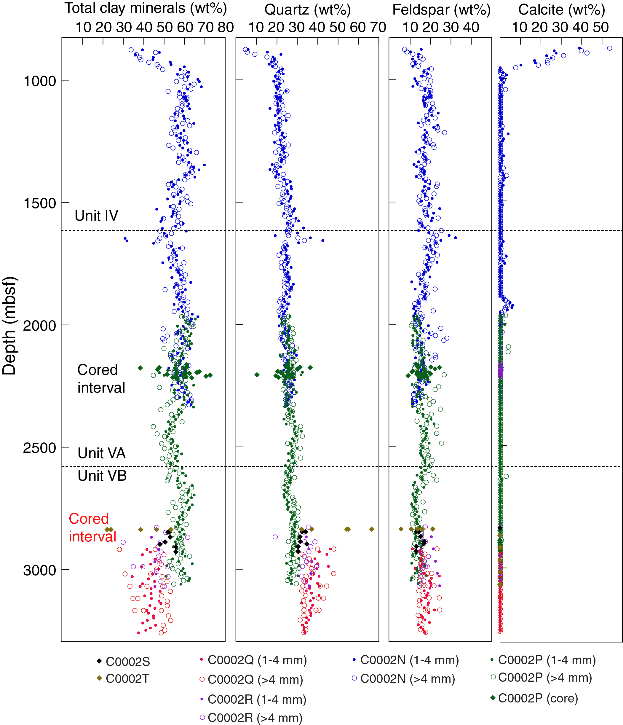
Figure F17. Bulk powder XRD data.
Another obvious discrepancy arises when comparing data from Hole C0002P with results from overlapping depths in Holes C0002Q–C0002T. Part of that apparent mismatch can be explained in terms of the difference between analysis of bulk mix cuttings as opposed to individual lithologies. Most of the data from Expedition 358 show more scatter (Figure F17) because the lithologies were segregated prior to XRD analyses. Fine sandstone and siltstone samples naturally contain a higher relative percentage of quartz (averages of 44.1 and 53.1 wt%, respectively). Their total clay mineral concentrations are lower (averages of 31.6 and 31 wt%, respectively) compared to silty claystone samples (average of 50.6 wt%). Even after taking that grain size effect into account, however, we see a systematic shift toward modestly higher proportions of quartz and feldspar compared to correlative strata from Hole C0002P. That shift is consistent with the results of visual cuttings descriptions (Figure F18). As discussed below, we believe these variations are a reflection of the natural heterogeneity in a steeply dipping succession of interbedded silty claystone, siltstone, and fine sandstone.
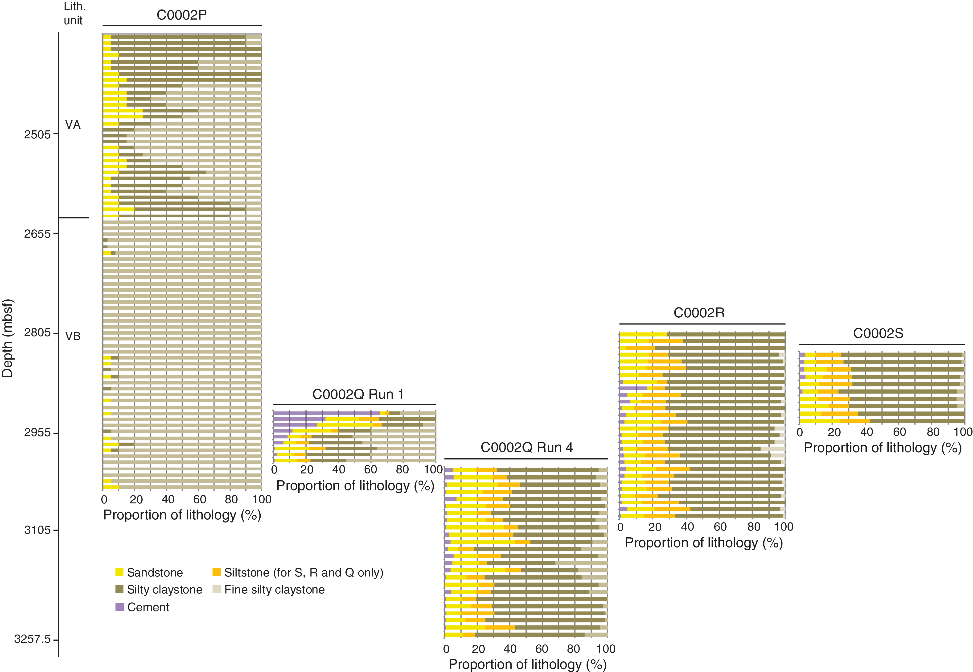
Figure F18. Lithologic proportions, Holes C0002Q–C0002S.
Provisional interpretations
Lithologic variations in cuttings
The Subunit VA/VB boundary was defined in Hole C0002P at 2625.5 mbsf (Figure F3); the depth interval assigned to Subunit VB is characterized by abundant fine silty claystone and rare sandstone (Tobin et al., 2015). The same depth interval in Holes C0002Q–C0002T appears to contain more fine sandstone and siltstone with minor amounts of fine silty claystone in the cuttings. XRD results are consistent with small increases in the proportion of quartz balanced by reductions in total clay minerals.
Our QA/QC tests of specimens from Holes C0002P–C0002R demonstrated that the differences summarized above were not caused by biases introduced by modified cuttings description methods. The mechanical and/or chemical effects of using different mud compositions (e.g., adding Fracseal and Barolift) and drilling parameters (e.g., drill bits, underreamer, and ROP) are more difficult to evaluate, particularly in terms of preferential preservation of more and less resistant lithologies. We note that LWD data show subtle changes in resistivity and gamma ray near the inferred subunit boundary in Hole C0002P (see Logging). That observation supports true changes in facies character. On the other hand, differences in bulk geochemistry are no more pronounced across the subunit boundary than in Subunit VA.
In situ bedding dips are typically steep in the inner accretionary prism (Boston et al., 2016) (see Logging), so relatively small changes in proportions of coarse–fine interbeds within one depositional facies (e.g., cyclic packets of turbidites separated by shale-dominated intervals) could lead to noticeable variations in cuttings proportions (i.e., increases or decreases of 10%–15% in quartz and total clay). Having cuttings and cavings mixed in the drilling mud during circulation, which probably occurs over 40–50 m depth intervals, smooths that effect in cuttings data relative to what might be expected with continuous coring. Thus, our provisional interpretation is that the apparent shift toward a slightly coarser lithofacies in Holes C0002Q–C0002T relative to Hole C0002P is real. At the same time, the changes are not significant enough to warrant designating a different lithologic unit or subunit.
Depositional processes and environments
Strata recovered from Site C0002 during Expedition 358 are part of the inner accretionary prism of the Nankai Trough (Boston et al., 2016). Our interpretations of facies relations are hampered by the lack of intact core and uncertainties regarding the true proportion of various lithologies in situ. During Expedition 348, cores were recovered from the upper part of Lithologic Unit V. They consist of hemipelagic mudstone (silty claystone) with thin interbeds of siltstone, fine sandstone, and scattered lamination of pyrite; that facies character is suggestive of a largely hemipelagic depositional environment with sporadic introduction of fine-grained turbidity currents (Tobin et al., 2015). The cuttings collected during Expedition 358 are likewise consistent with a hemipelagic/turbidite facies. The environment of deposition for Unit V may have been a trench or an abyssal plain seaward of the trench. On the other hand, correlations of facies character and composition with coeval facies in the Shikoku Basin are problematic in several respects (Underwood, 2018). Additional shore-based research will be required to help resolve this enigma.
Evidence for sediment diagenesis, including cementation, maturation of terrigenous organic matter, and transformation of smectite to illite (e.g., Fukuchi et al., 2017; Underwood, 2018; Hüpers et al., 2019), is plentiful below ~2200 mbsf. Contrasts of color and physical properties between "softer" fine silty claystone (light gray) and "harder" silty claystone (dark gray) remain enigmatic. Textural influences on differential diagenesis, cementation, and/or clay mineral reactions are all possible as contributing factors, but another consideration would be artifacts caused by differences in drilling operations. Additional shore-based research will also be required to answer this question.
Structural geology
Structural analyses at Site C0002 included (1) description of cuttings retrieved from Holes C0002Q (2887.3–3262.5 mbsf), C0002R (2789.5–3082.5 mbsf), C0002S (2842.5–2933.5 mbsf), and C0002T (2817.5–2848.5 mbsf) and (2) analyses of cores from Hole C0002T (2836.5–2848.5 mbsf).
Cuttings description
Description of deformation structures in intact cuttings
Deformation structures were investigated on the 1–4 and >4 mm size fractions of intact cuttings (from here onward called "cuttings") from Holes C0002Q–C0002T. Excluding drilling-induced disturbance, observed deformation structures were limited to slickenlines and mineral veins. All observed deformation structures are summarized in Excel files in STRUCTURE in Supplementary material that include observation notes and the number of each type of deformation feature, sedimentary structure, and drilling-induced deformation observed in each sample, differentiated by the cuttings size fraction (>4 and 1–4 mm) and by lithology. Cuttings showing only sedimentary structures are classified as "nondeformed." Close-up photographs of cuttings with notable deformation structures, drilling-induced structures, and sedimentary structures are included in CUTTINGS in Supplementary material.
Distribution of deformation structures in intact cuttings samples
Figure F19 summarizes the percentage of deformed cuttings obtained by dividing the number of cuttings that show deformation structures by the total number of described cuttings from Holes C0002Q–C0002T. Overall, very little structural deformation (<1% of total cuttings) occurs in the interval between 2827.5 and 3257.5 mbsf. Granular and dogtooth calcite veins occur throughout the section; slickenlines and stepped striae are rare. Dogtooth calcite veins occur more frequently than granular calcite veins below ~3000 mbsf, where dogtooth veins in Holes C0002Q and C0002R are generally better developed than those observed in Hole C0002P (Tobin et al., 2015). No scaly fabrics, minor faults, or cataclastic bands were recovered in cuttings from Holes C0002Q–C0002T.

Figure F19. Deformation features in intact cuttings.
Mineral veins
The terminology used for mineral vein description is outlined in Table T9. The distribution of veins in all holes at Site C0002 is shown in Figure F19. Individual veins have thicknesses of less than a few millimeters and are filled mainly with calcite (Figure F20). Veins appear most commonly in silty claystone but are occasionally observed in sandstone. Entire cuttings composed of vein material also occur.
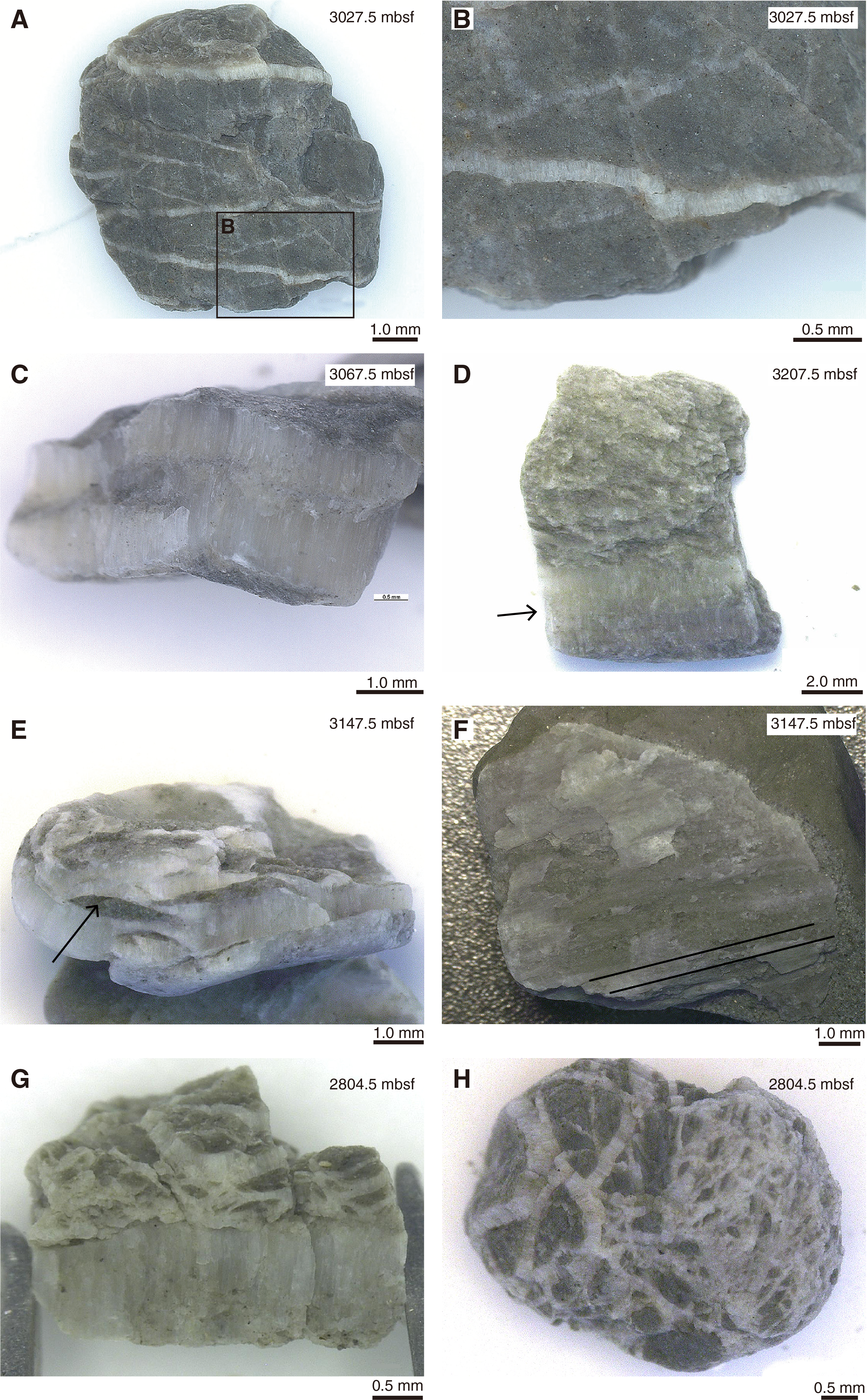
Figure F20. Calcite veins in cuttings.
Documented vein geometries include individual veins and vein networks where veins exhibit either granular or dogtooth crystal morphology at the mesoscopic scale (Figure F20). Contacts between mineral veins and host rock are often sharp and planar but may be wavy or anastomosing (Figures F21, F22, F23, F24, F25). Vein networks show variable spacing between individual veins resulting in various degrees of fragmentation or brecciation of the host rock (Figure F20A, F20B, F20D, F20E, F20G, F20H). Granular veins show blocky texture at the microscale and document syntaxial (inward) growth, where the wall rock is lined by small crystals that increase in size toward the vein interior (Figures F21, F23A, F23B). Dogtooth veins show fibrous crystals at the microscopic scale that reflect antitaxial (outward) growth approximately perpendicular to the wall rock (Figures F22E, F23C, F24). The width of crystal fibers is commonly constant, and fiber boundaries are normally smooth (Figures F22E, F24).
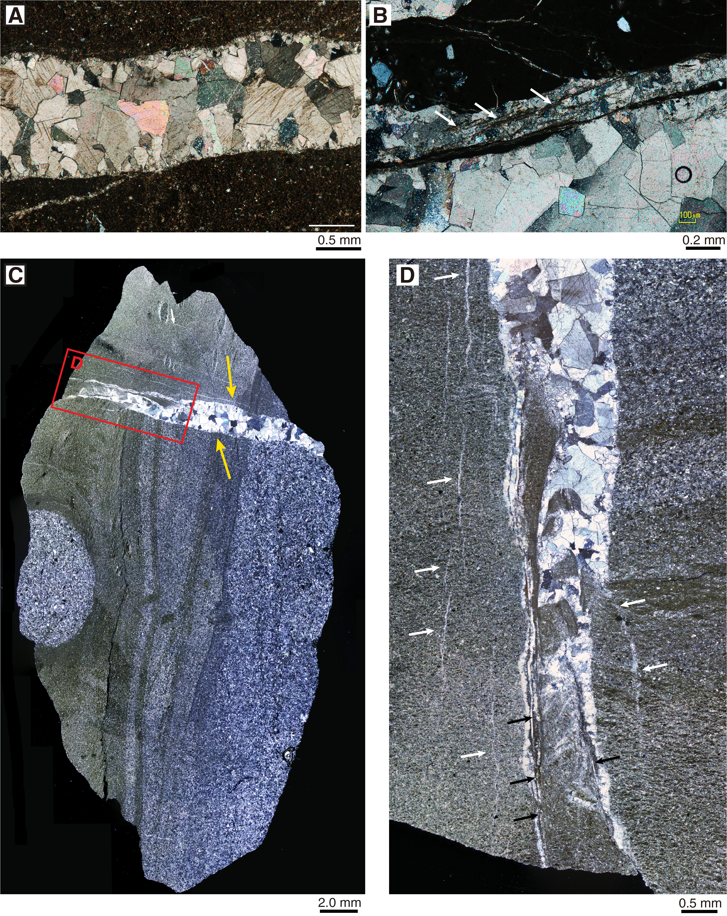
Figure F21. Crack-seal calcite veins.
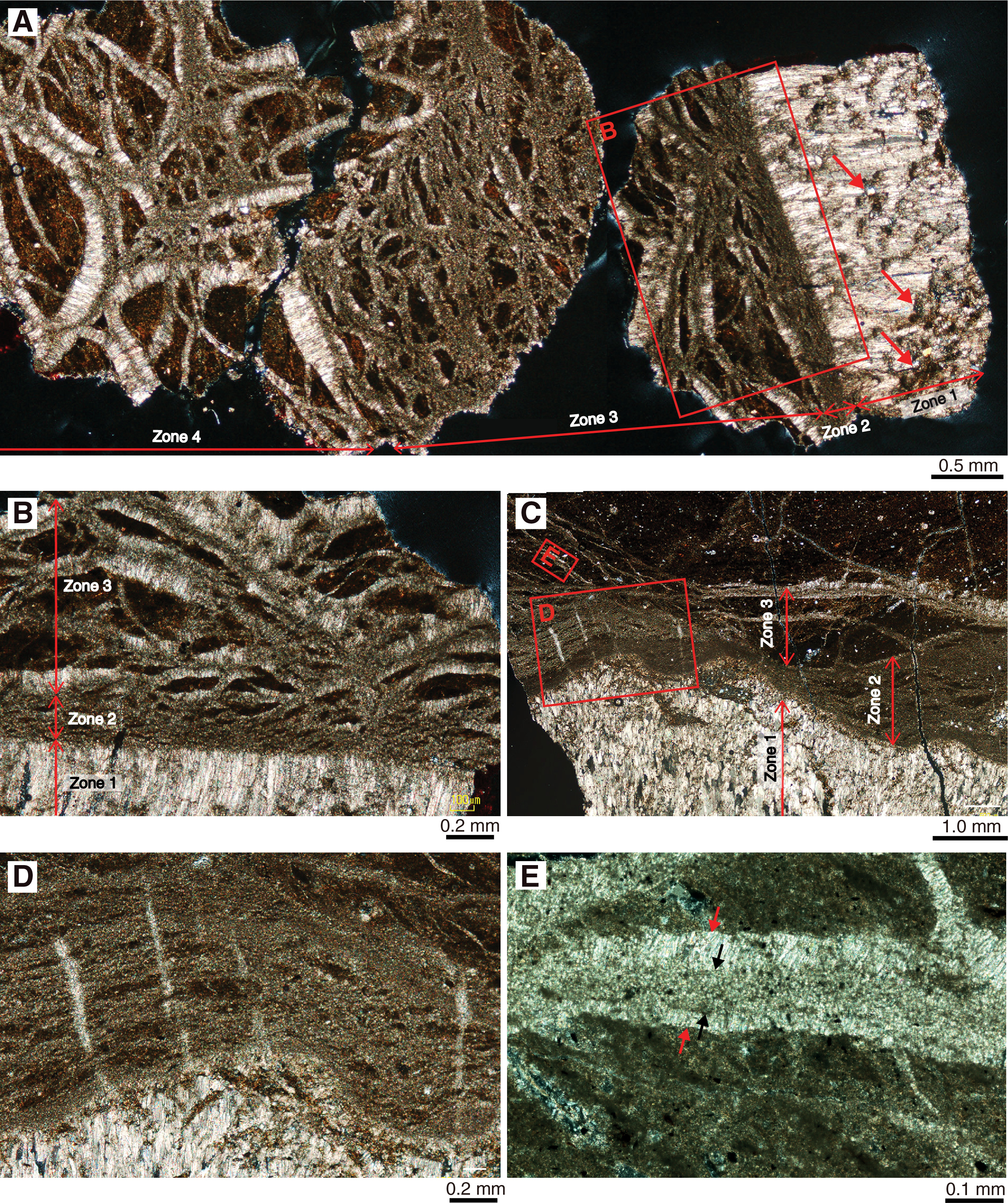
Figure F22. Fibrous calcite veins and host rock breccia.

Figure F23. Crosscutting and overprinting relationships, calcite veins.
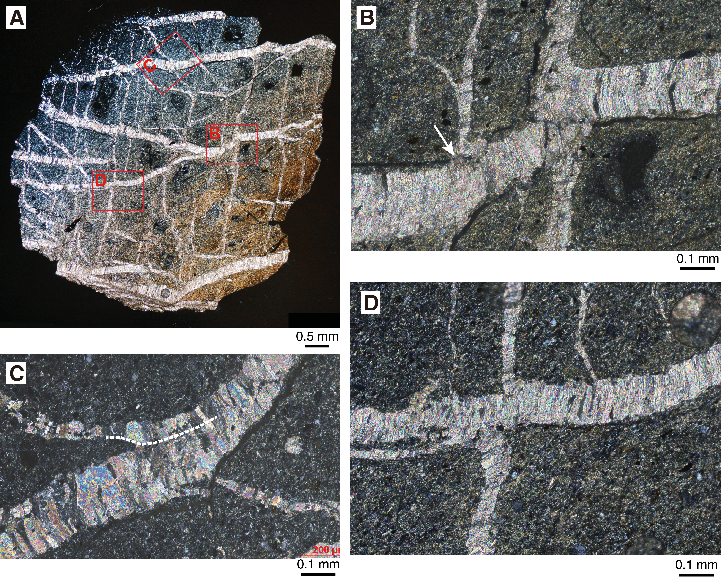
Figure F24. Fibrous calcite veins.
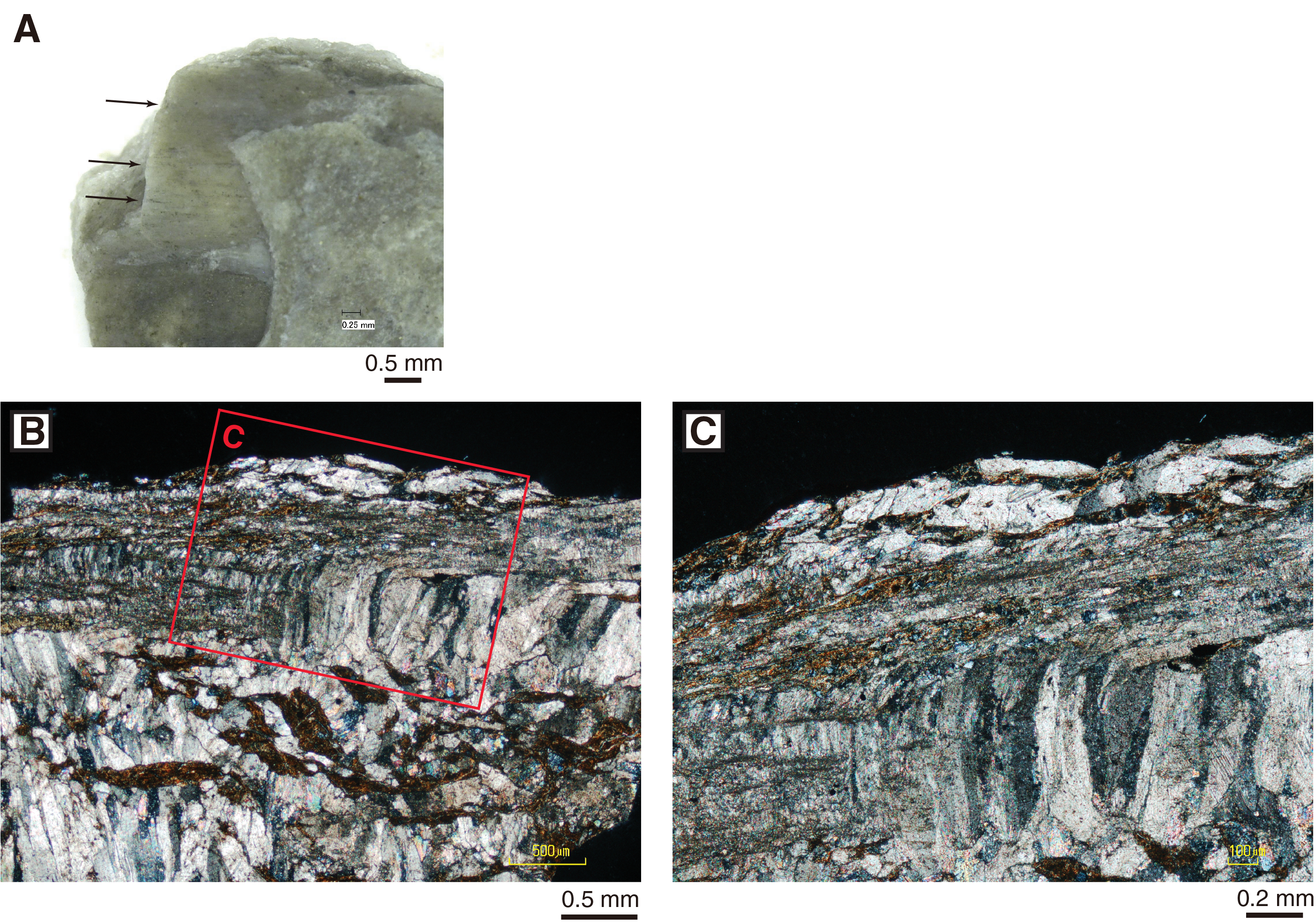
Figure F25. Slickenfibers.
Mineral veins with the granular/blocky crystal morphology represent crack-seal veins and record extension perpendicular to the wall rock (Figures F21A, F23A). The absence of stretched or elongate crystal morphologies suggests that individual crack-seal veins record only a restricted number of crack-seal events (Bons et al., 2012). Sample 358-C0002R-343-SDB (drill bit sample at ~2790–2870.5 mbsf) preserves a ~1.5 mm thick crack-seal vein that is oriented approximately orthogonal to bedding (Figure F21C). The vein records bedding-parallel extension and probably some shear offset, as suggested by the truncated bedding and lack of continuation of bedding across the vein. The tip of the vein records delocalized fracturing, causing the fragmentation of the host rock and apparent incorporation of rock fragments into the vein (Figure F21D). Hairline veins subparallel to the vein record additional fracturing in the surrounding host rock (Figure F21C, F21D).
Whether crack-seal veins record a shear component in addition to extension is often uncertain. Sample 358-C0002R-49-SDB (~2789.5–2804.5 mbsf) shows a parallel set of crack-seal veins that are crosscut and displaced by a younger set of crack-seal veins oblique to the older veins, causing cracking of the latter (Figure F23A). The displacement of the older veins is consistent with pure extension, suggesting that these crack-seal veins record no shear component. In contrast, Sample 72-SDB (~2790–2804.5 mbsf) preserves an extensional crack-seal vein that shows evidence for later stages of deformation, potentially associated with shearing and a cataclastic reduction of calcite crystal sizes (Figure F21B).
Mineral veins with the dogtooth/fibrous crystal morphology represent antitaxial veins that record a two-stage evolution: initial fracturing and sealing of the host rock followed by continuous antitaxial growth of crystal fibers on both sides of the initial fracture (Bons et al., 2012). Antitaxial veins were found in different structural contexts. Samples 358-C0002R-49-SDB and 72-SDB (~2789.5–2804.5 mbsf) show antitaxial veins associated with anastomosing hairline calcite veins that exhibit a faint mineralization and fragment or brecciate the host rock (silty claystone; Figure F22A). Based on microstructural observations, it is possible to discriminate four zones related to the development of antitaxial veins (Figure F22A). Zone 1 represents a thicker antitaxial vein (>1 mm) that contains disperse inclusions of host rock or hairline vein fragments. Zone 2 contains no antitaxial veins but densely spaced hairline calcite veins that overprint the host rock almost entirely (Figure F22B). The hairline veins are oriented subparallel to the antitaxial vein in Zone 1 and can be overprinted by thin calcite veins oriented approximately orthogonal to the hairline veins (Figure F22C, F22D). Zone 3 comprises branches of densely spaced hairline veins with intercalated elongated host rock fragments. The long axis of the host rock fragments is subparallel to the antitaxial vein of Zone 1, mimicking preferred orientation. Antitaxial veins are poorly developed in Zone 3. Zone 4 is similar to Zone 3, but host rock fragments are larger and antitaxial veins are better developed. Furthermore, both hairline veins and antitaxial veins can be strongly curved and sometimes show an elliptical geometry (Figure F22A). In Zones 3 and 4, the thin hairline veins represent the median line of antitaxial veins (Figure F22E; Bons et al., 2012), indicating that the antitaxial veins developed from the hairline veins. Further formation conditions of the entire vein network remain difficult to constrain because of the limited observations of cuttings.
Antitaxial veins were further documented in Samples 358-C0002R-343-SDB (~2790–2870.5 mbsf) and 358-C0002Q-365-SMW (3027.5 mbsf). Sample 358-C0002R-343-SDB shows a complex pattern of crosscutting antitaxial veins that sometimes exhibit blocky crystal morphology, suggesting that the growth of mineral fibers was repeatedly interrupted by crack-seal events (Figure F23D, F23E). Sample 358-C0002Q-365-SMW shows a vein network of antitaxial veins comprising two sets of subparallel veins oriented approximately orthogonal to each other (Figure F24A). Individual mineral veins show no consistent relation to each other. Instead, mineral veins may terminate at the contact to adjacent veins (Figure F24B) or merge into the adjacent vein (Figure F24C, F24D), suggesting that the entire vein network developed contemporaneously.
Taken together, mineral veins observed in cuttings from Holes C0002Q–C0002T record crack-sealing and fibrous growth events. Deformation associated with vein formation was largely extensional, with minor evidence for shearing.
Slickenlined surfaces
Slickenlines were found only in a few samples from Holes C0002Q–C0002S. They appear as striated polished surfaces in silty claystones and sandstones and can be associated with the growth of fibrous calcite crystals defining slickenfibers (Figure F20F). We found one example of slickenfibers in Sample 358-C0002R-240-SMW (2917.5 mbsf) that overprints an earlier antitaxial vein (Figure F25). In detail, some fibrous crystals of the antitaxial vein merge into slickenfibers (Figure F25C), suggesting a gradual transition from extension (growth of the antitaxial vein) to shearing (growth of the slickenfibers).
Structures possibly related to drilling-induced deformation
Deformation and associated structures potentially related to drilling are common in Holes C0002Q and C0002R and occur as shiny striae or shiny surfaces (Figure F26), locally associated with grooves or gouge marks. Unlike naturally occurring striae, drilling-induced striae are noted on rough or nonplanar surfaces and are not associated with stepped mineral growth, clay mineral coatings, or chemical alteration of the fractured surface.
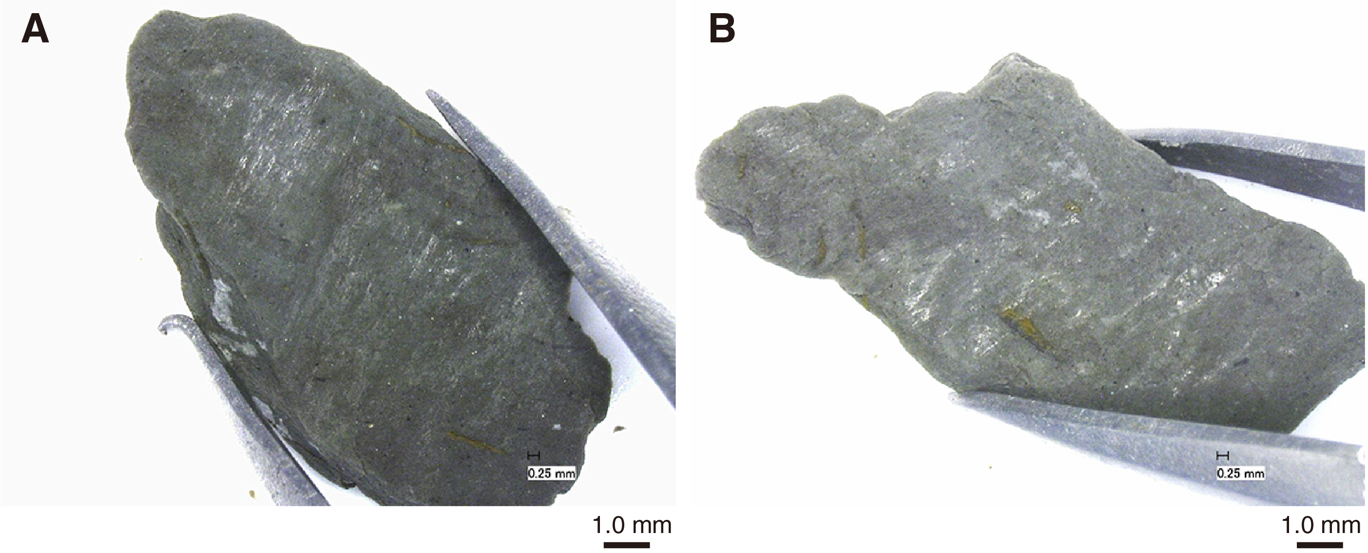
Figure F26. Drilling-induced deformation.
Sedimentary structures
Sedimentary structures including laminations and bedding planes were occasionally observed in cuttings from all boreholes at Site C0002 (Figures F21C, F27). In thin section, bedding laminations can occur at an oblique angle to the cuttings edges, suggesting that the tabular faces of cuttings are not necessarily correlated with bedding surfaces. Many samples show deformed burrows and sponge spicules that have experienced bulk strain. One sample with deformed burrows and bedding documents bedding-normal compaction.
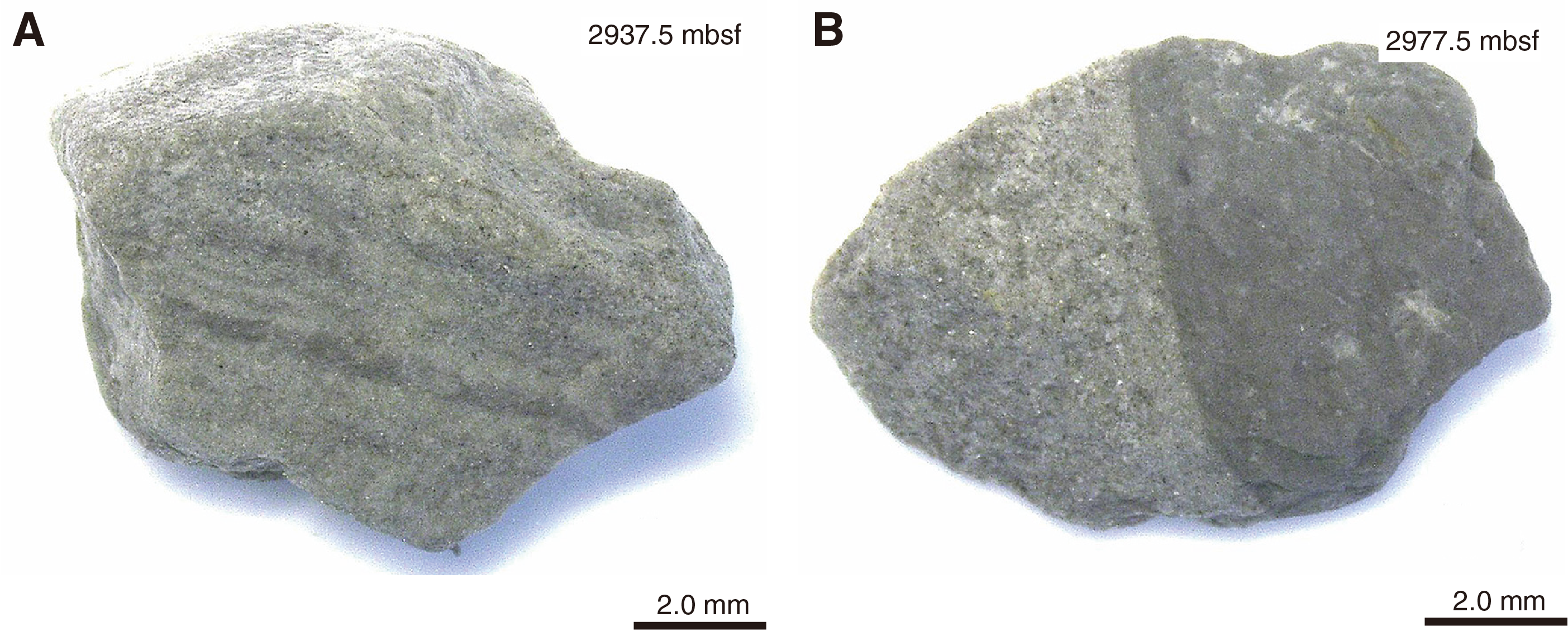
Figure F27. Intact cuttings representing sedimentary structures.
Structures in cement cuttings
Significant concentrations of artificial cement cuttings were retrieved from the uppermost parts of Holes C0002Q and C0002R, where sidetrack operations were conducted (Figure F28). The cement was emplaced during Expedition 348, 5 y prior to Expedition 358. The cement cuttings are composed of brown and light gray cements and white sand aggregates. Light gray cement hosts silty claystone cuttings (Figure F28A, F28B). Apparent alteration rims were identified between brown and light gray cement and between light gray cement and silty claystone cuttings, which may have occurred during cement curing.
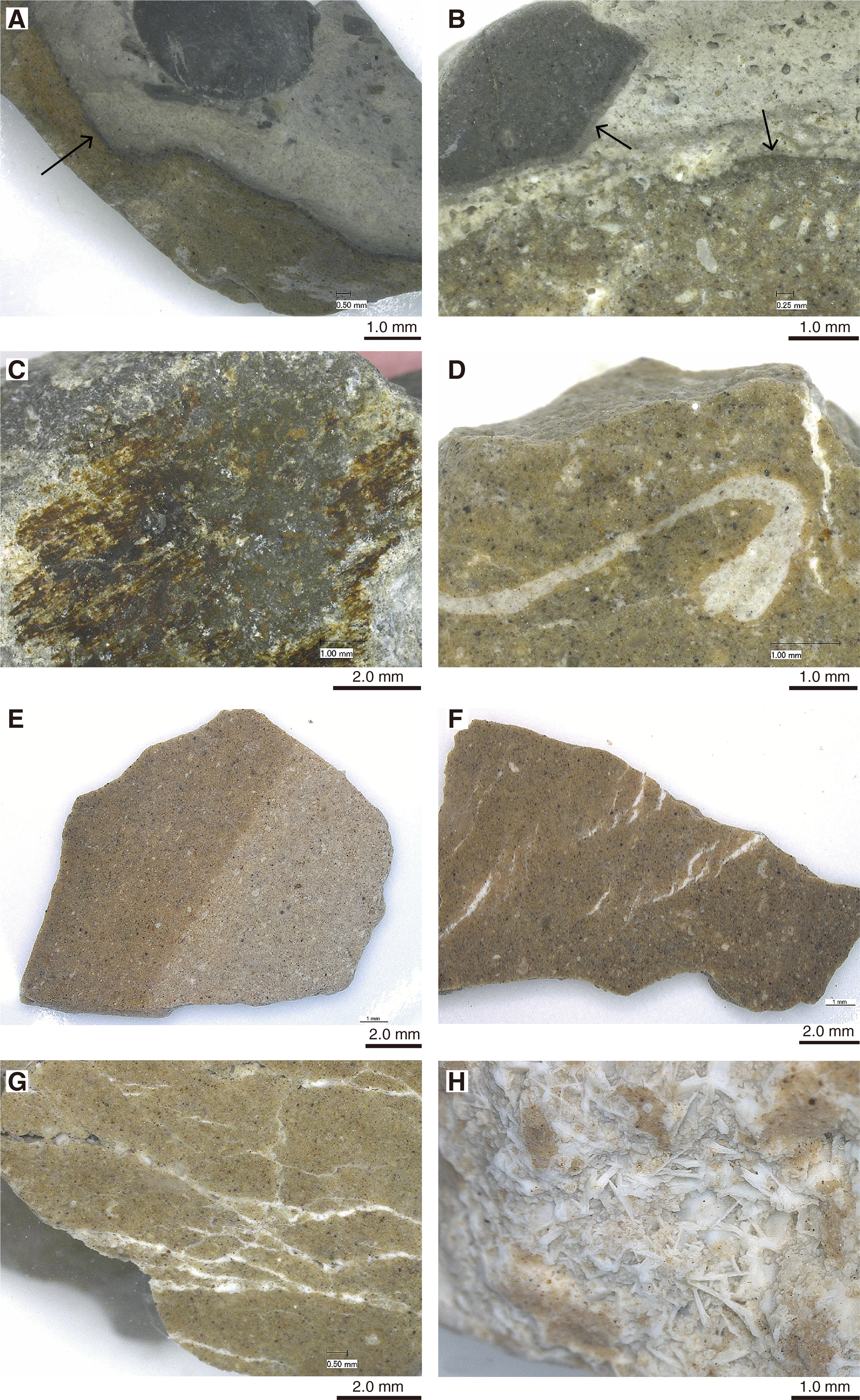
Figure F28. Cement cuttings.
Cement cuttings in Hole C0002Q show evidence of fracturing, shear, and mineral precipitation. A slickenlined surface coated by iron oxide was identified from a cement cutting (Figure F28C), likely caused by shear between the cement and casing contact. En echelon and web-like patterned fracture systems filled by mineralization are commonly developed (Figure F28F, F28G), and some cement cuttings show evidence of shear and Mode I fractures (Figure F28G). Open fractures can host idiomorphic mineralization (Figure F28H).
X-ray computed tomography imaging
X-ray CT scan images enable observation of the 3-D geometry of intact cuttings, including bioturbation and deformation structures. These structures can be visible in X-ray CT scan images if their sizes are larger than ~1 mm scale and they have a significant contrast in CT number with their surrounding matrix. Formation cuttings show relatively low CT numbers between ~1900 and 2200 (light green, Figure F29), and the CT numbers for silty claystone and sandstone are not significantly different. Open fractures show lower CT numbers than the surrounding matrix, whereas pyrite and calcite show high to very high CT numbers. CT numbers are often greater than 3000 for cement (red to white; Figure F29), ~2500–4000 for pyrite (yellow to white), and ~2500–3400 for calcite (yellow to red). Because the CT numbers of calcite and pyrite vary by sample and overlap with those of cement, it is difficult to distinguish between pyrite, calcite, and cement based on the difference in CT number. There is no clear relation between the type of cement (light gray or brown) and the CT number.

Figure F29. Typical X-ray CT image for cutting samples.
Calcite veins, open fractures, and pyrite in burrows and sponge spicules can be identified in the X-ray CT images of cuttings, although feature edges are often blurred rather than sharp. Comparisons of representative structures between images taken by binocular microscope and X-ray CT scan are shown in Figure F30. Under the optical microscope (Figure F21C), Sample 358-C0002R-343-SDB (Figure F30B) is composed of siltstone and sandstone laminations sandwiched between a coarser sand-rich zone and a clay-rich zone with a large (~1 cm) rounded clast of sandstone. These three zones are separated by two wavy open fractures that follow the orientation of the laminations and are truncated orthogonally by a planar thick granular calcite vein developing a brecciated structure at one tip. In the X-ray CT scan image (Figure F30A), the calcite vein is clearly visible and occurs as a high–CT number (~2500, red) planar, sharp, and thick line, separating two zones of moderate CT number (2000–2250, yellow to orange). The tip of the calcite vein is not resolved in the X-ray CT image. The two open fractures occur as more discrete, discontinuous wavy lines with lower CT numbers (1850–1900, green). The variations in lithology around the open fractures are not visible in the X-ray CT image. In Sample 49-SDB, multiphase dogtooth calcite veining is visible at the mesoscopic scale (Figure F30D). These veins and their geometry are well resolved in the corresponding X-ray CT image (Figure F30C) where they appear as a parallel set of crosscutting lines with high CT numbers (2750–3000, red), contrasting with the lower CT numbers (~2550–2650, yellow to orange) of the surrounding matrix. At the mesoscopic scale, Sample 25-SDB shows a network of crosscutting open fractures with low CT numbers visible in 2-D (<1550, blue; Figure F30E). Burrows tend to create a network with high CT numbers (~3000, red), probably due to pyrite infilling as observed in Sample 358-C0002Q-507-SMW (Figure F30F–F30H).

Figure F30. 2-D and 3-D X-ray CT images for cuttings.
Core description
Cores recovered from Hole C0002T show significant drilling-induced deformation but almost no tectonic features except for some small mineral veins. Interval 358-C0002T-3K-1, 24–28 cm (2843.24 mbsf), contains one fragment of light gray carbonate including 1–2 mm thick planar to curviplanar calcite veins. One silty claystone fragment hosts aligned burrows, roughly tracing bedding planes. Drilling-induced breccia is observed in all recovered cores and is marked by fragments of silty claystone and cement in a soft drilling mud matrix (Figure F31). Fractured silty claystone commonly preserves cracks with or without drilling mud. Disaggregated silty claystone represents drilling-induced fragmentation and brecciation of the host rock.

Figure F31. Silty claystone and cement clasts in drilling mud.
Preliminary observations
The key observations made on cuttings in Holes C0002Q–C0002T, together with structural analysis of cores retrieved in Hole C0002T are as follows:
- Holes C0002Q–C0002T contain very few cuttings with slickenlines (<1%) and no cuttings exhibiting scaly fabric (Figure F32). Compared to Hole C0002P, which showed a significant abundance (>20%) of cuttings with slickenlines and scaly fabrics (Tobin et al., 2015), the low abundance of deformation structures suggests that the sections of Holes C0002Q–C0002T between 2789.5 and 3262.5 mbsf are weakly deformed.
- The large number of deformed cuttings in the lower portion of Hole C0002P is likely due to downhole contamination from shear zones crossed at shallower levels that do not appear in Holes C0002Q and C0002R because that interval is now cased. This interpretation is supported by the observation that a large number of intact cuttings were retrieved immediately after waiting on weather or other time-consuming operations during Expedition 348 (Tobin et al., 2015). This observation helps constrain the depth of the shear zone inferred from Hole C0002P cuttings to between 2430 and 2789.5 mbsf, the latter of which is the depth of the first sample in Hole C0002R.
- Mineral veins observed in cuttings from Holes C0002Q–C0002T record different modes and phases of mineral vein formation. Crack-seal veins document repeated episodes of extensional fracturing potentially driven by fluctuations in pore fluid pressure or prevailing stress state. Extensional fracturing can be followed by shear deformation as recorded by shear veins and/or slickenlines, partially overprinting crack-seal veins and vice versa. The occurrence of fibrous mineral veins indicates prolonged mineral precipitation during continuous deformation following individual crack-seal events (e.g., Bons et al., 2012). Orthogonal vein sets appear to be mutually crosscutting, suggesting that vein formation occurred as a result of temporal variations in the orientation of the stress field (e.g., Takeshita et al., 2014) possibly facilitated by elevated fluid pressure and small differential stress.

Figure F32. Deformation features in accretionary prism.
Taken together, the restricted occurrence of deformation structures in Holes C0002Q–C0002T suggests that the drilled sections represent a weakly deformed portion of the Nankai accretionary prism. The observed structural features are characteristic of shallow deformation processes and consistent with deformation structures documented in active and fossil accretionary prisms elsewhere (Maltman et al., 1993; Yamamoto et al., 2005: Takeshita et al., 2014; Dielforder et al., 2016).
Biostratigraphy and paleomagnetism
Biostratigraphy
Preliminary age determination for cuttings from Holes C0002Q–C0002T is based exclusively on examination of calcareous nannofossils. Abundance and preservation of calcareous nannofossils vary throughout the sequence. Different states of abundance and preservation are recognized even in different pieces from the same sample of cuttings. Nannofossil assemblages from all four holes contain Reticulofenestra pseudoumbilicus (≥7 µm) except for a single piece from Sample 358-C0002Q-365-SMW (3022.5–3027.5 mbsf). R. pseudoumbilicus (≥7 µm) has an age range of 12.8–3.63 Ma with an absence interval of 8.8–7.09 Ma. R. pseudoumbilicus together with the presence of Discoaster prepentaradiatus (Zones NN9–NN10A; ~10.5–8.3 Ma) in some samples from the four holes (2847.5–3257.5 mbsf) are likely assigned an age of 10.5–8.8 Ma. The assemblage from Sample 365-SMW (3022.5–3027.5 mbsf) that lacks R. pseudoumbilicus (≥7 µm) indicates an age of 8.8–7.09 Ma.
Radiolarians and foraminifers were also found in Holes C0002Q–C0002S. They are not used for age determination because of very rare occurrences. All radiolarians are possibly reworked.
Calcareous nannofossils
Calcareous nannofossil dating for this site is based on the biostratigraphic framework presented in Figure F33. Nannofossils are almost continuously present throughout the sequence. Nannofossils from 74 cuttings samples (358-C0002Q-32-SMW to 633-SMW, 358-C0002R-89-SMW to 334-SMW, 358-C0002S-9-SMW to 37-SMW, and 358-C0002T-6-SMW to 14-SMW) and 3 core samples (358-C0002T-1K-CC, 42.0–47.0 cm, to 3K-CC, 39.0–44.0 cm) were examined.

Figure F33. Biostratigraphic framework, calcareous nannofossils.
Hole C0002Q
A total of 146 smear slides were prepared from 36 cuttings samples (358-C0002Q-30-SMW to 633-SMW; 2902.5–3257.5 mbsf), and 49 of 146 smear slides contained calcareous nannofossils (Table T10).
The composition of calcareous nannofossils in Slide C from Sample 358-C0002Q-365-SMW differed from the other 48 smear slides in that it did not contain any R. pseudoumbilicus (≥7 µm) (12.8–8.8 and 7.09–3.63 Ma) but did contain Discoaster berggrenii (first occurrence [FO] at 8.2 Ma). Therefore, the age of the sample in this slide is estimated to be 8.8–7.09 Ma.
Calcareous nannofossil assemblages in the remaining 48 smear slides are similar to each other and are characterized by the occurrence of R. pseudoumbilicus (≥7 µm) (12.8–8.8 and 7.09–3.63 Ma) and Sphenolithus spp. (last occurrence [LO] at 3.7 Ma) and the absence of early–middle Miocene species such as Coccolithus miopelagicus (≥14 µm) (LO at 10.61 Ma) and Cyclicargolithus floridanus (LO at 13.3 Ma). D. prepentaradiatus (Zones NN9–NN10A; ~10.5–8.3 Ma) was found in Slide B from Sample 358-C0002Q-633-SMW and Slide C from Sample 541-SMW. The 48 samples can probably be assigned to Zone NN10A, which is the interval between the FO of D. prepentaradiatus (~10.5 Ma) and the bottom of the temporary absence of R. pseudoumbilicus (~8.8 Ma). However, they may be assigned to Zone NN11B or younger if rare specimens of D. prepentaradiatus are reworked.
Hole C0002R
A total of 108 smear slides were prepared from 27 cuttings samples (358-C0002R-89-SMW to 334-SMW; 2812.5–3077.5 mbsf), and 31 contained calcareous nannofossils (Table T11).
Calcareous nannofossil assemblages observed in the 31 smear slides from the samples at 2812.5–3057.5 mbsf are similar to each other and are characterized by the occurrence of R. pseudoumbilicus (≥7 µm) (12.8–8.8 and 7.09–3.63 Ma), Sphenolithus spp. (LO at 3.7 Ma), and the absence of early–middle Miocene species such as C. miopelagicus (≥14 µm) (LO at 10.61 Ma) and C. floridanus (LO at 13.3 Ma) (Table T11). D. prepentaradiatus (Zones NN9–NN10A; ~10.5–8.3 Ma) was found in a few smear slides from cuttings Samples 358-C0002R-89-SMW (2812.5–2817.5 mbsf) and 328-SMW (3052.5–3057.5 mbsf) (Table T11). The age between Samples 89-SMW and 328-SMW (2812.5–3057.5 mbsf) is therefore estimated to be 10.5–8.8 Ma, as the interval between the FO of D. prepentaradiatus (~10.5 Ma) and the bottom of the temporary absence of R. pseudoumbilicus (≥7 µm) (~8.8 Ma).
Hole C0002S
A total of 40 smear slides were prepared from 10 cuttings samples (358-C0002S-9-SMW to 37-SMW; 2842.5–2933.5 mbsf), and 15 contained calcareous nannofossils (Table T12).
Calcareous nannofossil assemblages observed in the 15 smear slides are similar to each other and are characterized by the occurrence of R. pseudoumbilicus (≥7 µm) (12.8–8.8 and 7.09–3.63 Ma). One of the smear slides from cuttings Sample 358-C0002S-37-SMW (2932.5–2933.5 mbsf) yielded D. prepentaradiatus (Zones NN9–NN10A; ~10.5–8.3 Ma). Therefore, the age of the sample is estimated to be ~10.5–8.8 Ma, as the interval between the FO of D. prepentaradiatus (~10.5 Ma) and the bottom of the temporary absence of large R. pseudoumbilicus (≥7 µm) (~8.8 Ma). Only one broken specimen that resembles Discoaster hamatus, a marker species of Zone NN9, was found in one of the smear slides from cuttings Sample 32-SMW (2912.5–2917.5 mbsf). If it is D. hamatus, this sample could be assigned to Zone NN9 (10.49–9.65 Ma).
Hole C0002T
A total of 20 smear slides were prepared from two cuttings and three core catcher samples collected from 2832.5 to 2843.7 mbsf in Hole C0002T, and 6 contained calcareous nannofossils (Table T13).
Calcareous nannofossil assemblages observed from the six smear slides were similar to each other and were characterized by the occurrence of R. pseudoumbilicus (≥7 µm) (12.8–8.8 and 7.09–3.63 Ma). One of the smear slides prepared from Sample 358-C0002T-2K-CC (2841.15–2841.2 mbsf) yielded multiple specimens of D. prepentaradiatus (Zones NN9–NN10A; ~10.5–8.3 Ma) and a specimen of Minylitha convallis (Zones NN9–NN11A; ~9.76–7.78 Ma). D. hamatus (Zone NN9) was not found in the sample. Therefore, the age of the sample is estimated to be ~9.76–8.8 Ma (Zone NN10A) on the basis of the occurrences of M. convallis and D. prepentaradiatus.
Comparison with Hole C0002P
In Hole C0002P, Tobin et al. (2015) assigned 88 samples from 2145.5 to 3055.5 mbsf to Zone NN9 based on the occurrence of D. hamatus (marker species of Zone NN9; 10.49–9.65 Ma), which was found in only 2 of 88 samples; however, they did not observe any R. pseudoumbilicus (≥7 µm), which normally coexists with D. hamatus. The number of samples that yielded D. hamatus is too small (2 of 88), so using D. hamatus for age interpretation is unreliable. D. hamatus observed by Tobin et al. (2015) could be reworked fossils or misidentification of broken D. pentaradiatus. The continuous absence of R. pseudoumbilicus (≥7 µm) from 2195.5 to 3055.5 mbsf in Hole C0002P suggests that the samples from this interval are in the "small Reticulofenestra interval," which is determined by the temporal absence of R. pseudoumbilicus (≥7 µm) (8.8–7.09 Ma; Zones NN10B–NN11A), but not in Zone NN9.
Cuttings samples from the same depth in Holes C0002Q–C0002T contain R. pseudoumbilicus (≥7 µm). Based on R. pseudoumbilicus together with the presence of D. prepentaradiatus (Zones NN9–NN10A; ~10.5–8.3 Ma) found in some samples, sediments recovered from Holes C0002Q–C0002T are likely 10.5–8.8 Ma in age. The sediments recovered from Hole C0002P and those from Holes C0002Q–C0002T are therefore likely different in age, although they overlap in terms of depth and are located very close to each other (<50 m).
Radiolarians
Radiolarian tests were found in 24 of 72 samples (Figure F34); their abundance is generally very rare. Spherical and subspherical forms are common. Identification at species and genus levels is difficult because of poor preservation. The most abundant forms are spherical spumellarians with a concentric test, typical in Family Actinommidae. Some forms resemble the Mesozoic or Paleogene multisegmented nassellarians. Surface ornamentation of the radiolarian tests is highly eroded. Radiolarian tests seem to be filled with quartz and are fine sand sized, similar in size to terrigenous materials such as quartz and feldspar in the sieved residues (see Biostratigraphy in the Expedition 358 methods chapter [Hirose et al., 2020]). Medium sand–sized radiolarian tests were not found in the residues. Radiolarian tests were found in fine sandstone fragments in the cuttings. No biogenic silica, including diatom tests, silicoflagellate skeletons, and sponge spicules, except for fine sand–sized radiolarian tests, were found in the residues examined. All of radiolarians are possibly reworked.

Figure F34. Radiolarian tests.
Foraminifers
Foraminiferal tests were found in 25 of 73 samples (Table T14; Figure F35) during radiolarian research. Their abundance is generally very rare, and preservation is moderate. Identification at species and genus levels by optical microscope observation is difficult. Most specimens are planktonic; benthic specimens are rare. Foraminiferal tests are generally larger than fine sand. Some foraminiferal tests are partly embedded in silty claystone. The insides of foraminiferal tests are empty; this is different from radiolarian tests, which are filled with quartz.
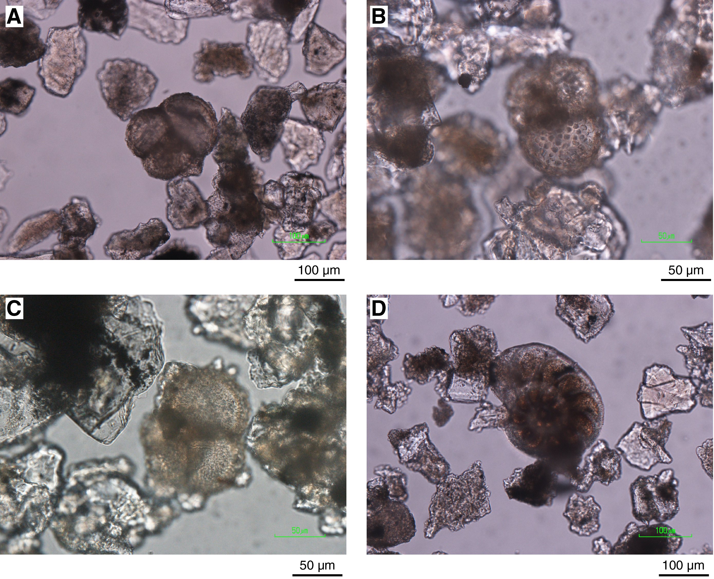
Figure F35. Foraminiferal tests.
Paleomagnetism
Hole C0002T
Remanent magnetizations of archive halves from Hole C0002T cores were measured at demagnetization levels of 0, 5, 10, and 20 mT peak alternating fields to identify characteristic directions. Removing low-coercivity components by demagnetization steps of 5–10 mT is confirmed in Figure F36A. Inclination, declination, and intensity profiles with depth after 20 mT demagnetization are shown in Figure F36B. The declination profile represents widely scattered directions, which is indicative of "biscuiting" of sections formed during SD-RCB coring operations. Because of sporadic data, magnetic polarity on this hole is not interpreted.
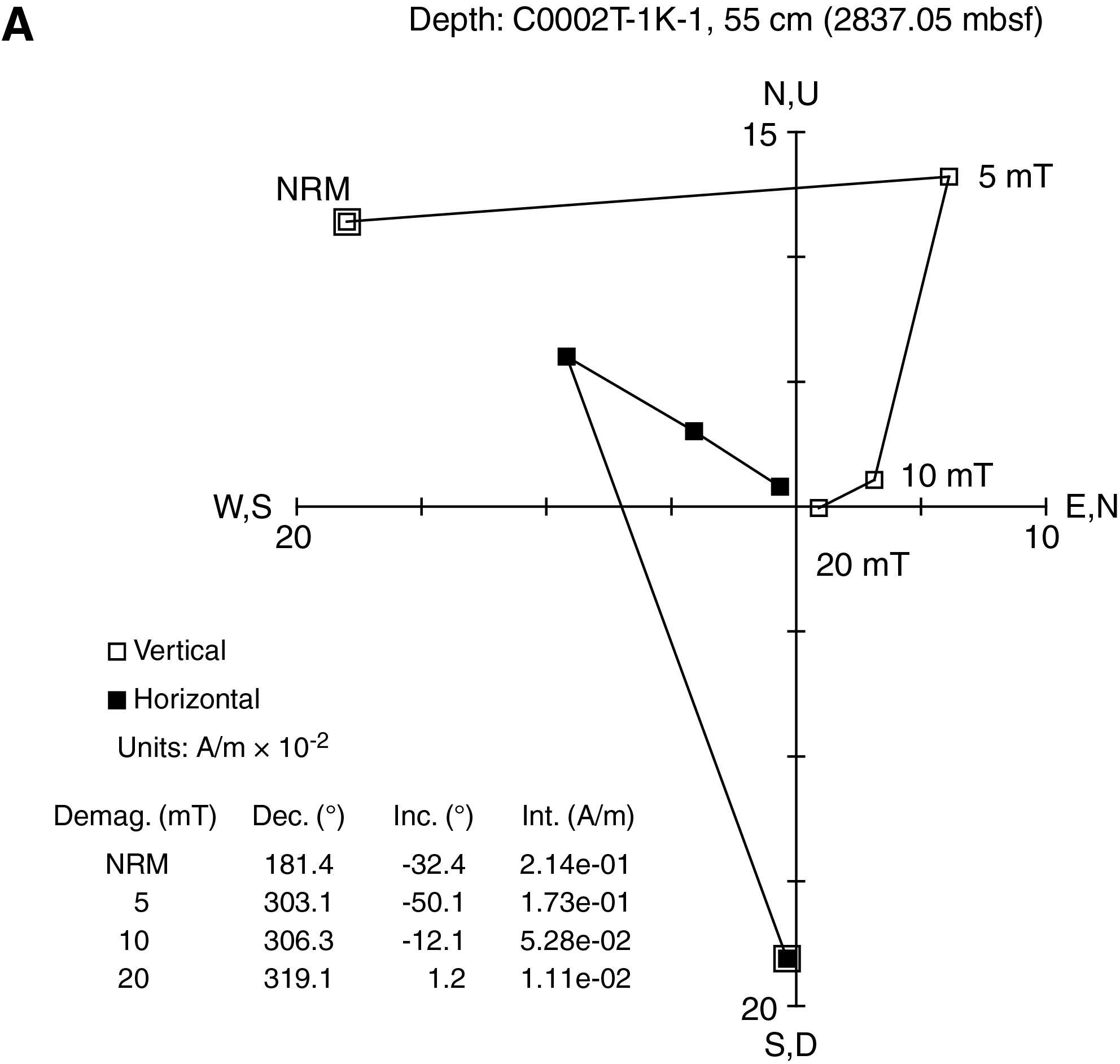
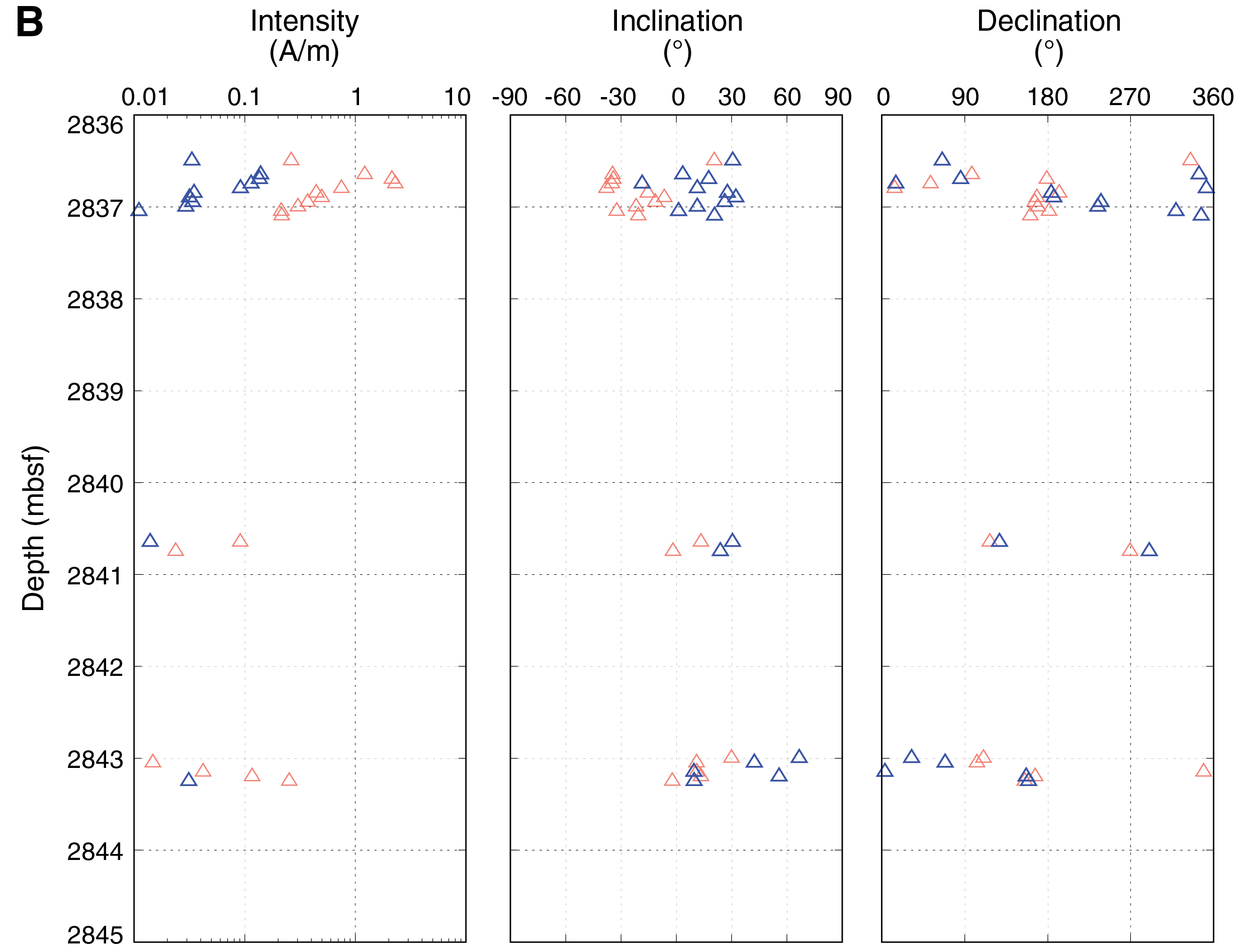
Figure F36. AF demagnetization and remanent magnetization, Hole C0002T.
Geochemistry
Chemical and isotopic compositions of mud gas
Hydrocarbons in mud gas
Methane concentrations in mud gas were measured by three instruments: the methane carbon isotope analyzer (MCIA), gas chromatograph (GC)–natural gas analyzer (NGA), and process gas mass spectrometer (PGMS) (see Geochemistry in the Expedition 358 methods chapter [Hirose et al., 2020]). The results for all holes, including δ13C for methane results, are shown in Figure F37. Although the downhole profiles of methane determined by the three instruments show similar trends, concentrations measured by the PGMS are systematically higher than those measured by the MCIA and GC-NGA, probably due to the calculation method of the gas percentages from the raw data by the PGMS (see Geochemistry in the Expedition 358 methods chapter [Hirose et al., 2020]). Methane concentrations measured by NGA show consistently low values <1000 ppm for most depths below 2900 mbsf (Figure F37B). Local maxima include a large peak in concentration as high as ~7700 ppm at around 2810 mbsf in Hole C0002R, two peaks with moderate concentrations as high as 3000 ppm at around 2880 mbsf in Hole C0002R and 2950 mbsf in Hole C0002Q Run 4, and a small concentration peak of 1000 ppm at around 3200 mbsf in Hole C0002Q Run 4. Methane concentrations from Hole C0002S do not vary much with depth with constantly low values <1000 ppm between 2840 and 2940 mbsf. Similar variations occur in methane concentrations measured by the MCIA and PGMS (Figure F37A, F37C). δ13CCH4 was measured shipboard by the MCIA. In Figure F37D, only values ≥500 ppm are shown because the isotopic values are not reliable when methane concentrations are <500 ppm (see Geochemistry in the Expedition 358 methods chapter [Hirose et al., 2020]). δ13CCH4 values from the four holes are relatively constant between −50‰ and −40‰ except for between 2910 and 2930 mbsf in Hole C0002Q, where the values are as high as −32‰.

Figure F37. Methane and δ13C in mud gas.
Concentrations of other higher hydrocarbons, such as ethane (C2H6), propane (C3H8), iso-butane (iso-C4H10), and n-butane (n-C4H10), were also measured by GC-NGA. iso-butane was only detected between 2922 and 2924 mbsf in Hole C0002Q, with concentrations of 5–10 ppm. n-butane was not detected in any hole during this expedition. Therefore, only the depth profiles of ethane and propane concentrations are shown in Figure F38. Profiles of methane concentrations analyzed by the GC-NGA are also shown for comparison. Because propane concentrations are generally low and commonly below the detection limit during this expedition (Figure F38C), the methane to ethane (C1/C2) ratio was calculated instead of C1/(C2 + C3) (Figure F38D). The depth profiles of ethane concentrations from Holes C0002Q–C0002S generally show trends similar to those of methane, although ethane concentrations are one order of magnitude lower than methane concentrations. In Hole C0002R, ethane concentrations drop below the detection limit deeper than 2910 mbsf, except for at 2923, 2995, and 3078 mbsf. Ethane concentrations slightly increase between 2900 and 2920 mbsf in Hole C0002S, whereas methane concentrations remain constant. Propane is observed only in certain depth ranges from Holes C0002Q and C0002R (e.g., 10–25 ppm between 2806 and 2875 mbsf in Hole C0002R and 10–15 ppm at 2950 mbsf in Hole C0002Q), where methane and ethane concentrations are relatively high compared to those from other depths. From various depths, both methane to ethane plus propane (C1/[C2 + C3]) concentration ratios and stable carbon isotopic compositions of methane (δ13CCH4) indicate different gas sources (e.g., Bernard et al., 1978; Whiticar, 1994). Between 2800 and 3000 mbsf, the C1/C2 ratios vary between 15 and 60. On the other hand, between 3030 and 3190 mbsf, the C1/C2 ratios linearly decrease with depth from 40 to 25, where methane concentration decreases with depth and ethane concentration slightly increases.
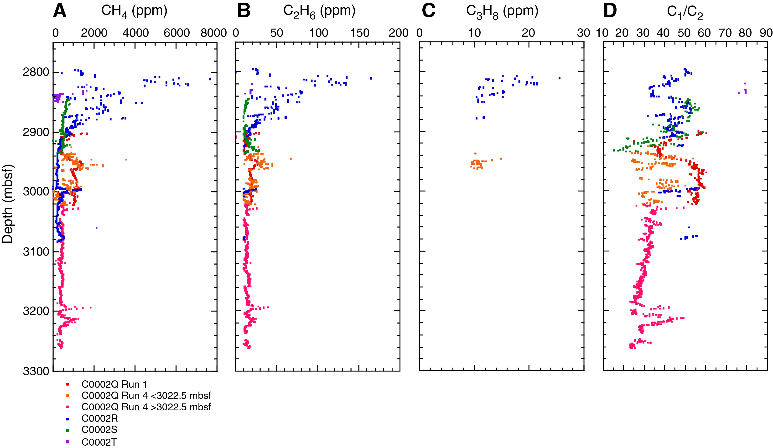
Figure F38. Methane, ethane, propane, and C1/C2 in mud gas.
Nonhydrocarbon gases in mud gas
Concentrations of major atmospheric components (i.e., nitrogen [N2], oxygen [O2], and argon [Ar]) were measured by PGMS, and N2 and O2 were also measured by the GC-NGA (Figure F39). N2 concentrations measured by GC-NGA are relatively constant at 76%–77% throughout Holes C0002Q and C0002S. Above 2985 mbsf in Hole C0002R, N2 concentrations are similar in range to those in Holes C0002Q and C0002S, but the concentrations consistently increase by ~1% below 2985 mbsf. N2 concentrations measured by PGMS fluctuate between 76% and 80% in Hole C0002Q and are relatively constant at ~78% in Holes C0002R and C0002S. O2 concentrations in Hole C0002Q measured by NGA are constant at 20%, whereas those measured by PGMS fluctuate between 19% and 21%. In Holes C0002R and C0002S, O2 concentrations measured by both NGA and PGMS are fairly constant at ~21%, although those measured by PGMS show relatively large fluctuations. The variations in O2 analyzed by GC-NGA and PGMS are similar to those of N2, indicating that the stability and accuracy of the obtained values depend on the type of instrument. The larger fluctuations in gas content measured by PGMS compared to those measured by NGA are likely due to the calculation process using the PGMS results (see Geochemistry in the Expedition 358 methods chapter [Hirose et al., 2020]). The measured N2, O2, and Ar concentrations are generally consistent with those of the Earth's surface atmosphere (N2 = 78.08%; O2 = 20.95%; Ar = 0.93%), indicating that the main component in mud gas is atmospheric air that was dissolved in drilling mud and zero air pumped into the degasser (see Geochemistry in the Expedition 358 methods chapter [Hirose et al., 2020]). Differences in N2 and O2 concentrations measured by NGA and PGMS are probably due to the calibration with standard gases for which N2 and O2 concentrations are significantly different from the atmospheric values (see Geochemistry in the Expedition 358 methods chapter [Hirose et al., 2020]). For Hole C0002Q, N2 and O2 concentrations were not measured precisely by NGA because of the different standard gas used for calibration (see Geochemistry in the Expedition 358 methods chapter [Hirose et al., 2020]). Major gas compositions of the mud gas from Hole C0002T have larger variances, but the ranges are not very different from those for the other holes.
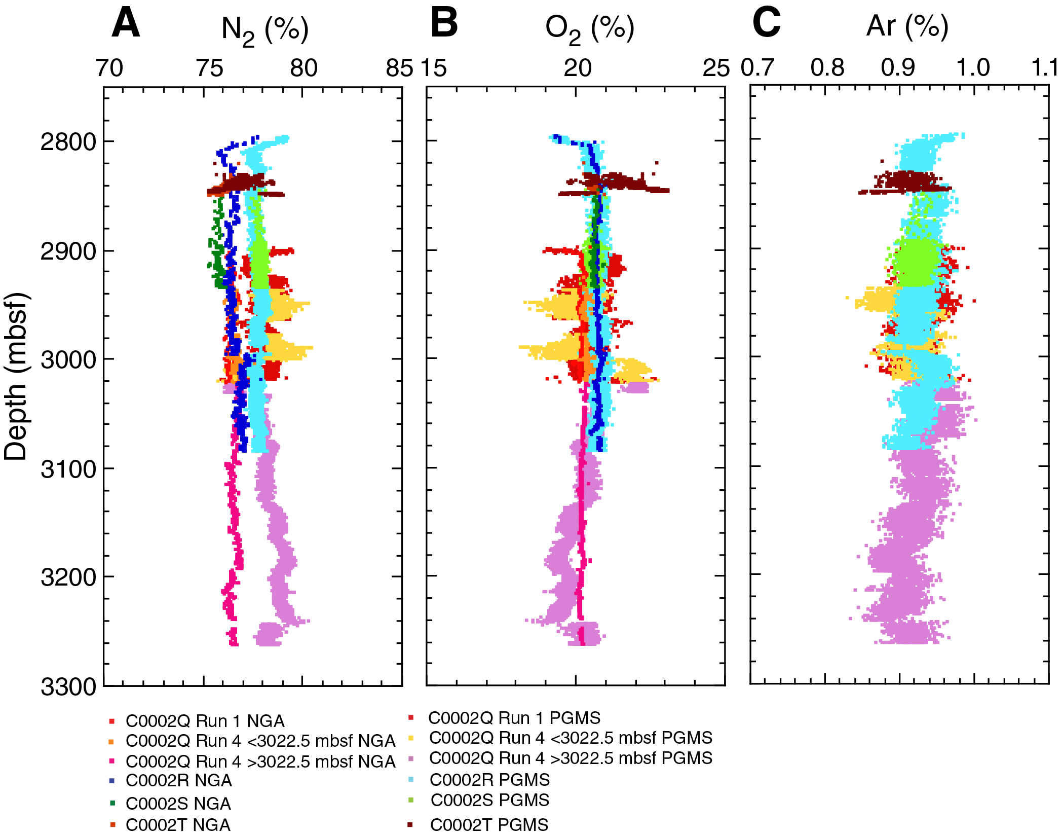
Figure F39. N2, O2, and Ar in mud gas.
Atmospheric minor and trace gaseous components, such as carbon dioxide (CO2), carbon monoxide (CO), helium (He), and xenon (Xe), were measured by PGMS (Figure F40). The NGA only detected CO2 twice (190 and 200 ppm) in Hole C0002Q and only a few times in Holes C0002R and C0002S. Except for those measurements, CO2 concentrations were below the detection limit of ~160 ppm (see Geochemistry in the Expedition 358 methods chapter [Hirose et al., 2020]), indicating that CO2 concentrations in mud gas were lower than the atmospheric CO2 concentration of ~400 ppm. The observed low CO2 content could be explained by adsorption by drilling mud that had a high pH (average pH ~ 10) during drilling in Hole C0002Q. The PGMS data show CO2 peaks at several depths where it is not detected by the NGA. Similar features appear in the He, CO, and Xe profiles. CO and He were rarely detected by NGA (detection limits of these components for GC-NGA are unknown; see Geochemistry in the Expedition 358 methods chapter [Hirose et al., 2020]), whereas the PGMS data show spikes in concentrations of these gases as well as Xe at several depths, which is consistent with the CO2 profiles. Based on these observations, the PGMS seems to be more sensitive to CO2, CO, and He in mud gas than the GC-NGA. However, further investigation is needed because it is still unclear whether the spike signals in the PGMS data are noise or the background concentrations of these trace components in mud gas. Despite the low concentrations, these gas components should be continuously monitored to potentially detect gas-rich layers in ultradeep subseafloor environments such as this drilling site. Trace components of mud gas in Hole C0002T are also shown in Figure F40. The ranges of concentrations are almost the same as those described above.

Figure F40. CO2, CO, He, and Xe in mud gas.
Depth profiles of hydrogen (H2) and radon (222Rn) concentrations in mud gas are shown in Figure F41. H2 concentrations increase below 3050 mbsf and stay relatively high with large scatter in Hole C0002Q Run 4. Above 3050 mbsf, H2 concentrations are relatively low and less than ~100 ppm with several moderate peaks, which tend to coincide with drilling in the initial stage of new holes, at around 2800 mbsf in Hole C0002R and 2900 mbsf in Hole C0002Q Run 1. In Hole C0002R, however, concentrations remain low deeper than 2810 mbsf at 20–50 ppm (Figure F41). 222Rn concentrations vary in the range of 80–200 Bq/m3 and are >300 Bq/m3 at around 2820, 2940, and 3190 mbsf (Figure F41). Hydrogen concentrations from Hole C0002T are slightly higher than those from the other holes at similar depths.
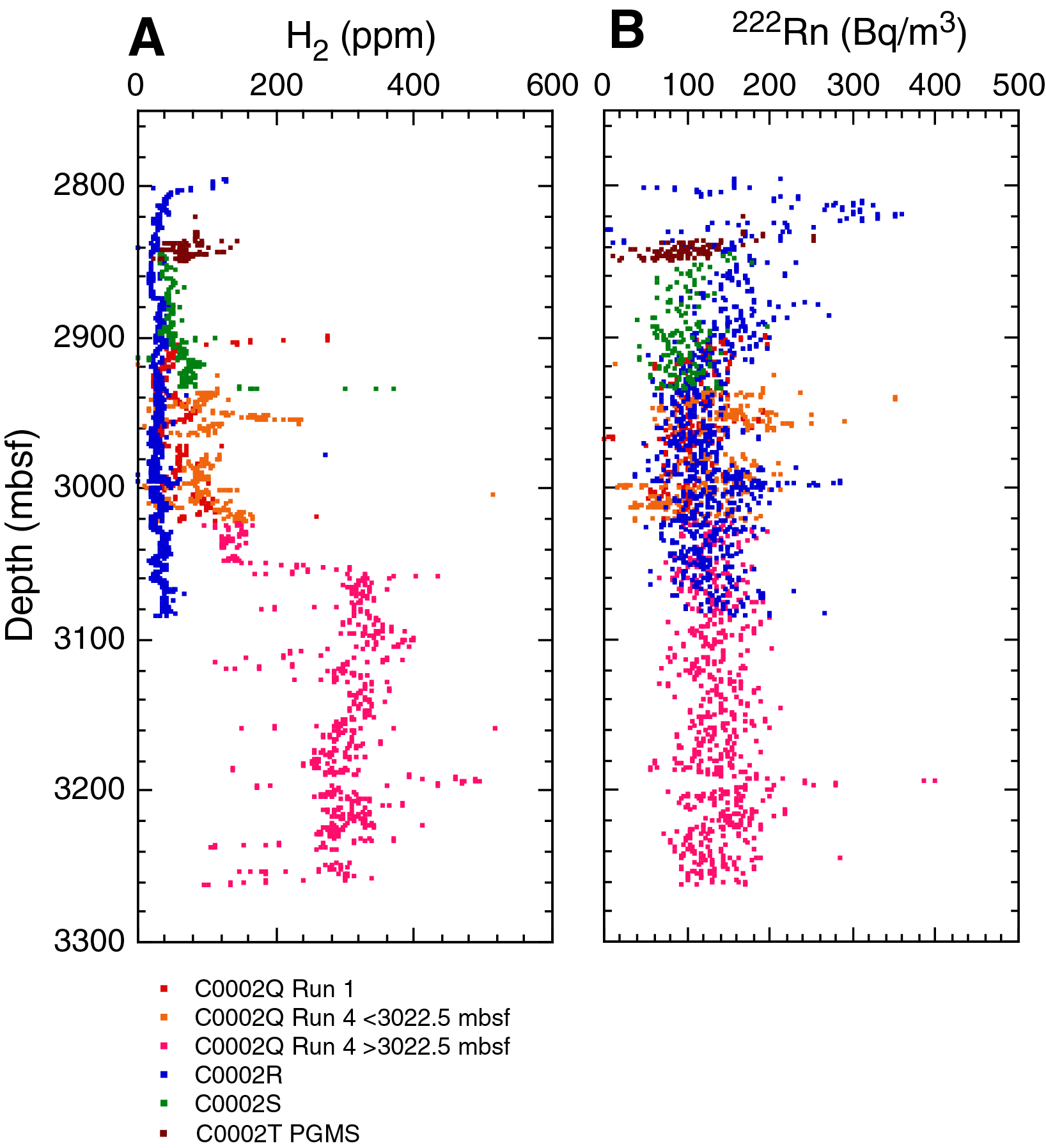
Figure F41. H2 and 222Rn in mud gas.
Chemical composition of headspace gas from cuttings and cores
Unwashed cuttings samples for headspace gas analyses were obtained at 10 m sampling intervals from Holes C0002Q–C0002S (see Introduction and operations in the Expedition 358 methods chapter [Hirose et al., 2020]), and three samples from the core catcher were taken from three core sections from Hole C0002T. Analytical results are summarized in Tables T15, T16, T17, T18, and T19 and shown in Figure F42.
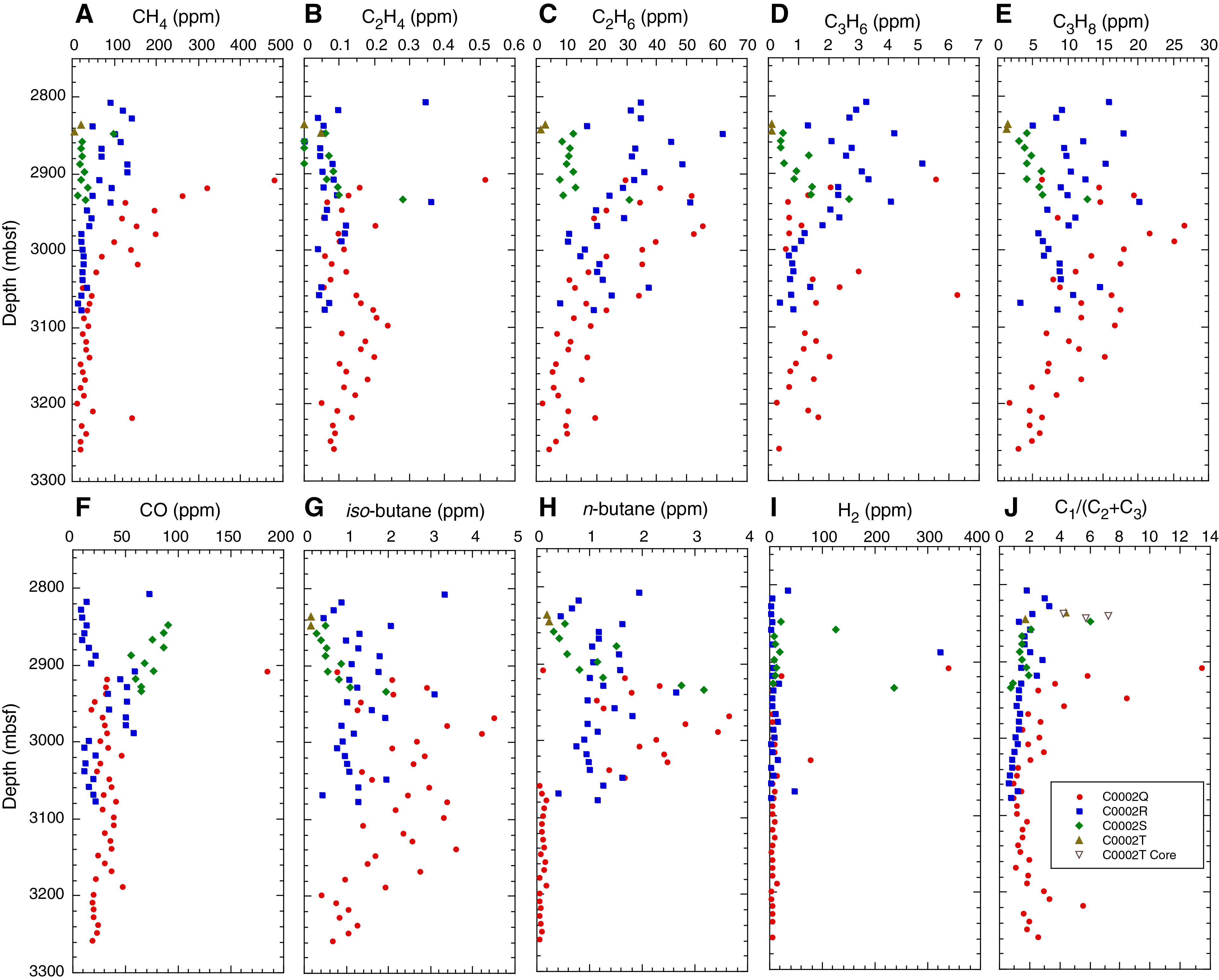
Figure F42. Headspace gas components.
The composition of hydrocarbon gases in the headspace from cuttings samples was detected by GC–flame ionization detector. H2 and CO in headspace gas were analyzed in unwashed cuttings from Holes C0002Q–C0002S by GC–pulsed discharge helium ionization detector. Methane, n-butane, and H2 show significantly lower concentrations deeper than 3050 mbsf in Hole C0002Q. As for the other components, the concentrations above 3050 mbsf are higher than those below 3050 mbsf in all holes (Figure F42).
Comparison of mud-gas data among Holes C0002P–C0002T
Here, the sources of gaseous components in the sediments and reasons for fluctuations in the concentrations are discussed based on the analytical results of the mud gas from Holes C0002Q–C0002T of this expedition in comparison with those from Hole C0002P of Expedition 348 (Tobin et al., 2015).
Origin of gas
C1/C2 ratios ≥1000 indicate that the methane is generated by microbial metabolism, whereas ratios <100 indicate that the hydrocarbons are produced thermogenically through the breakdown of organic matter under high temperatures (Bernard et al., 1978; Whiticar, 1994). In Figure F43, methane data from holes drilled during this expedition are plotted together with those from Expedition 348 Hole C0002P. The gas composition determined during Expedition 358 plots in the region of thermogenic origin. A thermogenic methane origin is plausible because the in situ temperature increases with depth and is presumably as high as >100°C at deeper than 2500 mbsf (Tobin et al., 2015; see Logging).

Figure F43. δ13C of methane vs. C1/(C2 + C3) ratio of mud gas.
Other sources of gas include air from both the atmosphere and zero air that was pumped into the degassers, as well as gas produced mechanically by drilling (Figures F39, F44). Nitrogen and oxygen concentrations analyzed by GC-NGA do not vary much with depth. On the other hand, nitrogen and oxygen concentrations analyzed by PGMS show large variations (Figure F44). This is probably due to the calculation procedure of the raw data from the PGMS, which forces the summation of all gas components to 100% (see Geochemistry in the Expedition 358 methods chapter [Hirose et al., 2020]). Despite the large fluctuations in composition analyzed by PGMS, the O2/Ar ratios in addition to H2/CH4 ratios are still useful to differentiate the different gas sources. High H2 concentrations appear at shallow depths in each hole (e.g., ~2900 mbsf in Hole C0002Q Run 1, ~2800 mbsf in Hole C0002R, ~2840 mbsf in Hole C0002T, and 2930–3020 mbsf in Hole C0002Q Run 4) (Figure F41). In addition, H2/CH4 ratios are also relatively high at these depths (Figure F44B). Hydrogen gas can be produced during grinding between metal and minerals that allows water to react with a new reaction surface (Bjornstad et al., 1994; Kameda et al., 2004a, 2004b; Kita et al., 1982; Wakita et al., 1980). Drill bit penetration of fresh rocks or sticking against hard rock are processes that might generate hydrogen gas. The same process could possibly explain the rapid increase in H2 concentrations downhole from ~3050 mbsf in Hole C0002Q Run 4. This depth coincides with an increase in the rotation speed of the drill bit from 110 to 150 rpm (see Logging; Figure F58). Future investigations on the origin of hydrogen gas through isotope measurements might elucidate the source of the hydrogen.
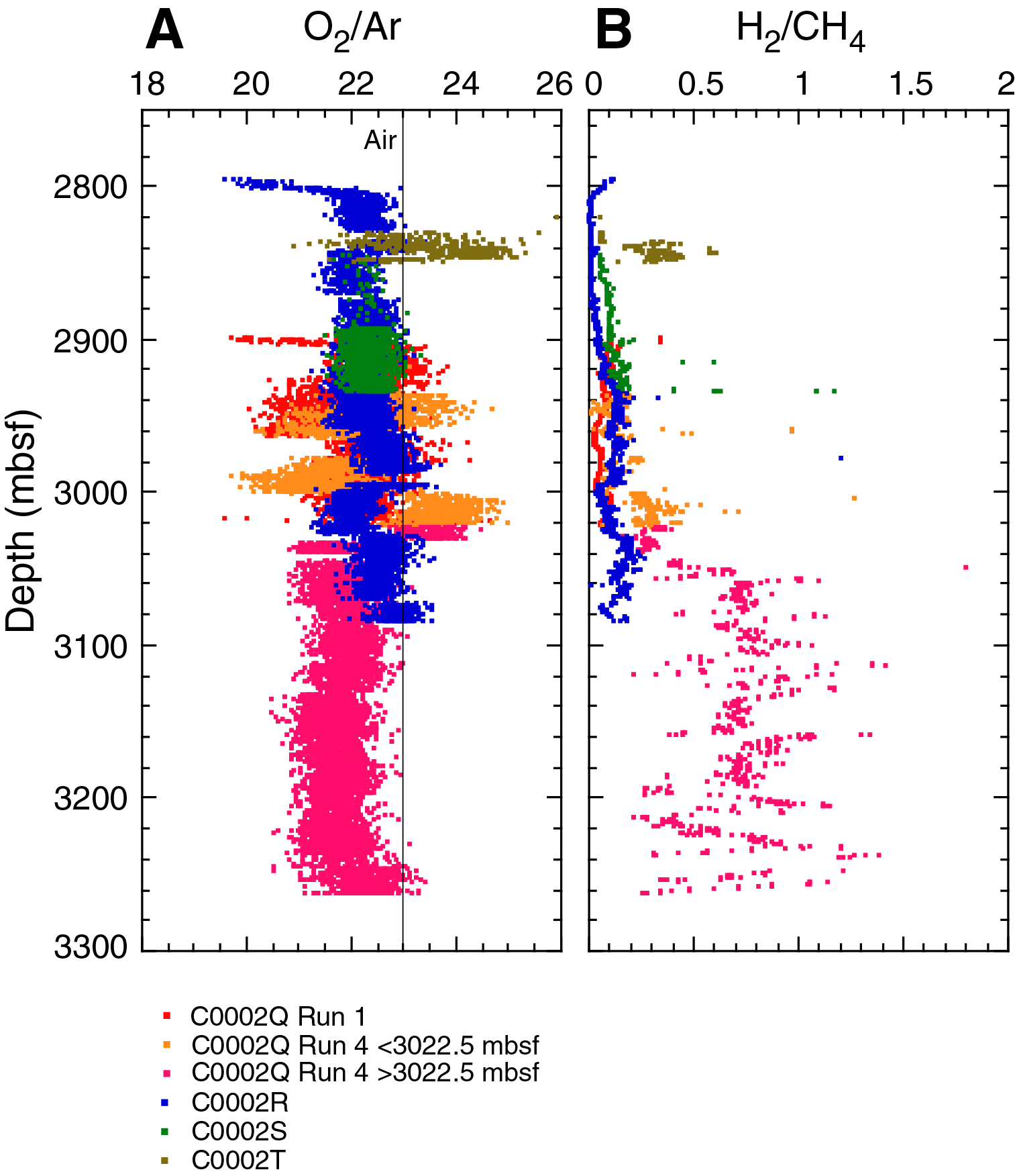
Figure F44. O2/Ar and H2/CH4 ratios in mud gas.
Comparison with mud gas composition from Hole C0002P
CH4 concentrations, C1/C2 ratios, and δ13CCH4 in mud gas from Holes C0002Q–C0002S are compared with those in Hole C0002P from Expedition 348 (Tobin et al., 2015) (Figure F45). Methane concentrations from Hole C0002P are in general one order of magnitude higher than those from Holes C0002Q–C0002S except for the shallowest part of Hole C0002R where high methane concentrations may be related to drilling disturbance. Relocation of the degassers might explain the large differences in methane concentrations from Hole C0002P and those from the holes drilled during this expedition (see Geochemistry in the Expedition 358 methods chapter [Hirose et al., 2020]).
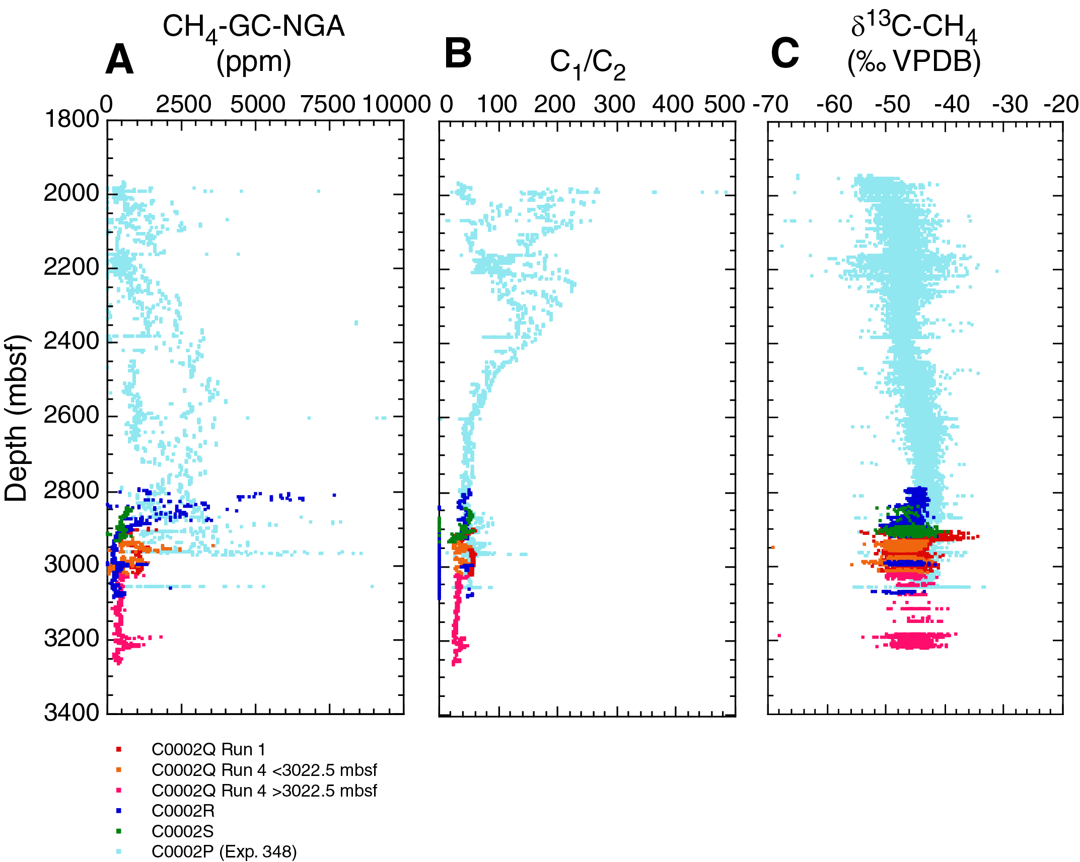
Figure F45. Methane, C1/C2 ratio, and δ13C of methane in mud gas.
In Hole C0002P, C1/C2 ratios are highly scattered and decrease from maximum values of ~250 to ~50 at 2200–2600 mbsf, whereas δ13CCH4 slightly increases from −48‰ at 2300 mbsf to −44‰ at 2600 mbsf. Below 2600 mbsf, C1/C2 ratios and δ13CCH4 are characteristic of thermogenic gas (50 and −40‰, respectively) (e.g., Whiticar, 1994; Tobin et al., 2015). These changes in gas composition and isotopic signature suggest the transition from shallow biogenic to deep thermogenic hydrocarbon gases in the interval between 2000 and 2600 mbsf. Below 2600 mbsf, C1/C2 ratios generally decrease with depth from ~50 to ~25 to the bottom of Holes C0002Q–C0002S. It is notable that C1/C2 ratios increase at the depths where high methane concentration peaks appear (e.g., the C1/C2 ratio of >50 between 2850 and 3050 mbsf in all holes). The higher C1/C2 ratios observed between 2850 and 3050 mbsf suggest that the methane could be partially derived from a different source (i.e., thermogenic gas derived from different source rock). The ratios in Hole C0002Q, however, linearly decrease with depth from ~40 at 3030 mbsf to ~30 at 3190 mbsf. The decreasing trend of C1/C2 ratios with depth seems to be an extension of the decreasing trend observed between 2600 and 2820 mbsf in Hole C0002P. The δ13CCH4 values in Holes C0002Q and C0002R are comparable with those in Hole C0002P (Figure F45).
Carbonates, organic carbon, and total nitrogen of cuttings and cores
CaCO3, total organic carbon (TOC), and total nitrogen (TN) contents were analyzed in cuttings (Figures F46, F47; Tables T20, T21, T22). Two types of cuttings were analyzed: (1) bulk cuttings from the 1–4 mm size fraction that were gently washed by seawater and (2) intact cuttings from the >4 mm size fraction that were handpicked and further washed by seawater in a sonicator (see Introduction and operations in the Expedition 358 methods chapter [Hirose et al., 2020]).
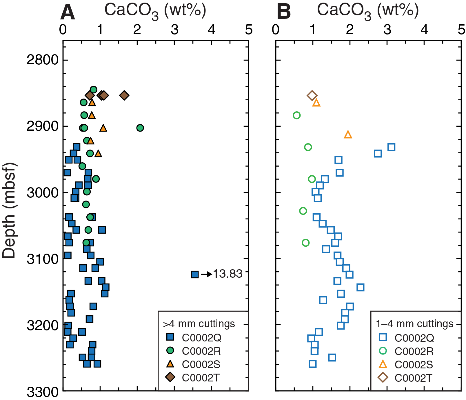
Figure F46. CaCO3 content, cuttings.

Figure F47. TOC, TN, and TOC/TN ratio, cuttings.
In Hole C0002Q, CaCO3 content in the bulk cuttings from the 1–4 mm size fraction decreases from 3.1 wt% at 2918 mbsf to ~1 wt% at 2988 mbsf and then slightly increases to ~2.5 wt% at around 3130 mbsf, below which it decreases to ~1 wt% at the bottom of the hole (Figure F46B). CaCO3 content in the intact cuttings from the >4 mm size fraction is generally lower than 1 wt%, except for samples between ~3100 and ~3140 mbsf, where concentrations are slightly higher than 1 wt%. One anomalously high value of 13.8 wt% occurs at 3118 mbsf (Figure F46A). The high CaCO3 values might reflect the higher abundance of man-made cement observed in the cuttings (see Lithology). CaCO3 content in the bulk cuttings are generally higher than those in the intact cuttings by 0.4–2.7 wt%, except for the sample at 3118 mbsf (Figure F46).
In Holes C0002R–C0002T, CaCO3 contents in the bulk cuttings from the 1–4 mm size fraction range from 0.5 to 1 wt%, whereas those of the intact cuttings from the >4 mm size fraction fluctuate between 0.5 and 0.9 wt% except for two samples at 2887.5 and 2839.5 mbsf with higher contents, possibly due to contamination by casing cement (see Lithology) (Table T18). Bulk cuttings have slightly higher CaCO3 contents than those from the intact cuttings, and there is no clear variation with depth. In addition, lithology (i.e., sandstone or silty claystone) does not show obvious differences in CaCO3 contents. In Hole C0002R, TOC contents in the bulk cuttings vary between 0.7 and 1.0 wt%, whereas TOC contents of handpicked sandstone and silty claystone cuttings generally increase from 0.5 to 0.6 wt% from 2827 to 2907 mbsf and stay constant at ~0.6 wt% below that depth (Figure F47). The bulk cuttings show higher TOC contents than the handpicked sandstone and silty claystone cuttings, which may be attributed to higher levels of drilling mud contamination. Additionally, TOC contents are slightly higher in silty claystone than sandstone. In Hole C0002R, TN contents are barely above the detection limit, ranging from 0.01 to 0.06 wt% (Figure F47), whereas TN contents in both silty claystone and the bulk cuttings generally increase from 0.05 to 0.06 wt% from 2807 to 3067 mbsf. TN contents in sandstone are all below the detection limit. In Hole C0002R, TOC/TN ratios in the bulk cuttings range between 13 and 17, which are higher than those of silty claystone, which range from 8 to 10 (Figure F47). Sandstone has higher TOC/TN ratios than silty claystone.
Among all the holes drilled during this expedition, the highest TOC value is 2.9 wt% at 2918 mbsf in Hole C0002Q, and the value decreases with depth to ~1 wt% at ~2940 mbsf. Below this depth, TOC varies over a narrow range, mostly between 0.7 and 1.1 wt%. TOC contents in the intact cuttings obtained during this expedition are ~0.5 wt% on average and range from 0.4 to 0.6 wt%. The highest TOC content in the cuttings from Hole C0002T occurs at the shallowest depth of this hole, likely due to contamination by artificial cement. TOC contents in the bulk cuttings are higher than those in the intact cuttings by ~0.5% and could be as high as 2.4 wt%. The higher TOC contents in the bulk cuttings likely reflect contamination by drilling mud, which has a TOC content as high as 12 wt%, as determined during Expedition 348 (Tobin et al., 2015), or as high as 5.9%, as determined during the drilling of Holes C0002Q and C0002R (Table T23). Interpretation of TOC results should be treated with caution because of the high potential for contamination from drilling mud and cement.
TN contents in the bulk cuttings lie in a narrow range between 0.05 and 0.07 wt% and are generally similar to or slightly higher than those in the intact cuttings by 0.01–0.02 wt%. TOC/TN ratios in the bulk and intact cuttings range from 11 to 43 and from 7 to 13, respectively.
Both TOC contents >1 wt% (as high as 2.9 wt%) and TOC/TN ratios >11 in the bulk cuttings are much higher than those expected for the sediments in the deep accretionary prism. High TOC contents ≥1 wt% are observed at areas of high productivity or high inflow rate of terrestrial organic matter, typically found in settings such as coastal areas. TOC/TN ratios >10 suggest a significant contribution of terrestrial organic matter to sediments (e.g., Meyers, 1997). TOC/TN ratios may increase in mature sediments because of preferential degradation of N-bound organic matter during early diagenesis. However, generally similar values of TN contents between the bulk and intact cuttings from the same depth suggest that highly C-enriched organic matter was added to the cuttings. Thus, the bulk cuttings are likely contaminated with drilling mud, which has extraordinarily high TOC contents and TOC/TN ratios of ~12 wt% and ~1300, respectively (data from Expedition 348 [Tobin et al., 2015]). In contrast, low TOC contents (0.5 ± 0.06 wt%) and TOC/TN ratios (~9) in the intact cuttings are most consistent with the values for typical marine sediments. However, it is still unclear whether high TOC contents and TOC/TN ratios observed at 3028–3048 and 3108–3168 mbsf reflect the input of terrestrial organic matter or contamination from drilling mud.
Physical properties
Moisture and density measurements
Cuttings
Moisture and density (MAD) measurements were made on 240 cuttings samples from Holes C0002Q, C0002R, C0002S, and C0002T (2917.5–3257.5, 2817.5–3077.5, 2847.5–2933.5, and 2836.5–2847.5 mbsf, respectively) to provide a detailed characterization of grain density, bulk density, and porosity. A total of 148 measurements were made on bulk cuttings from the 1–4 and >4 mm size fractions (74 from each size fraction; Table T24) at a spacing of 10 m. In addition, 72 measurements were made on separately handpicked intact samples of mixed lithologies from the >4 mm size fraction every 10 m (Table T25). To capture potential variability of porosity associated with lithology, handpicked intact samples of sandstone, silty claystone, and incohesive fine silty claystone (5, 8, and 3 samples, respectively) were analyzed as well. Artificial cement cuttings picked from Hole C0002R cuttings (4 samples) were measured to determine its effect on bulk cuttings porosity measurements.
Grain density values for the 1–4 and >4 mm size fractions are in close agreement throughout the depth interval the cuttings were collected from during Expedition 358 (Figure F48D), as are those for the bulk and handpicked intact cuttings (Figure F48A, F48D). Grain density generally ranges from 2.66 to 2.73 g/cm3 throughout the depth interval. Exceptions are at the top of Hole C0002Q Run 1 at 2917.5–2937.5 mbsf, where greater scatter occurs in grain density measurements for the bulk cuttings, with values as low as 2.51 g/cm3, at 2877.5 mbsf in Hole C0002S for an intact cuttings sample with a value of 2.8 g/cm3, and at 2836.5–2847.5 mbsf in Hole C0002T for bulk cuttings with values of 2.56 and 2.64 g/cm3. Except for the anomalously high value in Hole C0002S, these depth intervals coincide with high abundances of cement cuttings (see Lithology for volume percentages) and hence are interpreted to reflect cement contamination. Overall, a slight increase from 2.70 to 2.71 g/cm³ occurs over the entire interval. In comparison, grain density values from previously drilled Hole C0002P also scatter around an average of 2.7 g/cm³ but with a much higher variability of 0.11 g/cm³ even for the handpicked intact cuttings (Figure F49A).
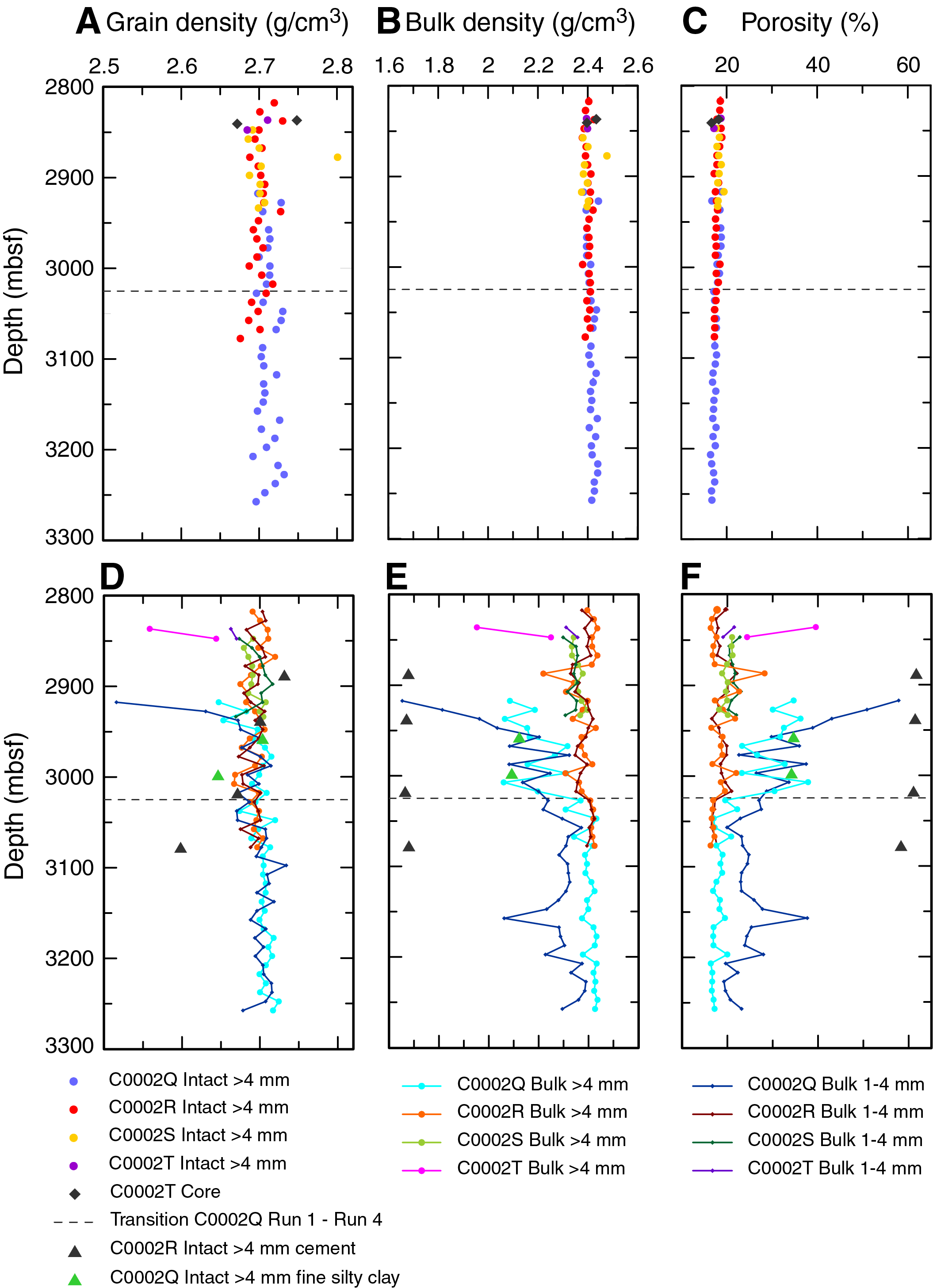
Figure F48. MAD measurements.

Figure F49. Comparison of MAD measurements on cuttings.
Both intact and bulk cuttings from Holes C0002R–C0002T exhibit similar bulk density and porosity values (Figure F48B, F48C, F48E, F48F). A few instances of bulk cuttings have noticeably lower bulk density and higher porosity than intact cuttings (e.g., at 2887.5–2907.5 mbsf in Hole C0002R and 2836.5–2847.5 mbsf in Hole C0002T). These discrepancies correlate well with observations of a higher percentage of cement in the bulk cuttings samples, which has low bulk density and high porosity, and thus are likely the result of cement contamination.
In contrast to Holes C0002R–C0002T, significant differences in bulk density and porosity occur between the two size fractions and also between the bulk and intact cuttings throughout Hole C0002Q. Additionally, Hole C0002Q Run 1 (2917.5–3017.5 mbsf) and Run 4 (3027.5–3257.5 mbsf) differ significantly from each other, which may reflect either the use of different drill bits, different ROPs, or different formations encountered by the two runs. In Hole C0002Q Run 1, significant scatter and difference in porosity occur between the different bulk size fractions, ranging between 23% and 37% for the >4 mm cuttings and between 23% and 58% for the 1–4 mm cuttings. Furthermore, all measurements on bulk cuttings exhibit higher porosity values than those on intact cuttings, with a maximum discrepancy at the top of Hole C0002Q (2917.5–2937.5 mbsf) and a decreasing difference with depth. The overall difference between size fractions is likely caused by contamination of the bulk cuttings with cement and by the high percentage of the fine silty claystone in the bulk cuttings (see Lithology for volume percentages). The decreasing difference with depth likely reflects the decrease in contamination from high-porosity cement (porosity ~60%), which becomes insignificant below 2967.5 mbsf according to the volume fractions described in Lithology. The small differences below 2967.5 mbsf in Hole C0002Q Run 1 are likely due to the presence of fine silty claystone. Fine silty claystone, which has a porosity of ~34% (Figure F48F), is less cohesive than other lithologies and is therefore selected against during the handpicking process in the larger cuttings size fraction. It is uncertain whether the fine silty claystone lithology represents formation in its in situ state or formation damaged by drilling operations (see Lithology for diagnostic characteristics). In Hole C0002Q Run 4, the scatter is significantly lower and the porosity of the >4 mm bulk cuttings agrees well with the values measured using the handpicked intact cuttings (16%–18%; Figure F48C). The scatter in the 1–4 mm size fraction is also lower, although the measured values remain consistently higher than those measured for the >4 mm size fraction, typically ranging between 20% and 27%.
Porosity of the handpicked intact cuttings is the most consistent throughout Holes C0002Q–C0002T, ranging from 16% to 19%. Intact cuttings porosity values exhibit minimal scatter, with an overall decrease of about 2% with depth across all of the boreholes (Figure F48C). Nevertheless, there is a relatively small but sudden decrease in porosity of the intact cuttings from 18% to 17% between Hole C0002Q Run 1 and Run 4 (Figure F50C). Bulk density shows an almost equal but opposite trend to that observed for the porosity data (Figure F48B). Bulk density increases slightly with depth (from approximately 2.37 to 2.42 g/cm3 for the intact cuttings) and exhibits a difference between the different size fractions that is reflected in the porosity.

Figure F50. MAD measurements of lithologies, Holes C0002Q and C0002R.
To further analyze the porosity evolution across the transition between Hole C0002Q Run 1 and Run 4, four sets of time-based cuttings were measured. These samples were collected by the real-time geomechanics (RTG) team (see Introduction and operations in the Expedition 358 methods chapter [Hirose et al., 2020]) during Hole C0002Q Run 4 at depths that overlap with Hole C0002Q Run 1 (Figure F50). The porosity of these RTG team samples (17%) is lower than that of the samples from the same depth range in Hole C0002Q Run 1. Their porosity is closer to the values determined for Hole C0002Q Run 4 below 3022.5 mbsf, possibly suggesting that a change in formation properties occurs in the horizontal direction between the boreholes.
Comparing bulk density and porosity data from Holes C0002Q–C0002T to all previous holes drilled at Site C0002 during Integrated Ocean Drilling Program Expeditions 315, 338, and 348, values of both intact cuttings and discrete core samples are consistent with the overall depth trend (Figure F51) (Expedition 315 Scientists, 2009; Strasser et al., 2014; Tobin et al., 2015). Comparison of data collected from holes drilled during Expedition 358 (Holes C0002Q–C0002T) with Hole C0002P (Figure F49) shows that bulk density and porosity values of intact cuttings are consistent with those from Hole C0002P (Tobin et al., 2015). Bulk density of the intact cuttings exhibits an overall monotonic trend increasing from 2.32 to 2.43 g/cm³, and porosity exhibits a decreasing trend from 24% to 18% from 1965.5 to 3045.5 mbsf. On the other hand, bulk cuttings porosity values reported for Hole C0002P are significantly higher (by approximately 20%) than the porosity of intact cuttings from any holes, except for at 2165.5–2225.5 mbsf, which correlates with waiting on weather. This discrepancy results from selectively handpicking competent intact cuttings, as opposed to the softer fine silty claystone, a lithology that was much more abundant in Hole C0002P (see Lithology). Porosity values of bulk cuttings from Holes C0002R and C0002S, on the other hand, are similar to values of intact cuttings, likely because the percentage of fine silty claystone recorded in Holes C0002R and C0002S is very small.

Figure F51. MAD measurements, all Site C0002 holes.
As noted above, for a subset of measurements the handpicked intact cuttings were separated by lithology. At two different depths in Hole C0002Q Run 1 (2957.5 and 2997.5 mbsf), MAD analyses were carried out on cuttings of fine silty claystone (Figure F48D, F48E, F48F). Measurements were also made on sandstone and cohesive silty claystone cuttings at 2937.5, 3017.5, and 3077.5 mbsf in Hole C0002R, as well as at 2947.5 mbsf in Hole C0002Q Run 1 and 3077.5 mbsf in Hole C0002Q Run 4 (Figure F50). Additionally, MAD measurements of cohesive silty claystone were made for samples from 2927.5, 3007.5, and 3067.5 mbsf (Hole C0002R). Porosity values of cohesive silty claystone are in good agreement with those of unseparated intact cuttings, whereas sandstone porosity values are higher than unseparated intact cuttings, ranging from 18% to 21% (Figure F50C). According to these analyses, MAD measurements on unseparated intact cuttings typically reflect the properties of cohesive silty claystone. This is consistent with the small percentage of sandstone cuttings compared to the silty claystone cuttings in Holes C0002R and C0002Q (see Lithology).
Discrete core samples
Two discrete core samples from Hole C0002T were measured for MAD (Figure F48; Table T26). Grain density, bulk density, and porosity at 2836–2840 mbsf for these samples range 2.67–2.75 g/cm3, 2.40–2.43 g/cm3, and 16.7%–18.2%, respectively. These values are consistent with those of handpicked intact cuttings at a similar depth in Holes C0002R and C0002T.
Bit samples
Large cuttings recovered directly from the drill bits when they were recovered to the rig floor (bit samples) were used for MAD analyses and also to measure electrical resistivity and P-wave velocity on cube samples of approximately 8 cm3 (Table T27). In total, six cubes that were large and competent enough to cut cubes 20 mm with parallel faces were obtained from selected bit samples. Grain density values range from 2.70 to 2.75 g/cm3. Porosity values for Samples 358-C0002Q-21-SDB and 358-C0002R-25-SDB exhibit values of 16%–19%, whereas porosity values for more calcareous Samples 358-C0002R-49-SDB and 72-SDB (see Lithology for description) are as low as 4%–6%. Bulk density values follow an inverse trend, with values from 2.41 to 2.44 g/cm3 and values of 2.59 and 2.64 g/cm³ for the calcareous samples.
P-wave velocity measurements (discrete core and bit samples)
Cores recovered from Hole C0002T contain a large amount of either unconsolidated or heavily fractured material, making it unsuitable for P-wave velocity and electrical resistivity measurements. Therefore, only two discrete samples (358-C0002T-1K-1, 24.5–29.5 cm, and 2K-1, 14.0–18.0 cm), which were large and competent enough to cut parallel surfaces 20 mm apart, were collected at 2836.75–2836.79 and 2840.64–2840.68 mbsf. P-wave velocity was measured in only one direction for each sample using the 500 kHz transducer because only one pair of parallel surfaces in either the x- or z-direction was successfully prepared. P-wave velocity values are 2760 m/s (Vx) for Sample 1K-1, 24.5–29.5 cm, and 2978 m/s (Vz) for Sample 2K-1, 14.0–18.0 cm (Table T28).
Because the shape of the cubes was not ideal, P-wave velocity measurements could not be made in all three directions for all bit samples (Table T27; see PP in Supplementary material). For these samples, P-wave velocity values measured with the 500 kHz transducer are ~40 m/s higher than those measured with the 230 kHz transducer on noncalcareous rocks (Samples 358-C0002Q-21-SDB and 358-C0002R-25-SDB) and as much as 600 m/s higher than those measured with the 230 kHz transducer for calcareous samples (358-C0002R-49-SDB and 72-SDB). Because the sample size is only slightly larger than the wavelengths in the lower frequency measurements, P-wave velocity values obtained with the 500 kHz transducer likely better represent the formation properties. Discrepancy in velocity values measured at the different frequencies also may arise from frequency dispersion effects (Mavko et al., 2009). After the first measurement series at 230 kHz, two of the samples from Sample 358-C0002Q-21-SDB were damaged by a through-going fracture; thus, measurements at 500 kHz were not performed on these samples.
Electrical resistivity measurements (discrete core and bit samples)
Electrical resistivity measurements were conducted in only one direction for each discrete core sample on the same samples used for P-wave velocity measurements, again because only one pair of parallel surfaces in either the x- or z-direction was successfully prepared. Resistivity values are 5.392 Ωm (ρx) for Sample 358-C0002T-1K-1, 24.5–29.5 cm, and 2.634 Ωm (ρz) for Sample 2K-1, 14.0–18.0 cm (Table T28).
For bit samples, the measured resistivity values of Samples 358-C0002Q-21-SDB (2887.5–2900 mbsf) and 358-C0002R-25-SDB (2789.5–2794.5 mbsf) range from 3.3 to 5.2 Ωm, which agrees with resistivity values obtained from logging (1.2–4.2 Ωm) (Table T27) (see Logging). However, Samples 358-C0002R-49-SDB and 72-SDB show higher resistivity values of 23.7 and 22.2 Ωm, respectively, reflecting the high carbonate content in the samples (see Lithology).
Thermal conductivity (half-round cores)
One thermal conductivity measurement was performed on a working-half section from Hole C0002T using a half-space probe (Figure F52; Table T29), yielding a value of 2.162 W/(m·K). Although thermal conductivity is typically measured on lithified core sections using pieces >10 cm in length (e.g., Strasser et al., 2014), we relaxed this criterion to make a measurement on a piece ~5 cm in length because coherent core materials were otherwise not available.
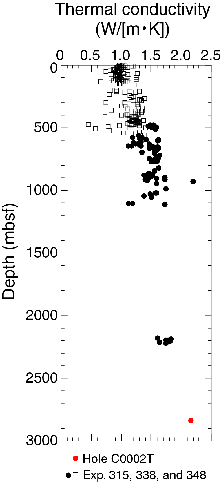
Figure F52. Thermal conductivity.
The thermal conductivity of a rock can be regarded as a function of porosity, grain thermal conductivity (ks), and water thermal conductivity (kw) in the following geometric mean mixing model:
Thermal conductivity data from Kumano Basin sediments at Site C0002 and Shikoku Basin sediments at Integrated Ocean Drilling Program Sites C0011 and C0012 have shown that thermal conductivity values generally lie between the trends calculated using grain thermal conductivity ranging from 2.1 to 3.4 W/(m·K), centered at 2.6 W/(m·K) (Figure F53) (Expedition 315 Scientists, 2009; Expedition 322 Scientists, 2010a; 2010b; Expedition 333 Scientists, 2012a; 2012b; Strasser et al., 2014; Tobin et al., 2015). The measurement from the Hole C0002T sample also lies within these bounds close to the ks = 2.6 W/(m·K) trend line.
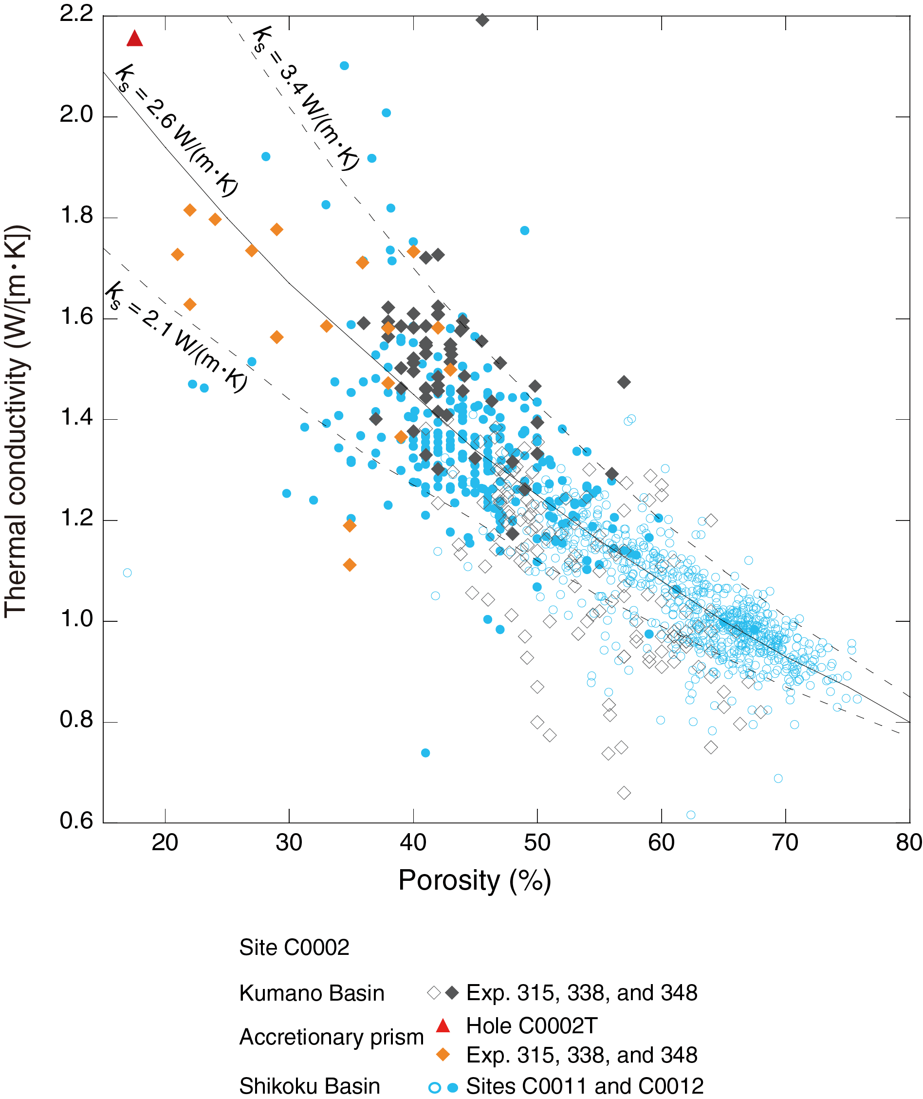
Figure F53. Thermal conductivity vs. porosity.
MSCL-W (whole-round cores)
Whole-round cores recovered using the SD-RCB system from Hole C0002T (2836.54–2843.74 mbsf) were analyzed using the whole-round multisensor core logger (MSCL-W). The results of gamma ray attenuation (GRA), bulk density, magnetic susceptibility, natural gamma radiation (NGR), and electrical resistivity measurements (see Physical properties in the Expedition 358 methods chapter [Hirose et al., 2020]) on whole-round cores are summarized in Figure F54. MSCL-W P-wave measurements are not presented because they exhibit very large scatter due to poor contact between the liner and core material.
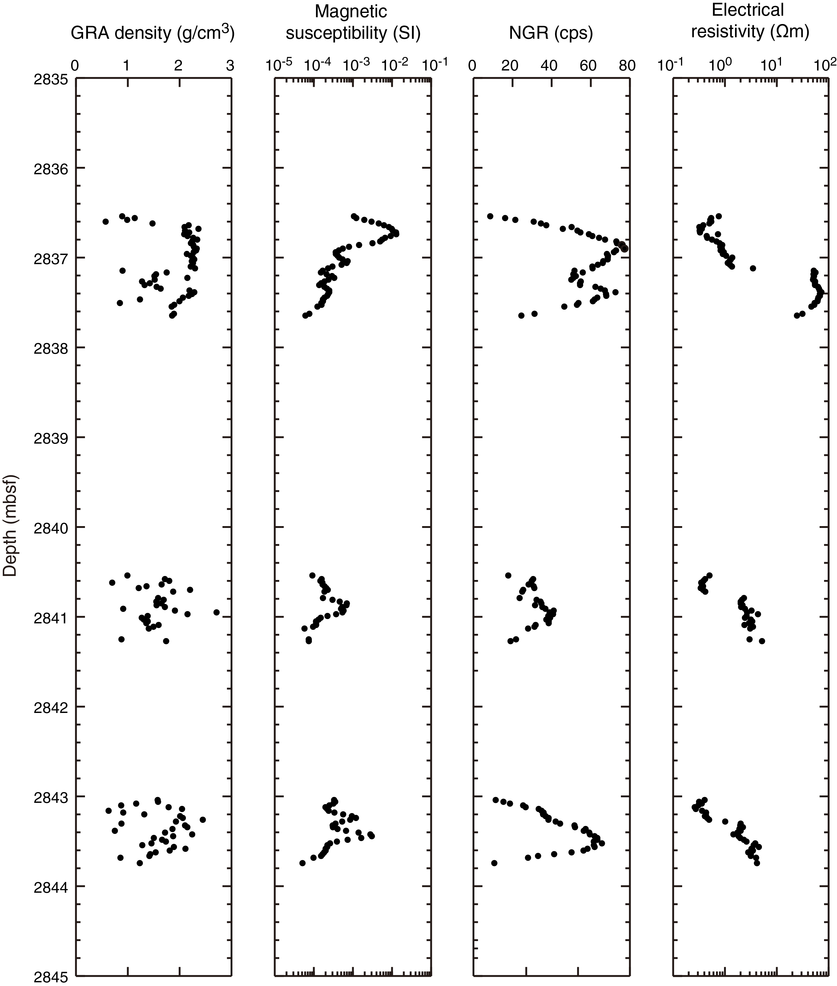
Figure F54. MSCL-W measurements, Hole C0002T.
Overall, MSCL-W data from Hole C0002T do not show an obvious trend with depth; this is probably due to the short depth range of coring (~19 m). GRA, magnetic susceptibility, NGR, and electrical resistivity values range from 0.57 to 2.71 g/cm3, from 5.13 × 10⁻⁵ to 1.28 × 10⁻² SI, from 8.57 to 76.67 counts/s, and from 0.26 to 99.16 Ωm, respectively.
Natural gamma radiation (cuttings)
The NGR of liner-packed cuttings from Holes C0002Q–C0002T generally lies between 28 and 38 counts/s. Anomalously low values were observed at the beginning of Hole C0002Q shallower than 2930 mbsf because of the presence of cement cuttings (Figure F55A), but NGR values increase with decreasing cement contamination away from the sidetrack window (see Lithology). Measurements were made on washed and unwashed cuttings, with unwashed cuttings generally having higher NGR values than washed cuttings throughout the measured interval with a few exceptions (Table T30). This is because the unwashed cuttings have an additional source of NGR, such as KCl and rock powder/fragments, present in the drilling mud. The presence of drilling mud in the unwashed cuttings is also reflected in the heavier weight of the unwashed cuttings present inside the plastic liners (Table T30).
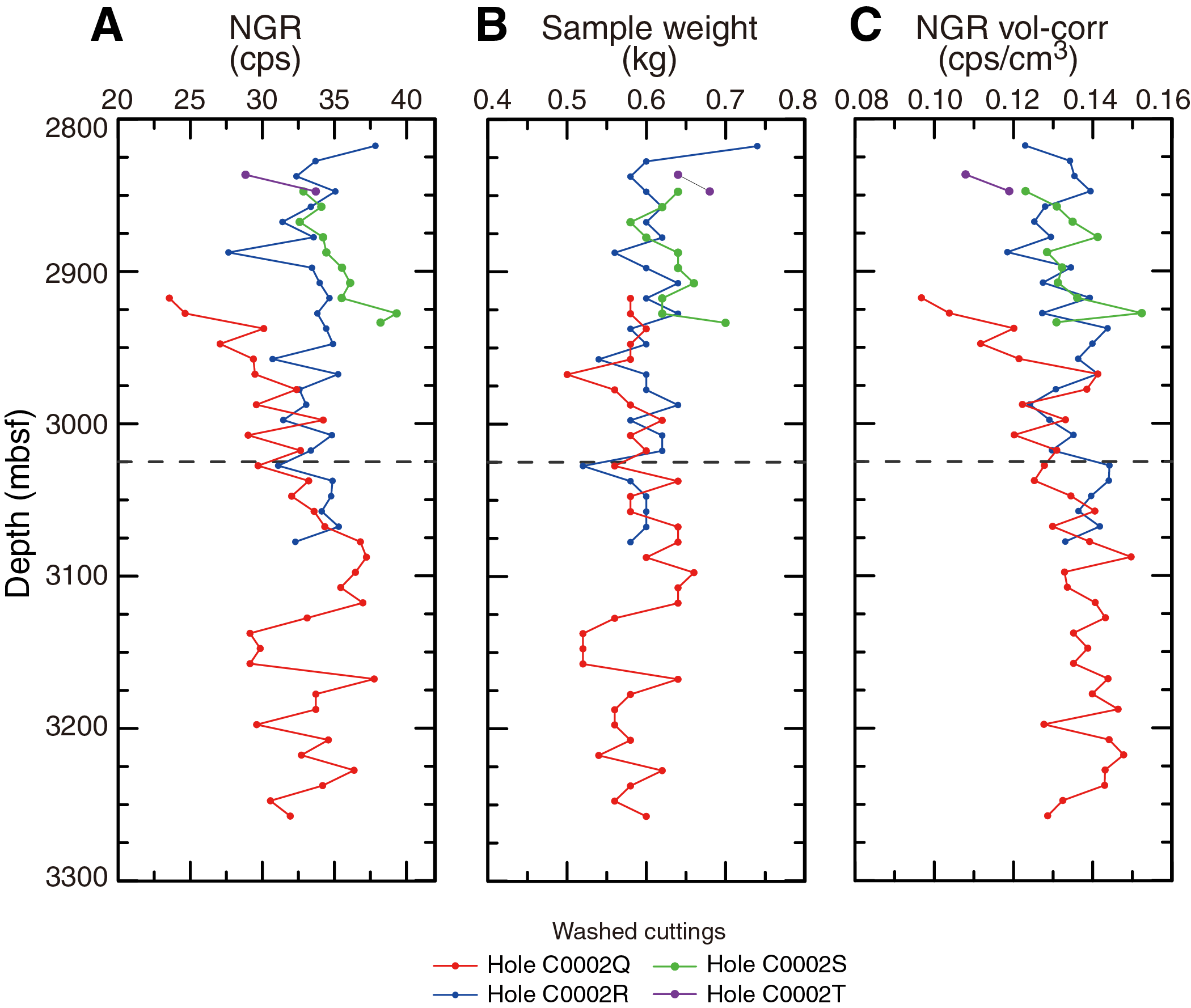
Figure F55. NGR, washed cuttings.
The fluctuation in measured NGR values is correlated with fluctuations in cuttings mass, which suggests that the measured NGR values are influenced by the amount of material inside the plastic liner. Thus, the fluctuations in measured NGR may not solely reflect variations in rock properties or composition. To best capture the geological trend and minimize measurement artifacts, we normalized the measured NGR values of the washed cuttings by the volume of cuttings inside the liner and report the results in units of counts/s/cm3 (Figure F55C). Cuttings volume was estimated by dividing the cuttings mass by the MAD bulk density of the handpicked intact samples at corresponding depths. As shown in Figure F55C, the normalization removes the correlation between measured NGR and cuttings mass. The NGR of drilling mud collected at various times was also measured by filling the 400 cm3 plastic liners with mud. Measured NGR values of the drilling mud increased by 2 counts/s from the beginning of Hole C0002Q operations to the end of Hole C0002R operations, but considering the extremely small amount of drilling mud that would have invaded the washed cuttings compared to the total measured volume of the drilling mud (400 cm3), the effect of mud property variation on the data is negligible. Therefore, we conclude that the trend of the volume-normalized NGR of the washed cuttings is the most representative of the formation.
The measured NGR values in Holes C0002Q–C0002T are lower than values from Hole C0002P at overlapping depth ranges (Figure F56). When comparing the NGR values of water-filled liners and the standard granite core measured during past expeditions, substantial differences are found between Expeditions 338, 348, and 358 (Table T31). Such shifts in the standard measurement values were found to have occurred when the MSCL-W sensors were switched to accommodate larger core liner sizes during other expeditions. The gamma ray detectors must be detached and reattached during such operations, which causes a slight change in detector alignments and thus their sensitivity. Thus, direct comparison of NGR values between expeditions was not possible without further corrections.
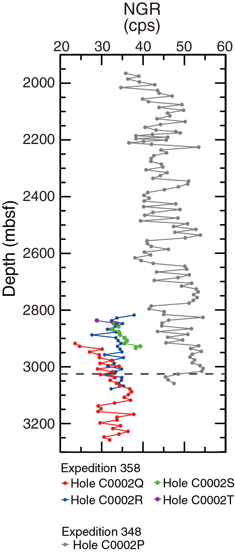
Figure F56. Comparison of MSCL NGR, washed cuttings.
Magnetic susceptibility (cuttings)
The mass magnetic susceptibility (MMS) of the >4 mm cuttings fraction shows little variation and is consistently lower than the MMS of the 1–4 mm cuttings fraction except for a few instances (Figure F57). MMS ranges between 9.7 × 10⁻⁸ and 2.1 × 10⁻⁷ m3/kg in the >4 mm fraction and between 1.0 × 10⁻⁷ and 1.2 × 10⁻⁶ m3/kg in the 1–4 mm fraction. Overall, the background MMS values for Holes C0002Q–C0002S are consistent with each other at around 1.0 × 10⁻⁷ m3/kg. The MMS at ~2930 mbsf in Hole C0002T shows relatively larger values of 1.64 × 10⁻⁷ and 2.47 × 10⁻⁷ m3/kg for the 1–4 mm and >4 mm cuttings fractions, respectively. Two major occurrences of high MMS occur in the 1–4 mm cuttings fraction from Hole C0002Q. In the section above 3017.5 mbsf in Hole C0002Q Run 1, we visually confirmed the presence of metal fragments in bulk cuttings used for MAD measurements by using a magnet. Thus, the high MMS is most likely caused by the presence of metal fragments produced by the milling operations through the casing window. High MMS also occurs between 3067.5 and 3147.5 mbsf in Hole C0002Q Run 4, with distinctively high values at 3077.5, 3087.5, and 3117.5 mbsf. These depths correspond to where volcanic glass and volcanic lithics were observed in smear slide observations, which may contain minerals with relatively high MMS (see SMEARSLD in Supplementary material). However, this depth range also corresponds to where cement contamination (<5%) was found in the cuttings (3067.5–3137.5 mbsf; see Lithology). Although cements are not expected to exhibit high MMS properties, cement contamination may imply concurrent contamination by metal fragments. In fact, the presence of metal fragments was common throughout Hole C0002Q; thus, it is difficult to reject the possibility that some metal fragments remained in the sample even after the passage of magnets during the cuttings washing procedures. Further examination at a finer scale is needed to determine whether volcanic fragments, metal fragments, or both were the cause of high MMS.
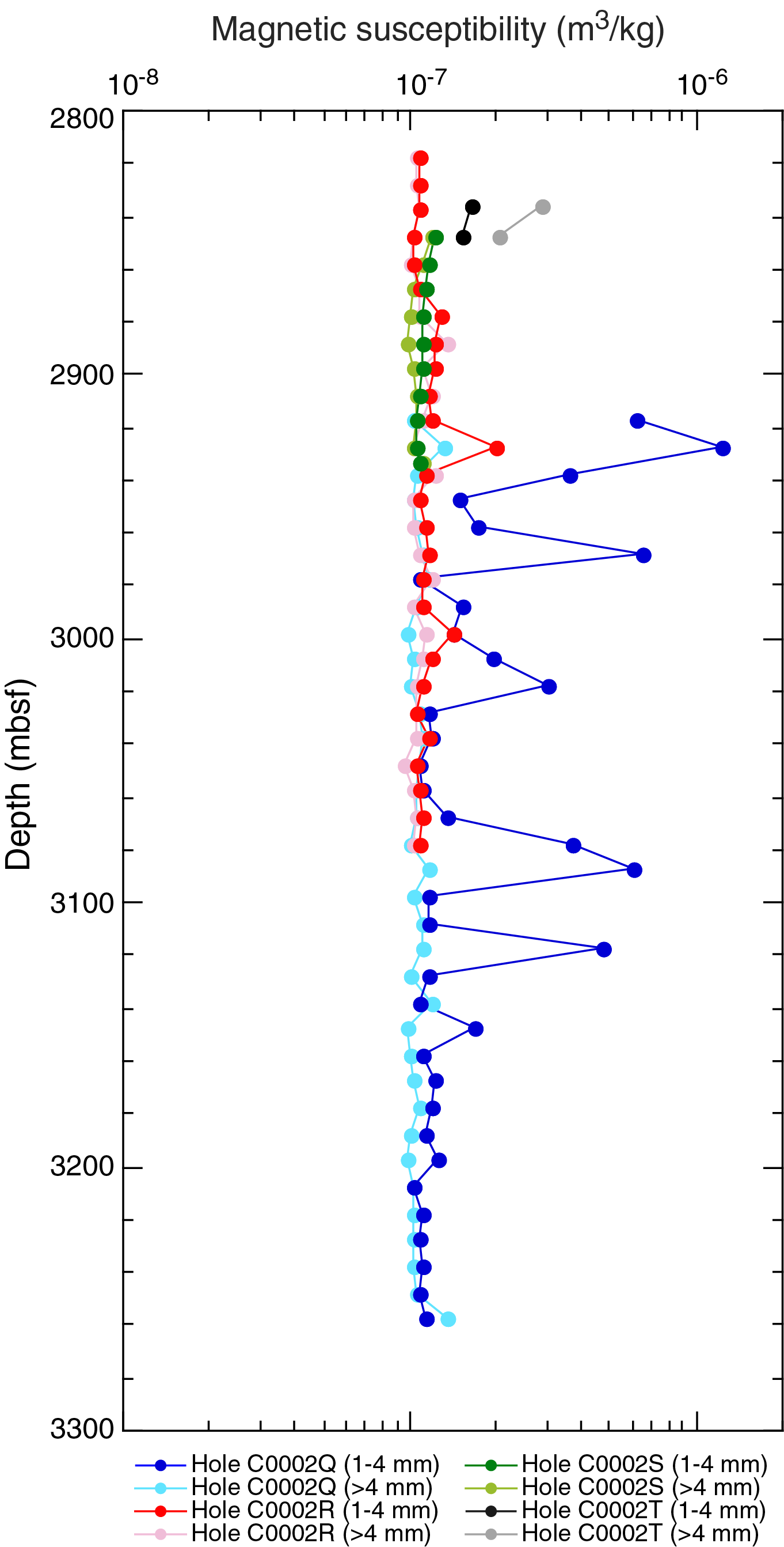
Figure F57. Mass magnetic susceptibility, bulk cuttings.
Logging
Hole C0002Q
Data acquisition
Hole C0002Q was drilled with LWD/measurement-while-drilling (MWD) tools, and logging data were acquired during three of the five runs down the hole (see Introduction and operations). The first run, which used the mud motor BHA, acquired only real-time MWD data. The second run was equipped with a full LWD BHA (TeleScope, arcVISION, MicroScope, SonicScope, and seismicVISION), and MWD/LWD data were recorded from 2888 to 2931 mbsf; however, the seismicVISION tool did not pass through the kick-off window, so no seismic data were recorded in the formation. Data were acquired only with a reduced LWD BHA during the last two runs in Hole C0002Q, from 2923 to 3262 mbsf (Run 4; longest run) and from 2912 to 2955 mbsf (Run 5). Table T32 gives a summary of the tools used and intervals logged during each LWD/MWD run. See Logging in the Expedition 358 methods chapter (Hirose et al., 2020) for a detailed description of the tools and bottom-hole configuration.
Figure F58 displays some of the main drilling parameters recorded during the various runs in Hole C0002Q. The average ROP during Run 2 once the bit passed through the casing window into Hole C0002Q was between 20 and 40 m/h. However, the bit was not drilling intact formation because the hole had been opened during Run 1. During Run 4, ROP ranged between 2 and 5 m/h over the entire logged section. All drilling parameters such as rotation rate and equivalent circulating density (ECD) indicate good drilling conditions during this run. Run 5 is thought to have followed one or several different branches while trying to return to the original hole (see Introduction and operations), and the high variability in the drilling parameters is an indication of the difficult drilling conditions that were experienced.
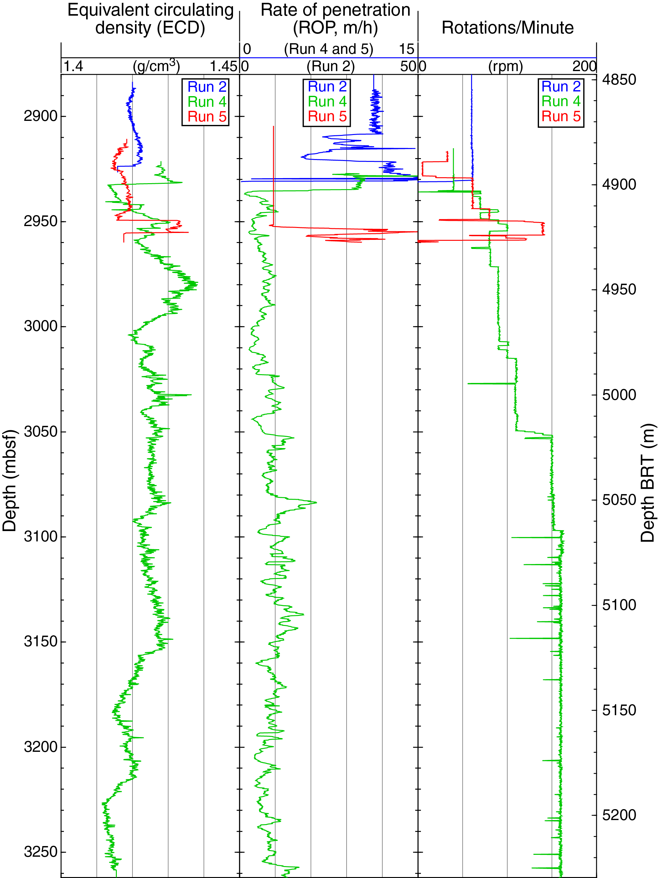
Figure F58. Drilling parameters, Hole C0002Q.
Data quality
The main logs recorded during Runs 2 and 4 are displayed in Figures F59 and F60. Although the quality of the data recorded over most of Hole C0002Q was good, the interval logged immediately below the kick-off window to ~2950 mbsf seems to have suffered from degraded hole conditions (Figures F61, F62). Because data acquired during Run 2 were recorded as late as 5 days after the hole was originally opened, LWD logs from 2900 to 2930 mbsf were measured after long exposure times, which can cause degradation of the borehole condition (i.e., caving, drilling mud invasion, etc.), compromising the data quality. Runs 4 and 5 were acquired even later in the same interval and were also likely affected by further hole degradation (to ~2950 mbsf). Another possible influence on the data quality in the upper logged section is the proximity of the steel casing in Hole C0002P, which may have affected some of the measurements shallower than 2922.5 mbsf.
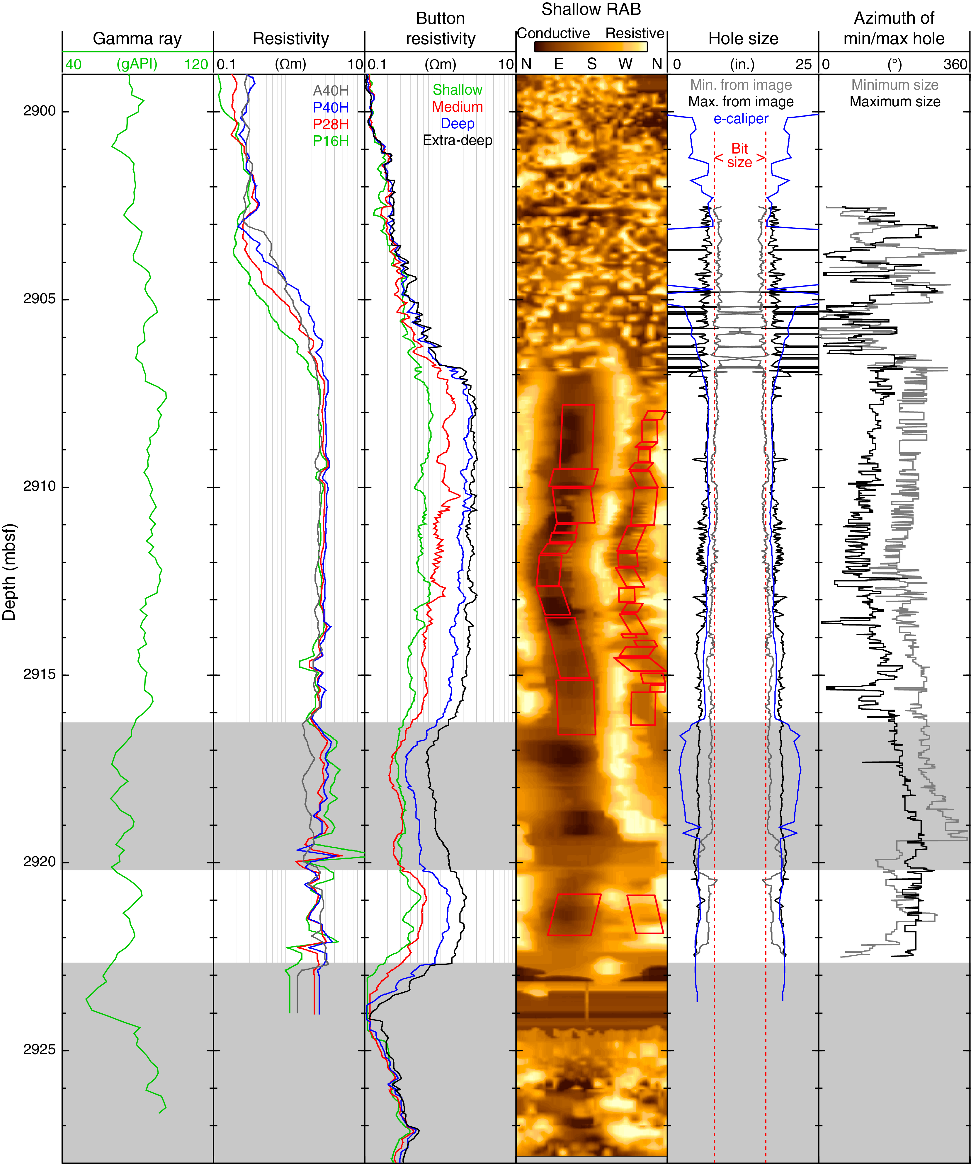
Figure F59. Logs recorded with full LWD suite, Hole C0002Q Run 2.
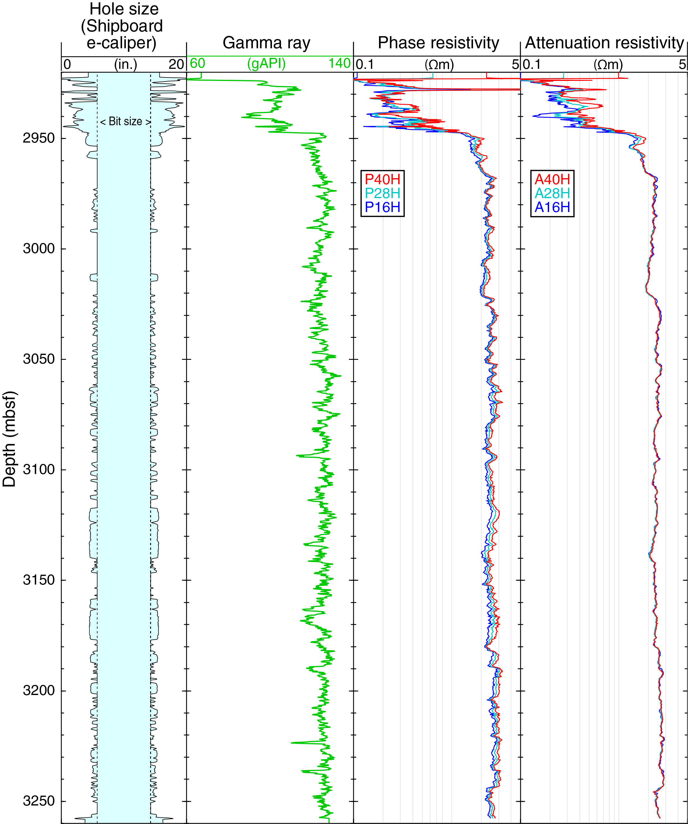
Figure F60. Logs recorded, Hole C0002Q Run 4.
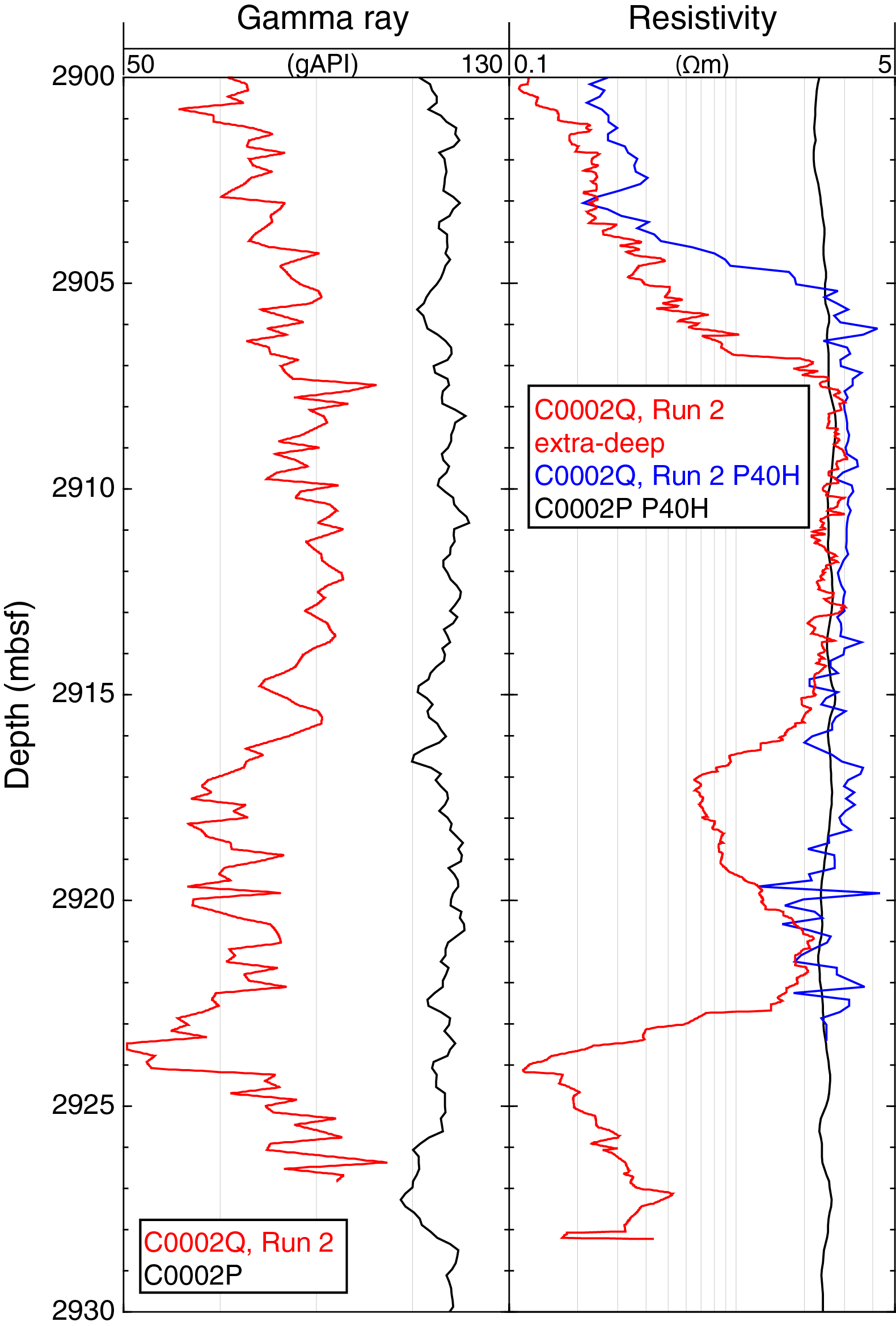
Figure F61. Gamma ray and resistivity logs, Hole C0002Q Run 2.
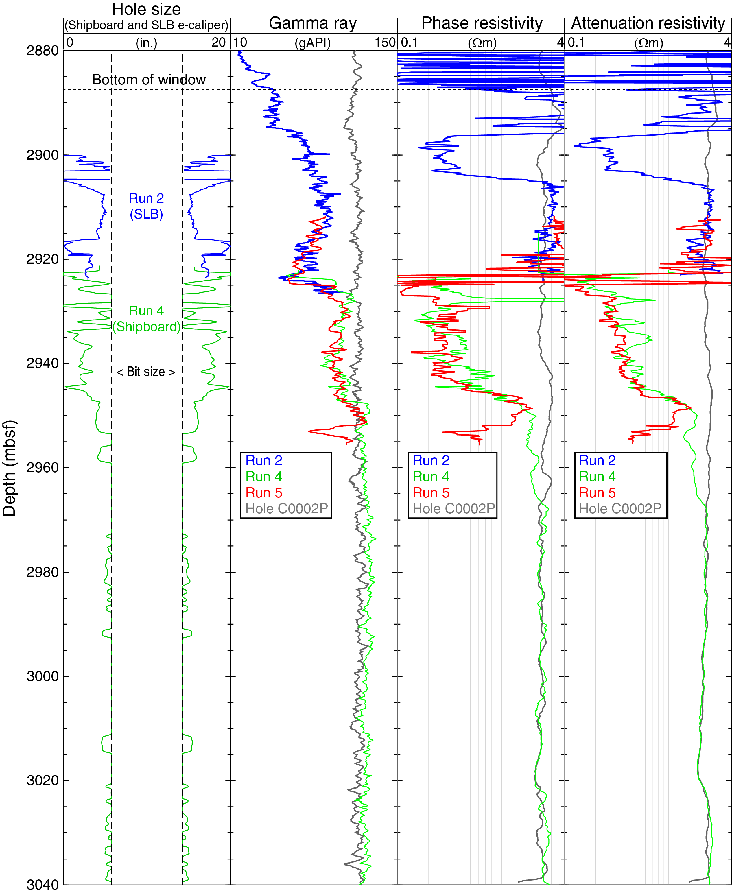
Figure F62. e-caliper, gamma ray, and resistivity logs, Hole C0002Q.
One of the clearest indications of degraded hole conditions in the upper section is the poor agreement with the gamma ray and resistivity logs recorded in Hole C0002P in the same interval (Figure F61). Although there is a chance that Hole C0002Q may have sampled a different lithology, as suggested by some of the observations in the cuttings (see Lithology), the very good agreement between the logs of the two holes below ~2950 mbsf suggests that this is unlikely to be the reason for differing log response (Figure F62). The significantly lower gamma ray and resistivity readings in Hole C0002Q above this depth and the separation observed between the electrical resistivity curves at various depths of investigation are all consistent with the influence of an enlarged borehole.
Caliper logs usually provide the most direct assessment of the quality of a borehole, but none of the tools deployed in Hole C0002Q provided a direct measure of the borehole size. For Runs 2 and 4, borehole size was estimated from the resistivity measured by the arcVISION tool (electromagnetic caliper [e-caliper]). The e-caliper data for Run 2 were provided by Schlumberger, and values were calculated by shipboard scientists for Run 4. They are derived by inverting the raw arcVISION amplitude and phase data with various depths of investigations under the assumption that the curve separation is due only to hole size and borehole fluid (Figures F59, F60, F62). Although it is not as reliable a measure of borehole size as the ultrasonic caliper or mechanical tools, it provides a qualitative measure of the borehole conditions. The results shown in Figures F59, F60, and F62 confirm that above 2950 mbsf the borehole was much larger than the bit size. Resistivity images and e-caliper logs indicate a hole diameter larger than 11 inches because of caving from 2916 to 2919 mbsf (Figure F59). Some of the most degraded intervals display e-caliper values larger than 20 inches. Deeper in the hole, consistent separation between the shallow and deep phase resistivity curves throughout the logged interval suggests that the hole was slightly enlarged, as illustrated by the e-caliper log. But the almost perfect superposition of the various attenuation resistivity curves (Figure F60) shows that the data quality is very good below ~2960 mbsf.
The influence of borehole size on gamma radiation measurements is accounted for during acquisition using proprietary algorithms of the geophysical service company. In the absence of direct caliper measurements, the correction applied assumed an in-gauge hole of 8½ inches (based on the drill bit size). As a result, the "corrected" gamma ray values in the enlarged regions of Hole C0002Q appear lower than in the deeper sections of the hole (Figures F59, F60, F62).
During Run 2, in an effort to get the BHA through the casing window, the drill pipe was jarred multiple times. The resulting shocks damaged some of the tools and in some cases affected the log measurement. The seismicVISION, MicroScope, and TeleScope tools were sent to shore to be inspected. Shore-based analysis of the recovered tools indicated that the seismicVISION and MicroScope were both affected by jarring of the drill pipe. The analysis indicated that the damage to the seismicVISION did not affect the measurements. However, the damage to the MicroScope affected three of the eight buttons on the ultrahigh-resolution pad, resulting in missing data. No damage was found on the TeleScope. Spare TeleScope and arcVISION tools were used during Runs 3 and 4. Repeated jarring during Run 4 damaged the TeleScope, and a third tool without downhole torque and downhole weight on bit (WOB) measurements had to be deployed during Run 5. The arcVISION tool used during Run 2 was not sent to shore but was redeployed during Run 5.
The MicroScope tool acquired resistivity images from 2900 to 2928 mbsf during Run 2 (Figures F59, F63). Four types of images at different depths of investigation (shallow, medium, deep, and extradeep) were acquired as well as ultrahigh-resolution images (UHRIs). As mentioned above, jarring the drill pipe affected the UHRIs. The button resistivity images were not affected because these sensors were not damaged. The quality of the resistivity images was adequate for the interpretation of borehole breakouts, but drilling-induced tensile fractures and bedding planes could not be resolved (Figures F59, F63). The hole shape was also estimated using the MicroScope resistivity data. However, because of the shallower depth of investigation of the MicroScope tool relative to the arcVISION tool, the estimated hole diameter is only accurate from 2908 to 2916 mbsf and from 2920 to 2922 mbsf. At these depths, the hole diameter estimated from the MicroScope data is consistent with the e-caliper estimation from the arcVISION data (Figure F59).
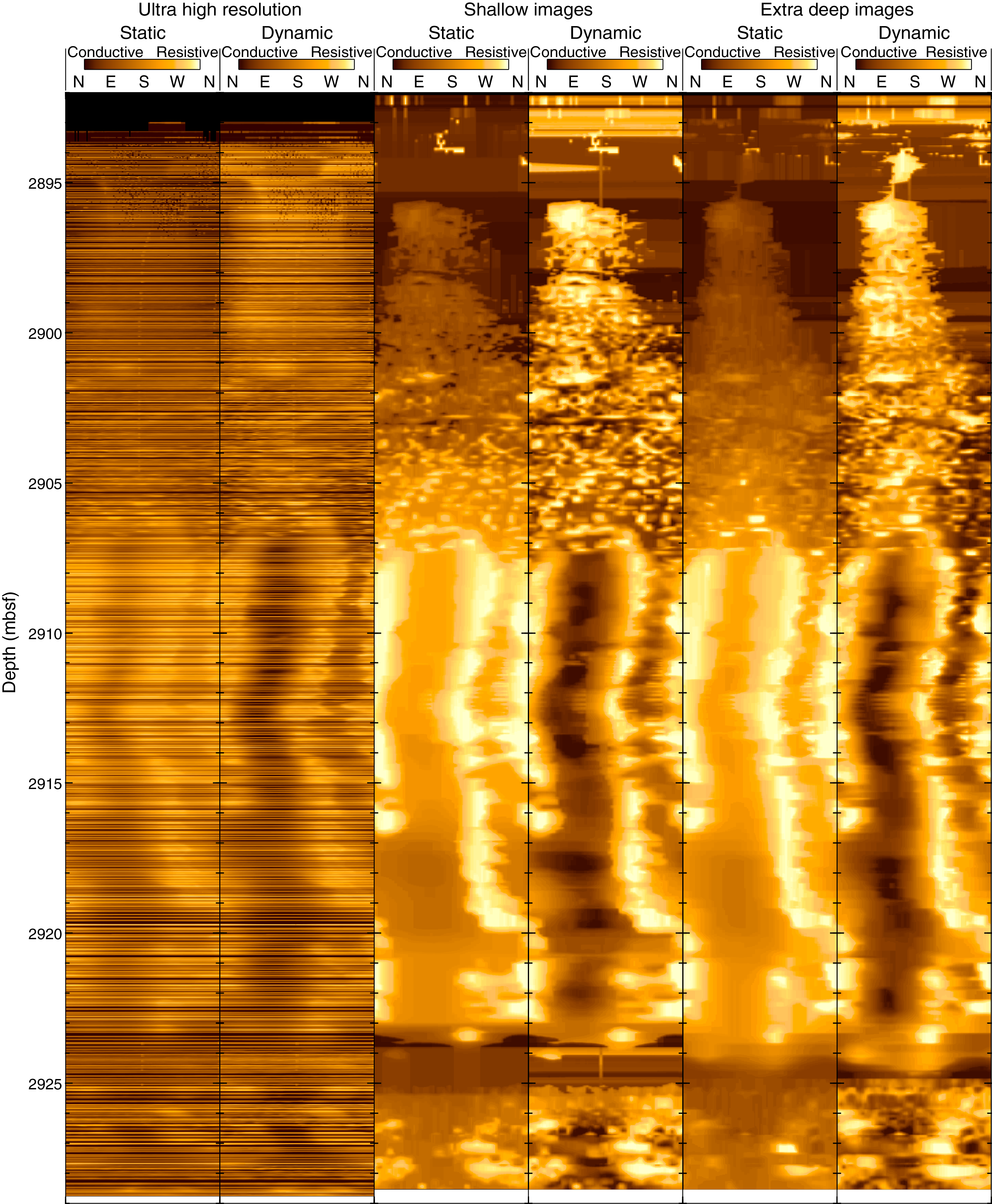
Figure F63. MicroScope resistivity images, Hole C0002Q Run 2.
Sonic logs were recorded by the SonicScope tool during Run 2 (Figure F64). Although most of the data were recorded while the tool was still inside the casing, monopole and quadrupole waveforms were recorded in open hole from the bottom of the casing window at 2887.3 mbsf to 2908 mbsf. Because of the poor hole conditions in this interval, coherent P-wave arrivals were identified only over short intervals at the time of acquisition, but they were consistent with previous data in Hole C0002P (Tobin et al., 2015). The waveform amplitudes shown from Receiver 1 (out of 12) display significant loss of energy in the earlier arrivals, making it difficult to extract reliable P-wave velocity values.
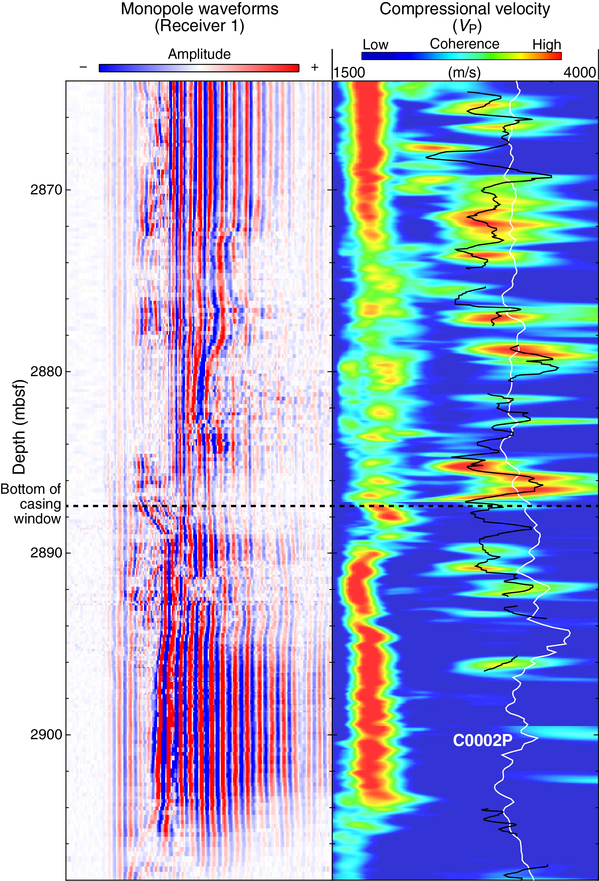
Figure F64. SonicScope data, Hole C0002Q.
Logging data characterization and interpretations
Logging data recorded in Hole C0002Q were characterized based on the variations in trends and character of the measurements available (gamma ray and resistivity). Depth intervals displaying similar logging responses were designated as logging subunits, following criteria established during previous Nankai Trough Seismogenic Zone Experiment (NanTroSEIZE) expeditions at this site (Expedition 314 Scientists, 2009; Strasser et al., 2014; Tobin et al., 2015). The data recorded in Hole C0002Q fit the characteristics of Logging Subunit Ve identified in the deeper section of Hole C0002P. The resistivity and gamma ray data recorded during Run 4 below the final depth of Hole C0002P (3040 mbsf) remain within the range and trends of Logging Subunit Ve, suggesting that the entire logged interval belongs to the same subunit.
The highly variable gamma ray and resistivity values measured in the upper section of Hole C0002Q are affected by poor hole conditions and are unlikely to reflect lithologic changes in this interval. It is also noted that the third-party contractors and logging tools were different between Hole C0002P during Expedition 348 (Halliburton) and Hole C0002Q during this expedition (Schlumberger) and that differences in tool configuration and calibration standards may contribute to some of the differences in readings between the two holes.
In Logging Subunit Ve in Hole C0002Q, phase resistivity remains almost uniform, ranging between 2 and 3 Ωm over most of the logged interval (Figure F62). Gamma radiation is slightly more variable, suggesting a mostly uniform lithology except for short excursions to lower values that could indicate fine sandy intervals or other minor lithologies.
Resistivity image interpretation
Resistivity images in Hole C0002Q were recorded only during Run 2. Acquisition of the resistivity images occurred as late as 5 days after the hole was originally drilled (see Introduction and operations). During that time, the borehole experienced significant caving, which can be seen in the resistivity images. This caving is likely due to the long exposure time, the presence of a preexisting zone of weakness created during previous drilling in Hole C0002P during Expedition 348, and the drill string jarring that was done while running the tools through the window.
The resolution of the resistivity images allows for the interpretation of borehole breakouts, but bedding and fractures could not be identified (Figures F59, F63). Failure of sensors used for the acquisition of UHRIs led to significant data gaps. Standard image processing and smoothing routines improved the image quality and provided correct orientations (Hansen and Buczak, 2010). Hole azimuth and deviation values used for image interpretation were obtained from the drilling deviation survey.
In the static images derived from the button resistivity measurement, the magnitude and range of resistivity is similar at all depths of investigation (Figure F63). However, the UHRIs have less contrast between zones of high and low resistivity. Although low-resistivity zones in the UHRIs are similar in magnitude to low-resistivity zones in the button images, high-resistivity zones in the UHRIs have lower resistivity compared to the same regions in the button images. The UHRIs are more affected by the drilling mud because of its very shallow depth of investigation. Because of this mud effect and the missing data, we do not use the UHRIs for interpretation. We also primarily use the shallow button resistivity images for interpretation rather than the deeper images because we are interested in features observed close to the borehole wall.
Wellbore failures
Significant wellbore failures in the upper section of Hole C0002Q are observed in the resistivity data acquired during Run 2. High resistivity values from 2907 to 2916 mbsf indicate that the tool was measuring intact formation (Figures F59, F63). Over this depth range, alternating pairs of high- and low-resistivity zones, with ~180° separation, are observed in the resistivity images. These zones are interpreted to be borehole failures, most probably caused by the abrasion of the borehole wall by the tool string. From 2916 to 2921 mbsf, resistivity decreases and the image shows a wider conductive zone and a narrower, more resistive zone, indicating an increase in the borehole diameter due to caving. Between 2921 and 2923 mbsf, resistivity increases and laterally alternating high- and low-resistivity zones are observed again. Below 2923 mbsf, the shallow and deep resistivity logs converge at a very low resistivity and the image log shows a dark low-resistivity band, indicating that the borehole diameter has increased so that the MicroScope tool is only measuring the borehole fluid resistivity.
The observed borehole failures are oriented northwest–southeast. The southeastern conductive zone has larger width (~93°) compared to the northwestern zone (~61°). Because the southeast and northwest azimuths are approximately equivalent to the upper and lower sides of the deviated borehole, respectively, the wider low-resistivity zone in the southeast orientation, or at the upper side of the hole, indicates that the tool was farther away from the upper side of the borehole and the low-resistivity zone is imaging the additional drilling mud between the borehole wall and the tool. In contrast, the narrower low-resistivity zone on the northwest, or lower, side of the hole indicates that the tool was largely in contact with the lower side of the borehole. Therefore, the narrower low-resistivity zone in the northwest is considered to reflect the actual width of the borehole failure. Based on the northwest wellbore failure, the average width is 61° and the observed maximum is 86°. Note that this is the apparent azimuthal width measured by an off-centered tool in a slightly enlarged borehole. Thus, it overestimates the actual azimuthal width of wellbore failures that would be observed in an in-gauge borehole. The borehole failure orientation rotates from a northwest orientation at 2908 mbsf to a west to southwest orientation at 2912 mbsf before returning to a northwest orientation at 2915 mbsf. The average borehole failures coincide with the top and bottom of the hole.
Porosity and density estimation
The reduced LWD BHA used in Runs 4 and 5, with only arcVISION resistivity and gamma ray measurements, did not provide a full lithostratigraphic and petrophysical characterization of the drilled interval. The limited set of data still allows estimation of some of the physical properties that could not be measured directly. In particular, resistivity is closely related to pore space structure and can be used to estimate the porosity of the formation. Combined with the grain density measurements made on the cuttings, porosity can then be used to estimate formation density.
Archie (1942) established an empirical relationship between porosity (ϕ), formation resistivity (Rt), and pore water resistivity (Rw) in sandy formations:
where m and a are two empirical parameters that are often called cementation and tortuosity (or Archie) coefficients, respectively. The resistivity of seawater (Rw) was calculated as a function of temperature and salinity (Fofonoff, 1985). Pore water salinity was assumed to be 35‰, and temperature was assumed to follow a linear gradient of 30°C/km (e.g., Sugihara et al., 2014). The most realistic and simplest value for the tortuosity coefficient is a = 1 because this gives a resistivity equal to formation water resistivity when porosity is 100%. A value of m = 2.1 (within the standard accepted range of 1.5 ≤ m ≤ 2.5) was chosen iteratively to provide the best baseline match with porosity data measured on the larger intact cuttings (>4 mm). The resulting porosity log is consistent with MAD porosity data deeper than 2950 mbsf for intact handpicked cuttings (Figure F65; also see Physical properties). We used the resistivity-derived porosity with the average of the MAD grain density to calculate a bulk density curve, which is also in good agreement with measurements made on the intact cuttings. The lack of variation in the porosity and density curves (slightly less than 20% for porosity and near 2.4 g/cm3 for bulk density) is a direct consequence of the almost uniform resistivity values measured over the logged interval.

Figure F65. Estimation of formation porosity and density.
Hole C0002R
Data acquisition
Hole C0002R was drilled with LWD/MWD tools, and logging data were acquired during two of the four runs down the hole (see Introduction and operations). Run 3 was made with a BHA including the TeleScope and arcVISION under a 12¼ inch Z-Reamer and recorded data between 2852 and 2908 mbsf. Run 4 included the same LWD/MWD tools located above a 12¼ inch hole opener and reached a maximum depth of 2872.5 mbsf. Table T32 gives a summary of the tools used and intervals logged. See Logging in the Expedition 358 methods chapter (Hirose et al., 2020) for a detailed description of the tools and bottom-hole configurations.
Figure F66 displays some of the basic drilling parameters in Hole C0002R during Runs 3 and 4. The very fast ROPs in some intervals were achieved because we were reentering an existing hole. The slower penetration during Run 3 between ~4836 and 4865 m BRT (2868.5–2897.5 mbsf) is similar to that achieved deeper in Hole C0002Q (Figure F58). The decrease in ECD observed between 4860 and 4866 m BRT (2893–2999 mbsf) seems to be associated with an increase in gas (as much as 2%) measured in the mud at that time, which dissipated after a period of careful monitoring (see Geochemistry).
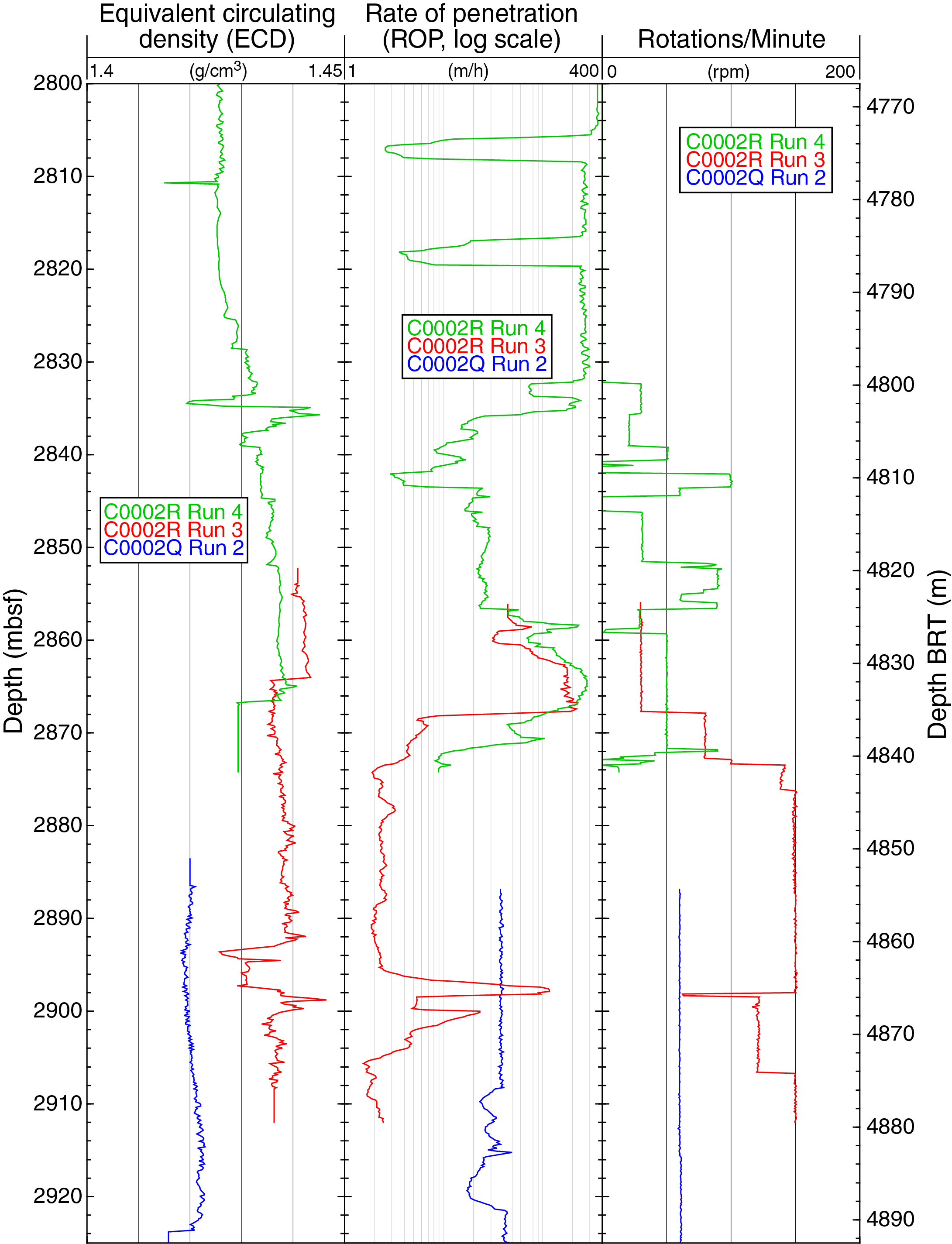
Figure F66. Drilling parameters, Holes C0002Q Run 2 and C0002R Runs 3 and 4.
Data quality
The resistivity and gamma ray logs recorded during Runs 3 and 4 are displayed in Figure F67. For both runs, the hole size was estimated from the raw attenuation and phase resistivity data from the arcVISION tool using the “arcWizard for arcVISION” feature in Techlog. This calculation assumes that only borehole size is responsible for any separation between phase and attenuation resistivity data recorded with different spacings. Because of the need for an accurate volume calculation in preparation for cementing the expandable casing, a more complex estimation of the borehole size was provided by the logging contractor for Run 4.
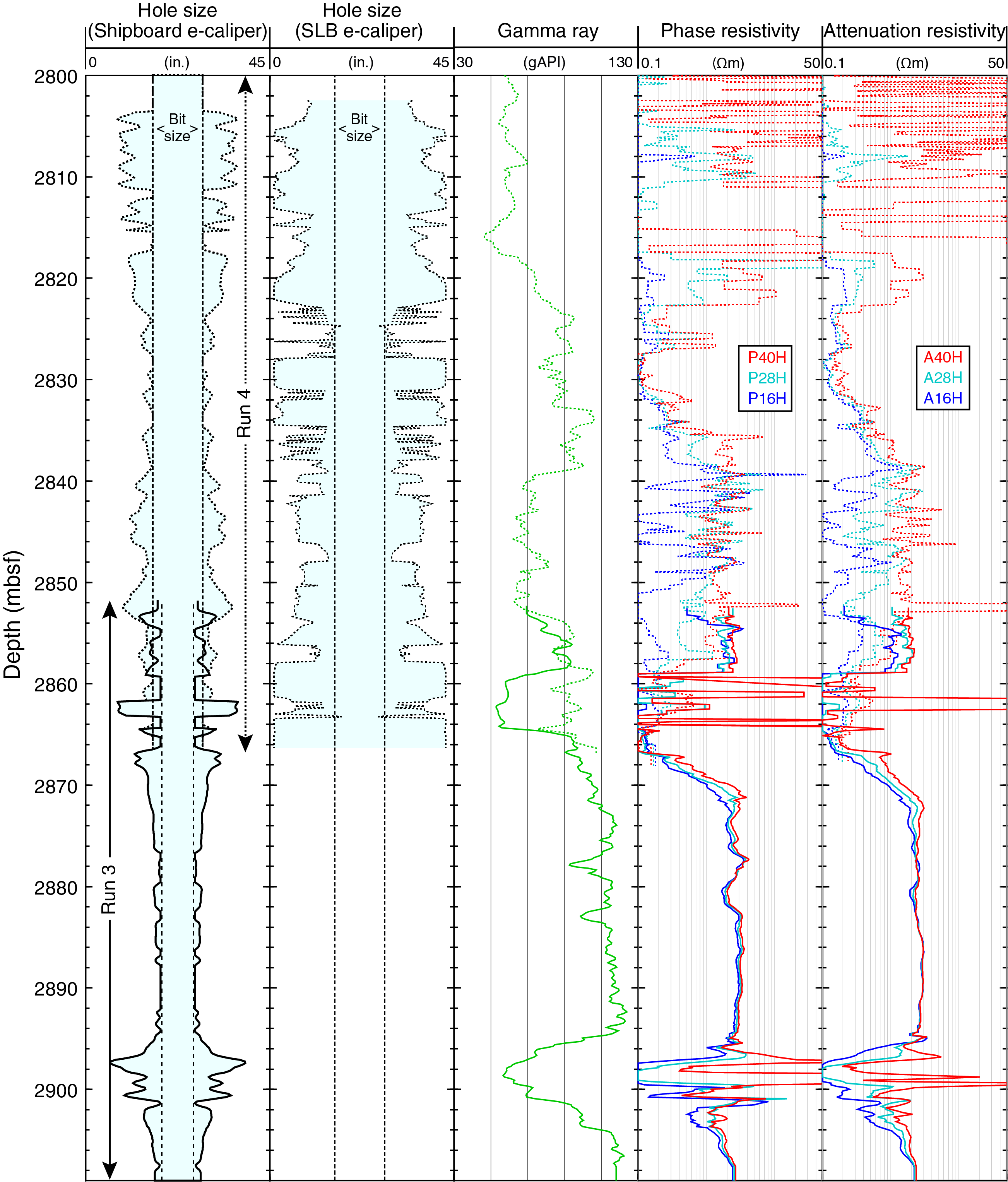
Figure F67. Logs recorded, Hole C0002R Runs 3 and 4.
Comparison of the various hole size estimates with the bit size (Figure F67) shows that the hole was in poor condition and enlarged in many places, with a diameter possibly reaching 45 inches in some intervals. Because the 12¼ inch hole opener was located below the LWD tools during Run 4, the nominal hole diameter for the measurements during that run was 12¼ inches. The e-caliper delivered by Schlumberger provides the most direct assessment of the quality of the borehole, suggesting that none of the data recorded during Run 4 are representative of the properties of the formation surrounding the borehole. The poor hole condition is clearly indicated by the strong separation between the resistivity curves at different depths of investigation, in particular over most of the interval logged during Run 4. Comparison with the data recorded in Hole C0002P over the same interval (Figure F68) suggests that neither the highly variable resistivity values nor the lower gamma ray values above 2865 mbsf and between 2894 and 2904 mbsf are indicative of lithologic changes. The only data of reasonable quality were recorded between 2872 and 2894 mbsf during Run 3.
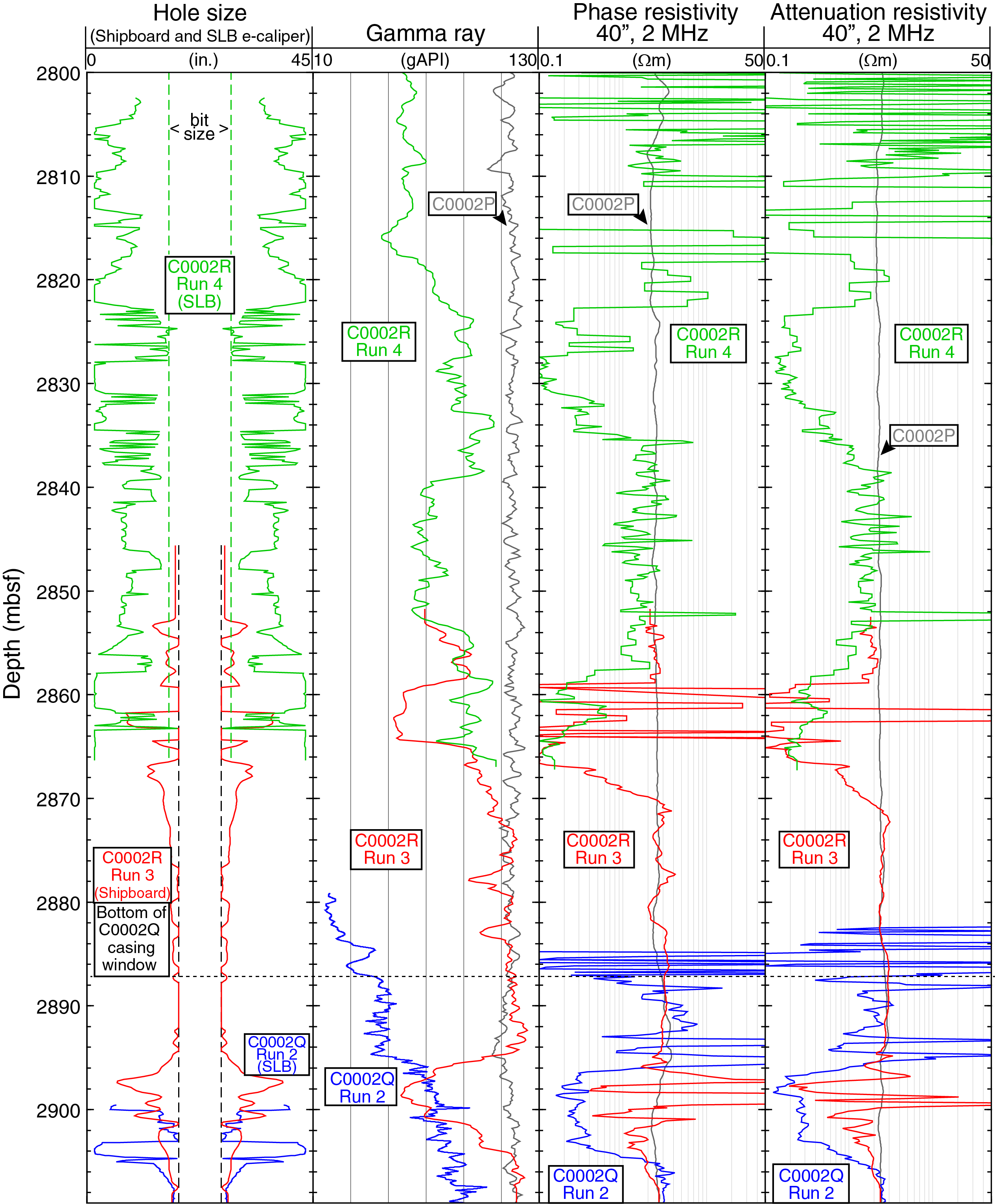
Figure F68. e-caliper, gamma ray, and resistivity logs, Holes C0002R and C0002Q.
One hypothesis that could explain the highly variable resistivity measurements, including anomalously high values from the deep reading (A40H and P40H) (e.g., at 2852 and 2860–2964 mbsf), would be the proximity of the casing in Hole C0002P. To evaluate this hypothesis, we used the well surveys to estimate the distance between the wells as well as their relative positions (Figure F69). Comparison with the gamma ray logs suggests that the intervals with the lower gamma ray readings, which coincide with the erratic resistivity logs or intervals with high curve separation, do not seem to occur where the distance between the wells is the shortest.
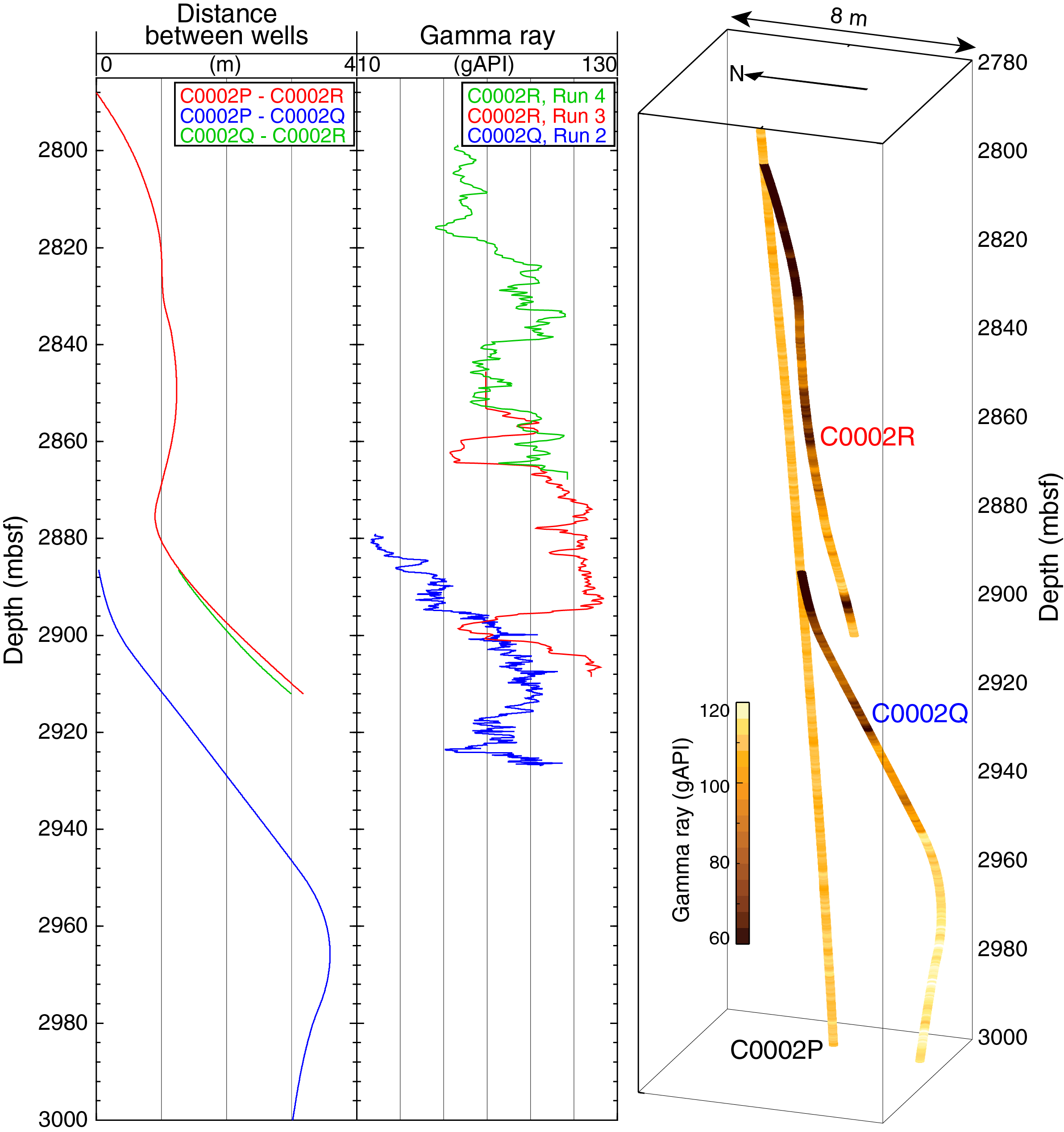
Figure F69. Distance between Holes C0002P, C0002Q, and C0002R.
Logging data characterization and interpretations
Of the logging data acquired in Hole C0002R, the data interval with sufficient quality is limited to 2872–2894 mbsf in Run 3, as described in Data quality. Gamma ray and resistivity indicate approximately constant values of ~110 gAPI and 2.0 Ωm, respectively. These values are consistent with the values from Hole C0002P in the same depth interval, suggesting that Hole C0002R corresponds to Logging Subunit Ve (Figure F68).
Hole C0002S
Data acquisition
Hole C0002S was drilled with LWD/MWD tools, and logging data were acquired during the last of the two runs down this hole (see Introduction and operations). Run 1 acquired only real-time MWD data (Table T32) without downhole torque and downhole WOB. Like Hole C0002Q Run 2, Hole C0002S Run 2 used a full LWD BHA (from bottom to top: MicroScope, arcVISION, TeleScope, SonicScope, and seismicVISION; see Figure F26 in the Expedition 358 methods chapter [Hirose et al., 2020]). It was completed from 5 to 9 February 2019 between 2821 and 2934 mbsf. Unlike all the previous LWD runs, no underreamer was used. This run was terminated prematurely because of failure of the BHA. However, the failed connection was below the LWD tools, and memory data could be retrieved to complement the real-time MWD data.
Figure F70 shows the principal drilling parameters acquired during the main run in Hole C0002S. After drilling through cement around the kick-off window, drilling went smoothly. Below 2860 mbsf, the ROP stabilized at 2 m/h. The high ROP between 2876 and 2880 mbsf is an artifact related to tripping after an orientation survey. The surface torque stayed constant at around 13 kNm, whereas the surface WOB increased by a factor of 2 after reducing the mud weight between 2876 and 2080 mbsf. Downhole torque and WOB (from the TeleScope) are significantly lower than the surface measurements because of the drag caused by the friction of the drill string along the casing, especially at the various kick-off windows. Downhole torque suffered a calibration issue below 2905.6 mbsf and began to collect unrealistic negative values. Finally, ECD (from arcVISION) followed the mud weight change without any pressure spikes, indicating the absence of pack-offs or pressure kicks.
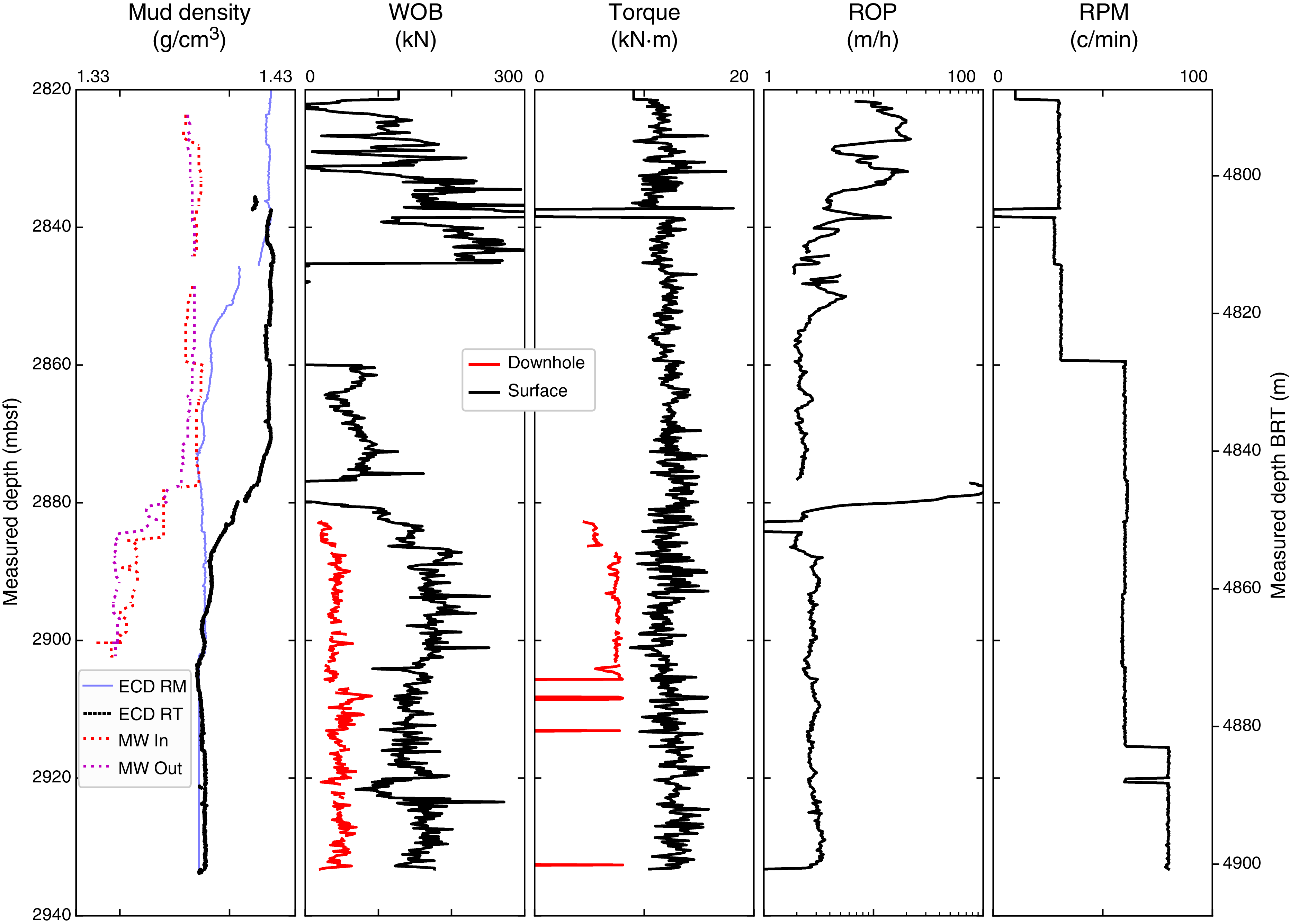
Figure F70. Drilling parameters, Hole C0002S Run 2.
Data quality
The main logs recorded during Run 2 in Hole C0002S are summarized in Figures F71, F72, F73, and F74. The quality of the data is strongly dependent on borehole diameter. Both MicroScope and arcVISION provide resistivity at different depths of investigation, which allows computation of e-caliper. MicroScope e-caliper was provided by the contractor, and arcVISION e-caliper was computed by shipboard scientists using Techlog's arcWizard for arcVISION.
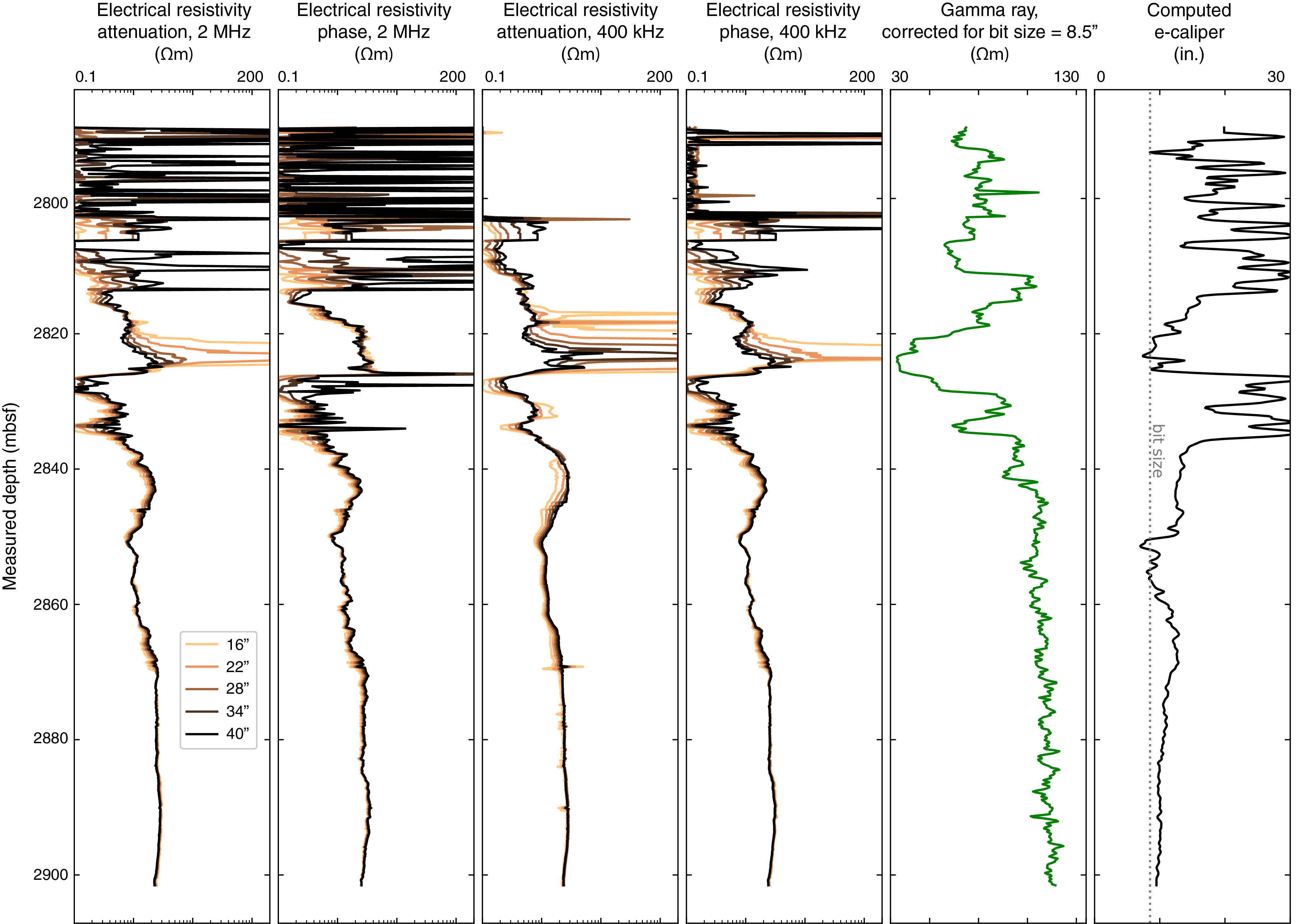
Figure F71. arcVISION tool data, Hole C0002S Run 2.
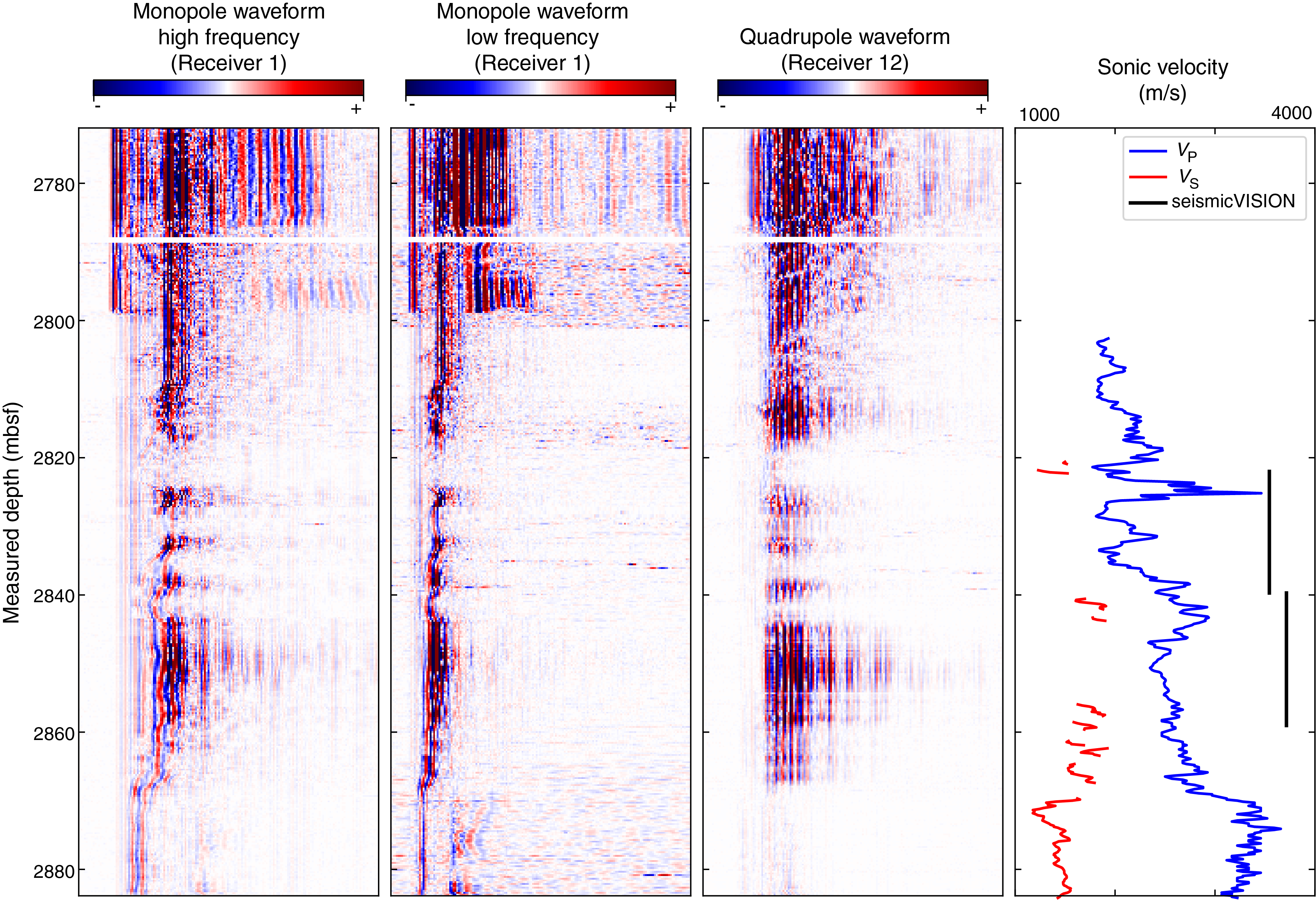
Figure F72. Sonic data from SonicScope tool, Hole C0002S Run 2.
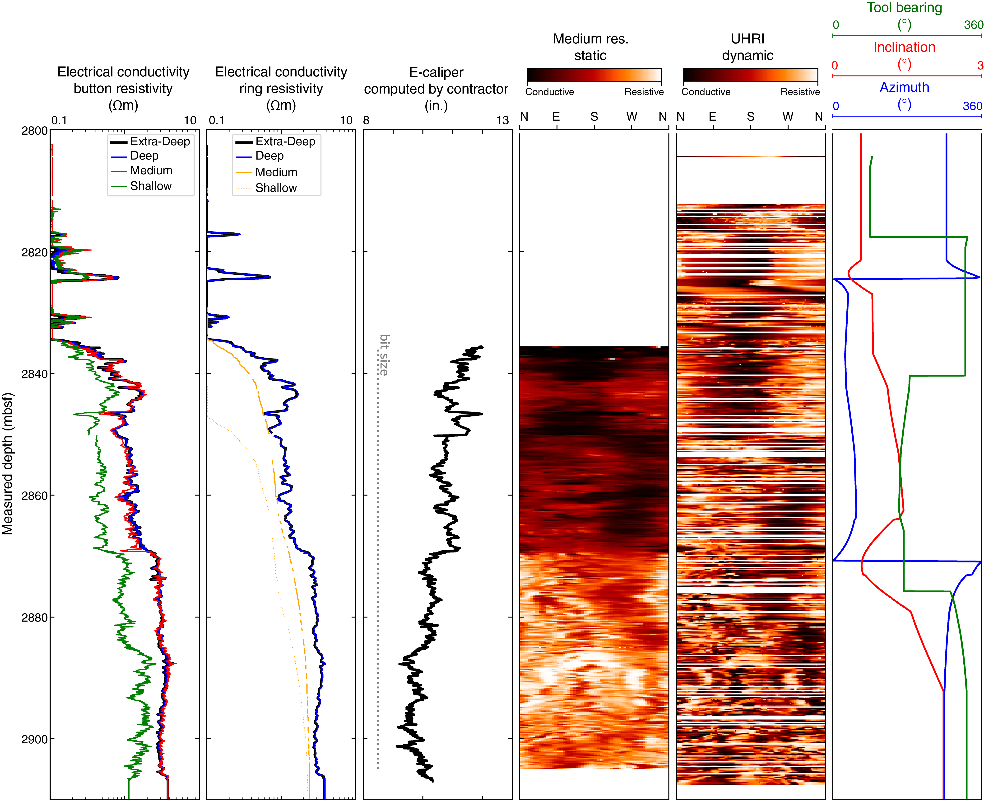
Figure F73. MicroScope tool data, Hole C0002S Run 2.

Figure F74. Resistivity images from MicroScope tool, Hole C0002S Run 2.
Comparison of the e-calipers with bit size (Figure F75) shows that the borehole was severely enlarged above 2836 mbsf. Inversion from arcVISION data suggests that the borehole diameter reached 30 inches, although these latter values have to be taken with caution because the resistivity data used in the computation show unrealistic excursions that could be related to the nearby metallic casing in Hole C0002R (e.g., 2830–2825 mbsf). Under these conditions, button resistivity sensors from the MicroScope only measure mud because of their shallow depths of investigation, and the data are clipped at 0.1 Ωm above 2836 mbsf. This also caused the loss of the button electrical images above that depth (Figure F74), and no MicroScope e-caliper could be retrieved (Figure F73). Between 2836 and 2869 mbsf, the e-calipers differ slightly but are both less than 12½ inches. The arcVISION e-caliper has larger excursions and seems less reliable because it suggests diameters smaller than the bit size at 2851 mbsf; however, it converges with the MicroScope e-caliper values below 2869 mbsf. The MicroScope e-caliper shows less variation, with constant caliper measurements of around 11 inches above 2869 mbsf and 9.5–10.0 inches below. In summary, the data above 2836 mbsf are of poor quality, and most of the log response below this depth must have also been affected by the consistent enlargement (~1–3 inches).
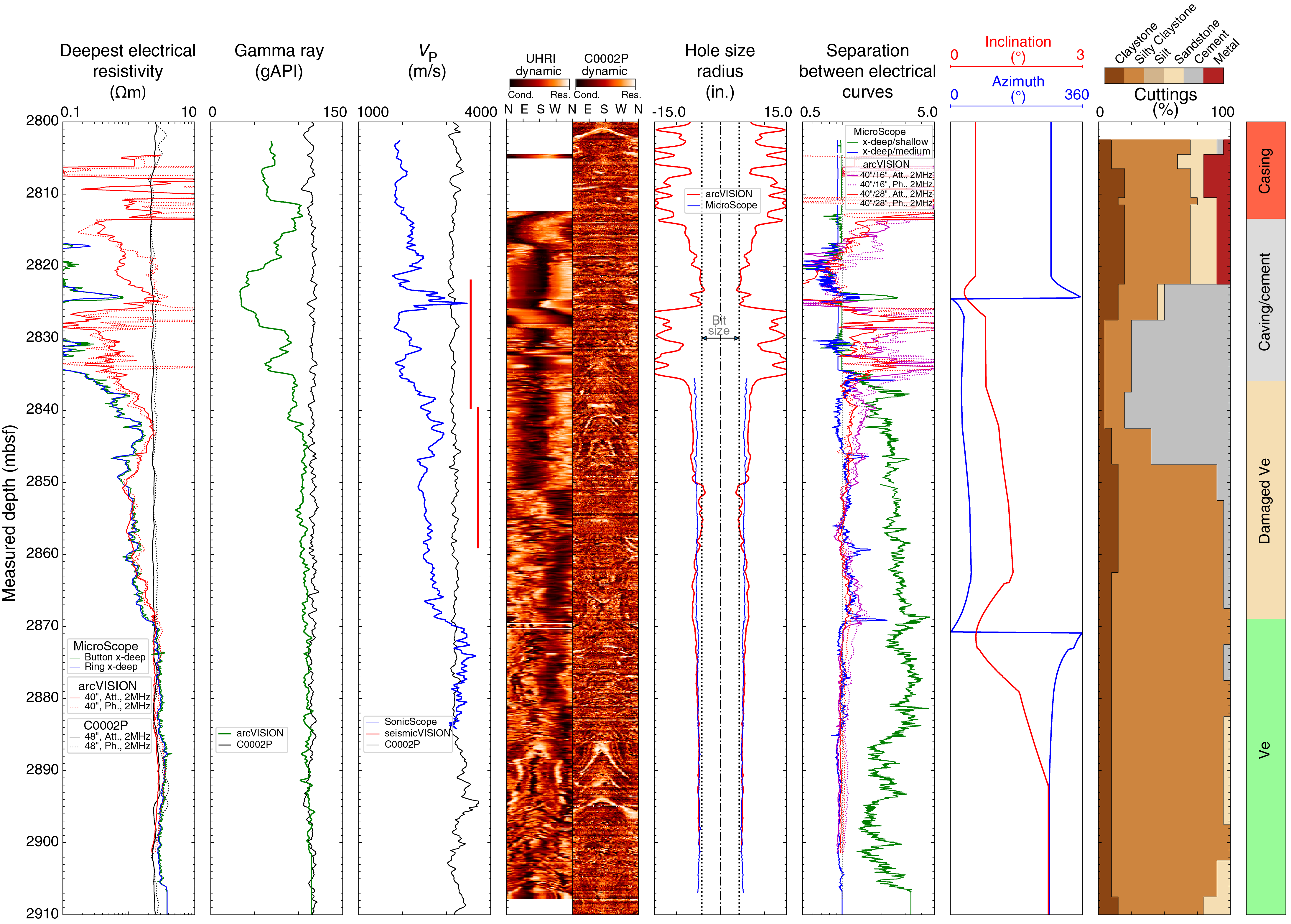
Figure F75. Main data acquired and determination of logging units, Hole C0002S.
UHRI data could not be properly sampled (Figure F73), and vertical smoothing had to be applied prior to interpretation (Figure F74). Also, the proximity of casing in Holes C0002P and C0002R may have caused perturbations in the magnetic field and induced fluctuations in the image orientation (Figures F73, F74). A reorientation survey caused an apparent shift in borehole orientation at 2850.2 mbsf. In addition, the relative bearing changes sharply with depth in places. The image orientation is therefore unreliable above 2850.2 mbsf.
Logging data characterization and interpretations
Figure F75 summarizes the main logging data used for characterization. The interpretation is strongly affected by the borehole quality (see Data quality), and comparison with the data from Hole C0002P (Tobin et al., 2015) helps assess the damage experienced by the formation. The electrical data provide repeated information about the borehole quality and the formation integrity and are therefore used for determining the logging units along Hole C0002S.
In a kick-off window, the departure from the casing is transitional because the kick off departs at a small angle. The full departure from the casing was determined by the end of the irregular values in electromagnetic data at 2813.5 mbsf. Below that depth, UHRIs could be acquired.
The large borehole enlargement below casing lowers the recorded electrical resistivity, gamma ray, and sonic velocity, and the borehole images do not show any geological features in this interval. At around 2820 mbsf, the borehole narrows in an apparently stronger zone and changes direction. There, the low button resistivity and gamma ray data suggest that the borehole is still in cement, which is consistent with cuttings description. The high interval velocity recorded immediately below that depth by the seismicVISION tool confirms that the apparently weak petrophysical properties are local to the borehole vicinity. Hence, between 2813.5 and 2836 mbsf, Hole C0002S is considered to be drilled in the unstable cement around Hole C0002R.
Between 2836 and 2869 mbsf, all resistivity data, gamma ray, and P-wave velocity show constant values and the borehole caliper values decrease. Borehole images are still poor quality, but the most prominent fractures can be picked (Figure F76). The convergence of all deep resistivity data despite their different depths of investigation (see Table T11 in the Expedition 358 methods chapter [Hirose et al., 2020]) suggests documentation of the actual formation resistivity. However, values (~1 Ωm) remain lower than the electrical resistivity in Hole C0002P (~2–3 Ωm). This suggests that the formation is affected by drilling compared to Logging Subunit Ve in Hole C0002P (Tobin et al., 2015). This is consistent with the reduced P-wave velocity (2850 m/s instead of 3300 m/s for Hole C0002P) and the separation between medium and deep resistivity that suggests invasion of the borehole wall by drilling fluid. Hence, between 2836 and 2869 mbsf, Hole C0002S is considered to be drilled in Logging Subunit Ve that has been pervasively damaged by previous drilling operations.

Figure F76. Geological structures and borehole wall failures.
Below 2869 mbsf, all logs are similar to Hole C0002P data. Hence, below 2869 mbsf, Hole C0002S is considered to be drilled in undamaged Logging Subunit Ve. When entering this undisturbed Subunit Ve, the borehole changed direction and its diameter decreased. The quality of the borehole image in the bottom part of Hole C0002S is good enough to pick geological structures that can be correlated with Hole C0002P (e.g., the low-resistivity sandstone layers at 2890 mbsf). Bedding is also identifiable.
Resistivity image interpretation
Exposure times for resistivity images from Hole C0002S range from 14 to 16 h. Therefore, the e-calipers and poorly resolved resistivity images in the upper part of the borehole indicate that the borehole began caving (see Logging data characterization and interpretations). Moreover, measurement of azimuth from magnetic sensors seems to have been affected by the metallic casing in Hole C0002R, and the orientation of the images are not reliable above 2851 mbsf. Hence, analysis of resistivity images is performed below 2851 mbsf only.
The static images highlight the increase in electrical resistivity when entering the undamaged Subunit Ve at 2869 mbsf (Figure F74). Static shallow resistivity images show a continuous zone of high conductivity related to the enlargement of one side of the hole, possibly related to abrasion of the borehole wall by the drill string. Images oriented to the upper side of the hole suggest that this enlargement is not restricted to the "lower" side of an inclined borehole (Figure F76). Given the complex well trajectory of Hole C0002S (Figure F70), the drill string is not always lying on the lower side of the hole.
Several planar features resolved on the UHRIs are either conductive or resistive (Figure F76; Table T33). Most of the structures are detected in the undisturbed zone of Subunit Ve below 2869 mbsf. Their orientation varies with depth. Two series of strongly conductive planes with similar orientations were interpreted to be bedding (2883–2885 and 2895–2907 mbsf). The orientation of the deeper bedding group (average azimuth and dip of 338°N and 79°, respectively) is consistent with Hole C0002P bedding (Tobin et al., 2015). The shallower group (average azimuth and dip angle of 344°N and 62°, respectively) has smaller dips. The two groups are separated by a resistive plane that offsets a steeply dipping resistive vein-like structure that can grossly be fitted as two partially resistive planes having different dip angles but the same orientation.
In the undisturbed Subunit Ve, vertical conductive zones separated by an angle of 180° are indicative of borehole failure. Their orientation changes with depth and can vary by 90° within 5 m. These failures are deeply rooted, and no splintery cuttings were observed at their depths; therefore, they may not be isotropic breakouts (Zoback, 2007) but damage enhanced on preexisting planes of structural weakness.
Correlation between Holes C0002P, C0002Q, C0002R, and C0002S
Only the TeleScope and arcVISION tools were used in every hole during this expedition. Therefore, propagation resistivity and gamma radiation provide a common data set to correlate between Holes C0002Q, C0002R, and C0002S and to compare them to reference Hole C0002P, where similar data were acquired with a different suite of instruments (Figure F77).
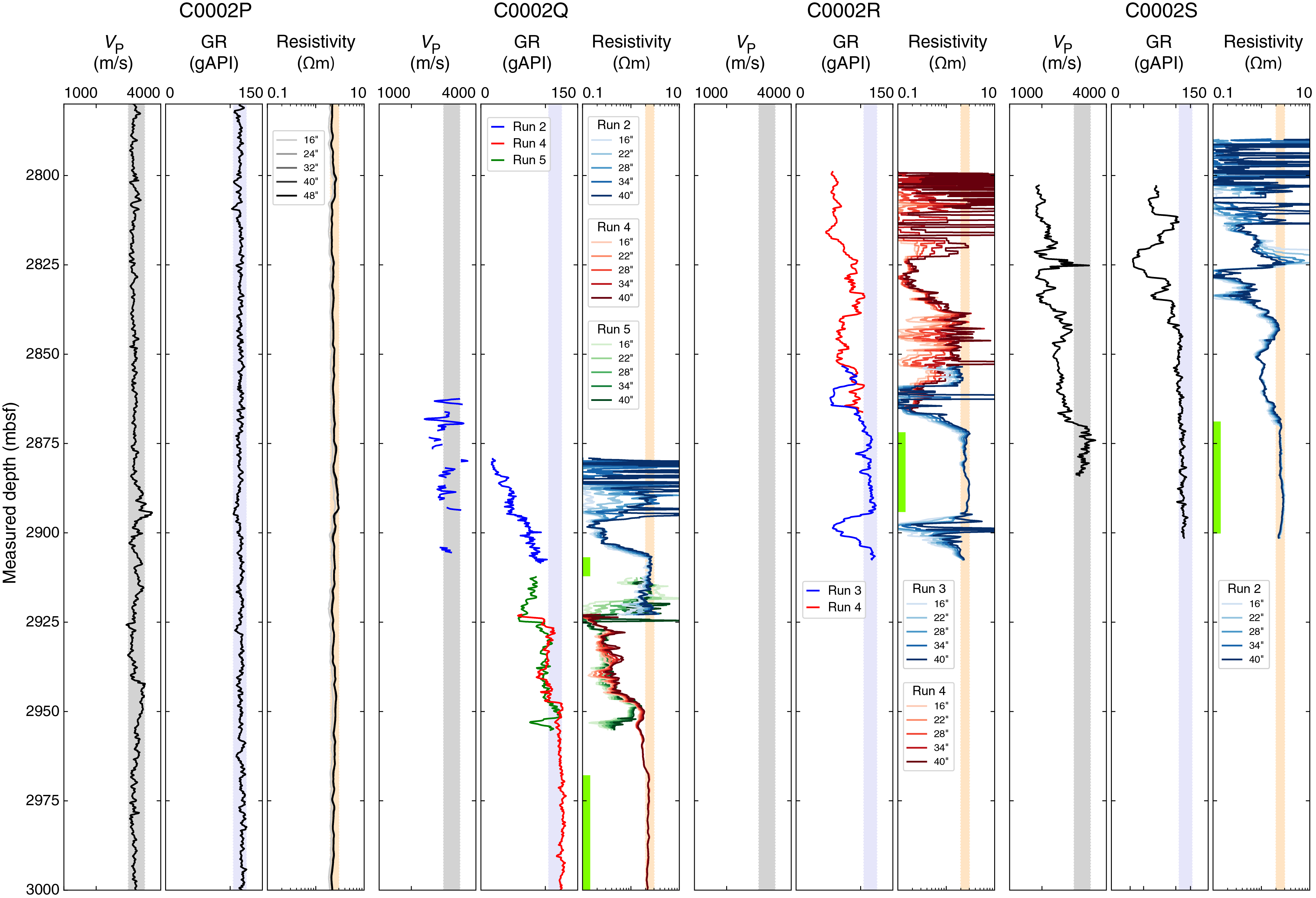
Figure F77. Major petrophysical data acquired.
Following the discussion about the logging units in Hole C0002S, electrical resistivity data provide the best criterion for quality control. Only intervals in which the deep electrical resistivity values are within the range 2–3 Ωm are considered suitable to be representative of Logging Subunit Ve, as identified in Hole C0002P (Tobin et al., 2015). Hence, the high-quality zones are restricted to (1) the interval between 2907 and 2912 mbsf in Hole C0002Q Run 2, (2) the interval below 2968 mbsf in Hole C0002Q Run 4, (3) the interval between 2875 and 2893 mbsf in Hole C0002R Run 3, and (4) the interval below 2869 mbsf in Hole C0002S Run 2.
Caving can be also identified as sharp decreases in electrical resistivity data. Figure F77 shows that these occur at similar measured depths over the runs: (1) between 2810 and 2830 mbsf, (2) between 2860 and 2870 mbsf, (3) between 2890 and 2910 mbsf, and (4) between 2925 and 2950 mbsf. Because each run was likely made in different subholes, caving and disturbance of the formation have been extensive at these depths.
Figure F78 compares the electrical resistivity for the deepest spacing for the four modes of measurement of the propagation tool. Hole C0002P is used as a reference to compare the electrical resistivity for all undamaged zones. Although the logging tools were different, the four modes of measurement agree well, especially for the low electrical resistivity values, which correspond to the zone around 3020 mbsf. However, the correlation varies for the four modes of measurement. The correlation is slightly better for the attenuation resistivity at 2 MHz, and this data set will be used for further petrophysical discussion.

Figure F78. Deep spacing of measured resistivity data.
No clear correlation can be seen between gamma radiation and electrical resistivity (Figure F79) for the undamaged zones. Some of the differences between Hole C0002P and the data recorded during Expedition 358 may be due to the incapacity of the environmental corrections applied to fully account for the enlargement of the boreholes.
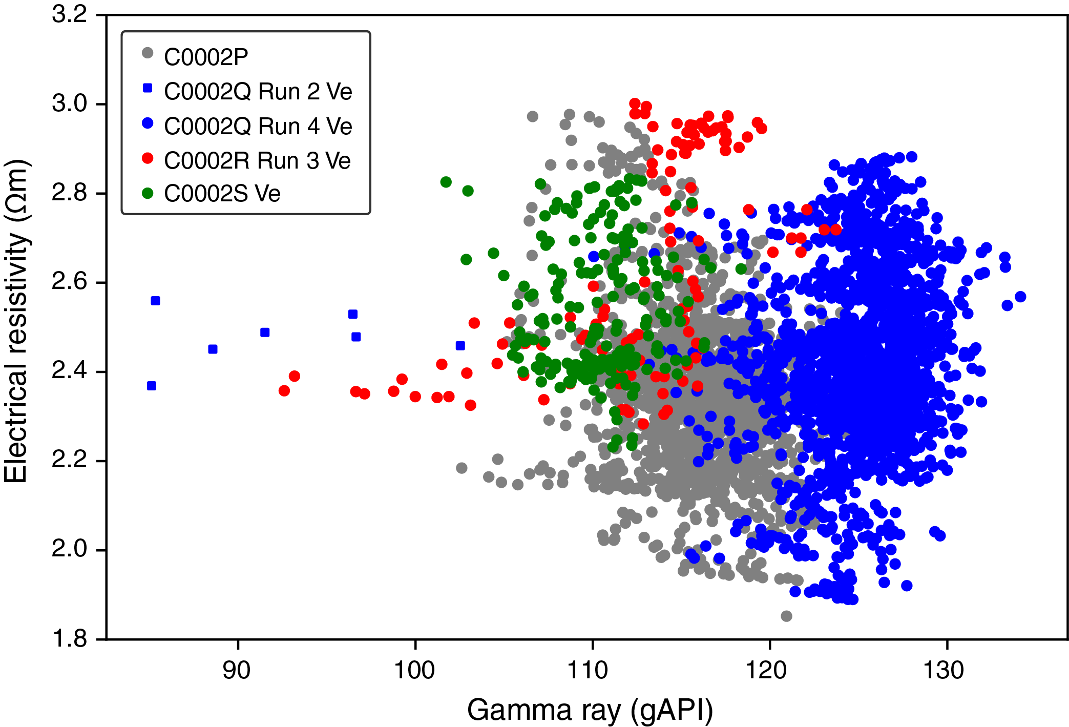
Figure F79. Gamma radiation and attenuation resistivity.
Sonic data were acquired in undamaged Subunit Ve only in Hole C0002S. A crossplot of sonic velocity versus electrical resistivity shows a positive correlation because both data sets are sensitive to porosity (Figure F80). The undamaged section in Hole C0002S where P-wave velocity was recorded is short (Figure F77), so the variation in these data is limited. The damaged zone shows a trend similar to the Hole C0002P data but with lower P-wave velocity and electrical resistivity values.
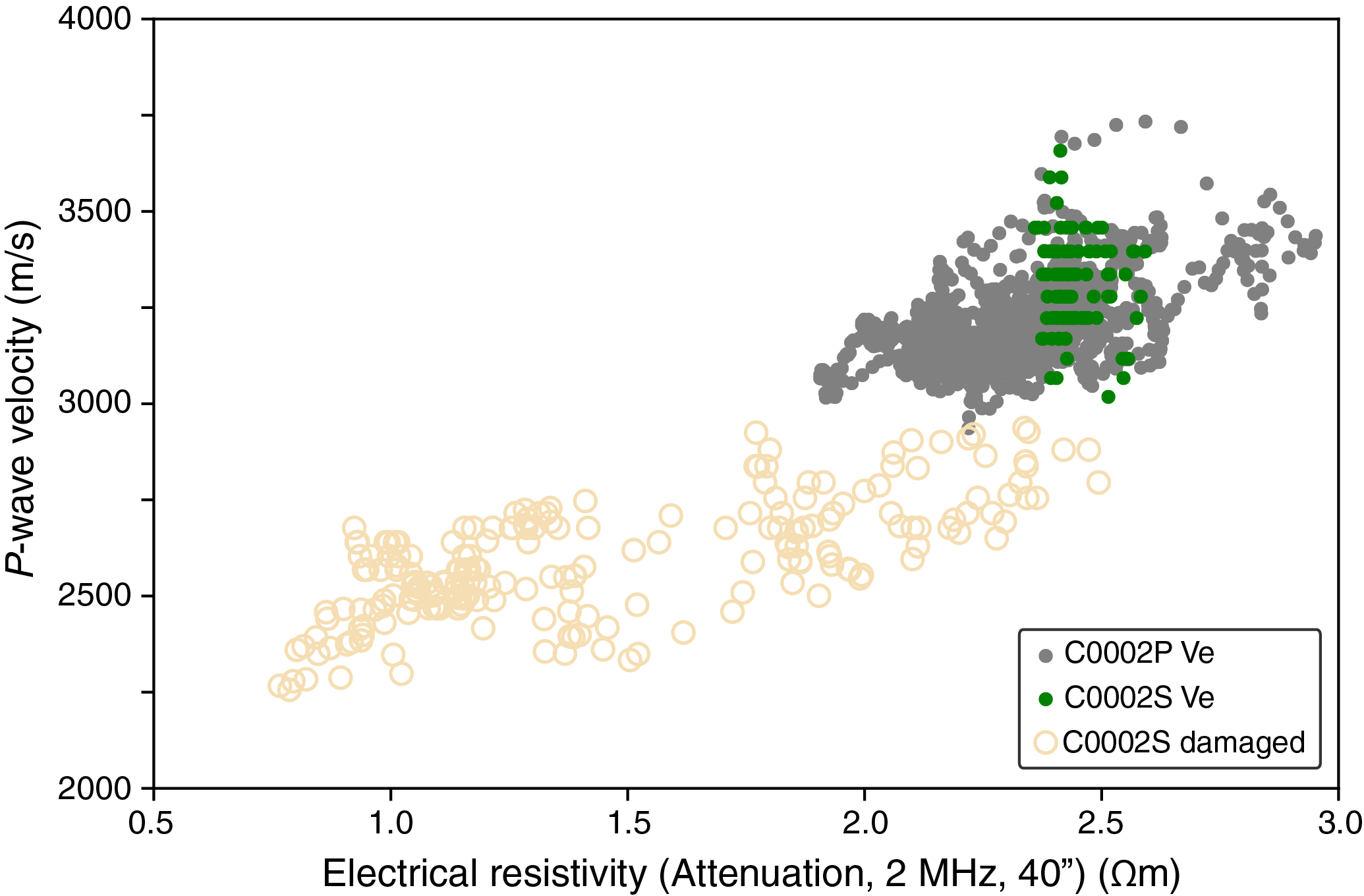
Figure F80. P-wave velocity vs. deep electrical resistivity.
In Hole C0002P, which is very slightly enlarged, P-wave and S-wave velocity are not affected by borehole enlargement (Figure F81). In contrast, P-wave velocity decreases and S-wave velocity increases when entering the undisturbed section in Hole C0002S. P-wave velocity is affected by borehole enlargement in the disturbed zone in Hole C0002S probably due to poor environmental correction or to a direct correlation of the borehole enlargement with the mechanical properties of the formation. S-wave velocity in the disturbed zone in Hole C0002S shows the opposite effect. S-wave velocity values are difficult to acquire. Those acquired in Hole C0002P are unrealistically low, so they cannot be used as a reference data set. In contrast, the VP/VS ratio for Hole C0002S ranges between 1.5 and 2.5, which is more realistic (Mavko et al., 2009).
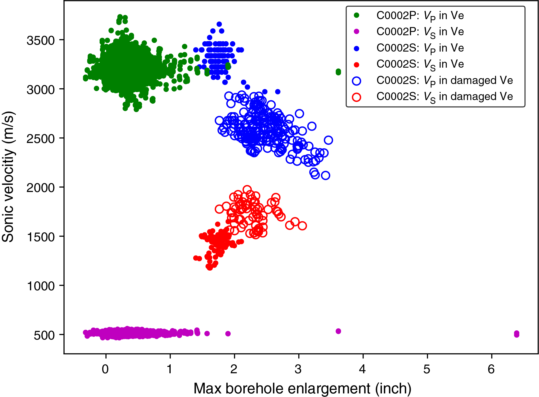
Figure F81. Sonic data vs. hole enlargement.
References
Archie, G.E., 1942. The electrical resistivity log as an aid in determining some reservoir characteristics. Transactions of the AIME, 146(1):54–62. https://doi.org/10.2118/942054-G
Bernard, B.B., Brooks, J.M., and Sackett, W.M., 1978. Light hydrocarbons in recent Texas continental shelf and slope sediments. Journal of Geophysical Research: Oceans, 83(C8):4053–4061. https://doi.org/10.1029/JC083iC08p04053
Bons, P.D., Elburg, M.A., and Gomez-Rivas, E., 2012. A review of the formation of tectonic veins and their microstructures. Journal of Structural Geology, 43:33–62. https://doi.org/10.1016/j.jsg.2012.07.005
Bjornstad, B.N., McKinley, J.P., Stevens, T.O., Rawson, S.A., Fredrickson, J.K., and Long, P.E., 1994. Generation of hydrogen gas as a result of drilling within the saturated zone. Groundwater Monitoring and Remediation, 14(4):140–147. https://doi.org/10.1111/j.1745-6592.1994.tb00492.x
Boston, B., Moore, G.F., Jurado, M.J., and Sone, H., 2016. Deformation of the Nankai Trough inner accretionary prism: the role of inherited structures. Geochemistry, Geophysics, Geosystems, 17(2):485–500. https://doi.org/10.1002/2015GC006185
Cohen, K.M., Finney, S.C., Gibbard, P.L., and Fan, J.-X., 2019. International Chronostratigraphic Chart. International Commission on Stratigraphy.
Dielforder, A., Berger, A., and Herwegh, M., 2016. The accretion of foreland basin sediments during early stages of continental collision in the European Alps and similarities to accretionary wedge tectonics. Tectonics, 35(10):2216–2238. https://doi.org/10.1002/2015TC004101
Expedition 314 Scientists, 2009. Expedition 314 Site C0002. In Kinoshita, M., Tobin, H., Ashi, J., Kimura, G., Lallemant, S., Screaton, E.J., Curewitz, D., Masago, H., Moe, K.T., and the Expedition 314/315/316 Scientists, Proceedings of the Integrated Ocean Drilling Program, 314/315/316: Washington, DC (Integrated Ocean Drilling Program Management International, Inc.). https://doi.org/10.2204/iodp.proc.314315316.114.2009
Expedition 315 Scientists, 2009. Expedition 315 Site C0002. In Kinoshita, M., Tobin, H., Ashi, J., Kimura, G., Lallemant, S., Screaton, E.J., Curewitz, D., Masago, H., Moe, K.T., and the Expedition 314/315/316 Scientists, Proceedings of the Integrated Ocean Drilling Program, 314/315/316: Washington, DC (Integrated Ocean Drilling Program Management International, Inc.). https://doi.org/10.2204/iodp.proc.314315316.124.2009
Expedition 322 Scientists, 2010a. Site C0011. In Saito, S., Underwood, M. B., Kubo, Y., and the Expedition 322 Scientists, Proceedings of the Integrated Ocean Drilling Program, 322: Tokyo (Integrated Ocean Drilling Program Management International, Inc.). https://doi.org/10.2204/iodp.proc.322.103.2010
Expedition 322 Scientists, 2010b. Site C0012. In Saito, S., Underwood, M. B., Kubo, Y., and the Expedition 322 Scientists, Proceedings of the Integrated Ocean Drilling Program, 322: Washington, DC (Integrated Ocean Drilling Program Management International, Inc.). https://doi.org/10.2204/iodp.proc.322.104.2010
Expedition 333 Scientists, 2012a. Site C0011. In Henry, P., Kanamatsu, T., Moe, K., and the Expedition 333 Scientists, Proceedings of the Integrated Ocean Drilling Program, 333: Tokyo (Integrated Ocean Drilling Program Management International, Inc.). https://doi.org/10.2204/iodp.proc.333.104.2012
Expedition 333 Scientists, 2012b. Site C0012. In Henry, P., Kanamatsu, T., Moe, K., and the Expedition 333 Scientists, Proceedings of the Integrated Ocean Drilling Program, 333: Tokyo (Integrated Ocean Drilling Program Management International, Inc.). https://doi.org/10.2204/iodp.proc.333.105.2012
Fofonoff, N.P., 1985. Physical properties of seawater: a new salinity scale and equation of state for seawater. Journal of Geophysical Research: Oceans, 90(C2):3332–3342. https://doi.org/10.1029/JC090iC02p03332
Fukuchi, R., Yamaguchi, A., Yamamoto, Y., and Ashi, J., 2017. Paleothermal structure of the Nankai inner accretionary prism estimated from vitrinite reflectance of cuttings. Geochemistry, Geophysics, Geosystems, 18(8):3185–3196. https://doi.org/10.1002/2017GC006928
Hansen, B., and Buczak, J., 2010. Making interpretable images from image logs. In Pöppelreiter, M., García-Carballido, C., and Kraaijveld, M. (Eds.), Dipmeter and Borehole Image Log Technology. AAPG Memoir, 92:51–66. https://doi.org/10.1306/13181277M923405
Hirose, T., Ikari, M., Kanagawa, K., Kimura, G., Kinoshita, M., Kitajima, H., Saffer, D., Tobin, H., Yamaguchi, A., Eguchi, N., Maeda, L., Toczko, S., Bedford, J., Chiyonobu, S., Colson, T.A., Conin, M., Cornard, P.H., Dielforder, A., Doan, M.-L., Dutilleul, J., Faulkner, D.R., Fukuchi, R., Guérin, G., Hamada, Y., Hamahashi, M., Hong, W.-L., Ijiri, A., Jaeger, D., Jeppson, T., Jin, Z., John, B.E., Kitamura, M., Kopf, A., Masuda, H., Matsuoka, A., Moore, G.F., Otsubo, M., Regalla, C., Sakaguchi, A., Sample, J., Schleicher, A., Sone, H., Stanislowski, K., Strasser, M., Toki, T., Tsuji, T., Ujiie, K., Underwood, M.B., Yabe, S., Yamamoto, Y., Zhang, J., Sanada, Y., Kido, Y., Le Ber, E., and Saito, S., 2020. Expedition 358 methods. With contributions by T. Kanamatsu. In Tobin, H., Hirose, T., Ikari, M., Kanagawa, K., Kimura, G., Kinoshita, M., Kitajima, H., Saffer, D., Yamaguchi, A. Eguchi, N., Maeda, L., Toczko, S., and the Expedition 358 Scientists, NanTroSEIZE Plate Boundary Deep Riser 4: Nankai Seismogenic/Slow Slip Megathrust. Proceedings of the International Ocean Discovery Program, 358: College Station, TX (International Ocean Discovery Program). https://doi.org/10.14379/iodp.proc.358.102.2020
Hüpers, A., Grathoff, G., Warr, L.N., Wemmer, K., Spinelli, G., and Underwood, M.B., 2019. Spatiotemporal characterization of smectite-to-illite diagenesis in the Nankai Trough accretionary prism revealed by samples from 3 km below seafloor. Geochemistry, Geophysics, Geosystems, 20(2):933–951. https://doi.org/10.1029/2018GC008015
Kameda, J., Saruwatari, K., and Tanaka, H., 2004a. H2 generation during dry grinding of kaolinite. Journal of Colloid and Interface Science, 275(1):225–228. https://doi.org/10.1016/j.jcis.2004.02.014
Kameda, J., Saruwatari, K., Tanaka, H., and Tsunomori, F., 2004b. Mechanisms of hydrogen generation during the mechanochemical treatment of biotite within D2O media. Earth, Planets and Space, 56(12):1241–1245. https://doi.org/10.1186/BF03353346
Kita, I., Matsuo, S., and Wakita, H., 1982. H2 generation by reaction between H2O and crushed rock: an experimental study on H2 degassing from the active fault zone. Journal of Geophysical Research: Solid Earth, 87(B13):10789–10795. https://doi.org/10.1029/JB087iB13p10789
Maltman, A.J., Byrne, T., Karig, D.E., and Lallement, S., 1993. Deformation at the toe of an active accretionary prism: synopsis of results from ODP Leg 131, Nankai, SW Japan. Journal of Structural Geology, 15(8):949–964. https://doi.org/10.1016/0191-8141(93)90169-B
Mavko, G., Mukerji, T., and Dvorkin, J., 2009. The Rock Physics Handbook: Tools for Seismic Analysis of Porous Media (2nd edition): Cambridge, UK (Cambridge University Press). https://doi.org/10.1017/CBO9780511626753
Meyers, P.A., 1997. Organic geochemical proxies of paleoceanographic, paleolimnologic, and paleoclimatic processes. Organic Geochemistry, 27(5–6):213–250. https://doi.org/10.1016/S0146-6380(97)00049-1
Raffi, I., Backman, J., Fornaciari, E., Pälike, H., Rio, D., Lourens, L., and Hilgen, F., 2006. A review of calcareous nannofossil astrobiochronology encompassing the past 25 million years. Quaternary Science Reviews, 25(23–24):3113–3137. https://doi.org/10.1016/j.quascirev.2006.07.007
Strasser, M., Dugan, B., Kanagawa, K., Moore, G.F., Toczko, S., Maeda, L., Kido, Y., Moe, K.T., Sanada, Y., Esteban, L., Fabbri, O., Geersen, J., Hammerschmidt, S., Hayashi, H., Heirman, K., Hüpers, A., Jurado Rodriguez, M.J., Kameo, K., Kanamatsu, T., Kitajima, H., Masuda, H., Milliken, K., Mishra, R., Motoyama, I., Olcott, K., Oohashi, K., Pickering, K.T., Ramirez, S.G., Rashid, H., Sawyer, D., Schleicher, A., Shan, Y., Skarbek, R., Song, I., Takeshita, T., Toki, T., Tudge, J., Webb, S., Wilson, D.J., Wu, H.-Y., and Yamaguchi, A., 2014. Site C0002. In Strasser, M., Dugan, B., Kanagawa, K., Moore, G.F., Toczko, S., Maeda, L., and the Expedition 338 Scientists, Proceedings of the Integrated Ocean Drilling Program, 338: Yokohama (Integrated Ocean Drilling Program). https://doi.org/10.2204/iodp.proc.338.103.2014
Sugihara, T., Kinoshita, M., Araki, E., Kimura, T., Kyo, M., Namba, Y., Kido, Y., Sanada, Y., and Moe, K.T, 2014. Re-evaluation of temperature at the updip limit of locked portion of Nankai megasplay inferred from IODP Site C0002 temperature observatory. Earth, Planets and Space, 66:107. https://doi.org/10.1186/1880-5981-66-107
Takeshita, T., Yamaguchi, A., and Shigematsu, N., 2014. Stress reversal recorded in calcite vein cuttings from the Nankai accretionary prism, southwest Japan. Earth, Planets and Space, 66:144. https://doi.org/10.1186/s40623-014-0144-4
Tobin, H., Hirose, T., Ikari, M., Kanagawa, K., Kimura, G., Kinoshita, M., Kitajima, H., Saffer, D., Yamaguchi, A., Eguchi, N., Maeda, L., Toczko, S., Bedford, J., Chiyonobu, S., Colson, T.A., Conin, M., Cornard, P.H., Dielforder, A., Doan, M.-L., Dutilleul, J., Faulkner, D.R., Fukuchi, R., Guérin, G., Hamada, Y., Hamahashi, M., Hong, W.-L., Ijiri, A., Jaeger, D., Jeppson, T., Jin, Z., John, B.E., Kitamura, M., Kopf, A., Masuda, H., Matsuoka, A., Moore, G.F., Otsubo, M., Regalla, C., Sakaguchi, A., Sample, J., Schleicher, A., Sone, H., Stanislowski, K., Strasser, M., Toki, T., Tsuji, T., Ujiie, K., Underwood, M.B., Yabe, S., Yamamoto, Y., Zhang, J., Sanada, Y., Kido, Y., Le Ber, E., and Saito, S., 2020a. Expedition 358 summary. With contributions by T. Kanamatsu. In Tobin, H., Hirose, T., Ikari, M., Kanagawa, K., Kimura, G., Kinoshita, M., Kitajima, H., Saffer, D., Yamaguchi, A. Eguchi, N., Maeda, L., Toczko, S., and the Expedition 358 Scientists, NanTroSEIZE Plate Boundary Deep Riser 4: Nankai Seismogenic/Slow Slip Megathrust. Proceedings of the International Ocean Discovery Program, 358: College Station, TX (International Ocean Discovery Program). https://doi.org/10.14379/iodp.proc.358.101.2020
Tobin, H., Hirose, T., Ikari, M., Kanagawa, K., Kimura, G., Kinoshita, M., Kitajima, H., Saffer, D., Yamaguchi, A. Eguchi, N., Maeda, L., Toczko, S., and the Expedition 358 Scientists, 2020b. Supplementary material, https://doi.org/10.14379/iodp.proc.358supp.2020. Supplement to Tobin, H., Hirose, T., Ikari, M., Kanagawa, K., Kimura, G., Kinoshita, M., Kitajima, H., Saffer, D., Yamaguchi, A. Eguchi, N., Maeda, L., Toczko, S., and the Expedition 358 Scientists, NanTroSEIZE Plate Boundary Deep Riser 4: Nankai Seismogenic/Slow Slip Megathrust. Proceedings of the International Ocean Discovery Program, 358: College Station, TX (International Ocean Discovery Program). https://doi.org/10.14379/iodp.proc.358.2020
Tobin, H., Hirose, T., Saffer, D., Toczko, S., Maeda, L., Kubo, Y., Boston, B., Broderick, A., Brown, K., Crespo-Blanc, A., Even, E., Fuchida, S., Fukuchi, R., Hammerschmidt, S., Henry, P., Josh, M., Jurado, M.J., Kitajima, H., Kitamura, M., Maia, A., Otsubo, M., Sample, J., Schleicher, A., Sone, H., Song, C., Valdez, R., Yamamoto, Y., Yang, K., Sanada, Y., Kido, Y., and Hamada, Y., 2015. Site C0002. In Tobin, H., Hirose, T., Saffer, D., Toczko, S., Maeda, L., Kubo, Y., and the Expedition 348 Scientists, Proceedings of the Integrated Ocean Drilling Program, 348: College Station, TX (Integrated Ocean Drilling Program). https://doi.org/10.2204/iodp.proc.348.103.2015
Underwood, M., 2018. The origin of strata within the inner accretionary prism of Nankai Trough: evidence from clay mineral assemblages along the NanTroSEIZE transect. Island Arc, 27(3):e12252. https://doi.org/10.1111/iar.12252
Wakita, H., Nakamura, Y., Kita, I., Fujii, N., and Notsu, K., 1980. Hydrogen release: new indicator of fault activity. Science, 210(4466):188–190. https://doi.org/10.1126/science.210.4466.188
Whiticar, M.J., 1994. Correlation of natural gases with their sources. In Magoon, L.B., and Dow, W.G. (Eds.), The Petroleum System–from Source to Trap. AAPG Memoir, 60. https://doi.org/10.1306/M60585C16
Yamamoto, Y., Mukoyoshi, H., and Ogawa, Y., 2005. Structural characteristics of shallowly buried accretionary prism: rapidly uplifted Neogene accreted sediments on the Miura-Boso Peninsula, central Japan. Tectonics, 24(5):TC5008. https://doi.org/10.1029/2005TC001823
Zoback, M.D., 2007. Reservoir Geomechanics: Cambridge, United Kingdom (Cambridge University Press). https://doi.org/10.1017/CBO9780511586477
1 Kitajima, H., Hirose, T., Ikari, M., Kanagawa, K., Kimura, G., Kinoshita, M., Saffer, D., Tobin, H., Yamaguchi, A., Eguchi, N., Maeda, L., Toczko, S., Bedford, J., Chiyonobu, S., Colson, T.A., Conin, M., Cornard, P.H., Dielforder, A., Doan, M.-L., Dutilleul, J., Faulkner, D.R., Fukuchi, R., Guérin, G., Hamada, Y., Hamahashi, M., Hong, W.-L., Ijiri, A., Jaeger, D., Jeppson, T., Jin, Z., John, B.E., Kitamura, M., Kopf, A., Masuda, H., Matsuoka, A., Moore, G.F., Otsubo, M., Regalla, C., Sakaguchi, A., Sample, J., Schleicher, A., Sone, H., Stanislowski, K., Strasser, M., Toki, T., Tsuji, T., Ujiie, K., Underwood, M.B., Yabe, S., Yamamoto, Y., Zhang, J., Sanada, Y., Kido, Y., Le Ber, E., and Saito, S., 2020. Site C0002. With contributions by T. Kanamatsu. In Tobin, H., Hirose, T., Ikari, M., Kanagawa, K., Kimura, G., Kinoshita, M., Kitajima, H., Saffer, D., Yamaguchi, A. Eguchi, N., Maeda, L., Toczko, S., and the Expedition 358 Scientists, NanTroSEIZE Plate Boundary Deep Riser 4: Nankai Seismogenic/Slow Slip Megathrust. Proceedings of the International Ocean Discovery Program, 358: College Station, TX (International Ocean Discovery Program). https://doi.org/10.14379/iodp.proc.358.103.2020
2 Expedition 358 Scientists' affiliations.
This work is distributed under the Creative Commons Attribution 4.0 International (CC BY 4.0) license. 