Tobin, H., Hirose, T., Ikari, M., Kanagawa, K., Kimura, G., Kinoshita, M., Kitajima, H., Saffer, D., Yamaguchi, A., Eguchi, N., Maeda, L., Toczko, S., and the Expedition 358 Scientists
Proceedings of the International Ocean Discovery Program Volume 358
publications.iodp.org

https://doi.org/10.14379/iodp.proc.358.104.2020
Site C00241
A. Yamaguchi, T. Hirose, M. Ikari, K. Kanagawa, G. Kimura, M. Kinoshita, H. Kitajima, D. Saffer, H. Tobin, N. Eguchi, L. Maeda, S. Toczko, J. Bedford, S. Chiyonobu, T.A. Colson, M. Conin, P.H. Cornard, A. Dielforder, M.-L. Doan, J. Dutilleul, D.R. Faulkner, R. Fukuchi, G. Guérin, Y. Hamada, M. Hamahashi, W.-L. Hong, A. Ijiri, D. Jaeger, T. Jeppson, Z. Jin, B.E. John, M. Kitamura, A. Kopf, H. Masuda, A. Matsuoka, G.F. Moore, M. Otsubo, C. Regalla, A. Sakaguchi, J. Sample, A. Schleicher, H. Sone, K. Stanislowski, M. Strasser, T. Toki, T. Tsuji, K. Ujiie, M.B. Underwood, S. Yabe, Y. Yamamoto, J. Zhang, Y. Sanada, Y. Kido, E. Le Ber, and S. Saito with contributions by T. Kanamatsu2
Keywords: International Ocean Discovery Program, IODP, Chikyu, Expedition 358, NanTroSEIZE Plate Boundary Deep Riser 4: Nankai Seismogenic/Slow Slip Megathrust, Site C0024, Shikoku Basin, Nankai accretionary prism, frontal thrust, trench fill, logging while drilling, LWD
MS 358-104: Published 18 July 2020
Introduction and operations
Site C0024 (proposed Site NT1-03C) is located near the deformation front of the Nankai accretionary prism off the Kii Peninsula (Figures F1, F2; also see Figures F1, F2 in the Expedition 358 summary chapter [Tobin et al., 2020a]). The scientific objective of the International Ocean Discovery Program (IODP) Nankai Trough Seismogenic Zone Experiment (NanTroSEIZE) project is to understand seismogenic and tsunamigenic processes in the subduction zone, especially where the accretionary prism is well developed. Understanding the function of the frontal décollement in coseismic and interseismic periods is a specific target for the drilling sites around the deformation front.
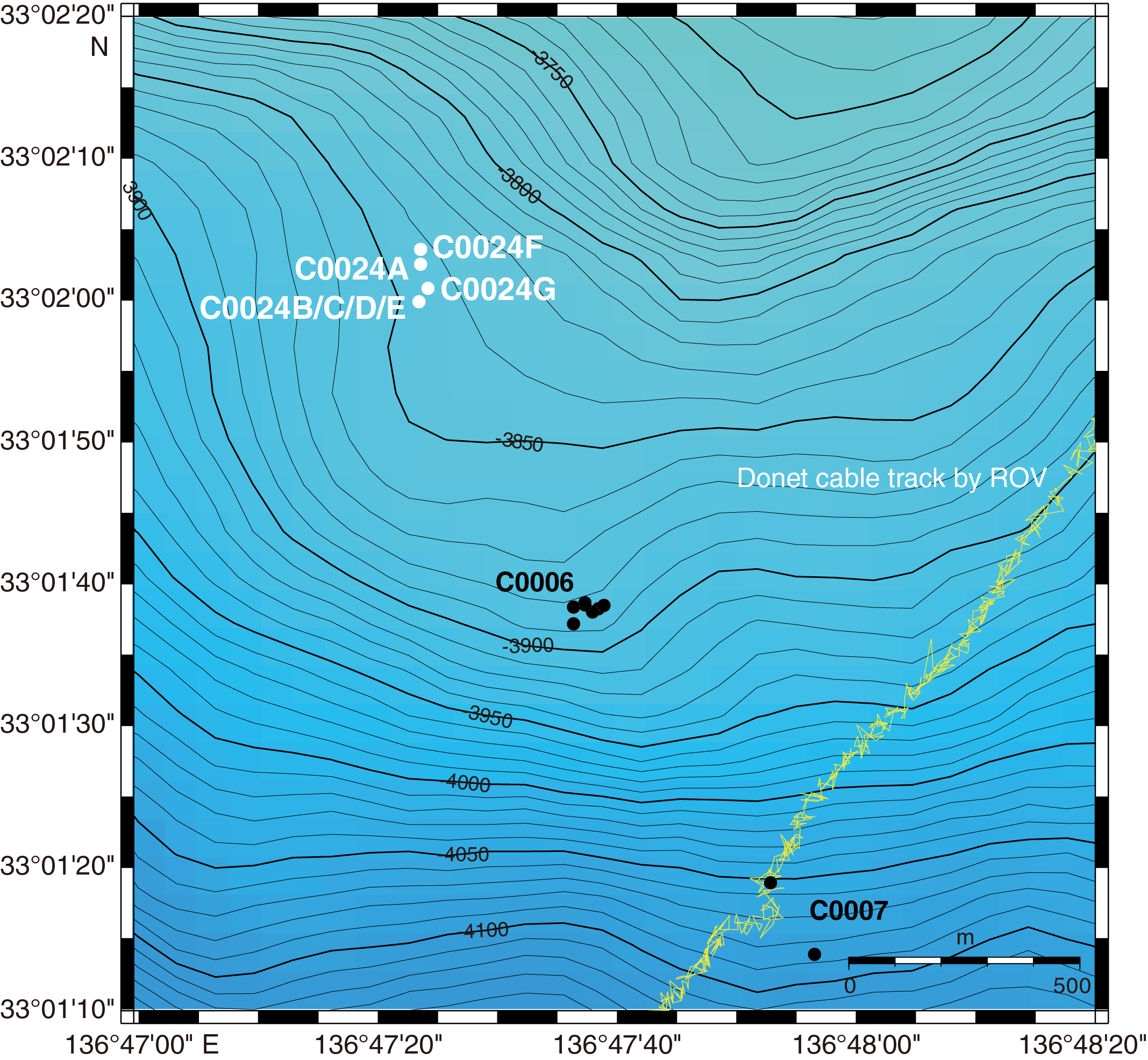
Figure F1. Area map.
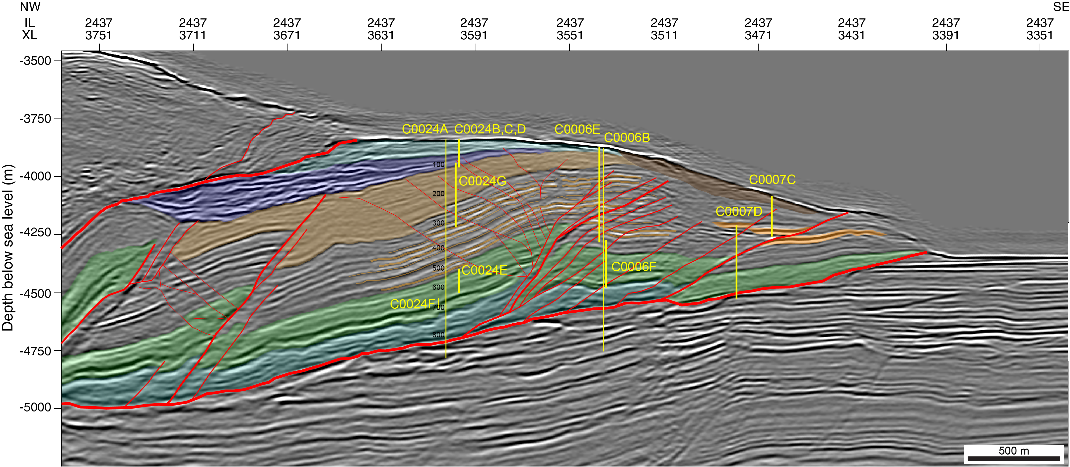
Figure F2. Interpreted seismic depth section.
The NanTroSEIZE project drilled sites near Site C0024 during three previous expeditions, Integrated Ocean Drilling Program Expeditions 314 and 316 and IODP Expedition 380 (Expedition 314 Scientists, 2009; Expedition 316 Scientists, 2009a; Kinoshita et al., 2018). Expedition 314 drilled to 885.5 meters below seafloor (mbsf) with logging while drilling (LWD) at Site C0006 and penetrated through the plate boundary décollement. Expedition 316 cored the sediments of the accretionary prism at Sites C0006 and C0007 and the plate boundary décollement zone at Site C0007 (Kimura et al., 2008; Expedition 316 Scientists, 2009a; Screaton et al., 2009a, 2009b).
The expeditions documented rapid growth of the outer accretionary prism since ~2.2 Ma (Screaton et al., 2009b; Strasser et al., 2009). Another significant result was evidence for rapid slip along the frontal décollement on the basis of a vitrinite reflectance that recorded a thermal anomaly indicative of frictional heating (Sakaguchi et al., 2011; Yamaguchi et al., 2011; Fulton and Harris, 2012). The slip rate was considered rapid enough to generate a tsunami near the trench (Hamada et al., 2015). The 2011 Tohoku-Oki Mw 9.1 earthquake documented that a large and runaway slip could reach to the trench and generate a large tsunami. The geological record from the frontal décollement at Site C0007 also suggests a possible tsunamigenic rapid slip along the frontal décollement, although the age of the event has not been constrained.
A significant progression in seismology since the initiation of the Integrated Ocean Drilling Program is the observation of shallow slow earthquakes and tremors in the Nankai Trough and other subduction zones (e.g., Obara, 2002; Ito et al., 2007, 2009; Obara and Kato, 2016). These earthquakes and tremors are located beneath or in the accretionary prism and mainly within and along the base of the outermost 40 km of the fore arc (Ito et al., 2007, 2009; Sugioka et al., 2012). The causal relationship between the coseismic large slip and interseismic (pre and/or post) slow slip is a key scientific target of a wide range of investigations.
Additionally, the 1 April 2016 off-Mie Mw 6.0 earthquake took place along the plate boundary megathrust (Wallace et al., 2016). A slow slip event (SSE) and tremors followed the earthquake and propagated to the frontal part of décollement (Wallace et al., 2016; Araki et al., 2017). This triggered SSE represents one of several repeating shallow SSEs (some triggered and some spontaneously occurring) accompanied by shallow low-frequency earthquakes with low-angle thrust focal mechanisms (e.g., Araki et al., 2017; Nakano et al., 2018). Recent shallow SSEs have also been detected by Global Navigation Satellite System acoustic data (Yokota and Ishikawa, 2019). These observations along with a need to better understand mechanical and hydrological properties and processes in the outer accretionary prism and along the shallow décollement motivated the installation of a borehole observatory at Site C0006 during Expedition 380.
As a contingency drilling site for Expedition 358, an additional drill site near the frontal thrust (Site C0024) was selected. This site lies north of Site C0006 and addresses the following primary scientific objectives:
- Document geophysical and geological properties and conditions in the hanging wall prism near the frontal thrust and above the décollement near the trench where SSEs may propagate and
- Characterize the architecture and properties of the décollement fault in the region near the trench.
Site C0024
To achieve these objectives, drilling operations at Site C0024 were planned to fill the following priorities: (1) LWD to penetrate through the plate boundary décollement, (2) deep coring to target the plate boundary décollement and the Shikoku Basin deposit correlated with the unrecovered part of Sites C0006 and C0007, and (3) shallow coring to document fault activities recorded in shallow sediments. Because of severe hole conditions during LWD, part of the shallow coring was conducted prior to deep coring.
Operations at Site C0024 (Figure F1; Table T1) began with preparations to set up the rotating guide roller and setting up the underwater TV (UWTV) in the moonpool at 0545 h (Japan Standard Time [JST]) on 4 March 2019 (see Table T2 in the Expedition 358 summary chapter [Tobin et al., 2020a]). The 8½ inch LWD bottom-hole assembly (BHA) (Table T2) was made up and run in the hole from 0730 h on 5 March, reaching 3813 m below rotary table (BRT) by 2400 h. The UWTV was set around the drill pipe in the moonpool and run down to conduct a seabed survey at 0330 h on 6 March. Three survey points for deep coring, LWD, and shallow coring holes were checked for any obstructions on the seabed. The seabed looked clear, and LWD Hole C0024A was spudded at 0715 h on 6 March.
Hole C0024A
The LWD BHA was spudded in and washed down from 3870 to 3950 m BRT by 1045 h. Spudding stopped so that the UWTV could be retrieved to the surface before drilling began. Drilling started at 1145 h and only paused for a series of surveys (N = 22) approximately every stand (~32 m). No major issues occurred with real-time data transmission during drilling. Nonstop driller connections every stand began at 0200 h on 8 March 2019. Reaming up and down started from 4731 m BRT at 0600 h on 9 March. Worsening hole conditions from the beginning of reaming resulted in the decision to halt drilling at 4738 m BRT (868 mbsf) at 0845 h on 9 March. While pulling out of the hole, the LWD BHA was stopped to perform check shots for the seismicVISION tool starting at 4665 m BRT (795 mbsf). After the BHA was pulled out of the hole above 4440 m BRT (570 mbsf) by 1930 h on 9 March, it could not pass below this point again. Repeat logs were conducted from 4180 to 4130 m BRT and from 3885 to 3867 m BRT. The LWD BHA was laid out by 1700 h on 10 March.
Holes C0024B–C0024D
After the LWD BHA was laid out and a short waiting on weather break, the derrick was inspected after it was struck by lightning. The inner core barrel was spaced out in the auxiliary well while the 10⅝ inch hydraulic piston coring system (HPCS)/extended punch coring system (EPCS)/extended shoe coring system (ESCS) BHA (Table T2) was made up and run in the hole. Another waiting on weather pause occurred as a cold front passed. The HPCS/EPCS/ESCS BHA was run to the seafloor while the D/V Chikyu shifted approximately 40 m to begin coring. At 0100 h on 12 March 2019, HPCS Core 358-C0024B-1H was cut (Table T3). Overpull of 70 kN occurred when trying to recover the inner barrel (see Table T2 in the Expedition 358 summary chapter [Tobin et al., 2020a]), so the BHA was pulled above the seafloor (drawworks assist) to allow recovery. The HPCS BHA was run to 6 mbsf in Hole C0024C to shoot the second core (358-C0024C-1H) with a 1 m advance. Again, significant overpull required the drawworks to pull the BHA above the seafloor to recover the inner core barrel. The HPCS BHA was run again to 7 mbsf in Hole C0024D to shoot the next core (358-C0024D-1H); at this point, the formation was hard enough to confirm that the same hole was reentered for further coring. At 3902 m BRT (30 mbsf), HPCS coring was replaced in succession by EPCS, ESCS, EPCS, and finally ESCS coring and drilling ahead for each core. When coring reached 4000 m BRT (128 mbsf), the inner barrel pull bar broke, requiring the BHA to be pulled out of the hole to recover the inner barrel. The decision was made to abandon shallow coring in this hole on 13 March. By 0600 h on 14 March, the inner barrel was laid out and preparations for rotary core barrel (RCB) coring began.
Hole C0024E
The 10⅝ inch RCB BHA (Table T2) was made up and run in the hole at 1345 h on 14 March 2019. Hole C0024E was spudded in at 0315 h on 15 March, washed down from 3872 to 3879 m BRT (0–7 mbsf), and drilled down from 3879 to 4382 m BRT (7–510 mbsf). Cutting and retrieving RCB cores began at 0615 h on 16 March. Coring continued to 4493.5 m BRT (621.5 mbsf; Core 358-C0024E-12R) at 0630 h on 18 March without any hole condition problems (Table T3). However, standpipe pressure fluctuation was observed twice while dropping the inner barrel for Core 13R, and pressure increased from 1.9 to 5.1 MPa. Reaming up and down between 4492.5 and 4456 m BRT (620.5–584 mbsf) was conducted, but hole conditions worsened. The decision to stop coring was made at 0745 h on 18 March, and the BHA was pulled out of the hole to 111 m above the seabed by 1015 h on 18 March.
Hole C0024F
The same BHA used in Hole C0024E (Table T2) was spudded in Hole C0024F at 1915 h on 18 March 2019 to core deeper than the bottom of Hole C0024E. Drilling without coring continued to 4589.5 m BRT (721.5 mbsf). While drilling from 4442 to 4599 m BRT (574–731 mbsf), hole conditions became worse, with an increase in standpipe pressure, hydraulic power swivel stall, overtorque, and overpull. The BHA was pulled out of the hole to 4553 m BRT (691 mbsf) for a sinker bar running simulation (pump and rotate strings at 100 gal/min × 1.3 MPa and 10 rpm × 1–4 kNm for 30 min and then stop pumping and rotation for 10 min) to confirm whether hole conditions were manageable for coring. The center bit was recovered at 0400 h to attempt coring. However, torque fluctuation, standpipe pressure increase, and string stall were frequently observed, so the BHA was pulled out of the hole and recovered on deck at 1945 h on 21 March. Several 10 cm pieces were recovered from the bit and registered as a "ghost core" (358-C0024F-1G).
Hole C0024G
To extend the shallow core interval, the BHA was again changed from RCB to ESCS coring (Table T2) and spudded in Hole C0024G at 1045 h on 22 March 2019. Drilling continued to the coring start depth at 3971.5 m BRT (100 mbsf). Core cutting with the ESCS began at 1845 h on 22 March, and the target depth was reached at 4191.0 m BRT (319.5 mbsf) by 0345 h on 25 March. A total of 24 ESCS cores were collected (Table T3).
Transponders were recovered by the watch boat while the BHA was pulled out of the hole. Operations at Site C0024 were completed by 2100 h on 25 March, and the ship started moving to Site C0025.
Lithology
We documented the lithologic character of cores from five holes at Site C0024 (Holes C0024B–C0024E and C0024G). Coring systems included the HPCS, ESCS, EPCS, and the RCB system. Sediments from shallow cores are unconsolidated (e.g., sand), whereas equivalent lithologies in RCB cores are lithified (e.g., sandstone). The material in Core 358-C0024C-1H was thoroughly fragmented and mixed to slurry by coring disturbance and flow-in, so it was not used in facies description or interpretation. The combined depth interval for all of the cores extends from the seafloor to 621.50 mbsf (Figure F3), but a coring gap occurs between 318.9 mbsf in Hole C0024G and 510 mbsf in Hole C0024E (Table T4).
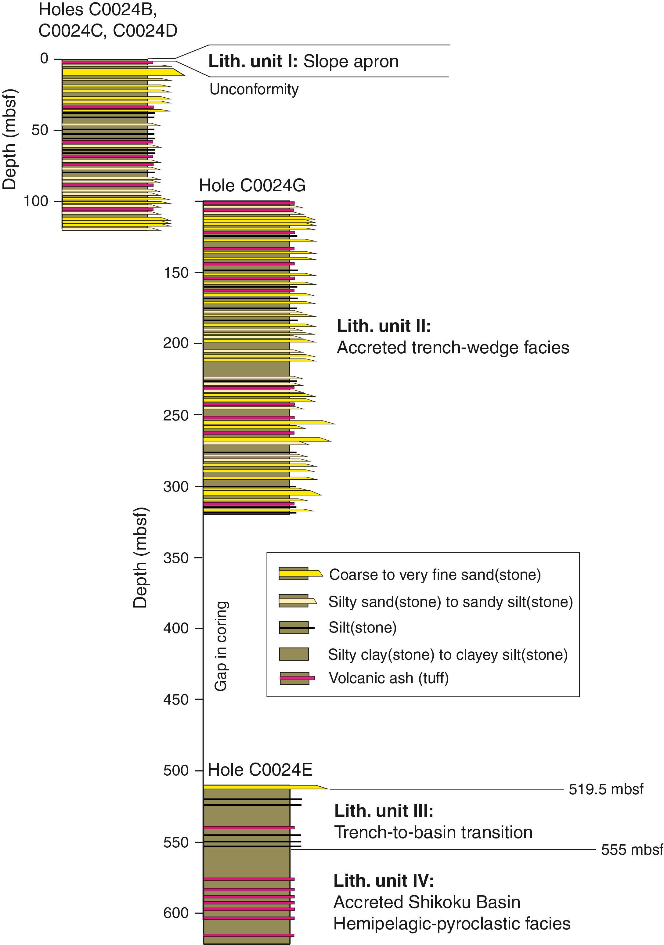
Figure F3. Composite stratigraphic column.
Each lithology was characterized based on visual observations of the split core, smear slide petrography, bulk powder X-ray diffraction (XRD), and bulk sediment X-ray fluorescence (XRF) (see Lithology in the Expedition 358 methods chapter [Hirose et al., 2020]). We also considered the attributes of logging units from Hole C0024A (see Logging), relevant measurements of physical properties (see Physical properties), and information from broadly correlative facies that were sampled previously at nearby Sites C0006 and C0007 (Expedition 316 Scientists, 2009a, 2009b). Strata incorporated into the frontal accretionary prism include the upper part of the Shikoku Basin as well as trench-wedge sediment (Screaton et al., 2009a). We assigned the sediments and sedimentary rocks at the scale of depositional facies to four lithologic units (Figure F3). Sedimentologic criteria for those divisions include grain size, bed thickness and geometry, composition, internal sedimentary structures, and inferred mode of deposition. The depositional ages assigned to each lithologic unit are based on biostratigraphy and magnetostratigraphy data (see Biostratigraphy and Paleomagnetism).
Unit I (slope facies)
Description and interpretation of lithology
Lithologic Unit I is composed of silty clay to clayey silt. We set the base of Unit I at the top of the uppermost turbidite in Hole C0024B at 3.76 mbsf (Figure F4). No age-diagnostic nannofossils were identified in this interval, so the Holocene age is only inferred. Our provisional interpretation for the depositional environment is hemipelagic suspension fall out above an unconformity that truncates the top of the accretionary prism.
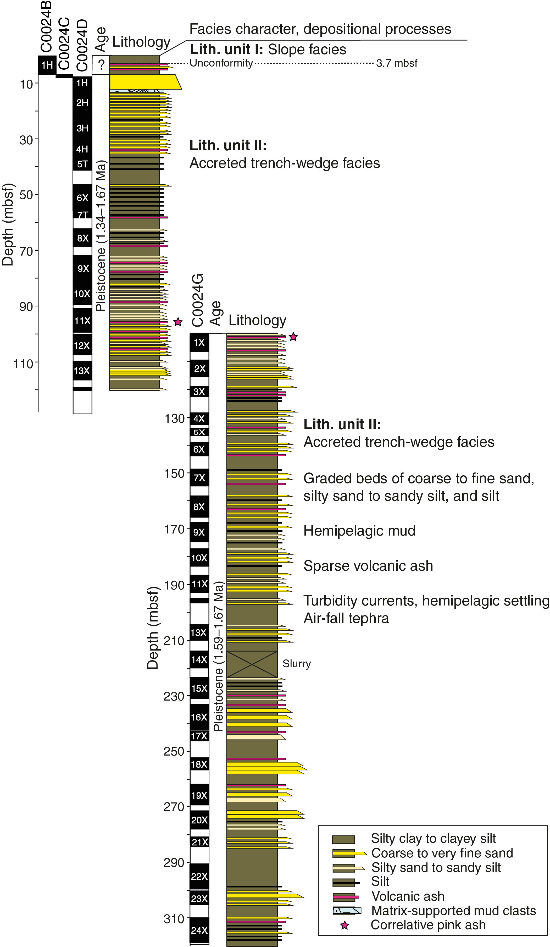
Figure F4. Lithologic Unit I and II stratigraphic columns.
Unit II (trench-wedge facies)
- Intervals: 358-C0024B-1H-4, 120 cm, to 1H-CC, 50 cm; 358-C0024C-1H-1, 0 cm, to 1H-CC, 18 cm; 358-C0024D-1H-1, 0 cm, to 14X-CC, 87 cm; 358-C0024E-1R-1, 0 cm, to 1R-CC, 17 cm; 358-C0024G-1X-1, 0 cm, to 24X-CC, 40 cm
- Depth: 3.76–519.50 mbsf
- Age: early to middle Pleistocene (1.34–2.45 Ma) or early to late Pleistocene (≤0.78–2.45 Ma)
Description of lithologies
Most of Lithologic Unit II is composed of four lithologies in a continuum of gradational attributes: silty clay to clayey silt, fine to coarse silt, sandy silt to silty sand, and very fine to coarse sand (Figure F4). Scattered beds of volcanic ash are also present (Figure F5). The sand- and silt-rich beds typically display normal size grading, and most such beds are thin. In Hole C0024G, many of the sand beds are thicker (>10 cm), and their grain size coarsens to medium and coarse sand (Figure F6). Nannofossil dating suggests a prominent unconformity at the top of Unit II with a minimum age of 1.34 Ma and that most of Unit II is 1.59–1.67 Ma in age (see Biostratigraphy). These ages correspond to the Matuyama Chron of reversed magnetic polarity. However, paleomagnetic data indicate consistently normal polarity to 278 mbsf and dominantly reversed polarity below, suggesting that the Brunhes/Matuyama boundary (0.78 Ma) is located there (see Paleomagnetism). In this case, most of Unit II is younger than 0.78 Ma. The oldest dated interval in Unit II is from Section 358-C0024E-1R-CC (at 512.365 mbsf; below the coring gap), and those nannofossils yield an age range of 2.06–2.45 Ma.

Figure F5. Unit II lithologies, Holes C0024D and C0024G.
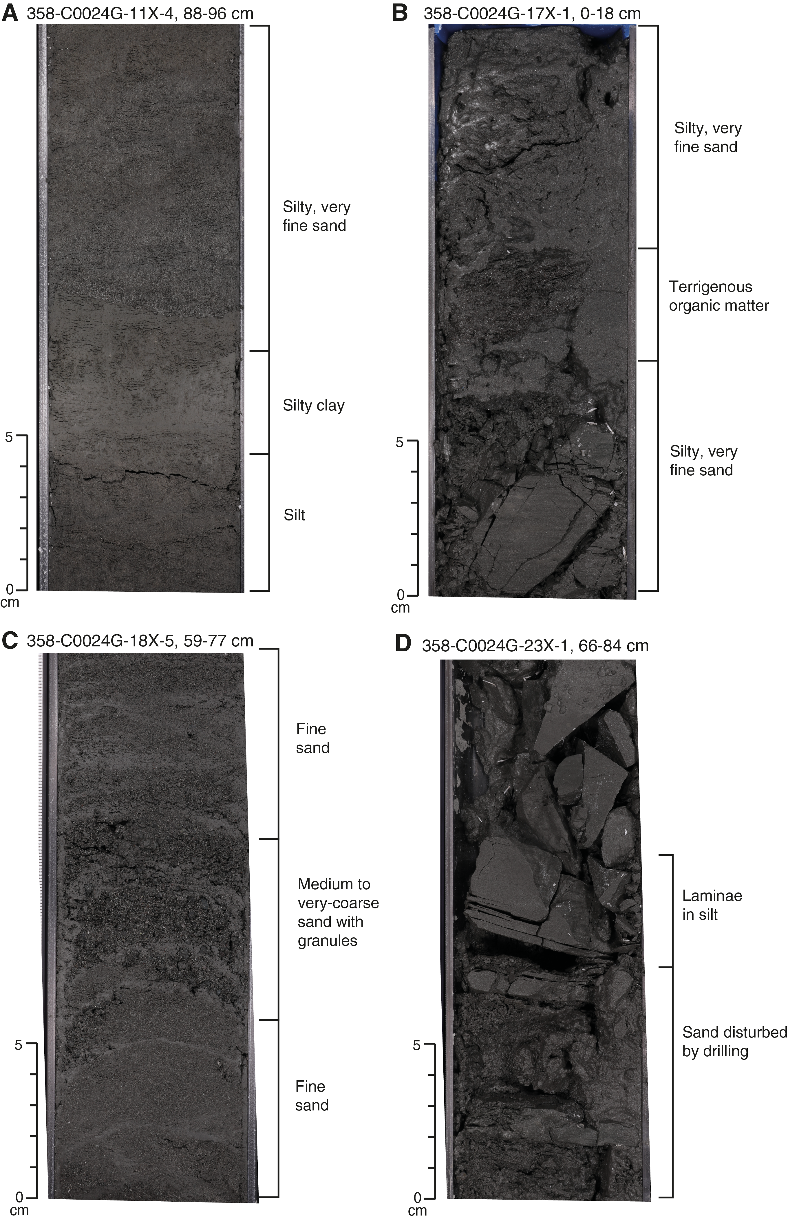
Figure F6. Unit II lithologies, Hole C0024G.
The background sediment of silty clay to clayey silt is gray to dark olive-gray. Changes in color are related to variable proportions of clay- and silt-sized grains, together with minute biopelagic grains (e.g., calcareous nannofossils) and dispersed vitric fragments. Rare sedimentary structures include parallel lamination, but most of the fine-grained sediment is mottled or structureless (Figure F5A). Laminations are formed by silt grains. We also found scattered pumice clasts and sand-sized microfossils (e.g., foraminifers and sponge spicules) (Figure F5A). Some cores contain scattered patches with higher concentrations of sand and/or silt, although their presence might be due to coring disturbance. Terrigenous organic matter and lamination are noteworthy in Sections 358-C0024G-16X-9 through 24X-CC. Except for the mottled colors, manifestations of bioturbation are rare.
The second common lithology, coarse to very fine sand, is darker gray than the silty clay (Figure F5B). One unusual bed in interval 358-C0024G-18X-5, 64–70 cm (Figure F6C), contains granule-sized clasts with a wide range of compositions. Those clast lithologies include granite, diorite, andesite, basalt, metasedimentary rock, mudstone, vein quartz or quartzite, and chert (Figure F7). The typical beds of sand are very thin (few millimeters) to thin (~2 cm). In rare cases, thicknesses increase to >10 cm. Some of the thicker examples are disrupted to slurry, however, and their apparent thicknesses are probably artifacts of drilling disturbance. Most of the sand deposits display normal size grading and sharp bases; the lowermost parts of some such beds are dark gray (rich in opaque grains and pyrite) or light gray to white (rich in microfossils). Pumice clasts also occur near some bases. Planar laminations are more common near the tops of beds, where they grade into overlying silty clay.
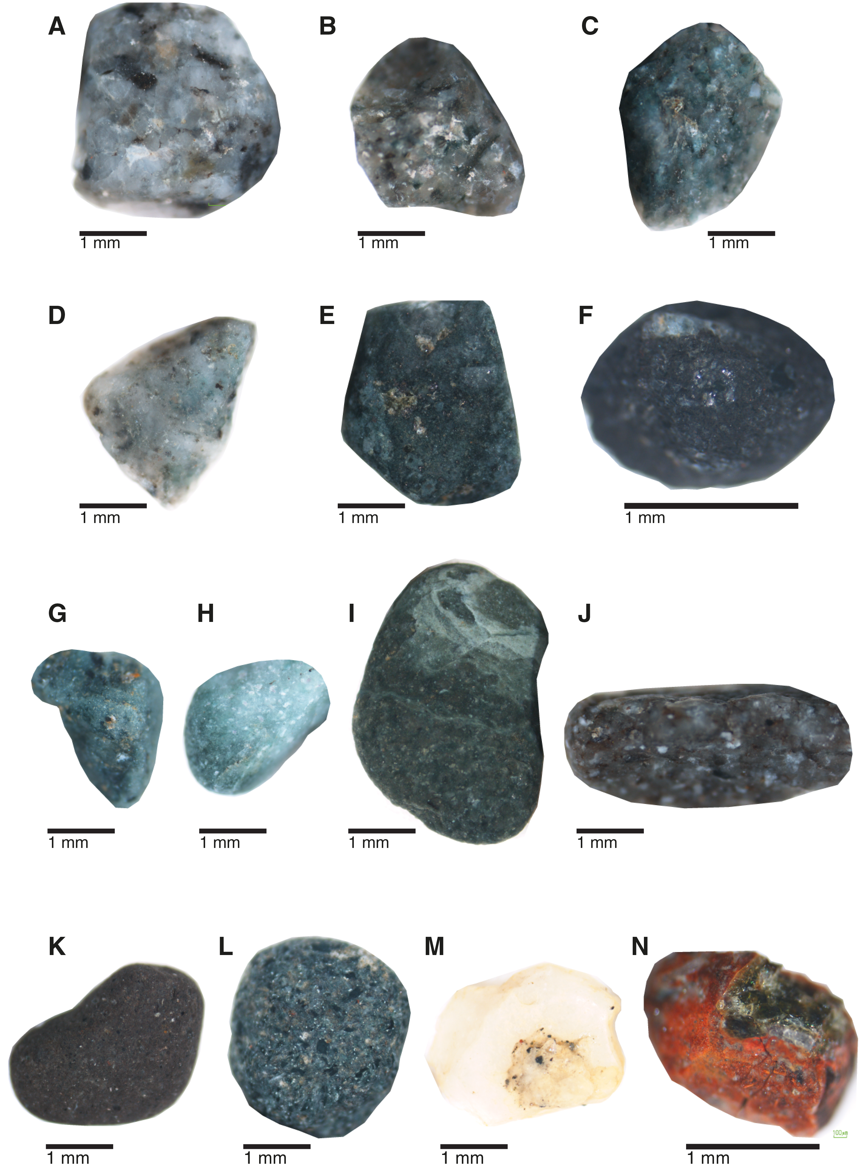
Figure F7. Granules in very coarse sand in Unit II.
Beds of finer grained silt, sandy silt, and silty sand are similar in color to those of the coarse to very fine sand. Most of the silty beds are likewise very thin to thin and display sharp bases, normal size grading, and gradational (diffuse) tops that merge into silty clay. From Core 358-C0024G-16X to the bottom of Hole C0024G, beds of sandy silt to silty sand are more consolidated and planar in geometry. They cluster in stacked graded beds with low-angle cross-lamination. Some laminations are highlighted by organic matter. The stacked planar beds typically alternate with a slurry of very fine to medium sand. Another variety is gray yellowish brown to reddish brown and contains mixtures of volcaniclastic (vitric) and siliciclastic grains; the thickest such bed (~6 m) occurs at 7–13 mbsf in Cores 358-C0024C-1H and 358-C0024D-1H (Figure F4). Coring disturbance, however, renders the archived thickness of that deposit unreliable.
A total of 30 thin to thick beds of volcanic ash were recovered from Unit II (see EVENTBED in Supplementary material for tabulated results). These discrete layers are diverse, with colors ranging from light gray to light brown, reddish brown, pink-grayish brown, beige, and pinkish orange. Such colors reflect the variable proportions of glass shards, siliciclastic rock fragments, primary crystals, nannofossils, and opaque grains (Figure F5C). Most of the ash layers show a sharp base and lack internal structure. Some layers display normal size grading and erosive bases. The tops are generally irregular to diffuse. We found one particularly distinctive pinkish ash layer in Sections 358-C0024D-11X-7 and 358-C0024G-1X-3 (archived depths of 96.77 and 101.99 mbsf, respectively). Incomplete core recovery means that the bed's archived depths might be offset by 4–5 m from its true in situ depth, but we used this ash bed (Figure F5C, F5D) to correlate the stratigraphic column for Hole C0024D with the column for Hole C0024G (Figure F4).
We found one bed of matrix-supported mud-clast conglomerate, a minor lithology, in Section 358-C0024D-2H-2 (Figure F4). The bed is 17 cm thick and was probably deposited from a small debris flow that entrained remobilized fragments of cohesive sediment.
Strata assigned to Unit II also occur in the first core recovered from Hole C0024E (Table T4). That sediment is composed of one very thick bed of poorly consolidated dark gray muddy sandstone to silty sandstone. No sedimentary structures are evident. The core is highly disturbed with fractures and biscuits induced by RCB drilling, so the archived thickness is probably distorted. Furthermore, the large coring gap between the bottom of Hole C0024G and the top of Hole C0024E (Figure F3) places this deposit out of stratigraphic context.
Petrography
Smear slides were used to record the compositional proportions and texture of common lithologies in Unit II from Site C0024 (for tabulated results, see Core descriptions; also see SMEARSLD in Supplementary material). Quartz and plagioclase are ubiquitous constituents of silty clay to clayey silt (Figures F8, F9). Grains of mica and heavy minerals are few to common. Clusters of clay minerals are dominant to abundant. Dispersed shards of volcanic glass and volcanic lithics are few to common and increase to abundant in several horizons (Figures F8, F9). Lithic fragments are common to abundant. Calcareous nannofossils are common to abundant; higher contents impart a lighter gray macroscopic color (e.g., Sections 358-C0024G-17X-4, 19X-7, and 22X-2). Fragments of diatoms, sponge spicules, radiolarians, foraminifers, silicoflagellates, and terrestrial organic matter are few to common, with several localized horizons of nannofossils and sponge spicules (Figures F8, F9). Opaque grains (e.g., pyrite) are common, and glauconite grains are few to common.
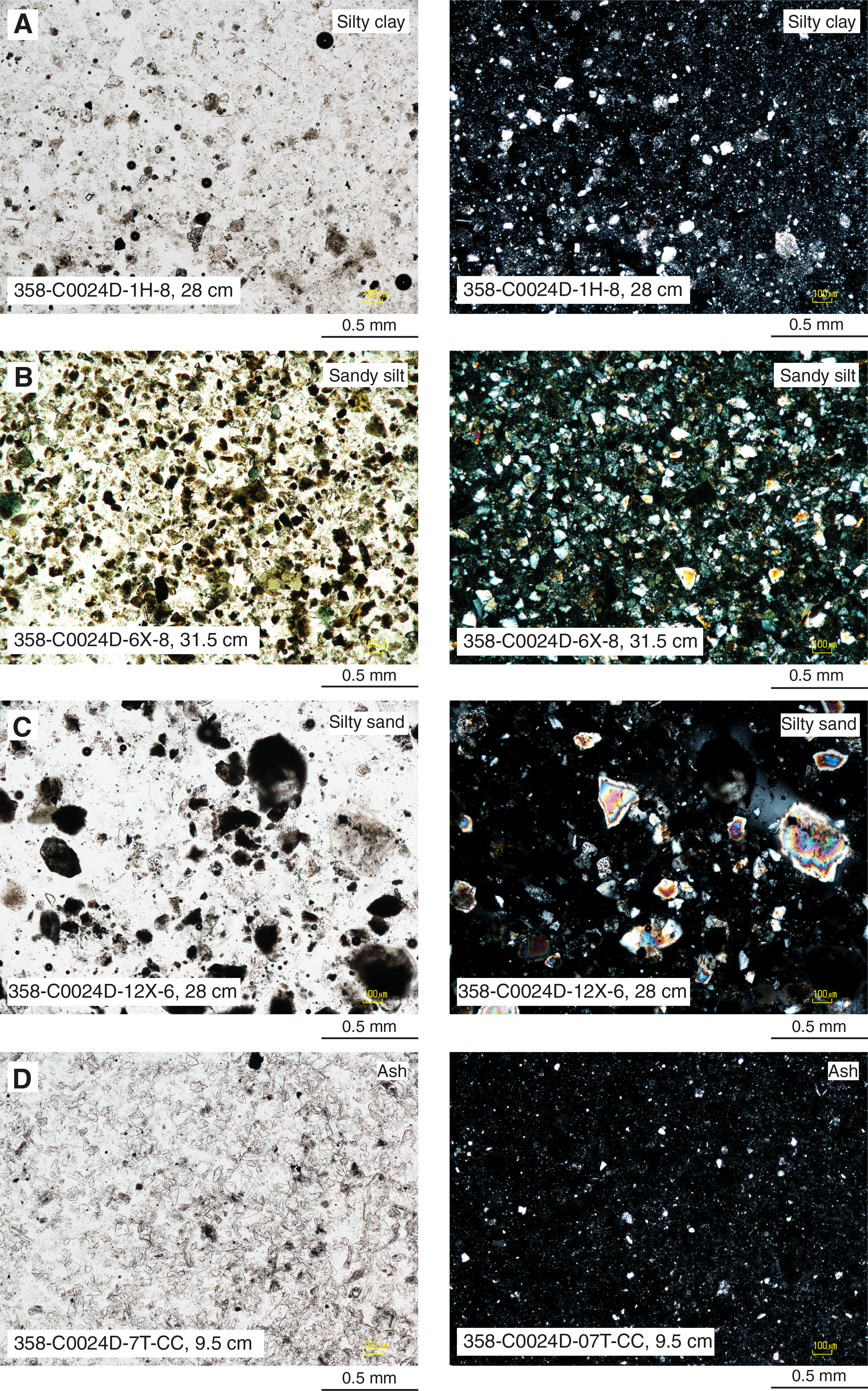
Figure F8. Unit II lithologies, Hole C0024D.

Figure F9. Unit II lithologies, Holes C0024E and C0024G.
The coarser grained granular lithologies in Unit II are classified compositionally as quartzofeldspathic. Angular to subangular quartz and feldspar grains are the main components (Figures F8, F9). Lithic fragments are common to abundant. Polycrystalline clasts are presumably of metamorphic origin; however, heavy alteration and small particle size render precise characterization difficult. Sedimentary lithic grains include lower birefringent mudstone, siltstone, and chert (polycrystalline quartz). Sand-sized, very dark to opaque grains are likely aggregates of clay minerals. Some carbonate clasts (higher birefringence) are also polycrystalline. Clear vitric fragments and volcanic lithic fragments are few to abundant. Grains of heavy minerals (pyroxene, amphibole, zircon, rutile, tourmaline, and apatite), glauconite, chlorite, biotite, and terrigenous organic matter are common. Lithic grains are typically coated with Mn oxide and/or clay. Nannofossils, foraminifers, and diatoms are few to common.
The predominant constituents of volcanic ash beds are clear silt- to sand-sized glass shards. Vesicular glass occurs among the coarser grains. Layers of volcanic ash (Figures F8D, F9D) vary significantly in terms of the abundance ranges of such secondary constituents as quartz, feldspar, and mica (few to common); volcanic lithic fragments (abundant to dominant); sedimentary lithic fragments and/or aggregates of clay to silty clay (common to rare); pyrite and other opaque grains (few to common); and calcareous nannofossils (few to abundant). In several specimens, vitric fragments are coated with clay, pyrite, and opaque minerals (Mn oxides). All of the ash beds contain minor to moderate quantities of siliciclastic material. Calcareous nannofossils are also abundant in some specimens.
Depth distribution of event beds
We recorded a total of 1112 event beds in Unit II (see EVENTBED in Supplementary material for tabulation). This total includes 30 layers of volcanic ash and 1081 inferred turbidites, with grain sizes ranging from silt to coarse sand. A few of the turbidites are present in the overlap between Holes C0024D and C0024G (Figure F4). Furthermore, because of coring disturbance, some of the designated event beds are suspect, essentially transformed into slurry between biscuits of more cohesive mudstone. Core recovery averaged 67% in Unit II (Figure F4), so the number of beds recovered significantly underestimates the number in situ.
The depth distribution and cumulative thickness of event beds are illustrated in Figure F10A. Ash beds are not abundant enough to define any trends with depth or age. For the turbidites, we recognize a coarsening-upward trend from ~320 to 230 mbsf. A prominent cluster of thick to very thick beds is also obvious between ~270 and 230 mbsf. That interval is where most of the medium to coarse sand beds were found. Three thick to very thick beds were measured around 230 mbsf; however, judging from their grain size (silty sand), the absence of internal sedimentary structures, and obvious coring disturbance (soupy to slurry), we regard their apparent thicknesses as artifacts. Above that sandy interval, the trend is fining upward from ~230 (in Hole C0024G) to ~58 mbsf (in Hole C0024D). Generally, the upper part of the section is coarser, and a coarsening-upward trend is apparent from ~40 mbsf to the seafloor (Figure F10A).
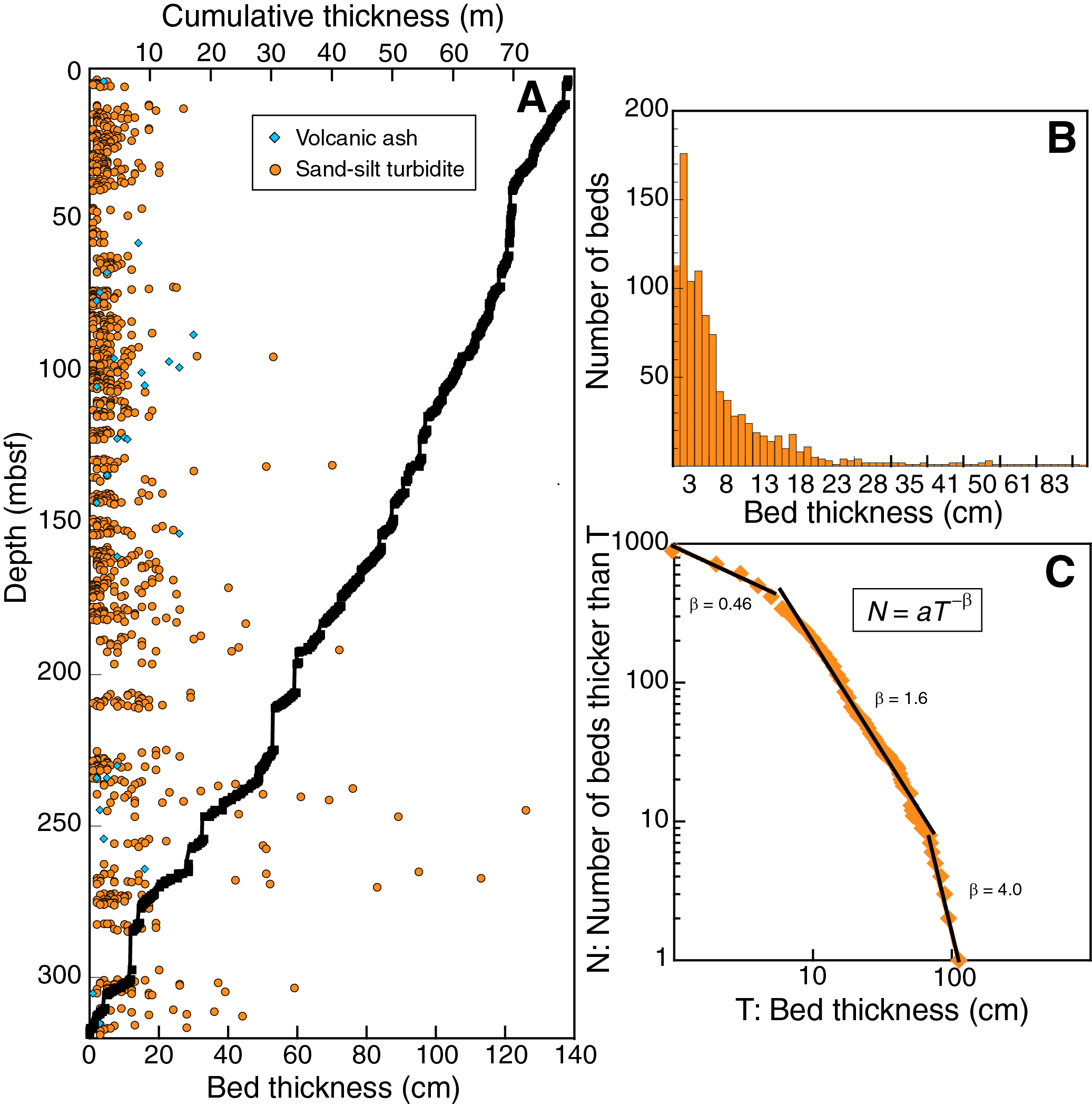
Figure F10. Analysis of event bed frequency, Unit II.
X-ray fluorescence
We used XRF analysis of bulk sediment samples to quantify compositional trends of silty clay(stone) with depth (Table T5). The XRF samples were usually colocated in "clusters" next to whole-round samples (e.g., for interstitial water [IW]) together with specimens for XRD and coulometric carbon measurements. The results provide contents of major and minor element oxides (SiO2, Al2O3, CaO, K2O, Na2O, Fe2O3, MgO, TiO2, P2O5, and MnO) complemented by loss on ignition (LOI) measurements.
The XRF results for Unit II are displayed in Figure F11. CaO values show considerable scatter above ~100 mbsf, probably in response to variable proportions of calcareous nannofossils. We also see variability in TiO2 and LOI values in the upper part of the unit. Overall, however, bulk sediment geochemistry changes very little with depth.
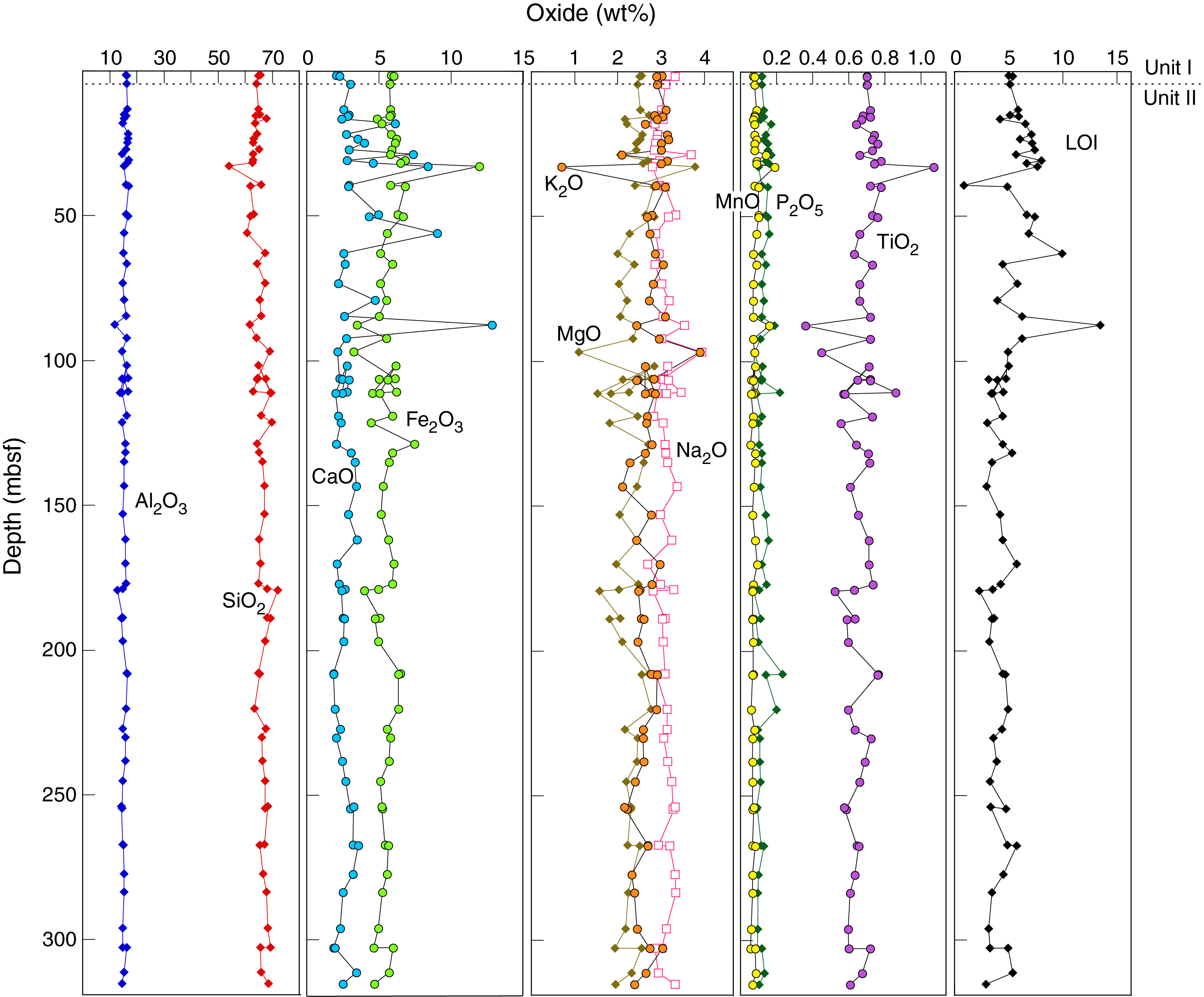
Figure F11. XRF chemical compositions, Units I and II.
X-ray diffraction mineralogy
We routinely used XRD to calculate proportions of common minerals in the dominant lithology of silty clay(stone) to clayey silt(stone), where total clay minerals + quartz + feldspar + calcite = 100%. Most of the specimens were colocated in clusters next to whole-round intervals. In some cases, handpicked samples of minor lithologies (e.g., volcanic ash and clay-rich bands) were analyzed to verify their compositions.
Data from Lithologic Unit II are displayed in Figure F12 and tabulated in Table T6. We do not observe systematic trends or shifts in composition with depth. Calcite is above the detection limit in many samples with an average normalized abundance of 2.3 wt%; the highest value is 17.7 wt%. These results correlate well with coulometric carbonate data (see Geochemistry). The average total clay mineral content is 35.9 wt% (range = 20.8–58.3 wt%). The average quartz content is 29.7 wt% (range = 18.5–37.7 wt%). Feldspar content ranges from 18.9 to 45.4 wt% (average = 32.1 wt%). The data show considerable scatter throughout Unit II that we attribute to differences in grain size. In other words, some of the specimens were extracted from beds of silt or silty sand rather than silty clay. Proportions of clay minerals are higher in silty clay(stone), and proportions of feldspar are higher in silt-rich beds. XRD also confirms the abundance of glass shards in three ash deposits (Table T6); the amorphous grains cause elevated baseline counts.
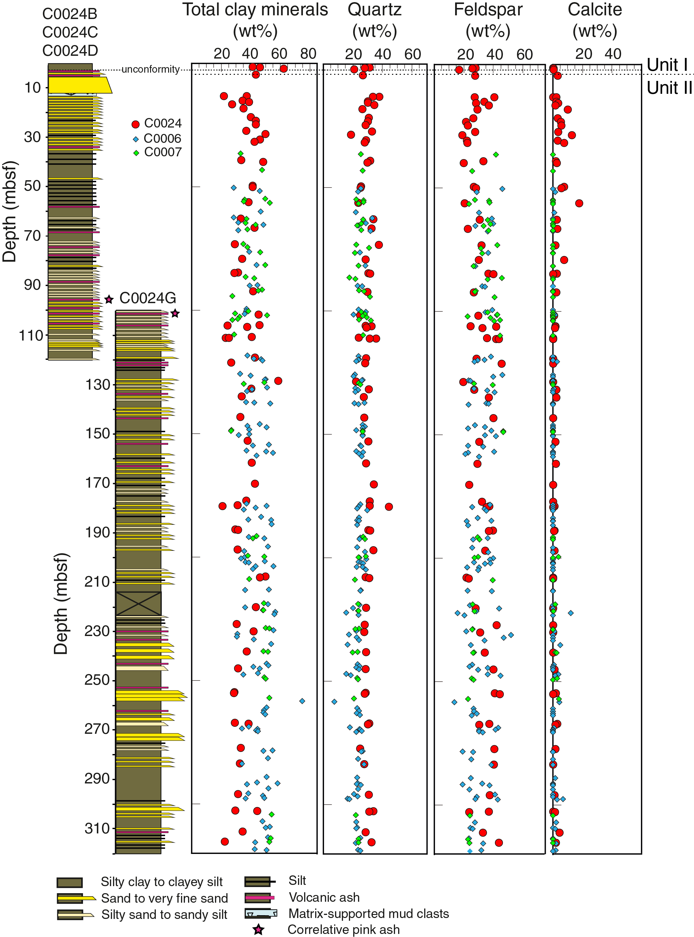
Figure F12. Bulk powder XRD, Units I and II.
For broader context, Figure F12 also shows bulk powder XRD values for comparative trench-wedge facies from Sites C0006 and C0007 (Expedition 316 Scientists, 2009a, 2009b). We note here that the correlation is based on facies character rather than age. The data sets match closely in terms of both scatter and averages. These results are good indicators of consistent precision in XRD methods over the duration of the NanTroSEIZE project, in spite of such changes as instrument replacement and recalculation of singular value decomposition (SVD) normalization factors (see Lithology in the Expedition 358 methods chapter [Hirose et al., 2020]).
Interpretation of depositional processes and environment
We interpret the mottled and structureless mud in Unit II (silty clay to clayey silt), which has modest nannofossil contents, to be the commonplace product of sustained hemipelagic settling in a deepwater environment near the calcite compensation depth. We interpret the structureless and normally graded beds of coarse to medium sand, fine to very fine sand, muddy sand, sandy silt to silty sand, and silt to be products of sandy to silty turbidity currents. The turbidites are interspersed with fine-grained suspension fall-out deposits together with scattered beds of air fall volcanic ash. The structureless ash layers were probably deposited by settling of tephra through the water column. Conversely, the graded ash layers with irregular bases and high contents of nonvolcanic grains (i.e., clay, quartz, and nannofossils) may have been reworked by density flows and transported downslope from their initial positions of deposition by explosive eruption.
The overall facies character of Unit II is consistent with the depositional processes expected in a trench-wedge environment (e.g., Underwood and Moore, 1995). The sustained background of slow hemipelagic settling in this type of environment is punctuated by frequent influxes by turbidity currents and related sediment gravity flows. The short recurrence interval of ~50 y for turbidites in Unit II means that multiple triggering mechanisms were probably in effect (e.g., earthquakes, flood-induced hyperpycnal flows, and typhoon-scale storm waves). Unlike comparable facies at Sites C0006 and C0007 (Expedition 316 Scientists, 2009a, 2009b), we recovered only a few medium- to coarse-grained sand beds, and no beds of gravel were recovered. Thus, if compared to nearby sections of accreted trench-wedge sediment in the hanging wall of the frontal thrust, the depositional environment represented by Unit II at Site C0024 was probably dominated by dilute unconfined flows rather than high-density axial-channel deposition. Most of the turbidity currents were probably funneled through large submarine canyons on the landward trench slope (e.g., Tenryu Canyon and Suruga Trough) and then transported downgradient through the trench-floor system. Postcruise studies of detrital provenance will be needed to refine the reconstruction of sediment routing over time, particularly the discrimination between transverse and trench-axis pathways.
Unit III (trench-to-basin transition)
- Interval: 358-C0024E-2R-1, 0 cm, to 6R-1, 0 cm
- Depth: 519.50–555.00 mbsf
- Age: early Pleistocene (2.06–2.45 Ma)
Description of lithologies
The Lithologic Unit II/III boundary appears to be conformable and is defined by a paucity of sand beds below. Nannofossils dated as 2.06–2.45 Ma reveal no contrast in age across the unit boundary (see Biostratigraphy). The dominant lithology in Unit III is silty claystone to clayey siltstone (Figure F13). Hole C0024E cores are disturbed by RCB drilling with ubiquitous drilling-induced fractures, biscuits, and soupy intervals that contain cuttings floating in a slurry of drilling mud. Intact pieces of the background mudstone (silty claystone to clayey siltstone) vary from gray to dark olive-gray and dark green. As in Unit II above, variations in color are caused by variable proportions of clay- and silt-sized grains together with calcareous nannofossils. Some intervals show mottled coloring associated with bioturbation (Figure F14A). Generally, the mudstone is structureless, with scattered and diffuse parallel lamination. Foraminifers are also present locally.
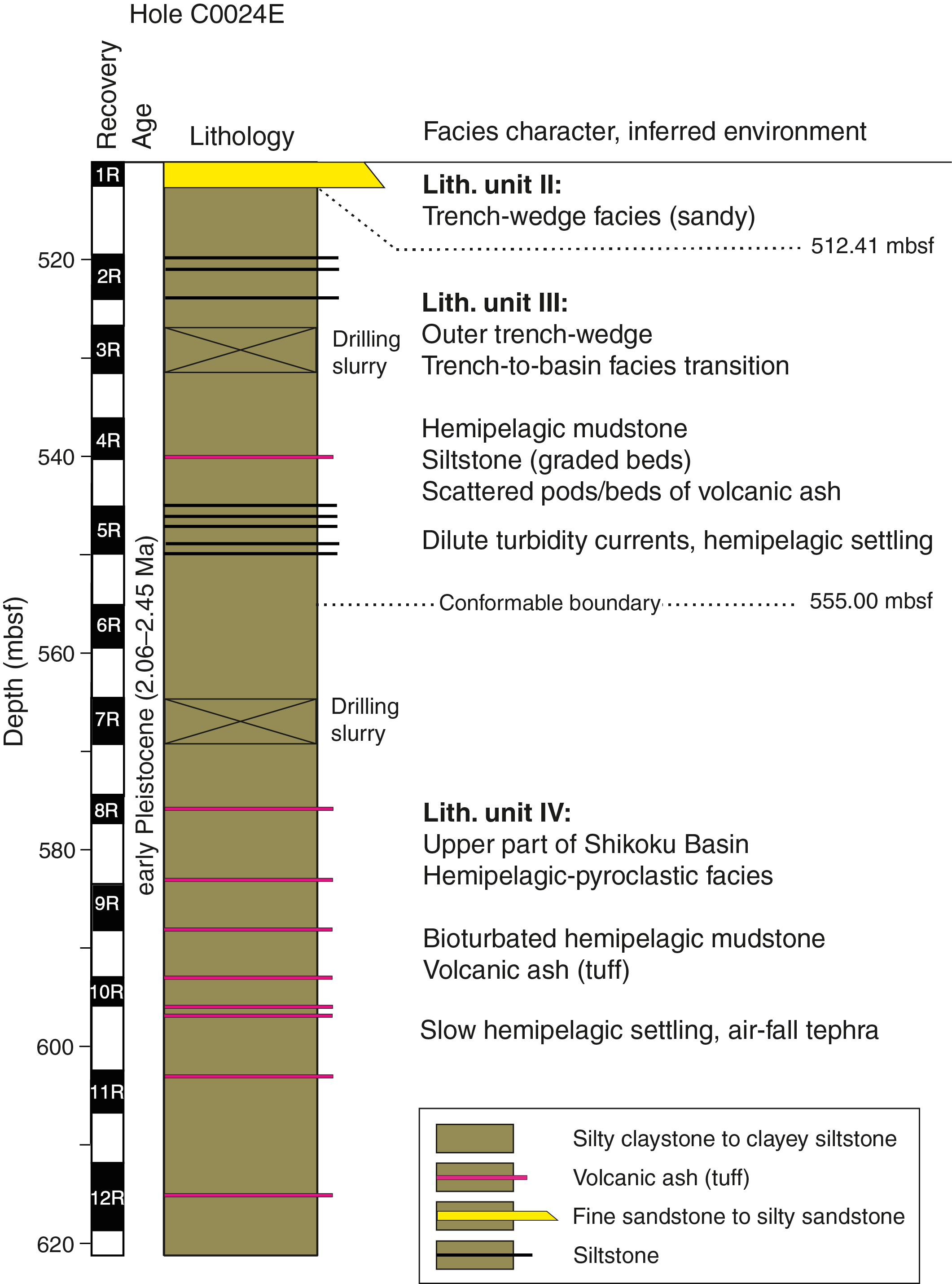
Figure F13. Lithologic Unit III and IV stratigraphic column.
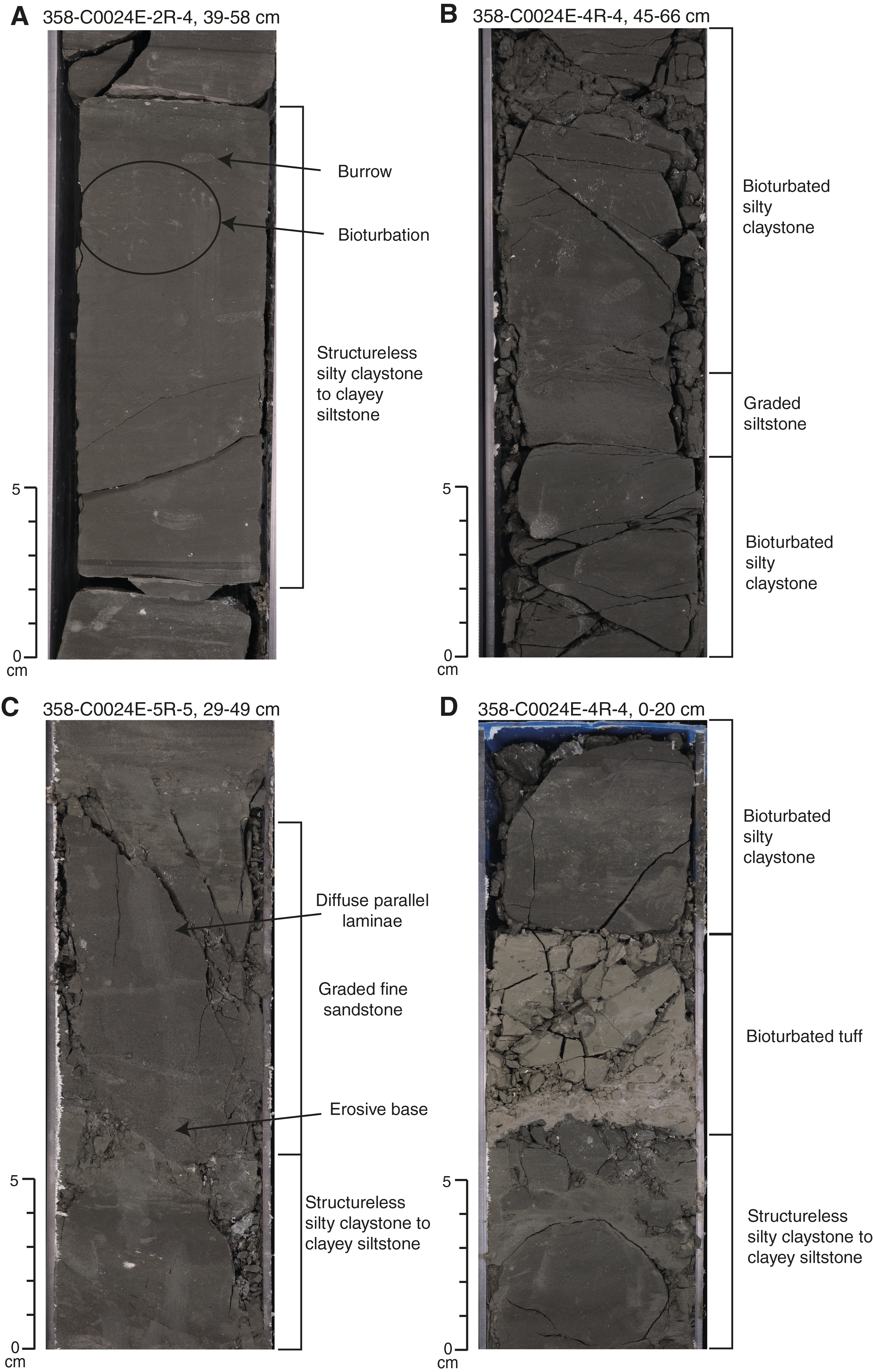
Figure F14. Typical Unit III facies.
Minor lithologies in Lithologic Unit III include very fine sandstone, siltstone, and volcanic ash or tuff. The beds of very fine sandstone and siltstone are very thin to thin and normally graded (Figure F14B, F14C). Graded beds are concentrated in the upper and basal parts of Unit III. One prominent tuffaceous layer at 539 mbsf is light to medium dark gray and shows extensive bioturbation (Figure F14D). The event beds are not abundant enough for statistical analyses of depth distribution; all of their occurrences, however, have been tabulated (see EVENTBED in Supplementary material).
Petrography
Smear slides demonstrate that the silty claystone to clayey siltstone in Unit III contains abundant to dominant quantities of clay minerals (Figure F15). For tabulated results, see Core descriptions (also see SMEARSLD in Supplementary material). Angular to subangular grains of quartz and feldspar are common to abundant. Grains of biotite and chlorite are few to common. Grains of glauconite (few) and opaque grains (common) are present. Clear angular shards of dispersed volcanic glass are few to common and have grain sizes consistently smaller than the bulk of the sediment. Carbonate is common in the form of calcareous nannofossils. Heavy minerals range from few to common, and the bulk is composed of amphibole, pyroxene, apatite, rutile, and zircon. Very dark to almost opaque polycrystalline grains of unidentifiable composition are abundant. They are either altered lithic fragments, clumps of mudstone that were not disaggregated, or rock fragments coated with Mn oxide.
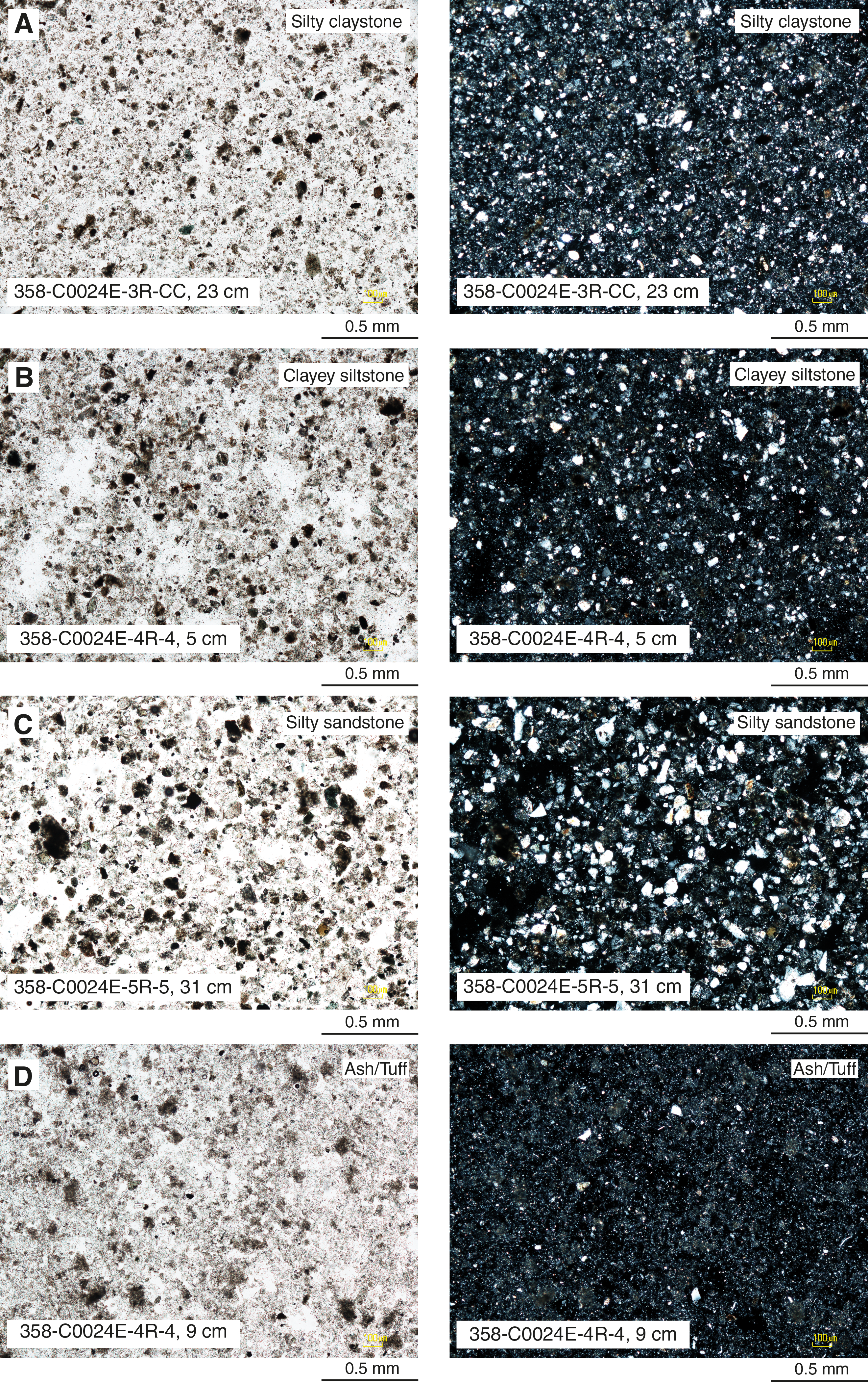
Figure F15. Representative Unit III lithologies.
The composition of siltstone to very fine sandstone is, apart from notably lower mica- and clay-mineral contents, equivalent to that of silty claystone to clayey siltstone. Samples of ash/tuff from Unit III are dominated by clear angular silt- to sand-sized glass shards. Clay minerals are abundant. Siliciclastic minerals and lithic fragments are also abundant in the ash layers and reveal the same composition as the equivalent grain size fractions in the typical silty claystone and siltstone.
X-ray fluorescence
Figure F16 illustrates depth-dependent variations in bulk sediment geochemistry for Hole C0024D based on XRF measurements. Compared to the one sandstone sample from Unit II (Core 358-C0024E-1R), the results from Unit III display significant increases in Fe2O3, TiO2, and LOI contents. For the most part, however, the values do not change significantly in Unit III. The exception is CaO, which decreases markedly below ~525 mbsf.
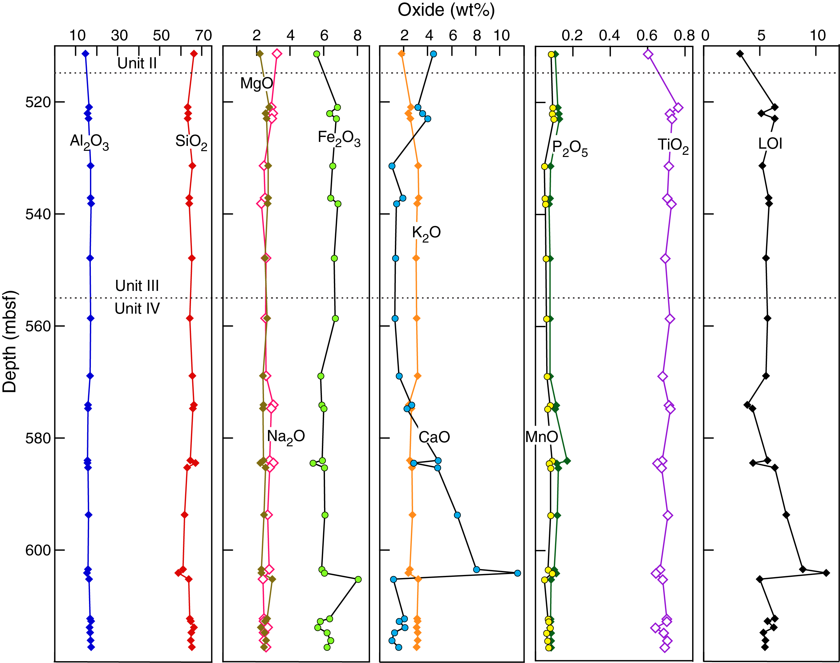
Figure F16. XRF chemical compositions, Hole C0024E.
X-ray diffraction mineralogy
Bulk powder XRD results for Unit III are shown in Figure F17 and tabulated in Table T6. Normalized relative proportions of total clay minerals range from 35.4 to 44.0 wt% (average = 39.1 wt%). Relative proportions of quartz range from 24.9 to 29.6 wt% (average = 27.1 wt%). The average abundance of feldspar is 30.9 wt% (range = 21.5–33.2 wt%). Calcite contents are above the detection limit with an average normalized value of 2.9 wt%. All of these values are similar to those in Unit II above (Figure F12).

Figure F17. Random bulk powder XRD, Units III and IV.
Interpretation of depositional environment for Unit III
We regard the intervals of structureless silty claystone to clayey siltstone in Unit III as deposits from sustained hemipelagic settling in an outer trench-wedge setting; that environment probably spanned across the bathymetric boundary between the seaward edge of the Nankai Trough and the subducting Shikoku Basin (e.g., Pickering et al., 1992). Thin to very thin beds of siltstone are probably related to entrained layers of turbidity currents that lapped onto or spilled over the seaward slope of the trench. This facies transition (trench-to-basin) is similar to the one documented at Ocean Drilling Program (ODP) Sites 808 and 1174 along the Muroto transect of Nankai Trough (Shipboard Scientific Party, 1991, 2001b), as well as Sites C0006 and C0007 (Expedition 316 Scientists, 2009a, 2009b; Underwood and Moore, 2012).
Unit IV (Shikoku Basin hemipelagic-pyroclastic facies)
- Interval: 358-C0024E-6R-1, 0 cm, through 358-C0024E-13G-2
- Depth: 555.00–621.50 mbsf
- Age: early Pleistocene (2.06–2.45 Ma)
Description of lithologies
The Lithologic Unit III/IV boundary appears to be conformable and is defined by the last occurrence (moving downsection) of trench-related silty turbidites (Figure F13). Nannofossils reveal no change in age (2.06–2.45 Ma) across the unit boundary (see Biostratigraphy). Positioning of the unit boundary at 555 mbsf (top of Core 358-C0024E-6R) also matches the top of an anomalous trend in porosity values (see Physical properties) and the top of a well-defined trend in XRD mineralogy (see below).
The dominant lithology in Unit IV is gray to olive-gray silty claystone to clayey siltstone. Disturbance by RCB drilling is moderate to high with some entire cores reduced to drilling breccia and slurry (Cores 358-C0024E-3R and 7R). Dark green color bands (clay rich) and irregular patches are distributed throughout the intact intervals of mudstone (Figure F18A). This background sediment shows mottled and patchy coloring resulting from intense bioturbation. Manifestations of bioturbation also include Zoophycos, Chondrites, and other unidentified trace fossils (Figure F18A, F18B). Burrows are typically filled with pyrite or volcanic ash (Figure F18C). Pyrite nodules, pumice clasts, ash pods, and foraminifer pods are also scattered throughout Unit IV (Figure F18D).
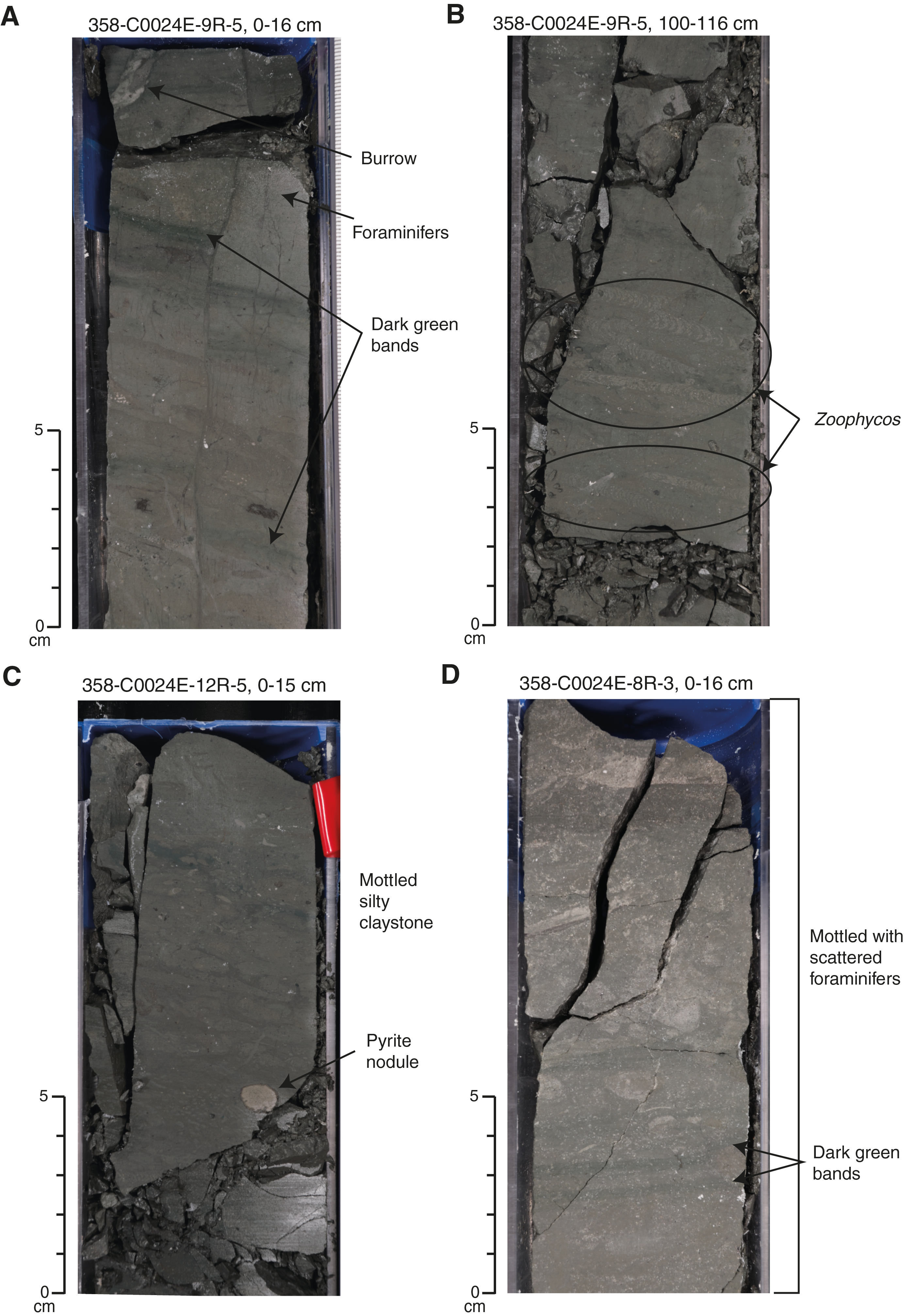
Figure F18. Typical Unit IV facies.
We recovered six thin beds of light gray poorly lithified tuff from Unit IV (Figure F13). The number of tuff layers increases significantly compared to Unit III, and that distinction provides another criterion for placement of the unit boundary. The event beds are not abundant enough for meaningful statistical analyses of depth distribution, but all of their occurrences have been tabulated (see EVENTBED in Supplementary material). In addition, the content of dispersed ash in silty claystone to clayey siltstone increases compared to similar lithologies in Unit III. The enrichment of dispersed ash is probably the main factor responsible for nearly constant porosity values in Unit IV (see Physical properties). This same type of anomaly is characteristic of the upper facies throughout the Shikoku Basin (Spinelli et al., 2007; White et al., 2011).
Petrography
The mineral composition and texture of specimens from Unit IV were determined using smear slides (Figure F19). Silty claystone to clayey siltstone contains clay minerals in abundant to dominant quantities. Mica grains are common; clear angular glass shards are common to abundant and dispersed throughout the unit. Calcareous nannofossils, foraminifers, and diatoms are generally rare except for several horizons with foraminifers (Figure F19C). Pyrite and other opaque grains (possibly Mn oxide–coated grains) are common.
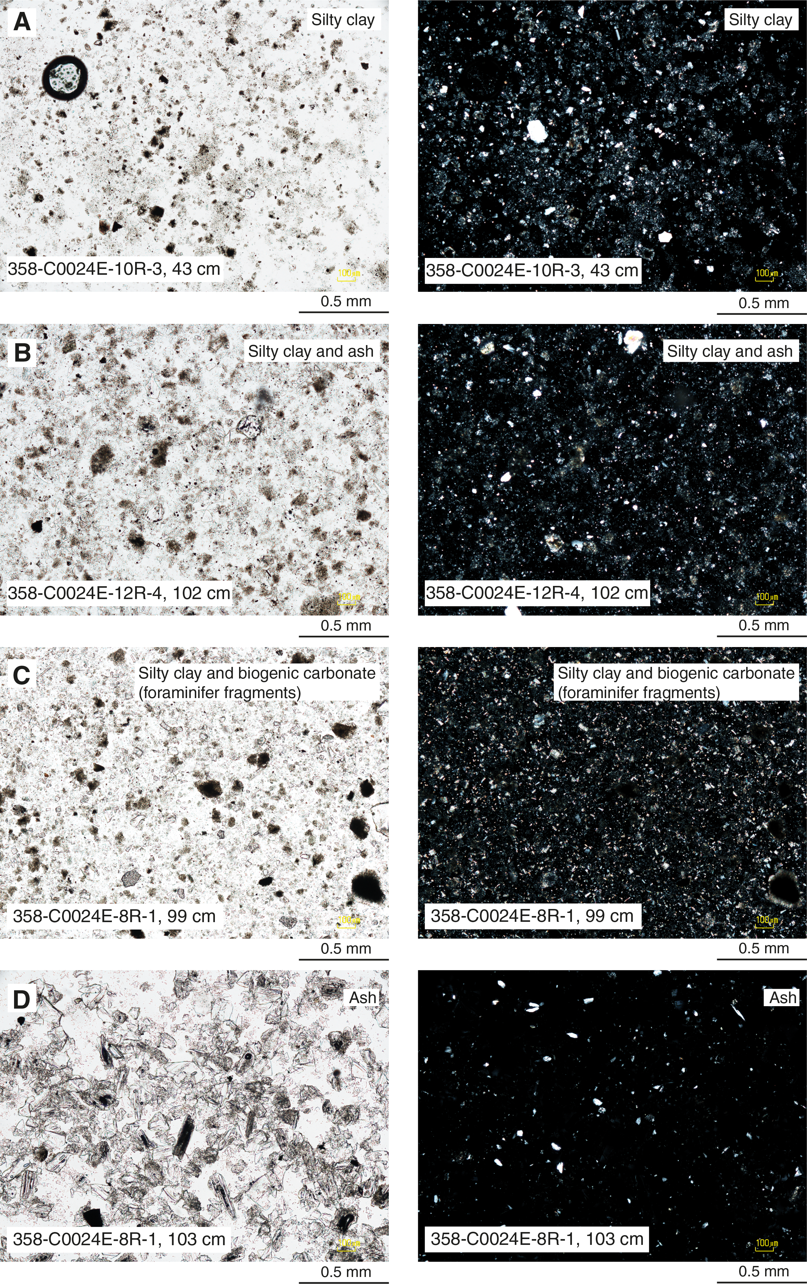
Figure F19. Representative Unit IV lithologies.
The lithified volcanic ash in Unit IV contains clear angular silt- to sand-sized glass shards, abundant vesicular glass, and/or pumice. Microlitic grains are common. Additionally, tuff deposits are characterized by abundant calcareous nannofossils and common foraminifers. Few grains of quartz, feldspar, and mica are present. Clay minerals are common to abundant. The few to common opaque grains observed include pyrite and possibly Mn oxide–coated detrital grains. These mixtures of volcaniclastic, siliciclastic, and biocalcareous constituents are probably a result of intense bioturbation.
X-ray fluorescence
Figure F16 shows depth-dependent variations in bulk sediment geochemistry for Lithologic Unit IV based on XRF measurements (Table T5). Compared to the data from Unit III, we see very little change across the boundary into Unit IV. For the most part, values do not change significantly in Unit IV. The exceptions are CaO and LOI, which increase steadily deeper than ~570 mbsf and then shift abruptly to lower values at ~605 mbsf. These trends are difficult to explain in terms of calcite concentrations because XRD values (see below) remain consistently at or below the detection limit. Zeolite is another possible authigenic mineral, although diagnostic peaks for common zeolites (e.g., clinoptilolite) are not obvious on bulk powder X-ray diffractograms.
X-ray diffraction mineralogy
Bulk powder XRD results for Unit IV are shown in Figure F17 and tabulated in Table T6. Normalized relative proportions of total clay minerals are substantially higher than in overlying units, ranging from 47.4 to 67.8 wt% (average = 58.6 wt%). The highest value for total clay minerals comes from a dark green band that was sampled in Section 358-C0024E-9R-1. Relative proportions of quartz range from 17.5 to 25.4 wt% (average = 22.5 wt%). The average abundance of feldspar is reduced to 15.8 wt% (range = 11.3–21.5 wt%). Calcite contents are generally low with an average normalized value of 3.0 wt%. Higher calcite values cluster at the top of the unit (Figure F17).
The overall downhole trends in XRD mineral abundances from Hole C0024E are consistent with the results from equivalent facies at Sites C0006 and C0007 (Expedition 316 Scientists, 2009a, 2009b). Figure F20 provides a compilation of those bulk powder XRD results. Note that the plotted depths for data points from Sites C0006 and C0007 have been adjusted downward to match the correlative unit boundary at 555 mbsf (i.e., the common contact between trench-to-basin transition and Shikoku Basin hemipelagic-pyroclastic facies). The unit boundary's depth is 449 mbsf at Site C0006 and 362 mbsf at Site C0007 (Expedition 316 Scientists, 2009a, 2009b).
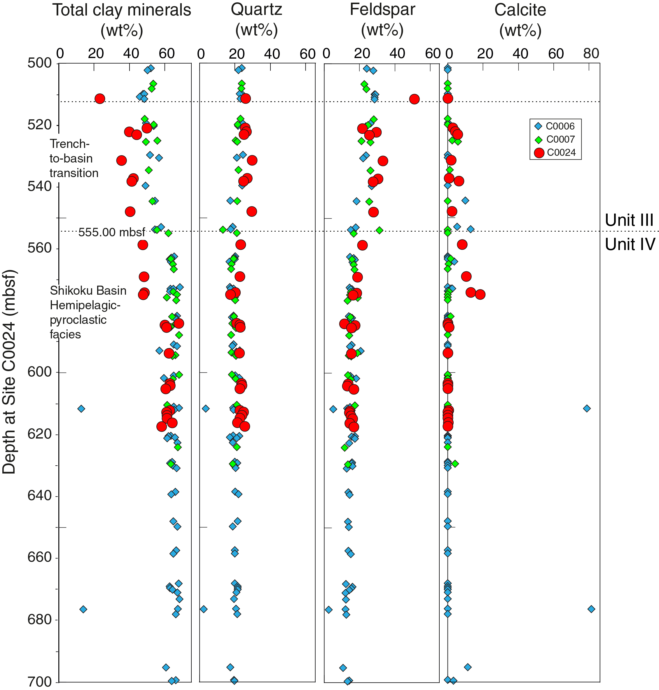
Figure F20. Bulk powder XRD, Units III and IV.
Three caveats need to be considered when evaluating these merged data sets. First, the ages or key(?) lithologic units do not correlate from site to site. Second, the X-ray diffractometer on Chikyu was replaced before Expedition 358. Third, we used a different matrix of SVD normalization factors for calculations of mineral abundance (see Lithology in the Expedition 358 methods chapter [Hirose et al., 2020]). After accounting for those differences, the data sets match closely, especially in Unit IV and its facies-correlative equivalents (Figure F20). In particular, we see a consistent and significant increase in proportions of total clay minerals across the Unit III–IV transition. The shift toward higher clay mineral contents is quite abrupt at Sites C0006 and C0007, where the unit boundary coincides with an unconformity. Those abrupt increases in clay minerals are matched by small decreases in quartz and substantial decreases in feldspar. In contrast, at Site C0024, four samples near the top of Unit IV contain higher than average proportions of calcite (8–18 wt%), and the clay mineral contents increase gradually downsection. We attribute those increases in calcite to enhanced preservation of calcareous nannofossils and foraminifers, perhaps in response to shallower paleowater depths in the Shikoku Basin (i.e., above basements highs). The enrichment of calcite is compensated for by smaller than expected increases in total clay minerals across the unit boundary compared to the increases at Sites C0006 and C0007 (Figure F20). These gradual changes in bulk mineralogy reinforce the idea that the Unit III/IV boundary is conformable at Site C0024.
Interpretation of depositional environment for Unit IV
We regard the processes of sedimentation for Lithologic Unit IV as dominated by slow hemipelagic settling in an environment that was isolated from sediment gravity flows. The ubiquity of bioturbation supports the interpretation of relatively quiet conditions on the seafloor. Fall out of suspended sediment was interrupted periodically by deposits of air fall volcanic ash, and the ash beds are also heavily bioturbated. These environmental conditions are commonplace across the Shikoku Basin (e.g., Underwood and Pickering, 2018), and similar hemipelagic-pyroclastic facies have been documented in considerable detail at Integrated Ocean Drilling Program Sites C0011 and C0012, the so-called subduction inputs reference sites for the NanTroSEIZE drilling transect (Expedition 333 Scientists, 2012a, 2012b).
Provisional interpretations for Site C0024
Statistical analysis of bed thickness frequency
Figure F10A shows the distribution of bed thickness throughout Unit II. Thin and very thin sand beds are dominant: 40% and 39% of the total, respectively (Figure F10B). Medium (17%), thick (3%), and very thick (1%) beds are also present and mainly located between 230 and 270 mbsf. The cumulative thickness curve displays a low-gradient slope from 318 to 230 mbsf. From 230 mbsf to the seafloor, the curve steepens and remains nearly constant.
When plotted in a log-log format of N > T versus T (Figure F10C), the data follow a segmented power law distribution. Several authors (e.g., Hiscott et al., 1992; Rothman et al., 1994) have demonstrated that the thicknesses of turbidite beds measured in a vertical section follow a power law distribution:
Changes in the power law exponent β have been related to such factors as the properties of the density flows, the 3-D geometry of the basin, erosion and amalgamation of successive beds (Rothman and Grotzinger, 1995; Carlson and Grotzinger, 2001), tectonic forcing (Hiscott et al., 1992), and climate (Winkler and Gawenda, 1999). β values have also been used to assess the degree to which gravity flows are confined by narrow basin shape and/or channels (Felletti and Bersezio, 2010).
Three groups of data are evident in the event bed results from Unit II (Figure F10C). The first group has a low β value (~0.45) and corresponds to beds with thicknesses of 1–5 cm; this represents 59% of the total. We relate this low β value to density flows in an unconfined setting and/or low-density turbidity currents. Such sheet flows are typical of the flat floor of a wide trench without a prominent axial channel. The second group corresponds to beds with thicknesses of 6–69 cm (Figure F10C). They represent 40% of the total, and the corresponding β value is ~1.6. This β value indicates deposition in a more confined environment (e.g., an axial channel in the trench) and/or by high-density turbidity currents. The third group has thicknesses from 70 to 126 cm and represents only 1% of the total (8 beds). The high β value (~4) might be a sign of larger, sporadic events. Amalgamation surfaces may have escaped our detection because of coring disturbance, however, so caution is required in this interpretation.
Stratigraphic evolution at Site C0024
Strata recovered by coring at Site C0024 are now part of the frontal accretionary domain of the Nankai Trough (Screaton et al., 2009a). In our interpretation of stratigraphic evolution, Unit IV was deposited during the early Pleistocene by slow settling of suspended hemipelagic sediment seaward of the trench in the Shikoku Basin. That background was punctuated by ash falls from sporadic volcanic eruptions. Contents of dispersed ash are also consistently higher than in the overlying trench deposits (e.g., Scudder et al., 2018). Unit IV at Site C0024 correlates in both age and lithology with the basinwide hemipelagic-pyroclastic facies of the Shikoku Basin (e.g., Underwood and Pickering, 2018). The base of the hemipelagic-pyroclastic facies is time-transgressive across the basin, however, with significantly older basal ages on the northeast side. Strata at Site C0024 correlate with what appear to be similar deposits in the basal hanging wall of the frontal thrust at Sites C0006 and C0007 (Expedition 316 Scientists, 2009a, 2009b), as well as the coeval subduction inputs documented at Sites C0011 and C0012 (Expedition 333 Scientists, 2012a, 2012b). The nannofossil ages at Site C0024 (2.06–2.45 Ma) are younger, however, than the comparable units at Sites C0006 and C0007.
To reiterate, we used three criteria to position the Unit III/IV boundary at 555 mbsf: (1) the deepest occurrence of normally graded siltstone beds that we interpret (moving upsection) to be the first products of deposition from a dilute turbidity current on the seaward edge of the trench floor, (2) the top of a trend of nearly constant porosity (see Physical properties) that we relate to higher contents of dispersed ash in upper Shikoku Basin deposits, and (3) the top of an interval over which total clay mineral content increases with depth. The key gravity flow events did not occur until the reference position in Shikoku Basin (the subducting Philippine Sea plate) approached close enough to the trench to receive spillover. Unlike Sites C0006 and C0007, however, we do not recognize an unconformity at Site C0024 between the top of Shikoku Basin sediments and the basal trench-wedge deposits. That unconformity (Expedition 316 Scientists, 2009a, 2009b) was attributed to localized mass wasting of the uppermost Shikoku Basin deposits along the flank of a subducting seamount prior to burial beneath the trench wedge (e.g., Underwood and Moore, 2012). We suggest that the conformable facies change at Site C0024 is responsible for a more gradual upsection decrease in total clay minerals across the Unit III/IV boundary (Figure F20), whereas the unconformity at Sites C0006 and C0007 imparts an abrupt shift in bulk mineralogy.
Most of the accretionary prism at Site C0024 is represented by Lithologic Unit II. Those turbidites and hemipelagic interbeds were initially deposited on the floor of the trench, which is correlated with younger trench-wedge facies at Sites C0006 and C0007. Most of the turbidites at Site C0024 are relatively thin and fine grained, which is suggestive of sheet flow deposition in a basin-plain type environment. Most of the flows probably spread across the width of the trench. We regard the thicker and coarser deposits as axial-channel deposits.
We regard Unit I as the Holocene (?) carapace of trench-slope sediment resting unconformably above the truncated accretionary prism. Its thickness is considerably less than the slope facies at Sites C0006 and C0007.
Structural geology
Structural geology analyses at Site C0024 included description of cores retrieved from 0 to 128.0 mbsf (0–6 mbsf in Hole C0024B, 6–7 mbsf in Hole C0024C, and 7–128.0 mbsf in Hole C0024D), from 100.0 to 319.5 mbsf (Hole C0024G), and from 510 to 621.5 mbsf (Hole C0024E). Features observed and measured in cores from Site C0024 include bedding planes, fissility, deformation bands, sediment-filled veins, faults, shear zones, and brecciated zones (Figure F21). Where possible, we corrected the measurements of planar and linear structures to true geographic coordinates using paleomagnetic data (see Structural geology in the Expedition 358 methods chapter [Hirose et al., 2020]). The distribution of planar structures is shown in Figure F22 (see StructureMeasurementSheet_C0024_C0025.xls in CORE in STRUCTURE in Supplementary material). Deformation related to drilling and core recovery was noted. Here, we describe and provide examples of each of the features that were recorded and relate them to features observed during previous ODP and Integrated Ocean Drilling Program expeditions in this vicinity to allow easy cross-referencing.
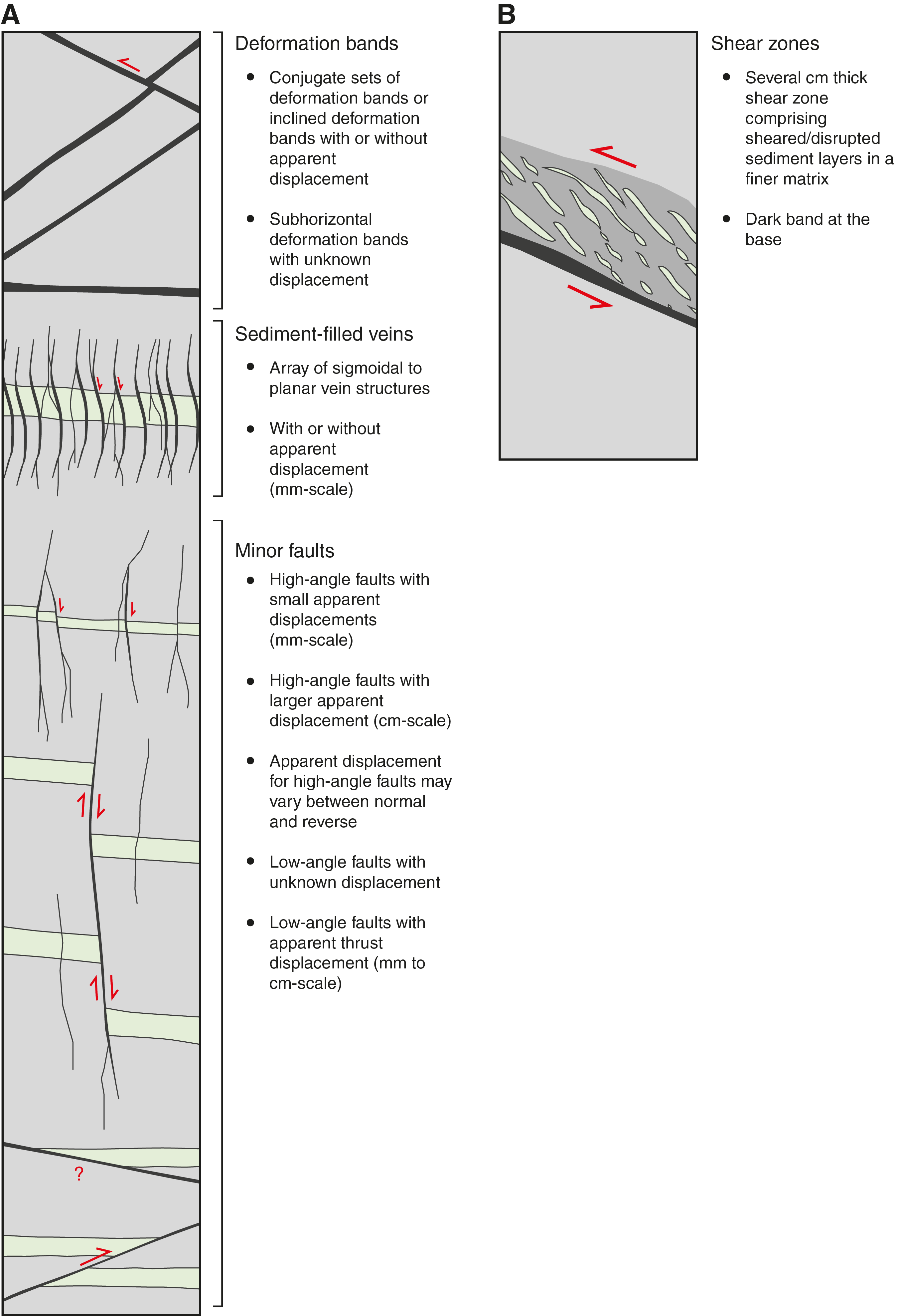
Figure F21. Deformation bands, veins, minor faults, and shear zones.
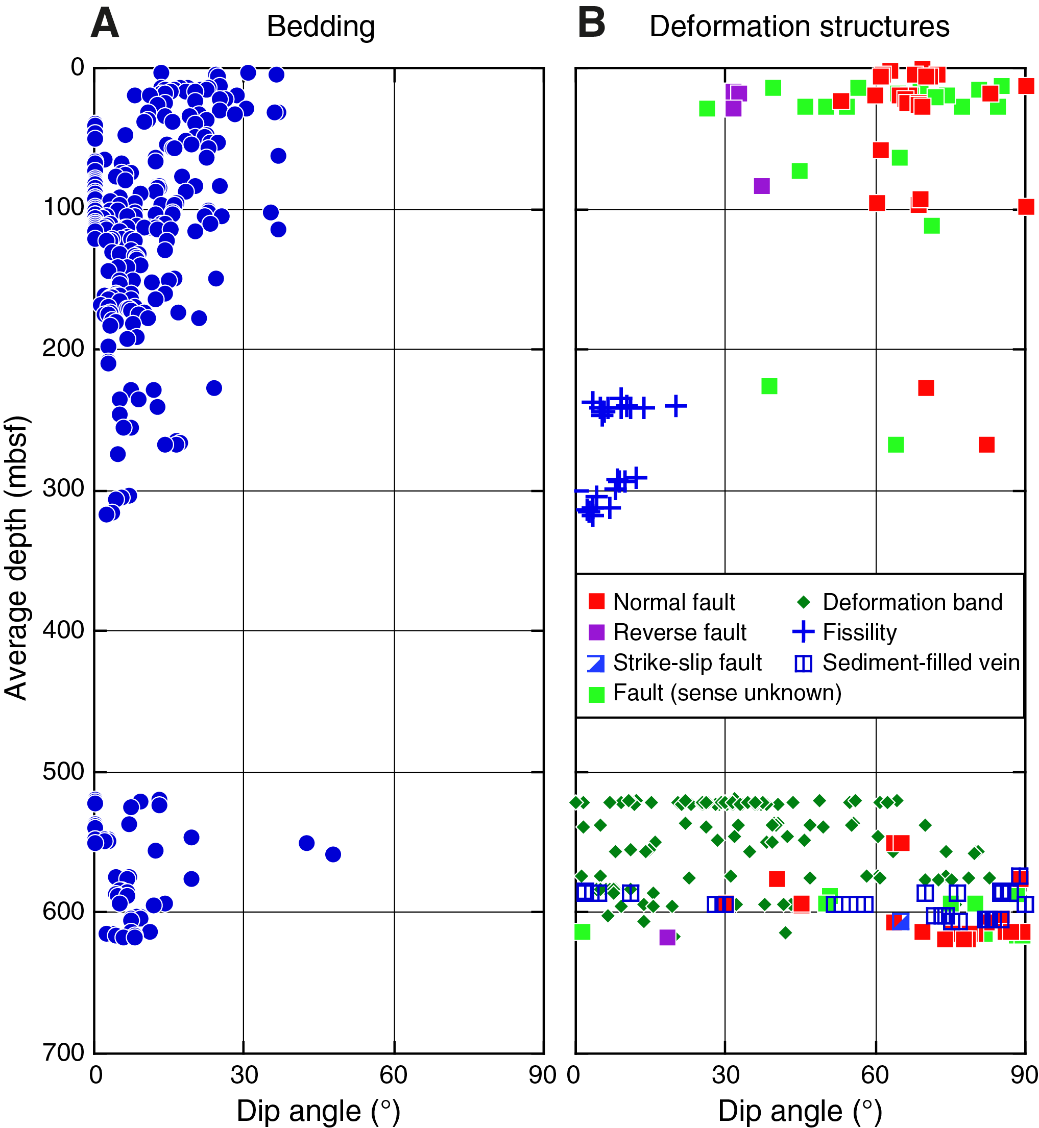
Figure F22. Dip data of bedding and deformation structures.
Bedding and fissility
Bedding planes (N = 301) are gently to moderately inclined (~10°–37°; mean dip = 20°) at 0–38 mbsf in Lithologic Units I and II (Figure F22A). Inclined bedding planes at 0–38 mbsf consistently dip toward the southwest (Figure F23A). At 38–316 mbsf in Lithologic Unit II, bedding planes are either subhorizontal (~0°) or gently to moderately inclined (~10°–30°; mean dip = 8°; Figure F22). At 510–618.9 mbsf in Lithologic Units III and IV, bedding planes are typically subhorizontal (0°–48°; mean dip = 8°; Figure F22A) with no clear preferred dip direction (Figure F23B). Fissility (i.e., finely spaced foliation parallel to bedding) is gently inclined (~2°–20°; mean dip = 7°) at 235–318 mbsf in Lithologic Unit II.
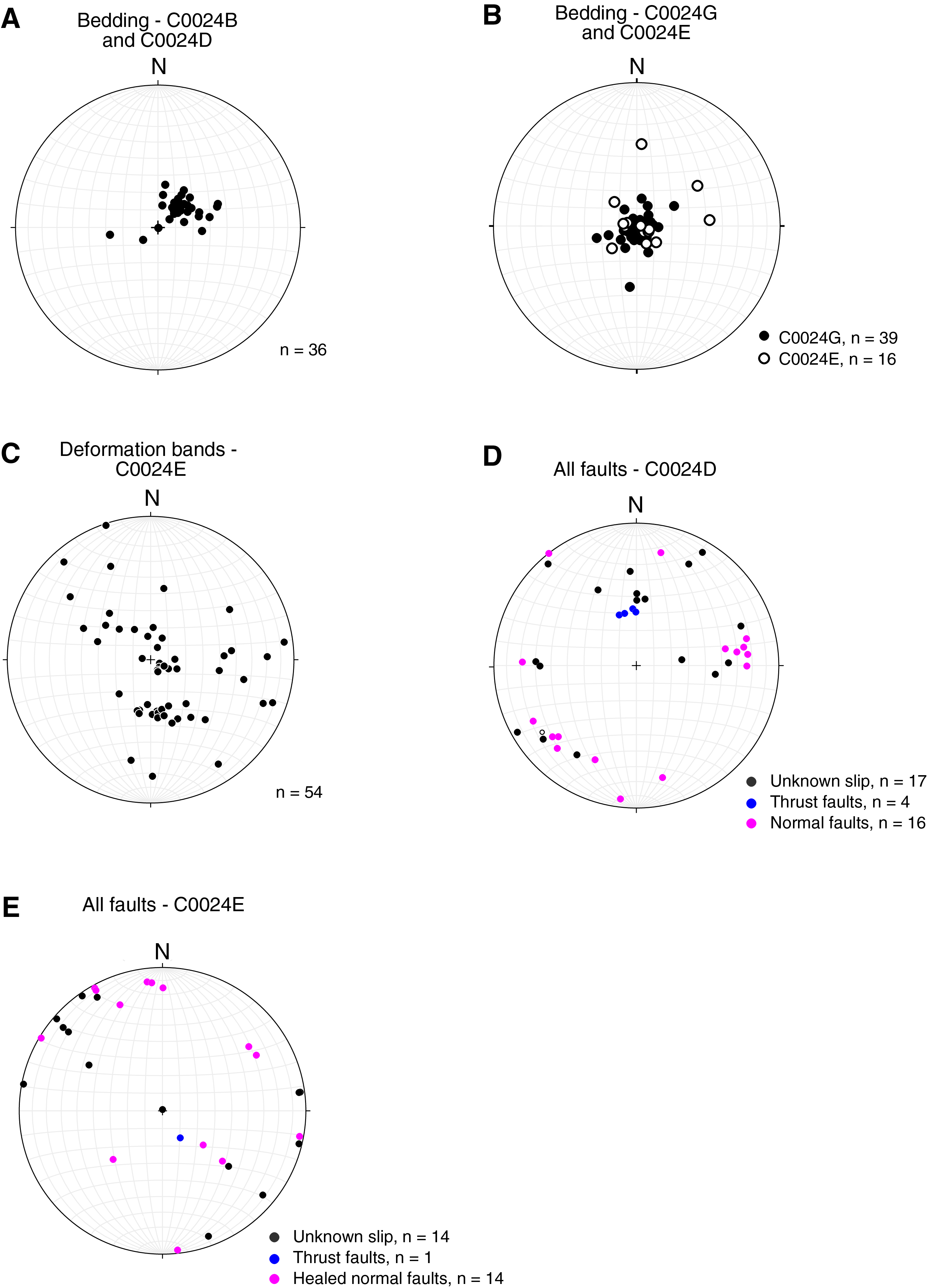
Figure F23. Poles to bedding, faults, and deformation bands.
Deformation structures observed at Site C0024
Deformation bands
Deformation bands are defined here as ~1–5 mm thick planar structures developed in silty to clayey sediments that are typically darker than the surrounding rock (Figure F24) and appear as bright features in X-ray computed tomography (CT) images. More generally, the term "deformation band" has previously been used to describe localized deformation features in granular porous rocks (Aydin, 1978). Types of deformation bands can be classified kinematically as compaction bands, shear bands, and dilation bands (Aydin et al., 2006), although Fossen et al. (2007) attempted a mechanistic classification. These features have also been recognized previously in unconsolidated sediments (Cashman and Cashman, 2000). We did not document subclassifications of deformation bands because of limited microstructural evidence.
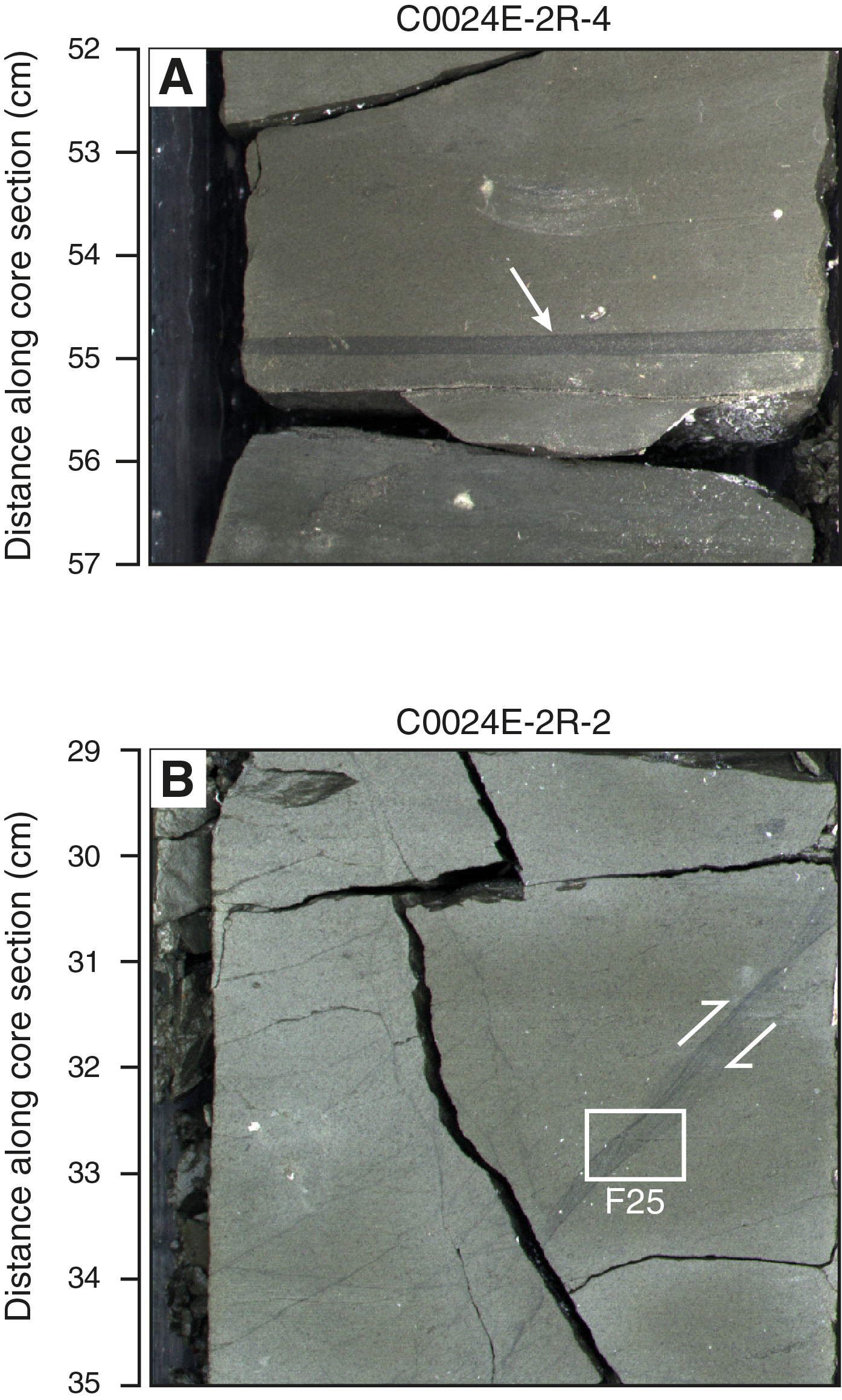
Figure F24. Deformation bands.
Two types of deformation bands are documented at 519–619 mbsf (Cores 358-C0024E-2R through 12R). The first type is defined by dark bands that are parallel or subparallel to bedding (Figure F24A). Microstructural analysis on this type of deformation bands was not performed.
The second type of deformation bands has moderate to steep dips with respect to bedding and sometimes occur as conjugate sets, where one set offsets the other by 1–2 mm with an apparent reverse sense of shear (Figures F21A, F24B). Inclined deformation bands in Hole C0024E dip toward the northwest or southeast with variable dip magnitude (Figure F23C). Conjugate sets of deformation bands are consistent with their formation in a compressional regime with σ1 gently plunging toward the southeast, subparallel to the local plate convergence direction. Microstructural analysis was carried out on one inclined deformation band at 520.5 mbsf (Section 358-C0024E-2R-2) that shows a reverse sense of shear (Figure F25). The deformation band consists of ~50–100 µm thick subbands framing a 3–4 mm thick zone of reduced porosity (Figure F25A). The subbands appear dark under plane-polarized light and yellow-brown under cross-polarized light (Figure F25A, F25B). Each subband comprises ~1–10 µm thick strands that run parallel to the bands, are composed mainly of clay minerals, and are separated from each other by thin layers of sediment (Figure F25C, F25D).
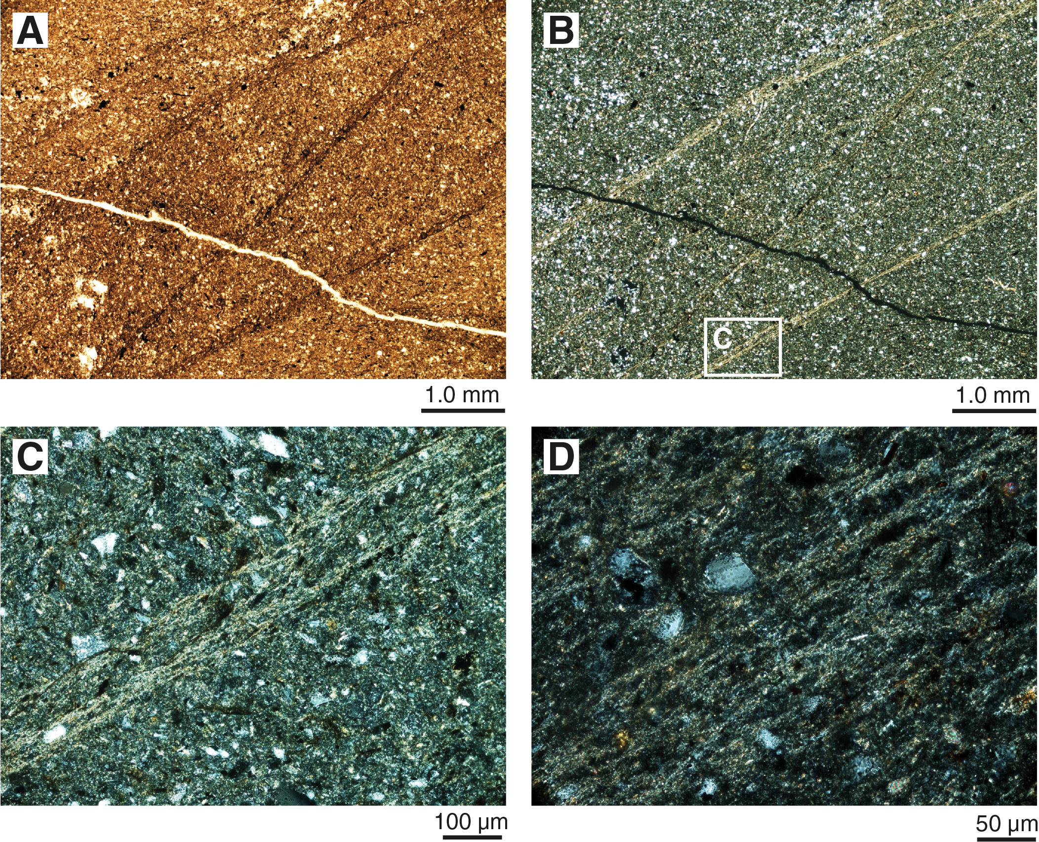
Figure F25. Deformation band.
The two types of deformation bands described here resemble structures that have been previously documented in sediments within accretionary prisms (Maltman et al., 1993; Ujiie et al., 2004; Expedition 316 Scientists, 2009a; Tobin et al., 2015). Subhorizontal dark bands were observed at Sites C0006, C0007, and C0011 (Expedition 316 Scientists, 2009a), where they were termed "healed faults." The bedding-parallel or subparallel deformation bands are comparable to layer-parallel structures observed in mudstone in the accretionary prism on shore (Hanamura and Ogawa, 1993). The latter structures are thought to have formed in association with gravitational instability near the trench prior to entering the accretionary prism along with layer-parallel shortening during early phases of accretion (Yamamoto et al., 2005, 2009). Inclined deformation bands, particularly showing two opposite dipping sets of a reverse shear sense, are interpreted to record layer-parallel shortening during frontal accretion (Maltman et al., 1993; Ujiie et al., 2004).
Sediment-filled veins
Sediment-filled veins are recognized as parallel sets of sigmoidal or planar seams generally <1 mm wide that tend to extend perpendicular to bedding (Figure F21). They are only found in Lithologic Unit IV at 574.5–612.1 mbsf. Arrays of sediment-filled veins are oriented subhorizontal to bedding and typically have a thickness of 1–5 cm (Figures F26, F27). Some sediment-filled veins offset bedding or burrows and show apparent normal offset with displacements of less than a few millimeters (Figure F27). Some sediment-filled veins extend upward/downward and are sometimes difficult to distinguish from high-angle cohesive faults (see below). Sediment-filled veins were found in cores from 584.5 to 616.4 mbsf (Cores 358-C0024E-9R through 12R), where they occur over 2%–28% of the core sections (Figure F22). Similar vein structures were reported in drilled cores at subduction zones such as Nankai, Costa Rica, and Oregon and in shallowly buried accretionary prism/slope sediments in the Miura/Boso Peninsulas (Japan) and Monterey Formation (United States). Field and experimental studies revealed that the structure formed by earthquake shaking (Hanamura and Ogawa, 1993; Brothers et al., 1996).
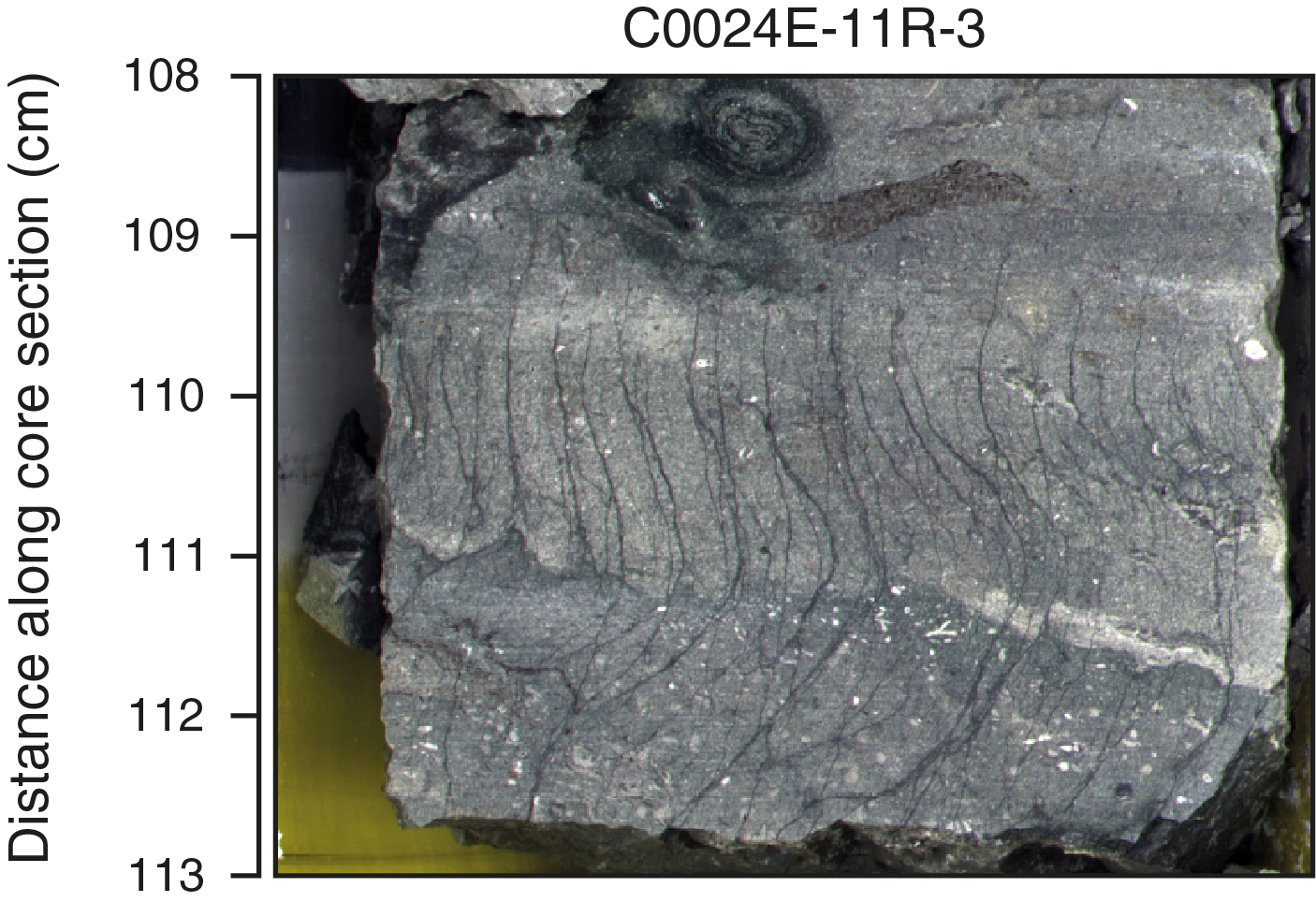
Figure F26. Array of sediment-filled veins.
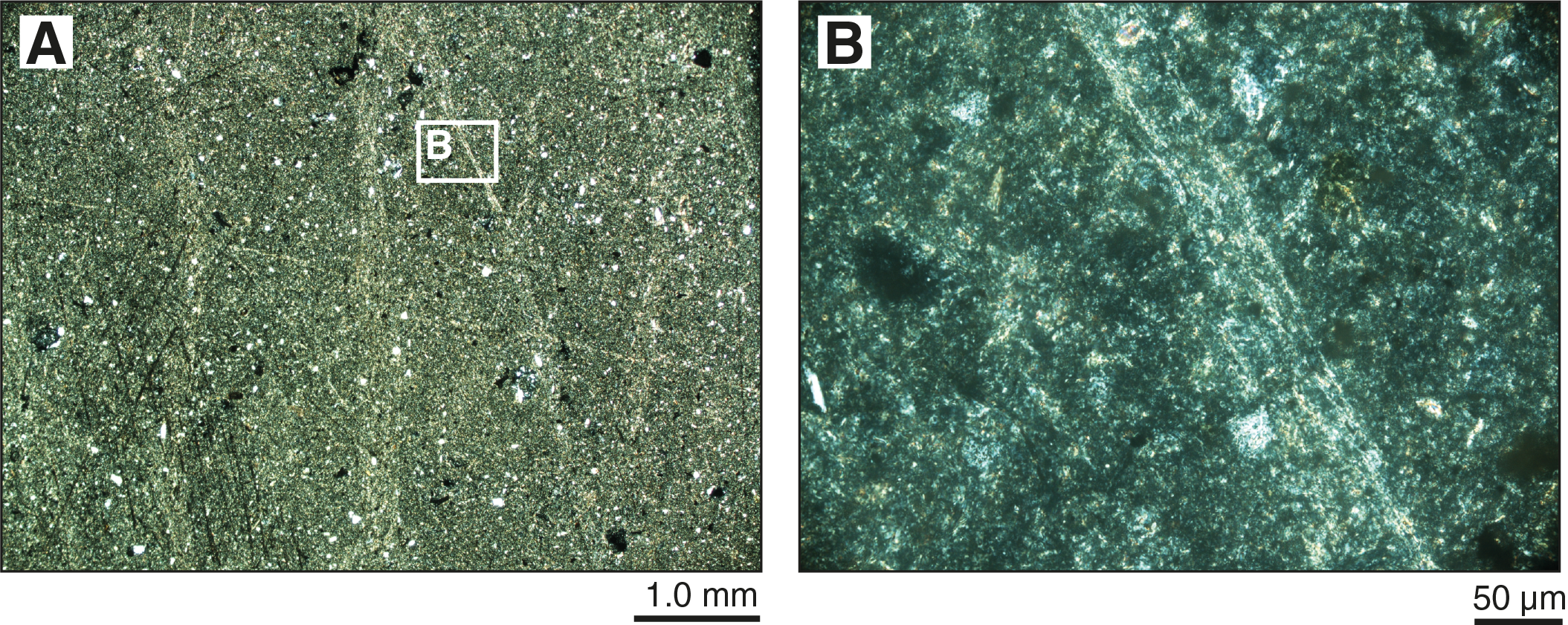
Figure F27. One sediment-filled vein.
Minor faults
Minor faults occur as small-displacement structures that are clearly identifiable on the split core surface (Figures F21, F28). They show small apparent displacements of a few millimeters to centimeters. Minor faults occur as single features or as sets in cores and can branch into splays or anastomosing networks (Figure F21).
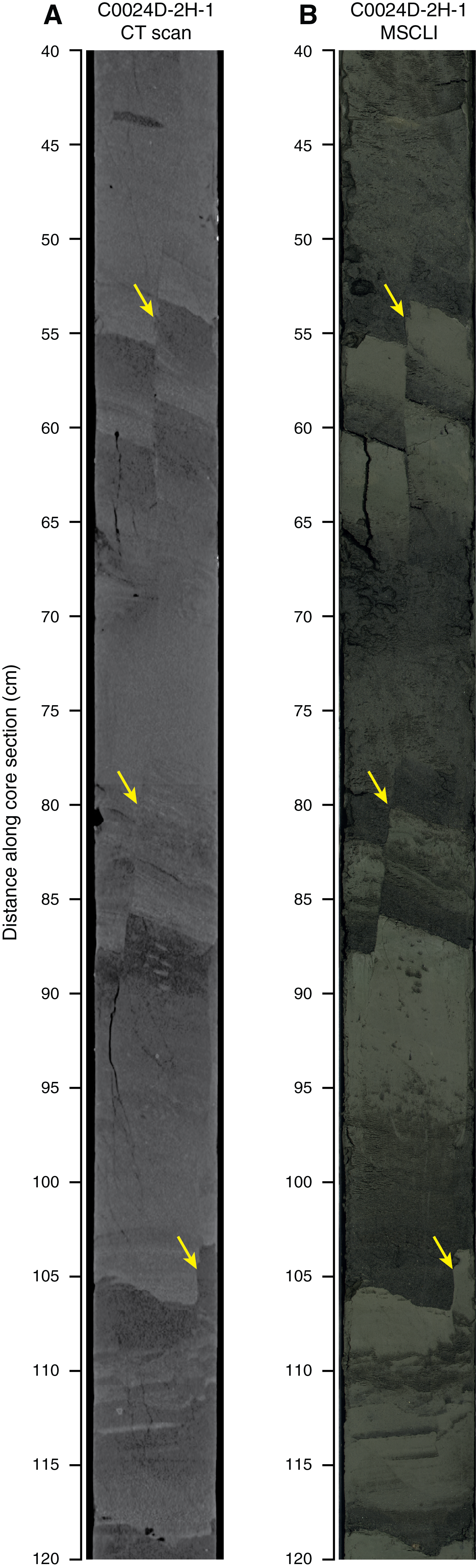
Figure F28. High-angle normal faults.
In the upper ~30 m in Lithologic Units I and II (Holes C0024B and C0024C), minor faults have apparent normal displacement or undetermined displacement on the cut surface (Figure F29). Apparent normal faults (n = 32) are steeply inclined (~60°–90°; mean dip = 68°), have localized (or sharp) fault planes, and record displacements (dip-slip) between <1 and ~4 cm. They are well resolved in X-ray CT images of whole-round cores as ~1–2 mm bands of bright, high CT number material and can be visually identified on split core surfaces where they displace bedding (Figure F28). Apparent normal faults have variable strike directions, but some may define a conjugate set with southwest and northeast dip directions (Figure F23D). Faults with undetermined displacement (n = 17) are moderately to steeply inclined (~30°–85°), have variable strike directions (Figure F23D), and are mainly inferred from X-ray CT images perpendicular to the split core surface. These features appear as thin, brighter X-ray CT bands apparently offsetting sedimentary structures but are difficult to identify both on split core surfaces and in X-ray CT images parallel to the split core surface (Figure F29). Some faults show an apparent reverse sense of displacement of magnitude as much as ~2 mm slip (Figure F29), but displacement is poorly constrained for most of these faults. Apparent thrust faults have a dip direction toward the southeast (Figure F23D).
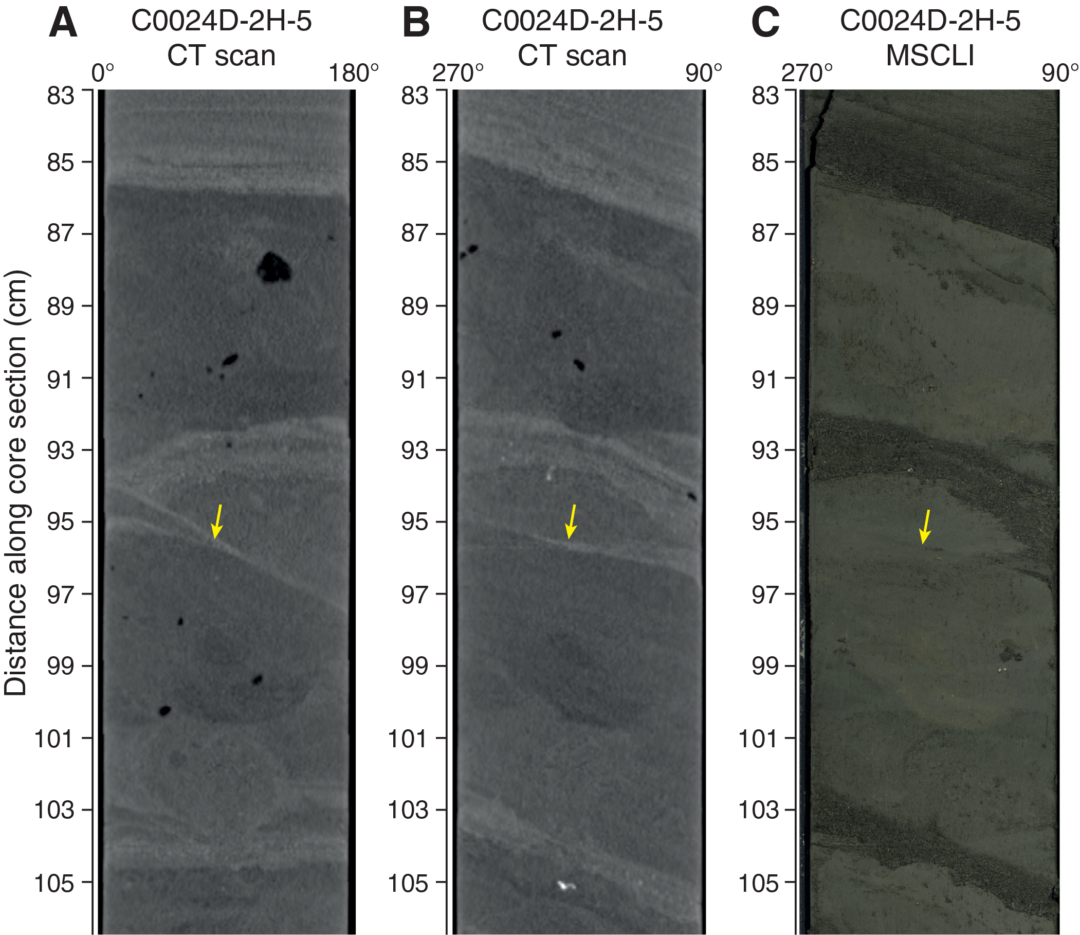
Figure F29. Shallow fault with undetermined displacement.
At 510–620 mbsf in Lithologic Units III and IV (Hole C0024E), two types of faults occur: incohesive fault planes and cohesive ("healed") faults (Figure F30). Incohesive fault planes can have striated polished surfaces (slickenlines) that are stepped (Figure F30F), from which the sense of shear may be determined. These types of faults are uncommon in Hole C0024E but are associated with subhorizontal slickenlines and centimeter-scale offset of bedding where observed.
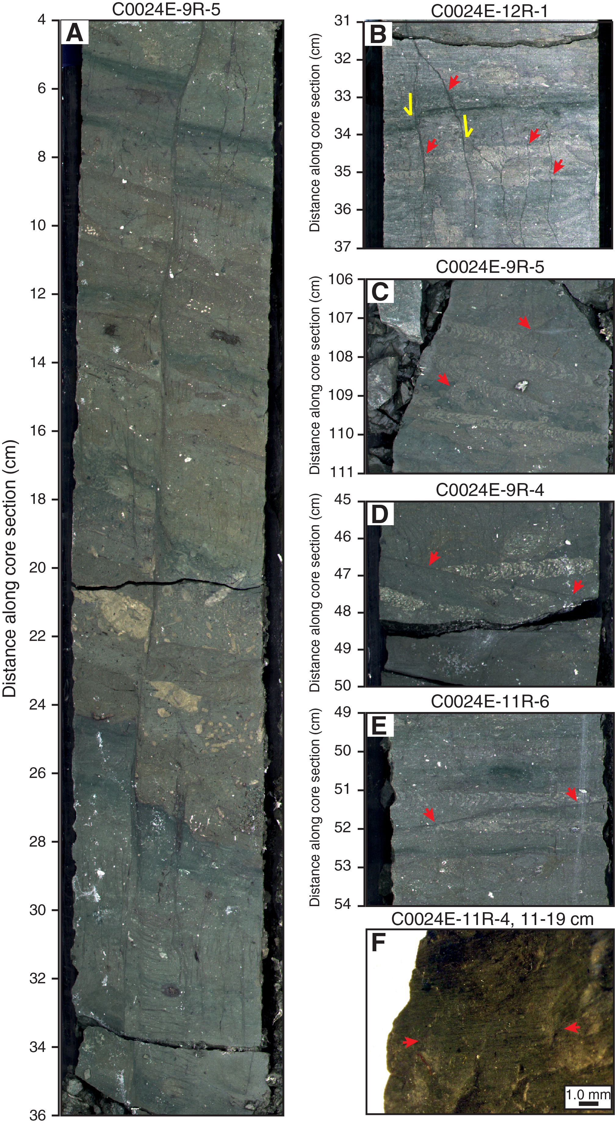
Figure F30. Deformation structures observed.
Cohesive faults are defined by very thin (~0.5 mm wide) zones that appear as very dark or black seams that dip between 30° and 90° (Figure F30). They clearly offset bedding but not typically by more than a few millimeters. They can be planar or curviplanar. Where offset markers occur, the apparent sense of shear is typically normal, but they can also display apparent thrust-sense offset along fault segments with curviplanar geometries (Figure F30C, F30E). Commonly, they occur as sets and are sometimes restricted to horizons within the core over depth intervals of several centimeters. Healed normal faults in this depth interval generally dip toward the northwest or southeast but do not have orientations that are uniquely separable from those with thrust or uncertain slip sense (Figure F23E). This type of healed fault is similar to that reported in the hemipelagic mudstone at the base of Sites C0006 and C0007 (Expedition 316 Scientists, 2009a) and in the Muroto transect in the Nankai accretionary prism (Shipboard Scientific Party, 2001a) and is thought to result from vertical compaction of sediments during burial.
Shear zones
Shear zones are defined here as several centimeter-thick zones recording shear deformation that have a presumed lateral extent much greater than the core diameter. We observed one shear zone at 295.2–295.3 mbsf (interval 358-C0024G-22X-4, 40–47 cm) that is preserved in an interval of poorly lithified silty claystone comprising elongated sandstone fragments that show a sigmoidal or asymmetric geometry consistent with a reverse sense of shear (Figure F31). Sedimentary laminae in sandstone fragments are cut and truncated. A ~1–3 mm thick dark band is developed at the base of the shear zone. In X-ray CT images, the sheared piece of silty claystone shows a higher CT number than the surrounding material. The dark band at the base of the shear zone cannot be distinguished from the sheared silty claystone in X-ray CT images, indicating that it has a similar bulk density and chemical composition.

Figure F31. Shear zone.
Brecciated zone
Mudstone from 243.5 to 247 mbsf (Core 358-C0024G-17X) is highly brecciated into ~2–3 mm sized fragments. The matrix of the breccia is composed of a mixture of unconsolidated sand and mud. The mudstone clasts preserve fissility and coring- and splitting-induced cracks. Brecciated mudstone fragments are absent above and below Core 17X.
Drilling-induced deformation
Drilling-induced disturbances in cores from Site C0024 include degassing fractures and voids, drilling-induced fractures and striae, and biscuiting. Degassing structures were observed at shallow depths, where X-ray CT images of cores show variable intensities of subhorizontal or subvertical cracks or circular void space ranging in scale from millimeters to centimeters (Figure F32). The distribution of cracks and pores appears to be lithologically controlled, where fractures and voids occur preferentially in silty clay and fine sands, respectively. We interpret these structures to be related to degassing and expansion during core recovery. This interpretation is supported by the expansion of the core length observed during recovery and by the high concentrations of hydrocarbon in headspace gas samples (see Geochemistry). Drilling-induced fractures were observed at 36–319 mbsf and are characterized by planar to curviplanar surfaces that are fresh, unaltered, and often rough and may contain shiny, curvilinear striae. Biscuiting was observed at 45–319 mbsf during ESCS and RCB drilling and is characterized by several centimeter-thick sections of core separated by sharp, curved surfaces that have accommodated rotation between the core disks.
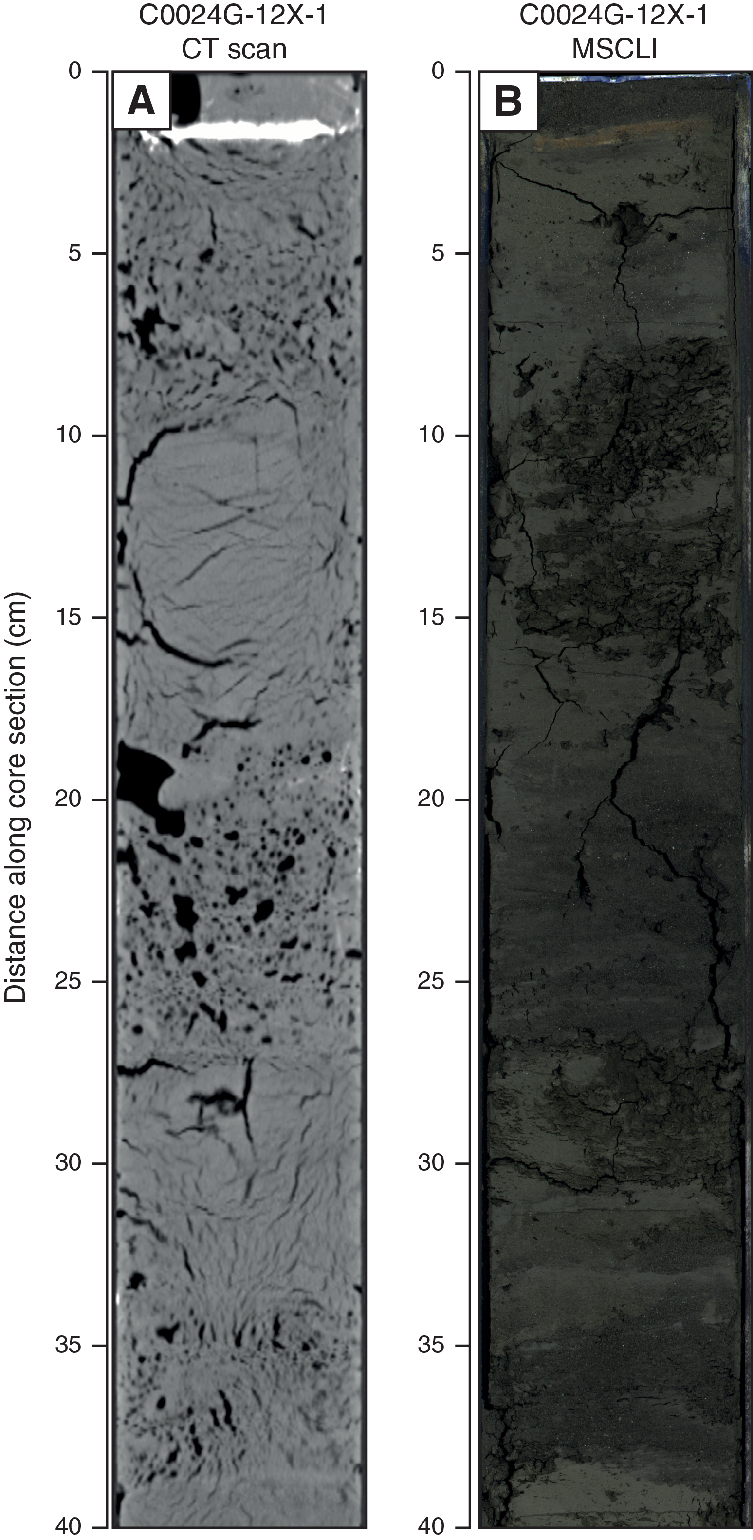
Figure F32. Cracks and voids.
Preliminary interpretations
Structures preserved in shallow cores recovered from Site C0024 provide the following key observations:
- Bedding dips vary in Hole C0024D from ~10° to 37° (mean = 20°) at 0–38 mbsf, from 0° to 30° (mean = 8°) at 38–316 mbsf, and from 0° to 48° (mean = 8°) at 510–618.9 mbsf. At 0–38 mbsf, bedding dips toward the southwest.
- Steep minor faults are most common at 0–38 mbsf and are characterized by normal apparent displacement. At 0–38 mbsf, normal faults generally dip toward the southwest and northeast, whereas deeper than 100 mbsf, normal faults generally dip toward the northwest and southeast.
- Deformation bands, healed faults, and sediment-filled vein structures are commonly developed at 510–618.9 mbsf. Deformation bands generally dip toward the northwest or southeast.
- One observed brecciated zone occurs at 243.5–247 mbsf.
- One observed shear zone occurs at 295 mbsf.
We interpret the high-angle faults and inclined bedding observed at 0–119.4 mbsf to be related to soft-sediment deformation at the very shallow depth, potentially resulting from slumping or sediment compaction near the seafloor, rather than a result of tectonic deformation during accretion. The dip directions of normal faults developed in the upper 38 m of the slope basin suggest they accommodated southwest–northeast extension. Cohesive faults and low-angle deformation bands are also identified throughout the input sites (Sites C0011 and C0012) (Underwood et al., 2010; Expedition 333 Scientists, 2012a, 2012b), whereas the sediment-filled vein structures are developed only in the upper ~200 m of the incoming sediment sequence. Therefore, these structures likely formed soon after sedimentation; the former apparently formed by vertical compaction of sediments during burial, and the latter likely formed near the trench associated with earthquake shaking. High-angle deformation bands have not been reported at the input sites and are formed at the toe of accretionary prisms (Maltman at al., 1993; Ujiie et al., 2004). The dip directions of these deformation bands are approximately parallel to the azimuth of local plate convergence direction.
Although Hole C0024G crossed two back thrusts identified in the seismic and resistivity-at-the-bit tool (RAB) resistivity images (at ~150–275 mbsf; see Figure F65), shear-related deformation is very rare in this hole. It is not clear where the two back thrusts are located in Hole C0024G. It is possible that one back thrust is associated with the brecciated zone at 243.5–247 mbsf based on an absence of a brecciated zone above and below, poor core recovery, and the depth correlation between the brecciated interval and the location of a back thrust on the seismic profile. The core preserving the brecciated zone shows poor recovery of 37%. Alternatively, the brecciated zone could be the manifestation of the brecciation of fissile mudstone due to drilling- and splitting-induced deformation as well as degassing- and expansion-related cracking during core recovery, although nontectonic deformation is observed throughout Hole C0024G and is commonly not associated with strong brecciation. The shear zone at 295 mbsf is only slightly overprinted by coring-related deformation and shows a shear sense consistent with thrust faulting. The dark band at the bottom of the shear zone resembles a deformation band in argillaceous sediments (Maltman et al., 1993; Ujiie et al., 2004) or a ~1–3 mm thick fault gouge. The displacement associated with this structure is not constrained, and it is unclear if it could represent one of the back thrusts.
Biostratigraphy and paleomagnetism
Biostratigraphy
Preliminary age determination for core samples from Holes C0024B–C0024E and C0024G is based exclusively on the examination of calcareous nannofossils.
Calcareous nannofossils
We examined all core catcher samples from Holes C0024B–C0024E and C0024G for calcareous nannofossil biostratigraphy. Very poorly to moderately preserved nannofossils were found in most samples, and species diversity is comparatively low. Most Quaternary datum planes described by Sato et al. (2009) and the lower Pliocene zonal marker of Martini (1971) and Okada and Bukry (1980) were identified in the sedimentary sequence. The numerical ages of calcareous nannofossil biostratigraphy follow a review by Raffi et al. (2006). The nannofossils found in each hole are listed in Tables T7, T8, T9, T10, and T11.
Calcareous nannofossil assemblages found in samples from Holes C0024B, C0024C, C0024G, and C0024E are mainly composed of Calcidiscus leptoporus, Coccolithus pelagicus, genus Gephyrocapsa, Helicosphaera carteri, Pseudoemiliania lacunosa, and Reticulofenestra spp. Large Gephyrocapsa spp. (>5.5 µm) and Helicosphaera sellii, which appear between 1.34 and 1.59 Ma (Zone NN19/CN13b), were found in Samples 358-C0024C-1H-CC, 13.0–18.0 cm (7.32–7.37 mbsf), and 358-C0024D-1H-CC, 19.0–24.0 cm (11.755–11.805 mbsf). Samples 358-C0024D-2H-CC, 55.5–60.5 cm (21.095–21.145 mbsf), to 14X-CC, 82.0–87.0 cm (119.32–119.37 mbsf), and 358-C0024G-1X-CC, 29.5–34.5 cm (106.265–106.315 mbsf), to 24X-CC, 35.0–40.0 cm (318.855–318.905 mbsf), are characterized by the occurrence of medium Gephyrocapsa spp. (Gephyrocapsa oceanica and Gephyrocapsa caribbeanica) and P. lacunosa and by the absence of large Gephyrocapsa spp. (>5.5 µm) and genus Discoaster, which indicates that the sediments recovered downhole from 21 mbsf in Hole C0024D and those from Hole C0024G correlate with Zone NN19/CN13b (middle Pleistocene; 1.56–1.67 Ma). H. sellii (last occurrence [LO] at 1.34 Ma) was sporadically obtained in samples from Holes C0024C, C0024D, and C0024G. Emiliania huxleyi, which occurs from the bottom of Zone NN21 (0.291 Ma), and Gephyrocapsa parallela, which first occurs from 1.04 Ma, were absent throughout Holes C0024B–C0024E and C0024G. These results suggest that the sediments recovered from Holes C0024C, C0024D, and C0024G (7.3–319 mbsf) correlate with Zone NN19/CN13b (middle Pleistocene; 1.34–1.67 Ma). On the other hand, Discoaster brouweri (LO at 2.06 Ma) was found throughout the sequence in Hole C0024E with Discoaster asymmetricus. Discoaster pentaradiatus (LO at 2.45 Ma) was absent in samples from Hole C0024E. The sediments recovered from Hole C0024E (512–619 mbsf) therefore correlate with Zone NN18/CN12d (2.06–2.45 Ma).
Paleomagnetism
Remanent magnetizations of archive halves and discrete samples from Holes C0024B–C0024E and C0024G were measured at demagnetization levels of 0, 5, 10, and 20 mT peak alternating fields for archive halves and at 0, 5, 10, 15, 20, 30, 40, 50, 60, 70, and 80 mT for discrete samples. Removing low-coercivity components by demagnetization steps of 5–10 mT is confirmed in discrete samples (Figure F33) and archive halves. Positive inclinations after 20 mT demagnetization are dominant at 0–280 mbsf (Figures F34, F35, F36), although a short negative inclination interval at 6–11.5 mbsf (Figure F34) and a mixed interval at 212.0–223.0 mbsf (Figure F36) are intercalated. Negative inclination becomes dominant between 280.0 and 320.0 mbsf (Figure F36). Short positive and negative inclination intervals appear alternately with some mixed inclination intervals between 516.0 and 620.0 mbsf (Figure F37). Clustered declinations identified at 0–57.37 mbsf (Figure F34) are likely due to the HPCS or EPCS used for coring this interval. On the contrary, scattered declinations at 61–319.5 and 510–621.5 mbsf (Figures F35, F36, F37) are indicative of "biscuiting" caused by coring those intervals using the ESCS and RCB system.
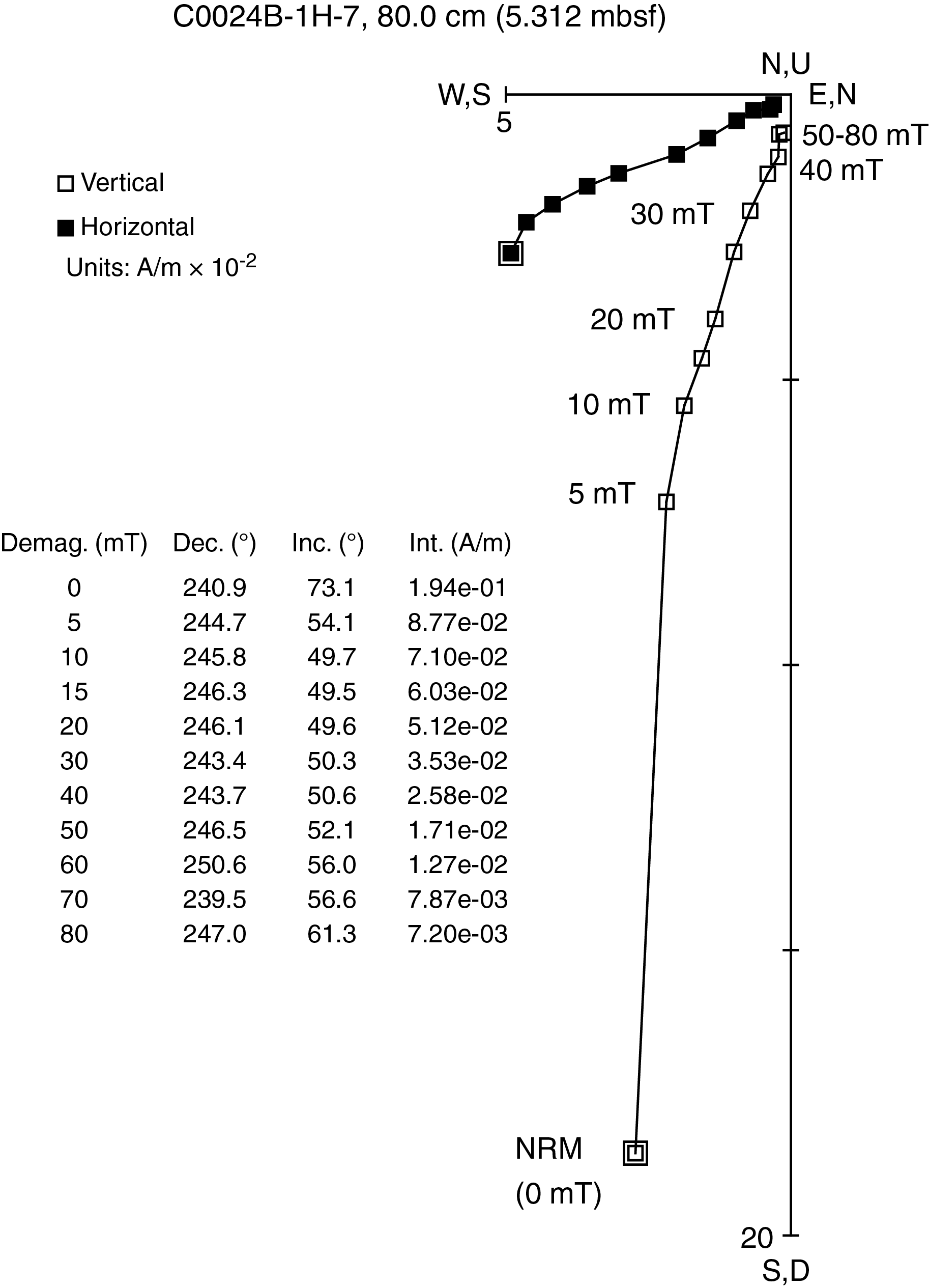
Figure F33. Alternating field demagnetization.
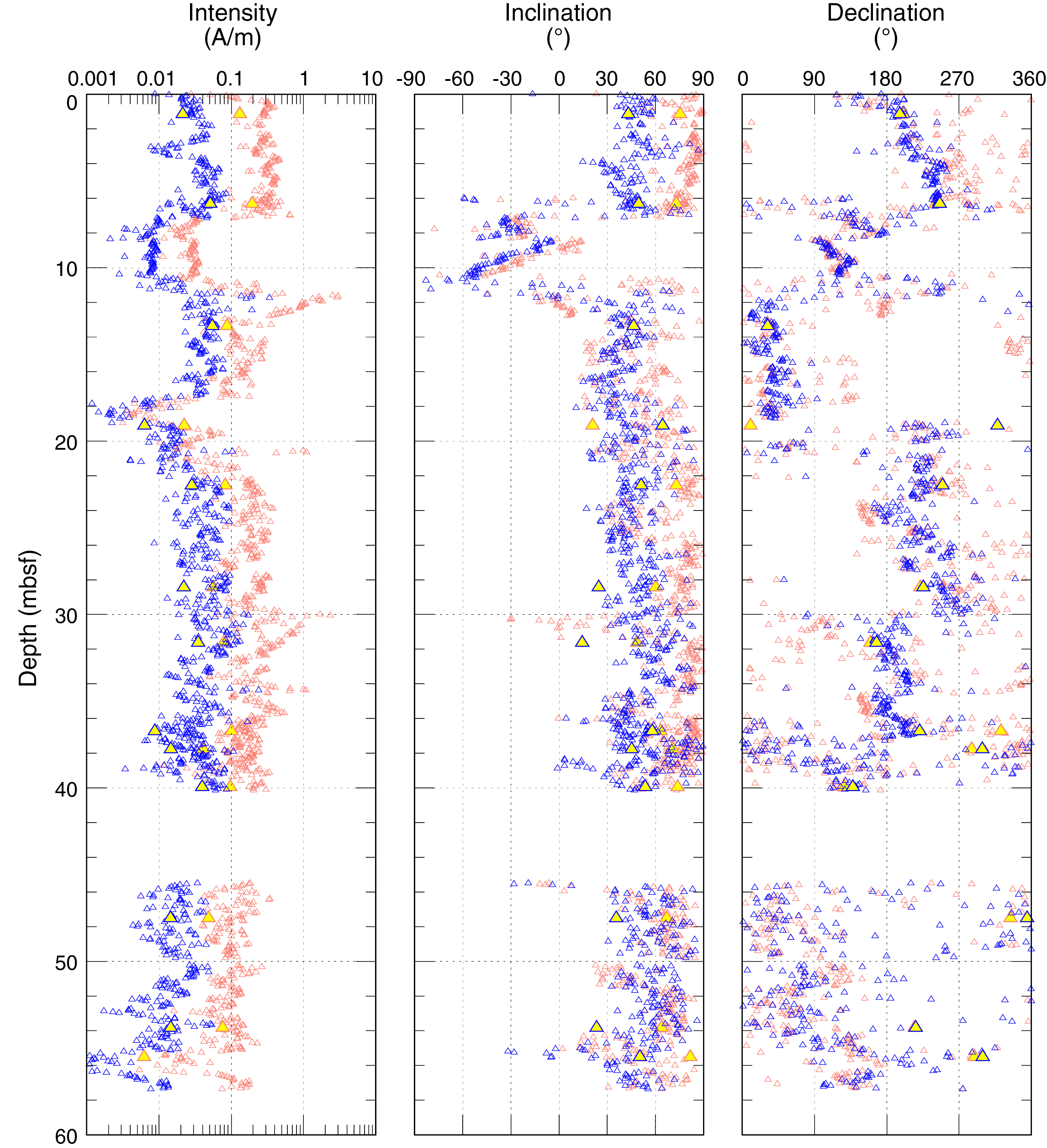
Figure F34. Remanent magnetization, Holes C0024B–C0024D.
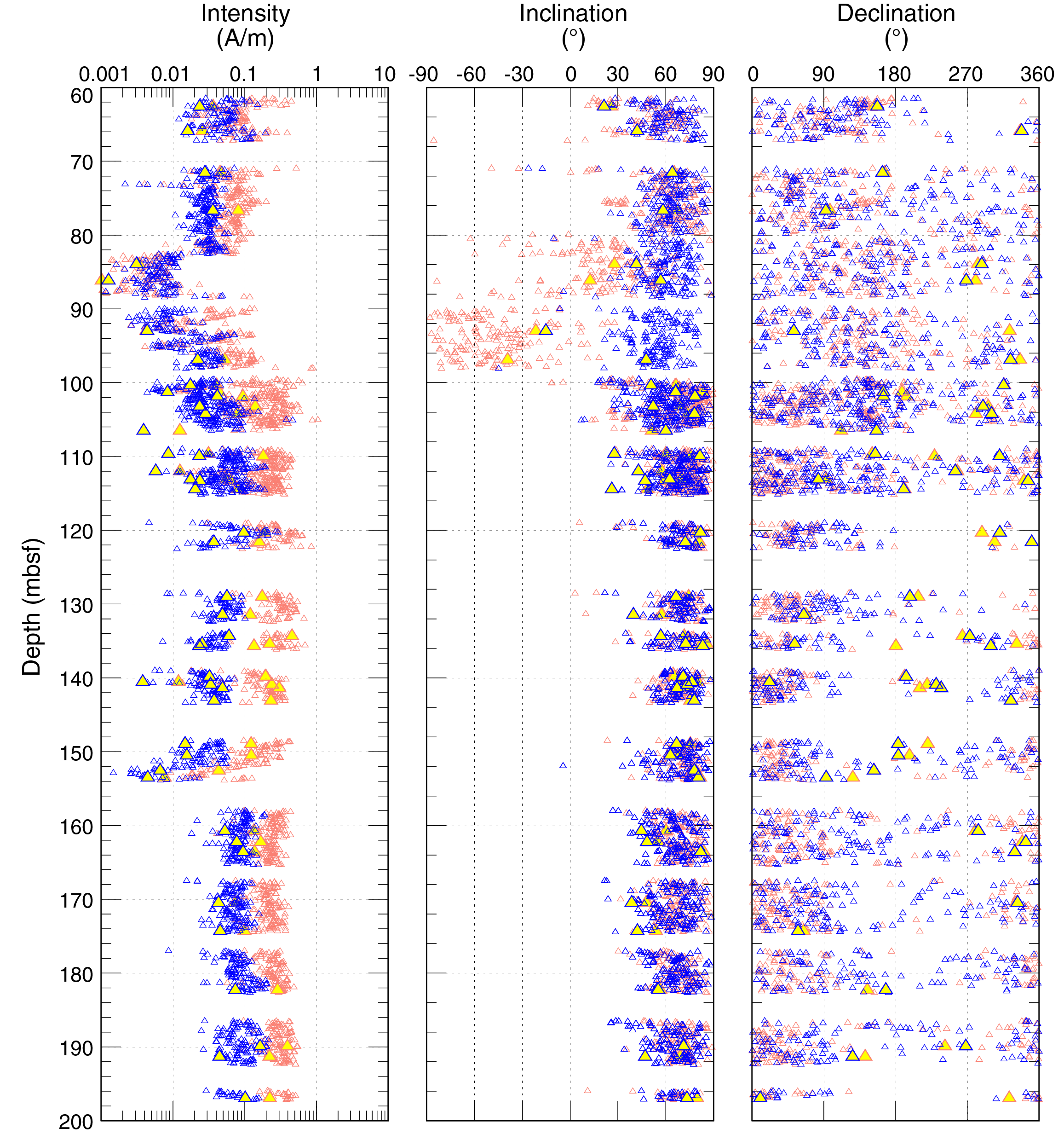
Figure F35. Remanent magnetization, Holes C0024D and C0024G.

Figure F36. Remanent magnetization, Hole C0024G.
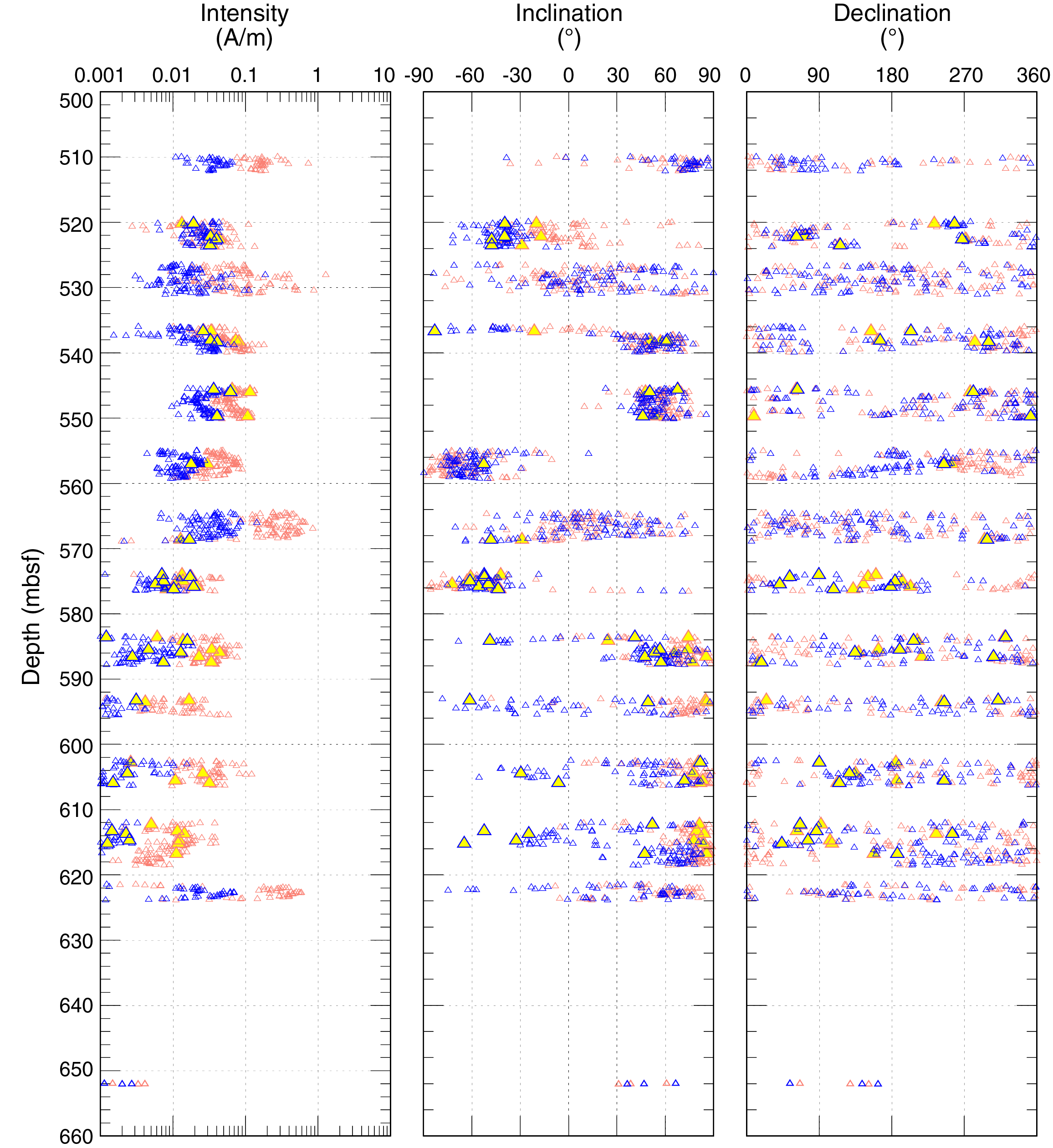
Figure F37. Remanent magnetization, Hole C0024E.
Stratigraphic interpretation
Inclinations are used to identify magnetic polarity sequences (Figure F38). Downhole variations in polarity are categorized into intervals of predominantly positive inclination, predominantly negative inclination, and mixed inclination. Although recovery was incomplete, some magnetic reversals can be discerned on the basis of changes in the sign of inclinations as partial magnetostratigraphic records. If the cored interval at Site C0024 covers enough time, the inclination distribution is expected to be bimodal between negative and positive. However, a histogram of inclinations after 20 mT from Holes C0024B–C0024E and C0024G are biased toward positive (Figure F39). This distribution pattern may indicate that the most recovered intervals correspond to the normal polarity of the Brunhes Chron. In this case, the positive inclination interval at 0–278.0 mbsf may correspond to the Brunhes Chron and 278.0 mbsf may be the Brunhes/Matuyama boundary at 0.78 Ma. However, calcareous nannofossil assemblages suggest that the sediment recovered from 7.3–319 mbsf is 1.34–1.67 Ma in age (see Biostratigraphy; Table T8), which is in the Matuyama Chron (reversed). Therefore, magnetostratigraphy based on paleomagnetic data is inconsistent with biostratigraphy based on calcareous nannofossil assemblages. Further chronological information is necessary to resolve this inconsistency.
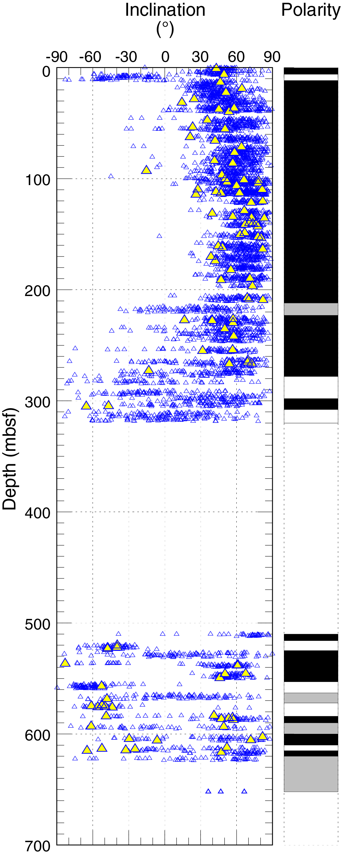
Figure F38. Downhole variation in inclination and inferred magnetic polarity.
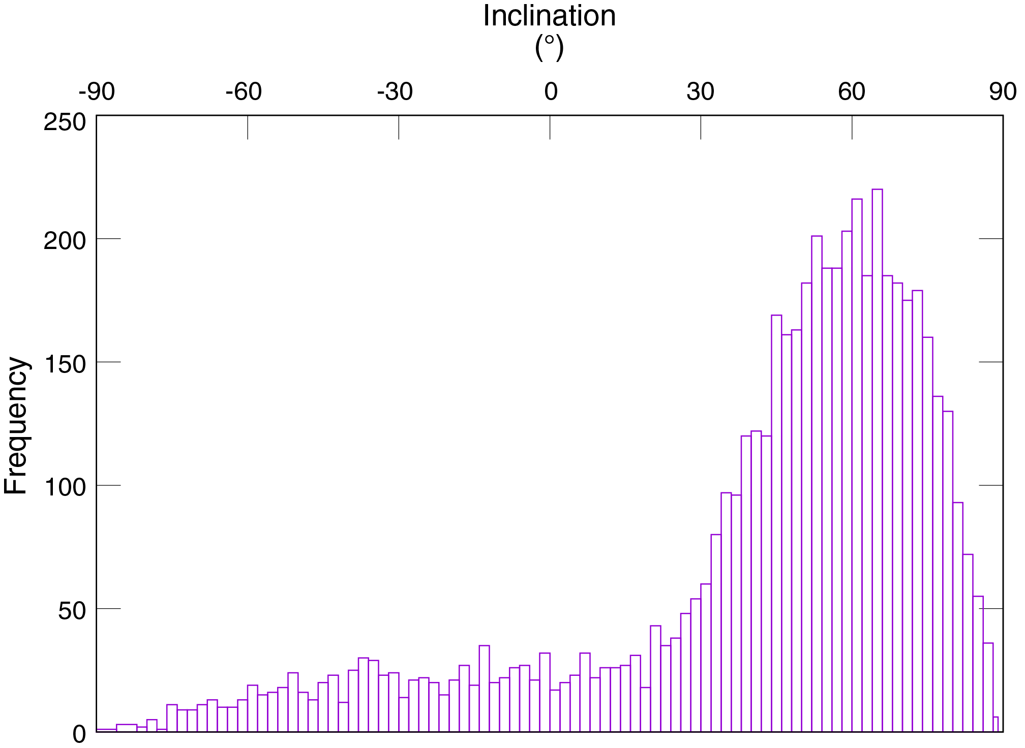
Figure F39. Histogram of archive-half inclinations.
Geochemistry
Inorganic geochemistry
IW was taken from cores from Holes C0024B, C0024D, C0024E, and C0024G. Evidence of gas expansion was observed in all cores, and this process is likely responsible for some contamination of sediments by seawater while cutting and retrieving cores. Raw concentration data are shown in Table T12. IW yields and squeezing parameters are shown in Table T13.
Salinity and chlorinity
Bottom water salinity was not measured but is estimated at just over 35‰ from the trend of salinity near the seafloor in Hole C0024B (Figure F40). In shallow Holes C0024B and C0024D, salinity decreases to 33.4‰ by 20 mbsf, remains relatively constant until 131 mbsf, and then trends toward lower values below. Important exceptions to the overall trend are several elevated salinity values. These include two values higher than inferred bottom water. Based on the two measurements in Hole C0024B, pore water chlorinity decreases from 558 mM at 1.3 mbsf to 552 mM at 4.6 mbsf. Deeper, there is a general increase in chlorinity concentrations of 3%. Processes that can lead to increases in salinity and chlorinity include recent gas hydrate formation, which leaves behind a residual brine, alteration of volcanic ash, and formation of authigenic clay minerals (Kastner et al., 1991). In Holes C0024B and C0024D, the small changes in salinity suggest processes related to variation in local lithology, whereas the more steady increases in chlorinity could be attributed to a constant downhole change such as recent formation of disseminated gas hydrate, increasing hydration of unstable mineral phases, or contribution from a brine.
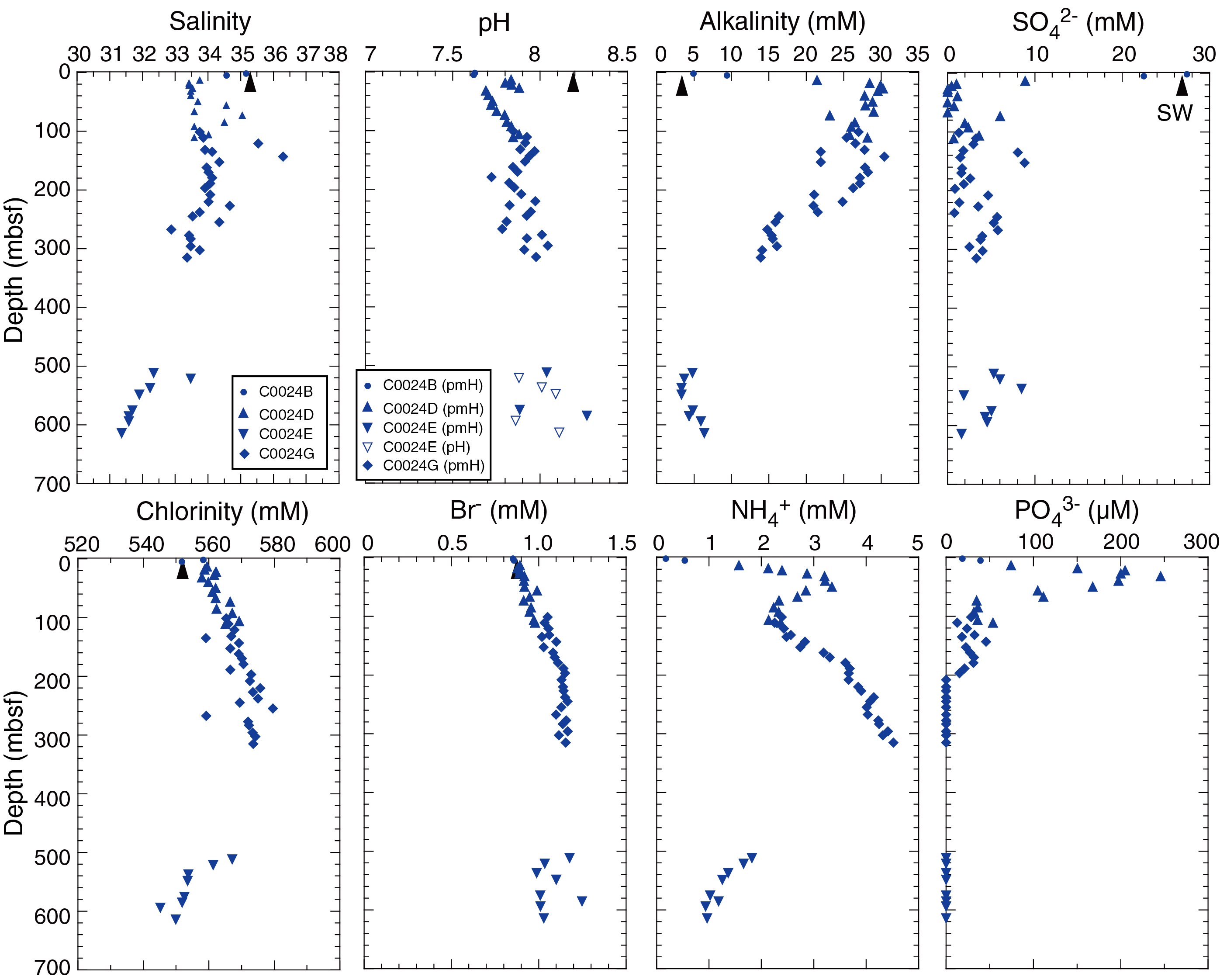
Figure F40. Salinity, pH/pmH, alkalinity, sulfate, chlorinity, bromide, ammonium, and phosphate.
In the deeper sections (Holes C0024E and C0024G), salinity trends toward lower values, reaching a minimum of 31.4 at 613.9 mbsf. Chlorinity continues to increase with depth in Hole C0024G to values > 570 mM at 320 mbsf. Chlorinity values greater than seawater require the removal of water from the interstitial fluid. However, chlorinity decreases in Hole C0024E from 567 mM at 511.6 mbsf to a minimum value of 545 mM at 593.9 mbsf, which is equivalent to a freshening of >2% relative to the inferred bottom water chlorinity and nearly 4% relative to the maximum chlorinity observed in the first measurement from Hole C0024E at 511.6 mbsf. A possible source of freshened water at greater depth is transport of fluids along conduits below the cored interval. This could explain the deep trend of slight pore water freshening, but the lack of deeper coring prevents testing of this hypothesis.
Sulfate and alkalinity
Sulfate (SO42−) decreases from a near-seawater value of 27.4 mM at 1.3 mbsf to 0.1 mM at 27.3 mbsf (Figure F40), which probably represents the depth of the sulfate–methane transition zone (SMTZ). At shallow depths, the alkalinity profile mirrors that of the sulfate and suggests production by the microbially mediated reaction:
resulting in the production of 1 mole of bicarbonate for each mole of sulfate consumed. The combined observations that sulfate concentrations never drop to zero below 27.3 mbsf and the range of values is from 0.1 to nearly 9 mM is possible evidence of seawater contamination in core material during drilling, recovery, and processing. This is not surprising given the ubiquitous evidence for core damage by gas expansion. Additional evidence that the elevated sulfate concentrations in deeper sediments could be due to contamination is the abundant methane found below 20 mbsf, where sulfate should be absent; sulfate and methane do not coexist under natural, steady-state conditions below the SMTZ because sulfate is consumed anaerobically to produce HS−. However, the possibility of a recent influx of sulfate at depth from natural processes cannot be completely excluded. For example, Torres et al. (2015) reported crustal fluid circulation with high sulfate concentration from the sediment overlying the incoming Philippine Sea plate.
Ammonium, phosphate, bromide, and manganese
Ammonium (NH4+) increases steadily in the sulfate reduction zone as a result of organic matter degradation during sulfate reduction (Figure F40). Ammonium reaches a local maximum value of 3.35 mM at 49.8 mbsf, indicating a source from organic matter degradation below the SMTZ. Ammonium concentrations then steadily decrease to 2.14 mM at 106.1 mbsf in Hole C0024D. In Hole C0024G, ammonium concentrations increase to a local maximum value of 4.52 mM at 314.9 mbsf, likely the result of continued breakdown of organic matter. Throughout Hole C0024E, ammonium concentrations steadily decrease from 1.82 to 0.96 mM.
Phosphate (PO43−) concentrations increase in the sulfate reduction zone and reach a maximum value of 246 µM at 31.8 mbsf (Figure F40). The concentrations decrease dramatically further below, which may be due to the precipitation of diagenetic apatite, the main sink for phosphate. Below 208 mbsf, phosphate concentrations are below the detection limit.
Bromide (Br−) concentrations increase steadily from 0.85 mM at 1.3 mbsf to 1.15 mM at 196.9 mbsf (Figure F40). Concentrations in Hole C0024E remain at a similar level, ranging from 0.99 to 1.25 mM, and are more scattered. The breakdown of marine organic matter can provide a source of bromide. Bromide concentrations at Site C0024 are similar to those observed at Site C0006, where they were interpreted to reflect a mixture of marine and terrestrial organic matter, dominated by terrestrial organic matter (Expedition 316 Scientists, 2009a).
Manganese concentrations are significantly higher than the seawater value (0 µM) in the upper 27 m, ranging from 19.1 to 2.5 µM (Figure F41). Concentrations never reach a value of zero but vary from 1.5 to 11.1 µM in the deeper part of the section in Holes C0024D and C0024G. In Hole C0024E, manganese values scatter between ~4 and 17 µM. Above the SMTZ, manganese is likely released from the microbial reduction of MnO2 to release soluble Mn2+. Elevated Mn concentrations in pore fluid below the sulfate reduction zone could be explained by MnO2 reduction coupled to sulfide reduction (Thamdrup et al., 1993), which may be responsible for the appearance of sulfate similar to that observed from Site C0012 (Torres et al., 2015). In general, fluctuations in manganese concentrations can be related to a combination of organic matter diagenesis, microbially mediated manganese reduction reactions, and crystallization of Mn-bearing carbonates.
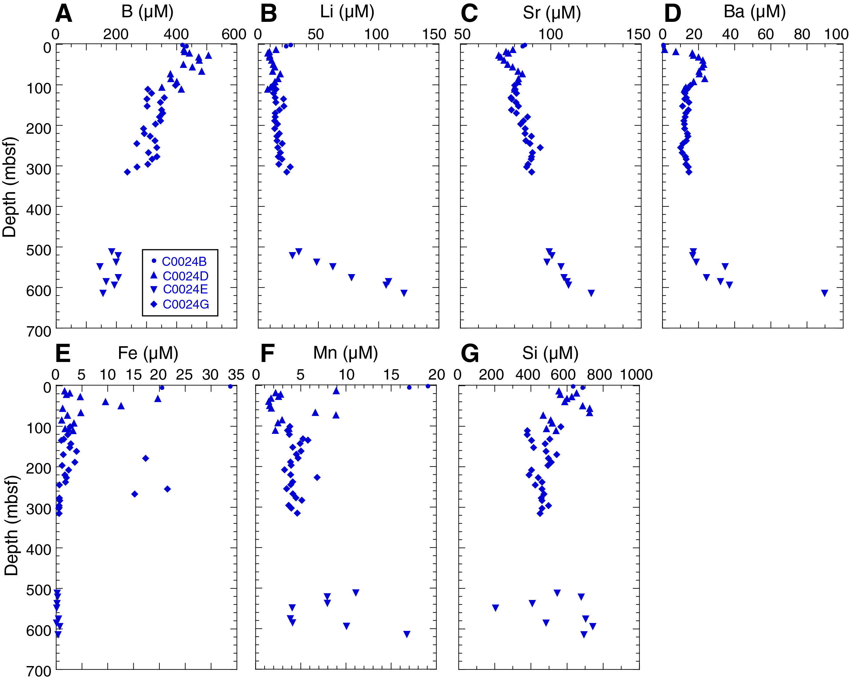
Figure F41. Minor elements.
Major cations (Ca, Mg, and K)
Calcium and magnesium concentrations covary from the seafloor to ~110 mbsf (Figure F42). A sharp decrease from 10.2 to 4.2 mM and from 51.8 to 42.8 mM for calcium and magnesium, respectively, occurs above 18.4 mbsf, below which both cation concentrations stay relatively constant until ~110 mbsf. The decrease in both cations could be related to the formation of Ca-Mg–bearing carbonates as alkalinity increases in the sulfate reduction zone. Below ~150 mbsf in Hole C0024G, magnesium concentrations decrease and calcium concentrations increase. These patterns are consistent with weathering of Ca-bearing silicates such as plagioclase with depth and loss of magnesium either to formation of clay minerals or adsorption onto existing surfaces of clay minerals resulting from silicate alteration. In Hole C0024E, calcium concentrations decrease with depth from 511.6 to 585.2 mbsf, below which concentrations increase. This may result from increased availability of reactive volcanic matter observed beginning at ~576 mbsf in Lithologic Unit IV (see Lithology). Magnesium on the other hand decreases steadily from ~21 to 2 mM with depth below 511.6 mbsf in Hole C0024E.
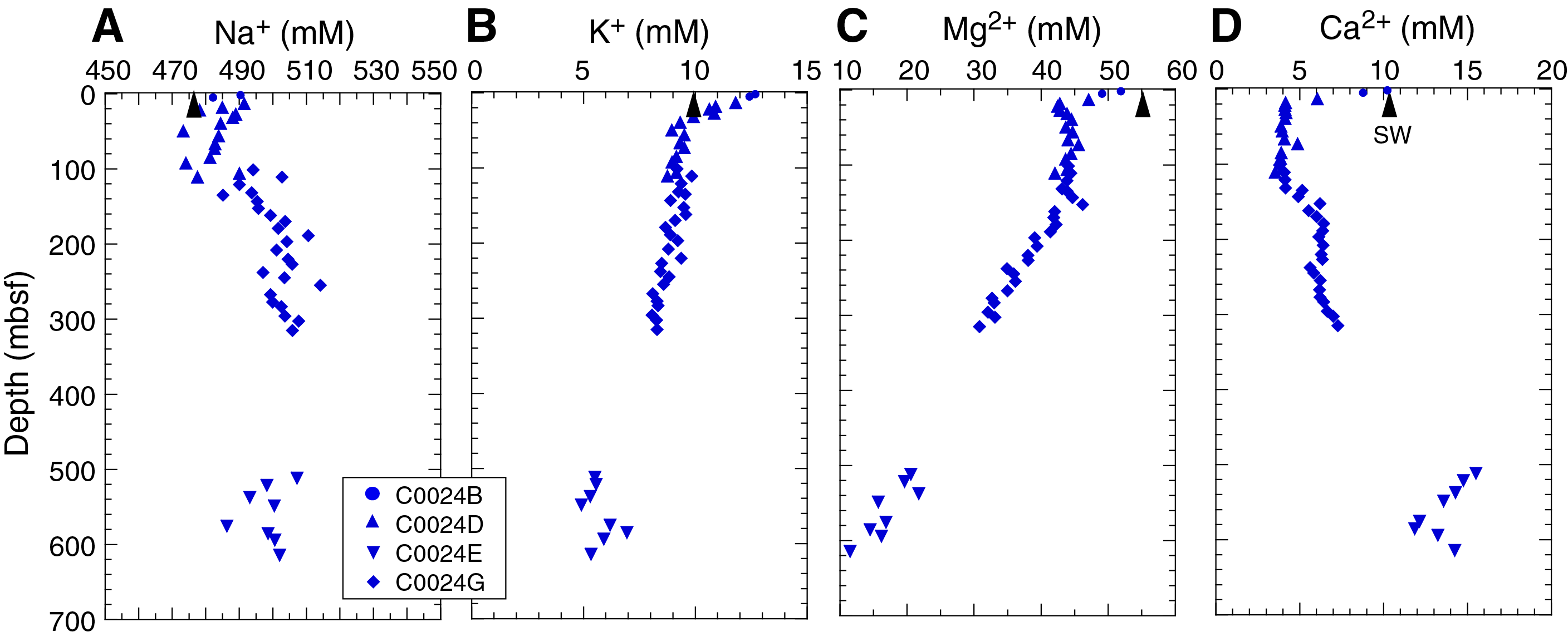
Figure F42. Major elements.
Potassium shows a concentration trend similar to magnesium (Figure F42). Potassium decreases from 12.7 to 8.9 mM over 1.3–49.8 mbsf. Formation of illitic clays is unlikely over this shallow depth range, but zeolite formation and cation exchange reactions with smectite are alternate options to explain the uptake in potassium from IW into the sediments.
Minor elements (B, Li, Si, Sr, Ba, and Fe)
Boron is near or slightly below seawater value near the seafloor (Figure F41) and then reaches values slightly higher than seawater (as high as 506 µM at 27.3 mbsf) before beginning a scattered, overall decreasing trend to values as low as 351 µM at 106.1 mbsf. Boron can be added to IW by low-temperature alteration of volcanic matter or stress-induced desorption from clay mineral surfaces and removed by (re-)adsorption onto clay minerals. The high values at shallow depths may be related to the incipient diagenesis of volcanic ash layers (see Lithology). From 511.6 to 613.9 mbsf in Hole C0024E, boron is significantly lower (156–207 µM), suggesting that less boron is available from the diagenesis of volcanic matter and/or clay adsorption becomes a more important process.
Lithium concentrations are generally lower than the average seawater value in the upper 300 m, ranging from 8.0 to 26.9 µM. In contrast, there is a strong increase from 29 to 121 µM from 511.6 to 613.9 mbsf in Hole C0024E, reaching a value nearly five times the concentration in seawater (Figure F41). The reduction in Li concentrations may be explained by adsorption onto clay minerals (James and Palmer, 2000), whereas the increase in Li concentrations in Hole C0024E may relate to the contribution of deep fluid often observed in the Nankai Trough (e.g., You et al., 1995).
Silica concentrations mostly range from 400 to 742 µM (Figure F41). The values scatter with depth and show no obvious downhole trends. The concentrations are significantly higher than the seawater value. The most likely source of silica is from the dissolution of volcanic glass in ash layers or ash shards disseminated throughout the silty muds and mudstones. Siliceous fossil tests are rare in the sediments (see Lithology), and thus their dissolution is likely not an important source for dissolved silica.
Strontium concentrations are close to seawater concentration in the shallowest sample. Several fluctuations occur over the upper 130 m of cored sediments (Figure F41). Alteration of volcanic material could explain the elevated Sr concentrations; this process was often observed in Nankai Trough sediments (Torres et al., 2015; Joseph et al., 2013). The alternating pattern of decreasing and increasing concentrations may be related to variations in volcanic matter content. The increase to 84.3 µM at 73.0 mbsf might be related to the increase in volcanic matter observed at this depth. The overall increase in strontium below 135 mbsf may be related to a greater abundance of reactive volcanic ash layers and disseminated volcanic glass shards and increasing diagenesis. This is supported by the observation of higher calcium concentrations in this depth range (Figure F42) and also agrees with the B and Si observations (see above).
Barium concentrations increase steadily from 0.4 to 22.9 µM from the seafloor to 49.8 mbsf (Figure F41) over approximately the same depth interval of sulfate reduction. Barite dissolution below the sulfate reduction zone is one major source of barium in pore waters because the removal of sulfate from solution could increase barite solubility (Torres et al., 1996). The decrease in barium concentrations from 49.8 to 110.9 mbsf is more puzzling. This might be related to an overall decrease in barium in the host sediments, but resolution will have to await shore-based analysis.
Iron is present from 1.1 to 33.7 µM in the upper 110 m (Figure F41). Concentrations may vary because of microbially mediated iron reduction reactions in the SMTZ and recycling of iron during redox reactions to 110 mbsf. Reduction of iron oxides coupled to sulfide oxidation may explain the elevated iron concentrations in the deeper sediments (Torres et al., 2015).
Trace elements (Rb, Cs, V, Cu, Zn, As, Mo, Pb, and U)
Rubidium mimics the behavior of potassium in marine sediments. In Holes C0024B and C0024D, the steady decrease of Rb from 1843 to 1148 nM at 49.8 mbsf may reflect cation exchange with ammonium on clay mineral surfaces (Figure F43). This is supported by the inverse pattern of rubidium compared to ammonium. Deeper in the section, no notable variations in concentrations occur.
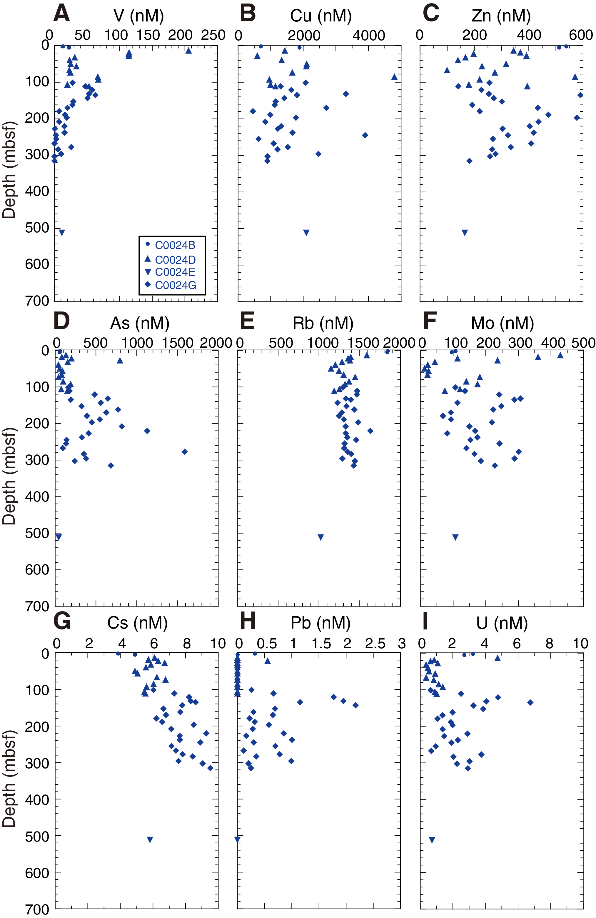
Figure F43. Trace elements.
Zinc, copper, vanadium, arsenic, molybdenum, and uranium concentrations are highly variable. Zinc and vanadium concentrations are higher than seawater values, whereas uranium concentrations are lower, with the latter reflecting the lower solubility in reducing environments. Molybdenum ranges from 12 to 441 nM, which is both lower and higher than seawater concentration.
Organic geochemistry
Chemical compositions of hydrocarbon gases
Hydrocarbon gases in headspace gas
Hydrocarbon gas concentrations in the headspace (HS) samples taken from Holes C0024B, C0024D, C0024E, and C0024G were analyzed by gas chromatograph (GC)–flame ionization detector (FID) (Figure F44; Table T14). Methane concentrations shallower than 13 mbsf are ≤4 ppm. Between 13 and 310 mbsf, concentrations scatter between 3,900 and 50,600 ppm. Below 512 mbsf in Hole C0024E, concentrations range from ~12,700 to ~22,500 ppm with the exceptions of relatively low concentrations of 4,900 and 1,400 ppm at 512 and 528 mbsf, respectively. Ethane was not detected shallower than 13 mbsf. Ethane concentrations increase from 0.1 ppm at 22 mbsf to 1.7 ppm at ~130 mbsf. Below 140 mbsf, ethane concentrations increase to ~3 ppm at ~180 mbsf and then decrease to 0.8 ppm at ~220 mbsf. Below ~220 mbsf, concentrations increase to ~6 ppm at 311 mbsf. In Hole C0024E, ethane concentrations are generally higher than those shallower than 311 mbsf. Concentrations range from 8 to 12 ppm except for two low concentrations at 512 and 528 mbsf. Propane concentrations are low and show little variation from 0 to 135 mbsf. Propane was not detected shallower than 22 mbsf. Below this depth is a small peak of 0.3 ppm at around ~37 mbsf. Propane also steadily increases to 1 ppm from 63 to 135 mbsf. Below 140 mbsf, concentrations mostly range from 1 to 6 ppm but are scattered. Below 512 mbsf, propane is not present or has very low concentrations of <0.3 ppm.
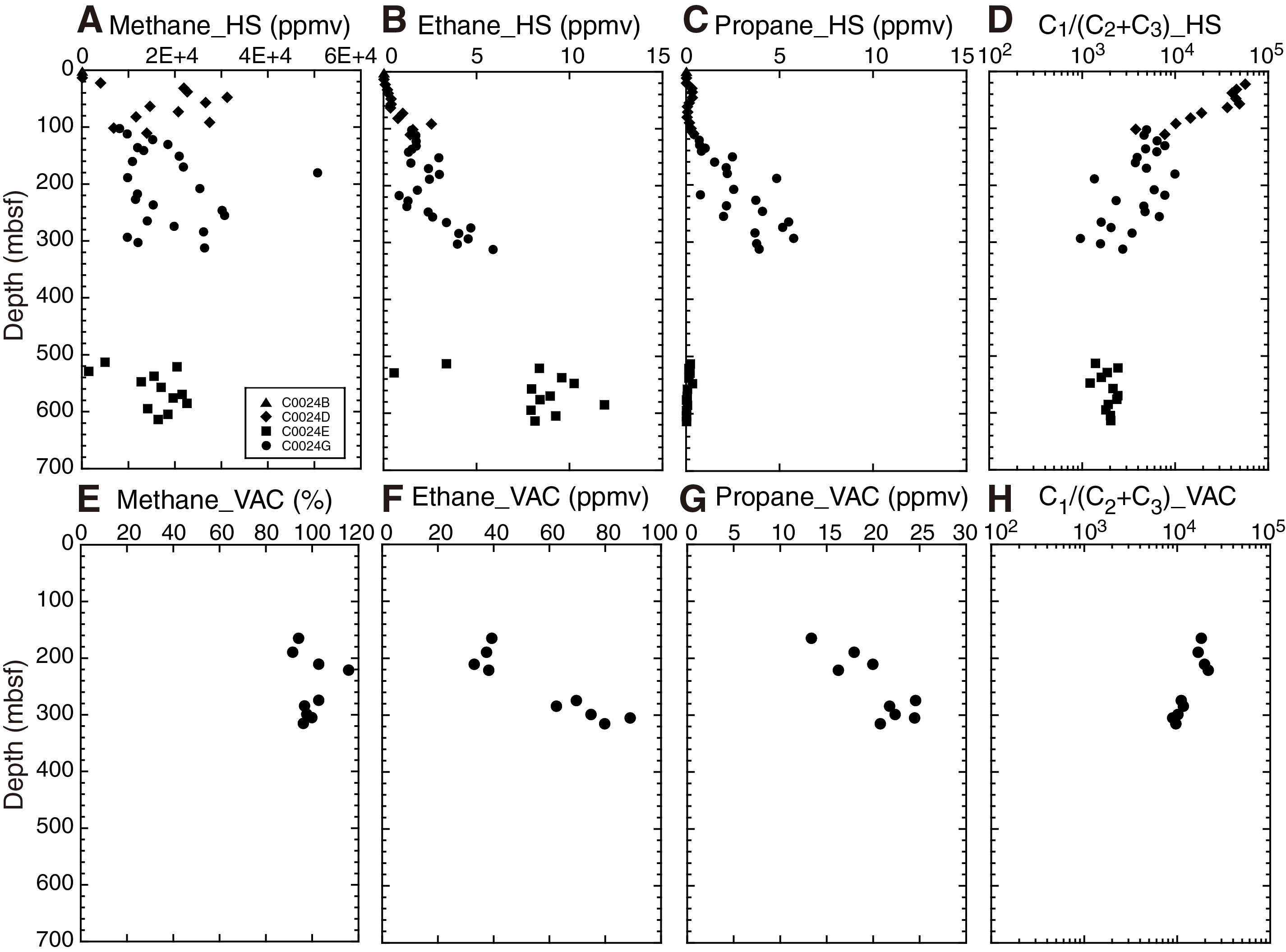
Figure F44. Headspace and void space gases.
The methane to ethane plus propane (C1/[C2 + C3]) molar ratios decrease from ~56,000 at 22 mbsf to ~5,000 at ~140 mbsf, reflecting an overall downhole increase in C2+ hydrocarbons. Between ~140 and ~300 mbsf, the ratios scatter but generally decrease to 1000–2000 with depth. In Hole C0024E, the ratios range from 1200 to 2400.
Hydrocarbon gases in void gas
Nine void gas samples (VAC) were collected from Hole C0024G, and the compositions of hydrocarbon gases in those samples were analyzed by GC-FID (Figure F44; Table T15). The proportion of methane in all samples is higher than 90%. Measured concentrations of more than 100% are due to the insufficient degassing of samples to reach 1 atm equivalent pressure before analysis. Ethane concentrations between 164 and 220 mbsf are 32–39 ppm. Between 273 and 314 mbsf, concentrations generally increase from 62 to 89 ppm with depth. Propane concentrations generally increase from 13 ppm at 164 mbsf to ~25 ppm at ~300 mbsf. As a result, C1/(C2 + C3) ratios between 164 and 220 mbsf are 16,500–21,000 and then slightly decrease from ~11,000 at 273 mbsf to ~9,000 at 304 mbsf. The C1/C2+ ratios indicate the gas is likely biogenic in origin. The presence of ethane and propane suggests an input of thermogenic gas, but this will be investigated further by shore-based carbon isotope studies.
Carbonates, organic carbon, and total nitrogen of cores
Results for calcium carbonate, total organic carbon (TOC), total nitrogen (TN), total sulfur (TS), and the TOC/TN ratio are shown in Table T16 and Figure F45. TOC is generally low, ranging from 0.1 to 0.9 wt%. The deeper cored interval (511–618 mbsf) has slightly lower TOC than the interval above 316 mbsf. Calcium carbonate is generally <4 wt%. One important exception occurs from 537.1 to 574.7 mbsf, where the highest value reaches 15.2 wt%. This interval lies in Lithologic Unit IV, inferred to be accreted Shikoku Basin sediments (see Lithology), and the increase is inferred to result from enhanced preservation of nannofossils. Nitrogen and sulfur contents are low and highly variable throughout the cored intervals. The TOC/TN ratio generally decreases downhole. In the upper 100 m, ratios of >10 are common and are consistent with burial of terrestrial organic matter. The highest ratios of 16–24 occur at 227.0–277.2 mbsf. The lowest cored section has TOC/TN ratios mostly <10, which is consistent with organic matter dominated by marine material.

Figure F45. Inorganic carbon, calcium carbonate, TN, total carbon, TS, TOC, and TOC/TN.
Physical properties
Physical property measurements were performed on core samples from Holes C0024B and C0024D–C0024G. Moisture and density (MAD) and P-wave velocity measurements were conducted on discrete samples taken from working halves. Electrical resistivity measurements were performed on either working halves using a four-pin array electrode or discrete samples taken from working halves using two electrodes. The whole-round multisensor core logger (MSCL-W) measurements were conducted on whole-round cores. Thermal conductivity was measured on either whole-round cores using a full-space needle probe or working halves using a half-space line source probe. Shear strength was measured on working halves using both the vane shear apparatus and penetrometer.
MSCL-W (whole-round cores)
Whole-round cores from Holes C0024B (0.067–5.557 mbsf), C0024C (6.058–6.847 mbsf), C0024D (7.075–119.3 mbsf), C0024E (510.08–621.5 mbsf), C0024F (652.02–652.1 mbsf), and C0024G (100.08–318.49 mbsf) were analyzed using the MSCL-W (see Physical properties in the Expedition 358 methods chapter [Hirose et al., 2020]). The results of gamma ray attenuation (GRA) bulk density, magnetic susceptibility, natural gamma radiation (NGR), and electrical resistivity measurements on whole-round cores are summarized in Figure F46. Core liners made of butyrate were used in Holes C0024B–C0024D and C0024G, whereas those made of polycarbonate were used in Holes C0024E and C0024F.
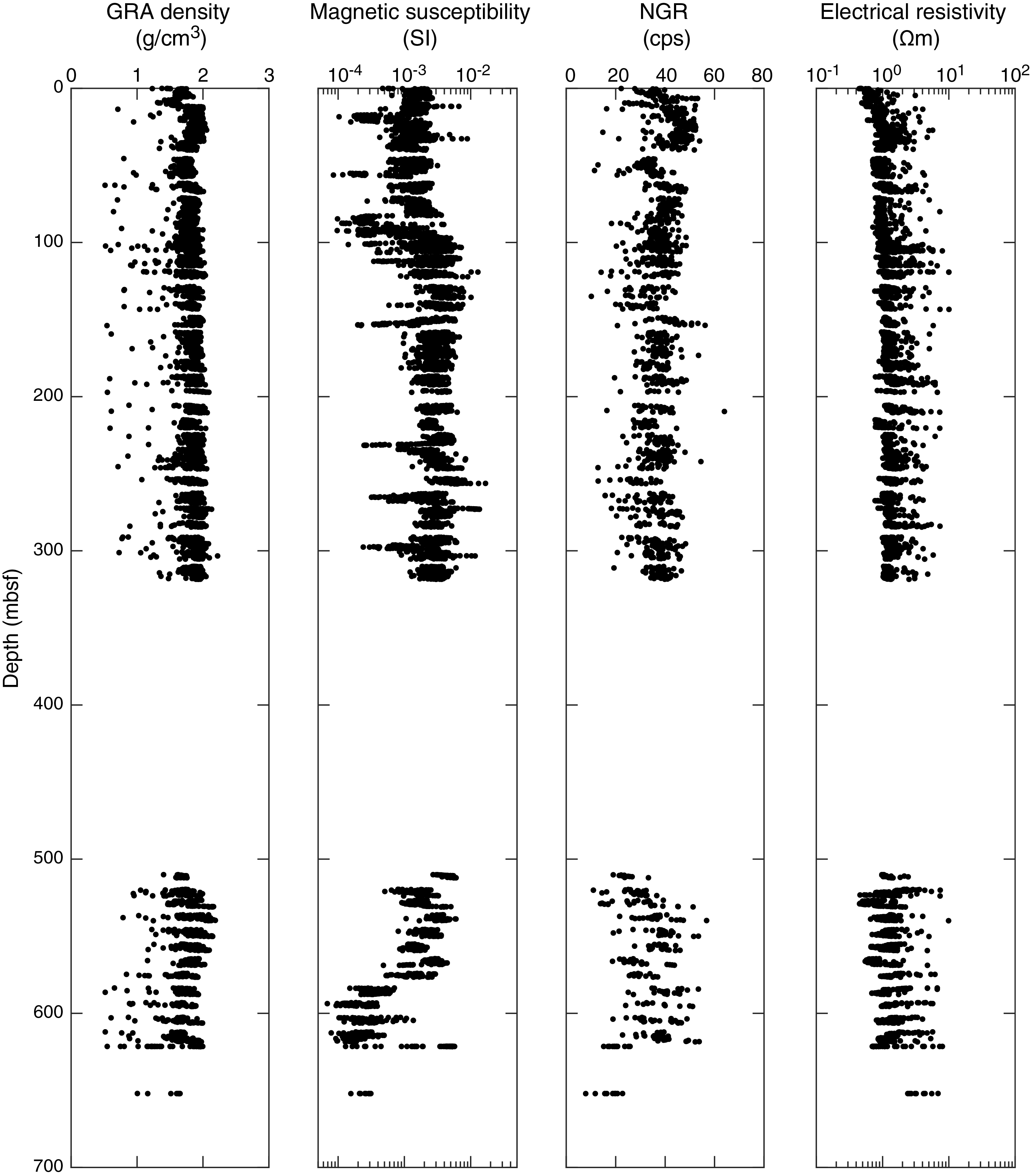
Figure F46. MSCL-W measurements.
GRA bulk density, NGR, and electrical resistivity range from ~0.5 to ~2.2 g/cm3, from 11 to 64 counts/s, and from 0.5 to 10 Ωm, respectively, at 0–318.5 and 510–621.5 mbsf. These three parameters do not show any clear or systematic changes with depth, although GRA bulk density and electrical resistivity both increase slightly with depth above 318.5 mbsf. Magnetic susceptibility values are approximately 1.5 × 10⁻³ SI at 0–80 mbsf before gradually increasing to ~4 × 10⁻³ SI at ~130 mbsf and then remaining relatively constant at 3 × 10⁻³ SI to 320 mbsf. In the deeper sections, magnetic susceptibility values decrease from ~5 × 10⁻³ at ~510 mbsf to ~1.5 × 10⁻⁴ SI at ~595 mbsf. In addition to the general trend, we observed low magnetic susceptibility values of ~8.5 × 10⁻⁵ SI at 18, 56, and ~86 mbsf and ~2.5 × 10⁻⁴ SI at 153, 231, 265, and 297 mbsf. P-wave velocity was measured using the MSCL-W for cores collected from Holes C0024B and C0024D, but data are shown in Figure F47 only for depths shallower than 36 mbsf where P-wave amplitudes reached 100 mV. This is because low P-wave amplitude reflects voids and poor contact between the liner and sediment, which influences arrival time. When focusing on measurements with P-wave amplitudes >100 mV (red in Figure F47), P-wave velocity shows a slight increase with depth from about 1495 m/s at 0 mbsf to 1590 m/s at 7 mbsf and then stays constant to 33 mbsf (Figure F47). P-wave velocity values measured using the MSCL-W in Holes C0024E–C0024G are not presented because the results are low quality due to poor contact between the liner and sediment.
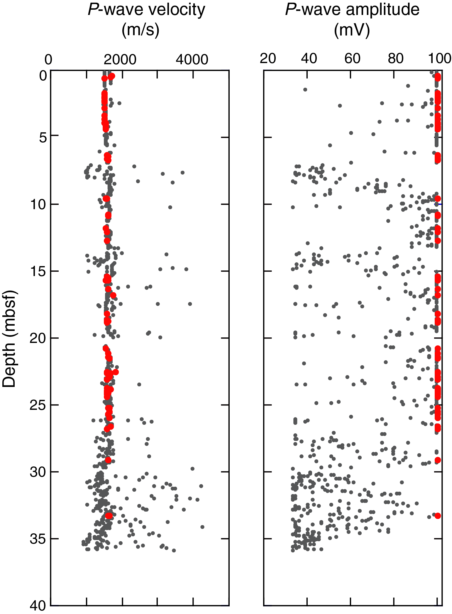
Figure F47. P-wave from MSCL-W.
Moisture and density measurements
MAD measurements were carried out to determine grain density, bulk density, and porosity on a total of 378 discrete core samples at Site C0024 (Table T17): 10 from Hole C0024B (0.16–5.36 mbsf), 126 from Hole C0024D (11.85–115.00 mbsf), 61 from Hole C0024E (510.39–618.13 mbsf), 1 from Hole C0024F (652.04 mbsf), and 180 from Hole C0024G (100.43–317.93 mbsf) (Figure F48).
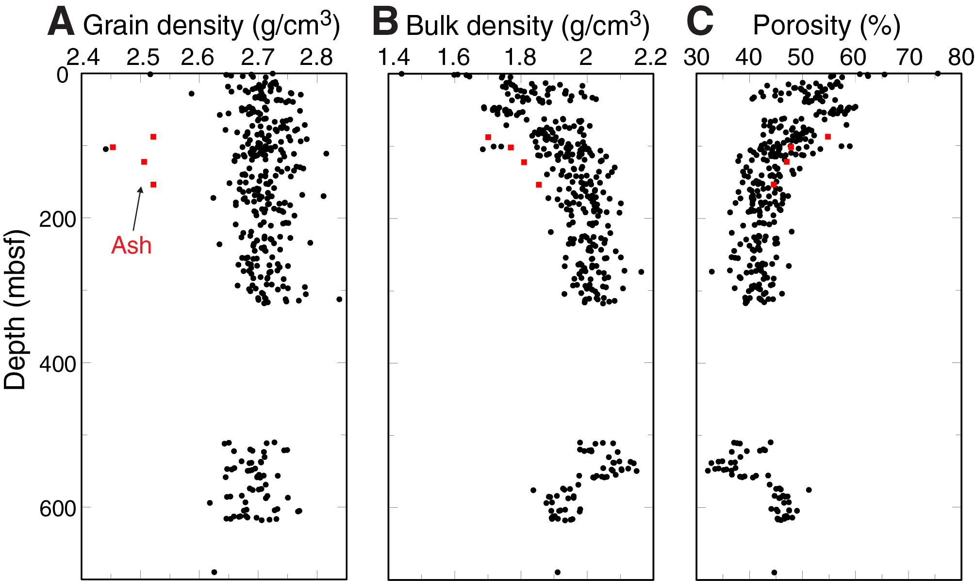
Figure F48. MAD, discrete core samples.
Grain density values throughout the sampled depth interval mostly scatter between 2.65 and 2.78 g/cm3. Values appear to be independent of lithology except for four samples from the ash layers, which have lower grain density values of 2.45–2.52 g/cm3 (Figure F48A).
Bulk density increases from 1.44 to 2.03 g/cm3 and porosity decreases from 75.5% to 40.5% between 1.14 and 33.281 mbsf and then they remain relatively constant at ~1.77–1.87 g/cm3 and 45.8%–56.1%, respectively, to 40.02 mbsf (Figure F48B, F48C). Bulk density and porosity shift to 1.69 g/cm3 and 60.0%, respectively, at ~46 mbsf, with a gradual increase to 1.93–2.10 g/cm3 and decrease to 47.4%–36.3%, respectively, at ~318 mbsf. Between 510.39 and 549.78 mbsf, bulk density increases from 1.98 to 2.15 g/cm3 and porosity decreases from 44.0% to 32.1%. Then bulk density shifts to 1.84–1.95 g/cm3 and porosity shifts to 45.9%–51.2% at ~577 mbsf, representing a deviation from the general compaction trend. This change in bulk density and porosity between ~550 and 577 mbsf occurs at or near the Lithologic Unit III/IV boundary at 555 mbsf (see Lithology). Below 584.21 mbsf, bulk density and porosity remain relatively constant, ranging between 1.88 and 1.98 g/cm3 and between 44.6% and 49.0%, respectively, to the bottom of Hole C0024E at ~618 mbsf. The sample at 652.04 mbsf in Hole C0024F exhibits a bulk density of 1.91 g/cm3 and a porosity of 44.6%.
Ash samples exhibit lower grain density values of ~2.5 g/cm3, bulk density values of 1.14–1.40 g/cm3, and relatively higher porosity values of 44.6%–54.8% than other silty sediment samples.
Electrical resistivity and P-wave velocity measurements (working half and discrete core samples)
Electrical resistivity and P-wave velocity measurements were made along x-, y- and z-directions from the recovered cores in Holes C0024E (520.11–616.19 mbsf) and C0024F (652.04 mbsf) where the material was indurated enough to be cut into cubic samples. For the cores recovered from shallower depths in Holes C0024B (0.12–5.459 mbsf), C0024D (12.629–114.975 mbsf), C0024E (510.865–512.115 mbsf), and C0024G (100.825–512.415 mbsf), the material was largely unconsolidated and thus could not be cut into cubic samples, except three samples recovered from Hole C0024G at 234.935, 291.95, and 312.265 mbsf where the material was indurated enough to be cut into cubes. Therefore, P-wave velocity measurements were not made for the majority of these samples and electrical resistivity measurements were made only along y- and z-directions using the four-pin electrode array that was pushed into the soft sediment.
Resistivity increases overall with depth (Figure F49A), although an exception to this trend occurs between 40 and 100 mbsf where resistivity decreases. Correlation between resistivity measured on recovered core and that measured from LWD (see Logging) is also poor at these depths. This could possibly be due to void spaces created by gas expansion in the core when it was recovered. Although significant data scatter occurs below 100 mbsf, an overall trend of increasing resistivity is observed as well as a shift in this trend at approximately 550 mbsf. This shift to lower resistivity values correlates with the depth of a shift in porosity and the Lithologic Unit III/IV boundary (see Lithology). Electrical resistivity anisotropy shows significant scatter and no clear trend with depth (Figure F49B). Below 510 mbsf, where anisotropy was characterized in both the horizontal and vertical directions, the magnitude of vertical anisotropy is larger on average than horizontal anisotropy, as seen by the persistent clustering of data to the left of the 0% line for vertical anisotropy. This indicates that resistivity values are higher in the z-direction, likely reflecting a fabric developed by vertical compaction that leads to a greater degree of pore space connectivity in the horizontal direction. The relationship between resistivity and porosity can be seen in Figure F50, with higher resistivity associated with lower porosity.
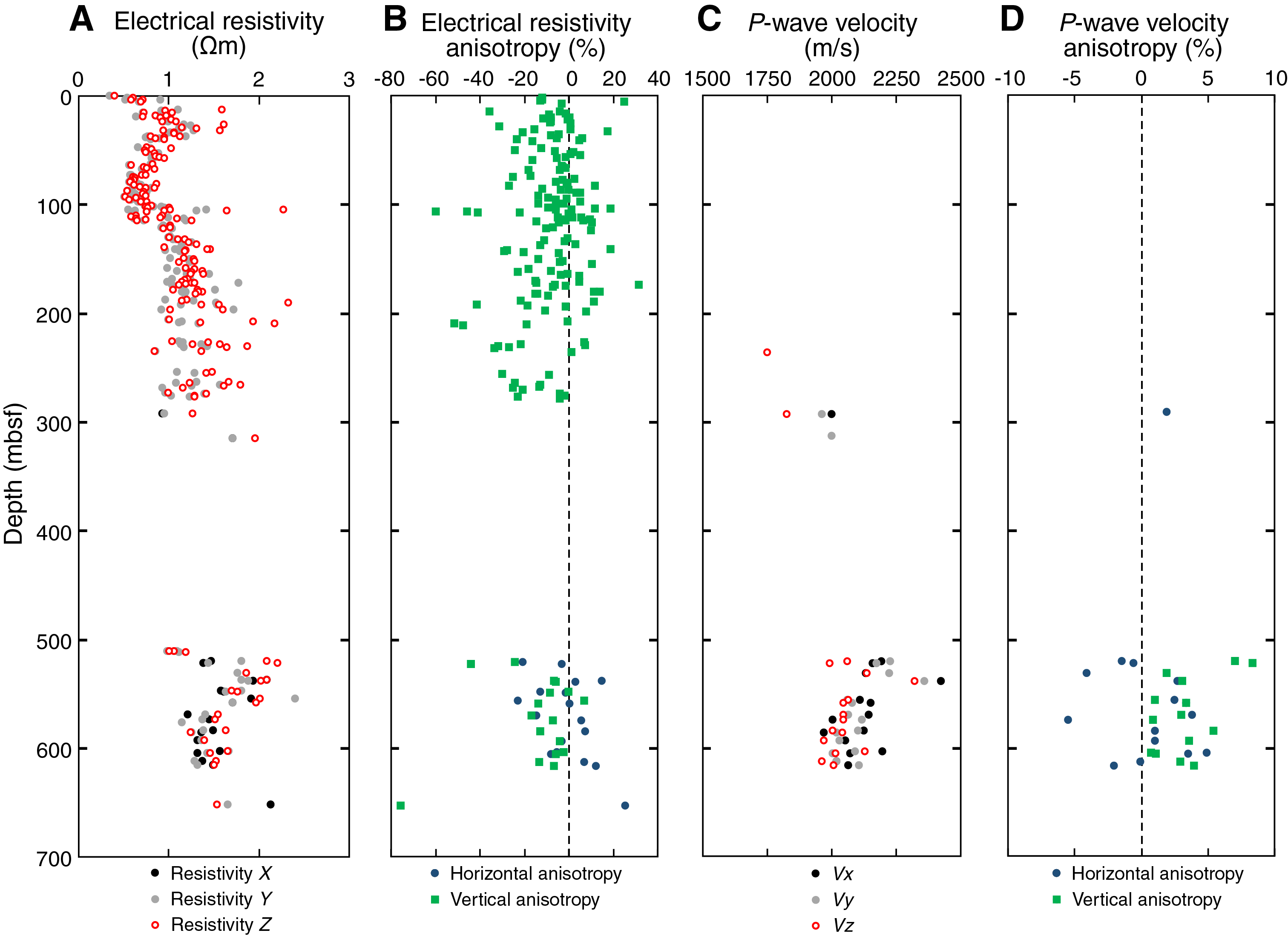
Figure F49. Electrical resistivity, P-wave velocity, and anisotropy.
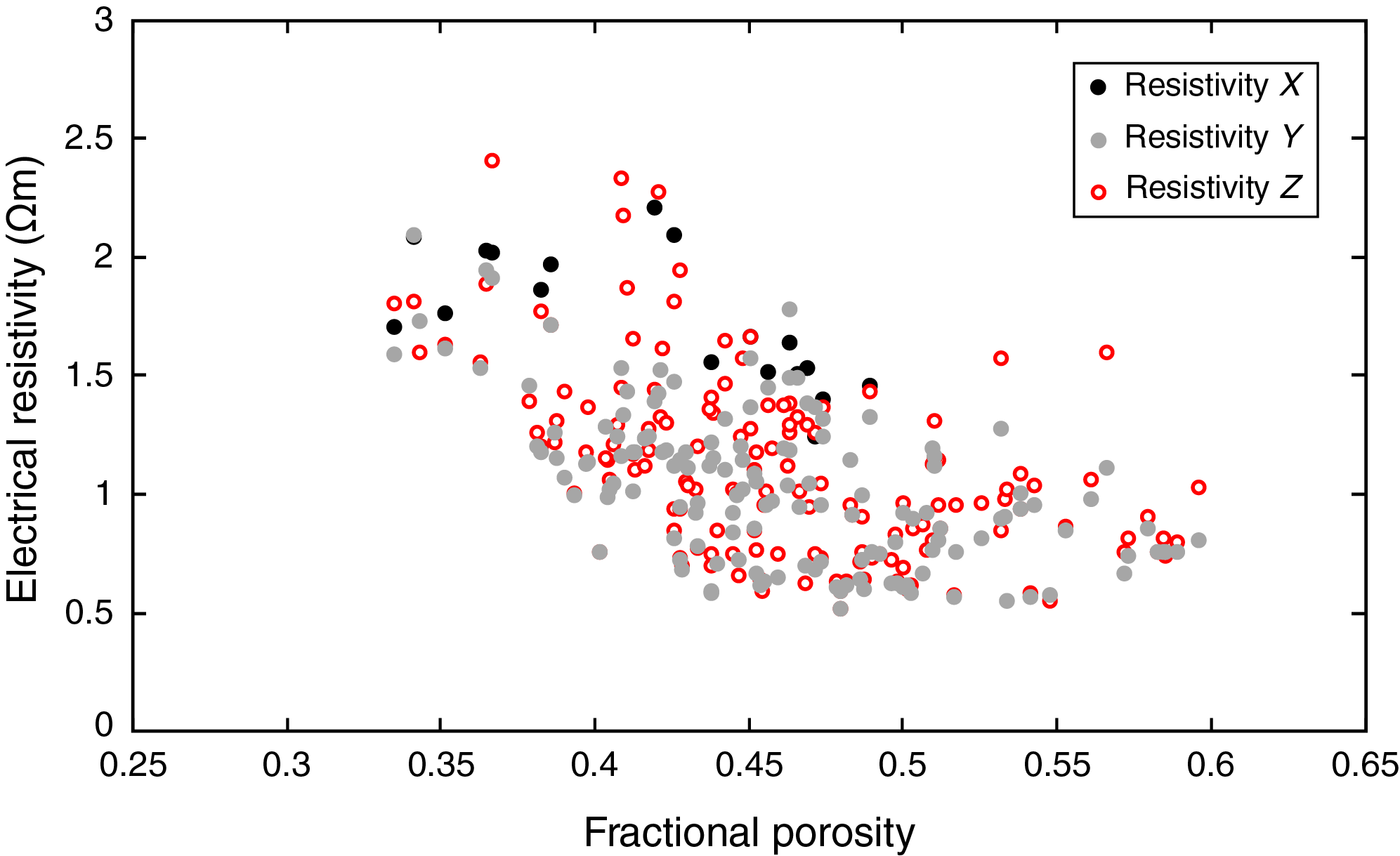
Figure F50. Porosity vs. electrical resistivity.
Apart from three samples collected at 234.935, 291.95, and 312.265 mbsf in Hole C0024G, P-wave velocity was only measured over a narrow depth range below 510 mbsf; as such, it is difficult to determine an overall trend with depth. Values typically scatter between 1950 and 2200 m/s (Figure F49C). At ~550 mbsf, P-wave velocity data are consistent with a shift observed in electrical resistivity data (Figure F49A), porosity (Figure F48C), and the Lithologic Unit III/IV boundary (see Lithology). In terms of P-wave velocity anisotropy, significant scatter occurs for both horizontal and vertical anisotropy (Figure F49D). Although horizontal anisotropy data scatter almost symmetrically about the 0% line, vertical anisotropy values all plot on the positive side, ranging between 0% and 9%, suggesting slower P-wave velocity in the vertical direction compared to the horizontal direction.
Thermal conductivity (whole-round cores and working halves)
Thermal conductivity was measured on whole-round cores from Holes C0024B (0.067–1.141 mbsf), C0024D (7.075–119.3 mbsf), and C0024G (100.1–318.5 mbsf) using a full-space needle probe and on working halves from Holes C0024E (510.1–621.5 mbsf) and C0024F (652.0–652.1 mbsf) using a half-space line source probe (Figure F51; Table T18). Thermal conductivity ranges from 1.11 to 1.50 W/(m·K) from 1 to 312 mbsf and from 1.14 to 1.72 W/(m·K) from 512 to 652 mbsf. Overall, thermal conductivity increases with depth.
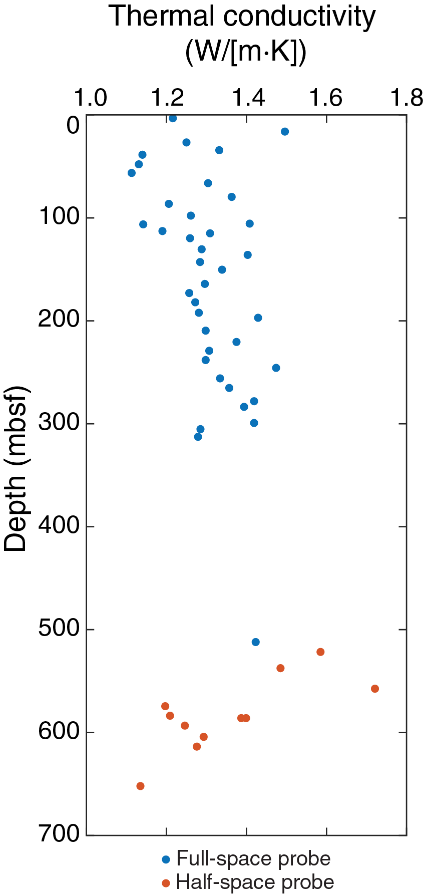
Figure F51. Thermal conductivity.
The correlation between thermal conductivity and porosity is shown in Figure F52. The empirical relation that describes thermal conductivity of a formation (k) as a function of porosity (ϕ) and grain thermal conductivity (ks) is given by the following geometrical mean model (e.g., Brigaud and Vasseur, 1989):
where kw is the thermal conductivity of pore water (0.6 W/[m·K]). The relationship between thermal conductivity and porosity of the sediments from Site C0024 follows the trend obtained from the upper Shikoku Basin sediments at Sites C0006 and C0011 (Expedition 316 Scientists, 2009a; Expedition 322 Scientists, 2010; Expedition 333 Scientists, 2012a).
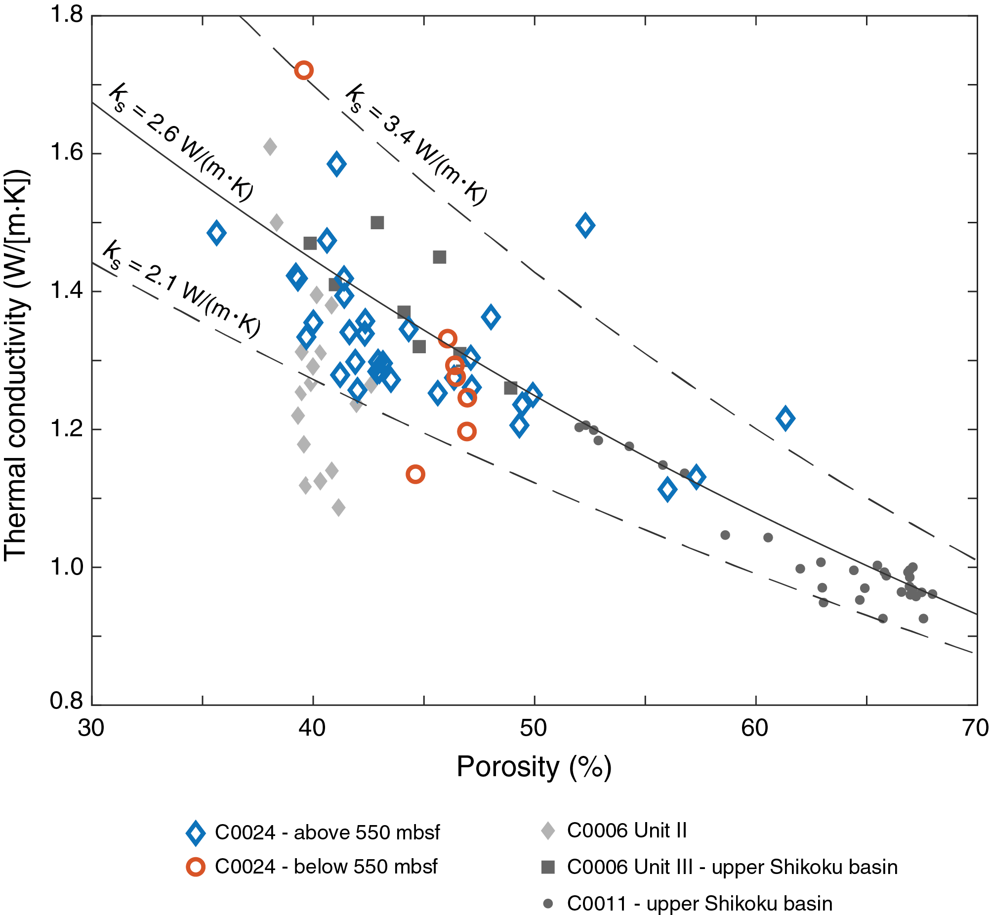
Figure F52. Thermal conductivity vs. porosity.
Shear strength (working halves)
Shear strength was measured using a vane shear apparatus and a pocket penetrometer (see Physical properties in the Expedition 358 methods chapter [Hirose et al., 2020]) on working halves from 0.14 to 512.1 mbsf at Site C0024 (Figure F53). When possible, both types of strength measurements were made per section. Undrained shear strength measured using the vane shear apparatus gradually increases from 1.3 kPa at 0.17 mbsf to 31.0 kPa at 21.8 mbsf. Undrained shear strength values are similar for both the vane shear and penetrometer measurements above ~5.4 mbsf, whereas undrained shear strengths measured from vane shear tests are typically lower than those from penetration tests below ~12.7 mbsf. We note that the two dial needles on the vane shear apparatus are expected to separate when the material reaches failure; however, this separation never occurred during Expedition 358 testing because of machine conditions. We therefore manually stopped the rotating vane and read the corresponding value when we recognized visible cracks in the core because we interpreted this to represent failure. Undrained shear strength measured from penetrometer tests ranges from 1.0 to 264.6 kPa at 0.14–512.1 mbsf. Considerable scatter occurs in the data, which increases with depth.

Figure F53. Undrained shear strength.
Anelastic strain recovery
During the expedition, we conducted anelastic strain recovery (ASR) measurements using fresh whole-round core samples on the ship to estimate the in situ stress orientation and the 3-D stress regime. The time-sensitive ASR measurements were started a few hours after the core samples were cut from the formation. We applied the same ASR measurement techniques as those successfully used during previous NanTroSEIZE expeditions (Byrne et al., 2009; Yamamoto et al., 2013; Oohashi et al., 2017).
At Site C0024, we conducted shipboard ASR measurements for three whole-round core samples (358-C0024E-2R-4, 70–83 cm, 8R-1, 78–92 cm, and 12R-2, 18–32 cm). To illustrate the results of the shipboard ASR measurements, the anelastic strain data, three principal strains, and mean strains are shown in Figure F54.
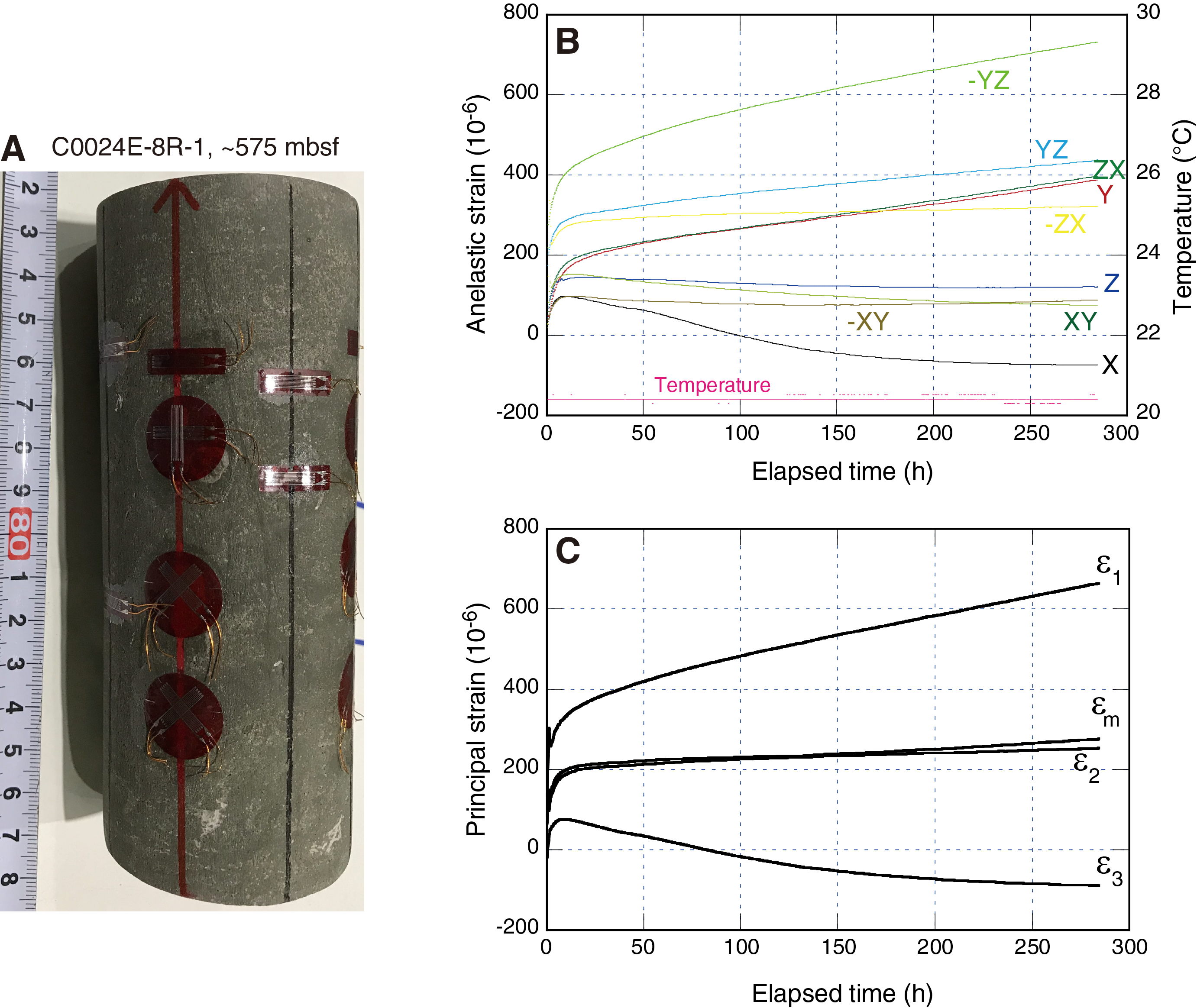
Figure F54. ASR.
Downhole measurements
In situ temperature was measured using the advanced piston corer temperature (APCT-3) tool at four depths in Holes C0024B–C0024D (Table T19). Three of the temperature measurements at 6, 20.5, and 36 mbsf (bottom of Cores 358-C0024B-1H, 358-C0024D-2H, and 4H, respectively) show a characteristic heating pulse from probe penetration followed by smooth decay with time (Figure F55). The average water temperature at the mudline, which was measured by holding the APCT-3 tool for 5–10 min before lowering the BHA to the bottom of the borehole, was 1.67°C. An estimate of the in situ temperature was obtained by extrapolation of a model fit to the smooth portion of the decay in the data (see Downhole measurements in the Expedition 358 methods chapter [Hirose et al., 2020]). Estimated in situ temperature increases from 1.67°C at 0 mbsf (mudline) to 4.08°C at 36 mbsf with a best-fit geothermal gradient of 74°C/km (R2 = 0.957) (Figure F56). This is significantly greater than the gradient of 27°C/km reported at Site C0006 (determined based on APCT-3 data from 0 to 220 mbsf) (Expedition 316 Scientists, 2009a). It should be noted that the depth interval of APCT-3 measurements at Site C0024 was limited to <40 mbsf because the HPCS was halted because of high tension while pulling up the shot piston (see Introduction and operations).

Figure F55. APCT-3 at 6.0, 20.5, and 36.0 mbsf.
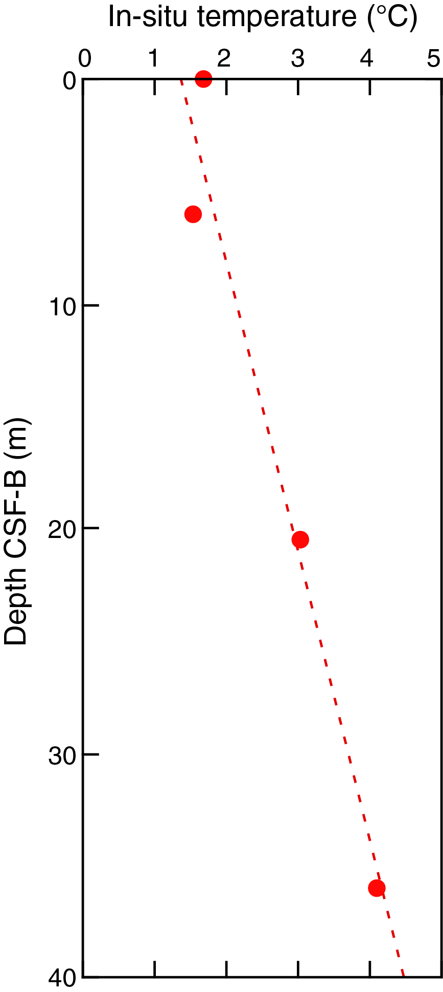
Figure F56. In situ temperature estimated from APCT-3.
If heat transfer is by conduction and heat flow is uniform, the thermal gradient is inversely proportional to thermal conductivity according to Fourier's law. Using a technique developed by Bullard (1939), the heat flow is the slope of the linear relationship between temperature and thermal resistance, which is calculated from conductivity measurements on core samples (Figure F57). The best-fit heat flow is estimated to be 98 mW/m2. As described above, it is possible that the estimated temperature gradient and heat flow might not reflect the thermal regime at this site because of the limited number of APCT-3 measurements.
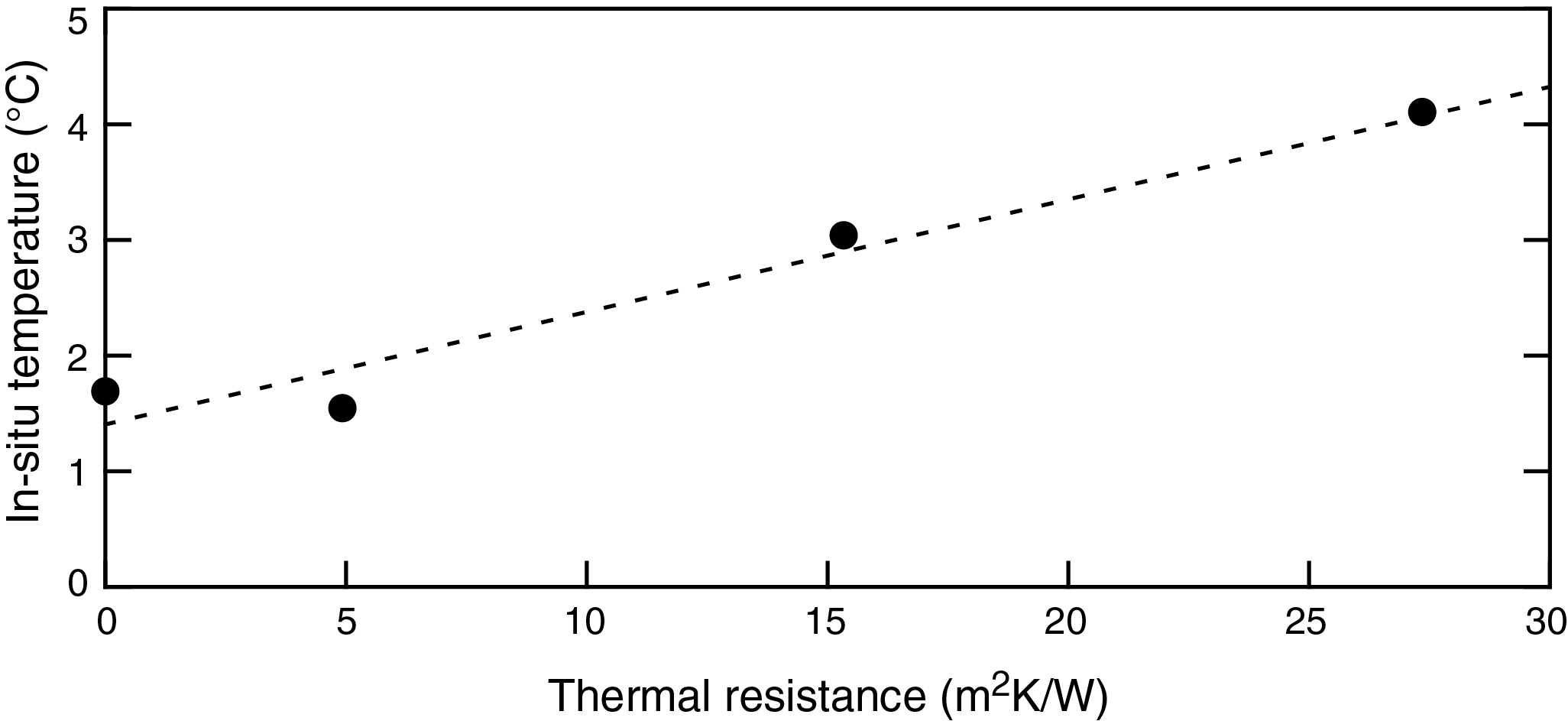
Figure F57. Temperature as a function of thermal resistance.
Logging
Data and log quality
Data acquisition
Logging data were acquired with a full LWD BHA in Hole C0024A (MicroScope, arcVISION, TeleScope, SonicScope, and seismicVISION) from the seafloor to a maximum depth of 4739 m BRT (869 mbsf). After completion of the main pass, two short repeat passes were recorded (1) between 4127 and 4180 m BRT (257–310 mbsf) to reimage an interval where wellbore breakout orientation appeared to be changing to capture a possible evolution of breakouts with time and (2) between 3860 and 3885 m BRT to confirm the seafloor depth. While pulling out of the hole, seismicVISION stations were recorded at each half pipe stand when conditions permitted. See Introduction and operations as well as Logging in the Expedition 358 methods chapter (Hirose et al., 2020) for a detailed description of the operations and tools.
Depth shift
The water depth of 3870.0 m BRT was determined from the characteristic abrupt increase in gamma radiation and resistivity as the tools crossed the seafloor into the formation (Figure F58). The depth of 3870.0 m BRT identified from the logs was the same as that estimated by the drillers at the time of spud-in. All data were converted to LWD depth below seafloor (LSF or mbsf) by subtracting this water depth value.
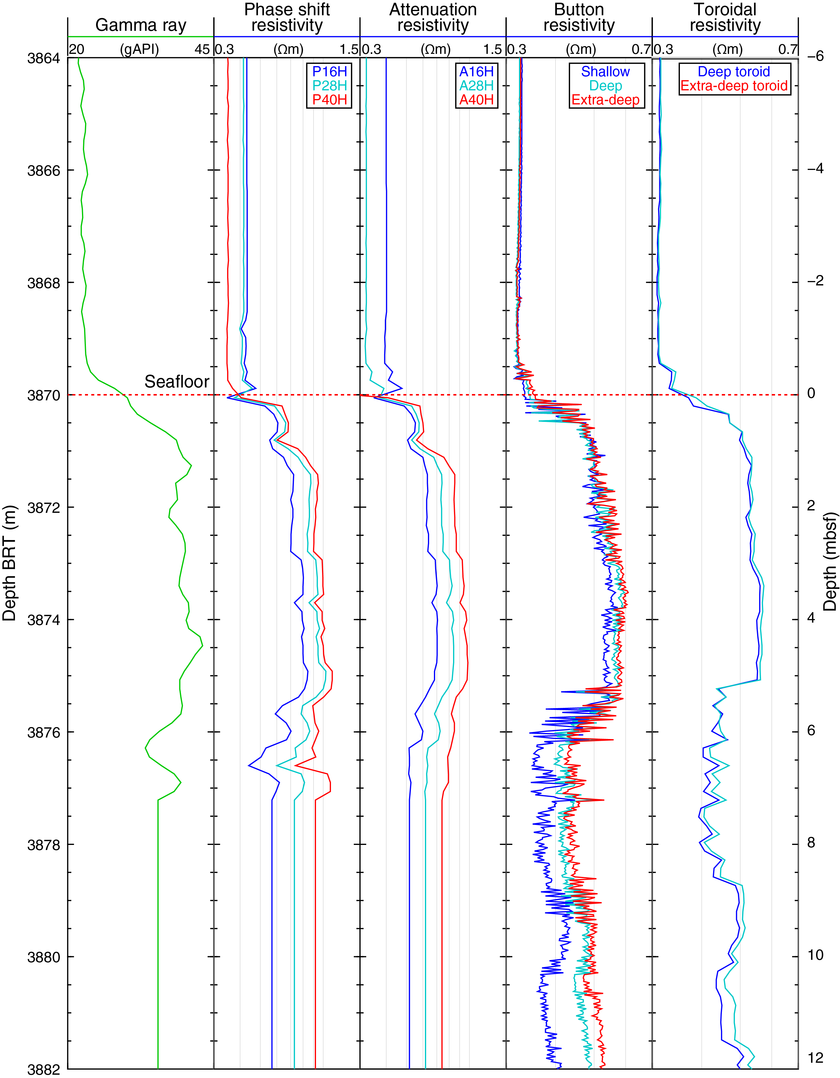
Figure F58. Identification of seafloor using gamma ray and resistivity logs.
Logging data quality
Selected drilling parameters including rate of penetration (ROP), rotation rate (or rotations per minute), equivalent circulating density (ECD), and time-after-bit (TAB) logs are shown in Figure F59. ROP was stable at around 20 m/h below ~70 mbsf, and rotation rate remained constant at ~110 rpm below ~180 mbsf. The gradual increase in ECD with depth from ~1.02 to ~1.05 g/cm3 is normal as the amount of cuttings in the borehole fluid column increases with depth, but the higher values below ~650 mbsf, and more significantly below ~810 mbsf, illustrate the increasingly difficult drilling conditions at the bottom of the hole. TAB is stable over the section except for artifacts at pipe connections. At the beginning of drilling, electric power was not supplied from the TeleScope because of low flow rate during jet-in. Therefore, gamma ray and resistivity measurements from the arcVISION tool started at 20 mbsf and resistivity measurements by the MicroScope tool started at 24 mbsf. The MicroScope borehole image record started at 77 mbsf, where rotation of the BHA started.
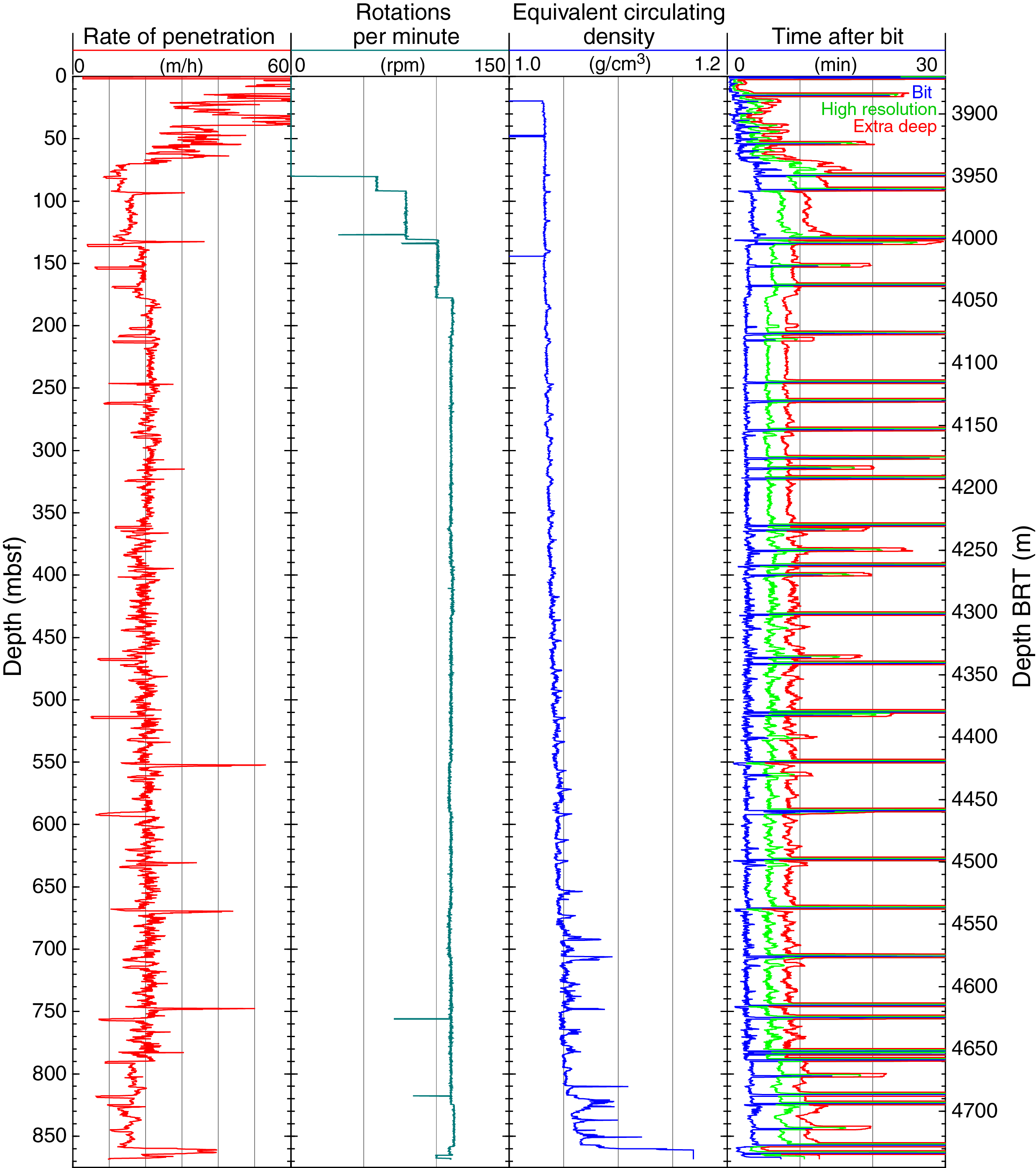
Figure F59. Drilling parameters.
Deviation surveys made at regular intervals show borehole deviation to the west from vertical that steadily increased as the hole was deepened. Hole inclination reached a maximum of ~9° at the bottom of the hole, resulting in a horizontal offset of about 80 m west from the top of the hole (Table T20). Figure F60 shows the complete trajectory and illustrates how the well crosses various in-lines and cross-lines on the 3-D grid.
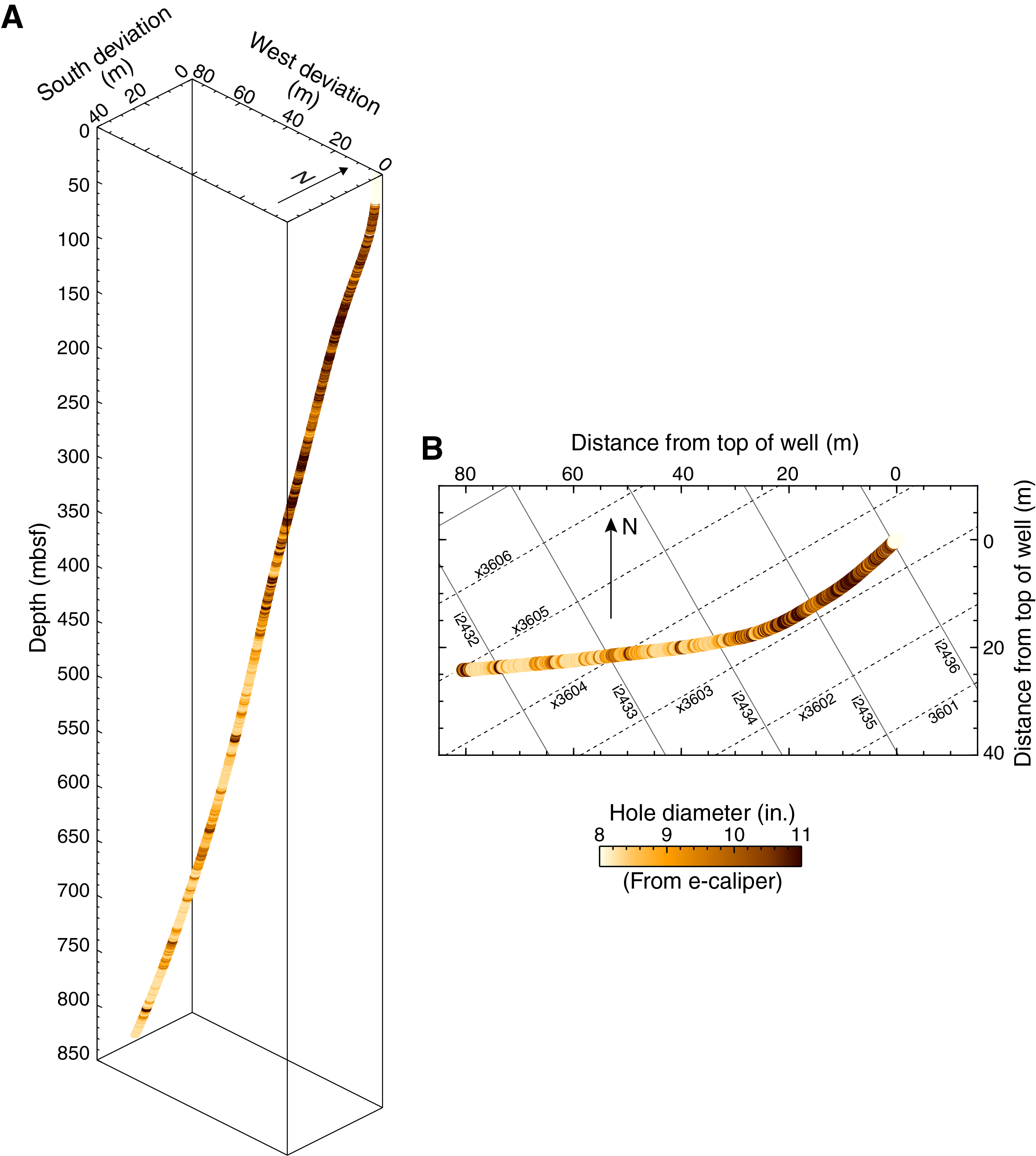
Figure F60. Hole deviation calculated from deviation surveys.
Data quality is strongly dependent on borehole diameter. Because no mechanical or ultrasonic calipers were included in the LWD tools, an electromagnetic caliper (e-caliper) was computed from MicroScope resistivity values and used to estimate the borehole diameter (see Logging in the Expedition 358 methods chapter [Hirose et al., 2020]). The estimated hole diameter is as wide as ~11½ inches from the seafloor to 438 mbsf, whereas the borehole diameter below 438 mbsf is close to the 8½ inch bit size (Figure F61). Some short intervals were enlarged as wide as ~11½ inches because of formation features or longer exposure time during pipe connections (TAB in Figure F59). Another estimate of borehole size was calculated from the raw attenuation and phase propagation data from the arcVISION tool. The data in Figure F61 show higher variability and significantly larger diameter values than the e-caliper in the shallower portion of the hole (as wide as ~20 inches), but the overall locations of intervals most affected by borehole conditions are consistent for the two estimates of hole gauge.
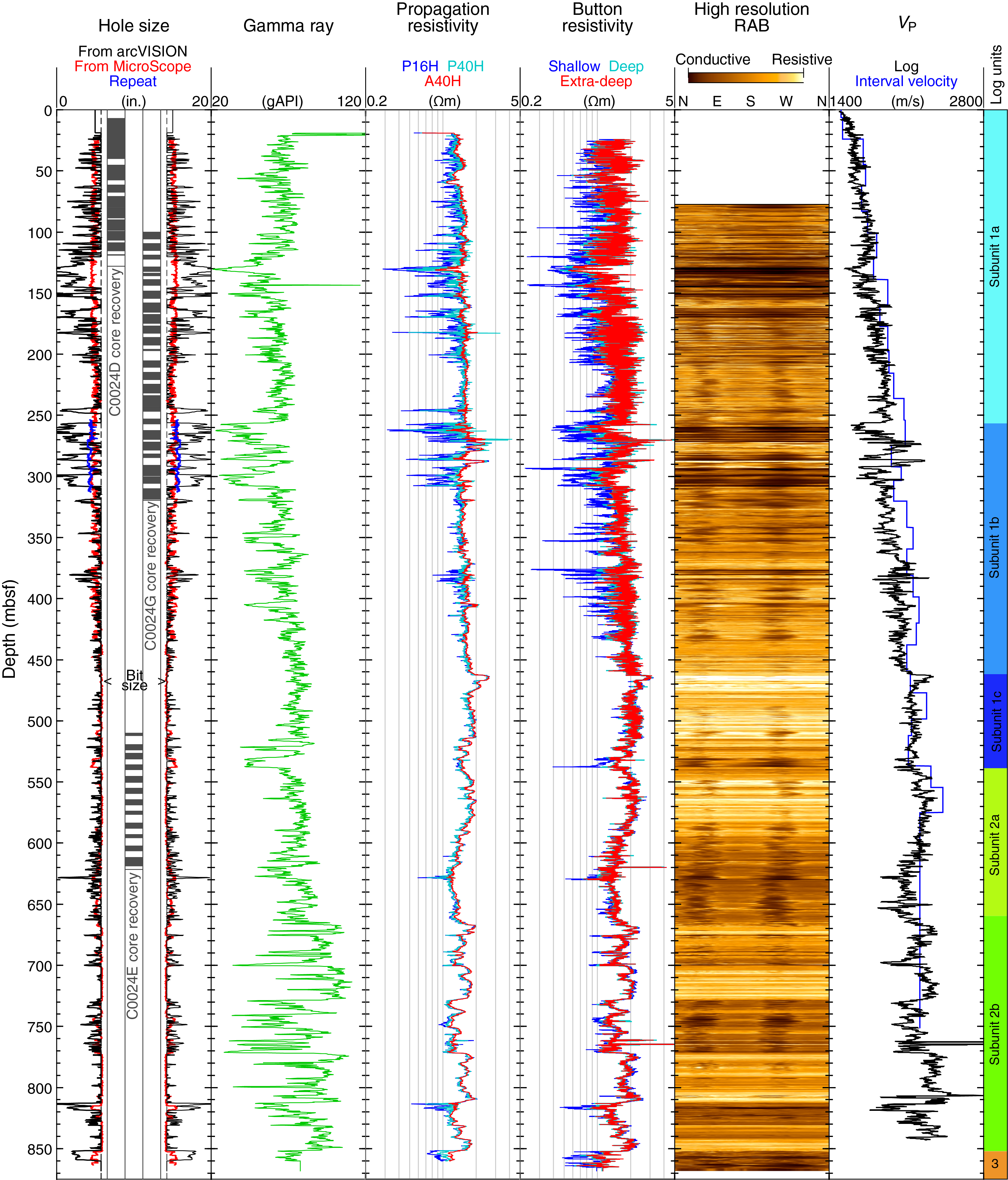
Figure F61. Summary of logs recorded.
The wide variations in MicroScope button resistivity values above 438 mbsf are likely due to the enlarged and irregular borehole size as shown by the e-caliper. Occasional large heave may have caused missing data indicated by gaps in some of the MicroScope images, but the overall good drilling conditions and the proximity of the MicroScope tool to the bit provided good quality image data over most of the logged interval (Figure F62).
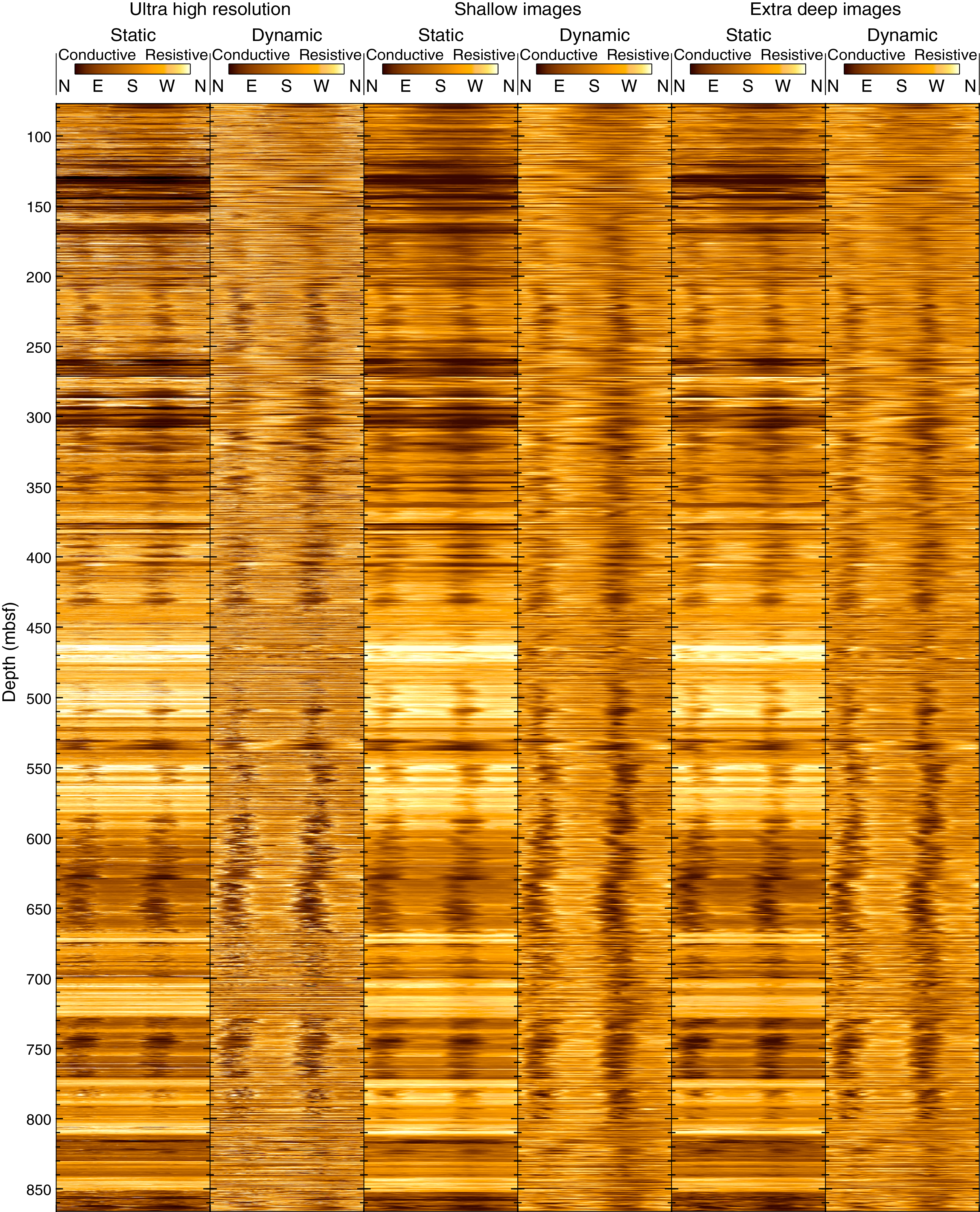
Figure F62. MicroScope resistivity images.
The strong coherence measured while processing the P-wave velocity (VP) logs from the low-frequency monopole waveforms and the robust signal displayed by the waveforms in Figure F63 suggest that the SonicScope tool was not severely affected by the irregular hole size. Quadrupole waveforms yielded good coherency and therefore usable shear velocity values over most of the logged interval between ~410 mbsf and the bottom of the hole, with notable exceptions including the basal fault zone. However, despite attempts at reprocessing, no reliable shear velocity data could be derived from the quadrupole waveforms recorded above ~330 mbsf.
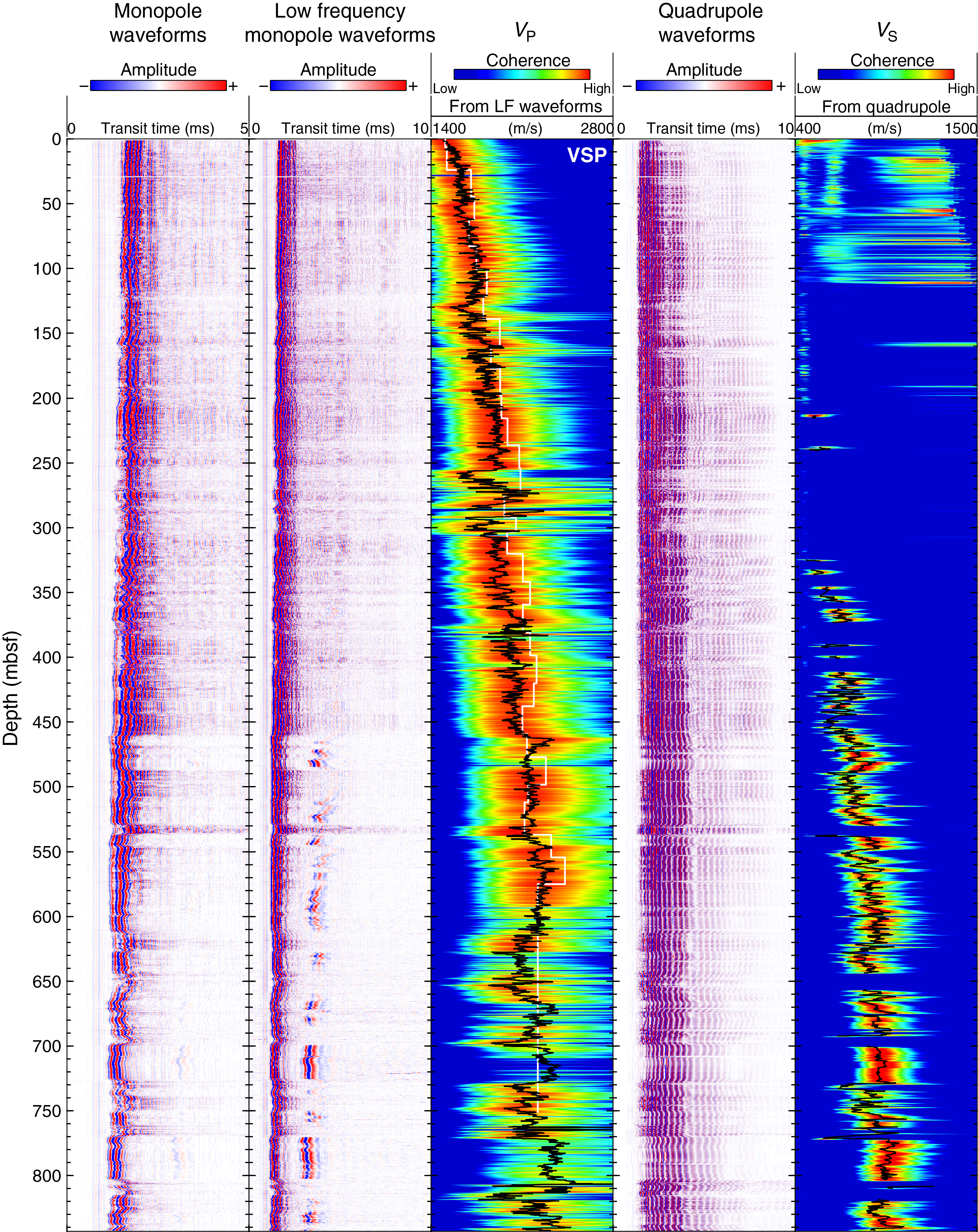
Figure F63. SonicScope data.
The last data set to be recorded in Hole C0024A was a vertical seismic profile (VSP) with the seismicVISION tool. The very clear first arrivals displayed at each station recorded provide a robust calibration for the seismic velocity model around Site C0024.
Log characterization and lithologic interpretation
Identification of logging units
The LWD logs acquired in Hole C0024A are summarized in Figures F61, F62, and F63. Combined visual inspections of the natural gamma ray, button and propagation resistivity, and sonic velocity logs allow definition of three logging units and five subunits with distinct characteristics.
Logging Unit 1 (0–538.6 mbsf) is divided into three subunits (Figure F61). It is characterized by an overall trend of increasing resistivity, gamma ray, and VP and a discrepancy between the shallow, medium, and deep resistivity buttons. This discrepancy is generally related to poor hole conditions but also to borehole fluid invasion that likely reflects the presence of more permeable sediments, possibly rich in silty and sandy material.
Logging Subunit 1a (0–256.1 mbsf) is defined by a constant mean gamma ray value of ~65 gAPI except for intervals with the poorest hole conditions. The resistivity-derived caliper data exhibit high-frequency variations with high amplitude. At a larger scale, sonic velocity (VP) values and average resistivity values increase throughout the subunit, possibly representative of a compaction trend.
Logging Subunit 1b (256.1–462.8 mbsf) is characterized by increasing natural gamma ray, resistivity, and VP values with depth and high-amplitude fluctuations from the top of the subunit to 311 mbsf and from 375 to 435 mbsf. The magnitude of the variations in the first interval is ~30 gAPI for gamma ray, ~2 Ωm for resistivity (deep button [BD]), and approximately 550 m/s for VP. A separation between shallow and deep resistivity is also seen throughout most of this subunit except for a few intervals where gamma ray and VP values show less fluctuation (e.g., 366–374 mbsf). Shear wave velocity (VS) measurements obtained in some portions of this subunit (Figure F63) indicate a gradual increase from ~500 m/s at 334 mbsf to 750 m/s at 418 mbsf. VS then decreases from 418 mbsf to the bottom of the subunit (600 m/s). Borehole caliper measurements in this subunit indicate hole diameter larger than 10 inches in most sections but show that the borehole is in gauge at a depth that corresponds to low fluctuation in resistivity.
The transition to Logging Subunit 1c (462.8–538.6 mbsf) from Subunit 1b is marked by a significant peak in both resistivity and VP. It is defined as an interval of gradually increasing to decreasing trends in gamma ray, resistivity, and VP logs. Resistivity and VP indicate the largest values at the top of this subunit at 3.1 Ωm and 2350 m/s, respectively. These values gradually decrease with depth to 1.8 Ωm and 2140 m/s, respectively, at 478 mbsf. The base of this subunit is characterized by a 9 m thick interval of low gamma ray and resistivity values, probably representative of a sand-rich interval (see Core-log integration and Lithology).
Logging Unit 2 (538.6–851.7 mbsf) is separated from Logging Unit 1 by a short trough in gamma ray, resistivity, and VP, possibly a sandy layer, at the bottom of Logging Unit 1 (Figure F61). This unit is characterized by (1) a decrease in the discrepancy between the resistivity buttons, possibly related to a lack of invasion of drilling fluid into the formation and suggestive of less permeable sediments; (2) higher frequency variations in the log responses; and (3) an overall constant trend in VP and resistivity. The crossplot between bit resistivity and VP shows a clear difference in trends between Logging Units 1 and 2 (Figure F64).
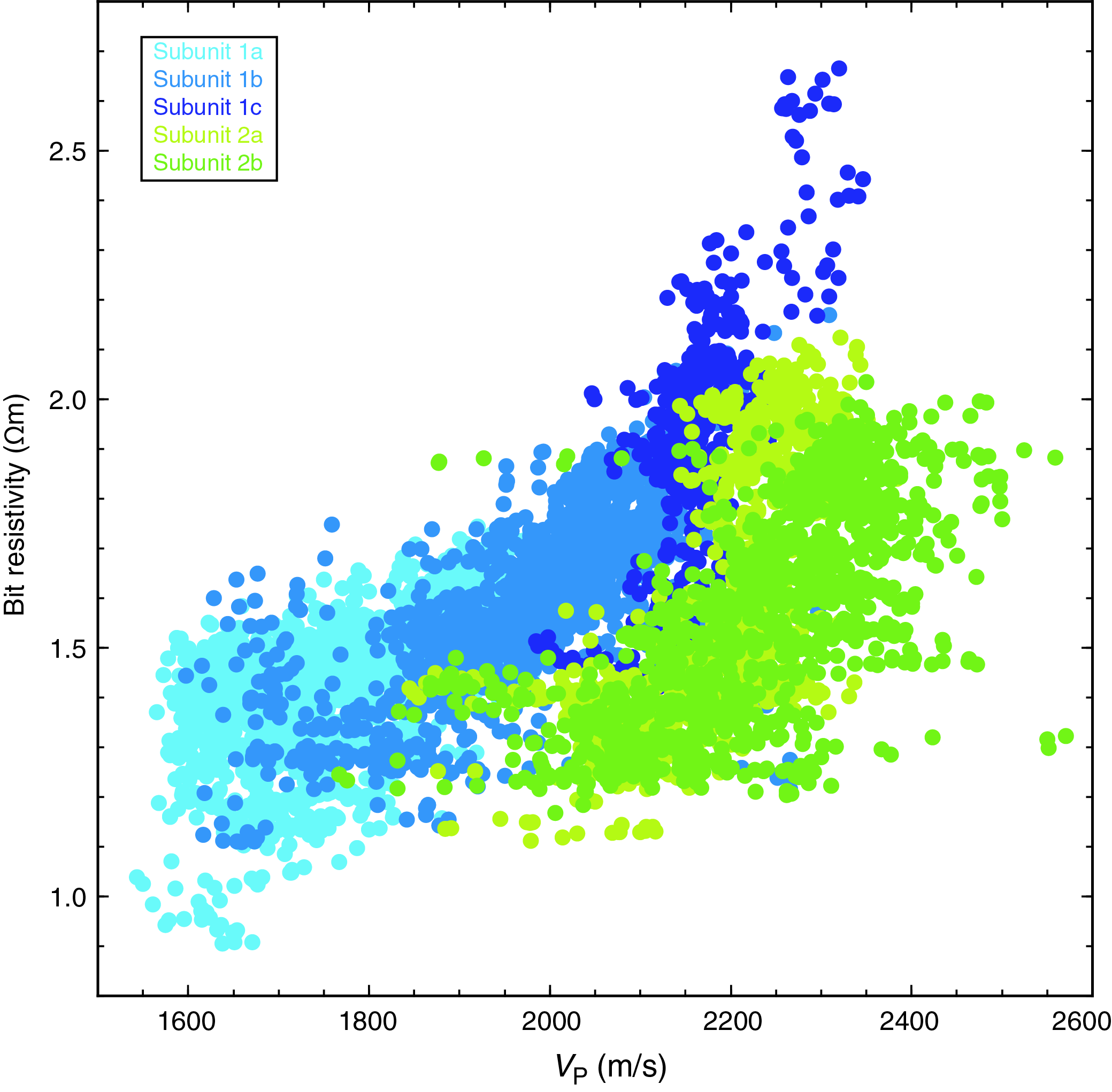
Figure F64. Bit resistivity and VP.
Logging Subunit 2a (538.6–659.6 mbsf) exhibits a trend of increasing gamma ray, resistivity, and VP values to 570 mbsf, followed by decreases in gamma ray, resistivity, and VP values to 623 mbsf and near-constant values for all logging parameters to 659.6 mbsf.
Logging Subunit 2b (659.6–851.7 mbsf) is characterized by larger variations in the log responses but with overall constant values. Significant negative spikes with spacing of ~5–10 m are present above 810 mbsf. The hole is close to in gauge throughout with lower variability in hole size than the units above.
Logging Unit 3 (851.7–868.6 mbsf) is the lowermost section of the logged interval. It is characterized by a significant decrease in resistivity. Both button and propagation resistivity show large separation between shallow and deep resistivity over this unit. Resistivity (BD) values fluctuate from 0.65 to 1.7 Ωm, but those values may be affected by poor borehole conditions. Natural gamma ray values decrease from the bottom of Logging Unit 2 to 70 gAPI.
Resistivity image interpretation
Resistivity images were acquired starting at 77 mbsf, when the BHA began rotating. The ultrahigh-resolution images are of good to very good quality throughout the hole, although the uppermost ~120 m (77–200 mbsf) is noisier than the rest of the borehole (Figure F62). This probably results from the poorer borehole conditions here (see Logging data quality). The other images, provided by the extradeep, deep, medium, and shallow buttons, are of similar quality but lower resolution and were not used for image interpretation. In addition to a standard image processing flow, smoothing and orientation routines were applied to improve image quality and provide true orientation and angles of bedding and tectonic features. Hole deviation values as high as 9° toward N267° at 846.26 mbsf were obtained from the drilling deviation survey and were used in the image processing. As a result, all features, including bedding, fractures, and faults, are given with their true dip direction and magnitudes.
Bedding and fractures
Numerous bedding planes and several fractures can be identified on the processed images for most of the logged section (Figure F65) except in the zones of poor hole conditions. The shallowest of the logging images (76 to ~95 mbsf) display gentle bedding dips (5°–20°) toward the southwest, in agreement with the direction observed in the seismic data. From 95 to 651 mbsf, bedding dips gently toward the north-northwest, with two excursions toward higher dip values at the base of Logging Subunit 1b (459–461 mbsf) and the Logging Unit 1/2 boundary (536–544 mbsf). A densely fractured zone at 393–401 mbsf corresponds to a back thrust observed in the seismic section (Figure F2).
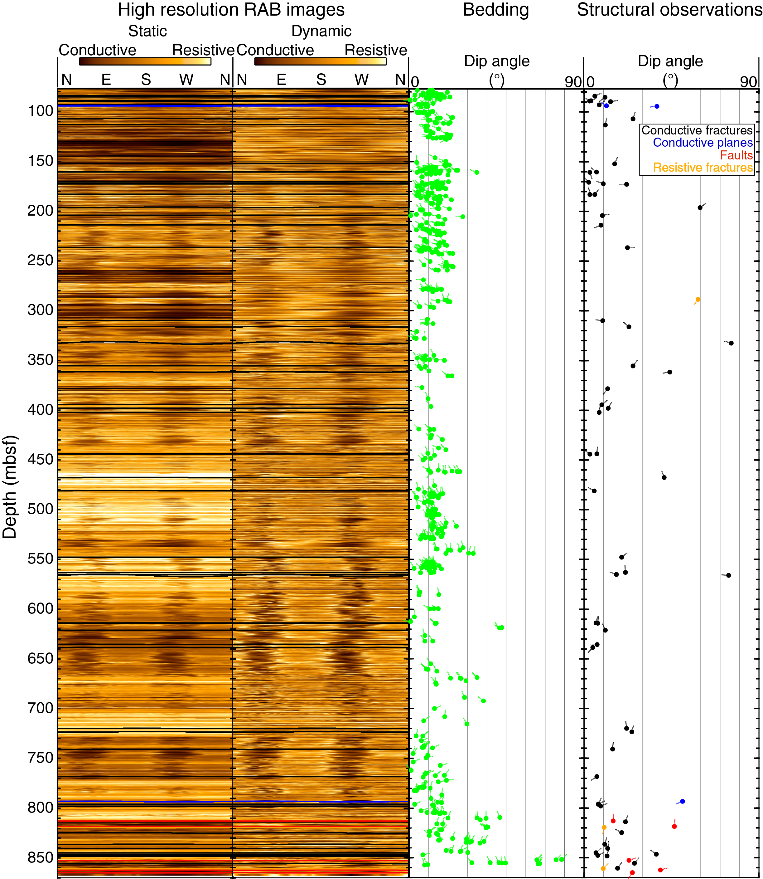
Figure F65. Bedding attitude and fracture orientations.
From 651 to 727 mbsf, bedding dips increase and shift from north-northwest to north-northeast at the bottom of this interval. This interval corresponds to the top of an interval of poor borehole conditions with high caliper values and probably coincides with an interval with high torque and standpipe pressure in Hole C0024F, which prevented further advances in the deeper portion of this cored borehole (Figure F59). The higher VP and resistivity values around 670 and 715 mbsf correspond to two strong positive reflectors in the seismic data (see Seismic-well integration). From 727 to 809 mbsf, bedding dips gently toward the north-northeast with few fractures.
Plate boundary fault zone
Between ~806 and 807 mbsf, VP and resistivity exhibit sharp decreases. Below 809 mbsf, bedding dips increase sharply, with a mean value around 40° and a maximum close to 90° at 851 mbsf. This change is accompanied by increasing fracture density and worsening drilling conditions. Fractures exhibit various dip angles to either the north-northeast or the north-northwest. At 813 mbsf, a pair of faults, dipping 15° and 20° toward the north, coincide with another drop in VP, as well as resistivity and gamma ray values. On the basis of (1) decreases in VP and resistivity (Figures F61, F66), (2) the observation of increased bedding dip and onset of variably dipping conductive fractures (Figure F65), and (3) the coincidence of the decrease in VP between ~806 and ~819 mbsf with the interpreted fault reflection in seismic data (as discussed below; see Core-log integration), our preliminary interpretation is that the onset of deformation at ~806 to ~819 mbsf marks the top of the plate boundary fault zone.
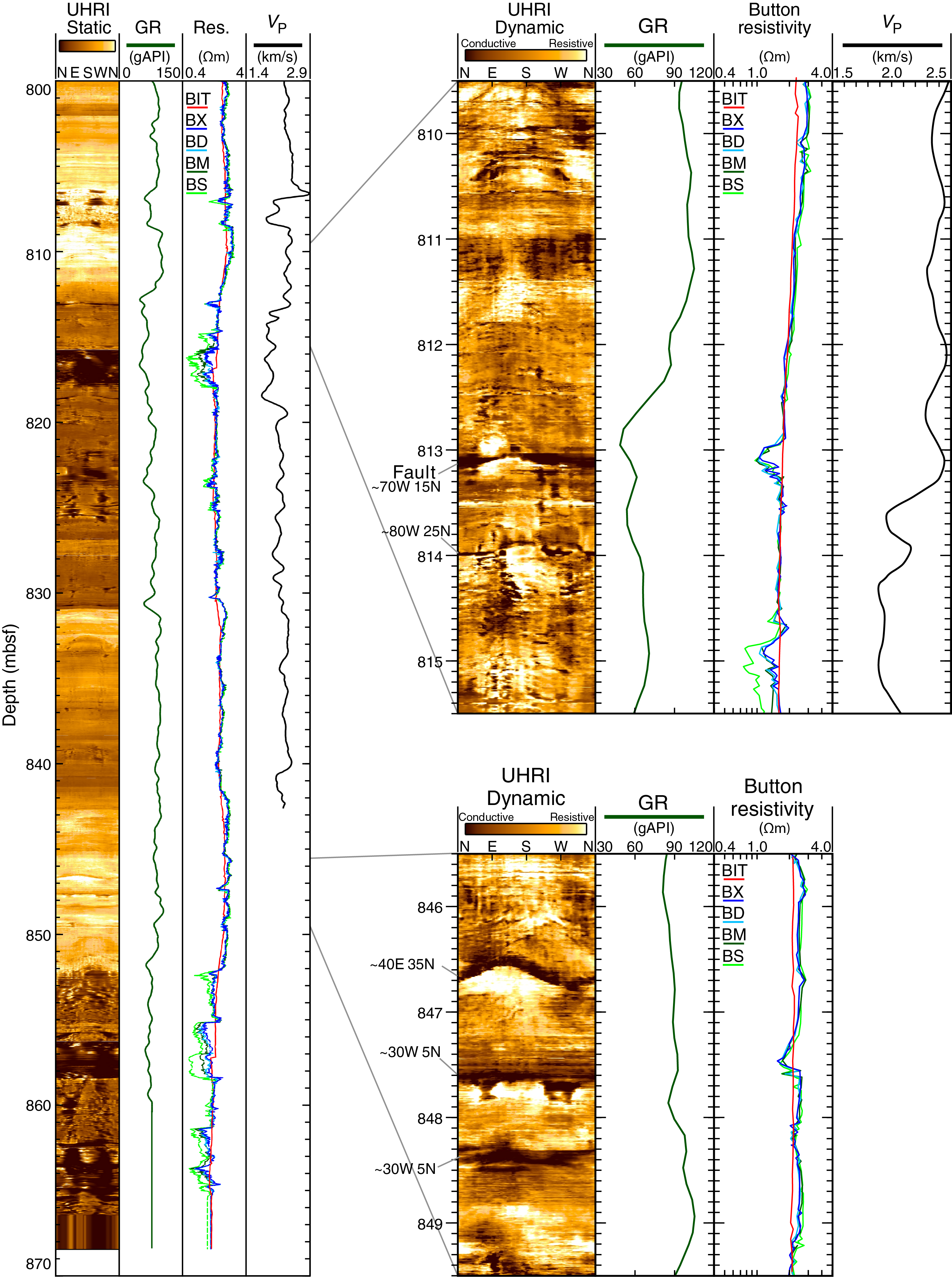
Figure F66. Logs from 800 mbsf to total depth.
At 851 mbsf, a major structure identified in resistivity images is accompanied by a shift toward subvertical bedding dips and a sharp decrease in resistivity and gamma ray values below. This is identified as a fault plane dipping 20° toward the northeast. Below this in Logging Unit 3, resistivity remains low; gamma ray values are also slightly lower than in Logging Unit 2. This may mark the base of the plate boundary fault zone or an imbricate thrust; alternatively, it may represent a zone of poor borehole conditions associated with drilling through damaged formation, and the fault zone may extend to greater depths below the total depth of Hole C0024A.
The presence of numerous fractures and steepened bedding dips throughout the interval (~806.7–851.7 mbsf and possibly deeper) suggests that the plate boundary fault zone at this location may correspond to a ~40 m or more thick complex stack of individual structures with variable local dip directions. More detailed and careful postcruise analysis of the bedding and structures should be undertaken in this interval (see Logging data quality).
Wellbore failure analysis
Numerous borehole failures were observed in resistivity images throughout the hole. Most of these correspond to borehole breakouts. Their occurrence and width seem to be correlated with lithology, as they tend to widen in more conductive zones and to be narrower or absent in the most resistive intervals. The overall orientation of the breakouts is generally consistent throughout the hole, with a mean orientation of 070° and a standard deviation of 12° (on 252 measurements); this corresponds to a SHMAX azimuth of 160° (Figure F67). Below ~600 mbsf, we observe a slight shift in breakout orientation to lower azimuths, and below 810 mbsf, we observe a 15°–20° rotation to an azimuth of ~100°. The overall breakout azimuth of 070° is consistent with a mean breakout azimuth of 060° (SHMAX azimuth of 150°) reported at Site C0006 (Expedition 314 Scientists, 2009) and is approximately normal to the trench. A few drilling-induced tensile fractures are observed at 822 mbsf, indicating an SHMAX orientation of 135°, in relatively good agreement with the borehole breakouts.
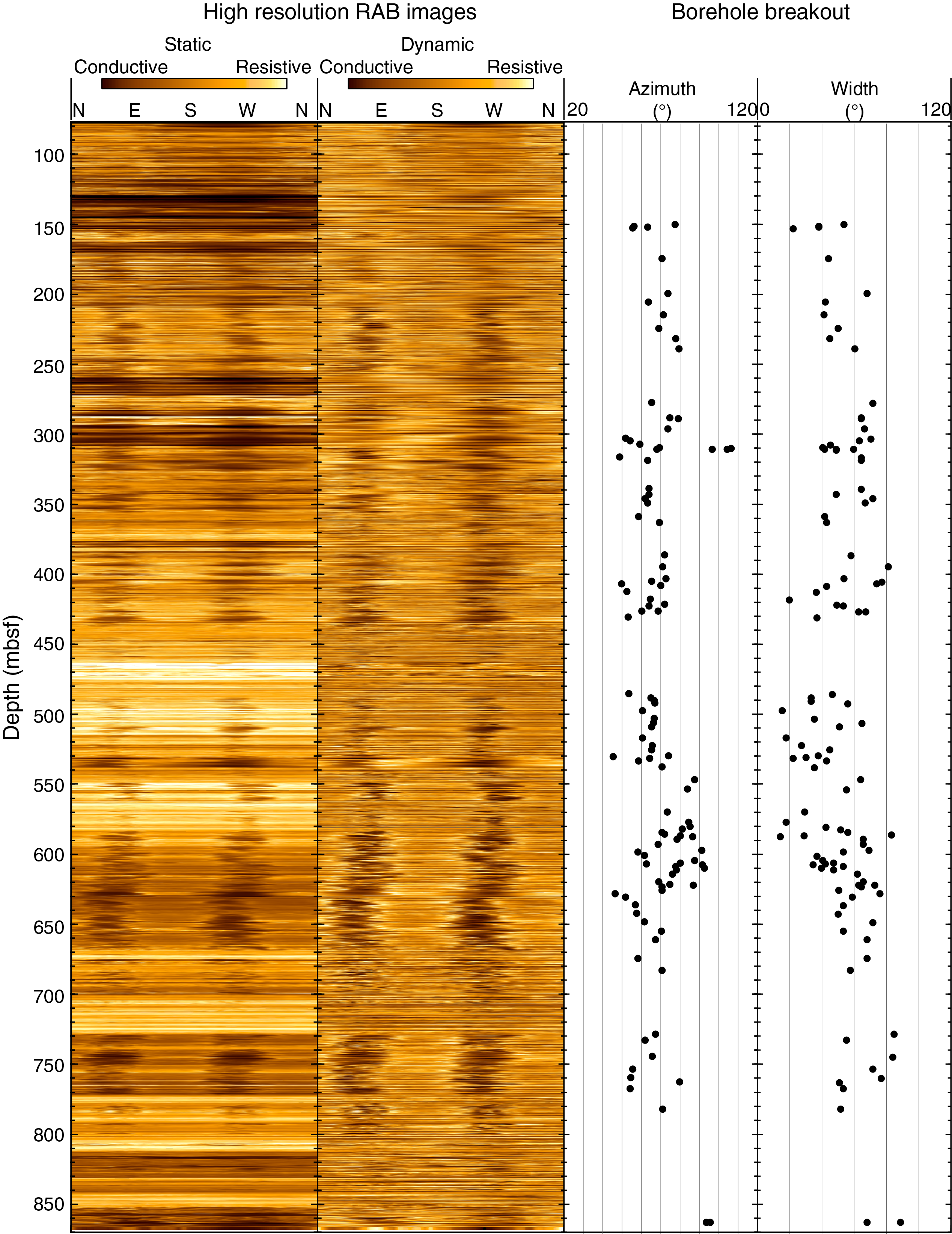
Figure F67. Breakout azimuths and widths.
Porosity and density estimation
The LWD tool string did not include a lithodensity or neutron porosity tool. However, generation of reliable synthetic seismograms for integration with the seismic data requires density data to accurately simulate seismic impedance and reflectivity. We used the empirical relationship defined by Archie (1942) to estimate porosity from the resistivity logs and combined the results with the grain density measurements made on core samples to estimate formation density (see Logging in the Expedition 358 methods chapter [Hirose et al., 2020] for a detailed description of the method). We then compared these estimates with values determined from MAD measurements on discrete samples (see Physical properties). The resistivity of seawater (Rw) was calculated as a function of temperature and salinity (Fofonoff, 1985). Pore water salinity was assumed to be 35‰, and temperature was assumed to follow a linear gradient of 30°C/km (e.g., Expedition 316 Scientists, 2009a). This value is lower than the gradient measured in the shallower section with the APCT-3 tool (see Downhole measurements), which may be biased by the shallow depth of the measurements (<40 mbsf). In any case, temperature has little effect on the density and reflectivity calculations. The most realistic and simplest value for the tortuosity coefficient is a = 1 because this gives a resistivity equal to formation water resistivity when porosity is 100%. A value of m = 2.0 (which is the most standard and within the standard accepted range 1.5 ≤ m ≤ 2.5) was chosen for the cementation factor to provide the best baseline match with porosity data measured on cores from Site C0024. We used the resistivity-derived porosity with the average of the MAD grain density to calculate a bulk density curve (Figure F68). The deepest attenuation resistivity (A40L) was used because it was the least affected by the borehole conditions.
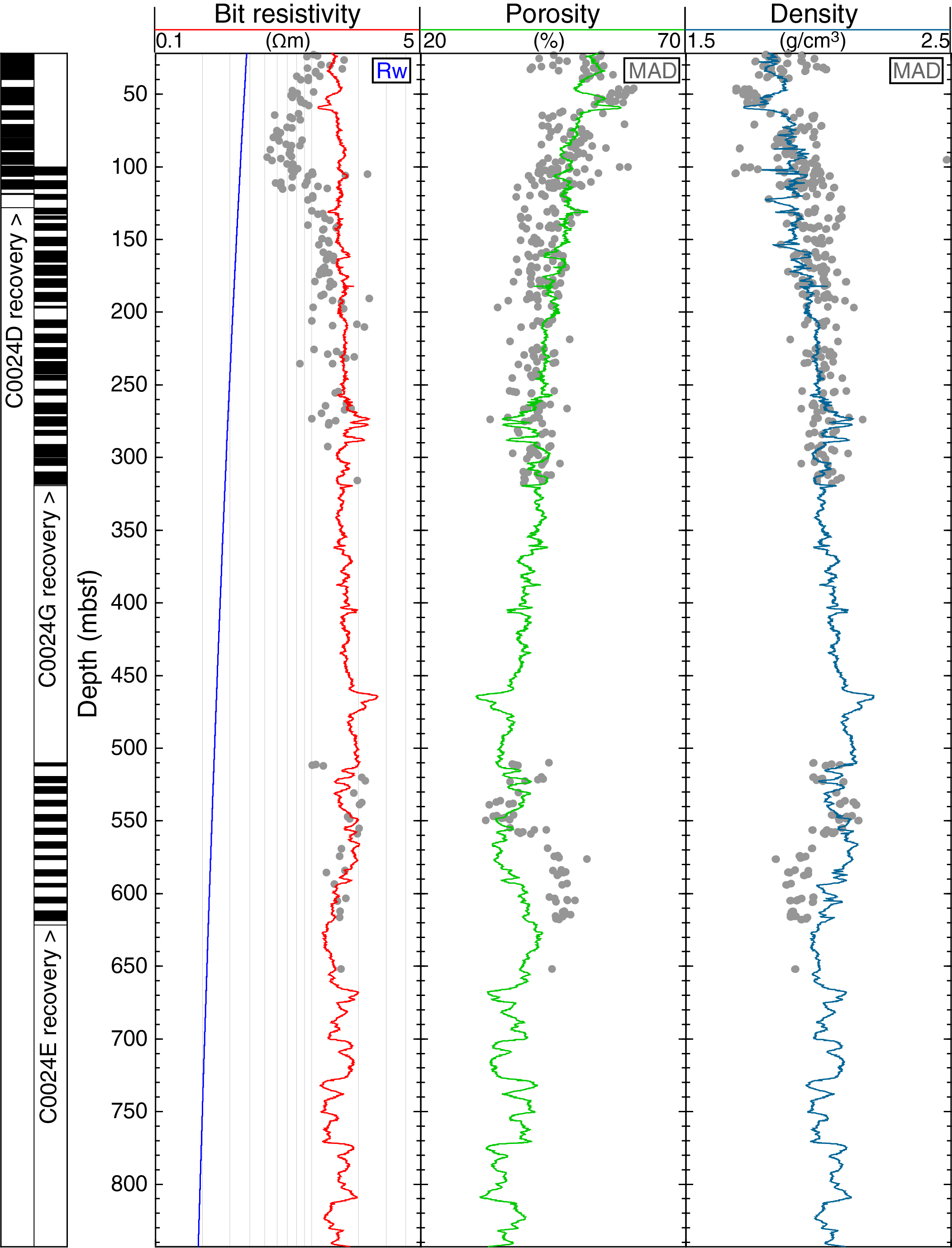
Figure F68. Estimation of formation porosity and density.
Core-log integration
Site C0024 was partially cored in Holes C0024B–C0024E and C0024G over different intervals with limited overlap, incomplete recovery, and in some cases significant spatial separation. Figure F69 shows a comparison between the gamma ray, density, and porosity data from the logs with the same measurements made on cores from Holes C0024D and C0024G. The units for gamma ray values are not the same for the log and core data, but the trends and variations agree reasonably well considering the incomplete recovery and the lateral hole offsets. The density values derived from the resistivity log coincide with the upper envelope for the GRA density data measured on cores and are slightly lower than the MAD values between ~100 and 200 mbsf in Hole C0024G. Similar to the density data, the resistivity-derived porosity values are in general good agreement with the core measurements. This agreement seems to improve for all measurements after a depth shift of the core data by about 7 m in Hole C0024D and by 12 m in Hole C0024G (Figure F69). The improved match is most apparent between ~40 and 70 mbsf in Hole C0024D in a low–gamma ray and high-porosity sandy interval but also over most of Hole C0024G. The depth differences between the holes reflect the shift in lithology due to the dipping bedding plane and high variability in bed thicknesses and slopes in proximity to the deformation front.
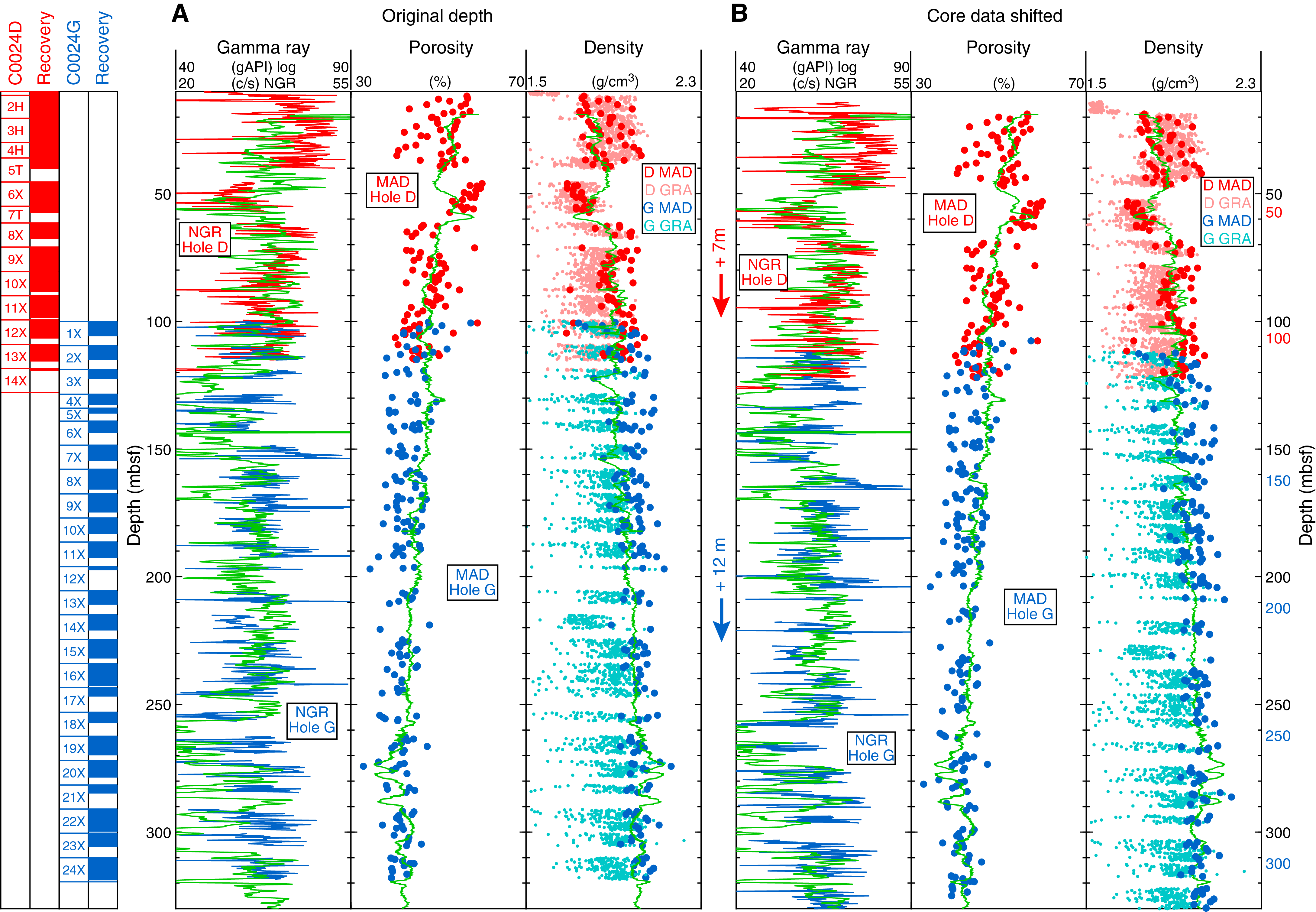
Figure F69. Gamma ray, porosity, and density from logs and core.
Using these offsets, we can attempt to compare the resistivity images measured in Hole C0024A with some of the cores recovered at Site C0024. Figure F70 displays RAB images from Hole C0024A and photographs from Cores 358-C0024G-6X and 8X. Because of the incomplete recovery of these two cores, particularly for Core 6X and the crude estimation method applied to shift the depth, it is unlikely that any of the beds seen in the images and in the cores are the same. However, they display similar patterns of variability at ~10 cm scales, suggesting that the resistivity images can provide useful information about structure and the orientation and cyclicity of beds not recovered by coring.
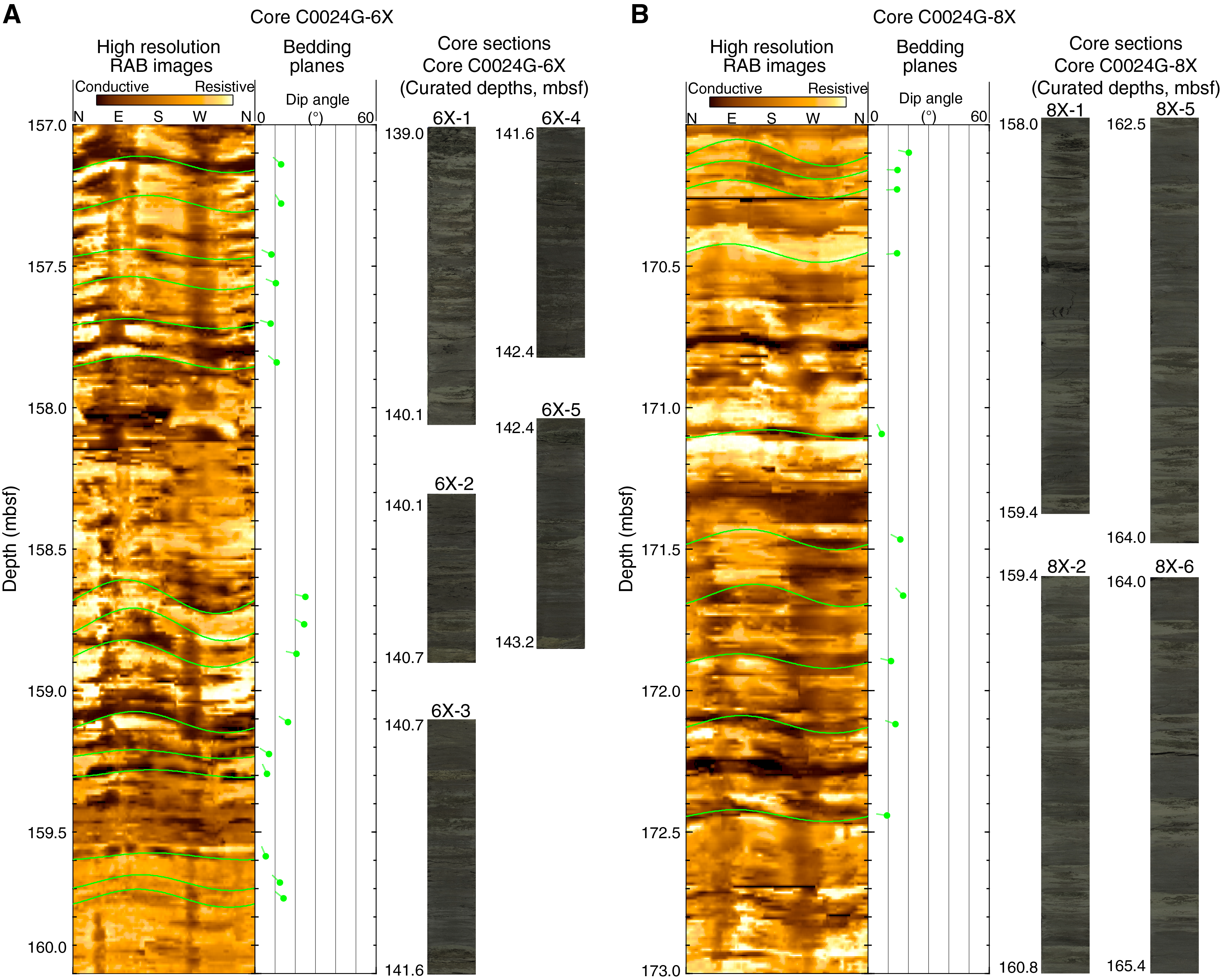
Figure F70. High-resolution RAB and core images.
Comparison between the log response and the lithology observed in the depth-shifted cored intervals also provides insights into the log responses (Figures F61, F69). In Logging Subunit 1a from 115 to 130 mbsf, gamma ray and resistivity decrease but the discrepancy between the resistivity buttons increases, suggesting increased fluid invasion into the formation during drilling (Figure F61). This trend is generally consistent with an upward-fining sequence and correlates with an increase of coarser and thicker sand material observed Cores 358-C0024G-1X and 2X (see Lithology). Below 212 mbsf, smaller fluctuations in gamma ray, resistivity, and VP correspond to an interval of thin turbidites in Hole C0024G cores (see Lithology).
At the top of Logging Subunit 1b (256–300 mbsf), fluctuations in the gamma ray and resistivity buttons are likely related to the presence of coarse sand and/or ash-rich layers observed in Cores 358-C0024G-16X through 20X (~230 to ~260 mbsf in the cores) (see Lithology; Figures F61, F69). The log response may also be influenced by the presence of a back thrust observed in the seismic sections and by borehole conditions. At the bottom of Logging Subunit 1c (530–540 mbsf), a 10 m thick interval of low gamma ray values (45 gAPI) corresponds to a thick package of sand observed in Core 358-C0024E-1R (~510 mbsf) (Figure F68). The bottom of this interval, correlated with the Logging Unit 1/2 boundary, was identified as the boundary between the trench-wedge facies and the outer trench-wedge–trench-to-basin facies transition interval (see Lithology). The reversal in depth-dependent trends in gamma ray, resistivity, and VP data observed at 570 mbsf in Logging Subunit 2b could correspond to the Lithostratigraphic Unit III/IV boundary (see Lithology).
Seismic-well integration
All of the NanTroSEIZE sites were chosen based on the 3-D seismic data set collected and processed in 2006/2007 (Moore et al., 2009). The locations of all holes at Site C0024 are shown on Seismic In-line 2437 (Figure F7 in the Expedition 358 summary chapter [Tobin et al., 2020a]). To reliably link borehole measurements to the seismic stratigraphy and provide a regional framework for the interpretation of the data, one of the objectives of the logging program was to calibrate the relationship between seismic traveltime and depth at Site C0024.
Vertical seismic profile
The most direct way to build this relationship is to use the VSP recorded with the seismicVISION tool. The first break in the waveforms displayed in Figure F71A illustrates the time taken by a seismic pulse to travel from the sea surface to each of the 32 stations where the seismicVISION tool was held during the survey, spaced at ~19 m (i.e., every half pipe stand) when conditions permitted. All traces, produced by stacking ~10 shots at each station, show clear first arrivals (Table T21). Figure F71B shows the resulting relationship between depth and two-way traveltime (TWT) that was then used to tie the well results to the lines crossing Site C0024. This relationship can be compared to the seismic velocity model from the depth migration of the 3-D seismic reflection data in the vicinity of Site C0024 and to a similar relationship derived by integrating the sonic log recorded by the SonicScope tool over depth. The comparison shows that the depth migration predicted deeper depths for any given traveltime, whereas the sonic log integration suggests shallower depths. It illustrates the generally slower velocity values measured by the sonic log and the higher values from the depth migration (Figure F71C).
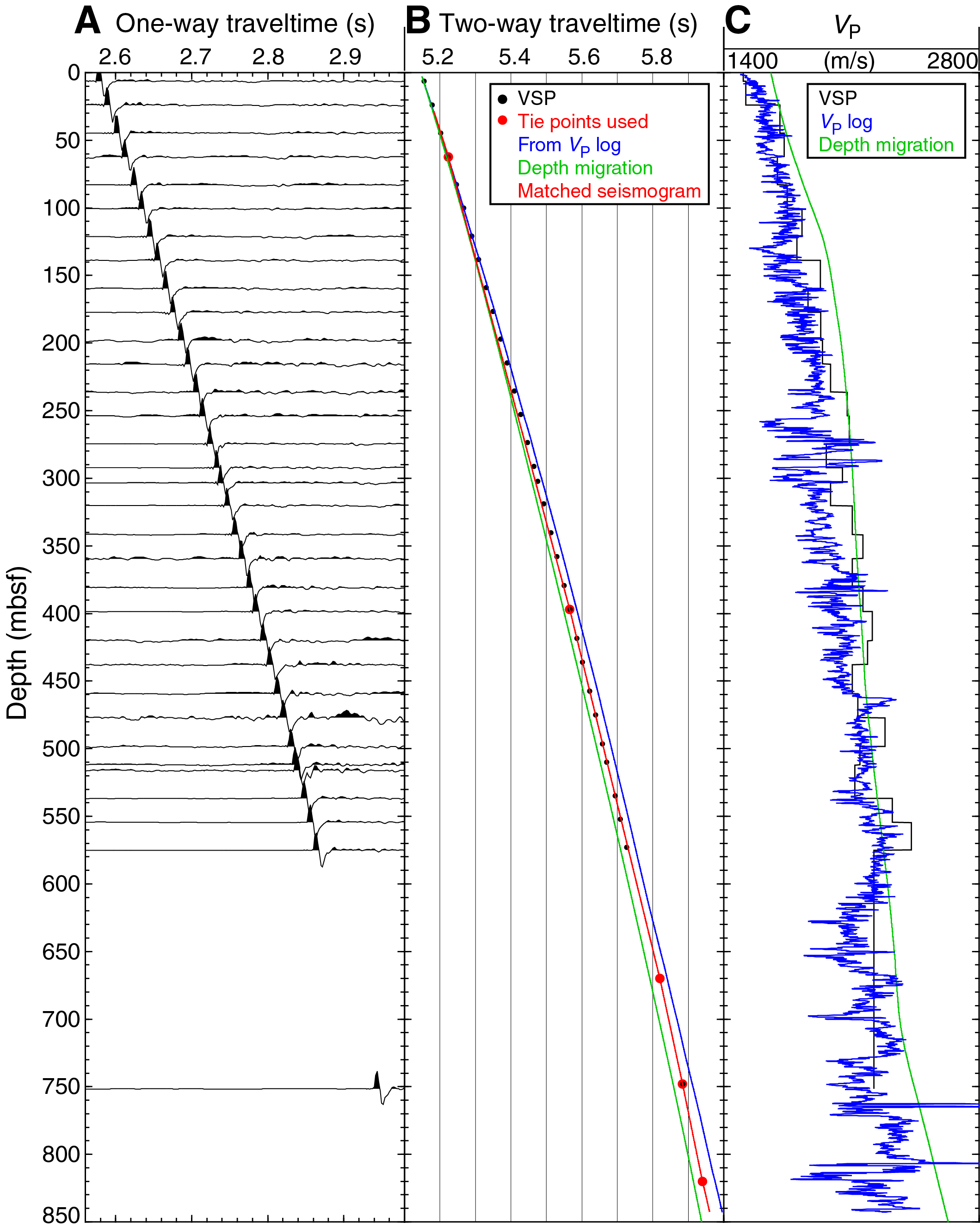
Figure F71. VSP results.
Synthetic seismogram
A complementary way to fine tune the integration between the seismic and well data is to use the VP logs to generate a synthetic seismogram, reproducing the seismic trace closest to the site (Figure F72). By recognizing individual reflectors, it is then possible to identify any changes or features in the logs that can be associated with specific seismic reflectors and to determine the depth of these reflectors. Seismic reflectivity is controlled by changes in impedance, which is the product of VP and bulk density. As noted above, because we did not have a density log, we used the density estimated from the deep attenuation resistivity (A40L) to calculate impedance and the reflection coefficient series for the synthetic seismogram (see Porosity and density estimation).
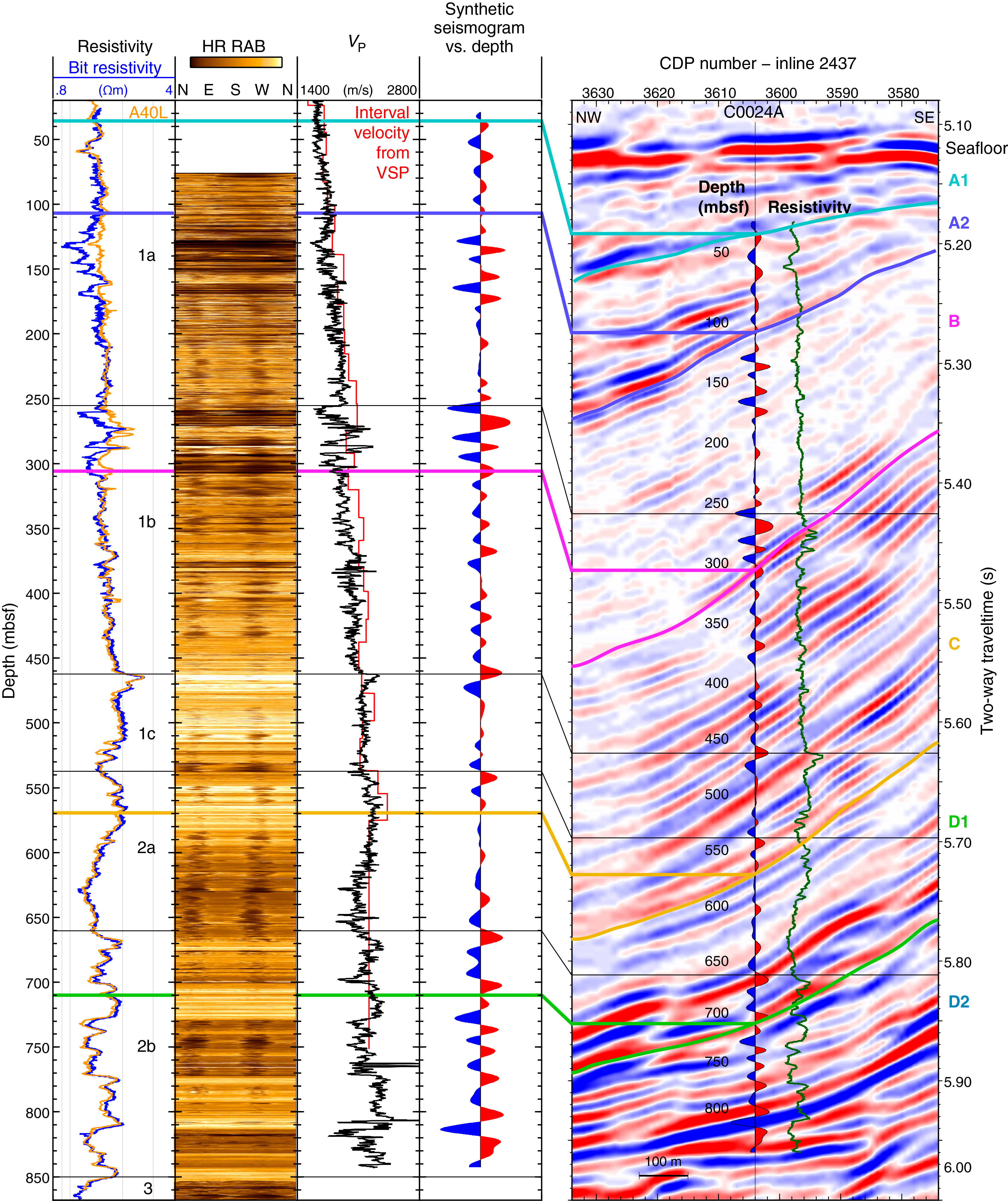
Figure F72. Synthetic seismogram with other logging data and In-line 2437.
The synthetic trace was generated by convolution of a synthetic 40 Hz Ricker wavelet (that best matched the frequency content of the survey trace) with the reflection coefficients. To match the time-depth relationship defined by the VSP check shots, three of the VSP stations were used (at 100.26, 397.09, and 748.11 mbsf). Such adjustments allow us to anchor the synthetic trace to a reference depth and to correct the "drift" of the time relationship derived from integration of the VP log. Two additional ties were made, including one below the deepest VSP stations, to match clear reflectors at 5.94 and 5.82 s TWT (820 and 670 mbsf, respectively). Although the synthetic seismograms make it possible to match seismic reflectors and well data, it is obvious from Figure F72 that the synthetic trace fails to reproduce the seismic attributes at several intervals, most noticeably at ~150 mbsf and between 250 and 300 mbsf, where strong variability in the VP logs generates high reflectivity, which does not match the seismic profiles. However, some of the best-defined reflectors coincide with the boundaries between various logging units and subunits. One of the strongest reflectors in the logged interval is the negative reflector at 5.94 s TWT that is generated by a sharp drop in velocity at ~806 or ~819 mbsf and is associated with the top of the interpreted plate boundary.
Deep seismic imaging
Recording closely spaced VSP stations along most of the hole allows imaging of some of the seismic reflectors below the maximum depth reached in Hole C0024A. The main steps for this "look ahead" VSP analysis (Payne et al., 1994) are the separation of the downgoing (direct) and upgoing (reflected) wavefields for each station and the deconvolution of the upgoing wavefield with the downgoing wavefield. The results of this analysis, performed by the Schlumberger processing center, show that reflectors as deep as 2 s TWT below the maximum depth of the hole (or 3 km if we assumed an average velocity of 3 km/s) were captured in the traces recorded in Hole C0024A (Figure F73).
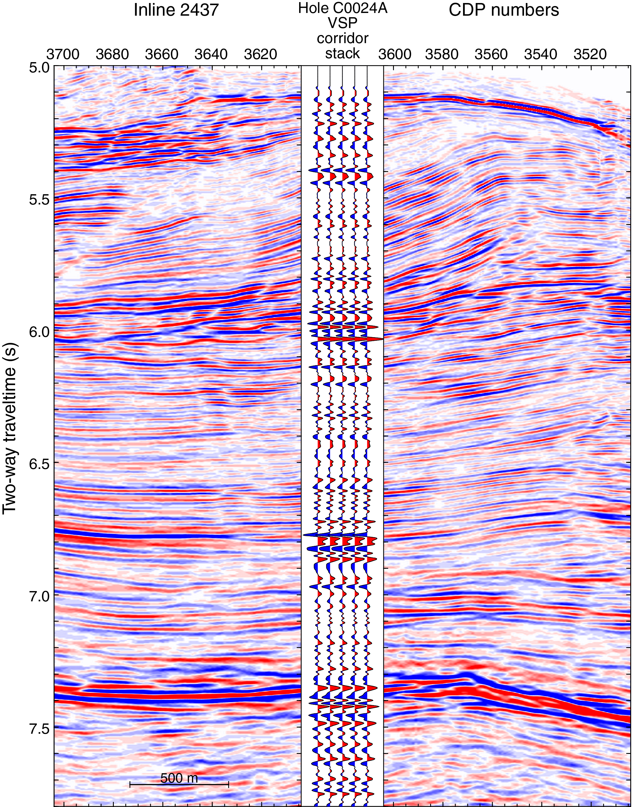
Figure F73. Corridor stack generated from traces recorded during VSP survey.
References
Araki, E., Saffer, D.M, Kopf, A.J., Wallace, L.M., Kimura, T., Machida, Y., Ide, S., Davis, E., and IODP Expedition 365 Shipboard Scientists, 2017. Recurring and triggered slow-slip events near the trench at the Nankai Trough subduction megathrust. Science, 356(6343):1157–1160. https://doi.org/10.1126/science.aan3120
Archie, G.E., 1942. The electrical resistivity log as an aid in determining some reservoir characteristics. Transactions of the AIME, 146(1):54–62. https://doi.org/10.2118/942054-G
Aydin, A., 1978. Small faults formed as deformation bands in sandstone. Pure and Applied Geophysics, 116(4):913–930. https://doi.org/10.1007/BF00876546
Aydin, A., Borja, R.I., and Eichhubl, P., 2006. Geological and mathematical framework for failure modes in granular rock. Journal of Structural Geology, 28(1):83–98. https://doi.org/10.1016/j.jsg.2005.07.008
Brigaud, F., and Vasseur, G., 1989. Mineralogy, porosity and fluid control on thermal conductivity of sedimentary rocks. Geophysical Journal International, 98(3):525–542. https://doi.org/10.1111/j.1365-246X.1989.tb02287.x
Brothers, R.J., Kemp, A.E.S., Maltman, A.J., 1996. Mechanical development of vein structures due to the passage of earthquake waves through poorly consolidated sediments. Tectonophysics, 260(4):227–244. https://doi.org/10.1016/0040-1951(96)00088-1
Bullard, E.C., 1939. Heat flow in South Africa. Proceedings of the Royal Society of London, Series A: Mathematical, Physical and Engineering Sciences, 173(955):474–502. https://doi.org/10.1098/rspa.1939.0159
Byrne, T.B., Lin, W., Tsutsumi, A., Yamamoto, Y., Lewis, J.C., Kanagawa, K., Kitamura, Y., Yamaguchi, A., and Kimura, G., 2009. Anelastic strain recovery reveals extension across SW Japan subduction zone. Geophysical Research Letters, 36(23):L23310. https://doi.org/10.1029/2009GL040749
Carlson, J., and Grotzinger, J.P., 2001. Submarine fan environment inferred from turbidite thickness distributions. Sedimentology, 48(6):1331–1351. https://doi.org/10.1046/j.1365-3091.2001.00426.x
Cashman, S., and Cashman, K., 2000. Cataclasis and deformation-band formation in unconsolidated marine terrace sand, Humboldt County, California. Geology, 28(2):111–114. https://doi.org/10.1130/0091-7613(2000)28<111:CADFIU>2.0.CO;2
Expedition 314 Scientists, 2009. Expedition 314 Site C0006. In Kinoshita, M., Tobin, H., Ashi, J., Kimura, G., Lallemant, S., Screaton, E.J., Curewitz, D., Masago, H., Moe, K.T., and the Expedition 314/315/316 Scientists, Proceedings of the Integrated Ocean Drilling Program, 314/315/316: Washington, DC (Integrated Ocean Drilling Program Management International, Inc.). https://doi.org/10.2204/iodp.proc.314315316.118.2009
Expedition 316 Scientists, 2009a. Expedition 316 Site C0006. In Kinoshita, M., Tobin, H., Ashi, J., Kimura, G., Lallemant, S., Screaton, E.J., Curewitz, D., Masago, H., Moe, K.T., and the Expedition 314/315/316 Scientists, Proceedings of the Integrated Ocean Drilling Program, 314/315/316: Washington, DC (Integrated Ocean Drilling Program Management International, Inc.). https://doi.org/10.2204/iodp.proc.314315316.134.2009
Expedition 316 Scientists, 2009b. Expedition 316 Site C0007. In Kinoshita, M., Tobin, H., Ashi, J., Kimura, G., Lallemant, S., Screaton, E.J., Curewitz, D., Masago, H., Moe, K.T., and the Expedition 314/315/316 Scientists, Proceedings of the Integrated Ocean Drilling Program, 314/315/316: Washington, DC (Integrated Ocean Drilling Program Management International, Inc.). https://doi.org/10.2204/iodp.proc.314315316.135.2009
Expedition 322 Scientists, 2010. Site C0011. In Saito, S., Underwood, M. B., Kubo, Y., and the Expedition 322 Scientists, Proceedings of the Integrated Ocean Drilling Program, 322: Tokyo (Integrated Ocean Drilling Program Management International, Inc.). https://doi.org/10.2204/iodp.proc.322.103.2010
Expedition 333 Scientists, 2012a. Site C0011. In Henry, P., Kanamatsu, T., Moe, K., and the Expedition 333 Scientists, Proceedings of the Integrated Ocean Drilling Program, 333: Tokyo (Integrated Ocean Drilling Program Management International, Inc.). https://doi.org/10.2204/iodp.proc.333.104.2012
Expedition 333 Scientists, 2012b. Site C0012. In Henry, P., Kanamatsu, T., Moe, K., and the Expedition 333 Scientists, Proceedings of the Integrated Ocean Drilling Program, 333: Tokyo (Integrated Ocean Drilling Program Management International, Inc.). https://doi.org/10.2204/iodp.proc.333.105.2012
Felletti, F., and Bersezio, R., 2010. Quantification of the degree of confinement of a turbidite-filled basin: a statistical approach based on bed thickness distribution. Marine and Petroleum Geology, 27(2):515–532. https://doi.org/10.1016/j.marpetgeo.2009.11.003
Fofonoff, N.P., 1985. Physical properties of seawater: a new salinity scale and equation of state for seawater. Journal of Geophysical Research: Oceans, 90(C2):3332–3342. https://doi.org/10.1029/JC090iC02p03332
Fossen, H., Schultz, R.A., Shipton, Z.K., and Mair, K., 2007. Deformation bands in sandstone: a review. Journal of the Geological Society, 164:755–769. https://doi.org/10.1144/0016-76492006-036
Fulton, P.M., and Harris, R.N., 2012. Thermal considerations in inferring frictional heating from vitrinite reflectance and implications for shallow coseismic slip within the Nankai subduction zone. Earth and Planetary Science Letters, 335–336:206-215. https://doi.org/10.1016/j.epsl.2012.04.012
Hamada, Y., Sakaguchi, A., Tanikawa, W., Yamaguchi, A., Kameda, J., and Kimura, G., 2015. Estimation of slip rate and fault displacement during shallow earthquake rupture in the Nankai subduction zone. Earth, Planets and Space, 67(1):39. https://doi.org/10.1186/s40623-015-0208-0
Hanamura, Y., and Ogawa, Y., 1993. Layer-parallel faults, duplexes, imbricate thrust and vein structures of the Miura Group: keys to understanding the Izu fore-arc sediment accretion to the Honshu fore arc. Island Arc, 2(3):126-141. https://doi.org/10.1111/j.1440-1738.1993.tb00081.x
Hirose, T., Ikari, M., Kanagawa, K., Kimura, G., Kinoshita, M., Kitajima, H., Saffer, D., Tobin, H., Yamaguchi, A., Eguchi, N., Maeda, L., Toczko, S., Bedford, J., Chiyonobu, S., Colson, T.A., Conin, M., Cornard, P.H., Dielforder, A., Doan, M.-L., Dutilleul, J., Faulkner, D.R., Fukuchi, R., Guérin, G., Hamada, Y., Hamahashi, M., Hong, W.-L., Ijiri, A., Jaeger, D., Jeppson, T., Jin, Z., John, B.E., Kitamura, M., Kopf, A., Masuda, H., Matsuoka, A., Moore, G.F., Otsubo, M., Regalla, C., Sakaguchi, A., Sample, J., Schleicher, A., Sone, H., Stanislowski, K., Strasser, M., Toki, T., Tsuji, T., Ujiie, K., Underwood, M.B., Yabe, S., Yamamoto, Y., Zhang, J., Sanada, Y., Kido, Y., Le Ber, E., and Saito, S., 2020. Expedition 358 methods. With contributions by T. Kanamatsu. In Tobin, H., Hirose, T., Ikari, M., Kanagawa, K., Kimura, G., Kinoshita, M., Kitajima, H., Saffer, D., Yamaguchi, A. Eguchi, N., Maeda, L., Toczko, S., and the Expedition 358 Scientists, NanTroSEIZE Plate Boundary Deep Riser 4: Nankai Seismogenic/Slow Slip Megathrust. Proceedings of the International Ocean Discovery Program, 358: College Station, TX (International Ocean Discovery Program). https://doi.org/10.14379/iodp.proc.358.102.2020
Hiscott, R.N., Colella, A., Pezard, P., Lovell, M.A., and Malinverno, A., 1992. Sedimentology of deepwater volcaniclastics, Oligocene Izu-Bonin forearc basin, based on formation microscanner images. In Taylor, B., Fujioka, K., et al., Proceedings of the Ocean Drilling Program, Scientific Results, 126: College Station, TX (Ocean Drilling Program), 75–96. https://doi.org/10.2973/odp.proc.sr.126.118.1992
Ito, Y., Asano, Y., and Obara, K., 2009. Very-low-frequency earthquakes indicate a transpressional stress regime in the Nankai accretionary prism. Geophysical Research Letters, 36(20):L20309. https://doi.org/10.1029/2009GL039332
Ito, Y., Obara, K., Shiomi, K., Sekine, S., and Hirose, H., 2007. Slow earthquakes coincident with episodic tremors and slow slip events. Science, 315(5811):503–506. https://doi.org/10.1126/science.1134454
James, R.H., and Palmer, M.R., 2000. Marine geochemical cycles of the alkali elements and boron: the role of sediments. Geochimica et Cosmochimica Acta, 64(18):3111–3122. https://doi.org/10.1016/S0016-7037(00)00418-X
Joseph, C., Torres, M.E., and Haley, B., 2013. Data report: 87Sr/86Sr in pore fluids from NanTroSEIZE Expeditions 322 and 333. In Saito, S., Underwood, M.B., Kubo, Y., and the Expedition 322 Scientists, Proceedings of the Integrated Ocean Drilling Program, 322: Tokyo (Integrated Ocean Drilling Program Management International, Inc.). https://doi.org/10.2204/iodp.proc.322.207.2013
Kastner, M., Elderfield, H., and Martin, J.B., 1991. Fluids in convergent margins: what do we know about their composition, origin, role in diagenesis and importance for oceanic chemical fluxes? Philosophical Transactions of the Royal Society A: Mathematical, Physical and Engineering Sciences, 335(1638):243–259. https://doi.org/10.1098/rsta.1991.0045
Kimura, G., Screaton, E.J., Curewitz, D., and the Expedition 316 Scientists, 2008. Expedition 316 Preliminary Report: NanTroSEIZE Stage 1A: NanTroSEIZE Shallow Megasplay and Frontal Thrusts. Integrated Ocean Drilling Program. https://doi.org/10.2204/iodp.pr.316.2008
Kinoshita, M., Becker, K., Toczko, S., Edginton, J., Kimura, T., Machida, Y., Roesner, A., Senyener, B., and Sun, T., 2018. Site C0006. In Becker, K., Kinoshita, M., Toczko, S., and the Expedition 380 Scientists, NanTroSEIZE Stage 3: Frontal Thrust Long-Term Borehole Monitoring System (LTBMS). Proceedings of the International Ocean Discovery Program, 380: College Station, TX (International Ocean Discovery Program). https://doi.org/10.14379/iodp.proc.380.103.2018
Maltman, A.J., Byrne, T., Karig, D.E., and Lallement, S., 1993. Deformation at the toe of an active accretionary prism: synopsis of results from ODP Leg 131, Nankai, SW Japan. Journal of Structural Geology, 15(8):949–964. https://doi.org/10.1016/0191-8141(93)90169-B
Martini, E., 1971. Standard Tertiary and Quaternary calcareous nannoplankton zonation. In Farinacci, A. (Ed.), Proceedings of the Second Planktonic Conference, Roma 1970: Rome (Edizioni Tecnoscienza), 2:739–785.
Moore, G.F., Park, J.-O., Bangs, N.L., Gulick, S.P., Tobin, H.J., Nakamura, Y., Sato, S., et al., 2009. Structural and seismic stratigraphic framework of the NanTroSEIZE Stage 1 transect. In Kinoshita, M., Tobin, H., Ashi, J., Kimura, G., Lallemant, S., Screaton, E.J., Curewitz, D., Masago, H., Moe, K.T., and the Expedition 314/315/316 Scientists, Proceedings of the Integrated Ocean Drilling Program, 314/315/316: Washington, DC (Integrated Ocean Drilling Program Management International, Inc.). https://doi.org/10.2204/iodp.proc.314315316.102.2009
Nakano, M., Hyodo, M., Nakanishi, A., Yamashita, M., Hori, T., Kamiya, S., Suzuki, K., et al., 2018. The 2016 Mw 5.9 earthquake off the southeastern coast of Mie Prefecture as an indicator of preparatory processes of the next Nankai Trough megathrust earthquake. Progress in Earth and Planetary Science, 5:30. https://doi.org/10.1186/s40645-018-0188-3
Obara, K., 2002. Nonvolcanic deep tremor associated with subduction in southwest Japan. Science, 296(5573):1679–1681. https://doi.org/10.1126/science.1070378
Obara, K., and Kato, A., 2016. Connecting slow earthquakes to huge earthquakes. Science, 353(6296):253–257. https://doi.org/10.1126/science.aaf1512
Okada, H., and Bukry, D., 1980. Supplementary modification and introduction of code numbers to the low-latitude coccolith biostratigraphic zonation (Bukry, 1973; 1975). Marine Micropaleontology, 5:321–325. https://doi.org/10.1016/0377-8398(80)90016-X
Oohashi, K., Lin, W., Wu, H.-Y., Yamaguchi, A., and Yamamoto, Y., 2017. Stress state in the Kumano Basin and in slope sediment determined from anelastic strain recovery: results from IODP Expedition 338 to the Nankai Trough. Geochemistry, Geophysics, Geosystems, 18(10):3608–3616. https://doi.org/10.1002/2017GC007137
Payne, M.A., Eriksen, E.A., and Rape, T.D., 1994. Considerations for high-resolution VSP imaging. The Leading Edge, 13:173–180. https://doi.org/10.1190/1.1437010
Pickering, K.T., Underwood, M.B., and Taira, A., 1992. Open-ocean to trench turbidity-current flow in the Nankai Trough: flow collapse and reflection. Geology, 20(12):1099–1102. https://doi.org/10.1130/0091-7613(1992)020<1099:OOTTTC>2.3.CO;2
Raffi, I., Backman, J., Fornaciari, E., Pälike, H., Rio, D., Lourens, L., and Hilgen, F., 2006. A review of calcareous nannofossil astrobiochronology encompassing the past 25 million years. Quaternary Science Reviews, 25(23–24):3113–3137. https://doi.org/10.1016/j.quascirev.2006.07.007
Rothman, D.H., Grotzinger, J.P., and Flemings, P.B., 1994. Scaling in turbidite deposition. Journal of Sedimentary Research, 64(1A):59–67. https://doi.org/10.1306/D4267D07-2B26-11D7-8648000102C1865D
Rothman, D.H., and Grotzinger, J.P., 1995. Scaling properties of gravity-driven sediments. Nonlinear Processes in Geophysics, 2(3–4):178–185. https://doi.org/10.5194/npg-2-178-1995
Sakaguchi, A., Chester, F., Curewitz, D., Fabbri, O., Goldsby, D., Kimura, G., Li, C.-F., et al., 2011. Seismic slip propagation to the updip end of plate boundary subduction interface faults: vitrinite reflectance geothermometry on Integrated Ocean Drilling Program NanTroSEIZE cores. Geology, 39(4):395–398. https://doi.org/10.1130/G31642.1
Sato, T., Chinyonobu, S., and Hodell, D.A., 2009. Data report: Quaternary calcareous nannofossil datums and biochronology in the North Atlantic Ocean, IODP Site U1308. In Channell, J.E.T., Kanamatsu, T., Sato, T., Stein, R., Alvarez Zarikian, C.A., Malone, M.J., and the Expedition 303/306 Scientists, Proceedings of the Integrated Ocean Drilling Program, 303/306: College Station, TX (Integrated Ocean Drilling Program Management International, Inc.). https://doi.org/10.2204/iodp.proc.303306.210.2009
Screaton, E., Kimura, G., Curewitz, D., Moore, G., Chester, F., Fabbri, O., Fergusson, C., Girault, F., et al., 2009a. Interactions between deformation and fluids in the frontal thrust region of the NanTroSEIZE transect offshore the Kii Peninsula, Japan: results from IODP Expedition 316 Sites C0006 and C0007. Geochemistry, Geophysics, Geosystems, 10(12):Q0AD01. https://doi.org/10.1029/2009GC002713
Screaton, E.J., Kimura, G., Curewitz, D., and the Expedition 316 Scientists, 2009b. Expedition 316 summary. In Kinoshita, M., Tobin, H., Ashi, J., Kimura, G., Lallemant, S., Screaton, E.J., Curewitz, D., Masago, H., Moe, K.T., and the Expedition 314/315/316 Scientists, Proceedings of the Integrated Ocean Drilling Program, 314/315/316: Washington, DC (Integrated Ocean Drilling Program Management International, Inc.). https://doi.org/10.2204/iodp.proc.314315316.131.2009
Scudder, R.P., Murray, R.W., Kutterolf, S., Schindlbeck, J.C., Underwood, M.B., and Wang, K.-L., 2018. Sedimentary inputs to the Nankai subduction zone: the importance of dispersed ash. Geosphere, 14(4):1451–1467. https://doi.org/10.1130/GES01558.1
Shipboard Scientific Party, 1991. Site 808. In Taira, A., Hill, I., Firth, J.V., et al., Proceedings of the Ocean Drilling Program, Initial Reports, 131: College Station, TX (Ocean Drilling Program), 71–269. https://doi.org/10.2973/odp.proc.ir.131.106.1991
Shipboard Scientific Party, 2001a. Leg 190 summary. In Moore, G.F., Taira, A., Klaus, A., et al., Proceedings of the Ocean Drilling Program, Initial Reports, 190: College Station, TX (Ocean Drilling Program), 1–87. https://doi.org/10.2973/odp.proc.ir.190.101.2001
Shipboard Scientific Party, 2001b. Site 1174. In Moore, G.F., Taira, A., Klaus, A., et al., Proceedings of the Ocean Drilling Program, Initial Reports, 190: College Station, TX (Ocean Drilling Program), 1–149. https://doi.org/10.2973/odp.proc.ir.190.105.2001
Spinelli, G.A., Mozley, P.S., Tobin, H.J., Underwood, M.B., Hoffman, N.W., and Bellew, G.M., 2007. Diagenesis, sediment strength, and pore collapse in sediment approaching the Nankai Trough subduction zone. Geological Society of America Bulletin, 119(3–4):377–390. https://doi.org/10.1130/B25920.1
Strasser, M., Moore, G.F., Kimura, G., Kitamura, Y., Kopf, A.J., Lallemant, S., Park, J.-O., Screaton, E.J., Su, X., Underwood, M.B., and Zhao, X., 2009. Origin and evolution of a splay fault in the Nankai accretionary wedge. Nature Geoscience, 2(9):648–652. https://doi.org/10.1038/ngeo609
Sugioka, H., Okamoto, T., Nakamura, T., Ishihara, Y., Ito, A., Obana, K., Kinoshita, M., Nakahigashi, K., Shinohara, M., and Fukao, Y., 2012. Tsunamigenic potential of the shallow subduction plate boundary inferred from slow seismic slip. Nature Geoscience, 5(6):414–418. https://doi.org/10.1038/ngeo1466
Thamdrup, B., Finster, K., Hansen, J.W., and Bak, F., 1993. Bacterial disproportionation of elemental sulfur coupled to chemical reduction of iron or manganese. Applied Environmental Microbiology, 59(1):101–108. https://aem.asm.org/content/aem/59/1/101.full.pdf
Tobin, H., Hirose, T., Ikari, M., Kanagawa, K., Kimura, G., Kinoshita, M., Kitajima, H., Saffer, D., Yamaguchi, A., Eguchi, N., Maeda, L., Toczko, S., Bedford, J., Chiyonobu, S., Colson, T.A., Conin, M., Cornard, P.H., Dielforder, A., Doan, M.-L., Dutilleul, J., Faulkner, D.R., Fukuchi, R., Guérin, G., Hamada, Y., Hamahashi, M., Hong, W.-L., Ijiri, A., Jaeger, D., Jeppson, T., Jin, Z., John, B.E., Kitamura, M., Kopf, A., Masuda, H., Matsuoka, A., Moore, G.F., Otsubo, M., Regalla, C., Sakaguchi, A., Sample, J., Schleicher, A., Sone, H., Stanislowski, K., Strasser, M., Toki, T., Tsuji, T., Ujiie, K., Underwood, M.B., Yabe, S., Yamamoto, Y., Zhang, J., Sanada, Y., Kido, Y., Le Ber, E., and Saito, S., 2020a. Expedition 358 summary. With contributions by T. Kanamatsu. In Tobin, H., Hirose, T., Ikari, M., Kanagawa, K., Kimura, G., Kinoshita, M., Kitajima, H., Saffer, D., Yamaguchi, A. Eguchi, N., Maeda, L., Toczko, S., and the Expedition 358 Scientists, NanTroSEIZE Plate Boundary Deep Riser 4: Nankai Seismogenic/Slow Slip Megathrust. Proceedings of the International Ocean Discovery Program, 358: College Station, TX (International Ocean Discovery Program). https://doi.org/10.14379/iodp.proc.358.101.2020
Tobin, H., Hirose, T., Ikari, M., Kanagawa, K., Kimura, G., Kinoshita, M., Kitajima, H., Saffer, D., Yamaguchi, A. Eguchi, N., Maeda, L., Toczko, S., and the Expedition 358 Scientists, 2020b. Supplementary material, https://doi.org/10.14379/iodp.proc.358supp.2020. Supplement to Tobin, H., Hirose, T., Ikari, M., Kanagawa, K., Kimura, G., Kinoshita, M., Kitajima, H., Saffer, D., Yamaguchi, A. Eguchi, N., Maeda, L., Toczko, S., and the Expedition 358 Scientists, NanTroSEIZE Plate Boundary Deep Riser 4: Nankai Seismogenic/Slow Slip Megathrust. Proceedings of the International Ocean Discovery Program, 358: College Station, TX (International Ocean Discovery Program). https://doi.org/10.14379/iodp.proc.358.2020
Tobin, H., Hirose, T., Saffer, D., Toczko, S., Maeda, L., Kubo, Y., Boston, B., Broderick, A., Brown, K., Crespo-Blanc, A., Even, E., Fuchida, S., Fukuchi, R., Hammerschmidt, S., Henry, P., Josh, M., Jurado, M.J., Kitajima, H., Kitamura, M., Maia, A., Otsubo, M., Sample, J., Schleicher, A., Sone, H., Song, C., Valdez, R., Yamamoto, Y., Yang, K., Sanada, Y., Kido, Y., and Hamada, Y., 2015. Expedition 348 summary. In Tobin, H., Hirose, T., Saffer, D., Toczko, S., Maeda, L., Kubo, Y., and the Expedition 348 Scientists, Proceedings of the Integrated Ocean Drilling Program, 348: College Station, TX (Integrated Ocean Drilling Program). https://doi.org/10.2204/iodp.proc.348.101.2015
Torres, M.E., Bohrmann, G., and Suess, E., 1996. Authigenic barites and fluxes of barium associated with fluid seeps in the Peru subduction zone. Earth and Planetary Science Letters, 144(3–4):469–481. https://doi.org/10.1016/S0012-821X(96)00163-X
Torres, M.E., Cox, T., Hong, W.-L., McManus, J., Sample, J.C., Destrigneville, C., Gan, H.M., Gan, H.Y., and Moreau, J.W., 2015. Crustal fluid and ash alteration impacts on the biosphere of Shikoku Basin sediments, Nankai Trough, Japan. Geobiology, 13(6):562–580. https://doi.org/10.1111/gbi.12146
Ujiie, K., Maltman, A.J., and Sánchez-Gómez, M., 2004. Origin of deformation bands in argillaceous sediments at the toe of the Nankai accretionary prism, southwest Japan. Journal of Structural Geology, 26(2):221–231. https://doi.org/10.1016/j.jsg.2003.06.001
Underwood, M.B., and Moore, G.F., 1995. Trenches and trench-slope basins. In Busby, C.J., and Ingersoll, R.V. (Eds.), Tectonics of Sedimentary Basins: Cambridge, MA (Blackwell Science), 179–220.
Underwood, M.B., and Moore, G.F., 2012. Evolution of sedimentary environments in the subduction zone of southwest Japan: recent results from the NanTroSEIZE Kumano transect. In Busby, C., and Azor, A. (Eds.), Tectonics of Sedimentary Basins: Recent Advances: Cambridge, MA (Blackwell Publishing, Ltd.), 310–327. https://doi.org/10.1002/9781444347166.ch15
Underwood, M.B., and Pickering, K.T., 2018. Facies architecture, detrital provenance, and tectonic modulation of sedimentation in the Shikoku Basin: inputs to the Nankai Trough subduction zone. In Byrne, T., Underwood, M.B. III, Fisher, D., McNeill, L., Saffer, D., Ujiie, K., and Yamaguchi, A. (Eds.), Geology and Tectonics of Subduction Zones: A Tribute to Gaku Kimura. Special Paper - Geological Society of America, 534:1–34. https://doi.org/10.1130/2018.2534(01)
Underwood, M.B., Saito, S., Kubo, Y., and the Expedition 322 Scientists, 2010. Expedition 322 summary. In Saito, S., Underwood, M.B., Kubo, Y., and the Expedition 322 Scientists, Proceedings of the Integrated Ocean Drilling Program, 322: Tokyo (Integrated Ocean Drilling Program Management International, Inc.). https://doi.org/10.2204/iodp.proc.322.101.2010
Wallace, L.M., Araki, E., Saffer, D., Wang, X., Roesner, A., Kopf, A., Nakanishi, A., et al., 2016. Near-field observations of an offshore Mw 6.0 earthquake from an integrated seafloor and subseafloor monitoring network at the Nankai Trough, southwest Japan. Journal of Geophysical Research: Solid Earth, 121(11):8338–8351. https://doi.org/10.1002/2016JB013417
White, R.J., Spinelli, G.A., Mozley, P.S., and Dunbar, N.W., 2011. Importance of volcanic glass alteration to sediment stabilization: offshore Japan. Sedimentology, 58(5):1138–1154. https://doi.org/10.1111/j.1365-3091.2010.01198.x
Winkler, W., and Gawenda, P., 1999. Distinguishing climatic and tectonic forcing of turbidite sedimentation, and the bearing on turbidite bed scaling: Palaeocene-Eocene of northern Spain. Journal of the Geological Society, 156:791–800. https://doi.org/10.1144/gsjgs.156.4.0791
Yamaguchi, A., Sakaguchi, A., Sakamoto, T., Iijima, K., Kameda, J., Kimura, G., Ujiie, K., et al., 2011. Progressive illitization in fault gouge caused by seismic slip propagation along a megasplay fault in the Nankai Trough. Geology, 39(11):995–998. https://doi.org/10.1130/G32038.1
Yamamoto, Y., Lin, W., Oda, H., Byrne, T., and Yamamoto, Y., 2013. Stress states at the subduction input site, Nankai subduction zone, using anelastic strain recovery (ASR) data in the basement basalt and overlying sediments. Tectonophysics, 600:91–98. https://doi.org/10.1016/j.tecto.2013.01.028
Yamamoto, Y., Mukoyoshi, H., and Ogawa, Y., 2005. Structural characteristics of shallowly buried accretionary prism: rapidly uplifted Neogene accreted sediments on the Miura-Boso Peninsula, central Japan. Tectonics, 24(5):TC5008. https://doi.org/10.1029/2005TC001823
Yamamoto, Y., Nidaira, M., Ohta, Y., and Ogawa, Y., 2009. Formation of chaotic rock units during primary accretion processes: examples from the Miura–Boso accretionary complex, central Japan. Island Arc, 18(3):496–512. https://doi.org/10.1111/j.1440-1738.2009.00676.x
Yokota, Y., and Ishikawa, T., 2019., Shallow slow slip events along the Nankai Trough detected by GNSS-A. Science Advances, 6(3):eaay5786. https://doi.org/10.1126/sciadv.aay5786
You, C.-F., Chan, L.H., Spivack, A.J., and Gieskes, J.M., 1995. Lithium, boron, and their isotopes in sediments and pore waters of Ocean Drilling Program Site 808, Nankai Trough: implications for fluid expulsion in accretionary prisms. Geology, 23(1):37–40. https://doi.org/10.1130/0091-7613(1995)023<0037:LBATII>2.3.CO;2
1 Yamaguchi, A., Hirose, T., Ikari, M., Kanagawa, K., Kimura, G., Kinoshita, M., Kitajima, H., Saffer, D., Tobin, H., Eguchi, N., Maeda, L., Toczko, S., Bedford, J., Chiyonobu, S., Colson, T.A., Conin, M., Cornard, P.H., Dielforder, A., Doan, M.-L., Dutilleul, J., Faulkner, D.R., Fukuchi, R., Guérin, G., Hamada, Y., Hamahashi, M., Hong, W.-L., Ijiri, A., Jaeger, D., Jeppson, T., Jin, Z., John, B.E., Kitamura, M., Kopf, A., Masuda, H., Matsuoka, A., Moore, G.F., Otsubo, M., Regalla, C., Sakaguchi, A., Sample, J., Schleicher, A., Sone, H., Stanislowski, K., Strasser, M., Toki, T., Tsuji, T., Ujiie, K., Underwood, M.B., Yabe, S., Yamamoto, Y., Zhang, J., Sanada, Y., Kido, Y., Le Ber, E., and Saito, S., 2020. Site C0024. With contributions by T. Kanamatsu. In Tobin, H., Hirose, T., Ikari, M., Kanagawa, K., Kimura, G., Kinoshita, M., Kitajima, H., Saffer, D., Yamaguchi, A. Eguchi, N., Maeda, L., Toczko, S., and the Expedition 358 Scientists, NanTroSEIZE Plate Boundary Deep Riser 4: Nankai Seismogenic/Slow Slip Megathrust. Proceedings of the International Ocean Discovery Program, 358: College Station, TX (International Ocean Discovery Program). https://doi.org/10.14379/iodp.proc.358.104.2020
2 Expedition 358 Scientists' affiliations.
This work is distributed under the Creative Commons Attribution 4.0 International (CC BY 4.0) license. 