Hall, I.R., Hemming, S.R., LeVay, L.J., and the Expedition 361 Scientists
Proceedings of the International Ocean Discovery Program Volume 361
publications.iodp.org

https://doi.org/10.14379/iodp.proc.361.201.2020
Data report: X-ray fluorescence core scanning of IODP Site U1474 sediments, Natal Valley, Southwest Indian Ocean, Expedition 3611
Daniel P. Babin,2, 3 Allison M. Franzese,2, 4 Sidney R. Hemming,2, 3 Ian R. Hall,5 Leah J. LeVay,6 Stephen Barker,5 Luis Tejeda,4 Margit H. Simon,2, 7, 8 and the Expedition 361 Scientists9
Keywords: International Ocean Discovery Program, IODP, JOIDES Resolution, Expedition 361, South African Climates, Site U1474, Natal Valley, Agulhas Current, Geochemistry, XRF core scanning
MS 361-201: Received 13 August 2019 · Accepted 19 March 2020 · Published 5 June 2020
Abstract
X-ray fluorescence (XRF) core scanning was conducted on core sections from International Ocean Discovery Program Site U1474, located in the Natal Valley off the coast of South Africa. The data were collected at 2 mm resolution along the 255 m length of the splice, but this setting resulted in noisy data. This problem was addressed by applying a 10 point running sum on the XRF data prior to converting peak area to element intensities. This effectively integrates 10 measurements into 1, representing an average over 2 cm resolution, and significantly improves noise in the data. With 25 calibration samples, whose element concentrations were derived using inductively coupled plasma–optical emission spectrometry, the XRF measurements were converted to concentrations using a univariate log-ratio calibration method. The resulting concentrations of terrigenously derived major elements (Al, Si, K, Ti, and Fe) are anticorrelated with Ca concentrations, indicating the main control on sediment chemistry is the variable proportion of terrigenous to in situ produced carbonate material.
Introduction
X-ray fluorescence (XRF) core scanning is widely used in paleoceanography and provides qualitative, high-resolution, direct geochemical measurements along the length of a sediment or rock core. Although log ratios represent well the amount of variability in the data, there is a clear advantage to calibrating XRF data (Weltje, 2002; Weltje et al., 2015; Weltje and Tjallingii, 2008), which enables direct comparison to geochemical data gathered with other methods. The calibration process involves subsampling along the length of the core, determining absolute elemental concentrations using a different geochemical method such as inductively coupled plasma mass spectrometry, and comparing these values to the counts derived by XRF.
Site U1474 of International Ocean Discovery Program (IODP) Expedition 361 was drilled 88 nmi southwest of Durban, South Africa, in the Natal Valley at 31°13.00ʹS, 31°32.71ʹE and 3045 m below sea level and produced a record back to at least 6 Ma (see the Site U1474 chapter [Hall et al., 2017]) (Figure F1). The site is located in the path of the Agulhas Current, a large western boundary current (70 Sv) flowing south along Africa’s southeast margin (Lutjeharms, 2006). The record was obtained with the intention of documenting changes in both Agulhas Current variability and southern African paleoclimate. The composition of sediment at Site U1474 is largely terrigenous (55%–65%), and clay abundance is high (see the Site U1474 chapter [Hall et al., 2017]). Likely terrigenous sediment contributors include river systems proximal to the core site such as the Tugela, Mfolozi, and Mkomazi Rivers, which drain the nearby Drakensberg Mountains (see the Site U1474 chapter [Hall et al., 2017]; Simon et al., 2015) (Figure F1). The Natal Valley also receives sedimentation from more distant sources such as the Limpopo and Zambezi Rivers, inferred from the high 87Sr/86Sr ratio of the >63 µm fraction of Natal Valley sediment, which reflects the Archean age of the Kaapvaal and Zimbabwe Cratons that are eroded by the Zambezi and Limpopo Rivers (Franzese et al., 2006, 2009) (Figure F1). Sediment from these rivers is presumably transported to the Natal Valley via the Mozambique Current, estimated today to have a 15 Sv flux (Ridderinkhof et al., 2010) (Figure F1), and ultimately the Agulhas Current.
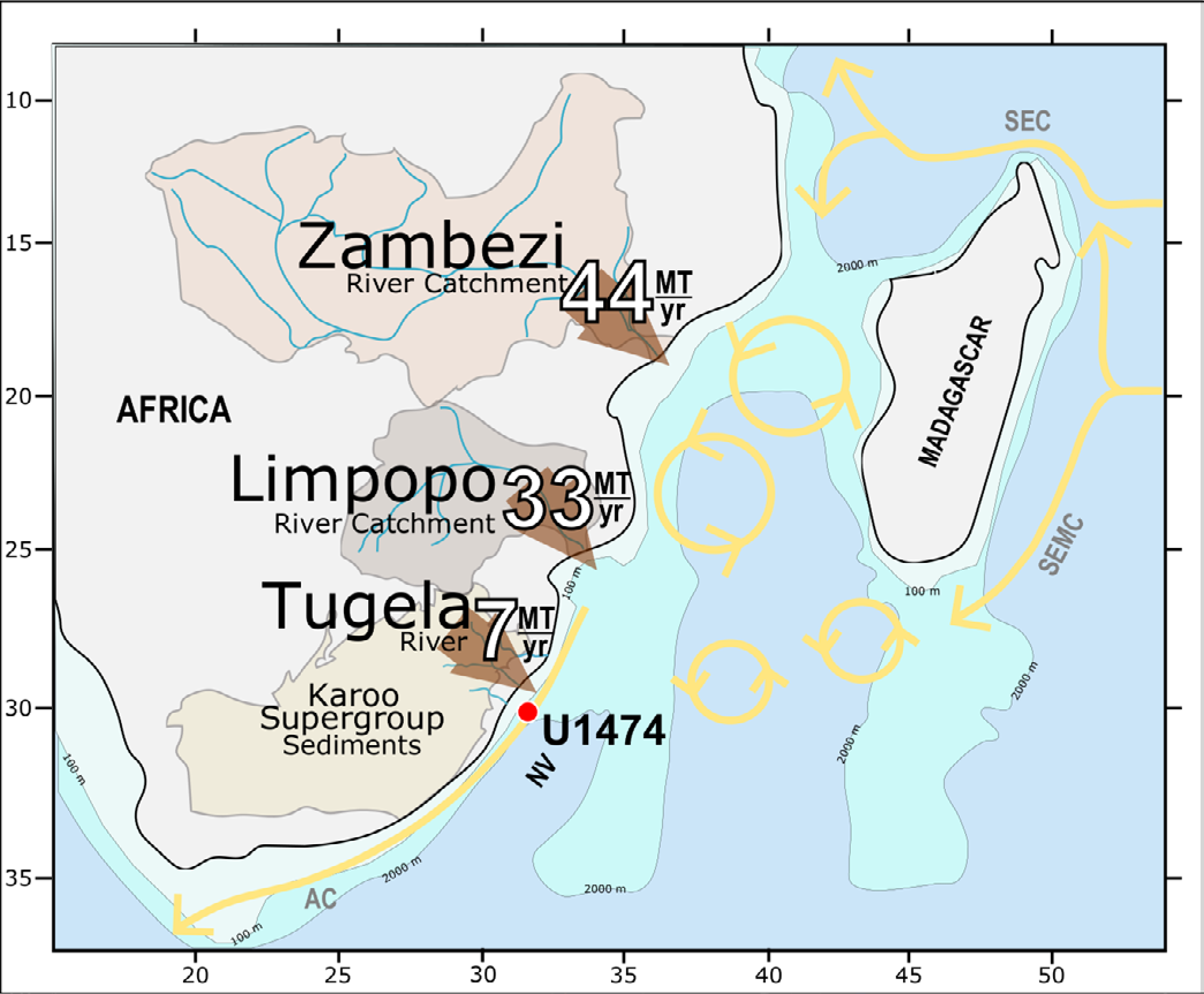
Figure F1. Drainage configuration and oceanography of southern Africa.
Work conducted by Simon et al. (2015) on a piston core collected near Site U1474 for the pre-site survey (CD-154-10-06P; 31°10.36ʹS, 032°08.91ʹE; 3076 m water depth) used the Fe/K ratio of bulk sediment derived from XRF core scanning to monitor the changing character of the terrigenous fraction. Because K is more mobile during weathering than Fe (Kossoff et al., 2012) and the spatial distribution of Fe and K in surface marine sediments tends to reflect the wetness or dryness of proximal sediment sources (Govin et al., 2012), Simon et al. (2015) argued that the changing Fe/K ratio indicated changes in chemical weathering as a consequence of changing hydroclimatic conditions. They also found precessional variation in the intensity of chemical weathering of sediment consistent throughout the 270 ky length of the record. A similar application of XRF core scanning on the 6 My record at Site U1474 could be useful in monitoring hydroclimate on longer timescales.
Methods and materials
In an effort to promote transparency and reproducibility in the geosciences, especially with large and cumbersome data sets such as XRF scans, the entirety of the process detailed in this work is documented on GitHub, a free online software version control platform commonly used for open source projects. This includes all of the raw data files, the XRF spectra for each scan, element signal intensities from the inductively coupled plasma–optical emission spectrometer (ICP-OES), and all the code used to organize the data, calibrate the XRF scans, and produce figures. Each process is displayed in IPython Jupyter Notebook, a web-based interactive computational environment. These can be examined by any reader in a web browser or can be downloaded and reprocessed by Python users. Each notebook can be viewed at https://github.com/danielbabin/U1474_XRF_Data_Report under Notebooks.
Data collection
XRF core scans
The ITRAX Core Scanner (Croudace et al., 2006) in the Core Repository at Lamont-Doherty Earth Observatory was used to scan 213 archive-half sections composing the Site U1474 splice. Each section was removed from refrigeration 30 min before measurement to allow the core to warm to room temperature. Surface roughness was removed from the core with a plastic card, and the core was covered with 4 μm thick Ultralene plastic film (SPEX Centriprep, Inc.) before being placed on the scanner, which is essential to minimize variation in parameter S (measurement geometry and specimen inhomogeneity) in the XRF calibration (Weltje and Tjallingii, 2008). Warming before adding the film helps prevent condensation on the film because condensation absorbs X-ray spectra, especially biasing light elements (Kido et al., 2006). X-ray illumination area was set at 2 mm in the downcore direction and 2 cm in the crosscore direction, and the scan was run down the center of the split core section half. Measurement spacing was set at 2 mm, voltage at 30 kV, current at 55 mA, and exposure time at 2 s using a Cr tube.
Because of shipping error, one core (Sections 361-U1474E-17H-1 through 17H-3; splice depth 221.6–225.50 m core composite depth below seafloor [CCSF]) did not reach Lamont-Doherty Earth Observatory. Consequently, data from this interval are missing.
Calibration samples
Discrete 10 cm3 samples were taken from the working halves for (nondestructive) shipboard measurements of moisture and density (MAD). Because water content is one of the key variables that affects measured XRF intensities, we used a subset of the MAD sample residues for this calibration. After XRF scanning was complete, we selected 25 of the MAD residues to capture the range of variability seen in the XRF scan data. Because the MAD samples were taken from Hole U1474A, not the splice, we used the magnetic susceptibility records to tie each MAD sample to a precise depth interval on the archive halves that were used for scanning (Table T1). This correlation for each MAD sample is documented on GitHub in the notebook mad_correlation.ipynb. The 25 discrete samples were digested using a standard lithium metaborate flux-fusion method along with a set of six powdered rock standards and six procedural blanks. Element concentrations were measured using the Agilent 720 axial ICP-OES at the Lamont-Doherty Earth Observatory and American Museum of Natural History inductively coupled plasma–mass spectrometry (ICP-MS) laboratory, for which routine precision is 1%–2%. Signal intensities were corrected for blanks and instrumental drift, then converted to concentrations using the accepted values for the six rock standards (Table T2) (Flanagan, 1984; Imai et al., 1996; McLennan and Taylor, 1980; Pretorius et al., 2006). The raw data and data reduction process for calculating elemental concentrations for the calibrations samples are documented on GitHub in the notebook xrf_calibration_samples_reduction.ipynb.
Calcium carbonate percent
An aliquot of the bulk moisture and density samples was powdered and measured for percent CaCO3 using a UIC CM5012 CO2 coulometer at Lamont-Doherty Earth Observatory’s Core Repository. Precision is determined to be <4% by replicate measurements every 10 samples. These measurements of percent CaCO3 are combined with measurements of CaCO3 performed aboard R/V JOIDES Resolution. These data are listed in Table T3.
XRF data processing
Preprocessing: running sum spectra
For this study, we focus only on the major elements detectable with the ITRAX: Al, Si, K, Ca, Ti, and Fe. The results of our XRF core scanning at 2 mm resolution can be found in Table T4. Unfortunately, even for the major elements, the low dwell time chosen (2 s) yielded noisy records, especially for light elements like Al (Figure F2). The minimum recommended dwell time with the ITRAX core scanner is 2 s. We chose this short dwell time, applied at a high resolution (2 mm), because we had a large volume of core to analyze and limited funds for analysis time. Fortunately, our high-resolution scanning allowed us to integrate the raw spectral data across a wider depth interval, increasing the height of our spectra and improving the signal-to-noise ratio.
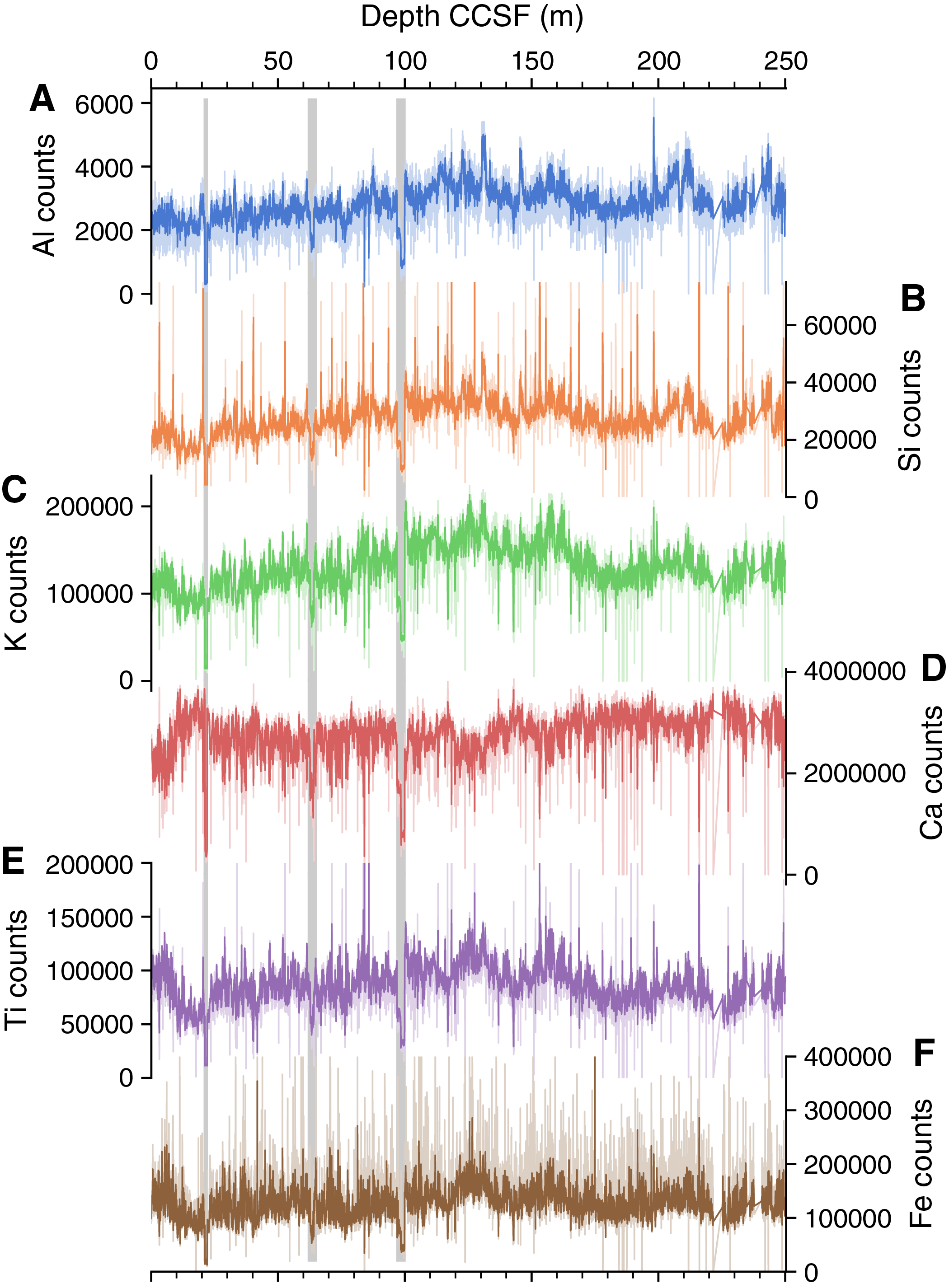
Figure F2. Raw XRF data, Site U1474.
To accomplish this, we access the raw spectral data, in the form of an .spe file, created with each measurement. The file contains a single vector of intensities at different energy wavelengths. We import all the spectral intensities from each .spe file (~750 for 1.5 m of core) from a single section into a data structure and take a 10 measurement running sum at each energy level across that data structure. Taking a 10 measurement running sum across these data, collected every 2 mm for 2 s, simulates a 2 cm exposure for 20 s. The section “offset” assigned to these integrated measurements represents the depth of the median (fifth) measurement out of every 10 exposures integrated. This process was repeated for the 213 sections scanned. Some sections had measurements with very low total spectra intensities (the sum of each element in the spectra). These resulted from measuring air at the tops or bottoms of sections or cracks in the core. All measurements with total spectral intensities lower than 300,000 were dropped for this reason. The Python code using these steps is available on GitHub in the notebook xrf_pre-processing.ipynb.
For the ITRAX core scanner, converting a spectra of energy intensities to element intensities involves fitting the observed spectra from a measurement with a model and computing the relevant area under the spectral peaks. This is done using the software Q-Spec, provided by ITRAX and Cox Analytical Systems for XRF data reduction (Croudace et al., 2006). To optimize the fit for several measurements (for example, along the length of a core section), the ITRAX software sums the spectra from each measurement in a section and outputs a “sumspectra” .spe file. To optimize the model fit for our 213 sections, we averaged the intensities of our 213 sumspectra files. This average sumspectra was then fit using the Q-spec software. We chose elements for the spectral model that minimized mean-squared error (MSE). The parameters keV/channel, energy offset, full width at half maximum (FWHM) slope, FWHM offset, and FWHM cutoff were also optimized to minimize MSE. We found that this method provides the highest quality record of element-intensity continuity in depth-space, minimizing jumps between sections. The MSE parameter provides a continuous assessment of how well the model fits each measurement. The results of this data processing can be found in Table T5. The Q-spec settings file (.dfl file type) that we used for our data reduction can be found in the GitHub repository for this paper under the subdirectory Settings.
Section positions were first converted into core depth below seafloor, Method A (CSF-A) and then into the CCSF scale used for the splice. No preprocessing steps, outlier removal, or filtering were necessary beyond the steps previously mentioned. The final result is 11,877 measurements of elemental intensities along 250 m of core. Although we only focus on major elements here (Al, Si, K, Ca, Ti, and Fe), an extensive suite of elements not suitable for calibration are available in the full XRF data tables (T4, T5). Table T4 contains the 2 mm, 2 s XRF data. Table T5 contains the 2 cm, 20 s integrated XRF data set.
The XRF data are shown by depth in Figures F3 and F4. Figure F3 shows individual element intensities for both the 2 cm, 20 s data set (full color) and the 2 mm, 2 s (paler colors) data sets. Figure F4 presents element intensities from both data sets normalized to Ca intensity. These figures clearly visualize the noise reduction offered by the 2 cm integration of the raw spectra.
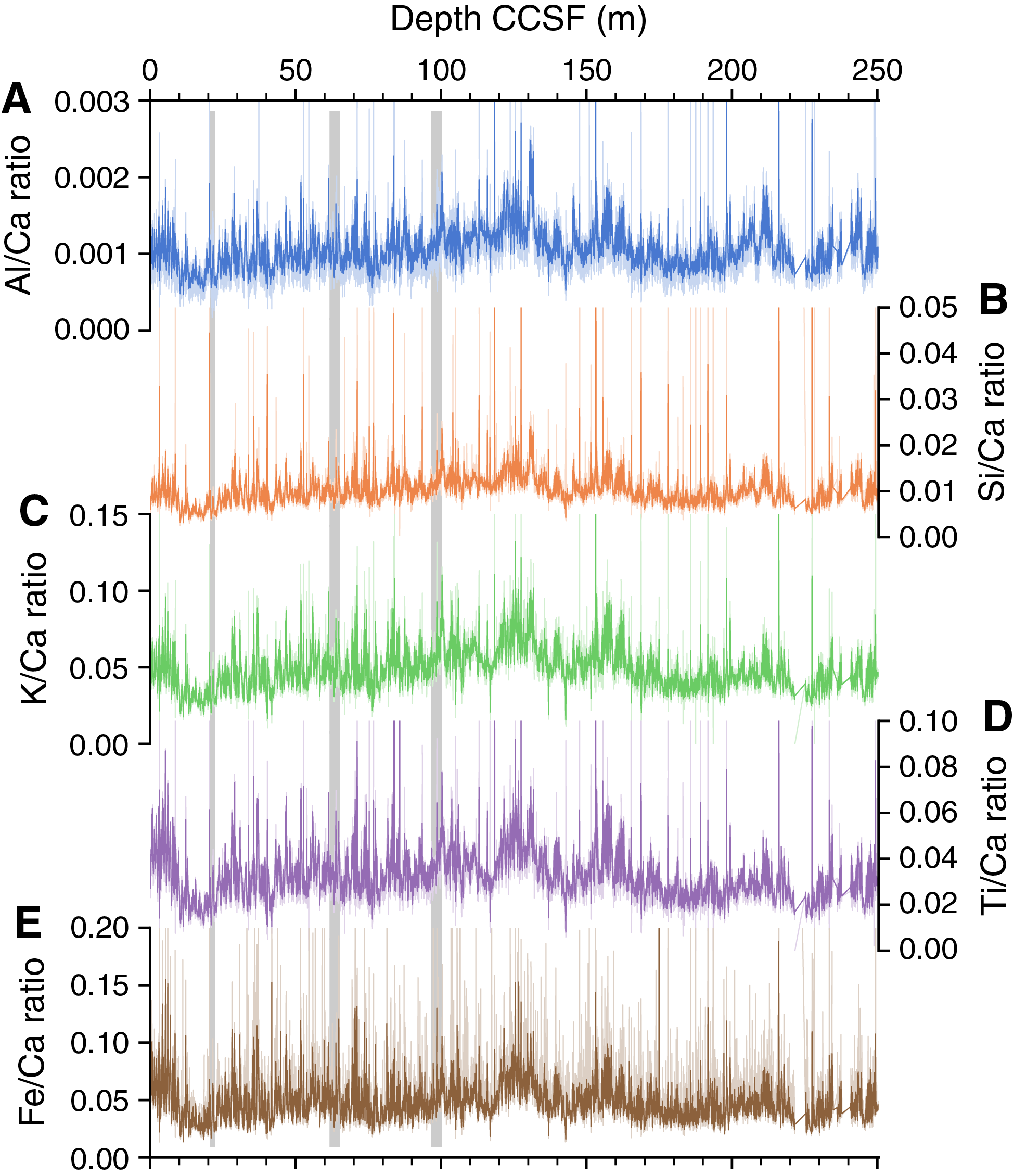
Figure F3. Raw XRF data normalized to Ca counts, Site U1474.
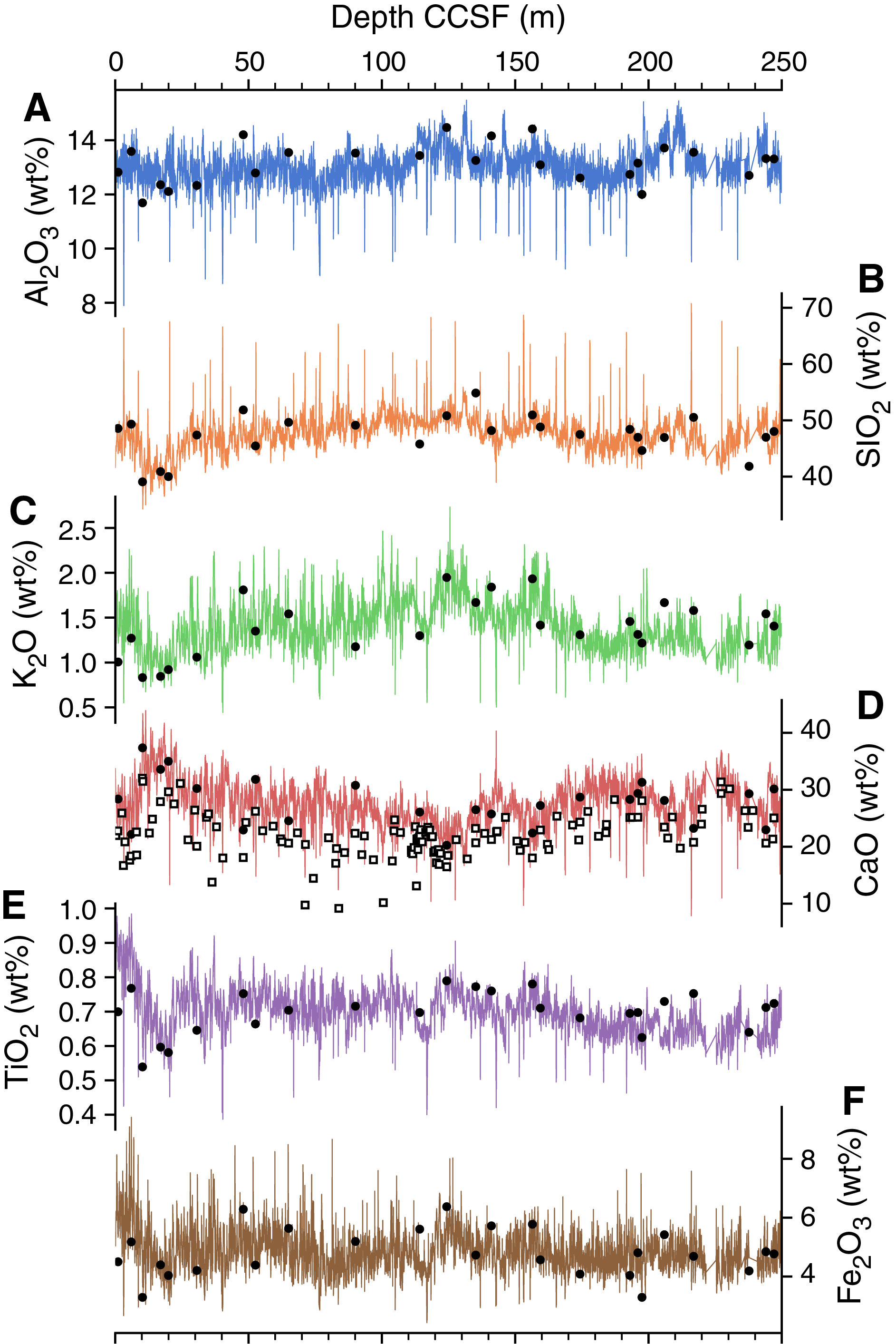
Figure F4. Calibrated XRF data, Site U1474.
XRF core scanning data calibration to element concentrations
The relative abundances provided by the XRF in “counts” were converted to concentrations with a calibration data set of 25 samples (Table T6; Figures F4 and F5). The conversion was made using the univariate log-ratio calibration (ULC) of Weltje and Tjallingii (2008) and used Ca counts and concentrations in the denominator of each element ratio. We chose the simpler ULC as opposed to the more sophisticated multivariate log-ratio calibration of Weltje et al. (2015) because of the relative sparse spacing of our calibration samples compared to the total length of our core. Concentrations are reported as weight percent element oxides. The Python code used for the calibration process, including the calculation of α and β parameters, is available on GitHub in the notebook xrf_calibration.ipynb. Model parameters α and β are available in Table T7.
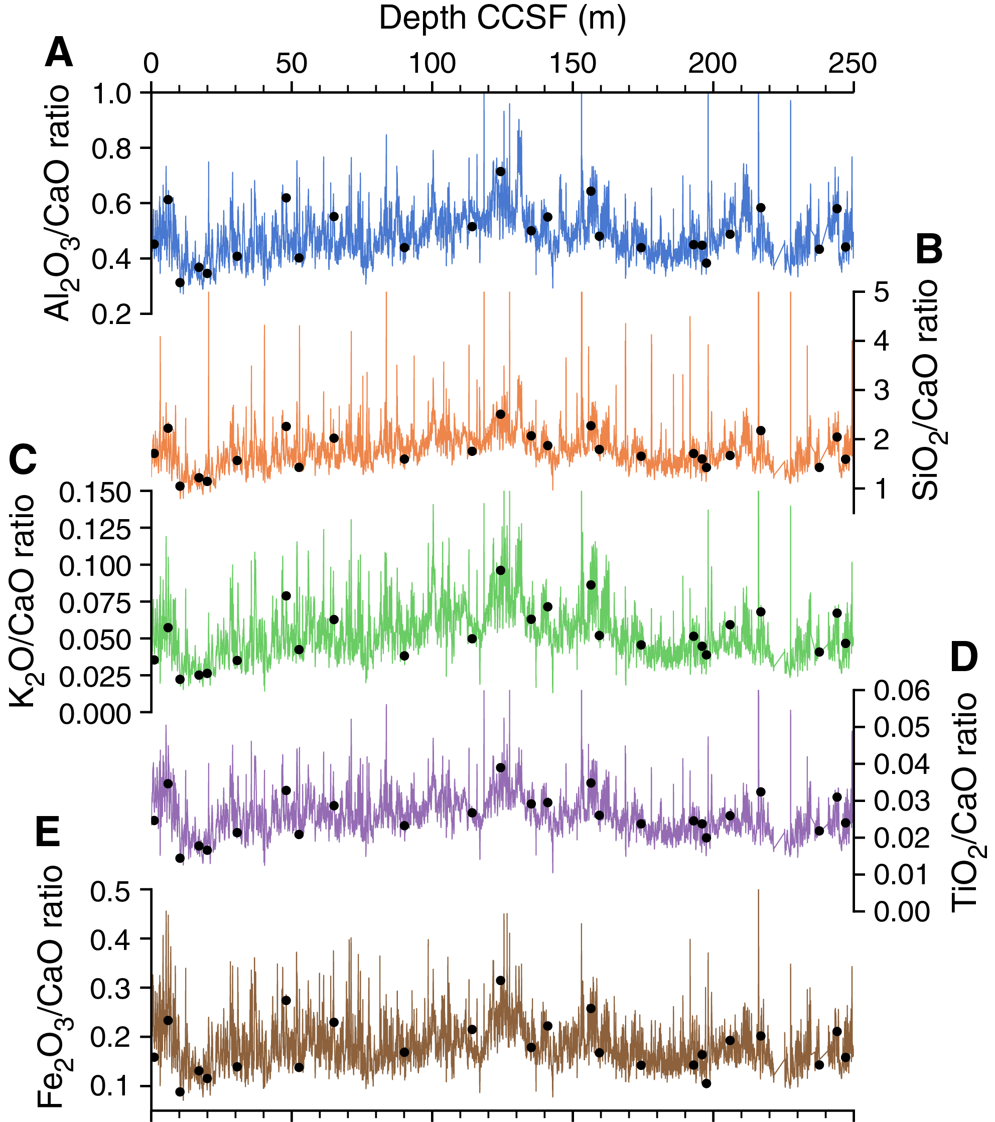
Figure F5. Calibrated XRF data, normalized to CaO, Site U1474.
The ULC is designed to calibrate element ratios, not necessarily individual element concentrations. However, if the elements in the collection of ratios are assumed to compose the entire sample, the relative concentrations of each element can be calculated. To ensure that the resulting concentrations derived from the XRF core scanning data reflect the concentrations of our calibration samples as closely as possible, we normalized the sum of each calibrated XRF measurement to 96.2%, the average sum of Al2O3 + SiO2 + K2O + CaO +TiO2 + Fe2O3 in the 25 calibration samples. This simply reflects the fact that the XRF did not measure Na2O and MgO, which sum to 3.8% on average in the calibration data set.
The results of the calibration are shown by depth in Figures F4 and F5. Figure F4 shows individual element intensities. Figure F5 presents element intensities from both data sets normalized to Ca intensity. Solid circles along each depth series are the concentrations and element ratios from the calibration samples.
Results
Data quality
Figure F2 shows individual element intensities and indicates a few sections with unusually low counts, highlighted by shaded bars (Sections 361-U1474D-4H-1, 8H-3, 11H-4, and 11H-5). We attribute these anomalous measurements to malfunctions with the ITRAX scanner. The sections cannot be rescanned because these anomalous data were not discovered until after the cores were shipped back to Kochi Core Center in Japan. However, counts of individual element intensities are affected by this malfunction, whereas ratios seem less affected (Figures F3, F6). Figure F6 shows, on the left, signal intensity for each major element across a section with a scanning error and low counts (Section 8H-3; section signal colored orange). The right panels show how, when plotted as element ratios, the ratios from the adjacent core sections join together, making the element ratio–depth series continuous. As ratios are the typical application of XRF data, we argue these sections may be used with caution.
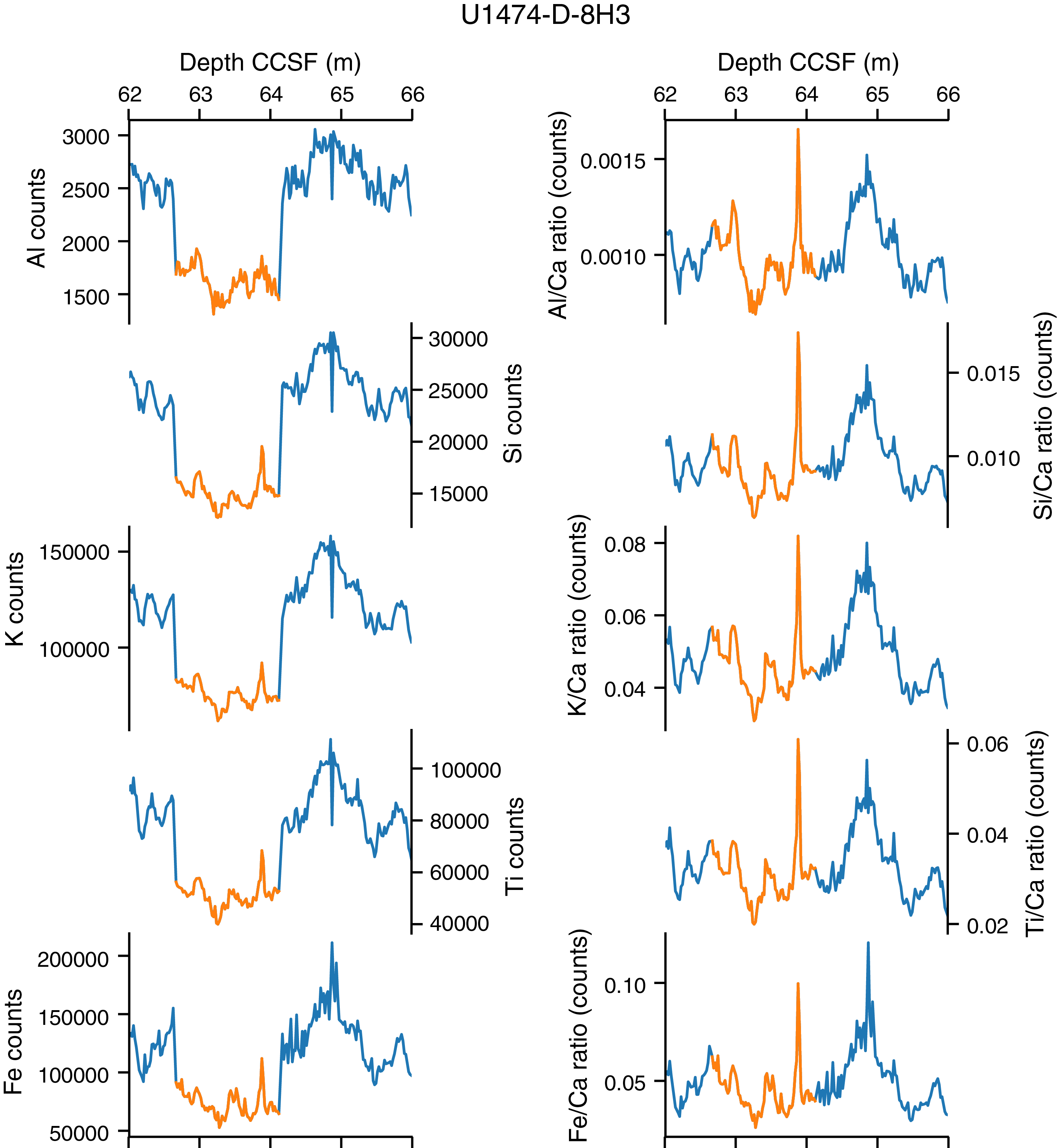
Figure F6. XRF scanner anomalous low counts, Site U1474.
Figure F7 compares the concentrations measured on the calibration samples with the XRF measurements at the appropriate depth and includes the ratios of the raw counts (Figure F7A), the log ratios of the calibration and the XRF counts (Figure F7B), and ratios of the results and the calibrated XRF ratios (Figure F7C). For each element ratio, there is a strong correlation with an intercept at zero, within bootstrapped uncertainty.
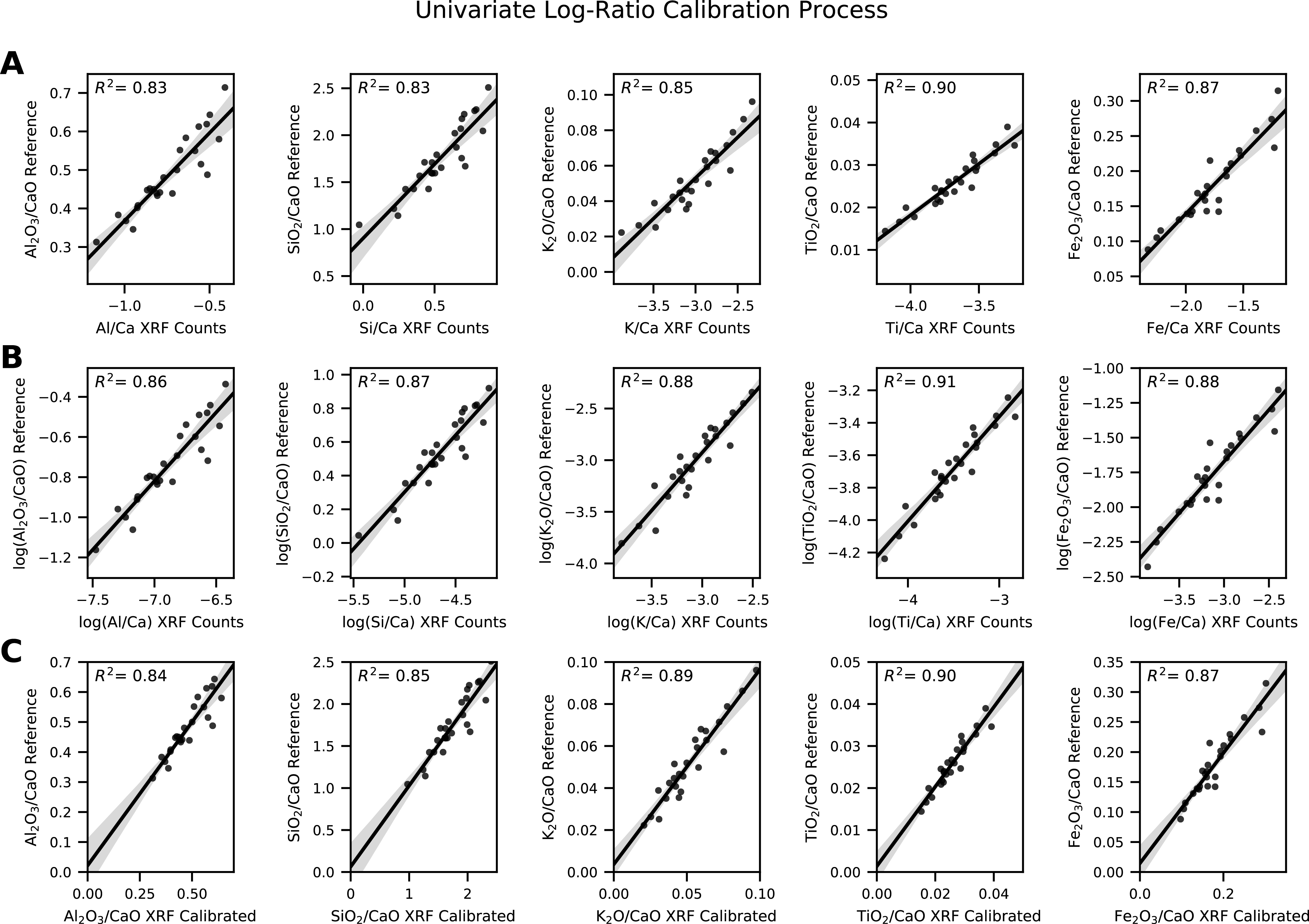
Figure F7. XRF data quality check, Site U1474.
As mentioned previously, the ULC works best for ratios, but individual element concentrations can be derived if the collection of ratios is assumed to compose the entire sample, summed and normalized. Figure F8 shows how effectively our calibration yielded individual element concentrations. Most elements have high quality calibrations with R2 coefficients greater than 0.53 and intercepts at or near zero within bootstrapped uncertainty intervals. Only titanium has a lower R2 coefficient. Titanium counts have a strong relationship with concentrations from the calibration sample; however, the relationship with XRF-derived concentrations is weaker.
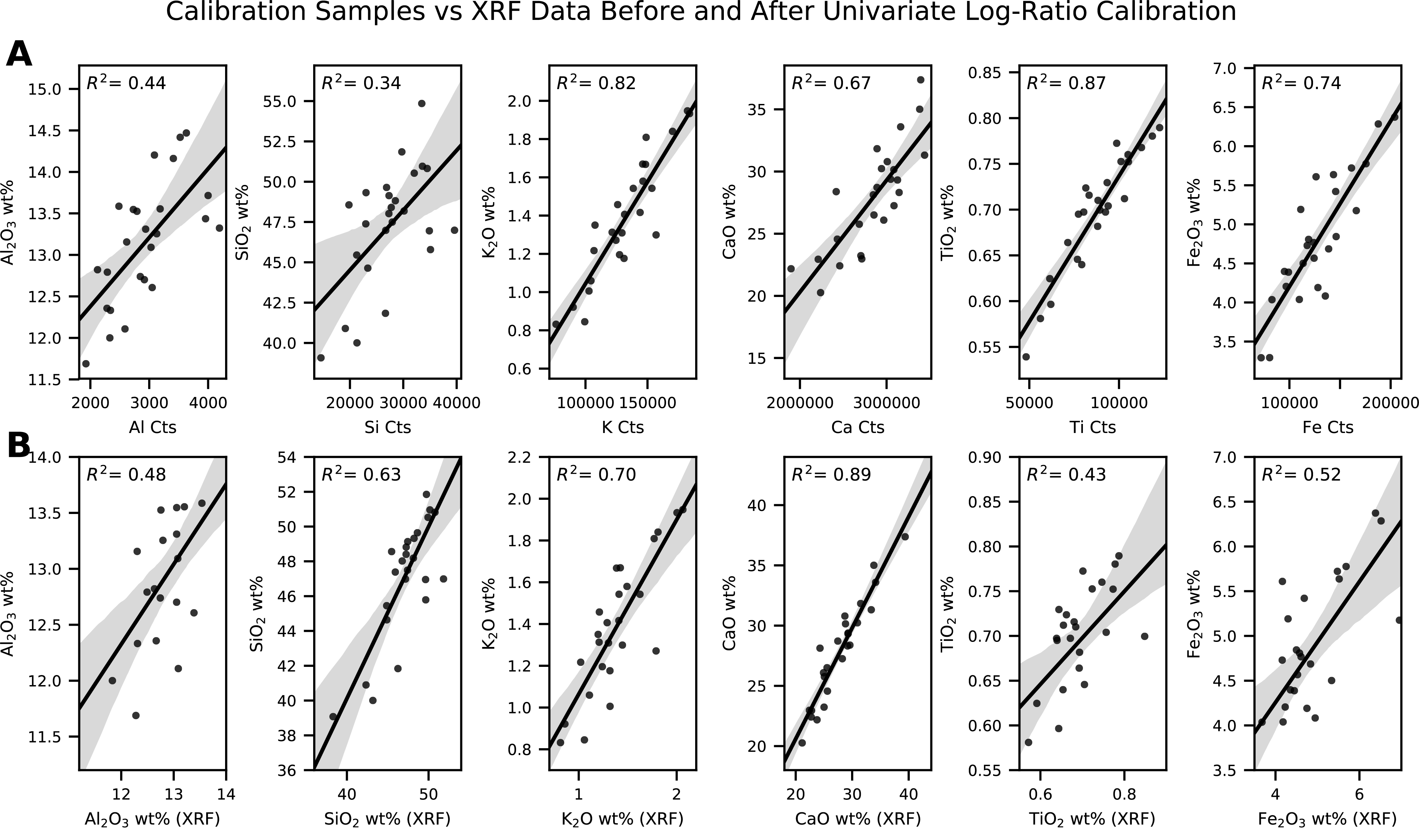
Figure F8. XRF data element comparison to calibration samples, Site U1474.
Description of results
For marine sediment, CaO concentration at Site U1474 is low, ranging from 13 to 41 wt% (Figure F4D). CaO concentration–derived CaCO3 coulometry (Table T3) are plotted alongside the XRF data as open squares (Figure F4D), and the CaO concentration from both methods at identical depths is crossplotted in Figure F9. The results indicate that most of the Ca is borne within CaCO3. By calculating the difference between total CaO and CaCO3-borne CaO for each sample, we estimate an average terrigenous CaO content of approximately 5%. CaO abundance is lowest between 100 and 170 m CCSF. There is a large excursion toward higher CaO deposition between 10 and 20 m CCSF.
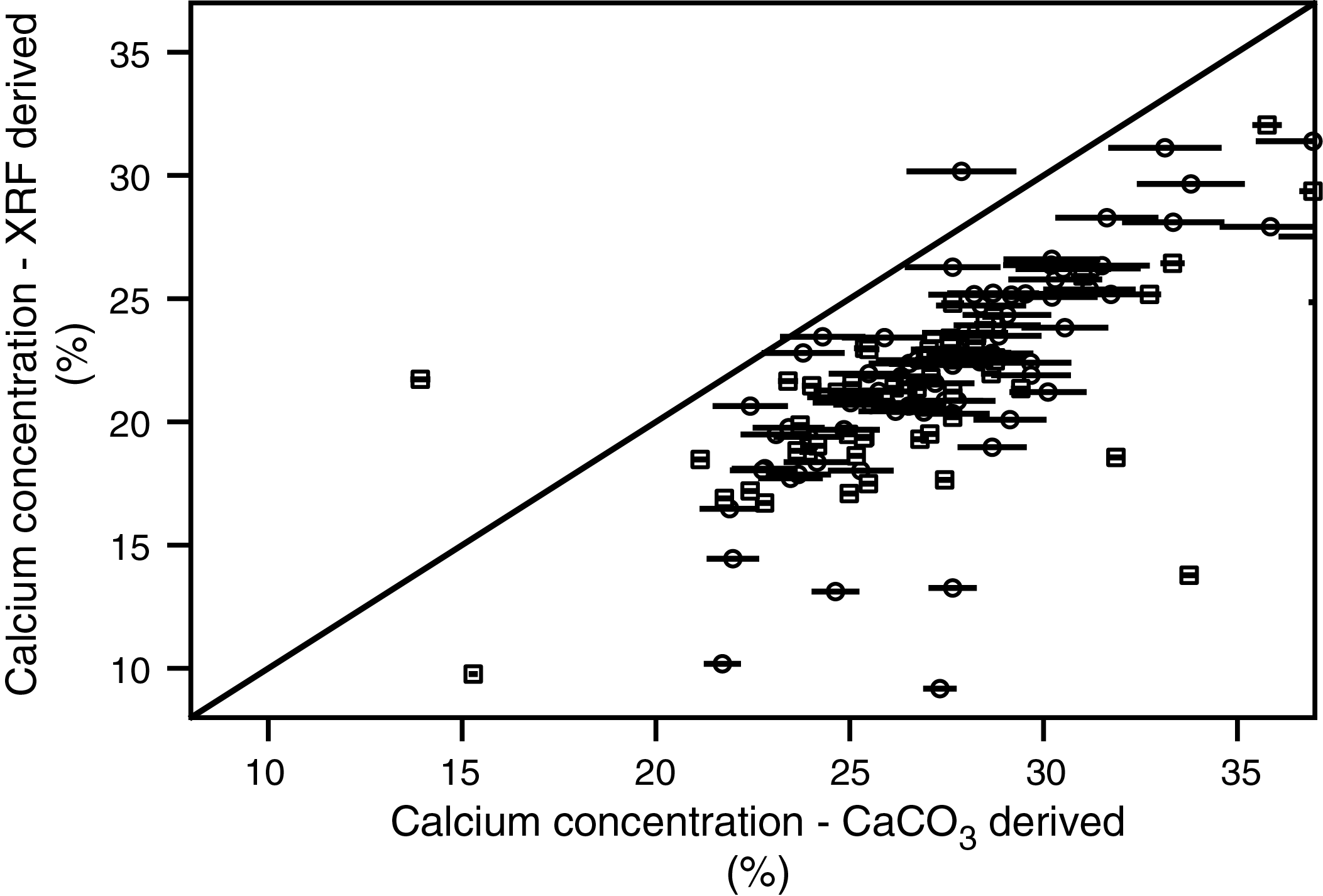
Figure F9. CaO calculation method comparison, Site U1474.
Elements derived from the continental crust, borne in terrigenous phases, vary inversely with Ca content (Figure F4). The element with the greatest variability in the core scan data set is K (Figure F4C), varying by more than a factor of 2 through the core. From 250 to 175 m CCSF, K content is low, about 1.25 wt%, compared to the rest of the record (Figure F4C). From 170 to 100 m CCSF, K content increases to ~1.75 wt%, overprinted by two low-frequency excursions to even higher values. From 100 to 20 m CCSF, K concentration declines gradually to a minimum of ~0.75 wt%. Above this interval, K content increases again. Long-term trends in variability of the other terrigenously derived elements (Al, Si, Ti, and Fe) largely follow the pattern for K described above (Figure F4A, F4B, F4E, F4F). The covariance of the terrigenously derived elements and anticorrelation of calcium carbonate indicate that the main control on the chemical composition of sediment at Site U1474 is the variable input of terrigenous material.
Acknowledgments
This research used samples and/or data provided by the International Ocean Discovery Program (IODP). We thank the International Ocean Discovery Program and the Expedition 361 sailing scientists and staff for the collection of core material. Funding for XRF scanning was provided by IODP. The staff operating the ITRAX core scanner at the Lamont-Doherty Earth Observatory Core Repository, Clara Chang and Nicole Anest, were extremely helpful in the XRF data collection process. We thank individuals from Lamont-Doherty Earth Observatory’s Climate and Life (2016) High School Intern Program: Andrew T. Celli, Elmina David, Ayla K. Markowski, Sonja O'Brien, Taiya Sharif, and Tess N. Strohm, who aided with the long hours of core scanning. We thank an anonymous reviewer for their helpful input.
References
Croudace, I.W., Rindby, A., and Rothwell, R.G., 2006. ITRAX: description and evaluation of a new multi-function X-ray core scanner. Special Publication - Geological Society of London, 267(1):51– 63. https://doi.org/10.1144/GSL.SP.2006.267.01.04
Flanagan, F.J., 1984. Three USGS mafic rock reference samples, W-2, DNC-1, and BIR-1. U.S. Geological Survey Bulletin, 1623. https://pubs.usgs.gov/bul/1623/report.pdf
Franzese, A.M., Hemming, S.R., Goldstein, S.L., and Anderson, R.F., 2006. Reduced Agulhas leakage during the Last Glacial Maximum inferred from an integrated provenance and flux study. Earth and Planetary Science Letters, 250(1–2):72–88. http://dx.doi.org/10.1016/j.epsl.2006.07.002
Franzese, A.M., Hemming, S.R., and Goldstein, S.L., 2009. Strontium isotopes in detrital sediments to constrain the glacial position of the Agulhas retroflection. Paleoceanography, 24(2):PA2217. https://doi.org/10.1029/2008PA001706
Govin, A., Holzwarth, U., Heslop, D., Keeling, L.F., Zabel, M., Mulitza, S., Collins, J.A., and Chiessi, C.M., 2012. Distribution of major elements in Atlantic surface sediments (36°N– 49°S): imprint of terrigenous input and continental weathering. Geochemistry, Geophysics, Geosystems, 13(13):Q01013. https://doi.org/10.1029/2011GC003785
Hall, I.R., Hemming, S.R., LeVay, L.J., Barker, S., Berke, M.A., Brentegani, L., Caley, T., Cartagena-Sierra, A., Charles, C.D., Coenen, J.J., Crespin, J.G., Franzese, A.M., Gruetzner, J., Han, X., Hines, S.K.V., Jimenez Espejo, F.J., Just, J., Koutsodendris, A., Kubota, K., Lathika, N., Norris, R.D., Periera dos Santos, T., Robinson, R., Rolinson, J.M., Simon, M.H., Tangunan, D., van der Lubbe, J.J.L., Yamane, M., and Zhang, H., 2017. Site U1474. In Hall, I.R., Hemming, S.R., LeVay, L.J., and the Expedition 361 Scientists, South African Climates (Agulhas LGM Density Profile). Proceedings of the International Ocean Discovery Program, 361: College Station, TX (International Ocean Discovery Program). https://doi.org/10.14379/iodp.proc.361.103.2017
Imai, N., Terashima, S., Itoh, S., and Ando, A., 1996. 1996 compilation of analytical data on nine GSJ geochemical reference samples, “Sedimentary rock series.” Geostandards Newsletter, 20(2):165–216. https://doi.org/10.1111/j.1751-908X.1996.tb00184.x
Johnson, M.R., Van Vuuren, C.J., Hegenberger, W.F., Key, R., and Shoko, U., 1996. Stratigraphy of the Karoo Supergroup in southern Africa: an overview. Journal of African Earth Sciences, 23(1):3–15. https://www.sciencedirect.com/science/article/pii/S0899536296000486
Kido, Y., Koshikawa, T., and Tada, R., 2006. Rapid and quantitative major element analysis method for wet fine-grained sediments using an XRF microscanner. Marine Geology, 229(3–4):209–225. https://doi.org/10.1016/j.margeo.2006.03.002
Kossoff, D., Hudson-Edwards, K.A., Dubbin, W.E., and Alfredsson, M., 2012. Major and trace metal mobility during weathering of mine tailings: implications for floodplain soils. Applied Geochemistry, 27(3):562–576. https://doi.org/10.1016/j.apgeochem.2011.11.012
Lutjeharms, J.R.E., 2006. The Agulhas Current: Berlin (Springer-Verlag). https://doi.org/10.1007/3-540-37212-1
McLennan, S.M., and Taylor, S.R., 1980. Geochemical standards for sedimentary rocks: trace-element data for U.S.G.S. standards SCo-1, MAG-1 and SGR-1. Chemical Geology, 29(1–4):333–343. https://doi.org/10.1016/0009-2541(80)90029-7
Milliman, J.D., and Meade, R.H., 1983. World-wide delivery of river sediment to the oceans. The Journal of Geology, 91(1):1–21. https://www.jstor.org/stable/30060512
Pretorius, W., Weis, D., Williams, G., Hanano, D., Kieffer, B., and Scoates, J., 2006. Complete trace elemental characterisation of granitoid (USGS G-2, GSP-2) reference materials by high resolution inductively coupled plasma-mass spectrometry. Geostandards and Geoanalytical Research, 30(1):39–54. https://doi.org/10.1111/j.1751-908X.2006.tb00910.x
Ridderinkhof, H., van der Werf, P.M., Ullgren, J.E., van Aken, H.M., van Leeuwen P.J., and de Ruijter, W.P.M., 2010. Seasonal and interannual variability in the Mozambique Channel from moored current observations. Journal of Geophysical Research: Oceans, 115(C6):C06010. https://doi.org/10.1029/2009JC005619
Simon, M.H., Ziegler, M., Bosmans, J., Barker, S., Reason, C.J.C., and Hall, I.R., 2015b. Eastern South African hydroclimate over the past 270,000 years. Scientific Reports, 5:18153. https://doi.org/10.1038/srep18153
Weltje, G.J., 2002. Quantitative analysis of detrital modes: statistically rigorous confidence regions in ternary diagrams and their use in sedimentary petrology. Earth-Science Reviews, 57(3–4):211–253. https://doi.org/10.1016/S0012-8252(01)00076-9
Weltje, G.J., Bloemsma, M.R., Tjallingii, R., Heslop, D., Röhl, U., and Croudace, I.W., 2015. Prediction of geochemical composition from XRF core scanner data: a new multivariate approach including automatic selection of calibration of samples and quantification of uncertainties. In Croudace, I.W., and Rothwell, R.G. (Eds.), Micro-XRF Studies of Sediment Cores. Developments in Paleoenvironmental Research, 17:507–534. https://doi.org/10.1007/978-94-017-9849-5_21
Weltje, G.J., and Tjallingii, R., 2008. Calibration of XRF core scanners for quantitative geochemical logging of sediment cores: theory and application. Earth and Planetary Science Letters, 274(3–4):423–438. https://doi.org/10.1016/j.epsl.2008.07.054
1 Babin, D.P., Franzese, A.M., Hemming, S.R., Hall, I.R., LeVay, L.J., Barker, S., Tejeda, L., Simon, M.H., and the Expedition 361 Scientists, 2020. Data report: X-ray fluorescence core scanning of IODP Site U1474 sediments, Natal Valley, Southwest Indian Ocean, Expedition 361. In Hall, I.R., Hemming, S.R., LeVay, L.J., and the Expedition 361 Scientists, South African Climates (Agulhas LGM Density Profile). Proceedings of the International Ocean Discovery Program, 361: College Station, TX (International Ocean Discovery Program). https://doi.org/10.14379/iodp.proc.361.201.2020
2 Lamont Doherty Earth Observatory, Geochemistry Division, Columbia University, USA. Correspondence author: daniel.p.babin@gmail.com
3 Department of Earth and Environmental Sciences, Lamont-Doherty Earth Observatory, Columbia University, USA.
4 Natural Sciences Department, Hostos Community College, USA.
5 School of Earth and Ocean Sciences, Cardiff University, United Kingdom.
6 International Ocean Discovery Program, Texas A&M University, USA.
7 Norwegian Research Centre (NORCE), Bjerknes Centre for Climate Research, Norway.
8 SFF Centre for Early Sapiens Behaviour (SapienCE), University of Bergen, Norway.
9 Expedition 361 Scientists’ affiliations.
This work is distributed under the Creative Commons Attribution 4.0 International (CC BY 4.0) license. 