McNeill, L.C., Dugan, B., Petronotis, K.E., and the Expedition 362 Scientists
Proceedings of the International Ocean Discovery Program Volume 362
publications.iodp.org
https://doi.org/10.14379/iodp.proc.362.103.2017

Site U14801
L.C. McNeill, B. Dugan, K.E. Petronotis, J. Backman, S. Bourlange, F. Chemale, W. Chen, T.A. Colson, M.C.G. Frederik, G. Guèrin, M. Hamahashi, T. Henstock, B.M. House, A. Hüpers, T.N. Jeppson, S. Kachovich, A.R. Kenigsberg, M. Kuranaga, S. Kutterolf, K.L. Milliken, F.L. Mitchison, H. Mukoyoshi, N. Nair, S. Owari, K.T. Pickering, H.F.A. Pouderoux, S. Yehua, I. Song, M.E. Torres, P. Vannucchi, P.J. Vrolijk, T. Yang, and X. Zhao2
Keywords: International Ocean Discovery Program, IODP, JOIDES Resolution, Expedition 362, Site U1480, Sumatra, Sumatra subduction zone, Sunda subduction zone, Andaman-Nicobar Islands, Wharton Basin, Indo-Australian plate, Bengal Fan, Nicobar Fan, Himalaya, Ninetyeast Ridge, Sumatra-Andaman 2004 earthquake, shallow seismogenic slip, décollement, megathrust, tsunami, forearc, Neogene, late Miocene, Late Cretaceous, subduction input sediment, diagenesis, sediment gravity flow, pelagic, oceanic crust, volcanic ash, mud, clay, silt, sand, siliciclastic, calcareous ooze, chalk
MS 362-103: Published 6 October 2017
Background and objectives
Site U1480 (proposed Site SUMA-11C) is located on the Indian oceanic plate, east of the Ninetyeast Ridge and west of the North Sumatran subduction margin (Figure F1; see also Figure F4 in the Expedition 362 summary chapter [McNeill et al., 2017c]). The primary drilling objective at Site U1480 was
- To recover a complete section of the oceanic-plate sedimentary section and the uppermost basaltic basement.
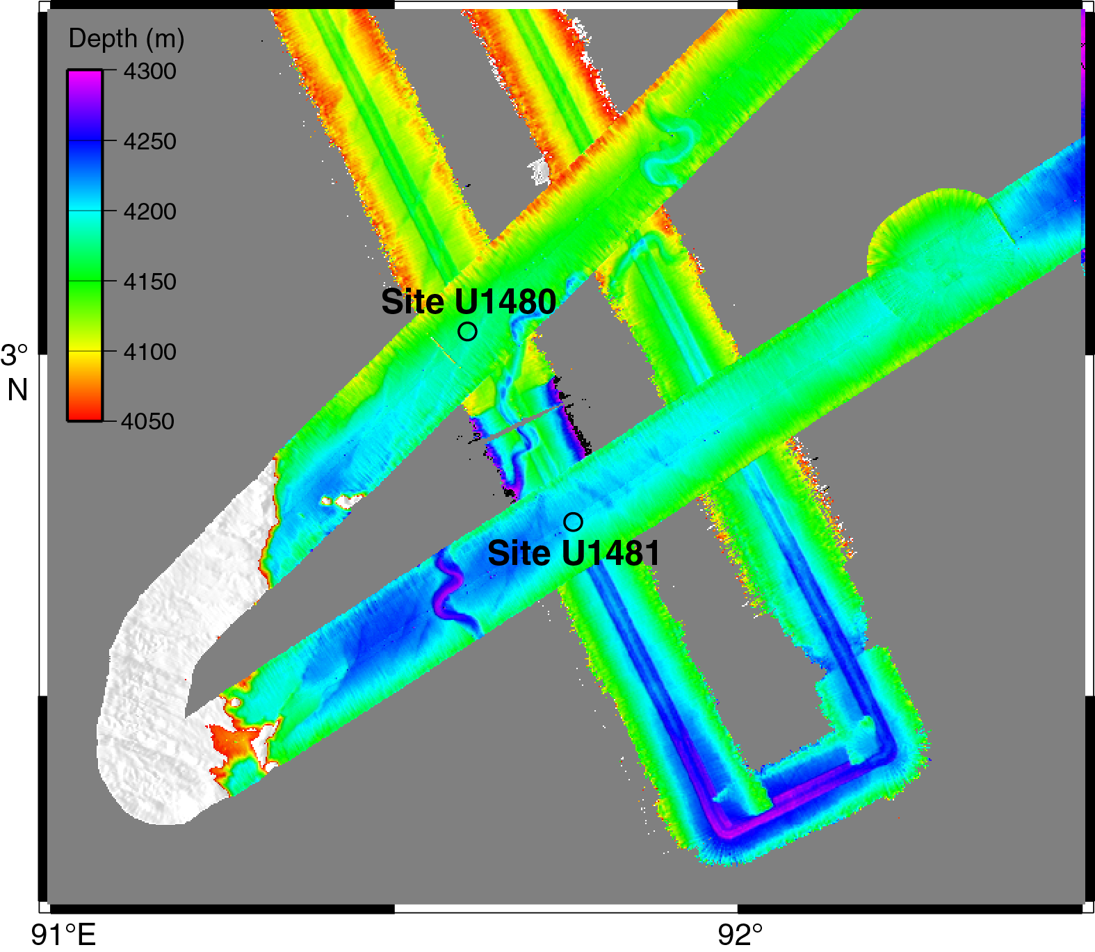
Figure F1. Bathymetric map.
Moving toward the trench, this section is overlain by the rapidly deposited trench wedge, and eventually this section is subducted at the margin offshore North Sumatra (see Figure F6 in the Expedition 362 summary chapter [McNeill et al., 2017c]). The sedimentary section is 4–5 km thick at the subduction deformation front. Based on preexpedition seismic interpretation, the sedimentary section at Site U1480 (Figure F2) includes, from top to bottom,
- A thin sediment section of the distal onlapping element of the trench wedge which overlies an angular unconformity (seismic Horizon A);
- The Nicobar Fan sequence, which includes a reflective section and an underlying nonreflective section separated by seismic Horizon B (the section below Horizon B was interpreted preexpedition as pelagic); and
- The pelagic prefan sequence extending from seismic Horizon C to oceanic basement (seismic Horizon D).
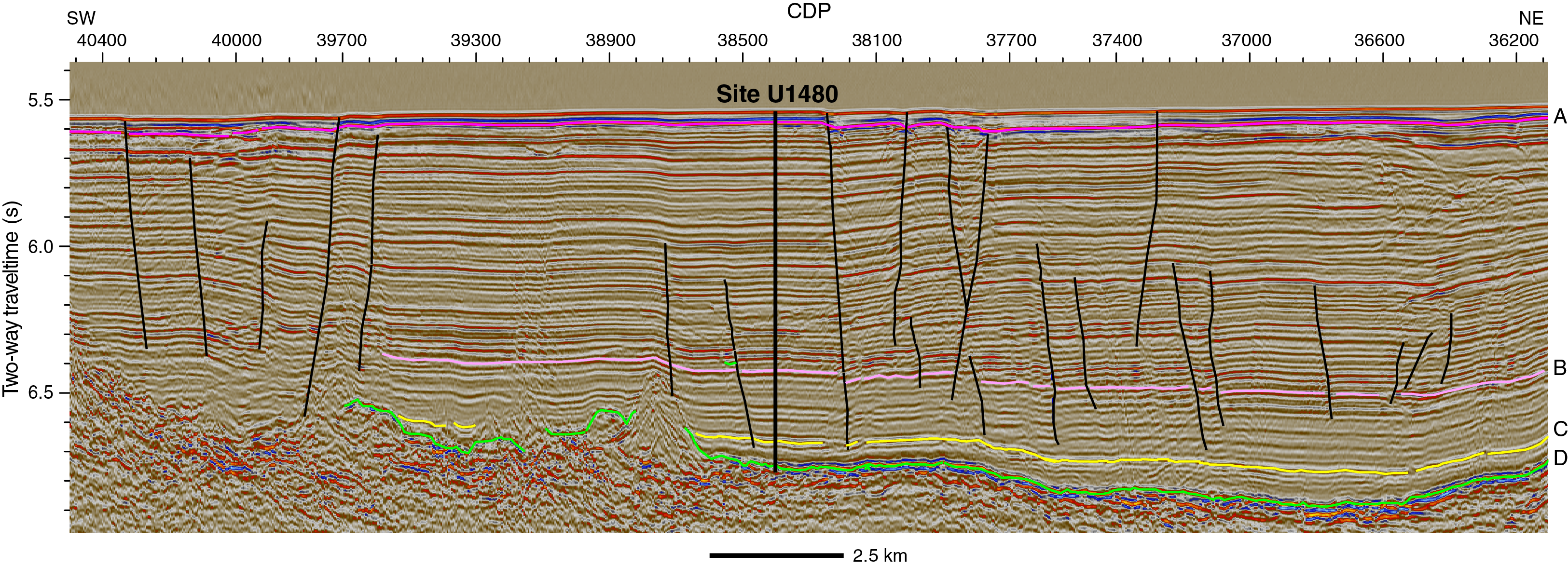
Figure F2. Seismic reflection Profile BGR06-102.
The prominent seismic Horizon C is one of the potential candidates for décollement development (Dean et al., 2010). This site was targeted for drilling because it provides constraints on the initial physical, chemical, thermal, and mechanical properties and potentially the state of stress of the lower part of the input section where the plate boundary décollement develops and allows us to understand the material that may contribute to the formation of the unusual, wide forearc plateau. Because the section thickens significantly on approaching the subduction zone (see Figure F6 in the Expedition 362 summary chapter [McNeill et al., 2017c]), postexpedition experiments and numerical modeling will evaluate the impact of increasing burial, temperature, and diagenetic alteration. Site U1480 will therefore allow us to address the three primary objectives (see Scientific objectives in the Expedition 362 summary chapter [McNeill et al., 2017c]) to determine how the properties of the input section may lead to shallow seismogenic slip and unusual forearc/prism development. Site U1480 also offers the opportunity to obtain a complete section of the Nicobar Fan sequence at 3°N where the onset of fan deposition was expected to be ~30–40 Ma based on a simple fan progradational model but with limited borehole data. The Nicobar Fan is separated from the Bengal Fan by the Ninetyeast Ridge, and understanding its onset and growth is important for a complete sedimentary history of fan deposition related to Himalayan uplift, erosion, and monsoon development.
Specific objectives for this site include the following:
- To identify the principal lithologies that may be involved in development of the broad prism and the plate boundary fault;
- To establish how the mechanical/strength properties of the different lithologies change with depth to determine the trends and effects of burial rate and burial time;
- To identify potential discontinuities that may be candidates for décollement positions;
- To identify any thermal history indicators and any effects of early diagenesis and to establish the present-day thermal structure of the section;
- To identify fluid sources and changes with depth; and
- To determine the primary sources of sediment delivered to the site (in particular sediment above seismic Horizon C) and changes in source with time. Potential sources include the Himalaya and Ganges Brahmaputra floodplain through the Bengal Fan system, the Indo-Burman range and Irrawaddy River, the Sunda forearc, the Sumatran mainland (including volcanic arc), and the Ninetyeast Ridge.
Site U1480 is located at 3°2.04ʹN, 91°36.35ʹE in a water depth of 4148 m. The operational goals at this site were to core the entire sedimentary section and reach the sediment/basement interface and to log the section. Holes U1480A–U1480D missed the mudline and were not studied extensively. Hole U1480E was cored to 99.7 m below seafloor (mbsf) but was terminated short of its target depth (Figure F3B). Hole U1480F penetrated to 815 mbsf. Hole U1480G had a reentry system installed to 754 mbsf, followed by coring to 1431.6 mbsf, which is ~17 m into igneous basement. Hole U1480H penetrated to 129.4 mbsf and was an additional shallow hole for biostratigraphy, paleomagnetism, geochemistry, and microbiology studies. Limited logging was conducted in Hole U1480G. Formation temperature measurements were taken in Holes U1480E, U1480F, and U1480H.
Operations
Transit to Site U1480
The R/V JOIDES Resolution left Colombo, Sri Lanka, at 1018 h on 9 August 2016. The 842 nmi transit to Site U1480 was completed in 65.8 h at an average speed of 12.8 kt. After arriving at Site U1480 at 0615 h on 12 August (ship local time; UTC + 7 h), the thrusters and hydrophones were lowered, an acoustic seafloor positioning beacon was deployed, and the dynamic positioning system was engaged.
Site U1480
The Site U1480 coring summary is shown in Table T1. The Site U1480 hole locations and details of operations and depths at each hole are shown in Figure F3.
Table T1. Site U1480 core summary. Download table in .csv format. View PDF table.
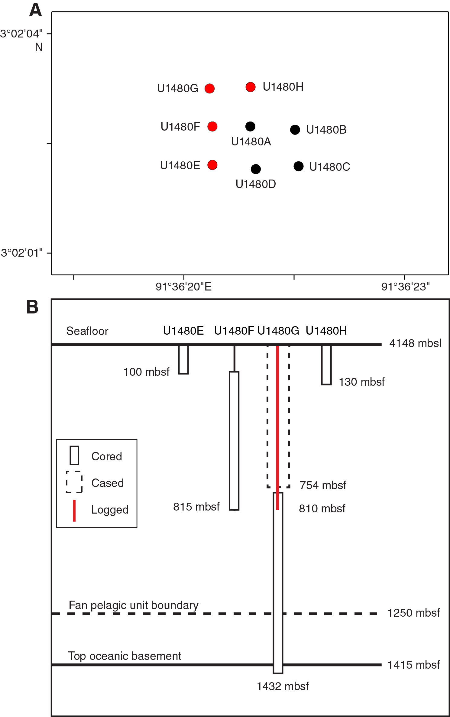
Figure F3. Location of Holes U1480A–U1480H and details of operations for Holes U1480E–U1480H.
Holes U1480A–U1480D
An advanced piston corer (APC)/extended core barrel (XCB) bottom-hole assembly (BHA) was assembled and run to 4120 m below rig floor (mbrf; see Introduction in the Expedition 362 methods chapter [McNeill et al., 2017b] for depth scale definitions). All drill string joints were measured during the pipe trip. After the top drive was picked up and spaced out, a wiper pig was pumped through the drill string to clean any rust or debris from the inside of the drill string. The calculated precision depth recorder depth for the site was 4161.4 mbrf (4150.2 m below sea level [mbsl]). The drill string was spaced out to 4157 mbrf, the sinker bars were picked up and inserted through the main blocks, and the Icefield MI-5 core orientation tool was installed.
Hole U1480A was spudded at 0050 h on 13 August 2016. The core barrel was retrieved, and it was evident that we had overpenetrated the seafloor. The pipe count was checked to make sure that our depth was correct. Hole U1480A was terminated, the vessel was moved 20 m east of Hole U1480A, and the drill string was raised 9 m to 4148 mbrf. Hole U1480B was spudded at 0235 h. The recovery of the mudline again eluded us. The pipe count was checked again to make sure that our depth was correct. Hole U1480B was terminated, the vessel was moved 20 m south of Hole U1480B, and the drill string was raised an additional 7 m to 4141 mbrf. Hole U1480C was spudded at 0400 h. For the third time, there was no mudline. Hole U1480C was terminated, the vessel was moved 20 m west of Hole U1480C, and the drill string was raised an additional 4 m to 4137 mbrf. Hole U1480D was spudded at 0535 h. After pulling the fourth full core barrel without recovering the mudline, the drillers found a calculation error in their pipe tally that caused all depth measurements to be ~28 m shallower than anticipated. The total time spent on Holes U1480A–U1480D was 24 h.
Hole U1480E
Following the correction of the pipe tally and depth calculation, the drill string was repositioned at 4157 mbrf, and Hole U1480E was spudded at 0710 h on 13 August. Core 362-U1480E-1H recovered 7.76 m of sediment, and the seafloor was calculated to be at 4158.7 mbrf (4147.5 mbsl). Nonmagnetic core barrels were used for all cores. Orientation with the Icefield MI-5 core orientation tool began with Core 1H, but the orientation tool was pulled after Core 8H because of sandy layers. APC coring continued through Core 12H, and advanced piston corer temperature tool (APCT-3) temperature measurements were taken with Cores 6H, 8H, and 12H. Of the 99.7 m cored, 97.6 m was recovered (98%). Coring was suspended after Core 12H so that the temperature dual-pressure tool (T2P) could be deployed.
The T2P tool was rigged up with the Motion Decoupled Hydraulic Delivery System (MDHDS) and Electronic Release System (ERS) (Flemings et al., 2013) and was run to the bottom of the drill string on the Schlumberger wireline. After the MDHDS was released using the ERS, the drill string was pressured up to ~1200 psi to shear the shear pins and, after holding pressure for ~1 min, the pressure was released to allow the MDHDS to release the T2P tool. The drill string was pressured up again to pump the T2P into the formation. After waiting for 30 min for the measurement to be completed, we attempted to reconnect the ERS to the MDHDS tool but were unable to engage the MDHDS tool even though the ERS appeared to be functioning normally. The wireline was pulled back to the surface, and the coring line was rigged up to fish for the MDHDS tool. Following three unsuccessful attempts to engage the MDHDS with the coring line, the drill string was pulled clear of the seafloor. Finally, a fishing spear was rigged up to attempt to catch the outer core barrel and was successful on the second attempt. Once the MDHDS and T2P tools were brought to the surface, it was evident that the T2P tool had sustained considerable damage. After clearing the seafloor, the vessel moved 20 m north of Hole U1480E to Hole U1480F. The total time spent on Hole U1480E was 33.6 h, or 1.4 days.
Hole U1480F
Hole U1480F was spudded at 1910 h on 14 August and was drilled down without coring to 98.0 mbsf. A seafloor depth of 4147.5 mbsl was assigned to Hole U1480F based on Hole U1480E. Piston coring began with Core 362-U1480F-2H and continued through Core 8H (146.5 mbsf). Because all attempts at full-length piston coring were partial strokes, coring continued with the half-length APC (HLAPC) system from Core 9F through 29F (245.2 mbsf). APCT-3 temperature measurements were taken with Cores 4H, 6H, 13F, and 22F. All HLAPC cores were also partial strokes, and a new strategy was employed: we began alternating 5 m drilled intervals with 5 m HLAPC cores to save time while still complying with the safety guideline of taking headspace gas measurements every ~10 m. Cores 31F through 51F advanced from 250.2 to 357.7 mbsf. Within that interval, the nature of the formation required the recovery of XCB Cores 34X, 35X, and 37X. Continuous XCB coring started from Core 52X through 98X to a final hole depth of 815.0 mbsf. Of the 672.0 m cored, 249.4 m was recovered (37%). After reaching the total depth planned for this hole, the drill string was pulled out of the hole, clearing the rig floor at 0740 h on 21 August, and the vessel was moved 20 m north of Hole U1480F to Hole U1480G. The total time spent on Hole U1480F was 160 h, or 6.7 days.
Hole U1480G
The target depth in Hole U1480G was ocean crust basement, which was estimated to be at 1450 mbsf. To achieve this goal we had to install a reentry system (Figure F4) and reenter the hole, which took ~4.5 days. This involved the following steps:
- A 755.9 m long casing string was assembled out of 64 joints of 10¾ inch casing and suspended from the mud skirt.
- A drilling assembly was made up with a 9⅞ inch tricone bit, an underreamer, and a mud motor; the mud motor and underreamer were tested in the moonpool.
- Approximately 687 m of 5 inch drill pipe was assembled above the drilling assembly and connected to the Hydraulic Release Tool (HRT).
- The drilling assembly and pipe were lowered into the casing until the HRT running tool was bolted onto the casing hanger.
- After the mud skirt, casing string, and drilling stinger were lowered to ~150 mbrf, a free-fall funnel (FFF) was assembled in the moonpool and allowed to drop onto the reentry system. The subsea camera was deployed so that we could verify that the FFF had landed correctly. Initially, the FFF was found to be slightly askew, but the vertical movement of the drill string through the water column caused it to slide into place.
- The 10¾ inch casing string was lowered toward the seafloor and the subsea camera was deployed to observe the drilling operation.
- Hole U1480G was spudded at 0105 h on 23 August. Approximately 9 h into the operation, the mud skirt came unlatched and descended down the casing to the seafloor. Drilling continued until the reentry system landed on the seafloor at 1330 h on 24 August. The depth of the hole was calculated at 759.6 mbsf.
- The HRT was released from the casing at 1400 h, the subsea camera was recovered, the drill string was pulled back to the surface, and the mud motor and underreamer were flushed with freshwater and stored.
- The drill string was lowered to the seafloor with a rotary core barrel (RCB) BHA.
- The subsea camera was deployed to observe the reentry operations and Hole U1480G was reentered at 2005 h on 25 August.
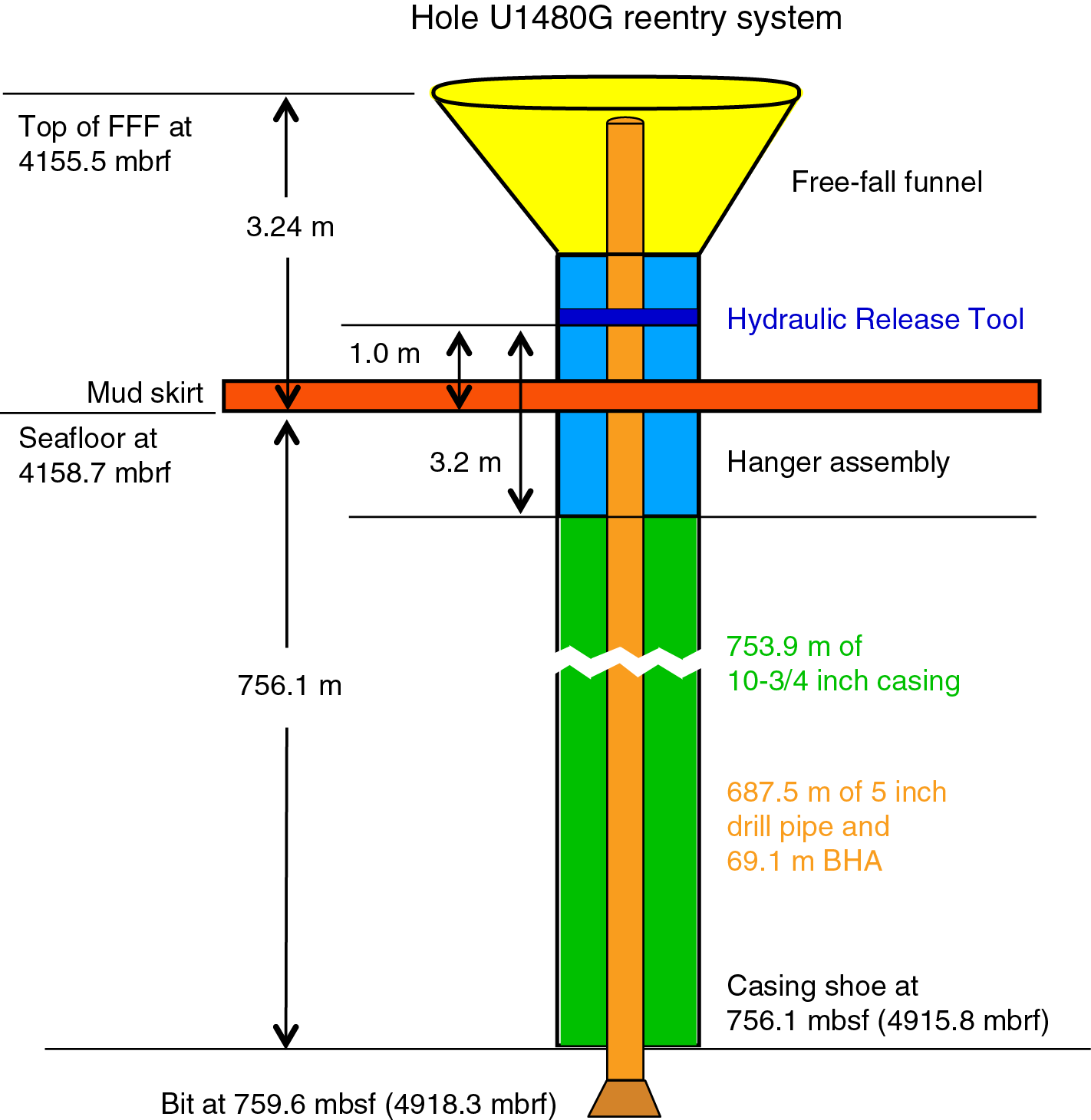
Figure F4. Site U1480 reentry system.
When the drill string reached 573.3 mbsf, it encountered fill that had to be removed from the casing before coring could resume. Coring began at 0700 h on 26 August with Core 362-U1480G-2R from 759.6 mbsf and continued through Core 73R to a final hole depth of 1431.6 mbsf. Of the 672.0 m cored, 329.2 m was recovered (49%). Nonmagnetic core barrels were used for all cores. Coring was halted at 0930 h on 4 September when penetration and high torque indicated a possible bit failure after 77 operating hours, which was confirmed by the tapered end of the last core.
In preparation for logging, a 40 bbl mud sweep was pumped to condition the hole and the drill bit was released at the bottom of the hole. The end of the drill string was raised to 1249.3 mbsf and the hole was displaced with 300 bbl of heavy (11.0 lb/gal) mud. The drill string was pulled out of the hole but encountered significant drag at 1025.3 mbsf. After working the drill string with 150,000 lb overpull, the top drive was engaged and the vessel was offset 210 m to give the driller room to work with the top drive. As the vessel was repositioned over the hole, the top drive was slowly picked up to ~10 m above the rig floor. After spending 4 h trying to free the drill string with 150,000 lb of overpull and 1700 psi of standpipe pressure, the drill pipe came free at 0155 h on 5 September. We resumed pulling the drill string out of the hole until it reached 63.3 mbsf, the depth set for logging.
The rig floor was prepared for logging, and an abbreviated tool string was assembled with the Hostile Environment Natural Gamma Ray Sonde (HNGS) and High-Resolution Laterolog Array (HRLA) tools. During the first pass, the tool string encountered an obstruction at 4967.6 mbrf (809.3 mbsf) and was unable to descend any further. A repeat pass was conducted from this depth upward for ~70 m, and the tools were lowered a second time, again coming to rest on a firm obstruction at the same depth. Because the HRLA resistivity data were spikey during the repeat pass, the presurvey calibration was repeated in the open-hole section prior to starting the main upward pass. Once the main pass was completed from 4967.6 to 4140 mbrf (809.3 mbsf to ~18 m above seafloor), the tools were pulled to the surface and rigged down. Logging activities were completed at 1730 h on 5 September. The drill string was pulled out of the hole and cleared the rig floor at 0510 h. The vessel moved 20 m east of Hole U1480G to Hole U1480H. The total time spent on Hole U1480G was 381.5 h, or 15.9 days.
Hole U1480H
An APC/XCB BHA was made up and the drill string was lowered to the seafloor. Hole U1480H was spudded at 1545 h on 6 September. APC coring continued through Core 362-U1480H-17H to 129.4 mbsf. Of the 124.4 m cored, 116.0 m was recovered (93%). Nonmagnetic core barrels were used, the cores were oriented with the FlexIT core orientation tool, and APCT-3 formation temperature measurements were taken with Cores 4H, 7H, 10H, 12H, and 17H. The drill string was pulled out of the hole, clearing the rig floor at 2359 h. A subbottom profile survey was conducted with the 3.5 kHz sonar array while the drill string was being pulled to the surface. The rig floor was secured, the acoustic positioning beacon was recovered, and the thrusters and hydrophones were secured for the transit to Site U1481. The total time spent in Hole U1480H was 45 h, or 1.9 days. Site U1480 activities concluded at 0212 h on 8 September. The total time spent at Site U1480 was 644 h or 26.8 days.
Sedimentology and petrology
Sediment and sedimentary rock were recovered from the seafloor to 1415.35 mbsf in eight holes (U1480A–U1480H) (Figure F5). Overall, the succession at Site U1480 consists of mainly siliciclastic sediment interpreted as Nicobar Fan underlain by mixed tuffaceous and pelagic sediment and intervals of intercalated pelagic and igneous material overlying oceanic crust. In the lowermost and oldest sedimentary intervals, near acoustic basement (see Core-log-seismic integration), sediment is interbedded with extrusive and intrusive igneous material (Sections 362-U1480G-62R-1, 0 cm, through 71R-4, 5 cm; 1327.4–1415.35 mbsf). The sediment section encompasses the Late Cretaceous to Recent (see Biostratigraphy) deep-marine sedimentary cover on the ocean floor between the Ninetyeast Ridge and the Sumatra (Sunda) subduction zone. A thin interval (from 1415.35 to deeper than 1431.63 mbsf) of basic volcanic rock was recovered from the igneous basement. Core recovery was 52%, including basement, and distributed as 94% for APC coring, 18% for XCB coring, and 49% for RCB coring.
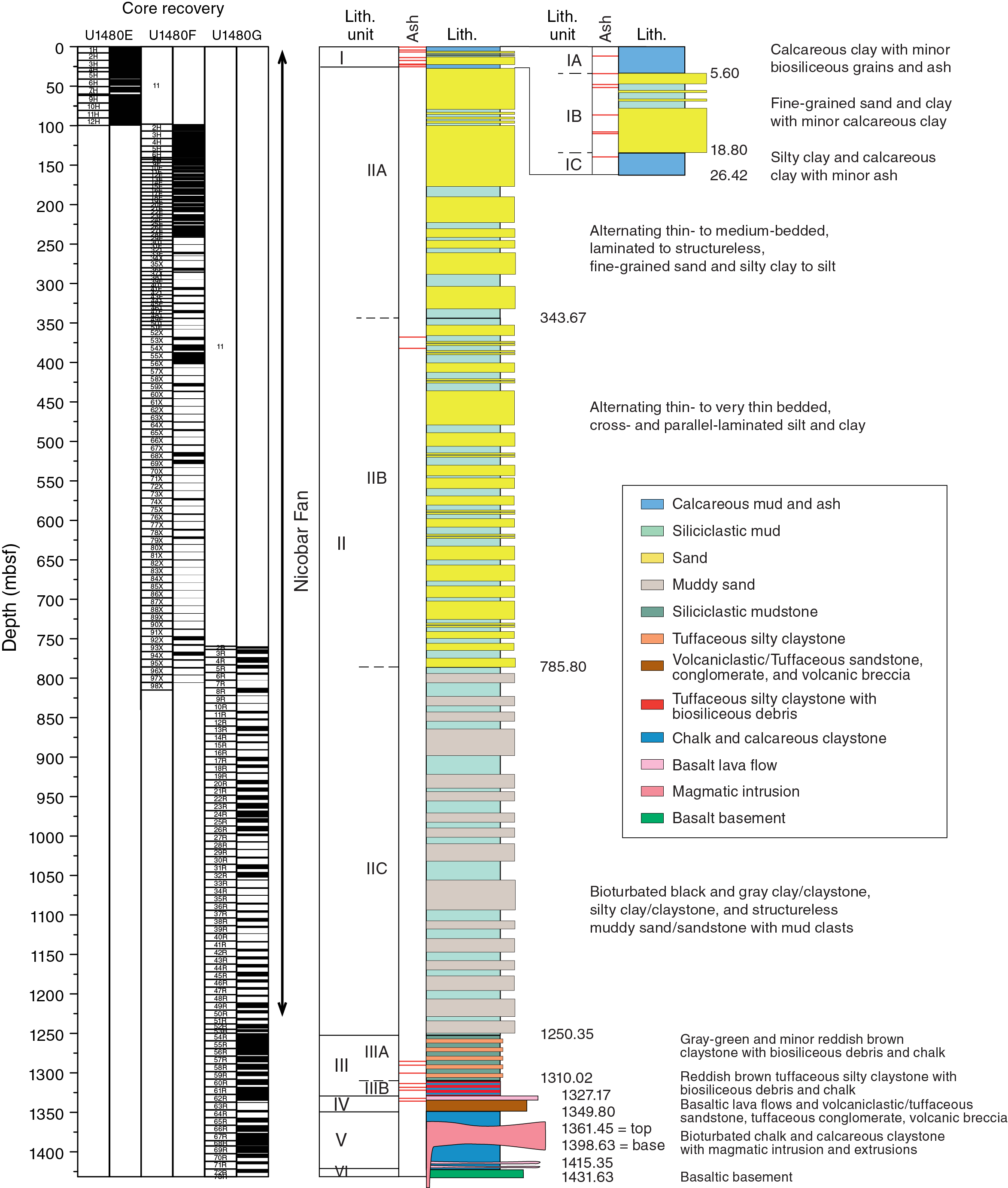
Figure F5. Schematic summary of lithostratigraphic units defined in Holes U1480E–U1480G.
The succession was divided on the basis of lithologic attributes. Lithostratigraphic definitions for Site U1480 were based exclusively on cores recovered from Holes U1480E–U1480G. Holes U1480A–U1480D missed the mudline, and resampled stratigraphy was recovered in Cores 362-U1480E-1H through 4H. Hole U1480H was drilled to better constrain the interstitial water chemistry, biostratigraphy, and paleomagnetism in the upper 120 m. Sediment was classified based on both texture and composition of the grain assemblage as explained in Sedimentology and petrology in the Expedition 362 methods chapter (McNeill et al., 2017b). Sediment containing ≥50% siliciclastic components is classified by texture (sand-silt-clay ratio) alone with the exception of sediment containing >5% ash or carbonate allochems. Where appropriate and practical in discussion of lithologic data, the term “mud” or “mudstone” is used to refer collectively to sediment textural classes having ≥50% grains of silt size or less (<62.5 μm). Similarly, “muddy sand” (or “sandstone”) refers to sandy sediment containing ≥25% silt + clay.
The sediment at Site U1480 is mostly unlithified. However, in the intervals near basement, semilithified and lithified materials were encountered. Materials that are lithified by the criteria listed in Sedimentology and petrology in the Expedition 362 methods chapter (McNeill et al., 2017b) are referred to as “stone” or, in the case of lithified calcareous oozes, as “chalk.”
Six major lithostratigraphic units were identified (Units I–VI), with some units divided into subunits designated by letters (e.g., A–C) (Figure F5).
Unit I consists of Subunits IA–IC. Subunit IA (0–5.60 mbsf) is dominated by calcareous clay with minor biosiliceous components and ash. Subunit IB (5.60–18.80 mbsf) is characterized by fine-grained sand and clay, with minor calcareous clay. Subunit IC (18.80–26.42 mbsf) contains silty clay and calcareous clay with minor ash.
Unit II consists of Subunits IIA–IIC. Subunit IIA (26.42–343.67 mbsf) is composed of interbedded thin- to medium-bedded, laminated to structureless, fine-grained sand with silty clay and silt. Subunit IIB (343.67–785.80 mbsf) contains alternating thin- to very thin bedded, cross- and parallel-laminated silt and clay. Subunit IIC (785.80–1250.35 mbsf) is bioturbated black and dark gray clay/claystone and silty clay/claystone and structureless muddy sand/sandstone with plant material and mud clasts. Within Subunit IIC, sediment is mostly unlithified, but local lithified material was encountered (carbonate-cemented sandstone and mudstone). The base of Unit II and top of Unit III marks a transition to sediment that is essentially lithified and, therefore, classified as “-stone.”
Unit III is divided into an upper Subunit IIIA containing gray-green and minor reddish brown claystone (1250.35–1310.10 mbsf) with agglutinated foraminifers and a lower Subunit IIIB (1310.10–1327.18 mbsf) dominated by reddish brown tuffaceous silty claystone with biosiliceous debris and minor chalk.
Unit IV (1327.18–1349.80 mbsf) is composed of basaltic lava flows, volcanic breccia, and tuffaceous and volcaniclastic sandstone. Lithification in this unit reflects the presence of substantial cementation by zeolite and carbonate.
Unit V (1349.80–1415.35 mbsf) is defined on the basis of the appearance of calcareous claystone and chalk, intruded by diorite. The degree of lithification is similar to that in Subunit IIIA.
Unit VI (1415.35–1431.63) is basaltic basement represented by moderately altered plagioclase-pyroxene–bearing basalt that displays intersertal texture.
The silt and sand of the Nicobar Fan succession (Units I and II) is quartzofeldspathic. Based on the ratio of detrital quartz (q) and feldspar (f) in X-ray diffraction (XRD) analysis (f/(q + f) = 0.38) and visual estimates of the lithic grain content (~5%–10% pelitic metamorphic lithic grains), these sediments are termed arkose to lithic arkose by the classification of Folk (1980). The pelitic lithic grain assemblage includes a variety of mica slate and quartz-mica slate, phyllite, and schist. The sand is prominently micaceous with an abundance of biotite in addition to chlorite and muscovite. The heavy mineral assemblage is diverse and dominated by green amphibole and pyroxene. Other heavy minerals include garnet, kyanite, staurolite, apatite, zircon, and rutile. In the tuffaceous and pelagic sediment beneath the fan (Units III–V), quartz content is much reduced relative to feldspar and sandstone. The associated conglomerate has a grain composition in the volcanic-arenite field (Folk, 1980).
Bulk mineralogic determination by XRD (see Sedimentology and petrology in the Expedition 362 methods chapter [McNeill et al., 2017b]) can be correlated to the broad textural and compositional categories of sediment recognized in smear slides and in macroscopic core description (Figure F6; Table T2; see also XRD in SEDIMENT in Supplementary material for full XRD data tables). Sediments containing ≥75 wt% siliciclastic clay-size (i.e., <25% silt) material generally have clay-mineral contents from 60 to 80 wt% and quartz contents from 5 to 20 wt% (Figure F7A). Feldspar content in the clay is typically 10–15 wt% (Figure F7B). The average sum of quartz and feldspar in the bulk analysis exceeds the typical amount of silt (<25%). Thus, in clay and silty clay, both quartz and feldspar are significant components of the clay-size fraction, although in general they predominantly occur as silt size.
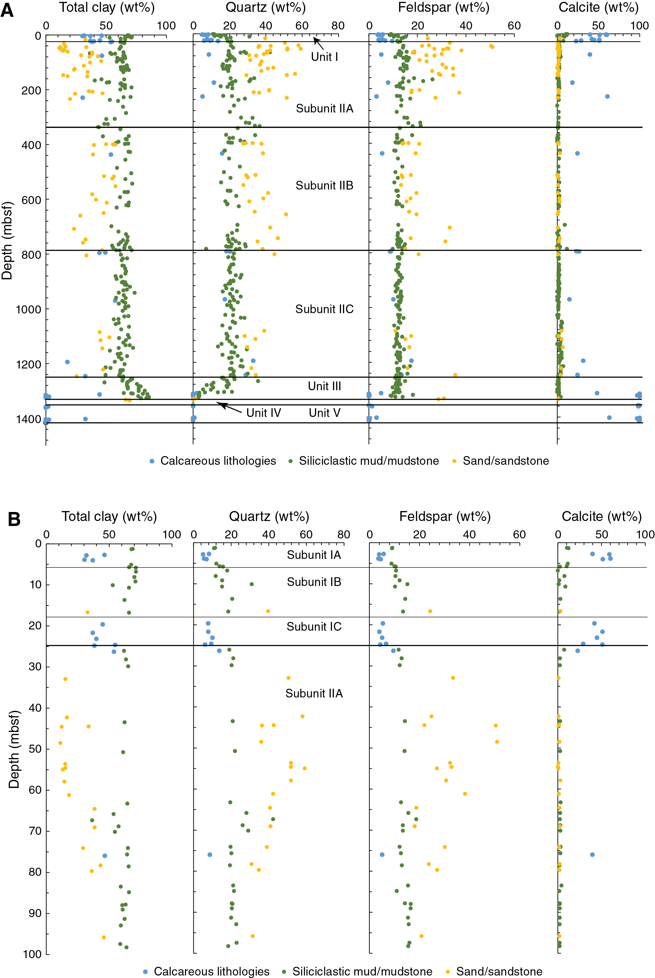
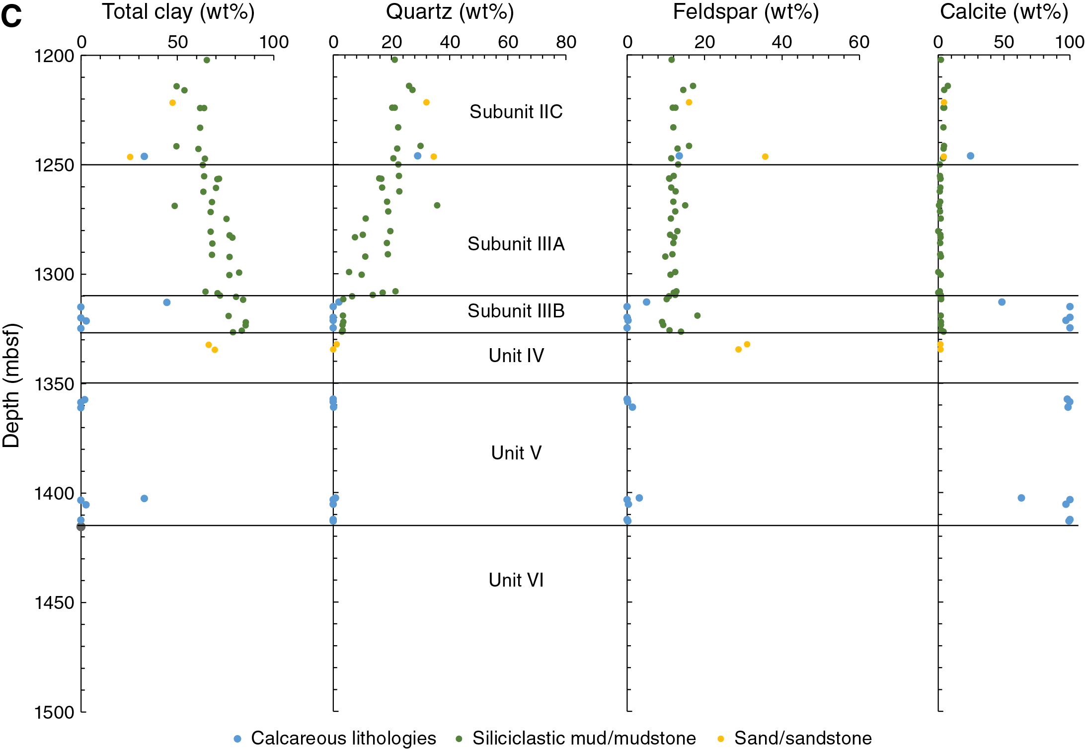
Figure F6. Bulk mineralogy as determined by XRD.
Table T2. Distribution and composition of lithologies. Download table in .csv format.
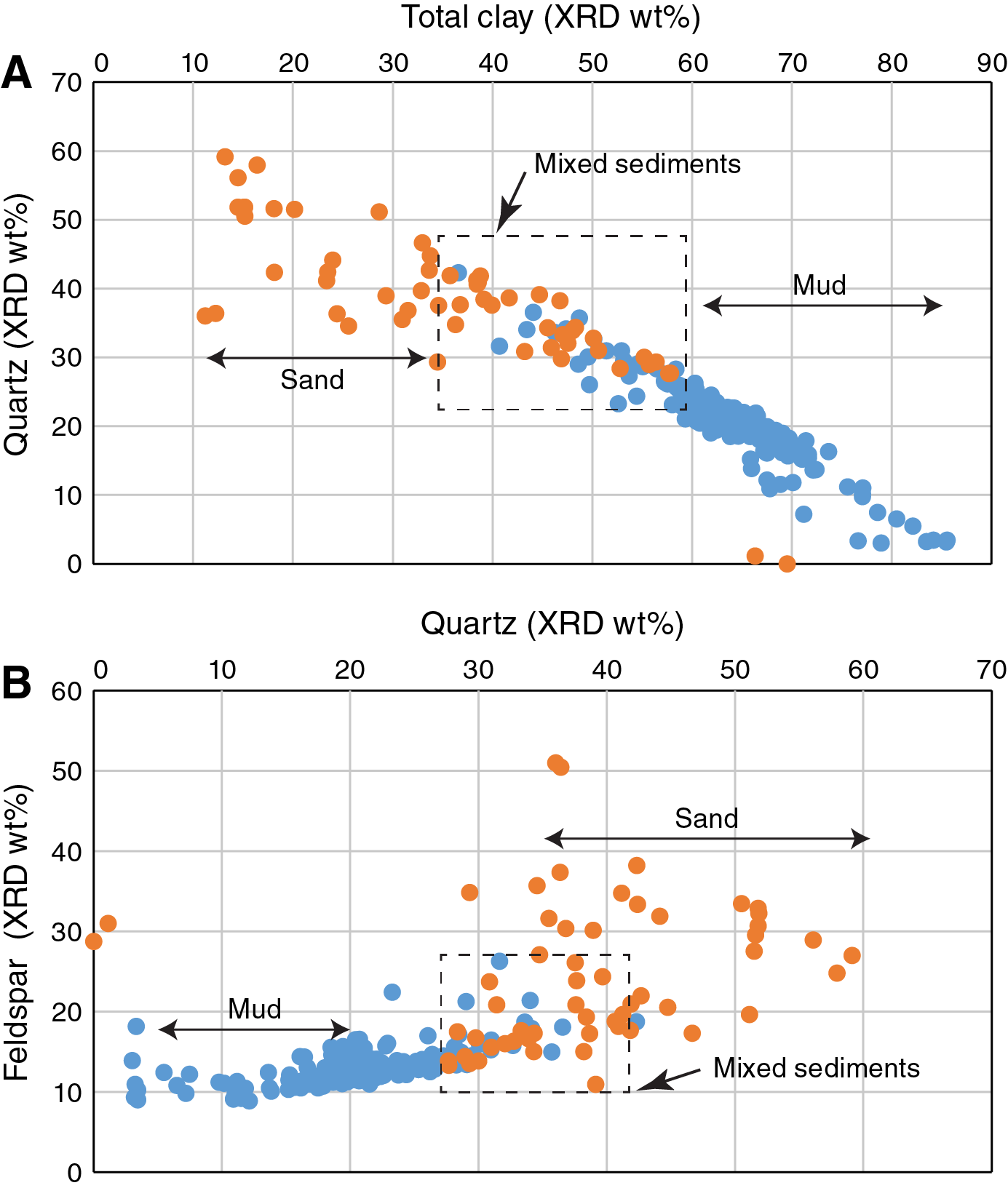
Figure F7. Mineral composition.
Lithostratigraphic units
Major lithologies at Site U1480 are summarized in Figure F5. The main lithologies encountered at Site U1480 are nannofossil-bearing mud (Figures F6, F8A, F8B), siliciclastic mud (Figure F8C), and siliciclastic sand (Figure F8D). Dominant siliciclastic lithologies are clay (clay-mineral dominated), silty clay, and well sorted fine-grained sand. Less abundant siliciclastic lithologies are mixtures of clay, silt, and sand (e.g., silty clay, silty sand, sandy silt, and silty sand with clay) (Figure F9).
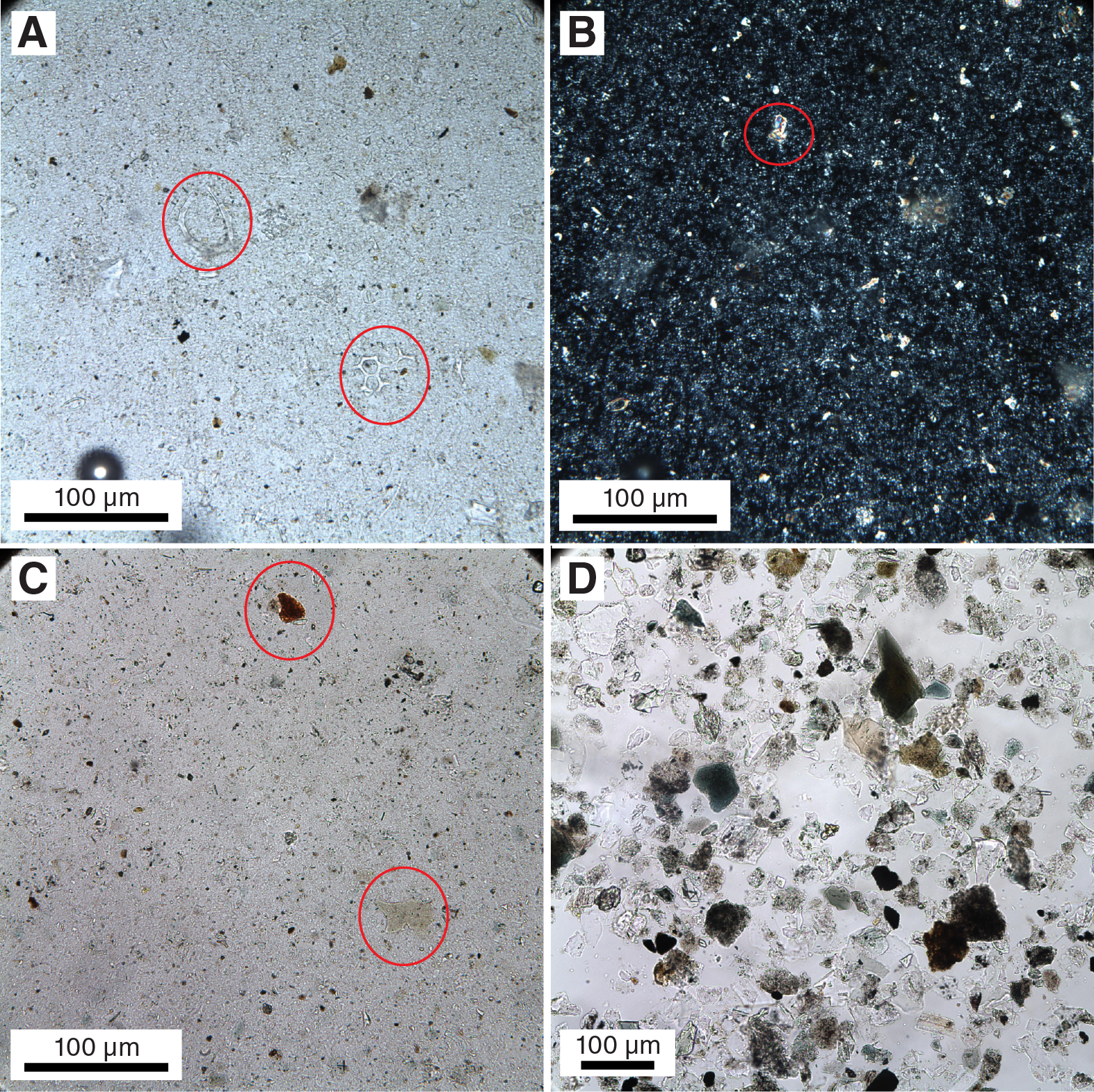
Figure F8. End-member textures and compositions of major lithologies, Hole U1480E.
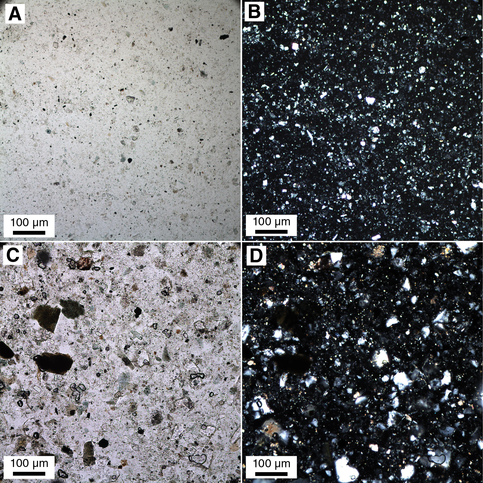
Figure F9. Typical mixed siliciclastic sediment, Hole U1480F.
Variants of nannofossil muds include nannofossil ooze (≥50% nannofossils), nannofossil clay (≥25% and <50% nannofossils), and clay with nannofossils (5%–25% nannofossils). Nannofossil mud (calcareous clay, calcareous ooze, and variants containing admixtures of silt and sand) contains various placolith groups and sphenoliths with locally abundant discoasters (Figure F10). Nannofossil mud typically contains a minor component (<5 wt%) of biosiliceous debris (radiolarians, diatoms, and rare sponge spicules), foraminifers, and organic matter. Bulk carbonate content by both coulometric analysis (see Geochemistry) and XRD shows that calcareous ooze (>50% calcite) is variable but generally high in Unit I and again in the lowest part of Unit III and in Units IV and V (Figure F11).
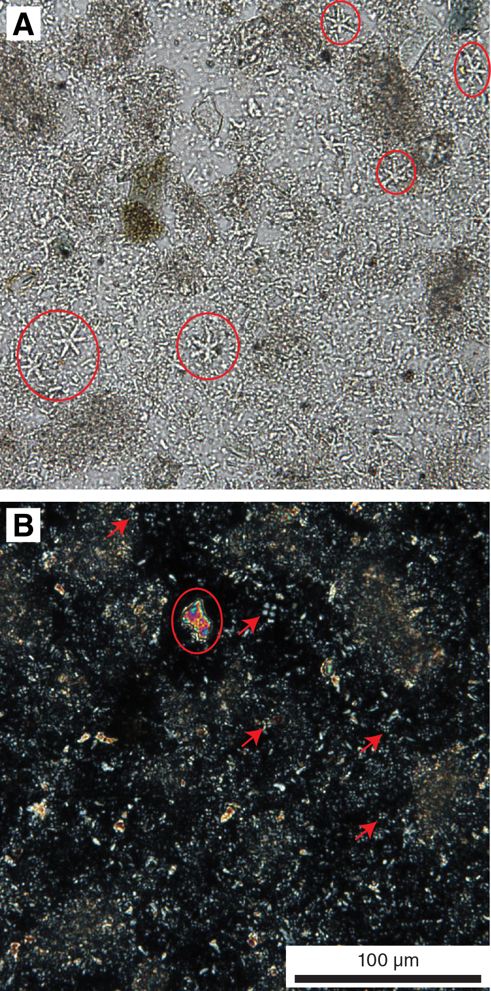
Figure F10. Nannofossils and other grains in calcareous clay, Hole U1480F.
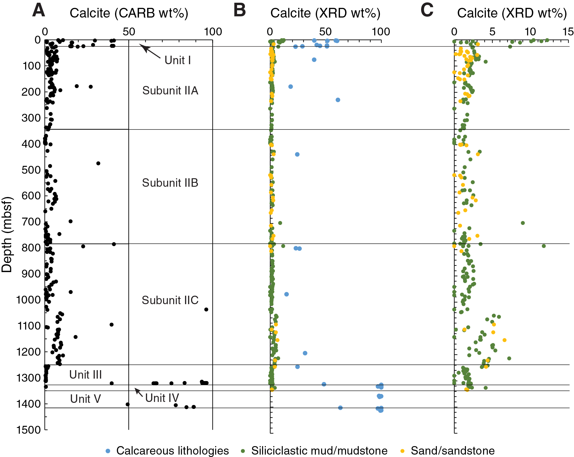
Figure F11. Depth trend for bulk calcite content in Units I–IV, Site U1480.
Sediment in Units I and II is mostly unconsolidated and can be readily dispersed for smear slide examination. Localized cementation (concretions) by carbonate minerals, pyrite, and zeolite was rarely observed. Starting with Core 362-U1480G-54R (1250.35 mbsf), sediment generally has a greater degree of lithification (using the criteria outlined in Sedimentology and petrology in the Expedition 362 methods chapter [McNeill et al., 2017b]), a transition in mechanical properties that is one of the defining characteristics of the boundary between Unit II and III. Sediment in Units IV–V is also lithified.
Unit I
- Interval: 362-U1480E-1H-1, 0 cm, to 3H-7, 20 cm; 362-U1480H-1H-1, 0 cm, to 4H-1, 134 cm
- Thickness: Hole U1480E = 26.42 m; Hole U1480H = 24.84 m
- Depth: Hole U1480E = 0.00–26.42 mbsf; Hole U1480H = 0.00–24.84 mbsf
- Age: early Pleistocene–Recent
- Lithology: calcareous clay and silty clay with ash and alternating fine-grained sand and clay
Unit I contains two major lithologies (Figure F5; Table T3): (1) pale yellow to brown calcareous clay and (2) alternating fine-grained sand to silt with silty clay to clay with silt layers (Figure F12). The unit is divided into Subunits IA–IC. Compositional contrast from XRD and smear slide analysis supports discrimination of Units I and II (Figures F6B, F11). Unit I contains a significantly greater proportion of calcareous mud and siliciclastic mud that is notably clay-mineral rich (60–70 wt%).
Table T3. Summary of unit and subunit thicknesses. Download table in .csv format.

Figure F12. Typical calcareous clay with intercalated layers.
The detrital grain assemblage is dominated by clay minerals and nannofossils with quartz, feldspar, lithic grains (mostly metamorphic rock fragments), mica, and dispersed ash (Figure F8A). A minor component (3–5 wt%) of silt-size detrital monocrystalline carbonate with no clear affinity to fossil fragments is present in most samples. Fourteen intercalated, generally pinkish gray to whitish felsic ash layers, 1–41 cm thick, were recorded in Unit I in Holes U1480E and U1480H.
Diagenesis in Unit I is dominated by compaction (as indicated by the loss of porosity in the absence of cementation; see Physical properties) and precipitation of minor Fe sulfides related to sulfate reduction (see Geochemistry). Fe sulfides appear in microcrystalline and framboidal form, fill small burrows, and coat grains, especially mica, in the silt and sand fractions. Apart from these localized occurrences of Fe sulfide cement, the sediment is unlithified.
Subunit IA
- Interval: 362-U1480E-1H-1, 0 cm, to 1H-4, 125 cm; 362-U1480H-1H-1, 0 cm, to 2H-1, 53 cm
- Thickness: Hole U1480E = 5.60 m; Hole U1480H = 5.10 m
- Depth: Hole U1480E = 0.00–5.60 mbsf; Hole U1480H = 0.00–5.10 mbsf
- Age: late Pleistocene–Recent
- Lithology: calcareous clay with minor volcanic ash
Subunit IA consists of brown to very pale brown calcareous clay (Figure F12A) with volcanic ash. The calcareous clay is nongraded with sparse to moderate bioturbation dominated by Thalassinoides and Scolicia, mottling, foraminifers, macrofossils, and disseminated ash pods. Centimeter-wide burrows are generally filled by dark brown material.
One thick interval of gray to pinkish gray ash occurs in Holes U1480E and U1480H (intervals 362-U1480E-1H-2, 5–46 cm; 362-U1480H-1H-2, 0–34 cm) (Figure F12A). This interval is structureless and normally graded from coarse-grained sand to silt with no bioturbation but shows slight displacement at the base caused by drilling disturbance. A darker color at the base is a crystal-rich horizon caused by gravity segregation during ash-layer emplacement. The upper part is characterized by a several centimeter–thick gradual transition into background sediment.
XRD analysis shows the average composition of Subunit IA as calcareous clay (36% total clay, 7% quartz, 5% plagioclase, and 53% calcite) and siliciclastic mud (68% total clay, 12% quartz, 9% plagioclase, and 11% calcite) (Table T2).
Subunit IB
- Interval: 362-U1480E-1H-4, 125 cm, to 3H-1, 145 cm; 362-U1480H-2H-1, 53 cm, to 3H-4, 119 cm
- Thickness: Hole U1480E = 13.20 m; Hole U1480H = 14.57 m
- Depth: Hole U1480E = 5.60–18.80 mbsf; Hole U1480H = 5.10–19.67 mbsf
- Age: middle Pleistocene–late Pleistocene
- Lithology: fine-grained sand and clay with minor calcareous clay
Subunit IB is a siliciclastic succession dominated by alternation of coarser grained (very fine grained sand to silt) and finer grained (silty clay and clay with silt) material with disseminated ash layers (Figure F12B). Coarser grained material consists of very thin to thick intervals of greenish gray to gray, structureless to planar-laminated, very fine grained sand and silt typically with a sharp subhorizontal base, normal grading, and no bioturbation. Finer grained material consists of very thin to thick-bedded silty clay and clay and silt characterized by a range of mottling, planar lamination, absent to slight bioturbation (Thalassinoides, Scolicia, and Phycosiphon), a sharp to gradational subhorizontal basal contact with coarser grained material, and disseminated ash pods and foraminifers.
Nine whitish to dark pinkish gray and black ash, very thin to medium-bedded layers were identified in Subunit IB of Holes U1480E and U1480H. The beds are all characterized by normal grading, a planar and sharp horizontal base, and an absence of structures other than bioturbation. Grain size typically ranges from silt to coarse-grained sand, and the beds commonly show a darker horizon at the coarser grained base due to mineral concentrations and a gradual transition into background sediment at the top.
A ~1 m thick bed of calcareous clay characterized by slight bioturbation (Thalassinoides), mottling, and greenish gray color occurs at 8.27–9.21 mbsf in Hole U1480E (7.5–8.6 mbsf in Hole U1480H) and includes a 3 cm thick ash pod.
XRD analysis defines the average composition of Subunit IB as siliciclastic mud (66% total clay, 18% quartz, 12% plagioclase, and 4% calcite) and sand (33% total clay, 40% quartz, 24% plagioclase, and 3% calcite) (Table T2).
Subunit IC
- Interval: 362-U1480E-3H-1, 145 cm, to 3H-7, 20 cm; 362-U1480H-3H-4, 119 cm, to 4H-1, 134 cm
- Thickness: Hole U1480E = 7.62 m; Hole U1480H = 5.17 m
- Depth: Hole U1480E = 18.80–26.42 mbsf; Hole U1480H = 19.67–24.84 mbsf
- Age: early Pleistocene–middle Pleistocene
- Lithology: silty clay and calcareous clay with minor ash
Subunit IC consists of pale yellow to very pale brown calcareous clay. This subunit shows mottling with moderate bioturbation (Thalassinoides) and contains foraminifers and macrofossils (Figure F12C). The top and base of Subunit IC are characterized by decimeter-thick intervals of calcareous clay intercalated with medium-bedded silty clay and very thin bedded ash (1–3 cm thick). A color change from pale brown to gray starts at 26–40 mbsf and marks the transition into Unit II. Muddy layers are darker and browner, whereas nannofossil-rich layers are whiter. Changes between lithologies are gradational, and the sediment is burrow-mottled throughout.
Three intercalations of felsic ash of generally gray to pinkish white and up to 8 cm thick occur throughout Holes U1480E and U1480H in Subunit IC (Figure F12C). These intercalations are structureless, normally graded from fine-grained sand to silt, and nonbioturbated or weakly bioturbated. These layers commonly have a sharp, horizontal, mineral-rich basal contact and a gradual transition into the overlying calcareous clay.
XRD analysis shows the average composition of Subunit IC as calcareous clay (43% total clay, 8% quartz, 5% plagioclase, and 44% calcite), siliciclastic mud (62% total clay, 19% quartz, 11% plagioclase, and 7% calcite), and sand (33% total clay, 40% quartz, 24% plagioclase, and 3% calcite) (Table T2).
Unit II
- Interval: 362-U1480E-3H-7, 20 cm, to end of hole at 12H-CC, 29 cm; 362-U1480F-2H-1, 0 cm, to 98X-CC, 38 cm; 362-U1480G-2R-1, 0 cm, to 54R-1, 65 cm; 362-U1480H-4H-1, 134 cm, to end of hole at 17H-CC, 5 cm
- Thickness: Hole U1480E = 73.51 m; Hole U1480F = 707.68 m; Hole U1480G = 490.75 m; Hole U1480H = 104.52 m
- Depth: Hole U1480E = 26.42–99.93 mbsf; Hole U1480F = 98.00–805.68 mbsf; Hole U1480G = 759.60–1250.35 mbsf; Hole U1480H = 24.84–129.36 mbsf
- Age: late Miocene–early Pleistocene
- Lithology: clay, silt, and sand
Unit II contains Subunits IIA–IIC (Figure F5; Table T3) and is dominated by silty clay to silt, sandy silt, and fine-grained sand. Unit II is characterized by alternations of thin- to medium-bedded, structureless to laminated sand and silty clay to silt in the upper part and alternating thin- to very thin bedded, parallel- and cross-laminated silt and clay in the middle part of the unit. Bioturbated clay and silty clay with some intercalated muddy sand, containing abundant plant debris and mud clasts, dominate the lower part of the unit. Compositional contrasts from XRD analysis support discrimination of Units I and II (Figures F6, F11). The detrital grain assemblage is similar to that of Unit I but with a reduced abundance of nannofossils and biosiliceous debris. A minor component (3%–5%) of detrital, silt-size monocrystalline carbonate with no clear affinity to fossil fragments is present in most Unit II samples.
Four intercalated laminae and beds of felsic ash up to 11 cm thick are observed in Unit II. Only those at the boundary with Unit I contain fresh glass and have the typical appearance of the ash layers of Unit I (i.e., normal grading, sharp horizontal basal contacts, and median grain size of fine-grained sand). Ash horizons in Subunit IIB are strongly altered, with pyroclasts showing devitrification and transformation into zeolite.
Well-sorted quartzofeldspathic silt is another minor lithology observed in Unit II (Figure F13). This lithology is distinctly light in color (light gray) and occurs in thin (a few millimeters to 1 cm) layers with parallel laminations.
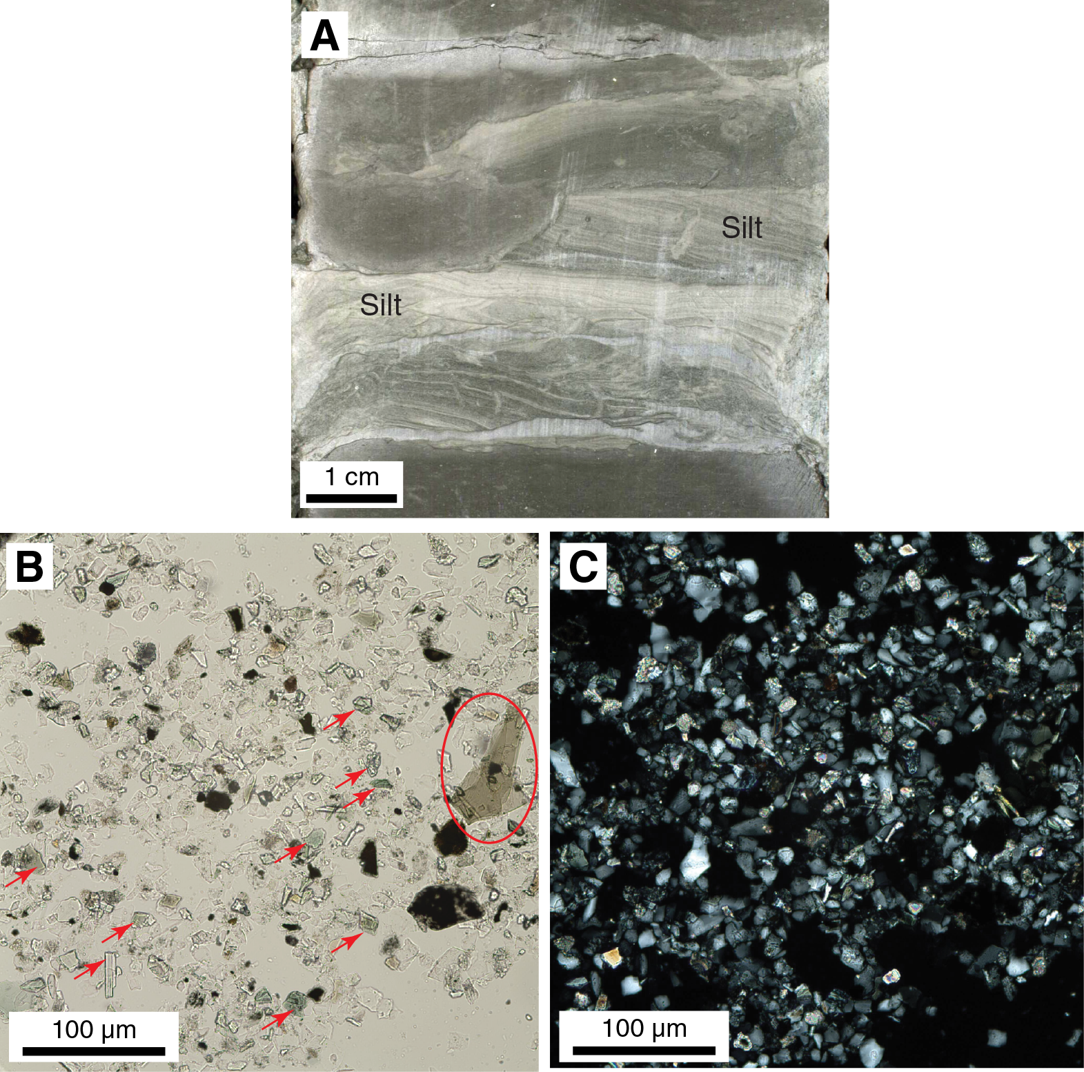
Figure F13. Well-sorted silt, Hole U1480F.
Quartz is primarily angular and monocrystalline with near-straight to slightly undulose extinction. Feldspars in smear slides cannot be stained for compositional determination (plagioclase versus K-feldspar), but XRD results, together with the lack of observed microcline twinning, suggest that Ca-plagioclase is the dominant feldspar. Most of the plagioclase is untwinned (Figure F14A). The ratio of feldspar to feldspar + quartz is remarkably similar in mud and sand and averages 0.38, making the silt-sand fraction in all the lithologies arkosic by the classification of Folk (1980).
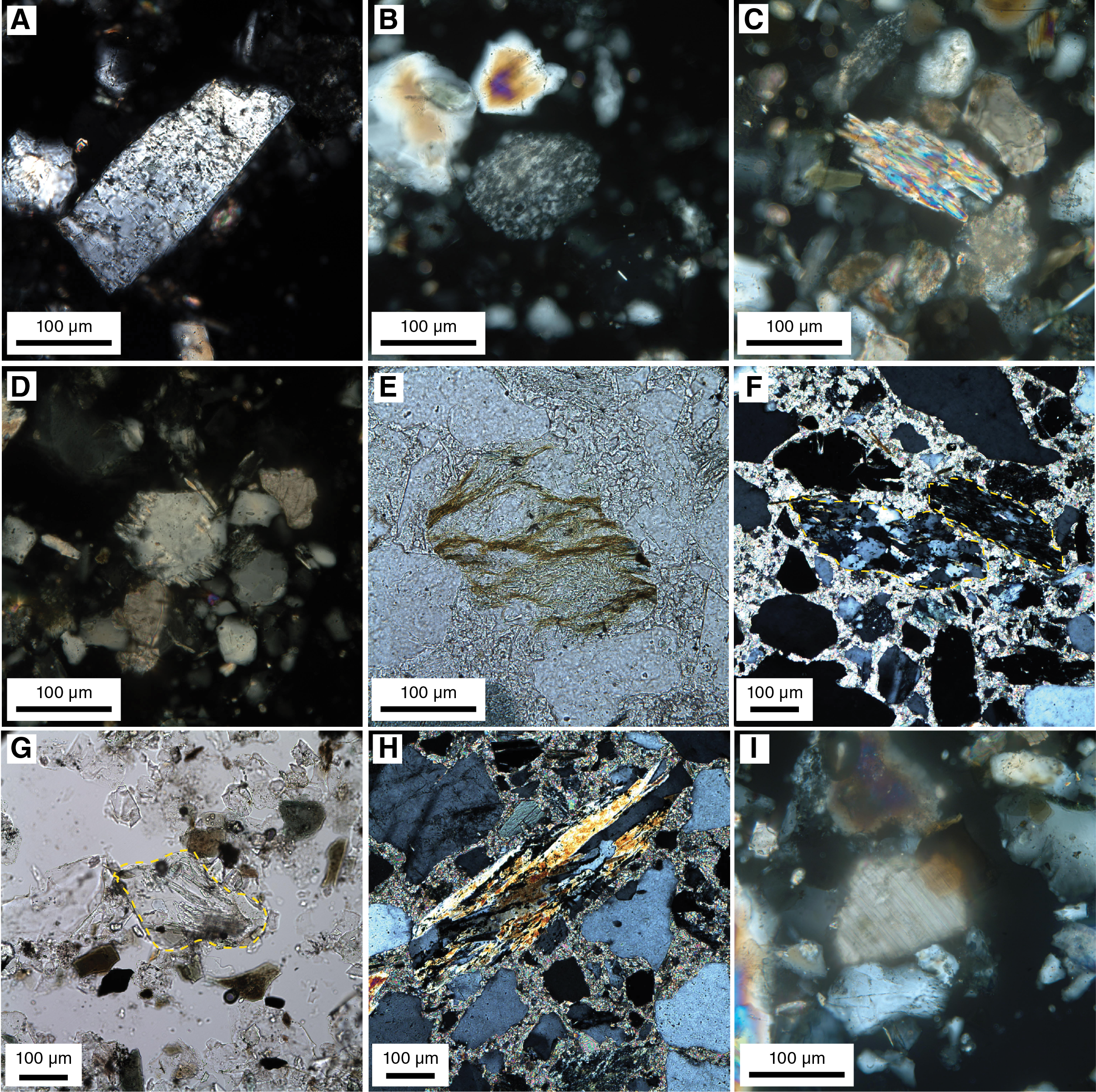
Figure F14. Feldspar and pelitic metamorphic lithic fragments.
The principal lithic grain type in the silt and sand fraction is metasedimentary (pelitic) (Figure F14B–F14H). The dominant metamorphic rock fragments (MRF) are fine-grained quartz-mica intergrowths that range from mica rich to quartz rich and show discernible foliation. A variety of schist types were identified. Dominantly monocrystalline and anhedral equant calcite was observed in sand-, silt-, and upper clay–size fractions of the siliciclastic samples and is interpreted as detrital based on shape and similarity in size with the associated silicate grains (Figure F14B–F14I). A few polycrystalline carbonate fragments were observed, but their precise lithology (limestone versus calcareous metasediment) could not be determined.
There is an abundant (1%–3%) and diverse component of dense minerals in the sand and coarser silt fraction that includes a dominant fraction of green and blue-green amphiboles plus pyroxene, garnet, epidote, kyanite, sillimanite, titanite, apatite, monazite, brown tourmaline, zircon, and rutile (Figure F15A–F15E). The sand and coarse-silt fraction is also predominantly micaceous (Figure F15F). The most abundant mica is biotite. In general, the mica component is coarser than the associated quartz and feldspar grains, and mica is clearly visible in the cores without magnification.
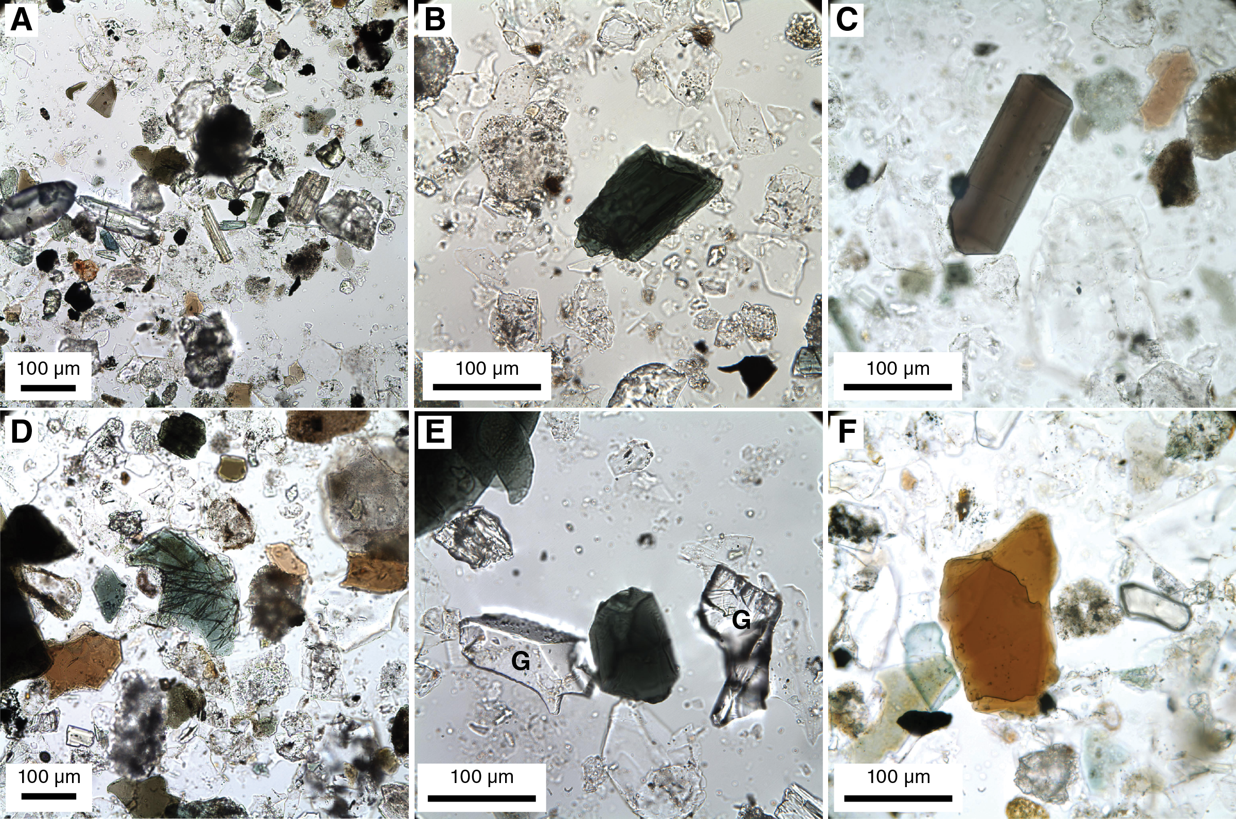
Figure F15. Dense minerals and mica in sand and silt fractions.
Organic matter of clay to fine silt size occurs in trace amounts in most of the muds and in larger amounts (up to 3%) and as coarser particles (up to coarse-grained sand size and cobble size in one instance) in sand. Organic matter in the sand appears to be dominantly terrigenous; in mud, however, the origin of the organic matter is unclear. The most common form of organic matter is equant to slightly elongate red-brown masses in coarse-grained clay to fine-grained silt. Coarser organic matter of medium-size silt to sand-size fraction, typically showing a pronounced stringy texture, is suggestive of woody material (Figure F16).
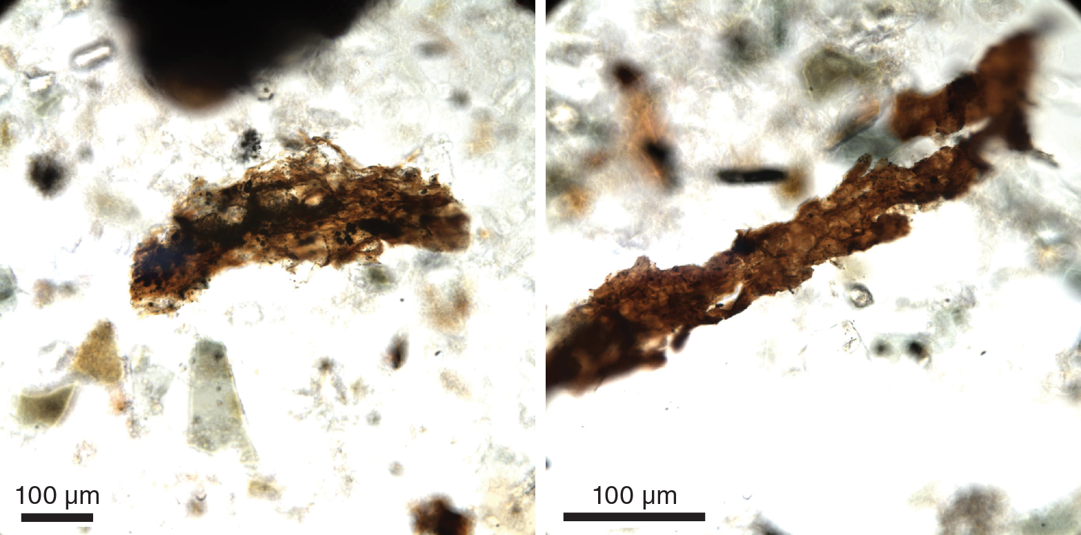
Figure F16. Examples of stringy red-brown sand-size organic matter.
In the absence of substantial carbonate and ash, the overall compositional variation within Unit II mud-rich and sand-rich lithologies with depth is minor (Figure F6). Feldspar content in sandstone has a larger range and higher overall values in Subunit IIA (generally from 20–40 wt%) than in Subunit IIB, in which feldspar is generally 15–20 wt%. Carbonate content averages 2.3 wt% in siliciclastic muds and 1.4 wt% in sand.
Few diagenetic features were observed in Unit II. Pyroxene grains and some garnets display prominent crystallographically controlled etch fabrics (Figure F17). However, it is intrinsically difficult to attribute the formation of these fabrics to subsurface dissolution because etched surfaces on pyroxenes and other heavy minerals are known to develop during continental weathering (Berner and Schott, 1982) as well as during burial diagenesis (Turner and Morton, 2007).
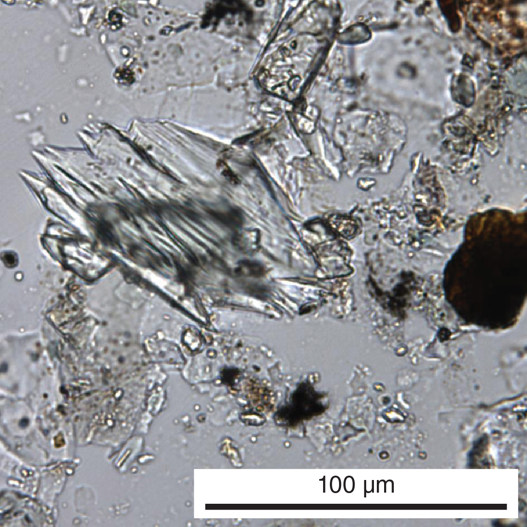
Figure F17. Pyroxene displaying crystallographically controlled dissolution fabric.
Occurrences of authigenic minerals are highly localized. The most common authigenic mineral is pyrite (or possibly other amorphous or crystalline Fe sulfides) in a variety of forms, including framboids, euhedra of coarse clay and fine silt size, microcrystalline grain coatings, and rare spiky rosettes (Figure F18). Pyrite is observed in mud and sand, but in the sand it is more coarsely crystalline and typically takes the form of grain coatings, especially in material that contains abundant organic matter. Pyrite as a lining or filling of millimeter- to centimeter-scale burrows is common.
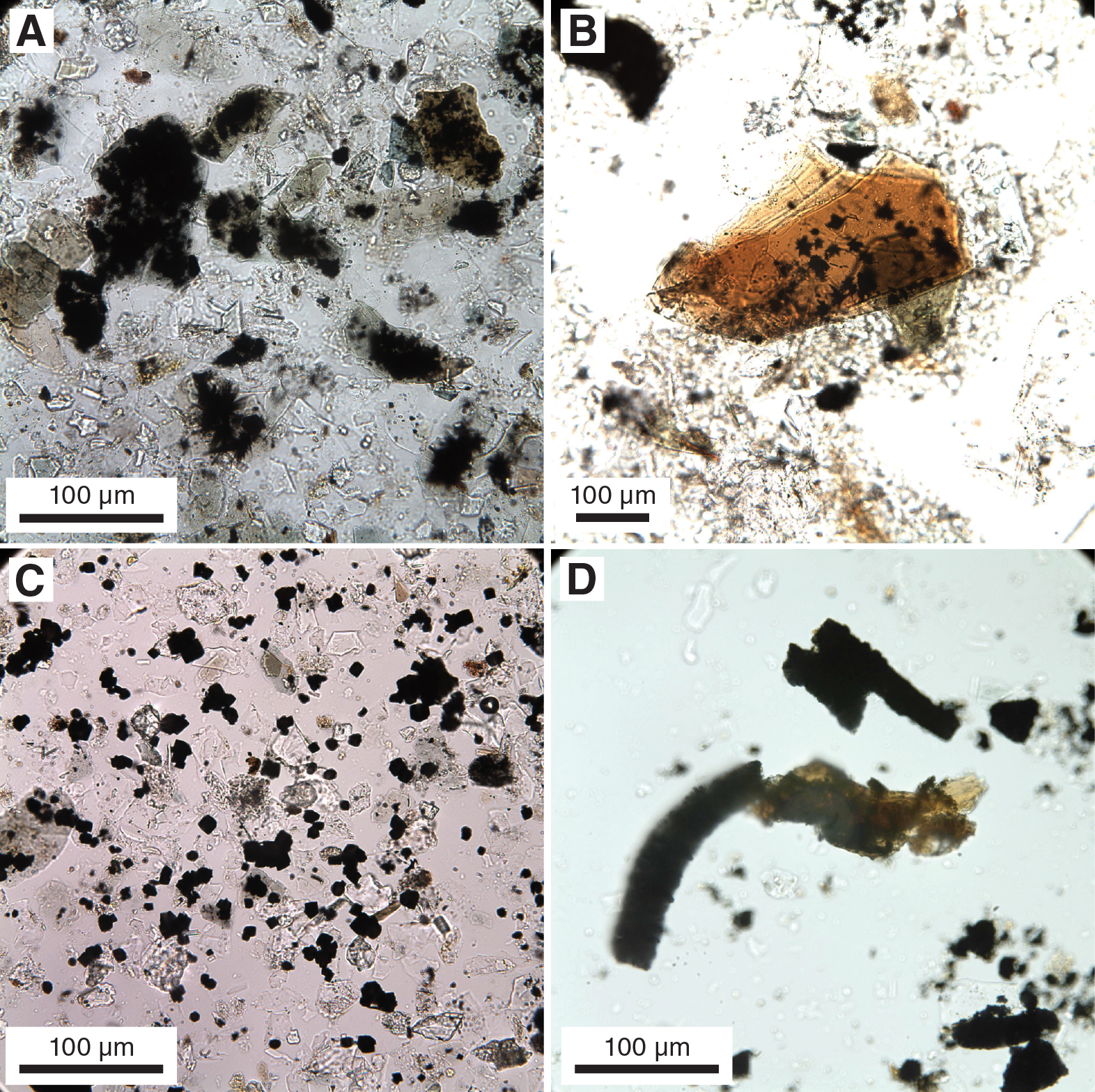
Figure F18. Iron sulfide in smear slides.
Fibrous zeolite rosettes are observed in several samples from Cores 362-U1480F-53X through 60X (from ~370 to ~435 mbsf; Figure F19). Up to 30% of the sediment volume appears to be made of zeolite in these occurrences, but volumetrically, zeolitized material is distributed as rare centimeter-scale lenses and millimeter-scale blebs and is not pervasive. A careful search for a vitric component in association with zeolite did not reveal any clear examples of glass particles.
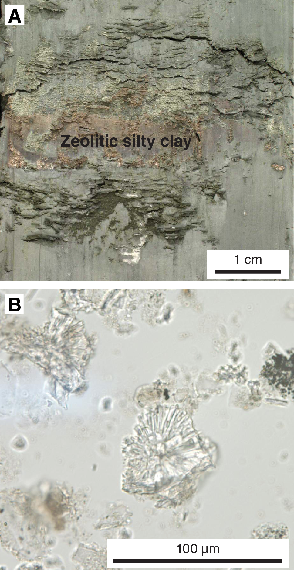
Figure F19. Zeolites, Hole U1480F.
Carbonate concretions are a relatively rare but persistent feature of Subunit IIC (see Subunit IIC). In general, the sediment of Unit II is unlithified.
Subunit IIA
- Interval: 362-U1480E-3H-7, 20 cm, to end of hole at 12H-CC, 29 cm; 362-U1480F 2H-1, 0 cm, to 49F-1, 37 cm; 362-U1480H-4H-1, 134 cm, to end of hole at 17H-3, 86 cm
- Thickness: Hole U1480E and Hole U1480F= 317.25 m; Hole U1480H = >104.52 m
- Depth: Hole U1480E = 26.42–99.93 mbsf; Hole U1480F = 98.00–343.67 mbsf; Hole U1480H = 24.84–129.36 mbsf
- Age: late Pliocene–early Pleistocene
- Lithology: alternating thin- to medium-bedded, laminated to structureless, fine-grained sand and silty clay to silt
Subunit IIA consists mainly of alternating thin- to medium-bedded fine-grained sand, silt, and silty clay (Figure F20A). Fine-grained sand layers with silt occur as thick to very thick beds that are generally structureless (Figure F20B). Throughout Subunit IIA, despite many sand layers appearing structureless due to severe drilling disturbance, some preserved layers display normal grading.
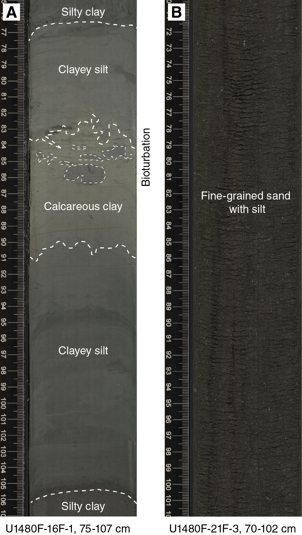
Figure F20. Intercalation of silty clay, clayey silt, and calcareous clay and structureless fine-grained sand with silt.
Two 3–8 cm thick, gray to pinkish gray ash layers occur in the uppermost part of Subunit IIA and show sharp basal contacts, normal gradation from fine-grained sand to silt, and a transition into overlying background deposits.
XRD analysis shows the average composition of Subunit IIA as calcareous clay (48% total clay, 10% quartz, 7% plagioclase, and 35% calcite), siliciclastic mud (60% total clay, 23% quartz, 15% plagioclase, and 2% calcite), and sand (27% total clay, 43.0% quartz, 29% plagioclase, and 1% calcite) (Table T2).
Subunit IIB
- Interval: 362-U1480F-49F-1, 37 cm, to 96X-1, 0 cm; 362-U1480G-2R-1, 0 cm, to 5R-1, 120 cm
- Thickness: Hole U1480F = 442.13 m
- Depth: Hole U1480F = 343.67–785.80 mbsf; Hole U1480G = 759.60–784.33 mbsf
- Age: late Miocene–late Pliocene
- Lithology: alternating thin- to very thin bedded, cross- and parallel-laminated silt and clay
Subunit IIB includes extensive intervals of alternating thin- to very thin bedded silt and clay (Figure F21). Thick- to very thick bedded, fine- to medium-grained sand with silty clay and clayey silt are also present. Some alternating silt and clay layers contain fine-grained sand lenses with normal grading and cross-lamination structures.
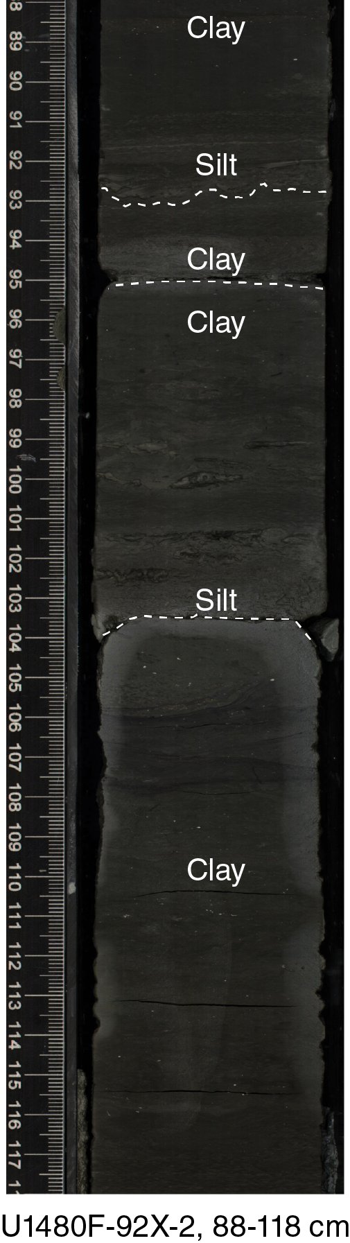
Figure F21. Alternating thin- to very thin bedded silt and clay.
In this subunit, two altered, nongraded, very fine grained light brown-gray ash beds and laminae occur at 369.05 and 383.29 mbsf. Both ash beds are displaced by drilling disturbance and show strong devitrification features and common zeolite in smear slides.
XRD analysis shows the average composition of Subunit IIB as calcareous clay (57% total clay, 15% quartz, 8.0% plagioclase, and 21% calcite), siliciclastic mud (64% total clay, 22% quartz, 12% plagioclase, and 2% calcite), and sand (44% total clay, 36% quartz, 18% plagioclase, and 1% calcite) (Table T2).
Subunit IIC
- Interval: 362-U1480F-96X-1, 0 cm, to 98X-CC, 38 cm; 362-U1480G-5R-1, 120 cm, to 54R-1, 65 cm
- Thickness: Hole U1480F = 464.55 m; Hole U1480G = 466.02 cm
- Depth: Hole U1480F = 785.80–806.68 mbsf; Hole U1480G = 784.33–1250.35 mbsf
- Age: late Miocene
- Lithology: bioturbated black and gray clay/claystone and silty clay/claystone and structureless muddy sand/sandstone with mud clasts
Subunit IIC is characterized by bioturbated black and gray clay and silty clay and structureless muddy sand with abundant plant material and mud clasts (Figure F22). Anomalously high magnetic susceptibility is typically associated with structureless mudstone that lies immediately below intensely bioturbated intervals and above muddy sediment gravity flow (SGF) deposits rich in plant material (Figure F23). The major lithology is highly bioturbated very dark gray clay with silt that is interrupted by parallel laminated millimeter- to centimeter-scale laminae of normal-graded silt and very fine grained sand. Intervals of structureless medium-grained sand with silty clay and mud clasts up to pebble size are commonly intercalated. Injection structures of medium- to fine-grained sand occur at various angles to bedding structures.
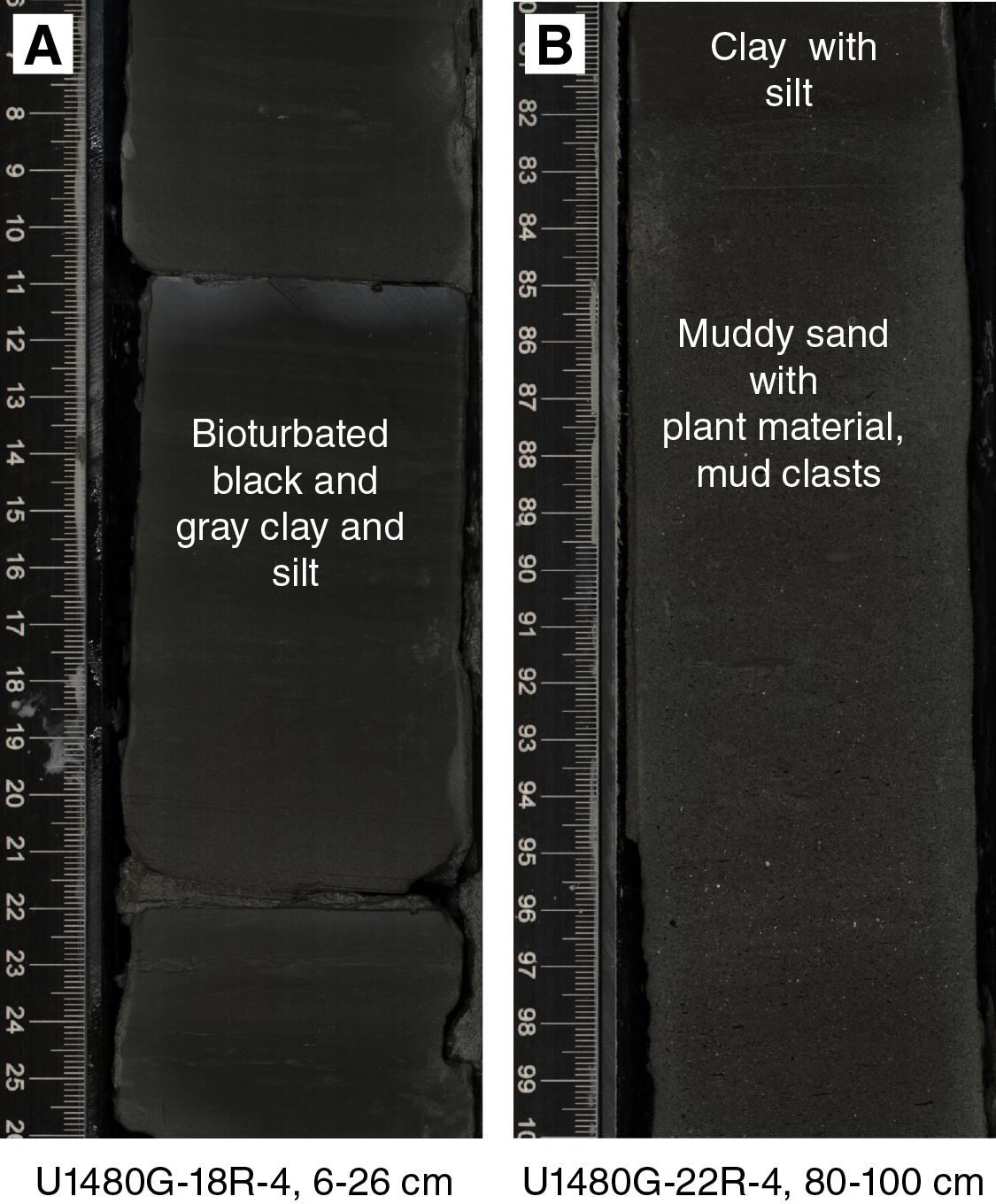
Figure F22. Bioturbated black and gray clay and silt and structureless muddy sand with plant material and mud clasts.
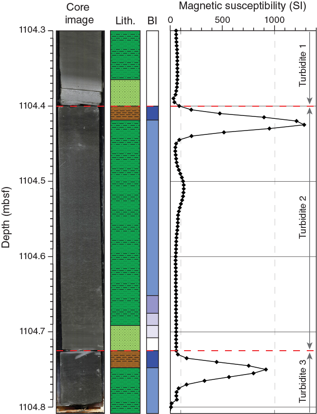
Figure F23. Core showing anomalously high magnetic susceptibility in structureless mudstone.
Abundant pyritized and coaly wood fragments occur throughout the sandy intervals. Prominent pyritized woody layers appear in Subunit IIC, consisting of either a single large coaly wood fragment (e.g., interval 362-U1480G-11R-3, 43–67 cm; 844.13–844.37 mbsf) or multiple individual platy wood clasts, typically 10–30 mm long and 1 mm thick (interval 12R-1, 79–85 cm; 851.79–851.85 mbsf) with rounded ends (Figure F24).
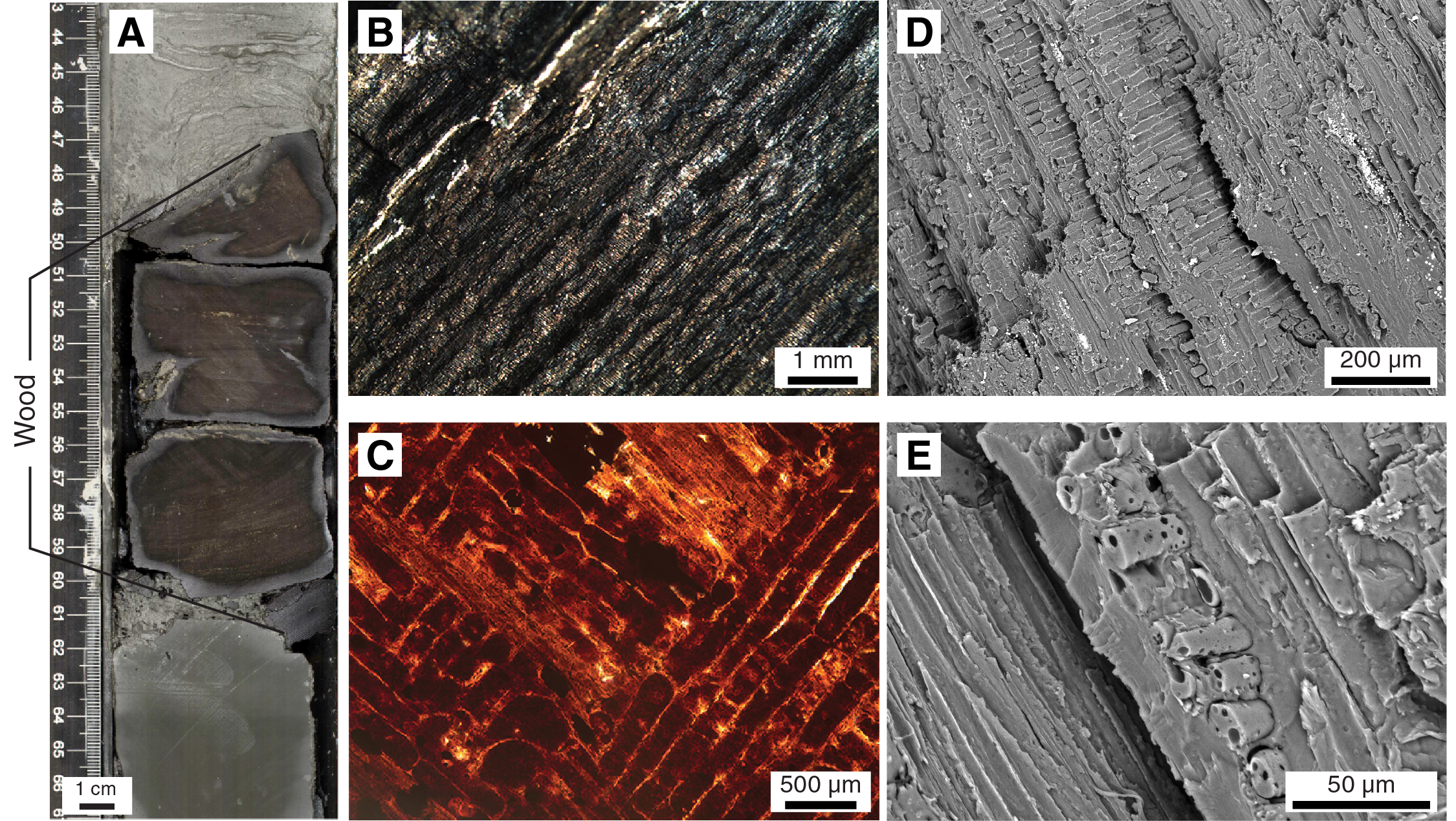
Figure F24. Large coaly wood fragment, binocular microscope image, and SEM images.
Calcite-cemented sediment was observed in interval 362-U1480F-96X-1, 2–27 cm (785.82–786.07 mbsf) (Figure F25). The upper portion of the interval (96X-1, 2–19 cm; 785.82–785.99 mbsf) is cemented medium-grained sandstone underlain by lighter colored calcareous mudstone (interval 96X-1, 19–23 cm; 785.99–786.03 mbsf) and a further interval of darker calcareous mudstone (interval 96X-1, 23–27 cm; 786.03–786.30 mbsf). Smear slides, made with some difficulty from each of these lithologies, reveal an abundance of microcrystalline (1–5 µm) equant calcite. XRD indicates 26.4% calcite in the shallower of these two cemented mudstones (interval 96X-1, 19–23 cm; 785.99–786.03 mbsf) and an unquantified volume of siderite. Similar concretionary sandstone and calcareous claystone locally occurs throughout Subunit IIC.
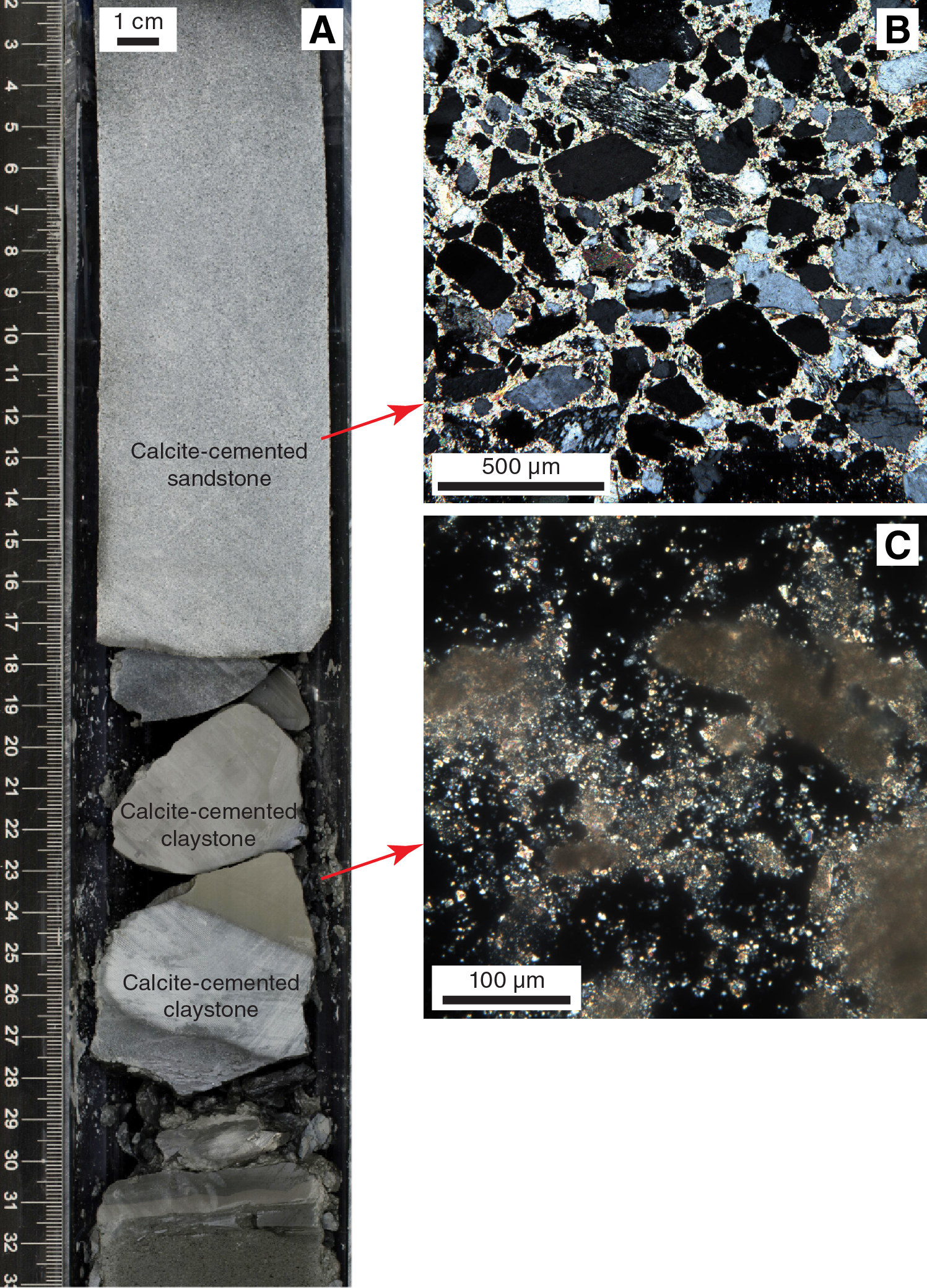
Figure F25. Calcite cementation.
XRD analysis shows the average composition of Subunit IIC as calcareous clay (40% total clay, 25% quartz, 13% plagioclase, and 24% calcite), siliciclastic mud (63% total clay, 22% quartz, 12% plagioclase, and 3% calcite), and sand (44% total clay, 33% quartz, 19% plagioclase, and 5% calcite) (Table T2).
Unit III
- Interval: 362-U1480G-54R-1, 65 cm, to 61R-CC, 15 cm
- Thickness: 76.83 m
- Depth: 1250.35–1327.18 mbsf
- Age: late Paleocene–late Miocene
- Lithology: calcareous claystone, siltstone, tuffaceous silty claystone, and chalk
The top of Unit III (Figure F5; Table T3) is placed below the last occurrence of an interval of micaceous quartzofeldspathic silt as well as a marked increase in lithification and brittleness, defining the start of a lithologically diverse succession in the 165 m between the base of Subunit IIC and the top of basaltic basement (Unit VI). The top of Unit III also marks the transition into mudstones containing greater amounts of claystone and less quartz (Figure F6). Unit III is composed of Subunits IIIA and IIIB, which are dominated by clay-rich materials with various admixtures of siltstone that display lithologic heterogeneity (Figures F6, F9).
Downhole, volcanic ash and carbonate of planktonic origin become increasingly important components. Sediment in Units III and V has bulk compositions that are outside the compositional range of the standards used for onboard XRD calibration (see Sedimentology and petrology in the Expedition 362 methods chapter [McNeill et al., 2017b]), and thus the values for XRD bulk mineralogy in these deeper units (Figures F5, F11; Table T2) should be treated with caution.
Cementation and replacement features in Unit III also mark the appearance of a different style of diagenesis in comparison to Units I and II, with more pervasive (nonconcretionary) cementation in some lithologies and greater degrees of ash alteration. Grain assemblages and biogenic components (e.g., fish bones and teeth) observed in Unit III also provide supportive evidence for slow sediment accumulation rates (see Biostratigraphy) and increased volcanogenic input to the lower pelagic succession.
Eleven intercalated structureless and nongraded gray to pale yellowish brown felsic ash and tuff layers from 0.3 to 3 cm thick were recorded in Unit III. The layers typically have planar sharp and horizontal basal contacts, but the gradational transition into the overlying pelagic sediment, as observed in Unit I and II ash layers, is missing, probably because of greater drilling disturbance.
Subunit IIIA
- Interval: 362-U1480G-54R-1, 65 cm, to 60R-2, 68 cm
- Thickness: 59.75 m
- Depth: 1250.35–1310.10 mbsf
- Age: early Oligocene–late Miocene
- Lithology: gray-green and minor reddish brown claystone with biosiliceous debris and chalk
Subunit IIIA consists mainly of thin- to medium-bedded, gray-green or brown mudstone of very clay rich composition (claystone) and intercalated siltstone (Figure F26). Beds have diffuse parallel lamination toward their base and scattered agglutinated foraminifers in the structureless mud caps. Throughout the cores, rare and isolated, very thin bedded siltstone characteristically shows parallel lamination. Some beds grade from silty claystone at the base to claystone tops with increasing bioturbation uphole.

Figure F26. Typical very dark gray silty claystone and intercalated dark gray siltstone.
After being nearly absent in Unit II, ash material in the background sediment increases in abundance downsection through Subunit IIIA, with the presence of three very thin, structureless, nongraded light gray to greenish gray discrete ash layers and some ash pods in Cores 362-U1480G-57R (1285.42 mbsf), 58R (1289.67 mbsf), and 59R (1299.35 mbsf). Locally, reddish brown claystone occurs in intervals that typically range from 10 to 30 cm thick at depths from 1255.71 to 1259.63 mbsf (e.g., Sections 54R-5 and 54R-6). Intervals dominated by reddish brown claystone occur in Sections 59R-3 (1301.36 mbsf) and 59R-4 (1302.17 mbsf).
In contrast to overlying Subunit IIC, Subunit IIIA has no calcareous claystone or sandstone. XRD analysis of 21 samples defines the average composition of the siliciclastic mudstone as 70% total clay, 17% quartz, 12% plagioclase, and 1% calcite (Table T2). Diagenetic effects in this subunit are, in general, difficult to detect either macroscopically or by using light microscopy, although a degree of increased lithification compared to lithologies in Units I and II is denoted by increasing difficulty in disaggregating the mud for smear slide preparation.
Subunit IIIB
- Interval: 362-U1480G-60R-2, 68 cm, to 61R-CC, 15 cm
- Thickness: 17.08 m
- Depth: 1310.10–1327.18 mbsf
- Age: late Paleocene–early Oligocene
- Lithology: reddish brown tuffaceous silty claystone with biosiliceous debris and chalk
Subunit IIIB differs from Subunit IIIA by the predominantly reddish brown color in the mudstone and the appearance of lithified light-colored chalk (Figure F27). Mudstones of Subunit IIIB are generally structureless with a color pattern that ranges from uniform to mottled (Figure F28). Thin ash layers and pods are important components throughout this subunit, and mudstone is tuffaceous. A darker mudstone appears in smear slides as homogeneous red microcrystalline material. This material may be palagonite, representing alteration of a mudstone that is rich in dispersed mafic ash. Chalk is a second major lithology (Figure F27) with nannofossils, foraminifers, minor biosiliceous debris, and clearly visible stylolites. All of the lithologies display bioturbation, but discrete burrows are more evident in the clay-rich intervals.
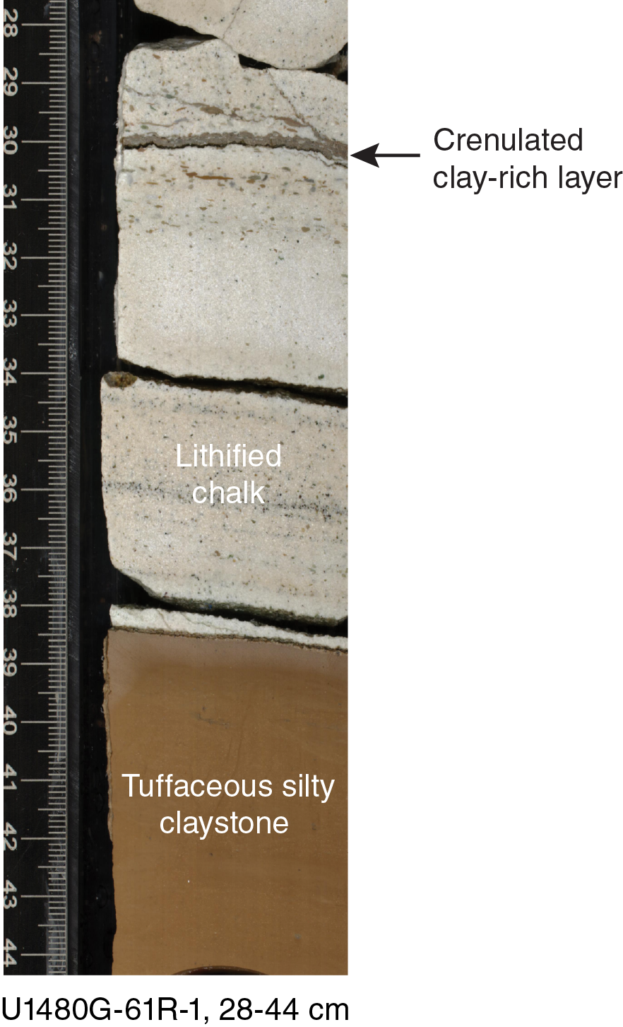
Figure F27. Typical lithologies of reddish brown tuffaceous silty claystone.
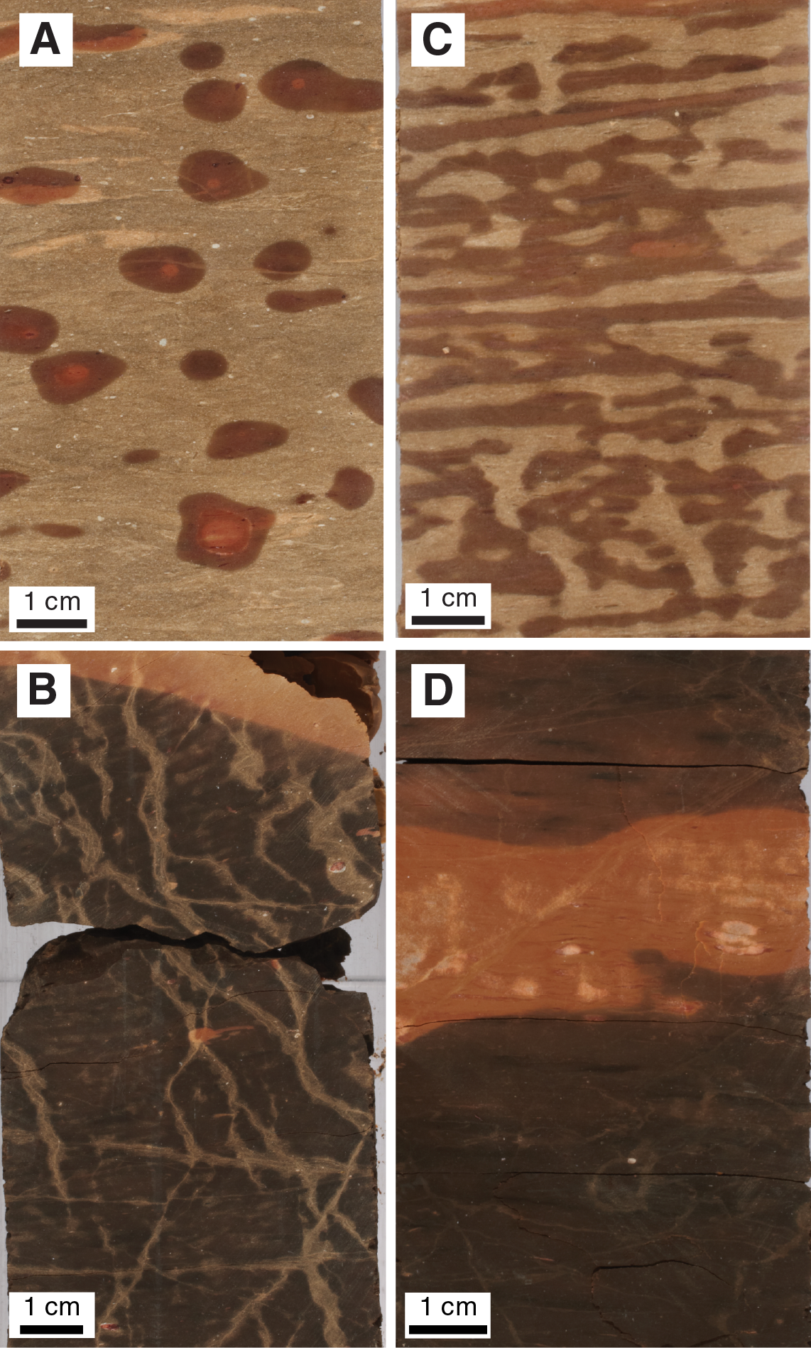
Figure F28. Variations of oxidation mottling.
Siliciclastic mudstone in Subunit IIIB (seven XRD analyses) is more clay rich than in Subunit IIIA (total clay minerals = 82%, quartz = 4%, feldspar = 12%, and calcite = 2%; Table T2). The clay minerals in this subunit give a weak XRD peak intensity with very broad peaks, suggesting poorly crystalline claystone and the likely admixture of amorphous material (glass or palagonite) (Figure F29). The chalk approaches a nearly pure carbonate composition (Figure F11). XRD analysis defines the composition of the chalk as 10% total clay, 0.4% quartz, 1% feldspar, and 89% calcite.
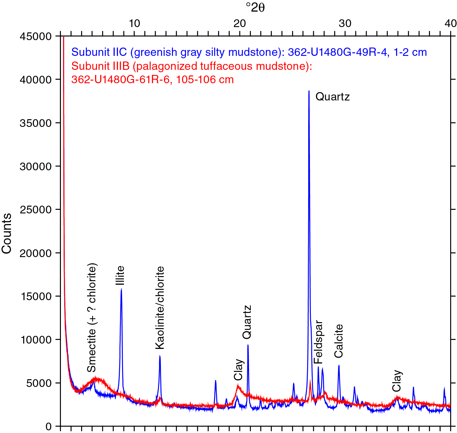
Figure F29. Comparison of XRD patterns of mud/mudstone.
Several minor lithologies contribute to the lithologic heterogeneity in Subunit IIIB. Thin layers of calcite-cemented granule and pebble conglomerate are observed in Cores 362-U1480G-60R and 61R (1312.43–1323.83 mbsf) (Figure F30). Grains in these coarse zones (Figure F31) are diverse and include foraminifers (planktonic and agglutinated), radiolarians, sponge spicules, vertebrate teeth and bones, vesicular pumice with large phenocrysts of Ca-plagioclase (vesicles partially infilled by carbonate cement), lathwork volcanic rock fragments (VRF; basaltic composition), diorite, clear glass shards, palagonized material, chert/chalcedony, plagioclase monocrystals and aggregates, biotite, reworked zeolite cement, glauconite, and several types of claystone and silty claystone clasts.
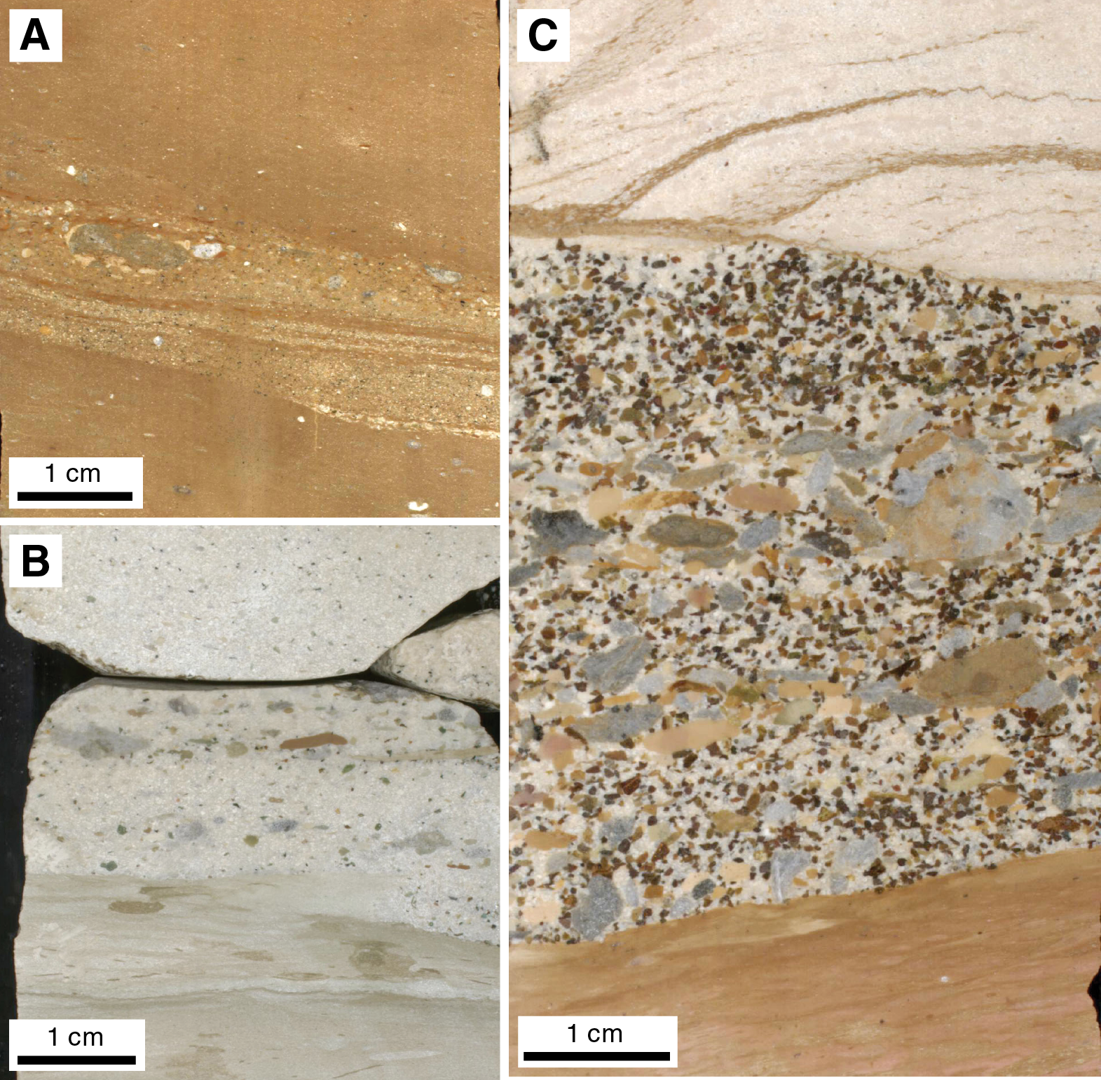
Figure F30. Lithologies from Hole U1480G.

Figure F31. Grains in the coarser grained sedimentary lithologies, Hole U1480G.
Another minor lithology consists of very thin brown layers of claystone-rich material within intervals of chalk. This lithology displays millimeter-scale wavy lamination that can be seen in thin section (Figure F32C, F32D). Claystone appears to have been compacted over rigid grains to create a crenulation in the clay-mineral orientation. A variety of silt- and sand-size grains are distributed throughout the wavy clay-size material. These grains display a compositional range similar to that of the conglomerate described above, with the addition of large agglutinated foraminifers and an unknown biosiliceous component present as elongate bed-parallel accumulations of silt-size pieces decorating the surface of a central clay mass (Figure F33). A possible interpretation is that these features represent partially collapsed and compacted remains of clay- and silty clay–filled sponges. Together with the agglutinated foraminifers, these represent a benthic component within the biogenic grain assemblage.
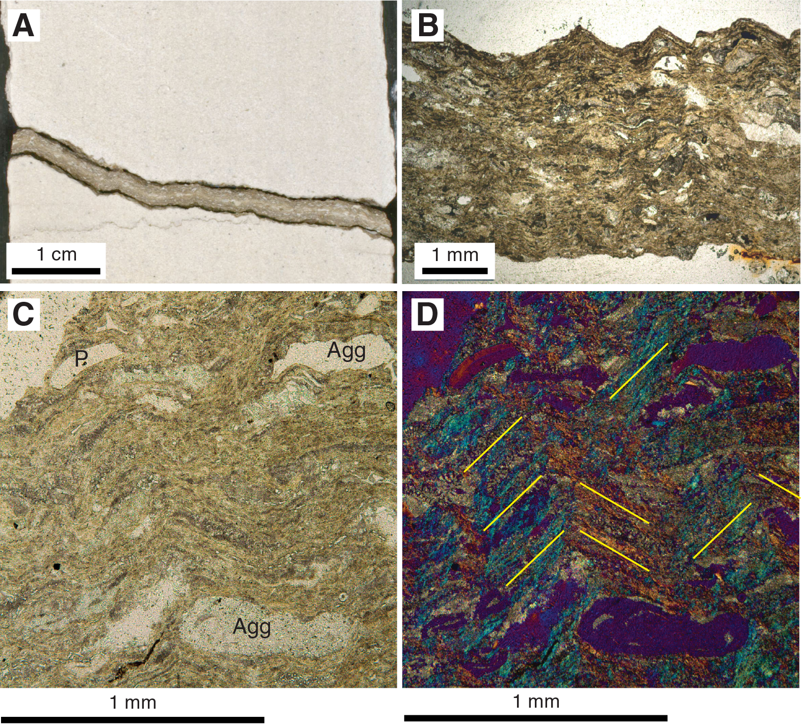
Figure F32. Thin, brownish crenulated mudstone lithology.
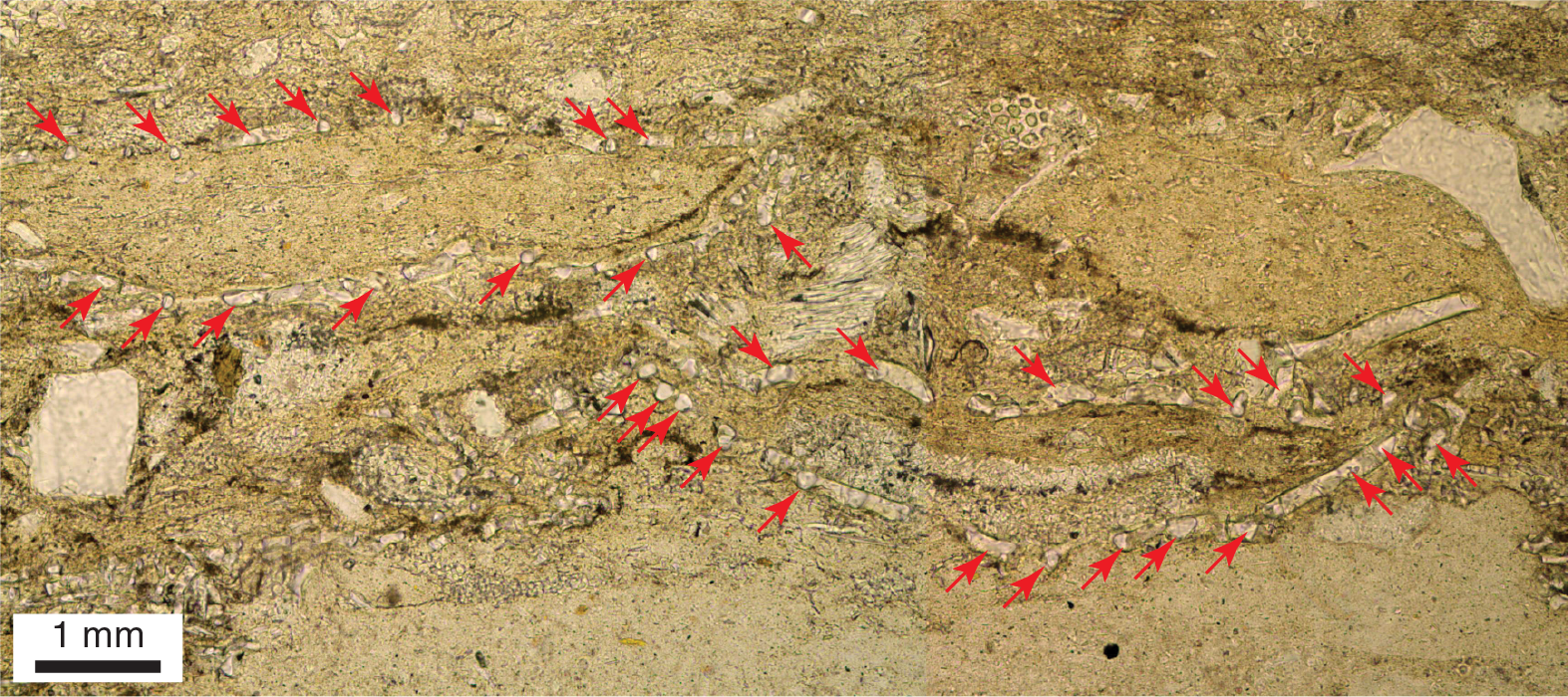
Figure F33. Biosiliceous fossils of uncertain affinity, likely cross-sections of partially crushed deep-marine sponges.
Eight very thin to thin, very pale brown to pinkish gray ash layers were observed from 1313 mbsf (Section 60R-4, 55 cm) to 1322 mbsf (Section 61R-3, 123 cm). The ash layers are as thick as 2 cm and show a planar to irregular, mostly horizontal basal contact, but because of drilling disturbance the lower and upper boundaries are less distinct than in Units I and II. Grain size ranges from very fine grained sand to silt, and only two layers show normal grading. All the ash layers are lithified and have experienced secondary cementation by calcite and/or zeolite.
With the exception of cementation in the calcareous oozes (chalks) and pebble conglomerates, diagenetic features in Subunit IIIB are difficult to detect macroscopically, or even with a light microscope. Evidence of homogeneous oxidation observed in the vivid color mottling of orange and brown mudstones (Figure F28) does not correspond to variation of lithologic components that can be detected in smear slides.
Unit IV
- Interval: 362-U1480G-61R-CC, 15 cm, to 64R-2, 130 cm
- Thickness: 22.62 m
- Depth: 1327.18–1349.80 mbsf
- Age: Late Cretaceous–late Paleocene
- Lithology: basaltic lava flows and volcaniclastic and tuffaceous sandstone, tuffaceous conglomerate, and volcanic breccia
The sediment in Unit IV (Figure F5; Table T3) is siliciclastic in composition and dominated by material of volcanic derivation. The top of Unit IV is composed of a lava flow that has breccia at the top showing a distinctive zone of greenish alteration in highly fractured glass in interval 362-U1480G-62R-1, 0–11 cm (1327.40–1327.50 mbsf) (Figures F34, F35). Three basaltic lava flows, 3.47 m in total thickness with centimeter-thick interlayered chalk, are distinctly brecciated at their top and base and more structureless in the center (Figure F34).
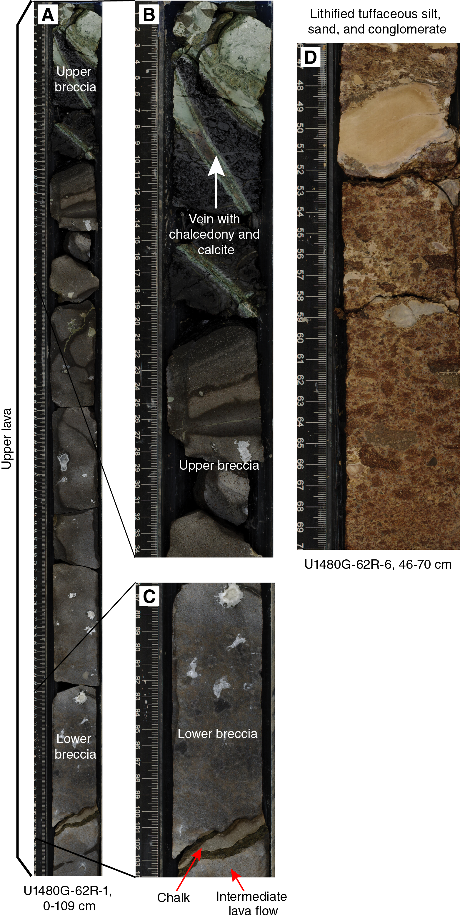
Figure F34. Basaltic lava-flow material and tuffaceous sandstone and conglomerate.

Figure F35. Vein in breccia, Hole U1480G.
Tuffaceous sandstone and conglomerate occur below the basaltic lava flows in Sections 62R-4 through the top of 63R-1 (1332.11–1337.26 mbsf) and contain a grain assemblage predominantly composed of vesicular silicified reddish brown glass shards (Figures F34, F36). A few of the grains are palagonized. These sandstones have some remaining intergranular pores, but most of the pore spaces are filled by rosettes of zeolite cement (Figure F36). In Sections 63R-1, 64R-1, and 64R-2 (1337.28–1349.80 mbsf), the reddish volcanic sandstone grades downward into a conglomerate containing a similar assemblage of silicified and palagonized vesicular glass shards but having a greenish color and cementation by chalcedony and fibrous carbonate. A minor lithology in Unit IV is thin layers of calcareous claystone from which nannofossil ages were obtained (see Biostratigraphy).
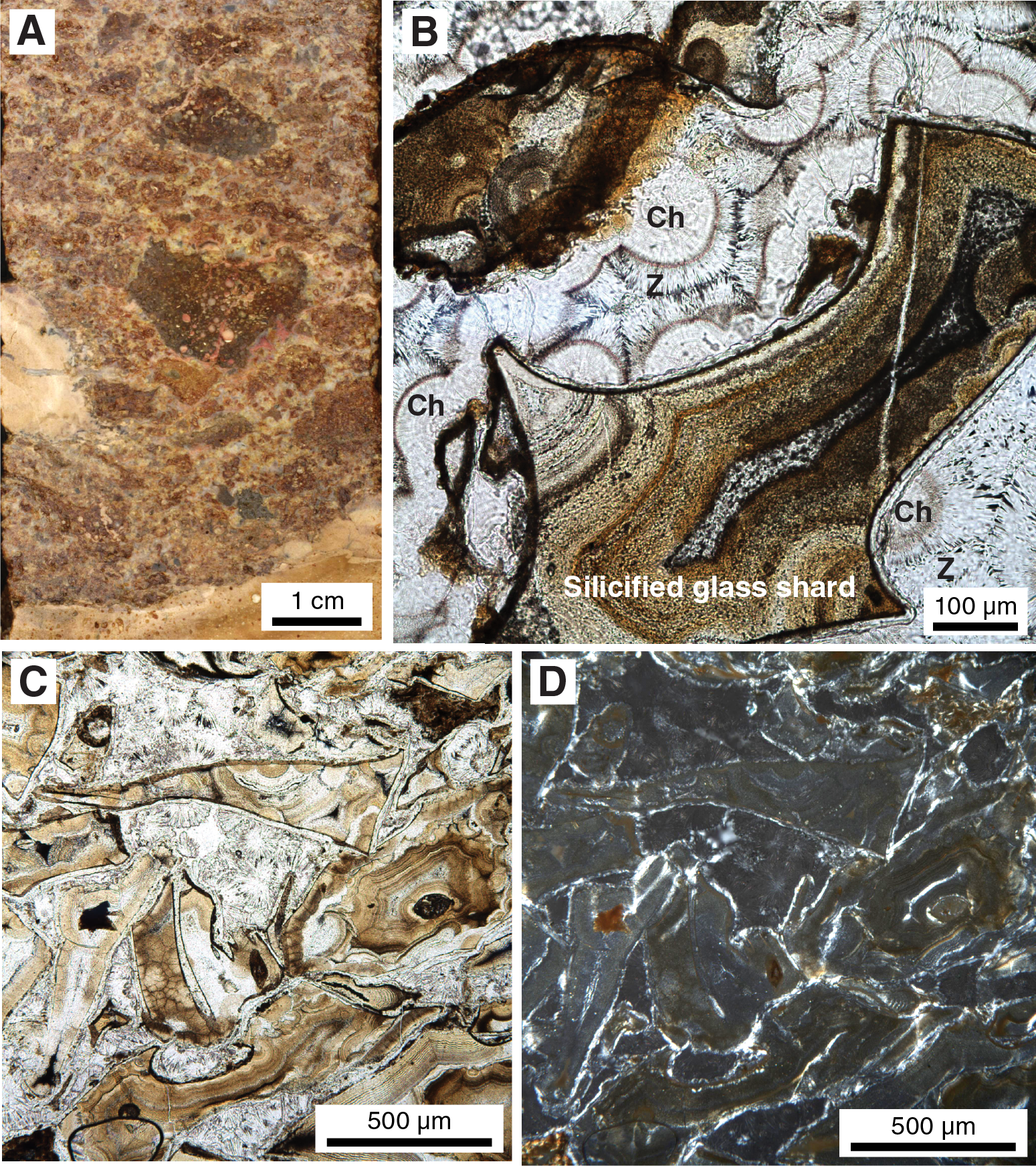
Figure F36. Tuffs, Hole U1480G.
The average XRD bulk mineralogy from two samples of zeolite-cemented tuffaceous sandstone is 68% total clay, 0.6% quartz, 29.9% feldspar, and 2% calcite (Table T2).
The mafic igneous rocks in this unit (interval 62R-1, 0 cm, to 62R-4, 100 cm; 1327.4–1322.11 mbsf) are meter-thick basaltic lava flows showing strong alteration including partial to complete replacement of minerals (e.g., plagioclase) and/or filling of intergranular pore space by carbonate and/or minor zeolite (Figure F37B). Some of the dissolution features and/or former vesicles remain unfilled. The basalt has a dominant intergranular texture (Figure F37A) and is composed of clinopyroxene and plagioclase, both strongly altered. The plagioclase crystals are mostly albitized, whereas the clinopyroxene crystals are replaced by Fe oxide or other opaque minerals and hydroxide and calcite. Typically, the Fe oxide or opaques are aligned along the cleavage of the mafic minerals. The alteration of this basalt flow suggests interaction with seawater and/or other interstitial fluids, leading to a hydrothermal (spilitization) process of the effusive rock.
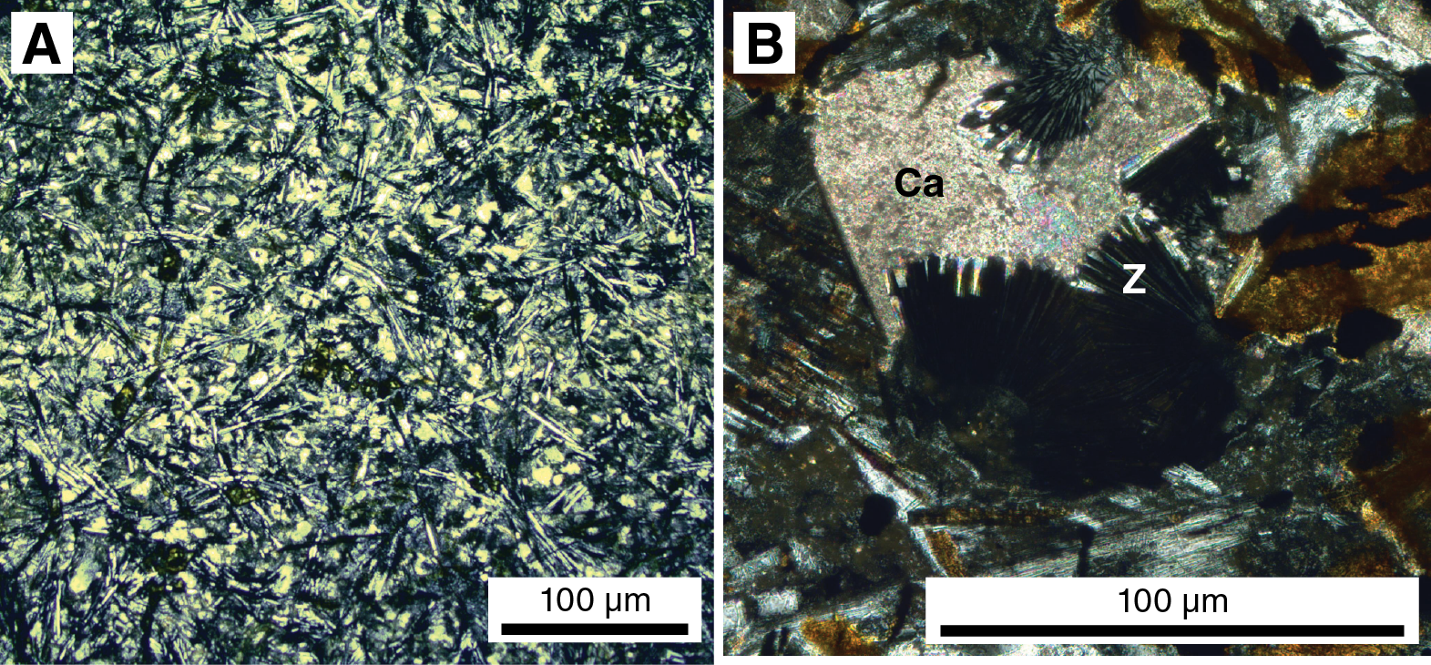
Figure F37. Basalt, Hole U1480G.
Unit V
- Interval: 362-U1480G-64R-2, 130 cm, to 71R-4, 5 cm
- Thickness: 65.55 m
- Depth: 1349.80–1415.35 mbsf
- Age: Late Cretaceous
- Lithology: bioturbated chalk and calcareous claystone with magmatic intrusion and extrusives
Unit V consists mainly of bioturbated chalk (Figure F38A) and calcareous claystone intercalated with a magmatic intrusion of intermediate composition (Figure F38B) and extrusives. This thick intrusion (>37.18 m) with chilled margins is observed between Sections 362-U1480G-65R-4, 32 cm, and 69R-5, 78 cm (1361.24–1398.69 mbsf) and shows several intervals of alternating finer and coarser grain size. Calcareous claystone at the upper and lower contacts of this intrusion is visibly altered adjacent to the chilled margins of the intrusion (Figure F39). Petrographic analysis of the hypabyssal intermediate rocks suggests classification as plagioclase-clinopyroxene-hornblende-biotite-opaque diorite with different degrees of alteration and ophitic texture composed of dominant plagioclase laths (Figure F40A–F40C). The alteration products are mostly chlorite, serpentine(?), and Fe oxide and hydroxide. Plagioclase laths show saussuritization, the alteration of calcium-rich plagioclase feldspar to a mineral assemblage including zoisite, chlorite, amphibole, and carbonate. Additionally, dark gray secondary alteration occurs along fractures cutting across the core (Figure F40D). The phenocrysts can reach up to 4 mm with a mean size of 0.5–1 mm. The matrix is formed of fine-grained plagioclase and mafic crystals with opaques, which are mostly altered to Fe oxide, Fe hydroxide, chlorite, serpentine (?), and carbonate.
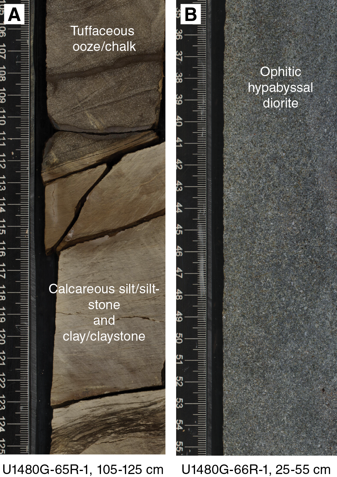
Figure F38. Typical reddish brown tuffaceous chalk and ophitic hypabyssal diorite.
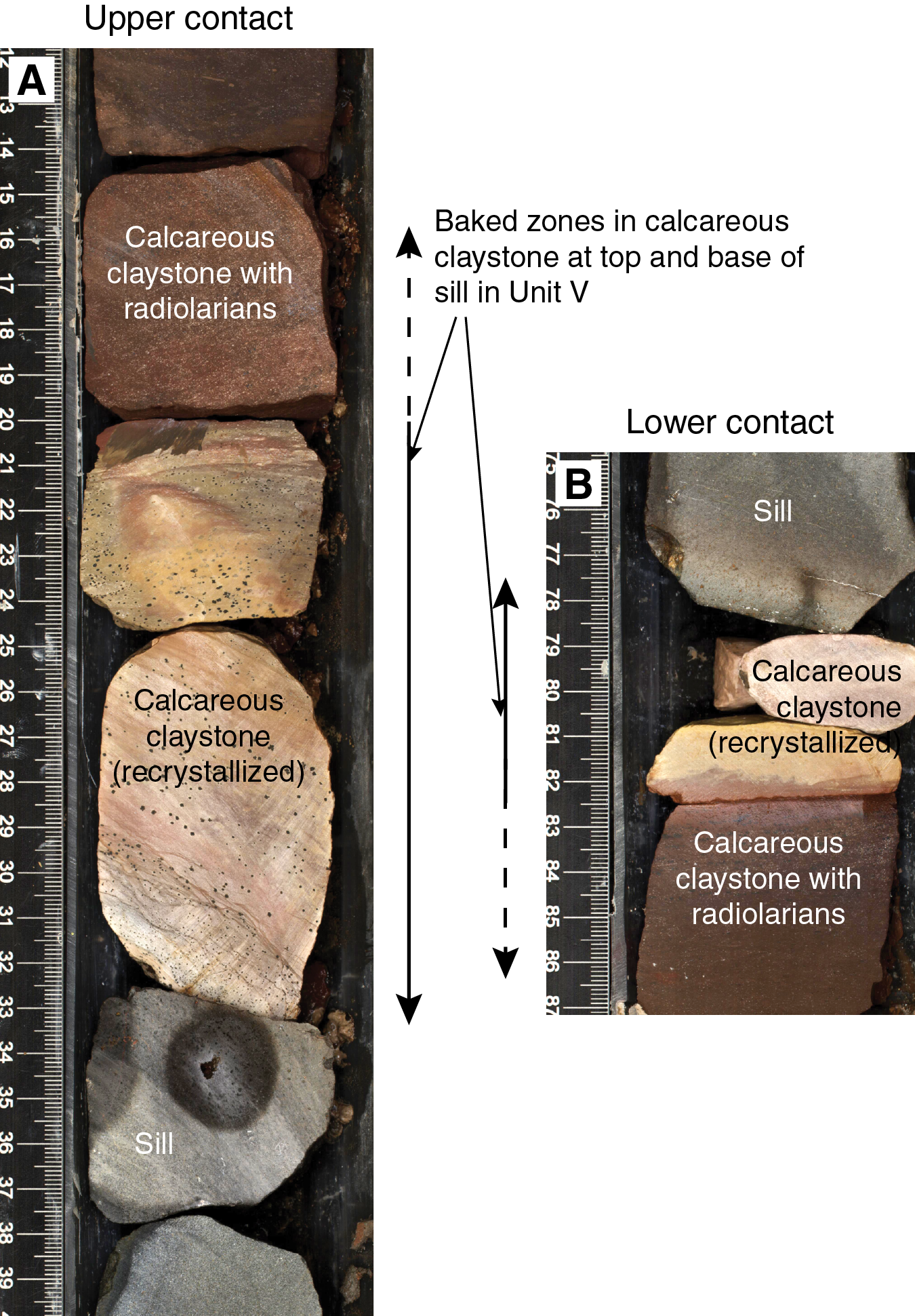
Figure F39. Baked contacts in calcareous mudstone.
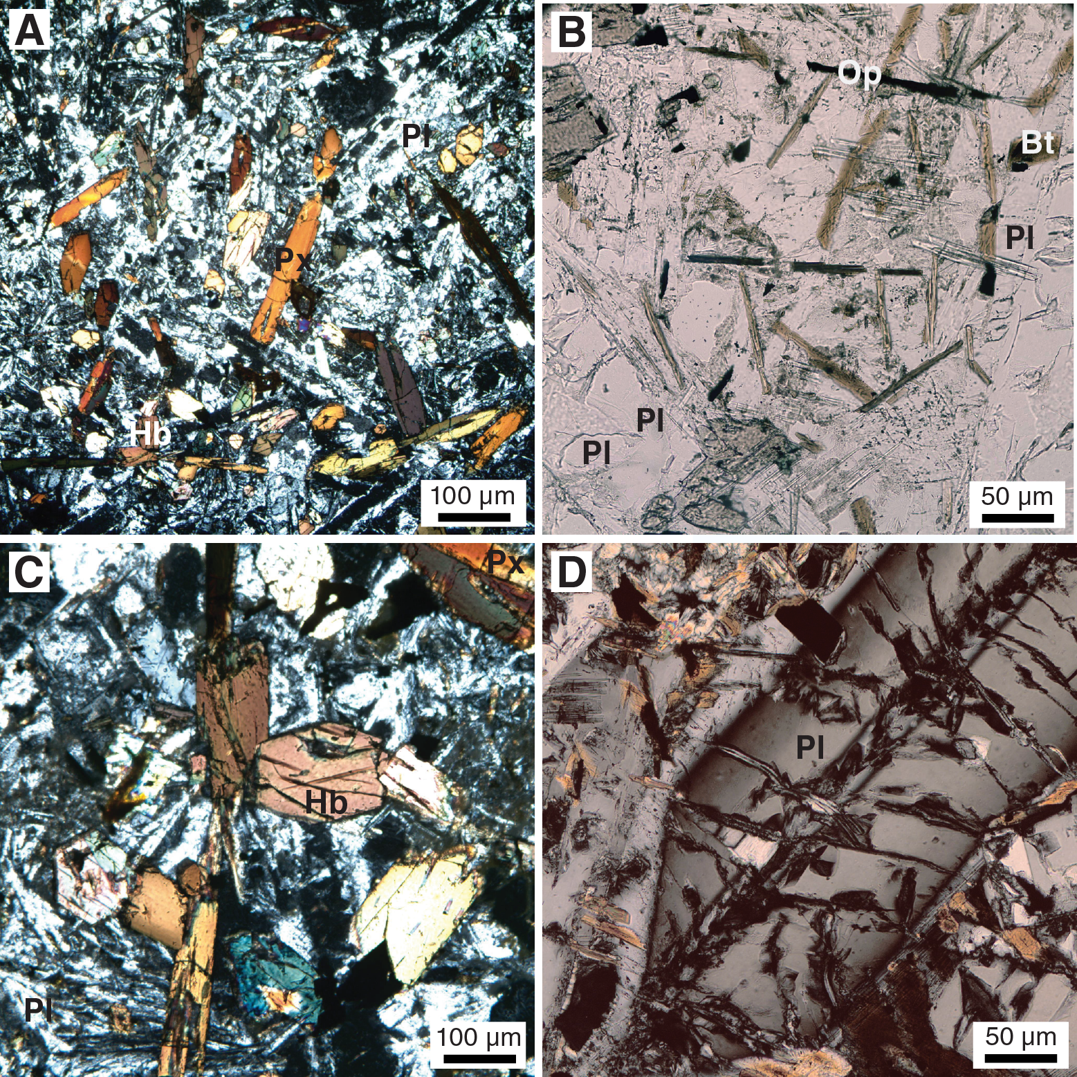
Figure F40. Ophitic textures, Hole U1480G.
Intergranular pore space (caused by dissolved igneous minerals) is filled with radiaxial calcite and microquartz and/or zeolite in at least two phases of hydrothermal crystallization (presumably associated with seawater interaction) (Figure F41A); in some cases it is associated with chlorite as a fine-grained agglomerate or as aligned crystals (Figure F41B). In thin section, Samples 68R-2, 59–61 cm, and 67R-9, 5–7 cm, show millimeter-thick veins filled by calcite and calcite plus microquartz (or opal), which can also be found throughout the entire intrusive body.
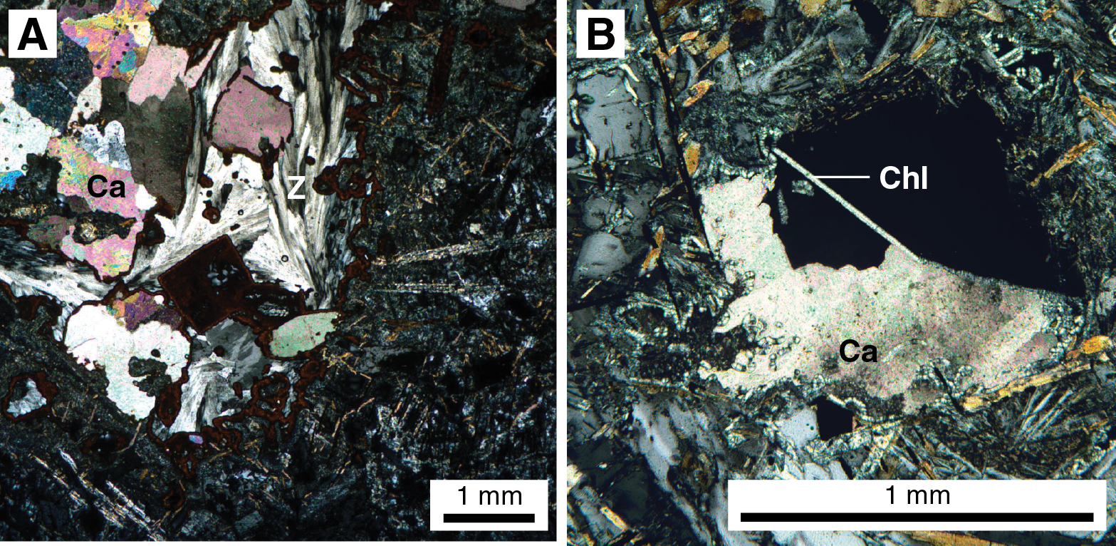
Figure F41. Vein fillings, Hole U1480G.
Below the intrusion, in Cores 69R and 70R, the light brown chalk is bioturbated with many discrete trace fossils (Figure F42). Near the top of Section 71R-3, 30 cm, an upper extrusion from the basaltic basement is encountered (1414.79–1415.29 mbsf). The lowest sedimentary rock at Site U1480 (chalk) is found in interval 71R-4, 0–5 cm (1415.29–1415.34 mbsf).
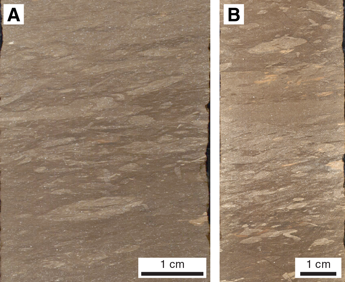
Figure F42. Bioturbation structures in calcareous claystone.
The average XRD bulk mineralogy from 11 chalk samples shows 7% total clay, 0.2% quartz, 1% feldspar, and 91% calcite (Table T2).
Unit VI
- Interval: 362-U1480G-71R-4, 6 cm, to 73R-CC, 12 cm
- Thickness: >16.28 m
- Depth: 1415.35–1431.63 mbsf
- Age: Late Cretaceous
- Lithology: basaltic basement
Unit VI comprises basaltic basement (Figure F5; Table T3). Igneous basement was recovered in Sections 362-U1480G-71R-4, 6 cm (1415.35 mbsf), through 73R-CC, 12 cm, with drilling termination at 1431.63 mbsf. The basement consists of fine- to medium-grained plagioclase- and pyroxene-bearing seriate-textured basalt with low vesicle content (<1%). An overall moderate to high alteration state is indicated by a brownish color and the occurrence of several mineral-filled fractures (Figure F43).
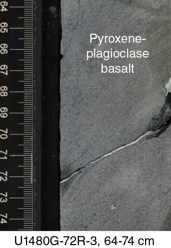
Figure F43. Basement represented by pyroxene-plagioclase–bearing basalt.
The basement rock is plagioclase-pyroxene–bearing basalt with intersertal texture. The phenocryst assemblage includes plagioclase (51%–57%), clinopyroxene (26%–30%), and opaques (3%–7%) distributed in a microcrystalline groundmass (10%) (Figure F44). The groundmass consists of opaques and secondary alteration minerals (predominantly chlorite), probably representing altered glass. Locally, some vesicles or holes are filled with dark green material (possible clay minerals). The alteration is moderate in these rocks, with some saussuritization of plagioclase and pyroxene altered to chlorite. Overall, the recovered basaltic basement contains common black and white calcite/zeolite veins.
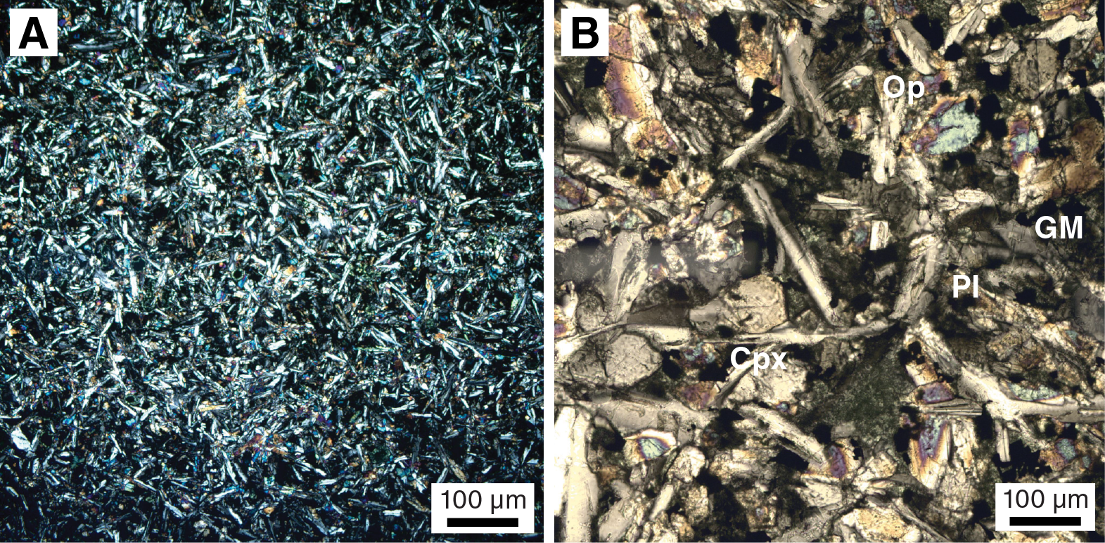
Figure F44. Basaltic basement with interstitial texture of augite-plagioclase basalt.
Ash petrology
An important minor component of Units I–II and parts of Units III–V is vitric ash (Figure F45). Ash is dispersed in the background sediment and also appears as discrete ash layers. The entire drilled succession includes 33 discrete layers of volcanic ash, mainly derived from air fall, but also potentially by a variety of bottom-reworking processes (e.g., SGFs). Textures and vesicles of pyroclasts vary between the ash layers. Using appearance and texture, some of the ash layers in Unit I can be correlated between Holes U1480A, U1480B, U1480C, U1480E, and U1480H. Typically, ash layers are pale pinkish to dark pinkish gray and are restricted mainly to Unit I and the uppermost part of Unit II, but are also present in Units III and IV (Figure F5). Coring commonly displaces ash layers, especially where they are thick and coarser grained. Where ash remained intact, and in some larger displaced pods, the ash layers/pods have a sharp basal contact with underlying deep-marine sediment and, in many cases, show normal grading and display a several-centimeter-thick gradual transition into the overlying sediment (Figure F45). Within Units I and II, the middle part of very thick ash layers is commonly disturbed by fluidization linked to coring and sediment-retrieval processes.

Figure F45. Ash layer, Hole U1480G.
Average grain size in ash layers ranges from silt to medium-grained sand; the coarsest grain size is typically represented by phenocrysts. In contrast to the background sediment, the structureless ash layers are generally nonbioturbated or weakly bioturbated. Because of fluid-sediment interactions, some ash layers in Units I and II are slightly lithified at the basal contact with underlying sediment and show a color change (e.g., Figure F12), probably reflecting precipitation of silicate or carbonate minerals derived from alteration of the ash. Unconformable and/or inclined bedding of ash is interpreted as drilling disturbance, but erosion, creep, or sediment slumping cannot be discounted. In Unit III, pinkish gray to dark gray ash layers are finer grained, mostly lithified, and commonly show signs of zeolitization. Reddish brown tuffaceous sandstone in Unit IV is composed mainly of strongly altered, palagonized glass shards and pumiceous fragments partially devitrified to chert and cemented by zeolite. These sandstones may represent tuffaceous deposits from proximal pyroclastic sediment gravity flows.
Ash layers were characterized on the basis of the relative abundance of phenocrysts, glass shard colors, textures, and vesicles (Figure F46). The felsic ash layers of Unit I and Subunit IIA are dominated by fresh, colorless volcanic glass with rare but persistent occurrences of plagioclase and biotite, as well as variable amounts of quartz, amphibole, pyroxene, and traces of allanite. Mineral content in the ash beds is highly variable from mineral poor (<2 vol%) to mineral rich (up to 10 vol%). Crystal-rich zones occur particularly at the base of coarse ash beds, suggesting normal density grading. Some of the ash layers contain small amounts of clay and fossil debris (up to 10 vol%). Overall, the ashes in Unit I and Subunit IIA contain glass shards characterized by mainly dense, blocky, and commonly cuspate shards, together with common to abundant tubular-vesicular pumiceous clasts (Figure F46). Round and elliptical vesicles are rare. In contrast, the lithified ash layers (tuffs) in Unit III are slightly to strongly altered (devitrified), and zeolite is commonly observed in smear slides. Overall, the moderately crystal rich tuffs contain common to rare feldspar and quartz, as well as rare to trace amounts of amphibole and biotite. Biogenic constituents, mostly calcareous nannofossils and some radiolarians and diatom fragments, together with authigenic calcite and clay, are commonly intermixed. The tuffs are predominantly composed of low-vesicular, dense, blocky, and cuspate glass shards together with some rare pumiceous clasts that have some elongate and round gas bubbles. The occurrence of mainly transparent, small, dense, blocky glass shards is consistent with a volcanic origin in a submarine environment or emplacement very distal from a source, in both cases of felsic composition.
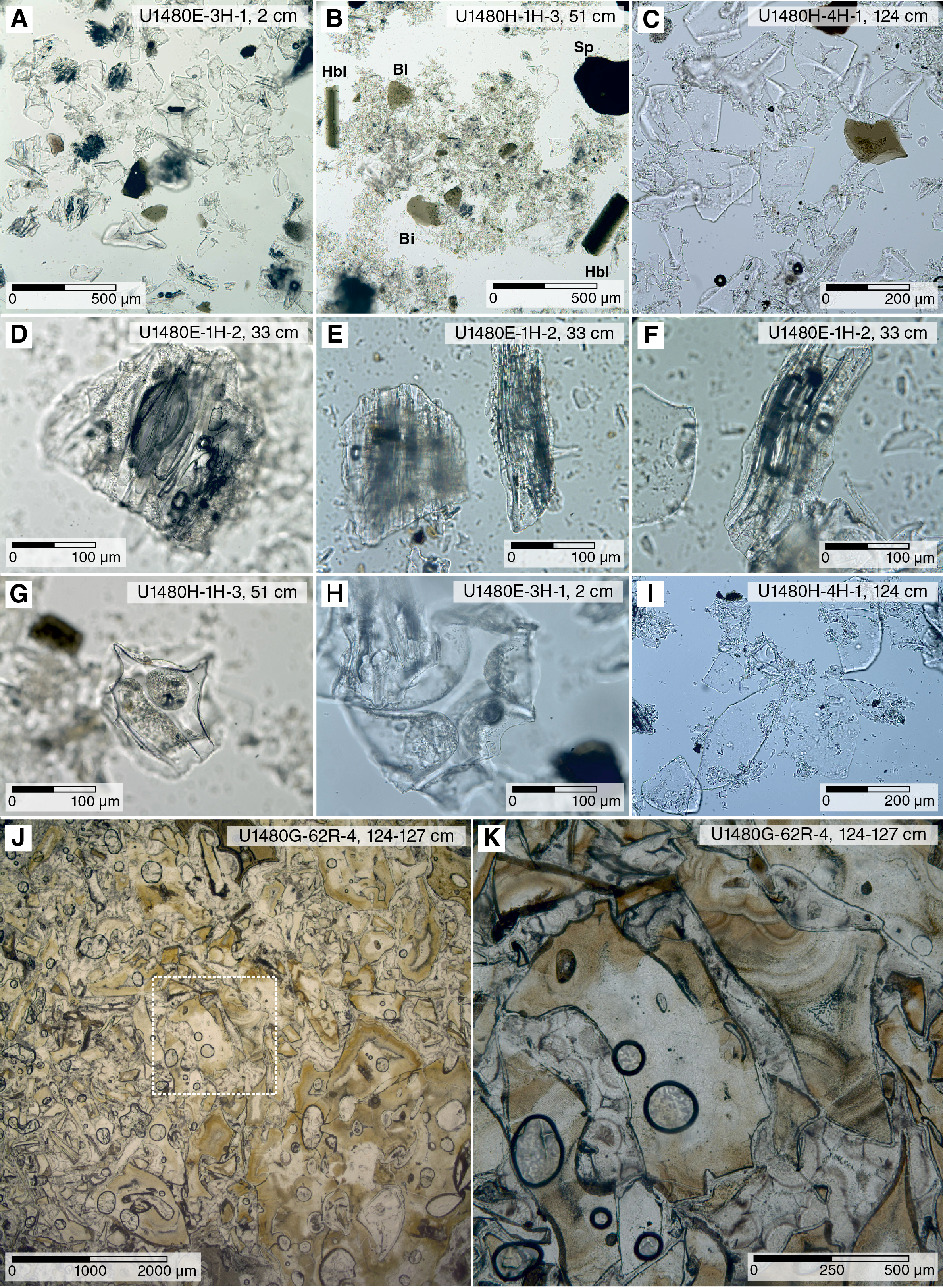
Figure F46. Examples of textures and vesicles of pyroclasts in smear slides and thin sections of ash layers.
Tuffaceous zeolite–cemented sandstones and conglomerates in Unit IV (Sections 362-U1480G-62R-4 through the top of 63R-1; 1332.11–1337.26 mbsf) are characterized by brownish mafic glass shards that are strongly altered to palagonite and chert from the rim to the center of the clasts (Figure F46). The tuffs are mineral poor (<1 vol%) but contain rare amounts of volcanic lithic fragments. Rare to trace amounts of calcareous nannofossils and planktonic foraminifers are mixed into the ash layers. The tuffaceous sandstone is predominantly made up of dense, blocky, and cuspate glass shards with moderate vesicularity and mostly round and rare elliptical gas bubbles. A minor amount of moderately vesicular pumiceous clasts have common round to elongate bubbles (e.g., thin sections 62R-4, 124–127 cm, and 62R-6, 14–17 cm). The grain size and more mafic appearance of the tuffaceous sandstones, as well as the position near basement and the presence of intercalated basalt flows, all suggest an origin related to the igneous units of the basement.
Interpretation of lithostratigraphic units
The overall succession consists of predominantly siliciclastic sediments interpreted as Nicobar Fan underlain by mixed tuffaceous and pelagic sediments and intervals of intercalated pelagic and igneous material overlying oceanic crust. Figure F47 is a schematic depositional model for a large mud-rich submarine fan, such as the Bengal-Nicobar Fan, showing the range of sedimentary environments interpreted from the sediment recovered at Site U1480 (boxed area).
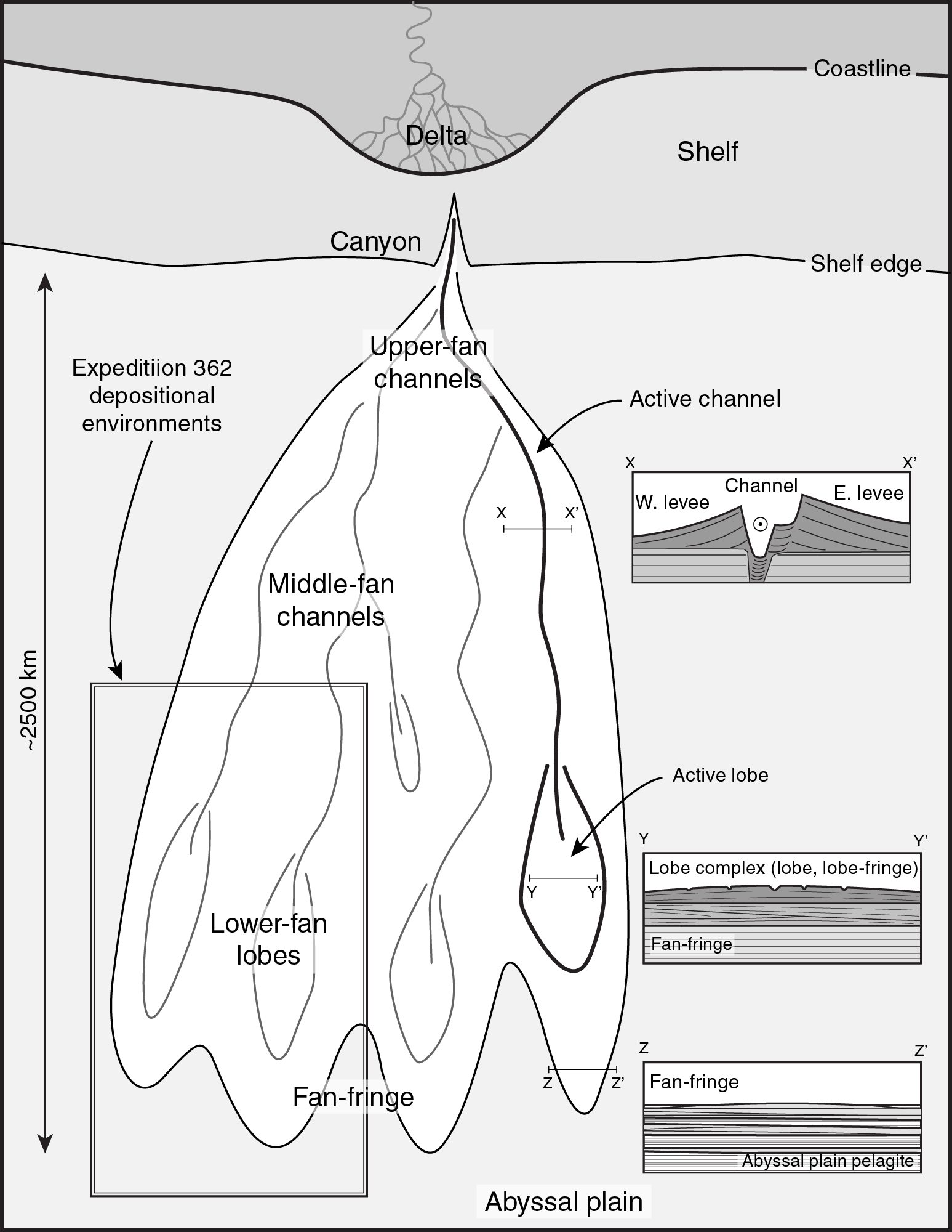
Figure F47. Schematic depositional model for a large mud-rich submarine fan system.
The broad lithostratigraphic interpretation of Site U1480 divides the succession into a mainly siliciclastic interval of mud and sand of the Nicobar Fan (Units I–II) and an underlying and older pelagic/hemipelagic-dominated succession that comprises both siliciclastic and carbonate mud/mudstone containing a substantial component of volcanic ash (Units III–V). Sediment accumulation rates for the Nicobar Fan are relatively high, especially when compared with the prefan Units III–V (i.e., for the Nicobar Fan they are up to two orders of magnitude higher than rates interpreted for pelagic Units III–V) (Figures F82, F83, F84). The lower and older succession of slowly accumulated material also includes chalk, siltstone, sandstone, and conglomerate of essentially local derivation, reflecting erosional processes that generated sediment from semilithified to lithified pelagic mud/mudstone and seafloor-exposed and highly altered basement material. The rocks of Units IV and V include basalt flows and a diorite magmatic intrusion.
Drilling at Site U1480 has shown that the Nicobar Fan is unexpectedly thick and young (~10 Ma). Subunits IIA–IIC represent contrasting stages of fan development, from fan initiation represented by distal mud-rich deposits at the base of Subunit IIC through a period of rapid construction of stacked SGF deposits (e.g., turbidites and debrites). The various stages of fan development are evidenced by alternating deposits of likely fan-fringe, lobe, and lobe-fringe deposits in “lobe complexes” locally cut by channel-levee-overbank complexes to a later stage of fan abandonment with a middle interval (Subunit IB) of levee-overbank sediment interpreted to originate from a channel ~20 km east of Site U1480 (Figure F1). The low core recovery in Unit II, together with a lack of high-quality downhole logs to make detailed ties to regional seismic data, precludes the confident recognition of discrete lobe, channel, and related fan environments in Subunits IIA–IIC. The evolution of the Nicobar Fan (including the significant sediment accumulation rates), its stratigraphic context within the Indian Ocean and environs, the provenance of the Nicobar Fan sands, and links to exhumation and erosion in the Himalaya-Tibetan Plateau are addressed in McNeill et al. (2017a).
Subunit IA is interpreted as fan abandonment potentially related to late Pleistocene to Recent glacio-eustatic rise in sea level and/or tectonic blocking of any northerly derived sediment routing to the Nicobar Fan by the Ninetyeast Ridge as it collided with the Sunda subduction zone (figures 12A–E in Curray, 2014). Based on sidescan sonar and seismic images, Subunit IB is interpreted as levee-overbank sediment from the submarine channel ~10 km east of Site U1480 (Figure F1). Subunit IC appears to represent an earlier phase of fan abandonment. We speculate that during the deposition of Subunit IB, a submarine channel and its associated levee-overbank system, similar to that observed at the present seafloor (Figure F1) (Geersen et al., 2015; Jena et al., 2016), cut through the Ninetyeast Ridge to reestablish the channelized connection between the northerly sediment source and the Nicobar Fan. Below Subunit IC, Unit II represents deposition on the Nicobar Fan (Figure F46). Overall, Subunits IIA and IIB represent establishment of a thick and broadly middle- and lower-fan succession above relatively distal fan-fringe deposits of Subunit IIC, although Subunit IIC includes local channel and related deposits developed during phases of fan progradation (Figure F47). Much of the fan sediments were supplied by various SGFs from the north. Overall, Subunit IIB is interpreted as relatively more distal fan environments than those in Subunit IIA and includes undifferentiated submarine lobe, lobe-fringe, and fan-fringe deposits but predominantly lobe-fringe and fan-fringe deposits and channel and related deposits. Subunit IIC, with its black and gray muddy SGF deposits, rich in plant debris and containing many intervals with low to moderate bioturbation intensity, is interpreted as generally distal-fan, fine-grained sediments (e.g., lobe, lobe-fringe, and fan-fringe environments) that probably accumulated in bottom waters with low oxygen levels, at least in the vicinity of Site U1480.
The predominant lithology in Unit II is siliciclastic and composed of normally graded to structureless intervals of mica-rich quartzofeldspathic fine-grained sand, silt, and clay of varying thickness (e.g., turbidites and debrites). The observed mineralogical assemblage is characteristic of sediments found in Himalayan rivers (Garzanti et al., 2004). Sandy intervals are generally separated by hemipelagic and pelagic intervals (mottled calcareous clays and calcareous oozes) and some glassy volcanic ash layers. Lithologic differences between siliciclastic units and variations in grain size and bed thickness reflect cycles of increased or decreased SGF activity to construct channel-levee-overbank, lobe, lobe-fringe, and fan-fringe deposits. Bioturbated calcareous clay likely represents times of relative fan inactivity at Site U1480 and hence reduced deposition of terrigenous material.
Overall, siliciclastic units (silt, clay, and sand) at Site U1480 are compositionally classified as mica rich (muscovite and biotite) and quartzofeldspathic. Feldspars and heavy minerals (e.g., amphibole, garnet, clinozoisite, zoisite, tourmaline, zircon, rutile, epidote, sillimanite, chloritoid, pyroxene, staurolite, and opaque minerals) are common in silt- and sand-rich layers and may contain euhedral carbonate minerals and carbonate aggregate grains. Lithic fragments of largely metamorphic affinity appear in the sand. The grain assemblage is consistent with a general provenance from Himalayan river sands (e.g., Garzanti et al., 2004; McNeill et al., 2017a). Thus, the provenance of the Nicobar Fan sediments, in common with those of the adjacent Bengal Fan (Curray and Moore, 1974; Cochran, Stow, et al., 1989; Stow et al., 1990; Curray et al., 2003; Curray, 2014; France-Lanord et al., 2016; McNeill et al., 2017a), is almost exclusively continental, with a large volume of quartzofeldspathic material juxtaposed along the Sunda subduction margin.
A summary of the bulk mineralogic composition from XRD analysis of sediment at Site U1480 is shown in Figure F48 (see also Figure F6; Table T2), highlighting the intervals of sand versus mud (sandstone versus mudstone).
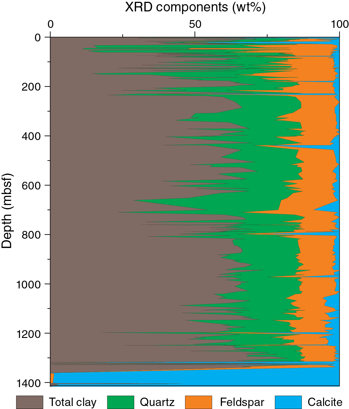
Figure F48. Summary of the bulk mineralogic composition from XRD analysis.
Quartzofeldspathic sand and silt of compositions of Unit II will be prone to quartz cementation at higher temperatures (>80°C) (Walderhaug, 1996; Lander and Walderhaug, 1999), suggesting the potential for generation of strong mechanical rock properties in response to burial heating. Thus, rock property evolution of the relatively unreactive continental grain assemblage in the input materials of the northern Sunda subduction zone may be attributed mainly to thermally driven reactions rather than early cementation of unstable grains of marine or volcanic derivation.
The 160 m of pelagic/hemipelagic-dominated sediment below the Nicobar Fan succession (~11% of the total sediment thickness at Site U1480) includes a diverse lithologic assemblage of siliciclastic mud/mudstone, siliciclastic sand/sandstone and conglomerate, and carbonate mud/mudstone, all containing a substantial component of volcanic ash (Units III–V). In addition to the pelagic and hemipelagic components, there are coarser grained rocks (semilithified and lithified silt, sand, and gravel) with grain assemblages of essentially local derivation (such as from parts of the Ninetyeast Ridge). These coarser materials reflect erosional processes that generated sediment from previously deposited pelagic mud/mudstone and/or highly altered extrusive and intrusive rocks then exposed at the seafloor. Within Unit IV, sediments are overlain by basalt flows. Sediments in Unit V are intruded by diorites, further denoting materials and processes unlike those observed in the Nicobar Fan.
Petrologic features in Units III–V reflect sediment accumulation rates that are as much as two orders of magnitude or more lower than rates for the overlying fan (see Biostratigraphy). The Unit II/III boundary represents a transition downhole into a nearly sand/sandstone-free, mud/mudstone-dominated, pelagic/hemipelagic succession with a diverse range of trace fossils and agglutinated foraminifers. This lithologic shift represents an increased level of syndepositional reworking that contrasts with that of the mud/mudstone in the overlying fan.
Clay content increases progressively downhole through Subunit IIIA, possibly related to increased admixtures of glass content and the formation of smectite during seafloor exposure under slow sediment accumulation. Higher P-wave velocities and shifts in several other physical properties (see Physical properties) likely reflect these changes in composition and early diagenesis under conditions of slower sediment accumulation. Subunit IIIB displays pervasive (nonconcretionary) cementation in some lithologies and a greater degree of ash alteration, again representing the impact of slower sediment accumulation. Grain assemblages in Subunit IIIB sandstone and conglomerate appear to reflect recycling of locally higher topography basement material with a different thermal history (from petrological observation; similar to or derived from Units IV and V). Glauconite and certain biogenic components (e.g., fish bones and teeth, encrusting biota, and possible microbial mats) provide further supportive evidence for condensation of the sedimentary record near basement and/or a hiatus (see Biostratigraphy). These “condensed sediments” are reminiscent of the classic so-called “red clays” found, for example, throughout the North Pacific Ocean.
Mineral alteration (e.g., macroquartz filling of vugs and zeolite cementation) of the basalt flow and volcanogenic (tuffaceous) sandstone and conglomerate in Unit IV suggests reactions at somewhat elevated temperatures (~80°–100°C). Whereas Unit III contains readily identified minor biosilica and an abundance of highly altered volcanic glass in the form of palagonite, Units IV and V contain less evidence of biosilica and former volcanic glass. It is uncertain whether this contrasting thermal history relates to a period of burial or local circulation of hot fluids near the seafloor, but it seems likely that the boundary between Units III and IV represents not only a contrast in composition but also a difference in burial and fluid-flow history. Combined with the above-cited evidence for reworking of Unit IV, it is possible that the Unit III/IV boundary with its conglomerates represents an erosional unconformity. Unit V contains no preserved volcanic glass but does contain well-preserved nannofossils that can be dispersed for smear slide preparation. Thus, hydrothermal alteration approaching metamorphic conditions is not indicated. The underlying basement (Unit VI) also displays evidence for substantial fluid-rock interaction but contains authigenic minerals such as quartz, chalcedony, calcite, palagonite, and chlorite, consistent with diagenetic temperatures.
Structural geology
We made observations of both natural and drilling-induced deformation features in the cores recovered at this site. Our workflow also included an evaluation of drilling parameters (see Drilling conditions) and their impact on core recovery and drilling-induced deformation. Compilation of observations and interpretations across all aspects of core deformation leads us to a qualitative inference of relative strength in the drilled section following a workflow defined in Structural geology in the Expedition 362 methods chapter (McNeill et al., 2017b).
The reflection seismic data show that Site U1480 is located away from steeply dipping faults with normal apparent offset that cut the Indian plate sedimentary sequence and in some instances develop fault scarps on the seafloor (e.g., Geersen et al., 2015). The tectonic structures observed and described in cores confirm that Site U1480 failed to intersect any major faults. Mesoscale normal faults (<1 mm thick and with displacements of a few millimeters to 2 cm) are mostly present in the deeper part of the drilled section, supporting the overall extensional nature of the deformation as shown in the seismic reflection lines. However, the timing of faults observed in the cores may be earlier than the seismically imaged faults.
Observed structures
Cores at Site U1480 consist of sediments and sedimentary rocks to ~1415 mbsf, including a minor magmatic intrusion and extrusives at the base, overlying basaltic crustal basement. Bedding orientations in the core coordinate system (see Structural geology in the Expedition 362 methods chapter [McNeill et al., 2017b]) were measured routinely in the core working-half sections. Bedding is generally subhorizontal (<5°–10°) with some exceptions that have a much larger dip angle and are interpreted to be related to slumping (Figure F49). Average dip angle increases with burial depth, but dips become more scattered and near-horizontal measurements persist with depth. According to the abundance of natural faults observed in the cores, we recognize two structural domains in the sedimentary sequence: (1) Domain I, from 0 to 1280 mbsf, corresponds to the terrigenous and hemipelagic sequence of the Nicobar submarine fan system (lithostratigraphic Units I and II), where there are few, mostly synsedimentary, natural faults; and (2) Domain II, from 1280 to 1414.4 mbsf, where there are numerous natural normal faults, some pervasively cutting through the pelagic units (lithostratigraphic Units III–V) (Figure F50). Soft-sediment deformation structures, such as faults, sand or mud injections, slump folds, deformation bands, and sediment-filled veins (interpreted as vein structures) are also present in Domain II.
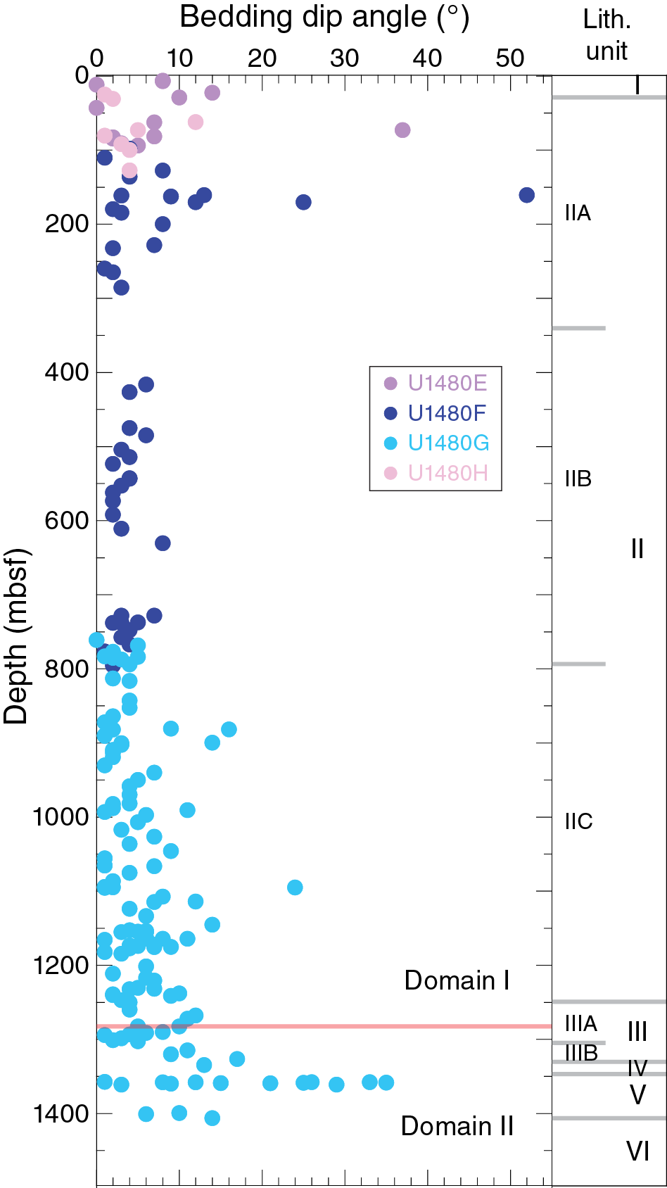
Figure F49. Bedding dip angles.
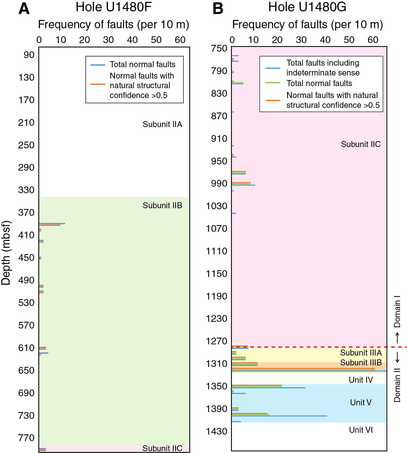
Figure F50. Frequency of observed faults.
Deformation in the igneous rocks of Units IV–VI is manifested by veins infilled by calcite, quartz, palagonite(?), chlorite, or zeolite that might be closely related to hydrothermal activity.
Domain I
In the upper part of Domain I (0–1280 mbsf), bedding is horizontal to subhorizontal. Three isolated exceptions where bedding dip angle is >10° were observed (Figure F49). These observations are interpreted as a result of submarine slumping, as they are discordant to the dips in adjacent cores, although some component of dip may be related to drilling operations (see Drilling-induced structures). Toward the bottom of Domain I, bedding dips >10° occur more often than in the shallower part of Domain I.
We observed the first natural fault in Core 362-U1480F-55X (391.5 mbsf), and additional faults were observed in a cluster downhole to 400.3 mbsf. This interval (391.5–400.3 mbsf) represents the highest concentration of faults observed in cores from Holes U1480E and U1480F (Figure F50). All of these observed faults are minor with apparent offsets of 2–10 mm; most display normal offset, but the displacement vector, and often the magnitude of displacement, remains unresolved. These faults commonly have a planar to listric shape (Figure F51), and they preferentially occur in thin-bedded sand intervals. Our observations suggest that some of these faults are probably synsedimentary (Figure F51B), in agreement with the high deposition–rate sedimentary environment. However, on an individual fault basis there are no textures that preclude faulting below the seafloor. For example, some faults occur simultaneously with bedding-parallel deformation bands (Figure F51A) that are interpreted to be related to compaction at a shallow depth (compared to the current depth of faults in Core 362-U1480F-55X at 392 mbsf).
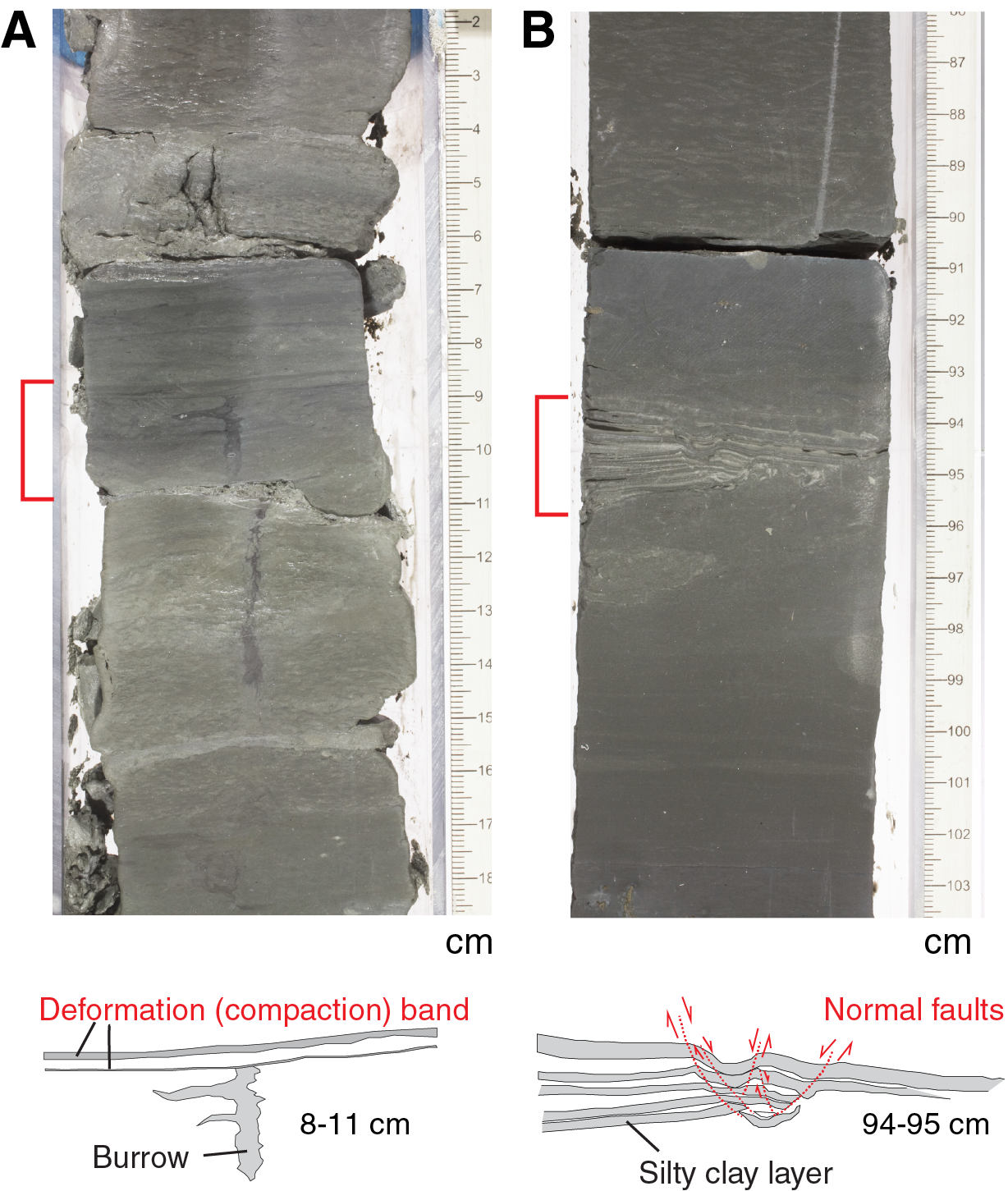
Figure F51. Minor synsedimentary faults and deformation bands.
A common deformation structure in Domain I involves sand and mud injection into overlying sediments (Figure F52). The close occurrence of sand and mud injections (within 70 cm of one another) suggests that sediment mobilization can be caused by fluid overpressure in sand or alternatively by a density contrast in which sand settles into mud layers.

Figure F52. Sand and clay injections and soft-sediment deformation structures.
A set of roughly spaced sediment-filled veinlets in clay beds are identified as vein structures (e.g., Shipboard Scientific Party, 1988) in the 1048.2–1048.5 mbsf interval (Figure F53). These vein structures are nearly perpendicular to bedding and confined to clay beds. Each vein is <2 mm thick, straight or curved, and may bifurcate at the ends. An interval of scaly fabric ~5 cm thick was observed in Cores 362-U1480F-94X and 362-U1480G-4R. Because these features are so rare, we interpret these occurrences within the same stratigraphic interval in both cores and propose these parallel occurrences as a stratigraphic correlation marker.
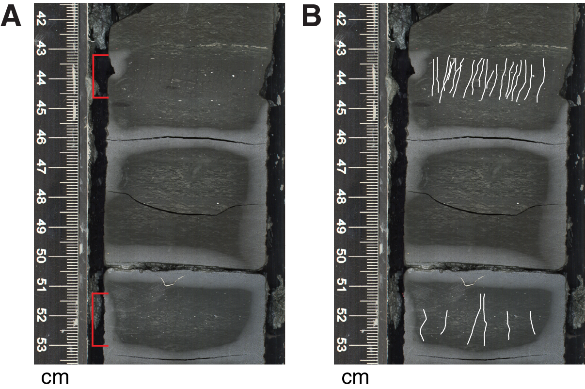
Figure F53. Vein structure: thin, black, small fractures aligned parallel to depth.
Domain II
Domain II (1280.0–1414.4 mbsf) is characterized by an abrupt increase in faults (Figure F50) over a >120 m depth interval, mostly with a normal offset in the split core surface (Figure F54). These faults form an anastomosing network with each surface <1 mm thick and with displacements of a few millimeters to 2 cm, and they are developed through the entire width of the core. The faults are commonly observed in silty clay beds. Synsedimentary faults related to slumps are still present in Domain II, but they are less common than in Domain I. Bedding dips range from 0° to 10°, but values up to 20° are also present (Figure F49). A few recumbent folds together with bed disruption are most likely related to mass-wasting processes that can account for some of these high bedding dip values (Figure F55). Other structures, such as sand injections and sediment-filled veinlets, are still present (Figure F56).
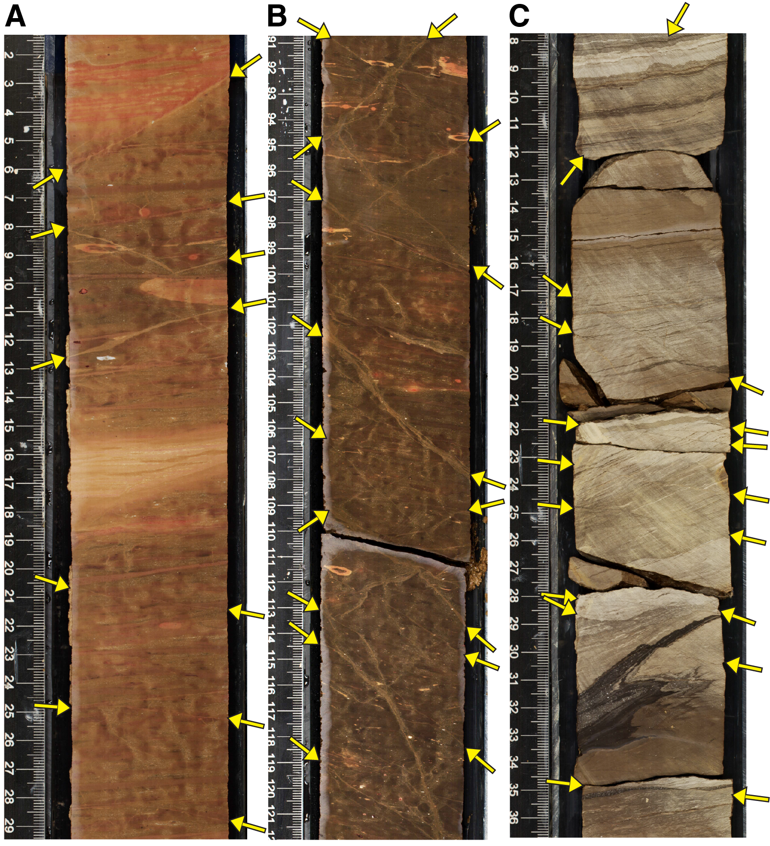
Figure F54. Pelagic section with abundant normal faults.
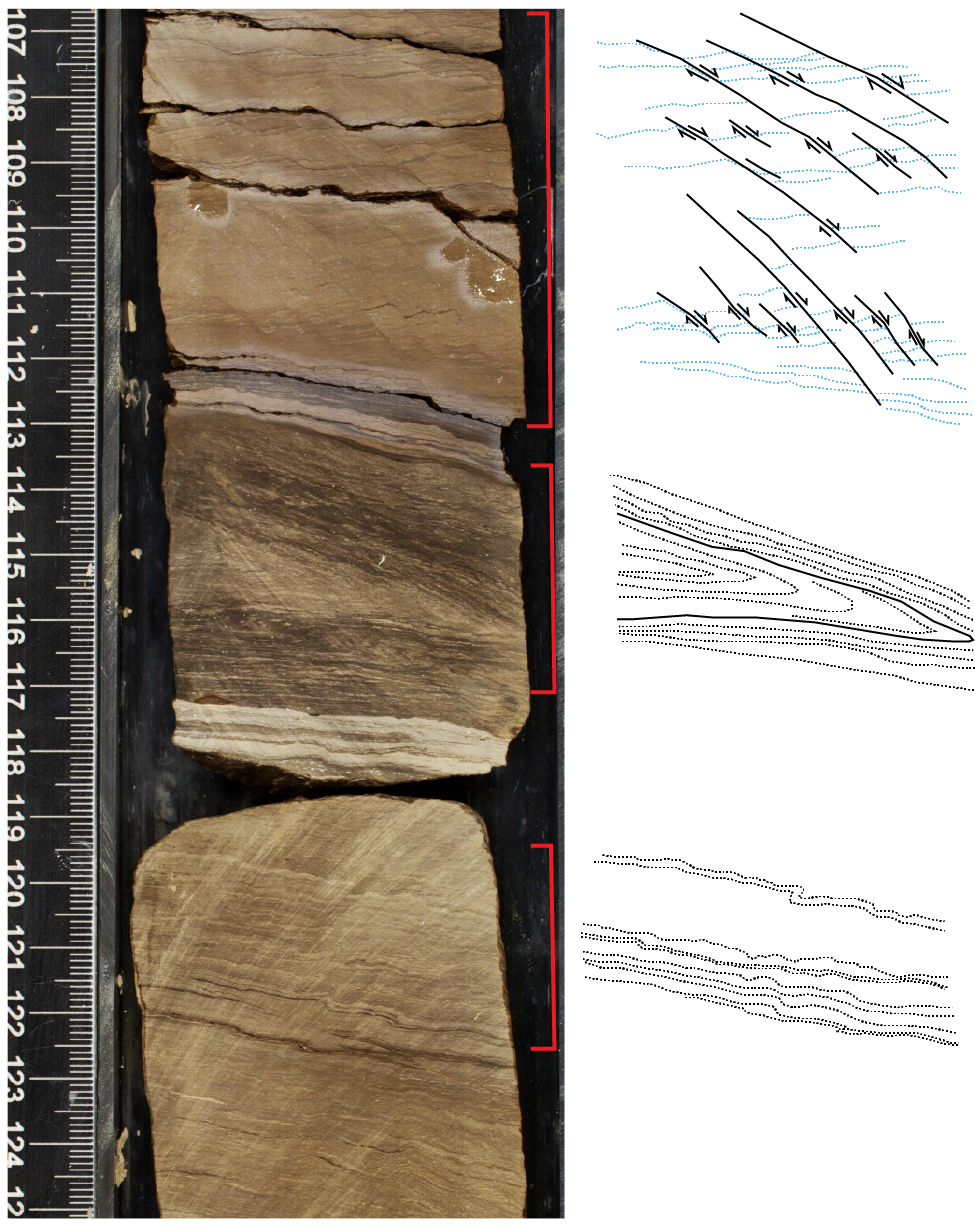
Figure F55. Synsedimentary recumbent folds associated with faulting.
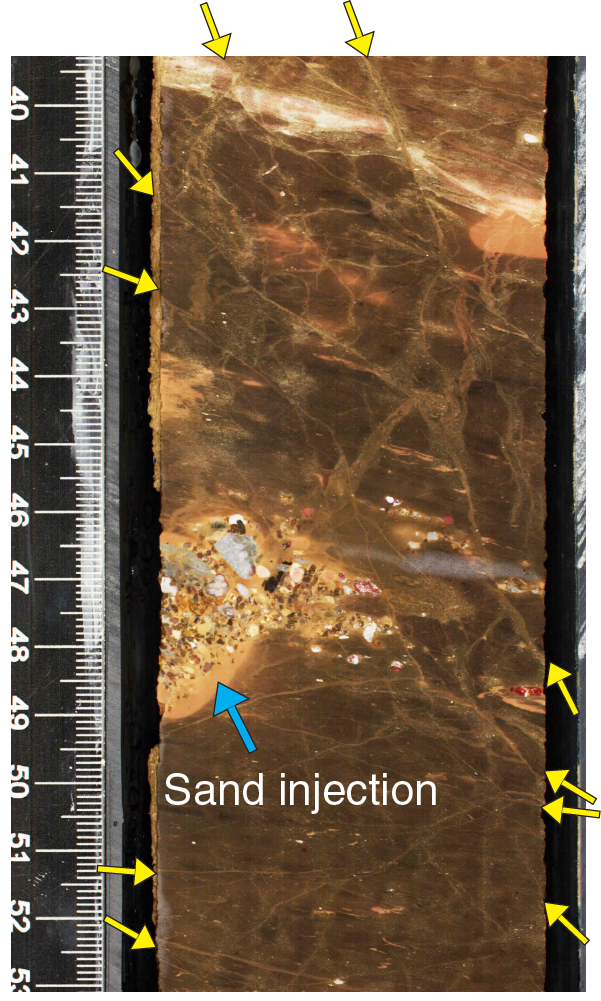
Figure F56. Sand injection that implies soft-sediment deformation structures.
Redox spots (diagenetic spots whose origin awaits further analysis) are common in Cores 362-U1480G-60R and 61R (1308–1326 mbsf) and occur as elliptical (ellipsoidal in three dimensions), dark red spots in pale reddish sedimentary rocks with an aspect ratio of 1.5 to 3 (Figure F57). Most of these features may initially develop as spheres around a fossil or small mineral fragment and are expected to be associated with bacterially mediated diagenetic reactions. The flattened ellipsoidal shape is thus, in most cases, a direct indicator of strain. In Cores 60R and 61R, the major axes of the ellipses are almost parallel to bedding (Figure F57), indicating that the maximum principal stress is perpendicular to bedding, in agreement with the lithostatic stress. Oxidation spots record no offset by the normal faults that cut and displace sand injections. For this reason, we conclude there has been a considerable amount of deformation induced by consolidation after the faults formed, and these faults formed early in the burial history.
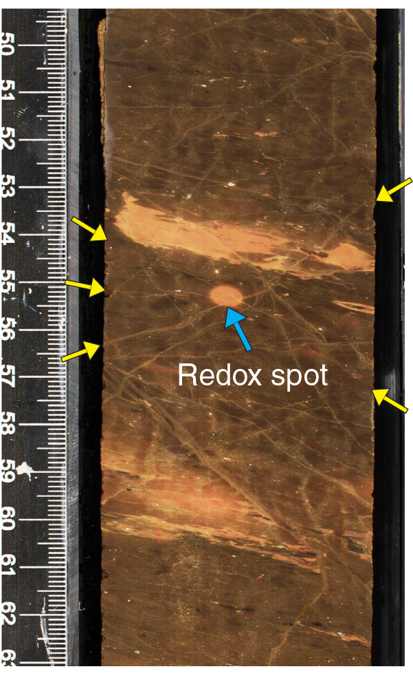
Figure F57. Representative image of redox spots.
In interval 61R-1, 107–132 cm, two 2–3 cm thick shear zones are oriented at a high angle to bedding (Figure F58) and have a normal sense of slip in the split core surface. In interval 61R-1, 115–130 cm, one of the shear zones contains red sediments that are darker than the surrounding sediments. This suggests that after their formation the shear zones may have focused the advection of diagenetic subsurface fluids that were also responsible for redox spots, but microscopy to evaluate textures requires postcruise work.
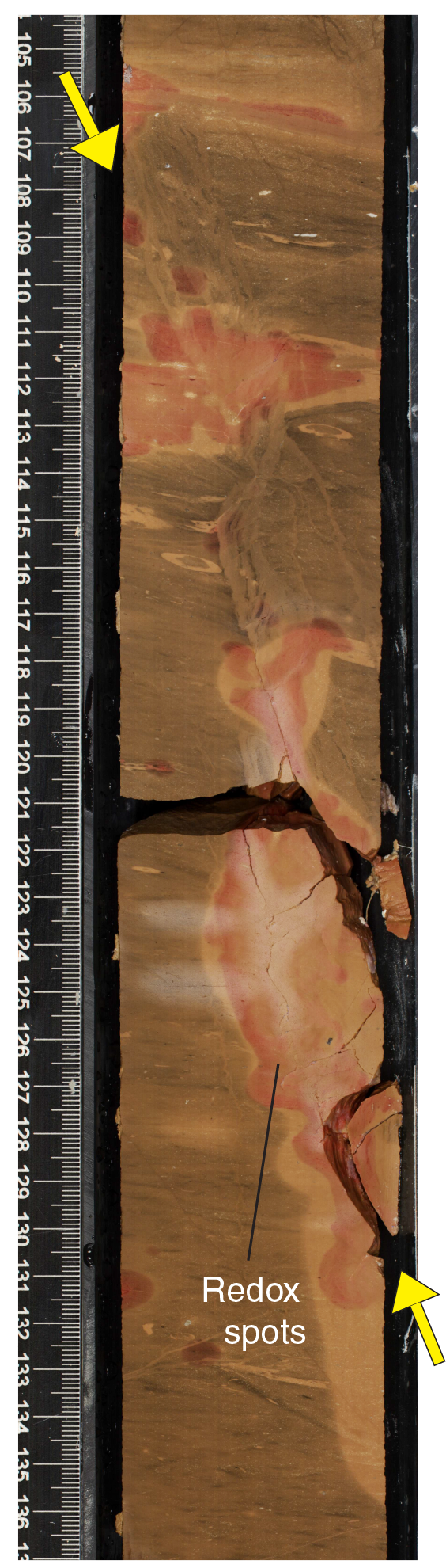
Figure F58. High-angle normal shear band.
The chalk intervals in lithostratigraphic Units III and V (1314–1327, 1356.7–1361.5, and 1398.6–1414.4 mbsf) have developed thin deformation bands and stylolites (Figure F59). Deformation bands are <2 mm thick, are darker in color than host sediments, and show subparallel bedding. Stylolites are bedding-parallel or sometimes bedding-subparallel with a very low amplitude and have a nearly vertical acute bisectrix in the split surface, indicating the presence of vertical shortening or compaction during formation. We observed no cross-cutting relationships between these deformation bands and any other structures in the cores.

Figure F59. Stylolites in lithified nannofossil ooze.
Diorite sill and ocean crust basement
In core sections of igneous rocks we observe networks of mineral veins in a multitude of orientations and with complex cross-cutting relationships (Figure F60). Vein fillings consist of calcite, a red amorphous Fe oxide(?) phase, chlorite(?), microcrystalline quartz/chalcedony, zeolite, palagonite, and magnetite(?). Vein orientations range from low to high angle in the core reference frame, and high-angle veins on occasion branch into or truncate thinner, low-angle veins. Most veins have a wavy shape with a thickness of ~1–2 mm, whereas others are subplanar. Veins are often rimmed by translucent halos 1–2 mm thick, although rare thicker halos are also observed. Green-tinted veins with chlorite(?) ± chalcedony ± calcite occur in Cores 362-U1480G-67R and 68R (intrusive interval of Unit V).

Figure F60. Mineral veins in sections of diorite intrusion.
Drilling-induced structures
A variety of drilling-induced structures were observed in cores (Figure F61), including mingling and distortion of beds, soupy sand, upward-arching bed contacts, biscuits, fall-in, midcore flow-in between biscuits, breccia, fractures, and faults. The genesis of these structures (with depth distribution shown in Figure F62) relates to coring type, lithology, and consolidation state. These drilling-induced structures are primarily observed in sand-rich intervals.
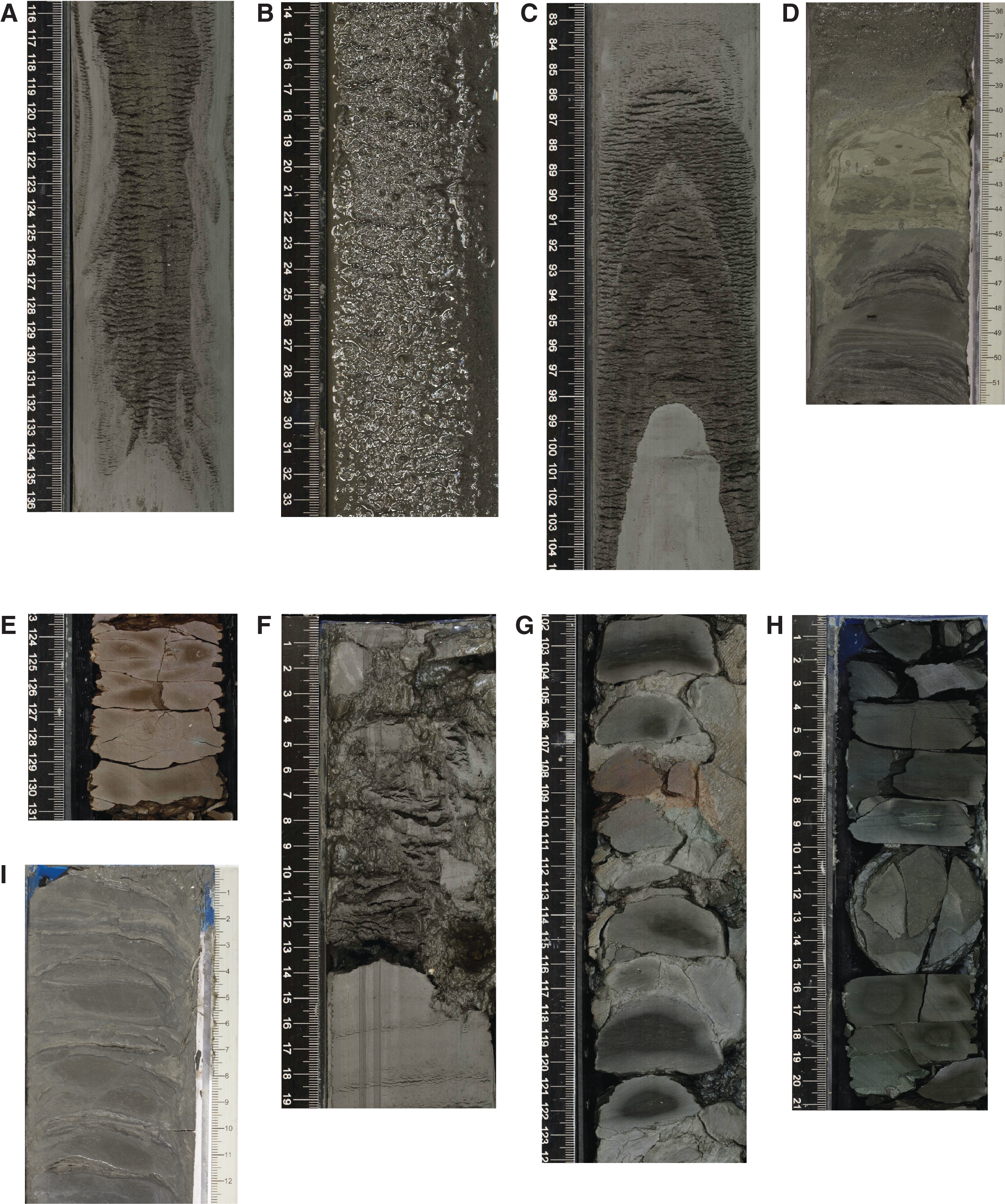
Figure F61. Types of drilling-induced structures visible in cores.
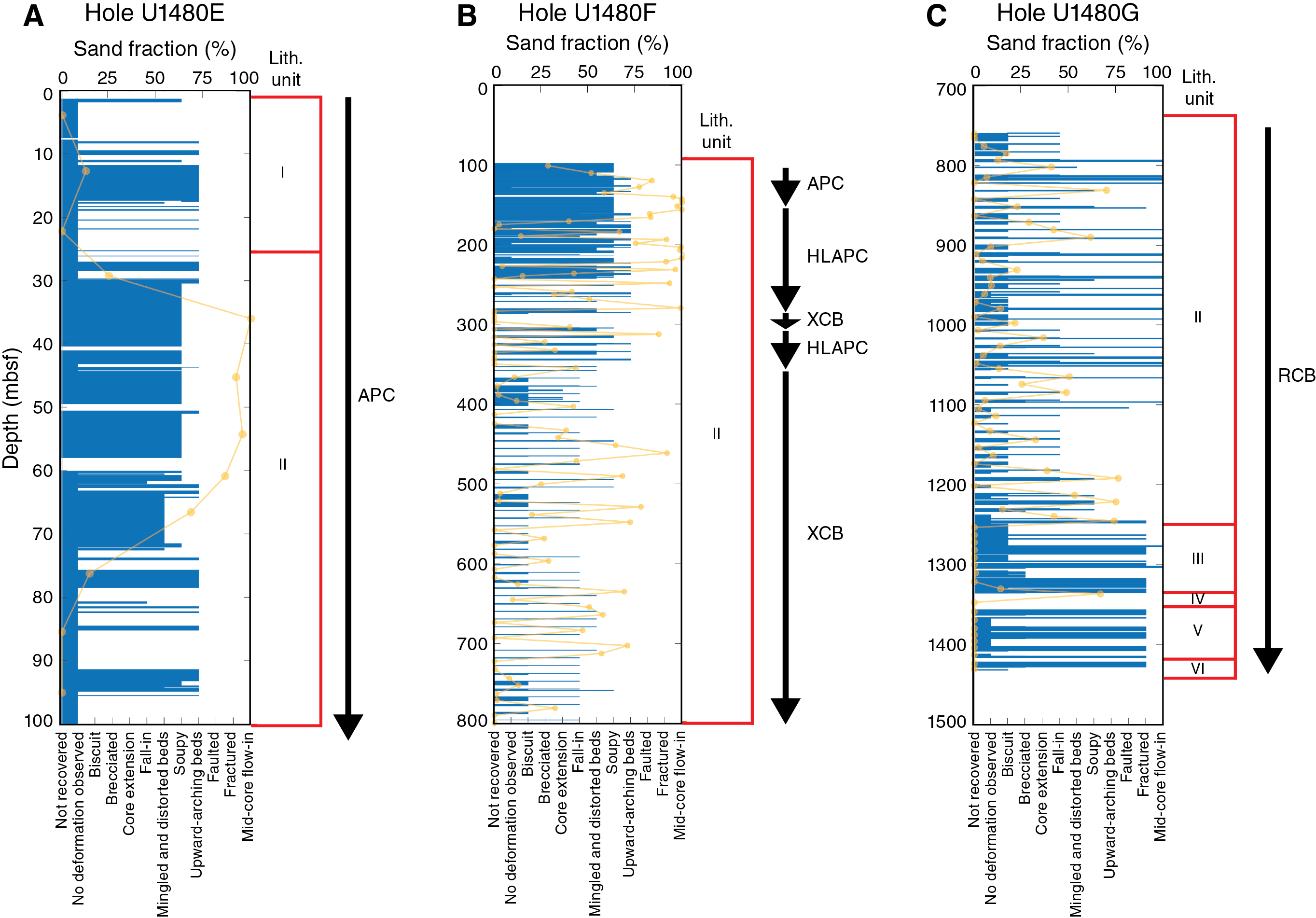
Figure F62. Distribution of drilling disturbance structures, Holes U1480E–U1480G.
In the upper sandy part of Holes U1480E and U1480F where APC coring was used, the main drilling deformation types are mingling and distortion of beds, soupy sand, and upward-arching bed contacts (Figure F62A, F62B). These forms are most prevalent shallower than 250 mbsf and almost exclusively down to the interval above 360 mbsf in lithostratigraphic Subunit IIA. Once XCB coring started in Subunit IIB, the main drilling deformation types are biscuits and material fall-in ( Figure F62B). Core recovery also diminishes through this interval.
In Holes U1480E and U1480F, soupy disturbance occurs when unconsolidated sand is fluidized by coring. In Hole U1480G, the sand is generally more consolidated than in Holes U1480E and U1480F, but soupy disturbance is still observed in rare cases in Hole U1480G within sand horizons bounded by mud layers. The sand appears to become fluidized through the drilling process but not to the extent observed in Holes U1480E and U1480F, as the soupy portions in Hole U1480G are smaller and localized within thicker packages of sand and mud. Soupy sand is primarily observed in HLAPC and APC cores and only rarely observed in XCB and RCB cores, as indicated by the Hole U1480F cores (Figure F63).
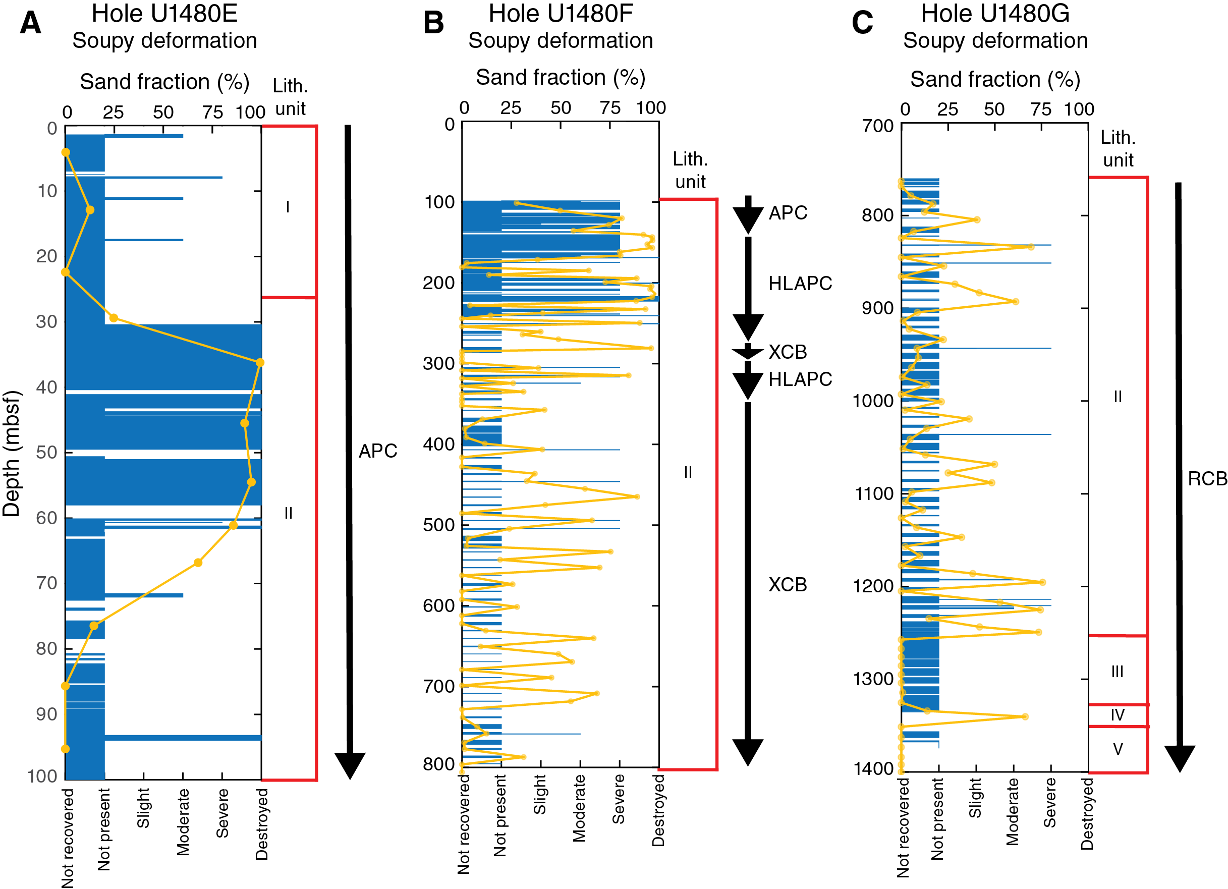
Figure F63. Soupy drilling deformation, Holes U1480E–U1480G.
In the upper part of Hole U1480G (~800–1100 mbsf), biscuits with midcore flow-in between them dominate (Figure F62C). Deeper in the hole (~1280–1431 mbsf), biscuits, breccia, fractures, and faults become more frequent as the sediments become stronger. We interpret midcore flow-in structures as an extreme version of biscuit development because the deformed section contains many small biscuits, some only half the core diameter, with the biscuits surrounded by a matrix of pulverized rock. Similarly, breccias are an extreme condition of fracturing resulting in rock fragments smaller than the core diameter.
In silt- and clay-rich sediment, different combinations of drilling-induced structures are present for different coring types. For APC and HLAPC cores, ductile deformation is characterized by upward-arching beds and mingling and distortion of beds, whereas for rotary XCB and RCB coring, brittle deformation generates biscuits, midcore flow-in, fall-in, breccia, fractures, and faults (rare). Upward-arching beds and mingling and distortion of beds typically coincide in depth, only occurring in Holes U1480E and U1480F, and severe upward-arched beds and/or mingling and distortion coincide with an intermediate sand/silt and clay ratio (Figure F64). In Hole U1480F XCB cores (i.e., deeper than 357.7 mbsf), mingling and distortion of beds becomes rare and upward-arching beds are absent; upward-arching beds are only present in Unit I and Subunit IIA. The absence of upward-arching beds in Subunit IIB is likely a function of coring method rather than lithology (Figure F64).
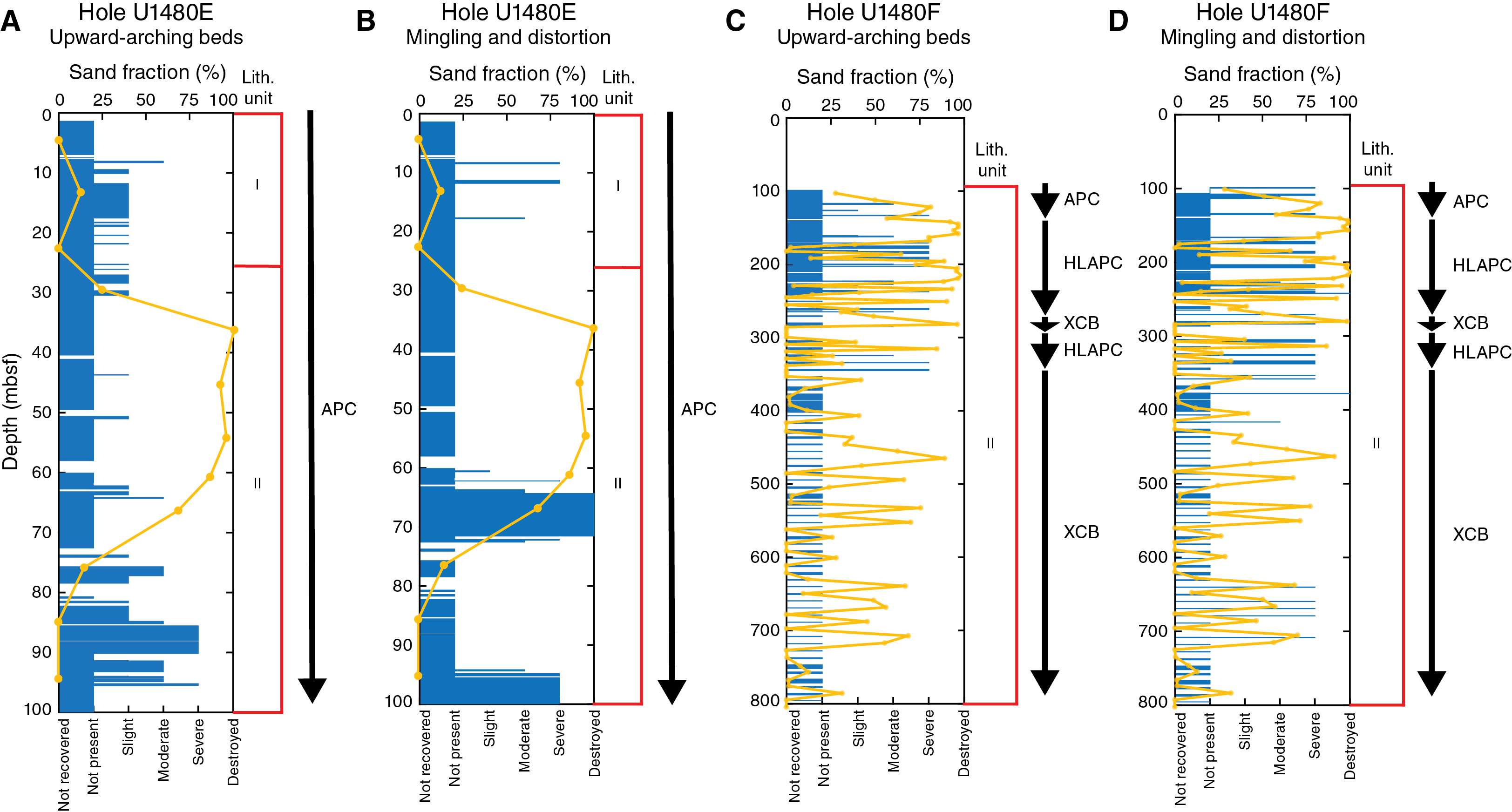
Figure F64. Upward-arching beds and mingling and distortion, Holes U1480E and U1480F.
Fall-in is observed in Holes U1480E, U1480F, and U1480G and increases in prevalence from APC to HLAPC to XCB/RCB cores. However, there is no observed fall-in within RCB-cored Units III–VI, possibly as a result of an increase in material strength and a more stable borehole (Figure F65).
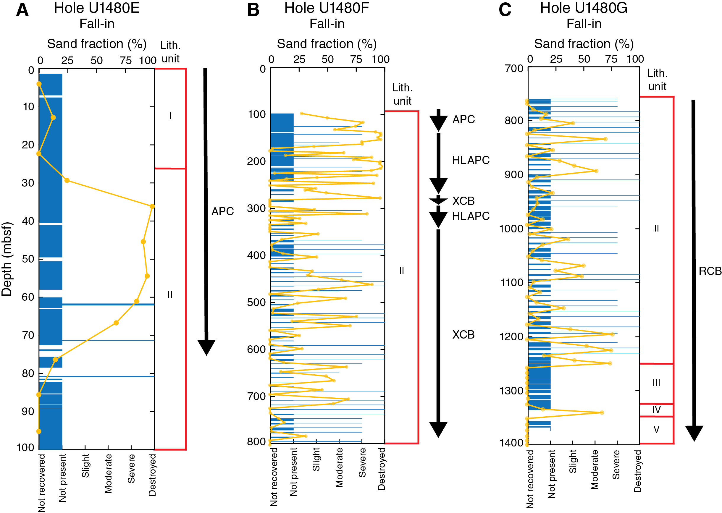
Figure F65. Fall-in, Holes U1480E–U1480G.
Drilling biscuits are not observed in Hole U1480E or U1480F APC cores, rarely observed in Hole U1480F HLAPC cores, and primarily observed in Hole U1480F XCB cores and Hole U1480G RCB cores. Biscuits are never observed in Unit I but are more common in Units II–V. An increase in intensity of the biscuits is observed at the Unit II/III boundary. Midcore flow-in is only associated with fine-grained, biscuit-prone intervals within Unit II (Hole U1480G), with rare appearances in Unit III. Midcore flow-in appears to correlate with biscuits of higher (severe) intensity ratings (Figure F66; see also Structural geology in the Expedition 362 methods chapter [McNeill et al., 2017b] for explanation of the drilling-induced deformation intensity scale).

Figure F66. Drilling biscuits, Holes U1480F and U1480G.
Drilling disturbance breccia was observed rarely in Unit II in Holes U1480F and U1480G but becomes much more frequent and severe within Units III and IV in Hole U1480G. Drilling-induced fractures are almost exclusive to Units III and IV. The sudden appearance of fractured and brecciated cores in these units is possibly due to stronger material (Figure F67).
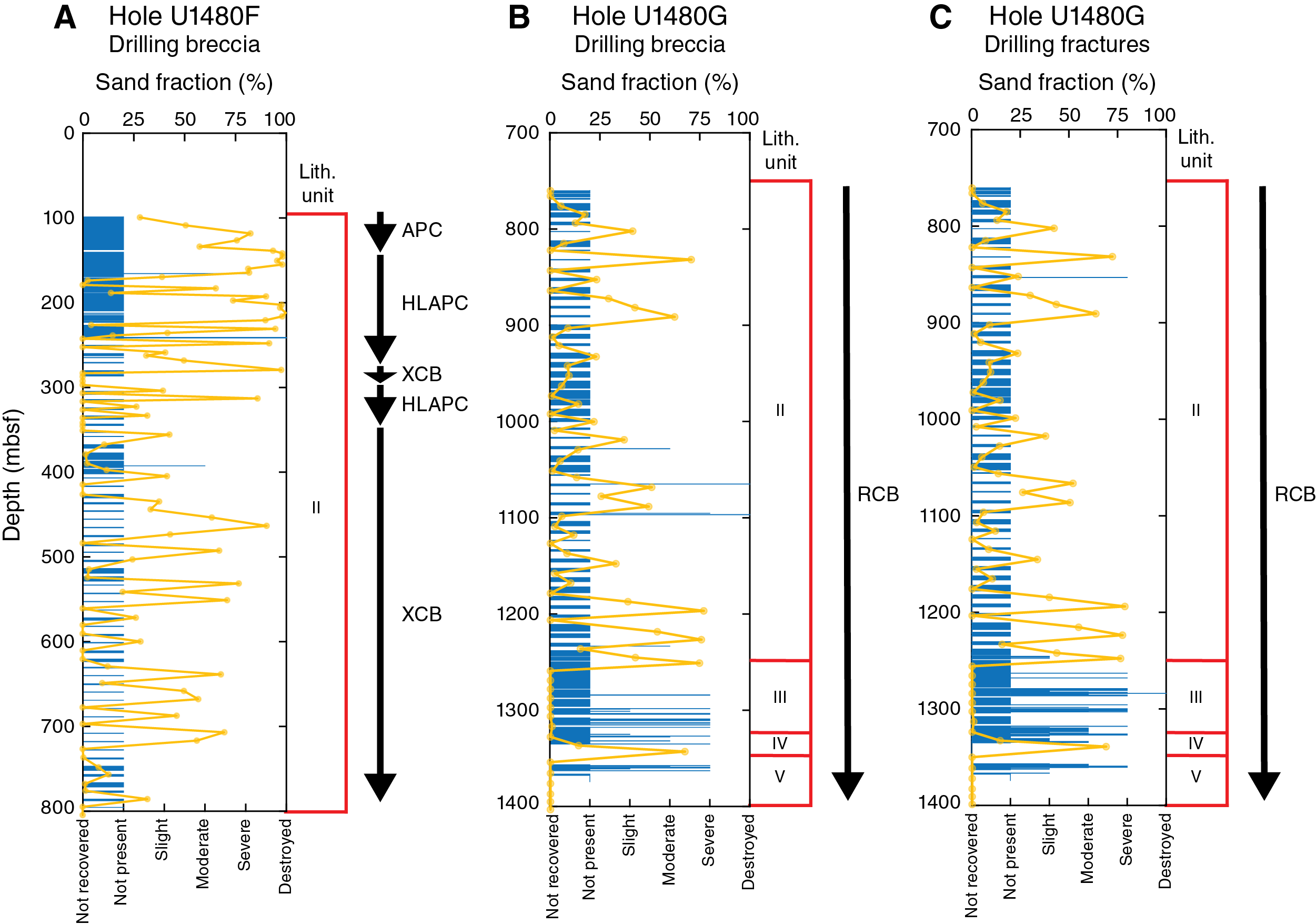
Figure F67. Drilling breccia, Holes U1480F and U1480G.
Core extension was only observed in Cores 362-U1480F-54X and 55X. We therefore interpret that only very little gas is present within the cores (Figure F68), consistent with geochemical results (see Geochemistry).
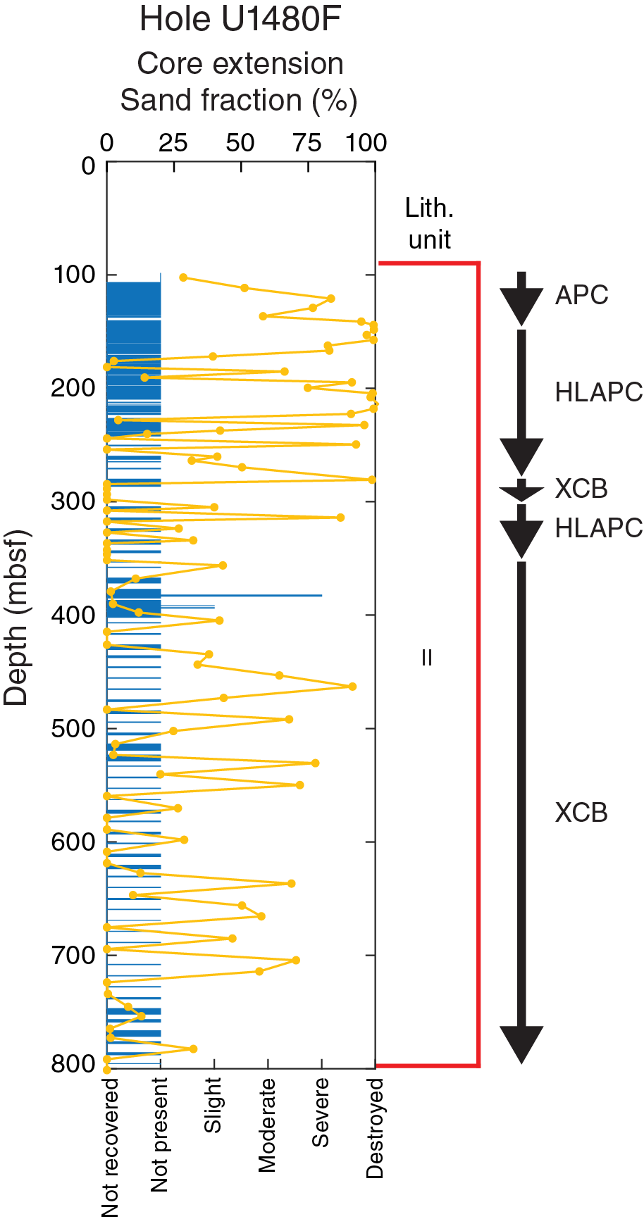
Figure F68. Core extension in Hole U1480F associated with gas content.
Drilling-induced deformation is present in all holes. Although changing coring methods appears to coincide with changes in style of drilling deformation from ductile to a combination of ductile and brittle deformation, this transition is likely a manifestation of increasing strength with depth, as a result of increasing compaction and/or cementation. APC coring may induce the most intense ductile deformation (e.g., injection folds described below); however, the most undisturbed beds are associated with APC coring. For example, in sandy regions, APC and HLAPC cores typically cause soupy deformation, whereas in silt/clay these coring methods cause upward-arching beds and mingling and distortion. In contrast, biscuiting occurs during XCB and RCB coring in stronger sediments and rocks deeper in Hole U1480F (~357.7 mbsf) and in Hole U1480G.
Borehole deviation and impact on bedding dips
During core observations in Hole U1480G, we noticed local deviations in bedding dips in which intervals 10–30 m long may have dips of 5°–10° (e.g., 950 mbsf). If a borehole deviates from vertical while encountering dipping beds without the means to define dip direction, then dispersion of dip angles will increase. A significant problem in trying to deduce small changes in bedding dip as the result of tectonic processes is that bedding dips created by sedimentary processes and the drilling process may overwhelm the tectonic signal that we are trying to measure. For the moment, the possibility of borehole deviation as a contributor to measured dips remains speculative because the absence of a gyroscope log in this hole prevents confirmation of this hypothesis.
Mud intrusion into the core barrel
Section 362-U1480E-10H-6 (78 mbsf) marks the first occurrence of an isoclinal fold structure symmetric around the core axis (Figure F69) that we interpret to be caused by APC coring. This is similar to an exaggerated version of upward-arching bed contacts, but an enormous shear strain has developed in the fold limbs over many tens of centimeters, and frictional drag within the core barrel cannot explain the largest of these features. These folds do not occur at the top of the cored interval and are underlain by unfolded bedding contacts. Each fold structure is associated with a partial stroke of the core barrel (Table T4), which means that a void is present during core barrel extraction (Figure F69), similar to the core history described by Jutzeler et al. (2014). We interpret the fold to be material sucked into the core barrel during extraction. In the largest folds, we correlate the following parameters with this type of fold structure: (1) partial core barrel stroke; (2) up to 40,000 lb overpull to release the core barrel from the formation, creating suction into the core barrel; and (3) >95% core recovery (considered anomalous in the context of a partial core barrel stroke).
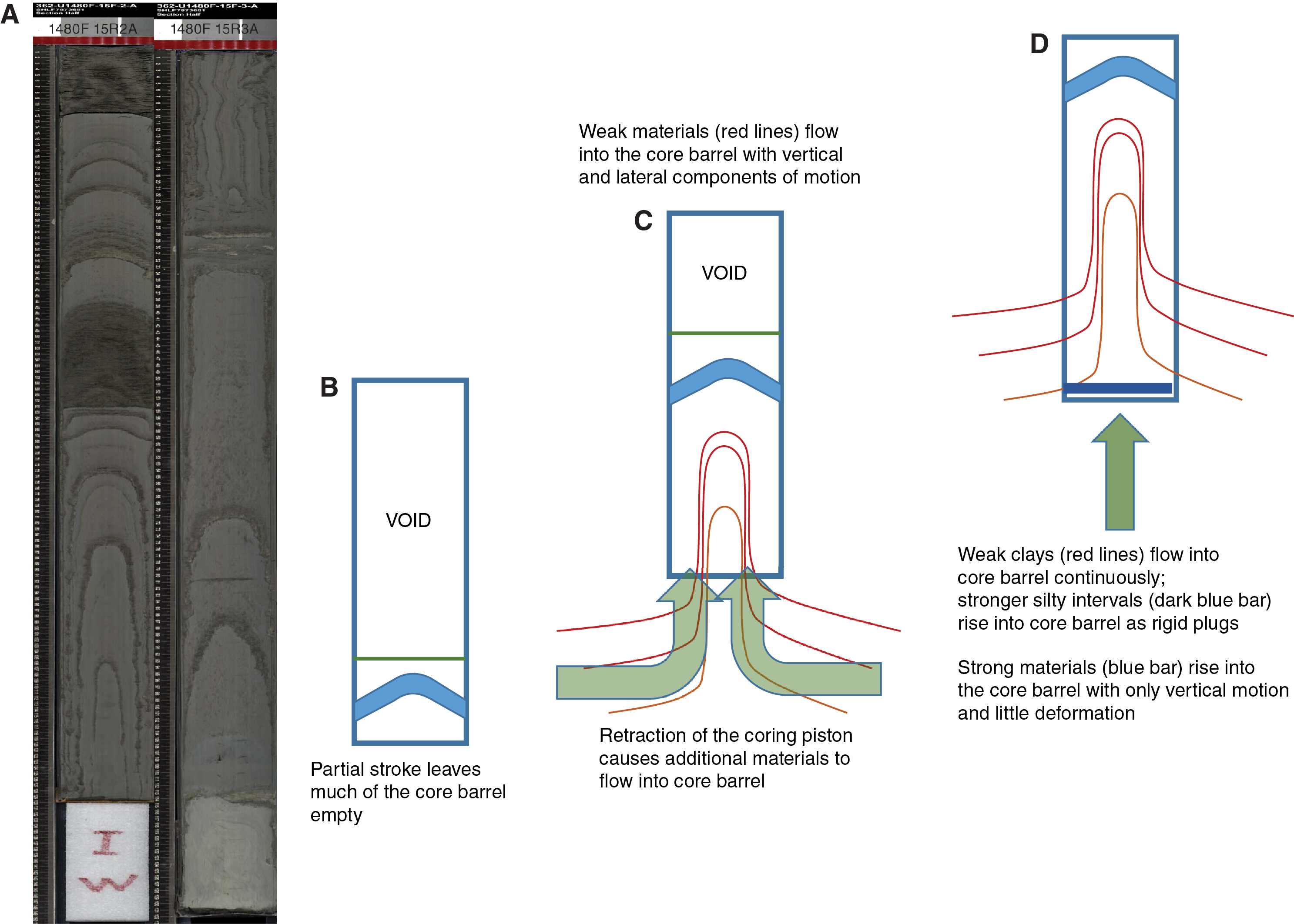
Figure F69. Isoclinal fold caused by ductile deformation during a partial stroke.
Table T4. Cores with mingling and distortion of beds. Download table in .csv format.
In some instances, overpull was applied without the development of an isoclinal fold structure (Table T5). One instance has sand at the base of the core, and thus it is impossible to identify if an isoclinal structure exists, and in the other two instances some minor mingling and distortion of beds was observed higher in the core. There are many examples of high core recovery (>95%), but the majority of these have sand at the base, which would fail to record the isoclinal fold structure (Table T6).
Table T5. Cores with overpull and no evidence of mingling or distortion. Download table in .csv format.
Table T6. Cores with high recovery and no mingling or distortion. Download table in .csv format.
In some instances, a tall intruded isoclinal clay/silt fold is floored by a flat horizontal, often siltier, bed (Figure F69). We interpret the clay/silt intrusion to be a combination of vertical and lateral flow that carries the stiffer, siltier interval into the core barrel undeformed, and then a new isoclinal fold develops beneath it. Lacking logs to help test whether silt/clay lithologies are preferentially intruded into the core, we interpret that weaker, clay-rich intervals are able to flow in a ductile manner, whereas stiffer, siltier beds remain undeformed.
Summary
Drilling disturbance recorded at Site U1480 is similar in style and intensity to other IODP sites with similar sediments and using the same coring methods (Expedition 334 Scientists, 2012; Harris et al., 2013c; Reagan et al., 2015). Our observations reflect increasing consolidation with depth and responses to the coring method employed. However, local deviations from this trend occur where intense drilling deformation was observed. A main motivation for recording deformation style and intensity is to combine those observations with information about drilling conditions (next section) to infer strength conditions and identify weak and strong horizons with relevance to the objectives of this expedition.
Drilling conditions
Drilling conditions were evaluated for Holes U1480F and U1480G in order to account for differences in XCB and RCB drilling. No separate evaluation of APC or HLAPC coring was undertaken. We generated a series of summary plots that relate the drilling parameters (rate of penetration [ROP], weight-on-bit [WOB], torque, top-drive rotations [TD-RPM], mud pumps total [MPT], and stand pipe pressure [SPP]; see Structural geology in the Expedition 362 methods chapter [McNeill et al., 2017b]) to the types of cores recovered (see DRILLING in STRUCTURE in Supplementary material) and physical property data (porosity and P-wave velocity) to identify anomalous intervals that may be more susceptible to deformation (e.g., localization candidates).
The single most important factor controlling the time it takes to cut a core (ROP) in Hole U1480F is proportion of sand. In sand-rich sections, cores were cut faster than in more clay rich sections (Figure F70A), and core recovery was lower (Figure F70B). In order to infer differences in strength properties of drilled sections (e.g., unconfined compressive strength [UCS]), comparisons need to be made on a constant lithology basis. The sand component is defined here as the sum of fine sand and very fine sand in the lithologic description (see Sedimentology and petrology).

Figure F70. Sand fraction vs. coring time, Hole U1480F.
A by-product of this analysis is the tentative identification of sand-rich intervals in poor core recovery intervals, supported by the interpretation of turbidite channel geometry in the seismic reflection data (see Core-log-seismic integration). For example, most cores with >25% sand were cut in <30 min, whereas clay-rich cores often took >40 min (Figure F70A). Moreover, cores drilled in <25 min mostly had recoveries of <10%. Figure F70B illustrates how cores with low sand fraction cut within 40–50 min have a wide range of recoveries, and Figure F71 reveals how high sand fraction intervals (e.g., 640–718 mbsf) were drilled in <20 min/core and are therefore extrapolated across low- and no-recovery intervals. This result is also in line with the specific energy factor (SEF; see Structural geology in the Expedition 362 methods chapter [McNeill et al., 2017b]), such that little drilling energy is required to advance through the unconsolidated sand section.
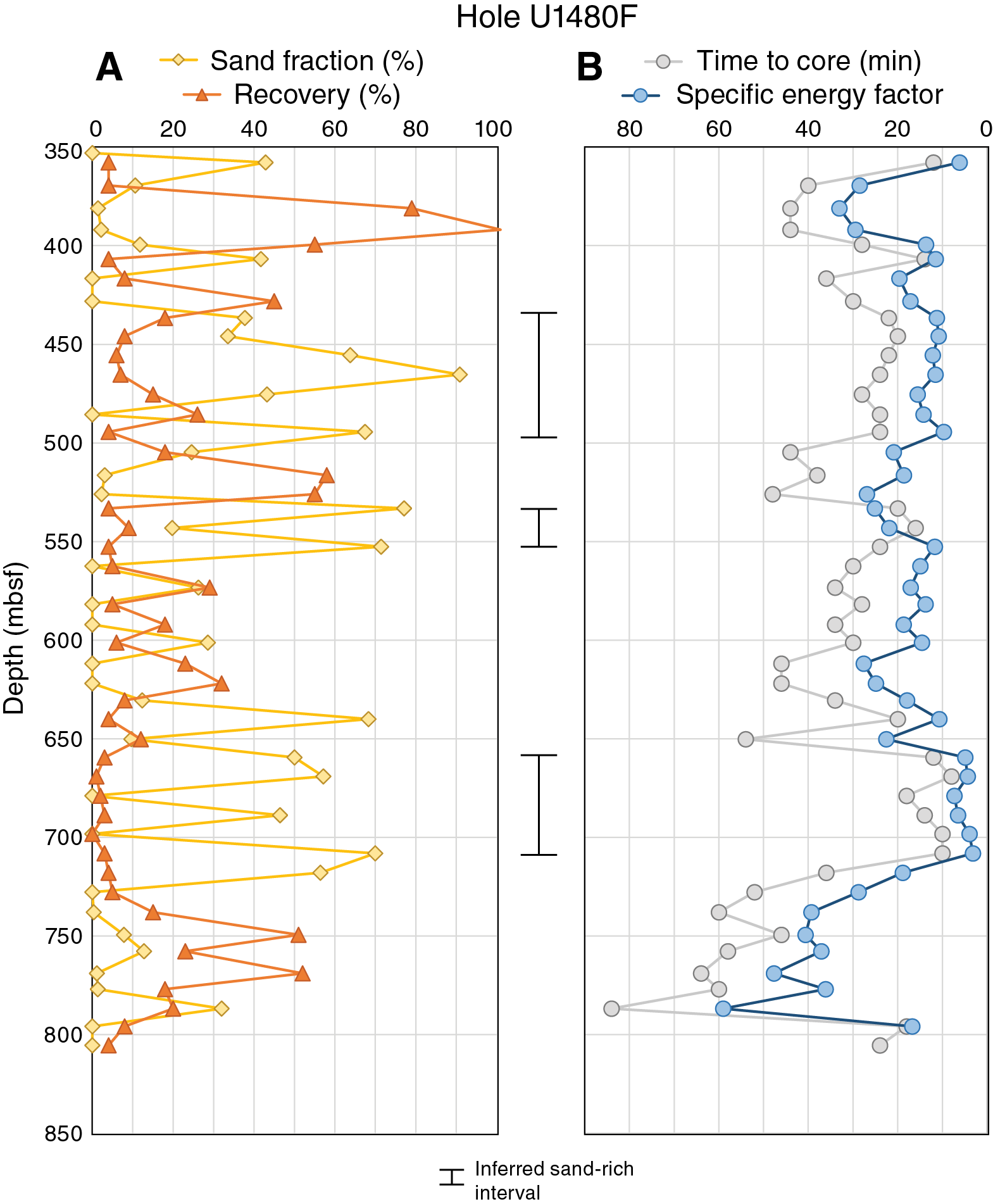
Figure F71. Sand fraction, recovery, time to core, and SEF, Hole U1480F.
The ability to predict sand-rich sections by time-to-drill (coring time) is lost in Hole U1480G (Figure F72). This may in part reflect consolidation of the sand intervals, perhaps by the initiation of grain-bridging cements. Alternatively, the thinner sands of the deeper Hole U1480G section may also result in better recovery. RCB drilling also offers more feedback and control of the coring process than XCB (S. Midgley, pers. comm., 2016), and this may play an additional factor in better recovery.
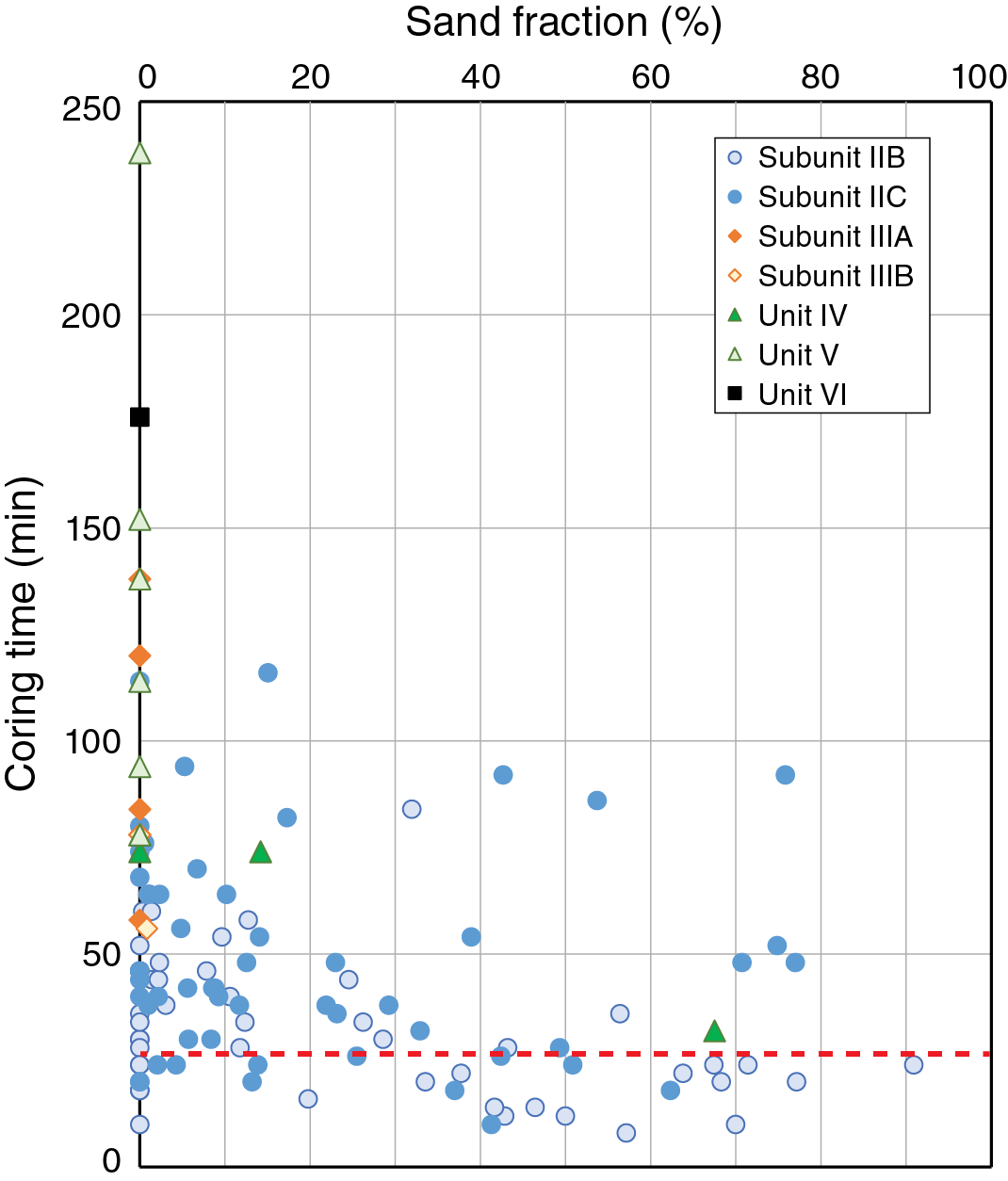
Figure F72. Sand fraction vs. coring time, Hole U1480G.
A more elusive goal is to identify weak intervals that may be more susceptible to deformation (strain localization candidates). The SEF (Figure F73) ranges between ~20 and 50 from 750 to 1150 mbsf, increases from 1150 to 1250 mbsf at the base of Subunit IIC, and then reaches higher, more variable values in the pelagic and igneous intervals deeper than 1250 mbsf (Units III–VI). The highest SEF values (Figure F74A) are found in the igneous sections at the bottom of the hole (deeper than 1300 mbsf; Units IV and V). Here the SEF tracks time-to-core, indicating that ROP (related to time-to-core) has the greatest influence on SEF, whereas torque and RPM play only secondary roles.

Figure F73. Sand fraction, recovery, time to core, and SEF, Hole U1480G.
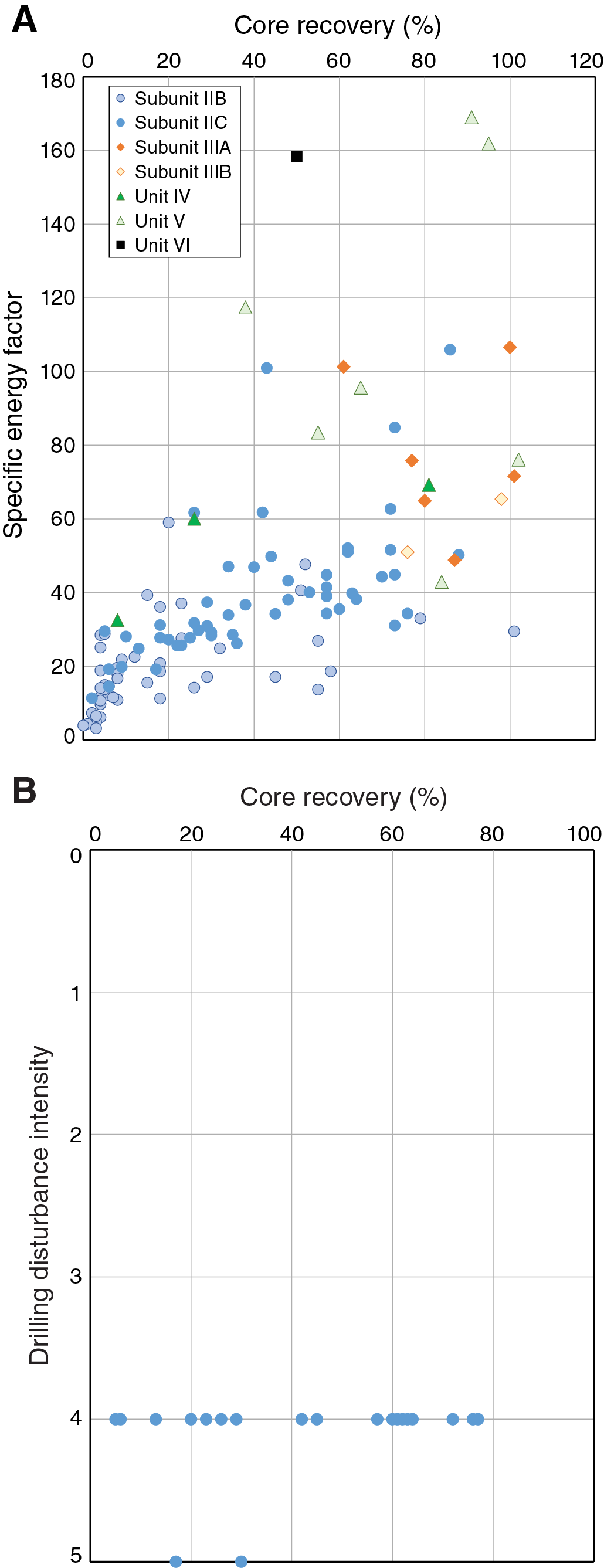
Figure F74. Core recovery vs. SEF, Holes U1480F and U1480G.
We also considered whether core recovery is more correlative with SEF than with drilling disturbance. As Figure F74 shows, a reasonable relationship exists between SEF and recovery, but a poor relationship is seen between drilling deformation intensity and recovery. When recovery decreases, we expect more disturbed sediments recovered due to the difficulty in cutting core, but Figure F74B refutes this hypothesis. A limitation of using a recovery parameter arises when the core barrel becomes jammed and no further core enters the liner. Of the eight instances of core-jamming recorded in Hole U1480G, none depart from the population plotted in Figure F74A.
Examining the SEF in Subunit IIC between 750 and 1250 mbsf in Hole U1480G (Figure F75), several minima stand out as potential anomalies, and these anomalies are often associated with low recovery. Some examples are correlated with high porosity and low P-wave velocity, with a stronger correlation for the velocity z-component than the x-component (see Physical properties). The best examples are found between 800 and 850 mbsf, whereas the association of low SEF with high porosity and low velocity is poorer in deeper intervals. Note that additional high porosity/low P-wave velocity intervals are identified deeper in the section (e.g., ~935 mbsf) but without a corresponding minimum in SEF. Because of the low recovery around some of the SEF minima, the material properties such as P-wave velocity are not well determined.

Figure F75. Sand fraction, recovery, and SEF.
The SEF minima at 800–850 mbsf correlate to the reflective package near the top of Subunit IIC (see Core-log-seismic integration and Figure F128) at 6.35 s two-way traveltime (TWT). Seismic Horizon B (Table T24; Figure F119) is interpreted at 930 mbsf, and the deepest low SEF value that corresponds with high porosity and low velocity occurs at 920 mbsf. It is plausible to conclude that the SEF minimum and seismic reflection occur at the same depth, and thus we interpret seismic Horizon B as a localization candidate based on its association with low SEF.
Using the compiled drilling parameters, it is also possible to consider cores with similar drilling conditions and material content but with different structural deformation and recovery results (Figure F76). In this example, Core 362-U1480F-55X had 12 faults observed over a 9 m interval and 101% recovery. For the same drilling conditions, recovered sand content, and coring times, Core 58X had no observed faults and only 8% recovery. The limited recovery may have prevented sampling of faults, but the contrast in recovery is dramatic. The interval represented by Core 58X may be weaker than Core 55X, but this interpretation requires further work to verify. In a deeper interval (560–600 mbsf; Cores 73X through 76X) with no deformation structures and little to no sand, each core was drilled in 28–34 min with 5%–29% recovery, and the intensity of drilling biscuits ranges from slight to severe. We deduce that this interval may be weaker and more prone to destruction by drilling but acknowledge that unconsolidated sand may also cause poor recovery. Petrophysical logs could address this uncertainty in future studies.
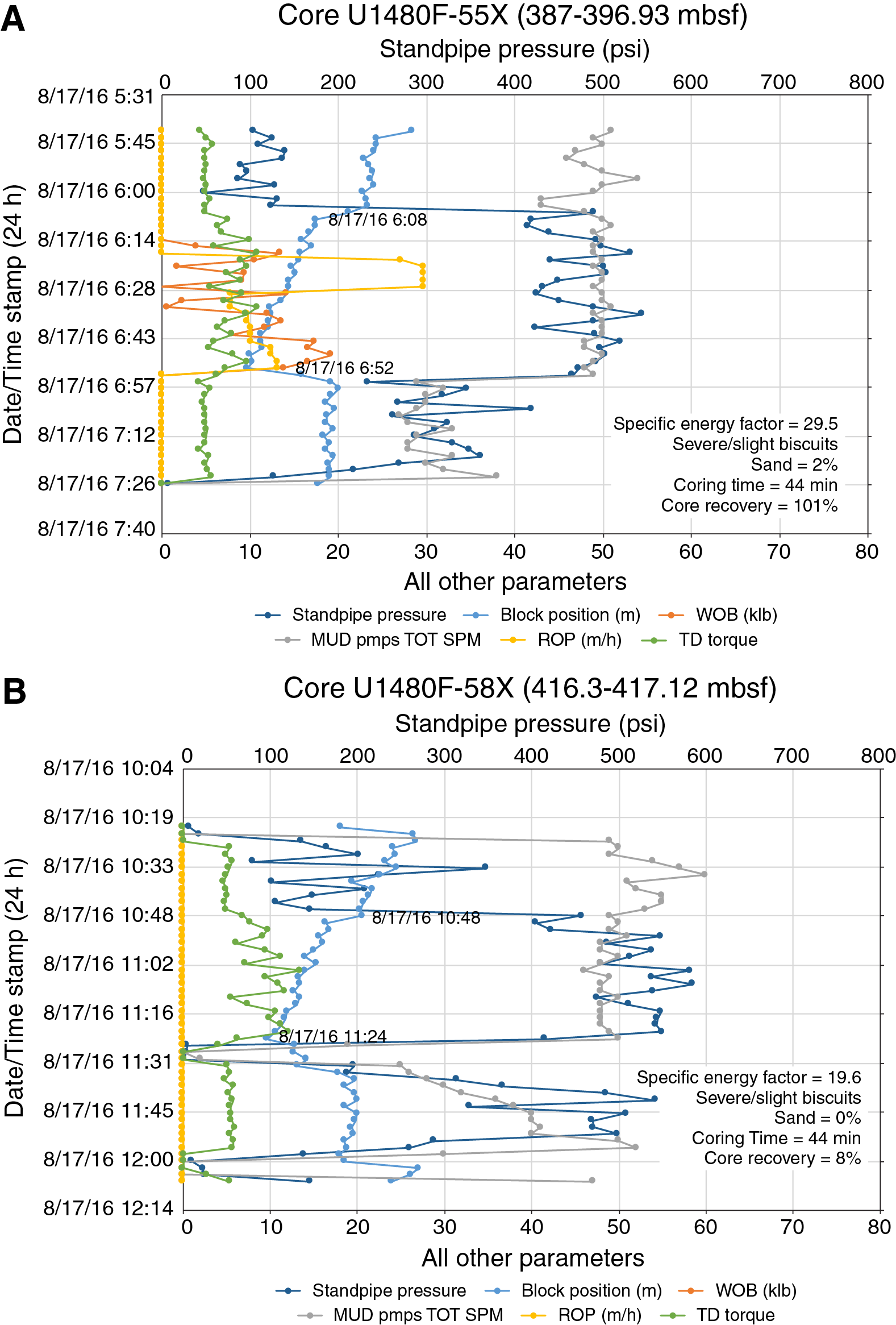
Figure F76. Drilling parameters, Cores U1480F-55X and 58X.
Strength interpretation
We use three different approaches to evaluate the strength characteristics of sediments at Site U1480: (1) a strength log from visual core description, (2) a detailed record of drilling disturbance, and (3) a log of SEF based on drilling parameters. The strength log reflects subtle changes in the core to interpret local changes in mechanical properties. A general trend of increasing strength with depth based on observed drilling deformation structures, fault structures, and firmness of the cored sediments is consistent with an increasing consolidation of sediment with depth. However, we found scant evidence for strength deviations because there were few observations to evaluate relative strength contrasts. The coincidence of sand and clay intrusions (Figure F52) provides strong evidence for equivalent sand and clay mechanical properties, but structures consistent with contrasting strength properties are rare. The intrusion of mud into the core barrel during APC and HLAPC coring may reflect a weak clay-rich interval and could be evaluated for mechanical clay injection potential (MCIP) as described by van der Zee et al. (2003). Because many or most of the deformation structures observed are interpreted as synsedimentary or formed under shallow burial conditions, they may be poor predictors of future deformation. The three localization candidates defined in the VCDs (391.5–400.3, 427.6–429.2, and 990.0–990.6 mbsf) are based on the assumption that the observed fault structures are in fact indicators of future deformation.
Drilling disturbance also appears to reflect increasing consolidation and strength with depth when viewed in the context of coring method. We identified anomalous intervals that depart from this trend, but a positive relationship between drilling disturbance and deformation-prone intervals (i.e., weakest intervals are most deformed by drilling) remains speculative. The lack of correlation between the most intense drilling deformation and low core recovery (Figure F74B), for example, is taken as evidence against such a relationship.
The most promising indicator of strength may be the SEF, especially when it is correlated with high porosity and low velocity. The interpretation of SEF values remains speculative, however, in the absence of continuous petrophysical logs.
Biostratigraphy
Single cores were retrieved from Holes U1480A–U1480D. Because these cores did not retrieve the mudline, they were correlated to Holes U1480E and U1480H; see Core-log-seismic integration for their inferred depth offsets relative to the seafloor. Only Holes U1480E and U1480H sampled the water/sediment interface.
Samples containing biosilica (diatoms, radiolarians, and silicoflagellates) are limited to the upper 62 m of Hole U1480E, between 18 and 26 m in Hole U1480B, and in the upper 26 m of Hole U1480H. Below this interval, all samples are barren until 787.55 mbsf, where poorly preserved radiolarian tests become common. Preservation improves between 1255 and 1324 mbsf (Hole U1480G), permitting identification of pyritized radiolarians at the species level. In this part of Hole U1480G, poorly preserved pyritized diatoms were observed between 1264 and 1269 mbsf.
Biogenic carbonate occurs discontinuously throughout Holes U1480A–U1480H, mostly at low abundances albeit with a few exceptions. Preservation mostly varies between moderate and poor.
Calcareous nannofossils
Core catcher samples were investigated from the initial four holes (one core per hole), with one barren sample (Hole U1480A) and three samples (Holes U1480B–U1480D) containing Pleistocene calcareous nannofossil assemblages. Sediments in Holes U1480E (0–99.98 mbsf) and U1480H (0–129.40 mbsf) are of Pleistocene age, whereas sediments in Hole U1480F (98.00–815.00 mbsf) range in age from the early Pleistocene to the late Miocene. Sediments in Hole U1480G (759.60–1415.35 mbsf) range in age from the late Miocene to the Late Cretaceous (Maastrichtian). The biostratigraphic results of calcareous nannofossils at Site U1480 are summarized in Table T7.
Table T7. Calcareous nannofossil biostratigraphy. Download table in .csv format.
Holes U1480A–U1480D
The two cores from Holes U1480A and U1480B were examined in some detail because physical property data indicated a stratigraphic overlap with Core 362-U1480E-3H (17.59–27.09 mbsf; see Core-log-seismic integration), which includes an apparent condensed interval according to the combined biostratigraphies of calcareous nannofossils, planktonic foraminifers, diatoms, and radiolarians. Physical property data indicate that the top of Core 362-U1480A-1H begins at 29.4 m composite depth (mcd), the top of Core 362-U1480B-1H at 18.6 mcd, the top of Core 362-U1480C-1H at 10.6 mcd, and the top of Core 362-U1480D-1H at 7.7 mcd. Depth scales for Holes U1480A through U1480D are therefore given as mcd (see CCSF scale defined in Core-log-seismic integration).
Six samples were investigated from Core 362-U1480A-1H. The core catcher sample is barren, as is Sample 1H-1, 12–13 cm (29.53 mcd). Rare calcareous nannofossils were observed in Sample 1H-3, 1–2 cm (32.42 mcd), one species being Calcidiscus macintyrei, indicating a youngest possible age of 1.60 Ma. Rare Helicosphaera sellii was observed in Sample 1H-1, 119–120 cm (30.60 mcd), indicating a youngest possible age of 1.2 Ma. Other age-indicative species were not observed in this core.
Core 362-U1480B-1H is partly characterized by a consistent presence of abundant Pseudoemiliana lacunosa. Three consecutive samples in the bottom of the core contain few C. macintyrei. Discoaster brouweri and Gephyrocapsa spp. ≥4 µm are absent. The latter category appears in Sample 1H-5, 90–91 cm (25.54 mcd), and includes Gephyrocapsa parallela, indicating that this sample was deposited after the top absence interval of medium-size gephyrocapsids and that the sample may be attributed to Biozone CNPL10 (0.43–1.06 Ma) (Raffi et al., 1993). Presence of few C. macintyrei in Sample 1H-6, 70–71 cm (26.84 mcd), indicates a youngest possible age of 1.60 Ma. Gephyrocapsa spp. >5.5 µm was observed in five consecutive samples, through Sample 1H-4, 123–124 cm (24.37 mcd), marking the top of Biozone CNPL8 and with a youngest possible age of 1.25 Ma. Common medium-size gephyrocapsids were observed in the two uppermost samples investigated in Sections 1H-1, 57 cm, and 1H-1, 102 cm (19.17 and 19.62 mcd, respectively), placing these samples in Biozone CNPL10 (0.43–1.06 Ma). Reticulofenestra asanoi was observed in Sample 1H-1, 137–138 cm (19.98 mcd), and in the two overlying samples (19.62 and 9.17 mcd). This species appears in upper Biozone CNPL9 at 1.14 Ma and disappears in Biozone CNPL10 at 0.91 Ma.
Samples 362-U1480C-1H-CC (20.26 mcd) and 362-U1480D-1H-CC (17.59 mcd) both contain P. lacunosa and Gephyrocapsa spp. ≥4 µm, including G. parallela. These two samples are considered to represent Biozone CNPL10 (0.43–1.06 Ma).
Holes U1480E and U1480F
The calcareous nannofossil assemblages from Holes U1480E (0–99.98 mbsf) and U1480F (98.00–815.00 mbsf) are briefly described below. Physical property data suggest that there may be a short gap in depth between Holes U1480E and U1480F (see Core-log-seismic integration).
Calcareous nannofossils are generally characterized by rare abundances or absence in most investigated samples. Abundant calcareous nannofossils were observed in a few samples of earliest Pleistocene and late Pliocene age, all with strongly dissolved assemblages biased toward concentration of discoasters. Obvious reworking is minor in samples holding abundant calcareous nannofossils. Examples of reworking include rare Sphenolithus abies (late Miocene–early Pliocene) and Dictyococcites bisectus (middle Eocene–Oligocene) in Pleistocene assemblages.
Twelve cores were recovered from Hole U1480E. Four of the twelve core catcher samples are barren. Calcareous nannofossils are rare in six of the remaining eight core catcher samples, and few in the other two samples. One sample in Core 1H and three samples in Core 3H contain abundant nannofossils. Preservation varies from moderate to poor.
Sample 1H-2, 56 cm (1.91 mbsf), is dominated by small- (<4 µm) and medium-size (4–5.5 µm) Gephyrocapsa, including G. parallela. Rare occurrences of small (<4 µm) placoliths having relatively large central openings are interpreted as Emiliania huxleyi. Other assemblage components include common Calcidiscus leptoporus, few Helicosphaera carteri, few Ceratolithus telesmus and Ceratolithus cristatus, and few Umbilicosphaera sibogae. Placoliths interpreted to represent E. huxleyi were also observed in Sample 1H-CC (7.74 mbsf). This sample and Sample 2H-CC (17.57 mbsf) are considered to represent Biozone CNPL11 (0–0.43 Ma).
The shallowest occurrence of P. lacunosa was observed in Sample 3H-1, 146 cm (18.77 mbsf). The interval between Samples 3H-6, 5 cm (24.85 mbsf), and 3H-CC (27.07 mbsf) holds three biohorizons: the top of Gephyrocapsa >5.5 µm, the base of Gephyrocapsa spp. ≥4 µm at 25.36 mbsf, and the top of C. macintyrei at 27.07 mbsf. Sample 3H-CC at 27.07 mbsf is partly characterized by the absence of both discoasters and gephyrocapsids ≥4 µm, placing the 24.85–27.07 mbsf interval in Biozones CNPL7 and CNPL8 (1.25–1.93 Ma).
Below this condensed interval (24.85–27.07 mbsf), samples from Hole U1480E contain rare occurrences of calcareous nannofossils or are barren. D. brouweri is rare between Samples 10H-CC (81.32 mbsf) and 12H-5, 11 cm (96.31 mbsf), indicating a youngest possible age of 1.93 Ma at 81.32 mbsf.
Samples from the upper 14 cores in Hole U1480F are barren or contain rare and poorly preserved specimens. Strongly dissolved yet common to abundant calcareous nannofossils were observed in Sample 15F-3, 130–131 cm (178.26 mbsf), and are dominated by complete specimens and fragments of D. brouweri together with abundant P. lacunosa. This characteristic assemblage was also observed in Samples 16F-1, 85 cm (180.25 mbsf), and 17F-1, 3 cm (184.16 mbsf). Other assemblage components in these three samples include C. leptoporus, C. macintyrei, C. cristatus, Ceratolithus rugosus, Coccolithus pelagicus, Dictyococcites spp. (<3 µm), Discoaster triradiatus, H. carteri, and Reticulofenestra minuta. The prominent abundance of D. brouweri together with the absence of Discoaster pentaradiatus suggest Biozone CNPL6 (1.93–2.39 Ma) for the above three samples.
Deeper than 184.16 mbsf, a 37 m thick interval occurs with barren samples or, in a few samples, rare occurrences of calcareous nannofossils. The next deeper productive samples are in Core 26F. Five samples from that core contain abundant D. brouweri and common to abundant D. pentaradiatus. Reticulofenestra pseudoumbilicus was not observed, indicating Biozones CNPL4 and CNPL5 (2.39–3.82 Ma). These two biozones cannot be distinguished from each other because of the absence of Discoaster tamalis. The assemblage in these five samples includes C. rugosus, C. pelagicus, D. brouweri, Dictyococcites spp. (<3 µm), D. triradiatus, H. carteri, P. lacunosa, and R. minuta. A similar assemblage, with the presence of D. pentaradiatus and the absence of R. pseudoumbilicus, was observed in Samples 49F-1, 115 cm (344.45 mbsf), and 53X-1, 94 cm (368.34 mbsf).
Common R. pseudoumbilicus and few C. rugosus occur in Samples 55X-2, 70–71 cm (389.21 mbsf), and 55X-3, 23–24 cm (390.24 mbsf), placing these samples in Biozones CNPL2 and CNPL3 (3.82–5.08 Ma). These two biozones cannot be distinguished from each other because of the absence of Discoaster asymmetricus. Sample 64X-1, 42–43 cm (475.13 mbsf), is the next deeper sample with common to abundant calcareous nannofossils. Discoasters are heavily overgrown by secondary calcite, making it possible to distinguish between five-rayed and six-rayed forms but not to which species these overgrown morphotypes belong. However, the distinct species Ceratolithus acutus is present, placing this sample at or close to the Miocene/Pliocene boundary (Biozone CNPL1; 5.04–5.36 Ma).
A series of barren samples follow downhole to Sample 68X-CC (519.19 mbsf). The first downhole occurrence of Discoaster quinqueramus was observed in Sample 69X-1, 45–46 cm (523.75 mbsf), and the first downhole occurrence of typical Discoaster berggrenii was observed in Sample 77X-CC (601.61 mbsf). Rare occurrences of the D. quinqueramus/D. berggrenii plexus were observed through Sample 97X-CC, 4 cm (795.91 mbsf). The absence of Nicklithus amplificus and Amaurolithus spp. places the interval from Sample 68X-CC through 97X-CC (519.19–796.30 mbsf) into the combined Biozones CNM16–CNM19 (5.53–8.20 Ma) of the late Miocene. Some of the samples in the interval characterized by the D. quinqueramus/D. berggrenii plexus only contain discoasters, probably because of intense calcite dissolution.
A 3–4 mm thin clast of white calcareous ooze was observed in Sample 82X-1, 37 cm (650.07 mbsf), with abundant and moderately preserved calcareous nannofossils of early Miocene age. The assemblage includes common Coccolithus miopelagicus, common C. pelagicus, abundant Cyclicargolithus floridanus, abundant Discoaster deflandrei, few Sphenolithus dissimilis, common Sphenolithus moriformis, common Triquetrorhabdulus carinatus, and few Triquetrorhabdulus milowii. This assemblage suggests the sample was deposited during Biozones CNM2 and CNM3 (19.0–22.4 Ma) and was reworked into its present late Miocene position (Biozones CNM16–CNM19).
Hole U1480G
Reticulofenestra rotaria is a short-ranged species (6.94–7.40 Ma) (Raffi et al., 2003) that was observed in Samples 362-U1480F-97X-CC, 4 cm (795.91 mbsf), and 362-U1480G-6R-CC (795.61 mbsf), providing good biostratigraphic correlation between Holes U1480F and U1480G. Specimens belonging to the D. quinqueramus/D. berggrenii plexus (5.53–8.20 Ma) occur downhole through Sample 362-U1480G-26R-1, 131–132 cm (988.42 mbsf), which indicates that this marker was present over a 465 m thick interval when also taking into account data from Hole U1480F. The uppermost distinct Discoaster bellus was observed in Sample 31R-2, 24–25 cm (1037.22 mbsf). This sample did not contain R. pseudoumbilicus, suggesting a position within the late Miocene paracme interval of this species (Rio et al., 1990) and indicating an age range from 8.20 to 8.80 Ma. Sample 43R-2, 91–92 cm (1154.25 mbsf), contains abundant R. pseudoumbilicus, together with common D. bellus, abundant D. brouweri, common D. pentaradiatus, and few D. prepentaradiatus. The presence of abundant R. pseudoumbilicus and the absence of D. hamatus in an otherwise discoaster-rich assemblage indicates a stratigraphic position above the extinction of D. hamatus, within Biozone CNM14, and an age range from 8.80 to 9.65 Ma. Biozone CNM14 was observed downhole through Sample 54R-1, 12–13 cm (1249.83 mbsf).
Fifty samples were investigated in the 63.57 m thick interval between Samples 54R-1, 66–67 cm (1250.37 mbsf), and 60R-5, 43–44 cm (1313.94 mbsf). These fifty samples are barren. Further downhole, calcareous nannofossils reappear in Sample 60R-5, 55–56 cm (1314.06 mbsf), with common Cyclicargolithus floridanus, common D. deflandrei, common Sphenolithus deflandrei, rare Coccolithus eopelagicus, Dictyococcites bisectus, Discoaster barbadiensis, Helicosphaera compacta, Sphenolithus predistentus, and, possibly, Chiasmolithus medius. This assemblage indicates a possible age range from 40.34 Ma (base of D. bisectus) to 34.77 Ma (top of D. barbadiensis). Sphenolithus obtusus co-occurs with D. bisectus in a single sample (61R-6, 113 cm; 1325.95 mbsf), suggesting an age range from 38.57 to 40.34 Ma in the late middle Eocene.
A poorly preserved late Paleocene assemblage was observed in Sections 61R-7 through 62R-4, with common Fasciculithus tympaniformis, few Discoaster mohleri, and absence of Discoaster multiradiatus, indicating Biozones CNP9–CN10 (57.22–58.97 Ma). Heliolithus cantabriae and Fasciculithus ulii were observed in Sample 65R-1, 73 cm (1357.43 mbsf). C. pelagicus and Cruciplacolithus intermedius were observed in several samples within Core 69R, from Sample 69R-6, 37 cm (1399.06 mbsf), through Sample 69R-8, 54 cm (1401.20 mbsf). These two species evolved 300–350 ky after the Late Cretaceous/Paleocene boundary, suggesting that the earliest Paleocene and the Late Cretaceous/Paleocene boundary itself was most likely not recovered when considering that Sample 69R-CC (1401.45 mbsf) contains a Late Cretaceous (Maastrichtian) assemblage lacking Paleocene forms. The lack of thoracosphaerids in the transition interval supports the interpretation that the Late Cretaceous/Paleocene boundary was not recovered because this group of calcareous dinoflagellates flourished immediately after the boundary (Manivit, 1989; Galbrun and Gardin, 2004; Fornaciari et al., 2007). Reworking of Late Cretaceous species up to Sample 69R-7, 64 cm (1400.45 mbsf) has blurred the transition interval.
Below Core 69R poorly preserved assemblages of Late Cretaceous (Maastrichtian) age were observed through the bottom of the recovered sedimentary sequence to Sample 71R-2, 79 cm (1414.31 mbsf). These assemblages include Arkhangelskiella spp., Cyclagelosphaera spp., Eiffellithus spp., Micula decussata, Micula murus, Microrhabdulus spp., and Watznaueria spp.
Hole U1480H
Calcareous nannofossils are common to abundant in the upper 27 m of Hole U1480H, below which samples are dominantly barren or show rare occurrences. An exception is Sample 10H-1, 7 cm (80.57 mbsf), which has abundant calcareous nannofossils.
P. lacunosa is common in Sample 3H-5, 10 cm (19.93 mbsf), and absent in Sample 3H-4, 79–80 cm (19.13 mbsf), representing a sharp disappearance within ±0.4 m and a youngest possible age of 0.43 Ma. Medium-size gephyrocapsids, including G. parallela, occur from Sample 3H-5, 10 cm (19.93 mbsf) and uphole, indicating an oldest possible age of 1.06 Ma. Sample 4H-1, 100–101 cm (24.51 mbsf) contains both medium-size (≥4 µm) and large (>5.5 µm) gephyrocapsids, providing an age range from 1.25 to 1.71 Ma. Sample 10H-1, 7 cm (80.57 mbsf), contains both D. brouweri and D. triradiatus with a proportion of 9:1, indicating an age not older than 0.2 My prior to their mutual extinction at the base of the Olduvai Subchron (Backman and Shackleton, 1983). The first downhole occurrence of D. brouweri occurred at similar depths in Holes U1480E (81.32 mbsf) and U1480H (80.57 mbsf), providing a correlation point between the two holes.
Planktonic foraminifers
Planktonic foraminifers were examined in all core catchers and some additional core samples from Holes U1480A (4 samples), U1480B (6 samples), U1480E (23 samples), U1480F (92 samples), U1480G (87 samples), and U1480H (34 samples). This helped improve age control with depth. The biostratigraphic results of planktonic foraminifers are shown in Table T8.
Table T8. Planktonic foraminiferal biostratigraphy. Download table in .csv format.
Planktonic foraminifers recovered from the calcareous ooze above Sample 362-U1480B-1H-CC (28.43 mcd), above Sample 362-U1480E-4H-4, 15–17 cm (30.58 mbsf), and above Sample 362-U1480H-4H-4, 0–5 cm (27.93 mbsf) are generally abundant. Preservation varies from moderate to poor because of frequent fragmentation. Planktonic foraminifers sporadically occurred in low abundance between Samples 362-U1480E-4H-CC and 362-U1480F-64X-CC (31.60–476.13 mbsf) and between Samples 362-U1480H-4H-CC and 17H-CC (32.72–129.38 mbsf). Preservation varies from poor to good but is usually good. However, between Samples 362-U1480F-65X-CC and 98X-CC (486.92–805.71 mbsf), planktonic foraminifers are largely absent except for three samples bearing rare and poorly preserved specimens.
Between Samples 362-U1480G-2R-CC and 53R-CC (762.51–1248.32 mbsf), planktonic foraminifers were occasionally observed in low abundance, whereas benthic foraminifers are common. Preservation varies from poor to moderate. The interval from Sample 54R-CC through 59R-CC (1259.39–1304.19 mbsf) is barren of planktonic foraminifers except for two samples yielding abundant specimens with heavy overgrowth. The calcareous ooze of Sample 60R-CC (1315.31 mbsf) contains abundant planktonic foraminifers. However, it was difficult to extract them from the calcareous ooze due to recrystallization. In the deepest interval between Samples 69R-6, 53–55 cm, and 70R-CC (1399.23–1407.64 mbsf), planktonic foraminifers are generally abundant but are poorly preserved. The following species and zones were recognized on initial examination of shipboard samples.
Hole U1480A
In Hole U1480A, Sample 362-U1480A-1H-1, 121–123 cm (30.62 mcd), contains Neogloboquadrina acostaensis, suggesting an age older than 1.58 Ma.
Hole U1480B
In Hole U1480B, the concurrent occurrence of Globortalia tosaensis (top at 0.61 Ma) and Globoratalia hessi (base at 0.75 Ma) in Sample 362-U1480B-1H-2, 62–64 cm (20.76 mcd), indicates the uppermost part of Subzone PT1a. The random to dextral coiling change of Pulleniatina at 0.80 Ma was observed between Samples 1H-2, 62–64 cm, and 1H-3, 135–137 cm (20.76–22.99 mcd). The last occurrence of N. acostaensis at 1.58 Ma was found in Sample 1H-3, 135–137 cm (22.99 mcd), concurrent with the last occurrence of Pulleniatina showing random coiling. Sample 1H-5, 15–17 cm (24.79 mcd), was assigned to the uppermost part of Zone PL6, marked by the last occurrence of Globigerinoides fistulosus at 1.88 Ma. Within Sample 1H-7, 14–17 cm (27.78 mcd), the coexistence of Globorotalia truncatulinoides (base at 1.93 Ma) and Globoturborotalia woodi (top at 2.30 Ma), which might result from diachrony of the biohorizons or reworking, makes the depositional age difficult to determine.
Hole U1480E
In Hole U1480E, similar foraminiferal species were recorded with little to no offset to Hole U1480B. The first event is the assignment of the uppermost part of Subzone PT1a in Sample 362-U1480E-3H-2, 70–72 cm (19.51 mbsf), based on the concurrent occurrence of G. tosaensis (top at 0.61 Ma) and G. hessi (base at 0.75 Ma). The coiling change of Pulleniatina from random to dextral at 0.80 Ma was observed between Samples 3H-2, 70–72 cm (19.51 mbsf), and 3H-3, 130–132 cm (21.61 mbsf). The top of N. acostaensis at 1.58 Ma was found in Sample 3H-3, 130–132 cm (21.61 mbsf). The top of G. fistulosus was observed in Sample 3H-4, 81–83 cm (22.62 mbsf), denoting an age younger than 1.88 Ma in the uppermost part of Zone PL6.
Hole U1480F
The appearance of Globigerinoides extremus (top at 1.98 Ma) in Sample 362-U1480F-2H-CC (106.71 mbsf) suggests an age older than 1.98 Ma. Sample 6H-CC (140.59 mbsf) can be assigned to Zone PL5 because of the presence of Globorotalia pseudomiocenica (top at 2.39 Ma). Sample 33F-CC (262.80 mbsf) was assigned to Zone PL5 based on the concurrent occurrence of Globoturborotalita decoraperta (top at 2.75 Ma) and G. fistulosus (base at 3.33 Ma). The appearance of Dentoglobigerina altispira (top at 3.47 Ma) in Sample 49F-1, 114 cm (344.44 mbsf), suggests an age older than 3.47 Ma. The interval from Sample 55X-2, 29–31 cm, through 64X-CC (388.80–476.13 mbsf) was assigned to Zones PL1–PL3 (5.57–3.59 Ma) based on the occurrence of Sphaeroidinellopsis seminulina (top at 3.59 Ma), Pulleniatina primalis (top at 3.66 Ma), Globoturborotalia nepenthes (top at 4.37 Ma; one specimen showed affinity to G. nepenthes), Sphaeroidinella dehiscens (base at 5.53 Ma), and Globorotalia tumida (base at 5.57 Ma). Furthermore, the sinistral coiling of Pulleniatina in this interval indicates an age older than 4.08 Ma. In the deeper intervals of Hole U1480F (487.38–805.71 mbsf), only Sample 77X-CC (601.61 mbsf) contains age-diagnostic fossils of G. decoraperta (base at 11.49 Ma) and Sphaeroidinellopsis subdehiscens (base at 13.02 Ma), indicating an age younger than middle Miocene.
Hole U1480G
The interval from Sample 362-U1480G-2R-CC through 44R-CC (762.51–1166.46 mbsf) can be assigned to Subzone M13b–Zone M14 (5.57–8.58 Ma) based on the appearance of Sphaeroidinellopsis kochi (top at 4.53 Ma), Candeina nitida (base at 8.43 Ma), and Globorotalia plesiotumida (base at 8.58 Ma), along with the absence of S. dehiscens (base at 5.53 Ma) and G. tumida (base at 5.57 Ma). The first occurrence of G. extremus at 8.93 Ma was observed in Sample 49R-CC (1217.64 mbsf), indicating the upper part of Subzone M13a. The appearance of G. nepenthes (base at 11.63 Ma) and Globigerinoides obliquus (base at 11.25 Ma) in Sample 53R-CC (1248.32 mbsf) suggests an age not older than Zone M11. In the interval from Sample 54R-CC through 59R-CC (1259.39–1304.19 mbsf), planktonic foraminifers were only found in Samples 58R-1, 24–27 cm (1288.86 mbsf), and 58R-1, 118–122 cm (1289.80 mbsf). Although they are covered by calcite overgrowth, Globigerinoides trilobus (base at 22.96 Ma) and its descendant Globigerinoides sacculifer were identified, indicating an age younger than 22.96 Ma. Sample 64R-CC (1350.07 mbsf) contains Praemurica inconstans (base at 63.90 Ma), suggesting an age younger than 63.90 Ma.
The Paleogene/Cretaceous boundary was placed between Samples 69R-6, 53–55 cm, and 69R-8, 34–36 cm (1399.23–1401.01 mbsf). Sample 69R-6, 53–55 cm (1399.23 mbsf), was assigned to the early Paleocene (Subzone P1c; 63.90–62.60 Ma) based on the presence of Parasubbotina pseudobulloides (base at 65.75 Ma), Subbotina triloculinoides (base at 65.25 Ma), Parasubbotina varianta (base at 64.02 Ma), and Globanomalina compressa (base at 63.90 Ma), along with the absence of Praemurica uncinata (base at 62.60 Ma). Samples 69R-8, 34–36 cm, through 69R-CC (1401.01–1401.45 mbsf) contained Globotruncana spp. (top at 66.00 Ma), Abathomphalus mayaroensis (top at 66.26 Ma), Globotruncana patelliformis (top at 66.64 Ma), Pseudoguembelina hariaensis (base at 67.25 Ma), and Planoglobulina acervulinoides (base at 70.00 Ma), indicating a late Maastrichtian age (P. hariaensis Zone; 66.26–67.25 Ma). Sample 70R-CC (1407.64 mbsf) was assigned to the A. mayaroensis Zone (68.32–69.13 Ma) based on the concurrent occurrence of A. mayaroensis (base at 69.13 Ma) and Globotruncana linneiana (top at 68.32 Ma).
Hole U1480H
The interval from Sample 362-U1480H-2H-4, 104–108 cm, to 3H-5, 96–100 cm (9.83–20.81 mbsf), was assigned to the uppermost part of Subzone PT1a based on the coexistence of G. tosaensis (top at 0.61 Ma) and G. hessi (base at 0.75 Ma). The coiling change from random to dextral of Pulleniatina at 0.80 Ma was observed between Samples 3H-5, 96–100 cm, and 3H-7, 72–76 cm (20.81–23.57 mbsf). In addition, the latter sample contains N. acostaensis (top at 1.58 Ma). Sample 4H-2, 129–134 cm (26.32 mbsf), was assigned to Zone PL6 based on the presence of G. fistulosus (top at 1.88 Ma). The concurrent occurrence of G. truncatulinoides (base at 1.93 Ma), G. extremus (top at 1.98 Ma), and G. decoraperta (top at 2.75 Ma) in Sample 8H-CC (71.13 mbsf) makes its depositional age difficult to constrain.
Diatoms
Diatom abundance is generally low at Site U1480, even relative to other microfossils. However, several biostratigraphically useful Pleistocene and middle Miocene species were observed between long barren sections. For a summary of all observed diatom and silicoflagellate marker species, see Table T9 and Figure F77.
Table T9. Diatom and silicoflagellate biostratigraphy. Download table in .csv format.

Figure F77. Diatom and silicoflagellate biostratigraphy, Holes U1480B, U1480E, and U1480H.
Holes U1480B, U1480E, and U1480H
Diverse, well preserved Quaternary diatom assemblages are present in the relatively biosilica rich uppermost 5 m in Holes U1480E and U1480H. Species observed included Azpeitia nodulifera, Hemidiscus cuneiformis, Alveus marina, Thalassiosira lineata, Coscinodiscus africanus, Asteromphalus arachne, Rhizosolenia styliformis, and occasionally abundant fragments of Ethmodiscus rex. Fragilariopsis doliolus (top at 1.92 Ma; base at 2.12 Ma) is also present, providing a maximum age of 2.12 Ma for this interval. However, the absence of silicoflagellate marker species (see below) suggests that this section is likely younger than 0.85 Ma.
Beneath a barren interval corresponding with lithostratigraphic Subunit IB (5.60–18.80 mbsf; see Sedimentology and petrology), the section between ~19 and 26 mcd in Hole U1480B and between ~19 and 27 mbsf in Holes U1480E and U1480H contains diatom species similar to those described in the Quaternary assemblages above. However, the quadrate silicoflagellates Mesocena elliptica (top at 0.79 Ma) and Mesocena quadrangula (top at 0.85 Ma), as well as numerous transitional forms between the two species, are also relatively abundant throughout this interval. M. quadrangula, in particular, has a well-defined extinction in the Indian Ocean just before, and an acme approximately during, the Jaramillo Subchron (0.99–1.07 Ma), for which it can be used as a marker species (Mikkelsen, 1990; Fourtanier, 1991; Schrader, 1974). The presence of M. quadrangula, therefore, indicates a minimum age of 0.85 Ma for Sample 362-U1480B-1H-1, 120 cm (19.80 mcd).
Biostratigraphically useful diatoms sporadically observed between 19 and 26 mbsf include Nitzschia reinholdii (top at 1.04 Ma) and Rhizosolenia matuyamai (top at 1.02 Ma; base at 1.20 Ma), constraining the age between Samples 362-U1480H-3H-6, 54 cm (21.87 mbsf), and 362-U1480E-3H-5, 82 cm (24.12 mbsf), to between 1.04 and 1.20 Ma. Finally, Sample 3H-6, 83 cm (25.63 mbsf), close to the base of Unit I, contains a well-preserved specimen of the Oligocene diatom Rocella gelida, indicating potential transport of different source material at this depth rather than reworking, because no other Oligocene diatoms were identified at Site U1480.
Holes U1480E–U1480G
Diatoms are largely barren in Holes U1480E and U1480F below the transition into lithostratigraphic Unit II at 26.80 mbsf. An exception is Sample 362-U1480E-9H-1, 12 cm (61.82 mbsf), which contains a well-preserved, relatively diverse floral assemblage including Diploneis bombus, Thalassiosira eccentrica, and Azpeitia nodulifera as well as various Coscinodiscus spp. and Rhizosolenia spp. Shionodiscus oestrupii (base at 5.69 Ma) was also observed, likely constraining the age to within the Pliocene–Pleistocene. Falling within a tuff horizon, this sample possibly represents enhanced diatom preservation following volcanic silica input.
Beginning at 759.26 mbsf, Hole U1480G is almost entirely barren of diatoms, even in the relatively biosilica rich Cores 60R through 62R. However, an important section within Core 55R (Samples 55R-5, 25 cm [1264.4 mbsf]; 55R-7, 12 cm [1267.27 mbsf]; and 55R-CC [1269.17 mbsf]), close to the boundary between Units II and III, contains relatively diverse though poorly preserved pyritized diatoms that were identifiable to species level. Species observed included Coscinodiscus radiatus and Hemidiscus cuneiformis (base at 11.67 Ma), as well as Actinocyclus ellipticus f. lanceolata (base at 10.62 Ma) and Actinocyclus moronensis (top at 9.78 Ma), constraining the age from 1264.4 to 1269.2 mbsf to between 10.62 and 9.78 Ma.
Radiolarians
Preliminary radiolarian biostratigraphic constraints at Site U1480 were provided from core catchers and additional samples. Out of the 583 samples that were processed, radiolarian abundance varied from barren to common throughout the Pleistocene and early Miocene to middle Eocene. Although a broad range of species of radiolarians is present, attention was most closely paid to known and stratigraphically useful species.
Calcareous-rich strata with minor biosilica in Holes U1480B, U1480E, and U1480H provided an excellent stratigraphic record of Quaternary radiolarians (Figure F78). This allowed the application of low-latitude radiolarian biostratigraphy (Table T10). Faunas consisted of warm-water forms, such as pterocorythids, eucyrtids, and carpocaniids. These assemblages also contain a mixture of deep-living forms such as cornutellids and artostrobiids, and shallow-living forms represented by cosmopolitan species of lophophaenids. This suggests bathyal water depths and high rates of biological productivity (Gupta, 1996). The Lamprocyrtis neoheteroporos (top at 1.08 Ma) transition to L. nigriniae (base at 1.31 Ma) can also be identified in Samples 362-U1480B-1H-2, 40–41 cm, through 1H-6, 62–63 cm (20.54–26.76 mcd). The first appearance of L. nigriniae defines the oldest constraint in Samples 1H-3, 8–9 cm (21.72 mcd), and 362-U1480H-4H-1, 64–66 cm (24.15 mbsf), where its morphology varies slightly from specimens found in Sample 362-U1480B-1H-2, 40–41 cm (20.54 mcd). At its last occurrence, L. nigriniae is smaller, more compact, and terminates in a slightly constricted, weak peristome.
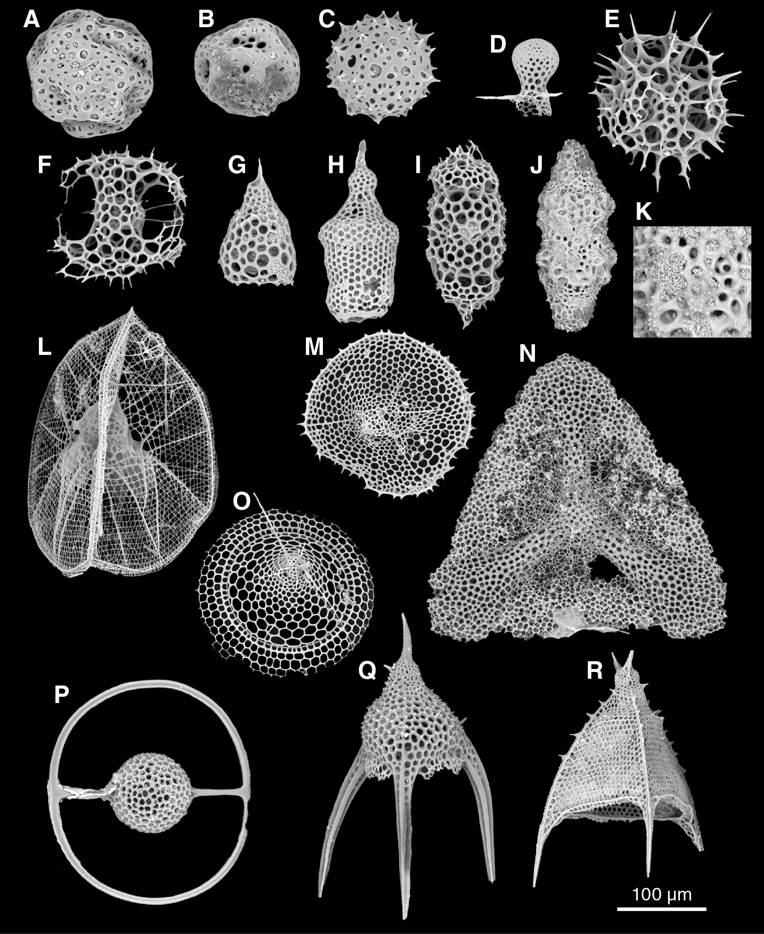
Figure F78. Quaternary radiolarians.
Table T10. Radiolarian biostratigraphy. Download table in .csv format.
A large, barren interval coincides with a major shift in sedimentation rates. Samples 362-U1480B-1H-7, 50–51 cm, through 362-U1480G-54R-4, 111–112 cm (28.14–1255.15 mbsf), are dominated by beds of fine-grained sand and mud of lithostratigraphic Unit II (see Sedimentology and petrology). Unit II is represented by poorly preserved, impoverished fossil assemblages. Radiolarians provided no chronostratigraphic information for Hole U1480F due to their absence or poor preservation, although monospecific and robust spumellarians were observed in rare occurrences in Sample 362-U1480F-96X-CC (787.76 mbsf). The recrystallized and/or dissolved tests, however, made it impossible to resolve the taxonomy at the species level.
Well-preserved pyritized silica biota (radiolarians, diatoms, silicoflagellates, and sponge spicules) were found within gray-green mud in Samples 362-U1480G-54R-4, 111–112 cm, through 55R-CC (1255.17–1269.32 mbsf). The pyritization, which probably occurred in the anoxic water column during the early stages of deposition (Bąk and Sawlowicz, 2000), excellently preserved specimens of late Miocene age (Figure F78J). The skeletons also contained numerous pyrite framboids (Figure F78K), which are likely to have formed during later stages of sediment diagenesis (Szczepanik et al., 2004). Sample 54R-4, 111–112 cm (1255.17 mbsf), contains abundant pyritized radiolarians, with a dominance of the marker species Didymocyrtis antepenultima (top at 8.51 Ma; base at 10.01 Ma). Rare unidentified spumellarians and Cornutella profunda were also noted. Sample 55R-CC (1269.32 mbsf) is dominated by pyritized diatoms and sponge spicules together with rare, well-preserved radiolarians.
Middle Eocene (Figure F79) radiolarians were recovered from Samples 362-U1480G-60R-5, 45–46 cm, through 61R-5, 13–14 cm (1313.96–1323.49 mbsf). The middle Eocene radiolarians generally dominated the fauna, which consist of many deep-living forms such as artostrobiids and warm-water forms such as pterocorythids. Sample 61R-5, 13–14 cm (1323.49 mbsf), contains marker events within the T. triacantha Zone, which was determined by the concurrent presence of Podocyrtis sinuosa (top at 43.38 Ma) and Podocyrtis trachodes (base at 43.59 Ma). Other species in this assemblage include Calocyclas hipsida, Podocyrtis ampla, Theocotylissa ficus, Eusyringium fistuligerum, Thyrsocyrtis triacantha, Dictyopora sp., and Thyrsocyrtis rhizodon. Common occurrences of porcellanite and chert were observed together with abundant radiolarian ghosts, which will be processed postcruise. No age-diagnostic radiolarians were preserved in the recovered Paleocene to Cretaceous interval.

Figure F79. Miocene and Oligocene radiolarians.
Ichthyoliths were observed throughout the lower part of the recovered sequence, especially in the interval lacking siliceous and calcareous microfossils. The critical late Paleocene interval near the top of Section 362-U1480G-61R-7 (1326.37–1326.70 mbsf) yielded much microscopic fish skeletal debris (Figure F80).
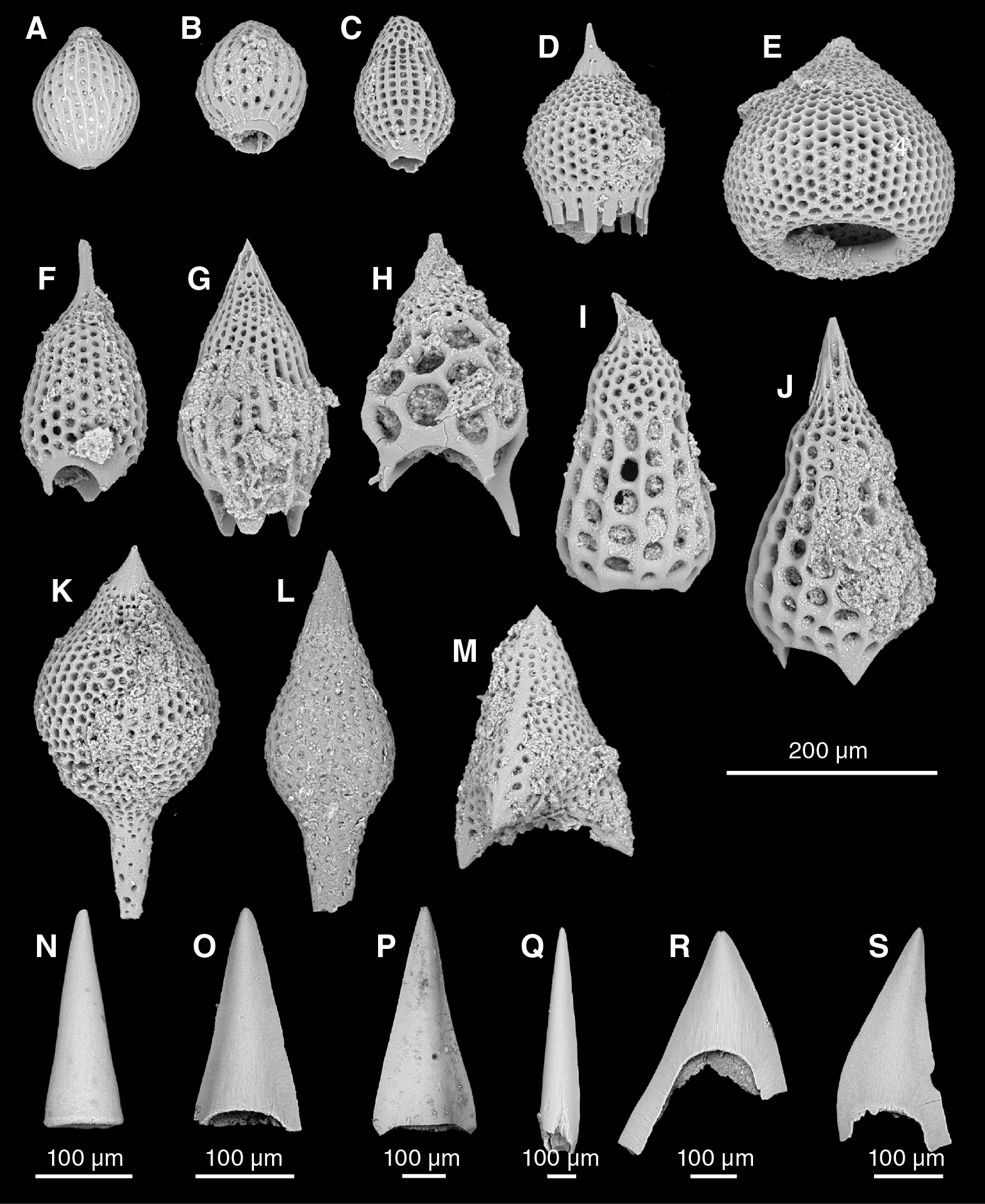
Figure F80. Middle Eocene radiolarians and ichthyoliths.
Age-depth relationships and sedimentation rates
Biostratigraphic and biochronologic data were used for determinations of age-depth relationships and linear sedimentation rates (LSRs). When microfossils occur abundantly and continuously in stratigraphic sequences, age-calibrated evolutionary first appearances (base) and/or extinctions (top) can be used as fixed age points in age-depth plots. In such cases, uncertainties are limited to the sample distance bracketing individual biohorizons (datums) and are, by definition, limited to the depth domain in age-depth plots (e.g., Kroenke, Berger, Janecek, et al., 1991). When microfossils do not occur abundantly and/or continuously or are poorly preserved, this approach is less successful because of the large uncertainties involved in determining exact stratigraphic ranges (top, base, or both) of critical marker species. In these sequences, presence of a species in a sample having an age-calibrated top provides a minimum age, and presence of a species having an age-calibrated base provides a maximum age for that sample. Thus the uncertainties are limited to age at given depths. Presence of a species having both an age-calibrated top and base provides a minimum and maximum age for that depth level.
Microfossil contents of Site U1480 sediment were often characterized by sporadic occurrences, low abundances, and/or poor preservation. Combinations of depth uncertainties (at a given age) and age uncertainties (at a given depth) were used when establishing LSRs based on biochronology. Age-depth distributions of calcareous nannofossils, planktonic foraminifers, diatoms, silicoflagellates, and radiolarians are presented in Tables T7, T8, T9, and T10. Tie points for sedimentation rates are presented in Table T11. Correlations between the single cores retrieved from Holes U1480A–U1480D are presented in detail in Core-log-seismic integration. Mudline sediment was retrieved from Holes U1480E and U1480H, whereas coring began at depth in Holes U1480F and U1480G.
Table T11. Tie points and linear sedimentation rate. Download table in .csv format.
The biostratigraphy of Holes U1480B, U1480E, and U1480H is presented in Figure F81. The distribution of these biostratigraphic data does not show a progressive increase in age with increasing depth, but rather a trend with rapidly increasing ages over a 9 m interval. Tentative LSR tie points from the uppermost 30 m in Hole U1480E are presented in Table T11. A hiatus is indicated at 19.9 mbsf, having a duration of 630 ky. Support for the suggested LSRs is provided by the similarity of the age-depth distribution patterns of microfossil markers in Holes U1480B, U1480E, and U1480H (Figure F81). However, interpretations of paleomagnetic and biostratigraphic data differ slightly for the upper 31 m in Hole U1480H. The paleomagnetic interpretation involves identification of both the Brunhes/Matuyama boundary (0.781 Ma) at 18.5 mbsf, and the Jaramillo Subchron (0.988–1.072 Ma) from 28 to 31 mbsf. The biostratigraphic interpretation involves the presence of a hiatus (0.43-1.06 Ma) at 19.9 mbsf. This discrepancy remains to be investigated by postcruise studies.
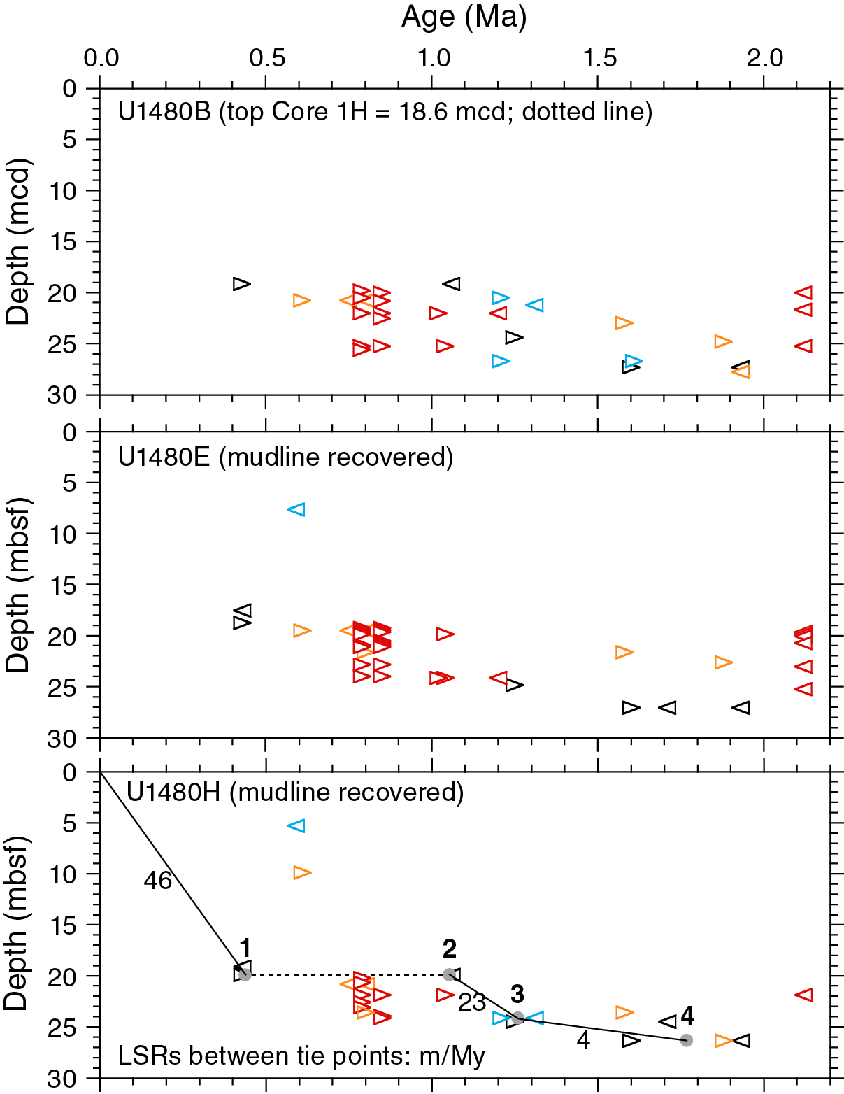
Figure F81. Age-depth plot of biostratigraphic markers, Holes U1480B, U1480E, and U1480H.
Nine biostratigraphic indicators are used to depict a combined sedimentation rate history from Holes U1480F and U1480H. These indicators, or LSR tie points, are labeled 1–9 in Figure F82 and Table T11.
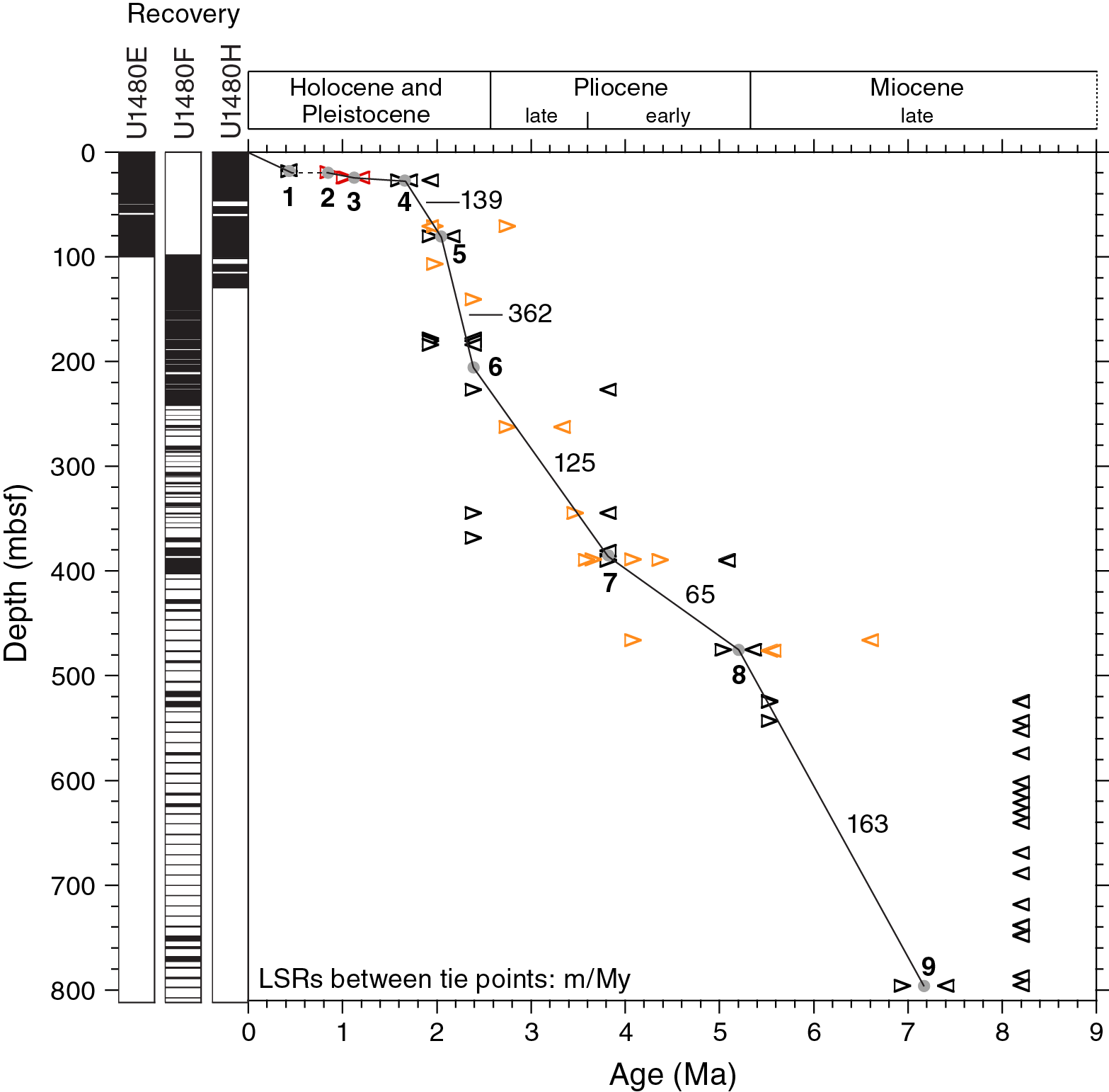
Figure F82. Linear sedimentation rates based on biostratigraphy, Holes U1480H and U1480F.
Another 11 biostratigraphic tie points were used to construct the sedimentation rate history in Hole U1480G (Figures F83, F84; Table T11). There is a slow increase in LSRs starting during the early Miocene and lasting until 9.4 Ma, when sedimentation rates increased by well over an order of magnitude (from 15 to 217 m/My at 1255 mbsf). The Site U1480 late Eocene through Pleistocene sedimentation rate history, including the high rates from 9.5 Ma during Nicobar Fan deposition, has been compared with the corresponding histories from several other DSDP/ODP/IODP sites from the eastern Indian Ocean (McNeill et al., 2017a).
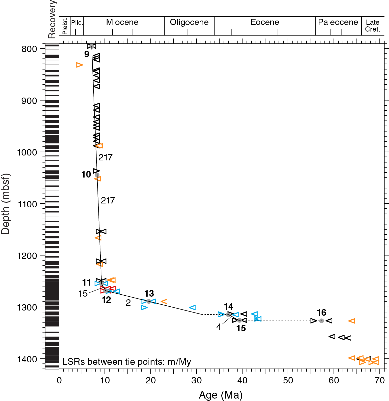
Figure F83. Linear sedimentation rates based on biostratigraphy, Hole U1480G.
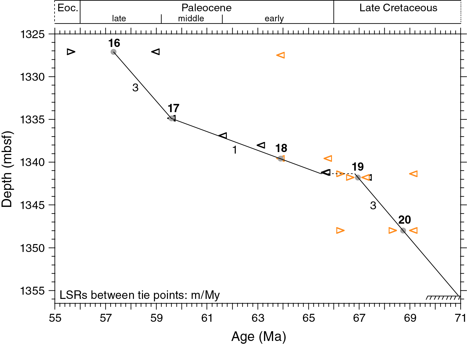
Figure F84. Linear sedimentation rates based on biostratigraphy.
Prior to 9.4 Ma, biostratigraphic age-depth indicators were distributed over a large age span (~60 My) but over a short depth span (1255–1414 mbsf). Condensed sediment was preserved during the late early Oligocene through the early late Miocene, the middle Eocene, the Paleocene, and the Maastrichtian.
A 5.7 My long hiatus is indicated between 37.0 Ma (late Eocene) and 31.3 Ma (early Oligocene) (Figure F83). A second, longer (17.6 My) hiatus is indicated between 57.3 Ma (late Paleocene) and 39.7 Ma (middle Eocene). A total of 59.66 m of Paleocene basalt, volcanic breccia, and basaltic intrusion was encountered in two intervals: 1327.23–2349.80 and 1361.54–1398.63 mbsf. In the plot showing LSRs for the Late Cretaceous–Paleocene interval (Figure F84), these intervals were removed in order to better depict the preserved accumulation of sediment. A 1.3 My long (65.5–66.8 Ma) hiatus is indicated across the Late Cretaceous–Paleocene transition.
Paleomagnetism
Orientation tools were deployed during APC operations but could not be deployed during XCB or RCB operations, resulting in most of the magnetic declinations being uncorrected. For this reason, we summarize coring operations at Site U1480 as follows:
- Cores 362-U1480B-1H, 362-U1480E-1H through 12H, 362-U1480F-2H through 8H, and 362-U1480H-1H through 17H were cored with the APC coring system using nonmagnetic cutting shoes.
- Cores 362-U1480F-9F through 51F were cored with the HLAPC system using nonmagnetic cutting shoes.
- Cores 362-U1480F-52X through 98X were cored with the XCB system using standard cutting shoes.
- Cores 362-U1480G-2R through 73R were cored with the RCB system using nonmagnetic cutting shoes.
- Cores 362-U1480E-1H through 8H, 362-U1480F-2H through 8H, and 362-U1480B-1H were oriented with the Icefield MI-5 core orientation tool.
- Cores 362-U1480H-1H through 17H were oriented with the FlexIT core orientation tool.
The derived paleomagnetic directions can be used to construct a magnetostratigraphy for dating the sediment. The use of orientation data to correct declinations facilitates the magnetostratigraphic investigation at Site U1480.
We made pass-through magnetometer measurements on all archive-half sections and on representative discrete samples taken from working halves. In order to isolate the characteristic remanent magnetization (ChRM), sedimentary archive-half cores were demagnetized in an alternating field (AF) using steps of 5, 10, 15, 20, and 25 mT and were measured with the pass-through superconducting rock magnetometer (SRM) at 2.5 cm intervals. A new IMS-SRM software program was used, and in the case of basement cores, we were able to adjust the track speed, which is a critical parameter for strongly magnetized basement rocks. Selected discrete samples were AF demagnetized with an ASC Scientific D-2000 AF demagnetizer using steps of 5, 10, 15, 20, 25, 30, 40, 60, 80, and 100 mT. A total of 24 discrete samples were also subjected to stepwise thermal demagnetization up to 575°C with steps of 25°C below and 50°C above 100°C. The remanence of discrete samples was measured using a spinner magnetometer (AGICO model JR-6A). The results are displayed in Zijderveld diagrams (Zijderveld, 1967) and the ChRM direction is calculated using principal component analysis (PCA; Kirschvink, 1980).
Natural remanent magnetization of cores
To illustrate the overall magnetic properties and demagnetization behavior of Site U1480 sediments and rocks, we show the natural remanent magnetization (NRM) intensities, inclinations, and declinations before and after 20 mT AF demagnetization (Figures F85, F86, F87, F88, F89). Variations in NRM intensity generally correlate with lithology. Paleomagnetic measurements indicate that the calcareous clay in Unit I (0–26.42 mbsf) has a mean NRM intensity of ~3 × 10⁻² A/m, whereas the fine sand with silty clay in Subunit IC (18.80–26.42 mbsf) has a lower NRM intensity of ~1 × 10⁻³ A/m. NRM intensities remain constant (~3 × 10⁻² A/m) for the silt and bioturbated clay/claystone in Unit II (26.42–1250.35 mbsf) and for the grayish green and reddish brown clay/claystone in Unit III (1250.35–1327.18 mbsf). NRM intensities range between 5 × 10⁻³ and ~5 × 10⁻² A/m for the basaltic lava flow, ash-rich volcanogenic sand, and mudstone in Unit IV (1327.23–1349.80 mbsf) and bioturbated lithified calcareous ooze (chalk) and calcareous clay/claystone in Unit V (1349.80–1415.35 mbsf) and increase to ~2 A/m for the basaltic basement rock in Unit VI (1415.35–1431.63 mbsf). The high values in Unit VI reflect the high iron oxide content of the basalt. Many discrete peaks of NRM and magnetic susceptibility (see Physical properties) in Units II and III can be tied directly to the presence of ferrimagnetic greigite in these layers (see Sedimentology and petrology). To the first order, this indicates that the magnetic moment is a function of the concentration of magnetic minerals.

Figure F85. Paleomagnetic measurements of Hole U1480B archive-half sections.
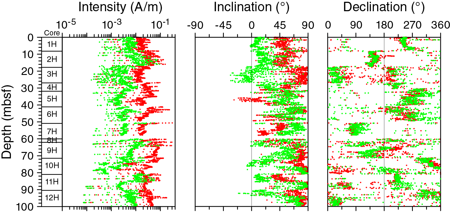
Figure F86. Paleomagnetic measurements of Hole U1480E archive-half sections.

Figure F87. Paleomagnetic measurements of Hole U1480F archive-half sections.
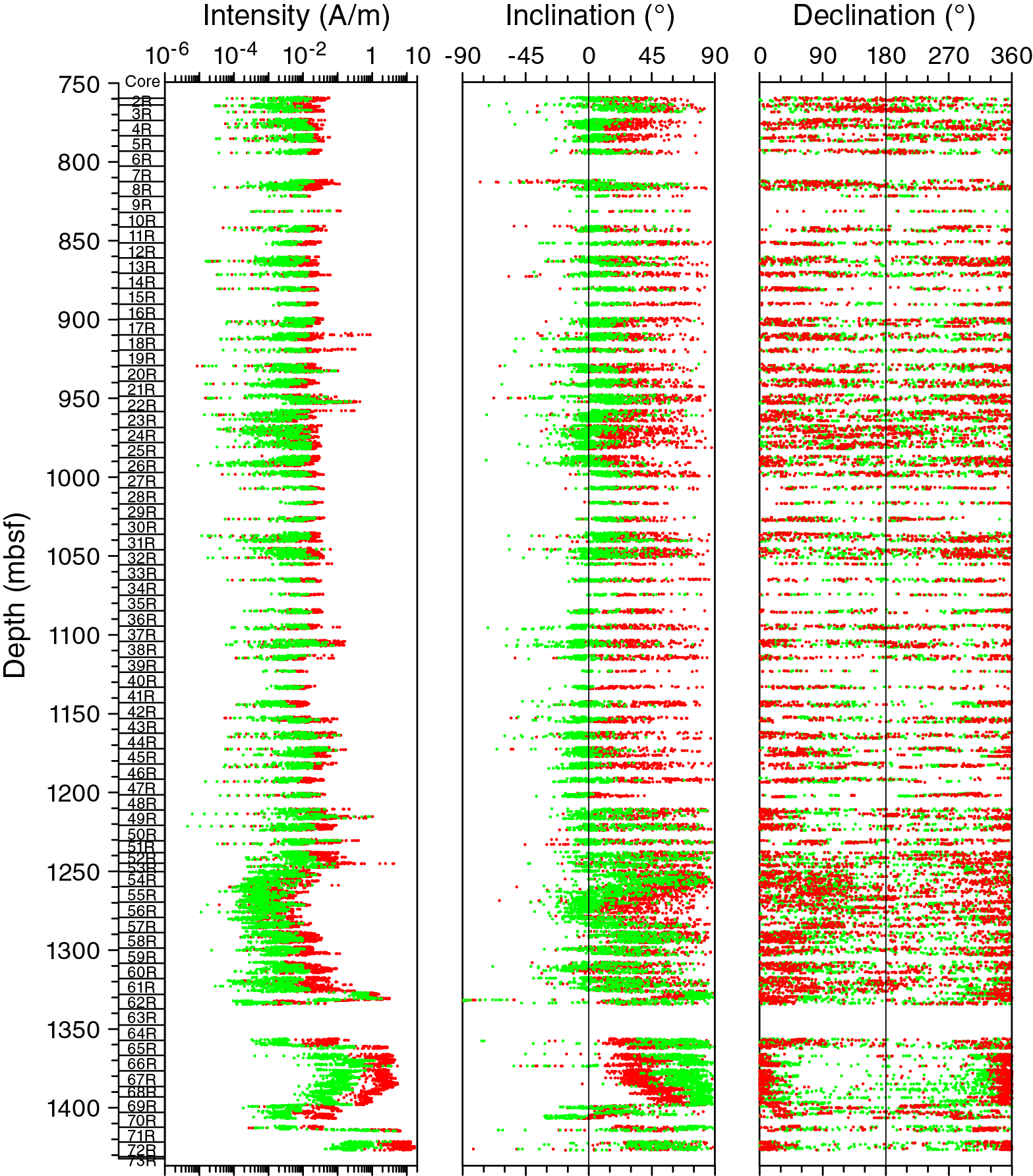
Figure F88. Paleomagnetic measurements of Hole U1480G archive-half sections.

Figure F89. Paleomagnetic measurements of Hole U1480H archive-half sections.
As with many other ocean drilling expeditions, remagnetization imparted by the coring process is significant at Site U1480. NRM inclinations are strongly biased toward the vertical (mostly toward +90°) in the majority of cores. AF demagnetization to 5–10 mT is effective in removing the drilling overprint for a high percentage of samples, as shown by inclinations shifted toward shallower values that are comparable with the expected inclination for the site (approximately ±6°), by a factor of ~3–4 decrease in magnetization intensity after 5 mT demagnetization, and by an order of magnitude decrease in magnetization intensity after 20 mT AF demagnetization.
Paleomagnetic demagnetization results
NRM declinations of APC cores (i.e., Cores 362-U1480B-1H, 362-U1480E-1H through 8H, 362-U1480F-2H through 8H, and 362-U1480H-1H through 17H) before orientation correction differ significantly, as expected. After orientation correction using data from the two orientation tools, declinations come close to magnetic north for normal polarity cores and magnetic south for reversed polarity cores, which is consistent with the remanence being of primary origin. The depth plots of declinations and inclinations for APC cores from Hole U1480E after 25 mT AF demagnetization and Holes U1480H and U1480B after 20 mT AF demagnetization are illustrated in Figure F90. The similarity of results from 0 to 40 mbsf attests to the fidelity of these paleomagnetic records. In addition, this indicates that the chronology of Hole U1480H can be faithfully translated to Hole U1480E. We note that steep inclinations (>50°) are present throughout the rest of the section (deeper than 40 mbsf). These values are most probably caused by magnetic drilling overprints and/or disturbance within the recovered sand sections.
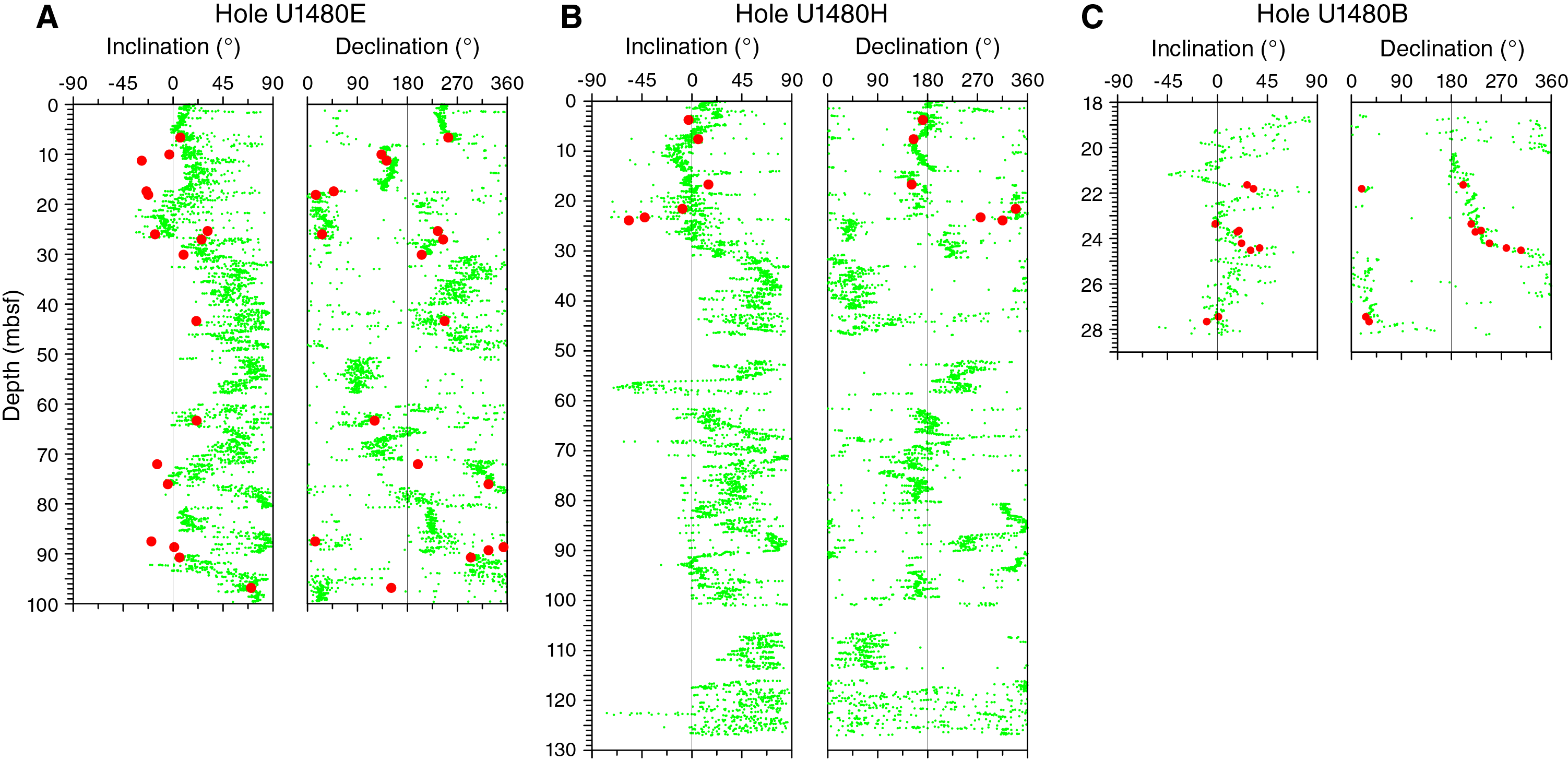
Figure F90. Comparison of declinations and inclinations from archive-half sections.
The magnetic properties of the archive section halves were confirmed by discrete sample measurements (Figures F90, F91). The nearly vertical overprint was removed by 5–10 mT AF demagnetization (e.g., Figure F91) for nearly all samples. AF demagnetization was generally successful in isolating ChRM for most discrete samples. The majority of discrete samples in lithostratigraphic Units I and II showed straightforward demagnetization behavior and revealed the ChRM. Several discrete samples from the lower part of Unit II and upper part of Unit III, however, displayed more complicated demagnetization paths that do not simply decay toward the origin (Figure F91), indicating that there is a remaining magnetic component in the sample. A few samples also displayed erratic or incoherent demagnetization behavior with data points that could not be fit to a line using the PCA method (Kirschvink, 1980). The most likely cause of this erratic behavior is drilling-related disturbance/deformation and weaker NRM intensity.
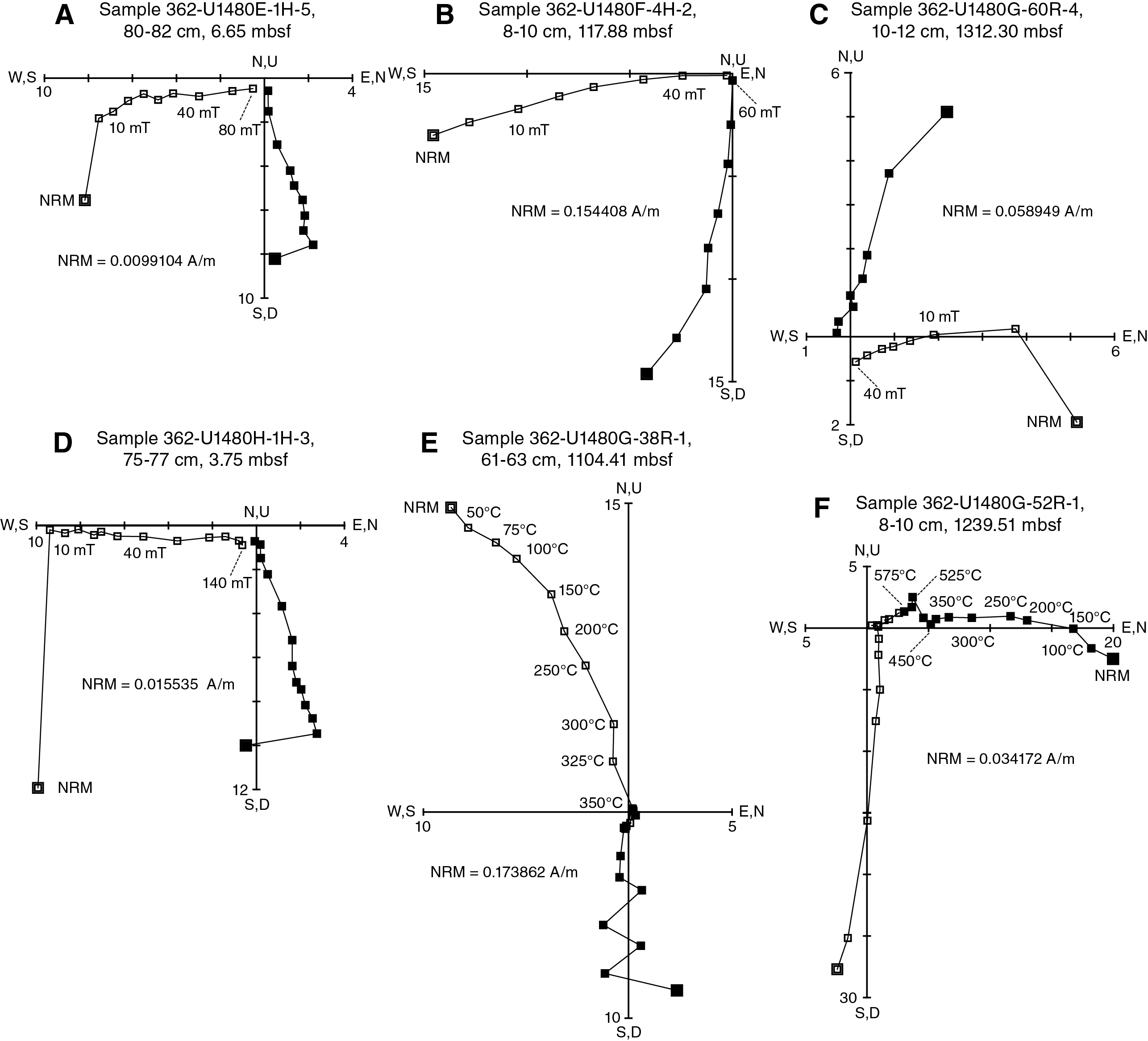
Figure F91. Representative vector endpoint diagrams.
For thermal demagnetization results, magnetite and greigite are the two dominant magnetic carriers for the ChRM (Figure F91). The secondary drilling-induced overprints are not easily removed by thermal treatments. Because of the complexities of the coercivity and unblocking spectra of the NRM, we suggest that sequential demagnetization by combining AF and thermal methods could be the best approach to fully isolate the ChRM, specifically for those sections cored with the XCB system, which uses standard cutting shoes that are magnetic.
Magnetostratigraphy
Construction of a magnetostratigraphy is based on the correlation between the measured polarity pattern and the geomagnetic polarity time scale (GPTS) as well as biostratigraphic constraints. At a low-latitude area such as the location of Site U1480 (~3°N), a near 180° shift in declination in the cores is a more reliable sign of a polarity transition than a change in inclination sign. This is because the inclination is very shallow near the Equator; hence, the sign of the inclination is not indicative of the polarity given data uncertainties and because the vertical drilling overprint affects the inclinations more than the declinations. As shown in Figure F90, the stable inclinations identified from both discrete samples and corresponding archive sections are close to the expected value at the site, indicating the ChRM directions of these samples may be representative of the direction of the geomagnetic field at the time of deposition.
Based on the corrected magnetic declination records (see Paleomagnetism in the Expedition 362 methods chapter [McNeill et al., 2017b]), the Brunhes/Matuyama Chron boundary (0.78 Ma) is placed at ~18.5 mbsf, which also matches the polarity shift in Hole U1480E at a similar depth (Figure F92). Sediment between 28 and 31 mbsf shows normal polarity, indicating that the Jaramillo Subchron (0.988–1.072 Ma) may have been recorded in the sediment with a moderate deposition rate. Identification of reliable polarity deeper than ~40 mbsf is hindered by the uncertainty in declination of the loose material (e.g., soupy sand) and drilling disturbance of cores.

Figure F92. Magnetostratigraphic results of corrected paleomagnetic declinations.
Interpretations of paleomagnetic and biostratigraphic data differ slightly for the upper 31 m in Hole U1480H. As mentioned above, the paleomagnetic interpretation involves identification of both the Brunhes/Matuyama boundary (0.781 Ma) at 18.5 mbsf, and the Jaramillo Subchron (0.988–1.072 Ma) from 28 to 31 mbsf. The biostratigraphic interpretation involves the presence of a hiatus (0.43–1.06 Ma) at 19.9 mbsf (see Biostratigraphy). This difference remains to be investigated by postcruise studies.
For unoriented cores, declinations cannot be used to construct a magnetostratigraphy because the rotary drilling technique frequently produces relative rotations between different segments of sediment within each core. For Cores 362-U1480F-9F through 98X (146.5–805.725 mbsf) and 362-U1480G-2R through 51R (759.6–1233.6 mbsf), strong magnetic overprinting and drilling disturbance preclude reliable identification of polarity chrons. We observed that some of the directional swings correspond to sandy layers, suggesting there is a high possibility these are caused by loose material and drilling disturbance of cores. In contrast, coherent core sections in Cores 362-U1480G-52R and 53R and Section 362-U1480G-61R-5 revealed magnetozones by both pass-through and discrete sample measurements. Preliminary shipboard lithologic and biostratigraphic studies suggest that sediment around 1250 and 1318 mbsf should be late Miocene (~9 Ma) and middle Eocene (~36–38 Ma), respectively. With these age constraints, we tentatively correlated the short polarity intervals at 1239.08–1241.5 mbsf to the reversed and normal polarity zones in Chron C4 (7.528–9.786 Ma) and those at 1317.83–1319.12 mbsf to Chron C17 (36.668–38.449 Ma).
For basement rock units, the observed paleomagnetic signals cannot be directly linked to the GPTS because of the intermittent eruptive nature of basalt (short timescale of emplacement) and the very low sedimentation rate of the overlying pelagic sediment in Cores 362-U1480G-54R through 71R (1250.35–1415.28 mbsf). Biostratigraphic constraints based on planktonic foraminifer ages (Late Cretaceous; ~68.32 Ma) for this interval (see Biostratigraphy) suggest the observed magnetization polarity intervals could correlate with Chron C31 (68.32–71.40 Ma). Further tests in shore-based studies are necessary to achieve a robust magnetic characterization of the basement units.
Geochemistry
Inorganic geochemistry
The main objective of the inorganic geochemistry program at Site U1480 is to document variations in chemical composition of interstitial water that can be used to elucidate fluid–rock interactions, which in turn may affect the state and geomechanical properties of the formation before and during subduction. A total of 175 interstitial water samples were squeezed for chemical and isotopic analyses from selected whole-round sections. We collected 29 samples (10 cm in length) from Hole U1480E (APC cores), 43 samples (20 cm in length) from Hole U1480F (6 from APC, 22 from HLAPC, and 21 from XCB cores), 47 samples (20–25 cm in length) from Hole U1480G (RCB cores), and 56 samples (10 cm in length) from Hole U1480H (APC cores). Samples were collected on the catwalk at a frequency of 3 or 4 samples per core from Cores 362-U1480E-1H through 4H, 1 or 2 samples per core in most cored intervals of Holes U1480F and U1480G, and 4–7 samples per core from Hole U1480H. In addition, 41 Rhizon samplers were inserted into the uncut liner of Cores 362-U1480H-9H through 11H at a resolution of 2 samplers per section. From these, only 32 samplers yielded interstitial water in volumes from 2 to 12 mL. A set of whole-round samples was collected for shore-based microbiological analyses, each contiguous to every interstitial water whole round collected from Hole U1480H. These microbiological samples were immediately frozen at –80°C.
All samples from whole rounds were thoroughly cleaned of drill fluid contamination. The uppermost four cores (1.2–29 mbsf) in Hole U1480E and all cores (1.4–127 mbsf) in Hole U1480H were processed under a nitrogen atmosphere for postcruise studies of biogeochemical cycling of redox-sensitive elements in shallow sediment. All cleaned samples were placed in Ti squeezers and squeezed at maximum pressures of 24.5 MPa (gauge forces of up to 35,000 lb). The volume of recovered interstitial water varied with lithology, depth, and coring technique and ranged between 15 and 60 mL in APC cores, 22 and 57 mL in HLAPC cores, 8 and 38 mL in XCB cores, and 3 and 20 mL in RCB cores.
The chemical composition of the samples from below the sulfate–methane transition zone (SMTZ; ~120 mbsf at Site U1480) was corrected for drill fluid contamination where the sulfate data indicate a seawater component (see Geochemistry in the Expedition 362 methods chapter [McNeill et al., 2017b]). This correction was applied only to samples from Holes U1480F and U1480G. Specific aliquots were used for shipboard analyses, and the remaining fluid was subsampled for shore-based analyses.
The raw data for the major and minor element concentrations are listed in Tables T12 and T13. In Tables T14 and T15, we list the sulfate-corrected concentration data. In Table T16, we list the data collected from the Rhizon samples in Hole U1480H. Figures F93 and F94 illustrate downhole profiles for both raw and sulfate-corrected data for all holes drilled at Site U1480. Data from high-resolution sampling in the upper 150 mbsf are shown in Figure F95.
Table T12. Organic metabolites and major element uncorrected concentrations in interstitial water. Download table in .csv format.
Table T13. Minor element uncorrected concentrations in interstitial water. Download table in .csv format.
Table T14. Organic metabolites and major element sulfate-corrected concentrations in interstitial water. Download table in .csv format.
Table T15. Minor element sulfate-corrected concentrations in interstitial water. Download table in .csv format.
Table T16. Organic metabolites and chloride concentrations in Rhizon interstitial water. Download table in .csv format.
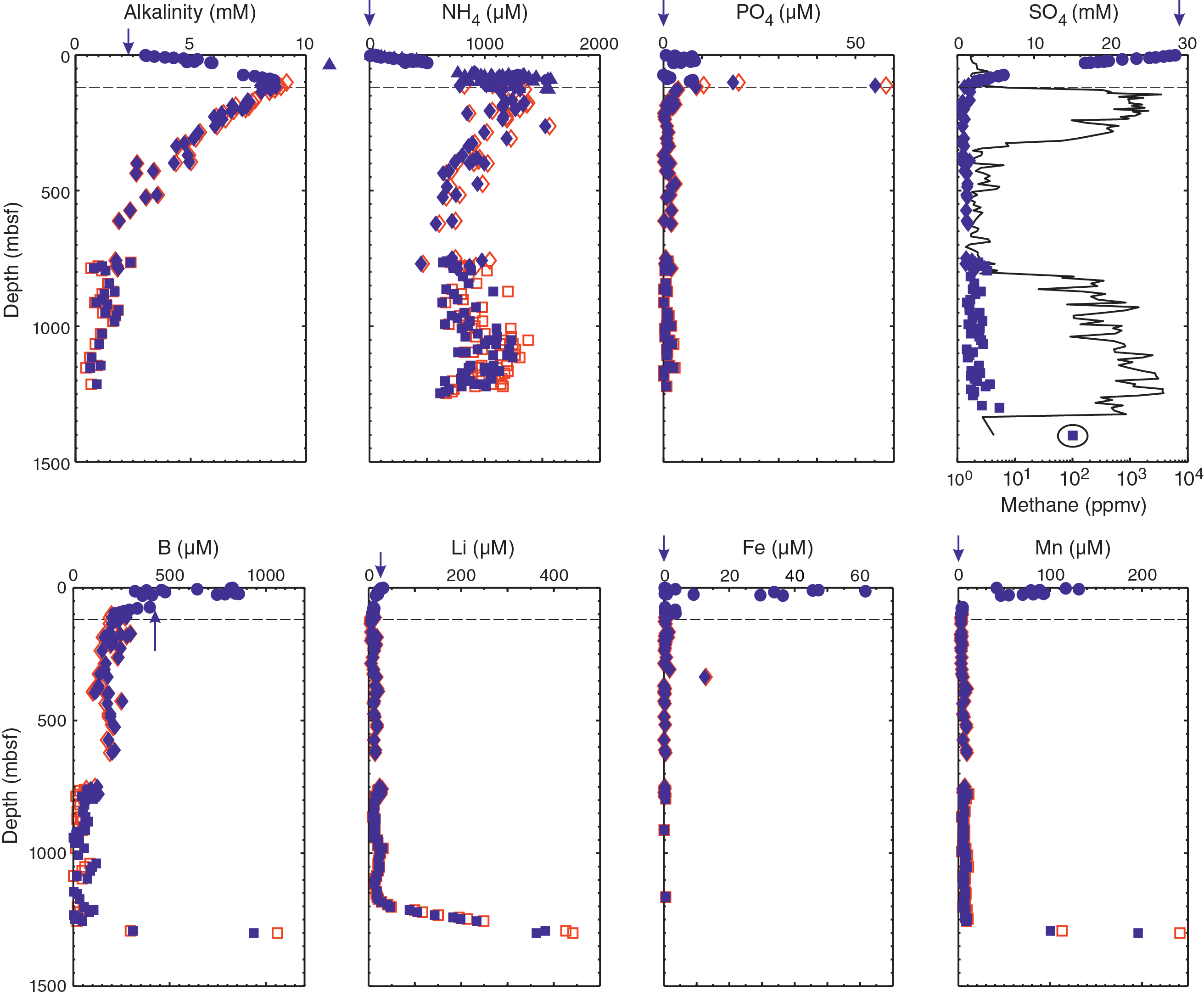
Figure F93. Alkalinity, ammonium, phosphate, sulfate, boron, lithium, iron, and manganese profiles.
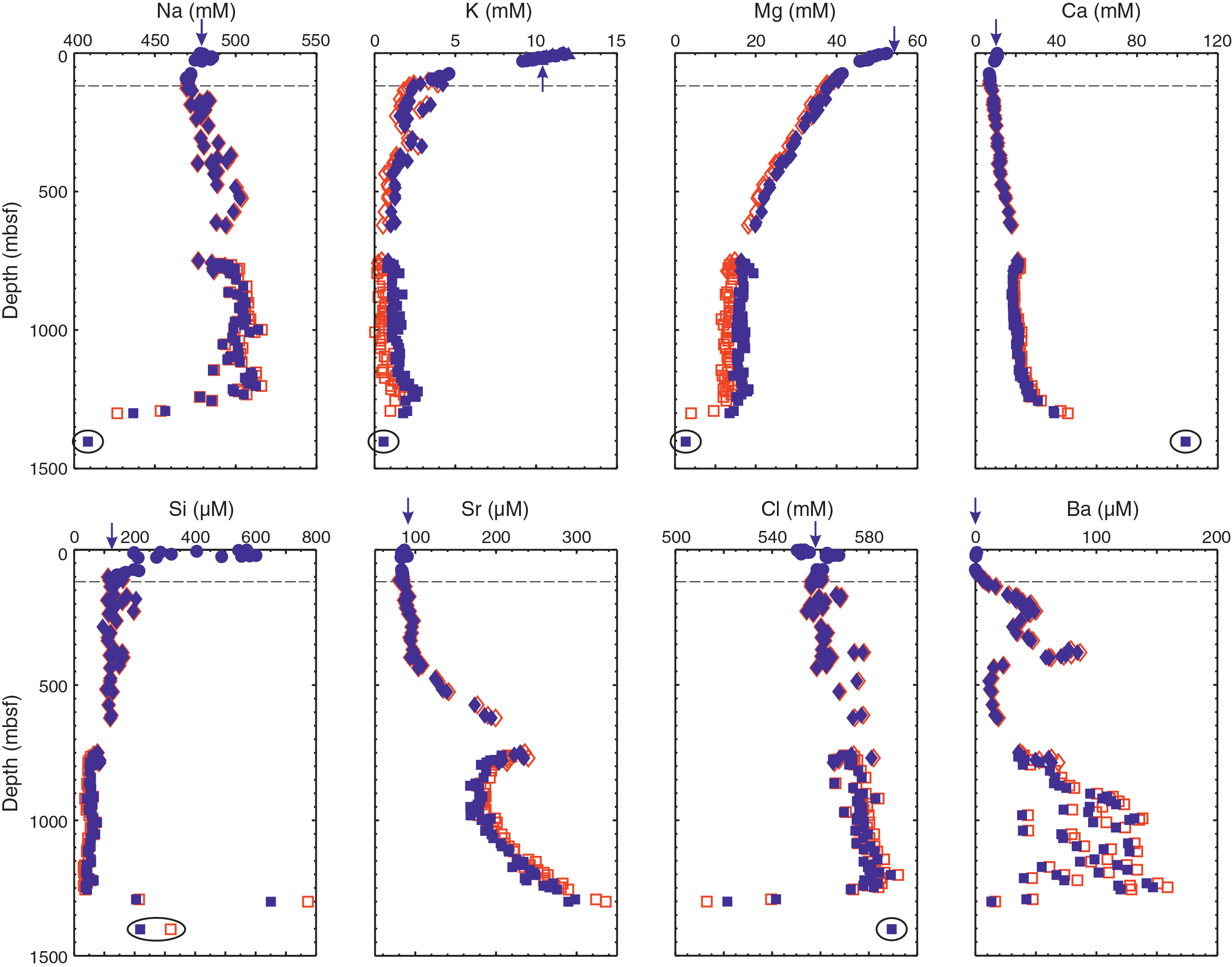
Figure F94. Sodium, potassium, magnesium, calcium, silica, strontium, chloride, and barium profiles.
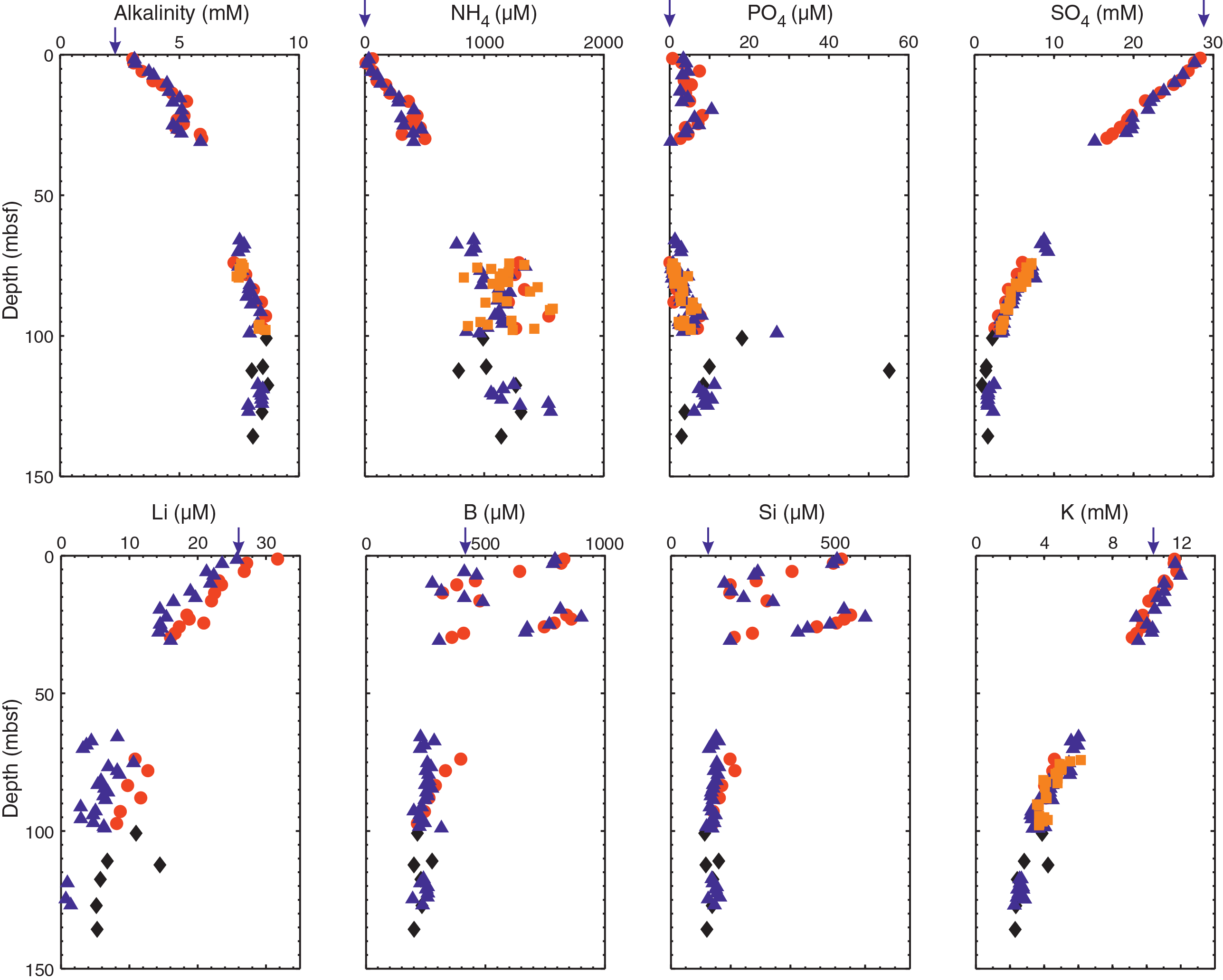
Figure F95. Alkalinity, ammonium, phosphate, sulfate, lithium, boron, silica, and potassium profiles.
We note that the deepest sample collected in Hole U1480G (Sample 362-U1480G-70R-1, 31–39 cm; 1402 mbsf) has a sulfate concentration of 15 mM, which may reflect the in situ sulfate value resulting from diffusional contact from a sulfate-bearing basement aquifer. Sulfate supply from basement has been documented in deep sediment sections of both the Costa Rica and Nankai input sites (Silver et al., 2000; Harris et al., 2013a; Torres et al., 2015). Because of the limited number of samples close to basement at Site U1480, we cannot discount the possibility of a sulfate contribution from basement, which would argue for the use of uncorrected (raw) data. Thus, in the following sections we refer only to raw concentration values, but we include the tables with sulfate-corrected data to illustrate the maximum error that could be introduced by drill-fluid contamination.
The geochemical profiles at Site U1480 reflect the combined effects of organic matter diagenesis, alteration of volcanogenic sediment, and reactions in oceanic basement. Where there was poor core recovery and/or intense sample disturbance, no interstitial water was collected, as indicated by data gaps in the figures.
Biogeochemical processes
The interstitial water profiles of sulfate, alkalinity, ammonium, and phosphate in the uppermost 150 m at this site have concentration-depth profiles that reflect characteristic organic matter remineralization (Figure F93). Sulfate concentrations decrease almost linearly from the seafloor to the SMTZ at ~120 mbsf (dotted line in Figure F93). Alkalinity increases from a seawater value at the seafloor to a maximum of 8.7 mM at 117 mbsf and gradually decreases with depth to <1 mM in the deepest sections (deeper than 1000 mbsf) cored at Site U1480. Alkalinity is involved in authigenic carbonate formation in the upper ~150 mbsf and in carbonate cementation below ~800 mbsf, as suggested by the drawdown in calcium concentration in the upper 150 mbsf and between ~800 and 1200 mbsf (Figure F94). This is consistent with the presence of calcareous clay in lithostratigraphic Unit I and observation of carbonate cements (concretions) in the cores from Units II and III (see Sedimentology and petrology) and discussed further in the following sections. Ammonium peaks at ~150 mbsf, where it reaches a maximum value of ~1500 µM and then decreases with depth to 750 mbsf and subsequently increases with a maximum of >1000 µM between 1038 and 1193 mbsf; the data in this deeper section show more scatter. Phosphate increases from seawater values near the seafloor to a high value of ~8 µM at 20 mbsf (Figure F93). There is a second phosphate concentration maximum of 55 µM at 113 mbsf, below which phosphate concentrations decrease sharply with depth, which is discussed further in the following sections.
High-resolution sampling in Hole U1480H aimed at investigating whether the maxima in the dissolved phosphate distribution observed between 15 and 26 mbsf (maximum value = 10 µM at 20 mbsf) and between 80 and 130 mbsf (maximum value = 55 µM at 113 mbsf) in Holes U1480E and U1480F may indicate regional fluid transport along shallow sandy horizons (Figure F95). Fluids collected by interstitial water whole-round and Rhizon sampling both give consistent results and help delineate the phosphate maxima first observed in Holes U1480E and U1480F, which correspond to sediment sections with a significant sand fraction in Unit I and Subunit IIA (see Sedimentology and petrology). No interstitial water samples were retrieved from intervals of unconsolidated sand from 31 to 62 mbsf (Sections 362-U1480H-4H-5 through 8H-3) and from 99 to 117 mbsf (Sections 11H-7 through 16H-1).
Although barium is not directly related to organic matter cycling, consumption of sulfate by biogeochemical reactions (organic matter diagenesis and anaerobic methane oxidation) results in release of barium to the interstitial water from dissociation of marine barite (BaSO4) (Torres et al., 1996). We observe a rapid increase in dissolved barium that coincides with the SMTZ (Figure F94). The barium source for the second and third maxima in barium concentration, with values >80 µM at 380 mbsf and >150 µM in some samples deeper than 800 mbsf, is not clear at this time but likely reflects alteration of detrital and/or volcanogenic siliciclastics.
Chemical changes caused by alteration of volcaniclastics
The sediment of lithostratigraphic Unit I contains various ash layers in the upper four cores of Holes U1480E and U1480H (1.5–25 mbsf; see Sedimentology and petrology). In general terms, ash in deep-seafloor sediment undergoes a series of alteration reactions including hydration of silicic ash layers, smectite generation, and crystallization of zeolites (Sheppard and Hay, 2001; Kastner et al., 2014). During the first of these steps, hydration of volcanic ash layers results in an increase in chloride concentration to ~570 mM in the upper 20 m, which is accompanied by a release of cations (K, Ca, Na, and Al) and silica to the interstitial water. This reaction is evidenced by an increase in potassium in the upper 12 m from its seawater value (10 mM) to 12 mM with a concomitant calcium increase from its seawater value (10 mM) to 11 mM and a sodium increase from 480 to 485 mM (Figures F93, F94). Silica increases from its seawater value (125 µM) to 600 µM at ~22 mbsf. Aluminum concentrations were not measured. The presence of magnesium and potassium in the interstitial water permits the precipitation of smectites (most likely montmorillonite) as a secondary mineral. At Site U1480, the concomitant removal of potassium and silica, which reach concentration minima at ~120 mbsf, is consistent with the formation of K-rich smectites. Further depletion of potassium below 400 mbsf to values as low as 1 mM may reflect zeolite formation (e.g., K-clinoptilolite). Zeolites were observed in Cores 362-U1480F-53X, 54X, and 60X (369–436 mbsf) (see Sedimentology and petrology).
The concentrations of minor cations (Li, B, Mn, and Fe) are also influenced by ash alteration reactions (Figure F93). Fe and Mn are released from volcanogenic siliciclastics in the upper 20 m, where they reach high values of 60 µM (Fe) and 130 µM (Mn). These extremely high values rapidly decrease downhole, possibly as a result of utilization by microbes.
Lithium and boron are consumed during formation of smectite, and these elements show a concentration decrease concomitant with the uptake of silica and potassium, with low values (<10 µM Li and <200 µM B) observed between 100 and 130 mbsf (Figure F95). The maxima in B and Si around 20 mbsf correspond to a small peak in PO4 at this horizon, which may reflect fluid transport along this shallow coarse-grained horizon. Below 150 mbsf, Li and B concentrations remain low until 1250 mbsf (Figure F93). These low concentration values indicate continuous uptake of these elements throughout Units I and II and are likely due to extensive alteration of volcaniclastics at depth.
Collectively, geochemical data in the upper 600 m reflect the expected effects of alteration of volcaniclastics with an overall decrease in the concentration of K, Li, and B and a release of Ca. These changes are common in ash-bearing sediment and underlying volcaniclastics (e.g., Gieskes et al., 1990; Lawrence and Gieskes, 1981), as discussed below.
Effect of underlying volcaniclastic sediments and oceanic basement
Below the depth of calcium removal by carbonate precipitation at the SMTZ (~120 mbsf), there is an overall increase in dissolved calcium and strontium and a decrease in magnesium toward the base of the sediment section (Figure F94), likely reflecting supply from alteration of deep volcaniclastics and/or oceanic basement (e.g., Lawrence and Gieskes, 1981). The increase in dissolved calcium appears to support carbonate precipitation even at very low alkalinity values (<1 mM) and may be responsible for the carbonate cements observed in lithostratigraphic Unit II (Sections 362-U1480F-96X-1 and 362-U1480G-9R-1; 786 and 822 mbsf, respectively) and in several cores from Unit III (see Sedimentology and petrology). Postcruise chemical and isotopic characterization of these carbonate cements will help establish their depth of formation. The magnesium profile shows a continuous decrease with depth from its seawater concentration (54 mM) to ~15 mM at 1242 mbsf (Table T14). Chloride increases with depth to 578 mM at 1242 mbsf (Table T12), reflecting hydration of volcaniclastics. The curvature in the Mg concentration profile in the upper 1242 m suggests a component of upward fluid advection (Figure F94), for which the driving mechanism requires additional postcruise studies.
Interstitial water collected from three samples between 1255 and 1300 mbsf (Sections 362-U1480G-54R-4 through 59R-2) shows pronounced concentration changes in most of the dissolved cations: decreases in sodium to ~437 mM and magnesium to ~13 mM and attendant increases in calcium to 39 mM, boron to ~940 µM, lithium to ~363 µM, and silica to ~651 µM (Figures F93, F94). Associated with these marked changes is a sharp decrease in chloride from ~580 to ~520 mM in the interval between 1250 and 1300 mbsf. Analysis and implications of this freshening anomaly for diagenetic dehydration reactions and their influence on development of the plate boundary décollement and its properties are discussed in Hüpers et al. (2017). A single sample (362-U1480G-70R-1, 31–39 cm) collected at 1403 mbsf shows a distinct reversal in the silica and chloride gradients, with values of 589 mM Cl and 219 µM Si (indicated by a circle in Figure F94). These values are indicative of alteration reactions in oceanic basement. Consistent with such reactions, Ca shows a high value of 104 mM and Mg a low value of 3 mM at this depth (Figure F94). The sulfate concentration of 15 mM at this depth likely reflects a sulfate-enriched fluid in basement. There was insufficient interstitial water from this sample for minor element analyses. Collectively, these concentration changes point to dehydration reactions below the carbonate-cemented sediment observed in the cores of Subunit IIC (see Sedimentology and petrology); furthermore, the trend reversal observed in Core 362-U1480G-70R (1403 mbsf, highlighted by a circle around the square symbols in Figure F94) precludes a water contribution from dehydration reactions in oceanic basement, such as those proposed upon subduction in the Nankai margin (Kameda et al., 2011). Instead, the fluid is likely released from hydrated silica phases currently at this depth horizon (see CHEMISTRY in Supplementary material) (Hüpers et al., 2017).
The release of water evidenced by the decrease in chloride between 1250 and 1300 mbsf corresponds to the interval where changes in seismic reflection characteristics are associated with the Nicobar Fan/pelagic unit boundary and can be correlated to the high-amplitude negative polarity (HANP; Dean et al., 2010) horizon closer to the subduction zone (see Horizon C in Core-log-seismic integration). The released water, which is inferred to be the cause of the HANP reflector, may have consequences for the mechanical properties of this sedimentary section within the subduction zone (Hüpers et al., 2017).
High B and Li concentrations can be used to estimate reaction temperatures (e.g., Wei, 2007; Hüpers and Kopf, 2012). The high Li and B concentration values (corrected and uncorrected) in the interval from 1250 to 1300 mbsf (Figure F94) require temperatures above 100°C, which are higher than the estimated current temperature of 61°C at 1350 mbsf (see Downhole measurements). Such high concentrations in the deepest 50 m above basement suggest a recent high-temperature pulse, perhaps caused by a magmatic intrusion (see lithostratigraphic Unit V in Sedimentology and petrology).
Organic geochemistry
Hydrocarbon sampling
Headspace or void gas samples were taken from each sediment core to monitor for the presence and abundance of C1–C3 hydrocarbons, as part of the standard IODP safety protocol (Pimmel and Claypool, 2001). A total of 158 headspace samples were analyzed by gas chromatography (see Geochemistry in the Expedition 362 methods chapter [McNeill et al., 2017b]). Only Section 362-U1480E-10H-5 had clear voids and was sampled accordingly. Instrumental blanks were determined to be ~2 ppmv for methane, and methane abundances were indistinguishable from the detection threshold from 0 to 112.8 mbsf. Methane concentrations increase, reaching 3474 ppmv at 145.3 mbsf, which is slightly below the base of the SMTZ (Figures F93, F96; Table T17) indicative of methanogenesis. Methane levels decrease and remain at the detection limit from 344.7 to 805.3 mbsf, where concentrations increase abruptly and reach a maximum of 3645 ppmv at 1242 mbsf, the base of Unit II (see Sedimentology and petrology). Methane remained detectable throughout the rest of Hole U1480G. Ethane becomes detectable starting at 881.1 mbsf, and methane/ethane ratios reach a minimum of 49 at 1283 mbsf, indicating hydrocarbon maturation (Figure F96; Table T17). Ethene, propene, and propane were detected in nonconsecutive samples but never exceed ~1 ppmv (Table T17). Ethene and propane were detected in samples with abundant methane and ethane; however, methane levels in the two samples in which propene was detected are close to the detection limit, and neither C2 hydrocarbons nor propane are present at measurable concentrations, lending doubt to the reliability of the propene measurements.
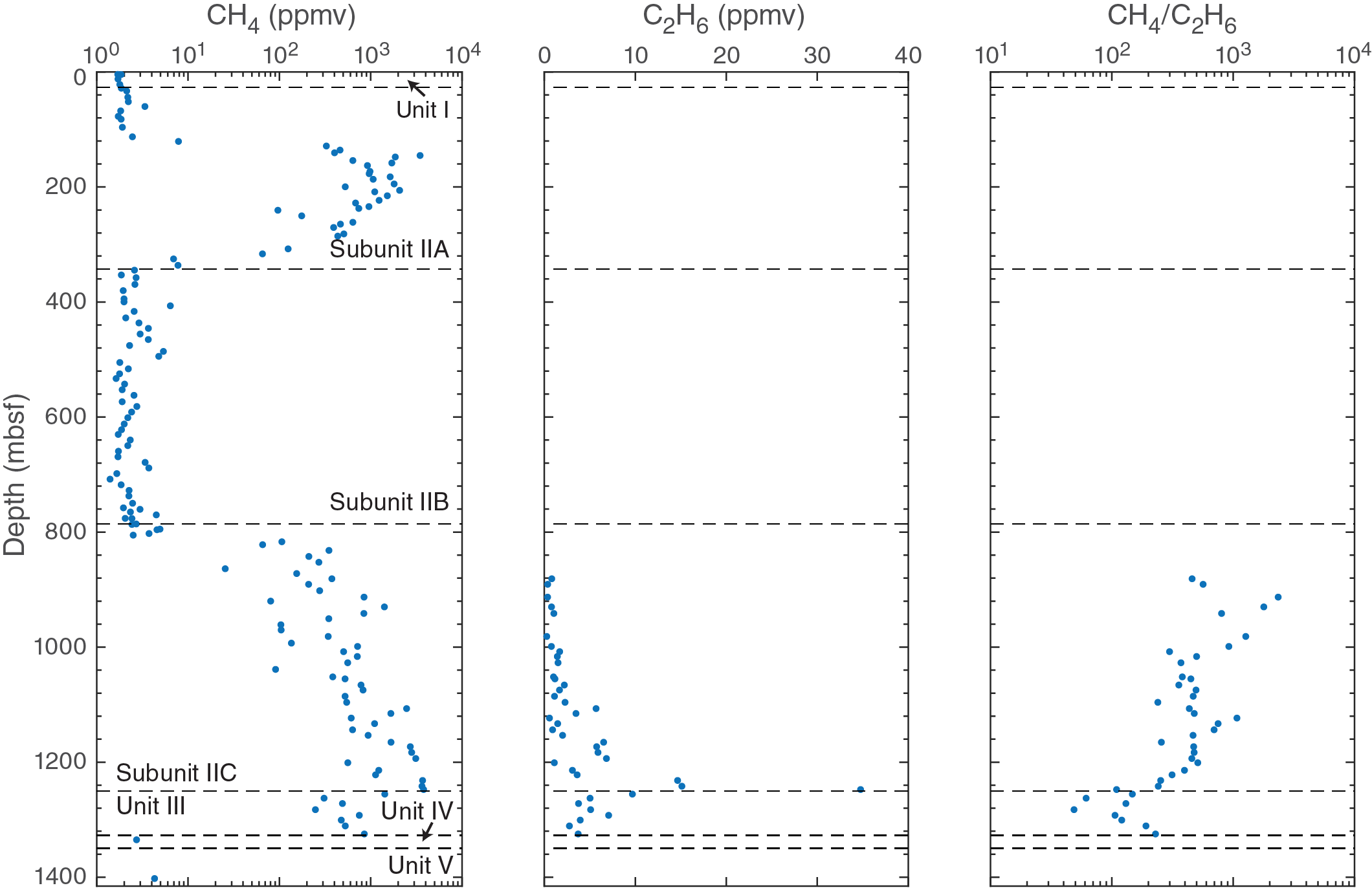
Figure F96. Methane, ethane, and methane/ethane ratio profiles.
Table T17. Results from headspace and void gas sample analyses. Download table in .csv format.
Major changes in methane concentration and the methane/ethane ratio generally align with unit and subunit boundaries (Figure F96). The first region in which methane is above the detection limit ends at the base of Subunit IIA, and concentrations remain below 2.5 ppmv until 805 mbsf, 20 m below the boundary between Subunits IIB and IIC. If the methane in Subunit IIC is strictly biogenic, the dramatic increase from Subunit IIB to IIC could be due to an increase in organic C content (see Bulk sediment analysis) or change in organic matter composition, rendering the organic C more labile. Although no trend is apparent in the ratio of organic C to total N (Figure F97), which is a tracer of organic matter composition and provenance (see below), Subunit IIC contains discrete horizons of woody organic material (see Sedimentology and petrology), which suggests local enrichment in terrestrial organic material that could fuel methanogenesis.

Figure F97. CHNS and organic C/total N.
Alternatively, low-temperature thermogenic processes may partially account for hydrocarbons in Subunit IIC, where ethane first became detectable, but thermogenic contributions are likely minor. Methane/ethane ratios of ~240–2400 remain well above the ratio of 5–10 expected for hydrocarbons of strictly thermogenic origin (Claypool and Kvenvolden, 1983), and biologic degradation of organic matter has been shown to produce heavier hydrocarbons (e.g., Hinrichs et al., 2006), so their presence does not necessarily indicate thermogenic methanogenesis. Furthermore, with a thermal gradient of 44.4°C/km (see Downhole measurements), the temperature at 805 mbsf, where methane concentrations increase dramatically, is ~37°C, low for thermogenic methane production (Claypool and Kvenvolden, 1983).
Ethane concentrations peak sharply at the base of Subunit IIC before returning to ~5 ppmv in Unit III. A decrease in methane concentration drives a similar decrease in methane/ethane ratio in Unit III, and methane concentrations drop significantly in Unit IV, where magmatic intrusions become prominent (see Sedimentology and petrology). No headspace samples were taken from cores deeper than 1402 mbsf as they primarily sampled igneous material.
Bulk sediment analysis
A total of 270 samples were taken for elemental analysis to determine total C and N and for coulometric measurement of carbonate content (Table T18). The depth profile of total C closely matches that of carbonate. Values up to 6 wt% C and 40 wt% calcium carbonate (CaCO3) were recorded in the calcareous clays of Unit I (Figure F97). Unit II (26.42–1250.35 mbsf; see Sedimentology and petrology), which was deposited at high sedimentation rates of 65–362 m/My (see Table T11), generally falls between 1 and 10 wt% CaCO3 with localized peaks reaching a maximum of 96.2 wt% (Figure F98). Total carbon and carbonate content both decrease to nondetectable levels in Unit III before increasing to 11.7 wt% C and 96.4 wt% CaCO3 in the chalk at the base of Unit III. Carbonate values generally correspond with values determined by XRD (Figure F6A), including carbonate-enriched intervals, but sometimes the data sets diverge (e.g., around 200 mbsf), reflecting the local development of carbonate enrichment by either diagenetic or sediment deposition processes (see Sedimentology and petrology for discussion of resedimented carbonate detritus).
Table T18. Bulk sediment CHNS. Download table in .csv format.
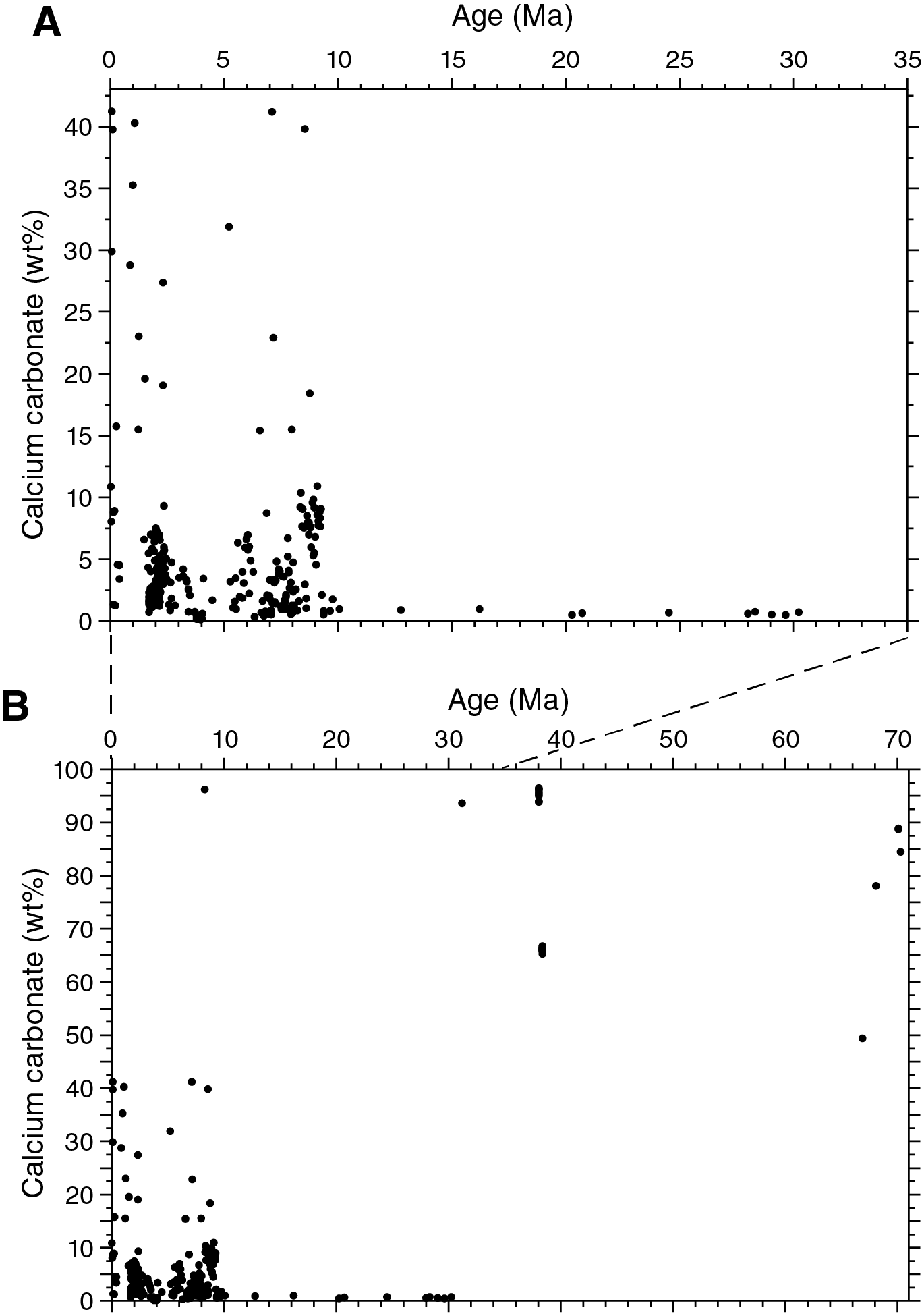
Figure F98. Carbonate content vs. sediment age.
Organic C, calculated as the difference between total C and carbonate C content (see Geochemistry in the Expedition 362 methods chapter [McNeill et al., 2017b]), is highest in Unit I, reaching a maximum of 1.8 wt% C. Subunit IIC is characterized by slightly higher organic C content than Subunit IIB (averages of 0.28 and 0.43 wt% C, respectively), and an unpaired two-sample T-test reveals that this difference is statistically significant at the 95% confidence level (p = 1.1 × 10⁻⁹). Organic C remains close to nondetectable levels through Unit III until 1403 mbsf where it reaches 0.24 wt%. Concentrations of organic C in the chalk of Unit V remain between 0 and 0.25 wt%.
Total N values are highly variable from 0 to 90 mbsf and range from 0.03 to 0.20 wt% before stabilizing around 0.15 wt% for the rest of Subunits IIA and IIB. A slight increase in total N in Subunit IIC mirrors the increase in organic C content, so the organic C/total N ratio does not change significantly from Subunits IIB to IIC. Total N content remains relatively constant at ~0.15 wt% in Unit III and the chalk in Unit V.
The ratio of organic C to total N can give information on organic material provenance as terrestrial organic matter typically has a C/N ratio of ~20, whereas marine organic matter, which is more proteinaceous, is characterized by a C/N ratio of ~5 to 8 (Pimmel and Claypool, 2001). Highly variable C/N ratios, ranging from <0.5 to >40 in lithostratigraphic Unit I, indicate rapid changes in the proportion of organic matter derived from terrigenous and marine sources. Localized peaks in the C/N ratio from 0 to 180 mbsf suggest that terrestrial organic matter, likely transported by sediment gravity flows (see Sedimentology and petrology), punctuates the background accumulation of marine organic material. Deeper than 200 mbsf, the C/N ratio remains between ~1 and 7, suggesting a predominantly marine source. However, discrete horizons containing millimeter-size dark organic material and two sections of preserved woody material, one ~20 cm (interval 362-U1480G-11R-3, 45–65 cm) and the second ~6 cm in length (interval 12R-1, 79–85 cm), are clear indications of terrigenous organic input earlier in the depositional history.
Care should be taken, however, when using organic C/total N ratios to interpret organic matter provenance because inorganic sources of N, such as ammonium adsorbed to or incorporated within clay minerals, may contribute to measured total N values (de Lange, 1992; Müller, 1977). Inorganic N is measured with N from organic sources during the analysis (see Geochemistry in the Expedition 362 methods chapter [McNeill et al., 2017b]), but as long as the amount of organic N is large, inorganic N contributions will be minor. However, in sediment with 0.1 to 0.2 wt% C, inorganic N may account for ~40% of the total N (Müller, 1977). Therefore the values of organic C/total N in lithostratigraphic Units II–V that are well below the canonical average for marine organic matter may be driven primarily by a greater inorganic N contribution.
Physical properties
Physical properties of the cores recovered at Site U1480 were characterized through a set of measurements on core sections and discrete samples (see details in Physical properties in the Expedition 362 methods chapter [McNeill et al., 2017b]). Gamma ray attenuation (GRA) density, magnetic susceptibility (Magnetic Susceptibility Logger [MSL]), and P-wave velocity (P-wave Logger [PWL]) were obtained on the sediment cores using the Whole-Round Multisensor Logger (WRMSL), whereas only GRA and magnetic susceptibility were obtained on hard rock cores. Natural gamma radiation (NGR) was measured by the Natural Gamma Radiation Logger (NGRL). Point magnetic susceptibility (MSP) and reflectance spectroscopy and colorimetry (RCS) data were acquired using the Section Half Multisensor Logger (SHMSL). Thermal conductivity (TCON) was obtained on whole-round soft sediment sections and half-round or on discrete semilithified to lithified sediment and hard rock samples. Moisture and density (MAD) and P-wave velocity measurements were obtained on sediments and discrete semilithified/lithified sediment and igneous rock samples. All data were uploaded to the Laboratory Information Management System database. Changes in the trends of the physical properties observed with depth generally correlated with lithostratigraphic Units I–VI defined in Sedimentology and petrology (Figure F99). Physical properties showed strong differentiation between sedimentary and igneous lithologies.
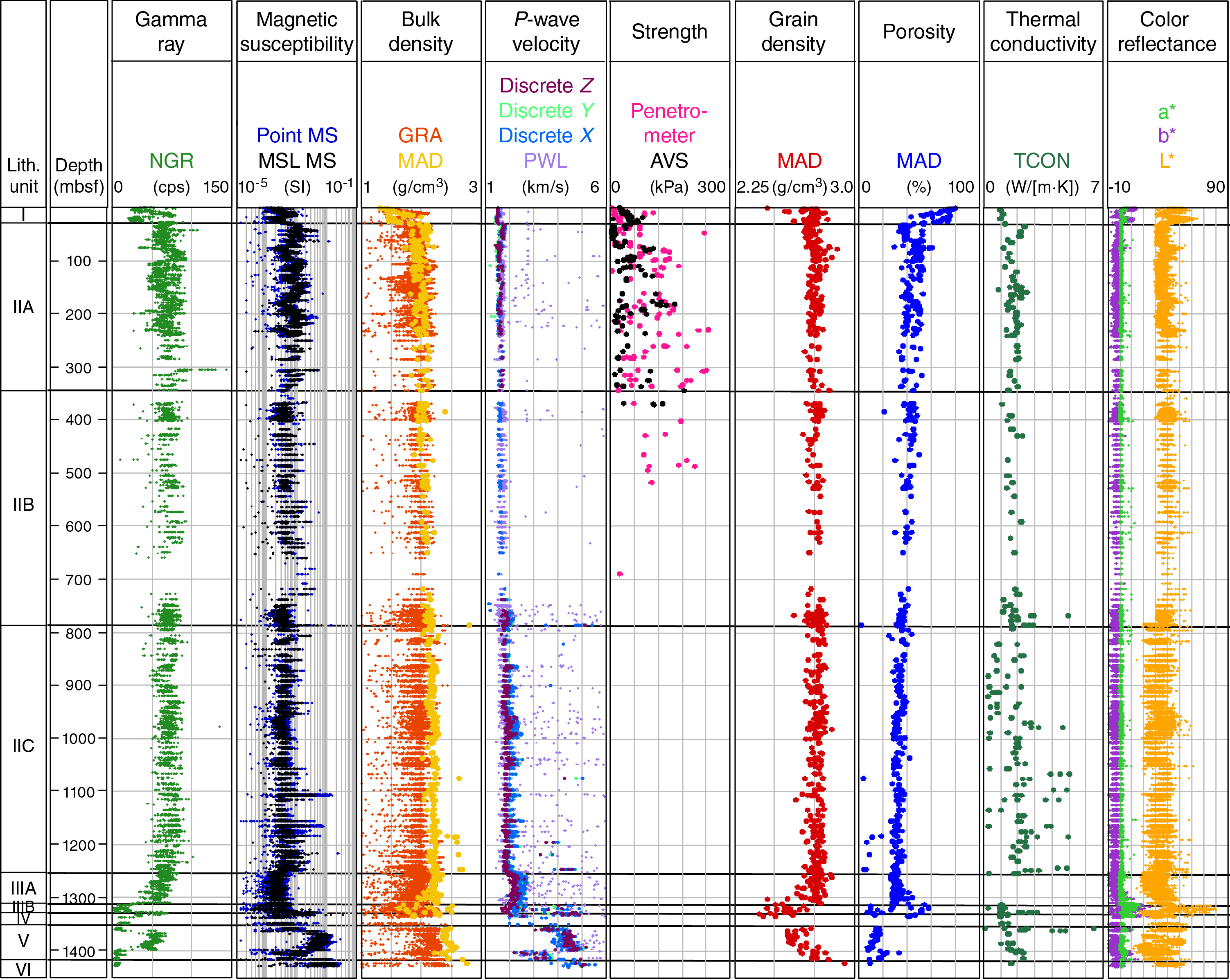
Figure F99. Physical property measurements.
Unit I (0–26.42 mbsf) has a combination of lower NGR, magnetic susceptibility, and bulk density and higher porosity relative to the deeper Unit II. Reflectance and colorimetry are distinct in Unit I, showing higher L* and b* values. Unit II (26.42–1250.35 mbsf) is a thick sediment package with higher NGR, magnetic susceptibility, bulk density, and P-wave velocity relative to Unit I. At the Subunit IIA/IIB boundary (343.67 mbsf), physical properties do not show significant variations. An increase in P-wave velocity to ~2000 m/s and an onset of anisotropy is observed at 760 mbsf, which does not coincide with the Subunit IIB/IIC boundary (785.80 mbsf). The Subunit IIB/IIC boundary, however, does show a decrease in L* values.
Unit III (1250.35–1310.10 mbsf), composed of pelagic sediment, is characterized by a decrease in magnetic susceptibility, NGR, and L* and an increase in P-wave velocity relative to Unit II above (Figure F100). Subunit IIIB (1310.10–1327.18 mbsf) is defined by low NGR and a deviation from the gradually decreasing porosity trend with depth that occurs in Subunits IIA–IIIA. Both low and high porosity (6%–60%) values relative to this trend were measured in Subunit IIIB (corresponding to chalk for low values and calcareous silty clay for high values). The grain density (2.4–2.7 g/cm3) also differs from the relatively constant and higher grain density (2.7–2.8 g/cm3) measured in Unit I through Subunit IIIA.
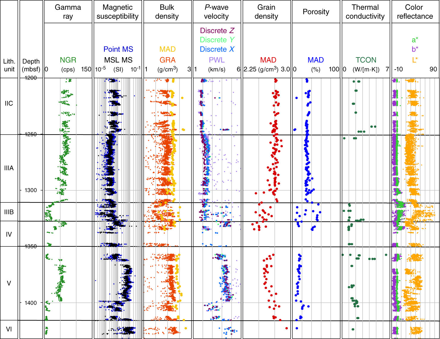
Figure F100. Physical property measurements in Hole U1480G deeper than 1200 mbsf.
The top of Unit IV is distinguishable by broad peaks in NGR, magnetic susceptibility, and P-wave velocity and by lower grain density values, and correlates precisely with the top of a basaltic lava flow. The top and bottom portions of Unit V (1349.8–1415.35 mbsf), composed of calcareous claystone and chalk, show low NGR and magnetic susceptibility and relatively lower P-wave velocity. A magmatic intrusion (1361.45–1398.63 mbsf) yields high NGR, very high magnetic susceptibility, high bulk density, and high P-wave velocity (4000–5000 m/s). Grain density of the intrusion is 2.6–2.7 g/cm3 and porosity is 10%–20%. Unit VI (1415.35–1431.63 mbsf), corresponding to the basaltic basement, shows high magnetic susceptibility and P-wave velocity increasing to ~6000 m/s.
In the following subsections and figures, physical property data are grouped into five principal lithologies based on the initial visual core description stored in DESClogik (see Sedimentology and petrology):
- Mud, which includes clay, silt, and mixtures of clay and silt;
- Sand;
- Calcareous sediments (calcareous ooze, chalk, calcareous clay/claystone, calcareous silt/siltstone);
- Tuffaceous material (ash, tuff, and volcaniclastic sediments); and
- Igneous rock (basalt, diorite, and volcaniclastic breccia).
Natural gamma radiation
NGR values for Holes U1480E–U1480H range from 2 to 157 counts/s, with an average of 63 ± 18.2 counts/s (Figure F99). Within lithostratigraphic Unit I (0–26.42 mbsf), NGR values vary from 20 to 80 counts/s (Figure F101). Deeper than Unit I, the average NGR value increases but remains highly variable, fluctuating between 30 and 90 counts/s, until the base of Subunit IIC (1250.35 mbsf). NGR decreases gradually in Subunit IIIA from 70 to 40 counts/s (Figure F100). The Subunit IIIA/IIIB boundary appears as a sharp decrease in NGR (Figure F102). Subunit IIIB shows low NGR values (5–40 counts/s, but dominantly <20 counts/s). Unit IV starts with an abrupt increase of NGR to 70 counts/s at ~1335 mbsf followed by a downhole decrease to lower values (~10 counts/s). The peak at the top of Unit IV correlates very well with basalt lava flows seen in the cores (see Sedimentology and petrology). Unit V has low NGR at its top and bottom, corresponding to calcareous claystone and chalk, and a zone of high NGR (typically 35-60 counts/s) between 1361 and 1399 mbsf. This zone corresponds precisely with a thick magmatic intrusion (see Sedimentology and petrology). NGR values remain constant (5–20 counts/s; average = 9 counts/s) from 1398 mbsf to the bottom of the hole.
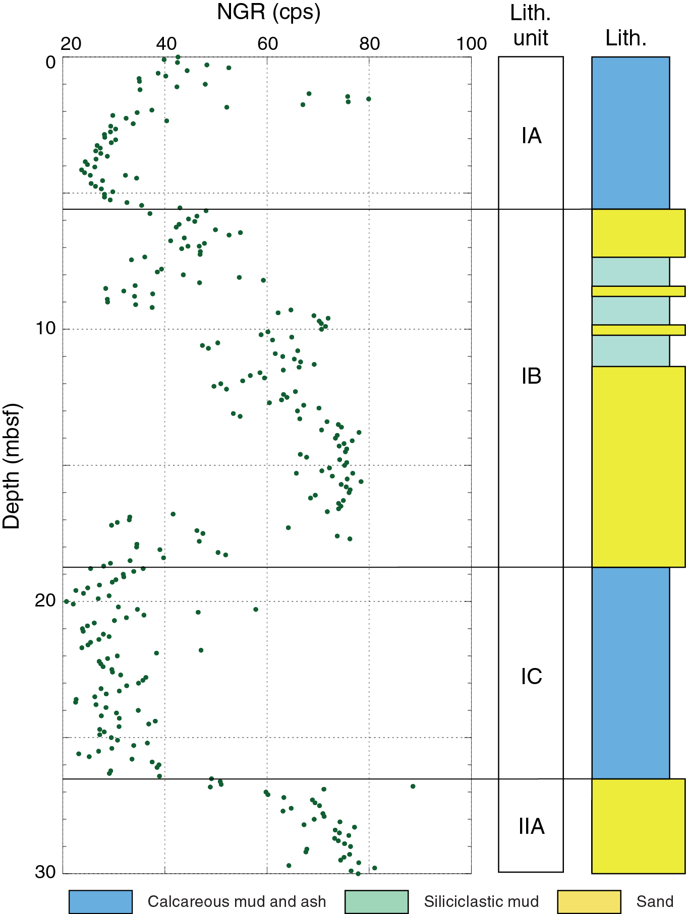
Figure F101. NGR and lithostratigraphic units from 0 to 30 mbsf, Hole U1480E.
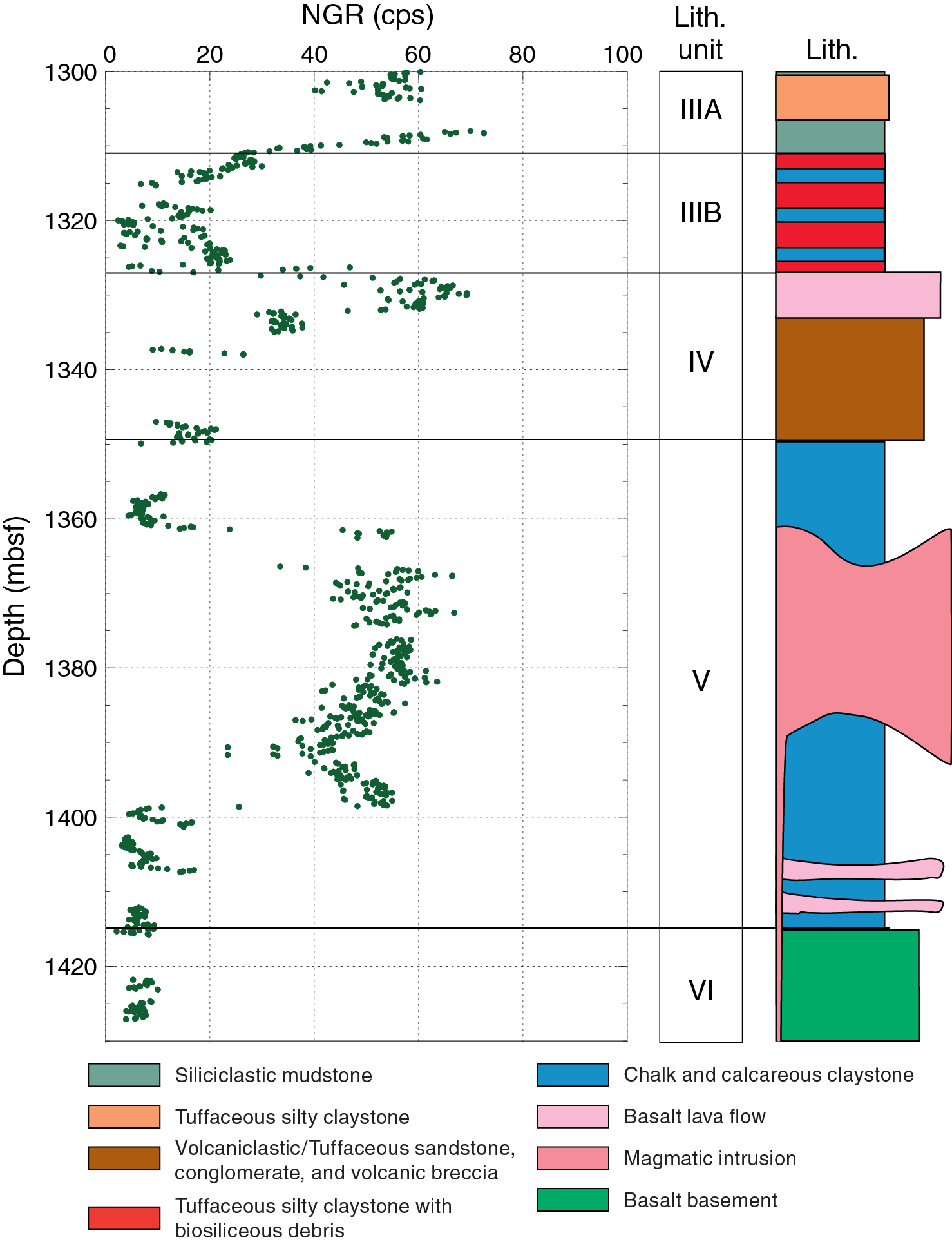
Figure F102. NGR and lithostratigraphic units from 1300 to 1427 mbsf, Hole U1480G.
The highest NGR values occur in mud (average = 70 counts/s). Intermediate values correlate with sand (average = 67 counts/s). The lowest values correlate with tuffaceous (average = 23 counts/s) and calcareous (average = 15 counts/s) material. The contrast in NGR between the basaltic lava flows and igneous intrusions and the basaltic basement suggests different compositions of the igneous materials.
NGR variation by lithology can also be correlated with total clay content as determined by XRD analysis (Figure F103). Mud samples have higher NGR values (generally 50–90 counts/s) and higher total clay (generally 50%–75%). Sand samples have high NGR values (average = 64 counts/s) similar to mud but have less total clay (average = 34%). Calcareous samples have low NGR values (usually <40 counts/s; average = 19 counts/s) and highly variable total clay (0%–85%). Tuffaceous samples have low NGR values (35–50 counts/s) and high total clay (70%–80%).
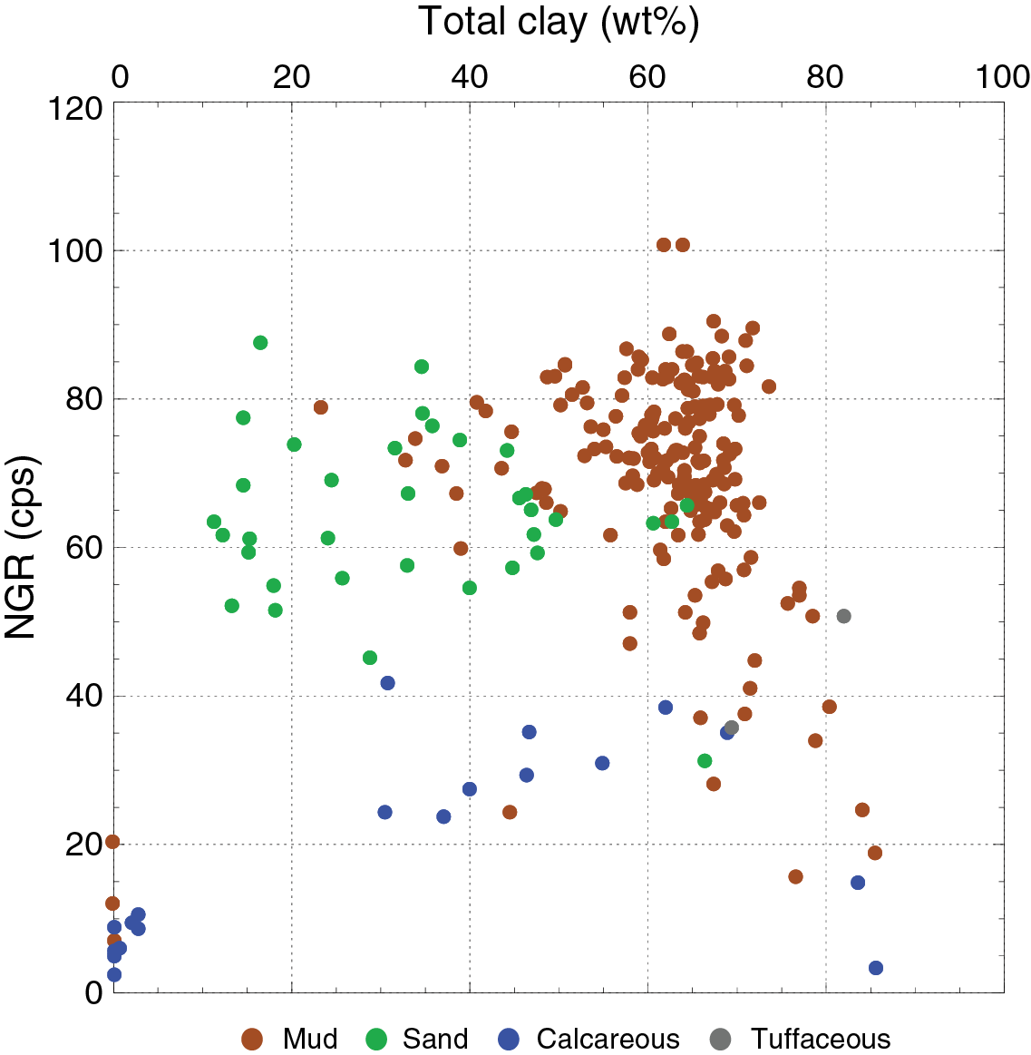
Figure F103. NGR vs. total clay content.
Magnetic susceptibility
Magnetic susceptibility was measured using the WRMSL on whole-round cores and with the SHMSL on the archive-half sections of cores from Holes U1480E–U1480H. Changes in magnetic susceptibility (Figure F99) generally correspond with changes in lithology. At 26.42 mbsf, the change in lithology from calcareous clay (Subunit IC) to sandy silt and silty clay (Subunit IIA) is marked by an increase in magnetic susceptibility from an average of 33 × 10–5 SI to an average of 61 × 10–5 SI. Another distinct change occurs at ~1250 mbsf (near the Unit II/III boundary), where magnetic susceptibility decreases, marking the transition from fan to pelagic sediment (see Sedimentology and petrology). Unit III has a magnetic susceptibility average of 56 × 10–5 SI from 1250 to 1327.18 mbsf. Magnetic susceptibility values increase rapidly from the base of Unit III to the top of Unit IV (average = 75 × 10–5 SI). This increase is likely caused by the presence of magnetic minerals in the basalt flows (see Sedimentology and petrology). Within Unit V, magnetic susceptibility is low at the top and bottom of the unit; however, magnetic susceptibility increases to an average value of 568 × 10–5 SI from 1361 to 1399 mbsf. At 1415 mbsf, a sharp increase occurs in magnetic susceptibility (Unit VI) where the lithology changes from calcareous sedimentary rock to basalt (average = 386 × 10–5 SI). MSP measurements match well with the WRMSL magnetic susceptibility results (Figure F99).
P-wave velocity
P-wave velocities measured with the WRMSL PWL and >3000 PWC velocity measurements made with the velocity gantry (see Physical properties in the Expedition 362 methods chapter [McNeill et al., 2017b]) are in good overall agreement (Figure F99). The gantry velocities (manual pick) tend to be slightly slower than the PWL velocities due to not picking the initial arrival. Once corrected, the gantry velocities are approximately equal to or greater than the PWL velocities. The PWL velocities are expected to be slower than the corrected gantry measurements, as is observed, because of water- or air-filled gaps between the core and core liner.
P-wave velocities are constant (~1500 m/s) until 30 mbsf, 4 m below the top of Subunit IIA, where velocities increase by 250 m/s. Through the rest of Subunit IIA (26.42–343.67 mbsf) and most of Subunit IIB (343.67–785.80 mbsf) velocities range from ~1600 to 1700 m/s. At 760 mbsf, velocities increase to ~2000 m/s, potentially indicating that the siliciclastic sediment from the Nicobar Fan succession may be more cemented or lithified. Velocities do not change significantly through Subunit IIC (785.80–1250.35 mbsf). At the top of Subunit IIIA (1250.35 mbsf), velocities increase by 600 m/s to 2600 m/s. This increase is associated with the presence of pelagic clays. Through Subunit IIIA, velocities decrease slightly with depth to 2200 m/s at the base (1310.10 mbsf). Within Subunit IIIB (1310.10–1327.18 mbsf), velocities are highly variable. At some depths, velocities are 2200 m/s or slower in the z-direction, but there are many measurements with significantly faster velocities, up to 5000 m/s. Slow velocities correspond to samples of lithified tuffaceous sediment, whereas faster velocities correspond to samples of chalk. Unit IV (1327.18–1349.8 mbsf) coincides with a zone of poor core recovery. A cluster of high velocities at the top of this unit (1327–1331 mbsf) range from 4200 to 5000 m/s. This velocity cluster is associated with volcanic breccias and basaltic lava flows. In the rest of Unit IV, velocities range from 1900 to 4400 m/s. In Unit V (1349.8–1415.35 mbsf), variability in velocity decreases, and in the diorite intrusion velocities gradually increase with depth from 4200 m/s at 1357 mbsf to 5000 m/s at 1398 mbsf. Deeper than 1398 mbsf, velocities rapidly decrease to 2500 m/s in the calcareous claystone and chalk before beginning to increase again with depth to 4600 m/s at the Unit V/VI boundary. Velocities do not significantly change at the top of Unit VI (1415.35–1431.63 mbsf); however, velocities increase through this unit, and the average velocity of the basaltic basement is 5500 m/s. Average velocities and standard deviations for each unit can be found in Table T19.
Table T19. Averages and standard deviations for P-wave logger and P-wave caliber velocities. Download table in .csv format.
The calculated vertical and horizontal anisotropy (see P-wave velocity measurements in the Expedition 362 methods chapter [McNeill et al., 2017b]) is <14% from 0 to 400 mbsf (Figure F104). Horizontal anisotropy is always less than ±0.3%; although the cores are not consistently oriented, this implies there is essentially no horizontal anisotropy. Vertical anisotropy reaches 14% in this interval, but the average value is 1.6%. There are no anisotropy data between 400 and 700 mbsf because these cores were too hard for the gantry bayonets and too soft to extract intact cubes, so measurements were only made in the x-direction. Below 700 mbsf, horizontal anisotropy remains low (<0.3%), but vertical anisotropy increases and is greatest in Subunit IIIA, with an average of 12.9% and a maximum of 30%. Deeper than 700 mbsf, velocity in the vertical (z) direction is consistently the slowest, indicating that the material is transversely isotropic with a vertical axis of symmetry.

Figure F104. Corrected discrete P-wave velocity data, Holes U1480E–U1480H.
Bulk density, grain density, and porosity
Density
GRA bulk density data measured with the WRMSL and MAD bulk and grain density data measured on discrete samples are shown in Figures F99 and F105. GRA data generally show increasing bulk density with depth (red circles in Figure F99); this trend is more pronounced in MAD bulk density data (orange circles in Figure F99). GRA bulk density values range from ~1.1 g/cm3 for mud to ~2.6 g/cm3 for igneous rocks; discrete sample values range from ~1.3 g/cm3 for calcareous material to ~2.8 g/cm3 for igneous rocks. Grain densities range from ~2.3 g/cm3 for tuffaceous sediment and rocks to ~2.9 g/cm3 for igneous rocks (one measurement). Most grain density values are between 2.7 and 2.8 g/cm3 for depths shallower than 1300 mbsf, where sand grain density mostly ranges from 2.70 to 2.75 g/cm3 and mud grain density ranges from 2.75 to 2.80 g/cm3.
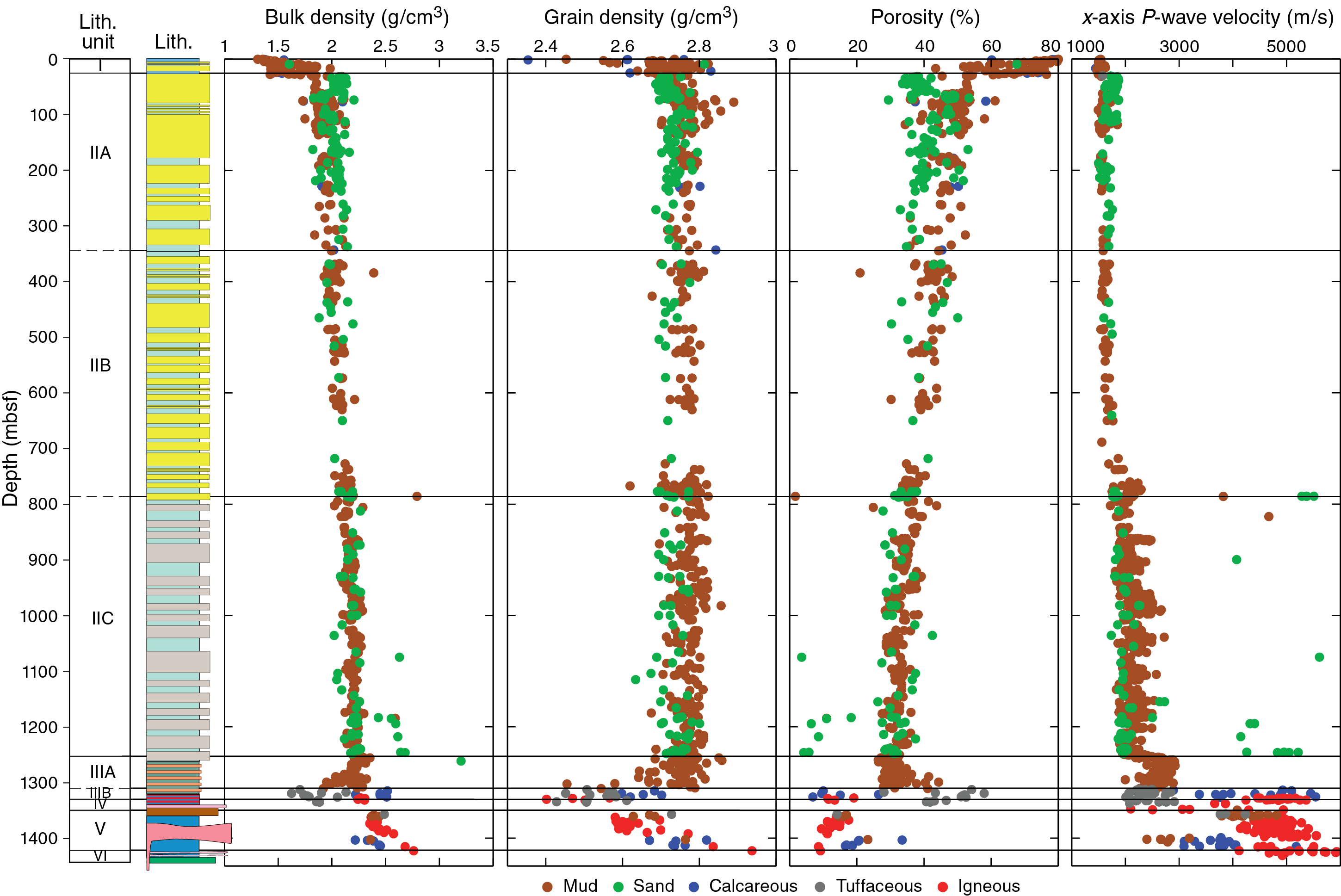
Figure F105. Density, porosity, and P-wave velocity as a function of lithology.
Figure F105 displays bulk density, grain density, porosity, and x-axis P-wave velocity for discrete samples separated according to lithology. Bulk densities are predominantly between 1.9 and 2.5 g/cm3, and grain densities are predominantly between 2.7 and 2.8 g/cm3. Bulk densities <2.0 g/cm3 and high porosities >60% are exhibited in the shallow calcareous sediment of Unit I (26.42 mbsf and shallower). In Unit II, which is mainly composed of mud and sand, bulk densities increase with depth to ~2.4 g/cm3, whereas grain densities remain between 2.7 and 2.8 g/cm3. Bulk and grain density values start to deviate from these general trends at ~1270 mbsf, ~40 m above the Subunit IIIA/IIIB boundary. Bulk densities show both low (~1.5 g/cm3) and high (~2.5 g/cm3) values within Subunit IIIB, whereas grain densities decrease to ~2.4 g/cm3. Bulk density values of ~1.6–2.2 g/cm3 correspond to tuffaceous sediment/sedimentary rock, and grain density values of 2.4–2.6 g/cm3 correspond to igneous, tuffaceous and mud materials. Bulk density values of ~2.0–2.5 g/cm3 correspond to calcareous sediment/sedimentary rock with corresponding grain density values of 2.6–2.8 g/cm3.
Unit IV exhibits a bulk density value ~1.9 g/cm3 that corresponds to tuffaceous sediment and sedimentary rock; the corresponding grain densities are 2.4–2.7 g/cm3. Bulk densities in Unit V are 2.2–2.7 g/cm3, corresponding mostly to igneous and calcareous rock; grain density values are 2.55–2.85 g/cm3 for igneous rock and 2.65–2.85 g/cm3 for calcareous sedimentary rock. One MAD sample in the basaltic basement of Unit VI has a bulk density of 2.75 g/cm3 and grain density of 2.9 g/cm3.
Porosity
A large range (3.6%–80.5%) of porosity values were measured at Site U1480. Unit I is characterized by the highest porosities (~43%–80%; average = 66%; Figure F105) where the lithology is composed of siliclastic mud and sand and calcareous sediments with minor biosiliceous components and ash. In Unit II and Subunit IIIA, porosities decrease with depth to ~30% by ~1300 mbsf, and separate trends exist for sand and mud (Figure F106). The general trend of the porosity reduction is consistent with vertical consolidation (Biot, 1941; Gibson, 1958), allowing definition of a porosity-effective stress curve (Rubey and Hubbert, 1959),
- ϕ0 = reference porosity at seafloor,
- β = compaction parameter,
- σv′ = σv – P is effective vertical stress,
- σv = vertical overburden, and
- P = pore pressure.
The best fit model to the data assuming hydrostatic pressure provides values for ϕ0 and β of 41.6% and 0.027 1/MPa for sand and 49.8% and 0.040 1/MPa for mud (Figure F106). These values for reference porosity and compaction parameter are lower than those found in the lower Shikoku facies at IODP Site 1173 of the Nankai Trough, Japan where ϕ0 and β are 66% and 0.115 1/MPa (Tsuji et al., 2008). The difference may come from the two different sedimentary environments: a rapid sediment accumulation rate fan system (Site U1480) versus a slower sediment accumulation rate system (Nankai Trough Site 1173).
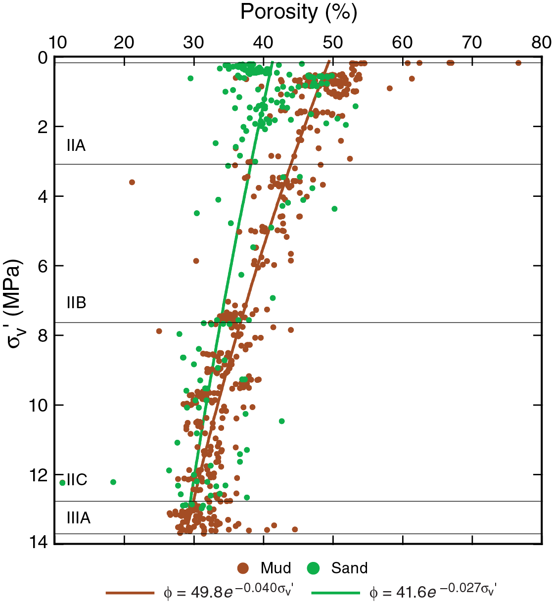
Figure F106. Porosity as a function of effective vertical stress assuming hydrostatic pressure for mud and sand lithologies.
Although most of the data from Site U1480 show a normal compaction trend, porosity varies widely (4%–60%) in Subunit IIIB through Unit VI. This variation is related to lithology (Figure F107). Subunit IIIB is composed of chalk and calcareous mud/mudstone (average porosity = 17% ± 6.3%) and tuffaceous sediment/rock (average porosity = 39% ± 14%). Igneous rocks in Units IV–VI show consistent porosities of 13% ± 2.5%. The porosity of calcareous sedimentary rock in Subunit IIIB through Unit VI is much lower than those at shallow depths (Units I and II), probably because of compaction and cementation.

Figure F107. Porosity vs. depth from 1300 to 1420 mbsf as a function of lithology.
Velocity-porosity relationships
A velocity-porosity relationship was developed for the sedimentary samples using measured P-wave velocity in the x-direction and nearest neighbor (<20 cm offset) porosity data (Figure F108; see Velocity-porosity relationships in the Expedition 362 methods chapter [McNeill et al., 2017b]). Based on the total clay volume from XRD, velocity-porosity curves were plotted for clay volumes of 20% and 60%, as most of the sediment fell within this range (see Sedimentology and petrology). The majority of Site U1480 core samples lie along the curve for normal consolidation (Figure F108; Erickson and Jarrard, 1998). At high porosities (>30%), both the 20% and 60% Vsh curves provide a good match to the data. At porosities <30%, the Vsh = 20% curve provides a better fit in the low porosity calcareous sediments, although there is significant scatter, and we note that the compilation of Erickson and Jarrard (1998) was for siliciclastic sediments. This result is, however, consistent with the lowest porosities correlating with low clay volume in the deepest section of Hole U1480G (see Sedimentology and petrology).
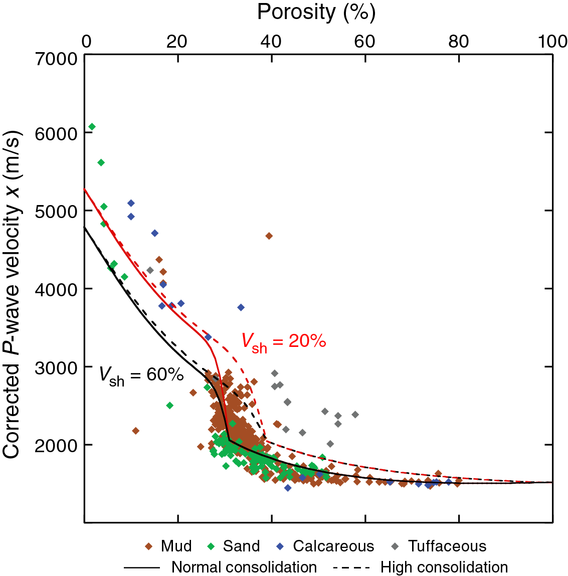
Figure F108. Corrected discrete P-wave velocity in the x-direction as a function of porosity and lithology, Holes U1480E–U1480H.
Thermal conductivity
Thermal conductivity was measured on soft sediment in whole-round cores (shallower than ~800 mbsf) using the full-space needle probe. Thermal conductivity on semilithified sediments and hard rocks was measured on split core samples using the half-space puck with a small quantity of thermal coupling paste or, if necessary, in a water bath (see Thermal conductivity in the Expedition 362 methods chapter [McNeill et al., 2017b]). Stable thermal conductivity measurements could not be obtained from the TEKA software for a number of samples despite numerous attempts to improve the thermal coupling or the use of different heating power values; some of these issues occurred in unlithified sands where convection may have occurred, but the majority were in lithified samples. Values calculated using the TCON_CALC method are included in the database but should not be used; this method is not documented and generally returns thermal conductivity values with large spreads or in some cases even negative values. The TEKA manual suggests that measurements where the repeat values differ by more than a few percent should be considered unreliable.
Thermal conductivity values calculated using the TEKA method and with a standard deviation of <7% of the mean for the repeat measurements (Figure F109; Table T20) range from 0.94 to 4.51 W/(m·K), with most values between 1 and 2.25 W/(m·K). Some trends between and within individual lithologies were observed (Figure F110). Fine-grained (mud) samples show a general increase downhole from 1–1.5 W/(m·K) near the seafloor to 2 W/(m·K) at 1200 mbsf, with unlithified and semilithified samples showing similar trends. Sand samples show little evidence of change in thermal conductivity downhole, but shallower than 200 mbsf they are more conductive than the fine-grained samples, consistent with the compilation of Lovell (1985). Near the base of the hole, the tuffaceous samples in Subunit IIIB and Units IV and V cluster around 1 W/(m·K) and the igneous samples from Units IV–VI cluster around 1.5 W/(m·K). To test whether the thermal conductivity is controlled by porosity, we compared observations with a simple model for thermal conductivity. We used a geometric mean model between a range of assumed grain conductivities and water (e.g., Lovell, 1985); however, clear trends are absent, even when considering a single lithology (Figure F111).
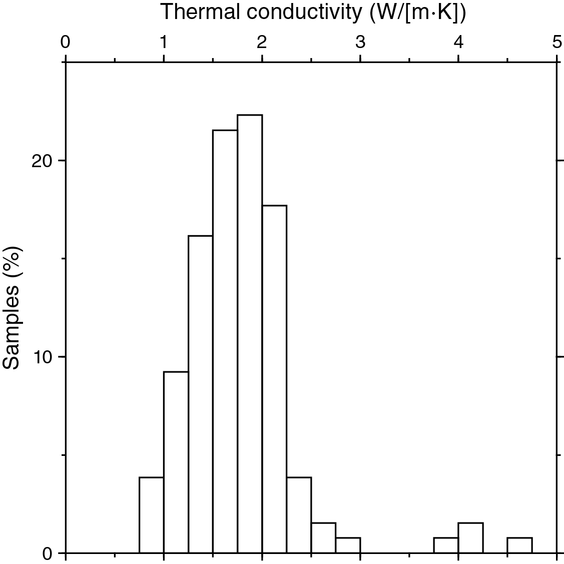
Figure F109. Histogram of reliable measured thermal conductivities.
Table T20. Thermal conductivity values and standard deviations. Download table in .csv format.
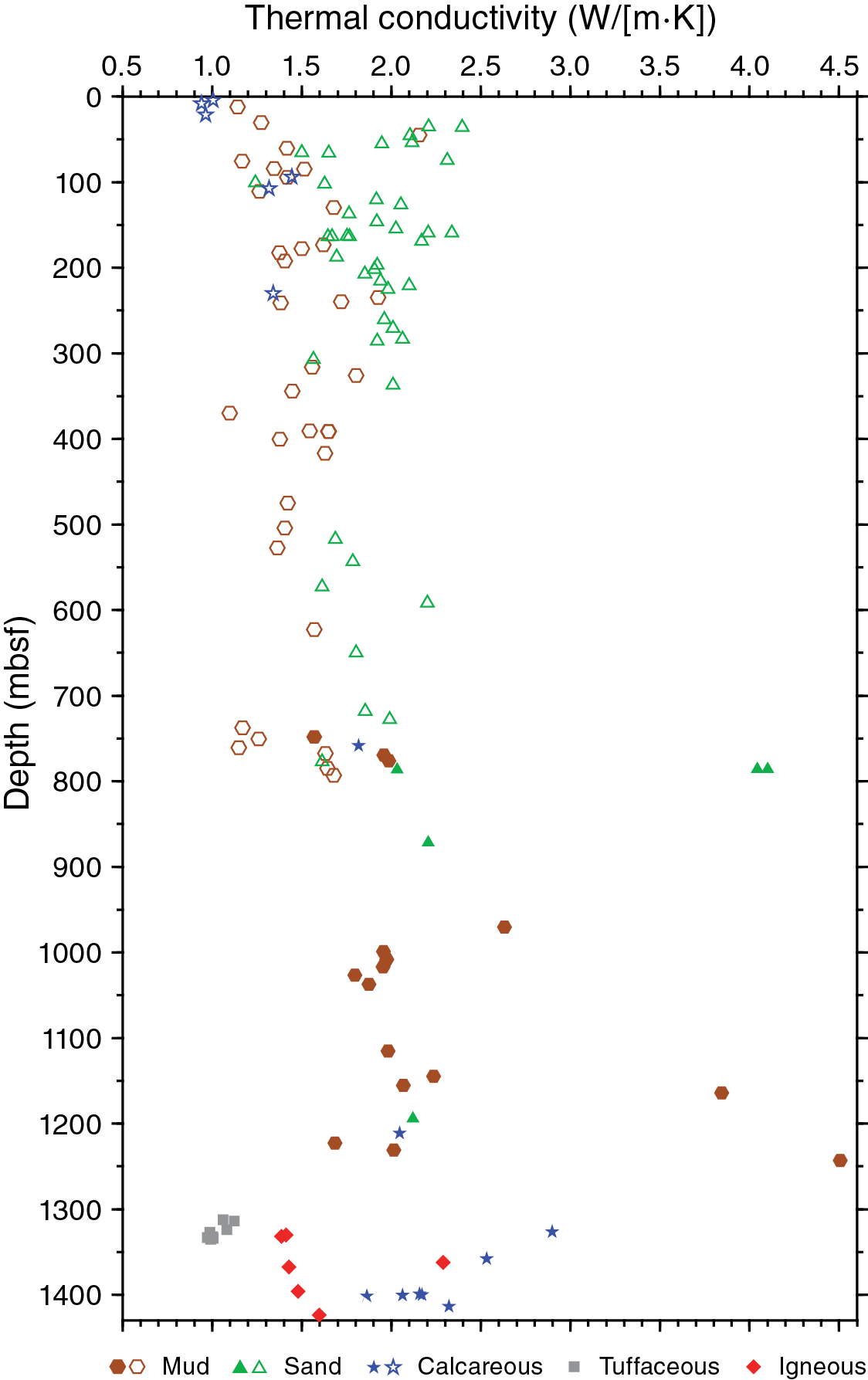
F110. Reliable measured thermal conductivities vs. depth and lithology.
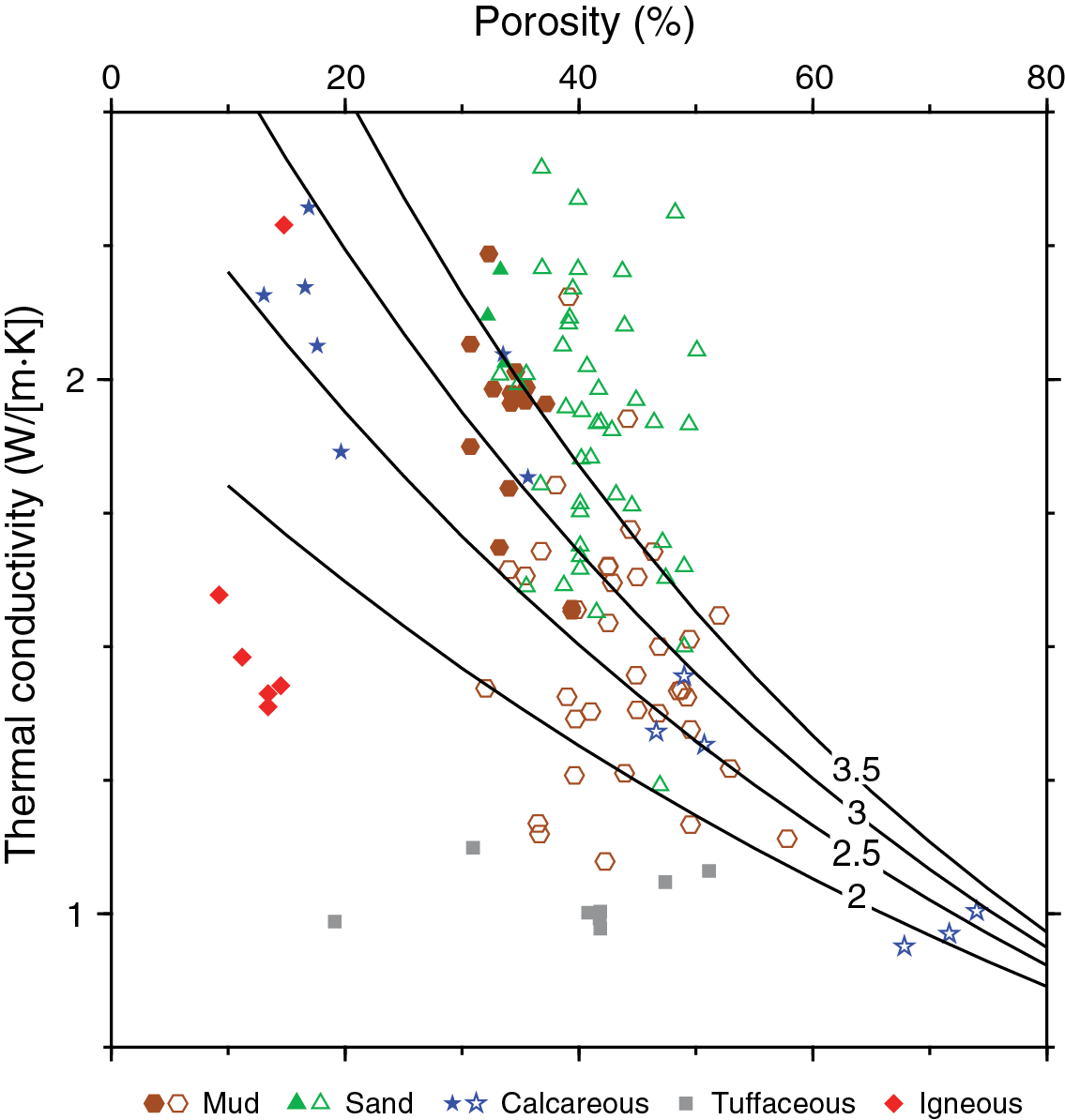
Figure F111. Reliable thermal conductivities vs. porosity.
Reflectance spectrophotometry and colorimetry
Color reflectance data include L*, a*, and b* measurements made on the SHMSL (see Reflectance spectrophotometry and colorimetry in the Expedition 362 methods chapter [McNeill et al., 2017b]). In Unit I, L*, a*, and b* values range from 30 to 60, 0 to 5, and –5 to 15, respectively (Figure F99). The respective ranges decrease to 30 to 40, 0 to 2, and –8 to 2 in Subunits IIA and IIB. Subunit IIC shows lower L* values (20–50), which may be the consequence of higher organic material content and/or changes in redox conditions of the sediments (see Sedimentology and petrology). a* and b* show the same range in Subunit IIC as in Subunits IIA and IIB. In Subunit IIIA, the L* value range shifts to 18–45 and a* and b* value ranges increase to –1 to 9 and –8 to 10, respectively. a* and b* values increase with depth in Subunit IIIA (Figure F100). Subunit IIIB shows the highest values of Site U1480, with L* values of 35–80, a* values of 0–15, and b* values of –10 to –20. In Units IV–VI, L* values range from 15 to 55. a* and b* show higher values ranging from 5 to 13 and 5 to 18, respectively, in the upper part of Unit IV. These ranges decrease to 0–7 and –10 to 10, respectively, in the lower part of Unit IV and Units V and VI. Changes expressed by these data correlate well with color changes observed in cores (see Sedimentology and petrology).
Rock strength
Sediment undrained shear strength values determined by the pocket penetrometer and Automated Vane Shear (AVS) device display broad scatter but generally increase with depth (Figure F99). The high level of drilling disturbance in the sandy sediment reduced confidence in these strength measurements. Furthermore, these measurements do not work well in loose sands where assumptions regarding cohesion and pore pressure become erroneous. Deeper than 370 mbsf, sediment became too strong for pocket penetrometer and AVS strength measurements.
Qualitative strength assessment can be made from drilling observations. Cores exhibited varying degrees of ductile deformation and core biscuiting as a result of variation in rock strength and cohesion and depending on the coring process (see Structural geology). Formation strength was more reflected by drilling ROP; ROP was typically faster in the weaker, less consolidated sands than in the harder, more cohesive clays (see Structural geology). Postcruise work on geomechanical experiments will help provide constraints on these qualitative observations.
Downhole measurements
The downhole measurements plan at Site U1480 included formation temperature measurements with the APCT-3 and the T2P, formation pressure measurements with the T2P, and a petrophysical characterization with a complete suite of logging tools (see Downhole measurements in the Expedition 362 methods chapter [McNeill et al., 2017b] for description of the tools). Because of tool failure during the deployment of the T2P and unstable borehole conditions, downhole measurements were limited to temperature measurements with the APCT-3 and a reduced set of logs through the casing and ~52 m of open hole in Hole U1480G.
T2P deployment
Following a bench-top pressure test, the T2P was prepared for deployment after Core 362-U1480E-12H (bottom of core at 99.7 mbsf). The ERS, MDHDS, and T2P were connected and lowered downhole with the Schlumberger wireline. Two hydrostatic pressure reference measurements were made while lowering the tool downhole (at 2000.3 mbrf and at the seafloor at 4158.7 mbrf). Once the tool landed in the BHA, the ERS released the MDHDS. The drill string was then pressurized to ~6.9 MPa (1000 psi) to shear the brass shear screws in the MDHDS, after which the pressure was bled off to allow the MDHDS latch spring to expand and the latch piston to shift into place. Next the drill string pressure was increased again to pump the T2P into the formation. After 30 min, the ERS was lowered to recover the MDHDS/T2P. Several recovery attempts and systems were necessary to bring the MDHDS/T2P to the rig floor (see Operations). Visual inspection of the tools showed significant damage to the T2P and sand within the MDHDS, including packing off the top of the fishing neck. Postdeployment analysis of the T2P and rig instrumentation data suggest that the MDHDS deployed early, perhaps when it landed in the BHA. Damage to the T2P was likely the result of early deployment and attempted penetration into a sandy interval. A time line of the deployment events is provided in Table T21.
Table T21. Temperature dual-pressure tool deployment details. Download table in .csv format.
Formation temperature and heat flow measurements
The APCT-3 was deployed 12 times at Site U1480: 3 times in Hole U1480E, 4 times in Hole U1480F, and 5 times in Hole U1480H (Table T22). Only one of these deployments failed to provide a reliable temperature measurement. Although the temperature decay curves show that some of these penetrations were steady for only a few minutes (Figure F112), the resulting temperatures define a clear linear temperature profile with a least-squares linear fit gradient of 44.4°C/km (Figure F113).
Table T22. Core top depths defined by the composite depth scale. Download table in .csv format.
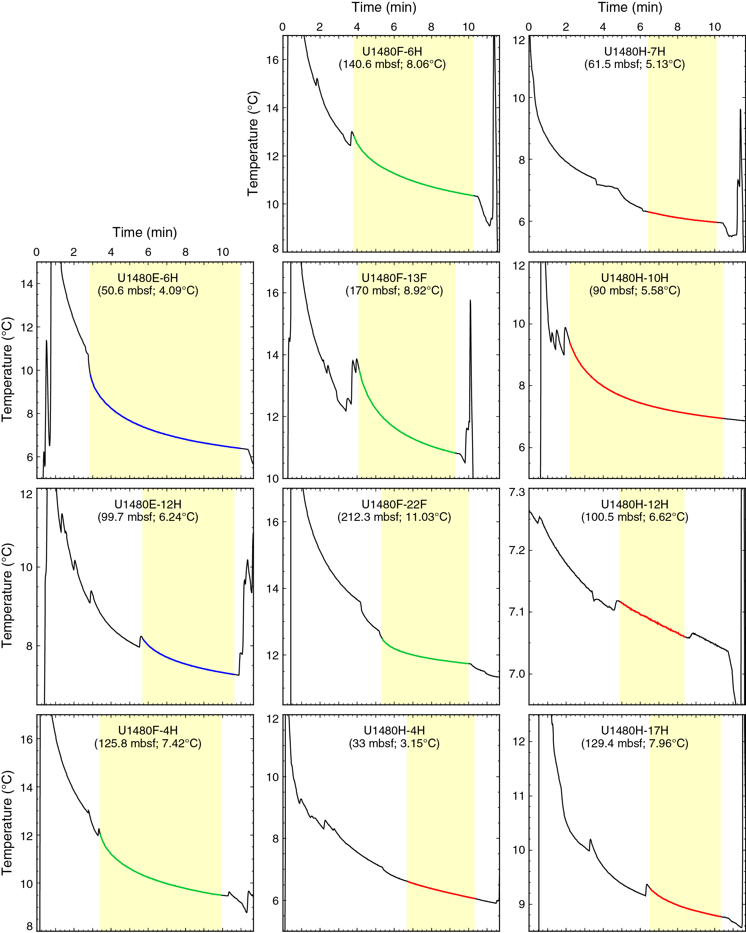
Figure F112. APCT-3 temperature records.

Figure F113. Summary of APCT-3 formation temperature measurements and formation temperature data as a function of thermal resistance.
A simple estimate of the vertical conductive heat flow (q, in mW/m2) can be made from the product of the temperature gradient with the average thermal conductivity (K, in W/[m·K]) measured on the cores recovered over this interval:
Using only the conductivity values with a standard deviation over repeat measurements <0.15 W/(m·K), the average conductivity is 1.69 W/(m·K) (see Physical properties). Based on the average thermal conductivity and temperature gradient, the resulting vertical conductive heat flow is 75.0 mW/m2, well within the wide range of previous measurements in the area (Figure F114; with data from Vacquier and Taylor [1966] and the global heat flow database of the international heat flow commission from http://www.heatflow.und.edu/index.html).
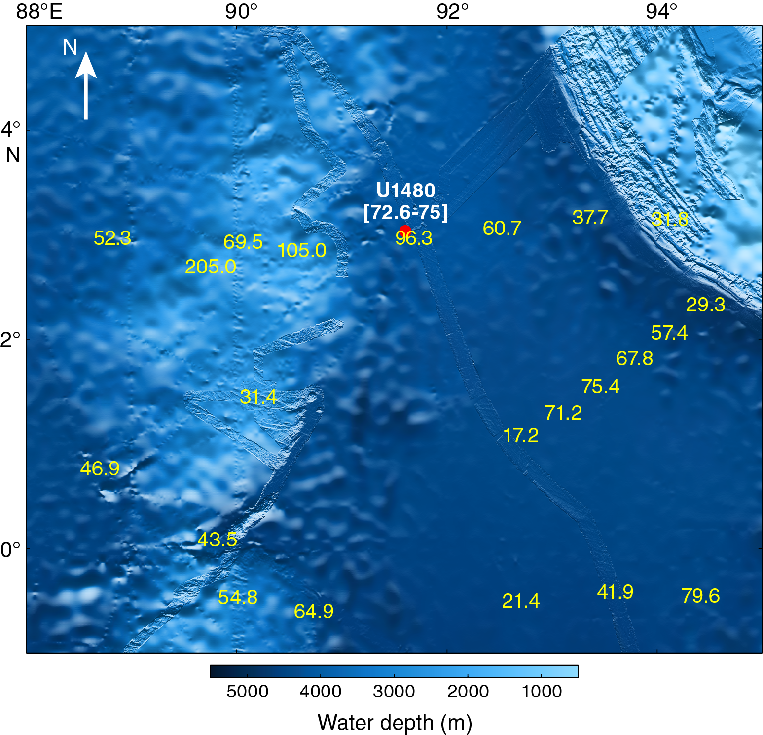
Figure F114. Comparison of heat flow measured at Site U1480 with other measurements in the region.
Another measure of the heat flow in a conductive regime may be established with a Bullard plot. If the vertical heat flow (q) is assumed constant with depth, the temperature at a depth Z can be calculated by a reworking of Equation E2 integrated from the seafloor to Z by
(E3)where To is the seafloor temperature. The value calculated in the integral is the thermal resistance of the interval between the seafloor and Z. If the heat flow is constant with depth, Equation E3 defines a linear relationship between temperature and thermal resistance, whose slope is the vertical heat flow (Bullard, 1939). The thermal resistance of the formation overlying each APCT-3 measurement is given in Table T22, and the heat flow estimate defined by the slope of the least-square linear fit is 72.6 mW/m2 (Figure F113), close to the estimate obtained using Equation E2 with the average conductivity and the temperature gradient.
Downhole logging
Operations
Unstable hole conditions encountered at Site U1480 led to a reduced logging program in Hole U1480G. In preparation for a full suite of logs, the bit was released at the bottom of Hole U1480G after completion of coring, and 300 bbl of 11.0 lb/gal mud were pumped to displace and stabilize the hole. While raising the drill string to logging depth, it became stuck (see Operations). Several hours were necessary to release the pipe from the formation, making it clear that only a limited interval of the hole, if any, likely remained open for logging and that the hole was unstable. We moved ahead with logging in the casing, as well as in any interval left open below the casing. A 19 m long tool string made of the HNGS and the HRLA resistivity tool was rigged up at 0630 h on 5 September 2016 and run into the hole at 0740 h.
Data were recorded while the tools were lowered in the casing at a speed of 3000 ft/h. The tools were not able to go deeper than 809.3 mbsf (52 m below the casing shoe), and a first pass was recorded for quality control over the open hole interval between 809.3 and 742 mbsf. The tool string was lowered again, and after failing to go deeper than the first attempt (809.3 mbsf), the main pass started at 1125 h. Resistivity and gamma ray logs were recorded from 809.3 mbrf to the seafloor at a speed of 1000 ft/h in order to optimize the quality of the data recorded. The pass was completed at 1400 h. The seafloor was identified in the gamma ray log at 4158.5 mbrf, or 4147.1 mbsf. The tools were back at the surface at 1635 h, and the rig floor was clear of all logging equipment by 1725 h.
Data quality
Figure F115 gives an overview of the data recorded during the main pass in Hole U1480G: in the open hole (below 759 mbsf, marked most clearly by the resistivity log); inside the casing; and inside the pipe (above 62 mbsf, apparent in all spectral gamma ray data). Because most of the data were recorded inside the casing, without any indication of the size of the hole behind the casing, it is not possible to assess the influence of variations in hole size on the gamma ray data. The limited core recovery in the interval logged in the open hole below the casing (759–800 mbsf) makes it difficult to compare with the shipboard core NGR measurements, to assess any agreement between the two measures of natural radioactivity, or to assign definitive depths for the cores recovered in the corresponding interval (Figure F116). The strong curve separation seen between all resistivity curves recorded in the open hole suggests that the hole was considerably enlarged over the entire logged interval; the apparent resistivity curves (RLA1–5) are recorded by electrodes with increasing spacing and depth of investigation, and such full separation between all curves can be produced only by a very large borehole or deep invasion of the formation. However the true resistivity of the formation is calculated from all the curves using a one-dimensional (i.e., radius) inversion algorithm, which should compensate for the hole size.
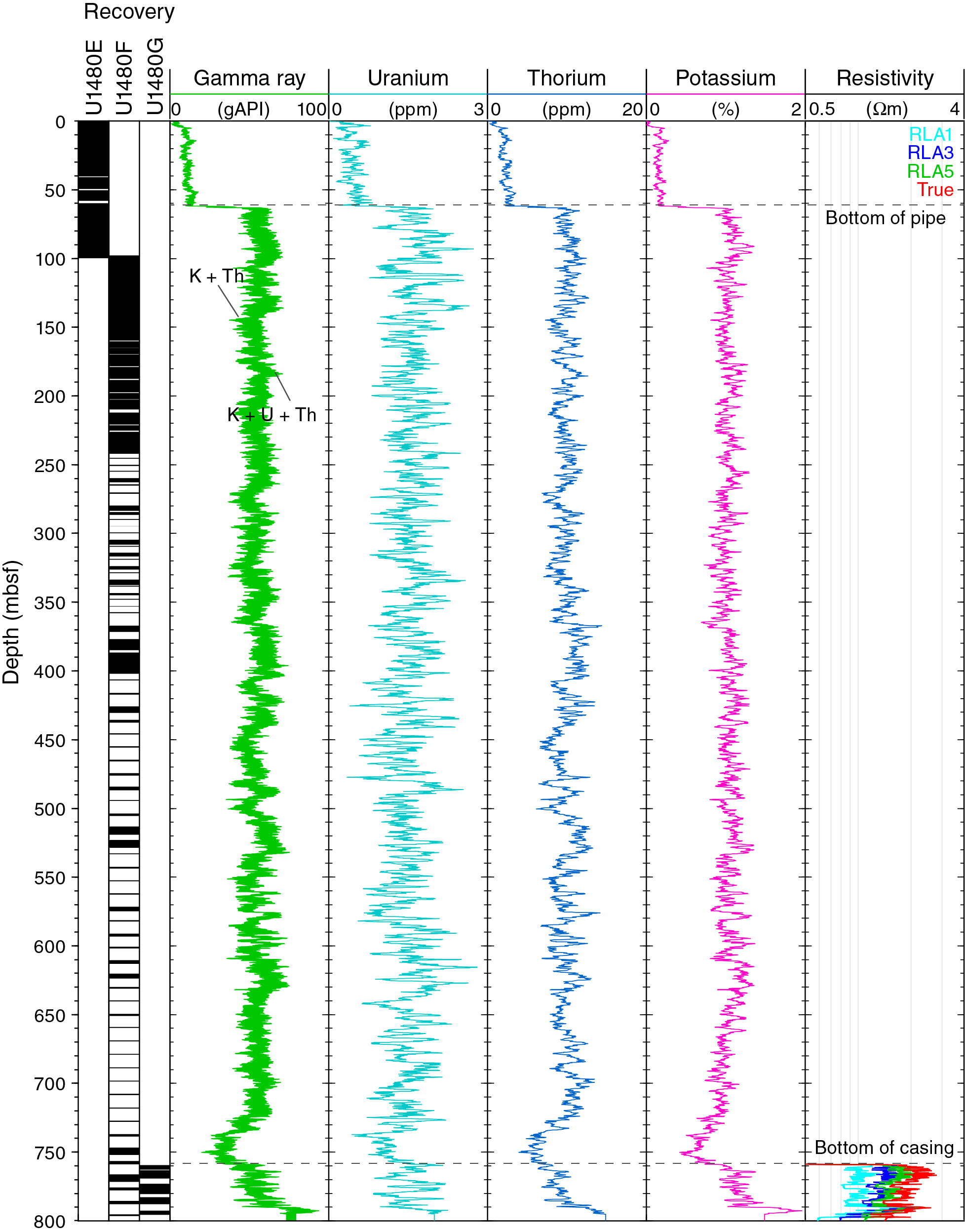
Figure F115. Log summary, Hole U1480G.

Figure F116. Logging data recorded in the open-hole below casing in Hole U1480G and core NGR, Holes U1480F and U1480G.
Without a sharp gamma ray increase at the bottom of the casing (759 mbsf), such as the one at the bottom of the pipe, we can only tentatively quantify the influence of the casing on the measurements or attribute the moderate increase in gamma radiation at this depth to the end of the casing versus an actual change in lithology. No significant change was observed in lithology on the limited amount of core recovered at this depth or in the gamma ray counts measured on the cores (see Sedimentology and petrology and Physical properties). The range of values of the gamma ray log below the casing is almost the same as throughout most of the cased section, where it should be attenuated. This suggests that the hole below the casing shoe is very large and that the end of the attenuating effect of the casing is balanced by a similar effect from the larger hole diameter in the open hole. The lower gamma ray values in the ~35 m above the bottom of the casing could indicate that the top of the larger hole interval is at ~725 mbsf. Between 725 and 759 mbsf, the lower readings are interpreted as showing the combined effect of the casing and of an enlarged hole. Some of the material that collapsed on the pipe and closed the hole may have fallen from this large washout.
The higher gamma ray values at the bottom of the logged interval could coincide with the top of lithostratigraphic Subunit IIC at 785.80 mbsf, but they could also indicate a reduction in hole size and the tool making actual contact with the formation before being stopped from going any deeper.
In an attempt to compensate for the strong influence of the pipe shallower than 62 mbsf and allow a comparison with the core measurements in this high-recovery interval, the spectral gamma ray data shown in Figure F117 were multiplied by a gain calculated from the ratio of the averages over 10 m intervals immediately below and above the bottom of the pipe. The values of these gains for the total gamma ray, potassium, thorium, and uranium data were 4.16, 5.66, 3.58, and 2.79, respectively. The scaled logs display an amplitude of variability higher than below the pipe, suggesting that a more accurate correction should probably include a shift in baseline and a smaller gain. However, the variations in total gamma ray can be matched in several intervals with the core data (Figure F118), showing that despite the influence of the pipe and casing, the logs can be used for a qualitative assessment of the lithology in other intervals behind the casing that have low recovery.

Figure F117. Spectral gamma ray logs from the upper section of Hole U1480G compared with core NGR in Hole U1480H.
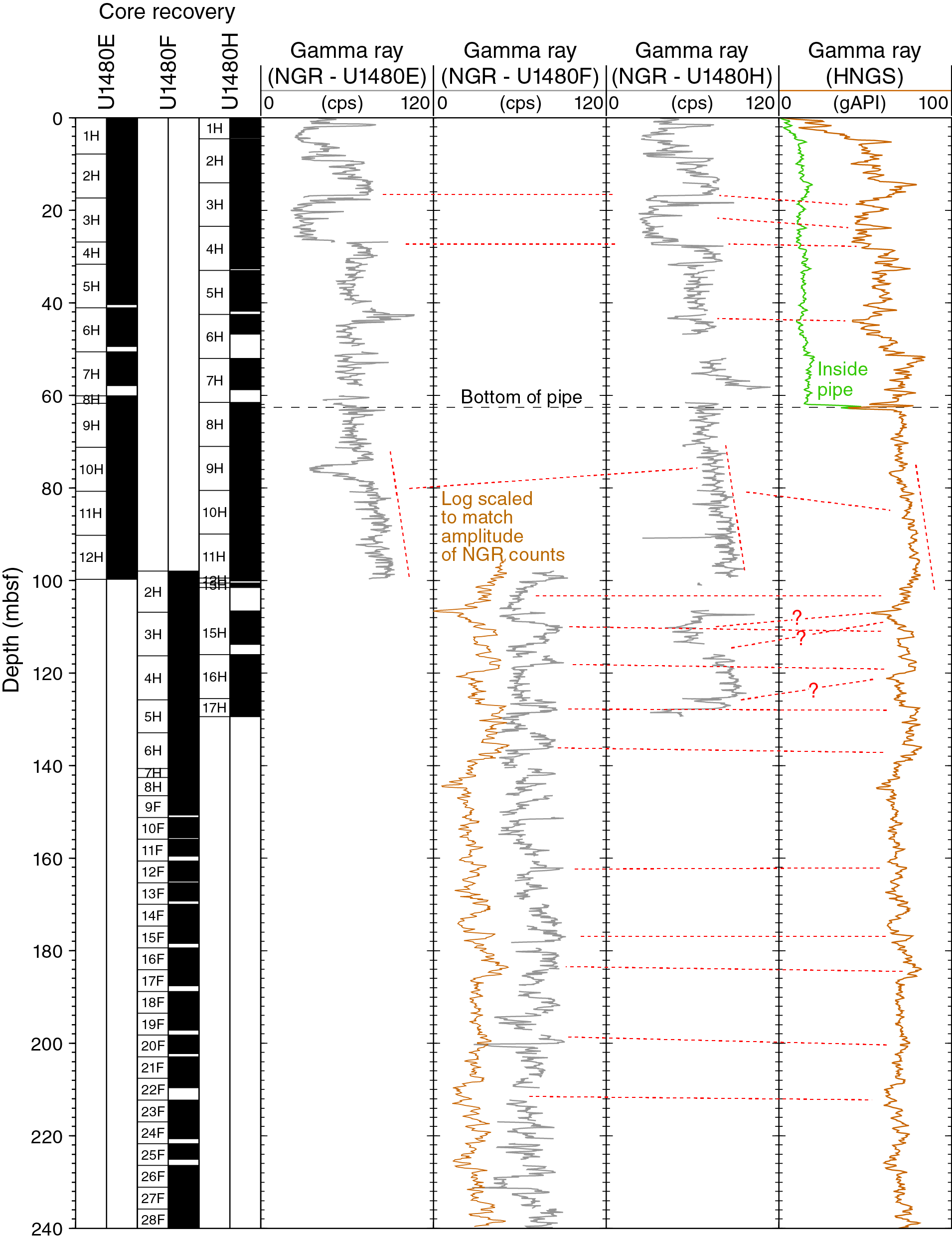
Figure F118. Comparison between logging HNGS and core NGR, Holes U1480E, U1480F, and U1480H.
Data overview
One of the main observations is that, regardless of the casing, the recorded logs display little large-scale variability or trend and remain within a limited range of values. This agrees with the interpretation from the recovered cores that one lithostratigraphic unit (II) encompasses most of the logged interval (see Sedimentology and petrology). The alternation of intervals dominated by fine-grained sand (lower gamma ray values), silt, silty clay, or clay (higher gamma ray values) that comprise this unit is likely responsible for the finer variations observed in the spectral gamma ray data (although at a different resolution: over several meters in log data, larger than many of the individual beds described in cores). Even in intervals with good recovery and a mostly continuous gamma ray record from the cores, the lack of strong character in the gamma ray curves limits the identification of clear ties between the logs and the core measurements in Holes U1480E, U1480F, and U1480H (Figure F118). The main exceptions are in the upper 30 m, where strong variations in the cores and logs can be matched with the subunits of Unit I and have been used successfully to adjust the depths of the various shallow holes (see Core-log-seismic integration). Deeper in the hole, only tentative correlations can be made between features in the logs and core measurements. To help establish some ties with Hole U1480F, we scaled the log to visually match the amplitude of the variations of gamma ray counts in this hole (Figure F118), making it possible to match some of the peaks between the log and the core measurements.
The absence of strong changes in gamma radiation through the casing also suggests that even in the intervals with the lowest recovery, we did not fail to recover any major lithology or any thick, clean sand layers that would have generated noticeable excursions in the logs, even through the casing. It is likely that the material recovered in these intervals is representative of the complete lithology. The only trends that can be observed in the ~35 m of data in the open hole are a slight decrease in resistivity with depth, whereas the total gamma radiation, thorium, and potassium increase steadily, indicating an increase in clay content throughout the transition to clay-dominated Subunit IIC (see Sedimentology and petrology).
Core-log-seismic integration
A key objective of Expedition 362 is to place regional seismic reflection profiles within the context of the drilling results. This requires the establishment of a relationship between time on the seismic sections and depth downhole. At Site U1480 this was accomplished by using core physical property measurements and petrological observations in conjunction with seismic reflection Profile BGR06-102 (Gaedicke, 2007) (Figure F119). At this site, we also established a composite depth scale for shallow holes.
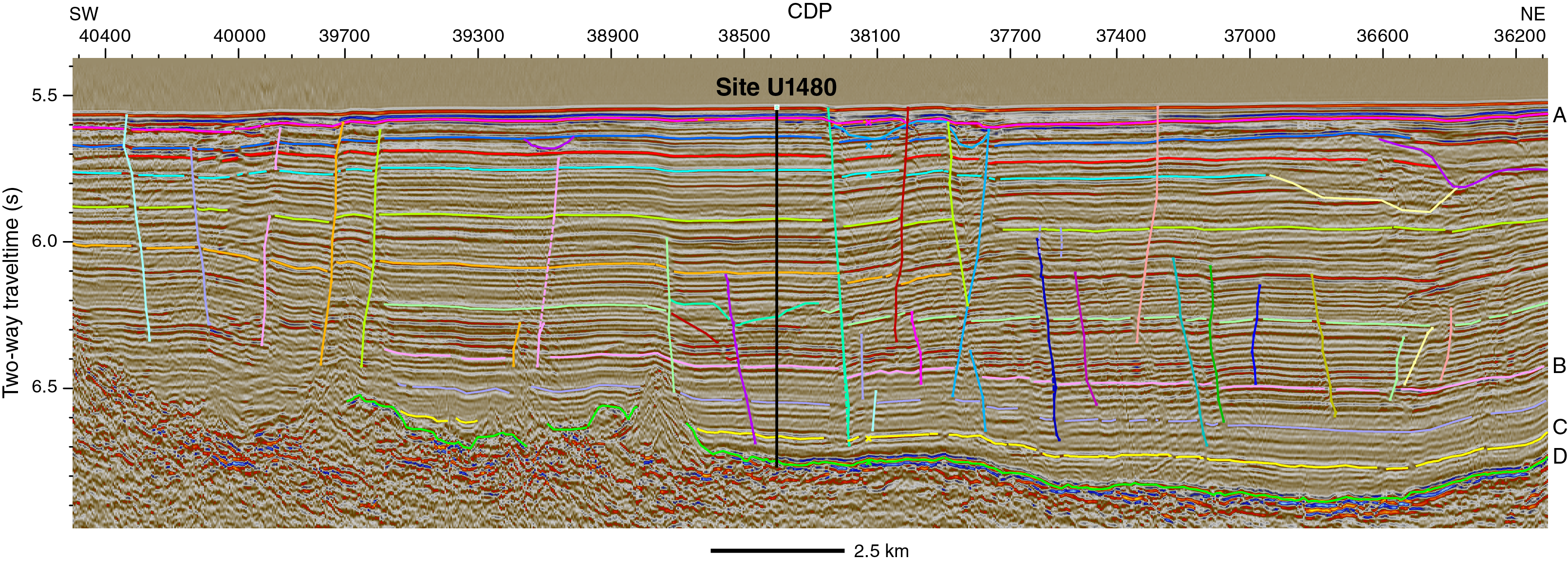
Figure F119. Regional interpretation of seismic Line BGR06-102 around Site U1480.
Composite depth scale
We established a composite depth scale for Site U1480 in order to allow integration of data between the holes that sampled the shallow section (Holes U1480A–U1480E and U1480H). This was particularly important for Holes U1480A–U1480D (one core per hole), which did not sample the water/sediment interface and therefore had an unknown depth. An initial assessment placed these cores relative to depths in Hole U1480E. However, after Hole U1480H was cored, a correlation between Holes U1480E and U1480H allowed a complete composite depth scale to be developed from 0 to 32 mbsf. Correlation focused on NGR (Figure F120) and WRMSL magnetic susceptibility data (Figure F121) because these are less affected by coring disturbance than WRMSL P-wave velocity or GRA density. However, the correlation is also consistent with the PWL, GRA density, and RSC colorimetry data (Figure F122). For these intervals, b* and L* are essentially similar, so the combination of b* and a* provides the best distinction. In developing the composite scale we assumed that there has been no core expansion, although in reality the composite section has expanded by ~2 m by 32 mbsf. The tops of cores shallower than 32 mbsf do not occur at the same depths in Holes U1480E and U1480H, which enabled a robust correlation. At 32 mbsf, Holes U1480E and U1480H core tops come into synchronization, preventing further detailed compositing. In this section, we refer to core composite depths below seafloor (CCSF), whereas the remainder of the report presents data in mbsf as sufficiently accurate.
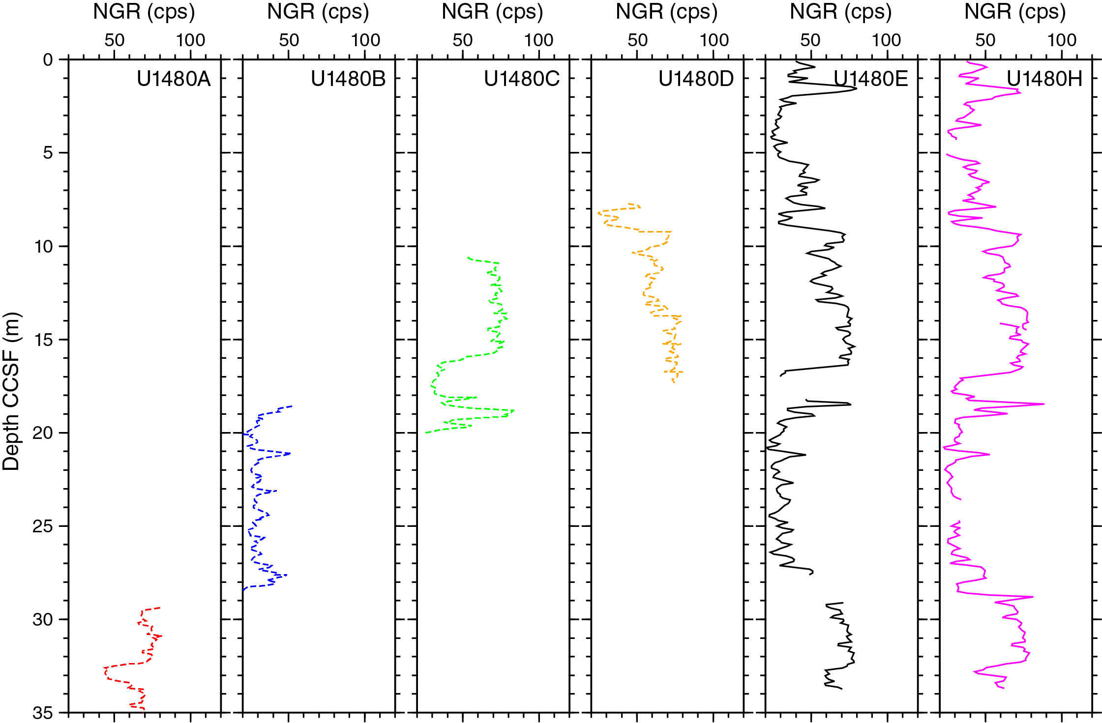
Figure F120. NGR measured on cores, Holes U1480A–U1480E and U1480H.
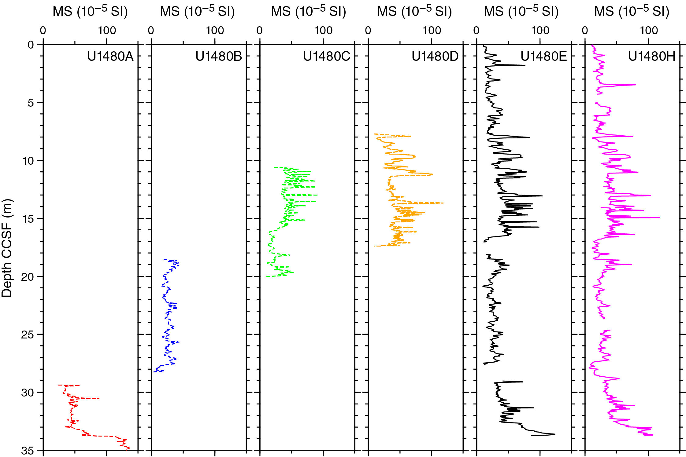
Figure F121. Whole-core magnetic susceptibility, Holes U1480A–U1480E and U1480H.
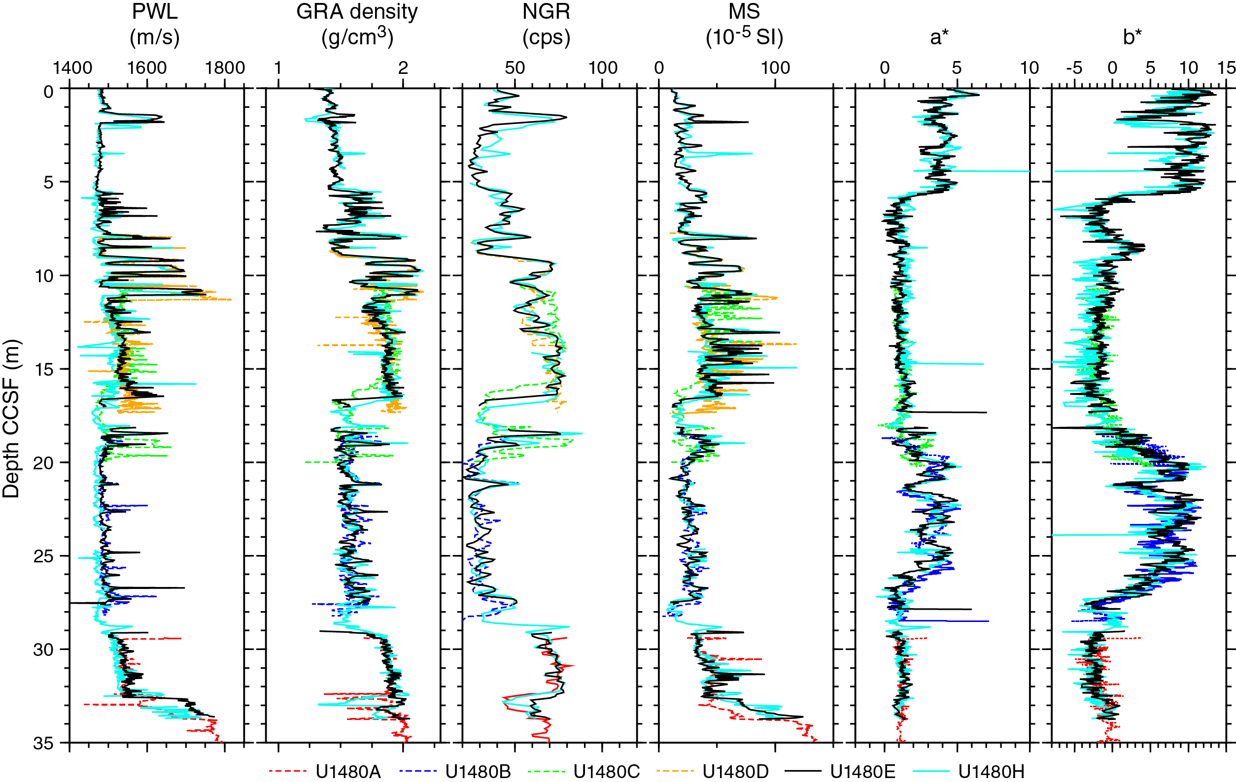
Figure F122. Physical property measurements, Holes U1480A–U1480E and U1480H.
Correlation of shallow cores (0–32 mbsf)
From 0 to 4 m CCSF, Holes U1480E and U1480H have a good NGR match with multiple short-wavelength peaks (Figure F120). This indicates depth agreement between the two holes. An NGR doublet at 5–7 m CCSF links Core 362-U1480E-1H to 362-U1480H-2H. A trough with a small central peak at 8–9 m CCSF links Core 362-U1480H-2H to 362-U1480E-2H. A sharp drop in NGR at 16–17 m CCSF links Core 362-U1480E-2H to 362-U1480H-3H. An NGR doublet peak at 18–19 m CCSF links Core 362-U1480H-3H to 362-U1480E-3H. The sequence of NGR peaks from 25 to 28 m CCSF links Cores 362-U1480E-3H and 362-U1480H-4H, with a trough at 33–34 m CCSF linking Cores 362-U1480H-4H and 362-U1480E-4H.
Hole U1480A can be positioned in depth by the same low value in NGR at 33–34 m CCSF, supported by an increase in magnetic susceptibility at 34 m CCSF (Figure F121) and in PWL over the same depth range (Figure F122). The top of Hole U1480A cannot be placed any shallower without violating the broad peak in b* that extends from 18 to 29 m CCSF (Figure F122).
Hole U1480B has a long sequence of low NGR values (mean = 30 counts/s) but also has a peak that is well-matched at 21 m CCSF in Holes U1480E and U1480H (Figure F120). This gives an excellent match to the structure of b*, including a trough at 21 m CCSF as well as detailed structure in GRA density near the base of Core 362-U1480B-1H (Figure F122).
Hole U1480C is the most difficult to position in depth. NGR data show consistent values of ~70 counts/s in the upper part of the hole, with a trough to 20 counts/s and then a complex peak at the base of the hole (Figure F120). Overall, this is a good fit to the NGR values from 14 to 20 m CCSF in Holes U1480E and U1480H. Core 362-U1480C-1H, however, had >100% recovery, and to best fit the gradients in physical properties and to appropriately match the full core to this interval requires that the core be shrunk in length by a factor of ~2. This is not feasible in the Correlator software and may not be possible within the current database affine table structure. Therefore, the position of Hole U1480C in the composite depth scale is set to match the trough at 17 m CCSF, which produces systematic physical property mismatches shallower in the core. We note that the inability to match the physical property data more fully has essentially no impact on the analyses conducted during Expedition 362.
Hole U1480D is positioned in depth by the relatively complex pattern of NGR data from 8 to 17 m CCSF, possibly with some stretching in the deepest 1–2 m of the core (Figure F120).
Overlaid PWL, GRA density, NGR, magnetic susceptibility, a*, and b* based on these correlations are shown in Figure F122, with depths to the top of each core section given in Table T23. The relative depths are consistent with the information from the drilling depth offset between each hole (see Operations).
Table T23. APCT-3 formation temperature measurement summary. Download table in .csv format.
Correlation of deeper cores (deeper than 32 mbsf)
We attempted to perform a detailed correlation of deeper cores where there was overlap between the drilling intervals, specifically between Holes U1480E, U1480F, and U1480H (98.0–99.7 mbsf) and between Holes U1480F and U1480G (759.6–815.0 mbsf). Holes U1480E and U1480F have discordant physical properties in the overlap (Figure F123), even though they both had >99% recovery (Table T1). This discordance may be related to the high degree of core deformation near the base of Hole U1480E (Figure F64). The reduced recovery in this part of Hole U1480H (71%) could not provide a tighter depth tie for the top of Hole U1480F.
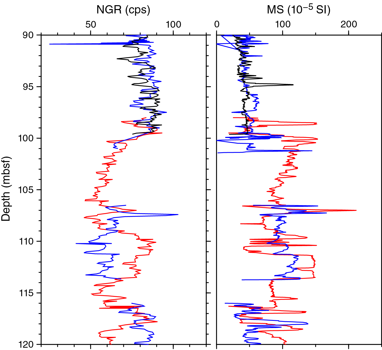
Figure F123. Comparison between NGR and WRMSL magnetic susceptibility in the region of overlap between Holes U1480E, U1480F, and U1480H.
Holes U1480F and U1480G overlap between 760 and 815 mbsf, where recovery was very variable (2%–73%) and physical properties lack distinctive features, so establishing a unique correlation was not possible. Although there are a number of good (and in some cases excellent) potential tie points between cores in Holes U1480F and U1480G based on detailed lithologic observations, most of the intervals would allow the cores to be positioned with no overlap, even assuming that each core represents a contiguous sampling of the subsurface. Therefore, we were not able to create a composite depth scale for the overlapping intervals, and some uncertainty remains over the relative position of cores from Holes U1480F and U1480G in this interval.
Core-seismic integration
A key objective of Expedition 362 is to place regional seismic reflection profiles within the context of the drilling results. This requires the establishment of a relationship between time on the seismic Line BGR06-102 (Gaedicke, 2007) and depth downhole. Unstable borehole conditions limited opportunities to log at Site U1480. In particular, we did not collect any in situ seismic velocity data, either as sonic logs or a vertical seismic profile. We did, however, use a number of complementary approaches to establish a good time-depth relationship, including constructing pseudologs from physical property measurements, identification of clear single reflections or reflection packages, and study of the drilling parameters.
Summary of regional and site survey seismic reflection data
Most of the modern seismic reflection data within the region were collected between 2006 and 2009 and focused on the subduction zone trench and forearc (e.g., Fisher et al., 2007; Singh et al., 2008; Franke et al., 2008; Dean et al., 2010; Singh et al., 2010; Gulick et al., 2011; Frederik et al., 2015). Within the trench, a wedge of recently deposited sediment (the trench wedge) overlies an angular unconformity that can be traced across the incoming plate (Dean et al., 2010; Geersen et al., 2015) and has been interpreted as continuous with a shallow, strong reflector at Site U1480 (seismic Horizon A in Figure F119). Within and immediately seaward of the trench and beneath the outermost accretionary prism, a high-amplitude negative polarity (HANP) reflector was interpreted by Dean et al. (2010) as a possibly fluid-rich or high-porosity horizon that might act as a décollement surface within the subduction zone. This reflector can be mapped 50 km west of the trench on the oceanic plate (Singh et al., 2010) but becomes lower in amplitude and changes to positive polarity farther west, away from the trench (Geersen et al., 2013), indicating a change in the physical properties around this horizon. The equivalent level within the sediment section can be traced to Site U1480 as a distinct package of relatively strong reflections with positive polarity (seismic Horizon C on Figure F119) above the acoustic basement (seismic Horizon D on Figure F119). A well-layered, strongly reflective sequence within which channels can be seen is interpreted as Nicobar Fan sediment (e.g., Gulick et al., 2011; McNeill et al., 2016) with a change at depth to reduced reflectivity (at seismic Horizon B on Figure F119). The sediment section is extensively faulted due to a combination of deformation within the India-Australia plate system and bending of the oceanic plate approaching the subduction zone (Geersen et al., 2015).
Establishing a time-depth relationship
Establishing a time-depth relationship requires identifying features that are either unique in both seismic and core data or sufficiently distinctive as to be unique within a particular time-depth interval. The seabed gives the first definitive tie in this study. From 0 to 250 mbsf, cores provide essentially continuous sampling of physical properties at laboratory temperature and pressure conditions, with good quality measurements of both P-wave velocity and bulk density (Figure F99). Reflectivity on the seismic section is controlled by variations in acoustic impedance (the product of P-wave velocity and density). Because velocity variations are more significant than density variations, the variations in P-wave velocity account for the expected reflectivity. Therefore, initial ties were tested and/or refined by matching reflectivity on the seismic section with the core velocity profiles (determined from the WRMSL from 0 to 250 mbsf and from the PWC measurements deeper than 250 mbsf) over the interval that each tie controls.
In the shallow section (to ~200 mbsf), the measured PWL data give time-depth tie points at 30, 142, and 186 mbsf where the core properties implied strong reflections from the top of sand intervals and strong reflections were also observed on the seismic section (Figure F124). Acoustic basement (seismic Horizon D) provides another clear tie point, with complex strong reflectivity distinct from the sediments above; the tie here is made to the observed sharp increase in core P-wave velocities from ~2500 to 4800m/s (Figure F99) at 1365 mbsf (6.74 s TWT). The acoustic basement identification gives an overall mean P-wave velocity downhole for the entire sedimentary sequence of ~2250 m/s. This then enables us to place an additional tie between the strong reflection package deep in the sediment section (seismic Horizon C) and an abrupt increase of 600–800 m/s in P-wave velocity in core samples around 1260 mbsf. This broadly corresponds to the boundary between Nicobar Fan and pelagic sediments (i.e., the lithostratigraphic Unit II/III boundary).
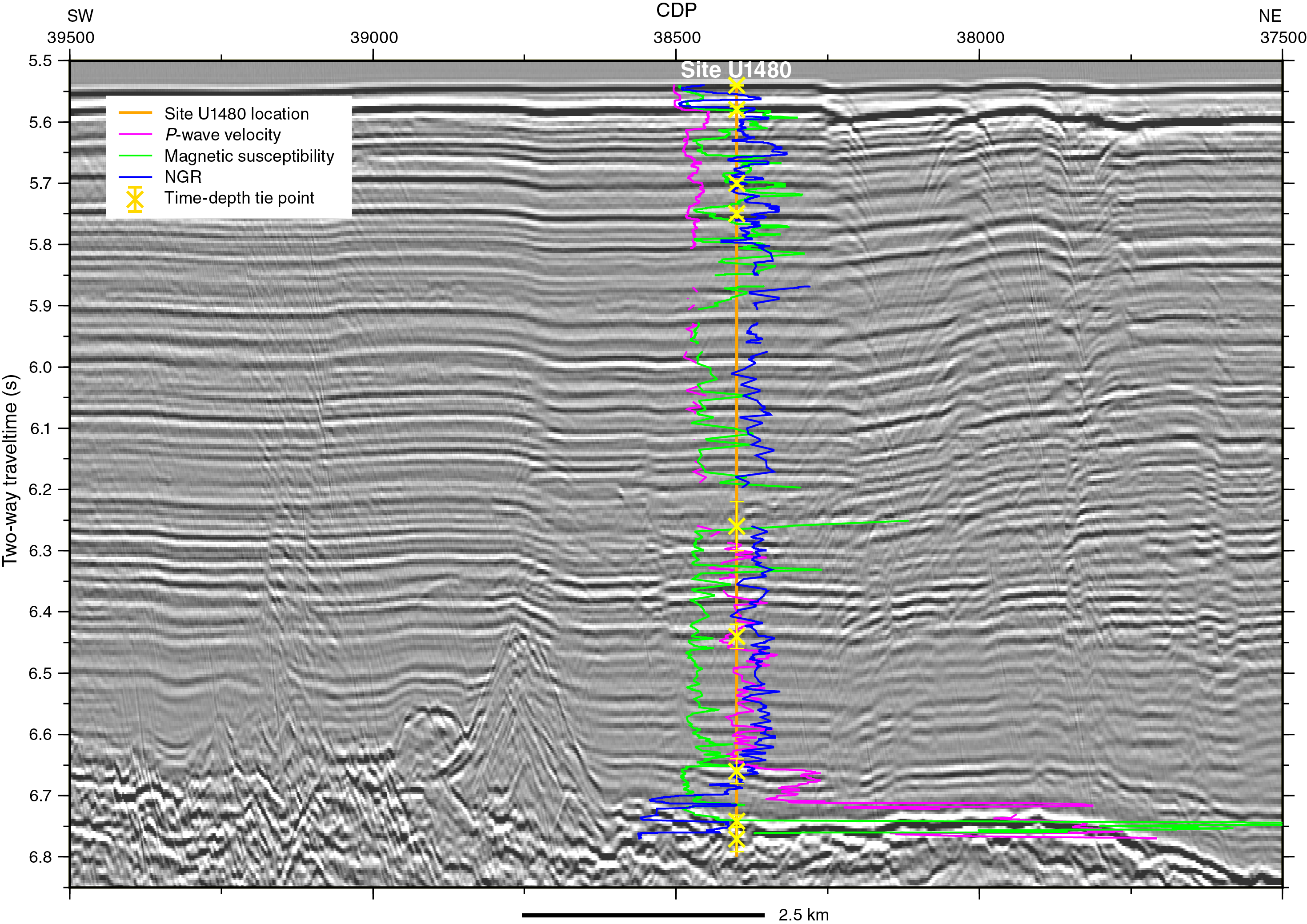
Figure F124. Seismic reflection Line BGR06-102 at Site U1480 with overlaid time-depth tie points and selected physical properties data.
A critical tie point in the middle of the sediment section was obtained from the careful analysis of drilling data (see Structural geology). We were able to identify the base of a channel complex by a combination of core recovery statistics, rate of penetration, and lithology (time = 6.26 s TWT; depth = 728 mbsf). The channel complex base can also be identified on the seismic section, although with some ambiguity whether the correct time is given from the zone over which reflections terminate laterally, a dipping event that apparently represents the channel base, or enhanced reflectivity on the horizon beneath the channel (Figure F124). Despite this ambiguity, this is an important tie within a thick interval of poor core recovery and repetitive strong reflections.
The final tie point is placed at the decrease of reflection amplitudes on the seismic section, interpreted preexpedition as the boundary between fan and pelagic sediments (seismic Horizon B). This correlates with a subtle change in the magnetic susceptibility data (Figure F124); the magnetic susceptibility data stay within the same overall range, but there are fewer peaks than within the strong reflectivity of the section above. The constraints on this tie point are weaker than the others, so it was placed in the middle of the most likely interval.
Time-depth ties are summarized in Table T24 and shown in Figure F125 together with associated interval velocities and estimates of velocity uncertainties that take into account the uncertainties in times and depths of each tie point. Through most of the section, the interval velocities required by these ties are up to 40% higher than the best estimate of velocity obtained from the shipboard velocity measurements on cores (Figure F126). In part this is caused by core sample measurements underestimating in situ velocity because of microcracks that form as pressure is reduced when cores are brought to the surface. However the degree of difference is higher than observed at other ODP/IODP sites (both regional and globally) between in situ and shipboard measurements (e.g., Expedition 315 scientists, 2009; Harris et al., 2013b; Cochran, Stow, et al., 1990). This suggests that in addition to the expected effect of pressure, materials with higher seismic velocity, most likely sands, were systematically under-recovered. The degree of core recovery is anticorrelated with the sand fraction (see Structural geology), which supports this hypothesis.
Table T24. Time-depth ties. Download table in .csv format.
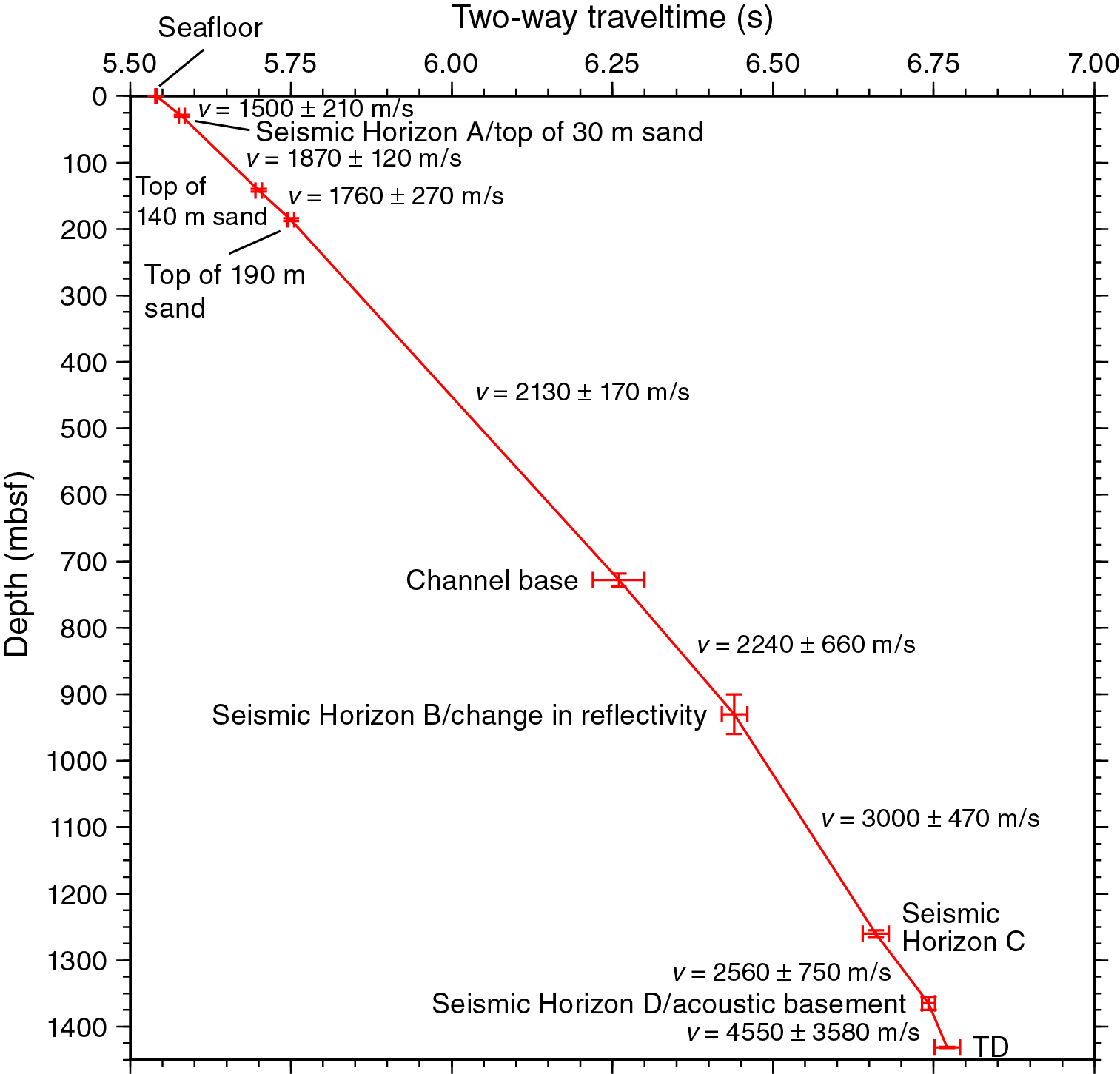
Figure F125. Tie points between time on seismic Line BGR06-102 and depth at Site U1480.
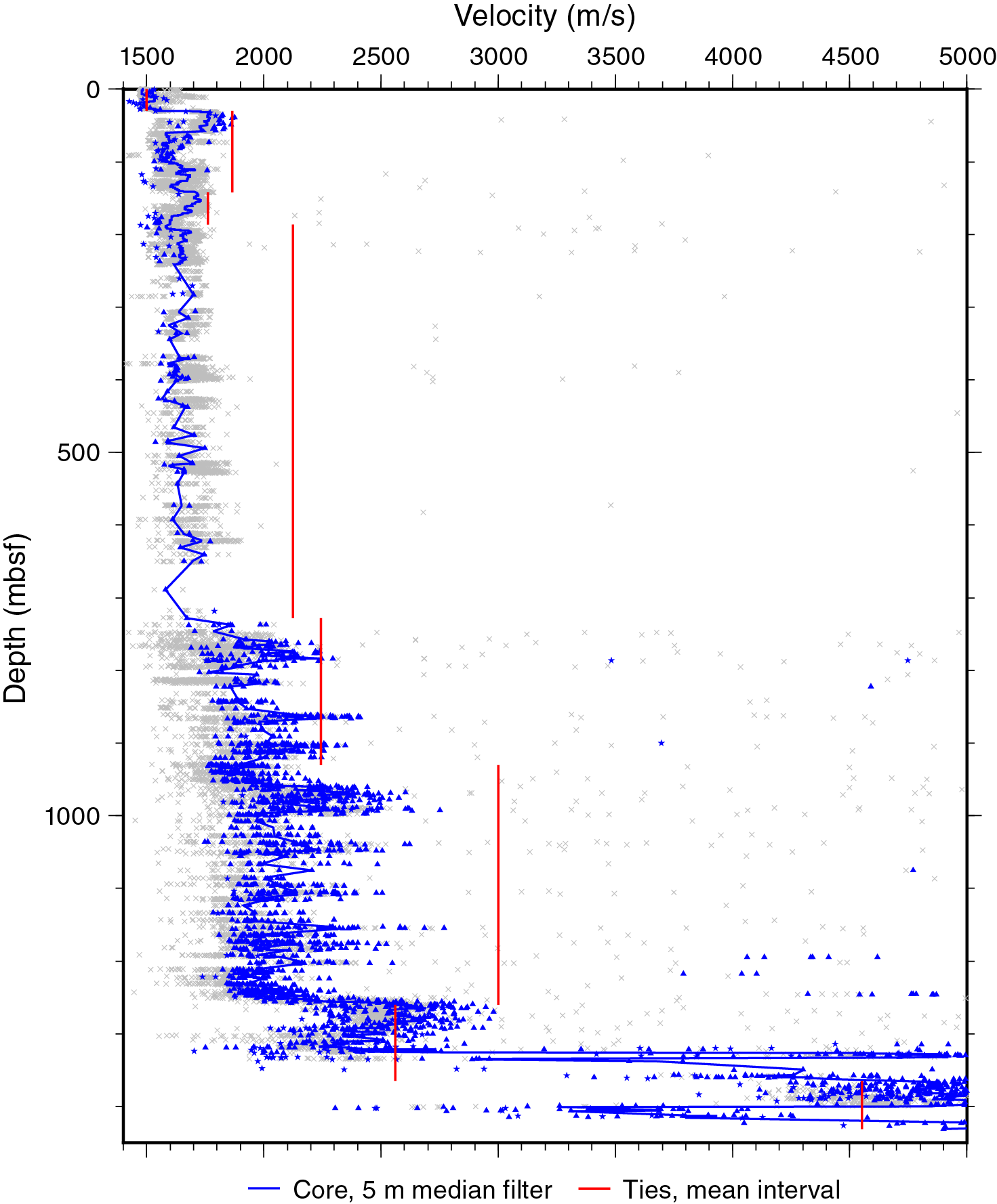
Figure F126. Comparison between the interval velocities from the time-depth relationship and P-wave seismic velocity in whole-round cores and samples.
Comparison between core observations and site survey seismic reflection data
Comparison between cores and seismic data indicates that the strong, laterally continuous reflections are due to sand-rich intervals. In the upper section of the site (<250 mbsf), where recovery was near complete, magnetic susceptibility and NGR data show variations on the scale of individual reflections that suggest these represent individual units with distinct compositions (Figure F127). For example, the thick sand-dominated interval extending from 30 to 60 mbsf (5.58–5.62 s TWT) has reflectivity variations at the lowest limit of the seismic resolution (7–10 m) that correlate with obvious variations in NGR and magnetic susceptibility data.
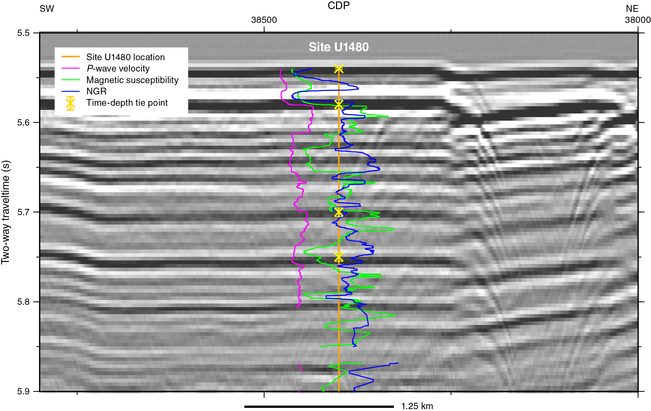
Figure F127. Shallow section of seismic reflection Line BGR06-102 with overlaid time-depth tie points and selected physical property curves.
Comparison of the seismic data with the lithostratigraphic units (Figures F5, F128) shows correlation in broad terms. The base of Unit I approximately matches the strong reflection 40 ms below the seabed (seismic Horizon A; first yellow X below seafloor on Figures F124, F127). This is a reflection that can be tracked >100 km on seismic Line BGR06-102 toward the subduction zone and by crossing seismic Line MD116 onto Lines BGR06-103 and BGR06-104. However, in detail, the reflection at Site U1480 comes from the thick sand within Subunit IIA that lies 3–4 m beneath the base of Unit I (Figure F5). Unit II broadly correlates with the interval of variably strong, laterally continuous reflections that show limited evidence for lateral change in thickness. The subunits within Unit II do not correspond in a simple way to changes in the seismic reflection profile. Nevertheless, the Nicobar Fan origin of Unit II (see Sedimentology and petrology) is consistent with the large number of channels imaged in the seismic section. The transition from Unit II to III (submarine fan to pelagic sediment) correlates well with the package of reflectivity at 6.65 s TWT (seismic Horizon C). Beneath the top of Unit III, the seismic section and the lithostratigraphic units display poor correlation, and the lowermost sediment above the acoustic basement is not well imaged. Our interpretation is that the acoustic basement seismic Horizon D corresponds to igneous rocks intercalated with the deepest sediment (~1360 mbsf within Unit V) rather than the top of ocean crust basalt encountered at 1415 mbsf (top of Unit VI). Although the uppermost igneous rocks of Unit IV also have high velocities, they are probably too thin to cause a strong reflection and would require a lower velocity between the tie points. The complexity of igneous-sedimentary layering here results in a reflector package that does not represent a single stratigraphic surface.
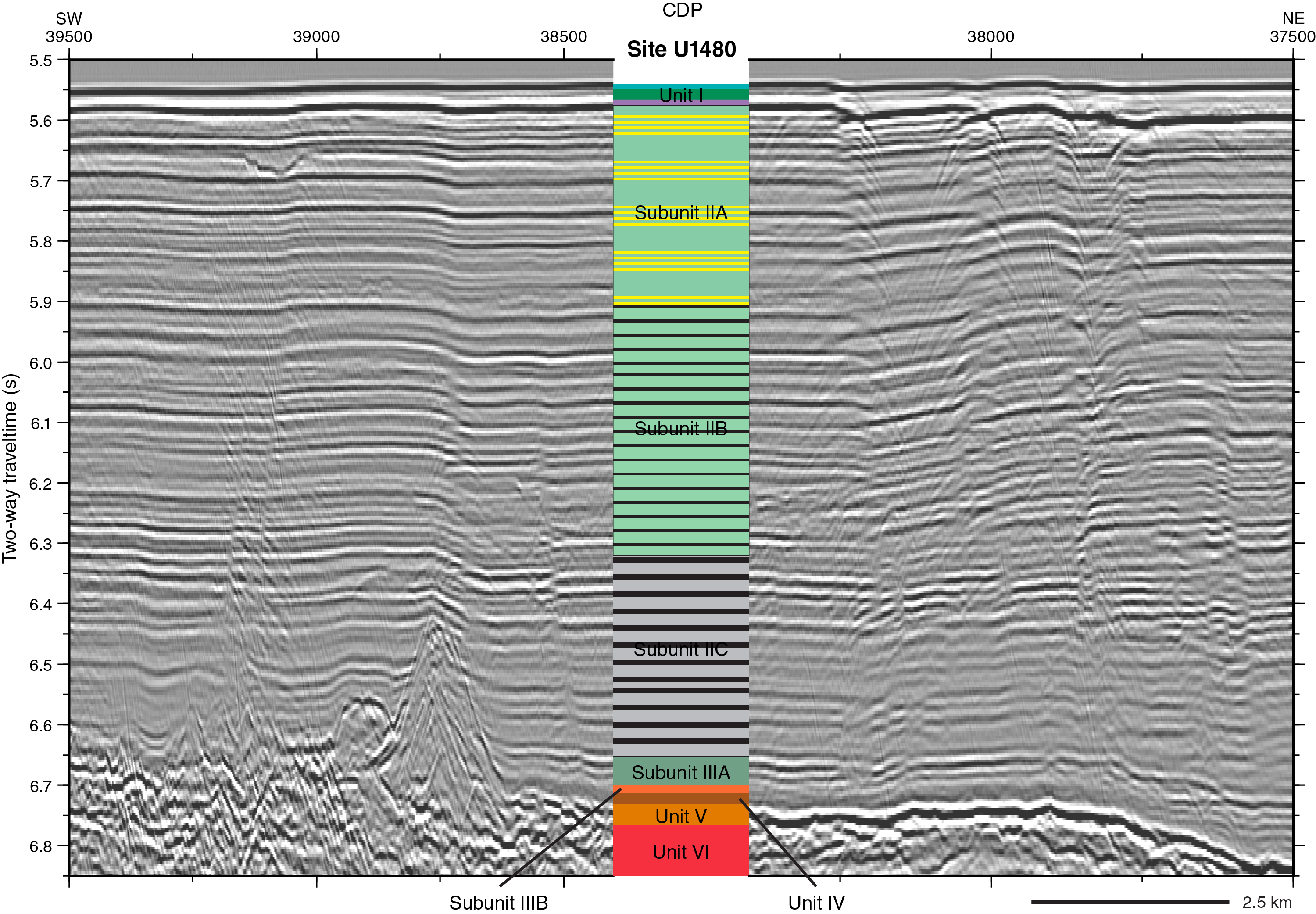
Figure F128. Relationship between seismic reflection Line BGR06-102 and lithostratigraphic units.
Reevaluation of the site survey seismic reflection data: regional implications
Linking drilling results to the site survey seismic data confirms that the sequence of strong subhorizontal reflections accompanied by channel complexes through much of the section represents Nicobar Fan deposits. Individual reflections throughout the sequence can be traced over distances of tens to one hundred kilometers (e.g., Figure F119). A careful interpretation of seismic Lines BGR06-102 and BGR06-103/104/105 indicates that each interval of strong reflections can be linked to a channel-levee system.
We can now show that seismic Horizon C correlates with a package that marks the boundary between the rapidly accumulated Nicobar Fan sediment (Unit II) and a thinner, low sedimentation–rate pelagic section (Unit III). This new information will help the interpretation of the HANP reflection (the equivalent of seismic Horizon C closer to the subduction zone) by Dean et al. (2010) and Geersen et al. (2013) and may explain why seismic Horizon C has higher amplitude and negative polarity close to the trench and why it is absent to the south of the 2004 rupture zone (see Hüpers et al., 2017, for relevant discussion).
Interval velocities measured on core samples and those inferred from the time-depth matching process (Figure F126) are lower than those estimated near the trench from seismic data (Dean et al., 2010; Singh et al., 2010) but match reasonably well those from regional velocity data sets in the fan (e.g., Bull and Scrutton, 1990). The interval velocities derived here may be useful for time-depth interpretations in other parts of the fan where velocity data are absent.
References
Backman, J., and Shackleton, N.J., 1983. Quantitative biochronology of Pliocene and early Pleistocene calcareous nannofossils from the Atlantic, Indian and Pacific Oceans. Marine Micropaleontology, 8(2):141–170. https://doi.org/10.1016/0377-8398(83)90009-9
Bąk, M., and Sawlowicz, Z., 2000. Pyritized radiolarians from the mid-Cretaceous deposits of the Pieniny Klippen Belt—a model of pyritization in an anoxic environment. Geologica Carpathica, 51:91–99. http://www.geologicacarpathica.com/GeolCarp_Vol51_No2_91_99.html
Barron, J.A., 1992. Neogene diatom datum levels in the equatorial and North Pacific. In Ishizaki, K., and Saito, T. (Eds.), Centenary of Japanese Micropaleontology: Tokyo (Terra Scientific Publishing Company), 413–425. http://www.terrapub.co.jp/e-library/cjm/pdf/0413.pdf
Berner, R.A., and Schott, J., 1982. Mechanism of pyroxene and amphibole weathering II. Observations of soil grains. American Journal of Science, 282(8):1214–1231. https://doi.org/10.2475/ajs.282.8.1214
Biot, M.A., 1941. General theory of three-dimensional consolidation. Journal of Applied Physics, 12(2):155–164. https://doi.org/10.1063/1.1712886
Bull, J.M., and Scrutton, R.A., 1990. Sediment velocities and deep structure from wide-angle reflection data around Leg 116 sites. In Cochran, J.R., Stow, D.A.V., et al., Proceedings of the Ocean Drilling Program, Scientific Results, 116: College Station, TX (Ocean Drilling Program), 311–316. http://dx.doi.org/10.2973/odp.proc.sr.116.155.1990
Bullard, E.C., 1939. Heat flow in South Africa. Proceedings of the Royal Society of London, Series A, 173(955):474–502. http://dx.doi.org/10.1098/rspa.1939.0159
Claypool, G.E., and Kvenvolden, K.A., 1983. Methane and other hydrocarbon gases in marine sediment. Annual Review of Earth and Planetary Sciences, 11(1):299–327. https://doi.org/10.1146/annurev.ea.11.050183.001503
Cochran, J.R., Stow, D.A.V., et al., 1989. Proceedings of the Ocean Drilling Program, Initial Reports, 116: College Station, TX (Ocean Drilling Program). http://dx.doi.org/10.2973/odp.proc.ir.116.1989
Cochran, J.R., Stow, D.A.V., et al., 1990. Proceedings of the Ocean Drilling Program, Scientific Results, 116: College Station, TX (Ocean Drilling Program). https://doi.org/10.2973/odp.proc.sr.116.1990
Curray, J.R., 2014. The Bengal depositional system: from rift to orogeny. Marine Geology, 352:59–69. https://doi.org/10.1016/j.margeo.2014.02.001
Curray, J.R., Emmel, F.J., and Moore, D.G., 2003. The Bengal Fan: morphology, geometry, stratigraphy, history and processes. Marine and Petroleum Geology, 19(10):1191–1223. http://dx.doi.org/10.1016/S0264-8172(03)00035-7
Curray, J.R., and Moore, D.G., 1974. Sedimentary and tectonic processes in the Bengal deep-sea fan and geosyncline. In Burk, C.A., and Drake, C.L. (Eds.), The Geology of Continental Margins: New York (Springer-Verlag), 617–627.
de Lange, G.J., 1992. Distribution of exchangeable, fixed, organic and total nitrogen in interbedded turbiditic/pelagic sediments of the Madeira Abyssal Plain, eastern North Atlantic. Marine Geology, 109(1–2):95–114. https://doi.org/10.1016/0025-3227(92)90223-5
Dean, S.M., McNeill, L.C., Henstock, T.J., Bull, J.M., Gulick, S.P.S., Austin, J.A., Jr., Bangs, N.L.B., Djajadihardja, Y.S., and Permana, H., 2010. Contrasting décollement and prism properties over the Sumatra 2004–2005 earthquake rupture boundary. Science, 329(5988):207–210. http://dx.doi.org/10.1126/science.1189373
Erickson, S.N., and Jarrard, R.D., 1998. Velocity-porosity relationships for water-saturated siliciclastic sediments. Journal of Geophysical Research: Solid Earth, 103(B12):30385–30406. http://dx.doi.org/10.1029/98JB02128
Expedition 315 Scientists, 2009. Expedition 315 Site C0001. In Kinoshita, M., Tobin, H., Ashi, J., Kimura, G., Lallemant, S., Screaton, E.J., Curewitz, D., Masago, H., Moe, K.T., and the Expedition 314/315/316 Scientists, Proceedings of the Integrated Ocean Drilling Program, 314/315/316: Washington, DC (Integrated Ocean Drilling Program Management International, Inc.). https://doi.org/10.2204/iodp.proc.314315316.123.2009
Expedition 334 Scientists, 2012. Methods. In Vannucchi, P., Ujiie, K., Stroncik, N., Malinverno, A., and the Expedition 334 Scientists, Proceedings of the Integrated Ocean Drilling Program, 334: Tokyo (Integrated Ocean Drilling Program Management International, Inc.). http://dx.doi.org/10.2204/iodp.proc.334.102.2012
Fisher, D., Mosher, D., Austin, J.A., Jr., Gulick, S.P.S., Masterlark, T., and Moran, K., 2007. Active deformation across the Sumatran forearc over the December 2004 Mw9.2 rupture. Geology, 35(2):99–102. http://dx.doi.org/10.1130/G22993A.1
Flemings, P.B., Polito, P.J., Pettigrew, T.L., Iturrino, G.J., Meissner, E., Aduddell, R., Brooks, D.L., Hetmaniak, C., Huey, D., Germaine, J.T., and the IODP Expedition 342 Scientists, 2013. The Motion Decoupled Delivery System: a new deployment system for downhole tools is tested at the New Jersey Margin. Scientific Drilling, 15:51–56. http://dx.doi.org/10.2204/iodp.sd.15.07.2013
Folk, R.L., 1980. Petrology of Sedimentary Rocks (2nd edition): Austin, TX (Hemphill’s).
Fornaciari, E., Giusberti, L., Luciani, V., Tateo, F., Agnini, C., Backman, J., Oddone, M., and Rio, D., 2007. An expanded Cretaceous−Tertiary transition in a pelagic setting of the Southern Alps (central-western Tethys). Palaeogeography, Palaeoclimatology, Palaeoecology, 255(1–2):98–131. https://doi.org/10.1016/j.palaeo.2007.02.044
Fourtanier, E., 1991. Diatom biostratigraphy of equatorial Indian Ocean Site 758. In Weissel, J., Peirce, J., Taylor, E., Alt, J., et al., Proceedings of the Ocean Drilling Program, Scientific Results, 121: College Station, TX (Ocean Drilling Program), 189–208. http://dx.doi.org/10.2973/odp.proc.sr.121.137.1991
France-Lanord, C., Spiess, V., Klaus, A., Adhikari, R.R., Adhikari, S.K., Bahk, J.-J., Baxter, A.T., Cruz, J.W., Das, S.K., Dekens, P., Duleba, W., Fox, L.R., Galy, A., Galy, V., Ge, J., Gleason, J.D., Gyawali, B.R., Huyghe, P., Jia, G., Lantzsch, H., Manoj, M.C., Martos Martin, Y., Meynadier, L., Najman, Y.M.R., Nakajima, A., Ponton, C., Reilly, B.T., Rogers, K.G., Savian, J.F., Schwenk, T., Selkin, P.A., Weber, M.E., Williams, T., and Yoshida, K., 2016. Site U1451. In France-Lanord, C., Spiess, V., Klaus, A., Schwenk, T., and the Expedition 354 Scientists, Bengal Fan. Proceedings of the International Ocean Discovery Program, 354: College Station, TX (International Ocean Discovery Program). http://dx.doi.org/10.14379/iodp.proc.354.105.2016
Franke, D., Schnabel, M., Ladage, S., Tappin, D.R., Neben, S., Djajadihardja, Y.S., Müller, C., Kopp, H., and Gaedicke, C., 2008. The great Sumatra-Andaman earthquakes—imaging the boundary between the ruptures of the great 2004 and 2005 earthquakes. Earth and Planetary Science Letters, 269(1–2):118–130. http://dx.doi.org/10.1016/j.epsl.2008.01.047
Frederik, M.C.G., Gulick, S.P.S., Austin, J.A., Jr., Bangs, N.L.B., and Urdrekh, 2015. What 2-D multichannel seismic and multibeam bathymetric data tell us about the North Sumatra wedge structure and coseismic response. Tectonics, 34(9):1910–1926. https://doi.org/10.1002/2014TC003614
Gaedicke, C., 2007. SEACAUSE Cruise SO186-2 report. http://www.bgr.bund.de/EN/Themen/MarineRohstoffforschung/Projekte/HC-Potential-of-continental-margins/Abgeschlossen/forschungsfahrt_SO_186_2_en.html
Galbrun, B., and Gardin, S., 2004. New chronostratigraphy of the Cretaceous–Paleogene boundary interval at Bidart (France). Earth and Planetary Science Letters, 224(1–2):19–32. https://doi.org/10.1016/j.epsl.2004.04.043
Garzanti, E., Vezzoli, G., Andò, S., France-Lanord, C., Singh, S.K., and Foster, G., 2004. Sand petrology and focused erosion in collision orogens: the Brahmaputra case. Earth and Planetary Science Letters, 220(1–2):157–174. http://dx.doi.org/10.1016/S0012-821X(04)00035-4
Geersen, J., Bull, J.M., McNeill, L.C., Henstock, T.J., Gaedicke, C., Chamot-Rooke, N., and Delescluse, M., 2015. Pervasive deformation of an oceanic plate and relationship to large >Mw 8 intraplate earthquakes: the northern Wharton Basin, Indian Ocean. Geology, 43(4):359–362. http://dx.doi.org/10.1130/G36446.1
Geersen, J., McNeill, L., Henstock, T.J., and Gaedicke, C., 2013. The 2004 Aceh-Andaman earthquake: early clay dehydration controls shallow seismic rupture. Geochemistry, Geophysics, Geosystems, 14(9):3315–3323. http://dx.doi.org/10.1002/ggge.20193
Gibson, R.E., 1958. The progress of consolidation in a clay layer increasing in thickness with time. Geotechnique, 8(4):171–182. https://doi.org/10.1680/geot.1958.8.4.171
Gieskes, J.M., Blanc, G., Vrolijk, P., Elderfield, H., and Barnes, R., 1990. Interstitial water chemistry—major constituents. In Moore, J.C., Mascle, A., et al., Proceedings of the Ocean Drilling Program, Scientific Results, 110: College Station, TX (Ocean Drilling Program), 155–178. https://doi.org/10.2973/odp.proc.sr.110.170.1990
Gulick, S.P.S., Austin, J.A., Jr., McNeill, L.C., Bangs, N.L.B., Martin, K.M., Henstock, T.J., Bull, J.M., Dean, S., Djajadihardja, Y.S., and Permana, H., 2011. Updip rupture of the 2004 Sumatra earthquake extended by thick indurated sediments. Nature Geoscience, 4(7):453–456. https://doi.org/10.1038/ngeo1176
Gupta, S.M., 1996. Quantitative radiolarian assemblages in surface sediments from the Central Indian Basin and their paleomonsoonal significance. Journal of the Geological Society of India, 47:339–354. http://drs.nio.org/drs/handle/2264/2240
Harris, R.N., Sakaguchi, A., Petronotis, K., Baxter, A.T., Berg, R., Burkett, A., Charpentier, D., Choi, J., Diz Ferreiro, P., Hamahashi, M., Hashimoto, Y., Heydolph, K., Jovane, L., Kastner, M., Kurz, W., Kutterolf, S.O., Li, Y., Malinverno, A., Martin, K.M., Millan, C., Nascimento, D.B., Saito, S., Sandoval Gutierrez, M.I., Screaton, E.J., Smith-Duque, C.E., Solomon, E.A., Straub, S.M., Tanikawa, W., Torres, M.E., Uchimura, H., Vannucchi, P., Yamamoto, Y., Yan, Q., and Zhao, X., 2013a. Expedition 344 summary. In Harris, R.N., Sakaguchi, A., Petronotis, K., and the Expedition 344 Scientists, Proceedings of the Integrated Ocean Drilling Program, 344: College Station, TX (Integrated Ocean Drilling Program). https://doi.org/10.2204/iodp.proc.344.101.2013
Harris, R.N., Sakaguchi, A., Petronotis, K., Baxter, A.T., Berg, R., Burkett, A., Charpentier, D., Choi, J., Diz Ferreiro, P., Hamahashi, M., Hashimoto, Y., Heydolph, K., Jovane, L., Kastner, M., Kurz, W., Kutterolf, S.O., Li, Y., Malinverno, A., Martin, K.M., Millan, C., Nascimento, D.B., Saito, S., Sandoval Gutierrez, M.I., Screaton, E.J., Smith-Duque, C.E., Solomon, E.A., Straub, S.M., Tanikawa, W., Torres, M.E., Uchimura, H., Vannucchi, P., Yamamoto, Y., Yan, Q., and Zhao, X., 2013b. Input Site U1414. In Harris, R.N., Sakaguchi, A., Petronotis, K., and the Expedition 344 Scientists, Proceedings of the Integrated Ocean Drilling Program, 334: Tokyo (Integrated Ocean Drilling Program Management International, Inc.). https://doi.org/10.2204/iodp.proc.344.104.2013
Harris, R.N., Sakaguchi, A., Petronotis, K., Baxter, A.T., Berg, R., Burkett, A., Charpentier, D., Choi, J., Diz Ferreiro, P., Hamahashi, M., Hashimoto, Y., Heydolph, K., Jovane, L., Kastner, M., Kurz, W., Kutterolf, S.O., Li, Y., Malinverno, A., Martin, K.M., Millan, C., Nascimento, D.B., Saito, S., Sandoval Gutierrez, M.I., Screaton, E.J., Smith-Duque, C.E., Solomon, E.A., Straub, S.M., Tanikawa, W., Torres, M.E., Uchimura, H., Vannucchi, P., Yamamoto, Y., Yan, Q., and Zhao, X., 2013c. Methods. In Harris, R.N., Sakaguchi, A., Petronotis, K., and the Expedition 344 Scientists, Proceedings of the Integrated Ocean Drilling Program, 344: College Station, TX (Integrated Ocean Drilling Program). https://doi.org/10.2204/iodp.proc.344.102.2013
Hinrichs, K.-U., Hayes, J.M., Bach, W., Spivack, A.J., Hmelo, L.R., Holm, N.G., Johnson, C.G., and Sylva, S.P., 2006. Biological formation of ethane and propane in the deep marine subsurface. Proceedings of the National Academy of Science of the United States of America, 103(40):14684–14689. http://dx.doi.org/10.1073/pnas.0606535103
Hüpers, A., and Kopf, A.J., 2012. Effect of smectite dehydration on pore water geochemistry in the shallow subduction zone: an experimental approach. Geochemistry, Geophysics, Geosystems, 13(10):QOAD26. https://doi.org/10.1029/2012GC004212
Hüpers, A., Torres, M.E., Owari, S., McNeill, L.C., Dugan, D., Henstock, T.J., Milliken, K.L., Petronotis, K.E., Backman, J., Bourlange, S., Chemale, F., Jr., Chen, W., Colson, T.A., Frederik, M.C.G., Guèrin, G., Hamahashi, M., House, B.M., Jeppson, T.N., Kachovich, S., Kenigsberg, A.R., Kuranaga, M., Kutterolf, S., Mitchison, F.L., Mukoyoshi, H., Nair, N., Pickering, K.T., Pouderoux, H.F.A., Shan, Y., Song, I., Vannucchi, P., Vrolijk, P.J., Yang, T., and Zhao, X., 2017. Release of mineral-bound water prior to subduction tied to shallow seismogenic slip off Sumatra. Science, 356(6340):841–844. https://doi.org/10.1126/science.aal3429
Jena, B., Kurian, P.J., and Avinash, K., 2016. Morphology of submarine channel-levee systems in the eastern Bay of Bengal near Andaman region. Journal of Coastal Conservation, 20(3):211–220. https://doi.org/10.1007/s11852-016-0431-2
Jutzeler, M., White, J.D.L., Talling, P.J., McCanta, M., Morgan, S., Le Friant, A., and Ishizuka, O., 2014. Coring disturbances in IODP piston cores with implications for offshore record of volcanic events and the Missoula megafloods. Geochemistry, Geophysics, Geosystems, 15(9):3572–3590. http://dx.doi.org/10.1002/2014GC005447
Kameda, J., Yamaguchi, A., Saito, S., Sakuma, H., Kawamura, K., and Kimura, G., 2011. A new source of water in seismogenic subduction zones. Geophysical Research Letters, 38(22):L22306. https://doi.org/10.1029/2011GL048883
Kastner, M., Solomon, E.A., Harris, R.N., and Torres, M.E., 2014. Fluid origins, thermal regimes, and fluid and solute fluxes in the forearc of subduction zones. In Stein, R., Blackman, D., Inagaki, F., and Larsen, H.-C., Developments in Marine Geology (Volume 7): Earth and Life Processes Discovered from Subseafloor Environments: a Decade of Science Achieved by the Integrated Ocean Drilling Program (IODP). R. Stein (Series Ed.): Amsterdam (Elsevier B.V.), 671–733. https://doi.org/10.1016/B978-0-444-62617-2.00022-0
Kirschvink, J.L., 1980. The least-squares line and plane and the analysis of palaeomagnetic data. Geophysical Journal of the Royal Astronomical Society, 62(3):699–718. http://dx.doi.org/10.1111/j.1365-246X.1980.tb02601.x
Kroenke, L.W., Berger, W.H., Janecek, T.R., et al., 1991. Proceedings of the Ocean Drilling Program, Initial Reports, 130: College Station, TX (Ocean Drilling Program). http://dx.doi.org/10.2973/odp.proc.ir.130.1991
Lander, R.H., and Walderhaug, O., 1999. Predicting porosity through simulating sandstone compaction and quartz cementation. AAPG Bulletin, 83(3):433–449. http://aapgbull.geoscienceworld.org/content/83/3/433.short
Lawrence, J.R., and Gieskes, J.M., 1981. Constraints on water transport and alteration in the oceanic crust from the isotopic composition of pore water. Journal of Geophysical Research: Solid Earth, 86(B9):7924–7934. http://dx.doi.org/10.1029/JB086iB09p07924
Lovell, M.A., 1985. Thermal conductivities of marine sediments. Quarterly Journal of Engineering Geology and Hydrogeology, 18(4):437–441. https://doi.org/10.1144/GSL.QJEG.1985.018.04.14
Manivit, H., 1989. Calcareous nannofossil biostratigraphy of Leg 108 sediments. In Ruddiman, W., Sarnthein, M., et al., Proceedings of the Ocean Drilling Program, Scientific Results, 108: College Station, TX (Ocean Drilling Program), 35–69. https://doi.org/10.2973/odp.proc.sr.108.126.1989
McNeill, L.C., Dugan, B., Backman, J., Pickering, K.T., Pouderoux, H.F.A., Henstock, T.J., Petronotis, K.E., Carter, A., Chemale, F., Jr., Milliken, K.L., Kutterolf, S., Mukoyoshi, H., Chen, W., Kachovich, S., Mitchison, F.L., Bourlange, S., Colson, T.A., Frederik, M.C.G., Guèrin, G., Hamahashi, M., House, B.M., Hüpers, A., Jeppson, T.N., Kenigsberg, A.R., Kuranaga, M., Nair, N., Owari, S., Shan, Y., Song, I., Torres, M.E., Vannucchi, P., Vrolijk, P.J., Yang, T., Zhao, X., and Thomas, E., 2017a. Understanding Himalayan erosion and the significance of the Nicobar Fan. Earth and Planetary Science Letters, 475:134–142. https://doi.org/10.1016/j.epsl.2017.07.019
McNeill, L., Dugan, B., and Petronotis, K., 2016. Expedition 362 Scientific Prospectus: the Sumatra Subduction Zone. International Ocean Discovery Program. http://dx.doi.org/10.14379/iodp.sp.362.2016
McNeill, L.C., Dugan, B., Petronotis, K.E., Backman, J., Bourlange, S., Chemale, F., Chen, W., Colson, T.A., Frederik, M.C.G., Guèrin, G., Hamahashi, M., Henstock, T., House, B.M., Hüpers, A., Jeppson, T.N., Kachovich, S., Kenigsberg, A.R., Kuranaga, M., Kutterolf, S., Milliken, K.L., Mitchison, F.L., Mukoyoshi, H., Nair, N., Owari, S., Pickering, K.T., Pouderoux, H.F.A., Yehua, S., Song, I., Torres, M.E., Vannucchi, P., Vrolijk, P.J., Yang, T., and Zhao, X., 2017b. Expedition 362 methods. In McNeill, L.C., Dugan, B., Petronotis, K.E., and the Expedition 362 Scientists, Sumatra Subduction Zone. Proceedings of the International Ocean Discovery Program, 362: College Station, TX (International Ocean Discovery Program). https://doi.org/10.14379/iodp.proc.362.102.2017
McNeill, L.C., Dugan, B., Petronotis, K.E., Backman, J., Bourlange, S., Chemale, F., Chen, W., Colson, T.A., Frederik, M.C.G., Guèrin, G., Hamahashi, M., Henstock, T., House, B.M., Hüpers, A., Jeppson, T.N., Kachovich, S., Kenigsberg, A.R., Kuranaga, M., Kutterolf, S., Milliken, K.L., Mitchison, F.L., Mukoyoshi, H., Nair, N., Owari, S., Pickering, K.T., Pouderoux, H.F.A., Yehua, S., Song, I., Torres, M.E., Vannucchi, P., Vrolijk, P.J., Yang, T., and Zhao, X., 2017c. Expedition 362 summary. In McNeill, L.C., Dugan, B., Petronotis, K.E., and the Expedition 362 Scientists, Sumatra Subduction Zone. Proceedings of the International Ocean Discovery Program, 362: College Station, TX (International Ocean Discovery Program). https://doi.org/10.14379/iodp.proc.362.101.2017
Mikkelsen, N., 1990. Cenozoic diatom biostratigraphy and paleoceanography of the western equatorial Indian Ocean. In Duncan, R.A., Backman, J., Peterson, L.C., et al., Proceedings of the Ocean Drilling Program, Scientific Results, 115: College Station, TX (Ocean Drilling Program), 411–432. http://dx.doi.org/10.2973/odp.proc.sr.115.157.1990
Müller, P.J., 1977. C/N ratios in Pacific deep-sea sediments: effect of inorganic ammonium and organic nitrogen compounds sorbed by clays. Geochimica et Cosmochimica Acta, 41(6):765–776. https://doi.org/10.1016/0016-7037(77)90047-3
Nigrini, C., and Caulet, J.-P., 1988. The genus Anthocyrtidium (Radiolaria) from the tropical late Neogene of the Indian and Pacific Oceans. Micropaleontology, 34(4):341–360. https://doi.org/10.2307/1485602
Nigrini, C., and Sanfilippo, A., 2001. Technical Note 27: Cenozoic radiolarian stratigraphy for low and middle latitudes with descriptions of biomarkers and stratigraphically useful species. Ocean Drilling Program. http://dx.doi.org/10.2973/odp.tn.27.2001
Pimmel, A., and Claypool, G., 2001. Technical Note 30: Introduction to Shipboard Organic Geochemistry on the JOIDES Resolution. Ocean Drilling Program. http://dx.doi.org/10.2973/odp.tn.30.2001
Poore, R.Z., Tauxe, L., Percival, S.F., Jr., LaBrecque, J.L., Wright, R., Petersen, N.P., Smith, C.C., Tucker, P., and Hsü, K.J., 1983. Late Cretaceous–Cenozoic magnetostratigraphic and biostratigraphic correlations for the South Atlantic Ocean: DSDP Leg 73. Palaeogeography, Palaeoclimatology, Palaeoecology, 42(1–2):127–149. https://doi.org/10.1016/0031-0182(83)90041-X
Raffi, I., Backman, J., Rio, D., and Shackleton, N.J., 1993. Plio–Pleistocene nannofossil biostratigraphy and calibration to oxygen isotope stratigraphies from Deep Sea Drilling Project Site 607 and Ocean Drilling Program Site 677. Paleoceanography, 8(3):387–408. https://doi.org/10.1029/93PA00755
Raffi, I., Mozzato, C., Fornaciari, E., Hilgen, F.J., and Rio, D., 2003. Late Miocene calcareous nannofossil biostratigraphy and astrobiochronology for the Mediterranean region. Micropaleontology, 49(1):1–26. https://doi.org/10.2113/49.1.1
Reagan, M.K., Pearce, J.A., Petronotis, K., Almeev, R., Avery, A.A., Carvallo, C., Chapman, T., Christeson, G.L., Ferré, E.C., Godard, M., Heaton, D.E., Kirchenbaur, M., Kurz, W., Kutterolf, S., Li, H.Y., Li, Y., Michibayashi, K., Morgan, S., Nelson, W.R., Prytulak, J., Python, M., Robertson, A.H.F., Ryan, J.G., Sager, W.W., Sakuyama, T., Shervais, J.W., Shimizu, K., and Whattam, S.A., 2015. Expedition 352 methods. In Reagan, M.K., Pearce, J.A., Petronotis, K., and the Expedition 352 Scientists, Izu-Bonin-Mariana Fore Arc. Proceedings of the International Ocean Discovery Program, 352: College Station, TX (International Ocean Discovery Program). http://dx.doi.org/10.14379/iodp.proc.352.102.2015
Rio, D., Fornaciari, E., and Raffi, I., 1990. Late Oligocene through early Pleistocene calcareous nannofossils from western equatorial Indian Ocean (Leg 115). In Duncan, R.A., Backman, J., Peterson, L.C., et al., Proceedings of the Ocean Drilling Program, Scientific Results, 115: College Station, TX (Ocean Drilling Program), 175–235. http://dx.doi.org/10.2973/odp.proc.sr.115.152.1990
Rubey, W.W., and Hubbert, M.K., 1959. Role of fluid pressure in mechanics of overthrust faulting, Part 2. Overthrust belt in geosynclinal area of western Wyoming in light of fluid-pressure hypothesis. Geological Society of America Bulletin, 70(2):167–206. https://doi.org/ 10.1130/0016-7606(1959)70[167:ROFPIM]2.0.CO;2
Schrader, H.-J., 1974. Cenozoic marine planktonic diatom stratigraphy of the tropical Indian Ocean. In Fisher, R.L., Bunce, E.T., et al., Initial Reports of the Deep Sea Drilling Project, 24: Washington, DC (U.S. Government Printing Office), 887–967. http://dx.doi.org/10.2973/dsdp.proc.24.122.1974
Sheppard, R.A., and Hay, R.L., 2001. Formation of zeolites in open hydrologic systems. Reviews in Mineralogy and Geochemistry, 45(1):261–275. https://doi.org/10.2138/rmg.2001.45.8
Shipboard Scientific Party, 1988. Site 676. In Mascle, A., Moore, J.C., et al., Proceedings of the Ocean Drilling Program, Initial Reports, 110: College Station, TX (Ocean Drilling Program), 509–573. https://doi.org/10.2973/odp.proc.ir.110.110.1988
Silver, E., Kastner, M., Fisher, A., Morris, J., McIntosh, K., and Saffer, D., 2000. Fluid flow paths in the Middle America Trench and Costa Rica margin. Geology, 28(8):679–682. https://doi.org/10.1130/0091-7613(2000)28<679:FFPITM>2.0.CO;2
Singh, S.C., Carton, H., Chauhan, A.S., Androvandi, S., Davaille, A., Dyment, J., Cannat, M., and Hananto, N.D., 2010. Extremely thin crust in the Indian Ocean possibly resulting from plume–ridge interaction. Geophysical Journal International, 184(1):29–42. https://doi.org/10.1111/j.1365-246X.2010.04823.x
Singh, S.C., Carton, H., Tapponnier, P., Hananto, N.D., Chauhan, A.P.S., Hartoyo, D., Bayly, M., Moeljopranoto, S., Bunting, T., Christie, P., Lubis, H., and Martin, J., 2008. Seismic evidence for broken oceanic crust in the 2004 Sumatra earthquake epicentral region. Nature Geoscience, 1(11):777–781. http://dx.doi.org/10.1038/ngeo336
Stow, D.A.V., Amano, K., Balson, P.S., Brass, G.W., Corrigan, J., Raman, C.V., Tiercelin, J.-J., Townsend, M., and Wijayananda, N.P., 1990. Sediment facies and processes on the distal Bengal Fan, Leg 116. In Cochran, J.R., Stow, D.A.V., et al., Proceedings of the Ocean Drilling Program, Scientific Results, 116: College Station, TX (Ocean Drilling Program), 377–396. http://dx.doi.org/10.2973/odp.proc.sr.116.110.1990
Szczepanik, P., Sawłowicz Z., and Bąk M., 2004. Pyrite framboids in pyritized radiolarian skeletons (mid-Cretaceous of the Pieniny Klippen Belt, Western Carpathians, Poland). Annales Societatis Geologorum Poloniae, 74:35–41.
Torres, M.E., Brumsack, H.-J., Bohrmann, G., and Emeis, K.C., 1996. Barite fronts in continental margin sediments: a new look at barium remobilization in the zone of sulfate reduction and formation of heavy barites in diagenetic fronts. Chemical Geology, 127(1–3):125–139. https://doi.org/10.1016/0009-2541(95)00090-9
Torres, M.E., Cox, T., Hong, W.-L., McManus, J., Sample, J.C., Destrigneville, C., Gan, H.M., Gan, H.Y., and Moreau, J.W., 2015. Crustal fluid and ash alteration impacts on the biosphere of Shikoku Basin sediments, Nankai Trough, Japan. Geobiology, 13(6):562–580. https://doi.org/10.1111/gbi.12146
Tsuji, T., Tokuyama, H., Pisani, P.C., and Moore, G., 2008. Effective stress and pore pressure in the Nankai accretionary prism off the Muroto Peninsula, southwestern Japan. Journal of Geophysical Research: Solid Earth, 113(B11):B11401. https://doi.org/10.1029/2007JB005002
Turner, G., and Morton, A.C., 2007. The effects of burial diagenesis on detrital heavy mineral grain surface textures. In Mange, M.A., and Wright, D.T. (Eds.), Developments in Sedimentology (Volume 58): Heavy Minerals in Use: Amsterdam (Elsevier), 93–412. https://doi.org/10.1016/S0070-4571(07)58014-3
Vacquier, V., and Taylor, P.T., 1966. Geothermal and magnetic survey off the coast of Sumatra–1. Presentation of data. Bulletin of the Earthquake Research Institute, 44:531–540.
van der Zee, W., Urai, J.L., and Richard, P.D., 2003. Lateral clay injection into normal faults. GeoArabia, 8(3):501–522.
Walderhaug, O., 1996. Kinetic modeling of quartz cementation and porosity loss in deeply buried sandstone reservoirs. AAPG Bulletin, 80(5):731–745. http://archives.datapages.com/data/bulletns/1994-96/data/pg/0080/0005/0700/0731.html
Wei, W., 2007. Fluid origins, paths, and fluid-rock reactions at convergent margins, using halogens, Cl stable isotopes, and alkali metals as geochemical tracers [Ph.D. thesis]. Scripps Institution of Oceanography, University of California San Diego. http://gradworks.umi.com/32/50/3250070.html
Zidjerveld, J.D.A., 1967. A.C. demagnetization of rocks: analysis of results. In Collinson, D.W., Creer, K.N., and Runcorn, S.K. (Eds.), Methods in Paleomagnetism: Amsterdam (Elsevier), 254–286.
1 McNeill, L.C., Dugan, B., Petronotis, K.E., Backman, J., Bourlange, S., Chemale, F., Chen, W., Colson, T.A., Frederik, M.C.G., Guèrin, G., Hamahashi, M., Henstock, T., House, B.M., Hüpers, A., Jeppson, T.N., Kachovich, S., Kenigsberg, A.R., Kuranaga, M., Kutterolf, S., Milliken, K.L., Mitchison, F.L., Mukoyoshi, H., Nair, N., Owari, S., Pickering, K.T., Pouderoux, H.F.A., Yehua, S., Song, I., Torres, M.E., Vannucchi, P., Vrolijk, P.J., Yang, T., and Zhao, X., 2017. Site U1480. In McNeill, L.C., Dugan, B., Petronotis, K.E., and the Expedition 362 Scientists, Sumatra Subduction Zone. Proceedings of the International Ocean Discovery Program, 362: College Station, TX (International Ocean Discovery Program). https://doi.org/10.14379/iodp.proc.362.103.2017
2 Expedition 362 Scientists’ addresses.
This work is distributed under the Creative Commons Attribution 4.0 International (CC BY 4.0) license. 