McNeill, L.C., Dugan, B., Petronotis, K.E., and the Expedition 362 Scientists
Proceedings of the International Ocean Discovery Program Volume 362
publications.iodp.org
https://doi.org/10.14379/iodp.proc.362.102.2017

Expedition 362 methods1
L.C. McNeill, B. Dugan, K.E. Petronotis, J. Backman, S. Bourlange, F. Chemale, W. Chen, T.A. Colson, M.C.G. Frederik, G. Guèrin, M. Hamahashi, T. Henstock, B.M. House, A. Hüpers, T.N. Jeppson, S. Kachovich, A.R. Kenigsberg, M. Kuranaga, S. Kutterolf, K.L. Milliken, F.L. Mitchison, H. Mukoyoshi, N. Nair, S. Owari, K.T. Pickering, H.F.A. Pouderoux, S. Yehua, I. Song, M.E. Torres, P. Vannucchi, P.J. Vrolijk, T. Yang, and X. Zhao2
Keywords: International Ocean Discovery Program, IODP, JOIDES Resolution, Expedition 362, Site U1480, Site U1481, Sumatra, Sumatra subduction zone, Sunda subduction zone, Andaman-Nicobar Islands, Wharton Basin, Indo-Australian plate, Bengal Fan, Nicobar Fan, Himalaya, Ninetyeast Ridge, Sumatra-Andaman 2004 earthquake, shallow seismogenic slip, décollement, megathrust, tsunami, forearc, Neogene, late Miocene, Late Cretaceous, subduction input sediment, diagenesis, sediment gravity flow, pelagic, oceanic crust, volcanic ash, mud, clay, silt, sand, siliciclastic, calcareous ooze, chalk
MS 362-102: Published 6 October 2017
Introduction
This section provides an overview of operations, depth conventions, core handling, curatorial procedures, and analyses performed on the R/V JOIDES Resolution during International Ocean Discovery Program (IODP) Expedition 362. This information will help the reader understand the basis of our shipboard observations and preliminary interpretations. It will also enable interested investigators to identify data and to select samples for further study. The information presented here concerns shipboard operations and analyses described in the two site chapters.
Site locations
GPS coordinates from precruise site surveys were used to position the vessel at Expedition 362 sites. A SyQwest Bathy 2010 CHIRP subbottom profiler was used to monitor seafloor depth on the approach to each site to confirm the depth estimates from precruise surveys. Once the vessel was positioned at a site, the thrusters were lowered and a positioning beacon was dropped to the seafloor. Dynamic positioning control of the vessel uses navigational input from the GPS system and triangulation to the seafloor beacon, weighted by the estimated positional accuracy. The final hole position is the mean position calculated from the GPS data collected over a significant portion of the time during which the hole was occupied.
Drilling operations
The advanced piston corer (APC), half-length advanced piston corer (HLAPC), extended core barrel (XCB), and rotary core barrel (RCB) systems were used during Expedition 362.
The APC and HLAPC systems cut soft-sediment cores with minimal coring disturbance relative to other IODP coring systems. After the APC/HLAPC core barrel is lowered through the drill pipe and lands above the bit, the drill pipe is pressured up until the two shear pins that hold the inner barrel attached to the outer barrel fail. The inner barrel then advances into the formation and cuts the core (Figure F1). The driller can detect a successful cut, or “full stroke,” by observing the pressure gauge on the rig floor because the excess pressure accumulated prior to the stroke drops rapidly.

Figure F1. APC system.
APC refusal is conventionally defined in one of two ways: (1) the piston fails to achieve a complete stroke (as determined from the pump pressure and recovery reading) because the formation is too hard, or (2) excessive force (>60,000 lb) is required to pull the core barrel out of the formation. When a full stroke could not be achieved, one or more additional attempts were typically made, and each time the bit was advanced by the length of the core barrel. Note that this resulted in a nominal recovery of ~100% based on the assumption that the barrel penetrated the formation by the length of core recovered. During Expedition 362, there were a number of partial strokes that returned nearly full core liners. In these cases, the partial strokes were not viewed as refusal and additional APC cores were attempted. When a full or partial stroke was achieved but excessive force could not retrieve the barrel, the core barrel was “drilled over,” meaning that after the inner core barrel was successfully shot into the formation the drill bit was advanced to total depth to free the APC barrel.
The standard APC system uses a 9.5 m long core barrel, whereas the HLAPC system uses a 4.7 m long core barrel. In most instances, the HLAPC was deployed after the standard APC consistently had <50% recovery. During use of the HLAPC, the same criteria were applied in terms of refusal as for the APC system. Use of the HLAPC allowed for significantly greater APC sampling depths to be attained than would have otherwise been possible.
When the HLAPC system had insufficient recovery, the XCB system was typically used. In our case, however, the XCB system was not able to recover the unconsolidated sands encountered at depths where the XCB would normally be used. To recover some amount of sediment, we employed a hybrid strategy of advancing 9.7 m where the upper 4.7 m was cored with the HLAPC system and the lower 5 m was drilled without recovery. This allowed us to advance 9.7 m in a similar amount of time as it would have taken to recover an XCB core, and to also comply with the IODP safety protocol.
The XCB system was used to advance the hole when HLAPC refusal occurred before the target depth was reached, or when drilling conditions required it. The XCB is a rotary system with a small cutting shoe that extends below the large rotary APC/XCB bit (Figure F2). The smaller bit can cut a semi-indurated core with less torque and fluid circulation than the main bit, potentially improving recovery. The XCB cutting shoe extends ~30.5 cm ahead of the main bit in soft sediments but is allowed to retract into the main bit when hard formations are encountered. XCB core barrels are 9.5 m long.
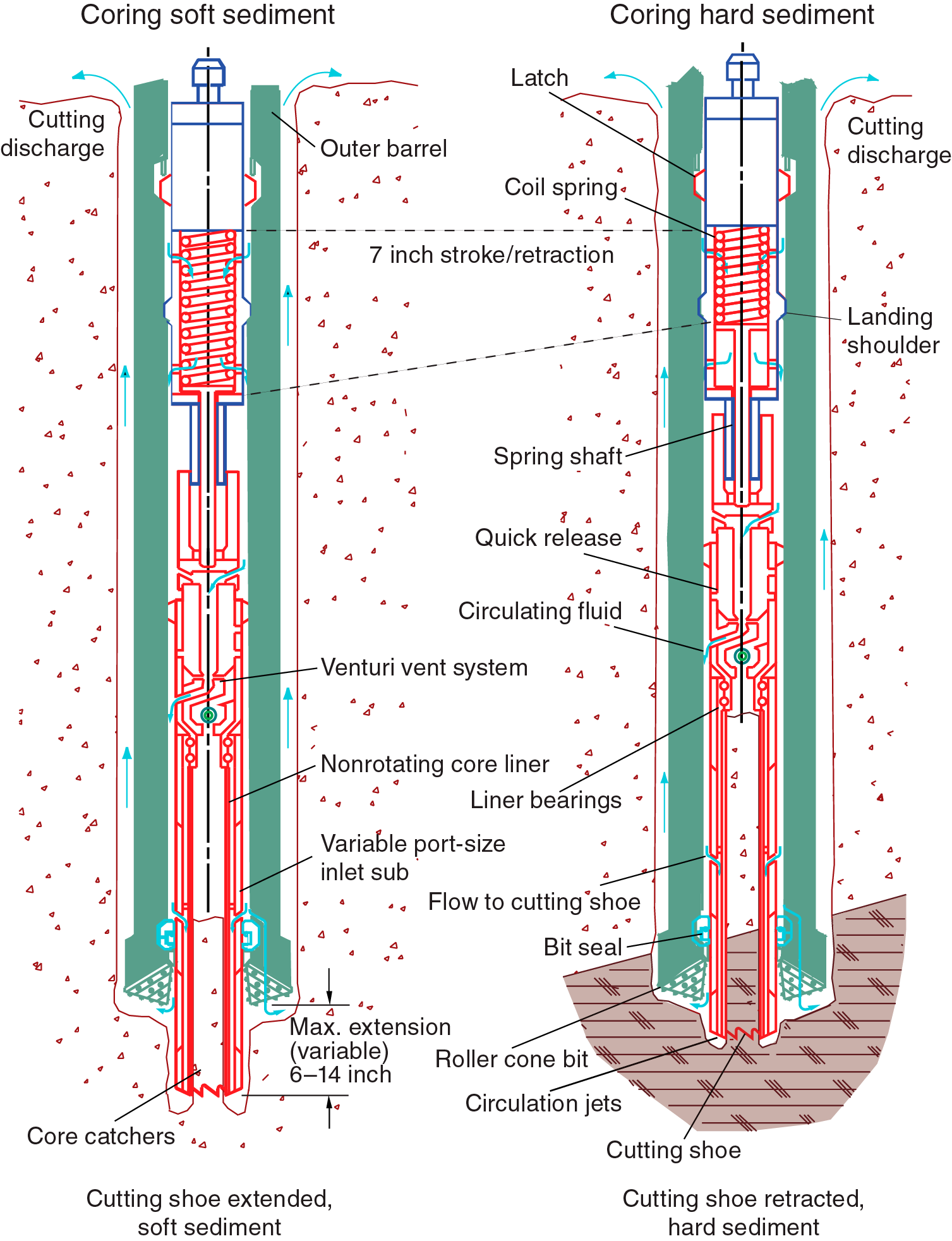
Figure F2. XCB system.
The bottom-hole assembly (BHA) used for APC and XCB coring was composed of an 11⁷⁄₁₆ inch (~29.05 cm) drill bit, a bit sub, a seal bore drill collar, a landing saver sub, a modified top sub, a modified head sub, five 8¼ inch control length drill collars, a tapered drill collar, two stands of 5½ inch transition drill pipe, and a crossover sub to the drill pipe that extended to the surface.
The RCB system is a rotary system designed to recover firm to hard sediments and igneous basement. The BHA, including the bit and outer core barrel, is rotated with the drill string while bearings allow the inner core barrel to remain stationary (Figure F3). RCB core barrels are 9.5 m long.

Figure F3. RCB system.
The RCB BHA included a 9⅞ inch drill bit, a bit sub, an outer core barrel, a modified top sub, a modified head sub, a variable number of 8¼ inch control length drill collars, a tapered drill collar, two stands of 5½ inch drill pipe, and a crossover sub to the drill pipe that extended to the surface.
Nonmagnetic core barrels were used in APC, HLAPC, and RCB deployments. APC cores were oriented with the Icefield MI-5 and FlexIT core orientation tools when coring conditions allowed. Formation temperature measurements were taken with the advanced piston corer temperature tool (APCT-3), and one deployment was attempted with the temperature dual-pressure (T2P) tool (see Downhole measurements). Information on recovered cores, drilled intervals, tool deployments, and related information are provided in the Operations section of each site chapter.
IODP depth conventions
The primary depth scales used are based on the length of the drill string deployed (e.g., drilling depth below rig floor [DRF] and drilling depth below seafloor [DSF]), the length of core recovered (e.g., core depth below seafloor [CSF] and core composite depth below seafloor [CCSF]), and the length of logging wireline deployed (e.g., wireline log depth below rig floor and wireline log depth below seafloor) (see IODP Depth Scales Terminology at http://www.iodp.org/policies-and-guidelines). In cases where multiple logging passes are made, wireline log depths are mapped to one reference pass, creating the wireline log matched depth below seafloor. All depth units are in meters. The relationship between scales is defined either by protocol, such as the rules for computation of CSF from DSF, or by user-defined correlations, such as core-to-log correlation. The distinction in nomenclature should keep the reader aware that a nominal depth value in different depth scales usually does not refer to the exact same depth below seafloor.
Depths of cored intervals are measured from the drill floor based on the length of drill pipe deployed beneath the rig floor (DRF scale). The depth of the cored interval is referenced to the seafloor (DSF scale) by subtracting the seafloor depth of the hole from the DRF depth of that interval. Standard depths of cores in meters below the seafloor (CSF-A scale) are determined based on the assumption that (1) the top depth of a recovered core corresponds to the top depth of its cored interval (at the DSF scale) and (2) the recovered material is a contiguous section even if core segments are separated by voids when recovered. Standard depths of samples and associated measurements (CSF-A scale) are calculated by adding the offset of the sample or measurement from the top of its section and the lengths of all higher sections in the core, to the top depth of the core.
If a core has <100% recovery, for curation purposes all cored material is assumed to originate from the top of the drilled interval as a continuous section. In addition, voids in the core are closed by pushing core segments together, if possible, during core handling at the core receiving area. Therefore, the true depth interval within the cored interval is unknown. This should be considered a sampling uncertainty in age-depth analysis or in correlation of core data with downhole logging data.
When core recovery is >100% (the length of the recovered core exceeds that of the cored interval), the CSF depth of a sample or measurement taken from the bottom of a core will be deeper than that of a sample or measurement taken from the top of the subsequent core (i.e., the data associated with the two core intervals overlap at the CSF-A scale). This can happen when a soft to semisoft sediment core recovered from below the seafloor expands upon recovery, for example due to release of gas or removal of overburden pressure (typically by a few percent to as much as 15%). Therefore, a stratigraphic interval may not have the same nominal depth at the DSF and CSF scales in the same hole.
During Expedition 362, unless otherwise noted, depths below rig floor are reported as meters below rig floor (mbrf), core depths below seafloor are reported as meters below seafloor (mbsf), and downhole wireline depths are reported as mbsf. A core composite depth scale (CCSF) was constructed for Site U1480 to mitigate coring gap problems and to create a continuous stratigraphic record for the upper ~30 m. Core depths from adjacent holes were vertically shifted using core-based physical property data, verified with core photos. This process produced a CCSF depth scale, which is defined in Core-log-seismic integration in the Site U1480 chapter (McNeill et al., 2017). In Biostratigraphy in the Site U1480 chapter (McNeill et al., 2017), core composite depths are reported as meters composite depth (mcd).
Curatorial procedures and sample depth calculations
Numbering of sites, holes, cores, and samples followed standard IODP procedure. A full curatorial identifier for a sample consists of the following information: expedition, site, hole, core number, core type, section number, section half, piece number (hard rocks only), and interval in centimeters measured from the top of the core section. For example, a sample identification of “362-U1480E-2H-5W, 80–85 cm” indicates a 5 cm sample removed from the interval between 80 and 85 cm below the top of Section 5 (working half) of Core 2 (“H” designates that this core was taken with the APC system) of Hole E at Site U1480 during Expedition 362 (Figure F4). The “U” preceding the hole number indicates the hole was drilled by the U.S. platform, the JOIDES Resolution. The drilling system used to obtain a core is designated in the sample identifiers as follows: H = APC, F = HLAPC, R = RCB, and X = XCB. Integers are used to denote the “core” type of drilled intervals (e.g., a drilled interval between Cores 2H and 4H would be denoted by Core 31).
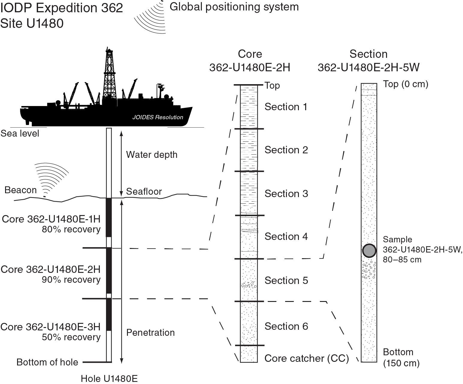
Figure F4. IODP naming convention.
Core handling and analysis
Sediment
When the core barrel reached the rig floor, the core catcher from the bottom of the core was removed and a whole-round sample was extracted for paleontologic analysis. Next, the sediment core was extracted from the core barrel in its plastic liner. The liner was carried from the rig floor to the core receiving area on the catwalk outside the core laboratory, where it was split into ~1.5 m sections.
Once the core was cut into sections, whole-round samples were taken for interstitial water chemical analyses and for postcruise mechanical and physical property experiments. Syringe samples were taken for headspace gas analyses according to the IODP hydrocarbon safety monitoring protocol. Once all catwalk samples were collected, blue (uphole direction) and clear (downhole direction) liner caps were glued with acetone onto the cut liner sections. Yellow caps were used to denote missing intervals where whole-round samples were removed. Rhizon sampling was also conducted in one hole.
The core sections were placed in a core rack in the laboratory. When the core sections reached equilibrium with laboratory temperature (typically after 2 h), they were run through the Whole-Round Multisensor Logger (WRMSL) for P-wave velocity (P-wave logger [PWL]), magnetic susceptibility, and gamma ray attenuation (GRA) bulk density (see Physical properties). The core sections were also run through the Natural Gamma Radiation Logger (NGRL), and thermal conductivity measurements were typically taken once per core when the material was suitable.
The core sections were then split lengthwise from bottom to top into working and archive halves. Investigators should note that older material can be transported upward on the split face of each section during splitting.
The working half of each core was described by the structural geologists. Discrete samples were then taken for moisture and density (MAD) and paleomagnetic analyses, for shipboard analyses such as X-ray diffraction (XRD) and carbonate, and for shore-based studies based on the sampling plan agreed upon by the science party and shipboard curator. Sampling of certain intervals was delayed until personal samples could be prioritized. Samples were not collected when the lithology was unsuitable or the core was severely deformed. Discrete strength and P-wave velocity measurements were made when the lithology permitted.
The archive half of each core was scanned on the Section Half Imaging Logger (SHIL) and measured for point magnetic susceptibility (MSP) and reflectance spectroscopy and colorimetry (RSC) on the Section Half Multisensor Logger (SHMSL). Labeled foam pieces were used to denote missing whole-round intervals in the SHIL images. The archive-half sections were then described visually and by means of smear slides for sedimentology. Finally, the magnetization of archive-half sections and working-half discrete pieces was measured with the cryogenic magnetometer and spinner magnetometer.
Hard rock
Pieces were extracted from the core liner on the catwalk or directly from the core barrel on the rig floor. The pieces were pushed to the bottom of 1.5 m liner sections, and the total rock length was measured. The length was entered into the database as “created length” using the SampleMaster application. This number was used to calculate recovery. The liner sections were then transferred to the core splitting room.
Oriented pieces of core were marked on the bottom with a wax pencil to preserve orientation. Adjacent but broken pieces that could be fit together along fractures were curated as single pieces. The structural geologist on shift confirmed piece matches and marked the split line on the pieces, which defined how the pieces were to be cut into two equal halves. The aim was to maximize the expression of dipping structures on the cut face of the core while maintaining representative features in both archive and working halves. A plastic spacer was secured with acetone to the split core liner between individual pieces or reconstructed contiguous groups of subpieces. These spacers can represent substantial intervals of no recovery. The length of each section of core, including spacers, was entered into the database as “curated length,” which commonly differs by several centimeters from the length measured on the catwalk. Finally, the depth of each piece in the database was recalculated based on the curated length.
The core sections were placed in a core rack in the laboratory. When the core sections reached equilibrium with laboratory temperature (typically after 2 h), the whole-round core sections were run through the WRMSL (for GRA density and magnetic susceptibility only) and the NGRL (see Physical properties).
Each piece of core was split with a diamond-impregnated saw into an archive half and a working half, with the positions of plastic spacers between pieces maintained in both halves. Pieces were numbered sequentially from the top of each section, beginning with the number 1. Separate subpieces within a single piece were assigned the same number but lettered consecutively (e.g., 1A, 1B, etc.). Pieces were labeled only on the outer cylindrical surfaces of the core. If it was evident that an individual piece had not rotated around a horizontal axis during drilling, an arrow pointing to the top of the section was added to the label. The piece’s oriented character was recorded in the database using the SampleMaster application.
The working half of each core was first described by the structural geologists. Samples were then taken for thin section preparation and shipboard paleomagnetic and physical properties analyses. The archive half of each core was scanned on the SHIL and measured for MSP and RSC on the SHMSL. Thermal conductivity measurements were made on selected archive-half samples (see Physical properties). The archive halves were then described visually for petrology, followed by microscopic description of thin sections taken from the working half. Finally, the magnetization of archive-half sections, archive-half pieces, and discrete samples taken from the working half was measured with the cryogenic magnetometer and spinner magnetometer.
Sampling for shore-based studies was delayed until the end of hard rock coring. Sampling was conducted based on the sampling plan agreed upon by the science party and shipboard curator.
When all steps were completed, cores were wrapped, sealed in plastic tubes, and transferred to cold storage space aboard the ship. At the end of the expedition the cores were sent to storage at the IODP Kochi Core Center in Japan.
Drilling and handling core disturbance
Cores may be significantly disturbed and contain extraneous material as a result of the coring and core handling process (Jutzeler et al., 2014). In formations with loose sand layers, sand from intervals higher in the hole may be washed down by drilling circulation, accumulate at the bottom of the hole, and be sampled with the next core. The uppermost 10–50 cm of each core must therefore be examined critically during description for potential “fall-in.” Common coring-induced deformation includes the concave-downward appearance of originally horizontal bedding. Piston action can result in fluidization (“flow-in”) at the bottom of APC cores. Retrieval from depth to the surface can result in elastic rebound. Gas that is in solution at depth may become free and drive apart core segments within the liner. When gas content is high, pressure must be relieved for safety reasons before the cores are cut into segments. This is accomplished by drilling holes into the liner, which forces some sediment as well as gas out of the liner. These disturbances are described in each site chapter and graphically indicated on the visual core descriptions.
Authorship of chapters
The separate sections of the site chapters were written by the following scientists (authors are listed in alphabetical order; see Expedition 362 scientists for contact information):
- Background and objectives: Dugan, McNeill, Petronotis
- Operations: Midgley, Petronotis
- Sedimentology and petrology: Chemale, Kutterolf, Milliken, Mukoyoshi, Pickering, Pouderaux
- Structural geology: Hamahashi, Kenigsberg, Shan, Vannucchi, Vrolijk
- Biostratigraphy: Backman, Chen, Kachovich, Mitchison
- Paleomagnetism: Yang, Zhao
- Geochemistry: House, Hüpers, Owari, Torres
- Physical properties: Bourlange, Colson, Frederik, Guèrin, Henstock, Jeppson, Kuranaga, Nair, Song
- Downhole measurements: Guèrin
- Core-log-seismic integration: Henstock
Sedimentology and petrology
This section outlines procedures used to document the composition, texture, and sedimentary structures of the sediment, sedimentary rock, and igneous rock recovered during Expedition 362. For the level of core disturbance, see Structural geology. The procedures include visual core description, smear slide and petrographic thin section analysis, digital color imaging, color spectrophotometry, and XRD and carbonate analysis.
Core sections from the archive halves were used for sedimentological and petrographic observation. Sections dominated by unlithified sediment were split using a thin wire held in high tension. The split surface of the archive half was then assessed for quality (e.g., smearing or surface unevenness) and, if necessary, gently scraped with a glass slide. Hard rock was split with a diamond-impregnated saw. After splitting, the archive half was imaged by the SHIL and then analyzed for color reflectance and magnetic susceptibility using the SHMSL (see Physical properties). The archive-half section was in some cases reimaged when visibility of sedimentary structures or fabrics improved following treatment of the split core surface. Following imaging, the archive-half sections of the sediment cores were macroscopically described for lithologic and sedimentary features aided by use of a 20× wide-field hand lens and binocular microscope.
Lithostratigraphic units were defined following visual inspection and smear slide analysis, and, where relevant, thin section analysis. Visual inspection of sediments and sedimentary rocks yielded information particularly concerning lithologic variation, color, sedimentary structures, and drilling disturbance, whereas smear slide analysis was used to identify sedimentary constituents including microfossils. For igneous rocks, initial analysis focused on visual inspection where intervals of igneous rock were recognized on the basis of minerals, texture, grain size, color, contacts, chilled margins, and changes in primary and secondary mineralogy. Selected thin sections provided important detailed descriptions of mineral composition, texture, and evidence for alteration. All of the descriptive data were entered into DESClogik (see IODP use of DESClogik for details). Based on preliminary visual descriptions and physical property data, samples were taken from the working-half sections to make thin sections and to provide samples for XRD. All descriptions and sample locations were recorded using curated depths and documented on visual core description (VCD) graphic reports (Figures F5, F6, F7).
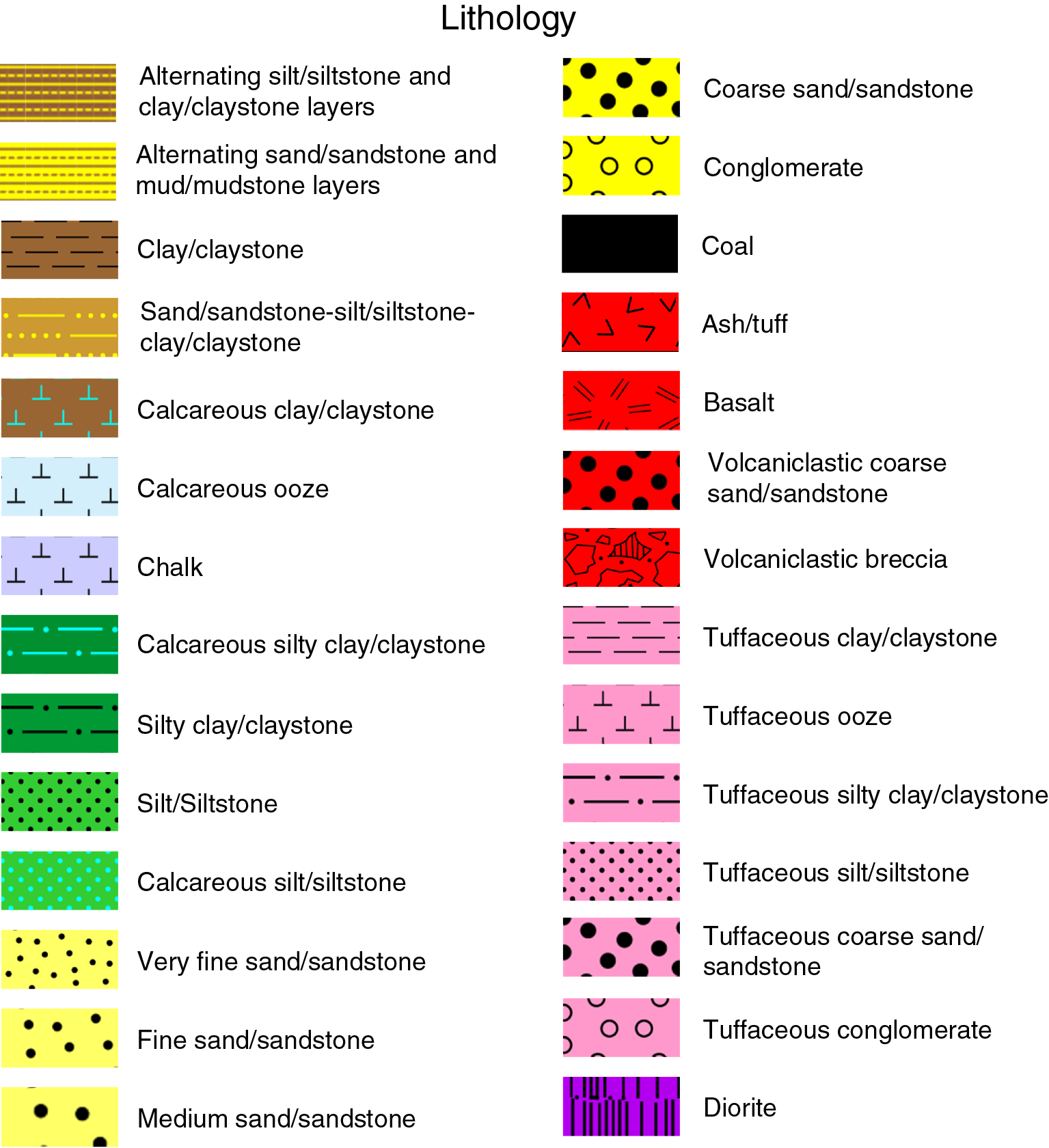
Figure F5. Graphic patterns for sedimentary lithologies.

Figure F6. Legend for sedimentary and tectonic structures.
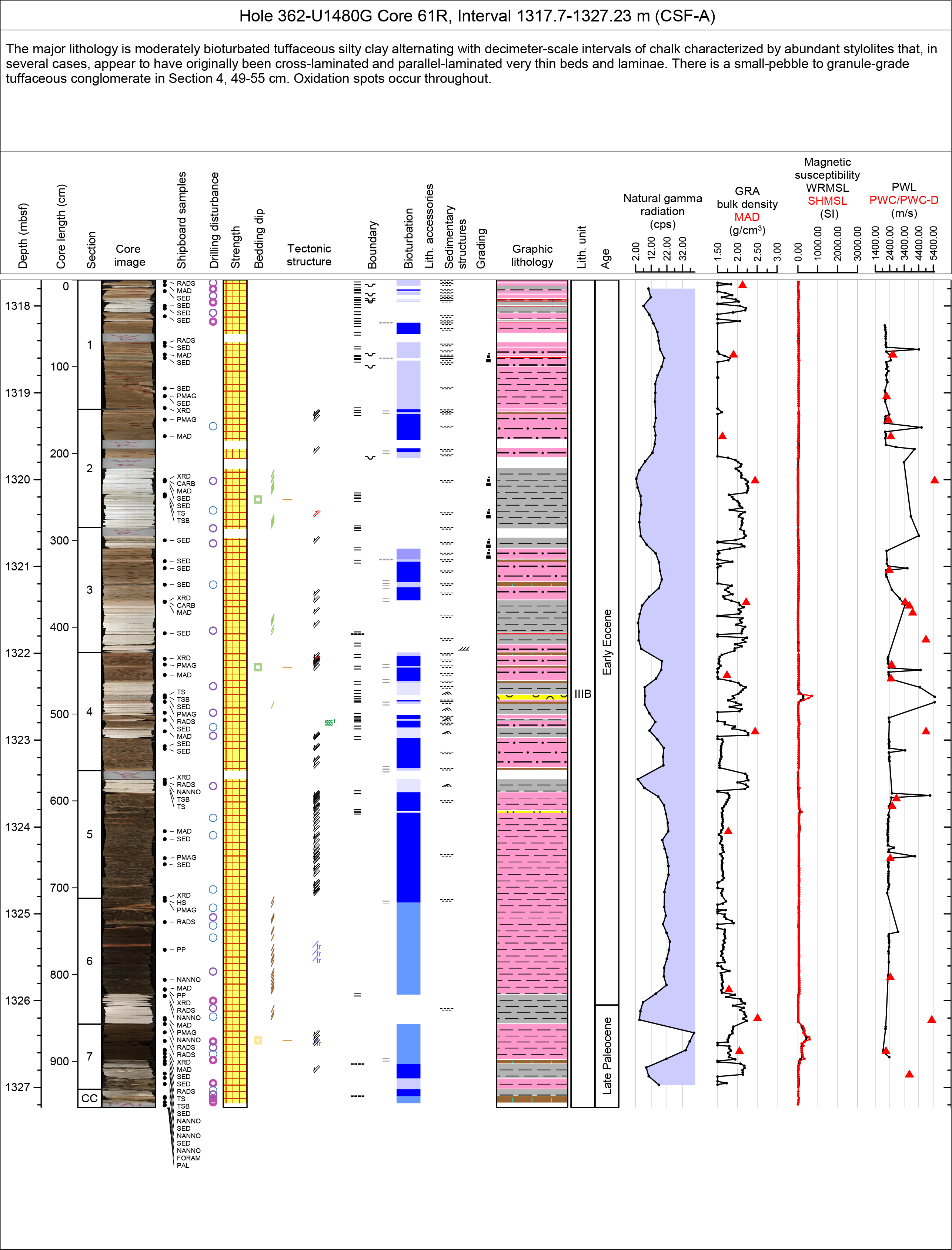
Figure F7. Example of an Expedition 362 VCD sheet.
Visual core descriptions
Principal lithologies
Lithologic description was based on visual core description, supported by smear slide analysis of dominant and minor lithologies, bulk analysis of mineralogy by XRD, and bulk analysis of carbonate content.
The basic lithologic groups used in Expedition 362 core description for sediments and sedimentary rocks were modified from the scheme of Mazullo and Graham (1988) (Figure F8). If the sediment contained <50% biogenic debris (calcareous or siliceous), then it was classified as either siliciclastic (implied terrigenous) or volcanogenic, based on whichever nonbiogenic component had greater abundance. Sediment with >50% biogenic debris was classified pelagic, and as either biocalcareous or biosiliceous, based on the biogenic component that was most abundant. Shallow-water (neritic) carbonate sediment was not recovered during this expedition.
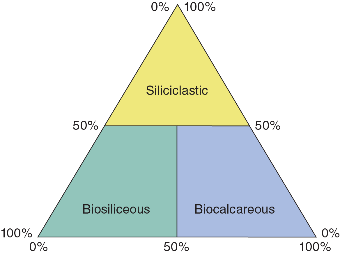
Figure F8. Basic lithologic groups used for sedimentary core description.
All sediment/sedimentary rock samples were classified based on texture (Figure F9; see also Shepard, 1954). Siliciclastic sediment/sedimentary rock was classified primarily based on texture alone, with compositional modifiers as appropriate. Components present in amounts of 25%–50% are primary modifiers (e.g., biocalcareous silty clay and tuffaceous silty clay), whereas components of 5%–25% are secondary modifiers (e.g., clayey silt with glauconite). Pelagic sediment was classified as ooze based on the dominant allochem (e.g., biosiliceous ooze and calcareous ooze).
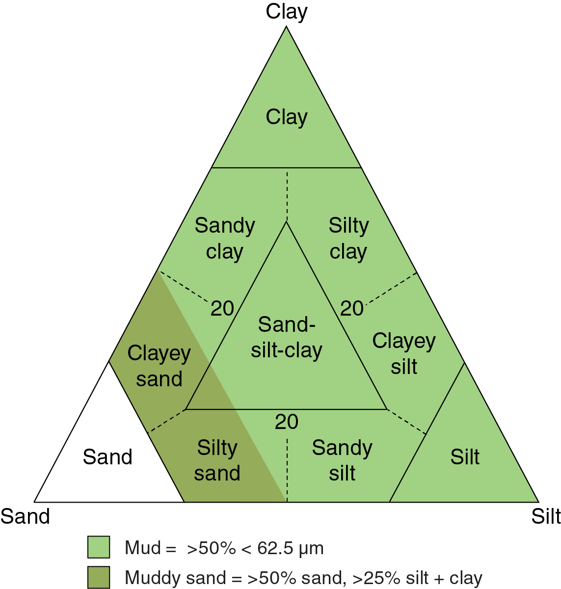
Figure F9. Classification of sediment based on texture only.
Most of the sediment/sedimentary rock categories shown in Figure F9 contain >50% particles of <62.5 µm size (silt and clay). When referring to fine-grained sediment or sedimentary rock collectively, the term “mud” (mudstone) is applied. The term “sand” (sandstone) refers to materials with ≥50% sand-size particles. Cases in which sandy sediment or sedimentary rock contains ≥25% silt + clay, the term “muddy sand” (sandstone) is used to refer to these poorly sorted sands (sandstones), collectively.
All grain size designations followed the conventional Wentworth (1922) scheme as depicted by Folk (1980). Maximum grain size was described based on the terms in the Wentworth grain size classification.
Color was determined qualitatively for core intervals using Munsell Color Charts (Munsell Color Company, Inc., 2000). Visual inspections of the archive-half sections were used to identify compositional and textural elements of the sediment and sedimentary rock, including rock fragments, sedimentary structures, and diagenetic features such as color mottling and the results of element mobility in diagenesis (e.g., manganese oxide segregation).
Sediment and sedimentary rock were classified using an approach that integrated the nature of volcanic particles into the sedimentary descriptive scheme. Sediment and sedimentary rock were divided into four lithologic classes based on composition (types of particles) (Table T1):
- Volcaniclastic sediment and rock of pyroclastic origin with >75% volcaniclastic or pyroclastic particles;
- Tuffaceous/volcaniclastic sediment and rock of sedimentary origin (25%–75% volcaniclastic or pyroclastic particles);
- Siliciclastic sediment and sedimentary rock with <25% volcaniclastic and tuffaceous particles and <5% biogenic particles; and
- Pelagic to hemipelagic sediment (rock) with <25% volcaniclastic and tuffaceous particles and >5% biogenic particles.
Table T1. Classification of volcanic lithologies. Download table in .csv format.
Within each class, the principal lithology name was based on particle size. In addition, appropriate prefixes and suffixes were applied. For example, the prefix tuffaceous was used for the tuffaceous lithologic classes, and prefixes that indicate the dominant biogenic component as determined by microscopic examination were used for pelagic/hemipelagic sediment and sedimentary rock. Suffixes were also used to indicate minor components within each principal lithologic type.
To emphasize the differences in composition of the recovered volcaniclastic sandstones, the rocks were further classified using the scheme of Fisher and Schmincke (1984). In general, coarser grained sedimentary rock (63 μm to 2 mm average grain size) was designated as “sand” where the volcaniclastic components were <25% of the total clasts. Volcaniclastic rocks can be (1) reworked and commonly altered heterogeneous assemblages of volcanic material, including lava, tuff fragments, and compositionally different ash lenses/particles; or (2) fresh or relatively unaltered, compositionally homogeneous, unconsolidated pyroclastic material directly resulting from explosive eruptions on land or effusive/explosive vents on the seafloor. Pyroclasts are composed of volcanogenic material that was fragmented during explosive eruption.
Where there are ≥25% volcaniclasts but <25% pyroclasts, the sediment or sedimentary rock was designated as volcaniclastic sand/sandstone. Where the clast composition is 25%–75% pyroclasts, the sediment/sedimentary rock was classified as tuffaceous sand/sandstone. However, if the clast composition is ≥75% pyroclasts, it was classified using the volcanological terms ash/tuff (<2 mm), lapilli/lapillistone (2–64 mm), bombs, or blocks/pyroclastic breccia/agglomerate (modified after Fischer and Schmincke, 1984).
Breccia-conglomerate is composed of predominantly rounded and/or subrounded clasts (≥50 vol%) and subordinate angular/subangular clasts. Breccia is predominantly composed of angular and subangular clasts (≥50 vol%). The description was refined by indicating whether the fabric is either clast supported or matrix supported. For the equivalent pyroclastic lithologic class the term agglomerate or pyroclastic breccia was used in place of conglomerate and breccia, respectively (Fisher and Schmincke, 1984) (Table T1). Depending on grain size, degree of compaction, and lithification, the nomenclature was adjusted accordingly.
Sedimentary textures, structures, and fabric
For relatively coarse grained material (coarse-grained sand and above), sediment grain size, particle shape, and sorting were determined using the Wentworth scale (Wentworth, 1922). However, for finer grained sediments the textural analysis required inspection at high magnification, which was performed on smear slides and thin sections (see below). The classification of sorting and rounding used the scheme of Folk (1980) (Figure F10).
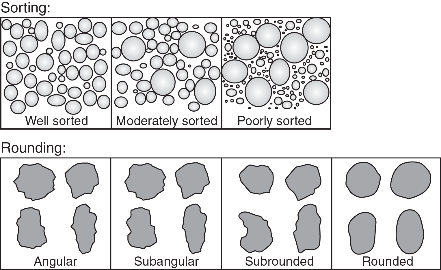
Figure F10. Classification of sediment sorting and roundness.
Sedimentary structures described in the cores included bedding, grading (normal and reverse), soft-sediment deformation, bioturbation, and diagenetic effects. Bed thickness (see Ingram, 1954) are defined as follows:
- Very thick bedded = >100 cm.
- Thick bedded = >30–100 cm.
- Medium bedded = >10–30 cm.
- Thin bedded = >3–10 cm.
- Very thin bedded = 1–3 cm.
- Laminae = <1 cm.
The lower contacts of stratification features were described based on geometry (irregular, planar, curviplanar, and wavy), shape or form (sharp, gradational, hardground, and bioturbated), and orientation (subhorizontal, inclined, horizontal, subvertical, and vertical). Sediment grading was described as ungraded, normally graded (fining upward), and inversely graded.
Designation of lithification state followed the somewhat subjective physical property test applied during Expeditions 353 and 354 (Clemens et al., 2016; France-Lanord et al., 2016). If a core of siliciclastic sediment cannot be easily deformed by pushing on it with a finger, it is designated as “-stone,” as in claystone, silty claystone, sandstone, and so on. The general term mudstone is used when referring collectively to lithified fine-grained lithologies. Following the same criteria, lithified ash is designated “tuff.” Lithified calcareous ooze is designated “chalk.” It is important to recognize that lithification state is a transient property that changes across contrasting pressure/temperature/fluid regimes and also evolves as cores dry and age. Most of the sediment encountered during this expedition could be dispersed into its constituent detrital particles for smear slide preparation. Some, but not all, of the sediment designated as “stone” disaggregated with some difficulty but still sufficiently for smear slide examination.
Bioturbation
Bioturbation intensity in deposits was measured and shown on the VCDs using the semiquantitative ichnofabric index as described by Droser and Bottjer (1986, 1991) and the thickness of the bioturbated section. The indexes refer to the degree of biogenic disruption of primary fabric, such as lamination, and range from 1 for nonbioturbated sediment to 6 for total homogenization:
- 1 = No bioturbation is recorded; all original sedimentary structures are preserved.
- 2 = Discrete, isolated trace fossils recorded; up to 10% of original bedding is disturbed.
- 3 = Approximately 10%–40% of original bedding is disturbed; burrows are generally isolated but locally overlap.
- 4 = Last vestiges of bedding are discernible; approximately 40%–60% disturbed; burrows overlap and are not always well defined.
- 5 = Bedding is completely disturbed, but burrows are still discrete in places and the fabric is not mixed.
- 6 = Bedding is nearly or totally homogenized.
The ichnofabric index in cores was identified with the help of visual comparative charts (Heard et al., 2008, 2014) (Figure F11). Any distinct burrows that could be identified as particular ichnotaxa were also recorded. On the VCDs, the six above bioturbation indexes are shown in a separate column as varying color density with the following terms:
Figure F11. Visual comparative charts for ichnofabric index.
Smear slides and thin sections
Smear slides are useful for identifying and reporting basic sediment attributes, but the results are semiquantitative at best (cf. Marsaglia et al., 2013, 2015). We estimated the abundance of biogenic, volcanogenic, and siliciclastic constituents using a visual comparison chart (Rothwell, 1989), with an emphasis on major lithologies. If a distinct minor lithology was abundant, an additional smear slide was made for that interval.
Visual estimates for normalized percentages of sand, silt, and clay (Terry and Chilingar, 1955) were recorded along with abundance for the individual observed grain types. The component categorization applied to smear slides is shown in Figure F12. Smear slides sampled from tephra layers were described using a customized categorization of ash components (Figure F13). In smear slides of ash, visual estimates of component abundance were made semiquantitatively and given the following ratings:
- R = rare (<1 vol%).
- C = common (1–10 vol%).
- A = abundant (>10–50 vol%).
- D = dominant (>50–80 vol%).
- M = major (>80 vol%).
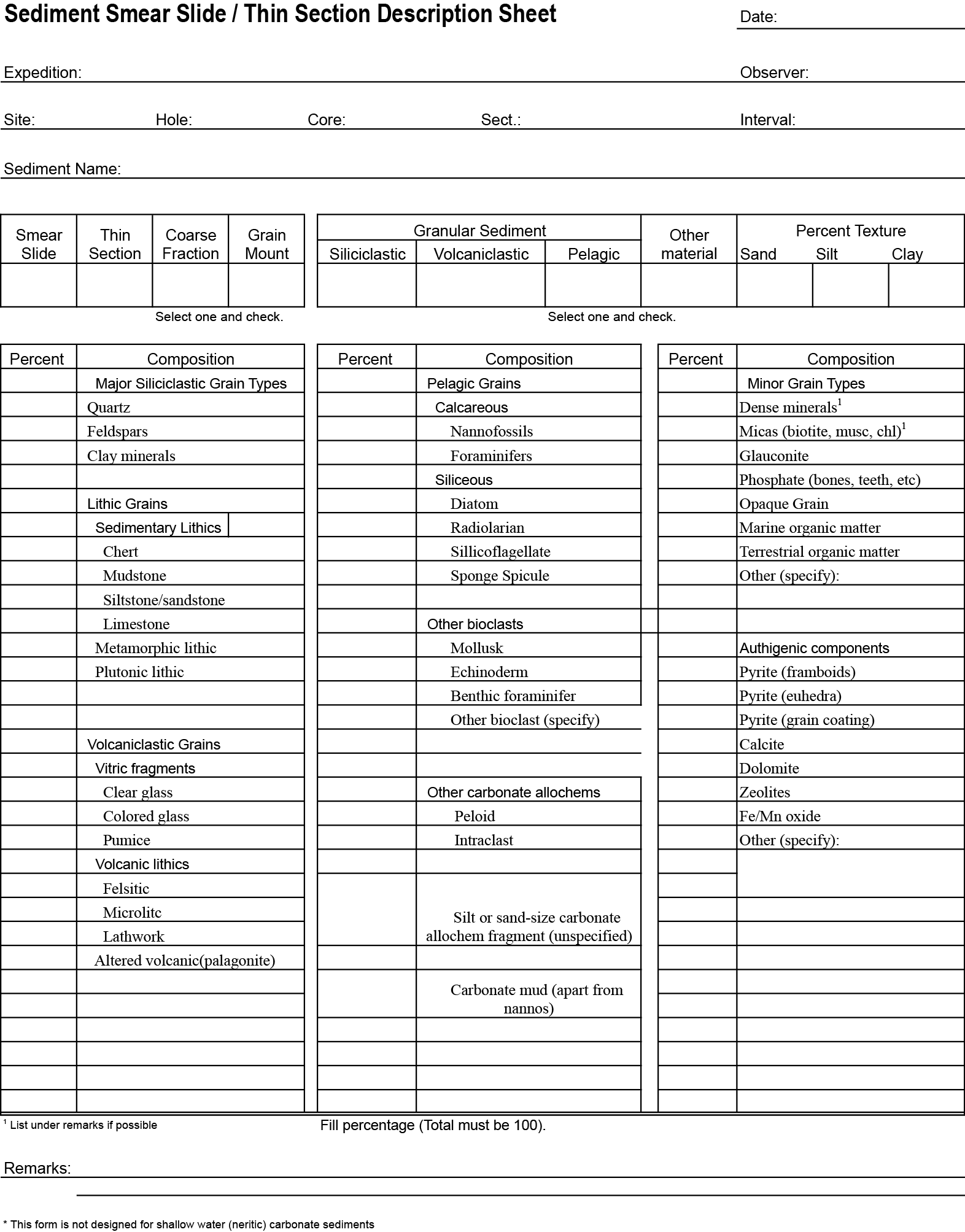
Figure F12. Smear slide component categories for sediment description.
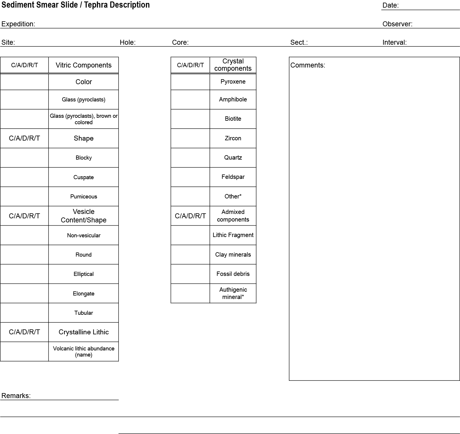
Figure F13. Smear slide component categories for tephra description.
The relative abundance of major components was validated by XRD (see X-ray diffraction) and by the absolute weight percent of carbonate determined by coulometric analysis (see Geochemistry).
Smear slides were observed in transmitted light using an Axioskop 40A polarizing microscope (Carl Zeiss) equipped with a Flex Spot digital camera.
Description of both sedimentary and igneous lithologies in thin section followed standard protocols as described during Integrated Ocean Drilling Expedition 344 (Harris, et al., 2013). The general techniques described above for smear slide analysis were also applied to thin section description of sedimentary lithologies. The composition and proportion (modal) of primary and secondary (altered/hydrothermal) minerals in the igneous rocks were further defined by using microscopic examination. Textural domains of igneous rocks were defined after MacKenzie et al. (1982).
IODP use of DESClogik
Data for the macroscopic and microscopic descriptions of recovered cores were entered into the IODP Laboratory Information Management System (LIMS) database using the IODP data-entry software DESClogik. DESClogik is a core-description software used to store macroscopic and/or microscopic descriptions of cores. Data were entered in the Sediment tab of the Macroscopic template. Core description data are available through the Descriptive Information LIMS Report (http://web.iodp.tamu.edu/DESCReport). A single row in DESClogik defines one descriptive interval, which is commonly one bed but may also be used, for example, to designate marked color variation that may be of diagenetic origin. In addition, the position of each smear slide or petrographic thin section is shown in the VCDs with a sample code of “SED” or “TS,” respectively. The VCDs were generated using the plotting software Strater.
X-ray diffraction
Material for XRD was obtained from a 5 cm3 sample. All samples were vacuum dried, crushed for 3 min with a ball mill, and mounted as randomly oriented bulk powders. Routine powder XRD analyses of bulk powders were performed using a Bruker D4 Endeavor diffractometer. XRD instrument settings were as follows:
- Generator = 40 kV.
- Current = 40 mA.
- Tube anode = Cu.
- Wavelength = 1.54060 Å (Kα1) and 1.54443 Å (Kα2).
- Step spacing = 0.008°2θ.
- Scan step time = 0.648 s.
- Divergent slit = automatic.
- Irradiated length = 10 mm.
- Scanning range = 2°–40°2θ.
- Spinning = yes.
The principal goal of XRD analysis is to estimate relative weight percentages of total clay minerals (smectite + illite + kaolinite), quartz, plagioclase (representing feldspar), and calcite from the areas of relevant peaks. Peaks used are shown in Table T2. Gross peak intensities (counts) were determined using the Bruker software package, DIFFRAC EVA.
Table T2. Characteristic XRD peaks for semiquantitative analysis of clay minerals. Download table in .csv format.
Ten XRD standards made from artificial mineral mixtures (Table T3) were used to determine simple second-order polynomial regressions describing the relationship between peak intensity and mineral abundance (Table T4). Weight percentages of minerals calculated using the regression equations were normalized to 100%. Errors were assessed from the difference between the analyzed standard compositions and compositions calculated from the regressions (Table T5). Finally, weight percentages indicated by peak areas of the unknowns were assessed from the regression equations and also normalized to 100%.
Table T3. Compositions of XRD standard mineral mixtures. Download table in .csv format.
Table T4. Normalization factors for calculation of relative mineral abundance. Download table in .csv format.
Table T5. Error assessed by comparison of analyzed and calculated compositions of standard mineral mixtures. Download table in .csv format.
The method described is semiquantitative and results should be interpreted with caution. It is important to keep in mind that other phyllosilicates (e.g., micas) may be represented in the value for total clay minerals, especially in silt- and sand-rich materials, and may skew results to higher total clay values because of their strong crystallinity. The contrast in peak response between poorly crystalline minerals at low diffraction angles (e.g., clay minerals) and highly crystalline minerals at higher diffraction angles (e.g., quartz and plagioclase) also impacts these results. Overall, calculated mineral abundances should be regarded as relative percentages within the four-component system of clay minerals + quartz + plagioclase + calcite. The closeness of these estimates to absolute percentages within the total solids depend on the abundance of amorphous solids (e.g., biogenic opal and volcanic glass) and the total of all other minerals that occur in minor or trace quantities.
Sediment-process interpretations
To interpret the likely sediment transport and deposition processes for the range of sediment gravity flows encountered during Expedition 362, we adopted the terminology of Pickering and Hiscott (2015; outlined in Figure F14). Conventional usage is adopted for grain settling from suspension fallout to produce hemipelagic and pelagic deposits.

Figure F14. Summary of flow characteristics and relative importance of particle-support mechanisms.
Structural geology
The principal objective of the structural geology team during Expedition 362 was to record deformation structures observed in the core, both natural and drilling induced, and to evaluate from them an early deformation history of the section and the gross strength characteristics and potential deformation mode of the cored section once it encounters the subduction zone. To achieve this objective, we made detailed structural observations following methods used in previous expeditions, but we also complemented these methods with detailed observations of drilling-induced structures. In addition, we compiled and analyzed data from drilling performance to help evaluate first-order strength trends.
The methods for documenting structural features encountered in Expedition 362 cores largely follow those of Expeditions 334, 344, and 352 (Expedition 334 Scientists, 2012; Harris et al., 2013; Reagan et al., 2015). Blenkinsop and Doyle (2010) also provide valuable information on measuring planar structures from core. Structures observed in the split cores were classified and quantified in terms of depth extent, orientation, and sense of displacement. Each structure was recorded manually on a description table sheet (Table T6) at the core table. For planar structures, sectional orientation measurements were transformed into dip, strike, and dip direction results using trigonometric transformations applied in an Excel spreadsheet. The resulting orientations defined in a core reference frame were then logged through the DESClogik interface to the LIMS database with all other descriptive information about each structure (see Visual core descriptions; Figure F7).
Table T6. Core description categories. Download table in .csv format.
In order to address Expedition 362’s technical objectives, we added some additional observations and interpretations about drilling disturbance to the structural geology work flow. Our motivation is to make as many inferences about how the cored section might deform once it reaches the Sumatra subduction zone based on the clues provided by natural and drilling-induced deformation. To better interpret the drilling-induced deformation, we calibrated the observed features against a series of drilling parameters (especially weight-on-bit [WOB], rate of penetration [ROP], and torque). The result of this analysis is a first-order speculative interpretation of the strength of the entire cored column, intended as a guide to follow-up studies.
Structural data acquisition and orientation measurements
Structural measurement methods have been important contributions to Ocean Drilling Program (ODP) legs and IODP expeditions undertaken in the past decades, and quantitative measurements have become more common in recent years. The current basis for making quantitative measurements was laid during Expedition 334 (Expedition 334 Scientists, 2012) and further modified during Expedition 344 (Expedition 344 Scientists, 2013) and Expedition 352 (Expedition 352 Scientists, 2015).
We used a plastic protractor for orientation measurements (Figure F15). This measurement process was performed on the working half of the split core because it provided greater flexibility in removing—and cutting, if necessary—pieces of the core for structural measurements. Orientations of planar and linear features in cores were determined relative to the core axis, which represents the vertical axis in the core reference frame, and the split line marked on the working half of the split core liner, which represents 0° (and 360°) in the plane perpendicular to the core axis (Figure F16). To determine the orientation of a planar structural element, apparent dips were measured in two independent sections in the core reference frame. These two apparent dips were then converted, using an Excel spreadsheet (see 362_Structure_Calculations.xlsx in STRUCTURE in Supplementary material) to a plane represented by a dip angle, a strike, and a dip direction (Figure F17). One apparent dip is represented by the intersection of the planar feature with the split face of the core and is quantified by measuring the dip direction and angle in the core reference frame (β1; Figure F18). Such a measurement has a trend or azimuth of 90° or 270° and ranges in plunge or dip from 0° to 90° (β2; Figure F18). A second apparent dip is represented by the intersection of the planar feature and a cut or fractured surface at a high angle to the split face of the core. In most cases this surface lies either parallel or perpendicular to the core axis. When parallel, the apparent dip trace trends 0° or 180° and plunges from 0° to 90°; when perpendicular, the trend ranges either from 0° to 90° or from 270° to 360° and plunges 0°. Linear features observed in the cores are systematically associated with planar structures (e.g., a striation on a fault plane), and their orientations were determined by measuring either the rake on the associated plane or the trend and plunge in the core reference frame. In postcruise research further orientation corrections may be made using paleomagnetic data (Figure F17). During Expedition 362, we measured rake for striations on fault surfaces (Figure F19) and azimuth and plunge for other lineations.
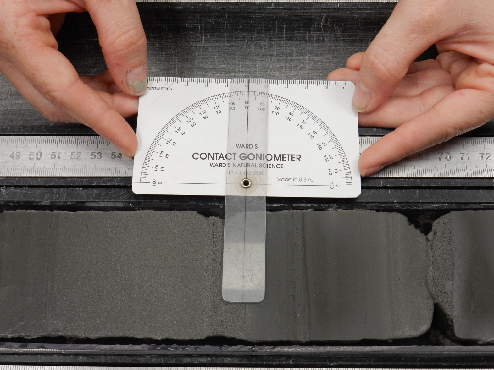
Figure F15. Protractor used to measure apparent dips, trends, plunges, and rakes.
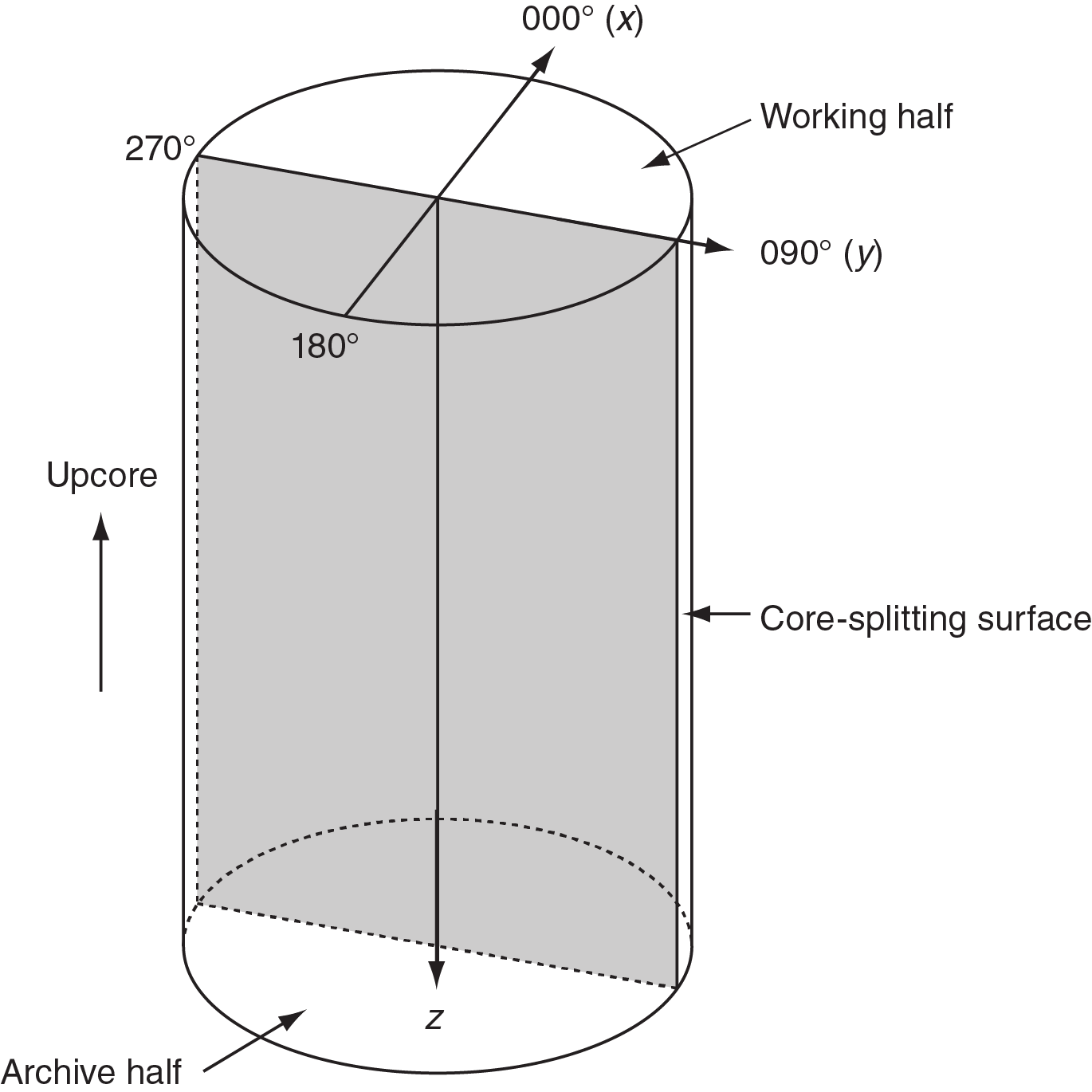
Figure F16. Diagram of core reference frame and x-, y-, z-coordinates.
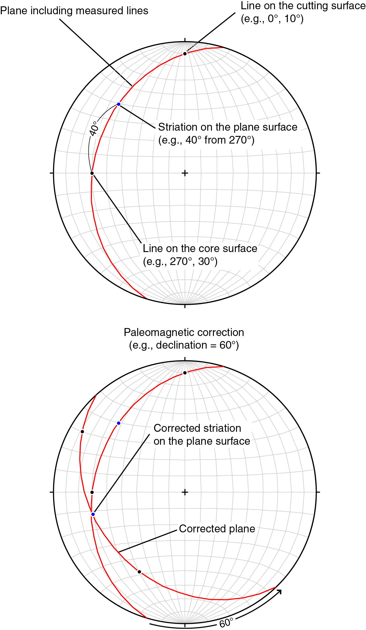
Figure F17. Lower hemisphere equal area projections showing the procedure for converting 2-D measured data to 3-D data.
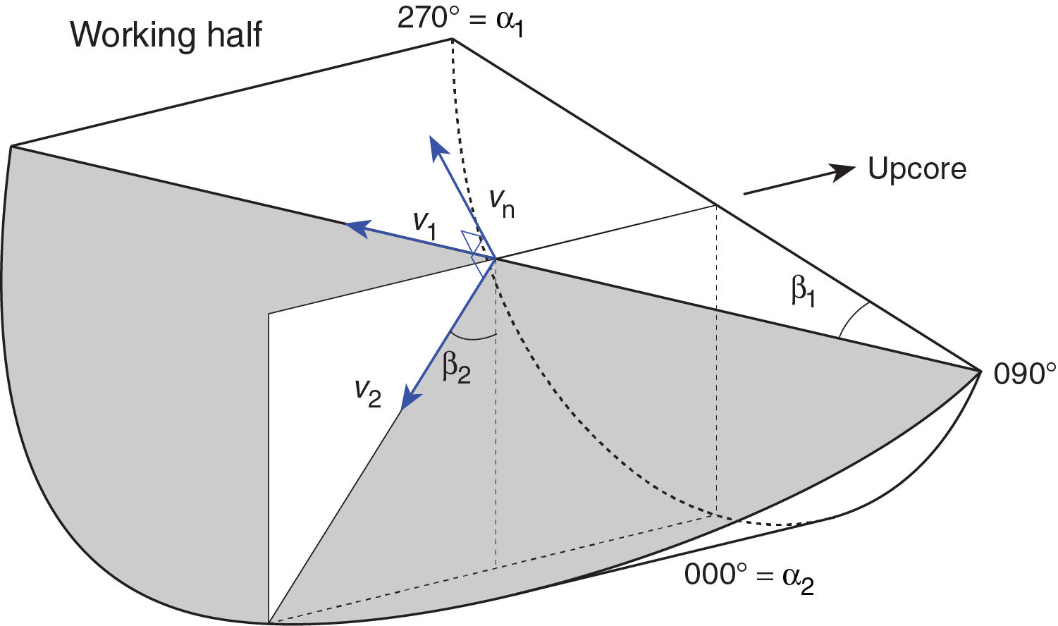
Figure F18. Calculation of plane orientation from two apparent dips.

Figure F19. Apparent rake measurement of striations on a fault surface.
Description and classification of structures
We constructed a structural geology template for DESClogik that aids the description and classification of observed structures. We define the terminology used to describe deformation structures, both for clarity and as the basis for differentiating natural structures from drilling-induced features. We adopt a descriptive hierarchy (Table T6) for our structural classification in which we first define a structure type (e.g., fault, fracture, fold, shear zone, bedding, etc.) and then add a secondary descriptor to further classify the structure (e.g., normal, reverse, strike slip, or indeterminate). An indeterminate fault is one in which a structural surface has slickenlines that suggest displacement but without sufficient markers to define the sense of slip. A series of additional qualifying observations are also defined according to the structure defined (e.g., for fractures we include descriptors of fracture geometry and a description of open or closed).
Veins are defined as extensional fractures that are healed with minerals precipitated from a fluid. The lithology of the host rock and the mineralogy of the vein minerals are included in the comments section of the vein description, and the orientations of veins, foliations, and other structural features are part of the routine structural description.
Recognizing that there is often uncertainty in objectively defining structures as either natural (sedimentary or tectonic) or drilling induced, we categorize an interpretation confidence for each observation both to minimize the potential for any conflict and to maintain all observations in the database that remain equivocal; the intent is to provide the means to include or exclude observations in postcruise analyses based on different confidence thresholds. For deformation structures such as faults, the confidence scale is defined from 0 to 1, where 0 = no confidence (i.e., a fault is drilling induced with 100% certainty) that the observed structure is natural (tectonic or synsedimentary), and 1 = perfect confidence. We approach each structure (e.g., a fracture) initially with a confidence of 0.5 and look for observations to shift our confidence one way or another. For example, if we observe a fracture in the center of the core with petal fractures at its end, we shift to a confidence value <0.5 (i.e., it looks like a drilling-induced fracture). In practice, confidence values range from 0.1 to 0.9 in order to maintain some possibility that any individual structure may have a component of natural or drilling-induced deformation.
A second confidence criterion is recorded for faults in order to define the confidence in that the sense of slip is uniquely determined by the observations. For example, the highest confidence is assigned if offset marker horizons are visible in the core and striations define slip direction (e.g., dip-slip versus strike-slip).
For folds, the confidence factor reflects our ability to distinguish between tectonic and synsedimentary folds, whereas for bedding, confidence reflects our ability to assign the measured dip entirely to structural dip free from sedimentary dips (most importantly for low dips). For example, bedding surfaces associated with an erosional contact are likely to relate to depositional onlap or downlap, and we consult with the sedimentology group to help assess the likelihood and magnitude of possible sedimentary dips.
Calculation of plane orientation
For planar structures (e.g., bedding or faults), two measured apparent dips on two different surfaces are converted into the core reference frame as azimuths (measured clockwise from north, looking down) and plunges (Figures F16, F17, F18). A coordinate system was defined in such a way that the positive x-, y-, and z-directions coincide with north, east, and vertical downward, respectively. If the azimuths and plunges of the two apparent dips are given as (α1, β1) and (α2, β2), respectively, as in Figure F18, then the unit vectors representing these two lines, v1 and v2, are
The unit vector normal to the plane, vn (Figure F18), is then defined as
where
The azimuth, αn, and plunge, βn, of vn are given by
The dip direction, αd, and dip angle, β, of this plane are αn and 90° + βn, respectively, when βn is <0° (Figure F20A). They are αn ± 180° and 90° – βn, respectively, when βn ≥ 0° (Figure F20B). The right-hand rule strike of this plane, αs, is then given by αd – 90°.

Figure F20. Dip direction, right-hand rule strike, and dip of a plane deduced from its normal azimuth and dip.
Calculation of slickenline rake
For a fault with striations, the apparent rake angle of the striation, ϕa, was measured on the fault surface from either the 90° or 270° direction of the split-core surface trace (Figures F17, F19). Fault orientation was measured as described above. Provided that vn and vc are unit vectors normal to the fault and split core surfaces, respectively, the unit vector of the intersection line, vi, is perpendicular to both vn and vc (Figure F20) and is therefore defined as
Knowing the right-hand rule strike of the fault plane, αs, the unit vector, vs, toward this direction is then
The rake angle of the intersection line, ϕi, measured from the strike direction is given by
vs × vi = |vs||vi|cos ϕi = cos ϕi ∴ |vs| = |vi| = 1.
Drilling deformation
One of the objectives of Expedition 362 includes characterizing the strength of the drilled sedimentary section in order to extrapolate those properties into the deformation environment of the Sumatra subduction zone. To help serve this objective, we seek to extract information about the relative strength and the deformation mode of the recovered materials by recording drilling deformation and considering the deformation experiment that drilling imposes on the sediments. Faults, fractures, breccias, and shear zones interpreted as drilling induced yield the most pertinent information about deformation mode, and the variation in lithology that supports those structures provides information about relative strengths. Drilling-induced folded and distorted beds developed in APC cores, which include upward-arching beddings that are caused by materials being forced into the core barrel (Figure F21), suggest that the material is weak and ductile. Another example is mingled and distorted beddings that are likely caused by suction of the materials into the core barrel during APC coring, and is perhaps an extreme version of upward-arching beds (Figure F22). Various flow structures (e.g., basal flow-in, midcore flow-in) and sandy sediment injected between segmented mud intervals also suggest that ductile deformation is possible. Drilling biscuits in XCB and RCB cores (Figure F23) are caused by rotation of the drill bit with respect to the sediments, and in the case of XCB coring the core liner rotates as well. Where biscuits break and in what lithology may lead to insights into mechanical heterogeneity. Drilling-induced gouge is often formed between biscuits by relative rotation and injection of drilling cuttings. Other coring disturbances, such as fall-in (Figure F24), soupy texture (Figure F25), gas expansion, core extension, and voids, offer less information about the properties of the sediment. We used terminology and examples documented by Jutzeler et al. (2014) and Schmidt et al. (2012) to guide our description scheme and employ common description of drilling disturbance intensity (slight, moderate, severe, and destroyed). For example, drilling disturbance intensity for upward-arching bedding and mingled and distorted bedding were rated based on the intensity of folding and destruction of primary bedding. For biscuiting of cores, intensity rating was given based on the thickness of biscuits as follows:
- Slight: >5 cm thickness.
- Moderate: 2–5 cm thickness.
- Severe: <2 cm thickness.
- Destroyed: brecciated biscuits.
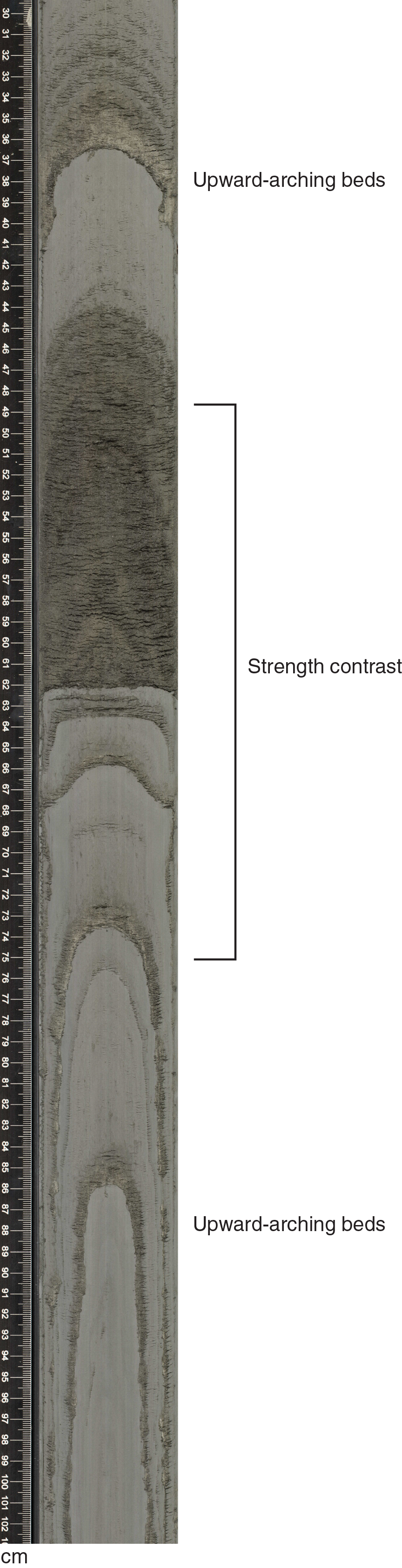
Figure F21. Upward-arching bedding observed in APC cores.
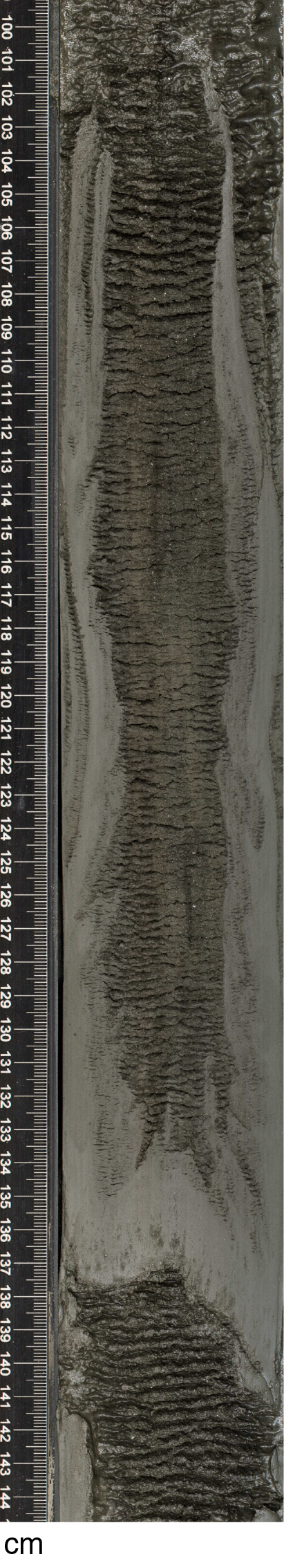
Figure F22. Mingling and distortion of bedding observed in APC cores.

Figure F23. Drilling biscuits observed in XCB and RCB cores due to rotation of sediment.
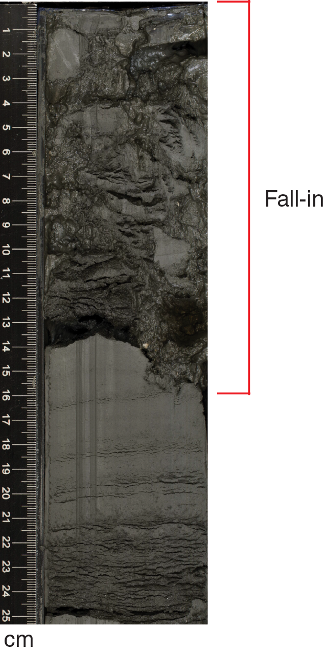
Figure F24. Fall-in at top of core, present at the top of many cores, and given a drilling disturbance intensity rating of destroyed.
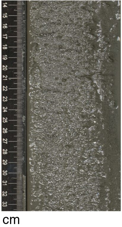
Figure F25. Soupy section in the sediment caused by drilling disturbance in which the primary structure is destroyed.
In addition to the drilling disturbance intensity, we added a column to interpret the drilling disturbance as either brittle, ductile, or indeterminate deformation mode, recognizing that this is a subjective, speculative interpretation, but one that we nevertheless think can serve as a guide for sample selection and site interpretation.
Our interpretation of drilling deformation is qualified by actual drilling parameters collected as the core is taken, including WOB, ROP, and torque. For example, increased WOB with a constant ROP or decreased ROP for constant WOB may reflect a stronger interval (e.g., Warren, 1981). Increased torque may reflect a sticky mud section that could develop ductile deformation mechanisms.
Strength log
The continuous strength log for each cored section, also a subjective interpretation, is one in which we speculate how each interval might deform based on observations of natural deformation features, drilling-induced deformation, and general sediment character in the core (see Visual core descriptions; Figure F7). This qualitative classification is intended in the context of a field descriptive term, one used to help comprehend and assimilate detailed descriptive data in order to keep track of relative strength changes within a core and between adjacent cores. We also hope to remain more alert for changes that occur over several cores by recording observations of this property. We expect that the strength interpretation will become superseded by detailed analysis of physical property data and postcruise geomechanical tests and that the value of this description is greater during the expedition than afterward.
Based on these goals and expectations, there are no definitive criteria for defining the boundaries between weak, intermediate, and strong sediments or the expectation that an interval will deform by brittle or ductile methods. Rather, we used team experience and knowledge and apply that knowledge in a consistent manner.
Examples of end-member behavior help illustrate the strength description. For example, cores taken with a piston core (i.e., APC or HLAPC) and where physical property scientists are able to obtain a penetrometer reading are interpreted as weak. When drilling deformation in these cores results in folding (i.e., upward-arching beds or mingling and distortion of beds), the strength is interpreted as weak and ductile (Figure F26). In contrast, strong beds develop a more rock-like appearance (e.g., clay-rich sediments begin to develop fissility), are sampled more easily by a rock saw than chisel and hammer, and include lithologies like igneous rocks, concretions, and hard claystones (Figure F27). Biscuit formation, fracturing, brecciation, and similar types of drilling deformation lead to the inference of strong brittle deformation (Figure F28). Intermediate strengths lie between these two end-members (Figure F29), and the brittle versus ductile interpretation is based on the types of natural and drilling deformation observed in the core. Local, relative strength contrasts are interpreted when drilling deformation style and intensity varies between different lithologies (Figure F21).

Figure F26. Weak, ductile material showing upward-arching beds, mingling and distortion of beds, and soupy deformation.
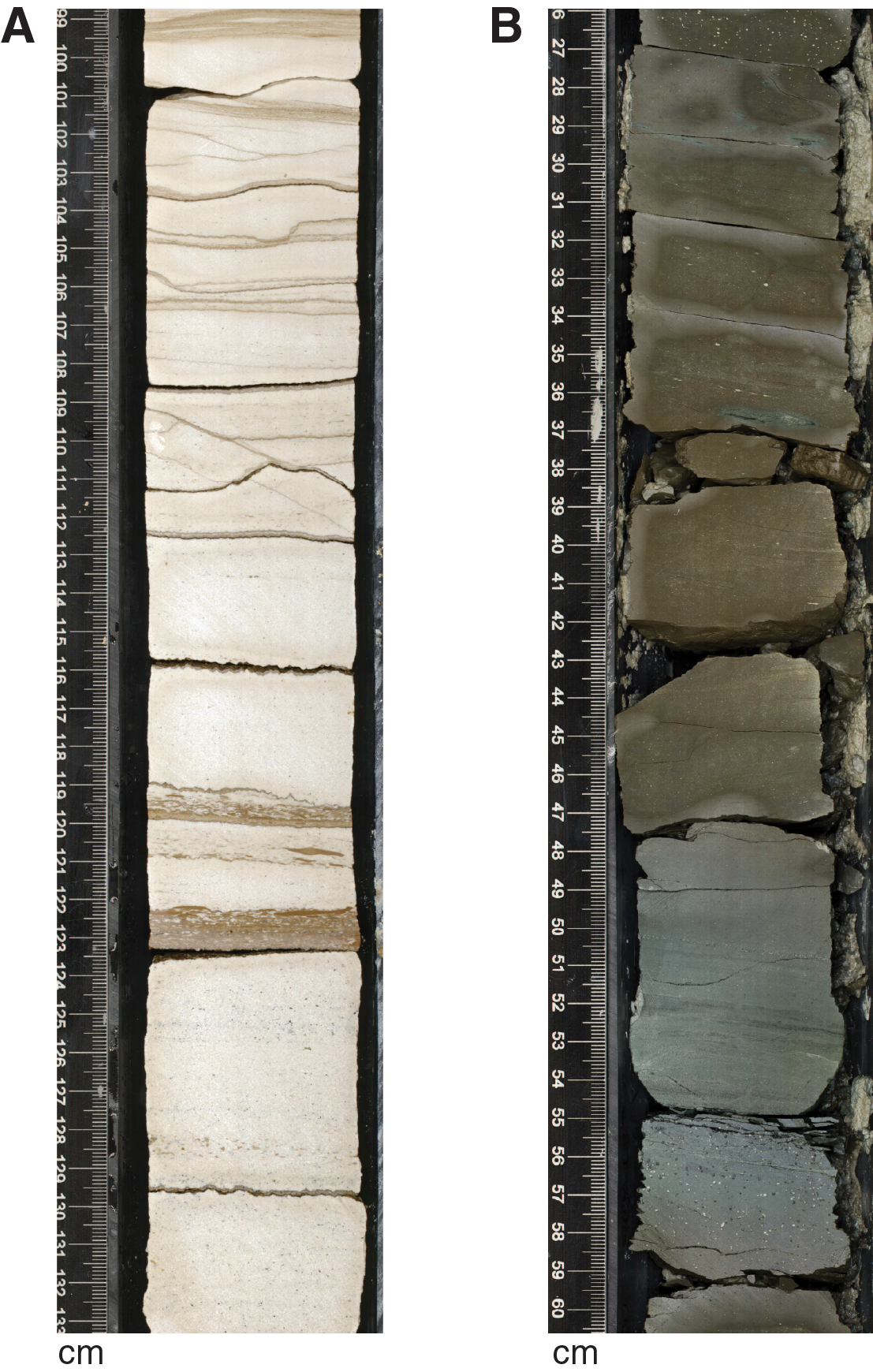
Figure F27. Cores rated strong and brittle in strength.
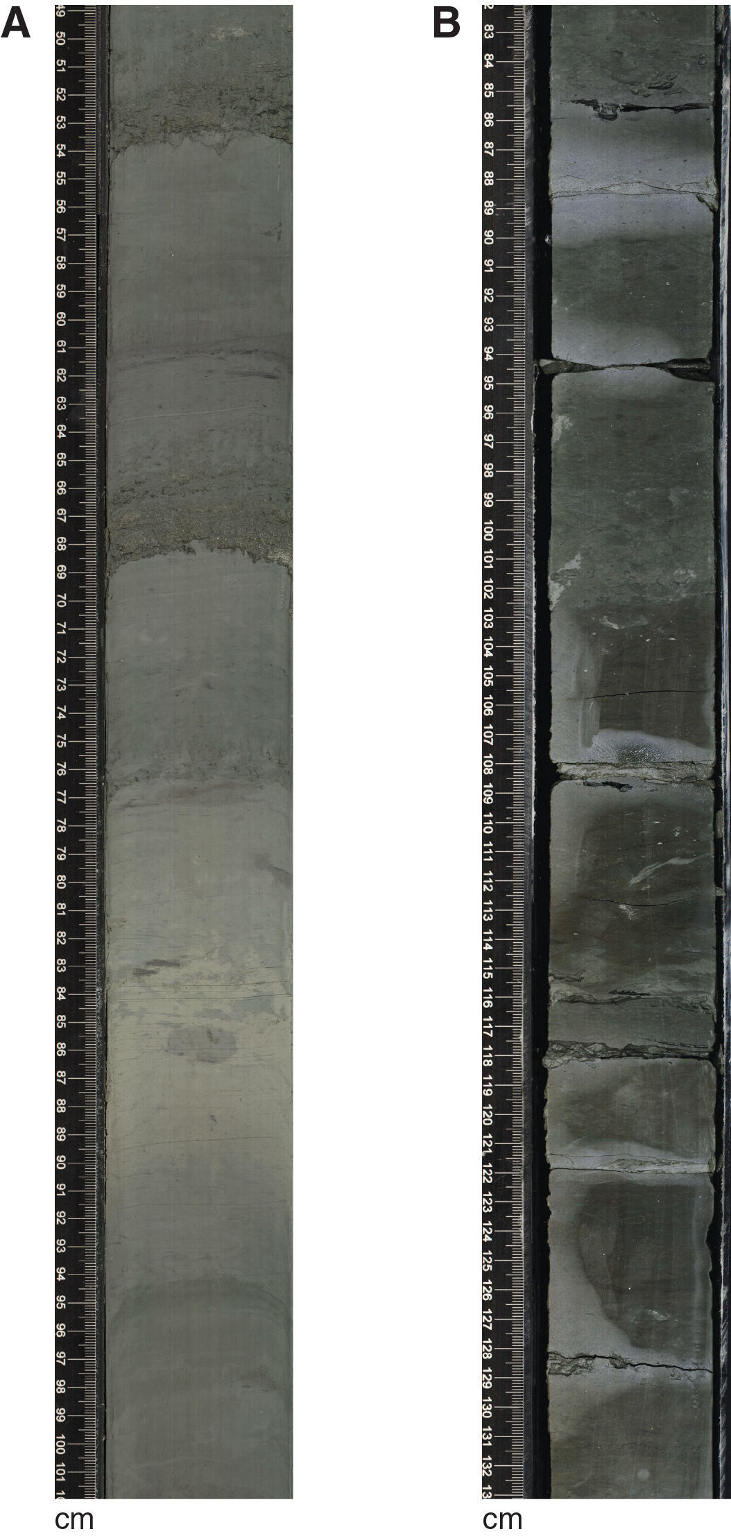
Figure F28. Core rated intermediate and ductile in strength and core rated intermediate and brittle in strength.
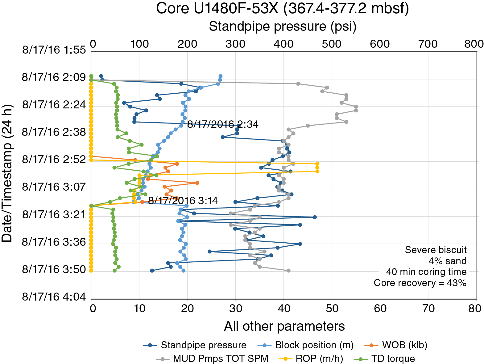
Figure F29. Example XCB drilling record.
Strain localization candidates are identified by an anomalous abundance of natural or drilling-induced deformation structures. We exclude unequivocal synsedimentary structures from this interpretation because they may reflect processes other than those that lead to deformation localization. Localization candidates are intended as placeholders for further evaluation with the expectation that many will prove to be irrelevant.
DESClogik structural geology database
The DESClogik database is a program used to store a visual (macroscopic and/or microscopic) description of core structures at a given depth. During Expedition 362, only the locations of structural features, calculated orientations in the core reference frame, and restored orientations based on the paleomagnetic data, were input into DESClogik. Orientation data management and planar fabric analysis were made with a spreadsheet as described above.
Drilling parameters used to interpret drilling deformation observations and strength inferences
Drilling and coring sediment and rock is a deformation experiment on the penetrated section. Hydraulic piston coring (APC and HLAPC) and rotary coring (XCB and RCB) are the two most distinct deformation experiments, but during this expedition we are most interested in the rotary shear experiment imposed by the XCB and RCB coring methods. An important difference between the XCB and RCB coring designs (Figures F2, F3) is that the core barrel in the XCB system latches into the BHA and thus rotates with the drill string and bit. Once the core passes the edge of the cutting surface, it is subject to torsion around the core similar to a ring-shear device in the laboratory. In contrast, the RCB lands in a support bearing in the BHA and has a vertical latch that keeps the core barrel in place; the core barrel remains stationary while the outer core barrel rotates around the inner core barrel. The cored material is only subject to torsion as it passes through the drill bit, and those forces end once the core enters the core barrel. In addition, the XCB bit extends in front of the main cutting bit and thus is less influenced by the hydraulic flow of drilling fluid used in the roller cone bit that completes the hole. The RCB coring method uses a roller cone design that both cuts the core and creates the hole at the same time.
In order to optimize drilling, maintain good hole conditions, and maximize core recovery, a vast number of drilling parameters are recorded by the Rig Instrumentation System (RIS; Graber et al., 2002). Although these parameters provide only a rough estimate of conditions at the bit, they provide one of the only continuous records of the drilled section. This information can prove useful in intervals with reduced core recovery (S. Midgley, pers. comm., 2016).
Our motivation is to attempt a first-order interpretation of relative strength contrasts, to normalize for constant drilling conditions when the type or intensity of drilling deformation is observed or qualify those differences if conditions change, and to provide a potential basis for extrapolating postcruise laboratory testing results across the drilled section. To address this problem, we use the concept of mechanical specific energy (MSE) introduced into the drilling literature by Teale (1965), a concept that relates normal and torsional forces to the speed at which a rock is penetrated. These forces are related to the unconfined compressive strength of a rock, one of many parameters that describes the constitutive behavior of rocks.
Four drilling parameters define MSE: WOB, torque, rotary speed, and ROP (Teale, 1965). Although these parameters are used to diagnose drilling problems and optimize drilling performance based on assumed or independently determined rock properties (e.g., Dupriest and Koederitz, 2005; Pessler and Fear, 1992; Koederitz, 2005, Caicedo et al., 2005; Waughman et al., 2002; Bjornsson et al., 2004, Dupriest et al., 2005), we invert the problem by assuming that the driller is operating with a consistent level of performance by adjusting parameters to maintain maximum core recovery so that differences in MSE reflect changing rock properties. Recognizing that the assumption of consistent, optimized drilling performance is flawed, we proceed under the reasonable assumption that large differences in MSE still reflect changes in mechanical properties.
Definitions
The following are definitions of drilling parameters used in this analysis:
- WOB: the weight that the drill bit exerts on the rocks being cored and adjusted to optimize ROP (https://en.wikipedia.org/wiki/Weight_on_bit). Weight is provided by the massive drill collars that sit above the bit, but this weight is only a small fraction of the total weight of the drill string across the 4.1–5.9 km between the ship and the drill bit during Expedition 362. In the case of Expedition 362, the drilling operations plan attempted to maintain a constant WOB. However, WOB is manually controlled to optimize coring and is affected by vessel heave, so there is variability with each core. WOB is reported from the RIS in kilopounds (klb; 103 lb), and the most reliable measure of WOB reported by the RIS is AD Hook Load.
- ROP: the speed that the drilling bit cuts through rock (https://en.wikipedia.org/wiki/Rate_of_penetration). ROP is reported from the RIS in meters per hour (m/h).
- Torque (TD-Torque): a rotational force created by the top-drive motors to rotate the drill pipe and bit and allow a hole to be drilled. Torque thus reflects the resistance of a rock to be drilled. Torque is recorded by the RIS in amps, and these values are converted and reported in the RIS as kilo foot-pound (ft/lb·k).
- Rotary speed (TD-RPM): revolutions of the drill string defined as revolutions per minute (RPM).
- Mud pumps total (MPT): reflects the sum total volume of two mud pumps supplying hydraulic pressure to the drilling fluid and represents the flux of drilling fluid at the coring bit. Although the RIS records this in a number of different forms, we tracked this value in units of strokes per minute (SPM).
- Standpipe pressure (SPP): total pressure loss in a system that occurs due to fluid friction. SPP is the total system pressure, which is equal to pressure loss in the annulus, pressure loss in the drill string, pressure loss in the BHA, and pressure loss across the bit (https://www.petropedia.com/definition/3692/standpipe-pressure). This parameter was used in concert with the MPT parameter to help identify the initiation of coring because SPP increases to reflect the work being done by the bit on the formation to drill a core. Units of SPP in the RIS are pounds per square inch (psi and presumably gauge pressure).
- Block position: a measure of depth defined with respect to the rig floor; a reference frame that is in constant flux because of swell heave and tides (Graber et al., 2002). Block position is considered the most reliable measure of depth recorded by the RIS and is used to define the start and end of coring (end of coring is recognized by a significant increase in block position after a long interval of decreasing block position, and start of coring is the advancement depth added to the block position at the end of coring). Block position is measured in meters (m).
The MPT and SPP parameters represent the hydraulic aspect of the drilling system used to remove cuttings from the drilling surface. These parameters provide a useful independent measure of the time that coring starts and stops because cuttings are generated during the coring process.
Comments and limitations of RIS data
Depth as recorded by the RIS on the JOIDES Resolution, a riserless vessel, is an uncertain quantity without the benefit of a fixed depth reference like the seafloor that is used in riser systems. Hence, parameters recorded by the RIS that rely on depth, like ROP, can be suspect (Graber et al., 2002). For this reason, we follow the recommendation of the RIS documentation and use block position defined with respect to the rig floor to monitor drill bit advancement.
The RIS also records continuous data up to 15 days at a time, at which point it is possible to export the data in ASCII format for processing and analysis. Given this time lag, it is difficult to use these data to influence operational decisions other than to observe RIS data using RigWatch.
The RIS records data at 1 s intervals; in one day 86,400 records are generated and, over a maximum 15-day timespan, 1,296,000 records. Coring occupies only a small fraction of that time, so any analysis requires the means to identify the beginning and end of each cored interval in the drilling time domain.
Methods applied
We chose to decimate the RIS data set to analyze records at 2 min. This provides a data set more suitable for initial screening analysis (Figure F29). Based on this analysis, we identify a limited number of discrete intervals appropriate for more detailed analysis. To decimate the data set, we used the FINDSTR command in Windows (provided by IODP Applications Developer Tim Blaisdell), which is described in STRUCTURE in Supplementary material. An alternative approach is offered by Tim Henstock using AWK scripts in a UNIX or LINUX environment (also in STRUCTURE in Supplementary material).
Data plotting
We plotted each parameter monitored between the times recorded for core on deck. In other words, the start of each plot (Figure F29) is based on the time the previous core is reported on deck, and the plot ends when the core under investigation is reported on deck. The following is a detailed example of the work flow.
The onset of coring is identified from the following characteristics:
- Change in block position. In this instance, the block position changes from a constant value to a decreasing value at 2:34.
- Increase in SPP. SPP increases at the same time as the break in slope in block position.
- Onset of high and constant MPT. In this plot, this occurs at 2:34.
- Increase in torque at 2:38. In the instances evaluated so far, this tends to lag the block position parameter.
- WOB and ROP lag the onset of coring by 16 min. We often observe this lag, and in many cases neither WOB nor ROP deviate from zero when the core is taken.
The end of coring is defined by the following:
- Minimum block position value followed by a large increase in block position at 3:14.
- When ROP and WOB register in a plot, they drop to zero at the same time as the block position minimum.
- Drop in torque.
- Change in SPP and MPT. These values may increase if hole conditioning follows coring.
- As a final check, because the end of coring is better defined than the onset of coring in many instances, the block position value is identified, the coring interval is added to the final block position to obtain its depth at the start of coring, and the time at the start of coring is rechecked. For example, in the example in Figure F29, the final block position is 8.84 m, the cored interval is 9.7 m, and the block position at the start of coring is 18.54 m. The block position at 2:34 is 18.73 m, which is the closest value to the target 18.54 m. A more detailed analysis with more frequent data records will improve this resolution.
Data analysis
Drilling data were combined into a value termed the specific energy factor (SEF) based on the MSE principle. MSE is defined as the sum of WOB and the quotient of torsional forces with ROP (Teale, 1965). Various constants and bit geometry terms are also included. For the sake of simplicity, we combined parameters without regard for reconciling units, neglected constants, and applied a factor of 100 to ROP to generate SEF values between 1 and 100. The form of SEF is
SEF ~ WOB + (TD-Torque × TD-RPM)/ROP.
We chose this simplified approach both to avoid the appearance of unwarranted precision that might be indicated by calculating MSE explicitly and to emphasize that we are searching for relative differences.
Four additional parameters were also compiled about the cored interval:
- The predominant type and intensity of drilling deformation.
- The fraction of sand recorded in the cored interval.
- The time it took to collect the core.
- The core recovery percentage as recorded in the Core Summary report in the LIMS database.
Although we recognize that every core contains a variety of drilling deformation types and intensities, we elected to characterize each core with the dominant types for initial data screening purposes. Part of the problem is that when there is incomplete recovery, it is difficult or impossible to assign any particular interval in the core with a specific coring interval. For example, in a core with 20% recovery, does that segment belong to the beginning, end, or middle of the coring cycle? Without a clear method to address this issue, we chose to apply a more generalized core disturbance summary.
Sand fraction is based on the lithologic description. For most of the interval cored the remaining fraction is clay or silt, but the lithologic log is the ultimate record of all lithologies cored.
The time to collect a core is based on the difference between onset and end of coring. Because our screening analysis is based on a 2 min decimated data set, the precision of this determination is ±2 min.
Biostratigraphy
Biozonations and biohorizons
Preliminary age assignments were based on biostratigraphic analyses of calcareous nannofossils, diatoms, planktonic foraminifers, and radiolarians. Biostratigraphy was tied to the geomagnetic polarity timescale (GPTS) used for Expedition 362, which is a composite timescale based on Hilgen et al. (2012), Pälike et al. (2006), Vandenberghe et al. (2012), and Husson et al. (2011). See Paleomagnetism for details of the timescale used (Table T11). Summaries of biozones from all four microfossil groups together with the GPTS used for Expedition 362 are shown in Figure F30, with each part showing a ~23 My time interval.
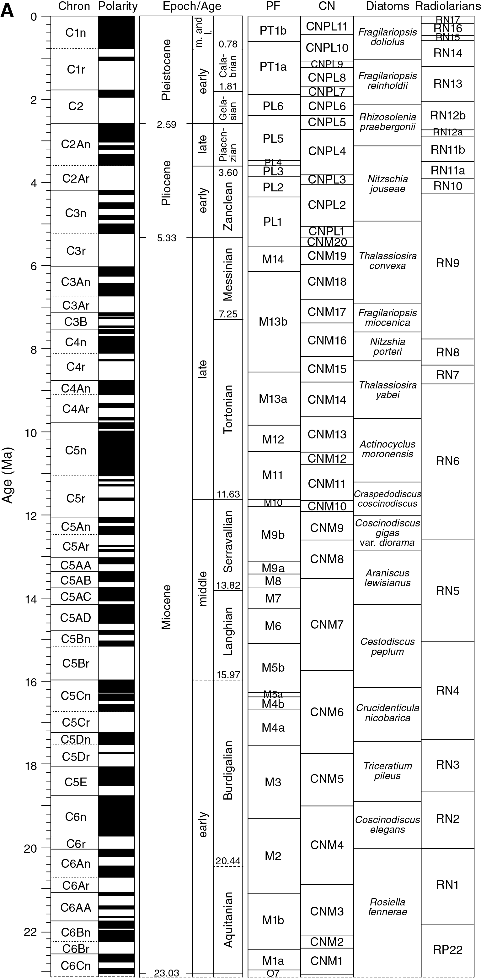
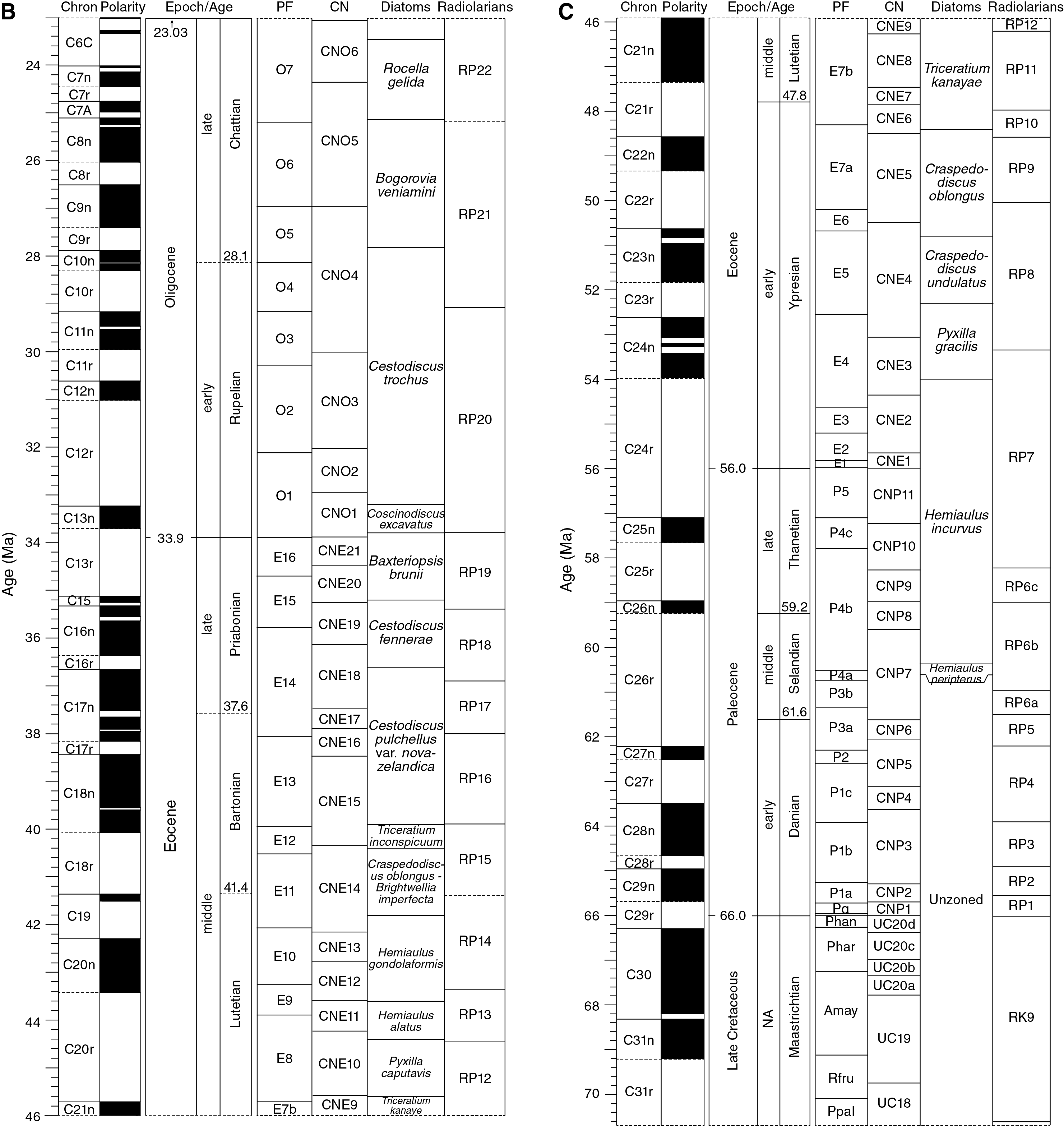
Figure F30. Expedition 362 timescale with planktonic foraminifer, calcareous nannofossil, diatom, and radiolarian biozones.
Biostratigraphic data were collected from core catcher samples. Additional samples were analyzed, when suitable and time permitted, from within cores in order to decrease the depth uncertainty of individual biohorizons and to improve biostratigraphic resolution. All sample depths are cited in the text as midpoint depths within the sample interval of interest, where appropriate. Microfossil preservation, abundance, and biozone assignment data were entered through DESClogik and are available in the LIMS database (http://web.iodp.tamu.edu/DESCReport). In site chapters, we present the biostratigraphic data in tables showing depths of age-diagnostic biohorizons, stratigraphic distribution charts of these biohorizons, integrated biozonation figures, and age-depth plots. It should be noted that the distribution charts are based on shipboard study only and are, therefore, strongly biased toward age-diagnostic species.
Calcareous nannofossils
Three biozone schemes were employed: Backman et al. (2012) for the Miocene through Pleistocene interval, Agnini et al. (2014) for the Paleogene interval, and Burnett (1998) for the Maastrichtian interval. These biozonations represent a general framework for the biostratigraphic classification of middle- to low-latitude nannofossil assemblages throughout the Cenozoic and into the Maastrichtian, divided into three intervals: 0–23, 23–46, and 46–70 Ma. Biozones and chronostratigraphy for each of these intervals are presented in Figure F31. Age estimates of biohorizons defining biozone boundaries as well as many additional biohorizons are presented in Table T7. Nannofossil taxonomy follows Bown (1998, 2005) and Perch-Nielsen (1985a, 1985b), in which full taxonomic lists can be found.

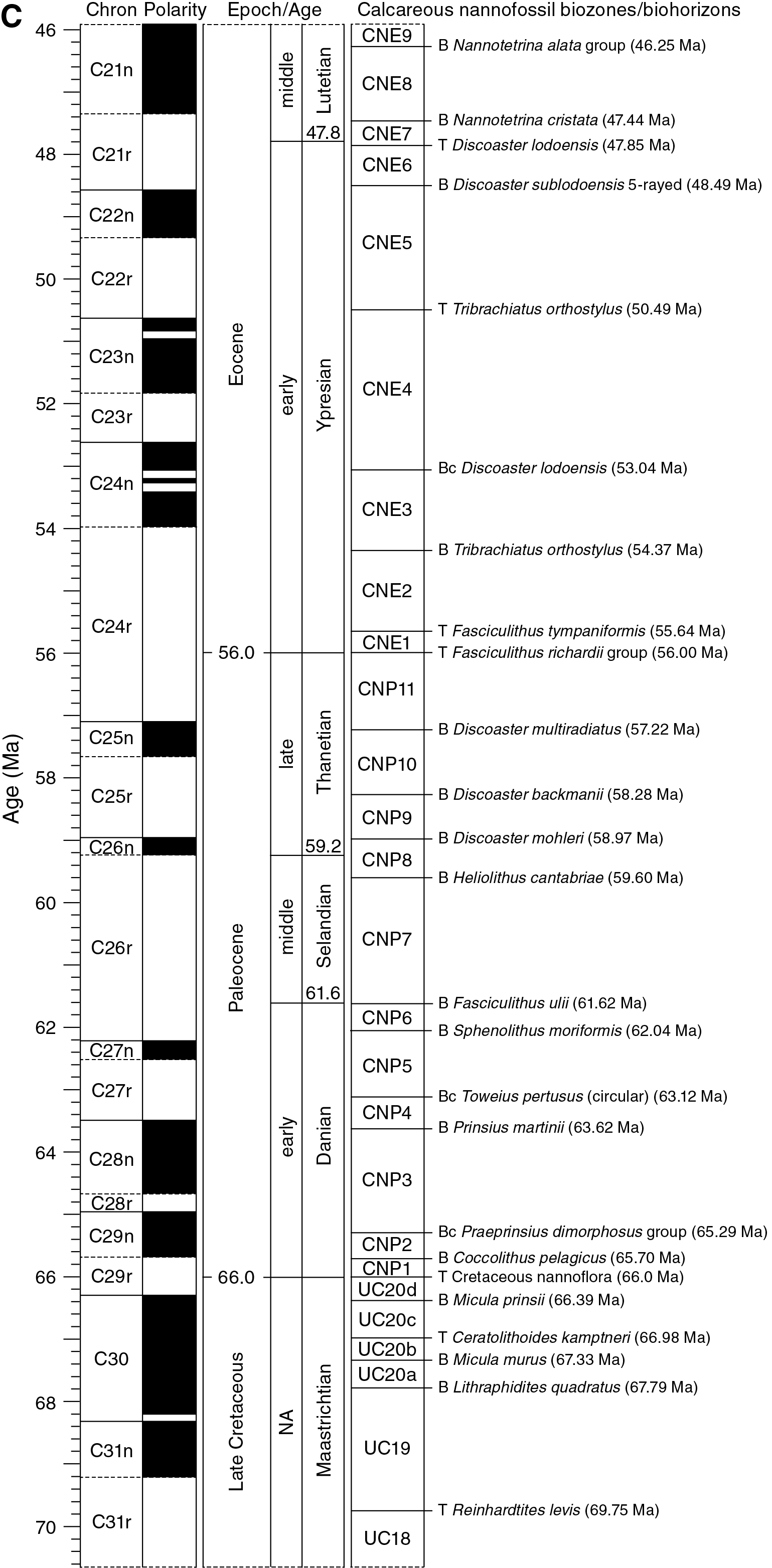
Figure F31. Calcareous nannofossil biozones and biohorizons defining biozone boundaries.
Table T7. Age estimates of calcareous nannofossil biohorizons. Download table in .csv format.
Calcareous nannofossils were examined in smear slides using standard preparation and light microscope techniques under crossed polarizers and transmitted light. Samples were initially investigated using 50 fields of view (FOVs) at 630× magnification. Assemblages were investigated at 1000× magnification when needed for taxonomic resolution. Total calcareous nannofossil abundance within the sediment was recorded as
- A = abundant (>50% of sediment particles).
- C = common (>10%–50% of sediment particles).
- F = few (1%–10% of sediment particles).
- R = rare (<1% of sediment particles).
- B = barren (no specimens).
Abundance of individual calcareous nannofossil taxa is recorded as
- A = abundant (>10 specimens per FOV).
- C = common (>1–10 specimens per FOV).
- F = few (1 specimen per 1–10 FOVs).
- R = rare (<1 specimen per 10 FOVs).
Preservation of the calcareous nannofossils is recorded as
- G = good (little or no evidence of dissolution and/or recrystallization, primary morphological characteristics only slightly altered, and specimens were identifiable to the species level).
- M = moderate (specimens exhibit some etching and/or recrystallization, primary morphological characteristics somewhat altered; however, most specimens were identifiable to the species level).
- P = poor (specimens were severely etched or overgrown, primary morphological characteristics largely destroyed, fragmentation has occurred, and specimens often could not be identified at the species and/or generic level).
The combination of barren intervals, low abundances, and poor preservation of calcareous nannofossils made it impossible to follow the complete distribution of expected ranges of individual species throughout the investigated sediments. Rather, the distribution of presence and, in a few cases, absence, of species was recorded with a focus on age-calibrated marker species. Presence of a species having an age-calibrated extinction in a sample implies a youngest possible age for that sample depth. Presence of a species having an age-calibrated first evolutionary appearance in a sample implies an oldest possible age for that sample depth.
Planktonic foraminifers
The zonal scheme of Anthonissen and Ogg (2012) was used for the Late Cretaceous. The zonal scheme of Berggren and Pearson (2005), as modified by Wade et al. (2011), was used for the Paleogene (zonal codes P, E, and O), and that of Berggren et al. (1995), as modified by Wade et al. (2011), was used for the Quaternary and Neogene (zonal codes M, PL, and PT). The planktonic foraminifer zonal scheme used during Expedition 362 is illustrated in Figure F32. Calibrated ages are from Anthonissen and Ogg (2012) and adjusted to the Expedition 362 timescale (Table T8).
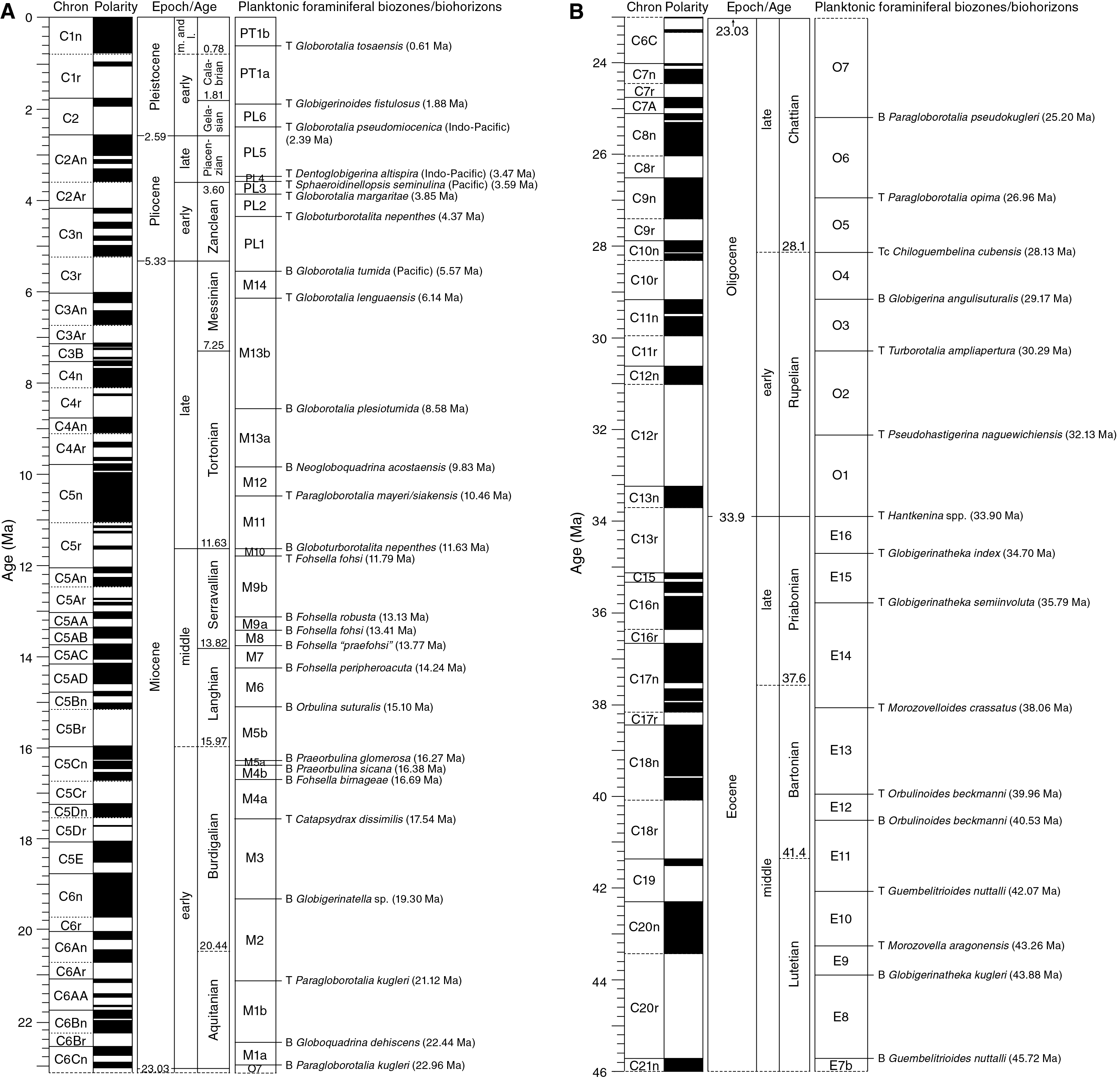
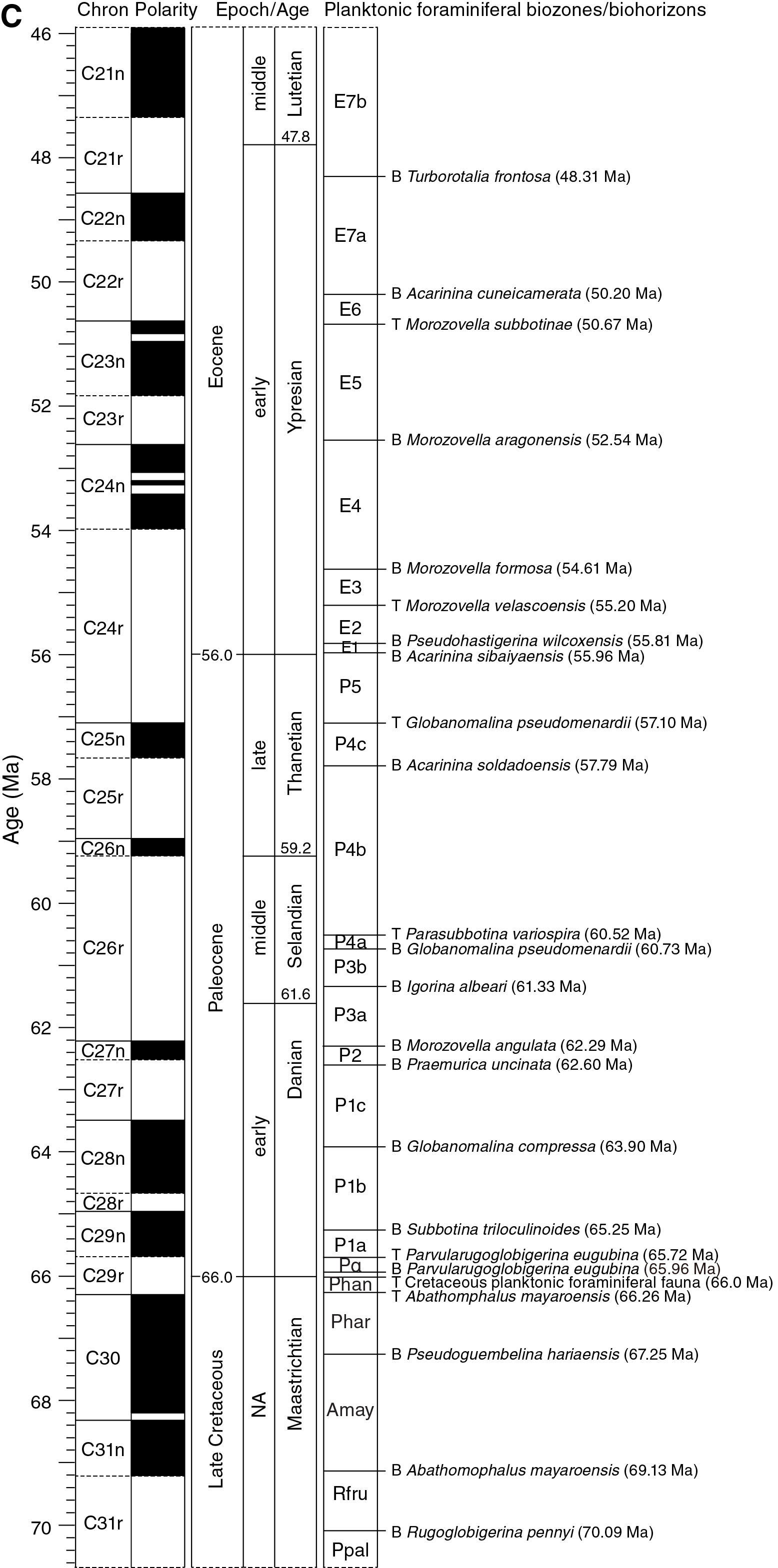
Figure F32. Planktonic foraminiferal biozones and biohorizons defining biozone boundaries.
Table T8. Age estimates of planktonic foraminifer biohorizons. Download table in .csv format.
Planktonic foraminifer taxonomic concepts in the Late Cretaceous mainly follow Robaszynski et al. (1984) and Caron (1985). Taxonomic concepts in the Cenozoic mainly follow Blow (1979), Kennett and Srinivasan (1983), Toumarkine and Luterbacher (1985), Bolli and Saunders (1985), and Pearson et al. (2006).
Core catcher samples (plus one sample per section, as needed) were soaked in tap water or in a weak hydrogen peroxide solution when necessary, warmed on a hot plate, and washed over a 63 μm mesh sieve. Lithified material was crushed into ~2 cm3 pieces, heated in a hydrogen peroxide solution, and then sieved as above. All samples were dried in sieves or on filter papers in a <60°C oven. To minimize contamination of foraminifers, the sieves were placed into a sonicator for several minutes, cleaned with pressurized air, and thoroughly checked between samples. The dried samples were sieved over a 150 µm sieve, retaining the <150 µm size fraction for additional observation when necessary. The >150 µm size fraction specimens were examined under a Zeiss Discovery V8 microscope for species identification.
The total abundance of planktonic foraminifers was estimated from visual examination of the dried >63 µm residue and was defined as
- A = abundant (>25% in total residue).
- C = common (>10%−25% specimens in total residue).
- F = few (5%−10% specimens in total residue).
- R = rare (<5% specimens in total residue).
- VR = very rare (<0.1% specimens in total residue).
- B = barren (no specimens in total residue).
Individual planktonic foraminifers were recorded in qualitative terms, based on an assessment of forms, observed in a random sample of ~150 specimens from the >150 µm size fraction. In samples where fewer than 150 specimens were present, all specimens were counted. Relative abundances were reported using the following categories:
- A = abundant (>25 specimens).
- C = common (11−25 specimens).
- F = few (5−10 specimens).
- R = rare (<5 specimens).
- B = barren (none present).
The preservation status of planktonic and benthic foraminifers was estimated as
- VG = very good (no evidence of overgrowth, dissolution, or abrasion).
- G = good (little evidence of overgrowth, dissolution, or abrasion).
- M = moderate (calcite overgrowth, dissolution, or abrasion are common but minor).
- P = poor (substantial overgrowth, dissolution, or abrasion).
Diatoms
Because of the overall low abundance of diatoms, it was necessary to concentrate diatoms by boiling sediment in HCl and H2O2 to remove carbonate and organic material before sieving at 150 µm (with the fine fraction retained) and 10 µm (with the coarse fraction retained). Strewn slides were then prepared with the residue, using 22 mm × 40 mm coverslips and a few drops of Norland optical adhesive. As a result of processing, only relative abundances of taxa were recorded. At least four traverses of each strewn slide were examined on a Zeiss Axiophot light microscope at 500× magnification, with species identification at 1000× magnification if necessary.
Diatom biohorizons for Expedition 362 were compiled from Baldauf (1985), Fourtanier (1991a, 1991b), Barron (1992, 2006), and Barron et al. (2004, 2014, 2015). Diatom biozones follow Burckle (1972) for the late Miocene–Quaternary, Barron (2006) for the early Miocene–late Oligocene, Barron et al. (2014) for the early Oligocene–late Eocene, and Fourtanier (1991b) for the early Eocene–Paleocene. All biohorizons and biozone boundaries were modified where necessary according to the Expedition 362 timescale. Modified diatom biohorizons and biozones are detailed in Table T9 and shown in Figure F33.
Table T9. Age estimates of diatom and silicoflagellate biohorizons. Download table in .csv format.
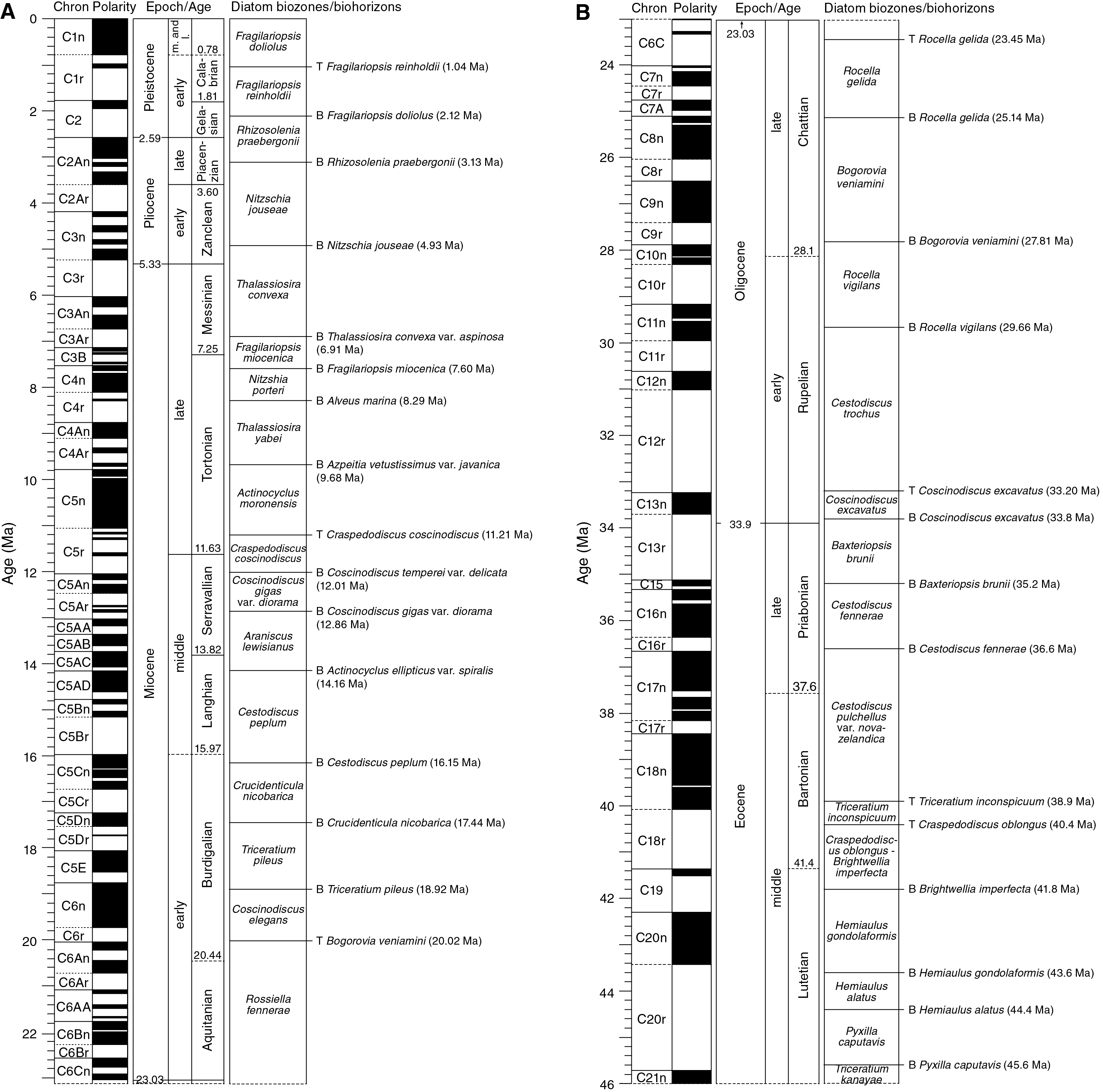
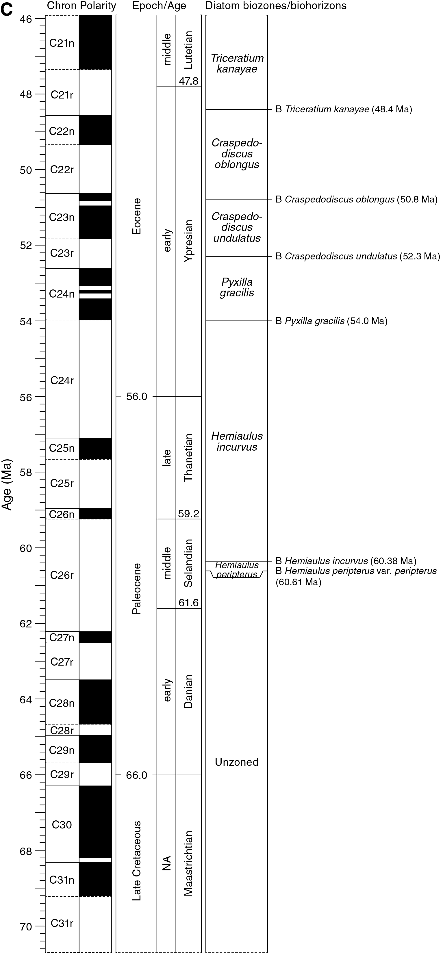
Figure F33. Diatom biozones and biohorizons defining biozone boundaries.
Relative abundances of individual diatom taxa were estimated from counts per FOV:
- A = abundant (>5 valves/FOV).
- C = common (3–5 valves/FOV).
- F = few (1–2 valves/FOV).
- R = rare (≥2 valves/traverse of coverslip).
- P = present (at least 1 valve observed, including fragments).
- B = barren (no valves observed).
Diatom preservation was described qualitatively following Barron and Gladenkov (1995):
- VG = very good (no breakage or dissolution).
- G = good (majority of specimens complete, with minor dissolution and/or breakage and no significant enlargement of the areolae or dissolution of frustule rims detected).
- M = moderate (minor but common areolae enlargement and dissolution of frustule rims, with a considerable amount of broken specimens).
- P = poor (strong dissolution or breakage, some specimens unidentifiable, strong dissolution of frustule rims and areolae enlargement).
- VP = very poor (very strong dissolution or breakage, most specimens unidentifiable).
Radiolarians
Cenozoic low-latitude radiolarian taxonomy and zonation followed that of Kamikuri and Wade (2012), Nigrini and Moore (1979), Nigrini and Sanfilippo (2001), Sanfilippo and Nigrini (1998), Sanfilippo et al. (1985), and Takahashi (1991). Full taxonomic lists and zonal assignments can be found in these references. For an explanation of evolutionary transitions, see Sanfilippo and Nigrini (1998). The zonal schemes of Sanfilippo and Nigrini (1998; codes RN and RP), Nigrini et al. (2006; codes RN and RP), and Kamikuri and Wade (2012; code RP) were used for Cenozoic radiolarian biostratigraphy. The Maastrichtian radiolarian biostratigraphy is represented in the global Late Cretaceous biozonation following Hollis (2002; code RK), De Weaver et al. (2001), and O’Dogherty et al. (2009) systematics. All biohorizons and biozones were modified where necessary according to the Expedition 362 timescale. Modified diatom biohorizons and biozones are detailed in Table T10 and shown in Figure F34. Accuracy of the correlation depends on many factors including core recovery, preservation, reworking, consistent recognition of taxa, geographical variability of taxa, and absence from or presence in some regions.
Table T10. Age estimates of radiolarian biohorizons. Download table in .csv format.
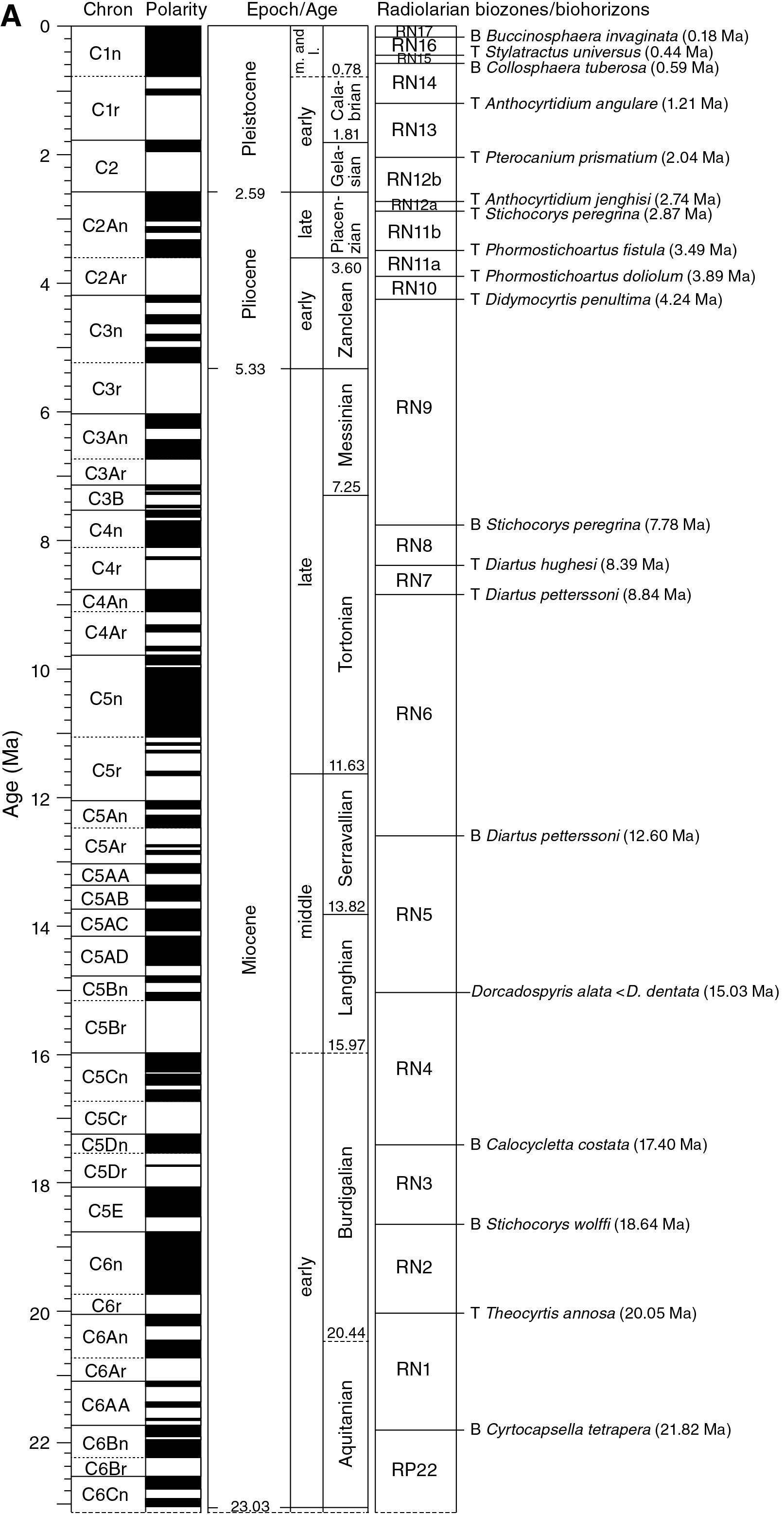
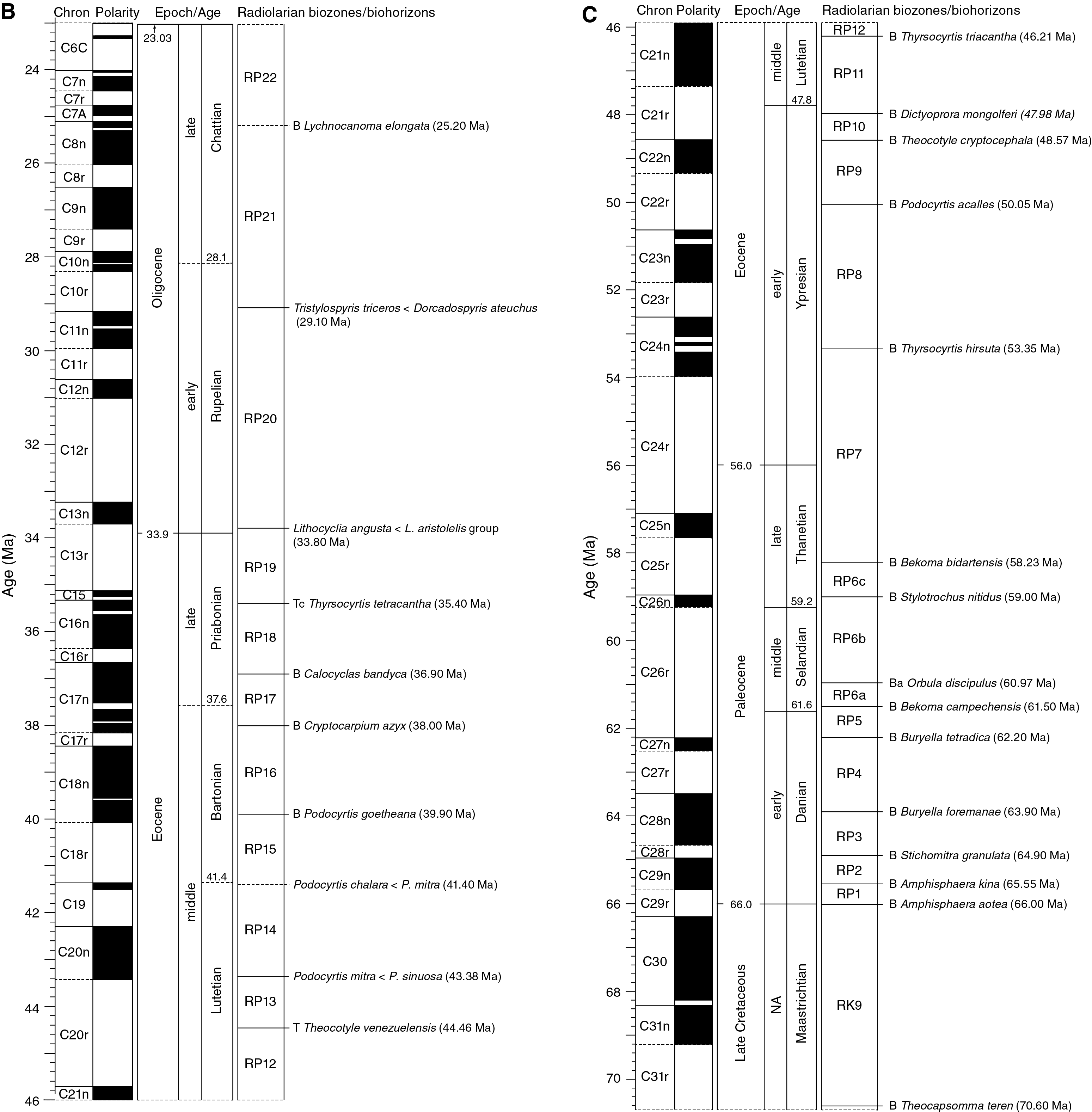
Figure F34. Radiolarian biozones and biohorizons defining biozone boundaries.
The age estimate of the base of Diartus hughesi was originally derived from Deep Sea Drilling Project Site 214 in the Indian Ocean (Johnson and Nigrini, 1985). This biohorizon occurs at 153.96 ± 0.75 mbsf in Core 22-214-17R (Gartner, 1974). The nannofossil Catinaster calyculus has its total range confined to Core 17R (Gartner, 1974), between 161.02 ± 0.98 mbsf (10.71 Ma) and 153.30 ± 0.75 mbsf (9.64 Ma). Linear interpolation between top and base C. calyculus results in an age of base D. hughesi of 9.73 Ma on the Expedition 362 timescale.
Samples were disaggregated by treatment with 10% H2O2 for 2 h, or until effervescence subsided. The samples were then washed through a 63 μm sieve. A second treatment with a 10% solution of HCl was used if any carbonate was present. While wet, residue samples were mounted by pipetting onto a microscope slide and the remainder residue was dried for scanning electron microscope (SEM) analysis. A few drops of mounting medium, Norland optical adhesive 61 (NOA 61) were applied to the dry slide, followed by a 22 mm × 40 mm glass coverslip. After curing under ultraviolet light, slides were examined using Zeiss Axiophot light microscopes under phase contrast, brightfield, and cross-polarized light at 50× and 100× magnification.
For the treatment of clayey sediment that contained pyritized radiolarians, samples were boiled for 4–5 min with tetrasodium phosphate before being further processed with 10% HCl for 2 h, or until effervescence subsided. Freed skeletons were frequently removed to avoid oxidation, and mechanical agitation (ultrasonic device and strong flows while sieving) was avoided. Cleaning with H2O2 was avoided when dealing with pyritized radiolarians. Sample residues were observed under a Zeiss Discovery V8 microscope, and representative radiolarians were picked from a tray and mounted on aluminum stubs. Stubs were sputter-coated with gold for 3–4 min to enhance conductivity. Specimens were then examined and photographed with a Hitachi-TM3030 desktop SEM at 10 kV. Images were optimized using Adobe Photoshop. SEM analysis was used to confirm species identification.
When radiolarians were diluted with detrital particles, sample residues were observed under a Zeiss Discovery V8 microscope. SEM analysis was used to confirm species identification.
When possible, relative abundances of individual radiolarian taxa were recorded. Abundance estimates, based on one slide of total radiolarian abundance in each sample, were determined using the following criteria:
- A = abundant (>30 specimens per slide traverse).
- C = common (6–30 specimens per slide traverse).
- F = few (>1–5 specimens per slide traverse).
- B = barren (no radiolarians present).
Relative preservation of each radiolarian taxon were noted using the following qualitative criteria:
- G = good (individual specimens exhibit little overgrowth, dissolution, or abrasion, but delicate parts of the skeleton are preserved).
- M = moderate (dissolution and breakage of individual specimens apparent but identification of species not impaired).
- P = poor (substantial overgrowth or infilling, dissolution, or fragmentation, where identification of some species is not possible).
Paleomagnetism
Shipboard paleomagnetism was investigated mainly to determine directions of natural remanent magnetization (NRM) components and downhole variation of magnetic properties. Routine measurements were conducted on archive section halves with stepwise alternating field (AF) demagnetization. Discrete cube and minicore samples were taken from selected working-half sections and measured with stepwise AF and thermal demagnetization. These data were used for core orientation and magnetostratigraphic and relative paleointensity dating (e.g., Guyodo and Valet, 1999; Laj et al., 2000; Channell et al., 2009).
Magnetic measurements
Remanent magnetization was measured using a 2G superconducting rock magnetometer (SRM; 2G Enterprises model 760R) equipped with direct-current superconducting quantum interference devices and an in-line, automated AF demagnetizer capable of reaching a peak field of 80 mT. Ocean drilling cores generally carry secondary overprint remanence components. Common overprints for ocean drilling cores include natural viscous remanent magnetization (VRM) and a steep downward-pointing component imparted by the drill string. To separate overprints from the characteristic remanence (ChRM), stepwise demagnetization was performed, as described below.
Archive-half sections
Measurements of archive halves were conducted using the new SRM software (IMS-SRM version 9.1) with a nominal sample area parameter of 15.59 cm2. The interval between measurement points and the measurement speed were selected as 2.5 cm and 10 cm/s, respectively.
We performed successive AF demagnetization using the SRM in-line AF demagnetizer on all split-core archive sections. The in-line AF demagnetizer applies a field to the x-, y-, and z-axes of the SRM in this fixed order (Figure F35). Previous reports suggest that higher AF demagnetization fields have produced significant anhysteretic remanent magnetization (ARM) along the z-axis of the SRM (e.g., Harris et al., 2013). With this limitation, we used demagnetization steps up to 30 mT to demagnetize the sections. For most of the sediment sections, we performed 4–6 steps from NRM to 25 mT demagnetization. AF demagnetization results were plotted individually as vector plots (Zijderveld, 1967), stereoplots of equal area projections, and downhole variations with depth. We inspected the plots visually to judge whether the remanence after demagnetization at the highest AF step reflects the ChRM and geomagnetic polarity sequence.

Figure F35. IODP coordinate systems for paleomagnetic samples, Natsuhara-Giken sampling cubes with sample coordinate system, and SRM coordinate system.
Discrete samples
Oriented discrete samples were collected from working-half sections. In soft sediment, discrete samples were taken in plastic “Japanese” Natsuhara-Giken sampling cubes (7 cm3 sample volume; Figure F35). Cubes were pushed into the working half of the core by hand with the “up” arrow on the cube pointing upsection in the core. For indurated intervals, cubes were cut with a table saw and trimmed to fit into the plastic sample cubes. In lithified sediment and hard rock, minicores (~11 cm3) were taken. Discrete sample locations were chosen in fine-grained intervals where drilling deformation was minimal or not visible.
Discrete samples were subjected to successive AF demagnetization with the DTech AF demagnetizer (model D-2000) and measured on the JR-6A spinner magnetometer before and after 5, 10, 15, 20, 25, 30, 35, 40, 60, and 80 mT AF demagnetization (majority of samples) and to 180 mT (for several high-coercivity samples). We also performed progressive thermal demagnetization using a thermal specimen demagnetizer (ASC Scientific model TD-48SC) for several selected discrete samples up to 575°C. Temperature increments of 25°–100°C were used, depending on the unblocking temperature of each sample. We analyzed the stepwise demagnetization data of the discrete samples by principal component analysis (PCA) to define the ChRM (Kirschvink, 1980). Section-half and discrete data collected on the pass-through SRM and spinner magnetometer, respectively, were uploaded to the LIMS database.
Low-field magnetic susceptibility (κ) measured on whole-round core sections using the WRMSL and archive-half core sections using the SHMSL (see Physical properties) was used to reveal the concentration of magnetic minerals and to determine the downhole relative paleointensity (NRM/κ).
Coordinates
All magnetic data are reported relative to the standard IODP orientation conventions: +x points into the face of the working half, +y points toward the left side of the face of the working half, and +z points down section (Figure F35). The relationship of the SRM coordinates (x-, y-, and z-axes) to the data coordinates (x-, y-, and z-directions) is as follows: for archive halves, x-direction = x-axis, y-direction = –y-axis, and z-direction = z-axis; for working halves, x-direction = –x-axis, y-direction = y-axis, and z-direction = z-axis. The coordinate systems for the spinner magnetometer (AGICO model JR-6A) and Natsuhara-Giken sampling cubes are shown in Figure F36.
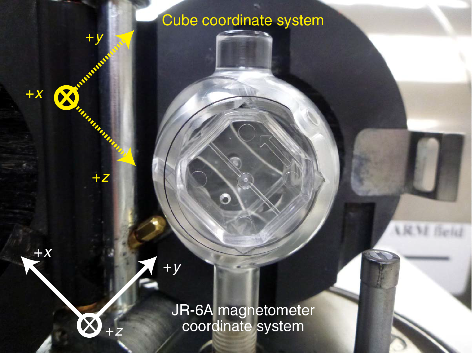
Figure F36. Positioning of discrete samples in the automatic holder of the JR-6A spinner magnetometer.
Core orientation
Paleomagnetic study of marine sediment cores can be greatly enhanced if the angle between magnetic north and the double-line orientation marked on the core liner can be oriented. Core orientation of APC cores during Expedition 362 was achieved with two orientation tools (Icefield MI-5 multishot and FlexIT tools) mounted on the core barrel. The Icefield MI-5 tool consists of triaxial magnetometers and accelerometers, and the FlexIT tool uses three mutually perpendicular fluxgate magnetic sensors and two perpendicular gravity sensors. The information from the magnetometers and sensors allows measuring the azimuth and dip of the hole, as well as the azimuth of the APC core. This azimuth combined with the local magnetic declination allows us to reorient the measured core declinations back to true geographic coordinates. We used the method of Richter et al. (2007) to obtain the azimuthally corrected declination (DTrue):
DTrue = DObserved + MTF + MIGRF,
- DObserved = the measured declination output from the cryogenic magnetometer.
- MTF = the magnetic tool face angle (the angle between magnetic north and the double line orientation mark on the core liner measured in a clockwise manner when the APC fired, see Figure F37).
- MIGRF = the site-specific deviation of magnetic north from true north.
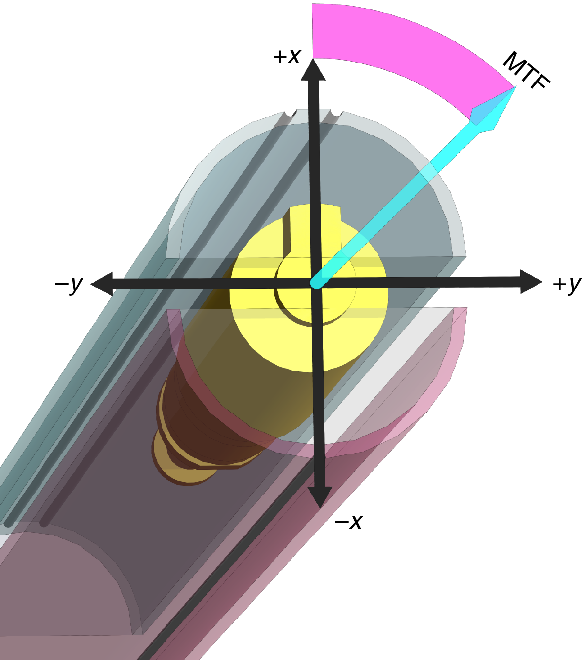
Figure F37. Relationship between IODP coordinate system, MTF of the orientation tool, and core liner.
During orientation, a tool is connected to the core barrel in such a way that the double lines on the core liner are at a fixed and known angle relative to the tool’s sensors. This angle has been assumed to be zero as long as these tools have been deployed in ocean drilling history. Previous expeditions have reported that in general these orientation tools have an accuracy of 20°–30°. During Expedition 362, however, a puzzling anomaly was observed in the declinations after core reorientation using the orientation tool data. The declination for the youngest sediment near the seafloor was expected to be near zero based on biostratigraphic and ash ages, yet the corrected declination was near ~180°, indicating an age older than the Bruhnes Chron (0.78 Ma). To track down the possible origin of this anomaly, an experiment with both the Icefield and FlexIT orientation tools was conducted by the IODP technical staff and Siem crew members during the transit back to Site U1481 on 20 September 2016. During the experiment, the tools residing above the core barrel were aligned to the double lines on the core liner (Figure F37), which were pointed to the ship’s heading direction (which was kept fixed relative to north) (Figure F38). The tools were suspended vertically in the derrick. Starting from the zero mark on the ship’s heading, four 90° clockwise rotations and four 90° counterclockwise rotations were performed. At each station, the APC assembly was held steady for 2 min to obtain a mean magnetic tool face value at each station. The ship’s heading varied only ~3° during the orientation testing experiment. Both tools measured the relative rotations between stations accurately, but both showed an average error of ~150° from the expected value. After analyzing various factors, we concluded that this 150° error is unlikely to be entirely caused by a local distortion of the magnetic field around the rig floor. Rather, we suspect that the magnetic tool face recorded a true deviation of ~180° from the double lines on the core liner. Indications from subsequent expeditions show that the problem was caused when a shock absorber included in the orientation tool’s sinker bar assembly periodically failed through shearing or twisting. This element has been removed from the redesigned orientation tool connector. It thus became apparent that measured remanent declinations should be corrected to magnetic north by adding 180° to the magnetic tool face angle. Declinations can also be further corrected to true north by adding the deviation of magnetic north from true north (i.e., local declination, which can be determined from the International Geomagnetic Reference Field coefficients; see above and Richter et al. 2007). The information provided by this experiment contributed greatly to paleomagnetic polarity determinations and magnetostratigraphic interpretations of Expedition 362 cores.

Figure F38. APC assembly used for orientation tool testing.
ChRM also provides a reference frame to orient cores (see Structural geology). Provided that the reference magnetic pole is known, the orientation of the paleomagnetic vector is then used to restore the azimuth of the core: the horizontal component of the mean ChRM makes an angle with the reference line, which specifies the rotation of the core relative to the geographic coordinates (e.g., Fuller, 1969). The assumptions for orientation are
- The section has enough measurements to average out geomagnetic secular variation;
- The original bedding is horizontal;
- The borehole is vertical; and
- The sedimentary unit has not experienced any vertical axis rotation.
Assumptions 2 and 3 were confirmed with shipboard structural geologists, seismic profiles across the drill sites, and drilling operational records. Assumptions 1 and 4 will be checked postcruise. For intervals of particular interest for structural geology, we report the ChRMs defined from discrete samples. More detailed demagnetization steps for the discrete samples allowed more accurate ChRMs than those from the archive halves. In addition, well-defined VRM overprints from discrete samples could also be used in orienting observed structures in the core.
Magnetostratigraphy
A magnetostratigraphy was constructed at each site by correlating observed polarity sequences with the geomagnetic polarity timescale (GPTS) in combination with biostratigraphic biohorizons. The chosen GPTS for Expedition 362 is based on the combination of the following data sets (Table T11):
- Hilgen et al. (2012) from the top of Chron C1n at 0.00 Ma (Holocene) through the base of Chron C6Cn.2n at 23.03 Ma (base of the Miocene),
- Pälike et al. (2006) from the base of Chron C6Cn.2r at 23.27 Ma (Oligocene) through the base of Chron C19n at 41.41 Ma (middle Eocene),
- Vandenberghe et al. (2012) from the base of Chron C19r at 42.30 Ma (middle Eocene) through the base of Chron C29n at 65.69 Ma (early Paleocene), and
- Husson et al. (2011) from the top of Chron C30n at 66.30 Ma through the base of Chron C31r at 71.40 Ma (Maastrichtian); the Expedition 362 timescale ends at 70.65 Ma, within Chron C31r.
Table T11. Data sets used to construct the Expedition 362 GPTS. Download table in .csv format.
This composite GPTS, together with microfossil biozone summaries, are plotted in Figures F30, F31, F32, F33, and F34.
For azimuthally unoriented sedimentary samples that formed in low latitudes, such as those retrieved from the Expedition 362 drill sites, determining the polarity of sedimentary units can be difficult. The polarity ambiguity arises when the samples are azimuthally unoriented and the inclination is very shallow near the Equator (the angular distance between reversed and normal polarity inclinations is small). Because paleomagnetic inclinations from any samples will have some degree of dispersion about their mean inclination, it is likely that when the mean inclination is shallow (near zero), the sign of the inclination will not be indicative of the polarity (e.g., McFadden and Reid, 1982; Cox and Gordon, 1984). The sign of the inclination of these samples should be used with caution as a definitive estimate of magnetic polarity.
We applied the following methods to establish magnetozones:
- Observing near-180° shifts in declinations and significant changes in inclinations (for the deeper section) from pass-through measurements on long coherent core sections after 15 mT demagnetization. The observed magnetozones are then checked with the ChRM directions of the discrete samples from the corresponding intervals as well as taking biostratigraphic age constraints into account.
- Comparing inclination trends with predicted paleolatitudes of the drill sites according to the absolute plate motion of the Capricorn (Indian) plate following the latest, state-of-the art plate reconstructions (van Hinsbergen et al., 2015). Based on global plate circuit reconstructions, our drill sites have moved northward since the formation of this sediment. Following the reconstructed position of the drill holes for two representative periods at 20 and 40 Ma, the paleolatitudes would be ~5° and ~12° to the south of their present-day positions (3°N), respectively.
- Using relative paleointensity as a proxy. In recent years, independent records of relative paleointensity (RPI) data from sediment cores in different oceans of the world have been stacked and correlated with magnetic polarity chrons, even down to millennial scale. Several global paleointensity stacks have been produced including GLOPIS (for the last 75 ky; Laj et al., 2004), Sint-800 (for the last 800 ky; Guyodo and Valet, 1999), Sint-2000 (for the last 2000 ky; Valet et al., 2005), and PISO-1500 (for the last 1.5 My, which also combines isotope records; Channell et al., 2009). Regional stacks for the last 75 ky have also been generalized for the North Atlantic (NAPIS; Laj et al., 2000), South Atlantic (SAPIS; Stoner et al., 2002), and western equatorial Pacific (EPAPIS, covering the 0.75–3.0 Ma interval; Yamazaki and Oda, 2005). The RPI stacks provide a stratigraphic template that can be potentially used to correlate the relative paleointensity records from Expedition 362 Indian Ocean sediment and hence help refine the magnetostratigraphy of the drill sites.
Whenever possible, we offer an interpretation of the magnetic polarity, with the naming convention following that of correlative anomaly numbers prefaced by the letter C (Tauxe et al., 1984). Normal polarity subchrons are referred to by adding suffixes (n1, n2) that increase with age. For the younger part of the timescale (Pliocene–Pleistocene), we use the traditional names to refer to the various chrons and subchrons (e.g., Brunhes, Jaramillo, Olduvai, etc.). In general, polarity reversals occurring at core section ends have been treated with extreme caution.
Data reduction and software
Data reduction (Zijderveld demagnetization plots and equal area projections) was conducted using PuffinPlot (Version 1.03, 23 April 2015) (Lurcock and Wilson, 2012), a versatile, user-friendly desktop application. PCA (Kirschvink, 1980) was also performed using PuffinPlot to determine ChRM directions.
Geochemistry
Expedition 362 was designed to establish initial and evolving properties of the incoming section to the North Sumatran subduction zone and their role in shallow seismogenesis and forearc plateau development. The thick input section has likely undergone substantial diagenetic alterations below the trench wedge and just in front of the subduction zone, which may alter mechanical properties of the wedge and so may influence shallow seismogenic slip. Fluids and associated diagenetic reactions, both at the drill sites and reactions expected from the sediment mineralogy and pore fluid chemistry, are thus a key component of this study. The concentration of dissolved species and their isotopic composition provide critical data for identification of fluid–rock reactions, assessment of potential fluid flow through the underlying oceanic crust, and identification of any potential migration pathways and fluid sources within the sediment section. In addition, geochemical data can help characterize biogeochemical cycling, guide paleoceanographic reconstructions, and aid in constraining mass balance inventories operating in this subduction zone.
Interstitial water sampling protocol
During Expedition 362, most of the interstitial water samples were collected from whole-round samples; in addition, fluids were collected using Rhizon samplers inserted into the uncut liner of Cores 362-U1480H-9H, 10H, and 11H. Interstitial water whole-round samples were collected at a frequency of 3–7 samples per core in the first 4 or 5 cores and subsequently at a resolution of 1 or 2 samples per core to the bottom of the hole. The length of the whole rounds used was 10 cm in the shallow cores and increased with depth, depending on interstitial water recovery, to a maximum of 25 cm. Rhizon samples were collected at a resolution of 2 samples per section and yielded pore water volumes from 0 to 12 mL. Details of sampling protocols for each site are given in the corresponding site chapters.
For headspace analyses of gas concentrations, 1 or 2 sediment plugs were routinely collected; one was used for standard hydrocarbon concentration monitoring on board and the other for stable-isotope measurements at onshore laboratories. The headspace samples were collected adjacent to each interstitial water sample when one was taken. For safety monitoring, purposed headspace samples were also taken from cores with not enough recovery for interstitial water sampling.
Interstitial water collection
Whole-round cores were cut on the catwalk, capped, and taken to the laboratory for processing. In general, samples collected from the seafloor to ~130 mbsf were processed inside a nitrogen bag to avoid oxidation of redox-sensitive elements. All other cores were processed under normal atmospheric conditions. During high-resolution sampling, when there were too many interstitial water cores to process immediately, capped whole-round core sections were stored under a nitrogen atmosphere at 4°C until they were squeezed, which occurred no later than 24 h after core retrieval.
After extrusion from the core liner, the surface of each whole-round interstitial water sample was carefully scraped with a spatula to remove potential contamination from seawater and sediment smearing in the borehole. For APC and most RCB cores, removal of ~0.5 cm of material from the outer diameter, top, and bottom faces was sufficient, whereas in XCB and some RCB cores where borehole contamination seemed higher, as much as two-thirds of the sediment was removed from each whole round. The remaining sediment (~150–300 cm3) was placed into a titanium squeezer modified after the stainless-steel squeezer of Manheim and Sayles (1974). Samples were squeezed at maximum pressures of 24.5 MPa (gauge forces of up to 35,000 lb). The squeezed interstitial water was filtered through a prewashed Whatman No. 1 filter placed in the squeezers above a titanium screen. The squeezed interstitial water was collected in precleaned, plastic syringes attached to the squeezing assembly and subsequently filtered through a 0.45 µm Gelman polysulfone disposable filter. In the deeper sections of the sites, fluid recovery was as low as 1 mL after squeezing the sediment for up to ~24 h.
Sample allocation was determined based on the recovered interstitial water volume and analytical priorities based on the objectives of the expedition. The shipboard analytical protocols are summarized in the following section.
Shipboard interstitial water analyses
Interstitial water samples were analyzed on board following protocols in Gieskes et al. (1991), Murray et al. (2000), and the IODP user manuals (http://iodp.tamu.edu/labs/documentation/).
Salinity, alkalinity, and pH
Salinity, alkalinity, and pH were measured immediately after squeezing. Salinity was measured using a Fisher temperature-compensated handheld refractometer, pH was measured with a combination glass electrode, and alkalinity was determined by Gran titration with an autotitrator (Metrohm 794 basic Titrino) using 0.1 M HCl at 20°C. Certified reference material (CRM) 104 obtained from the laboratory of Andrew Dickson, Marine Physical Laboratory, Scripps Institution of Oceanography (USA), was used for calibration of the acid. International Association for the Physical Sciences of the Oceans (IAPSO) standard seawater was analyzed at the beginning and end of a set of samples for each site and after approximately every 10 samples.
Chloride, sulfate, and bromide
High-precision chloride concentrations were acquired using a Metrohm 785 DMP autotitrator and silver nitrate (AgNO3) solutions that were calibrated against repeated titrations of an IAPSO standard. A 0.1 mL aliquot of sample was diluted with 10 mL of 90 ± 2 mM HNO3 and titrated with 0. 014 M AgNO3. Repeated analyses of an IAPSO standard yielded a precision better than 0.35%.
In samples from Holes U1480E and U1480F, concentrations of sulfate (SO42–), chloride (Cl–), and bromide (Br–) were analyzed using 100 µL aliquots diluted 1:100 with deionized water (18 MΩ). Subsequent samples were diluted 1:100 using a 50 µM KNO3 solution used as an internal standard. In all cases, we used an ion chromatograph (IC; Metrohm 850 Professional) and eluent solutions of 3.2 mM Na2CO3 and 1.0 mM NaHCO3. Concentrations were based on peak areas. The analytical protocol used was to run a standard after 5 samples for 6 cycles, after which 3 extra standards were analyzed. The standards used were based on IAPSO dilutions of 50×, 80×, 150×, 250×, 500×, 750×, 1000×, 1200×, 1500×, and 2000×. Sample replicates (N = 5) were analyzed during each run for reproducibility. Reproducibility was also checked based on the interspersed standard samples run throughout the expedition. Analytical precision was 2% for sulfate, chloride, and bromide when no internal standard was used but yielded precision better than 1% when using KNO3 as an internal standard. Chloride analyses by both titration and IC agree within 2%; for this expedition we report both values but plot only the titration data.
Ammonium, phosphate, and silica
Ammonium, phosphate, and silica concentrations were determined by spectrophotometry using an Agilent Technologies Cary Series 100 UV-Vis spectrophotometer with a sipper sample introduction system following the protocol in Gieskes et al. (1991). Phosphate was measured using the ammonium molybdate method described in Gieskes et al. (1991), using appropriate dilutions. Orthophosphate reacts with Mo(VI) and Sb(III) in an acidic solution to form an antimony-phosphomolybdate complex. Ascorbic acid reduces this complex to form a blue color, and absorbance is measured spectrophotometrically at 885 nm.
The ammonium method is based on diazotization of phenol and subsequent oxidation of the diazo compound by household bleach (sodium hypochlorite) to yield a blue color measured spectrophotometrically at 640 nm. Samples were diluted prior to color development so that the highest concentration was <1000 µM.
Silica was also measured spectrophotometrically using the method based on the production of a yellow silicomolybdate complex. The complex is reduced by ascorbic acid to form molybdenum blue, measured at 812 nm.
Major elements
In past expeditions, major elements (Ca, Mg, K, and Na) were commonly analyzed by inductively coupled plasma–atomic emission spectroscopy (ICP-AES) with a Teledyne Prodigy high-dispersion ICP spectrometer. Samples and standards were diluted 1:100 using 2% HNO3 spiked with 10 ppm Y as an internal standard. However, because the new IC instrument yields cation concentration data during the standard IC run for anions (sulfate, bromide, and chloride), we compared both analytical approaches by repeated analyses of standards and samples (archived data from IODP Expedition 344 Site U1414 and a dedicated run for samples from Site U1480). The data generated by both approaches agreed to better than 1.5%; therefore, we used the IC data to report major cation concentrations measured during Expedition 362.
IC analyses were conducted using the same aliquot dilutions as the ones used for anions: 1:100 using a 50 µM KNO3 solution as an internal standard. The eluent solutions used for cation measurements were 3.2 mM Na2CO3 and 1.7 mM PDCA (pyridine-2,6-dicarboxylic acid) supplied by Metrohm (CAS#499-83-2). Concentrations were based on peak areas and corrected against the average area of the KNO3 internal standard. Analogous to the protocol used for anion measurements, the analytical protocol for cations was to run a standard after 5 samples for 6 cycles, after which 3 extra standards were analyzed. The standards used were based on IAPSO dilutions of 50×, 80×, 150×, 250×, 500×, 750×, 1000×, 1200×, 1500×, and 2000×. Sample replicates (N = 5) were analyzed during each run for reproducibility. Reproducibility was also checked based on the interspersed standard samples run throughout the expedition. Analytical precision was 0.3% for Na and K, 0.6% for Mg, and 1.0% for Ca.
Minor elements
Minor elements (Fe, Li, Ba, B, and Mn) were analyzed by ICP-AES with a Teledyne Prodigy high-dispersion ICP spectrometer. The general method for shipboard ICP-AES analysis of samples is described in Murray et al. (2000) and user manuals for shipboard instrumentation. Each batch of samples run on the ICP spectrometer contains blanks and solutions of known concentrations. Each item aspirated into the ICP spectrometer was counted 4 times from the same dilute solution within a given sample run. Following each instrument run, the measured raw-intensity values were transferred to a data file and corrected for instrument drift and blank. If necessary, a drift correction was applied to each element by linear interpolation between the drift-monitoring solutions.
For the minor element concentration analyses, an interstitial water sample aliquot was diluted by a factor of 20 (0.5 mL sample added to 9.5 mL of a 10 ppm Y solution). Because of the high concentration of matrix salts in the interstitial water samples at a 1:20 dilution, matrix-matching of the calibration standards is necessary to achieve accurate results by ICP-AES. A matrix solution that approximated IAPSO standard seawater major ion concentrations was prepared according to Murray et al. (2000). A stock standard solution was prepared from ultrapure primary standards (SPC Science PlasmaCAL) in a 2% nitric acid solution. The stock solution was then diluted in the same 2% ultrapure nitric acid solution to concentrations of 100%, 75%, 50%, 25%, 10%, 5%, and 1%. In addition to this set of standards, we include dilutions of IAPSO standard to constrain the lower-end range of concentrations measured in interstitial water during Expedition 362. The calibration standards and IAPSO solutions were diluted using the same method as the samples for consistency. The final matrix-matched 100% standard solution contained the following concentrations of elements: B = 1388.9 µM, Li = 288.2 µM, Mn = 54.6 µM, Fe = 17.9 µM, Sr = 228.1 µM, and Ba = 36.4 µM. The 100%, 75%, 50%, 25%, 10%, and 5% standards were repeatedly analyzed for each batch and over the 2-month expedition as a check of analytical precision. The average precision of the minor element analyses were B < 1%, Ba < 1%, Mn < 1%, Li < 1.5%, Si < 1.5%, and Sr <1%.
Fluid organic geochemistry
Routine analysis of hydrocarbon gas in sediment cores is a part of the standard IODP shipboard monitoring of the cores to ensure that the sediments being drilled do not contain greater than the expected amount of hydrocarbons. The most common method of hydrocarbon monitoring used during IODP expeditions is the analysis of gas samples obtained from either sediment samples (headspace analysis) or from gas expansion pockets visible through clear plastic core liners (void gas analysis) following the procedures described by Kvenvolden and McDonald (1986).
When gas pockets were detected, the free gas was drawn from the sediment void using a syringe attached to a hollow stainless-steel tool used to puncture the core liner. The gas then was analyzed on the natural gas analyzer (NGA). For headspace analyses, a 3 cm3 bulk sediment sample was collected from the freshly exposed top end of a core section and next to the interstitial water sample immediately after core retrieval using a brass boring tool or plastic syringe. The sediment plug was sealed with an aluminum crimp cap with Teflon/silicon septa. The vial was then heated to 70°C for ~30 min to evolve hydrocarbon gases from the sediment plug. When consolidated or lithified samples were encountered, chips of material were placed in the vial and sealed. For gas chromatographic analysis, a 5 cm3 volume of headspace gas was extracted from the sealed sample vial using a standard gas syringe and analyzed by gas chromatography.
The standard gas analysis program for safety was complemented by collecting an additional headspace sample at the same resolution as described above to measure the stable carbon and hydrogen isotope composition of hydrocarbons at onshore laboratories. The sampling method is the same as that used for the safety analysis, except that the sediment plug is extruded into a 20 cm3 headspace glass vial filled with 10 cm3 of a 1 M potassium chloride (KCl) solution containing borosilicate glass beads and immediately sealed with an aluminum crimp cap with Teflon/silicon septa. The vial was then vigorously shaken to help dissociate the sediment. Potassium chloride is toxic and was thus used to stop all microbial activity in the sediment. The glass beads (3 mm diameter) were used to help break up the sediment plug during shaking and liberate gas trapped in sediment pore space or adsorbed on particles. The vials were flushed with N2 and capped within 1 h prior to sampling in order to remove air from the headspace and ensure the sample is preserved anaerobically.
Headspace and void gas samples were directly injected into the gas chromatograph–flame ionization detector (GC-FID) or into the NGA. The headspace samples were analyzed using an Agilent/HP 6890 Series II gas chromatograph (GC3) equipped with an 8 ft, 2.00 mm inner diameter × ⅛ inch outer diameter stainless steel column packed with 80/100 mesh HayeSep R and an FID set at 250°C. The GC3 oven was programmed to hold temperature at 80°C for 8.25 min, ramp at 40°C/min to 150°C, hold for 5 min, and return to 100°C postrun for a total of 15 min. Helium was used as the carrier gas. The GC3 system determines concentrations of methane (C1), ethane (C2), ethene (C2=), propane (C3), and propene (C3=).
Data were collected using the Hewlett Packard 3365 Chemstation data processing program. Chromatographic response is calibrated to nine different gas standards with variable quantities of low molecular weight hydrocarbons. The gas concentrations for the required safety analyses are expressed as component parts per million by volume (ppmv) relative to the analyzed gas.
Sediment geochemistry
For the shipboard sediment geochemistry analyses, 5 cm3 of sediment was freeze-dried for ~24 h, crushed to a fine powder using a pestle and agate mortar, and subsampled to analyze inorganic carbon, total carbon (TC), and total nitrogen (TN).
Elemental analysis
TC and TN of sediment samples were determined with a ThermoElectron Corporation FlashEA 1112 CHNS elemental analyzer equipped with a ThermoElectron CHNS/NCS packed column and a thermal conductivity detector (TCD). Approximately 10–15 mg of freeze-dried, ground sediment was weighed in a tin cup and the sample was combusted at 900°C in a stream of oxygen. The reaction gases were passed through a reduction chamber to reduce nitrogen oxides to nitrogen and were then separated by gas chromatography before detection by TCD. All measurements were calibrated to a standard soil reference material (soil Standard 33840025) for carbon and nitrogen detection (Thermo), which was run every 6 samples as a verification. The detection limit was 0.001% for TN (instrument limit) and 0.002% for TC (procedural blank; measured as an empty tin cup). Sample replicates (N = 10 for each of 5 samples) yielded precisions of <10% for TN and <7% for TC.
Inorganic and organic carbon content
Total inorganic carbon (TIC) concentrations were determined using a UIC 5011 CO2 coulometer. Between 10 and 15 mg of freeze-dried, ground sediment was weighed and reacted with 2 M HCl. The liberated CO2 was titrated and the end-point was determined by a photodetector. Calcium carbonate content expressed as weight percent was calculated from the TIC content assuming that all evolved CO2 was derived from dissolution of CaCO3, using the following equation:
CaCO3 (wt%) = TIC × 8.33 (wt%).
No correction was made for the presence of other carbonate minerals. Accuracy during individual batches of analyses was determined by running a carbonate standard (100 wt% CaCO3) every 10 samples. Typical precision, assessed using replicate analyses of a carbonate sample (N = 10 for each of 5 samples), was 2%. The detection limit for CaCO3, defined here as 3 times the standard deviation of the blank (2 M HCl), was 0.1% for 100 mg of pelagic clay. Total organic carbon (TOC) content was calculated as the difference between TC (measured on the elemental analyzer) and inorganic carbon (measured by coulometry):
Physical properties
Core material was characterized by multiple physical property measurements. For soft sediment, the general sample work flow was as follows:
- Cores were thermally equilibrated to ambient room temperature (20°C) over a period of 1–3 h.
- Whole-round cores were run on the WRMSL. The WRMSL includes a GRA bulk densitometer, a magnetic susceptibility pass-through loop system (MSL), and a PWL.
- Whole-round cores were run on the NGRL when the length of an individual section was >50 cm.
- Thermal conductivity (TCON) was measured on 1 section (typically Section 3) of each core.
- Cores were split.
- The archive half of the core was passed through the SHIL for imaging and SHMSL for RSC and MSP.
- Shipboard samples for MAD analyses were collected (generally 2 per section and adjacent to all whole-round samples). Samples were taken in representative lithologies. In case of delayed sampling, the samples were resaturated.
- Discrete compressional velocity measurements were made on the working half cores using the P-wave velocity gantry.
- Strength measurements (for soft sediment only) were made on the working half using the Automated Vane Shear and/or a pocket penetrometer.
For hard rock cores, a slightly different sequence was used:
- Cores were thermally equilibrated to ambient room temperature for at least 2 h.
- Whole-round cores were run on the WRMSL with the PWL turned off.
- Whole-round cores were run on the NGRL when the length of an individual section was >50 cm.
- Cores were split.
- The archive half of the core was passed through the SHIL for imaging and SHMSL for RSC and MSP.
- Oriented, discrete cube samples (~2 cm3) were taken from the working half for P-wave velocity and MAD measurements. When taken more than ~12 h after the arrival of the core on deck, the samples were placed in seawater under vacuum for 24 h for resaturation before measurement. The samples were measured for P-wave velocity in three orthogonal directions and then processed for MAD measurements. P-wave measurements were also made on PMAG samples (but without resaturation).
- Selected pieces of the core sections >7 cm were measured for thermal conductivity.
All raw data were uploaded to the LIMS database.
Whole-Round Multisensor Logger measurements
The WRMSL was used to measure GRA density, magnetic susceptibility, and P-wave velocity nondestructively. The sampling interval for WRMSL measurements was set at 2.5 cm.
GRA bulk density
The GRA densitometer on the WRMSL operates by passing gamma rays from a 137Cs source through a whole-round core and into a 75 mm3 sodium iodide (NaI) detector located directly below the core. The input gamma ray peak has a principal energy of 0.662 MeV that is attenuated as it passes through the core. Attenuation of gamma rays, mainly by Compton scattering, is related to electron density, which is related to material bulk density by
- ρb = bulk density,
- ρe = electron density,
- w = molecular weight, and
- N = atomic number of elements in the material.
For the majority of elements and for rock-forming minerals, w/2ΣN is ~1; although, w/2ΣN for hydrogen is 0.5040. Therefore, for a known sample thickness the gamma ray count is proportional to density. Calibration of the GRA densitometer was performed using a core liner filled with freshwater and aluminum density standards at the beginning of the expedition. Calibration was verified after each core measurement by passing the freshwater-filled core liner through the densitometer. Recalibration was performed if the measured density of the freshwater standard exceeded limits of 1.00 ± 0.02 g/cm3.
Magnetic susceptibility
Magnetic susceptibility, Κ, is a dimensionless measure of the degree to which a material can be magnetized by an external magnetic field:
where M is the magnetization induced in the material and H is the strength of an external field. Magnetic susceptibility varies in response to the type and concentration of magnetic grains and responds to variations in the magnetic composition of the sediment, both commonly related to variations in mineralogical composition (e.g. terrigenous versus biogenic materials) and diagenetic overprinting. Materials such as clay generally have a magnetic susceptibility several orders of magnitude lower than magnetite and some other iron oxides that are common constituents of igneous and volcanogenic material. Water and plastics (such as the core liner) have a slightly negative magnetic susceptibility.
The WRMSL measures volume magnetic susceptibility using a Bartington Instruments MS2 meter (Bartington instruments, 2011) coupled to an MS2C sensor coil (88 mm diameter). An oscillator circuit in the sensor operates at an alternating field of ~100 mT and frequency of 565 Hz, producing a low-intensity nonsaturating magnetic field. During Expedition 362, the instrument was set to record instrumental units with an integration period of ~1 s, which produced a sensitivity of 1 × 10⁻⁵ SI units. No correction was applied for volume effects caused by differing APC, XCB, and RCB core diameters. The spatial resolution of the method is ±4 cm; therefore, core material that is not continuous over an 8 cm interval will underestimate the magnetic susceptibility.
P-wave velocity
P-wave velocity is the rate at which a (compressional) P-wave travels through a medium. P-wave velocity is dependent on the composition, bulk density, stiffness, fabric, and temperature of the material, which in turn are functions of consolidation and lithification, state of stress, and degree of fracturing. The PWL system on the WRMSL transmits 500 kHz P-wave pulses across the core liner and core with a 200 Hz repetition frequency. The pulser and receiver are mounted on a caliper-type device and are aligned in order to make wave propagation perpendicular to the section’s long axis. A linear variable differential transducer (LVDT) measures the P-wave travel distance between the pulse source and the receiver. Good coupling between transducers and core liner is facilitated with water dripping onto the contact from a peristaltic water pump system. Signal processing software picks the first arrival of the wave at the receiver. Measured travel distance and time are corrected for twice the liner thickness.
A series of acrylic cylinders of varying thicknesses are used to calibrate the PWL system. The regression of traveltime versus travel distance yields the P-wave velocity of the standard material, which should be 2750 ± 20 m/s. The calibration is verified by measuring a core liner filled with pure water, and the calibration passes if the velocity is within ± 20 m/s of the expected value for pure water (1480 m/s at 20°C). The calibration of the PWL system was conducted after hardware maintenance, at each drill bit change (APC/XCB to RCB), and at each new hole during the expedition.
Natural Gamma Radiation Logger measurements
The NGRL measures the NGR emitted from whole-round core sections arising primarily from the radioactive decay of 238U, 232Th, and 40K isotopes. The main NGRL detector unit consists of 8 sodium iodide (NaI) scintillator detectors, 7 plastic scintillator detectors, 22 photomultipliers, and passive lead shielding (8 cm). In addition, lead separators (~7 cm of low-background lead) are positioned between the NaI detectors. Half of the lead shielding closest to the NaI detectors is composed of low-background lead, and the outer half is composed of regular (virgin) lead. In addition to passive lead shielding, the NGRL employs a plastic scintillator to suppress the high-energy gamma and muon components of cosmic radiation by producing a canceling signal when these charged particles pass through the plastic scintillators. The NGRL was calibrated using a source consisting of 137Cs and 60Co and identifying the peaks at 662 keV (137Cs) and 1330 keV (60Co). The NGRL installed on the JOIDES Resolution was designed and built by IODP-USIO at Texas A&M University (Vasiliev et al., 2011). Calibration materials are provided by Eckert & Ziegler Isotope Products, Valencia, California (USA).
For presentation purposes, the counts were summed over a range from 100 to 3000 keV. Background measurements of an empty core liner counted for 12 h were made before each site. Over the 100–3000 keV integration range, background counts averaged 4–5 count/s.
A measurement run consists of 8 measurements made simultaneously at 20 cm intervals for the section of core, normally 150 cm long, repeated with an offset of 10 cm to give a total of 16 measurements at 10 cm intervals for the section. The core was wiped dry prior to NGR measurement. The quality of the energy spectrum measured in a core depends on the concentration of radionuclides in the sample but also on the counting time, with higher times yielding better spectra. The count time in each position was 5 min.
Section Half Image Logger measurements
The SHIL scans the surface of archive-half cores and creates a digital image. The line-scan camera contains three charge-coupled devices; each charge-coupled device has 1024 arrays. Light reflection from the sample surface passes through the lens and is split into three paths (red, green, and blue) by a beam splitter inside the line-scan camera. Then, each reflection is detected by the corresponding charge-coupled device. Finally, the signals are combined and a digital image is produced. Optical distortion is avoided by precise movement of the camera. Spatial resolution is 100 pixels/cm.
Section Half Multisensor Logger measurements
The SHMSL measures magnetic susceptibility and spectral reflectance on archive-half core sections. The archive half of the split core is placed on the system’s core track. An electronic platform moves along a track above the core section, recording the sample height with a laser sensor. The laser establishes the location of the bottom of the section, and the platform reverses the direction of movement, moving from bottom to top, making measurements of point magnetic susceptibility and spectral reflectance data at 2.5 cm intervals.
Reflectance spectrophotometry and colorimetry
Reflectance of visible light from the archive halves of sediment cores was measured using an Ocean Optics USB4000 spectrophotometer mounted on the SHMSL. For sediment and sedimentary rock, freshly split cores were covered with clear plastic wrap. Spectral data are reduced to the L*a*b* colorspace for output and presentation. L* is lightness ranging between 0 (black) and 100 (white), a* is the red–green value ranging between –60 (green) and 60 (red), and b* is the yellow–blue value ranging between –60 (blue) and 60 (yellow). The color reflectance spectrophotometer calibrates on two spectra, pure white (reference) and pure black (dark). Measurements were recorded every 2.5 cm in wide spectral bands from 380 to 900 nm in 2 nm steps. Each measurement took ~5 s.
Point magnetic susceptibility
Point magnetic susceptibility was measured on the SHMSL using a Bartington MS2K point sensor (high-resolution surface-scanning sensor) operating at an alternating field of 100 mT and a frequency of 930 Hz, similar to the Bartington sensor MSL on the WRMSL. The sensor takes and averages 3 measurements at 1 s intervals to an accuracy of 5%. Measurements were made on the archive halves of split cores covered with clear plastic wrap. Measurements were taken at 2.5 cm spacing, integrating over a volume of 10.5 mm × 3.8 mm × 4 mm, where 10.5 mm is the length perpendicular to the core axis, 3.8 mm is the width along the core axis, and 4 mm is the depth. The probe was zeroed in air before each measurement point, and a background magnetic field was measured and removed from the data before being output.
P-wave velocity measurements
Discrete compressional wave (P-wave) velocity measurements were obtained on soft-sediment cores at a typical frequency of one per section, where conditions allowed, using the P-wave velocity gantry. X-axis measurements (Figure F35) were acquired with a caliper-type contact probe with one transducer contact on the face of the working half of the core and the other contact against the core liner. To maximize contact with the transducers, deionized water was applied to the sample and transducer surfaces. Measurements along the y- and z-axes were acquired using two pairs of bayonet probes inserted perpendicular and parallel to the axis of the working half, respectively. The system uses Panametrics-NDT Microscan delay line transducers, which transmit at 500 kHz.
For consolidated samples, the caliper-type contact probe was used to measure the P-wave velocity on discrete sample cubes (2 cm × 2 cm × 2 cm or 2 cm × 1 cm × 1 cm) at a typical frequency of 1 per section. The cubes were oriented following standard IODP conventions and then placed on the gantry caliper probe and rotated so that P-wave velocity was measured across all three axes (x-, y-, and z-directions; Figure F35). Next, these sample cubes were used for MAD measurements. Samples taken >12 h after arrival of the core on the deck, lithified samples, and igneous samples were resaturated in seawater under vacuum for at least 24 h before measurement. The stability of the vacuum was monitored by checking the pressure gauge every 5 h. Additional P-wave velocity measurements were conducted on oriented paleomagnetism samples when the PWL of the WRMSL was turned off. These samples were not resaturated prior to measurement.
The initial P-wave arrival was identified as the first significant positive amplitude peak (Figure F39) by manual picking. This peak is a feature that can be consistently picked even when the signal quality is low. Additionally, a built-in algorithm picked the arrival as the first zero crossing for waveforms with a high signal-to-noise ratio. Both the manual and autopicked arrivals and the complete waveforms are stored in the database in case reanalysis is deemed necessary.
Figure F39. Examples of good P-waveforms.
The distance between transducers was measured with a built-in LVDT. Calibration was performed between each site with a series of acrylic cylinders of differing thicknesses and known P-wave velocity of 2750 ± 20 m/s for the caliper-type contact probe. Water was used to calibrate the bayonet probes. The system time delay determined from calibration was subtracted from the picked arrival time to yield a traveltime of the P-wave through the sample. The thickness of the sample (from the LVDT) was divided by the traveltime to calculate a P-wave velocity.
For noisy waveforms, the automatic picker either generated an unrealistic velocity or did not pick. Comparison of the manual and automatic picks yielded conversions that can be used to shift the manual picks to the zero-crossing location of the autopicks. The conversion for the caliper (x-direction and discrete samples [x, y, and z]) is
Vcorrected = 1.1451Vmanual – 180.52;
the conversion for the y-bayonet is
Vcorrected = 1.3131Vmanual – 362.04, and
the conversion for the z-bayonet is
Vcorrected = 1.0968Vmanual – 104.78,
where Vmanual is the velocity calculated from the manual pick and Vcorrected is the shifted velocity, both expressed in meters per second. The average difference between the shifted velocity and the automatic pick is <1.2%.
From these measurements, the P-wave anisotropy between the average horizontal and vertical velocities (Anis(xy)z) and horizontal velocities (Anisxy) was calculated as
Anis(xy)z = [mean(Vx, Vy) – Vz]/mean(Vx, Vy, Vz) and
Anisxy = (Vx – Vy)/mean(Vx, Vy),
where Vx and Vy are the transverse core velocities and Vz is the longitudinal core velocity.
MAD measurements
MAD measurements on discrete samples provide several basic physical properties that can be used for characterizing lithostratigraphic units and for correlating cored material with logging data. Most commonly used MAD properties are moisture content, bulk density, porosity, and void ratio. These properties are calculated based on measured wet mass, dry mass, and dry volume. As with most other expeditions, we used Method C (Blum, 1997) as described below.
Sampling procedure
Generally two samples of ~10 cm3 volume were taken on each sediment core section working half and adjacent to each whole-round sample. The samples were taken using a plastic cylinder syringe in soft sediments, and cubes were cut with a saw in consolidated materials. Each sample was placed in a labeled glass vial of known mass and volume (measured prior to the cruise). The mass and volume were obtained by subtracting the vial mass and volume from the total mass and volume, respectively.
Measurement of mass
The wet sample mass (Mwet) was measured using a dual balance system composed of two Mettler-Toledo XS204 electric balances designed to compensate for ship heave. After taring (zeroing) the balances, a reference mass expected to be similar to that of the sample + container was placed on the reference balance as well as the real sample + container on the “unknown mass” balance. After a cycle of weighing, the reference mass was changed for one that was closer to the measured mass of the sample + container. This process was iterated until the difference between reference and measured masses was <5 g. Once the mass was measured, the wet samples were placed in a convection oven for >24 h at 105° ± 5°C to dry. The dry samples were then cooled in a dessicator for at least 1 h before the dry mass and volume measurements. The dry mass (Mdry) was determined using the same mass measurement process. To assess the impact of drying technique and time on mass calculations, and thus on grain density and porosity calculations, we completed two separate drying experiments (ODP Information Technology and Data Services, 2007). In one set of experiments we looked at differences caused by freeze drying in comparison to oven drying. In another set of experiments we looked at differences caused by oven drying for 24 h in comparison to drying for >24 h. Results are provided in PHYSPROP in Supplementary material.
Measurement of volume
After measuring dry mass, the sample was placed in a chamber of the Micromeretics AccuPyc 1330TC helium-displacement pycnometer, an IODP custom-built system composed of six cell units, electronics, and control programs. The six cells are mounted in a chassis to protect the electronics and to help provide temperature stability. The system measures dry sample volume using pressurized He-filled chambers with a precision of 0.04 cm3. For each measurement, five unknown cells and one cell with two stainless steel calibration spheres (3 and 7 cm3) with a total volume of ~10 cm3 were run. Calibration spheres were cycled through the cells to identify any systematic error and/or instrument drift. Spheres are assumed known to within 1% of their volume. If the volumes of the calibration spheres deviated by >1% of their known volume, then the specific pycnometer cell was recalibrated.
Phase relations in marine sediments
Saturated marine sediments are composed of fluid (water plus dissolved salt) and solid. From the direct measurements of Mwet, Mdry, and Vdry, and assuming known values for salinity and water properties, we can obtain the mass and volume of each component; pore water mass (Mwater), pore fluid mass (Mf), salt mass (Msalt), mass of solids excluding salt (Ms), pore water volume (Vwater), pore fluid volume (Vf), salt volume (Vsalt), and volume of solids excluding salt (Vs):
Msalt = Mf – Mwater = Mwater × s/(1 – s),
Ms = Mwet – Mf = Mdry – Msalt,
Vf = Mf/ρf = Mwater/[(1 – s) × ρf],
Vsalt = Msalt/ρsalt = Mwater × s/[(1 – s) × ρsalt], and
Vs = Vdry – Vsalt = Vdry – Mwater × s/[(1 – s) × ρsalt],
- Mwet = total mass of the wet sample,
- Mdry = mass of the dried sample,
- s = salinity (0.035%),
- ρf = density of pore fluid (1.024 g/cm3),
- ρsalt = density of salt (2.220 g/cm3), and
- ρwater = density of water (1.0 g/cm3).
Calculation of physical properties
Bulk density (ρb) and grain density (ρg) are calculated as follows:
ρb = Mwet/Vwet = Mwet/(Vdry + Vf – Vsalt) and
ρg = Ms/Vs = Ms /(Vdry – Vsalt),
where Vwet is the bulk volume of the wet sample determined from the pycnometer measurements of dry volume Vdry and the calculated volume of the pore fluid (Vf) and salt (Vsalt). Porosity ( ϕ) and void ratio (e) are obtained by
Velocity-porosity relationships
Empirical relationships for P-wave velocity (VP) and porosity ( ϕ) can be compared to the shipboard measurements (Erickson and Jarrard, 1998). The empirical relation is based on global compilations for “normal” consolidation:
VP = 0.739 + 0.552
ϕ + 0.305/[(
ϕ + 0.13)2 + 0.0725] +
0.61(Vsh – 1) × [X1 – ǀX1ǀ],
and Vsh is the volume of the clay or shale fraction.
For “high” consolidation we use
VP = 1.11 + 0.178
ϕ + 0.305/[(
ϕ + 0.135)2 + 0.0775] +
0.61(Vsh – 1) × [X2 – ǀX2ǀ],
A sediment is normally consolidated if the stress it is currently under is the highest it has experienced. High consolidation, or overconsolidation occurs when the current stress is less than the sediment has previously experienced.
Undrained shear strength
The undrained shear strength of soft sediments in the working half of the core was determined using an AVS device (Giesa AVS) and a pocket penetrometer. Measurements were made at discrete locations on the working halves as long as the materials permitted; this corresponded to a measurable shear strength <260 kPa. Where possible, the measurements were made near MAD samples. Care was taken to conduct tests within minimally disturbed, homogeneous sediments. Measurements were made on the working half of split cores with vane rotation axis and penetrometer penetration direction perpendicular to the y–z plane of the core (Figure F35).
Shear strength with AVS
Vane shear strength (Su[v]) can be determined by the torque required to cause failure (T) and a vane constant (Kv):
All vane shear strength measurements were obtained using a vane with a height of 12.7 mm and a blade length of 6.35 mm rotating at an angular speed of 1.5°/s. Failure torque was determined by measuring the rotation of a torsional spring using a spring-specific relation between rotation angle and torque. Vane shear strength results were only reliable for samples with vane shear strength <100–150 kPa. When cracking or core separation occurred, measurements were discarded.
Compressive strength with pocket penetrometer
The pocket penetrometer (model ELE 29-3729) is a spring-operated device used to measure compressive strength by pushing a 6.4 mm diameter probe fully into the split-core surface. The pocket penetrometer provides a measure of unconfined compressive strength (qu), which can be related to undrained shear strength (Su(penet)) by
where g is acceleration due to gravity. For very soft samples, an adapter foot increased the area of the probe by a factor of 16 to improve the accuracy of the readings.
Thermal conductivity
At steady state, thermal conductivity (k; W/[m·K]) is the coefficient of heat transfer that relates heat flow (q) and thermal gradient (dT/dz) by
which depends on temperature, pressure, type of saturating fluid, composition, distribution, porosity, structure, and alignment of mineral phases.
The TK04 system measures thermal conductivity by transient heating of the sample with a needle of known heating power and geometry. The temperature of the superconductive needle probe has a quasi-linear relationship with the natural logarithm of the time after the initiation of heating (Blum, 1997). Changes in temperature with time during heating are recorded and used to calculate thermal conductivity. Variable heating power is used for soft and lithified sediments. The measurement time depends on the dimensions of the probe (the larger the probe, the longer the required measuring time). The default measuring time for standard laboratory probes is 80 s. The software controlling the TK04 device uses an approximation method to calculate thermal conductivity and to assess the fit of the heating curve. This method (Blum, 1997) fits discrete windows of the heating curve to a theoretical temperature (T) with time (t) function for a constantly heated line source:
where A1–4 are constants calculated by linear regression over a series of different time windows. A1 is the initial temperature. A2, A3, and A4 are related to the geometry of the probe and material properties surrounding the needle probe. These constants define a time-dependent apparent thermal conductivity (ka) given by
where Q is the input heat flux. Each fit to the data provides a possible value of the true thermal conductivity k, given by a local maximum in the function ka. The quality of each measurement is evaluated using the standard deviation of each least-squares fit; the number of valid solutions for k; and tmax, the time at which the maximum in ka occurs in each case. The value of k output is that for which tmax is highest. The software also assesses contact resistance between the probe and the sample to ensure good thermal exchange.
All measurements were made after the cores had equilibrated to ambient laboratory temperature. The instrument measures temperature drift within the sample and does not begin a heating run until sufficient thermal equilibrium is attained. The probe was checked every other day using the MACOR ceramic standard.
For soft sediment, a full-space single-needle probe TeKa TK04 unit (Blum, 1997) is utilized to measure thermal conductivity of whole cores. To insert this probe, a hole was made in the core liner at a position based on visual inspection of the core to avoid disturbed regions. Three repeat measurements were made at the same location; typically the sample was left to equilibrate for 10 min between measurements. Initially the heating power was set in a range recommended for soft sediments, typically 3 W/m.
Thermal conductivity on samples too lithified for insertion of the probe was measured on the working half of the split core with the thermal conductivity meter in half-space mode, using a needle probe embedded in the bottom of a Plexiglass block (Vacquier, 1985). Smooth and flat samples were coated with joint compound for adequate contact with the heating needle to ensure good heat transfer. The heating power was typically set to 1 W/m. The TK04 documentation indicates that heat flow through the Plexiglass block itself is only significant for samples with thermal conductivities <1 W/(m·K).
For hard rock, core pieces from the working half were measured at irregular intervals downhole depending on the availability of homogeneous and relatively vein/crack-free pieces long enough to be measured without edge effects (pieces >7 cm long; i.e., longer than the instrument needle). At least three measurements were performed on each sample to verify the consistency of the results and provide an average value. Thermal joint compound was smeared on the probe during measurement to ensure good contact with the sample.
Downhole measurements
In situ pressure and temperature measurements
Measurements of formation temperature and pore pressure were attempted at selected intervals at Site U1480 to assess the thermal structure of the input sediment section and evaluate in situ pore pressure.
The APCT-3 was deployed to measure formation temperature, and the T2P was unsuccessfully deployed once to measure formation pressure and temperature. The T2P was deployed with the Motion Decoupled Hydraulic Delivery System (MDHDS) (Flemings et al., 2013) in order to decouple the probe from the drill string, thereby reducing heave effects and improving reliability of measurements.
The temperature sensors in the APCT-3 record the temperature of the surrounding formation as it recovers from the instantaneous frictional heating generated when inserting the tool. The formation temperature is estimated from the recorded data by fitting model curves that are specific to the sensor and to the probe geometry (Heesemann et al., 2007). The small size of the T2P tip creates very little frictional heating, and the location of the temperature sensor at its end allows a direct measure of the formation temperature. All successful temperature measurements were used to estimate geothermal gradients, which were combined with the thermal conductivity measurements made on core samples (see Physical properties) to provide an estimate of the local vertical heat flow.
Advanced piston corer temperature tool
The APCT-3 fits directly into a modified coring shoe of the APC (Figure F40) and consists of a battery pack, data logger, and platinum resistance-temperature device calibrated over a temperature range from 0° to 30°C. Before entering the borehole, the tool is stopped at the seafloor for 5 min to thermally equilibrate with bottom water. After the APC penetrates the sediment, it is held in place for ~10 min as the APCT-3 records the temperature of the cutting shoe every second. Shooting the APC into the formation generates an instantaneous temperature rise from frictional heating. This heat dissipates into the surrounding sediment as the temperature at the APCT-3 equilibrates toward the temperature of the sediment. A model fit of this temperature decay curve provides an estimate of the formation temperature (Heesemann et al., 2007).
Figure F40. Tools used to measure formation temperature and pore pressure.
Temperature dual-pressure tool
The T2P is a narrow-diameter penetration probe with one temperature sensor and two pressure sensors developed by the University of Texas at Austin to evaluate in situ fluid pressure, hydraulic conductivity, and temperature in low-permeability sediment (Flemings et al., 2006). The T2P measures pressure and temperature at the tool tip and pressure 21 cm up-probe from the tip (Figure F40B). The slim design of the T2P facilitates rapid, high-quality measurements of in situ conditions in low-permeability sediment by minimizing pressure and temperature pulses generated during penetration. The two pressure sensors have different dissipation rates because they are at locations on the tool with different diameters (Flemings et al., 2008). Comparison of the dissipation curves allows equilibrium pressure to be interpreted from a shorter part of the recorded dissipation than if only one sensor was used.
The T2P is deployed on a dedicated wireline run including several stations at predefined depths for pressure calibration. Once the MDHDS/T2P assembly reaches the bottom of the BHA, the MDHDS is released using the electronic release system, and the probe is initially driven into the formation by its own mass. It is driven further into the formation by pressuring up the MDHDS. Once the tool is inserted in the formation, the bit is raised by ~2 m for maximum heave accommodation facilitated by the MDHDS, and pressure and temperature are recorded for >30 min. Pressure and temperature data are recorded at a sampling rate of 1 Hz.
Wireline logging
Wireline logs are measurements of physical, chemical, and structural properties of the formation surrounding a borehole that are made by lowering sondes with an electrical wireline in the hole after completion of drilling. The data are acquired continuously with depth (at vertical sampling intervals ranging from 2.5 mm to 15 cm) and are measured in situ. The sampling and depth of investigation are intermediate between laboratory measurements on core samples and geophysical surveys, and provide a link for the integrated understanding of physical properties on a wide range of scales.
Logs can be interpreted in terms of stratigraphy, lithology, mineralogy, physical properties, and geochemical composition. They also provide information on the status and size of the borehole and on possible deformation induced by drilling or formation stress. In intervals where core recovery is incomplete, log data may provide the only way to characterize the formation, and can be used to determine the actual thickness of individual units or lithologies when contacts are not recovered, to pinpoint the actual depth of features in cores with incomplete recovery, or to identify and characterize intervals that were not recovered. Where core recovery is good, log and core data complement one another and may be interpreted jointly.
Operations
Logs are recorded with a variety of tools combined into strings. The measurements planned for Expedition 362 included a full suite of tools to measure spectral gamma ray, porosity, density, resistivity, sonic velocity, acoustic and electrical images of the borehole, and seismic transit times. Because of hole instability and time constraints, only a limited set of data was recorded at each site (Figure F41; Tables T12, T13).

Figure F41. Wireline tool strings.
Table T12. Wireline tool string downhole measurements. Download table in .csv format.
Table T13. Acronyms and units used for downhole wireline tools, data, and measurements. Download table in .csv format.
After completion of coring, the bottom of the drill string was set high enough above the bottom of the casing for the longest tool string to fit inside the casing before entering the open hole. The main data were recorded in the open hole section. The gamma ray tool (see below) is the only tool that provides meaningful data inside the drill pipe or casing (mostly qualitative). Such data are used primarily to identify the depth of the seafloor but can also be used for stratigraphic characterization.
Each deployment of a tool string is a logging run, starting with the assembly of the tools and the necessary calibrations. The tool string is then lowered to the bottom of the hole while recording a partial set of data and pulled back uphole at a constant speed, typically 250–500 m/h, to record the main data. During each run, tool strings can be lowered and pulled up several times for control on repeatability or to try to improve quality or coverage of the data. Each lowering or raising of the tool string while collecting data constitutes a pass. During each pass the incoming data are monitored in real time and recorded on the surface system.
Logged properties and tool measurement principles
The main logs recorded during Expedition 362 are listed in Table T13. More detailed information on individual tools and their geological applications may be found in Ellis and Singer (2007), Goldberg (1997), Rider (1996), Schlumberger (1989), and Serra (1984, 1986). A complete online list of acronyms for the Schlumberger tools and measurement curves is available at http://www.apps.slb.com/cmd/index.aspx.
Natural radioactivity
The Hostile Environment Natural Gamma Ray Sonde (HNGS) was used on all tool strings to measure natural radioactivity in the formation. The HNGS uses two bismuth germanate scintillation detectors and five-window spectroscopy to determine concentrations of K, Th, and U, whose radioactive isotopes dominate the natural radiation spectrum.
The enhanced telemetry cartridge (EDTC; see Telemetry cartridges), which is used primarily to communicate data to the surface, includes a sodium iodide scintillation detector to measure the total natural gamma ray emission. It is not a spectral tool, but it provides an additional high-resolution total gamma ray measurement for each pass.
Density
The Hostile Environment Litho-Density Sonde (HLDS) normally uses a radioactive cesium (137Cs) gamma ray source to measure the formation density. Because of concerns about hole stability, the HLDS was run without the source in Hole U1481A, using its extended arm to provide a caliper log of the size of the borehole that can be used to assess the data quality and the reliability of measurements that could be affected by an enlarged or irregular borehole.
Electrical resistivity
The High-Resolution Laterolog Array (HRLA) provides six resistivity measurements with different depths of investigation (including the borehole fluid or mud resistivity and five measurements of formation resistivity with increasing penetration into the formation). The sonde sends a focused current beam into the formation and measures the intensity necessary to maintain a constant drop in voltage across a fixed interval, providing a direct resistivity measurement. The array has one central source electrode and six electrodes above and below it, which serve alternately as focusing and returning current electrodes. By rapidly changing the role of these electrodes, a simultaneous resistivity measurement is achieved at six penetration depths.
Typically, minerals found in sedimentary and crustal rocks are electrical insulators, whereas ionic solutions like pore water are conductors. In most rocks, electrical conduction occurs primarily by ion transport through pore fluids and is strongly dependent on the porosity, the type of pores and connectivity, the permeability, and the pore fluid.
Acoustic velocity
The Dipole Shear Sonic Imager (DSI) generates acoustic pulses from various sonic transmitters and records the waveforms with an array of eight receivers. The waveforms are then used to calculate the sonic velocity in the formation. The omnidirectional monopole transmitter emits high-frequency (5–15 kHz) pulses to extract the compressional velocity (VP) of the formation, as well as the shear velocity (VS) when it is faster than the sound velocity in the borehole fluid. The same transmitter can be fired in sequence at a lower frequency (0.5–1 kHz) to generate Stoneley waves that are sensitive to fractures and variations in permeability. The DSI also has two dipole transmitters generating flexural waves along the borehole that allow the measurement of shear wave velocity in “slow” formations, where VS is slower than the velocity in the borehole fluid.
Magnetic susceptibility
The Magnetic Susceptibility Sonde, a tool designed by Lamont-Doherty Earth Observatory (LDEO), measures the ease with which formations are magnetized when subjected to the Earth’s magnetic field. This is ultimately related to the concentration and composition (size, shape, and mineralogy) of magnetizable material within the formation. These measurements provide one of the best methods for investigating stratigraphic changes in mineralogy and lithology because the measurement is quick, repeatable, and because different lithologies often have strongly contrasting susceptibilities. In particular, volcanoclastic deposits can have a very distinct magnetic susceptibility signature. The data can be compared to the susceptibility measurements made on the recovered core by the WRMSL and the point magnetic susceptibility measurements of the SHMSL (see Physical properties). The sensor used during Expedition 362 was a dual-coil sensor providing deep-reading measurements, with a vertical resolution of ~40 cm.
Auxiliary logging equipment
Cable head
The Schlumberger logging equipment head (or cable head) measures tension at the very top of the wireline tool string, which diagnoses difficulties in running the tool string up or down the borehole or when exiting or entering the drill string or casing.
Telemetry cartridges
Telemetry cartridges are used in each tool string to transmit the data in real time from the tools to the surface. The EDTC also includes a sodium iodide scintillation detector to measure the total natural gamma ray emission of the formation, which can be used to help match depths between the different passes and runs.
Joints and adapters
Because the tool strings combine tools of different generations and with various designs, they include several adapters and joints between individual tools to allow communication, provide isolation, avoid interferences (mechanical and acoustic), terminate wirings, or position the tool properly in the borehole. Knuckle joints in particular were used to allow some of the tools such as the HRLA to remain centralized in the borehole while the overlying HLDS sonde was pressed against the borehole wall.
All these additions are included and contribute to the total length of the tool strings in Figure F41.
Log data quality
The principal factor in the quality of log data is the condition of the borehole. If the borehole diameter varies over short intervals because of washouts or ledges, the logs from tools that require good contact with the borehole wall may be degraded. Deep investigation measurements such as gamma ray, resistivity, and sonic velocity, which do not require contact with the borehole wall, are generally less sensitive to borehole conditions. Very narrow (“bridged”) sections will also cause irregular log results.
The accuracy of the logging depth depends on several factors. The depth of the logging measurements is determined from the length of the cable spooled out from the winch on the ship. Uncertainties in logging depth occur because of ship heave, cable stretch, cable slip, or even tidal changes. Similarly, uncertainties in the depth of the core samples occur because of incomplete core recovery or incomplete heave compensation. All these factors generate some depth discrepancy between core samples and logs, and between individual logging passes. The gamma ray log recorded during each logging pass is used to match the logging depths (see below) and provide depth consistency across all logging data. To minimize the effect of ship heave, a hydraulic wireline heave compensator (WHC) was used to adjust the wireline length for rig motion during wireline logging operations.
Wireline heave compensator
The WHC system is designed to compensate for the vertical motion of the ship and maintain a steady motion of the logging tools. It uses vertical acceleration measurements made by a Motion Reference Unit located under the rig floor near the ship’s center of gravity to calculate the vertical motion of the ship. It then adjusts the length of the wireline by varying the distance between two sets of pulleys through which the wireline passes.
Logging data flow and processing
Data from each logging run were monitored in real time and recorded using the Schlumberger MAXIS 500 system. The data were shortly thereafter transferred to LDEO for standardized processing, formatting for the online logging database, and archiving. The processed data were returned to the ship and made available to the shipboard scientists within a couple of days.
The processing includes several stages. First, using the gamma ray logs recorded by every tool string, a visually interactive program is used to match the depths of recognizable features across all the passes to a reference curve, commonly the gamma ray log of the longest upward pass. After depth matching, all the logging depths are shifted to the seafloor based on the seafloor identified by a step in the gamma ray profile. All the processed data are made available in ASCII and DLIS formats for most logs and in GIF for the images.
Core-log-seismic integration
During Expedition 362, we carried out two primary core-log-seismic integration activities. First, at Site U1480 where multiple holes were drilled, we used physical property measurements made on the cores to establish a depth correlation between holes and to build a composite depth scale. Second, we used information from the cores and from wireline logs to establish links to the seismic reflection data used for site selection (Gaedicke, 2007; Geersen et al., 2013). This information includes both continuous and discrete physical property measurements on the cores, wireline log data, and a detailed interpretation of the seismic profiles at the site.
Interhole depth correlations
The principal physical properties used to establish depth correlations between holes were NGR and magnetic susceptibility. These are volume-averaging measurements that are likely to be less affected by drilling disturbance than P-wave velocity or bulk density data. The color reflectance values measured on the split cores were also used. The depth model was generated using Correlator version 2.1rc2, and the resulting affine tables were uploaded into the LIMS database. Finally, the full range of physical property data was checked using the constructed affine table.
Seismic reflection data
The primary seismic reflection data for Sites U1480 and U1481 were collected on FS Sonne during the SEACAUSE campaign in 2006 (Gaedicke, 2007) using a tuned array of 16 air guns with total volume of 50.4 L, towed at 6 m depth and fired every 50 m, and a 3 km 240 channel hydrophone streamer towed at 9 m depth. The data were stacked and migrated using a Kirchhoff poststack time migration. Because of the water depth at the sites, the first seafloor multiple is beyond the zone of interest. The data have a dominant period of 20 ms, which is approximately constant throughout the sediment column; hence, the vertical resolution estimated from the data (quarter wavelength) is 7.5 m at the seafloor increasing to 15–20 m in the deepest sediments. The width of the first Fresnel zone at the seafloor is 120 m, and the horizontal resolution based on residual diffracted energy at fault planes is 50 m. Although this is a 2-D data set, the expected lateral variability is limited, and there is little evidence of out-of-the-plane energy close to the sites. A secondary data set used in assessing site locations was collected on the R/V Marion Dufresne during Cruise MD 116 in 2000 (Chamot-Rooke, 2000).
Correlation between seismic data and holes
The key task of correlation between the seismic data (recorded in time) and the borehole data (measured in depth) is to determine a time-depth relationship. This can best be achieved by using downhole logs and particularly a vertical seismic profile. Unfortunately, a combination of hole conditions and time constraints resulted in a limited set of logs at both sites. No sonic logs were recorded at Site U1480. A time-depth relationship was established for this site using a combination of the lithology and physical properties measured on core samples to determine ties between changes in these properties and characteristic seismic reflections. At Site U1481, sonic logs were successfully collected throughout the uncased interval to the bottom of the hole, and the time offset from the seabed through the cased interval was determined by comparing the logs with the seismic reflection data.
Seismic reflectivity
At Site U1480, we made additional ties between the cores and the seismic reflection data by comparing the reflectivity with the acoustic impedance (product of P-wave velocity and density) using the best available values for P-wave velocity and density to determine the impedance. Seismic velocity data were selected from PWL and PWC P-wave velocity, using a 5 m median filter to exclude outliers and extract trends on a scale similar to the seismic reflection wavelengths. Bulk density values from both GRA density data and from MAD core sample measurements were then used to make correlations between intervals in the core that would produce strong reflections in the seismic profiles, giving additional time-depth tie points.
At Site U1481, the cored section of the hole started at 1150 mbsf, so there was no fix at the seafloor. Sonic logs were available from the bottom of the casing at ~730 mbsf to just above the base of the hole (1494 mbsf), but the traveltime to 730 mbsf is unknown. The sonic logs were used to create synthetic seismograms with bandwidth equivalent to the seismic reflection profiles, and these were compared against the seismic profiles to determine the depth-time tie based on correlation between predicted and observed reflectivity.
Correlation to coring data
Once a satisfactory correlation between the seismic, log, and core data was established, intervals with complementary data were examined. This included the main unit boundaries (unconformity below the recent trench-wedge material, onset of Nicobar Fan deposition, and the sediment/basement interface), as well as other key reflections such as Horizon C, which correlates with the Dean et al. (2010) high-amplitude negative polarity event nearer the subduction zone and is a potential décollement horizon.
References
Agini, C., Fornaciari, E., Raffi, I., Catanzariti, R., Pälike, H., Backman, J., and Rio, D., 2014. Biozonation and biochronology of Paleogene calcareous nannofossils from low and middle latitudes. Newsletters on Stratigraphy, 47(2):131–181. http://dx.doi.org/10.1127/0078-0421/2014/0042
Anthonissen, D.E., and Ogg, J.G., 2012. Appendix 3—Cenozoic and Cretaceous biochronology of planktonic foraminifera and calcareous nannofossils. In Gradstein, F.M., Ogg, J.G., Schmitz, M.D., and Ogg, G.M., (Eds.), The Geologic Time Scale 2012: Amsterdam (Elsevier), 1083–1127. http://dx.doi.org/10.1016/B978-0-444-59425-9.15003-6
Backman, J., Raffi, I., Rio, D., Fornaciari, E., and Pälike, H., 2012. Biozonation and biochronology of Miocene through Pleistocene calcareous nannofossils from low and middle latitudes. Newsletters on Stratigraphy, 45(3):221–244. http://dx.doi.org/10.1127/0078-0421/2012/0022
Baldauf, J.G., 1985. A high resolution late Miocene–Pliocene diatom biostratigraphy for the eastern equatorial Pacific. In Mayer, L., Theyer, F., Thomas, E., et al., Initial Reports of the Deep Sea Drilling Project, 85: Washington, DC (U.S. Government Printing Office), 457–475. http://dx.doi.org/10.2973/dsdp.proc.85.109.1985
Barron, J., Bukry, D., and Gersonde, R., 2014. Diatom and silicoflagellate biostratigraphy for the late Eocene: ODP 1090 (sub-Antarctic Atlantic). In Kociolek, J.P., Kulikovskiy, M.S., Witkowski, J.A., and Harwood, D.M. (Eds.), Nova Hedwigia Beihefte Series (Volume 143): Diatom Research over Time and Space: Stuttgart, Germany (Schweizerbart Science Publishers), 1–31.
Barron, J.A., 1992. Neogene diatom datum levels in the equatorial and North Pacific. In Ishizaki, K., and Saito, T. (Eds.), Centenary of Japanese Micropaleontology: Tokyo (Terra Scientific Publishing Company), 413–425. http://www.terrapub.co.jp/e-library/cjm/pdf/0413.pdf
Barron, J.A., 2006. Diatom biochronology for the early Miocene of the equatorial Pacific. Stratigraphy, 2(4):281–309. http://sedis.iodp.org/pub-catalogue/index.php?id=2006-071151
Barron, J.A., Fourtanier, E., and Bohaty, S.M., 2004. Oligocene and earliest Miocene diatom biostratigraphy of ODP Leg 199 Site 1220, equatorial Pacific. In Wilson, P.A., Lyle, M., Janecek, T.R., and Firth, J.V. (Eds.), Proceedings of the Ocean Drilling Program, Scientific Results, 199: College Station, TX (Ocean Drilling Program), 1–25. http://dx.doi.org/10.2973/odp.proc.sr.199.204.2004
Barron, J.A., and Gladenkov, A.Y., 1995. Early Miocene to Pleistocene diatom stratigraphy of Leg 145. In Rea, D.K., Basov, I.A., Scholl, D.W., and Allan, J.F. (Eds.), Proceedings of the Ocean Drilling Program, Scientific Results, 145: College Station, TX (Ocean Drilling Program), 3–19. http://dx.doi.org/10.2973/odp.proc.sr.145.101.1995
Barron, J.A., Stickley, C.E., and Bukry, D., 2015. Paleoceanographic, and paleoclimatic constraints on the global Eocene diatom and silicoflagellate record. Palaeogeography, Palaeoclimatology, Palaeoecology, 422:85–100. http://dx.doi.org/10.1016/j.palaeo.2015.01.015
Bartington Instruments, Ltd., 2011. Operation Manual for MS2 Magnetic Susceptibility System: Oxford, United Kingdom (Bartington Instruments, Ltd.). http://www.bartington.com/Literaturepdf/Operation%20Manuals/om0408%20MS2.pdf
Berggren, W.A., Kent, D.V., Swisher, C.C., III, and Aubry, M.-P., 1995. A revised Cenozoic geochronology and chronostratigraphy. In Berggren, W.A., Kent, D.V., Aubry, M.-P., and Hardenbol, J. (Eds.), Geochronology, Time Scales and Global Stratigraphic Correlation. Special Publication - SEPM (Society for Sedimentary Geology), 54:129–212. http://dx.doi.org/10.2110/pec.95.04.0129
Berggren, W.A., and Pearson, P.N., 2005. A revised tropical to subtropical Paleogene planktonic foraminiferal zonation. Journal of Foraminiferal Research, 35(4):279–298. http://dx.doi.org/10.2113/35.4.279
Bjornsson, E., Hucik, B., Szutiak, G., Brown, L.A., Jr., Evans, H., Curry, D., and Perry, P., 2004. Drilling optimization using bit selection expert system and ROP prediction algorithm improves drilling performance and enhances operational decision making by reducing performance uncertainties [paper presented at the SPE Annual Technical Conference and Exhibition, Houston, Texas, 26–29 September 2004]. (Abstract SPE-90752-MS) http://dx.doi.org/10.2118/90752-MS
Blenkinsop, T.G., and Doyle, M.G., 2010. A method for measuring the orientations of planar structures in cut core. Journal of Structural Geology, 32(6):741–745. http://dx.doi.org/10.1016/j.jsg.2010.04.011
Blow, W.H., 1979. The Cainozoic Foraminifera (Volumes 1−3): Leiden, The Netherlands (E.J. Brill).
Blum, P., 1997. Technical Note 26: Physical Properties Handbook—A Guide to the Shipboard Measurement of Physical Properties of Deep-Sea Cores. Ocean Drilling Program. http://dx.doi.org/10.2973/odp.tn.26.1997
Bolli, H.M., and Saunders, J.B., 1985. Oligocene to Holocene low latitude planktic foraminifera. In Bolli, H.M., Saunders, J.B., and Perch-Nielsen, K. (Eds.), Plankton Stratigraphy (Volume 1): Planktic Foraminifera, Calcareous Nannofossils and Calpionellids: Cambridge, United Kingdom (Cambridge University Press), 155–262.
Bown, P.R. (Ed.), 1998. Calcareous Nannofossil Biostratigraphy: London (Chapman and Hall).
Bown, P.R., 2005. Palaeogene calcareous microfossils from the Kilwa and Lindi areas of coastal Tanzania (Tanzania Drilling Project 2003–4). Journal of Nannoplankton Research, 27(1):21–95.
Burckle, L.H., 1972. Late Cenozoic planktonic diatom zones from the eastern equatorial Pacific. In Simonsen, R. (Ed.), First Symposium on Recent and Fossil Marine Diatoms (Bremenhaven, Germany, 21–26 September 1970). Beihefte zur Nova Hedwigia, 39:217–249.
Burnett, J.A., 1998. Upper Cretaceous. In Bown, P.R. (Ed.), Calcareous Nannofossil Biostratigraphy: Dordrecht, The Netherlands (Kluwer Academic Publishing), 132–199.
Caicedo, H.U., Calhoun, W.M., and Ewy, R.T., 2005. Unique ROP predictor using bit-specific coefficient of sliding friction and mechanical efficiency as a function of confined compressive strength impacts drilling performance [paper presented at SPE/IADC Drilling Conference, Amsterdam, The Netherlands, 23–25 February 2005]. (Abstract SPE-92576-MS) http://dx.doi.org/10.2118/92576-MS
Caron, M., 1985. Cretaceous planktic foraminifera. In Bolli, H.M., Saunders, J.B., and Perch-Nielsen, K. (Eds.), Plankton Stratigraphy: Cambridge, United Kingdom (Cambridge University Press), 17–86.
Chamot-Rooke, N., 2000. MD 116/ANDAMAN cruise report, RV Marion Dufresne. http://dx.doi.org/10.17600/200030
Channell, J.E.T., Xuan, C., and Hodell, D.A., 2009. Stacking paleointensity and oxygen isotope data for the last 1.5 Myr (PISO-1500). Earth and Planetary Science Letters, 283(1–4):14–23. http://dx.doi.org/10.1016/j.epsl.2009.03.012
Clemens, S.C., Kuhnt, W., LeVay, L.J., Anand, P., Ando, T., Bartol, M., Bolton, C.T., Ding, X., Gariboldi, K., Giosan, L., Hathorne, E.C., Huang, Y., Jaiswal, P., Kim, S., Kirkpatrick, J.B., Littler, K., Marino, G., Martinez, P., Naik, D., Peketi, A., Phillips, S.C., Robinson, M.M., Romero, O.E., Sagar, N., Taladay, K.B., Taylor, S.N., Thirumalai, K., Uramoto, G., Usui, Y., Wang, J., Yamamoto, M., and Zhou, L., 2016. Expedition 353 methods. In Clemens, S.C., Kuhnt, W., LeVay, L.J., and the Expedition 353 Scientists, Indian Monsoon Rainfall. Proceedings of the International Ocean Discovery Program, 353: College Station, TX (International Ocean Discovery Program). http://dx.doi.org/10.14379/iodp.proc.353.102.2016
Coccioni, R., Monaco, P., Monechi, S., Nocchi, M., and Parisi, G., 1988. Biostratigraphy of the Eocene-Oligocene boundary at Massignano (Ancona, Italy). In Premoli Silva, I., Coccioni, R., and Montanari, A. (Eds.), The Eocene-Oligocene Boundary in the Marche-Umbria Basin (Italy): Ancona, Italy (International Union of Geological Sciences), 59–80.
Cox, A., and Gordon, R.G., 1984. Paleolatitudes determined from paleomagnetic data from vertical cores. Reviews of Geophysics and Space Physics, 22(1):47–71. http://dx.doi.org/10.1029/RG022i001p00047
De Wever, P., Dumitrica, P., Caulet, J.-P., Nigrini, C., and Caridroit, M., 2001. Radiolarians in the Sedimentary Record: New York (Gordon and Breach Science Publishers).
Dean, S.M., McNeill, L.C., Henstock, T.J., Bull, J.M., Gulick, S.P.S., Austin, J.A., Jr., Bangs, N.L.B., Djajadihardja, Y.S., and Permana, H., 2010. Contrasting décollement and prism properties over the Sumatra 2004–2005 earthquake rupture boundary. Science, 329(5988):207–210. http://dx.doi.org/10.1126/science.1189373
Droser, M.L., and Bottjer, D.J., 1986. A semiquantitative field classification of ichnofabric. Journal of Sedimentary Research, 56(4):558–559. http://dx.doi.org/10.1306/212F89C2-2B24-11D7-8648000102C1865D
Droser, M.L., and Bottjer, D.J., 1991. Trace fossils and ichnofabric in Leg 119 cores. In Barron, J., Larsen, B., et al., Proceedings of the Ocean Drilling Program, Scientific Results, 119: College Station, TX (Ocean Drilling Program), 635–641. http://dx.doi.org/10.2973/odp.proc.sr.119.206.1991
Dupriest, F.E., and Koederitz, W.L., 2005. Maximizing drill rates with real-time surveillance of mechanical specific energy [paper presented at the SPE/IADC Drilling Conference, Amsterdam, The Netherlands, 23–25 February 2005]. (Abstract SPE-92194-MS) http://dx.doi.org/10.2118/92194-MS
Dupriest, F.E., Witt, J.W., and Remmert, S.M., 2005. Maximizing ROP with real-time analysis of digital data and MSE [paper presented at the International Petroleum Technology Conference, Doha, Qatar, 21–23 November 2005]. (Abstract IPTC-10706-MS) http://dx.doi.org/10.2523/IPTC-10607-MS
Ellis, D.V., and Singer, J.M., 2007. Well Logging for Earth Scientists (2nd edition): New York (Elsevier).
Erickson, S.N., and Jarrard, R.D., 1998. Velocity-porosity relationships for water-saturated siliciclastic sediments. Journal of Geophysical Research: Solid Earth, 103(B12):30385–30406. http://dx.doi.org/10.1029/98JB02128
Expedition 334 Scientists, 2012. Methods. In Vannucchi, P., Ujiie, K., Stroncik, N., Malinverno, A., and the Expedition 334 Scientists, Proceedings of the Integrated Ocean Drilling Program, 334: Tokyo (Integrated Ocean Drilling Program Management International, Inc.). http://dx.doi.org/10.2204/iodp.proc.334.102.2012
Fisher, R.V., and Schmincke, H.-U., 1984. Pyroclastic Rocks: Berlin (Springer-Verlag). http://dx.doi.org/10.1007/978-3-642-74864-6
Flemings, P.B., Long, H., Dugan, B., Germaine, J., John, C.M., Behrmann, J.H., Sawyer, D., and IODP Expedition 308 Scientists, 2008. Pore pressure penetrometers document high overpressure near the seafloor where multiple submarine landslides have occurred on the continental slope, offshore Louisiana, Gulf of Mexico. Earth and Planetary Science Letters, 269(3–4):309–325. http://dx.doi.org/10.1016/j.epsl.2007.12.005
Flemings, P.B., Polito, P.J., Pettigrew, T.L., Iturrino, G.J., Meissner, E., Aduddell, R., Brooks, D.L., Hetmaniak, C., Huey, D., Germaine, J.T., and the IODP Expedition 342 Scientists, 2013. The Motion Decoupled Delivery System: a new deployment system for downhole tools is tested at the New Jersey margin. Scientific Drilling, 15:51–56. http://dx.doi.org/10.2204/iodp.sd.15.07.2013
Folk, R.L., 1980. Petrology of Sedimentary Rocks (2nd edition): Austin, TX (Hemphill’s).
Fourtanier, E., 1991a. Diatom biostratigraphy of equatorial Indian Ocean Site 758. In Weissel, J., Peirce, J., Taylor, E., Alt, J., et al., Proceedings of the Ocean Drilling Program, Scientific Results, 121: College Station, TX (Ocean Drilling Program), 189–208. http://dx.doi.org/10.2973/odp.proc.sr.121.137.1991
Fourtanier, E., 1991b. Paleocene and Eocene diatom biostratigraphy and taxonomy of eastern Indian Ocean Site 752. In Weissel, J., Peirce, J., Taylor, E., Alt, J., et al., Proceedings of the Ocean Drilling Program, Scientific Results, 121: College Station, TX (Ocean Drilling Program), 171–187. http://dx.doi.org/10.2973/odp.proc.sr.121.136.1991
France-Lanord, C., Spiess, V., Klaus, A., Adhikari, R.R., Adhikari, S.K., Bahk, J.-J., Baxter, A.T., Cruz, J.W., Das, S.K., Dekens, P., Duleba, W., Fox, L.R., Galy, A., Galy, V., Ge, J., Gleason, J.D., Gyawali, B.R., Huyghe, P., Jia, G., Lantzsch, H., Manoj, M.C., Martos Martin, Y., Meynadier, L., Najman, Y.M.R., Nakajima, A., Ponton, C., Reilly, B.T., Rogers, K.G., Savian, J.F., Schwenk, T., Selkin, P.A., Weber, M.E., Williams, T., and Yoshida, K., 2016. Expedition 354 methods. In France-Lanord, C., Spiess, V., Klaus, A., Schwenk, T., and the Expedition 354 Scientists, Bengal Fan. Proceedings of the International Ocean Discovery Program, 354: College Station, TX (International Ocean Discovery Program). http://dx.doi.org/10.14379/iodp.proc.354.102.2016
Fuller, M., 1969. Magnetic orientation of borehole cores. Geophysics, 34(5):772–774. http://dx.doi.org/10.1190/1.1440047
Gaedicke, C., 2007. SEACAUSE Cruise SO186-2 report. http://www.bgr.bund.de/EN/Themen/MarineRohstoffforschung/Projekte/HC-Potential-of-continental-margins/Abgeschlossen/forschungsfahrt_SO_186_2_en.html.
Gartner, S., 1974. Nannofossil biostratigraphy, Leg 22, Deep Sea Drilling Project. In von der Borch, C.C., Sclater, J.G., et al., Initial Reports of the Deep Sea Drilling Project, 22: Washington, DC (U.S. Government Printing Office), 577–599. http://dx.doi.org/10.2973/dsdp.proc.22.126.1974
Gee, J.S., Tauxe, L., and Constable, C., 2008. AMSSpin: a LabVIEW program for measuring the anisotropy of magnetic susceptibility with the Kappabridge KLY-4S. Geochemistry, Geophysics, Geosystems, 9(8):Q08Y02. http://dx.doi.org/10.1029/2008GC001976
Geersen, J., McNeill, L., Henstock, T.J., and Gaedicke, C., 2013. The 2004 Aceh-Andaman earthquake: early clay dehydration controls shallow seismic rupture. Geochemistry, Geophysics, Geosystems, 14(9):3315–3323. http://dx.doi.org/10.1002/ggge.20193
Gieskes, J.M., Gamo, T., and Brumsack, H., 1991. Technical Note 15: Chemical Methods for Interstitial Water Analysis Aboard JOIDES Resolution. Ocean Drilling Program. http://dx.doi.org/10.2973/odp.tn.15.1991
Goldberg, D., 1997. The role of downhole measurements in marine geology and geophysics. Reviews of Geophysics, 35(3):315–342. http://dx.doi.org/10.1029/97RG00221
Graber, K.K., Pollard, E., Jonasson, B., and Schulte, E. (Eds.), 2002. Technical Note 31: Overview of Ocean Drilling Program engineering tools and hardware. Ocean Drilling Program. http://dx.doi.org/10.2973/odp.tn.31.2002
Guyodo, Y., and Valet, J.-P., 1999. Global changes in intensity of the Earth’s magnetic field during the past 800 kyr. Nature, 399(6733):249–252. http://dx.doi.org/10.1038/20420
Harris, R.N., Sakaguchi, A., Petronotis, K., Baxter, A.T., Berg, R., Burkett, A., Charpentier, D., Choi, J., Diz Ferreiro, P., Hamahashi, M., Hashimoto, Y., Heydolph, K., Jovane, L., Kastner, M., Kurz, W., Kutterolf, S.O., Li, Y., Malinverno, A., Martin, K.M., Millan, C., Nascimento, D.B., Saito, S., Sandoval Gutierrez, M.I., Screaton, E.J., Smith-Duque, C.E., Solomon, E.A., Straub, S.M., Tanikawa, W., Torres, M.E., Uchimura, H., Vannucchi, P., Yamamoto, Y., Yan, Q., and Zhao, X., 2013. Methods. In Harris, R.N., Sakaguchi, A., Petronotis, K., and the Expedition 344 Scientists, Proceedings of the Integrated Ocean Drilling Program, 344: College Station, TX (Integrated Ocean Drilling Program). http://dx.doi.org/10.2204/iodp.proc.344.102.2013
Heard, T.G., Pickering, K.T., and Clark, J.D. 2014. Ichnofabric characterization of a deep-marine clastic system: a subsurface study of the middle Eocene Ainsa System, Spanish Pyrenees. Sedimentology, 61(5):1298–1331. http://dx.doi.org/10.1111/sed.12101
Heard, T.G., Pickering, K.T., and Robinson, S.A., 2008. Milankovitch forcing of bioturbation intensity in deep-marine thin-bedded siliciclastic turbidites. Earth and Planetary Science Letters, 272(1–2):130–138.
http://dx.doi.org/10.1016/j.epsl.2008.04.025
Heesemann, M., Villinger, H., Fisher, A.T., Tréhu, A.M., and White, S., 2006. Data report: testing and deployment of the new APCT-3 tool to determine in situ temperatures while piston coring. In Riedel, M., Collett, T.S., Malone, M.J., and the Expedition 311 Scientists. Proceedings of the Integrated Ocean Drilling Program, 311: Washington, DC (Integrated Ocean Drilling Program Management International, Inc.).
http://dx.doi.org/10.2204/iodp.proc.311.108.2006
Hilgen, F.J., Lourens, L.J., and Van Dam, J.A., 2012. The Neogene period. With contributions by A.G. Beu, A.F. Boyes, R.A. Cooper, W. Krijgsman, J.G. Ogg, W.E. Piller, and D.S. Wilson. In Gradstein, F.M., Ogg, J.G., Schmitz, M.D., and Ogg, G.M. (Eds.), The Geologic Time Scale: Oxford, United Kingdom (Elsevier), 923–978.
http://dx.doi.org/10.1016/B978-0-444-59425-9.00029-9
Hollis, C.J., 2002. Biostratigraphy and paleoceanographic significance of Paleocene radiolarians from offshore eastern New Zealand. Marine Micropaleontology, 46:265–316.
http://dx.doi.org/10.1016/S0377-8398(02)00066-X
Husson, D., Galbrun, B., Laskar, J., Hinnov, L.A., Thibault, N., Gardin, S., and Lockair, R.E., 2011. Astronomical calibration of the Maastrichtian (Late Cretaceous). Earth and Planetary Science Letters, 305(3–4):328–340. http://dx.doi.org/10.1016/j.epsl.2011.03.008
Johnson, D.A., and Nigrini, C.A., 1985. Synchronous and time-transgressive Neogene radiolarian datum levels in the equatorial Indian and Pacific Oceans. Marine Micropaleontology, 9(6):489–524.
http://dx.doi.org/10.1016/0377-8398(85)90015-5
Jutzeler, M., White, J.D.L., Talling, P.J., McCanta, M., Morgan, S., Le Friant, A., and Ishizuka, O., 2014. Coring disturbances in IODP piston cores with implications for offshore record of volcanic events and the Missoula megafloods. Geochemistry, Geophysics, Geosystems, 15(9):3572–3590. http://dx.doi.org/10.1002/2014GC005447
Kamikuri, S., and Wade, B.S., 2012. Radiolarian magnetobiochronology and faunal turnover across the middle/late Eocene boundary at Ocean Drilling Program Site 1052 in the western North Atlantic Ocean. Marine Micropaleontology, 88−89:41−53. http://dx.doi.org/10.1016/j.marmicro.2012.03.001
Kennett, J.P., and Srinivasan, M.S., 1983. Neogene Planktonic Foraminifera: A Phylogenetic Atlas: Stroudsburg, PA (Hutchinson Ross).
Kirschvink, J.L., 1980. The least-squares line and plane and the analysis of palaeomagnetic data. Geophysical Journal of the Royal Astronomical Society, 62(3):699–718. http://dx.doi.org/10.1111/j.1365-246X.1980.tb02601.x
Koederitz, W.L., 2005. A real-time implementation of MSE [paper presented at the AADE 2005 National Technical Conference and Exhibition, Houston, Texas, 5–7 April 2005]. (Abstract AADE-05-NTCE-66) http://www.aade.org/app/download/7238811258/AADE-05-NTCE-66+-+Koedertiz.pdf
Kvenvolden, K.A., and McDonald, T.J., 1986. Technical Note, 6: Organic Geochemistry on the JOIDES Resolution—An Assay. Ocean Drilling Program. http://dx.doi.org/10.2973/odp.tn.6.1986
Laj, C., Kissel, C., and Beer, J., 2004. High resolution global paleointensity stack since 75 kyr (GLOPIS-75) calibrated to absolute values. In Channell, J.E.T., Kent, D.V., Lowrie, W., and Meert, J.G. (Eds.), Timescales of the Paleomagnetic Field. Geophysical Monograph, 145:255–266. http://dx.doi.org/10.1029/145GM19
Laj, C., Kissel, C., Mazaud, A., Channell, J.E.T., and Beer, J., 2000. North Atlantic palaeointensity stack since 75 ka (NAPIS-75) and the duration of the Laschamp Event. Philosophical Transactions of the Royal Society, A: Mathematical, Physical & Engineering Sciences, 358(1768):1009–1025. http://dx.doi.org/10.1098/rsta.2000.0571
Lazarus, D., Spencer-Cervato, C., Pika-Biolzi, M., Beckmann, J.P., von Salis, K., Hilbrecht, H., and Thierstein, H., 1995. Technical Note, 24: Revised chronology of Neogene DSDP holes from the world ocean. Ocean Drilling Program. http://dx.doi.org/10.2973/odp.tn.24.1995
Lourens, L., Hilgen, F., Shackleton, N.J., Laskar, J., and Wilson, D., 2004. The Neogene period. In Gradstein, F.M., Ogg, J.G., and Smith, A. (Eds.), A Geologic Time Scale 2004: Cambridge, United Kingdom (Cambridge University Press), 409–440. http://dx.doi.org/10.1017/CBO9780511536045.022
Lurcock, P.C., and Wilson, G.S., 2012. PuffinPlot: a versatile, user-friendly program for paleomagnetic analysis. Geochemistry, Geophysics, Geosystems, 13(6):Q06Z45. http://dx.doi.org/10.1029/2012GC004098
MacKenzie, W.S., Donaldson, C.H., and Guilford, C., 1982. Atlas of Igneous Rocks and Their Textures: Essex, United Kingdom (Longman Group UK Limited).
Manheim, F.T., and Sayles, F.L., 1974. Composition and origin of interstitial waters of marine sediments, based on deep sea drill cores. In Goldberg, E.D. (Ed.), The Sea (Volume 5): Marine Chemistry: The Sedimentary Cycle: New York (Wiley), 527–568.
Marsaglia, K., Milliken, K., and Doran, L., 2013. Technical Note 1: IODP digital reference for smear slide analysis of marine mud—Part 1: Methodology and atlas of siliciclastic and volcanogenic components. Integrated Ocean Drilling Program. http://dx.doi.org/10.2204/iodp.tn.1.2013
Marsaglia, K., Milliken, K., Leckie, R.M., Tentori, D., and Doran, L., 2015. Technical Note 2: IODP smear slide digital reference for sediment analysis of marine mud, Part 2: Methodology and atlas of biogenic components. International Ocean Discovery Program. http://dx.doi.org/10.2204/iodp.tn.2.2015
Mazzullo, J., and Graham, A.G. (Eds.), 1988. Technical Note 8: Handbook for shipboard sedimentologists. Ocean Drilling Program. http://dx.doi.org/10.2973/odp.tn.8.1988
McFadden, P.L., and Reid, A.B., 1982. Analysis of paleomagnetic inclination data. Geophysical Journal of the Royal Astronomical Society, 69(2):307–319. http://dx.doi.org/10.1111/j.1365-246X.1982.tb04950.x
Mulder, T., and Alexander, J., 2001. The physical character of subaqueous sedimentary density flows and their deposits. Sedimentology, 48(2):269–299. http://dx.doi.org/10.1046/j.1365-3091.2001.00360.x
Murray, R.W., Miller, D.J., and Kryc, K.A., 2000. Technical Note 29: Analysis of Major and Trace Elements in Rocks, Sediments, and Interstitial Waters by Inductively Coupled Plasma–Atomic Emission Spectrometry (ICP-AES). Ocean Drilling Program. http://dx.doi.org/10.2973/odp.tn.29.2000
Nigrini, C., and Moore, T.C., Jr., 1979. A Guide to Modern Radiolaria. Special Publication - Cushman Foundation for Foraminiferal Research, 16. http://www.cushmanfoundation.org/specpubs/sp16.pdf
Nigrini, C., and Sanfilippo, A., 2001. Technical Note 27: Cenozoic radiolarian stratigraphy for low and middle latitudes with descriptions of biomarkers and stratigraphically useful species. Ocean Drilling Program.
http://dx.doi.org/10.2973/odp.tn.27.2001
Nigrini, C., Sanfilippo, A., and Moore, T.C., Jr., 2006. Cenozoic radiolarian biostratigraphy: a magnetobiostratigraphic chronology of Cenozoic sequences from ODP Sites 1218, 1219, and 1220, equatorial Pacific. In Wilson, P.A., Lyle, M., and Firth, J.V. (Eds.), Proceedings of the Ocean Drilling Program, Scientific Results, 199: College Station, TX (Ocean Drilling Program), 1–76. http://dx.doi.org/10.2973/odp.proc.sr.199.225.2006
O’Dogherty, L., Carter, E.S., Dumitrica, P., Goriččan, Š., De Wever, P., Bandini, A.N., Baumgartner, P.O., and Matsuoka, A., 2009. Catalogue of Mesozoic radiolarian genera. Part 2: Jurassic–Cretaceous. Geodiversitas, 31(2):271−356. http://dx.doi.org/10.5252/g2009n2a4
ODP Information Technology and Data Services, 2007. Technical Note 37: ODP prime scientific data: collection, archive, and quality. Ocean Drilling Program. http://dx.doi.org/10.2973/odp.tn.37.2007
Pälike, H., Norris, R.D., Herrle, J.O., Wilson, P.A., Coxall, H.K., Lear, C.H., Shackleton, N.J., Tripati, A.K., and Wade, B.S., 2006. The heartbeat of the Oligocene climate system. Science, 314(5807):1894–1898.
http://dx.doi.org/10.1126/science.1133822
Pearson, P.N., Olsson, R.K., Hemleben, C., Huber, B.T., and Berggren, W.A., 2006. Atlas of Eocene planktonic foraminifera. Special Publication - Cushman Foundation for Foraminiferal Research, 41.
Perch-Nielsen, K., 1985a. Cenozoic calcareous nannofossils. In Bolli, H.M., Saunders, J.B., and Perch-Nielsen, K. (Eds.), Plankton Stratigraphy: Cambridge, United Kingdom (Cambridge University Press), 427–554.
Perch-Nielsen, K., 1985b. Mesozoic calcareous nannofossils. In Bolli, H.M., Saunders, J.B., and Perch-Nielsen, K. (Eds.), Plankton Stratigraphy: Cambridge, United Kingdom (Cambridge University Press), 329–426.
Pessler, R.C., and Fear, M.J., 1992. Quantifying common drilling problems with mechanical specific energy and a bit-specific coefficient of sliding friction [paper presented at the SPE Annual Technical Conference and Exhibition, Washington, DC, 4–7 October 1992]. (Abstract SPE-24584) http://dx.doi.org/10.2118/24584-MS
Pickering, K.T., and Hiscott, R.N., 2015. Deep Marine Systems: Processes, Deposits, Environments, Tectonics and Sedimentation: Chichester, United Kingdom (Wiley-Blackwell).
Raffi, I., Mozzato, C., Fornaciari, E., Hilgen, F.J., and Rio, D., 2003. Late Miocene calcareous nannofossil biostratigraphy and astrobiochronology for the Mediterranean region. Micropaleontology, 49(1):1–26.
http://dx.doi.org/10.2113/49.1.1
Reagan, M.K., Pearce, J.A., Petronotis, K., Almeev, R., Avery, A.A., Carvallo, C., Chapman, T., Christeson, G.L., Ferré, E.C., Godard, M., Heaton, D.E., Kirchenbaur, M., Kurz, W., Kutterolf, S., Li, H.Y., Li, Y., Michibayashi, K., Morgan, S., Nelson, W.R., Prytulak, J., Python, M., Robertson, A.H.F., Ryan, J.G., Sager, W.W., Sakuyama, T., Shervais, J.W., Shimizu, K., and Whattam, S.A., 2015. Expedition 352 methods. In Reagan, M.K., Pearce, J.A., Petronotis, K., and the Expedition 352 Scientists, Izu-Bonin-Mariana Fore Arc. Proceedings of the International Ocean Discovery Program, 352: College Station, TX (International Ocean Discovery Program). http://dx.doi.org/10.14379/iodp.proc.352.102.2015
Richter, C., Acton, G., Endris, C., and Radsted, M., 2007. Technical Note 34: Handbook for Shipboard Paleomagnetists. Ocean Drilling Program. http://dx.doi.org/10.2973/odp.tn.34.2007
Rider, M.H., 1996. The Geological Interpretation of Well Logs (2nd edition): Caithness, Scotland (Whittles Publishing).
Robaszynski, F., Caron, M., Gonzales-Donoso, J.-M., Wonders, A.A.H., and the European Working Group on Planktonic Foraminifera, 1984. Atlas of Late Cretaceous globotruncanids. Revue de Micropaleontologie, 26(3–4):145–305.
Rothwell, R.G., 1989. Minerals and Mineraloids in Marine Sediments: An Optical Identification Guide: London (Elsevier).
Sanfilippo, A., and Nigrini, C., 1998. Code numbers for Cenozoic low latitude radiolarian biostratigraphic zones and GPTS conversion tables. Marine Micropaleontology, 33(1–2):109–117, 121–156.
http://dx.doi.org/10.1016/S0377-8398(97)00030-3
Sanfilippo, A., Westberg-Smith, M.J., and Riedel, W.R., 1985. Cenozoic Radiolaria. In Bolli, H.M., Saunders, J.B., and Perch-Nielsen, K. (Eds.), Plankton Stratigraphy (Vol. 2): Radiolaria, Diatoms, Silicoflagellates, Dinoflagellates, and Ichthyoliths: Cambridge, UK (Cambridge University Press), 631–712.
Schlumberger, 1989. Log Interpretation Principles/Applications: Houston (Schlumberger Education Services), SMP–7017.
Schrader, H.-J., 1974. Cenozoic marine planktonic diatom stratigraphy of the tropical Indian Ocean. In Fisher, R.L., Bunce, E.T., et al., Initial Reports of the Deep Sea Drilling Project, 24: Washington, DC (U.S. Government Printing Office), 887–967. http://dx.doi.org/10.2973/dsdp.proc.24.122.1974
Schmitt, D.R., Currie, C.A., and Zhang, L., 2012. Crustal stress determination from boreholes and rock cores: fundamental principles. Tectonophysics, 580:1–26. http://dx.doi.org/10.1016/j.tecto.2012.08.029
Serra, O., 1984. Fundamentals of Well-Log Interpretation (Volume 1): The Acquisition of Logging Data: Amsterdam (Elsevier).
Serra, O., 1986. Fundamentals of Well-Log Interpretation (Volume 2): The Interpretation of Logging Data: Amsterdam (Elsevier).
Shepard, F.P., 1954. Nomenclature based on sand-silt-clay ratios. Journal of Sedimentary Research, 24(3):151–158. http://dx.doi.org/10.1306/D4269774-2B26-11D7-8648000102C1865D
Shipboard Scientific Party, 1993. Explanatory notes. In Gillis, K., Mével, C, Allan, J., et al., Proceedings of the Ocean Drilling Program, Initial Reports, 147: College Station, TX (Ocean Drilling Program), 15–42.
http://dx.doi.org/10.2973/odp.proc.ir.147.102.1993
Stoner, J.S., Laj, C., Channell, J.E.T., and Kissel, C., 2002. South Atlantic and North Atlantic geomagnetic paleointensity stacks (0–80 ka): implications for inter-hemispheric correlation. Quaternary Science Reviews, 21(10):1141–1151. http://dx.doi.org/10.1016/S0277-3791(01)00136-6
Takahashi, K., 1991. Radiolaria: Flux, Ecology, and Taxonomy in the Pacific and Atlantic. Ocean Biocoenosis Series, 3. http://hdl.handle.net/1912/408
Tauxe, L., Tucker, P., Peterson, N.P., and LaBrecque, J.L., 1984. Magnetostratigraphy of Leg 73 sediments. In Hsü, K.J., LaBrecque, J.L., et al., Initial Reports of the Deep Sea Drilling Project, 73: Washington, DC (U.S. Government Printing Office), 609–621. http://dx.doi.org/10.2973/dsdp.proc.73.123.1984
Teale, R., 1965. The concept of specific energy in rock drilling. International Journal of Rock Mechanics and Mining Sciences & Geomechanics Abstracts, 2(1):57–73. http://dx.doi.org/10.1016/0148-9062(65)90022-7
Terry, R.D., and Chilingar, G.V., 1955. Summary of “Concerning some additional aids in studying sedimentary formations,” by M. S. Shvetsov. Journal of Sedimentary Research, 25(3):229–234. http://jsedres.geoscienceworld.org/cgi/content/abstract/25/3/229
Thibault, N., Husson, D., Harlou, R., Gardin, S., Galbrun, B., Huret, E., and Minoletti, F., 2012. Astronomical calibration of upper Campanian–Maastrichtian carbon isotope events and calcareous plankton biostratigraphy in the Indian Ocean (ODP Hole 762C): implication for the age of the Campanian–Maastrichtian boundary. Palaeogeography, Palaeoclimatology, Paleoecology, 337–338:52–71. http://dx.doi.org/10.1016/j.palaeo.2012.03.027
Toumarkine, M., and Luterbacher, H., 1985. Paleocene and Eocene planktic foraminifera. In Bolli, H.M., Saunders, J.B., and Perch-Nielsen, K. (Eds.), Plankton Stratigraphy: Cambridge, United Kingdom (Cambridge University Press), 87–154.
Vacquier, V., 1985. The measurement of thermal conductivity of solids with a transient linear heat source on the plane surface of a poorly conducting body. Earth and Planetary Science Letters, 74(2–3):275–279. http://dx.doi.org/10.1016/0012-821X(85)90027-5
Valet, J.-P., Meynadier, L., and Guyodo, Y., 2005. Geomagnetic dipole strength and reversal rate over the past two million years. Nature, 435(7043):802–805. http://dx.doi.org/10.1038/nature03674
van Hinsbergen, D.J.J., de Groot, L.V., van Schaik, S.J., Sparkman, W., Biji, P.K., Sluijs, A., Langeris, C.G., and Brinkhuis, H., 2015. A paleolatitude calculator for paleoclimate studies. PLoS One, 10(6):e0126946.
http://dx.doi.org/10.1371/journal.pone.0126946
Vandenberghe, N., Hilgen, F.J., and Speijer, R.P., 2012. The Paleogene Period. With contribution by J.G. Ogg, F.M. Gradstein, O. Hammer, Hollis C.J., and J.J. Hooker. In Gradstein, F.M., Ogg, J.G., Schmitz, M.D., and Ogg, G.M. (Eds.), The Geological Time Scale 2012: Amsterdam (Elsevier), 855−921. http://dx.doi.org/10.1016/B978-0-444-59425-9.00028-7
Vasiliev, M.A., Blum, P., Chubarian, G., Olsen, R., Bennight, C., Cobine, T., Fackler, D., Hastedt, M., Houpt, D., Mateo, Z., and Vasilieva, Y.B., 2011. A new natural gamma radiation measurement system for marine sediment and rock analysis. Journal of Applied Geophysics, 75:455–463. http://dx.doi.org/10.1016/j.jappgeo.2011.08.008
Wade, B.S., Pearson, P.N., Berggren, W.A., and Pälike, H., 2011. Review and revision of Cenozoic tropical planktonic foraminiferal biostratigraphy and calibration to the geomagnetic polarity and astronomical time scale. Earth-Science Reviews, 104(1–3):111–142. http://dx.doi.org/10.1016/j.earscirev.2010.09.003
Warren, T.M., 1981. Drilling model for soft-formation bits. Journal of Petroleum Technology, 33(6):963–970. http://dx.doi.org/10.2118/8438-PA
Waughman, R.J., Kenner, J.V., and Moore, R.A., 2002. Real-time specific energy monitoring reveals drilling inefficiency and enhances the understanding of when to pull worn PDC bits [paper presented at the IADC/SPE Drilling Conference, Dallas, Texas, 26–28 February 2002]. (Abstract SPE-74520-MS) http://dx.doi.org/10.2118/74520-MS
Wentworth, C.K., 1922. A scale of grade and class terms for clastic sediments. Journal of Geology, 30(5):377–392. http://dx.doi.org/10.1086/622910
Yamazaki, T., and Oda, H., 2005. A geomagnetic paleointensity stack between 0.8 and 3.0 Ma from equatorial Pacific sediment cores. Geochemistry, Geophysics, Geosystems, 6(11):Q11H20. http://dx.doi.org/10.1029/2005GC001001
Zijderveld, J.D.A., 1967. AC demagnetization of rocks: analysis of results. In Collinson, D.W., Creer, K.M., and Runcorn, S.K. (Eds.), Methods in Palaeomagnetism: Amsterdam (Elsevier), 254–286.
1 McNeill, L.C., Dugan, B., Petronotis, K.E., Backman, J., Bourlange, S., Chemale, F., Chen, W., Colson, T.A., Frederik, M.C.G., Guèrin, G., Hamahashi, M., Henstock, T., House, B.M., Hüpers, A., Jeppson, T.N., Kachovich, S., Kenigsberg, A.R., Kuranaga, M., Kutterolf, S., Milliken, K.L., Mitchison, F.L., Mukoyoshi, H., Nair, N., Owari, S., Pickering, K.T., Pouderoux, H.F.A., Yehua, S., Song, I., Torres, M.E., Vannucchi, P., Vrolijk, P.J., Yang, T., and Zhao, X., 2017. Expedition 362 methods. In McNeill, L.C., Dugan, B., Petronotis, K.E., and the Expedition 362 Scientists, Sumatra Subduction Zone. Proceedings of the International Ocean Discovery Program, 362: College Station, TX (International Ocean Discovery Program). https://doi.org/10.14379/iodp.proc.362.102.2017
2 Expedition 362 Scientists’ addresses.
This work is distributed under the Creative Commons Attribution 4.0 International (CC BY 4.0) license. 
- F1. APC system.
- F2. XCB system.
- F3. RCB system.
- F4. IODP naming convention.
- F5. Graphic patterns for sedimentary lithologies.
- F6. Legend for sedimentary and tectonic structures.
- F7. Example of an Expedition 362 VCD sheet.
- F8. Basic lithologic groups used for sedimentary core description.
- F9. Classification of sediment based on texture only.
- F10. Classification of sediment sorting and roundness.
- F11. Visual comparative charts for ichnofabric index.
- F12. Smear slide component categories for sediment description.
- F13. Smear slide component categories for tephra description.
- F14. Summary of flow characteristics and relative importance of particle-support mechanisms.
- F15. Protractor used to measure apparent dips, trends, plunges, and rakes.
- F16. Diagram of core reference frame and x-, y-, z-coordinates.
- F17. Lower hemisphere equal area projections showing the procedure for converting 2-D measured data to 3-D data.
- F18. Calculation of plane orientation from two apparent dips.
- F19. Apparent rake measurement of striations on a fault surface.
- F20. Dip direction, right-hand rule strike, and dip of a plane deduced from its normal azimuth and dip.
- F21. Upward-arching bedding observed in APC cores.
- F22. Mingling and distortion of bedding observed in APC cores.
- F23. Drilling biscuits observed in XCB and RCB cores due to rotation of sediment.
- F24. Fall-in at top of core, present at the top of many cores, and given a drilling disturbance intensity rating of destroyed.
- F25. Soupy section in the sediment caused by drilling disturbance in which the primary structure is destroyed.
- F26. Weak, ductile material showing upward-arching beds, mingling and distortion of beds, and soupy deformation.
- F27. Cores rated strong and brittle in strength.
- F28. Core rated intermediate and ductile in strength and core rated intermediate and brittle in strength.
- F29. Example XCB drilling record.
- F30. Expedition 362 timescale with planktonic foraminifer, calcareous nannofossil, diatom, and radiolarian biozones.
- F31. Calcareous nannofossil biozones and biohorizons defining biozone boundaries.
- F32. Planktonic foraminiferal biozones and biohorizons defining biozone boundaries.
- F33. Diatom biozones and biohorizons defining biozone boundaries.
- F34. Radiolarian biozones and biohorizons defining biozone boundaries.
- F35. IODP coordinate systems for paleomagnetic samples, Natsuhara-Giken sampling cubes with sample coordinate system, and SRM coordinate system.
- F36. Positioning of discrete samples in the automatic holder of the JR-6A spinner magnetometer.
- F37. Relationship between IODP coordinate system, MTF of the orientation tool, and core liner.
- F38. APC assembly used for orientation tool testing.
- F39. Examples of good P-waveforms.
- F40. Tools used to measure formation temperature and pore pressure.
- F41. Wireline tool strings.
- T1. Classification of volcanic lithologies.
- T2. Characteristic XRD peaks for semiquantitative analysis of clay minerals.
- T3. Compositions of XRD standard mineral mixtures.
- T4. Normalization factors for calculation of relative mineral abundance.
- T5. Error assessed by comparison of analyzed and calculated compositions of standard mineral mixtures.
- T6. Core description categories.
- T7. Age estimates of calcareous nannofossil biohorizons.
- T8. Age estimates of planktonic foraminifer biohorizons.
- T9. Age estimates of diatom and silicoflagellate biohorizons.
- T10. Age estimates of radiolarian biohorizons.
- T11. Data sets used to construct the Expedition 362 GPTS.
- T12. Wireline tool string downhole measurements.
- T13. Acronyms and units used for downhole wireline tools, data, and measurements.