Rosenthal, Y., Holbourn, A.E., Kulhanek, D.K., and the Expedition 363 Scientists
Proceedings of the International Ocean Discovery Program Volume 363
publications.iodp.org
https://doi.org/10.14379/iodp.proc.363.102.2018

Expedition 363 methods1
Y. Rosenthal, A.E. Holbourn, D.K. Kulhanek, I.W. Aiello, T.L. Babila, G. Bayon, L. Beaufort, S.C. Bova, J.-H. Chun, H. Dang, A.J. Drury, T. Dunkley Jones, P.P.B. Eichler, A.G.S. Fernando, K. Gibson, R.G. Hatfield, D.L. Johnson, Y. Kumagai, T. Li, B.K. Linsley, N. Meinicke, G.S. Mountain, B.N. Opdyke, P.N. Pearson, C.R. Poole, A.C. Ravelo, T. Sagawa, A. Schmitt, J.B. Wurtzel, J. Xu, M. Yamamoto, and Y.G. Zhang2
Keywords: International Ocean Discovery Program, IODP, JOIDES Resolution, Expedition 363, Site U1482, Site U1483, Site U1484, Site U1485, Site U1486, Site U1487, Site U1488, Site U1489, Site U1490, Western Pacific Warm Pool, Indo-Pacific Warm Pool, Intertropical Convergence Zone, Indonesian Throughflow, Timor Sea, Australian monsoon, equatorial Pacific, eastern Indian Ocean, Northwest Australian margin, Papua New Guinea, Sepik River, Manus Basin, Eauripik Rise, Neogene, Miocene, Pliocene, Pleistocene, millennial-scale climate variability, orbital-scale climate variability, carbonate accumulation, high-resolution interstitial water samples, Antarctic Intermediate Water, North Pacific Intermediate Water, Upper Circumpolar Water, Leeuwin Current, West Australian Current, early diagenesis, soft-sediment deformation, exceptional foraminifer and nannofossil preservation, biosilica, hydroclimate, Admiralty Islands volcanism, Last Glacial Maximum ocean density structure, middle-upper Miocene magnetostratigraphy, stratigraphic intercalibration and cyclostratigraphy
MS 363-102: Published 8 June 2018
Introduction
This section documents the procedures and methods employed in the shipboard laboratories on the R/V JOIDES Resolution during International Ocean Discovery Program (IODP) Expedition 363. This information applies only to the shipboard work described in the Expedition Reports section of the Expedition 363 Proceedings of the International Ocean Discovery Program volume. Methods used by investigators for shore-based analyses of Expedition 363 data and samples will be described in separate, individual publications. This introductory section provides an overview of operations, curatorial conventions, depth scale terminology, and general core handling and analyses.
Site locations
GPS coordinates from precruise site surveys were used to position the vessel at all Expedition 363 sites. A SyQuest Bathy 2010 CHIRP subbottom profiler was used to monitor seafloor depth on the approach to each site to reconfirm the depth profiles from precruise surveys. Once the vessel was positioned at a site, the thrusters were lowered, and a positioning beacon was dropped to the seafloor. The dynamic positioning control of the vessel used navigational input from the GPS system and triangulation to the seafloor beacon, weighted by the estimated positional accuracy. The final hole position was the mean position calculated from the GPS data collected over a portion of the time the hole was occupied.
Coring and drilling operations
Three standard coring systems, the advanced piston corer (APC), the half-length advanced piston corer (HLAPC), and the extended core barrel (XCB) were used during Expedition 363. The coring strategy typically consisted of APC coring to the depth limit of the system, referred to as APC refusal, in two or three holes (typically A, B, and C) at each site. Multiple holes were cored at each site to build a composite depth scale and a stratigraphic splice for continuous subsampling after the expedition (see Curatorial procedures and sample depth calculations and Stratigraphic correlation). At some sites, APC refusal was followed by HLAPC coring to refusal. We also utilized the XCB coring system once we reached HLAPC refusal at Sites U1482, U1489, and U1490.
The APC was used in the upper portion of each hole to obtain high-quality cores. The APC cuts soft-sediment cores with minimal coring disturbance relative to other IODP coring systems. After the APC core barrel is lowered through the drill pipe and lands near the bit, the drill pipe is pressured up until the two shear pins that hold the inner barrel attached to the outer barrel fail. The inner barrel then advances into the formation and cuts the core (Figure F1). The driller can detect a successful cut, or “full stroke,” from the pressure gauge on the rig floor.
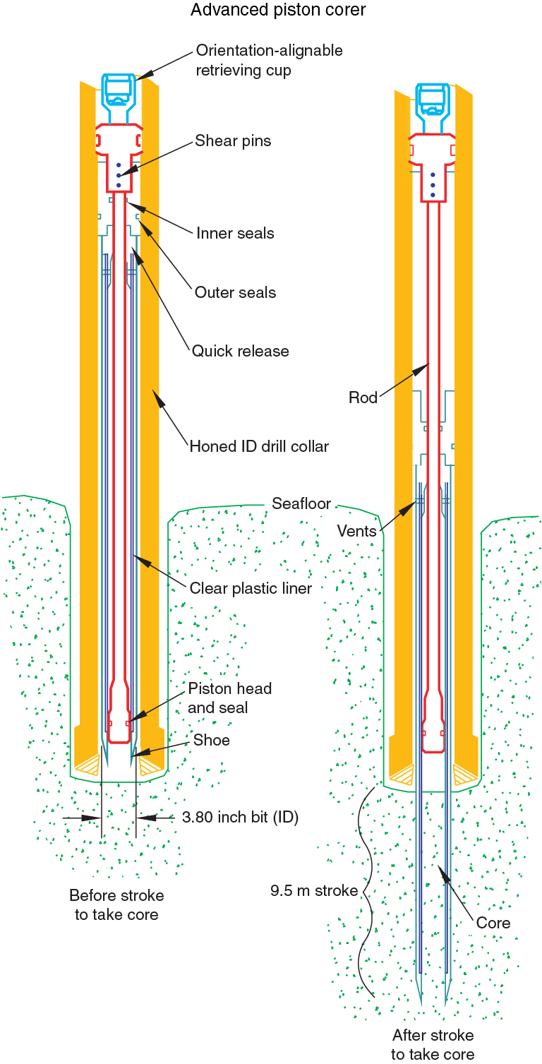
Figure F1. Schematic of the APC system.
APC refusal is conventionally defined in two ways: (1) the piston fails to achieve a complete stroke (as determined from the pump pressure reading) because the formation is too hard or (2) excessive force (>60,000 lb; ~267 kN) is required to pull the core barrel out of the formation. When a full stroke could not be achieved, additional attempts were typically made, and after each attempt the bit was advanced by the length of recovered core. The number of additional attempts is generally dictated by the length of recovery of the partial stroke core and the time available to advance the hole by piston coring. Note that this process results in a nominal recovery of ~100% based on the assumption that the barrel penetrates the formation by the equivalent of the length of core recovered. When a full or partial stroke is achieved but excessive force cannot retrieve the barrel, the core barrel is sometimes “drilled over,” meaning that after the inner core barrel is successfully shot into the formation, the drill bit is advanced to total depth to free the APC barrel.
The standard (full) APC system contains a 9.5 m long core barrel, whereas the HLAPC system uses a 4.8 m core barrel. In most cases, the HLAPC is deployed after the full APC reaches refusal. During the use of the HLAPC, we applied the same criteria for refusal as with the full APC system. Use of this technology allowed for deeper continuous piston coring than would have otherwise been possible with the standard APC.
Nonmagnetic core barrels were used during all APC coring to a pull force of ~40,000 lb. Steel core barrels were used for the XCB system. In addition, full-length APC cores recovered during Expedition 363 were oriented using the Icefield MI-5 or FlexIT core orientation tools (see Paleomagnetism). We also used the advanced piston corer temperature tool (APCT-3) to obtain in situ formation temperatures in the first deep hole at each site to determine the geothermal gradient and estimate heat flow (see Physical properties). At Site U1489, we collected a second set of APCT-3 formation temperature measurements in Hole U1489D because the data from Hole U1489B showed disturbances likely resulting from excessive ship motion.
The XCB system was used to advance the hole when APC or HLAPC refusal occurred before the target depth was reached or when the formation became either too stiff for APC coring or hard substrate was encountered. The XCB is a rotary system with a small cutting shoe that extends below the large rotary APC/XCB bit. The smaller bit can cut a semi-indurated core with less torque and fluid circulation than the main bit, optimizing recovery. The XCB cutting shoe (bit) extends ~30.5 cm ahead of the main bit in soft sediments but retracts into the main bit when hard formations are encountered (Figure F2).

Figure F2. Schematic of the XCB system.
The bottom-hole assembly (BHA) constitutes the lowermost part of the drill string. The configuration of the BHA is reported in the operations section in each site chapter. A typical APC/XCB BHA consists of a drill bit (outer diameter = 11⁷⁄₁₆ inches), a bit sub, a seal bore drill collar, a landing saver sub, a modified top sub, a modified head sub, a nonmagnetic drill collar (for APC/XCB), a number of 8¼ inch (~20.32 cm) drill collars, a tapered drill collar, six joints (two stands) of 5½ inch (~13.97 cm) drill pipe, and one crossover sub. A lockable float valve was used when downhole logging was planned so that downhole logs could be collected through the bit. In some cases, the drill string was drilled or “washed” ahead without recovering sediments to advance the drill bit to a target depth to resume core recovery. Such intervals were typically drilled using a center bit installed within the APC/XCB bit.
IODP depth scales
Primary depth scale types are based on the measurement of drill string length deployed beneath the rig floor (drilling depth below rig floor [DRF] and drilling depth below seafloor [DSF]), the length of core recovered (core depth below seafloor [CSF] and core composite depth below seafloor [CCSF]), and the length of the logging wireline deployed (wireline log depth below rig floor [WRF], wireline log depth below seafloor [WSF], and wireline log matched depth below seafloor [WMSF]). All depth units are in meters. The relationship between scales is defined either by protocol, such as the rules for computation of CSF from DSF, or by combinations of protocols with user-defined correlations (e.g., CCSF). The distinction in nomenclature should keep the user aware that a nominal depth value at two different depth scales usually does not refer to exactly the same stratigraphic interval (see Curatorial procedures and sample depth calculations). For more information on depth scales, see “IODP Depth Scales Terminology” at http://www.iodp.org/policies-and-guidelines. To more easily communicate shipboard results, CSF-A depths are reported in this volume as meters below seafloor (mbsf) unless otherwise noted.
Depths of cored intervals are measured from the drill floor based on the length of drill pipe deployed beneath the rig floor (DRF scale). The depth of the cored interval is referenced to the seafloor (DSF scale) by subtracting the seafloor depth at the time of the first core from the DRF depth of the interval. During Expedition 363, the seafloor depth is the length of pipe deployed minus the length of the mudline core recovered.
Standard depths of cores on the CSF-A scale are determined based on the assumptions that (1) the top depth of a recovered core corresponds to the top depth of its cored interval (DSF scale) and (2) the recovered material is a contiguous section even if core segments are separated by voids when recovered. Voids in the core are closed by pushing core segments together, if possible, during core handling. This convention is also applied if a core has incomplete recovery, in which case the true position of the core within the cored interval is unknown and should be considered a sample depth uncertainty, up to the length of the core barrel used, when analyzing data associated with the core material. Standard depths of subsamples and associated measurements (CSF-A scale) are calculated by adding the offset of the subsample or measurement from the top of its section, as well as the lengths of all shallower sections in the core, to the top depth of the cored interval.
A soft to semisoft sediment core from less than a few hundred meters below seafloor expands upon recovery (typically a few percent to as much as 15%), so the length of the recovered core can exceed that of the cored interval. Therefore, a stratigraphic interval may not have the same nominal depth at the DSF and CSF scales in the same hole. When core recovery (the ratio of recovered core to cored interval) is >100%, the CSF depth of a sample taken from the bottom of a core will be deeper than that of a sample from the top of the subsequent core (i.e., the data associated with the two core intervals overlap on the CSF-A scale).
CCSF depth scales are constructed for sites, whenever feasible, to mitigate the CSF-A core overlap problem, as well as the coring gap problem and to create as continuous a stratigraphic record as possible. Using shipboard core logger–based physical property data, verified with core photos, core depths in adjacent holes at a site are vertically shifted to correlate between cores recovered in adjacent holes. This process produces the CCSF depth scale. The correlation process results in affine tables, indicating the vertical shift of cores on the CCSF scale relative to the CSF-A scale. Once the CCSF scale is constructed, a splice can be defined that best represents the stratigraphy of a site by utilizing and splicing the best portions of individual sections and cores from each hole. Because of core expansion, the CCSF depths of stratigraphic intervals are typically 10%–15% deeper than their CSF-A depths. CCSF depth scale construction also reveals that coring gaps on the order of 1.0–1.5 m typically occur between two subsequent cores, despite the apparent >100% recovery. For more details on construction of the CCSF depth scale, see Stratigraphic correlation.
Core handling and analysis
Cores recovered during Expedition 363 were extracted from the core barrel in 67 mm diameter plastic liners. These liners were carried from the rig floor to the core processing area on the catwalk outside the Core Laboratory, where they were split into ~1.5 m sections. Liner caps (blue = top; colorless = bottom; yellow = whole-round sample taken) were glued with acetone onto liner sections on the catwalk by the marine technicians. The length of each section was entered into the database as “created length” using the Sample Master application. This number was used to calculate core recovery.
As soon as cores arrived on deck, headspace samples were taken using a syringe for immediate hydrocarbon analysis as part of the shipboard safety and pollution prevention program. Core catcher samples were taken for biostratigraphic analysis. Whole-round samples were taken from some core sections for shipboard and postcruise interstitial water analyses.
Whole-round core sections were immediately run through the Special Task Multisensor Logger (STMSL) when necessary for stratigraphic correlation after being cut on the catwalk. The STMSL measures gamma ray attenuation (GRA) bulk density and magnetic susceptibility and is used to aid in real-time stratigraphic correlation. For Sites U1488 and U1490, low magnetic susceptibility made stratigraphic correlation difficult and so the Whole-Round Multisensor Logger (WRMSL) was used as the “fast track” logging system to quickly measure P-wave velocity (see Stratigraphic correlation and Physical properties). After measurement, these cores were placed on the core racks in the laboratory. Cores not run through the STMSL or WRMSL first were immediately placed in core racks after being cut on the catwalk. When the cores reached equilibrium with laboratory temperature (typically after ~4 h), whole-round core sections were run through the WRMSL and the Natural Gamma Radiation Logger (NGRL). For Sites U1488 and U1490, the STMSL was used to collect higher resolution magnetic susceptibility and GRA bulk density data when the WRMSL was employed as the fast track. Additionally, we also ran some core sections through the NGRL prior to equilibration to speed up core flow through the laboratory. Thermal conductivity measurements were typically taken at a rate of one per core (see Physical properties). The core sections were then split lengthwise from bottom to top into working and archive halves. Investigators should note that older material may have been transported upward on the split face of each section during splitting.
The working half of each sedimentary core was sampled for shipboard (biostratigraphy, physical properties, carbonate, paleomagnetism, and X-ray diffraction [XRD]) analyses. The archive half of all cores was scanned on the Section Half Imaging Logger (SHIL) with a line scan camera at 20 pixels/mm and measured for color reflectance and magnetic susceptibility on the Section Half Multisensor Logger (SHMSL). At the same time, the archive halves were described visually and by means of smear slides and thin sections (see Core description). All observations were recorded in the Laboratory Information Management System (LIMS; http://web.iodp.tamu.edu/LORE/) database using the DESClogik descriptive data capture application. After visual description, the archive halves were run through the cryogenic magnetometer (see Paleomagnetism). Finally, digital color close-up images were taken of particular features of the archive or working halves, as requested by individual scientists. All samples taken are recorded by the IODP curator. Sampling for personal postcruise research was deferred until a postcruise sampling meeting; however, shipboard residues were made available for scientists to request for postcruise analyses to guide personal sampling during the sampling meeting.
In preparation for storage, soft-sediment section-half cores were wrapped in plastic wrap. Sites U1484 and U1485 contain high total organic carbon and low carbonate content. In order to preserve the carbonate, the cores were shrink-wrapped with oxygen scrubbers. After wrapping, both halves of the core were put into labeled plastic tubes that were sealed and transferred to cold storage space aboard the ship. At the end of the expedition, the cores were transported from the ship to cold storage at the Gulf Coast Repository (GCR) at Texas A&M University in College Station, Texas. Shore-based sampling of the cores for postcruise research took place at the GCR ~6 months after the end of the expedition. Following the sampling meeting and completion of X-ray fluorescence core scanning, the cores were shipped to permanent cold storage at the Kochi Core Center (KCC) at Kochi University in Kochi, Japan. The KCC houses cores collected from the western Pacific Ocean, Indian Ocean, and Bering Sea.
Drilling disturbance
Cores may be significantly disturbed as a result of the drilling process and contain extraneous material as a result of the coring and core handling processes. In formations with loose sand layers, sand from intervals higher in the hole may be washed down by drilling circulation, accumulate at the bottom of the hole, and be sampled with the next core. The uppermost 10–50 cm of each core must therefore be examined critically during description for potential “fall-in.” Common coring-induced deformation includes the concave-downward appearance of originally horizontal bedding. Piston action may result in fluidization (flow-in) at the bottom of APC and HLAPC cores. Retrieval from depth to the surface may result in elastic rebound. Gas that is in solution at depth may become free and drive core segments within the liner apart. Both elastic rebound and gas pressure can result in a total length for each core that is longer than the interval that was cored and thus a calculated recovery of >100%. If gas expansion or other coring disturbance results in a void in any particular core section, the void can be closed by moving material if very large, stabilized by a foam insert if moderately large, or left as is. When gas content is high, pressure must be relieved for safety reasons before the cores are cut into segments. This is accomplished by drilling holes into the liner, which forces some sediment, as well as gas, out of the liner. These disturbances are described in the Core description sections in each site chapter and graphically indicated on the core summary graphic reports (visual core descriptions [VCDs]). In extreme instances, core material can be ejected from the core barrel, sometimes violently, onto the rig floor by high pressure in the core or other coring problems. This core material was replaced in the plastic core liner by hand and should not be considered to be in stratigraphic order. Core sections so affected are marked by a yellow label marked “disturbed,” and the nature of the disturbance is noted in the coring log.
Curatorial procedures and sample depth calculations
Numbering of sites, holes, cores, and samples follows standard IODP procedure (Figure F3). Drilling sites are numbered consecutively from the first site drilled by the D/V Glomar Challenger in 1968. Integrated Ocean Drilling Program Expedition 301 began using the prefix “U” to designate sites occupied by the United States Implementing Organization (USIO) platform, the JOIDES Resolution. For all IODP drill sites, a letter suffix distinguishes each hole drilled at the same site. The first hole drilled is assigned the site number modified by the suffix “A,” the second hole the site number and the suffix “B,” and so on.
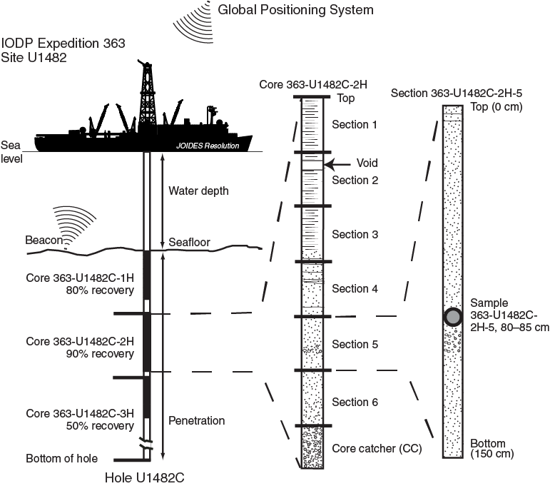
Figure F3. IODP conventions for naming sites, holes, cores, and samples.
Cores taken from a hole are numbered sequentially from the top of the hole downward. When an interval is drilled down, this interval is also numbered sequentially and the drill down designated by a “1” instead of a letter that designates the coring method used (e.g., 363-U1482B-191). Cores taken with the APC system are designated with “H,” “F” designates HLAPC cores, and “X” designates XCB cores. Core numbers and their associated cored intervals are unique in a given hole. Generally, maximum recovery for a single core is 9.5 m of sediment (APC) or 9.7 m of sediment (XCB) contained in a plastic liner (6.6 cm internal diameter) plus an additional ~0.2 m in the core catcher, which is a device at the bottom of the core barrel that prevents the core from sliding out when the barrel is retrieved from the hole. In certain situations, recovery may exceed the 9.5 or 9.7 m maximum. In soft sediments, this is normally caused by core expansion resulting from depressurization. High heave, tidal changes, and overdrilling can also result in an advance that differs from the planned 9.5/9.7 m.
Recovered cores are typically divided into 1.5 m sections that are numbered serially from the top downward, although occasionally sections will be cut slightly longer or shorter than 1.5 m. When full recovery is obtained, the sections are numbered 1–7, with the last section usually being <1.5 m. Rarely, an unusually long core may require more than seven sections. When the recovered core is shorter than the cored interval, by convention the top of the core is deemed to be located at the top of the cored interval for the purpose of calculating (consistent) depths. In sedimentary cores, the core catcher (CC) section is treated as a separate section. When the only recovered material is in the core catcher, it is placed at the top of the cored interval.
A full curatorial sample identifier consists of the following information: expedition, site, hole, core number, core type, section number, and interval in centimeters measured from the top of the core section. For example, a sample identification of “363-U1482C-2H-5, 80–85 cm,” represents a sample taken from the interval between 80 and 85 cm below the top of Section 5 of Core 2 (collected using the APC system) of Hole C of Site U1482 during Expedition 363 (Figure F3).
Authorship of site chapters
All shipboard scientists contributed to this volume. However, the separate sections of the site chapters and Expedition 363 methods chapter were written by the discipline-based groups of scientists listed below (authors are listed in alphabetical order; no seniority is implied):
- Background and objectives: A.E. Holbourn, D.K. Kulhanek, Y. Rosenthal
- Operations: K. Grigar, D.K. Kulhanek
- Core description: I.W. Aiello, S.C. Bova, J.-H. Chun, H. Dang, B.K. Linsley, N. Meinicke, B.N. Opdyke, T. Sagawa
- Biostratigraphy: L. Beaufort, T. Dunkley Jones, P.P.B. Eichler, A.G. Salazar Fernando, T. Li, P.N. Pearson, C.R. Poole
- Paleomagnetism: R.G. Hatfield, Y. Kumagai
- Physical properties: A.J. Drury, A. Schmitt, J.B. Wurtzel, J. Xu
- Stratigraphic correlation: G.S. Mountain, A.C. Ravelo
- Geochemistry: T.L. Babila, G. Bayon, K.A. Gibson, D.L. Johnson, M. Yamamoto, Y.G. Zhang
- Downhole measurements: G.S. Mountain, A. Schmitt
Core description
The descriptions of the sediment cores recovered during Expedition 363 are based on a combination of visual core description (VCD), smear slide and thin section examination under a petrographic microscope, XRD, digital color imaging, spectrophotometry, and visual color determination. The methods employed are adapted from those used during Ocean Drilling Program (ODP) Leg 199 (Shipboard Scientific Party, 2002) and Integrated Ocean Drilling Program Expeditions 320/321 (Expedition 320/321 Scientists, 2010; Mazzullo et al., 1988), and 323 (Expedition 323 Scientists, 2011).
Visual core description
VCDs of the archive half of the split cores provide a summary of the lithologic, age (based on biostratigraphy and magnetostratigraphy), and physical property data obtained during shipboard analyses (Figure F4). IODP VCDs are equivalent to the “barrel sheets” used during the Deep Sea Drilling Project (DSDP) and ODP. Lithologic data for VCDs are recorded digitally in real time using the DESClogik software application (version 16.1.0.7; see DESCWKB in Supplementary material). Prior to operations, a spreadsheet template with five tabs was constructed in Tabular Data Capture and customized for Expedition 363. The tabs were used to record the following information:
- Drilling disturbance,
- General (lithologic core description and bioturbation intensity),
- Detail (higher level detail than general core description),
- Core summary (written description of major lithologic findings by core, lithologic unit, and age), and
- Hole summary (lithologic unit and age).

Figure F4. Example VCD form.
To aid core description, core data are displayed graphically in LIMSpeak, a separate browser-based application that displays core images alongside physical property and geochemical data. Visual core description was initially carried out on paper printouts of VCDs. Reporting included notes and observations, drawings of sedimentary structures, Munsell colors, and the location of samples collected for smear slides and XRD. The VCD form used was based on Mazzullo et al. (1988; figure 7). The handwritten notes were then transferred into Desklogic.
The Strater software package was used to compile the VCDs for each core. Site, hole, and core number are given at the top of the VCD together with a summary core description. The written description for each core contains a succinct overview of major and minor lithologies, their Munsell colors, and notable features such as sedimentary structures and major disturbances resulting from the coring process (Figure F4). Core depth below seafloor (mbsf), core length (recorded in centimeters), section breaks, lithologic unit, and age are indicated along the left side of the digital color image of the core. The two columns between the color image and the graphic lithology columns show the locations of shipboard samples and tephra (ash) layers. Columns to the right of the graphic lithology column show drilling disturbance, bioturbation intensity, lithologic accessories, sedimentary structures, and physical property data collected by the WRMSL and SHMSL (see Physical properties). These include natural gamma radiation (NGR), lightness (L*) and color (a* and b*) as determined by color reflectance, and magnetic susceptibility. Symbols used in the VCDs are given in Figure F5.
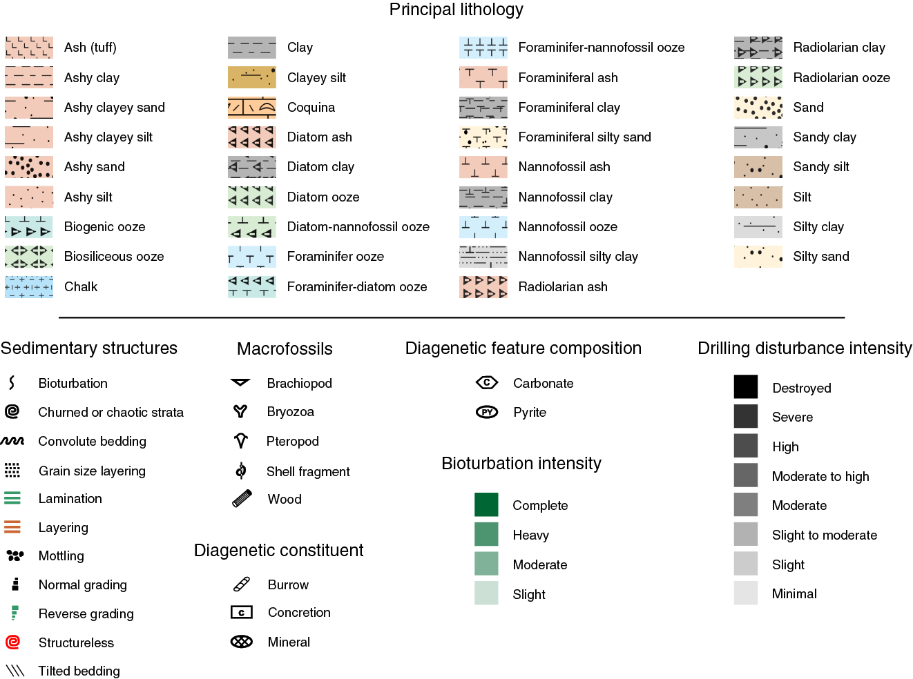
Figure F5. Symbols for VCD graphic reports.
Digital color image
The SHIL images the flat face of the archive half of the split cores using a line-scan camera. Sediment cores are split, and the archive half is scraped with the edge of a glass slide or stainless steel rectangular plate to provide a “clean” surface for imaging. The cleaned, flat face of the archive section halves are imaged as soon as possible after splitting and surface scraping to minimize color changes that may occur through oxidation and drying. Images are taken at an interval of 10 lines/mm. Camera height is preadjusted so that image pixels are square. Light is provided by three pairs of Advanced Illumination high-current focused LED line lights with fully adjustable angles to the lens axis. Note that compression of line-scanned images into compiled stacks (like the core image shown in the VCDs) may result in visual artifacts (e.g., the false appearance of lamination).
Sediment classification
Our approach for sediment classification consists of two parts: a principal name (e.g., silt) and one or more prefixes (e.g., foraminifer-rich; foraminifer- and clay-rich). The principal name applied to a sediment is determined by the component or group of components making up >60% of the sediment. For example, sediment composed of 70% silt-sized siliciclastic material and 30% foraminifers would be classified as a foraminifer-rich silt. The naming scheme for sediments with subequal mixtures of biogenic and siliciclastic and/or volcanogenic material is described below (see Mixed sediment). Visual percentage estimates of biogenic, nonbiogenic, and textural features (grain size) are made from smear slides following the visual estimate methods reported by Rothwell (1989) (Figure F6) (see Smear slide description for more details). The principal names are determined as follows.
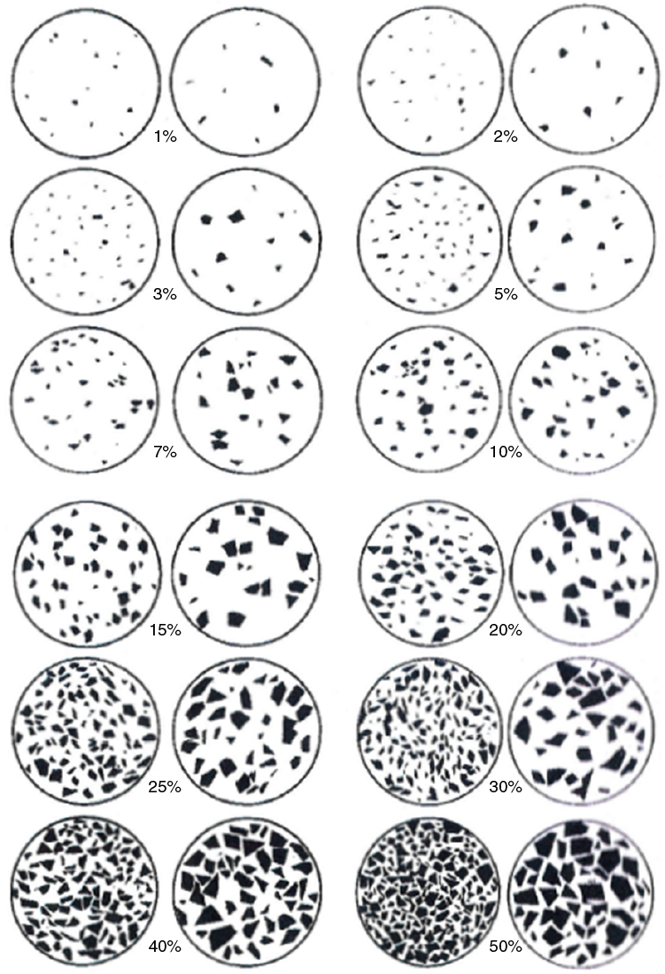
Figure F6. Visual composition chart for sedimentary components.
Siliciclastic sediment
If total siliciclastic content is >60%, the principal name is determined by the texture of the siliciclastic grains (i.e., the relative proportions of sand-, silt-, and clay-sized grains when plotted on a modified Shepard [1954] ternary classification diagram) (Figure F7A). The siliciclastic principal names are clay, silt, sand, silty clay, sandy clay, clayey silt, sandy silt, clayey sand, and silty sand.
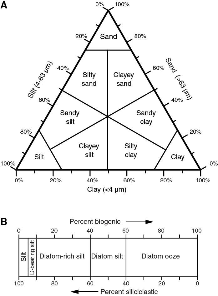
Figure F7. Lithologic classification.
Biogenic sediment
If total biogenic content is >60% (i.e., siliciclastic is <40%), the principal name applied is ooze, chalk, or chert depending on the degree of lithification and composition. Ooze refers to biogenic sediment that can be deformed with a finger. Chalk refers to an indurated sediment mainly composed of calcareous microfossils showing different degrees of preservation that can be easily scratched with a fingernail. Chert is used for dominantly siliceous lithologies which display conchoidal fracturing and semitransparent, glassy luster. Note that in some cases the complete recrystallization of the original biocalcareous or biosiliceous components can make identification of the original (prediagenesis) sediment difficult or impossible. Moreover, nonbiogenic particles of amorphous silica (e.g., volcanogenic glass) can also recrystallize during diagenesis and produce indurated siliceous rocks that have characteristics similar to those composed of biogenic particles. The major modifier consists of the name(s) of the major fossil group(s) composing at least 40% of the biogenic fraction. Biogenic components are not described in textural terms. Thus, the principal name of sediment containing 65% sand-sized foraminifers and 35% siliciclastic clay is foraminifer ooze, not foraminifer sand.
Volcanogenic sediment
Volcanogenic sediments are composed of more than 60% volcanogenic grains. Volcanogenic sediments include volcanogenics (volcanogenic detritus that is produced by erosion of volcanogenic rocks by wind, water, and ice), pyroclastic sediments including volcanogenic ash and tephra (fragments of rock that are produced when magma or rock is explosively ejected), and hydroclastic sediments (the products of the granulation of volcanogenic glass by steam explosions). The principal name applied to sediment containing >60% ash (i.e., siliciclastic and biogenic components total <40%) is ash. Ash components, like biogenic components, are not described in textural terms.
As mentioned in the previous section, the diagenesis of sediments dominated by ash can create siliceous rocks that have characteristics similar to the biogenic-derived ones and they have been identified as chert.
Mixed sediment
Mixed sediment includes sediment in which no one type of sedimentary component (siliciclastic, biogenic, or volcanogenic) is dominant (>60%). If siliciclastic grains compose 40%–60% of the sediment, the principal name is determined by the texture of the siliciclastic grains. For example, the principal name of a sample containing 10% ash, 40% diatoms, and 50% siliciclastic grains that are >75% silt sized is a diatom silt. If the abundances of diatoms and siliciclastic grains were reversed (i.e., 50% diatoms and 40% siliciclastic), the principal name is still diatom silt, as neither comprises >60% of the sediment.
If ash and biogenic components each comprise between 40% and 60% of the sediment, the principal name is ash. The major modifier consists of the name of the major fossil group. For example, the principal name of a sample containing 5% siliciclastics, 10% foraminifers, 40% nannofossils, and 45% ash is nannofossil ash.
Prefixes
If a sediment type composes 5%–40% of the sediment and this group is not included as part of the principal name, minor modifiers are used. When a microfossil group, a siliciclastic group, or ash composes 10%–40% of the sediment, a minor modifier consisting of the component name hyphenated with the suffix “rich” (e.g., diatom-rich clay, silt-rich foraminifer ooze) is used. When a microfossil group, siliciclastic group, or ash composes 5%–10% of the sediment, a minor modifier consisting of the component name hyphenated with the word “bearing” (e.g., diatom-bearing clay, ash-bearing clayey silt) is used. When two minor components are present, minor modifiers are listed before the principal name in order of increasing abundance. For example, sediment with 15% foraminifers, 30% nannofossils, and 55% clay is foraminifer-rich nannofossil-rich clay; a sediment with 5% diatoms, 15% radiolarians, and 80% clay is diatom-bearing radiolarian-rich clay (Figure F7B).
Smear slide description
One or more smear slide samples of the main lithologies were collected from the archive half of each core to define the lithologies. Additional samples were sometimes collected to characterize minor lithologies and small-scale sedimentary structures such as laminations and ash layers. A small amount of sediment was taken by toothpick from the cores and dispersed evenly in deionized water on a glass slide to create a very thin (less than ~50 μm) uniform layer of sediment grains for quantification. The dispersed sample was then dried on a hot plate. A drop of mounting medium (Norland optical adhesive 61) and a cover glass were added, and then the slide was placed in an ultraviolet light box for 15 min to cure.
Smear slides were examined and photographed with a Zeiss transmitted-light petrographic microscope (Axioskop USG90207) equipped with a standard eyepiece micrometer. Visual percentage estimates of biogenic, nonbiogenic, and textural features were made from each slide using a 40× objective. Biogenic and mineral component percentage abundances were visually estimated following Rothwell (1989) (Figure F6). Grain size distributions of clay (<4 µm), silt (4–63 µm), and sand (>63 µm) were estimated using an eyepiece micrometer, calibrated using an inscribed stage micrometer. The texture of siliciclastic grains (relative abundance of sand-, silt-, and clay-sized grains) and the proportions and presence of biogenic and mineral components were recorded on a smear slide sample sheet (Figure F8). Because sand-sized and larger grains are difficult to incorporate into a smear slide, analyses may underestimate their abundance. Clay minerals can also be difficult to identify, due to their small size.
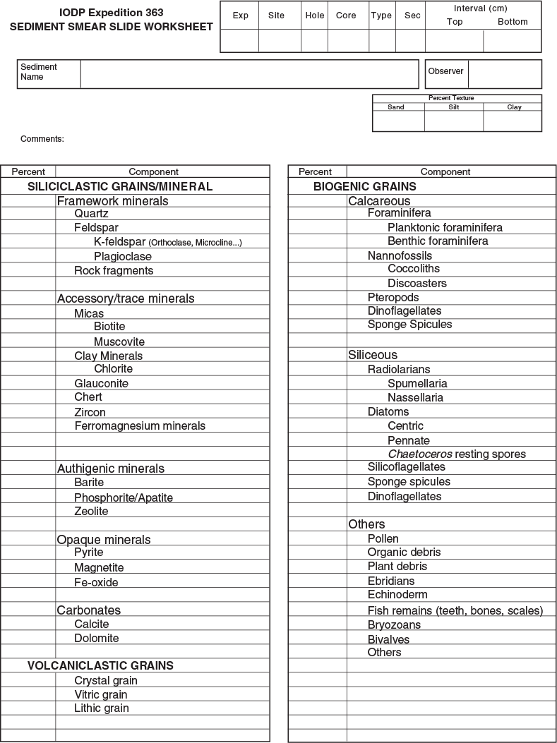
Figure F8. Sediment smear slide worksheet.
Spectrophotometry, visual color determination, and point magnetic susceptibility
Spectrophotometry and point magnetic susceptibility of the archive section halves were measured with the SHMSL. The SHMSL was set to take measurements every 2.5 cm, with the exception of empty intervals, cracks, and intervals where the top surface was below the level of the core liner. This was done to avoid spurious measurements. Magnetic susceptibility was measured with a Bartington Instruments MS2E point sensor (high-resolution surface-scanning sensor). Because the SHMSL demands flush contact between the magnetic susceptibility point sensor and the split core, measurements were made on the archive halves of split cores that were covered with clear plastic wrap. Measurement resolution is 1.0 SI, and each measurement integrated a volume of 10.5 mm × 3.8 mm × 4 mm, where 10.5 mm is the length perpendicular to the core axis, 3.8 mm is the width along the core axis, and 4 mm is the depth into the core. Only one measurement was taken at each measurement position.
Reflectance of visible light from the archive halves of sediment cores was measured using an Ocean Optics USB4000 spectrophotometer mounted on the automated SHMSL. Measurements were taken at 2.5 cm spacing to provide a high-resolution stratigraphic record of color variation for visible wavelengths. Each measurement was recorded in 2 nm wide spectral bands from 400 to 700 nm. Data are converted to L*, a*, b* and X, Y, Z color reflectance parameters for efficient archival and display. Both zero and white calibrations were conducted before measurement on each core. Additional detailed information about measurement and interpretation of spectral data can be found in Physical properties, Balsam et al. (1997, 1998), and Balsam and Damuth (2000).
In addition to the digital color image captured by the SHIL, VCDs include a description of sediment color and the corresponding hue, value, and chroma data as determined qualitatively using Munsell Soil Color Charts for each major and minor lithology (Munsell Color Company, Inc., 1994).
Sedimentary structures
Sedimentary structures formed by natural processes (i.e., not a result of drilling disturbance) are represented on the VCD with symbols in the Sedimentary structures column (see Figure F5 for structure symbols). Structures formed by both biogenic and physical processes are included.
An estimate of bioturbation intensity is indicated on the VCD. Bioturbation intensity is classified as
- Absent: laminated sediment;
- Slight: sediment with still-visible horizontal bedding;
- Moderate: sediment with obvious burrows;
- Heavy: sediment with a nearly uniform appearance and rare burrows; and
- Complete: completely uniform (homogeneous) sediment with no obvious burrows or sedimentary layers.
When identifiable, ichnofossils such as Zoophycos, Chondrites, Planolites, and Skolithos burrows were reported in the lithologic description. All contacts between lithologies are gradational unless otherwise specified.
Drilling disturbance
Sediment disturbance resulting from the coring process (e.g., fall-in, flow-in, biscuits, and drilling breccia) is illustrated in the Drilling disturbance column on the VCD. The depth interval and the degree of disturbance are represented on the VCD using a grayscale color bar. Blank regions indicate an absence of drilling disturbance. Disturbance intensity is described using the following subjective scheme:
- Slight to moderate: bedding contacts are slightly bent or bowed;
- Moderate: bedding contacts strongly bent or bowed;
- Moderate to high: bedding contacts are disturbed but are likely still in the correct stratigraphic sequence;
- High: bedding contacts are present but are likely not in the correct stratigraphic sequence; and
- Destroyed: sediment shows no traces of the original bedding or structure.
Types of drilling disturbances observed in soft and firm sediment include the following:
- Fall-in: out-of-place material at the top of a core that has fallen downhole onto the cored surface (this type of disturbance is considered high to destroyed);
- Bowed: bedding contacts are slightly to moderately deformed but still subhorizontal and continuous (this type of disturbance is considered slight to moderate);
- Upward-arching: material retains its coherency, with material closest to the core liner bent downward. This is most apparent when horizontal features are distorted (this type of disturbance is considered slight to moderate);
- Void: empty space within the cored material (e.g., caused by gas expansion during core retrieval). Voids may also be related to partial strokes during the coring process (this type of disturbance is considered destroyed);
- Flow-in, coring/drilling slurry, along-core gravel/sand contamination: soft-sediment stretching and/or compressional shearing structures are severe and are attributed to coring/drilling. The particular type of deformation may also be noted (e.g., flow-in, gas expansion, etc.) (this type of disturbance is considered high to destroyed);
- Soupy or mousse-like: intervals are water saturated and have lost all aspects of original bedding (this type of disturbance is considered high to destroyed);
- Biscuit: sediment of intermediate stiffness shows vertical variations in the degree of disturbance. Softer intervals are washed and/or soupy, whereas firmer intervals are relatively undisturbed (this type of disturbance is considered moderate to high);
- Cracked or fractured: firm sediment is broken during drilling but not displaced or rotated significantly (this type of disturbance is considered moderate); and
- Fragmented or brecciated: firm sediment that is pervasively broken by drilling and may be displaced or rotated (this type of disturbance is considered moderate to destroyed).
Volcanogenic ash
Volcanogenic ash layers >1 cm thick are identified on the VCD to the left of the Graphic lithology column. Ash color and thickness are logged in DESClogik. In the site reports we also differentiate between tephra layers composed predominantly of glass shards, scoria, and pumice based on smear slide analysis, visual inspection of the core, and scanning electron microscope (SEM) imaging. Furthermore, at sites where ash layers occur regularly, bulk sample XRD analyses were performed on 3 or 4 representative ash layers.
Definition of lithologic units and subunits
Each site drilled during Expedition 363 was divided into units to highlight major lithologic changes downhole. These were established where a prominent change in sediment lithology matched changes in other sediment characteristics including color reflectance, magnetic susceptibility, and other physical properties. When more subtle yet significant changes were observed within a unit, the unit was further divided into subunits. Units are numbered in order from the top of the stratigraphic succession using Roman numerals. Subunits are distinguished from the main lithologic units by adding a letter to the unit number.
Shipboard sampling
VCDs display the locations of sample material taken for shipboard analysis (whole-round and discrete samples taken to aid core description). Whole-round samples consist of material taken for interstitial water and paleontological analyses. Samples taken to aid core description include toothpick samples for microscopic analyses using both transmitted light and scanning electron microscopy, as well as 5–10 cm3 samples for mineralogical XRD analysis; moisture and density (MAD); weight percent carbonate, carbon, nitrogen, and hydrogen; and paleomagnetism. Typically, one smear slide was prepared and examined per core; however, the number of smear slides analyzed was adjusted depending on the degree of lithologic variability in various parts of the core.
SEM and XRD analysis
SEM imaging of the bulk sediment as well as lithologic accessories (i.e., concretions) was performed to confirm smear slide identification of major and trace lithologic components using a Hitachi Tabletop TM3000 scanning electron microscope. The sample was mounted on a stub and secured on an exchange rod inside a vacuum chamber. If image quality was low, the sample was sputter coated with an ultrathin coating of gold palladium. Sputter coating reduces sample charging and improves secondary electron emission, which improves the signal-to-noise ratio. SEM images are available from the LIMS database.
Bulk sample XRD analyses were performed to assess lithologic components using a Bruker D-4 Endeavor X-ray diffractometer with a Vantec detector using Ni-filtered CuKα radiation. The number of XRD analyses depended on the degree of lithologic complexity in various parts of the core. Generally, we analyzed ~5–10 samples per site to assess the mineralogy of the bulk sediment and lithologic accessories. Samples were freeze-dried, ground in a metal ball mill, and top-mounted onto a sample holder prior to analysis. Instrument settings were as follows:
- Voltage = 40 kV.
- Current = 40 mA.
- Goniometer scan = 2°–70°2θ (air-dried samples).
- Step size = 0.01°2θ.
- Scan speed = 1.2°2θ/min.
- Count time = 0.5 s.
Bulk sample diffractograms were interpreted using the EVA software package, which enabled mineral identification and basic peak characterization (e.g., baseline removal and maximum peak intensity). Digital files are available from the LIMS database.
Biostratigraphy
Calcareous nannofossils, planktonic foraminifers, and benthic foraminifers were studied in core catcher samples at all sites. At most sites, samples from split core sections were also examined for both calcareous nannofossils and planktonic foraminifers as time allowed to provide more refined age determinations or to investigate where significant changes in lithology occurred. Nannofossils and planktonic foraminifers were used for biostratigraphy, and benthic foraminifers were used mainly to acquire estimates of paleobathymetry. Biostratigraphy focused mainly on the identification of biostratigraphic horizons (biohorizons) in the cores, generally the top (T) or base (B) of the stratigraphic range of a species, but also including top common (Tc) and base common (Bc) occurrences. For nannofossils, the top acme (Ta), base acme (Ba), base paracme (Bpa), and the crossover in abundance between two species (X) were also used; for planktonic foraminifers, coiling direction changes in certain species were used.
Identification of a sequence of biohorizons in stratigraphic order allowed the identification of biostratigraphic zones (biozones; often referred to simply as “zones”) and subbiozones (“subzones”) using standard schemes. Biohorizons are assumed to result from biological events (bioevents) in the past, such as migrations, extinctions, and evolutionary transitions. These biohorizons have been assigned absolute ages based on calibrations from other areas, mainly referenced to the paleomagnetic reversal timescale. These ages may or may not be accurate for the study sites because of diachrony and/or imprecise calibration. In some instances, we adopted revised calibrations based on experience during the expedition; these are highlighted on the relevant data tables.
The timescale used for Expedition 363 is that of Gradstein et al. (2012; GTS2012). Age assignments for bioevents are quoted on the astronomically tuned Neogene timescale of Hilgen et al. (2012; ATNTS2012) as used in Gradstein et al. (2012) and using recent compilations of bioevents for both planktonic foraminifers (Wade et al., 2011) and calcareous nannofossils (Raffi et al., 2006; Backman et al., 2012).
For division of the formal series of the timescales and their geochronologic equivalent epochs, we use informal subseries/subepoch terms such as “upper Pliocene” when referring to strata and “late Pliocene” when referring to time. These have a lower case modifier to emphasize their informal status in accordance with long-established DSDP/ODP/IODP policy, including the current style guidelines, and in accordance with a recent (2016) vote held by the Paleogene, Neogene, and Quaternary subcommissions of the International Commission on Stratigraphy (Finney and Bown, 2017; Pearson et al., 2017). We have not routinely used formal stages/ages such as Piacenzian, although these are shown in Figures F9 and F10. A special problem arises in the Pleistocene series where the International Chronostratigraphic Chart current at the time of Expediton 363 (version 2016/04; available at http://www.stratigraphy.org) indicates a formal Upper Pleistocene and Middle Pleistocene at the rank of stage. These terms are temporary placeholders for geographic names that are currently under discussion and awaiting formal ratification and definition (M. Head, Chair of the Subcommission for Quaternary Stratigraphy, pers. comm., 2016), which may be why they are given in italics on the chart. Therefore, we avoid these terms, although we do refer to upper/late Pleistocene and middle Pleistocene informally at the subseries rank with a lowercase modifier in a way that is consistent with our use of lower Pleistocene, upper Pliocene, and so on, as described above.
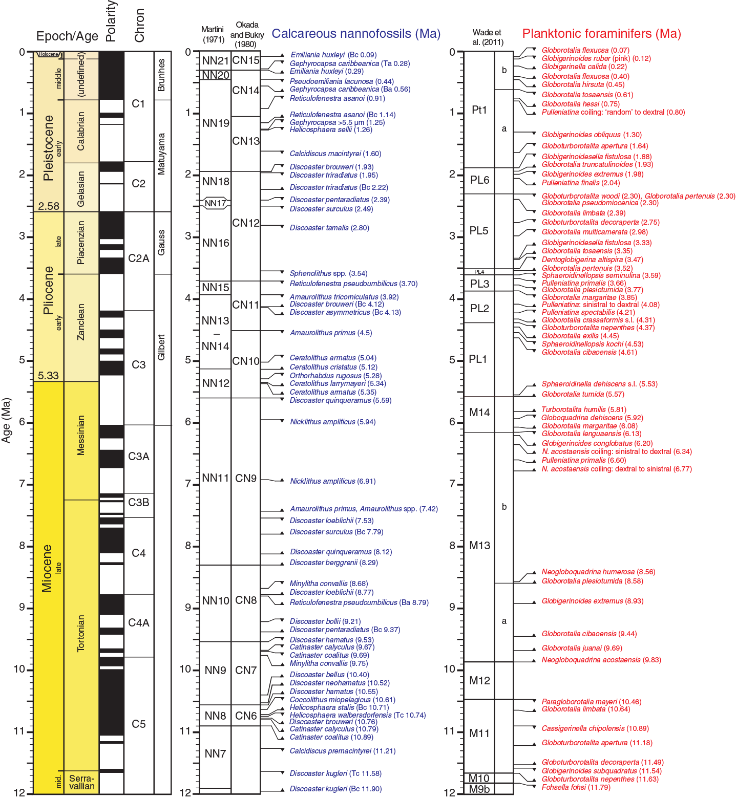
Figure F9. Biostratigraphic framework, 0–12 Ma.
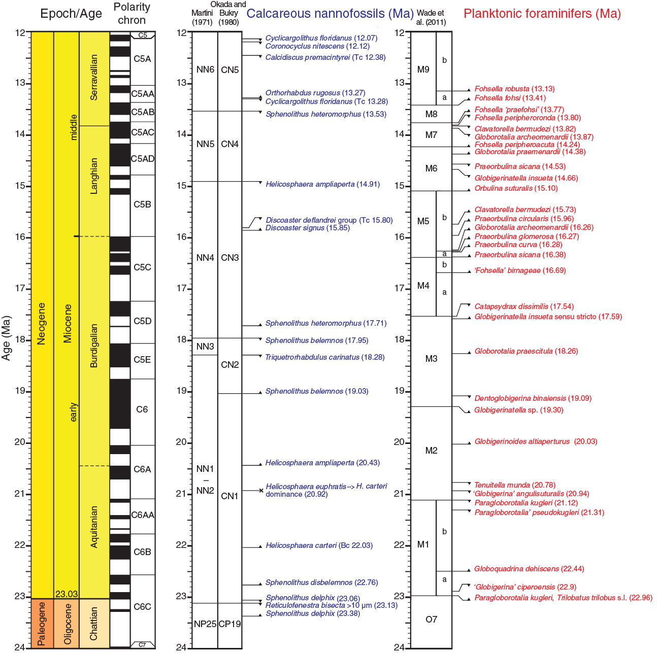
Figure F10. Biostratigraphic framework, 12–23.03 Ma.
All paleontological data gathered during shipboard investigations are available from the LIMS database in accordance with IODP policy. Data are in the form of taxonomic occurrence tables by sample studied for each hole and each taxonomic group (calcareous nannofossils, planktonic foraminifers, and benthic foraminifers). These data are provisional because taxonomic concepts evolved with experience during drilling, and time was insufficient to cross-check, intercompare, and revalidate all recorded occurrences and relative abundance estimates in the way that would be done in a more mature laboratory-based investigation. In particular, the study time that could be allocated to each sample was necessarily more limited than it would be otherwise, for instance in the search for rare species. The tables are also incomplete because the focus is mainly on biostratigraphic marker species close to their biohorizon levels plus other occurrences that were deemed interesting or noteworthy at the time (e.g., rare or unexpected species), whereas common species of little stratigraphic value are generally omitted. The taxonomic occurrence tables are also used to record suspected reworked or otherwise out-of-place species (e.g., through downhole contamination), although they are not distinguished as such. The provisional, incomplete, and systematically biased nature of the data makes them unsuitable for inclusion in meta-analytical studies that attempt to synthesize or compare patterns of species distributions or diversity in time or space.
Calcareous nannofossils
Calcareous nannofossil assemblages were examined and described from standard smear slides made from core catcher samples (at ~10 m intervals) and from mudline samples in multiple holes at each site. Additional toothpick samples were taken between core catcher samples from working half core sections when necessary to refine the stratigraphic position of bioevents. Typically, this sampling was at a resolution of 3 samples per core taken from one hole per site. Standard smear slides were made from bulk sediment. At sites where volcanogenic ash particles are very abundant, the sediment was sieved to isolate the <20 µm size fraction, which was then centrifuged and smeared onto microscopic slides. Slides were fixed with Norland optical adhesive Number 61 and cured under UV light for immediate biostratigraphic examination using a Zeiss Axioscope. Samples were analyzed under plane-transmitted, cross-polarized, phase-contrast, and/or circular-polarized light using oil immersion at a magnification of 1000×. All photomicrographs were taken using a SpotFlex camera with the IODP image capture software. Additional observations with a Hitachi TM3000 tabletop SEM were made to identify Emiliania huxleyi and verify the preservation state of calcareous nannofossils.
Nannofossil taxonomy follows Perch-Nielsen (1985), Aubry (1988, 1990), Young (1998), and Young and Bown (2014) as compiled in the online Nannotax 3 database (http://ina.tmsoc.org/Nannotax3). The compilations of Aubry (2015) were used as an additional taxonomic reference where necessary. The zonal scheme of Martini (1971) was used for calcareous nannofossil biostratigraphy (Neogene alphanumeric shorthand NN code) (Figures F9, F10; Table T1). This zonation represents a general framework for the biostratigraphic classification of middle- to low-latitude nannofossil assemblages. The zonal scheme of Okada and Bukry (1980; CN code), which provides a secondary framework that is more detailed in some intervals, is also shown. Zone NN13‒NN14 is undifferentiated due to difficulties in placing the Bc occurrence of Discoaster asymmetricus and the poor calibration of this event (see discussion in Backman et al., 2012).
Table T1. Cenozoic calcareous nannofossil bioevents. Download table in CSV format.
Biohorizons and bioevents were compiled from a range of sources, with assigned ages derived from the calibrations listed in Table T1 updated to ATNTS2012. A full taxonomic list for the bioevents is given in Table T2.
Table T2. Taxonomic list for calcareous nannofossil bioevents. Download table in CSV format.
The following qualitative abundance codes were used in the DESClogik data entry program and uploaded to the LIMS database.
Total calcareous nannofossil abundance within the sediment was recorded as
- D = dominant (>90% of sediment particles).
- A = abundant (>50%–90% of sediment particles).
- C = common (>10%–50% of sediment particles).
- F = few (1%–10% of sediment particles).
- R = rare (<1% of sediment particles).
- B = barren (none present).
Abundance of individual calcareous nannofossil taxa is based on specimens per field of view (FOV) at 1000× magnification:
- V = very abundant (>100 specimens per FOV).
- A = abundant (10–100 specimens per FOV).
- C = common (1–9 specimens per FOV).
- F = few (1 specimen per 2–10 FOV).
- R = rare (1 specimen per 11–100 FOV).
- P = present (1 specimen per >100 FOV).
Preservation of calcareous nannofossils was recorded as
- VG = very good (no evidence of dissolution and/or recrystallization, no alteration of primary morphological characteristics, and specimens identifiable to the species level).
- G = good (little or no evidence of dissolution and/or recrystallization; primary morphological characteristics unaltered or only slightly altered; specimens identifiable to the species level).
- M = moderate (specimens exhibit some etching and/or recrystallization; primary morphological characteristics somewhat altered; however, most specimens identifiable to the species level).
- P = poor (specimens were severely etched or overgrown; primary morphological characteristics largely destroyed; fragmentation has occurred; specimens often could not be identified at the species and/or generic level).
Planktonic foraminifers
Planktonic foraminifers were examined from core catcher samples and 3 additional samples per core from a minimum of one hole at most sites except for the high-sedimentation Sites U1484 and U1485, where only core catcher samples were examined. Planktonic foraminifers were also examined from mudline samples from the top of most holes as described in Benthic foraminifers.
Sample volumes of 10 or 20 cm3 were washed over 150 and 63 μm sieves, and then the two separated size fractions were dried on a hot plate at 40°C. Empty sieves were cleaned in an ultrasonic bath to minimize cross-contamination between samples and then rinsed in water dyed with methylene blue to stain any remaining foraminifers and highlight any contaminants in subsequent samples. Dried residues (>150 and 63–150 μm fractions) were transferred to labeled glass vials from which subsamples were examined on metal trays using binocular Zeiss Discovery V8 stereomicroscopes. Occasional specimens of special interest were removed for SEM study, but in general planktonic foraminifers were not picked (partly because the same residues were subsequently used to estimate planktonic/benthic foraminifer ratios).
Most shipboard work focused on the >150 μm size fraction for biostratigraphic purposes, but the 63–150 μm fraction was also examined for marker species and to assess fragmentation and scan for the smaller species. Selected specimens were imaged using a Spot RTS system with IODP image capture and commercial Spot software for photomicrographs. A Hitachi TM3000 tabletop SEM was used for higher magnification micrographs (primarily wall texture examination) of selected specimens.
The list of biohorizons and their age assignments and zonal schemes (Table T3) follows Wade et al. (2011; table 3) with two modifications:
- The list was edited to be relevant to the tropical Indo-Pacific Ocean only.
- The generic assignments of some species were updated according to Spezzaferri et al. (2015) and Pearson and Wade (2015).
Table T3. Neogene planktonic foraminifer bioevents. Download table in CSV format.
A full taxonomic list for the planktonic foraminifer bioevents is given in Table T4.
Table T4. Taxonomic list for planktonic foraminifer bioevents. Download table in CSV format.
Alphanumeric shorthand is given for the zones and subzones in Figures F9 and F10 and throughout the site chapters; the formal names are as in Wade et al. (2011) except that Zone PL6 is now the “Globigerinoidesella fistulosa Highest Occurrence Zone” because of the generic redesignation of the marker species. This zone is retained as Zone PL6 (where PL is shorthand for Pliocene) despite the fact that it now lies wholly within the Pleistocene series following the nontraditional (from the point of view of most deep-sea studies) definition of the Pliocene/Pleistocene boundary at 2.59 Ma (Gibbard et al., 2010).
The following planktonic foraminifer abundance categories relative to total sediment particles were estimated from visual examination of the dried sample in the >150 µm fraction as
- D = dominant (>30% of sediment particles).
- A = abundant (10%–30% of sediment particles).
- F = few (5% to <10% of sediment particles).
- R = rare (1% to <5% of sediment particles).
- P = present (<1% of sediment particles).
- B = barren.
Abundances of planktonic foraminifer species in their respective size fractions were estimated using the following scheme:
- A = abundant (>20% of the planktonic foraminifer assemblage).
- C = common (>10%–20% of the planktonic foraminifer assemblage).
- F = few (>5%–10% of the planktonic foraminifer assemblage).
- R = rare (1%–5% of the planktonic foraminifer assemblage).
- P = present (<1% of the planktonic foraminifer assemblage).
Planktonic foraminifer preservation as viewed under the light microscope was recorded as
- E = excellent, with most specimens having a “glassy” appearance indicating very little recrystallization and very little evidence of overgrowth or dissolution, and little abrasion.
- VG = very good, some show minor evidence of diagenetic overgrowth, dissolution, or abrasion; recrystallization may or may not have occurred.
- G = good, with some specimens showing signs of significant overgrowth, dissolution, or abrasion, and may show some infilling with cement or indurated sediment.
- M = moderate, with most specimens showing evidence of overgrowth, dissolution, and abrasion; tests generally infilled with cement or indurated sediment obscuring apertures.
- P = poor, with substantial diagenetic overgrowth, dissolution, and abrasion. Foraminifers can be fragmentary and difficult to identify because of major overgrowth and/or dissolution.
In addition to this fast visual estimation, samples from selected burial depths (generally ~100 m apart plus a sample from near the bottom of the hole) at each site were taken using the following protocol for more systematic evaluation of foraminifer preservation, primarily as a guide for future geochemical sampling:
- A low-power photomicrograph of the scattered >50 µm residue was taken with the light microscope in reflected light using a Zeiss Discovery V8 microscope and camera to record the visual appearance including discoloration, fragmentation, and test transparency and to provide an indication of the frequency of foraminifers relative to other microfossil groups and grain types.
- Selected specimens of planktonic and benthic foraminifers (in this case usually 3 specimens each of Trilobatus trilobus and Planulina wuellerstorfi) were imaged by light microscope and SEM using a Hitachi TM3000 tabletop SEM after coating with conductive gold-palladium. Low-power and high-power images of the wall texture were taken at standard magnifications.
- Specimens were removed from the SEM and gently broken on the SEM pedestal using a clean glass slide, rearranged if necessary under a binocular microscope, recoated with gold-palladium, and returned to the SEM. Images of the broken wall cross section and inner surface were taken in standard views and magnification to facilitate the comparison of preservation states between samples and sites.
All images are available from the LIMS database. Selected images were used to illustrate variations in preservation for each site.
Benthic foraminifers
Benthic foraminifers were examined from all core catcher sample residues (see Planktonic foraminifers) from one hole at each site. A full taxonomic list of benthic foraminifer taxa is given in Table T5. The identification of benthic foraminifer taxa was generally made on the >150 µm size fraction, but the 63–150 µm size fraction was also examined for distinctive taxa and to help assess preservation. The ratio of planktonic to benthic foraminifers was calculated from the >150 μm size fraction by counting at least 100 specimens. Taxonomic assignments mainly follow van Morkhoven et al. (1986), Jones (1994), and Holbourn et al. (2013).
Table T5. Taxonomic list for benthic foraminifer bioevents. Download table in CSV format.
Paleodepth estimates are based on van Morkhoven et al. (1986) using the following categories:
Shipboard age models
For each site, tables of biohorizons (calcareous nannofossils and planktonic foraminifers) were constructed listing the samples above and below which each biohorizon was identified and the midpoint depth (mbsf) between those samples. Biohorizons were numbered on these tables to correspond with the precoring bioevent master lists presented in Tables T1 and T3. Not every bioevent proved useful during the expedition, and some were located in some sites only. In three instances (the planktonic foraminifer bioevents B Globorotalia truncatulinoides, T Dentoglobigerina altispira, and T Globorotalia margaritae), we found that the precoring age calibrations were not applicable to the study area because of diachrony (either between ocean basins or across latitudes), and an alternative published tropical Indo-Pacific calibration was preferred. To avoid circular reasoning, we did not alter the precoring bioevent lists; instead, we indicated the citation for the revised calibration on the biohorizon tables. In several other cases, we found that certain biohorizons plotted consistently off the expected trend throughout the expedition, suggesting that the precoring calibration requires revision. We did not attempt to recalibrate any event during the expedition because we expect more precise formal recalibration will follow during postcruise research based on the full combined stratigraphic information from Expedition 363 sites including, in most cases, cyclostratigraphy. We indicated in the text when such issues arose.
The identified biohorizons were combined with the available magnetic reversal information (using reversal midpoint mbsf depths) on age-depth plots for each site, with biohorizons numbered consistently throughout the expedition according to the precoring master lists. Levels of inferred hiatuses and other disturbances were indicated on these plots. Biohorizons that were found to plot off the general trend were included and discussed in the accompanying text. In most cases, these plots were derived from a specific hole from which most of the biostratigraphic information was gathered; when data from multiple holes were combined, this is clearly indicated on the plots. The accompanying text highlights any major discrepancies or difficulties of interpretation that were encountered in establishing the preliminary shipboard age models.
Approximate ages for depths at each site can be estimated visually from the trend of the age-depth plots. In most cases, we chose not to indicate a “best fit” or preferred line of correlation because not all biohorizons are equally reliable, and we expect that formal age models will be developed postcruise based on composite depth scales and cyclostratigraphic tuning.
Paleomagnetism
Software and instrumentation
Paleomagnetic studies during Expedition 363 comprised routine measurements of the natural remanent magnetization (NRM) of archive-half sections before and after alternating field (AF) demagnetization. Remanence measurements and AF demagnetizations were made using the section-half superconducting rock magnetometer (SRM; 2-G Enterprises model 760-R). This instrument is equipped with direct-current superconducting quantum interference devices (DC-SQUIDs) and has an inline AF demagnetizer capable of reaching peak fields of 80 mT. The spatial measurement resolution estimated by the full width at half-height of the pickup coil response is <10 cm for all three axes (although the full sensitivity range extends over a sample length up to ~30 cm), yielding an assumed measured volume of ~100 cm3. The noise level of the SRM is reported as 2 × 10⁻⁹ Am2 based on tests during ODP Legs 186 and 200 (Richter et al., 2007). For measurement of a split core, the minimum measurable remanent intensities are ~2 × 10⁻⁵ A/m, with previous results suggesting intensities 2–5 times this value (~1 × 10⁻⁴ A/m) are likely to yield accurate results (Richter et al., 2007). We adopted the standard IODP magnetic coordinate system for archive halves (+x = vertical upward from the split surface of archive halves, +y = left-hand split surface when looking upcore, and +z = downcore) (Figure F11A, F11B). Data were stored using the standard IODP file format and automatically uploaded to the LIMS database using the newly developed Integrated Measurement System (IMS) software for the SRM that was first used during IODP Expedition 362 (McNeill et al., 2017).
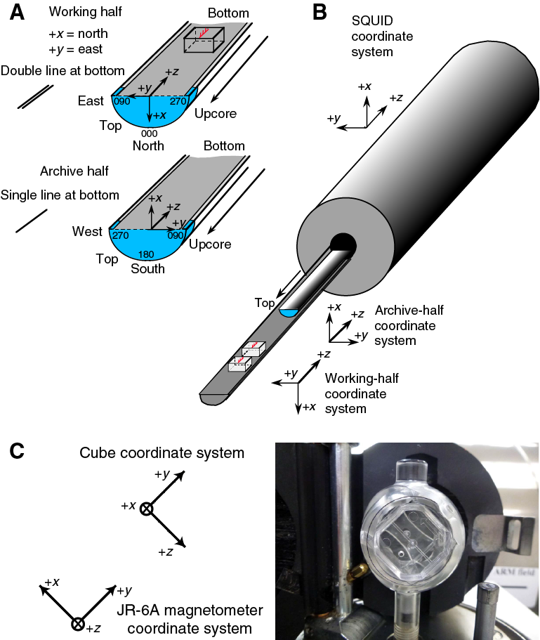
Figure F11. Coordinate systems for archive- and working-half core sections.
To cross-check the SRM data and to provide rock magnetic information on the carriers of the NRM, we took 1–3 discrete samples from the working half of each core recovered, typically from Hole A at each site. In some instances, coring was terminated in Hole A after a single core due to a missed mudline; in these cases, we took discrete samples from cores from the subsequent hole. Samples were taken using plastic “Japanese” Natsuhara-Giken sampling cubes (7 cm3 sample volume) that were pushed into the working half of the core by hand with the “up” arrow on the cube pointing upsection (–z axis) in the core (Figure F11A). Selection of representative intervals for discrete sampling was guided by the WRMSL magnetic susceptibility data, generally fine-grained intervals free from tephra or other discrete deposits (unless otherwise stated) and where drilling deformation was minimal or not visible. Discrete samples were measured on the JR-6A spinner magnetometer (sensitivity = ~2 × 10⁻⁶ A/m) under Remasoft 3.0 AGICO software control. To make the NRM data from working-half discrete samples directly comparable to the SRM data recovered from the archive half, we loaded the samples in the JR-6A spinner magnetometer following the cube coordinate system with the +x away from the user, +y upward to the right, and –z upward to the left (Figure F11C). To correct the cube coordinate system for the JR-6A magnetometer coordinate system, we applied an orientation correction (azimuth = 0°, dip = 90°) to each specimen in the Remasoft 3.0 AGICO software. Discrete paleomagnetic data were processed in Puffinplot software (Lurcock and Wilson, 2012) to produce demagnetization curves, Zijderveld diagrams (Zijderveld, 1967), and stereoplots and to calculate maximum angular deviation values from the principal component analysis of successive demagnetization steps (generally 15–40 mT) following Kirschvink (1980). All discrete data were manually uploaded to the LIMS database.
Core orientation
During APC and HLAPC operations, full-length and half-length nonmagnetic core barrels were used; full-length steel barrels were required for XCB coring (see Coring and drilling operations). Azimuthal correction of declination is crucial to help establish magnetostratigraphy at low-latitude sites; therefore, the Icefield MI-5 or FlexIT core orientation tool was deployed with all APC cores unless otherwise stated in the individual site chapters. These instruments use three orthogonally mounted fluxgate magnetometers to record orientation of the double lines (working half) scribed on the core liner with respect to magnetic north. Orientation tools record declination, inclination, and temperature to their internal memory every 6 s. Prior to firing the APC, the core barrel is held stationary for 5 min so that the best approximation of orientation can be made at the moment of APC penetration. Tools were switched every 8–12 h, well before the limits of both battery life and memory capacity were reached. The orientation tools can only be deployed with full-length APC cores. When sediment was recovered using the HLAPC, we used, where possible, observations from the final APC recovered core and observations across multiple holes to manually align declination to reflect expected periods of reversed or normal polarity, respectively. When sediment was recovered using the XCB, declination remains uncorrected. To obtain azimuthally corrected declination (DTrue) for APC cores, we follow the method of Richter et al. (2007):
DTrue = DObserved + MTF + MIGRF,
- DObserved = the measured declination output from the cryogenic magnetometer;
- MTF = the magnetic tool face angle (the angle between magnetic north and the double-line orientation mark on the core liner measured in a clockwise manner when the APC fired); and
- MIGRF = the site specific deviation of magnetic north from true north.
At Site U1481 during IODP Expedition 362, a rotational error was reported in the corrected declination using both the Icefield MI-5 and the FlexIT core orientation tools that yielded reversed directions (i.e., 180° instead of 0°) during a period of normal polarity (McNeill et al., 2017). Investigation and onboard testing revealed that this error was not observed during shipboard laboratory testing but only when mounted inside pressure casing on the sinker bars in the BHA of the drill string. It was concluded during Expedition 362 that this simply amounted to incorrect alignment of the Icefield MI-5 tool relative to the working-half reference and that a constant correction of ~180° could be used during sample processing (McNeill et al., 2017). During the port call prior to the beginning of Expedition 363, the Icefield MI-5 and FlexIT core orientation tools were both tested by the JOIDES Resolution Science Operator–Texas A&M University technical staff. This test consisted of orienting the tools with a compass to magnetic north followed by four 90° clockwise rotations so that the magnetic tool face was pointing in the north, east, south, west, and finally north directions, respectively. The resulting data (Figure F12) showed that the MTF of the Icefield MI-5 and FlexIT core orientation tools faithfully recorded the orientations the tools experienced during the test. The Icefield MI-5 core orientation tool was also tested inside its pressure casing; these tests yielded the same results (Figure F12).
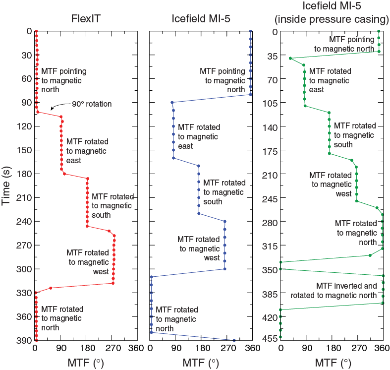
Figure F12. Orientation data from the FlexIT and Icefield MI-5 core orientation tools.
Orientation during Expedition 363 drilling operations at Sites U1482–U1487 revealed that the issues that affected DTrue during Expedition 362 continued to affect orientation during Expedition 363, with declination generally clustering around 180° (0°) for periods of normal (reversed) polarity. An exception to this was in Hole U1483C when this issue apparently self-corrected, with declination clustered around 0° (180°) for normal (reversed) polarity intervals. Conversations with the operations superintendent revealed nothing peculiar or different about coring operations in Hole U1483C compared to any other holes drilled during the expedition, and the specific tool used (Icefield tool #2007) had previously exhibited the 180° offset during orientation of Hole U1482B. No obvious cause for the error or apparent self-correction could be determined, and the cause of this offset remains unclear.
Although absolute values of declination appear correct for Hole U1483C, an additional declination error developed during azimuthal correction of Cores 363-U1483C-1H and 18H whereby DTrue values of several cores were ~45°–60° shallower than expected. This issue appeared again during operations in Hole U1485A, although this time it was accompanied by the persistent ~180° baseline offset. We concluded that this was likely a tool-specific issue (related to Icefield tool #2007), and after operations at Site U1485 we requested that Icefield tool #2007 not be used during the remainder of Expedition 363. For Sites U1486–U1490, we exclusively used Icefield tools #2052 and #2043. During azimuthal correction for Sites U1488–U1490, we again developed issues with declination shallowing superimposed on the 180° baseline offset as periods of normal polarity clustered between 90°–180° and reversed polarity between 270°–360°. These offsets generally remained consistent during tool deployment, thus enabling interpretation of polarity; however, in an isolated incident we had to assume a 90° MTF error to reconcile the declination data of Core 363-U1488B-6H with that measured in cores from Holes U1488A and U1488C over the same interval. Although these absolute offsets varied from site to site and often from hole to hole, relative shifts of 180° relating to changes in polarity were still observed and could be used for determination of magnetostratigraphy. Because of the varied, and often hole-specific, nature of these offsets, we do not apply the 180° correction detailed in McNeill et al. (2017) and leave the DTrue values as calculated following Richter et al. (2007).
Measurements and data acquisition program
At the beginning of every new hole and/or when deemed necessary we physically cleaned the sample boat with isopropyl alcohol and the tray runners with antistatic solution. The sample tray was then AF demagnetized using a peak field of 80 mT followed by a remanence measurement to maintain accurate tray correction values that were applied to each measured section. The NRM of archive halves of all APC and HLAPC core sections was measured unless precluded or made unreliable by coring-related disturbance. Core catchers were not routinely measured. Measurements were made at intervals of 2.5 cm with leader and trailer lengths of 15 cm. Using a track speed setting of 10 cm/s, one measurement per interval, and a delay between measurements of 25 ms, one three-axis AF demagnetization and subsequent section measurement at 2.5 cm intervals took ~4.5 min. Measurements without AF demagnetization took ~3 min.
The magnetic susceptibility of whole-round core sections was measured on two separate core logging systems (Table T6). Whole-round core sections were measured on the STMSL at 5 cm intervals to rapidly acquire magnetic susceptibility data for stratigraphic correlation (see Stratigraphic correlation and Physical properties). After whole-round core sections equilibrated to room temperature, measurements were made at 2.5 cm intervals on the WRMSL (see Physical properties). Additionally, point-source magnetic susceptibility measurements were made on the archive halves of split-core sections using the SHMSL at the same 2.5 cm spacing (see Core description and Physical properties).
Table T6. Typical physical properties sampling strategy. Download table in CSV format.
Discrete samples were first measured for NRM on the JR-6A spinner magnetometer before being subjected to manual three-axis AF demagnetization using the DTech AF demagnetizer (model D-2000) in incrementally increasing peak AF fields of 5, 10, 15, 20, (25), 30, 40, (60), and (80) mT. NRM was remeasured following each AF demagnetization step; demagnetization steps in parentheses were often dropped after Site U1482 to speed up measurement. In addition to NRM measurements, we measured bulk magnetic susceptibility on the Kappabridge (KLY 4), acquired an anhysteretic remanent magnetization (ARM) by demagnetizing the sample in a peak AF of 100 mT in the presence of a 0.05 mT DC bias field on the DTech AF demagnetizer, and acquired an isothermal remanent magnetization (IRM) in a DC field of 300 mT and a saturation IRM (SIRM) in a DC field of 1000 mT using the IM-10 impulse magnetizer. All remanence measurements were made on the JR-6A spinner magnetometer. Sample masses were recorded to facilitate mass-normalized estimations of magnetic susceptibility (χ), ARM, and IRM. ARM was corrected for the strength of the DC field to calculate susceptibility of ARM (χARM), and (inter)parametric ratios (e.g., IRM300mT/IRM1000mT, χARM/SIRM) were generated to provide estimates of magnetic grain size and magnetic mineralogy.
To characterize both the NRM behavior and the pervasiveness of the drill string overprint, we developed a four- to five-step demagnetization and measurement protocol for the first few SRM-measured sections from the first core recovered from Hole A at each site. This protocol involved measurement of the NRM before and after AF demagnetization in fields of 5, 10, 15, and sometimes 20 mT. We used these data in conjunction with the discrete sample data from Hole A that were demagnetized in peak AFs up to 40–80 mT to decide on the lowest peak field required to remove the drill string overprint. Low peak AF demagnetizations of 10–15 mT used during Expedition 363 ensured that archive halves remain useful for shore-based higher resolution U-channel or cube studies of NRM. Subsequent cores from the same site were only demagnetized using this single AF step following NRM measurement to maintain core flow through the laboratory. In summary, the measurement interval, number of demagnetization steps, and peak field used reflected the quality and demagnetization characteristics of the recovered sediments, the severity of the drill string magnetic overprint, the desire to keep peak AFs low, and the need to maintain efficient core flow through the laboratories.
Data presentation and magnetostratigraphy
Data presented for each hole includes the NRM intensity before and after peak AF demagnetization, inclination and declination (azimuthally corrected if available) after peak AF demagnetization, and WRMSL magnetic susceptibility. We also show rock magnetic properties based on analysis of discrete samples (inclination and declination of the same SRM peak AF field, and maximum angular deviation values calculated from principal component analyses over several AF demagnetization steps) and interstitial water geochemistry and methane concentration if diagenesis was regarded as an important influence on the magnetic assemblage within the sediment. Although the leader and trailer data were saved within the data files, we trim these intervals and the first and last 5 cm from the SRM data set in the presented figures because they are affected by volumetric differences associated with the response function of the SRM pickup coils. Disturbed intervals caused by coring or sedimentological variations (e.g., fall-in, suck-in, and/or unconsolidated material) or core sections that experienced strong flux jumps in intensity on the DC-SQUID were also manually removed before presentation. We use the uncompressed core depth below seafloor (CSF-A) depth scale (denoted as mbsf throughout the volume) to show data from each hole. Where shipboard AF demagnetization of core sections and discrete cubes appears to have removed the drill string overprint and isolated the characteristic remanent magnetization, we made an initial designation of magnetic polarity zones. The ATNTS2012 timescale (Hilgen et al., 2012) within the GTS2012 (Gradstein et al., 2012) was used as a reference for the ages of correlative Cenozoic polarity chrons (Table T7). We used the naming convention following that of correlative anomaly numbers prefaced by the letter C (Tauxe et al., 1984). Normal polarity subchrons are referred to by adding suffixes (n1, n2, etc.) that increase with age. For the younger part of the timescale (Pliocene–Pleistocene), we use the traditional names to refer to the various chrons and subchrons (e.g., Brunhes, Jaramillo, Olduvai, etc.; Laj and Channell, 2007). Normal polarity zones are denoted using black bars and reverse polarity zones with white bars in the classic “barcode diagram” presented in the figures. We determined the depth of a magnetic reversal to be the arithmetic midpoint between the last point of stable polarity and the first point of newly stable polarity. Because this can be a relatively subjective designation, we provide these depths alongside the midpoint in table form when we determine a reversal boundary.
Table T7. Geomagnetic polarity timescale. Download table in CSV format.
Physical properties
High-resolution physical property measurements were made during Expedition 363 to provide information on the bulk physical character and acoustic and elastic parameters of recovered sediment. Such data enhance our understanding of the physicochemical context and history for oceanic deposits, augment lithologic characterization, and facilitate the correlation of downhole logging data with discrete core measurements and core descriptions. In contrast to isotopic ratios and grain size distributions, physical property data can be measured quickly and as such serve as important first-order proxies for determining changes in environmental conditions, geological processes, and/or depositional environments. Shipboard physical property data play a key role in the following tasks:
- Completion of hole-to-hole correlation for construction of composite stratigraphic sections;
- Detection of discontinuities and inhomogeneities, either caused naturally or by the drilling process;
- Identification of differences in the composition and texture of sediments;
- Creation of time-series analysis for detection of orbital cycles and tuning to reference sections for stratigraphic purposes;
- Calculation of sedimentation rates;
- Completion of core-log-seismic integration; and
- Identification of major seismic reflectors and construction of synthetic seismic profiles.
A variety of techniques were used on whole-round sections, split-core sections, and discrete samples to characterize the physical properties of Expedition 363 cores. Before splitting, core sections were analyzed using three whole-round core logging systems: (1) the STMSL, (2) the WRMSL, and (3) the NGRL. In most instances, the STMSL was typically run for all holes requiring real-time stratigraphic correlation immediately after the core sections were brought on board. STMSL measurements were generally not collected for the first deep hole at each site (typically Hole A) because higher resolution WRMSL data were available for the first hole by the time stratigraphic correlation to subsequent holes was required. All holes were run on the WRMSL after equilibration for ~4–5 h to ambient laboratory temperature (20°–21°C). Following WRMSL scanning, whole-round sections were logged on the NGRL, which generates spectral gamma ray data. However, because NGR is not affected by temperature change, beginning with Site U1484, cores were measured on the NGRL immediately after being brought onboard to maximize the amount of time available for these measurements (see Natural gamma radiation for more details). Thermal conductivity was measured on one whole-round section per core (typically the third section) for soft-sediment cores and on a split core section once the sediment became too indurated. After whole-round measurements were completed, core sections were split longitudinally, with one half designated as the archive half and the other as the working half for sampling and destructive analyses. Four in situ downhole temperature measurements were made with the APCT-3, typically in Hole A at each site. These temperature measurements can be combined with the thermal conductivity measurements to calculate heat flow.
Discrete P-wave velocity was measured on the working halves, typically at a frequency of once per section. P-wave velocity measurements employed transducers oriented in the x-, y-, and z-axis directions on the Section Half Measurement Gantry (SHMG). P-wave y-axis velocity measurements were discontinued after the first site due to time constraints. Archive halves were measured with the SHMSL for color reflectance with an Ocean Optics sensor and magnetic susceptibility using a discrete point-source Bartington probe. Discrete samples were also typically collected from every other section of the working halves (~3 per core), primarily from Hole A, to measure wet bulk density, dry bulk density, water content, porosity, and grain density using MAD procedures. Subsequent holes were only sampled for MAD measurements if Hole A was cored to a shallower depth, there were extensive gaps in the Hole A sample series, unusual sediments were recovered in later holes with no equivalent in Hole A, or an interval in Hole A required validation.
An overview of the sampling strategy of physical property measurements is given in Table T6. A full discussion of all methodologies and calculations used in the Physical Properties laboratory aboard the JOIDES Resolution is available in Blum (1997).
Whole-round logger measurements (STMSL, WRMSL, and NGRL)
During Expedition 363, whole-round core logging operations recorded high-resolution GRA bulk density, magnetic susceptibility, P-wave velocity (WRMSL; Figure F13), and NGR (NGRL; Figure F14) data. The STMSL rapidly recorded medium-resolution GRA density and magnetic susceptibility data sets; this rapid data acquisition allowed for near-real-time stratigraphic correlation to previously drilled holes to inform drilling decisions that would ensure that core gaps were at different stratigraphic depths among holes. The STMSL measurements were typically taken at 5 cm resolution in all holes requiring stratigraphic correlation (typically Hole B onward at a given site). Scanning time averaged 3 s per measurement point with a single measurement for both GRA and magnetic susceptibility, resulting in a scanning time of 4–5 min per 1.5 m section.
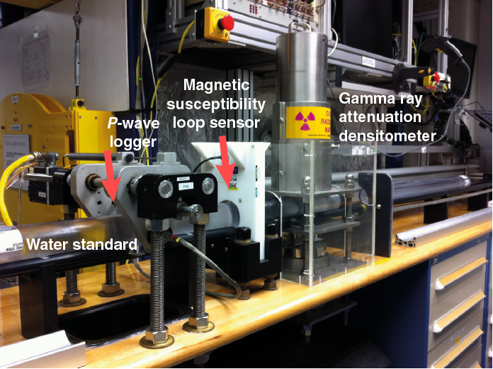
Figure F13. Whole-Round Multisensor Logger.
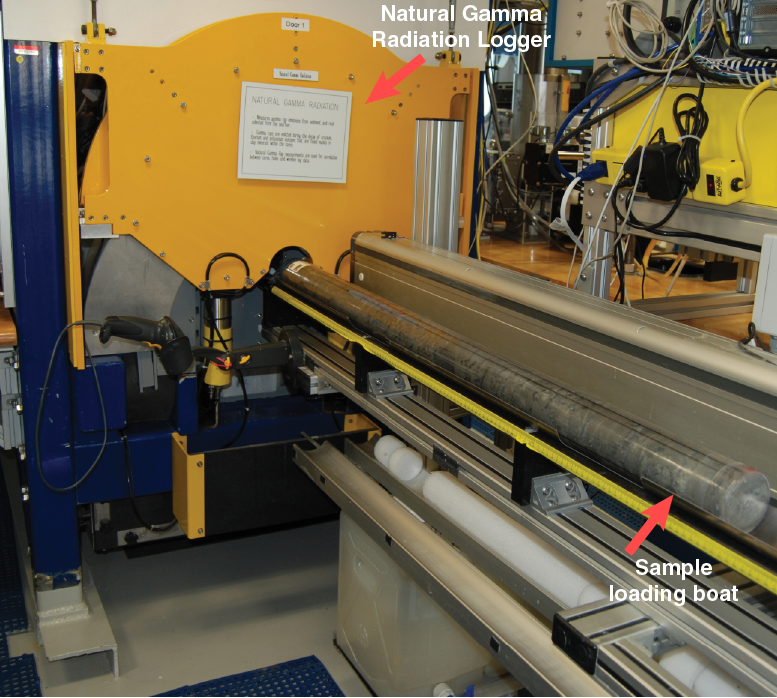
Figure F14. Natural Gamma Radiation Logger.
The WRMSL employs, in order, a GRA bulk densitometer, a magnetic susceptibility loop sensor, and a compressional P-wave velocity logger. Cores recovered with the XCB coring system are slightly smaller in diameter than those cored with the APC system. As a result, sections cored with the XCB system typically have gaps between the liner and the core; therefore, P-wave velocity was not measured with the WRMSL on those cores. In addition, when APC core sections contained abundant cracks or gas in sediment that resulted in unreliable values, the P-wave logger was also switched off. A 2.5 cm measurement resolution was chosen for the WRMSL to avoid encumbering downstream core processing and sample collection and to ensure consistency with other high-resolution logging techniques (e.g., NGRL, color reflectance, line-scan images, and NRM). Scanning time averaged ~8 s per measurement point, including three repeat magnetic susceptibility measurements to enhance data quality, resulting in a scanning time of ~7 min per 1.5 m section. The quality of the STMSL and WRMSL data is highly dependent on the structural integrity of the sediment (cracks, voids, biscuiting, etc.) and whether any gaps between the sediment and the core liner are present. The structural integrity and incomplete filling of liners were recorded where necessary.
At Sites U1488 and U1490, P-wave velocity proved to be the most useful correlation tool over parts of the records. Because the STMSL did not include a P-wave logger (PWL), we switched the function of the STMSL and WRMSL while coring Holes U1488C and U1490B. The core sections were immediately run on the WRMSL at 5 cm spacing to rapidly collect GRA bulk density, magnetic susceptibility, and P-wave velocity data. After equilibration, the cores were then run at 2.5 cm spacing on the STMSL to collect higher resolution GRA bulk density and magnetic susceptibility data. Core sections were then run on the WRMSL PWL at 2.5 cm as time allowed. The GRA bulk densitometer and magnetic susceptibility loop incorporated in the STMSL and WRMSL are effectively identical.
For the NGRL, each section was initially scanned for 5 min at two positions, resulting in 10 cm resolution data at a scanning time of ~11 min per 1.5 m section. This strategy was adapted throughout the expedition to avoid encumbering the core flow (see Natural gamma radiation for further details).
GRA bulk density
Bulk density is a reflection of water-saturated porosity, grain density (dominant mineralogy), grain packing, and coring disturbance. GRA density is an estimate of bulk density based on the attenuation of a gamma ray beam. To measure bulk density, the GRA densitometer uses a 10 mCi 137Cs capsule as a gamma ray source (principal energy peak at 0.662 MeV) at a radiation level of 370 Mbq within a lead shield with a 5 mm collimator; the radiation is directed through the whole-round core and has a spatial resolution of <1 cm. The gamma ray detector on the opposite side of the core from the source includes a scintillator and an integral photomultiplier tube to record the gamma radiation that passes through the core. The narrow collimated peak is attenuated as it passes through the center of the core. Incident photons are scattered by the electrons of the sediment through Compton scattering, in which gamma rays are scattered by electrons in the formation; the degree of scattering is related to the material bulk density. Therefore, for a known sample diameter (d), the density (ρ) is proportional to the intensity of the attenuated gamma rays (I0) and can be expressed as
where I is the measured intensity of the gamma rays passing through the sample and μ is the Compton attenuation coefficient (Evans, 1965; Harms and Choquette, 1965). Because the attenuation coefficient for aluminum is similar to that of most common minerals, bulk density is obtained through direct calibration of the densitometer using aluminum rods of different diameters mounted in a core liner filled with distilled water.
In general, STMSL and WRMSL GRA bulk density measurements are most accurate when taken on a completely filled core liner with minimal drilling disturbance; otherwise, measurements tend to underestimate true values. By default, the instrument reports measurements using the internal diameter of the core liner (66 mm) as the assumed sample diameter. This assumption is suitable for most sediment cores obtained by the APC system; however, for sediment cored by the XCB system, core diameter is usually ~58 mm or less. Following Jarrard and Kerneklian (2007), past IODP expeditions (e.g., Expedition 355) corrected the density measurements of XCB cores by multiplying the density values by 66/58 = 1.138 to account for this bias. We initially applied this correction to data obtained by XCB coring (notably Site U1482); however, the corrected GRA data from XCB cores showed a large offset with MAD bulk density data. Because MAD bulk density is a more accurate measure of true bulk density, we chose not to apply the XCB correction to GRA data (see Physical properties in the Site U1482 chapter [Rosenthal et al., 2018] for further details). Irregularly filled core liners also influence GRA measurements and should be considered when interpreting the data.
The gamma ray detector is calibrated with sealed calibration cores (one standard core liner filled with distilled water and aluminum cylinders of various diameters). To establish the calibration curves, gamma ray counts were taken through each aluminum cylinder for 60 s. Each aluminum cylinder has a density of 2.7 g/cm3, and d is 1, 2, 3, 4, 5, or 6 cm. The relationship between l and µd is
where A, B, and C are coefficients determined from the calibration. Recalibration was performed as needed when the deionized water QA/QC standard deviated significantly (e.g., more than a few percent) from 1 g/cm3.
Magnetic susceptibility (loop)
Magnetic susceptibility (χ) is a dimensionless measurement of the degree to which a material can be magnetized by an external magnetic field:
where M is the magnetization induced in the material by an external field of strength H. It provides information on the magnetic composition of the sediment that commonly can be related to mineralogical composition (e.g., terrigenous versus biogenic materials) and diagenetic overprinting. Magnetite and a few other iron oxides with ferromagnetic characteristics have a specific magnetic susceptibility several orders of magnitude higher than clay, which has paramagnetic properties. Carbonate layers, opal, water, and plastic (core liner) have small negative values of magnetic susceptibility. Calcareous and biogenic deposits with very small amounts of clay and iron-bearing mineral debris thus have values approaching the detection limit of magnetic susceptibility meters.
Magnetic susceptibility measurements were made with the Bartington Instruments MS2C loop sensor. The WRMSL operates at 565 Hz in a 90 mm loop with a correction value of 1 (e.g., no correction). The STMSL operates at 452 Hz in a 90 mm loop with a correction value of 1.174. The loop sensors have a spatial measurement resolution estimated by the full width at half maximum height of the response function of 4.0–4.5 cm and are accurate to within 5% as indicated in Bartington specifications (Blum, 1997). The loop is zeroed in air before each measurement run in order to avoid influence from the logger. The output of the magnetic susceptibility sensors can be set to centimeter-gram-second (cgs) units or dimensionless SI units. SI units (×10−5) are used as the IODP standard and are reported as such in the database.
Compressional P-wave velocity
P-wave velocity varies with the material’s lithology, porosity, and bulk density, as well as state of stress, temperature, and fabric or degree of fracturing. In sediment and rock, velocity is controlled by the degree of consolidation, lithification, and fracturing, along with the occurrence and abundance of free gas and gas hydrate. Together with bulk density, velocity data are used to calculate acoustic impedance and reflection coefficients to construct synthetic seismic profiles and to estimate the depth of specific seismic horizons. P-wave velocity (VP) is defined by the time required for a compressional wave to travel a specific distance:
where d is the path length of the wave across the core and tcore is the traveltime through the core.
The P-wave velocity sensor measures the ultrasonic P-wave velocity of the whole-round sample residing in the core liner. The P-wave logger transmits a 500 kHz P-wave pulse across the core section at a specified repetition rate. Waves are transmitted to the core by plastic transducer contacts connected to linear actuators. Pressure was applied to the actuators to ensure coupling between the transducers and the core liner. Traveltime is determined by signal processing software that automatically detects the first arrival of the P-wave signal to a precision of 50 ns. The wave travels horizontally across the whole core and core liner. Ultrasonic P-wave velocity is calculated after correcting for system propagation delay, liner thickness, and liner material velocity. The total observed traveltime tcore is composed of
- tdelay = time delay related to transducer faces and electronic circuitry,
- tpulse = delay related to the peak detection procedure,
- tliner = transit time through the core liner, and
- tcore = traveltime through the sediment.
The system is calibrated using a core liner filled with distilled water, which provides control for tdelay, tpulse, and tliner. From these calibrations, VP can be calculated for the whole-round specimens in core liners as
VP = (dcl – 2dliner)/(to – tpulse – tdelay – 2tliner),
- dcl = measured diameter of core and liner,
- dliner = liner wall thickness, and
- t0 = measured total traveltime.
The above equation assumes that the core completely fills the core liner. The WRMSL P-wave logger was turned off for XCB cores, which typically do not fill the core liner and therefore do not give accurate measurements using the WRMSL P-wave system.
Natural gamma radiation
The NGRL was designed and built at the Texas A&M University IODP facility and measures gamma radiation emitted from whole-round core sections (Vasiliev et al., 2011) (Figure F14). Gamma radiation detected by the logger arises primarily from the decay of mineral-hosted 238-uranium (238U), 232-thorium (232Th), and 40-potassium (40K) isotopes. When 238U, 232Th, and 40K radioisotopes decay, they and their daughter isotopes emit gamma radiation at specific energy levels unique to each isotope. NGR spectroscopy measures a wide energy spectrum that can be used to estimate the abundance of each isotope based on the strength of the signal at characteristic energies (Blum, 1997). Spectral data were collected but were not processed on board and can be used for postcruise processing for U, Th, and K abundance (e.g., De Vleeschouwer et al., 2017). In general, high counts identify fine-grained deposits containing K-rich clay minerals and their absorbed U and Th atoms. NGR data reveal stratigraphic details that aid in core-to-core correlations.
The main NGR detector unit consists of 8 sodium iodide (NaI) scintillator detectors surrounding the lower half of the section, 7 shielding plastic scintillator detectors, 22 photomultipliers, and passive lead shielding (Figure F15). The NaI detectors are covered by at least 8 cm of lead shielding. In addition, lead separators (~7 cm of low-background lead) are positioned between the NaI detectors. Half of the lead shielding closest to the NaI detectors is composed of low-background lead, whereas the outer half is composed of common (virgin) lead. In addition to this passive lead shielding, the overlying plastic scintillators detect incoming high-energy gamma and muon cosmic radiation and remove this signal from the total counted by the NaI detectors.
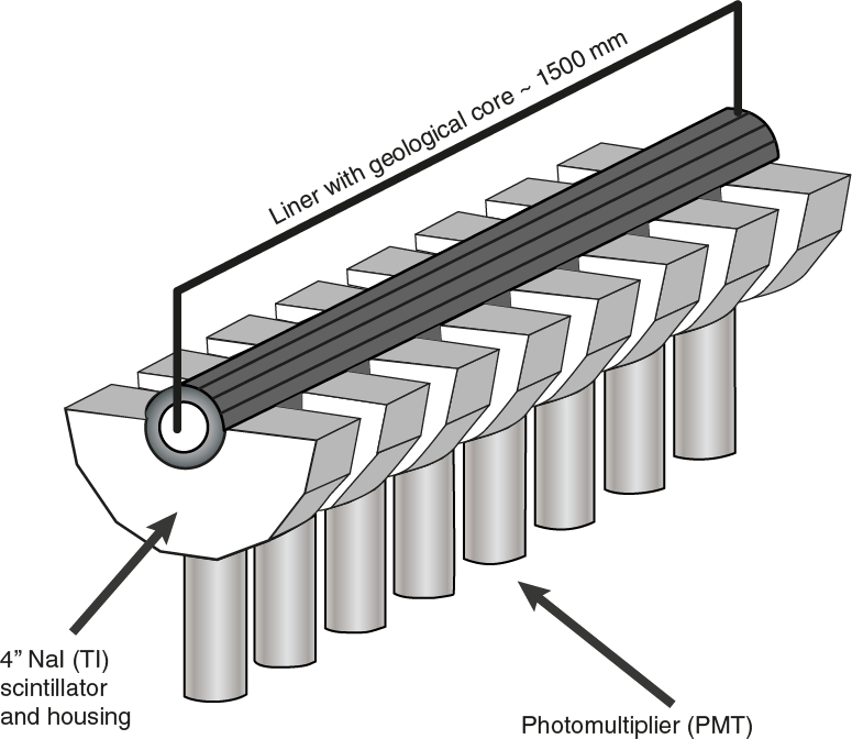
Figure F15. Main elements of the NGRL.
A measurement run consisted of one or two sample positions 10 cm apart, for a total of 8 measurements per 150 cm section per position. The quality of the energy spectrum measured in a core depends on the concentration of radionuclides in the sample but also on the counting time, with higher times yielding better spectra. Further information may be found in Vasiliev et al. (2011) and Dunlea et al. (2013). Counting times for all holes were 5 min per position, resulting in measurement times of ~11 min per section/77 min per core for two positions to yield statistically significant energy spectra. However, because this was a high-recovery expedition, these scanning times significantly encumbered core flow. This delay was accommodated at Sites U1482 and U1483 due to the long transit following completion of operations at these sites. We adopted a different NGRL strategy for the second half of the expedition when there was minimal transit time between sites. First, at the start of coring at a new site, cores were run prior to equilibration to laboratory temperature, as temperature does not affect NGR. Care was taken to ensure that no water leaked from the sections while in the NGRL. Hole A was measured at two positions for 5 min at each position (10 cm resolution data), but subsequent holes were measured at a single position (position 2) for 5 min (20 cm resolution data). Cores measured at a single position could be scanned in ~45 min per core, which significantly improved core flow. If time allowed (e.g., coring in deeper water) or if subsequent holes were cored deeper than Hole A, subsequent holes or portions of subsequent holes were measured at two positions for 5 min each, primarily to aid stratigraphic correlation. We opted not to reduce the count time at both positions even though we found that reducing the count time would not affect the quality of the data for correlation purposes, but the strength of the U peak was significantly reduced relative to a longer count time. Measuring at a single position was therefore preferred, as it ensured the quality of the spectra obtained at each position, although the 20 cm resolution NGR data were more difficult to use for stratigraphic correlation purposes.
Thermal conductivity
Thermal conductivity is an intrinsic material property for which the values depend on the chemical composition, porosity, density, structure, and fabric of the material. Thermal conductivity profiles are used along with in situ temperature measurements to determine heat flow, which is an indicator of age of ocean crust and fluid circulation processes.
After NGR measurements were completed, thermal conductivity was measured with the TK04 (Teka Berlin) system using the needle-probe method in full-space configuration for whole-round sediment cores (Von Herzen and Maxwell, 1959). The needle probe contains a heater wire and calibrated thermistor. The probe was inserted into a 2 mm hole drilled through the liner along the splitting line of the core section. To avoid interference from airflow in the laboratory, a foam rubber insulating jacket was placed over the core section during measurement of thermal conductivity. We also placed the core section inside a large plastic box outfitted with foam to further reduce thermal disturbances. A heating power of 0.5 to 2 W/m was typically used. The solution to the heat conduction equation with a line source of heat was then fit to the temperature measurements to obtain the thermal conductivity. Because the probe is much more conductive than sediment, the probe is assumed to be a perfect conductor. Under this assumption, the temperature of the superconductive probe has a linear relationship with the natural logarithm of the time after the initiation of the heat:
- T = temperature (K),
- q = heat input per unit length per unit time (J/m/s),
- k = thermal conductivity (W/[m·K]),
- t = time after the initiation of the heat (s), and
- C = instrumental constant.
Three measuring cycles/replicates were automatically performed at each probe location (usually ~75 cm offset from the top of the section) to calculate average thermal conductivity in the core material. The instrument routinely performed a self-test, which included a drift measurement, at the beginning of each measurement cycle. Once the probe temperature stabilized, the heater circuit was closed and the temperature rise in the probe was recorded. Thermal conductivity was calculated from the rate of temperature rise while the heater current was flowing. Temperatures measured during the first 150 s of the heating cycle were fitted to an approximate solution of a constantly heated line source (for details, see Kristiansen, 1982; Blum, 1997). Thermal conductivity measurements were routinely taken in the first hole at each site and in one section per core (typically Section 3), with measurements taking ~30 min. Once the sediment became too hard to penetrate with the needle probe, a different method for measuring thermal conductivity using a puck probe was applied. First, a piece of sediment (ideally 5–10 cm in length) was removed from a split-core section. The flat surface of a puck probe was placed on the surface of the sediment piece and secured with a rubber band. The sediment and puck were then placed in a water bath containing seawater, and thermal conductivity measurements were taken using TK04 with power supplied by interruptible power supply battery. Thermal conductivity was regularly measured using the puck probe in XCB cores, particularly because the sediment eventually becomes too indurated to insert the needle probe successfully. Even in less indurated sediment, needle-probe thermal conductivity measurements on XCB cores typically yield spurious results because frequent cracks in the cores induced during XCB coring lead to inadequate coupling between the needle probe and the sediment and additional fluid convection through the sediment.
Section Half Measurement Gantry
P-wave velocity measurements on split-core sections were initially performed once or twice per section in Hole A and as needed on subsequent holes, using the SHMG (Figure F16). Generally, the measurements were taken at ~100 cm in the section; however, if necessary, measurements were taken at varying section intervals to accommodate lithological variations and core quality. Discrete z-, y-, and x-axis P-wave measurements were ideally taken at the same section interval by first using the z-axis bayonet, then the y-axis bayonet, and finally the x-axis caliper contact probe transducers on the SHMG. Where the sediment surface was too disturbed by the z- and y-axis measurements, the x-axis measurement would be offset slightly. We observed good reproducibility between y-axis measurements by the SHMG and P-wave velocity measurements using the WRMSL in Hole U1482A and stopped measuring SHMG y-axis P-wave velocity at all other sites during Expedition 363. The system uses Panametrics-NDT Microscan delay line transducers, which transmit at 0.5 MHz. The signal received was recorded, and the peak (P-wave arrival) was chosen with autopicking software, which was adjusted manually to the first positive peak. The peak was always manually chosen to ensure a consistent first arrival time was selected. The distance between transducers was measured with a built-in linear voltage displacement transformer (LDVT).

Figure F16. Section Half Measurement Gantry.
Calibration was performed with a series of acrylic cylinders of differing thicknesses and a known P-wave velocity of 2750 ± 20 m/s. The determined system time delay from calibration was subtracted from the picked arrival time to give a traveltime of the P-wave through the sample. The thickness of the sample (calculated by LDVT in meters) was divided by the traveltime (in seconds) to calculate P-wave velocity in meters per second.
Moisture and density
Discrete samples were collected from the working halves after measurement on the SHMG to determine wet and dry bulk density, grain density, water content, salt content, and porosity. In soft sediment, ~10 cm3 samples were collected with a 2 cm diameter plastic syringe that fits into a 12 cm3 glass vial so that the vial will be completely filled with sediment. To accommodate the large volume of cored sediment and subsequent carbonate analysis, three MAD samples were taken and measured per core (usually at ~100 cm in Sections 1, 3, and 5). Additional MAD samples were taken where lithologies of interest were present.
Samples were placed in prelabeled and preweighed 16 mL Wheaton glass vials for wet and dry sediment mass measurement. The volumes of the numbered Wheaton vials were calculated before the expedition by multiplying each vial’s weight by the average density of the vial glass. After wet sediment analysis, the samples were dried in a convective oven at 105° ± 5°C for at least 24 h and allowed to cool in a desiccator for at least 4 h before taking the dry volume measurements. The weights of wet and dry sample masses were determined to a precision of 0.005 g using two Mettler Toledo electronic balances, with one balance acting as a reference. A standard weight of value similar to that of the sample was placed on the reference balance to increase accuracy. A computer averaging system was used to compensate for the ship’s motion. The default setting of the balances is 300 measurements, taking ~1.5 min.
Dry sample volume was determined using a hexapycnometer system of a six-celled, custom-configured Micromeritics AccuPyc 1330TC helium-displacement pycnometer (Figure F17). The precision of each cell is 1% of the full-scale volume. Volume measurement was preceded by three purges of the sample chamber with helium warmed to ~28°C. Three measurement cycles were run for each sample. A reference volume (calibration spheres) was sequentially placed in one of the six chambers to check for instrument drift and systematic error.
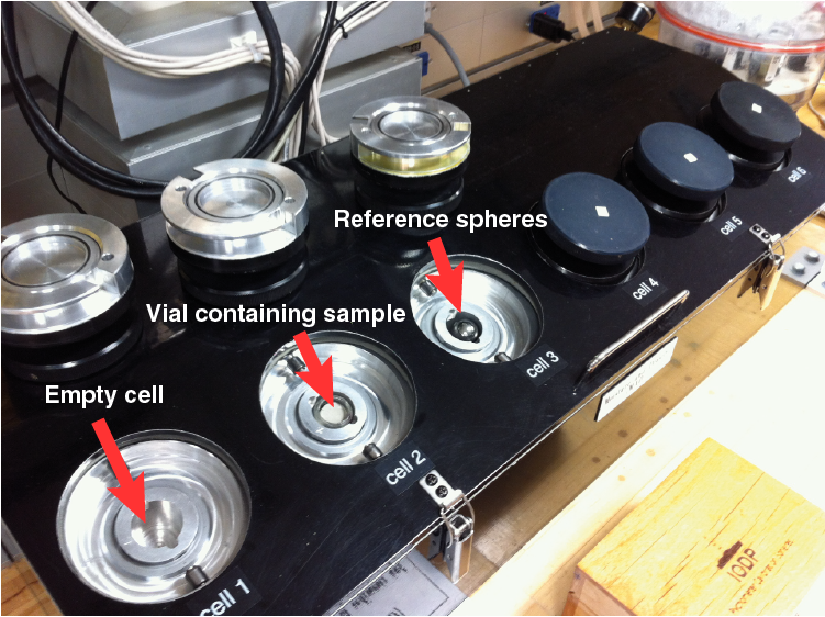
Figure F17. Pycnometer used for discrete soft-sediment samples.
The procedures for the determination of these physical properties comply with the American Society for Testing and Materials (ASTM) designation (D) 2216 (ASTM International, 1990). The fundamental relationships and assumptions for the calculations of all physical property parameters are discussed by Blum (1997) and summarized below.
Mass and volume calculation
Wet mass (Mwet), dry mass (Mdry), and dry volume (Vdry) were measured in the laboratory. The ratio of mass (rm) is a computational constant of 0.965 (i.e., 0.965 g of freshwater per 1 g of seawater). Salt precipitated in sediment pores during the drying process is included in the Mdry and Vdry values. The mass of the evaporated water (Mwater) and salt (Msalt) in the sample are given by
where s is the assumed saltwater salinity (0.035%) corresponding to a pore water density (ρpw) of 1.024 g/cm3 and a salt density (ρsalt) of 2.22 g/cm3. The corrected mass of pore water (Mpw), volume of pore water (Vpw), mass of solids excluding salt (Msolid), volume of salt (Vsalt), volume of solids excluding salt (Vsolid), and wet volume (Vwet) are, respectively,
Vwet = Vdry – Vsalt + Vpw, and
Calculation of bulk properties
For all sediment samples, water content (w) is expressed as the ratio of mass of interstitial water to wet sediment (total) mass:
Wet bulk density (ρwet), dry bulk density (ρdry), sediment grain density (ρsolid), porosity (φ), and void ratio (VR) are calculated as
MAD properties reported and plotted in the Physical properties sections of all site chapters were calculated with the MADMax shipboard program, set with the “method C” calculation process (Blum, 1997).
Section-half logger measurements
Section Half Image Logger
The surfaces of the archive halves of split cores were digitally imaged using a 3CCD (charge-coupled device) line-scan camera (JAI model CV107CL) with a macro lens (AF micro Nikkor 60 mm, 1:2.8). The camera is mounted on the Section Half Image Logger (SHIL; Figure F18) and moves along the core section by a motorized gantry. Prior to imaging, the core face was prepared by scraping across, rather than along, the core section using a stainless steel or glass scraper. Scraping parallel to bedding with a freshly cleaned tool prevented cross-stratigraphic contamination. After splitting, the archive halves were imaged as soon as possible to capture the core surface prior to drying and/or oxidation (see Core description). Images were scanned at an interval of 10 lines/mm, with camera height adjusted such that pixels are square. Light for imaging was provided by three pairs of advanced illumination high-current focused LED line lights with fully adjustable angles to the lens axis. Compression of line-scanned images on VCDs or summary figures may result in visual artifacts, primarily lamination that is not present in the actual sections. Along with the images, the variations in the red, green, and blue (RGB) color channels were also recorded by the SHIL and used as a primary tool for stratigraphic correlation.
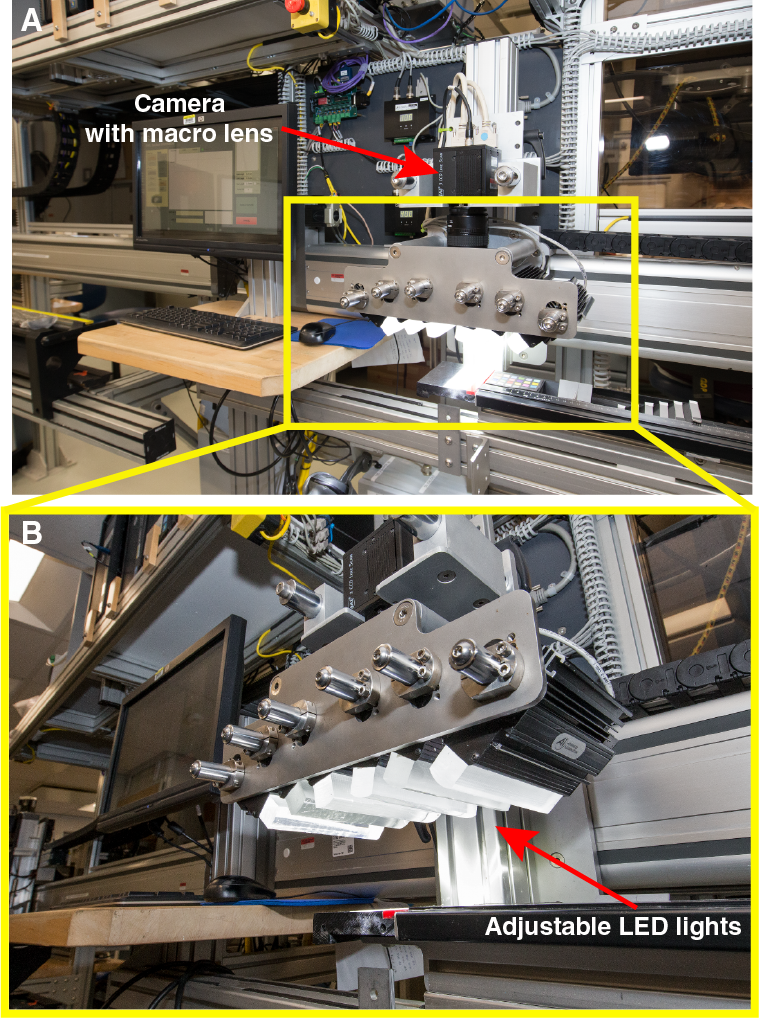
Figure F18. Section Half Imaging Logger.
Section Half Multisensor Logger
Spectrophotometry
After imaging, spectrophotometry was measured on the archive halves with the SHMSL (Figure F19). Spurious measurements may occur from small cracks, drilling disturbance, plastic section dividers, or where the sensors did not make adequate contact with the core surface, which results in leakage of ambient room light into the spectrophotometer readings. The reflectance of visible light was measured using an Ocean Optics USB4000 spectrophotometer mounted on the automated SHMSL. A halogen light source, covering a wavelength range through the visible spectrum and slightly into the infrared domain, was used. Freshly split cores were covered with clear plastic wrap and placed on the SHMSL. Measurements were taken at 2.5 cm spacing to provide a high-resolution stratigraphic record of color variation for visible wavelengths. Each measurement was recorded in 2 nm wide spectral bands from 380 to 900 nm. The approximate 3 s data acquisition offset was applied for the entire scan of the archive section half. The data are reported using the L*a*b* color system, in which L* is lightness, a* is redness (positive) versus greenness (negative), and b* is yellowness (positive) versus blueness (negative) of the sediment. The color reflectance spectrophotometer calibrates on two spectra, pure white (reference) and pure black (dark). Color calibration was conducted approximately once every 6 h (twice per shift). Additional details regarding measurement and interpretation of spectral data can be found in Balsam et al. (1997), Balsam and Damuth (2000), and Giosan et al. (2002).
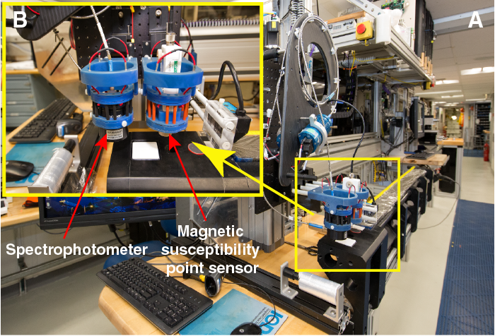
Figure F19. Section Half Multisensor Logger.
Point magnetic susceptibility
Point magnetic susceptibility was measured with a Bartington MS2 meter and an MS2K contact probe with a flat 15 mm diameter round sensor with a field of influence of 25 mm and an operation frequency of 930 Hz. The instrument averages three measurements from the sensor for each offset, leading to an accuracy of ~5%. The horizontal spatial resolution of the point magnetic susceptibility instrument is ~3.8 mm, higher than that of the whole-round magnetic susceptibility loop. As with whole-round measurements, the point magnetic susceptibility sensor output is given in dimensionless SI units (×10–5). The probe is zeroed in air before each measurement run in order to avoid influence from the metal track. The point magnetic susceptibility meter was calibrated by the manufacturer before installation on the ship and is quality checked every ~6 h, at the same time as color reflectance sensor calibration.
In situ temperature measurements
During Expedition 363, in situ temperature measurements were made with the APCT-3, typically in Hole A at each site, when the APC was deployed. If Hole A was a short hole (because of a missed mudline or other coring problems), the APCT-3 was deployed in Hole B. The APCT-3 fits directly into the coring shoe of the APC and consists of a battery pack, a data logger, and a platinum resistance-temperature device calibrated over a temperature range from 0° to 30°C. Before entering the borehole, the tool is first stopped at the mudline for 5 min to thermally equilibrate with bottom water. However, the lowest temperature recorded during the run was occasionally used instead of the average temperature at the mudline as an estimate of the bottom water temperature because (1) it was more repeatable and (2) the bottom water is expected to have the lowest temperature in the profile. When the APC is plunged into the formation, there is an instantaneous temperature rise from frictional heating. This heat gradually dissipates into the surrounding sediment as the temperature at the APCT-3 equilibrates toward the temperature of the sediment. After the APC penetrated the sediment, it was held in place for 10 min while the APCT-3 recorded the temperature of the cutting shoe every second.
The equilibrium temperature of the sediment was estimated by applying a mathematical heat-conduction model to the temperature decay record (Horai and Von Herzen, 1985). The synthetic thermal decay curve for the APCT-3 is a function of the geometry and thermal properties of the probe and the sediment (Bullard, 1954; Horai and Von Herzen, 1985). Equilibrium temperature was estimated by applying a fitting procedure (Pribnow et al., 2000). However, where the APC did not achieve a full stroke or where ship heave pulled the APC up from full penetration, the temperature equilibration curve is disturbed and temperature determination is less accurate. The nominal accuracy of the APCT-3 temperature measurements is ±0.05°C.
APCT-3 temperature data were combined with measurements of thermal conductivity (see Thermal conductivity) obtained from core sections to obtain heat flow values. Heat flow was calculated according to the Bullard (1954) method, to be consistent with the synthesis of ODP heat flow data by Pribnow et al. (2000).
Data preconditioning
The data acquired using the shipboard logging systems were conditioned to remove outliers related to end caps, voids, and cracks. A simple script written in MATLAB removed these data points for plotting and visualization purposes. NGR data were treated only by culling the first point of every core to eliminate core disturbance effects. WRMSL magnetic susceptibility and P-wave velocity data were treated by culling the first and last point of each section to eliminate end cap effects. The uppermost three points of each core were also eliminated from WRMSL magnetic susceptibility data to avoid core disturbance. In addition, P-wave velocities >1750 m/s were deemed unrealistic and were culled, except for Sites U1486, U1487, and U1490, where a 2050 m/s threshold was used because of the large volume of volcanogenic-rich material present, which was associated with peaks in magnetic susceptibility.
As with WRMSL magnetic susceptibility data, the first and last measurements of core sections were removed from all WRMSL GRA density data to correct for end cap effects. In addition, unrealistic GRA bulk density values of less than 1.2 g/cm3 were removed because they most likely relate to sediment cracks. Following the initial treatment, a Hampel filter was applied to the WRMSL GRA density data to detect and remove noise. This filter computes a sliding median window with a user-defined window length and calculates the median absolute deviation of each data point about its window median. If the data point differs from the median by more than a user-defined number of absolute deviations, the point is culled. The size of the window and deviation limit was varied depending on data type and site (see Table T8 for site-specific procedures). In addition to the data preconditioning to remove unreliable data points, GRA density data were detrended by a linear regression to remove the linear compaction trend. All cleaned data are included as tables in each site chapter.
Table T8. Site-specific parameters for data preconditioning. Download table in CSV format.
Stratigraphic correlation
Continuous sedimentary sections cannot be collected from a single IODP borehole due to gaps that occur between successive cores, even when nominal recovery is 100% or greater (Ruddiman et al., 1987; Hagelberg et al., 1995). Consequently, to meet the scientific objectives of Expedition 363 we drilled more than one hole at each site to ensure that a column of cored section as complete as possible was assembled (“spliced”) from selected intervals of separate holes (see also OFFSPLICE in Supplementary material).
Constructing a spliced section follows two similar but separate activities. The first is to track the downward coring progress of each hole after the first hole is completed at a given site. The stratigraphic correlator identifies and links features to previously drilled cores at this site while the hole is being deepened and advises the driller if adjustments are needed to avoid alignment of intercore gaps between holes. To do this while the drill bit is advancing relies on measurements obtained within a few minutes of the time cores reach the core laboratory and are curated; during Expedition 363 we primarily used magnetic susceptibility and GRA bulk density measurements obtained on the STMSL. At Sites U1488 and U1490 within intervals with very low magnetic susceptibility (notably below ~100 mbsf at Site U1488 and between ~20 and 175 mbsf at Site U1490), P-wave velocity proved to be the most useful for rapid correlation. At these sites, we used the WRMSL to collect GRA density, magnetic susceptibility, and P-wave velocity data at 5 cm resolution immediately after the cores were brought on deck. The STMSL was then used to collect higher resolution (2.5 cm) GRA density and magnetic susceptibility data after the cores equilibrated to room temperature (see Physical properties).
The second part of stratigraphic correlation is joining intervals of proven correlation between two or more holes to assemble a continuous spliced record. The goal is to construct a downhole “map” that will guide samplers to the most continuous stratigraphic section available at that site. The stratigraphic correlator begins by identifying a tie point in each core of every hole that places it in stratigraphic position most in agreement with cores in neighboring holes. This step is referred to as “compositing.” To do this, the correlator uses several types of information to identify features common to cores from multiple holes. Although not used during this expedition, downhole log measurements can also be incorporated to establish the proper stratigraphic position of core data that may be unclear due to incomplete core recovery. During Expedition 363, we used WRMSL measurements of magnetic susceptibility and GRA density, similar to those obtained from the STMSL (only at higher resolution, usually at 2.5 cm measurement intervals for WRMSL versus 5 cm from the STMSL) plus P-wave velocity (from the WRMSL PWL), NGR, color reflectance, and color spectroscopy (L*a*b* and RGB), aided at times by core photographs. This procedure is intended to locate gaps in the sedimentary section of any hole and then find where those gaps may be present in the recovered sediment of one or more adjacent holes at that site. Usually two complete holes and a third partial hole must be cored at a single site in order to be able to construct a complete section in the interval cored with the APC system.
When all cores at a site are composited, the stratigraphic correlator begins with the most reliable mudline core (the one that recovered the seafloor) and works downhole through the collection of composited cores to construct an unbroken splice of the most favorable intervals. Many criteria are used in selecting which intervals, joined by tie points, offer the most complete stratigraphic succession (see discussion in each site chapter). The product of this effort is a spliced record. Additional holes can be cored to allow for the construction of additional splices.
Constructing composite and splice intervals during Expedition 363 followed the basic strategy first developed during Ocean Drilling Program (ODP) Leg 138 (e.g., Hagelberg et al., 1995) and refined during subsequent legs. This same approach is now common practice on all high-resolution paleoceanographic expeditions, although the measurements on individual cores and the computer software used to match events between holes and to construct the splice are not the same in all cases.
The procedure for these activities involved consideration of several different depth scales (Figure F20). In this example, five cores were recovered from Holes A and B; Core B1 is intentionally shorter than A1 to ensure that intercore gaps do not align between the two holes. Core B2 unintentionally had less than full recovery. The CSF-A scale was established by adding the curated core length (brown intervals) to the depth of each core top determined by the DSF scale. If recovery is >100%, this results in overlap between cores (red). The CCSF scale corrects for this and other inadequacies of the CSF-A scale.
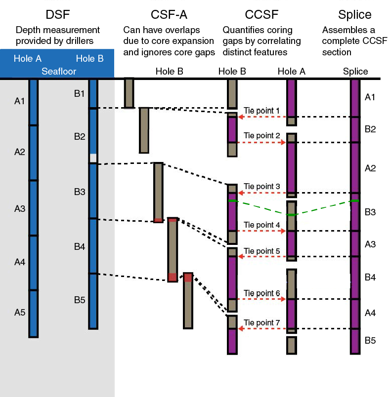
Figure F20. Interrelationships between cored material and depth scales.
The CCSF scale is based on locating features common to cores in multiple holes at a given site and working from the top of the site downward to select tie points (red dashed lines) that correlate features in one hole to those in another. Because of core expansion and the unavoidable absence of complete recovery at the tops and bottoms of cores, Holes A and B on the CCSF scale are longer than they are on the CSF-A scale. The primary splice on the CCSF scale at the far right is constructed by combining selected intervals between tie points so that coring gaps and disturbed sections are excluded, ideally resulting in a complete stratigraphic sequence. This procedure assumes identical sediment thickness between tie points joining two holes, which may not be the case due to differences in accumulation rate and/or compaction and expansion due to the coring process. Consequently, the CCSF depth of a sedimentary horizon in the splice is not necessarily equivalent to the CCSF depth for the same horizon not included in the splice, as illustrated by the green dashed lines joining the green horizon in Cores A3 and B3. The depth scales used during Expedition 363 followed IODP convention (http://www.iodp.org/policies-and-guidelines) and are described below.
Core depth below seafloor scale
We began the process of building a composite section by assigning a depth to the top of each core, based initially on the DSF. DSF is a drill string measurement, determined as the difference between (1) the length of the drill string between the rig floor and the top of the cored interval and (2) the length of the drill string between the rig floor and the mudline (assumed to be the seafloor). DSF error includes phenomena such as pipe and BHA stretch and compression, tides, and uncompensated heave. Tidal influence on this depth measurement can be significant (Hagelberg et al., 1995), and the prediction of tides is generally useful for guiding drilling to avoid gap alignment (Mix, Tiedemann, Blum, et al., 2003). The full tidal range at some Expedition 363 sites was slightly more than 4 m and appeared to contribute to slow diurnal changes in the size of intercore gaps. This was especially prevalent at Site U1482.
The depth to a given position within any core was then determined relative to the DSF core top depth. The CSF-A depth scale therefore combined the DSF core-top depth with the curated length of the core after retrieval. The CSF-A depth scale is equivalent to the historical Deep Sea Drilling Project (DSDP), ODP, and Integrated Ocean Drilling Program mbsf scale and is specific to each hole. For the Expedition 363 Proceedings volume site chapters, we use mbsf instead of CSF-A for simplicity. It is important to note that the “within-core” position of any given sedimentary feature may change after recovery due to the relief of overburden, gas-induced expansion, or water loss. Thus, error in the CSF-A scale includes both drilling effects and core expansion effects. For example, the CSF-A scale permits stratigraphically impossible overlaps between successive cores caused by gas-induced expansion. In principle, the composite depth scale, described below, eliminates such artifacts.
Core composite depth below seafloor scale
The construction of a common, composite depth scale for a given IODP site involves identification of coeval, laterally continuous features in all drilled holes (which will generally occur at different depths on the CSF-A depth scales for each hole). Once correlative features were identified during Expedition 363, the depth of individual cores was offset relative to the CSF-A depth scale in that hole such that the features aligned on a common (CCSF) depth scale. This depth scale is equivalent to the historical ODP and Integrated Ocean Drilling Program meters composite depth (mcd) scale. In constructing the CCSF scale, the depths of individual cores were offset by a constant amount (without stretching or squeezing within individual cores). This composite depth scale provided good estimates of the length of coring gaps and formed the basis for developing the spliced record (on the CCSF scale). The vertical depth offset of every core in every hole was tabulated in an affine table, one of the principal “deliverables” of the stratigraphic correlator.
The CCSF scale was built by correlating features downhole from the mudline. The mudline established the top of the stratigraphic section, anchoring the entire composite depth scale for all cores from all holes at a single site. Compositing proceeded sequentially by establishing specific tie points among the various holes, working from the mudline (anchor) core to the bottom of the drilled section. The CCSF scale very rarely (if ever) resulted in alignment of all coeval features because of the contrasting effects of coring-induced stretching and squeezing among cores, as well as stratigraphic differences between holes.
In principle, if core gaps never come into alignment between all holes at a site, and if recovery is sufficiently high, then it should be possible to correlate each successive core in one hole to a core from an adjacent hole, all the way to the bottom of a drilled section. However, aligned coring gaps across all holes at a site are often difficult to avoid. In the case of aligned core gaps between holes, cores below the gap are no longer tied to the anchor core. They can, however, still be tied to one another to produce correlated sections that are “floating” on the CCSF scale. Such floating ties were denoted in the affine table as “APPENDED” or “SET,” depending on whether the offset to the top of that section was estimated by inheriting the absolute offset of the core above (APPEND) or by assuming a constant growth rate of the difference between mbsf and CCSF (SET). The second method (SET) is preferable because it produces a more realistic estimate of the core gap, based on estimates of the expansion of overlying cores from the same hole.
During the process of constructing the composite section, the CCSF depth becomes systematically larger than that of the CSF-A depth for equivalent horizons. This expansion, which during Expedition 363 was as much as 25%, has four main causes (e.g., Hagelberg et al., 1995; Acton et al., 2001):
- Decompression of the sediment as it is brought to atmospheric pressure;
- Pore-space gases coming out of solution, warming, and expanding;
- Stretching that occurs as part of the coring process; and
- Recovering borehole wall sediment that fell downhole and was cored.
Splice
Once the CCSF scale was developed and the between-core gaps identified, a complete stratigraphic section (splice) was constructed by combining selected intervals between the previously established tie points. In the case of core gaps aligned across all holes, any spliced sections below the gap were appended to those above and designated as floating splice sections. In some cases, the amount of missing section between anchored and floating sections can be determined using downhole logs. However, we logged only one site (U1482) during Expedition 363, so the amount of missing section in aligned core gaps could only be estimated at that site. Where needed at other sites, the length of the missing section in the splice was estimated based on the percent expansion observed where we had a continuous splice.
Intervals outside of the splice
Once the splice was constructed, we mapped into the splice those intervals not included in the splice itself by treating the splice as a downhole log. The methodology is based on identifying correlative tie points at the highest possible resolution, with linear adjustments of depths between ties. This scale was also designated as the CCSF scale because it is roughly equivalent to the splice depth. In reality, these depth scales are only equivalent to the extent that the correlations are accurate. At core boundaries, where evidence of stretching and compression were most prevalent, these detailed depth maps are considered less accurate. Thus, the CCSF scale is not precisely the same at all holes within a site except exactly where the splice tie points are made. Additional details and guidance are found in the individual site chapters.
Measurements and methods for correlation
For the majority of sites, initial development of composite sections (CCSF scale) was based on the stratigraphic correlation of magnetic susceptibility data sets acquired from the WRMSL and the STMSL as soon as possible after core retrieval. In many cases, this method allowed stratigraphic correlation to take place in near real time so that bit depth could be adjusted as necessary to avoid alignment of core gaps between holes. However, no single variable proved to be universally powerful at all sites for stratigraphic correlation or splice construction. At all sites, therefore, correlation proceeded through a combination of WRMSL, STMSL, NGR, and digitized color reflectance (RGB and L*a*b*) data. Color reflectance data were extracted from core images acquired from the Section Half Imaging Logger (SHIL; RGB data) and the SHMSL (L*a*b* data). Magnetic susceptibility, GRA bulk density, and L* (or a* and b*) were measured at 2.5 or 5 cm intervals, whereas RGB values were calculated at 0.5 cm intervals in the form of 0.5 cm averages measured continuously along a 1.5 cm wide strip centered on digital color SHIL images. Details on instrument calibrations, settings, and measurement intervals for Expedition 363 are given in Physical properties (Table T6).
Compositing and splicing were accomplished using Correlator software (version 2.1). This procedure generated standard affine tables (listings of the vertical offset in meters added to each core to generate the CCSF scale) and splice interval tables (listings of the specific core intervals used to construct the splice). These tables were uploaded into the LIMS database, which then linked the appropriate depth scale to any associated data set.
Geochemistry
The shipboard geochemistry program characterized the gases, interstitial water, and sediment composition of the cores recovered during Expedition 363. Headspace samples were analyzed for routine shipboard safety and pollution prevention purposes. Interstitial water chemistry, sedimentary carbonate (CaCO3), and total organic carbon (TOC) content were analyzed to understand the depositional history of each site and guide shore-based sampling and research. Selected sites were also targeted for high-resolution interstitial water sampling to reconstruct the vertical water mass structure (e.g., McDuff, 1985; Adkins et al., 2002; Insua et al., 2014) across a range of sampled water depths (~880–3420 m) in the western equatorial Pacific Ocean during the Last Glacial Maximum, a key scientific objective of Expedition 363.
Sedimentary gas geochemistry
Routine analysis of hydrocarbon gases in sediment cores is a part of standard IODP shipboard monitoring to ensure that the sediment being drilled does not contain more than the level of hydrocarbons that is safe for drilling operations. The most common method of hydrocarbon monitoring used is the analysis of gas samples obtained from sediment samples (headspace analysis). Sediment gas composition was typically determined once per core (usually at the top of Section 7) over the total stratigraphic interval cored at a given site. For this analysis, a 3 cm3 bulk sediment sample was collected immediately after core retrieval from the freshly exposed top end of a core section using a brass boring tool or plastic syringe. The sediment plug was placed in a glass vial and sealed with an aluminum crimp cap with a polytetrafluoroethylene (PTFE)/silicone septa. The vial was then heated to 70°C for ~30 min to evolve hydrocarbon gases from the sediment plug before analysis. When consolidated or lithified samples were encountered, chips of material were placed in the vial and sealed. For analysis, a 5 cm3 volume of headspace gas was extracted from the sealed sample vial using a gas-tight 5 mL PTFE Luer lock glass syringe and analyzed by gas chromatography.
Headspace samples were injected into the Agilent/Hewlett Packard 6890 Series II gas chromatograph (GC3) fitted with a flame ionization detector (FID) or the natural gas analyzer (NGA). The NGA was run for the analysis of Site U1482 samples. The GC3 is equipped with an 8 ft (2.4 m) (2.00 mm inner diameter [ID]; ⅛ inch outer diameter [OD]) stainless steel column packed with 80/100 mesh HayeSep (Restek) and an FID set at 250°C. The GC3 oven temperature was programmed to hold a temperature of 80°C for 8.25 min, ramp at 40°C/min to 150°C, hold that temperature for 5 min, and return to 100°C postrun, for a total run time of 15 min. Helium was used as the carrier gas. The GC3 system determines concentrations of methane (C1), ethane (C2), ethene (C2=), propane (C3), and propene (C3=). For hydrocarbon analysis, the NGA is outfitted with an Agilent 7890 gas chromatograph equipped with an Agilent DB-1 dimethylpolysiloxane capillary column (60 m × 0.320 mm diameter × 1.50 µm film thickness) fitted with an FID and using He as carrier gas (constant flow of 21 mL/min). The NGA oven temperature was programmed to hold a temperature of 50°C for 2 min, ramp at a rate of 8°C/min to 70°C, and then ramp at 25°C/min to 200°C, with a final holding time of 5.1 min. The FID temperature was 250°C. Data were collected and evaluated with an Agilent ChemStation data-handling program. The chromatographic response was calibrated to different gas standards with variable quantities of low molecular weight hydrocarbons. Gas components are reported as parts per million by volume (ppmv) of the injected sample.
Sediment geochemistry
For shipboard sediment geochemistry, the 10 cm3 of oven-dried sediment (105°C for 12 h) used for physical property measurements of MAD (see Physical properties) was crushed to a fine powder using an agate pestle and mortar and sampled to analyze inorganic carbon, total carbon (TC), and total nitrogen (TN). Because one of the expedition objectives was to document Neogene variations in CaCO3 accumulation rates, the MAD and sediment sampling resolution was increased from the standard one sample per core to a minimum of three samples per core. At the final site (U1490), separate samples were taken for geochemistry so that analyses could be finished before the end of the expedition. These samples were freeze-dried for ~24 h before processing.
Elemental analysis
TC and total TN contents of the sediment samples were determined with a ThermoElectron FlashEA 1112 carbon-hydrogen-nitrogen-sulfur (CHNS) elemental analyzer equipped with a ThermoElectron packed column CHNS/NCS gas chromatograph and a thermal conductivity detector (TCD). Approximately 10–15 mg of dried, ground sediment was weighed into a tin capsule, and the sample was combusted at 900°C in a stream of oxygen. The reaction gases were passed through a reduction chamber to reduce nitrogen oxides to N2 and were then separated by the gas chromatograph before detection by the TCD. For samples with high carbon content (>4 wt%), measurements were calibrated with the La Luna shale (11.52% C) and Buffalo River sediment (3.35% C) reference materials. For samples with low carbon content (<4 wt%), the Thermo Soil Reference Material 33840025, which was run approximately every 10 samples, was used for verification. Repeated (n = 7) analyses of the standards yielded a precision of better than 0.08% for TC.
Inorganic and organic carbon content
Total inorganic carbon (TIC) concentration was determined using a UIC 5011 CO2 coulometer. Between 10 and 12 mg of dried, ground sediment was weighed and reacted with 2 M HCl. The liberated CO2 was titrated, and the end-point was determined by a photodetector. Calcium carbonate (CaCO3) content, expressed as weight percent, was calculated from the TIC content, assuming that all evolved CO2 was derived from the dissolution of CaCO3 by the following equation:
CaCO3 (wt%) = TIC × 8.33 (wt%).
No correction was made for the presence of other carbonate minerals. Precision during individual batches of analyses was determined by running a pure CaCO3 standard approximately every 10 samples. Typical precision assessed from 36 replicate analyses of a carbonate sample was 1%. The detection limit for CaCO3, defined here as three times the standard deviation of the blank (2 M HCl), was 0.1% for 100 mg of pelagic clay. TOC content was calculated as the difference between total carbon (TC; measured on the elemental analyzer) and TIC (measured by coulometry):
For selected samples with very low organic carbon the “acidification method” of TOC analysis was also applied to improve analytical precision. Approximately 30 mg of dried sample was weighed into a silver capsule and treated with small aliquots of 2 M HCl at room temperature to remove CaCO3; samples were treated with repeated aliquots until no further reaction was visible and then dried on a hot plate at 60°C. TOC concentration was determined using a Thermo Electron Flash EA 1112 element analyzer for total carbon, calibrated using the Thermo Reference Material 33840025 (TOC = 2.26%). The acidification method resulted in errors with TN measurements and so was not employed after Site U1482.
Interstitial water geochemistry
Interstitial water collection
For interstitial water analyses, 5–10 cm long whole rounds were cut on the catwalk immediately after core retrieval, capped, and taken to the laboratory for processing. For Sites U1482, U1483, U1484, U1487, and U1490, we sampled two whole rounds per core in the upper 30 mbsf of Hole A, typically from the bottom of Sections 3 and 6. Deeper than 30 mbsf, one whole round per core was taken, typically from the bottom of Section 6, or from every other core when using the HLAPC system, from the second to last section of the core. Whole-round thickness was increased to a maximum of 10 cm when 5 cm long whole rounds no longer yielded enough water for shipboard and shore-based analyses.
At Sites U1485, U1486, U1488, and U1489, 5 cm long whole-round samples were taken from each section (every 1.5 m) for high-resolution interstitial water sampling, typically from Hole A unless Hole A was terminated early due to a missed mudline, in which case Hole B was sampled. High-resolution sampling was conducted to 54 mbsf at Site U1485, 82 mbsf at Site U1489, and 150 mbsf at Sites U1486 and U1488. Shipboard analyses of interstitial water were conducted on two whole rounds per core (typically from the bottom of Sections 3 and 6) over high-resolution sampling intervals and on one whole round per core (typically from the bottom of Section 6) below the high-resolution intervals. The remainder of the samples were split, fixed, and archived for shore-based analyses. For sections where both shipboard and shore-based analyses were performed, whole-round thickness was increased to 10 cm to ensure sufficient water volume was recovered for all analyses. At each site, a ~50 mL sample was taken from the mudline of the first core recovered for comparison between bottom water and interstitial water. Whole-round samples that could not be immediately processed were stored under a nitrogen atmosphere in a glove bag.
After extrusion from the core liner, the outer surface of each whole-round sample was carefully scraped with a spatula to remove potential contamination from seawater and sediment smearing in the borehole. In APC cores, ~0.5 cm of material from the outer diameter was removed, as well as from the top and bottom surfaces. The remaining sediment (~150–300 cm3) was placed into a titanium squeezer modified after the stainless steel squeezer of Manheim and Sayles (1974). Gauge forces up to a maximum of 35,000 lb were applied using a laboratory hydraulic press to extract interstitial water.
Squeezed interstitial water was filtered through a prewashed Whatman No. 1 filter placed in the squeezers above a titanium screen. The first ~0.5 mL of squeezed water was discarded to avoid contamination. The squeezed interstitial water was filtered into a precleaned plastic syringe attached to the squeezing assembly and then through a 0.45 µm polysulfone disc filter.
Shipboard interstitial water analyses
Interstitial water samples were analyzed on board the ship following the protocols in Gieskes et al. (1991), Murray et al. (2000), and the IODP user manuals for shipboard instrumentation.
Salinity, alkalinity, and pH
Alkalinity and pH were measured immediately after squeezing following the procedures in Gieskes et al. (1991). Salinity was estimated using a Fisher temperature-compensated handheld refractometer. A few drops of interstitial water were applied to the daylight plate assembly with an eyedropper, and the measurement was read through the eyepiece. Typical measurement precision based on repeated measurements of International Association for the Physical Sciences of the Oceans (IAPSO) seawater was ±1. To monitor for contamination, 18.2 MΩ nanopure water blanks were analyzed at the start and finish of each round of measurements.
The pH was measured with a combined glass electrode, and alkalinity was determined by Gran titration with an autotitrator (Metrohm 794 basic Titrino) using 0.1 M HCl at 20°C. The pH data are reported on the NBS scale. Prior to running, the electrode was calibrated using a series of NBS buffers with a pH of 4, 7, and 10. Three milliliters of interstitial water was titrated with 0.1 M HCl at 20°C. Standard ratios were calculated by running a series of standard solutions of different concentrations of Na2CO3 (5, 20, 40, 50, and 100 mM) and IAPSO seawater, with the standard correction factor specified before each analysis depending on alkalinity ranges. For calibration, IAPSO standard seawater was analyzed every 8–10 samples or after a period of nonuse to check instrument accuracy. An in-house seawater standard (surface seawater collected at Site U1482) was also analyzed at this frequency as an additional control on precision and accuracy. Repeated analyses of standards yielded a 1σ precision better than 3%.
Ion chromatography
Major cations (Ca2+, Na2+, Mg2+, and K+) and anions (Cl–, SO42–, and Br–) were measured using a Metrohm 850 professional ion chromatograph (IC) with an 858 professional sample processor. Interstitial water was diluted at a 1:100 ratio with 18.2 MΩ nanopure water in preparation for ion chromatography analysis. The IAPSO seawater standard was diluted at a range of 1:20 to 1:500 to create a five-point calibration curve. The relative standard deviation for each calibration curve varied from 0.2% to 5.2% but was typically better than 3%.
Instrument accuracy was checked by running a 1:150 dilution of IAPSO standard seawater every ~10 samples, and a new calibration curve was run if measured concentrations deviated from expected values. Precision (1σ) was determined from the repeated analyses of the standards and was better than 2% for each cation and anion concentration (Table T9). Results are presented as concentrations in millimolars or micromolars, and valence states are left off of cations and anions for consistency with results from samples run on the inductively coupled plasma–atomic emission spectroscopy (ICP-AES).
Table T9. Accuracy and precision for major anions and cations. Download table in CSV format.
Chlorinity
In addition to the IC analysis, Cl concentration was acquired using a Metrohm 785 DMP autotitrator and silver nitrate (AgNO3) solution calibrated against repeated titrations of an IAPSO standard. A 0.5 mL aliquot of interstitial water was diluted with 30 mL of 0.32 N HNO3 then titrated with 0.09866 M AgNO3. Repeated analyses of the IAPSO standard and an in-house seawater consistency standard yielded a 1σ precision ~0.65%, which is identical to precision for Cl run on the IC. The titration data are reported in the LIMS database; however, in the summary figures we only report [Cl] data obtained by IC.
Spectrophotometry
Dissolved ammonium (NH4+) and phosphate (PO43–) concentrations were determined by spectrophotometry using an Agilent Technologies Cary Series 100 UV-visible spectrophotometer with an Agilent Technologies SPS3 autosampler following the protocol in Gieskes et al. (1991). Samples were diluted prior to color development so that the highest PO43− concentration was <1000 μM and the highest NH4+ concentration was <3000 μM, with NH4+ dilutions guided by NH4+ peaks from the IC results. PO43− was measured using the ammonium molybdate method described in Gieskes et al. (1991) with appropriate dilutions. Standards were prepared with each run to create 11-point (for PO43−) and 14-point (for NH4+) calibration curves to convert absorbance to concentration. A standard was run independent of the calibration curve to check for accuracy, and sample replicates were run to check for precision. Precision (1σ) was better than 5% on PO43− concentration measurements and better than 10% on NH4+ concentration measurements. Results are presented as concentrations in millimolars or micromolars, and valence states are left off of cation and anions for consistency with results from samples run on the ICP-AES.
Inductively coupled plasma–atomic emission spectroscopy
The following suite of minor and trace elements was analyzed by ICP-AES with a Teledyne Prodigy high-dispersion ICP spectrometer: boron (B), barium (Ba), iron (Fe), manganese (Mn), silicon (Si), and strontium (Sr). The general method for shipboard ICP-AES analysis of samples is described in Murray et al. (2000) and the user manuals for shipboard instrumentation.
Samples and standards were diluted at a 1:20 ratio using 2% ultrapure HNO3 and spiked with 10 ppm yttrium (Y). Batches of 30–50 samples were run with an 11-point calibration curve created using synthetic seawater spiked with minor and trace elements (1%, 2.5%, 5%, 10%, 25%, 50%, 75%, 100%, 200%, 500%, and 1000%; values are percent of the primary standards) and used to convert background-corrected intensities to concentrations. A drift solution was run every ~12 samples, and blanks were run with every batch to check for contamination and allow for blank subtractions. Concentrations of Ba, Fe, Mn, and Si in IAPSO standard seawater commonly fall below detection limit, so an aliquot of IAPSO seawater was spiked with minor elements and three to five samples were run as unknowns on each run. Up to three replicates of the 50% synthetic seawater standard were also run as checks on precision. The standard deviation of these analyses indicated the 1σ precision of each run was better than 6.5% for most wavelengths (Table T10).
Table T10. Precision for ICP-AES trace and minor elements. Download table in CSV format.
Multiple wavelengths were measured for each element, and reported wavelengths were selected based on possible interferences, linearity of calibration curves, and the precision and accuracy of IAPSO seawater measurements:
- Li = 670.784 nm (except for Site U1483, for which Li = 610.364 nm).
- B = 249.772 nm.
- Si = 288.158 nm.
- Mn = 257.610 nm.
- Fe = 259.940 nm.
- Sr = 421.552 nm.
- Ba = 493.409 nm.
Detection limits for the trace/minor elements, defined here as three times the standard deviation of the blank intensities converted to concentrations, are given for each run in Table T11. These values are multiplied by 20 to account for sample dilution.
Table T11. Detection limits for ICP-AES minor elements. Download table in CSV format.
The high concentration of salt in the interstitial water samples at the 1:20 dilution requires matrix-matching of standards and samples, so standards were prepared with a NaCl matrix solution to have an ionic strength similar to 20× diluted seawater. A stock standard solution was gravimetrically prepared from ultrapure primary standards (SPC Science PlasmaCAL) diluted in 1% HNO3. This solution was diluted, along with the NaCl matrix, to have minor element concentrations bracketing the samples. Analytical precision was estimated by repeated analyses of the spiked IAPSO seawater (Table T10). Results from the ICP-AES are reported as elemental (rather than ionic) concentrations in millimolars or micromolars due to the insensitivity of ICP-AES to valence state or protonation. However, consideration of typical interstitial water chemistry suggests that [B] can reasonably be assumed to be the sum of [B(OH)3] and [B(OH)4–], [Ba] to be [Ba2+], [Fe] to be [Fe2+], [Li] to be [Li+], [Mn] to be [Mn2+], [Si] to be [H2SiO3], and [Sr] to be [Sr2+].
Interstitial water samples for shore-based research
Interstitial water remaining after shipboard analyses was split into aliquots for shore-based analyses of δ18Ο, high-precision Cl, δ34S, [H2S], δ234U, δ11B, and 87Sr/86Sr with sample and analysis priority indicated in Table T12. Squeeze cake samples were also split for shore-based major element, δ15Ν, δ34S, εNd, δ11B, and biomarker analyses. Any remaining interstitial water and squeeze cake sediments were archived.
Table T12. Interstitial water analyses and budget. Download table in CSV format.
Downhole measurements
Downhole logs determine various in situ physical, chemical, and structural properties of the formation penetrated by a borehole. The data are collected when all coring operations at a given hole are finished and are most often monitored in real time as the downhole tool is raised up through the borehole. The data are available for incorporating into science operations shortly after all logging is completed at that site. Where core recovery is incomplete or disturbed, log data may provide the only reliable characterization of the formation. Where core recovery is good, certain log measurements provide a direct tie to core data and lead to highly reliable integrated interpretations.
Downhole logs measure formation properties at scales between those obtained from laboratory measurements on core samples (centimeter scale) and those from conventional geophysical surveys (meter scale). They are useful in calibrating the interpretation of seismic survey data (e.g., through the use of synthetic seismograms) and provide a necessary link for the integrated understanding of physical and chemical properties on different scales.
During Expedition 363, downhole logging measurements were conducted in Hole U1482C only.
Wireline logging
Logs were recorded during Expedition 363 with standard Schlumberger tools lowered into the hole when coring was finished. Two tool strings were used in separate log deployments. Both strings contained a telemetry cartridge for communicating via wireline to the Schlumberger data acquisition system (MultiAcquisition and Imaging System or “MAXIS” unit) on the drillship.
The first logging tool string (Figure F21; Tables T13, T14), informally called the “triple combo,” recorded natural gamma radiation (NGR; using the Hostile Environment Natural Gamma Ray Sonde [HNGS]), porosity (using the Accelerator Porosity Sonde [APS]), formation density (using the Litho-Density Sonde [HLDS]), and electrical resistivity (using the High-Resolution Laterolog Array [HRLA]/Phasor Dual Induction-Spherically Focused Resistivity Tool). We also recorded magnetic susceptibility using a nonstandard wireline tool designed by Lamont-Doherty Earth Observatory (LDEO) (magnetic susceptibility sonde [MSS]). In addition, a caliper tool measured borehole diameter to provide information about borehole integrity and log data quality.
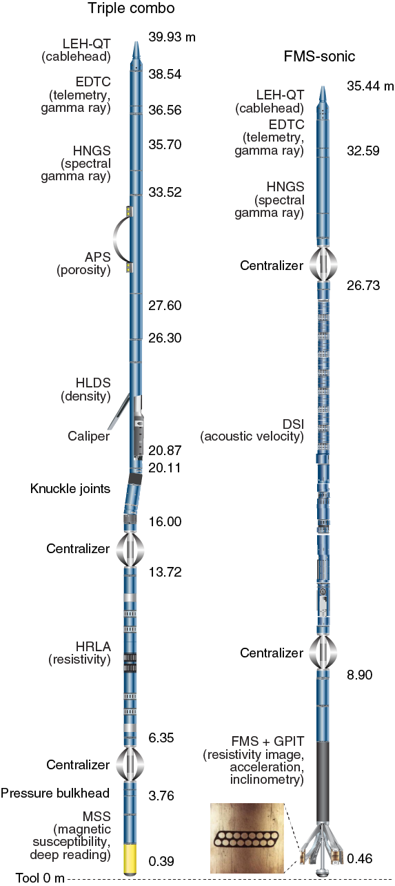
Figure F21. Triple combo and FMS-sonic tool strings.
Table T13. Downhole measurements made by wireline tool strings. Download table in CSV format.
Table T14. Acronyms and units used for downhole wireline tools and measurements. Download table in CSV format.
The second logging deployment used the Formation MicroScanner (FMS)-sonic tool string (Figure F21; Tables T13, T14) to provide an oriented resistivity image of the borehole wall plus P- and S-wave acoustic velocity of the formation using the Dipole Shear Sonic Imager (DSI). Magnetometry was measured with a fluxgate magnetometer in the General Purpose Inclinometry Tool (GPIT) that simultaneously measured any borehole deviation from vertical. The HNGS was included to record NGR to depth-match features between the logging runs, and a caliper again measured borehole diameter to indicate hole and data quality.
To prepare for logging of Hole U1482C, the hole was cleared of drilling cuttings with a mud sweep followed by flushing with seawater. The bottom-hole assembly (BHA) was set at 74.7 m drilling depth below seafloor (DSF) to cover the most unstable upper part of the hole; therefore, an attenuated NGR signal is the only available logging data for the upper ~75 m of the hole. Both tool strings were lowered downhole on a seven-conductor wireline cable to the total depth before being pulled up at constant speed, typically ~550 m/h for the triple combo and 500–550 m/h for the FMS-sonic.
Each tool string deployment is termed a logging “run.” During each run, tool strings were lowered and pulled up in the hole several times to check repeatability and to increase coverage of the FMS borehole images. Each lowering or hauling-up of the tool string while collecting data constitutes a “pass.” Incoming data were recorded and monitored in real time on the Modular Configuration MAXIS (MCM) logging computer. Ship heave was minimal during logging at Hole U1482C, so the wireline heave compensator (WHC) was not used.
Logged sediment properties and tool measurement principles
Logged properties and the principles used in the tools that measure them are briefly described below. The main logs collected during this expedition are listed in Table T13. More detailed information on individual tools and their geological applications may be found in Serra (1984, 1986, 1989), Schlumberger (1989, 1994), Rider (1996), Goldberg (1997), Lovell et al. (1998), and Ellis and Singer (2007). A complete online list of acronyms for the Schlumberger tools and measurement curves is at http://iodp.tamu.edu/tools/logging/index.html.
Natural gamma radiation
The HNGS was used on both the triple combo and FMS-sonic tool strings to measure NGR in the formation. The HNGS uses two bismuth germanate scintillation detectors and five-window spectroscopy to determine concentrations of potassium (in weight percent), thorium (in parts per million), and uranium (in parts per million) from the characteristic gamma ray energies of isotopes in the 40K, 232Th, and 238U radioactive decay series, which dominate the natural radiation spectrum. The computation of elemental abundances uses a least-squares method of extracting U, Th, and K elemental concentrations from the spectral measurements. The HNGS filters out gamma ray energies below 500 keV, eliminating sensitivity to bentonite or KCl in the drilling mud and improving measurement accuracy. The HNGS also provides a measure of the total gamma ray emission (HSGR) and uranium-free or computed gamma ray emission (HCGR) in American Petroleum Institute units (gAPI). The HNGS response is influenced by the borehole diameter, and therefore the HNGS data are corrected for borehole diameter variations during acquisition.
An additional NGR sensor was housed in the Enhanced Digital Telemetry Cartridge (EDTC), which was used primarily to communicate data to the surface. This sensor includes a sodium iodide scintillation detector that also measures the total NGR emission of the formation. It is not a spectral tool (i.e., it does not provide U, Th, and K concentrations), but it provides total gamma radiation for each pass.
Including the HNGS in both tool strings enabled us to use the gamma ray data for precise depth match processing between logging strings and provided a reliable means of core-log integration.
Density and photoelectric factor
Formation density was measured with the HLDS. The sonde contains a radioactive cesium (137Cs) gamma ray source (622 keV) and both far and near gamma ray detectors mounted on a shielded skid, which is pressed against the borehole wall by a hydraulically activated decentralizing arm. Gamma rays emitted by the source undergo Compton scattering, in which gamma rays are scattered by electrons in the formation. The number of scattered gamma rays that reach the detectors is proportional to the density of electrons in the formation, which is in turn related to bulk density. Porosity may also be derived from this bulk density if the matrix (grain) density is known.
The HLDS also measures the photoelectric effect (PEF), a measure of the photoelectric absorption of low-energy gamma radiation. Photoelectric absorption occurs when gamma radiation energy falls below 150 keV as a result of being repeatedly scattered by electrons in the formation. The PEF is determined by comparing the counts from the far detector in the high-energy region, where only Compton scattering occurs, with those in the low-energy region, where count rates depend on both reactions. Because PEF depends on the atomic number of the elements in the formation (heavier elements have higher PEF), it also varies according to the chemical composition of the minerals present and can be used for the identification of the overall mineral make-up of the formation. For example, the PEF of calcite is 5.08 b/e–, illite is 3.03 b/e–, quartz is 1.81 b/e–, and hematite is 21 b/e– (Serra, 1984; Schlumberger, 1989). Good contact between the tool and borehole wall is essential for good HLDS logs; poor contact results in underestimation of density values. Both the density correction and caliper measurement of the hole are used to check the contact quality. The PEF log should be used with caution when multiple mud sweeps are used to stabilize the borehole and especially in washouts, because barium in the logging mud swamps the signal, regardless of attempts to correct for the mud effect.
Porosity
Formation porosity was measured with the APS. The sonde includes a minitron neutron generator that produces fast (14.4 MeV) neutrons, along with five neutron detectors (four epithermal and one thermal) positioned at different distances from the minitron. The tool’s detectors count neutrons that arrive at the detectors after being scattered and slowed by collisions with atomic nuclei in the formation.
The highest energy loss occurs when neutrons collide with hydrogen nuclei, which have practically the same mass as the neutrons (the neutrons bounce off heavier elements without losing much energy). If the hydrogen (i.e., water) concentration is low, as in low-porosity formations, neutrons can travel farther before being captured and the count rates increase at the detector. The opposite effect occurs in high-porosity formations where the water content is high. However, because hydrogen that is bound to minerals such as clays or that forms part of hydrocarbon molecules also contributes to the measurement, the raw porosity value is often overestimated and, when possible, should be checked against laboratory-derived values from the core.
Upon reaching thermal energies (0.025 eV), neutrons are captured by the nuclei of Cl, Si, B, and other elements, resulting in a gamma ray emission. This neutron capture cross section (Σf) is also measured by the tool.
Electrical resistivity
The HRLA tool provides six resistivity measurements with different depths of investigation throughout the logged interval (including the borehole mud resistivity and five measurements of formation resistivity with increasing penetration into the formation). The tool sends a focused current into the formation and measures the intensity necessary to maintain a constant drop in voltage across a fixed interval, providing direct resistivity measurements. The array has one central (source) electrode and six electrodes above and below it, which serve alternatively as focusing and returning current electrodes. By rapidly changing the role of these electrodes, a simultaneous resistivity measurement at six penetration depths is achieved. The tool is designed to ensure that all signals are measured at exactly the same time and to reduce the sensitivity to “shoulder bed” effects when crossing sharply defined beds that are thinner than the electrode spacing. The design of the HRLA, which eliminates the need for a surface reference electrode, improves formation resistivity evaluation compared to traditional dual induction resistivity methods and allows the full range of resistivity to be measured, from low (e.g., in high-porosity sediment) to high (e.g., in basalt). The HRLA tool needs to be run centralized in the borehole for optimal results, so bowspring centralizers were used to keep the HRLA in the center of the borehole. Knuckle joints above the HRLA allowed the density tool to be eccentralized to maintain good contact with the borehole wall (Figure F21).
Calcite, silica, and hydrocarbons are electrical insulators, whereas ionic solutions like interstitial water are conductors. Electrical resistivity, therefore, can be used to evaluate porosity for a given salinity and resistivity of the interstitial water (Schlumberger, 1989). Clay surface conduction also contributes to the resistivity values, but at high porosities this is a relatively minor effect.
Magnetic susceptibility
The MSS is a nonstandard wireline tool designed by LDEO. It measures the ease with which formations are magnetized when subjected to a magnetic field. The ease of magnetization is ultimately related to the concentration and composition (size, shape, and mineralogy) of magnetic minerals (principally magnetite) in the formation. These measurements provide one of the best methods for investigating stratigraphic changes in mineralogy and lithology because the measurement is quick, repeatable, and nondestructive and because different lithologies often have strongly contrasting susceptibilities.
The MSS dual-coil sensor provides ~40 cm resolution measurements with ~20 cm horizontal penetration. The MSS was run as the lowermost tool in the triple combo tool string, using a specially developed data translation cartridge to enable the MSS to be run in combination with the Schlumberger tools. The MSS also has an optional single-coil sensor to provide high-resolution measurements (~10 cm), but this was not used during Expedition 363 because it requires a large bowspring to achieve adequate contact with the borehole wall. This would mean that the MSS would have to be run higher up in the tool string so it could be eccentralized and ultimately would have required an additional log run.
Magnetic susceptibility data from the deep-reading sensor are plotted as uncalibrated units. The MSS reading responses are affected by temperature and borehole size (higher temperatures lead to higher susceptibility measurements). No apparent temperature drift was seen in the data, and therefore no corrections were made offshore. When the magnetic susceptibility signal in sediment is very low, the detection limits of the tool may be reached. For quality control and environmental correction, the MSS also measures internal tool temperature, z-axis acceleration, and low-resolution borehole conductivity.
Acoustic velocity
The DSI measures the transit times between sonic transmitters and an array of eight receivers. It combines replicate measurements, thus providing a direct measure of sound velocity through formations that is relatively free from the effects of formation damage and an enlarged borehole (Schlumberger, 1989). Along with the monopole transmitters found on most sonic tools, it also has two crossed-dipole transmitters that allow measurement of shear wave velocity in addition to compressional wave velocity. Dipole measurements are necessary to measure shear wave velocities in slow formations where shear wave velocity is less than the velocity of sound in the borehole fluid. Such slow formations are often encountered in deep-ocean drilling.
Formation MicroScanner
The FMS provides high-resolution electrical resistivity–based images of borehole walls. The tool has four orthogonal arms and pads, each containing 16 button electrodes that are pressed against the borehole wall during logging (Figure F21). The electrodes are arranged in two diagonally offset rows of eight electrodes each. A focused current is emitted from the button electrodes into the formation, with a return electrode near the top of the tool. Resistivity of the formation at the button electrodes is derived from the intensity of current passing through the button electrodes.
Processing transforms the resistivity measurements into oriented high-resolution images that reveal geologic structures of the borehole wall. Features such as bedding, stratification, fracturing, slump folding, and bioturbation can be resolved (Luthi, 1990; Salimullah and Stow, 1992; Lovell et al., 1998). Because the images are oriented to magnetic north, further analysis can provide measurement of the dip and direction (azimuth) of planar features in the formation. In addition, when the corresponding planar features can be identified in the recovered core samples, individual core pieces can be reoriented with respect to true north.
Approximately 30% of a borehole with a diameter of 25 cm (9.8 inches) is imaged during a single pass. Standard procedure is to make two full uphole passes with the FMS to maximize the chance of getting nearly full borehole coverage with the pads. The maximum extension of the caliper arms is 40.6 cm (16 inches). In holes with a diameter greater than this maximum, the pad contact at the end of the caliper arms will be inconsistent, and the FMS images may appear out of focus and too conductive. Irregular (rough) borehole walls will also adversely affect the images if contact with the wall is poor.
Acceleration and inclinometry
Three-component acceleration and magnetic field measurements were made with the GPIT. The primary purpose of this tool, which incorporates a three-component accelerometer and a three-component magnetometer, is to determine the acceleration and orientation of the FMS-sonic tool string during logging. This information allows the FMS images to be corrected for irregular tool motion and the dip and direction (azimuth) of features in the images to be determined. The GPIT is run with other tools on the FMS-sonic tool string that can carry remanent or induced magnetization; therefore, its magnetic measurements can be affected by the other tools, the rocks and/or sediment in the borehole wall, and magnetization of the casing and/or drill pipe. On the FMS-sonic tool string, however, the GPIT has greater nonmagnetic insulation from the other tools, which greatly reduces the effects on its magnetic measurements.
Log data quality
The main influence on log data quality is the condition of the borehole wall. Where the borehole diameter varies over short intervals because of washouts (wide borehole) of softer material or ledges of harder material, the logs from tools that require good contact with the borehole wall (i.e., FMS, density, and porosity) may be degraded. Deep investigation measurements, such as NGR, resistivity, and sonic velocity, which do not require contact with the borehole wall, are generally less sensitive to borehole conditions. “Bridged” sections, where borehole diameter is much lower than the bit size, will also cause irregular log results. The quality of the borehole is improved by minimizing the circulation of drilling fluid while drilling, flushing the borehole to remove debris, and logging the borehole as soon as possible after drilling and conditioning are completed.
The quality of the wireline depth determination depends on several factors. The depth of the logging measurements is determined from the length of the cable payed out from the winch on the ship. The seafloor is identified on the NGR log by the abrupt reduction in gamma ray count at the water/sediment interface (mudline). Discrepancies between the drilling depth and the wireline log depth may occur. In the case of drilling depth, discrepancies are caused by core expansion, incomplete core recovery, or incomplete heave compensation. In the case of log depth, discrepancies between successive runs occur because of incomplete heave compensation, incomplete correction for cable stretch, and cable slip. Tidal changes in sea level and unaccounted-for changes in trim of the drillship affect both drilling and logging depths.
Logging data flow and log depth scales
Data for each wireline logging run were monitored in real time and recorded using the Schlumberger MAXIS 500 system. Initial logging data were referenced to the rig floor (WRF). After logging was completed, data were shifted to a seafloor reference (WSF) based on the step in logged gamma radiation at the sediment/water interface.
Data were transferred to LDEO, where standardized data processing took place. A main part of this was depth matching to remove depth offsets between logs from different logging runs. This resulted in a new depth scale: wireline log matched depth below seafloor (WMSF). Also, corrections were made to certain tools and logs (e.g., FMS imagery was corrected for tool acceleration, including “stick and slip” motion), documentation for the logs (with assessment of log quality) was prepared, and data were converted to ASCII for conventional logs and to GIF for FMS images. Schlumberger Geo-Quest’s GeoFrame software was used for most of the processing of the collected wireline logging data. The data were transferred back to the ship within a few days after logging, and the processed data sets were made available to the science party.
References
Acton, G.D., Borton, C.J., and the Leg 178 Shipboard Scientific Party, 2001. Palmer Deep composite depth scales for Leg 178 Sites 1098 and 1099. In Barker, P.F., Camerlenghi, A., Acton, G.D., and Ramsay, A.T.S. (Eds.), Proceedings of the Ocean Drilling Program, Scientific Results, 178: College Station, TX (Ocean Drilling Program), 1–35. https://doi.org/10.2973/odp.proc.sr.178.202.2001
Adkins, J.F., McIntyre, K., and Schrag, D.P., 2002. The salinity, temperature, and δ18O of the glacial deep ocean. Science, 298(5599):1769–1773. https://doi.org/10.1126/science.1076252
Anthonissen, D.E., and Ogg, J.G., 2012. Appendix 3—Cenozoic and Cretaceous biochronology of planktonic foraminifera and calcareous nannofossils. In Gradstein, F.M., Ogg, J.G., Schmitz, M.D., and Ogg, G.M., (Eds.), The Geologic Time Scale 2012: Amsterdam (Elsevier), 1083–1127. https://doi.org/10.1016/B978-0-444-59425-9.15003-6
ASTM International, 1990. Standard method for laboratory determination of water (moisture) content of soil and rock (Standard D2216–90). In Annual Book of ASTM Standards for Soil and Rock (Volume 04.08): Philadelphia (American Society for Testing Materials). [revision of D2216-63, D2216-80]
Aubry, M.-P., 1988. Handbook of Calcareous Nannoplankton (Book 2): Ortholithae (Catinasters, Ceratoliths, Rhabdoliths): New York (Micropaleontology Press).
Aubry, M.-P., 1990. Handbook of Calcareous Nannoplankton (Book 4): Heliolithae (Helicoliths, Cribriliths, Lopadoliths, and Others): New York (Micropaleontology Press).
Aubry, M.-P., 2015. Cenozoic Coccolithophores (Volume B–E): Discoasterales: New York (Micropaleontology Press).
Backman, J., and Raffi, I., 1997. Calibration of Miocene nannofossil events to orbitally tuned cyclostratigraphies from Ceara Rise. In Shackleton, N.J., Curry, W.B., Richter, C., and Bralower, T.J. (Eds.), Proceedings of the Ocean Drilling Program, Scientific Results, 154: College Station, TX (Ocean Drilling Program), 83–99. https://doi.org/10.2973/odp.proc.sr.154.101.1997
Backman, J., Raffi, I., Rio, D., Fornaciari, E., and Pälike, H., 2012. Biozonation and biochronology of Miocene through Pleistocene calcareous nannofossils from low and middle latitudes. Newsletters on Stratigraphy, 45(3):221–244. https://doi.org/10.1127/0078-0421/2012/0022
Balsam, W.L., and Damuth, J.E., 2000. Further investigations of shipboard vs. shore-based spectral data: implications for interpreting Leg 164 sediment composition. In Paull, C.K., Matsumoto, R., Wallace, P., and Dillon, W.P. (Eds.), Proceedings of the Ocean Drilling Program, Scientific Results, 164: College Station, TX (Ocean Drilling Program), 313–324. https://doi.org/10.2973/odp.proc.sr.164.222.2000
Balsam, W.L., Damuth, J.E., and Schneider, R.R., 1997. Comparison of shipboard vs. shore-based spectral data from Amazon Fan cores: implications for interpreting sediment composition. In Flood, R.D., Piper, D.J.W., Klaus, A., and Peterson, L.C. (Eds.), Proceedings of the Ocean Drilling Program, Scientific Results, 155: College Station, TX (Ocean Drilling Program), 193–215. https://doi.org/10.2973/odp.proc.sr.155.210.1997
Balsam, W.L., Deaton, B.C., and Damuth, J.E., 1998. The effects of water content on diffuse reflectance spectrophotometry studies of deep-sea sediment cores. Marine Geology, 149(1–4):177–189. https://doi.org/10.1016/S0025-3227(98)00033-4
Baumann, K.-H., and Freitag, T., 2004. Pleistocene fluctuations in the northern Benguela Current system as revealed by coccolith assemblages. Marine Micropaleontology, 52(1–4):195–215. https://doi.org/10.1016/j.marmicro.2004.04.011
Berggren, W.A, Hilgen, F.J., Langereis, C.G., Kent, D.V., Obradovich, J.D., Raffi, I., Raymo, M.E., and Shackelton, N.J., 1995a. Late Neogene chronology: new perspectives in high-resolution stratigraphy. Geological Society of America Bulletin, 107(11):1272–1287. https://doi.org/10.1130/0016-7606(1995)107<1272:LNCNPI>2.3.CO;2
Berggren, W.A., Kent, D.V., Swisher, C.C., III, and Aubry, M.-P., 1995b. A revised Cenozoic geochronology and chronostratigraphy. In Berggren, W.A., Kent, D.V., Aubry, M.-P., and Hardenbol, J. (Eds.), Geochronology, Time Scales and Global Stratigraphic Correlation. Special Publication - SEPM (Society for Sedimentary Geology), 54:129–212. https://doi.org/10.2110/pec.95.04.0129
Blum, P., 1997. Technical Note 26: Physical Properties Handbook—A Guide to the Shipboard Measurement of Physical Properties of Deep-Sea Cores. Ocean Drilling Program. https://doi.org/10.2973/odp.tn.26.1997
Bullard, E.C., 1954. The flow of heat through the floor of the Atlantic Ocean. Proceedings of the Royal Society of London, Series A: Mathematical, Physical and Engineering Sciences, 222(1150):408–429. https://doi.org/10.1098/rspa.1954.0085
Chaisson, W.P., and Pearson, P.N., 1997. Planktonic foraminifer biostratigraphy at Site 925: middle Miocene–Pleistocene. In Shackleton, N.J., Curry, W.B., Richter, C., and Bralower, T.J. (Eds.), Proceedings of the Ocean Drilling Program, Scientific Results, 154: College Station, TX (Ocean Drilling Program), 3–31. https://doi.org/10.2973/odp.proc.sr.154.104.1997
Chaproniere, G.C.H., Styzen, M.J., Sager, W.W., Nishi, H., Quinterno, P.J., and Abrahamsen, N., 1994. Late Neogene biostratigraphic and magnetostratigraphic synthesis, Leg 135. In Hawkins, J., Parson, L., Allan, J., et al., Proceedings of the Ocean Drilling Program, Scientific Results, 135: College Station, TX (Ocean Drilling Program), 857–877. https://doi.org/10.2973/odp.proc.sr.135.116.1994
Curry, W.B., Shackleton, N.J., Richter, C., et al., 1995. Proceedings of the Ocean Drilling Program, Initial Reports, 154: College Station, TX (Ocean Drilling Program). https://doi.org/10.2973/odp.proc.ir.154.1995
De Vleeschouwer, D., Dunlea, A.G., Auer, G., Anderson, C.H., Brumsack, H., de Loach, A., Gurnis, M., Huh, Y., Ishiwa, T., Jang, K., Kominz, M.A., März, C., Schnetger, B., Murray, R.W., Pälike, H., and Expedition 356 Shipboard Scientists, 2017. Quantifying K, U, and Th contents of marine sediments using shipboard natural gamma radiation spectra measured on DV JOIDES Resolution. Geochemistry, Geophysics, Geosystems, 18(3):1053–1064. https://doi.org/10.1002/2016GC006715
Dunlea, A.G., Murray, R.W., Harris, R.N., Vasiliev, M.A., Evans, H., Spivack, A.J., and D’Hondt, S., 2013. Assessment and use of NGR instrumentation on the JOIDES Resolution to quantify U, Th, and K concentrations in marine sediment. Scientific Drilling, 15:57–63. https://doi.org/10.2204/iodp.sd.15.05.2013
Ellis, D.V., and Singer, J.M., 2007. Well Logging for Earth Scientists (2nd edition): New York (Elsevier).
Evans, H.B., 1965. GRAPE—a device for continuous determination of material density and porosity. Transactions of the SPWLA Annual Logging Symposium: 6(2):B1–B25. https://www.spwla.org/SymposiumTransactions/grape-device-continuous-determination-material-density-and-porosity
Expedition 320/321 Scientists, 2010. Methods. In Pälike, H., Lyle, M., Nishi, H., Raffi, I., Gamage, K., Klaus, A., and the Expedition 320/321 Scientists. Proceedings of the Integrated Ocean Drilling Program, 320/321: Tokyo (Integrated Ocean Drilling Program Management International, Inc.). http://dx.doi.org/10.2204/iodp.proc.320321.102.2010
Expedition 323 Scientists, 2011. Methods. In Takahashi, K., Ravelo, A.C., Alvarez Zarikian, C.A., and the Expedition 323 Scientists, Proceedings of the Integrated Ocean Drilling Program, 323: Tokyo (Integrated Ocean Drilling Program Management International, Inc.). https://doi.org/10.2204/iodp.proc.323.102.2011
Finney, S., and Bown, P.R., 2017. The status of subseries/subepochs for the Paleocene to Holocene: recommendations to authors and editors. Episodes, 40(1):2–4. https://doi.org/10.18814/epiiugs/2017/v40i1/017001
Fornaciari, E., Di Stefano, A., Rio, D., and Negri, A., 1996. Middle Miocene quantitative calcareous nannofossil biostratigraphy in the Mediterranean region. Micropaleontology, 42(1):37–63. https://doi.org/10.2307/1485982
Gartner, S., 1992. Miocene nannofossil chronology in the North Atlantic, DSDP Site 608. Marine Micropaleontology, 18(4):307–331. https://doi.org/10.1016/0377-8398(92)90045-L
Gibbard, P.L., Head, M.J., and Walker, M.J.C., 2010. Formal ratification of the Quaternary system/period and the Pleistocene series/epoch with a base at 2.58 Ma. Journal of Quaternary Science, 25(2):96–102. https://doi.org/10.1002/jqs.1338
Gieskes, J.M., Gamo, T., and Brumsack, H., 1991. Technical Note 15: Chemical Methods for Interstitial Water Analysis Aboard JOIDES Resolution. Ocean Drilling Program. https://doi.org/10.2973/odp.tn.15.1991
Giosan, L., Flood, R.D., and Aller, R.C., 2002. Paleoceanographic significance of sediment color on western North Atlantic drifts: I. Origin of color. Marine Geology, 189(1–2):25–41. https://doi.org/10.1016/S0025-3227(02)00321-3
Goldberg, D., 1997. The role of downhole measurements in marine geology and geophysics. Reviews of Geophysics, 35(3):315–342. https://doi.org/10.1029/97RG00221
Gradstein, F.M., Ogg, J.G., Schmitz, M.D., and Ogg, G.M. (Eds.), 2012. The Geological Time Scale 2012: Amsterdam (Elsevier).
Hagelberg, T.K., Pisias, N.G., Shackleton, N.J., Mix, A.C., and Harris, S., 1995. Refinement of a high-resolution, continuous sedimentary section for studying equatorial Pacific Ocean paleoceanography, Leg 138. In Pisias, N.G., Mayer, L.A., Janecek, T.R., Palmer-Julson, A., and van Andel, T.H. (Eds.), Proceedings of the Ocean Drilling Program, Scientific Results, 138: College Station, TX (Ocean Drilling Program), 31–46. https://doi.org/10.2973/odp.proc.sr.138.103.1995
Harms, J.C., and Choquette, P.W., 1965. Geologic evaluation of a gamma-ray porosity device. Transactions of the SPWLA Annual Logging Symposium, 6(2):C1–C37.
Hilgen, F.J., Lourens, L.J., and Van Dam, J.A., 2012. The Neogene period. With contributions by A.G. Beu, A.F. Boyes, R.A. Cooper, W. Krijgsman, J.G. Ogg, W.E. Piller, and D.S. Wilson. In Gradstein, F.M., Ogg, J.G., Schmitz, M.D., and Ogg, G.M. (Eds.), The Geologic Time Scale: Oxford, United Kingdom (Elsevier), 923–978. https://doi.org/10.1016/B978-0-444-59425-9.00029-9
Holbourn, A., Henderson, A.S., and MacLeod, N., 2013. Atlas of Benthic Foraminifera: Chichester, United Kingdom (John Wiley & Sons, Ltd.). https://doi.org/10.1002/9781118452493
Horai, K., and Von Herzen, R.P., 1985. Measurement of heat flow on Leg 86 of the Deep Sea Drilling Project. In Heath, G.R., Burckle, L.H., et al., Initial Reports of the Deep Sea Drilling Project, 86: Washington, DC (U.S. Government Printing Office), 759–777. https://doi.org/10.2973/dsdp.proc.86.135.1985
Insua, T.L., Spivack, A.J., Graham, D., D’Hondt, S., and Moran, K., 2014. Reconstruction of Pacific Ocean bottom water salinity during the Last Glacial Maximum. Geophysical Research Letters, 41(8):2914–2920. https://doi.org/10.1002/2014GL059575
Jarrard, R.D., and Kerneklian, M.J., 2007. Data report: physical properties of the upper oceanic crust of ODP Site 1256: multisensor track and moisture and density measurements. In Teagle, D.A.H., Wilson, D.S., Acton, G.D., and Vanko, D.A. (Eds.), Proceedings of the Ocean Drilling Program, Scientific Results, 206: College Station, TX (Ocean Drilling Program), 1–11. https://doi.org/10.2973/odp.proc.sr.206.011.2007
Jones, R.W., 1994. The Challenger Foraminifera: New York (Oxford University Press USA).
Kirschvink, J.L., 1980. The least-squares line and plane and the analysis of palaeomagnetic data. Geophysical Journal of the Royal Astronomical Society, 62(3):699–718. https://doi.org/10.1111/j.1365-246X.1980.tb02601.x
Kristiansen, J.I., 1982. The transient cylindrical probe method for determination of thermal parameters of earth materials [Ph.D. dissertation]. Åarhus University, Åarhus, Denmark.
Laj, C., and Channell, J.E.T., 2007. Geomagnetic excursions. Treatise on Geophysics, 5:373–416. https://doi.org/10.1016/B978-044452748-6.00095-X
Lourens, L., Hilgen, F., Shackleton, N.J., Laskar, J., and Wilson, D., 2004. The Neogene period. In Gradstein, F.M., Ogg, J.G., and Smith, A. (Eds.), A Geologic Time Scale 2004: Cambridge, United Kingdom (Cambridge University Press), 409–440. https://doi.org/10.1017/CBO9780511536045.022
Lovell, M.A., Harvey, P.K., Brewer, T.S., Williams, C., Jackson, P.D., and Williamson, G., 1998. Application of FMS images in the Ocean Drilling Program: an overview. In Cramp, A., MacLeod, C.J., Lee, S.V., and Jones, E.J.W. (Eds.), Geological Evolution of Ocean Basins: Results from the Ocean Drilling Program. Geological Society Special Publication, 131(1):287–303. https://doi.org/10.1144/GSL.SP.1998.131.01.18
Lurcock, P.C., and Wilson, G.S., 2012. PuffinPlot: a versatile, user-friendly program for paleomagnetic analysis. Geochemistry, Geophysics, Geosystems, 13(6):Q06Z45. https://doi.org/10.1029/2012GC004098
Luthi, S.M., 1990. Sedimentary structures of clastic rocks identified from electrical borehole images. In Hurst, A., Lovell, M.A., and Morton, A.C. (Eds.), Geological Applications of Wireline Logs. Geological Society Special Publication, 48:3–10. https://doi.org/10.1144/GSL.SP.1990.048.01.02
Manheim, F.T., and Sayles, F.L., 1974. Composition and origin of interstitial waters of marine sediments, based on deep sea drill cores. In Goldberg, E.D. (Ed.), The Sea (Volume 5): Marine Chemistry: The Sedimentary Cycle: New York (Wiley), 527–568.
Martini, E., 1971. Standard Tertiary and Quaternary calcareous nannoplankton zonation. In Farinacci, A. (Ed.), Proceedings of the Second Planktonic Conference, Roma 1970: Rome (Edizioni Tecnoscienza), 2:739–785.
Mazzullo, J.M., Meyer, A., and Kidd, R.B., 1988. New sediment classification scheme for the Ocean Drilling Program. In Mazzullo, J., and Graham, A.G. (Eds.), Technical Note 8: Handbook for Shipboard Sedimentologists. Ocean Drilling Program, 44–67. https://doi.org/10.2973/odp.tn.8.1988
McDuff, R.E., 1985. The chemistry of interstitial waters, Deep Sea Drilling Project Leg 86. In Heath, G.R., Burckle, L.H., et al., Initial Reports of the Deep Sea Drilling Project, 86: Washington, DC (U.S. Government Printing Office), 675–687. https://doi.org/10.2973/dsdp.proc.86.131.1985
McNeill, L.C., Dugan, B., Petronotis, K.E., Backman, J., Bourlange, S., Chemale, F., Chen, W., Colson, T.A., Frederik, M.C.G., Guèrin, G., Hamahashi, M., Henstock, T., House, B.M., Hüpers, A., Jeppson, T.N., Kachovich, S., Kenigsberg, A.R., Kuranaga, M., Kutterolf, S., Milliken, K.L., Mitchison, F.L., Mukoyoshi, H., Nair, N., Owari, S., Pickering, K.T., Pouderoux, H.F.A., Yehua, S., Song, I., Torres, M.E., Vannucchi, P., Vrolijk, P.J., Yang, T., and Zhao, X., 2017. Expedition 362 summary. In McNeill, L.C., Dugan, B., Petronotis, K.E., and the Expedition 362 Scientists, Sumatra Subduction Zone. Proceedings of the International Ocean Discovery Program, 362: College Station, TX (International Ocean Discovery Program). https://doi.org/10.14379/iodp.proc.362.101.2017
Mix, A.C., Pisias, N.G., Rugh, W., Wilson, J., Morey, A., and Hagelberg, T.K., 1995. Benthic foraminifer stable isotope record from Site 849 (0–5 Ma): local and global climate changes. In Pisias, N.G., Mayer, L.A., Janecek, T.R., Palmer-Julson, A., and van Andel, T.H. (Eds.), Proceedings of the Ocean Drilling Program, Scientific Results, 138: College Station, TX (Ocean Drilling Program), 371–412. https://doi.org/10.2973/odp.proc.sr.138.120.1995
Mix, A.C., Tiedemann, R., Blum, P., et al., 2003. Proceedings of the Ocean Drilling Program, Initial Reports, 202: College Station, TX (Ocean Drilling Program). https://doi.org/10.2973/odp.proc.ir.202.2003
Munsell Color Company, Inc., 1994. Munsell Soil Color Chart (revised edition): Newburgh, MD (Munsell Color).
Murray, R.W., Miller, D.J., and Kryc, K.A., 2000. Technical Note 29: Analysis of Major and Trace Elements in Rocks, Sediments, and Interstitial Waters by Inductively Coupled Plasma–Atomic Emission Spectrometry (ICP-AES). Ocean Drilling Program. https://doi.org/10.2973/odp.tn.29.2000
Okada, H., and Bukry, D., 1980. Supplementary modification and introduction of code numbers to the low-latitude coccolith biostratigraphic zonation (Bukry, 1973; 1975). Marine Micropaleontology, 5:321–325. https://doi.org/10.1016/0377-8398(80)90016-X
Pearson, P.N., 1995. Planktonic foraminifer biostratigraphy and the development of pelagic caps on guyots in the Marshall Islands group. In Haggerty, J.A., Premoli Silva, I., Rack, F., and McNutt, M.K. (Eds.), Proceedings of the Ocean Drilling Program, Scientific Results, 144: College Station, TX (Ocean Drilling Program), 21–59. https://doi.org/10.2973/odp.proc.sr.144.013.1995
Pearson, P.N., and Chaisson, W.P., 1997. Late Paleocene to middle Miocene planktonic foraminifer biostratigraphy of the Ceara Rise. In Shackleton, N.J., Curry, W.B., Richter, C., and Bralower, T.J. (Eds.), Proceedings of the Ocean Drilling Program, Scientific Results, 154: College Station, TX (Ocean Drilling Program), 33–68. https://doi.org/10.2973/odp.proc.sr.154.106.1997
Pearson, P.N., and Wade, B.S., 2015. Systematic taxonomy of exceptionally well-preserved planktonic foraminifera from the Eocene/Oligocene boundary of Tanzania. Special Publication - Cushman Foundation for Foraminiferal Research, 45. http://www.cushmanfoundation.org/specpubs/sp45.pdf
Pearson, P.N., Wade, B.S., Backman, J., Raffi, I., and Monechi, S., 2017. Sub-series and sub-epochs are informal units and should continue to be omitted from the International Chronostratigraphic Chart. Episodes, 40(1):5–7. https://doi.org/10.18814/epiiugs/2017/v40i1/017002
Perch-Nielsen, K., 1985. Cenozoic calcareous nannofossils. In Bolli, H.M., Saunders, J.B., and Perch-Nielsen, K. (Eds.), Plankton Stratigraphy: Cambridge, United Kingdom (Cambridge University Press), 427–554.
Pribnow, D., Kinoshita, M., and Stein, C., 2000. Thermal Data Collection and Heat Flow Recalculations for Ocean Drilling Program Legs 101–180: Hanover, Germany (Institute for Joint Geoscientific Research, Institut für Geowissenschaftliche Gemeinschaftsaufgaben [GGA]). http://www-odp.tamu.edu/publications/heatflow/ODPReprt.pdf
Pujol, C., and Duprat, J., 1983. Quaternary planktonic foraminifers of the southwestern Atlantic (Rio Grande Rise) Deep Sea Drilling Project Leg 72. In Barker, P.F., Carlson, R.L., Johnson, D.A., et al., Initial Reports of the Deep Sea Drilling Project, 72: Washington, DC (U.S. Government Printing Office), 601–615. https://doi.org/10.2973/dsdp.proc.72.128.1983
Raffi, I., 2002. Revision of the early-middle Pleistocene calcareous nannofossil biochronology (1.75–0.85 Ma). Marine Micropaleontology, 45(1):25–55. https://doi.org/10.1016/S0377-8398(01)00044-5
Raffi, I., Backman, J., Rio, D., and Shackleton, N.J., 1993. Plio–Pleistocene nannofossil biostratigraphy and calibration to oxygen isotope stratigraphies from Deep Sea Drilling Project Site 607 and Ocean Drilling Program Site 677. Paleoceanography, 8(3):387–408. https://doi.org/10.1029/93PA00755
Raffi, I., Backman, J., Zachos, J.C., and Sluijs, A., 2009. The response of calcareous nannofossil assemblages to the Paleocene Eocene Thermal Maximum at the Walvis Ridge in the South Atlantic. Marine Micropaleontology, 70(3–4):201–212. https://doi.org/10.1016/j.marmicro.2008.12.005
Raffi, I., and Flores, J.-A., 1995. Pleistocene through Miocene calcareous nannofossils from eastern equatorial Pacific Ocean (Leg 138). In Pisias, N.G., Mayer, L.A., Janecek, T.R., Palmer-Julson, A., and van Andel, T.H. (Eds.), Proceedings of the Ocean Drilling Program, Scientific Results, 138: College Station, TX (Ocean Drilling Program), 233–286. https://doi.org/10.2973/odp.proc.sr.138.112.1995
Raffi, I., Rio, D., d’Atri, A., Fornaciari, E., and Rocchetti, S., 1995. Quantitative distribution patterns and biomagnetostratigraphy of middle and late Miocene calcareous nannofossils from equatorial Indian and Pacific oceans (Leg 115, 130, and 138). In Pisias, N.G., Mayer, L.A., Janecek, T.R., Palmer-Julson, A., and van Andel, T.H. (Eds.), Proceedings of the Ocean Drilling Program, Scientific Results, 138: College Station, TX (Ocean Drilling Program), 479–502. https://doi.org/10.2973/odp.proc.sr.138.125.1995
Rea, D.K., Basov, I.A., Janecek, T.R., Palmer-Julson, A., et al., 1993. Proceedings of the Ocean Drilling Program, Initial Reports, 145: College Station, TX (Ocean Drilling Program). https://doi.org/10.2973/odp.proc.ir.145.1993
Richter, C., Acton, G., Endris, C., and Radsted, M., 2007. Technical Note 34: Handbook for Shipboard Paleomagnetists. Ocean Drilling Program. https://doi.org/10.2973/odp.tn.34.2007
Rider, M.H., 1996. The Geological Interpretation of Well Logs (2nd edition): Caithness, Scotland (Whittles Publishing).
Rio, D., Raffi, I., and Villa, G., 1990. Pliocene–Pleistocene calcareous nannofossil distribution patterns in the western Mediterranean. In Kastens, K.A., Mascle, J., et al., Proceedings of the Ocean Drilling Program, Scientific Results, 107: College Station, TX (Ocean Drilling Program), 513–533. https://doi.org/10.2973/odp.proc.sr.107.164.1990
Rosenthal, Y., Holbourn, A.E., Kulhanek, D.K., Aiello, I.W., Babila, T.L., Bayon, G., Beaufort, L., Bova, S.C., Chun, J.-H., Dang, H., Drury, A.J., Dunkley Jones, T., Eichler, P.P.B., Fernando, A.G.S., Gibson, K.A., Hatfield, R.G., Johnson, D.L., Kumagai, Y., Li, T., Linsley, B.K., Meinicke, N., Mountain, G.S., Opdyke, B.N., Pearson, P.N., Poole, C.R., Ravelo, A.C., Sagawa, T., Schmitt, A., Wurtzel, J.B., Xu, J., Yamamoto, M., and Zhang, Y.G., 2018. Site U1482. In Rosenthal, Y., Holbourn, A.E., Kulhanek, D.K., and the Expedition 363 Scientists, Western Pacific Warm Pool. Proceedings of the International Ocean Discovery Program, 363: College Station, TX (International Ocean Discovery Program). https://doi.org/10.14379/iodp.proc.363.103.2018
Rothwell, R.G., 1989. Minerals and Mineraloids in Marine Sediments: An Optical Identification Guide: London (Elsevier). https://doi.org/10.1007/978-94-009-1133-8
Ruddiman, W.F., Kidd, R.B., Thomas, E., et al., 1987. Initial Reports of the Deep Sea Drilling Project, 94: Washington, DC (U.S. Government Printing Office). https://doi.org/10.2973/dsdp.proc.94.1987
Salimullah, A.R.M., and Stow, D.A.V., 1992. Application of FMS images in poorly recovered coring intervals: examples from ODP Leg 129. In Hurst, A., Griffiths, C.M., and Worthington, P.F. (Eds.), Geological Application of Wireline Logs II. Geological Society Special Publication, 65(1):71–86. https://doi.org/10.1144/GSL.SP.1992.065.01.06
Schlumberger, 1989. Log Interpretation Principles/Applications: Houston (Schlumberger Education Services), SMP–7017.
Schlumberger, 1994. IPL Integrated Porosity Lithology: Houston (Schlumberger Education Services), SMP-9270.
Serra, O., 1984. Fundamentals of Well-Log Interpretation (Volume 1): The Acquisition of Logging Data: Amsterdam (Elsevier).
Serra, O., 1986. Fundamentals of Well-Log Interpretation (Volume 2): The Interpretation of Logging Data: Amsterdam (Elsevier).
Serra, O., 1989. Formation MicroScanner Image Interpretation: Houston (Schlumberger Education Services), SMP-7028.
Shackleton, N.J., Baldauf, J.G., Flores, J.-A., Iwai, M., Moore, T.C., Jr., Raffi, I., and Vincent, E., 1995. Biostratigraphic summary for Leg 138. In Pisias, N.G., Mayer, L.A., Janecek, T.R., Palmer-Julson, A., and van Andel, T.H. (Eds.), Proceedings of the Ocean Drilling Program, Scientific Results, 138: College Station, TX (Ocean Drilling Program), 517–536. https://doi.org/10.2973/odp.proc.sr.138.127.1995
Shackleton, N.J., Crowhurst, S.J., Weedon, G.P., and Laskar, J., 1999. Astronomical calibration of Oligocene–Miocene time. In Shackleton N.J., McCave, I.N., and Graham, P.W. (Eds.), Astronomical (Milankovitch) Calibration of the Geological Time-Scale. Philosophical Transactions of the Royal Society, A: Mathematical, Physical & Engineering Sciences, 357(1757):1907–1929. https://doi.org/10.1098/rsta.1999.0407
Shepard, F.P., 1954. Nomenclature based on sand-silt-clay ratios. Journal of Sedimentary Research, 24(3):151–158. https://doi.org/10.1306/D4269774-2B26-11D7-8648000102C1865D
Spezzaferri, S., Kucera, M., Pearson, P.N., Wade, B.S., Rappo, S., Poole, C.R., Morard, R., and Stalder, C., 2015. Fossil and genetic evidence for the polyphyletic nature of the planktonic foraminifera “Globigerinoides”, and description of the new genus Trilobatus. PLoS One, 10(5):e0128108. https://doi.org/10.1371/journal.pone.0128108
Shipboard Scientific Party, 2002. Explanatory notes. In Lyle, M., Wilson, P.A., Janecek, T.R., et al., Proceedings of the Ocean Drilling Program, Initial Reports, 199: College Station, TX (Ocean Drilling Program), 1–70. https://doi.org/10.2973/odp.proc.ir.199.102.2002
Tauxe, L., Tucker, P., Peterson, N.P., and LaBrecque, J.L., 1984. Magnetostratigraphy of Leg 73 sediments. In Hsü, K.J., LaBrecque, J.L., et al., Initial Reports of the Deep Sea Drilling Project, 73: Washington, DC (U.S. Government Printing Office), 609–621. https://doi.org/10.2973/dsdp.proc.73.123.1984
Thierstein, H.R., Geitzenauer, K.R., Molfino, B., and Shackleton, N.J., 1977. Global synchroneity of late Quaternary coccolith datum levels validation by oxygen isotopes. Geology, 5(7):400–404. https://doi.org/10.1130/0091-7613(1977)5<400:GSOLQC>2.0.CO;2
Thompson, P.R., Bé, A.W.H., Duplessy, J.-C., and Shackleton, N.J., 1979. Disappearance of pink-pigmented Globigerinoides ruber at 120,000 yr BP in the Indian and Pacific Oceans. Nature, 280(5723):554–558. https://doi.org/10.1038/280554a0
Turco, E., Bambini, A.M., Foresi, L., Iaccarino, S., Lirer, F., Mazzei, R., and Salvatorini, G., 2002. Middle Miocene high-resolution calcareous plankton biostratigraphy at Site 926 (Leg 154, equatorial Atlantic Ocean): palaeoecological and palaeobiogeographical implications. Geobios, 35(1):257–276. https://doi.org/10.1016/S0016-6995(02)00064-5
van Morkhoven, F.P.C.M., Berggren, W.A., Edwards, A.S.,and Oertli, H.J., 1986. Cenozoic cosmopolitan deep-water benthic foraminifera. Bulletin des Centres de Recherches Exploration-Production Elf-Aquitaine, 11.
Vasiliev, M.A., Blum, P., Chubarian, G., Olsen, R., Bennight, C., Cobine, T., Fackler, D., Hastedt, M., Houpt, D., Mateo, Z., and Vasilieva, Y.B., 2011. A new natural gamma radiation measurement system for marine sediment and rock analysis. Journal of Applied Geophysics, 75:455–463. https://doi.org/10.1016/j.jappgeo.2011.08.008
Von Herzen, R., and Maxwell, A.E., 1959. The measurement of thermal conductivity of deep-sea sediments by a needle-probe method. Journal of Geophysical Research, 64(10):1557–1563. https://doi.org/10.1029/JZ064i010p01557
Wade, B.S., Pearson, P.N., Berggren, W.A., and Pälike, H., 2011. Review and revision of Cenozoic tropical planktonic foraminiferal biostratigraphy and calibration to the geomagnetic polarity and astronomical time scale. Earth-Science Reviews, 104(1–3):111–142. https://doi.org/10.1016/j.earscirev.2010.09.003
Young, J.R., 1998. Neogene. In Bown, P.R. (Ed.), Calcareous Nannofossil Biostratigraphy: Dordrecht, The Netherlands (Kluwer Academic Publishing), 225–265.
Young, J.R., and Bown, P.R., 2014. Some emendments to calcareous nannoplankton taxonomy. Journal of Nannoplankton Research, 33(1):39–46. http://ina.tmsoc.org/JNR/online/33/Young&Bown_2014_JNR33-1.pdf
Zijderveld, J.D.A., 1967. AC demagnetization of rocks: analysis of results. In Collinson, D.W., Creer, K.M., and Runcorn, S.K. (Eds.), Methods in Palaeomagnetism: Amsterdam (Elsevier), 254–286.
1 Rosenthal, Y., Holbourn, A.E., Kulhanek, D.K., Aiello, I.W., Babila, T.L., Bayon, G., Beaufort, L., Bova, S.C., Chun, J.-H., Dang, H., Drury, A.J., Dunkley Jones, T., Eichler, P.P.B., Fernando, A.G.S., Gibson, K., Hatfield, R.G., Johnson, D.L., Kumagai, Y., Li, T., Linsley, B.K., Meinicke, N., Mountain, G.S., Opdyke, B.N., Pearson, P.N., Poole, C.R., Ravelo, A.C., Sagawa, T., Schmitt, A., Wurtzel, J.B., Xu, J., Yamamoto, M., and Zhang, Y.G., 2018. Expedition 363 methods. In Rosenthal, Y., Holbourn, A.E., Kulhanek, D.K., and the Expedition 363 Scientists, Western Pacific Warm Pool. Proceedings of the International Ocean Discovery Program, 363: College Station, TX (International Ocean Discovery Program). https://doi.org/10.14379/iodp.proc.363.102.2018
2 Expedition 363 Scientists’ addresses.
This work is distributed under the Creative Commons Attribution 4.0 International (CC BY 4.0) license. 
- F1. Schematic of the APC system.
- F2. Schematic of the XCB system.
- F3. IODP conventions for naming sites, holes, cores, and samples.
- F4. Example VCD form.
- F5. Symbols for VCD graphic reports.
- F6. Visual composition chart for sedimentary components.
- F7. Lithologic classification.
- F8. Sediment smear slide worksheet.
- F9. Biostratigraphic framework, 0–12 Ma.
- F10. Biostratigraphic framework, 12–23.03 Ma.
- F11. Coordinate systems for archive- and working-half core sections.
- F12. Orientation data from the FlexIT and Icefield MI-5 core orientation tools.
- F13. Whole-Round Multisensor Logger.
- F14. Natural Gamma Radiation Logger.
- F15. Main elements of the NGRL.
- F16. Section Half Measurement Gantry.
- F17. Pycnometer used for discrete soft-sediment samples.
- F18. Section Half Imaging Logger.
- F19. Section Half Multisensor Logger.
- F20. Interrelationships between cored material and depth scales.
- F21. Triple combo and FMS-sonic tool strings.
- T1. Cenozoic calcareous nannofossil bioevents.
- T2. Taxonomic list for calcareous nannofossil bioevents.
- T3. Neogene planktonic foraminifer bioevents.
- T4. Taxonomic list for planktonic foraminifer bioevents.
- T5. Taxonomic list for benthic foraminifer bioevents.
- T6. Typical physical properties sampling strategy.
- T7. Geomagnetic polarity timescale.
- T8. Site-specific parameters for data preconditioning.
- T9. Accuracy and precision for major anions and cations.
- T10. Precision for ICP-AES trace and minor elements.
- T11. Detection limits for ICP-AES minor elements.
- T12. Interstitial water analyses and budget.
- T13. Downhole measurements made by wireline tool strings.
- T14. Acronyms and units used for downhole wireline tools and measurements.