Saffer, D., Kopf, A., Toczko, S., and the Expedition 365 Scientists
Proceedings of the International Ocean Discovery Program Volume 365
publications.iodp.org
https://doi.org/10.14379/iodp.proc.365.102.2017

Expedition 365 methods1
D. Saffer, A. Kopf, S. Toczko, E. Araki, S. Carr, T. Kimura, C. Kinoshita, R. Kobayashi, Y. Machida, A. Rösner, and L.M. Wallace with contributions by S. Chiyonobu, K. Kanagawa, T. Kanamatsu, G. Kimura, and M.B. Underwood2
Keywords: International Ocean Discovery Program, IODP, Chikyu, Expedition 365, Site C0010, Nankai Trough, Nankai Trough Seismogenic Zone Experiment, NanTroSEIZE, long-term borehole monitoring system, LTBMS, GeniusPlug, Flow-through Osmo Colonization System, FLOCS, borehole observatory
MS 365-102: Published 5 August 2017
Introduction
This chapter documents the methods used for shipboard measurements and analyses during International Ocean Discovery Program (IODP) Expedition 365. All are closely based on earlier Nankai Trough Seismogenic Zone Experiment (NanTroSEIZE) expeditions (i.e., Integrated Ocean Drilling Program Expeditions 315 [Expedition 315 Scientists, 2009], 316 [Expedition 316 Scientists, 2009], 319 [Expedition 319 Scientists, 2010], 322 [Expedition 322 Scientists, 2010], 332, [Expedition 332 Scientists, 2011], 333 [Expedition 333 Scientists, 2012], 338 [Strasser et al., 2014], and 348 [Tobin et al., 2015]).
Reference depths
All cores, except the whole-round samples taken for time-critical analyses (i.e., interstitial water and microbiology), were described and samples were analyzed during the Expedition 365 shore-based sampling party. Depths are reported relative to both the drilling vessel rig floor (rotary table) and the seafloor. These depths are determined by drill pipe and wireline lengths and correlated to each other by the use of distinct reference points. Drilling engineers on the D/V Chikyu refer to pipe length when reporting depth and report it as meters below rotary table (BRT). This can be converted to meters from mean sea level (MSL) or meters below seafloor (mbsf) by subtracting the height of the rotary table above sea level (28.5 m) from all calculations. Core depths below the rotary table can likewise be converted to core depth below seafloor (CSF-B) (see IODP depth scales terminology at http://www.iodp.org/policies-and-guidelines); however, we used mbsf in place of CSF-B in this volume.
GeniusPlug
Instrumented retrievable casing packer (temporary monitoring system)
As part of operations in Hole C0010A during Expedition 332, a mechanically set retrievable casing packer (Baker Hughes A-3 Lok-Set) was installed inside the 9⅝ inch casing string (Figure F1) (Expedition 332 Scientists, 2011). This packer was equipped with a small instrument package (the “GeniusPlug”) designed to monitor pore pressure and temperature and collect samples for chemistry and microbiology. The center of the packer was set at 373 mbsf. The bottom of the GeniusPlug was set at 395 mbsf, within the screened casing interval that spans the shallow megasplay fault zone. The GeniusPlug was connected via 3½ inch tubing (19.2 m) to the bridge plug. The instrument package includes a data logger, a platinum temperature sensor within the data logger housing, a self-contained temperature sensor, and two pressure gauges: one “upward looking” and one “downward looking.” The pressure sensors monitor (1) below the packer in the screened interval that is open to the fault zone and (2) above the packer to serve as a hydrostatic reference open to the overlying water column. This unit is an evolution of the “SmartPlug” (Kopf et al., 2011) and includes an extension to accommodate additional experiments (Figure F2). This is accomplished by replacing the end cap (bullnose) with a second unit of the same diameter, which adds 30 cm to the length of the plug. The extension hosts a continuous fluid sampler (OsmoSampler) (Jannasch et al., 2004) and a microbiological colonization experiment (Flow-through Osmo Colonization System [FLOCS]) (Orcutt et al., 2010). The SmartPlug and GeniusPlug instruments developed in 2009 can monitor formation pore pressure and temperature from the time the bridge plug is set until the instruments are retrieved during following expeditions.

Figure F1. Borehole configuration for GeniusPlug deployment.
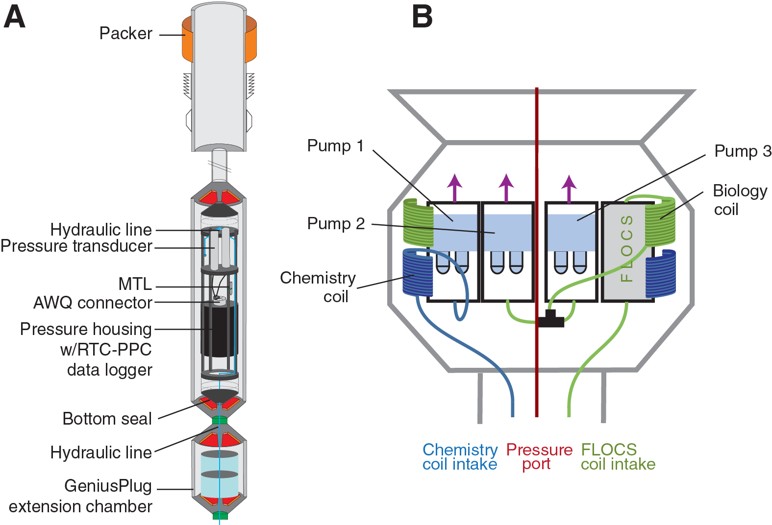
Figure F2. SmartPlug/GeniusPlug schematic.
General description
The core elements of the SmartPlug, an instrument built for Expedition 319, remain unchanged given their robust design and uncomplicated handling; the GeniusPlug extension follows the same design. Structurally, each unit includes a hollow-bore 3½ inch EU 8RD box-end threaded coupling at the upper end that mates with the lower end of the packer and an outer O-ring sealed structural shell designed to withstand the loads encountered during hole reentry operations (Figure F3). Inside the main unit is a frame holding a high-precision pressure period counter with a 12.8 MHz real-time clock (RTC-PPC system, resolving ~10 ppb of full-scale pressure, or ~0.7 Pa), a 24-bit/channel A/D converter and data logger (designed and built by Bennest Enterprises, Ltd.; Minerva Technologies, Ltd.; and the Pacific Geoscience Centre, Geological Survey of Canada), two pressure sensors (Models 8B7000-2-CE and 8B7000-1, Paroscientific, Inc., USA), and an independent miniature temperature logger (MTL) (Antares, Germany). Three independent temperature readings are recorded: (1) with the MTL, (2) with a platinum thermometer mounted on the primary data logger end cap, and (3) with the upward-looking pressure sensor. The inside of the structural shell is open to the sea through the internal open bore of the casing packer seal. One pressure sensor is connected to this volume to provide a hydrostatic reference, and the other sensor is connected to the sealed, screened borehole interval via hydraulic tubing that passes through the bottom end of the structural shell (Figure F2).
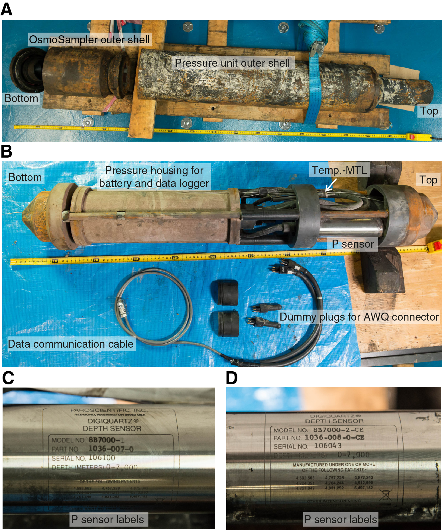
Figure F3. GeniusPlug in laboratory after recovery.
RS-422 communications with the main instrument for setting recording parameters and downloading data are conducted via a multisegment SEACON All Wet-mate QQ-C-465 (AWQ) connector on the logger pressure case. Communications with the MTL are conducted through a reader obtained from Antares. The instrument frame is shock-mounted within the structural shell, and the pressure sensors are mounted with secondary shock pads within the frame (Figure F3). Structural components are constructed with 4140 alloy steel, and pressure sensor housings and hydraulic tubing are constructed from 316 stainless steel.
The extension unit for the GeniusPlug configuration is made of the same material and includes a bulkhead to hydraulically separate the SmartPlug body from the OsmoSampler and FLOCS (Figure F2). This way, only trapped borehole fluid as well as formation fluid entering through the casing screens will enter the lower portion of the instrument where the intakes for the OsmoSampler and FLOCS are located. These two experiments are contained in a 7.15 inch high and 6.3 inch diameter space.
The OsmoSampler has two 2ML1 ALZET membranes attached to the housing with two-part epoxy (Hysol ES1902). The ends of the distilled water and saturated salt (noniodized table salt, NaCl) reservoirs are sealed with a single O-ring and held in place with a set screw. This configuration will pump 73 mL/y at 20°C. The pump is attached to 150 m of small-bore polytetrafluoroethylene (PTFE) tubing that holds 170 mL (1.19 mm inside diameter [ID] and 2.0 mm outside diameter [OD]). The tubing was filled with 10% HCl for 5 days before it was rinsed with 18.2 MΩ water. This sampler can be deployed at 20°C and maintain a continuous record for 2.3 y (or longer if the borehole temperature is cooler than 20°C).
The FLOCS experiment is attached to two pumps, each identical to the ones described above for the OsmoSampler. Both pumps are attached via a T-connection to double the pump rate (146 mL/y at 20°C). These pumps are attached to 150 m of small-bore PTFE tubing that holds 170 mL and were prepared as above. At 20°C these pumps will fill the sample coil in 14 months. The pumps will continue to work because of the excess salt in the pump but will only preserve the most recent 14 months of fluid within the sample coil. The FLOCS is filled with about 50 mL of sterile seawater that must pass through the coils before borehole fluids are collected within the coils. As this sterile seawater enters the distilled water portion of the pump, it will decrease the pump rate, but only minimally, even for a multiyear deployment. The inlet was attached to a syringe filled with 18.2 MΩ water until just before deployment.
The FLOCS experiment consists of a single unit that has four chambers. All components were sterilized and materials packed with sterile tools in a hood. The chamber closest to the inlet contained two plastic grids with autoclaved rock chips (1–2 mm thick and 5 mm × 5 mm) mounted with epoxy. These two grids were held in place with autoclaved glass wool and 5 mm borosilicate glass beads. Rock chips were attached to the plastic grids also using epoxy. One grid has basalt glass in the bottom portion (AT11-20-4055-B6) and basalt above it (J2-246-R2). The other grid has basalt in the bottom portion (J2-244-R4) and olivine above it. Above the grids are three chambers filled with barite, olivine, and accreted Nankai sediment (Expedition 316 sample material from Section 316-C0004D-47R-2; ~357 mbsf), respectively. These materials were crushed from bulk rocks and autoclaved. PTFE mesh screens were placed inside the cassette caps to prevent rock fragments from escaping the cassette. At sea, the FLOCS was filled with >50 mL of sterile seawater to remove air bubbles. During this process, some of the sediment from the end capsule escaped with excess seawater. Up to the point of deployment the inlet was capped with a syringe filled with sterile seawater.
Settings
The GeniusPlug was shipped to the Chikyu before Expedition 332 began. The time intervals for data acquisition for the formation and hydrostatic pressure sensors (serial Numbers 106043 and 106100) and the internal platinum thermometer (Number 94) were set to 30 s; at this rate, battery power (provided by six Tadiran TL-5137 DD primary lithium cells) is the limiting factor for operational lifetime, which is roughly 7 y, including a derating factor of 75% applied to full-power withdrawal. The instruments are equipped with 512 MB low-power flash memory cards, which provide storage capacity until the year 2024 at a 30 s sampling rate. The independent MTL in the GeniusPlug was set to sample temperature at 1 h intervals. The main logger clock was synchronized to UTC on 6 November 2010 during Expedition 332, and the MTL clocks were set on the same date. The GeniusPlug extension units were set up during the first weeks of Expedition 332. The GeniusPlug was deployed at Site C0010 only a few days after the OsmoSampler and FLOCS units were filled (Figure F4).

Figure F4. OsmoSampler pumps and FLOCS cylinder prior to installation in GeniusPlug extension unit.
Recovery
Expedition 365 planned to retrieve the GeniusPlug installed in 2010. Figure F5 shows the rig floor configuration and the instrument before entering the wellhead. The GeniusPlug was pulled out of the water at 0413 h (Japan Standard Time [JST]) on 3 April 2016 and was successfully moved from the moonpool to the rig floor by 0438 h. At this point, end caps were placed over the two sample intakes of the OsmoSampler to help prevent fluid loss. Once the GeniusPlug was detached from the bridge plug, the OsmoSampler was recovered and brought into the laboratory. On the laboratory bench, the coils and FLOCS were disconnected from the pumps. The FLOCS unit was immediately wrapped in aluminum foil and brought into the anaerobic chamber for microbiological sampling. Next, the OsmoSampler coil and then the FLOCS experiment coil (referred to as the chemistry and biology coils, respectively) were sampled. Coils were measured and cut into 1 m sections (Figure F6), and fluid was drained by gravity into 2 mL centrifuge tubes. Sample tubes were previously washed in 10% HCl at 60°C for 24 h and then washed 3 times with 18 MΩ water. Fluids trapped by gas bubbles were forced from the tubing using an air filled syringe. Sampling of both coils was completed by 1130 h. Select splits were analyzed for chlorinity, alkalinity, cations, anions, and major elements (Table T1). Additionally, a few samples were preserved for dissolved inorganic carbon, dissolved organic carbon, and isotopic analyses of carbon, oxygen, boron, and lithium. A total of 2 samples from each coil were quickly placed inside a 20 mL glass ampule directly after cutting and immediately sealed with a septum and metal crimp cap for hydrocarbon analyses.
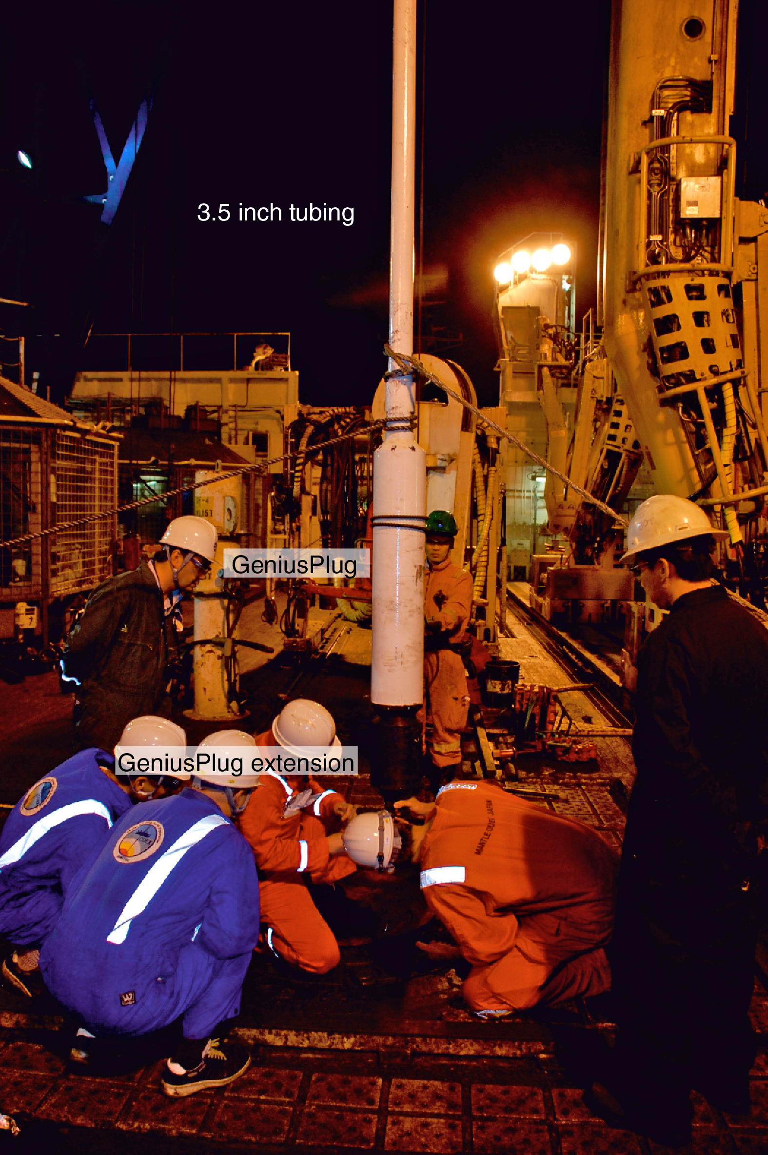
Figure F5. GeniusPlug and tubing joints on rig floor before deployment during Expedition 332.
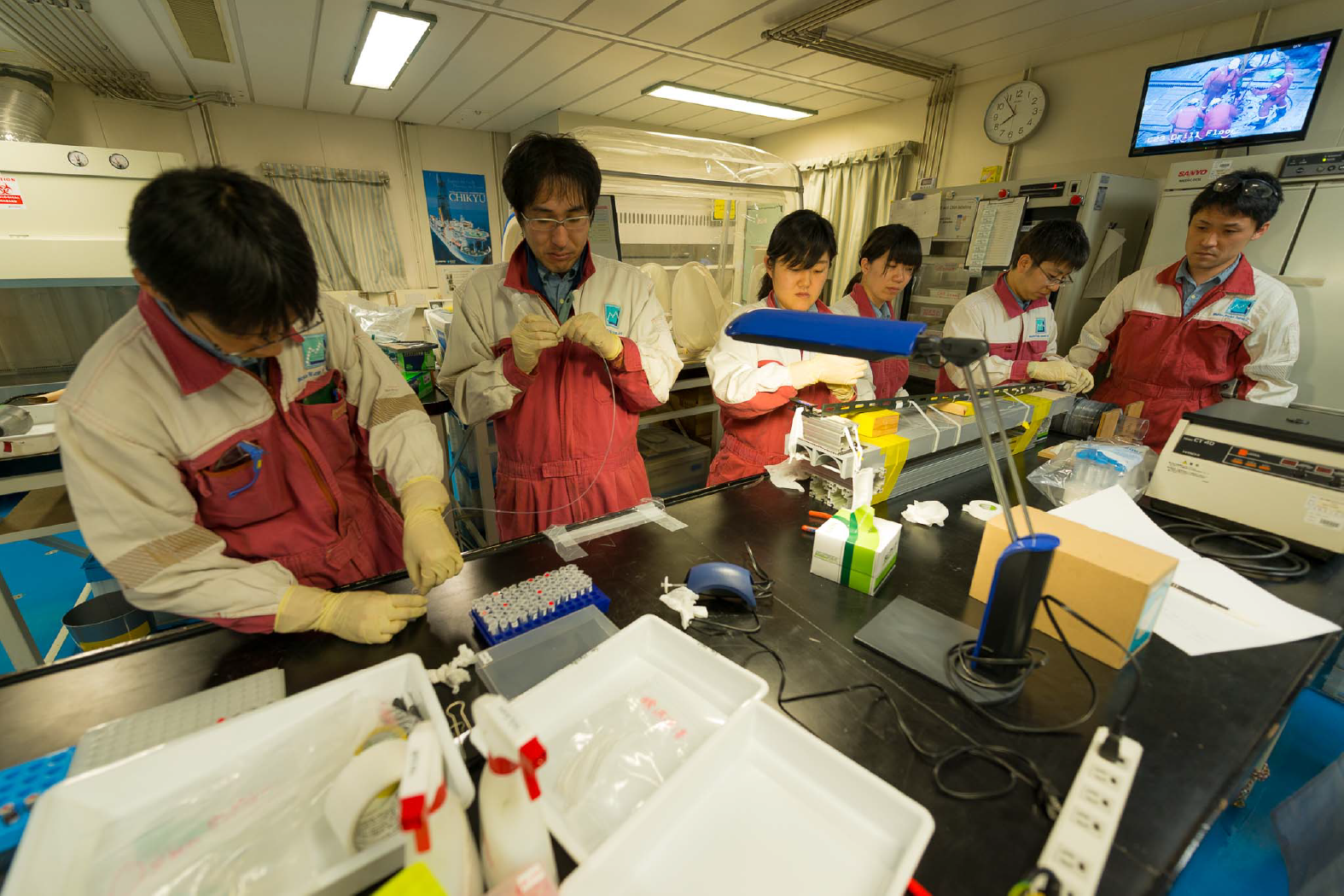
Figure F6. Laboratory technicians measuring and cutting OsmoSampler coil.
Table T1. OsmoSampler coil fluid splits and their respective shipboard measurements. Download table in .csv format.
Drill pipe accelerometer
Vortex-induced vibration (VIV) was measured while lowering the drill pipe from the Chikyu to recover the GeniusPlug on 30 March 2016, using a self-recording drill pipe accelerometer equipped with a triaxial acceleration sensor. VIV is caused by the strong Kuroshio Current (>3 kt) that flows over Hole C0010A. Kitada et al. (2011, 2013) documented VIV during the long-term borehole monitoring system (LTBMS) deployment in Integrated Ocean Drilling Program Hole C0002G during Expedition 332. VIV had a dominant frequency of 3–15 Hz and a maximum acceleration of 2 G. For Expedition 365, the LTBMS system was redesigned to withstand these conditions; the accelerometer deployment was intended to verify that VIV did not exceed this range before deploying the observatory.
The accelerometer was secured to the 5½ inch drill pipe using an attachment tool. The accelerometer was positioned 387 m above the bottom of the drill string and remained above the seafloor during the entire operation. Specifications of the accelerometer are described in Table T2, and its orientation is shown in Figure F7. Our procedure to measure VIV was as follows. First, the accelerometer was attached to the drill pipe, which was then lowered to the seabed in a low-current area (LCA). It remained on the drill string while the Chikyu drifted to Hole C0010A and into the strong current area to retrieve the GeniusPlug. Finally, the Chikyu drifted back to the LCA, retrieved the drill string, and recovered the accelerometer.
Table T2. Accelerometer specifications. Download table in .csv format.
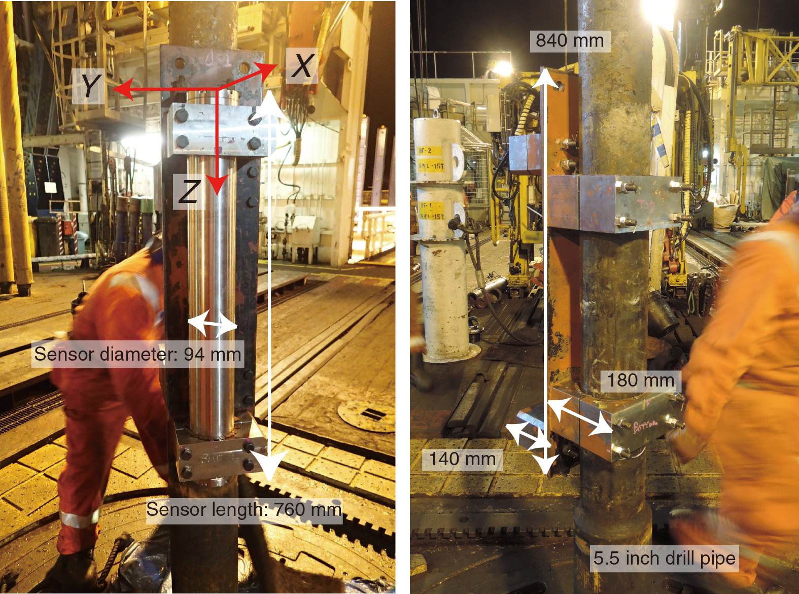
Figure F7. Attachment of accelerometer sensor to drill pipe showing mounting orientations and dimensions.
Pressure data recovery and processing
The GeniusPlug was connected via an RS-422 serial interface at the AWQ connector to a laptop computer running OS Ubuntu 10.4 with the programs mlterm, mlbin, and mldat installed, which are specifically designed to interface with the pressure data logging system and convert the data into usable formats. Mlterm software establishes communication between the instrument and the laptop and is used to check instrument status, change settings, download data, or display data in real time. After establishing communication, clock drift was analyzed. For this purpose, an accurate time is needed. Downloaded raw data (.raw format) are converted via mlbin software into a .bin file. Mlbin software strips off the file system information and tries to fix any bugs. The .bin file contains the data record in binary format. The final step is usually a conversion from .bin to .dat (ASCII) via the tool mldat9. However, the GeniusPlug is a hybrid in terms of pressure sensors, and mldat9 was unable to convert these data. The GeniusPlug uses an upward-looking 2-channel pressure (P) sensor measuring P and temperature (T), whereas the downward-looking sensor measures only P. Thus, a special processing routine from .bin to .dat is necessary. Two Python programs (dumpBin.py and calibrateLogfile.py) were used to perform the final conversion. All of these programs can be downloaded from http://corkobservatory.sourceforge.net/index.html.
LTBMS
The LTBMS was developed to observe fault and crustal dynamics off the Kii Peninsula. The LTBMS measures multiple parameters in a partially cased borehole, such as ground motion, crustal deformation, and hydrogeological processes. Ground motion is measured near the bottom of the borehole by a set of seismometers housed in a combined tiltmeter, broadband seismometer, and strainmeter package. The set of seismometers includes three-component accelerometers (two sets), a three-component broadband seismometer, and three-component geophones. Crustal deformation is measured by a tiltmeter and a volumetric strainmeter. These sensors are coupled to the formation by cement; this also eliminates noise in these sensors caused by fluid flow. All of the sensors (with the exception of the strainmeter) are mounted on an instrument carrier (see Figure F6 in the Expedition 365 summary chapter [Kopf et al., 2017]). All sensors and cables (including backups) were loaded aboard the Chikyu during the port call in Shimizu Harbor on 25 March 2016.
The LTBMS also includes temperature and pore fluid pressure sensors distributed within the central and lower part of the borehole. Pore fluid pressure is measured at three pressure ports within the borehole: one at the bottom of the borehole (Port P1) below the cemented section, another below the strainmeter (Port P2) within the cemented section, and one (Port P3) at the depth of the megasplay fault in the screened section of the casing (see Figure F6 in the Expedition 365 summary chapter [Kopf et al., 2017]). A swellable packer within the casing isolates the formation pressure in the screened zone from the ocean. A pressure sensing unit (PSU) mounted on the LTBMS head holds four pressure sensors. Three pressure transducers in the PSU connect to ¼ inch stainless tubing terminating at each of the three downhole pressure ports (P1–P3). The fourth sensor measures seafloor pressure and temperature. A thermistor string and stand-alone heat flow (SAHF) digitizer connected to the tilt combo package measures borehole temperature at five depths between the seismometer/crustal deformation sensor packages and the megasplay fault. Table T3 describes the dimensions of the downhole instruments and sensors.
Table T3. LTBMS instrument and sensor specifications and dimensions. Download table in .csv format.
All downhole LTBMS components in the borehole are attached to a backbone of 3½ inch tubing for structural support. The 3½ inch tubing also serves as a conduit for cement for the hole completion. All downhole sensors are connected by three communication/power cables (21.3 mm OD) to the LTBMS head. Each sensor package (strainmeter, seismometer, and tilt combo) is connected to the seafloor LTBMS head by one cable and each terminates with an ODI underwater mateable connector (UMC). These are mounted on the LTBMS head and temporarily connected to a battery pack/data logger unit mounted on the remotely operated vehicle (ROV) platform. Figure F8 (see also Figure F6 in the Expedition 365 summary chapter [Kopf et al., 2017]) shows a schematic of the LTBMS. Table T3 shows specifications of the LTBMS instrument and sensors. After the LTBMS is connected to the Dense Oceanfloor Network System for Earthquakes and Tsunamis (DONET) seafloor cabled network, all data from the sensors are streamed to shore in real time.
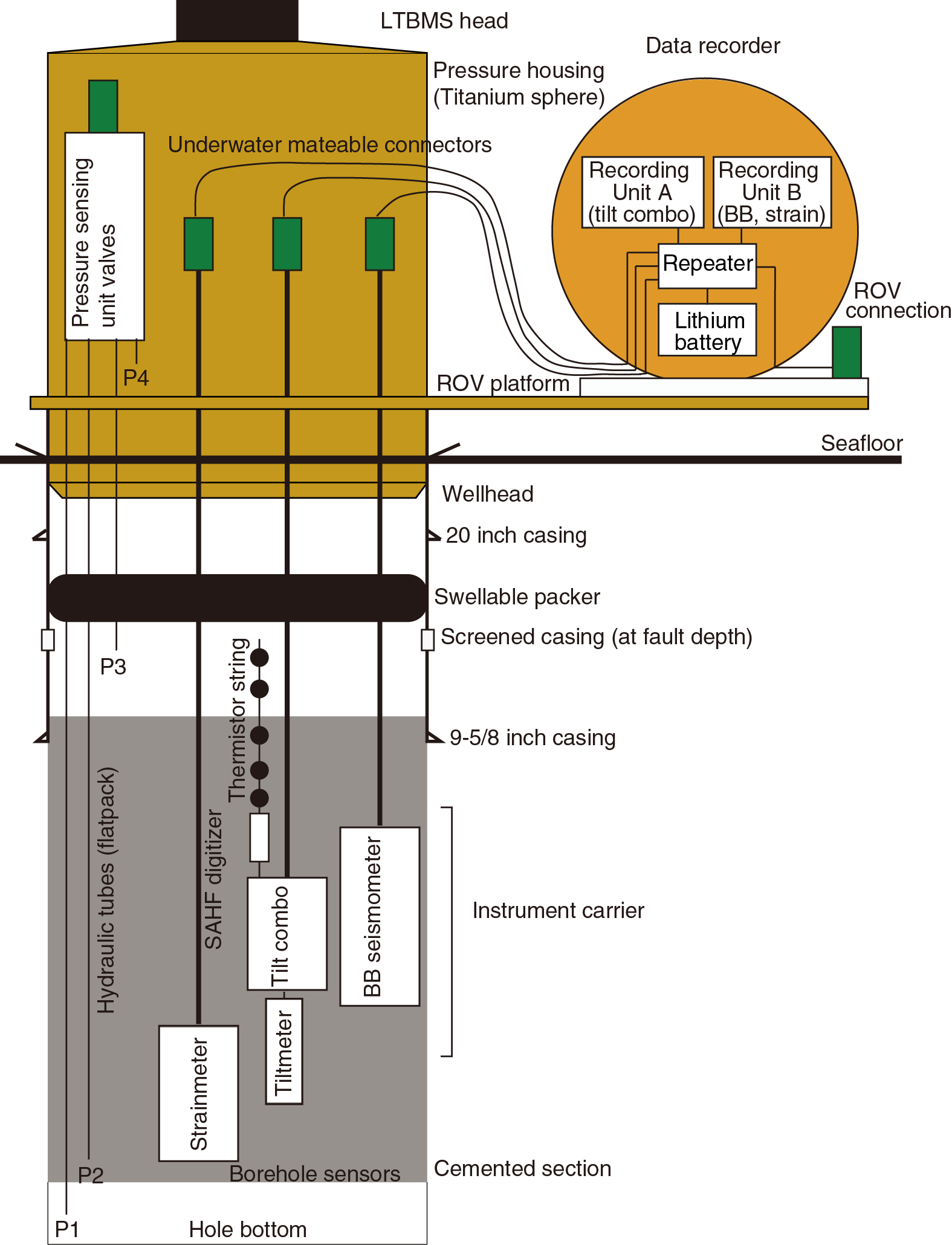
Figure F8. Schematic of LTBMS system configuration.
Observatory string
Instrument carrier
An H-beam–shaped instrument carrier (Expedition 332 Scientists, 2011) is designed to hold the sensors and protect them from the Kuroshio Current during deployment (Figure F9). This includes the borehole sensors, electrical cables, a thermistor string, and hydraulic lines. A 190 mm diameter and 30 mm thick flange at each end provides sufficient strength to resist bending and tension loading. Cables, the thermistor string, and hydraulic lines pass through six preformed slits in the flanges, and six M16 high-tension bolts with self-locking nuts were used for each flange connection. A cement pipe (48.6 mm OD and 34.4 mm ID) was installed along the instrument carrier to route the cement to the bottom of the hole. Before being loaded onto the Chikyu, a test of sensor positioning and cable routing was performed on the instrument carrier to confirm the attachment procedures for the cables, thermistor string, and hydraulic line routing.
The broadband seismometer (CMG3T) and tilt combo consist of a geophone, an accelerometer and data logger, an SAHF digitizer, and a tiltmeter, which were installed on the instrument carrier using a band-type attachment tool. Fiberglass-reinforced plastic isolated the sensor casings from the instrument carrier. All cables and hydraulic lines were connected to the 3½ inch tubing and the instrument carrier using steel bands and plastic zip ties. The thermistor string was connected to the SAHF digitizer and attached to the instrument carrier. Specifications of the sensors and instrument carrier are summarized in Figure F9. The orientation of the sensors is shown in Figure F10.
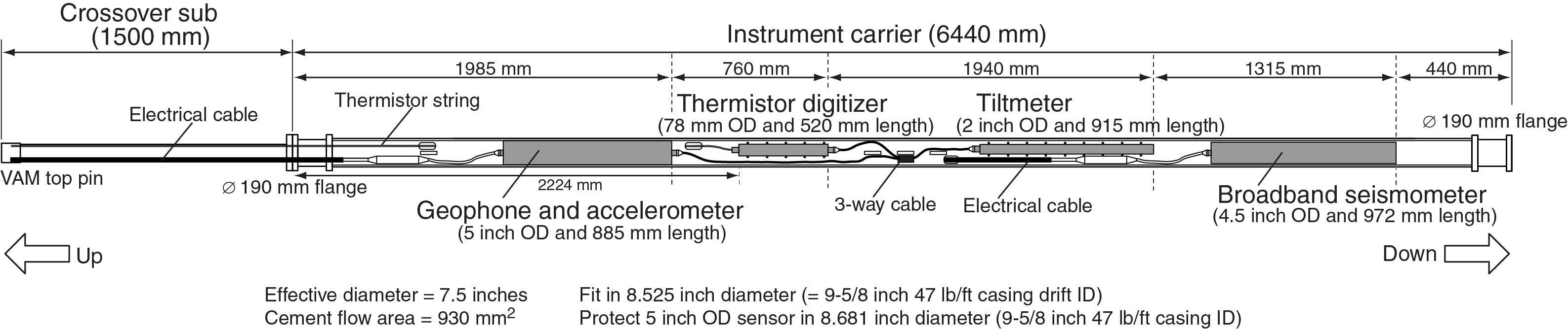
Figure F9. Instrument carrier showing instrument locations and connections.
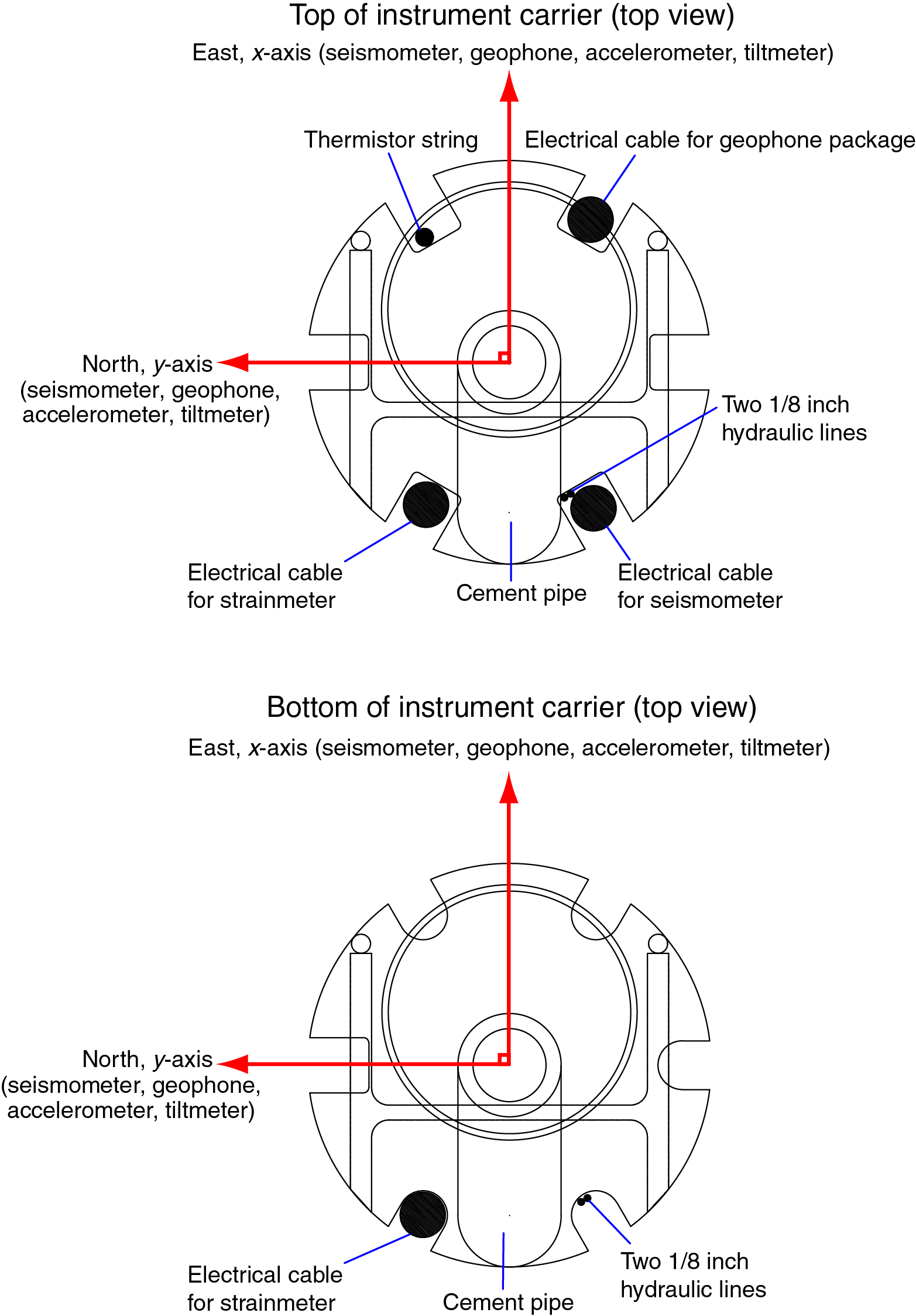
Figure F10. Cross sections at top and bottom of instrument carrier with sensor orientation.
Electrical cable
Three electrical cables (21.3 mm OD) developed specifically for the LTBMS were connected to borehole sensors (tilt combo, seismometer, and strainmeter). They were designed with near neutral buoyancy to avoid operational risk and for weight reduction. Sensor connectors (SEACON MINK connectors) were molded to the ends of each cable before being loaded onto the Chikyu (Figure F11). The upper ends of the cables were terminated and molded with ODI Teledyne UMCs on board the Chikyu at the time the LTBMS head was ready for deployment.
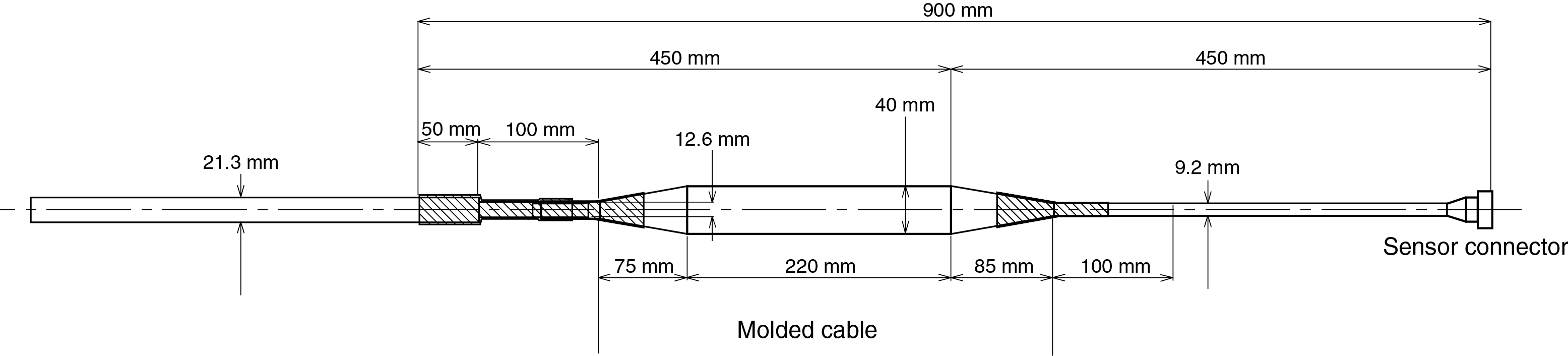
Figure F11. Molded electrical cable.
3½ inch tubing and centralizers
A total of 640 m of 3½ inch 12.7 lb/ft tubing was connected to the LTBMS head as the main support for the downhole LTBMS assembly. Two types of centralizers were used. Bowspring centralizers were attached below the strainmeter and above the cement port to allow uniform cement flow around the instruments. At other depths, four rigid centralizers with cable protectors were attached to each joint of 3½ inch tubing to protect the cables and hydraulic lines from damage (Figure F12). Cables and the thermistor string were also protected by rubber hose sheaths in areas with sharp edges or where a change in diameter of the string was encountered.
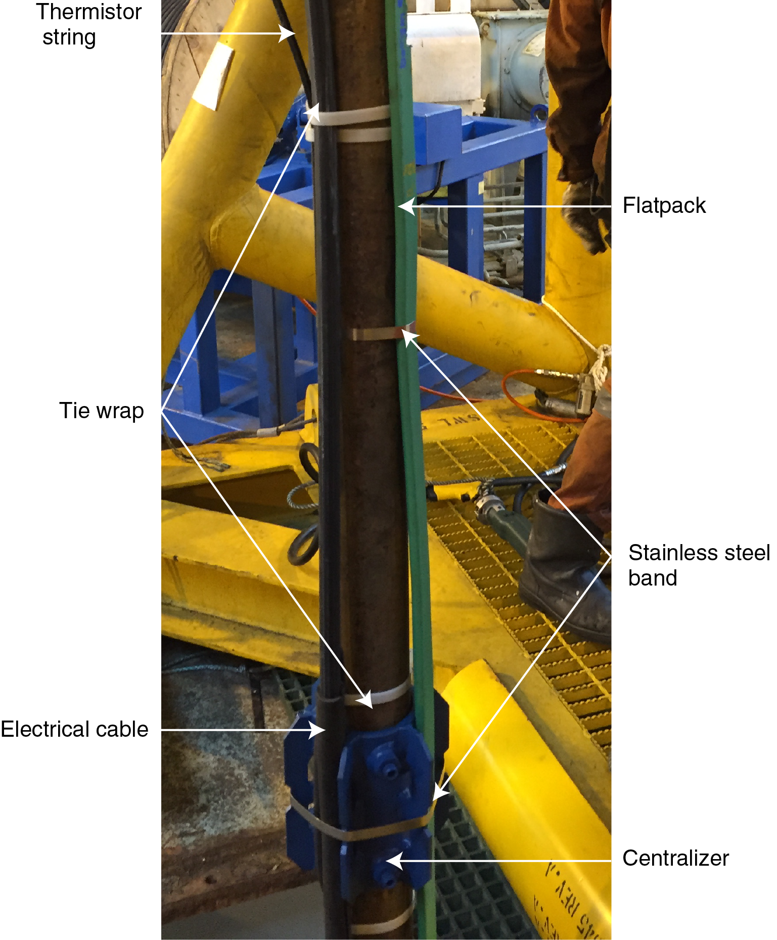
Figure F12. Centralizer and attachment of cables, thermistor, and flatpack.
Cementing the sensors
Cementing was used to couple the sensors installed at the bottom of the hole to the surrounding formation (and casing). A cement port was set on the 3½ inch tubing to the planned depth of the bottom of the cement column at 602 mbsf (see Figure F6 in the Expedition 365 summary chapter [Kopf et al., 2017]).
Swellable packer
The swellable packer (Halliburton, P/N 101938037) (Figure F13) is a nonmechanical borehole seal that upon contact with seawater begins to swell up to 350% of its original volume (depending on pressure and temperature conditions). The swellable packer was installed on the 3½ inch tubing to be set at 374.6–376.7 mbsf in Hole C0010A. The swellable packer’s initial OD is 7.89 inches and its length is 1.5 m. The ID of the 9⅝ inch casing is 8.68 inches. Antiextrusion end rings (with the same OD as the packer) were attached to each end of the packer; these rings expand radially against the casing ID so that the packer seal elements are not able to extrude above or below them. A packer mandrel (3½ inch OD and 4.5 m length) was connected to the 3½ inch tubing while the packer was covered with a diffusion barrier (8L), a low-permeability material that retards water migration into the packer. Based on swelling simulations at 4°C, the 7.89 inch OD packer with 8L diffusion barrier should swell to 8.09 inches after 1 week and 8.17 inches after 2 weeks. At 40°C, the packer is expected to swell to 8.12 inches after 1 week, and 8.19 inches after 2 weeks. Previous swelling simulation tests at the Japan Agency for Marine-Earth Science and Technology (JAMSTEC) showed that the packer swelling rate is slightly slower at lower temperatures.
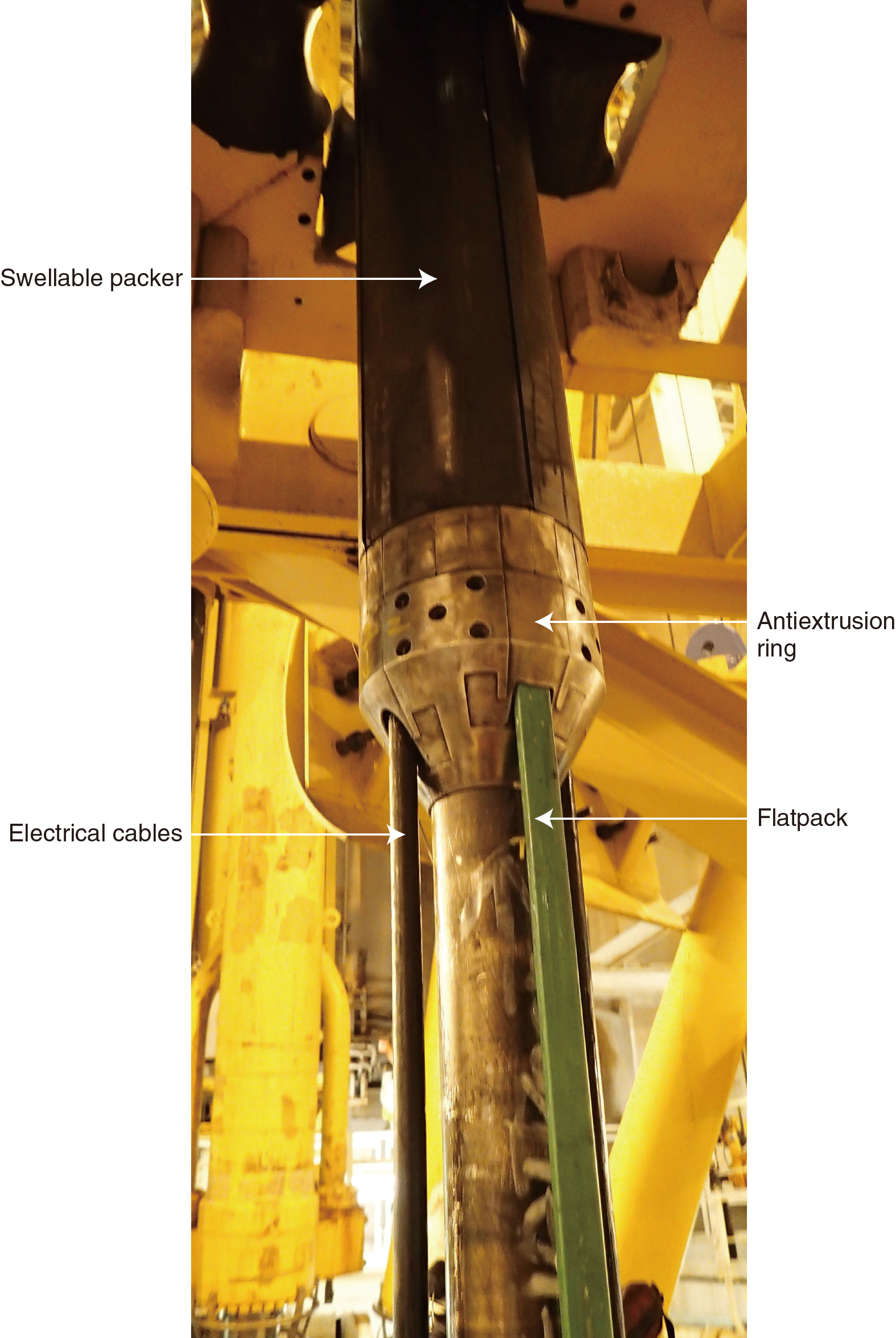
Figure F13. Swellable packer.
The electrical cables and hydraulic flatpack (28 mm × 12 mm) were fed through the swellable packer on the working cart in the moonpool while lowering the sensor assembly. The clearance around the cable through the packer was set at 2.5 mm (5 mm total). This clearance is needed to reduce any risk of cable damage due to cable pull force and slack while the packer is lowered into the borehole. The packer was cut four times length-wise (each slit 90° apart) to feed through the three electrical cables and the flatpack. After cable installation, the antiextrusion end rings with the cable slit cover were tightened and the cables were fixed to the 3½ inch tubing above and below the packer (Figure F13).
LTBMS head
The LTBMS head (30 inch effective diameter and 24 ft, 2⅞ inches long) sits at the top of the observatory on the seafloor SG-5 riserless wellhead. Figure F14 shows the LTBMS head with the PSU installed. The ODs of the inner and outer mandrels are 4½ inch and 9⅝ inch, respectively. The central part of the LTBMS head has three bays: Bay 1 for the PSU and valves, Bay 2 with three ODI Teledyne UMCs for downhole sensors, and Bay 3 to attach extra lengths of cable.
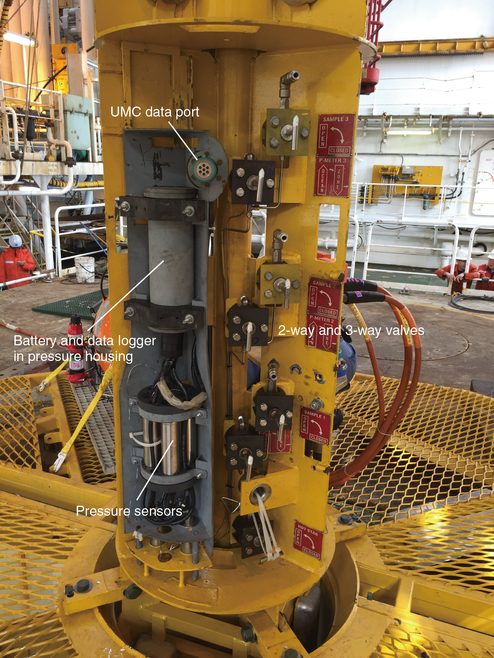
Figure F14. Bay 1 of LTBMS head.
The PSU was installed in Bay 1 and contains four high-precision quartz pressure sensors (Paroscientific, Inc.) (Figures F14, F15). Each sensor on the PSU is plumbed to a series of three-way valves for the pressure sensors to access either the formation (via hydraulic lines) or the ocean, in series with two-way valves that allow fluid sampling. A UMC port at the top of the pressure logger is used to connect to the measurement and download data (Figure F14) (see Observatory pressure sensing unit for more details).
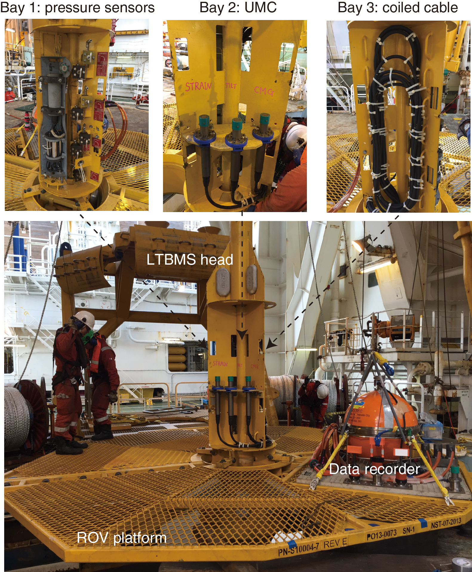
Figure F15. Assembled LTBMS head with ROV platform and data recorder.
The top ends of the electrical cables for the downhole sensors were terminated on board the Chikyu and then attached to UMCs (Figure F15). After termination, the electrical cables were securely attached to the split chain links welded on the bay panels and the outer mandrel using tie wraps and duct tape to prevent any damage while drifting to the site and during hole reentry. The three UMCs were mounted on the attachment plate in Bay 2 via M16 bolts with self-locking nuts. The height of the mounting plate was set at a minimum of 790 mm from the top of the ROV platform to account for the bending radius of the cables and to allow clearance for ROV operations. An ROV access platform (8 ft radius) was attached to the LTBMS head before lowering the LTBMS head into the moonpool.
Strainmeter
A strainmeter was designed by JAMSTEC for deep-sea borehole installation (Figure F16). The principle of the strainmeter is similar to the Sacks-Evertson type of volumetric strainmeter that measures the volume of an oil-filled cylindrical strain-sensing volume in response to deformation of the surrounding formation (Sacks et al., 1971). This deformation is transmitted to the volume through the cement filling the annulus between the formation and the strainmeter.
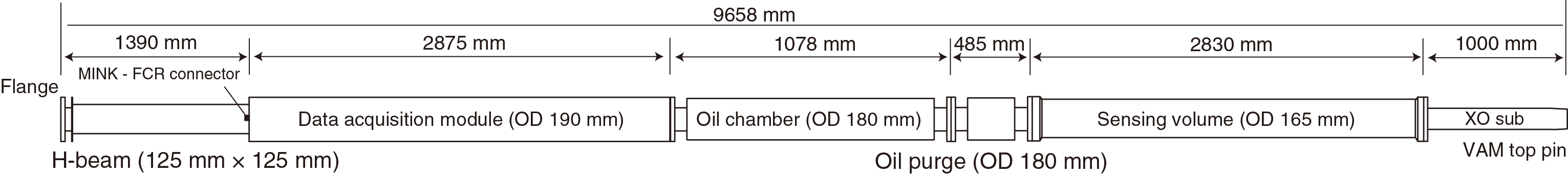
Figure F16. Diagram of deep-sea borehole strainmeter.
This strainmeter was designed with a 165 mm sensing volume diameter, which is much larger than conventional land-based strainmeters (typically ~75 mm). The strainmeter is ~10 m long, including digitizer electronics and a transducer housing, chambers, joints, and the sensing volume (~2.8 m length). It also incorporates a line through its center so that cement can be pumped through the instrument to reach the cement port on the bottom of the observatory (see Figure F6 in the Expedition 365 summary chapter [Kopf et al., 2017]).
The strainmeter is designed to withstand ambient pressures up to 70 MPa that the instrument may experience as it passes through the water column to the borehole. The strainmeter is very sensitive to deformation; the full-scale range of the volume change measured by the bellows is approximately 1 cm3, corresponding to a strain of 3 × 10⁻⁵ in the sensing volume. While being lowered from the ship, the strainmeter experiences much larger strains than it can tolerate within the full scale of measurement. Therefore, a valve bypassing the bellows is installed to protect the sensor and is kept open while the instrument is deployed. After the instrument is cemented into position, the bypass valve is closed (and measurements begin) by issuing a command via the ROV connection to the UMC on the LTBMS head. The bypass valve also opens automatically when the instrument measures strains outside its full measurement range. Opening the valve recenters the bellows to zero to reset accumulated strain; the valve is then subsequently closed to resume strain measurements. The bellows position (indicating strain change) is recorded by a digitizer in the strainmeter, and the strain data are transmitted uphole to the data recorder by an electrical cable. A Paroscientific pressure gauge (8B7000-2) is also connected to the strain sensing volume, and its pressure reading is used to check the status of other components, including the bypass valve. A three-component accelerometer (JA-5H200, JAE) is also included in the strainmeter.
A controller inside the strainmeter regulates the digitizing displacement of bellows and pressure, valve position (open or closed), and acceleration. The cable transmits serial data and power (24–30 V DC) to the strainmeter. The power consumption of the strainmeter is approximately 3 W during normal operations and is increased to ~6.0 W while the valve is changing position (Table T3).
VIV is a common effect of the strong Kuroshio Current (Kitada et al., 2011, 2013), and operating in the current causes wear and damage to equipment and sensors. VIV exhibits a dominant frequency of 3–15 Hz and a maximum acceleration of 2 G. Vibration tests approximating these conditions were performed to confirm that the strainmeter design is capable of withstanding these vibrations during installation. These tests were applied to all sensors and electronics. High-pressure tests (up to 60 MPa) successfully showed that the valve, bellows, and sensor plumbing systems function correctly under pressure.
Broadband seismometer
A CMG3T borehole broadband seismometer (Guralp Systems, Ltd) was installed in the instrument carrier to measure ground velocity in three orthogonal (x-, y-, and z-) directions in the frequency range between ¹⁄₃₆₀ and 50 Hz. Separate sensors measuring ground motion for each axis are housed in a titanium pressure housing (Figure F17). The seismometer is mounted near the bottom of the instrument carrier and is cemented in the hole to ensure good coupling to the formation. Each sensor has a motorized leveling mechanism so that the sensors are functional within 4.5° of tilt.
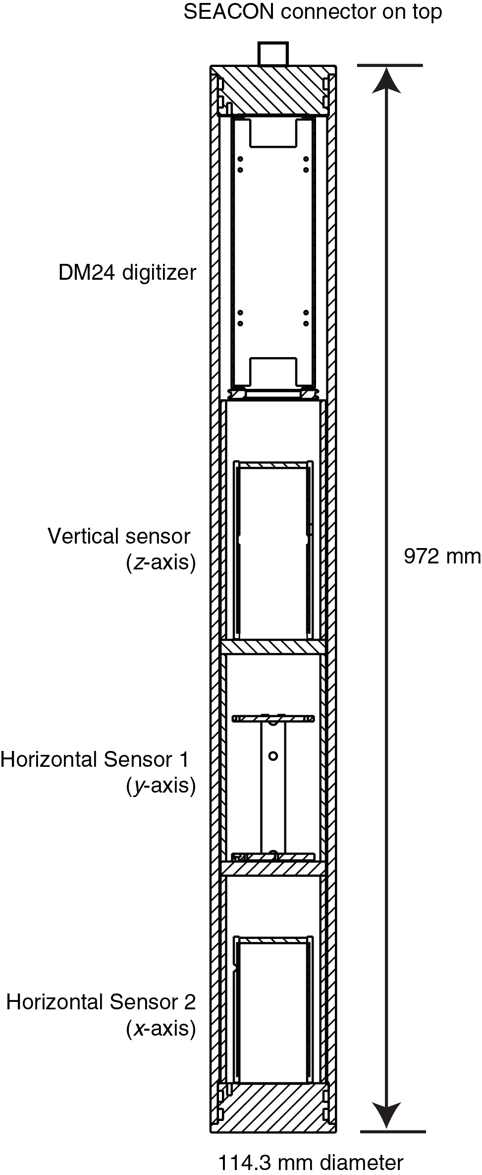
Figure F17. Diagram of CMG3T borehole broadband seismometer.
Each sensor has a proof mass supported on a pivot and suspended by a leaf spring during operation. The pivot is designed to be weak to assure very high sensitivity to ground motion. To protect this weak pivot from damage during transport, the proof mass must be motion-locked. Locking and unlocking the proof mass, leveling each sensor, and digitizing the x, y, and z ground motion are performed via a DM24 digitizer, which is installed within the pressure housing.
The three-component ground velocity data along with the position of the proof mass and inclination of the sensor from a Micro-Electro-Mechanical Systems (MEMS) tiltmeter are encoded in Guralp compressed format (GCF). The data are digitally uplinked through the borehole on a RS-422 serial cable. The three-component ground velocity data are digitized at 100 Hz in 24-bit resolution, whereas the mass position and tilt from the MEMS sensor are digitized at 4 samples/s.
Time synchronization of the data is governed by the DM24 digitizer. The DM24 receives a time reference through the RS-422 downlink on the serial cable in Streamsync format. The same downlink serial connection is also used to send commands to the DM24 to control the CMG3T seismometer (e.g., level the sensor; lock, unlock, and center the proof mass; and calibrate the sensor).
Power for the CMG3T broadband seismometer is supplied by the same cable used for the data link. Power consumption of the seismometer ranges from 2 to 3 W and increases to 6 W when operating the onboard motor to level, unlock, and lock the sensors. Because the 600 m long borehole cable dissipates power over its length due to resistance (approximately 15 Ω), higher voltages (~30 V) need to be applied so that the seismometer can receive sufficient power to run the motor. Table T3 includes the specifications of the CMG3T borehole sensor for this observatory installation.
The CMG3T borehole seismometer installed in Hole C0010A is the same design as that installed in Hole C0002G during Expedition 332 (Expedition 332 Scientists, 2011). This design was modified from the original specifications in advance of Expedition 332 to reduce the impact of severe vibration and shock to the sensor during deployment and installation. A series of vibration tests for each sensor confirmed that the redesign was effective. After assembly, each sensor was checked for noise performance in a vault, subjected to vibration, and rechecked for noise performance to make sure that vibration did not affect the performance of the seismometer.
Tilt combo (tiltmeter, geophone, accelerometer, and thermometer digitizer)
Specifications
The tilt combo is an integrated sensor module that includes a tiltmeter, geophone, accelerometer, and thermometer digitizer (SAHF). A schematic diagram of the tilt combo is shown in Figure F18. One titanium housing unit contains the three-component geophone (4.5 Hz GS-11D, Geospace Technology), the three-component accelerometer (JA-5H200, JAE), electrical boards, a CPU board, an A/D conversion board, a power supply board, and internal batteries. Signals from the three-component geophone and accelerometer are digitized by an A/D converter (ADS1282, Texas Instruments) on the A/D conversion board with a 125 Hz sampling rate. The A/D board has a calibration circuit for the geophone that can transmit electrical pulses to the geophone.
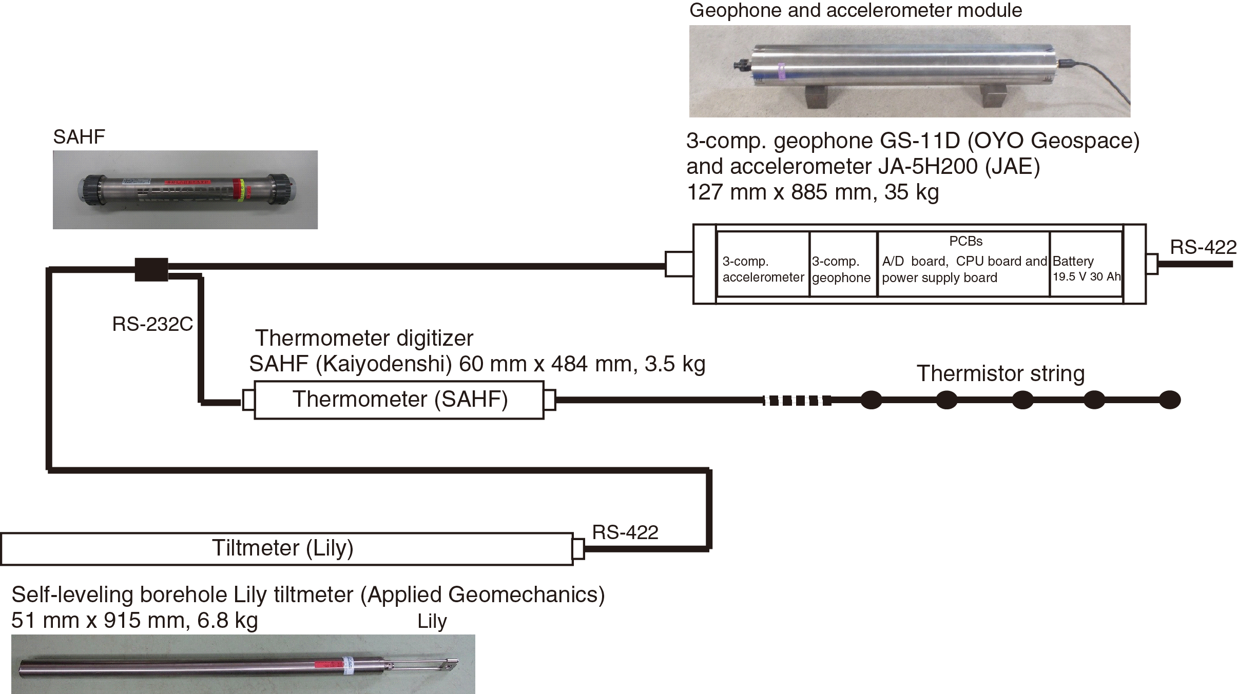
Figure F18. Tilt combo module configuration and schematic.
The tiltmeter (Lily, Applied Geomechanics) and thermometer digitizers (SAHF, Kaiyo-denshi) have their own A/D converters and titanium housings and are connected to the CPU board through an electrical cable using dry-mate connectors. The tiltmeter, SAHF digitizer, and accelerometer can individually be set to active or sleeping modes by switching electrical relays on the power supply board.
All data are merged on the CPU board and telemetered via an RS-422 interface to the recorder on the ROV platform in WIN format. A stand-alone acquisition mode is also available, in which all data are stored on an secure digital (SD) memory card mounted on the CPU board. The CPU clock time can be synchronized to a GPS 1 pulse/s signal (Table T3).
The tilt combo sensors were fixed to the instrument carrier before installation. Additional sets of sensors were prepared as backups. These sensors included two sets of the geophone and accelerometer modules, two sets of Lily tiltmeters (serial Numbers N8035 and N8069), and two sets of SAHF digitizers.
Thermistor string
The thermistor string is designed for monitoring temperature in the borehole for long periods of time. It has five thermistors placed at intervals along an electrical cable for array monitoring as shown in Figure F19. The electrical wires are covered by a hydrolytically stable polyether-based material, and the thermistors and connectors are molded using the same material as the cable. The thermistor string is connected to the SAHF thermistor digitizer, and the A/D converted data are merged to a WIN file on the CPU board in the geophone and accelerometer modules. Thermistor cables were calibrated in a precise isothermal bath for temperatures ranging from 5° to 30°C. We calibrated the data using the following empirical formula:
T = 1/{A + B × ln(R/2 − R0) + C × [ln(R/2 − R0)]2} − 273.15,
- T = temperature (degrees C) in the isothermal bath measured by a high-precision quartz thermometer,
- R = data logger reading (2 × resistance in ohms),
- R0 = resistance of lead cable (in this case up to 170 m two-way, depending on the position of the sensors), and
- A, B, and C = coefficients determined for each thermistor.
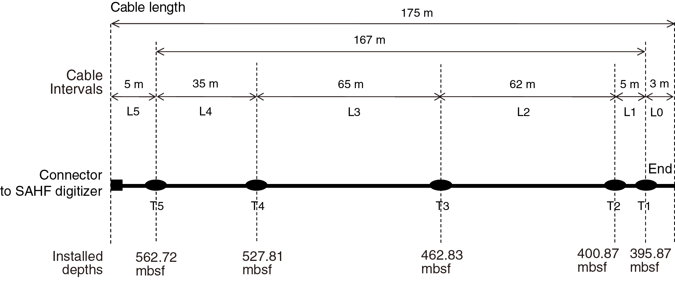
Figure F19. Diagram of thermistor string.
Temperature differences between the measured and calculated values (ΔT) are primarily attributed to actual temperature fluctuation in the isothermal bath. The absolute accuracy is thus estimated as ~10 mK.
Observatory pressure sensing unit
A PSU developed for the LTBMS was deployed during Expedition 365 for multilevel monitoring of pore pressure. The PSU is equipped with four Paroscientific Digiquartz pressure transducers (Model 8B7000-2-I; serial Numbers 106012, 106103, 106104, and 106096), a RTC-PPC system (resolving ~10 ppb of full-scale pressure, or ~0.7 Pa), a 24-bit/channel A/D converter and data logger (Bennest Enterprises Ltd., Minerva Technologies, Ltd., and the Pacific Geoscience Centre, Geological Survey of Canada), and associated “Paroscientific Intelligent Module” A/D converters. The Paroscientific gauges, which are also used in the GeniusPlug (see GeniusPlug), have proven to be accurate and reliable, with accuracy within ±0.01% of the full-scale range and pressure resolution to ±1 ppb of full scale (Becker and Davis, 2005). Three transducers connect to ¼ inch stainless tubing that terminates at three measurement points in the subseafloor, and one transducer measures hydrostatic pressure at the seafloor. The three ¼ inch hydraulic lines are housed in a urethane-coated flatpack umbilical that connects the monitored intervals to the LTBMS head (Figure F8; see also Figure F6 in the Expedition 365 summary chapter [Kopf et al., 2017]). A swellable packer set at 374.6–376.7 mbsf inside the casing isolates the screened intervals to enable monitoring of in situ formation pressures once the response to drilling and open hole operations has dissipated.
The lowermost monitoring interval is located below the megasplay fault in the overridden slope sediments (Unit II) at the bottom of the open borehole, below the strainmeter (Figure F8; see also Figure F6 in the Expedition 365 summary chapter [Kopf et al., 2017]). The pressure monitoring port is protected from clogging by three 1 inch diameter miniscreens, which are plumbed to a single manifold that connects to a ¼ inch stainless steel hydraulic tube (Figure F20). At the base of the strainmeter, this is connected to a ⅛ inch hydraulic line that passes through the strainmeter and instrument carrier above. The miniscreen configuration maximizes azimuthal coverage of the borehole while minimizing the possibility of screen obstruction. The second hydraulic line terminates within the instrument carrier in the cemented interval (see Observatory string). The third line monitors the screened interval within the megasplay fault zone centered at 405 mbsf and below the swellable packer that serves to isolate the monitoring interval from the seafloor. The fourth sensor in the PSU is open to the ocean and is used as a reference at the seafloor. The fourth sensor was grounded to the frame of the PSU to prevent crevice corrosion of the Paroscientific sensor housing (this is made of 316 stainless steel, which is highly prone to crevice corrosion). A ¼ inch stainless steel bolt was screwed into a pretapped hole at the end of the sensor (these holes are normally intended to attach small zinc anodes to the sensor) and used to secure a ¹⁄₁₆ inch hydraulic line to the sensor. The ¹⁄₁₆ inch line was then grounded to the base of the steel PSU frame (Figure F21). This measure is not necessary for the three formation sensors, as they are connected to hydraulic lines attached to drill pipe on the observatory string, the latter of which serves as a very large anode to prevent corrosion.
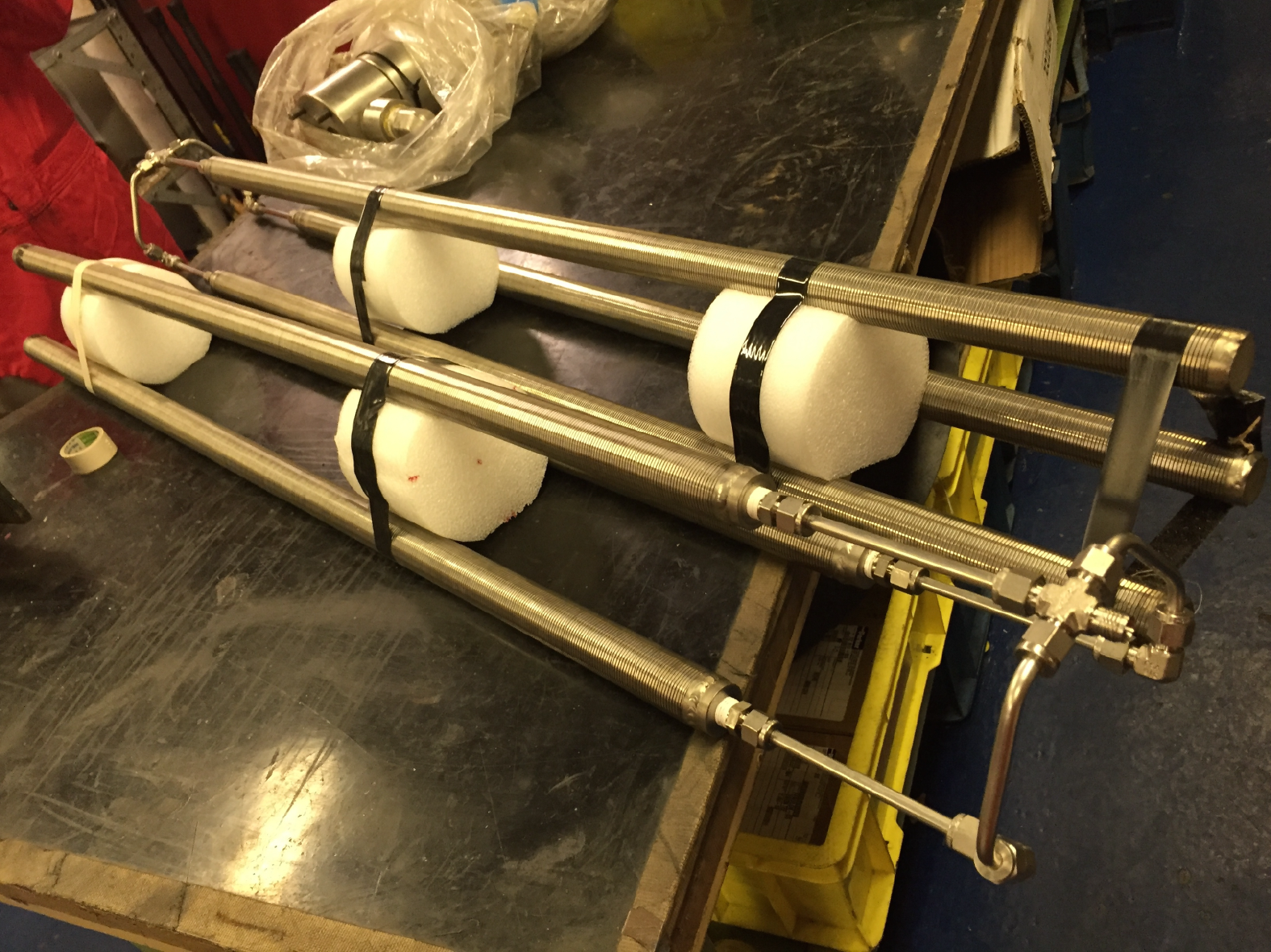
Figure F20. Miniscreens at lowermost pressure termination (P1).

Figure F21. Seafloor reference pressure sensor grounding line and termination on PSU steel frame.
When finally assembled, the PSU filled Bay 1 of the wellhead (Figure F14). The data logger within the PSU at the wellhead can be accessed via an ODI Teledyne UMC with the same specifications as the set of three UMCs mounted in Bay 2 for the other instruments (i.e., seismometer, strainmeter, and tilt combo). The ODI connector has a pin layout that is compatible to its three counterparts and hence allows the ROV pilot to use the same interface for communication and data download.
A few days prior to deployment, the hydraulic lines on the LTBMS head were flushed and the PSU was mounted on the wellhead for pressure tests to ensure that all of the plumbing and valves on the wellhead were configured correctly and pressure tight. This was done with a hand pump, first checking that water was flowing through the correct pathways for each valve setting and then each hydraulic line was individually pressurized. During the test for each of the three pressure sensing intervals, each hydraulic line connecting the formation and the Paroscientific sensor was kept pressurized (typically at ~10 MPa of pump pressure) for at least 1–2 h and then pressure was released at the conclusion of each test. There was some initial difficulty evaluating the data from the pressure tests, as the tests cause pressure spikes each time the pressure is increased or decreased. This caused problems with the conversion programs mlbin and mldat9, which are commonly used to convert the raw data files to ASCII data with time, temperature, and pressure values. This is an issue because mldat9 despikes the pressure data automatically, and this despiking procedure causes all subsequent records (after any pressure spikes) to be incorrect. Python codes to convert the data without despiking can be found at https://sourceforge.net/projects/corkobservatory.
Initial pressure tests revealed that the valve for pressure Sensor 2 was faulty, and it was replaced with another valve from a spare wellhead that was already on board the Chikyu. After the valve was replaced, it appeared to be operating correctly. Most of the other valves were found to be loose and did not operate correctly in the initial tests. These were all tightened and the pressure tests were repeated; all valves and hydraulic lines held pressure. Still, all connections were checked and tightened prior to deployment. Prior to the pressure tests, multiple tests were also performed in the laboratory to ensure that the PSU was logging data correctly at both high (>9 V) and low (7.5–9 V) voltages. The PSU in Hole C0010A is set to log at 60 s when powered below 9 V (e.g., when it is running on battery power), and the sampling rate will automatically increase to 1 Hz when voltage exceeds 9 V. Upon connection to DONET the sampling rate increases to 1 Hz, as the cabled network provides power at ~24 V.
Seafloor recording and submarine cabled network
The LTBMS has three separate cables for the downhole sensors: one each for the strainmeter, broadband seismometer, and tilt combo (tiltmeter, geophones, accelerometer, and thermistor array). Pore fluid pressure is measured by sensors in the PSU mounted on the LTBMS head that are connected to the formation at depth via hydraulic lines; data are recorded on a data logger in the PSU. These can be regarded as four separate instrument packages sharing the same borehole. The electrical connection specifications are designed to be the same in order to give flexibility in operations to connect to them. When the system was initially deployed, three of the sensor packages (strainmeter, broadband seismometer, and tilt combo) were connected to a data recorder on the ROV platform to facilitate connection by an ROV through a single UMC on the data recorder as well as to record observations prior to connecting the observatory to the DONET network (Figure F8). Similarly, pressure data are recorded on a data logger at a 1 min sampling rate prior to DONET connection via a UMC on the PSU.
Data recorder (for strainmeter, broadband seismometer, and tilt combo sensors)
The data recorder on the ROV platform consists of a repeater, two recording units, and batteries housed in a titanium sphere and connects via UMCs to the borehole strainmeter, broadband seismometer, and tilt combo sensors. The repeater exchanges data between the data recorder and the borehole sensors and also controls the power supply to each sensor. The repeater also switches data flow between the ROV connection, each borehole sensor, and the recording units. The data recorder has memory and batteries to support up to 6 months of continuous operation of these sensors. The data recorder has another UMC for control and online data recovery by a cable connection from the ROV. Time synchronization of the entire observatory is made through a GPS-referenced time signal sent from the ROV through the cable connection. The ROV can also connect to the pressure data logger via a UMC on the PSU for pressure data recovery.
ROV connection
During installation, the condition of the downhole sensors was inspected via an ROV connection with the UMCs. An interface circuit attached to the ROV Magnum on the Chikyu was used to change power settings and RS-422 data connections. By receiving 24 V power from the ROV, the interface circuit can control power fed to the borehole instrument and measure supplied current and voltage to the borehole sensor. The interface circuit also converts the data format from the borehole sensors (RS-422) to a format supported by the ROV (RS-232C). The ROV Magnum on board the Chikyu supports up to 115,200 bps speed in two-way communication to the surface. We used 57,600 bps as a standard speed to communicate with the borehole sensors.
Long-term observatory operation plans
During Expedition 365, we confirmed that the borehole sensors were operating correctly, and we then began recording data via the ROV connection. The data recorder sphere was recovered during a subsequent JAMSTEC ROV cruise and was replaced on 19 June 2016 with an interface box to connect the sensors to the DONET network (Figure F22). The pressure sensors were also connected to DONET via the UMC mounted on the PSU. The DONET junction point is <10 km from the observatory in Hole C0010A. Connected to DONET, all the borehole sensors receive power from the cable and the data are received in real time on land. Time synchronization of the borehole data is also governed by precise time references from DONET.
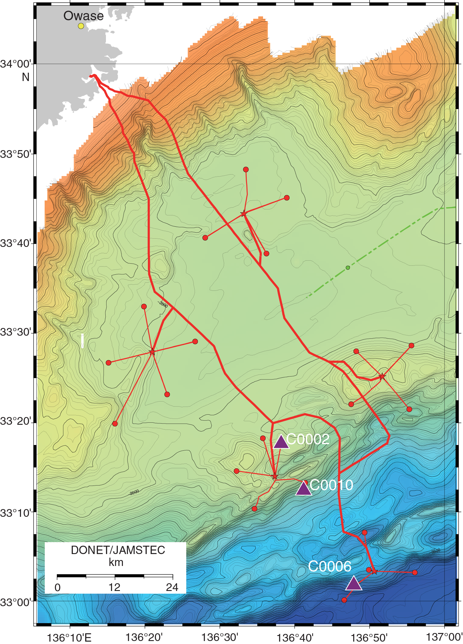
Figure F22. Location of observatory Sites C0002, C0010, and C0006.
X-ray computed tomography
X-ray computed tomography (XCT) imaging helps to identify key structural and sedimentological features in the recovered core and to find the best potential locations for discrete whole-round (WR) sampling (see XCT2D in Supplementary material). The latter include WR sections for interstitial water (IW) and microbiological (MBIO) analyses, as well as individual WR sample requests. Because core splitting, description, and most other analyses (excepting whole-round multisensor core logger [MSCL-W] and headspace gas) were deferred until a shore-based sampling party in July–August 2016, no other samples were taken during the expedition. Scientist “watchdogs” reviewed each XCT image for each core section to identify structures and sedimentological features and to select IW and MBIO samples of optimal quality while also preserving materials for other expedition-related sampling and science objectives.
XCT scanning methods followed those in the measurement manual prepared for the Center for Deep Earth Exploration (CDEX) by technicians from Marine Works Japan (3-D X-ray CT Scanning, Version 3.00, 24 March 2015; based on GE Healthcare, 2013a, 2013b, 2013c; Mees et al., 2003; Nakano et al., 2000) and are the same as those followed during previous expeditions (e.g., Moore et al., 2014). The XCT scanner on the Chikyu is a Discovery CT 750HD (GE Yokogawa Medical Systems, Ltd.). This instrument scans a 1.4 m core section in 10 min: 5 min to scan and then 5 min to create, or “reformat,” a coronal image. Images are core-axis-normal planes of X-ray attenuation values with dimensions of 512 × 512 pixels. Each axial scan of a 140 cm core section consists of approximately 2200 slice images, and each slice is 0.625 mm thick. Data are stored as Digital Imaging and Communication in Medicine (DICOM) formatted files.
Background
The theory behind XCT is well established in medical research and the Earth and planetary sciences (Carlson, 2006) and is only briefly outlined here. X-ray intensity varies as a function of X-ray path length and a linear attenuation coefficient (LAC) of the target material:
- I = transmitted X-ray intensity,
- I0 = initial X-ray intensity,
- η = LAC of the target material, and
- L = X-ray path length through the material.
- ηt = LAC for the target material, and
- ηw = LAC for water.
LAC is a function of the chemical composition and density of the target material. The basic measure of attenuation, or radiodensity, is the computed tomography (CT) number given in Hounsfield units (HU):
CT number = [(ηt − ηw)/ηw] × 1000,
The distribution of raw attenuation values in a given slice is then used for image processing. Successive 2-D slices yield a representation of attenuation values in 3-D pixels (voxels).
During Expedition 365, an acrylic three-layer core liner section mock-up (calibration “standard”) was run to calibrate the XCT once every 24 h during coring operations. This quality control (QC) standard was used to recalibrate the CT numbers of air, water, and aluminum if the “Fast Cal” CT numbers for air (CT number = −1000), water (CT number = 0), and aluminum (2477 < CT number < 2487) fall out of normal range. For each standard analysis, the CT number was determined for a 24.85 mm2 area at fixed coordinates near the center of the cylinder.
XCT scan data usage
XCT scans were used during Expedition 365 to
- Examine features of interest, including deformation structures and bioturbation, in 3-D;
- Distinguish natural fractures and faults from drilling-induced structures;
- Provide an assessment of core integrity;
- Determine locations for WR samples; and
- Identify important structural and sedimentological features to be preserved and therefore avoided by WR sampling.
XCT scanning was performed immediately after core sections were cut on the catwalk, logged in the J-CORES curation database in the core cutting area, and transported to the core processing deck. All WR sections were screened by XCT watchdog scientists to avoid destructive testing of important structural and sedimentological features when selecting WR samples to be used for IW or frozen as MBIO samples. An important criterion when selecting either IW or MBIO WR samples is to select samples with minimal fracturing or drilling disturbance in order to minimize effects of contamination by drilling fluid.
Lithology
Lithologic boundaries and lithologic units for Holes C0010C–C0010E were selected using criteria from visual core description and smear slides. These descriptions were compared with logging-while-drilling (LWD) data from Expedition 319 (Expedition 319 Scientists, 2010), including gamma ray, resistivity, and sonic data, as well as coring results from Integrated Ocean Drilling Program Site C0004.
Core description methods during Expedition 365 drew upon protocols developed for NanTroSEIZE (e.g., Expedition 315 Scientists, 2009). Descriptions of core sections in Holes C0010C–C0010E were based on
- Macroscopic observations following standard IODP visual core description (VCD) protocols,
- Microscopic observations (smear slides), and
- Bulk mineralogical data from X-ray diffraction (XRD) and bulk elemental data from X-ray fluorescence (XRF).
Macroscopic observations of core
We followed conventional Ocean Drilling Program (ODP), Integrated Ocean Drilling Program, and IODP procedures for recording sedimentology information on VCD forms on a section-by-section basis (Mazzullo and Graham, 1988) (see VCDSCAN in Supplementary material). VCDs were transferred to section-scale templates using J-CORES software and then converted to core-scale depictions using Strater (Golden Software). Texture (defined by the relative proportions of sand, silt, and clay) follows the classification of Shepard (1954). The classification scheme for siliciclastic lithologies follows Mazzullo et al. (1988). The classification scheme of Fisher and Schmincke (1984) was used to describe pyroclastic deposits.
The Graphic lithology column on each VCD plots all beds ≥2 cm thick to scale. Interlayers <2 cm thick are identified as laminae in the Sedimentary structures column. It is often difficult to discriminate between the dominant lithologies of silty claystone and clayey siltstone without quantitative grain-size analysis; therefore, we usually grouped that range of textures into the category “silty claystone” on illustrations. Figure F23 shows the graphic patterns for all lithologies encountered during Expedition 365. Also shown are symbols for sedimentary structures and severity of coring disturbance.
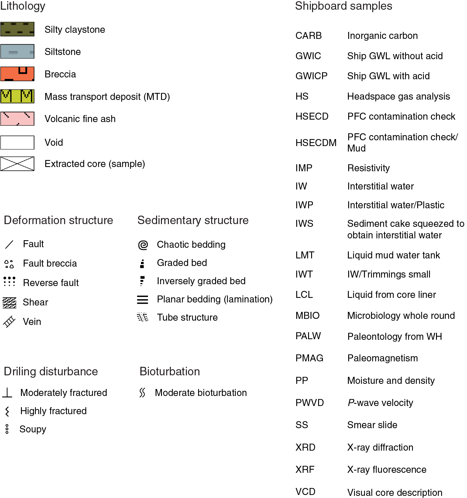
Figure F23. Graphic patterns and symbols used in visual core descriptions.
Smear slides
Smear slides are useful for identifying and reporting basic sediment attributes (texture and composition) in core samples, but the results are qualitative (Marsaglia et al., 2013). Smear slides were observed in plane-polarized light using an Axioskop 40A polarizing microscope (Carl Zeiss) equipped with a Nikon DS-Fi1 digital camera. We estimated the abundance of biogenic, volcaniclastic, and siliciclastic constituents using a visual comparison chart (Rothwell, 1989). Estimates of sand, silt, and clay percentages were entered into the J-CORES samples database along with abundance categories for the observed grain types. The relative abundance of major components (quartz, feldspar, and clay minerals) was verified by XRD (see X-ray diffraction), and the absolute weight percent of carbonate was verified by coulometric analysis (see Organic geochemistry).
X-ray diffraction
The principal goal of XRD analysis was to estimate the relative weight percentages of total clay minerals, quartz, feldspar, and calcite in specimens of bulk sediment. Material for XRD analysis was obtained from a 10 cm3 sample that was also used for XRF and carbonate analyses. All samples were vacuum-dried, crushed with a ball mill, and mounted as randomly oriented bulk powders. Routine analyses of bulk powders were completed using a newly acquired PANalytical CubiX3 diffractometer. This system was used by IODP for the first time during Expedition 365. Instrument settings were as follows:
- Generator voltage = 45 kV.
- Tube current = 40 mA.
- Tube anode = Cu.
- Wavelength = 1.540598 Å (Kα1) and 1.544426 Å (Kα2).
- Start angle = 2°2θ.
- End angle = 60°2θ.
- Step spacing = 0.005°2θ.
- Scan step time = 1.27 s.
- Scan speed = 0.50134°2θ/s.
- Divergent slit = fixed 1/4.
- Monochromator used = yes.
- Irradiated length = 10 mm.
- Scanning range = 2°–60°2θ.
- Scan type = continuous.
To maintain as much consistency as possible with previous NanTroSEIZE results, we processed the digital data using MacDiff 4.2.5 (http://www.ccp14.ac.uk/ccp/ccp14/ftp-mirror/krumm/Software/macintosh/macdiff/MacDiff.html). Functions included “find baseline,” “smooth counts,” and correction of peak position using the quartz peak at 3.343 Å. The upper and lower limits for each diagnostic peak were adjusted manually following the guidelines shown in Table T4.
Table T4. Characteristic XRD peaks for semiquantitative analysis of composite clay minerals, quartz, plagioclase feldspar, and calcite. Download table in .csv format.
Calculations of relative mineral abundance utilized regression curves that were generated from analyses of standard mineral mixtures with all values normalized to 100%. Bulk powder mixtures for the Nankai Trough are the same as those reported by Underwood et al. (2003): quartz (Saint Peter sandstone), feldspar (Ca-rich albite), calcite (Cyprus chalk), smectite (Ca-montmorillonite), illite (Clay Mineral Society IMt-2, 2M1 polytype), and chlorite (Clay Mineral Society CCa-2). The standards were run three times, and correlations between mean peak area and weight percent were defined for each mineral. The following polynomial equations provide the statistical fits, where X = peak area and r = correlation coefficient:
Total clay minerals = 5.0314 + 0.0072495(X) − 1.919E−7(X2), r = 0.923;
Quartz = −1.1695 + 0.00037795(X) − 1.2198E−10(X2), r = 0.991;
Feldspar = 0.96439 + 0.00052385(X) + 4.2326E−9(X2), r = 0.990; and
Calcite = −1.9208 + 0.00082643(X) + 2.3405E−9(X2), r = 0.997.
Average errors (calculated weight percent minus true weight percent) for the standard mineral mixtures are as follows:
Values of relative abundance for natural specimens, however, should be interpreted with some caution. One of the fundamental problems with any bulk powder XRD method is the difference in peak response between poorly crystalline minerals at low diffraction angles (e.g., clay minerals) and highly crystalline minerals at higher diffraction angles (e.g., quartz and feldspar). Clay mineral content is best characterized by measuring the peak area, whereas peak intensity may be more accurate for quartz, feldspar, and calcite. Analyzing oriented aggregates of clay-size fractions enhances basal reflections of the clay minerals, but that approach is time consuming. For clay mineral assemblages in bulk powders, the two options are to measure one peak for each mineral and add the estimates together (thereby propagating the error) or to measure a single composite peak at 19.4°–20.4°2θ (Table T4). Chlorite does not contribute counts to that composite peak, so natural specimens with high contents of chlorite will yield larger errors. The same source of error also applies to the standard mineral mixtures. Other sources of error include contamination of mineral standards by impurities such as quartz and zeolites (e.g., the illite standard contains ~20% quartz) and differences in crystallinity between standards and natural clay minerals.
In the final assessment, calculated mineral abundances reported here should be regarded as relative percentages within a four-component system of clay minerals + quartz + feldspar + calcite. The accuracy of these values in representing absolute percentages within the total volume of solids depends on the abundance of amorphous solids (e.g., biogenic opal and volcanic glass) and the total of all other minerals that occur in minor or trace quantities. For most natural samples from Site C0010, the difference between calculated relative abundance and absolute weight percentage is probably 5%–10%.
X-ray fluorescence
XRF analyses were obtained in two modes: analysis of whole-rock powders and scanning of the WR core surface on some selected intervals. Whole-rock quantitative XRF spectrometry analysis was undertaken for major elements on core working halves. Material for XRF was obtained from a 10 cm3 sample that was also used for XRD and carbonate analyses. All samples were vacuum-dried and crushed with a ball mill. Major elements were measured using the fused glass bead method and are presented as weight percent oxide proportions (Na2O, MgO, Al2O3, SiO2, P2O5, K2O, CaO, TiO2, MnO, and Fe2O3). An aliquot of 0.9 g of ignited sample powder was fused with 4.5 g of SmeltA12 flux for 7 min at 1150°C to create glass beads. Loss on ignition was measured using weight changes on heating at 1000°C for 3 h. Analyses were performed on the wavelength dispersive XRF spectrometer Supermini (Rigaku) equipped with a 200 W Pd anode X-ray tube at 50 kV and 4 mA. Analytical details and measuring conditions for each component are given in Table T5. Rock standards of the National Institute of Advanced Industrial Science and Technology (Geological Survey of Japan) were used as the reference materials for quantitative analysis. Table T6 lists the results for selected standard samples. A calibration curve was created with matrix corrections provided by the operating software, using the average content of each component.
Table T5. Analytical conditions for major element analysis of glass beads. Download table in .csv format.
Table T6. Averaged measured values and 3σ standard deviations on the Supermini XRF spectrometer from a selection of standard samples. Download table in .csv format.
Structural geology
During Expedition 365, cores were recovered from Holes C0010C–C0010E. With the exception of Core 365-C0010C-2R-2, which was split on board the ship during the expedition, all cores were stored in the core refrigerator on the Chikyu for examination during the shore-based sampling party. Only XCT images and MSCL-W analyses were conducted during the expedition. IW and MBIO WR samples were collected after XCT watchdogs ensured that no key structures were present in these intervals. The methods used to document the structural geology data of Expedition 365 cores are largely based on those used by previous NanTroSEIZE expeditions (e.g., Expedition 315 Scientists; 2009; Expedition 319 Scientists, 2010).
Description and data collection
Structures preserved in the cores were documented on split cores and on XCT images of WR cores (see X-ray computed tomography). Observations on split cores were manually logged onto the structural geology observation sheet (Figure F24; also see STRUCTUR in Supplementary material) at the core description table and then transferred to both a calculation sheet and the J-CORES database (see Data processing). Core observations and measurements followed procedures from previous ODP and Integrated Ocean Drilling Program NanTroSEIZE expeditions (e.g., ODP Legs 131, 170, and 190 and Expeditions 315, 316, 319, 322, 333, 338, and 348).
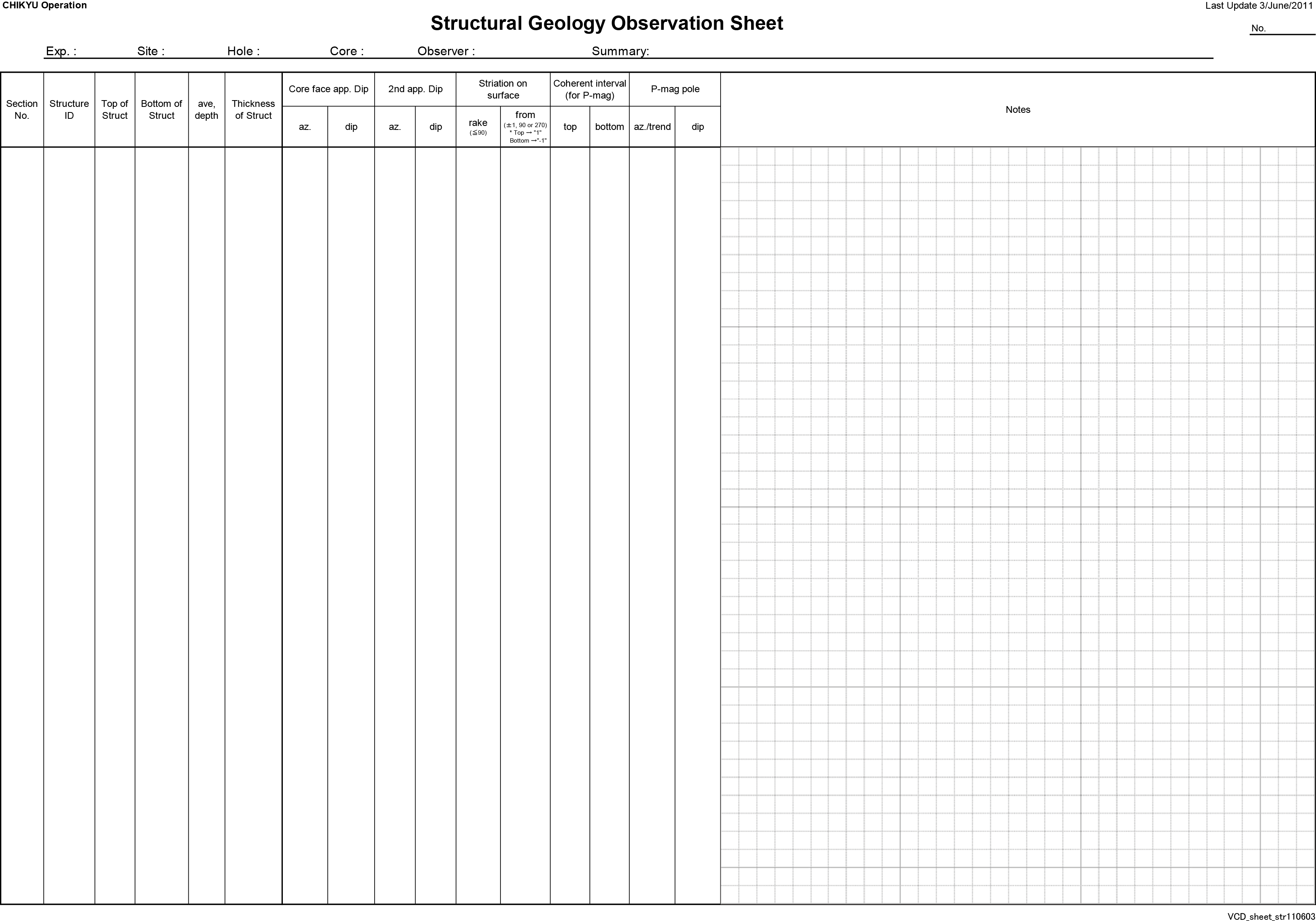
Figure F24. Example of log sheet used to record structural observations and measurements from working half.
We measured the orientations of all structures observed in cores using a modified plastic protractor (Figure F25) and then noted the measurements on the structural geology observation sheet along with descriptions and sketches of structures. The orientations of planar or linear features in cores were defined with respect to the core reference frame, where the core axis is oriented vertically and the double line marked on the working half of the core liner is prescribed to be “north,” 0° or 360° (Figure F26). The orientations of planes in the core reference frame were determined by measuring the apparent dip angle of any planar feature in two independent sections parallel to the core axis. The 2-D orientation was then calculated using the two linear measurements (see Data processing). In practice, one section is typically the split surface of the core, on which the trace of the plane has a bearing (α1) and a plunge angle (β1) in the core reference frame. α1 is either 90° or 270°. The other section is, in most cases, a cut or fractured surface at a right or high angle to the split core surface, on which the bearing (α2) and plunge angle (β2) of the trace of the plane are measured. In the case where the second measurement surface is at an angle to the core split surface, bearing α2 is either 0° or 180° (Figure F27). Both β1 and β2 are between 0° and 90°. Similar measurements were made for planar features visible in XCT images.
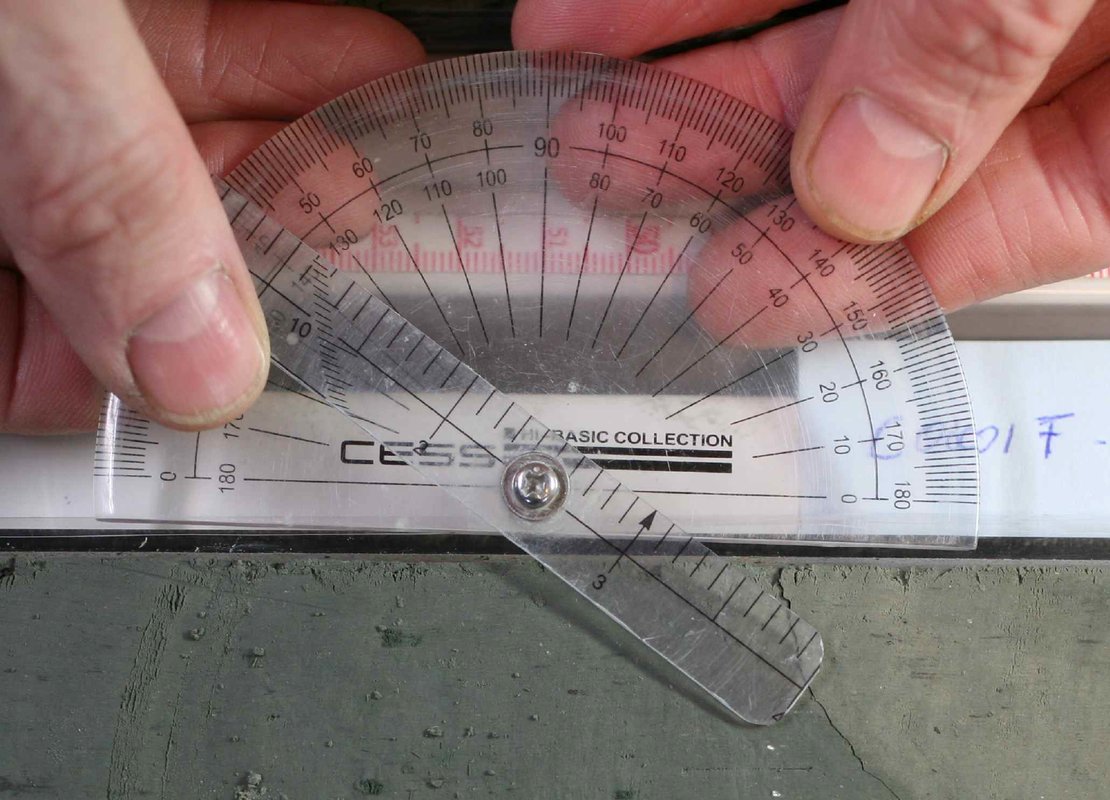
Figure F25. Modified protractor.
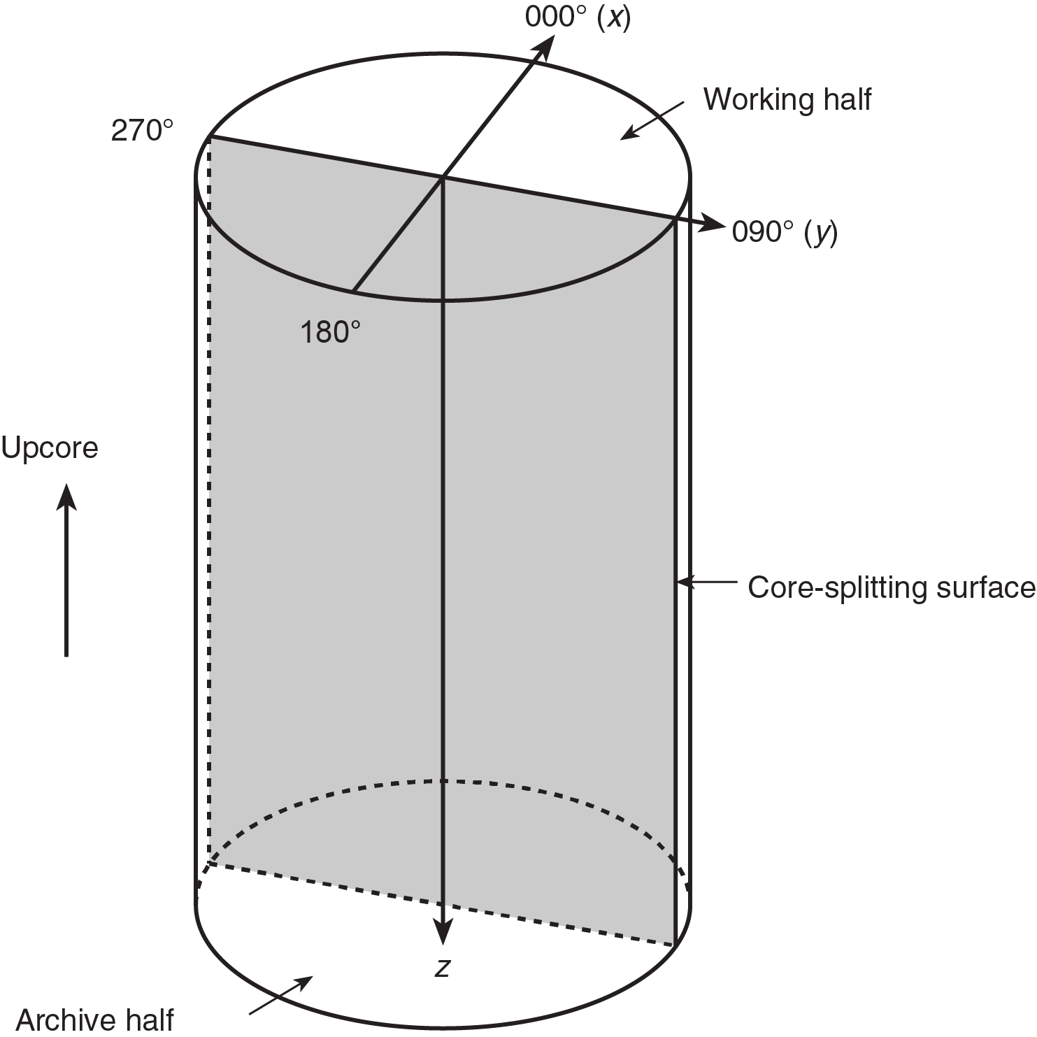
Figure F26. Core coordinate system showing x-, y-, and z-axes used for orientation data measurements.
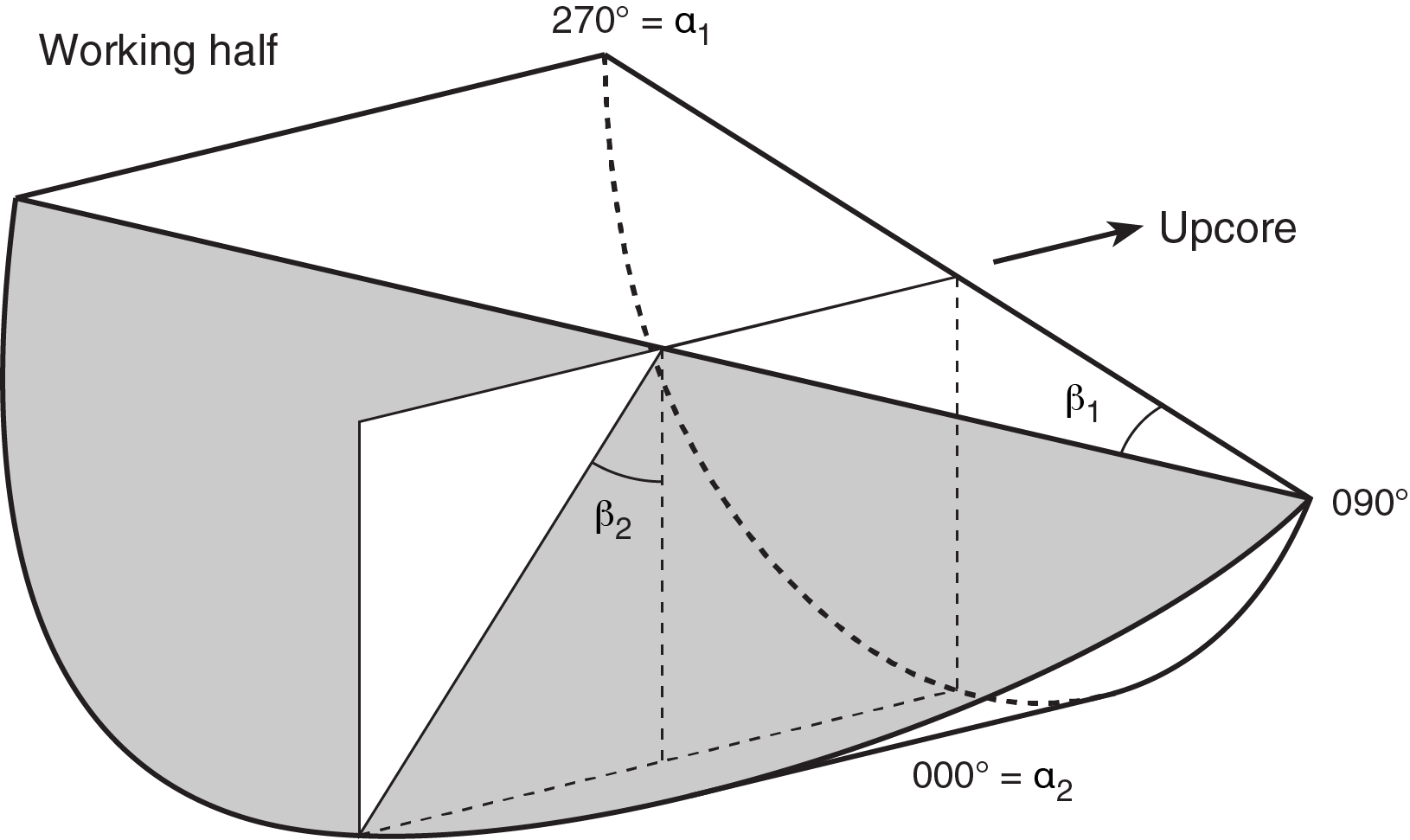
Figure F27. Determination of geological plane orientation from two auxiliary measurements.
Linear features (e.g., slickenlines) were commonly observed on planar structures (typically fault or shear surfaces). Their orientations were determined in the core reference frame by measuring either their bearing and plunge or their rakes (or pitches) (ϕa) on the planes (Figure F28). When using rakes, in order to avoid confusion between two lines having the same rake but raking toward two opposite azimuths (e.g., a N45°E–60°SE fault bearing two striations, one raking 30°NE and the other raking 30°SW) we used the following convention, which applies for all cases except for subvertical planes. If the linear feature rakes from an azimuth between N1°E and 179°E or between N181°E and N359°E, then 90° or 270°, respectively, will follow the value of the rake. In the example shown in Figure F28, 270° would be added after the ϕa value. In the case of subvertical planes, +1° would follow the rake value to indicate rakes from the top of the core or −1° to indicate rakes from the bottom of the core. The calculation sheet accounts for this information for data processing.

Figure F28. Rake measurement of slickenlines on a fault surface.
All of the above-mentioned data as well as any necessary descriptive notes were recorded on the structural geology observation sheet.
Data processing
Orientation data calculation and true north correction
A spreadsheet developed during NanTroSEIZE Expeditions 315, 316, 319, 322, 333, 338, and 348 was used to calculate orientation data in the core reference frame (Expedition 315 Scientists, 2009; Expedition 316 Scientists, 2009; Expedition 319 Scientists, 2010; Expedition 322 Scientists, 2010; Expedition 333 Scientists, 2012; Strasser et al., 2014; Tobin et al., 2015). Based on the measured bearings (α1 and α2) and plunge angles (β1 and β2), this spreadsheet determines the strikes and dip angles of the planar features in the core reference frame. Because of drilling-induced core fragmentation (e.g., biscuiting) and ensuing core recovery and core preparation operations, the orientation of the core with respect to the present-day magnetic north is not known. A correction routine is therefore required to rotate orientations measured in the core reference frame to the magnetic reference frame. Paleomagnetic data were collected by the cryogenic magnetometer at the Kochi Core Center following the shore-based sampling party (see Paleomagnetism) and used to reorient structures and bedding observed in the cores in cases where there was a paleomagnetic datum point within the same coherent interval. When paleomagnetic data are available, the spreadsheet further converts the core reference data to geographic coordinates.
J-CORES structural database
The J-CORES database has a VCD program to store visual (macroscopic and/or microscopic) descriptions of core structures and a record of planar structures in the core coordinate system. The orientations of such features are saved as comments or notes but do not appear on the plots from the Composite Log Viewer. During the Expedition 365 shore-based sampling party, only the locations of structural features were entered in the J-CORES database, and orientation data management and analyses were performed separately with a spreadsheet as described above. Later, structural elements were converted to core-scale depictions using Strater software.
Biostratigraphy
Core samples for biostratigraphy were sent to a shore-based scientist for analysis and reporting after the end of the sampling party.
Calcareous nannofossils
Calcareous nannofossils were used to date core catcher and small discrete core samples.
Zonation and biohorizons
The biostratigraphic zonation of calcareous nannofossils was based on the schemes of Martini (1971) and Okada and Bukry (1980). The application of zonal markers and additional datums here is mostly based on the compilation by Raffi et al. (2006), consistent with previous NanTroSEIZE expeditions (e.g., Expeditions 315, 316, 319, 322, and 333) for biostratigraphic consistency and subsequent correlation (Expedition 315 Scientists, 2009; Expedition 316 Scientists, 2009; Expedition 319 Scientists, 2010; Expedition 322 Scientists, 2010; Expeditions 333 Scientists, 2012).
Each nannofossil datum was assigned an astronomically calibrated age compiled by Raffi et al. (2006) and followed original descriptions by these authors. The astrochronological framework for the Neogene follows the International Commission on Stratigraphy (ICS) 2004 timescale (Lourens et al., 2004). The timescale and biostratigraphic zones of calcareous nannofossils are summarized in Figure F29 and Table T7.
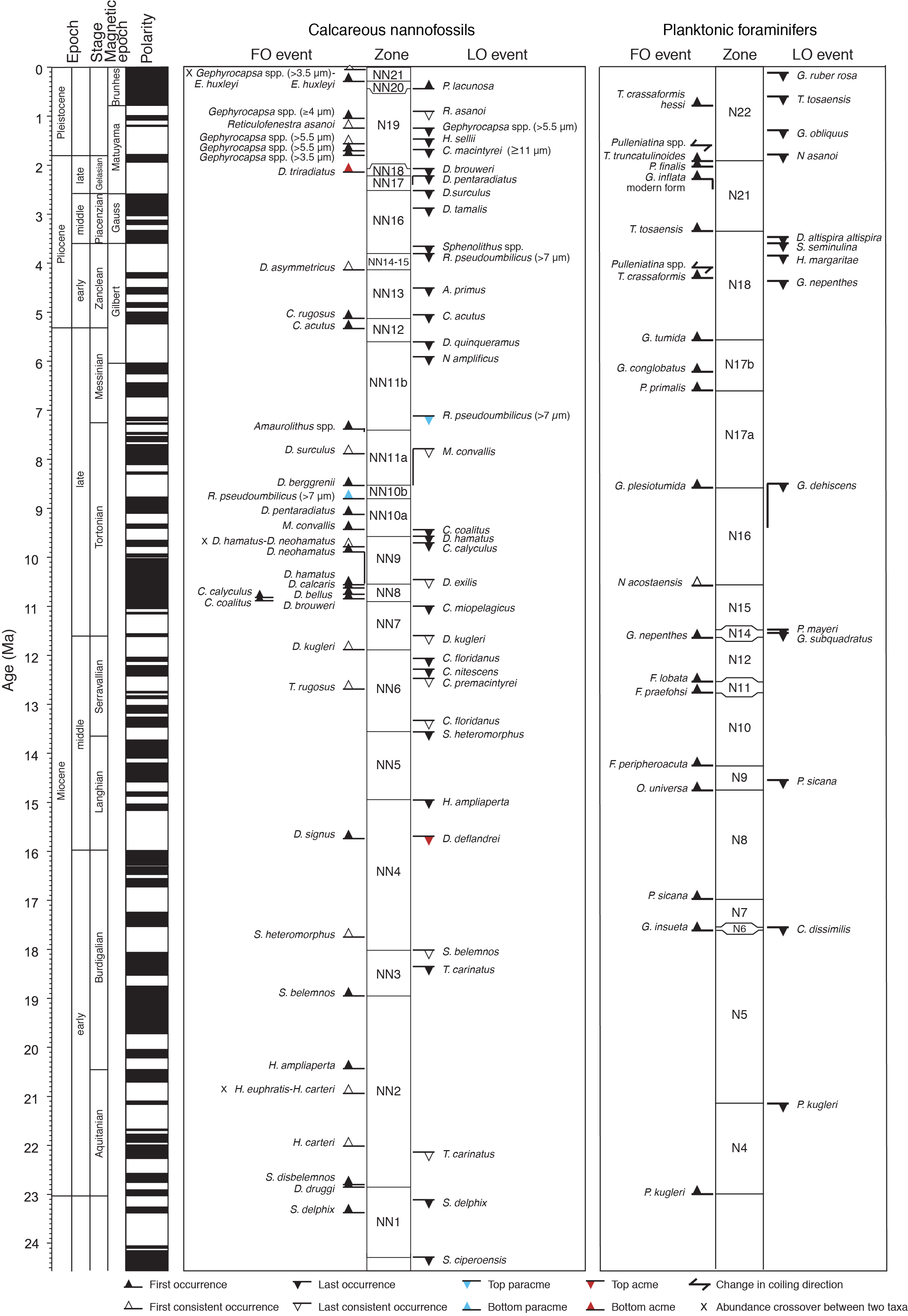
Figure F29. Late Cenozoic magnetostratigraphic and biostratigraphic events.
Table T7. Astronomically calibrated age estimates of calcareous nannofossil datums used as biostratigraphic tie points. Download table in .csv format.
Taxonomic remarks
Taxonomy followed the compilation of Perch-Nielsen (1985) and Young (1998). Previous work suggested grouping species in the reticulofenestrids, including genera Gephyrocapsa and Reticulofenestra, by size. This is because their species show a great variation in size and other morphological features (e.g., relative size of the central opening and orientation of the bar in the case of Gephyrocapsa).
Accordingly, Gephyrocapsa is divided into three major groups by maximum coccolith length following biometric subdivision by Rio (1982), Raffi et al. (1993), and Raffi (2002): small Gephyrocapsa (<4 µm), medium Gephyrocapsa (≥4 to <5.5 µm), and large Gephyrocapsa spp. (≥5.5 µm). Some important morphologic features (e.g., bar orientation) were also considered during the analysis. In addition, Reticulofenestra pseudoumbilicus should have a coccolith length greater than 7 µm.
Methods
Samples were prepared for calcareous nannofossil analysis using standard smear slide methods and optical adhesive as a mounting medium (Bown and Young, 1998). Smear slides were examined with an optical microscope at 1500× magnification.
The total abundance (per field of view [FOV]) of coccoliths for each sample was determined using the following scale:
- A = very abundant (>50 specimens per FOV).
- C = common (10–50 specimens per FOV).
- R = rare (1–10 specimens per 1–2 FOV).
- + = present (1 specimen per 2 or more FOV).
In order to investigate occurrences of other rare species in each sample, additional observations were made along three to four other transects of a smear slide. Nannofossil preservation was recorded following the criteria originally provided by Steinmetz (1979):
- G = good (little or no evidence of dissolution and/or overgrowth; only slight alteration of diagnostic characteristics; all taxa are easily identified).
- M = moderate (evident etching and/or overgrowth; no diagnostic changes).
- P = poor (severe dissolution, fragmentation, and/or overgrowth; diagnostic characteristics largely destroyed; identification of most specimens difficult at the species and/or generic level).
All information regarding the nannofossil assemblages and preservation data are summarized in Table T12 in the Site C0010 chapter (Saffer et al., 2017).
Paleomagnetism
Paleomagnetic and rock magnetic investigations were not performed on board the Chikyu during Expedition 365. The cores were sampled during the shore-based sampling party, and samples were later examined by an on-shore specialist after the shore-based sampling party was completed. These analyses were primarily designed to determine characteristic remanence directions for use in magnetostratigraphic and structural studies.
Discrete samples and sampling coordinates
A total of 48 discrete samples were collected from Holes C0010C–C0010E at a frequency of one sample per section (~140 cm). Magnetic measurements on the samples were then conducted using a magnetometer (2G Enterprises, model 760) at JAMSTEC (Yokosuka, Japan). Natural remanent magnetization demagnetized directions and intensities of all samples at 0, 2.5, 5, 10, 15, 20, 25, 30, 35, 40, 45, 50, 55, 60, 65, 70, 75, and 80 mT peak fields were measured.
The relationship between the orientation of archive section and that of a discrete sample is shown in Figure F30.
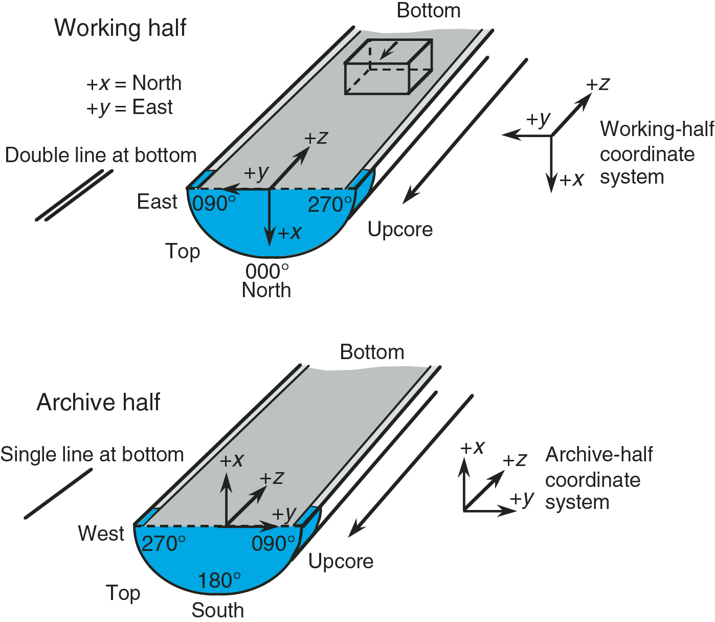
Figure F30. Orientation system used for sampling cubes for paleomagnetism analysis.
Magnetic reversal stratigraphy
Whenever possible, magnetic polarity interpretations are provided with the naming convention following that of correlative anomaly numbers prefaced by the letter C (Tauxe et al., 1984). Normal polarity subchrons are referenced by adding suffixes (e.g., n1, n2, etc.) that increase with age. For the younger part of the timescale (Pliocene–Pleistocene) traditional names are often used to refer to the various chrons and subchrons (e.g., Brunhes, Jaramillo, Olduvai, etc.). The ages of the polarity intervals used during Expedition 365 are a composite of four previous magnetic polarity timescales (magnetostratigraphic timescale for the Neogene by Lourens et al. [2004]).
Inorganic geochemistry
Fluid splits of the OsmoSampler chemistry and biochemistry coils were divided among the following shipboard analyses: chlorinity, alkalinity, major cations, anions, and minor and trace elements (Table T1; Figure F31). Additionally, a total of six IW samples from Holes C0010C and C0010E and were analyzed for chlorinity, alkalinity, major cations, anions, and minor and trace elements (Table T8). WR cores were immediately taken from the catwalk to the XCT laboratory to be scanned for important lithologic boundaries and structures. The watchdog scientist viewed the composite scan to determine size and sampling depth of each IW sample. The length of IW WR samples increased with depth, ranging from 21 to 36 cm, because a greater volume of core was needed to produce sufficient IW for analysis as a result of decreasing porosity and increasing induration with depth. Each IW WR sample was taken to the quality assurance (QA)/QC laboratory and immediately removed from the core liner into a nitrogen-flushed glove bag. The exterior of the WR sample was then thoroughly cleaned of drilling contamination with a spatula, and the clean parts were placed into a Manheim-type titanium squeezer (Manheim, 1966) on top of two filter papers rinsed with Millipore 18.2 Ω·cm Type 1 ultrapure (Milli-Q) water placed on 2–4 320 mesh stainless steel screens. A Ti squeezer with a 5.5 cm ID was used during Expedition 365. In a first step, the stress was manually increased to squeeze the first drops of IW out before the sample was transferred to an automated hydraulic system where sediments were squeezed at ambient temperatures and loads of up to 6,804 kg to ensure that the interlayer water of clay minerals was not released during the squeezing process. This IW was collected through the filters into a 60 mL acid-washed plastic syringe that was attached to the bottom of the squeezer assembly. After squeezing, the water was filtered through a 0.45 µM disposable PTFE filter into sample vials.
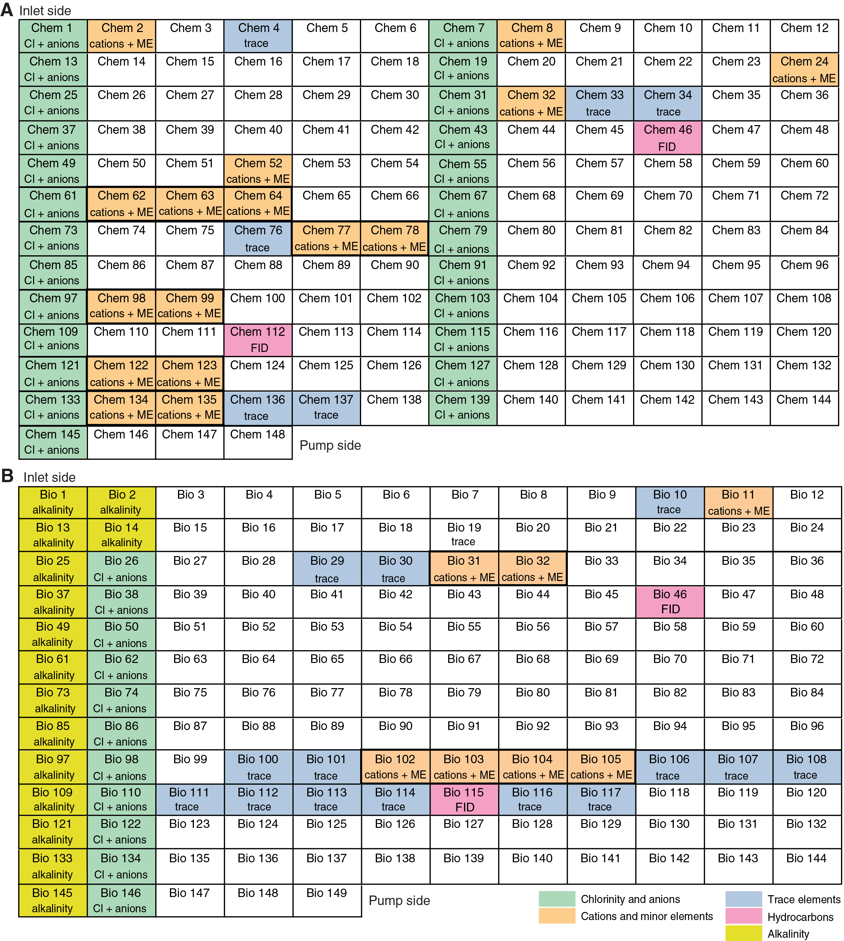
Figure F31. OsmoSampler coil fluid splits indicating the shipboard measurements conducted.
Table T8. Core sections sampled for inorganic geochemistry analyses. Download table in .csv format.
Alkalinity and pH were determined by Gran titration with a pH electrode and a Metrohm autotitrator. Refractive index was measured with a RX-5000i refractometer (Atago) and converted to salinity based on repeated analyses of the International Association of Physical Sciences of the Oceans (IAPSO) standard seawater. These repeated measurements suggested a precision of 0.1%.
Chlorinity concentrations were determined by titration with silver nitrate (AgNO3). This measurement includes concentrations of dissolved chloride, bromide, and iodide. The dissolved chloride values reported here are the titration measurements minus concentrations of bromide determined by inductively coupled plasma–atomic emission spectrometry (ICP-AES). Iodide concentrations are assumed to be negligible. The average precision of this measurement, and all those listed below, was determined as 1σ standard deviation of the mean of multiple measurements of a standard. In this case precision was calculated from multiple measurements of IAPSO standard seawater and was determined to be 0.2% of the value.
Sulfate, bromide, nitrate, and nitrite concentrations were analyzed by ion chromatograph (Dionex ICS-2100) using samples that were diluted 1:100 with Milli-Q water. Several different dilutions of IAPSO standard seawater were analyzed as a QC measure at the beginning, at an intermediate point during, and at the end of each run. These standards were used to compensate for instrument drift and to calculate analytical precision. Precision for sulfate and bromide was 1.1% and 1.5%, respectively. Limits of detection for sulfate, nitrate, and nitrite are 3, 8, and 18 µM, respectively.
Major cations (Mg, Ca, Na, and K) were analyzed by ICP-AES (Horiba Jobin Yvon Ultima2). First, samples were acidified with 6 M HCl to a concentration of 0.4% (v/v). A 5 µL aliquot was then diluted with ultrapure water by a factor of 200 for the measurements. Standardization was achieved by successive dilution of IAPSO standard seawater to 100%, 75%, 50%, and 25% relative to the 1:200 primary dilution ratio. Analytical precision for each element was based on repeated analyses of the 50% dilution standard (Ca = 0.7%, Mg = 1.0%, Na = 0.7%, and K = 0.9%).
To analyze the minor elements (B, Ba, Fe, Li, Mn, Si, and Sr), a second aliquot of the previously acidified sample was further diluted by a factor of 20 (0.5 mL sample added to 9.5 mL of a 1% nitric acid solution containing yttrium as an internal standard at 10 ppm). A standard dilution series was made from ultrapure primary standards (SPC Science PlasmaCAL) to concentrations of 100%, 50%, 25%, 10%, 5%, and 1%, all diluted with 1% nitric acid. Because of the high concentration of matrix salts in the IW samples at 1:20 dilution, matrix matching of the calibration standards was necessary to achieve accurate results by ICP-AES. A matrix solution that approximated IAPSO standard seawater major ion concentrations was prepared by dissolving the following salts in 1 L of Milli-Q water acidified with 4 mL of optima-grade 6 M HCl: 27 g NaCl, 3.8 g MgCl, 1.0 g CaCO3, and 0.75 g KCl. Sulfate was not added to the matrix-matching solution because sulfate concentrations in these samples were relatively low compared to seawater. A 1.25 mL aliquot of each standard in the dilution series was then added to 8.75 mL of the matrix solution. These matrix standards were again diluted by a factor of 20 with the same 1% nitric acid and 10 ppm Y solution used with the samples. The final matrix-matched 100% standard solution contained the following concentrations of elements: B = 2891 µM, Li = 450.2 µM, Si = 1113 µM, Mn = 56.88 µM, Fe = 55.96 µM, Sr = 356.7 µM, and Ba = 227.6 µM. This dilution series was used to create a calibration curve for each element. The average errors for minor element analyses were as follows: B =1.4%, Ba =1.0%, Fe = 2.2%, Mn = 1.2%, Li = 2.5%, Si = 1.1%, and Sr = 1.2%.
Trace elements (V, Cu, Mo, Rb, Cs, Pb, Zn, and U) were analyzed by inductively coupled plasma–mass spectrometry (ICP-MS) (Agilent 7500ce ICP-MS) equipped with an octopole reaction system to reduce polyatomic and double-charge interferences. Sample aliquots were diluted to 10% of their initial concentration with a 1% nitric acid solution and an indium internal standard solution (500 µL sample with 4.0 mL of 1% nitric acid solution and 500 µL of a 500 ppb indium standard). A primary standard solution was made that matched the maximum range of predicted concentrations based on published results of deep-sea pore fluid compositions in a variety of settings. The composition of this standard was as follows: Cs, Cu, Mo, Pb, U, and V = 40 ppb; and Rb = 500 ppb. This primary standard was diluted in 1% nitric acid solution to relative concentrations of 50%, 25%, 10%, 5%, and 1%. A 500 µL aliquot of each serial dilution was further diluted with 3500 µL of a 1% HNO3 solution, 500 µL of 560 mM NaCl, and 500 µL of the 500 ppb indium internal standard. The 25% standard was diluted accordingly and analyzed every eight samples throughout every analysis series to determine precision (errors were as follows: Cs = 4.0%, Cu = 6.6%, Mo = 0.4%, Pb = 10.5%, U = 5.2%, V = 1.6%, Rb = 1.3%). A matrix blank was prepared with a NaCl concentration similar to IAPSO standard seawater values and analyzed to calibrate for interferences by the major ions Na+ and Cl−. A procedural blank consisting of 500 µL Milli-Q water, 4.0 mL of 1% nitric acid solution, and 500 µL of the 500 ppb indium standard was analyzed every eight samples. Limits of detection were calculated from 10 analyses of the procedural blank (Cd = 2.8 nM, Co = 4.3 nM, Cu = 2.1 nM, Mo = 1.2 nM, Pb = 0.14 nM, U = 0.01 nM, and V = 3.7 nM).
Organic geochemistry
Gas analysis
After cutting the OsmoSampler coils for sampling, four 1 m lengths were placed into 20 mL glass ampules and immediately sealed with a septum and metal crimp cap for hydrocarbon analyses (Table T1). During coring operations, one hydrocarbon gas sample was collected from each core for standard shipboard headspace measurements. Samples were collected from core sections that appeared to be relatively undisturbed by drilling. A 5 cm3 sediment sample was collected in the core cutting area from the bottom of the selected core section using a cut-off plastic syringe and was extruded into a 20 mL glass vial that was immediately sealed with a septum and metal crimp cap.
All vials for hydrocarbon analyses were incubated at room temperature for at least 15 h and then at 70°C for 30 min before analysis. The coil samples were incubated at 100°C for an additional 30 min to ensure that all gas escaped the coil liner. The evolved C1–C4 gases were analyzed using an Agilent 8890B gas chromatograph (GC) equipped with a flame ionization detector (FID). Chromatographic response on the GC was calibrated against a one-point calibration curve, which was verified with additional authentic standards with variable quantities of low molecular weight hydrocarbons. A 400 µL volume of headspace gas was extracted from the vial using a standard gas syringe and injected into the GC. The methane concentration was derived from the headspace measurement using the following equation, which assumes that quantities of undetected methane dissolved in the aqueous phase are minimal (e.g., Duan et al., 1992):
CH4 = (χM × P × VH)/(R × T × ϕ × VS),
- VH = volume of the sample vial headspace (less the volume of the coil when appropriate, 3 mL),
- VS = volume of the whole sediment sample or coil volume,
- χM = molar fraction of methane in the headspace gas (obtained from GC analysis),
- P = pressure in the vial headspace (assumed to be the measured atmospheric pressure when the vials were sealed),
- R = universal gas constant,
- T = temperature of the vial headspace in Kelvin, and
- ϕ = sediment porosity (when appropriate, determined either from moisture and density [MAD] measurements on nearby samples or from porosity estimates derived from gamma ray attenuation [GRA] data representative of the sampled interval).
Core analysis
Total carbon (TC), total nitrogen (TN), and total sulfur (TS) were measured using samples from cores. Samples (~60 mg) were freeze-dried under a vacuum and ground to powder. TC, TN, and TS were determined using a Thermo Finnigan Flash elemental analysis (EA) 1112 carbon-hydrogen-nitrogen-sulfur analyzer. Calibration was based on the synthetic standard sulfanilamide, which contains 41.81 wt% C, 16.27 wt% N, and 18.62 wt% S. A total of 15–25 mg of sediment powder was weighed and placed in a tin container for carbon and nitrogen analyses. The same amount of powdered sediment was weighed for sulfur analysis and mixed with an oxidizer (vanadium pentoxide [V2O5]) in a tin container. Sediment samples were combusted in an oxygen stream at 900°C for carbon and nitrogen and 1000°C for sulfur. The sample and container melt, and the tin promotes a violent reaction (flash combustion) in the enriched oxygen stream. The combustion produced CO2, SO2, and NO2, which were carried by a constant flow of carrier gas. Then, NO2 was reduced to N2, and the mixture of N2, CO2, and SO2 was separated using a GC equipped with a thermal conductivity detector. The accuracy of the analysis was confirmed using soil NCS reference material (Thermo Scientific, Milan, Italy), sulfanilamide standard (Thermo Scientific), and JMS-1 reference material.
Total organic carbon is usually estimated by the difference between the TC value and inorganic carbon (IC) value. IC was determined with the same set of samples used for elemental analysis. Approximately 15–25 mg of sediment powder was weighed and acidified with 2 M HCl to convert the carbonate to CO2. The released CO2 was titrated, and the change in light transmittance was measured with a photodetection cell. The weight percentage of calcium carbonate was calculated from the IC content, assuming that all evolved CO2 was derived from dissolution of calcium carbonate:
CaCO3 (wt%) = IC (wt%) × 100/12.
No correction was made for the presence of other carbonate minerals. Standard deviation for the samples was less than ±0.05 wt%. NIST-SRM 88b and JSD-2 were used as standard reference materials to check accuracy.
Microbiology
FLOCS sampling
The construction of the FLOCS and the substrates have been described previously (Figure F2B; Kopf et al., 2011). Briefly, the FLOCS unit includes four chambers containing the following (in order from inlet to outlet): polished rock chips, crushed barite, crushed olivine, and clayey mudstone collected from Site C0004 during Expedition 316 (Figure F32A). Basalt and olivine rock chips were attached to two plastic slides using epoxy and were held in place using glass beads and glass wool. Crushed minerals were held in place with PTFE mesh. Once removed from the GeniusPlug and OsmoSampler, the FLOCS was wrapped in autoclaved aluminum foil and brought into the shipboard anaerobic chamber, which had a mixed atmosphere of nitrogen (97.5%) and hydrogen (2.5%). The FLOCS was intact and in good condition (Figure F32B); however, most of the fluid had escaped from the chambers.
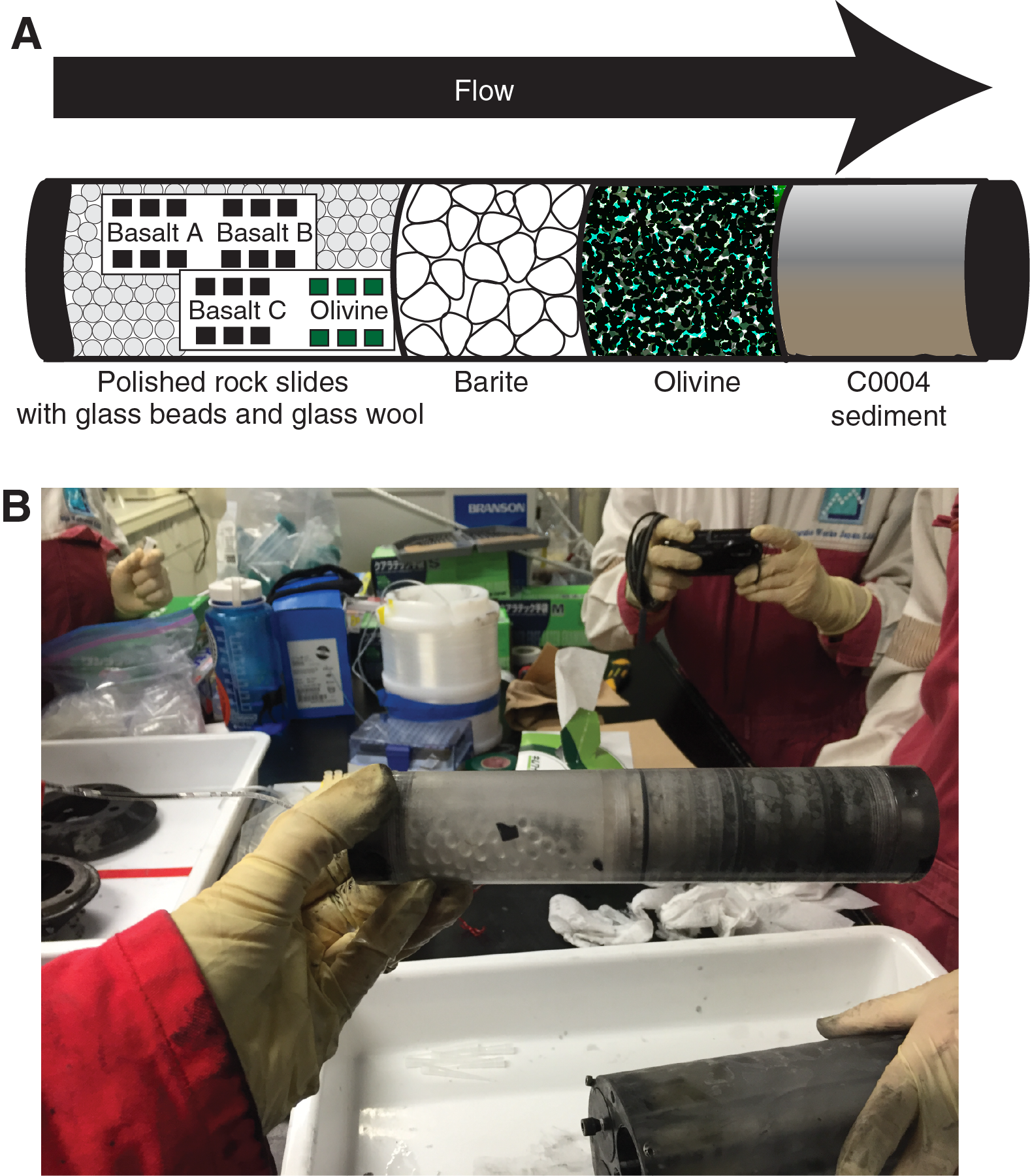
Figure F32. FLOCS unit.
Polished rock chips were sorted by rock type and preserved for scanning electron microscopy (SEM). These chips were transferred to 2 mL tubes containing 4% paraformaldehyde in 1× phosphate-buffered saline (PBS, diluted with seawater) and allowed to soak for 4 h at 4°C before being stored in a PBS:ethanol solution (50:50 [v/v]) at 4°C. The glass beads and glass wool surrounding the rock chip slides were frozen at −80°C for postexpedition DNA analyses.
Crushed minerals and clay sediment were sampled using autoclaved tweezers as follows: 35% for DNA analyses, 25% for culturing analyses, 25% for single-cell genomics (SCG), and 15% for microscopy. Samples for DNA analyses were collected in 15 mL conical tubes and frozen immediately at −80°C. Barite minerals were saved for SEM and preserved as described above. Olivine and sediment samples were preserved for microscopic cell counts. Approximately 0.5 g of each material was placed in a 2 mL tube containing 1 mL of 4% paraformaldehyde in 1× PBS and stored at 4°C without washing.
Material for culture experiments was divided between two 20 mL serum vials, each containing 10 mL of artificial seawater (ASW) medium (Table T9) and incubated at room temperature. Four additional cultures were made from fluids scavenged from the FLOCS chamber (2 mL FLOCS fluids in 10 mL ASW medium, two replicates) and iron precipitates scraped from the inside of the GeniusPlug’s casing (0.5 mL scrapings in 10 mL ASW medium, two replicates).
Table T9. Medium for culture experiments. Download table in .csv format.
Crushed minerals aliquoted for SCG analyses were transferred to 15 mL tubes containing 3.5 mL of filtered 1× PBS. Tubes were inverted several times over a period of 2 h, vortexed for 30 s at high speed, and centrifuged for 30 s at 2000 rotations/min. The supernatant was then divided into three cryovials as 1 mL replicates. Each cryovial received 100 µL of glyTE stock solution (Table T10; Single Cell Genomic Center, 2014). Finally, the cryovials were inverted and incubated at room temperature for 10 min and stored at −80°C. Any cells that may have been caught on the PTFE mesh were also preserved for SCG. All microbiology samples were preserved for onshore analyses at their shipboard storage temperatures.
Table T10. Chemical composition of the glyTE stock solution. Download table in .csv format.
A total of two fluid samples from the chemistry and biology coils of the OsmoSampler were aliquoted for cell counts. These fluid samples were diluted with an equal volume of 4% paraformaldehyde in 1× PBS and then stored and shipped at 4°C.
Microscopy
FLOCS cultures were analyzed for microbial life after an incubation time of 6 days. In the anaerobic chamber, a volume of 250 µL was sampled from each culture. This volume was filtered onto a 0.2 µM GTTP Isopore membrane filter (Millipore). Filters were then stained for 10 min with a 1× SYBR Green I solution (Life Technologies) diluted with a 1× Tris-EDTA (TE) solution. Filters were washed with ultrapure water for 10 min. The filters were dried and mounted on a slide with Type F immersion oil. Slides were observed using a Zeiss Axioplan 2 fluorescent microscope equipped with the fluorescent filter set of 485/20 nm for excitation (center wavelength/bandwidth) and 515 nm for emission.
Whole-round sampling
WR cores were first scanned by the XCT scanner and reviewed for structural quality and to identify intact core material while also avoiding regions of interest for later analyses related to other key expedition objectives. Areas demonstrating minimal drilling disturbance and void spaces were selected for microbiology samples. WR sections were cut in the core processing laboratory and immediately transported to the shipboard anaerobic chamber. Within the chamber, cores were removed from the core liner and the outer portion of each WR was shaved off to minimize the risk of contamination of the core interior by drilling fluid. The remaining central portion of each WR sample was then divided for cultivation assays, microbial cell counts, SCG, and DNA extractions.
A total of 1 cm3 of each WR was added to 9 mL of 4% paraformaldehyde in 1× PBS for cell enumeration. Samples were vortexed on high for 30 s and stored at 4°C. A total of 1 cm3 of each WR sample was also diluted in 4 mL filtered 1× PBS for SCG. These samples were handled as described above. Two replicate culture experiments were made from each WR by inoculating 10 mL of anaerobic ASW medium (Table T9) with 1 cm3 of sediment, and cultures were incubated at room temperature. The remaining sediment was saved for DNA analyses and frozen at −80°C.
Contamination tests for whole-round sampling
Contamination tests for core samples were carried out by chemical tracer quantification. Perfluorocarbon tracer (PFT; perfluoromethylcyclohexane, C7F14) was supplied directly to drilling mud that was used to sweep Holes C0010C and C0010E. PFT measurements followed the protocol outlined in Smith et al. (2000) with slight modifications. Two 2.5 cm3 plugs of sediment were collected from core sections directly adjacent to MBIO WR samples to evaluate drilling fluid intrusion into the cores. One sample was taken from the outer edges and the second was taken from the center of the remaining core. The sediment plugs were placed into 20 mL vials and sealed with silicone septa and metal crimp caps. Headspace vials were incubated for 30 min at 80°C prior to measurement. Samples were analyzed by a GC with an electron capture detector (Network GC System 7890B, Agilent Technologies) connected to an autosampler (Network Headspace Sampler G1888, Agilent Technologies). The following equation was used to determine the amount of drill-water intrusion in each sample (Smith et al., 2000):
- Ps = integrated peak area of PFT in sample (in arbitrary units),
- Pb = integrated peak area of PFT in blank (in arbitrary units),
- a = slope derived from the calibration curve (in arbitrary units per gram),
- CDW = concentration of PFT in drilling fluid (in grams per liter),
- W = weight of sample (in grams), and
- FI = fraction of the total headspace gas injected.
- Vinj = volume of sample injected (in liters),
- Vvial = volume of vial (in liters),
- ρ = sample density (in grams per liter), and
- W = weight of sample (in grams).
Physical properties
Physical property measurements provide key parameters for characterization of consolidation state and deformation of rock formations and are an important tool for integrating information from core, cuttings materials, and LWD. In addition, physical properties are indicators for composition and environmental conditions and are essential for stratigraphic correlation (Blum, 1997), evaluation of flow properties, and more generally for formation evaluation.
Cores were first scanned by XCT and then thermally equilibrated at room temperature for approximately 3 h before any physical property measurements were conducted. Nondestructive measurements on WR sections included GRA density, magnetic susceptibility, natural gamma radiation (NGR), and ultrasonic P-wave velocity using the MSCL-W (GeoTek Ltd., London, United Kingdom). Noncontact electrical resistivity (NCR) is normally part of the MSCL-W measurement suite but was not included during Expedition 365 because of a malfunction of the NCR system. Following MSCL-W measurements, cores were stored at 4°C, capped, and sealed. All other physical properties measurements were deferred until the shore-based sampling party held from 26 July to 5 August 2016, when the cores were split. The measurements included MAD, electrical conductivity, and P-wave velocity. Half-round MSCL measurements were performed on the archive halves of split cores to obtain photo imagery and color spectroscopy data (see MSCL-l: photo image logger (archive half) and MSCL-C: color spectroscopy (archive half)).
MSCL-W (whole-round cores)
Gamma ray attenuation density
A well-collimated gamma ray beam (primary photon energy of 662 keV) is produced from a small (370 MBq) 137Cs source. The intensity of the beam is measured across the core with a scintillation detector that is composed of a scintillation crystal and an integrated photomultiplier tube. The first-order mechanism for GRA is inelastic scattering by electrons, resulting in a partial energy loss (Compton effect). Because it is directly related to electron density, sediment bulk density (ρb) can be determined from the amount of attenuation by
- µ = Compton attenuation coefficient,
- d = sample thickness or outer liner diameter,
- I0 = gamma ray source intensity, and
- I = measured intensity through the sample.
Accordingly, the GRA method can provide information about bulk rock density by measuring the attenuation of a gamma ray beam that passes through a core. Here, an empirical approach is used to relate bulk density and GRA. The system is calibrated with a special calibration “core section,” comprising a set of aligned aluminum cylinders of various diameters surrounded by distilled water in a sealed core liner. Density (ρ) depends on the diameter of the aluminum cylinder and spans from ρ = 1 g/cm3 (only water) to 2.71 g/cm3 (only aluminum). For calibration measurements, gamma ray counts were taken for each aluminum cylinder once per second for 60 s; these values were then averaged. The resulting ln(I) was plotted against the product of the known parameters ρ and d of the calibration core section and fitted with a regression curve:
ln(I) = A(ρ × d)2 + B(ρ × d) + C,
where d is the internal diameter of the liner and A, B, and C are coefficients determined from the polynomial equation fit. Density measurements were conducted perpendicular to the core axis every 4 cm. The gamma source collimator is 5 mm in diameter, so each data point reflects the properties of the surrounding 5 mm interval, corresponding to a maximum volume of investigation of about 15.6 cm3.
P-wave velocity
Ultrasonic P-wave velocity (VP) was measured for WR cores by measuring sonde length (d) (outer liner diameter) and traveltime (t0):
A linear variable differential transformer, used to measure the liner thickness, is integrated with a 230 kHz P-wave transmitter/receiver system. The system is mounted horizontally on the MSCL-W system and measures d and t0 perpendicular to the core axis at 4 cm intervals. The measured traveltime (t0) between the transducers is delayed by the pulse traveltime through the liner, the threshold peak detection procedure, and the pulse travel between transducers and the electronic circuitry. Traveltime is corrected for these parameters by calibrating the system using a core liner filled with pure water, which has a known P-wave velocity (1480 m/s at 20°C). The corrected P-wave velocity through the core (Vcore) (m/s) is
Vcore = (d − W)/[t0 − tw − (d − W)/Vw],
- W = total wall thickness of the core liner,
- tw = measured traveltime through the water-filled calibration liner, and
- Vw = known P-wave velocity of pure water at room temperature.
Magnetic susceptibility
Magnetic susceptibility is the degree to which a material can be magnetized by an external magnetic field. Magnetic susceptibility was measured with a Bartington Instrument MS2C system with an 8 cm diameter loop sensor on the MSCL-W. A nonsaturating, low-intensity alternating magnetic field (8.0 × 10⁻⁴ mA/m root mean square at 0.565 kHz) is produced by an oscillator circuit in the sensor. Any material near the sensor that has a magnetic susceptibility causes a change in the oscillator frequency. This pulse frequency is then converted into a magnetic susceptibility value. With a reference piece of known magnetic susceptibility, the long-term consistency of the calibration is checked regularly. The spatial resolution of the loop sensor is ~4 cm with an accuracy of 5%. Magnetic susceptibility data were obtained at 4 cm intervals with an acquisition time of 1 s.
Natural gamma radiation
NGR emissions were measured on all core sections to determine variations in the radioactive counts. The NGR system records radioactive decays of long-period isotopes 40K, 232Th, and 238U in a lead-shielded detector unit. The unit is composed of a scintillator, which is coupled to a photomultiplier tube and connected to a bias base that supplies high-voltage power and a signal preamplifier. Two horizontal and two vertical detection units were mounted in a lead cube-shaped housing around the core. NGR was measured every 16 cm for 30 s on core sections.
Moisture and density measurements
Index properties, including bulk density, dry density, grain density, water content, and porosity, were derived from wet and dry mass and dry volume, measured on discrete samples from core section working halves. One or two samples were taken from every working half core section, each with an approximate volume of 10 cm3. The sampling interval was dependent on lithology and internal sedimentological structures. Additionally, MAD samples were taken as a part of routine “cluster” samples adjacent to WR samples that also included samples for carbonate, XRD, and XRF analyses.
Bulk density, dry density, grain density, porosity, and void ratio were calculated by Method C as described in Blum (1997). Wet and dry masses were measured using a paired electronic balance system, which compensates for the ship’s heave. The sample mass was counterbalanced with a precisely known mass that was within 5 g of the sample mass. The balance system has a precision of ±0.01 g, and the balance system was calibrated daily during the sampling party. Immediately after sampling, wet sediment mass (Mt) was measured. Care was taken to avoid sampling drilling mud, and any water or drilling mud on the surfaces of the sample was carefully removed. Sediment dry mass (Md) was determined after drying 24 h in a convection oven at 105°C. The dried samples were cooled in a desiccator for 1 h before their dry mass was measured. Dry volume was measured using the Quantachrome helium displacement pycnometer with a nominal precision of ±0.04 cm3, and all pycnometer values were averaged over five measurements. During each run, a reference sphere was measured to check for systematic errors.
Water content, porosity, and void ratio were defined by the water mass or volume difference before and after the drying process. Standard seawater density (1.024 g/cm3) was assumed for pore water density.
Water content
Water content (Wc) was determined according to American Society for Testing and Materials (ASTM) D2216. Water content measurements for marine samples require corrections for salt. Additionally, the percent water weight was calculated. The equations for water content are as follows:
Wc (% dry wt) = (Mt − Md)/(Md − rMt), and
Wc (% wet wt) = (Mt − Md) × (1 + r)/Mt,
Bulk density
Bulk density (ρ) of the soil is the ratio of total mass to total volume:
where Vt = total sample volume.
Total mass was measured using the balance, and total volume (Vt) was determined from the pycnometer measurements grain volume (Vd) and the calculated pore fluid volume (Vpore):
Porosity
Porosity (ϕ) is the ratio of the volume of voids to the total volume of the soil:
- ρw = density of the pore fluid, and
- Wc = water content expressed as a decimal ratio of percent dry weight.
Grain density
Grain density (ρgrain) was determined from dry mass and dry volume measurements made with the gas pycnometer and the balance. Mass and volume were corrected for salt:
ρgrain = (Md − s)/[Vd − (s/ρsalt)],
- s = salt content (in grams),
- ρsalt = density of salt (2.257 g/cm3), and
- Vd = volume of the dried sample.
Void ratio
Void ratio (e) is the ratio of the volume of voids to the volume of solids:
where Vpore = volume of fluid.
Electrical conductivity and P-wave velocity
Electrical conductivity and P-wave velocity measurements were performed on approximately 15 mm × 15 mm × 15 mm cubic samples cut from the working half. All cubes/cuboid faces were cut orthogonal to the x-, y-, and z-axes of the core reference. This three-component measurement plan enables first-order estimation of anisotropy in both electrical conductivity and P-wave velocity. The axis orientation is the same as defined for structural geology and paleomagnetism, with the z-axis pointing down along the core axis, y perpendicular to the z-axis within the core face, and x perpendicular to the z-axis pointing into the working half. The measurements followed the approach of Carlson and Christensen (1977).
Electrical conductivity
Samples were measured between two stainless steel electrodes covered with filter paper soaked in 35 g/L NaCl solution. Electrical impedance was measured with a 40–10 MHz frequency sweep between opposite cube faces with an Agilent 4494A precision impedance analyzer using a 16451B measuring unit. Along every axis three measurements were taken. The impedance corresponding to 25 kHz was entered into the J-CORES database. The impedance of each configuration was calculated by subtracting the impedance of the coupling from the measured impedance. The coupling impedance was measured by stacking the two water-saturated filters against each other before the impedance measurement. Sample resistivity along a given axis (Rx, Ry, and Rz) was calculated from the measured impedance, phase angle and the sample dimensions by
Rx = (LyLz)/Lx[Zxcos(θx) − Zfiltercos(θfilter)],
- Lx, Ly, and Lz = length of cubic discrete sample in the x-, y-, and z-direction, respectively,
- Zx = electrical impedance,
- θx = phase angle,
- Zfilter = measured impedance of the filter, and
- θfilter = measured phase angle of the filter.
Electrical conductivity (σx, σy, or σz) is also commonly reported and is simply the inverse of the resistivity:
The horizontal plane anisotropy (αRhor) and vertical plane anisotropy (αRvert) of electrical resistivity calculations compare the horizontal (x and y) and vertical (z) components of electrical resistivity expressed as a percentage of the mean:
αRhor (%) = 200[(Rx − Ry)/(Rx + Ry)], and
αRvert (%) = 200[(Rx + Ry)/2 − Rz]/[(Rx + Ry)/2 + Rz],
where Rx, Ry, and Rz are the electrical resistivity in the x-, y-, and z-direction, respectively.
P-wave velocity
P-wave velocity was measured with the P-wave logger for discrete samples (GeoTek). The logger consists of two transducers, which act as transmitter and receiver. The transducer had a resonant frequency of 230 kHz. The sample height was measured with a laser distance sensor. The transmitting transducer was connected to a pulse generator, and the receiving transducer was connected to an oscilloscope. The oscilloscope signal was displayed digitally and the first P-wave arrival can be picked manually. The sample was placed between the transducers and the receiving P-wave was recorded. P-wave velocity in a given direction (i.e., VPx) was calculated using the following equation:
The traveltime delay was determined by placing the transmitter and transducer in direct contact and measuring traveltime. The transducer/receiver unit and the laser distance sensor calibration were checked daily using measuring standards.
The horizontal plane anisotropy (αVPhor) and vertical plane anisotropy (αVPvert) of P-wave velocity calculations compare the horizontal (x and y) and vertical (z) components of P-wave velocity expressed as a percentage of the mean:
αVPhor (%) = 200[(VPx − VPy)/(VPx + VPy)], and
αVPvert (%) = 200[(VPx + VPy)/2 − VPz]/[(VPx + VPy)/2 + VPz],
where VPx, VPy, and VPz are the P-wave velocity in the x-, y-, and z-direction, respectively.
Thermal conductivity
Thermal conductivity was measured on the working half using a half-space line source (Vacquier, 1985), which approximates an infinite line source. A Teka TK04 mini HLQ probe was used for thermal conductivity measurements. The half-space probe was placed directly on the split core with the line source oriented parallel to the core axis. The measurement took place after the core had equilibrated to room temperature. Thus before every measurement, the sediment temperature was monitored to ensure that thermal drift was <0.4 mK/min. After temperature equilibration, a calibrated heat impulse was applied, and the rise in temperature was recorded for 60 s. The source power was adjusted to the thermal conductivity of the sample to optimize the measurement results. Thermal conductivity was based on the observed rise in temperature for a given quantity of heat. The probe was checked daily by measuring standards.
MSCL-l: photo image logger (archive half)
The GeoTek photo image logger (MSCL-I) scans the surface of the archive half and creates a digital image. The line-scan camera (Nikon Lens: AF Nikkor 50 mm 1:1.8D) is equipped with three charge-coupled devices, each with 2048 arrays. The reflected light from the core surface is split into three channels (red, blue, and green) by a beam splitter inside the line-scan camera. The signals are combined and the digital image is processed. A correction is made for any mechanical differences among the charge-coupled device responses. Calibrations are conducted before scanning each core to compensate for pixel-to-pixel response variation, uneven lightning, and lens effects. Optical distortion is avoided by precise movement of the camera, and the spatial resolution is 100 pixels/cm.
MSCL-C: color spectroscopy (archive half)
The GeoTek color spectroscopy logger (MSCL-C) system is equipped with a color spectrophotometer (Konica Minolta, CM-2600d). The spectrophotometer moves along the split core surface and takes a measurement every 4 cm. The reflected light is collected in the color spectrophotometer’s integration sphere and divided into wavelengths at a 10 nm pitch (360–740 nm). The color spectrum is then normalized by the source light of the reflectance and calibrated with the measurement of a pure white standard. The measured color spectrum is normally converted to lightness (L*) and chromaticity variables a* and b* (see Blum [1997] for details). These parameters can provide information on relative changes in bulk material composition that are useful for stratigraphic correlation and to identify lithologic characteristics and cyclicity of lithologic changes.
References
Becker, K., and Davis, E.E., 2005. A review of CORK designs and operations during the Ocean Drilling Program. In Fisher, A.T., Urabe, T., Klaus, A., and the Expedition 301 Scientists, Proceedings of the Integrated Ocean Drilling Program, 301: College Station, TX (Integrated Ocean Drilling Program Management International, Inc.). http://dx.doi.org/10.2204/iodp.proc.301.104.2005
Blum, P., 1997. Technical Note 26: Physical Properties Handbook—A Guide to the Shipboard Measurement of Physical Properties of Deep-Sea Cores. Ocean Drilling Program. http://dx.doi.org/10.2973/odp.tn.26.1997
Bown, P.R., and Young, J.R., 1998. Techniques. In Bown, P.R. (Ed.), Calcareous Nannofossil Biostratigraphy: Dordrecht, The Netherlands (Kluwer Academic Publishing), 16–28.
Carlson, R.L., and Christensen, N.I., 1977. Velocity anisotropy and physical properties of deep-sea sediments from the western South Atlantic. In Supko, P.R., Perch-Nielsen, K., et al., Initial Reports of the Deep Sea Drilling Project, 39: Washington, DC (U.S. Government Printing Office), 555–559. http://dx.doi.org/10.2973/dsdp.proc.39.124.1977
Carlson, W.D., 2006. Three-dimensional imaging of earth and planetary materials. Earth and Planetary Science Letters, 249(3–4):133–147. http://dx.doi.org/10.1016/j.epsl.2006.06.020
Duan, Q., Sorooshian, S., and Gupta, V., 1992. Effective and efficient global optimization for conceptual rainfall-runoff models. Water Resources Research, 28(4):1015–1031. http://dx.doi.org/10.1029/91WR02985
Expedition 315 Scientists, 2009. Expedition 315 methods. In Kinoshita, M., Tobin, H., Ashi, J., Kimura, G., Lallemant, S., Screaton, E.J., Curewitz, D., Masago, H., Moe, K.T., and the Expedition 314/315/316 Scientists, Proceedings of the Integrated Ocean Drilling Program, 314/315/316: Washington, DC (Integrated Ocean Drilling Program Management International, Inc.). http://dx.doi.org/10.2204/iodp.proc.314315316.122.2009
Expedition 316 Scientists, 2009. Expedition 316 methods. In Kinoshita, M., Tobin, H., Ashi, J., Kimura, G., Lallemant, S., Screaton, E.J., Curewitz, D., Masago, H., Moe, K.T., and the Expedition 314/315/316 Scientists, Proceedings of the Integrated Ocean Drilling Program, 314/315/316: Washington, DC (Integrated Ocean Drilling Program Management International, Inc.). http://dx.doi.org/10.2204/iodp.proc.314315316.132.2009
Expedition 319 Scientists, 2010. Methods. In Saffer, D., McNeill, L., Byrne, T., Araki, E., Toczko, S., Eguchi, N., Takahashi, K., and the Expedition 319 Scientists, Proceedings of the Integrated Ocean Drilling Program, 319: Tokyo (Integrated Ocean Drilling Program Management International, Inc.). http://dx.doi.org/10.2204/iodp.proc.319.102.2010
Expedition 322 Scientists, 2010. Methods. In Saito, S., Underwood, M.B., Kubo, Y., and the Expedition 322 Scientists, Proceedings of the Integrated Ocean Drilling Program, 322: Tokyo (Integrated Ocean Drilling Program Management International, Inc.). http://dx.doi.org/10.2204/iodp.proc.322.102.2010
Expedition 332 Scientists, 2011. Methods. In Kopf, A., Araki, E., Toczko, S., and the Expedition 332 Scientists, Proceedings of the Integrated Ocean Drilling Program, 332: Tokyo (Integrated Ocean Drilling Program Management International, Inc.). http://dx.doi.org/10.2204/iodp.proc.332.102.2011
Expedition 333 Scientists, 2012. Methods. In Henry, P., Kanamatsu, T., Moe, K., and the Expedition 333 Scientists, Proceedings of the Integrated Ocean Drilling Program, 333: Tokyo (Integrated Ocean Drilling Program Management International, Inc.). http://dx.doi.org/10.2204/iodp.proc.333.102.2012
Fisher, R.V., and Schmincke, H.-U., 1984. Pyroclastic Rocks: Berlin (Springer-Verlag). http://dx.doi.org/10.1007/978-3-642-74864-6
GE Healthcare, 2013a. Discovery CT Series Service Methods (revision 15): Waukesha, Wisconsin (GE Healthcare).
GE Healthcare, 2013b. Discovery CT750 HD User Manual (revision 1): Waukesha, Wisconsin (GE Healthcare).
GE Healthcare, 2013c. Technical Reference Manual (revision 1): Waukesha, Wisconsin (GE Healthcare).
Jannasch, H.W., Wheat, C.G., Plant, J.N., Kastner, M., and Stakes, D.S., 2004. Continuous chemical monitoring with osmotically pumped water samplers: OsmoSampler design and applications. Limnology and Oceanography: Methods, 2(2):102–113. http://dx.doi.org/10.4319/lom.2004.2.102
Kitada, K., Araki, E., Kimura, T., Kinoshita, M., Kopf, A., Hammerschmidt, S., Toczko, S., Saruhashi, T., Sawada, I., Kyo, M., Namba, Y., Kido, Y., Saffer, D.M., Lauer, R., and Wheat, G., 2011. Drill pipe monitoring of vortex-induced vibration during IODP Expedition 332 observatory installations. In Kopf, A., Araki, E., Toczko, S., and the Expedition 332 Scientists, Proceedings of the Integrated Ocean Drilling Program, 332: Tokyo (Integrated Ocean Drilling Program Management International, Inc.). http://dx.doi.org/10.2204/iodp.proc.332.106.2011
Kitada, K., Araki, E., Kimura, T., Mizuguchi, Y., Kyo, M., Saruhashi, T., Sawada, I., Namba, Y., and Kinoshita, M., 2013. Field experimental study on vortex-induced vibration behavior of the drill pipe for the ocean borehole observatory installation. IEEE Journal of Ocean Engineering, 38(1):158–166. http://dx.doi.org/10.1109/JOE.2012.2213973
Kopf, A., Saffer, D., Toczko, S., Araki, E., Carr, S., Kimura, T., Kinoshita, C., Kobayashi, R., Machida, Y., Rösner, A., and Wallace, L.M., 2017. Expedition 365 summary. With contributions by S. Chiyonobu, K. Kanagawa, T. Kanamatsu, G. Kimura, and M.B. Underwood. In Saffer, D., Kopf, A., Toczko, S., and the Expedition 365 Scientists, NanTroSEIZE Stage 3: Shallow Megasplay Long-Term Borehole Monitoring System. Proceedings of the International Ocean Discovery Program, 365: College Station, TX (International Ocean Discovery Program). http://dx.doi.org/10.14379/iodp.proc.365.101.2017
Kopf, A., Saffer, D.M., Davis, E.E., Hammerschmidt, S., LaBonte, A., Meldrum, R., Toczko, S., Lauer, R., Heesemann, M., Macdonald, R., Wheat, C.G., Jannasch, H.W., Edwards, K., Orcutt, B., Haddad, A., Villinger, H., Araki, E., Kitada, K., Kimura, T., and Kido, Y., 2011. The SmartPlug and GeniusPlug: a “Mini-CORK” retrievable observatory system for initial NanTroSEIZE borehole monitoring. In Kopf, A., Araki, E., Toczko, S., and the Expedition 332 Scientists, Proceedings of the Integrated Ocean Drilling Program, 332: Tokyo (Integrated Ocean Drilling Program Management International, Inc.). http://dx.doi.org/10.2204/iodp.proc.332.105.2011
Lourens, L., Hilgen, F., Shackleton, N.J., Laskar, J., and Wilson, D., 2004. The Neogene period. In Gradstein, F.M., Ogg, J.G., and Smith, A. (Eds.), A Geologic Time Scale 2004: Cambridge, United Kingdom (Cambridge University Press), 409–440. http://dx.doi.org/10.1017/CBO9780511536045.022
Manheim, F.T., 1966. A hydraulic squeezer for obtaining interstitial waters from consolidated and unconsolidated sediments. U. S. Geological Survey Professional Paper, 550-C:256–261.
Marsaglia, K., Milliken, K., and Doran, L., 2013. Technical Note 1: IODP digital reference for smear slide analysis of marine mud—Part 1: Methodology and atlas of siliciclastic and volcanogenic components. Integrated Ocean Drilling Program. http://dx.doi.org/10.2204/iodp.tn.1.2013
Martini, E., 1971. Standard Tertiary and Quaternary calcareous nannoplankton zonation. In Farinacci, A. (Ed.), Proceedings of the Second Planktonic Conference, Roma 1970: Rome (Edizioni Tecnoscienza), 2:739–785.
Mazzullo, J., and Graham, A.G. (Eds.), 1988. Technical Note 8: Handbook for shipboard sedimentologists. Ocean Drilling Program. http://dx.doi.org/10.2973/odp.tn.8.1988
Mazzullo, J.M., Meyer, A., and Kidd, R.B., 1988. New sediment classification scheme for the Ocean Drilling Program. In Mazzullo, J., and Graham, A.G. (Eds.), Technical Note 8: Handbook for Shipboard Sedimentologists. Ocean Drilling Program, 44–67. http://dx.doi.org/10.2973/odp.tn.8.1988
Mees, F., Swennen, R., Van Geet, M., and Jacobs, P., 2003. Applications of X-ray computed tomography in the geosciences. Geological Society Special Publication, 215(1):1–6. http://dx.doi.org/10.1144/GSL.SP.2003.215.01.01
Moore, G.F., Kanagawa, K., Strasser, M., Dugan, B., Maeda, L., Toczko, S., and the IODP Expedition 338 Scientific Party, 2014. IODP Expedition 338: NanTroSEIZE Stage 3: NanTroSEIZE plate boundary deep riser 2. Scientific Drilling, 17:1–12. http://dx.doi.org/10.5194/sd-17-1-2014
Nakano, T., Nakashima, Y., Nakamura, K., and Ikeda, S., 2000. Observation and analysis of internal structure of rock using X-ray CT. Chishitsugaku Zasshi, 106(5):363–378.
Okada, H., and Bukry, D., 1980. Supplementary modification and introduction of code numbers to the low-latitude coccolith biostratigraphic zonation (Bukry, 1973; 1975). Marine Micropaleontology, 5:321–325. http://dx.doi.org/10.1016/0377-8398(80)90016-X
Orcutt, B., Wheat, C.G., and Edwards, K.J., 2010. Subseafloor ocean crust microbial observatories: development of FLOCS (Flow-Through Osmo Colonization System) and evaluation of borehole construction materials. Geomicrobiology Journal, 27(2):143–157. http://dx.doi.org/10.1080/01490450903456772
Perch-Nielsen, K., 1985. Cenozoic calcareous nannofossils. In Bolli, H.M., Saunders, J.B., and Perch-Nielsen, K. (Eds.), Plankton Stratigraphy: Cambridge, United Kingdom (Cambridge University Press), 427–554.
Raffi, I., 2002. Revision of the early-middle Pleistocene calcareous nannofossil biochronology (1.75–0.85 Ma). Marine Micropaleontology, 45(1):25–55. http://dx.doi.org/10.1016/S0377-8398(01)00044-5
Raffi, I., Backman, J., Fornaciari, E., Pälike, H., Rio, D., Lourens, L., and Hilgen, F., 2006. A review of calcareous nannofossil astrobiochronology encompassing the past 25 million years. Quaternary Science Reviews, 25(23–24):3113–3137. http://dx.doi.org/10.1016/j.quascirev.2006.07.007
Raffi, I., Backman, J., Rio, D., and Shackleton, N.J., 1993. Plio–Pleistocene nannofossil biostratigraphy and calibration to oxygen isotope stratigraphies from Deep Sea Drilling Project Site 607 and Ocean Drilling Program Site 677. Paleoceanography, 8(3):387–408. http://dx.doi.org/10.1029/93PA00755
Rio, D., 1982. The fossil distribution of coccolithophore genus Gephyrocapsa Kamptner and related Plio–Pleistocene chronostratigraphic problems. In Prell, W.L., Gardner, J.V., et al., Initial Reports of the Deep Sea Drilling Project, 68: Washington, DC (U.S. Government Printing Office), 325–343. http://dx.doi.org/10.2973/dsdp.proc.68.109.1982
Rothwell, R.G., 1989. Minerals and Mineraloids in Marine Sediments: An Optical Identification Guide: London (Elsevier).
Sacks, I.S., Suyehiro, S., Evertson, D.W., and Yamagishi, Y., 1971. Sacks-Evertson strainmeter: its installation in Japan and some preliminary results concerning strainsteps. Papers in Meteorology and Geophysics, 22:195–208.
Saffer, D., Kopf, A., Toczko, S., Araki, E., Carr, S., Kimura, T., Kinoshita, C., Kobayashi, R., Machida, Y., Rösner, A., and Wallace, L.M., 2017. Site C0010. With contributions by S. Chiyonobu, K. Kanagawa, T. Kanamatsu, G. Kimura, and M.B. Underwood. In Saffer, D., Kopf, A., Toczko, S., and the Expedition 365 Scientists, NanTroSEIZE Stage 3: Shallow Megasplay Long-Term Borehole Monitoring System. Proceedings of the International Ocean Discovery Program, 365: College Station, TX (International Ocean Discovery Program). http://dx.doi.org/10.14379/iodp.proc.365.103.2017
Shepard, F.P., 1954. Nomenclature based on sand-silt-clay ratios. Journal of Sedimentary Research, 24(3):151–158. http://dx.doi.org/10.1306/D4269774-2B26-11D7-8648000102C1865D
Single Cell Genomic Center, 2014. Aquatic, Sediment, and Soil Sample Cryopreservation for Microbial Single Cell Genomics, Using glyTE: East Boothbay, MN (Bigelow Laboratory for Ocean Sciences). https://scgc.bigelow.org/PDFs/Sample_cryopreservation_glyTE.pdf
Smith, D.C., Spivack, A.J., Fisk, M.R., Haveman, S.A., Staudigel, H., and the Leg 185 Shipboard Scientific Party, 2000. Technical Note 28: Methods for Quantifying Potential Microbial Contamination during Deep Ocean Coring. Ocean Drilling Program. http://dx.doi.org/10.2973/odp.tn.28.2000
Steinmetz, J.C., 1979. Calcareous nannofossils from the North Atlantic Ocean, Leg 49, Deep Sea Drilling Project. In Luyendyk, B.P., Cann, J.R., et al., Initial Reports of the Deep Sea Drilling Project, 49: Washington, DC (U.S. Government Printing Office), 519–531. http://dx.doi.org/10.2973/dsdp.proc.49.116.1979
Strasser, M., Dugan, B., Kanagawa, K., Moore, G.F., Toczko, S., Maeda, L., Kido, Y., Moe, K.T., Sanada, Y., Esteban, L., Fabbri, O., Geersen, J., Hammerschmidt, S., Hayashi, H., Heirman, K., Hüpers, A., Jurado Rodriguez, M.J., Kameo, K., Kanamatsu, T., Kitajima, H., Masuda, H., Milliken, K., Mishra, R., Motoyama, I., Olcott, K., Oohashi, K., Pickering, K.T., Ramirez, S.G., Rashid, H., Sawyer, D., Schleicher, A., Shan, Y., Skarbek, R., Song, I., Takeshita, T., Toki, T., Tudge, J., Webb, S., Wilson, D.J., Wu, H.-Y., and Yamaguchi, A., 2014. Methods. In Strasser, M., Dugan, B., Kanagawa, K., Moore, G.F., Toczko, S., Maeda, L., and the Expedition 338 Scientists, Proceedings of the Integrated Ocean Drilling Program, 338: Yokohama, Japan (Integrated Ocean Drilling Program). http://dx.doi.org/10.2204/iodp.proc.338.102.2014
Tauxe, L., Tucker, P., Peterson, N.P., and LaBrecque, J.L., 1984. Magnetostratigraphy of Leg 73 sediments. In Hsü, K.J., LaBrecque, J.L., et al., Initial Reports of the Deep Sea Drilling Project, 73: Washington, DC (U.S. Government Printing Office), 609–621. http://dx.doi.org/10.2973/dsdp.proc.73.123.1984
Tobin, H., Hirose, T., Saffer, D., Toczko, S., Maeda, L., Kubo, Y., Boston, B., Broderick, A., Brown, K., Crespo-Blanc, A., Even, E., Fuchida, S., Fukuchi, R., Hammerschmidt, S., Henry, P., Josh, M., Jurado, M.J., Kitajima, H., Kitamura, M., Maia, A., Otsubo, M., Sample, J., Schleicher, A., Sone, H., Song, C., Valdez, R., Yamamoto, Y., Yang, K., Sanada, Y., Kido, Y., and Hamada, Y., 2015. Methods. In Tobin, H., Hirose, T., Saffer, D., Toczko, S., Maeda, L., Kubo, Y., and the Expedition 348 Scientists, Proceedings of the Integrated Ocean Drilling Program, 348: College Station, TX (Integrated Ocean Drilling Program). http://dx.doi.org/10.2204/iodp.proc.348.102.2015
Underwood, M.B., Basu, N., Steurer, J., and Udas, S., 2003. Data report: normalization factors for semiquantitative X-ray diffraction analysis, with application to DSDP Site 297, Shikoku Basin. In Mikada, H., Moore, G.F., Taira, A., Becker, K., Moore, J.C., and Klaus, A. (Eds.), Proceedings of the Ocean Drilling Program, Scientific Results, 190/196: College Station, TX (Ocean Drilling Program), 1–28. http://dx.doi.org/10.2973/odp.proc.sr.190196.203.2003
Vacquier, V., 1985. The measurement of thermal conductivity of solids with a transient linear heat source on the plane surface of a poorly conducting body. Earth and Planetary Science Letters, 74(2–3):275–279. http://dx.doi.org/10.1016/0012-821X(85)90027-5
Young, J.R., 1998. Neogene. In Bown, P.R. (Ed.), Calcareous Nannofossil Biostratigraphy: Dordrecht, The Netherlands (Kluwer Academic Publishing), 225–265.
1 Saffer, D., Kopf, A., Toczko, S., Araki, E., Carr, S., Kimura, T., Kinoshita, C., Kobayashi, R., Machida, Y., Rösner, A., and Wallace, L.M., 2017. Expedition 365 methods. With contributions by S. Chiyonobu, K. Kanagawa, T. Kanamatsu, G. Kimura, and M.B. Underwood. In Saffer, D., Kopf, A., Toczko, S., and the Expedition 365 Scientists, NanTroSEIZE Stage 3: Shallow Megasplay Long-Term Borehole Monitoring System. Proceedings of the International Ocean Discovery Program, 365: College Station, TX (International Ocean Discovery Program). https://doi.org/10.14379/iodp.proc.365.102.2017
2 Expedition 365 Scientists’ addresses.
This work is distributed under the Creative Commons Attribution 4.0 International (CC BY 4.0) license. 
- F1. Borehole configuration for GeniusPlug deployment.
- F2. SmartPlug/GeniusPlug schematic.
- F3. GeniusPlug in laboratory after recovery.
- F4. OsmoSampler pumps and FLOCS cylinder prior to installation in GeniusPlug extension unit.
- F5. GeniusPlug and tubing joints on rig floor before deployment during Expedition 332.
- F6. Laboratory technicians measuring and cutting OsmoSampler coil.
- F7. Attachment of accelerometer sensor to drill pipe showing mounting orientations and dimensions.
- F8. Schematic of LTBMS system configuration.
- F9. Instrument carrier showing instrument locations and connections.
- F10. Cross sections at top and bottom of instrument carrier with sensor orientation.
- F11. Molded electrical cable.
- F12. Centralizer and attachment of cables, thermistor, and flatpack.
- F13. Swellable packer.
- F14. Bay 1 of LTBMS head.
- F15. Assembled LTBMS head with ROV platform and data recorder.
- F16. Diagram of deep-sea borehole strainmeter.
- F17. Diagram of CMG3T borehole broadband seismometer.
- F18. Tilt combo module configuration and schematic.
- F19. Diagram of thermistor string.
- F20. Miniscreens at lowermost pressure termination.
- F21. Seafloor reference pressure sensor grounding line and termination on PSU steel frame.
- F22. Location of observatory Sites C0002, C0010, and C0006.
- F23. Graphic patterns and symbols used in visual core descriptions.
- F24. Example of log sheet used to record structural observations and measurements from working half.
- F25. Modified protractor.
- F26. Core coordinate system showing x-, y-, and z-axes used for orientation data measurements.
- F27. Determination of geological plane orientation from two auxiliary measurements.
- F28. Rake measurement of slickenlines on a fault surface.
- F29. Late Cenozoic magnetostratigraphic and biostratigraphic events.
- F30. Orientation system used for sampling cubes for paleomagnetism analysis.
- F31. OsmoSampler coil fluid splits indicating the shipboard measurements conducted.
- F32. FLOCS unit.
- T1. OsmoSampler coil fluid splits and their respective shipboard measurements.
- T2. Accelerometer specifications.
- T3. LTBMS instrument and sensor specifications and dimensions.
- T4. Characteristic XRD peaks for semiquantitative analysis of composite clay minerals, quartz, plagioclase feldspar, and calcite.
- T5. Analytical conditions for major element analysis of glass beads.
- T6. Averaged measured values and 3σ standard deviations on the Supermini XRF spectrometer from a selection of standard samples.
- T7. Astronomically calibrated age estimates of calcareous nannofossil datums used as biostratigraphic tie points.
- T8. Core sections sampled for inorganic geochemistry analyses.
- T9. Medium for culture experiments.
- T10. Chemical composition of the glyTE stock solution.