Saffer, D., Kopf, A., Toczko, S., and the Expedition 365 Scientists
Proceedings of the International Ocean Discovery Program Volume 365
publications.iodp.org
https://doi.org/10.14379/iodp.proc.365.103.2017

Site C00101
D. Saffer, A. Kopf, S. Toczko, E. Araki, S. Carr, T. Kimura, C. Kinoshita, R. Kobayashi, Y. Machida, A. Rösner, and L.M. Wallace with contributions by S. Chiyonobu, K. Kanagawa, T. Kanamatsu, G. Kimura, and M.B. Underwood2
Keywords: International Ocean Discovery Program, IODP, Chikyu, Expedition 365, Site C0010, Nankai Trough, Nankai Trough Seismogenic Zone Experiment, NanTroSEIZE, long-term borehole monitoring system, LTBMS, CORK, Mie-ken Nanto-oki earthquake, megasplay fault, Dense Oceanfloor Network System for Earthquakes and Tsunamis, DONET, GeniusPlug, Flow-through Osmo Colonization System, FLOCS, Kumano fore-arc basin, OsmoSampler, coring, borehole observatory
MS 365-103: Published 5 August 2017
Introduction
Background
Site C0010 was originally drilled with logging while drilling (LWD) and measurement while drilling (MWD) tools and cased during Integrated Ocean Drilling Program Expedition 319. Operations included drilling across the megasplay fault to a total depth (TD) of 555 meters below seafloor (mbsf), casing the borehole (with casing screens spanning the fault), conducting an observatory “dummy run” to test strainmeter and seismometer deployment procedures, and installing a simple pore pressure and temperature monitoring system (SmartPlug) attached to a retrievable bridge plug (see Figures F1 and F3 in the Expedition 365 summary chapter [Kopf et al., 2017]) (Expedition 319 Scientists, 2010a). The hole was revisited during Integrated Ocean Drilling Program Expedition 332, when the SmartPlug was recovered and replaced with a similar temporary instrument package that also included geochemical and microbiological sampling coils and an in situ microbiological colonization experiment; this temporary instrument package is termed the “GeniusPlug” (see Figures F4 and F5 in the Expedition 365 summary chapter [Kopf et al., 2017]) (Kopf, Araki, Toczko, and the Expedition 332 Scientists, 2011).
Drilling during Expedition 319 identified three distinct lithologic packages at Site C0010, defined on the basis of LWD data and further guided by comparison with coring and LWD results at nearby Integrated Ocean Drilling Program Site C0004 (located 3.5 km to the northeast along strike). From top to bottom, these lithologic packages are hemipelagic slope deposits composed primarily of mud with minor distal turbidite interbeds (Unit I, 0–182.5 m LWD depth below seafloor [LSF]), a thrust wedge composed of overconsolidated and fractured clay- and mudstones (Unit II, 182.5–407 m LSF), and overridden slope deposits (Unit III, 407 m LSF to TD). At Site C0010, Unit I is divided into two subunits: Subunit IA (0–161.5 m LSF), characterized by gamma ray and resistivity patterns similar to those observed in Unit I at Site C0004 (Expedition 314 Scientists, 2009), and Subunit IB (161.5–182.8 m LSF), interpreted as slope sediments composed of material reworked from the underlying thrust wedge.
For International Ocean Discovery Program (IODP) Expedition 365, the observatory system at Site C0010 consisted of an array of sensors (see LTBMS in the Expedition 365 methods chapter [Saffer et al., 2017]) designed to monitor crustal deformation and hydrologic processes in the offshore portion of the subduction system over a wide range of timescales, including seismicity and microseismicity, slow slip events and very low frequency (VLF) earthquakes, hydrologic transients, ambient pore pressure, and temperature. To ensure the long-term and continuous monitoring necessary to capture such events, the borehole observatory was designed for connection to the Dense Oceanfloor Network System for Earthquakes and Tsunamis (DONET) submarine cabled network (http://www.jamstec.go.jp/donet/e) following the drilling expedition; this connection was completed on 19 June 2016. For the long-term borehole monitoring systems (LTBMS) installed at Integrated Ocean Drilling Program Sites C0002 and C0010, both connected to DONET, the formation pressure data can be viewed and downloaded at an open-access observatory data portal (http://offshore.geosc.psu.edu).
Scientific objectives
The primary plan for Expedition 365 was to recover the GeniusPlug, deepen Hole C0010A from 555 to 655 mbsf, underream the hole below the 9⅝ inch casing to 10 inches in diameter, and install the LTBMS. Site C0010 constitutes the second permanent LTBMS installation during the Nankai Trough Seismogenic Zone Experiment (NanTroSEIZE). The downhole configuration of the observatory includes (1) three pressure ports, (2) a volumetric strainmeter, (3) a broadband seismometer, (4) a tiltmeter, (5) three-component geophones, (6) three-component accelerometers, and (7) a thermometer array (see Figure F6 in the Expedition 365 summary chapter [Kopf et al., 2017] and LTBMS in the Expedition 365 methods chapter [Saffer et al., 2017]). The set of sensors is designed to collect, as a whole, multiparameter observations in a wide period range from months to 0.01 s and over a dynamic range covering tectonic and hydrologic events that include responses to local microearthquakes, VLF earthquakes, and the largest potential earthquake slips of the Tonankai plate boundary 6 km below the sensors. Once connected to DONET, the observatory measurements can be accessed in real time from a shore-based monitoring station. Prior to connection to DONET, the system was designed for an initial “standalone” deployment period using seafloor batteries and data recorders, with data recovery by subsequent remotely operated vehicle (ROV) operations. As a contingency option in case of unforeseeable problems during installation of the full LTBMS, a second GeniusPlug was prepared to function as a replacement temporary observatory.
Specific objectives for Site C0010 during Expedition 365 were to
- Recover the GeniusPlug installed in 2010 and conduct initial shipboard analyses of the recovered pore pressure and temperature data, fluids sampled by the sampling coils, and microbiological colonization experiment.
- Extend the borehole to 655 mbsf and deploy a LTBMS that includes pore pressure ports at three levels, a thermistor string, and a suite of geophysical instruments (strainmeter, tiltmeter, and seismometer) in a configuration like that in Hole C0002G (Kopf, Araki, Toczko, and the Expedition 332 Scientists, 2011). The detailed configuration of the LTBMS and borehole are described in LTBMS in the Expedition 365 methods chapter (Saffer et al., 2017).
Operational strategy
Operational plans for Expedition 365 included two main operations in cased Hole C0010A (see Figure F7 in the Expedition 365 summary chapter [Kopf et al., 2017]). The first operation was the recovery of the GeniusPlug autonomous sampling unit. This was to begin following transit from Shimizu Harbor to Site C0010 and after ROV dives to conduct a seafloor survey, set transponders, and remove the Hole C0010A well corrosion cap. Once complete, the vessel was to move away from the Kuroshio Current to a low-current area (LCA) to make up the GeniusPlug recovery bottom-hole assembly (BHA). The BHA consisted of the L-10 on/off tool, designed to recover the retrievable bridge plug from which the GeniusPlug was suspended. Once recovered from Hole C0010A, the vessel was to return to the LCA while the BHA was pulled out of the hole to the rig floor; the GeniusPlug would then be moved to the laboratory for data download, and the OsmoSampler/Flow-through Osmo Colonization System (FLOCS) experiment would be moved to the microbiology laboratory for sampling and analysis.
The second operation was to extend previously drilled Hole C0010A from 555 to 655 mbsf using a combination drill bit and underreamer BHA for later LTBMS deployment. Once drilling was finished, the drilling/underreaming BHA was to be pulled out of the hole and replaced with a scraper BHA to ensure the cased section of the well was clear of any obstructions. The expedition science objectives would be completed with operations to deploy the LTBMS. This involved considerable moonpool preparation using newly developed guide rollers to run the completion.
A major impediment to observatory deployment in the Nankai region is the extremely strong Kuroshio Current. Current speeds up to 6 kt are possible, and the current flow past the drill string commonly results in vortex-induced vibration (VIV), which has caused lost drill pipe, dropped casing, and destroyed electronic sensors during past Integrated Ocean Drilling Program expeditions (Expedition 319 Scientists, 2010a). The Center for Deep Earth Exploration (CDEX) has developed a series of mitigation techniques and equipment to minimize or suppress VIV. These include the attachment of ropes to drill string sections exposed to the current, which prevent the formation of vortices as the current flows past the drill string. Other newly developed tools are the moonpool guide rollers, which support the drill string in the moonpool and provide a safe platform for moonpool work, and guides for attaching the VIV-suppressing ropes, cables, and hydraulic flatpack lines to the LTBMS observatory instruments.
The operational plan called for the LTBMS to be made up from the bottom bullnose to the seafloor LTBMS head as the completion was run into the moonpool. A series of system checks on the status of the strainmeter, tiltmeter, broadband seismometer, and pressure sensor unit (PSU) were to be performed at set stages as the LTBMS and sensors were assembled. Once the LTBMS was completed and run into the water, the D/V Chikyu would then drift back into the Kuroshio Current to run the LTBMS into Hole C0010A. After checking that all systems were working, the LTBMS would be cemented in place, and the vessel would release the LTBMS running tool and recover the drill string.
Actual operations could be constrained by weather, sensor health, equipment readiness, and remaining operations time. Contingency plans included returning a refurbished GeniusPlug into Hole C0010A in the event that the LTBMS could not be deployed.
Operations
Port call and transit to Site C0010
Expedition 365 began in the port of Shimizu, Shizuoka Prefecture, Japan, on 26 March 2016. The first few days were spent quayside, loading cargo and supplies. The science party boarded the Chikyu on 27 March and participated in the shipboard prespud meeting on 28 March. The Chikyu sailed from Shimizu at 0900 h on 29 March (Table T1), lowered the azimuth thrusters, and arrived on location at Site C0010 at 0330 h on 30 March (see OPERATION in Supplementary material for the daily morning reports).
Table T1. Expedition 365 operations summary. Download table in .csv format.
Hole C0010A
Water depth: 2552 m below rotary table (BRT)/2523.5 m from mean sea level (MSL)
The supply boat was sent to find a location where the Kuroshio Current was ~2 kt (the LCA). The LCA was found approximately 15 nmi north-northwest of the well center of Site C0010. The ROV was launched at 0500 h on 30 March 2016 to begin a seabed survey, set 4 transponders, and standby for dynamic positioning system (DPS) calibration. The corrosion cap was removed by 1530 h. The Baker-Hughes A-3 bridge plug L-10 on/off retrieval tool (Table T2) was made up by 1730 h and put on standby until the Chikyu moved to the LCA to begin running the BHA in the hole from 2145 h. The science party attached an accelerometer (see GeniusPlug in the Expedition 365 methods chapter [Saffer et al., 2017]) to the drill pipe at 0245 h once the L-10 BHA reached 521.5 m MSL (550 m BRT) to measure the Kuroshio Current effects (VIV) on the drill string as preparation for running the LTBMS and to measure acceleration during the GeniusPlug recovery. A 40 m towing rope for the ROV was attached at 771.5 m MSL (800 m BRT) and then the rig crew began attaching anti-VIV ropes to the drill string. These ropes help reduce Kuroshio Current–induced vibration on the drill string, which could otherwise damage the BHA, the instruments inside the GeniusPlug, or the LTBMS sensors while drifting to deploy into Hole C0010A. A rise on the seafloor along the drifting route (1900 m MSL) required that the BHA be run down to a maximum of 1771.5 m MSL (1800 m BRT). The Chikyu reached the LCA 12 nmi northwest of Site C0010 at 0000 h on 31 March and began drifting back to the well center at ~0.7 kt relative to the Kuroshio Current. Once past the seafloor rise at 0230 h on 1 April, running the BHA to 2500 m BRT resumed. At 1136 h, an M6.0 earthquake struck, with the reported epicenter ~10 nmi northwest of Site C0010 and a depth of 15 km. The quake was felt aboard the ship. Running drill pipe resumed, reaching 2542 m BRT at 1300 h. At 1300 h on 1 April, the Chikyu was 12 m offset of the Hole C0010A wellhead. The L-10 BHA moved over the wellhead and was stabbed in at 1350 h. The BHA was slowly run into the well and landed on the bridge plug at 1730 h. The drill string was rotated to release the mechanical seal. After confirming taking on weight, the L-10 BHA was slowly recovered from the wellhead. The bridge plug cleared the wellhead at 2024 h, and the GeniusPlug successfully cleared the wellhead at 2040 h. The ship moved off Hole C0010A, racked back drill pipe to bring the BHA to 1800 m BRT, and then began moving toward the LCA to recover the BHA and GeniusPlug on deck. At 1100 h, the accelerometer was removed from the drill pipe and racking back continued. After reaching the LCA 13.5 nmi from Site C0010, the L-10 tool, the bridge plug, and the GeniusPlug were recovered on deck at 0500 h on 3 April. The OsmoSampler portion of the GeniusPlug was opened, and the FLOCS and OsmoSampler experiments were moved to the microbiology laboratory (see CURATION in Supplementary material).
Table T2. Site C0010 BHAs. Download table in .csv format.
From 0930 h, the Chikyu began drifting to the LCA 8 nmi west of Site C0010. During drifting, rigging up the guide horn began. By 2100 h, the lower and middle guide horn rigging was complete, and installing the wear bushing and upper guide horn continued. From early on 4 April (0100 h), the drilling and underreaming BHA (Table T2) was assembled and run in the hole. Drifting from 8 nmi northwest of Site C0010 had begun from 0000 h that morning, and running in stopped once the BHA reached 2550 m BRT. At that depth, the ROV visually confirmed return flow through the bit nozzle. Between 0930 and 1000 h, the crown-mounted heave compensator was activated to align the BHA with the Hole C0010A well center for stabbing in. The top of cement was tagged at 3074 m BRT, 3 m deeper than planned. Drilling out the cement started from 1200 h. Once drilling out cement was completed (1430 h), the 8½ inch drill bit BHA drilled ahead and the underreamer was activated at 3103.5 m BRT from 1500 h; drilling and opening the hole continued until reaching TD (654 mbsf; 3206 m BRT) at 1945 h. A short wiper trip confirmed no excessive overpull or torque. From 2130 h, the hole was swept with 1.3 sg mud, and then a protect zone was spotted to keep an open rathole after cementing operations. The drilling bit and underreamer BHA began pulling out of the hole at 0115 h on 5 April, reaching 2050 m BRT by 1045 h.
While the drilling/underreaming BHA was being pulled out of the hole, the cement stand was prepared. The 9⅝ inch casing scraper BHA was made up and run in the hole after the drilling/underreaming BHA was recovered and laid down. The BHA reached 2510 m BRT by 2130 h on 5 April, stabbing into the Hole C0010A wellhead at 2200 h. The BHA scraped to 2934 m BRT by 2400 h, and within 45 min had circulated and bottoms-up two times. No obstructions were observed. The scraper BHA was pulled out of the hole and laid down by 0900 h on 6 April. Once the BHA was laid down, rigging down the guide horn began, finishing by 1330 h. Preparations for running the LTBMS completion began from that time, but the approach of a cold front necessitated evacuation to a safe area from 0730 h on 7 April. All outside operations ceased, and the day was spent waiting for the front to pass, which it did by 0245 h on 8 April. At that time, the Chikyu stood by the cargo loading point 22 nmi northwest of Site C0010 and met the supply boat for loading/backloading. In the meantime, LTBMS preparations were restarted.
The LTBMS completion string began running in the hole to 30.6 m BRT, installing miniscreens for pressure Port P1 8 m below cement Port 1. From 1500 h to midnight, cables and sensors were attached to the completion string, with scientists checking sensor and cable conditions on a regular basis. Running in the hole continued, pausing for 6 h on the morning of 9 April to connect the sensor cables to the strainmeter, seismometer, and thermistor. Testing revealed that the strainmeter and seismometer were giving faulty readings, so running the LTBMS in the hole was halted to pull the assembly out of the hole to the rig floor so that the faulty sensors could be replaced with standby instruments. Testing of the replacement sensors and connecting them to the LTBMS assembly was completed by 1615 h, when the LTBMS completion was again run in the hole. The sensor cables were terminated in the moonpool to each respective sensor, finishing by 0100 h on 10 April. All sensors responded successfully, so the LTBMS completion assembly was run to 226 m BRT by 1515 h. Pressure port P3 was opened on the flatpack at the planned 399 mbsf port depth. The LTBMS assembly continued to be run after that, pausing to install the swellable packer in the moonpool from 1815 h. Another sensor communication test before running the sensor cables and flatpack through the packer showed that all sensors were still responding as planned. The cables were finally run through the swellable packer by 2400 h, after which communication Test 3 was performed. The swellable packer entered the water at 0015 h on 11 April.
The LTBMS head and hydraulically activated running tool (HART) (Table T2) were picked up and connected on the riser transport system on the middle pipe rack then made up to the rest of the LTBMS completion assembly and lowered into the moonpool by 1700 h on 11 April. There, the flatpack was cut and connected to three stainless steel hydraulic ¼ inch lines leading to the PSU mounted on the LTBMS head. The sensor cables were measured and prepared for termination in ODI connectors by 2400 h. Termination was completed by 2315 h on 12 April. Once completed, sensor communication Test 4 was successfully run, finishing by 0100 h on 13 April. The sensor cables were bound and mounted on the LTBMS head, and then the ROV platform was fixed on the LTBMS head. A data logger and battery unit was mounted on the ROV platform so that data could be collected until the connection to the DONET undersea cabled network (which was successfully completed on 19 June 2016). Sensor communication Test 5 was run once the sensors were connected to the data logger unit. From 0945 h, the LTBMS completion assembly was run into the water, pausing at 700 m BRT so that the ROV could dive.
Once the ROV reached the LTBMS platform at 1245 h, sensor communication Test 6 was conducted at 720 m BRT. The LTBMS completion assembly was run from 1300 to 1800 m BRT, all the while attaching VIV-suppression ropes to the drill string. From 2000 h, a “wet connection” sensor communication Test 7 was completed in 1 h, and the vessel started drifting at 0.6 kt back toward the Hole C0010A well center. By 1000 h on 14 April the vessel was back at Site C0010, and sensor Test 8 was performed successfully. The LTBMS completion assembly was run in the hole to 2250 m BRT, and a circulation test at 1500 h was observed by the ROV at the circulation port. The VIV-suppression ropes were terminated on the drill string at 2290 m BRT, and the LTBMS was run in the hole to 2509 m BRT by 2100 h. After a short downtime to fix a burst hydraulic hose, the LTBMS completion assembly reentered the Hole C0010A wellhead by 2245 h.
The ROV observed the LTBMS assembly running into the Hole C0010A wellhead and moved the PSU 2-way valves from “open” to “ocean” to protect the lines from damage and filling during the landing and cementing. The LTBMS head landed by 0515 h on 15 April, and sensor Test 9 was performed to check sensor health. The cement lines were flushed and pressure-tested before cement was run into the LTBMS completion. Cementing finished by 1045 h, and preparations to release the HART and pull the running BHA out of the hole began. By 1215 h the HART was released from the LTBMS and pulled out of the hole while VIV-suppression ropes were removed in the moonpool. We then performed Test 10 of the sensor suite successfully by ROV. The ROV was recovered by 2230 h, while the BHA was laid down on the rig floor by 2300 h. The moonpool completion guide, completion guide roller, and VIV-suppression rope drums were removed from the working cart and blowout preventer cart so that rigging up the guide horn could begin from 0215 h on 16 April for contingency coring operations at Site C0010.
Hole C0010B
Water depth: 2554.0 m BRT/2525.5 m MSL
The rotary core barrel (RCB) BHA (Table T2) was prepared and made up from 1000 h on 16 April 2016. Once the BHA was run in the hole to 800 m BRT, the ROV dove to begin the drift to Hole C0010B from 2045 h. This location is approximately 20 m west-southwest of the Hole C0010A well center, along strike of the megasplay, and judged far enough to obviate any worry of intersecting the LTBMS (see Figures F1 and F3 in the Expedition 365 summary chapter [Kopf et al., 2017]). The Chikyu drifted at 3 kt in the 4.5 kt Kuroshio Current as the BHA was run to 2500 m BRT. From midnight on 16 April the Chikyu drifted at 1.2 kt before dropping the center bit at 0215 h on 17 April. The ROV dove to 2500 m BRT and followed to perform a seafloor survey as the BHA was run in the hole to 2554 m BRT, just before spudding in. From 0430 h, the RCB BHA washed down 33 mbsf before drilling ahead to 2663 m BRT by 0830 h. A cold front passed over the drill site, so a short wait on weather (WOW) suspended drilling from 0830 to 0945 h. Drilling to 2854 m BRT was completed by 0445 h on 18 April, and the first core was cut to 2863.5 m BRT (Table T3; also see CURATION in Supplementary material). There were no apparent problems coring, but core recovery was zero. Downhole conditions suddenly worsened, so from 0800 h the BHA was pulled out of the hole to 2544 m BRT and the hole was abandoned.
Table T3. Site C0010 coring details. Download table in .csv format.
Hole C0010C
Water depth: 2553.0 m BRT/2524.5 m MSL
From 0900 h on 18 April 2016, the vessel moved to Hole C0010C and tagged the seabed at 2553 m BRT by 1000 h. This hole is located approximately 10 m west-southwest of Hole C0010B (see Figures F1 and F3 in the Expedition 365 summary chapter [Kopf et al., 2017]). Spud-in and wash down to 2588 m BRT commenced and drilling ahead proceeded, reaching 2853 m BRT by 2355 h. The sinker bar was run down to retrieve the center bit, which was recovered so that coring could begin from 0130 h on 19 April. RCB coring continued until 1915 h on 20 April, collecting 12 cores (Table T3). When the inner barrel was dropped to begin coring the thirteenth RCB core, trouble downhole started immediately, with the pipe stalling and high torque in the hydraulic power swivel (18 kNm). There had been other indications during coring that the hole condition was not optimal, with several instances of pack-off indicated, but sweeping had resolved these earlier instances. After several attempts to recover the hole failed, it was decided to abandon Hole C0010C and begin a new hole. The BHA was pulled out of the hole from 2948 to 2510 m BRT, 10 m above the seabed, and the Chikyu moved to the next location.
Hole C0010D
Water depth: 2555.0 m BRT/2526.5 m MSL
Hole C0010D is located approximately 20 m east-northeast of the Hole C0010A well center, also along strike but offset from the LTBMS hole in the opposite direction as Holes C0010B and C0010C (see Figures F1 and F3 in the Expedition 365 summary chapter [Kopf et al., 2017]). The seabed was tagged at 2555 m BRT by 0630 h on 21 April 2016, and the BHA spudded in and began jetting/drilling ahead, reaching 2589 m BRT by 2200 h. A weather front passed the area, and at 2250 h, a combination of strong winds (~18 m/s) and a strong Kuroshio Current (5.2 kt) caused the Chikyu’s dynamic positioning (DP) status to change from “green” to “yellow.” The decision was made to pull up to near the seabed and wait out the front’s passage. During the WOW, the drill string was kept reciprocating in the borehole by 0.5 m every 30 min to keep the drill string from getting stuck. At 0550 h on 22 April, the DP status returned to green, so preparations to run in the hole began. No excessive drag or other indication was observed from 2585 to 2787 m BRT, so drilling to 2940 m BRT resumed from 0645 h. Sweeping and reaming seemed to be keeping the hole in good condition, so at 1845 h the inner barrel was dropped to core from 385 to 394.5 mbsf (Table T3). After coring, more sweeping was performed, and on breaking connection, no trapped pressure was observed. The inner barrel was recovered at 2100 h and the second inner barrel dropped. Immediately, the drill pipe became stuck and continuous flowback (~3.0 MPa) was observed, even when pumps shut off. Efforts to recover the hole failed, but the BHA was recovered with some slight overpull. At 2932 m BRT, the pipe was free, and the BHA was pulled out of the hole to move to a new coring hole.
Hole C0010E
Water depth: 2566.5 m BRT/2538 m MSL
Hole C0010E is located updip of Hole C0010A, ~95 m to the east-southeast, where the megasplay fault target is accessible at a shallower depth below seafloor (see Figures F1 and F3 in the Expedition 365 summary chapter [Kopf et al., 2017]). The seabed was surveyed from 0330 h on 23 April 2016, and spud-in and drill down began once the Co-Chief and Expedition Project Manager confirmed the hole location from 0430 h. The open hole was reamed to confirm hole stability, and with no excessive drag observed, drilling down continued. The bit reached 2926.5 m BRT by 2100 h, and the sinker bar was prepared to recover the center bit, drop the inner barrel, and begin cutting the first core from 2215 h. Core was collected from 360 to 391 mbsf (Table T3). Once 391 mbsf was reached, the remaining expedition time and maintenance needs for the drawworks necessitated that coring operations end. The RCB BHA was pulled out of the hole and was laid down on 24 April by 1500 h. The guide horn was rigged down and moved aft for storage by 2145 h, and the Chikyu entered a period of maintenance on the drawworks while slowly returning to Shimizu harbor. The Chikyu entered the anchorage at 0830 h on 27 April, raised the azimuth thrusters, and the pilot boarded. The Chikyu was along quayside by 1030 h, lowered the gangway, and operations related to Expedition 365 ended.
GeniusPlug
A few hours after reentry into Hole C0010A, the latching tool connected to the retrievable bridge plug without difficulty, and the bridge plug and GeniusPlug were successfully pulled out of the hole (see Operations). The GeniusPlug remained undamaged during its trip through the water column and was recovered on deck, detached from the running tool and bridge plug, and cleaned for opening and data download. The data were downloaded to a laptop using mlterm software and then transferred to an external drive for backup and subsequent processing. The data indicate successful continuous monitoring of pore pressure (P) and temperature (T) for each of the sensors since initial deployment on 6 November 2010. This includes data from three temperature sensors and two pressure transducers. The data are presented here to provide evidence for successful deployment and data recovery, give an overview of general observations, and illustrate key details in the time series data set.
Pressure data
The GeniusPlug was designed to monitor pressure and temperature in the megasplay fault zone through screened casing and to monitor a reference hydrostatic pressure for tidal and other oceanographic corrections. The screened interval of the casing spans the splay fault located at 407 mbsf and was hydraulically separated from the seafloor by the bridge plug. The GeniusPlug and bridge plug configuration are described in detail in GeniusPlug in the Expedition 365 methods chapter (Saffer et al., 2017).
An overview of the complete pressure data set from 01:12:30 h (UTC) on 6 November 2010 to 11:34:00 h on 3 April 2016 is shown in Figure F1. Despiking and clock drift correction were applied to all of the data, including the temperature data. The instrument clock was 139.086 s ahead of the reference computer time, which had been recently synced to network time. This yields a clock drift of ~27.7 s/y.
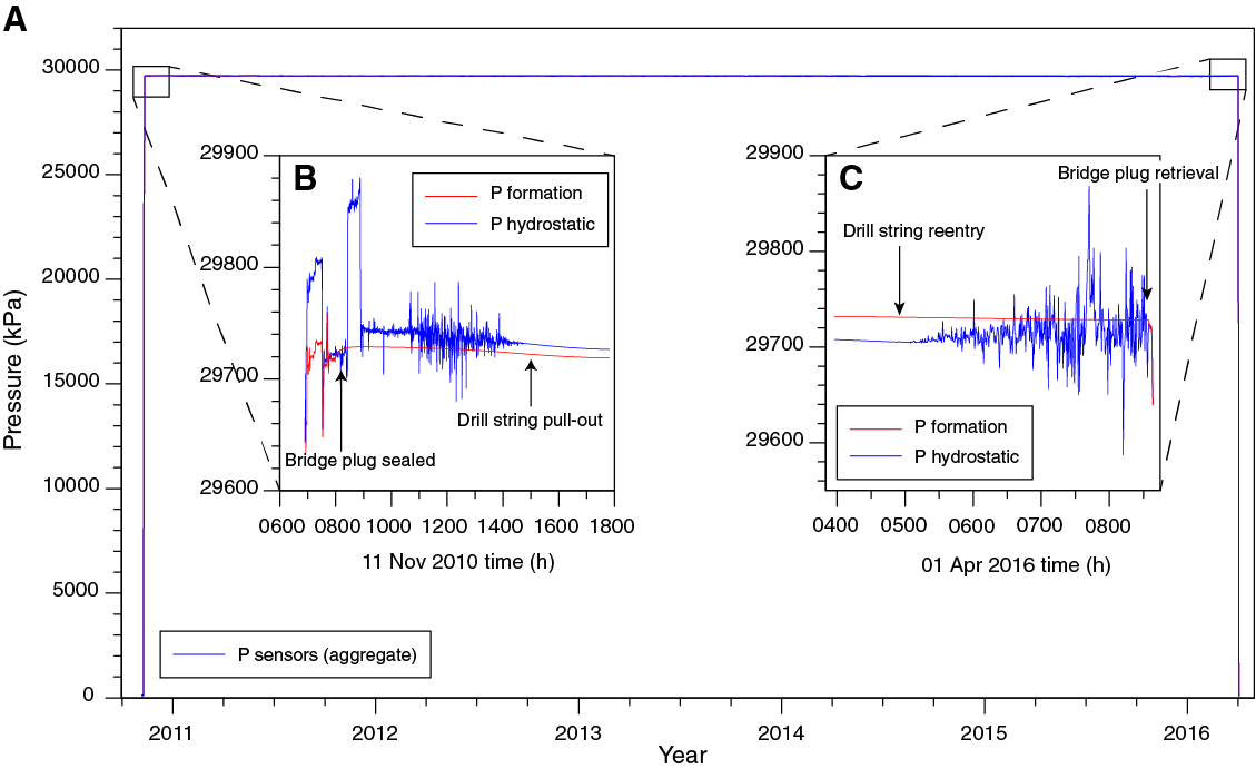
Figure F1. Pressure record of entire 5.3 y deployment, including predeployment and postrecovery.
The pressure record at the time of deployment shows installation disturbances and then the subsequent deployment of the packer and bridge plug to achieve hydraulic isolation of the borehole (Figure F1). After the bridge plug was set, a number of pressure anomalies can be observed in the hydrostatic pressure reference, whereas the formation appears to be stable. The data suggest that the GeniusPlug was successfully isolated from the seafloor. A lack of formation pressure anomalies associated with drill string reentry during Expedition 365 into the borehole provides further evidence for successful isolation, as shown in the data during retrieval of the GeniusPlug. In contrast, the hydrostatic pressure sensor is strongly affected by the drill string reentry.
Paroscientific sensors are well known to undergo long-term drift (Polster et al., 2009). The data recorded between the deployment and retrieval of the GeniusPlug show a linear drift in both sensors. The formation sensor shows a positive drift of 1.6 kPa/y, whereas the hydrostatic sensor shows a negative drift of 4 kPa/y (Figure F2).
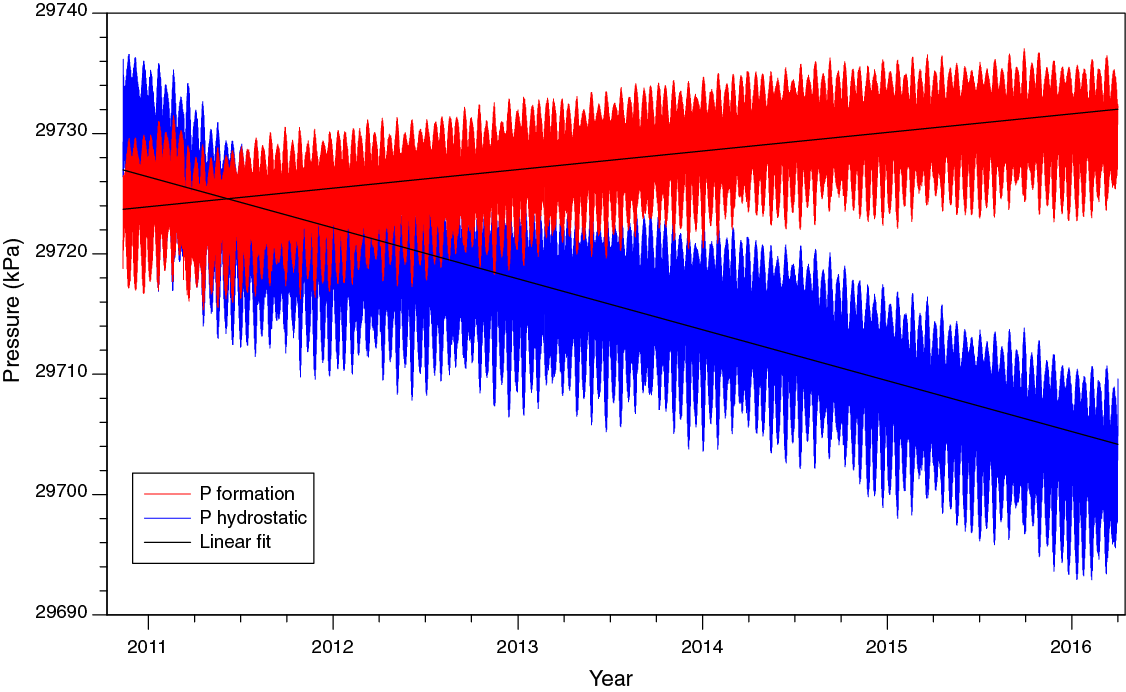
Figure F2. Raw data record, not including deployment and retrieval disturbance.
The diurnal ocean tidal signal in the formation pressure data has a smaller amplitude than the hydrostatic reference pressure (Figure F3). A tidal loading efficiency of approximately 0.74 was calculated for the formation. A cursory review of the data identified multiple pressure transients potentially related to seismic events, although further detrending and processing of the data are required to filter the tidal signal and resolve these transients. In the raw data it is possible to clearly identify the 11 March 2011 Tohoku earthquake (Figure F4) and a major aftershock. The tsunami can be seen approximately 1.5 h after the mainshock. According to the hydrostatic reference sensor, the tsunami wave height was approximately 30 cm.
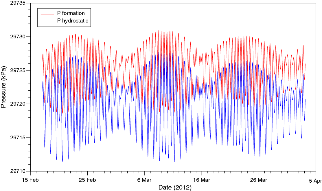
Figure F3. 1.5 months of pressure data showing characteristic tidal forcing.

Figure F4. Pressure records at time of 11 March 2011 Tohoku earthquake.
An additional example of pressure changes in both the formation and hydrostatic reference sensors is observed during the M6.0 earthquake at 02:39:07 h (UTC) on 1 April 2016 (Figure F5). The earthquake occurred a few hours before the GeniusPlug retrieval, and its epicenter was located approximately 35 km northwest of Site C0010. Both sensors registered a response for the event 4–34 s (30 s sampling interval) after the mainshock. A permanent offset of 0.4 kPa in formation pressure was induced by the earthquake, indicating compressional strain in Hole C0010A (Wallace et al., 2016). The hydrostatic reference also shows a pressure increase, diminishing gradually after the shock to preearthquake conditions.

Figure F5. Data record showing removal of corrosion cap, 1 April 2016 earthquake, and reentry of drill string.
Temperature data
The GeniusPlug incorporates three different temperature sensors: one stand-alone miniature temperature logger (MTL), one temperature sensor in the pressure housing (platinum chip), and one thermistor in the “upward-looking” hydrostatic reference transducer. An overview of the temperature data gathered during the full 5.3 y deployment period is given in Figure F6. The MTL stopped logging on 1 June 2014. Thus, only a shorter record is shown for this sensor.
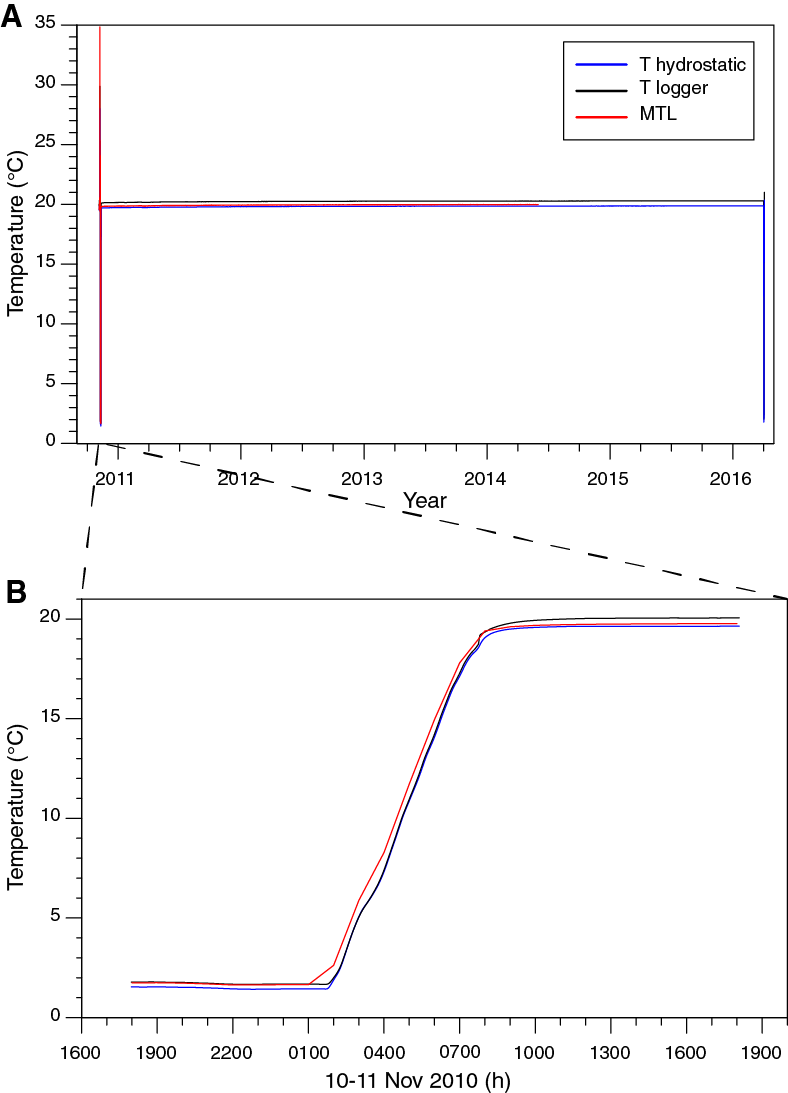
Figure F6. Temperature record of entire 5.3 y, as recorded with the three temperature sensors.
In general, all temperature sensors show similar variations with time. The pressure housing temperature is slightly higher than the two other sensors. The initial deployment phase is marked by strong temperature variations, differing in amplitude as well as frequency. After deployment in the borehole, all sensors registered a sudden increase in temperature, from approximately 2°C to 19°C in less than 12 h (Figure F6). The rapid increase is an indicator of equilibration of the temperature in the borehole following disturbances created by deployment of the GeniusPlug. The subsequent evolution of temperatures shows a progression typical for a borehole in advanced stages of equilibration (Figure F7). After an initial abrupt increase, the following year is characterized by a total temperature increase of ~0.08°C/y in all three sensors. The last recorded year in the MTL data exhibits an increase of ~0.007°C/y, the last recorded year for the platinum sensor exhibits ~0.004°C/y, and the hydrostatic reference exhibits 0.006°C/y, all of which indicate near equilibrium conditions.

Figure F7. Temperature record, not including deployment and retrieval disturbances.
The least-squares temperature gradient based on in situ temperature measurements at Site C0004 is 52°C/km (Kinoshita, Tobin, Ashi, Kimura, Lallemant, Screaton, Curewitz, Masago, Moe, and the Expedition 314/315/316 Scientists, 2009), which yields a predicted formation temperature of 20.54°C at the GeniusPlug deployment depth. All logged temperatures are slightly below this estimated formation temperature: the platinum sensor measured 20.29°C, the hydrostatic reference sensor measured 19.87°C, and the MTL measured 19.98°C (1 June 2014). When comparing data from the three temperature sensors, the platinum chip mounted sensor inside the pressure housing is consistently ~0.43°C warmer than the hydrostatic reference sensor and ~0.3°C warmer than the MTL (Figure F7). This temperature offset might be related to isolation and buildup of heat in the pressure housing or to a calibration offset. The ~0.13°C offset between the hydrostatic reference and the MTL is probably caused by poor calibration.
Similar to the installation phase, the final part of the GeniusPlug recovery is clearly visible in the data, with the former trend of the temperature curves ending with an abrupt strong decrease of overall temperature as the sensor traveled through the water column. This is followed by a sudden increase when the sensor emerged from the water.
A closer look at the main deployment phase shows three distinct temperature drops in the first year. The magnitudes of temperature decline are similar in all sensors. The three different temperature drops are referred to as A, B, and C in Figure F7. Temperature Drop A is approximately 0.015°C and occurs over 4 days. The subsequent recovery lasts approximately 14 days. At Drop B, temperature decreases by approximately 0.025°C over a period of 6 days and the recovery phase lasts approximately 1 month. Temperature Drop C involves a decrease of 0.15°C over 6 days with a recovery similar to that for temperature Drop B. The initiation of temperature Drop B might be related to the Tohoku earthquake, which occurred ~18 h before the drop. Temperature Drops A and C cannot be easily correlated to large earthquakes or significant changes in the pressure data.
Measurement of VIV using drill pipe accelerometer
VIV during the GeniusPlug recovery was measured using drill pipe accelerometers equipped with a triaxial sensor (see Figure F7 in the Expedition 365 methods chapter [Saffer et al., 2017]). The sensors were attached to the drill pipe on the rig floor and lowered to the seabed. VIV-suppression ropes were attached along the drill pipes above the BHA in the same way as during Integrated Ocean Drilling Program Expedition 332 (Expedition 332 Scientists, 2011). The Kuroshio Current speed was measured during the entire operation (Figure F8) and compared with the VIV. The current speed was less than 2.5 kt when the pipe was running into the water column. The Chikyu then drifted to Hole C0010A at a ground speed of 1 kt. The current speed increased near Hole C0010A, reaching a maximum of 4.3 kt. The accelerometer stopped working due to CPU trouble about 6 h after the Chikyu began drifting toward the site, and VIV data acquisition was stopped. The Chikyu was ~3.5 km away from Hole C0010A at this time.

Figure F8. Kuroshio Current speed during GeniusPlug recovery.
Although VIV of the drill pipe was not recorded over the full duration of drifting, the recorded accelerometer data capture the maximum current, and therefore allow an estimation of the maximum expected VIV. While lowering the drill pipe in the LCA, peak accelerations were 1.5 and 0.5 G for the horizontal and vertical components, respectively. Then the Chikyu started to drift into the strong current region. Accelerations were less than 1.0 G during drifting to Hole C0010A for all three components (Figure F9). The horizontal component accelerations were about three times higher than the vertical component. The result indicates that VIV caused by the Kuroshio Current remained within the operational limits of the LTBMS, which is designed to withstand a maximum acceleration of 2 G.

Figure F9. VIV acceleration data recorded by drill pipe accelerometer attached to 5½ inch drill pipe during GeniusPlug recovery.
LTBMS
Overview of deployment
The assembly and deployment operations for the LTBMS installation in Hole C0010A are described in detail in the following sections. During Expedition 365, a completion string was prepared with all of the sensors, cables, pressure ports and hydraulic lines, and a swellable packer attached to 3½ inch tubing joints (see LTBMS in the Expedition 365 methods chapter [Saffer et al., 2017]). The assembly was terminated at the LTBMS head, where underwater mateable connectors (UMCs), hydraulic lines, valving, and the PSU were mounted. During assembly, a series of tests were conducted to confirm the operational health of the downhole instruments. Table T4 describes the depths of the major observatory elements (see also Figure F6 in the Expedition 365 summary chapter [Kopf et al., 2017]). An ROV platform was attached to the LTBMS head prior to lowering it into the water. A titanium sphere data recorder and communications unit was attached to the ROV platform, with UMC cables connected to each downhole sensor (see Figure F15 in the Expedition 365 methods chapter [Saffer et al., 2017]).
Table T4. Depths of observatory components. Download table in .csv format.
The entire string was assembled and lowered into the water column in a LCA to avoid potential vibration and damage caused by the Kuroshio Current prior to drifting to the drill site. VIV during subsequent drifting to the site was suppressed by temporarily tying four ropes to the drill string. During Expedition 365, newly developed moonpool guide rollers (Figure F10) were also used to support the drill string and contributed to safe and smooth operations (see Preliminary scientific assessment in the Expedition 365 summary chapter [Kopf et al., 2017]).
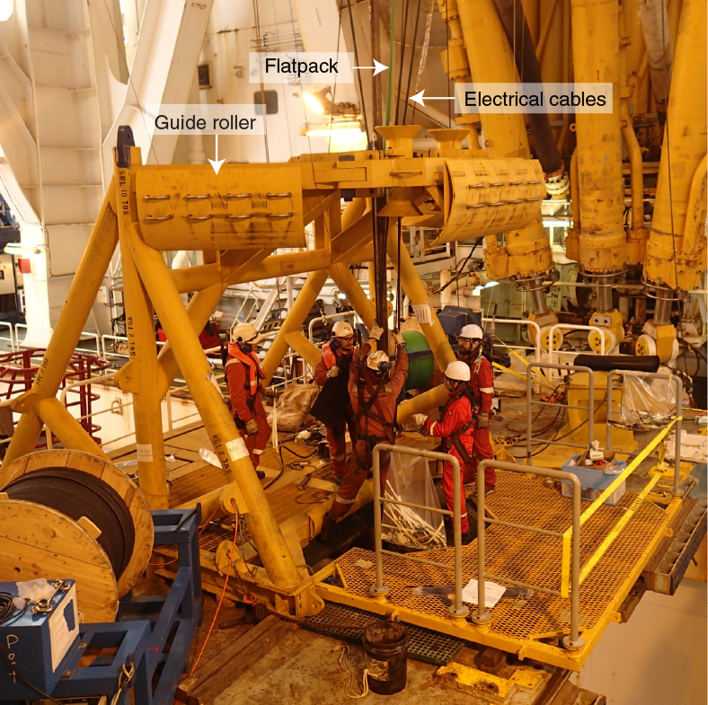
Figure F10. Guide roller over the moonpool used to support tubing and cables during deployment.
During deployment (assembly, lowering, drifting in, reentry, landing, and cementing), a series of tests were conducted on the strainmeter, tilt combo, and broadband seismometer systems by ROV communication via the data recorder to verify the health of the sensors (Table T5). After landing the LTBMS head, we initialized the data recorder to start data acquisition for the tilt combo package and strainmeter and then checked the condition of the broadband seismometer before shutting off power. During circulation and cementing, pressure was monitored via a pressure gauge installed in the strainmeter. Prior to departing from Hole C0010A, the wellhead valves were opened to the formation hydraulic lines and initial borehole pressure data (recording the descent and deployment) were recovered by ROV.
Table T5. Instrument function checklist. Download table in .csv format.
A more detailed sequence of deployment operations is discussed in Operations. Here, we describe and report the configuration and assembly of the borehole and completion string, the results of tests conducted to verify the condition of observatory components, and the initial data obtained from the borehole.
Sensor configuration
The locations of the strainmeter, tiltmeter, seismometers, and pressure ports were planned on the basis of resistivity and gamma ray logs from Expedition 319, combined with Site C0004 coring results from Integrated Ocean Drilling Program Expedition 316 (Expedition 316 Scientists, 2009; Expedition 319 Scientists, 2010b) (see Figure F6 in the Expedition 365 summary chapter [Kopf et al., 2017]). Pressure Port P1 is located below the megasplay fault zone, within the overridden slope sediments in the footwall. Pressure is monitored via three miniscreens plumbed to a single hydraulic line (see LTBMS in the Expedition 365 methods chapter [Saffer et al., 2017]; Figure F11). The strainmeter (Figure F12) and tilt combo (Figure F13) were also set in the footwall sediments. The seismic sensor was located below the casing shoe to ensure that no casing motion from above is transmitted to the sensors; the top of the instrument carrier is at 565.23 mbsf, well below the casing shoe at 544 mbsf. Pressure Port P2 occupies a position just below the strainmeter sensing surface and is within the cemented interval. The total thermistor string length is 175 m, with the two uppermost nodes situated within the screened casing interval, two more nodes below the screened interval, and the bottom node in the open hole section just above the instrument carrier. An upper pressure port (P3) is located in the screened casing to measure pore fluid pressure within the fault zone. The swellable packer was installed above but near the screened casing interval to minimize the volume monitored by Port P3, while also ensuring that the packer sealing surface (~1.5 m height) did not overlap with a casing joint.

Figure F11. Pressure Port P1 with 3 miniscreens plumbed to single ¼ inch hydraulic line.
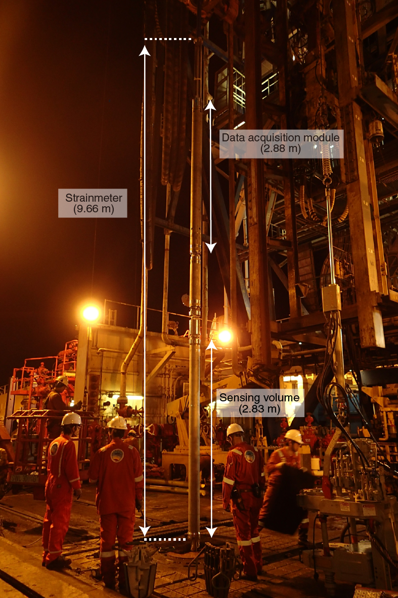
Figure F12. Strainmeter suspended from rig floor.
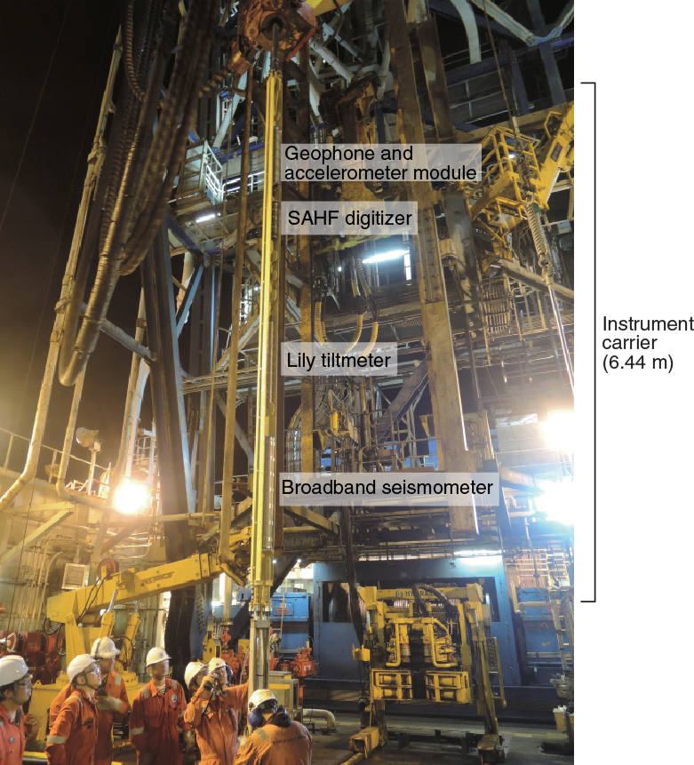
Figure F13. Instrument carrier suspended from rig floor.
The strainmeter must be well-coupled to the formation to detect crustal strain. Fluid flow around the strainmeter and seismic sensors also causes severe noise. These sensors were cemented into the open hole section below the 9⅝ inch casing shoe to provide good coupling (see Figure F6 in the Expedition 365 summary chapter [Kopf et al., 2017]). To obtain cement physical properties as similar as possible to those of the formation, Schlumberger “FlexSTONE” cement slurry with nonshrinking performance was used. The slurry was optimized and tested in the laboratory and had a Young’s modulus of 4.019 GPa, a Poisson’s ratio of 0.218, and a specific gravity of 1.90 g/cm3, similar to that of the target formation.
The backbone of the completion string was the 3½ inch tubing that functioned as a cement delivery line for cementing the strainmeter and seismic instruments and as a support for the cables, thermistor string, and hydraulic lines. The cables and thermistor string were secured to the tubing by tie wraps at intervals of approximately 1 m (see Figure F12 in the Expedition 365 methods chapter [Saffer et al., 2017]). We also attached centralizers to the tubing to prevent the cables from contacting the borehole wall. In the lower section, four centralizers were installed per tubing joint, and two centralizers per tubing joint were installed above the float collar depth. In each centralizer location, cables were covered by rubber protectors (Figure F14). Hydraulic tubes were attached to the tubing by stainless bands (BAND-IT) (Figure F15).
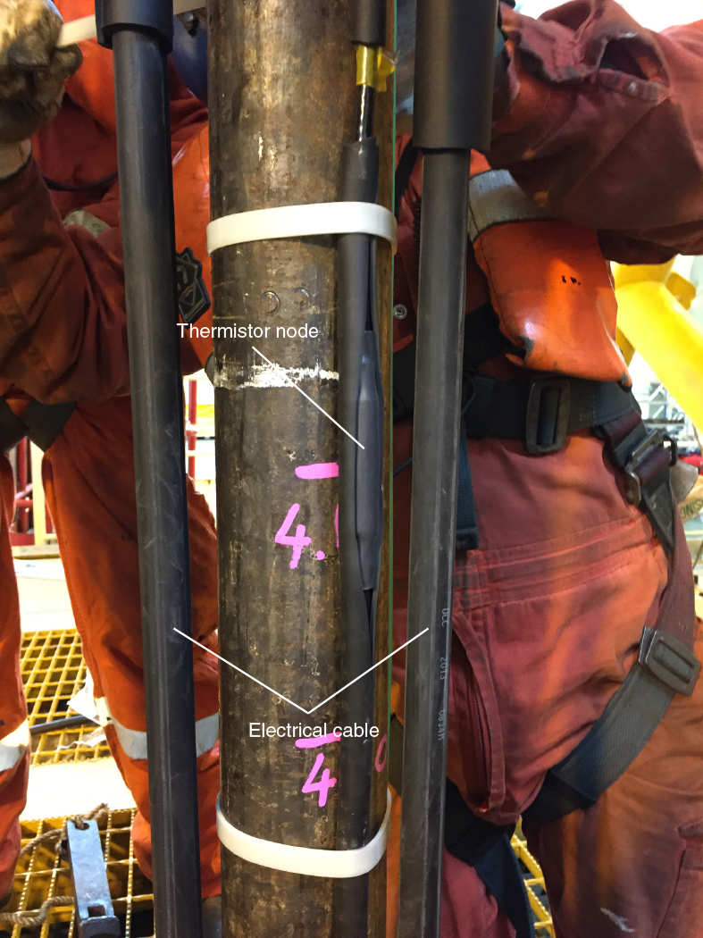
Figure F14. Thermistor node attached to 3½ inch tubing.
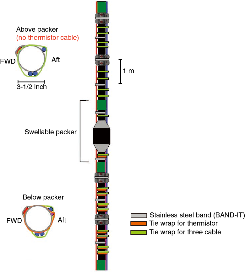
Figure F15. Spacing of centralizers, tie wraps, and steel bands securing cables to 3½ inch tubing.
Because we had relatively small clearance between the outside diameter of the 3½ inch tubing and the drift diameter of the 9⅝ inch casing, extra care was taken not to increase the effective diameter of the string after fastening the cable and wrapping it with tie wraps, tapes, and rubber protectors. The swellable packer is another point where clearance to the 9⅝ inch casing is limited. The packer began swelling once it was added to the string and lowered into the sea. The packer is designed to swell to the inside diameter of the 9⅝ inch casing over a period of 2 weeks (or more) after installation. We checked the packer condition via ROV camera before running the string into the borehole (Figure F16). Visual inspection showed little inflation at the time of reentry, and no difficulty was encountered during insertion of the observatory and the packer into the cased borehole.
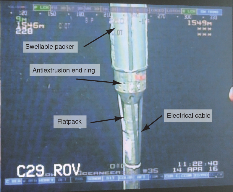
Figure F16. Bottom of swellable packer after 3.5 days in seawater.
Tests during assembly and installation
Prior to assembly of the completion string, each sensor was subjected to extensive testing. The strainmeter was tested in a Japan Agency for Marine-Earth Science and Technology (JAMSTEC) warehouse for background noise performance before shipment to Shimizu; it was also tested and set up for deployment in the Core-tech workshop on the Chikyu before it was made up with 3½ inch tubing on the rig floor. The tilt combo system and broadband seismometer were tested in the Kamioka mine, a land test site, before shipment to the Chikyu. These instruments were also tested on board the Chikyu in the Core-tech workshop and on the middle pipe rack before being mounted in the instrument carrier. The software in the strainmeter and tilt combo was configured to proceed through an automated checking procedure upon power up so that any changes in instrument operation could be identified by comparison with previous test results.
During assembly and deployment, we performed function checks of the strainmeter, seismometer, and tilt combo instruments at several stages:
- Upon connection to the borehole cable.
- Before inserting the cable into the swellable packer.
- After inserting the cable to the swellable packer.
- Before cutting the cable for termination to ODI connectors.
- After cable termination.
- After mounting the terminated connectors on the LTBMS head with the data recorder unit.
- After running the string into the water and when the LTBMS head was at 100 meters below sea level (mbsl).
- After drifting and before running the string into the borehole.
- After the LTBMS head landed on the reentry funnel.
- After cementing and disconnection of the drill string from the LTBMS head.
For each of these tests, we performed function checks for the items listed in Table T5. These tests produced the same results each time and in accordance with expected values, confirming the working condition of each instrument until the last test prior to cementing.
Observatory status and initial data recovery
After the LTBMS head was landed on the Hole C0010A wellhead and the sensor systems were checked, the ROV maintained a connection to the data recorder to monitor the status of the sensors during cementing. Temperature data from this time period suggest cooling of the borehole by circulation (Table T6). During cementing, pressure was also monitored using the sensor installed in the strainmeter (Port P2). Pressure increased by ~0.7 MPa after cement injection, indicating the displacement of 78 m of seawater above the sensor (Figure F17).
Table T6. Borehole temperature data obtained during cementing. Download table in .csv format.

Figure F17. Time series of pressure data at Port P2 during cementing.
After cementing, continuous data recording was started on the tilt combo module. Figure F18 shows a power spectral density (PSD) plot of the accelerometer, geophone, and tiltmeter. The broadband seismometer was also confirmed to be in good condition after cementing and was powered down.
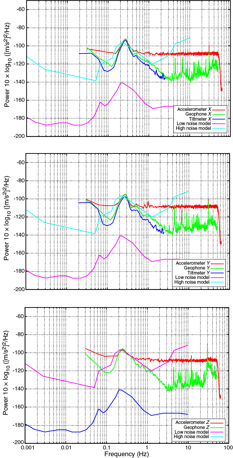
Figure F18. PSD plots of sensor responses in tilt combo module after cementing.
Pressure and temperature data were then downloaded from the PSU by UMC using the ROV. The download was completed at 0343 h (UTC) on 15 April 2016 using the mlterm software. The PSU logger memory was cleared immediately following the download. After the download and clearing the logger memory, mlterm was disconnected and then reconnected to verify that the PSU continued logging. The downloaded data record pressure and temperature changes prior to and during deployment from the Chikyu, including descent of the PSU through the water column and landing of the LTBMS head at the borehole (Figure F19).
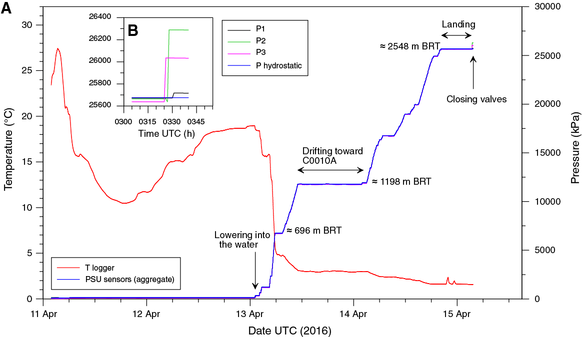
Figure F19. Pressure and temperature record recovered just after LTBMS deployment on 15 April 2016.
From 11 to 13 April while the PSU was still on board the Chikyu, pressure readings are consistent with atmospheric pressure (~1 kPa) and temperatures reflect normal fluctuations throughout the day (Figure F19). The PSU was lowered into the water at approximately 0103 h (UTC) on 13 April, and pressure increases and temperature decreases observed after this period reflect the descent of the LTBMS head through the water column. The pressure record flattens out for the latter portion of 13 April and into 14 April, during the period of time that the Chikyu was drifting to Hole C0010A with the LTBMS head at a constant depth of ~1200 m BRT. Pressure increases after this time reflect further descent of the LTBMS head through the water column and eventual landing of the LTBMS onto the wellhead at 2023 h on 14 April. Figure F19B shows the end of the pressure record after the three-way valves were turned to the formation by the ROV, beginning formation pressure sensing in Ports P1, P2, and P3. The ROV turned the valves in the order of Ports P3, P2, and P1, which is confirmed in the pressure record. All of the pressure and temperature results demonstrate that the PSU was operating correctly at the time the Chikyu deployed the LTBMS and departed the site on 15 April. Before leaving the observatory, valve configurations and positions of all instruments installed on the ROV platform were checked by visual inspection and were readied for the ROV visit to connect the DONET cable on 19 June 2016.
Lithology
Lithologic Unit I (upper accretionary prism; hanging wall to megasplay fault)
- Intervals: 365-C0010C-1R-1, 0 cm, through 12R-CC, 26.5 cm; 365-C0010D-1R-1, 0 cm, through 1R-CC, 10.5 cm
- Depths: Hole C0010C = 300.0–395.0 mbsf; Hole C0010D = 385.0–394.5 mbsf
- Age: 3.79–5.59 Ma
The dominant sediment type in lithologic Unit I (Figure F20) is dark gray to greenish gray silty claystone (hemipelagic mudstone) with moderate degrees of induration. Intact pieces of the mudstone are typically mottled by bioturbation and some display faint plane-parallel laminae. Sand and silt beds were not observed. Volcanic ash layers are rare and thin. The ash is light to medium gray in color and composed primarily of fresh clear glass shards. Calcareous nannofossil contents are variable in this unit, as shown by the X-ray diffraction (XRD) values for calcite (Figure F21), which range from 0.4 to 15.7 wt% (average = 5.1 wt%). Quartz and plagioclase contents in the bulk sediment average 17.5 and 12.6 wt%, respectively, and the content of total clay minerals averages 64.8 wt% (Table T7). The results of bulk sediment X-ray fluorescence (XRF) analyses are shown in Table T8). Values of total organic carbon (TOC) are less than 0.5 wt%, and sulfur and nitrogen contents are consistently below 0.7 and 0.4 wt%, respectively (Table T9; Figure F22).
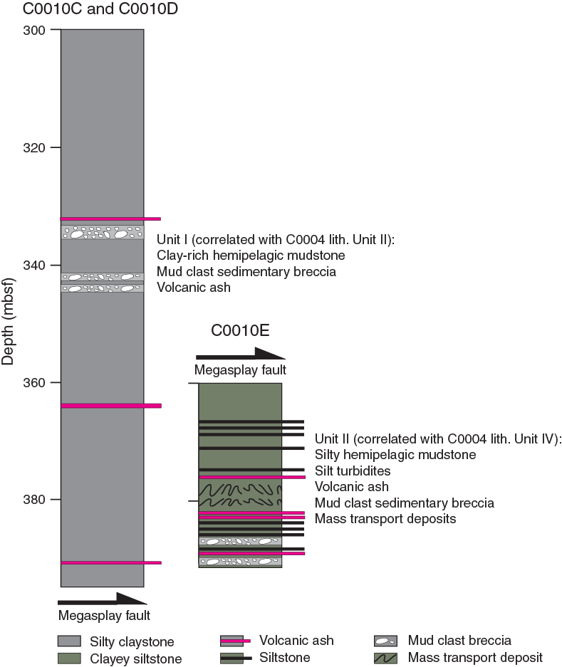
Figure F20. Generalized stratigraphic columns.
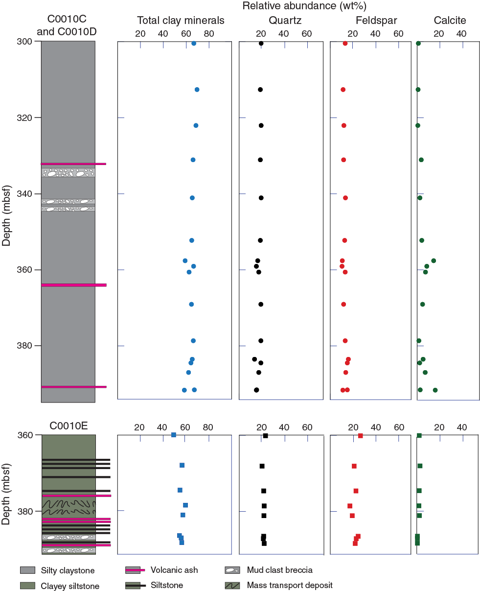
Figure F21. Results of bulk sediment XRD.
Table T7. Results of bulk powder XRD. Download table in .csv format.
Table T8. Major element oxide results of XRF analysis for bulk powder specimens. Download table in .csv format.
Table T9. Total carbon, inorganic carbon, TOC, TN, and TS contents in the solid phase. Download table in .csv format.
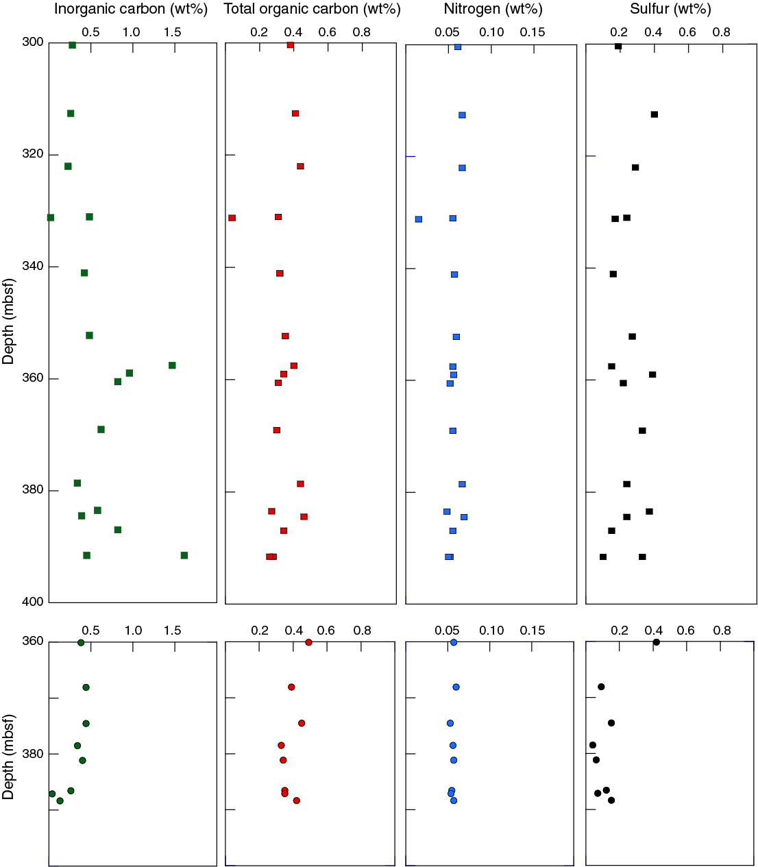
Figure F22. Results of bulk sediment carbon-nitrogen-sulfur analyses.
Figure F23 shows the correlation between computed values of calcite (in weight percent) from XRD and CaCO3 (in weight percent) from carbon-nitrogen-sulfur measurements. Linear regression yields a statistically significant correlation coefficient of 0.99. The XRD method is obviously unreliable if calcite content of a specimen is below the detection limit (approximately 1.8 wt%). Specimens with concentrations of less than 4 wt% CaCO3 consistently yield XRD results that are too low. At concentrations greater than 8 wt%, XRD slightly overestimates values of percent calcite. This is to be expected because normalized relative percentages (where calcite + quartz + feldspar + clay minerals = 100%) should be less than absolute abundances within the total mass of solids.
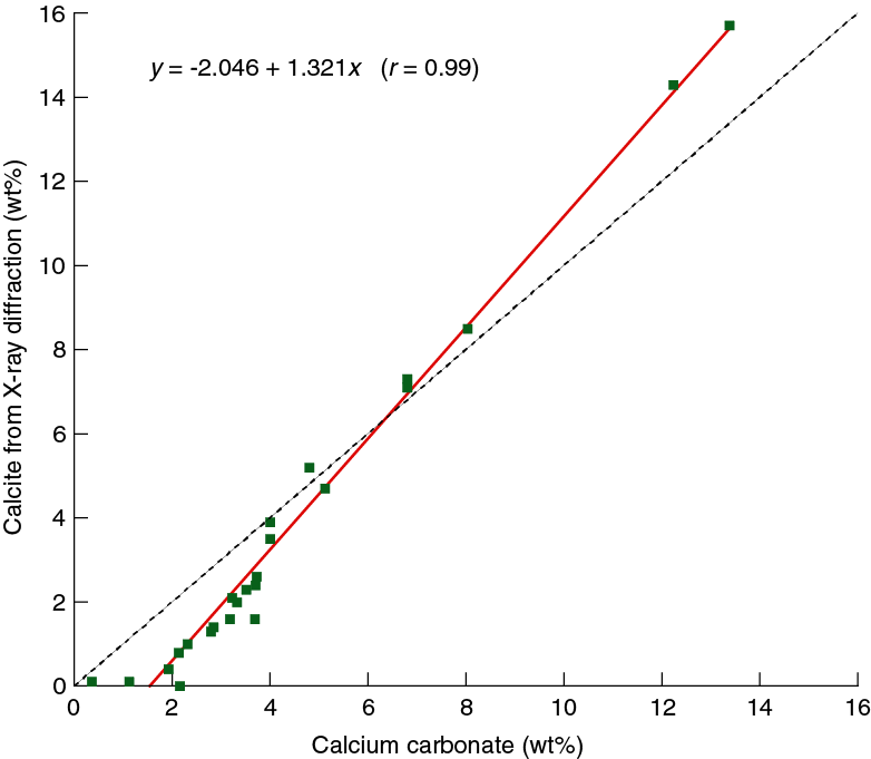
Figure F23. Correlation between CaCO3 values from carbon-nitrogen-sulfur analyses and normalized relative abundances of calcite from XRD.
Stratal disruption in Unit I occurs in the form of synsedimentary breccia. These intervals display a clear fabric with subrounded to subangular mudstone and claystone clasts supported by a matrix of mudstone. Differences between the clasts and surrounding matrix include subtle changes in color (gray tone), carbonate content, and clay content. In some cases, the matrix is less indurated than the clasts. We recognized three intervals of synsedimentary breccia separated by intervals of intact mudstone. Additional zones of stratal disruption may occur, but they are difficult to recognize because of extensive drilling-induced brecciation of the core and low core recovery.
We interpret Unit I to have accumulated in an abyssal plain environment that was dominated by slow deposition of fine-grained suspended sediment, with occasional input of air fall volcanic ash. The depositional environment was located seaward of the trench, and the strata were subsequently accreted. The seafloor outboard of the subduction front must have been inclined steeply enough, at least locally, to induce gravitational failure. The upslope source of the remobilized clasts cannot be determined from shipboard data, but relief may have been associated with the flanks of seamounts or other types of basement highs on the subducting oceanic plate.
We broadly correlate lithologic Unit I at Site C0010 with lithologic Unit II at Site C0004 (Expedition 316 Scientists, 2009) but also note some important differences. Calcite contents at Site C0010 are as high as 15 wt% (Figure F21). In contrast, the mudstones in lithologic Unit II at Site C0004 are consistently depleted in calcium carbonate, so those hemipelagic muds were probably deposited in deeper water closer to the calcite compensation depth (CCD). Mass transport deposits (MTDs, or synsedimentary breccias) occur at both sites and display similar attributes. Such deposits at Site C0010 are thin and occur near the middle of the cored interval. In contrast, at Site C0004 MTDs are approximately 40 m in total thickness and restricted to the top of Unit II (at Site C0004 these occur in Subunit IIA). LWD data from Site C0010 (Expedition 319 Scientists, 2010b) indicate that the correlative logging unit for the upper accretionary prism (designated as logging Unit II during Expedition 319) is approximately 225 m in thickness. The logging subunit with concentrated MTDs (Subunit IB) lies at 161.5–182.8 m LSF, well above the top of the interval cored during Expedition 365. Thus, although the MTDs at both sites share similar mechanisms of remobilization and emplacement, it is likely that we did not actually core the equivalent of Site C0004 lithologic Subunit IIA at Site C0010.
Lithologic Unit II (underthrust slope facies; footwall to megasplay fault)
- Interval: 365-C0010E-1R-1, 0 cm, through 4R-CC, 18.5 cm
- Depth: Hole C0010E = 360.0–391.0 mbsf
- Age: 1.56–1.67 Ma
The dominant sediment type of lithologic Unit II (Figure F20) is dark olive-gray clayey siltstone (hemipelagic mudstone) with trace amounts of calcareous nannofossils. Calcite content from XRD ranges from 0 to 2 wt% and averages 1.1 wt% (Table T7). Clayey siltstone in this facies is consistently coarser than comparable clay-rich mudstones in the overlying hanging wall. Silty mudstone is typically mottled by bioturbation but locally displays plane-parallel laminae. This textural contrast is confirmed by the XRD values for total clay minerals, which average 55.4 wt% in Unit II (Figure F21). The average abundances of quartz and feldspar are 21.5 and 21.9 wt%, respectively (Table T7). Results of bulk XRF analyses are shown in Table T8. Carbon-nitrogen-sulfur data reveal no significant differences between mudstones from Units I and II, however, inorganic carbon seems to decrease at the base of lithologic Unit II compared to Unit I (Figure F22).
Thin beds of dark gray siltstone and sandy siltstone are common in lithologic Unit II, and most show normal size grading with gradational to diffuse upper boundaries. The siltstone beds are poorly indurated and some display plane-parallel laminae. We interpret these deposits as turbidites. Thin beds of gray to light gray volcanic ash are also common. The ash layers are poorly indurated and composed largely of unaltered clear volcanic glass shards.
Several intervals in lithologic Unit II display mesoscopic evidence for mass transport with two contrasting varieties. The first type of MTD consists of sedimentary breccia with clasts of resedimented mudstone and moderately indurated lithic fragments (e.g., claystone). The clasts are granule to pebble size, subrounded to subangular, and supported by a matrix of mudstone. The second type of stratal disruption consists of contorted layering in the mudstone, as defined by laminae with irregular to steep dips, sharp truncation surfaces, and scattered subrounded pebbles of moderately indurated lithic fragments. Smear slides show that some of the larger clasts are extraformational, with compositions and textures unlike the surrounding matrix and interbeds (see SMEARSLD in Supplementary material).
We interpret lithologic Unit II to have accumulated in a lower trench-slope environment (i.e., above the frontal accretionary prism). The dominant process was slow settling of suspended sediment with occasional input by silty turbidity currents and air fall volcanic ash. This facies correlates broadly with lithologic Unit IV at Site C0004 (Expedition 316 Scientists, 2009), but we also note some important differences. In particular, the slope environment at Site C0010 was affected by several mass transport events that resulted in remobilization of cohesive hemipelagic mud and incorporation of moderately indurated, extraformational lithic fragments. Evidently, the slope facies at Site C0004 was not subjected to cohesive mass transport events (Expedition 316 Scientists, 2009). In addition, the turbidites at Site C0004 contain mostly fine sand rather than mostly silt-size grains. The coarser textures are indicative of a slightly flatter gradient to the seafloor (i.e., a slope basin) or closer proximity to feeder channels. The slope facies at both sites contains low concentrations of biogenic calcium carbonate, which indicates that deposition occurred close to the CCD.
Structural geology
We measured the orientations of 18 bedding planes and 54 faults and shear zones in cores taken from Holes C0010C–C0010E (Tables T10 and T11). In Holes C0010C and C0010D in the hanging wall of the shallow megasplay fault, bedding is either horizontal or gently dipping (<20°) from ~300 to ~350 mbsf. Bedding becomes steeper and dips at 35°–60° deeper than 360 mbsf (Figure F24A). This steepening likely reflects deformation along the megasplay fault (located at ~407 mbsf). Faults in Holes C0010C and C0010D are sparse and dip at 30°–60° (Figure F24B). They exhibit a mix of normal and reversed senses of slip. These faults are commonly healed and accompanied by an ~1 mm thick black band (e.g., Figure F25), implying faulting at unconsolidated conditions. A few faults, however, are accompanied by heavily fractured zones, an example of which is found at 330.85 mbsf (Section 365-C0010C-4R-3). Here, light gray ash is in fault contact with dark gray mud below, both of which are brecciated (Figure F26). The fault dips at ~60° and exhibits slickenlines at a high angle to the fault strike, indicating that it is a dip-slip fault. Although trails of the brecciated ash layer suggest a normal sense of slip, two minor faults immediately above this fault clearly indicate a reversed sense of slip.
Table T10. Orientation data of bedding and faults observed, Holes C0010C and C0010D. Download table in .csv format.
Table T11. Orientation data of bedding, faults, and shear zones observed, Hole C0010E. Download table in .csv format.
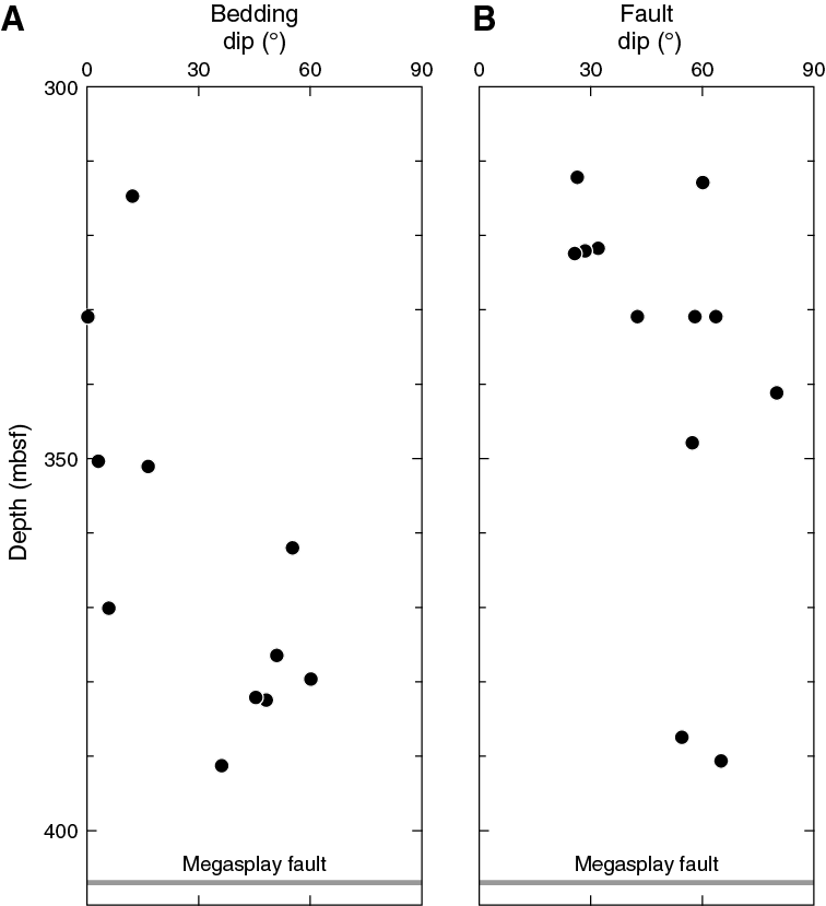
Figure F24. Bedding dips and fault dips, Holes C0010C and C0010D.
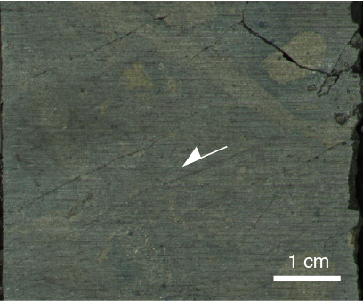
Figure F25. Split core image of a fault.
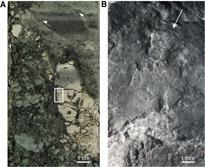
Figure F26. Split core image of faults.
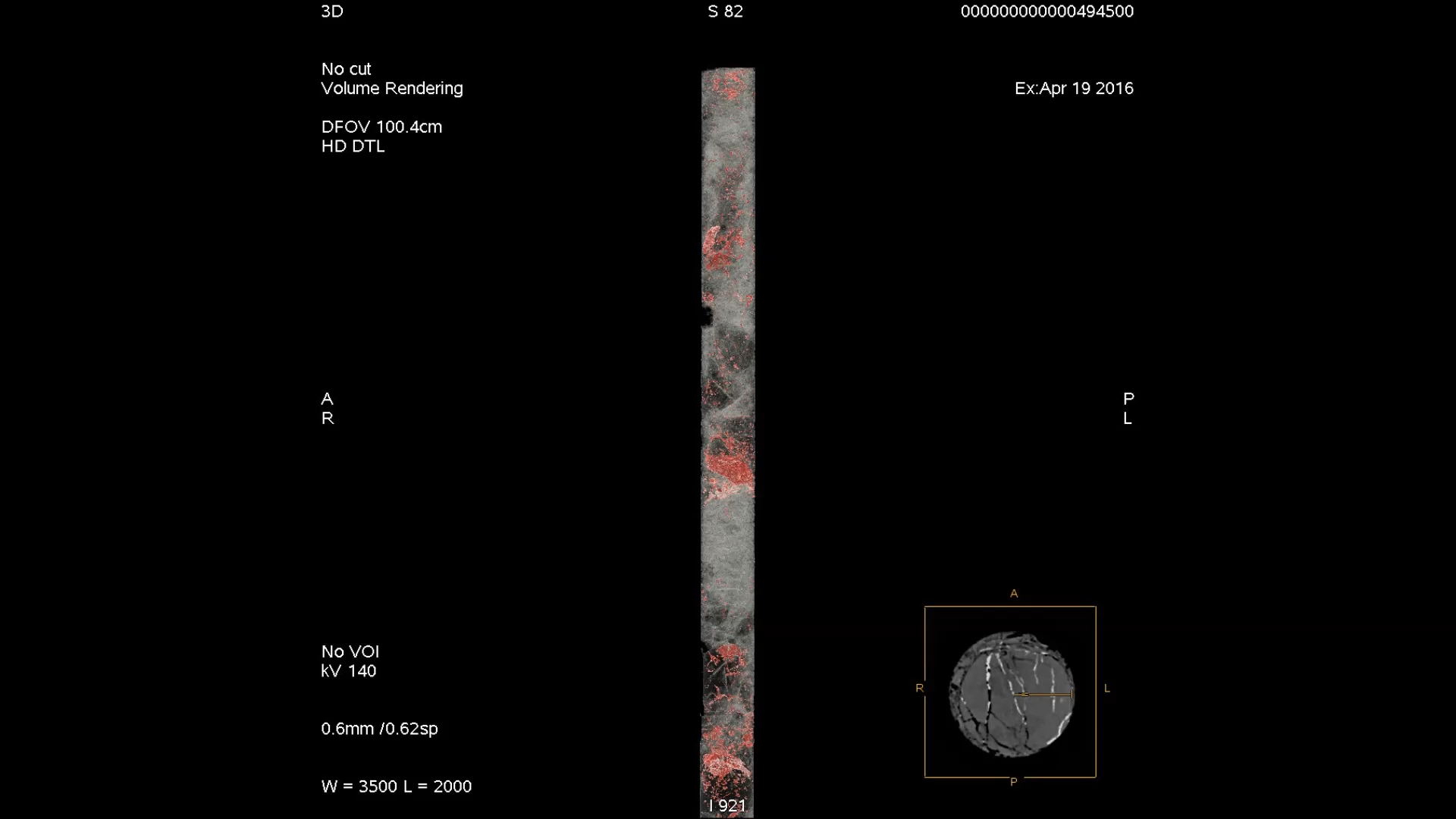
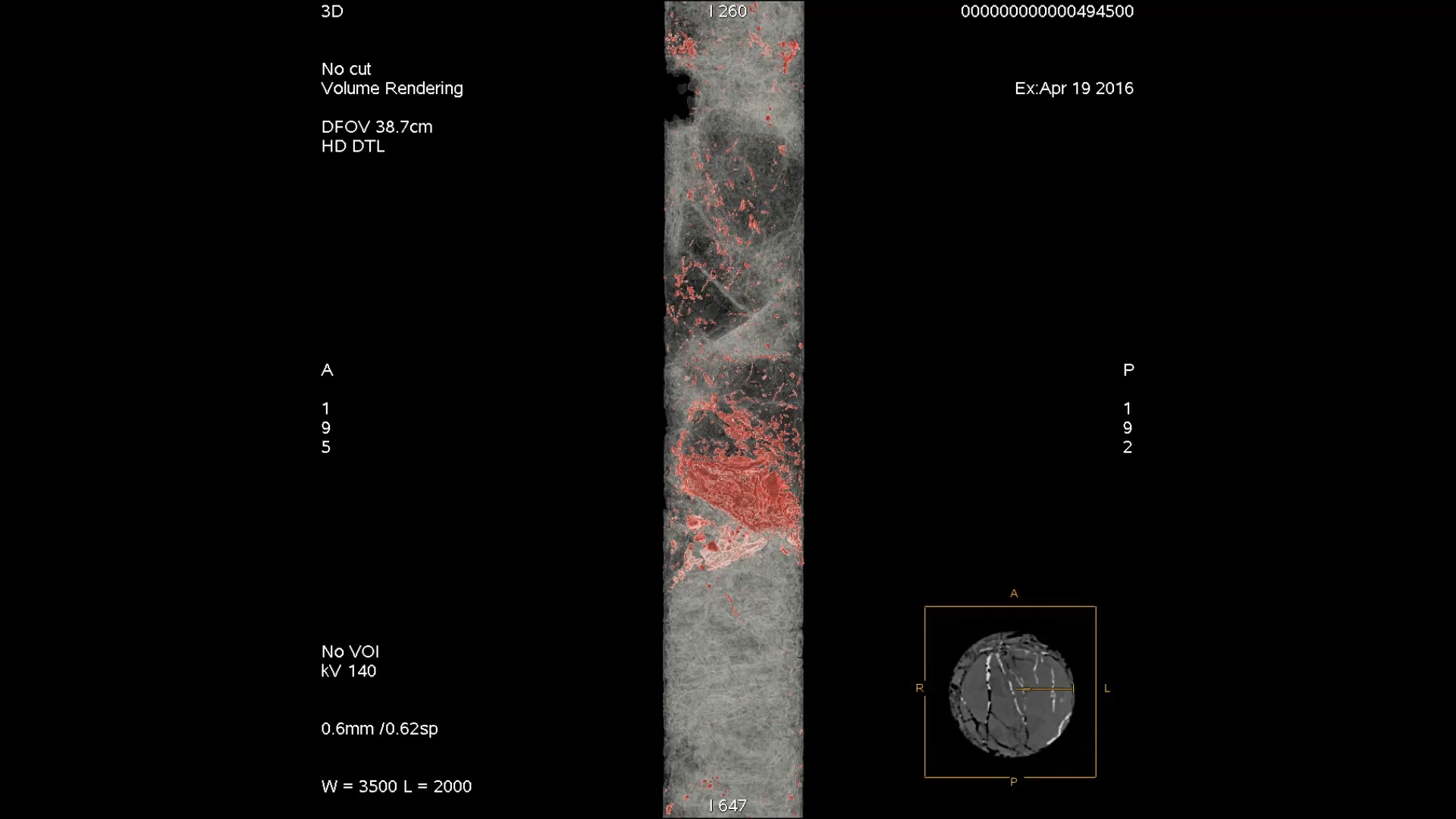
X-ray computed tomography (XCT) 3-D image analysis of this fault (see Movies M1, M2; Figure F27; also see XCT3D in Supplementary material) indicates that it is composed of an ~1 cm thick zone of gouge with a 1 mm thick carbonate vein on the surface of the hanging wall. Precipitated carbonate veins, as denser material, are depicted as bright spots, lineaments, or planes in XCT scanned images, and they are aligned approximately parallel to the fault. The footwall immediately below the fault contains closely packed microbreccia (different from drilling-induced breccia, which is characterized by the presence of void spaces in the core).
Movie M1. 3-D MP4 of C0010C-4R-3.
Movie M2. 3-D MP4 of crack-filling veins in acidic tuff layer bounded by breccia layers above and below.

Figure F27. 2-D XCT image of fault at 330.85 mbsf.
An XCT image of the middle of Section 365-C0010C-4R-3 shows cracks filled with denser veins, truncated by a flat-lying brecciated shear zone (Figure F27). The breccia zone is also characterized by a bright matrix. 3-D reconstruction shows that these denser veins are systematically oriented at a high angle to the shear zone both above and below the breccia. The cracks comprise a conjugate set with opposite dips and the same strike. The close-up XCT image indicates that these cracks are micronormal faults with an opening component. Visual observation of the archive half of the split core section shows that the host lithology of the cracks is acidic ash, the veins are carbonate, and the brecciated shear zones below and above comprise a lithologic boundary with entrained pelagic muds.
In Hole C0010E, cores were taken from the footwall of the megasplay fault, which is estimated to lie at ~360 mbsf at this location (see Figure F3 in the Expedition 365 summary chapter [Kopf et al., 2017]). Observed bedding is horizontal or gently dipping (Figure F28A), although bedding is often obscured by soft sediment deformation features associated with interpreted MTDs (see Lithology). Low-angle (<30°) anastomosing shear zones (e.g., Figure F29) are observed in many of the cores (Figure F28B). Several of these shear zones indicate a normal sense of slip (e.g., Figure F29). They are commonly healed and accompanied by an ~1 mm thick black band, again implying shearing at unconsolidated conditions. High-angle faults, one of which is identified as a reversed fault (Figure F30), are only observed at ~375 mbsf (Figure F28B).

Figure F28. Bedding dips and fault and shear zone dips, Hole C0010E.
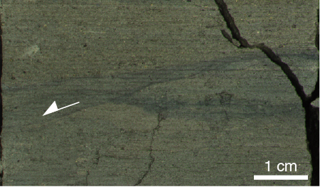
Figure F29. Split core image of an anastomosing shear zone.
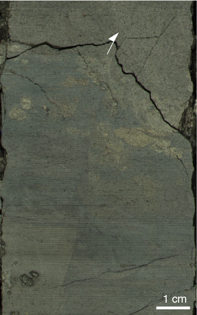
Figure F30. Split core image of a reversed fault.
Biostratigraphy
Calcareous nannofossil results
We examined all core catcher samples from Holes C0010C–C0010E for calcareous nannofossil biostratigraphy. Poor- to moderately preserved nannofossils were present in most samples, and species diversity is low. Most Quaternary datum planes described by Sato et al. (2009) and the lower Pliocene zonal marker of Martini (1971) and Okada and Bukry (1980) were identified in the sedimentary sequence. The absolute ages of calcareous nannofossil biostratigraphy follow a recent review by Raffi et al. (2006). The nannofossils observed in each hole are listed in Table T12.
Table T12. Calcareous nannofossil abundance. Download table in .csv format.
The assemblages found in Samples 365-C0010C-1R-CC through 12R-CC and 365-C0010D-1R-CC are mainly composed of Calcidiscus macintyrei, small Reticulofenestra spp. (<4 µm), Reticulofenestra pseudoumbilicus, Sphenolithus abies, and Discoaster sp. The last and first occurrences of Amaurolithus spp. are found in Samples 365-C0010C-6R-CC and 365-C0010D-1R-CC, respectively, and the last and first occurrences of Ceratolithus spp. are found in Samples 365-C0010C-3R-CC and 10R-CC, respectively; these last and first occurrences are early Pliocene datums recognized in low- to middle-latitude regions. Discoaster quinqueramus, which last occurs at the Miocene/Pliocene boundary (5.59 Ma), is absent in samples from Holes C0010C and C0010D. These results indicate that samples from Holes C0010C and C0010D correlate with Biozones NN12–NN14 (early Pliocene; 3.79–5.59 Ma).
Samples 365-C0010E-1R-CC through 3R-CC are characterized by the occurrence of medium Gephyrocapsa spp. (≥4 but <5.5 µm; Gephyrocapsa oceanica and Gephyrocapsa caribbeanica) and Pseudoemiliania lacunosa and also by the absence of large Gephyrocapsa spp. (≥5.5 µm) and the genus Discoaster. This indicates that the sediments recovered from Hole C0010E correlate with Biozone NN19 (middle Pleistocene; 1.56–1.67 Ma).
Paleomagnetism
Results
A typical demagnetization is shown in Figure F31A. A large downward component observed at lower demagnetization levels (between 0 and 15–20 mT) is clustered at inclinations ranging from 60° to 90° (Figure F31B). These magnetic components are generally considered as drilling-induced overprints (e.g., Gee et al., 1989). The characteristic remanent magnetizations of individual samples, which are free from such vertical magnetic components, were calculated by principal component analysis. Inclinations and declinations obtained are plotted in Figure F32A–F32B. Intensity after demagnetization at 20 mT and magnetic susceptibility are shown in Figure F32C–F32D. The effectiveness of demagnetization is manifested as directional changes in inclination and declination and as decreasing intensity. Intensity and magnetic susceptibility values in Hole C0010E are substantially larger than those in Holes C0010C and C0010D.
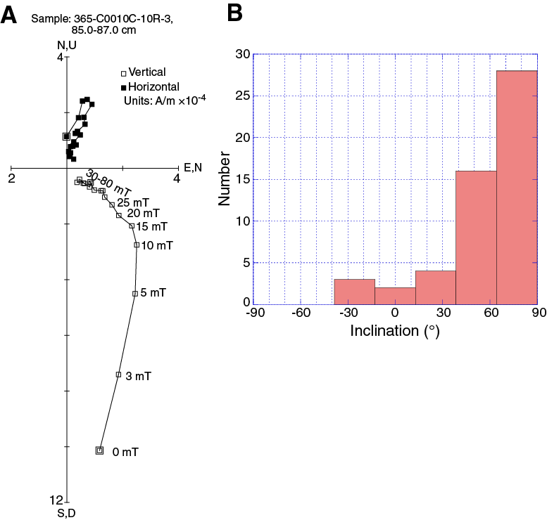
Figure F31. Vector component diagrams of progressive alternating field demagnetization.
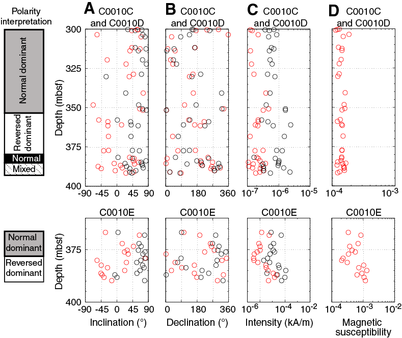
Figure F32. Inclination, declination, intensity, and magnetic susceptibility.
Polarity
Inclination from 300 to 350 mbsf in Holes C0010C–C0010D is dominantly positive, whereas inclination from 350 to 380 mbsf is dominantly reversed (Figure F32). The interval from 380 to 385 mbsf shows normal polarity, whereas polarity in the interval between 385 and 395 mbsf is not clear. Referring to the age model (see Biostratigraphy) and the magnetostratigraphic timescale for the Neogene (Lourens et al. 2004), these frequent polarity changes may be correlated to Chron 3n (4.187–5.235 Ma).
Inorganic geochemistry
Physical description of OsmoSampler
Formation fluids and dissolved gases were pumped and diffused into the two Teflon coils of the OsmoSampler during the period of its deployment. When recovered, the decrease in pressure caused gas expansion within the tubes, and fluid discharge through the inlets was observed on the rig floor as a result of this expansion. In total, approximately 70% of the fluids from the geochemistry coil and 88% from the biology coil were lost. The fluids that remained were shifted through the coils by gas bubbles but are believed to have retained their relative chronological order. It is unclear, however, where exactly they should be placed within the 5.3 y record. One explanation for the large amount of gas, in particular when compared to earlier FLOCS deployments in oceanic crust, may be the fact that microbial metabolism rates were enhanced in this nutrient-rich sedimentary setting with Site C0004 sediment as substrate.
The chemistry and biology coils were cut into 1 m long sections (see Table T1 in the Expedition 365 methods chapter [Saffer et al., 2017]), and fluid was drained by gravity into 2 mL centrifuge tubes. There were a total of 148 and 149 sample splits from the chemistry and biology coils, respectively. Selected sample splits were analyzed for chlorinity, alkalinity, major cations, anions, and minor and trace elements (see Table T1 and Figure F31, both in the Expedition 365 methods chapter [Saffer et al., 2017]). Fluid samples from each of the three OsmoSampler pumps (both the freshwater and saltwater reservoirs) were subjected to the same tests. All pumps were filled with a milky, possibly sulfuric precipitant. In general, the membranes of all three pumps looked and felt intact; however, a crack was observed between the freshwater and saltwater reservoirs of Pump 1, raising the possibility of leakage between these two reservoirs.
Coil chemistry
Refractive index, salinity, pH, and alkalinity
Refractive index (1.3), salinity (34.0), and pH (8.0) were measured from a single mixture of biology coil splits (Table T13). These values differ slightly from interstitial water (IW) sampled from the megasplay fault interval at Site C0004 (Sections 316-C0004D-26R-3 through 36R-2; salinity = 35.7 and pH = 7.5) but are consistent with values from Hole C0010C (refractive index = 1.3 and pH = 7.7; Table T14). Alkalinity was also measured from this same mixture of biology splits but could not be detected.
Table T13. Salinity, pH, refractive index, chlorinity, and anion and cation concentrations for OsmoSampler coils. Download table in .csv format.
Table T14. Salinity, pH, refractive index, chlorinity, and anion and cation concentrations in sediments. Download table in .csv format.
Chloride and cations
Chlorinity in the chemistry coil increased systematically from ~670 mM at the pump end to ~730 mM near the inlet (Table T13; Figure F33). The increase in chlorinity parallels the sodium profile (Figure F34), which fluctuated along the coil but generally increased from 633.2 to 689.8 mM toward the inlet. Chlorinity and sodium concentrations in the biology coil ranged between 601.5 and 608.3 mM and between 525.9 and 574.4 mM, respectively. The values remained relatively constant along the coil and are similar to those observed in IW extracted from cores at Site C0004 and in Hole C0010C. Magnesium, calcium, and potassium were similar in both coils (Table T13; Figures F34, F35).
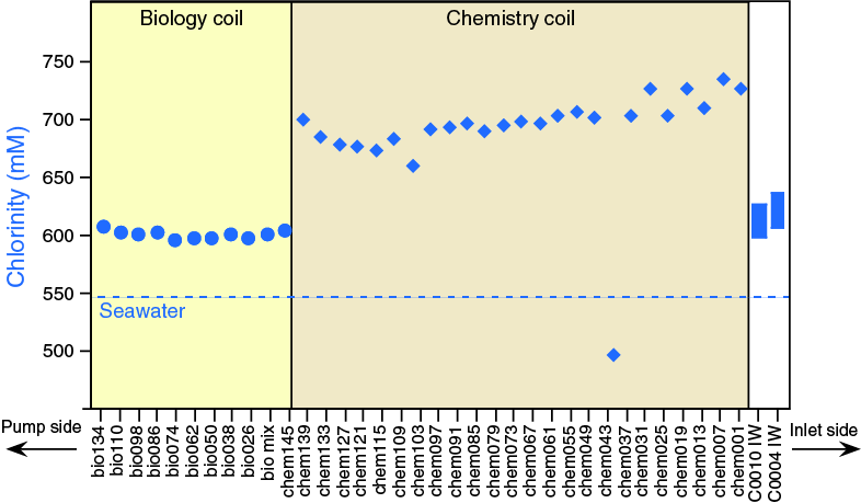
Figure F33. Chlorinity concentrations in selected splits from OsmoSampler coils.
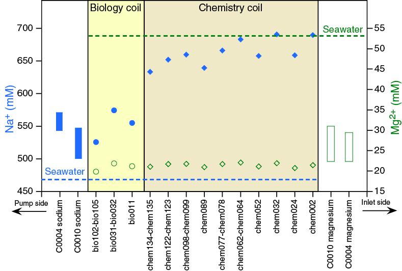
Figure F34. Sodium and magnesium concentrations in selected splits from OsmoSampler coils.
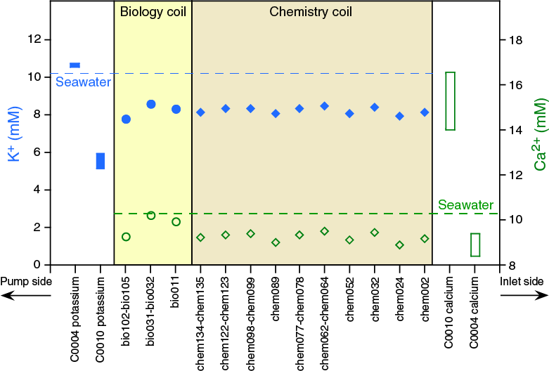
Figure F35. Potassium and calcium concentrations in selected splits from OsmoSampler coils.
Anions
Bromide concentrations in the chemistry and biology coils fluctuated between 1.1 and 1.2 mM, which is similar to concentrations found at Site C0004 and in Hole C0010C (Table T13; Figure F36). Sulfate concentrations in the chemistry coil were low relative to Site C0004 and Hole C0010C toward the pump end of the coil (60 µM) and increased toward the inlet (250 µM) (Table T13; Figure F36). This differs from the biology coil, where sulfate concentrations were constant (~2.8 mM) and are found to be similar to those at Site C0004 and in Hole C0010C.
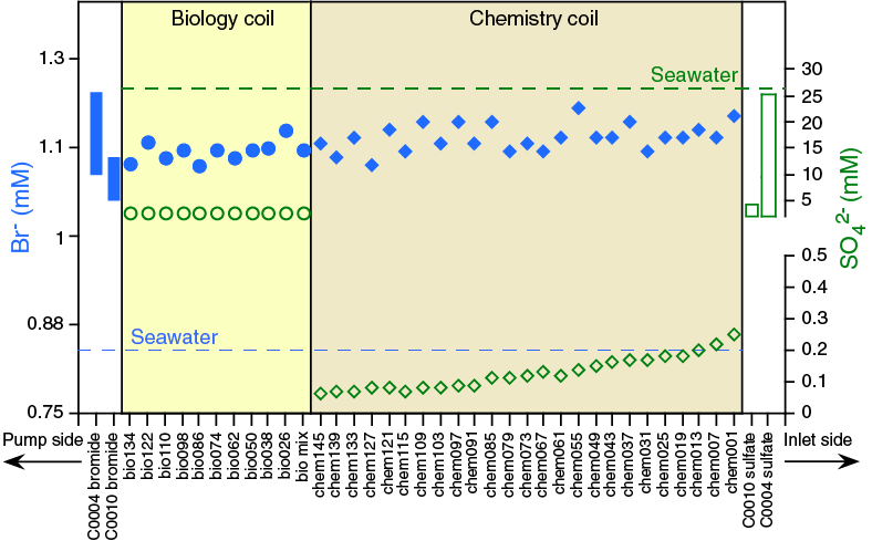
Figure F36. Bromide and sulfate concentrations in selected splits from OsmoSampler coils.
Minor elements
Lithium and silicon concentrations were slightly lower in the biology coils than in the chemistry coils but remained relatively constant through each coil (Table T15; Figure F37). Lithium concentrations averaged 68 and 74 µM in the chemistry and biology coils, respectively, and are lower than concentrations measured in cores at Site C0004 and in Hole C0010C. Silicon concentrations averaged 198 and 276 µM in the chemistry and biology coils, respectively, and are again lower than concentrations measured at Site C0004 and in Hole C0010C. Strontium concentrations were similar in both coils. The average concentration was 118 µM, which is lower than concentrations measured at Site C0004 and in Hole C0010C. Boron concentrations in the biology coil averaged 1245 µM and were significantly higher than those in the chemistry coil (average = 298 µM) and those reported from IW from cores at Site C0004 and in Hole C0010C (Figure F38). Barium and manganese concentrations were higher in the chemistry coil than in the biology coil (Figure F39). Barium concentrations averaged 11 and 3.9 µM in the chemistry and biology coils, respectively. Manganese concentrations averaged 16 and 1.9 µM in the chemistry and biology coils, respectively.
Table T15. Major element concentrations for OsmoSampler coils. Download table in .csv format.
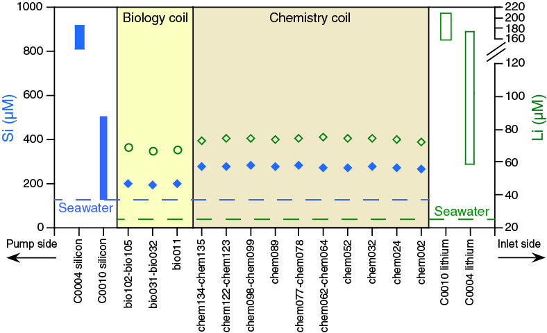
Figure F37. Dissolved silica and lithium concentrations in selected splits from OsmoSampler coils.
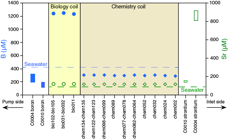
Figure F38. Boron and strontium concentrations in selected splits from OsmoSampler coils.
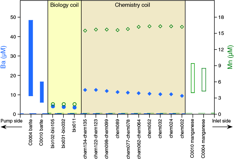
Figure F39. Barium and manganese concentrations in selected splits from OsmoSampler coils.
Trace elements
Cesium, copper, lead, molybdenum, uranium, and yttrium were found at nanomolar concentrations in both coils and showed no trends with time (Table T16; Figures F40, F41, F42). The average concentrations for cesium and copper were 5.4 and 20.0 nM, respectively. Copper concentrations are lower than those at Site C0004 and in Hole C0010C, which were above 700 nM. Molybdenum concentrations were relatively constant in the biology coil but decreased toward the pump end of the chemistry coil. Rubidium concentrations were approximately 1.0 µM and decreased slightly toward the inlet ends of both coils. Uranium, lead, and yttrium concentrations were relatively similar in both coils, averaging 0.2, 1.3, and 0.5 nM, respectively. Cadmium and chromium were undetectable. Cobalt was undetectable in the chemistry coil, and vanadium was undetectable in all but biology Sample bio010, where the concentration was 16 nM.
Table T16. Trace element concentrations for OsmoSampler coils. Download table in .csv format.
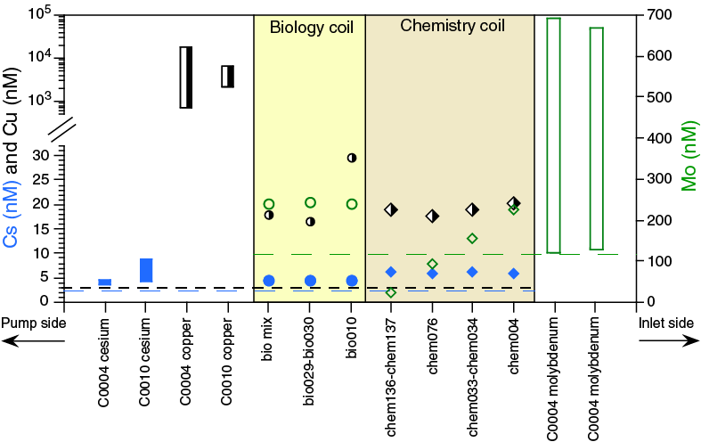
Figure F40. Cesium, copper, and molybdenum concentrations in selected splits from OsmoSampler coils.
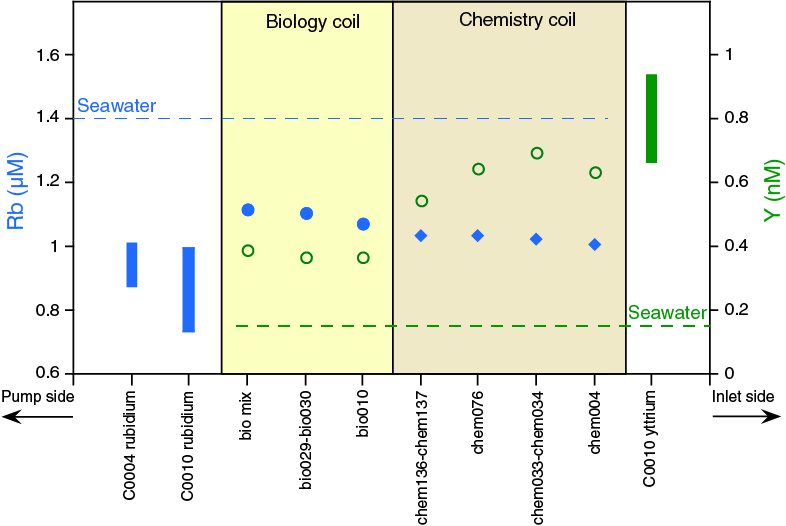
Figure F41. Rubidium and yttrium concentrations in selected splits from OsmoSampler coils.
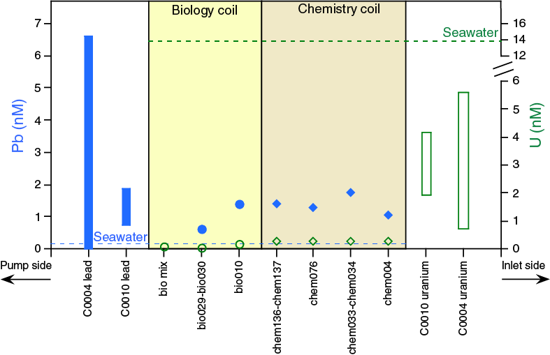
Figure F42. Lead and uranium concentrations in selected splits from OsmoSampler coils.
Pump chemistry
The final fluid composition of the chemistry pump (1) was drastically different from the biology pumps (2 and 3, Table T17). The freshwater and saltwater reservoirs of Pump 1 had similar elemental compositions: chlorinities for the freshwater and saltwater pumps were 665 and 653 mM, respectively; sodium concentrations were 595 and 579 mM, respectively. These concentrations exceed those in IW from Hole C0010C and Site C0004 (~625 mM chlorinity and ~560 mM sodium) but are similar to coil splits from the pump side of the chemistry coil.
Table T17. Geochemistry of saltwater and freshwater reservoirs of OsmoSampler pumps. Download table in .csv format.
Chlorinity and sodium concentrations in the saltwater reservoirs of Pumps 2 and 3 (biology pumps) averaged 4529 and 4296 mM, respectively (Table T17). These values are higher than their respective freshwater reservoirs, which averaged 3277 and 2606 mM, respectively. Barium, boron, bromide, calcium, magnesium, manganese, lithium, potassium, silicon, strontium, and sulfate concentrations in the freshwater reservoirs all exceeded those in the biology coil and IW from Hole C0010C and Site C0004.
Pump integrity
The similar compositions of the chemistry pump reservoirs suggest that the observed crack between the membranes may have resulted in a leak (Figure F43A). Because the saltwater reservoir was located above the freshwater reservoir, the denser saltwater may have leaked into the freshwater reservoir and geochemistry coils, thus drawing water into to the outlet port and reversing the direction of flow through the geochemistry coil. This possibility is consistent with the observation that chlorinity and sodium concentrations increase toward the inlet, as would be expected if fluids were drawn through the pump port and were expelled through the inlet (Table T13; Figures F33, F34). If this was the case, it is most likely that fluid flow through the coils and pumps would have ceased once most of the dense salt brine had been exported. The lack of fluid flow, lower salinity, and abundant carbon availability (the acetate pump membrane) would allow microorganisms to grow within the pump reservoirs and potentially consume the sulfate, which is consistent with the low sulfate concentrations in Pump 1 and the decrease of sulfate toward the pump end of the chemistry coil.

Figure F43. Chemistry Pump 1, chemistry coil, biology Pumps 2 and 3, and biology coil.
The biology pumps were still functioning properly when recovered (Figure F43B). Higher chlorinity and sodium concentrations in the saltwater reservoirs and an accumulation of ions in the freshwater reservoir confirm continual osmotic diffusion toward the saltwater reservoirs.
Interstitial water chemistry
A total of six whole-round (WR) core samples were collected for IW analyses at Site C0010 (four from Hole C0010C and two from Hole C0010E). WR sample lengths ranged from 21 to 36 cm, with larger samples collected from cores recovered from greater depths where sediments were more consolidated. The amount of IW recovered from each WR in Hole C0010C ranged from 9 to 12 mL. The lithology of Hole C0010C was comparable to that at the depth of the GeniusPlug deployment, and thus IW analyses from this hole were compared to those of the OsmoSampler (Figures F33, F34, F35, F36, F37, F38, F39, F40, F41, F42). Sediments of Hole C0010E are from lithologic Unit II (the footwall of the megasplay fault), which was below the depth of the GeniusPlug deployment. Therefore, measurements from this hole were not compared to OsmoSampler measurements.
Refractive index, salinity, pH, and alkalinity
Refractive index (1.3) was consistent with depth across both holes (Table T14). pH was slightly lower in Hole C0010C (7.7) than in Hole C0010E (8.0). Alkalinity concentrations initially dropped from 5.4 mM at 301 mbsf to 1.8 mM at 341 mbsf (Figure F44). Deeper than 341 mbsf, concentrations increased with increasing depth to a maximum of 8.34 mM at 387 mbsf in Hole C0010E.
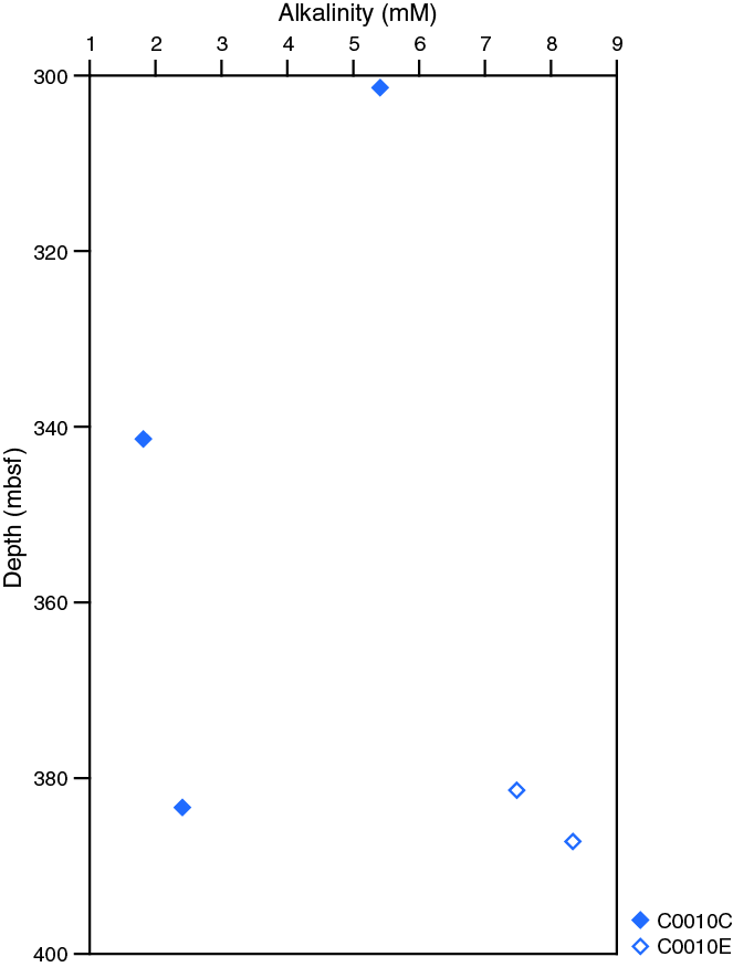
Figure F44. Alkalinity concentrations in sediments.
Chloride and cations
Chlorinity and sodium concentrations mirrored each other downcore, reaching a maximum of 639 and 573 mM, respectively. These concentrations were similar to those measured at Site C0004 at comparable depths (Table T14; Figures F33, F34, F45). Calcium and potassium concentrations were consistent with depth and averaged 14 and 6.6 mM, respectively (Figure F46). These calcium and potassium concentrations were greater and lesser than measurements from Site C0004, respectively (Figure F35). The shallowest and deepest magnesium measurements (31 and 25 mM, respectively) were greater than at intermediate depths (average = 24 mM). Ammonium increased with increasing depth, ranging from 1.9 to 5.0 mM, suggesting organic matter degradation (Figure F47).
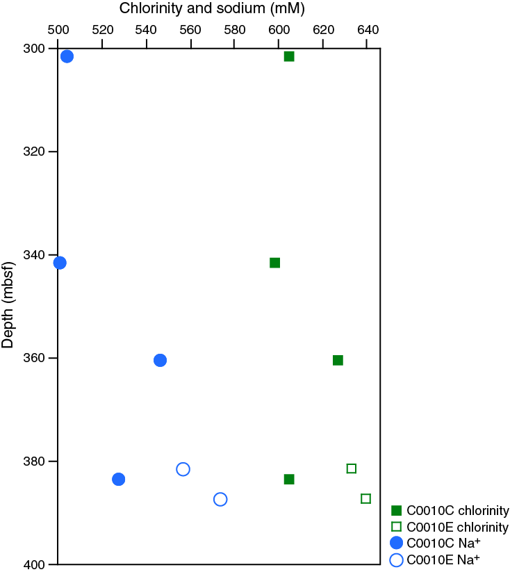
Figure F45. Chlorinity and sodium concentrations in sediments.
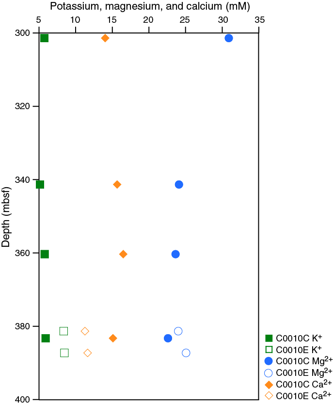
Figure F46. Potassium, magnesium, and calcium concentrations in sediments.
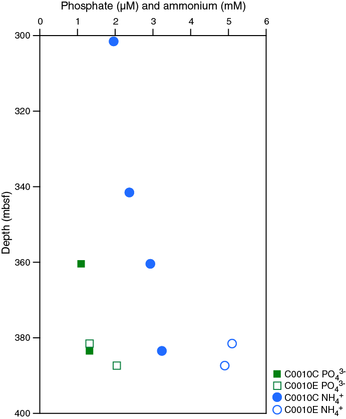
Figure F47. Phosphate and ammonium concentrations in sediments.
Anions
Bromide concentrations were constant throughout both holes and averaged 1.1 mM (Table T14; Figure F48). Sulfate concentrations were also relatively constant and averaged 2.2 mM, with the exception of the deepest sample in Hole C0010C, which had twice as much sulfate as the average (4.1 mM). Nitrate concentrations ranged from below detection limit (BDL) to 25 mM. Phosphate increased with increasing depth, ranging from BDL to 2.0 µM and, like ammonium, points toward organic matter degradation (Figure F47).
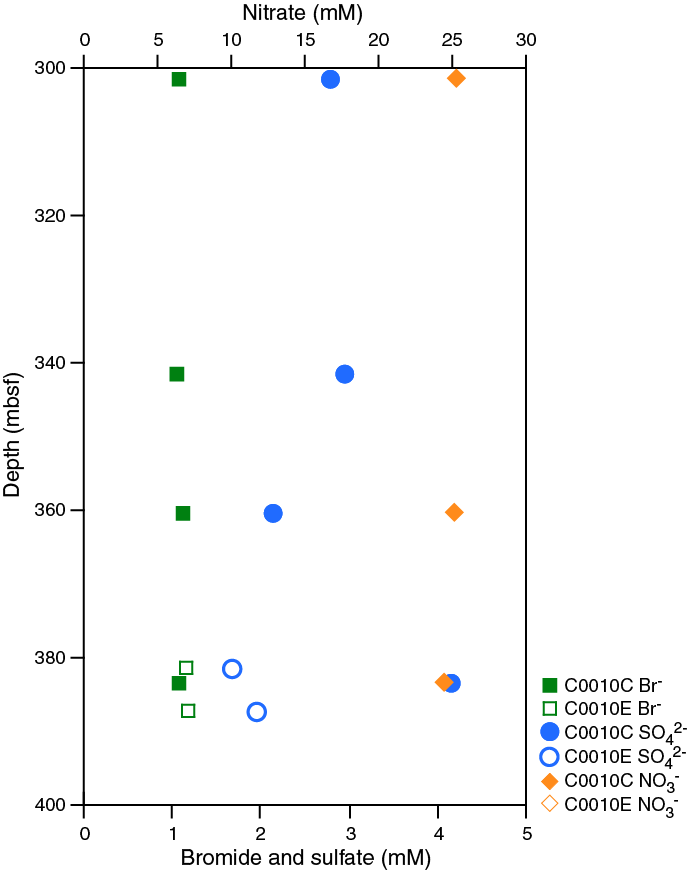
Figure F48. Bromide, sulfate, and nitrate concentrations in sediments.
Minor elements
Lithium, boron, and strontium concentrations were consistent with depth in both holes and averaged 149, 195, and 141 µM, respectively (Table T18; Figure F49). Silicon and barium concentrations showed no trend with depth in Hole C0010C and fluctuated between 127 and 505 µM and between 6.2 and 17 µM, respectively (Figures F49, F50). Silicon and barium concentrations were greater in Hole C0010E than in Hole C0010C and reached maximum concentrations of 702 and 81 µM, respectively. Manganese showed no trends with depth and ranged between 4.0 and 9.4 µM (Figure F50). Iron was not detected in Hole C0010C, but was detected in Hole C0010E at a concentration of approximately 0.6 µM.
Table T18. Major element concentrations in sediments. Download table in .csv format.
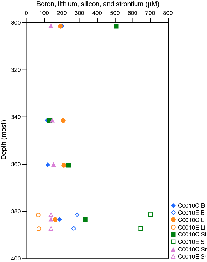
Figure F49. Boron, lithium, silicon, and strontium concentrations in sediments.
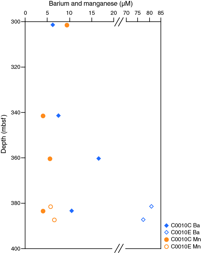
Figure F50. Barium and manganese concentrations in sediments.
Trace elements
Rubidium concentrations increased with increasing depth and were greater in Hole C0010E than in Hole C0010C (Table T19; Figure F51). These concentrations ranged from 730 to 1120 nM. Molybdenum reached a maximum concentration of 690 nM at 341 mbsf in Hole C0010C and then decreased with depth. Nanomolar concentrations of vanadium, yttrium, molybdenum, cesium, lead, and uranium were measured in both holes (Figures F52, F53). Vanadium concentrations initially decreased from 10.23 nM at 301 mbsf to 6.47 nM at 341 mbsf and then increased to a maximum concentration of 13 nM at 387 mbsf. Cesium and uranium concentrations were relatively constant throughout both holes and averaged 7.1 and 3.0 nM, respectively. Yttrium concentrations were constantly lower than 3 nM throughout both holes. Copper concentrations ranged from 2.1 to 6.5 µM. Lead concentrations ranged between BDL and 1.86 nM. Zinc isotopes could not be measured consistently, and therefore, their concentrations could not be measured accurately.
Table T19. Trace element concentrations in sediments. Download table in .csv format.
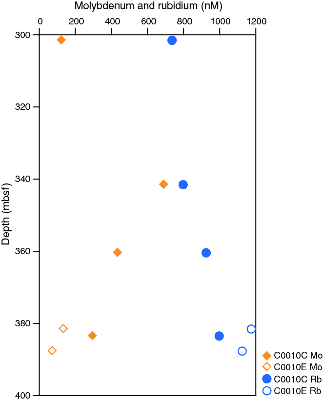
Figure F51. Molybdenum and rubidium concentrations in sediments.
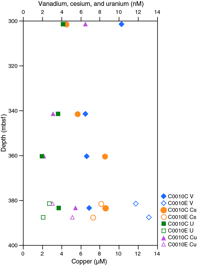
Figure F52. Vanadium, cesium, uranium, and copper concentrations in sediments.
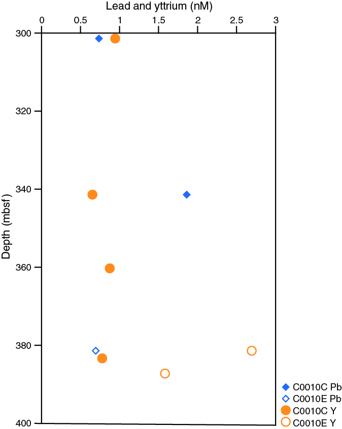
Figure F53. Lead and yttrium concentrations in sediments.
Organic geochemistry
Gas analysis
OsmoSampler
The chemistry and biology coils were cut into 1 m long sections (see Table T1 in the Expedition 365 methods chapter [Saffer et al., 2017]) and fluid was drained by gravity into 2 mL centrifuge tubes. A total of four coils were placed into 20 mL glass bottles and sealed with a septum and metal crimp cap for hydrocarbon analyses.
Methane was present in all four coils and concentrations ranged from 0.04 to 63 mM (Table T20). Ethane was also detected in all samples, and the methane/ethane (C1/C2) ratio ranged from 42 to 1409, indicating a biogenic origin for the hydrocarbon gases. It was observed that the cap for Sample chem046 was not sealed correctly and had allowed gas to leak, likely leading to lower gas concentrations and a lower C1/C2 ratio relative to the other samples.
Table T20. Hydrocarbon gases in headspace samples from OsmoSampler coils. Download table in .csv format.
The original blanks for the analysis were 1 m long empty coils that were cut from the recovered OsmoSampler and were washed with 30 mL of ultrapure water. The first blank (washed Coil 1) was washed and sealed within a vial approximately 15 h after the OsmoSampler was recovered. The second blank (washed Coil 2) was washed and sealed within a vial approximately 40 h after recovery. Both of these blanks contained methane. A new, clean, 1 m tube was also measured as a third blank. This third blank contained only atmospheric amounts of methane. This indicates that calculated concentrations for dissolved methane are an overestimation of in situ concentrations because some methane was also held within the walls of the polytetrafluoroethylene (PTFE) tubing.
Headspace sampling
Headspace sampling provides an estimation of hydrocarbon gas concentrations, although some gas may have escaped during core recovery as a result of depressurization. A total of 12 headspace samples from Hole C0010C, 1 headspace sample from Hole C0010D, and 3 headspace samples from Hole C0010E were analyzed. Methane was present in all samples and fluctuated with depth ranging from approximately 3,700 to 38,000 parts per million by volume (ppmv) (Table T21). Ethane was also present, ranging from 0.8 to 9 ppmv. The C1/C2 ratio ranged from 1,100 to 14,000 and decreased with depth in Hole C0010C (Figure F54). This ratio is consistent with data from Site C0004 and indicates a biogenic origin for the hydrocarbon gases.
Table T21. Hydrocarbon gases in headspace samples from sediments. Download table in .csv format.

Figure F54. Dissolved hydrocarbon C1/C2 values.
Sediment carbon, nitrogen, and sulfur composition
A total of 25 samples were selected for carbon, nitrogen, and sulfur elemental analyses (Table T22, Figure F55). Calcium carbonate (CaCO3) content from Holes C0010C–C0010E averaged 4.21 wt% but was as high as 12.2 and 13.4 wt% in Holes C0010C (357.6 mbsf) and C0010D (391.6 mbsf), respectively. These values are consistent with XRD measurements (on average within 1 wt% difference, see Lithology) and generally similar to carbonate values measured at Site C0004 (Figure F55). TOC and total nitrogen (TN) content were similar across all three holes and averaged 0.35 (Holes C0010C/C0010D) and 0.06 wt% (Hole C0010E), respectively. These averages are slightly lower than those at Site C0004. The TOC/TN ratio averaged 6.2, consistent with Site C0004, suggesting that the organic matter at this site is of marine origin. Total sulfur (TS) content ranged from 0.04 to 0.4 wt%.
Table T22. Carbonate, carbon, nitrogen, and sulfur in sediments. Download table in .csv format.
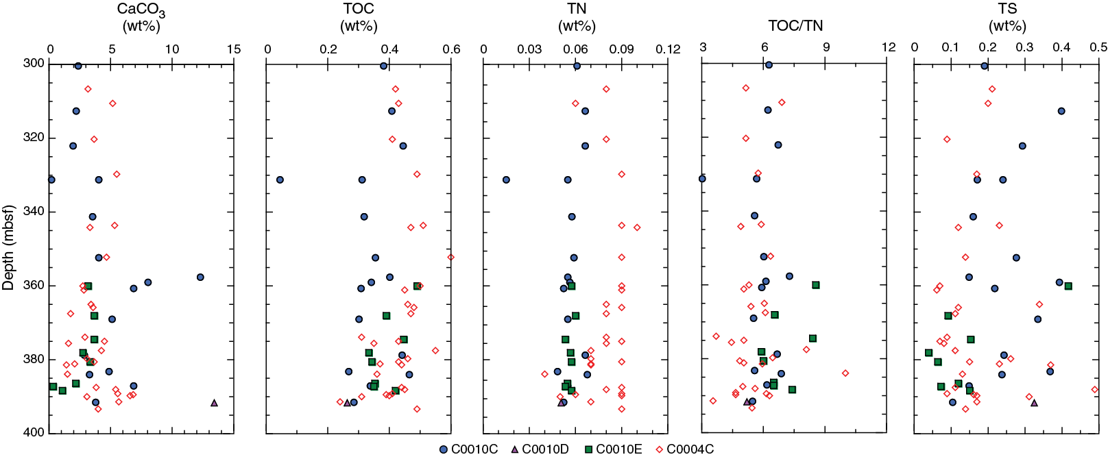
Figure F55. CaCO3, TOC, TN, TOC/TN ratio, and TS in sediments.
Microbiology
Culture growth
Substrates collected from the FLOCS of the OsmoSampler were sampled and preserved for shore-based DNA, microscopy, and single-cell genomics (SCG) analyses (Table T23). Additionally, the barite, olivine, sediment, fluids, and iron precipitates (collected from the outside of the GeniusPlug) were used to inoculate anaerobic saltwater media for shore-based culture experiments. After 6 days of growth, all cultures were sampled, and potential cells were stained as a qualitative check for growth using epifluorescent microscopy (Figure F56). Cells were clearly observed in the barite, fluid, and sediment cultures, suggesting successful inoculation and growth from these substrates. Possible cells were observed in the olivine culture; however, given the florescence of the small-grained olivine, it was not possible to confirm growth. No cells were observed on the filters from either the control or iron precipitate cultures.
Table T23. Microbiology samples collected from FLOCS substrates, coil fluids, and GeniusPlug casing. Download table in .csv format.
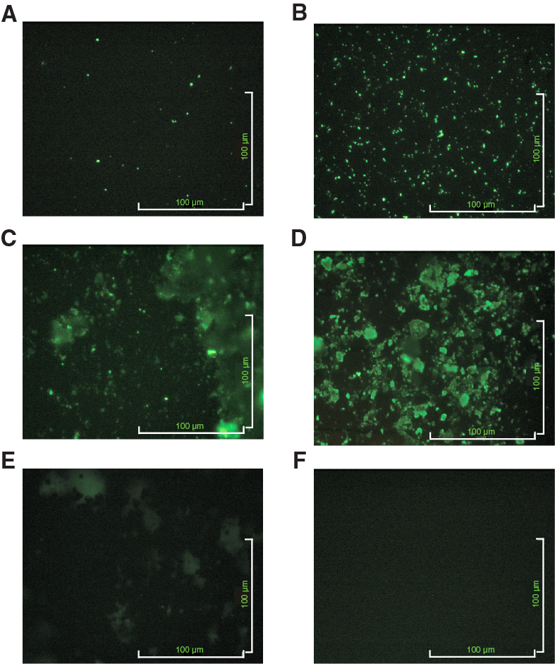
Figure F56. Microscope images of microbiology cultures.
Contamination test
Contamination tests for core samples were carried out by chemical tracer quantification. Perfluorocarbon tracers (PFTs; perfluoromethylcyclohexane, C7F14) were supplied directly to drilling mud that was used to sweep Holes C0010C and C0010E, but not to the seawater drilling fluid used during coring. After the PFTs were added to the mud tanks, the mud was sampled for PFT concentrations. These initial PFT concentrations ranged from 84 to 3412 ng/L.
Two 2.5 cm3 plugs of sediment were collected from core sections directly adjacent to microbiology WR samples to evaluate drilling mud invasion. However, results showed that PFT concentrations in core liner fluid and core sample exterior and interiors varied wildly with no clear patterns (Table T24).
Table T24. PFT concentrations measured from sediment cores and core liner fluid. Download table in .csv format.
Physical properties
During Expedition 365, a range of physical property measurements were conducted on cores acquired in Holes C0010C–C0010E, using the whole-round multisensor core logger (MSCL-W) (see Physical properties in the Expedition 365 methods chapter [Saffer et al., 2017]). These measurements included gamma ray attenuation (GRA) density, magnetic susceptibility, natural gamma radiation (NGR), and ultrasonic P-wave velocity. Resistivity measurements on whole rounds are not reported here, because the noncontact electrical resistivity sensor was not operating correctly during the expedition. During the sampling party conducted from 26 July to 5 August 2016, further physical properties, including moisture and density (MAD), electrical conductivity on discrete samples, P-wave velocity on discrete samples, thermal conductivity, and reflectance spectrophotometry were measured. Data from Holes C0010C and C0010D (megasplay depth at 407 mbsf) are plotted together, whereas data from Hole C0010E (megasplay depth ~360 mbsf) are plotted separately; Holes C0010C and C0010D represent the hanging wall, whereas Hole C0010E represents the footwall of the megasplay fault (see Structural geology and Lithology).
MSCL-W
Overall, there are no significant variations in any of the measured parameters in Holes C0010C and C0010D over the depths we cored (300–392 mbsf) (Figures F57, F58). However, there are significant differences in magnetic susceptibility and NGR between Holes C0010C–C0010D and Hole C0010E. Magnetic susceptibility (MS) values are much larger (and more variable) in Hole C0010E relative to Holes C0010C and C0010D (Figure F59). Overall, NGR values in Hole C0010E are somewhat lower (generally ranging from 20 to 30 American Petroleum Institute gamma radiation units [gAPI]) compared to Holes C0010C and C0010D (~30–50 gAPI). This decrease in NGR with depth is similar to NGR decreases observed in LWD data from Hole C0010A when the megasplay fault zone was crossed (Expedition 319 Scientists, 2010b). The higher MS and lower NGR values in Hole C0010E would be consistent with a transition from clay-dominated sediments to siltier or sandier lithologies. Overall, density values for Hole C0010E are lower than in Holes C0010C and C0010D. Together, these observations are consistent with the interpretation that Hole C0010E samples Unit II (underthrust slope basin sediments), whereas cores from Holes C0010C and C0010D are derived from the clay-rich thrust wedge material of Unit I (see Lithology and Structural geology).
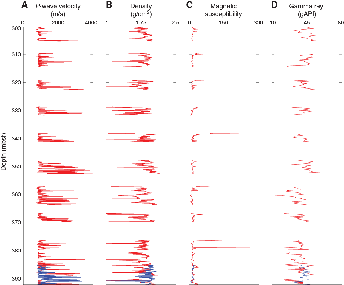
Figure F57. MSCL-W results, Holes C0010C and C0010D.
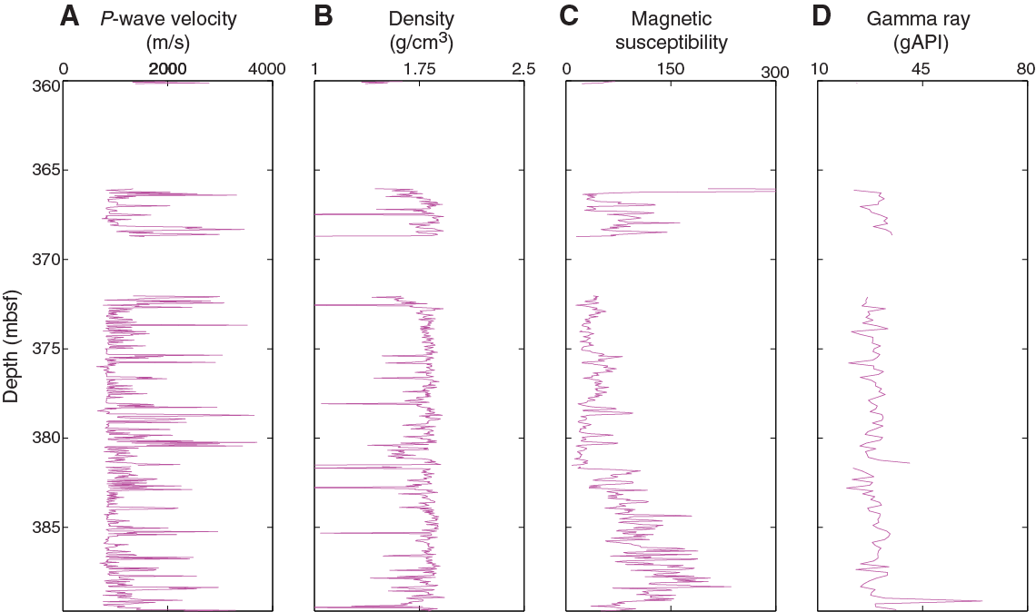
Figure F58. MSCL-W results, Hole C0010E.
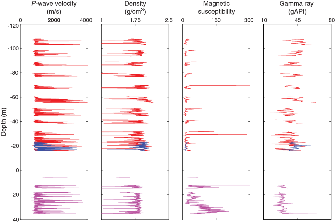
Figure F59. Composite of MSCL-W results.
Moisture and density measurements
MAD measurements were conducted on 113 discrete samples from Holes C0010C–C0010E to provide a detailed characterization of bulk density, grain density, and porosity. Wet bulk density values are scattered mostly between 1.85 and 2.1 g/cm3 (Figure F60). Data from Hole C0010E exhibit less scatter and lower bulk density than data from Holes C0010C and C0010D. The average bulk densities are 1.98, 2.02, and 1.89 g/cm3 for Holes C0010C, C0010D, and C0010E, respectively. Two ash layers at 331 and 362 mbsf show the smallest bulk density (~1.78 g/cm3). Overall, GRA and discrete bulk density measurements are consistent. Similar to bulk density, the grain density scatter is larger in Holes C0010C and C0010D than in Hole C0010E, with most values ranging from ~2.68 to 2.8 g/cm3 (Figure F61). Other than the larger scatter, the general trend shows an overall slightly lower grain density in Hole C0010E relative to Holes C0010C and C0010D. The average grain densities are 2.73, 2.73, and 2.70 g/cm3 in Holes C0010C, C0010D, and C0010E, respectively. The two ash layers at 331 and 363 mbsf show the lowest grain density (~2.45 g/cm3).
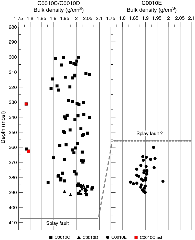
Figure F60. Wet bulk density measured on discrete samples.

Figure F61. Grain density measured on discrete samples.
Porosity shows a large scatter in Holes C0010C and C0010D with values between 0.40 and 0.50 (Figure F62). In contrast, Hole C0010E exhibits values mainly between 0.45 and 0.50. Average porosities are 0.44, 0.42, and 0.48 in Holes C0010C, C0010D, and C0010E, respectively. Thus, the porosity in the footwall of the megasplay is generally slightly higher than in the hanging wall.
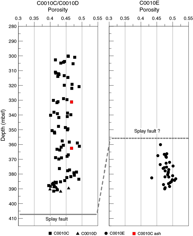
Figure F62. Porosity measured on discrete samples.
Electrical conductivity, P-wave velocity, and anisotropy
Electrical conductivity was measured in the x-, y-, and z-directions, as described in Physical properties in the Expedition 365 methods chapter (Saffer et al., 2017). The data scatter between 0.2 and 1.0 S/m (Figure F63A). In Holes C0010C and C0010D, no general trend is observed. Hole C0010E exhibits an offset to higher values. The average conductivity is ~0.52 and ~0.58 S/m for Holes C0010C and C0010D. There is no significant orientation dependency. Hole C0010E has an average conductivity of ~0.85 S/m in the x- and y-directions, whereas the z-direction has a lower average conductivity of 0.76 S/m.
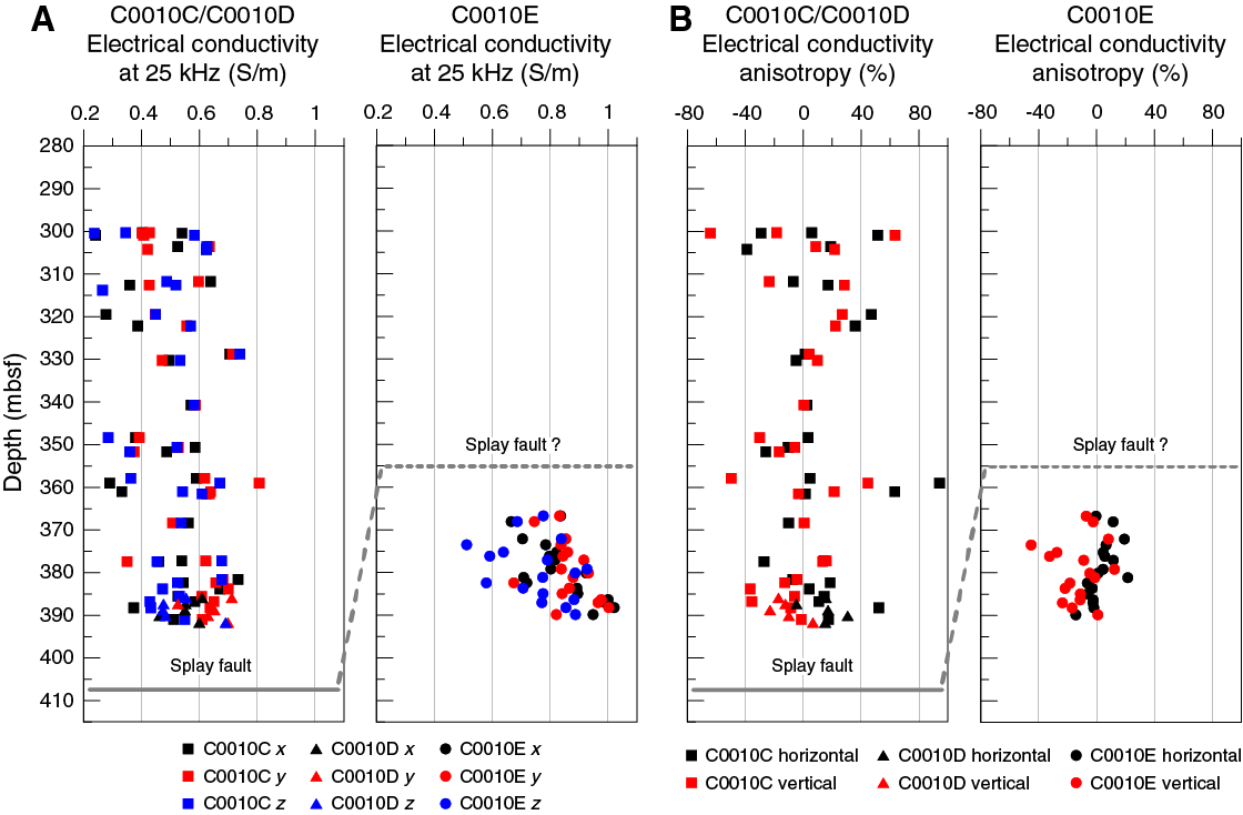
Figure F63. Electrical conductivity and anisotropy measured on discrete samples.
The anisotropy of electrical conductivity was calculated for the in-plane anisotropy (between the two directions perpendicular to the core axis x and y) and the transverse anisotropy (between the core axis, z, and the horizontal planes, x and y) (Figure F63B). The scatter of the in-plane and transverse anisotropy in Hole C0010C is larger than in Holes C0010D and C0010E. No trend with depth is observed in the anisotropy data. In general, Holes C0010D and C0010E show mainly positive in-plane anisotropies in contrast to negative transverse anisotropies. The average values for in-plane and transverse anisotropy are in the range of −13% to 15%.
P-wave velocity was measured along the three main orientations (x, y, and z) (Figure F64A). P-wave velocity in all three orientations increases gradually with depth over the range from ~1800 to ~2100 m/s in the interval 300–380 mbsf (Hole C0010C). From 380 to 395 mbsf (Holes C0010C and C0010D), P-wave velocity is fairly constant at around 1965 m/s. In the footwall (Hole C0010E), P-wave velocity is nearly constant with depth at approximately 1800–2000 m/s (average ~1880 m/s).
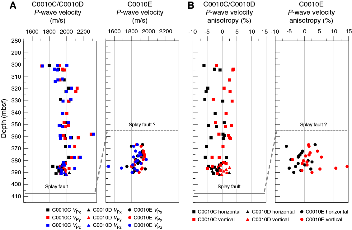
Figure F64. P-wave velocity and anisotropy measured on discrete samples.
The P-wave in-plane anisotropy and transverse anisotropy were calculated (Figure F64B). P-wave velocity anisotropy scatters mainly between −5% and 5%, and there is no trend with depth. The transverse anisotropy is mainly positive, whereas the in-plane anisotropy is slightly negative. The average values are approximately −1.5% and +1.4% for in-plane and transverse anisotropy, respectively.
Thermal conductivity
Thermal conductivity was measured on the working half of cores from Holes C0010C–C0010E using a half-space probe. In total, 24 measurements were performed; all data are summarized in Figure F65. Thermal conductivity ranges from 1.23 to 1.49 W/(m·K). Average thermal conductivities are 1.37, 1.47, and 1.3 W/(m·K) for Holes C0010C, C0010D, and C0010E, respectively. In general, thermal conductivity in the hanging wall is higher and shows a wider scatter than in the footwall, which is consistent with its lower porosity but higher degree of deformation.
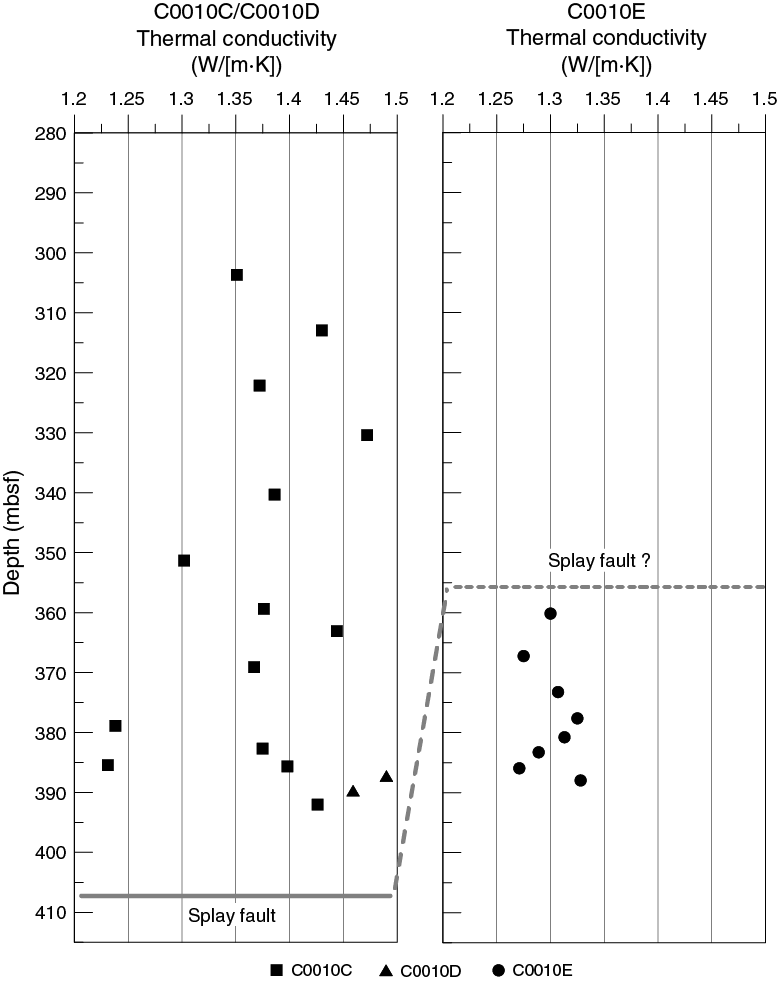
Figure F65. Thermal conductivity measured on discrete samples using half space method.
Color spectrometry
Color reflectance results are presented in Figures F66, F67, and F68. L* values range from ~13% to 56%. The average values for Holes C0010C and C0010D are similar at ~39%, whereas the average value for Hole C0010E decreases to ~34%. Values of a* range from approximately −6% to 6%. As for thermal conductivity, scatter in Holes C0010C and C0010D is much higher than in Hole C0010E. The average values are −0.70%, −0.75%, and −0.73% for Holes C0010C, C0010D, and C0010E, respectively. Values of b* range from approximately −3% to 8%. The average values for Holes C0010C and C0010D are similar at 1.7% and 1.5%, respectively, whereas the average value for Hole C0010E is higher at 2.5%.
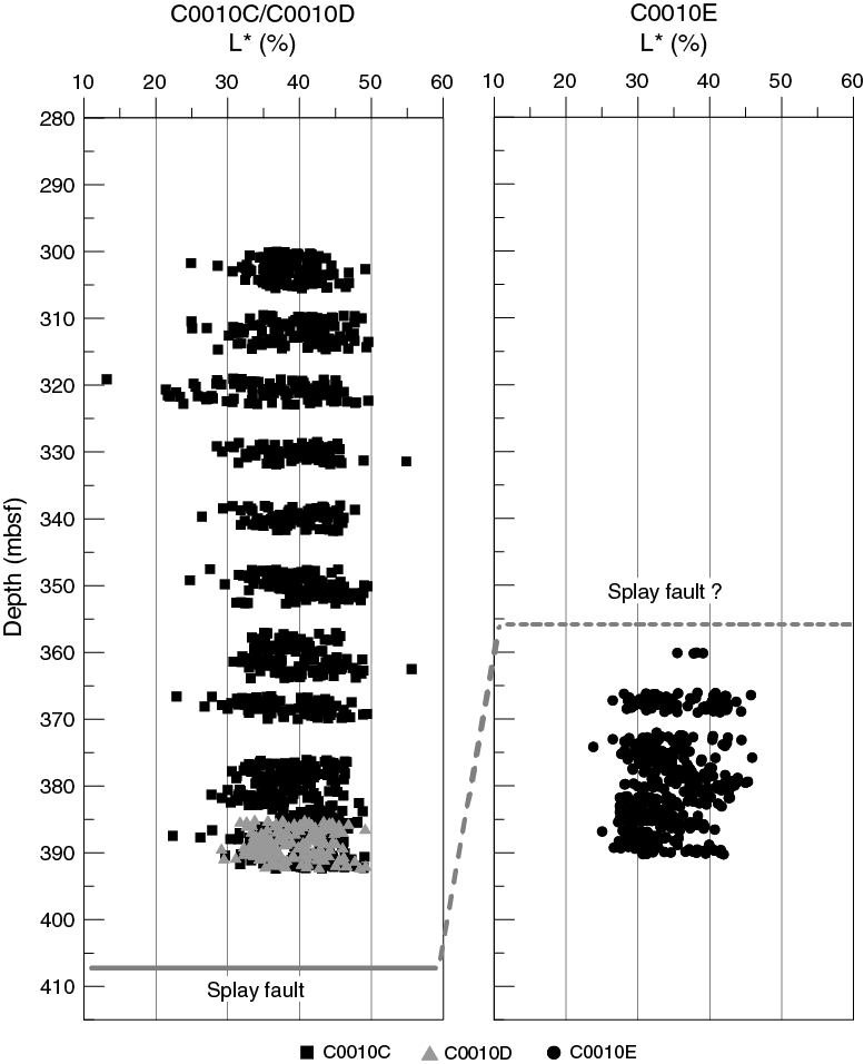
Figure F66. Color reflectance L* data.

Figure F67. Color reflectance a* data.
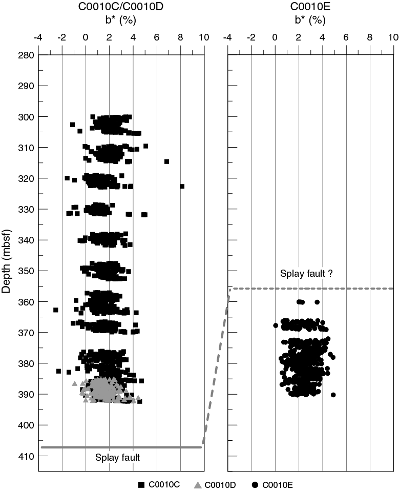
Figure F68. Color reflectance b* data.
References
Expedition 314 Scientists, 2009. Expedition 314 Site C0004. In Kinoshita, M., Tobin, H., Ashi, J., Kimura, G., Lallemant, S., Screaton, E.J., Curewitz, D., Masago, H., Moe, K.T., and the Expedition 314/315/316 Scientists, Proceedings of the Integrated Ocean Drilling Program, 314/315/316: Washington, DC (Integrated Ocean Drilling Program Management International, Inc.). http://dx.doi.org/10.2204/iodp.proc.314315316.116.2009
Expedition 316 Scientists, 2009. Expedition 316 Site C0004. In Kinoshita, M., Tobin, H., Ashi, J., Kimura, G., Lallemant, S., Screaton, E.J., Curewitz, D., Masago, H., Moe, K.T., and the Expedition 314/315/316 Scientists, Proceedings of the Integrated Ocean Drilling Program, 314/315/316: Washington, DC (Integrated Ocean Drilling Program Management International, Inc.). http://dx.doi.org/10.2204/iodp.proc.314315316.133.2009
Expedition 319 Scientists, 2010a. Expedition 319 summary. In Saffer, D., McNeill, L., Byrne, T., Araki, E., Toczko, S., Eguchi, N., Takahashi, K., and the Expedition 319 Scientists, Proceedings of the Integrated Ocean Drilling Program, 319: Tokyo (Integrated Ocean Drilling Program Management International, Inc.). http://dx.doi.org/10.2204/iodp.proc.319.101.2010
Expedition 319 Scientists, 2010b. Site C0010. In Saffer, D., McNeill, L., Byrne, T., Araki, E., Toczko, S., Eguchi, N., Takahashi, K., and the Expedition 319 Scientists, Proceedings of the Integrated Ocean Drilling Program, 319: Tokyo (Integrated Ocean Drilling Program Management International, Inc.). http://dx.doi.org/10.2204/iodp.proc.319.104.2010
Expedition 332 Scientists, 2011. Methods. In Kopf, A., Araki, E., Toczko, S., and the Expedition 332 Scientists, Proceedings of the Integrated Ocean Drilling Program, 332: Tokyo (Integrated Ocean Drilling Program Management International, Inc.). http://dx.doi.org/10.2204/iodp.proc.332.102.2011
Gee, J., Staudigel, H., and Tauxe, L., 1989. Contribution of induced magnetization to magnetization of seamounts. Nature, 342(6246):170–173. http://dx.doi.org/10.1038/342170a0
Kinoshita, M., Tobin, H., Ashi, J., Kimura, G., Lallemant, S., Screaton, E.J., Curewitz, D., Masago, H., Moe, K.T., and the Expedition 314/315/316 Scientists, 2009. Proceedings of the Integrated Ocean Drilling Program, 314/315/316: Washington, DC (Integrated Ocean Drilling Program Management International, Inc.). http://dx.doi.org/10.2204/iodp.proc.314315316.2009
Kopf, A., Araki, E., Toczko, S., and the Expedition 332 Scientists, 2011. Proceedings of the Integrated Ocean Drilling Program, 332: Tokyo (Integrated Ocean Drilling Program Management International, Inc.). http://dx.doi.org/10.2204/iodp.proc.332.2011
Kopf, A., Saffer, D., Toczko, S., Araki, E., Carr, S., Kimura, T., Kinoshita, C., Kobayashi, R., Machida, Y., Rösner, A., and Wallace, L.M., 2017. Expedition 365 summary. With contributions by S. Chiyonobu, K. Kanagawa, T. Kanamatsu, G. Kimura, and M.B. Underwood. In Saffer, D., Kopf, A., Toczko, S., and the Expedition 365 Scientists, NanTroSEIZE Stage 3: Shallow Megasplay Long-Term Borehole Monitoring System. Proceedings of the International Ocean Discovery Program, 365: College Station, TX (International Ocean Discovery Program). http://dx.doi.org/10.14379/iodp.proc.365.101.2017
Lourens, L.J., Hilgen, F.J., Laskar, J., Shackleton, N.J., and Wilson, D., 2004. The Neogene period. In Gradstein, F.M., Ogg, J., et al. (Eds.), A Geologic Time Scale 2004: Cambridge, United Kingdom (Cambridge University Press), 409–440.
Martini, E., 1971. Standard Tertiary and Quaternary calcareous nannoplankton zonation. In Farinacci, A. (Ed.), Proceedings of the Second Planktonic Conference, Roma 1970: Rome (Edizioni Tecnoscienza), 2:739–785.
Okada, H., and Bukry, D., 1980. Supplementary modification and introduction of code numbers to the low-latitude coccolith biostratigraphic zonation (Bukry, 1973; 1975). Marine Micropaleontology, 5:321–325. http://dx.doi.org/10.1016/0377-8398(80)90016-X
Polster, A., Fabian, M., and Villinger, H., 2009. Effective resolution and drift of Paroscientific pressure sensors derived from long-term seafloor measurements. Geochemistry, Geophysics, Geosystems, 10(8):Q08008. http://dx.doi.org/10.1029/2009GC002532
Raffi, I., Backman, J., Fornaciari, E., Pälike, H., Rio, D., Lourens, L., and Hilgen, F., 2006. A review of calcareous nannofossil astrobiochronology encompassing the past 25 million years. Quaternary Science Reviews, 25(23–24):3113–3137. http://dx.doi.org/10.1016/j.quascirev.2006.07.007
Saffer, D., Kopf, A., Toczko, S., Araki, E., Carr, S., Kimura, T., Kinoshita, C., Kobayashi, R., Machida, Y., Rösner, A., and Wallace, L.M., 2017. Expedition 365 methods. With contributions by S. Chiyonobu, K. Kanagawa, T. Kanamatsu, G. Kimura, and M.B. Underwood. In Saffer, D., Kopf, A., Toczko, S., and the Expedition 365 Scientists, NanTroSEIZE Stage 3: Shallow Megasplay Long-Term Borehole Monitoring System. Proceedings of the International Ocean Discovery Program, 365: College Station, TX (International Ocean Discovery Program). http://dx.doi.org/10.14379/iodp.proc.365.102.2017
Sato, T., Chinyonobu, S., and Hodell, D.A., 2009. Data report: Quaternary calcareous nannofossil datums and biochronology in the North Atlantic Ocean, IODP Site U1308. In Channell, J.E.T., Kanamatsu, T., Sato, T., Stein, R., Alvarez Zarikian, C.A., Malone, M.J., and the Expedition 303/306 Scientists, Proceedings of the Integrated Ocean Drilling Program, 303/306: College Station, TX (Integrated Ocean Drilling Program Management International, Inc.). http://dx.doi.org/10.2204/iodp.proc.303306.210.2009
Wallace, L.M., Araki, E., Saffer, D., Wang, X., Roesner, A., Kopf, A., Nakanishi, A., Power, W., Kobayashi, R., Kinoshita, C., Toczko, S., Kimura, T., Machida, Y., and Carr, S., 2016. Near-field observations of an offshore Mw 6.0 earthquake from an integrated seafloor and subseafloor monitoring network at the Nankai Trough, southwest Japan. Journal of Geophysical Research: Solid Earth, 121(11):8338–8351. http://dx.doi.org/10.1002/2016JB013417
1 Saffer, D., Kopf, A., Toczko, S., Araki, E., Carr, S., Kimura, T., Kinoshita, C., Kobayashi, R., Machida, Y., Rösner, A., and Wallace, L.M., 2017. Site C0010. With contributions by S. Chiyonobu, K. Kanagawa, T. Kanamatsu, G. Kimura, and M.B. Underwood. In Saffer, D., Kopf, A., Toczko, S., and the Expedition 365 Scientists, NanTroSEIZE Stage 3: Shallow Megasplay Long-Term Borehole Monitoring System. Proceedings of the International Ocean Discovery Program, 365: College Station, TX (International Ocean Discovery Program). https://doi.org/10.14379/iodp.proc.365.103.2017
2 Expedition 365 Scientists’ addresses.
This work is distributed under the Creative Commons Attribution 4.0 International (CC BY 4.0) license. 
- F1. Pressure record of entire 5.3 y deployment, including predeployment and postrecovery.
- F2. Raw data record, not including deployment and retrieval disturbance.
- F3. 1.5 months of pressure data showing characteristic tidal forcing.
- F4. Pressure records at time of 11 March 2011 Tohoku earthquake.
- F5. Data record showing removal of corrosion cap, 1 April 2016 earthquake, and reentry of drill string.
- F6. Temperature record of entire 5.3 y, as recorded with the three temperature sensors.
- F7. Temperature record, not including deployment and retrieval disturbances.
- F8. Kuroshio Current speed during GeniusPlug recovery.
- F9. VIV acceleration data recorded by drill pipe accelerometer attached to 5½ inch drill pipe during GeniusPlug recovery.
- F10. Guide roller over the moonpool used to support tubing and cables during deployment.
- F11. Pressure Port P1 with 3 miniscreens plumbed to single ¼ inch hydraulic line.
- F12. Strainmeter suspended from rig floor.
- F13. Instrument carrier suspended from rig floor.
- F14. Thermistor node attached to 3½ inch tubing.
- F15. Spacing of centralizers, tie wraps, and steel bands securing cables to 3½ inch tubing.
- F16. Bottom of swellable packer after 3.5 days in seawater.
- F17. Time series of pressure data at Port P2 during cementing.
- F18. PSD plots of sensor responses in tilt combo module after cementing.
- F19. Pressure and temperature record recovered just after LTBMS deployment on 15 April 2016.
- F20. Generalized stratigraphic columns.
- F21. Results of bulk sediment XRD.
- F22. Results of bulk sediment carbon-nitrogen-sulfur analyses.
- F23. Correlation between CaCO3 values from carbon-nitrogen-sulfur analyses and normalized relative abundances of calcite from XRD.
- F24. Bedding dips and fault dips, Holes C0010C and C0010D.
- F25. Split core image of a fault.
- F26. Split core image of faults.
- F27. 2-D XCT image of fault at 330.85 mbsf.
- F28. Bedding dips and fault and shear zone dips, Hole C0010E.
- F29. Split core image of an anastomosing shear zone.
- F30. Split core image of a reversed fault.
- F31. Vector component diagrams of progressive alternating field demagnetization.
- F32. Inclination, declination, intensity, and magnetic susceptibility.
- F33. Chlorinity concentrations in selected splits from OsmoSampler coils.
- F34. Sodium and magnesium concentrations in selected splits from OsmoSampler coils.
- F35. Potassium and calcium concentrations in selected splits from OsmoSampler coils.
- F36. Bromide and sulfate concentrations in selected splits from OsmoSampler coils.
- F37. Dissolved silica and lithium concentrations in selected splits from OsmoSampler coils.
- F38. Boron and strontium concentrations in selected splits from OsmoSampler coils.
- F39. Barium and manganese concentrations in selected splits from OsmoSampler coils.
- F40. Cesium, copper, and molybdenum concentrations in selected splits from OsmoSampler coils.
- F41. Rubidium and yttrium concentrations in selected splits from OsmoSampler coils.
- F42. Lead and uranium concentrations in selected splits from OsmoSampler coils.
- F43. Chemistry Pump 1, chemistry coil, biology Pumps 2 and 3, and biology coil.
- F44. Alkalinity concentrations in sediments.
- F45. Chlorinity and sodium concentrations in sediments.
- F46. Potassium, magnesium, and calcium concentrations in sediments.
- F47. Phosphate and ammonium concentrations in sediments.
- F48. Bromide, sulfate, and nitrate concentrations in sediments.
- F49. Boron, lithium, silicon, and strontium concentrations in sediments.
- F50. Barium and manganese concentrations in sediments.
- F51. Molybdenum and rubidium concentrations in sediments.
- F52. Vanadium, cesium, uranium, and copper concentrations in sediments.
- F53. Lead and yttrium concentrations in sediments.
- F54. Dissolved hydrocarbon C1/C2 values.
- F55. CaCO3, TOC, TN, TOC/TN ratio, and TS in sediments.
- F56. Microscope images of microbiology cultures.
- F57. MSCL-W results, Holes C0010C and C0010D.
- F58. MSCL-W results, Hole C0010E.
- F59. Composite of MSCL-W results.
- F60. Wet bulk density measured on discrete samples.
- F61. Grain density measured on discrete samples.
- F62. Porosity measured on discrete samples.
- F63. Electrical conductivity and anisotropy measured on discrete samples.
- F64. P-wave velocity and anisotropy measured on discrete samples.
- F65. Thermal conductivity measured on discrete samples using half space method.
- F66. Color reflectance L* data.
- F67. Color reflectance a* data.
- F68. Color reflectance b* data.
- T1. Expedition 365 operations summary.
- T2. Site C0010 BHAs.
- T3. Site C0010 coring details.
- T4. Depths of observatory components.
- T5. Instrument function checklist.
- T6. Borehole temperature data obtained during cementing.
- T7. Results of bulk powder XRD.
- T8. Major element oxide results of XRF analysis for bulk powder specimens.
- T9. Total carbon, inorganic carbon, TOC, TN, and TS contents in the solid phase.
- T10. Orientation data of bedding and faults observed, Holes C0010C and C0010D.
- T11. Orientation data of bedding, faults, and shear zones observed, Hole C0010E.
- T12. Calcareous nannofossil abundance.
- T13. Salinity, pH, refractive index, chlorinity, and anion and cation concentrations for OsmoSampler coils.
- T14. Salinity, pH, refractive index, chlorinity, and anion and cation concentrations in sediments.
- T15. Major element concentrations for OsmoSampler coils.
- T16. Trace element concentrations for OsmoSampler coils.
- T17. Geochemistry of saltwater and freshwater reservoirs of OsmoSampler pumps.
- T18. Major element concentrations in sediments.
- T19. Trace element concentrations in sediments.
- T20. Hydrocarbon gases in headspace samples from OsmoSampler coils.
- T21. Hydrocarbon gases in headspace samples from sediments.
- T22. Carbonate, carbon, nitrogen, and sulfur in sediments.
- T23. Microbiology samples collected from FLOCS substrates, coil fluids, and GeniusPlug casing.
- T24. PFT concentrations measured from sediment cores and core liner fluid.