pXRF and ICP-AES characterization of shipboard rocks and sediments
PDF Download figures Download tables Cited byFryer, P., Wheat, C.G., Williams, T., and the Expedition 366 Scientists
Proceedings of the International Ocean Discovery Program Volume 366
publications.iodp.org
https://doi.org/10.14379/iodp.proc.366.110.2018

pXRF and ICP-AES characterization of shipboard rocks and sediments: protocols and strategies1
Raymond M. Johnston,2 Jeffrey G. Ryan,2 and the Expedition 366 Scientists2
Keywords: International Ocean Discovery Program, IODP, JOIDES Resolution, Expedition 366, portable XRF, pXRF, ICP-AES, rock surface analysis, basalt, Mariana forearc, core analysis, serpentinite, mud volcano, ultramafic
MS 366-110: Received 26 June 2017 · Accepted 16 February 2018 · Published 29 May 2018
Abstract
Recovered shipboard solids (rocks and sediments) may be characterized for elemental abundances on International Ocean Discovery Program (IODP) expeditions in several ways, using either the shipboard inductively coupled plasma–atomic emission spectrometer (ICP-AES) or a handheld portable X-ray fluorescence spectrometer (pXRF). These two instruments have overlapping capabilities in terms of the elements they measure but are designed to meet different analytical needs. During Expedition 366, we made extensive use of both instruments to conduct standard bulk elemental analysis of samples and in situ measurements on rock surfaces of cores. The following is a description of current shipboard measurement protocols for recovered rocks and sediments using these instruments, an analysis of the respective methodologies, and recommendations for best analytical practices.
Portable X-ray fluorescence spectrometry
Based on the success in using portable X-ray fluorescence spectrometry (pXRF) for core characterization during International Ocean Discovery Program (IODP) Expedition 352 (Ryan et al., 2017; Reagan et al., 2015, 2017), pXRF was used both to conduct near–real time characterization of recovered rock samples from cores and to analyze serpentinite rock powders and unconsolidated serpentinite samples during Expedition 366. A new pXRF—an Olympus DeltaX handheld instrument—was acquired by IODP for use during Expedition 366 and future expeditions. Compared to the original Fisher Niton instrument described in Ryan et al. (2017), this new instrument has overall expanded analytical capabilities.
The Olympus DeltaX is a self-contained energy-dispersive XRF survey tool that includes data correction packages tailored to geological applications. The data correction methods are based on “fundamental parameters” methodology, which solves a series of nonlinear equations for each analyzed element. The parameters used in these equations comprise metrics for the X-ray source, fluorescence intensities, absorption coefficients, and absorption edge effects for each wavelength analyzed, together with parameters for sample geometry (e.g., van Sprang, 2000) and a Compton normalization scheme (Reynolds, 1963). The “geochemistry/soils” protocol used on the ship presumes a perpendicular sample geometry. The protocol analyzes for elements at two different filter settings to optimize results.
Analysis of different core materials
Generally, the pXRF instrument is operated by the shipboard scientist(s), typically from the Petrology/Core Description or Geochemistry teams, who are tasked with overseeing its use. The protocol for rock surface analyses used during Expedition 366 is as follows.
Rock surface samples
The primary shipboard use of the pXRF instrument during Expedition 366 was to conduct quick geochemical assessments of the cored material through direct measurements on rock surfaces of either working- or archive-half core pieces. For these measurements, rock samples that could be removed from the core without damage were placed in a specially made shielded sample analysis assembly (Figure F1). Samples that were too fragile to be removed were analyzed in situ using a shielded sleeve analyzer mount (Figure F1). For in situ measurements, a layer of 3525 Ultralene 0.16 mil (4 µm) thin film was placed over the core to prevent contamination and/or damage to the X-ray analyzer. In all cases, it is important that the geometry of the sample is consistent, surface parallel to and in close proximity to the analyzer face, to minimize atmospheric absorption effects and geometry-related losses. Selection criteria for choices of materials to be analyzed and the specifics for making measurements with the Olympus pXRF are outlined in the Appendix.
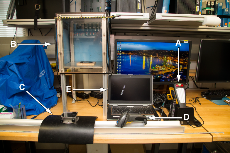
Figure F1. Olympus DeltaX pXRF.
Sample powders
The pXRF can also be used to quantitatively assess elemental abundances in powdered samples. Sample powder analyses were conducted using XRF powder mount assemblies, the use of which is outlined in detail in Reagan et al. (2015); a synoptic description of their use is included in the Appendix.
For both rock surface and powder measurements, a powder-mounted standard reference material (BHVO-2 was used during Expedition 366) should be analyzed with each set of unknowns to track instrument performance over time (Table T1). During Expedition 366, the total variation among individual measurements of the same sample was always well within the measurement uncertainties reported by the instrument and was often less than or equal to ±5%. Day-to-day variation in results for BHVO-2 indicated ±1% variability for higher precision elements and no worse than ±6.5% for trace elements over the course of the expedition (Table T2).
Table T1. Elemental abundance data for standard reference materials. Download table in CSV format.
Table T2. Precision and accuracy of pXRF determinations for BHVO-2. Download table in CSV format.
pXRF calibration of geologic materials
Although the Olympus pXRF presents data in concentration terminology (either parts per million or weight percent), it is important to recognize that these values are, for all practical purposes, merely intensity readings. It is necessary to calibrate the instrument against recognized standard reference materials for each element to be measured quantitatively (e.g., Ryan et al., 2017). During Expedition 366, calibration curves for the different elements measured via pXRF were determined using the same suite of standard reference materials used for inductively coupled plasma–atomic emission spectrometer (ICP-AES) analyses to improve inter-instrument data comparisons (Table T1). Powder mounts for each of the reference materials were analyzed to develop the working curves, as well as for periodic checks on instrument performance during pXRF measurements of unknowns. The working curves were developed in Microsoft Excel, and slope and intercept values from the working curves were used to calculate concentration results for unknowns (Figure F2). Both rock and powder samples were analyzed using powder-based working curves because past results indicated no differences in instrument performance between rocks and powders (Ryan et al., 2017; Reagan et al., 2015).
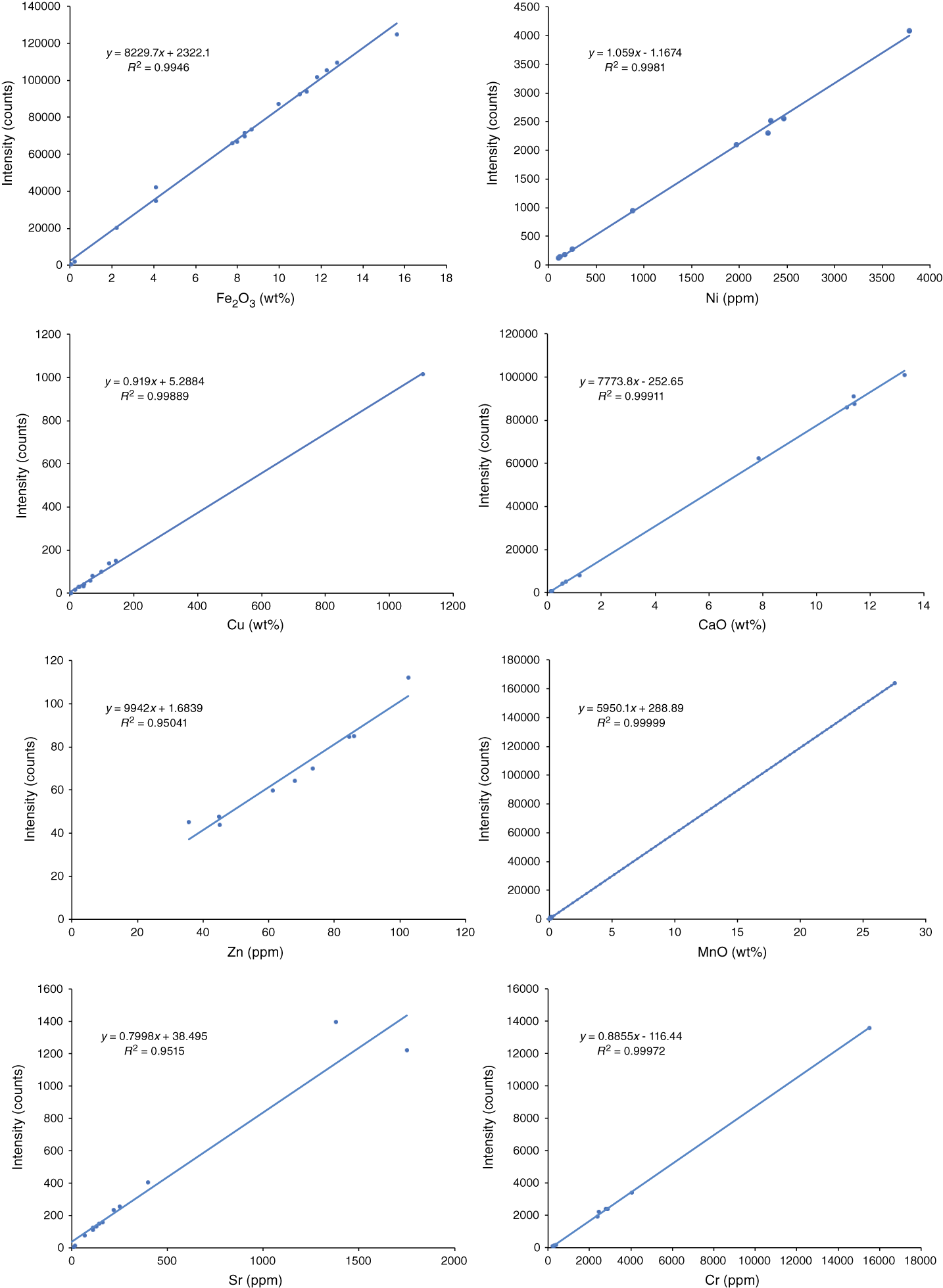
Figure F2. Calibration curves for elements quantitatively analyzed via pXRF.
The elements routinely measured via pXRF for quantitative determination during Expedition 366 were Ca, Mn, Fe (calibrated as oxides: CaO, MnO, and Fe2O3), Ni, Cr, Cu, Zn, and Sr. Ti, K and Rb, Zr, and V, which were analyzed quantitatively by pXRF during Expedition 352 (Reagan et al., 2015), were generally below pXRF detection limits in Expedition 366 materials. Sulfur was attempted, based on the possibility of gypsum in some recovered materials (see Igneous and metamorphic petrology and alteration in the Expedition 366 methods chapter [Fryer et al., 2018]), but an insufficient number of standards were available with sulfur data to produce a reasonable working curve. P, Co, As, Se, Y, Nb, Ag, Cd, Sn, Sb, Mo, W, Hg, Pb, Bi, Th, and U are all reported by the pXRF but were all below detection in our samples.
The pXRF instrument also collects and reports results for Mg, Al, and Si, elements that produce low-energy X-rays that are readily absorbed in air and so are not usually accessible via pXRF systems. We constructed correlation curves for these elements, and given the challenges regarding instrument sensitivity and reliability, the curves are surprisingly linear, albeit with comparatively poor correlation coefficients and nonzero intercepts (Figure F3). Although the instrument does not produce quantitative data for these elements, we could obtain “ballpark” results for Mg and Si using the correlation curves in Figure F3, which aided in petrographic identification of clast samples in the cores.
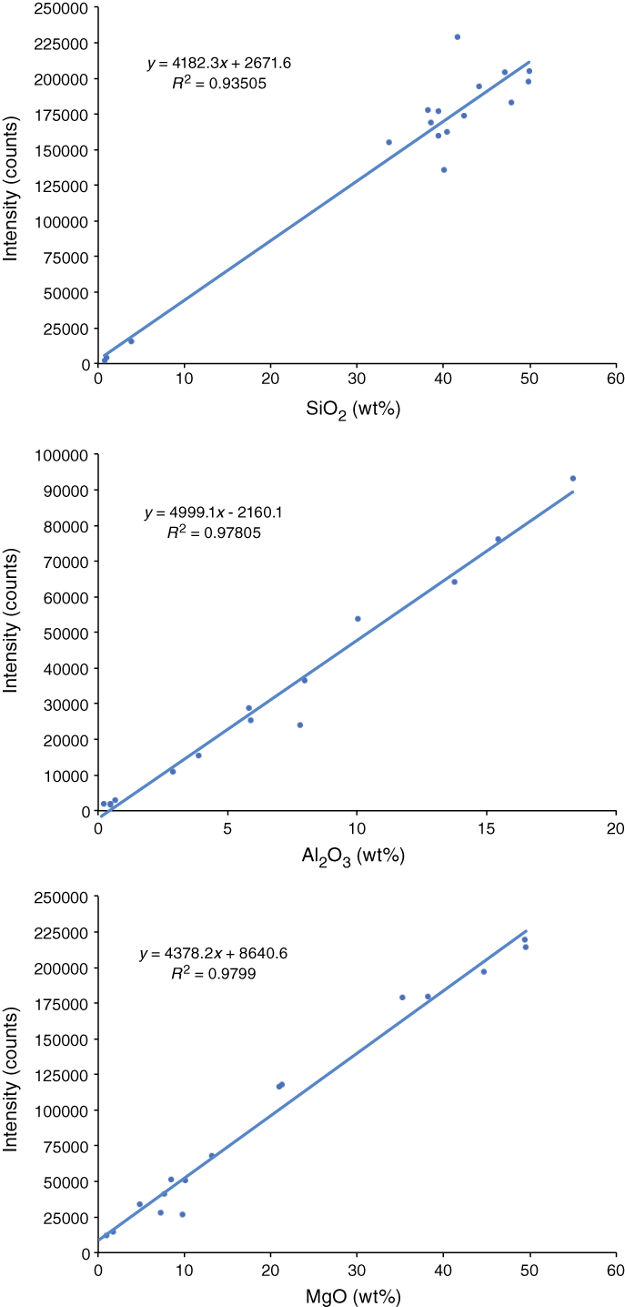
Figure F3. Correlation curves for Si, Al, and Mg.
Following the approaches taken during Expedition 352, we made interpretive quantitative use of pXRF data for those elements with curves with high correlation r values (>0.95) and good intercepts (Y intercept approximating 0); this information was recorded in the Laboratory Information Management System (LIMS) database. For species (like Si, Mg, and Al) that show scattered but linear correlations, we used the pXRF results to make first-cut estimates of material composition to inform our petrologic interpretations and decide on samples for ICP-AES analysis.
Recommendations for pXRF use and data correction/management
Aside from the protocols described above and in the Appendix, the following additional considerations may improve the quality of data collected, reduce the amount of time necessary to process raw data, and facilitate archiving of results for future use:
- The collection window on the “barrel” of the DeltaX pXRF handheld device should always be covered with a layer of 3525 Ultralene 0.16 mil (4 µm) film to prevent contamination/damage to the cover of the analyzer face.
- Data may not download from the analyzer or computer interface if the power supply is disrupted. In this case, disconnect the power supply from the unit, download all collected data, including both numerical results and spectrum files, to an external hard drive or to the shipboard server (Uservol) before proceeding. During Expedition 366, we stored (at a minimum) one copy of all data files on the instrument’s notebook PC as well as one copy on Uservol to ensure redundancy in the event of file loss, deletion, or corruption.
- The laboratory technician(s) tasked with pXRF support should upload data files for input to LIMS regularly because this allows other members of the scientific party (i.e., geochemists performing the ICP-AES analysis, core describers, etc.) access to the data, as well as further redundancy.
- When transferring data files from the instrument to an external computer for calibration, change the data file types from CSV (pXRF default) to TXT (basic text file). This allows manual identification of the column delimiters in the file; MS Excel does not identify them correctly in the CSV files.
Because the pXRF allows one to conduct large numbers of analyses very rapidly, managing and organizing these data becomes a major concern. During Expedition 352, more than 2000 pXRF measurements were conducted (Reagan et al., 2015), and during Expedition 366 more than 800 pXRF analyses were made. Our initial plan for using a single MS Excel spreadsheet for collection, storage, and processing of raw data in real time failed, as we quickly discovered that the amount of data generated outpaced the storage and calculation capabilities of a single spreadsheet. Therefore, careful attention needs to be paid at the beginning of an expedition to the amount of data likely to be gathered and how it will need to be managed and used. For Expedition 366, it was determined that maintaining separate spreadsheets for the following data was necessary, as follows:
- Calibration curves: several sets of working curves appropriate to the materials being analyzed may be necessary, and plots of these curves will need to be generated for publication.
- Raw data: a single master sheet was sufficient. Password protection is strongly recommended so that data cannot accidentally be lost or altered.
- Processed data and diagrams/plots/charts: we used a calculation spreadsheet into which raw pXRF data were pasted and then calibrated using the appropriate set of working curves. During Expedition 366, we maintained several such files, some tailored to the compositional character of the samples being measured, to more readily resolve our measurements on powders from in situ rock surface analyses.
Data from the pXRF system can be captured using the “Raw Data” MS Excel spreadsheet import function. When “File, Import…” is selected, a user prompt requests the import file type. Select “Text file,” find the appropriate pXRF DataExport file (files are named by date, such as “ExportData-XX-XX-20XX.txt” and “ExportSpm-XX-XX-20XX.txt”), and select “Get Data.” Delimiting with the “Tab,” “Comma,” and “Space” options selected was the format best suited for pulling in the raw pXRF results; however, this format may vary, depending on how the MS Excel data spreadsheet is designed.
Inductively coupled plasma–atomic emission spectrometry
Shipboard procedures for digestion of rocks and subsequent chemical analysis via ICP-AES have historically referred to Murray et al. (2000), which is based on the Jobin-Yvon ICP-AES system available on the R/V JOIDES Resolution at that time. Subsequently, the ICP-AES system on the JOIDES Resolution has been upgraded several times, most recently in 2017, and the technology of ICP-AES instrumentation has changed markedly. The most significant changes relate to wide adoption of Echelle monochromator systems for improved wavelength resolution and the use of high-sensitivity charge-coupled device (CCD)-based detector arrays. Together, these two advances improve sensitivity markedly and allow resolution and simultaneous quantitative analysis of many more optical wavelengths than was possible on such instruments in the past. Therefore, although some general information about ICP spectrophotometry and analytical practices in Murray et al. (2000) are still relevant, current ICP-AES technology affords greater flexibility and sensitivity for many elements of interest, along with new challenges related to these capabilities. Below are updates to protocols for sample preparation, ICP-AES calibration and analysis, and data reduction based on specific experiences during Expeditions 366 and 352, as well as broader experiences with this class of instrumentation (e.g., Ryan and Langmuir, 1987, 1993; Tenthorey et al., 1996; Savov et al., 2001, 2005; Peterson et al., 2009).
ICP-AES operation and elements analyzed
The shipboard ICP-AES is operated by JOIDES Resolution Science Operator (JRSO) shipboard geochemistry laboratory technicians, and JRSO laboratory technicians also handle sample powdering, oxidation/loss on ignition (LOI) determination, flux fusion digestion, and dissolution. However, the geochemistry technicians routinely seek guidance from the shipboard party geochemists in selecting calibration standards and check samples, setting up run queues, assaying data quality, and addressing questions regarding sample preparation, oxidation, and dissolution concerns. They may also seek assistance in making ICP sample dilutions if their workload on the other instruments in the laboratory is high.
Echelle monochromator/CCD-based ICP-AES detector systems allow analysts to select from a large menu of optical wavelengths for elements of interest (see Table T3 for examples) with very few instrument-related limitations on the number of different elements and/or optical wavelengths per element analyzed. For shipboard work, the primary constraint on which elements can be successfully measured by ICP-AES is the large dilution factor (4000:1) used for routine rock analysis. This degree of dilution is common for major element measurements via ICP-AES, and it is necessary to ensure that Si and Al (and during Expedition 366, Mg) are at low enough solution concentration levels to permit their measurement without detector saturation (see discussion below). A second benefit is that these dilute solutions produce less wear on the ICP torch and sample handling assembly, important for an instrument at sea where replacement parts and/or instrument servicing are unavailable. However, this high degree of dilution prevents the measurement of lower abundance elements, which either end up below the instrument detection limits or outside its linear dynamic range (on ICP-AES systems, this range typically begins at 10× the detection limit for the analytical wavelength in question; Potts, 1992). The elements that cannot be quantitatively measured by ICP-AES on the ship include geologically interesting species that occur at low parts per million levels in marine sediments and igneous rocks, as well as moderately higher abundance elements traditionally examined via ICP on more concentrated solutions (Nb, Be, Rb, Zn, Cu, Y, P, Ni, and Cr in mafic rocks and sediments; in Expedition 366 ultramafic samples K, Mn, and Ti). The menu of elements that can be measured successfully on the ship thus depends in part on the materials recovered. Because the ICP-AES will report results for elements that are outside their analytical ranges, it is necessary to calculate the practical limits of determination for the species being analyzed, based on measured instrument detection limits for the analytical lines selected (e.g., the lower limit of detection = 3× standard deviation of the blank; see Potts 1992), to identify those elements that will yield reliable results via ICP-AES on the ship.
Table T3. Example analytical wavelengths and detection limits. Download table in CSV format.
Sample preparation and LOI determination
Shipboard sample preparation and LOI determination procedures described in Murray et al. (2000) and updated in recent IODP Proceedings volumes (Reagan et al., 2015, for Expedition 352) are appropriate for a range of sediment and rock compositions, but care must be taken with unusual sample matrixes. In an example from Expedition 366, sample ignitions on carbonate-rich materials in quartz crucibles resulted in crucible devitrification because of reactions between quartz and carbonates. Alumina ceramic crucibles are less susceptible to such interactions and are thus probably more suitable for shipboard use on unknown matrixes. Although ignition temperatures of ~1000°C were acceptable for LOI determinations on the serpentinites and ultramafic materials recovered during Expedition 366, these high temperatures also resulted in sample sintering and/or sticking when the materials were more Si or Ca rich. Conversely, ignition temperatures of <850°C were inadequate to decompose carbonates, even if held at this temperature for several hours. Thus, heating samples to at least 900°C is advisable to ensure decomposition of all volatile-bearing phases and obtain reliable measures of LOI.
Sample powdering for ICP-AES analyses is commonly done using the shipboard tungsten carbide (WC) shatterbox system, which is effective for powdering a wide range of sample types but can contaminate for elements of geological interest such as W, Hf, Nb, and Ta. Also available on the JOIDES Resolution are several ball mill shakers with alumina ceramic mills, which cause fewer issues with sample contamination for trace elements. A number of recent expeditions have sought to make organized use of ICP sample powder residues to generate a single coherent elemental and isotopic data set for those samples analyzed on the ship (e.g., Reagan et al., 2015). This kind of coordinated analytical program can be facilitated by powdering samples in materials that will minimize issues with sample contamination but still permit the time-efficient powdering of samples for shipboard measurement.
Sample digestion and dilution procedures
Flux-fusion sample digestion using LiBO2 is the preferred means for shipboard sample dissolution and is widely utilized to digest silicate rocks of all types for dissolution in dilute acids (see Murray et al., 2000; Tenthorey et al., 1996; Potts, 1992; Klein et al., 1991; and others). This approach affords additional benefits for ICP-AES measurement because Li is a strong light emitter and, as such, can at concentrations >1000 ppm produce a strong positive light matrix that flattens the optical background and neutralizes sample matrix effects, a significant challenge in ICP-AES measurements (e.g., Murray et al., 2000; Potts, 1992). Although CCD detector systems help minimize issues with proper background correction, matrix enhancement effects are still a significant concern for the alkaline elements (in particular Na and K but also Mg and Ca). Even at a 4000:1 dilution factor, matrix-related problems with measurements can still occur if the samples being analyzed are compositionally very different from each other and/or from the standards used for instrument calibration. For example, analyzing basalts along with marine sediments using sediment and other higher-Si igneous rock standards for calibration will yield inaccurate information on Na and K in basalts, related to matrix effects associated with their different Si concentrations. A similar problem was evident during Expedition 366, when sediments or mafic igneous rocks were run along with serpentinites, which have very high Mg concentrations.
A time-efficient means for addressing this problem is the intentional use of Li as a peak enhancer in ICP-AES solutions. Addition of Li to the ≥1000 ppm level in solution creates a uniform optical matrix for all elements analyzed, swamping the effects of other high-abundance dissolved species (Si, Al, Fe Mg, Ca, and Na). One can generate such solutions using a Li-spiked HNO3 solution to dilute digested ICP-AES samples for analysis. As long as each sample has the same level of added Li, ensured by pipetting or weighing a constant amount of dilution acid, and that level is ≥1000 ppm Li, a strong uniform optical sample matrix can be maintained.
Analysis, calibration, and data reduction
ICP-AES data are corrected and calibrated externally using analyst-prepared drift and baseline correction solutions and solutions of geological reference samples as calibration standards. Baseline corrections are made using a procedural blank (i.e., a sample of fused and acidified LiBO2 flux otherwise prepared identically to the samples), whereas drift corrections are made with a drift monitor solution, commonly a rock or sediment of broadly similar composition to the unknowns being analyzed, prepared along with the samples and standards. Generally, at high analyte concentrations on ICP-AES instruments baseline corrections are a minimal concern, but drift correction is essential for reliable data. The drift monitor may be analyzed a dozen or more times during a typical analytical session, spaced evenly throughout to “bracket” the unknowns and standards. Commonly, one of the standard reference samples or another compositionally appropriate sample available in abundance is chosen to serve as a drift monitor. Alternatively, a mixed solution drawn from a number of the sample solutions being analyzed may be prepared.
Internal standard corrections
Data correction to an internal standard is commonly applied to shipboard ICP-AES results. The internal standard is an element that is optically similar to a large number of the species being analyzed but is of no analytical interest; it is added to all sample solutions. Ge and Y have both been commonly used as internal standards for shipboard analyses. The internal standard correction is done by generating a ratio of the intensities of analyte species to that of the internal standard for each measured sample. This correction is useful in addressing physical instrument performance variations (i.e., nonuniform sample input and/or temperature variations in the plasma). However, this correction can create complications for elements that are optically very different from the chosen standard. Thus, the alkali metals Na and K, which have analytical lines at the red/infrared end of the spectrum, are not normally corrected to internal standards.
Calibration standards
A wide range of standard reference materials are available on the JOIDES Resolution. At least six reference materials are prepared and used for calibration, although more are acceptable. During Expedition 366, eight standards were routinely included in analytical runs. Reference materials chosen as calibration standards need to be compositionally comparable to the unknowns being analyzed but at the same time provide a sufficient range in concentrations to permit calculation of reasonable calibration curves. For the unusual Mg-rich compositions of the Expedition 366 materials, six ultramafic reference materials (three peridotites, two serpentinites, and a komatiite) and two magnesian basalts were routinely used. Data for standard reference materials can be obtained from GeoReM (Govindaraju, 1994; Jochum et al., 2005; see Table T1). New reference materials, if necessary, can be requested before an expedition. It is also shipboard practice to include one or two “check standards” in every analytical run. The check standards, not used for calibration, are run as unknowns and can thus test the accuracy and reproducibility of ICP-AES data. Calibration standards can be run as check standards because their concentrations are known.
Data reduction
Raw results from the ICP-AES must be corrected and calibrated to generate concentration data. Historically, the raw results are uploaded into an MS Excel–based calibration spreadsheet, although newer instruments have built correction and calibration protocols into their operational software. The calibration spreadsheet in use during Expedition 366 prompted the user to identify sample type (blank, drift monitor, standard, check standard, or unknown) and, based on this information, completed all data corrections (internal standard, blank, and drift corrections, in that order). Calibration curves were generated from corrected data for each analyzed optical wavelength, with linear regression equations (including slope, y-intercept, and r values for quality of fit) for analyst review. Analysts select which calibrations to use for calculating the concentrations of unknowns. Concentration data are reported by element for each analyzed wavelength, and downhole plots of elemental abundances can be generated to compare results of the same element analyzed at different wavelengths.
Although JRSO laboratory technicians often conduct initial ICP data manipulations, these results are reviewed, revised, and approved by the shipboard geochemists. Baseline criteria for acceptable results include the following:
- Linear calibration curve that includes all of the standards run,
- Quality of fit (r) value of at least 0.99XX, and
- A y-intercept close to 0.
For elements showing relatively limited concentration ranges (e.g., Si, Mg, and Fe in the ultramafic rocks examined during Expedition 366), r values can be markedly reduced by a single spurious standard reading without impacting the slope or the intercept of the line. In such cases, the spurious standard reading can be removed from the correlation and the corrected array accepted.
A serious analytical problem that only becomes evident at the calibration stage is ICP-AES detector saturation. At higher analyte concentrations (typically 500–1000 ppm in solution, but for some elements as low as 50 ppm in solution), the detector response to increasing concentrations becomes nonlinear. This response looks like the intensity vs. concentration curve flattens above a certain abundance level (Figure F4; see also Figure F15 in the Expedition 366 methods chapter [Fryer et al., 2018] for examples of Na and Ca detector saturation during pore water analyses). Detector saturation is a concern for the highest abundance elements analyzed (Si, Al, and sometimes Mg for silicates or Ca for carbonates, but it can also occur when analyzing matrix-sensitive elements such as Na and K). A check for potential detector saturation problems involves calculating the likely solution concentrations of the higher abundance species in the different kinds of materials to be analyzed. If likely solution concentrations are >100 ppm at a 4000:1 dilution factor, then it may be necessary to vary from standard procedures and dilute samples further.
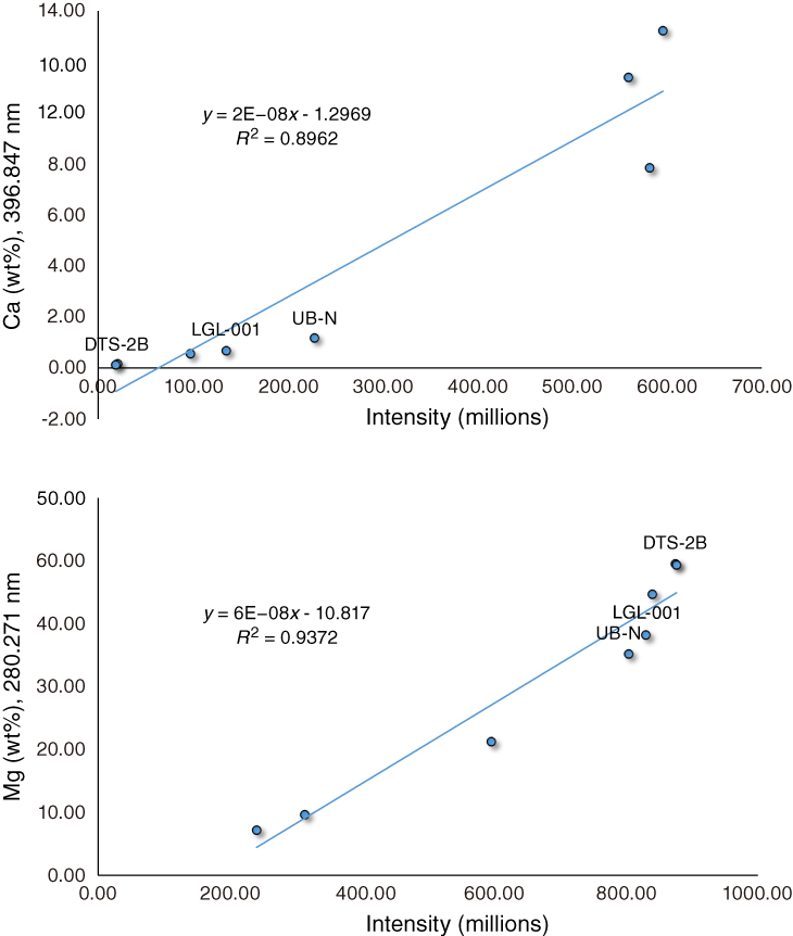
Figure F4. ICP-AES calibration curves for the Ca and Mg spectral lines.
Results of check standards provide estimates of precision and accuracy for each analytical run, as do comparisons among results from different wavelengths for a particular element. During Expedition 366, run-to-run relative standard deviation for the ICP-AES was generally ±1%–2% for major elements and ±5%–15% for trace elements. Accuracy was better than 2% for major elements and better than 5% for those trace elements above procedure detection limits.
Comparisons of pXRF and ICP-AES results
Direct comparisons of pXRF and ICP-AES measurements for quality assurance/quality control (QA/QC) purposes can be difficult to make because of the very different treatment of the samples. pXRF requires almost no sample preparation beyond a dry, flat surface, whereas samples for ICP-AES analysis must be powdered, ignited, and dissolved into a dilute acid solution for measurement. As demonstrated during Expedition 352 (Reagan et al., 2015; see Ryan et al., 2017, for an expanded comparative study), the shipboard sample type that afforded the best comparison of results was sample powders after being oxidized for LOI determinations that were dissolved for ICP-AES analysis and were analyzed directly on the pXRF.
Figure F5 compares ICP-AES and pXRF results on oxidized Expedition 366 sample powders for some of the elements that both instruments measured quantitatively. As discussed in Ryan et al. (2017), correlations between ICP-AES and pXRF data on the same samples, although linear, do not show 1:1 relationships because of the very different data correction and calibration protocols of the two instruments. In Figure F5, the better correlated species (Ca and Fe) intercept near zero, whereas most slopes are <1.0, particularly for those species near Fe, where Compton normalization strategies can be the most problematic.
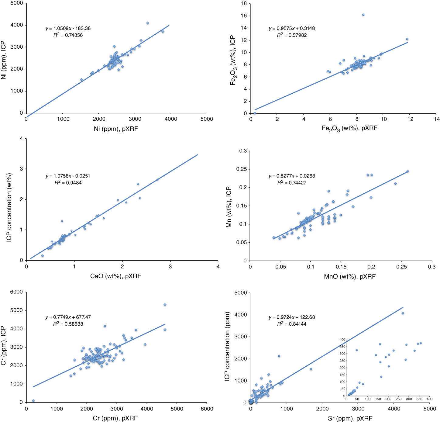
Figure F5. pXRF vs. ICP-AES data comparisons of Expedition 366 samples.
Also evident from Figure F5 is that several analyzed trace elements are not highly precise: Mn and Cr results both show considerable scatter. In the Sr data comparison, extensive scatter is evident at values >300 ppm Sr, with many of the ICP-AES measurements running to comparatively higher values. This lack of correlation at higher Sr concentrations likely relates to limitations in the calibration of ICP-AES measurements at higher Sr contents, as the highest Sr standard used on the ICP-AES is BHVO-1, (432 ppm Sr; Table T1). Samples that are markedly higher (and some Expedition 366 samples with >5000 ppm Sr were recovered) are outside the range of the Sr working curve, which means that large systematic errors related to small variations in working curve slope or intercept can occur. The pXRF calibration curve for Sr includes data for much higher Sr standards (Table T1; Figure F3) and is linear throughout this concentration range. As such, the pXRF likely produced more reliable measurements for Sr than the ICP-AES did during Expedition 366.
Shipboard rock analysis best practices
The shipboard pXRF and ICP-AES instruments offer different measurement capabilities for major and trace elements in the rocks recovered during Expeditions 366 and 352. The ICP-AES can measure more elements quantitatively than the pXRF, including all the key major elements. However, the pXRF can provide comparably precise (and on occasion more accurate) data for a subset of the elements routinely measured by ICP-AES, as well as reasonably precise data for several other trace elements (Zn, Cu, and Rb) that are not accessible by ICP-AES on the ship.
The biggest difference between these two different rock analysis tools relates to the time involved in acquiring results on unknowns. pXRF calibrations for quantitative measurements can be done at the beginning of an expedition using a suite of calibration standards to cover the entire likely range of sample compositions. These calibrations are robust: over the course of 1–2 months there is little variation in measurements on replicate samples (e.g., Reagan et al., 2015; Ryan et al., 2017; Table T2). The measurement of unknowns by pXRF is very quick (20+ samples require less than an hour to measure), and data calibration involves uploading raw data to a spreadsheet. By contrast, ICP-AES calibrations must be done in-run for each set of unknowns using new preparations of reference materials, and the time commitment required for measuring a set of unknowns, from sample powdering through fusion, dissolution, and analysis, is a week or more.
An effective combination of the pXRF and ICP-AES as analytical tools for rocks involves several strategies:
- Leveraging the quick exploration capabilities of the pXRF by using it to “ballpark” results on interesting core materials to identify samples to undergo ICP-AES analysis.
- Conducting pXRF measurements on the oxidized sample powder splits prepared for ICP-AES work, both to obtain results on some species that are inaccessible via ICP on the ship and to test concentrations on samples that yield unusual results on the ICP.
- Using the pXRF when the ICP-AES cannot be used. Because the pXRF is not sensitive to motion, it can gather sample data during transits when the ICP-AES cannot operate, and it can also measure samples recovered very late in an expedition when laboratory shutdown procedures make ICP-AES measurements impossible.
Despite improvements in its capabilities for low atomic number species, pXRF systems cannot replace the ICP-AES as the primary quantitative elemental analysis tool on the JOIDES Resolution. However, in combination the two instruments offer the means to conduct a more strategic and effective shipboard analytical program on all recovered solids.
References
Fryer, P., Wheat, C.G., Williams, T., Albers, E., Bekins, B., Debret, B.P.R., Deng, J., Dong, Y., Eickenbusch, P., Frery, E.A., Ichiyama, Y., Johnson, K., Johnston, R.M., Kevorkian, R.T., Kurz, W., Magalhaes, V., Mantovanelli, S.S., Menapace, W., Menzies, C.D., Michibayashi, K., Moyer, C.L., Mullane, K.K., Park, J.-W., Price, R.E., Ryan, J.G., Shervais, J.W., Sissmann, O.J., Suzuki, S., Takai, K., Walter, B., and Zhang, R., 2018. Expedition 366 methods. In Fryer, P., Wheat, C.G., Williams, T., and the Expedition 366 Scientists, Mariana Convergent Margin and South Chamorro Seamount. Proceedings of the International Ocean Discovery Program, 366: College Station, TX (International Ocean Discovery Program). https://doi.org/10.14379/iodp.proc.366.102.2018
Govindaraju, K., 1994. 1994 compilation of working values and sample description for 383 geostandards. Geostandards Newsletter, 18(1). https://doi.org/10.1111/j.1751-908X.1994.tb00502.x
Jochum, K.P., Nohl, U., Herwig, K., Lammel, E., Stoll, B., and Hofmann, A.W., 2005. GeoReM: a new geochemical database for reference materials and isotopic standards. Geostandards and Geoanalytical Research, 29(3):333–338. https://doi.org/10.1111/j.1751-908X.2005.tb00904.x
Klein, E.M., Langmuir, C.H., and Staudigel, H.S., 1991. Geochemistry of basalts from the SE Indian Ridge, 115°–138°. Journal of Geophysical Research: Solid Earth, 96(B2):2089–2108. https://doi.org/10.1029/90JB01384
Murray, R.W., Miller, D.J., and Kryc, K.A., 2000. Technical Note 29: Analysis of Major and Trace Elements in Rocks, Sediments, and Interstitial Waters by Inductively Coupled Plasma–Atomic Emission Spectrometry (ICP-AES). Ocean Drilling Program. https://doi.org/10.2973/odp.tn.29.2000
Peterson, V.L., Ryan, J.G., and the 1997–1998 REU Site Program Participants, 2009. Petrogenesis and structure of the Buck Creek mafic-ultramafic suite, southern Appalachians: constraints on ophiolite evolution and emplacement in collisional orogens. Geological Society of America Bulletin, 121(3–4):615–629. https://doi.org/10.1130/B26302.1
Potts, P.J., 1992. A Handbook of Silicate Rock Analysis: New York (Springer US). https://doi.org/10.1007/978-1-4615-3270-5
Reagan, M.K., Pearce, J.A., Petronotis, K., Almeev, R., Avery, A.A., Carvallo, C., Chapman, T., Christeson, G.L., Ferré, E.C., Godard, M., Heaton, D.E., Kirchenbaur, M., Kurz, W., Kutterolf, S., Li, H.Y., Li, Y., Michibayashi, K., Morgan, S., Nelson, W.R., Prytulak, J., Python, M., Robertson, A.H.F., Ryan, J.G., Sager, W.W., Sakuyama, T., Shervais, J.W., Shimizu, K., and Whattam, S.A., 2015. Expedition 352 methods. In Reagan, M.K., Pearce, J.A., Petronotis, K., and the Expedition 352 Scientists, Izu-Bonin-Mariana Fore Arc. Proceedings of the International Ocean Discovery Program, 352: College Station, TX (International Ocean Discovery Program). http://dx.doi.org/10.14379/iodp.proc.366.102.2015
Reagan, M.K., Pearce, J.A., Petronotis, K., Almeev, R., Avery, A.A., Carvallo, C., Chapman, T., Christeson, G.L., Ferré, E.C., Godard, M., Heaton, D.E., Kirchenbaur, M., Kurz, W., Kutterolf, S., Li, H., Li, Y., Michibayashi, K., Morgan, S., Nelson, W.R., Prytulak, J., Python, M., Robertson, A.H.F., Ryan, J.G., Sager, W.W., Sakuyama, T., Shervais, J.W., Shimizu, K., and Whattam, S.A., 2017. Subduction initiation and ophiolite crust: new insights from IODP drilling. International Geology Review, 59(11):1439–1450. https://dx.doi.org/10.1080/00206814.2016.1276482
Reynolds, R.C., Jr., 1963. Matrix corrections in trace element analysis by X-ray fluorescence: estimation of the mass absorption coefficient by Compton scattering. American Mineralogist, 48:1133–1143. http://www.minsocam.org/ammin/AM48/AM48_1133.pdf
Ryan, J.G., and Langmuir, C.H., 1987. The systematics of lithium abundances in young volcanic rocks. Geochimica et Cosmochimica Acta, 51(6):1727–1741. http://dx.doi.org/10.1016/0016-7037(87)90351-6
Ryan, J.G., and Langmuir, C.H., 1993. The systematics of boron abundances in young volcanic rocks. Geochimica et Cosmochimica Acta, 57(7):1489–1498. https://doi.org/10.1016/0016-7037(93)90008-K
Ryan, J.G., Shervais, J.W., Li, Y., Reagan, M.K., Li, H.Y., Heaton, D., Godard, M., et al., 2017. Application of a handheld X-ray fluorescence spectrometer for real-time, high-density quantitative analysis of drilled igneous rocks and sediments during IODP Expedition 352. Chemical Geology, 451:55–66. https://doi.org/10.1016/j.chemgeo.2017.01.007
Savov, I., Ryan, J.G., Haydoutov, I., and Schijf, J., 2001. Late Precambrian Balkan-Carpathian ophiolite—a slice of the Pan-African ocean crust?: geochemical and tectonic insights from the Tcherni Vrah and Deli Jovan massifs, Bulgaria and Serbia. Journal of Volcanology and Geothermal Research, 110(3–4):299–318. https://doi.org/10.1016/S0377-0273(01)00216-5
Savov, I.P., Ryan, J.G., D’Antonio, M., Kelley, K., and Mattie, P.D., 2005. Geochemistry of serpentinized peridotites from the Mariana Forearc Conical Seamount, ODP Leg 125: implications for the elemental recycling at subduction zones. Geochemistry, Geophysics, Geosystems, 6(6):Q04J15. https://doi.org/10.1029/2004GC000777
Tenthorey, E.A., Ryan, J.G., and Snow, E.A., 1996. Petrogenesis of sapphirine-bearing metatroctolites from the Buck Creek ultramafic body, southern Appalachians. Journal of Metamorphic Geology, 14(2):103–114. https://onlinelibrary.wiley.com/doi/abs/10.1046/j.1525-1314.1996.05793.x
van Sprang, H.A., 2000. Fundamental parameter methods in XRF spectroscopy. Advances in X-ray Analysis, 42:1–10. http://www.icdd.com/resources/axa/vol42/v42_01.pdf
Appendix
Sample selection protocols and Olympus pXRF operations procedures as used during Expedition 366.
Please note, per Texas A&M University and JRSO guidelines, anyone using the pXRF handheld system must wear a radiation ring or other approved radiation monitoring device at all times during sample analysis.
Sample selection protocols
Use the following guidelines for selecting samples for pXRF analysis:
- Adequate size for analysis (~4 cm2 or greater sample surface is required, given the ~7–8 mm pXRF excitation diameter).
- Sufficient spacing within the core to characterize observed variation (i.e., changes in lithology, differences in grain size/texture/color, proximity to zones of alteration, and/or other distinguishing features), but not too many locations, which would generate numerous redundant measurements within the same interval.
- Suitably flat surface (cut surface preferred).
- Dry surface to optimize X-ray penetration. Wet surfaces were dried with absorptive material (e.g., Kimwipes) to improve signal penetration depth.
Documentary information, including the Expedition, Site, Hole, date, run number, core and section, measurement type, position within the core (offset), time of measurement, operator, and any other comments, were recorded on the pXRF laboratory notebook for later use in describing the samples and/or reproducing the measurements.
pXRF operation
The Olympus Delta instrument is operated from a notebook PC (Dell XRF host) on which the Delta Advanced PC operating software for the pXRF is loaded. A detailed user manual for the instrument is available for reference from the X-ray technician aboard the JOIDES Resolution.
- Before initial use and approximately every 10 h or once per shift, perform a calibration check by placing the handheld unit in its storage cradle and selecting the “CalCheck” icon at the bottom left-hand corner of the “Analysis” screen. Calibration checks should be run before any sample analyses are attempted.
- If the calibration checks are successful, place samples, smooth side down, on the excitation window within the shielded assembly, or mount the analyzer and shielded core sleeve over the core on the sample to be analyzed.
- Enter information about the specific sample into the computer by selecting the “…” tab (Figure F2), which shifts the software into “Setup” mode. Enter the run number (these are sequential for the length of the expedition, regardless of date, time, core, hole, etc.), sample name (or scan the core’s bar code on the cap of the D tube with the “Symbol” bar code scanner), and the sample offset (distance from the top of the section, in cm). The “Text_ID” field is populated and saved by the software automatically.
- Select “Save,” followed by “Back,” which returns the software to the “Analysis” screen.
- Press “Start” at the bottom of the screen to begin the analysis. During Expedition 366, all samples were measured manually for 60 s, with three measurements per unknown (three spots on a sample surface, or three repeat analyses on sample powders) constituting a single analysis.
pXRF powder mount preparation
A supply of reusable pXRF plastic powder mounts are maintained on the JOIDES Resolution. The mount consists of a short (~1 cm) plastic cylinder and ring-caps that snap together on either side.
- Cover one end of the cylindrical mount with a short length of Ultralene 4 µm film. Use the plastic ring-cap to secure the Ultralene in place and produce a smooth, transparent surface onto which sample powders can be loaded.
- Load at least a 2–3 mm layer of sample powder onto the Ultralene, backed by a small circle of filter paper (Whatman 24 mm circles, grade 540) and either a round 24 mm plastic foam spacer (like those used to fill the gaps in sediment cores left by sampling) or plastic floss packing to hold the sample powder in place, followed by the snap-on sealing cap.
- Place the transparent surface of the mount face-down in the shielded XRF sample holder for analysis of the powder.
- Sample powders used for pXRF can be recovered for other uses when mounts are taken apart for cleaning and reuse.
1 Johnston, R.M., Ryan, J.G., and the Expedition 366 Scientists, 2018. pXRF and ICP-AES characterization of shipboard rocks and sediments: protocols and strategies. In Fryer, P., Wheat, C.G., Williams, T., and the Expedition 366 Scientists, Mariana Convergent Margin and South Chamorro Seamount. Proceedings of the International Ocean Discovery Program, 366: College Station, TX (International Ocean Discovery Program). https://doi.org/10.14379/iodp.proc.366.110.2018
2 Expedition 366 Scientists’ addresses.
This work is distributed under the Creative Commons Attribution 4.0 International (CC BY 4.0) license. 
pXRF and ICP-AES characterization of shipboard rocks and sediments
PDF Download figures Download tables Cited by