Fryer, P., Wheat, C.G., Williams, T., and the Expedition 366 Scientists
Proceedings of the International Ocean Discovery Program Volume 366
publications.iodp.org
https://doi.org/10.14379/iodp.proc.366.102.2018

Expedition 366 methods1
P. Fryer, C.G. Wheat, T. Williams, E. Albers, B. Bekins, B.P.R. Debret, J. Deng, Y. Dong, P. Eickenbusch, E.A. Frery, Y. Ichiyama, K. Johnson, R.M. Johnston, R.T. Kevorkian, W. Kurz, V. Magalhaes, S.S. Mantovanelli, W. Menapace, C.D. Menzies, K. Michibayashi, C.L. Moyer, K.K. Mullane, J.-W. Park, R.E. Price, J.G. Ryan, J.W. Shervais, O.J. Sissmann, S. Suzuki, K. Takai, B. Walter, and R. Zhang2
Keywords: International Ocean Discovery Program, IODP, JOIDES Resolution, Expedition 366, Site 1200, Site U1491, Site U1492, Site U1493, Site U1494, Site U1495, Site U1496, Site U1497, Site U1498, Mariana, Asùt Tesoru Seamount, Conical Seamount, Fantangisña Seamount, South Chamorro Seamount, Yinazao Seamount, Cretaceous seamount, subduction, subduction channel, forearc, seismogenic zone, mud volcano, fluid discharge, serpentinite, carbonate, harzburgite, clasts, ultramafic rock, breccia, gypsum, mudstone, chert, reef limestone, volcanic ash, guyot, CORK, CORK-Lite, screened casing
MS 366-102: Published 7 February 2018
Introduction
This chapter documents the procedures and methods employed in the various shipboard laboratories on the research vessel (R/V) JOIDES Resolution during International Ocean Discovery Program (IODP) Expedition 366. This information applies only to shipboard work described in the Expedition Reports section of the Expedition 366 Proceedings of the International Ocean Discovery Program volume. Methods used by investigators for shore-based analyses of Expedition 366 data will be described in separate publications. This introductory section provides an overview of operations, curatorial conventions, depth scale terminology, and general core handling and analyses.
Site locations
The ship’s GPS system was used to position the vessel at site locations determined from pre-expedition site surveys, submersible dives, and short core locations. A SyQuest Bathy 2010 compressed high-intensity radar pulse (CHIRP) subbottom profiler was used to monitor seafloor depth on the approach to each site to confirm the depth profiles from pre-expedition surveys. In areas of steep seafloor slopes, this depth is often shallower than the actual depth at the site because the radar pulse widens with depth and can reflect from shallower parts of the seafloor not directly underneath the ship. Once the vessel was positioned at a site, the thrusters were lowered and a positioning beacon was dropped to the seafloor (Figure F1). Dynamic positioning control of the vessel used navigational input from the GPS system and triangulation to the seafloor beacon, weighted by the estimated positional accuracy. The final hole position was the mean position calculated from the GPS data collected over a significant time interval.

Figure F1. IODP conventions for coring operations.
Coring and drilling operations
All four standard coring systems, the advanced piston corer (APC), half-length APC (HLAPC), extended core barrel (XCB), and rotary core barrel (RCB) systems, were used during Expedition 366. The APC system was used in the upper portion of each hole to obtain high-quality core. The APC system cuts soft-sediment cores with minimal coring disturbance relative to other IODP coring systems (Figure F2). After the APC core barrel is lowered through the drill pipe and lands near the bit, the drill pipe is pressured up until the two shear pins that hold the inner barrel attached to the outer barrel fail. The inner barrel then advances into the formation and cuts the core. The driller can detect a successful cut, or “full stroke,” from the pressure gauge on the rig floor.
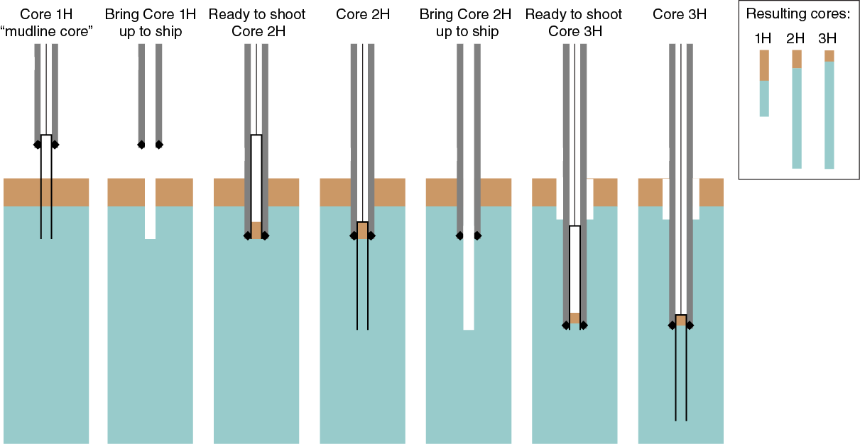
Figure F2. APC coring sequence for the first three cores.
APC refusal is conventionally defined in two ways: (1) the piston fails to achieve a complete stroke (as determined from the pump pressure reading) because the formation is too hard, or (2) excessive force (>60,000 lb; ~267 kN) is required to pull the core barrel out of the formation. When a full stroke cannot be achieved, additional attempts are typically made, and after each attempt, the bit is advanced by the length of core recovered. Note that this results in a nominal recovery of ~100% based on the assumption that the barrel penetrates the formation by the equivalent of the length of core recovered. Many of the Expedition 366 APC and HLAPC cores did not achieve full stroke, especially in the unconsolidated but low-porosity serpentinite muds. In some cases, we proceeded using “advance-by-recovery,” starting the next core assuming the recovered length was a good measure of penetration. More often, we drilled down to the base of what would have been a full HLAPC stroke using an XCB core barrel; cores collected in this way were labeled as ghost cores, and their depth was assigned to be within the bottom part of the drilled interval. The number of additional attempts at coring without full stroke was generally dictated by the length of recovery of the partial stroke core and the time available to advance the hole by piston coring.
The APC system contains a 9.5 m long core barrel. The recently engineered HLAPC coring system uses a 4.7 m long core barrel. In most instances, the HLAPC system is deployed after the APC reaches refusal. During Expedition 366, the HLAPC system was used in preference to the APC system because of the greater risk of bending the APC core barrel, as happened with the first Hole U1493A core. When using the HLAPC system, the same criteria were applied in terms of refusal as for the APC system. Use of this new technology allowed for significantly greater continuous APC sampling depths to be attained than would have otherwise been possible. Often during Expedition 366, the APC system could not adequately penetrate the serpentinite mud formations, resulting in poor recovery and ruptured core liners that severely damaged the core that was recovered. As a result, we mostly used the HLAPC system.
Nonmagnetic core barrels were initially used during conventional APC and HLAPC coring, up to a pull force of ~40,000 lb (note that nonmagnetic core barrels were used for all coring systems except where noted). After the first site (U1491) and the loss of the bottom-hole assembly (BHA), APC cores were not oriented because of risk of damage to the Icefield MI-5 core orientation tool and the need to preserve the available BHA for the next IODP expedition, which required paleomagnetic data. Formation temperature measurements were made with the advanced piston corer temperature tool (APCT-3) to obtain temperature measurements from which gradients and heat flow were calculated (see Downhole measurements).
The XCB system is used to advance the hole when APC refusal occurs before the target depth is reached or when the formation becomes either too stiff for APC coring or hard substrate is encountered. The XCB system is a rotary system with a small cutting shoe (bit) that extends below the large APC/XCB bit. The smaller bit can cut a semi-indurated core with less torque and fluid circulation than the main bit and thus optimizes recovery. The XCB cutting shoe extends ~30.5 cm ahead of the main bit in soft sediment but retracts into the main bit when hard formations are encountered. The XCB system was used with moderate success, although HLAPC coring was preferred.
The BHA is the lowermost part of the drill string. A typical APC/XCB BHA consists of a drill bit (outer diameter = 11⁷⁄₁₆ inches), a bit sub, a seal bore drill collar, a landing saver sub, a modified top sub, a modified head sub, a nonmagnetic drill collar (for APC/XCB coring), a number of 8¼ inch drill collars, a tapered drill collar, six joints (two stands) of 5½ inch (~13.97 cm) drill pipe, and one crossover sub. The nonmagnetic drill collar was replaced with a regular (magnetic) drill collar after breaking off the lower part of the BHA in Hole U1491C.
The RCB system is deployed when deeper penetration in consolidated rocks is expected. During Expedition 366, the RCB system was only employed at the last site (U1498). The RCB system requires a dedicated RCB BHA and bit. The BHA used for RCB coring included a 9⅞ inch RCB drill bit, a mechanical bit release (used when wireline logging is planned), a modified head sub, an outer core barrel, a modified top sub, and 7–10 control-length drill collars followed by a tapered drill collar to the two stands of 5½ inch drill pipe. Most cored intervals are ~9.7 m long, which is the length of a standard rotary core and approximately the length of a joint of drill pipe. In some cases, the drill string is drilled or “washed” ahead without recovering sediment to advance the drill bit to a target depth to resume core recovery. Such intervals are typically drilled using a center bit installed within the RCB bit.
Core handling and analysis
Recovered cores were extracted from the core barrel in plastic liners (62 mm inner diameter; 67 mm outer diameter. These liners were carried from the rig floor to the core processing area on the catwalk outside the core laboratory, where they were split into ~1.5 m long sections (Figures F1, F3). Liner caps (blue = top, colorless = bottom, and yellow = whole-round sample taken) were glued with acetone onto liner sections on the catwalk by the IODP Core Technicians. The length of each section was entered into the database as “created length” using the Sample Master application. This length measurement was used to calculate core recovery.
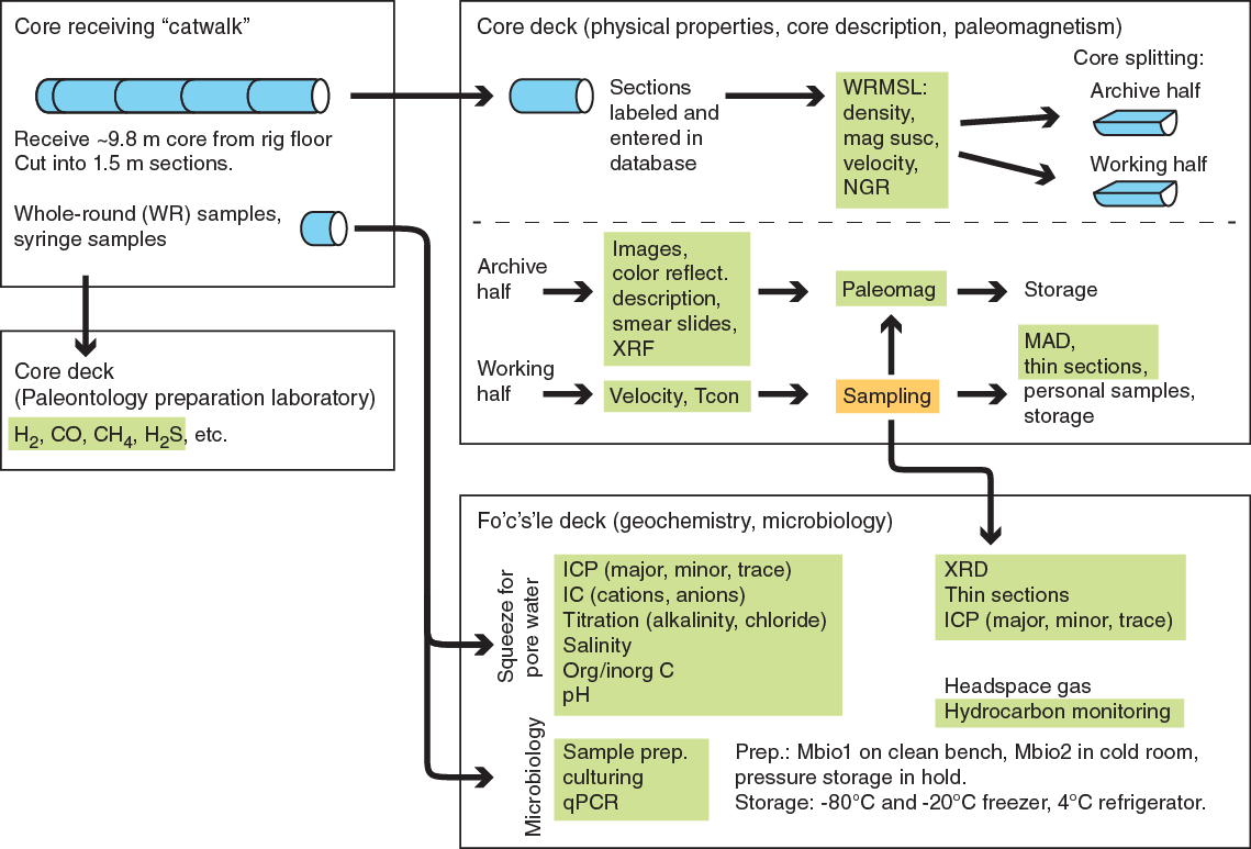
Figure F3. General pattern of recovered material from the core receiving area on the catwalk through the laboratories.
As soon as cores arrived on deck, “headspace” samples were taken either by using a syringe in soft formations or taking chips of harder material for immediate hydrocarbon analysis as part of the shipboard safety and pollution prevention program. Further syringe samples were immediately taken from the ends of some cut sections for analysis of dissolved gases such as H2, CH4, and H2S. In cores where gas was already coming out of solution, holes were drilled in the liner and gases were sampled directly. Whole-round samples were taken from core sections for shipboard and postexpedition interstitial water and microbiological analyses (see Fluid geochemistry and Microbiology) (Figure F3). No core catcher samples were taken for biostratigraphic analysis because microfossils are not found in erupted serpentinite muds.
Core sections were then placed in core racks in the laboratory. When the cores reached equilibrium with laboratory temperature (typically after ~4 h), whole-round core sections were run through the Whole-Round Multisensor Logger (WRMSL; measuring P-wave velocity, density, and magnetic susceptibility) and the Natural Gamma Radiation Logger (NGRL). Thermal conductivity measurements were typically taken at a rate of approximately one per core (see Physical properties). The core sections were then split lengthwise from bottom to top into working and archive halves. After initial experimentation with the wire cutter used for typical soft sediments and spatulas used for stiff sediments, the clast-bearing serpentinite muds proved to be better suited to be split with the diamond-impregnated saw.
The working half of each sedimentary core was sampled for shipboard physical property, paleomagnetic, and geochemical analyses. Personal sampling of soft matrix muds for postexpedition analyses then took place at the sample table. Personal sampling of hard rock clasts took place daily after the midday crossover meeting after all of the scientists had a chance to view the cores. The archive half of all cores was scanned on the Section Half Imaging Logger (SHIL) and measured for color reflectance and magnetic susceptibility on the Section Half Multisensor Logger (SHMSL). At the same time, the archive halves were described visually and by means of smear slides and thin sections. All observations were recorded in the Laboratory Information Management System (LIMS) database using DESClogik, a descriptive data capture application. After visual description, the archive halves were run through the cryogenic magnetometer.
Both halves of the core were put into labeled plastic tubes that were sealed and transferred to cold storage aboard ship. At the end of the expedition, the cores remained on board for the next 2 month expedition before being transported to permanent cold storage at the Kochi Core Center (KCC) at Kochi University (Japan). The delay was due to construction work at KCC.
Drilling disturbance
Cores may be significantly disturbed as a result of the drilling process and may contain extraneous material as a result of the coring and core handling processes. Several types of disturbance were encountered during the expedition. Material from intervals higher in the hole may be washed down by drilling circulation, accumulate at the bottom of the hole, and be sampled with the next core (Figure F2). The uppermost 10–50 cm of each core was examined critically during description for potential “fall-in” or other coring deformation. Common coring-induced deformation includes the concave-downward appearance of originally horizontal bedding. Piston action may result in fluidization (“flow-in” or “suck-in”) of unlithified sediment, apparent as tube-parallel banding or concave-downward bending. This most often occurs at the bottom of APC cores but can occur anywhere in a core. Some Expedition 366 cores contain fining-upward sequences of coarse to fine gravel without matrix. These sequences were probably caused by rock pieces ground up by the drilling process that were incompletely flushed up out of the hole before falling to the base of the hole, with the larger pieces settling first, resulting in an apparent graded bed. Multiple sequences of such grading can form when sea state is especially high because the drill string rises and lowers in the hole.
Retrieval from depth to the surface may result in elastic rebound. Gas that is in solution at depth may become free and drive apart intervals of recovered material within the liner. Both elastic rebound and gas pressure can result in a total length for each core that is longer than the interval cored, resulting in a calculated recovery of >100%. If gas expansion or other coring disturbance results in a void in any particular core section, the void was closed by moving material. If material could not be moved, then the void was identified by a foam insert. When gas content is high, pressure must be relieved by drilling holes into the liner for safety reasons before the cores are cut into segments. These disturbances are described in the Lithostratigraphy section in each site chapter and are graphically indicated on the core summary graphic reports (visual core descriptions [VCDs]).
Curatorial procedures
Numbering of sites, holes, cores, and samples follows standard IODP procedure. Drilling sites are numbered consecutively from the first site drilled by the drilling vessel (D/V) Glomar Challenger in 1968. Integrated Ocean Drilling Program (ODP) Expedition 301 began using the prefix “U” to designate sites occupied by the JOIDES Resolution. For all IODP drill sites, a letter suffix distinguishes each hole drilled at the same site. The first hole drilled is assigned the site number modified by the suffix “A,” the second hole the site number and the suffix “B,” and so on.
Cores taken from a hole are numbered sequentially from the top of the hole downward (Figure F1). Cores taken with the APC system are designated with “H” (APC) or “F” (HLAPC), “X” designates XCB cores, and “R” designates RCB cores. “G” designates ghost cores that are collected while washing down through a previously drilled portion of a hole with a core barrel in place or in a cased borehole where material ascends the base of the casing string. The core barrel is then retrieved prior to coring the next interval. Core numbers and their associated cored intervals are unique in a given hole.
Generally, maximum recovery for a single core is 9.5 m of sediment (APC; 4.7 m for HLAPC) or 9.7 m of rock or sediment (XCB/RCB) contained in a plastic liner (6.6 cm internal diameter) plus an additional ~0.2 m in the core catcher, which is a device at the bottom of the core barrel that prevents the core from sliding out when the barrel is retrieved from the hole. In certain situations, recovery may exceed the 9.5 or 9.7 m maximum. In soft material, this is normally caused by core expansion resulting from depressurization or gas-induced expansion. High heave, tidal changes, and overdrilling can also result in an advance that differs from the planned 9.5/9.7 m.
Recovered cores are divided into 1.5 m sections that are numbered serially from the top downcore. When full recovery is obtained, the sections are numbered 1–7 (or 1–3 for HLAPC) with the last section usually being <1.5 m. Rarely, an unusually long core may require more than seven sections. When the recovered core is shorter than the cored interval, by convention the top of the core is deemed to be located at the top of the cored interval for the purpose of calculating (consistent) depths. Samples and descriptions of cores are designated by distance measured in centimeters from the top of the section to the top and bottom of each sample or interval. In unconsolidated cores, the core catcher section is treated as a separate section (CC). When the only recovered material is in the core catcher, it is placed at the top of the cored interval.
A full curatorial sample identifier consists of the following information: expedition, site, hole, core number, core type, section number, and interval in centimeters measured from the top of the core section. For example, a sample identification of “366-U1492A-2H-5, 80–85 cm,” represents a sample taken from the interval between 80 and 85 cm below the top of Section 5 of Core 2 (collected using the APC system) of the first hole (Hole A) of Site U1492 during Expedition 366 (Figure F1).
Sample depth calculations
For a complete description of depths, see IODP Depth Scales Terminology, v.2 (http://www.iodp.org/policies-and-guidelines). The primary depth scale types are based on the measurement of the drill string length deployed beneath the rig floor (drilling depth below rig floor [DRF] and drilling depth below seafloor [DSF]), the length of each core recovered (core depth below seafloor [CSF] and core composite depth below seafloor [CCSF]), and the length of the logging wireline deployed (wireline log depth below rig floor [WRF], wireline log depth below seafloor [WSF], and wireline log matched depth below seafloor [WMSF]). All units are in meters. Depths of samples and measurements are calculated at the applicable depth scale either by fixed protocol (e.g., CSF) or by combinations of protocols with user-defined correlations (e.g., CCSF). The definition of these depth scale types and the distinction in nomenclature should keep the user aware that a nominal depth value at two different depth scale types might not refer to exactly the same stratigraphic interval in a hole.
Depths of cored intervals are measured from the drill floor based on the length of drill pipe deployed beneath the rig floor (DRF scale). The depth of the cored interval is referenced to the seafloor (DSF scale) by subtracting the seafloor depth at the time of the first hole from the DRF depth of the interval. In most cases, the seafloor depth is the length of pipe deployed minus the length of the mudline core recovered. However, some seafloor depths can be determined in another manner (e.g., by offset from a previous known measurement of depth or by observing the bit tag the seafloor with the camera system).
Standard depths of cores in meters below the seafloor (CSF-A scale) are determined based on the assumption that (1) the top depth of a recovered core corresponds to the top depth of its cored interval (DSF scale) and (2) the recovered material is a contiguous section even if core segments are separated by voids when recovered. When possible, voids in the core are closed by pushing core segments together on the catwalk during core handling. This convention is also applied if a core has incomplete recovery, in which case the true position of the core within the cored interval is unknown and should be considered a sample depth uncertainty, up to the length of the core barrel used, when analyzing data associated with the core material. Standard depths of samples and associated measurements (CSF-A scale) are calculated by adding the offset of the sample or measurement from the top of its section and the lengths of all higher sections in the core to the top depth of the cored interval.
A soft to semisoft sediment core from less than a few hundred meters below seafloor expands upon recovery (typically a few percent to as much as 15%), so the length of the recovered core often exceeds that of the cored interval. Therefore, a stratigraphic interval may not have the same nominal depth at the DSF and CSF scales in the same hole. When core recovery (the ratio of recovered core to cored interval times 100%) is >100%, the CSF depth of a sample taken from the bottom of a core will be deeper than that of a sample from the top of the subsequent core (i.e., the data associated with the two core intervals overlap at the CSF-A scale).
Cored intervals are defined by the core top depth in DSF and the distance the driller advanced the bit and/or core barrel in meters. The length of the core is defined by the sum of lengths of the core sections. The CSF depth of a sample is calculated by adding the offset of the sample below the section top and the lengths of all higher sections in the core to the core top depth measured with the drill string (DSF). During Expedition 366, all core depths below seafloor were calculated according to the core depth below seafloor Method A (CSF-A) depth scale. This calculated depth has units of meters below seafloor (mbsf).
Screened casing deployments
Deployment of 10.75 inch diameter screened casing at three sites during the expedition was accomplished using the drill-in method to target depths between 110 and 220 mbsf. The casing infrastructure included a reentry cone and a remotely operated vehicle (ROV) landing platform, with the objective that these holes can be revisited by future (non-IODP) research expeditions for deployment of borehole fluid samplers, instruments to monitor temporal changes in serpentinite mud volcanism, and manipulative experiments. Details of the casing strings and casing operations are given in the Operations sections of the Site U1492 chapter, the Site U1496 chapter, and the Site U1497 chapter (Fryer et al., 2018a, 2018b, 2018c).
Lithostratigraphy
The lithology of sediment recovered during Expedition 366 was primarily determined using observations based on visual (macroscopic) core descriptions, smear slides, thin sections, and occasional use of the scanning electron microscope. In some cases, digital core imaging, color reflectance spectrophotometry, and magnetic susceptibility analysis provided complementary discriminative information. The methods employed during this expedition were similar to those used during IODP Expedition 352 (Reagan et al., 2015b) and supplemented by methods used during ODP Legs 125 and 195 (Shipboard Scientific Party, 1990, 2002b).
We used the DESClogik application to record and upload descriptive data into the LIMS database (see the DESClogik user guide at https://iodp.tamu.edu/labs/documentation). Spreadsheet templates were set up in DESClogik and customized for Expedition 366 before the first core arrived on deck. The templates were used to record visual core descriptions and microscopic data from smear slides and thin sections, which in turn helped to quantify the texture and relative abundance of biogenic and nonbiogenic components.
Because of the unusual nature of serpentinite mud volcano deposits, which are sequential mudflow deposits that incorporate clasts of mantle peridotites, metavolcanic rocks, volcanic rocks, various types of limestone, chert, and fault rocks, we adopted a hybrid approach to core description. Our approach was to log all materials in the DESClogik Sediment tab (the software does not have a category for mudflow), including igneous and metamorphic clasts, to produce a continuous log of all recovered core. In addition, clasts of igneous or metamorphic material selected as shipboard samples for whole-rock analysis and/or thin section preparation were described under the appropriate tab for that material in DESClogik (Intrusive_mantle, Volcanic_hypabyssal, or Metamorphic). Likewise, drilling disturbances and structures were logged in the appropriate tabs within DESClogik.
The locations of all smear slide and thin section samples taken from each core were recorded in the Sample Master application. Descriptive data uploaded to the LIMS database were also used to produce visual core description standard graphic reports (VCDs).
The standard method of splitting cores into working and archive halves (using a spatula, piano wire, or a saw) can affect the appearance of the split core surface and obscure fine details of lithology and sedimentary structure. When necessary, the archive halves of cores were gently scraped across, rather than along, the core section using a stainless steel or glass scraper to prepare the surface for unobscured sedimentologic examination and digital imaging. Scraping parallel to bedding with a freshly cleaned tool prevented cross-stratigraphic contamination. Cleaned sections were then described in conjunction with measurements using the SHIL and SHMSL.
Visual core descriptions
After descriptions of the cores were uploaded into the LIMS database, the data were used to produce VCDs, which include a simplified graphic representation of the core on a section-by-section basis with accompanying descriptions of the features observed. An example VCD is shown in Figure F4. Site, hole, and depth in meters below seafloor, calculated according to the CSF-A depth scale, are given at the top of each VCD, with depths of core sections indicated along the left margin. Observations of the physical characteristics of the core correspond to entries in DESClogik, including sediment color determined qualitatively using Munsell soil color charts (Munsell Color Company, Inc., 1994). Because sediment color may evolve during drying and subsequent oxidization, color was described shortly after the cores were split and imaged or measured by the SHIL and SHMSL. Sediment color was especially useful for distinguishing pelagic muds from serpentinite muds and for distinguishing among various types of serpentinite mud. Symbols used in the VCDs are given in Figure F5. Additionally, the VCDs display the locations of samples taken for shipboard measurements, color reflectance, natural gamma radiation (NGR), and magnetic susceptibility. Section summary text provides a generalized overview of the core section’s lithology and features.
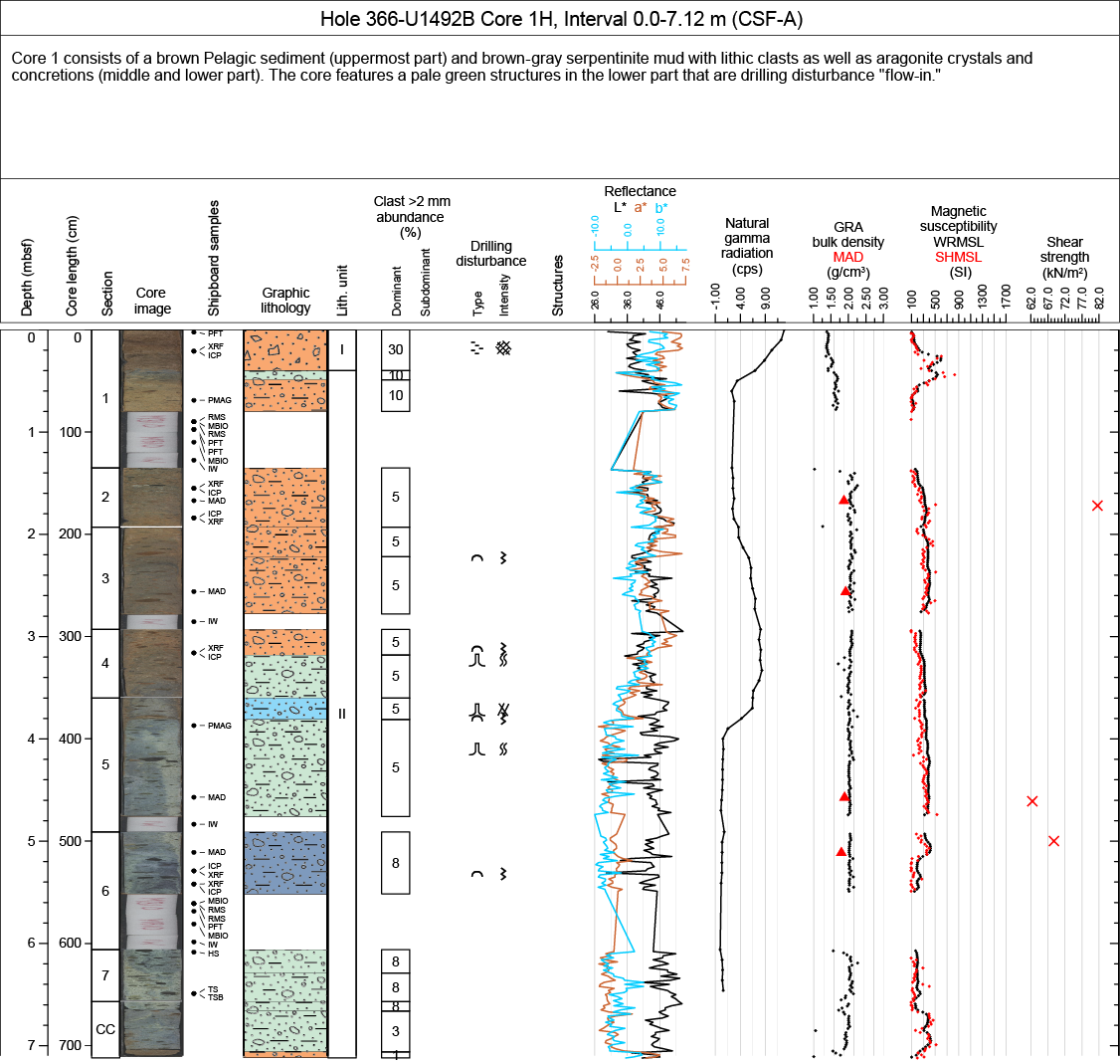
Figure F4. Example VCD.
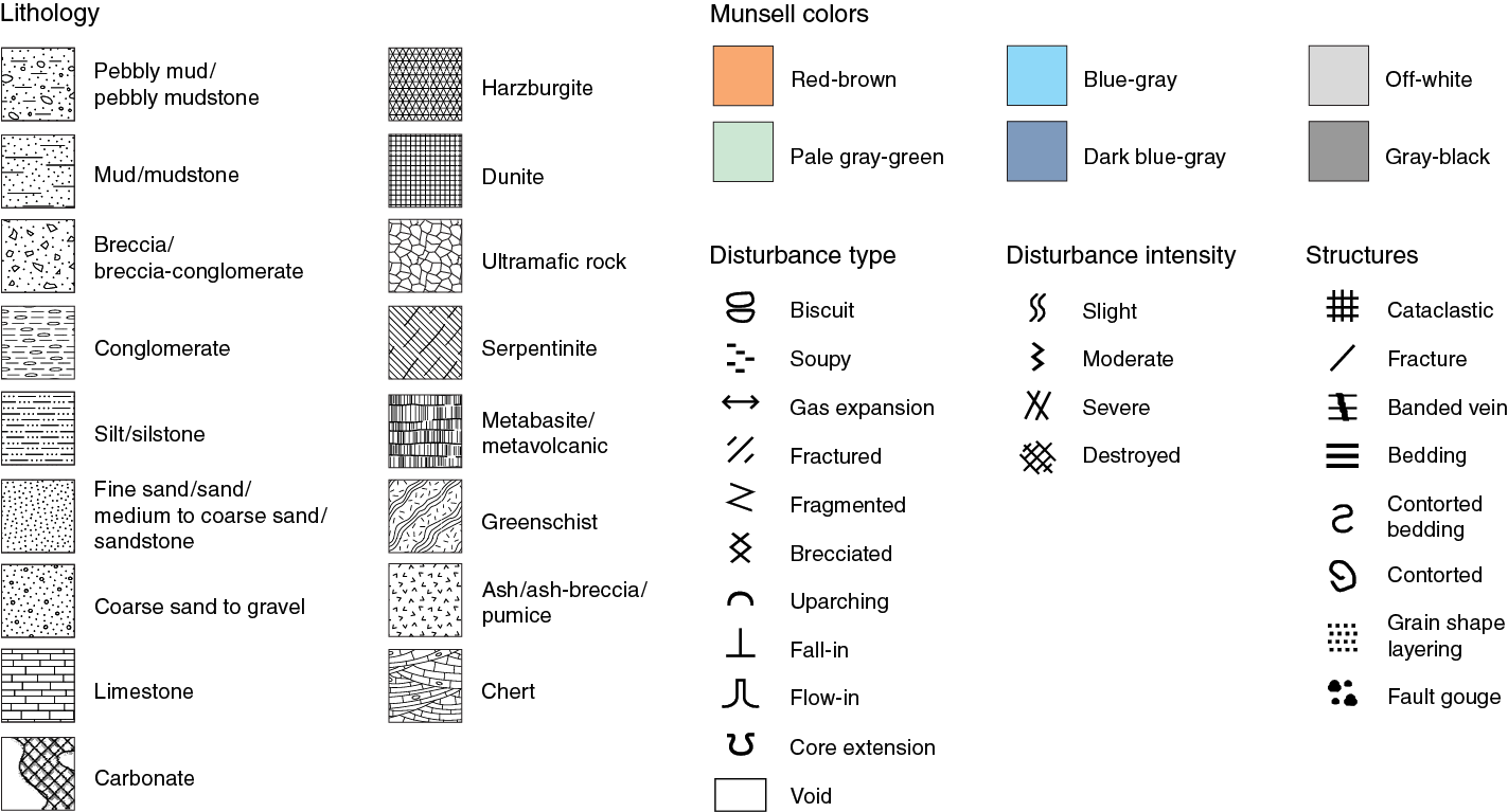
Figure F5. Symbols used in VCDs.
Section summary
An overview of major and minor lithologies present in the section, as well as notable features (e.g., sedimentary structures), is presented in the section summary text field at the top of the VCD.
Section-half imaging
The flat faces of the archive halves were scanned with the SHIL as soon as possible after splitting and scraping to avoid color changes caused by sediment oxidation and/or drying. The SHIL uses three pairs of advanced illumination high-current-focused LED line lights to illuminate large cracks and blocks in the core surface and sidewalls. Each LED pair has a color temperature of 6,500 K and emits 90,000 lx at 3 inches. A line-scan camera imaged 10 lines per millimeter to create high-resolution TIFF files. The camera height was adjusted so that each pixel imaged a 0.1 mm2 section of the core. However, actual core width per pixel varied because of differences in section-half surface height. High- and low-resolution JPEG files were subsequently created from the high-resolution TIFF file. All image files include a grayscale and ruler. Section-half depths were recorded so that these images could be used for core description and analysis.
Graphic lithology
The primary lithologies in the core intervals recovered are represented on the VCDs by graphic patterns in the Graphic lithology column using the symbols in Figure F5. The Graphic lithology column plots to scale all beds that are at least 2 cm thick. A maximum of two different lithologies (for interbedded sediments) are shown within the same core interval for interlayers <2 cm thick. Colors are assigned to the graphic lithology pattern as an underlay based on the Munsell soil color assigned to that core interval. Each color in the underlay represents a group of similar Munsell colors: red-brown, pale green, pale blue-gray, dark blue-gray, blue-black (all serpentinite variations), and off-white (typically mixed black and white clasts). The assignment of Munsell colors to these six groups is detailed in Figure F6.
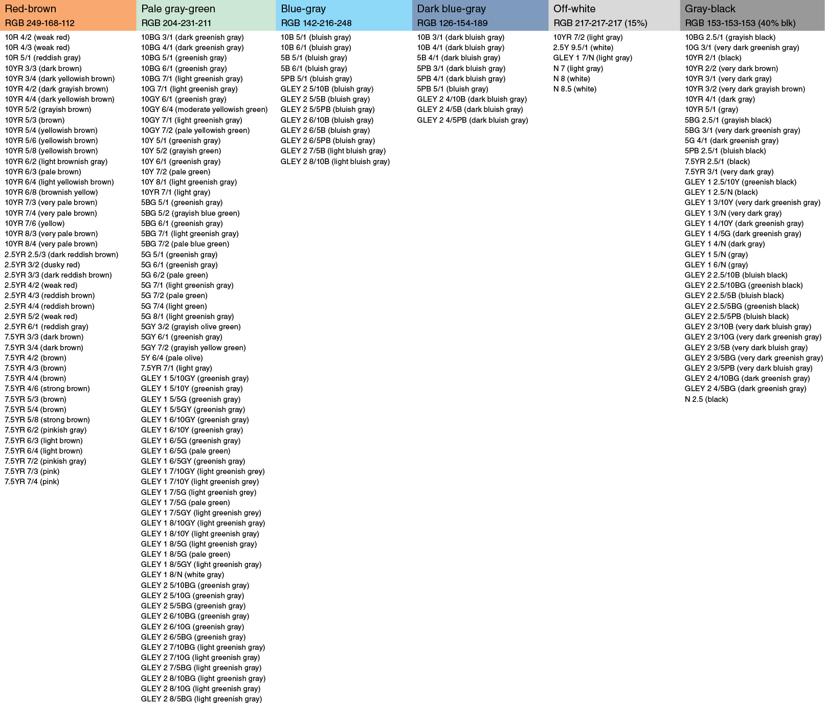
Figure F6. Color assignment chart.
Sedimentary structures
The locations and types of stratification and sedimentary or mudflow structures visible on the prepared surfaces of the split cores are recorded in DESClogik but are not shown on the VCDs. For Expedition 366, the following terminology (based on Stow, 2005) was used to describe the scale of stratification:
- Thin lamination = <3 mm thick.
- Medium lamination = 0.3–0.6 cm thick.
- Thick lamination = >0.6–1 cm thick.
- Very thin bed = <1–3 cm thick.
- Thin bed = >3–10 cm thick.
- Medium bed = >10–30 cm thick.
- Thick bed = >30–100 cm thick.
- Massive = >100 cm thick or no apparent bedding.
Descriptive terms for bed boundaries, such as sharp, erosive, gradual, irregular, and bioturbated, are noted in DESClogik.
Lithologic accessories
Lithologic, diagenetic, and paleontologic accessories are identified in smear slides and recorded in the DESClogik Microscopy template but are not indicated on the VCDs. The following terminology was used to describe the abundance of lithologic accessories in DESClogik and written core descriptions:
- Trace = 1 observed per section of core.
- Rare = 2–10 observed per section of core.
- Common = >10–20 observed per section of core.
- Abundant = >20–50 observed per section of core.
- Dominant = >50 observed per section of core.
Clasts
When clasts >2 mm are present, this was noted in the VCDs with the clast lithology, estimated percent abundance, average size, maximum size, and roundness recorded under the appropriate column. If two clasts types were present in the same interval, the same information was recorded for the subdominant (second order) clast type. Where only holes or depressions caused by clasts were observed, the working half was also examined to better estimate clast abundances. Details of unusual features were noted under the DESClogik General interval comments column.
Where different rock types are mixed, the interval was logged as separate domains with the estimated percent abundance of each domain noted along with its lithology, grain size, color, and other characteristics as discussed above. Clasts <2 mm were not broken into domains but were noted under the matrix description.
Tephra type
The occurrence of tephra layers is recorded in DESClogik but not noted on the VCDs. The type of tephra is defined visually and classified as follows:
- V = vitric (primarily volcanic glass shards).
- P = pumice (white to yellowish pumice grains).
- S = scoria (black–dark gray scoria grains).
Characteristics of tephra layers such as grain size, color, and sedimentary structures and characteristics of their components, such as glass type (bubble-walled, pumice-walled, or fibrous), glass morphology, associated heavy minerals, and rock fragments, were recorded in DESClogik.
Drilling disturbance
Drilling-related disturbances are recorded in the Disturbance column using the symbols shown in Figure F5. The style of drilling disturbance is described for soft and firm sediments or mudflow units using the following terms:
- Biscuit: unconsolidated material of intermediate stiffness show vertical variations in the degree of disturbance. Softer intervals are washed and/or soupy, whereas firmer intervals are relatively undisturbed.
- Soupy or mousse-like: intervals are water saturated and have lost all aspects of original bedding.
- Cracked or fractured: firm unconsolidated materials are broken but not displaced or rotated significantly.
- Fragmented or brecciated: firm unconsolidated materials are pervasively broken and may be displaced or rotated.
- Up-arching: disturbances result from weak to moderate coring-induced shear between the recovered material and core liner. These disturbances are easily recognized because layering is uniformly bent upward along the core margins (Jutzeler et al., 2014).
- Fall-in: out-of-place material at the top of a core has fallen downhole onto the cored surface.
- Flow-in, coring/drilling slurry, along-core gravel/sand contamination: stretching of soft, unconsolidated material and/or compressional shearing structures are severe and are attributed to coring/drilling. The particular type of deformation may also be noted (e.g., flow-in, gas expansion, etc.).
- Bowed: layering contacts are slightly to moderately deformed but still subhorizontal and continuous.
The degree of fracturing within indurated recovered materials is described using the following categories:
- Slightly fractured: core pieces are in place and broken.
- Moderately fractured: core pieces are in place or partly displaced, but original orientation is preserved or recognizable.
- Highly fractured: core pieces are probably in correct stratigraphic sequence, but original orientation is lost.
- Drilling breccia: core is crushed and broken into many small and angular pieces, with original orientation and stratigraphic position lost.
Sediment classification
The unconsolidated materials recovered during Expedition 366 are composed of serpentinite muds, pelagic muds, volcaniclastic ashes, and carbonate and siliceous biogenic components and are described using a classification scheme derived from Expedition 352 (Reagan et al., 2015b) and Stow (2005). The siliciclastic component is dominantly serpentinite mud with additional mineral and rock fragments derived from igneous, sedimentary, and metamorphic rocks. Serpentinite mud is classified on the basis of clast compositions, sizes, and abundances, whereas the matrix name is modified based on its color and the occurrence of other components (e.g., calcium carbonate or brucite).
Serpentinite mudflows are named based on their principal lithology (grain size: mud, silt, or pebbly mud) with a prefix indicating composition (typically “serpentinite”) and a suffix for additional characteristics (e.g., “with lithic clasts”). “Pebbly mud” and “pebbly mudstone” refer to unconsolidated and consolidated deposits (respectively) that are matrix-supported diamictons with a clay- to sand-sized matrix and granule- to cobble-sized clasts. Because the color of serpentinite mud is diagnostic, Munsell colors are tracked closely in DESClogik.
Pelagic sediments recovered from above or below the serpentinite mudflows comprise more typical siliciclastic components (volcanic ash, clays, and silicate minerals). The biogenic components are found in pelagic sediments that cap the serpentinite mudflows and in volcanic ash deposits under the mud volcano edifices. They are composed of the skeletal remains of open-marine calcareous and siliceous microfauna (e.g., foraminifers and radiolarians), microflora (e.g., calcareous nannofossils and diatoms), and macrofossil fragments (shell fragments). The relative proportion of these two components is used to define the major classes of sediment in this scheme.
Naming conventions for Expedition 366 follow the general guidelines of the ODP sediment classification scheme (Mazzullo et al., 1988), with the exception that a separate “mixed sediment” category was not distinguished during Expedition 366. As a result, biogenic sediments are those that contain >50% biogenic grains and <50% siliciclastic grains, whereas siliciclastic sediments are those that contain >50% siliciclastic grains and <50% biogenic grains. Sediments containing >50% silt- and sand-sized primary volcanic grains are classified as ash layers. We follow the naming scheme of Shepard (1954) for the classification of siliciclastic sediments and sedimentary rocks depending on the relative proportion of sediments of different grain sizes. Sediment grain size divisions for both biogenic and siliciclastic components are based on Wentworth (1922), with eight major textural categories defined on the basis of the relative proportions of sand-, silt-, and clay-sized particles; however, distinguishing between some of these categories can be difficult (e.g., silty clay versus sandy clay) without accurate measurements of grain size abundances. The term “clay” is only used to describe particle size and is applied to both clay minerals and all other grains <4 µm in size.
The lithologic names assigned to these sediments consist of a principal name and prefix based on composition and degree of lithification and/or texture as determined from visual descriptions of the cores and from smear slide observations.
For sediments that contain >90% of one component (either the siliciclastic or biogenic component), only the principal names are used. For sediments with >90% biogenic components, the name applied indicates the most common type of biogenic grain. For example, a sediment composed of >90% calcareous nannofossils is called a nannofossil ooze/chalk, and a sediment composed of 50% foraminifers and 45% calcareous nannofossils is called a calcareous ooze/chalk. For sediments with >90% siliciclastic grains, the principal names are based on the textural characteristics of all sediment particles (both siliciclastic and biogenic).
For sediments that contain significant mixtures of siliciclastic and biogenic components (between 10% and 90% of both siliciclastic and biogenic components), the principal names are determined by the more abundant component. If the siliciclastic components are more abundant, the principal names are based on the textural characteristics of all sediment particles (both siliciclastic and biogenic). If the biogenic components are more abundant, the principal names are based on the predominant biogenic components.
If a microfossil group composes 10%–50% of the sediment and this group is not included as part of the principal name, minor modifiers are used. When a microfossil group (e.g., diatoms, nannofossils, or foraminifers) comprises 20%–50% of the sediment, a minor modifier consisting of the component name hyphenated with the suffix “-rich” (e.g., diatom-rich clay) is used.
If one component forms 80%–90% of the sediment, the principal name is followed by a minor modifier (e.g., “with diatoms”), with the minor modifier based on the most abundant component that forms 10%–20% of the sediment. If the minor component is biogenic, the modifier describes the group of biogenic grains that exceeds the 10% abundance threshold. If the minor component is siliciclastic, the minor modifier is based on the texture of the siliciclastic fraction.
The following terms describe lithification that varies depending on the dominant composition:
- Sediments composed predominantly of siliciclastic materials: if the sediment can be deformed easily with a finger, no lithification term is added and the sediment is named for the dominant grain size (i.e., sand, silt, or clay). For more consolidated material, the lithification suffix “-stone” is appended to the dominant size classification (e.g., claystone), except for gravel-sized sediment, when the terms conglomerate or breccia are used.
- Sediments composed predominantly of calcareous, pelagic organisms (e.g., calcareous nannofossils and/or foraminifers): the lithification terms “ooze” and “chalk” reflect whether the sediment can be deformed with a finger (ooze) or can be scratched easily by a fingernail (chalk).
- Sediments composed predominantly of siliceous microfossils (diatoms, radiolarians, and siliceous sponge spicules): the lithification terms “ooze” and “radiolarite/diatomite” reflect whether the sediment can be deformed with a finger (ooze) or cannot be easily deformed manually (radiolarite/diatomite). The term “chert” is applied to lithified, siliceous sediments that are amorphous or have microscopically fine-grained texture.
- Sediments composed of a mixture of calcareous pelagic organisms and siliceous microfossils and sediments composed of a mixture of siliceous microfossils: the lithification terms “ooze” and “indurated sediment” reflect whether the sediment can be deformed with a finger (ooze) or cannot be easily deformed manually (indurated sediment).
The subclassification of volcaniclastic sediments followed here differs from the standard ODP classification (Mazzullo et al., 1988) in that we adopted a descriptive (nongenetic) terminology similar to that employed during ODP Leg 197 (Shipboard Scientific Party, 2002a) and Integrated Ocean Drilling Program Expedition 324 (Expedition 324 Scientists, 2010). Unless an unequivocally pyroclastic origin for volcanogenic particles could be determined, we simply described these deposits as for siliciclastic sediment (i.e., sand, silt, etc.).
Where evidence for a pyroclastic origin was compelling, we adopted the classification scheme of Fisher and Schmincke (1984). In these instances, we used the grain size terms “volcanic blocks” (>64 mm), “lapilli/lapillistone” (2–64 mm), and “ash/tuff” (<2 mm). The term “hyaloclastite” was used for vitroclastic (i.e., glassy) materials produced by the interaction of water and hot magma or lava (Fisher and Schmincke, 1984).
Spectrophotometry
Reflectance of visible light from the archive half cores of unconsolidated material was measured using an Ocean Optics USB4000 spectrophotometer mounted on the automated SHMSL. Freshly split soft cores were covered with clear plastic wrap and placed on the SHMSL. Measurements were taken at 1.0 or 2.0 cm spacing to provide a high-resolution stratigraphic record of color variations for visible wavelengths. Spectral data are routinely reduced to the L*a*b* color space for output and presentation, in which L* is lightness (greater value = lighter) in the range between 0 (black) and 100 (white), a* is the red-green value (greater value = redder) in the range between −60 (green) and 60 (red), and b* is the yellow-blue value (greater value = yellower) in the range between −60 (blue) and 60 (yellow). The color reflectance spectrometer calibrates on two spectra, pure white (reference) and pure black (dark). Each measurement was recorded in wide spectral bands from 400 to 900 nm in 2 nm steps. Each measurement takes ~5 s.
The SHMSL takes measurements in empty intervals and over intervals where the core surface is well below the level of the core liner, but it cannot recognize relatively small cracks, disturbed areas of core, or plastic section dividers. Thus, SHMSL data may contain spurious measurements that have to be edited out of the data set by the user. Additional detailed information about measurement and interpretation of spectral data can be found in Balsam et al. (1997, 1998) and Balsam and Damuth (2000).
Natural gamma radiation
NGR occurs primarily as a result of the decay of 238U, 232Th, and 40K isotopes. This radiation is measured using the NGRL (see Physical properties). Data generated from this instrument are used to augment geologic interpretations.
Magnetic susceptibility
Magnetic susceptibility was measured with a Bartington Instruments MS2E point sensor (high-resolution surface-scanning sensor) on the SHMSL. Because the SHMSL demands flush contact between the magnetic susceptibility point sensor and the split core, measurements were made on the archive halves of split cores that were covered with clear plastic wrap. Measurements were taken at 1.0 or 2.0 cm spacing. Measurement resolution was 1.0 SI, and each measurement integrated a volume of 10.5 mm × 3.8 mm × 4 mm, where 10.5 mm is the length perpendicular to the core axis, 3.8 mm is the width along the core axis, and 4 mm is the depth into the core. One measurement was taken at each measurement position.
Smear slide observation
Smear slide samples of the main lithologies were collected from the working half of each core when the recovery was not lithified. Additional samples were collected from areas of interest (e.g., laminations, ash layers, and nodules). A small sample of unconsolidated material was taken with a wooden toothpick and put on a 2.5 cm × 7.5 cm glass slide. The sample was homogenized with a drop of deionized water and evenly spread across the slide to create a very thin (about <50 µm) uniform layer of grains for quantification. The dispersed sample was dried on a hot plate. A drop of Norland optical adhesive was added as a mounting medium to a coverslip, which was carefully placed on the dried sample to prevent air bubbles from being trapped in the adhesive. The smear slide was then fixed in an ultraviolet light box.
Smear slides were examined with a transmitted-light petrographic microscope equipped with a standard eyepiece micrometer. The textures of siliciclastic grains (relative abundance of sand-, silt-, and clay-sized grains) and the proportions and presence of biogenic and mineral components were recorded and entered into DESClogik. Biogenic and mineral components were identified, and their percentage abundances were visually estimated according to the method of Rothwell (1989). The mineralogy of clay-sized grains could not be determined from smear slides. Note that smear slide analyses tend to underestimate the amount of sand-sized and larger grains because these grains are difficult to incorporate onto the slide.
Igneous and metamorphic petrology and alteration
The procedures for core description outlined here were adapted from ODP Legs 125 and 209 (Fryer et al., 1990; Kelemen, Kikawa, Miller, et al., 2004) and Expedition 352 to the Izu-Bonin-Mariana forearc (Reagan et al., 2015a). All of the igneous and metamorphic rocks encountered during this expedition occur as clasts in serpentinite mudflow deposits or in fines-depleted gravel deposits (formed by drilling disturbance). As a result, all igneous and metamorphic rocks were described initially within the Sediment tab in DESClogik; all clasts sampled for shipboard analysis were also described in the appropriate tab within DESClogik: Intrusive_mantle, Extrusive_hyabyssal, or Metamorphic. Alteration features including secondary mineral assemblages and veins were described in the Alteration and Veins_halos tabs. Features cataloged in these tabs include the following:
- Lithology, modal abundances and appearances, and characteristic igneous or metamorphic textures, and
- Alteration assemblages and parageneses, as well as vein and vesicle infillings and halos.
These macroscopic observations were combined with detailed thin section petrographic studies of key lithologies and alteration intervals.
Before splitting sections into working and archive halves, each hard rock piece large enough to be curated individually was labeled with unique piece/subpiece numbers from the top to the bottom centimeter of each section. If the top and bottom of a piece of rock could be determined, an arrow was added to the label to indicate the uphole direction. Archive halves were imaged using the SHIL.
After imaging, archive halves were analyzed for color reflectance and magnetic susceptibility at 1–2.5 cm intervals using the SHMSL (see Physical properties). Working halves were sampled for shipboard physical properties, paleomagnetic studies, thin sections, and inductively coupled plasma–atomic emission spectroscopy (ICP-AES) analysis.
Each igneous and metamorphic clast was first examined macroscopically and described for petrologic and alteration characteristics, and then structures were described (see Structural geology). All descriptions during Expedition 366 were made on the archive halves of the cores, except for thin sections, which were sampled from the working halves. For macroscopic observations and descriptions, DESClogik was used to record the primary igneous characteristics (e.g., lithology, texture, modal mineralogy, and grain size) and alteration (e.g., color, secondary minerals, and vein/fracture fillings). Mineral modes, sizes, and textures were estimated by examining the archive halves under binocular microscopes or using hand lenses with graticules of 0.1 mm. For microscopic observations, as many as 12 thin sections were made daily, and the descriptions were entered in DESClogik. Macroscopic features observed in the cores are summarized and presented in the VCDs.
Igneous petrology
Igneous rocks encountered during Expedition 366 include a range of ultramafic rocks of presumed mantle origin and, much more rarely, volcanic or metavolcanic rocks, all as clasts within the serpentinite mudflow units.
Plutonic and mantle rocks: primary igneous lithologies and features
Igneous rock names were assigned a primary lithology name based on the mineral phases present prior to alteration using the International Union of Geological Sciences (IUGS) classification scheme for igneous rocks (LeMaitre et al., 1989), a prefix that includes a grain-size designation or other descriptive feature, and an optional suffix for special features. Grain sizes, modal mineralogy, textures, and mineral shapes were recorded, and the full rock name is concatenated from the primary lithology, prefix, and suffix. For severely altered rocks, the term “primary assemblage” was often used to refer to the estimated prealteration mineral assemblage. Where alteration in ultramafic rocks was so extensive that estimation of the primary phase assemblages was not possible, the protolith is called “serpentinite.” If primary assemblages and their pseudomorphs and textures could be recognized in ultramafic samples, even though they are partially or completely replaced, the rock name used was based on the reconstructed primary assemblage and was termed either “serpentinized” or “altered” (i.e., serpentinized dunite, altered lherzolite, etc.).
Ultramafic rocks are by far the most common igneous clast type, and their nomenclature required special attention. The most common ultramafic rocks are classified based on abundance of primary minerals, grain size, and texture. When modal analyses can be reliably obtained, ultramafic rocks are classified according to the Streckeisen (1974) classification as follows (Figure F7):
- Dunite = olivine > 90%.
- Lherzolite = olivine > 40%, orthopyroxenite > 5%, clinopyroxenite > 5%.
- Harzburgite = olivine > 40%, orthopyroxenite > 5%, clinopyroxenite < 5%.
- Wehrlite = olivine > 40%, orthopyroxenite < 5%, clinopyroxenite > 5%.
- Orthopyroxenite = orthopyroxenite (enstatite) > 90%.
- Clinopyroxenite = clinopyroxene (diopside) > 90%.
- Websterite = olivine < 5%, orthopyroxenite > 5%, clinopyroxenite > 5%.
- Olivine websterite = olivine 5%–40%, orthopyroxenite > 5%, clinopyroxenite > 5%.
- Olivine orthopyroxenite = olivine 5%–40%, orthopyroxenite > 5%, clinopyroxenite < 5%.
- Olivine clinopyroxenite = olivine 5%–40%, orthopyroxenite < 5%, clinopyroxenite > 5%.
- Serpentinite = any largely serpentinized ultramafic rock in which the primary lithology can no longer be discerned.
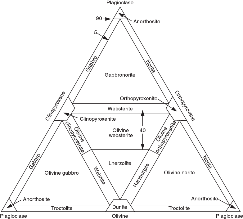
Figure F7. Modal classification scheme for plutonic igneous rocks.
The first four rock types (dunite, lherzolite, harzburgite, and wehrlite) are often referred to collectively as “peridotites,” whereas rocks dominated by pyroxene are referred to collectively as “pyroxenites” (websterite, orthopyroxenite, clinopyroxenite, and their olivine-bearing namesakes). Typical accessory minerals may include an aluminous phase such as spinel (chromite), plagioclase, or garnet. These may be added as a prefix to the primary rock name. Prefixes are commonly only added when plagioclase or garnet-bearing varieties are present; most peridotites are spinel bearing, and when no aluminous phase is listed, it can be assumed that spinel or chromite is present.
Ultramafic rocks typically have special textural characteristics that require definition (Mercier and Nicolas, 1975; Nelson Pike and Schwarzman, 1977) for those who are not specialists in ultramafic petrology. Some of the more common terms include the following:
- Tectonite: a general term applied to mantle-derived peridotites to distinguish them from cumulate peridotites. Most commonly, these are porphyroclastic.
- Porphyroclastic: a common peridotite texture with large grains of enstatite and more rarely olivine set in groundmass of finer grained olivine and pyroxene. Olivine is typically kink-banded with small, strain-free neoblasts.
- Equigranular equant (mosaic): olivine and enstatite are similar in size with smooth curvilinear grain boundaries, and 120° triple grain boundaries are common, with diopside and spinel scattered throughout, commonly at triple-grain boundaries. Aspect ratios are close to 1.0. This texture resembles that of granulites in high-grade gneiss terranes.
- Equigranular tabular: identical to equigranular equant but with olivine and enstatite aspect ratios typically 2:1 or larger.
- Protogranular: olivine and enstatite are large (3–4 mm) and similar in size with curvilinear grain boundaries and no foliation. Spinel occurs as amoeboid-shaped clusters typically associated with diopside and enstatite. The spinel–diopside clusters are interpreted as representing exsolution from primary Al- and Ca-rich enstatite.
- Cataclastic to ultracataclastic: rock is strongly deformed under brittle conditions. Uniformly small grain size is common, olivine and pyroxene are highly kinked or granulated, and serrated grain boundaries occur.
- Mylonitic: rock is strongly deformed under ductile conditions. Most grains are small and recrystallized (neoblasts) with less common, highly strained augen of olivine or pyroxene.
- Decussate: typical of pyroxenites. Blocky-shaped pyroxenes form a brick-like intergrowth where crystal shapes dominate the texture.
Ultramafic rocks may be highly altered to serpentinite yet still retain their primary textural characteristics. Whenever possible, partially or largely serpentinized peridotites that retain their primary textures are referred to by the name consistent with their primary mineralogy, with or without the modifier “serpentinized.” Where the primary lithology is obscured by deformation or pervasive serpentinization, these rocks were referred to simply as “serpentinites.” There are a number of terms specific to serpentinized ultramafic rocks that are commonly used and may occur in the core descriptions (Figure F8).
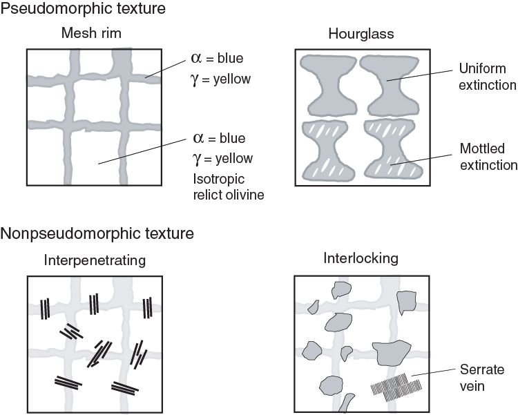
Figure F8. Schematic sketches of serpentinite microtextures.
Pseudomorphic textures include the following:
- Mesh texture: a common texture that results from the serpentinization of olivine. It resembles a fine mesh in thin section, consisting of fibrous mesh rims that surround massive mesh centers. Mesh centers may consist of fine-grained serpentine or may retain primary olivine. This texture typically forms in two or more stages.
- Hourglass texture: results from serpentinization of olivine in a single stage, such that the fibrous mesh rims extend to the center of the grain.
- Bastite: a topotaxic (meaning “placement” or “local” arrangement; i.e., of crystallographic orientation) replacement of pyroxene or amphibole by serpentine. Typically, this refers to enstatite grains that are replaced by serpentine without altering the morphology of the original grain; thus, they resemble the unaltered enstatite grains macroscopically.
Nonpseudomorphic textures include the following:
- Ribbon texture: an extreme texture from pervasive serpentinization or deformation in which serpentine occurs as zones of parallel serpentine fibers that define thin bands or ribbons. This texture may be elongate parallel to foliation if foliation is present (not shown in Figure F8).
- Interpenetrating texture: interlocking of mutually interfering, anhedral elongate blades, flakes, or plates that form a tight interpenetrating fabric. It begins as randomly oriented blades in lizardite mesh textures and progresses to massive interlocking texture. It is commonly formed as antigorite crystallizes.
- Interlocking texture: interlocking texture of irregular equant (or more rarely, spherulitic) grains. It begins in isolated patches that grow together as reaction progresses. It differs from interpenetrating texture by lack of elongate grains and may consist of lizardite or antigorite.
Macroscopic descriptors include the following:
- Massive: serpentinite that does not preserve primary features and contains little or no foliation or schistosity.
- Phacoidal: a schistose form of serpentine composed of scales or chips of serpentine 1 mm or larger in size that may have slickensided surfaces and whose long axes define an anastomosing foliation. This foliation may enclose angular to subangular blocks of unsheared serpentinite (1 cm or larger in size) or may be associated with horizontal or vertical convolute bedding.
Serpentinized ultramafic rocks are commonly associated with a large range of vein types (e.g., fibrous chrysotile, crack-seal, etc.). Mineral assemblages of such veins often cannot be identified macroscopically; if not stated otherwise, veins referred to as “serpentine veins” may consist of pure serpentine or of serpentine with accessory minerals (e.g., brucite, magnetite, etc.). Any large serpentine veins (e.g., width > 0.5 cm) were described on DESClogik using the Veins_halos tab. The descriptions and structures of small veins were noted as a texture comment in the appropriate table in DESClogik (Intrusive_mantle, Volcanic_hypabyssal, or Metamorphic).
Primary plutonic minerals
The primary rock-forming minerals recovered were olivine, orthopyroxene, clinopyroxene, spinel, plagioclase, Fe-Ti oxide, and amphibole. For each, the following data are available for each site based on thin section examination:
- Visually estimated modal percent of the primary original minerals;
- Maximum and average grain size; and
- Crystal shape, habit, and texture.
Accessory phases, when present, were also noted. The modal percentage of the mineral includes both the fresh and altered parts of the rocks interpreted to represent that mineral. Grain size refers to the average long dimension of the minerals and is given in millimeters, as are the crystal sizes. The shape describes the aspect ratio of the grains and was used when deformation had modified the original crystal morphology. The aspect ratio is the ratio of the short to the long dimension of the crystal. The terms “euhedral,” “subhedral,” “anhedral,” and “interstitial” were used to describe the shapes of crystals interpreted to preserve their igneous morphology. The shapes are divided into four classes:
- Equant: aspect ratio = less than 1:2.
- Subequant: aspect ratio = 1:2 to 1:3.
- Tabular: aspect ratio = 1:3 to 1:5.
- Elongate: aspect ratio = more than 1:5.
Spinel occurs in various shapes that can be divided into three categories:
- Equant: the shape is equidimensional with flat and/or curved surfaces.
- Interstitial: transitional category between vermicular and equant. The outer surfaces of these spinels are often concave outward and have thin tips departing from the corner of the grain (“holly leaf” habit).
- Vermicular or amoeboid: intricate shape forming symplectic (i.e., fine-grained) intergrowths with pyroxenes and/or olivine (typically at their margins). Characteristic of protogranular textures.
The presence of linear arrays of spinel grains, which sometimes form in peridotite and are termed “trains,” was noted in the comments. Descriptions and estimates are based primarily on hand-sample inspection with a more limited sample suite also studied in petrographic thin sections. Thin section observations were used to refine the hand-sample descriptions.
Volcanic and basaltic hypabyssal rocks: primary igneous lithologies and features
Volcanic rock clasts recovered during Expedition 366 are less common than ultramafic clasts but are not rare, and they range from pebble-sized clasts to boulders. They are commonly partially altered, but their primary mineralogy and textures are recognizable and they often preserve relatively unaltered clinopyroxenes, although plagioclase is generally pervasively altered to sericite. Naming conventions follow those of Expedition 352 (Reagan et al., 2015b). Porphyritic basaltic rocks were named according to major phenocryst phase(s) when the total abundance of phenocrysts was >1%. The most abundant phenocrysts appear last in the phenocryst-based lithology name. The term “phenocryst” was used for any crystal that was (1) significantly larger (typically at least five times) than the average size of the groundmass crystals, (2) >1 mm, and (3) euhedral or subhedral. “Skeletal” phenocrysts are phenocrysts that grew as, or have been corroded to, a skeletal framework with a high proportion of internal voids. The term “microphenocryst” was used for crystals larger than the modal groundmass grain size but smaller than 1 mm and was reported in the Microscopic (thin section) description template in DESClogik and in the Lithologic unit summary in the Description column on the VCDs. A prefix was applied as a modifier to the primary lithology names to indicate the abundance of phenocrysts in the hand samples as follows:
- Aphyric = <1% phenocrysts.
- Sparsely phyric = 1%–5% phenocrysts.
- Moderately phyric = >5%–10% phenocrysts.
- Highly phyric = >10% phenocrysts.
Aphyric rocks were not assigned any mineralogical modifier. Likewise, in coarser grained rocks with seriate to equigranular textures, we did not use modifiers unless there was a clear distinction in size between phenocrysts and groundmass crystals. The term “dolerite” was used for fine- to medium-grained basaltic rocks containing clinopyroxene and plagioclase with ophitic to subophitic texture.
Groundmass is defined as the finer grained matrix (or the mesostasis) between the phenocryst phases, if the latter are present. Groundmass is generally characterized by its texture and grain size with the following standard notation:
- G = glassy.
- cx = cryptocrystalline (<0.1 mm).
- μx = microcrystalline (0.1–0.2 mm).
- fg = fine grained (>0.2–1 mm).
- mg = medium grained (>1–2 mm).
- cg = coarse grained (>2 mm).
An estimate of the average modal groundmass size (in millimeters) is included in the VCDs, whereas in the reports and description summaries we used descriptive terms, for example, fine-grained or coarse-grained groundmasses.
For volcanic and hypabyssal basaltic rocks, the following terms were used to describe textures when microlites are present in the groundmass:
- Variolitic (fan-like arrangement of divergent microlites),
- Intergranular (olivine and pyroxene grains between plagioclase laths),
- Intersertal (glass between plagioclase laths),
- Subophitic (partial inclusion of plagioclase in clinopyroxene), and
- Ophitic (total inclusion of plagioclase in clinopyroxene).
Flow textures present in the groundmass were described as follows:
- Trachytic (subparallel arrangement of plagioclase laths in the groundmass),
- Pilotaxitic (aligned plagioclase microlites embedded in a matrix of granular and usually smaller clinopyroxene grains), and
- Hyalopilitic (aligned plagioclase microlites with glassy matrix).
Rock colors were determined on a wet, cut archive half surface using Munsell soil color charts (Munsell Color Company, Inc., 1994) and converted to a more intuitive color name. Wetting of the rock was carried out using tap water and a sponge. Wetting was kept to a minimum because of adsorption of water by clay minerals (particularly saponite and celadonite) that could be present in the core.
Metamorphic petrology
Metamorphic basic rocks encountered during Expedition 366 all occur as clasts within the serpentinite mudflows. They mostly consist of greenschist metabasites and metagabbros. These clasts are typically less than 3 cm in size. The greenschist clasts are assumed to be derived from the subduction channel of the Mariana convergent margin system. All clasts >2 cm receive a piece number during curation and were categorized using the Metamorphic tab in DESClogik.
In general, the major features of metamorphic rocks were used for their classification (Schmid et al., 2007):
- Minerals present,
- Structure of the rock,
- Nature of the rock prior to metamorphism,
- Genetic conditions of metamorphism (usually in terms of pressure and temperature, with or without deformation), and
- Chemical composition of the rock.
The considerable diversity of mineralogical names found in metamorphic rocks are conveyed by the use of mineral names as prefixes to the root structural term (for example, plagioclase–pyroxene metabasite), with the mineral names arranged in order of increasing modal abundance. The fundamental terms (based on rock type alone) are placed at the end of compound hyphenated names of the type described previously. The metamorphic rocks are therefore named using one of the three fundamental terms (protolith, dominant mineral if ≥75%, or specific name like greenschist) to convey the basic rock type, whereas the mineralogical features are given by prefixing the rock type with the names of the appropriate mineral constituents. A compound hyphenated name may always be applied and allows a systematic set of names for petrographic descriptions.
Three terms essentially cover the principal varieties of lithologies found in metamorphic rocks, particularly as seen in hand specimen (and are therefore easily applicable). These three terms are schist, gneiss, and granofels and reflect the degree of fissility or schistosity shown by the rock (preferred orientation of nonequant mineral grains or grain aggregates produced by metamorphic processes). If the schistosity in a metamorphic rock is well developed, the rock has a schistose structure and is termed a “schist.” If it is poorly developed, the rock has a gneissose structure and is termed a “gneiss.” If the rock has a medium- to coarse-grained granoblastic texture without or with only indistinct foliation or lineation it is termed a “granofels.”
Metamorphic rocks not named by the application of the fundamental terms based on the protolith or a dominant mineral are categorized by specific names like blueschist, greenschist, amphibolite, eclogite, or granulite. Blueschists are metamorphic rocks characterized by the presence of high-pressure metamorphic assemblages such as jadeite-quartz, lawsonite, phengite, crossite, or glaucophane. Greenschists are metamorphic rocks characterized by intermediate pressure–temperature assemblages, which typically comprise albite, actinolite, chlorite, and epidote. Amphibolites reflect higher temperature metamorphism than greenschists; they typically contain plagioclase and hornblende, along with other minerals. Eclogites are garnet-omphacite rocks metamorphosed under higher pressure conditions than blueschists. Granulites form at higher temperatures than amphibolites and represent metamorphism at higher temperatures and pressures.
The description of fault rocks is based on the distinction between cataclastic and mylonitic (plastic–viscous) deformation mechanisms (Brodie et al., 2007). Mylonites are cohesive and characterized by well-developed schistosity resulting from tectonic reduction of grain sizes and commonly contain rounded porphyroclasts and lithic fragments of similar composition to minerals in the matrix. Fine-scale layering is commonly present. Brittle deformation of some minerals may be present, but deformation is commonly plastic. Mylonites may be divided according to the relative proportion of finer grained matrix into protomylonite, mesomylonite, and ultramylonite.
Cataclasites (cataclastic rocks) are cohesive with a poorly developed or absent schistosity or are incohesive, characterized by generally angular porphyroclasts and lithic fragments in a finer grained matrix of similar composition. Generally, no preferred orientation of grains of individual fragments is present as a result of deformation, but fractures may have a preferred orientation. Foliation is not generated unless the fragments are drawn out or new minerals grow during deformation. Plastic deformation may be present but is always subordinate to some combination of fracturing, rotation, and frictional sliding of particles. Cataclasites may be divided according to the relative proportion of finer grained matrix into protocataclasite, mesocataclasite, and ultracataclasite. Fault gouges are incohesive, clay-rich, fine- to ultrafine-grained cataclasites that may possess a schistosity and contain <30% visible fragments. Lithic clasts may be present.
Alteration, veins, and halos
Alteration features including secondary mineral assemblages and veins were described in the Alteration and Veins_halos tabs. Methods for describing alteration include hand-sample descriptions and inspection of thin sections. These observations provided information on the alteration of primary igneous features such as phenocrysts, groundmass minerals, and volcanic glass. In addition, the abundance of veins and vesicles and the succession of infilling materials were recorded to ascertain the order of mineral precipitation.
Alteration
Alteration minerals are identified by color, habit and shape, association with primary minerals (if distinguishable), and hardness. Visual estimates of alteration degree, type, color, and textures (e.g., halos and patches) were recorded, as well as abundance (percentage) of minerals filling veins and vesicles and the proportion of altered groundmass, volcanic glass, and all the different primary phenocryst phases. Complications arise in identification of secondary phases because many minerals produced during submarine alteration are visually similar, often being microcrystalline or amorphous, and are thus indistinguishable in the cores. Hence, identification of some alteration phases remains preliminary pending detailed shore-based X-ray diffraction (XRD) studies and analyses by electron microprobe, micro-Raman spectroscopy, and so on.
The degree of the overall background alteration of groundmass and glass was defined and reported graphically on the VCDs according to various ranges of intensity in the alteration state. Different patterns were used to indicate slight, moderate, high, complete, or no (fresh) alteration. Alteration color was defined using Munsell soil color charts (Munsell Color Company, Inc., 1994) and converted to a more intuitive color name (dark blue-gray, red-brown, etc.).
Veins and halos
During Expedition 366, descriptions of veins included location, shape, crosscutting nature, width, color, and the amount (percentage) and nature of filling minerals. Vein orientation data were exclusively taken from veins from their in situ orientation with reference to the host rock (see Structural geology). All features were recorded in DESClogik using a series of codes for vein shape (straight, sigmoidal, irregular, pull-apart, and fault vein), connectivity (isolated, single, branched, and network), texture (massive, cross-fiber, slip-fiber, vuggy, and polycrystalline), structure (simple, composite, banded, haloed, and intravenous), and geometry (en echelon, ribbon, and cross fractures) (Figure F5).
Alteration halos commonly form around hydrothermal veins and indicate transfer of fluids of varying composition into the surrounding rock. They can be different from the overall background alteration and vesicle filling in color, secondary mineral composition, and abundance. Color, thickness, and secondary minerals of alteration halos were recorded in the Veins_halo tab of DESClogik. Alteration color was defined using Munsell soil color charts (Munsell Color Company, Inc., 1994) and converted to a more intuitive color name (dark blue-gray, red-brown, etc.).
Macroscopic visual core description
We used DESClogik to document each section of the igneous cores and their alteration by uploading our descriptions into the central LIMS database. These uploaded data were then used to produce VCDs, which include a simplified graphical representation of the core (for each section) with accompanying descriptions of the features observed. The VCDs display the following items:
- Description summary for each igneous lithologic unit;
- Depth in meters below seafloor (based on the CSF-A depth scale);
- Scale for core section length (0–150 cm);
- Sample piece number;
- Scanned digital image of the archive half;
- Sample type and position of intervals selected for different types of shipboard analytical studies, such as thin sections (TS), ICP-AES (ICP), X-ray fluorescence (XRF), X-ray diffraction (XRD), paleomagnetism, and physical properties (PP);
- Graphical representation of lithology;
- Igneous lithologic unit number;
- Dominant and subdominant clast abundance;
- Drilling disturbance;
- Symbolized structural information;
- Plot of color reflectance with total reflectance (L*), red (a*), and blue (b*) data arranged side by side;
- Plot of NGR;
- Plot of bulk and MAD densities;
- Plot of point source and whole-round magnetic susceptibility measurements; and
- Plot of shear strength.
Microscopic thin section description
Thin section analyses of sampled core intervals were used to complement and refine macroscopic core observations. Shipboard thin sections were selected, examined, and logged to represent both typical and unusual lithologies as they occurred. To maintain consistency, the same terminology and nomenclature are used for macroscopic and microscopic descriptions. Phenocryst assemblages (and their modal percentages, shapes, habits, and sizes), groundmass, and alteration phases were determined, and textural features were described. All observations were entered into the LIMS database with a special DESClogik thin section template. Downloaded tabular reports of all thin section descriptions can be found in Core descriptions.
Thin section descriptions include both primary (igneous or metamorphic) and secondary (alteration) features, for example, textural and structural features, grain size of phenocrysts and groundmass minerals, mineralogy, abundance (percentage), inclusions, alteration color, alteration extent (percentage) in the total rock, and alteration veins (type and number).
Textural terms used are defined by MacKenzie et al. (1982) and include the following:
- Heterogranular (different crystal sizes),
- Equigranular (similar crystal sizes),
- Seriate (continuous range in grain size),
- Porphyritic (increasing presence of phenocrysts),
- Glomeroporphyritic (containing clusters of phenocrysts),
- Holohyaline (100% glass),
- Hypo- or holocrystalline (100% crystals),
- Variolitic (fine, radiating fibers of plagioclase or pyroxene),
- Intergranular (olivine and pyroxene grains between plagioclase laths),
- Intersertal (groundmass fills the interstices between unoriented feldspar laths),
- Ophitic (lath-shaped euhedral crystals of plagioclase, grouped radially or in an irregular mesh, completely surrounded with large anhedral crystals of pyroxene), and
- Subophitic (partial inclusion of plagioclase in pyroxene).
Textural terms for plutonic and metamorphic rocks include the following:
- Equigranular equant (uniform grain size and equant grain shape),
- Equigranular tabular (uniform grain size and tabular, elongate grain shape),
- Porphyroclastic (clasts embedded within fine grain matrix),
- Porphyroblastic (metamorphic blasts embedded within fine-grained matrix),
- Granoblastic (coarse-grained, equigranular fabric),
- Poikiloblastic (elongate, lozenge-shaped metamorphic blasts embedded within fine-grained matrix),
- Decussate (interlocking, randomly oriented arrangement of mineral grains), and
- Nodular (rounded clasts or blasts embedded within fine grained matrix).
Recovered ultramafic clasts commonly display a high degree of serpentinization (>80%) and are described in the Intrusive_mantle tab in DESClogik. Textural terms for these rocks are based on Wicks and Whittaker (1977). The texture of the clast is first described as “pseudomorphic” or “nonpseudomorphic.” When the texture is pseudomorphic, the initial mode and the degree of serpentinization of peridotite minerals are given per mineral domain (e.g., orthopyroxene, olivine, or clinopyroxene) in DESClogik. Serpentine textures are defined as follows (Figure F5):
- Bastite (serpentine pseudomorph after orthopyroxene),
- Mesh (serpentine pseudomorph after olivine composed of a fibrous rim and an isotropic core),
- Hourglass (serpentine pseudomorph after olivine composed of fibrous serpentine),
- Interpenetrating (serpentine nonpseudomorphic texture of mutually interfering, anhedral elongate blades, flakes, or plates),
- Interlocking (serpentine nonpseudomorphic texture of irregular equant grains),
- Fibrous (parallel fibers orientated perpendicularly to the vein footwall), and
- Crack-seal (banded veins of fibrous serpentine displaying an overall preferred orientation perpendicular to the vein footwall; micrometric interstices separate the different layers) (Andreani et al., 2004).
Late stages of alteration (e.g., carbonated breccia or ophicarbonate) are described as a second sample domain in DESClogik. To differentiate late stages of alteration from serpentinization, these features are described in the Alteration tab in DESClogic.
Furthermore, for alteration descriptions, thin sections were examined to do the following:
- Confirm macroscopic identification of secondary minerals;
- Determine their mode of occurrence in terms of vesicle and void fillings, vein composition, and primary mineral replacement;
- Determine the chronological relationships between different secondary minerals;
- Establish the distribution, occurrences, and abundance of secondary minerals downhole;
- Quantify the overall amount of alteration in the basaltic rocks;
- Identify mineralogies of vein and vesicle infillings, as well as cement and voids present in basaltic breccia; and
- Calculate the total alteration (percentage) using the modal proportions of phenocrysts and groundmass minerals and their respective percentages of alteration.
For structural descriptions, thin sections were examined following Kelemen, Kikawa, Miller, et al. (2004) to determine the following:
- Anisotropy, including the shape-preferred orientation of minerals and clasts and foliation when possible;
- Grain shape;
- Grain boundaries (straight, irregular, sutured, and lobate);
- Grain internal structures (e.g., undulatory extinction, subgrains, deformation bands, and twins); and
- Microfractures.
In some cases, individual thin sections contain multiple domains that required separate description. In DESClogik, the user can enter multiple records for a single thin section in which more than one domain can be recognized. We defined the “domain” concept of DESClogik based on apparent observable differences in lithology, alteration, vesicle banding and grouping, veining, and, when more than one clast type is present, volcaniclastic lithologies. Thin sections typically are taken so they represent a singular lithology, and thus by definition they encompass a single lithology domain. In some cases, thin sections contain more than one lithology with a sharp or diffuse boundary splitting the thin section into two lithology domains, whereby a diffuse (wider) boundary zone could be defined as a separate, third domain. Alteration can result in many different domains in a rock, including the background alteration and various halos surrounding cracks and veins. Multiple generations of veins with different filling patterns were often visible in thin section; some were therefore assigned different domain names.
Finally, estimated volume percentages were required to quantify phase abundances. In DESClogik, the user is required to enter modal percentages of mineral phases for all rocks. The whole-rock constituents become the sum of all mineral phases present; veins and void spaces are ignored in this calculation. In DESClogik, the user records the percentage of the originally present mineral phases, whenever possible, the replacement phases, and how much has been replaced (i.e., altered or filled) ensuring that Original (%) = Present (%) + Replaced (%).
Structural geology
The methods for documenting structural features encountered in Expedition 366 cores largely follow those of Integrated Ocean Drilling Program Expeditions 334 and 344 (see the Structural geology sections in the respective Methods chapters [Expedition 334 Scientists, 2012; Harris et al., 2013]. Structures observed on split cores were classified and quantified in terms of depth extent and sense of displacement. Orientation data were only measured on structures in their original orientation; no orientation data from rotated clasts, fragments, and so on, were documented. Orientation data were typed into both an MS Excel spreadsheet and DESClogik.
Structural data acquisition and orientation measurements
Core measurements followed ODP procedures. We used a plastic goniometer for orientation measurements (Figure F9). Using the working half of the split core provided greater flexibility in removing—and cutting, if necessary—pieces of the core for structural measurements.
Figure F9. Protractor used to measure features in a split core.
Orientations of planar and linear features in cores were determined relative to the core axis, which represents the vertical axis in the core reference frame, and the “double line” marked on the working half of the split core liner, which represents 0° (and 360°) in the plane perpendicular to the core axis (Figure F10). To determine the orientation of a planar structural element, two apparent dips of this fabric were measured in the core reference frame. These were then converted using an MS Excel spreadsheet to a plane represented by dip angle and either a strike or dip direction (Figure F11). One apparent dip was usually represented by the intersection of the planar feature with the split face of the core and was quantified by measuring the dip direction and angle in the core reference frame (β1) (Figure F12). Typical apparent dip measurements had a trend of 90° or 270° and ranged in plunge from 0° to 90° (β2). The second apparent dip was usually represented by the intersection of the planar feature and a cut or fractured surface at a high angle to the split face of the core. In most cases, this was a surface either parallel or perpendicular to the core axis. In the former, the apparent dip lineation trended to 000° or 180° and plunge trended from 0° to 90°; in the latter, the trend ranged from 000° to 360° and plunge was 0°.
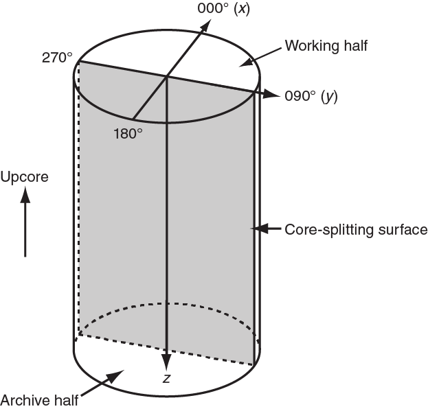
Figure F10. Diagram of core reference frame.

Figure F11. Lower hemisphere equal area projection used for converting 2-D measured data to 3-D diagrams.
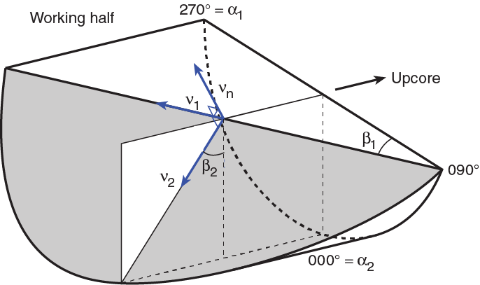
Figure F12. Diagram showing calculation of plane orientation.
Description and classification of structures
We constructed a structural geology template for DESClogik that facilitates the description and classification of observed structures.
Structural data can sometimes be disturbed by drilling-induced structures such as flow-in structures in APC cores and biscuiting, fracturing, faulting, and rotation of fragments in XCB and RCB cores. Where structures were disturbed by flow-in on >60% of the cross section of the core, we excluded measurements because of the intense disturbance (bending, rotation, etc.) of these structures.
For planar structures (e.g., bedding, flow boundaries, fractures as joints, veins, and faults), two apparent dips on two different surfaces (e.g., one on the working half surface of the split core, which is east–west vertical, and the other on the horizontal or north–south vertical surface of the same split core) were measured in the core reference frame as azimuths (measured clockwise from north, looking down) and plunges (Figures F10, F11, F12). A coordinate system was defined so that the positive x-, y-, and z-directions coincide with north, east, and vertical downward, respectively. If the azimuths and plunges of the two apparent dips are given as (α1, β1) and (α2, β2), respectively (Figure F12), then the unit vectors representing these two lines, v1 and v2, are
The unit vector normal to the plane, vn, is then defined as
where
The azimuth, αn, and plunge, βn, of vn are given by
The dip direction, αd, and dip angle, β, of this plane are αn and 90° + βn, respectively, when βn < 0° (Figure F13). They are αn ± 180° and 90° − βn, respectively, when βn ≥ 0°. The right-hand rule strike of this plane, αs, is then given by αd − 90°.
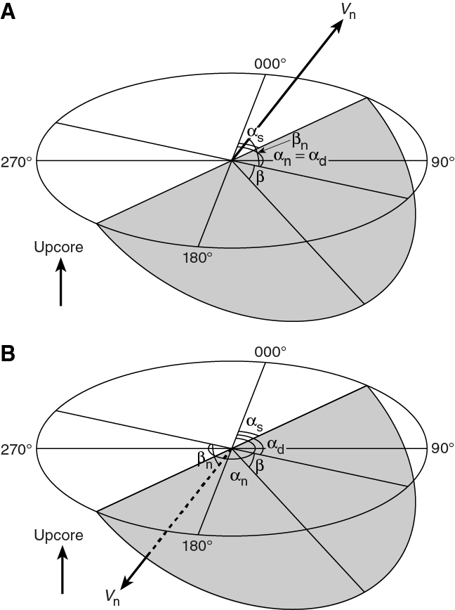
Figure F13. Diagrams of dip direction.
DESClogik structural database
DESClogik is an interface application used to store data used to produce a visual (macroscopic and/or microscopic) description of core structures at a given depth in LIMS. During this expedition, only the locations of structural features, calculated orientations in the core reference frame, and restored orientations based on the paleomagnetic data were input into DESClogik. Orientation data management and planar fabric analysis were made with a spreadsheet as described above.
Rock, mud, and sediment geochemistry
Portable X-ray fluorescence spectrometer
Portable X-ray fluorescence spectrometer (pXRF) measurements were conducted on nearly 1000 serpentinite rock and mud samples from all sites during Expedition 366. Most of these analyses were rock surface measurements made to facilitate material identification during core description activities. pXRF measurements were also made on splits of the oxidized sample powders used to prepare solutions for ICP-AES measurements. See Johnston et al. (2018) for detailed information on pXRF and ICP-AES analysis protocols for geological solids.
Inductively coupled plasma–atomic emission spectrometer
The current shipboard procedure for digestion of rocks and subsequent ICP-AES analysis is described in Johnston et al. (2018). Here, we outline specific procedures used to prepare the unusual Mg-rich and pore fluid–heavy samples recovered during Expedition 366.
Serpentinite mud samples were taken from the interiors of cores and were heated in a drying oven at 150°C for 12 h to remove entrained pore waters. All samples were prepared from 10–50 cm3 of material for rocks and 10–30 cm3 of interior material for serpentinite muds. Rock samples were cut from clasts in the cores using a diamond-blade rock saw. Outer surfaces of rock samples were ground on a diamond-impregnated grinding wheel to remove saw marks and altered rinds resulting from drilling. Each cleaned rock sample was placed in a beaker containing isopropanol and put in an ultrasonic bath for 15 min. The isopropanol was decanted, and the samples were then put twice in an ultrasonic bath with nanopure deionized water (18 MΩ·cm) for 10 min. The cleaned pieces were then dried for 10–12 h at 110°C. After drying, rock samples and the more lithified serpentinite mud materials were crushed to <1 cm between two Delrin plastic disks in a hydraulic press.
The prepared serpentinite mud samples and the crushed chips of rock were ground to a fine powder using a SPEX ball mill powdering system with an alumina ceramic mill. In rare cases, small samples from critical intervals were crushed in an agate mortar under isopropanol. After powdering, a 2.00 to 5.00 ± 0.02–0.05 g aliquot of the sample powder was weighed on a Mettler Toledo balance into pure quartz glass crucibles for oxidation. It was ignited for 1 h at 900°C and for 4 h at 1025°C to determine weight loss on ignition (LOI) with an estimated precision of 0.02 g (0.4%). Some samples (metamorphosed mafic igneous rocks and calc-silicate metamorphic rocks [rodingites]) were found to sinter at the 1025°C maximum furnace temperature, so these materials were reweighed and LOI was determined based on heating to 900°C for 4 h.
After determination of LOI, each sample and standard was weighed on a Cahn C-31 microbalance to 100.0 ± 0.2 mg splits; weighing errors are estimated to be ±0.05 mg under relatively smooth sea-surface conditions. Splits of ignited whole-rock powders were mixed with 400.0 ± 0.5 mg of LiBO2 flux (preweighed on shore).
Aqueous LiBr solution (10 mL of 0.172 mM) was added to the flux and rock powder mixture as a nonwetting agent prior to sample fusion to prevent the fused bead from sticking to the crucible during cooling. Samples were fused individually in Pt-Au (95:5) crucibles for ~12 min at a maximum temperature of 1050°C in an internally rotating induction furnace (Bead Sampler NT-2100).
The fused beads were transferred into 125 mL high-density polypropylene bottles and dissolved in a 50 mL solution containing 10% HNO3 and 10 ppm Y. The solution bottle was shaken in a Burrell wrist-action shaker until the bead dissolved. Increments of 20 mL of the solution were passed through a 0.45 µm filter into a clean 60 mL wide-mouth high-density polypropylene bottle. From this filtered solution, between 1.0 and 1.25 mL was pipetted into a sample tube and diluted with 8.75–10 mL of dissolution solution of 10% HNO3, 10 ppm Y, and 1000 ppm Li (added as a peak enhancer to improve sensitivity). The proportions of sample to solution were reduced to address ICP-AES calibration issues related to signal saturation for Mg see Johnston et al. (2018) and for Ca in Site U1491 and U1492 samples. The final solution-to-sample dilution factor was 4000:1 in our early runs and 5500:1 in later runs. Within any analytical run, the dilution factor was kept constant for all samples, blanks, and standards. Changing the dilution factor may have impacted the measurement of some of our lowest abundance major elements, K and Ti, although both were above instrument detection limits in only a fraction of our samples in all runs so a clear effect was not evident.
Major and trace element concentrations of standards and samples were determined using the shipboard Teledyne Leeman Labs Prodigy ICP-AES system. Samples were measured for major elements (SiO2, Al2O3, Fe2O3, MgO, CaO, MnO, Na2O, K2O, and TiO2) and selected trace elements that occur in measurable abundances in ultramafic materials (Ni, Cr, Sr, Ba, Sc, and V). The standards used for ICP-AES calibration were a subset of those used in pXRF calibration, selected to provide the best quantification of the extremely Mg-rich compositions of our recovered materials (see Table T1 in Johnston et al. (2018). The optical wavelengths used for sample analysis during Expedition 366 are provided in Table T3 in Johnston et al. (2018) and in Table T1. Certified international rock reference materials, calibration and drift solutions, and chemical procedure blanks were included with the unknown samples for each sample run. Limits of quantification for each element, calculated as 10× the reported detection limit, are given in Table T1.
Table T1. Methods of analysis and limits of determination for analytes. Download table in CSV format.
Fluid geochemistry
Shipboard geochemical analyses were performed on fluids and gases from all eight sites cored during Expedition 366. No samples were collected at Site 1200. Chemical measurements conducted during Expedition 366 include hydrocarbon, headspace gas, and interstitial water analyses using standard protocols. Additionally, H2, CO, and H2S were measured by gas chromatography and electrochemical sensor methods. Each of the analytes measured during Expedition 366, along with their methods of analysis and limits of determination, are listed in Table T1.
Gas analyses
Headspace analysis of hydrocarbon gases for safety monitoring
One sample per core was routinely collected for headspace hydrocarbon gas analysis as part of the standard shipboard safety monitoring procedure, as described in Kvenvolden and McDonald (1986) and Pimmel and Claypool (2001), to ensure that drilled materials did not contain amounts of hydrocarbons above prescribed safety levels.
A 3–5 cm3 sample of unconsolidated material was taken from a freshly exposed end of the core directly after it was brought on deck. The sample was placed in a 20 cm3 glass vial and sealed with a Teflon/silicon septum and a crimped aluminum cap. During Expedition 366, headspace samples were typically taken at the top of Section 5 (below the interstitial water whole-round sample). Each sample was placed in an oven at 80°C for 30 min. A 5 cm3 aliquot of the evolved hydrocarbon gases was extracted from the headspace vial with a standard gas syringe and manually injected into an Agilent/Hewlett Packard 6890 Series II gas chromatograph (GC) equipped with a flame ionization detector (FID) set at 250°C. The column (2 mm inner diameter [ID]; 6.3 mm outer diameter [OD]) was packed with 80/100 mesh HayeSep (Restek). The GC oven program was set to remain at 80°C for 8.25 min with a subsequent rise to 150°C at 40°C/min. Analysis required 15 min.
Results were processed using the Hewlett Packard 3365 ChemStation data software package. The chromatographic response was calibrated using nine different gas standards and checked daily. Concentrations of hydrocarbon gases are reported in parts per million by volume (ppmv).
Headspace analysis of H2, CO, and CH4
A separate headspace sample (1 cm3 of unconsolidated material) was collected from a freshly exposed end of the core after the core was brought on deck and sectioned. This sample was placed in a 20 cm3 glass vial with 3 mL of distilled water and a small amount of HgCl2 to prevent microbial activity. The vial was sealed with a Teflon-coated butyl rubber septum and a crimped aluminum cap and then placed in the oven at 80°C for 30 min. A 0.5 cm3 aliquot of the evolved gases was extracted from the headspace vial with a standard gas syringe and manually injected into a GL Science GC4000 GC equipped with a helium ionization detector (HID) set at 250°C. The column (2 mm ID; 6.3 mm OD) was packed with molsieve 5A (Agilent/Hewlett Packard). The GC oven program was set at 80°C isothermal.
The chromatographic response was calibrated using two different gas standards and checked daily. The concentration of the analyzed H2, CO, and CH4 was reported as parts per million by volume (ppmv).
The GC4000 experienced a power surge during the transit after the first site (U1491); thus, this detection method was abandoned for the remainder of the expedition.
Electrochemical sensing of H2 and H2S
Interstitial water H2 concentrations were measured using an electrochemical H2 probe (H2-40N, Unisense, Denmark) on freshly exposed core after it was brought on deck. The H2 concentrations were calibrated with H2 saturated seawater and then measured at the same temperature as core samples.
In addition, 1 cm3 of unconsolidated material was collected from a freshly exposed end of the core directly after the core was brought on deck and sectioned. The sample was placed in a 20 cm3 glass vial and slurried in 3 mL of 1 M HCl solution with a Teflon-coated butyl rubber septum. The slurried sample was measured using an electrochemical H2S probe (H2S-40N, Unisense, Denmark). H2S concentrations were calibrated using seawater containing 10 mM Na2S solution acidified by 1 M HCl seawater at the same temperature as the measurement.
Interstitial water analyses
Sampling
A whole-round core sample was taken immediately after core sectioning on deck for subsequent extraction of interstitial water. The length of the whole-round core taken for interstitial water analyses varied from 10 cm in the upper part of the core to 40 cm in deeper parts where the volume of extracted interstitial water was limited. Typically, one whole round per section was collected between 0 and 10 mbsf and two whole rounds were selected every 10 m from 10 mbsf to total depth.
Whole-round samples were processed in a nitrogen-filled glove-bag after cooling in a refrigerator for about 1 h. Within the glove-bag, the cored material was extruded from the core liner, and then portions of the material that were potentially contaminated by seawater and smearing were removed by scraping the core’s outer surface with a spatula. For APC cores, about 0.5 cm of material from the outer diameter and the top and bottom faces were removed. In contrast, XCB cores required additional removal of material; as much as two-thirds of the recovered material was removed from each whole-round sample. The remaining inner core of uncontaminated material (~150–300 cm3) was placed into a titanium squeezer (modified after Manheim and Sayles, 1974) and compressed using a laboratory hydraulic press to extract interstitial water, using a total pressure <30 MPa.
Fluids extracted from the compressed sample were filtered through a prewashed Whatman No. 1 filter situated above a titanium mesh screen in the titanium squeezer. Approximately 15–80 mL of interstitial water was collected in acid-cleaned plastic syringes attached to the squeezing assembly and filtered through a Gelman polysulfone disposable filter (0.45 µm). After extraction, the squeezer parts were cleaned with shipboard water, rinsed with deionized water, and dried thoroughly.
Shipboard interstitial water analyses
Interstitial water samples were analyzed on board following Gieskes et al. (1991), Murray et al. (2000) and, for newer shipboard instrumentation, IODP user manuals, with some modifications when necessary (see below). Precision and accuracy were tested using International Association for the Physical Sciences of the Oceans (IAPSO) standard seawater with the following composition: alkalinity (2.325 mM), Ca (10.55 mM), Mg (54.0 mM), K (10.44 mM), Sr (87 mM), sulfate (28.9 mM), Cl (559 mM), Na (480 mM), and Li (27 mM) (Gieskes et al., 1991).
The interstitial water extracted from the compressed sample was split into aliquots for the following shipboard analyses: (1) ~50 µL for salinity measurement with a refractometer, (2) 3 mL for pH and alkalinity, (3) 100 µL for ion chromatography (IC) analysis of major anions and cations, (4) 500 µL for chloride titration, (5) 100 µL for ammonium analysis by spectrophotometry, (6) 300 µL for phosphate analysis by spectrophotometry, (7) 600 µL for ICP-AES analysis, (8) ~4.5 mL for sulfide spectrophotometry analysis, and (9) 4–6 mL for dissolved inorganic carbon (DIC)/dissolved organic carbon (DOC) analysis by total organic carbon (TOC) analyzer.
Salinity, alkalinity, and pH
Salinity, alkalinity, and pH were measured immediately after interstitial water extraction, following Gieskes et al. (1991). Salinity was measured using a Fisher temperature-compensated handheld refractometer (Fisher model S66366). A transfer pipette was used to transfer two drops of interstitial water to the salinity refractometer, and the corresponding salinity value was manually registered in the corresponding log book. Error is estimated at ±0.25.
pH was measured with a combination glass electrode, and alkalinity was determined by Gran titration with an autotitrator (Metrohm 794 basic Titrino) using 0.1 M HCl at 20°C. Certified Reference Material 104 was used for calibration of the acid. Standard IAPSO seawater was used for calibration and analyzed at the beginning and end of the sample set for each site and after every 10 samples. Repeated measurements of IAPSO seawater for alkalinity yielded a precision better than 0.8%. Precision for pH was better than 0.01 pH units.
Chlorinity
Chlorinity in interstitial water samples were measured by titration using a Metrohm 785 DMP autotitrator and silver nitrate (AgNO3) solution calibrated against repeated titrations of IAPSO seawater. Where fluid recovery was sufficient, a 0.5 mL of sample was diluted with 30 mL of nitric acid (HNO3) solution (92 ± 2 mM) and titrated with 0.1015 M AgNO3. In all other cases, a 0.1 mL aliquot was diluted with 10 mL of 90 ± 2 mM HNO3 and titrated with 0.1778 M AgNO3. Samples of IAPSO seawater were analyzed interspersed with interstitial water samples, yielding a precision better than 0.5%. Chloride concentrations were reported based on the liberation of any potential sulfide in solution during the titration with dilute acid and the minor amounts of bromide in these samples.
Chloride, sulfate, bromide, sodium, magnesium, potassium, and calcium
Major ions in interstitial water samples were analyzed on a Metrohm 850 Professional II IC equipped with a Metrohm 858 Professional sample processor, an MSM CO2 suppressor, and a thermal conductivity detector. For anion (Cl−, SO42−, and Br−) analyses, a Metrosep C6 column (100 mm long, 4 mm ID) was used, with 3.2 mM Na2CO3 and 1.0 mM NaHCO3 solutions used as the eluents. For cation (Na+, Mg2+, K+, and Ca2+) analyses, a Metrosep A supp 7 column (150 mm long, 4 mm ID) was used, with 1.7 mM HNO3 and 1.7 mM PDCA (pyridine-2,6-dicarboxylic acid, CAS# 499-83-2) solutions used as the eluents.
The calibration curve was established by diluting IAPSO seawater by 100×, 150×, 200×, 350×, and 500×. For interstitial water samples with high Ca concentrations, which were encountered at some sites, a spiked IAPSO solution was prepared with 6× seawater Ca concentration and then diluted as noted above to generate a calibration curve. Analysis of samples began by taking an aliquot of 100 µL of sample and diluting it 1:100 with deionized water using specifically designated pipettes. For every 10 samples, an IAPSO standard was analyzed as an unknown to ensure accuracy. Repeated measurement of anion and cation concentrations in IAPSO seawater yielded a precision better than 1% for all the ions listed above and an accuracy better than 2.5% for all elements except Ca (8%).
Ammonium, phosphate, silica, and hydrogen sulfide
Concentrations of ammonium, phosphate, silica, and hydrogen sulfide in interstitial water were determined using an Agilent Technologies Cary Series 100 UV-Vis spectrophotometer equipped with a sipper sample introduction system, following Gieskes et al. (1991). The determination of ammonium in 100 µL of interstitial water utilized a method that incorporates diazotization of phenol and subsequent oxidation of the diazo compound by Chlorox to yield a blue color, measured spectrophotometrically at 640 nm. Following initial measurements, which indicated typical ammonium concentrations were low, the method was modified by using 1100 µL of sample instead of diluting 100 µL of sample with 1000 µL of deionized water.
Determination of phosphate concentrations was based on the reaction of orthophosphate with Mo(VI) and Sb(III) in an acidic solution that forms an antimony-phosphomolybdate complex that is subsequently reduced by ascorbic acid to form a blue color. The absorbance was measured spectrophotometrically at 885 nm (Gieskes et al., 1991). For phosphate analysis, 300 µL of interstitial water was diluted prior to color development so that the highest concentration was <1000 µM. This method was modified to use 2000 µL of sample with no dilution step because concentrations of phosphate in Expedition 366 samples are low and generally <10 µM.
Silica concentrations were determined by ICP-AES; however, when concentrations were below the detection limit, 200 µL of interstitial water was used for the spectrophotometry method based on a reaction with ammonium molybdate tetrahydrate solution to form a yellow silicomolybdate complex (Gieskes et al., 1991). This complex was then reduced with ascorbic acid, which was prepared immediately before analysis from a mix of metol sulfite, oxalic acid, and sulfuric acid solutions. The formed complex is molybdenum blue, which was measured at 812 nm after 4 h. This blue complex was very stable, enabling delayed reading of the samples.
Concentrations of hydrogen sulfide (expected to be HS− or S−2 at the pH of most interstitial water samples collected during Expedition 366) were analyzed following Cline (1969) with modifications that adapt the technique for small volumes of interstitial fluids (T. Ferdelman et al., unpubl. data). Initially, a 0.5 mL sample was fixed with 40 µL of a 1% zinc acetate solution. This combination of sample volume/reagents was designed for a range of 6 to 80 µM sulfide. However, because most samples were below detection using this mixture, a 4 mL sample was fixed with 800 µL zinc acetate solution, and analyses were conducted following the lowest range (1–3 µM) outlined in Cline (1969), which had a linear range up to 10 µM. The zinc acetate–fixed sample was vigorously shaken, and 320 µL of a diamine solution consisting of 0.5 g N,N-dimethyl-p-phenylenediamine sulfate and 0.75 g ferric chloride (FeCl3·6H2O) per 500 mL deionized water was added. The solution was shaken and left for 30 min in the dark and then measured by spectrophotometry at 670 nm. If the blue color of the sample was visually darker than that of the highest standard (10 µM), the sample was diluted with deionized water until a lighter color was achieved.
Dissolved inorganic carbon and dissolved organic carbon
DIC and DOC concentrations were measured with the OI Analytical Aurora 1030C TOC analyzer, consisting of a syringe module, a sample-stripping manifold, and an infrared CO2 analyzer. Pore water samples (1 mL for each injection) were acidified with 0.2 mL of 2 M HCl. The CO2 released during this acid addition step was stripped and injected into the CO2 analyzer. Subsequently, any remaining carbon in the sample was combusted, and the DOC was obtained by difference. The CO2 Beer-Lambert absorption law was integrated to determine the total CO2 released from the sample.
Major and minor elements
Major and minor elements were analyzed by ICP-AES with a Teledyne Prodigy high-dispersion ICP spectrometer (Table T1). The general method for shipboard ICP-AES analysis of samples is described in ODP Technical Note 29 (Murray et al., 2000) and the user manuals for new shipboard instrumentation, with modifications as indicated (see table T7 in the user manual). Samples and standards were diluted 1:20 using 2% HNO3 spiked with 10 ppm Y for trace element analyses (Li, B, Mn, Fe, Sr, Ba, and Si) and 1:100 for major constituent analyses (Na, K, Mg, and Ca). Each batch of samples analyzed on the ICP spectrometer contained blanks and solutions of known concentrations. Each item aspirated into the ICP spectrometer was counted four times from the same dilute solution within a given sample run. Following each instrument run, measured raw intensity values were transferred to a data file and corrected for instrument drift and blank. If necessary, a drift correction was applied to each element by linear interpolation between the drift-monitoring solutions.
Standardization of major cations was achieved by successive dilution of IAPSO standard seawater to 100%, 75%, 50%, 25%, 10%, 5%, and 2.5% relative to the 1:100 primary dilution ratio of the sample. For a subset of interstitial water samples with elevated Ca and Sr concentrations (encountered primarily at Site U1492), a spiked IAPSO solution was prepared with the equivalent of 6× seawater Ca and 8× seawater Sr concentrations, and this solution was diluted as noted above to create a calibration curve. Replicate analyses of 100% IAPSO seawater, analyzed as an unknown throughout each batch of analyses, yielded estimates for precision and accuracy.
For minor element concentration analyses, the interstitial water sample aliquot was diluted by a factor of 20 (0.5 mL sample added to 9.5 mL of a 10 ppm Y solution). Because of the high concentration of matrix salts in these samples, matrix matching of the calibration standards was necessary to achieve accurate results. A matrix solution that approximated IAPSO standard seawater major ion concentrations was prepared according to Murray et al. (2000). A stock standard solution was prepared from ultrapure primary standards (SPC Science PlasmaCAL) in 2% nitric acid solution. The stock solution was then diluted in the same 2% ultrapure nitric acid solution to concentrations of 100%, 75%, 50%, 25%, 10%, 5%, and 1%. Calibration standards were then diluted using the same method as the samples. All calibration standards were analyzed in triplicate with a reproducibility of Li = 0.83%, B = 1.3%, Si = 0.91%, and Sr = 0.83%. IAPSO standard seawater was analyzed as an unknown during the same analytical session to assess accuracy. Relative deviations are as follows: Li = 1.8%, B = 4.0%, Si = 4.1%, and Sr = −1.8%. Because values of Ba, Mn, and Fe in IAPSO seawater are close to or below the detection limit with this method, the accuracy of the ICP-AES determinations cannot be quantified, and reported values should be regarded as preliminary.
Comparative analysis of analytical methodologies for interstitial waters
IODP standard shipboard analytical protocols produce multiple data sets for a number of elements (e.g., K, Mg, Ca, Na, and Cl). These data were compared to identify the most effective analytical approach for each species. A series of comparison plots (Figure F14) shows data from the two methods for K, Ca, Mg, Sr, and Cl. Each of these elements was analyzed via IC. In addition, K, Ca, Mg, and Na were analyzed by ICP-AES. Cl was also measured as chlorinity via titration (see above).
Figure F14. Comparison of ion chromatography and ICP-AES and titration methods.
Concentrations of K and Mg have overall good correlations between ICP-AES and IC data, showing a nearly 1:1 correlation with slopes near 1.0 and high correlation coefficients (R2 > 0.997 for each element). The intercepts for both data sets are within the uncertainties of the determinations (e.g., ≈ ±5% for the total procedure for both ICP-AES and IC). At the lowest concentrations for both elements, a slight shift toward higher values is observed in the IC data, which may indicate that the ICP-AES results are more accurate at lower abundance levels, but overall, data from both instruments are comparable in terms of precision and accuracy.
Ca measurements were conducted using three spectral lines on the ICP-AES. Of these, the 317.9 nm spectral line provides the best results (≥0.998 calibration curves), and the correlation between Ca data collected on this spectral line and the IC results for Ca is good, with an R2 value of ~0.994 and a small Y intercept. However, the other two Ca spectral lines, 393.366 and 396.847 nm, show poor correlations, with the lower concentration standards showing a linear correlation and the highest concentration standards showing nonlinear behavior with no clear variation in intensity with increasing concentration (Figure F15). The general pattern of using these Ca spectral lines is also evident in the ICP-AES results using Na lines of 589.592 and 588.995 nm. As a result, the correlation between ICP-AES Na and IC Na is poor, with a low R2 value and a nonzero intercept (Figure F14).
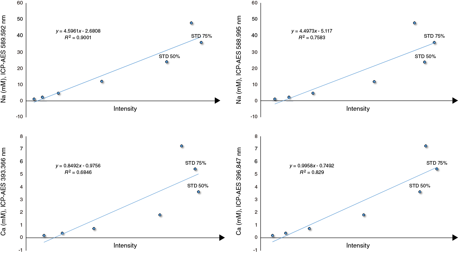
Figure F15. Na and Ca intensities from the ICP-AES.
The pattern of the calibration curves for the two Ca and Na lines in Figure F15 is consistent with signal saturation in the ICP-AES detector array. For most cations, ICP-AES provides a linear dynamic range of 5–6 orders of magnitude, but for many of the alkaline elements, this range can be curtailed substantially due to matrix enhancement or self-enhancement effects (e.g., intensity increases due to the sum of light-producing species in the ICP analysis solutions and/or greater than normal intensity related to increasing concentration of the analyte; Potts, 1992). The spectral lines for the alkaline elements, particularly the alkali metals, are particularly sensitive to matrix effects. Li, Na, and K ICP spectral lines are all susceptible to matrix enhancement, as are many of the spectral lines for the alkaline earths.
Using a dilution of 1:100, the concentration of Na in the ICP-AES solutions exceeds 100 ppm for seawater, which is beyond the linear dynamic range of the instrument for Na, taking matrix effects into account. Based on the curves in Figure F15, solutions containing as little as 50 ppm Na could show signal saturation effects, which would argue for a more substantial dilution for major cations (possibly 300:1 or 400:1). This level of dilution can create analytical challenges for Mg and K, which are considerably lower in abundance than Na in both seawater and interstitial waters.
The correlation between IC Cl determinations and chlorinity determined via the titration method outlined in Gieskes et al. (1991) (Figure F14) is poor, with a low R2 value and a positive Y intercept, raising the possibility of a systematic bias between these two methods. Re-analysis of several Site U1492 interstitial water samples confirmed the reproducibility of the two methods. Replication of the IAPSO seawater standard by the titration method is within ±1% of the accepted value, and a sample replication for Cl via IC is within 1%–2% of accepted values for standards at two different concentration levels. Therefore, both methods appear to be accurate.
Gieskes et al. (1991) noted the necessity of correcting titration Cl values for the presence of Br and like anions that might be present in solution and might also react with AgNO3. As such, the presence of S2− or other anions could complicate titration readings for Cl−. It appears that a number of horizons within the Site U1492 summit cores, from which the data for this analysis was taken, have significant sulfide mineralization. Testing for sulfide generally requires using a fixing agent to prevent H2S volatility losses, and because Site U1492 interstitial waters were not initially collected with shipboard sulfide determinations in mind, the samples were not fixed. As a result, primary sulfide could not be measured. The potential for dissolved sulfide adds a potential source of uncertainty to our titration-based chlorinity determinations that is not a concern with Cl on the IC. However, given that nitric acid was added before the chlorinity titration, the decrease in sample pH should have mobilized volatile hydrogen sulfide, eliminating the need to correct the chlorinity for these ions.
For Expedition 366, rather than reanalyzing recovered samples or institute fundamentally different analytical protocols, we have chosen to do the following to address the issues our comparative analysis has uncovered:
- We did not use interstitial water Na data collected by ICP-AES, given the concerns with signal saturation, and instead used Na results determined by IC.
- Given that Ca interstitial water results with the 317.9 nm spectral line appear to be as reliable as the IC results, we used these data in our interpretations because the reported precision of ICP-AES data (at less than ±5%) are better than typical precision of Ca by IC. Ca results using the other ICP-AES spectral lines were neglected because signal saturation is a concern for these wavelengths.
- We used interstitial water Cl results collected using IC in our interpretations, primarily because of the potential for uncertainty in the titration-based chlorinity measurements even though this method has a much better precision.
Microbiology
During Expedition 366, samples for microbiological analysis were collected from serpentinite muds and pelagic sediments. The collective overarching objectives for microbiological study will focus on determining the biomass, activity, and community structure of these subsurface microbial and viral communities, as well as assessing microbial ecology, diversity, and metabolic potential using an array of molecular microbiological applications. Relatively few shipboard analyses were performed because most measurements needed to be made in shore-based laboratories. Accordingly, the majority of our effort was dedicated to collecting and preserving an adequate number of samples for subsequent shore-based molecular biological studies.
Shore-based analyses will use a number of techniques to achieve the overall objectives. DNA analyses of small-subunit (SSU) ribosomal gene amplicon sequencing will be conducted to address community structure. Metagenomics analysis will be conducted to reconstruct the metabolic potential and identify entire genomes from microbial populations in the samples. RNA determination using metatranscriptomics will help to establish potential community activity (i.e., the genes that are most highly expressed in a given microbial environment). Both functional gene quantification through quantitative polymerase chain reaction (qPCR) and single-cell genomics will provide detailed information about the potential metabolic characteristics of microbes, link those potentials to cellular identity, and provide clues related to the best environment to cultivate cells from recovered samples. Enrichment for specific groups of organisms will identify the unique physiological properties of the organisms. A considerable amount of time during the expedition was dedicated to collecting samples for quality assurance and quality control to constrain the microbiological quality of the samples.
Ship- and shore-based microbiologists plan to correlate these molecular microbiological and cultivation results with variations in interstitial water geochemistry to interpret the metabolic potential of the microbial communities. Our goal for these comparisons will be to test specific hypotheses in the context that such microbial taxa are the residual survivors exposed to ultradeep subsurface serpentinization processes and mud volcanism mass transport encountered in the Mariana subduction system.
Microbial core handling and sampling
Microbiological sampling depends on careful sample handling techniques and the use of tracers to assess potential contamination. Microorganisms collected from beneath the seafloor are expected to be sensitive to chemical and physical changes that they encounter when brought to the surface. Changes in oxygen concentration and temperature are two important factors to be considered when bringing cells from cold, anoxic settings to the surface. Accordingly, the following procedures were followed to minimize harm to subsurface microbes without compromising other expedition objectives.
Contamination testing
Considerable potential exists for contamination and cross-contamination by microbes through the drilling process. Accordingly, it has become common practice to add tracers to the drilling fluids so that the extent of contamination from the drilling fluids and core recovery methods can be effectively evaluated. To check for potential intrusion of drilling fluids from the outside to the center of cores and to confirm the suitability of cored material for microbiological research, perfluorocarbon tracers (PFTs) were used while coring with the APC system, and periodic sampling of the drilling fluids, seawater (used to mix the drilling fluids), and outer surfaces of the whole rounds was conducted to obtain community data based on extracted DNA. Comparison of microbial community profiles derived from likely sources of contamination with profiles from the core interior should yield notable differences; otherwise, there is reason to believe that the interior of the sample was compromised.
Perfluorocarbon tracer
As a group, PFTs are nontoxic, inert, insoluble in water, and easily detected in a GC with an electron capture detector (ECD). Either perfluoromethylcyclohexane (PMCH) or perfluoromethyldecalin (PFMD) were used, depending upon availability for all drilling operations when microbial samples were collected. PFMD is produced in Russia and was difficult to secure in sufficient quantities prior to the expedition; it was therefore used in selected holes, and PMCH was used in the remainder of the holes. PFTs were introduced into the drilling fluids with a high-pressure liquid chromatography pump at a constant concentration of 1 mg/L. PFTs serve as an imperfect tracer for potential contamination of core material by nonindigenous microbes in the drilling fluids because it is much smaller than microbes; however, it is an efficacious guide for qualitative estimates of contamination.
Previous expeditions have used PMCH or, more recently, PFMD injected into drilling fluid to try to quantify intrusion of drilling fluid into the interior of samples (Smith et al., 2000; Lever et al., 2006; Inagaki et al., 2015; Dick et al., 2016). Based on prior reports from Expeditions 329 and 360 (Expedition 329 Scientists, 2011; Dick et al., 2017) and difficulties associated with release of PFTs from core material, we did not attempt to develop the PFT as a quantitative tracer. Instead, PFT samples were prepared according to previously established methods (Smith et al., 2000; Lever et al., 2006; Inagaki et al., 2015), slightly modified by taking 5 mL of core liner fluid or 2 cm3 mud samples on the catwalk immediately after core recovery. Samples were collected at the top of the core, where contamination is expected to be highest, and in the interior, halfway, and exterior of all microbiology whole-round samples. All samples were quickly placed into GC vials containing 5 mL of milliQ water, closed with screw caps, and stored at 4°C for later analysis. Analyses were done on board using an Agilient 6890N GC with ECD.
Fluid community tracers
To further evaluate the extent to which contaminating cells may have penetrated a sample, a postexpedition comparison will be made of the microbial community diversity between the serpentinite mud and pelagic sediment samples and the respective drilling fluid collected at the time of coring. This technique was first performed with deep continental samples (Lehman et al., 1995) but is common for studies of subseafloor samples, in which contamination is ubiquitous and genomic signatures of the contaminating material are subtracted from those of the subseafloor samples (Inagaki et al., 2015). The comparison can be accomplished by obtaining and preserving an adequate number of samples from the different sources of contamination (seawater or drilling fluid) and from the interior of the cores and then carrying out high-throughput sequencing of the SSU rRNA genes in the respective samples. Subsequent evaluation of the community signatures can help identify samples that significantly overlap in community structure with the drilling fluids (deeming them contaminated) or samples that have unique community structure when compared to the fluids (deeming them unlikely to be contaminated). For fluid community tracers, microorganisms were collected on 0.2 µm pore filters by filtering 1 L of seawater or drilling fluid collected from the drilling fluid pumped down the drill string. The filters were frozen (−80°C) and will be analyzed postexpedition to compare the microbial community structures in the drilling fluids with those in the core samples.
Microbiological whole-round sampling
Whole-round cores were collected immediately after the core reached the catwalk. Two 20 cm long whole rounds were broken away from the rest of the core to minimize the potential for cross-contamination by breaking or cutting with an ethanol-rinsed spatula when necessary. The cores were handled only with nitrile gloves and capped on both ends with ethanol-rinsed plastic caps. The whole-round samples were labeled and transferred to the Microbiology laboratory, where they were stored in the cold room (4°C) to minimize alteration of the microbial communities. Samples were partitioned under aseptic conditions.
As soon as possible, the 20 cm long whole-round samples were sampled into sterile 3 mL syringes, of which 2 cm3 were transferred into fixative buffer (see below) for onshore determination of microbial cell numbers. Further sampling was done with sterile 30 mL cut-tip syringes, and then samples were (1) transferred into sterile Whirl-Pak bags or 50 mL centrifuge tubes or (2) sampled into sterile 5 mL cut-tip syringes and then transferred into sterile 15 mL centrifuge tubes. Samples were then either stored in an ultralow-temperature freezer (−80°C) for molecular analyses, in a freezer (−20°C) for later D:L amino acid determination, or in a refrigerator (4°C) for cultivation-based analyses and cell counts. The outer portions and bigger clasts of the cores that remained after microbiological sampling were returned to the Core laboratory.
Preservation of samples for total cell counts
Cells were fixed with a solution (100 mM CAPS [pH = 10.5], 2% formaldehyde, and 3% NaCl) and stored at 4°C until further processing. Quantitative cell counting will be carried out on shore.
Preservation of samples for single cell genomics
Three 5 cm3 samples were placed into sterile 5 mL tip-cut syringes and then transferred into sterile 15 mL centrifuge tubes and stored in the 4°C cold room. To each of these samples, we added 10 mL of sterile buffer (phosphate-buffered saline). Samples and buffer were vortexed for 30 s and then centrifuged for 30 s at 2000 × g to remove large particles. Inside a cryovial, 1 mL of the supernatant was added to 1/10 volume of filtered glyTE buffer, placed in liquid nitrogen, and stored at −80°C for future analysis.
Preservation of samples for metagenomics and metatranscriptomics
Four to eight 25 cm3 subsamples were placed into extra heavy duty 50 mL centrifuge tubes using sterile 30 mL tip-cut syringes as described above. These were either fast frozen in the −80°C freezer for metagenomic analysis or samples had an equal volume of RNALater reagent added to them. This sample-solution mixture was made into a slurry and stored overnight in the 4°C cold room. After ~12 h, the sample-solution mixture was fast frozen in the −80°C freezer for either metagenomic or transcriptomic analysis on shore. Larger volumes from whole-round samples were also collected from depths >50 mbsf and stored at −80°C in an effort to address deep subsurface metagenomics.
Preservation of samples for FACS culturing
Two 5 cm3 samples were placed into sterile 5 mL tip-cut syringes and then transferred into sterile 50 mL centrifuge tubes and stored in the 4°C cold room. These will be transported unfrozen on ice and processed by fluorescence-activated cell sorting (FACS) for high-throughput culturing once on shore.
Cultivation of potentially piezophilic microbes
Incubations at high pressure started with 50 cm3 of mud from three depths (approximately 5, 100, and 250 mbsf). From this subsample, 10 cm3 of unconsolidated material was sealed anaerobically in aluminum bags and stored at −80°C for Illumina amplicon sequencing of the time zero communities. The remaining 40 cm3 was turned into a slurry in an anaerobic glove box (flushed with nitrogen) by adding equal volumes of alkaline basal salts medium + NH4Cl (ABSN) and vortexing the mixture. A portion of the mixture was placed into two cryovials, mixed with glyTE buffer, and placed in the −80°C freezer for future culturing. The remaining slurry was used for incubations under high pressure. High-pressure experiments used 4 mL of slurry placed in a 5 mL glass serum vial and amended with one of the following:
- No amendment, 5 mL of slurry supernatant;
- 1 mL of 5× Caminibacter medium for thermophilic bacteria;
- 1 mL of 5× Alkaline MJYTGL medium for bacteria living at a pH of 10.5;
- 1 mL of 3 mM sodium formate; or
- 1 mL of 3 mM sodium acetate.
These serum vials were then crimp-sealed, and all air bubbles were removed; each of these amendments was duplicated. One set of these amendments (five vials in total) was stored at atmospheric pressure in the 4°C cold room, and the other set of amendments was placed in a pressure vessel and pressurized using a hand pump created by the Bartlett laboratory. Samples from 5 and 100 mbsf were incubated at 20 or 40 MPa. Samples from 250 mbsf were incubated at 90 MPa. Pressure vessels were stored in the 4°C cold room for incubation.
Mud samples (50 cm3) were also taken approximately every 10 m at each drilling site. From these samples, 10 cm3 of mud was sealed anaerobically in aluminum bags and stored at −80°C. A slurry was made, as described above, using 2 cm3 of mud and was placed into two cryovials, mixed with glyTE buffer, and placed in the −80°C freezer for future culturing. The remaining mud sample was anaerobically sealed in an aluminum bag and stored in the 4°C cold room.
Preservation of samples for virus assessment and quantification
Samples (10 cm3) for virus counting were collected as described above using sterilized cut syringes and then stored in the −80°C freezer. The 5 cm long whole rounds were anaerobically stored at 4°C for viral production analysis. Considering the small amount of genetic materials in viral particles, 15 cm long whole rounds were collected and stored at −80°C for further viral diversity study based on polymerase chain reaction amplification.
Physical properties
High-resolution physical property measurements were made during Expedition 366 to characterize recovered material and lithostratigraphy and tie core descriptions to borehole data and seismic profiles. In particular, physical property data play a major role in detection of discontinuities and inhomogeneities, revealing information about changes in the composition and texture of muds and rocks that can indicate different mud volcano flows or distinguish between pelagic sediments and mud matrix. A variety of techniques and methods were used to characterize Expedition 366 whole-round cores, split section half cores, and discrete samples. Core sections are generally 1.5 m in length, so a typical coring length (stroke) of 9.5 m yields six sections plus a shorter seventh section, and a HLAPC core of 4.7 m yields three plus a short fourth section if there is full recovery. During this expedition, some core sections were shorter because of whole-round sampling for microbiology, interstitial water geochemistry, and personal samples.
Unlithified cores (pelagic sediments and serpentinite muds) were measured in the following sequence:
- Cores were thermally equilibrated to ambient room temperature (~3–4 h).
- Whole-round cores were run on the WRMSL. The WRMSL includes a gamma ray attenuation (GRA) bulk densitometer, a magnetic susceptibility logger (MSL), and a P-wave logger (PWL). The sampling interval was set to 2 cm.
- Whole-round cores were run on the NGRL.
- Thermal conductivity was measured on two sections of each core.
- Cores were split.
- Color reflectance and magnetic susceptibility were measured on archive section halves using the SHMSL.
- Undrained shear strength and P-wave velocity measurements were performed on the working halves. P-wave velocity analyses were conducted with the transducers oriented in the x- and z-axis directions.
- Discrete samples of soft and more consolidated materials for MAD analyses were collected typically at 50 cm in every section. MAD measurements were performed on wet samples and after samples were dried in an oven for 24 h. Bulk density, dry density, grain density, and porosity were calculated from the measurements. Large hard rock serpentinite clasts were collected when possible.
- P-wave velocity and MAD measurements were performed on discrete cube samples of the rock material (~2 cm × 2 cm × 2 cm). P-wave velocity was measured for wet cube samples in three orthogonal directions. (Some samples were first analyzed for paleomagnetism study; see Paleomagnetism).
Throughout Expedition 366, all raw data were uploaded to the LIMS database. A comprehensive discussion of methodologies and calculations used in the JOIDES Resolution Physical Properties Laboratory is presented in Blum (1997).
Whole-round measurements
GRA-derived bulk density, P-wave velocity, and magnetic susceptibility were measured nondestructively with the WRMSL. To optimize the measurement process, sampling intervals and measurement integration times were the same for all sensors. Sampling intervals are common denominators of the distances between the sensors installed on the WRMSL (30–50 cm), which allows sequential and simultaneous measurements. After every core, quality assurance/quality control (QA/QC) were monitored by passing a calibration core liner filled with deionized water through the WRMSL. The nominal accuracy of the calibrated instruments was between 1% and 2%.
Gamma ray attenuation bulk density
Bulk density can be used to estimate the pore volume in unlithified material and evaluate the consolidation state of the material. GRA density is an estimate of bulk density based on the attenuation of a gamma ray beam. The beam is produced by a 137Cs gamma ray source at a radiation level of 370 MBq within a lead shield with a 5 mm collimator, which is vertically directed through the whole-round core. The gamma ray receiver consists of a 75 mm3 sodium iodine (NaI) detector located on the top side of the core, opposite to the source, that records the gamma radiation that passes through the core. The input gamma ray peak has a principal energy of 0.662 MeV and is attenuated as it passes through the core. The gamma ray attenuation occurs primarily by Compton scattering, in which the gamma rays are scattered by electrons in the formation. The degree of scattering is related to the material bulk density. Therefore, for a known thickness of sample, density (ρ) is proportional to the intensity of the attenuated gamma rays:
- I = the measured intensity of gamma rays passing through the sample,
- I0 = gamma ray source intensity,
- μ = Compton attenuation coefficient, and
- d = sample diameter.
The μ and I0 are treated as constants so ρ can be calculated from I (Harms and Choquette, 1965).
In general, WRMSL measurements are most accurate when taken on a completely filled core liner with minimal drilling disturbance; otherwise, measurements tend to underestimate true values. By default, the instrument reports measurements using the internal diameter of the core liner (66 mm) as the assumed sample diameter. This assumption is suitable for most cores of unconsolidated material obtained by the APC system. The spatial resolution of the GRA densitometer is less than 1 cm. The gamma ray detector is calibrated with a sealed calibration core (one standard core liner filled with distilled water and a telescoped aluminum bar machined into discrete diameter steps of various diameters, located at the top of the core). To establish the calibration curves, gamma ray counts were taken through each of the discrete diameter steps for 60 s. Recalibration was performed whenever the deionized water QA/QC standard deviated significantly (more than 0.021 g/cm3) from 1 g/cm3.
Magnetic susceptibility
Magnetic susceptibility (χ) is a dimensionless measure of the degree to which a material can be magnetized by an external magnetic field:
where M is the magnetization induced in the material by an external field of strength H.
Magnetic susceptibility varies in response to the type and concentration of magnetic grains, such as the ferrimagnetic minerals (e.g., magnetite and maghemite), making it useful for identifying compositional variations. Magnetic susceptibility responds to variations in the magnetic composition of cored materials that are commonly related to variations in mineralogical composition (e.g., terrigenous versus biogenic materials) and diagenetic overprinting. Materials such as clay generally have a magnetic susceptibility several orders of magnitude lower than magnetite or some other iron oxides that are common constituents of igneous material. Water and plastics (such as the core liner) have a slightly negative magnetic susceptibility.
Measurements were made using a Bartington MS2C loop sensor with a 9.0 cm diameter (Bartington Instruments, 2011). The loop sensor has a spatial resolution of 23–27 mm and is accurate to within 2%. An oscillator circuit in the sensor, which operates at a frequency of 0.565 kHz and an alternating field (AF) of ~140 A/m, produces a low-intensity, nonsaturating alternating magnetic field. Core sections of unconsolidated materials going through the influence of this field cause a change in oscillator frequency. Frequency information returned in pulse form to the susceptometer is converted into magnetic susceptibility. The instrument was set to record SI units with an integration period of ~1 s, which produced a sensitivity of 1 × 10⁻⁵ SI.
The along-core response curve of the MS2C coil has a full width at half maximum of ~4 cm (Blum, 1997) and is consistent with the decay in magnetic intensity with distance from a dipole. Therefore, measurements of susceptibility from core pieces <8 cm long will significantly underestimate magnetic susceptibility by more than 10%.
P-wave velocity
P-wave velocity data can be used to evaluate small-strain moduli and evaluate porosity, compaction, and cementation. P-wave velocity is the rate at which a (compressional) P-wave travels through a medium per unit time, expressed in meters per second. P-wave velocity is dependent on the composition, porosity, bulk density, fabric, and temperature of the material, which in turn are functions of consolidation and lithification, state of stress, and degree of fracturing. P-wave velocity (VP) is defined by the time required for a compressional wave to travel a specific distance:
where d is the path length of the wave across the core and tcore is the traveltime through the core.
The PWL system on the WRMSL transmits a 500 kHz P-wave pulse across the core liner at a specified repetition rate. Pulser and receiver are mounted on a caliper-type device and are aligned in order to make wave propagation perpendicular to the section’s long axis. A linear variable differential transducer measures the P-wave travel distance between the pulse source and the receiver. Good coupling between transducers and core liner is facilitated with water dripping onto the contact from a peristaltic water pump system. Signal processing software picks the first arrival of the wave at the receiver, and the processing routine corrects for the thickness of the liner. The total observed traveltime tcore is composed of
- tdelay = time delay related to transducer faces and electronic circuitry,
- tpulse = delay related to the peak detection procedure,
- tliner = transit time through the core liner, and
- tcore = traveltime through the cored material.
The system is calibrated using a core liner filled with distilled water, which provides control for tdelay, tpulse, and tliner. From these calibrations, VP can be calculated for the whole-round specimens in core liners as
VP = (dcl − 2dliner)/(to − tpulse − tdelay − 2tliner),
- dcl = measured diameter of core and liner,
- dliner = liner wall thickness, and
- to = measured total traveltime.
The above equation assumes that the core completely fills the core liner. The PWL was deemed worthless for cores recovered with the XCB system, which often do not fill the core liner.
A series of acrylic cylinders of varying thicknesses are used to calibrate the PWL system. The regression of traveltime versus travel distance yields the P-wave velocity of the standard material, which should be 2750 ± 20 m/s. The thickness of the calibration samples, corrected for liner thickness, are divided by the travel time to calculate P-wave velocity in meters per second. The calibration is verified by measuring a core liner filled with pure water, and the calibration passes if the velocity is within ± 20 m/s of the expected value for water (1485 m/s).
Natural gamma radiation logger
Gamma radiation is emitted from the decay series of mineral-hosted 238-uranium (238U), 232-thorium (232Th), and 40-potassium (40K). The system in use was designed and built at the Integrated Ocean Drilling Program-US Implementing Organization (USIO) at Texas A&M University (Vasiliev et al., 2011). When 238U, 232Th, and 40K radioisotopes decay, they and their daughter products emit gamma radiation at specific energy levels unique to each isotope. NGR spectroscopy measures a wide energy spectrum that can be used to estimate the abundance of each isotope based on the strength of the signal at characteristic energies. Spectral data were collected and can be used for postexpedition processing for U, Th, and K abundance but were not processed on board. Total counts were used on board, with high counts usually identifying fine-grained deposits containing K-rich clay minerals and their absorbed U and Th isotopes. NGR data thus reveal stratigraphic details that aid in core-to-core correlations. Serpentinite muds and ultramafic rocks have very low concentrations of U, K, and Th.
The main NGR detector unit consists of 8 sodium iodide (NaI) scintillator detectors arranged along the core measurement axis at 20 cm intervals surrounding the section. The section is measured once and then moves 10 cm and is measured again to provide 10 cm measurement spacing. The detector array has passive (layers of lead) and active (plastic scintillators) shielding to reduce the background environmental and cosmic radiation. The overlying plastic scintillators detect incoming high-energy gamma and muon cosmic radiation and cancel this signal from the total counted by the NaI detectors. The NGRL was calibrated using 137Cs and 60Co sources to identify peaks at 662 and 1330 keV, respectively.
Total counts are routinely summed over the range of 100–3000 keV. The quality of the measured energy spectrum depends on the concentration of radionuclides in the sample and on the counting time, with longer counting times providing better counting statistics. A live counting time of 5 min was set in each position (for a total live count time of about 10 min per section). Sections were scanned only once.
Thermal conductivity
Thermal conductivity measurements at one location in every other section were made using the TK04 (Teka Bolin) system described by Blum (1997). For whole-round soft-recovery cores, a needle probe in full-space configuration (Von Herzen and Maxwell, 1959) was used. The probes contain a heater wire and calibrated thermistor.
For soft recovery, the needle probe was inserted into a 2 mm diameter hole drilled along one of the lines that later guided core splitting. The location was at around 60–70 cm from the top of the section or in an interval with low disturbance based on visual inspection. To avoid interference from airflow in the laboratory, the core was placed into an enclosed box insulated with foam.
A heating power of 0.5–2 W/m was typically used in soft recovery. The solution to the heat conduction equation with a line source of heat was then fit to the temperature measurements to obtain the thermal conductivity. Because the probe is much more conductive than sediment or igneous rock, the probe is assumed to be a perfect conductor. Under this assumption, the temperature of the superconductive probe has a linear relationship with the natural logarithm of the time after the initiation of the heat:
- T = temperature (K),
- q = heat input per unit length per unit time (J/m/s),
- k = thermal conductivity (W/[m·K]),
- t = time after the initiation of the heat (s), and
- C = instrumental constant.
Three measuring cycles separated by a cooling interval of 10 min were automatically performed to calculate average conductivity. A self-test, which included a drift study, was conducted at the beginning of each measurement cycle. Once the probe temperature stabilized, the heater circuit was closed and the temperature rise in the probe was recorded. Thermal conductivity was calculated from the rate of temperature rise while the heater current was flowing. Temperatures measured during the first 60 to 80 s of the heating cycle were fitted to an approximate solution of a constantly heated line source (for details, see Blum, 1997). Measurement errors were 5%–10%. Data are reported in watts per meter degree Kelvin.
Section Half Multisensor Logger measurements
Color reflectance and magnetic susceptibility were measured on archive section halves using the SHMSL. The archive half was placed on the core track, above which an electronic platform moves along a track recording the height of the split-core surface with a laser sensor. The laser establishes the height of the section half’s surface and the location of the bottom of the section, and then the platform reverses the direction of movement, moving from bottom to top making measurements of point magnetic susceptibility and color reflectance. Intervals where material did not fill the section half or contained foam inserts were excluded from measurement, so the measured range of values represents that of core material only. Color reflectance and point magnetic susceptibility data were collected at constant intervals of 2 cm.
Color reflectance spectrometry
At the first two sites (U1491 and U1492), the color reflectance spectrometer was equipped with an Ocean Optics USB4000 sensor. After Site U1492, the color spectrophotometer sensor was upgraded to an Ocean Optics QEPro model that provides a slightly larger spectral range and has a significant increase in low-light resolution. Both spectrophotometers used a 30 mm integrating sphere and were illuminated using a combined OceanOptics HL-2000 halogen and the OceanOptics BluLoop LED light sources. The HL-2000 provides illumination from 360 to 2400 nm, and the BluLoop, using four LED sources, provides a balanced output from 400 to 700 nm, covering wavelengths from ultraviolet through visible to near infrared. Measurements were taken from 380 to 900 nm wavelengths at 2 nm intervals. The ~3 s data acquisition offset was applied for the entire scan of the archive half. Data are reported using the L* a* b* color system, in which L* is lightness, a* is redness (positive) versus greenness (negative), and b* is yellowness (positive) versus blueness (negative). The color reflectance spectrometer calibrates on two spectra, pure white (reference) and pure black (dark). Color calibration was conducted once every 6 h.
Point magnetic susceptibility
Point magnetic susceptibility was measured with a Bartington MS2 meter and an MS2K contact probe with a flat 15 mm diameter round sensor with a field of influence of 25 mm and an operation frequency of 930 Hz. The instrument averages three measurements from the sensor for each offset, leading to an accuracy of ~5%. The spatial resolution of the point magnetic susceptibility instrument is ~3 mm, higher than that of the whole-round magnetic susceptibility measurement (20 mm). As with whole-round measurements, the output displayed by the point magnetic susceptibility sensor must be converted to dimensionless SI units by multiplying by 10−5. The probe is zeroed in air before each measurement location to avoid influence from the metal track. The point magnetic susceptibility meter was calibrated by the manufacturer before installation on the ship and is quality checked every 6 h, at the same time as color reflectance sensor calibration. The SHMSL magnetic susceptibility measurements integrate over a smaller depth than the WRMSL loop measurements.
Discrete measurements
P-wave velocity
The P-wave velocity system uses Panametrics-NDT Microscan delay line transducers (transmitting at 0.5 MHz). The signal received through the section half or discrete sample was recorded by the Velocity Gantry 2.0.5.0 IODP software, where the peak of the first P-wave arrival is automatically or manually chosen. In case of a weak signal, manual picking of the first arrival was performed.
The distance between transducers was measured with a built-in linear voltage displacement transformer. Calibration was performed daily with a series of acrylic cylinders of differing thicknesses and a known P-wave velocity of 2750 ± 20 m/s. The determined system time delay from calibration was subtracted from the picked arrival time to give a traveltime of the P-wave through the sample. The thickness of the sample (calculated by the linear voltage displacement transformer, in meters) was divided by the traveltime (in seconds) to calculate P-wave velocity in meters per second. It was difficult to pick a clean first P-wave arrival from the serpentinite mud data from this instrument, and measurements were typically attempted on only the first few cores at each site. The WRMSL P-wave instrument, in contrast, produced more reliable P-wave data.
For soft-recovery cores, P-wave velocity measurements were performed on the working half before any sampling. Following standard IODP conventions, P-wave velocity measurements used the x- and z-axis of the Section Half Measurement Gantry (SHMG), with several analyses per core. Different positions with respect to lithology were chosen to generate viable data. Rock cube samples were oriented following Blum (1997) and placed on a gantry that measures P-wave velocity in three orthogonal directions (x-, y- and z-directions). P-wave anisotropy ratios were calculated from these multidirectional analyses. Before measurements, the cubes were seawater saturated using a vacuum pump for at least 24 h.
Automated vane shear
The shear strength of a material describes the point at which a significant structural failure occurs in response to an applied shear stress. Shear strength of the mudflow matrix and pelagic sediment was measured using the automated vane shear by Giesa because this method is suited for measuring the shear strength of very soft to relatively stiff marine sediments. This geotechnical test is useful for determining the undrained shear strength of undisturbed clay- or silt-rich samples; it is not suitable for coarser grained sediments or sediment containing silt or sand laminations.
The Giesa system consists of a controller and a gantry for shear vane insertion. A four-bladed miniature vane was pushed carefully into the sediment of the working halves until the top of the vane was level with the core surface. The vane was then rotated at a constant rate of 60°/min to determine the torque required to cause the core material to be sheared (failure torque). All vane shear strength measurements were obtained using a vane with a height of 12.7 mm and a blade length of 6.35 mm. Failure torque was determined by measuring the rotation of a torsional spring using a spring-specific relation between rotation angle and torque.
Then, vane shear strength (Su[V]) can be determined as follows:
- T = torque required to induce material failure (N·m),
- Kv = constant, depending on vane dimensions (m3),
- Δ = maximum torque angle (°) at failure, and
- B = spring constant that relates the deflection angle to the torque (°/N·m) (Blum, 1997).
Typically, there was one measurement per core section until the recovered material became too firm for vane insertion. Measurements were generally taken in undisturbed relatively fine grained intervals, where possible.
Moisture and density
To perform MAD analysis in working halves, the unconsolidated materials were sampled using plastic syringes or spatulas for ~10 cm3 volume. Preweighed, numbered 16 mL Wheaton glass vials were used to process and store the samples. Typically, one sample per section was collected. Measured samples were strategically chosen to capture lithologic variations in the core and to correct for WRMSL GRA measurements. For hard rock, the discrete cubes initially used for paleomagnetism and P-wave velocity (P-wave caliper [PWC]) measurements were also used for MAD analyses when possible.
Mass and volume measurements were made to determine wet and dry bulk density, grain density, water content, and porosity. After measurement of wet mass, samples were dried in a convection oven for at least 24 h at 105° ± 5°C. Dried samples were then cooled in a desiccator for at least 1 h before the dry mass and volume were measured.
Dual balance system
The weights of wet and dry sample masses were determined to a precision of 0.005 g using two Mettler Toledo (XS204) electronic balances and a computer averaging system to compensate for the ship’s motion. A standard weight of comparable value to the sample (maximum = >10% of the sample mass) was placed on a reference balance to increase accuracy. The default setting of the balances is 300 measurements. After wet mass determinations and P-wave measurements (for cube samples), samples were placed in the drying oven and then allowed to cool in the desiccator prior to the determination of dry masses.
Hexapycnometer volume measurement
Dry sample volume was determined using a hexapycnometer system of a six-celled, custom-configured Micromeritics AccuPyc 1330TC helium-displacement pycnometer. The system measures dry sample volume using pressurized He-filled chambers; the precision of each cell is better than 1% of the full-scale volume when properly calibrated and operated. Volume measurements were preceded by three purges of the sample chamber with helium. For each measurement, five unknown cells and one cell that contained two stainless steel calibration spheres (3 and 7 cm3) with a total volume of ~10 cm3 were run. Calibration spheres were cycled through the cells to identify any systematic error and/or instrument drift. Spheres are assumed known to within 1% of their total volume. The volumes occupied by the numbered Wheaton vials were calculated before the expedition by multiplying each vial’s weight against the average density of the vial glass. The procedures for the determination of these physical properties comply with the American Society for Testing and Materials (ASTM International, 1990).
Moisture and density calculations
The calculations given below are used as an IODP standard in accordance with Blum (1997). MAD properties reported and plotted in the Physical properties section of each site chapter were calculated with the MADMax shipboard program set with the method applicable to saturated, fine-grained sediments called “Method C.” Method C is based on the measurement of wet mass (Mwet), dry mass (Mdry), and volume (Vdry). The ratio of mass (rm) is a computational constant of 0.965 (i.e., 0.965 g of freshwater per 1 g of seawater). Salt precipitated in pores in the samples during the drying process is included in the Mdry and Vdry values. The mass of the evaporated water (Mwater) and salt (Msalt) in the sample are given by
where s is the assumed saltwater salinity (0.035) corresponding to a pore water density (ρpw) of 1.024 g/cm3 and a salt density (ρsalt) of 2.22 g/cm3. The corrected mass of pore water (Mpw), volume of pore water (Vpw), mass of solids excluding salt (Msolid), volume of salt (Vsalt), volume of solids excluding salt (Vsolid), and wet volume (Vwet) are
Vwet = Vdry − Vsalt + Vpw, and
For all samples, water content (w) is expressed as the ratio of mass of pore water to wet sample (total) mass:
Wet bulk density (ρwet), dry bulk density (ρdry), sample grain density (ρsolid), porosity (φ), and void ratio (VR) are calculated as
An accuracy and precision of MAD measurements of ~0.5% can be achieved with the shipboard devices. The largest source of potential error is the loss of material or moisture during the ~30–48 h long procedure for each sample.
Downhole measurements
Temperature measurements
During Expedition 366, downhole temperature measurements were made using the APCT-3 and the water-sampling temperature probe (WSTP) to characterize transport of heat, fluids, and solutes in active serpentinite mud volcanoes. Fluid flow transports solutes from the subducting slab through the mantle wedge, where the fluids react with mantle rocks before discharging on the seafloor; one aim of the temperature measurements is to provide constraints on rates of fluid flow. If sufficiently detailed, the measured temperature profiles can be used to estimate flow rates where they are greater than ~0.1 mm/day for equilibrated standard conditions. These rates can then be compared to those that can be calculated from systematic variations in pore water chemical profiles.
Formation temperatures were measured using the APCT-3 at five sites. The WSTP was used to measure temperature profiles and collect water samples in cased Holes U1496C and U1497D. A temperature dual-pressure tool (T2P) deployment in Hole U1492C was canceled at the last minute due to deteriorating borehole conditions. Revisions to the T2P deployment procedure based on Expedition 362 operations (McNeill et al., 2017b) are briefly outlined below.
Advanced piston corer temperature tool
In situ temperature measurements were made with the APCT-3 when the APC was deployed. The APCT-3 fits directly into the coring shoe of the APC and can therefore be used to measure formation temperatures during regular piston coring. The tool consists of a battery pack, data logger, and platinum resistance-temperature device calibrated over a temperature range from 0° to 30°C. Before entering the borehole, the tool is first stopped at the mudline for 5 min to thermally equilibrate and to estimate the bottom water temperature. However, the lowest temperature recorded during the run was occasionally used as an estimate of the bottom water temperature instead of the average temperature at the mudline because (1) it was more repeatable and (2) the bottom water is expected to have the lowest temperature in the profile. When the APCT-3 is plunged into the formation, there is an instantaneous temperature rise from frictional heating. This heat gradually dissipates into the surrounding formation as the temperature within the APCT-3 equilibrates to the temperature of the unconsolidated materials. After the APCT-3 penetrates the formation, it is held in place for 10 min while it records the temperature of the cutting shoe every second.
Thermal data reduction
The transient thermal decay curves for formation thermal probes are known to be a function of the geometry of the probes and the thermal properties of the probe and the formation (Bullard, 1954; Horai and Von Herzen, 1985). Data analysis requires fitting the measurements to analytical or synthetic decay curves calculated based on tool geometry, sampling interval, and tool and formation thermal properties. The thermal time constant of the cutting shoe assembly into which the APCT-3 tool is inserted is ~2–3 min. Data reduction for the APCT-3 was performed using the program TP-Fit (Heeseman, 2008). It is generally not possible to obtain a perfect match between the synthetic curves and the data because (1) the probe does not reach thermal equilibrium during the penetration period, (2) contrary to ideal theory, the frictional pulse upon insertion is not instantaneous, and (3) temperature data are sampled at discrete intervals, so the exact time of penetration is uncertain. Thus, both the effective penetration time and equilibrium temperature must be estimated by applying a fitting procedure, which involves shifting the synthetic curves in time to obtain a match with the recorded data. Heeseman (2008) suggests that the best fit is obtained from the final third of the data set. Shipboard thermal conductivities were used for calculating heat flow and also input into the TP-Fit calculation for estimating in situ temperatures. Laboratory thermal conductivity measurements were not corrected for in situ conditions because the correction would be small at the shallow depths that were drilled.
Heat flow was calculated with the same approach used for Ocean Drilling Program Site 1200 (Shipboard Science Party, 2002c) by applying a single thermal conductivity value in the equation
- q = heat flow (W/m2),
- K = thermal conductivity (W/[m·K]), and
- ΔT/ΔZ = average thermal gradient (°K/m).
Water-sampling temperature probe
Samples of water and temperature profiles were collected inside the summit casings at two sites using the WSTP, a passive sampler deployed in the BHA. Before deployment, the overflow chamber was filled with nitrogen and the fluid path was flushed with nanopure water. A timer was set to open the valve at a fixed time, exposing the sampling line and chamber to ambient pressure. The timer also closes the chamber after a prearranged time interval has passed. In operation, the WSTP is mounted inside a core barrel and lowered within the drill pipe by wireline. The tool was lowered approximately 40 m, with the probe tip extending 1.2 m ahead of the RCB bit and in the open hole below the APC bit. The tool is then held in position with the pumps off, and the timer-operated valve is opened. The valve was left open 5 min. When the valve is open, bottom water is drawn into the sample coils under negative relative pressure through the filter and into the sample chamber, displacing the nitrogen. The chamber contains three sample volumes, a coiled titanium tube, a coiled copper tube (for dissolved helium and hydrogen), and the chamber itself (~1 L).
During both deployments, temperatures were recorded each second. The depth of the tool was held constant for 30 min at the locations of the water samples. At other selected locations in each cased hole, the depth was held constant for 5–10 min.
Temperature dual-pressure tool
For details on the T2P, see the Expedition 362 methods chapter (McNeill et al., 2017a). Based on Expedition 362 operations, there were several recommended revisions to the deployment strategy for the T2P during Expedition 366. The most important recommendation was to limit the applied standpipe pressure to less than 750 psi when driving the tool into the formation to remain below the buckling strength of the tool. Other deployment changes concerned preparing and unlatching the motion decoupled hydraulic delivery system (MDHDS). A series of steps were added to the deployment manual to ensure the MDHDS latch is engaged prior to deployment in the drill string. Once the MDHDS is in position, the new recommendation is to raise standpipe pressure to a maximum of 750 psi for unlatching. The previous value was 1000–1200 psi.
Wireline logging
Downhole logs are used to determine physical, chemical, and structural properties of the formation penetrated by a borehole. The data are rapidly collected, continuous with depth, and measured in situ; they can be interpreted in terms of the stratigraphy, lithology, mineralogy, and geochemical composition of the penetrated formation. Where core recovery is incomplete or disturbed, log data may provide the only way to characterize the borehole section. Where core recovery is good, log and core data complement one another and may be interpreted jointly. Downhole logs measure formation properties on a scale that is intermediate between those obtained from laboratory measurements on core samples and those from geophysical surveys. They are useful in calibrating the interpretation of seismic profiles and provide a link for the integrated understanding of physical properties on all scales.
During wireline logging operations, the logs are recorded with Schlumberger logging tools combined into tool strings, which are lowered into the hole after completion of coring operations. One tool string was used during Expedition 366: the triple combo, which measures magnetic susceptibility, NGR, resistivity, borehole diameter, and borehole fluid temperature (Figure F16; Tables T2, T3). The tool string also contains a telemetry cartridge for communicating through the wireline to the Schlumberger data acquisition system (multi-tasking acquisition and imaging system [MAXIS] unit) on the ship. Active sources were omitted from the string due to the short time before the end of the expedition, so formation density was not measured.
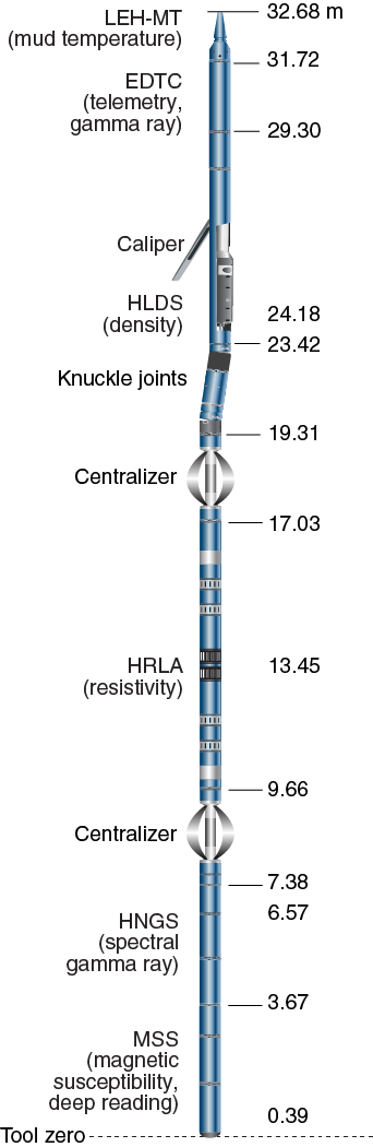
Figure F16. Wireline tool string.
Table T2. Downhole measurements by wireline tool strings. Download table in CSV format.
Table T3. Acronyms and units used for downhole wireline tools and measurements. Download table in CSV format.
In preparation for logging, the boreholes were flushed of debris by circulating a high-viscosity mud (sepiolite) sweep. The BHA was pulled up to about 52 m wireline logging depth below seafloor (WSF) to cover the unstable upper part of the hole. The tool strings were then lowered downhole on a seven-conductor wireline cable before being pulled up at constant speed of ~275 m/h to provide continuous measurements of several properties simultaneously. A wireline heave compensator (WHC) was used to minimize the effect of ship’s heave on the tool position in the borehole, except when ship heave was minimal. During each logging run, incoming data were recorded and monitored in real time on the Schlumberger Minimum Configuration MAXIS (MCM) logging computer.
Logged formation properties and tool measurement principles
The logged properties and the principles used in the tools to measure them are briefly described in this section. The main logs are listed in Table T2. More detailed information on individual tools and their geological applications may be found in Rider (1996), Goldberg (1997), and Ellis and Singer (2007). A complete online list of acronyms for Schlumberger tools and measurement curves is available at http://www.apps.slb.com/cmd/.
Natural gamma radiation
The Hostile Environment Natural Gamma Ray Sonde (HNGS) was used on the triple combo tool string to measure and classify NGR in the formation. It has two bismuth germanate scintillation detectors, and concentrations of K, U, and Th are determined from the characteristic gamma ray energy spectra of isotopes in the 40K, 232Th, and 238U radioactive decay series. An additional NGR sensor is housed in the Enhanced Digital Telemetry Cartridge (EDTC), run on all tool strings. Its sodium iodide scintillation detector measures the total NGR emission of the formation with no spectral information. The inclusion of a NGR sonde in every tool string allows use of NGR data for depth correlation between logging strings and passes and for core-log integration.
Electrical resistivity
The High-Resolution Laterolog Array (HRLA) provides six resistivity measurements with different depths of investigation (including borehole mud resistivity and five measurements of formation resistivity with increasing penetration into the formation). The tool sends a focused current into the formation and measures the intensity necessary to maintain a constant drop in voltage across a fixed interval, providing direct resistivity measurements. The tool has one central (source) electrode and six electrodes above and below it, which serve alternatively as focusing and returning current electrodes. By rapidly changing the role of these electrodes, a simultaneous resistivity measurement at six penetration depths is achieved. The tool is designed to ensure that all signals are measured at exactly the same time and tool position and to reduce the sensitivity to “shoulder bed” effects when crossing sharp beds thinner than the electrode spacing. The design of the HRLA, which eliminates the need for a surface reference electrode, improves formation resistivity evaluation compared to the traditional dual induction tool. The HRLA needs to be run centralized in the borehole for optimal results, so bowspring centralizers were used to keep the HRLA in the center of the borehole, and knuckle joints allowed the density tool to be eccentralized and maintain good contact with the borehole wall (Figure F16). Calcite, silica, and hydrocarbons are electrical insulators, whereas ionic solutions like interstitial water are conductors. Electrical resistivity can therefore be used to evaluate porosity for a given salinity and resistivity of interstitial water. Clay surface conduction also contributes to resistivity values, but at high porosities this effect is relatively minor.
Magnetic susceptibility
The magnetic susceptibility sonde (MSS) is a nonstandard wireline tool designed by the Lamont-Doherty Earth Observatory (LDEO; Columbia University, USA). It measures the ease with which formations are magnetized when subjected to a magnetic field. The ease of magnetization is ultimately related to the concentration and composition (size, shape, and mineralogy) of magnetic minerals (principally magnetite) in the formation. These measurements provide one of the best methods for investigating stratigraphic changes in mineralogy and lithology because the measurement is quick, repeatable, and nondestructive and because different lithologies often have strongly contrasting magnetic susceptibilities.
The MSS dual-coil sensor provides ~40 cm resolution measurements with ~20 cm depth of horizontal investigation. The MSS was run as the lowermost tool in the triple combo tool string, using a data translation cartridge to enable the MSS to be run in combination with the Schlumberger tools. Magnetic susceptibility data from the MSS are plotted as uncalibrated units and are affected by temperature and borehole size (higher temperatures lead to higher susceptibility measurements). The high susceptibility variations of the formations drilled during Expedition 366 are much larger than the effects due to temperature and hole size. For quality control and environmental correction, the MSS also measures internal tool temperature, z-axis acceleration, and low-resolution borehole conductivity.
Log data quality
The main influence on log data quality is the condition of the borehole wall. Where the borehole diameter varies over short intervals because of washouts (wide borehole) or ledges made of layers of harder material, the logs from tools that require good contact with the borehole wall (i.e., the Formation MicroScanner [FMS], density, and porosity tools) may be degraded. Deep investigation measurements such as NGR, resistivity, and sonic velocity, which do not require contact with the borehole wall, are generally less sensitive to borehole conditions. Very narrow (“bridged”) sections also cause irregular log results. The quality of the borehole is improved by minimizing the circulation of drilling fluid while drilling, flushing the borehole to remove debris, and logging as soon as possible after drilling and hole conditioning are completed. During the expedition, circulation of drilling fluid, necessary to cool the bit and clear the hole of cuttings, washed out (widened) the borehole in places, particularly in less consolidated materials.
The quality of the wireline depth determination depends on several factors. The depth of the logging measurements is determined from the length of the cable played out from the winch on the ship. The seafloor is identified on the NGR log by the abrupt reduction in gamma ray count at the water/seabed boundary (mudline). Discrepancies between the drilling depth and the wireline log depth occur. In the case of drilling depth, discrepancies are because of core expansion, incomplete core recovery, or incomplete heave compensation. In the case of log depth, discrepancies between successive runs occur because of incomplete heave compensation, incomplete correction for cable stretch, and cable slip. Tidal changes in sea level affect both drilling and logging depths.
Wireline heave compensator
The WHC system is designed to compensate for the vertical motion of the ship and maintain a steady motion for the logging tools. It uses vertical acceleration measurements made by a motion reference unit (MRU) located under the rig floor near the center of gravity of the ship to calculate the vertical motion of the ship. It then adjusts the length of the wireline by varying the distance between two sets of pulleys through which the cable passes. Real-time measurements of uphole (surface) and downhole acceleration are made simultaneously by the MRU and the EDTC, respectively.
Logging data flow and log depth scales
Data for each wireline logging run were monitored in real time and recorded using the Schlumberger MAXIS 500 system. The initial logging data were referenced to the rig floor (wireline depth below rig floor [WRF] scale). After logging was completed, the data were shifted to a seafloor reference (WSF scale) based on the step in gamma radiation at the water/seabed interface. The data were transferred to the Borehole Research Group at LDEO, where standardized data reduction took place. The main correction was depth matching to remove depth offsets between data from different logging runs, which results in a new depth scale, wireline log matched depth below seafloor (WMSF). The second uplog became the wireline depth reference, and its WSF scale is the same as its WMSF scale. The logs are documented with an assessment of log quality, and the data were converted to ASCII. Schlumberger Geo-Quest’s Techlog software package is used for most of the wireline log data processing. Data were transferred back to the ship within a few days of logging, and this processed data set was made available to the science party (in ASCII format).
Paleomagnetism
Shipboard paleomagnetic measurements during Expedition 366 were investigated to determine the direction and intensity of paleomagnetic remanent magnetization. Routine measurements were conducted on archive halves with stepwise AF demagnetization. Discrete cube samples were taken from working halves and measured with stepwise AF demagnetization for selected intervals.
Magnetostratigraphy was attempted in the ash-rich pelagic sediments that drape most of the sites located on the flanks of the seamounts and in the ash-rich deposits underlying the mud volcano serpentinite muds close to the toe of slope at Site U1498. In the serpentinite mudflow units, if there is a reversal in the paleomagnetic polarity from one mudflow unit to the next, it could provide a first-order indication of the time interval between mudflow events and help distinguish between flows that are otherwise similar in appearance. Because magnetite is produced by the serpentinization process, rock-magnetic properties of serpentinized material will also be useful to distinguish between mudflows.
New superconducting rock magnetometer
During the port call in Guam, a new 2G Enterprises model 760R cryogenic magnetometer was installed in the Core laboratory, and it was used throughout the expedition. The system performed well, and the results are satisfactory, based on comparisons of results from the JR6 spinner magnetometer and the new 2G cryogenic magnetometer. However, no comprehensive testing program using standard samples was carried out during the expedition. For half-core sections, we used the factory-supplied geometric correction.
Challenges of paleomagnetic measurements on serpentinite mudflow materials
The materials collected during Expedition 366 present particular challenges for paleomagnetic measurements. First, after the loss of part of the BHA at the first site, it was considered prudent not to use the remaining nonmagnetic drill collars for the rest of the expedition. This choice resulted in some strong subvertical magnetic overprints imparted to the cores (as well as possible subhorizontal overprints in some cores). Second, unlike pelagic sediments, mudflow units are not deposited steadily over time, and it is not clear how well the magnetic minerals acquire the magnetic remanence when the mud stops flowing. Third, serpentinization is thought to continue after deposition, which may involve alteration of the magnetic minerals. Fourth, the serpentinite muds contain randomly oriented rock clasts of variable magnetization intensity, which can locally dominate the paleomagnetic signal.
Coordinates
Magnetic data are reported relative to the IODP orientation conventions: +x is into the face of the working half, +y points toward the left side of the face of the working half, and +z is downhole. The relationship of the superconducting rock magnetometer (SRM) coordinates (X, Y, Z) to data coordinates (x, y, z) are x = X, y = Y, and z = −Z for archive halves and x = −X, y = −Y, and z = −Z for working halves.
Magnetic measurements
Remanent magnetization was measured using the 2G Enterprises model 760R SRM equipped with superconducting quantum interference devices (SQUIDs) and an in-line, automated AF demagnetizer capable of reaching a peak field of 80 mT. Ocean drilling cores generally carry secondary overprint remanence components. Common overprints for ocean drilling cores include natural viscous remanence and a steep downward-pointing component attributed to the drill strings. To separate them from the characteristic remanence (ChRM), stepwise demagnetization experiments were performed, as described below.
The calibrated bulk magnetic susceptibility (χ), normalized by volume, of representative discrete samples from Sites U1496–U1498 was measured with an AGICO KLY 4S Kappabridge instrument using the Sufar (AGICO) software.
Archive halves
We performed successive AF demagnetization using the in-line AF demagnetizer on the SRM (2G Enterprises model 760R-4K) on most of the archive sections. The in-line AF demagnetizer applies field to the X-, Y-, and Z-axis of the 2G SRM in this fixed order. We used demagnetization steps up to 30 mT for demagnetizing tray and sections. AF demagnetization results are plotted individually as vector plots (Zijderveld, 1967) and as downhole variations with depth. The response curve from the SRM sensor coils corresponds to a region ~15 cm wide; therefore, only measurements taken every 15 cm are independent from each other. Measurements on archive sections are conducted using the software (IMS-Version 9.2).
Discrete samples
Oriented discrete samples representative of the lithology were collected from the working section halves. In soft unconsolidated materials, discrete samples are normally taken in plastic “Japanese” Natsuhara-Giken sampling cubes (7 cm3 sample volume). Cubes are pushed into the working half of the core by hand with the “up” arrow on the cube pointing upsection. For indurated intervals, cubes are cut with a table saw and trimmed to fit into the plastic containers. In lithified sediments and hard rocks, minicores (~11 cm3) are taken.
Paleomagnetic data collected on the pass-through SRM are directly uploaded to the LIMS database.
Magnetostratigraphy
Expedition 366 sites are located at low latitudes, between 13.8° and 18.1°N, corresponding to magnetic inclinations between 25° and 33°, assuming an axial geocentric dipole. Transitions between normal and reversed geomagnetic polarity should therefore be detectable. Micropaleontological analysis and biostratigraphy will be conducted postexpedition and will help define age constraints for magnetostratigraphy. If obtained, we would correlate geomagnetic polarity sequences from Expedition 366 pelagic sediments with the geomagnetic polarity timescale (GPTS) of Gradstein et al. (2012).
References
Andreani, M., Baronnet, A., Boullier, A.M., and Gratier, J.P., 2004. A microstructural study of a “crack-seal” type serpentine vein using SEM and TEM techniques. European Journal of Mineralogy, 16(4):585–595. https://doi.org/10.1127/0935-1221/2004/0016-0585
ASTM International, 1990. Standard method for laboratory determination of water (moisture) content of soil and rock (Standard D2216–90). In Annual Book of ASTM Standards for Soil and Rock (Volume 04.08): Philadelphia (American Society for Testing Materials). [revision of D2216-63, D2216-80]
Balsam, W.L., and Damuth, J.E., 2000. Further investigations of shipboard vs. shore-based spectral data: implications for interpreting Leg 164 sediment composition. In Paull, C.K., Matsumoto, R., Wallace, P., and Dillon, W.P. (Eds.), Proceedings of the Ocean Drilling Program, Scientific Results, 164: College Station, TX (Ocean Drilling Program), 313–324. https://doi.org/10.2973/odp.proc.sr.164.222.2000
Balsam, W.L., Damuth, J.E., and Schneider, R.R., 1997. Comparison of shipboard vs. shore-based spectral data from Amazon Fan cores: implications for interpreting sediment composition. In Flood, R.D., Piper, D.J.W., Klaus, A., and Peterson, L.C. (Eds.), Proceedings of the Ocean Drilling Program, Scientific Results, 155: College Station, TX (Ocean Drilling Program), 193–215. https://doi.org/10.2973/odp.proc.sr.155.210.1997
Balsam, W.L., Deaton, B.C., and Damuth, J.E., 1998. The effects of water content on diffuse reflectance spectrophotometry studies of deep-sea sediment cores. Marine Geology, 149(1–4):177–189. https://doi.org/10.1016/S0025-3227(98)00033-4
Bartington Instruments, Ltd., 2011. Operation Manual for MS2 Magnetic Susceptibility System: Oxford, United Kingdom (Bartington Instruments, Ltd.). http://www.bartington.com/Literaturepdf/Operation%20Manuals/om0408%20MS2.pdf
Blum, P., 1997. Technical Note 26: Physical Properties Handbook—A Guide to the Shipboard Measurement of Physical Properties of Deep-Sea Cores. Ocean Drilling Program. https://doi.org/10.2973/odp.tn.26.1997
Brodie, K., Fettes, D., Harte, B., and Schmid, R., 2007. Structural terms including fault rock terms. In Fettes, D., and Desmons, J. (Eds.), Metamorphic Rocks: A Classification and Glossary of Terms: Cambridge, UK (Cambridge University Press), 24–31.
Bullard, E.C., 1954. The flow of heat through the floor of the Atlantic Ocean. Proceedings of the Royal Society of London, Series A: Mathematical, Physical and Engineering Sciences, 222(1150):408–429. https://doi.org/10.1098/rspa.1954.0085
Cline, J.D., 1969. Spectrophotometric determination of hydrogen sulfide in natural waters. Limnology and Oceanography, 14(3):454–458. https://doi.org/10.4319/lo.1969.14.3.0454
Dick, H.J.B., MacLeod, C.J., Blum, P., Abe, N., Blackman, D.K., Bowles, J.A., Cheadle, M.J., Cho, K., Ciazela, J., Deans, J.R., Edgcomb, V.P., Ferrando, C., France, L., Ghosh, B., Ildefonse, B.M., Kendrick, M.A., Koepke, J.H., Leong, J.A.M., Liu, C., Ma, Q., Morishita, T., Morris, A., Natland, J.H., Nozaka, T., Pluemper, O., Sanfilippo, A., Sylvan, J.B., Tivey, M.A., Tribuzio, R., and Viegas, L.G.F., 2017. Expedition 360 summary. In MacLeod, C.J., Dick, H.J.B., Blum, P., and the Expedition 360 Scientists, Southwest Indian Ridge Lower Crust and Moho. Proceedings of the International Ocean Discovery Program, 360: College Station, TX (International Ocean Discovery Program). http://dx.doi.org/10.14379/iodp.proc.360.101.2017
Ellis, D.V., and Singer, J.M., 2007. Well Logging for Earth Scientists (2nd edition): New York (Elsevier).
Expedition 324 Scientists, 2010. Methods. In Sager, W.W., Sano, T., Geldmacher, J., and the Expedition 324 Scientists, Proceedings of the Integrated Ocean Drilling Program, 324: Tokyo (Integrated Ocean Drilling Program Management International, Inc.). https://doi.org/10.2204/iodp.proc.324.102.2010
Expedition 329 Scientists, 2011. Expedition 329 summary. In D’Hondt, S., Inagaki, F., Alvarez Zarikian, C.A., and the Expedition 329 Scientists, Proceedings of the Integrated Ocean Drilling Program, 329: Tokyo (Integrated Ocean Drilling Program Management International, Inc.). http://dx.doi.org/10.2204/iodp.proc.329.101.2011
Expedition 334 Scientists, 2012. Methods. In Vannucchi, P., Ujiie, K., Stroncik, N., Malinverno, A., and the Expedition 334 Scientists, Proceedings of the Integrated Ocean Drilling Program, 334: Tokyo (Integrated Ocean Drilling Program Management International, Inc.). https://doi.org/10.2204/iodp.proc.334.102.2012
Fisher, R.V., and Schmincke, H.-U., 1984. Pyroclastic Rocks: Berlin (Springer-Verlag). https://doi.org/10.1007/978-3-642-74864-6
Fryer, P., Pearce, J.A., Stokking, L.B., et al., 1990. Proceedings of the Ocean Drilling Program, Initial Reports, 125: College Station, TX (Ocean Drilling Program). https://doi.org/10.2973/odp.proc.ir.125.1990
Fryer, P., Wheat, C.G., Williams, T., Albers, E., Bekins, B., Debret, B.P.R., Deng, J., Dong, Y., Eickenbusch, P., Frery, E.A., Ichiyama, Y., Johnson, K., Johnston, R.M., Kevorkian, R.T., Kurz, W., Magalhaes, V., Mantovanelli, S.S., Menapace, W., Menzies, C.D., Michibayashi, K., Moyer, C.L., Mullane, K.K., Park, J.-W., Price, R.E., Ryan, J.G., Shervais, J.W., Sissmann, O.J., Suzuki, S., Takai, K., Walter, B., and Zhang, R., 2018a. Site U1492. In Fryer, P., Wheat, C.G., Williams, T., and the Expedition 366 Scientists, Mariana Convergent Margin and South Chamorro Seamount. Proceedings of the International Ocean Discovery Program, 366: College Station, TX (International Ocean Discovery Program). https://doi.org/10.14379/iodp.proc.366.105.2018
Fryer, P., Wheat, C.G., Williams, T., Albers, E., Bekins, B., Debret, B.P.R., Deng, J., Dong, Y., Eickenbusch, P., Frery, E.A., Ichiyama, Y., Johnson, K., Johnston, R.M., Kevorkian, R.T., Kurz, W., Magalhaes, V., Mantovanelli, S.S., Menapace, W., Menzies, C.D., Michibayashi, K., Moyer, C.L., Mullane, K.K., Park, J.-W., Price, R.E., Ryan, J.G., Shervais, J.W., Sissmann, O.J., Suzuki, S., Takai, K., Walter, B., and Zhang, R., 2018b. Site U1496. In Fryer, P., Wheat, C.G., Williams, T., and the Expedition 366 Scientists, Mariana Convergent Margin and South Chamorro Seamount. Proceedings of the International Ocean Discovery Program, 366: College Station, TX (International Ocean Discovery Program). https://doi.org/10.14379/iodp.proc.366.107.2018
Fryer, P., Wheat, C.G., Williams, T., Albers, E., Bekins, B., Debret, B.P.R., Deng, J., Dong, Y., Eickenbusch, P., Frery, E.A., Ichiyama, Y., Johnson, K., Johnston, R.M., Kevorkian, R.T., Kurz, W., Magalhaes, V., Mantovanelli, S.S., Menapace, W., Menzies, C.D., Michibayashi, K., Moyer, C.L., Mullane, K.K., Park, J.-W., Price, R.E., Ryan, J.G., Shervais, J.W., Sissmann, O.J., Suzuki, S., Takai, K., Walter, B., and Zhang, R., 2018c. Site U1497. In Fryer, P., Wheat, C.G., Williams, T., and the Expedition 366 Scientists, Mariana Convergent Margin and South Chamorro Seamount. Proceedings of the International Ocean Discovery Program, 366: College Station, TX (International Ocean Discovery Program). https://doi.org/10.14379/iodp.proc.366.108.2018
Gieskes, J.M., Gamo, T., and Brumsack, H., 1991. Technical Note 15: Chemical Methods for Interstitial Water Analysis Aboard JOIDES Resolution. Ocean Drilling Program. https://doi.org/10.2973/odp.tn.15.1991
Goldberg, D., 1997. The role of downhole measurements in marine geology and geophysics. Reviews of Geophysics, 35(3):315–342. https://doi.org/10.1029/97RG00221
Gradstein, F.M., Ogg, J.G., Schmitz, M.D., and Ogg, G.M. (Eds.), 2012. The Geological Time Scale 2012: Amsterdam (Elsevier).
Harms, J.C., and Choquette, P.W., 1965. Geologic evaluation of a gamma-ray porosity device. Transactions of the SPWLA Annual Logging Symposium, 6(2):C1–C37.
Harris, R.N., Sakaguchi, A., Petronotis, K., Baxter, A.T., Berg, R., Burkett, A., Charpentier, D., Choi, J., Diz Ferreiro, P., Hamahashi, M., Hashimoto, Y., Heydolph, K., Jovane, L., Kastner, M., Kurz, W., Kutterolf, S.O., Li, Y., Malinverno, A., Martin, K.M., Millan, C., Nascimento, D.B., Saito, S., Sandoval Gutierrez, M.I., Screaton, E.J., Smith-Duque, C.E., Solomon, E.A., Straub, S.M., Tanikawa, W., Torres, M.E., Uchimura, H., Vannucchi, P., Yamamoto, Y., Yan, Q., and Zhao, X., 2013. Methods. In Harris, R.N., Sakaguchi, A., Petronotis, K., and the Expedition 344 Scientists, Proceedings of the Integrated Ocean Drilling Program, 344: College Station, TX (Integrated Ocean Drilling Program). https://doi.org/10.2204/iodp.proc.344.102.2013
Heeseman, M., 2008. Advances in the acquisition and processing of subseafloor temperature and pressure data and their interpretation in the context of convergent margin processes [Ph.D. thesis]. University of Bremen, Germany. https://elib.suub.uni-bremen.de/peid=D00011137
Horai, K., and Von Herzen, R.P., 1985. Measurement of heat flow on Leg 86 of the Deep Sea Drilling Project. In Heath, G.R., Burckle, L.H., et al., Initial Reports of the Deep Sea Drilling Project, 86: Washington, DC (U.S. Government Printing Office), 759–777. https://doi.org/10.2973/dsdp.proc.86.135.1985
Inagaki, F., Hinrichs, K.-U., Kubo, Y., Bowles, M.W., Heuer, V.B., Long, W.-L., Hoshino, T., Ijiri, A., Imachi, H., Ito, M., Kaneko, M., Lever, M.A., Lin, Y.-S., Methé, B.A., Morita, S., Morono, Y., Tanikawa, W., Bihan, M., Bowden, S.A., Elvert, M., Glombitza, C., Gross, D., Harrington, G.J., Hori, T., Li, K., Limmer, D., Liu, C.-H., Murayama, M., Ohkouchi, N., Ono, S., Park, Y.-S., Phillips, S.C., Prieto-Mollar, X., Purkey, M., Riedinger, N., Sanada, Y., Sauvage, J., Snyder, G., Susilawati, R., Takano, Y., Tasumi, E., Terada, T., Tomaru, H., Trembath-Reichert, E., Wang, D.T., and Yamada, Y., 2015. Exploring deep microbial life in coal-bearing sediment down to ~2.5 km below the ocean floor. Science, 349(6246):420–424. http://dx.doi.org/10.1126/science.aaa6882
Johnston, R.M., Ryan, J.G., and the Expedition 366 Scientists, 2018. pXRF and ICP-AES characterization of shipboard rocks and sediments: protocols and strategies. In Fryer, P., Wheat, C.G., Williams, T., and the Expedition 366 Scientists, Mariana Convergent Margin and South Chamorro Seamount. Proceedings of the International Ocean Discovery Program, 366: College Station, TX (International Ocean Discovery Program). https://doi.org/10.14379/iodp.proc.366.110.2018
Jutzeler, M., White, J.D.L., Talling, P.J., McCanta, M., Morgan, S., Le Friant, A., and Ishizuka, O., 2014. Coring disturbances in IODP piston cores with implications for offshore record of volcanic events and the Missoula megafloods. Geochemistry, Geophysics, Geosystems, 15(9):3572–3590. https://doi.org/10.1002/2014GC005447
Kelemen, P.B., Kikawa, E., Miller, D.J., et al., 2004. Proceedings of the Ocean Drilling Program, Initial Reports, 209: College Station, TX (Ocean Drilling Program). http://dx.doi.org/10.2973/odp.proc.ir.209.2004
Kvenvolden, K.A., and McDonald, T.J., 1986. Technical Note, 6: Organic Geochemistry on the JOIDES Resolution—An Assay. Ocean Drilling Program. https://doi.org/10.2973/odp.tn.6.1986
Lehman, R.M., Colwell, F.S., Ringelberg, D.B., and White, D.C., 1995. Combined microbial community-level analyses for quality assurance of terrestrial subsurface cores. Journal of Microbiological Methods, 22(3):263–281. https://doi.org/10.1016/0167-7012(95)00012-A
Le Maitre, R.W., Bateman, P., Dudek, A., Keller, J., Lameyre, J., Le Bas, M.J., Sabine, P.A., Schmid, R., Sorensen, H., Streckeisen, A., Woolley, A.R., and Zanettin, B., 1989. A Classification of Igneous Rocks and Glossary of Terms: Oxford, United Kingdom (Blackwell Science Publishing).
Lever, M.A., Alperin, M., Engelen, B., Inagaki, F., Nakagawa, S., Steinsbu, B.O., Teske A., and IODP Expedition 301 Scientists, 2006. Trends in basalt and sediment core contamination during IODP Expedition 301. Geomicrobiology Journal, 23(7):517–530. https://doi.org/10.1080/01490450600897245
MacKenzie, W.S., Donaldson, C.H., and Guilford, C., 1982. Atlas of Igneous Rocks and Their Textures: Essex, United Kingdom (Longman Group UK Limited).
Manheim, F.T., and Sayles, F.L., 1974. Composition and origin of interstitial waters of marine sediments, based on deep sea drill cores. In Goldberg, E.D. (Ed.), The Sea (Volume 5): Marine Chemistry: The Sedimentary Cycle: New York (Wiley), 527–568.
Mazzullo, J.M., Meyer, A., and Kidd, R.B., 1988. New sediment classification scheme for the Ocean Drilling Program. In Mazzullo, J., and Graham, A.G. (Eds.), Technical Note 8: Handbook for Shipboard Sedimentologists. Ocean Drilling Program, 44–67. https://doi.org/10.2973/odp.tn.8.1988
McNeill, L.C., Dugan, B., Petronotis, K.E., Backman, J., Bourlange, S., Chemale, F., Chen, W., Colson, T.A., Frederik, M.C.G., Guèrin, G., Hamahashi, M., Henstock, T., House, B.M., Hüpers, A., Jeppson, T.N., Kachovich, S., Kenigsberg, A.R., Kuranaga, M., Kutterolf, S., Milliken, K.L., Mitchison, F.L., Mukoyoshi, H., Nair, N., Owari, S., Pickering, K.T., Pouderoux, H.F.A., Yehua, S., Song, I., Torres, M.E., Vannucchi, P., Vrolijk, P.J., Yang, T., and Zhao, X., 2017a. Expedition 362 methods. In McNeill, L.C., Dugan, B., Petronotis, K.E., and the Expedition 362 Scientists, Sumatra Subduction Zone. Proceedings of the International Ocean Discovery Program, 362: College Station, TX (International Ocean Discovery Program). https://doi.org/10.14379/iodp.proc.362.102.2017
McNeill, L.C., Dugan, B., Petronotis, K.E., Backman, J., Bourlange, S., Chemale, F., Chen, W., Colson, T.A., Frederik, M.C.G., Guèrin, G., Hamahashi, M., Henstock, T., House, B.M., Hüpers, A., Jeppson, T.N., Kachovich, S., Kenigsberg, A.R., Kuranaga, M., Kutterolf, S., Milliken, K.L., Mitchison, F.L., Mukoyoshi, H., Nair, N., Owari, S., Pickering, K.T., Pouderoux, H.F.A., Yehua, S., Song, I., Torres, M.E., Vannucchi, P., Vrolijk, P.J., Yang, T., and Zhao, X., 2017b. Expedition 362 summary. In McNeill, L.C., Dugan, B., Petronotis, K.E., and the Expedition 362 Scientists, Sumatra Subduction Zone. Proceedings of the International Ocean Discovery Program, 362: College Station, TX (International Ocean Discovery Program). https://doi.org/10.14379/iodp.proc.362.101.2017
Mercier, J.-C.C., and Nicolas, A., 1975. Textures and fabrics of upper-mantle peridotites as illustrated by xenoliths from basalts. Journal of Petrology, 16(2):454–487. https://doi.org/10.1093/petrology/16.2.454
Munsell Color Company, Inc., 1994. Munsell Soil Color Chart (revised edition): Newburgh, MD (Munsell Color).
Murray, R.W., Miller, D.J., and Kryc, K.A., 2000. Technical Note 29: Analysis of Major and Trace Elements in Rocks, Sediments, and Interstitial Waters by Inductively Coupled Plasma–Atomic Emission Spectrometry (ICP-AES). Ocean Drilling Program. https://doi.org/10.2973/odp.tn.29.2000
Nielson Pike, J.E., and Schwarzman, E.C., 1977. Classification of textures in ultramafic xenoliths. Journal of Geology, 85(1):49–61. https://doi.org/10.1086/628268
Pimmel, A., and Claypool, G., 2001. Technical Note 30: Introduction to Shipboard Organic Geochemistry on the JOIDES Resolution. Ocean Drilling Program. https://doi.org/10.2973/odp.tn.30.2001
Potts, P.J., 1992. A Handbook of Silicate Rock Analysis: New York (Springer US). https://doi.org/10.1007/978-1-4615-3270-5
Reagan, M.K., Pearce, J.A., Petronotis, K., Almeev, R., Avery, A.A., Carvallo, C., Chapman, T., Christeson, G.L., Ferré, E.C., Godard, M., Heaton, D.E., Kirchenbaur, M., Kurz, W., Kutterolf, S., Li, H.Y., Li, Y., Michibayashi, K., Morgan, S., Nelson, W.R., Prytulak, J., Python, M., Robertson, A.H.F., Ryan, J.G., Sager, W.W., Sakuyama, T., Shervais, J.W., Shimizu, K., and Whattam, S.A., 2015a. Expedition 352 summary. In Reagan, M.K., Pearce, J.A., Petronotis, K., and the Expedition 352 Scientists, Izu-Bonin-Mariana Fore Arc. Proceedings of the International Ocean Discovery Program, 352: College Station, TX (International Ocean Discovery Program). http://dx.doi.org/10.14379/iodp.proc.352.101.2015
Reagan, M.K., Pearce, J.A., Petronotis, K., Almeev, R., Avery, A.A., Carvallo, C., Chapman, T., Christeson, G.L., Ferré, E.C., Godard, M., Heaton, D.E., Kirchenbaur, M., Kurz, W., Kutterolf, S., Li, H.Y., Li, Y., Michibayashi, K., Morgan, S., Nelson, W.R., Prytulak, J., Python, M., Robertson, A.H.F., Ryan, J.G., Sager, W.W., Sakuyama, T., Shervais, J.W., Shimizu, K., and Whattam, S.A., 2015b. Expedition 352 methods. In Reagan, M.K., Pearce, J.A., Petronotis, K., and the Expedition 352 Scientists, Izu-Bonin-Mariana Fore Arc. Proceedings of the International Ocean Discovery Program, 352: College Station, TX (International Ocean Discovery Program). https://doi.org/10.14379/iodp.proc.352.102.2015
Rider, M.H., 1996. The Geological Interpretation of Well Logs (2nd edition): Caithness, Scotland (Whittles Publishing).
Rothwell, R.G., 1989. Minerals and Mineraloids in Marine Sediments: An Optical Identification Guide: London (Elsevier). https://doi.org/10.1007/978-94-009-1133-8
Schmid, R., Fettes, D., Harte, B., Davis, E., and Desmons, J., 2007. How to name a metamorphic rock. In Fettes, D., and Desmons, J. (Eds.), Metamorphic Rocks: A Classification and Glossary of Terms: Cambridge, UK (Cambridge University Press), 3–15.
Shepard, F.P., 1954. Nomenclature based on sand-silt-clay ratios. Journal of Sedimentary Research, 24(3):151–158. https://doi.org/10.1306/D4269774-2B26-11D7-8648000102C1865D
Shipboard Scientific Party, 1990. Explanatory notes. In Fryer, P., Pearce, J.A., Stokking, L.B., et al., Proceedings of the Ocean Drilling Program, Initial Reports, 125: College Station, TX (Ocean Drilling Program), 15–40. http://dx.doi.org/10.2973/odp.proc.ir.125.102.1990
Shipboard Scientific Party, 2002a. Explanatory notes. In Bralower, T.J., Premoli Silva, I., Malone, M.J., et al., Proceedings of the Ocean Drilling Program, Initial Reports, 198: College Station, TX (Ocean Drilling Program), 1–63. https://doi.org/10.2973/odp.proc.ir.198.102.2002
Shipboard Scientific Party, 2002b. Explanatory notes. In Salisbury, M.H., Shinohara, M., Richter, C., et al., Proceedings of the Ocean Drilling Program, Initial Reports, 195: College Station, TX (Ocean Drilling Program), 1–56. http://dx.doi.org/10.2973/odp.proc.ir.195.102.2002
Shipboard Scientific Party, 2002c. Site 1200. In Salisbury, M.H., Shinohara, M., Richter, C., et al., Proceedings of the Ocean Drilling Program, Initial Reports, 195: College Station, TX (Ocean Drilling Program), 1–173. https://doi.org/10.2973/odp.proc.ir.195.103.2002
Smith, D.C., Spivack, A.J., Fisk, M.R., Haveman, S.A., and Staudigel, H., 2000. Tracer-based estimates of drilling-induced microbial contamination of deep sea crust. Geomicrobiology Journal, 17(3):207–219. https://doi.org/10.1080/01490450050121170
Stow, D.A.V., 2005. Sedimentary Rocks in the Field: A Colour Guide: London (Manson Publishing)
Streckeisen, A., 1974. Classification and nomenclature of plutonic rocks recommendations of the IUGS subcommission on the systematics of igneous rocks. Geologische Rundschau, 63(2):773–786. https://doi.org/10.1007/BF01820841
Vasiliev, M.A., Blum, P., Chubarian, G., Olsen, R., Bennight, C., Cobine, T., Fackler, D., Hastedt, M., Houpt, D., Mateo, Z., and Vasilieva, Y.B., 2011. A new natural gamma radiation measurement system for marine sediment and rock analysis. Journal of Applied Geophysics, 75:455–463. https://doi.org/10.1016/j.jappgeo.2011.08.008
Von Herzen, R., and Maxwell, A.E., 1959. The measurement of thermal conductivity of deep-sea sediments by a needle-probe method. Journal of Geophysical Research, 64(10):1557–1563. https://doi.org/10.1029/JZ064i010p01557
Wentworth, C.K., 1922. A scale of grade and class terms for clastic sediments. Journal of Geology, 30(5):377–392. https://doi.org/10.1086/622910
Wicks, F.J., and Whittaker, E.J.W., 1977. Serpentine textures and serpentinization. Canadian Mineralogist, 15:459–488. http://canmin.geoscienceworld.org/content/15/4/459
Zijderveld, J.D.A., 1967. AC demagnetization of rocks: analysis of results. In Collinson, D.W., Creer, K.M., and Runcorn, S.K. (Eds.), Methods in Palaeomagnetism: Amsterdam (Elsevier), 254–286.
1 Fryer, P., Wheat, C.G., Williams, T., Albers, E., Bekins, B., Debret, B.P.R., Deng, J., Dong, Y., Eickenbusch, P., Frery, E.A., Ichiyama, Y., Johnson, K., Johnston, R.M., Kevorkian, R.T., Kurz, W., Magalhaes, V., Mantovanelli, S.S., Menapace, W., Menzies, C.D., Michibayashi, K., Moyer, C.L., Mullane, K.K., Park, J.-W., Price, R.E., Ryan, J.G., Shervais, J.W., Sissmann, O.J., Suzuki, S., Takai, K., Walter, B., and Zhang, R., 2018. Expedition 366 methods. In Fryer, P., Wheat, C.G., Williams, T., and the Expedition 366 Scientists, Mariana Convergent Margin and South Chamorro Seamount. Proceedings of the International Ocean Discovery Program, 366: College Station, TX (International Ocean Discovery Program). https://doi.org/10.14379/iodp.proc.366.102.2018
2 Expedition 366 Scientists’ addresses.
This work is distributed under the Creative Commons Attribution 4.0 International (CC BY 4.0) license. 