Heuer, V.B., Inagaki, F., Morono, Y., Kubo, Y., Maeda, L., and the Expedition 370 Scientists
Proceedings of the International Ocean Discovery Program Volume 370
publications.iodp.org

https://doi.org/10.14379/iodp.proc.370.102.2017

Expedition 370 methods¹

Y. Morono, F. Inagaki, V.B. Heuer, Y. Kubo, L. Maeda, S. Bowden, M. Cramm, S. Henkel, T. Hirose, K. Homola, T. Hoshino, A. Ijiri, H. Imachi, N. Kamiya, M. Kaneko, L. Lagostina, H. Manners, H.-L. McClelland, K. Metcalfe, N. Okutsu, D. Pan, M.J. Raudsepp, J. Sauvage, F. Schubotz, A. Spivack, S. Tonai, T. Treude, M.‑Y. Tsang, B. Viehweger, D.T. Wang, E. Whitaker, Y. Yamamoto, and K. Yang²

Keywords: International Ocean Discovery Program, IODP, Chikyu, Expedition 370, Site C0023, Muroto Transect, deep biosphere, limits of deep subseafloor life, biotic–abiotic transition, low biomass, microbial cell counting, microbial activity, DNA, RNA, biomarker, methanogenesis, sulfate reduction, iron reduction, metabolic rate measurement, geosphere–biosphere interactions, super-clean technology, QA/QC, temperature limit of life, heat sterilization, heat flow, geothermal gradient, hydrothermal vent, temperature observatory, ash layers, mineralization, biogenic gas, thermogenic gas, kerogen, high-pressure incubation, high-temperature incubation, X-ray computed tomography, CT, advanced piston corer temperature tool, APCT-3, KOACH air filtration system, perfluorocarbon tracer, PFC, radiotracer, stable isotope probing, Nankai Trough, Shikoku Basin, Japan, Kochi Core Center

MS 370-102: Published 23 November 2017

Introduction

This chapter documents the procedures and methods used for shipboard and shore-based measurements and analyses during International Ocean Discovery Program (IODP) Expedition 370. During Expedition 370, we conducted riserless drilling to 1180.0 m drilling depth below seafloor (DSF) and collected 112 core samples in IODP Hole C0023A. In order to meet the expedition goals, microbial cells and activities needed to be detected down to the detection limits of existing methods. Therefore, contamination control and quality assurance (QA) were of crucial importance. An extensive set of measurements was carried out on board the D/V Chikyu, and selected samples were transported to the Kochi Core Center (KCC) by helicopter for further analysis. All shipboard and shore-based scientists contributed to the completion of this volume.

Reference depths

Depths of each measurement or sample are reported relative to both the drilling vessel rig floor (rotary table) and the seafloor. These depths are determined by drill pipe length and are correlated with each other by the use of distinct reference points. Drilling engineers on the Chikyu refer to pipe length when reporting depth and report this as drilling depth below rig floor (DRF) in meters. Core depths are based on the drilling depth below the rig floor to the top of the cored interval and curated length of the recovered core. Core depths are converted to core depth below seafloor, Method B (CSF-B), in which overlapping sections are compressed when recovery is >100% (see IODP Depth Scales Terminology at http://www.iodp.org/policies-and-guidelines).

The depths reported in DRF are converted to depths below seafloor (DSF or CSF-B) by subtracting water depth and the height of the rig floor from the sea surface, with corrections relative to DRF where appropriate (Figure F1). DSF and CSF-B are therefore equivalent. In this report, core depth described in meters below seafloor (mbsf) is equivalent to CSF-B. Seismic depths are reported in either time (s) or depth (m). For time sections, a two-way traveltime (s) scale is used below sea level. For depth sections, seismic depth below seafloor (SSF) or seismic depth below sea level (SSL) are expressed in meters.

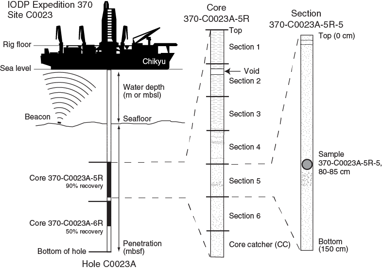
Figure F1. IODP conventions for naming sites, holes, cores, and samples.

Site, hole, core, section, and sample numbering

Sites drilled by the Chikyu are numbered consecutively from the first site with a prefix “C,” which indicates that the hole was drilled by the Japan Agency for Marine-Earth Science and Technology (JAMSTEC)/Center for Deep Earth Exploration (CDEX) platform. A site refers to one or more holes drilled while the ship is positioned within 300 m of the first hole. The first hole drilled at a given site is assigned the site number modified by the suffix “A,” the second hole takes the site number and the suffix “B,” and so forth. These suffixes are assigned regardless of recovery, as long as penetration takes place. During Expedition 370, we drilled at Site C0023 and occupied Hole C0023A.

Cored intervals were calculated based on an initial 1.2–10.0 m length (i.e., the standard core barrel lengths of the various coring systems employed during Expedition 370). In addition, we specified the collection of different coring intervals in areas of poor recovery or slow rate of penetration. Expansion of cores and gaps related to unrecovered material resulted in recovery percentages greater or less than 100%, respectively. Depth intervals were assigned starting from the depth below seafloor at which coring started (IODP coring depth scale calculated using Method A [CSF-A]). Short cores (incomplete recovery) were all assumed to start from that initial depth by convention. Core expansion was corrected during final processing of core measurements by subtracting void spaces, subtracting exotic material, and accounting for expansion (CSF-B).

A recovered core is typically divided into 1.4 m long sections that are numbered sequentially from 1 beginning at the top. Material recovered from the core catcher is assigned to a separate section, labeled core catcher (CC), and placed at the bottom of the lowermost section of the recovered core.

A full identification number for a sample from a core section consists of the following information: expedition, site, hole, core number, core type, section number, and top to bottom interval in centimeters measured from the top of the section. For example, a sample identification of “370-C0023A-20R-1, 80–85 cm,” represents a sample removed from the interval between 80 and 85 cm below the top of Section 1 of the twentieth core taken by rotary core barrel (RCB) from Hole C0023A, during Expedition 370 (Figure F1).

Core handling

The following sections describe the flow of core from the drill floor through the laboratory. Core handling during Expedition 370 followed the general core flow procedure implemented during recent IODP expeditions on the Chikyu but was optimized to process and store the samples properly for the scientific objectives of the expedition. The specific core flow for this expedition is illustrated in Figure F2.

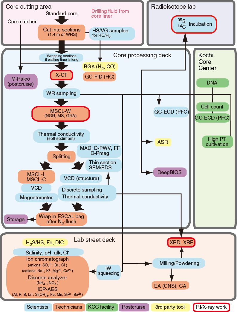
Figure F2. Core processing and measurement flow.

Core cutting area

As soon as the core was retrieved on deck, the core catcher was delivered to the core cutting area. A small volume (5–10 cm³) sample of material taken from the core catcher was preserved for postcruise micropaleontological analysis, and the rest of the core catcher material was packed into a core liner and entered into the general core flow. The recovered core length and the total length of void space were then measured and entered into the J-CORES database, along with core identification information, drilling advance, and depth information.

Upon recovery of gas-rich hydraulic piston coring system (HPCS) cores, infrared images were taken in order to identify temperature anomalies indicative for the decomposition of gas hydrates. Samples were taken from gas voids for various gas analyses.

Prior to cutting the core into sections up to 1.4 m long, a visual inspection was made to identify structurally important features and to avoid cutting directly through lithologic contacts or structures. When the core was cut into sequentially numbered sections, drilling fluid left in the core liner was sampled. About 50 cm³ of sample was taken at freshly cut section ends and split into subsamples to monitor the composition of drilling fluid for contamination control in geochemical and microbiological investigations of the core. In addition, the outer rim of sediment cores that had been in contact with drilling fluid was sampled for contamination control purposes.

Core processing deck

Each core section was imaged using the X-ray computed tomography (CT) scanner. X-ray CT scans were performed on all sections, and data were reviewed by a Co-Chief Scientist and an X-ray CT watchdog for lithostratigraphy and structural geology in order to select the most suitable locations for a complex set of whole-round core (WRC) samples for shipboard, shore-based, and postcruise investigations.

WRC samples were then cut out and stored under appropriate conditions, used for shipboard analyses of interstitial water (IW), or transferred by helicopter to KCC for further processing in the super-clean room facility. The cutting was performed with sterile tools, and all end caps of WRCs were cleaned with ethanol, dried in a clean bench, and radiated with UV light for at least 20 min prior to use. Samples were packed in gas-tight bags and stored under nitrogen atmosphere.

The remaining parts of the core sections were examined by whole-round multisensor core logger (MSCL-W) for gamma ray attenuation (GRA) density, magnetic susceptibility (MS), and natural gamma radiation (NGR). MSCL-W analysis was conducted at 4 cm intervals for GRA and MS and at 16 cm intervals for NGR. Subsequently, thermal conductivity was determined if the consolidation state of the sediment allowed for the measurement.

After the MSCL-W scan and thermal conductivity measurement, the core section was split lengthwise along the lines delimiting the archive and working halves. Archive-half sections were processed in the following way: digital images were taken with the photo image logger (MSCL-I) and color spectroscopy logger (MSCL-C) prior to visual core description by shipboard scientists. Although core description focused primarily on lithology, features of possible structural interest were noted so that their complement could be identified in the working half for additional description, measurement, and sampling, if warranted. Minuscule samples (approximately the amount that could easily be picked up on the end of a toothpick) were taken from the archive half in areas of lithologic interest for smear slide analysis. After the visual core description was completed, paleomagnetic measurements were conducted using the superconducting rock magnetometer (SRM) before the archive halves were prepared for storage.

For working-half sections of consolidated sediments, thermal conductivity measurement on the split surface of working-half sections started immediately after core splitting. Then, discrete samples were taken from the homogeneous portion, which is free from fractures or structures (e.g., faults, foliations, etc.), in the working halves for shipboard analysis of physical properties (see Moisture and density measurements). Subsequently, working halves were investigated with respect to structural geology and relevant features were described as outlined in Structural description. Finally, the working halves were sampled for paleomagnetic investigation of discrete samples (see Discrete samples and sample coordinates) and for postcruise research according to the approved sample requests for Expedition 370.

All half-round core sections were vacuum-sealed in ESCAL bags (Mitsubishi Gas Chemical, Japan) following 3× N₂ flush and transferred to cold storage. After the expedition, all cores were transported under cool temperature (4°C) for archiving at KCC in Kochi, Japan.

Transport of samples to shore

Selected samples were transported to KCC at a frequency of six flights on average per week for further analysis by the shore-based team of the science party. Samples were packed with ice packs in an icebox to maintain either chilled or frozen conditions. Samples for cell counts were kept chilled, whereas samples for DNA analysis were frozen on board the ship. Transport took roughly 3–4 h from sample packing in the shipboard laboratory to unpacking at KCC. Preliminary test measurements showed that the temperature was below −50°C for mock frozen samples after such a period. Samples were immediately transferred to appropriate storage space at KCC upon delivery and kept until further processing.

Contamination control

Driven by goals of finding microbial cells and activities down to the detection limits of existing methods, rigorous QA and quality control (QC) was implemented for all core recovery steps, core processing, and in particular microbiological and geochemical analyses of samples. Procedures were used to identify and account for the introduction of microbial cells, viruses, and chemical species into the pristine sediment and rock samples from the following potential sources of contamination:

Intrusion of seawater and drilling mud during core cutting and recovery, potentially paired with cross contamination resulting from loose borehole fills accumulating on the bottom of the hole;
Formation of molecular hydrogen due to corrosion of the drill bit and release of organic compounds due to heating of the core liner at high in situ temperatures;
Introduction of microbial cells and chemical compounds from equipment and chemicals used during sample processing; and
Contamination of sediment samples during laboratory work from airborne particles.

In order to minimize the risk of drilling-induced contamination, samples for microbiological and geochemical investigations were taken as WRCs from the most undisturbed parts of the recovered cores, which were identified based on visual inspection and X-ray CT imaging of the individual core sections. Moreover, concerted sampling for microbiological and geochemical analyses provides a means for the confirmation of sample integrity (e.g., elevated sulfate concentrations in IW samples would be an indicator for the intrusion of seawater during drilling). Furthermore, in general the first section was not sampled for microbiological investigations in order to avoid cross contamination with borehole fills.

To sensitively track intrusion of drilling fluid into the sediment cores, a perfluorocarbon (PFC) compound was added as a chemical tracer to the drilling fluid, and its presence was monitored in the exterior, midway, and interior portion of WRCs taken for microbiological investigations. In order to determine the PFC concentration of the drilling fluid, we sampled drilling fluid caught inside the core liner (hereafter called “core liner fluid”) when cores were cut into sections in the core cutting area. Moreover, PFC concentrations were determined in bulk samples taken from the top of Section 1 in order to have a means of comparison between all cores in case no drilling fluid was caught in the core liner. In addition, reference samples were taken from the active mud tanks containing seawater gel once per day. For details, see QC: assessing potential contamination of sediment samples from drilling fluid during coring.

In order to monitor the contamination of sediment cores with molecular hydrogen and organic compounds, which are potentially released from the drill bit and core liner, respectively, samples of core liner fluid, exposed sediment, and drilling fluid from active mud tanks were taken for both inorganic geochemistry (see Dissolved hydrogen and carbon monoxide) and organic geochemistry (see Contamination tests).

Numerous measures were taken to minimize the introduction of microbial cells during sample processing (for details, see Quality assurance and quality control for sample processing). WRCs were packed with end caps that had been sterilized by ethanol and UV exposure. Surfaces of workbenches were routinely decontaminated by wiping with RNase AWAY (Molecular Bioproducts Inc., USA) or by exposure to UV light. In addition, the working surface was covered with a fresh sheet of aluminum foil each time a new WRC was processed. All microbiological samples were collected using sterilized tools, and the nitrogen gas used to flush samples to be stored under anaerobic conditions was filtered through a 0.22 µm filter to remove potential contamination.

Contamination of sediment samples with airborne particles in the laboratory is a major concern. For this reason, shipboard processing of microbiological samples focused on sample storage, and further sample processing and analyses were conducted at KCC. On the Chikyu, microbiological sampling was done in clean air environments created by a mobile tabletop air filtration unit that produces filtered laminar airflow that match International Organization for Standardization (ISO) Class 1 clean room standards (KOACH T 500-F, Koken Ltd., Japan) and an ionizer (Koken Ltd., Japan) that reduces static attraction of potentially contaminating airborne particles. At KCC, further sample processing, including crushing into powder, cell separation and filtration for counting, and DNA extraction, was conducted in a super-clean room equipped with a Floor KOACH Ez (KOACH F 1050-F, Koken Ltd., Japan) that produces horizontal ISO Class 1 quality of laminar airflow from the end wall of the clean space and an ionizer to neutralize static charge throughout the workspace of the workbench. During both shipboard and shore-based work, airborne particles in the anaerobic chamber, clean bench, and surrounding laboratory air were periodically monitored by a particle counter throughout the expedition, and the concentration of airborne microbial cells that may potentially contaminate cores during core handling were determined in representative air samples from various workspaces. For details, see Quality assurance and quality control for sample processing.

Operations

This chapter describes a newly developed short advance modified HPCS (short HPCS) and the temporary temperature observatory (TTO) that was deployed in Hole C0023A during Expedition 370.

Short HPCS

The HPCS is able to obtain high-quality (less disturbed and less invaded) core samples of soft to semiconsolidated sediment. However, penetration of the core shoe is refused at greater depths once the sediment becomes firm and/or lithified. To extend the applicability of the HPCS to deeper and harder sedimentary formations, the conventional HPCS has been modified to a shorter advance length of either a 1.5, 3.0, or 4.5 m core shoe (Figure F3). In addition, the configuration of the piston and the extension rods can be modified for the short advance length (i.e., the shorter advance creates stronger penetration power with the increased shooting speed, and consequently extends the applicable depth deeper than the standard 9.5 m HPCS). The diameter of the core sample (61 mm) is the same as the standard HPCS. The bottom-hole assembly and the applicability of the advanced piston corer temperature tool (APCT-3) on the core shoe are compatible for both the standard HPCS and short HPCS.

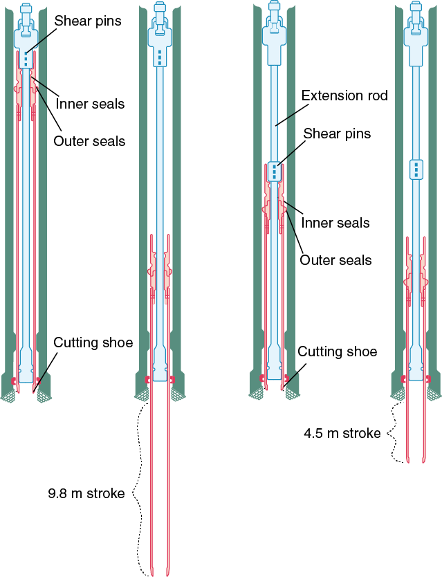
Figure F3. Conventional HPCS and short HPCS.

Temperature observatory

The TTO was installed to monitor the formation temperature profile in the cased borehole. The TTO was equipped with 39 stand-alone temperature sensor loggers (miniature temperature loggers [MTLs]) on a rope and 13 thermistor sensors on 3 flatpack tubes. The former were designed to be recoverable from the TTO by a remotely operated vehicle (ROV), and the latter were designed for permanent installation in the borehole and equipped with data recording units at the CORK head. The ROV operational platform and the CORK head were set onto the wellhead of Hole C0023A, allowing future ROV operations to retrieve the rope with the temperature sensor loggers and/or thermistor data.

Originally, the TTO was designed to cover the full depth to the hole bottom, but the hole condition below the casing (at 858 mbsf) did not allow installation of the tubing. Therefore, the design was changed on site and the tubing was shortened to 863 m, which extends 5 m below the casing shoe. Table T1 shows the final positions of the sensors.

Table T1. Thermometer sensor positions, including thermistors and MTLs. Download table in .csv format.

Thermistor string

The thermistor string consists of 13 thermistor sensors (30 kΩ at 0°C) installed along 3 flatpack strong cables at depths targeting the décollement zone (Figure F4; Tables T1, T2). The flatpack cable is a product of Gulf Coast Downhole Technologies, registered as Stainless Electric Cable with Safety-Strip. It is 11 mm in diameter and made of stainless steel pipe (6.35 mm in diameter) encapsulated with Santoprene material. Inside the pipe are seven electrical conductors for the thermistor connection. For future pressure monitoring, we deployed one flatpack line with no conductor inside.

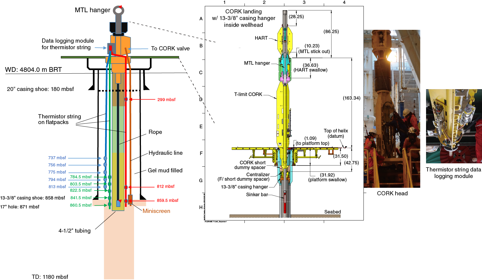
Figure F4. TTO and CORK system configuration.

Table T2. Temperature sensor specifications. Download table in .csv format.

In order to protect the cables and sensors during deployment, cable protectors are attached at every tubing joint and at every sensor module (Figure F5). The thermistor sensor module and conductor connection parts are protected with a stainless steel pipe filled with epoxy (Figure F6).

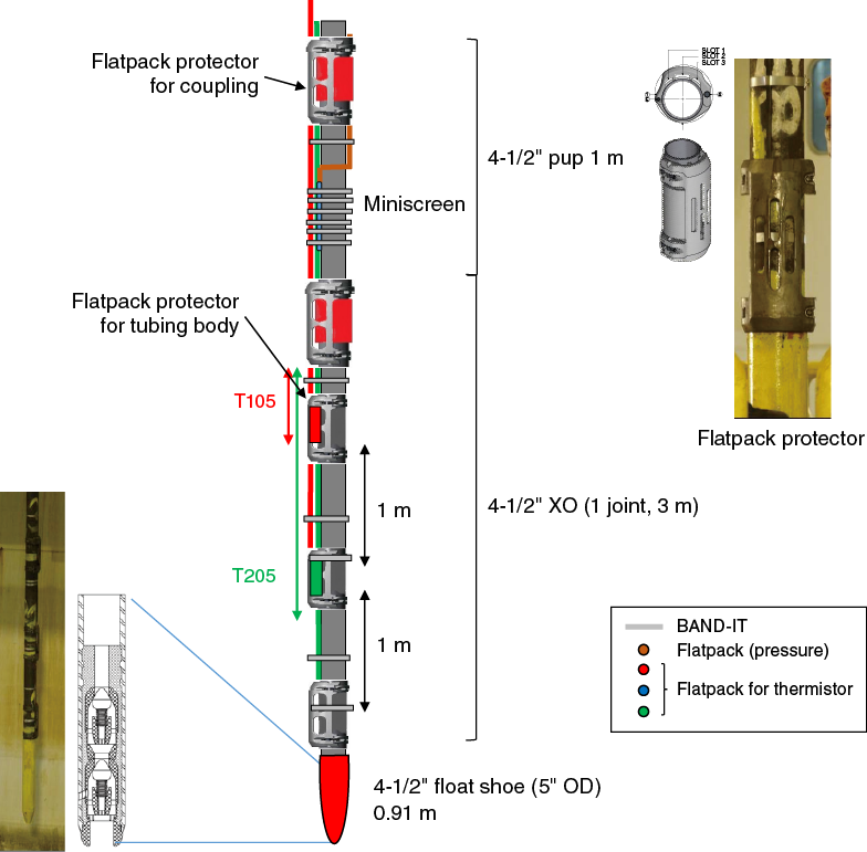
Figure F5. Configuration of thermistor string near tip of 4½ inch tubing.

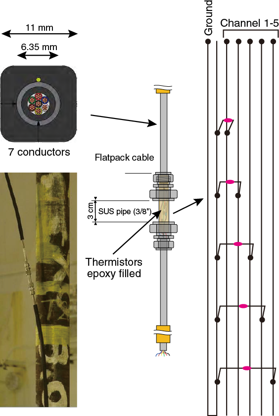
Figure F6. Thermistor sensor module and electrical connection of thermistor string.

Miniature temperature loggers

A total of 39 stand-alone, self-recording loggers were attached to a 1 cm thick Vectran rope (Figures F4, F7; Table T2). They included 6 MTL1854 loggers, 7 MTL1882 loggers, and 27 HOBO U12 loggers. The bottom of the rope was connected to a sinker bar to assist free-fall lowering in the tubing. MTL sensors were deployed at 50 m intervals, but depth resolution was increased in intervals with prominent peaks in geochemical profiles (Table T1).

Figure F7. Rope-attached self-recording temperature loggers.

MTL1854

MTL Model 1854 is a product of Antares Datensysteme GmbH. It is a small autonomous system with a very high temperature precision (~mK) at a water depth of 6000 m for long-term observation in the water column or in deep-sea sediments. Temperature data are stored in its internal memory and are retrieved through the galvanic coupling (i.e., the data logger is placed in spring-loaded clamps for communication and data transfer through a USB or RS-232C interface). The maximum operating temperature is 50°C.

MTL1882

MTL Model 1882 is another Antares data logger newly developed for operations up to 120°C for 1 y.

HOBO U12

The HOBO U12 deep ocean temperature logger is a single-channel temperature logger with 12-bit resolution that can record up to 43,000 measurements. It is designed to withstand water pressure to 11,000 m and temperatures ranging from −40° to 125°C.

Temperature data are stored in memory and can be downloaded via USB connection to a PC. The battery will last ~3 y for logging intervals >1 min and with no more than 60 min of operation at 125°C per day.

Calibration and high-temperature test

All thermistor sensor elements and HOBO U12 loggers were calibrated in a water bath for a temperature range between 2° and 60°C and in an autoclave between 60° and 120°C. All Antares MTL1882 loggers were tested for 48 h in 60°–120°C environments. All HOBO U12 loggers were tested for 6 days in a 120°C environment. Two of the HOBO U12 sensors were tested for ~2 months at 120°C.

Gel mud

The annulus of the casing and the tubing is filled with a gel mud, which has a shear strength of 2~3 kg/m², in order to prevent water circulation due to the geothermal gradient in the formation.

Lithostratigraphy

During Expedition 370, a large fraction of the retrieved core sections was taken as WRCs for crucial geochemical and microbial analyses. Samples were taken immediately after imaging by X-ray CT. Nevertheless, a detailed lithostratigraphic description was still needed to provide a correlation of Site C0023 to nearby Ocean Drilling Program (ODP) Sites 1174 (Shipboard Scientific Party, 2001b) and 808 (Shipboard Scientific Party, 1991) and to provide standard sample and site descriptions. Lithostratigraphic correlation of Site C0023 with the legacy sites was an important aim of shipboard work. Lithostratigraphic description of cores during Expedition 370 aimed to provide fundamental geological characterization and was based on

Macroscopic observations during visual core description,
Petrography targeted to support visual core description and expedition science aims, and
X-ray CT image observation.

Visual core description

Split sections were described by shipboard sedimentologists and structural geologists. Visual core description (VCD) was carried out on the archive (lithostratigraphy) and working (structural geology) halves of each core using traditional ODP and IODP procedures (e.g., Mazzullo and Graham, 1988). Cores were logged by section, and the information from VCD forms was transferred to the J-CORES database before conversion to core-scale plots. When a significant part of a section was missing due to frequent WRC sampling, X-ray CT images and lithologic description of whole-round sample residues were used. The legend used for VCDs is shown in Figure F8. The sedimentological VCD log sheet is presented in Figure F9. Scans of handwritten VCD forms entered into the J-CORES database are available in VCDDATA in Supplementary material.

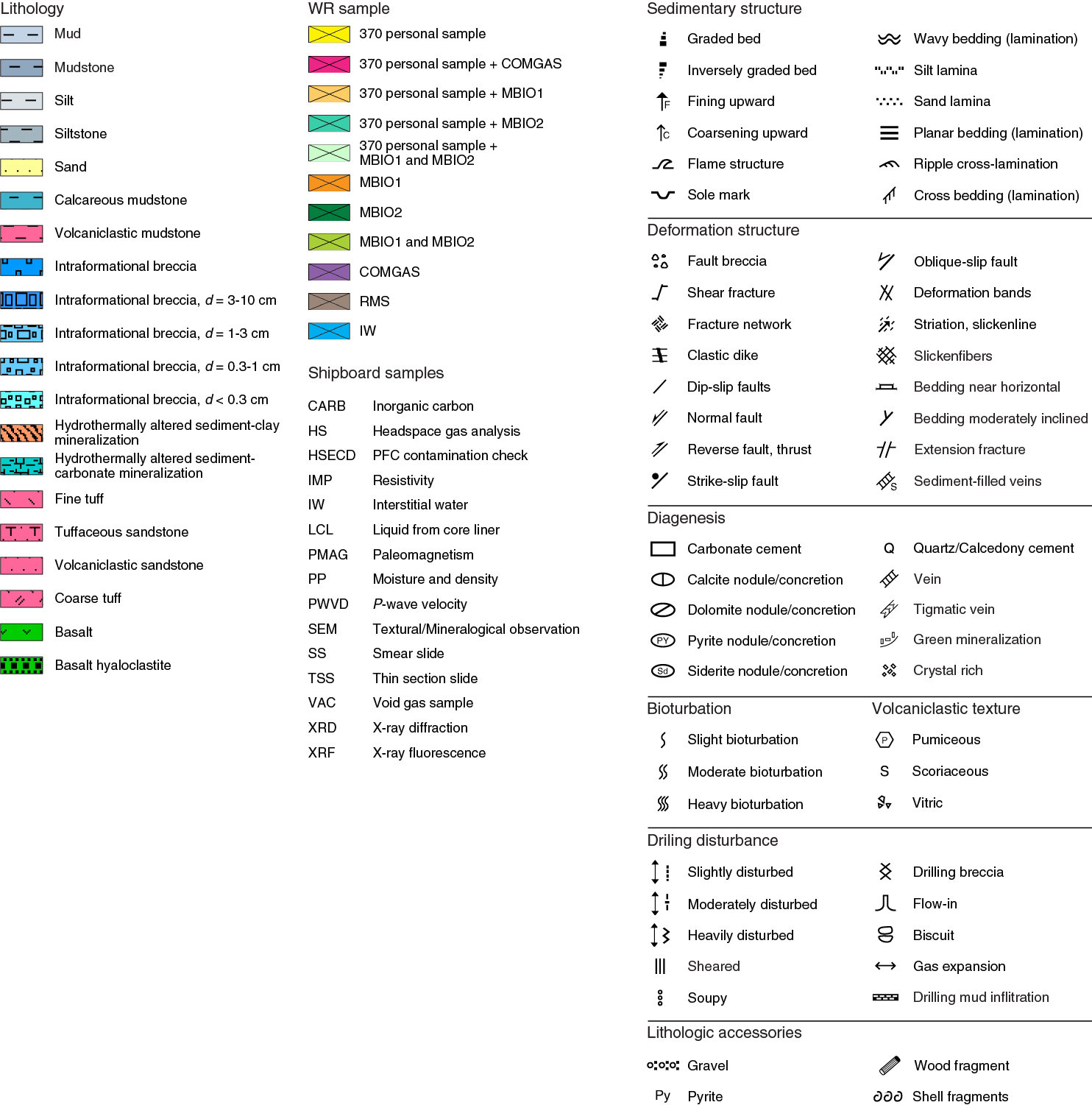
Figure F8. Graphic patterns, abbreviations, and symbols used in macroscopic core descriptions.

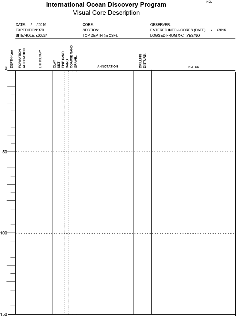
Figure F9. VCD form.

Lithostratigraphic description

Lithostratigraphic description was performed with formation nomenclature used at Sites 808 and 1174 wherever possible for lithostratigraphic correlation with these two sites. Previous work at these sites made use of facies associations and deformation styles distinct within the Nankai Trough subduction zone off Cape Muroto. Previously logged units and their identification criteria are summarized here and tabulated in Table T3 with data synthesized from Shipboard Scientific Party (1991, 2001a). A basaltic pillow lava forms the upper unit of the basement (16 Ma), which is overlain by a basal unit of acidic volcaniclastics (15 Ma). Overlying these units is the lower Shikoku Basin facies (i.e., mid-Miocene to mid-Pliocene), which is distinguished from the unit above by the absence of volcanic ash layers. The overlying upper Shikoku Basin facies is differentiated from the unit beneath by the presence of abundant tephra layers (i.e., upper Pliocene to lower Pleistocene). Above this is a Quaternary hemipelagic facies comprising mud and turbidites (i.e., Pleistocene). At ODP Leg 190 Site 1174, this unit was divided into (1) a transitional facies comprising hemipelagic mud with tephra layers and the first occurrences of turbidites, (2) hemipelagic mud containing silt turbidites, and (3) a unit comprising hemipelagic mud and sand and silt turbidites (Shipboard Scientific Party, 2001a). The topmost unit encountered at Site 1174 was hemipelagic mud. A comparison between these units and their correlative equivalents at Site C0023 is presented in Lithostratigraphy in the Site C0023 chapter (Heuer et al., 2017b).

Table T3. Criteria for identifying correlatable units. Download table in .csv format.

A lithostratigraphic approach based on sedimentary facies alone is not sufficient to enable correlation to other sites because of the presence of laterally traceable structural features. These include a regionally extensive décollement zone consisting of fault breccia, which was reported to be approximately 30 m or greater thickness at Site 1174 (Shipboard Scientific Party, 2001a). Deformation styles above the fault breccia are distinctly different from those beneath; above the décollement zone deformation styles predominantly consist of fracturing, whereas beneath, steepening of bedding is observed. Because core recovery in brecciated horizons can be low and because geological brecciation can be hard to distinguish from brecciation caused by drilling operations, structural features were also logged to help demarcate boundaries and differentiate drilling and core-handling disturbance from fault brecciation. Further details of structural features are listed in Structural description.

Sedimentology and mineralogy

The main quantitative data gathered to help demarcate formation boundaries were (1) instances of core width to lamina-scale bedforms such as asymmetrical ripples, cross-lamination, and low-angle planar lamination; (2) the bases of sand and silt beds and sand and silt lamina; (3) the level of bioturbation; (4) the presence of volcaniclastics; and (5) the occurrence of macrofossils and macrophytoclastic wood. These observations were entered into the J-CORES database.

Mineralization

Mineralization was described according to its habit and major observable mineral components. Distinctions were made between stigmatic veins formed in soft sediment, mineralization hosted in deformation structures, and mineralization associated with or following sedimentary features. The occurrence of early stage diagenetic minerals (e.g., pyrite and calcite) was logged separately and, where appropriate, included within the description of a lithology (e.g., calcareous mudstones).

Volcanic sediments

To emphasize the differences in composition of sedimentary horizons containing volcaniclastic sediments, the classification scheme of Fisher and Schmincke (1984) was modified for rapid core description. The prefix “volcaniclastic” was reserved for sedimentary rock containing >25% but <75% volcaniclastics (e.g., a sandstone with >25% volcaniclastics would be termed a “volcaniclastic sandstone” and a mudstone with >25% volcaniclastics would be termed a “volcaniclastic mudstone”). Previous work in the region has differentiated between reworked volcaniclastics and less altered pyroclasts (Saito, Underwood, Kubo, and the Expedition 322 Scientists, 2010). Such an approach has many strengths, such as the potential to differentiate between depositional and emplacement mechanisms. But in this case, to facilitate rapid core description the freshness of volcanic clasts was not routinely differentiated. Units were logged as tuffs if they comprised >75% volcanic clasts.

Bioturbation

Bioturbation intensity was estimated using a modified version of the ichnofabric index as described by Droser and Bottjer (1986, 1991). For ease of logging, these values were then recoded for entry into the J-CORES database as follows:

Level 1 = burrows observed.
Level 2 = slight bioturbation where burrows cut each other or another sedimentary fabric.
Level 3 = burrows and other bioturbation are the main sedimentary fabric at the expense of all other sedimentary structures (e.g., laminae are discontinuous and changes in composition due to depositional processes are obfuscated).

Structural description

Our methods for documenting the structural geology of Expedition 370 cores largely followed those used by Expedition 315 Scientists (2009) and Expedition 316 Scientists (2009), which in turn were based on previous ODP procedures developed at the Nankai accretionary margin (i.e., ODP Legs 131 and 190). We documented the deformation observed in the split cores by classifying structures, determining the depth extent, measuring orientation data, and recording the sense of displacement. The collected data were hand logged onto a printed form at the core table and then typed into both a spreadsheet and the J-CORES database. Scans of handwritten structural description forms are available in VCDDATA in Supplementary material. The orientation data should be corrected for rotations related to drilling on the basis of paleomagnetic declination. However, because of the limitations of time, number of paleomagnetic specialists, and heavy magnetic overprint, we did not conduct the paleomagnetic restoration during Expedition 370.

Structural data acquisition and orientation measurements

Each structure was recorded manually on a description table sheet (Figure F10). We used a plastic protractor for orientation measurements (Figure F11). Use of the working half of the split core provided greater flexibility in removing—and cutting, if necessary—pieces of the core for measurements.

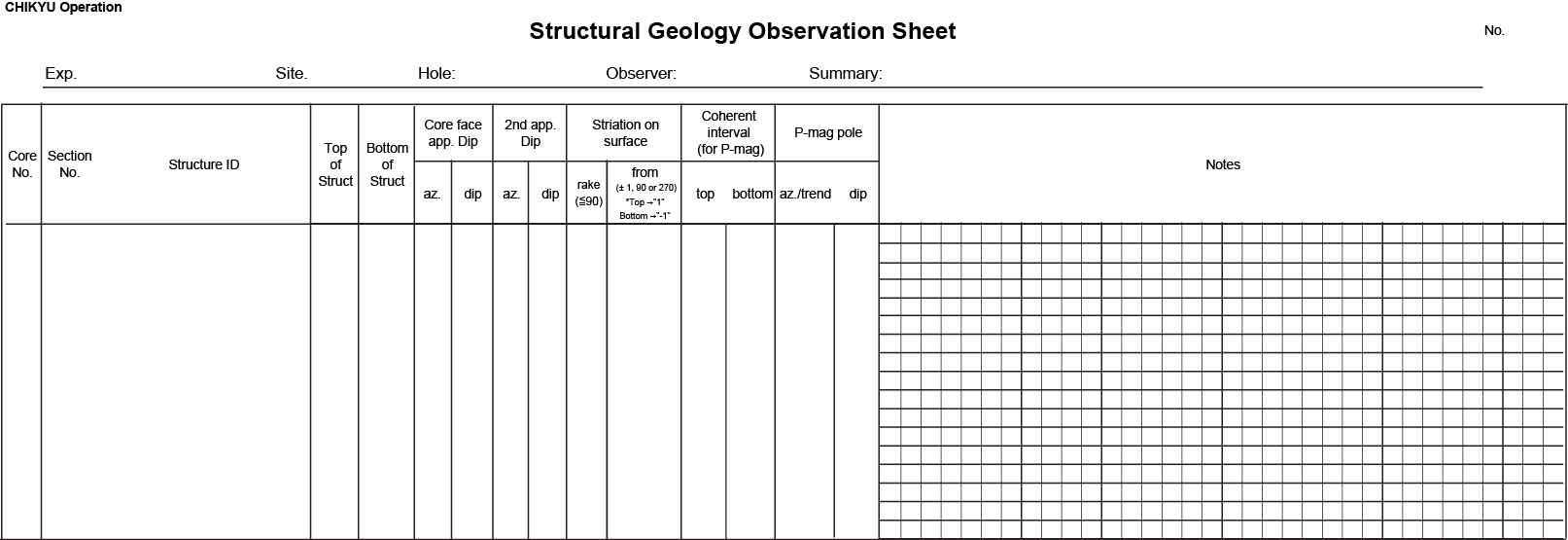
Figure F10. Structure log sheet.

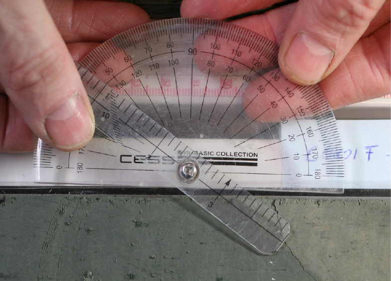
Figure F11. Protractor used to measure apparent dips, trends, plunges, and rakes.

Orientations of planar and linear features in cored materials were determined relative to the core axis, which represents the vertical axis in the core reference frame, and the double line marked on the working half of the split core liner, which represents 000° (and 360°) in the plane perpendicular to the core axis (Figure F12). To determine the orientation of a planar structural element, two apparent dips of this element were measured in the core reference frame and converted to a plane represented by dip angle and either a strike or dip direction (Figure F13). One apparent dip is usually represented by the intersection of the planar feature with the split face of the core and is quantified by measuring the dip direction and angle in the core reference frame (β₁ in figure). Typical apparent dip measurements have a trend of 090° or 270° and range in plunge from 0° to 90° (β₂ in figure). The second apparent dip is usually represented by the intersection of the planar feature and a cut or fractured surface at a high angle to the split face of the core. In most cases, this was a surface either parallel or perpendicular to the core axis. In the former cases, the apparent dip lineation would trend 000° or 180° and plunge from 0° to 90°; in the latter cases, the trend would range from 000° to 360° and plunge 0°. Linear features observed in the cores were always associated with planar structures (e.g., striations on faults), and their orientations were determined by measuring either the rake (or pitch) on the associated plane or the trend and plunge in the core reference frame. During Expedition 370, we measured rake for striations on the fault surface (Figure F14), whereas azimuth and plunge were measured for other lineations (e.g., fold axes). All data were recorded on the log sheet with appropriate depths and descriptive information.

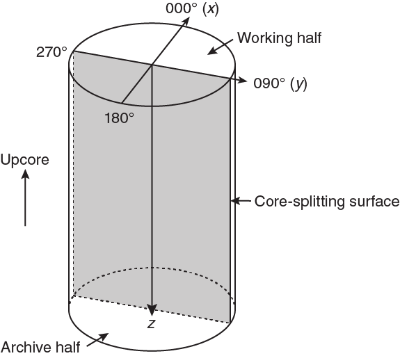
Figure F12. Core reference frame and x-, y-, and z-coordinates for orientation data calculations.

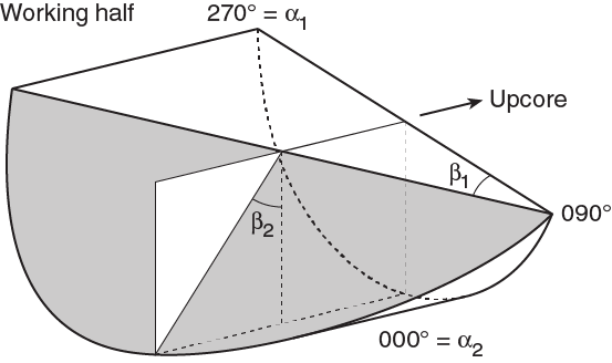
Figure F13. Calculation of plane orientation from two apparent dips.

Figure F14. Apparent rake measurement of striations on a fault surface.

Description and classification of structures

We constructed a structural geology template for the J-CORES database that facilitated the description and classification of observed structures. For clarity, we defined the terminology used to describe fault-related rocks, as well as the basis for differentiating natural structures from drilling-induced features.

Faults were classified into several categories based on the sense of fault slip and their structural characteristics. The sense of the fault slip was identified using offsets of markers (e.g., bedding and older faults) across the fault plane and predominance by slicken steps. A fault with cohesiveness across the fault zone was described as a healed fault. Zones of dense fault distribution and intense deformation were termed “fault zones.” Fault zones are intensively deformed zones fragmented into centimeter-sized and smaller fragments, containing only a few larger fragments. The size of the majority of fragments was then logged and the zone recorded as an intraformational breccia—breccia comprising clasts of overlying and underlying lithologies. Clearly, there is the potential for such units to be an artifact of the drilling process as well as many geological processes aside from faulting. Where information and geological context supported such an interpretation, these intervals were treated as a distinct fault-generated rock type and named accordingly.

The mineralization style and mineralogy of vein minerals were described by the sedimentologists (see above), but the orientations of veins, foliations, and other structural features were measured by structural geologists.

Structural data can sometimes be disturbed by drilling-induced structures such as flow-in structures in HPCS cores and biscuiting, fracturing, faulting, and rotation of fragments in extended shoe coring system (ESCS) and RCB cores. Where structures have been disturbed by flow-in that occupies >50% of the cross-sectional width of the core, we excluded measurements of bedding because of the intense disturbance (i.e., bending, rotation, etc.) of these structures.

Calculation of plane orientation

For planar structures (e.g., bedding or faults), two apparent dips on two different surfaces (e.g., one being the split core surface, which is east–west vertical, and the other being the horizontal or north–south vertical surface) were measured in the core reference frame as azimuths (measured clockwise from north, looking down) and plunges (Figure F12). A coordinate system was defined in such a way that the positive x-, y-, and z-directions coincide with north, east, and vertical downward, respectively. If the azimuths and plunges of the two apparent dips are given as (α₁, β₁) and (α₂, β₂), respectively, as in Figure F13, then the unit vectors representing these two lines (v₁ and v₂) are as follows:

ν_{1} = (\begin{matrix} l_{1} \\ m_{1} \\ n_{1} \end{matrix}) = (\begin{matrix} \begin{matrix} \cos α_{1} & \cos β_{1} \end{matrix} \\ \begin{matrix} \sin α_{1} & \cos β_{1} \end{matrix} \\ \sin β_{1} \end{matrix}),  and

(E1)

ν_{2} = (\begin{matrix} l_{2} \\ m_{2} \\ n_{2} \end{matrix}) = (\begin{matrix} \begin{matrix} \cos α_{2} & \cos β_{2} \end{matrix} \\ \begin{matrix} \sin α_{2} & \cos β_{2} \end{matrix} \\ \sin β_{2} \end{matrix}) .

(E2)

where l, m, and n represent the x-, y-, and z-components of the vectors.

The unit vector normal to the plane (v_n) (Figure F15) is then defined as follows:

ν_{n} = (\begin{matrix} l_{n} \\ m_{n} \\ n_{n} \end{matrix}) = \frac{ν_{1} \times ν_{2}}{|ν_{1} \times ν_{2}|},

(E3)

where

ν_{1} \times ν_{2} = (\begin{matrix} |\begin{matrix} m_{1} & m_{2} \\ n_{1} & n_{2} \end{matrix}| \\ |\begin{matrix} n_{1} & n_{2} \\ l_{1} & l_{2} \end{matrix}| \\ |\begin{matrix} l_{1} & l_{2} \\ m_{1} & m_{2} \end{matrix}| \end{matrix}) = (\begin{matrix} m_{1} n_{2} - m_{2} n_{1} \\ n_{1} l_{2} - n_{2} l_{1} \\ l_{1} m_{2} - l_{2} m_{1} \end{matrix}) .

(E4)

Figure F15. Dip direction, right-hand rule strike, and dip of a plane.

The azimuth (α_n) and plunge (β_n) of v_n are given by the following:

α_{n} = \tan^{- 1} (m_{n} / l_{n}) and

(E5)

β_{n} = \sin^{- 1} n_{n} .

(E6)

The dip direction (α_d) and dip angle (β) of this plane are α_n and 90° + β_n, respectively, when β_n < 0° (Figure F15). They are α_n ± 180° and 90° − β_n, respectively, when β_n ≥ 0°. The right-hand rule strike of this plane (α_s) is then given by α_d − 90°.

Calculation of slickenline rake

For a fault with striations, the apparent rake angle of the striation (ϕ_a) was measured on the fault surface from either the 090° or 270° direction of the split core surface trace (Figure F14). Fault orientation was measured as described above. Provided that v_n and v_c are unit vectors normal to the fault and split core surfaces, respectively, the unit vector of the intersection line (v_i) is perpendicular to both v_n and v_c (Figure F16) and is therefore defined as follows:

ν_{i} = (\begin{matrix} l_{i} \\ m_{i} \\ n_{i} \end{matrix}) = \frac{ν_{n} \times ν_{c}}{|ν_{n} \times ν_{c}|},

(E7)

where

ν_{c} = (\begin{matrix} 1 \\ 0 \\ 0 \end{matrix}), and

(E8)

ν_{n} \times ν_{c} = (\begin{matrix} |\begin{matrix} m_{n} & 0 \\ n_{n} & 0 \end{matrix}| \\ |\begin{matrix} n_{n} & 0 \\ l_{n} & 1 \end{matrix}| \\ |\begin{matrix} l_{n} & 1 \\ m_{n} & 0 \end{matrix}| \end{matrix}) = (\begin{matrix} 0 \\ n_{n} \\ - m_{n} \end{matrix}) .

(E9)

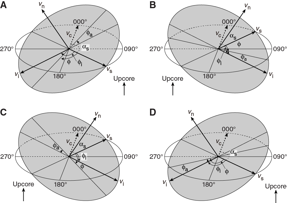
Figure F16. Rake of striations.

Knowing the right-hand rule strike of the fault plane (α_s), the unit vector (v_s) toward this direction is then

ν_{s} = (\begin{matrix} \cos α_{s} \\ \sin α_{s} \\ 0 \end{matrix}) .

(E10)

The rake angle of the intersection line (ϕ_i) measured from the strike direction is given by

ϕ = \cos^{- 1} (ν_{s} \times ν_{i}),

(E11)

because

ν_{s} \times ν_{i} = |ν_{s}| |ν_{i}| \cos ϕ_{i} = \cos ϕ_{i}, ∴ |ν_{s}| = |ν_{i}| = 1 .

(E12)

The rake angle of the striation (ϕ) from the strike direction is ϕ_i ± ϕ_a, depending on the direction from which the apparent rake was measured and on the dip direction of the fault. ϕ_a should be subtracted from ϕ_i when the fault plane dips toward the west and ϕ_a was measured from either the top or 090° direction or when the fault plane dips toward the east and ϕ_a was measured from either the bottom or 090° direction (Figure F16). On the other hand, ϕ_a should be added to ϕ_i when the fault plane dips toward the east and ϕ_a was measured from either the top or 270° direction or when the fault plane dips toward the west and ϕ_a was measured from either the bottom or 270° direction.

J-CORES structural database

The J-CORES database is a program used to store a visual (macroscopic and/or microscopic) description of core structures at a given section index. During Expedition 370, only the locations of structural features and calculated orientations in the core reference frame were input into the J-CORES database, and orientation data management and planar fabric analysis were made with a spreadsheet as described above.

Petrographic and mineralogical analysis

Smear slides

Smear slides were produced by smearing a small amount (~0.1 cm) of sample across a glass slide using a toothpick, dispersing the sample in tap water, and then drying it on a hot plate. Following drying, optical adhesive was added and a cover glass placed on top. The adhesive was cured under UV radiation.

The sample location for each smear slide was entered into the J-CORES database with a sample code of SS. Smear slide description followed the sheet shown in Figure F17; a scheme that matched the resources of shipboard scientists. Smear slide description primarily focused on supplying lithology description for the fine-grained component of mud and mud rocks. Microscopic images of smear slides are available in SMEARSLD in Supplementary material.

Figure F17. Smear slide description sheet.

Thin sections

Thin sections were only taken from semiconsolidated or consolidated core. Thin sections were prepared for more intensive analysis of mineral components not amenable to X-ray diffraction (XRD) and to observe microstructures and petrographic fabrics, particularly fine-grained igneous rocks. A 30 µm × 2 cm × 3 cm section was used for each thin section. Thin sections were polished and observed in transmitted light using a Zeiss Axioskop AX10 polarizing microscope equipped with a Nikon DS-Fi1 digital camera. In a few instances, point counting was done to obtain quantitative information on mineral phases and authigenic mineral phases in particular. Microscopic images of thin sections are available in THINSECT in Supplementary material.

X-ray diffraction

The principal goal of XRD analysis was to estimate the relative weight percentages of total clay minerals, quartz, feldspar, and calcite in specimens of bulk sediment. Material for XRD was obtained from a 10 cm³ sample that was also used for X-ray fluorescence (XRF) and carbonate analyses. All samples were vacuum-dried, crushed with a ball mill, and mounted as randomly oriented bulk powders. Routine analyses of bulk powders were completed using a newly acquired PANalytical CubiX3 diffractometer. This system has been used on the Chikyu since Expedition 365. Instrument settings were as follows:

Generator voltage = 45 kV.
Tube current = 40 mA.
Tube anode = Cu.
Wavelength = 1.540598 Å (Kα1) and 1.544426 Å (Kα2).
Start angle = 2°2θ.
End angle = 60°2θ.
Step spacing = 0.005°2θ.
Scan step time = 1.27 s.
Scan speed = 0.50134°2θ/s.
Divergent slit = fixed 1/4.
Monochromator used = yes.
Irradiated length = 10 mm.
Scanning range = 2°–60°2θ.
Scan type = continuous.

To maintain as much consistency as possible with previous results obtained from IODP Nankai Trough Seismogenic Zone Experiment (NanTroSEIZE) expeditions, we processed the digital data using MacDiff 4.2.5 (http://www.ccp14.ac.uk/ccp/web-mirrors/krumm/html/software/macdiff.html). Functions included find baseline, smooth counts, and correction of peak position using the quartz peak at 3.343 Å. The upper and lower limits for each diagnostic peak were adjusted manually following the guidelines in Expedition 319 Scientists (2010).

Calculations of relative mineral abundance utilized regression curves that were generated from analyses of standard mineral mixtures, with all values normalized to 100%. This follows a general procedure first described in Fisher and Underwood (1995). Bulk powder mixtures for the Nankai Trough are the same as those reported by Underwood et al. (2003): quartz (Saint Peter sandstone), feldspar (Ca-rich albite), calcite (Cyprus chalk), smectite (Ca-montmorillonite), illite (Clay Mineral Society IMt-2, 2M1 polytype), and chlorite (Clay Mineral Society CCa-2). The standards were run three times, and the correlations for each mineral are between mean peak area and weight percent. The following polynomial equations provide the statistical fits, where X = peak area and r = correlation coefficient:

Total clay minerals = 5.0314 + 0.0072495 (X) - 1.919 E - 7 (X^{2}), r = 0.923;

(E13)

Quartz = - 1.1695 + 0.00037795 (X) - 1.2198 E - 10 (X^{2}), r = 0.991;

(E14)

Feldspar = 0.96439 + 0.00052385 (X) + 4.2326 E - 9 (X^{2}), r = 0.990;

(E15)

Calcite = - 1.9208 + 0.00082643 (X) + 2.3405 E - 9 (X^{2}), r = 0.997;

(E16)

Average errors (calculated weight percent minus true weight percent) for the standard mineral mixtures are as follows:

Total clay minerals = 3.3%.
Quartz = 1.9%.
Feldspar = 1.1%.
Calcite = 1.7%.

Values of relative abundance for natural specimens, however, should be interpreted with some caution. One of the fundamental problems with any bulk powder XRD method is the difference in peak response between poorly crystalline minerals at low diffraction angles (e.g., clay minerals) and highly crystalline minerals at higher diffraction angles (e.g., quartz and plagioclase). Clay mineral content is best characterized by measuring the peak area, whereas peak intensity may be more accurate for quartz, feldspar, and calcite. Analyzing oriented aggregates of clay-size fractions enhances basal reflections of the clay minerals, but that approach is time consuming. For clay mineral assemblages in bulk powders, the two options are to measure one peak for each mineral and add the estimates together (thereby propagating the error) or to measure a single composite peak at 19.4°–20.4°2θ (Table T4). Chlorite does not contribute counts to that composite peak; therefore, natural specimens with high contents of chlorite will yield larger errors. That source of error also applies to the standard mineral mixtures. Other sources of error include contamination of mineral standards by impurities such as quartz and zeolites (e.g., the illite standard contains ~20% quartz) and differences in crystallinity between standards and natural clay minerals.

Table T4. Characteristic XRD peaks for semiquantitative analysis. Download table in .csv format.

In the final assessment, the calculated mineral abundances reported here should be regarded as relative percentages within a four-component system of clay minerals + quartz + feldspar + calcite. How close those estimates resemble their absolute percentages within the total volume of solids depends on the abundance of amorphous solids (e.g., biogenic opal and volcanic glass) and the total of all other minerals that occur in minor or trace quantities. For most natural samples from Site C0023, the difference between calculated relative abundance and absolute weight percentage is probably between 5% and 10%.

X-ray fluorescence

Core materials were subjected to whole-rock quantitative XRF spectrometry for analysis of major elements (Na, Mg, Al, Si, Fe, P, K, Ca, Ti, and Mn). XRF analyses were performed on splits of samples used for XRD. All samples were dried and crushed before analysis, together with samples for XRD.

A glass bead was prepared from approximately 1 g of sample powder before analysis. Analyses were performed using a Supermini XRF spectrometer (Rigaku) with a 200 W Pd anode X-ray tube operated at 50 kV and 4 mA. Rock standards from the National Institute of Advanced Industrial Science and Technology were used for calibration of the XRF spectrometer, using matrix corrections within the operation software. Results were reported as weight percent oxide (Na₂O, MgO, Al₂O₃, SiO₂, P₂O₅, K₂O, CaO, TiO₂, MnO, and Fe₂O₃). XRF results are available in XRF in Supplementary material.

X-ray computed tomography

During Expedition 370, the preliminary assessment of core quality was performed using X-ray CT images. Scanning for preliminary assessment was done immediately after dividing the core into sections. WRC sections were screened to avoid destruction of key geological features and drilling disturbance (Figure F18).

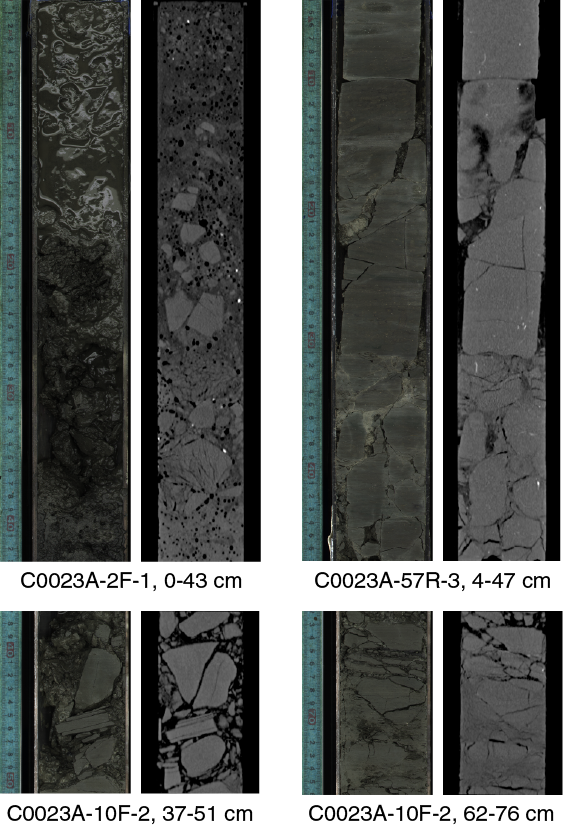
Figure F18. Photographs and X-ray CT images of drilling disturbance.

X-ray CT images were also used to identify 3-D sedimentary and structural features, such as bioturbation burrows, bedding planes, faults, mineral veins, and so on, and also to infer lithology in intervals where visual core description was not possible because core had been taken as WRC samples for IW analysis or microbiological analyses.

Our methods followed those in the measurement manual prepared by CDEX (X-ray CT Scanning, Version 3.00; 24 March 2015) and used during previous expeditions (e.g., Integrated Ocean Drilling Program Expeditions 337 and 348). The X-ray CT instrument on the Chikyu is a Discovery CT 750HD (GE Medical Systems) capable of generating thirty-two 0.625 mm thick slice images every 0.4 s, the time for one revolution of the X-ray source around the sample. Data generated for each core consist of core-axis-normal planes of X-ray attenuation values with dimensions of 512 × 512 pixels. Data were stored on the server as Digital Imaging and Communication in Medicine (DICOM) formatted files. The DICOM files were restructured to create 3-D images for further investigation.

The theory behind X-ray CT has been well established through medical research and is very briefly outlined here. X-ray intensity varies as a function of X-ray path length and the linear attenuation coefficient (LAC) of the target material:

I = I_{0} \times e^{- μ L},

(E17)

where

I = transmitted X-ray intensity,
I₀ = initial X-ray intensity,
µ = LAC of the target material, and
L = X-ray path length through the material.

LAC is a physical index about the X-ray beam reduction during translation of target materials. LAC is led from the relationship between physical properties of target materials (i.e., chemical composition, density, and state). The basic measure of attenuation, or radiodensity, is the CT number given in Hounsfield units (HU):

CT number = [(μ_{t} - μ_{w}) / μ_{w}] \times 1000,

(E18)

where

µ_t = LAC for the target material, and
µ_w = LAC for water.

The distribution of attenuation values mapped to an individual slice comprises the raw data that are used for subsequent image processing. Successive 2-D slices yield a representation of attenuation values in 3-D pixels referred to as voxels. Analytical standards used during Expedition 370 were air (CT number = −1000), water (CT number = 0), and aluminum (2477 < CT number < 2487) in an acrylic core mock-up. All three standards were run once daily after air calibration. For each standard analysis, the CT number was determined for a 24.85 mm² area at fixed coordinates near the center of the cylinder.

Core quality factor using the CT number

The core quality factor (CQF) is a measure of the quality of recovered core that is calculated using data acquired during X-ray CT scanning. It was measured on each section using X-ray CT scanned DICOM files of 0.625 mm thick slice images. The process for CQF measurement in this report is as follows. First, we selected a circular region of interest 30–50 mm in diameter at the slice center, depending on the diameter of the core. A histogram of the number of pixels with a given CT number was examined to identify the representative material within the section; the CT number of the representative material creates a peak in the histogram, and 70% of the representative CT number at the peak was used as the threshold to differentiate pristine, high-quality areas from damaged areas. When the ratio of high-quality area to total area was higher than 0.99, the slice was regarded as a “high-quality slice.” This was repeated for each slice of the section. Finally, the percentage of high-quality slices to the number of all slices of the section was measured as the CQF score. These calculations were conducted using ImageJ software (Schneider et al., 2012).

Average CT number

To characterize the major constituting materials of core samples, the average CT number of each slice was measured using a 10 mm diameter × 0.625 mm thick slice taken at the slice center. DICOM files of the slices were processed using ImageJ.

High CT number area

A profile of areas with distinctly high CT numbers was made to show the distribution of higher density minerals such as pyrite, rhodochrosite, and barite. Within each 0.625 mm thick slice image, we selected a circular area of 30–50 mm diameter at the center of a slice, depending on the diameter of the core. Within the selected area, the fractional area that has CT numbers of >3000 was calculated using ImageJ. The calculation was conducted for each slice image and then presented as a depth profile.

Scanning electron microscopy

Scanning electron microscopy (SEM) and energy dispersive spectrometry (EDS) using a JEOL electron microscope on the Chikyu was used for detailed observation and detection of minerals for a few selected samples. Observations were qualitative in nature and limited primarily to crystal and grain morphology with limited data on relative elemental abundance obtained. Data from SEM-EDS are available in SEM in Supplementary material.

Paleomagnetism

Paleomagnetic investigations during Expedition 370 were primarily designed to determine the characteristic remanence directions for establishing magnetostratigraphy and to reorient cores for structural analysis. To accomplish these goals, paleomagnetic measurements were performed on archive halves and discrete cube samples. It is essential to know the primary magnetization components to estimate magnetostratigraphy. To obtain these data, secondary magnetization components first needed to be demagnetized. Archive halves were demagnetized with a 2G600 sample degaussing system coupled to a SRM. For discrete samples, alternating field (AF) demagnetization was used. After demagnetization, SRM measurements were conducted on archive halves, and spinner magnetometer measurements were conducted on discrete samples. Paleomagnetic direction (declination, inclination, and magnetic intensity) was generated using these measurements. Detailed procedures and sample coordinates are described below.

Laboratory instruments

Magnetic shielding is particularly important to protect cores from magnetic noise during measurement. The paleomagnetism laboratory on the Chikyu is a magnetically shielded room (7.3 m × 2.8 m × 1.9 m), in which the internal total magnetic field is ~1% of Earth’s magnetic field. The room is oriented with its long axis transverse to the long axis of the ship and houses an SRM and other magnetically sensitive instruments. The room is large enough to comfortably handle a standard IODP core section (~150 cm in length).

Superconducting rock magnetometer

The long-core SRM system (2G Enterprises, model 760) is ~6 m long with an 8.1 cm diameter access bore that allows the measurement of a 1.5 m long split core. The SRM has three sets of superconducting pickup coils, two for transverse moment measurement (x- and y-axes) and one for axial moment measurement (z-axis) (Figure F19). The noise level of the magnetometer is <10⁻⁷ A/m for a 10 cm³ volume rock. A 2G600 sample degaussing system is coupled to the SRM to allow automatic AF demagnetization of samples up to 100 mT. The system is controlled by an external computer and enables programming of a complete sequence of measurements and degauss cycles without removing the long core from the holder. During Expedition 370, the measurement interval was 2.5 cm. Archive halves were demagnetized at 10 and 20 mT to allow further demagnetization during postcruise analysis. Because of time constraints, core catcher samples and core sections <10 cm long were not measured. Archive halves deeper than Core 370-C0023A-84R were only demagnetized at 20 mT and were measured by laboratory technicians.

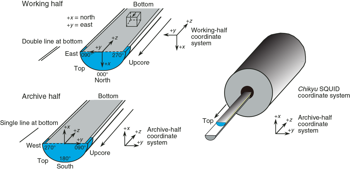
Figure F19. Orientation system of cores, discrete samples, and SRM.

Spinner magnetometer

A spinner magnetometer, model SMD-88 (Natsuhara Giken Co., Ltd.), is available on the Chikyu for remanent magnetization measurement of discrete samples. The noise level is ~5 × 10⁻⁷ mAm², and the measurable range is from 5 × 10⁻⁶ to 3 × 10⁻¹ mAm². During Expedition 370, two different sizes of sample holders were used for measuring weak (1 × 10⁻⁵ ~ 1 × 10⁻² mAm²) and strong (1 × 10⁻⁴ ~ 1.0 mAm²) samples, respectively. Five standard samples with different intensities were prepared to calibrate the magnetometer. Samples in standard 7 cm³ Natsuhara cubes were measured in three or six positions with a typical stacking of 64–256 spins.

Alternating field demagnetizer

The DEM-95 AF demagnetizer (Natsuhara Giken Co., Ltd.) equipped with a sample tumbling system was set for AF demagnetization of standard discrete samples (maximum AF = 180 mT). After measuring natural remanent magnetization (NRM), samples were stepwise demagnetized at 10 and 20 mT to decipher paleomagnetic data. Some samples near structural features were demagnetized using up to 80 mT.

Discrete samples and sample coordinates

Discrete cubic samples (~7 cm³) were taken, one per section, from the working halves in order to determine paleomagnetic direction for magnetostratigraphy and reorientation of cores. The actual spacing depended on the properties and conditions of the core material (e.g., avoiding flow-in, coring disturbances, etc.). Paleomagnetic sampling mostly concentrated on hemipelagic mud (or mudstone) as the dominant lithology. In some cases, samples were taken near structural features to assist reorientation of the features. Samples from the dominant lithology were demagnetized up to 20 mT, and samples near structural features were demagnetized up to 80 mT. The orientation of discrete samples is shown in Figure F19.

Magnetostratigraphy

Magnetic polarity was determined based on the inclination sign of the discrete samples after AF demagnetization at 20 mT. For some discrete samples, further steps of AF demagnetization (0, 10, 20, 30, 40, 60, or 80 mT) were conducted. Zijderveld plots (Zijderveld, 1967) were inspected visually for behavior of remanent magnetization after demagnetization. Stable (primary) remanent magnetization directions of discrete samples were fit using principal component analysis (PCA) (Kirschvink, 1980), and the obtained inclination was used for the determination of paleomagnetic field polarity. The ages of the polarity intervals used during Expedition 370 were from the geomagnetic polarity timescale 2012 (Gradstein et al., 2012) (Table T5).

Table T5. Geomagnetic polarity timescale. Download table in .csv format.

Data processing

Data from archive halves and discrete samples were saved in DAT and TXT file formats and uploaded to the J-CORES database by shipboard laboratory technicians. Data reduction (Zijderveld demagnetization plots and equal-area projections) was conducted using the visualization software Progress, programmed by H. Shibuya (Kumamoto University, Japan). This software also allows PCA (Kirschvink, 1980).

Physical properties

Continuous physical properties measurements provide crucial parameters required to identify lithostratigraphic units, to correlate seismic reflection data with discrete core measurements and descriptions, and to characterize the habitat of subseafloor microbial communities. A variety of techniques and methods were used on Expedition 370 core samples. Prior to sampling and interpretation, X-ray CT images were captured for all cores. After the X-ray CT scans were completed, GRA density, MS, and NGR were measured using the MSCL-W (Geotek, Ltd., London, United Kingdom) for whole-round analysis. After MSCL-W measurements and core splitting, digital photo image scanning using the MSCL-I and color spectrophotometry scanning using the MSCL-C were carried out on the split surfaces of archive halves. Thermal conductivity was measured mostly on working halves and partially on WRCs. P-wave velocity and electrical resistivity measurements were taken on discrete cube samples in the x-, y-, and z-directions to evaluate anisotropy of velocity and resistivity. Moisture and density (MAD) were measured on discrete samples collected from WRCs for shipboard gas analysis (community gas [COMGAS] samples) and from working halves. MAD analyses provide information on water content, bulk density, porosity, void ratio, and grain density. Anelastic strain recovery (ASR) measurements were conducted on 15 WRCs to evaluate both orientation and magnitude of 3-D present-day principal stress. In addition to physical properties measurements on core samples, in situ temperature measurements were carried out using the APCT-3. Details and procedures for each measurement are described below.

MSCL-W

Gamma ray attenuation density

Bulk density is used to evaluate pore volume in sediment, which provides information on the consolidation state. GRA is based on the detection of a gamma ray beam during its passage through the sediment. The beam, produced by a 370 MBq ¹³⁷Cs gamma ray source within a lead shield with a 5 mm collimator, was directed through WRCs. The gamma ray detector includes a scintillator and an integral photomultiplier tube to record the gamma rays that pass through the WRC. GRA bulk density (ρ_b) was calculated as

ρ_{b} = \ln (I_{0} / I) / μ d,

(E19)

where

I₀ = gamma ray source intensity,
I = measured intensity of gamma rays passing through the sample,
µ = Compton attenuation coefficient, and
d = sample diameter.

The Compton attenuation coefficient (µ) and source intensity (I₀) were treated as constants, so ρ_b can be calculated from I. The gamma ray detector was calibrated with a sealed calibration core (a standard core liner filled with distilled water and aluminum cylinders of various diameters). To establish the calibration curves, gamma ray counts were measured through a 7 cm diameter standard cylinder composed of aluminum with six different diameters (1–6 cm) (density = 2.7 g/cm³) filled with surrounding water. The relationship between I and µd is

\ln (I) = A (μ d) + B,

(E20)

where A and B are coefficients determined from the calibration experiment. GRA density measurements on core samples were conducted every 4 cm for 4 s. The spatial resolution is 5 mm.

Magnetic susceptibility

MS is the degree to which a material can be magnetized by an external magnetic field. Therefore, MS reflects the composition of sediment. An 8 cm diameter Bartington loop sensor was used to measure MS. An oscillator circuit in the sensor produces a low-intensity (~80 A/m root-mean-square) nonsaturating alternating magnetic field (0.565 kHz). This pulse frequency was converted into MS. The spatial resolution of the loop sensor is 23–27 mm. MS data were collected every 4 cm along the core.

Natural gamma radiation

NGR measurements provide insights into sediment composition and thus can be used to identify lithology. WRCs are monitored for NGR emissions to obtain spatial variability in radioactivity. NGR measurement employs lead-shielded counters optically coupled to a photomultiplier tube and connected to a bias base that supplies high-voltage power and a signal preamplifier. Two horizontal and two vertical sensors are mounted in a lead cube-shaped housing. The NGR system records radioactive decay of ⁴⁰K, ²³²Th, and ²³⁸U and has a resolution of 120–170 mm in terms of core length. Measurements were conducted every 16 cm with a count time of 30 s. Background radiation noise was determined by taking measurements on a water-filled calibration core. Two radioactive isotope standards (¹³³Ba and ⁶⁰Co) were used for energy calibration and adjustment of the spectral detection windows.

Thermal conductivity

The rate at which heat flows through a material depends on thermal conductivity and is dependent on mineral and fluid compositions, porosity, and structure. Thermal conductivity was measured on sediment and rock samples using either the full-space needle probe (Von Herzen and Maxwell, 1959) or the half-space line source (Vacquier, 1985), which approximates an infinite line source. In unconsolidated sediment where a probe could be inserted into the core without fracturing the sediment, the full-space needle probe was inserted into WRCs through a hole drilled in the core liner. When sediment strength precluded use of the full-space probe, the half-space probe was used on the split working half. For consolidated sediment, the half-space probe was placed directly on the split surface with seawater used to provide good contact. Both full- and half-space measurements produce a scalar thermal conductivity value in the plane perpendicular to the orientation of the probe.

All measurements were made after the cores had equilibrated to room temperature (i.e., ~24°C). At the beginning of each measurement, temperature in the core was monitored to ensure that thermal drift was <0.4 m°C/min (typically within 1–2 min). After it was established that the temperature was near equilibrium, a calibrated heat source was applied and the rise in temperature was recorded for ~80 s. Values of thermal conductivity were based on the observed rise in temperature for a given quantity of heat. The full-space needle and the half-space line probes were calibrated at least once every 24 h. The calibration was performed on Macor samples of known thermal conductivity (1.611 ± 2% W/[m·K] and 1.652 ± 2% W/[m·K] for the full- and half-space probes, respectively).

P-wave velocity

Discrete P-wave velocity was measured with the P-wave logger (Geotek, Ltd., London, United Kingdom) on cubic samples (~2 cm × 2 cm × 2 cm) cut from working halves. The oriented cubic samples were soaked in 35‰ NaCl solution and rotated manually to measure x-, y-, and z-axis velocities (Figure F20). The P-wave logger is equipped with two 230 kHz transducers, one used as a transmitter and one as a receiver. Sample length (L) was measured with a laser distance sensor. During measurement, the sample was placed between the transducers and held in place with a constant force. The transmitter was connected to a pulse generator, and the receiver was connected to an oscilloscope synchronized with the pulse generator. P-wave total traveltime (t) for the first arrival was picked and logged from the digitally displayed oscilloscope signal. The velocity in any direction (e.g., V_Px) was calculated from the sample length (e.g., L_x), total traveltime (t_x), and system-calibrated delay time (t_delay):

V_{P x} = L_{x} / (t_{x} - t_{delay}) .

(E21)

Figure F20. Core reference frame for physical properties sampling.

Horizontal anisotropy of velocity (A_vh) and vertical anisotropy of velocity (A_vv) were calculated using the following equations:

A_{v h} = 200 [(V_{P x} - V_{P y}) / (V_{P x} + V_{P y})], and

(E22)

A_{v v} = 200 [(V_{P x} + V_{P y}) / 2 - V_{P z}] / [(V_{P x} + V_{P y}) / 2 + V_{P z}],

(E23)

where V_Px, V_Py, and V_Pz are the velocity in each axial direction.

Routine QC measurements were performed every 24 h by measuring velocity on glass and acrylic standards with known lengths and velocities.

Electrical impedance

Electrical impedance was measured with an Agilent 4294A precision impedance analyzer using the bridge method with either two electrodes for cubic samples or a four-pin electrode for unconsolidated sediment.

For consolidated sediment from which a cubic sample could be made, the oriented cube was placed between two stainless steel electrodes covered with seawater-saturated filter paper. The magnitude (|Z|) and phase (θ) of the complex impedance were measured at 25 kHz between opposite cube faces. The cube was rotated to measure impedance in the x-, y-, and z-directions (Figure F20). The electrical resistivity for each direction (e.g., R_x) was computed from the complex impedance measured along each direction (e.g., x) and sample dimensions defined by face length (L):

R_{x} = (|Z_{x}| \cos θ - |Z_{f}| \cos θ_{f}) \times (L_{y} \times L_{z} / L_{x}) / 100,

(E24)

where |Z_f|cosθ_f is the resistance of the paper filters and L_x, L_y, and L_z are the lengths of the triaxial directions. Other resistivity values on the y- and z-directions (R_y and R_z) are described by the same equation.

Horizontal anisotropy of electrical resistivity (A_rh) and vertical anisotropy of electrical resistivity (A_rv) were calculated using the following equations:

A_{r h} = 200 (R_{x} - R_{y}) / (R_{x} + R_{y}), and

(E25)

A_{r v} = 200 [(R_{x} + R_{y}) / 2 - R_{z}] / [(R_{x} + R_{y}) / 2 + R_{z}],

(E26)

where R_x, R_y, and R_z are electrical resistivity in each axial direction.

In order to account for temperature variations, between 23.5° and 24.4°C in the laboratory, resistivity data are represented as apparent formation factor, which is the ratio of sediment resistivity and seawater resistivity at the same temperature:

F_{x} = R_{x} / R_{f},

(E27)

where F_x is the apparent formation factor on the x-direction and R_f is the resistivity of standard seawater at room temperature as mentioned below. The relationship between R_f and temperature (T) is given by (Shipley, Ogawa, Blum, et al., 1995):

R_{f} = 1 / (2.8 + 0.1 T) .

(E28)

Apparent formation factors for the y- and z-directions (F_y and F_z) were derived by the same relation.

Formation factor of bulk rock (F_bulk) is defined as

F_{b u l k} = R_{b u l k} / R_{f l u i d},

(E29)

where R_bulk is the mean value of triaxial resistivity described as

R_{b u l k} = {({R_{x}}^{2} + {R_{y}}^{2} + {R_{z}}^{2})}^{1 / 2}

(E30)

and R_fluid is the resistivity of standard seawater (Shipley, Ogawa, Blum, et al., 1995).

Calibration was required prior to measurement and every 24 h when using the instrument continuously. For calibration, the two-electrode bridge was brought into both open and short states. A standard disk attachment was applied to the calibration with the nonconductive cap on at an open state and also without the cap at a short state.

For unconsolidated sediments, the complex impedance was measured using the impedance analyzer with a four-pin array consisting of four electrodes spaced 7.5 mm apart. The array was inserted directly into the y-direction of the working half (Figure F20) and measured the complex impedance (magnitude [|Z|] and phase [θ]) at 25 kHz, from which the electrical resistivity is calculated:

R_{y} = |Z_{y}| \cos θ_{y} / d_{r},

(E31)

where d_r is dependent on the geometry of the electrode array and was determined every 24 h by comparing the measured impedance with an International Association for the Physical Sciences of the Oceans (IAPSO) standard seawater solution (35 g/L NaCl) of a known electrical impedance. Formation factor on the y-axis (F_y) was calculated from Equations E27 and E28.

Moisture and density measurements

Discrete samples from working-half cores and from WRCs collected for shipboard gas analysis were used for determination of index properties (bulk density, grain density, dry density, water content, porosity, and void ratio). Index properties were determined from phase relations, mass measurements on wet and dry specimens, volume measurements on dry specimens, and corrections for salinity. In general, one discrete sample (~8 cm³) adjacent to cube samples for P-wave and electrical impedance measurements was collected from each core section for determination of index properties. Sample intervals were adjusted to obtain minimally disturbed homogeneous samples.

Wet and dry masses were measured using a paired electronic balance system, which is designed to compensate for ship heave. A standard mass of similar value to the sample was placed on the reference balance to increase accuracy. The sample mass was determined to a precision of ±0.005 g. The balance system was calibrated at least once per 12 h.

To minimize desiccation, MAD sample collection was immediately followed by measurement of wet sediment mass (M_wet). After M_wet measurements, samples were dried in a convection oven at 105° ± 5°C for 24 h. Dry samples were placed in a desiccator for at least 1 h to equilibrate to room temperature (~24°C), and then dry sediment mass (M_dry) and dry sediment volume (V_dry) were measured. A five-chamber Quantachrome pentapycnometer was used to measure V_dry with a helium-displacement technique providing precision of ±0.04 cm³. The five-chamber system allowed the measurement of four sample volumes and one calibration sphere. Each measured volume is the average of five volume measurements. The calibration sphere was rotated between all measurement chambers to monitor for errors in each chamber. The pycnometer was calibrated at least once per 24 h.

Standard ODP/IODP practices were used to determine pore water mass and volume, salt mass and volume, and solid grain mass and volume (Blum, 1997). From these data, bulk density, dry density, grain density, porosity, and void ratio were calculated (Blum, 1997) as described below. Standard seawater density (1.024 g/cm³), salinity (35 parts per thousand [ppt]), and a constant salt density (2.22 g/cm³) were assumed for all calculations.

Water content

Water content (W_c) was determined following the American Society for Testing and Materials (ASTM) standard D2216 (ASTM International, 1990). Corrections are required for salt when measuring the water content of marine samples. In addition to the water content calculation in ASTM D2216 (i.e., the ratio of pore fluid mass to dry sediment mass; W_c[dry]), we also calculated the ratio of pore fluid mass to total sample mass (W_c[wet]). The equations for water content are

W_{c} (d r y) = (M_{w e t} - M_{d}) / (M_{d} - {s M}_{w e t}), and

(E32)

W_{c} (w e t) = (M_{w e t} - M_{d}) / M_{w e t} (1 - s),

(E33)

where

M_wet = total mass of the discrete sample,
M_d = mass of the dry sample, and
s = salinity (assumed dimensionless constant at 0.035).

Bulk density

Bulk density is the density of a discrete core sample (ρ_b = M_wet/V_t). Total wet sample mass (M_wet) was measured immediately after collecting each discrete sample using the dual-balance system. Total sample volume assuming 100% saturation (V_t = V_g + V_pw) was determined from the pycnometer measurement of grain volume (V_g) and the calculated volume of pore water (V_pw). Solid grain and pore water volume were determined as

V_{g} = V_{d} - (M_{w e t} - M_{d}) s / ρ_{s a l t} (1 - s), and

(E34)

V_{p w} = (M_{w e t} - M_{d}) / ρ_{s w} (1 - s),

(E35)

where

V_d = dry volume,
ρ_salt = salt density, and
ρ_sw = standard seawater density.

Porosity and void ratio

Porosity (ϕ) relates the volume of the pores to total sample volume; void ratio (e) relates the pore volume to solid grain volume. They are calculated as

ϕ = ρ_{b} V_{p w} / M_{w e t}, and

(E36)

e = V_{p w} / V_{g} .

(E37)

Grain density

Grain density (ρ_g) was determined from measurements of dry mass and dry volume made with the balance and the pycnometer, respectively. Mass and volume were corrected for salt, yielding

ρ_{g} = (M_{d} - M_{s a l t}) / \{V_{d} - (M_{w e t} - M_{d}) s / [ρ_{s a l t} (1 - s)]\},

(E38)

where the density of salt (ρ_salt) is assumed to be constant at 2.22 g/cm³.

MSCL-I: photo image logger for archive halves

Digital images of archive-half cores were acquired by a line-scan camera equipped with three charge-coupled devices. Each charge-coupled device has 2048 arrays. The reflected light from the core surface is split into three channels (red, green, and blue [RGB]) by a beam splitter inside the line-scan camera and detected by the corresponding charge-coupled device. The signals are combined, and the digital image is reconstructed. A correction is made for any minor mechanical differences among the charge-coupled device responses. A calibration is conducted before scanning each core to compensate for pixel-to-pixel response variation, uneven lighting, and lens effects. After colors of black (RGB = 0) and white (RGB = 255) are calibrated with an f-stop of f/16, the light is adjusted to have an adequate grayscale of RGB = 137 at an f-stop of f/11. Optical distortion was avoided by precise movement of the camera. Spatial resolution is 100 pixels/cm. A white chart and grayscale card were scanned as QC measurements while scanning each section. Approximately every 20 cm interval of a section was scanned to produce several image files from this instrument, and then all relevant images were merged to produce a whole section image. Resolution of the images obtained on the Chikyu is 300 dpi. Merged images were processed by gamma correction at the value of 1.4 using a batch file to change the brightness. The images were processed by Adobe Photoshop to adjust RGB values of the grayscale to around 100, 100, and 100, respectively.

MSCL-C: color spectroscopy for archive halves

The MSCL-C system equipped with a color spectrophotometer (Konica-Minolta, CM-2600d) was used to measure color reflectance of split core sections. The spectrophotometer moves over each section and moves down to contact the split archive core surface at every 4 cm interval to collect color data. The reflected light is collected in the color spectrophotometer’s integration sphere and divided into wavelengths at 10 nm pitch (400–700 nm). The color spectrum is then normalized by the source light of the reflectance and calibrated with the measurement of a pure white standard. The measured color spectrum is normally converted to lightness (L*) and chromaticity variables a* and b* (for details, see Blum, 1997). The L* value represents lightness, from black (L* = 0) to white (L* = 100). The a* value represents color changing from pure green (a*= −127) to pure red (a* = 127), and the b* value represents color changing from pure yellow (b* = −127) to pure blue (b* = 127). These parameters can provide information on relative changes in bulk material composition that are useful to analyze stratigraphic correlation and lithologic characteristics and cyclicity.

In situ temperature measurements

Direct measurements of in situ temperature are critical to defining transport, diagenesis, and microbial activity in marine sediments. During Expedition 370, in situ temperature measurement was carried out using the APCT-3 (Heesemann et al., 2006), which was equipped with the HPCS core shoe to measure downhole in situ temperatures. The APCT-3 consists of three components: electronics, coring hardware, and computer software (http://iodp.tamu.edu/tools/pdf/apct3.pdf). In situ temperature measurements were conducted during short HPCS coring between 189.3 and 407.6 mbsf. The sensor was calibrated for a working range of −5°–50°C.

The electronics fit into a special cutting shoe, which was lowered to the seafloor and shot into the formation. To equilibrate with seafloor temperature, the cutting shoe was held at the mudline for ~10 min before shooting. After shooting, it takes ~10 min for the sensor to equilibrate to the in situ temperature of the formation. Mud pumps needed to be off during temperature equilibration. Shooting the barrel into the formation normally causes a rapid increase in temperature due to frictional heating. After that, temperature changes with time to equilibrate toward the formation temperature. Temperature was measured as a time series with a sampling rate of 1 s. Temperature data were logged onto a microprocessor within the downhole tool; when the tool was retrieved, data were downloaded into a computer.

In situ temperatures are extrapolated from the APCT-3 measurements for approximately 10 min, using the program TP-Fit developed by Heesemann et al. (2006), which includes the 3-D geometry effect and the dependence of the thermal diffusion process on thermal properties (e.g., thermal conductivity). Heesemann et al. (2006) reported that the exact tool penetration time is virtually impossible to predict a priori. This is because actual penetration (and thus frictional heating) occurs in a complicated way, whereas the model assumes instantaneous frictional heating. Practically, the time shift relative to the penetration is statistically determined to minimize the misfit between measurements and the model. The overall uncertainties in equilibrium temperatures are estimated to be 0.1°~0.2°C (e.g., Kinoshita et al., 2015).

If heat transfer is by conduction and heat flow is constant, the thermal gradient will be inversely proportional to thermal conductivity, according to Fourier’s law. This relationship can be linearized by plotting temperature as a function of cumulative thermal resistance (Bullard, 1939):

T (z) = T_{0} + q \sum_{i = 0}^{N} (\frac{Δ z_{i}}{k {(z)}_{i}}),

(E39)

where

T = temperature,
z = depth,
T₀ = temperature at the seafloor,
q = heat flow,
$\sum_{i = 0}^{N} (\frac{Δ z_{i}}{k {(z)}_{i}})$ = thermal resistance,
k = thermal conductivity, and
N = number of thermal conductivity measurements.

In practice, q and T₀ are estimated by plotting T(z) against cumulative thermal resistance. By using the plot of temperature versus cumulative thermal resistance, we can make an assessment of the consistency of heat flow with depth. Assuming heat flow is constant with depth, formation temperature is estimated by the product of heat flow and thermal resistance to the depth of interest.

Anelastic strain recovery analysis

The ASR technique is a core-based stress measurement that can evaluate both orientation and magnitude of 3-D present-day principal stress on rock. The ASR approach is to measure the anelastic strain change by releasing the stress soon after core recovery. The methodology used for ASR measurement during Expedition 370 is based on Matsuki (1991), following the guideline described in Lin et al. (2007). An ~15 cm long undisturbed WRC section was selected for ASR measurement by checking the X-ray CT image. MSCL-W measurements were not performed on the ASR samples because the measurement is time sensitive and requires instrumentation as soon as core is retrieved from the subsurface to capture early strain recovery. The WRC samples for ASR measurement were pushed out of their core liners, and the outer surface was immediately sanded with 120 mesh sandpaper wet with seawater to remove drilling mud and make a flat surface prior to analysis.

The anelastic strains shown by elliptical shape of the specimens in nine directions, including six independent directions, were measured using 18-wire strain gauges (6 cross and 6 single gauges). In cases where a few fractures had developed in the specimen, the fractures were glued to prevent the sample from splitting into pieces. It took 1–2 h to mount 18 strain gauges, and the total elapsed time just after core on deck was 2–4 h before starting to record the strain recovery. The core samples were double-bagged (with plastic and aluminum) and submerged in a thermostatic water bath where temperature changes were kept controlled at 22° ± 0.1°C for the duration of the measurement. Strain values were collected every 10 min for at least 5 days.

Inorganic geochemistry

Inorganic geochemical data, in particular sedimentary IW profiles, provide essential information about the availability of metabolic reactants and the abundance of metabolic products. These data are used to identify and quantify the rates of biogeochemical reactions. In addition, abiotic reactions, mineral alteration (e.g., smectite-to-illite transformation or precipitation of authigenic carbonates), and advective fluid flow can be identified using profiles of dissolved species.

During Expedition 370, we sampled IW for a wide range of shipboard and shore-based chemical and isotopic analyses. We also collected squeeze cakes (residue of sediment after pore water extraction) and other solid-phase samples from working halves for analyses of organic and inorganic chemical species.

Interstitial water collection

We collected IW samples by squeezing WRC samples in titanium squeezers (87 mm diameter) modified after the stainless steel squeezer of Manheim and Sayles (1974). WRCs were selected based on X-ray CT image analysis to largely avoid horizons with fractures and disturbances and varied in length from 10 to 80 cm, depending on core recovery, lithology, and desired IW volume. Sample spatial frequency typically varied between 1 and 2 per 10 m. After cutting, WRCs were placed into a nitrogen-flooded glove bag where they were cleaned from drilling fluid, and squeezers were filled with sediment, flushed with nitrogen, and closed. We carried out this procedure in a glove bag in order to minimize the oxidation of oxygen-sensitive species such as Fe²⁺ and H₂S/HS⁻.

We carefully removed the outer layer of sediment with a ceramic knife to minimize contamination of the IW sample by seawater and drilling fluid. Initially, we removed ~3 mm from the outside of the core and then increased this to 5 mm after Core 370-C0023A-54R (715 mbsf) because we discovered a variance in dissolved sulfate that, based on a diffusion model, could be explained by diffusion of liner fluid sulfate into the core. After Core 83R, we further increased this removal of outer layer to 7 mm. The thickness of the material removed from the WRC was measured with a caliper. For WRCs with interior fractures, all fracture surfaces were cleaned to the target scraping depth.

We applied up to 30,000 lb force to the squeezers using a Carver laboratory hydraulic press. This maximum force was chosen to avoid clay mineral dehydration. A select subset of low volume–yielding WRCs were first squeezed at 30,000 lb and then squeezed at 60,000 lb to increase the total IW volume yield. Chlorinity titrations were performed on water extracted at both forces, in case higher pressures caused sample freshening.

Squeezers were rinsed with 18 MΩ water and thoroughly dried with compressed air before each use. IW was passed through a prewashed (with 18 MΩ water) Advantec 13 100% alpha cotton cellulose 3 µm filter fitted above a titanium screen within the squeezer and collected in a 24 mL acid-washed plastic syringe. Expressed IW was then extruded through a Millipore Millex-LH hydrophilic 0.45 µm polytetrafluoroethylene (PTFE) disposable filter fitted to the syringe tip into an acid-washed high-density polyethylene (HDPE) vial. We recovered between 0.5 and 33 mL of water.

We determined aliquot volumes for the various analyses based on yield. Aliquots for sulfide and iron analyses were taken first in a nitrogen-flushed box to minimize oxidation of these analytes. See Table T6 for a list of aliquots collected for shore-based analyses.

Table T6. IW samples for nonshipboard analyses. Download table in .csv format.

Interstitial water analysis

Salinity

We used an Atago RX-5000i refractometer to determine salinity. IAPSO standard seawater and 18 MΩ water was used for calibration. The standard deviation of the daily measurement of IAPSO standard seawater is equivalent to 0.4 mg/kg salinity.

Alkalinity

We measured alkalinity immediately following extraction except for Samples 370-C0023A-27R-1, 40.0–65.0 cm, through 54R-1, 6.0–36.0 cm, which were analyzed within 7 days of collection during which time we conducted method modifications. Furthermore, Samples 21R-2, 10.0–32.0 cm, 22R-8, 122.0–147.0 cm, 25R-6, 0.0–31.0 cm, and 26R-1, 65.0–97.0 cm, were remeasured using the modified method 15–16 days after sample collection. Alkalinity was determined by Gran titration with a Metrohm 794 basic Titrino autotitrator and a glass pH electrode. IW volumes between 0.3 and 3.0 mL were titrated with nominal 0.1 or 0.01 M HCl at 25°C. Total volumes titrated were made to 3.0 mL with a 0.7 M KCl solution. A 100 mM Na₂CO₃ solution was used for weekly calibration of the acid. Quality checks were conducted twice per day using either a 50 mM solution of Na₂CO₃ for the 0.1 M HCl or 1:3 diluted IAPSO standard for the 0.01 M HCl. The standard deviations were 0.5 mM (N = 15) and 0.09 mM (N = 33), respectively. Acid dosing during the linear part of the Gran titration was either 8 or 12 steps. For all aforementioned samples that were run with the modified alkalinity method with 0.01 M HCl, the number of steps was 12, which increased precision and more effectively covered the voltage range of 220–240 mV.

Dissolved inorganic carbon

We determined dissolved inorganic carbon (DIC) concentration with a Marianda automated infrared inorganic carbon analyzer (AIRICA) system, a third-party tool provided by the Geobiology Laboratory, University of Rhode Island Graduate School of Oceanography (USA). The AIRICA system consists of a syringe module, a sample-stripping manifold, and a LI-COR LI-7000 CO₂/H₂O analyzer. An IW sample or standard was acidified in the stripper with three 50 µL strokes of 10% phosphoric acid. The CO₂ was stripped from the sample with N₂ and dried using a series of two Perma Pure Nafion tubes and a cooling chamber before measurement of infrared absorption due to CO₂. The absorption was integrated and the total CO₂ of a sample was calculated based on comparison to the standard using the Beer-Lambert law. A single determination consisted of three separate 1 mL injections of sample or standard; each injection was preceded by two 1.1 mL rinses of the stripper. The integrated absorption of the first injection was discarded to avoid carryover, and the remaining two were averaged to calculate DIC concentration. IW samples were variably diluted with aerated 18 MΩ water.

The laboratory standard for DIC was certified reference material (CRM) Batch 156 seawater prepared at the Marine Physical Laboratory, Scripps Institution of Oceanography (USA). Total DIC in the standard is assayed by batch. Batch 156 has a DIC concentration of 2.099 mM. The standard was analyzed at the start of an analytical run and was subsequently analyzed following every five samples to constrain instrument drift. All standards and samples were run in duplicate. The detrended average of CRM Batch 156 seawater from each daily analytical run was used for determining concentration.

DIC concentration was calculated using the following equation:

D I C = (A_{s a m p l e} / A_{s t a n d a r d}) \times 2.099 m M,

(E40)

where A_sample and A_standard are the average integrated Beer-Lambert CO₂ absorptions of the sample and standard, respectively. Uncertainty is given as the standard error of the mean based on the pooled standard deviation (0.052 mM) of duplicates.

Chloride

Chloride concentration was determined by AgNO₃ titration of 100 µL of IW. All samples were analyzed in duplicate. We used a Metrohm 794 basic Titrino autotitrator and a Metrohm Ag electrode. The AgNO₃ titrant was nominally 0.01 M. Our ion chromatography results demonstrate that bromide concentrations do not vary enough to affect the calculated chloride concentrations. Standardization was based on replicate analyses of IAPSO Batch P157 (salinity = 34.994; chloride = 559.2 M at the typical measured laboratory temperature [21.5°C]). We report the standard error of the mean as 0.052 mM based on the pooled standard deviations of duplicate analyses.

Sulfate and bromide

We determined sulfate and bromide with a Dionex ICS-2100 ion chromatograph. The column oven was set at 30°C. The eluent solution was 40 mM potassium hydroxide. A 1:200 dilution of IW with 18.2 MΩ deionized water was analyzed. Aliquots of a standard (IAPSO Batch 157, salinity = 34.994) were used in all analytical batches. In each batch, every diluted sample was analyzed twice. An IAPSO standard was analyzed after every fifth analysis.

Reported concentrations are based on the measured ratios to chloride (SO₄²⁻/Cl or Br/Cl) and titration chloride, as this method removes variations caused by temperature-dependent changes in the injected volume and sample dilution. Measured area ratios of the standard vary slightly with time during an analytical run (drift) and with the peak area of chloride. Drift was corrected for by detrending the measured IAPSO standard that was analyzed after every fifth analysis, and sensitivity to chloride was accounted for using IAPSO standard diluted to various extents.

The values are reported as both percent anomalies in ratios to Cl⁻ normalized to the measured IAPSO standard ratios and as concentrations as described previously (Expedition 329 Scientists, 2011). Sulfate and bromide anomalies, symbolized by ΣSO₄ and ΣBr, are the percent difference in the X/Cl⁻ ratio (where X = SO₄²⁻ or Br⁻) of the sample relative to the ratio of the IAPSO standard:

Σ X = [(R_{s a m p l e} / R_{I A P S O}) - 1] \times 100,

(E41)

where

R_{s a m p l e} / R_{I A P S O} = {(X / {C l}^{-})}_{s a m p l e} / {(X / {C l}^{-})}_{I A P S O} .

(E42)

We present the anomalies as they are measured with very high precision and are independent of dilution in the laboratory and in situ. For example, dehydration reactions can lead to a sulfate gradient but do not affect the anomaly.

The standard deviations of the detrended drift standards were 0.03 mM for SO₄²⁻ and 0.003 mM for Br. This was similar to the pooled standard deviations of the sample duplicates. Based on this, we report uncertainty as the error of the mean for the average of duplicate analyses, 0.02 mM for SO₄²⁻ and 0.002 mM for Br⁻.

Sulfate and bromide concentrations (mM) were calculated from ratios to Cl⁻ and titration chloride (mM) with the following formulas:

X = (R_{s a m p l e} / R_{I A P S O}) \times {({C l}^{-})}_{t i t r a t i o n} \times {(X / {C l}^{-})}_{s w},

(E43)

where (SO₄²⁻/Cl⁻)_sw = 5.173 × 10⁻² and (Br⁻/Cl⁻)_sw = 1.543 × 10⁻³.

Ammonium

Dissolved ammonium was determined colorimetrically utilizing an automated spectrophotometer (SEAL Analytical AQ2 discrete analyzer). The AQ2 has a sampling probe with a stepper motor–driven syringe, a quartz-halogen lamp, a flow-through cuvette (50 µL), and a photodiode. The analytical procedure is based on absorption spectroscopy of indophenol blue. Indophenol blue is formed by reaction of ammonium with the diazotization of phenol and subsequent oxidation of the diazo compound by sodium hypochlorite. Samples and reagents are taken into reaction segments with the sampling probe and warmed to 37°C for 8 min to enhance color development. Then the colored solution is transferred to the cuvette and its absorbance is read at 620 nm. All operations, including sample dilution, color development, measurement, and calculation, are automated and controlled by operation software. Concentrations were calculated based on a standard curve determined before each analytical run. A drift standard was run after every five samples. The standard deviation of replicate analyses of the 0.071 mM QC standard was 0.001 mM.

Nitrate

Dissolved nitrate was determined colorimetrically utilizing an AQ2 discrete analyzer. Nitrate is reacted with vanadium(III) chloride, HCl, and a color reagent (sulfanilamide and N-1-naphthylethylenediamine dihydrochloride), and absorbance is measured with a photodiode. A calibration curve was measured at the start of each batch. For the shallow samples, the concentration limit of the calibration curve was 71.25 µM, whereas this was adjusted for the deeper samples to a lower concentration range <17.81 µM. A blank test was performed after the first batch of samples, consisting of five different blanks (Table T7). Results indicate that careful sample collection and storage in non-nitric acid–cleaned vials will set the detection limit of the nitrate analysis at a conservative value of 10 µM.

Table T7. Nitrate blank concentrations. Download table in .csv format.

Sulfide

Hydrogen sulfide (H₂S, HS⁻) concentrations were determined using the methylene blue method based on Fischer (1883) after Cline (1969). As hydrogen sulfide is volatile and oxidizes rapidly to sulfate, we used IW samples derived from WRCs that were prepared for squeezing in a N₂-filled glove bag. After squeezing, 0.5–1.0 mL of IW was transferred into 0.4 or 0.6 mL of a 0.05 M zinc acetate (ZnAc) solution (dilution factor = 1.4) to precipitate sulfide as ZnS. Samples were stored at 4°C until measurement in batches (a maximum of 2 weeks after sampling) using a Hach DR 2800 spectrophotometer. Calibrations were performed for concentrations up to 1.5 mg/L of sulfide using a solution of Na₂S·9H₂O. Before analysis, samples were shaken thoroughly and pipetted into half-micro cuvettes. Small volume samples were diluted 1:2 with N₂-bubbled ZnAc solution. Then 15 µL of color reagent (0.4 g N,N-dimethyl-1.4.phenylendiammonium-dihydrochloride in 100 mL 30% v/v HCl) and 30 µL of catalyst (1.6 g FeCl₃·6H₂O in 100 mL 30% v/v HCl) were added and mixed with the IW/ZnAc solution. Samples were measured after 10–15 min at 670 nm wavelength. Detection and quantification limits of the method were 0.2 and 0.4 µM, respectively.

Ferrous iron

The determination of Fe²⁺ was based on Stookey (1970) and performed with a Hach DR 2800 spectrophotometer. As Fe²⁺ oxidizes quickly, samples were taken from WRCs that were prepared for squeezing in a N₂-filled glove bag. To avoid exposure to ambient air, the syringes in which the IW was collected were also placed into a N₂-flooded workstation for anaerobic sample transfer into cuvettes.

All of the flasks used for reagent and standard preparations were rinsed with 1:20 diluted HCl and 18 MΩ water before use and all solutions were prepared with N₂-bubbled 18 MΩ water. For calibration up to 1 mg/L Fe²⁺, a standard solution of FeSO₄·7H₂O and ascorbic acid (C₆H₈O₆) in O₂-free 18 MΩ water was prepared. The color reagent was prepared from 0.25 g of ferrozine in 5 mL of 18 MΩ water. Aliquots of 100–1000 µL of IW were pipetted into cuvettes prefilled with 50 µL of the ferrozine solution. Deeper than 540 mbsf, samples were generally diluted 1:10 with N₂-bubbled artificial seawater, as sample volume was limited. After 5–10 min, samples were measured at 565 nm (photometer zeroed with 18 MΩ water). Detection and quantification limit were 0.3 and 0.8 µM Fe²⁺, respectively, for diluted samples.

Major cations

We determined major cations (Na⁺, K⁺, Mg⁺², and Ca⁺²) using a Thermo Scientific Dionex ICS-2100 ion chromatograph equipped with an IonPac CS12 analytical column (4 mm × 250 mm; part number 46073) with methanesulfonic acid eluent. Concentrations were determined based on a standard curve made from variably diluted IAPSO standard. Samples were either diluted 1:200 or 1:400 with 18 MΩ water. A large volume of 1:200 diluted IAPSO standard was prepared as drift standard and measured after every five analyses to enable drift correction. The relationship between peak area and Na⁺ concentration of the standard was linear within measurement precision; however, K⁺, Mg⁺², and Ca⁺² peak area sensitivity depended on the peak area of Na⁺, presumably due to the peak spreading associated with higher Na⁺ concentrations. We corrected for this effect by creating a standard working curve for K⁺, Mg⁺², and Ca⁺² peak areas as a function of the Na⁺ peak area.

Precision based on the standard deviations of the detrended drift standard were 0.4, 0.03, 0.2, and 0.03 mM for Na, K, Mg, and Ca, respectively.

Minor elements

Minor elements (B, Ba, Fe, Mn, Sr, Li, Si, and Al) were analyzed using inductively coupled plasma–atomic emission spectrometry (ICP-AES) (Horiba Jobin Yvon ULTIMA 2). IW samples were acidified with 6 M HCl and stored at 4°C until measurement in a total of 5 batches, whereby sample distribution into the different sequences was random. An aliquot of the acidified sample was diluted 1:20 with 0.15 M HNO₃ containing 10 ppm yttrium (Y) as internal standard water. A multielement stock solution was prepared from ultrapure primary standards (SPC Science PlasmaCAL) and diluted with dilution factors of 100, 20, 10, 4, 2, and 1 with 0.15 M HNO₃. The resulting solutions were further diluted 1:8 with sulfate-free artificial seawater to match the sample matrix. Finally, these working standards were diluted 1:20 before each sequence using the same Y-containing 0.15 M HNO₃ solution as for the actual samples. A second multielement solution prepared separately from the calibration stock solution was used as a QC. Furthermore, the third calibration standard was run as an additional “drift check” sample. QC, drift check, and a blank were measured after each group of five IW samples. We subtracted the averaged blank intensities from net intensities of all calibration standards, samples, QCs, and drift checks and divided the ratio of the blank-corrected intensity of each cation (Int_X) over the respective Y intensity (Int_Y) by slope m of the calibration regression line:

X = ({I n t}_{X} / {I n t}_{Y}) / m,

(E44)

where

m = ({I n t}_{X - C A L} / {I n t}_{Y - C A L}) / X .

(E45)

In this way, we corrected for drift within an analytical sequence. However, calculated cation concentrations still showed small offsets between batches. Therefore, we used the drift check samples for a second correction of the data, where we multiplied all element concentrations derived from one run with the respective ratio of the target drift check concentration over the average drift check concentration for the specific sequence. The resulting detection and quantification limits and the precision for each cation are given in Table T8. Boron concentrations of the quality check derived from one sequence were consistently 15% too high. Respective information is given as a remark for all affected samples in the data summary sheet.

Table T8. Detection and quantification limits and recoveries of elements in quality check solution. Download table in .csv format.

Headspace gas analysis

Dissolved hydrogen and carbon monoxide

We quantified dissolved H₂ and CO concentrations using a Peak Performer 1 (PP1) gas chromatograph (GC), a third-party tool provided by the Geobiology Laboratory, University of Rhode Island Graduate School of Oceanography (USA). Immediately following X-ray CT scan of the recovered core, a minimally disturbed 5–10 cm core interval adjacent to the IW-dedicated WRC sample was identified for COMGAS sampling. The COMGAS WRC was sampled using a plastic cut-off syringe or ceramic knife, depending on the hardness of the sediment. Two types of samples were collected for H₂ and CO concentration measurements: (1) duplicate 5 cm³ samples were taken from the interior part of the core and (2) one additional sample was taken from the outer edge of the whole round to assess potential liner fluid contamination of the WRC sample. Two additional samples were taken in the core cutting area immediately after core recovery to complement the assessment of liner fluid contamination: (1) about 5 mL core liner fluid samples were collected at the top, middle, and bottom of the core, depending on the availability of liner fluid, and (2) 1–5 cm³ of sediment was scraped off the edge of the core with a ceramic knife on two opportunity cuts (i.e., core section cuts).

Samples were extruded into 20 mL borosilicate glass headspace vials with septum screw caps and completely filled with 18 MΩ water. Care was taken to overfill the vials with the 18 MΩ water before closing to avoid any air contamination. The 18 MΩ water used for this analysis was prepared in a single batch and analyzed periodically to assess the blank.

The method relies on the nearly complete extraction of dissolved H₂ and CO into a defined H₂/CO-free gas volume. Using a gas-tight syringe, 1 cm³ of nitrogen (N₂) gas headspace was inserted into the vial through a needle. The N₂ gas used for the headspace injection was taken from the bypass-out outlet from the PP1, thus ensuring low H₂ and CO content, as this gas has gone through a catalytic converter that oxidizes H₂ and CO. To avoid overpressurization of the sample vial during the headspace injection, an equivalent amount of water was allowed to escape from the vial through a separate needle. Next, the samples were stored upside down for up to 24 h to allow H₂ and CO to diffuse out of the IW and equilibrate with the headspace. Prior to measurement, the vials were vortex mixed for 30 s to ensure that the dissolved H₂ and CO were concentrated in the headspace. Similar approaches for H₂ analysis have successfully been applied during Integrated Ocean Drilling Program Expeditions 322, 329, and 337 (Expedition 322 Scientists, 2010; Expedition 329 Scientists, 2011; Expedition 337 Scientists, 2013), and more detailed information on this method can be found in Lin et al. (2012).

The PP1 was fitted with a 25 µL sample loop and calibrated on a daily basis using a 14.3 parts per million by volume (ppmv) H₂ gas standard and a 14.2 ppmv CO gas standard. A four-point calibration curve was obtained by measuring the standards using different size sample loops (10, 25, 50, and 100 µL). To perform a measurement, 500 µL of headspace gas was extracted using a gas-tight syringe with a needle and injected into the PP1. The measured H₂ and CO concentrations of the headspace were then converted to molar IW H₂ and CO concentrations using the following equations:

n_{H 2} = X_{H 2} (V_{h e a d s p a c e} / V_{m o l a r}), and

(E46)

n_{C O} = X_{C O} (V_{h e a d s p a c e} / V_{m o l a r}),

(E47)

where

n = total number of moles (H₂ or CO) in the sample (mol),
X = molar fraction of H₂ (or CO) in the headspace gas (ppm, obtained from GC analysis),
V_molar = molar volume of headspace gas at laboratory temperature (L/mol), and
V_headspace = volume of the headspace (L).

Also,

{[H_{2}]}_{I W} = n_{H 2} (V_{s e d} / ϕ) and

(E48)

{[C O]}_{I W} = n_{C O} (V_{s e d} / ϕ),

(E49)

where

[H₂]_IW = concentration of H₂ dissolved in the IW (M),
[CO]_IW = concentration of CO dissolved in the IW (M),
V_sed = sediment sample volume (L), and
ϕ = sediment porosity.

Each sample was analyzed in duplicate. The pooled relative standard deviation of these duplicates was 65 and 26 nM for H₂ and CO, respectively. Based on this, we report the standard error of the mean as 46 and 19 nM for the average of each duplicate pair. A headspace extraction efficiency experiment was performed in duplicate prior to the measuring campaign and demonstrated that on average 87% of the total H₂ within each sample was captured into the headspace. We correct for this incomplete recovery of H₂ and CO in the headspace by multiplying measured concentrations by a factor of 1.15.

Procedural blank samples, headspace vials solely filled with 18 MΩ water, were prepared for each WRC sampled for gas analysis. The procedural blank associated with this method averaged 3.4 ± 0.6 nM for H₂ and 4.0 ± 0.2 nM for CO. The PP1 H₂ and CO blank-corrected concentration detection limit (based on three times the standard deviation of the blank) obtained using this protocol was 0.6 nM H₂ and 0.2 nM CO. Laboratory air H₂ and CO concentrations were monitored regularly throughout the span of the measuring campaign.

In parallel to the extraction method for determination of H₂ concentrations, we also performed incubation experiments where the H₂ concentrations were monitored as a time series, similar to the experiments conducted by Hoehler et al. (1998). Approximately 5 cm long WRC samples taken every 100 m of core were dedicated to incubation experiments. Given the determined core flow in the laboratory, WRC samples couldn’t be processed right away and were therefore stored in N₂-flushed bags at 4°C for a few hours prior to sampling. Using a ceramic knife, a 5 mm layer around the edges of the WRC was carefully scraped off. Following scraping, about 60 cm³ of sediment was collected and subsequently dispersed into six 20 mL head space vials (i.e., 10 cm³ per vial), closed with thick butyl rubber stoppers, and crimp capped. Headspace vials were thoroughly flushed with ultrapure and 0.22 µm filtered N₂ gas in order to create an O₂-free and H₂-free gas phase inside the vials. Three vials were spiked with H₂ gas to create a 100 ppm H₂ headspace gas concentration, whereas the remaining three vials were kept N₂ flushed. Additionally, six procedural blank samples composed of N₂-flushed headspace vials were prepared. Three of these vials were similarly spiked with H₂ gas to obtain a 100 ppm headspace gas concentration. After analysis of the initial H₂ concentration, samples were incubated at estimated in situ temperatures, and H₂ concentration was monitored as a time series. For each point in the time series, 500 µL headspace gas was extracted from the vial using a gas-tight syringe to measure H₂ concentration. The extracted volume of headspace gas was immediately replaced by an equal volume of pure N₂ gas to maintain constant pressure within the vial. We intend to continue the incubation until the H₂ concentration remains unchanged with time, upon which a steady-state H₂ concentration is reached between H₂ production and consumption. The above-described incubation method can be used to determine steady-state dissolved H₂ concentrations if two requirements are fulfilled: (1) the headspace gas is in equilibrium with the dissolved H₂ in the sediment IW and (2) the incubation of the samples in the laboratory allows the establishment of a steady state between production and consumption. The incubation method was originally developed to monitor H₂ concentrations in environments characterized by relatively high microbial activity (e.g., shallow sediment; see Hoehler, et al., 1998). In the deep subseafloor sediments recovered from Hole C0023A, we anticipate that metabolic rates of microbial community in situ might be a few orders of magnitude lower than those typically observed in shallow subsurface environments. Therefore, it is questionable whether a steady state can be reached within the timeframe of the expedition, and if a steady state is reached, whether it is representative of in situ conditions. If no steady state has been reached in the incubated samples during the time span of the expedition, the incubation period will be continued on shore.

Organic geochemistry

Shipboard organic geochemical data provide crucial and complementary information to microbiological and inorganic geochemical studies, such as the type and quantity of organic substrates and products of microbial activity. These enable the identification and quantification of metabolic pathways that occur in situ. Postexpedition analyses of organic biomarker molecules, such as microbial membrane lipids and dipicolinic acid in endospores, will provide additional information on the composition and scale of benthic microbial communities. With in situ temperatures reaching up to 120°C, thermal alteration of sedimentary organic matter is a highly relevant geochemical process at Site C0023 and will be investigated postcruise using methods such as pyrolysis-GC–mass spectrometry (GC-MS).

A wide range of gas, fluid, and solid-phase samples were collected for shipboard and postcruise research (Table T9). In addition, control samples were taken to account for different potential contamination sources, such as intrusion of drilling fluid into sediment cores and release of organics from the plastic core liner at elevated temperatures. The gas sampling program was a joint effort of organic geochemists, inorganic geochemists, and microbiologists and comprised samples for shipboard analysis of hydrocarbons (C₁–C₄), H₂, and CO (detailed in Inorganic geochemistry) and the drilling fluid tracer PFC (see Microbiology). Gas samples were also taken for postcruise analysis of δ¹³C-CO₂ and clumped and stable isotope analysis of free and sorbed hydrocarbon gases. Samples for dissolved organic matter analysis were collected from IW samples (see Inorganic geochemistry).

Table T9. Sample codes collected during gas and solid-phase sampling. Download table in .csv format.

Gas analyses

Gas sampling

Shipboard investigations included safety gas monitoring and high-resolution gas analysis in WRC samples using established ODP/IODP protocols (Kvenvolden and McDonald, 1986; Pimmel and Claypool, 2001). Sampling was conducted immediately after core retrieval in the core cutting area and as soon as possible after core sections had been imaged by X-ray CT and cut into WRCs. Usually this procedure was finished within 1 h after cores had arrived in the core cutting area. In addition, large volume samples were occasionally taken from selected depths and processed shipboard to extract and sample hydrocarbon gases for postexpedition position-specific and clumped isotope analysis.

Sampling in the core cutting area

Core samples for safety gas monitoring and samples for time-sensitive contamination control of H₂, CO, and PFC in drilling fluid were collected in the core cutting area immediately after core arrival to avoid loss of gases during further core processing. The sampling scheme is outlined in Figure F21 and sample codes are defined in Table T9. For safety gas monitoring, approximately 5 cm³ of sediment was collected from the core catcher with a cut-off syringe for soft to semiconsolidated sediment or was chiseled out of the sediment core with a ceramic knife or chisel when the sediment became more lithified (deeper than 360 mbsf in Hole C0023A). Sediment samples were extruded or placed into a preweighed 21.6 mL glass vial (precombusted at 450°C for 4 h) and immediately sealed with a silicone septum (prebaked at 100°C for 4 h) and metal crimp cap (sample code HS). These samples were collected from the core catcher rather than the top of Section 1 as has been done during previous expeditions (e.g., Expedition 322 Scientists, 2010; Expedition 337 Scientists, 2013) in order to preserve the core sections for X-ray CT imaging. The contamination control comprised a set of samples for H₂ and CO analysis (sample code 370RGA3) and PFC monitoring (sample code HSECDM) that were taken from the outer part of the sediment core, which had been in contact with drilling fluid, as well as a set of samples taken from the drilling fluid caught inside the core liner (sample code LCL) for microbiological and chemical contamination control (see Microbiology), for PFC analysis (sample code HSECD), and for both H₂ and CO analysis (sample code 370RGA4). For H₂ and CO analysis, ~5 cm³ of sediment or 5 mL of drilling fluid was placed in a 20 mL vial filled with low H₂ 18 MΩ water and stored upside down (see Inorganic geochemistry for a detailed description of sampling and analysis). For PFC analysis, ~2 cm³ of sediment or 5 mL of drilling fluid was transferred to a 21.6 mL glass vial, 5 mL of 18 MΩ water was added to the HSECD sample, and the vials were immediately sealed with a silicone septum and metal crimp cap (see Microbiology for a detailed description of sampling and analysis). LCL samples were collected in sterile 50 mL Falcon tubes split into personal samples on the core processing deck. When voids were observed in HPCS and ESCS cores due to the expansion of gases during recovery, void gas samples were collected in the core cutting area. Void gases were collected by piercing the core liner with a custom piercing tool and allowing gas to expand into a 60 mL gas-tight syringe connected to the tool. Both the syringe and piercing tool were flushed with helium prior to piercing. This measure was taken to minimize contamination of the void gas samples by air to allow for determination of in situ concentrations of CH₄ via measurement of CH₄/N₂ and N₂/O₂ ratios (Spivack et al., 2006). Samples were then transferred into crimp-capped headspace vials prefilled with a saturated solution of NaCl for shipboard analysis of hydrocarbon gases (sample code VAC). Void gas samples for postexpedition analysis of stable isotopes of CO₂ (sample code 370AIVG), hydrocarbon gases (sample code 370FSVG), and methane clumped isotopologues (sample code 370DTWVG) were also collected.

Figure F21. Sampling scheme for gas analyses.

Sampling on the core processing deck

After X-ray CT imaging of the cores, 5–10 cm long COMGAS WRC samples were taken for gas analysis as part of a complex sampling program in which samples for interdependent analyses were located next to each other. Typically, a WRC for gas analysis was collected adjacent to the IW sample and close to microbiology (MBIO1 and MBIO2) samples (Figure F21).

A total of 141 COMGAS WRC slices were taken, averaging 1 COMGAS sample per 4 m of core. From each COMGAS WRC, the following samples were collected for shipboard analysis (all samples were collected from the center of the WRC unless otherwise stated; see also Figure F21):

One ~5 cm³ sample for shipboard analysis of headspace hydrocarbon gases (sample code 370HS), treated in the same manner as the HS sample taken in the core cutting area (see Sampling in the core cutting area).
Two ~5 cm³ samples for shipboard analysis of H₂ and CO (sample codes 370RGA1 and 370RGA2) (see Inorganic geochemistry); one ~5 cm³ sample was also taken from the edge of the core to check for any drilling-induced contamination (sample code 370RGA5). These samples were treated in the same way as samples for H₂ and CO analysis taken in the core cutting area (sample codes 370RGA3 and 370RGA4) (see Sampling in the core cutting area).

For postexpedition shore-based analysis, the following samples were taken:

One ~5 cm³ sample for δ¹³C of DIC (sample code 370AIHS), which was completely filled with a saturated NaCl solution, sealed with a soft gray chlorobutyl stopper, and crimp capped. Within ~2 h after sampling, an artificial headspace was introduced by replacing 5 mL of NaCl solution with pure CO₂-free N₂ gas; vials were stored thereafter upside down at 4°C (cf. Inagaki et al., 2015).
Two ~5 cm³ samples for determination of concentrations and stable isotope ratios (δ¹³C and δ²H) of free and sorbed C₁–C₅ hydrocarbons (sample codes 370FSHS1 and 370FSHS2). 370FSHS1 samples were stored in 5 mL of a 1 M NaOH solution, capped with a precleaned butyl stopper (heated to boiling with 1 M KOH for ~1 h and subsequently rinsed and left immersed with nanopure water overnight; cf. Oremland et al., 1987), and frozen upside down at −20°C (cf. Hinrichs et al., 2006; Ertefai et al., 2010). 370FSHS2 samples were treated in the same manner as 370AIHS samples.
A ~60 cm³ sample for development of a new method to determine in situ concentrations of CH₄ (sample code 370DTWWR2). The ~60 cm³ sample was taken as a ~2 cm whole-round slice (or an equivalent volume of large pieces) from the top of the COMGAS sample, sealed in ESCAL gas-barrier film (Mitsubishi Gas Chemical, Japan), and immediately frozen at −80°C.
Remaining material from the interior of the COMGAS sample was used for shipboard MAD (see Physical properties), XRD, XRF, and total carbon/inorganic carbon (sample codes XRD, XRF, and CARB) analyses of the solid phases (see below) and visual description (see Lithostratigraphy).

Sampling for position-specific and clumped isotope analysis

One 10–80 cm WRC sample was taken at intervals of ~30–50 m (sample code 370DTWWR) for postexpedition extraction of CH₄ and C₂₊ for measurement of the abundances of methane clumped isotopologues and position-specific ¹³C/¹²C ratios in propane, respectively (Ono et al., 2014; Wang et al., 2015; Gilbert et al., 2016). This sample was either sealed in ESCAL gas-barrier film and stored at −80°C or placed into a glass container (Schott Duran GLS 80, 500 mL), sealed, flushed with He, and stored at 4°C to determine whether different methods of storage affect the gas concentrations.

The determination of relative abundances of four stable isotopologues of methane (¹²CH₄, ¹³CH₄, ¹²CH₃D, and a “clumped” isotopologue [¹³CH₃D]) of 370DTWWR samples will occur postexpedition via tunable infrared laser spectroscopy. This analysis requires a minimum of 40 µmol of pure methane (~1 cm³ at standard ambient temperature and pressure [SATP]; 25°C, 1 bar); the analysis is described in Ono et al. (2014) and Wang et al. (2015). The amount of core material required was estimated from methane contents determined by headspace gas analyses. Core material assigned to sample code 370DTWWR had contiguous lengths ranging between 15 and 73 cm (i.e., up to ~2,000 cm³ of sediment). Samples longer than ~40 cm were usually divided into two or three portions, with each portion processed separately.

Several different processing and storage methods were employed for 370DTWWR samples. A literature search conducted prior to the expedition found no documented attempts to quantitatively extract methane from such large quantities of sediment core material during previous IODP expeditions. All procedures described here should be considered experimental; their effectiveness must be further evaluated by postexpedition research. Most WRC samples were sealed in ESCAL gas-barrier film and immediately frozen at −100° or −80°C. For several samples, a custom purge and trap apparatus was used to extract CH₄ and other gases from the periphery of the core slices. These samples of WRCs were packed in ESCAL gas-barrier film bags into which two standard-size holes had been punched and across which stopcocks (GL Sciences) had been preinstalled. The gas-tight bags were flushed under a stream of helium (at ~10–100 cm³ SATP/min) through a series of two U-traps held at −196°C in liquid nitrogen. The first U-trap removes water vapor, carbon dioxide, and C₂₊ hydrocarbons. The second U-trap contained silica gel (Sigma-Aldrich, Bellefonte, Pennsylvania, USA), which adsorbs methane and air. After several minutes, the stream of helium was stopped, the U-traps were isolated, and the second U-trap was evacuated to remove noncondensable gases (primarily helium). Thereafter, the second U-trap was warmed to room temperature, the amount of trapped gases was quantified manometrically, and extracted gases were transferred to a gas-tight storage flask containing silica gel held at −196°C. In many cases, the volume of extracted gases was substantially higher than would be expected given the CH₄ contents in the sediments (<10 cm³ SATP) and exceeded the pressure limit of the manometer. Estimated trapped volumes were up to ~100 cm³, suggestive of possible entrainment of atmospherically derived air during the helium flushing. Samples were then resealed in ESCAL gas-barrier film and stored frozen at −100° or −80°C until extraction on shore. Some samples that were stored at −100°C shipboard had to be transferred to a −20°C freezer on shore because of space limitations.

Several other WRC samples were placed in Schott Duran GLS 80 bottles sealed with custom rubber stoppers. The headspace was briefly flushed with helium, and the bottles were then stored at 4°C until extraction on shore.

Hydrocarbon gas analysis

Concentrations and distributions of light hydrocarbon gases, including methane (C₁ or CH₄), ethene/ethylene (C₂₌), ethane (C₂), propene/propylene (C₃₌), propane (C₃), i-butane (i-C₄), and n-butane (n-C₄) were monitored following standard headspace (sample code HS) gas sampling and analysis procedures (Kvenvolden and McDonald, 1986). The IODP pollution prevention and safety protocol (JOIDES Pollution Prevention and Safety Panel, 1992; Shipboard Scientific Party, 1994; Fritz, 1980), required by IODP safety regulations, was modified as described below to better constrain the concentrations and ratios of dissolved gases. Hereby, we followed the approaches that were employed during previous expeditions with a strong biogeochemical focus, in particular ODP Legs 164 and 201 (Hoehler et al., 2000; Shipboard Scientific Party, 2003) and Integrated Ocean Drilling Program Expeditions 301, 307, 311, 322, and 337 (Expedition 301 Scientists, 2005; Expedition 307 Scientists, 2006; Expedition 311 Scientists, 2006; Expedition 322 Scientists, 2010; Expedition 337 Scientists, 2013).

For shipboard C₁–C₄ hydrocarbon gas analysis of HS and 370HS samples, the vial was placed in an Agilent Technologies 7697A headspace sampler, where it was heated to 70°C for 30 min before an aliquot of the headspace gas was automatically injected into an Agilent 7890B GC equipped with a packed column (HP PLOT-Q) and flame ionization detector (FID). He was the carrier gas (10 cm³/min). VAC samples were injected directly on the GC column without prior heating. After injection, the initial column oven temperature of 60°C was ramped at a rate of 10°C/min to 150°C. Chromatographic response of the FID was calibrated with commercial standards containing 1.0 × 10⁴ ppm (by volume) of each of C₁, C₂, C₃, and i-/n-C₄ alkanes (standard gas Type X, GL Sciences, Japan), as well as the C₂–C₃ alkenes (C₂₌ and C₃₌; standard gas Type XI, GL Sciences, Japan). Linearity of the FID response was verified using five different standards (standard gas Types VIII–XII, GL Sciences, Japan) with variable quantities of C₁, C₂₌, C₂, C₃₌, C₃, i-C₄, and n-C₄ (10²–10⁵ ppm). The response of the FID, checked on a daily basis via analysis of Type X standard, was stable within ±6% for the duration of the expedition. Blanks of laboratory air consistently showed 2.1 ppm CH₄ (close to the atmospheric concentration, 1.9 ppm), and occasionally contained detectable amounts of C₃₌, up to ~0.3 ppm); other hydrocarbons were consistently below detection (<0.01 ppm). The high propene blank is likely related to the use of polypropylene disposable syringes during preparation of samples (Kuley, 1963), and thus the C₃₌ data are suspect.

Methane concentration in IW was derived from the headspace concentration using a mass balance approach (modified from Expedition 322 Scientists, 2010):

{C H}_{4} = [χ_{M} \times P_{a t m} \times V_{H}] / [R \times T \times V_{p w}],

(E50)

where

χ_M = molar fraction of methane in the headspace gas (obtained from GC-FID analysis),
P_atm = pressure in the vial headspace (assumed to be the measured atmospheric pressure when the vials were sealed),
V_H = volume of headspace in the sample vial,
R = universal gas constant (8.314 × 10⁻² L·bar/mol·K),
T = temperature of the vial headspace in Kelvin, and
V_pw = volume of pore water in the sediment sample.

The volume of IW in the sediment sample (V_pw) was determined based on the mass of the bulk wet sample (M_b), the sediment’s porosity (ϕ, taken from shipboard MAD measurements in adjacent samples), grain density (ρ_g), and the density of pore water (ρ_pw):

V_{p w} = M_{p w} / ρ_{p w} = ϕ \times M_{b} / [ϕ \times ρ_{p w} + (1 - ϕ) ρ_{g}],

(E51)

where

M_pw = mass of pore water in the sample,
ρ_pw = 1.024 g/cm³, and
ρ_s = 2.8 g/cm³.

The volume of headspace in the sample vial (V_H) was determined by the difference between the total volume of the vial (V_vial) and the volume of the bulk sediment sample (V_b):

V_{H} = V_{v i a l} - V_{b} = V_{v i a l} - M_{b} / ρ_{b},

(E52)

where

V_vial = 21.6 cm³, and
ρ_b = bulk density of the sediment (from MAD data).

After measurement of the headspace gas content via GC-FID, the mass of the bulk wet sample (M_b) was measured. Sample mass was determined to a precision of 0.01 g using two electronic balances and a computer averaging system that compensates for ship motion (Ocean High Technology Institute, Inc., Tokyo, Japan).

Solid-phase analysis

For solid-phase analyses, samples were collected from the same WRCs as the gas samples (COMGAS samples). The solid-phase program comprised the shipboard analysis of total carbonate content and elemental analysis of total carbon (TC), nitrogen (TN), and sulfur (TS) (Pimmel and Claypool, 2001). Neither GC-MS analyses nor Rock-Eval pyrolysis (Espitalié et al., 1977) were performed shipboard because the analytical instrumentation was not available during this expedition. Instead, these analyses will be conducted postcruise together with further characterization of organic matter by pyrolysis-GC-MS.

Inorganic carbon content

Inorganic carbon (IC) concentrations were measured using a Coulometrics 5012 CO₂ coulometer. Approximately 40 mg (±5 mg) of powdered core sample was accurately weighed using two electronic balances and a computer averaging system that compensates for ship motion (Ocean High Technology Institute, Inc., Tokyo, Japan) and subsequently reacted with 6.5 mL of 2 M HCl. The liberated CO₂ was reacted with a solution containing excess monoethanolamine, forming the carbamate salt of monoethanolamine. This solution was titrated with electrochemically generated OH⁻ to a colorimetric end point, and the change in light transmittance was monitored with a photodetection cell. The weight percentage of calcium carbonate was calculated from the IC content, assuming that all the evolved CO₂ was derived from dissolution of calcium carbonate, using the following equation:

{C a C O}_{3} (w t %) = I C (w t %) \times 100 / 12 .

(E53)

No correction was made for the presence of other carbonate minerals. Standard reference materials (National Institute of Standards and Technology standard reference material 88b and JSd-2) were used to monitor analytical precision (standard deviation [SD] < ±0.1 wt%). The detection limit for this method was estimated at 0.03 wt% CaCO₃ (three times the SD of the blanks).

Total carbon, nitrogen, and sulfur contents

Samples were collected at an average resolution of 1 sample per 4 m, depending on core recovery and length, for the shipboard analysis of TC, TN, and TS contents. These samples were collected directly from each COMGAS sample (~3 cm³ wet volume) together with samples for XRF (~10 cm³ wet volume) and XRD (~5 cm³ wet volume). The COMGAS sample was typically taken directly adjacent to IW samples to provide IW, gas, and elemental data from horizons as closely paired as possible (see above; Figure F21). For TC and TN contents, samples were freeze-dried, powdered, and approximately 40 mg (±5 mg) was accurately weighed into tin cups, which were carefully folded. For TS analysis, approximately 20 mg (±5 mg) of sample was accurately weighed into a second tin cup and mixed with an equivalent mass of V₂O₅ catalyst. Analysis was conducted using a Thermo Finnigan Flash EA 1112 carbon-hydrogen-nitrogen-sulfur (CHNS) analyzer, where the sample was combusted (1000°C) in a stream of O₂, nitrogen oxides were reduced to N₂, and the mixture of CO₂, N₂, and SO₂ gases was separated by GC and detected by a thermal conductivity detector. A calibration standard (sulfanilamide; 41.81 wt% C, 16.27 wt% N, and 18.62 wt% S) and two reference materials (soil NCS reference material [Thermo Scientific, Milan, Italy] and JMS-1 reference material) were used to monitor analytical precision (SD < ±0.1%).

Total organic carbon (TOC) contents were calculated by subtraction of IC from TC contents as determined by elemental analysis. Furthermore, the TOC/TN atomic ratio was determined as a source indicator of the organic matter.

Contamination tests

Ensuring strict QA/QC was an essential part of this expedition due to (1) the goal of evaluating low-biomass indigenous microbial communities in the deep and hot sedimentary biosphere (see Introduction) and (2) the potential release of organic material from the plastic liner used during coring at high temperatures. Organic compounds that might be released include stabilizers and antioxidants that have the potential to contaminate future organic geochemical analyses. In our QC, two possible sources of contamination of the cored samples during drilling were considered: (1) input of microbial biomass by the seawater-based drilling fluid (see Microbiology), and (2) the release of plasticizers from the plastic core liner to the core interior, induced by high in situ temperatures of up to ~120°C at the top of the basaltic basement. In order to account for this source of contamination, we collected drilling fluid (sample code HSECDM), core material (sample code HSECD), and samples of core liner, typically from the top of the core in the core cutting area (Figure F21). Samples from mud tanks were also taken three times as a baseline reference for organic components introduced by drilling fluid.

Microbiology

During Expedition 370, high-quality core sampling and microbiological analyses were undertaken by shipboard and shore-based microbiologists using super-clean technologies on the Chikyu and at KCC, respectively. All processing was subjected to rigorous QA and QC. In order to minimize potential contamination of cored materials during sample processing and storage, all microbiological samples that we considered critical for exploring the limits of the deep biosphere at Site C0023 were transferred to the shore-based research facility at KCC by helicopter. The shore-based expedition scientists immediately processed and investigated these samples in KCC’s super-clean laboratory using state-of-the-art microbiological techniques. Analyses conducted during the expedition period included quantification of microbial cells and molecular ecological studies using environmental DNA extracted from cored samples, all accompanied by thorough chemical and microbiological contamination tests. In addition, time-sensitive experiments were initiated that will continue beyond the end of the expedition, such as activity measurements using radioactive and stable isotopic tracers and cultivation of subseafloor microorganisms in both batch and high-pressure and high-temperature bioreactors. Moreover, samples were carefully prepared for postcruise research projects that include but are not limited to in-depth molecular analyses using “omics” approaches (i.e., iTAG sequencing and metagenomics), cultivation with a continuous flow bioreactor, and probing microbial activity using nanoscale secondary ion mass spectrometry.

Complementary to core samples, a large number of control samples were obtained to evaluate potential contamination that might have occurred during either coring operations in the borehole or core sampling and subsequent experiments in the laboratory. These contamination control samples provide crucial baseline information for determining the analytical background of the anticipated low-biomass deep biosphere samples. The methods for sampling and QA/QC approaches used during Expedition 370 are described in the following sections.

Quality assurance and quality control for sample processing

Microbiological sampling during Expedition 370 was highly mindful of contamination control. Rigorous QA and QC was implemented for all steps involved in core recovery, core processing, and sample analysis. Careful measures were taken to account for the introduction of microbial cells and viruses into the pristine sediment and rock samples from the following potential sources of contamination:

Intrusion of seawater and drilling mud during core cutting and recovery, potentially paired with cross contamination resulting from loose borehole fills accumulating on the bottom of the hole;
Introduction of microbial cells and chemical compounds from equipment and chemicals used during sample processing; and
Contamination of sediment samples during laboratory work from airborne particles.

Work flow and QA during microbiological sampling on the Chikyu

To minimize the risk of drilling-induced contamination, samples for microbiological investigations were taken as WRCs from the most undisturbed parts of the recovered core sections. These were identified by the Co-Chief Scientists and sedimentology watchdogs based on visual inspection and X-ray CT imaging of individual core sections. In general, the first section was not sampled for microbiological investigations in order to avoid cross contamination with borehole fills. Sampling of WRCs for shipboard, shore-based, and postcruise microbiological and geochemical investigations was based on a closely coordinated WRC sampling plan where all WRCs were cut from intact core sections in a concerted way in the QA/QC laboratory immediately after X-ray CT imaging.

During cutting, sediment only came in contact with precleaned (with 18 MΩ water) and autoclaved spatulas. WRCs were packed with end caps that had been cleaned with ethanol, dried in a clean bench, and radiated with UV light for at least 20 min prior to use. Samples that required further processing were transferred either to an anaerobic chamber (95:5 [v/v] N₂:H₂ atmosphere; COY Laboratory Products, USA) or to a clean bench, depending on sampling requirements. A KOACH T 500-F tabletop air filtration unit (Figure F22) was installed in both the anaerobic chamber and clean bench. The KOACH T 500-F unit produces filtered laminar airflow, creating conditions that match ISO Class 1 clean room standards. An ionizer was also installed inside the anaerobic chamber to reduce static attraction of potentially contaminating airborne particles. Airborne particles in the anaerobic chamber, clean bench, and surrounding laboratory air were periodically monitored throughout the expedition (see below). Interior surfaces of the anaerobic chamber were routinely decontaminated by wiping with RNase AWAY. Interior surfaces of the clean bench were decontaminated by exposure to UV light. In addition, the working surface was covered with a fresh sheet of aluminum foil each time a new WRC was processed. All microbiological samples were collected using precleaned (with 18 MΩ water) and sterilized tools, such as cut-off syringes, ceramic knives, and spatulas, depending on the hardness of the core material. Sampling tools were sterilized by autoclaving. The nitrogen gas used to flush samples to be stored under anaerobic and H₂-free conditions was filtered with a 0.22 µm filter to remove potential contamination.

Figure F22. KOACH system on the Chikyu.

Work flow and QA during microbiological sampling at KCC

At KCC, initial sampling of refrigerated and frozen samples was conducted inside an anaerobic chamber (COY Laboratory Products, USA) with a KOACH T 500-F tabletop laminar flow air filtration unit or an all air exhaust clean bench, respectively. To avoid static attraction of potentially contaminating airborne particles, an ionizer (Winstat air ionizer, BF-X2MB; Shinshido Electrostatic Ltd., Japan) was placed in both the anaerobic chamber and clean bench working environment to neutralize the surface charge of equipment and airborne particles. The working surface was covered with precombusted (500°C for 5 h) aluminum foil; tools for sampling (ceramic knives, spatulas, and spoons) were autoclaved and replaced whenever potential contamination by contact with a nonsterile surface was suspected. RNase AWAY and ethanol were liberally used to sterilize all equipment, surfaces, and gloves not in direct contact with samples inside the anaerobic chamber.

Further processing of samples, including crushing into powder, cell separation and filtration for counting, and DNA extraction was conducted in a super-clean room at KCC (Figure F23). The super-clean room is equipped with a Floor KOACH Ez that produces horizontal ISO Class 1 quality of laminar airflow from the end wall of the clean space. All of the clean experiments were conducted upstream, in front of the KOACH clean units, and electronic equipment (centrifuges, refrigerator, and sonicator) was placed downstream of the clean space. To neutralize the static electricity of the samples, plastic equipment, and gloves (hands), a bar-type sheath-sensing ionizer (SJ-H180, Keyence, Japan) was placed approximately 40 cm above the working area of the stainless steel laboratory bench (Figure F24). The ionizer was operated at a frequency of 1 Hz so that static charge was effectively neutralized throughout the workspace of the workbench (1800 mm × 750 mm). The static elimination capacity was routinely checked with high-precision electrostatic sensors (SK-H055 and SK-J050, Keyence, Japan) by checking the time required to neutralize 1 kV of charge. Static charge was consistently reduced to <10% within 30 s.

Figure F23. Super-clean room at KCC.

Figure F24. Bar-type ionizer at stainless steel workbench at KCC.

QC: assessing potential contamination of sediment samples from airborne particles during laboratory work

Monitoring airborne particles

Shipboard airborne particles with a size range of 0.3–1.0 µm were enumerated with a Met One HHPC 3+ airborne particle counter (Met One Instruments, Inc.; Grants Pass, Oregon, USA). Air was sampled for 1 min at a flow rate of 2.8 L/min. Particle subfractions of >0.3, >0.5, and >1 µm were recorded. Particle counts were performed in the clean bench and the COY anaerobic chamber for each core (i.e., after cleaning and before processing of a new core in the WRC sectioning area). At each time point, ambient laboratory air was also sampled for comparison (Figures F25, F26). Air quality was also measured in the shore-based laboratories and workspaces at KCC using a Biotest particle counter (9303-01BT).

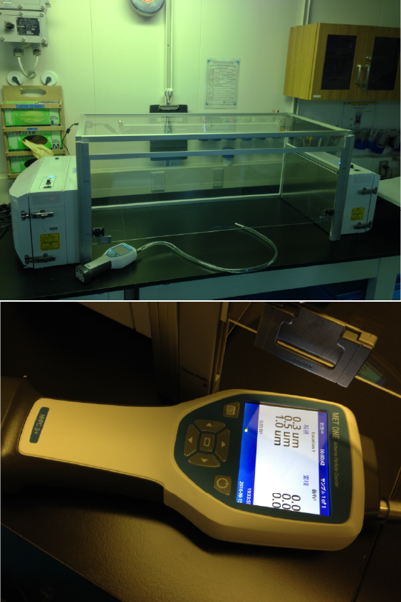
Figure F25. Measuring particle counts in KOACH system on the Chikyu.

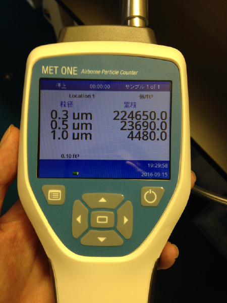
Figure F26. Particle counts of QA/QC laboratory air on the Chikyu core processing deck.

Monitoring airborne microbial cells

To quantify the concentration of airborne microbial cells that may potentially contaminate cores during shipboard core handling, cells in 1 L of air were counted from various workspaces: (1) the QA/QC laboratory, (2) the microbiology laboratory, (3) the UV-sterilized hood (i.e., clean bench) equipped with a KOACH air purification system, and (4) the COY anaerobic chamber also equipped with a KOACH air purification system. At KCC, 1 L of air was sampled at the following workspaces: (1) the clean bench in the super-clean room, (2) the COY anaerobic chamber equipped with a KOACH air purification system, and (3) the super-clean room, where unfiltered laboratory air was also sampled. To collect cells from a 1 L volume of air, 50 mL of air was sampled via a syringe through a 0.2 µm polycarbonate membrane in a syringe filter housing (Swinnex Filter Holder, 25 mm, Merck Millipore) and this procedure was repeated 20 times (Figure F27; Table T10). Formaldehyde fixation solution (4% in 3% NaCl solution) was subsequently applied to the filter and incubated at room temperature for 10–20 min to fix cells. Fixation solution was then purged from the polycarbonate membrane using 5 mL of KOACH sterile air with a 0.22 µm pore-sized polyethersulfone (PES) filter (Millex-GP filter unit, Merck Millipore). The filters were stored at 4°C in sterilized plastic bags until further processing and cell counting at KCC.

Figure F27. Filtering airborne microbial cells in laboratory air.

Table T10. Overview of samples for QA. Download table in .csv format.

QC: assessing potential contamination of sediment samples from drilling fluid during coring

The use of drilling fluid during coring operations is necessary for a number of reasons, including cleaning of the borehole from cuttings, cooling of the drill bit, and ensuring borehole stability. Three types of drilling fluid contamination samples were collected for biological and chemical contamination analyses: the fluid contacting the core samples, drilling fluid from the delivery pump, and drilling fluid at the preparation tank as shown below.

Drilling fluid as a potential source of contamination

Drilling fluids are composed of seawater and varying amounts of chemical compounds, all of which are potential sources of microbial cells, viruses, and chemical contamination into low-biomass core samples (see Masui et al., 2008). The composition of the drilling fluid is adjusted during operations to optimize drilling performance (Figure F28). To account for the intrusion of drilling fluid into the core, a PFC compound is added as a chemical tracer to the drilling fluid before pumping it down the borehole (Smith et al., 2000a, 2000b). During RCB operations, drilling fluid caught inside the core liner (sample code LCL) was sampled when cores were cut into sections in the core cutting area immediately after retrieval (see Sampling in the core cutting area; Figure F21). LCL samples were used to monitor the input concentration of PFC and changes in numbers and community structure of microbial cells and viruses during drilling operations and sample recovery (Table T10). In addition, drilling fluid from Pump 2 (drilling fluid from delivery pump) and seawater gel from active mud tanks (drilling fluid at preparation tanks) were sampled once per day to assess the abundance of microbial cells and viruses in the drilling fluid. More information on the composition of drilling fluids is available in the Technical Report of Expedition 370 (Center of Deep Earth Exploration, 2016). A conceptual overview of drilling fluid circulation during riserless drilling on the Chikyu and fluid sampling points is shown in Figure F28, and a summary of terms and acronyms is found in Table T11.

Figure F28. Drilling fluid pumping and contamination sampling procedure.

Table T11. Terms and acronyms for drilling fluid and PFC samples. Download table in .csv format.

Sampling for biological assessment of drilling fluid contamination

For enumeration of microbial cells, 1–2 mL of LCL samples were fixed with prefiltered (0.22 µm pore-sized PES filter) saline formaldehyde solution (3% NaCl and 4% formaldehyde) and stored at 4°C. For enumeration of virus-like particles (VLP), 1–2 mL of LCL samples were fixed with virus-free (0.02 µm filtered; Anodisc, GE) saline formaldehyde solution, immediately frozen in liquid nitrogen, and stored at −80°C (Suttle and Furhman, 2010). In addition, samples of drilling fluid from Pump 2, seawater gel, and LCL were frozen and stored at −80°C for onshore DNA-based assessment of core sample drilling fluid contamination.

To assess potential infiltration of microbial cells and VLPs from drilling fluid into the interior of cores, 1 cm³ samples were periodically taken for enumeration of cells and VLPs from the interior, midway, and exterior portions of a subsection of MBIO1 WRCs. The samples were collected inside the COY anaerobic chamber using sterile tools (cut-off syringes, sterile ceramic knives, and other tools, depending on the hardness of the material) and placed into Falcon tubes. For cell enumeration, the samples were fixed in prefiltered (0.22 µm) saline formaldehyde solution and stored at 4°C. For virus enumeration, the samples were fixed in prefiltered (0.02 µm) saline formaldehyde solution, frozen in liquid nitrogen, and stored at −80°C.

Monitoring contamination by drilling fluid with PFC

A PFC-based tracer contamination test was first implemented in terrestrial subsurface environment exploration (Colwell et al., 1992) and was adopted during ODP Leg 185 to provide an estimate of the drilling fluid intrusion into the core interior (Smith et al., 2000a, 2000b). Since then, PFC has frequently been used as a chemical tracer during scientific ocean drilling, including on the R/V JOIDES Resolution (Smith et al., 2000a, 2000b; House et al., 2003; Lever et al., 2006) and the Chikyu (Yanagawa et al., 2013; Inagaki et al., 2015). During Expedition 370, we used the compound perfluoromethylcyclohexane (C₇F₁₄) as the PFC chemical tracer. In the main pump room, PFC was supplied via a high-pressure liquid chromatography (HPLC) pump into the drilling fluid at the inlet of charge Pump 2. The HPLC pump supplied a constant flow rate of 0.6 mL/min of 94% pure PFC. During drilling operations, flow in the borehole was adjusted, using up to three charge pumps; therefore, the input PFC concentration varied depending on the Pump 2 flow rate and its relative ratio to the total flow rate.

To verify and quantify the presence of PFC in the drilling fluid, LCL samples were taken when the core sections were cut in the core cutting area unless no fluid was caught in the core liner. LCL samples that were collected into 50 mL Falcon tubes in the core cutting area and then sampled into headspace vials (~5 mL fluid into 20 mL vials) in the microbiology laboratory were designated as FAL-L samples (Table T11). LCL samples collected directly into headspace vials (~5 mL fluid into 20 mL vials; sample code HSECDM; see also Table T9 and Figure F21) were designated as CCA-L samples. Moreover, solid-phase samples (designated as CCA-S samples; sample code HSECD) were taken from the top of Section 1 for every core, starting at Core 370-C0023A-34R in the core cutting area (Figure F29) in order to have a means of comparison of PFC concentration between all cores if liner fluid was not present. This quick sampling scheme immediately after core recovery aimed to avoid PFC loss while cores underwent curation and X-ray CT image scanning.

Figure F29. Sampling scheme for microbiological community WRCs.

To determine the potential diffusion of drilling fluid into the interior of cores, three solid-phase samples (~2 cm³) were taken from the exterior (EX), midway (MD), and interior (IN) portion of the core cross section from every MBIO2 WRC (Figure F29; Table T11). In soft sediments, the samples were taken from the disk with a 5 mL cut-off sterilized syringe. In hard sediments (after Core 14X), the exterior sample and then the interior and midway samples were scraped out of the disk with a ceramic knife. Cores 111R and 112R were not monitored for the presence of PFC because the core material consisted of small basaltic pieces. Each sediment sample was placed in a 20 mL headspace vial, 5 mL of water was added, and the vial was immediately crimp capped with a Teflon-coated silica septum. Sample weights (CCA-S, IN, MD, and EX) were determined using two electronic balances and a computer averaging system that compensates for ship motion (Ocean High Technology Institute, Inc., Tokyo, Japan). The volumes of LCL samples (FAL-L and CCA-L) were estimated by comparison with reference vials.

At KCC, routine PFC sampling was conducted as an integral part of sample processing. Scrapings of WRC samples that were processed in an anaerobic chamber, as well as the innermost part of WRCs were also subjected to PFC measurements (see Shore-based sampling procedure below).

All samples were vortexed for 2 min each to create a slurry and enhance PFC release into the headspace. Vials were then mounted onto a rotating wheel and incubated at 80°C for at least 2 h. Following incubation, vials were placed in an Agilent G1888 network headspace sampler (shipboard and at KCC) that incubated vials at 80°C for an additional 30 min before injection. In the autosampler, 0.5 mL of the headspace was transferred into an Agilent 7890B GC (7890A GC at KCC) coupled to an electron capture detector (ECD). Samples were injected at 180°C with a split ratio of 1:5. The shipboard GC-ECD was equipped with a GS-GasPro column (30 m × 0.32 mm, Agilent, USA) and was operated with a constant helium flow rate of 3.4 mL/min. The initial oven temperature was set to 120°C, followed by a 20°C/min increase to a 180°C final temperature that was held for 3.5 min. After the 6.5 min sample run, a postrun was started at 200°C for 15 min and a final equilibration time of 1.5 min, equaling a total run time of 23 min per sample. The shore-based GC-ECD was also equipped with a GS-GasPro column and operated at the same conditions as the shipboard GC-ECD until 11 October 2016, when it was changed to an HP-ALM column (30 m × 0.53 mm, Agilent, USA) operated with a constant helium flow rate of 4.8 mL/min (Smith et al., 2000a). For the HP-ALM column, the initial oven temperature was set to 120°C, followed by a 20°C/min increase to 150°C final temperature that was held for 20 min, equaling a total run time of 22 min per sample.

For quantification of PFC in the samples, a five-point calibration curve was prepared by mixing liquid PFC solution (94% purity and 1.787 g/cm³ density) with methanol to create stock solutions from 10⁻⁸ to 10⁻⁴ (PFC:methanol [v/v]) (see EXP370_PFC_CALIBRATION_CURVE.XLSX in MBIO in Supplementary material). From this stock solution, 10 µL was transferred to an empty 20 mL headspace vial, resulting in standard PFC headspace concentrations from 8.4 × 10⁻³ to 8.4 × 10¹ µg/L. The shipboard GC-ECD detection limit (~1.6 × 10⁻³ µg/L PFC in headspace; area ~10) was about an order of magnitude lower than the lowest calibration standard used in the curve. The linearity of the standard curve was separately checked at KCC down to 8.4 × 10⁻⁴ µg/L PFC in headspace, which was defined as the lower limit of quantification (LOQ). For sediments, this corresponds to an average LOQ of PFC of 8.4 × 10⁻⁶ µg/cm³ sediment (assumptions: 4 g sediment, 2 g/cm³ density, addition of 5 mL water, and 20 mL headspace crimp vial). Linearity was assumed for all samples between the highest standard of the calibration curve (8.4 × 10¹ µg/L PFC in headspace) and detector saturation. Whenever oversaturation of the detector was observed, a defined amount of heated headspace gas was transferred into a new empty headspace vial and reanalyzed.

PFC concentration was calculated according to the procedure outlined by Expedition 337 Scientists (2013). In brief, for fluid samples, the headspace PFC concentration was multiplied by the vial volume and then divided by the sample volume. For sediment samples, the headspace PFC concentration was multiplied by the vial volume and then divided by the sample mass. PFC concentration in sediments was then converted from µg PFC/g sediment to µg PFC/cm³ using the core-specific MAD data (see Physical properties in the Site C0023 chapter [Heuer et al., 2017b]).

Shipboard WRC sampling for microbiological investigations and experiments

WRC sampling for microbiological investigations

WRCs for microbiological investigations were taken according to the expedition’s WRC sampling plan immediately after core retrieval and X-ray CT imaging of core sections on the core processing deck. Depending on requested storage conditions, WRCs for microbiological investigations were either anaerobically packed and flushed with N₂ gas into ESCAL gas-barrier bags prior to vacuum-sealing (V-301G, Fuji Impulse, Japan) or sealed aerobically without N₂ flushing. The packed WRC was then placed into a secondary gas-tight aluminum bag and vacuum-sealed following flushing with nitrogen gas.

WRCs for sampling and expeditionary analyses (referred to as “community WRCs”) were typically 30 cm long, and generally two adjacent WRC sections (MBIO1 and MBIO2) were taken from each 9.5 m core interval (Figure F29). MBIO1 was stored and transferred at refrigerated (4°C) conditions for cell and virus counts, cell visualization, enzymatic activity, and enrichment (Table T12), and MBIO2 was deep frozen at −80°C for molecular analysis and virus visualization (Table T13). MBIO1 and MBIO2 WRC processing was immediately carried out in anaerobic and aerobic super-clean conditions, respectively (see Quality assurance and quality control for sample processing).

Table T12. Allocation and treatment for MBIO1 WRC samples. Download table in .csv format.

Table T13. Samples taken from subcores of MBIO2 WRCs. Download table in .csv format.

The surface of each MBIO1 WRC was scraped using sterilized ceramic knives in the anaerobic chamber. After that, a disk sample was taken from MBIO1 and MBIO2 and samples were taken for microbiological, enzymatic, and organic geochemical investigations; contamination tests by PFC; and organic geochemistry (Figure F29). MBIO1 WRCs and personal samples were placed into ESCAL bags and temporarily clipped closed within the anaerobic chamber. The bags were removed from the chamber, immediately flushed with nitrogen gas to remove H₂ gas, and vacuum-sealed. MBIO1 WRCs were then stored at 4°C and personal samples were stored at requested temperatures. MBIO2 WRCs were removed from core liners in the clean bench. The WRCs were placed into ESCAL bags, sealed without nitrogen gas flushing, frozen by the shipboard Cells Alive System (CAS) freezer (Abi Co. Ltd., Japan; see Morono et al., 2015), and stored at −80°C.

Redox-sensitive WRC samples used for activity measurements and shore-based/postexpedition cultivation were processed in the anaerobic chamber. After removing the outer surface with sterile ceramic knives, samples were placed into ESCAL bags. The bags were removed from the anaerobic chamber, flushed once with N₂ to remove H₂ gas, vacuum-sealed, and stored at requested temperatures prior to shipping.

Preparation of WRC samples for potential metabolic activity determination with radiotracers

For shipboard determination of potential metabolic activity (i.e., sulfate reduction and hydrogenotrophic methanogenesis) using radioisotopes, WRC samples (approximately 10 cm long) were scraped, stored, and further processed under anaerobic conditions when a sufficient number of samples had been collected. In the anaerobic chamber (95:5 [v/v] N₂:H₂), another ~2–3 mm was scraped from the WRC surface with a sterile ceramic knife. The innermost part of the core was chopped off with the knife to create a mixture of very small sediment chips and powder. Approximately 5 mL of this chipped sediment was placed into a 20 mL crimp vial to which 5 mL of either methanogenic (sulfate-free, 1 mM NaHCO₃) or sulfate reducing (5 mM SO₄²⁻, 5 mM NaHCO₃) medium was added. Three replicate vials were prepared from each sample for both methanogenesis and sulfate reduction rate determination, respectively. Vials were crimp-sealed with nontoxic blue chlorobutyl stoppers (Bellco) and aluminum crimps. After sealing, the vial headspace was flushed with N₂ gas to remove surplus hydrogen, followed by the addition of 40 µL N₂:H₂ gas (95:5 [v/v]) to provide approximately 400 nM of dissolved hydrogen to the liquid phase. All vials and stoppers were autoclaved, and solutions were either autoclaved or filtered through sterile syringe filters (0.20 µm pore sized) prior to use.

In the radioisotope laboratory on the Chikyu, 10 µL of radiolabeled (³⁵S) Na₂SO₄ (3.7 MBq) and 100 µL of radiolabeled (¹⁴C) NaHCO₃ (3.7 MBq) were injected into sulfate reduction and methanogenesis samples, respectively, followed by vigorous shaking. Samples were incubated at temperatures within the estimated in situ range: 40°C for 360 mbsf or shallower, 60°C for 405–585 mbsf, 80°C for 604–775 mbsf, and 95°C for 816 mbsf or deeper. After a maximum 10 days of incubation, 3 mL of 20% (w/v) zinc acetate solution was injected into each sulfate reduction vial to trap produced H₂S gas. Vials were thoroughly shaken before they were opened to transfer the sediment slurries to 50 mL centrifuge tubes containing 7 mL of 20% (w/v) zinc acetate solution. Tubes were shaken and frozen immediately at −20°C to stop microbial activity and shipped to GFZ Potsdam (Germany) after the expedition for analysis. Methanogenic activity was stopped by injecting 500 µL of 50% (w/v) sodium hydroxide into each methanogenesis vial followed by shaking. Samples were then shipped to Aarhus University (Denmark) for analysis. Sediment controls for both methods were incubated without radiotracer addition. Radiotracer was then added after microbial activity was stopped in order to check for abiotic reactions after incubation. Negative controls (5 mL sterile medium and no sediment) and drilling fluid controls (5 mL core liner fluid, drilling fluid from Pump 2, and seawater gel) were incubated at the same experimental conditions to check for nonbiological reactions from the negative controls and biological reactions originating from drilling fluid, respectively.

Artificial seawater medium for sediment slurry incubations was prepared as follows. The subsequent salts were each added to two 2 L glass bottles (one bottle for sulfate reducing medium and one for methanogenic medium):

400 mg KH₂PO₄
500 mg NH₄Cl
1 g MgCl₂·6H₂O
1 g KCl, 300 mg CaCl₂·2H₂O
50 g NaCl

In addition, 1.42 g Na₂SO₄ was added to only the sulfate reducing medium. The bottles were filled to 2 L with ultrapure H₂O. Some drops of resazurin solution (0.1% [w/v]) were added. The bottles were covered (but not completely closed) with a screw cap and autoclaved. After autoclaving, the medium was purged with N₂ gas while still hot (>60°C). During purging, 10 and 2 mL of sterile filtered NaHCO₃ solution (84 g NaHCO₃ in 100 mL H₂O) was added to the sulfate reducing medium and methanogenic medium, respectively. When necessary, pH was adjusted with sterile filtered 6.5% HCl or NaOH solution to pH 7.5. The bottles were then capped with a sterile butyl stopper and a screw cap, and ~3 mL of sterile filtered Na₂S solution (1.2 g Na₂S in 100 mL H₂O) was added through the stopper with a syringe to reduce the medium. Reduction was confirmed by the decoloration of the resazurin in solution.

Sample shipment to KCC

MBIO1 and MBIO2 WRCs were transported by helicopter to KCC at a frequency of six flights per week on average to ensure rapid processing and minimize potential bias due to the effects of prolonged storage after core retrieval. During transit, WRCs were stored in thermally insulated bags to maintain the temperatures at which they were temporarily stored on the ship.

Shore-based WRC sampling for microbiological investigations and experiments at KCC

Shore-based sampling procedure

All sample surfaces of MBIO1 WRCs had been prescraped on the Chikyu to prevent diffusion of potential contaminants from seawater and drilling fluid further into the core during storage and transport. The received samples ranged in length from approximately 10 to 30 cm WRC equivalent. The range of sample quality and coherency varied, especially at shallower depths. To further minimize the potential contamination of core samples, the outer layer of prescraped core (~5 mm thickness) was removed again from all surfaces of hard and intact WRCs, including the surface of cracks through the core, using a sterile ceramic knife in an anaerobic chamber following the QA/QC routines described in Quality assurance and quality control for sample processing. A sample of the removed surface material was collected for PFC analysis (KCC secondary scrapings), and the rest was archived. From the remaining core, an intact 1–2 cm whole-round slice was cut with a ceramic knife for structural visualization analysis. Next, the integrity of samples for cell and virus counts were prioritized: for this the core was placed inside a sterile bag, mounted in a holding clamp, and a minicore sample was taken from the center of the core using a core drill with a sterilized core bit to obtain the cleanest sample possible. This minicore was divided in half and stored according to Table T12. Drilling usually caused disintegration of the remaining core within the sterile bag, and the subsequent samples were taken from the disintegrated pieces using a spatula. Any remaining scraped sample was saved as “Internal” core in a new sterile bag, flushed with N₂ in a heat-sealed aluminum bag, and then stored at 4°C. If the received WRCs were soft but intact, the same procedure was followed, except that cut-off syringes were used in place of the minicore drill. If the WRCs were not intact, surface scraping was not possible, and samples were taken directly using cut-off syringes. Treatment for individual samples is given in Table T12.

Anaerobically stored CAS-frozen MBIO2 WRCs were first cut into two WRC pieces when the WRC was longer than 12 cm using a band saw with an electron-deposited diamond coated edge, located inside a clean booth equipped with two HEPA filter units (Masui et al., 2009; Morono and Inagaki, 2016). Anaerobically stored MBIO2 WRCs shorter than 12 cm were not cut. The surface of the WRC was briefly flamed to soften the sediment, allowing the removal of its surface by scraping with a sterile spatula in an effort to prevent surface contaminants from touching the subcore. A subcore was then aseptically taken from the center of the frozen WRC sample using a tabletop 2 cm diameter minicore drill. The subcore was further sectioned for DNA extraction, virus visualization, and PFC analysis and stored at −80°C prior to the analysis. The volume and treatment of the subcores are described in Table T13.

Cell counts

All sample preparation for cell counting was carried out in the super-clean room at KCC. Cell count samples of drilling fluids (see Drilling fluid as a potential source of contamination) and LCL were diluted with 2.5% sodium chloride and directly filtered onto polycarbonate membranes (Millipore, USA). Sediment samples for cell counts were crushed into powder using ceramic mortars and pestles, which were combusted at 500°C for 5 h prior to use. Approximately 10 cm³ of powdered sediment was transferred into a sterile 50 mL centrifuge tube containing 20 mL of 3% (w/v) sodium chloride, with 10% (v/v) neutralized formalin (containing 3.8% formaldehyde) as a fixative, and then thoroughly mixed by vortexing to form a homogeneous suspension. The slurry sample was then subjected to the cell detachment and separation steps as follows:

An aliquot of 1 mL diluted paraformaldehyde (PFA)-fixed sediment slurry was put into a 15 mL tube. Then 1.4 mL of 2.5% NaCl, 300 µL of detergent mix (100 mM ethylenediamine tetra-acetic acid [EDTA], 100 mM sodium pyrophosphate, 1% [v/v] Tween-80), and 300 µL of pure methanol were added. The sample was shaken by the Shake Master (Bio Medical Science, Japan) at 500 rpm for 60 min.
The slurry sample was sonicated at 160 W for 30 s for 10 cycles (Bioruptor UCD-250HSA; Cosmo Bio, Japan).
The sample was loaded onto density layers composed of 30% Nycodenz (1.15 g/cm³), 50% Nycodenz (1.25 g/cm³), 80% Nycodenz (1.42 g/cm³), and 67% sodium polytungstate (2.08 g/cm³), which were prepared by overlaying lighter density solution onto heavy layers.
Cells and sediment particles were then separated by centrifugation at 10,000× g for 1 h at 25°C with swinging rotors.
The light density layer that might contain microbial cells was carefully collected using a 20G needle syringe.
The heavy fraction, including precipitated sediment particles, was washed by resuspending with 5 mL of 2.5% NaCl, and then centrifuged at 5000× g for 15 min at 25°C. The recovered supernatant was placed on the same cell fraction obtained above (i.e., Step 5).
The precipitated sediment was resuspended in 2.1 mL of 2.5% NaCl, 300 µL of detergent mix, and 300 µL of methanol. Then the sample was shaken at 500 rpm for 60 min at 25°C.
The slurry sample was layered onto a second density gradient with 30% Nycodenz, 50% Nycodenz, 80% Nycodenz, and 67% sodium polytungstate (same as Step 3).
Cells and sediment particles were then separated by centrifugation at 10,000× g for 1 h at 25°C with swinging rotors.
The light density layer that might contain microbial cells was collected using a 20G needle syringe, and all the supernatants were mixed together as a cell suspension for cell count.

The half-aliquot of the supernatant was passed through a 0.22 µm polycarbonate membrane filter. Cells on the membrane filter were stained with SYBR Green I staining solution (1/40 of SYBR Green I in Tris-EDTA [TE] buffer). The number of SYBR Green I–stained cells was enumerated either by direct microscopic count (Inagaki et al., 2015) or a fluorescent image-based cell counting system as described in Morono et al. (2009) and Morono and Inagaki (2010).

Visualization of cells with electron microscopy

Some density separates from core samples were subjected to further purification by cell sorting (Morono et al., 2013). Cells in a density separate were first trapped onto an Anodisc membrane (Whatmann, USA) and stained with SYBR Green I. After resuspension by gentle sonication, cells were specifically sorted by a Moflo cell sorter (Beckman Coulter, USA) directly onto a silicon nitride (SiN) membrane.

One microliter of filtered seawater containing 2.5% glutaraldehyde was dropped on the SiN membrane with the sorted cells, which were then fixed for 1 h at 4°C in a humid chamber. The sample was washed 6 times for 10 min with 1 µL drop of filtered seawater at 4°C in a humid chamber. Subsequently, the sample was postfixed and contrast was enhanced using the osmium and tannic acid procedure (Kajikawa et al., 1975; Bastini et al., 1984). First, 1 µL of filtered 2% osmium tetroxide solution was dropped on the SiN membrane for 1 h at 4°C in a humid chamber and washed 6 times for 10 min with 1 µL drop of distilled water at 4°C in a humid chamber. After that, 1 µL of filtered 3% tannic acid solution at pH 6.8 was dropped on the SiN membrane, incubated for 1 h at 4°C in a humid chamber, and then the membrane was washed 6 times for 10 min with 1 µL drop of distilled water at 4°C in a humid chamber. After washing, 1 µL of filtered 2% osmium tetroxide solution was further dropped on SiN membrane for 1 h at 4°C in a humid chamber and washed 6 times again for 10 min with 1 µL drop of distilled water in a humid chamber. The staining work was done by onshore collaborator Dr. Goichiro Uramoto at KCC (Kochi University, Japan).

The location of stained cells on a SiN membrane was checked with a fluorescence microscope based on the SYBR Green I–derived green fluorescence, and the same location was observed with transmission electron microscopy (JEM-ARM200F, JEOL, Japan) operated by onshore collaborator Dr. Naotaka Tomioka at KCC (JAMSTEC).

DNA extraction

A frozen sediment sample collected by minicore drilling was crushed into powder using a ceramic mortar and pestle, which were precombusted at 500°C for 5 h to eliminate exogeneous contaminant DNA. DNA was extracted from 5 g of the crushed sediment using a PowerLyzer PowerSoil DNA isolation kit (MO BIO Laboratories, USA) according to the manufacturer’s instructions with modifications. All kit components were irradiated by gamma ray to eliminate endogenous DNA contamination prior to use. Zirconium beads were substituted for the garnet beads in the kit to enhance cell disruption efficiency. The obtained DNA was further concentrated by ethanol precipitation by adding 10% (v/v) of 3 M sodium acetate, 250% (v/v) of absolute ethanol, and 20 µL of linear acrylamide (Thermo Fisher Scientific) to the DNA solution and incubating overnight at −20°C. DNA was precipitated by centrifugation at 10,000× g for 1 h followed by washing twice with 70% ethanol. The precipitated DNA was dissolved in 50 µL of TE buffer and stored at −20°C for subsequent analyses.

PCR, sequencing, and data analysis

For determining microbial taxonomic composition and community structure, the V4 region of the bacterial and archaeal 16S rRNA genes was amplified by PCR using U515F–U806R primers (Table T14). PCR amplifications were performed on Veriti Thermal Cyclers or StepOnePlus Thermal Cyclers (Thermo Fisher Scientific) using MightyAmp DNA polymerase ver.3 (Takara Bio) following the manufacturer’s instructions with 2 µL of the extracted DNA. The first round PCR thermal cycles consisted of initial denaturation for 2 min at 98°C, followed by 35 cycles of 5 s denaturation at 95°C, 15 s annealing at 55°C, and 30 s elongation at 68°C. The obtained PCR products were purified using AMPure XP beads (Beckman Coulter). Adaptor and index sequences were added to the purified amplification products by 2nd round PCR using KAPA HiFi HotStart ReadyMix with 515F-MiSeq and 806R-MiSeq primers according to the manufacturer’s instructions. Second round PCR cycles consisted of initial denaturation at 95°C for 3 min, followed by 10 cycles of 30 s denaturation at 95°C, 30 s annealing at 55°C, 30 s elongation at 72°C, and final elongation at 72°C for 5 min. We purified the PCR product twice using AMPure XP beads and measured the concentration of DNA using a NanoDrop 3300 fluorospectrometer with PicoGreen reagent (Thermo Fisher Scientific). Based on the measured concentrations, an equal amount of each purified product was pooled to make a sequence library. We sequenced the library on an MiSeq platform using a MiSeq Reagent Kit v3 in a 600-cycle format (Illumina).

Table T14. Oligonuceotide probes. Download table in .csv format.

Microbial diversity based on the obtained 16S rRNA gene assemblages was analyzed using the MetaAmp pipeline developed by Dong and Strous (unpublished, http://ebg.ucalgary.ca/metaamp).

High-pressure/temperature incubation

Innermost sediment core samples were taken from WRCs (sample code 370YMWR) for shore-based stable isotope probing incubation experiments under high-pressure and high-temperature conditions at KCC. Stable isotope–labeled compounds (¹³C, ¹⁵N, and deuterium [D]) were used as substrates to monitor the microbial dissimilatory respiration and/or the assimilation into cellular biomass.

For the high-temperature/pressure (high-P/T) incubation, we set up a custom-made high-P/T chamber system with a heat jacket (Syn Corporation, Ltd., Kyoto, Japan). The high-P/T chamber system is composed of five titanium-based pressure chamber units, the inner temperature of which can be controlled separately (see Figure F30). Each of the pressure chambers holds four inner incubation units, which consist of a polyetheretherketone (PEEK) tube (155 mm long and 24 mm ID), PEEK upper stopper, and PEEK free piston. The PEEK upper stopper and PEEK free piston each have two O-rings. The PEEK upper stoppers are connected to the stainless steel tube (100 mm × 0.2 mm ID) through the lid of the pressure chamber. The other end of the stainless steel tube is connected to a stainless steel syringe for substrate injection and fluid sampling into/from the inner cell under high-P/T conditions. Five pressure chambers are connected to a cylinder pump (Teledyne Isco, NE, USA, 100D, 100 mL) to maintain constant pressure throughout the incubation period. A thermal circulator (Julabo, Baden-Württemberg, Germany) is connected to the heat jacket of each high-P/T chamber to maintain the designated temperature condition.

Figure F30. High-temperature/pressure chamber system.

In the anaerobic chamber, ~50 cm³ of sediment was taken from each of 11 WRC samples, which were collected from 660 to 855 mbsf. The sediment powder was obtained by scraping an interior piece of the WRC with a sterilized ceramic knife and then mixed thoroughly to make a master sample. A 30 cm³ aliquot of the master sediment sample was put in each of the inner incubation units attached to the lid of the high-P/T chamber. After 35 mL of a basal medium (see Table T15) was added to each of the inner incubation units, they were sealed with the PEEK free piston and then transferred from the anaerobic chamber to the high-P/T chambers. The high-P/T chambers were then preheated to 50°C and pressurized to 55 MPa by a hand pump for the leak check. After completion of the leak check, the cylinder pump was activated to maintain a constant pressure at 55 MPa. Then, each heater deployed on the five high-P/T chambers was set at 80°, 95°, 110°, 125°, and 140°C, respectively. After every chamber reached the designated incubation temperature, 0.7 mL of substrate solution (see Table T16) was injected into each inner incubation unit using a stainless steel syringe. Because there was void space in the connecting line, 2 mL of the basal medium was injected to push the solution into the inner incubation unit after the injection of the substrate solution. The injected volume of the substrates or medium solutions was monitored by the cylinder pump through the volume of water pulled out from each high-P/T chamber to compensate for the added liquid volume. During the incubation, 2 mL of fluid samples was periodically collected using a stainless steel syringe to determine the carbon isotopic composition of methane and DIC. After sampling, 2 mL of the basal media was supplemented to the inner incubation unit using the stainless steel syringe to keep the liquid volume constant in the sample chamber. Two milliliters of sampled fluid was transferred to a 5 mL glass vial from the stainless syringe through a needle. Before the fluid was added, 20 µL of phosphoric acid was added to the vial then it was covered with a butyl rubber stopper and an aluminum cap and vacuumed with an oil rotary vacuum pump through a needle.

Table T15. Medium for high-P/T reactor. Download table in .csv format.

Table T16. Substrate solution. Download table in .csv format.

Sampling for postexpedition investigations

Cultivation experiments

WRC samples were prepared for postexpedition cultivation experiments by shipboard microbiologists. The contaminated outermost surface of each WRC was removed using a sterilized ceramic knife. The clean inner portions were stored in glass bottles, flushed with N₂, and sealed with rubber butyl stoppers. Alternatively, samples were packed in gas-tight ESCAL bags, which were flushed with N₂ and vacuum-sealed. All samples were stored at either 4°C or room temperature (approximately 23°C) in the dark prior to shore-based cultivation experiments.

Scanning electron microscopy

On the Chikyu, approximately 5 cm³ of sediment was sampled from the interior of the PFC disk under the KOACH system in the clean bench for scanning electron microscopy to determine characteristics of microbe–mineral attachment. These samples were preserved in 5 mL of 2.5% glutaraldehyde and stored at 4°C. Another 5 cm³ of sediment was sampled from the interior disk in the super-clean anaerobic chamber for further postexpedition cultivation work, including enrichment of iron-reducing bacteria and methanogens. Future experiments will examine preferential attachment of deep subsurface enrichment cultures to the minerals present in the core material. All fixed samples will be imaged under a JEOL JSM-7100F field-emission SEM at 3 kV. The elemental composition of the minerals will be determined using dispersive X-ray spectroscopy.

Environmental tag sequencing and metagenomics

To study the extent and adaptations of the deep subseafloor biosphere characterized by increasing in situ temperature to a depth of 1180 mbsf, WRCs were taken and cleaned on the Chikyu for DNA- and RNA-based molecular analyses. According to biomass estimates, different amounts of sample will be used to extract DNA and RNA using methods specifically developed for low-biomass deep sediments (e.g., Lever et al., 2015). Amplicon tag sequencing of bacterial and archaeal 16S rRNA genes will be performed using a MiSeq sequencer (Illumina) in order to characterize the microbial taxonomic diversity and community structure. Other personal deep-frozen WRC samples (e.g., sample codes 370LLWR and 370THWR) were dedicated to molecular ecological studies, including sequence analysis of PCR-amplified key functional genes, and molecular quantification using the digital PCR technique (Hoshino and Inagaki, 2012), as well as cultivation-dependent and -independent metagenomic and transcriptomic analyses.

Bio-orthogonal noncanonical amino acid tagging

Recently developed methods to detect in situ protein synthesis were applied by shipboard microbiologists. Following the protocol of Hatzenpichler et al. (2014), we introduced an artificial amino acid analog (L-homopropargylglycine [HPG]; Click Chemistry Tools), into selected WRCs after core processing and preparation for incubation. This artificial amino acid, substituting for methionine, could be used to detect in situ microbial activity, as the alkyne moiety on HPG will readily react with appropriate fluorescent azide dyes upon dye introduction into the incubation, thus enabling an investigator to detect microbial protein synthesis via fluorescence of a given biosynthesizing microbe. Downstream reaction of HPG with alkyne dyes accompanied by microscopy and cell sorting was planned for incubation processing postcruise.

Microbe–mineral interactions

To reveal microscale ecological partitioning within the sediments, shipboard microbiologists prepared WRC samples for separation of minerals using density and magnetic techniques following the methods of Harrison and Orphan (2012). Postcruise, density separation will be performed using different dilutions of a sodium metatungstate (H₂Na₆O₄₀W₁₂) solution, allowing for partitioning of sediment particles into different fractions corresponding to their density. Partitions will be further separated by magnetic susceptibility using a Frantz L-1 isodynamic magnetic separator. DNA will be subsequently extracted from these partitions, amplified by PCR, and sequenced using Illumina iTAG technology. This will enable the examination of microbial attachment to different clays, the surface properties of which are known to exhibit important controls over carbon burial (Mayer, 1994), as well as microbial attachment to authigenic clays or silica phases, which may control the smectite–illite transition through reduction of octahedral Fe (Vorhies and Gaines, 2009) or modulation of dissolved silica activities (Abercrombie et al., 1994).

Virus analyses

Samples for VLP enumeration were processed in the shore-based super-clean room at KCC. Postcruise, viruses will be detached from sediment by the same method as samples for cell separation and enumeration (see Cell counts). The mixture of detached cells and viruses will be filtered (0.22 µm, polyvinylidene difluoride [PVDF], Millipore) to remove cells. The viruses will be filtered onto 0.02 µm pore-sized aluminum oxide filters (Anodisc, GE) and stained with SYBR Gold (25× concentration) for 15 min. The stained filters will be mounted onto glass slides with an antifade mounting medium (VECTASHIELD, Vector Labs) and observed by epifluorescence microscopy at 1000× magnification. Viruses will be enumerated from 20 random fields of view (FOVs) or until 200 particles are enumerated. The abundance of viruses will be calculated from the average number of viral particles per FOV.

Potential viral contamination deriving from drilling fluid will also be assessed by enumerating drilling fluid samples that have been fixed in formaldehyde and frozen in liquid nitrogen (Suttle and Furhman, 2010). The fixed and frozen drilling fluid samples were stored at −80°C until analysis at KCC.

Samples for electron microscopy analysis of infected cells were taken on shore at KCC from MBIO2 WRCs, which had been frozen on board in a CAS freezer (Morono et al., 2015).

Temperature-induced plasticity of metabolism

Sediment samples (5–20 cm WRCs; sample code 370HLWR) had the external surface removed on the Chikyu to prevent further potential penetration of drilling fluid contaminants. They were maintained in anaerobic conditions and sent to KCC in sterile, air-tight packaging. There, samples were subjected to a second round of surface removal in the super-clean anaerobic chamber before being crushed to a coarse powder. An aliquot of this powder was fixed with formaldehyde and set aside as sample T₀. Another aliquot was set aside for potential future experiments, and the rest was stored in anaerobic and H₂-free conditions prior to inoculation to the medium that contains stable isotope–labeled substrates (see below).

Incubation volumes ranged from 120 mL for the shallower sediment samples to 1000 mL for the deeper samples to partially account for the decrease in apparent cell densities and maximize the potential to generate measurable material. The incubation medium was anaerobic sterile artificial seawater (5% [v/v] D₂O), with ¹⁵NH₄⁺ (50% [v/v]) as the nitrogen source and acetate as the carbon substrate and electron donor. Sulfate (5 mM) was included for sulfate reduction.

Postcruise, the isotopic composition of CO₂ in the headspace will be monitored to ascertain when the lag phase ends and exponential growth begins. Once exponential growth begins, samples of liquid medium will be extracted using a sterile needle and syringe at 3 time points at approximately 1 month intervals, fixed with formaldehyde, and stored for analysis. At the end of the incubation period, fixed cells will be fluorescently stained, sorted from sediment with flow cytometry, and mounted upon conductive membranes, and the isotopic composition of cells will be analyzed using secondary ion mass spectrometry to assess the incorporation rate of isotopically labeled substrate (Morono et al., 2011).

High-temperature enrichment of thermophilic endospore–forming microorganisms

At KCC, sediment (35 g) from WRC samples (sample code 370MCWR) was pasteurized at 80°C for 1 h and anaerobically incubated at 50°C, 60°C, or 70°C in 70 mL of artificial seawater medium (Widdel and Bak, 1992; Isaksen et al., 1994) amended with the organic acids lactate, propionate, succinate, acetate, formate, and butyrate, each to a final concentration of 1 mM, to enrich for thermophilic endospore–forming microorganisms. The microcosms were incubated for 21 days. They were sampled daily for the first 6 days of incubation. Sampling decreased in frequency between 6 and 21 days of incubation. Samples will be used for downstream molecular and genetic analysis. These analyses will include the monitoring of molecular indicators of anaerobic growth, such as organic acid measurement and sulfate measurement, and microbial community profiling, such as 16S rRNA gene and functional gene sequencing.

Exoenzyme activity

At KCC, enzyme activity was measured by supplying fluorogenic substrate, which produces fluorescence only after the functional group is cleaved by the relevant enzyme. This results in an increase in fluorescence over time when substrate concentrations are saturating. Activities were obtained by sampling each incubation at two or three time points and measuring fluorescence to obtain a slope. Each sample was run with a standard curve of fluorescent moiety (methylumbelliferone [MUF] or 7-amino-4-methylcoumarin [AMC]) in order to obtain absolute units of substrate cleaved.

Incubations were set up by placing 15 mL of sediment slurry containing ~10 g (exact mass determined) of powdered sediment and anaerobic P-free artificial seawater into 30 mL serum vials sealed with blue butyl rubber stoppers. Sediment crushing and incubation setup was carried out in an anaerobic chamber and vial headspace was flushed with N₂. Substrate was then added at estimated enzyme-saturating concentrations (see Table T17)

Table T17. Starting concentrations of substrate analogs for each enzyme. Download table in .csv format.

After flushing the headspace, 700 µL of homogenized slurry was removed to a 1.5 mL Eppendorf tube to serve as time point zero. This was briefly centrifuged before removing the supernatant to read in triplicate on a plate-reading fluorometer with an excitation wavelength of 380 nm and an emission wavelength of 454 nm for all substrates and standards. Subsequent time points were taken after 2 weeks and then again at 4–6 weeks to generate an activity slope. During this time, the incubations were kept at near–in situ temperatures. Fluorescence of MUF and AMC is at a maximum at pH 10, so 67 µL of 50 mM sodium tetraborate (pH 10.8) was added to each well to be read on the plate reader.

Biological core archives (DeepBIOS)

During Expedition 370, we collected ~10 cm WRCs for long-term storage at KCC (Masui et al., 2009). These legacy archive cores, denoted “DeepBIOS” (sample code 370RMS), will be used for future biological investigation upon request. DeepBIOS WRCs were collected following X-ray CT image scanning in the QA/QC laboratory and immediately frozen by a CAS freezer. DeepBIOS WRCs were stored at −80°C prior to shipping to KCC.

References

Abercrombie, H.J., Hutcheon, I.E., Bloch, J.D., and de Caritat, P., 1994. Silica activity and the smectite-illite reaction. Geology, 22(6):539–542. https://doi.org/10.1130/0091-7613(1994)022<0539:SAATSI>2.3.CO;2

ASTM International, 1990. Standard method for laboratory determination of water (moisture) content of soil and rock (Standard D2216–90). In Annual Book of ASTM Standards for Soil and Rock (Volume 04.08): Philadelphia (American Society for Testing Materials). [revision of D2216-63, D2216-80]

Bastini, M.J., Raper, J.A., and Goodman, C.S., 1984. Pathfinding by neuronal growth cones in grasshopper embryos, III. Selective affinity of the G growth cone for the P cells within the AP fascicle. Journal of Neuroscience, 4(9):2311–2328. http://www.jneurosci.org/content/4/9/2311.long

Blum, P., 1997. Technical Note 26: Physical Properties Handbook—A Guide to the Shipboard Measurement of Physical Properties of Deep-Sea Cores. Ocean Drilling Program. http://dx.doi.org/10.2973/odp.tn.26.1997

Bullard, E.C., 1939. Heat flow in South Africa. Proceedings of the Royal Society of London, Series A, 173(955):474–502. http://dx.doi.org/10.1098/rspa.1939.0159

Center for Deep Earth Exploration, 2016. CDEX Technical Report (Volume 28): Drilling Program IODP Expedition 370 T-Limit of the Deep Biosphere off Muroto: Yokosuka, Japan (JAMSTEC).

Cline, J.D., 1969. Spectrophotometric determination of hydrogen sulfide in natural waters. Limnology and Oceanography, 14(3):454–458. http://dx.doi.org/10.4319/lo.1969.14.3.0454

Colwell, F.S., Stormberg, G.J., Phelps, T.J., Birnbaum, S.A., McKinley, J., Rawson, S.A., Veverka, C., Goodwin, S., Long, P.E., Russell, B.F., Garland, T., Thompson, D., Skinner, P., and Grover, S., 1992. Innovative techniques for collection of saturated and unsaturated subsurface basalts and sediments for microbiological characterization. Journal of Microbiological Methods, 15(4):279–292. http://dx.doi.org/10.1016/0167-7012(92)90047-8

Droser, M.L., and Bottjer, D.J., 1986. A semiquantitative field classification of ichnofabric. Journal of Sedimentary Research, 56(4):558–559. http://dx.doi.org/10.1306/212F89C2-2B24-11D7-8648000102C1865D

Droser, M.L., and Bottjer, D.J., 1991. Trace fossils and ichnofabric in Leg 119 cores. In Barron, J., Larsen, B., et al., Proceedings of the Ocean Drilling Program, Scientific Results, 119: College Station, TX (Ocean Drilling Program), 635–641. http://dx.doi.org/10.2973/odp.proc.sr.119.206.1991

Ertefai, T.F., Heuer, V.B., Prieto-Mollar, X., Vogt, C., Sylva, S.P., Seewald, J., and Hinrichs, K.-U., 2010. The biogeochemistry of sorbed methane in marine sediments. Geochemica et Cosmochimica Acta, 74(1):6033–6048. https://doi.org/10.1016/j.gca.2010.08.006

Espitalié, J., Madec, M., Tissot, B., Mennig, J.J., and Leplat, P., 1977. Source rock characterization method for petroleum exploration. Proceedings of the 9th Annual Offshore Technology Conference, 3:439–448. https://doi.org/10.4043/2935-MS

Expedition 301 Scientists, 2005. Methods. In Fisher, A.T., Urabe, T., Klaus, A., and the Expedition 301 Scientists, Proceedings of the Integrated Ocean Drilling Program, 301: College Station, TX (Integrated Ocean Drilling Program Management International, Inc.). https://doi.org/10.2204/iodp.proc.301.105.2005

Expedition 307 Scientists, 2006. Methods. In Ferdelman, T.G., Kano, A., Williams, T., Henriet, J.-P., and the Expedition 307 Scientists, Proceedings of the Integrated Ocean Drilling Program, 307: Washington, DC (Integrated Ocean Drilling Program Management International, Inc.). https://doi.org/10.2204/iodp.proc.307.102.2006

Expedition 311 Scientists, 2006. Methods. In Riedel, M., Collett, T.S., Malone, M.J., and the Expedition 311 Scientists, Proceedings of the Integrated Ocean Drilling Program, 311: Washington, DC (Integrated Ocean Drilling Program Management International, Inc.). https://doi.org/10.2204/iodp.proc.311.102.2006

Expedition 315 Scientists, 2009. Expedition 315 methods. In Kinoshita, M., Tobin, H., Ashi, J., Kimura, G., Lallemant, S., Screaton, E.J., Curewitz, D., Masago, H., Moe, K.T., and the Expedition 314/315/316 Scientists, Proceedings of the Integrated Ocean Drilling Program, 314/315/316: Washington, DC (Integrated Ocean Drilling Program Management International, Inc.). http://dx.doi.org/10.2204/iodp.proc.314315316.122.2009

Expedition 316 Scientists, 2009. Expedition 316 methods. In Kinoshita, M., Tobin, H., Ashi, J., Kimura, G., Lallemant, S., Screaton, E.J., Curewitz, D., Masago, H., Moe, K.T., and the Expedition 314/315/316 Scientists, Proceedings of the Integrated Ocean Drilling Program, 314/315/316: Washington, DC (Integrated Ocean Drilling Program Management International, Inc.). http://dx.doi.org/10.2204/iodp.proc.314315316.132.2009

Expedition 319 Scientists, 2010. Methods. In Saffer, D., McNeill, L., Byrne, T., Araki, E., Toczko, S., Eguchi, N., Takahashi, K., and the Expedition 319 Scientists, Proceedings of the Integrated Ocean Drilling Program, 319: Tokyo (Integrated Ocean Drilling Program Management International, Inc.). http://dx.doi.org/10.2204/iodp.proc.319.102.2010

Expedition 322 Scientists, 2010. Methods. In Saito, S., Underwood, M.B., Kubo, Y., and the Expedition 322 Scientists, Proceedings of the Integrated Ocean Drilling Program, 322: Tokyo (Integrated Ocean Drilling Program Management International, Inc.). http://dx.doi.org/10.2204/iodp.proc.322.102.2010

Expedition 329 Scientists, 2011. Methods. In D’Hondt, S., Inagaki, F., Alvarez Zarikian, C.A., and the Expedition 329 Scientists, Proceedings of the Integrated Ocean Drilling Program, 329: Tokyo (Integrated Ocean Drilling Program Management International, Inc.). http://dx.doi.org/10.2204/iodp.proc.329.102.2011

Expedition 337 Scientists, 2013. Methods. In Inagaki, F., Hinrichs, K.-U., Kubo, Y., and the Expedition 337 Scientists, Proceedings of the Integrated Ocean Drilling Program, 337: Tokyo (Integrated Ocean Drilling Program Management International, Inc.). http://dx.doi.org/10.2204/iodp.proc.337.102.2013

Fischer, E., 1883. Bildung von Methylenblau als Reaktion auf Schwefelwasserstoff. In Bergmann, M., (Ed.), Untersuchungen aus Verschiedenen Gebieten: Berlin (Springer Berlin Heidelberg), 2234–2236. https://doi.org/10.1007/978-3-642-51364-0_24

Fisher, A.T., and Underwood, M.B., 1995. Calibration of an X-ray diffraction method to determine relative mineral abundances in bulk powders using matrix singular value decomposition: a test from the Barbados accretionary complex. In Shipley, T.H., Ogawa, Y., Blum, P., et al., Proceedings of the Ocean Drilling Program, Initial Reports, 156: College Station, TX (Ocean Drilling Program), 29–37. https://doi.org/10.2973/odp.proc.ir.156.103.1995

Fisher, R.V., and Schmincke, H.-U., 1984. Pyroclastic Rocks: Berlin (Springer-Verlag). http://dx.doi.org/10.1007/978-3-642-74864-6

Fritz, D., 1980. Safety and pollution-prevention program, Deep Sea Drilling Project Leg 50, Sites 415 and 416. In Lancelot, Y., Winterer, E. L., et al., Initial Reports of the Deep Sea Drilling Project, 44: Washington, DC (U.S. Government Printing Office), 855–859. https://doi.org/10.2973/dsdp.proc.50.app5.1980

Gilbert, A., Yamada, K., Suda, K., Ueno, Y., and Yoshida, N., 2016. Measurement of position-specific ¹³C isotopic composition of propane at the nanomole level. Geochimica et Cosmochimica Acta, 177:205–216. https://doi.org/10.1016/j.gca.2016.01.017

Gradstein, F.M., Ogg, J.G., Schmitz, M.D., and Ogg, G.M. (Eds.), 2012. The Geological Time Scale 2012: Amsterdam (Elsevier).

Harrison, B.K., and Orphan, V.J., 2012. Method for assessing mineral composition–dependent patterns in microbial diversity using magnetic and density separation. Geomicrobiology Journal, 29(5):435–449. https://doi.org/10.1080/01490451.2011.581327

Hatzenpichler, R., Scheller, S., Tavormina, P.L., Babin, B.M., Tirrell, D.A., and Orphan, V.J., 2014. In situ visualization of newly synthesized proteins in environmental microbes using amino acid tagging and click chemistry. Environmental Microbiology, 16(8):2568–2590. https://doi.org/10.1111/1462-2920.12436

Heesemann, M., Villinger, H., Fisher, A.T., Tréhu, A.M., and White, S., 2006. Data report: testing and deployment of the new APCT-3 tool to determine in situ temperatures while piston coring. In Riedel, M., Collett, T.S., Malone, M.J., and the Expedition 311 Scientists. Proceedings of the Integrated Ocean Drilling Program, 311: Washington, DC (Integrated Ocean Drilling Program Management International, Inc.). http://dx.doi.org/10.2204/iodp.proc.311.108.2006

Heuer, V.B., Inagaki, F., Morono, Y., Kubo, Y., Maeda, L., Bowden, S., Cramm, M., Henkel, S., Hirose, T., Homola, K., Hoshino, T., Ijiri, A., Imachi, H., Kamiya, N., Kaneko, M., Lagostina, L., Manners, H., McClelland, H.-L., Metcalfe, K., Okutsu, N., Pan, D., Raudsepp, M.J., Sauvage, J., Schubotz, F., Spivack, A., Tonai, S., Treude, T., Tsang, M.-Y., Viehweger, B., Wang, D.T., Whitaker, E., Yamamoto, Y., and Yang, K., 2017a. Expedition 370 summary. In Heuer, V.B., Inagaki, F., Morono, Y., Kubo, Y., Maeda, L., and the Expedition 370 Scientists, Temperature Limit of the Deep Biosphere off Muroto. Proceedings of the International Ocean Discovery Program, 370: College Station, TX (International Ocean Discovery Program). https://doi.org/10.14379/iodp.proc.370.101.2017

Heuer, V.B., Inagaki, F., Morono, Y., Kubo, Y., Maeda, L., Bowden, S., Cramm, M., Henkel, S., Hirose, T., Homola, K., Hoshino, T., Ijiri, A., Imachi, H., Kamiya, N., Kaneko, M., Lagostina, L., Manners, H., McClelland, H.-L., Metcalfe, K., Okutsu, N., Pan, D., Raudsepp, M.J., Sauvage, J., Schubotz, F., Spivack, A., Tonai, S., Treude, T., Tsang, M.-Y., Viehweger, B., Wang, D.T., Whitaker, E., Yamamoto, Y., and Yang, K., 2017b. Site C0023. In Heuer, V.B., Inagaki, F., Morono, Y., Kubo, Y., Maeda, L., and the Expedition 370 Scientists, Temperature Limit of the Deep Biosphere off Muroto. Proceedings of the International Ocean Discovery Program, 370: College Station, TX (International Ocean Discovery Program). https://doi.org/10.14379/iodp.proc.370.103.2017

Hinrichs, K.-U., Hayes, J.M., Bach, W., Spivack, A.J., Hmelo, L.R., Holm, N.G., Johnson, C.G., and Sylva, S.P., 2006. Biological formation of ethane and propane in the deep marine subsurface. Proceedings of the National Academy of Science of the United States of America, 103(40):14684–14689. http://dx.doi.org/10.1073/pnas.0606535103

Hoehler, T.M., Alperin, M.J., Albert, D.B., and Martens, C.S., 1998. Thermodynamic control on hydrogen concentrations in anoxic sediments. Geochimica et Cosmochimica Acta, 62(10):1745–1756. https://doi.org/10.1016/S0016-7037(98)00106-9

Hoehler, T.M., Borowski, W.S., Alperin, M.J., Rodriguez, N.M., and Paull, C.K., 2000. Model, stable isotope, and radiotracer characterization of anaerobic methane oxidation in gas hydrate–bearing sediments of the Blake Ridge. In Paull, C.K., Matsumoto, R., Wallace, P.J., and Dillon, W.P. (Eds.), Proceedings of the Ocean Drilling Program, Scientific Results, 164: College Station, TX (Ocean Drilling Program), 79–85. https://doi.org/10.2973/odp.proc.sr.164.242.2000

Hoshino, T., and Inagaki, F., 2012. Molecular quantification of environmental DNA using microfluidics and digital PCR. Systematic and Applied Microbiology, 35(6):390–395. http://dx.doi.org/10.1016/j.syapm.2012.06.006

Hoshino, T., and Inagaki, F., 2017. Application of stochastic labeling with random-sequence barcodes for simultaneous quantification and sequencing of environmental 16S rRNA genes. PLoS One, 12(1):e0169431. https://doi.org/10.1371/journal.pone.0169431

House, C.H., Cragg, B.A., Teske, A., and the Leg 201 Scientific Party, 2003. Drilling contamination tests during ODP Leg 201 using chemical and particulate tracers. In D’Hondt, S.L., Jørgensen, B.B., Miller, D.J., et al., Proceedings of the Ocean Drilling Program, Initial Reports, 201: College Station, TX (Ocean Drilling Program), 1–19. https://doi.org/10.2973/odp.proc.ir.201.102.2003

Inagaki, F., Hinrichs, K.-U., Kubo, Y., Bowles, M.W., Heuer, V.B., Long, W.-L., Hoshino, T., Ijiri, A., Imachi, H., Ito, M., Kaneko, M., Lever, M.A., Lin, Y.-S., Methé, B.A., Morita, S., Morono, Y., Tanikawa, W., Bihan, M., Bowden, S.A., Elvert, M., Glombitza, C., Gross, D., Harrington, G.J., Hori, T., Li, K., Limmer, D., Liu, C.-H., Murayama, M., Ohkouchi, N., Ono, S., Park, Y.-S., Phillips, S.C., Prieto-Mollar, X., Purkey, M., Riedinger, N., Sanada, Y., Sauvage, J., Snyder, G., Susilawati, R., Takano, Y., Tasumi, E., Terada, T., Tomaru, H., Trembath-Reichert, E., Wang, D.T., and Yamada, Y., 2015. Exploring deep microbial life in coal-bearing sediment down to ~2.5 km below the ocean floor. Science, 349(6246):420–424. http://dx.doi.org/10.1126/science.aaa6882

Isaksen, M.F., Bak, F., and Jørgensen, B.B., 1994. Thermophilic sulfate-reducing bacteria in cold marine sediment. FEMS Microbiology Ecology, 14:1–8. https://doi.org/10.1111/j.1574-6941.1994.tb00084.x

JOIDES Pollution Prevention and Safety Panel, 1992. Ocean Drilling Program guidelines for pollution prevention and safety. JOIDES Journal, 18(7):24. http://www.odplegacy.org/PDF/Admin/JOIDES_Journal/JJ_1992_V18_No7.pdf

Kajikawa, K., Yamaguchi, T., Katsuda, S., and Miwa, A., 1975. An improved electron stain for elastic fibers using tannic acid. Journal of Electron Microscopy, 24(4):287–289. https://doi.org/10.1093/oxfordjournals.jmicro.a049983

Kinoshita, M., Fukase, H., Goto, S., and Toki, T., 2015. In situ thermal excursions detected in the Nankai Trough forearc slope sediment at IODP NanTroSEIZE Site C0008. Earth, Planets and Space, 67:16. https://doi.org/10.1186/s40623-014-0171-1

Kirschvink, J.L., 1980. The least-squares line and plane and the analysis of palaeomagnetic data. Geophysical Journal of the Royal Astronomical Society, 62(3):699–718. http://dx.doi.org/10.1111/j.1365-246X.1980.tb02601.x

Kuley, C.J., 1963. Gas chromatographic analysis of C₁ to C₄ hydrocarbons in the parts per million range in air and in vaporized liquid oxygen. Analytical Chemistry, 35(10):1472–1475. https://doi.org/10.1021/ac60203a015

Kvenvolden, K.A., and McDonald, T.J., 1986. Technical Note 6: Organic Geochemistry on the JOIDES Resolution—An Assay. Ocean Drilling Program. http://dx.doi.org/10.2973/odp.tn.6.1986

Lever, M.A., Alperin, M., Engelen, B., Inagaki, F., Nakagawa, S., Steinsbu, B.O., Teske A., and IODP Expedition 301 Scientists, 2006. Trends in basalt and sediment core contamination during IODP Expedition 301. Geomicrobiology Journal, 23(7):517–530. http://dx.doi.org/10.1080/01490450600897245

Lever, M.A., Torti, A., Eickenbusch, P., Michaud, A.B., Šantl-Temkiv, T., and Jørgensen, B.B., 2015. A modular method for the extraction of DNA and RNA, and the separation of DNA pools from diverse environmental sample types. Frontiers in Microbiology, 6:1–25. http://dx.doi.org/10.3389/fmicb.2015.00476

Lin, W., Yeh, E.-C., Ito, H., Hirono, T., Soh, W., Wang, C.-Y., Ma, K.-F., Hung, J.-H., and Song, S.-R., 2007. Preliminary results of stress measurements using drill cores of TCDP Hole-A: an application of anelastic strain recovery method to three-dimensional in-situ stress determination. Terrestrial, Atmospheric and Oceanic Sciences, 18(2):379. https://doi.org/10.3319/TAO.2007.18.2.379(TCDP)

Lin, Y.-S., Heuer, V.B., Goldhammer, T., Kellermann, M.Y., Zabel, M., and Hinrichs, K.-U., 2012. Toward constraining H₂ concentration in subseafloor sediment: a proposal for combined analysis by two distinct approaches. Geochimica et Cosmochimica Acta, 77:186–201. https://doi.org/10.1016/j.gca.2011.11.008

Manheim, F.T., and Sayles, F.L., 1974. Composition and origin of interstitial waters of marine sediments, based on deep sea drill cores. In Goldberg, E.D. (Ed.), The Sea (Volume 5): Marine Chemistry: The Sedimentary Cycle: New York (Wiley), 527–568.

Masui, N., Morono, Y., and Inagaki, F., 2008. Microbiological assessment of circulation mud fluids during the first operation of riser drilling by the deep-earth research vessel Chikyu. Geomicrobiology Journal, 25(6):274–282. https://doi.org/10.1080/01490450802258154

Masui, N., Morono, Y., and Inagaki, F., 2009. Bio-archive core storage and subsampling procedure for subseafloor molecular biological research. Scientific Drilling, 8:35–37. http://dx.doi.org/10.2204/iodp.sd.8.05.2009

Matsuki, K., 1991. Three-dimensional in situ stress measurement with anelastic strain recovery of a rock core. Proceedings - International Congress on Rock Mechanics, 7:557–560. http://www.onepetro.org/mslib/servlet/onepetropreview?id=ISRM-7CONGRESS-1991-110

Mayer, L.M., 1994. Relationships between mineral surfaces and organic carbon concentrations in soils and sediments. Chemical Geology, 114(3–4):347–363. https://doi.org/10.1016/0009-2541(94)90063-9

Mazzullo, J., and Graham, A.G. (Eds.), 1988. Technical Note 8: Handbook for Shipboard Sedimentologists. Ocean Drilling Program. http://dx.doi.org/10.2973/odp.tn.8.1988

Morono, Y., and Inagaki, F., 2010. Automatic slide-loader fluorescent microscope for discriminative enumeration of subseafloor life. Scientific Drilling, 9:32–36. http://dx.doi.org/10.2204/iodp.sd.9.06.2010

Morono, Y., and Inagaki, F., 2016. Analysis of low-biomass microbial communities in the deep biosphere. In Sima, S., and Gadd, G.M. (Eds.), Advances in Applied Microbiology: Amsterdam (Elsevier), 95:149–178. https://doi.org/10.1016/bs.aambs.2016.04.001

Morono, Y., Terada, T., Kallmeyer, J., and Inagaki, F., 2013. An improved cell separation technique for marine subsurface sediments: applications for high-throughput analysis using flow cytometry and cell sorting. Environmental Microbiology, 15(10):2841–2849. http://dx.doi.org/10.1111/1462-2920.12153

Morono, Y., Terada, T., Masui, N., and Inagaki, F., 2009. Discriminative detection and enumeration of microbial life in marine subsurface sediments. The ISME Journal, 3(5):503–511. http://dx.doi.org/10.1038/ismej.2009.1

Morono, Y., Terada, T., Nishizawa, M., Ito, M., Hillion, F., Takahata, N., Sano, Y., and Inagaki, F., 2011. Carbon and nitrogen assimilation in deep subseafloor microbial cells. Proceedings of the National Academy of Sciences of the United States of America, 108(45):18295–18300. http://dx.doi.org/10.1073/pnas.1107763108

Morono, Y., and Inagaki, F., 2016. Analysis of low-biomass microbial communities in the deep biosphere. In Sima, S., and Gadd, G.M. (Eds.), Advances in Applied Microbiology (Volume 95): Amsterdam (Elsevier), 149–178. https://doi.org/10.1016/bs.aambs.2016.04.001

Ono, S., Wang, D.T., Gruen, D.S., Sherwood Lollar, B., Zahniser, M.S., McManus, B.J., and Nelson, D.D., 2014. Measurement of a doubly substituted methane isotopologue, ¹³CH₃D, by tunable infrared laser direct absorption spectroscopy. Analytical Chemistry, 86(13):6487–6494. https://doi.org/10.1021/ac5010579

Oremland, R.S., Miller, L.G., and Whiticar, M.J., 1987. Sources and flux of natural gases from Mono Lake, California. Geochimica et Cosmochimica Acta, 51(11):2915–2929. https://doi.org/10.1016/0016-7037(87)90367-X

Pimmel, A., and Claypool, G., 2001. Technical Note 30: Introduction to Shipboard Organic Geochemistry on the JOIDES Resolution. Ocean Drilling Program. http://dx.doi.org/10.2973/odp.tn.30.2001

Saito, S., Underwood, M.B., Kubo, Y., and the Expedition 322 Scientists, 2010. Proceedings of the Integrated Ocean Drilling Program, 322: Tokyo (Integrated Ocean Drilling Program management International, Inc.). http://dx.doi.org/10.2204/iodp.proc.322.2010

Schneider, C.A., Rasband, W.S., and Eliceiri, K.W., 2012. NIH Image to ImageJ: 25 years of image analysis. Nature Methods, 9(7):671–675. https://doi.org/10.1038/nmeth.2089

Shipboard Scientific Party, 1991. Site 808. In Taira, A., Hill, I., Firth, J.V., et al., Proceedings of the Ocean Drilling Program, Initial Reports, 131: College Station, TX (Ocean Drilling Program), 71–269. http://dx.doi.org/10.2973/odp.proc.ir.131.106.1991

Shipboard Scientific Party, 1994. Explanatory notes. In Westbrook, G.K., Carson, B., Musgrave, R.J., et al., Proceedings of the Ocean Drilling Program, Initial Reports, 146 (Part 1): College Station, TX (Ocean Drilling Program), 15–48. https://doi.org/10.2973/odp.proc.ir.146-1.005.1994

Shipboard Scientific Party, 2001a. Leg 190 summary. In Moore, G.F., Taira, A., Klaus, A., et al., Proceedings of the Ocean Drilling Program, Initial Reports, 190: College Station, TX (Ocean Drilling Program), 1–87. http://dx.doi.org/10.2973/odp.proc.ir.190.101.2001

Shipboard Scientific Party, 2001b. Site 1174. In Moore, G.F., Taira, A., Klaus, A., et al., Proceedings of the Ocean Drilling Program, Initial Reports, 190: College Station, TX (Ocean Drilling Program), 1–149. http://dx.doi.org/10.2973/odp.proc.ir.190.105.2001

Shipboard Scientific Party, 2003. Explanatory notes. In D’Hondt, S.L., Jørgensen, B.B., Miller, D.J., et al., Proceedings of the Ocean Drilling Program, Initial Reports, 201: College Station, TX (Ocean Drilling Program), 1–103. https://doi.org/10.2973/odp.proc.ir.201.105.2003

Shipley, T.H., Ogawa, Y., Blum, P., et al., 1995. Proceedings of the Ocean Drilling Program, Initial Reports, 156: College Station, TX (Ocean Drilling Program), 1–103. https://doi.org/10.2973/odp.proc.ir.156.1995

Smith, D.C., Spivack, A.J., Fisk, M.R., Haveman, S.A., and Staudigel, H., 2000a. Tracer-based estimates of drilling-induced microbial contamination of deep sea crust. Geomicrobiology Journal, 17(3):207–219. http://dx.doi.org/10.1080/01490450050121170

Smith, D.C., Spivack, A.J., Fisk, M.R., Haveman, S.A., Staudigel, H., and the Leg 185 Shipboard Scientific Party, 2000b. Technical Note 28: Methods for Quantifying Potential Microbial Contamination during Deep Ocean Coring. Ocean Drilling Program. http://dx.doi.org/10.2973/odp.tn.28.2000

Spivack, A.J., McNeil, C., Holm, N.G., and Hinrichs, K.-U., 2006. Determination of in situ methane based on analysis of void gas. In Jørgensen, B.B., D'Hondt, S.L., and Miller, D.J. (Eds.), Proceedings of the Ocean Drilling Program, Scientific Results, 201: College Station, TX (Ocean Drilling Program), 1–11. https://doi.org/10.2973/odp.proc.sr.201.119.2006

Stookey, L.L., 1970. Ferrozine—a new spectrophotometric reagent for iron. Analytical Chemistry, 42(7):779–781. https://doi.org/10.1021/ac60289a016

Suttle, C.A., and Furhman, J.A., 2010. Enumeration of virus particles in aquatic or sediment samples by epifluorescence microscopy. In Wilhelm, S.W., Weinbauer, M.G., and Suttle, C.A. (Eds.), Manual of Aquatic Viral Ecology: Waco, TX (American Society of Limnology and Oceanography), 145–153. https://doi.org/10.4319/mave.2010.978-0-9845591-0-7.145

Underwood, M.B., Basu, N., Steurer, J., and Udas, S., 2003. Data report: normalization factors for semiquantitative X-ray diffraction analysis, with application to DSDP Site 297, Shikoku Basin. In Mikada, H., Moore, G.F., Taira, A., Becker, K., Moore, J.C., and Klaus, A. (Eds.), Proceedings of the Ocean Drilling Program, Scientific Results, 190/196: College Station, TX (Ocean Drilling Program), 1–28. http://dx.doi.org/10.2973/odp.proc.sr.190196.203.2003

Vacquier, V., 1985. The measurement of thermal conductivity of solids with a transient linear heat source on the plane surface of a poorly conducting body. Earth and Planetary Science Letters, 74(2–3):275–279. http://dx.doi.org/10.1016/0012-821X(85)90027-5

Von Herzen, R., and Maxwell, A.E., 1959. The measurement of thermal conductivity of deep-sea sediments by a needle-probe method. Journal of Geophysical Research, 64(10):1557–1563. http://dx.doi.org/10.1029/JZ064i010p01557

Vorhies, J.S., and Gaines, R.R., 2009. Microbial dissolution of clay minerals as a source of iron and silica in marine sediments. Nature Geoscience, 2(3):221–225. https://doi.org/10.1038/ngeo441

Walters, W.A., Caporaso, J.G., Lauber, C.L., Berg-Lyons, D., Fierer, N., and Knight, R., 2011. PrimerProspector: de novo design and taxonomic analysis of barcoded polymerase chain reaction primers. Bioinformatics, 27(8):1159–1161. https://doi.org/10.1093/bioinformatics/btr087

Wang, D.T., Gruen, D.S., Sherwood Lollar, B., Hinrichs, K.-U., Stewart, L.C., Holden, J.F., Hristov, A.N., Pohlman, J.W., Morrill, P.L., Könneke, M., Delwiche, K.B., Reeves, E.P., Sutcliffe, C.N., Ritter, D.J., Seewald, J.S., McIntosh, J.C., Hemond, H.F., Kubo, M.D., Cardace, D., Hoehler, T.M., and Ono, S., 2015. Nonequilibrium clumped isotope signals in microbial methane. Science, 348(6233):428–431. http://dx.doi.org/10.1126/science.aaa4326

Widdel, F., and Bak, F., 1992. Gram-negative mesophilic sulfate-reducing bacteria. In Balows, E., Trüper, H.G., Dworkin, M., Harder, W., and Schleifer, K.-H. (Eds.), The Prokaryotes (2nd edition): New York (Springer-Verlag), 3352–3378. https://doi.org/10.1007/978-1-4757-2191-1_21

Yanagawa, K., Nunoura, T., McAllister, S.M., Hirai, M., Breuker, A., Brandt, L., House, C.H., Moyer, C.L., Birrien, J.-L., Aoike, K., Sunamura, M., Urabe, T., Mottl, M.J., and Takai, K., 2013. The first microbiological contamination assessment by deep-sea drilling and coring by the D/V Chikyu at the Iheya North hydrothermal field in the Mid-Okinawa Trough (IODP Expedition 331). Frontiers in Microbiology, 4:327. http://dx.doi.org/10.3389/fmicb.2013.00327

Zijderveld, J.D.A., 1967. AC demagnetization of rocks: analysis of results. In Collinson, D.W., Creer, K.M., and Runcorn, S.K. (Eds.), Methods in Palaeomagnetism: Amsterdam (Elsevier), 254–286.

¹Morono, Y., Inagaki, F., Heuer, V.B., Kubo, Y., Maeda, L., Bowden, S., Cramm, M., Henkel, S., Hirose, T., Homola, K., Hoshino, T., Ijiri, A., Imachi, H., Kamiya, N., Kaneko, M., Lagostina, L., Manners, H., McClelland, H.-L., Metcalfe, K., Okutsu, N., Pan, D., Raudsepp, M.J., Sauvage, J., Schubotz, F., Spivack, A., Tonai, S., Treude, T., Tsang, M.-Y., Viehweger, B., Wang, D.T., Whitaker, E., Yamamoto, Y., and Yang, K., 2017. Expedition 370 methods. In Heuer, V.B., Inagaki, F., Morono, Y., Kubo, Y., Maeda, L., and the Expedition 370 Scientists, Temperature Limit of the Deep Biosphere off Muroto. Proceedings of the International Ocean Discovery Program, 370: College Station, TX (International Ocean Discovery Program). https://doi.org/10.14379/iodp.proc.370.102.2017

²Expedition 370 Scientists’ addresses.

This work is distributed under the Creative Commons Attribution 4.0 International (CC BY 4.0) license.

PDF Download figures Download tables Cited by

Contents: Expedition 370 methods

Figures

Tables

Expedition 370 methods1

Introduction

Reference depths

Site, hole, core, section, and sample numbering

Core handling

Core cutting area

Core processing deck

Transport of samples to shore

Contamination control

Operations

Short HPCS

Temperature observatory

Thermistor string

Miniature temperature loggers

MTL1854

MTL1882

HOBO U12

Calibration and high-temperature test

Gel mud

Lithostratigraphy

Visual core description

Lithostratigraphic description

Sedimentology and mineralogy

Mineralization

Volcanic sediments

Bioturbation

Structural description

Structural data acquisition and orientation measurements

Description and classification of structures

Calculation of plane orientation

Calculation of slickenline rake

J-CORES structural database

Petrographic and mineralogical analysis

Smear slides

Thin sections

X-ray diffraction

X-ray fluorescence

X-ray computed tomography

Core quality factor using the CT number

Average CT number

High CT number area

Scanning electron microscopy

Paleomagnetism

Laboratory instruments

Superconducting rock magnetometer

Spinner magnetometer

Alternating field demagnetizer

Discrete samples and sample coordinates

Magnetostratigraphy

Data processing

Physical properties

MSCL-W

Gamma ray attenuation density

Magnetic susceptibility

Natural gamma radiation

Thermal conductivity

P-wave velocity

Electrical impedance

Moisture and density measurements

Water content

Bulk density

Porosity and void ratio

Grain density

MSCL-I: photo image logger for archive halves

MSCL-C: color spectroscopy for archive halves

In situ temperature measurements

Anelastic strain recovery analysis

Inorganic geochemistry

Interstitial water collection

Interstitial water analysis

Salinity

Alkalinity

Dissolved inorganic carbon

Chloride

Sulfate and bromide

Ammonium

Nitrate

Sulfide

Ferrous iron

Major cations

Expedition 370 methods¹