Heuer, V.B., Inagaki, F., Morono, Y., Kubo, Y., Maeda, L., and the Expedition 370 Scientists
Proceedings of the International Ocean Discovery Program Volume 370
publications.iodp.org
https://doi.org/10.14379/iodp.proc.370.103.2017

Site C00231
V.B. Heuer, F. Inagaki, Y. Morono, Y. Kubo, L. Maeda, S. Bowden, M. Cramm, S. Henkel, T. Hirose, K. Homola, T. Hoshino, A. Ijiri, H. Imachi, N. Kamiya, M. Kaneko, L. Lagostina, H. Manners, H.-L. McClelland, K. Metcalfe, N. Okutsu, D. Pan, M.J. Raudsepp, J. Sauvage, F. Schubotz, A. Spivack, S. Tonai, T. Treude, M.‑Y. Tsang, B. Viehweger, D.T. Wang, E. Whitaker, Y. Yamamoto, and K. Yang2
Keywords: International Ocean Discovery Program, IODP, Chikyu, Expedition 370, Site C0023, Muroto Transect, ODP Leg 190, Leg 131, Site 1174, Site 1173, Site 808, deep biosphere, limits of deep subseafloor life, biotic–abiotic transition, low biomass, microbial activity, mesophiles, thermophiles, hyperthermophiles, biomarker, methanogenesis, sulfate reduction, iron reduction, metabolic rate measurement, protothrust zone, décollement, fluid and gas flow, geosphere–biosphere interactions, super-clean technology, QA/QC, temperature limit of life, heat sterilization, heat flow, geothermal gradient, hydrothermal vent, temperature observatory, ash layers, authigenic mineralization, clay mineralization, biogenic gas, thermogenic gas, kerogen, sulfate–methane transition zone, SMTZ, high-pressure incubation, high-temperature incubation, X-ray computed tomography, CT, advanced piston corer temperature tool, APCT-3, KOACH air filtration system, CORK, perfluorocarbon tracer, PFC, Nankai Trough, Shikoku Basin, Japan, Kochi Core Center
MS 370-103: Published 23 November 2017
Introduction
One of the major scientific goals to be addressed by scientific ocean drilling is the determination of the factors that limit the biomass, diversity, and activity of subseafloor microbial communities (cf. International Ocean Discovery Program (IODP) Science Plan, Challenge 6; https://www.iodp.org/about-iodp/iodp-science-plan-2013-2023). Temperature is commonly used as the variable that defines the deepest boundary of the deep biosphere in estimates of its size, but the upper temperature limit of subseafloor life is not well constrained and scientific knowledge about the processes occurring at this boundary is lacking. The currently known upper temperature limit of life for microorganisms inhabiting comparatively energy rich hydrothermal vent environments ranges around 113°–122°C (Blöchl et al., 1997; Kashefi and Lovley, 2003; Takai et al., 2008). However, studies of petroleum biodegradation in deeply buried basins suggest that sterilization takes place at formation temperatures between 80° and 90°C (Head et al., 2003; Wilhelms et al., 2001), and this finding might be more relevant for the energy-limited marine sedimentary biosphere.
IODP Expedition 370 aimed to rigorously study the influence of temperature on the size, activity, and taxonomic composition of deep subseafloor microbial communities by revisiting an already well-characterized geological setting with high heat flow: the Muroto Transect in the central Nankai Trough off Japan. The expedition established Site C0023 in the vicinity of Ocean Drilling Program (ODP) Sites 1173, 1174, and 808 (Moore et al., 1991; Moore, Taira, Klaus, et al., 2001) about 125 km offshore Kochi Prefecture, Japan. In this area, heat flow is exceptionally high and was expected to result in temperatures of ~110°–130°C at the sediment/basement interface at ~1200 meters below seafloor (mbsf) (Moore et al., 1991; Moore and Saffer, 2001). This particular geological setting not only provides suitable conditions for examining the putative temperature-dependent biotic–abiotic transition zone at relatively shallow depth but also allows the investigation of temperature effects at high resolution, because the increase of temperature with depth is still gradual enough for the establishment of distinct depth horizons with suitable conditions for psychrophilic (optimal growth temperature range <20°C), mesophilic (20°–43°C), thermophilic (43°–80°C), and hyperthermophilic (>80°C) microorganisms.
Existing data from ODP Legs 131, 190, and 196 and lessons learned from previous drilling operations guided the scientific and operational approach of Expedition 370. In particular, depth profiles of microbial cell concentrations were obtained for Site 1174 by manual microscopic cell counting on the R/V JOIDES Resolution during Leg 190 in 2000. Despite the lower detection limit of ~105 cells/cm3, cell concentrations appeared to drop abruptly to undetectable levels at sediment depths around 600 mbsf, where the estimated in situ temperature exceeds ~70°C (Shipboard Scientific Party, 2001a). During Expedition 370, we aimed to closely examine the features of and understand the reasons for the observed decrease in cell concentrations using advanced cell separation and enumeration technologies. These new methods have lowered the minimum quantification limit (MQL) by a factor of ~10,000 and created entirely new approaches for the study of microbial life close to the limit of the deep biosphere.
Expedition 370 was designed to
- Comprehensively study the factors that control biomass, activity, and diversity of microbial communities in a subseafloor environment where temperatures increase from ~2° to ~130°C and thus likely encompasses the biotic–abiotic transition zone and
- Determine geochemical, geophysical, and hydrogeological characteristics in sediment and the underlying basaltic basement in order to determine if the supply of fluids containing thermogenic and/or geogenic nutrient and energy substrates potentially supports subseafloor microbial communities in the Nankai accretionary complex.
To meet these scientific objectives, the D/V Chikyu retrieved data and samples from Hole C0023A to 1180 mbsf and installed a borehole temperature observatory. A selection of samples for time-sensitive analyses was transferred to shore by helicopter and analyzed by a shore-based team of expedition scientists at the Kochi Core Center (KCC). For more information regarding research background, scientific objectives, and hypotheses, see the Expedition 370 summary chapter (Heuer et al., 2017).
The following sections summarize the Expedition 370 shipboard and shore-based findings for Site C0023. Shipboard work included investigations of lithostratigraphy (see Unit description), mineralogy (see X-ray diffraction mineralogy), deformation structures (see Deformation structures), authigenic and hydrothermal mineralization (see Authigenic and hydrothermal mineralization), paleomagnetism (see Paleomagnetism), physical properties (see Physical properties), inorganic geochemistry (see Inorganic geochemistry), organic geochemistry (see Organic geochemistry), and core quality (see X-ray CT image evaluation for core quality). Microbiological data (see Microbiology) were generated by shipboard and shore-based expedition scientists. The course of operations for Site C0023, including the installation of the temperature observatory, is also reported (see Operations).
Operations
Transit to Site C0023
The Chikyu departed Shimizu Port on 13 September 2016 after 3 days of port call and arrived at the drill site at 1730 h the next day. After transponder deployment, we sailed to the drift location, 10 nmi/237° away from Site C0023, while running 20 inch casing. We started making up and running the 17½ inch × 22 inch underreamer inner string bottom-hole assembly (BHA) into the wellhead at 2030 h on 15 September. After underreamer tests were successfully completed, we started running 20 inch casing with inner string to 4700 m below rotary table (BRT) at 1030 h on 16 September. The underwater television (UWTV) was lowered and the drill bit tagged the seafloor at 4804 m BRT (4775.5 meters below sea level [mbsl]). We started jetting in at 0800 h on 17 September to reach 4989.8 m BRT. The hydraulically activated running tool (HART) was released by 1530 h, and we pulled out of the hole to the surface.
Hole C0023A
We started making up the 11⁷⁄₁₆ inch hydraulic piston coring system (HPCS)/extended shoe coring system (ESCS) BHA at 1245 h on 18 September 2016. The test shoot of the short HPCS, which was newly developed for this expedition, was finished successfully on the third attempt by 1115 h on 19 September. When we stabbed in the wellhead, the water depth (4794 m BRT) was 10 m shallower than that during spud-in. We considered that the length of one joint was counted mistakenly in the last jetting assembly, but later it turned out the pipe tally of the HPCS/ESCS BHA was wrong. We use the corrected depth in this report (seafloor at 4804 m BRT/4775.5 mbsl).
Core 370-C0023A-1F was cut with the short HPCS from 4993 m BRT (189 mbsf) and recovered on deck at 0810 h on 20 September (see Table T2 in the Expedition 370 summary chapter [Heuer et al., 2017]). After the recovery of Core 1F, we had to pull out of the hole and wait on weather (WOW) during the passage of Typhoon Malakas. Operations resumed at 1845 h on the same day, and we reentered the hole by 0400 h on 21 September.
The inner barrel for the ESCS was dropped, but the landing was not confirmed. The inner barrel was found stuck inside the drill pipe and was retrieved to the surface. We drilled to 5007 m BRT (203 mbsf) to cut Cores 2F and 3F, which were on deck at 1629 and 1942 h, respectively, on 21 September.
We drilled from 5011 to 5057 m BRT (207 to 253 mbsf), and the next pair of cores (4F and 5F) were cut and recovered on deck at 0230 and 0940 h, respectively, on 22 September. We drilled from 5061 to 5107 m BRT (257 to 303 mbsf). Core 6F from 303 mbsf was recovered on deck at 1550 h. The first ESCS core with modified latch dog, Core 7X, was cut from 305 to 314.5 mbsf and recovered on deck at 1956 h. As the ESCS inner barrel was stuck again inside the drill pipe, coring was switched back to the short HPCS. Cores 8F and 9F from 314.5 to 318.5 mbsf were recovered on deck at 0412 and 0812 h, respectively, on 23 September.
We drilled from 5122.5 to 5157.0 m BRT (318.5 to 353 mbsf) by using the ESCS center bit without latch dog. Four cores (10F through 13F) were cut from 5157.0 m BRT (353 mbsf) and recovered on deck on 23–24 September.
We drilled to 5207 m BRT (403 mbsf). ESCS Core 14X was cut from 5207 to 5211.5 m BRT (403 to 407.5 mbsf) and was recovered on deck at 1242 h. Short HPCS Core 15F was cut from 5211.5 to 5214.5 m BRT (407.5 to 410.5 mbsf) and was recovered on deck at 1636 h. While we were chasing the ESCS inner barrel, high torque was observed and hole conditions got worse because of annulus cuttings and cavings. We made a decision to stop coring operations and pull out of the hole by 1900 h on 24 September. Among 13 short HPCS runs, formation temperature measurements with the advanced piston corer temperature tool (APCT-3) were attempted 9 times (see In situ temperature measurements in the Expedition 370 methods chapter [Morono et al., 2017]). Data were retrieved for 8 of the 9 runs. For Core 3F, the tool was damaged by a water leak. The results are reported in In situ temperature measurement and heat flow.
After we pulled out the HPCS/ESCS assembly, we switched to rotary core barrel (RCB) coring. Making up and running the 10⅝ inch RCB coring assembly started at 1930 h on 25 September. Reentry was successfully conducted by 1845 h on 26 September. At this point, we noticed that the pipe tally length used in the HPCS/ESCS assembly was wrong, and all the depths of HPCS/ESCS Cores 1F through 15F were corrected.
We reached the hole bottom by 0245 h on 27 September and started RCB coring. Swelling that had occurred during HPCS/ESCS coring was solved by using weighted mud and slick assembly. Five cores (16R through 20R) were recovered by the end of 27 September, and the core recovery and quality were generally good. RCB coring continued at a good speed, and six to seven cores were recovered each day from 28 September to 1 October. In Cores 42R and 43R, drilling disturbance was observed, and we attempted short advance (4.5–5.0 m) coring after Core 45R.
Core recovery of the short advance RCB was good, but drilling disturbance caused biscuiting of the core samples. On 3 October, the driller’s effort to improve core quality was successful in Cores 53R and 54R, during which a lower weight on bit (WOB) and slower rate of penetration (ROP) were attempted. Cores 53R and 54R were short but more intact than previous cores.
After recovery of Core 54R (712.5–717.5 mbsf) at 0900 h on 3 October, we spotted 1.30 specific gravity (sg) weighted mud and started pulling out of the hole to check the condition of the drill bit before we entered a scientifically critical interval of the hole. As the recovered drill bit showed no damage or failure, a stabilizer was added in the BHA, and we started running into the hole at 0845 h on 4 October. Reentry was successfully completed by 0545 h on 5 October, and the bit was lowered to the hole bottom by 1930 h. While running in, reaming and sweeping out of hi-vis mud was carried out when high torque was observed. After the center bit was retrieved, RCB coring resumed from 717.5 mbsf at 2230 h on 5 October.
Six cores (55R through 60R) were recovered through 6 October. Coring with low WOB and slow ROP while cutting short 5 m advance cores improved core quality. The next five cores (61R through 65R), recovered on 7 October, showed >50% recovery except for the short core (64R). Coring reached 798 mbsf at Core 71R as of the end of 8 October, but core recovery decreased after Core 68R.
RCB coring with a short advance continued for Cores 72R through 75R on 9 October. Core recovery was low for Cores 73R through 75R. Recovery improved to >50% after Core 76R, and five cores (76R through 80R) were recovered on deck on 10 October. The coring advance was back to full length (9.5 m) from Core 80R.
After recovery of Core 80R at 2010 h on 10 October, a wiper trip was carried out to the 20 inch casing shoe. When the drill bit returned near the hole bottom after the wiper trip, high torque was observed. We could manage to resume RCB coring, but it was decided to set 13⅜ inch casing once we confirmed that we passed through the fragile formation. Cores 81R and 82R were on deck at 1727 and 2223 h, respectively, on 11 October. After Core 83R (861.5–871 mbsf) was on deck at 0316 h on 12 October, coring was suspended to case the hole to this depth. Weighted mud was spotted and we started pulling out of the hole from 0445 h. Making up the 17 inch hole opener assembly started at 2145 h on 12 October. When the drill bit approached the seafloor, we found the wellhead almost buried with drill cuttings. We removed the pile of cuttings by pumping then reentered the hole by 0215 h on 14 October. Hole opening to 17 inches started at 0615 h on 14 October and reached the target depth (5675 m BRT) by 2330 h on 15 October.
It took more than 10 days for hole opening, reaming, and running 13⅜ inch casing string before coring resumed. During the wiper trip from 5675 to 4988 m BRT (20 inch casing shoe), tight spots were found at 5663–5667 and 5593–5594 m BRT, but it was possible to pass through with overpull of 180 kN. At 5407–5410 and 5375–5377 m BRT, >200 kN overpull was required to pass through, and reaming up and down was carried out. There was no tight spot shallower than 5213 m BRT. When we tried to run back from the casing shoe at 4988 m BRT without rotation and pumping, we could not pass through 5270–5280 m BRT. After several attempts of washing down and reaming up and down, we still could not pass through without rotation. By 1100 h on 16 October, we decided to pull out of the hole to change the BHA, as the current BHA had insufficient weight and improper float position.
We started making up and running the 17 inch reaming assembly by 0145 h on 17 October and reentered the hole by 0445 h on 18 October. We could run into the hole to 5250 m BRT without excessive drag. Tight spots were observed at 5270–5285, 5300–5306, 5340–5355, and 5382 m BRT, but we could pass through without pumping and rotation with maximum 100–150 kN weight after reaming. We reamed down to the hole bottom (5675 m BRT) by 0945 h on 19 October.
We pulled out to 4950 m BRT and started running back at 1815 h. There remained tight spots at several horizons, requiring reaming to pass through. We reached the hole bottom by 0900 h on 20 October. After spotting weighted mud, we pulled out of the hole to the surface. On 21 October, running 13⅜ inch casing started at 0745 h, and making up and running the inner string BHA into the 13⅜ inch casing started at 2330 h. After confirmation of stick out of bit with the mud motor by the UWTV image, running the casing and inner string continued to 4750 m BRT.
Following reentry, running the 13⅜ inch casing string into the hole resumed at 0700 h and successfully reached the bottom by 1315 h on 23 October. Although tight spots were observed at several horizons, we could pass through with pumping and the mud motor bit. The casing hanger running tool was released, and pulling the inner string out of the hole was completed by 1700 h on 24 October.
Making up and running the 10⅝ inch RCB coring assembly started at 2030 h on 24 October. Coring operations for Core 84R from 871 mbsf started at 2145 h on 25 October. Five cores were recovered on deck each day from 26 to 28 October, and four cores were recovered on deck on 29 October. The hole reached 1060.5 mbsf as of Core 102R. From Core 92R, the advance length was extended to save time without making large coring gaps. The coring advance of 10.0 m was followed by an extra 0.5 m of drilling for Cores 92R through 98R. From Core 99R, the coring advance was 10.0 m without extra drilling.
RCB coring continued and recovered four cores (103R through 106R) on 30 October. The ROP decreased, and the coring advance length was shortened to 8.0 m in Core 106R. Slow penetration caused another short advance in Cores 109R and 110R on 31 October. After Core 110R, trapped pressure and high torque were observed. The BHA was pulled out to the 13⅜ inch casing shoe and then to the seafloor. The condition of the BHA was confirmed by observation of the UWTV image, but no significant damage was found on the stabilizer and drill bit. After removing debris around the wellhead, we reentered the hole at 1930 h on 1 November to run back to the hole bottom. During the reentry, a slight flow out of the wellhead was observed in the UWTV image.
Reaming down took more time than expected, and it was 1900 h on 2 November when the bit reached the hole bottom. Although the plan was to finish coring operations by the end of 2 November, it was decided to extend the coring operations deadline 24 h to take a few cores of basement rock. We started drilling down to the coring point above the expected sediment/basement boundary and took Cores 111R and 112R from 1173 and 1176.5 mbsf, respectively, on 3 November. After recovery of Core 112R, gel mud was spotted, and the drill string was pulled out to below the seafloor. During pulling out without rotation and pumping, excessive drag was observed at several horizons. Considering the poor hole conditions and time limit, it was decided that the 4 inch tubing with temperature sensors would be installed to 863 mbsf, 5 m below the 13⅜ inch casing.
The remotely operated vehicle (ROV) platform was assembled with the UWTV and lowered to the seafloor. Slight flow from the wellhead was still observed and the amount could not be discerned once the platform was landed. Installation of the ROV platform was completed at 2115 h on 4 November.
After the UWTV and RCB coring BHA were recovered, preparation of the observatory installation started at 1230 h on 5 November. Running 4½ inch tubing with the banding sensor and flatpack for thermistor and hydraulic lines continued to reach 862 m BRT at 1845 h on 6 November. The CORK head with data loggers for the thermistor string was connected on the top of the tubing. Preparation for miniature temperature loggers (MTLs) started at 2245 h, and running the MTL rope into the tubing started at 0000 h on 7 November. The MTL rope length was adjusted to place the bottom sensor position at 852 mbsf. After the MTL rope was inserted into the tubing, the flatpack sensors were connected to the data loggers on the CORK head at the moonpool. The sensor of the shallowest depth (156.5 mbsf) was found not working during the test.
Running the completion assembly started at 0745 h on 7 November and reached 4760 m BRT by 2030 h. After a short WOW due to high waves, the UWTV was lowered to 4750 m BRT. No flow from the wellhead was observed. We reentered the hole and continued running the completion assembly into the well to 5667 m BRT. The CORK head landed on the wellhead successfully by 0900 h on 8 November. When we dropped the dart and chased it with 100 gallons/min of drilling fluid, standpipe pressure gradually increased to 5.5 MPa. We stopped chasing and waited for the dart landing by free fall, followed by running a sinker bar to catch up the dart. Landing on the HART landing point was confirmed by 1200 h.
Release of the HART from the CORK head was successful, but the MTL rope was found hanging from the bottom of the HART tool and the other end was connecting to inside the CORK head. We attempted pumping and then working the pipe to drop the MTL hanger. The attempts were unsuccessful and the MTL rope was found cut loose, leaving sensors in the tubing without the MTL hanger. We recovered the UWTV and started pulling out of the hole at 2100 h on 8 November. The running tool was recovered on deck at 1630 h on 9 November. The MTL hanger was found stuck inside the running tool.
Transit to Kochi, Japan
The ship departed the drilling site at 1830 h on 9 November 2016 and arrived at the stand-by point 10 nmi from Kochi Port at 1730 h on 10 November. Offshore operations of Expedition 370 were officially finished as of the end of 10 November, and the ship entered Kochi Port at 0900 h on 11 November.
Lithostratigraphy
Previous drilling in the Nankai Trough region has differentiated units based on shallow basin and deep trench sedimentary processes. These processes create distinctive depositional styles that can be used to assign the following intervals and cores to the units of a previously used lithostratigraphic framework. We make the following correlations to the five major lithostratigraphic units listed in Table T1. A lithostratigraphic column is provided in Figure F1.
Table T1. Lithostratigraphic summary. Download table in .csv format.
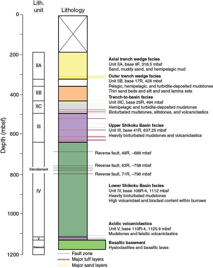
Figure F1. Lithostratigraphy of Hole C0023A.
Unit description
Axial trench-wedge facies (Subunit IIA)
Cores 1F through 9F contain intervals of mud and poorly sorted sand. Sand is the dominant lithology over mud and mudstone in Cores 1F through 9F. The sand units are muddy and evidence fluidization; sand is a frequent component of “drilling fill” found within core liners. Except for the muddiest sand beds, few internal structures were observed. An example of a muddier sand unit is shown in Figure F2. The base of the subunit contains gravel (subrounded quartz and volcaniclastics that include basalt with mineralized vesicles; see figure inset), and its top has an undulating contact with a mud unit above. A mud enclave in the middle of the bed likely represents the amalgamation of two successive flows rather than a detrital clast. The limited sandy ripple laminations in the mud at the top of the unit represent deposition under a waning sediment load. Sand bed thicknesses vary with the top half of the unit, having sand beds that are on average thinner than those at the base of the unit (0.5 m compared to 0.7 m). However, given the pervasive fluidization of beds and the recovery of core lengths greater than the length of drilling advance, the total thicknesses of sand beds are hard to evaluate.
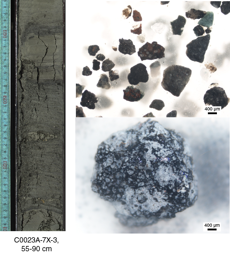
Figure F2. Sand unit, illustrating debris flow with graded bedding amalgamation of smaller turbidites at the top.
Within Cores 1F through 5F, mud beds are generally unconsolidated, and from Core 6F they are generally indurated because of carbonate cementation. Muds in Core 6F and deeper were logged as mudstone because they are lithified. Sand beds that are not lithified were logged as unconsolidated sand. Smear slide petrographic description identified that the muds and mudstones contain high sand content (Figure F3) and are distinct from the underlying units because of the presence of diatoms, sponge spicules, glauconite, and orthoclase. Polycrystalline calcite (i.e., micrite) is notably present in Cores 6F through 9F.
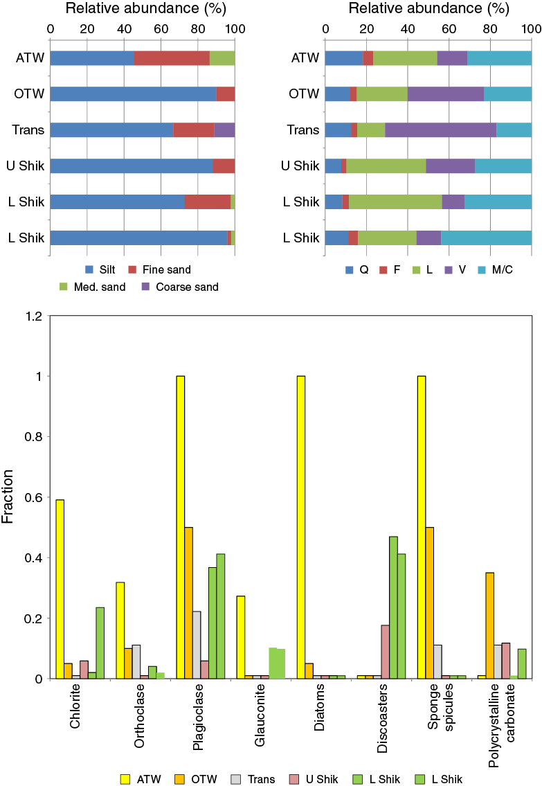
Figure F3. Formation characteristics based on smear slide description.
These observations are consistent with the rapid transportation of shelf sand and mud via high-density turbidity flows and episodic deposition within a hemipelagic or periodically pelagic environment.
Outer trench-wedge facies (Subunit IIB)
Cores 10F through 17R are notably muddier than Cores 1F through 9F; sand and siltstone beds represent <3% of the cored interval. In addition to a difference in the type of sediment supplied (more mud and less sand and silt), bedforms and ichnofacies in Cores 10F through 17R are also distinct; silt and sand laminae become abundant and bioturbation takes the form of burrows (often silt or bioclast filled) instead of the short burrows and short pyritized grazing trails seen in the unit above. In Sample 16R-5, 37–70 cm (Figure F4), low-angle asymmetric ripples and parallel laminations are evident in silt and fine sand laminae and lamina sets. These bedforms indicate deposition from a current.
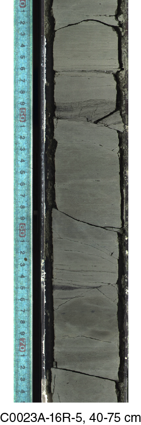
Figure F4. Muddy turbidites.
Despite the occurrence of sand laminations, most mud rocks within this unit are not sandier than those of the axial trench-wedge facies (Figure F3), and the proportion of both sand and quartz grains is lower. Glauconite, sponge spicules, and diatoms are less common. Green bentonite laminae (interpreted as smectite-rich ash horizons) are sparse but present. Relative to Subunit IIA, mud rocks in this interval are more bioturbated.
Trench-to-basin transitional facies (Subunit IIC)
The shallowest bed of volcaniclastic sediment is present in Core 18R. Volcaniclastic units typically have sharp bases and middle sections that often contain bedforms indicative of deposition from currents such as ripples, cross-lamination, and low-angle planar lamination (Figure F5). Grading from crystal-rich and black pumice-rich bases to pale tops or vice versa is also common. Volcaniclastic beds account for <5% of the cored interval from the transitional facies. At the base, many volcaniclastic units are tuffs (indurated with >70% volcanic glasses) but typically grade upward into overlying bioturbated mudstones, the inference being that bioturbation has mixed ash into overlying mudstones to create tuffaceous mudstones. These factors strongly suggest that volcanic sediment was deposited from debris flows or from mud-bearing turbidity currents. This also suggests that sediment provenances supplied either one or the other sediment types, as turbidites with a genuine mixture of the two lithologies are not common (except for mixing because of bioturbation). Thin section description reveals that tuff beds have a high vitric ash content (i.e., typically >75%) with igneous crystals typically of igneous province with an intermediate magmatic composition; commonly amphiboles, plagioclase, and biotite (for thin sections, see Figure F6).
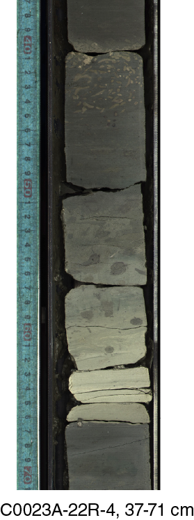
Figure F5. Tuff bed.
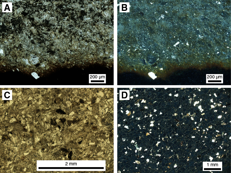
Figure F6. Volcaniclastic sandstone and tuff.
Mudstones within the transitional facies are similar to those above with the exception that as bioturbation becomes more common silt laminae become increasingly less common. Smear slide description also suggests that volcaniclastic content is highest within the mudstones from this facies. Because of high levels of bioturbation, clear identification of turbidite beds (Figure F7) becomes difficult, and thus the identification of a clear boundary is difficult. After Core 24R, no further silt and sand lamina sets with asymmetrical ripples or cross-lamination were observed. The first clear observation of a nonvolcaniclastic muddy turbidite appeared in Core 24R, and the last observation of tuff or volcaniclastic sandstone, marking the cessation of the upper Shikoku Basin style of deposition, was observed in Core 18R.
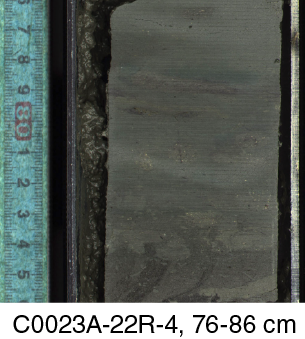
Figure F7. Heavily bioturbated volcaniclastic mudstone.
Upper Shikoku Basin facies (Unit III)
At Site C0023, the upper Shikoku Basin facies comprises heavily bioturbated mudstone and volcaniclastic sediments in beds 4–10 cm thick (Figure F8). Volcanic sediments comprise 8% of the unit’s total thickness. As for the volcaniclastic beds in the transitional facies, volcanic sediments are bioturbated to the extent that they grade and mix into the unit above. This is at the expense of the preservation of bedforms. Thin section petrography of selected tuffs and volcaniclastic sandstones reveals high ash contents with silt- to sand-sized clasts of volcanic glass. Volcaniclastics also include euhedral plagioclase, amphiboles, and biotite.
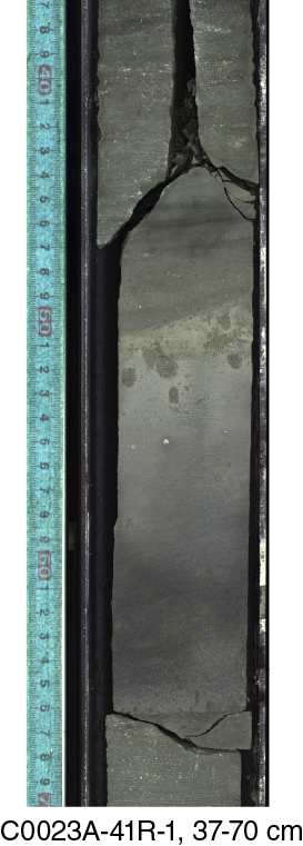
Figure F8. Heavily indurated tuff below a bioturbated volcaniclastic mudstone.
A distinctive feature of the basin facies mudstones is the high level of bioturbation and the presence of burrows (Figure F9). Ash, calcite, and bioclast content are often higher within burrows. Thus, although the unit has been homogenized to an extent, the burrows are lithologically distinct and often are sufficiently calcareous even when the rest of a mudstone bed is not. These differences are described in more detail for Unit IV (see below). The base of the unit was taken to be Section 41R-6, the section in which the first tuff is present.
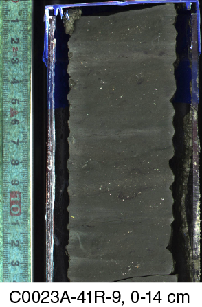
Figure F9. Heavily bioturbated Shikoku Basin mudstone.
Lower Shikoku Basin facies (Unit IV)
The lower Shikoku Basin comprises mud rocks, in which the dominant sedimentary features are ichnofabrics and occasional green bentonite ash-rich laminae. These laminae have high smectite and detrital chlorite. However, bioturbation disrupts these laminae to the extent that they are not continuous across the width of a core in most sections. As for Unit III, there are differences between the burrows and host lithology. The host lithology has a high proportion of microcrystalline quartz, and authigenic illite flakes are present but often light brown. The opaque content includes pyrite, clay, and partially devitrified ash (which is pale and translucent). Overall, vitric volcanic ash and carbonate content are low. Burrows contain sparse sand and are silt bearing with a mud fill that is light brown in color. Burrows have a high bioclast content, subangular quartz and plagioclase, illite flakes (authigenic), and small black pieces of volcanic glass (pumice).
Smear slide description also suggests that the content of the mud rocks has many characteristics similar to a shelf sediment derived from volcanic sediments (Figure F3) (e.g., the presence of glauconite and igneous phytoclasts of plagioclase and chlorite). Volcaniclastics content is also high within the lower Shikoku Basin and includes amphiboles, black glassy pumice, and scoria. Exotic lithologies within the lower Shikoku Basin include black mudstones and intervals of intense alteration by hydrothermal fluid flow, which are described later. Mudstones make up 97% of the thickness of the interval with brecciated zones of fault damage and hydrothermal alteration accounting for the other 3%.
Acidic volcaniclastics (Unit V)
A unit similar to the volcaniclastic facies (Unit V) from Sites 1174 and 808 was identified from Sections 108R-4 through 110R-4. Contact with overlying Unit IV is gradational; Cores 106R and 107R are both greener (more smectite and chlorite) in color than the overlying units, and Core 106R contains two pale ash units (silt-sized clasts of vitric volcanic ash without a high clay or crystal content). Despite the presence of these two thin ash units in Core 106R, the contact was taken at a poorly indurated ash layer present in Sample 108R-4, 43.5 cm, which exhibited a strong magnetic anomaly that is not seen in the overlying cores. At the hand specimen level, the main differences between volcaniclastic Units III–IV and Unit V is that volcaniclastic beds in Unit V are less indurated and of smaller clast size (silt or less) and are not mixed into overlying units by bioturbation. Small red clay fragments are ubiquitous in the volcaniclastic tuff beds in Sections 108R-4 through 110R-4. High levels of magnetic susceptibility are spatially associated with the occurrence of the red clay flakes.
Mudstones comprise the bulk of Unit V as they do for Unit IV, and similar ichnofabrics were observed (e.g., Zoophycos burrows as well as larger sand-filled burrows [Figure F10]). However, the degree of bioturbation appears to be less, as much as it can be deduced from the often heavily drilling disturbed core. Mineralogically, the units also differ; Unit V is often green with a high abundance of both chlorite and smectite (see X-ray diffraction mineralogy) and pyrite is in notably low abundance. At the contact with the underlying hyaloclastite horizon, calcareous red-colored beds are more abundant than pale green beds. The green- and red-colored intervals differ slightly; the green horizons have slightly more smectite and chlorite (Figure F11). The green beds also contain calcite veins in conjugate sets, which are scarce in the reddened beds.

Figure F10. Ichnofabrics with red and green alteration colors.
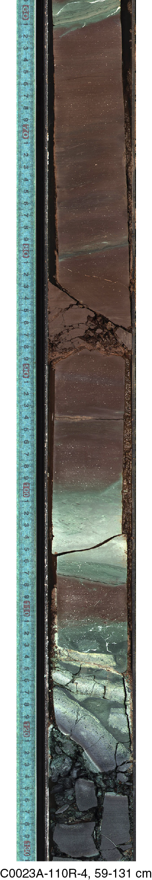
Figure F11. Contact between Unit V and underlying hyaloclastite deposit.
Basalt, lithologic basement
Hyaloclastite deposits are found from Sample 110R-4, 113 cm, until the base of Core 112R, and the main clasts are glass and basalt. This composite lithology includes fragments of green glass, in which calcite pseudomorphs after plagioclase, olivine, and amphibole. The basalts comprise a groundmass of acicular bladed plagioclase, in which euhedral plagioclase crystals and clay pseudomorphs of olivine and amphiboles are found (Figures F12, F13). Plagioclase also replaces other phenocrysts. Pieces of pillow basalt were recovered, although these were not intact and could not be used to confirm orientation (Figure F14). Calcite veining and ferrous clay mineralization were observed, both on the exterior and interior of clasts (Figure F11). The unit is broadly comparable to the basement lithology reported for Site 808 but is not identical.
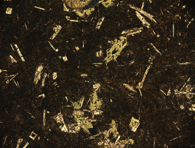
Figure F12. Heavily chloritized basalt.

Figure F13. Heavily altered basalt.
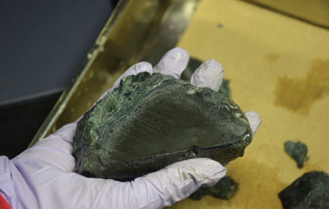
Figure F14. Chloritized pillow basalt.
X-ray diffraction mineralogy
The relative abundances of total clay minerals, quartz, feldspar, and calcite at Site C0023, based on X-ray diffraction (XRD) analyses of randomly orientated bulk powders obtained from systematically collected samples, are shown in Figures F15 and F16. Peak intensities and peak areas, calculated mineral abundance data, and results from spot sample analysis are in Tables T2, T3, and T4, respectively. For quality assurance (QA) purposes, a comparison between the normalized relative mineral abundance for samples scraped from the exterior and interior of whole-round core (WRC) samples (sample code 370KYWR; Samples 370-C0023A-16R-6, 50–55 cm, 26R-4, 2–13 cm, 34R-2, 30–40 cm, 45R-1, 42–47 cm, and 52R-1, 0–10 cm) was examined, resulting in variations of −2%–5% for total clay minerals, −2%–1% for quartz, −3%–0% for feldspar, and −2%–0% for calcite.
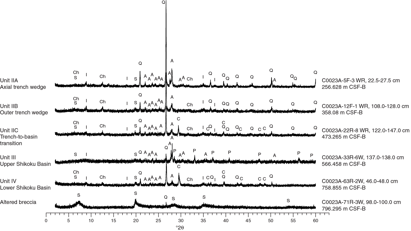
Figure F15. XRD profiles of 6 representative types of mudstone.

Figure F16. XRD total clay minerals, quartz, feldspar, and calcite.
Table T2. XRD analysis of bulk powder sediment samples. Download table in .csv format.
Table T3. Normalized relative mineral abundances based on XRD analyses, Hole C0023A. Download table in .csv format.
Table T4. Normalized relative mineral abundances of spot sample mineralogy, Hole C0023A. Download table in .csv format.
Mineralogical characteristics by facies and lithology
XRD analyses of representative mudstones show the associations between lithostratigraphic units and mineral compositions (Figure F15). Subunit IIA (256 mbsf) axial trench-wedge mudstones have prominent quartz peaks and feldspar (anorthite). Subunit IIB (358.08 mbsf) outer trench-wedge mudstones are mineralogically similar to the upper region of Subunit IIA; however, as described in Unit description and smear slide analysis (Figure F3), they are less sandy (lesser turbidites) and have less prominent quartz and feldspar peaks. Some mudstones have diffractograms that exhibit prominent peaks for calcite; this is notable in Subunit IIC where there are many calcareous horizons. Mudstones from volcaniclastic sand–rich Unit III (upper Shikoku Basin) have strong pyrite and feldspar peaks and weak illite peaks in their diffractograms. Greenish highly brecciated mudstones from the décollement zone have prominent peaks of calcite and quartz. However, clay minerals are notably abundant, and some of the greenish mudstones analyzed were, from a crystallographic perspective, almost purely smectite with very minor quartz and altered ash (796 mbsf).
Variation in total clay minerals, quartz, feldspar, and calcite
Downhole variations in total clay minerals, quartz, feldspar, and calcite are shown in Figure F16. The average values of normalized relative mineral abundance in the axial trench-wedge facies of Subunit IIA are 50% total clay minerals, 25% quartz, 25% plagioclase, and 0% calcite. The variances in mineral abundance within Subunit IIA are 24%–64% for total clay minerals, 21%–37% for quartz, and 14%–46% for feldspar. Both the absolute values and variances are typical for the axial trench-wedge facies because of the presence of sand-rich intervals. Smear slide descriptions show a higher abundance of quartz and orthoclase in this interval (Figure F3), and the relative abundance of both minerals is also higher. Total clay mineral content is higher (mean = 68%) in Subunit IIB (outer trench-wedge facies) and higher still (mean = 74%) in Unit IV (lower Shikoku Basin). The modest but consistent increase in clay mineral abundance with depth is probably a consequence of both diagenetic alteration of disseminated volcanic glass and a decrease in particle size within the hemipelagic mudstones of the Shikoku Basin. These deep units are also less sandy based on smear slide results.
There are several significant off-trend changes in total clay mineral abundance; around the décollement zone, the relative clay content varies from 65% to 83%, likely due to the conversion of volcanic ash into smectite clay and mineral precipitation within the pore space. Clay content also varies from 72% to 79% within and immediately above the basaltic basement (1058–1108 mbsf). This is likely a relative increase due to changes in the abundance of feldspar and calcite; there is calcite veining and albitization, and both quartz and feldspar concentrations have higher relative abundance in this interval.
The small increase (10.5%) in the proportion of feldspar in Units IV and V near the basaltic basement (1058–1108 mbsf) is also seen in smear slide data (Figure F3), possibly representing the erosion of igneous rocks rich in plagioclase phenocrysts. The feldspar content of upper Shikoku Basin volcanic tuffs was also generally high (27%).
Calcite content is erratic in Unit IV as a result of the scattering of calcareous nannofossils and shell clasts between clast-rich burrows and the host mud rock lithology. This patchiness in calcite concentration is further increased by patches of carbonate-rich hydrothermal alterations (see Authigenic and hydrothermal mineralization).
Comparison to Site 1174
The changes in relative mineral abundances of total clay minerals, quartz, feldspar, and calcite at Site C0023 were compared with the data originally presented in Shipboard Scientific Party (2001b) for Leg 190 Hole 1174B (gray circles in Figure F16). The total clay mineral contents we report here at Site C0023 are much higher (about +20%) than those at Site 1174 but show similar trends with increasing burial depth. Consequently, quartz contents at Site C0023 are much lower (about −20%) than at Site 1174 but also show similar changes with depth.
The differences in the percentage of clay between Sites C0023 and 1174 are likely due to methodological differences caused by the use of different types of X-ray diffractometers and different normalization equations for calculating mineral abundance; the singular value decomposition normalization factor was used for Site 1174, whereas a second-order polynomial calibration curve was used for Site C0023. To evaluate the effect of using the calibration curve instead of the normalization factor, 21 mud rock samples were taken from Hole 1174B legacy cores and remeasured on the ship using Hole C0023A experimental conditions (Table T5). The results showed that abundances of total clay, quartz, feldspar, and calcite from Hole 1174B (triangles in Figure F16, data are also available in XRD in Supplementary material) are generally in good agreement with those values from Hole C0023A. Thus, downhole trends in relative clay content can be compared between the two sites. The comparison of relative mineral abundances in this way suggests that sediments at Sites 1174 and C0023 are generally similar.
Table T5. Normalized relative mineral abundances based on XRD analyses, Hole 1174B. Download table in .csv format.
Opal-CT/Quartz transition
The peak-area ratio of cristobalite (101) to quartz (100) decreases with increasing burial depth (Figure F16). The cristobalite to quartz ratio varies within the base of Unit II because of the occurrence of sandy turbidites (that contain detrital quartz) and constantly decreases between Units II and III. This change coincides with a temperature of ~60°C (see Physical properties). The transformation of opal-CT (cristobalite) to crystalline quartz (Behl, 2011) is both temperature and time dependent. The peak-area ratio of cristobalite (101) to quartz (100) gently decreases and remains at a low plateau until reaching the boundary of Unit IV (mean = 0.22). The abrupt change in the ratio (from 0.29 to 0.37) near to the basaltic basement (1101.3–1108.7 mbsf) may be new mineralization of cristobalite resulting from hydrothermal activity.
Devitrification and volcanic ash
XRD analysis of two representative tuff beds from the transitional facies (468.9 mbsf) and upper Shikoku Basin (566.4 mbsf) illustrates a transformation from amorphous vitric fragment–rich deposits to zeolite of phillipsite (468.9 mbsf) and smectite-rich claystone or bentonite (566.4 mbsf) (Table T4). This transformation is a function of environmental conditions within the depositional environment of ash; in mildly alkaline conditions, the ash bed usually alters to smectite or bentonite, whereas in highly alkaline conditions, the ash transforms into a zeolite or a combination of zeolite and K-feldspar (Moore and Reynolds, 1989). Therefore, the different mineral assemblages within each tuff may represent differing environments and ash sources. Similar alteration products were documented at Site 808 (Shipboard Scientific Party, 1991).
X-ray fluorescence
X-ray fluorescence (XRF) data for selected oxide abundances are shown in Figure F17. Changes in downhole abundance can be explained as either functions of depositional environment or diagenetic or hydrothermal alteration. The downhole decrease in the abundance of sodium and downhole increase in the abundance of potassium likely reflects the formation of illite, given that the total abundances of silica and aluminum vary little (e.g., the total amount of aluminosilicate minerals does not vary; instead some are converted to potassium-rich clay). The amount of calcium shows a close spatial correspondence to intervals of calcareous mudstone. High abundances of manganese and iron have a broad spatial correspondence with zones of ferrous and manganese carbonate mineralization described later, as do some off-trend values for magnesium (particularly with regard to the décollement zone).
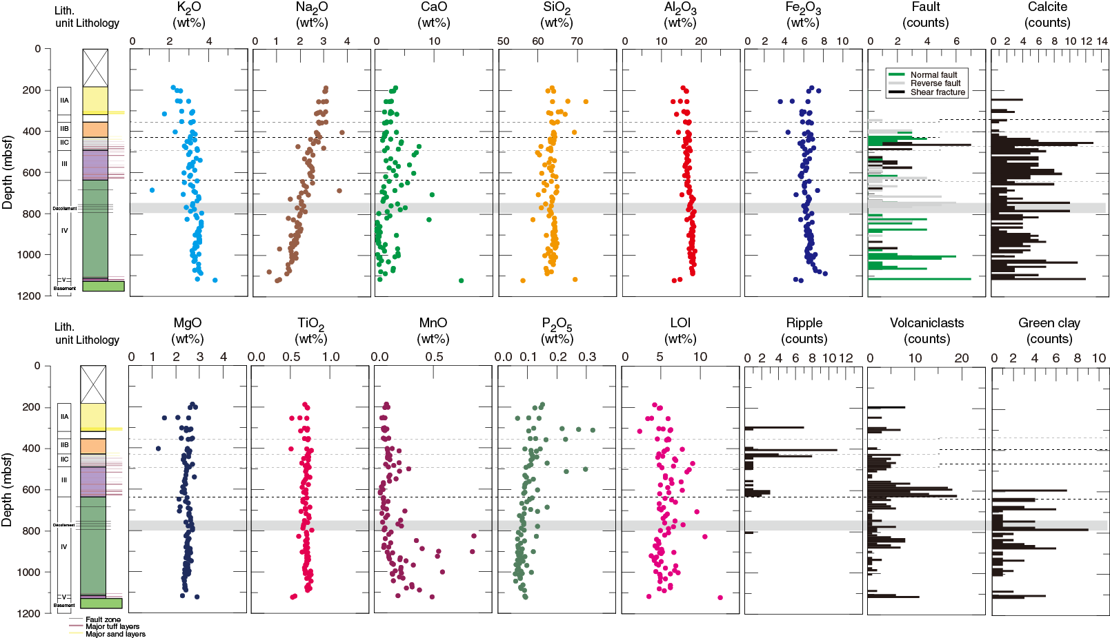
Figure F17. XRF major element oxides compared to total VCD observations.
Deformation structures
Cross sections based on seismic reflection data for Site C0023 indicate that the site is located toward the center of a low-amplitude syncline (Hinrichs et al., 2016). Consequently, deformation would be expected to be mild, and a protothrust zone or other map-scale deformation structure would not be expected. In general, core-scale observations are in keeping with these expectations.
Overall, bedding planes dip gently (<30°; mostly around 20°) and fracture density was generally low (Figure F18). This feature is consistent with the expectations. A notable feature is that bedding was found to be almost horizontal (<10°) in Units II and III shallower than 637 mbsf. However, steep bedding dips characteristically appear in the lower Shikoku Basin (Figures F18, F19), where dips were <30° (mostly 10°–20°) between 637 and 1000 mbsf and <40° (mostly 10°–30°) between 1000 and 1100 mbsf. Deeper than this interval, continuous lamination becomes hard to identify; however, a few laminations observed indicate a slightly inclined attitude (around 30°), which eventually returns back to a gentle dip (mostly <15°) in Unit V, just above the basement. Variations in bedding dip are broadly similar to Site 1174.

Figure F18. Bedding and deformation structure dip angles.
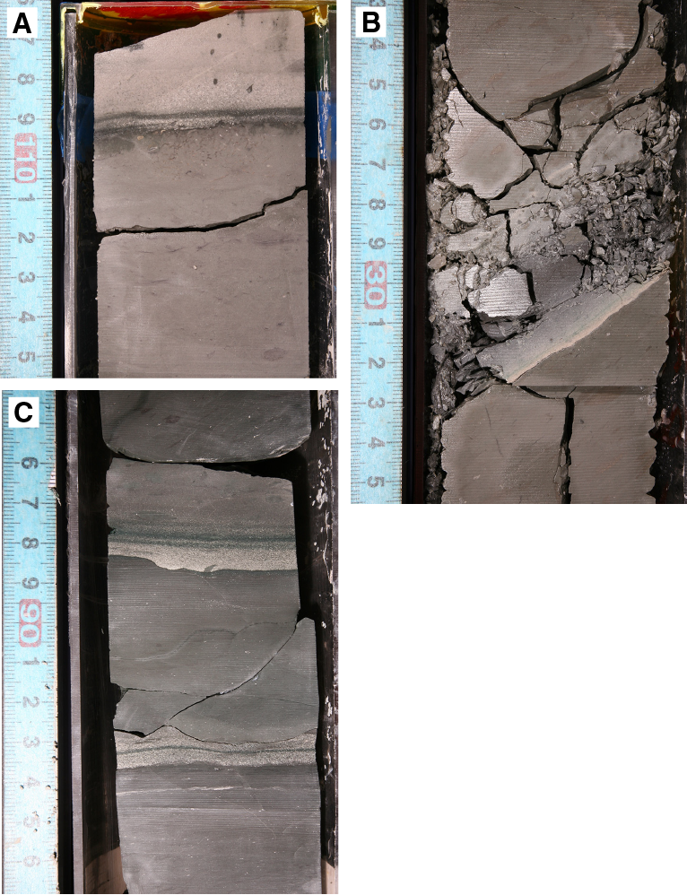
Figure F19. Bedding dip examples.
Several kinds of deformation structures are distributed at particular depths, representing distinct deformation styles as described in the following sections (Figure F18). Most of the core-scale reverse faults are located above and within the décollement zone (i.e., accretionary prism), whereas normal faults are present with dense populations beneath the décollement zone (underthrust sediment). Mineral veins composed of calcite, barite, and anhydrite occur beneath the décollement zone. Most of these mineral veins are located within or closely associated with faults. Core-scale healed faults, which mostly represent a normal fault sense, are typically present in the upper Shikoku Basin.
In Cores 370-C0023A-1F through 15F deformation structures and bedding were heavily disturbed and hard to identify because of heavy expansion and brecciation in cores obtained with the short HPCS and ESCS coring methods. After switching the BHA from HPCS/ESCS to RCB, some degrees of coring disturbance persisted (e.g., biscuiting and drilling-induced fractures and faults), but generally structures could still be identified on split surfaces.
Core-scale healed faults
Small healed faults are present throughout the cores obtained from Hole C0023A, and they become noticeably more common between ~465 and 584 mbsf in the upper Shikoku Basin (Figure F18). The faults appear as dark seams no more than 1–2 mm across and were commonly braided and distinctly curviplanar to irregular (Figure F20). Under X-ray computed tomography (CT), healed faults are characterized by higher CT numbers than the host rock, indicative of shear-induced consolidation leading to the formation of a dense fault zone that has a lower porosity than the surroundings. Markers for stratigraphic offset caused by faulting are infrequent but, where observed, in almost all cases show a normal sense of displacement, typically between 1 mm and several centimeters. The healed faults dip near vertical to steeply (mostly >60°), and any breakage along them reveals slickensides and, commonly, downdip slickenlines. There are a lesser number of healed faults beneath the underthrust interval, and their dipping angles are scattered (20°–80°). At Site 1174, the healed faults had an apparently random strike after paleomagnetic reorientation and were interpreted as an indicator of a lack of tectonic influence.
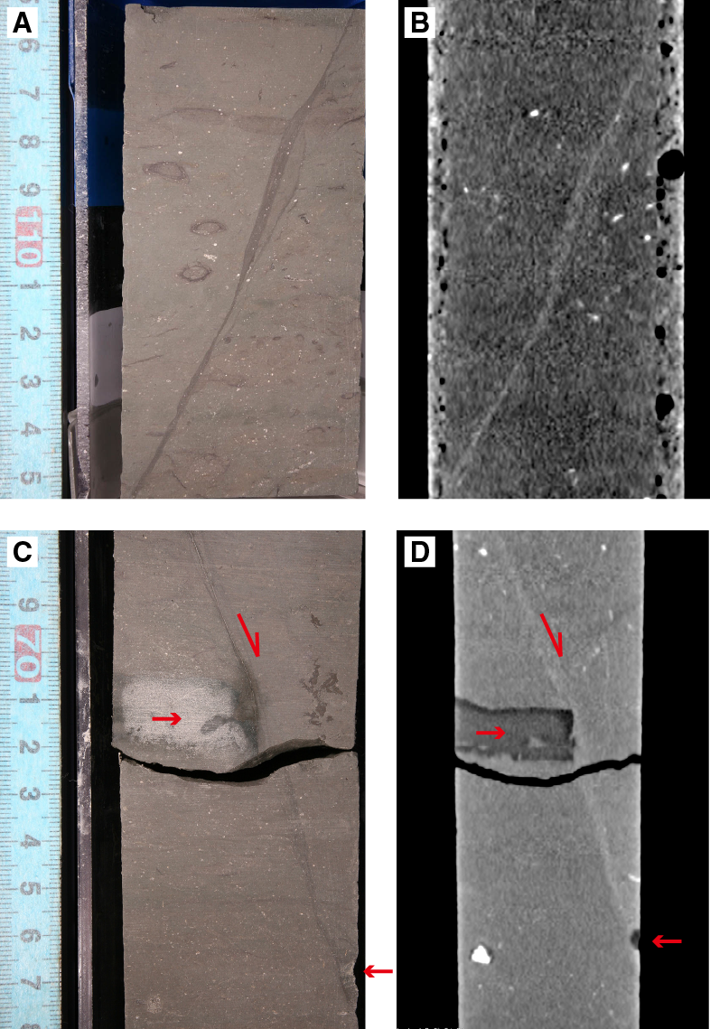
Figure F20. Core-scale healed faults.
Décollement zone
The first, but thin (<5 cm) fault zone was identified at 749 mbsf, and the first major fault zone was identified at ~758 mbsf (Figure F21). We took the onset of this fault zone to mark the top of the décollement at Sample 63R-1, 65 cm (758.15 mbsf) (Figures F18, F21). Bedding is slightly steepened in the zone (~30°). Deeper than Section 63R-1, the fault zone is underlain by generally intact sediment with gentle dips. Some fault zones were characteristically brecciated, found in Samples 65R-1, 65–75 cm (~767 mbsf), 67R-3, 64–90 cm (~778 mbsf), and 71R-2, 88–107 cm (~795 mbsf), but most of the recovered cores in the décollement zone were intact. Therefore, the décollement zone at Site C0023 appears to be composed of alternating intact intervals (~several meters in thickness) and thinner fault zones. Deeper than Sample 71R-2, 107 cm, at 796.4 mbsf, no thrust fault zone was identified, and thus we defined the depth as the base of the décollement zone (Figure F22).
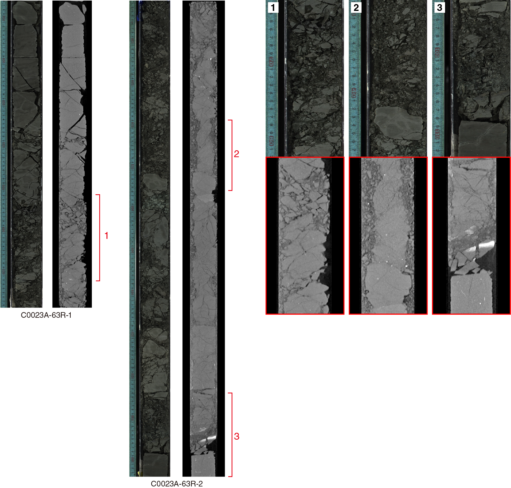
Figure F21. First major fault zone in décollement zone.

Figure F22. A damage zone apparently corresponding to base of décollement zone.
The size of the fragments within the décollement zone is commonly on the scale of millimeters, and slickenlines were commonly present on surfaces of the fragments. When observed on split core surfaces, most of the fractured/sheared surfaces were opened, leading to the impression that fault zones comprised fragments (Figures F21, F22). Such an impression might be misleading; in X-ray CT images acquired before splitting, tight, essentially closed jigsaw-puzzle fracture patterns were observed. Therefore, the fragments seemed to be opened during core splitting. However, given the slickenlines present on most of the surfaces of fragments, the fragments appeared to be the product of subsurface shear and not drilling disturbance.
The brecciated aspect of the décollement zone is similar to that reported from Sites 808 and 1174 but is in contrast to, for example, that of the northern Barbados prism with its scaly clay and S-C fabrics (e.g., asymmetric sheared fabrics; Maltman et al., 1997). Nevertheless, there are some differences between the décollement core samples from Site C0023 and Sites 1174 and 808; one of the major differences is the thickness of the fault zone. Although a few intact intervals were also reported in Sites 808 and 1174, the décollement zones at both sites were characterized by thick and intense sheared and pulverized material (approximately 20 and 32.6 m, respectively); in particular, the meters long sections of comminuted rock were reported from Site 1174. Although relatively intact intervals were also reported at Site 1174, the proportion of the brecciated zone is much larger than at Site C0023. Therefore, the décollement zone at Site C0023 is characterized by the existence of a relatively weaker deformation, or nonlocalized shear zone, as compared with Sites 1174 and 808. Alternatively, given the less successful recovery here, it is also conceivable that such heavily sheared rocks exist at depth but were simply not recovered in core. Major and successively negative reflectors were reported on seismic images corresponding to the décollement zone around Sites 808 and 1174, whereas relatively faint and intermittent reflectors were observed at Site C0023. Similarly, a clear gap in physical properties (e.g., porosity, bulk density, P-wave velocity, etc.) exists between the décollement zone and country rock at Sites 808 and 1174, whereas a relatively small difference in physical properties exists at Site C0023 (see Physical properties). These observations support the former interpretation: the presence of a relatively weaker deformation and nonlocalized shear at Site C0023.
Underthrust domain
In contrast to Sites 808 and 1174, the underthrust sediments below the décollement zone at Site C0023 were found to have intense and localized populations of normal faults and mineral veins, all of which have a wide range of dip angles (Figure F18). Two intervals have major populations of normal faults in the underthrust sediments: one just below the décollement zone at 820–890 mbsf and the other just above the basement at 980–1125 mbsf. The range in dip angle for normal faults in these intervals is 10°–67° (mostly 15°–60°) and 13°–60° (mostly 25°–50°), respectively (the former range represents a more scattered attitude).
Mineral veins are composed mainly of barites (rarely anhydrites), and calcites are commonly developed in the underthrust sediment (Figures F18, F23). Some of them are mineralized along fault planes. The barite veins, in most cases, represent scattered crystallization along the faults (Figure F24). Barite veins are common in the upper interval (~800–1100 mbsf), and calcite veins are present in the lower portion (~1100 mbsf). Where veins follow the planar surfaces of faults, slickenlines are present. Veins were present on approximately 30%–40% of fault planes between 820 and 890 mbsf and 70% of fault surfaces between 980 and 1125 mbsf (Figure F18).
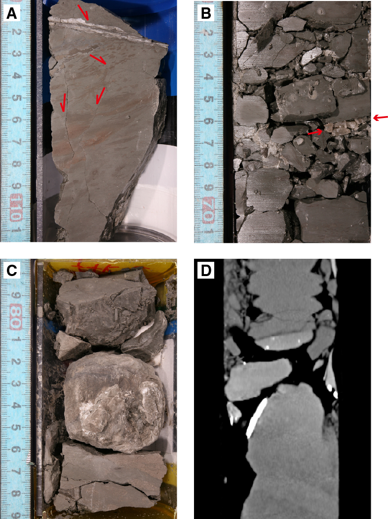
Figure F23. Mineral veins.
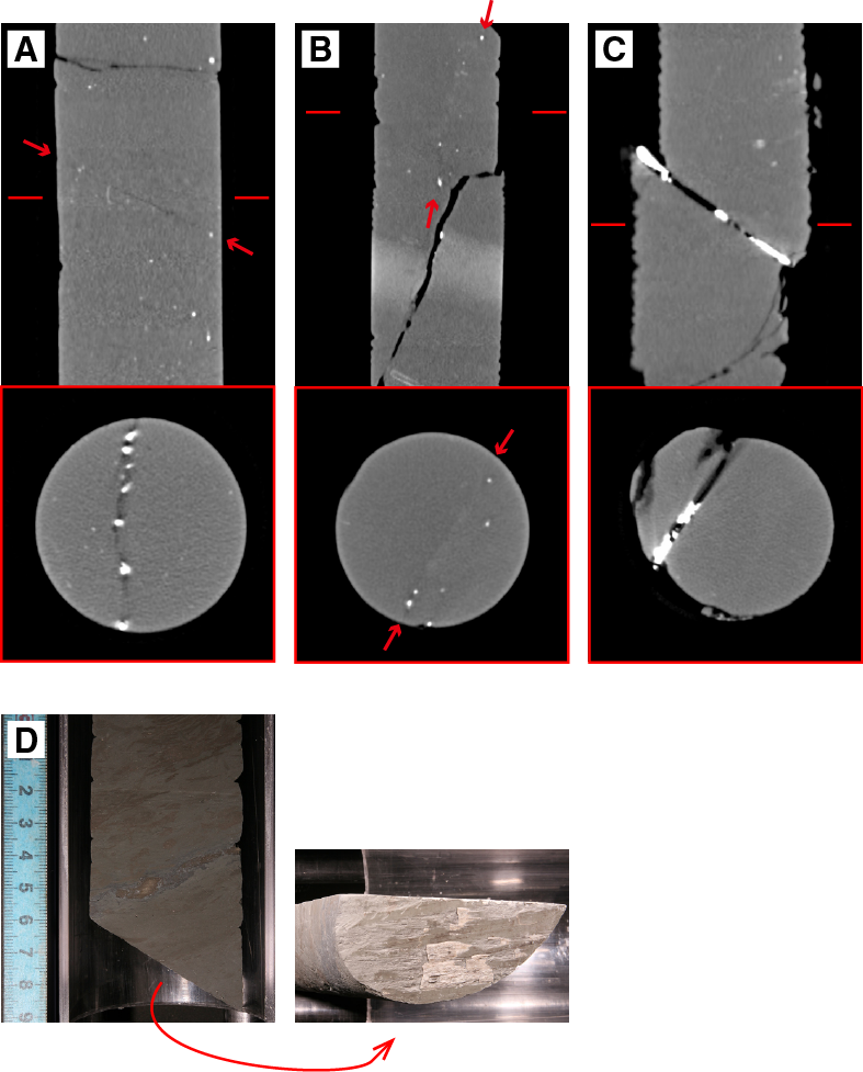
Figure F24. X-ray CT images of crystallized minerals along faults.
Other structures
Deformation bands are roughly planar, 0.5–5 mm wide, microscopic-scale bedding-oblique dark bands that typically develop in argillaceous sediments at the toes of accretionary prisms (e.g., Maltman, 1998; Ujiie et al., 2004). At Site 1174, deformation bands commonly develop at ~200–300 mbsf (Subunit IIA at Site C0023). Unfortunately, because of intense drilling-induced disturbance by short HPCS/ESCS coring at Site C0023 (Cores 1F through 15F), deformation structures in this interval were not clear. However, structures like deformation bands were identified at ~400–450 mbsf (Figures F18, F25). In X-ray CT images, deformation bands are characterized by higher CT numbers than the host rock, indicative of shear-induced consolidation as reported by Ujiie et al. (2004).
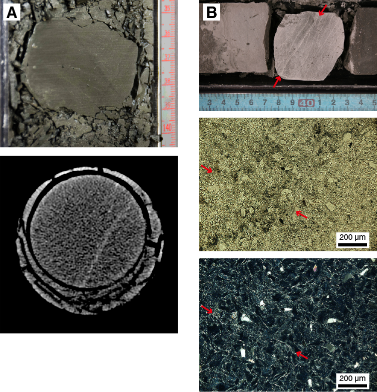
Figure F25. Deformation bands in mudstone and volcanic ash.
Some deformation bands are developed in tuff beds in the upper Shikoku Basin (Figure F25). Although the bands are composed of finer volcaniclastics and are superficially similar to cataclasis bands in hand specimen, no grain collapses at the microscale were identified under microscopic observation. However, clasts of volcanic glass were rotated and aligned in parallel bands, suggesting that the deformation bands in tuff beds are independent of particulate flow and dilatancy.
Dewatering features (Figure F26) such as sand intrusion (489 mbsf) and hydrofracturing (1034 mbsf) were observed and probably formed at the early stage of the consolidation processes.
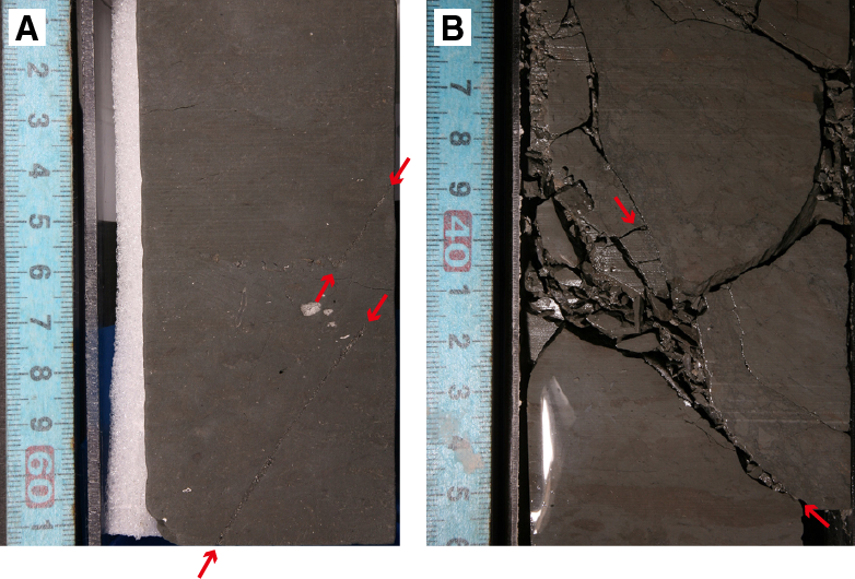
Figure F26. Sand dikes and a hydrofracture.
Authigenic and hydrothermal mineralization
From the perspective of the temperature limit of the deep subseafloor sedimentary biosphere, documenting diagenetic, authigenic, and hydrothermal mineralization is important in two respects: (1) such mineralizations are often formed at the terminal stage of geochemical redox reactions (e.g., reactive species are converted into species stable at geological time) and (2) many geochemical reactions producing minerals are calibrated against temperature. At Site C0023, we represent four main diagenetic alteration zones shown in Figure F27.
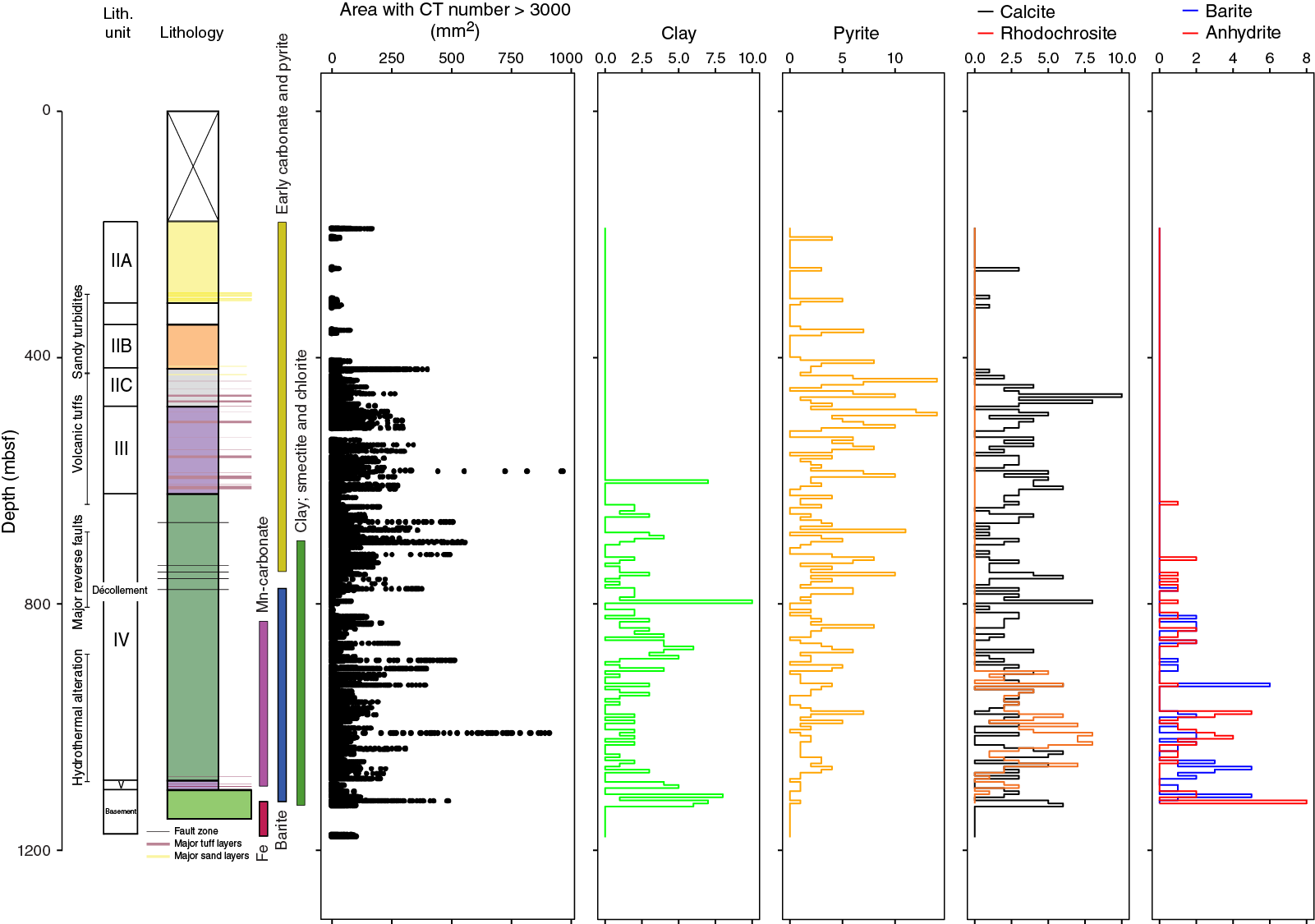
Figure F27. Downhole mineralization trends.
Early-stage diagenesis (Cores 1F–60R; 189–747.5 mbsf)
Low-temperature calcitization and pervasive pyritization were observed from Subunits IIA to IIC. Early-stage diagenetic processes that formed calcite and pyrite are nearly ubiquitous throughout Hole C0023A, but between 189 and 747.5 mbsf (Cores 370-C0023A-1F through 60R) such alterations are strongly strata bound and follow bedding, ichnofabrics, or occasionally mineralized small ptygmatic veins (e.g., irregular veins, found within soft sediment, that do not have sharp fracture-bounded sides). Such occurrences continue to greater depths, but they are the sole form of authigenic mineral growth between Cores 1F and 60R (Figure F28).
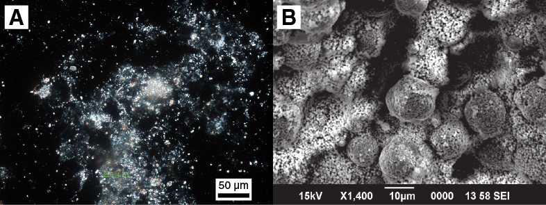
Figure F28. Calcite and pyrite in early-stage diagenesis.
Pyrite was observed throughout the sediment column of Hole C0023A. It frequently appeared as nodules in Unit III and also as a burrow infill. Shipboard observation of pyrite samples using scanning electron microscopy (SEM) showed the framboidal form of pyrite (Figure F28), which is a typical mineralization feature found in the shallow sediment samples.
In Subunits IIA and IIB, the pyrite nodules appear oxidized. This observation matches the more disturbed and oxidized environment created by turbidity currents and suggests that some of the pyrites may be detrital. In Units III and IV, pyrite nodules get larger and are often denser. The internal cavities within the nodules are consequently mineralized.
The first calcareous indurated mud (calcite-cemented mudstone) is found in Core 5F. In Core 6F and deeper, calcite formation is frequently observed as an early cementing stage from Subunit IIB to Unit V. Subunit IIC and Unit III have the highest frequency of calcite-cemented mud rocks (>52% of the total bed thickness), which is defined as a hardened mud rock with a matrix that reacts with 10% hydrochloric acid. Cementation of an original depositional fabric in this way is differentiated from the zones of calcite and sulfate alteration observed in deeper cores, which obfuscates or masks the original depositional fabric. Calcite is also common within burrow infills and forms concretions, which are harder and more durable than their surrounding mud rock, and is frequently found within drill breccias.
Green-colored mineralization (Cores 51R–110R; 697.5–1127 mbsf)
We observed multiple intervals of green-colored mineralization, starting with the décollement zone (Figure F29B) and carrying on to the basaltic basement (Figure F29C, F29E). XRD finds clay alteration, which usually consists of altered smectite and chlorite. However, there is variation in the clay compositions of green intervals. For example, the alteration zone in Core 370-C0023A-63R is rich in calcite. Apart from the green mineralization zones, chlorite is also found in the mud rock with smear slides and XRD, where it is likely a detrital component.
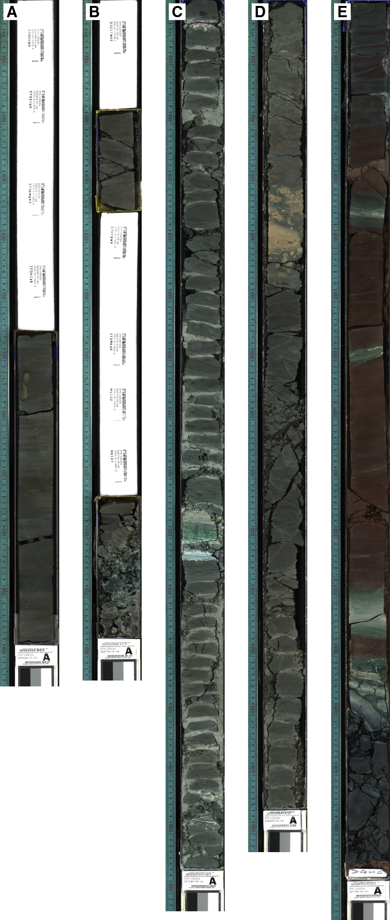
Figure F29. Core sections recovered from different mineralization zones.
Vein and strata-bound sulfate mineralization (Cores 67R–109R; 775–1121 mbsf)
Strata-bound and vein-filling crystals of anhydrite (Figure F30A) and barite are present throughout Cores 370-C0023A-67R through 109R. In Unit IV, they are associated with alteration patches. At the margins, these alteration patches predominantly affect burrows (Figure F31B), whereas at the center of an alteration patch, the entire bed is affected (e.g., the bed is homogenized and burrows cannot be distinguished). Within veins (Figure F31A) and fracture fills, both euhedral and slicken crystals were observed. Additional mineralization observed within the euhedral crystals, which are found in deformation structures, includes anhydrite, pyrite, calcite, and clay minerals. Within burrows, barite and anhydrite are replaced to bioclasts.
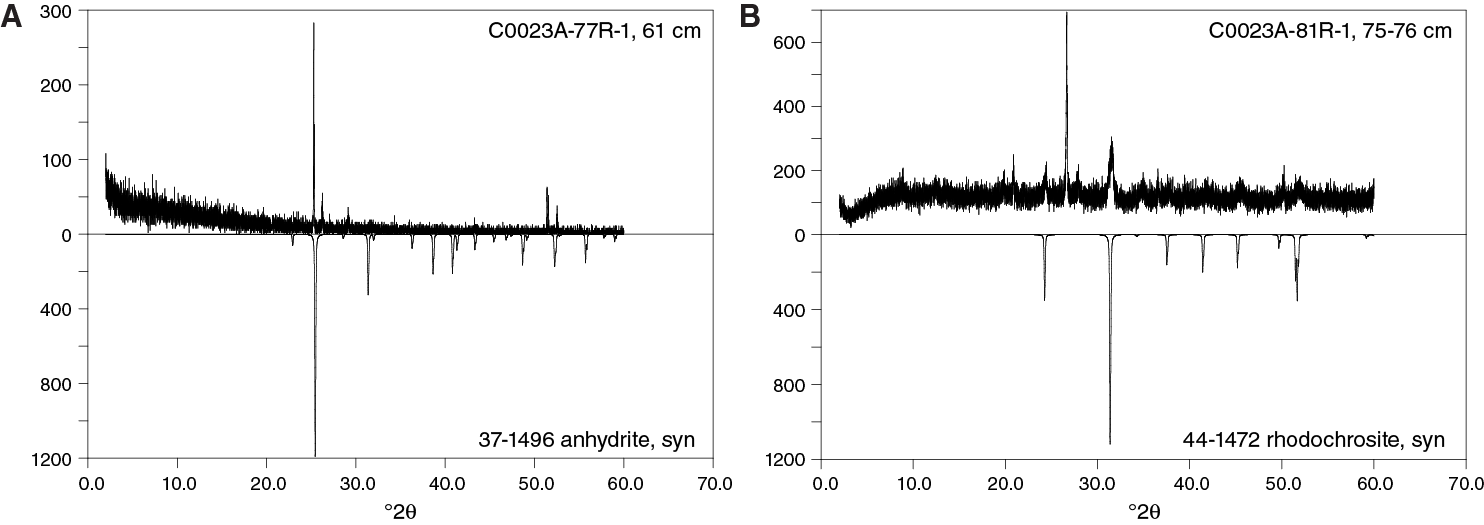
Figure F30. XRD data confirming anhydrite and rhodochrosite.
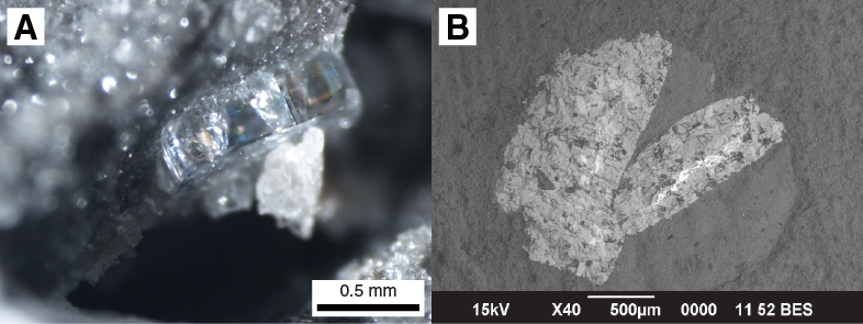
Figure F31. Vein and strata-bound sulfate mineralization.
Calcite replacement commonly occurs within sulfate-bearing alteration zones and is different from the early stage of calcite cementation because it is associated with the masking of the original rock fabric. Apatite, fluorapatite, carbonated fluorapatite, and dolomite are also present in some alteration zones and in some densely remineralized concretions and burrows found at the bottom of Unit IV. Their occurrence as a replacement product within burrows strongly suggests that these are the products of alteration. Some apatite grains were observed under SEM, but dolomite was only found by XRD analysis. Zones of alteration also contain elevated smectite concentrations. Instances where no carbonate was found but alteration was apparent are interpreted as smectite–clinochlore alteration zones.
The mineralization zones are best explained by locally changed pore water compositions and elevated temperature. SEM observed a copper-rich grain in Core 86R. XRD analysis suggests trace chalcopyrite in Core 99R at the bottom of Unit IV. If present, the chalcopyrite content should be very low. In the SEM photograph, the crystals apparently have a tetragonal crystal system, indicating mineral precipitation from hydrothermal fluids at temperatures <550°C (Yund and Kullerud, 1966).
Rhodochrosite in the zones with normal faulting (Cores 79R–106R; 828–1096 mbsf)
Rhodochrosite (MnCO3, Figure F30B) was observed at the bottom of Unit IV in a zone of normal faulting. Rhodochrosite usually appears as yellow alteration bands or pink and yellow burrow infills (Figure F29D) associated with calcite and replacing diatoms and other bioclasts. In Cores 370-C0023A-87R and 98R, burrows have abundant rhodochrosite and are often red instead of yellow. The presence of rhodochrosite, pyrite, and barite suggests a low-temperature hydrothermal environment (e.g., between 120° and 250°C [Sillitoe and Hedenquist, 2003]).
In intervals of rhodochrosite mineralization, barite and anhydrite appear frequently with rhodochrosite. XRD also suggests that magnesian calcite (Cores 80R through 108R), dolomite (Core 86R), and occasionally apatite, fluorapatite, and carbonate fluorapatite are present.
Iron minerals (Cores 110R–112R; 1121–1177 mbsf)
Iron mineralization (hematite, goethite, and magnetite) is abundant at the bottom of Unit V (Figure F29E) and in the basaltic basement. In Core 370-C0023A-110R, just above the basement, there is an interval of calcium iron–rich red clay. Inside the basalt in Core 112R, iron mineralization is also found in red-colored patches and rings within the basalt. The presence of magnetite in the red-colored intervals and in the basalt helps to explain the higher magnetic susceptibility within these intervals (Figure F38). This interval also hosts the only substantial network of calcite veins observed in Hole C0023A.
X-ray CT image evaluation for core quality
X-ray CT image
X-ray CT image analysis was conducted on 599 sections from 189 to 1177 mbsf in order to provide an assessment of core quality. This assessment is based on the averaged CT numbers for section images. For every section, 0.625 mm thick slice images have been analyzed. Figure F32 shows the profiles of core quality factor (CQF) and average CT number of cores obtained from Hole C0023A, which are described in detail below.
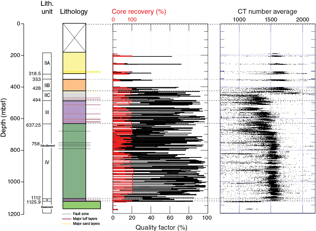
Figure F32. Site summary diagram of X-ray CT images.
Core quality factor
CQF was calculated based on X-ray CT images of each section. Generally, CQF in this site ranges between 40% and 95%. Intervals around each unit boundary show relatively low CQF. In Subunits IIA and IIB, CQF is mainly <70%, which is relatively low. This lower quality is interpreted as a consequence of heavy drilling disturbances. In Subunit IIC and Unit III, CQF is mainly between 60% and 90% with some deviations. This is a positive correlation with core recovery. In Unit IV, CQF mainly ranges from 40% to 95%. In particular, intervals from 717 to 790 mbsf and from 862 to 1083 mbsf have a CQF >80%, indicating decent core condition. On the other hand, an interval from 641 to 717 mbsf ranges between 40% and 80% CQF, which is lower than the two intervals above, although core recovery for this interval is relatively high (>60%). These characteristics are due to microcracks in the cored samples. CQF values from 790 to 862 mbsf and from 1083 to 1112 mbsf mainly range between 40% and 80%. Core recovery in these intervals is also lower than the other intervals of Unit III. In Unit V, CQF ranges between 50% and 85% and is lower than in Unit IV. The main cause for lower CQF is biscuiting (abrading of rock fragments at planes perpendicular to the core liner to produce concave and convex lenses of rock that fit together). In the basement unit, CQF is <10% and almost all core samples in this unit were broken into small pieces.
CT number average
The CT number average of each 0.625 mm thick slice image was calculated using a 10 mm diameter circle area measured at the slice center. Figure F32 shows the CT number average at 5 mm intervals for Site C0023.
The uppermost interval of Site C0023 is 189–449 mbsf and is characterized by a relatively high CT number average (1500–1750). These high CT numbers are interpreted as sand and muddy sand of axial and outer trench-wedge facies (Subunits IIA and IIB). A sharp increase at 439 mbsf and a sharp decrease at 449 mbsf were observed. Between 449 and 635 mbsf, the X-ray CT number average slightly increases from 1200 to 1450. Between 635 and 685 mbsf, the X-ray CT number average is stable. Between 685 and 1124 mbsf, the X-ray CT number average is from 1450 to 1600 and slightly higher than the above interval. Between 1124 and 1177 mbsf, the X-ray CT number average is much lower than the other interval. This is due to the core condition, which is characterized by fragmented hyaloclastites and basaltic lavas.
Comparison to Sites 808 and 1174B
Lithostratigraphic components at Sites 808 and 1174 include basal volcaniclastics, lower and upper Shikoku Basin facies, trench-to-basin transition facies, and trench-wedge facies and are quite similar to those at Site C0023 (Figure F33). The thickness of the lower Shikoku Basin is similar at these three sites. However, greater thicknesses of the topmost sedimentary units are present at Site 808 in comparison to Sites 1174 and C0023. The position of the décollement zone at Site 808 is deeper than the other two sites. This variation is due to the geographic position of the sites: Site 808 is located slightly further from the center of the trench compared with other sites, and the frontal thrust developed between them. Therefore, the amount of thickening of the prism because of accretion at Site 808 is larger than other sites. Also, variation in the apparent thickness of the accreted part because of tilting of the geologic body must also be taken into account. Deformation characteristics and associated variation of physical properties within and below the décollement zone is also different at Site C0023 (see Deformation structures and Physical properties). On the seismic sections, straight and clear reflectors are seen at the décollement at Sites 808 and 1174, whereas a weak and intermittent reflection is present at Site C0023.
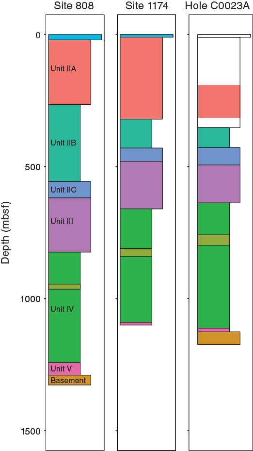
Figure F33. Comparison of Hole C0023A lithostratigraphic units to Sites 808 and 1174.
Conclusion
We draw the following conclusions:
- Lithostratigraphic units encountered at Site C0023 can be correlated to adjacent Sites 808 and 1174. Differences in thickness of trench facies can reasonably be explained by modern day location relative to the source of sediments.
- Except for intervals of higher temperature hydrothermal alteration, clay content and diagenesis is comparable at Sites 808, 1174, and C0023. Differences in the relative abundance of clay is due to different methods of instrument calibration.
- The décollement zone in Hole C0023A is of a similar thickness to that found in Hole 1174B, but its nature is different; brecciation at Site C0023 may be less and alteration by hydrothermal fluids has a deeper locus.
- Hydrothermal alteration is far more pervasive at depth than reported for Sites 808 and 1174, with alteration by manganese-bearing fluids significantly changing mineralogical composition. Alteration is associated with normal faulting but largely stratiform and associated with burrows. The main hydrothermal minerals present are barite and rhodochrosite, with clay minerals being smectite and chlorite. Immediately above the basement is a zone of intense ferrous mineralization.
Paleomagnetism
Natural remnant magnetization (NRM) and progressive demagnetization were determined on archive halves and discrete samples to extract the primary component of magnetizations acquired at the time of deposition. Each archive half was measured at 2.5 cm intervals with and without alternating field (AF) demagnetization (typically up to 20 mT) using the superconducting rock magnetometer. Because of time limitations, we did not measure core catcher sections and sections that were shorter than 10 cm. Discrete samples (N = 241) were collected from working halves, typically one sample from each section. Each sample was taken from the least disturbed part close to the center of each section and placed in a 7 cm3 plastic cube. All discrete samples were demagnetized up to 20 mT. Selected samples (N = 8) were further demagnetized up to 80 mT, and these results were presented in Zijderveld diagrams (Zijderveld, 1967) to determine the characteristic remanent magnetization directions using principal component analysis (Kirschvink, 1980). Shipboard analysis of discrete samples was conducted only through Core 370-C0023A-83R because of time constraints.
Downcore magnetic intensity variation
The archive halves and discrete samples showed consistent intensity variations downcore (Figure F34) that appeared to correspond to lithostratigraphic unit divisions. Intensity values started high (around 1.0 × 10⁻² ~ 1.0 × 10⁻¹ A/m) in Unit II, and decreased at Unit III (around 1.0 × 10⁻⁴ ~ 1.0 × 10⁻³ A/m). Within Unit IV, there are two distinct regions: relatively high values in the upper part and relatively low values in the lower part. Similar trends were observed in Leg 190 Holes 1174A and 1174B (Shipboard Scientific Party, 2001b), but the boundary within Unit IV is clearer in Hole C0023A. The variations are probably caused by changes in the type and/or content of magnetic minerals, but more detailed shore-based rock magnetic measurements are required to identify the cause.
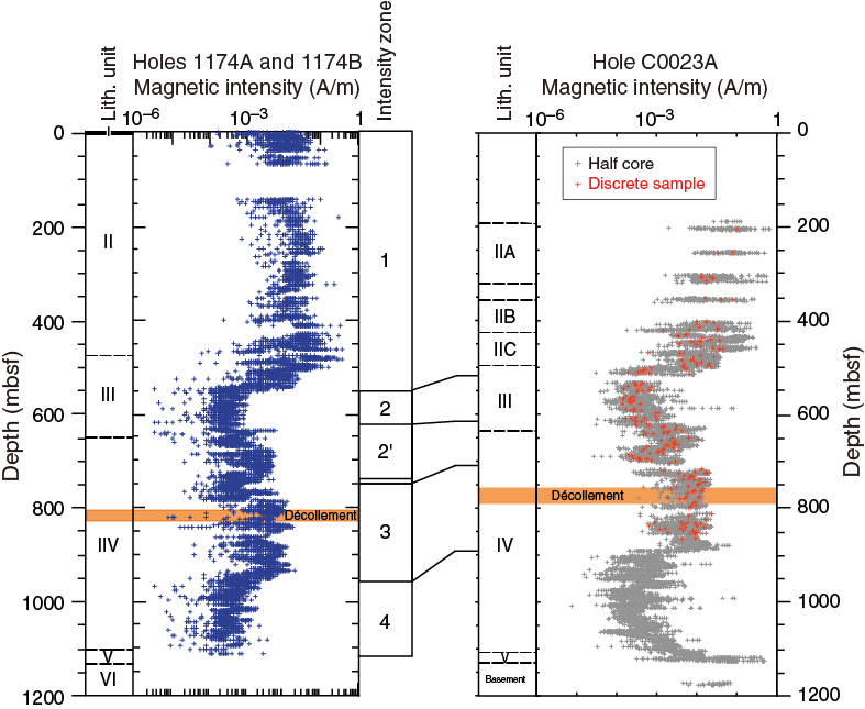
Figure F34. Magnetic intensity (after 20 mT demagnetization) in Hole C0023A compared to Holes 1174A and 1174B.
Downcore inclination variation
At Site C0023, the expected inclination value was 51.8° (−51.8°) for a normal (reversed) polarity period according to the geocentric axial dipole model. We relied on data obtained from discrete samples only because archive halves were often heavily disturbed and/or had severe overprinting from drilling operations.
The interval from 200 to 500 mbsf was mostly characterized by positive inclinations, steeper than ~30° (Figure F35), which were interpreted to be records of the Brunhes Chron (0–0.78 Ma). Typical demagnetization behavior is shown in Figure F36. Inclinations were scattered from 500 to 700 mbsf, and it was difficult to determine paleomagnetic polarity for this interval. This is probably due to low magnetic intensity (<10−3 A/m) for most of this interval; such a weak intensity tended to result in unreliable inclination values (lower sensitivity limit of the spinner magnetometer is ~10−3 A/m; typical demagnetization behavior is shown in Figure F37). Some inclination clusters at ±45° were observed for the interval deeper than ~700 mbsf. These might be records of normal and reversed polarities, as they were consistent with the expected inclinations. However, further analysis is required to determine paleomagnetic polarity and magnetochrons from samples with weak intensity.
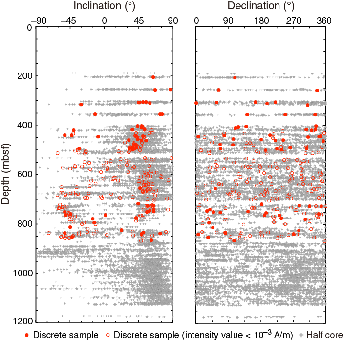
Figure F35. Paleomagnetic inclination and declination after 20 mT demagnetization.
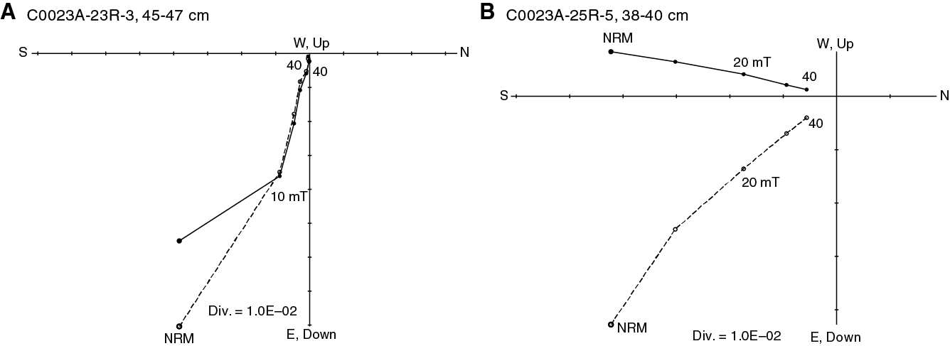
Figure F36. AF demagnetization of discrete samples.

Figure F37. AF demagnetization of discrete samples.
Physical properties
The goal of physical properties measurements in Hole C0023A was to obtain high-resolution data on bulk physical properties and their downhole variations. Whole-round multisensor core logger (MSCL-W) data were first collected on whole-round sections to define gamma ray attenuation (GRA) density, magnetic susceptibility, and natural gamma radiation (NGR). After MSCL-W measurements and core splitting, thermal conductivity, P-wave velocity, electrical resistivity, and moisture and density (MAD) were measured, mostly from the working halves of cores under room temperature and atmospheric pressure conditions. In addition to physical properties measurements on core samples, in situ temperature measurements were carried out from 189.3 to 407.6 mbsf using the APCT-3. Using the in situ temperature and thermal conductivity data, heat flow and formation temperature profiles at Site C0023 were estimated.
MSCL-W
Gamma ray attenuation density
GRA density results vary widely because of the presence of air and/or fluid between core and liner during measurement (Figure F38A). However, the upper range of the GRA density values seems to be valid, because the maximum GRA density values are in good agreement with bulk density obtained from MAD measurements on discrete samples (Figure F39A). Bulk densities determined by GRA increase downhole from ~2.0 g/cm3 at 200 mbsf to ~2.25 g/cm3 at 760 mbsf, the top of the décollement zone. From 760 to 830 mbsf, bulk densities tend to decrease gradually with increasing depth and then resume a general increasing trend to 2.5 g/cm3 to Unit V. Bulk density peaks at 905 and 1128 mbsf correspond to the presence of altered mud with carbonate cement and basaltic rocks, respectively.
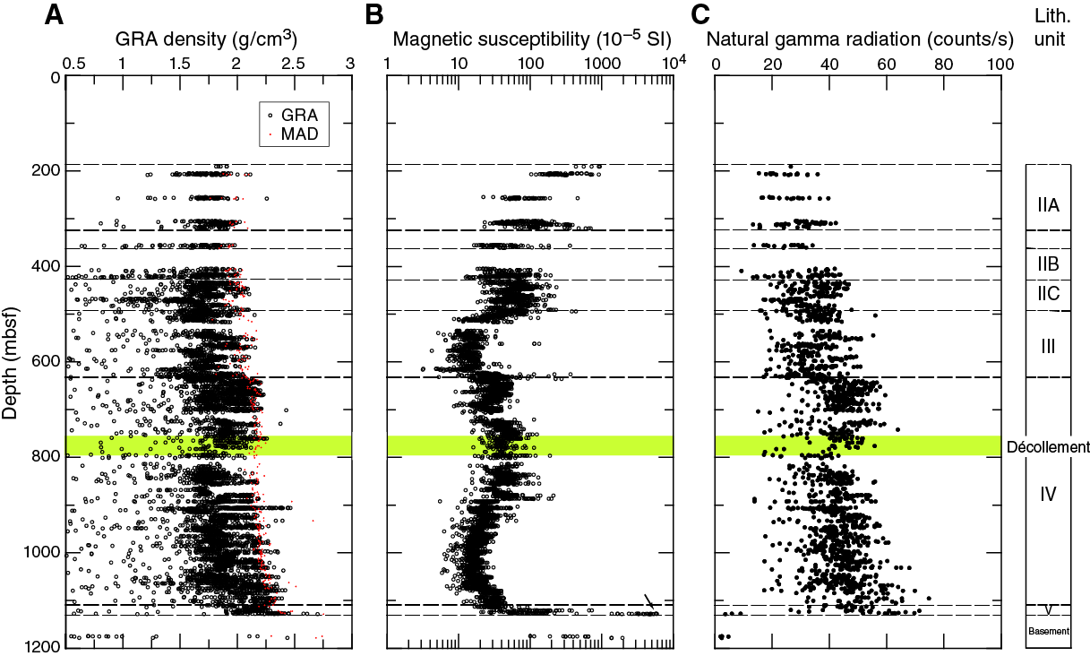
Figure F38. MSCL-W measurements.
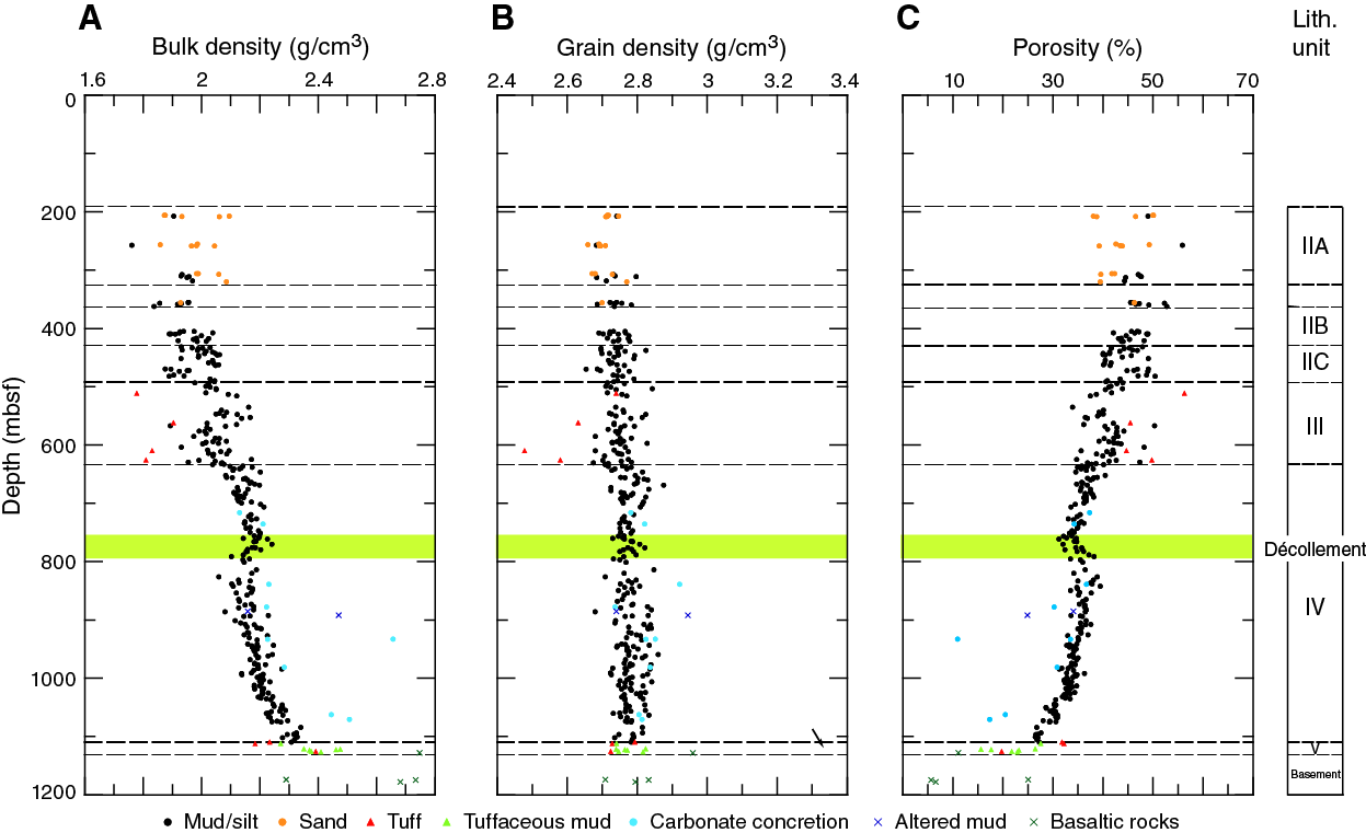
Figure F39. MAD measurements.
Magnetic susceptibility
Magnetic susceptibility decreases from ~200 mbsf toward the base of Subunit IIB at ~430 mbsf and becomes constant within Subunit IIC. In the middle part of Unit III, magnetic susceptibility displays the lowest values of 10 × 10−5 to 20 × 10−5 SI and displays slightly higher values ranging between 10−4 and 10−3 SI in Unit IV. A sharp increase in magnetic susceptibility deeper than 1115 mbsf correlates with tuffaceous mud and volcaniclastic sand in Unit V.
Natural gamma radiation
NGR increases downhole through Units II and III and into Unit IV by ~740 mbsf, and then displays a gradual decrease to ~820 mbsf. Deeper than this, NGR increases again toward the base of Unit V. Basaltic rocks recovered deeper than ~1126 mbsf show the lowest NGR (<10 counts/s) in Hole C0023A.
Moisture and density
MAD measurements characterize grain density, bulk density, porosity, void ratio, and water content in Hole C0023A. All MAD data are provided in Tables T6 and T7. Below, we summarize the most important parameters, which are bulk density, grain density, and porosity. Downhole variations are graphically shown in Figure F39, except for MAD data of discrete samples collected from WRCs for shipboard gas analyses (community gas [COMGAS] sample). The MAD data of COMGAS samples were more scattered than discrete samples from working halves (Table T7). This is most likely because COMGAS samples were more often physically disturbed during sampling for gas analyses.
Table T6. MAD measurements on discrete samples. Download table in .csv format.
Table T7. MAD measurements on COMGAS WRC samples. Download table in .csv format.
Bulk and grain density
Sediment bulk densities display the general pattern of downhole increase from 1.9–2.1 g/cm3 at 200 mbsf to ~2.2 g/cm3 by 760 mbsf, the top of the décollement zone. Within or even beneath the décollement zone, bulk density decreases by ~0.1 g/cm3 but resumes the general increase from ~2.1 g/cm3 at 820 mbsf to ~2.3 g/cm3 at 1110 mbsf, the base of Unit IV. Higher bulk densities deviated from the downhole increasing trend deeper than 820 mbsf in Unit IV, which correlate to either the presence of altered mudstone or carbonate concretion. Sediments in volcaniclastic facies (i.e., Unit V) and basaltic basement rocks exhibit a wide range of bulk density up to 2.76 g/cm3.
Grain densities increase from ~2.68 g/cm3 at ~250 mbsf to ~2.79 g/cm3 at ~1100 mbsf (Figure F39B). Within Unit IV, including the décollement zone, grain densities exhibit relatively constant values with an average of 2.77 g/cm3. Altered mudstone and carbonate concretion, in which pyrite and anhydrate are often crystallized, show higher grain density than 2.9 g/cm3.
Porosity
The calculated porosity profile is shown in Figure F39C. Porosity displays a downhole decrease from 40%–50% at 200 mbsf (Subunit IIA) to ~30% by 760 mbsf, the top of the décollement zone (Unit IV). The lower porosity values represent sand and silty sand at 200–300 mbsf in Subunit IIB. The scattered porosity values within Subunit IIB and Unit III may reflect subtle differences in grain size and composition of mud and silt. In contrast to tuffaceous sediments in Unit V, fine to coarse tuff and tuffaceous mud in Unit III characteristically show higher porosity values than their surroundings, ranging between 45% and 50%.
Distinct elevated porosity values, 5%–7%, appear across or even beneath the décollement zone between 760 and ~830 mbsf in Unit IV. This is a significant deviation from both normal compaction trends for silty clay (e.g., Athy, 1930) and the porosity reduction trend with depth observed within Units III and IV above and below (Figure F39C). Similar elevated porosity trends were reported at Sites 808 and 1174 (Shipboard Scientific Party, 1991, 2001b). However, it is a marked contrast at Site C0023 that porosity starts increasing gradually within the décollement zone, whereas sharp increasing curves in porosity were observed only at the base of the décollement zones at Sites 808 and 1174.
Deeper than ~830 mbsf, porosity values resume the compaction trend from ~38% at 830 mbsf to 32% by 1030 mbsf. Sediments cemented with carbonate and altered mudstones exhibit lower porosity than the general porosity reduction trend in Unit IV. The slope of porosity decrease with depth tends to be slightly higher from 1030 mbsf to the base of Unit IV, followed by a sharp increase within Unit V where tuffaceous mudstone becomes the dominant lithology. Basaltic rocks exhibit a range of porosity between 5.5% and 25%.
P-wave velocity
The depth profile of P-wave velocity in Hole C0023A displays considerable deviation from a smooth compaction curve (Figure F40A; Table T8). Between 200 mbsf and the base of the hole, three zones with higher velocities are identified: (1) ~630 mbsf, across the transition from the upper to lower Shikoku Basin facies (Unit III/IV boundary); (2) ~760 mbsf, near the top of the décollement zone; and (3) deeper than ~1080 mbsf, the bottom of the lower Shikoku Basin facies (Unit IV) to volcaniclastic facies (Unit V). Among these high-velocity anomalies, the shallowest one, at the Unit III/IV boundary, is characterized by lower, not higher, bulk density. The characteristic high velocities and low bulk density zone is likely related with fine to coarse tuff layers around the base of Unit III. Velocity decreases gradually across or even beneath the décollement zone by ~200 m/s and then increases toward the base of the hole. The velocity drop across the décollement zone correlates with the increase in porosity over the same interval. Carbonate concretion at 931 mbsf and basaltic rock at 1127 mbsf show velocities of more than 4000 m/s, which are significantly higher values than the general downhole velocity trend (not shown in Figure F40). The sharp increase in velocity at the base of Unit IV correlates with low porosity in tuffaceous mudstone (Figure F39C).
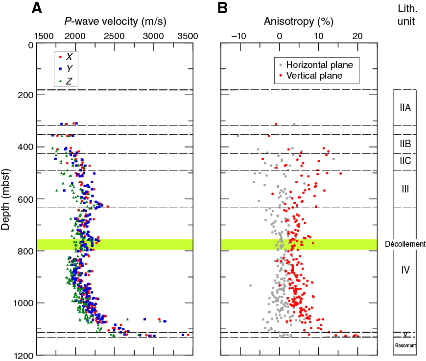
Figure F40. P-wave velocity and anisotropy of P-wave velocity.
Table T8. P-wave velocity measurements. Download table in .csv format.
Velocity anisotropy in planes parallel to the core axis (z-direction) tends to decrease with depth from ~15% at 400 mbsf to ~5% at 760 mbsf, just above the décollement zone. Beneath the décollement zone, anisotropy increases with depth, reaching up to ~20% at the base of the hole. A sharp increase in anisotropy appears around the base of Unit IV at 1080 mbsf, which is attributed to the well-developed volcaniclastic lamination interbedded in mudstone with low dip angle (<20°) (Figure F18).
Electrical resistivity
For unconsolidated sediments retrieved from 205.8 to 305.6 mbsf, electrical resistivity was determined on working half sections along the y-direction with a four-pin electrode. Deeper than 306 mbsf where the sediments were consolidated, resistivity was measured on the same cubic samples used for P-wave measurements with a two-electrode system. The cube was rotated to measure resistivity in the x-, y-, and z-directions. All resistivity data were represented as apparent formation factor (see Physical properties in the Expedition 370 methods chapter [Morono et al., 2017]).
Apparent formation factor tends to increase gradually with increasing depth to ~1050 mbsf, but a slope of the downhole trend line sharply changes around the base of Unit IV at ~1050 mbsf (Figure F41A; Table T9). Formation factor measured perpendicular to the core axis (x- and y-direction) is lower than that along the core axis (z-direction). Data acquired in the horizontal plane closely follow the variation in porosity and exhibit a reversal of the downhole porosity trend with a slight reduction of the formation factor across the décollement zone from 760 to 820 mbsf. Formation factor measured along the z-direction displays stronger variations than the horizontal components, particularly below the top of the décollement zone at 758 mbsf. Anomalously high values of formation factor along the z-direction at 891 and 931 mbsf and along the y-direction at 1061 and 1068 mbsf correlate with the sediments cemented with carbonate.
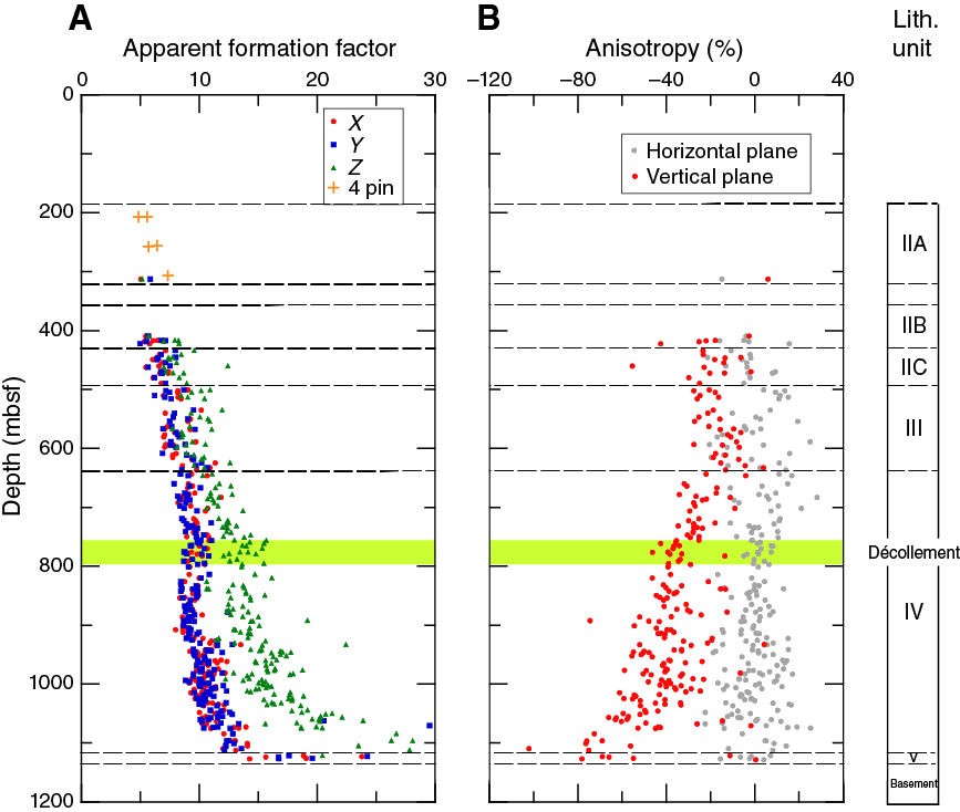
Figure F41. Apparent formation factor and anisotropy of formation factor.
Table T9. Electrical resistivity measurements. Download table in .csv format.
Anisotropy of formation factor in the vertical plane generally decreases with depth and appears lower (<−30%) in Unit IV than the shallower depth (Figure F41B). Distinct scatter of the anisotropy from 920 to 1030 mbsf may correlate with the variation of bedding dips and the occurrence of burrows in the cubic samples.
Thermal conductivity
Thermal conductivity was measured using one of two methods depending on core conditions. For unconsolidated sediments between 205.6 and 354.8 mbsf, a needle probe was inserted into the WRC for a full-space conductivity measurement. For sediments deeper than 403.4 mbsf, it became difficult to insert the needle into consolidated cores, so a half-space line source probe method was used on split cores.
Between 205 and 763 mbsf, thermal conductivity increases gradually with depth from ~1.2 to ~1.7 W/(m·K) (Figure F42; Table T10). Beneath the décollement zone at ~760 mbsf, thermal conductivity slightly decreases with depth and then exhibits relatively constant values ranging from 1.6 to 1.7 W/(m·K) until ~1050 mbsf. Deeper than this, thermal conductivity again increases with depth to 2.0 W/(m·K) toward the basement. One cracked basalt piece with calcite veins was recovered from the bottom of Hole C0023A (Core 370-C0023A-112R-1, 12 cm), showing a thermal conductivity of 1.8 W/(m·K). The overall downhole change in thermal conductivity inversely correlates well with those in porosity, particularly in Unit IV (Figure F39C).
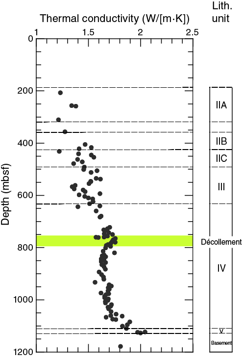
Figure F42. Thermal conductivity.
Table T10. Thermal conductivity measurements. Download table in .csv format.
In situ temperature measurement and heat flow
A total of eight formation temperature measurements were conducted in situ from 189.3 to 407.6 mbsf using the APCT-3 during coring with the short HPCS (see Operations). Table T11 summarizes the temperature data and their quality. Among the eight measurements, the temperature data obtained from 189.3, 314.6, and 407.6 mbsf were not reliable, as low core recovery at these three depths indicated that the APCT-3 on the short HPCS core shoe did not penetrate properly into the formation. A measurement at 256.8 mbsf was also not successful because the temperature record indicated probe movement while measuring. Given the quality assessment of coring and time series temperature data while measuring, we used four temperature data among the eight attempts to determine the thermal gradient and heat flow at Site C0023.
Table T11. Downhole temperature measurements. Download table in .csv format.
In situ temperatures increase linearly with depth between 204.1 and 355.2 mbsf (Figure F43). The average geothermal gradient determined by a least-squares regression on the formation temperatures in situ is 111°C/km. The seafloor temperature obtained from the intercept of a least-squares regression on the measured temperatures is 8.5°C, which is higher than the averaged mudline temperature (1.67°C) of the eight temperature measurements (Table T11).
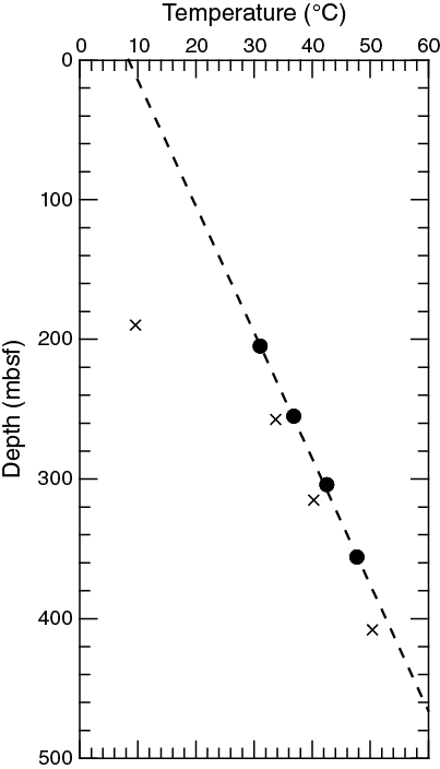
Figure F43. Temperatures obtained in situ by APCT-3 measurements.
Heat flow is calculated as the product of the temperature gradient at a certain depth and corresponding mean thermal conductivity of the formation interval where the temperature gradient is measured. Thus, heat flow in Hole C0023A can be estimated from APCT-3 temperatures and thermal conductivity data obtained from 201 to 407 mbsf by a fit of the Bullard equation (method of temperature versus integrated thermal resistance plot) (see Physical properties in the Expedition 370 methods chapter [Morono et al., 2017]). Consequently, the mean heat flow value at Site C0023 is 140.1 ± 2.5 mW/m2, which is lower than the previous heat flow estimate of 183 mW/m2 at Site 1174 (Shipboard Scientific Party, 2001b) and slightly higher than that of 130 mW/m2 at Site 808 (Shipboard Scientific Party, 1991). Based on the determined heat flow and measured thermal conductivity data, a temperature profile to the bottom of Hole C0023A is synthesized with the assumption of purely vertical conductive and steady-state heat flow (Figure F44). The projected downhole temperature reaches 86°C at the top of the décollement zone and 120°C at the bottom of the hole.

Figure F44. Temperatures projected to the bottom of Hole C0023A.
Anelastic strain recovery analysis
A total of 15 anelastic strain recovery measurements were performed on WRCs collected between 429 and 1122 mbsf. Strain recovery data were recorded for 5–20 days, depending on primary data screening. Preliminary shipboard data indicated that cores retrieved from 650 to 950 mbsf within the lower Shikoku Basin facies characteristically exhibit a gradual increase in strain but turn to an unusual decrease after an elapsed time of 36 h. All the stored data will be processed as postcruise research.
Inorganic geochemistry
We collected 139 sediment interstitial water (IW) samples (Table T12). Spatial resolution typically varied between one and two samples per 10 m. The length of the WRC section from which water was extracted was between 10 and 81 cm, and the volume of fluid extracted was between 0.5 and 33.0 mL (Table T12; Figure F45 for volumes normalized to WRC lengths). For most samples, we did not exceed 30,000 lb of applied force to the Manheim squeezers. For a few samples that did not yield sufficient water at 30,000 lb, we applied a force up to 60,000 lb, and these are noted in Table T13.
Table T12. WRCs used for IW sampling. Download table in .csv format.
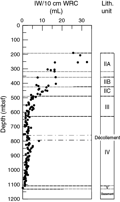
Figure F45. Volume of IW recovered from WRCs.
Table T13. Overview of samples taken from pressure squeezing. Download table in .csv format.
As described in Inorganic geochemistry in the Expedition 370 methods chapter (Morono et al., 2017), we initially removed approximately 3 mm of the core surface by scraping with a ceramic knife in a nitrogen-filled glove bag. This was increased to 5 mm at Core 370-C0023A-55R and 7 mm at Core 84R to minimize the likelihood of contamination. The suite of analyses that were conducted on the ship and the samples we stored for future shore-based analysis (see Table T6 in the Expedition 370 methods chapter [Morono et al., 2017]) depended on the volume of water recovered as well as spatial resolution. Geochemical data for IW samples that were not affected by intrusive contamination as evidenced by elevated sulfate (SO42−) concentrations are given in Table T14; data for samples affected by intrusive contamination are given in Table T15.
Table T14. Geochemical data for IW samples not affected by intrusive seawater contamination. Download table in .csv format.
Table T15. Geochemical data for IW samples affected by intrusive seawater contamination. Download table in .csv format.
Chloride, bromide, and salinity
Chloride (Cl−) concentrations (Figure F46), determined by titration, slightly increase through the upper 200–400 mbsf then decrease nearly linearly from the Cl− maximum (580 mM at 425 mbsf) to the Unit III/IV boundary at 637 mbsf, with some curvature in the 550–670 mbsf range. Cl− remains constant at approximately 460 mM from 860 to 1030 mbsf, except for a small excursion to slightly lower concentrations at 950 mbsf. The sharp, near-linear increase in Cl− from 1030 mbsf to the basement is likely due to diffusion of high Cl− fluid within the basement reaching 550 mM near the sediment/basement interface. Bromide (Br−) (Figure F46) is nearly 25% elevated relative to seawater (1.06 mM compared to 0.86 mM) in the shallowest sample we collected and then its profile generally parallels that of Cl−, with a minimum of 0.77 mM at 950 mbsf and a sharp increase to 0.94 mM at the basement. The shallow Br− maximum likely reflects diagenesis of marine organic matter in the shallower sediment, whereas the increase at depth is due to diffusion of a basement fluid with elevated Br− (You et al, 1993).
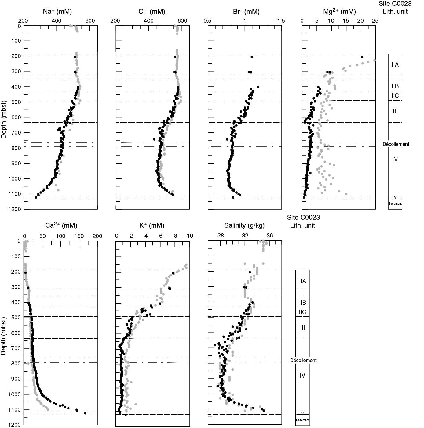
Figure F46. Major cations, Cl−, and salinity.
The salinity profile (Figure F46) is similar to that of Cl−, with a sharper increase from 1030 mbsf to the basement, reaching a maximum of 36 g/kg at the basement that exceeds the local maximum of 33 g/kg at 460 mbsf. The near-constant salinity values between 670 and 860 mbsf reach a minimum of 27 g/kg at 682 mbsf. It should be kept in mind that the salinity measurement is based on the refractive index of the sample and does not take into account the changing proportions of dissolved ions.
Sulfate
We expected SO42− to be below detection at in situ concentrations deeper than the top few meters below seafloor to at least 500 mbsf, based on results from Site 1174. However, from 190 mbsf (shallowest sample) to the Unit III/IV boundary, measured concentrations vary between 0.4 and 1.4 mM (Figure F47). We interpret this scatter as due to variable amounts of contamination with seawater-derived SO42− (see Quality assurance and quality control for microbiological sample processing for a more detailed discussion of contamination). In Table T15, we list samples that have SO42−-based percentages of seawater contamination >4% (assuming a seawater SO42− concentration of 28 mM) for all samples taken shallower than 500 mbsf, above the notable increase in SO42− concentrations in Units III and IV.
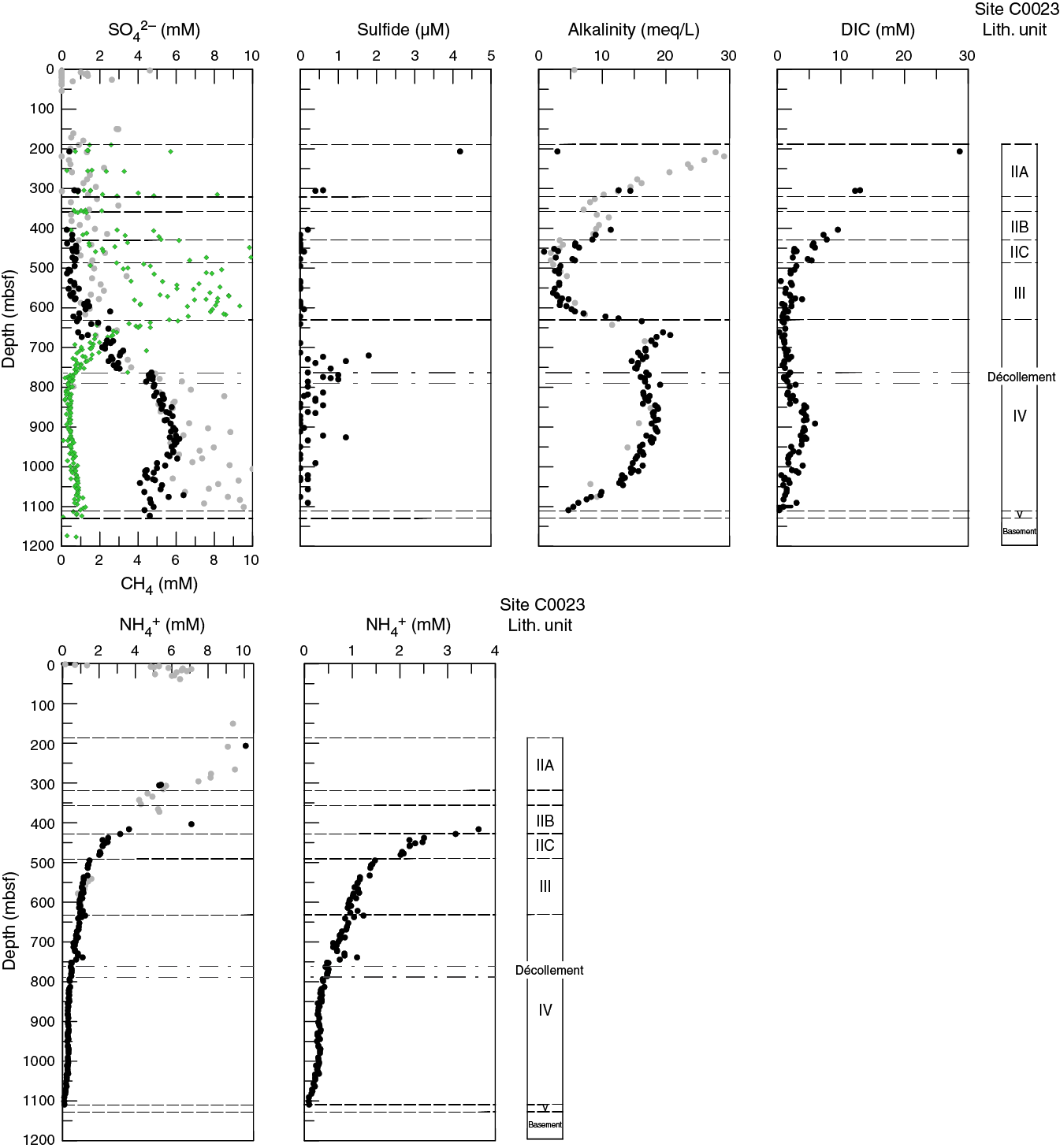
Figure F47. IW composition.
At approximately 550 mbsf, SO42− begins to increase with depth, reaching approximately 3 mM. This region, 640–764 mbsf, overlaps with a decreasing trend in methane and is identified as a sulfate–methane transition zone (SMTZ). At approximately 750 mbsf (close to the top of the décollement; Figure F47), there is a step increase in SO42− of approximately 2 mM. Concentrations increase to a maximum of approximately 6.5 mM between 900 and 950 mbsf. Between 950 and 1050 mbsf there is a decrease of about 1.5 mM and then values scatter between 5 and 7 mM to the bottom of the core.
Sulfide
Dissolved sulfide (H2S/HS−) concentration is highest (4.2 µM) in the shallowest sample at 206.5 mbsf (Figure F47). Concentrations are low (~0.5 µM) at 300 mbsf and remain close to and below the detection limit to 720 mbsf. Between 720 and 865 mbsf, H2S/HS− concentrations are scattered between below the detection limit and 1.8 µM, with the maximum concentration at the top of this interval coinciding with the SMTZ. A second zone of elevated H2S/HS− concentrations of up to 1.2 µM is centered at 926 mbsf. Toward the basement, H2S/HS− concentrations are below the detection limit (0.2 µM) or between the detection and quantification limits (0.4 µM).
Alkalinity and dissolved inorganic carbon
In Unit II, alkalinity is elevated relative to average seawater (2.23 meq/L), consistent with Site 1174 data, and decreases with depth in the range where we collected samples (Figure F47). Dissolved inorganic carbon (DIC) at Site C0023 is also high in the shallow sediment and decreases with depth (Figure F47). In the upper 600 mbsf, DIC and alkalinity both smoothly decrease to 1 and 4 mM, respectively, at the Subunit IIB/IIC boundary. At 600 mbsf, however, the profiles diverge, with alkalinity increasing sharply to a peak of 20 mM at 670 mbsf and DIC staying near-constant with a minimum of ~0.8 mM. DIC then increases gradually to 2.5 mM at 850 mbsf, where there is a sharp increase of 3 mM. Alkalinity follows the DIC profile with an increase of 3 meq/L at ~850 mbsf from a slight but resolvable dip of 16 meq/L at the décollement (770 mbsf). Alkalinity maintains a similar pattern to DIC for the remainder of the profile but with a much larger range in magnitude. DIC and alkalinity both decrease from the offset at 850 mbsf to the basement, with local minima at the basement of 0.4 mM and 5 meq/L, respectively. In the region of elevated alkalinity, the full titration curve is consistent with alkalinity being dominated by low molecular weight fatty acids.
Major cations
Above the décollement, sodium (Na+) parallels Cl− very closely (Figure F46), with a gradual decrease from 520 mM (elevated relative to average seawater Na+ of 480 mM) for the upper 670 mbsf, terminating in a shoulder and near-constant values through the décollement zone (670–770 mbsf). An offset of ~30 mM occurs at this shoulder. Below the décollement, Cl− and Na+ trend inversely, with Na+ decreasing gradually from 770 to 950 mbsf and more steeply from 950 mbsf to the basement, reaching an overall minimum of 280 mM in our deepest sample at 1123 mbsf.
Magnesium (Mg2+) generally decreases with depth, whereas calcium (Ca2+) increases with depth (Figure F46). A major feature in the Ca2+ profile is the sharp 120 mM increase in concentration across the 990–1123 mbsf depth interval. A possible source for this increase in Ca2+ is the underlying basement. Mg2+ concentrations sharply decrease from the top of the cored formation until the base of Unit III. A discontinuity in the Mg2+ profile occurs at 637 mbsf. This offset is followed by a smooth decrease from 2.33 to 0.61 mM over the lowermost 460 m of cored formation. This downhole change in concentration gradients is indicative of distinct mineral reactions. The top 431 m of the formation may be characterized by dolomitization processes, whereas the lowermost section (800–1100 mbsf) is indicative of alteration of the underlying basalt.
Potassium (K+) closely parallels the Mg2+ profile (Figure F46), with slightly different features in the upper 700 mbsf and a sharp increase near the basement (1100 mbsf). K+ shows a shoulder just below the Subunit IIC/Unit III boundary, followed by a decrease of 2 mM to 670 mbsf where a local minimum is followed by a linear increase to an offset at the décollement.
Ammonium and nitrate
Ammonium (NH4+) concentrations are highest at shallowest depths (10 mM at 206.5 mbsf) and decrease with depth to 0.1 mM at 1009 mbsf (Figure F47). The profile is in good agreement with Site 1174, where a concentration maximum of 12 mM was observed at approximately 200 mbsf in the limited NH4+ data set (Shipboard Scientific Party, 2001b); however, Site 1174 NH4+ data are only available to 600 mbsf. At Site C0023, subtle offsets in the NH4+ profile occur at the lithostratigraphic Subunit IIB/IIC, Subunit IIC/Unit III, and Unit III/IV boundaries. Similarly, some scatter was observed in the NH4+ profile of Site 808 (Shipboard Scientific Party, 1991 [figure 80]) at ~820 mbsf at the transition of upper Shikoku Basin facies to lower Shikoku Basin facies. Furthermore, at Site C0023 there is a small but well-expressed peak (1.1 mM compared to 0.4–0.6 mM deeper and shallower) at 739 mbsf (19 m above the top of the décollement).
Nitrate (NO3−) was measured only in a selection of samples (<20), because concentrations were expected to be below the detection limit. However, NO3− concentrations ranged from 4 to 12 µM in samples representing the upper 500 mbsf and varied between 13 and 160 µM in samples near the basement. We consider these unreliable data. The observed NO3− concentrations are likely to result from contamination of the sampling apparatus with HNO3 and from potential ammonium oxidation during sample storage. A complete NO3− profile was not measured shipboard.
Ferrous iron
Dissolved ferrous iron (Fe2+) was detected in IW of Units II and III (Figure F48) with the highest concentrations of 60 µM at 570 mbsf, coinciding with a high abundance of ash layers. Deeper than 600 mbsf, Fe2+ was generally close to or below the quantification limit (0.8 µM).
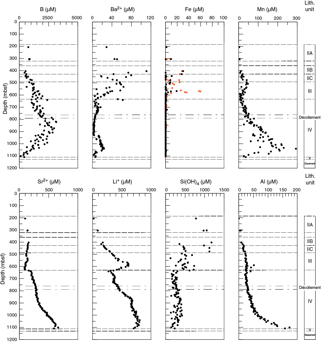
Figure F48. Minor cations in IW.
Minor elements
Minor element concentrations are shown in Figure F48. Boron (B) concentrations are generally scattered but show an overall increase from ~600 µM in Subunits IIA and IIB to ~3100 µM in Unit IV at 820 mbsf (~20 m below the base of the décollement). Toward the basement, B concentrations decrease to 110 µM at 1100 mbsf. This pattern is very similar to Site 808 data where B peaked at the décollement at ~950 mbsf, which has been attributed to desorption processes (You et al., 1993).
Barium (Ba2+) concentrations are scattered in Units II and III, with the highest concentrations of 80–110 µM at 400–450 mbsf, but show a general decrease with depth to 4 µM at the Unit III/IV boundary at ~650 mbsf. There is a slight but notable increase again between 650 and 700 mbsf to 17 µM followed by another smooth decrease to 2 µM at 929 mbsf. Within Core 370-C0023A-90R, where two WRCs were sampled for IW, there is an offset back to slightly elevated concentrations to 13 µM increasing further to 24 µM at 1040 mbsf. Toward the basement, Ba2+ concentrations decrease to ~5 µM.
Overall, the total iron (Fe) profile derived from inductively coupled plasma–atomic emission spectrometry (ICP-AES) is in agreement with Fe2+ concentrations derived from photometric analysis using the ferrozine method, showing elevated concentrations in Units II and III. However, Fe data derived from ICP-AES are lower, which indicates that IW samples partly oxidized before aliquots for ICP-AES were taken and acidified. The highest Fe concentrations are ~30 µM in comparison to 60 µM determined using the ferrozine method.
Manganese (Mn) increases from <5 µM in Subunit IIA to ~50 µM at ~500 mbsf and then decreases toward the Unit III/IV boundary. Deeper, Mn distinctly increases to 290 µM at 1040 mbsf. The data deeper than 900 mbsf are scattered, which could either be an effect of oxidation during sample handling (similar to that described for Fe) or natural variation due to mineral formation (e.g., rhodochrosite) and/or hydrothermal fluid flow.
Strontium (Sr2+) shows a slight increase with depth from 100 µM at 206 mbsf to ~150 µM at 400 mbsf and a decrease back to ~90 µM toward 625 mbsf, interrupted only by a small peak at 550 mbsf (140 µM). At 630–640 mbsf, coinciding with the Unit III/IV boundary (637 mbsf), the profile shows a very distinct offset by 100 µM and further increases downhole until reaching ~660 µM at 1100 mbsf.
The lithium (Li+) profile at Site C0023 is very similar to that of Site 808 (Shipboard Scientific Party, 1991). At Site C0023, Li+ concentrations increase steadily from ~20 µM at 206 mbsf to ~600 µM in the interval from 570 to 595 mbsf. Li+ concentrations then decrease with a steep gradient toward 240 µM at 640 mbsf (i.e., Unit III/IV boundary).
Dissolved silicon (Si[OH]4) concentrations show a lot of scatter between 125 and 1180 µM in Units II and III, but there is a trend to less scattered values and lower concentrations (~270 µM) below the Unit III/IV boundary at ~650 mbsf. A similar pattern, a decrease of Si(OH)4 coincident with the trench-to-basin transition, was observed for Site 808 (Shipboard Scientific Party, 1991 [figure 82]).
Aluminum concentrations are low in Subunit IIA (0 µM at 206 mbsf) and increase with depth to 170 µM at 1100 mbsf with a profile shape similar to Ca.
Hydrogen and carbon monoxide
Dissolved hydrogen (H2) and carbon monoxide (CO) concentrations of interior and exterior WRC samples were quantified at 142 horizons. The depths range from 189 to 1122 mbsf.
H2 concentrations for interior WRC samples range from below detection to 287 nM (Figure F49; Table T16). Based on the average of 81 procedural blanks, the detection limit at this site is 0.5 nM H2. The major features in the H2 profile are an approximately two order of magnitude decrease in concentration (from 287 to 7 nM) from 278 to 970 mbsf, followed by an order of magnitude increase in concentration (from 7 to 70 nM) over the 970–1100 mbsf depth interval. Whether downhole H2 concentrations are controlled by abotic or biotic processes is presently not clear.
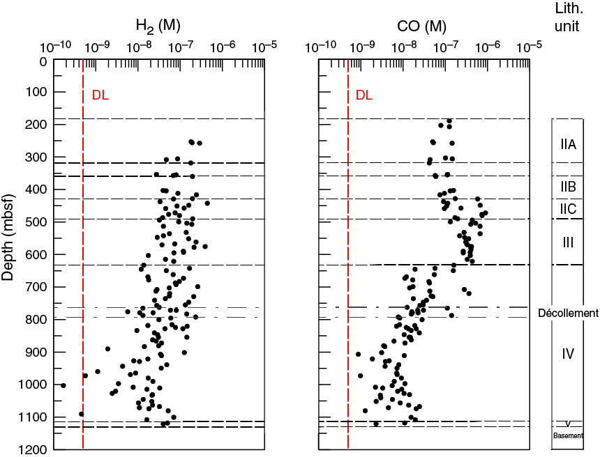
Figure F49. Downhole hydrogen and CO from interior WRC sample.
Table T16. Hydrogen concentrations measured in interior WRC samples. Download table in .csv format.
To constrain the contamination potential due to H2 generated during drilling, we quantified H2 concentrations in the core liner fluid. Liner fluid samples (sample code 370RGA4) at 133 core horizons were collected in the core cutting area immediately following core recovery. For RCB coring (Cores 370-C0023A-16R through 110R), liner fluid H2 concentrations are highly scattered (ranging from below detection to 2.3 µM) and show no discernible depth pattern (Figure F50; Table T17). This variation in liner fluid H2 concentrations is most likely due to a combination of factors: (1) the composition of the drilling fluid used during core cutting, (2) the timing of coring operations, and (3) the geological formation. Between 871 and 1124 mbsf, liner fluid H2 concentrations are consistently higher than concentrations measured in interior WRC samples. Presently, we cannot eliminate the possibility of contamination from liner fluid in this interval. Additional time-dependent diffusion calculations will be required to fully constrain the contamination potential of H2 concentrations measured in interior WRC samples. Exterior samples of WRCs were taken immediately after core recovery in the core cutting area (sample code 370RGA3), and about 1–2 h later on the core processing deck (sample codes 370RGA1 and 370RGA2). Both data sets show good agreement and follow the same general downhole pattern as interior samples, although a wider scatter is observed for exterior samples (Figure F50).
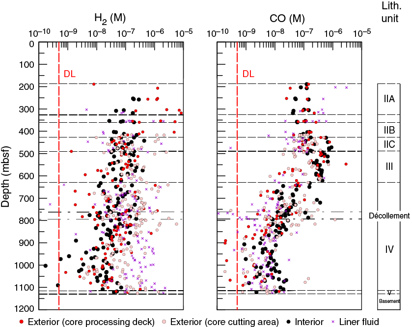
Figure F50. Downhole hydrogen and CO from liner fluid and interior and exterior WRC samples.
Table T17. Hydrogen concentrations measured in liner fluid. Download table in .csv format.
The top 404 m of cored formation was recovered using two different coring technologies (i.e., short HPCS and ESCS). In this interval, exterior H2 concentrations are 2 to 3 orders of magnitude higher than interior samples (average = 120 nM). This striking difference is likely due to H2 production caused by the sudden and localized frictional heating of the core liner and surrounding formation during penetration of the piston core system.
CO concentrations are above the detection limit (0.5 nM) and range from 0.9 to 9 µM (Figure F49; Table T18). Concentrations increase slightly from 0.13 µM at the top of the cored formation to 0.43 µM at the top of the SMTZ (620 mbsf). Concentrations decrease between 630 and 1003 mbsf, reaching a minimum of 5 nM, followed by an increase of 11 nM between 1003 and 1101 mbsf. CO concentrations for exterior samples follow the same downhole pattern as interior samples (Figure F50). For RCB coring (Cores 16R through 110R), liner fluid CO concentrations were generally lower than measured interior concentrations, excluding the risk for liner fluid contamination potential (Figure F50; Table T19).
Table T18. CO concentrations measured in interior WRC samples. Download table in .csv format.
Table T19. CO concentrations measured in liner fluid. Download table in .csv format.
Organic geochemistry
During Expedition 370, organic geochemists evaluated the habitability of the deeply buried sediment at Site C0023 by characterizing the quantity and quality of gaseous and solid-phase organic matter. The main objectives were to
- Search for chemical signatures of biological activity,
- Identify potential energy and carbon sources for the deep biosphere, and
- Relate the distribution of dissolved hydrocarbons and sedimentary carbonate and organic matter to diagenetic and catagenic processes at moderate to elevated temperatures.
These investigations will aid in testing existing hypotheses (Horsfield et al., 2006; Parkes et al., 2007) that catagenesis and the resulting transformation of organic matter and concomitant incipient generation of gaseous hydrocarbons and other small organic compounds may provide a continuous feedstock for indigenous microbial communities living at the upper temperature limit of deep subseafloor life.
To meet these goals, we (1) characterized particulate sedimentary organic matter composition by elemental analysis of total carbon (TC), total nitrogen (TN), and total sulfur (TS) contents and determined carbonate (expressed as CaCO3) and total organic carbon (TOC) contents in the sediment; (2) determined the composition and measured the quantity of hydrocarbon gases (C1–C4) from cored samples of sediment and basement rock and gas expansion voids; and (3) took a comprehensive set of samples for postcruise analyses.
The amount and nature of sedimentary organic matter at Site C0023 are compared and contrasted to those from nearby Sites 808 and 1174 (Shipboard Scientific Party, 1991, 2001b) and are put in context of the thermal, structural, and lithostratigraphic architecture of the Nankai accretionary prism off of Cape Muroto. Note that the names, numbers, and descriptions of stratigraphic units in this section and corresponding figures are those defined for Site C0023 (see Lithostratigraphy) and may deviate from those previously used for Sites 808 and 1174 (Shipboard Scientific Party, 1991, 2001b).
Carbon, nitrogen, and sulfur contents of the solid phase
Samples for analyses of CaCO3, TC, TN, and TS were taken from COMGAS WRC samples, which were assigned following X-ray CT imaging of core sections. This allowed for selection of minimally disturbed parts of the cores, while avoiding areas that were of interest for other research purposes, such as dolomite and rhodochrosite-rich horizons, pyrite nodules, and other mineral veins (see Lithostratigraphy). This sampling strategy likely resulted in a bias toward sample material with lower average carbonate contents. At Site C0023, measured CaCO3 contents are generally low (average CaCO3 = ~3.4 wt%). A larger scatter in the data is recorded between 470 and 600 mbsf, at 700–830 mbsf, and between 1120 and 1180 mbsf. Here, respective CaCO3 concentrations reach up to 10.5, 16.5, and 21.6 wt% in narrow sediment horizons (Figure F51; Table T20). Notably, high CaCO3 contents coincide with horizons of increased counts of calcite cements in calcareous claystones and calcite mineral abundances detected by XRD analysis, which are detected from 420 to 1070 mbsf, with maximal counts at ~470 mbsf in the trench-to-basin transitional facies, at ~550 mbsf within the upper Shikoku Basin facies (Unit III), and at ~830 mbsf and deeper than 950 mbsf in the lower Shikoku Basin facies (Unit IV) (see Figure F17, Table T3). Between 830 and 950 mbsf, CaCO3 abundance is generally low, roughly corresponding to a decrease in recorded calcite cementation; structural features are also relatively sparse in this interval (see Figure F13). Notably, increased abundances of other calcareous minerals such as rhodochrosite (MnCO3) are recorded deeper than 830 mbsf (see Figure F30). The method of carbonate analysis may have discriminated against rhodochrosite because rhodochrosite dissolves more slowly than CaCO3 in dilute acid (see Organic geochemistry in the Expedition 370 methods chapter [Morono et al., 2017]). As such, total carbonate contents are possibly underestimated here, whereas CaCO3 may be overestimated. In general, observations at Site C0023 are consistent with findings from Site 1174 (Shipboard Scientific Party, 2001b) where several CaCO3 maxima were recorded at 450 mbsf, corresponding to Subunit IIC (trench-to-basin transitional facies), ~at 650 mbsf in Unit III (upper Shikoku Basin facies), and deeper than 800 mbsf within Unit IV (lower Shikoku Basin facies).
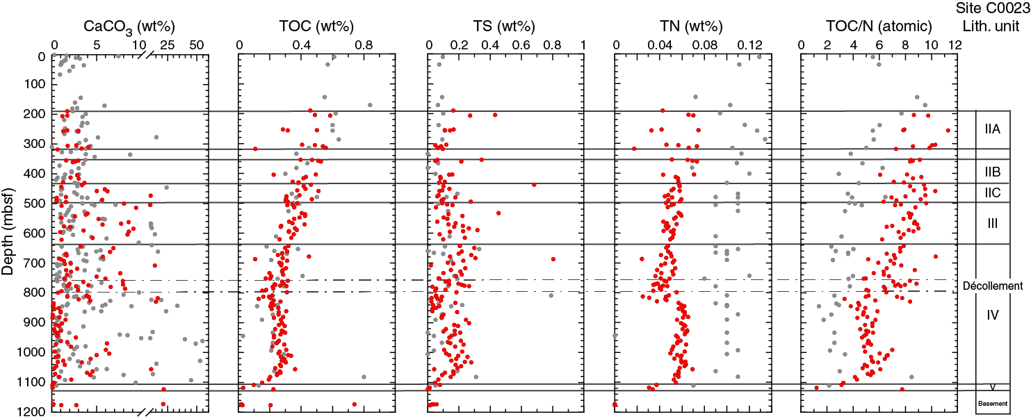
Figure F51. Solid phase contents of C, N, and S.
Table T20. C, N, and S. Download table in .csv format.
TC is variable throughout Hole C0023A, ranging from 0.04 to 3.28 wt%, averaging 0.71 wt%, and overall corresponding to the distribution of CaCO3 contents (Table T20). TOC content is generally low, ranging from 0.02 to 0.74 wt% (average = 0.3 wt%) and decreases steadily with depth to 800 mbsf and then increases again until ~1000 mbsf, coincident with a peak in hydrocarbon gases (Figures F52, F53). Deeper than 1050 mbsf, TOC concentrations show a sharp decrease to 0.02 wt% close to and within the basement. One of the lowermost basalt samples collected at 1176 mbsf had both high CaCO3 and TOC contents of 21 and 0.74 wt%, respectively. The elevated TOC contents might result from seawater that was introduced into the basement (cf. Klein et al., 2015) but could alternatively also be an artifact related to incomplete decalcification of carbonate minerals in the basalt matrix. The dip in TOC observed at ~800 mbsf roughly coincides with the base of the décollement (~796 mbsf), and the lowest TOC values are recorded within the volcaniclastic facies of Unit V. The low TOC values recorded throughout the lower Shikoku Basin may be representative of an aerobic depositional environment with limited potential for organic carbon preservation (Demaison and Moore, 1980). The greater occurrence of burrows at these depths is additional evidence for oxic conditions at the time of deposition (see Lithostratigraphy). Generally, TOC contents are similar to those measured at Site 1174 (Shipboard Scientific Party, 2001b).
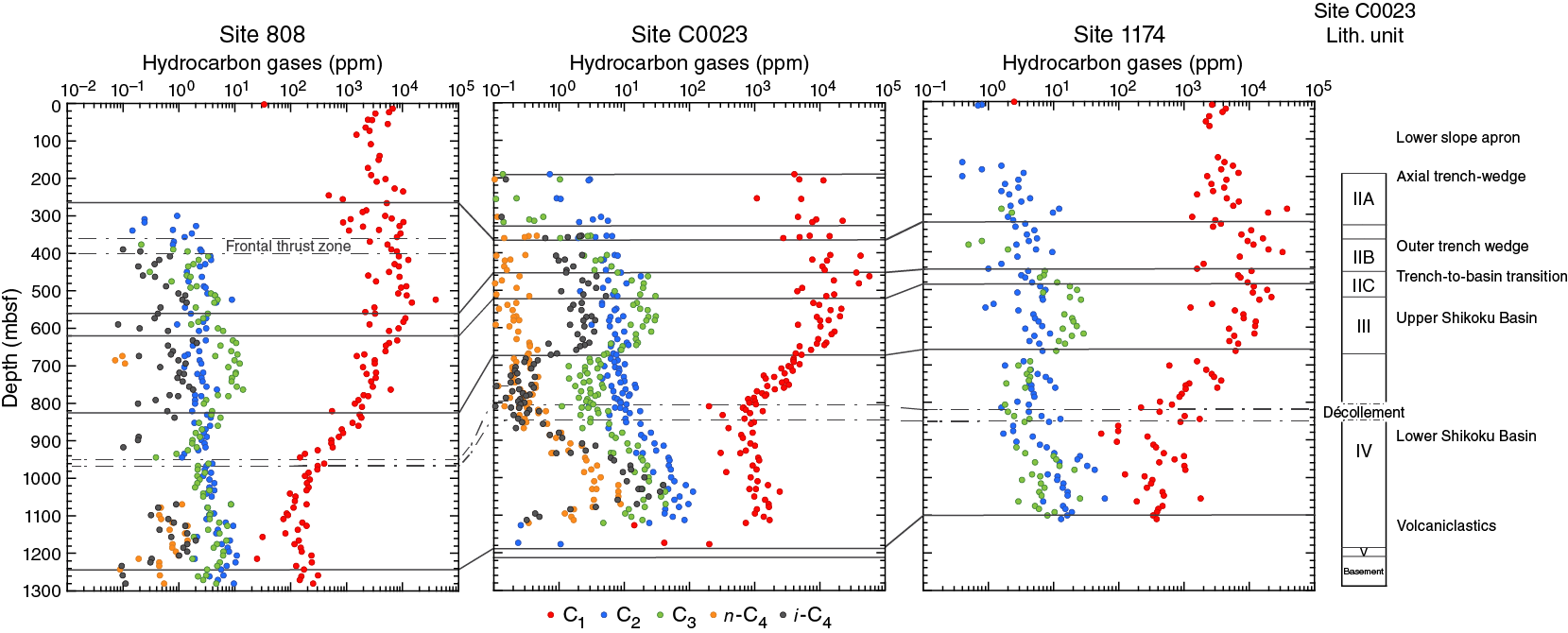
Figure F52. Mole fraction of hydrocarbon gases in headspace.
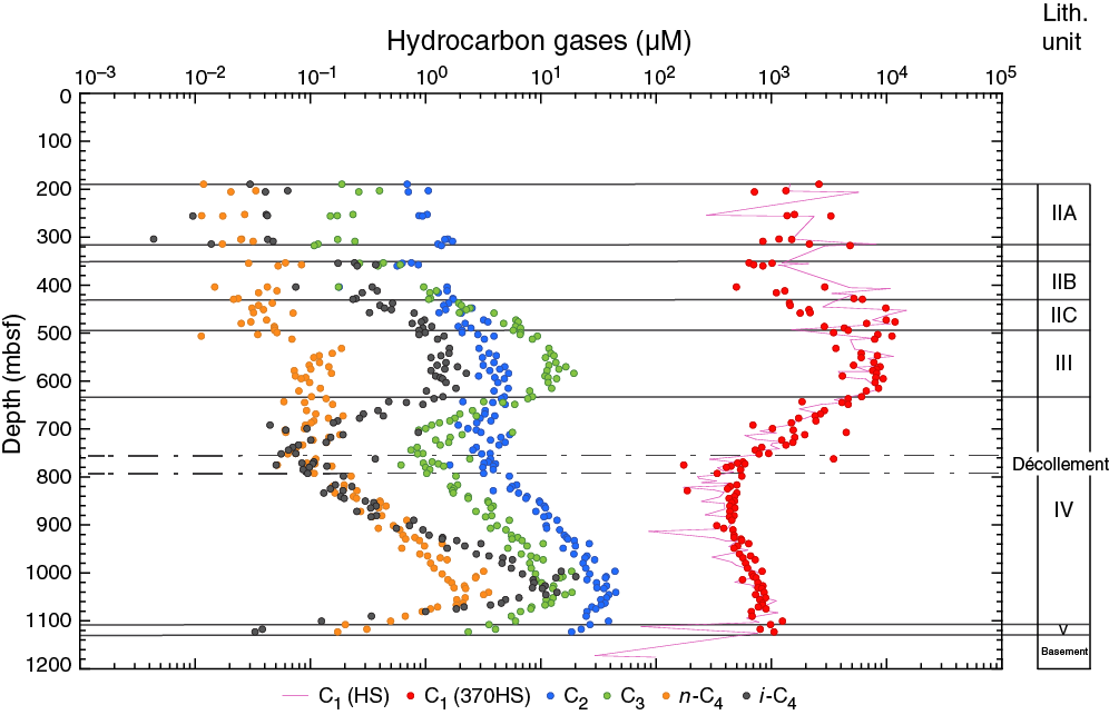
Figure F53. Dissolved hydrocarbon gases.
TN and TS contents are low throughout Hole C0023A, ranging from 0.02 to 0.07 wt% (average = 0.05 wt%) and from 0.01 to 0.79 wt% (average = 0.15 wt%), respectively (Figure F51; Table T20). TS contents are within the range of what was observed previously at Site 1174 (Shipboard Scientific Party, 2001b); nevertheless, the overall low TS contents were surprising considering the number of intervals where pyrite was observed (see Figure F28 and Upper Shikoku Basin facies (Unit III), Lower Shikoku Basin facies (Unit IV), and Acidic volcaniclastics (Unit V). As mentioned previously, the strategy used to select COMGAS WRC samples generally avoided areas of elevated mineral abundance, such as pyrite-rich horizons, which likely resulted in the observed low TS (wt%) of the analyzed core sections.
At Site C0023, TN contents are considerably lower (by 2–3×) than those recorded at Site 1174 (Shipboard Scientific Party, 2001b). Observed trends in the TN data are generally mirrored in changes in TOC: a gradual decrease in TN contents to ~800 mbsf coincides with a proportional decrease in TOC contents and an observed step-change in TN contents slightly deeper than ~800 mbsf, marking a switch from gradually decreasing TN values to less variable TN contents, is also partly observed in the TOC data. Notably, this step-change in TN contents coincides with a decrease in sediment compaction directly below the décollement, a decrease in the occurrence of calcite cementation (see Lithostratigraphy), a drop in the concentration of all gases (see below), and a decrease in TS contents. Nitrogen was not detectable in crushed rock samples from the basement. TOC/N ratios range from 1.3 to 12.5 and are generally proportional to TOC and TN profiles, exhibiting a steady decrease from 12.5 to 5 at ~800 mbsf and low but less variable values around 5 to 1000 mbsf, after which a rapid decrease in values to 1 is observed close to the basement. The low TOC/N ratios (<20) are consistent with a marine origin of the sedimentary organic matter (Meyer, 1994).
Hydrocarbon gases
As part of the IODP pollution prevention and safety protocol (JOIDES Pollution Prevention and Safety Panel, 1992; Shipboard Scientific Party, 1994; Fritz, 1980), one sample of sediment was taken per core for headspace analyses of hydrocarbon gases (sample code HS). The sample was collected immediately after arrival of the core in the core cutting area, typically from the core catcher to avoid disturbance of numbered core sections prior to X-ray CT imaging (see Organic geochemistry in the Expedition 370 methods chapter [Morono et al., 2017]). C1/C2 molar ratios were plotted versus in situ temperature (Figure F54) to identify anomalously low ratios indicative for accumulations of thermogenic hydrocarbons (Fritz, 1980; Emeis and Kvenvolden, 1986; Pimmel and Claypool, 2001). C1/C2 ratios were high (>103) shallower than 600 mbsf but decreased to a minimum of ~20 between 950 and 1100 mbsf (Figure F55; Table T21). Given the measured or estimated temperatures at Site C0023, these data are within the normal range in the context of safety considerations.
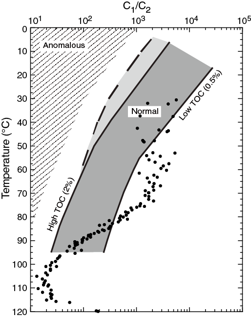
Figure F54. Methane/ethane molar ratios vs. temperature.

Figure F55. Dissolved sulfate, dissolved methane, and C1/C2.
Table T21. Hydrocarbon gas contents determined in headspace vials. Download table in .csv format.
As an integral part of the WRC sampling plan, additional gas samples (sample code 370HS) were taken from designated and carefully selected COMGAS WRC sample located adjacent to WRC slices assigned as IW and microbiology (MBIO1 and MBIO2) samples. WRC samples were selected after X-ray CT imaging to ensure that the selected horizons were minimally disturbed and minimally contaminated by drilling operations. The 370HS samples were taken from the center of the COMGAS slice after removal of >5 mm of the outer edges to avoid potential contamination from intrusion of drilling fluid. For these reasons, we expected that headspace gas analyses of the 370HS samples would generally reflect in situ hydrocarbon gas concentrations more accurately than the HS samples taken from the core cutting area, particularly in the more lithified and cemented deeper sediments retrieved using the RCB (after Core 370-C0023A-16R, >400 mbsf).
HS and 370HS sample data are plotted together in Figure F55, and a statistical comparison was performed using a two-tailed Student’s t-test, separating data for cores obtained using HPCS and RCB coring to determine the effect of coring type. The values for both HPCS and RCB coring indicate no significant difference between HS and 370HS methane concentrations (tAPC = 2.09, degrees of freedom = 15, confidence level = 97.5%; tRCB = −0.80, degrees of freedom = 41, confidence level = 97.5%), indicating that no measurable degassing occurred between the time of arrival of the core in the core cutting area and WRC sampling for either type of coring system. It is worth noting, however, that there is a greater difference between HS and 370HS methane concentrations for HPCS coring (tcalc is much closer to tcrit). We noticed less scatter in the 370HS gas data, which we partly attribute to the careful selection of minimally disturbed sediments for WRC sampling after X-ray CT scanning, whereas HS samples were taken nonselectively from core catcher material that varied more widely in core quality and lithology/sediment type.
Likewise, trends in C1/C2 are generally similar between the HS and 370HS data sets (Figure F55); C1/(C2 + C3) and C1/C3 ratios follow the depth trend of C1/C2 (Table T21). Deeper than ~700 mbsf, the C1/C2 ratio in the HS samples is slightly lower than in the 370HS samples. Preferential loss of methane due to degassing, relative to ethane, can explain this observation, as the solubility of ethane is greater than that of methane at 20°C (Bernard et al., 1976). Notably higher dissolved methane concentrations in COMGAS samples (370HS) than in HS samples deeper than ~700 mbsf support the conclusion that less methane is lost from the former samples due to degassing. Furthermore, the C1–C4 concentrations from the 370HS data set appear to be less noisy than the concentrations in the HS data set (Table T22; Figure F55). The improved smoothness and precision of the 370HS data set may be attributed to the availability of paired MAD data obtained on an adjacent sediment chunk taken from the same COMGAS sample as that from which the 370HS sample was derived (see Physical properties). The HS samples, collected in the core cutting area, did not have the benefit of paired porosity and density measurements and MAD data with which the dissolved gas concentrations were calculated; these were instead taken from the nearest MAD sample reported for a similar lithology as the HS sample.
Table T22. Hydrocarbon gas concentrations converted to molar concentrations. Download table in .csv format.
The HS and 370HS gas data are reported in parts per million (ppm) in the headspace gas sample (Table T21) and as corresponding molar concentrations (M) in IW (Table T22). HS gases, collected from the core cutting area, as in previous expeditions, are plotted in parts per million for better comparison to the gas data of Legs 131 and 190 (Figure F52). Methane concentrations in Hole C0023A have a wide scatter between 190 and ~700 mbsf, ranging from ~0.3 to 14.7 mM (average = ~4.4 mM) (Figure F55; Table T22). There is an apparent trend from lower values between 190 and 310 mbsf (average = 1.8 mM) to higher values between 410 and 640 mbsf (average = 6 mM), indicating a zone of methane production (cf. Claypool and Kvenvolden, 1983). This zone is followed by a sharp drop to <0.7 mM at 764 mbsf, coinciding with a zone of rising sulfate concentrations (Figures F55, F47), pointing to a SMTZ. Below this zone, methane concentrations remain low with average values around 0.4 mM to 900 mbsf and increase again to maximum values of ~1.2 mM at 1101 mbsf before dropping to ~0.2–0.8 mM in samples collected from basement rock at ~1175 mbsf.
Higher hydrocarbon gases, including ethane, propane, i-butane, and n-butane were detected in low amounts in headspace gas samples from nearly all depths (Figure F52; Table T21) with corresponding concentrations in IW averaging 3.2, 3.7, 0.1, and 0.5 µM, respectively (Figure F53; Table T22). Between 470 and 640 mbsf, there are notable increases in propane and i-butane with average values of 10 and 1.3 µM, respectively. A similar gas anomaly within the upper Shikoku Basin occurs at Sites 808 and 1174 (Shipboard Scientific Party, 1991, 2001b) (Figure F52). A combination of upward migration of thermogenic hydrocarbon gases along faults and gas production from immature kerogen were previously considered to be the cause of this anomalous hydrocarbon gas distribution (Berner and Faber, 1993). A depletion in all C2+ gases at ~750 mbsf coincides with the SMTZ observed in the methane and sulfate depth profiles (Figure F55, see also Figure F47) and may indicate a potential zone of microbial C2+ hydrocarbon gas consumption coupled to sulfate reduction. A second peak of all C2+ gases around 1050 mbsf, where estimated borehole temperatures exceed 100°C and C1/C2 ratios are consistent with typical ratios observed in areas with dominantly thermogenic methane, points to past and/or continuing breakdown of sedimentary organic matter to hydrocarbon gases. Higher i-butane over n-butane concentrations may be due to gas production from an immature kerogen as previously discussed for Site 808 (Berner and Faber, 1993), although other possibilities related to dynamic changes in sedimentation rate, large-scale deformation during the formation of the accretionary prism, and resultant passage of deep-sourced fluids and subsequent alteration by abiotic or microbially mediated reactions may also be responsible for the elevated i-butane levels. Several explanations can potentially account for decreasing concentrations in C2+ gases toward the basement, including (1) diffusive mixing of the dissolved hydrocarbon gas pool with that of hydrocarbon-poor fluids in the basement or (2) decreased hydrocarbon gas production due to lower TOC contents or poorer organic matter quality at these depths (Figure F51).
Conclusions
Shipboard organic geochemical analyses at Site C0023 lead to the following conclusions:
- Inorganic carbon (wt%) is variable with depth, reflecting changes in calcite cementation. Some underestimation and overestimation of carbonate and TOC contents, respectively, is possible due to potentially incomplete dissolution of carbonate minerals that are more resistant to acid attack (e.g., rhodochrosite); this remains to be evaluated in detail.
- TC and TOC contents are low throughout the cored part of the formation (<3 and <0.8 wt%, respectively), suggesting an aerobic depositional environment of the sediment with limiting potential for organic carbon preservation and large-scale hydrocarbon gas generation. The high number of burrows observed throughout the major part of all lithostratigraphic units is consistent with this interpretation. Generally, both TC and TOC contents decrease with depth to the décollement, below which TOC contents remain constant and may provide a steady source for C1–C4 hydrocarbon gas generation. High carbonate and TOC concentrations in the lowermost basalt sample suggest the presence of a calcite vein and the potential intrusion of organic carbon into the basalt via seawater.
- Nitrogen and sulfur contents are low in all cores, but a step-change is observed at 800 mbsf and coincides with changes in hydrocarbon gas concentrations, lithology, carbonate contents, and TOC/N ratio, suggesting there may be a common, as yet unexplained, origin for all these changes. TOC/N ratios indicate a marine source of the organic matter in all of the sediment samples.
- The C1/C2 ratio is consistent with a predominance of microbially generated methane to 800 mbsf. Deeper than 800 mbsf, thermally induced generation and release of short-chain hydrocarbons likely contribute in a larger part to concentrations of C1–C4 hydrocarbons.
Microbiology
Expedition 370 successfully collected numerous high-quality WRC sections for microbiological analyses and experiments. Core sampling and microbiological analyses were undertaken jointly by shipboard and shore-based microbiologists using super-clean technologies on the Chikyu and at KCC, respectively, and the QA and quality control (QC) protocols are outlined in Microbiology in the Expedition 370 methods chapter [Morono et al., 2017]). Investigations during the expedition relied on two types of WRC samples, namely MBIO1 (refrigerated for cell counts, etc.) and MBIO2 (frozen for molecular analysis), both typically 20–30 cm long. Multiple MBIO1 and MBIO2 samples were sometimes collected from a single recovered core, leading to a total of 150 MBIO1 and 141 MBIO2 samples from a total of 112 cores from Hole C0023A. Where possible, MBIO1 and MBIO2 samples were taken in close proximity to IW and COMGAS WRC samples. During the expedition, the transfer of critical microbiological samples from the Chikyu to KCC was accomplished with 44 helicopter flights.
Quality assurance and quality control for microbiological sample processing
Sampling of WRCs during Expedition 370 implemented multiple procedures to collect high-quality samples; to reduce and control potential microbial contamination from drilling fluid during coring, airborne particles, or laboratory equipment used to during sample processing; and to avoid cross contamination from previously taken cores (see Quality assurance and quality control for sample processing in the Expedition 370 methods chapter [Morono et al., 2017]). To reduce contamination from drilling fluid, undisturbed core sections were selected based on X-ray CT imaging and carefully cleaned. To quantify drilling-induced contamination of sediment cores, a perfluorocarbon (PFC) tracer (perfluoromethylcyclohexane [PMCH]) was added to drilling fluid before pumping it into the borehole and then measured in core liner fluid and in cross sections of core material. To decrease microbial contamination from airborne particles, all samples were processed under clean air conditions created by air filtration systems and static particle removers. Moreover, the airborne contamination potential was monitored with the help of particle counters and air samples. In the following, the results of contamination control are reported.
Assessment of airborne contamination potential
Monitoring airborne particles
Effective reduction of airborne particles by the KOACH air filtration system and static particle remover on the Chikyu was confirmed with the help of a particle counter before WRC processing. In the anaerobic glove box, the number of airborne particles sized between 0.3 and 1.0 µm ranged from not detected (ND; <3.53 × 10² particles/m3) to 1.8 × 10⁵ particles/m3. In the clean bench, the total number of airborne particles (0.3–1.0 µm sized) ranged from ND to 2.2 × 10⁴ particles/m3. In contrast, the number of particles in laboratory air surrounding the anaerobic glove box and outside of the clean bench had particle counts ranging from 1.8 × 10⁶ to 5.3 × 10⁷ particles/m3 and from 5.9 × 10⁵ to 3.1 × 10⁷ particles/m3, respectively (Figure F56; also see PARTICLE_COUNT_DATA.xlsx in MBIO in Supplementary material).
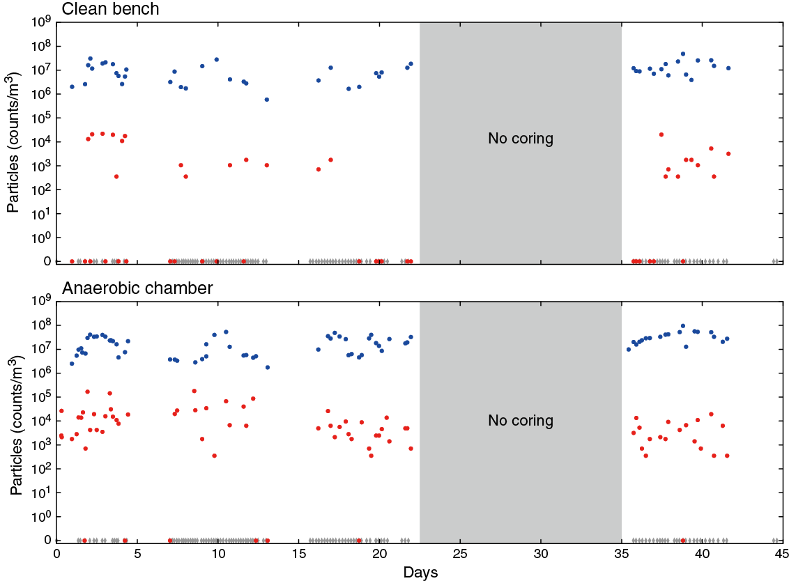
Figure F56. Airborne contamination potential during microbiology sample processing.
At KCC, airborne particle concentrations in the vicinity of the work area of the super-clean room were consistently below the detection limit of the particle counter (i.e., <1 particle/ft3). In the anaerobic chamber with a KOACH air filtration system fitted, counts for particles with a diameter of 0.3–2.5 µm ranged from 0 particles/m3 prior to sample processing to a maximum of 104 to 105 particles/m3 within 5 min after sample processing.
Monitoring airborne microbial cells
In order to assess the potential for airborne contamination of cores during shipboard core processing, air was collected for quantification of airborne microbial cells. Sampling of air was performed twice: once after processing Core 370-C0023A-82R and once after Core 83R. A 1 L volume of air was sampled from each of the following four core processing workspaces: (1) the QA)/QC laboratory, (2) the microbiology laboratory, (3) the clean bench equipped with a KOACH air purification system, and (4) the anaerobic chamber, also equipped with a KOACH air purification system. Airborne microbial cells in the sampled air were collected onto 0.2 µm membrane filters and fixed for cell counting at KCC.
Visual inspection of the membranes of shipboard air samples at KCC showed submicrometer-scale particle densities consistent with particle counts in all four core processing workspaces. However, very few of these airborne particles were cells. Cell counts after processing Cores 82R and 83R were 1 and 2 cells/L, respectively, in the microbiology laboratory and 0 and 1 cells/L, respectively, in the QA/QC laboratory. In the workspace of the UV-sterilized clean bench and in the anaerobic chamber, no cell was observed on any membrane.
At KCC, the same procedure was followed for air sampling from all workspaces where cores came into contact with the surrounding sampling environment: (1) the anaerobic chamber for MBIO1 core and other refrigerated sample processing, (2) the clean bench for MBIO2 subsampling, and (3) the super-clean room. Visual inspections of membranes show that submicrometer particle counts in these spaces were also consistent with particle counter analysis; however, no cell was detected on membranes from any of the workspaces. In addition, even a sample taken at one of the normal laboratory spaces showed no cell in 1 L of air.
These results in the context of the open air and nonclean laboratory positive controls suggest that airborne particle contamination in the clean workspaces should not be a major source of contamination.
Assessment of core contamination from drilling fluid
PFC chemical tracer was used to estimate the contamination level of cored materials. To gain in-depth information with regard to possible contaminants, samples for cell and virus counts as well as molecular (DNA, lipids, etc.) analyses were also prepared from seawater, seawater gel, core liner fluid, and cross-sectional parts of WRC subsections.
Monitoring contaminants in drilling fluid
In order to estimate the biological contamination potential and identify genetic markers of contamination, daily samples of potential drilling fluid components (drilling fluid from Pump 2 and seawater gel from an active mud tank; see also Figure F28 in the Expedition 370 methods chapter [Morono et al., 2017]) were collected into Falcon tubes. Information on sampling times and corresponding cores is given in Tables T23 and T24. Part of these samples (2 mL) was fixed in a cell-free saline formaldehyde solution and stored at 4°C for cell enumeration, and the other portion of these samples (2 mL) was fixed in virus-free saline formaldehyde solution, frozen in liquid nitrogen, and stored at −80°C. Samples for DNA analysis were stored at −80°C. Samples were transported to KCC for analysis.
Table T23. Drilling fluid samples collected from Pump 2. Download table in .csv format.
Table T24. Seawater gel samples collected from active mud tanks. Download table in .csv format.
Monitoring contaminants in core liner fluid
Core liner fluid samples (sample code LCL) were used to assess the biological contamination potential to core samples from surrounding fluid. If core liner fluid had not been lost during retrieval, the fluid was collected into Falcon tubes (Table T25). These samples (2 mL) were fixed in a cell-free saline formaldehyde solution and stored at 4°C for cell enumeration. Samples for virus enumeration (2 mL) were fixed in virus-free saline formaldehyde solution, frozen in liquid nitrogen, and stored at −80°C. During the expedition period, 26 samples (out of a total of 165) were processed and counted for microbial cell abundance at KCC (Table T26). Generally, cell abundance in the liner fluid consistently ranged from 104 to 105 cells/cm3. Processing and counting cells in remaining samples will be undertaken at KCC after the expedition. Samples for DNA analysis were stored at −80°C for future DNA extraction and sequencing.
Table T25. Samples collected from core liner fluid. Download table in .csv format.
Table T26. Cell abundance in core liner fluid. Download table in .csv format.
Monitoring contamination using PFC tracer
Since the early exploration stages of deep biosphere–dedicated scientific drilling, it has been recognized that drilling fluid is an important source of chemical and biological contamination (Colwell et al., 1992). Depending on the composition and storage of the drilling fluid, cell counts might be orders of magnitude higher in the drilling fluid compared to indigenous microbial populations in deep subseafloor sediments. Although we found that cell concentrations in drilling fluid probably did not exceed ~105 cells/cm3 during Expedition 370, which is 3 orders of magnitude lower than that used for riser drilling (Inagaki et al., 2015), small amounts of drilling fluid intrusion into cored samples may still cause changes in the microbial community size and structure. Consequently, it is of primary importance for any geobiological and microbial ecological study to assess the sample quality with regard to potential contamination.
During Expedition 370, PFC was supplied to the drilling fluid stream into the inlet of Pump 2 via a high-pressure liquid chromatography pump (see Figure F28 in the Expedition 370 methods chapter [Morono et al., 2017]), with an average flow rate of 0.6 mL/min of liquid PFC (i.e., 1.787 g/cm3 density and 94% purity; Manchester Organics M17797). The input concentration of PFC could not be determined exactly as it depended on both the total flow rate into the borehole (between 250 and 4000 L/min) and the flow rate of Pump 2 (between 0 and 1300 L/min), which varied as required by drilling operations. Based on observations of typical drill pump flow rate profiles, we determined at least 0.084 mg PFC/L was added to the drilling fluid during standard coring operations. Based on PFC solubility in water (Smith et al., 2000), the maximum concentration of PFC added to the drilling fluid was assumed to be 1.8 mg/L. Due to technical problems with the pumps delivering either PFC or drilling fluid, PFC was found to not be added to the drilling fluid for Cores 1F through 9F and only intermittently added for Cores 10F through 15F. Thus, the amount of contamination by drilling fluid into the short HPCS/ESCS cores could not be quantified reliably. For Cores 1F through 15F, other measures of contamination, such as records of drilling disturbance, X-ray CT images, and the proportion of seawater intrusion as determined by SO42− concentration (see Inorganic geochemistry), may be more useful than the drilling fluid contamination assessment via PFC monitoring.
During Expedition 370, the gas chromatograph–electron capture detector (GC-ECD) was demonstrated to be highly reliable and accurate for determining the headspace PFC concentration. Measurement of standards of the same concentration produced in parallel within 1 day resulted in an analytical error of <1%, even for the most diluted standard. During our extensive PFC monitoring program on the Chikyu, we observed that a volatile compound in the commercial surface decontamination product RNase AWAY (Thermo Fisher Scientific) coeluted with PFC when using a GS-GasPro column (Agilent; 30 m long and 0.320 mm inside diameter) in the GC-ECD. This coelution might lead to an overestimation of PFC in samples taken on the core processing deck or at KCC, where RNase AWAY was applied routinely but did not affect samples of core liner fluid or sediment taken in the core cutting area. As a precaution, after Core 370-C0023A-55R RNase AWAY was not used in the clean bench before PFC sample processing from MBIO2. On the other hand, coelution of the volatile component of RNase AWAY and PFC was not observed in the analysis using the GC-ECD equipped with an HP-ALM column. Because much of the sampling in the onshore microbiology laboratory at KCC was conducted in an anaerobic chamber, where routine surface decontamination by RNase AWAY was conducted, PFC analysis at KCC was performed with an HP-ALM column from 12 October 2006. More than an order of magnitude greater PFC concentrations were detected on average using the GS-GasPro over the HP-ALM column as shown below, indicating that the RNase AWAY interfered with the detection of PFC in those analyses.
Given the variability in input PFC concentrations into the drilling fluid pumped down the borehole, the concentration of PFC in the core liner fluid surrounding core samples was determined to confirm the minimum concentration of PFC present during core cutting. At the beginning of the expedition, core liner fluid was collected in 50 mL Falcon tubes in the core cutting area, and the liquid was subsampled in the microbiology laboratory into 20 mL headspace vials (FAL-L samples, see Table T11 in the Expedition 370 methods chapter [Morono et al., 2017] for detailed descriptions of samples). This procedure was chosen to minimize sample handling in the core cutting area. After Core 16R, core liner fluids were directly collected in the core cutting area immediately after core retrieval into 20 mL headspace vials (CCA-L samples). We found that there was more PFC loss in FAL-L samples compared to CCA-L samples (Figure F57), suggesting that sampling of the PFC tracer is time-sensitive and sample preservation in the core cutting area is critical. To determine if the difference between FAL-L and CCA-L samples was due to PFC loss during laboratory handling, multiple samples of core liner fluids from different core sections were collected in parallel in Falcon tubes and headspace vials for Cores 18R, 19R, 20R, 23R, 24R, and 33R. In some of these cores, the CCA-L PFC concentration was three orders of magnitude greater than FAL-L PFC concentrations (Figure F57). For this reason, from Core 33R onward we decided to only collect CCA-L samples instead of FAL-L samples. As core liner fluid was not present in some of the retrieved cores in the core cutting area, sediment scrapings from the top of the exterior of Section 1 (the most exposed part of the core to drilling fluid in the core barrel) were also collected in headspace vials after Core 34R (CCA-S sample). CCA-S samples were collected from the top of Section 2 if Section 1 was not available.
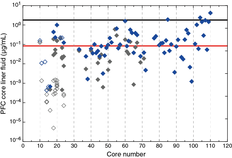
Figure F57. PFC tracer concentrations in core liner fluid.
In addition to samples of core liner fluid and exposed sediment taken in the core cutting area, cross sections of sediment cores were carefully sampled on the core processing deck. Altogether, more than 600 samples of cored material were analyzed on board for PFC concentration (Table T27, Figure F58; raw data can be found in PFC_RAW_DATA.xls in MBIO in Supplementary material). In RCB cores of deeper sediments, PFC concentration was greater in the exterior of the cores compared to the interior and midway parts by at least one order of magnitude. Many interior samples had very low PFC concentrations, and in 44% of the interior samples PFC was below detection (Figure F58). In some core sections that contained high concentrations of PFC in the interior sediment, the occurrence of microfractures was observed in the X-ray CT image (Figure F59). It is worth noting, however, that the measured PFC concentration cannot be used to determine the presence of microfractures as fractures are highly spatially variable. The PFC calibration curve and PFC raw data information are summarized in EXP370_PFC_CALIBRATION_CURVE.xlsx and PFC_RAW_DATA.xls, respectively, in MBIO in Supplementary material.
Table T27. PFC concentrations in core liner fluid and sediment cross sections, Hole C0023A. Download table in .csv format.
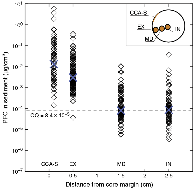
Figure F58. PFC tracer concentrations along cross sections of sediment cores.
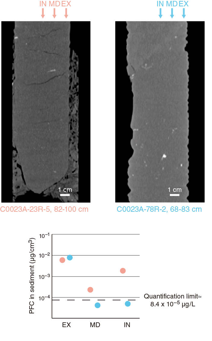
Figure F59. Impact of core quality on contamination of drilling cores with drilling fluid.
At KCC, PFC tracer was detected in 141 out of 144 MBIO1 KCC secondary scrapings and in 211 out of 305 MBIO1 KCC interior samples (Table T28). There was more than an order of magnitude difference in the average detected PFC concentration using the GC-GasPro (2.38 × 10⁻³ µg PFC/g sediment) compared to the HP-ALM (8.29 × 10⁻⁵ µg PFC/g sediment) column. Because much of the sampling at KCC was conducted with routine surface decontamination by RNase AWAY, these results indicated that as described above the volatile component of RNase AWAY strongly interfered with the detection of PFC using the GC-GasPro column. There was an overall trend that the KCC interior samples had lower PFC concentrations than the KCC secondary scrapings (detected mean abundances of 8.29 × 10⁻⁵ and 1.86 × 10⁻⁴ µg PFC/g sediment, respectively) when analyzed with the HP-ALM column. Because the samples for onshore PFC measurements were taken at least several days after core retrieval, the potential of contamination needs to be carefully assessed in combination with other measures of contamination tracing.
Table T28. PFC measurement results at KCC. Download table in .csv format.
Shipboard WRC sampling and experiments
Shipboard WRC sampling
Core sections for WRCs were prioritized for X-ray CT imaging. WRC locations were selected using the X-ray CT images and then immediately sampled, which greatly reduced potential exposure to oxygen. Most MBIO1 and MBIO2 samples were from the same section (or in close proximity) as the IW and COMGAS WRC samples. Following WRC cutting with sterile spatulas, the exterior of all MBIO1 sections was immediately scraped off in the anaerobic glove box. Notably, in Cores 370-C0023A-5F and 9F, the exterior of WRCs for personal requests could not be cleaned with a ceramic knife, as the core material had fluidized during core recovery. Two sets of MBIO1 and MBIO2 were sampled from Core 63R; one set was processed as described in Microbiology in the Expedition 370 methods chapter (Morono et al., 2017), whereas the second set was sampled ~14 h after core retrieval from the working half section (i.e., brecciated part of the décollement). Basalt cores (Cores 111R and 112R) were not processed in the anaerobic glove box but were immediately nitrogen flushed, vacuumed, sealed in a double ESCAL bag, and stored at 4°C. Information on MBIO1 and MBIO2 WRCs and their samples was summarized in MBIO_SAMPLE_LIST.xlsx in MBIO in Supplementary material. All WRC samples for cell counts, cultivation, and activity measurements were processed (see Microbiology in the Expedition 370 methods chapter [Morono et al., 2017]), packaged into ESCAL bags under N2-flushed anaerobic conditions, and then placed under the designated storage conditions within 4 h after core recovery on the rig floor. In general, WRCs for molecular microbiological studies were frozen by the Cells Alive System within 2 h.
WRC samples for potential metabolic activity tests with radiotracers
A total of 43 WRCs were obtained for potential sulfate reduction and potential hydrogenotrophic methanogenic activity determinations from Sections 1F-1 through 112R-1 (Table T29). From each WRC, triplicate samples were obtained for each analysis. Sample volumes were ~5 cm3; sample weight determination will be accomplished in the home laboratory (UCLA, USA). Samples were incubated at four different temperatures (40°, 60°, 80°, and 95°C) according to the closest in situ temperature. Additionally, drilling fluid samples were incubated at 40°, 60°, 80°, and 95°C to test for potential background contamination: DF2 and SWG samples from the mud tank and liner fluid, respectively (Table T29). One additional set of mud tank samples (DF2 and SWG) was preincubated at 95°C before incubation with radiotracers at 40°, 60°, 80°, and 95°C to test the effect of high temperature on contamination.
Table T29. Samples collected for potential metabolic activity tests with radiotracers. Download table in .csv format.
To each sulfate reduction and methanogenesis sample, 3.7 MBq of 35S-sulfate (10 µL aqueous solution) and 14C-bicarbonate (100 µL aqueous solution), respectively, was added until Section 108R-2. Incubation time was 10 days. Deeper samples (starting at Section 110R-3, sample code 370TT1WR) received a twofold amount of tracer (i.e., 7.4 MBq), as available incubation time became shorter (5–7 days) toward the end of the expedition.
Aside from short-term shipboard activity tests, incubations will continue in home laboratories with sediments from replicate WRCs to further examine methanogenesis (University of Aarhus, Denmark; sample code 370FBWR), sulfate reduction (GFZ Potsdam, Germany; sample code 370JKWR), methane oxidation (UCLA, USA; sample code 370TTWR2), and hydrogenase activity (University of Bremen, Germany; sample code 370RRAWR) with radiotracers in long-term experiments.
Shore-based WRC sampling and experiments at KCC
Shore-based WRC sampling
We adopted a strategy for the careful removal of potentially contaminated surfaces of WRCs. MBIO1 WRCs with the outer surface already removed were transferred by helicopter to KCC, and a secondary surface was removed immediately prior to sampling in an anaerobic chamber (for details see Microbiology in the Expedition 370 methods chapter (Morono et al., 2017). For core samples from the shallower part of the hole, we used a spatula (Sections 370-C0023A-1F-1, 3F-3, 9F-3, 12F-CC, and 13F-2) or cut-off syringe (Sections 2F-1, 4F-1, 5F-3, 6F-2, 7X-1, and 9F-1) for sampling because the core material was too soft or unconsolidated to scrape both on the Chikyu and at KCC. Approximately 10 cm3 of sediment was taken from each MBIO1 WRC under anaerobic conditions for analysis of cell abundance. For samples from Cores 1F through 33R, the sediment was immediately submerged in 20 mL of 0.3% saline and 4% formaldehyde fixation solution. Friable samples were shaken by vortex to form an approximately 1:2 (v/v) slurry and stored at 4°C. More compact samples required an additional crushing step to generate a homogeneous sediment slurry using a precombusted (500°C for 5 h) pestle and mortar in the super-clean room. Samples from Cores 34R through 112R were maintained under anaerobic conditions until crushing, immediately prior to immersion in fixation solution.
Frozen WRCs were also carefully sampled in the super-clean room at KCC for PFC monitoring, virus visualization, and DNA-based analysis of microbial composition. In total, 141 subcores were taken from the center of WRCs as described in Microbiology in the Expedition 370 methods chapter (Morono et al., 2017).
Cell counts
Fixed cells were separated from the slurry via ultrasonication and density gradient centrifugation (see Microbiology in the Expedition 370 methods chapter [Morono et al., 2017]), and the supernatant was filtered onto a 0.02 µm polycarbonate membrane and dyed with SYBR Green I nucleic acid stain. Cells were counted by eye: at least 900 fields of view (FOVs) were analyzed for each whole membrane and at least 450 FOVs were analyzed for each half membrane.
During the expedition, 27 cell count samples and 9 negative control samples were analyzed, ~20% of the anticipated total number of data points. In the context of sample preparation for cell counting at KCC, negative control membranes were prepared whereby saline solution was passed through all the cell separation and membrane preparation protocols. Of the nine negative control membranes, the mean number of particles on a membrane was 0.89 with a standard deviation of 1.1 and a maximum of 3. These negative control counts correspond to the MQL of 21 cells/cm3 for a slurry of 1 mL passed through the membrane. The 27 cell count samples include 4 samples where no cells were observed and 4 samples with a cell count below the maximum negative control.
Between 200 and 450 mbsf, cell counts decreased from 2.6 × 10⁴ to 18 cells/cm3 (Figure F60). Deeper than 450 mbsf, cell counts were consistently low; the maximum cell concentration was 405 cells/cm3 at 513 mbsf, with many samples below the detection limit. All data presented here should be considered to be preliminary as they have not yet been quantitatively corrected for potential contamination by drilling fluid via PFC analysis and a thorough uncertainty analysis has not yet been undertaken.
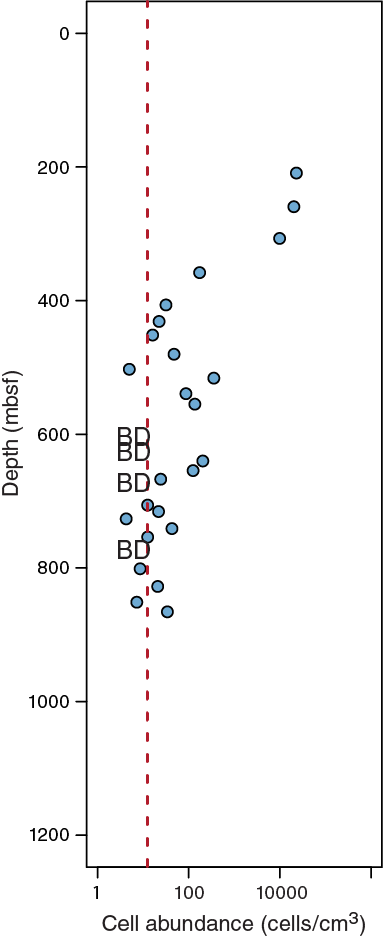
Figure F60. Preliminary cell count data.
Density-separated cells from Section 6F-2 (304 mbsf) were further sorted onto a SiN membrane for electron microscopy observation. The location of sorted microbial cells on the membrane was ascertained by fluorescent microscopy, and the coordinates were revisited with transmission electron microscopy for imaging at high magnification (Figure F61).
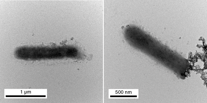
Figure F61. Transmission electron micrographs of microorganisms.
Molecular analysis
DNA was extracted from 5 g of crushed sediment taken from 115 WRCs (Table T30) as described in Microbiology in the Expedition 370 methods chapter (Morono et al., 2017). The concentration of DNA from the shallowest sample (Section 1F-1; 189.9 mbsf) was measured using a NanoDrop 3300 fluorospectrometer with PicoGreen staining (Thermo Fisher Scientific); however, the concentration was not measurable due to the low amount of DNA. Considering the cell count data (Figure F60), we assumed that the DNA concentration should decrease even further with depth, so we decided not to measure the DNA concentration for the deeper samples and directly amplified by PCR. After 35 cycles of PCR, amplified products could be obtained from almost all samples and those were purified and indexed as described in Microbiology in the Expedition 370 methods chapter (Morono et al., 2017). Together with the sediment samples, we also did negative control extractions by replacing samples with gamma ray–irradiated 18 MΩ water. In addition, no template control PCR amplification was performed by replacing samples also with gamma ray–irradiated 18 MΩ water.
Table T30. 16S rRNA gene sequences. Download table in .csv format.
During the expedition period, we sequenced 109 samples and obtained 10,045,606 sequences (Table T30) after quality trimming. Preliminary analysis on a phylum level classification of the 16S rRNA gene sequences indicated a potential boundary in microbial composition between lithostratigraphic Subunits IIA and IIB, consistent with the preliminary cell count data dropping at that boundary. Above the boundary, some well-known marine sedimentary bacteria and archaea were detected. Members of the phylum Atribacteria were highly abundant from Sections 1F-1 through 4F-1 (189.9–254 mbsf), comprising 57% of the total sequences in Section 3F-3 (Figure F62). Atribacteria have often been detected in organic-rich anoxic marine sediment, including hydrate-bearing sediments of the Nankai Trough and Peru margins (Reed et al., 2002; Inagaki et al., 2006). The phylum Chloroflexi, including class Dehalococcoidia, was also prevalent in the shallower sediment to Section 9F-3 (320 mbsf). Below the boundary, the proportion of Proteobacteira increased and it is higher than 60% in almost all samples through the depth tested during the expedition. Firmicutes and Actinobacteria were more abundant in the deeper sediment below the boundary than in the upper sediments. In-depth analysis of sequence data will be performed during postexpedition research, including intensive examination of control samples such as drilling fluid and negative controls (both DNA extraction and PCR amplification).
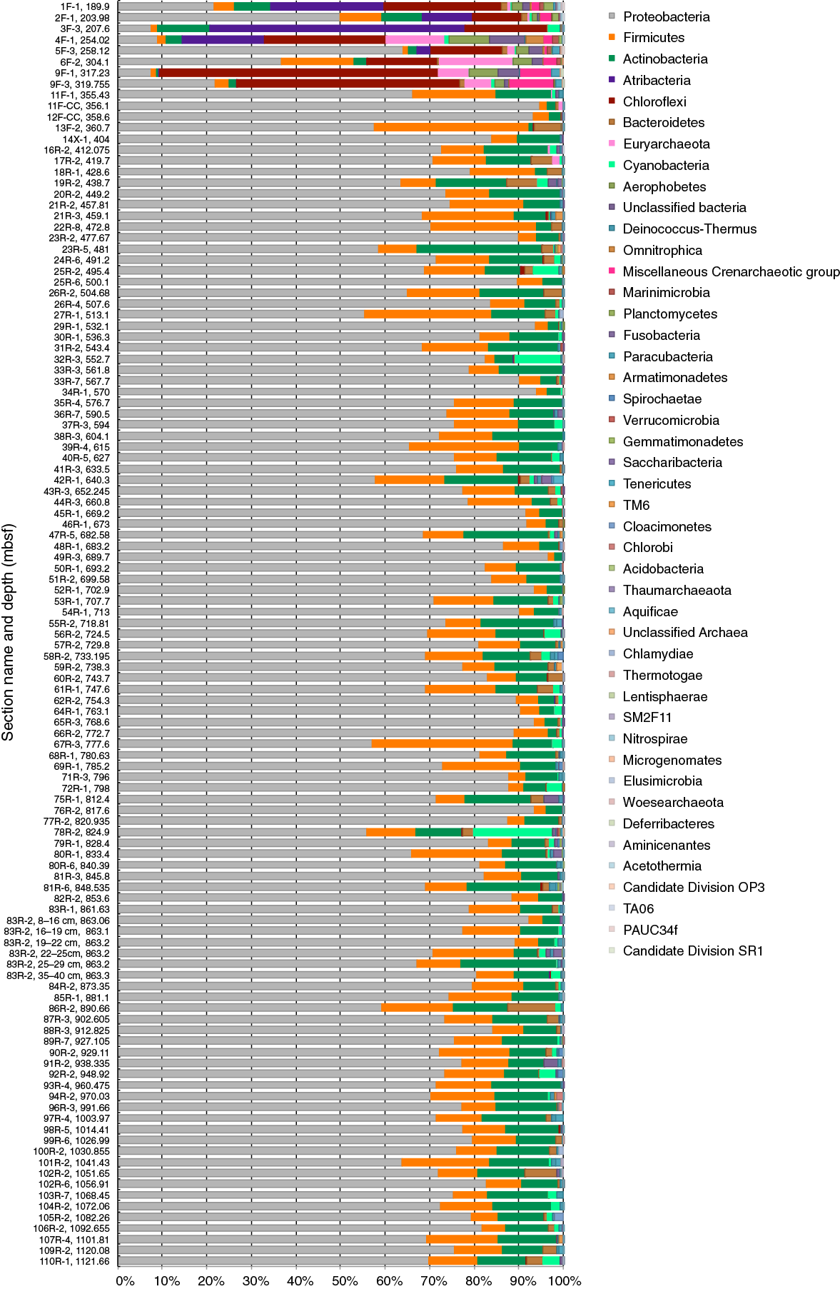
Figure F62. Phylum-level microbial composition of sediments.
High-pressure/temperature incubation
A total of 11 WRCs taken from 660 to 850 mbsf were used for the high-pressure/temperature (high-P/T) incubation experiment conducted at KCC to study microbial activity around the décollement zone (Table T31). The depth range corresponds to the upper part of Unit IV, including the décollement at 758–796 mbsf (see Lithostratigraphy) and the SMTZ at 640–764 mbsf (see Inorganic geochemistry). The surface of each 50 cm3 WRC was removed with ceramic knives and subsequently reduced to powder. All 11 powdered samples were mixed to make a master formation mix. In each incubator, 30 cm3 of the master formation mix was put into the inner incubation chamber together with 35 mL of basal media (see Microbiology in the Expedition 370 methods chapter [Morono et al., 2017]). The five incubators were set to the same pressure (55 MPa) and five different incubation temperatures (80°, 95°, 110°, 125°, and 140°C). Each incubation chamber has four inner incubation chambers. The incubation started without stable isotope–labeled substrates. After all five pressure chambers reached designated incubation temperatures and pressure, four different substrate mixtures were injected into four incubation chambers at respective incubation temperatures (see Microbiology in the Expedition 370 methods chapter [Morono et al., 2017]). The incubation was started during the expedition period and will be continued as postexpedition research.
Table T31. Samples for high-P/T incubation. Download table in .csv format.
Temperature-induced plasticity of metabolism
A suite of incubation experiments was undertaken with sediments collected from eight different horizons and incubated as slurry in anaerobic liquid media (2:1 sediment to liquid ratio) at five temperatures. The incubation temperatures are 37°, 50°, 60°, 70°, and 80°C. The sediment samples are from 253, 414, 497, 589, 689, 821, 922, and 1032 mbsf (Sections 4F-1, 16R-3, 25R-4, 36R-6, 49R-3, 77R-2, 89R-4, and 100R-3, respectively). These depths correspond to preliminary estimated in situ temperatures of approximately 37.1°, 53.6°, 61.8°, 70.6°, 79.9°, 91.5°, 100.0°, and 108.8°C, respectively.
High-temperature enrichment of thermophilic endospore–forming microorganisms
Enrichment culture microcosms were established with 35 g of finely crushed sediment from Sections 3F-3, 4F-1, 19R-2, 51R-3, and 83R-1 (207.435, 253.870, 438.790, 701.010, and 862.430 mbsf, respectively). The crushed sediment was combined with 70 mL of artificial seawater medium (Widdel and Bak, 1992; Isaksen et al., 1994) amended with organic acids (lactate, propionate, succinate, acetate, formate, and butyrate), each to a final concentration of 1 mM and pasteurized at 80°C for 1 h. Each microcosm was then incubated at 50°, 60°, or 70°C. The microcosms were sampled 13 times over a period of 21 days, with decreasing frequency of sampling as incubation time increased. DNA was extracted using the PowerLyzer PowerSoil DNA isolation kit (MO BIO Laboratories, USA) as per the manufacturer’s instructions. PCR and sequencing was done using the same method as used for the MBIO2 samples. 16S rRNA gene sequence analysis will be done using the MetaAmp pipeline developed by X. Dong and M. Strous (unpubl., http://ebg.ucalgary.ca/metaamp). Sequences were obtained but not analyzed upon completion of the expedition. They will be reported separately in future publications.
Exoenzyme activity
Exoenzyme control experiments were run to determine the feasibility of measuring exoenzyme activity in low-biomass samples at high temperatures using fluorescent substrate analogs. The primary concern was that the rate of abiotic, primarily thermal degradation of the substrate analog at high temperatures may be too high to detect biotic degradation by the sparse in situ microbial communities. To address this, sediment from Sample 1F-1WR MBIO1 was suspended in phosphorus-free artificial seawater and gamma ray irradiated to produce killed control samples. Substrate analogs for leucine aminopeptidase and alkaline phosphatase were then added in experimental concentrations (see Table T17 in the Expedition 370 methods chapter [Morono et al., 2017]) and incubated in anaerobic serum bottles at 30°, 50°, 60°, and 80°C. Abiotic degradation of substrate at each temperature was determined by measuring the increase in fluorescence over two time points, 3 days apart. Once normalized to a standard curve of fluorescent product, the increase in fluorescence over time was converted to nanomoles of substrate cleaved per hour. In addition, nonkilled Sample 1F-1WR MBIO1 sediment was also incubated with the same concentrations of substrate analogs at a near in situ temperature, 30°C, and activity was measured over the course of 6 days. Future experiments will expand these control experiments to the exoenzyme esterase and the other lithostratigraphic units as well as add controls for strictly thermal degradation of product versus sediment-mediated degradation.
References
Athy, L.F., 1930. Density, porosity, and compaction of sedimentary rocks. AAPG Bulletin, 14(1):1–24.
Behl, R.J., 2011. Chert spheroids of the Monterey Formation, California (USA): early-diagenetic structures of bedded siliceous deposits. Sedimentology, 58(2):325–351. https://doi.org/10.1111/j.1365-3091.2010.01165.x
Bernard, B.B., Brooks, J.M., and Sackett, W.M., 1976. Natural gas seepage in the Gulf of Mexico. Earth and Planetary Science Letters, 31(1):48–54. https://doi.org/10.1016/0012-821X(76)90095-9
Berner, U., and Faber, E., 1993. Light hydrocarbons in sediments of the Nankai accretionary prism (Leg 131, Site 808). In Hill, I.A., Taira, A., Firth, J.V., et al., Proceedings of the Ocean Drilling Program, Scientific Results, 131: College Station, TX (Ocean Drilling Program), 185–195. http://dx.doi.org/10.2973/odp.proc.sr.131.120.1993
Blöchl, E., Rachel, R., Burggraf, S., Hafenbradl, D., Jannasch, H.W., and Stetter, K.O., 1997. Pyrolobus fumarii, gen. and sp. nov., represents a novel group of archaea, extending the upper temperature limit for life to 113°C. Extremophiles, 1(1):14–21. http://www.ncbi.nlm.nih.gov/pubmed/9680332
Claypool, G.E., and Kvenvolden, K.A., 1983. Methane and other hydrocarbon gases in marine sediment. Annual Review of Earth and Planetary Sciences, 11(1):299–327. https://doi.org/10.1146/annurev.ea.11.050183.001503
Colwell, F.S., Stormberg, G.J., Phelps, T.J., Birnbaum, S.A., McKinley, J., Rawson, S.A., Veverka, C., Goodwin, S., Long, P.E., Russell, B.F., Garland, T., Thompson, D., Skinner, P., and Grover, S., 1992. Innovative techniques for collection of saturated and unsaturated subsurface basalts and sediments for microbiological characterization. Journal of Microbiological Methods, 15(4):279–292. http://dx.doi.org/10.1016/0167-7012(92)90047-8
Demaison, G.J., and Moore, G.T., 1980. Anoxic environments and oil source bed genesis. AAPG Bulletin, 64:1179–1209.
Emeis, K.-C., and Kvenvolden, K.A., 1986. Technical Note 7: Shipboard Organic Geochemistry on JOIDES Resolution. Ocean Drilling Program. https://doi.org/10.2973/odp.tn.7.1986
Fritz, D., 1980. Safety and pollution-prevention program, Deep Sea Drilling Project Leg 50, Sites 415 and 416. In Lancelot, Y., Winterer, E.L., et al., Initial Reports of the Deep Sea Drilling Project, 44: Washington, DC (U.S. Government Printing Office), 855–859. https://doi.org/10.2973/dsdp.proc.50.app5.1980
Head, I.M., Jones, D.M., and Larter, S.R., 2003. Biological activity in the deep subsurface and the origin of heavy oil. Nature, 426(6964):344–352. http://dx.doi.org/10.1038/nature02134
Heuer, V.B., Inagaki, F., Morono, Y., Kubo, Y., Maeda, L., Bowden, S., Cramm, M., Henkel, S., Hirose, T., Homola, K., Hoshino, T., Ijiri, A., Imachi, H., Kamiya, N., Kaneko, M., Lagostina, L., Manners, H., McClelland, H.-L., Metcalfe, K., Okutsu, N., Pan, D., Raudsepp, M.J., Sauvage, J., Schubotz, F., Spivack, A., Tonai, S., Treude, T., Tsang, M.-Y., Viehweger, B., Wang, D.T., Whitaker, E., Yamamoto, Y., and Yang, K., 2017. Expedition 370 summary. In Heuer, V.B., Inagaki, F., Morono, Y., Kubo, Y., Maeda, L., and the Expedition 370 Scientists, Temperature Limit of the Deep Biosphere off Muroto. Proceedings of the International Ocean Discovery Program, 370: College Station, TX (International Ocean Discovery Program). https://doi.org/10.14379/iodp.proc.370.101.2017
Hinrichs, K.-U., Inagaki, F., Heuer, V.B., Kinoshita, M., Morono, Y., and Kubo, Y., 2016. Expedition 370 Scientific Prospectus: T-Limit of the Deep Biosphere off Muroto (T-Limit). International Ocean Discovery Program. http://dx.doi.org/10.14379/iodp.sp.370.2016
Horsfield, B., Schenk, H.J., Zink, K., Ondrak, R., Dieckmann, V., Kallmeyer, J., Mangelsdorf, K., di Primio, R., Wilkes, H., Parkes, R.J., Fry, J., and Cragg, B., 2006. Living microbial ecosystems within the active zone of catagenesis: implications for feeding the deep biosphere. Earth and Planetary Science Letters, 246(1–2):55–69. http://dx.doi.org/10.1016/j.epsl.2006.03.040
Inagaki, F., Hinrichs, K.-U., Kubo, Y., Bowles, M.W., Heuer, V.B., Long, W.-L., Hoshino, T., Ijiri, A., Imachi, H., Ito, M., Kaneko, M., Lever, M.A., Lin, Y.-S., Methé, B.A., Morita, S., Morono, Y., Tanikawa, W., Bihan, M., Bowden, S.A., Elvert, M., Glombitza, C., Gross, D., Harrington, G.J., Hori, T., Li, K., Limmer, D., Liu, C.-H., Murayama, M., Ohkouchi, N., Ono, S., Park, Y.-S., Phillips, S.C., Prieto-Mollar, X., Purkey, M., Riedinger, N., Sanada, Y., Sauvage, J., Snyder, G., Susilawati, R., Takano, Y., Tasumi, E., Terada, T., Tomaru, H., Trembath-Reichert, E., Wang, D.T., and Yamada, Y., 2015. Exploring deep microbial life in coal-bearing sediment down to ~2.5 km below the ocean floor. Science, 349(6246):420–424. http://dx.doi.org/10.1126/science.aaa6882
Inagaki, F., Nunoura, T., Nakagawa, S., Teske, A., Lever, M., Lauer, A., Suzuki, M., Takai, K., Delwiche, M., Colwell, F.S., Nealson, K.H., Horikoshi, K., D’Hondt, S., and Jørgensen, B.B., 2006. Biogeographical distribution and diversity of microbes in methane hydrate-bearing deep marine sediments on the Pacific Ocean margin. Proceedings of the National Academy of Sciences of the United States of America, 103(8):2815–2820. http://dx.doi.org/10.1073/pnas.0511033103
Isaksen, M.F., Bak, F., and Jørgensen, B.B., 1994. Thermophilic sulfate-reducing bacteria in cold marine sediment. FEMS Microbiology Ecology, 14:1–8. https://doi.org/10.1111/j.1574-6941.1994.tb00084.x
JOIDES Pollution Prevention and Safety Panel, 1992. Ocean Drilling Program guidelines for pollution prevention and safety. JOIDES Journal, 18(7):24. http://www.odplegacy.org/PDF/Admin/JOIDES_Journal/JJ_1992_V18_No7.pdf
Kashefi, K., and Lovley, D.R., 2003. Extending the upper temperature limit for life. Science, 301(5635):934. http://dx.doi.org/10.1126/science.1086823
Kirschvink, J.L., 1980. The least-squares line and plane and the analysis of palaeomagnetic data. Geophysical Journal of the Royal Astronomical Society, 62(3):699–718. http://dx.doi.org/10.1111/j.1365-246X.1980.tb02601.x
Klein, F., Humphris, S.E., Guo, W., Schubotz, F., Schwarzenbach, E.M., and Orsi, W.D., 2015. Fluid mixing and the deep biosphere of a fossil Lost City–type hydrothermal system at the Iberia margin. Proceedings of the National Academy of Sciences of the United States of America, 112(39):12036–12041. https://doi.org/10.1073/pnas.1504674112
Maltman, A., Labaume, P., and Housen, B., 1997. Structural geology of the décollement at the toe of the Barbados accretionary prism. In Shipley, T.H., Ogawa, Y., Blum, P., and Bahr, J.M. (Eds.), Proceedings of the Ocean Drilling Program, Scientific Results, 156: College Station, TX (Ocean Drilling Program), 279–292. http://dx.doi.org/10.2973/odp.proc.sr.156.037.1997
Maltman, A.J., 1998. Deformation structures from the toes of accretionary prisms. Journal of the Geological Society, 155:639–650. https://doi.org/10.1144/gsjgs.155.4.0639
Meyers, P.A., 1994. Preservation of elemental and isotopic source identification of sedimentary organic matter. Chemical Geology, 114(3–4):289–302. http://dx.doi.org/10.1016/0009-2541(94)90059-0
Moore, D.M., and Reynolds, R.C., Jr., 1989. X-Ray Diffraction and the Identification and Analysis of Clay Minerals: Oxford, United Kingdom (Oxford University Press).
Moore, G.F., Karig, D.E., Shipley, T.H., Taira, A., Stoffa, P.L., and Wood, W.T., 1991. Structural framework of the ODP Leg 131 area, Nankai Trough. In Taira, A., Hill, I., Firth, J.V., et al., Proceedings of the Ocean Drilling Program, Initial Reports, 131: College Station, TX (Ocean Drilling Program), 15–20. http://dx.doi.org/10.2973/odp.proc.ir.131.102.1991
Moore, G.F., Taira, A., Klaus, A., et al., 2001. Proceedings of the Ocean Drilling Program, Initial Reports, 190: College Station, TX (Ocean Drilling Program). http://dx.doi.org/10.2973/odp.proc.ir.190.2001
Moore, J.C., and Saffer, D., 2001. Updip limit of the seismogenic zone beneath the accretionary prism of southwest Japan: an effect of diagenetic to low-grade metamorphic processes and increasing effective stress. Geology, 29(2):183–186. http://dx.doi.org/10.1130/0091-7613(2001)029<0183:ULOTSZ>2.0.CO;2
Morono, Y., Inagaki, F., Heuer, V.B., Kubo, Y., Maeda, L., Bowden, S., Cramm, M., Henkel, S., Hirose, T., Homola, K., Hoshino, T., Ijiri, A., Imachi, H., Kamiya, N., Kaneko, M., Lagostina, L., Manners, H., McClelland, H.-L., Metcalfe, K., Okutsu, N., Pan, D., Raudsepp, M.J., Sauvage, J., Schubotz, F., Spivack, A., Tonai, S., Treude, T., Tsang, M.-Y., Viehweger, B., Wang, D.T., Whitaker, E., Yamamoto, Y., and Yang, K., 2017. Expedition 370 methods. In Heuer, V.B., Inagaki, F., Morono, Y., Kubo, Y., Maeda, L., and the Expedition 370 Scientists, Temperature Limit of the Deep Biosphere off Muroto. Proceedings of the International Ocean Discovery Program, 370: College Station, TX (International Ocean Discovery Program). https://doi.org/10.14379/iodp.proc.370.102.2017
Parkes, R.J., Wellsbury, P., Mather, I.D., Cobb, S.J., Cragg, B.A., Hornibrook, E.R.C., and Horsfield, B., 2007. Temperature activation of organic matter and minerals during burial has the potential to sustain the deep biosphere over geological timescales. Organic Geochemistry, 38(6):845–852. http://dx.doi.org/10.1016/j.orggeochem.2006.12.011
Pimmel, A., and Claypool, G., 2001. Technical Note 30: Introduction to Shipboard Organic Geochemistry on the JOIDES Resolution. Ocean Drilling Program. http://dx.doi.org/10.2973/odp.tn.30.2001
Reed, D.W., Fujita, Y., Delwiche, M.E., Blackwelder, D.B., Sheridan, P.P., Uchida, T., and Colwell, F.S., 2002. Microbial communities from methane hydrate–bearing deep-marine sediments in a forearc basin. Applied and Environmental Microbiology, 68(8):3759–3770. https://doi.org/10.1128/AEM.68.8.3759-3770.2002
Shipboard Scientific Party, 1991. Site 808. In Taira, A., Hill, I., Firth, J.V., et al., Proceedings of the Ocean Drilling Program, Initial Reports, 131: College Station, TX (Ocean Drilling Program), 71–269. http://dx.doi.org/10.2973/odp.proc.ir.131.106.1991
Shipboard Scientific Party, 1994. Explanatory notes. In Westbrook, G.K., Carson, B., Musgrave, R.J., et al., Proceedings of the Ocean Drilling Program, Initial Reports, 146 (Part 1): College Station, TX (Ocean Drilling Program), 15–48. https://doi.org/10.2973/odp.proc.ir.146-1.005.1994
Shipboard Scientific Party, 2001a. Leg 190 summary. In Moore, G.F., Taira, A., Klaus, A., et al., Proceedings of the Ocean Drilling Program, Initial Reports, 190: College Station, TX (Ocean Drilling Program), 1–87. http://dx.doi.org/10.2973/odp.proc.ir.190.101.2001
Shipboard Scientific Party, 2001b. Site 1174. In Moore, G.F., Taira, A., Klaus, A., et al., Proceedings of the Ocean Drilling Program, Initial Reports, 190: College Station, TX (Ocean Drilling Program), 1–149. http://dx.doi.org/10.2973/odp.proc.ir.190.105.2001
Sillitoe, R.H., and Hedenquist, J.W., 2003. Linkages between volcanotectonic settings, ore-fluid compositions, and epithermal precious metal deposits. In Simmons, S.F., and Graham, I. (Eds.), Volcanic, Geothermal, and Ore-Forming Fluids: Rulers and Witnesses of Processes within the Earth. Society of Economic Geologists Special Publication, 10:315–343.
Smith, D.C., Spivack, A.J., Fisk, M.R., Haveman, S.A., and Staudigel, H., 2000. Tracer-based estimates of drilling-induced microbial contamination of deep sea crust. Geomicrobiology Journal, 17(3):207–219. http://dx.doi.org/10.1080/01490450050121170
Takai, K., Nakamura, K., Toki, T., Tsunogai, U., Miyazaki, M., Miyazaki, J., Hirayama, H., Nakagawa, S., Nunoura, T., and Horikoshi, K., 2008. Cell proliferation at 122°C and isotopically heavy CH4 production by a hyperthermophilic methanogen under high-pressure cultivation. Proceedings of the National Academy of Sciences of the United States of America, 105(31):10949–10954. http://dx.doi.org/10.1073/pnas.0712334105
Ujiie, K., Maltman, A.J., and Sánchez-Gómez, M., 2004. Origin of deformation bands in argillaceous sediments at the toe of the Nankai accretionary prism, southwest Japan. Journal of Structural Geology, 26(2):221–231. https://doi.org/10.1016/j.jsg.2003.06.001
Widdel, F., and Bak, F., 1992. Gram-negative mesophilic sulfate-reducing bacteria. In Balows, E., Trüper, H.G., Dworkin, M., Harder, W., and Schleifer, K.-H. (Eds.), The Prokaryotes (2nd edition): New York (Springer-Verlag), 3352–3378. https://doi.org/10.1007/978-1-4757-2191-1_21
Wilhelms, A., Larter, S.R., Head, I., Farrimond, P., di-Primio, R., and Zwach, C., 2001. Biodegradation of oil in uplifted basins prevented by deep-burial sterilization. Nature, 411(6841):1034–1037. http://dx.doi.org/10.1038/35082535
You, C.-F., Gieskes, J.M., Chen, R.F., Spivack, A., and Gamo, T., 1993. Iodide, bromide, manganese, boron, and dissolved organic carbon in interstitial waters of organic carbon–rich marine sediments: observations in the Nankai accretionary prism. In Hill, I.A., Taira, A., Firth, J.V., et al., Proceedings of the Ocean Drilling Program, Scientific Results, 131: College Station, TX (Ocean Drilling Program), 165–174. https://doi.org/10.2973/odp.proc.sr.131.116.1993
Yund, R.A., and Kullerud, G., 1966. Thermal stability of assemblages in the Cu–Fe–S system. Journal of Petrology, 7(3):454–488. https://doi.org/10.1093/petrology/7.3.454
Zijderveld, J.D.A., 1967. AC demagnetization of rocks: analysis of results. In Collinson, D.W., Creer, K.M., and Runcorn, S.K. (Eds.), Methods in Palaeomagnetism: Amsterdam (Elsevier), 254–286.
1 Heuer, V.B., Inagaki, F., Morono, Y., Kubo, Y., Maeda, L., Bowden, S., Cramm, M., Henkel, S., Hirose, T., Homola, K., Hoshino, T., Ijiri, A., Imachi, H., Kamiya, N., Kaneko, M., Lagostina, L., Manners, H., McClelland, H.-L., Metcalfe, K., Okutsu, N., Pan, D., Raudsepp, M.J., Sauvage, J., Schubotz, F., Spivack, A., Tonai, S., Treude, T., Tsang, M.-Y., Viehweger, B., Wang, D.T., Whitaker, E., Yamamoto, Y., and Yang, K., 2017. Site C0023. In Heuer, V.B., Inagaki, F., Morono, Y., Kubo, Y., Maeda, L., and the Expedition 370 Scientists, Temperature Limit of the Deep Biosphere off Muroto. Proceedings of the International Ocean Discovery Program, 370: College Station, TX (International Ocean Discovery Program). https://doi.org/10.14379/iodp.proc.370.103.2017
2 Expedition 370 Scientists’ addresses.
This work is distributed under the Creative Commons Attribution 4.0 International (CC BY 4.0) license. 
- F1. Lithostratigraphy of Hole C0023A.
- F2. Sand unit, illustrating debris flow with graded bedding amalgamation of smaller turbidites at the top.
- F3. Formation characteristics based on smear slide description.
- F4. Muddy turbidites.
- F5. Tuff bed.
- F6. Volcaniclastic sandstone and tuff.
- F7. Heavily bioturbated volcaniclastic mudstone.
- F8. Heavily indurated tuff below a bioturbated volcaniclastic mudstone.
- F9. Heavily bioturbated Shikoku Basin mudstone.
- F10. Ichnofabrics with red and green alteration colors.
- F11. Contact between Unit V and underlying hyaloclastite deposit.
- F12. Heavily chloritized basalt.
- F13. Heavily altered basalt.
- F14. Chloritized pillow basalt.
- F15. XRD profiles of 6 representative types of mudstone.
- F16. XRD total clay minerals, quartz, feldspar, and calcite.
- F17. XRF major element oxides compared to total VCD observations.
- F18. Bedding and deformation structure dip angles.
- F19. Bedding dip examples.
- F20. Core-scale healed faults.
- F21. First major fault zone in décollement zone.
- F22. A damage zone apparently corresponding to base of décollement zone.
- F23. Mineral veins.
- F24. X-ray CT images of crystallized minerals along faults.
- F25. Deformation bands in mudstone and volcanic ash.
- F26. Sand dikes and a hydrofracture.
- F27. Downhole mineralization trends.
- F28. Calcite and pyrite in early-stage diagenesis.
- F29. Core sections recovered from different mineralization zones.
- F30. XRD data confirming anhydrite and rhodochrosite.
- F31. Vein and strata-bound sulfate mineralization.
- F32. Site summary diagram of X-ray CT images.
- F33. Comparison of Hole C0023A lithostratigraphic units to Sites 808 and 1174.
- F34. Magnetic intensity (after 20 mT demagnetization) in Hole C0023A compared to Holes 1174A and 1174B.
- F35. Paleomagnetic inclination and declination after 20 mT demagnetization.
- F36. AF demagnetization of discrete samples.
- F37. AF demagnetization of discrete samples.
- F38. MSCL-W measurements.
- F39. MAD measurements.
- F40. P-wave velocity and anisotropy of P-wave velocity.
- F41. Apparent formation factor and anisotropy of formation factor.
- F42. Thermal conductivity.
- F43. Temperatures obtained in situ by APCT-3 measurements.
- F44. Temperatures projected to the bottom of Hole C0023A.
- F45. Volume of IW recovered from WRCs.
- F46. Major cations, Cl−, and salinity.
- F47. IW composition.
- F48. Minor cations in IW.
- F49. Downhole hydrogen and CO from interior WRC samples.
- F50. Downhole hydrogen and CO from liner fluid and interior and exterior WRC samples.
- F51. Solid phase contents of C, N, and S.
- F52. Mole fraction of hydrocarbon gases in headspace.
- F53. Dissolved hydrocarbon gases.
- F54. Methane/ethane molar ratios vs. temperature.
- F55. Dissolved sulfate, dissolved methane, and C1/C2.
- F56. Airborne contamination potential during microbiology sample processing.
- F57. PFC tracer concentrations in core liner fluid.
- F58. PFC tracer concentrations along cross sections of sediment cores.
- F59. Impact of core quality on contamination of drilling cores with drilling fluid.
- F60. Preliminary cell count data.
- F61. Transmission electron micrographs of microorganisms.
- F62. Phylum-level microbial composition of sediments.
- T1. Lithostratigraphic summary.
- T2. XRD analysis of bulk powder sediment samples.
- T3. Normalized relative mineral abundances based on XRD analyses, Hole C0023A.
- T4. Normalized relative mineral abundances of spot sample mineralogy, Hole C0023A.
- T5. Normalized relative mineral abundances based on XRD analyses, Hole 1174B.
- T6. MAD measurements on discrete samples.
- T7. MAD measurements on COMGAS WRC samples.
- T8. P-wave velocity measurements.
- T9. Electrical resistivity measurements.
- T10. Thermal conductivity measurements.
- T11. Downhole temperature measurements.
- T12. WRCs used for IW sampling.
- T13. Overview of samples taken from pressure squeezing.
- T14. Geochemical data for IW samples not affected by intrusive seawater contamination.
- T15. Geochemical data for IW samples affected by intrusive seawater contamination.
- T16. Hydrogen concentrations measured in interior WRC samples.
- T17. Hydrogen concentrations measured in liner fluid.
- T18. CO concentrations measured in interior WRC samples.
- T19. CO concentrations measured in liner fluid.
- T20. C, N, and S.
- T21. Hydrocarbon gas contents determined in headspace vials.
- T22. Hydrocarbon gas concentrations converted to molar concentrations.
- T23. Drilling fluid samples collected from Pump 2.
- T24. Seawater gel samples collected from active mud tanks.
- T25. Samples collected from core liner fluid.
- T26. Cell abundance in core liner fluid.
- T27. PFC concentrations in core liner fluid and sediment cross sections, Hole C0023A.
- T28. PFC measurement results at KCC.
- T29. Samples collected for potential metabolic activity tests with radiotracers.
- T30. 16S rRNA gene sequences.
- T31. Samples for high-P/T incubation.