Sutherland, R., Dickens, G.R., Blum, P., and the Expedition 371 Scientists
Proceedings of the International Ocean Discovery Program Volume 371
publications.iodp.org
https://doi.org/10.14379/iodp.proc.371.102.2019

Expedition 371 methods1
R. Sutherland, G.R. Dickens, P. Blum, C. Agnini, L. Alegret, G. Asatryan, J. Bhattacharya, A. Bordenave, L. Chang, J. Collot, M.J. Cramwinckel, E. Dallanave, M.K. Drake, S.J.G. Etienne, M. Giorgioni, M. Gurnis, D.T. Harper, H.-H.M. Huang, A.L. Keller, A.R. Lam, H. Li, H. Matsui, H.E.G. Morgans, C. Newsam, Y.-H. Park, K.M. Pascher, S.F. Pekar, D.E. Penman, S. Saito, W.R. Stratford, T. Westerhold, and X. Zhou2
Keywords: International Ocean Discovery Program, IODP, JOIDES Resolution, Expedition 371, Site U1506, Site U1507, Site U1508, Site U1509, Site U1510, Site U1511, Tasman Frontier, Zealandia, Reinga, Challenger, Eastern Australian Current, Lord Howe, Murihiku, New Caledonia, Norfolk, Northland, Pacific, Ring of Fire, Tasman, Taranaki, Tonga, Kermadec, Waka Nui, Wanganella, subduction, Early Eocene Climatic Optimum, EECO, Middle Eocene Climatic Optimum, MECO, biogenic bloom, stratigraphy, diagenesis, compaction, volcanism
MS 371-102: Published 2 February 2019
Introduction
The procedures and tools employed in drilling operations and in the various shipboard laboratories of the R/V JOIDES Resolution are documented here for International Ocean Discovery Program (IODP) Expedition 371. This information applies only to shipboard work described in the Expedition reports section of the Expedition 371 Proceedings of the International Ocean Discovery Program volume. Methods for shore-based analyses of Expedition 371 samples and data will be described in separate individual publications. This introductory section of the methods chapter describes procedures and equipment used for drilling, coring, core handling, sample registration, computation of depth for samples and measurements, and the sequence of shipboard analyses. Subsequent methods sections describe laboratory procedures and instruments in more detail.
Unless otherwise noted, all depths in this volume refer to the core depth below seafloor, Method A (CSF-A), depth scale.
Operations
Site locations and holes
GPS coordinates from site survey cruises were used to position the vessel at all Expedition 371 sites. A SyQuest Bathy 2010 CHIRP subbottom profiler was used to monitor the seafloor depth on the approach to each site and confirm depths suggested from precruise surveys. Once the vessel was positioned at a site, the thrusters were lowered and a positioning beacon was dropped to the seafloor at most sites. Dynamic positioning control of the vessel used navigational input from the GPS and triangulation to the seafloor beacon, weighted by the estimated positional accuracy. The final hole position was the mean position calculated from GPS data collected over a significant portion of the time the hole was occupied.
Drilling sites were numbered according to the series that began with the first site drilled by the Glomar Challenger in 1968. Starting with Integrated Ocean Drilling Program Expedition 301, the prefix “U” designates sites occupied by the JOIDES Resolution.
When drilling multiple holes at a site, hole locations are typically offset from each other by ~20 m. A letter suffix distinguishes each hole drilled at the same site. The first hole drilled is assigned the site number modified by the suffix “A,” the second hole takes the site number and the suffix “B,” and so forth. During Expedition 371, 11 holes were drilled at 6 sites (U1506–U1511).
Coring and drilling strategy
The coring strategy for Expedition 371 consisted primarily of penetrating as deeply as required to meet tectonic objectives at each site and secondarily of coring multiple holes in sections suitable for paleoceanographic objectives. At five of the six sites, the original plan called for one or two holes to be cored with the full-length advanced piston corer (APC), and possibly the half-length APC (HLAPC) system, to refusal and then to deepen the holes with the extended core barrel (XCB) system to ~500 to ~700 m. One site (U1506) was scheduled from the start to use the rotary core barrel (RCB) system. However, we ended up drilling more with the RCB system and less with the APC/XCB system due to hard formations and time constraints (Figure F1), and only one 66 m thick section at Site U1510 was double APC cored for paleoceanographic studies.
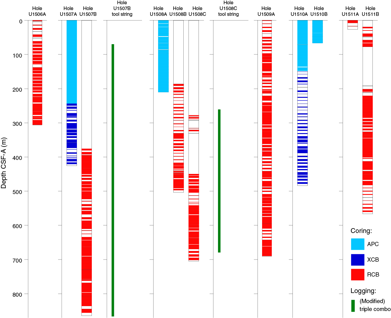
Figure F1. Coring systems and logging tool strings.
JOIDES Resolution standard coring systems
The APC and HLAPC coring systems cut soft-sediment cores with minimal coring disturbance relative to other IODP coring systems and are suitable for the upper portion of each hole. After the APC core barrel is lowered through the drill pipe and lands near the bit, the inside of the drill pipe is pressured up until one or two shear pins that hold the inner barrel attached to the outer barrel fail. The inner barrel then advances into the formation at high speed and cuts a core with a diameter of 66 mm (2.6 inches). The driller can detect a successful cut, or “full stroke,” from the pressure gauge on the rig floor. The depth limit of the APC system, often referred to as APC refusal, is indicated in two ways: (1) the piston fails to achieve a complete stroke (as determined from the pump pressure reading) because the formation is too hard or (2) excessive force (>60,000 lb; ~267 kN) is required to pull the core barrel out of the formation. When a full stroke is not achieved, typically additional attempts are made. The assumption is that the barrel penetrated the formation by the length of core recovered (nominal recovery of ~100%), so the bit is advanced by that length before cutting the next core. When a full or partial stroke is achieved but excessive force cannot retrieve the barrel, the core barrel is “drilled over,” meaning after the inner core barrel is successfully shot into the formation, the drill bit is advanced by the length of the APC barrel (~9.6 m). Typically, nonmagnetic core barrels are used, and a downhole orientation tool is deployed, except when refusal appears imminent. Formation temperature measurements can be taken with the advanced piston corer temperature tool (APCT-3), embedded in the APC coring shoe, at specified intervals. These measurements can be used to obtain temperature gradients and heat flow estimates.
The XCB is a rotary system with a small cutting shoe that extends below the large rotary APC/XCB bit. The smaller bit can cut a semi-indurated core with less torque and fluid circulation than the main bit, optimizing recovery. The XCB cutting shoe (bit) extends ~30.5 cm ahead of the main bit in soft sediment but retracts into the main bit when hard formations are encountered. It cuts cores with a nominal diameter of 5.87 cm (2.312 inches), slightly less than the 6.6 cm diameter of APC cores. XCB cores are often broken (torqued) into “biscuits,” which are disc-shaped pieces a few to several centimeters long with remolded sediment (including some drilling slurry) interlayering the discs in a horizontal direction and packing the space between the discs and the core liner in a vertical direction. This type of drilling disturbance may give the impression that the XCB cores have the same thickness (66 mm) as the APC cores. Although both XCB and RCB core recovery (below) generally lead to drilling disturbance in similar sedimentary material, switching from an APC/XCB bottom-hole assembly (BHA) to an RCB BHA requires a pipe trip.
The RCB system is the most conventional rotary coring system and is suitable for lithified rock material. During Expedition 371, it also became the coring system of choice for semilithified material (chalk) because the depth objectives were seemingly out of reach of the XCB system. Like the XCB system, the RCB system cuts a core with a nominal diameter of 5.87 cm. RCB coring can be done with or without the core liners used routinely with the APC/XCB soft-sediment systems. Coring without the liners is sometimes done when core pieces seem to get caught at the edge of the liner, leading to jamming and reduced recovery. During Expedition 371, all RCB cores were drilled with a core liner in place.
The BHA is the lowermost part of the drill string and is typically ~130–170 m long, depending on the coring system used and total drill string length. A typical APC/XCB BHA consists of a drill bit (outside diameter = 11 inches), a bit sub, a seal bore drill collar, a landing saver sub, a modified top sub, a modified head sub, a nonmagnetic drill collar (for APC/XCB), a number of 8 inch (~20.32 cm) drill collars, a tapered drill collar, 6 joints (two stands) of 5½ inch (~13.97 cm) drill pipe, and 1 crossover sub. A lockable flapper valve was used to collect downhole logs without dropping the bit when APC/XCB coring. A typical RCB BHA consists of a drill bit, a bit sub, an outer core barrel, a top sub, a head sub, 8 joints of 8¼ inch drill collars, a tapered drill collar, 2 joints of standard 5½ inch drill pipe, and a crossover sub to the regular 5 inch drill pipe.
Cored intervals may not be contiguous if separated by intervals drilled but not cored. During Expedition 371, we drilled ahead without coring using a center bit with both the APC/XCB and RCB systems. Drilling ahead was necessary during Expedition 371 to accelerate penetration because (1) an interval had already been cored in an adjacent hole (376 m in Hole U1507B, 187 m in Hole U1508B, and 420 m in Hole U1508C) or (2) a stratigraphically higher interval was of less interest than a lower interval (150 m in Hole U1511A). Holes thus consist of a sequence of cored and drilled intervals, or “advancements.” These advancements are numbered sequentially from the top of the hole downward. Numbers assigned to physical cores correspond to advancements and may not be consecutive.
Drilling disturbance
Cores may be significantly disturbed by the drilling process and contain extraneous material as a result of the coring and core handling process. In formations with loose granular layers (sand, ash, foraminifer ooze, chert fragments, shell hash, etc.), granular material from intervals higher in the hole may settle and accumulate in the bottom of the hole as a result of drilling circulation and be sampled with the next core. The uppermost 10–50 cm of each core must therefore be examined critically for potential “fall-in.”
Common coring-induced deformation includes the concave-downward appearance of originally horizontal bedding. Piston action may result in fluidization (“flow-in”) at the bottom of, or sometimes in, APC cores. Retrieval of unconsolidated (APC) cores from depth to the surface typically results to some degree in elastic rebound, and gas that is in solution at depth may become free and drive core segments in the liner apart. When gas content is high, pressure must be relieved for safety reasons before the cores are cut into segments. Holes are drilled into the liner, which forces some sediment and gas out of the liner. As noted above, XCB coring typically results in biscuits mixed with drilling slurry. RCB coring typically homogenizes unlithified core material and often fractures lithified core material.
Drilling disturbances are described in the Lithostratigraphy section of each site chapter and are indicated on graphic core summary reports, also referred to as visual core descriptions (VCDs), in Core descriptions.
Core and section handling
Whole core handling
All APC, XCB, and RCB cores recovered during Expedition 371 were extracted from the core barrel in plastic liners. These liners were carried from the rig floor to the core processing area on the catwalk outside the Core Laboratory and cut into ~1.5 m sections. The exact section length was noted and entered into the database as “created length” using the Sample Master application. This number was used to calculate recovery. Subsequent processing differed for sediment and igneous rock material.
Sediment section handling
Headspace samples were taken from selected section ends (typically one per core) using a syringe for immediate hydrocarbon analysis as part of the shipboard safety and pollution prevention program. Whole-round samples for interstitial water analysis were also taken immediately after the core was sectioned. Core catcher samples were taken for biostratigraphic analysis. When catwalk sampling was complete, liner caps (blue = top, colorless = bottom, and yellow = top of a whole-round sample removed from the section) were glued with acetone onto liner sections, and sections were placed in core racks for analysis.
For sediment cores, the curated length was set equal to the created length and was updated very rarely (e.g., in cases of data entry errors or when section length kept expanding by more than ~2 cm). Depth in hole calculations are based on the curated section length (see Depth calculations).
After completion of whole-round section analyses (see below), the sections were split lengthwise from bottom to top into working and archive halves. The softer cores were split with a wire, and harder cores were split with a diamond saw. Investigators should note that older material can be transported upward on the split face of a section during splitting.
Rock piece handling
At Site U1506, we performed “hard rock curation,” whereby pieces are separated with dividers and logged separately. Rock pieces were washed and arranged in section half liners. Plastic dividers made from core liner caps were inserted between core pieces to keep them in place for curation, which typically led to curated section lengths that exceeded created section lengths. Note that curated core lengths, defined by the sum of curated section lengths, can exceed the length of the cored interval, resulting in recovery rates >100%. Adjacent core pieces that could be fitted together along fractures were curated as single pieces. The spacers may represent substantial intervals of no recovery. Core pieces that appeared susceptible to crumbling were encased in shrink wrap.
A splitting line was marked on each piece with a red wax pencil so that the piece could be split into representative working and archive halves, ideally maximizing the expression of dipping structures on the cut face of the core in addition to maintaining representative features in both archive and working halves. To ensure a consistent protocol for whole-core imaging, the splitting line was drawn so that the working half was on the right side of the line with the core upright. The working half of each piece was marked with a “W” to the right of the splitting line (Figure F2). Where fabrics were present, cores were marked for splitting with the fabric dipping to the east (090°) in the IODP core reference frame. This protocol was sometimes overridden by the presence of specific features (e.g., mineralized patches) that were divided between the archive and working halves to ensure preservation and/or allow shipboard or postexpedition sampling.

Figure F2. Core reference frame.
Once the split line was drawn, the plastic spacers were secured with acetone, creating bins that constrained movement of pieces during core transport. Spacers were mounted into the liners with the angle brace facing uphole, ensuring that the top of each piece had the same depth as the top of the curated interval for each bin. The top and bottom offsets of each bin were entered into Sample Master. Based on the calculated bin lengths, the cumulative length of all bins, including spacers, was computed as the curated length of the section. The empty split liner with spacers glued in was then placed over the split liner containing the pieces and the two halves were taped together in a few places for temporary storage until core pieces were dry and equilibrated to laboratory conditions (usually <1 h after arrival from the catwalk).
Sample naming
Editorial practice
Sample naming in this volume follows standard IODP procedure. A full sample identifier consists of the following information: expedition, site, hole, core number, core type, section number, section half, and offset in centimeters measured from the top of the core section. For example, a sample identification of “371-U1507A-1H-2W, 10–12 cm” represents a sample taken from the interval between 10 and 12 cm below the top of the working half of Section 2 of Core 1 (“H” designates that this core was taken with the APC system) of Hole U1507A during Expedition 371.
When working with data downloaded from the Laboratory Information Management System (LIMS) database or physical samples that were labeled on the ship, three additional sample naming concepts may be encountered: text ID, label ID, and printed labels.
Text ID
Samples taken on the JOIDES Resolution are uniquely identified for use by software applications using the text ID, which combines two elements:
- Sample type designation (e.g., SHLF for section half) and
- A unique sequential number for any sample and sample type added to the sample type code (e.g., SHLF30495837).
The text ID is not particularly helpful to most users but is critical for machine reading and troubleshooting.
Label ID
The label ID is used throughout the JOIDES Resolution workflows as a convenient, human-readable sample identity. However, a label ID is not necessarily unique. The label ID is made up of two parts: primary sample identifier and sample name.
Primary sample identifier
The primary sample identifier is very similar to the editorial sample name described above, with two notable exceptions:
- Section halves always carry the appropriate identifier (371-U1507A-35R-2-A vs. 371-U1507A-35R-2-W for archive and working half, respectively).
- Sample top and bottom offsets, relative to the parent section, are indicated as “35/37” rather than “35–37 cm.”
Specific rules were set for printing the offset/offset at the end of the primary sample identifier:
- For samples taken out of the hole, core, or section, offset/offset is NOT added to the label ID. This has implications for the common process of taking samples out of the core catcher (CC), which technically is a section (for microbiology and paleontology samples).
- For samples taken out of the section half, offset/offset is always added to the label ID. The rule is triggered when an update to the sample name, offset, or length occurs.
- The offsets are always rounded to the nearest centimeter before insertion into the label ID (even though the database stores higher precisions and reports offsets to millimeter precision).
Sample name
The sample name is a free text parameter for subsamples taken from a primary sample or from subsamples thereof. It is always added to the primary sample identifier following a hyphen (-NAME) and populated from one of the following prioritized user entries in the Sample Master application:
- Entering a sample type (-TYPE) is mandatory (same sample type code used as part of the text ID; see above). By default, -NAME = -TYPE (examples include SHLF, CUBE, CYL, PWDR, and so on).
- If the user selects a test code (-TEST), the test code replaces the sample type and -NAME = -TEST. The test code indicates the purpose of taking the sample but does not guarantee that the test was actually completed on the sample (examples include PAL, TSB, ICP, PMAG, MAD, and so on).
- If the user selects a requester code (-REQ), it replaces -TYPE or -TEST and -NAME = -REQ. The requester code represents the name of the requester of the sample who will conduct postexpedition analysis.
- If the user types any kind of value (-VALUE) in the -NAME field, perhaps to add critical sample information for postexpedition handling, the value replaces -TYPE, -TEST, or -REQ and -NAME = -VALUE (examples include SYL-80deg, DAL-40mT, and so on).
In summary, and given the examples above, the same subsample may have the following label IDs based on the priority rule -VALUE > -REQ > -TEST > -TYPE:
- 371-U1507A-35R-2-W 35/37-CYL
- 371-U1507A-35R-2-W 35/37-PMAG
- 371-U1507A-35R-2-W 35/37-DAL
- 371-U1507A-35R-2-W 35/37-DAL-40mT
When subsamples are taken out of subsamples, the -NAME of the first subsample becomes part of the parent sample ID, and another -NAME is added to that parent sample label ID:
For example, a thin section billet (sample type = TSB) taken from the working half at 40–42 cm offset from the section top might result in a label ID of 371-U1507A-3R-4-W 40/42-TSB. After the thin section was prepared (~48 h later), a subsample of the billet might receive an additional designation of TS05, which would be the fifth thin section made during the expedition. A resulting thin section label ID might therefore be 371-U1507A-3R-4-W 40/42-TSB-TS_5.
Depth calculations
Sample and measurement depth calculations were based on the methods described in IODP Depth Scales Terminology v.2 at https://www.iodp.org/policies-and-guidelines/142-iodp-depth-scales-terminology-april-2011/file (Table T1). The definition of multiple depth scale types and their distinction in nomenclature should keep the user aware that a nominal depth value at two different depth scale types (and even two different depth scales of the same type) generally does not refer to exactly the same stratigraphic interval in a hole (Figure F3). The SI unit for all depth scales is meter (m).
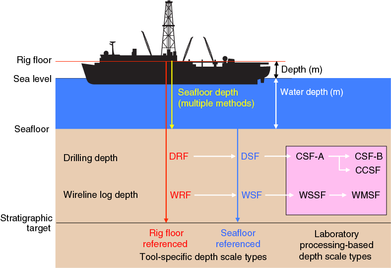
Figure F3. Depth scale types.
Depths of cored intervals were measured from the drill floor based on the length of drill pipe deployed beneath the rig floor and referred to as drilling depth below rig floor (DRF); it is traditionally referred to with custom units of meters below rig floor (mbrf). The depth of each cored interval, measured on the DRF scale, can be referenced to the seafloor by subtracting the seafloor depth measurement (in DRF) from the cored interval (in DRF). This seafloor-referenced depth of the cored interval is referred to as the drilling depth below seafloor (DSF), with a traditionally used custom unit designation of meters below seafloor (mbsf). In the case of APC coring, the seafloor depth was the length of pipe deployed minus the length of the mudline core recovered. In the case of RCB coring, the seafloor depth was adopted from a previous hole drilled at the site or by tagging the seafloor.
Depths of samples and measurements in each core were computed based on a set of rules that result in a depth scale type referred to as CSF-A. The two fundamental rules are that (1) the top depth of a recovered core corresponds to the top depth of its cored interval (top DSF = top CSF-A) regardless of type of material recovered or drilling disturbance observed and (2) the recovered material is a contiguous stratigraphic representation even when core segments are separated by voids when recovered, the core is shorter than the cored interval, or it is unknown how much material is missing between core pieces. When voids were present in the core on the catwalk, they were closed by pushing core segments together whenever possible. The length of missing core should be considered a depth uncertainty when analyzing data associated with core material.
When core sections were given their curated lengths, they were also given a top and a bottom depth based on the core top depth and the section length. Depths of samples and measurements on the CSF-A scale were calculated by adding the offset of the sample (or measurement from the top of its section) to the top depth of the section.
Per IODP policy established after the introduction of the IODP Depth Scales Terminology v.2, sample and measurement depths on the CSF-A depth scale type are commonly referred to with the custom unit mbsf, just like depths on the DSF scale type. The reader should be aware, though, that the use of mbsf for different depth scales can cause confusion in specific cases because different “mbsf depths” may be assigned to the same stratigraphic interval. For example, a soft-sediment core from less than a few hundred meters below seafloor often expands upon recovery (typically by a few percent to as much as 15%), and the length of the recovered core exceeds that of the cored interval. Therefore, a stratigraphic interval in a particular hole may not have the same depth on the DSF and CSF-A scales. When recovery in a core exceeds 100%, the CSF-A depth of a sample taken from the bottom of the core will be deeper than that of a sample from the top of the subsequent core (i.e., some data associated with the two cores overlap on the CSF-A scale). To overcome the overlap problem, core intervals can be placed on the core depth below seafloor, Method B (CSF-B), depth scale. The Method B approach scales the recovered core length back into the interval cored, from >100% to exactly 100% recovery. If cores had <100% recovery to begin with, they are not scaled. When downloading data using the JOIDES Resolution Science Operator (JRSO) LIMS Reports pages (http://web.iodp.tamu.edu/LORE), depths for samples and measurements are by default presented on both CSF-A and CSF-B scales. The CSF-B depth scale can be useful for data analysis and presentations at sites with a single hole.
A core composite depth below seafloor (CCSF) scale can be constructed to mitigate inadequacies of the CSF-A scale for scientific analysis and data presentation. The most common application is the construction of a CCSF scale from multiple holes drilled at a site using depth shifting of correlative features across holes. This method not only eliminates the CSF-A core overlap problem but also allows splicing of core intervals such that gaps in core recovery, which are inevitable in coring a single hole, are essentially eliminated and a continuous stratigraphic representation is established. This depth scale type was used at only one site during Expedition 371 (Site U1510).
A CCSF scale and stratigraphic splice are accomplished by downloading correlation data from the expedition (LIMS) database using the Correlation Downloader application, correlating stratigraphic features across holes using the Correlator or any other application and depth-shifting cores to create an “affine table” with an offset for each core relative to the CSF-A scale, and creating a “splice interval table” that defines which core intervals from the participating holes make up the stratigraphic splice. Affine and splice interval tables can be uploaded to the LIMS database, where internal computations create a CCSF depth scale. The CCSF depth can then be added to all subsequent data downloads from the LIMS database, and data can be downloaded for a splice.
Wireline logging data are collected at the wireline log depth below rig floor (WRF) scale, from which a seafloor measurement is subtracted to create the wireline log depth below seafloor (WSF) scale. For Expedition 371, the WSF depths were only used for preliminary data usage on the ship. Immediately after data collection was completed, the wireline logging data were transferred to the Lamont-Doherty Earth Observatory Borehole Research Group (LDEO-BRG), where multiple passes and runs were depth matched using the natural gamma radiation (NGR) logs. The data were returned to the ship at the wireline log matched depth below seafloor (WMSF) scale, which is the final and official logging depth scale type for investigators.
Shipboard core analysis
After letting cores thermally equilibrate for at least 1 h, whole-round core sections were run through the Whole-Round Multisensor Logger (WRMSL), which measures P-wave velocity, density, and magnetic susceptibility, and the Natural Gamma Radiation Logger (NGRL). Thermal conductivity measurements were also taken before the cores were split lengthwise into working and archive halves. The working half of each core was sampled for shipboard analysis, routinely for paleomagnetism and physical properties and more irregularly for thin sections, geochemistry, and biostratigraphy. The archive half of each core was scanned on the Section Half Imaging Logger (SHIL) and measured for color reflectance and magnetic susceptibility on the Section Half Multisensor Logger (SHMSL). The archive halves were described macroscopically and microscopically in smear slides, and the working halves were sampled for thin section microscopic examination. Finally, the archive halves were run through the cryogenic magnetometer. Both halves of the core were then put into labeled plastic tubes that were sealed and transferred to cold storage space aboard the ship.
A total of 7973 samples were taken for shipboard analysis. At the end of Expedition 371, all core sections and thin sections were shipped to the Gulf Coast Repository in preparation for a shore-based sampling party in January 2018. The sections and samples will be sent to the Kochi Core Center for permanent storage.
Lithostratigraphy
Sediments and rocks recovered during Expedition 371 were described macroscopically from archive-half sections and microscopically from smear slides and thin sections. Digital color images of all archive-half sections were produced using the SHIL, and visual color determination was performed using Munsell soil color charts (Munsell Color Company, Inc., 1994). In some cases, sedimentary description was aided by X-ray diffraction (XRD) analyses, handheld X-ray fluorescence scanning, scanning electron microscope (SEM) photomicrographs, and carbonate content measurements (see Geochemistry). Observations were recorded in separate macroscopic (drilling disturbance, lithologic description, and deformational structures) and microscopic (smear slide and thin section description) DESClogik templates (version x.16.1.0.14; see the DESClogik user guide at http://iodp.tamu.edu/labs/documentation). Final corrected DESC workbooks for Expedition 371 are available in DESC_WKB in Supplementary material. Selected data are presented in graphic core summaries (VCD form; Figure F4), and synthesized descriptions and lithostratigraphic units are presented in the Lithostratigraphy section of each site chapter.

Figure F4. Example VCD sheet.
Macroscopic descriptions
Section half images
Standard core splitting can affect the appearance of the split core surface, obscuring fine details of lithology and sedimentary structures. Therefore, when appropriate, the archive-half sections were scraped parallel to bedding using a stainless steel or glass scraper. After cleaning the core surface, the archive half was scanned with the SHIL as soon as possible to avoid color changes caused by oxidation and sediment drying. However, in cases of watery or soupy sediment, the surface was dried sufficiently with paper towels prior to scanning to avoid reflected light photographic artifacts. Three pairs of advanced illumination high-current, focused LED line lights with adjustable angles to the lens axis illuminated any large cracks and blocks in the core surface and sidewalls. Each of the LED pairs had a color temperature of 6,500 K and emitted 90,000 lx at 3 inches. Digital images were taken by a linescan camera at an interval of 10 lines/mm to create a high-resolution TIFF file. The camera height was set so that each pixel imaged a 0.1 mm2 area of the section half surface. However, actual core width per pixel varied because of slight differences in the section half surface height. JPEG files were created from the high-resolution TIFF files. One set of JPEG image files includes a gray scale and offset ruler; a second set is cropped to include only the section half surface.
Drilling disturbance
Drilling-related sediment disturbance was recorded for each core (Disturbance column; Figure F4). The type of drilling disturbance for soft and firm sediment was described using the following terms:
- Fall-in: out of place material at the top of a core that has fallen downhole onto the cored surface.
- Bowed: bedding contacts are slightly to moderately deformed but still subhorizontal and continuous.
- Up-arching: material retains its coherency, with material closest to the core liner bent downward.
- Void: empty space in the cored material (e.g., caused by gas or sediment expansion during core retrieval). To the extent possible, voids were closed on the core receiving platform by pushing the recovered intervals toward the top of the core before cutting the sections. The space left below all the recovered material due to incomplete recovery was not described as a void.
- Flow-in, coring/drilling slurry, or along-core gravel/sand contamination: soft-sediment stretching and/or compressional shearing structures when severe.
- Soupy or mousse-like: intervals are water saturated and have lost all aspects of original bedding.
- Biscuit: sediment of intermediate stiffness has vertical variations in the degree of disturbance, whereas firmer intervals are relatively undisturbed.
- Cracked or fractured: firm sediment is broken during drilling but not displaced or rotated significantly.
- Fragmented, brecciated, or pulverized: firm sediment is pervasively broken by drilling and may be displaced or rotated.
Each instance of drilling disturbance was assigned a degree of severity:
- Slight: core material is in place but broken or otherwise disturbed.
- Moderate: core material is in place or partly displaced, but original orientation is preserved or recognizable.
- Severe: core material is probably in correct stratigraphic sequence, but original orientation is lost.
- Destroyed: core material is in incorrect stratigraphic sequence, and original orientation is lost.
- Drilling breccia: core is crushed and broken into many small and angular pieces, and original orientation and stratigraphic position are lost.
Rock and sediment types
Sediment and rock types were entered in the lithology columns of the macroscopic DESClogik worksheet following the classification scheme presented in Sediment and sedimentary rock classification. Corresponding patterns and colors were defined and represented on the graphic core summaries and hole summaries.
Stratification and sedimentary structures
The locations and types of stratification and sedimentary structures visible on the prepared surfaces of the section halves were respectively entered in the Bedding and Sedimentary structures columns of the macroscopic DESClogik worksheet. Observations in these columns indicate the locations and scales of interstratification and the locations of individual bedding and sedimentary features, such as scours, ash layers, or ripple laminations. The following terminology (based on Stow, 2005) was used to describe the scale of lamination and bedding:
- Thin lamination = <3 mm thick.
- Medium lamination = 0.3–0.6 cm thick.
- Thick lamination = 0.6–1 cm thick.
- Very thin bed = 1–3 cm thick.
- Thin bed = 3–10 cm thick.
- Medium bed = 10–30 cm thick.
- Thick bed = 30–100 cm thick.
- Very thick bed = >100 cm thick.
The presence of graded beds was entered and presented in the Graded bed column separately from other sedimentary structures. “Normal grading” corresponds to layers with a gradual upward decrease in grain size, whereas “reverse grading” corresponds to layers with a gradual upward increase in grain size.
Bioturbation
When identifiable, trace fossils, such as Zoophycos, Chondrites, Skolithos, and Planolites (Ekdale et al., 1984), were reported in the core summary. We also distinguished five levels of bioturbation intensity, which were reported in the Bioturbation intensity column using the following numeric scale:
- 1 = no bioturbation (<10%).
- 2 = slight bioturbation (<10%–30%).
- 3 = moderate bioturbation (30%–60%).
- 4 = heavy bioturbation (60%–90%).
- 5 = complete bioturbation (>90%).
Lithologic accessories
Lithologic, diagenetic, and paleontologic features other than those delineated above were entered in the Lithologic accessories column and depicted as symbols in graphic core summaries (Figures F4, F5). Accessories include macroscopic biogenic remains, such as shells, sponge spicule aggregates, worm tubes, wood fragments, and mottling (e.g., ash, sand, and pyrite), as well as clasts, concretions, nodules, alteration halos, and blebs. When possible, clasts, concretions, and nodules were described by composition. For reference, a concretion is a small irregularly rounded knot, mass, or lump of a mineral or mineral aggregate that normally has a warty or knobby surface and no internal structure and usually exhibits a contrasting composition from the sediment or rock matrix within which it is embedded. A nodule is a regular globular structure. An alteration halo is a ring surrounding a grain or accessory phase where sediment has a different color or composition. Blebs (centimeter scale) and specks (millimeter scale) are spots or smears where material has a different color or composition than the surrounding sediment (it is not ring shaped, like an alteration halo).
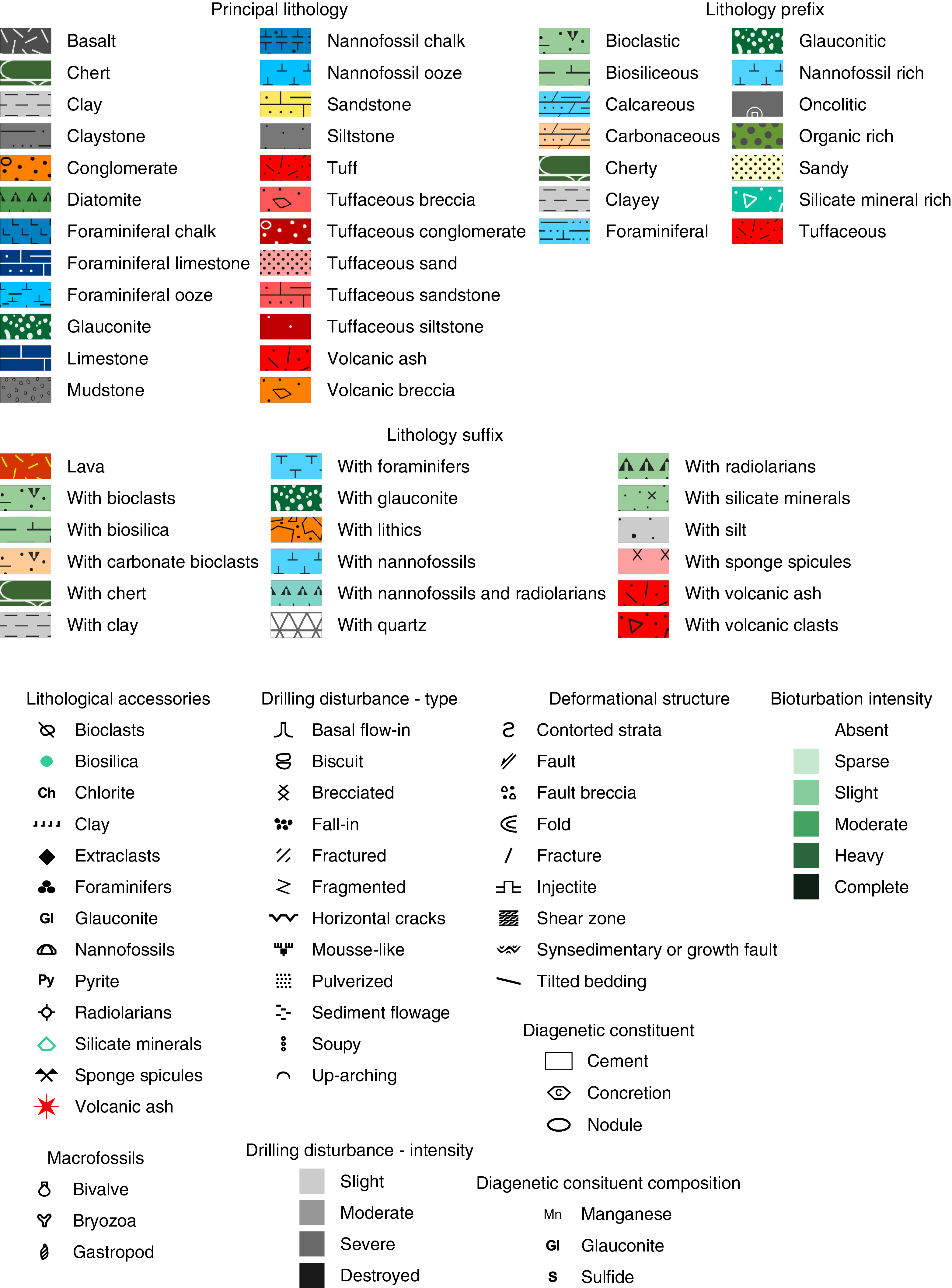
Figure F5. Symbols used on VCDs, graphic logs, and hole summaries.
Deformation
Deformation of the core clearly identified as not related to drilling was recorded and presented in the Deformational structures column using the symbols in Figure F5. These structures include synsedimentary deformation, such as dewatering structures, slump folds, or growth faults, and postdepositional features, such as fractures, faults, folds and dikes, or sills. When possible, sense of deformation (e.g., reverse or normal displacement) and dip angle were recorded in the comment section. Interval thickness was recorded from the uppermost to the lowermost extension of the described feature on the section half.
Microscopic descriptions
Smear slide descriptions
Sediment constituent size, composition, and abundance were estimated microscopically using smear slides. Smear slide samples of the main lithologies were collected from the archive-half sections unless lithification made sampling impossible. Additional samples were collected from areas of interest (e.g., laminations, clasts, blebs, and nodules).
For each smear slide, a small amount of sediment was removed from the section half using a wooden toothpick and put on a 25 mm × 75 mm glass slide. A drop of deionized water was added, and the sediment was homogenized and evenly spread across the glass slide. The dispersed sample was dried on a hot plate at a low setting (50°C). A drop of adhesive (Norland optical adhesive Number 61) was added as a mounting medium for a glass coverslip, which was carefully placed on the dried sample to prevent air bubbles from being trapped in the adhesive. The smear slide was then fixed in a UV light box for 5 min to cure the adhesive.
Smear slides were examined with a transmitted-light petrographic microscope equipped with a standard eyepiece micrometer. Biogenic and mineral components were identified following standard petrographic techniques as stated in the Rothwell (1989), Marsaglia et al. (2013), and Marsaglia et al. (2015) reference manuals. Several fields of view were examined at 10×, 20×, and 40× to assess the abundance of detrital (e.g., quartz, feldspar, clay minerals, mica, and heavy minerals), biogenic (e.g., nannofossils, other calcareous bioclasts, diatoms, foraminifers, and radiolarians), and authigenic (e.g., carbonate, iron sulfide, iron oxides, and glauconite) components. The average grain size of clay (<4 µm), silt (4–63 µm), and sand (>63 µm) was only estimated for sediments dominated by siliciclastic material. The relative percent abundances of the sedimentary constituents were visually estimated using the techniques of Rothwell (1989). The texture of siliciclastic lithologies (relative abundance of sand-, silt-, and clay-sized grains) and the proportions and presence of biogenic and mineral components were recorded in the smear slide worksheet of the microscopic DESClogik template.
Components observed in smear slides were categorized according to their abundance as follows:
- T = trace (<1%).
- R = rare (1%–10%).
- C = common (>10%–25%).
- A = abundant (>25%–50%).
- D = dominant (>50%).
Smear slides provide only a rough estimate of the relative abundance of sediment constituents. It should be noted that, on occasion, the lithologic name assigned based on smear slide observation does not match the name in the macroscopic lithology description because a small sample may not represent the much larger macroscopic description interval. Indeed, relatively minor features were sometimes targeted for smear slide analysis because of their contrast with the dominant sediment type. Additionally, clay-sized grains and larger than sand–sized grains are difficult to observe in smear slides, and their relative proportions in the sediment can be affected during slide preparation. Therefore, intervals dominated by sand and larger size constituents were also examined by macroscopic comparison with grain size reference charts.
Thin section descriptions
Description of indurated sediments and volcanic rocks was complemented with thin section analysis. Standard size thin section billets were cut from selected intervals or features, and thin sections prepared on board were examined with a transmitted-light petrographic microscope equipped with a standard eyepiece micrometer. Thin section analysis differs from that of smear slides, and certain observations are possible with only one method. For example, calcareous nannofossils can be recognized in smear slides but not in thin sections, whereas sand-sized grains can be examined in thin sections but not in smear slides. These differences have implications for the lithologic classification scheme (see below).
Sediment and sedimentary rock classification
Sediments and sedimentary rocks recovered during Expedition 371 were classified using a modified scheme initially developed during IODP Expedition 350 (Tamura et al., 2015). This scheme integrates volcanic particles into the sedimentary descriptive scheme typically used (e.g., Norris et al., 2014) to describe siliciclastic and biogenic sediments during IODP expeditions (Figures F5, F6, F7). The methodology allows a comprehensive description of mixed sediments, including volcaniclastic, biogenic, and siliciclastic sediment and sedimentary rocks, and igneous rocks. The purposes of this classification scheme are to (1) include volcanic particles in the assessment of sediment and rock recovered in cores, (2) make rock information accessible to scientists with diverse research backgrounds and experiences, (3) allow relatively quick and smooth data entry, and (4) display data seamlessly in graphical presentations (Figure F4). In this scheme, inferred fragmentation, transport, deposition, and alteration processes are not part of the lithologic name. Observations implying those processes are recorded in the relevant columns (Layer/Bedding, Lamination, Grading, Grain Size, etc.) and as comments in the macroscopic DESClogik template. Therefore, sizes of volcanic grains inferred to have formed by a variety of processes (i.e., pyroclasts, autoclasts, epiclasts, and reworked volcanic clasts; Fisher and Schmincke, 1984; Cas and Wright, 1987; McPhie et al., 1993) are classified using a common grain size terminology that allows for a more descriptive (i.e., nongenetic) approach.
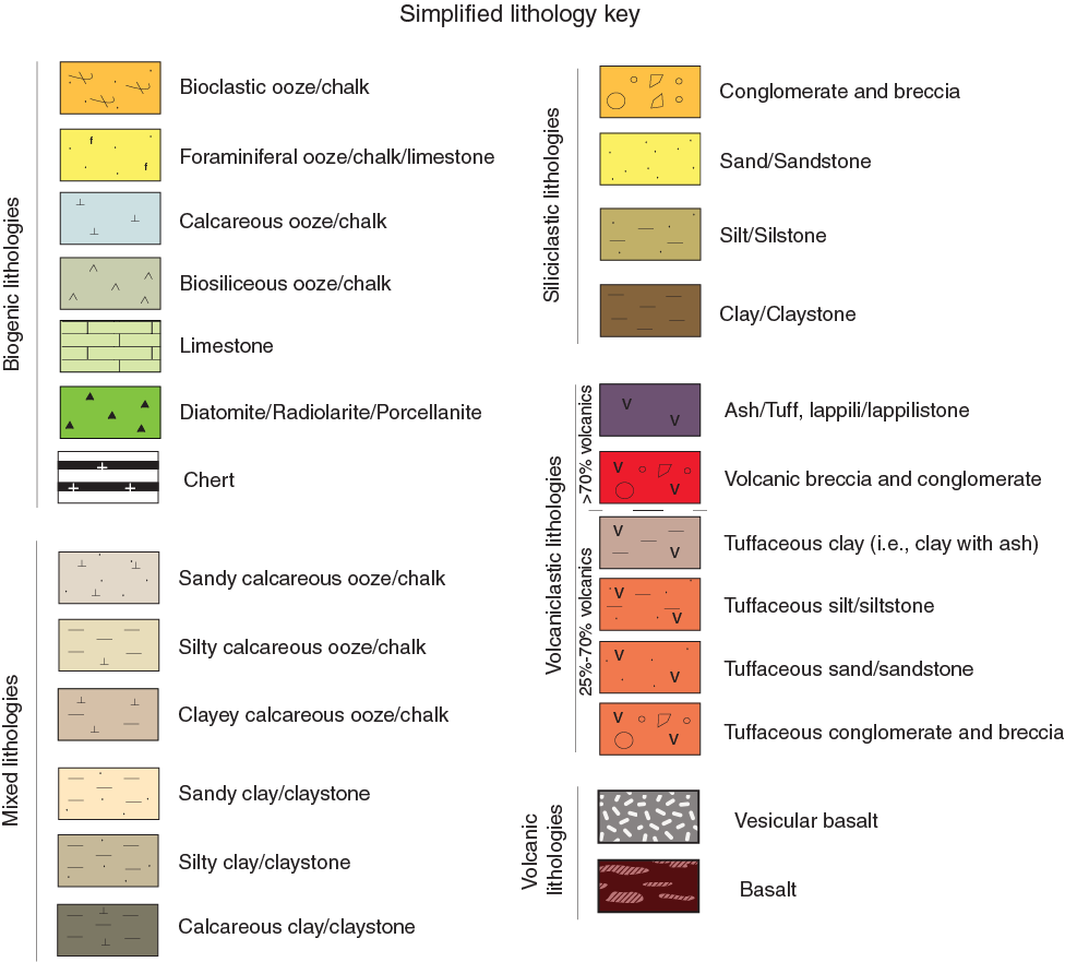
Figure F6. Simplified lithologic symbols.
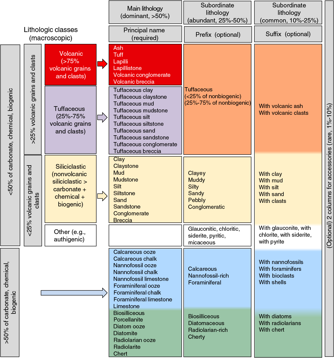
Figure F7. Sedimentary and volcaniclastic lithology naming conventions.
Sedimentary lithologic classes
Three main sedimentary lithologic classes are defined based on the primary origin of the sediment constituents (but not the depositional process):
- Biogenic: >50% carbonate, chemical, and biogenic particles.
- Siliciclastic: >50% siliciclastic particles, <25% volcanic particles, and <50% biogenic particles; therefore, nonvolcanic siliciclastic particles dominate chemical and biogenic particles.
- Volcaniclastic: >25% volcanic particles. In this lithologic class, volcanic sediments are defined as >75% of volcanic clasts and grains, whereas tuffaceous sediments contain 75%–25% volcanic clasts and grains mixed with nonvolcanic particles (either nonvolcanic siliciclastic, biogenic, or both). The definition of the term “tuffaceous” (25%–75% volcanic particles) is modified from Fisher and Schmincke (1984). Note that the term “volcaniclastic” is used sensu Fisher (1961) and therefore includes both volcanic and tuffaceous lithologies.
These three lithologic classes form the basis of the principal name of the described sediments and rocks, with appropriate prefixes and suffixes that may be chosen for mixed lithologies (see Principal names and modifiers below).
Principal names and modifiers
The principal name is based on the most abundant sediment class. Principal names for the siliciclastic class were adapted from the grain size classes of Wentworth (1922) (Figure F8), whereas principal names for the volcaniclastic class were adapted from the grain size classes of Fisher and Schmincke (1984) (Figure F7). Thus, the Wentworth (1922) and Fisher and Schmincke (1984) classifications are used to refer to particle type (siliciclastic versus volcanic, respectively) and the maximum size of the particles (Figures F6, F7, F8). For the biogenic sediment class, commonly used terms are applied (e.g., ooze and chalk) and do not have a separate size or texture notation because those aspects are inherent in the fossil groups that make up the sediment. For example, nannofossil and foraminiferal ooze imply a dominant grain size corresponding to clay and sand, respectively. For each principal name, both a consolidated (i.e., semilithified to lithified) and a nonconsolidated term exist that are mutually exclusive (e.g., clay or claystone; ash or tuff).
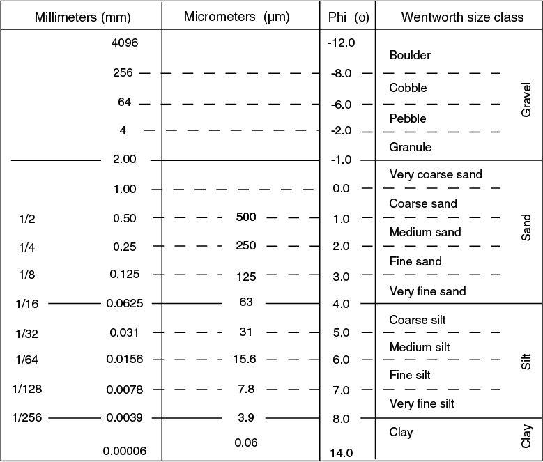
Figure F8. Udden-Wentworth grain size classification.
For all lithologies, the principal lithologic name can be modified by prefixes and/or suffixes representing secondary components as follows (Figure F7):
- Prefixes describe a secondary component with abundance between 25% and 50% (corresponding to “abundant” in smear slide descriptions).
- Suffixes are secondary or tertiary components with abundances of 10%–25% (corresponding to “common” in smear slide descriptions) and are indicated by the suffix “with” (e.g., with clay or with radiolarians) in order of decreasing abundance.
For example, a nonlithified sediment containing 45% nannofossils, 30% clay, 15% foraminifers, and 10% radiolarians would be described as clayey nannofossil ooze with foraminifers and radiolarians.
The degree of lithification is expressed in the principal name using alternate terms common in geology:
- Siliciclastic class: if the sediment can be deformed easily with a finger, no lithification term is applied (e.g., clay). If the sediment cannot be deformed easily with a finger, the suffix “-stone” is added to the grain size identifier (e.g., claystone).
- Biogenic class: if the sediment can be deformed easily with a finger, the nonlithified term “ooze” is used in conjunction with the most abundant component (e.g., nannofossil ooze or radiolarian ooze). If the calcareous sediment cannot be deformed easily with a finger but can be easily scratched with a fingernail, the semilithified term “chalk” is used for calcareous sediments (e.g., nannofossil chalk) and the terms “radiolarite,” “diatomite,” and “porcellanite” are used for siliceous sediments. If the sediment cannot be scratched easily with a fingernail, the lithified term “limestone” is used for calcareous sediments (e.g., foraminiferal limestone). If siliceous sediment cannot be scratched with a fingernail and displays a glassy luster, the term “chert” is used. Note that in this volume, the terms porcellanite and chert do not imply crystallinity of silica, in contrast to usage in some literature.
- Volcaniclastic class: if the sediment can be deformed easily with a finger, the terms “ash” and “lapilli” are applied. If the sediment cannot be deformed easily with a finger, the terms “tuff” and “lapillistone” are used.
Conglomerate, breccia-conglomerate, and breccia
The terms “breccia,” “conglomerate,” or “breccia-conglomerate” are used when particles exceed 2 mm. These terms include critical information on the angularity of fragments and replace the Wentworth (1922) terms “granule,” “pebble,” and “cobble.” A conglomerate is a deposit where the fragments are exclusively (>95 vol%) rounded and subrounded. A breccia-conglomerate is composed of predominantly rounded and/or subrounded clasts (>50 vol%) and subordinate angular clasts. A breccia is predominantly composed of angular clasts (>50 vol%). Breccia, conglomerates, and breccia-conglomerates may be consolidated (i.e., lithified) or unconsolidated. Clast sphericity is not evaluated.
We use the general term “particles” for fragments that constitute volcanic, tuffaceous, and nonvolcanic siliciclastic sediment and sedimentary rock, regardless of the size of the fragments. However, for reasons that are both meaningful and convenient, the term “grain” is used for particles <2 mm and “clast” is used for particles >2 mm. The cutoff size corresponds to the sand/granule grain size division of Wentworth (1922) and the ash/lapilli grain size divisions of Fisher (1961) (Figures F7, F8). Note that volcanic particles <2 mm in size commonly include volcanic crystals, whereas volcanic crystals virtually never exceed >2 mm in size. For example, using our definition an ash or tuff is made entirely of grains, a lapilli-tuff or tuff-breccia has a mixture of clasts and grains, and a lapillistone is made entirely of clasts. Irrespective of the sediment or rock composition, detailed average and maximum grain size follows Wentworth (1922). For example, an ash can be further described as sand-sized ash or silt-sized ash and a lapilli-tuff can be described as coarse sand sized or pebble sized.
Carbonate sediments and sedimentary rocks
Rocks with >50% carbonate were named according to the textural classification of Dunham (1962) and Embry and Klovan (1971). The only difference is the use of the term “mudstone,” which may create ambiguity with a siliciclastic rock of clay size constituents. Therefore, what is called mudstone in Dunham (1962) is here referred to as “micritic limestone.” Moreover, because the finest carbonate constituents, such as calcareous nannofossils, are not discernible in thin section, such rock types were classified with the general term “micrite.” Intergranular materials with crystalline texture were classified as “cement.” Rocks with <50% carbonate were classified with the primary scheme of principal names and modifiers described above.
Volcanic rock classification
Volcanic rock descriptions generally follow those used during relevant Integrated Ocean Drilling Program and IODP expeditions (e.g., Tamura et al., 2015). Volcanic rocks are composed of a glassy or microcrystalline groundmass (crystals < 1.0 mm) and can contain various proportions of phenocrysts (typically 5 times larger than groundmass, usually >0.1 mm) and/or vesicles.
Macroscopic observations were coordinated with thin section or smear slide petrographic observations of representative samples. During Expedition 371, volcaniclastic sediments containing particles of various sizes and volcanic rocks were recovered. Volcanic rocks were described as either a coherent igneous body or as large clasts in volcaniclastic sediment. Particles sufficiently large enough to be described individually at the macroscopic scale (>2 cm) were described as a principal lithology with prefix and suffix, texture, grain size, and contact relationships in the Extrusive hypabyssal and Intrusive mantle sections of the macroscopic DESClogik template.
Volcanic lithology
Volcanic rocks were classified using a simple scheme based on visual characteristics for macroscopic and microscopic determinations. The lithology name consists of a main principal name and optional prefix and suffix (Figure F9). The principal name depends on the nature of phenocryst minerals and/or the color of the groundmass. Three rock types are defined for phyric samples:
- Basalt: black to dark gray, typically olivine-bearing volcanic rock.
- Andesite: dark to light gray, containing pyroxenes and/or feldspar and/or amphibole, typically devoid of olivine and quartz.
- Rhyolite-dacite: light gray to pale white, usually plagioclase-phyric, and sometimes containing quartz ± biotite; this macroscopic category may extend to SiO2 contents <70% and therefore, may include dacite.
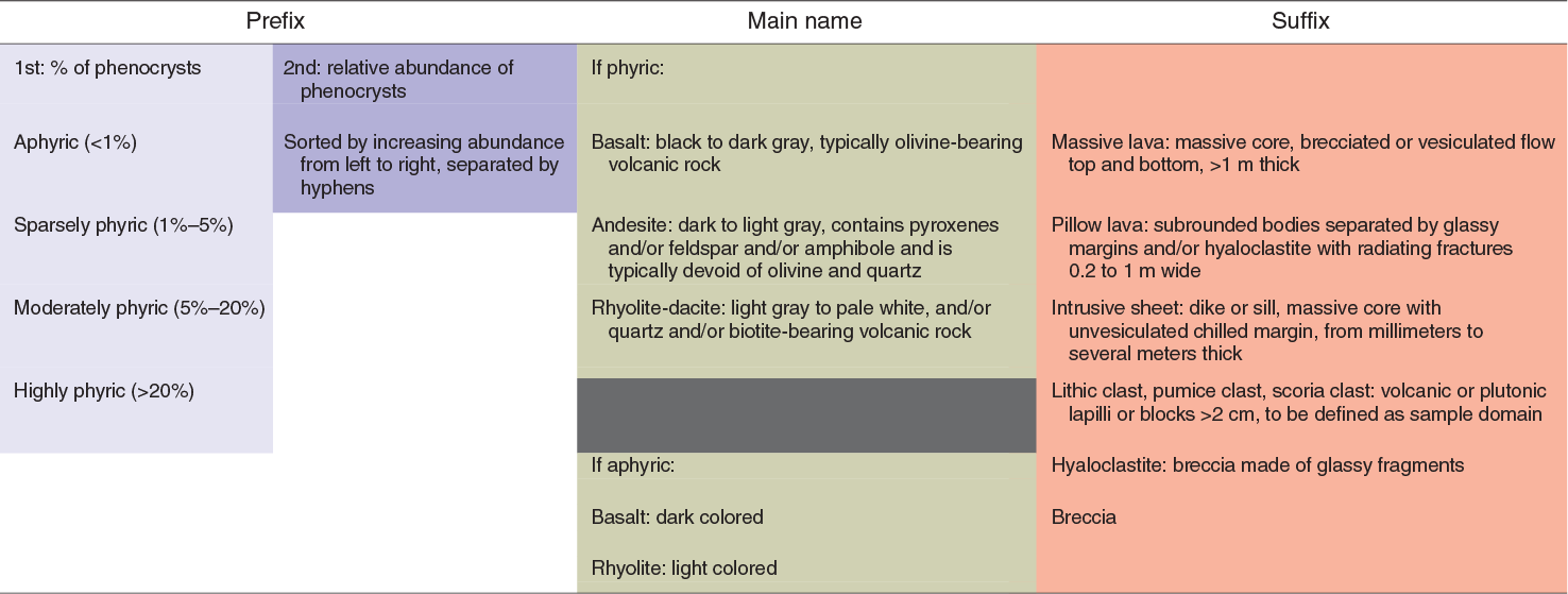
Figure F9. Principal names, prefixes, and suffixes for naming volcanic lithologies.
Volcanic clasts smaller than the cutoff defined for macroscopic (2 cm) and microscopic (2 mm) observations are described only as mafic (dark colored) or evolved (light colored) in the Sediment tab. Dark aphyric rocks are considered to be basalt, whereas light-colored aphyric samples are considered to be rhyolite-dacite, with the exception of obsidian (generally dark colored but rhyolitic in composition).
The prefix provides information on the proportion and the nature of phenocrysts. Phenocrysts are defined as crystals significantly larger (typically 5 times) than the average size of the groundmass crystals. Divisions in the prefix are based on total phenocryst proportions:
- Aphyric (<1% phenocrysts),
- Sparsely phyric (≥1%–5% phenocrysts),
- Moderately phyric (>5%–20% phenocrysts), and
- Highly phyric (>20% phenocrysts).
The prefix also includes the major phenocryst phase(s) (i.e., those that have a total abundance ≥1%) in order of increasing abundance from left to right so that the dominant phase is listed last. Macroscopically, pyroxene and feldspar subtypes are not distinguished, but microscopically, they are identified as orthopyroxene and clinopyroxene and as plagioclase and K-feldspar, respectively. Aphyric rocks are not given any mineralogical identifier.
Volcanic textures
Textures are described macroscopically for all volcanic rock core samples, but a smaller subset is described microscopically in thin sections or grain mounts. Textures are discriminated by average grain size (groundmass for porphyritic rocks), grain size distribution, shape and mutual relations of grains, and shape-preferred orientation. The distinctions are based on MacKenzie et al. (1982). Textures based on groundmass grain size of igneous rocks are defined as follows:
- Coarse grained (>5 mm),
- Medium grained (1–5 mm),
- Fine grained (0.5–1 mm), and
- Microcrystalline (<0.5 mm).
In addition, cryptocrystalline (<0.1 mm) is used for microscopic descriptions. The modal grain size of each phenocryst phase is described individually. For extrusive and hypabyssal categories, rock is described as holocrystalline, glassy (holohyaline), aphanitic, or porphyritic. Porphyritic texture refers to phenocrysts or microphenocrysts surrounded by groundmass of smaller crystals (microlites ≤ 0.1 mm; Lofgren, 1974) or glass. Aphanitic texture signifies a fine-grained nonglassy rock that lacks phenocrysts. Holocrystalline texture refers to medium- to coarse-grained nonglassy rock. In microscopic classification of basalts, the ophitic texture is also considered, signifying random plagioclase laths enclosed by mafic minerals. Individual mineral percentages and sizes are also recorded. Particular attention is paid to vesicles because they might be a major component of some volcanic rocks. However, they are not included in the rock-normalized mineral abundances.
Scanning electron microscope observations
Selected crushed or powdered samples were mounted for SEM observations. In some cases, the material was Au-Pd coated prior to analysis to enhance imagery. Observations were made with a Hitachi TM3000 tabletop SEM at 15 kV.
X-ray diffraction analysis
Intervals or features of interest (e.g., marked lithologic or color contrasts, diagenetic layers or nodules, or lithologies with heterogeneous mineral compositions) identified during visual core description and in smear slides were sampled for mineralogical analyses from the working halves of the cores. Minimum sample volumes of ~5 cm3 were frozen, freeze-dried, and ground to a homogeneous consistency. Most samples were ground in an agate mortar pestle. Rock samples were ground in tungsten carbide shatterbox vessels. Prepared samples were mounted onto a sample holder and analyzed by XRD using a Bruker D-4 Endeavor diffractometer mounted with a Vantec-1 detector using nickel-filtered CuKα radiation. The standard locked coupled scan was as follows:
- Voltage = 40 kV.
- Current = 40 mA.
- Goniometer scan = 3°–70°2θ.
- Step size = 0.015°2θ.
- Scan speed = 1 s/step.
- Divergence slit = 0.3 mm.
Diffractograms of single samples were evaluated with the Bruker DiffracSuite software package. Reliable results obtained by this analysis are limited to minerals representing at least 5% of the total sediment.
Visual core descriptions
Sediment lithology, structures, accessories, disturbances, and other observations recorded through DESClogik, as well as petrophysics data obtained during shipboard analysis, were used to produce two types of graphic summaries: one for each core and another for each hole (using the symbols in Figure F5). These graphic summaries were produced using the Strater software package. Additionally, simplified lithostratigraphic figures were produced using Adobe Illustrator for each site (using the symbols in Figure F6) and are provided in the Lithostratigraphy section of each site chapter.
The graphic summary for an individual core includes the site, hole, and core number at the top of the VCD, together with core description summary text (Figure F4). Core depth below seafloor (CSF-A; in meters), core length (in centimeters), section breaks, and lithostratigraphic unit are indicated along the left side of the digital core image. Next to the digital core image is a graphic representation of the lithology, per the legend in Figure F5. Columns to the right of the graphic lithology show grain size, sedimentary structures, lithologic accessories, and bioturbation intensity, followed by age, biozones (nannofossil, planktic foraminifer, and radiolarian; see Biostratigraphy and paleoenvironment), and type and intensity of drilling disturbance. NGR, lightness (L*) and color (a* and b*) determined by color reflectance, and corrected magnetic susceptibility (see Petrophysics) follow these columns. Shipboard sampling is noted on the final column.
Biostratigraphy and paleoenvironment
Microfossils were examined to provide (1) preliminary shipboard biostratigraphy and (2) paleoenvironment information, such as past bathymetry and coastal proximity. Biostratigraphic age assignments were based on analyses of calcareous nannofossils, planktic and benthic foraminifers, radiolarians, and organic-walled dinoflagellate cysts (dinocysts). Paleoenvironmental interpretations were based on benthic foraminifers and ostracods for bathymetry and palynomorphs for coastal proximity. The biostratigraphy was tied to the geomagnetic polarity timescale (GPTS2012), which is rooted in the geologic timescale (GTS2012) of Gradstein et al. (2012) (Figure F10). To incorporate recent age refinements for select datums, absolute ages for some events were taken from other sources and recalibrated to the GTS2012. The diverse set of datums are reported in Tables T2 (calcareous nannofossil events), T3 (planktic foraminifer events), T4 (low-latitude radiolarian events), T5 (southwest Pacific Zealandia radiolarian events), and T6 (dinocyst events; Table T7).

Figure F10. Global and New Zealand chronostratigraphy and datums.
Microfossil samples were collected from each core catcher sample, except those containing igneous rocks. Additional samples were taken from working-half sections to refine age estimates and to examine critical intervals. Where necessary, sample depths were cited as top depths within the sample interval. Datum and zone depths were given as the midpoint between the depth of the sample where the datum level was observed and the nearest sample examined where the index species was not observed. Microfossil group preservation, abundance, preliminary assemblage composition, and zonal assignment were entered through the DESClogik application into the LIMS database. It should be noted that the distribution charts for each microfossil group presented in each site chapter are based on shipboard study only and are biased toward age diagnostic species.
Calcareous nannofossils
Calcareous nannofossil taxonomy and zonal scheme
Nannofossil taxonomy follows that presented by Bown (1998, 2005) and Perch-Nielsen (1985a, 1985b) as compiled in the online Nannotax3 database (http://www.mikrotax.org/Nannotax3). A taxonomic list of nannofossils used for datums is given in Table T8. The zonal scheme of Martini (1971; zonal code numbers NP and NN) was used for Cenozoic calcareous nannofossil biostratigraphy, and the zonal scheme of Okada and Bukry (1980; zonal code numbers CP and CN) provided a secondary framework. Additional biohorizons from the Paleogene and Neogene biozonation schemes of Agnini et al. (2014; zonal code numbers CNP, CNE, and CNO) and Backman et al. (2012; numbers CNM and CNPL) provided further age constraints. These zonations represent a general framework for the biostratigraphic classification of mid- to low-latitude calcareous nannofossil assemblages (Figure F10).
Critical events, including epoch boundaries, often do not coincide precisely with nannofossil datums. However, several key events may be approximated as follows:
- Oligocene/Miocene boundary (23.03 Ma): the top of Sphenolithus delphix (23.11 Ma) occurs just below the boundary, and the top of Sphenolithus capricornutus (22.97 Ma) occurs just above the boundary in Zone NN1.
- Eocene/Oligocene boundary (33.89 Ma): the boundary falls in Zone NP21, 0.55 My above the top of Discoaster saipanensis (34.44 Ma) and close to the base acme of Clausicoccus subdistichus (33.78 Ma).
- Middle Eocene Climatic Optimum (MECO): the onset of the MECO is approximated by the top of Sphenolithus furcatolithoides (40.48 Ma) and the base of Dictyococcites bisectus (>10 µm; 40.36 Ma). The termination of the event (post-MECO) can be approximated by top common of Sphenolithus spiniger or the base of Sphenolithus obtusus (39.7 Ma).
Methods of study for calcareous nannofossils
Calcareous nannofossils were examined from standard smear slides (Bown and Young, 1998) and were analyzed using standard light microscope techniques under crossed polarizers, transmitted light, and phase contrast at 1000× or 1250× magnification on a Zeiss Axiophot microscope. All taxa have been assigned qualitative abundance codes.
Total calcareous nannofossil group abundance in the sediment was recorded as follows:
- D = dominant (>90% of sediment particles).
- A = abundant (>50%–90% of sediment particles).
- C = common (>10%–50% of sediment particles).
- F = few (1%–10% of sediment particles).
- R = rare (<1% of sediment particles).
- B = barren (no specimens).
Individual calcareous nannofossil taxa abundance was recorded as follows:
- D = dominant (>100 specimens per field of view).
- A = abundant (>10–100 specimens per field of view).
- C = common (>1–10 specimens per field of view).
- F = few (1 specimen per 1–10 fields of view).
- R = rare (<1 specimen per 10 fields of view).
- VR = very rare (<5 specimens seen while logging slide).
For critical intervals or critical taxa, the exact number of specimens observed during sample analysis was recorded (rather than qualitative data).
Calcareous nannofossil preservation was recorded as follows:
- G = good (little or no evidence of dissolution or recrystallization, primary morphological characteristics only slightly altered, and specimens were identifiable to the species level).
- M = moderate (specimens exhibit some etching or recrystallization, primary morphological characteristics somewhat altered, and most specimens were identifiable at species level).
- P = poor (specimens were severely etched or overgrown, primary morphological characteristics largely destroyed, fragmentation has occurred, and specimens often could not be identified at the species or genus level).
Intermediate categories (e.g., G/M or M/P) were used in some cases to better describe the preservation state of calcareous nannofossil assemblages.
All light microscope images were taken using a Spot RTS system with the IODP Image Capture and Spot commercial software. Selected samples were observed using a Hitachi TM3000 SEM to verify the preservation state of calcareous nannofossils.
Foraminifers
Planktic foraminifer taxonomy and zonal schemes
Planktic foraminifer taxonomic concepts follow those of Jenkins (1971), Kennett (1973), Hornibrook (1982), Kennett and Srinivasan (1983), Hornibrook et al. (1989), and Scott et al. (1990), as well as those compiled in the online pforams@mikrotax database (http://www.mikrotax.org/pforams). A taxonomic list of planktic foraminifer datum species used during Expedition 371 is given in Table T9.
For sediment intervals deposited during times of tropical waters, the zonal scheme of Wade et al. (2011) with datum ages from Gradstein et al. (2012) was used for the Cenozoic. The zonal scheme of Jenkins (1993) with ages updated to the GTS2012 by A.R. Lam et al. (unpubl. data) and datums used by GNS Science of New Zealand (Crundwell et al., 2016) for planktic foraminifer biostratigraphy were utilized at lower latitude sites. In addition, datum species used to define the base of New Zealand series and stages were used (Raine et al., 2015; Figure F10). The combination of zonal schemes was necessary due to the diachroneity of species between low- and mid-latitude regions. It should be noted that planktic foraminiferal datums for New Zealand and the southwest Pacific are not magnetostratigraphically calibrated.
Benthic foraminifer taxonomy and paleodepth determination
Species identification was made routinely on core catcher samples and on selected working-half sections. Taxonomic assignments mainly follow Tjalsma and Lohmann (1983), van Morkhoven et al. (1986), Miller and Katz (1987), Hornibrook et al. (1989), Thomas (1990), Katz and Miller (1991), Nomura (1995), Alegret and Thomas (2001), Katz et al. (2003), and Holbourn et al. (2013). The classification of Loeblich and Tappan (1988) was followed for determinations at the genus level and updated in some instances, in particular for uniserial taxa (Hayward et al., 2002, 2012).
The calcareous to agglutinated benthic foraminifer ratio was estimated, and all taxa were allocated into morphogroups following Corliss (1985, 1991), Jones and Charnock (1985), and Corliss and Chen (1988). Benthic foraminifers with planoconvex, biconvex, and rounded trochospiral tests and tubular, coiled flattened, milioline, and palmate tests are inferred to have had an epifaunal mode of life, living at the sediment surface or in its upper few centimeters. Infaunal foraminifers living in the deeper layers of the sediment have cylindrical or flattened tapered, spherical, rounded planispiral, flattened ovoid, globular unilocular, or elongate multilocular tests. The comparison between fossil and recent foraminifers is not straightforward, however, and for many taxa the close relationship between test morphology and microhabitat has not been observed. Instead, it is extrapolated from data on other taxa (e.g., Jorissen, 1999), and the relationship between morphology and microhabitat may not always be certain (Buzas et al., 1993). Morphogroup analysis is used as a proxy for combined oxygenation and food availability in the deep ocean (Jorissen et al., 2007).
The comparison between fossil and recent assemblages, the occurrence and abundance of depth-related species, and their upper depth limits (e.g., Hayward, 1986; van Morkhoven et al., 1986; Alegret and Thomas, 2001; Alegret et al., 2003; Hayward et al., 2013) allowed inference of paleobathymetry at each site. Paleodepth zones follow van Morkhoven et al. (1986) using the following categories:
- Neritic = <200 meters below sea level (mbsl).
- Bathyal = 200–2000 mbsl (upper bathyal = 200–600 mbsl; middle bathyal = 600–1000 mbsl; lower bathyal = 1000–2000 mbsl).
- Abyssal = >2000 mbsl.
Methods of study for foraminifers
Sediments were washed with tap water over a 63 µm wire mesh sieve. When necessary, clay-rich samples were boiled in water with added Borax (5 tablespoons per liter). Subsequently, samples were washed and dried repeatedly until a clear residue formed. Some lithified samples were treated with a 3% hydrogen peroxide solution for several minutes before washing, but due to time constraints and the low recovery of fine-grained particles this method was found to be ineffective. Instead, lithified sediments were cut into ~2 cm slices, and one slice was chopped into smaller particles using a sharp-edged tool. The sample was crushed using a mortar and pestle, and the remainder was sieved over a stack of 2 mm and 63 µm screens, with the crushing and sieving process repeated 2–3 times to obtain enough residue for analyses. To minimize contamination of foraminifers between samples, the empty sieves were placed in an ultrasonic bath to obliterate any remaining particles. All samples were dried on filter paper on a low-temperature hot plate, with careful attention paid to not burn the sample.
Residues were examined under binocular light microscopes for benthic and planktic foraminifer assemblages. Species identification for planktic foraminifers was generally made on the >125 µm size fractions, but the 63–125 µm size fraction was scanned for distinctive taxa at key intervals. Benthic foraminifer assemblage composition, paleodepth estimates, and relative abundance of morphogroups were based on counts of ~100 specimens from the >63 µm size fraction where possible.
The preservation status of planktic and benthic foraminifers was estimated as follows:
- E = excellent (totally glassy specimens with no to very little evidence of overgrowth, dissolution, or abrasion).
- VG = very good (some minor evidence of overgrowth, dissolution, or abrasion).
- G = good (little evidence of overgrowth, dissolution, or abrasion).
- M = moderate (calcite overgrowth, dissolution, or abrasion are common but minor).
- P = poor (substantial overgrowth, dissolution, or fragmentation).
The planktic to benthic foraminifer ratio (P:B) was visually estimated as a first approximation of carbonate dissolution.
Foraminifer abundance estimates
The following foraminifer group abundance categories relative to total sediment particles were estimated from visual examination of the dried sample in the >125 µm fraction as follows:
- D = dominant (>30% of sediment particles).
- A = abundant (>10%–30% of sediment particles).
- F = few (>5% to <10% of sediment particles).
- R = rare (>1% to <5% of sediment particles; only applies to planktic foraminifers).
- P = present (<1% of sediment particles).
- B = barren.
For a given sample, the percentage of key planktic foraminifer species (in the >125 µm fraction) and each benthic species (in the >63 µm fraction) were categorized as follows:
- A = abundant (>50% species on the tray).
- C = common (20%–49% species on the tray).
- F = few (10%–19% species on the tray).
- R = rare (2%–9% species on the tray).
- P = present (<2% species on the tray).
- B = barren.
Radiolarians
Radiolarian taxonomy and zonal schemes
Radiolarian taxonomic concepts for the Cenozoic primarily follow those of Sanfilippo et al. (1985), Foreman (1973), Sanfilippo and Riedel (1973), Riedel and Sanfilippo (1971), Nigrini (1977), Caulet (1991), Sanfilippo and Caulet (1998), Funakawa et al. (2006), Nigrini et al. (2006), Kamikuri et al. (2012), and additional sources as noted in the taxonomic list (Table T10).
Radiolarian assemblages from sediments recovered during Expedition 371 contain mixtures of low-, mid-, and high-latitude assemblages, and a single biostratigraphic zonation scheme raises issues. The mid-latitude regional southwest Pacific radiolarian zonation for the Late Cretaceous to middle Eocene (Hollis, 1993, 1997, 2002; Strong et al., 1995; Hollis et al., 2005) was integrated with the Southern Ocean zonation for the late Eocene to late Oligocene (Takemura, 1992; Funakawa and Nishi, 2005) and applied during Expedition 371. This integrated zonation was updated to the GPTS2012 by Hollis et al. (2017) and referred to as zRP (Zealandia) (Table T5). The late Eocene to late Oligocene radiolarian datums were updated to the GTS2012 herein. The low-latitude zonal scheme for the Cenozoic described in Sanfilippo and Nigrini (1998a, 1998b) and Kamikuri et al. (2012) (zonal code numbers RP and RN) was also applied when low-latitude marker species were present (Figure F10). This low-latitude radiolarian zonation was used during Integrated Ocean Drilling Program Expedition 342 (Norris et al., 2014), but calibrations to the GTS2012 have been thoroughly reviewed and revised herein (Table T4).
Methods of study for radiolarians
A ~10 cm3 sediment sample was disintegrated in a beaker by gently warming it on a hot plate in a 10% solution of hydrogen peroxide with a generous squirt of dilute Borax. After effervescence subsided, calcareous components were dissolved by adding a 10% hydrochloric acid solution. The mixture was then washed through a 63 µm sieve. Strewn slides were prepared by pipetting the residue onto a microscope coverslip that was dried on a hot plate. Norland mounting medium was applied to the coverslip (6–10 drops) while it was still warm. The coverslip was then inverted and gently placed on the slide. The mounting medium was fixed by placing the slide under a UV lamp for approximately 15 min.
Radiolarian preservation
Radiolarian assemblage preservation was recorded as follows:
- G = good (most specimens complete; fine structures preserved).
- M = moderate (minor dissolution and/or breakage).
- P = poor (common dissolution, recrystallization, and/or breakage).
Radiolarian abundance
For each sample, the total radiolarian abundance was quantitatively estimated by light microscopic observations at 100× magnification along several vertical traverses of the slide and recorded as follows:
- A = abundant (>100 specimens/slide traverse).
- C = common (51–100 specimens/slide traverse).
- F = few (11–50 specimens/slide traverse).
- R = rare (1–10 specimens/slide traverse).
- Tr = trace (1–10 specimens per slide).
- B = barren (absent).
Shipboard observations of radiolarian assemblages logged in DESClogik focused on the presence of age diagnostic species, so the distribution data do not represent the full radiolarian assemblage. Individual species were recorded as present (P); uncertain identifications were noted with a question mark (?).
Ostracods
Methods of study for ostracods
Ostracod abundance, assemblage composition, and paleodepth were estimated in quantitative and qualitative terms. The sample treatment for ostracod study was the same as that for foraminiferal investigation. A parent sample was wet sieved through a 63 µm mesh, and the dry residue was used for microscopic observation. Each sample was approximately standardized to 25 cm3 of parent sediment, and ostracods were counted from the >150 µm size fraction. Generic or specific identifications were made only for abundant species and target taxa necessary for paleodepth estimation (Table T11).
Ostracod abundance
In each sample, 5–10 trays of sediment were studied, and the number of specimens per tray was calculated. One tray approximately equals 45 cm2 of evenly distributed sediment. The number of trays studied varied (as many as 10 trays) depending on ostracod abundance and diversity.
Ostracod paleodepth estimation
The occurrence of a species in a sample depends on a variety of conditions during ecological and taphonomical processes in a complex environmental system. A single fossil group or merely a taxonomic abundance data set is inadequate for a robust paleodepth reconstruction. Therefore, the investigation presented in the subsequent site chapters of this volume only aims to show the difference in sample characteristics, and paleodepth estimates based on ostracods should be assessed together with other methods (e.g., foraminifers, palynology, lithostratigraphy, and tectonics).
Paleodepth estimates were based on changes in (1) the percentages of taxa representing bathyal and shallow environments and (2) the percentage of sighted individuals belonging to trachyleberidids. These estimates were calculated by applying the modern distribution ranges of extant species and by observing the presence or absence of ocular structures on individual trachyleberidid specimens, respectively (Figure F11). Dominant bathyal taxa of the region, such as Poseidonamicus spp. and Krithe spp., were targeted in the investigation (Ayress and Correge, 1992; Ayress et al., 1997; Mazzini, 2005; Hunt, 2007). Shallow shelf assemblages are typically more diverse, and major references for the regional shallow-marine genera include Ayress (1993, 1995, 2006), Yassini and Jones (1995), and Ayress et al. (2017). The presence of ocular structures indicates shallow-water origins of specimens (either in situ or transported). The threshold of the visual structure, which is closely related to photic condition, is around 500–600 m (Benson, 1984; McKenzie, 1986; Ayress, 1993, 2006). In addition, the Argilloecia/Krithe ratio was included in the assessment because it is generally (but not absolutely) higher in shallow-water depths (Ayress, 1994).
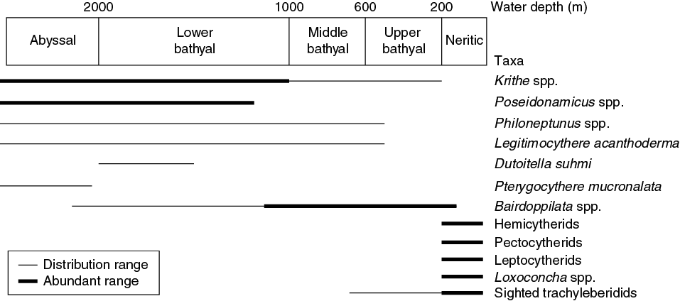
Figure F11. Depth distribution range of target ostracod taxa.
Terms used in the interpretation follow those for benthic foraminifers:
- Neritic = 0–200 m water depth.
- Upper bathyal = 200–600 m.
- Middle bathyal = 600–1000 m.
- Lower bathyal = 1000–2000 m.
- Abyssal = >2000 m.
Ostracod preservation
An assessment of ostracod preservation was attempted for all samples by observing Krithe spp. valves under a binocular light microscope. Transparency of these calcified valves generally becomes reduced during postmortem diagenesis. Therefore, the visual preservation index can be assigned to specimens based on their relative valve transparency, from 1 (transparent) to 7 (opaque white) (Dwyer et al., 1995).
Palynology
Dinocyst taxonomy and zonal scheme
Dinocyst taxonomy (Table T12) follows that presented in Williams et al. (1998) with emendations as proposed by Bijl et al. (2016) for the subfamily of Wetzelielloideae.
For the Paleogene, the Southern Ocean zonation by Bijl et al. (2013) was employed. This zonation is based primarily on analysis of sediments recovered at sites drilled during Ocean Drilling Program (ODP) Leg 189 and Integrated Ocean Drilling Program Expedition 318 and subsequently magnetostratigraphically calibrated to the GTS2012. This regional zonation has been shown to be compatible with regional dinocyst biostratigraphies from New Zealand (e.g., Wilson, 1988; Crouch and Brinkhuis, 2005) and Australia (e.g., Truswell, 1997).
No integrated stratigraphic dinocyst framework currently exists for the Neogene and Cretaceous southwest Pacific. The most recent update of a global integrated magnetostratigraphically calibrated dinocyst stratigraphy for the Late Cretaceous–Neogene is presented by Bijl et al. (2015). This work, which also includes an account of dinocyst events in the high southern latitudes, gives first and last occurrence data for dinocyst taxa calibrated to the GTS2012. Together with the Paleogene zonation by Bijl et al. (2013), the dinocyst event data presented here (Tables T6, T7) currently provides the best compilation of dinocyst biostratigraphy for the southwest Pacific.
Methods of study for palynology
A ~10 cm3 sample was processed according to standard palynological laboratory protocols (e.g., Sluijs et al. 2003). Samples were digested with 30% HCl and 40% hydrofluoric acid to dissolve carbonates and silicates, respectively, and was followed by HCl leaching to remove silicate gels, with centrifuging and decanting after each step. Residues were sieved with nylon 250 and 15 µm sieves, using an ultrasonic bath, and subsequently mounted on glass microscope slides using glycerin jelly.
Palynomorph abundance and preservation
Palynofacies were grouped into the following broad categories:
- Organic-walled dinoflagellate cysts (dinocysts),
- Foraminifer test linings,
- Prasinophytes,
- Acritarchs,
- Sporomorphs (pollen and spores),
- Black woody phytoclasts,
- Brown woody phytoclasts,
- Fungal spores,
- Insect remains,
- Pyritized siliceous microfossils, and
- Amorphous organic matter.
For semiquantitative estimates of the abundance of these palynofacies groups, the following scale was used:
- D = dominant (>90% of palynomorphs).
- A = abundant (>50%–90% of palynomorphs).
- C = common (>10%–50% of palynomorphs).
- F = few (1%–10% of palynomorphs).
- R = rare (<1% of palynomorphs).
- B = barren (not present).
For biostratigraphic and paleoenvironmental purposes, shipboard palynomorph analysis focused primarily on determining the presence of age-diagnostic dinocyst taxa and characterizing the palynological assemblage in terms of paleoenvironment. When possible given dinocyst yields and time, counts of ~100 dinocysts were carried out per sample and the remainder of the sample was visually scanned for stratigraphic marker species. Individual dinocyst taxa abundances were recorded using the same scale as for palynofacies but with percentages relative to the total amount of dinocysts.
Terrestrial sporomorphs identified during these counts were also quantitatively registered, attributing them to four broad categories:
Palynomorph preservation was qualitatively classified as one of the following levels:
Palynology-based paleoenvironmental analysis
The use of palynomorphs, in particular dinocysts, as paleoenvironmental indicators in the Paleogene is reviewed by Brinkhuis (1994), Pross and Brinkhuis (2005), and Sluijs et al. (2005). Dinocyst taxa are characteristic for different habitats in proximal to distal continental shelf transects. Based on this framework, the differential abundance of these taxa was used to reconstruct changes in coastal proximity (relative sea level) and offshore transport. The relative abundance of marine versus terrestrial palynomorphs was used to further substantiate this signal.
Paleomagnetism
Shipboard paleomagnetic analyses during Expedition 371 focused primarily on determining the orientation of the natural remanent magnetization (NRM) vector for recovered cores. This determination was made by performing quasicontinuous measurements on archive-half sections, which were integrated with measurements on discrete samples from working-half sections.
Remanence measurement of archive-half sections was performed using a 2G Enterprises superconducting rock magnetometer (SRM) equipped with direct current superconducting quantum interference devices (SQUIDs) and an in-line automated three-axes alternating field (AF) demagnetizer (maximum peak AF = 80 mT). The coordinate systems used for archive-half sections, the SRM, and AF demagnetizing coils are shown in Figure F12A. The background noise level (i.e., empty holder) along the three axes of the shipboard SRM was on average x-axis = ~0.5E−9 Am2, y-axis = ~0.5E−9 Am2, and z-axis = ~5E−9 Am2. Occasionally, the background noise level of the SRM increased to x-axis = ~1E−9 Am2, y-axis = ~1E−9 Am2, and z-axis = ~10E−9 Am2. In most cases, NRM was measured every 5 cm, and measurements were then repeated after AF demagnetization with peak fields of 10, 15, and 20 mT. Occasionally, the measurement spacing was increased to 10 cm or the AF demagnetization steps were limited to only 10 and 20 mT. Intervals with clearly visible drilling-related disturbance were not measured. To avoid possible magnetic contamination, the sample track was cleaned at the beginning of every work shift (~12 h). The magnetization of the sample tray was also measured at the beginning of every work shift, and the obtained value was subtracted from archive-half measurements.

Figure F12. Coordinate systems used for SRM and spinner magnetometer.
Usually 1–2 discrete samples per core were collected, mostly from undeformed and finer grained intervals, avoiding parts clearly affected by drilling-induced disturbance. Discrete sample analysis helps to monitor the behavior of sediments and rocks during AF demagnetization and determine the AF necessary to remove the magnetic overprint in the archive half. Paleomagnetic vectors isolated from fully AF demagnetized samples typically support magnetostratigraphic results from the measurements of the archive-half sections. For soft sediments, discrete samples were collected from the working-half sections using plastic Natsuhara-Giken sampling cubes (7 cm3 sample volume). Cubes were pushed by hand into the sediment, with the “up” arrow marked on the cube (i.e., negative z-axis) oriented toward the top of the core section (Figure F12B). For hard lithified sediment and volcanic rock intervals, 8 cm3 cubic samples (2 cm × 2 cm × 2 cm) were trimmed using a saw with two parallel blades. The orientation of the cube samples follows the right-hand rule.
Discrete sample AF demagnetization was performed using an ASC Scientific AF demagnetizer (model DTECH D-2000). After initial NRM measurement, samples were progressively demagnetized along three axes in peak AFs of 5, 10, 15, 20, 25, 30, 40, 50, and 70 mT. Occasionally, additional steps of 90 and 120 mT AFs were used. We measured the remanence after each demagnetization step using an AGICO JR-6A dual-speed spinner magnetometer. The background noise level of the shipboard JR-6A was around 10E−6 A/m (adopting a 8 cm3 volume). Data were transformed from the JR-6A instrument coordinate system to the core coordinate system (Figure F12B). The characteristic remanent magnetization (ChRM) component of the NRM was isolated by visual inspection of vector endpoint demagnetization diagrams (Zijderveld, 1967) using the principal component analysis (PCA) approach presented by Kirschvink (1980). This analysis was carried out using the PuffinPlot software package (Lurcock and Wilson, 2012).
Discrete samples were also measured for volume-normalized bulk susceptibility (χ) and anisotropy of magnetic susceptibility (AMS) with an AGICO Kappabridge (model KLY 4). The Kappabridge measures AMS by rotating the sample along three axes, stacking the data, and calculating the best-fit second-order tensor. Tensor elements were converted to eigenparameters (eigenvectors V1, V2, and V3) with corresponding eigenvalues τ1, τ2, and τ3, where τ1 and τ3 are the maximum and minimum value, respectively (Tauxe, 2010). Sedimentary AMS fabric is normally oblate (τ1 ≈ τ2 >> τ3) with the minimum susceptibility axis perpendicular to the sedimentation surface (i.e., vertical). Sediment affected by deformation or other disturbance generally produces different AMS fabrics. AMS data were analyzed using the AGICO ANISOFT 4.2 software package (Chadima and Jelínek, 2008).
During Expedition 371, the APC, XCB, and RCB systems were used for coring. Virtually all reliable magnetostratigraphic results were obtained from RCB cores. Correction for declination of the paleomagnetic vectors can be applied to APC cores but were not made during Expedition 371.
For correlation and age assignment of polarity chron boundaries, we adopted the GPTS2012 of Ogg (2012; Table T13). This timescale conforms to the GTS2012 of Gradstein et al. (2012).
Petrophysics
High-resolution physical properties measurements were made on cores and using downhole (in situ) logging during Expedition 371 with several primary objectives. The first was to measure the lithology- and depth-dependent density and porosity of the sections so that the tectonic subsidence of each of the sites could be interpreted in conjunction with the age model and paleobathymetry. Secondly, the physical properties aided lithostratigraphic characterization and were a valuable tie between core observations, downhole measurements, and seismic profiles. In particular, physical properties data played a major role in hole-to-hole and site-to-site stratigraphic correlation, detection of discontinuities and heterogeneities, identification of differences in sediment composition and texture, and identification of major seismic reflectors. Finally, we also measured the thermal properties of the recovered material and used those data in conjunction with the downhole temperature measurements to infer heat flow. A variety of techniques and methods were used on whole-round sections, section halves, and discrete samples to characterize Expedition 371 cores. Core sections are generally 1.5 m in length, so a typical coring length (stroke) of 9.5 m yields six sections plus a shorter seventh section. Procedures for measuring soft- or lithified-sediment cores differ slightly.
Downhole logs are used to determine physical, chemical, and structural properties of the formation penetrated by a borehole. The data are rapidly collected, continuous with depth, and measured in situ; they can be interpreted in terms of stratigraphy, lithology, physical properties, mineralogy, magnetic characteristics, and chemical composition. Where core recovery is incomplete or disturbed, log data may provide the only way to characterize the sedimentary succession. Where core recovery is good, log and core data complement one another and may be interpreted jointly.
Downhole logs measure formation properties on a scale that is intermediate between that of laboratory measurements on core samples and that of geophysical surveys. The logs are useful in calibrating the interpretation of geophysical survey data and provide a necessary link for the integrated understanding of physical and chemical properties on different scales. Moreover, the physical properties of the core can be changed from in situ characteristics either because of the drilling process or the change in pressure, and downhole measurements can thus help to characterize these changes.
In addition, during initial coring of some holes, we also measured the formation temperature as a function of depth, allowing us to estimate the heat flux, which is important for assessing the viability of models describing regional tectonic subsidence.
General sampling and measurement sequence
Core measurements
Whole-round sections were first allowed to equilibrate to ambient room temperature (~20°C) and pressure for ~4 h. After thermally equilibrating, core sections were run through the WRMSL for gamma ray attenuation (GRA) density, magnetic susceptibility, and, where contact between sediment and core liner was sufficiently good, compressional wave velocity on the P-wave logger (PWL). Cores recovered with the XCB or RCB systems have a slightly smaller nominal diameter (58 mm) than those cored with the APC system (66 mm). As a result, sections cored with the XCB or RCB system typically have gaps between the liner and the core. In these cases, GRA density computed by routine procedures underestimated actual bulk density by as much as 12% and P-wave velocity measurements with the WRMSL often failed or were outside the accepted velocity range (1000–4500 m/s) and therefore not retained.
To optimize the measurement process, sampling intervals (2 cm) and measurement times (5 s, 5 samples of 1 s duration each) were the same for all sensors on the WRMSL. These sampling intervals are common denominators of the distances between the sensors installed on the WRMSL (30–50 cm), which allows sequential and simultaneous measurements. After measuring a core, calibration verification measurements were made by passing a single core liner filled with deionized water through the WRMSL.
We used the Special Task Multisensor Logger (STMSL), which is essentially a clone of the WRMSL, to measure selected sections from Holes B (and C) out of sequence, before they had equilibrated, to provide near real-time feedback to the rig crew in terms of vertical offsets required to cover coring gaps in Hole A (see Stratigraphic correlation). Sections were subsequently measured with the NGRL.
In one hole at each site, thermal conductivity was measured on approximately one whole-round per core, and then repeat measurements were taken in subsequent holes as needed. Measurements were conducted with a needle probe inserted into the section through a small hole drilled through the plastic core liner close to the middle of the section. In lithified sediments, a contact probe method in a half-space configuration was used on section halves for thermal conductivity measurements.
After completion of measurements on whole-round sections, the cores were split longitudinally, with one half designated as the archive-half section and the other as the working-half section for sampling and analysis (see Core and section handling). The archive half of the core was passed through the SHMSL for measurement of point magnetic susceptibility (MSP), colorimetry, and color reflectance.
The archive-half section was placed on the SHMSL core holder, above which an electronic platform moves along the section half, recording the height of the surface with a laser sensor. The laser establishes the location of the bottom of the section and then the platform reverses the direction of movement, moving from bottom to top making MSP and color reflectance measurements. All foam inserts were removed from the section halves before measurement (except for MSP measurements) so that the laser could detect gaps and the measured range of values represents that of the core material only. During Expedition 371, MSP and color reflectance data were collected at constant intervals of 2 cm. This resolution facilitates comparison with results obtained from the WRMSL, which also has a sampling interval of 2 cm. The archive-half sections were covered with clear plastic wrap to ensure a flush contact between the MSP sensor and the split core without sediment contaminating the sensor. Deeper in the hole, when the core recovered lithified material and the core was dry, the plastic wrap was omitted during MSP and colorimetry measurement.
The working-half section was measured on the Section Half Measurement Gantry (SHMG). For soft-sediment cores, P-wave velocity and shear strength measurements were performed. P-wave velocity measurements used the y- and z-axis P-wave bayonet (PWB) probes, which were inserted into the sediment. In harder material, the x-axis P-wave caliper (PWC) contact probe was used with at least one analysis per core. PWC measurements were made on the cube samples cut for moisture and density (MAD) analysis. Shear strength (Torvane) and normal strength (penetrometer) were measured on the same section halves when the material was soft enough.
Discrete samples were collected from the working halves for MAD analysis. One sample was generally taken in Sections 1, 3, and 5 of the cores from Holes A and B. Depending on lithologic variability, additional samples were taken. These samples were then used to measure wet and dry mass and dry volume and to calculate wet bulk density, dry bulk density, water content, porosity, and grain density with MAD procedures.
A full discussion of methodologies and calculations used aboard the JOIDES Resolution in the Physical Properties Laboratory is presented by Blum (1997). Cleaned track data are available in CLEANEDTRACKDATA in Supplementary material. Details and procedures for each physical properties measurement are described below.
Downhole temperature measurements
During APC coring operations and generally above 200 m DSF, the formation temperature was measured with an APCT-3 that replaces the normal coring shoe. Normally, these measurements were made while coring Hole A; however, if the temperature record was judged to be of low quality, additional APCT-3 measurements were made on Hole B.
Wireline logging
During wireline logging operations, the logs are recorded with Schlumberger logging tools combined into tool strings, which are lowered into the hole after the completion of coring operations. One tool string was used during Expedition 371, the modified triple combo. The modified triple combo was configured to measure borehole diameter, total spectral gamma ray (HSGR), density, resistivity, magnetic susceptibility, and sonic P- and S-wave velocity. The tool string also contained a telemetry cartridge for communicating through the wireline to the Schlumberger data acquisition system (MAXIS unit) on the ship. In preparation for logging, the boreholes were flushed of debris by circulating drilling fluid and were at least partially filled with seawater-based logging gel (sepiolite mud mixed with seawater and weighted with barite; density of ~1258 kg/m3) to help stabilize the borehole walls in sections where instability was expected from drilling and coring disturbance. The BHA was pulled up to ~70 m DSF, where it protected the unstable upper part of the hole. The tool strings were then lowered downhole on a seven-conductor wireline cable before being pulled up at a constant speed of 550 m/h for the triple combo to provide continuous log measurements of several properties simultaneously.
Each tool string deployment is termed a logging “run.” During each run, tool strings can be lowered and pulled up in the hole several times to check repeatability, referred to as “passes.” Incoming data were recorded and monitored in real time on the MCM MAXIS logging computer. A wireline heave compensator (WHC) was used to minimize the effect of the ship’s heave on the tool position in the borehole.
The main influence on log data quality is the condition of the borehole wall. Where the borehole diameter varies over short intervals because of washouts of softer material or ledges of harder material, the logs from tools that require good contact with the borehole wall (i.e., density and porosity) may be degraded. Deep investigation measurements, such as gamma radiation, resistivity, magnetic susceptibility, and sonic velocity, do not require contact with the borehole wall and are generally less sensitive to borehole conditions. “Bridged” sections, where borehole diameter is significantly smaller than the bit size, will also cause irregular log results. The borehole quality is improved by minimizing drilling fluid circulation while drilling, flushing the borehole to remove debris, and logging as soon as possible after drilling and conditioning are completed.
The logging measurement depth is determined from the length of the cable payed out from the winch on the ship and is measured on the WRF depth scale. The seafloor is identified on the HSGR log by the abrupt upward reduction in gamma ray count at the water/sediment interface (mudline), and the seafloor depth is subtracted to give the WSF depth. Discrepancies between DSF and WSF depth scales may occur. In the case of drilling depth, discrepancies are due to incomplete heave compensation. In the case of log depth, discrepancies between successive runs occur because of incomplete heave compensation, incomplete correction for cable stretch, and cable slip (Iturrino et al., 2013). Both depth measurements may be affected by tides.
Data for each wireline logging run were monitored in real time and recorded using the Schlumberger MAXIS 500 system. Initial logging data were referenced to the rig floor (WRF scale). After logging was completed, the data were shifted to a seafloor reference (WSF scale). Data were transferred on shore to LDEO, where standardized data processing took place. The main part of the processing is depth matching to remove depth offsets between measurements from different logging runs, which results in a new depth scale: WMSF. Documentation for the logs (with an assessment of log quality) was prepared, and the data were converted to ASCII for the conventional logs. The data were transferred back to the ship within a few days of logging, and this processed data set was made available to the science party (in ASCII and digital log information standard [DLIS] formats) through the shipboard IODP logging database and shipboard servers. The Schlumberger TechLog software was used to visualize and unbundle the DLIS files.
The logged properties and the principles and tools used to measure them are briefly described below. More detailed information on individual tools and their geological applications may be found in Serra (1984, 1986, 1989), Schlumberger (1989), Rider (1996), Goldberg (1997), Lovell et al. (1998), and Ellis and Singer (2007). A complete online list of acronyms for the Schlumberger tools and measurement curves is at http://iodp.tamu.edu/tools/logging/index.html.
Core measurements
Gamma ray attenuation density
GRA density is measured on whole-round sections using the WRMSL. Bulk density can be used to estimate the pore volume in sediment and evaluate the consolidation state of sediment. GRA density is an estimate of bulk density based on the attenuation of a gamma ray beam. The beam is produced by a 137Cs gamma ray source at a radiation level of ~370 MBq in a lead shield with a 5 mm collimator, which is directed through the whole-round core. The gamma ray detector on the opposite side of the core from the source includes a scintillator and an integral photomultiplier tube to record the gamma radiation that passes through the core. The attenuation of gamma rays occurs primarily by Compton scattering, in which gamma rays are scattered by electrons in the formation; the degree of scattering is related to the material bulk density. Therefore, for a known thickness of sample, the density (ρ) is proportional to the intensity of the attenuated gamma rays and can be expressed as
- I = the measured intensity of gamma rays passing through the sample,
- I0 = gamma ray source intensity,
- μ = Compton attenuation coefficient, and
- d = sample diameter.
μ, d, and I0 are treated as constants, such that ρ can be calculated from I.
In general, GRA density measurements are most accurate when taken on a completely filled core liner with minimal drilling disturbance; otherwise, measurements tend to underestimate true values. By default, the instrument reports measurements using the internal diameter of the core liner (66 mm) as the assumed sample diameter. This assumption is suitable for most sediment cores obtained by the APC system; however, for sediment and/or hard rock cored by the XCB or RCB systems, core diameter is usually about 58 mm or less. The spatial resolution of the GRA densitometer is less than ±1 cm. Calibration details are documented elsewhere (Blum, 1997).
Magnetic susceptibility
Magnetic susceptibility is measured on whole-round sections using a pass-through loop magnetic susceptibility (MSL) system on the WRMSL and on section halves using a MSP contact probe system on the SHMSL. Magnetic susceptibility (χ) is a dimensionless measure of the degree to which a material can be magnetized by an external magnetic field:
where M is the magnetization induced in the material by an external field of strength H. Magnetic susceptibility is primarily sensitive to the concentration of ferrimagnetic minerals (e.g., magnetite, pyrite, and a few other iron oxides). It is also sensitive to magnetic mineralogy and can be related to the origin of the materials in the core and their subsequent diagenesis.
MSL measurements were made using a Bartington MS2C loop sensor with a 9 cm diameter. An oscillator circuit in the sensor, which operates at a frequency of ~0.565 kHz (with a slight offset for the WRMSL and STMSL to avoid interference) and an AF of ~140 A/m, produces a low-intensity nonsaturating alternating magnetic field. Sediment core sections going through the influence of this field cause a change in oscillator frequency. Frequency information returned in pulse form to the susceptometer is converted into magnetic susceptibility. The loop sensor is accurate to within 2% (Blum, 1997).
MSP was measured with a Bartington MS2 meter and an MS2K contact probe with a flat 15 mm diameter round sensor with a field of influence of 25 mm and an operation frequency of 930 Hz. The spatial resolution of the MSP instrument is ~3.8 mm. As with whole-round measurements, the output displayed by the MSP sensor is reported in instrument units (IU) and can be converted to approximate dimensionless SI units by multiplying by 10−5. The probe is zeroed in air before each measurement to avoid influence from the metal track. The MSP meter was calibrated by the manufacturer before installation on the ship and is quality checked every ~6 h at the same time as color reflectance sensor calibration is performed.
P-wave velocity
P-wave sonic velocity data can be used to assist in the correlation between the core and seismic sections, correlate between downhole logging and core data, and evaluate porosity and cementation. P-wave (compressional) velocity (VP) is defined by the time required for a compressional wave to travel a specific distance:
where dcore is the path length of the wave across the core and tcore is the traveltime through the core. P-wave velocity was measured on whole-round sections using the PWL system and on section halves using the PWB and PWC systems. The P-wave velocity systems use Panametrics-NDT Microscan delay line transducers, which transmit a 500 kHz pulse.
Cores drilled with the XCB and RCB systems generally did not provide usable PWL data because of bad sediment/liner contact and disturbed sediment. For lithified sediments, P-wave velocity was measured with the PWC on section halves or discrete cube samples prior to MAD analyses.
The PWL measures the traveltime of 500 kHz ultrasonic waves horizontally across the whole-round section at 2 cm intervals while it remains in the core liner. Waves are transmitted to the core by transducer contacts connected to linear actuators. Pressure is applied to the actuators to ensure coupling between the transducers and the core liner, and the space between the core liner and transducers was kept wet to ensure good coupling. P-wave velocity transducers measure total traveltime (t) of the compressional wave between transducers separated by the total distance (d) measured using a laser beam. By measuring the traveltime through a standard block of aluminum with a known velocity (6295 m/s), a system delay correction (δt) is found. The core is surrounded by a core liner of empirical thickness (δL), and a traveltime (δtL) is determined by measuring the traveltime through the core liner filled with distilled water of known velocity (corrected for the influence of temperature). Arrival times are taken for the second lobe of the waveform, requiring a correction (δtpulse) to get the first arrival. Consequently, the velocity in the core is
VP = (d − 2δL)/(t − δt − 2δtL − δtpulse).
The PWC measures the traveltime of 500 kHz ultrasonic waves vertically across the section half, which remains in the half liner, at selected intervals or on discrete sample cubes cut from the section halves. For the PWC, the distance between transducers was measured with a built-in linear voltage displacement transformer. Calibration was performed with a series of acrylic cylinders of differing thicknesses and a known P-wave velocity of 2750 ± 20 m/s. The determined system time delay from calibration was subtracted from the picked arrival time to give a traveltime of the P-wave through the sample. The thickness of the sample after appropriate subtraction of the liner thickness was divided by the traveltime to calculate P-wave velocity in meters per second.
Natural gamma radiation
Gamma radiation is emitted from the decay of 238-uranium (238U), 232-thorium (232Th), and 40-potassium (40K) in the core sample. The NGRL measures this natural emission on whole-round cores using a system designed and built at Texas A&M University (USA) (Vasiliev et al., 2011; Dunlea et al., 2013). When 238U, 232Th, and 40K radioisotopes decay, gamma radiation is emitted at specific energy levels. NGR spectroscopy measures a wide energy spectrum that can be used to estimate the abundance of each isotope based on the strength of the signal at characteristic energies (Blum, 1997; Gilmore, 2008). Spectral data were collected and can be used for postexpedition processing for U, Th, and K abundance but were not processed on board. Total counts were used on board, with high counts usually identifying fine-grained deposits containing K-rich clay minerals and their absorbed U and Th isotopes. NGR data thus revealed stratigraphic details that aid in hole-to-hole correlations. The main NGRL detector unit consists of eight sodium iodide (NaI) detectors arranged along the core measurement axis at 20 cm intervals surrounding the lower half of the section (Vasiliev, et al., 2011). The detector array has passive (layers of lead) and active (plastic scintillators) shielding to reduce the background environmental and cosmic radiation. The overlying plastic scintillators detect incoming high-energy gamma and muon cosmic radiation and cancel this signal from the total counted by the NaI detectors.
The quality of the energy spectrum measured in a core depends on the concentration of radionuclides in the sample but also on the counting time, with higher times yielding better spectra. Therefore, a measurement run consisted of counting on each core section for 300 s at Position 1. After 300 s, the section was offset by 10 cm (Position 2) and measured again for 300 s. This yielded a total of 16 measurements (10 cm apart) per 150 cm section. These settings yielded statistically significant total counts.
Thermal conductivity measurements
Thermal conductivity was measured with the TK04 (Teka) system using a needle probe method in full-space configuration on whole-round cores for soft sediments (Von Herzen and Maxwell, 1959) or a contact probe method in half-space configuration on section halves for lithified sediments and rocks. The probes contain a heater wire and calibrated thermistor. The contact probe was embedded in the surface of an epoxy block with a low thermal conductivity (Vacquier, 1985).
For soft sediment, the needle probe was inserted into a 2 mm diameter hole drilled through the liner along one of the lines that later guided core splitting. To avoid interference from airflow in the laboratory, the core was placed in an enclosed box outfitted with foam. For lithified sediment cores, the section half was put in the enclosed box and the contact probe was put on the cut face of the sample.
The calibrated heat source of the probe was turned on, and the increase in temperature was recorded for 80 s for measurements with the needle probe and 60 s for measurements with the contact probe. A heating power of 1 W/m was typically used in soft sediment, and 0.5–1.5 W/m was used for lithified sediments. The solution to the heat conduction equation with a line source of heat was then fit to the temperature measurements to obtain the thermal conductivity. Because the probe is much more conductive than sediment, the probe is assumed to be a perfect conductor. Under this assumption, the temperature of the superconductive probe has a linear relationship with the natural logarithm of the time after the initiation of the heat:
- T = temperature (K),
- q = heat input per unit length per unit time (J/m/s),
- k = thermal conductivity (W/[m·K]),
- t = time after the initiation of the heat (s), and
- C = instrumental constant.
Three automatic measuring cycles were used to calculate average conductivity. A self-test, which included a drift study, was conducted at the beginning of each measurement cycle. Once the probe temperature stabilized, the heater circuit was closed and the temperature rise in the probe was recorded. Thermal conductivity was calculated from the rate of temperature rise while the heater current was flowing. Temperatures measured during the first 60 or 80 s of the heating cycle were fit to an approximate solution of a constantly heated line source (for details, see Kristiansen [1982] and Blum [1997]). Measurement errors were 5%–10%. Thermal conductivity measurements were routinely taken in one section per core throughout the first hole. Some cores yielded no results for thermal conductivity because cracks in the sediment caused bad coupling of the needle probe to the sediment.
Color reflectance spectrometry
The color reflectance spectrometer used an Ocean Optics QE Pro detector integrating sphere and associated light sources, which cover wavelengths from UV through visible to near infrared (380–900 nm wavelengths at 2 nm intervals). The data are reported using the L*a*b* color system, in which L* is lightness, a* is redness (positive) versus greenness (negative), and b* is yellowness (positive) versus blueness (negative). The color reflectance spectrometer calibrates on two spectra, pure white (reference) and pure black (dark). Color calibration was conducted approximately once every 6 h (twice per shift).
Shear strength
Shear strength is the resistance of a material to failure in shear. Shear stress in unconsolidated materials is resisted only by the network of solid particles. Shear strength (τf) can be expressed as a function of the effective normal stress at failure (σʹ), the effective cohesion (cʹ), and friction angle (φʹ):
where c′ and φ′ are the shear strength parameters that define a linear relationship between τf and φʹ, according to the Mohr-Coulomb failure criterion.
Shear strength parameters can be determined by means of multiple laboratory tests. cʹ and φʹ are relevant in situations where field drainage conditions correspond to test conditions. The shear strength of a soil under undrained conditions (interstitial water drainage does not occur during failure) is different from that under drained conditions (interstitial water drainage occurs).
Undrained shear strength (Su) can be expressed in terms of total stress in the case of fully saturated materials of low permeability (e.g., clays). The most common strength tests in shipboard laboratories are the vane shear and penetrometer tests, which provide measurement of undrained shear strength (Blum, 1997).
During Expedition 371, Su was measured in undisturbed fine-grained sediment using the Torvane shear device in working-half sections. Undrained shear strength was determined by inserting a four-bladed vane into the split section surface and putting it under shear stress to cause a cylindrical surface to be sheared by the vane. This procedure provides a measurement of the peak shear strength (units of kPa). Measurements were made with the vane rotation axis perpendicular to the split surface. Shear strength was measured once in each core when sediments were within the instrument range.
A pocket penetrometer (Model 29-3729, Ele International) was used to measure the sediments’ response to normal stress (units of kPa). Measurements were made close to the stratigraphic position of the Su measurements described above.
Moisture and density
Discrete samples were collected from the working halves to determine wet and dry bulk density, grain density, water content, and porosity. In soft sediment, ~10 cm3 samples were collected with a plastic syringe with a diameter that fit in the glass vials used to process the samples. As a general rule, three samples were taken in each 9.5 m core and two were taken in each 4.5 m core in the first hole at each site. Depending on lithologic variability, additional samples were taken. In indurated sediment and hard rock, sawed 1.4 cm × 1.4 cm × 3 cm (to 1 cm × 1 cm × 1.5 cm) cubes were extracted from the working halves for MAD analysis, and many of these cubes were also used for P-wave velocity measurements. Sampling frequency was reduced to 1–2 samples every other core or less from overlapping portions of Hole B.
Soft-sediment samples were placed in numbered preweighed ~16 mL Wheaton glass vials for wet and dry sediment weighing, drying, and dry volume measurements. Samples were dried in a convection oven for at least 24 h at 105° ± 5°C. Dried samples were then cooled in a desiccator for at least 60 min before dry mass and volume were measured. Wet and dry sample masses were determined to a precision of 0.005 g using two Mettler Toledo electronic balances, with one acting as a reference. A standard with a mass similar to that of the sample was placed on the reference balance, and a computer averaging system was used to compensate for the ship’s motion. The default setting of the balances is 300 measurements (taking ~1.5 min).
Dry sample volume was determined using a hexapycnometer system of a six-celled custom-configured Micrometrics AccuPyc 1330TC helium-displacement pycnometer. The precision of each cell is 1% of the full-scale volume. Volume measurement was preceded by three purges of the sample chamber with helium warmed to ~28°C. Three measurement cycles were run for each sample. A reference volume (set of two calibration spheres) was placed sequentially in one of the chambers to check for instrument drift and systematic error. The volumes occupied by the numbered Wheaton vials were calculated before the expedition by multiplying each vial’s weight against the average density of the vial glass. Dry mass and volume were measured after samples were heated in an oven at 105° ± 5°C for 24 h and allowed to cool in a desiccator. The procedures for the determination of these physical properties comply with the American Society for Testing and Materials (ASTM) designation (D) 2216 (ASTM International, 1990). The fundamental relation and assumptions for the calculations of all physical properties parameters are discussed in Blum (1997). MAD properties reported and plotted in the Petrophysics section of each site chapter were calculated with the MADMax shipboard program set with the “Method C” calculation process.
MAD porosity (φ) versus depth (z) is fit with the linear regression of a simple exponential decay (i.e., φ = φoe−z/c). Uncertainty on the best-fitting parameters is reported as standard deviations. An exponential reduction of porosity with depth is theoretically predicted (through expulsion of fluids from the sediment pore space with increasing hydrostatic pressure) and is widely observed for shales and other sediments (Korvin, 1984; Gallagher, 1989). An exponential decay of porosity with depth is also widely found in the sediments of Taranaki Basin offshore the North Island of New Zealand (Funnell et al., 1996).
Downhole temperature measurements
During Expedition 371, in situ temperature measurements were made with the APCT-3 (Heesemann et al., 2006) at several sites. The APCT-3 fits directly into the coring shoe of the APC system and consists of a battery pack, data logger, and platinum resistance-temperature device calibrated over a temperature range of 0°–30°C. Before entering the borehole, the tool is first stopped at the mudline for 5 min to thermally equilibrate with bottom water. When the APC system is plunged into the formation, temperature rises instantaneously from frictional heating. This heat gradually dissipates into the surrounding sediment as the temperature at the APCT-3 equilibrates toward the temperature of the sediment. After the APC system penetrated the sediment, it was held in place for about 10 min while the APCT-3 recorded the temperature of the cutting shoe every 1 s.
The equilibrium temperature of the sediment was estimated by applying a heat conduction model to the temperature decay record (Horai and Von Herzen, 1985). The synthetic thermal decay curve for the APCT-3 is a function of the geometry and thermal properties of the probe and the sediment (Bullard, 1954; Horai and Von Herzen, 1985). Equilibrium temperature was estimated by applying a fitting procedure (Pribnow et al., 2000). However, if the APC system does not achieve a full stroke or if ship heave pulls the APC system up from full penetration, the temperature equilibration curve is disturbed and temperature determination is less accurate. The nominal accuracy of the APCT-3 temperature measurements is ±0.05°C.
The APCT-3 temperature data were combined with thermal conductivity measurements (see above) obtained from whole-round core sections to obtain heat flow values. Heat flow was calculated according to the Bullard method to be consistent with the synthesis of ODP heat flow data by Pribnow et al. (2000).
Slopes and intercepts of temperature and thermal conductivity versus depth and temperature versus thermal resistance are computed with linear regression. Uncertainties are quantified as standard deviations.
Wireline logging measurements
Natural gamma radiation
The Hostile Environment Natural Gamma Ray Sonde (HNGS) was used to measure NGR in the formation. The HNGS uses two bismuth germanate scintillation detectors and five-window spectroscopy to determine potassium (in weight percent), thorium, and uranium (both in parts per million) concentrations from the characteristic gamma ray energies of isotopes in the 40K, 232Th, and 238U radioactive decay series, which dominate the natural radiation spectrum. The computation of the elemental abundances uses a least-squares method to extract U, Th, and K elemental concentrations from the spectral measurements. The HNGS filters out gamma ray energies lower than 500 keV, eliminating sensitivity to bentonite or KCl in the drilling mud and improving measurement accuracy. The HNGS also provides a measure of the HSGR (total gamma ray) and uranium-free or computed gamma ray (HCGR) that are both measured in American Petroleum Institute gamma radiation units (gAPI). The HNGS response is influenced by the borehole diameter; therefore, the HNGS data are corrected for borehole diameter variations during acquisition.
An additional gamma ray sensor was housed in the Enhanced Digital Telemetry Cartridge (EDTC), which was used primarily to communicate data to the surface. The sensor includes a sodium iodide scintillation detector and is not a spectral analysis tool (does not provide U, Th, and K concentrations), but it provides total NGR for each pass. The inclusion of an NGR tool in every tool string allows the use of NGR data for precise depth matching between logging runs and passes and for core-log integration.
Density and photoelectric factor
Formation density was measured with the Hostile Environment Litho-Density Sonde (HLDS). The HLDS contains a cesium (137Cs) gamma ray source (662 keV) and far and near gamma ray detectors mounted on a shielded skid that is pressed against the borehole wall by a hydraulically activated decentralizing arm. Gamma rays emitted by the source undergo Compton scattering, in which gamma rays are scattered by electrons in the formation. The number of scattered gamma rays that reach the detectors is proportional to the density of electrons in the formation, which is in turn related to bulk density. Porosity may also be derived from this bulk density if the matrix (grain) density is known.
The HLDS also computes the photoelectric effect (PEF), a measure of the photoelectric absorption of low-energy gamma radiation. Photoelectric absorption of gamma rays occurs when their energy falls below 150 keV as a result of being repeatedly scattered by electrons in the formation. PEF is determined by comparing the counts from the far detector in the high-energy region, where only Compton scattering occurs, with those in the low-energy region, where count rates depend on both reactions. Because PEF depends on the atomic number of the elements in the formation (heavier elements have higher PEF), it also varies according to the chemical composition of the minerals present and can be used for the identification of the overall mineral make-up of the formation. For example, the PEF of calcite is 5.08 b/e−, illite is 3.03 b/e−, quartz is 1.81 b/e−, and hematite is 21 b/e−.
Good contact between the tool and borehole wall is essential for good HLDS logs; poor contact results in underestimation of density values. To limit the possibility of losing an environmentally hazardous package during deployment, the HLDS was not run in some holes. Both the density correction and caliper measurement of the hole are used to check the contact quality. In the deeper parts of the hole, the PEF log should be used with caution, especially in washouts, because barium in the logging mud swamps the signal despite a correction for the influence of logging mud.
Electrical resistivity
Resistivity measurements can be used to assist in differentiating formation material based on different electrical conductivity values. Calcite, silica, and hydrocarbons are electrical insulators, whereas ionic solutions like interstitial water are conductors. Therefore, electrical resistivity can be used to evaluate porosity for a given salinity and resistivity of the interstitial water. Clay surface conduction also contributes to the resistivity values but is a relatively minor effect at high porosity values.
The High-Resolution Laterolog Array (HRLA) provides six resistivity measurements with different depths of investigation, including the borehole (mud) resistivity and five measurements of formation resistivity. The HRLA sends a focused current into the formation and measures the intensity necessary to maintain a constant drop in voltage across a fixed interval, providing direct resistivity measurements. The array has one central (source) electrode and six electrodes above and below it, which serve alternatively as focusing and returning current electrodes. By rapidly changing the roles of these electrodes, a simultaneous resistivity measurement at six penetration depths is achieved. The tool is designed to ensure that all signals are measured at exactly the same time and tool position to reduce the sensitivity to “shoulder bed” effects when crossing sharp beds thinner than the electrode spacing. The design of the HRLA eliminates the need for a surface reference electrode, improves formation resistivity evaluation compared with traditional dual induction, and allows the full range of resistivity to be measured, from low (e.g., in high-porosity sediments) to high (e.g., in basalt). The HRLA needs to be run centralized in the borehole for optimal results, so knuckle joints were used to centralize the HRLA while allowing the density and porosity tools to maintain good contact with the borehole wall.
Acoustic velocity
The Dipole Sonic Imager (DSI) measures the transit times between sonic transmitters and an array of eight receivers. It combines replicate measurements, thus providing a direct measurement of sound velocity through formations that is relatively free from the effects of formation damage and an enlarged borehole (Schlumberger, 1989). Along with the monopole transmitters found on most sonic tools, it also has two crossed-dipole transmitters that allow shear wave velocity measurement in addition to compressional wave velocity. Dipole measurements are necessary to measure shear velocity in slow formations with shear velocity less than the velocity of sound in the borehole fluid. Such slow formations are typically encountered in deep ocean drilling.
Magnetic susceptibility
The magnetic susceptibility sonde (MSS) measures the ease with which formations are magnetized when subjected to a magnetic field. The ease of magnetization is ultimately related to the concentration and composition (size, shape, and mineralogy) of magnetic minerals (principally magnetite) in the formation. These measurements provide one of the best methods for investigating stratigraphic changes in mineralogy and lithology because the measurement is quick, repeatable, and nondestructive and because different lithologies often have strongly contrasting susceptibility values.
The MSS dual-coil sensor provides ~36 cm vertical resolution measurements and a ~20 cm depth of horizontal investigation. The MSS was run as the lowermost tool in the triple combo tool string using a specially developed data translation cartridge to enable the MSS to be run in combination with the Schlumberger tools. The MSS also has an optional single-coil sensor to provide high-resolution measurements (~10 cm), but it was not used during Expedition 371 because it has a large bowspring that would require the MSS to be run higher up in the tool string and because it is very sensitive to separation from the borehole wall.
Magnetic susceptibility data are plotted as uncalibrated units. The MSS reading responses are affected by temperature and borehole size (higher temperatures lead to higher susceptibility measurements). The magnetic susceptibility values were not fully corrected for temperature during Expedition 371, so values deeper than several hundred meters were generally not interpretable. When the magnetic susceptibility signal in sediment is very low, the detection limits of the tool may be reached. For quality control and environmental correction, the MSS also measures internal tool temperature, z-axis acceleration, and low-resolution borehole conductivity.
Borehole ties to multichannel seismic data
Rebound corrections
Wireline logging measurements of in situ P-wave velocity and density usually start at ~70 mbsf because drill pipe is left in the top of the hole to prevent collapse. To estimate in situ physical properties values over this unlogged section of the borehole and at sites where wireline logging data were not recorded, corrections for porosity rebound were applied for the purpose of establishing ties from the boreholes to the seismic data. To adjust velocity and density measurements under atmospheric conditions to their in situ equivalents, PWC velocity values were corrected for porosity rebound arising from overburden removal.
Comparisons between well logs and laboratory measurements of P-wave velocity values of Ontong Java carbonates (Urmos and Wilkens, 1993) were used to determine an empirical relationship between laboratory-measured and in situ values. Converting drill core measured P-wave velocity values to their in situ equivalents, the calculated velocity correction (ΔVP) with depth is given by Urmos and Wilkens (1993):
where C is 0.66, z is the depth below seafloor in meters, and ΔVP is in kilometers per second.
Synthetic seismograms
Synthetic seismograms were computed to correlate between lithology in the drill cores and reflections in seismic data recorded at the borehole. Seismic reflections are produced at contrasts in physical properties in the earth, and the amount of energy reflected from the interface between two layers of differing properties depends on the impedance (I) contrast between the two layers:
where VP is the P-wave velocity in meters per second and ρ is the density in grams per cubic centimeter.
The normal incidence reflection coefficient (RC) is the ratio between incident and reflected amplitudes, which is given by Sheriff and Geldart (1995):
where I1 is the impedance of the top layer and I2 is the impedance of the bottom layer.
Synthetic seismograms were constructed using the Clartias Synvert processing software with the aim to reproduce two-way traveltimes (TWTs) of prominent reflections in seismic traces extracted at the drill sites. The software uses input P-wave velocity, density (to calculate impedance), and the inverse of attenuation (Q) values (seawater = 1000; marine sediments = 250) to calculate reflection coefficients and produce a synthetic seismic response for a normal input Ricker wavelet.
Where available, P-wave and density values from wireline logging were used as the input impedance model. Rebound-corrected laboratory P-wave and density measurements were used to estimate physical properties in any gaps in wireline logging coverage, such as the top 70 m, or where wireline logging data were not available.
The validity of the synthetic model was visually checked by plotting the synthetic seismic trace over the multichannel seismic (MCS) trace extracted at the drill site. The product of real and synthetic data amplitude was used to identify correlations between the two traces. Strong correlations occur where real and synthetic seismic reflection events have the same TWT. Layer velocities and thicknesses from the synthetic model were used to calculate TWTs to compare borehole depths and lithology with MCS reflection events. Modeled TWT versus depth is calculated by summing the TWT of individual model layers:
where Z is the model layer thickness in meters and VP is the layer P-wave velocity in meters per second.
A polynomial regression is fit to these data to produce a numerical solution for TWT versus depth to aid interpretations of seismic reflection events away from the borehole.
Geochemistry
The shipboard geochemistry program for Expedition 371 included the collection and measurement of headspace gas, interstitial water, and sediment samples. Headspace samples were analyzed initially for routine hydrocarbon monitoring, as required for safety and pollution prevention protocol. Interstitial water and sediment were analyzed to understand the history of sediment deposition, including potential diagenesis.
Sampling strategy
One headspace gas (HS) sample was collected from each core from Hole A at each site, usually at the top of the lowermost section next to an interstitial water (IW) sample. Samples were also taken from cores of additional holes where depths exceeded those of previously drilled holes or where hydrocarbon concentrations became interesting.
For soft sediment, HS sediment plugs were collected using a graduated syringe, with the aim of collecting exactly 5 cm3. The plug was then extruded into a 21.5 cm3 glass serum vial. When sediment became too hard to collect with a syringe, a sample was broken into small pieces and the pieces were placed into a 21.5 cm3 glass serum vial with a red line that approximated the equivalent of 5 cm3. Notably, once in the vials, sample volumes include variable proportions of sediment grains, pore space, and air, which leads to large analytical imprecision.
One water sample was taken from within the core liner above the uppermost sediment recovered, typically in the first hole at each site. This “mudline” sample should approximate bottom water and provide a useful comparison to IW samples. A barrel of surface seawater was also collected at Site U1509. The collected seawater was filtered through a 0.2 µm membrane filter (Isopore) twice and stored for analysis following the protocol for IW samples.
IW samples were collected from all six sites during Expedition 371. Water samples were collected following different strategies that somewhat followed those applied during Integrated Ocean Drilling Program Expedition 346 (Tada et al., 2015). Ideally for squeezed samples, 30–40 mL of pore water was desired, but it was not always possible, especially in strongly indurated sediment, even after crushing.
For Sites U1506, U1509, and U1511, whole-round IW samples were collected as follows. An IW sample was taken from a lower section for the uppermost few cores. For deeper cores, an IW sample was generally collected every other core. For the other three sites, additional IW samples were collected. At Site U1510, for example, two IW samples were collected per core from the uppermost 150 m in Holes U1510A and U1510B and one IW sample was collected per core or every other core below 150 m in Holes U1510A and U1510B (and Hole U1510C if possible). In general, IW samples were targeted for the base of Sections 1 and 6 above 150 m and for the base of Section 6 below 150 m. When sediment recovery rates were low, IW samples were sometimes taken from the base of the lowermost section. The rationale for such sampling is that the IW whole rounds cut from the core most likely would be located on “off-splice” intervals of the stratigraphic section (see Geochemistry). Near the top of the hole, whole-round samples were 5 cm long. This length increased to a maximum of 20 cm downhole because porosity and water content generally decrease with depth below the seafloor.
At Site U1508, several half-round samples were taken from the working half after cores had been scanned, split, and examined for various sediment properties. This procedure was done in an effort to collect IW samples while also preserving and analyzing the sedimentary record.
Other than squeeze sampling, Rhizons were used to collect high-resolution IW samples from the uppermost 10 m in Hole U1508A, the uppermost 20 m in Holes U1510A and U1510B, and the uppermost 30 m in Holes U1511A and U1511B. Rhizon sampling was aimed at capturing changes in pore water chemistry over short depth increments, especially near the seafloor. Typically, each Rhizon collected 10 mL of water.
For all sites, one 5 cm3 sample was collected for bulk sediment content analysis, usually one sample per working-half core generally taken from Section 3. The analyses include total carbon (TC), total inorganic carbon (TIC) as carbonate content, total organic carbon (TOC), and total nitrogen (TN).
Headspace hydrocarbon analysis
After an HS sediment sample was extruded into a serum vial, it was sealed with a septum and metal crimp cap and usually heated for 30 min at 70°C (a few duplicate samples from Sites U1508 and U1509 were analyzed after other heating times). Then, 5 cm3 of headspace gas was removed from the vial using a glass syringe and injected into an Agilent/HP 6890 Series II gas chromatograph.
The gas chromatograph was equipped with a 2.4 m × 2.0 mm stainless steel column packed with 80/100 mesh HayeSep R and a flame ionization detector (FID). The instrument quickly measures methane (C1), ethane (C2), ethene (C2=), propane (C3), and propene (C3=) concentrations. Helium was used as the carrier gas. The gas chromatography oven temperature was programmed to start at 80°C and hold for 8.25 min before ramping at 40°C/min to 150°C, with a final holding time of 5 min.
Data were collected and evaluated using Agilent ChemStation software. Chromatographic response was calibrated against different gas standards with variable quantities of low molecular weight hydrocarbons, as provided by Scott Specialty Gases.
Multiple adjacent samples were collected from some cores and analyzed to check the reproducibility of measurements. In samples where gas was found, such repeated analyses revealed large differences in C1 concentrations (as much as 50%). As noted above, much of the discrepancy may reflect large differences in the size of samples placed into vials. Analyses of adjacent samples using variable heating times (30, 45, and 60 min and 1 week) did not result in a correlation between heating time and maximum gas concentration.
Interstitial water collection
Squeezing
Interstitial water was extracted from 5 to 20 cm long whole-round samples cut from sections on the catwalk and capped immediately afterward. Before squeezing, IW samples were removed from their core liners and the outer surfaces were trimmed carefully with a clean spatula to minimize potential contamination by extraneous sediment and/or seawater added along the liner during the coring process. Moreover, potential contamination can be recognized by looking at the IW chemistry profiles. Most dissolved species display relatively smooth concentration profiles, except across zones of chemical reaction or major porosity change. With contamination, the chemistry of multiple dissolved species lie off overall depth trends.
At Sites U1508 and U1509, samples from deeper cores were broken into smaller pieces with spatulas, placed into 2–4 plastic bags, and crushed to sand-sized sediment grains using a hard rubber hammer. This extra step allows for collection of much larger volumes of pore water. At Site U1508, a few IW samples were taken from core working halves (~15 cm intervals) 1–2 days after recovery and crushed in plastic bags (see Geochemistry in the Site U1508 chapter [Sutherland et al., 2019]). The first few samples from this atypical collection procedure were not trimmed, but the latter ones were trimmed as usual.
Prepared whole-round samples were placed into Manheim titanium squeezers and set within a hydraulic press. All parts of the squeezer assembly were cleaned with 18 MΩ Millipore deionized water and dried with compressed air prior to use. A titanium sleeve was put on top of a titanium base plate. Inside the sleeve, a rubber disc with a hole in the center, a titanium plate with a water exit slit, a titanium mesh screen, and a piece of filter paper were laid on top of the titanium base plate from bottom to top. The filter paper was previously rinsed with 18 MΩ Millipore deionized water and dried. The trimmed sediment was put in the sleeve and covered by a Teflon disc, a rubber disc, and a piston. Emergent waters were filtered through a 0.45 µm polyethersulfone disposable membrane and extruded into a prewashed (in 10% HCl) 60 mL plastic syringe attached to the bottom of the squeezer assembly. Squeezing occurred at ambient temperature (~19°C) and to pressures reaching 5800 psi.
Each water sample was subsequently split into aliquots for shipboard and shore-based analyses:
- One 10 mL aliquot was put into a 14 mL polypropylene round-bottom tube with a cap (Falcon). This aliquot was used for routine shipboard analysis of alkalinity and pH, chlorinity, salinity, major anions (SO42−, Cl−, and Br−), and nutrients (PO43−, NH4+, and H4SiO4). After the alkalinity measurement was finished, an empty 5 mL cryogenic vial with a screw cap (Fisherbrand) was labeled to collect an “alkalinity split.”
- One 3 mL aliquot was put into a 5 mL cryogenic vial with a screw cap (Fisherbrand) pretreated with 30 µL of HNO3. This aliquot was used for analysis of major (Ca, Mg, Na, and K) and minor (Li, Sr, B, Si, Mn, Fe, and Ba) elements, examined separately by inductively coupled plasma–atomic emission spectrometry (ICP-AES).
- Another two splits of water were archived for future offshore analyses, one of 5–15 mL sealed in a 14 mL polypropylene round-bottom tube with a cap (Falcon) or a 5 mL cryogenic vial with a screw cap (Fisherbrand) and the other one of 5 mL placed into a 5 mL cryogenic vial with a screw cap (Fisherbrand) and treated with 10 µL of HNO3. Any extra IW was put into additional tubes or vials, sealed, and archived.
After interstitial water was collected, squeeze cakes were removed from the squeezing device. These pressed intervals of sediment were split for shore-based sampling, with the remainder placed in a sterile bag, sealed, and labeled for potential future use.
Rhizon sampling
After some cores were separated into sections on the catwalk and scanned rapidly (~10 min for each section) for physical properties (see Petrophysics), they were placed on steel racks for IW sampling with Rhizons.
Rhizon collection of IW samples remains relatively new and has some advantages over the squeezing method. Unlike squeezing, this technique preserves the bulk structure of sediment and can be used to collect IW samples with high spatial resolution (Dickens et al., 2007). Rhizons have been successfully applied to marine sediments, although there exists some debate concerning how the technique impacts various measurements (Dickens et al., 2007; Miller et al., 2014; Schrum et al., 2012; Seeberg-Elverfeldt et al., 2005). Our main aim with Rhizon sampling during Expedition 371 was to test the method further and to document probable changes in concentration profiles of several species near the seafloor.
Holes with a ~5 mm diameter were drilled into the core liner along the splitting line. Usually one hole with the same size was also drilled through the caps at the ends of each section to let water drain from between the core and the liner. After ~10 min, Rhizons with attached tubing were inserted into the sediment through each hole along the section. Rhizons were inserted with an ~45° angle so that the bottom lay near the center of the sediment where contamination should be minimal. The Rhizons were then left in the sediment for ~10 min so that the surfaces became wet.
After the Rhizons sat, a precleaned 10 mL syringe was connected to the tubing, the syringe plunger was pulled, and a wood spacer was inserted beside the plunger to generate a vacuum and water flow. Once the syringe was filled with water or water flow ceased, the syringe was removed from the tubing and sealed with a screw cap. Each solution was split into two aliquots, one 5 mL and the other 2 mL, for shipboard analysis as described above for squeezed IW samples. Any extra water was archived for shore-based analysis.
Interstitial water analysis
Interstitial water analysis mostly followed procedures outlined by Gieskes et al. (1991), Murray et al. (2000), and user manuals for the new shipboard instrumentation.
Alkalinity, pH, chlorinity, and salinity
Alkalinity and pH were measured by an autotitrator (Metrohm 794 basic Titrino) equipped with a pH glass electrode and a stirrer (Model 728 Stirrer). pH was read from the LabView Alkalinity program directly, and alkalinity was measured by titrating a 3 mL of sample by 0.1 N HCl solution to reach an end point at about pH = 4.2. The International Association for the Physical Sciences of the Oceans (IAPSO) seawater standard was used for standardization of alkalinity. Chlorinity was measured by an autotitrator (Metrohm 785 DMP Titrino) with a stirrer (Model 728 Stirrer) that titrated chloride in the sample with 0.1 N AgNO3 solution. Salinity was analyzed with a Fischer Model S66366 refractometer calibrated using 18 MΩ Millipore deionized water. The known salinity of the IAPSO seawater standard was used as a check value (Table T14). Untreated samples were used to measure salinity. The salinity precision was usually 0.5 but became as good as 0.1 for sites drilled later during Expedition 371 as scientist skills improved.
Ion chromatography
Aliquots were diluted at 1:100 with 18 MΩ Millipore deionized water. Sulfate, Cl−, and Br−, as well as dissolved Ca, Mg, K, and Na concentrations, were determined with a Metrohm 85 Professional ion chromatograph (IC). The IAPSO seawater standard was used for standardization of measurements made on the IC, with the same diluting strategy as samples.
Spectrophotometer
Phosphate, ammonium, and silica concentrations in interstitial water were determined by an Agilent Cary 100 UV-Vis spectrophotometer. For phosphate measurement, orthophosphate reacted with Mo(VI) and Sb(III) in an acidic solution to form an antimony phosphomolybdate complex. Ascorbic acid reduced this complex to form a blue color, and absorbance was measured at a wavelength of 885 nm. Potassium phosphate monobasic (KH2PO4) was used to produce a calibration curve and as an internal standard. In the final solution for spectrophotometric analysis, 600 µL of IW solution or KH2PO4 standard solution was mixed with 18 MΩ Millipore deionized water and aforementioned reagent, forming a dilution ratio of 1:11.
For ammonium, phenol undergoes diazotization, and the subsequent diazo compound was oxidized by sodium hypochlorite to yield a blue color, which was measured spectrophotometrically at a wavelength of 640 nm. Ammonium chloride (NH4Cl) was used to produce a calibration curve and as an internal standard. Both IW samples and standard solutions were diluted at 1:31 with 18 MΩ Millipore deionized water and prepared reagent.
For dissolved silica, dissolved silica reacted with an ammonium molybdate tetrahydrate solution that was acidified with hydrochloric acid to form molybdosilicic acid. The complex was then reduced by ascorbic acid to form molybdenum blue, which was measured at a wavelength of 812 nm. A series of sodium silicofluoride (Na2SiF6) solutions of different concentrations were used as standards. In the final solution, IW samples and standard solutions were diluted at 1:46 with appropriate reagent.
Major and minor elements by ICP-AES
Selected element (Ca, Mg, Na, K, Li, Sr, B, Si, Mn, Fe, and Ba) concentrations were determined using an Agilent 5110 inductively coupled plasma–optical emission spectrometer (ICP-OES) with an SPS 4 autosampler. This instrument was newly installed at the start of Expedition 371. Data produced on the Agilent 5110 ICP-OES were collected in AES mode and are referred to as “ICP-AES” in the LIMS/LORE database and in this volume. Nonetheless, the shipboard ICP-AES analysis of samples followed methods described by Murray et al. (2000). Major and minor elements were measured separately. After splitting each IW sample into two aliquots, one was diluted at 1:100 for major elements and the other one was diluted at 1:20 for minor elements. The dilutant was 2% HNO3 added to 18 MΩ deionized water spiked with 10 ppm Y. The IAPSO seawater standard was used as a standard for major elements. Standards for minor elements were prepared separately. Standards were diluted at the same ratio as IW samples.
Each batch of ~30 samples examined by ICP-AES contained six artificial standards of known increasing concentrations for all elements of interest and two additional standards to monitor instrumental drift. Samples were analyzed in batches; each sample was analyzed five times from the same dilute solution in a given sample run, and the average values were reported.
Following each ICP-AES run, the measured raw intensity values were transferred to a data file. Element concentrations in samples were calibrated and calculated using software that accompanies the ICP-AES. Replicate analyses of standard solutions for each 5–10 IW samples were used to estimate the precision and accuracy for all elements, which typically were lower than 5%. Data with errors higher than 5% were not reported, which mostly happened with Fe and Mn measurements.
Seawater analysis
For Sites U1509–U1511, the IAPSO seawater standard and surface seawater collected from Site U1509 were analyzed with IW samples for each measurement. The data were used to compare the pore water and seawater chemistry and to provide long-term precisions of different shipboard measurements (Table T14).
Preference for multiple data sets
Often, more than one data set was produced for the concentration of a dissolved species. For example, Ca, Mg, K, Na, Sr, Si, B, Ba, Fe, and Mn were measured by ICP-AES using two wavelengths. In addition, Ca, Mg, K, and Na were measured by IC, and Si was measured by spectrophotometry. Cl− concentrations were analyzed by IC and titration. Data generated from two different wavelengths on the ICP-AES were usually similar. For Na, the data from the IC were consistently 10–20 mM higher than those from the ICP-AES, likely because the new ICP-AES was not adjusted very well for this element. For Ca, Mg, and K, however, the data obtained by ICP-AES using one of the wavelengths were adopted because of better accuracy and precision than the data from the IC. The adoption of each wavelength was based on the availability of data and on previous tests on the ICP-AES in other laboratories (Morishige and Kimura, 2008; Rüdel et al., 2007; van de Wiel, 2003). For Cl−, data from the IC were used, again because of better accuracy and precision. Ultimately, one data set for each element or ion was presented in the figures and tables for every site throughout this expedition (Table T15).
Bulk sediment geochemistry
For bulk carbonate and organic carbon, at least one sample per core was freeze-dried and powdered by hand using an agate mortar and pestle. Powdered sediment (~10 mg) was analyzed using a Coulometrics 5011 CO2 coulometer to measure TIC content. This method consists of letting the sediment react with 2 M HCl and backtitrating the liberated CO2 to a colorimetric end point. Carbonate content of the sediment, reported as weight percent, was calculated from the inorganic carbon content, assuming all inorganic carbon exists as CaCO3:
Analytical reproducibility was determined by replicate measurements of selected samples and internal standards. Expected errors (1σ), based on previous expeditions, range from 0.3 to 0.4 wt%.
To determine TC and TN contents, sediment samples were analyzed using a Thermo Electron Flash EA 1112 elemental analyzer equipped with a Thermo Electron packed gas chromatography (GC) column and thermal conductivity detector (TCD). An aliquot of ~10 mg of freeze-dried ground sediment in tin cups was combusted in the reactor oven of the instrument in a stream of O2 at 950°C. Reaction gases were passed through a reduction column, and the produced mixture of reduced gases (N2, CO2, H2, and SO2) was separated by the CHNS/NCS and measured with the TCD. The GC oven temperature was held at 65°C. All elemental analyzer measurements were calibrated by comparison with a pure sulfanilamide standard. TOC was determined as the difference between TC (measured on the elemental analyzer) and TIC (measured on the coulometer):
Because calculated TOC contents were based on measurements from two different machines and methods, a consistent small offset between the TC and TIC measurements can yield offset TOC values, including negative values in case of organic-lean sediments.
Stratigraphic correlation
The main objective of stratigraphic correlation is to generate a continuous lithologic record at a given site. Adjacent holes are required to achieve a continuous record even when core recovery in one hole exceeds 100% (e.g., Ruddiman et al., 1987; Hagelberg et al., 1995; Acton et al., 2001). More than 100% core recovery is common with the APC system because of core expansion during recovery from high pressures in the deep ocean. Tides, ship heave, drilling disturbance, and missing material (lost via coring or on purpose, such as through whole-round sampling) generally preclude complete recovery of the sediment package in a single drilled hole.
Compositing and splicing was applied to the upper sediment sequence at Site U1510. To allow for near real-time correlation at Site U1510, thermally unequilibrated cores from Hole U1510B were measured immediately after recovery and processing on the catwalk on the WRMSL and NGRL. Details on instrument calibrations, settings, and measurement intervals for Expedition 371 are given in Petrophysics.
Physical properties data were downloaded using the Stratigraphic Correlation Support (SCORS) downloader and loaded into the Correlator software (version 2.1) for analysis. To place coeval, laterally continuous stratigraphic features into a common frame of reference and to maximize the correlation between holes, a composite depth scale was assembled by depth-shifting individual cores (starting on the CSF-A scale). The resulting CCSF scale is equivalent to the historical ODP and Integrated Ocean Drilling Program meters composite depth (mcd) scale. The depths of individual cores were shifted by a constant amount (offset) without accounting for expansion or contraction in a core (affine translation).
The CCSF scale is built by assuming that the uppermost sediment (mudline) in the first core from a given hole is the sediment/water interface. This core becomes the “anchor” in the composite depth scale and is typically the only one in which depths are the same on both the CSF-A and CCSF scales. From this anchor, correlative features in physical properties core logging data are correlated between holes downsection. The selection of correlation tie points is highly subjective but is generally chosen to optimize correlation of specific features that will later define splice intervals. The depth offset of every core at a site is tabulated in an affine table uploaded to the LIMS database via the SCORS uploader. The CCSF depth for any point in a core equals the CSF-A depth plus the cumulative offset given in the affine table. The LIMS data reports offer the option to download any data with CCSF depths in addition to CSF-A depths.
After depth shifting and stratigraphic alignment of all cores, appropriate splice intervals are defined to form a complete and undisturbed record of the sedimentary sequence at the drill site. For splicing, we used the newly available Code for Ocean Drilling Data (CODD; Wilkens et al., 2017), which substantially simplifies handling complex and large data sets, particularly core images. During splice construction, the top and bottom ~0.5 m of cores, where drilling disturbance is more likely, were typically avoided. Notably at Site U1510, we attempted to avoid the top and bottom 1.5 m of cores in both Holes U1510A and U1510B, such that whole-round IW samples could be taken consistently from these sections with the possibility of still generating a spliced continuous sediment record. In general, undisturbed parts of the cores were picked to minimize the number of tie points and to simplify postexpedition sampling.
Correlation with wireline logging scale
At Sites U1507 and U1508, all cores were tied to downhole logging data by matching NGR measured on cores and in the borehole. Cores were shifted by a constant amount (offset) without accounting for expansion or contraction in a core. The correlation permitted translation of core depth scales from CSF-A to WMSF.
Age model and sedimentation rates
Age models
Biostratigraphic datums (i.e., calcareous nannofossil, planktic foraminifer, and radiolarian datums; see Biostratigraphy and paleoenvironment) and polarity chrons (see Paleomagnetism) identified on the ship were used to develop an age model for each site. Depths for ages were placed at midpoints between bounding samples for biostratigraphic datum indicators and placed between inflection points in the declination or inclination curves for polarity chron boundaries (see AGEMODEL in Supplementary material). Depth uncertainties in age-depth plots derive from the top and bottom depths of the bounding samples. Except for Site U1510, where a CCSF depth scale was used for the uppermost part of the section, the CSF-A depth scale was the basis for age model construction. Absolute ages come from those presented in the GPTS2012 (Gradstein et al., 2012) unless otherwise noted. Descriptions of datums and ages applied during Expedition 371 are given elsewhere (see Paleomagnetism and Biostratigraphy and paleoenvironment).
Linear sedimentation rates
Linear sedimentation rates (LSRs; m/My) were calculated for each site by dividing the difference in depth (on the CSF-A scale) by the difference in age between two samples. Such rates do not account for increased compaction of sediment with depth, elastic rebound of sediment cores with decreased pressure, or coring disturbance. LSR curves were drawn through selected biostratigraphic datums and polarity chrons that were chosen to avoid age inversions and to omit datums with large age uncertainties.
Mass accumulation rates
Bulk mass accumulation rates (MARs; g/cm2/ky) were calculated by multiplying the LSR and dry bulk density (DBD):
MAR (g/cm2/ky) = LSR (cm/ky) × DBD (g/cm3).
DBD was determined from shipboard MAD analyses for discrete samples (see Moisture and density). Bulk sediment MAR was therefore calculated for every depth where a DBD value was measured. Component MARs (e.g., CaCO3 MAR) can be calculated by multiplying the bulk sediment MAR by the weight fraction of the component.
References
Acton, G.D., Borton, C.J., and the Leg 178 Shipboard Scientific Party, 2001. Palmer Deep composite depth scales for Leg 178 Sites 1098 and 1099. In Barker, P.F., Camerlenghi, A., Acton, G.D., and Ramsay, A.T.S. (Eds.), Proceedings of the Ocean Drilling Program, Scientific Results, 178: College Station, TX (Ocean Drilling Program), 1–35. https://doi.org/10.2973/odp.proc.sr.178.202.2001
Agnini, C., Fornaciari, E., Raffi, I., Catanzariti., R., Pälike, H., Backman, J., and Rio, D., 2014. Biozonation and biochronology of Paleogene calcareous nannofossils from low and middle latitudes. Newsletters on Stratigraphy, 47(2):131–181. https://doi.org/10.1127/0078-0421/2014/0042
Agnini, C., Fornaciari, E., Raffi, I., Rio, D., Röhl, U., and Westerhold, T., 2007. High-resolution nannofossil biochronology of middle Paleocene to early Eocene at ODP Site 1262: implications for calcareous nannoplankton evolution. Marine Micropaleontology, 64(3–4):215–248. https://doi.org/10.1016/j.marmicro.2007.05.003
Agnini, C., Muttoni, G., Kent, D.V., and Rio, D., 2006. Eocene biostratigraphy and magnetic stratigraphy from Possagno, Italy: the calcareous nannofossil response to climate variability. Earth and Planetary Science Letters, 241(3–4):815–830. https://doi.org/10.1016/j.epsl.2005.11.005
Agnini, C., Spofforth, D.J.A., Dickens, G.R., Rio, D., Palike, H., Backman, J., Muttoni, G., and Dallanave, E., 2016. Stable isotope and calcareous nannofossil assemblage record of the late Paleocene and early Eocene (Cicogna section). Climate of the Past, 12(4):883–909. https://doi.org/10.5194/cp-12-883-2016
Alegret, L., Molina, E., and Thomas, E., 2003. Benthic foraminiferal turnover across the Cretaceous/Paleogene boundary at Agost (southeastern Spain): paleoenvironmental inferences. Marine Micropaleontology, 48(3–4):251–279. https://doi.org/10.1016/S0377-8398(03)00022-7
Alegret, L., and Thomas, E., 2001. Upper Cretaceous and lower Paleogene benthic foraminifera from northeastern Mexico. Micropaleontology, 47(4):269–316. https://doi.org/10.2113/47.4.269
Alvarez Zarikian, C.A., 2015. Cenozoic bathyal and abyssal ostracods beneath the South Pacific Gyre (IODP Expedition 329 Sites U1367, U1368 and U1370). Palaeogeography, Palaeoclimatology, Palaeoecology, 419:115–142. https://doi.org/10.1016/j.palaeo.2014.07.024
ASTM International, 1990. Standard method for laboratory determination of water (moisture) content of soil and rock (Standard D2216–90). In Annual Book of ASTM Standards for Soil and Rock (Volume 04.08): Philadelphia (American Society for Testing Materials). [revision of D2216-63, D2216-80]
Ayress, M., Neil, H., Passlow, V., and Swanson, K., 1997. Benthonic ostracods and deep watermasses: a qualitative comparison of Southwest Pacific, Southern and Atlantic Oceans. Palaeogeography, Palaeoclimatology, Palaeoecology, 131(3–4):287–302. https://doi.org/10.1016/S0031-0182(97)00007-2
Ayress, M.A., 1993. Ostracod biostratigraphy and palaeoecology of the Kokoamu Greensand and Otekaike Limestone (late Oligocene to early Miocene), North Otago and South Canterbury, New Zealand. Alcheringa: an Australasian Journal of Palaeontology, 17(2):125–151. https://doi.org/10.1080/03115519308619491
Ayress, M.A., 1994. Cainozoic paleoceanographic and subsidence history of the eastern margin of the Tasman Basin based on Ostracoda. In Van der Lingen, G.J., Swanson, K.M., and Muir, R.J. (Eds.), Evolution of the Tasman Sea Basin: Proceedings of the Tasman Sea Conference. Rotterdam, The Netherlands (A.A. Balkema), 139–157.
Ayress, M.A., 1995. Late Eocene Ostracoda (Crustacea) from the Waihao district, South Canterbury, New Zealand. Journal of Paleontology, 69(5):897–921. https://doi.org/10.1017/S0022336000035563
Ayress, M.A., 2006. Ostracod biostratigraphy of the Oligocene–Miocene (upper Waitakian to lower Otaian) in southern New Zealand. New Zealand Journal of Geology and Geophysics, 49(3):359–373. https://doi.org/10.1080/00288306.2006.9515173
Ayress, M.A., and Correge, T., 1992. On Senticytherura pulchra (Coles & Whately). In Athersuch, J., Horne, D.J., Siveter, D.J., and Whittaker, J.E. (Eds.), A Stereo-Atlas of Ostracod Shells: London (British Micropalaeontological Society), 19(Part 1):57–60.
Ayress, M.A., De Deckker, P., and Coles, G.P., 2004. A taxonomic and distributional survey of marine benthonic Ostracoda off Kerguelen and Heard Islands, South Indian Ocean. Journal of Micropalaeontology, 23(1):15–38. https://doi.org/10.1144/jm.23.1.15
Ayress, M.A., Robinson, J., and Lee, D., 2017. Mid-Cenozoic ostracod biostratigraphic range extensions and taxonomic notes on selected species from a new Oligocene (Duntroonian–Waitakian) fauna from southern New Zealand. Alcheringa: an Australasian Journal of Palaeontology, 41(4):487–498. https://doi.org/10.1080/03115518.2017.1297483
Ayress, M.A., Whatley, R., Downing, S.E., and Millson, K.J., 1995. Cainozoic and recent deep sea cytherurid Ostracoda from south-west Pacific and eastern Indian Oceans, Part I: Cytherurinae. Cytherurinae. Records of the Australian Museum, 47(2):203–223. https://doi.org/10.3853/j.0067-1975.47.1995.237
Backman, J., 1986. Late Paleocene to middle Eocene calcareous nannofossil biochronology from the Shatsky Rise, Walvis Ridge and Italy. Palaeogeography, Palaeoclimatology, Palaeoecology, 57(1):43–59. https://doi.org/10.1016/0031-0182(86)90005-2
Backman, J., 1987. Quantitative calcareous nannofossil biochronology of middle Eocene through early Oligocene sediment from DSDP Sites 522 and 523. Abhandlungen der Geologischen Bundesanstalt (Austria), 39:21–31. https://www.zobodat.at/pdf/AbhGeolBA_39_0021-0032.pdf
Backman, J., Raffi, I., Rio, D., Fornaciari, E., and Pälike, H., 2012. Biozonation and biochronology of Miocene through Pleistocene calcareous nannofossils from low and middle latitudes. Newsletters on Stratigraphy, 45(3):221–244. https://doi.org/10.1127/0078-0421/2012/0022
Below, R., 1981. Dinoflagellaten-Zysten aus dem oberen Hauterive bisunteren Cenoman Südwest-Marokkos. Palaeontographica, Abteilung B, 176(1–4):1–145.
Benson, R.H. 1984. Estimating greater paleodepths with ostracodes, especially in past thermospheric oceans. Palaeogeography, Palaeoclimatology, Palaeoecology, 48(1):107–141. https://doi.org/10.1016/0031-0182(84)90093-2
Berggren, W.A., Kent, D.V., Swisher, C.C., III, and Aubry, M.-P., 1995. A revised Cenozoic geochronology and chronostratigraphy. In Berggren, W.A., Kent, D.V., Aubry, M.-P., and Hardenbol, J. (Eds.), Geochronology, Time Scales and Global Stratigraphic Correlation. Special Publication - SEPM (Society for Sedimentary Geology), 54:129–212. https://doi.org/10.2110/pec.95.04.0129
Bijl, P.K., Brinkhuis, H., Egger, L.M., Eldrett, J.S., Frieling, J., Grothe, A., Houben, A.J.P., Pross, J., Śliwińska, K.K., and Sluijs, A., 2016. Comment on ‘Wetzeliella and its allies—the ‘hole’ story: a taxonomic revision of the Paleogene dinoflagellate subfamily Wetzelielloideae’ by Williams et al. (2015). Palynology, 41(3):423–429. https://doi.org/10.1080/01916122.2016.1235056
Bijl, P.K., Sluijs, A., and Brinkhuis, H., 2013. A magneto- and chemostratigraphically calibrated dinoflagellate cyst zonation of the early Palaeogene South Pacific Ocean. Earth-Science Reviews, 124:1–31. https://doi.org/10.1016/j.earscirev.2013.04.010
Bijl, P., Sluijs, A., Pearce, M., Verreussel, R., Munsterman, D., Houben, A., Brinkhuis, H., and Sangiorgi, F., 2015. Advanced course in Jurassic-Cretaceous-Cenozoic organic-walled dinoflagellate cysts: morphology, stratigraphy, and palaeoecology. Heidelberg, Germany (Utrecht University). https://www.tmsoc.org/dino-2015/
Blaj, T., Backman, J., and Raffi, I., 2009. Late Eocene to Oligocene preservation history and biochronology of calcareous nannofossils from paleo-equatorial Pacific Ocean sediments. Rivista Italiana di Paleontologia e Stratigraphia, 115(1):67–84. https://doi.org/10.13130/2039-4942/5920
Blum, P., 1997. Technical Note 26: Physical Properties Handbook—A Guide to the Shipboard Measurement of Physical Properties of Deep-Sea Cores. Ocean Drilling Program. https://doi.org/10.2973/odp.tn.26.1997
Bown, P.R. (Ed.), 1998. Calcareous Nannofossil Biostratigraphy: London (Chapman and Hall).
Bown, P.R., 2005. Palaeogene calcareous microfossils from the Kilwa and Lindi areas of coastal Tanzania (Tanzania Drilling Project 2003–4). Journal of Nannoplankton Research, 27(1):21–95.
Bown, P.R., and Young, J.R., 1998. Techniques. In Bown, P.R. (Ed.), Calcareous Nannofossil Biostratigraphy: Dordrecht, The Netherlands (Kluwer Academic Publishing), 16–28.
Brinkhuis, H., 1994. Late Eocene to early Oligocene dinoflagellate cysts from the Priabonian type-area (Northeast Italy): biostratigraphy and paleoenvironmental interpretation. Palaeogeography, Palaeoclimatology, Palaeoecology, 107(1–2):121–163. https://doi.org/10.1016/0031-0182(94)90168-6
Brinkhuis, H., and Biffi, U., 1993. Dinoflagellate cyst stratigraphy of the Eocene/Oligocene transition in central Italy. Marine Micropaleontology, 22(1–2):131–183. https://doi.org/10.1016/0377-8398(93)90007-K
Brinkhuis, H., Bujak, J.P., Smit, J., Versteegh, G.J.M., and Visscher, H., 1998. Dinoflagellate-based sea surface temperature reconstructions across the Cretaceous–Tertiary boundary. Palaeogeography, Palaeoclimatology, Palaeoecology, 141(1–2):67–83. https://doi.org/10.1016/S0031-0182(98)00004-2
Brinkhuis, H., and Leereveld, H., 1988. Dinoflagellate cysts from the Cretaceous/Tertiary boundary sequence of El Kef, northwest Tunisia. Review of Palaeobotany and Palynology, 56(1–2):5–19. http://dx.doi.org/10.1016/0034-6667(88)90071-1
Brinkhuis, H., Munsterman, D.K., Sengers, S., Sluijs, A., Warnaar, J., and Williams, G.L., 2003a. Late Eocene–Quaternary dinoflagellate cysts from ODP Site 1168, off western Tasmania. In Exon, N.F., Kennett, J.P., and Malone, M.J. (Eds.), Proceedings of the Ocean Drilling Program, Scientific Results, 189: College Station, TX (Ocean Drilling Program), 1–36. https://doi.org/10.2973/odp.proc.sr.189.105.2003
Brinkhuis, H., Powell, A.J., and Zevenboom, D., 1992. High-resolution dinoflagellate cyst stratigraphy of the Oligocene/Miocene transition interval in Northwest and central Italy. In Head, M.J., and Wrenn, J.H. (Eds.), Neogene and Quaternary Dinoflagellate Cysts and Acritarchs: Salt Lake City (Publishers Press), 219–258.
Brinkhuis, H., and Schiøler, P., 1996. Palynology of the Geulhemmerberg Cretaceous/Tertiary boundary section (Limburg, SE Netherlands). Geologie en Mijnbouw, 75(2):193–213.
Brinkhuis, H., Sengers, S., Sluijs, A., Warnaar, J., and Williams, G.L., 2003b. Latest Cretaceous–earliest Oligocene and Quaternary dinoflagellate cysts, ODP Site 1172, East Tasman Plateau. In Exon, N.F., Kennett, J.P., and Malone, M.J. (Eds.), Proceedings of the Ocean Drilling Program, Scientific Results, 189: College Station, TX (Ocean Drilling Program), 1–36. https://doi.org/10.2973/odp.proc.sr.189.106.2003
Brinkhuis, H., and Zachariasse, W.J., 1988. Dinoflagellate cysts, sea level changes and planktonic foraminifers across the Cretaceous–Tertiary boundary at El Haria, northwest Tunisia. Marine Micropaleontology, 13(2):153–191. https://doi.org/10.1016/0377-8398(88)90002-3
Bujak, J., and Mudge, D., 1994. A high-resolution North Sea Eocene dinocyst zonation. Journal of the Geological Society, 151(3):449–462. https://doi.org/10.1144/gsjgs.151.3.0449
Bujak, J.P., Downie, C., Eaton, G.L., and Williams, G.L., 1980. Dinoflagellate cysts and acritarachs from the Eocene of southern England. Special Papers in Palaeontology, 24.
Bullard, E.C., 1954. The flow of heat through the floor of the Atlantic Ocean. Proceedings of the Royal Society of London, Series A: Mathematical, Physical and Engineering Sciences, 222(1150):408–429. https://doi.org/10.1098/rspa.1954.0085
Buzas, M.A., Culver, S.J., and Jorissen, F.J., 1993. A statistical evaluation of the microhabitats of living (stained) infaunal benthic foraminifera. Marine Micropaleontology, 20(3–4):311–320. https://doi.org/10.1016/0377-8398(93)90040-5
Cande, S.C., and Kent, D.V., 1995. Revised calibration of the geomagnetic polarity timescale for the Late Cretaceous and Cenozoic. Journal of Geophysical Research: Solid Earth, 100(B4):6093–6095. https://doi.org/10.1029/94JB03098
Cas, R.A.F., and Wright, J.V., 1987. Volcanic Successions, Modern and Ancient: a Geological Approach to Processes, Products and Successions: London (Allen and Unwin).
Caulet, J.-P., 1991. Radiolarians from the Kerguelen Plateau, Leg 119. In Barron, J., Larsen, B., et al., Proceedings of the Ocean Drilling Program, Scientific Results, 119: College Station, TX (Ocean Drilling Program), 513–546. https://doi.org/10.2973/odp.proc.sr.119.137.1991
Chadima, M., and Jelínek, V., 2008. Anisoft 4.2.—anisotropy data browser. Contributions to Geophysics and Geodesy, 38. http://hdl.handle.net/11104/0163273
Corliss, B.H., 1985. Microhabitats of benthic foraminifera within deep-sea sediments. Nature, 314(6010):435–438. https://doi.org/10.1038/314435a0
Corliss, B.H., 1991. Morphology and microhabitat preferences of benthic foraminifera from the northwest Atlantic Ocean. Marine Micropaleontology, 17(3–4):195–236. https://doi.org/10.1016/0377-8398(91)90014-W
Corliss, B.H., and Chen, C., 1988. Morphotype patterns of Norwegian Sea deep-sea benthic foraminifera and ecological implications. Geology, 16(8):716–719. https://doi.org/10.1130/0091-7613(1988)016<0716:MPONSD>2.3.CO;2
Crouch, E.M., and Brinkhuis, H., 2005. Environmental change across the Paleocene–Eocene transition from eastern New Zealand: a marine palynological approach. Marine Micropalaeontology, 56(3–4):138–160. https://doi.org/10.1016/j.marmicro.2005.05.002
Crundwell, M.P., 2014. Pliocene to late Eocene foraminiferal and bolboformid biostratigraphy of IODP Hole 317-U1352C, Canterbury Basin, New Zealand. GNS Science Report, 2014/15.
Crundwell, M.P., Morgans, H.E.G., and Hollis, C.J., 2016. Micropaleontological report on dredge samples collected during the 2015 VESPA (Volcanic Evolution of South Pacific Arcs) expedition. GNS Science Internal Report.
Dallanave, E., Agnini, C., Bachtadse, V., Muttoni, G., Crampton, J.S., Strong, C.P., Hines, B.R., Hollis, C.J., and Slotnick, B.S., 2015. Early to middle Eocene magneto-biochronology of the southwest Pacific Ocean and climate influence on sedimentation: insights from the Mead Stream section, New Zealand. Geological Society of America Bulletin, 127(5–6):643–660. https://doi.org/10.1130/B31147.1
Davey, R.J., 1979. The stratigraphic distribution of dinocysts in the Portlandian (latest Jurassic) to Barremian (Early Cretaceous) of northwest Europe. American Association of Stratigraphic Palynologists Contributions Series, 5B:48–81.
Davey, R.J., and Verdier, J.P., 1971. An investigation of microplankton assemblages from the Albian of the Paris Basin. Nederlandse Akademie van Wetenschappen, Afdeling Natuurkunde, Verhandelingen, 26(2).
Davey, R.J., and Verdier, J.P., 1973. An investigation of microplankton assemblages from latest Albian (Vraconian) sediments. Revista Española de Micropaleontologia, 5(2):173–212.
Davey, R.J., and Verdier, J.P., 1974. Dinoflagellate cysts from the Aptian type sections at Gargas and La Bédoule, France. Palaeontology, 17(3):623–653.
de Graciansky, P.-C., Hardenbol, J., Jacquin, T., and Vail, P.R. (Eds.), 1998. Mesozoic and Cenozoic Sequence Stratigraphy of European Basins. Special Publication - Society of Economic Paleontologists and Mineralogists, 60.
De Schepper, S., and Head, M.J., 2008. Age calibration of dinoflagellate cyst and acritarch events in the Pliocene–Pleistocene of the eastern North Atlantic (DSDP Hole 610A). Stratigraphy, 5(2):137–161. http://www.brocku.ca/webfm_send/13703
de Verteuil, L., and Norris, G., 1996. Miocene dinoflagellate stratigraphy and systematics of Maryland and Virginia. Micropaleontology, 42(Suppl.). https://doi.org/10.2307/1485926
Dickens, G.R., Koelling, M., Smith, D.C., Schnieders, L., and the IODP Expedition 302 Scientists, 2007. Rhizon sampling of pore waters on scientific drilling expeditions: an example from the IODP Expedition 302, Arctic Coring Expedition (ACEX). Scientific Drilling, 4:22–25. https://doi.org/10.5194/sd-4-22-2007
Dunham, R.J., 1962. Classification of carbonate rocks according to depositional texture. In Ham, W.E. (Ed.), Classification of Carbonate Rocks. AAPG Memoir, 1:108–121. http://archives.datapages.com/data/specpubs/carbona2/data/a038/a038/0001/0100/0108.html
Dunlea, A.G., Murray, R.W., Harris, R.N., Vasiliev, M.A., Evans, H., Spivack, A.J., and D’Hondt, S., 2013. Assessment and use of NGR instrumentation on the JOIDES Resolution to quantify U, Th, and K concentrations in marine sediment. Scientific Drilling, 15:57–63. https://doi.org/10.2204/iodp.sd.15.05.2013
Duxbury, S., 1977. A palynostratigraphy of the Berriasian to Barremian of the Speeton Clay of Speeton, England. Palaeontographica, Abteilung B, 160(1–3):17–67.
Duxbury, S., 1980. Barremian phytoplankton from Speeton, east Yorkshire. Palaeontographica, Abteilung B, 173(4–6):107–146.
Duxbury, S., 1983. A study of dinoflagellate cysts and acritarchs from the Lower Greensand (Aptian to lower Albian) of the Isle of Wight, southern England. Palaeontographica, Abteilung B, 186(1–3):18–80.
Dwyer, G.S., Cronin, T.M., Baker, P.A., Raymo, M.E., Buzas, J.S., and Corrège, T., 1995. North Atlantic deepwater temperature change during late Pliocene and late Quaternary climatic cycles. Science, 270(5240):1347–1351. https://doi.org/10.1126/science.270.5240.1347
Ekdale, A.A., Bromley, R.G., and Pemberton, S.G. (Eds.), 1984. Ichnology: The Use of Trace Fossils in Sedimentology and Stratigraphy. SEPM Short Course, 15.
Eldrett, J.S., Harding, I.C., Firth, J.V., and Roberts, A.P., 2004. Magnetostratigraphic calibration of Eocene–Oligocene dinoflagellate cyst biostratigraphy from the Norwegian–Greenland Sea. Marine Geology, 204(1–2):91–127. https://doi.org/10.1016/S0025-3227(03)00357-8
Ellis, D.V., and Singer, J.M., 2007. Well Logging for Earth Scientists (2nd edition): New York (Elsevier).
Embry, A.F., III, and Klovan, J.E., 1971. A late Devonian reef tract on northeastern Banks Island, Northwest Territories. Bulletin of Canadian Petroleum Geology, 19(4):730–781. http://archives.datapages.com/data/cspg/data/019/019004/0730.html
Fisher, R.V., 1961. Proposed classification of volcaniclastic sediments and rocks. Geological Society of America Bulletin, 72(9):1409–1414. https://doi.org/10.1130/0016-7606(1961)72[1409:PCOVSA]2.0.CO;2
Fisher, R.V., and Schmincke, H.-U., 1984. Pyroclastic Rocks: Berlin (Springer-Verlag). https://doi.org/10.1007/978-3-642-74864-6
Foreman, H.P., 1973. Radiolaria of Leg 10 with systematics and ranges for the families Amphipyndacidae, Artostrobiidae, and Theoperidae. In Worzel, J.L., Bryant, W., et al., Initial Reports of the Deep Sea Drilling Project, 10: Washington, DC (U.S. Government Printing Office), 407–474. http://dx.doi.org/10.2973/dsdp.proc.10.118.1973
Fornaciari, E., Agnini, C., Catanzariti, R., Rio, D., Bolla, E.M., and Valvasoni, E., 2010. Mid-latitude calcareous nannofossil biostratigraphy and biochronology across the middle to late Eocene transition. Stratigraphy, 7(4):229–264. http://www.micropress.org/micropen2/articles/1/7/94581_articles_article_file_1717.pdf
Foucher, J.-C., 1979. Distribution stratigraphique des kystes de dinoflagellés et des acritarches dans le Crétacé supérieur du bassin de Paris et de l’Europe septentrionale. Palaeontographica, Abteilung B, 169(1–3):78–105.
Funakawa, S., and Nishi, H., 2005. Late middle Eocene to late Oligocene radiolarian biostratigraphy in the Southern Ocean (Maud Rise, ODP Leg 113, Site 689). Marine Micropaleontology, 54(3–4):213–247. https://doi.org/10.1016/j.marmicro.2004.12.002
Funakawa, S., Nishi, H., Moore, T.C., and Nigrini, C.A., 2006. Data report: late Eocene–early Oligocene radiolarians, ODP Leg 199 Holes 1218A, 1219A, and 1220A, central Pacific. In Wilson, P.A., Lyle, M., and Firth, J.V. (Eds.), Proceedings of the Ocean Drilling Program, Scientific Results, 199: College Station, TX (Ocean Drilling Program), 1–74. https://doi.org/10.2973/odp.proc.sr.199.216.2006
Funnell, R., Chapman, D., Allis, R., and Armstrong, P., 1996. Thermal state of the Taranaki Basin, New Zealand. Journal of Geophysical Research: Solid Earth, 101(B11):25197–25215. https://doi.org/10.1029/96JB01341
Gallagher, K., 1989. An examination of some uncertainties associated with estimates of sedimentation rates and tectonic subsidence. Basin Research, 2(2):97–114. https://doi.org/10.1111/j.1365-2117.1989.tb00029.x
Gieskes, J.M., Gamo, T., and Brumsack, H., 1991. Technical Note 15: Chemical Methods for Interstitial Water Analysis Aboard JOIDES Resolution. Ocean Drilling Program. https://doi.org/10.2973/odp.tn.15.1991
Gilmore, G.R., 2008. Practical Gamma-ray Spectrometry (2nd edition): Hoboken, NJ (John Wiley & Sons). https://doi.org/10.1002/9780470861981
Goldberg, D., 1997. The role of downhole measurements in marine geology and geophysics. Reviews of Geophysics, 35(3):315–342. https://doi.org/10.1029/97RG00221
Gradstein, F.M., Ogg, J.G., Schmitz, M.D., and Ogg, G.M. (Eds.), 2012. The Geological Time Scale 2012: Amsterdam (Elsevier).
Gradstein, F.M., Ogg, J.G., and Smith, A. (Eds.), 2004. A Geologic Time Scale 2004: Cambridge, United Kingdom (Cambridge University Press). https://doi.org/10.2277/0521786738
Habib, D., and Drugg, W.S., 1983. Dinoflagellate age of Middle Jurassic–Early Cretaceous sediments in the Blake-Bahama Basin. In Gradstein, F.M., Sheridan, R.E., et al., Initial Reports of the Deep Sea Drilling Project, 76: Washington, DC (U.S. Government Printing Office), 623–638. https://doi.org/10.2973/dsdp.proc.76.126.1983
Hagelberg, T.K., Pisias, N.G., Shackleton, N.J., Mix, A.C., and Harris, S., 1995. Refinement of a high-resolution, continuous sedimentary section for studying equatorial Pacific Ocean paleoceanography, Leg 138. In Pisias, N.G., Mayer, L.A., Janecek, T.R., Palmer-Julson, A., and van Andel, T.H. (Eds.), Proceedings of the Ocean Drilling Program, Scientific Results, 138: College Station, TX (Ocean Drilling Program), 31–46. https://doi.org/10.2973/odp.proc.sr.138.103.1995
Harding, I.C., 1990. A dinocyst calibration of the European Boreal Barremian. Palaeontographica, Abteilung B, 218(1–3):1–76.
Hayward, B.W., 1986. A guide to paleoenvironmental assessment using New Zealand Cenozoic foraminiferal faunas. New Zealand Geological Survey Report, 109.
Hayward, B.W., Kawagata, S., Sabaa, A., Grenfell, H., van Kerckhoven, L., Lewandowski, K., and Thomas, E., 2012. The last global extinction (mid-Pleistocene) of deep sea benthic foraminifera (Chrysalogoniidae, Ellipsoidinidae, Glandulonodosariidae, Plectofrondiculariidae, Pleurostomellidae, Stilostomellidae), their Late Cretaceous–Cenozoic history and taxonomy. Special Publication - Cushman Foundation for Foraminiferal Research, 438.
Hayward, B.W., Neil, H., Carter, R., Grenfell, H.R., and Hayward, J.J., 2002. Factors influencing the distribution patterns of recent deep-sea benthic foraminifera, east of New Zealand, southwest Pacific Ocean. Marine Micropaleontology, 46(1–2):139–176. https://doi.org/10.1016/S0377-8398(02)00047-6
Hayward, B.W., Sabaa, A.T., Grenfell, H.R., Neil, H., and Bostock, H., 2013. Ecological distribution of recent deep-water foraminifera around New Zealand. Journal of Foraminiferal Research, 43(4):415–442. https://doi.org/10.2113/gsjfr.43.4.415
Head, M.J., 1993. Dinoflagellates, sporomorphs, and other palynomorphs from the upper Pliocene St. Erth beds of Cornwall, southwestern England. Paleontological Society Memoir, 31. http://www.jstor.org/stable/1315589
Head, M.J., 1998. New goniodomacean dinoflagellates with a compound hypotractal archaeopyle from the late Cenozoic: Capisocyst Warny and Wrenn, emend. Journal of Paleontology, 72(5):797–809. https://pubs.geoscienceworld.org/jpaleontol/article-abstract/72/5/797/83091/new-goniodomacean-dinoflagellates-with-a-compound
Head, M.J., 2000. Geonettia waltonensis, a new goniodomacean dinoflagellate from the Pliocene of the North Atlantic region, and its evolutionary implications. Journal of Palaeontology, 74(5):812–827. https://doi.org/10.1666/0022-3360(2000)074<0812:GWANGD>2.0.CO;2
Head, M.J., and Norris, G., 2003. New species of dinoflagellate cysts and other palynomorphs from the latest Miocene and Pliocene of DSDP Hole 603C, western North Atlantic. Journal of Paleontology, 77(1):1–15. https://doi.org/10.1666/0022-3360(2003)077<0001:NSODCA>2.0.CO;2
Head, M.J., Norris, G., and Mudie, P.J., 1989. Palynology and dinocyst stratigraphy of the upper Miocene and lowermost Pliocene, ODP Leg 105, Site 646, Labrador Sea. In Srivastava, S.P., Arthur, M.A., Clement, B., et al., Proceedings of the Ocean Drilling Program, Scientific Results, 105: College Station, TX (Ocean Drilling Program), 423–451. http://dx.doi.org/10.2973/odp.proc.sr.105.135.1989
Heesemann, M., Villinger, H., Fisher, A.T., Tréhu, A.M., and White, S., 2006. Data report: testing and deployment of the new APCT-3 tool to determine in situ temperatures while piston coring. In Riedel, M., Collett, T.S., Malone, M.J., and the Expedition 311 Scientists. Proceedings of the Integrated Ocean Drilling Program, 311: Washington, DC (Integrated Ocean Drilling Program Management International, Inc.). https://doi.org/10.2204/iodp.proc.311.108.2006
Heilmann-Clausen, C., 1985. Dinoflagellate stratigraphy of the uppermost Danian to Ypresian in the Viborg I borehole, central Jylland, Denmark. Danmarks Geologiske Undersøgelse, Raekke A, 7.
Heilmann-Clausen, C., and Costa, L.I., 1989. Dinoflagellate zonation of the uppermost Paleocene? to lower Miocene in the Wursterheide Research Well, NW Germany. Geologisches Jahrbuch, 111:431–521.
Helby, R.J., Morgan, R., and Partridge, A.D., 1987. A palynological zonation of the Australian Mesozoic. In Jell, P.A. (Ed.), Studies in Australian Mesozoic Palynology. Memoir of the Association of Australasian Palaeontologists, 4:1–94.
Hoedemaeker, P.J., and Leereveld, H., 1995. Biostratigraphy and sequence stratigraphy of the Berriasian–lowest Aptian (Lower Cretaceous) of the Rio Argos succession, Caravaca, SE Spain. Cretaceous Research, 16(2–3):195–230. https://doi.org/10.1006/cres.1995.1016
Hoek, R.P., Eshet, Y., and Almogi-Labin, A., 1996. Dinoflagellate cyst zonation of Campanian–Maastrichtian sequences in Israel. Micropaleontology, 42(2):125–150. https://doi.org/10.2307/1485866
Holbourn, A., Henderson, A.S., and MacLeod, N., 2013. Atlas of Benthic Foraminifera: Chichester, United Kingdom (John Wiley & Sons, Ltd.). https://doi.org/10.1002/9781118452493
Hollis, C.J., 1993. Latest Cretaceous to late Paleocene radiolarian biostratigraphy: a new zonation from the New Zealand region. Marine Micropaleontology, 21(4):295–327. https://doi.org/10.1016/0377-8398(93)90024-R
Hollis, C.J., 1997. Cretaceous–Paleocene Radiolaria from Eastern Marlborough, New Zealand. Institute of Geological & Nuclear Sciences Monograph, 17.
Hollis, C.J., 2002. Biostratigraphy and paleoceanographic significance of Paleocene radiolarians from offshore eastern New Zealand. Marine Micropaleontology, 46:265–316. https://doi.org/10.1016/S0377-8398(02)00066-X
Hollis, C.J., Dickens, G.R., Field, B.D., Jones, C.M., and Strong, C.P., 2005. The Paleocene–Eocene transition at Mead Stream, New Zealand: a southern Pacific record of early Cenozoic global change. Palaeogeography, Palaeoclimatology, Palaeoecology, 215(3–4):313–343. https://doi.org/10.1016/j.palaeo.2004.09.011
Hollis, C.J., Handley, L., Crouch, E.M., Morgans, H.E.G., Baker, J.A., Creech, J., Collins, K.S., Gibbs, S.J., Huber, M., Schouten, S., Zachos, J.C., and Pancost, R.D., 2009. Tropical sea temperatures in the high latitude South Pacific during the Eocene. Geology, 37(2):99–102. https://doi.org/10.1130/G25200A.1
Hollis, C.J., Pascher, K.M., Kamikuri, S., Nishimura, A., Suzuki, N., and Sanfilippo, A., 2017. Towards an integrated cross-latitude event stratigraphy for Paleogene radiolarians. Radiolaria, Newsletter of the International Association of Radiolarists, 40:288–289. http://interrad2017.random-walk.org/wp-content/uploads/2017/10/Abstracts_InterRadXV_171016b.pdf
Horai, K., and Von Herzen, R.P., 1985. Measurement of heat flow on Leg 86 of the Deep Sea Drilling Project. In Heath, G.R., Burckle, L.H., et al., Initial Reports of the Deep Sea Drilling Project, 86: Washington, DC (U.S. Government Printing Office), 759–777. https://doi.org/10.2973/dsdp.proc.86.135.1985
Hornibrook, N.d.B., 1982. Late Miocene to Pleistocene Globorotalia (Foraminiferida) from DSDP Leg 29, Site 284, southwest Pacific. New Zealand Journal of Geology and Geophysics, 25(1):83–99. https://doi.org/10.1080/00288306.1982.10422507
Hornibrook, N.d.B., Brazier, R.C., and Strong, C.P., 1989. Manual of New Zealand Permian to Pleistocene foraminiferal biostratigraphy. New Zealand Geological Survey Paleontological Bulletin, 56.
Houben, A.J.P., Bijl, P.K., Guerstein, G.R., Sluijs, A., and Brinkhuis, H., 2011. Malvinia escutiana, a new biostratigraphically important Oligocene dinoflagellate cyst from the Southern Ocean. Review of Palaeobotany and Palynology, 165(3–4):175–182. https://doi.org/10.1016/j.revpalbo.2011.03.002
Hunt, G., 2007. Morphology, ontogeny, and phylogenetics of the genus Poseidonamicus (Ostracoda: Thaerocytherinae). Journal of Paleontology, 81(4):607–631. https://doi.org/10.1666/pleo0022-3360(2007)081[0607:MOAPOT]2.0.CO;2
Iturrino, G., Liu, T., Goldberg, D., Anderson, L., Evans, H., Fehr, A., Guerin, G., Inwood, J., Lofi, J., Malinverno, A., Morgan, S., Mrozewski, S., Slagle, A., and Williams, T., 2013. Performance of the wireline heave compensation system onboard D/V JOIDES Resolution. Scientific Drilling, 15:46–50. https://doi.org/10.2204/iodp.sd.15.08.2013
Jarvis, I., Carson, G., Hart, M., Leary, P., and Tocher, B., 1988. The Cenomanian–Turonian (late Cretaceous) anoxic event in SW England: evidence from Hooken Cliffs near Beer, SE Devon. Newsletters on Stratigraphy, 18(3):147–164. https://doi.org/10.1127/nos/18/1988/147
Jenkins, D.G., 1971. New Zealand Cenozoic planktonic foraminifera. New Zealand Geological Survey Paleontological Bulletin, 42.
Jenkins, D.G., 1993. Cenozoic southern mid- and high-latitude biostratigraphy and chronostratigraphy based on planktonic foraminifera. In Kennett, J.P., and Warnke, D.A. (Eds.), The Antarctic Paleoenvironment: A Perspective on Global Change: Part Two. Antarctic Research Series, 60:125–144. https://agupubs.onlinelibrary.wiley.com/doi/pdf/10.1002/9781118668061.ch7
Jones, R.W., and Charnock, M.A., 1985. “Morphogroups” of agglutinating foraminifera: their life positions and feeding habits and potential applicability in (paleo) ecological studies. Revue de Paleobiologie, 4:311–320.
Jorissen, F.J., 1999. Benthic foraminiferal microhabitats below the sediment-water interface. In Sen Gupta, B.K. (Ed.), Modern Foraminifera: Dordrecht (Kluwer), 161–179. https://doi.org/10.1007/0-306-48104-9_10
Jorissen, F.J., Fontanier, C., and Thomas, E., 2007. Paleoceanographical proxies based on deep-sea benthic foraminiferal assemblage characteristics. In Hillaire-Marcel, C., and De Vernal, A. (Eds.), Developments in Marine Geology (Volume 1): Proxies in Late Cenozoic Paleoceanography: Amsterdam (Elsevier), 263–325. https://doi.org/10.1016/S1572-5480(07)01012-3
Kamikuri, S., Moore, T.C., Ogane, K., Suzuki, N., Pälike, H., and Nishi, H., 2012. Early Eocene to early Miocene radiolarian biostratigraphy for the low-latitude Pacific Ocean. Stratigraphy, 9(1):77–108. http://www.micropress.org/micropen2/articles/1/7/27546_articles_article_file_1785.pdf
Katz, M.E., and Miller, K.G., 1991. Early Paleogene benthic foraminiferal assemblages and stable isotopes in the Southern Ocean. In Ciesielski, P.F., Kristoffersen, Y., et al., Proceedings of the Ocean Drilling Program, Scientific Results, 114: College Station, TX (Ocean Drilling Program), 481–512. https://doi.org/10.2973/odp.proc.sr.114.147.1991
Katz, M.E., Tjalsma, R.C., and Miller, K.G., 2003. Oligocene bathyal to abyssal benthic foraminifera of the Atlantic Ocean. Micropaleontology, 49(Suppl.2):1–45. http://dx.doi.org/10.2113/49.Suppl_2.1
Kennett, J.P., 1973. Middle and late Cenozoic planktonic foraminiferal biostratigraphy of the southwest Pacific—DSDP Leg 21. In Burns, R.E., Andrews, J.E., et al., Initial Reports of the Deep Sea Drilling Project, 21: Washington, DC (U.S. Government Printing Office), 575–639. https://doi.org/10.2973/dsdp.proc.21.117.1973
Kennett, J.P., and Srinivasan, M.S., 1983. Neogene Planktonic Foraminifera: A Phylogenetic Atlas: Stroudsburg, PA (Hutchinson Ross).
Kirsch, K.-H., 1991. Dinoflagellaten-Zysten aus der Oberkreide des Helvetikums und Nordultrahelvetikums von Oberbayern. Münchner Geowissenschaftliche, Reihe A, Geologie und Paläontologie, 22.
Kirschvink, J.L., 1980. The least-squares line and plane and the analysis of palaeomagnetic data. Geophysical Journal of the Royal Astronomical Society, 62(3):699–718. https://doi.org/10.1111/j.1365-246X.1980.tb02601.x
Korvin, G., 1984. Shale compaction and statistical physics. Geophysical Journal International, 78(1):35–50. https://doi.org/10.1111/j.1365-246X.1984.tb06470.x
Köthe, A., 1990. Paleogene dinoflagellates from northwest Germany: biostratigraphy and paleoenvironment. Geologisches Jahrbuch, Reihe A, 118:3–111.
Kristiansen, J.I., 1982. The transient cylindrical probe method for determination of thermal parameters of earth materials [Ph.D. dissertation]. Åarhus University, Åarhus, Denmark.
Kuhlmann, G., Langereis, C.G., Munsterman, D., van Leeuwen, R.-J., Verreussel, R., Meulenkamp, J.E., and Wong, T.E., 2006. Integrated chronostratigraphy of the Pliocene–Pleistocene interval and its relation to the regional stratigraphical stages in the southern North Sea region. Netherlands Journal of Geosciences, 85(1):19–35. https://doi.org/10.1017/S0016774600021405
Lazarus, D., Spencer-Cervato, C., Pika-Biolzi, M., Beckmann, J.P., von Salis, K., Hilbrecht, H., and Thierstein, H., 1995. Technical Note, 24: Revised chronology of Neogene DSDP holes from the world ocean. Ocean Drilling Program. https://doi.org/10.2973/odp.tn.24.1995
Leereveld, H., 1995. Dinoflagellate cysts from the Lower Cretaceous Rio Argos succession (southeast Spain) [Ph.D. thesis]. Universiteit Utrecht.
Loeblich, A.R., Jr., and Tappan, H., 1988. Foraminiferal Genera and Their Classification: New York (Van Nostrand Reinhold).
Lofgren, G., 1974. An experimental study of plagioclase crystal morphology: isothermal crystallization. American Journal of Science, 274:243–273.
Londeix, L., 1990. La distribution des kystes de dinoflagellés dans les sédiments hémipélagiques (Ardèche) et pélagiques (Arc de Castellane, s.e. de la France) en domaine vocontien, du Valanginien terminal au Barrémien inférieur - biostratigraphie et relations avec la stratigraphie sequentielle. Tome II -annexes [Ph.D. thesis]. University of Bordeaux.
Londeix, L., and Jan Du Chêne, R., 1998. Burdigalian dinocyst stratigraphy of the stratotypic area (Bordeaux, France). Geobios, 31(3):283–294. https://doi.org/10.1016/S0016-6995(98)80012-0
Lourens, L., Hilgen, F., Shackleton, N.J., Laskar, J., and Wilson, D., 2004. The Neogene period. In Gradstein, F.M., Ogg, J.G., and Smith, A. (Eds.), A Geologic Time Scale 2004: Cambridge, United Kingdom (Cambridge University Press), 409–440. https://doi.org/10.1017/CBO9780511536045.022
Louwye, S., Head, M.J., and De Schepper, S., 2004. Dinoflagellate cyst stratigraphy and palaeoecology of the Pliocene in northern Belgium, southern North Sea Basin. Geological Magazine, 141(3):353–378. https://doi.org/10.1017/S0016756804009136
Louwye, S., Mertens, K.N., and Vercauteren, D., 2008. New dinoflagellate cysts from the Miocene of the Porcupine Basin, offshore southwest Ireland. Palynology, 32(1):131–142. https://doi.org/10.2113/gspalynol.32.1.131
Lovell, M.A., Harvey, P.K., Brewer, T.S., Williams, C., Jackson, P.D., and Williamson, G., 1998. Application of FMS images in the Ocean Drilling Program: an overview. In Cramp, A., MacLeod, C.J., Lee, S.V., and Jones, E.J.W. (Eds.), Geological Evolution of Ocean Basins: Results from the Ocean Drilling Program. Geological Society Special Publication, 131(1):287–303. https://doi.org/10.1144/GSL.SP.1998.131.01.18
Lurcock, P.C., and Wilson, G.S., 2012. PuffinPlot: a versatile, user-friendly program for paleomagnetic analysis. Geochemistry, Geophysics, Geosystems, 13(6):Q06Z45. https://doi.org/10.1029/2012GC004098
Lyle, M., Wilson, P.A., Janecek, T.R., et al., 2002. Proceedings of the Ocean Drilling Program, Initial Reports, 199: College Station, TX (Ocean Drilling Program). https://doi.org/10.2973/odp.proc.ir.199.2002
MacKenzie, W.S., Donaldson, C.H., and Guilford, C., 1982. Atlas of Igneous Rocks and Their Textures: Essex, United Kingdom (Longman Group UK Limited).
Marsaglia, K., Milliken, K., and Doran, L., 2013. Technical Note 1: IODP digital reference for smear slide analysis of marine mud—Part 1: Methodology and atlas of siliciclastic and volcanogenic components. Integrated Ocean Drilling Program. https://doi.org/10.2204/iodp.tn.1.2013
Marsaglia, K., Milliken, K., Leckie, R.M., Tentori, D., and Doran, L., 2015. Technical Note 2: IODP smear slide digital reference for sediment analysis of marine mud, Part 2: Methodology and atlas of biogenic components. International Ocean Discovery Program. https://doi.org/10.2204/iodp.tn.2.2015
Martini, E., 1971. Standard Tertiary and Quaternary calcareous nannoplankton zonation. In Farinacci, A. (Ed.), Proceedings of the Second Planktonic Conference, Roma 1970: Rome (Edizioni Tecnoscienza), 2:739–785.
Mazzini, I., 2005. Taxonomy, biogeography and ecology of Quaternary benthic Ostracoda (Crustacea) from circumpolar deep water of the Emerald Basin (Southern Ocean) and the S Tasman Rise (Tasman Sea). Senckenbergiana Maritima, 35(1):1–119. https://doi.org/10.1007/BF03043180
McKenzie, M.G. 1986. Ostracoda: new aspects of their biogeography. In Gore, R.H., and Heck, K.L. (Eds.), Crustacean Issues (Volume 4): Crustacean Biogeography. Schram, F.R. (Series Ed.): Rotterdam, The Netherlands (A.A. Balkema), 257–277.
McMinn, A., 1992. Pliocene through Holocene dinoflagellate cyst biostratigraphy of the Gippsland Basin, Australia. In Head, M.J., and Wrenn, J.H. (Eds.), Neogene and Quaternary Dinoflagellate Cysts and Acritarchs: Salt Lake City, UT (Publishers Press), 147–161.
McPhie, J., Doyle, M., and Allen, R., 1993. Volcanic Textures: A Guide to the Interpretation of Textures in Volcanic Rocks: Hobart, Tasmania (Tasmanian Government Printing Office).
Miller, K.G., and Katz, M.E., 1987. Oligocene to Miocene benthic foraminiferal and abyssal circulation changes in the North Atlantic. Micropaleontology, 33(2):97–149. https://doi.org/10.2307/1485489
Miller, M.D., Adkins, J.F., and Hodell, D.A., 2014. Rhizon sampler alteration of deep ocean sediment interstitial water samples, as indicated by chloride concentration and oxygen and hydrogen isotopes. Geochemistry, Geophysics, Geosystems, 15(6):2401–2413. https://doi.org/10.1002/2014GC005308
Monteil, E., 1985. Les dinokystes du Valanginien du Bassin du Sud-Est (Ardèche, France) [Ph.D Thesis]. L’Université Pierre et Marie Curie, Paris.
Monteil, E., 1992. Kystes de dinoflagellés index (Tithonique-Valanginien) du sud-est de la France: proposition d’une nouvelle zonation palynologique. Revue de Paléobiologie, 11:299–306.
Morishige, Y., and Kimura, A., 2008. Ionization interference in inductively coupled plasma–optical emission spectroscopy. SEI Technical Review, 66:106–111. http://global-sei.com/technology/tr/bn66/pdf/66-14.pdf
Mudge, D.C., and Bujak, J.P., 1996. An integrated stratigraphy for the Paleocene and Eocene of the North Sea. In Knox, R.W.O.B., Corfield, R.M., and Dunay, R.E. (Eds.), Correlation of the Early Paleogene in Northwest Europe. Geological Society Special Publications, 101:91–113. https://doi.org/10.1144/GSL.SP.1996.101.01.06
Munsell Color Company, Inc., 1994. Munsell Soil Color Chart (revised edition): Newburgh, MD (Munsell Color).
Munsterman, D.K, and Brinkhuis, H., 2004. A southern North Sea Miocene dinoflagellate cyst zonation. Netherlands Journal of Geosciences, 83(4):267–285. https://doi.org/10.1017/S0016774600020369
Murray, R.W., Miller, D.J., and Kryc, K.A., 2000. Technical Note 29: Analysis of Major and Trace Elements in Rocks, Sediments, and Interstitial Waters by Inductively Coupled Plasma–Atomic Emission Spectrometry (ICP-AES). Ocean Drilling Program. https://doi.org/10.2973/odp.tn.29.2000
Nigrini, C., 1977. Tropical Cenozoic Artostrobiidae (Radiolaria). Micropaleontology, 23(3):241–269. https://doi.org/10.2307/1485215
Nigrini, C., Sanfilippo, A., and Moore, T.C., Jr., 2006. Cenozoic radiolarian biostratigraphy: a magnetobiostratigraphic chronology of Cenozoic sequences from ODP Sites 1218, 1219, and 1220, equatorial Pacific. In Wilson, P.A., Lyle, M., and Firth, J.V. (Eds.), Proceedings of the Ocean Drilling Program, Scientific Results, 199: College Station, TX (Ocean Drilling Program), 1–76. https://doi.org/10.2973/odp.proc.sr.199.225.2006
Nishimura, A., 1992. Paleocene radiolarian biostratigraphy in the northwest Atlantic at Site 384, Leg 43, of the Deep Sea Drilling Project. Micropaleontology, 38(4):317–362. https://doi.org/10.2307/1485764
Nomura, R., 1995. Paleogene to Neogene deep-sea paleoceanography in the eastern Indian Ocean: benthic foraminifera from ODP Sites 747, 757 and 758. Micropaleontology, 41(3):251–290. https://doi.org/10.2307/1485862
Norris, R.D., Wilson, P.A., Blum, P., Fehr, A., Agnini, C., Bornemann, A., Boulila, S., Bown, P.R., Cournede, C., Friedrich, O., Ghosh, A.K., Hollis, C.J., Hull, P.M., Jo, K., Junium, C.K., Kaneko, M., Liebrand, D., Lippert, P.C., Liu, Z., Matsui, H., Moriya, K., Nishi, H., Opdyke, B.N., Penman, D., Romans, B., Scher, H.D., Sexton, P., Takagi, H., Turner, S.K., Whiteside, J.H., Yamaguchi, T., and Yamamoto, Y., 2014. Methods. In Norris, R.D., Wilson, P.A., Blum, P., and the Expedition 342 Scientists, Proceedings of the Integrated Ocean Drilling Program, 342: College Station, TX (Integrated Ocean Drilling Program). https://doi.org/10.2204/iodp.proc.342.102.2014
Ogg, J.G., 2012. Geomagnetic polarity time scale. In Gradstein, F.M., Ogg, J.G., Schmitz, M.D., and Ogg, G.M. (Eds.), The Geologic Time Scale 2012: Amsterdam (Elsevier), 85–113. https://doi.org/10.1016/B978-0-444-59425-9.00005-6
Okada, H., and Bukry, D., 1980. Supplementary modification and introduction of code numbers to the low-latitude coccolith biostratigraphic zonation (Bukry, 1973; 1975). Marine Micropaleontology, 5:321–325. https://doi.org/10.1016/0377-8398(80)90016-X
Pälike, H., Norris, R.D., Herrle, J.O., Wilson, P.A., Coxall, H.K., Lear, C.H., Shackleton, N.J., Tripati, A.K., and Wade, B.S., 2006. The heartbeat of the Oligocene climate system. Science, 314(5807):1894–1898. https://doi.org/10.1126/science.1133822
Pearce, M.A., 2000. Palynology and chemostratigraphy of the Cenomanian to lower Campanian chalk of southern and eastern England [Ph.D. thesis]. Kingston University, London.
Pearce, M.A., Jarvis, I., Swan, A.R.H., Murphy, A.M., Tocher, B.A., and Edmunds, W.M., 2003. Integrating palynological and geochemical data in a new approach to palaeoecological studies: Upper Cretaceous of the Banterwick Barn Chalk borehole, Berkshire, UK. Marine Micropaleontology, 47(3–4):271–306. https://doi.org/10.1016/S0377-8398(02)00132-9
Perch-Nielsen, K., 1985a. Cenozoic calcareous nannofossils. In Bolli, H.M., Saunders, J.B., and Perch-Nielsen, K. (Eds.), Plankton Stratigraphy: Cambridge, United Kingdom (Cambridge University Press), 427–554.
Perch-Nielsen, K., 1985b. Mesozoic calcareous nannofossils. In Bolli, H.M., Saunders, J.B., and Perch-Nielsen, K. (Eds.), Plankton Stratigraphy: Cambridge, United Kingdom (Cambridge University Press), 329–426.
Powell, A.J. (Ed.), 1992. A Stratigraphic Index of Dinoflagellate Cysts: London (Springer).
Powell, A.J., Brinkhuis, H., and Bujak, J.P., 1996. Upper Paleocene–lower Eocene dinoflagellate cyst sequence biostratigraphy of southeast England. In Knox, R.W.O’B, Corfield, R.M., and Dunay, R.E. (Eds.), Correlation of the Early Paleogene in Northwest Europe. Geological Society Special Publication, 101:145–183. https://doi.org/10.1144/GSL.SP.1996.101.01.10
Pribnow, D., Kinoshita, M., and Stein, C., 2000. Thermal Data Collection and Heat Flow Recalculations for Ocean Drilling Program Legs 101–180: Hanover, Germany (Institute for Joint Geoscientific Research, Institut für Geowissenschaftliche Gemeinschaftsaufgaben [GGA]). http://www-odp.tamu.edu/publications/heatflow/ODPReprt.pdf
Prince, I.M., 1997. Palynology of the upper Turonian to lower Campanian chalks of Southern England [Ph.D. thesis]. University of Wales, Aberystwyth, United Kingdom.
Prince, I.M., Jarvis, I., and Tocher, B.A., 1999. High-resolution dinoflagellate cyst biostratigraphy of the Santonian–basal Campanian (Upper Cretaceous): new data from Whitecliff, Isle of Wight, England. Review of Palaeobotany and Palynology, 105(3–4):l43–169. https://doi.org/10.1016/S0034-6667(98)00077-3
Pross, J., and Brinkhuis, H., 2005. Organic-walled dinoflagellate cysts as paleoenvironmental indicators in the Paleogene; a synopsis of concepts. Paläontologische Zeitschrift, 79(1):53–59. https://doi.org/10.1007/BF03021753
Pross, J., Houben, A.J.P., van Simaeys, S., Williams, G.L., Kotthoff, U., Coccioni, R., Wilpshaar, M., and Brinkhuis, H., 2010. Umbria-Marche revisited: a refined magnetostratigraphic calibration of dinoflagellate cyst events for the Oligocene of the western Tethys. Review of Palaeobotany and Palynology, 158(3–4):213–235. https://doi.org/10.1016/j.revpalbo.2009.09.002
Prössl, K.F., 1990. Dinoflagellaten der Kreide—Unter-Hauterive bis Ober-Turon—im Niedersächsischen Becken. Stratigraphie und Fazies in der Kernbohrung Konrad 101 sowie einiger anderer Bohrungen in Nordwestdeutschland. Palaeontographica, Abteilung B, 218:93–191.
Raffi, I., Backman, J., Fornaciari, E., Pälike, H., Rio, D., Lourens, L., and Hilgen, F., 2006. A review of calcareous nannofossil astrobiochronology encompassing the past 25 million years. Quaternary Science Reviews, 25(23–24):3113–3137. https://doi.org/10.1016/j.quascirev.2006.07.007
Raine, J.I., Askin, R.A., Crouch, E.M., Hannah, M.J., Levy, R.H., and Wrenn, J.H., 1997. Palynomorphs. In Hannah, M.J., and Raine, J.I. (Eds), Southern Ocean Late Cretaceous/Early Cenozoic Biostratigraphic Datums. Institute of Geological & Nuclear Sciences, Science Report, 97:25–33.
Raine, J.I., Beu, A.G., Boyes, A., Campbell, H.J., Cooper, R.A., Crampton, J.S., Crundwell, M.P., Hollis, C.J., and Morgans, H.E., 2015. A revised calibration of the New Zealand Geological Timescale: NZGT2015 [paper presented at International Conference and Exhibition, Melbourne, Australia, 13–16 September 2015]. https://doi.org/10.1190/ice2015-2211449
Rider, M.H., 1996. The Geological Interpretation of Well Logs (2nd edition): Caithness, Scotland (Whittles Publishing).
Riedel, W.R., and Sanfilippo, A., 1971. Cenozoic Radiolaria from the western tropical Pacific, Leg 7. In Winterer, E.L., Riedel, W.R., et al., Initial Reports of the Deep Sea Drilling Project, 7: Washington, DC (U.S. Government Printing Office), 1529–1672. https://doi.org/10.2973/dsdp.proc.7.132.1971
Robaszynski, F., Alcayde, G., Amedro, F., Badillet, G., Damotte, R., Foucher, J.-C., Jardine, S., Legoux, O., Manivit, H., Monciardini, C., and Sornay, J., 1982. Le Turonien de la région-type: Saumurois et Touraine. Stratigraphie, biozonations, sédimentologie. Bulletin Des Centres de Recherches Exploration-Production Elf-Aquitaine, 6:119–225.
Rodriguez-Lazaro, J., and Ruiz-Muñoz, F., 2012. A general introduction to ostracods: morphology, distribution, fossil record and applications. In Horne, D.J., Holmes, J.A., Rodriguez-Lazaro, J., and Viehberg, F.A. (Eds.), Developments in Quaternary Sciences (Volume 17): Ostracoda as Proxies for Quaternary Climate Change: Amsterdam (Elsevier), 1–14. https://doi.org/10.1016/B978-0-444-53636-5.00001-9
Roncaglia, L., Field, B.D., Raine, J.I., Schiøler, P., and Wilson, G.J., 1999. Dinoflagellate biostratigraphy of Piripauan–Haumurian (Upper Cretaceous) sections from the northeast South Island, New Zealand. Cretaceous Research, 20(3):271–314. https://doi.org/10.1006/cres.1999.0153
Rothwell, R.G., 1989. Minerals and Mineraloids in Marine Sediments: An Optical Identification Guide: London (Elsevier). https://doi.org/10.1007/978-94-009-1133-8
Ruddiman, W.F., Cameron, D., and Clement, B.M., 1987. Sediment disturbance and correlation of offset holes drilled with the hydraulic piston corer: Leg 94. In Ruddiman, W.F., Kidd, R.B., Thomas, E., et al., Initial Reports of the Deep Sea Drilling Project, 94: Washington, DC (U.S. Government Printing Office), 615–634. https://doi.org/10.2973/dsdp.proc.94.111.1987
Rüdel, H., Kösters, J., and Schörmann, J., 2007. Guidelines for Chemical Analysis: Determination of the Elemental Content of Environment Samples using ICP-OES. Schmallenberg, Germany (Fraunhofer Institute for Molecular Biology and Applied Ecology). https://www.ime.fraunhofer.de/content/dam/ime/en/documents/AE/SOP_ICP-OES_en.pdf
Sanfilippo, A., and Blome, C.D., 2001. Biostratigraphic implications of mid-latitude Paleocene–Eocene radiolarian faunas from Hole 1051A, ODP Leg 171B, Blake Nose, western North Atlantic. In Kroon, D., Norris, R.D., and Klaus, A. (Eds.), Western North Atlantic Palaeogene and Cretaceous Palaeoceanography. Geological Society Special Publication, 183(1):185–224. https://doi.org/10.1144/GSL.SP.2001.183.01.10
Sanfilippo, A., and Caulet, J.P., 1998. Taxonomy and evolution of Paleogene Antarctic and tropical Lophocyrtid radiolarians. Micropaleontology, 44(1):1–43. https://doi.org/10.2307/1486083
Sanfilippo, A., and Nigrini, C., 1998a. Code numbers for Cenozoic low latitude radiolarian biostratigraphic zones and GPTS conversion tables. Marine Micropaleontology, 33(1–2):109–117, 121–156. https://doi.org/10.1016/S0377-8398(97)00030-3
Sanfilippo, A., and Nigrini, C., 1998b. Radiolarian stratigraphy at the Paleocene/Eocene boundary. In Lucas, S., Berggren W., and Aubry, M.-P. (Eds.), The Paleocene/Eocene Boundary: New York (Columbia University Press), IGCP Project 308, 244–276.
Sanfilippo, A., and Riedel, W.R., 1973. Cenozoic Radiolaria (exclusive of theoperids, artostrobiids and amphipyndacids) from the Gulf of Mexico, Deep Sea Drilling Project Leg 10. In Worzel, J.L., Bryant, W., et al., Initial Reports of the Deep Sea Drilling Project, 10: Washington, DC (U.S. Government Printing Office), 475–611. https://doi.org/10.2973/dsdp.proc.10.119.1973
Sanfilippo, A., Westberg-Smith, M.J., and Riedel, W.R., 1985. Cenozoic Radiolaria. In Bolli, H.M., Saunders, J.B., and Perch-Nielsen, K. (Eds.), Plankton Stratigraphy (Vol. 2): Radiolaria, Diatoms, Silicoflagellates, Dinoflagellates, and Ichthyoliths: Cambridge, UK (Cambridge University Press), 631–712.
Schiøler, P., and Wilson, G.J., 1993. Maastrichtian dinoflagellate zonation in the Dan Field, Danish North Sea. Review of Palaeobotany and Palynology, 78(3–4):321–351. https://doi.org/10.1016/0034-6667(93)90070-B
Schlumberger, 1989. Log Interpretation Principles/Applications: Houston (Schlumberger Education Services), SMP–7017.
Schrum, H.N., Murray, R.W., and Gribsholt, B., 2012. Comparison of Rhizon sampling and whole round squeezing for marine sediment porewater. Scientific Drilling, 13:47–50. https://doi.org/10.2204/iodp.sd.13.08.2011
Scott, G.H., Bishop, S., and Burt, B.J., 1990. Guide to some Neogene Globotalids (Foraminiferida) from New Zealand. New Zealand Geological Survey Paleontological Bulletin, 61:1–135.
Seeberg-Elverfeldt, J., Schlüter, M., Feseker, T., and Kölling, M., 2005. Rhizon sampling of porewaters near the sediment-water interface of aquatic systems. Limnology and Oceanography: Methods, 3(8):361–371. http://aslo.org/lomethods/free/2005/0361.pdf
Serra, O., 1984. Fundamentals of Well-Log Interpretation (Volume 1): The Acquisition of Logging Data: Amsterdam (Elsevier).
Serra, O., 1986. Fundamentals of Well-Log Interpretation (Volume 2): The Interpretation of Logging Data: Amsterdam (Elsevier).
Serra, O., 1989. Formation MicroScanner Image Interpretation: Houston (Schlumberger Education Services), SMP-7028.
Sheriff, R.E. and Geldart, L.P., 1995. Exploration Seismology (2nd edition): Cambridge, United Kingdom (Cambridge University Press).
Sluijs, A., and Brinkhuis, H., 2009. A dynamic climate and ecosystem state during the Paleocene–Eocene Thermal Maximum: inferences from dinoflagellate cyst assemblages on the New Jersey shelf. Biogeosciences, 6(8):1755–1781. https://doi.org/10.5194/bg-6-1755-2009
Sluijs, A., Brinkhuis, H., Stickley, C.E., Warnaar, J., Williams, G.L., and Fuller, M., 2003. Dinoflagellate cysts from the Eocene–Oligocene transition in the Southern Ocean: results from ODP Leg 189. In Exon, N.F., Kennett, J.P., and Malone, M.J. (Eds.), Proceedings of the Ocean Drilling Program, Scientific Results, 189: College Station, TX (Ocean Drilling Program), 1–42. https://doi.org/10.2973/odp.proc.sr.189.104.2003
Sluijs, A., Pross, J., and Brinkhuis, H., 2005. From greenhouse to icehouse: organic-walled dinoflagellate cysts as paleoenvironmental indicators in the Paleogene. Earth-Science Reviews, 68(3–4):281–315. https://doi.org/10.1016/j.earscirev.2004.06.001
Stover, L.E., and Hardenbol, J., 1993. Dinoflagellates and depositional sequences in the lower Oligocene (Rupelian) Boom Clay Formation, Belgium. Bulletin De La Société Belge De Géologie, 102(1–2):5–77.
Stover, L.E., and Williams, G.L., 1995. A revision of the Paleogene dinoflagellate genera Areosphaeridium Eaton 1971 and Eatonicysta Stover and Evitt 1978. Micropaleontology, 41(2):97–141. https://doi.org/10.2307/1485947
Stow, D.A.V., 2005. Sedimentary Rocks in the Field: A Colour Guide: London (Manson Publishing)
Strong, C.P., Hollis, C.J., and Wilson, G.J., 1995. Foraminiferal, radiolarian, and dinoflagellate biostratigraphy of Late Cretaceous to middle Eocene pelagic sediments (Muzzle Group), Mead Stream, Marlborough, New Zealand. New Zealand Journal of Geology and Geophysics, 38(2):171–209. https://doi.org/10.1080/00288306.1995.9514649
Sutherland, R., Dickens, G.R., Blum, P., Agnini, C., Alegret, L., Asatryan, G., Bhattacharya, J., Bordenave, A., Chang, L., Collot, J., Cramwinckel, M.J., Dallanave, E., Drake, M.K., Etienne, S.J.G., Giorgioni, M., Gurnis, M., Harper, D.T., Huang, H.-H.M., Keller, A.L., Lam, A.R., Li, H., Matsui, H., Morgans, H.E.G., Newsam, C., Park, Y.-H., Pascher, K.M., Pekar, S.F., Penman, D.E., Saito, S., Stratford, W.R., Westerhold, T., and Zhou, X., 2019. Site U1508. In Sutherland, R., Dickens, G.R., Blum, P., and the Expedition 371 Scientists, Tasman Frontier Subduction Initiation and Paleogene Climate. Proceedings of the International Ocean Discovery Program, 371: College Station, TX (International Ocean Discovery Program). https://doi.org/10.14379/iodp.proc.371.105.2019
Tada, R., Murray, R.W., Alvarez Zarikian, C.A., Anderson, W.T., Jr., Bassetti, M.-A., Brace, B.J., Clemens, S.C., da Costa Gurgel, M.H., Dickens, G.R., Dunlea, A.G., Gallagher, S.J., Giosan, L., Henderson, A.C.G., Holbourn, A.E., Ikehara, K., Irino, T., Itaki, T., Karasuda, A., Kinsley, C.W., Kubota, Y., Lee, G.S., Lee, K.E., Lofi, J., Lopes, C.I.C.D., Peterson, L.C., Saavedra-Pellitero, M., Sagawa, T., Singh, R.K., Sugisaki, S., Toucanne, S., Wan, S., Xuan, C., Zheng, H., and Ziegler, M., 2015. Methods. In Tada, R., Murray, R.W., Alvarez Zarikian, C.A., and the Expedition 346 Scientists, Proceedings of the Integrated Ocean Drilling Program, 346: College Station, TX (Integrated Ocean Drilling Program). https://doi.org/10.2204/iodp.proc.346.102.2015
Takemura, A., 1992. Radiolarian Paleogene biostratigraphy in the southern Indian Ocean, Leg 120. In Wise, S.W., Jr., Schlich, R., et al., Proceedings of the Ocean Drilling Program, Scientific Results, 120: College Station, TX (Ocean Drilling Program), 735–756. https://doi.org/10.2973/odp.proc.sr.120.177.1992
Tamura, Y., Busby, C.J., Blum, P., Guèrin, G., Andrews, G.D.M., Barker, A.K., Berger, J.L.R., Bongiolo, E.M., Bordiga, M., DeBari, S.M., Gill, J.B., Hamelin, C., Jia, J., John, E.H., Jonas, A.-S., Jutzeler, M., Kars, M.A.C., Kita, Z.A., Konrad, K., Mahony, S.H., Martini, M., Miyazaki, T., Musgrave, R.J., Nascimento, D.B., Nichols, A.R.L., Ribeiro, J.M., Sato, T., Schindlbeck, J.C., Schmitt, A.K., Straub, S.M., Vautravers, M.J., and Yang, Y., 2015. Expedition 350 methods. In Tamura, Y., Busby, C.J., Blum, P., and the Expedition 350 Scientists, Izu-Bonin-Mariana Rear Arc. Proceedings of the International Ocean Discovery Program, 350: College Station, TX (International Ocean Discovery Program). https://doi.org/10.14379/iodp.proc.350.102.2015
Tauxe, L., 2010. Essentials of Paleomagnetism: Berkeley, California (University of California Press).
Thomas, E., 1990. Late Cretaceous through Neogene deep-sea benthic foraminifers (Maud Rise, Weddell Sea, Antarctica). In Barker, P.F., Kennett, J.P., et al., Proceedings of the Ocean Drilling Program, Scientific Results, 113: College Station, TX (Integrated Ocean Drilling Program), 571–594. https://doi.org/10.2973/odp.proc.sr.113.123.1990
Tjalsma, R.C., and Lohmann, G.P., 1983. Paleocene–Eocene bathyal and abyssal benthic foraminifera from the Atlantic Ocean. Micropaleontology, Special Publication, 4.
Tocher, B.A., and Jarvis, I., 1987. Dinoflagellate cysts and stratigraphy of the Turonian (Upper Cretaceous) chalk near Beer, southeast Devon, England. In Hart, M.B. (Ed.), Micropalaeontology of Carbonate Environments: Chichester, United Kingdom (Ellis Horwood), 138–175.
Torricelli, S., 2006. Dinoflagellate cyst stratigraphy of the Scisti a Fucoidi Formation (early Cretaceous) from Piobbico, central Italy: calibrated events for the Albian of the Tethyan realm. Rivista Italiana di Paleontologia e Stratigrafia, 112(1):95–111.
Truswell, E.M., 1997. Palynomorph assemblages from marine Eocene sediments on the West Tasmanian continental margin and the South Tasman Rise. Australian Journal of Earth Sciences, 4(5):633–654. https://doi.org/10.1080/08120099708728342
Urmos, J., and Wilkens, R.H., 1993. In situ velocities for pelagic carbonates: new insights from Ocean Drilling Program Leg 130, Ontong Java Plateau. Journal of Geophysical Research: Solid Earth, 98(B5):7903–7920. https://doi.org/10.1029/93JB00013
Vacquier, V., 1985. The measurement of thermal conductivity of solids with a transient linear heat source on the plane surface of a poorly conducting body. Earth and Planetary Science Letters, 74(2–3):275–279. https://doi.org/10.1016/0012-821X(85)90027-5
van de Wiel, H.J., 2003. Determination of Elements by ICP-AES and ICP-MS. Bilthoven, The Netherlands (National Institute of Public Health and the Environment [RIVM]). https://www.ecn.nl/docs/society/horizontal/hor_desk_19_icp.pdf
van Morkhoven, F.P.C.M., Berggren, W.A., Edwards, A.S., and Oertli, H.J., 1986. Cenozoic cosmopolitan deep-water benthic foraminifera. Bulletin des centres de recherches Exploration-production Elf-Aquitaine: Mémoire, 11.
Van Simaeys, S., Munsterman, D., and Brinkhuis, H., 2005. Oligocene dinoflagellate cyst biostratigraphy of the southern North Sea Basin. Review of Palaeobotany and Palynology, 134(1–2):105–128. https://doi.org/10.1016/j.revpalbo.2004.12.003
Vasiliev, M.A., Blum, P., Chubarian, G., Olsen, R., Bennight, C., Cobine, T., Fackler, D., Hastedt, M., Houpt, D., Mateo, Z., and Vasilieva, Y.B., 2011. A new natural gamma radiation measurement system for marine sediment and rock analysis. Journal of Applied Geophysics, 75:455–463. https://doi.org/10.1016/j.jappgeo.2011.08.008
Verdier, J.-P., 1975. Les kystes de dinoflagellés de la section de Wissant et leur distribution stratigraphique au Crétacé moyen. Revue de Micropaléontologie, 17:191–197.
Versteegh, G.J.M., 1997. The onset of major Northern Hemisphere glaciations and their impact on dinoflagellate cysts and acritarchs from the Singa section, Calabria (southern Italy) and DSDP Holes 607/607A (North Atlantic). Marine Micropaleontology, 30(4):319–343. https://doi.org/10.1016/S0377-8398(96)00052-7
Versteegh, G.J.M., and Zevenboom, D., 1995. New genera and species of dinoflagellate cysts from the Mediterranean Neogene. Review of Palaeobotany and Palynology, 85(3–4):213–229. https://doi.org/10.1016/0034-6667(94)00127-6
Villa, G., Fioroni, C., Pea, L., Bohaty, S., and Persico, D., 2008. Middle Eocene–late Oligocene climate variability: calcareous nannofossil response at Kerguelen Plateau, Site 748. Marine Micropaleontology, 69(2):173–192. https://doi.org/10.1016/j.marmicro.2008.07.006
Von Herzen, R., and Maxwell, A.E., 1959. The measurement of thermal conductivity of deep-sea sediments by a needle-probe method. Journal of Geophysical Research, 64(10):1557–1563. https://doi.org/10.1029/JZ064i010p01557
Wade, B.S., Pearson, P.N., Berggren, W.A., and Pälike, H., 2011. Review and revision of Cenozoic tropical planktonic foraminiferal biostratigraphy and calibration to the geomagnetic polarity and astronomical time scale. Earth-Science Reviews, 104(1–3):111–142. https://doi.org/10.1016/j.earscirev.2010.09.003
Wentworth, C.K., 1922. A scale of grade and class terms for clastic sediments. Journal of Geology, 30(5):377–392. https://doi.org/10.1086/622910
Wilkens, R.H., Westerhold, T., Drury, A.J., Lyle, M., Gorgas, T., and Tian, J., 2017. Revisiting the Ceara Rise, equatorial Atlantic Ocean: isotope stratigraphy of ODP Leg 154. Climate of the Past, 13:779–793. https://doi.org/10.5194/cp-13-779-2017
Williams, G.L., Lentin, J.K., and Fensome, R.A. (Eds.), 1998. AASP Contributions Series (Volume 34): The Lentin and Williams Index of Fossil Dinoflagellates: Houston, TX (American Association of Stratigraphic Palynologists Foundation).
Williams, G.L., Stover, L.E., and Kidson, E.J., 1993. Morphology and Stratigraphic Ranges of Selected Mesozoic-Cenozoic Dinoflagellate Taxa in the Northern Hemisphere: Ottawa, ON (Geological Survey of Canada).
Wilpshaar, M., 1995. Direct stratigraphic correlation of the Vercors carbonate platform in SE France with the Barremian stratotype by means of dinoflagellate cysts. Cretaceous Research, 16(2–3):273–281. https://doi.org/10.1006/cres.1995.1020
Wilpshaar, M., Santarelli, A., Brinkhuis, H., and Visscher, H., 1996. Dinoflagellate cysts and mid-Oligocene chronostratigraphy in the central Mediterranean region. Journal of the Geology Society, 153(4):553–561. https://doi.org/10.1144/gsjgs.153.4.0553
Wilson, G.J., 1974. Upper Campanian and Maastrichtian dinoflagellate cysts from the Maastricht region and Denmark [Ph.D. dissert.]. Nottingham University
Wilson, G.J., 1988. Paleocene and Eocene dinoflagellate cysts from Waipawa, Hawkes Bay, New Zealand. New Zealand Geological Survey Bulletin, 57.
Wrenn, J.H., and Hart, G.F., 1988. Paleogene dinoflagellate cyst biostratigraphy of Seymour Island, Antarctica. In Feldmann, R.M., and Woodburne, M.O. (Eds.), Geology and Paleontology of Seymour Island Antarctic Peninsula. Memoir - Geological Society of America, 169:321–447. https://doi.org/10.1130/MEM169-p321
Yassini, I., and Jones, B.G., 1995. Foraminiferida and Ostracoda from Estuarine and Shelf Environments on Southeastern Coast of Australia. Wollongong, Australia (University of Wollongong Press).
Yasuhara, M., Hunt, G., Okahashi, H., and Brandão, S.N., 2015. Taxonomy of deep-sea Trachyleberidid, Thaerocytherid, and Hemicythrid genera (Ostracoda). Smithsonian Contributions to Paleobiology, 96. https://doi.org/10.5479/si.1943-6688.96
Zevenboom, D., 1995. Dinoflagellate cysts from the Mediterranean late Oligocene and Miocene [Ph.D. thesis]. Universiteit Utrecht.
Zijderveld, J.D.A., 1967. AC demagnetization of rocks: analysis of results. In Collinson, D.W., Creer, K.M., and Runcorn, S.K. (Eds.), Developments in Solid Earth Geophysics (Volume 3): Methods in Palaeomagnetism: Amsterdam (Elsevier), 254–286. https://doi.org/10.1016/B978-1-4832-2894-5.50049-5
1 Sutherland, R., Dickens, G.R., Blum, P., Agnini, C., Alegret, L., Asatryan, G., Bhattacharya, J., Bordenave, A., Chang, L., Collot, J., Cramwinckel, M.J., Dallanave, E., Drake, M.K., Etienne, S.J.G., Giorgioni, M., Gurnis, M., Harper, D.T., Huang, H.-H.M., Keller, A.L., Lam, A.R., Li, H., Matsui, H., Morgans, H.E.G., Newsam, C., Park, Y.-H., Pascher, K.M., Pekar, S.F., Penman, D.E., Saito, S., Stratford, W.R., Westerhold, T., Zhou, X., 2019. Expedition 371 methods. In Sutherland, R., Dickens, G.R., Blum, P., and the Expedition 371 Scientists, Tasman Frontier Subduction Initiation and Paleogene Climate. Proceedings of the International Ocean Discovery Program, 371: College Station, TX (International Ocean Discovery Program). https://doi.org/10.14379/iodp.proc.371.102.2019
2 Expedition 371 Scientists’ affiliations.
This work is distributed under the Creative Commons Attribution 4.0 International (CC BY 4.0) license. 
- F1. Coring systems and logging tool strings.
- F2. Core reference frame.
- F3. Depth scale types.
- F4. Example VCD sheet.
- F5. Symbols used on VCDs, graphic logs, and hole summaries.
- F6. Simplified lithologic symbols.
- F7. Sedimentary and volcaniclastic lithology naming conventions.
- F8. Udden-Wentworth grain size classification.
- F9. Principal names, prefixes, and suffixes for naming volcanic lithologies.
- F10. Global and New Zealand chronostratigraphy and datums.
- F11. Depth distribution range of target ostracod taxa.
- F12. Coordinate systems used for SRM and spinner magnetometer.
- T1. Depth scales.
- T2. Age estimates of calcareous nannofossil datum events.
- T3. Age estimates of planktic foraminifer datum events.
- T4. Age estimates of radiolarian bioevents for low-latitude radiolarian zonation.
- T5. Age estimates of radiolarian bioevents for Southwest Pacific Zealandia radiolarian zonation.
- T6. Stratigraphic ranges for selected Cenozoic dinocyst species.
- T7. References corresponding to dinocyst datum events.
- T8. Taxonomic list of calcareous nannofossil datums.
- T9. Taxonomic list of planktic foraminifer datums.
- T10. Taxonomic list of radiolarian datums.
- T11. Taxonomic list of ostracods.
- T12. Taxonomic list of dinocyst datums.
- T13. Geomagnetic polarity timescale.
- T14. Dissolved element concentrations of mudline samples, surface seawater, and IAPSO standard seawater.
- T15. Wavelengths selected for ICP-AES analyses.