Wallace, L.M., Saffer, D.M., Barnes, P.M., Pecher, I.A., Petronotis, K.E., LeVay, L.J., and the Expedition 372/375 Scientists
Proceedings of the International Ocean Discovery Program Volume 372B/375
publications.iodp.org

https://doi.org/10.14379/iodp.proc.372B375.103.2019
Site U15181
D.M. Saffer, L.M. Wallace, P.M. Barnes, I.A. Pecher, K.E. Petronotis, L.J. LeVay, R.E. Bell, M.P. Crundwell, C.H. Engelmann de Oliveira, A. Fagereng, P.M. Fulton, A. Greve, R.N. Harris, Y. Hashimoto, A. Hüpers, M.J. Ikari, Y. Ito, H. Kitajima, S. Kutterolf, H. Lee, X. Li, M. Luo, P.R. Malie, F. Meneghini, J.K. Morgan, A. Noda, H.S. Rabinowitz, H.M. Savage, C.L. Shepherd, S. Shreedharan, E.A. Solomon, M.B. Underwood, M. Wang, A.D. Woodhouse, S.M. Bourlange, M.M.Y. Brunet, S. Cardona, M.B. Clennell, A.E. Cook, B. Dugan, J. Elger, D. Gamboa, A. Georgiopoulou, S. Han, K.U. Heeschen, G. Hu, G.Y. Kim, H. Koge, K.S. Machado, D.D. McNamara, G.F. Moore, J.J. Mountjoy, M.A. Nole, S. Owari, M. Paganoni, P.S. Rose, E.J. Screaton, U. Shankar, M.E. Torres, X. Wang, and H.-Y. Wu2
Keywords: International Ocean Discovery Program, IODP, JOIDES Resolution, Expedition 372, Expedition 375, Site U1518, Hikurangi margin, slow slip events, splay fault, subduction, observatory
MS 372B375-103: Published 5 May 2019
Background and objectives
Site U1518 (proposed Site HSM-15A) is located on the lower continental slope near the Hikurangi Trench approximately 62 km from shore in ~2630 m water depth (Figure F1; see Figure F3 in the Expedition 372B/375 summary chapter [Saffer et al., 2019]). The site lies on the frontal accretionary wedge (Barker et al., 2009, 2018; Pedley et al., 2010; Bell et al., 2010) ~6.5 km west of the deformation front. Drilling at Site U1518 targeted a westward-dipping thrust fault, the Pāpaku fault, that ramps from the décollement below and reaches the seafloor along an escarpment 500–1000 m east of the drilling site (Figure F2; see Figure F2 in the Expedition 372B/375 summary chapter [Saffer et al., 2019]). The fault is thought to accommodate a significant component of plate motion and possibly to host slow slip events (SSEs) (e.g., Wallace et al., 2016). Coring and logging at Site U1518 during International Ocean Discovery Program (IODP) Expeditions 372 and 375 were intended to penetrate the fault and terminate 150–200 m in the footwall (Figure F2).

Figure F1. Bathymetry and location, Site U1518.
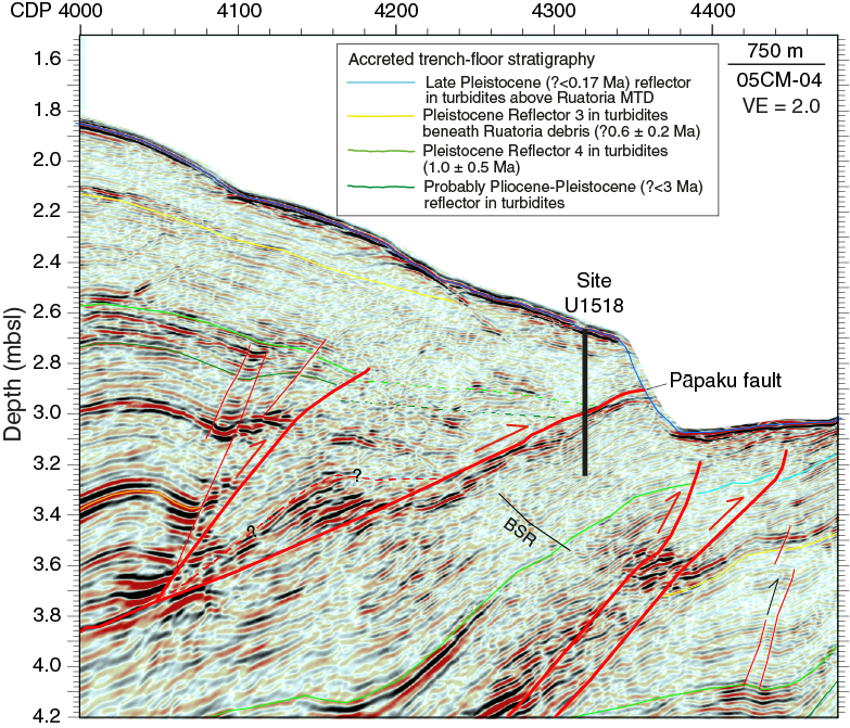
Figure F2. Seismic reflection image, Profile 05CM-04.
Based on predrilling interpretation of seismic data (Figure F2), drilling was expected to encounter accreted Pleistocene trench-fill sediments comprising sand and mud turbidites, ash, and mass transport deposits (MTDs) in both the hanging wall and footwall of the fault. The thrust fault was expected to lie between 295 and 325 meters below seafloor (mbsf). The hanging wall sequence was expected to include 65–82 m of moderately reflective sediment, assumed to be Plio–Pleistocene in age, that overlies an interval characterized by irregular weak seismic reflections. The hanging wall sequence apparently dips to the east in the forelimb of an anticlinal fold associated with the fault. The footwall sequence (i.e., below the fault) to the 600 mbsf target drilling depth was expected to include a strongly reflective interval about 145–180 m thick immediately below the fault, overlying a less reflective sequence below. The footwall sequence has an apparent westerly dip on the seismic profile, and the drilled interval was expected to be Plio–Pleistocene in age.
The primary objectives at Site U1518 were to (1) core and log to total depth with the highest priority of sampling the lower ~100 m of the hanging wall, the fault zone, and the footwall of the thrust (including possible additional subsidiary faults in the footwall) and (2) install a subseafloor observatory to monitor deformation, pore fluid pressure, and temperature and to sample fluids over time through the slow slip cycle (see Observatory). With shallow SSEs on this northern segment of the Hikurangi margin recurring every 1–2 y (Wallace and Beavan, 2010), it is anticipated that the borehole observatory will record pressure, temperature, and fluid flow and fluid chemistry transients associated with SSEs.
The objectives of logging and coring at Site U1518 were to define the structures and deformation, physical properties, age, thermal state, lithology and composition, and interstitial fluid geochemistry of the fault and surrounding sediments. Coring results were used in combination with logging-while-drilling (LWD) data to define the depth interval for observatory pore pressure monitoring and geochemical sampling in the fault zone and to select optimal locations for pore pressure monitoring in the hanging wall and footwall.
Key foci for post-expedition studies on core samples and LWD data sets include (but are not limited to) the following:
- Structural analyses to characterize deformation mechanisms and style, fracture and fault orientations, and wellbore failures (e.g., Byrne et al., 2009);
- Experimental investigation of rheology and friction to test hypotheses linking fault constitutive properties to slip behavior (e.g., Saffer and Wallace, 2015; Leeman et al., 2016);
- Geomechanical and thermal properties measurements to define poroelastic, strength, and heat transport properties of the formation to guide the interpretation of observatory data (e.g., Davis et al., 2009; Kinoshita et al., 2018); and
- Strength, permeability, and elastic moduli measurements to provide context for the interpretation of borehole failures as indicators of in situ stress magnitude, parameterization of hydrological models, and core-log-seismic integration.
The observatory will monitor formation pore pressure (as a proxy for volumetric strain) to document possible hydraulic transients linked to SSEs and to define ambient pore pressure and effective stress state (e.g., Davis et al., 2015; Araki et al., 2017; Kinoshita et al., 2018), as well as hydrological, thermal, and chemical properties and conditions throughout the slow slip cycle (e.g., Solomon et al., 2009). These observations will be accomplished using an integrated observatory design that includes multilevel pore pressure sensing, a string of temperature sensors spanning the borehole, and an OsmoSampler and OsmoFlowmeter installed in the fault zone (e.g., Jannasch et al., 2003) (see Observatory).
Drilling at Site U1518 included LWD to 117.8 and 600 mbsf in Holes U1518A and U1518B, respectively, during Expedition 372 in December 2017 (Figure F1B). During Expedition 375, advanced piston corer (APC)/extended core barrel (XCB) coring was conducted to 176 mbsf in Hole U1518E and rotary core barrel (RCB) coring was conducted to 494 mbsf in Hole U1518F. The observatory was installed in Hole U1518H, with three pore pressure monitoring intervals at 218, 323, and 393 mbsf (hanging wall, fault zone, and footwall, respectively); OsmoSampler and OsmoFlowmeter ports at 323 mbsf; and a string of distributed autonomous temperature sensors spanning from 52 to 370 mbsf.
Operations
Expedition 372
During Expedition 372, Site U1518 consisted of two LWD holes that were drilled to 117.8 and 600.0 mbsf (Table T1). The time spent at Site U1518 during Expedition 372 was 3.4 days with 21 h of that time spent waiting on weather.
Hole U1518A
The vessel arrived at Site U1518 at 1635 h (UTC + 13 h) on 19 December 2017 after a 20 nmi transit from Site U1517 (see Barnes et al., 2019). The LWD bottom-hole assembly (BHA) was made up behind an 8½ inch drill bit. Drill pipe was run to 300 meters below sea level (mbsl), the LWD tools were pump tested, and all turbine-based tools were activated in the water column. After the test, assembly of the drill string continued. The LWD BHA for Site U1518 contained the geoVISION, NeoScope, StethoScope, TeleScope, SonicScope, and proVISION tools (see Logging while drilling).
The LWD tools and drill string were run to 2460 mbsl, and the subsea camera was deployed to determine the depth of the seafloor. The seafloor was tagged at 2636.4 mbsl. The camera was brought to the surface, and the top drive was installed. Hole U1518A (38°51.5368ʹS, 178°53.7606ʹE; 2636.4 mbsl; Table T1) was spudded at 0855 h on 20 December. Weather conditions and sea state deteriorated over the next few hours, and the logging tools were pulled out of the hole at 1605 h, ending Hole U1518A. LWD data were collected from 0 to 117.8 mbsf. The ship began waiting on weather and was offset 20 m southeast of Hole U1518A with the LWD BHA suspended in the water column.
Hole U1518B
At 1310 h on 21 December 2017, an attempt was made to spud Hole U1518B; however, sea conditions were still too rough and prevented the start of the hole. After an additional 3 h of waiting on weather, Hole U1518B (38°51.5476ʹS, 178°53.7621ʹE; 2636.4 mbsl; Table T1) was successfully spudded at 1600 h. In total, 21 h was spent waiting on weather. No LWD measurements were collected in the uppermost ~50 m, including the seafloor depth, because of human error. LWD drilling continued to 372.7 mbsf. After logging a portion of the Pāpaku fault, drilling was paused and the tools were pulled up to 334.7 mbsf. Three pore pressure measurements were attempted using the StethoScope tool, but all three attempts failed because of poor sealing of the tool against the borehole wall. The tools were then pulled up to 234.0 mbsf to try three additional StethoScope measurements, which were unsuccessful as well (see Logging while drilling). The bit was lowered back to the bottom of the hole, a mud sweep was used to clean the hole, and drilling commenced. LWD continued to a total depth of 600 mbsf. After finishing the hole, a 30 bbl mud sweep was used to clean out the hole. The LWD tools and drill string were pulled out of the hole with the bit clearing the seafloor at 1825 h on 23 December. The bit cleared the rotary table at 0100 h on 24 December. The ship was secured for transit at 0257 h, ending Site U1518 for Expedition 372. Because the seafloor depth was not measured on the logs in Hole U1518B and no clear depth correlation occurs between Holes U1518A and U1518B, the seafloor was determined from multibeam bathymetry data to be 2634.6 mbsl.
Safety monitoring
Continuous safety monitoring (see Introduction in the Expedition 372B/375 methods chapter [Wallace et al., 2019a]) was conducted during LWD operations at Site U1518 to monitor for the presence of abnormal pressure or free gas and to ensure safe drilling conditions. Real-time monitoring in Hole U1518A started at 40 mbsf and continued to 115 mbsf. Real-time monitoring in Hole U1518B started at 55 mbsf and continued to 600 mbsf. Observed excess pressure was high (as high as 0.345 MPa [50 psi]) at the shallowest depths because of high cuttings load in the annulus. Pressures then decreased and eventually started to increase slowly again as drilling continued. A maximum pressure of 0.848 MPa (123 psi) above hydrostatic occurred at the bottom of Hole U1518B. With the exception of the shallowest measurements, all pressures were less than the pressure that could have been supplied using 10.5 lb/gal mud. No pressure kicks were observed during drilling.
Expedition 375
Expedition 375 began at 0848 h on 8 March 2018, in Timaru, New Zealand. The R/V JOIDES Resolution departed from Timaru at 0728 h (UTC + 13 h) on 11 March and began the 495 nmi journey to Site U1518. The vessel traveled at a reduced speed to allow Cyclone Hola to clear the area of operations. The vessel arrived at Site U1518 at 1900 h on 13 March. Upon arriving on location, the thrusters were lowered, the dynamic positioning system was engaged, and an acoustic positioning beacon was deployed. During Expedition 375, Site U1518 included four coring holes and two observatory holes (the first was abandoned, and the second was used) (Table T1). The time spent at Site U1518 during Expedition 375 was 13.22 days. The total time spent at Site U1518 during both expeditions was 16.62 days.
Holes U1518C and U1518D
The crew made up an APC/XCB BHA and lowered it to the seafloor. The top drive was picked up, and a “pig” (a high-density foam plug with metal bristles) was pumped through the pipe to clean it of rust. Hole U1518C (38°51.5692ʹS, 178°53.7616ʹE; 2631.7 mbsl; Table T1) was spudded at 0905 h on 14 March 2018. A full core barrel was retrieved following a partial stroke, and the hole was abandoned to attempt another mudline core. The bit was raised 3 m, and Hole U1518D (38°51.5699ʹS, 178°53.7634ʹE; 2628.2 mbsl) was spudded at 1020 h. Another full core barrel was retrieved, and then this hole was also abandoned.
Hole U1518E
The vessel was offset 5 m north, the bit was raised another 3 m, and Hole U1518E was spudded at 1125 h on 14 March 2018 (38°51.5669ʹS, 178°53.7618ʹE; 2626.1 mbsl; Table T1). APC Cores 375-U1518E-1H through 10H penetrated from 0 to 63.3 mbsf and recovered 61.57 m (97% recovery). Half-length APC (HLAPC) Cores 11F–25F penetrated from 63.3 to 123.5 mbsf and recovered 53.97 m (90% recovery). XCB Cores 26X–32X penetrated from 123.5 to 175.6 mbsf and recovered 45.52 m (87% recovery). Overall recovery in Hole U1518E was 92%. Formation temperature measurements were taken with the advanced piston corer temperature tool (APCT-3) for Cores 4H, 6H, 8H, 10H, and 14F. Nonmagnetic core barrels were used for all APC/HLAPC cores, and all APC cores were oriented with the Icefield MI-5 core orientation tool. The decision was made to switch to coring with the RCB system after discovering that the cutting shoe used with Core 31X had been completely destroyed and after it took 80 min to advance 3.6 m while cutting Core 32X.
Hole U1518F
The vessel was offset 5 m south, and an RCB BHA was made up and lowered to the seafloor. Hole U1518F (38°51.5694ʹS, 178°53.7619ʹE; 2626.1 mbsl; Table T1) was spudded at 0135 h on 17 March 2018 and was advanced without coring to 197.7 mbsf. Cores 375-U1518F-2R through 32R penetrated from 197.7 to 494.9 mbsf and recovered 126.82 m (43% recovery). Nonmagnetic core barrels were used for all cores. Coring was terminated so that observatory operations could start based on a forecast of deteriorating weather conditions. The bit was raised from the seafloor and reached the rig floor at 0110 h on 20 March.
Hole U1518G
In preparation for installing the observatory, the decision was made to predrill the observatory hole. The vessel was offset 35 m north of Hole U1518F (and ~5 m south of Hole U1518B) to take advantage of fault depths indicated by the LWD data collected during Expedition 372 and the core data collected during Expedition 375. A reentry system consisting of a reentry cone and a mud skirt was moved to the center of the moonpool. A BHA with a 14¾ inch drill bit was lowered to the seafloor.
Hole U1518G (38°51.5505ʹS, 178°53.7617ʹE; 2629.8 mbsl; Table T1) was spudded at 1050 h on 20 March 2018 and continued until the bit reached 433 mbsf at 0230 h on 22 March. A 40 bbl mud sweep was circulated to clean the hole of cuttings, and the bit was raised to 53 mbsf. At 0430 h, the reentry cone and its base were released from the moonpool and allowed to free fall down the drill string to the seafloor. After the subsea camera was deployed to check that the reentry cone had landed properly, we pulled the drill string out of the hole at 0615 h and tagged the top of the reentry cone to check the seafloor depth. With this new information, we made a final adjustment to the depth of the observatory’s middle screen designed to span the fault zone. The subsea camera was brought to the surface at 0745 h, and the drill string was recovered at 1320 h.
The next several hours were spent connecting the observatory wellhead to the hydraulic release tool (HRT) and securing them in the derrick. An umbilical reel consisting of three ¼ inch diameter stainless steel tubes was placed near the moonpool, and the area was staged to attach the umbilical to the casing and wellhead. At 2000 h, we started assembling the 422 m long ACORK casing string composed of 31 joints of 10¾ inch casing, 2 shorter (pup) joints used to adjust the total length, a casing shoe joint, 3 casing joints with pressure screens, and the umbilical secured on the outside of the casing (Figure F3A). As the ACORK casing string was assembled from the bottom up, the umbilical was connected first to the bottom 2 m screen, then the 8 m screen wrapped around a perforated joint of casing, and finally the top 2 m screen. The three screens were centered at 393, 323, and 218 mbsf, respectively, to monitor pressure from below the fault, the fault zone, and above the fault. The casing string was completed at 1700 h on March 23 and landed in the moonpool.
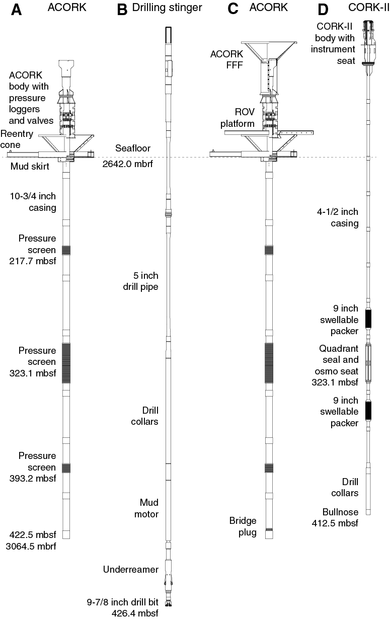
Figure F3. Site U1518 observatory installation.
Next, we assembled the drilling stinger needed to install the casing in the predrilled hole. The stinger was composed of a 9⅞ inch drill bit, an underreamer to clear any obstacles in the predrilled hole with its arms set to 14¾ inch diameter, and a mud motor to rotate the bit and underreamer in isolation from the ACORK casing (Figure F3B). The underreamer arms were tested at 1915 h on March 23, and the stinger was completed and landed inside the casing at 2130 h.
The umbilical was connected to the valves and data loggers on the ACORK wellhead at 0400 h on 24 March, the wellhead was submerged for 10 min with the valves in the open position to purge the lines of air, and the wellhead was brought back to the surface to set the valves to their deployment (closed) position. The wellhead was submerged for the last time at 0510 h, and the entire ACORK assembly with the HRT running tool, wellhead, 10¾ inch casing, umbilical tubes, and stinger was lowered to the seafloor between 0615 and 1030 h on 24 March. The subsea camera was then lowered to the seafloor to assist with the reentry of Hole U1518G. During our attempt to reenter Hole U1518G, unexpected heave caused the drill bit to bump the reentry cone at 1215 h. This resulted in the cone and its base sliding away from Hole U1518G, making reentry into the predrilled hole impossible.
Hole U1518H observatory
With the underreamer and drill bit inside of the ACORK casing and the entire assembly already at the seafloor, we decided to drill in the ACORK assembly at the new location of the reentry cone. Hole U1518H (38°51.5402ʹS, 178°53.7642ʹE; 2631.1 mbsl; Table T1) was spudded at 1245 h (UTC + 13 h) on 24 March 2018 a few meters northeast of Hole U1518G and reached a total depth of 427 mbsf at 0715 h on 25 March. The ACORK landed in the reentry cone and was released from the running tool, but it took several attempts to pull the underreamer and bit back into the casing. The drilling assembly was finally freed at 1040 h. The subsea camera was recovered so that the remotely operated vehicle (ROV) platform and a smaller ACORK free-fall funnel (FFF) could be deployed.
The ROV platform was assembled around the drill string in the moonpool and released at 1200 h. When the subsea camera was redeployed, it showed that the platform had hung up on the ACORK body and landed at an angle but would not pose a problem for deploying the ACORK funnel. The subsea camera was retrieved, the ACORK FFF was assembled around the drill pipe on the moonpool and released, and the subsea camera was redeployed (Figure F3C). The camera showed that the funnel had landed correctly. After the subsea camera was retrieved, we recovered the drill string at 0305 h on 26 March.
Next, the ACORK casing was checked for cuttings, and we inspected the ROV platform and funnel. A drilling assembly made up with a 9⅞ inch mill tooth bit reached the seafloor at 1015 h. The wellhead was inspected with the subsea camera, showing that the guide base is sitting on a slight slope and the ROV platform is hanging at an angle from the ACORK body. An attempt to bump the platform into position with the bit was unsuccessful (remediated by ROV on 15 February 2019). The ACORK funnel was then reentered at 1335 h on 26 March 2018. Upon reentry, the hole was discovered to be nearly full of cuttings. We spent the next ~8 h cleaning the cuttings out of the casing to prepare it for installing a bridge plug. The hole was swept with mud, and we recovered the drill bit from the seafloor at 0305 h on 27 March.
A BHA was then made up with a bridge plug to seal the base of the 10¾ inch ACORK casing. Once the drill string reached the seafloor at 1215 h, the subsea camera was deployed, and Hole U1518H was reentered at 1400 h. The end of the drill string was positioned at 421 mbsf inside the ACORK casing, and the bridge plug was activated until the bridge plug’s packer was set at 1845 h (Figure F3C). We recovered the drill string and the running tool used to install the bridge plug, which reached the rig floor at 0010 h on 28 March.
In preparation for installing the CORK-II stage of the observatory, we had ordered replacement seals to be sent to the vessel. Because we did not receive them in time to immediately begin CORK-II operations, we moved to Site U1520 to install a reentry system. We started the 12.5 nmi transit to Site U1520 at 0048 h on 28 March. The R/V Tangaroa arrived at 1615 h on 29 March to deliver the seals needed for the CORK-II installation. Once the reentry system at Site U1520 was completed, we departed for Site U1518 at 1310 h on 31 March.
We returned to Hole U1518H at 1506 h on 31 March and started assembling the CORK-II casing string. The 412 m long CORK-II casing string is composed of 29 full joints and a pup joint of 4½ inch drill pipe (342 m), two ~12 m swellable packer joints, one ~11 m quadrant seal joint, four 6¾ inch drill collars (~36 m), and a bullnose (Figure F3D). The CORK-II wellhead was attached at 0245 h (time switched to UTC + 12 h) on 1 April, and the entire assembly was lowered to 2627 meters below rig floor (mbrf). The subsea camera was deployed, and the CORK-II assembly reentered the ACORK funnel at 1005 h. The CORK-II wellhead was lowered to ~17 m above the ACORK and kept there while we deployed the instrument string.
At 1230 h, we started assembling the instrument string to be deployed inside the CORK-II casing. The instrument string is 407 m long and consists of 3 segments of Spectra rope carrying a total of 24 temperature sensing data loggers, the ~22 m long OsmoSampler package with an additional 7 temperature sensing data loggers inside, 3 weak links, 4 sinker bars, and the top plug. Once the instrument string was assembled, the top plug was connected to the Schlumberger wireline with the Electronic Release System (ERS), and the instrument string was lowered slowly to the seafloor. At 2105 h, the OsmoSampler package landed in the CORK-II seat at 323 mbsf, followed soon after by the top plug latching inside the CORK-II wellhead. After the instrument string was released by activating the ERS mechanism, the CORK-II landed inside the ACORK wellhead at 0020 h on 2 April, completing the observatory installation in Hole U1518H. We then recovered the subsea camera and the drill string, with the CORK running tool reaching the rig floor at 0600 h. The beacon was retrieved, the thrusters were raised, and we departed for Site U1520 at 0815 h on 2 April.
Lithostratigraphy
We defined three lithostratigraphic units at Site U1518, two of which (Units I and III) were divided into subunits (Figure F4; Table T2). All three units are Quaternary in age (see Biostratigraphy). Sediment composition and texture are broadly consistent between the units, with silty clay(stone) alternating with thin beds of silt(stone) that contain variable amounts of sand. Distinctions among the lithostratigraphic units are based largely on the character of coarser event beds (inferred to be turbidites) and soft-sediment deformation features (inferred to be intraformational MTDs). Figure F4 compares the lithostratigraphic units with the provisional logging units defined during Expedition 372 in Holes U1518A and U1518B (see Logging while drilling). Such correlations are valid at the scale of facies packets but are imprecise at the scale of individual beds.
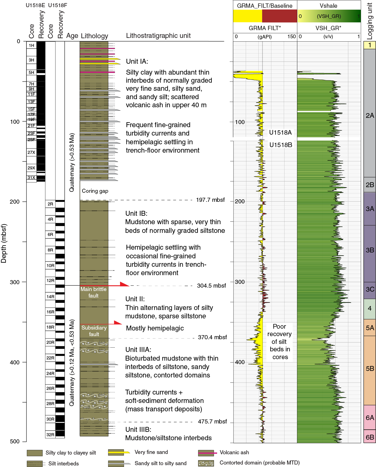
Figure F4. Lithostratigraphic summary and facies interpretations.
We also used color reflectance spectral data that show variations in digital color parameters over the complete stratigraphic section to further characterize the lithostratigraphic unit boundaries (see Figure F43). Most such color changes are also detectable during visual core description. L* (lightness) ranges between 0 (black) and 100 (white), a* (red–green) ranges between −60 (green) and 60 (red), and b* (yellow–blue) ranges between −60 (blue) and 60 (yellow).
Unit I
- Interval: 375-U1518E-1H-1, 0 cm, to 375-U1518F-13R-2, 0 cm
- Thickness: 304.53 m
- Depth: 0–304.53 mbsf
- Age: Quaternary (older than 0.53 Ma)
- Lithology: silty clay to clayey silt and silt to very fine sand
The mudline was recovered in Core 375-U1518E-1H, and the upper 2.2 m of material consists of a drape of Holocene sediment (see Biostratigraphy), which we deemed too thin to warrant its own unit designation. Sediment from Section 1H-CC has an age older than 0.53 Ma (see Biostratigraphy), and porosity is lower than expected for the current burial depth (see Physical properties). We therefore consider some of the original stratigraphic section to be missing because of submarine slides or other forms of mass wasting after frontal accretion.
If Holocene sediment above 2.2 mbsf is included, then Unit I begins at the seafloor and extends to 304.53 mbsf (top of Section 375-U1518F-13R-2) (Table T2; Figure F4). Unit I is composed mostly of greenish gray silty clay locally ranging to clayey silt, along with centimeter-scale interbeds of dark gray, normally graded sandy silt to silty sand and very fine sand. A minor lithology is represented by 18 felsic ash layers. The normally graded beds were probably deposited from fine-grained and relatively dilute turbidity currents; those event deposits were interspersed with background settling of suspended sediment. Deposition likely occurred in the trench-floor environment of the Hikurangi Trough.
Smear slides show that the detrital grain assemblage in the background silty clay lithology is dominated by clay minerals and nannofossils and has significant amounts of quartz, feldspar, and sedimentary lithic and volcaniclastic grains. Carbonate contents in mud specimens range from 2.13 to 13.41 wt% with an average value of 9.69 wt% (see Geochemistry). Normalized mineral abundances from bulk powder X-ray diffraction (XRD) are shown in Figure F5 and Table T3. Representative diffractograms are shown in Figure F6. Proportions of total clay minerals (smectite + illite + chlorite + kaolinite) range from 23.0 to 53.0 wt% (mean = 45.9 wt%). Quartz ranges from 22.2 to 43.7 wt% (mean = 27.9 wt%). Feldspar (plagioclase + K-feldspar) abundance ranges from 13.2 to 28.0 wt% (mean = 16.8 wt%), and calcite abundance ranges from 1.9 to 22.1 wt% (mean = 9.5 wt%). In general, decreases in total clay minerals are matched by increases in quartz and feldspar. This effect is likely due to grain size (i.e., silt-rich turbidites contain more quartz and feldspar).
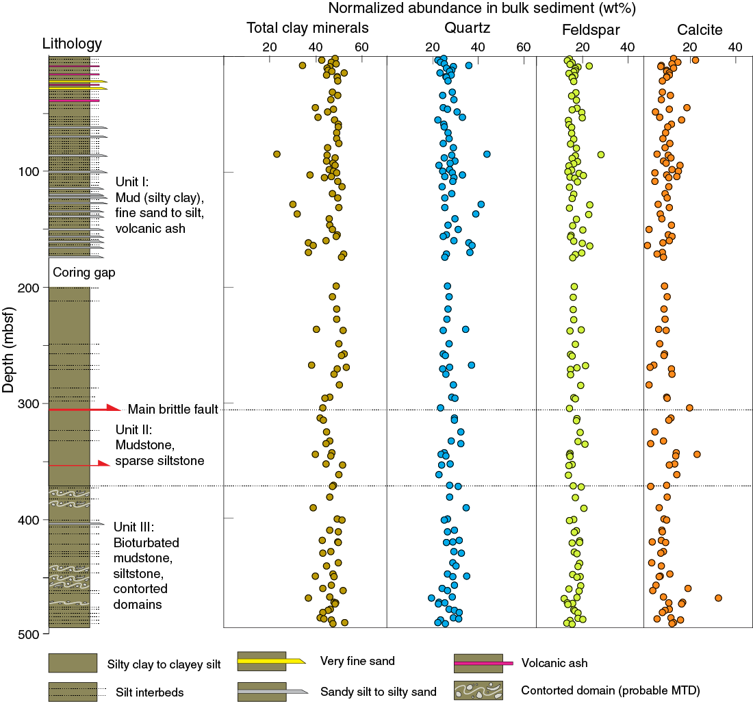
Figure F5. Lithostratigraphic summary and XRD abundance.
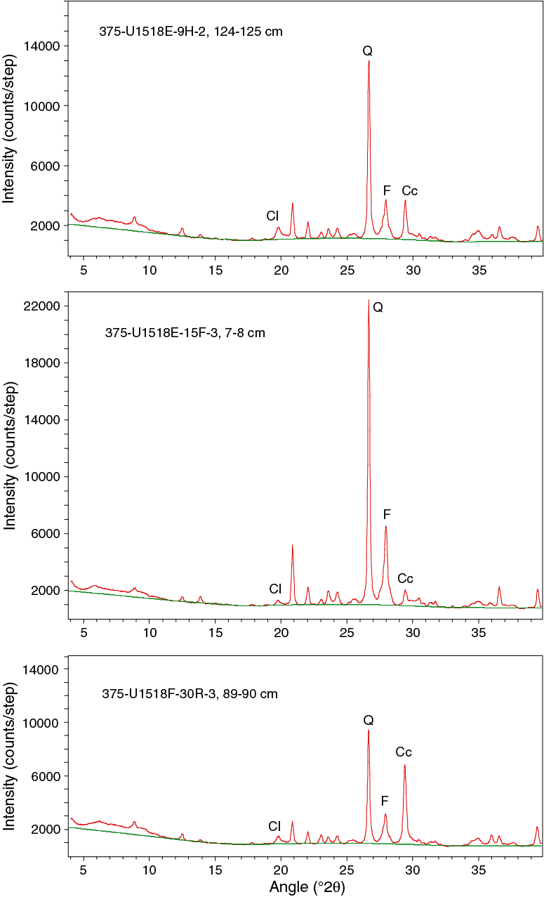
Figure F6. X-ray diffractograms for bulk sediments.
Subunit IA
- Interval: 375-U1518E-1H-1, 0 cm, to 375-U1518F-2R-1, 0 cm
- Thickness: 197.7 m
- Depth: 0–197.7 mbsf
- Age: Holocene (younger than 0.011 Ma) to Quaternary (older than 0.53 Ma)
- Lithology: silty clay and silt to silty sand and very fine sand
Subunit IA extends from the mudline to the bottom of Hole U1518E (Core 32X; 176.6 mbsf). A coring gap precludes direct identification of the subunit’s lower boundary (Figure F4), so we define the top of Core 375-U1518F-2R as the base. Most of the cores in this subunit were recovered using the APC system, and the primary forms of drilling disturbance are smearing of layering, upward arching of beds, and flow-in of coarser sediment along the edges of the core liner. We measured layer thicknesses at the centers of the cores wherever bedding exhibited signs of drilling disturbance. The depth interval for the base of each event bed was measured at the cross-core midpoint.
This lithofacies is composed of silty clay to clayey silt (mud) with abundant coarser grained interbeds that display sharp bases and normal grading (Figure F7). This association is typical of fine-grained turbidites. The grain size of most of these interbeds is sandy silt, with local occurrences of silty sand to very fine sand. Most of these beds are <10 cm thick (Figure F8). Smear slides show that the coarser interbeds are volcaniclastic to mixed detrital in composition (Figure F9), characterized by quartz, feldspar, nannofossils, volcanic lithic and sedimentary lithic grains, and sponge spicules and lesser amounts of calcite, pyrite, Fe/Mn oxides, heavy minerals, and glauconite.
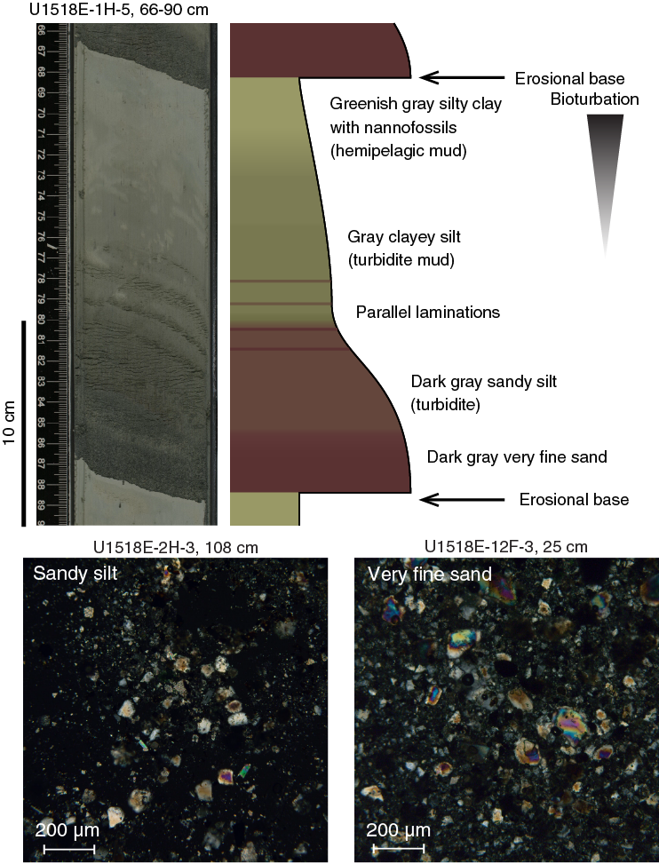
Figure F7. Thin-bedded turbidite deposit, Subunit IA.
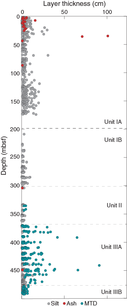
Figure F8. Event bed thickness.
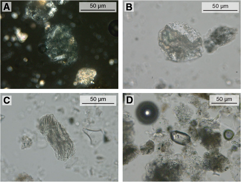
Figure F9. Lithic fragments and heavy minerals, Unit I.
Two defining features of Subunit IA are the more repetitive occurrence and greater thicknesses (as thick as 31 cm) of silty interbeds relative to other units (Figure F8). The distribution of such beds can be tracked visually and by magnetic susceptibility logs. Intervals with high magnetic susceptibility occur in Subunit IA in Sections 375-U1518E-2H-5 through 4H-3 (14.36–32.09 mbsf) and 9H-3 through 12F-CC (58.52–72.56 mbsf) (Figure F10). The spikes in magnetic susceptibility are typical responses to higher magnetic mineral abundances in the sand- and silt-sized fractions.
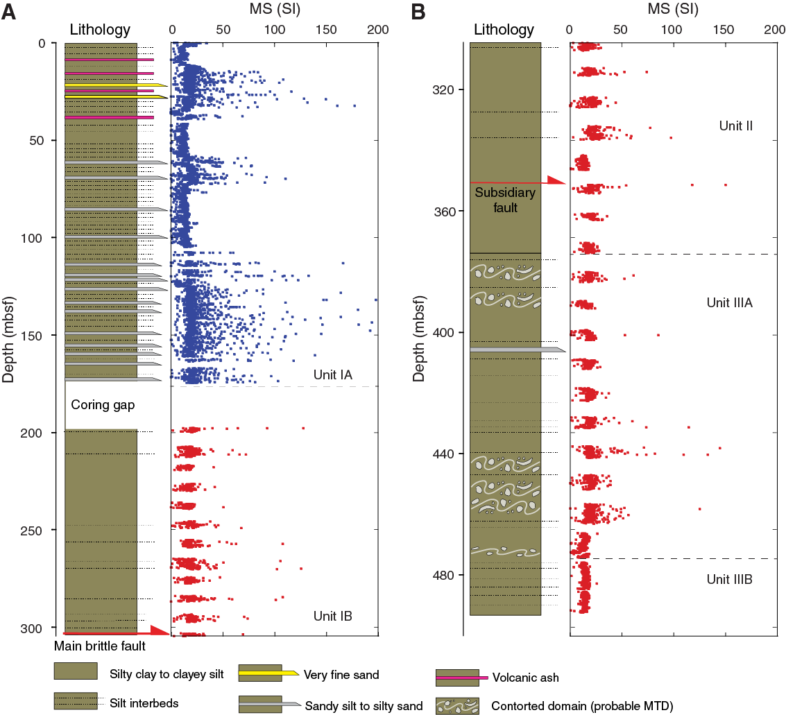
Figure F10. Magnetic susceptibility profile.
A general fining-upward trend extends from the bottom of Subunit IA to approximately 36 mbsf (Figures F8, F11A). The trend is particularly clear when comparing the distribution of silt layer thickness in the upper 100 m of Subunit IA (mean thickness = 3.5 cm) with the bottom 80 m of core from Subunit IA (mean thickness = 5.5 cm). The frequency distribution of silt layer thickness also changes with depth (Figure F11). The upper 36 m and the bottom 80 m of core from Subunit IA show segmented power (1/n) law distributions of silt layer thickness, whereas data from the middle part of Subunit IA (37–99 mbsf) can be fit to a single power (1/n) law distribution, except for very thin layers (<2 cm) with lower preservation potential. A similar power law distribution of bed thickness was previously reported from the Izu-Bonin forearc basin (Hiscott et al., 1992).

Figure F11. Statistical analysis of silt layer thickness, Subunit IA.
The top of Subunit IA is also characterized by ash layers and ash pods between 2.75 and 44 mbsf (Figure F4). Typically, these ash layers are normally graded and nonbioturbated or weakly bioturbated. They are generally coarser than the volcaniclastic silt layers and visually distinguished by their whitish pinkish gray color (Figure F12). The thickest example extends from Section 375-U1518E-5H-1, 0 cm, to Section 5H-2, 71 cm (35.3–37.1 mbsf). In this interval, we observed three coarser grained horizons that may represent separate ash layers, but their boundaries are obscured by drilling disturbance (Figure F13). Ash layers yield decreased magnetic susceptibility values compared with elevated values from silt layers. We interpret the deposits to be air fall derived because they have normal grading and lack sedimentary structures indicative of pyroclastic flow processes. Irregular ash pod layers are possible products of bioturbation and/or locally confined gravitational creep and subsequent dissemination shortly after initial emplacement by air fall (e.g., Kutterolf et al., 2008).
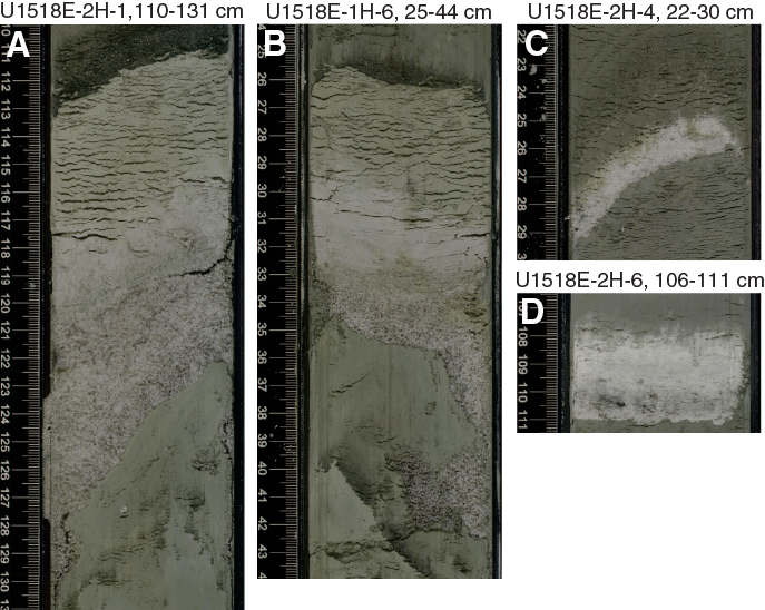
Figure F12. Ash layers, Subunit IA.
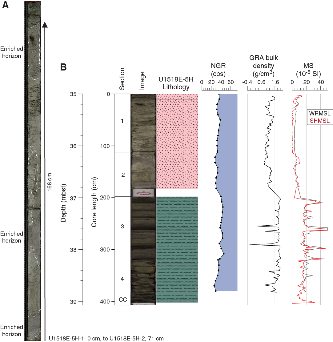
Figure F13. Thick ash deposit.
Smear slides show that the ash layers are dominated by colorless glass with lesser abundances of plagioclase and variable abundances of quartz, hornblende, biotite, and pyroxene. Two ash layers in Samples 375-U1518E-3H-1, 76 cm, and 3H-4, 93 cm, contain only amphibole, biotite, and allanite (Figure F14). We also found rare to trace amounts of planktonic foraminifers, as well as sedimentary lithic and volcanic lithic fragments.
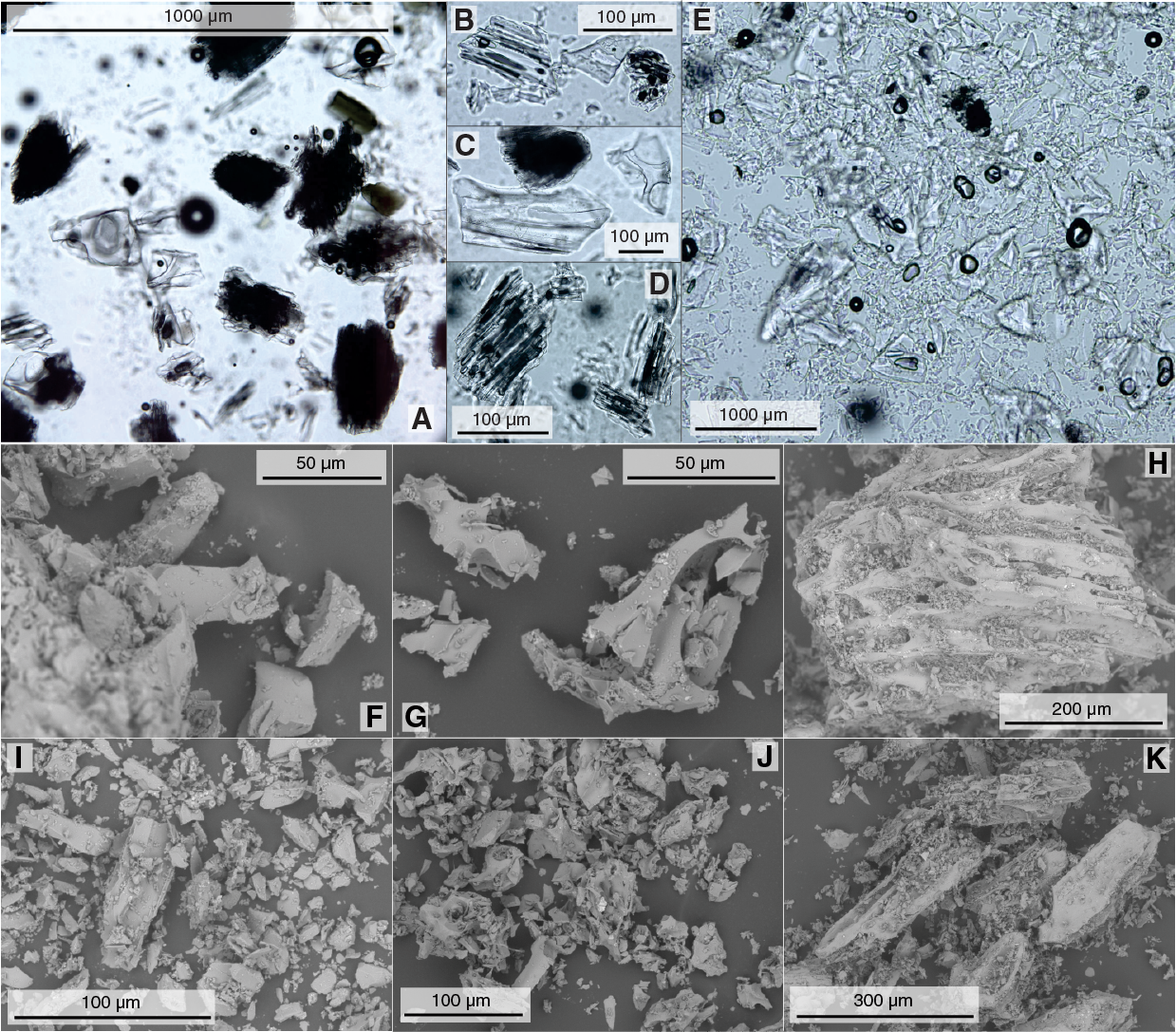
Figure F14. Textures and vesicles of pyroclasts.
Tephra subgroups are based on the relative abundance of glass textures and vesicles observed in smear slides (Figure F14). An upper group occurs in Cores 375-U1518E-1H and 2H. It contains predominantly blocky and dense glass shards, with lesser amounts of vesicular pumiceous clasts and cuspate shards. The vesicular glass shards display mostly tubular and elongated vesicle shapes and rare elliptical and round bubbles (Samples 1H-2, 122 cm; 1H-4, 16 cm; 1H-4, 18 cm; 1H-4, 121 cm; 2H-3, 24 cm; and 2H-3, 96 cm). Tephras with abundant and dominant cuspate glass shards, elongated vesicles, or dense shards are also common in the upper part of Subunit IA (Samples 2H-1, 120 cm; 2H-6, 110 cm; and 3H-1, 94 cm). Another group has a nearly equal mixture of tubular and elongate vesicle-rich pumiceous shards, as well as dense-blocky and cuspate pyroclasts (Samples 2H-4, 29 cm; 3H-4, 93 cm; and 3H-6, 16 cm). Pumiceous clasts with a variety of vesicle shapes are dominant in three tephras (Samples 1H-6, 37 cm; 3H-1, 76 cm; and 3H-7, 90 cm).
Mineral- and lithic fragment–rich tephras in Cores 375-U1518E-6H through 10H contain mostly dense-blocky glass shards (Samples 6H-2, 96 cm; 7H-3, 15 cm; 9H-3, 8 cm; 9H-3, 27 cm; and 10H-1, 52 cm). The shards in Core 5H change from dense-blocky in the uppermost part (Sample 5H-1, 6 cm) to an equal mixture of highly vesicular pumiceous, dense-blocky, and cuspate in the middle (Sample 5H-1, 40 cm). The pumiceous assemblage in Samples 5H-2, 52 cm, and 5H-2, 61 cm, has abundant tubular vesicles and common elliptical and elongated vesicles, as well as variable proportions of dense glass shards.
Distinctions among glass textures and vesicles provide important hints regarding eruption processes and conditions. The fine-grained blocky and dense glass shards, for instance, were probably derived from eruptions that caused extensive fragmentation (e.g., Zimanowski et al., 2015), possibly from Phreatoplinian eruptions (e.g., Houghton et al., 2000). In contrast, highly vesicular pyroclasts showing elongated and tubular vesicles are typical of extensively degassed magmas that fragment in the conduit because of strong gas expansion and subsequent shearing of the magma. These behaviors are often seen in subaerial eruptions with large explosions (e.g., Kutterolf et al., 2008, 2018).
Subunit IB
- Interval: 375-U1518F-2R-1, 0 cm, to 13R-2, 0 cm
- Thickness: 106.83 m
- Depth: 197.7–304.53 mbsf
- Age: Quaternary (older than 0.53 Ma)
- Lithology: silty clay to clayey silt and silt to sandy silt
Subunit IB extends from the top of Section 375-U1518F-2R to the top of Section 13R-2 (197.7–304.53 mbsf). Its upper boundary is gradational, and its placement coincides with the bottom of a zone that was not cored (Figure F4). Sediments from Hole U1518F exhibit porosity values >40% (see Physical properties) and are characterized by considerable drilling disturbance. Because these cores were recovered using the RCB system, we refer to all lithologies in this subunit as “consolidated” (see Lithostratigraphy in the Expedition 372B/375 methods chapter [Wallace et al., 2019a]).
This subunit is characterized by sparse and thin (<10 cm), normally graded siltstone layers (Figure F8). Magnetic susceptibility data show relatively low background values with small variations for alternating siltstone and mudstone. Bed-scale excursions are probably obscured by larger amounts of drilling disturbance (Figure F10). During RCB coring at relatively shallow burial depths, we expected preferential loss of coarser grained, cohesionless material. Siltstone layers in Subunit IB are typically mixed with surrounding silty claystone. Most of the interbeds are slightly darker in color than the surrounding silty claystone and further distinguished by their gritty feel. We probably underestimated their layer thicknesses in Hole U1518F because of truncated recoveries, but we note an upward-thinning trend similar to the lower part of Subunit IA (Figure F8).
Based on smear slide analysis, the predominant event beds are sandy siltstone to siltstone with volcaniclastic to mixed clastic compositions. Those layers are further characterized by present to common abundances of nannofossils, quartz, feldspar, volcaniclasts, and sedimentary lithic grains; rare to present amphibole, pyroxene, chlorite, glauconite, mica, pyrite, and Fe/Mn oxides; trace to rare sponge spicules; and rare calcite and zircon.
Unit II
- Interval: 375-U1518F-13R-2, 0 cm, to 20R-1, 0 cm
- Thickness: 65.87 m
- Depth: 304.53–370.4 mbsf
- Age: Quaternary (younger than 0.53 Ma)
- Lithology: mudstone and siltstone
Unit II extends from the top of Section 375-U1518F-13R-2 to the top of Section 20R-1 (304.53–370.4 mbsf). This lithostratigraphic unit is defined on the basis of a sharp reduction in silt-sized deposits and a subtle change in color from dominantly gray mud(stone) in Unit I to lighter greenish gray mudstone below. The mudstone in Unit II appears to contain more nannofossils, judging from smear slides, but calcite contents are actually lower on average than the average for Unit I (Table T3). The mudstone alternates with thin but sparse layers of silty mudstone, siltstone, and sandy siltstone. Thin layers of mud-rich nannofossil ooze also occur locally. Magnetic susceptibility in Unit II is consistently low, similar to that in Subunit IB, with small excursions from the mudstone background values induced by thin interbeds of siltstone (Figure F10).
Smear slides show that the detrital grain assemblage of the coarser layers in this unit is similar to that in Unit I (see above) but with an apparent increase in volcaniclastic grains and nannofossils. Subsidiary constituents include calcite, pyrite, and Fe/Mn oxides and trace to rare amounts of sponge spicules. One layer in Section 375-U1518F-14R-2, 36 cm (314.7 mbsf), contains mostly pyrite (Figure F15). Sedimentary lithic grains are present to common. Heavy minerals in the sand and silt fraction include amphibole, pyroxene, apatite, zircon, and mica (Figure F16). The most abundant mica is biotite. Amphibole and pyroxene grains display prominent dissolution.
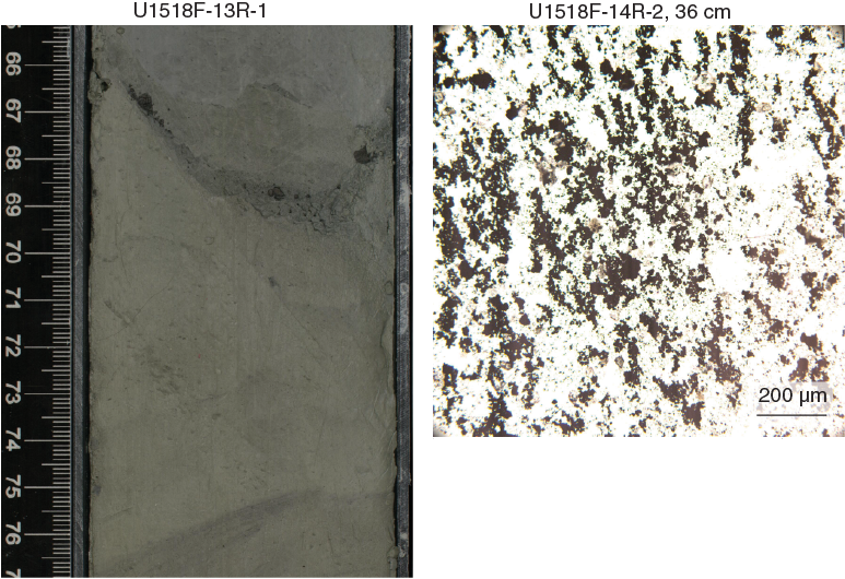
Figure F15. Greenish gray mudstone, Unit II.
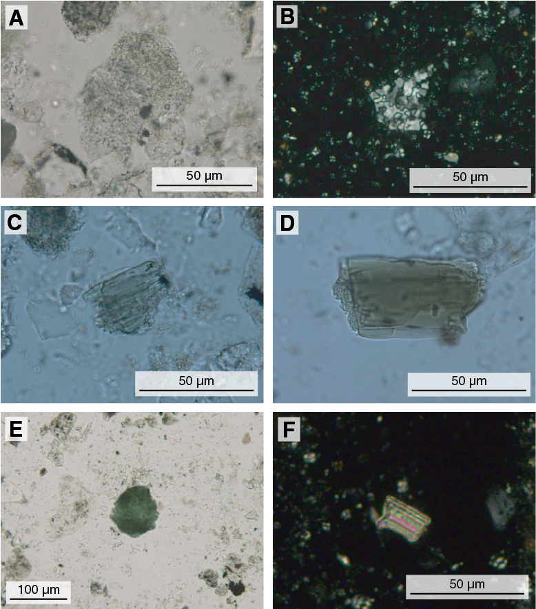
Figure F16. Lithic fragments and dense minerals, Unit II.
Carbonate contents in mud layers from Unit II range from 3.56 to 14.65 wt% (see Geochemistry). The average value of 8.85 wt% is less than the average for Unit I. Normalized mineral abundances from bulk powder XRD are shown in Figure F5 and Table T3. The bulk compositions are similar to those in Unit I. Proportions of total clay minerals range from 39.6 to 51.4 wt% (mean = 45.2 wt%). Quartz ranges from 22.6 to 32.2 wt% (mean = 27.2 wt%). Feldspar abundance ranges from 13.7 to 21.1 wt% (mean = 16.2 wt%), and calcite abundance ranges from 2.5 to 22.8 wt% (mean = 11.4 wt%).
The upper boundary of Unit II is not defined by a substantial change in lithofacies. Instead, it coincides with an age reversal from older than 0.53 Ma above the boundary to younger than 0.53 Ma below (see Biostratigraphy). The age inversion coincides with the top of the main brittle fault zone that marks the top of the Pāpaku fault zone (with older hanging wall over younger footwall) (see Structural geology). Distributed brittle and ductile deformation across the fault zone resulted in extensive disruption of the primary internal sedimentary structures and primary bedding, with numerous offset beds, small folds, and intervals of overturned normal grading. This boundary also coincides with a subtle change in color from tones of greenish gray in Unit I to lighter greenish tones in Unit II, which were recognized during visual core description.
Unit III
- Interval: 375-U1518F-20R-1, 0 cm, to 32R-7, 69 cm
- Thickness: 121.86 m
- Depth: 370.4–492.26 mbsf
- Age: Quaternary (younger than 0.53 Ma)
- Lithology: mudstone, siltstone to sandy siltstone, and contorted mudstone clasts
Unit III begins at the top of Section 375-U1518F-20R-1 and extends to the base of core recovery in Hole U1518F (370.4–492.26 mbsf). Similar to the overlying strata described above, this unit is composed of silty mudstone with interbedded, normally graded siltstone, sandy siltstone, and silty sandstone (Figure F4). Magnetic susceptibility patterns are similar to those in Subunit IB and Unit II, consistent with alternating siltstone and mudstone and/or convoluted mud clasts (Figure F10). The detrital grain assemblage of coarser beds is similar to that in Unit II but with fewer nannofossils. The age of Unit III is younger than 0.53 Ma throughout (see Biostratigraphy).
The most distinctive attribute of Unit III is soft-sediment deformation that is similar in many respects to intraformational MTDs described from a comparable depositional environment in the Nankai Trough (Expedition 316 Scientists, 2009; Expedition 333 Scientists, 2012; Strasser et al., 2014a, 2014b). We divided these MTD-bearing deposits into Subunits IIIA and IIIB largely on the basis of spatial concentrations of the MTD-type features, referred to collectively as contorted domains. Soft-sediment deformation intensity decreases significantly in Subunit IIIB; conversely, intricate varieties of bioturbation become more widespread and diverse below the subunit boundary.
Carbonate contents in mud layers in Unit III range from 3.99 to 23.13 wt% with an average value of 9.32 wt% (see Geochemistry). Normalized mineral abundances from bulk powder XRD are shown in Figure F5 and Table T3. The bulk compositions are similar to those in Units I and II. Proportions of total clay minerals range from 36.6 to 52.4 wt% (mean = 46.1 wt%). Quartz ranges from 19.4 to 34.7 wt% (mean = 27.6 wt%). Feldspar abundance ranges from 11.9 to 20.5 wt% (mean = 16.7 wt%), and calcite abundance ranges from 2.5 to 32.1 wt% (mean = 9.6 wt%).
Subunit IIIA
- Interval: 375-U1518F-20R-1, 0 cm, to 31R-1, 0 cm
- Thickness: 105.3 m
- Depth: 370.4–475.7 mbsf
- Age: Quaternary (younger than 0.53 Ma)
- Lithology: mudstone, siltstone to sandy siltstone, and contorted mudstone domains
Subunit IIIA extends from the top of Section 375-U1518F-20R-1 to the top of Section 31R-1 (370.4–475.7 mbsf). The coarser grained beds in Subunit IIIA are dark gray, and their composition is volcaniclastic to mixed clastic. Smear slide observations indicate that the proportion of sand-sized grains in the event beds decreases with depth from ~40 to ~10 vol% (Figure F17). We recorded positions of siltstone layers only where they are >1 cm thick. Compared with Unit II, Subunit IIIA is marked by an increase in the frequency of siltstone layers (Figure F8). These apparent trends, however, should be interpreted with some caution. Drilling-induced biscuit boundaries typically coincide with truncated siltstone layers, and as a result, most layer thicknesses in this subunit are underestimated.
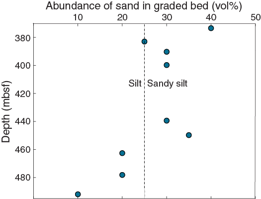
Figure F17. Sand-size fraction in coarse event beds, Unit III.
The most distinctive features in Subunit IIIA are discrete zones of stratal disruption containing clasts of different colored mudstone and discontinuous to convoluted color bands. Mixing is generally concentrated at the tops of both mudstone-rich and siltstone-bearing intervals (Figure F18). The typical relation is lighter greenish gray clasts surrounded by a darker gray matrix. The clasts typically differ in texture (finer grained) compared with the matrix, and the color-band surfaces and clast rims are usually subrounded to subangular with jigsawed to serrated details around the edges (Figure F18B). The sharpness and irregularity of clast surfaces indicate coherent behavior during fragmentation rather than brittle fracturing. Some of the contorted bands resemble flow structures (Figure F18C). Disturbance from RCB drilling may have contributed to some of the fragmentation, however, and we cannot eliminate the possibility of local tectonic overprints in the fault zones. To be conservative, we only measured layers as “contorted domains” where they extend uniformly across the entire width of the split core rather than being confined or concentrated along the side of the core liner (Figure F18). The contorted domains become more widespread with depth below the fault zone in zones where brittle deformation features are no longer evident (see Structural geology). This observation is opposite to the trend expected if the deformation is fault induced.

Figure F18. MTDs in Unit III.
Contorted domain thicknesses range from 1 to 90 cm with a mean value of 9.5 cm (Figure F8). The contorted domains are interspersed with intervals of intact strata (mudstone). As a provisional interpretation, we attribute the soft-sediment deformation to intraformational mass transport events. Some of the clasts may have been ripped up by energetic turbidity currents. Whether the gravity-driven deformation occurred mostly on the trench floor shortly after initial sedimentation from turbidity currents (e.g., along steeply inclined walls of a channel-levee system) or by oversteepening of the seafloor during the initial stages of frontal accretion remains unresolved.
Subunit IIIB
- Interval: 375-U1518F-31R-1, 0 cm, to 32R-7, 69 cm
- Thickness: 16.56 m
- Depth: 475.7–492.26 mbsf
- Age: Quaternary (younger than 0.53 Ma)
- Lithology: mudstone, siltstone to sandy siltstone, and contorted mudstone domains
We place the top of Subunit IIIB at the top of Section 375-U1518F-31R-1 (475.7 mbsf), defined by a noticeable decrease in the number and thicknesses of contorted domains. The subunit boundary is gradational. Aside from the reduction in soft-sediment deformation, the facies character is similar to Subunit IIIA, with numerous interbeds of mudstone and thin siltstone. Many of the darker gray siltstone beds show sharp bases, normal grading, plane-parallel laminae, and diffuse transitions into the overlying lighter greenish gray mudstone. All such attributes are consistent with deposition by relatively fine grained and dilute turbidity currents. The mudstone intervals are consistent with slower hemipelagic settling with slightly higher nannofossil concentrations. MTD-type layer thickness is consistently <10 cm (Figure F8), and various forms of distinct bioturbation become more prevalent below the subunit boundary. Mudstone clasts are more common at the tops of or in primary zones of plane-parallel laminae (Figure F19). The mud clasts, moreover, are locally overprinted by postemplacement bioturbation that extends from the matrix into clasts.
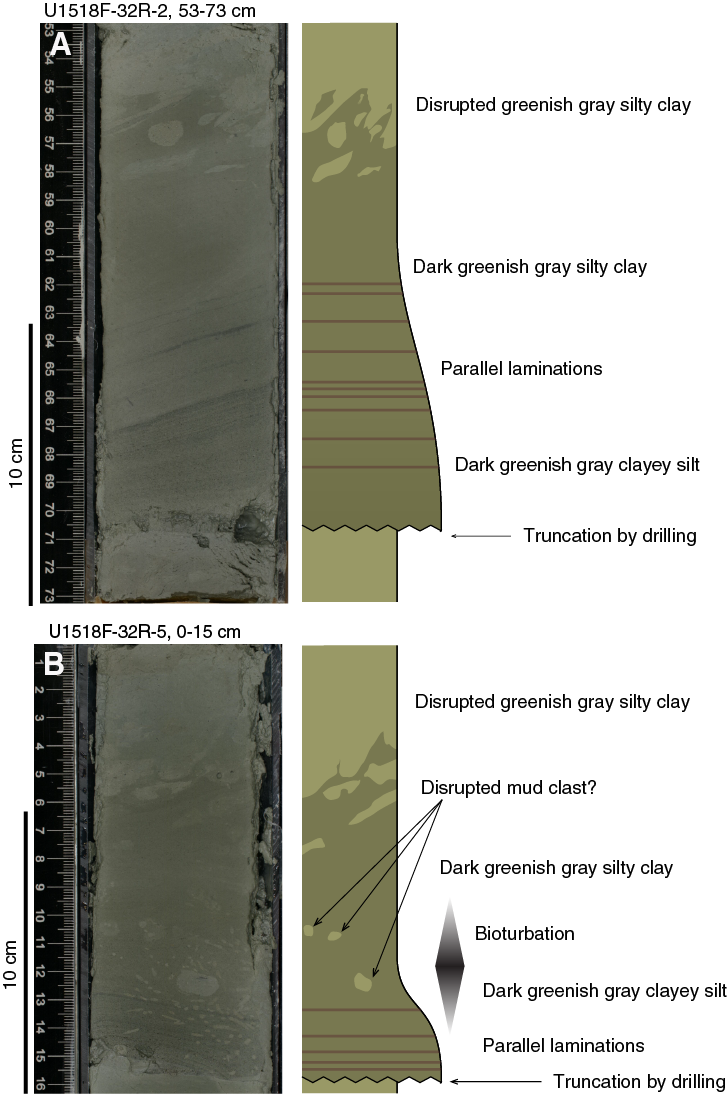
Figure F19. Turbidites and soft-sediment stratal disruption, Subunit IIIB.
Comparison of Hole U1518E/U1518F core data and Hole U1518A/U1518B log data
Broad, facies-level comparisons (i.e., packets of beds at a scale ≥10 m) can be made between the lithostratigraphy defined from core descriptions (Figure F4) and the provisional log-based stratigraphy defined in Holes U1518A and U1518B (see Logging while drilling and Core-log-seismic integration). Some caveats apply, however. The horizontal distance between the holes (30–60 m), differences and uncertainty in ocean depth, the inherent lateral variability of facies thickness, the dip of key structural features (i.e., main and subsidiary fault zones), and the different scales of observations and resolution make direct correlation on a bed-to-bed scale impossible. Nonetheless, the two data sets are complementary, especially where packets of interbedded lithologies and petrophysics attributes are grouped at the facies scale. Finer scale observations of sedimentary structures and microscopic views of grain size distributions help guide interpretations of the logging data (e.g., discriminating between beds of sand versus silt), and continuous logging records help fill gaps in the lithostratigraphy caused by incomplete core recovery.
Bed thickness and texture
Comparisons between logging data and lithostratigraphic observations are particularly helpful when considering the distribution of bed thicknesses and the associated textures of common interbeds. LWD data include multiple measurements of resistivity and porosity. The highest vertical resolution (~5–8 cm) resistivity measurements were collected with the geoVISION tool and include bit resistivity, ring resistivity, and button resistivity (see Logging while drilling). Coarser grained layers are relatively conductive and can be seen as local minima in ring resistivity and as dark bands in the resistivity image, whereas finer grained layers are more cohesive, have relatively higher resistivity, and are orange on the resistivity image (Figure F20). Hydrate-saturated coarse-grained layers have the highest resistivity spikes in Figure F20 and appear as white color bands in the resistivity image.
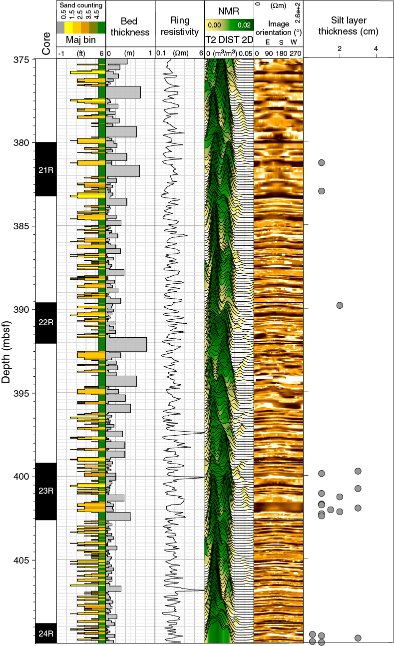
Figure F20. Core-log integration.
Another measurement that provides insight into the distribution and character of the coarser grained beds is the T2 relaxation time. This measurement was taken with the proVISION Plus tool, which is a nuclear magnetic resonance (NMR) measurement that induces a magnetic precession of polarized protons through fluids in the formation. The decay of the transverse magnetization (T2 relaxation time) is controlled by the size of the pore space. This tool has a vertical resolution of 25–51 cm depending on rate of penetration (Figure F20). A lower value T2 peak corresponds to material that has smaller pore sizes, and this is often a signal from clay-rich layers.
Measurements of resistivity and log-based proxies for porosity can also be used to estimate bed thickness (“sand counting”) using an array of porosity bins with defined cutoffs. This approach also yields an estimate of the bed-scale grain size scaled to a continuum with “sand” and “shale” as end-members (Figure F20). Microscopic and macroscopic observations of the lithologies recovered from Holes U1518E and U1518F (described above) indicate that silt-sized turbidites, rather than sand, largely comprise the more porous component of this signal. We note that bed thickness estimates from the LWD data differ from those measured in the split core (e.g., Figure F8) in that they consist of the entire interval from the bottom of one silt layer to the bottom of the next. Core measurements, in contrast, place the bed’s top where normal size grading merges the turbidite mud into the overlying hemipelagic mud. In spite of those differences, lithofacies packets with abundant silt interbeds match favorably with log intervals yielding similar values for bed thickness (Figure F20). This application becomes particularly useful for the deeper portions of the stratigraphy (below Core 375-U1518F-1R; 197.7 mbsf) where core recovery was relatively low (~42% recovery).
Comparisons among lithostratigraphic units and logging units
Below, we provide comparisons between the lithostratigraphic units and the lithologies inferred for logging units (see Logging while drilling). Part of Lithostratigraphic Subunit IA (2.2–197.7 mbsf) corresponds to Logging Unit 2 (10–188.0 mbsf). The closely spaced oscillations in resistivity, porosity, and gamma ray measurements are consistent with the observed character of Lithostratigraphic Subunit IA. The base of Subunit IA is defined at 197.7 mbsf because of the coring gap between Holes U1518E and U1518F, so the logging and coring unit boundaries cannot be matched with any precision.
The facies character of Lithostratigraphic Subunit IB (197.7–304.53 mbsf) correlates with part of Logging Unit 3 (188–299.5 mbsf). Small-scale oscillations in resistivity, NMR, and gamma ray measurements are consistent with observations of thinly bedded and uniformly fine grained sediments in cores. We observed a broadly analogous gradational reduction in silt layer occurrences in Subunit IB compared with Subunit IA (Figure F8).
Lithostratigraphic Unit II (304.53–370.4 mbsf) compares favorably with the lower part of Logging Subunit 3C (299–320.7 mbsf) and Logging Unit 4 (320.7–346 mbsf). The top boundary of Lithostratigraphic Unit II is based largely on the inversion of biostratigraphy rather than a change in lithology and is therefore not detectable by logging.
Lithostratigraphic Unit III (370.4–492.26 mbsf) does not very closely match the boundaries for Logging Units 5 (346–452 mbsf) and 6 (452–600 mbsf) or their subunits, which is probably the result of using different sets of criteria to define subdivisions. Recognition of Lithostratigraphic Unit III is based largely on an increase in syndepositional deformation (i.e., the contorted domains interpreted to be MTD-type deposits), whereas the designations for Logging Subunits 5A and 5B rely more on changes in petrophysical parameters, including porosity and resistivity, along with caliper records suggestive of washouts. Subunits 5B and 6A, moreover, are both indicative of downhole decreases in coarse bed thickness. The cores from those depths do not reveal obvious thinning or reduced numbers of siltstone layers; instead, we recognize a gradation from Subunit IIIA to Subunit IIIB based on a gradual reduction in MTD-type contorted domains.
Biostratigraphy
Planktonic foraminifers and calcareous nannofossils from core catcher samples and additional split-core samples from Holes U1518E and U1518F were examined to develop a shipboard biostratigraphic framework for Site U1518. Additionally, benthic foraminifers provided data on paleowater depths and downslope reworking.
A Holocene to Pleistocene sedimentary sequence was recovered at Site U1518. Biostratigraphic dating indicates a high sedimentation rate (2.8 m/ky) in the Pleistocene section, which will enable high-resolution paleontological and paleoenvironmental post-expedition studies. The base of the Holocene is identified between Samples 375-U1518E-1H-2, 47–52 cm, and 1H-2, 83–88 cm (1.97–2.33 mbsf). The underlying section to the lower portion of the hanging wall of the main brittle fault zone (Samples 375-U1518E-1H-2, 83–88 cm, through 375-U1518F-12R-CC, 0–10 cm [2.33–296.9 mbsf]) is Middle Pleistocene to possibly early Pleistocene (older than 0.53 Ma), and the succession from Sample 375-U1518F-13R-CC, 9–20 cm, through Sample 32R-CC, 0–12 cm (306.95–492.26 mbsf), is Middle Pleistocene (0.126–0.53 Ma) or younger.
Calcareous nannofossils
Calcareous nannofossil biostratigraphy in Holes U1518E and U1518F was established through the analysis of core catcher samples and additional split-core samples over intervals of interest. Nannofossils are common to abundant throughout the recovered sequence, with intervals of increased abundance throughout Hole U1518F. Preservation is moderate throughout the sequence, although reworking of older, poorly preserved material is common in most of the samples. Biostratigraphic datums are given in Table T4, and the distribution of calcareous nannofossil taxa is given in Table T5.
Split-core samples were analyzed under a scanning electron microscope to determine the presence/absence of Emiliania huxleyi. The presence of E. huxleyi in Samples 375-U1518E-1H-1, 21 cm, through 1H-2, 41 cm (0.21–1.92 mbsf), indicates a Late Pleistocene to Holocene age (0.29 Ma or younger) in Zone NN21 of Martini (1971). Below 1.92 mbsf, the recognition of key datums is problematic because of substantial reworking of Pliocene–Eocene taxa throughout the sequence. The last appearance datum of Pseudoemiliania lacunosa defines the Zone NN19/NN20 boundary. However, the top of P. lacunosa is difficult to identify because this taxon co-occurs with E. huxleyi in Sample 1H-1, 23 cm (0.23 mbsf). Consequently, we are unable to identify Zone NN20 in the cored sequence.
Small Gephyrocapsa spp. (<3.5 µm) are abundant to dominant through most of Site U1518, with an increase in dominance first observed downhole in Sample 375-U1518F-12R-CC, 0–10 cm (296.9 mbsf). Initial shipboard analysis tentatively assigns this acme event to the top of the small Gephyrocapsa spp. dominance event at 1.02 Ma (in Zone NN19). However, foraminifer data suggest that the sequence is younger than 0.64 Ma, and it is possible that this Gephyrocapsa acme corresponds to a younger acme event (Hine and Weaver, 1998, and references therein). Additional acmes of small Gephyrocapsa spp. occur farther downhole in Hole U1518F, specifically in Cores 13R, 17R, 23R, and 30R. Foraminifer evidence suggests that the interval below the main brittle fault zone (see Structural geology) (Samples 13R-CC, 9–20 cm, through 32R-CC, 0–12 cm [306.95–492.26 mbsf]) is a repeating sequence of younger sediments, and it is likely that these Gephyrocapsa acmes also correspond to younger events. However, because of the lack of other nannofossil datums through the sequence, it is difficult to constrain these events. Medium Gephyrocapsa spp. (4–5.55 µm) are recorded throughout the cored sequence at Site U1518 (Samples 375-U1518E-1H-CC, 35–40 cm, through 375-U1518F-32R-CC, 0–12 cm [8.65–492.26 mbsf]); therefore, the base of the sequence is interpreted to be early Pleistocene or younger based on the first appearance datum of medium Gephyrocapsa spp. (1.73 Ma or younger; in Zone NN19).
Other taxa in the Pleistocene sequence include rare to common specimens of Calcidiscus leptoporus, Coccolithus pelagicus, Helicosphaera carteri, P. lacunosa, Pseudoemiliania ovata, Reticulofenestra haqii, Reticulofenestra minuta, Reticulofenestra minutula, and Reticulofenestra producta and rare to few specimens of Calcidiscus tropicus, Calciosolenia brasiliensis, Ceratolithus cristatus, Helicosphaera hyalina, Helicosphaera inversa, Helicosphaera sellii, Helicosphaera wallichii, Pontosphaera discopora, Pontosphaera japonica, Pontosphaera multipora, Reticulofenestra perplexa, Rhabdosphaera clavigera, Umbilicosphaera rotula, and Umbilicosphaera sibogae.
Planktonic foraminifers
Planktonic foraminifer biostratigraphy at Site U1518 was based on the shipboard examination of core catcher samples. Additional split-core samples were also taken in intervals of interest. Absolute ages assigned to biostratigraphic datums follow those listed in Table T4 in the Expedition 372B/375 methods chapter (Wallace et al., 2019a). Biostratigraphic datums are given in Table T4, the distribution of planktonic foraminifer taxa is given in Table T6, and planktonic foraminifer abundances and indications of oceanicity (qualitative measure of the extent to which the paleoenvironment recorded by the faunal assemblage represents open ocean conditions relative to a nearshore-influenced environment), paleowater depths, and downslope reworking are given in Table T7 and Figure F21.
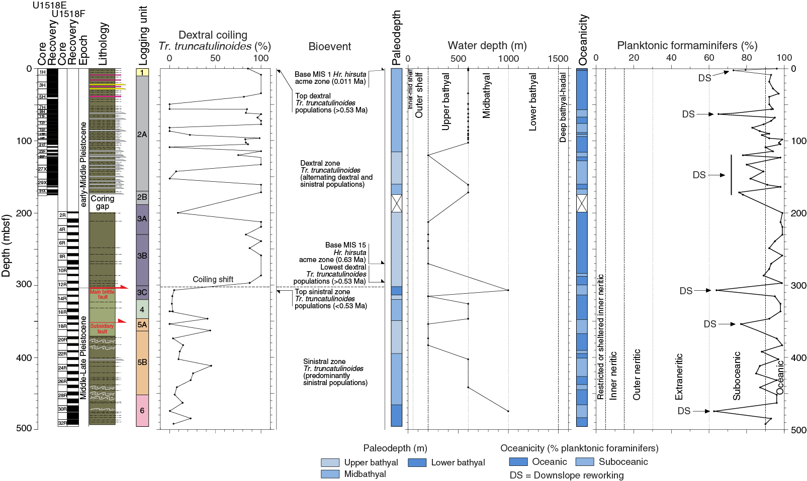
Figure F21. Lithostratigraphy, foraminifer abundance, and oceanicity.
Because of the high sedimentation rate and the very fine grained nature of the cored sedimentary sequence, microfossil residues (>125 µm) from washed samples are very small, even from 10 cm whole-round (353 cm3) samples. Foraminifers (mostly planktonic) dominate the small residues, however, and age markers are present in sufficient numbers to date most samples reliably. Tephra and clastic grains, minor pyrite, carbonaceous plant-derived matter, and other fossil material, including shell (mostly bivalve) fragments, echinoid spines and plate fragments, radiolarians, ostracods, otoliths, and fish teeth and remains, are also present in variable amounts in most samples. In addition, rare reworked Pliocene and Miocene taxa are present in some samples.
Truncorotalia truncatulinoides is common throughout the cored sequence at Site U1518 and indicates that the recovered sediments are Pleistocene age or younger (younger than 2.17 Ma), and possibly Middle Pleistocene or younger (younger than 0.62 Ma), based on the abundance of Tr. truncatulinoides. Higher biostratigraphic precision was achieved by correlating modal coiling changes in Tr. truncatulinoides and short-lived influxes of Hirsutella hirsuta with similar events in the isotopically tuned and calibrated Pleistocene biostratigraphic record at Ocean Drilling Program Site 1123 (after Crundwell et al., 2008). Datums recognized at both sites include a clearly defined coiling change in Tr. truncatulinoides at 0.53 Ma where populations with predominantly dextral coiled specimens (>50% dextral) are replaced in the overlying section by populations that are predominantly sinistral coiled (>50% sinistral). Three short-lived influxes (acme zones) of Hr. hirsuta are also recognized, including a Holocene acme zone correlated with Marine Isotope Stage (MIS) 1 (younger than 0.011 Ma) and two Middle Pleistocene acme zones, one of unknown age and the other correlated with MIS 15 (0.62–0.63 Ma). A fourth acme zone of Hr. hirsuta correlated with MIS 5 (0.12 Ma) was not recognized at Site U1518 and is presumed to be missing at a hiatus between the Holocene and Middle Pleistocene.
Holocene
Planktonic foraminifer assemblages from the Holocene section in Hole U1518E are mostly well preserved, but about 10% of specimens are broken or have partially dissolved shell walls. Rare reworked Pliocene and possibly Miocene specimens of Globoconella triangula and Zeaglobigerina woodi are also present.
The presence of common Hr. hirsuta in mudline Sample 375-U1518E-1H-1 (0 mbsf) and Sample 1H-2, 47–52 cm (1.97 mbsf), indicates that the uppermost part of the cored succession is Holocene. The base of the Holocene is placed immediately below the base of the MIS 1 Hr. hirsuta acme zone (0.011 Ma) between Samples 1H-2, 47–52 cm, and 1H-2, 83–88 cm (1.97–2.33 mbsf). The boundary is characterized by a change from well-preserved Holocene faunas in relatively soft (featureless) bioturbated silty claystone to less well preserved faunas in the underlying compacted, thin-bedded silty claystone sequence. The change in faunal preservation coincides with an abrupt shift in physical properties (see Physical properties).
Middle Pleistocene (hanging wall section)
Planktonic foraminifer assemblages are well preserved in Samples 375-U1518E-1H-2, 83–88 cm, through 375-U1518F-12R-CC, 0–10 cm (2.33–296.9 mbsf). Moderately well preserved specimens from downslope reworking and/or reworking of older sedimentary rocks are also present in some samples. Washed microfossil residues are very small in most of the examined samples, even in samples where 10 cm whole rounds (353 cm3) were washed, but taxa of diagnostic age are sufficiently well represented to date most samples reliably. Planktonic abundances through the hanging wall section are very high (average = 90%) and indicate deposition under an oceanic or suboceanic water mass (Figure F21). Lower planktonic abundances <80% to as low as 65% (e.g., Sample 375-U1518E-11F-CC, 34–39 cm [67.96 mbsf]) were interpreted to be downslope reworking, mostly of inner and midshelf faunal material. Rare Pliocene and Miocene reworking was also noted in some samples (e.g., Sample 375-U1518E-24F-CC, 13–18 cm [119.94 mbsf]).
Populations of Tr. truncatulinoides through the Pleistocene hanging wall section are dominated by either dextral or sinistral coiled specimens (Figure F21) similar to those in the Middle Pleistocene section at Site 1123 (after Crundwell et al., 2008), and they show that the top of the Pleistocene hanging wall section is Middle Pleistocene at the youngest (older than 0.53 Ma), indicating a hiatus between the Holocene and Pleistocene. The fauna in the shallowest Pleistocene sample (375-U1518E-1H-2, 83–88 cm [2.33 mbsf]) is notable in that it is more poorly preserved than most faunas from the hanging wall section; this poor preservation could be attributed to chemical weathering (e.g., due to proximity to the seafloor for an extended period or the migration of corrosive fluids).
A well-defined acme zone of Hr. hirsuta (Samples 375-U1518F-7R-3, 81–91 cm, through 9R-5, 98–108 cm [248.77–270.17 mbsf]) is correlated with the MIS 15 acme zone at Site 1123 and is dated Middle Pleistocene (0.62–0.63 Ma) based on the co-occurrence of Hr. hirsuta with common dextrally coiled specimens of Tr. truncatulinoides. Based on the difference in ages, a minimum sedimentation rate of 2.8 m/ky is estimated for the overlying section. Using the same sedimentation rate and extrapolating downward, the base of the cored hanging wall above the main brittle fault (304.5 mbsf) would be ~0.64 Ma.
Main brittle thrust fault
Based on foraminiferal evidence, an age discontinuity across the main brittle fault identified in cores (see Structural geology) is located between Samples 375-U1518F-12R-CC, 18–23 cm, and 13R-CC, 9–20 cm (296.9–306.95 mbsf), where populations in the hanging wall dominated by dextral or sinistral coiled populations of Tr. truncatulinoides overlie predominantly sinistral coiled populations (Figure F21; Table T7). An additional sample (14R-1, 129–133 cm [314.09 mbsf]) from a sliver in the fault zone has a small predominantly dextral coiled population of Tr. truncatulinoides, indicating that the sample is unlikely to be from the hanging wall.
Middle Pleistocene
Planktonic foraminifer assemblages in Samples 375-U1518F-13R-CC, 9–20 cm, through 32R-CC, 0–12 cm (306.95–492.26 mbsf), are well preserved, and specimens are very abundant to rare in samples diluted with tephra. More poorly preserved specimens from downslope reworking and older reworked sediments, as well as other fossil material, are also present in most samples. Washed microfossils are generally very small, but age markers are sufficiently well represented to date most samples reliably. Planktonic abundances below the age reversal at the brittle fault zone (Domain 2A; see Structural geology) average 89%, indicating deposition under an oceanic or suboceanic water mass (Figure F21; Table T7). Lower planktonic abundances in some samples are often associated with benthic taxa from the shelf that had been reworked downslope (e.g., Sample 29R-CC, 10–16 cm [462.92 mbsf]).
Populations of Tr. truncatulinoides below the hanging wall section are mostly sinistral coiled. Mixed populations with more sinistral than dextral coiled individuals are also present in some samples (e.g., 375-U1518F-17R-CC, 0–10 cm [346.41 mbsf]). The predominance of sinistral populations shows that the interval from 306.95 mbsf to the base of Hole U1518F is Middle Pleistocene or younger (younger than 0.53 Ma). In addition, the absence of Hr. hirsuta shows that the section either predates or postdates the Hr. hirsuta MIS 5 acme zone and the age is 0.011–0.90 or 0.126–0.53 Ma.
Benthic foraminifers
Benthic foraminifer abundances in Holes U1518E and U1518F are much lower than planktonic foraminifer abundances and range from 1% to 37%. Common inner to midshelf taxa (e.g., Zeaflorilus parri, Nonionella flemingi, Elphidium charlottensis, Haynesina depressula, Notorotalia spp., and miliolids) and less common midbathyal markers (e.g., Eggerella bradyi and Sigmoilopsis schlumbergeri) are present throughout both holes. The association of these taxa suggest sediment from the shelf was transported downslope and deposited in midbathyal water depths or deeper. Very rare lower bathyal markers were noted in a few samples (e.g., Planulina wuellerstorfi in Sample 375-U1518F-30R-CC, 4–14 cm [474.43 mbsf]). However, these markers are absent in most samples, even though the site was drilled in a water depth of 2626 m. The paucity of lower bathyal markers in the sedimentary sequence suggests the bulk of the sediment deposited during the Pleistocene was transported downslope. Higher benthic abundances are sometimes associated with occurrences of inner to midshelf taxa (e.g., Sample 375-U1518E-10H-CC, 52–57 cm [63.21 mbsf]) or upper to midbathyal taxa (e.g., Sample 375-U1518F-30R-CC, 4–14 cm [474.43 cm]). This association indicates that at least some of the redeposited sediment originated from the shelf, whereas other sediment originated from the upper to midslope or possibly both.
Paleomagnetism
Archive-half measurements
Paleomagnetic analyses in Holes U1518E and U1518F comprised natural remanent magnetization (NRM) measurements of archive-half core sections prior to and following stepwise alternating field (AF) demagnetization. Sections were measured on a superconducting rock magnetometer (SRM; 2G Enterprises, model 760R-4K) with 2.5 cm spacing prior to and following demagnetization up to a peak alternating current (AC) field of 20 mT (Sections 375-U1518E-1H-1 through 4H-1) or 30 mT (deeper than Section 4H-1 and all of Hole U1518F). To avoid erroneous data interpretation caused by the instrument response, we excluded a 5 cm segment from the top and bottom ends of each section during data analysis. An overview of the measured inclination and intensity data sets and corresponding susceptibility logs is displayed in Figure F22.
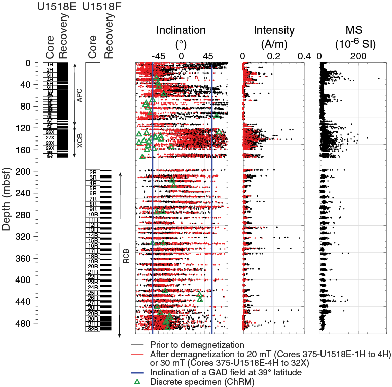
Figure F22. Paleomagnetic inclination and intensity and MS.
NRM intensity values range from 2.2 × 10⁻⁵ to 5 × 10⁻¹ A/m, including both primary magnetic remanence and drilling-induced overprints. Turbidite, silt, and sand layers yield significantly higher remanence intensity values and magnetic susceptibility compared with finer grained material. In the upper 12 m of Hole U1518E (Sections 1H-1 through 2H-2), a drilling overprint manifests as a positive and steep inclination. Upon routine demagnetization, the paleomagnetic vector rapidly rotates to negative inclinations, consistent with the expected direction in a normal polarity field. From 12 to 42 mbsf, NRM prior to and following demagnetization has a direction with negative inclination. Remanence intensity does not decrease significantly following AF treatment, suggesting that the sediment in this interval contains magnetically harder mineral phases that are less susceptible to the acquisition of a viscous remanent magnetization (VRM). Paleomagnetic analyses of Cores 6H–24F were strongly impacted by drilling disturbance, in particular the suction of material along the rims and bottom ends of each core liner. Although we did not measure intervals that were clearly not in situ, sections that exhibit significant coring disturbance (e.g., “suck in” or flow texture along the core liner) but have original bedding still present in the center were measured.
Following partial demagnetization, all APC cores (0–63 mbsf) yield negative inclinations, consistent with a normal polarity field. Declination swings fall into the range of secular variation expected in a normal polarity field, with random high-frequency data scatter superimposed. The declination records of APC cores show systematic offset from core to core but are coherent across individual core segments, suggesting that magnetic overprints from the coring, recovery, and cutting process were successfully removed (Figure F23).
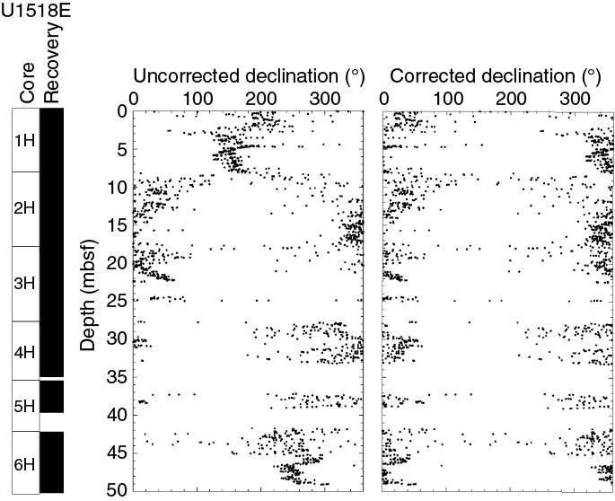
Figure F23. Magnetic declination as recorded and after rotating.
XCB cores (375-U1518E-26X through 32X) yield higher remanence intensity values on average that slowly decay toward the origin during routine demagnetization. Systematic differences between the declination records of individual cores are not apparent, which suggests that drilling-induced overprints may not have been fully removed at the 30 mT demagnetization level. Calculated magnetic inclinations are mostly shallow and positive, and the mean direction of measurements conducted on all six XCB cores averages to declination = 348.5°, inclination = 18.1°, α − 95 = 2.0°, and N = 1414. The mean inclination is significantly shallower than what would be expected in a reversed polarity geocentric axial dipole (GAD) field.
Coring continued in Hole U1518F at 198 mbsf using the RCB system. In the upper 70 m (Cores 375-U1518F-2R through 9R), inclinations are shallow and show a poorly defined pattern with frequent switches from negative to positive inclinations. At ~270 mbsf (Core 9R), inclinations return to negative values and remain as such to the bottom of the hole. The coring procedure in these intervals resulted in the dissection of the recovered material into a number of 4–20 cm thick subhorizontal biscuits (see Structural geology). The declination records are offset with respect to each other, each offset aligning with a marked biscuit boundary (Figure F24). A slight curvature in the declination values recorded along the edges of each biscuit is likely a feature of the instrument response. Nevertheless, the discontinuities in the declinations suggest that drilling overprints were successfully removed.

Figure F24. Paleomagnetic declinations compared with core images.
Discrete samples
Magnetic remanence
Starting with Section 375-U1518E-4H-1 and continuing downhole, as many as two samples per core were collected for more detailed rock magnetic and paleomagnetic investigations. Using a volume of 7 cm3, discrete specimen NRM intensity values range from ~9 × 10⁻⁴ to 1.2 × 10⁻³ A/m. Characteristic remanent magnetization (ChRM) directions were handpicked for each sample, and best-fit directions were calculated using principal component analysis (Kirschvink, 1980) using Agico’s Remasoft or PuffinPlot software (Lurcock and Wilson, 2012). We rejected results from samples that did not yield demagnetization through the origin or for which the maximum angular deviation of the best-fit direction exceeded 10°. If the demagnetization trajectory deviated from the origin during the high-field demagnetization steps, ChRM directions were calculated anchored to the origin.
During AF demagnetization, NRM intensity values usually peak at 10 mT, which is most likely due to the removal of the drilling overprint. Subsequently, NRM intensity values decay rapidly, with the low-coercivity component (≤60 mT) carrying between 70% and 80% of the total remanence. Upon demagnetization to higher levels, however, many samples appear to gain a secondary remanence along the y-axis that is characterized by a marked increase in intensity (Figure F25). The y-z plane is aligned perpendicular to the last direction of the applied AC field during demagnetization, and this behavior is interpreted to be gyroremanent magnetization (GRM) acquisition (see Paleomagnetism in the Expedition 372B/375 methods chapter [Wallace et al., 2019a]). To monitor the acquisition of unwanted remanences during AF demagnetization, we generally inverted the orientation of samples in the AF demagnetizer every second demagnetization step. We also subjected a subset of samples to the three-step demagnetization protocol of Stephenson (1993).
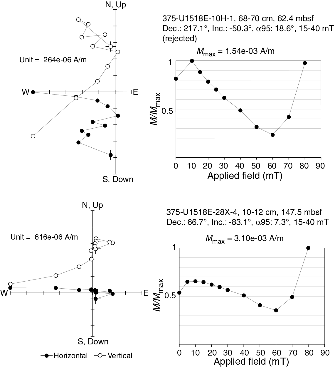
Figure F25. Vector components and NRM intensity, GRM acquisition.
In contrast to AF demagnetization and with few exceptions, all samples subjected to thermal demagnetization yield single component remanences that show a straight-line decay to the origin in the unblocking temperature range 100°–350°C (Figure F26). All thermal demagnetization results yield negative inclinations.
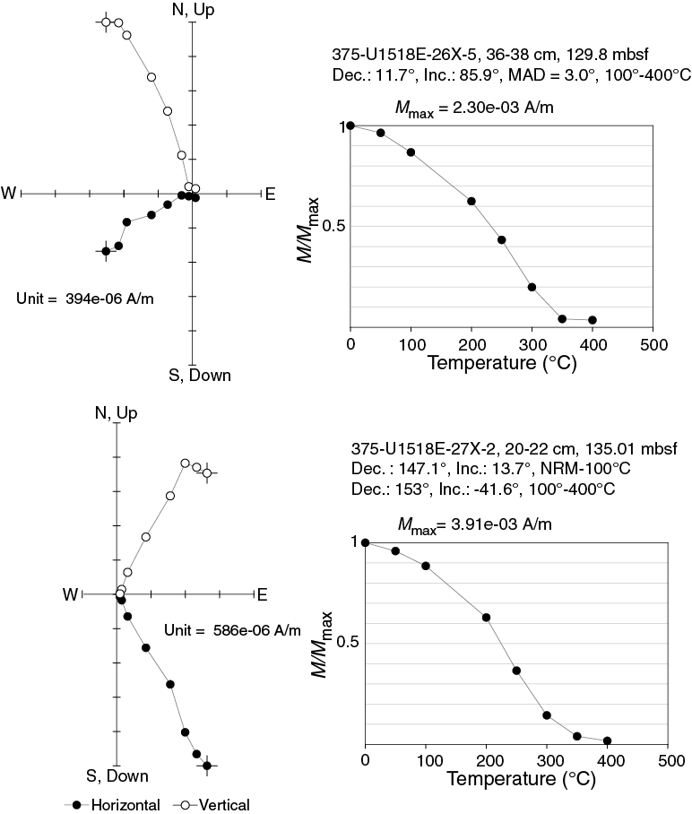
Figure F26. Vector components and NRM intensity, thermal demagnetization.
Magnetic mineralogy
Shipboard rock magnetic investigations were limited to determination of the magnetic coercivity distribution based on AF demagnetization, isothermal remanent magnetization (IRM) acquisition, and measurement of magnetic susceptibility data sets. Implications for the blocking temperature distributions can be drawn from thermal demagnetization diagrams. Bulk magnetic susceptibility and anisotropy of magnetic susceptibility (AMS) were measured on all discrete samples, whereas S−300mT and IRM1T/χ ratios were determined on samples subjected to AF demagnetization only. An interpretation of the rock magnetic parameter downhole trends is difficult because of the irregular spacing of shipboard samples collected from Holes U1518E and U1518F. No rock magnetic data were obtained from the fault zone.
AMS reveals that all samples exhibit oblate textures with F ratios ranging from 1.01 to 1.05 in the hanging wall and from 1.01 to 1.06 beneath the brittle fault zone at ~310 mbsf (Figures F27, F28). The principal axis of magnetic susceptibility (χ1) is predominantly core parallel, which is characteristic for deformation fabrics developed in response to lithostatic loading and compaction.
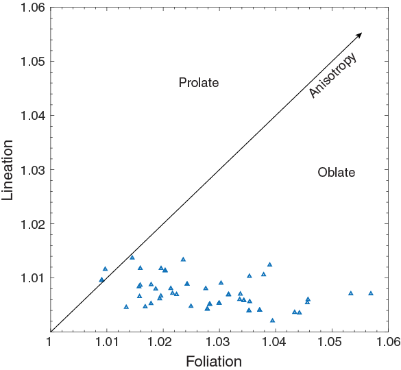
Figure F27. Flinn diagram showing shape of AMS.
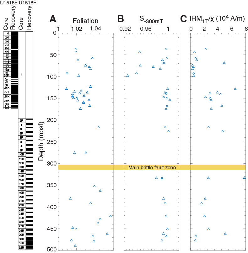
Figure F28. Rock magnetic parameters.
AF demagnetization experiments conducted on samples throughout Holes U1518E and U1518F suggest the presence of two distinct coercivity populations. The first population yields coercivity values ≤50 mT and is interpreted to be (titano)magnetite. The second population yields coercivity values ≥60 mT. Based on the GRM acquisition, we interpret this mineral phase to be greigite (Fe3S4) that likely formed by diagenesis following deposition (see Paleomagnetism in the Expedition 372B/375 methods chapter [Wallace et al., 2019a]). This interpretation is consistent with the thermal demagnetization diagrams: the observed blocking temperatures range from 100° to 350°C, a temperature interval in which the blocking temperature of authigenic greigite overlaps with that of (titano)magnetite (Liu et al., 2012; Tauxe, 2015).
The S−300mT ratios of sediments sampled in the upper 100 m of Lithostratigraphic Subunit IA (Hole U1518E) exhibit some scatter with values ranging from 0.92 to 0.99. An S−300mT ratio significantly lower than 1 is indicative of the presence of antiferromagnets such as goethite (FeOOH) and hematite (Fe2O3) that, unlike greigite and titanomagnetite, only begin to saturate at applied fields larger than 300 mT (e.g., Kars and Kodama, 2015; Liu et al., 2012). The small scatter in S−300mT ratios at 0–100 mbsf may reflect spatiotemporal variations in the source region for material deposited along the Hikurangi Trough. Samples collected from 120 to 220 mbsf (lower section of Lithostratigraphic Subunit IA) yield higher S−300mT (0.99 < S−300mT < 1.01) and IRM1T/χ (0.02 < IRM1T/χ < 0.07) ratios that may be explained by an increase in the degree of mineral diagenesis and production of iron sulfides such as greigite (Fe3S4) and pyrrhotite (Fe7S8). Samples collected from the footwall yield S−300mT ratios that range from 0.98 to 1.0 and IRM1T/χ ratios ranging from 0.007 to 0.7 A/m.
Magnetostratigraphy
We based our magnetostratigraphic interpretation on the identification of magnetic polarity zones or chrons based on paleomagnetic inclination. Interpretation of magnetic polarity records in an active tectonic setting is not straightforward. Rapid sedimentation, tectonic deformation, and overprinting of primary magnetic signals during diagenesis and/or the drilling and sampling process have to be considered. The results of more detailed thermal and AF demagnetization experiments and rock magnetic investigations on discrete samples aided our interpretations.
Overall, much of the paleomagnetic record displayed in Figure F22 is dominated by negative inclination values that fall into the range of a normal polarity field at this latitude. Reversed (positive) inclination was recorded in all XCB cores sampled between ~124 and 175 mbsf. Continuity in the declination records in this interval suggests that the sampled material may be affected by drilling-induced magnetic overprints. In contrast to the results from SRM archive-half measurements, the majority of discrete samples subjected to thermal or AF demagnetization yield ChRM directions that fall into the range expected for a normal polarity field. All samples subjected to thermal demagnetization carry low blocking temperature (TB) overprints that are more difficult to isolate on samples subjected to AF treatment. The demagnetization results from a sample collected from Section 375-U1518E-27X-2 (135.01–137.01 mbsf) allows us to resolve the primary and secondary components of magnetization (Figure F26). A low-temperature (NRM–100°C) segment yields a direction (declination = 147.1°, inclination = 13.7°, and maximum angular deviation = 4.6°) that is consistent with directional records of SRM measurements in this section. In contrast, the ChRM direction calculated from the high TB segment (200°–350°C) yields a direction (declination = 153°, inclination = −41.6°, and maximum angular deviation = 3.0°) that falls into the range of inclinations expected for a normal polarity field. Based on this ChRM direction, we suggest that this interval may in fact correspond to a normal polarity interval. The origin of the low-temperature overprint identified using thermal demagnetization techniques is unknown but may be a drilling overprint imparted during XCB coring.
Magnetic polarity was also difficult to determine in the upper 80 m of Hole U1518F (Cores 2R–7R), where inclination values are shallow and inconclusive. This interval is affected by significant deformation (see Structural geology). Unless the paleomagnetic vector is corrected for tilting and/or overturned bedding, it is not representative of the in situ depositional conditions.
In summary, the entire sequence recovered at Site U1518 is most likely of normal polarity despite an interval between ~220 and 270 mbsf in which the magnetic polarity remains unresolved. Assuming that Hole U1518F is of normal polarity, our interpretation is consistent with biostratigraphic observations that suggest an age younger than 0.64 Ma for the hanging wall sediments and younger than 0.53 Ma for the footwall sediments. These observations place our paleomagnetic record in the Brunhes Normal Chron (C1n) (Gradstein et al., 2012).
Structural geology
Site U1518 penetrated the Pāpaku fault and its hanging wall and footwall sequences. The Pāpaku fault is a splay fault near the deformation front. At Site U1518, it is identified as a tens of meters thick fault zone that comprises a main brittle fault and a lower subsidiary fault separated by less intensely deformed sediments. Structural features at this site include (1) folded and fractured hanging wall sediments above the fault; (2) a mix of intense ductile and brittle deformation in the fault zone, including flow banding and fractures; and (3) less deformed footwall sediments. The distribution of deformation structures with depth is shown schematically in Figure F29 and described more completely below. Cores were recovered from Holes U1518E and U1518F, and dip angles of bedding and brittle structures are compiled in Figure F30. Because of drilling disturbance, structural data are sparse throughout Hole U1518E; therefore, most reported structural observations are from Hole U1518F (197.7–494.9 mbsf). A complete set of structural measurements is obtained by incorporating bedding and fracture orientations determined from geoVISION (GVR) resistivity image logs obtained during Expedition 372 in Holes U1518A and U1518B (Figure F31; see Logging while drilling). Recognizing vertical offsets in both the seafloor and the depth of subsurface features between Expedition 372 Holes U1518A–U1518B and Expedition 375 Holes U1518E–U1518F, we discuss trends in both the LWD and core description data sets rather than comparisons of absolute depths or thicknesses of features. See Core-log-seismic integration for a more detailed description of correlations between core and logging data and associated uncertainties.
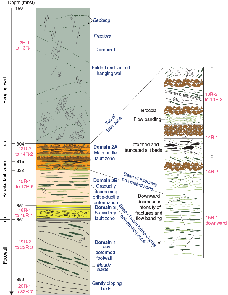
Figure F29. Key structural observations.
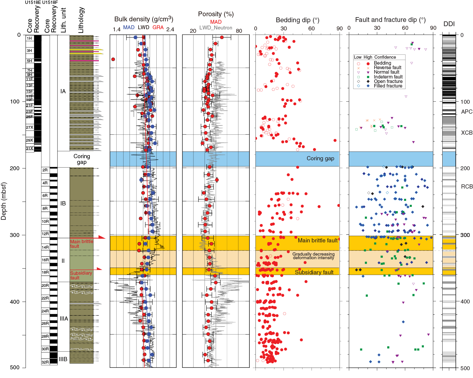
Figure F30. Dip angles of planar structures.
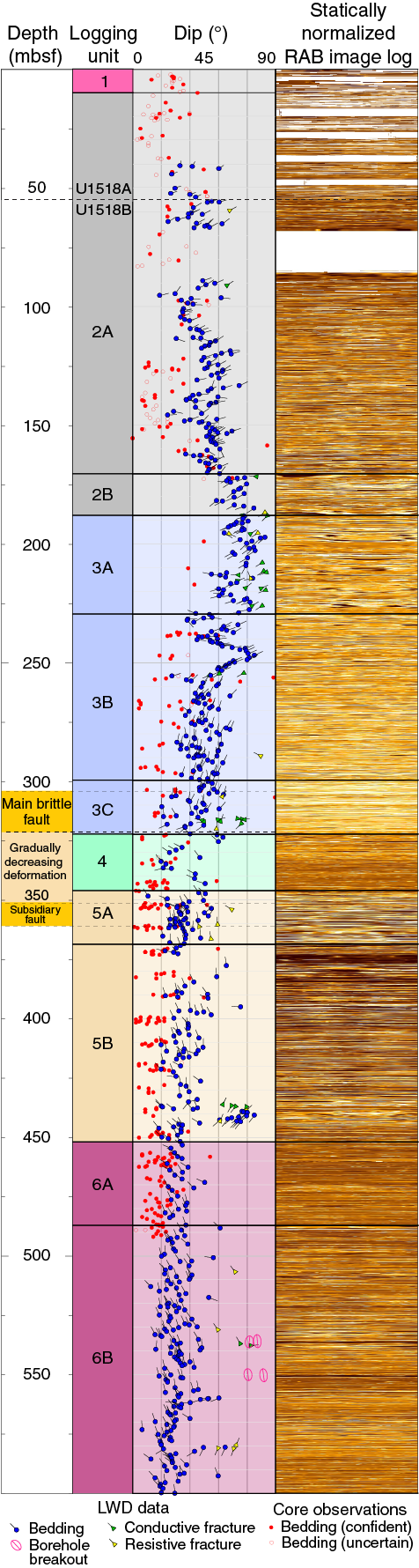
Figure F31. LWD bedding and fracture orientations.
Types of structures observed
The main structure types observed at Site U1518 are brittle features such as fractures (both open and filled), faults, and breccias, as well as a range of ductile deformation structures. Folds are inferred from variations in dip and dip direction, determined both in the core and in the GVR image logs (Figures F30, F31), and from rare preserved fold hinges that exhibit fractured hinge zones (e.g., Figure F32A). Features designated as “fractures” include all opening-mode discontinuities that show no evidence of apparent shear displacement. Breccias are defined as intensely fractured intervals where the rock consists of angular clasts in a matrix (Figures F32D, F33A). Breccias differ from fracture sets because the fractures in breccias have variable orientations and create a range of clast sizes, whereas fracture sets comprise regularly spaced and oriented fractures creating rock fragments of a limited size range. Breccias at this site are commonly but not always less cohesive than rocks with consistent fracture sets. Minor faulting was noted throughout the core, as defined by offset beds (Figure F32B). Where possible, the apparent magnitude and sense of separation was noted and/or measured. A fabric identified as color bands and defined locally by dismembered sedimentary layering and stretched features such as bioturbation was documented throughout the fault zone and the footwall (Figures F33B, F33D, F34). This planar fabric is referred to as flow banding, which implies layer-parallel particle paths, but no further interpretation of the type of strain or sense of displacement is intended. We identified four structural domains at Site U1518: (1) hanging wall; (2) main fault zone, including an upper main brittle fault zone (Domain 2A) and a lower ductile deformation zone (Domain 2B); (3) subsidiary fault zone; and (4) footwall.
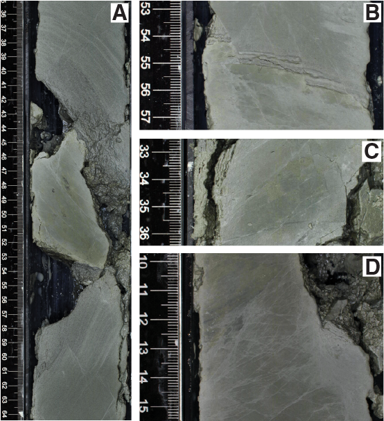
Figure F32. Hanging wall features.
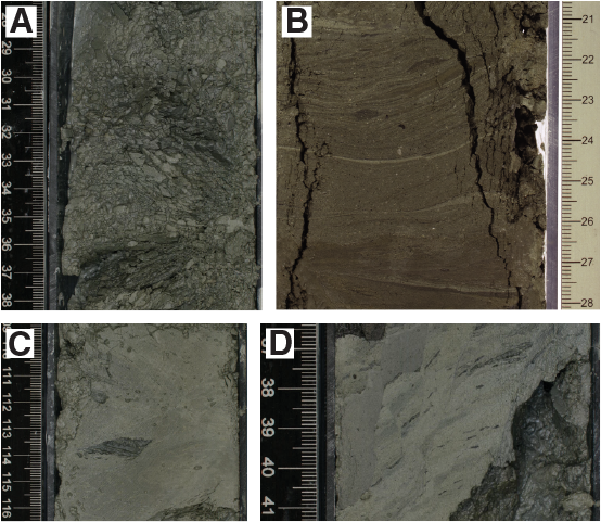
Figure F33. Fault zone structures.

Figure F34. Structures from Domains 2B and 3.
Domain 1: hanging wall
Holes U1518A and U1518E and the upper part of Holes U1518B and U1518F penetrated the hanging wall domain. Alternating silt and mud sequences define bedding planes with variable orientations from which folds are interpreted. Faults locally displace bedding, generally showing millimeter- to centimeter-scale, apparent normal offsets where resolvable (e.g., Figure F32B). Bedding dips throughout the hanging wall are highly variable but generally range between 0° and 50° throughout Hole U1518E and at the top of Hole U1518F (Figure F30). This variability is also apparent in bedding orientations determined in the GVR image logs, which document similar depth-dependent variations but generally with steeper dip angles (Figure F31). Paleomagnetic data were used to orient the observed structures in cores from the seafloor to 174.7 mbsf (see Paleomagnetism). For APC cores recovered from the seafloor to 123.3 mbsf, oriented bedding dips gently to moderately to the east, and the rotation based on paleomagnetic declination data significantly improves the consistency of the orientations (Figure F35A–F35B). The rotated data are also consistent with image log data from above 123 mbsf in Hole U1518A (Figure F35C). However, for the XCB cored interval from 123.3 to 174.7 mbsf, the paleomagnetic rotation has larger errors (as high as 30°) (Figure F35D–F35E). In this interval, the rotated orientations are significantly different from the image log data and from the shallower core measurements (Figure F35F). Thus, we do not have reliable dip directions in a geographic reference frame for structural measurements made on XCB cores, and we cannot resolve rotations caused by drilling-induced deformation such as biscuiting. Preliminary attempts to orient RCB cores in Hole U1518F were more successful; orienting measurements from Hole U1518F to a geographic reference frame is therefore a task for further work. In this section, we discuss only dip angles (Figure F30), not azimuths, for core observations from below 123.3 mbsf and refer to the GVR image log data for azimuth information.
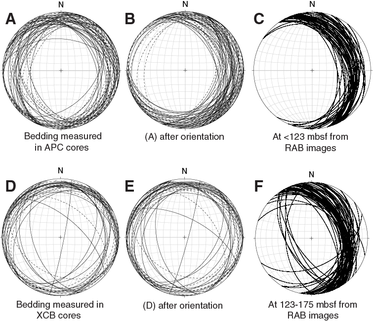
Figure F35. Bedding orientation data.
Folds were inferred from variable bedding dip angles, an observation also made from GVR image logs where dip directions are dominantly northeast but with southwest to west-southwest dips in places, particularly where dip angles are steep (e.g., Logging Subunits 2B and 3A at approximately 175–225 mbsf in Hole U1518B). In the core, a few cases of overturned bedding suggest tighter folding in localized zones (e.g., Core 375-U1518F-8R, particularly interval 8R-3, 22–52 cm). In interval 10R-2, 35–65 cm (~275 mbsf), we recovered a fold hinge zone with an overturned bed showing fractured limbs consistent with local tensile fracturing during folding (Figure F32A).
Fractures are present throughout the hanging wall, although they are best preserved in Hole U1518F cores. The lack of fractures in Hole U1518E could be caused by masking of these features by intense drilling disturbance in the APC and XCB cores (Figure F30), although GVR image logs also lack evidence for spatially frequent fractures above 175 mbsf (Figure F31). Domain 1 in Hole U1518F (Figure F30; 197.7–304.5 mbsf) exhibits moderately to steeply dipping (20°–80°) open and filled fractures that were generally formed in sets with 1–10 cm spacing. Steep fractures determined from the GVR image logs in Logging Subunit 3A (~185–230 mbsf) correspond to the upper hanging wall but with more clustered fractures than are observed in the core.
Fracture intensity was estimated throughout Hole U1518F (Figure F36; see Structural geology in the Expedition 372B/375 methods chapter [Wallace et al., 2019a]). From 284.0 to 304.5 mbsf (top of Section 375-U1518F-11R-1 to base of Section 13R-1), fracture intensity and the size and frequency of associated breccia zones increase markedly. Across this zone, bedding is still coherent and measurable despite intense fracturing.
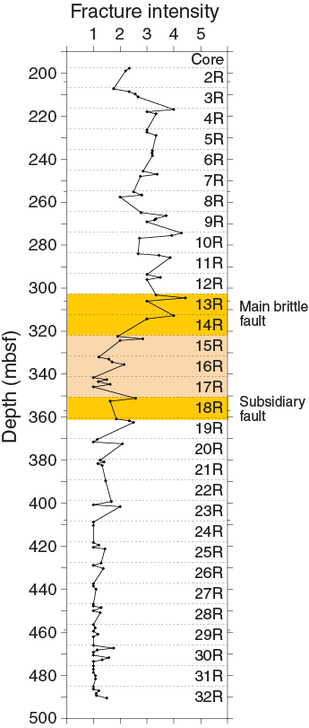
Figure F36. Fracture intensity.
Domain 2A: main brittle fault zone
As indicated in Figures F29 and F30, the upper boundary of the Pāpaku fault zone is defined at the top of Section 375-U1518F-13R-2 where an interval of intense breccia and zones of flow banding occur (Figures F29, F33A, F33B). Although the intensity of brittle deformation increases gradually through the lower few tens of meters of the hanging wall toward the top of the fault (Figures F30, F36), the preserved hanging wall fractures do not show significant shear displacement. Therefore, the boundary between the hanging wall damage zone and the fault is defined between the base of Section 13R-1 and the top of Section 13R-2 by a marked change in fracture intensity and deformation style (Figures F29, F36). The GVR image log indicates a distinct fractured interval somewhat deeper than the lowest hanging wall damage zone identified in the core at about 315–322 mbsf in Hole U1518B (Figure F31). However, the Hole U1518B seafloor depth differs from that of Hole U1518F, and the fault itself is dipping and lies at different depths below the seafloor at the two sites, which may explain some of this offset (see Core-log-seismic integration).
The lithology in the fault zone differs from that observed in cores above and is more consistent with the footwall lithology (see Lithostratigraphy). The top of Section 375-U1518F-13R-2 also corresponds to a small contrast in physical properties, with decreasing density and increasing porosity into and below the fault zone (Figure F30; see Physical properties). The coincidence of changes in physical properties and lithology and the defined top of the intensely deformed zone are consistent with our placement of the upper boundary of the fault zone at 304.5 mbsf in Hole U1518F.
The Pāpaku fault zone is characterized by a mixture of brittle and ductile deformation, with ductile features locally overprinted by brittle fractures and faults (e.g., Figure F33D). A zone of finely spaced flow banding with millimeter-scale asymmetric clasts in interval 375-U1518F-13R-3, 21–31 cm (306.13–306.23 mbsf; Figure F33B) is cut by a planar normal fault near its base. The most intense brittle deformation, characterized by pervasive brecciation (Figure F33A), occurs at the top of interval 14R-1, 0–104 cm (312.80–313.84 mbsf). This intense brittle deformation is likely enhanced by drilling disturbance; however, coherent intervals of angular clasts in a matrix appear well preserved (e.g., interval 14R-1, 41–45 cm). The extent of drilling disturbance and material loss is unknown, so the recovered breccia zone represents its minimum thickness.
A zone of distorted muds and thin silty layers occurs between two brecciated intervals from 313.8 to 314.3 mbsf (interval 375-U1518F-14R-1, 104–151 cm). Deformation of this zone is characterized by ductilely deformed silt layers truncated by curved faults (Figure F33C). A network of fine, planar, filled fractures crosscuts the upper part of this zone (interval 14R-1, 109–116 cm). This preserved overprinting relationship indicates that the ductile deformation structures are not a result of drilling disturbance.
Below 314.3 mbsf, brittle deformation is again evident, with intervals of discrete faulting (e.g., interval 375-U1518F-14R-2, 13–19 cm) and intense brecciation (e.g., interval 14R-2, 76–85 cm). However, much of this zone is also marked by flow banding of variable intensities that is locally displaced by later faulting, at least some of which has an apparent normal sense of slip (e.g., interval 14R-2, 34–44 cm; Figure F33B, F33D). The base of Core 14R represents the base of the zone containing preserved intervals of intense brecciation (Figures F29, F36). Thus, the base of Domain 2A is defined at the top of Core 15R.
Domain 2B: gradually decreasing brittle/ductile deformation
Domain 2B extends from 322.4 to 351.2 mbsf (top of Section 375-U1518F-15R-1 to top of Section 18R-1) and marks a gradual change in the structural character of the core. Average MAD density values remain low throughout this domain, and average porosity values remain high relative to the hanging wall immediately above the fault (Figure F30; see Physical properties and Logging while drilling). Both ductile and brittle deformation intensity are decreased relative to Domain 2A, and both continue to decrease downsection toward background levels, albeit with local zones of higher intensity (Figures F29, F36). The decrease in deformation intensity with depth is based on the observation that the thickness and frequency of deformed intervals decrease throughout this zone.
Superimposed bioturbation, soft-sediment deformation, and tectonic deformation lead to uncertainty in interpreting the source(s) of ductile deformation structures. Ductile deformation in Domain 2B likely reflects a combination of these mechanisms, characterized by deformed bioturbated layers and silty beds that are locally dismembered into elongate muddy clasts. A particularly well defined example identified in interval 375-U1518F-15R-1, 19–21 cm (Figure F34A), is characterized by the presence of a homogeneous gray unit with sharp irregular boundaries and an apparent flame structure. A dark planar layer interpreted to be a shear band also crosscuts this zone. Ductile features such as these commonly result in a fabric oblique to bedding that in places includes asymmetric clasts (intervals 15R-2, 2–16 cm, and 16R-1, 28–34 cm; similar to Figure F34C, F34D). Local zones of gently dipping faults with an indeterminate sense of shear also occur (e.g., interval 15R-2, 2–6 cm).
From 324.4 to 351.2 mbsf, deformation intensity is generally low but variable (Figures F29, F36). From 324.4 to 333.0 mbsf, scattered filled fractures and a few intervals of ductile deformation occur, but the frequency and thickness of deformed intervals is reduced compared with the sections above. In the GVR image log data (see Logging while drilling), moderate (<45°) dips to the northwest become dominant below 325 mbsf (Figure F31). From 333.0 to 341.6 mbsf, bioturbation features are well preserved and essentially no brittle or ductile structures can be confidently identified as tectonic in origin. Deformation intensity increases locally from 341.6 to 342.5 mbsf (throughout Section 375-U1518F-17R-1), with a few intervals of well-aligned, elongate clasts (e.g., intervals 17R-1, 51–58 cm, and 17R-1, 68–71 cm; Figure F34B, F34C). Below this interval, deformation intensity is again low to 351.2 mbsf, the top of Domain 3 (Figure F29).
Domain 3: subsidiary fault
The interval from 351.2 to 361.7 mbsf (Sections 375-U1518F-18R-1 through 19R-1) is more intensely deformed than Domain 2B and characterized by a mixture of both ductile and brittle structures. The GVR image log shows fractures and variable bedding dips from ~350 to 360 mbsf (Figure F31). In the core, in addition to pervasive color banding, several mud clasts entrained in the sediments exhibit elongate tails that could indicate simple shear (Section 18R-1). Locally, faults crosscut apparent flow banding on one side but are subparallel to differently oriented flow bands on the other side (interval 18R-1, 55–67 cm; Figure F34D). Faults are typically at a low angle or subparallel to dismembered bedding.
The highly deformed zone indicates the presence of a subsidiary fault in the footwall sequence but with no obvious lithologic change across it (see Lithostratigraphy) (Figures F29, F30). The fault zone boundaries are not accompanied by defined, discrete structures, but the change in deformation intensity is relatively abrupt both above and below the zone of elevated deformation intensity (Figures F29, F30, F36). The zone is also coincident with a marked change in physical properties, particularly an increase in porosity at the base of the fault zone (Figure F30; see Physical properties). The base of this subsidiary fault is gradual, accompanied by high porosity values, and placed at a depth defined by a change to more discrete and less frequent intervals of increased deformation intensity.
Domain 4: footwall
Beneath the subsidiary fault, the footwall sediments are less deformed and beds generally dip less than 30° (Figures F29, F30, F31). Scattered, steeper dips are associated with zones of increased soft-sediment deformation interpreted to be MTDs (see Lithostratigraphy). Zones of fractures and breccias are locally present but much less frequent than in the fault zone (e.g., 361–399 mbsf and interval 375-U1518F-32R-7, 49–58 cm). The GVR image logs indicate consistent north-northwest bedding dip directions and gentle to moderate dip angles below ~375 mbsf (Figure F31). The LWD data also indicate a zone of fractures and steeply dipping beds at ~430–445 mbsf, but a comparable interval was not seen in the recovered cores (see Logging while drilling). Scattered, small displacement normal faults are present (e.g., interval 32R-4, 5–8 cm), as are indeterminate faults (e.g., interval 30R-6, 64–74 cm). Bioturbation is extensive throughout this domain, along with evidence for soft-sediment deformation (e.g., entrained mud clasts and slump deposits) (see Lithostratigraphy).
Drilling disturbance
Drilling disturbance was common in cores from Site U1518, and the type of disturbance was highly dependent on the coring technique. APC cores collected from the upper portion of Hole U1518E successfully recovered the upper few meters, albeit with local upward-arching contacts. However, the bases of Cores 375-U1518E-3H through 9H and 12F through 15F exhibit significant midcore flow, including soft clays sucked in during retraction of the core barrel (Figure F37A). No structures could be resolved in these disturbed core sections.
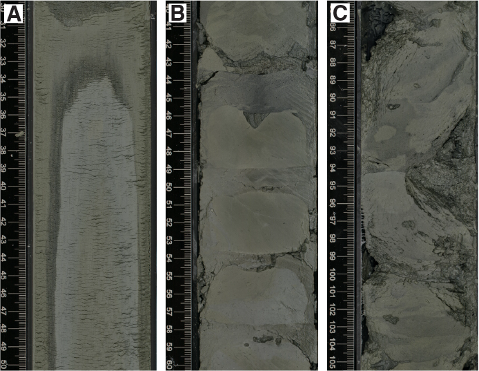
Figure F37. Drilling deformation.
Biscuiting was common in XCB cores from Hole U1518E and RCB cores from Hole U1518F. In unlithified and unconsolidated sediments, these biscuits were less than a few centimeters thick and structures within were uninterpretable (Figure F37B). More consolidated materials preserved the internal structure of the biscuited materials, allowing reliable measurements of structures and bedding dips in the core reference frame (Figure F37C). Gaps in dip data in Figure F30 correspond to zones of intense drilling disturbance.
Core splitting using the wire sediment saw tended to impart subhorizontal extensional fractures on the core faces that often obscured the underlying structures, bedding horizons, and biscuit boundaries (e.g., Cores 375-U1518E-1H through 28X). Although scraping the surfaces allowed identification of biscuit boundaries, some uncertainty remains in bedding orientations measured in this interval (0–152.5 mbsf). Cores 29X–32X were cut with a bladed rock saw and were significantly easier to interpret; well-preserved internal structures and fabrics and distinct biscuit boundaries resulted in much more reliable orientation measurements.
Differential biscuit rotation also affects our ability to orient deformation structures in a geographical reference frame, as described above. Magnetically determined declinations from core halves allowed us to successfully reorient shallow structures in APC cores (Figure F35) (see Paleomagnetism). Similar orientations may be possible on larger biscuits in RCB cores after post-expedition analysis of the declination data.
Summary
The deformation features at Site U1518 span a wide range of types and scales. Brittle structures include microfaults, core-scale brecciation, and both spaced and clustered fracture sets. Ductile features include decimeter-thick zones of flow-banded sediments in the footwall and folds in the hanging wall that are inferred from bedding dip variations in both core and GVR resistivity image data. High deformation intensity in the form of increased fracture intensity, local brecciation, and more intense flow banding define an interval containing various degrees of deformation spanning from 304.5 to 361.7 mbsf that we collectively define as the Pāpaku fault zone, the top of which coincides with a change in lithology and a biostratigraphic age inversion (see Lithostratigraphy and Biostratigraphy). The upper part of the fault is characterized as a dominantly brittle domain with locally intense ductile deformation from 304.5 to 322.4 mbsf (Domain 2A). Beneath this domain, a mix of brittle and ductile deformation grades into intermittently ductilely deformed footwall sediments (Domain 2B). A subsidiary fault, Domain 3, cuts the footwall sediments at 351.2–361.7 mbsf and is associated with a change in physical properties but not in lithology. Deformation intensity is locally high, producing ductile flow bands and millimeter-scale brecciation. Local brittle overprint on some of these preserved ductile fabrics indicates polyphase deformation in this area. The footwall below 361.7 mbsf is distinctly less deformed than the rocks above.
Geochemistry
Inorganic geochemistry
The main objective of the inorganic geochemistry program at Site U1518 was to document variations in the chemical and isotopic composition of pore fluids that can be used to elucidate fluid flow and fluid–rock interactions, which in turn may affect the physical and mechanical properties of the sediment and faults. A total of 82 whole-round (WR) samples were squeezed for pore water chemical and isotopic analyses. We collected 47 samples (10–20 cm long) from Hole U1518E (25 from APC cores, 12 from HLAPC cores, and 10 from XCB cores) and 35 samples (20 cm long) from Hole U1518F (RCB cores). Samples were collected on the catwalk at a frequency of six samples per core from Cores 375-U1518E-1H and 2H, three samples per core from Core 3H, and 1–2 samples per core from Cores 375-U1518E-4H through 375-U1518F-32R. Each core deeper than 30 mbsf was scanned with an IR camera to identify the occurrence of methane hydrates, indicated by cold temperature anomalies resulting from methane hydrate dissociation during core recovery.
All WR samples were thoroughly cleaned in an effort to remove drilling fluid contamination. The cleaned samples were placed in titanium squeezers and squeezed at gauge forces to a maximum of 30,000 pounds. The volume of recovered pore water varied with lithology, depth, and coring technique and ranged from 18 to 55 mL in APC cores, from 20 to 58 mL in HLAPC cores, from 22 to 40 mL in XCB cores, and from 9 to 26 mL in RCB cores.
The pore water data were corrected for contamination during drilling based on the sulfate concentration below the sulfate–methane transition zone (SMTZ) (see Geochemistry in the Expedition 372B/375 methods chapter [Wallace et al., 2019a]). The major and minor element concentrations not corrected for drilling water contamination are listed in Tables T8 and T9. Contamination-corrected concentration data are listed in Tables T10 and T11. Only the contamination-corrected data (except for the sulfate concentration profile) are shown in Figures F38, F39, and F40.
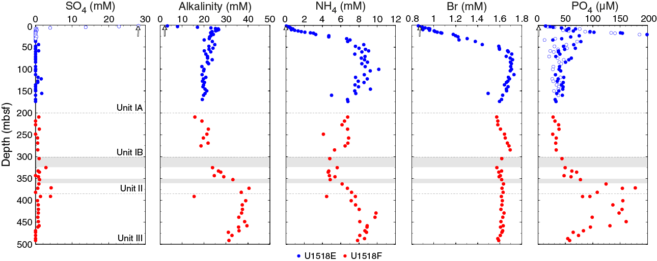
Figure F38. Sulfate, alkalinity, ammonium, bromide, and phosphate.
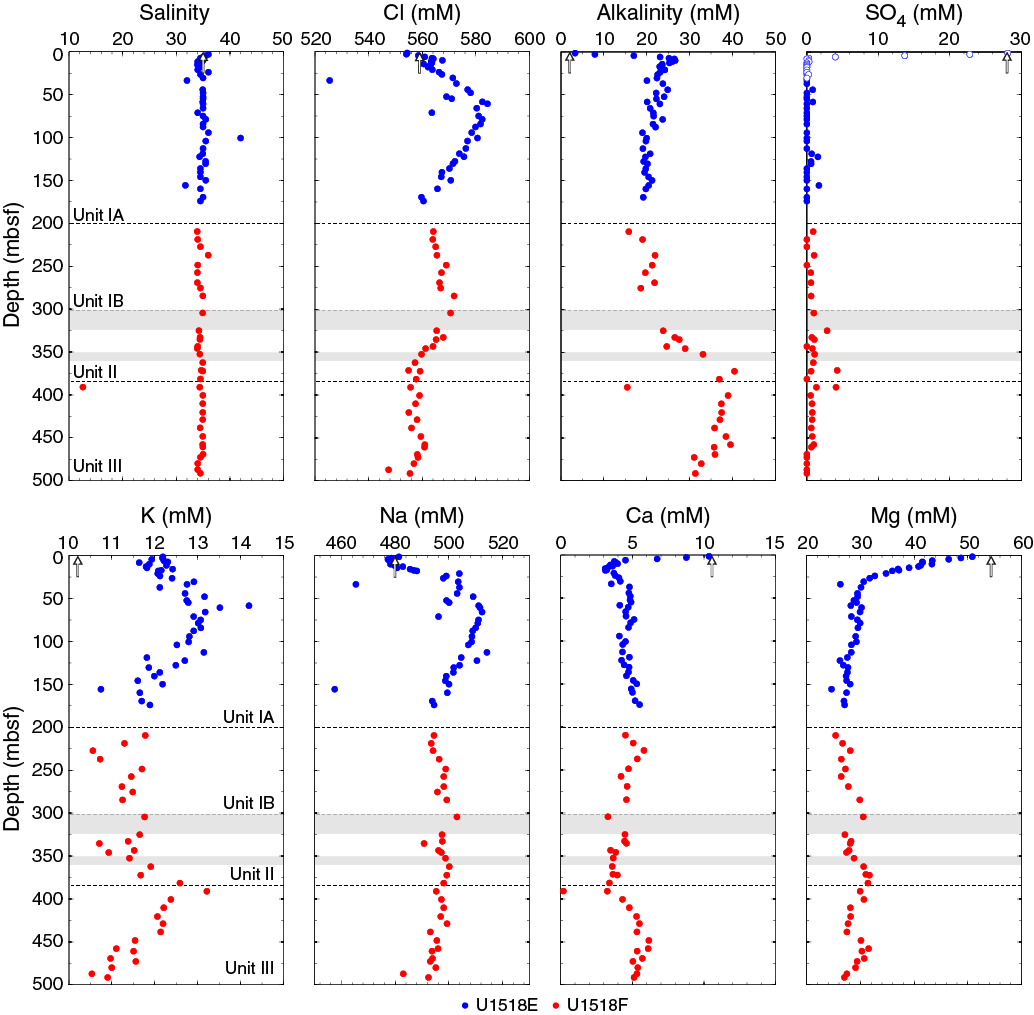
Figure F39. Salinity, chloride, alkalinity, sulfate, potassium, sodium, calcium, and magnesium.
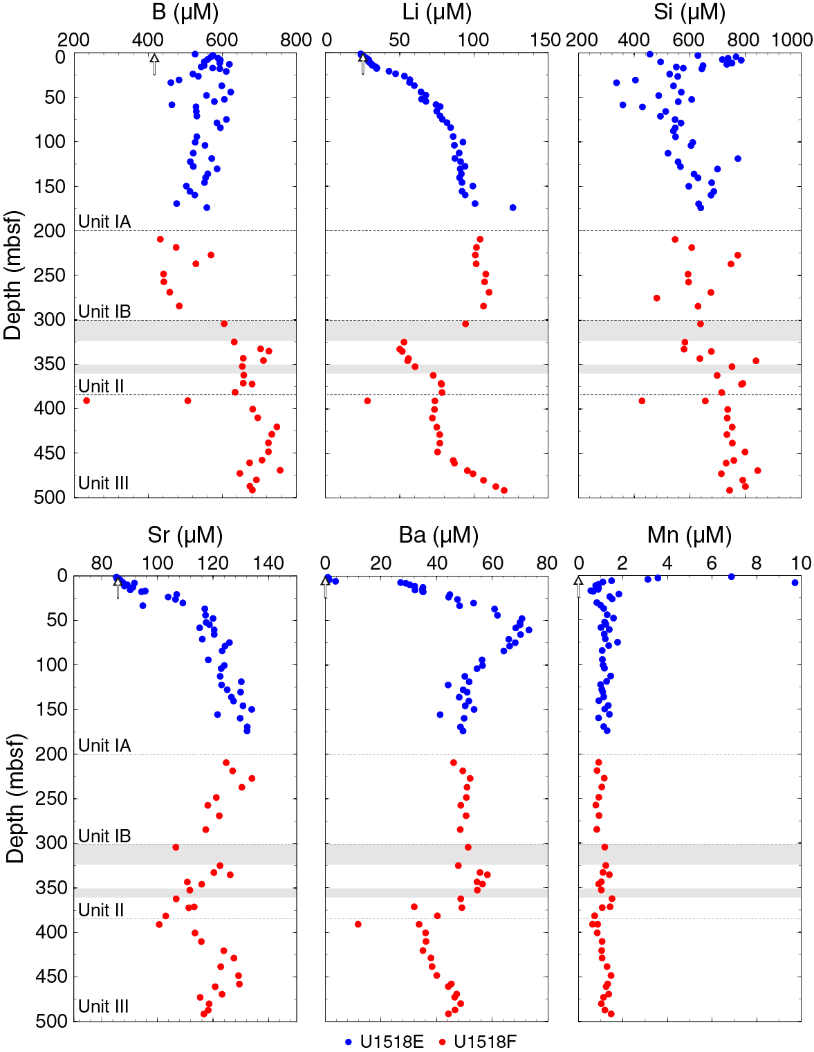
Figure F40. Boron, lithium, silica, strontium, barium, and manganese.
The geochemical profiles at Site U1518 reflect the combined effects of organic matter diagenesis, authigenic carbonate precipitation, volcanic ash alteration, and silicate weathering. The fault zone is clearly manifested by a repetition of the diagenetic sequence in the footwall; however, no geochemical evidence was found for active fluid flow along the fault zone.
Organic matter diagenesis
The pore water profiles of sulfate, alkalinity, ammonium, bromide, and phosphate in Lithostratigraphic Subunits IA and IB (the uppermost ~304 m; hanging wall) reflect typical organic matter degradation in continental margin sediments (Figure F38). Sulfate concentrations decrease almost linearly from 28.1 mM at the seafloor to 0 mM at ~8 mbsf, marking the SMTZ. The SMTZ is relatively shallower compared with nearby Site U1517 (~20 mbsf; see Barnes et al., 2019), which may indicate a higher upward methane flux at this site. Alkalinity increases from seawater value at the seafloor to a maximum value of ~27 mM at the SMTZ and then decreases gradually toward the bottom of Subunit IB to ~19 mM. The alkalinity profile reflects the competition between consumption in authigenic carbonate minerals and alkalinity production from sulfate reduction driven by particulate organic carbon oxidation (POCSR), anaerobic oxidation of methane (AOM), and CO2 buffering through silicate weathering (e.g., Solomon et al., 2014; Wallmann et al., 2008). Ammonium concentrations also increase with depth to a maximum of ~9 mM at 71 mbsf and then decrease toward the bottom of Subunit IB to ~5 mM. The trend of the bromide concentration profile mimics that of ammonium in Subunit IA and also peaks at ~71 mbsf, but Br increases slightly in Subunit IB. Phosphate concentrations also increase from seawater value in the upper sediment section but reach a peak concentration of 198 µM at a shallower depth of 21 mbsf.
A repetition of the diagenetic sequence observed in the hanging wall (Unit I) occurs below the main brittle fault zone in Units II and III (see Lithostratigraphy and Structural geology). Units II and III are characterized by an increase in alkalinity, ammonium, phosphate, and bromide concentrations, reaching a second concentration maxima between ~360 and 425 mbsf, followed by a decrease in concentrations to the base of the hole. The repetition of the early diagenetic sequence in the footwall likely indicates recent underthrusting and thus active displacement along the thrust fault.
Volcanic ash alteration and silicate mineral diagenesis
Lithostratigraphic Subunit IA contains volcanic ash layers and disseminated ash in the upper ~40 m. In general, volcanic ash in deep seafloor sediments undergoes a series of alteration reactions under various thermal regimes, including dissolution and hydration of volcanic ash and formation of smectite and zeolites (Sheppard and Hay, 2001; Kastner et al., 2014). These diagenetic reactions release some elements into the fluid, whereas other elements are consumed by the solids. During dissolution and hydration of volcanic ash, freshwater is also incorporated into the solids, causing an increase in chloride concentrations. At Site U1518, chloride concentrations increase to 584 mM in the upper ~66 m (Figure F39). This increase in chloride concentrations is accompanied by an increase in dissolved potassium and sodium with depth, reaching concentration maxima at 60 mbsf in Subunit IA. The change in Na and K concentrations from near seawater values at 1.5 mbsf to concentration maxima at 60 mbsf is greater than the relative increase in Cl concentrations, reflecting the combined effects of hydration reactions and release of these alkali metals to the pore water. Likewise, lithium and strontium concentrations steadily increase in Subunit IA (Figure F40). Sediments in Subunit IA contain several volcanic ash layers and disseminated ash and exhibit elevated K-feldspar concentrations. The increase in Cl, the alkali metals, and strontium in this unit reflects ongoing alteration of the rhyolitic ash and K-feldspar to authigenic hydrous aluminosilicate minerals. Typically, Li, B, and K are consumed from the pore water during volcanic ash alteration in margin sediments; however, it appears that the felsic composition of the ash at this site drives the net release of these elements into pore water, despite co-occurring consumption in authigenic phases. Similar to the geochemical tracers of organic matter diagenesis noted above, a repetition of the ash/silicate mineral diagenetic sequence occurs below the main brittle fault zone.
The dissolved Ca and Mg profiles are controlled by the combined effects of volcanic ash alteration/silicate weathering and authigenic carbonate precipitation. Ca concentrations decrease rapidly from a seawater value near the seafloor to a minimum of 3.1 mM just below the SMTZ, reflecting consumption in authigenic carbonate minerals driven by the alkalinity produced by POCSR and AOM. Calcium concentrations abruptly increase below the SMTZ to ~5 mM at 50 mbsf, likely due to Ca release during volcanic ash alteration and silicate mineral weathering. Calcium concentrations, however, remain below ~6 mM as a result of in situ sequestration in authigenic carbonates. The Mg concentration profile is similar to that of Ca but reflects net consumption from the pore water by both authigenic carbonate precipitation and the formation of authigenic aluminosilicate minerals (i.e., Solomon et al., 2014). Dissolved Ba concentrations increase abruptly below the SMTZ in response to barite dissolution because of sulfate depletion (i.e., Torres et al., 1996; Dickens, 2001). Ba concentrations continue to increase to 70 µM at ~70 mbsf, indicating a component of volcanic ash alteration in Subunit IA. Deeper than ~70 mbsf, Ba concentrations decrease but remain above 20 µM (~200× seawater concentrations).
Silicate weathering effectively buffers pore water pH by converting the CO2 generated during coupled microbial fermentation and methanogenesis to bicarbonate in anoxic sediments of continental margins (Wallmann et al., 2008; Solomon et al., 2014). A clear repetition of the sequence of release of metabolic products during the early diagenesis of organic matter occurs in the footwall on the main brittle fault zone (Units II and III). Alkalinity is higher than in the hanging wall, suggesting enhanced net microbial methanogenesis in these younger sediments that promotes chemical weathering of reactive silicate phases and drives authigenic carbonate precipitation, manifested by elevated concentrations of dissolved Si, K, B, Li, and Sr in Units II and III and relatively constant concentrations of Ca and Mg.
Methane hydrate occurrence
IR camera scans on the catwalk were used to detect the occurrence of methane hydrate in each core from deeper than 30 mbsf. Cold temperature anomalies were not frequently observed, partially because of poor core recovery from Cores 375-U1518F-2R through 28R. Two methane hydrate–bearing WRs identified by IR scanning were collected to quantify methane hydrate saturations with the aim of verifying the methane hydrate saturation calculations from LWD resistivity data collected during Expedition 372. However, we identified an additional six interstitial water samples that exhibited negative excursions in chloride concentrations at 33.5, 52.3, 54.8, 77.1, 155.7, and 391 mbsf.
Estimates of gas hydrate abundance are commonly based on the magnitude of discrete excursions to anomalously low chloride values, which are related to the amount of freshwater released by gas hydrate dissociation during core retrieval assuming a “closed system” during dissociation (e.g., Paull and Ussler, 2001). We used an empirical approach in which the in situ background chloride concentration is defined using observed concentrations from the sediments above and below the chloride anomalies. These discrete, sulfate-corrected chloride anomalies were used to estimate a gas hydrate saturation (Sh) value:
- Cb = in situ background pore water salinity,
- C = chloride concentration measured in the core sample after gas hydrate dissociation, and
- α = dimensionless constant that quantifies the density change because of gas hydrate dissociation assumed to equal 1.257 (Malinverno et al., 2008).
Malinverno et al. (2008) shows that by propagating the uncertainties associated with each parameter in this equation, the typical uncertainty in estimating Sh from chloride concentration data is ±1.5%. At Site U1518, chloride data suggest the presence of discrete methane hydrate occurrences between ~33 and 390 mbsf with Sh values ranging between 2% and 46% (Table T12). The shallow occurrence of methane hydrate at this site indicates an elevated methane flux that is also suggested by the relatively shallow SMTZ.
Organic geochemistry
Gas analyses
Headspace samples were taken from each sediment core to monitor for the presence and abundance of C1–C3 hydrocarbons as part of the standard safety protocol (Pimmel and Claypool, 2001). Where possible, these samples were taken immediately adjacent to WR samples collected for pore water geochemistry. A total of 77 headspace and 12 void gas samples were analyzed by gas chromatography (see Geochemistry in the Expedition 372B/375 methods chapter [Wallace et al., 2019a]). The results from Site U1518 are listed in Table T13 and shown in Figure F41.
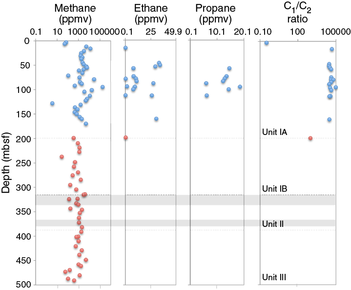
Figure F41. Methane, ethane, and propane.
Between 0 and 6.05 mbsf, methane concentrations are ~60 parts per million by volume (ppmv). Deeper than 6.05 mbsf, concentrations increase rapidly to 12,900 ppmv at 16.34 mbsf, marking the SMTZ and the onset of in situ microbial methanogenesis. Deeper than 70 mbsf, methane concentrations in the headspace samples remain between 100 and 29,000 ppmv with an average of 13,385 ppmv. Methane concentrations in void gas samples were at least an order of magnitude greater than methane concentrations in headspace samples from the same core (Table T13). Methane concentrations measured on void gas samples are not included in Figure F41 because the concentrations in the headspace samples do not reflect in situ concentrations but rather are impacted by gas solubility at the temperature and pressure conditions during core recovery. Conversely, the void gas samples reflect the gas concentrations in excess of solubility. Thus, the gas concentrations are strongly affected by degassing during core recovery, gas expansion, and/or gas hydrate decomposition.
Ethane was detected in some headspace samples shallower than 200 mbsf but was not detected deeper. The methane/ethane (C1/C2) ratios are consistently >20,000, suggesting a microbial source for the methane (Claypool and Kvenvolden 1983).
Bulk sediment analysis
A total of 120 samples were taken at Site U1518 for elemental analysis by coulometric and carbon-hydrogen-nitrogen-sulfur measurements to determine inorganic carbon, calcium carbonate (CaCO3), total carbon (TC), total nitrogen (TN), and total organic carbon (TOC) concentrations (Table T14). CaCO3 in Lithostratigraphic Units I–III exhibits a large degree of scatter (ranging from 2.1 to 23.1 wt%) and mimics the depth profile of TC (ranging from 0.7 to 2.8 wt%), with similar trends in all units. At 340 mbsf in Lithostratigraphic Unit II, values increase slightly with peaks in CaCO3 similar to TC (Figure F42).
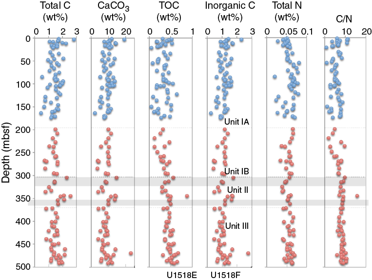
Figure F42. TC, CaCO3, TOC, inorganic carbon, TN, and C/N.
Organic carbon values, calculated as the difference between TC and carbonate carbon content (see Geochemistry in the Expedition 372B/375 methods chapter [Wallace et al., 2019a]), are low and variable in Lithostratigraphic Subunit IA (ranging from 0.05 to 0.64 wt%; average = 0.32 wt%) and increase slightly with depth in Units I–III, ranging from 0.12 wt% at 218.46 mbsf to 0.65 wt% at 488.16 mbsf. A few peak values as high as 0.88 wt% are observed in Unit II (344 mbsf) (Figure F42).
Inorganic C and TN concentrations are relatively constant in all lithostratigraphic units and range from 0.26 to 2.31 wt% (average = 1.12 wt%) and from 0.02 to 0.08 wt% (average = 0.05 wt%), respectively. The ratio of TOC to TN (C/N) can give information on organic material provenance: terrestrial organic matter typically has a C/N ratio of ~20, whereas marine organic matter, which is more proteinaceous, is characterized by a C/N ratio of ~5–8 (Pimmel and Claypool, 2001). At Site U1518, C/N ratios range from 0.85 to 15.80 (average = 6.84).
Physical properties
Physical properties were characterized through a set of measurements on whole cores, split cores, and discrete samples (see Physical properties in the Expedition 372B/375 methods chapter [Wallace et al., 2019a]). Physical properties reflect compositional, textural, and lithologic variations; diagenetic processes; natural deformation; and core disturbance.
At Site U1518, physical properties exhibit systematic changes between 0 and 50 mbsf (Figures F43, F44). Deeper than 50 mbsf, physical properties generally vary little with depth with a few specific exceptions. Bulk density, porosity, P-wave velocity, and natural gamma radiation (NGR) measured on core samples show broadly similar trends to those observed in LWD bulk density, porosity (neutron and NMR), P-wave velocity, and gamma ray measurements (Figure F45) (see also Logging while drilling and Core-log-seismic integration).

Figure F43. Core sample physical properties.
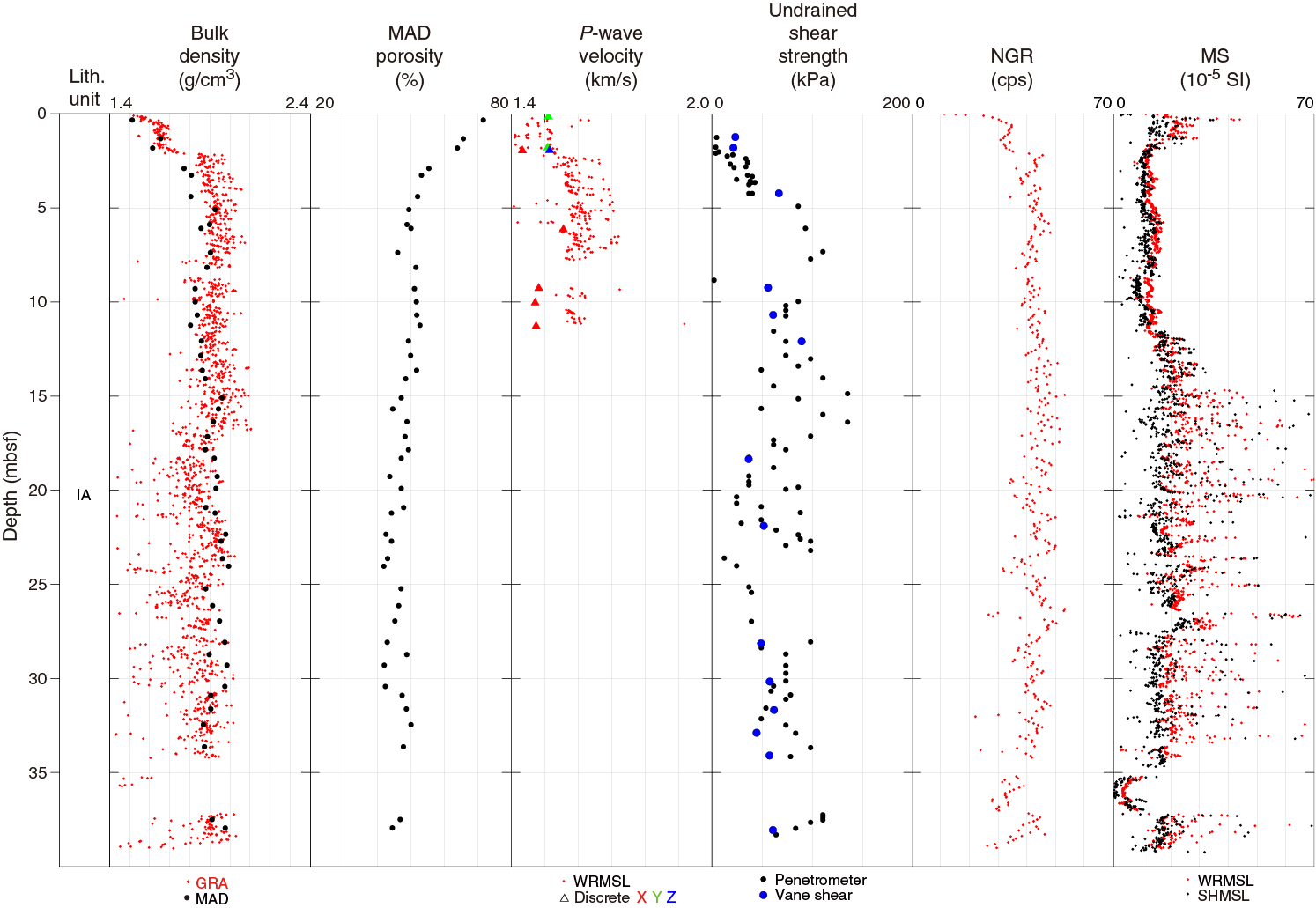
Figure F44. Core sample physical properties, 0–40 mbsf.
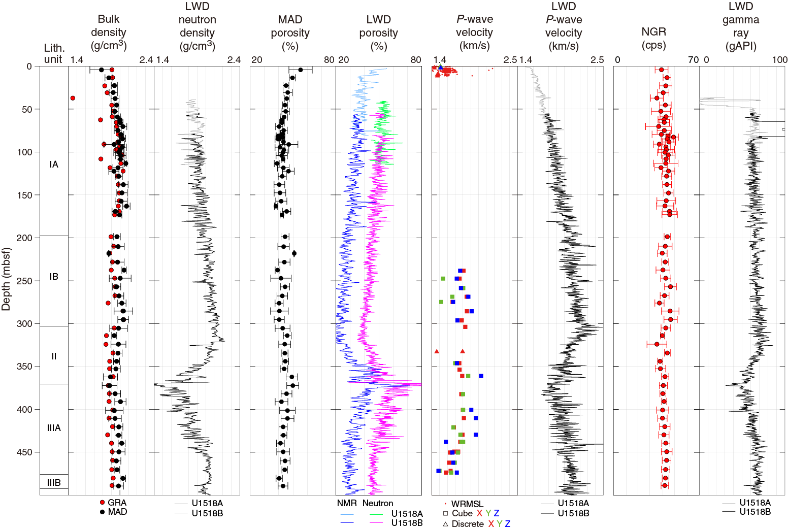
Figure F45. Comparison of core and LWD physical properties.
Some physical properties were measured on Cores 375-U1518C-1H and 375-U1518D-1H, but they are not described because of the unknown seafloor depth for Holes U1518C and U1518D. Gamma ray attenuation (GRA) bulk density and magnetic susceptibility were obtained on Core 375-U1518F-15R using the Whole-Round Multisensor Logger (WRMSL) immediately after sectioning on the catwalk without waiting for temperature equilibration because this particular core was preserved in the refrigerator for later geochemical sampling. NGR was measured on Core 375-U1518F-15R with the Natural Gamma Radiation Logger just before splitting.
Density and porosity
GRA bulk density was determined on WR cores, and moisture and density (MAD) bulk density, grain density, and porosity were determined on discrete samples from Hole U1518E and U1518F working halves (see Physical properties in the Expedition 372B/375 methods chapter [Wallace et al., 2019a]). GRA bulk density measured with the WRMSL is <1.7 g/cm3 near the seafloor and increases sharply to 1.9 g/cm3 at 2 mbsf, followed by a gradual increase to ~2.0 g/cm3 from 80 to 300 mbsf (Figures F43, F44). Between 300 and 320 mbsf, GRA bulk density decreases markedly from 2.1 to 1.8 g/cm3 (Figure F45).
MAD bulk density increases markedly from 1.50 g/cm3 at 0.3 mbsf to 1.9 g/cm3 at 5 mbsf, increases gradually with depth to ~2.0 g/cm3 at 100 mbsf, and then remains nearly constant with an average value of 1.99 g/cm3 (Figures F43, F44). Grain density is nearly constant, ranging 2.64–2.86 g/cm3 with an average value of 2.72 g/cm3. Some anomalous grain density values were measured in samples from Holes U1518E and U1518F. Subsequent investigation revealed that these anomalous values are associated with dry volume measurements made in specific chambers (Cells 1 and 2) of the helium pycnometer. These values have been corrected based on postmeasurement recalibration using standard spheres. The corrected values are reported here (Table T15), and the uncorrected values are available in the Laboratory Information Management System (LIMS) database.
From 0.3 to 100 mbsf, porosity decreases from 72% to ~35%–45%. Between 100 and 150 mbsf, maximum porosity values are ~50%, but values as low as 33% are observed near 150 mbsf. A slight shift to higher porosity occurs between 150 and 200 mbsf, although no MAD measurements were made between 174 and 198 mbsf because of a coring gap. From 300 to 370 mbsf, an interval approximately coincident with Structural Domains 2–3 defining the Pāpaku fault zone (see Structural geology), there is a reversal in trend to a depth-dependent increase in porosity. Average MAD porosity increases from ~40% to ~50% over this interval. Deeper than 370 mbsf, at the approximate depth where the base of a subsidiary fault was interpreted (see Structural geology), porosity returns to a general trend of gradual decrease with depth. The average porosity is 44% from 100 to 492 mbsf.
Both GRA and MAD bulk density values are consistent with LWD neutron bulk density data shallower than ~300 mbsf and deeper than ~430 mbsf (Figure F45), although some uncertainty in correlating depths occurs between the holes (see Operations and Core-log-seismic integration). Both GRA and MAD bulk density decrease slightly with depth from 300 to 400 mbsf, followed by a slight increase from 400 to 430 mbsf, whereas LWD bulk density increases slightly with depth from 300 to 320 mbsf, followed by a substantial decrease to ~1.4 g/cm3 at ~370 mbsf and an increase to 1.9 g/cm3 at 430 mbsf. These differences between GRA/MAD and LWD data are likely related to (1) a depth offset of the fault and damage zones between LWD Holes U1518A and U1518B and coring Holes U1518E and U1518F and (2) overestimates of LWD porosity caused by the enlarged borehole diameter (possibly related to washout in sandier zones) in this depth interval (see Operations, Logging while drilling, and Core-log-seismic integration).
MAD porosity is generally similar to LWD neutron porosity, with exceptions that follow those in bulk density described above, and is higher than LWD NMR porosity (Figure F45). The general depth-dependent trends are similar; however, the trend in MAD porosity is less pronounced than that in LWD neutron and NMR porosity.
P-wave velocity
WRMSL P-wave velocity measurements were made from the seafloor to 12 mbsf, and a deeper reliable signal was not obtained, likely due to poor contact between the core liner and core material. We attempted to measure P-wave velocity on working halves and discrete samples with the P-wave velocity gantry system; however, the measurements on working halves were unsuccessful in many cases (11–238 mbsf) because of existing cracks and new cracks created by inserting the bayonet blades into the cores. Thus, we largely relied on discrete samples and manually picked the P-wave arrival time from the waveform data to obtain P-wave velocity data (Table T16).
P-wave velocity measured with the WRMSL ranges from 1450 to 1600 m/s between the seafloor and 12 mbsf (Figures F43, F44; Table T16). P-wave velocity values measured on discrete samples deeper than 238 mbsf are scattered and vary between ~1500 and ~2000 m/s without showing distinct velocity anisotropy.
P-wave velocity values obtained from measurements on cores are consistent with LWD P-wave velocity values at depths shallower than ~15 mbsf (Figure F45). Deeper than 230 mbsf, P-wave velocity measured on discrete samples from the cores is generally lower than LWD P-wave velocity.
Shear strength
Undrained shear strength was determined on working halves using both the automated vane shear (AVS) instrument and a pocket penetrometer (see Physical properties in the Expedition 372B/375 methods chapter [Wallace et al., 2019a]). The penetrometer measurements on Cores 375-U1518F-2R through 6R were conducted 7 days after core splitting. The quality of these measurements was validated by comparison with measurements made on Core 7R immediately after core splitting. These values show no significant difference, indicating that possible desiccation did not affect the strength measurements. We note that during this time period, the cores were wrapped in plastic wrap and stored in D-tubes.
Undrained shear strength determined using the AVS shows a rapid increase from ~20 kPa at 1 mbsf to ~90 kPa at 12 mbsf followed by values with little variation around ~55 kPa to 50 mbsf (Figures F43, F44). Deeper than 150 mbsf, sediment strength was higher than the maximum capacity of the AVS (150 kPa), and consequently only the penetrometer was used.
Undrained shear strength determined using the penetrometer is consistent with that measured with the AVS (Figures F43, F44). Undrained shear strength increases rapidly with depth from 0 to 10 mbsf. Deeper than 10 mbsf, strength does not vary much, with values averaging ~79 kPa to 80 mbsf. Between 80 and 170 mbsf, shear strength values show significant scatter ranging from a low value of 25 kPa to a high value of 980 kPa. The scatter is mainly driven by high strength values, which could indicate highly resistant and variable formation properties but may also reflect overconsolidation induced by coring operations. In these intervals, severe disturbance associated with APC and XCB coring are observed (see Structural geology). Deeper than 200 mbsf, where RCB coring was conducted, the data are less scattered and average strength values gradually increase with depth from 120 kPa at 200 mbsf to 200 kPa at 280 mbsf and then decrease to 60 kPa at 300 mbsf. Shear strength is approximately constant between 300 and 450 mbsf. Deeper than 450 mbsf, strength values are scattered but gradually increase with depth, reaching maximum values of ~430 kPa.
Thermal conductivity
Thermal conductivity measurements were conducted on sediment WR cores using the needle probe method (see Physical properties in the Expedition 372B/375 methods chapter [Wallace et al., 2019a]). The TeKa probe was used on all cores from Holes U1518E and U1518F. The Huskeflux probe (Oregon State University, USA) was only used on cores from Hole U1518E (Table T17). Sediments from Hole U1518F were deemed too lithified for the Huskeflux probe to be safely inserted. In most cases, three measurements were made with each probe at each measurement position. A comparison of the two sets of measurements from Hole U1518E shows an apparent offset between the probes (Figure F43). The plotted value represents the mean of the three measurements, and the horizontal bar shows the standard deviation of the three measurements. In general, the scatter in the measurements appears less for the TeKa values relative to Huskeflux values. Throughout Hole U1518E, the TeKa thermal conductivity values have a mean and standard deviation of 1.38 and 0.11 W/(m·K), respectively. Over this same interval, the Huskeflux values have a mean and standard deviation of 1.53 and 0.13 W/(m·K), respectively. This difference is about 10% and is larger than can be accounted for by differences relative to the Macor calibration standard measurements. The TeKa measurements show that throughout Holes U1518E and U1518F thermal conductivity is relatively constant with depth and has a mean and standard deviation of 1.38 and 0.10 W/(m·K), respectively. These values are used to compute the heat flow (see Downhole measurements).
Natural gamma radiation
NGR values range from 6 to 63 counts/s with an average of 42 counts/s (Figures F43, F44, F45). NGR increases sharply from <25 counts/s at the seafloor to 40 counts/s at 2 mbsf. Deeper than 2 mbsf, average NGR gradually increases with depth, except for a shift to lower values at ~300 mbsf. The NGR spectra were used to estimate 40K, 232Th, and 238U concentrations using the algorithm presented by De Vleeschouwer et al. (2017) (Figure F46). The mean concentrations of K, Th, and U are 2.1 wt%, 5.5 ppm, and 1.4 ppm, respectively. Both K and Th show a depth-increasing trend over the first 20 mbsf, whereas U shows a depth-decreasing trend over this interval. In general, Th should show a negative trend with depth near the seafloor because Th is scavenged from the water column; the increasing trend may reflect an erosional event (see Biostratigraphy and Lithostratigraphy).
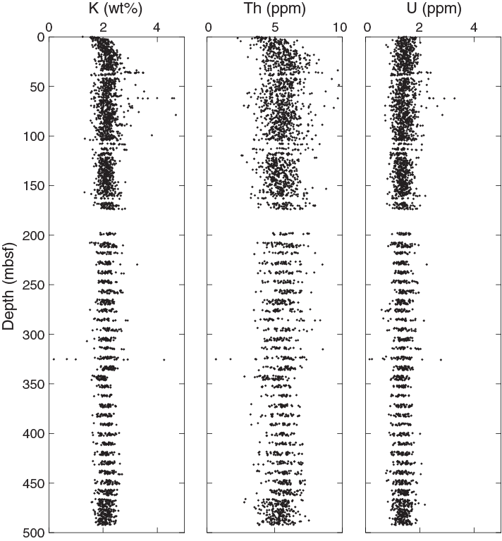
Figure F46. K, Th, and U.
The trend of gradually increasing NGR with depth and a shift to lower values at ~300 mbsf is similar to but less pronounced than that seen in the LWD gamma ray data (Figure F45) (see Logging while drilling and Core-log-seismic integration).
Magnetic susceptibility
Magnetic susceptibility is >20 × 10−5 SI near the seafloor and decreases markedly to 10 × 10−5 to 15 × 10−5 SI at 2 mbsf. Between 2 and 176 mbsf, three zones of lower magnetic susceptibility with less scatter and three zones of higher magnetic susceptibility with more scatter are observed. These changes in magnetic susceptibility generally correspond to sand/silt and ash in Lithostratigraphic Subunit IA (see Lithostratigraphy). The depth intervals at 2–12, 40–60, and 75–109 mbsf show lower magnetic susceptibility with average values of 11 × 10−5, 13 × 10−5, and 14 × 10−5 SI, respectively. The depth intervals at 13–40, 60–75, and 109–200 mbsf show higher magnetic susceptibility with average values of 22 × 10−5, 21 × 10−5, and 25 × 10−5 SI, respectively. A lower average value of 5 × 10⁻⁵ SI is observed between 35 and 37 mbsf where a ~1.8 m thick ash layer is observed. Between 200 and 462 mbsf, magnetic susceptibility shows less scatter than Subunit IA with values ranging from 10 × 10−5 to 30 × 10−5 SI. Values shift to a lower average value of 13 × 10−5 SI at 466 mbsf and then remain relatively constant with depth to 490 mbsf.
Reflectance spectroscopy and colorimetry
Color reflectance data collected from the archive halves are presented in the L*a*b* color space (Figure F43). Lithostratigraphic Subunit IA shows more data scatter (higher L*, higher a*, and lower b*) compared with other lithostratigraphic units, likely due to the presence of ash and silt (see Lithostratigraphy). From 0 to 30 mbsf, a decrease in L* from 45 to 40, a slight increase in a* from 0 to 2, and a slight decrease in b* from 0 to −2 are observed. Deeper than 30 mbsf, all parameters stay nearly constant; L* ranges between 35 and 45, a* ranges between 0 and 2, and b* ranges between −5 and 2.
Downhole measurements
Formation temperature and heat flow
The APCT-3 was deployed five times in Hole U1518E (Table T18). All temperature measurements show a clear frictional heating spike upon insertion, showing that the tool penetrated the sediment ahead of the drill bit (Figure F47). Measurement 1 at 35.2 mbsf (Core 375-U1518E-4H) and Measurement 3 at 56.4 mbsf (Core 8H) show smooth temperature decays following insertion. These measurements are of very high quality. In contrast, Measurement 2 at 49.6 mbsf (Core 6H) and Measurement 5 at 82.0 mbsf (Core 14F) show that the tool moved slightly after initial penetration, disturbing the temperature decay. For these measurements, the insertion time used for the analysis of the temperature-time series was reset to the time just following these disturbances. During Measurement 4 at 63.3 mbsf (Core 10H), the APCT-3 was disturbed before the normal 10 min of temperature decay ended, and the equilibrium temperature is computed from a relatively short temperature decay.
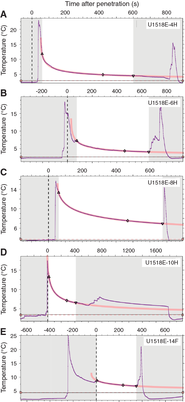
Figure F47. APCT-3 temperature-time series.
Estimated equilibrium temperatures are plotted as a function of measurement depth (Figure F48). Because thermal conductivity is relatively constant with depth, we expect a constant thermal gradient and compute the vertical conductive heat flow (q) using Fourier’s law:
where k is the thermal conductivity and Γ is the thermal gradient. Measurements 1, 3, and 5 at 35.2, 56.4, and 82.0 mbsf, respectively, yield a thermal gradient of 0.035°C/m, whereas Measurements 2, 4, and 5 at 49.6, 63.3, and 82.0 mbsf, respectively, yield a higher thermal gradient of 0.053°C/m. The average thermal conductivity of the shallow sedimentary section is 1.38 W/(m·K) (see Physical properties), yielding heat flow values of 48 and 75 mW/m2 that correspond to the low and high thermal gradients, respectively. We believe the low heat flow value is more reliable for at least three reasons: (1) estimated equilibrium temperatures based on Measurements 1 and 3 are deemed the most robust because of the smooth decay of the frictional penetration signal; (2) estimated equilibrium temperatures based on Measurements 1, 3, and 5 are all made with the same temperature tool (APCT-3 1858005C), so potential intertool calibrations are not an issue; and (3) the thermal gradient fit to Measurements 2, 4, and 5 yields a negative bottom water temperature, whereas the gradient fit to Measurements 1, 3, and 5 predicts a more reasonable bottom water temperature of 1.64°C.
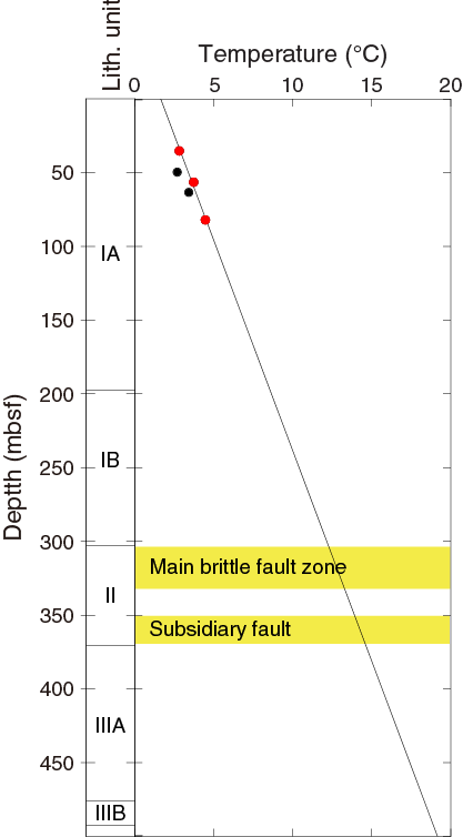
Figure F48. Estimated equilibrium temperatures.
The frontal thrust spans from 304 to 324 mbsf, and a subsidiary fault spans from 351 to 361 mbsf (see Structural geology). Using the preferred thermal gradient of 0.035°C/m yields predicted temperatures of 12°–13°C and 14°C for the thrust fault and subsidiary fault, respectively (Figure F48).
Logging while drilling
The LWD data for Site U1518 were acquired in two holes (U1518A and U1518B). Hole U1518A penetrated the seafloor at 2636.4 mbsl. For Hole U1518B, the seafloor depth is ambiguous because the tools were not activated and depth was not correctly tracked from spud-in to ~55 mbsf because of miscommunication between the drill floor and LWD Schlumberger engineers. Because the seafloor was not recorded during Hole U1518B LWD and no clear tie was found in the logging data between Holes U1518A and U1518B, we chose to identify the seafloor from 30 kHz 25 m grid multibeam bathymetry data and defined the seafloor at 2634.6 mbsl for Hole U1518B. Hole U1518A acquired LWD data from the seafloor to 122 mbsf, and Hole U1518B acquired LWD data from ~55 to 600.0 mbsf.
The LWD BHA for this site is composed of six LWD tools attached behind a 8½ inch drill bit (from bottom to top): geoVISION, NeoScope, StethoScope, TeleScope, SonicScope, and proVISION. These tools provide a wide array of measurements including gamma ray (geoVISION and NeoScope), resistivity (geoVISION and NeoScope), porosity (NeoScope and proVISION), and compressional (P-wave) and shear (S-wave) wave velocity (SonicScope) as described in Logging while drilling in the Expedition 372B/375 methods chapter (Wallace et al., 2019a).
Drilling parameters
A composite plot of drilling parameters is shown in Figure F49 for Hole U1518A and Figure F50 for Hole U1518B.

Figure F49. Drilling parameters, Hole U1518A.

Figure F50. Drilling parameters, Hole U1518B.
Hole U1518A was drilled to 122 mbsf. The data are displayed according to the drilling operations period starting on 19 December 2017 at 1754 h (UTC + 13 h) and terminating on 20 December at 0205 h. The rate of penetration (ROP) was 20–50 m/h. The drilling pipe rotation rate was around 20 rpm during initial spud-in and then increased to 50 rpm by total depth. Weight on bit (WOB) values ranged between −10 and 14 klb. Annular pressure increased progressively with depth. During drilling, the measured annular temperature was ~2°C; no value was recorded at the seafloor. The heave variation progressively increased while drilling. Drilling was stopped at 122 mbsf because of significant heave and poor weather conditions.
Hole U1518B data are displayed according to the drilling operations period starting on 21 December at 0015 h and terminating on 23 December at 0226 h. The target ROP was 20–30 m/h to acquire high-quality LWD data, and the ROP remained near this target during drilling. The spikes to high ROP >50 m/h are probably due to rapid initial reentry after making drill pipe connections. The drilling pipe rotation rate began at around 20 rpm and then was increased at 50 mbsf and maintained close to 50 rpm to total depth. WOB values ranged between −10 and 35 klb. For large intervals of the borehole, WOB was at negative or near zero values because almost no weight was on the bit. Annular pressure increased progressively with depth. The equivalent circulating density was 2.4 g/cm3 at the top of the borehole and decreased to 1.2 g/cm3 by the bottom of the hole. During drilling, the measured annular temperature slowly increased from ~2°C near the top of the borehole to ~5°C at total depth.
Data quality
Borehole conditions were assessed by the ultrasonic caliper measurement of the borehole diameter (Figures F51, F52). The ultrasonic caliper, however, can incorrectly identify intervals with extreme borehole enlargement (>5 cm) and instead report values near bit size; therefore, porosity and resistivity measurements were also used to identify enlarged or washout intervals. Enlarged boreholes, or washouts, are characterized by anomalously low resistivity readings (~0.3–0.9 Ωm) and unrealistically high porosity values (~0.7–1.0), both of which indicate the measurements are detecting more seawater than formation.
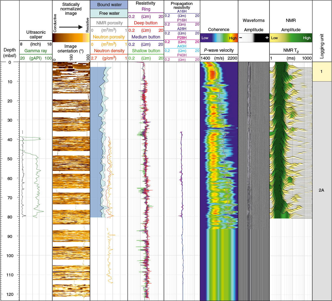
Figure F51. LWD measurements, Hole U1518A.
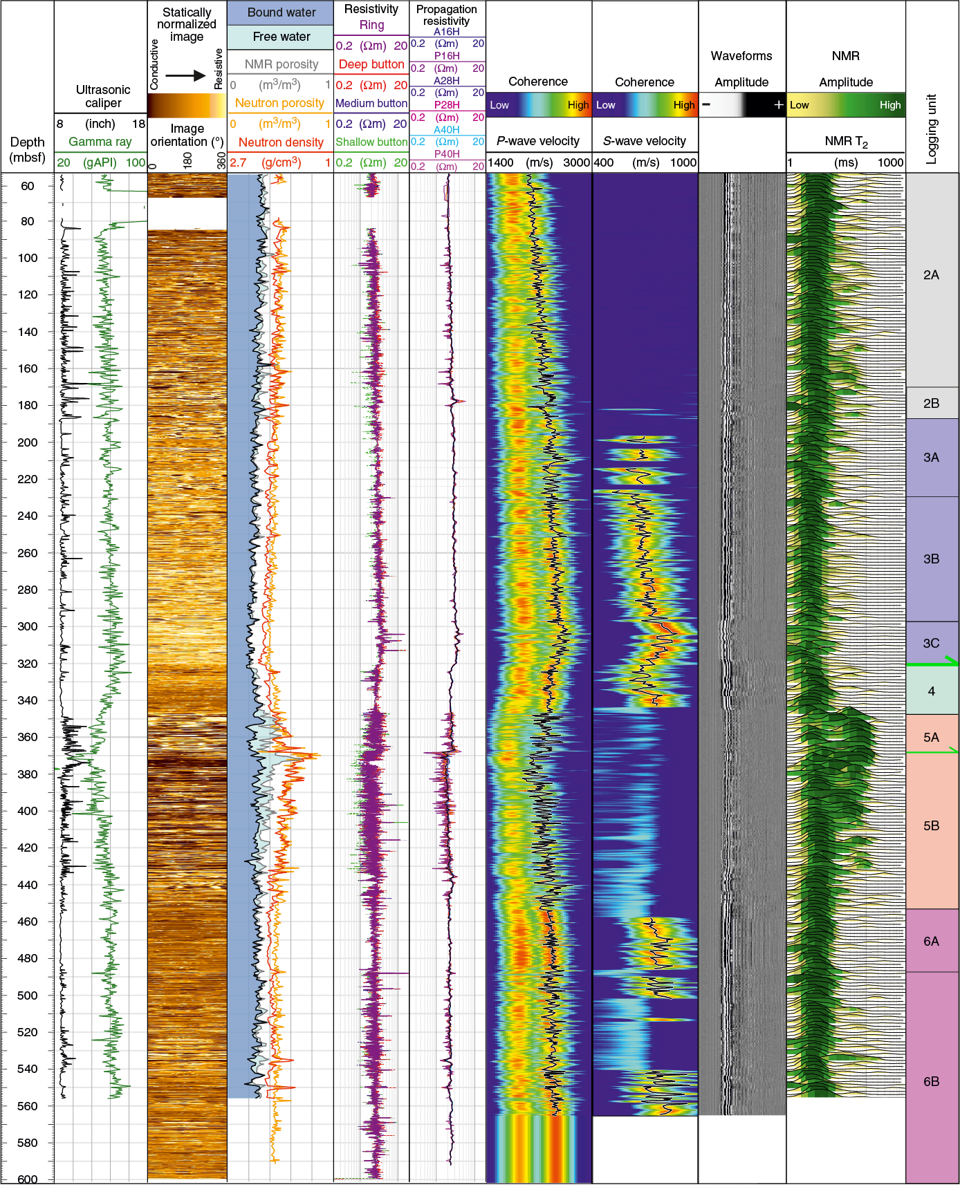
Figure F52. LWD measurements, Hole U1518B.
The LWD data are generally of good quality but are degraded in several intervals because of borehole washouts. Throughout Hole U1518A and near the top of Hole U1518B, some depth intervals are missing data as a result of the tools not being activated or because of low drilling pipe rotation rates or high ROP. The petrophysical interpretation is complicated by steeply dipping geological features intersecting the boreholes (Figures F53, F54). Geological features intersecting the boreholes at a high angle cause the NMR tool to sample a number of layers rather a single layer. The resistivity curves also show some small separation because of the electrical anisotropy caused by dipping layers; phase resistivity is more sensitive to high-angle dips compared with attenuation resistivity.
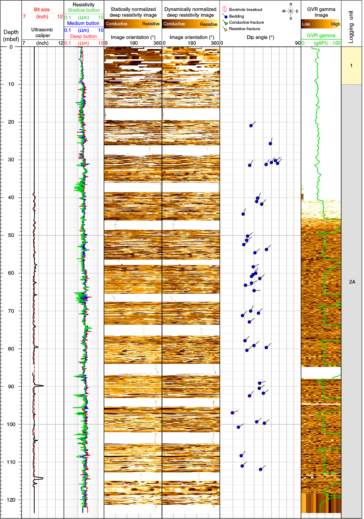
Figure F53. Resistivity image log data, Hole U1518A.
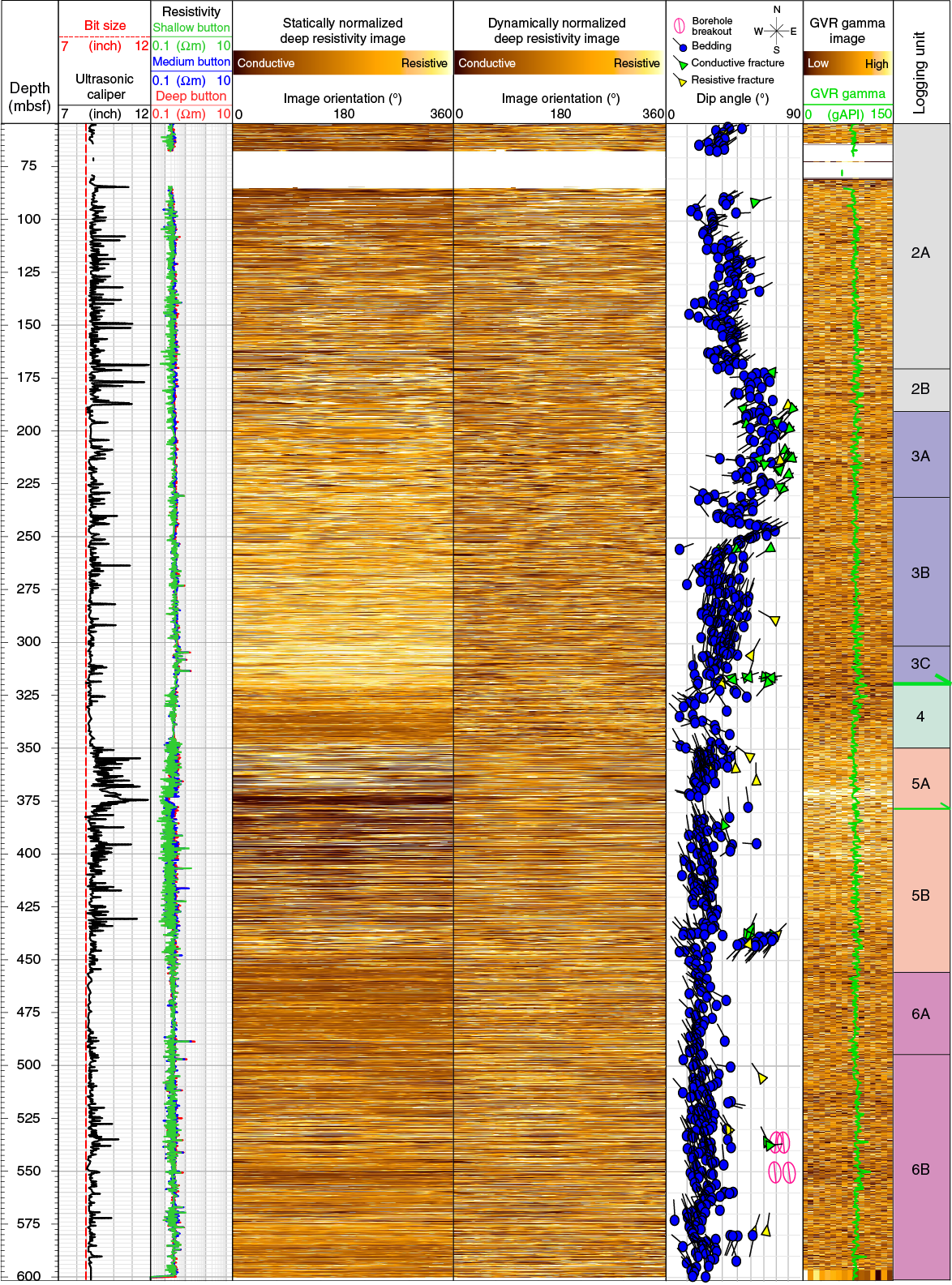
Figure F54. Resistivity image log data, Hole U1518B.
In Hole U1518A, twelve ~6–16 m long depth intervals are imaged by the GVR resistivity imaging tool and are separated by ~2–7 m intervals without image log data. Each of the imaged intervals contains variable degrees of data loss, yet some geological features can still be identified. Some stretching image log artifacts (e.g., 117 mbsf) are similar to stick and pull wireline image log artifacts and may be related to ship heave or roll during image acquisition. Horizontal imaging artifacts are common throughout the imaged interval and are probably related to stick and slide as the resistivity buttons rotate around the borehole.
No logging data were collected above 55 mbsf in Hole U1518B because drilling was started without communicating with the Schlumberger engineers to activate the LWD tools, which also means that the seafloor cannot be correctly identified from the logs. A gap in the resistivity image log and resistivity data occurs at 68–85 mbsf.
Overall, both the well log data and image log quality are good for Hole U1518B. Some small intervals of image log stretch artifacts similar to stick and pull wireline image log artifacts (e.g., 167, 328, 364, and 374 mbsf) locally reduce image log quality in depth intervals as long as 1 m. Between 357 and 383 mbsf, image stretch and horizontal image log artifacts are common and reduce image log quality. Despite these minor image log quality issues, geological features can be identified and characterized.
Logging units
The combination of different LWD measurements allowed us to define six logging units that correspond approximately to the seismic units defined at Site U1518 (see Core-log-seismic integration). Because Holes U1518A and U1518B were drilled in close proximity to each other (~20 m) and for the most part logged different parts of the upper stratigraphic section, logging units for those holes are combined.
Logging Unit 1 (0–10.0 mbsf)
The top of the stratigraphic sequence is defined by a marked increase in P-wave velocity and resistivity. Logging Unit 1 is therefore likely sediment drape, although it has few reliable log measurements in Hole U1518A (and no measurements in Hole U1518B). The button resistivity measurements show a higher resistivity than the expected 1 Ωm or less that is typical of near-seafloor sediment drape, implying that this sediment is more compacted than is normal for seafloor sediments. No geological features are observed from resistivity image logs in this logging unit.
Logging Unit 2 (10–188.0 mbsf)
Resistivity increases with depth from ~1.6 Ωm near the top of Hole U1518A to 2.7 Ωm at the base of Logging Unit 2 in Hole U1518B. Button resistivity, porosity, neutron density, and gamma ray curves oscillate because of variation between the coarser and finer sediments in this unit and may also be influenced by the high heave during drilling and data collection in Unit 2 (Figures F49, F50). Average neutron porosity decreases from 0.55 to 0.5 over this unit, and NMR porosity decreases from 0.4 to 0.35. Neutron porosity data are consistent with core porosity measurements at Site U1518 (see Physical properties). The NMR T2 distribution pattern in Unit 2 is complex, which we also attribute to alternating finer and coarser sediment layers. The resistivity image logs record alternating, thin (centimeters to decimeters) conductive and resistive beds. Bedding in this unit generally dips between ~20° and 70° dominantly to the northeast in Subunit 2A and to the southwest in Subunit 2B. Resistive mottling is observed at 10–31 and 59–62 mbsf on the image logs.
Two subunits are defined in Logging Unit 2 based on notable changes in bedding orientation and fracturing with depth. The boundary between Subunits 2A (83–170.4 mbsf) and 2B (170.4–188 mbsf) is marked by a change in bedding dip direction from northeast to southwest, an increase in bedding dip angle from 20°–40° to 45°–70°, and an increase in fracture intensity in Subunit 2B. Other geophysical log signatures do not show any variation across this boundary.
Logging Unit 3 (188.0–320.7 mbsf)
Logging Unit 3 comprises the lower hanging wall sequence of the Pāpaku fault as interpreted in the LWD data (see Background and objectives and Structural geology). The NMR T2 distribution is mostly unimodal with short peaks and a few intervals of alternating short to medium peaks. Resistivity oscillations are notably smaller in Unit 3 than in Unit 2, although the trend of increasing resistivity with depth continues. Neutron and NMR porosity vary less in Unit 3 than in Unit 2; neutron porosity measurements are closer to the MAD porosity values measured on core samples (Physical properties). P-wave velocity increases steadily from 2200 to 2600 m/s with depth in this unit.
Three subunits are identified in Logging Unit 3 based on variations in bedding orientation, fracture intensity, and P-wave and S-wave velocity. Subunit 3A (188–229.5 mbsf) is characterized by uniformly fine grained thin beds with steep dips (40°–70°) to the southwest, similar to bedding attitudes in Subunit 2B. Fracture intensity is high, comprising both conductive and resistive fractures (Figure F54). Bedding in Subunit 3B (229.5–299 mbsf) dips 15°–50° north-northeast. Bedding dips in this subunit (centered on ~245 mbsf) are consistent with folding associated with the Pāpaku fault, which is also suggested by observations on cores sampled from Hole U1518F (see Structural geology). Subunit 3C (299–320.7 mbsf) is identified on the basis of changes in the sediment physical properties, most notably increases in P-wave and S-wave velocity (both exhibit an initial increase followed by a decrease in both), and an increase in resistivity with depth (Figure F52).
Bedding in Logging Subunit 3C consistently dips 20°–40° to the north-northeast. A number of high-resistivity spikes near the base of this subunit at 304.7, 308.1, and 313.4 mbsf are likely caused by the presence of gas hydrate in sediment layers. Bedding above 314 mbsf displays a number of thin (10–20 cm thick), highly resistive layers that also likely contain gas hydrate. From 315 to 320 mbsf, deformation as documented by fractures in LWD image logs is more intense (Figure F54). We interpret the base of Subunit 3C to coincide with the top of the Pāpaku fault.
Logging Unit 4 (320.7–346.0 mbsf)
In Logging Unit 4, trends in physical properties logs show a reversal: resistivity, velocity, and density all decrease in a series of steps and then remain approximately constant with depth. Most of the physical properties reversals take place from 320.7 to 324.5 mbsf, with resistivity decreasing from 3.4 to 2.4 Ωm and neutron porosity increasing from ~0.4 to ~0.5. S-wave velocity reaches a local minimum at 330–335 mbsf. From the short NMR T2 peak, Unit 4 is inferred to be composed of relatively fine grained sediments, and the borehole is in gauge. No shear wave is recorded below 342 mbsf, suggesting that sediments in this part of the footwall have low rigidity.
Logging Unit 4 is interpreted to be the uppermost footwall of the main strand of the Pāpaku fault. At the top of this unit (top of the footwall), a cluster of north–south striking, conductive fractures, dipping both west and east, and perturbed bedding orientations are observed in the resistivity image log. This deformation is consistent with that observed in core obtained from Site U1518 (see Structural geology). Bedding is difficult to identify from the image log between 320.7 and ~333 mbsf, where conductivity increases overall (333–346 mbsf). Observed bedding dips are gentle to moderate toward the northwest.
Logging Unit 5 (346.0–452 mbsf)
The borehole in Logging Unit 5 is mostly enlarged or washed out, so the marked increases in porosity and decreases in gamma ray and resistivity recorded by the logs are likely exaggerated. Likewise, the low P-wave velocity is likely the result of borehole rugosity.
Logging Unit 5 is divided into two subunits. In Subunit 5A (346.0–368.5 mbsf), bed thickness increases and the GVR resistivity image logs shows a marked change to alternating bands of more conductive and resistive layers (striped appearance) relative to overlying Unit 4. The NMR T2 signal changes abruptly from a unimodal pattern in Unit 4 to a bimodal pattern in Subunit 5A with roughly equal long and short time peaks. In Subunit 5B (368.5–452.0 mbsf), the borehole remains enlarged but resistivity decreases (2.1 Ωm compared with 3.1 Ωm) and porosity increases (as high as around 0.61 for neutron porosity from approximately 0.51) relative to Subunit 5A. Core measurements of porosity agree more closely with neutron porosity measurements than NMR measurements (see Physical properties). P-wave velocity increases with depth in Subunit 5B. We interpret Unit 5 to be a thick, coarse-grained unit interbedded with finer grained beds throughout.
We interpret the Logging Subunit 5A/5B boundary (368.5 mbsf) to be a subsidiary fault. Structural observations from Hole U1518F cores identified a subsidiary fault at ~351–361 mbsf (see Structural geology). Bedding orientations identified from resistivity images consistently dip 10°–30° to the northeast across both logging subunits. Conductive and resistive fractures are observed throughout the unit but are less common than in overlying Unit 4.
Logging Unit 6 (452.0–600 mbsf)
The NMR signature of Logging Unit 6 has a single short T2 peak, and gamma ray is consistently between 60 and 75 gAPI. Resistivity images show sediments are thinly bedded (10–20 cm thick), alternating conductive and resistive layers. Highly resistive bedding layers are observed to 587 mbsf. The unit is interpreted to be relatively fine grained with thin, interbedded, centimeter-scale sand or silt layers that are most likely turbidite sequences. In Unit 6, bedding dips dominantly 10°–30° to the northwest. In a few short (3–5 m) intervals, beds dip to the southwest (e.g., 435–444 mbsf). These switches in bedding dip direction and the observation of bedding truncations in these intervals are likely related to the contorted domains as observed in cores (Figure F4) and are inferred to be MTDs.
We separate Logging Unit 6 into two subunits. In Subunit 6A (452–487 mbsf), resistivity is homogeneous at about ~2 Ωm, although on the finest scale, button resistivity ranges from ~1 to 3 Ωm, probably caused by thin, centimeter-scale, coarse-grained beds. P-wave velocity varies between ~1900 and 2120 m/s in this subunit.
Logging Subunit 6B (487–600 mbsf) marks an inferred change to somewhat thicker bedding of the same general lithology as Subunit 6A. NMR in this subunit is mostly unimodal with a short T2 peak, except for an interval between 534 and 536 mbsf that has a longer peak associated with decreased resistivity, high neutron porosity, and low neutron density, likely indicating a washout and larger pores/coarser sediment. Borehole conditions were variable in this subunit, with some partly washed out intervals toward the base. Subunit 6B was not fully measured by the tools highest in the LWD BHA, so useful NMR data are limited to the uppermost part.
Borehole breakouts are observed in resistivity images within Logging Subunit 6B at ~536 and ~550 mbsf. Borehole breakouts have an average azimuth of 173°/353° from which we estimate a minimum horizontal stress (Shmin) orientation of approximately north–south and consequently a maximum horizontal stress (SHmax) orientation of east–west. Borehole breakout widths range from 37.9° to 78.2°.
StethoScope
The downhole measurements plan for Expedition 372 included using the LWD StethoScope tool to determine formation pore pressure and fluid mobility. At Site U1518, the target intervals for observatory installation were the fault zone, approximately 50–100 m above the fault zone, and approximately 50–100 m below the fault zone. From the real-time LWD data, we interpreted the fault zone from a noticeable decrease in resistivity, P-wave and S-wave velocity, and density (Figure F52). We used this as the primary reference point for StethoScope measurements. We then used the real-time LWD data to identify an interval above the fault zone where the borehole conditions were favorable (in gauge, consistent resistivity, and constant density) for StethoScope measurements. Using this process, we identified a target at 323 mbsf (fault zone) and one at 222 mbsf (hanging wall). No deeper locations were targeted.
The LWD BHA was pulled up to the fault zone target for the first set of StethoScope measurements (see Operations). Test 1 was completed with the pumps off to provide quiet conditions downhole (Table T19). Test 2 was conducted with the pumps on to watch data in real time. Test 3 was a fixed-volume test with the pumps off. Throughout each test, the annular pressure and StethoScope probe pressure read similar values and no pressure drawdowns were observed, indicating that the tool did not seal against the borehole wall. Therefore, no pore pressure data were obtained from Tests 1–3. We decided to move to the shallower interval. Test 4 was a fixed-volume test with the pumps on. This test also included a set-line repressurization that resets the probe after the first drawdown with the goal of improving the chance for a seal. Test 5 was a fixed-volume test with the pumps on. This test was an extended test that ran the pistons and the probe to their maximum extent to improve the chance for a seal. Test 6 was an extended-set, fixed-volume test with the pumps on, similar to Test 5 but with a different pump rate. In Tests 4–6, the annular pressures and StethoScope pressures were similar and no pressure drawdowns were observed. We concluded that, as in the deeper target interval, we did not achieve a seal between the tool and the borehole, and again, no pore pressure measurements were obtained. Given the lack of seal in six StethoScope deployments and the time limits of the expedition, no additional StethoScope measurements were attempted during Expedition 372.
Core-log-seismic integration
A key objective of Expedition 375 was to integrate core-based observations and measurements with in situ physical properties measurements from LWD data collected during Expedition 372 (see Logging while drilling) and existing seismic reflection profiles. In this section, we discuss correlations between these different data sets that detect variations in physical properties, lithology, and structure at a range of scales. We first summarize important location and seafloor depth differences between the Site U1518 holes and develop a depth scale based on meters below rig floor depths to enable a comparison between sites that is needed because of variations in both seafloor depth and the subsurface depth of the interpreted Pāpaku fault. We then tie seismic data to the well data and discuss the facies character of seismic units in relation to the lithostratigraphy and logging units (see Lithostratigraphy and Logging while drilling). We focus on the interpretation of the fault zone and develop scenarios for the correlation of the fault identified from LWD data from Hole U1518B with core data from Hole U1518F. Finally, we consider the implications of these correlations for the likely host rocks in the borehole observatory monitoring zones (see Observatory).
Depth scale
During Expedition 372, LWD data were acquired in Holes U1518A and U1518B. The seafloor depth was tagged with the LWD bit next to Hole U1518A at 2636.41 mbsl, and the Hole U1518B seafloor depth was estimated to be 2634.6 mbsl using multibeam bathymetric data. Coring was undertaken in Holes U1518E and U1518F, and the seafloor was identified at 2626.14 mbsl and calculated at 2626.06 mbsl, respectively, based on the recovery of a mudline core in Hole U1518E. Holes U1518E and U1518F are located 4.5 m from each other. Because of this short distance between holes, similar water depth, and the fact that no core was recovered in a 22.1 m depth interval in Holes U1518E and U1518F, data from these holes were plotted together in the correlation panels in this section with no depth shifting. Hole U1518F is the closest hole to Seismic Profile 05CM-04, intersecting it at Common Depth Point (CDP) 4322 (Figure F2).
Holes U1518A and U1518B are separated from Holes U1518E and U1518F horizontally by as much as 50 m, and the seafloor depth changes about 10 m over this distance (see Figure F1). Because of the significant difference in seafloor depth between these holes, for correlation purposes it is most useful to consider the depth to physical properties changes and structures in terms of meters below rig floor and meters below seafloor. A summary of seafloor and rig floor depths is provided in Table T1.
Seismic-well ties
A seismic-well tie is needed to correlate LWD data, lithostratigraphic boundaries and structural elements in cores, and seismic reflections and seismic facies units to extrapolate results from drilling away from the boreholes. To correlate seismic data (recorded in time) with log/core data (recorded in depth), it is necessary to develop an accurate time-depth relationship. P-wave velocity data were acquired by the SonicScope LWD tool (see Logging while drilling) in both Holes U1518A and U1518B, providing velocity information from 0 to 564 mbsf, as far as 50 m away from Holes U1518E–U1518F and Seismic Line 05CM-04. We note that if lateral changes in structure and/or lithology occur over the 50 m separation, the sonic log from Holes U1518A–U1518B may not be accurate for a seismic-well tie at Seismic Profile 05CM-04.
The LWD P-wave velocity was compared with seismic velocity estimates produced for the depth migration of Seismic Line 05CM-04 and an unpublished full waveform inversion (FWI) (see Core-log-seismic integration in the Expedition 372B/375 methods chapter [Wallace et al., 2019a]). LWD sonic–derived interval velocity values in the shallow section of the hanging wall are generally higher than those from prestack depth migration (PSDM) and FWI velocity models; therefore, sonic depth to time (Z-T) and time back to depth (T-Z) relationships give higher depth estimates for the same traveltime to 180 mbsf (Figure F55). The FWI velocity model matches the LWD sonic velocity from 200 to 300 mbsf well but overestimates velocity below 300 mbsf.

Figure F55. Hole U1518B, PSDM, and FWI VP profiles.
Because of the discrepancies between the pre-expedition seismic velocity models and the drilling data, we used the LWD P-wave velocity log to perform depth-time conversion in the production of a synthetic seismic trace (Figure F55). An acoustic impedance log and reflection coefficient log were constructed for Holes U1518E and U1518F using the LWD P-wave velocity and sourceless neutron-gamma density logs from Holes U1518A and U1518B (see Core-log-seismic integration in the Expedition 372B/375 methods chapter [Wallace et al., 2019a]). The LWD density log recorded density from 40 to 550 mbsf. In the shallow section (<40 mbsf), laboratory-measured MAD values from Hole U1518E cores were used (see Figure F56); MAD bulk density values are in good agreement with the LWD sourceless neutron-gamma density in the upper 170 m (see Physical properties). Before the production of an acoustic impedance log, the density and velocity logs were averaged over 10 m intervals to sample at a scale relevant for the frequency range of seismic data (Figure F56). The resulting reflection coefficient log was converted from depth to time using the LWD velocity log shown in Figure F55.
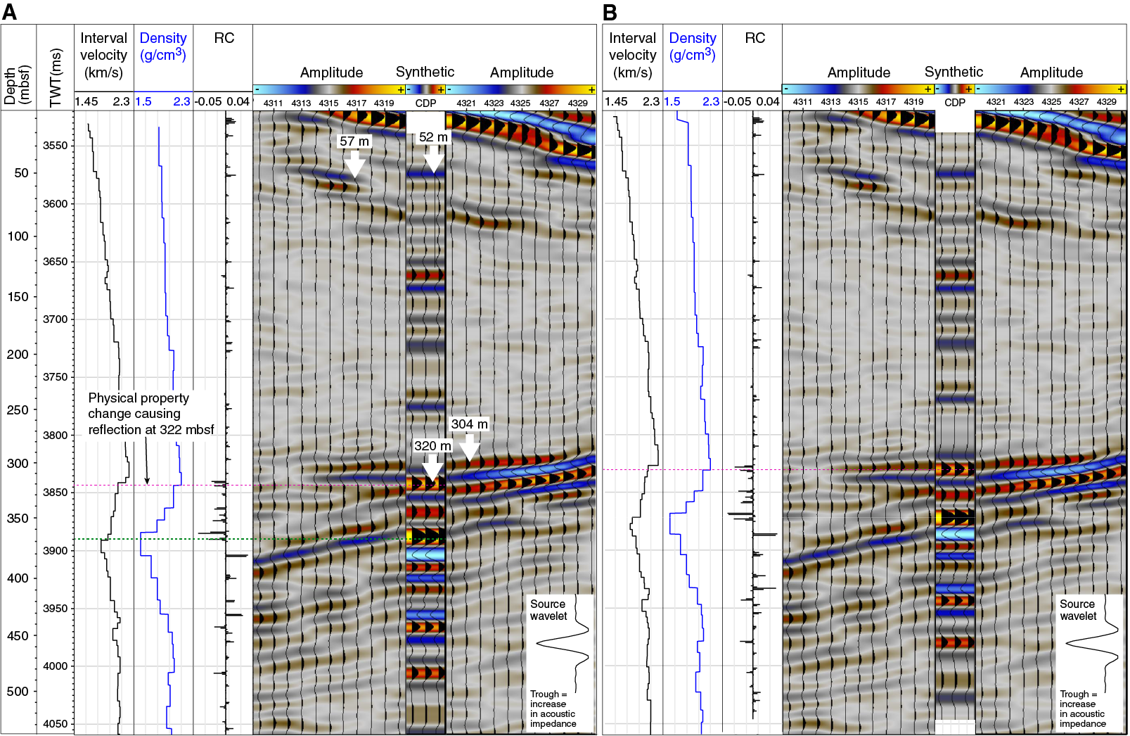
Figure F56. Synthetic seismic-well tie.
Following testing using analytical, statistical, and deterministic wavelet extractions, a preferred wavelet was selected from Seismic Line 05CM-04 by stacking 10 adjacent seismic traces from a flat region of the seafloor between CDPs 5220 and 5230 to yield a high signal-to-noise ratio (Figure F56). This wavelet was convolved with the reflection coefficient log measured in time to produce a synthetic seismic trace that can be compared with Seismic Profile 05CM-04 in the vicinity of CDP 4322 near Hole U1518F.
The resulting synthetic seismic trace in the time domain is shown in Figure F56A with the seismic data (Seismic Line 05CM-04, CDPs 4310–4330) and no depth shifts applied. To a first order, the synthetic trace predicts low- to moderate-amplitude reflections between 20 and 300 mbsf and a band of higher amplitude reflections between 310 and 380 mbsf, consistent with the observed seismic facies character. A moderate-amplitude, normal polarity reflection (blue trough; indicative of an increase in acoustic impedance downward) in the synthetic trace at 52 mbsf appears to match a moderate-amplitude, normal polarity reflection in the seismic data at 57 mbsf. These reflections are interpreted to represent an increase in density and velocity in Lithostratigraphic Subunit IA (see below). A high-amplitude, reversed polarity reflection (red peak; indicative of a decrease in acoustic impedance downward) observed in the synthetic trace at 320 mbsf correlates with a physical properties change at the interpreted depth of the top of the footwall of the main fault zone of the Pāpaku fault (322 mbsf; at the Logging Unit 3–4 transition) in Hole U1518B. A similar high-amplitude, reversed polarity reflection is observed at 304 mbsf on Seismic Profile 05CM-04 at CDPs 4319–4321. This reflection at 304 mbsf approximately coincides with the Lithostratigraphic Subunit IB–Unit II transition in Hole U1518F (see Lithostratigraphy) and the transition from a hanging wall damage zone in Section 375-U1518F-13R-1 to the main brittle fault zone described in Section 13R-2 (see Structural geology), suggesting that the high-amplitude reflection caused by the major physical properties change in Hole U1518B at 322 mbsf correlates with the high-amplitude, reversed polarity reflection observed on Seismic Line 05CM-04 at 304 mbsf.
This correlation requires that the physical properties change to decreased impedance across the top of the brittle fault zone occurs at a shallower depth in Hole U1518F than in Hole U1518B. To simulate the synthetic seismic trace that would be produced if this physical properties change was 15 m shallower in Hole U1518F than in Hole U1518B, we shifted the LWD density and sonic logs from Hole U1518B below 200 mbsf up by 15 m, keeping the logs above 200 mbsf constant (Figure F56B). This shift represents a scenario in which the geological section between 200 and 322 mbsf is 15 m thinner in Hole U1518F than in Hole U1518B and the physical properties change at 322 mbsf in Hole U1518B occurs at 307 mbsf in Hole U1518F. The resulting synthetic seismic trace reveals a much better match between high-amplitude reflections in the 300–400 mbsf zone. Not only does the predicted first high-amplitude, reversed polarity reflection fit the observed reflection at 304 mbsf better, but the other reflections below, including a very high amplitude, reversed polarity reflection at 353 mbsf, also match the observations better.
We note that strong reflections are predicted at the location of major physical properties changes in Hole U1518B close to 368 mbsf where an increase in borehole size recorded by the caliper tool coincides with decreased gamma ray, bulk density, resistivity, and P-wave velocity and an increase in porosity (Figure F57) (see Logging while drilling). Although the enlarged borehole may cause artifacts in LWD density and velocity values (lower density and higher porosity than in reality), the reflection predicted in our synthetic seismic trace from this physical properties transition (when shifted upward 15 m; Figure F56) matches a very high amplitude, reversed polarity reflection at 353 mbsf. We therefore consider that the physical properties change at 368 mbsf in the LWD data is likely real, albeit amplified by borehole washout.
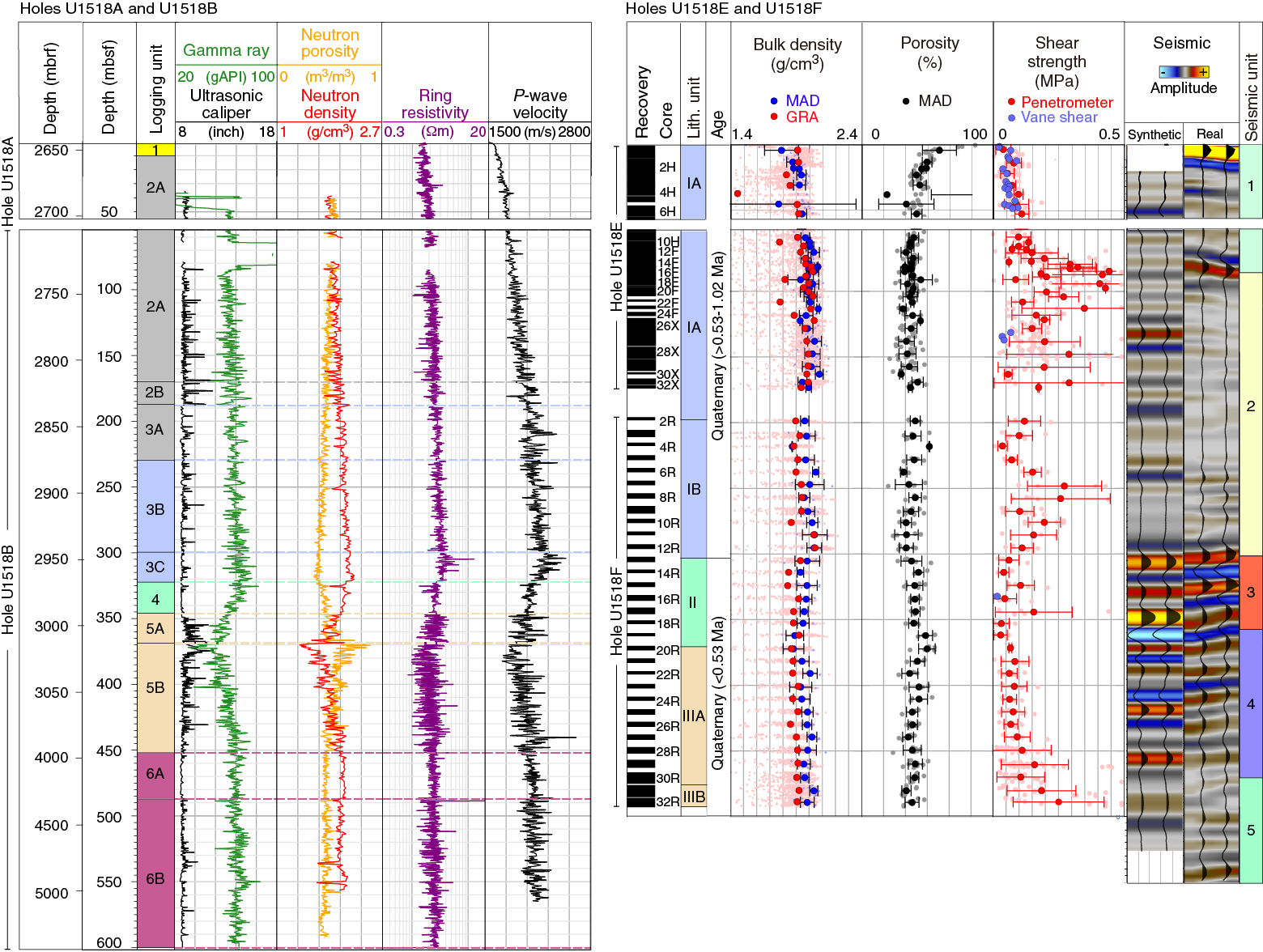
Figure F57. LWD, core, and seismic data.
Seismic stratigraphy
We define five seismic units in the vicinity of Hole U1518F at CDP 4322 based on reflection characteristics in Seismic Line 05CM-04 (Figure F58). A time-depth relationship derived from the high-quality sonic VP recorded in Holes U1518A and U1518B (Figure F55; Table T20) is used to calculate the depth extent of each seismic unit; these depths are presented in the discussion below.
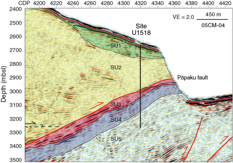
Figure F58. Interpreted seismic units.
Seismic Unit 1 (0–85 mbsf) is wedge shaped and thins westward (upslope) (Figure F58). The unit is characterized by relatively moderate to high-amplitude reflections that dip gently eastward (downslope) and are irregular and discontinuous. The easterly dip of the reflections relates to the site’s location on the forelimb of a thrust-related anticlinal fold and is consistent with northeast bedding dip azimuths from resistivity image logs in Hole U1518A (see Logging while drilling). The top of the unit is eroded at the seafloor, consistent with observations of sediment mass transport in the multibeam bathymetric geomorphology (Figure F1) and with anomalously low porosity values observed at the top of the unit (see Physical properties). The base of this unit is defined by a transition to lower reflectivity in the underlying unit. Seismic Unit 1 corresponds to Logging Units 1 and 2 and the upper part of Lithostratigraphic Subunit IA (see Logging while drilling and Lithostratigraphy). Sedimentology in Hole U1518E indicates the presence of silty clay (hemipelagic mud) with abundant fine-grained sand to silt turbidites and rhyolitic volcanic ash layers. Biostratigraphy indicates that Seismic Unit 1 is Quaternary (older than 0.53–0.63 Ma; see Biostratigraphy).
Seismic Unit 2 (85–304 mbsf) is characterized by relatively low amplitude reflections at Site U1518 that dip gently eastward, which is consistent with the overall north-northeast bedding dip azimuth determined from resistivity image logs in this unit (see Logging while drilling). Reflections in the lower part of the sequence increase in amplitude between 500 and 2000 m west of Site U1518. Some weak reflections dipping west at Site U1518 may be artifacts of the seismic processing. This unit corresponds to Logging Units 2 and 3 and Lithostratigraphic Subunits IA and IB (see Logging while drilling and Lithostratigraphy). Sedimentology in Holes U1518E–U1518F indicates the presence of hemipelagic mud and numerous silty turbidites. Biostratigraphy indicates that Seismic Unit 2 is Quaternary (older than 0.53–0.64 Ma). The Logging Unit 2/3 boundary and Lithostratigraphic Subunit IA/IB boundary coincide approximately with a strong reflection in the synthetic seismic trace that is not seen in the real seismic data (Figure F56). The base of Seismic Unit 2 is defined by an abrupt change to higher seismic amplitudes and a change in the apparent dip direction of the reflections. In the seismic reflection data, this contact is interpreted to be the main brittle fault that marks the top of the Pāpaku fault zone (Figure F58).
Seismic Unit 3 (304–365 mbsf) lies in the immediate footwall of the main brittle fault and is strongly reflective (Figure F58). The unit has variable thickness downdip and is characterized by high-amplitude, discontinuous seismic reflections with shingled geometries. The reflection architecture of the unit about 1–2 km downdip of Site U1518 (toward the west) is consistent with laterally migrating paleochannels associated with high-amplitude reflections. At Site U1518, it corresponds to Logging Units 4 and 5 and approximately to Lithostratigraphic Unit II (see Logging while drilling and Lithostratigraphy). Logging Unit 4 is ~25 m thick and is not resolved by the vertical resolution of the Seismic Line 05CM-04 data (Figure F58). Hole U1518F cores are characterized by poor recovery. It is possible that some coarse material was removed by RCB drilling circulation. However, the structural interpretation of this interval in cores from Hole U1518F (below the main brittle fault) suggests that it comprises a tens of meters thick interval of mixed brittle and ductile deformation associated with the Pāpaku fault (Structural geology). The structural interpretation from cores suggests that the base of this interval coincides with a subsidiary fault zone below which deformation intensity decreases markedly. The sedimentology of the cores indicates the presence of silty hemipelagic mud and sparse fine-grained turbidites, consistent with the interpretation of Logging Unit 4 (see Lithostratigraphy and Logging while drilling). Biostratigraphy indicates that Seismic Unit 3 is Quaternary (younger than 0.53 Ma). The base of Seismic Unit 3 marks an abrupt change in the LWD logs and core lithofacies.
Seismic Unit 4 (365–460 mbsf) consists of relatively high amplitude seismic reflections subparallel to the apparent orientation of the thrust fault (Figure F58). Resistivity image logs identify bedding to dip consistently north-northwest in this seismic unit. This unit corresponds to Logging Unit 5 and Subunit 6A and the upper part of Lithostratigraphic Unit III. The slightly coarser grain size, thicker beds, and low velocity and density in this unit likely contribute to the relatively high reflectivity. The observed lithofacies is dominated by silty clay, clayey silt, and silty turbidites. Bioturbated mudstone and soft-sediment disruption are also identified. Biostratigraphy indicates that Seismic Unit 4 is Quaternary (younger than 0.53 Ma). The contact with Seismic Unit 5 is gradational.
Seismic Unit 5 (460–600 mbsf) has lower reflectivity than Seismic Unit 4, which is consistent with the relatively small variations in density and P-wave velocity observed in Logging Unit 6. Seismic Unit 5 is characterized by lower amplitude reflections that dip west approximately parallel to the fault (Figure F58). Resistivity image logs document bedding dips that are consistently north-northwest in this seismic unit. The unit corresponds to Logging Subunits 6A and 6B and the lower part of Lithostratigraphic Unit III. Only the upper part of Seismic Unit 5 was cored at Site U1518. The core is characterized by improved recovery in Lithostratigraphic Unit III associated with predominantly silty mud with localized evidence of soft-sediment remobilization. Biostratigraphy indicates that Seismic Unit 5 is Quaternary (younger than 0.53 Ma).
Primary thrust fault zone (Pāpaku fault)
The contact between Seismic Units 2 and 3 marks the position of the Pāpaku fault as interpreted in seismic data. It is identified by hanging wall reflection cutoffs in Seismic Unit 2 and an associated fault propagation anticline beneath the slope west of Site U1518. Uncharacteristic of many frontal thrust faults beneath the Hikurangi margin (e.g., Barker et al., 2009; Bell et al., 2010; Pedley et al., 2010; Plaza-Faverola et al., 2012, 2016; Ghisetti et al., 2016; Barnes et al., 2010, 2018), the footwall sequence appears to dip parallel to the fault (westerly) and is not characterized by obvious footwall cutoffs. The thrust is interpreted to reach the seafloor about 450 m east of Site U1518 on a steep slope associated with a significant landslide scar. The thrust has an apparent dip of about 12°–13° in Profile 05CM-04 but is likely closer to a 20° true dip normal to strike.
The main fault zone is interpreted in LWD data to lie at 315–322 mbsf (or 2960.4–2967.3 mbrf). This interpretation is related to a cluster of conductive fractures mapped in GVR image logs at 315.3–317.6 mbsf (2960.5–2962.7 mbrf) and a major apparent physical properties change involving a decrease in density and resistivity and an increase in porosity below 322 mbsf (2967.3 mbrf) that is interpreted to be the top of the footwall to this main fault zone (see Logging while drilling) (Figure F59). The top of the fault zone in the cored sediments occurs at 304.5 mbsf (2941.3 mbrf) at the top of Section 375-U1518F-13R-2 (Structural Domain 2A; see Structural geology). This interpretation is supported by an age inversion recorded at a similar depth (see Biostratigraphy).

Figure F59. Data around primary thrust fault zone.
Physical properties data measured from cores reveal a subtle reduction in density and shear strength and an increase in porosity in Cores 375-U1518F-12R through 14R (see Physical properties; Figure F59). However, because of limited core recovery and scatter in laboratory-measured physical properties data, it is not clear exactly where these physical properties transitions take place.
The laboratory-measured physical properties changes around 304–315 mbsf (2941.3–2952.1 mbrf) in Hole U1518F are similar to the LWD physical properties changes that occur at 322 mbsf (2967.3 mbrf) in Hole U1518B in that they both involve a decrease in density and increase in porosity (Figure F59). This similarity suggests that the transition in physical properties at 304–315 mbsf (2941.3–2952.1 mbrf) in Hole U1518F cores may correspond to that observed at 322 mbsf (2967.3 mbrf) in the Hole U1518B LWD data. If this correlation is correct, it implies that the fault zone in Hole U1518F occurs 15.2–26.0 m shallower (in terms of mbrf) than in Hole U1518B.
When conducting the seismic-well tie in Figure F56, we also deduced that the impedance contrast modeled from the LWD data at 322 mbsf in Hole U1518B occurs 15 m deeper (i.e., at 2943.8 mbrf) than the strong reversed polarity reflection in the real seismic data crossing Hole U1518F. The shallower physical properties change measured in the laboratory and the seismic-well tie both suggest a shallowing of the feature in Hole U1518F that produces the significant response in LWD data at 322 mbsf in Hole U1518B.
This correlation raises the question of which structural features or physical properties changes observed in cores correspond to the interpreted LWD fault zone response at 322 mbsf in Hole U1518B. Given the poor core recovery, it is not possible to directly match the LWD and core-measured physical properties, so we identify two end-member scenarios (Figure F60).

Figure F60. Correlation of LWD with structural geology interpretations.
For Scenario 1, the LWD response in Hole U1518B, which is marked by a reduction in density and resistivity and an increase in porosity at 322 mbsf (2967.3 mbrf), correlates with a physical properties transition around the shallowest possible location of the physical properties changes observed in cores at the top of the fault zone at 304.5 mbsf (2941.3 mbrf) in Hole U1518F. This scenario would represent a shallow end-member for the fault depth, with the LWD response possibly representing the transition from deformed hanging wall rock into the fault zone at the top of Section 375-U1518F-13R-2 (Figure F60). This scenario requires a difference in absolute depth (referenced to rig floor or sea level) of the correlated feature between the two boreholes of 26.0 m.
For Scenario 2, the LWD response in Hole U1518B at 322 mbsf (2967.3 mbrf) correlates with the curated base of Core 375-U1518F-14R. Although Core 14R exhibits only partial recovery and therefore cannot tightly constrain the depth of the primary physical properties change, the seismic-well tie fits the data best when the physical properties change occurs no deeper than the curated base of the recovered interval in Core 14R (Figure F56). Density increases slightly from Core 14R to Core 15R, and we place the curated base of Core 14R as our lower bound depth estimate of the physical properties change in Hole U1518F (315 mbsf; 2952.1 mbrf), consistent with our seismic-well tie. Although this correlation honors the density and porosity data from the cores, it would also be permissible for the physical properties change and deformation structures in the core to occur deeper, in the unrecovered interval between the curated base of Core 14R (315 mbsf) and the top of Core 15R (322 mbsf); however, this deeper change would not provide as good a fit to the seismic-well tie. Deformation structures in Core 14R include fractured and brecciated intervals that could be equivalent to the increase in porosity and decrease in density across the 1.4 m thick interval below 320.6 mbsf in Hole U1518B. The contact at 2952.1 mbrf (Figure F60) may therefore correspond to the base of the dominantly brittle deformation zone between Cores 14R and 15R (see Structural geology). The implication of this interpretation is that the majority of the unrecovered section above Core 15R is considered likely to be part of Structural Domain 2B (see Structural geology) and that the LWD transition at 322 mbsf in Hole U1518B may not occur any deeper than 315 mbsf in Hole U1518F. This scenario therefore requires a difference in depth of the correlated feature between the two boreholes of 15.2 m (referenced to sea level or rig floor).
When the LWD, core, and seismic data are considered together, correlation Scenarios 1 and 2 are considered as end-members. The true location of the Hole U1518B physical properties change at 322 mbsf may occur anywhere between Scenarios 1 and 2 and be compatible with the available data. Both of these scenarios suggest that the primary changes in physical properties around the fault occur at a shallower depth in Hole U1518F than in Hole U1518B. The range of scenarios, the structural interpretation of the fault zone, and the seismic-well tie suggest the LWD physical properties transition at 322 mbsf in Hole U1518B occurs somewhere between 315 and 305 mbsf in Hole U1518F, which requires shallowing of the physical properties transition by 15.2–26.0 m between the two holes that are located 40 m apart.
The above correlations assume that the boreholes are vertical. No deviation was reported in Hole U1518B (see Logging while drilling), whereas Hole U1518F is assumed to be vertical because no deviation data are available from RCB coring operations. The Schlumberger LWD engineers have indicated (D. Pedulla, pers. comm., 2018) that a borehole deviation sufficient to account for the apparent vertical depth discrepancy between the correlated features is unlikely.
Implications of the fault zone correlation for observatory screen depths
The possible correlations between Holes U1518B and U1518F have implications for the location of the central screened interval in the Hole U1518H observatory installed during Expedition 375 (see Observatory). Given the large distance between Holes U1518E and U1518H (see Operations), the LWD data in Hole U1518B were used to define the observatory monitoring interval depths in Hole U1518H. The 8 m long fault zone observatory screen was centered at 2965 mbrf (323 mbsf) in Hole U1518H. This interval includes the cluster of conductive fractures overlying disturbed bedding interpreted in resistivity images below 2960 mbrf (315 mbsf) in Hole U1518B and spans the prominent physical properties change at 2967.3 mbrf (322 mbsf) (see Logging while drilling).
If the LWD physical properties change at 2967.3 mbrf (322 mbsf) in Hole U1518B corresponds to the hanging wall–fault zone transition in Section 375-U1518F-13R-1 (~2941.3 mbrf; Scenario 1), the conductive fractures and upper part of the observatory screen in Hole U1518H at 2961.5 mbrf are located in the bottom of the hanging wall and the observatory screen may also extend into the top of the fault zone (Figure F60; Scenario 1). The lower part of the screen would be placed in the top of the fault sequence equivalent to that observed in Section 375-U1518F-13R-2. If the LWD physical properties change corresponds to the base of the intensely deformed brittle fault zone described in Section 14R-2 (Scenario 2), the conductive fractures and observatory screens are located in the upper part of the main brittle-ductile fault zone in Hole U1518H (Scenario 2). Given that a similar fracture intensity was measured in cores in the upper part of the fault zone as in the lower part of the hanging wall (see Structural geology), it is likely that the screen is installed in a sequence with high fracture permeability.
Subsidiary fault zone correlation
A major physical properties change in the Hole U1518B LWD data involves an abrupt decrease in density, velocity, and gamma ray and an increase in porosity at 369 mbsf (3014.8 mbrf) (Figure F59). This feature coincides with the Logging Subunit 5A/5B boundary and approximately with the Lithostratigraphic Unit II–III transition (see Logging while drilling and Lithostratigraphy). These physical properties changes also coincide with a significant enlargement of the borehole and a bimodal T2 distribution in the NMR porosity data that are consistent with a relatively siltier formation than that found immediately beneath the primary thrust fault. In the laboratory, measured physical properties data indicate a significant physical properties change at around 353–365 mbsf (2990–3002 mbrf) involves an increase in porosity and compressive strength with depth. From the structural observations in cores, this depth range corresponds to the presence of a subsidiary fault zone (Structural Domain 3) at 351.2–361.7 mbsf (see Structural geology). We propose that the LWD response at 369 mbsf and the laboratory-based physical properties change at 353–365 mbsf correlate despite the signals not being in complete agreement (i.e., the density response in the laboratory measurements is quite different), which may be due to borehole collapse, poor recovery, or washout. The LWD response at this interval produces a high-amplitude reflection in the synthetic seismic trace. Upon application of a 15 m upward depth shift in the LWD-derived synthetic seismogram, this high-amplitude reflection fits a high-amplitude, reversed polarity reflection observed in the real seismic data (Figure F57). Therefore, the LWD response seen at 369 mbsf (3014.8 mbrf) in Hole U1518B is likely 12.8–24.8 m shallower in Hole U1518F.
Observatory
The borehole observatory in Hole U1518H is named “Te Matakite,” a Māori word that means “to see into the future.” The observatory is designed to provide a time series of formation pore fluid pressures, temperatures, fluid flow rates, and fluid chemistry. The data and fluid samples will be retrieved at a later date using a submersible ROV. The scientific objectives of the observatory are to characterize the hydrologic and thermal conditions in the fault zone, as well as hydrological processes and deformation over a range of timescales, including short-lived transients associated with fault slip.
General design
The observatory includes nested ACORK and CORK-II components (Becker and Davis, 2005). The ACORK consists of 10¾ inch steel casing with casing screens and an umbilical on its exterior (Figure F61). The umbilical contains hydraulic lines that are connected to the casing screens at depths of observation targets in the formation and to pressure gauges and a data logger at the wellhead. The CORK-II is installed inside the ACORK and consists of 4½ inch steel casing and a second wellhead that is seated on top of the ACORK. An instrument string containing temperature sensors and an osmotic fluid sampling assembly (OsmoSampler assembly) is hung inside the 4½ inch CORK-II casing. The OsmoSampler assembly rests in a seat within the CORK-II casing, located at the depth of the fault zone. The detailed installation procedure is described in Operations. The positioning of casing screens, the OsmoSampler seat, and all downhole components was based on the integration of seismic imaging, coring, and LWD data acquired at the site (see Core-log-seismic integration).

Figure F61. Completed observatory.
The three casing screens for pressure monitoring are centered at 217.72 (hanging wall), 323.06 (fault zone), and 393.17 mbsf (footwall) (Table T21). The fault zone screen, which also provides access for OsmoSampler fluid sampling and fluid flow rate monitoring, is 8 m long, whereas the screens set in the hanging wall and footwall are both 2 m long. The hanging wall and footwall casing screens are attached to the exterior of the ACORK casing and provide access only between the formation and the hydraulic lines in the umbilical (there is no access to the inner bore of the ACORK casing). In contrast, as described below, the ACORK casing inside the fault zone screen is perforated to allow the OsmoSampler and flowmeter to access formation fluids. The OsmoSampler assembly is seated at 323.11 mbsf inside the CORK-II casing, a few centimeters deeper than the center of the fault zone screen because of restrictions associated with casing joint sizes. The depth of the seat (323.11 mbsf) also marks the depth of the sampling ports for the flowmeter and OsmoSamplers.
The position and serial number of each of the 30 temperature sensors in the observatory are listed in Table T22. Fourteen temperature sensors are suspended on Spectra rope above the OsmoSampler assembly, seven are placed inside the assembly, and nine are suspended below the assembly on Spectra rope with sinker bars at the bottom. The reported sensor depths incorporate estimates of rope stretch that were constrained empirically by pre-expedition measurements under controlled tension.
Pressure sensing and ACORK
Seafloor and formation fluid pressures are measured with absolute pressure gauges (APGs) connected to a data logger on the ACORK wellhead (Figure F62B). Four APGs are mounted on the wellhead: three are connected to an umbilical that terminates in screened intervals in the hanging wall, footwall, and fault zone, and the fourth senses seafloor pressure. The pressure sensing package is equipped with Paroscientific Digiquartz pressure transducers (Model 8B4000-2), a high-precision pressure period counter with a 12.8 MHz real-time clock (RTC-PPC system resolving ~10 ppb of full-scale pressure or ~0.7 Pa), and a 24-bit/channel analog-to-digital converter and data logger (Bennest Enterprises, Ltd.; Minerva Technologies, Ltd.; and the Pacific Geoscience Centre, Geological Survey of Canada). The data logger in the pressure sensing unit at the wellhead can be accessed via an ODI Teledyne underwater mateable connector mounted on the pressure sensing unit. The data logger is programmed to record pressures once every 60 s from each APG.
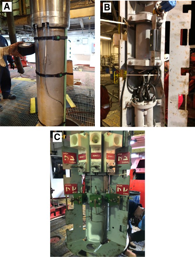
Figure F62. Pressure sensing components.
The APGs for the formation measurements are connected to a three-pass umbilical along the exterior of the ACORK casing that terminates in carbolite-filled external casing screens. The screens are made out of 316SS stainless steel and wrapped with 0.085 inch wire with a 0.01 inch wire-to-wire spacing that results in an open cross section of 15%. The carbolite beads have a diameter of 600 µm. The perforated casing is wrapped with a double screen so that the carbolite beads do not escape. Figure F62A shows the uppermost screen and some of the umbilical tubing. The umbilical tubes act as pressure conduits that relay pressures from the screens in communication with the formation to the APGs at the wellhead. The bottom of the ACORK casing is sealed with a bridge plug so that formation fluids can enter the inner bore of the ACORK casing only through the perforated ACORK casing and screen at the fault zone (Figure F61; see Operations). As described below, the CORK-II and OsmoSampler are designed to seal a volume in the interior of the perforated ACORK casing section to ensure that formation fluids are directed only to the fluid sampling and flowmeter systems and to minimize the interconnected volume for fluid pressure sensing in the fault zone interval. Valves at the wellhead allow individual pressure lines to be closed to the ocean so that the gauges directly record the pressure in the formation at depth or open to the ocean for periodic hydrostatic checks or to allow fluid sampling at a later date (Figure F62C).
Osmotic flowmeter and fluid sampling
Formation fluids are sampled from the fault zone through the flowmeter that is part of the OsmoSampler assembly. The OsmoSampler assembly was seated with a piston seal in the CORK-II casing so that the flowmeter ports are at a depth similar to the fault zone (323.11 mbsf) (Figure F61). The OsmoSampler assembly continuously samples fluids for analysis of solutes and gases and contains an osmotically driven flowmeter for monitoring fluid flow rates (e.g., Jannasch et al., 2003, 2004).
Formation fluids at the depth of the fault zone enter the observatory through the external casing screen, which is wrapped around a single joint of ACORK casing that is perforated to provide access to the inner volume of the ACORK casing (Figure F61). Inside the casing, vertical movement of formation fluids is restricted by swellable packers that create a seal between the CORK-II casing and the interior of the 10¾ inch ACORK casing above and below the perforated casing joint (Figures F61, F63). The swellable packers are centered 11.42 m above and below the sampling flow ports in the OsmoSampler assembly (Figure F61).
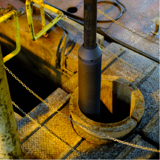
Figure F63. Swellable packer.
In the screened interval, four vertical seals (comprising strips of packer material) on the outside of the CORK-II casing divide the annulus between the CORK-II and ACORK casing into quadrants, each of which contains a flowmeter sampling port. This “quadrant seal” element of the CORK-II is designed to restrict lateral mixing of fluids so that the flow direction of formation fluids remains unmodified upon introduction to the OsmoSampler seat. This seal allows use of a chemical tracer to define approximate flow direction and flow rates (e.g., Jannasch et al., 2003).
The OsmoSamplers intake fluid at a constant rate using osmotically driven pumps that are connected to small diameter Teflon or copper tubing initially filled with ultrapure water. Figure F64A shows one of the osmotic pumps and a portion of a Teflon sampling coil. In this configuration, new (formation) fluid is continuously drawn into the open ends of the Teflon and copper tubing at the sampling ports, and the oldest samples are closest to the pumps. The tubing inside diameter is 1.2 mm. The small tubing diameter restricts dispersion, and the distance fluid is pumped is much greater than the diffusional distance over a given period of time, allowing for a temporal resolution of fluid samples of a few days. The length of tubing and pump rates were chosen to be sufficient for ~5 y of sampling.
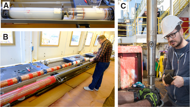
Figure F64. OsmoSampler assembly components.
The OsmoSampler assembly has eight OsmoSampler pumps with associated sampling coils: four for measuring the chemical tracer in order to determine flow rates (one in each of the four quadrants), two for measuring fluid composition, and two connected to copper tubing for gas composition (Jannasch et al., 2004). Figure F64B shows some of the sampling coils during assembly.
Temperature sensors
Temperature sensors are positioned in the OsmoSampler assembly and suspended on Spectra rope above and below the assembly (Figure F61; Table T22). We use RBRsolo T 10K abyssal temperature recorders manufactured by RBR. The instruments have a temperature accuracy of ±0.002°C and titanium enclosures that are pressure-rated for ocean depths as deep as 10,000 m. Each unit is autonomous, with its own sensor and data logger. They are programmed to measure once every 10 s; for this sampling rate, measurements are expected to continue for ~7 y (until April 2025). A temperature sensor is shown in Figure F65.
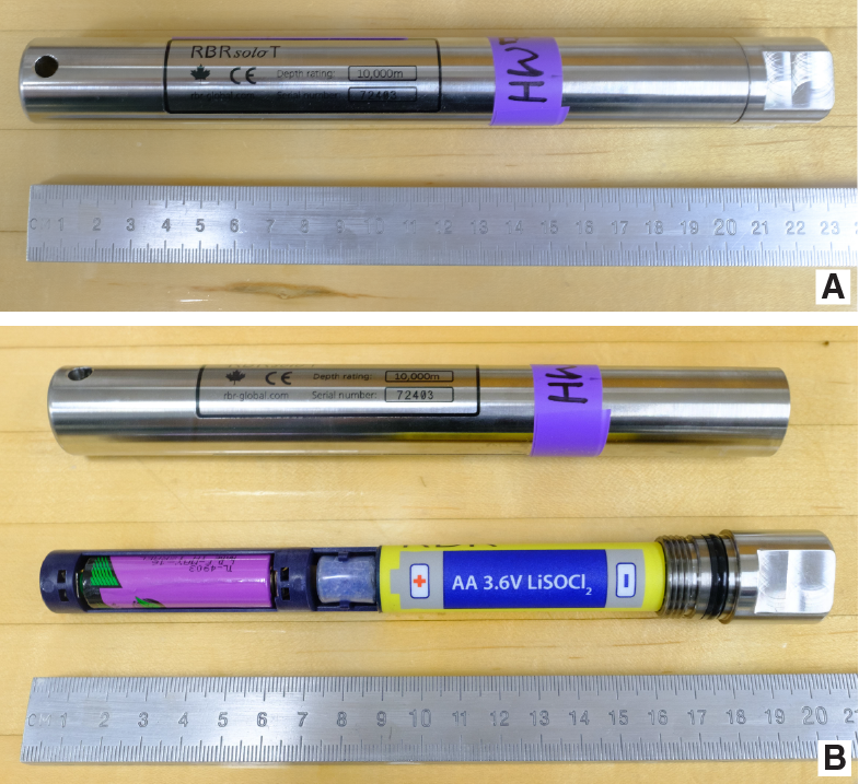
Figure F65. Temperature sensor.
The temperature sensors are connected to the instrument string with utility cord tied to attachment eyelets spliced into the Spectra rope. The instrument is then wrapped in a protective covering of ¼ inch (or thinner) rubber sheeting and wrapped in tape. The covering protects the instrument from impacts and creates a smooth profile to prevent the instrument string from snagging during deployment or recovery (Figure F66). Seven of the temperature sensors are also distributed in the housing of the OsmoSampler assembly (Figure F67).
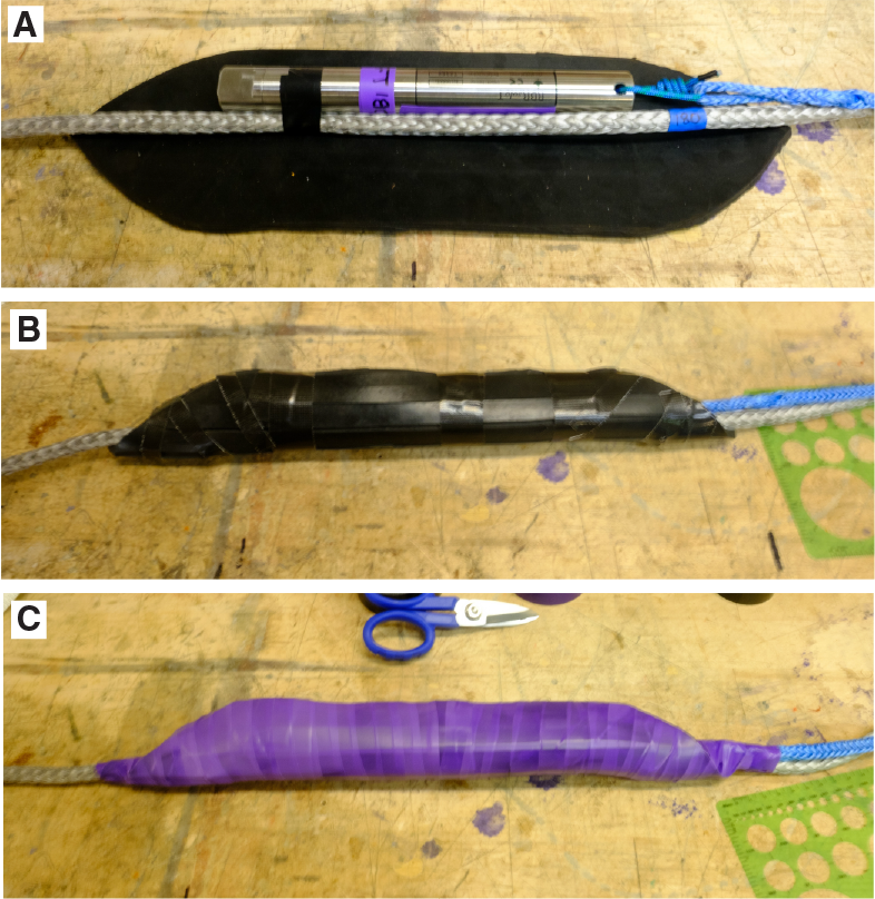
Figure F66. Temperature sensors and rope components.
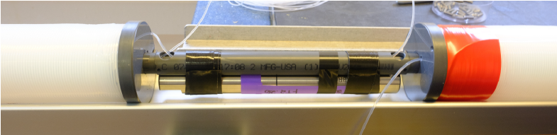
Figure F67. Temperature sensor between two Teflon coils.
Additional instrument string components
The instrument string consists of three rope sections, 30 temperature sensors, the OsmoSampler assembly, four sinker bars, three weak links, and the top plug (Figure F61). The rope sections are composed of ⅜ inch Spectra 12-strand line manufactured by Cortland, Ltd. (Anacortes, Washington, USA), a Class II rope material that is ideal for the purposes of the observatory because it has high strength and low stretch (~2%), is easy to splice, and is slightly positively buoyant (Fisher et al., 2005, 2011; Edwards et al., 2012). For the ⅜ inch rope, the mean tensile strength is 15,400 lb initially and 13,900 lb when spliced. Rope splices are used to connect rope sections to other parts, attach sensors, and provide handling eyes to facilitate deployment and recovery (Figure F68).
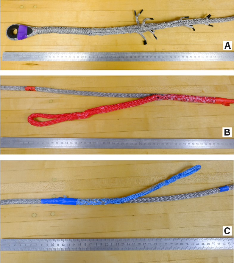
Figure F68. Rope splices.
To maintain the relative positioning of instruments in the uppermost rope section, a 0.55 m long, 30 lb sinker bar is used to remove slack above the OsmoSampler assembly. Three 20 ft long, 2 inch diameter sinker bars weighing a total of ~500 lb in water compose the lowermost portion of the instrument string (Figure F69). The purpose of the lower sinker bars is to keep the ropes taut during deployment to prevent components from hanging up at the OsmoSampler seat and wellhead and to keep the lower rope section with temperature sensors taut below the flowmeter seat.
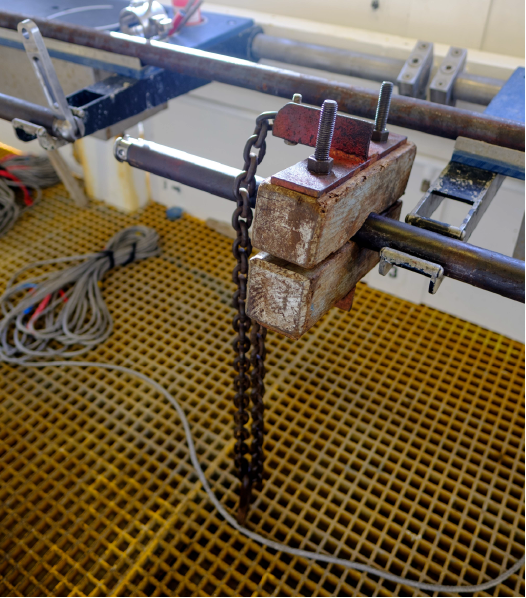
Figure F69. Lower sinker bars.
To address the possibility that components of the instrument string could get stuck during retrieval, weak links are included at strategically targeted locations in the string (Figure F70). The weak links were obtained from TLR, Inc. (Carmel, California, USA) and consist of metal components that include two end pieces and two connection plates. The pieces are sewn together with ⅛ inch polypropylene cord via as many as 150 pass-through holes that align between the pieces. The number of holes that are threaded controls the strength; the end pieces can only separate by shearing through the polypropylene cords. For Site U1518, we programmed three weak links (from top to bottom):
- Weak Link 1: 4400 lb tensile strength based on 39 threads on each end.
- Weak Link 2: 6400 lb tensile strength based on 57 threads on each end.
- Weak Link 3: 8400 lb tensile strength based on 75 threads on each end (i.e., utilizing all 150 pass-through threads available).
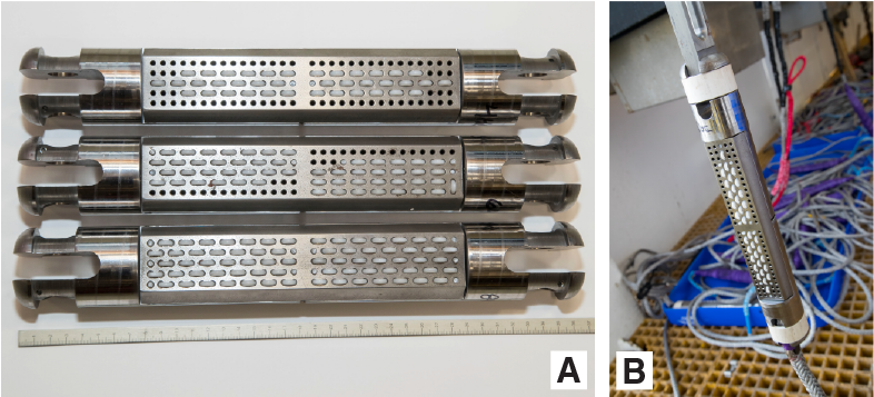
Figure F70. Weak links.
The top of the instrument string comprises a top plug with an O-ring and a 3⅝ inch seat that latches and seals the interior of the CORK-II casing from the ocean (Figure F71). The top plug also serves as the instrument hanger with a 1½ inch diameter ring where the Spectra line is attached. The top of the top plug is designed for retrieval with the ERS.
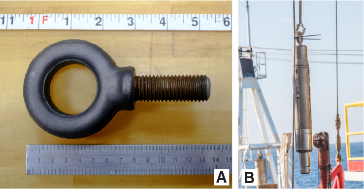
Figure F71. Top plug hanging ring.
Deployment and completion
Deployment
During deployment on the Schlumberger wireline (see Operations), the weight of the instrument string was continuously monitored. Wireline tension monitoring did not show any sign of hang ups or obstructions. The monitoring did record two considerable drops in tension that are interpreted to correspond to the seating of the OsmoSampler assembly in the hanger, followed roughly 10.85 m later by the seating of the top plug.
Following delivery of the instrument string, the CORK-II was lowered the remaining 16.8 m to its seat in the ACORK (see Operations). The CORK-II was then released from the drill pipe using the J running tool. There are two items to note regarding the release: (1) it is not clear whether the CORK-II properly latched in its seat in the ACORK, although initial visual inspection suggests that it did seat, and (2) the top seal (of two seals) designed to handle possible formation underpressures appears to have been damaged and became dislodged during the final stages of installation. Additionally, the ROV platform above the ACORK wellhead is seated at an angle that may partially restrict access to the pressure valves. Tentative plans are to use an ROV to download initial pressure data in 2019 and to recover the instrument string of temperature sensors and OsmoSamplers and conduct an additional pressure data download by 2023.
References
Araki, E., Saffer, D.M, Kopf, A.J., Wallace, L.M., Kimura, T., Machida, Y., Ide, S., Davis, E., and IODP Expedition 365 Shipboard Scientists, 2017. Recurring and triggered slow-slip events near the trench at the Nankai Trough subduction megathrust. Science, 356(6343):1157–1160. https://doi.org/10.1126/science.aan3120
Barker, D.H.N., Henrys, S., Caratori Tontini, F., Barnes, P. M., Bassett, D., Todd, E., and Wallace, L., 2018. Geophysical constraints on the relationship between seamount subduction, slow slip and tremor at the north Hikurangi subduction zone, New Zealand. Geophysical Research Letters, 45(23):12804–12813. https://doi.org/10.1029/2018GL080259
Barker, D.H.N., Sutherland, R., Henrys, S., and Bannister, S., 2009. Geometry of the Hikurangi subduction thrust and upper plate, North Island, New Zealand. Geochemistry, Geophysics, Geosystems, 10(2)Q02007. https://doi.org/10.1029/2008GC002153
Barnes, P.M., Ghisetti, F.C., Ellis, S., and Morgan, J.K., 2018. The role of protothrusts in frontal accretion and accommodation of plate convergence, Hikurangi subduction margin, New Zealand. Geosphere, 14(2):440–468. https://doi.org/10.1130/GES01552.1
Barnes, P.M., Lamarche, G., Bialas, J., Henrys, S., Pecher, I., Netzeband, G.L., Greinert, J., Mountjoy, J.J., Pedley, K., and Crutchley, G., 2010. Tectonic and geological framework for gas hydrates and cold seeps on the Hikurangi subduction margin, New Zealand. Marine Geology, 272(1–4):26–48. https://doi.org/10.1016/j.margeo.2009.03.012
Barnes, P.M., Pecher, I.A., LeVay, L.J., Bourlange, S.M., Brunet, M.M.Y., Cardona, S., Clennell, M.B., Cook, A.E., Crundwell, M.P., Dugan, B., Elger, J., Gamboa, D., Georgiopoulou, A., Greve, A., Han, S., Heeschen, K.U., Hu, G., Kim, G.Y., Kitajima, H., Koge, H., Li, X., Machado, K.S., McNamara, D.D., Moore, G.F., Mountjoy, J.J., Nole, M.A., Owari, S., Paganoni, M., Petronotis, K.E., Rose, P.S., Screaton, E.J., Shankar, U., Shepherd, C.L., Torres, M.E., Underwood, M.B., Wang, X., Woodhouse, A.D., and Wu, H.-Y., 2019. Site U1517. In Pecher, I.A., Barnes, P.M., LeVay, L.J., and the Expedition 372A Scientists, Creeping Gas Hydrate Slides. Proceedings of the International Ocean Discovery Program, 372A: College Station, TX (International Ocean Discovery Program). https://doi.org/10.14379/iodp.proc.372A.103.2019
Becker, K., and Davis, E.E., 2005. A review of CORK designs and operations during the Ocean Drilling Program. In Fisher, A.T., Urabe, T., Klaus, A., and the Expedition 301 Scientists, Proceedings of the Integrated Ocean Drilling Program, 301: College Station, TX (Integrated Ocean Drilling Program Management International, Inc.). https://doi.org/10.2204/iodp.proc.301.104.2005
Bell, R., Sutherland, R., Barker, D.H.N., Henrys, S., Bannister, S., Wallace, L., and Beavan, J., 2010. Seismic reflection character of the Hikurangi subduction interface, New Zealand, in the region of repeated Gisborne slow slip events. Geophysical Journal International, 180(1):34–48. https://doi.org/10.1111/j.1365-246X.2009.04401.x
Byrne, T.B., Lin, W., Tsutsumi, A., Yamamoto, Y., Lewis, J.C., Kanagawa, K., Kitamura, Y., Yamaguchi, A., and Kimura, G., 2009. Anelastic strain recovery reveals extension across SW Japan subduction zone. Geophysical Research Letters, 36(23):L23310. https://doi.org/10.1029/2009GL040749
Claypool, G.E., and Kvenvolden, K.A., 1983. Methane and other hydrocarbon gases in marine sediment. Annual Review of Earth and Planetary Sciences, 11(1):299–327. https://doi.org/10.1146/annurev.ea.11.050183.001503
Crundwell, M., Scott, G., Naish, T., and Carter, L., 2008. Glacial–interglacial ocean climate variability from planktonic foraminifera during the Mid-Pleistocene transition in the temperate Southwest Pacific, ODP Site 1123. Palaeogeography, Palaeoclimatology, Palaeoecology, 260(1–2): 202–229. https://doi.org/10.1016/j.palaeo.2007.08.023
Davis, E., Becker, K., Wang, K., and Kinoshita, M., 2009. Co-seismic and post-seismic pore-fluid pressure changes in the Philippine Sea plate and Nankai decollement in response to a seismogenic strain event off Kii Peninsula, Japan. Earth, Planets Space, 61(6):649–657. https://doi.org/10.1186/BF03353174
Davis, E.E., Villinger, H., and Sun, T., 2015. Slow and delayed deformation and uplift of the outermost subduction prism following ETS and seismogenic slip events beneath Nicoya Peninsula, Costa Rica. Earth and Planetary Science Letters, 410:117–127. https://doi.org/10.1016/j.epsl.2014.11.015
De Vleeschouwer, D., Dunlea, A.G., Auer, G., Anderson, C.H., Brumsack, H., de Loach, A., Gurnis, M., et al., 2017. Quantifying K, U, and Th contents of marine sediments using shipboard natural gamma radiation spectra measured on DV JOIDES Resolution. Geochemistry, Geophysics, Geosystems, 18(3):1053–1064. https://doi.org/10.1002/2016GC006715
Dickens, G.R., 2001. Sulfate profiles and barium fronts in sediment on the Blake Ridge: present and past methane fluxes through a large gas hydrate reservoir. Geochimica et Cosmochimica Acta, 65(4):529–543. https://doi.org/10.1016/S0016-7037(00)00556-1
Edwards, K.J., Wheat, C.G., Orcutt, B.N., Hulme, S., Becker, K., Jannasch, H., Haddad, A., Pettigrew, T., Rhinehart, W., Grigar, K., Bach, W., Kirkwood, W., and Klaus, A., 2012. Design and deployment of borehole observatories and experiments during IODP Expedition 336, Mid-Atlantic Ridge flank at North Pond. In Edwards, K.J., Bach, W., Klaus, A., and the Expedition 336 Scientists, Proceedings of the Integrated Ocean Drilling Program, 336: Tokyo (Integrated Ocean Drilling Program Management International, Inc.). https://doi.org/10.2204/iodp.proc.336.109.2012
Expedition 316 Scientists, 2009. Expedition 316 Site C0004. In Kinoshita, M., Tobin, H., Ashi, J., Kimura, G., Lallemant, S., Screaton, E.J., Curewitz, D., Masago, H., Moe, K.T., and the Expedition 314/315/316 Scientists, Proceedings of the Integrated Ocean Drilling Program, 314/315/316: Washington, DC (Integrated Ocean Drilling Program Management International, Inc.). https://doi.org/10.2204/iodp.proc.314315316.133.2009
Expedition 333 Scientists, 2012. Site C0018. In Henry, P., Kanamatsu, T., Moe, K., and the Expedition 333 Scientists, Proceedings of the Integrated Ocean Drilling Program, 333: Tokyo (Integrated Ocean Drilling Program Management International, Inc.). https://doi.org/10.2204/iodp.proc.333.103.2012
Fisher, A.T., Wheat, C.G., Becker, K., Cowen, J., Orcutt, B., Hulme, S., Inderbitzen, K., Turner, A., Pettigrew, T.L., Davis, E.E., Jannasch, H., Grigar, K., Adudell, R., Meldrum, R., Macdonald, R., and Edwards, K., 2011. Design, deployment, and status of borehole observatory systems used for single-hole and cross-hole experiments, IODP Expedition 327, eastern flank of Juan de Fuca Ridge. In Fisher, A.T., Tsuji, T., Petronotis, K., and the Expedition 327 Scientists, Proceedings of the Integrated Ocean Drilling Program, 327: College Station, TX (Integrated Ocean Drilling Program Management International, Inc.). https://doi.org/10.2204/iodp.proc.327.107.2011
Fisher, A.T., Wheat, C.G., Becker, K., Davis, E.E., Jannasch, H., Schroeder, D., Dixon, R., Pettigrew, T.L., Meldrum, R., McDonald, R., Nielsen, M., Fisk, M., Cowen, J., Bach, W., and Edwards, K., 2005. Scientific and technical design and deployment of long-term subseafloor observatories for hydrogeologic and related experiments, IODP Expedition 301, eastern flank of Juan de Fuca Ridge. In Fisher, A.T., Urabe, T., Klaus, A., and the Expedition 301 Scientists, Proceedings of the Integrated Ocean Drilling Program, 301: College Station, TX (Integrated Ocean Drilling Program Management International, Inc.). https://doi.org/10.2204/iodp.proc.301.103.2005
Ghisetti, F.C., Barnes, P.M., Ellis, S., Plaza-Faverola, A.A., and Barker, D.H.N., 2016. The last 2 Myr of accretionary wedge construction in the central Hikurangi margin (North Island, New Zealand): insights from structural modeling. Geochemistry, Geophysics, Geosystems, 17(7):2661–2686. https://doi.org/10.1002/2016GC006341
Gradstein, F.M., Ogg, J.G., Schmitz, M.D., and Ogg, G.M. (Eds.), 2012. The Geological Time Scale 2012: Amsterdam (Elsevier). https://doi.org/10.1016/C2011-1-08249-8
Hine, N., and Weaver, P.P.E., 1998. Quaternary. In Bown P.R. (Ed.), Calcareous Nannofossil Biostratigraphy: Dordrecht, The Netherlands (Kluwer Academic Publishing), 266–283.
Hiscott, R.N., Colella, A., Pezard, P., Lovell, M.A., and Malinverno, A., 1992. Sedimentology of deepwater volcaniclastics, Oligocene Izu-Bonin forearc basin, based on formation microscanner images. In Taylor, B., Fujioka, K., et al., Proceedings of the Ocean Drilling Program, Scientific Results, 126: College Station, TX (Ocean Drilling Program), 75–96. https://doi.org/10.2973/odp.proc.sr.126.118.1992
Houghton, B.F., Wilson, C.J.N., Smith, R.T., and Gilbert, J.S., 2000. Phreatoplinian eruptions. In Sigurdsson, H., Houghton, B.F., McNutt, S.R., Rymer, H., Stix, J., and Ballard, R.D. (Eds.), Encyclopedia of Volcanoes: San Diego (Academic Press), 513–525.
Jannasch, H.W., Davis, E.E., Kastner, M., Morris, J.D., Pettigrew, T.L., Plant, J.N., Solomon, E.A., Villinger, H.W., and Wheat, C.G., 2003. CORK-II: long-term monitoring of fluid chemistry, fluxes, and hydrology in instrumented boreholes at the Costa Rica subduction zone. In Morris, J.D., Villinger, H.W., Klaus, A., Proceedings of the Ocean Drilling Program, Initial Reports, 205: College Station, TX (Ocean Drilling Program), 1–36. https://doi.org/10.2973/odp.proc.ir.205.102.2003
Jannasch, H.W., Wheat, C.G., Plant, J.N., Kastner, M., and Stakes, D.S., 2004. Continuous chemical monitoring with osmotically pumped water samplers: OsmoSampler design and applications. Limnology and Oceanography: Methods, 2(2):102–113. https://doi.org/10.4319/lom.2004.2.102
Kars, M., and Kodama, K., 2015. Rock magnetic characterization of ferrimagnetic iron sulfides in gas hydrate–bearing marine sediments at Site C0008, Nankai Trough, Pacific Ocean, off-coast Japan. Earth, Planets and Space, 67:118. https://doi.org/10.1186/s40623-015-0287-y
Kastner, M., Solomon, E.A., Harris, R.N., and Torres, M.E., 2014. Fluid origins, thermal regimes, and fluid and solute fluxes in the forearc of subduction zones. In Stein, R., Blackman, D., Inagaki, F., and Larsen, H.-C., Developments in Marine Geology (Volume 7): Earth and Life Processes Discovered from Subseafloor Environments: a Decade of Science Achieved by the Integrated Ocean Drilling Program (IODP). R. Stein (Series Ed.): Amsterdam (Elsevier B.V.), 671–733. https://doi.org/10.1016/B978-0-444-62617-2.00022-0
Kinoshita, C., Saffer, D., Kopf, A., Roesner, A., Wallace, L.M., Araki, E., Kimura, T., et al., 2018. Changes in physical properties of the Nankai Trough Megasplay Fault induced by earthquakes, detected by continuous pressure monitoring. Journal of Geophysical Research: Solid Earth, 123(2):1072–1088. https://doi.org/10.1002/2017JB014924
Kirschvink, J.L., 1980. The least-squares line and plane and the analysis of palaeomagnetic data. Geophysical Journal of the Royal Astronomical Society, 62(3):699–718. https://doi.org/10.1111/j.1365-246X.1980.tb02601.x
Kutterolf, S., Freundt, A., Peréz, W., Mörz, T., Schacht, U., Wehrmann, H., and Schmincke, H.-U., 2008. Pacific offshore record of plinian arc volcanism in Central America: 1. Along-arc correlations. Geochemistry, Geophysics, Geosystems, 9(2):Q02S01. https://doi.org/10.1029/2007GC001631
Kutterolf, S., Schindlbeck, J., Robertson, A.H.F., Avery, A., Baxter, A., Petronotis, K., and Wang, K.-L., 2018. Tephrostratigraphy and provenance from IODP Expedition 352, Izu-Bonin arc: tracing tephra sources and volumes from the Oligocene to the Recent. Geochemistry, Geophysics, Geosystems, 19(1):150–174. https://doi.org/10.1002/2017GC007100
Leeman, J.R., Saffer, D.M., Scuderi, M.M., and Marone, C., 2016. Laboratory observations of slow earthquakes and the spectrum of tectonic fault slip modes. Nature Communications, 7:11104. https://doi.org/10.1038/ncomms11104
Liu, Q., Roberts, A.P., Larrasoaña, J.C., Banerjee, S.K., Guyodo, Y., Tauxe, L., and Oldfield, F., 2012. Environmental magnetism: principles and applications. Reviews of Geophysics, 50(4):RG4002. https://doi.org/10.1029/2012RG000393
Lurcock, P.C., and Wilson, G.S., 2012. PuffinPlot: a versatile, user-friendly program for paleomagnetic analysis. Geochemistry, Geophysics, Geosystems, 13(6):Q06Z45. https://doi.org/10.1029/2012GC004098
Malinverno, A., Kastner, M., Torres, M.E., and Wortmann, U.G., 2008. Gas hydrate occurrence from pore water chlorinity and downhole logs in a transect across the northern Cascadia margin (Integrated Ocean Drilling Program Expedition 311). Journal of Geophysical Research: Solid Earth, 113(B8):B08103. https://doi.org/10.1029/2008JB005702
Martini, E., 1971. Standard Tertiary and Quaternary calcareous nannoplankton zonation. In Farinacci, A. (Ed.), Proceedings of the Second Planktonic Conference, Roma 1970: Rome (Edizioni Tecnoscienza), 2:739–785.
Paull, C.K., and Ussler, W., III, 2001. History and significance of gas sampling during DSDP and ODP drilling associated with gas hydrates. In Paull, C.K., and Dillon, W.P. (Eds.), Natural Gas Hydrates: Occurrence, Distribution, and Detection. Geophysical Monograph, 124:53–66. https://doi.org/10.1029/GM124p0053
Pedley, K.L., Barnes, P.M., Pettinga, J.R., and Lewis, K.B., 2010. Seafloor structural geomorphic evolution of the accretionary frontal wedge in response to seamount subduction, Poverty Indentation, New Zealand. Marine Geology, 270(1–4):119–138. https://doi.org/10.1016/j.margeo.2009.11.006
Pimmel, A., and Claypool, G., 2001. Technical Note 30: Introduction to Shipboard Organic Geochemistry on the JOIDES Resolution. Ocean Drilling Program. https://doi.org/10.2973/odp.tn.30.2001
Plaza-Faverola, A., Henrys, S., Pecher, I., Wallace, L., and Klaeschen, D., 2016. Splay fault branching from the Hikurangi subduction shear zone: implications for slow slip and fluid flow. Geochemistry, Geophysics, Geosystems, 17(12):5009–5023. https://doi.org/10.1002/2016GC006563
Plaza-Faverola, A., Klaeschen, D., Barnes, P., Pecher, I., Henrys, S., and Mountjoy, J., 2012. Evolution of fluid expulsion and concentrated hydrate zones across the southern Hikurangi subduction margin, New Zealand: an analysis from depth migrated seismic data. Geochemistry, Geophysics, Geosystems, 13(8):Q08019. https://doi.org/10.1029/2012GC004228
Saffer, D.M., and Wallace, L.M., 2015. The frictional, hydrologic, metamorphic and thermal habitat of shallow slow earthquakes. Nature Geoscience, 8(8):594–600. https://doi.org/10.1038/ngeo2490
Saffer, D.M., Wallace, L.M., Barnes, P.M., Pecher, I.A., Petronotis, K.E., LeVay, L.J., Bell, R.E., Crundwell, M.P., Engelmann de Oliveira, C.H., Fagereng, A., Fulton, P.M., Greve, A., Harris, R.N., Hashimoto, Y., Hüpers, A., Ikari, M.J., Ito, Y., Kitajima, H., Kutterolf, S., Lee, H., Li, X., Luo, M., Malie, P.R., Meneghini, F., Morgan, J.K., Noda, A., Rabinowitz, H.S., Savage, H.M., Shepherd, C.L., Shreedharan, S., Solomon, E.A., Underwood, M.B., Wang, M., Woodhouse, A.D., Bourlange, S.M., Brunet, M.M.Y., Cardona, S., Clennell, M.B., Cook, A.E., Dugan, B., Elger, J., Gamboa, D., Georgiopoulou, A., Han, S., Heeschen, K.U., Hu, G., Kim, G.Y., Koge, H., Machado, K.S., McNamara, D.D., Moore, G.F., Mountjoy, J.J., Nole, M.A., Owari, S., Paganoni, M., Rose, P.S., Screaton, E.J., Shankar, U., Torres, M.E., Wang, X., and Wu, H.-Y., 2019. Expedition 372B/375 summary. In Wallace, L.M., Saffer, D.M., Barnes, P.M., Pecher, I.A., Petronotis, K.E., LeVay, L.J., and the Expedition 372/375 Scientists, Hikurangi Subduction Margin Coring, Logging, and Observatories. Proceedings of the International Ocean Discovery Program, 372B/375: College Station, TX (International Ocean Discovery Program). https://doi.org/10.14379/iodp.proc.372B375.101.2019
Sheppard, R.A., and Hay, R.L., 2001. Formation of zeolites in open hydrologic systems. Reviews in Mineralogy and Geochemistry, 45(1):261–275. https://doi.org/10.2138/rmg.2001.45.8
Solomon, E.A., Kastner, M., Wheat, C.G., Jannasch, H., Robertson, G., Davis, E.E., and Morris, J.D., 2009. Long-term hydrogeochemical records in the oceanic basement and forearc prism at the Costa Rica subduction zone. Earth and Planetary Science Letters, 282(1–4):240–251. https://doi.org/10.1016/j.epsl.2009.03.022
Solomon, E.A., Spivack, A.J., Kastner, M., Torres, M.E., and Robertson, G., 2014. Gas hydrate distribution and carbon sequestration through coupled microbial methanogenesis and silicate weathering in the Krishna–Godavari Basin, offshore India. Marine and Petroleum Geology, 58(A):233–253. https://doi.org/10.1016/j.marpetgeo.2014.08.020
Stephenson, A., 1993. Three-axis static alternating field demagnetization of rocks and the identification of natural remanent magnetization, gyroremanent magnetization, and anisotropy. Journal of Geophysical Research: Solid Earth, 98(B1):373–381. https://doi.org/10.1029/92JB01849
Strasser, M., Dugan, B., Kanagawa, K., Moore, G.F., Toczko, S., Maeda, L., Kido, Y., Moe, K.T., Sanada, Y., Esteban, L., Fabbri, O., Geersen, J., Hammerschmidt, S., Hayashi, H., Heirman, K., Hüpers, A., Jurado Rodriguez, M.J., Kameo, K., Kanamatsu, T., Kitajima, H., Masuda, H., Milliken, K., Mishra, R., Motoyama, I., Olcott, K., Oohashi, K., Pickering, K.T., Ramirez, S.G., Rashid, H., Sawyer, D., Schleicher, A., Shan, Y., Skarbek, R., Song, I., Takeshita, T., Toki, T., Tudge, J., Webb, S., Wilson, D.J., Wu, H.-Y., and Yamaguchi, A., 2014a. Site C0018. In Strasser, M., Dugan, B., Kanagawa, K., Moore, G.F., Toczko, S., Maeda, L., and the Expedition 338 Scientists, Proceedings of the Integrated Ocean Drilling Program, 338: Yokohama (Integrated Ocean Drilling Program). https://doi.org/10.2204/iodp.proc.338.105.2014
Strasser, M., Dugan, B., Kanagawa, K., Moore, G.F., Toczko, S., Maeda, L., Kido, Y., Moe, K.T., Sanada, Y., Esteban, L., Fabbri, O., Geersen, J., Hammerschmidt, S., Hayashi, H., Heirman, K., Hüpers, A., Jurado Rodriguez, M.J., Kameo, K., Kanamatsu, T., Kitajima, H., Masuda, H., Milliken, K., Mishra, R., Motoyama, I., Olcott, K., Oohashi, K., Pickering, K.T., Ramirez, S.G., Rashid, H., Sawyer, D., Schleicher, A., Shan, Y., Skarbek, R., Song, I., Takeshita, T., Toki, T., Tudge, J., Webb, S., Wilson, D.J., Wu, H.-Y., and Yamaguchi, A., 2014b. Site C0021. In Strasser, M., Dugan, B., Kanagawa, K., Moore, G.F., Toczko, S., Maeda, L., and the Expedition 338 Scientists, Proceedings of the Integrated Ocean Drilling Program, 338: Yokohama (Integrated Ocean Drilling Program). https://doi.org/10.2204/iodp.proc.338.106.2014
Tauxe, L., 2015. Essentials of Paleomagnetism (Third Web Edition). https://earthref.org/MagIC/books/Tauxe/Essentials/WebBook3li1.html
Torres, M.E., Brumsack, H.-J., Bohrmann, G., and Emeis, K.C., 1996. Barite fronts in continental margin sediments: a new look at barium remobilization in the zone of sulfate reduction and formation of heavy barites in diagenetic fronts. Chemical Geology, 127(1–3):125–139. https://doi.org/10.1016/0009-2541(95)00090-9
Wallace, L.M., and Beavan, J., 2010. Diverse slow slip behavior at the Hikurangi subduction margin, New Zealand. Journal of Geophysical Research: Solid Earth, 115(B12):B12402. https://doi.org/10.1029/2010JB007717
Wallace, L.M., Saffer, D.M., Barnes, P.M., Pecher, I.A., Petronotis, K.E., LeVay, L.J., Bell, R.E., Crundwell, M.P., Engelmann de Oliveira, C.H., Fagereng, A., Fulton, P.M., Greve, A., Harris, R.N., Hashimoto, Y., Hüpers, A., Ikari, M.J., Ito, Y., Kitajima, H., Kutterolf, S., Lee, H., Li, X., Luo, M., Malie, P.R., Meneghini, F., Morgan, J.K., Noda, A., Rabinowitz, H.S., Savage, H.M., Shepherd, C.L., Shreedharan, S., Solomon, E.A., Underwood, M.B., Wang, M., Woodhouse, A.D., Bourlange, S.M., Brunet, M.M.Y., Cardona, S., Clennell, M.B., Cook, A.E., Dugan, B., Elger, J., Gamboa, D., Georgiopoulou, A., Han, S., Heeschen, K.U., Hu, G., Kim, G.Y., Koge, H., Machado, K.S., McNamara, D.D., Moore, G.F., Mountjoy, J.J., Nole, M.A., Owari, S., Paganoni, M., Rose, P.S., Screaton, E.J., Shankar, U., Torres, M.E., Wang, X., and Wu, H.-Y., 2019a. Expedition 372B/375 methods. In Wallace, L.M., Saffer, D.M., Barnes, P.M., Pecher, I.A., Petronotis, K.E., LeVay, L.J., and the Expedition 372/375 Scientists, Hikurangi Subduction Margin Coring, Logging, and Observatories. Proceedings of the International Ocean Discovery Program, 372B/375: College Station, TX (International Ocean Discovery Program). https://doi.org/10.14379/iodp.proc.372B375.102.2019
Wallace, L.M., Saffer, D.M., Barnes, P.M., Pecher, I.A., Petronotis, K.E., LeVay, L.J., and the Expedition 372/375 Scientists, 2019b. Supplementary material, https://doi.org/10.14379/iodp.proc.372B375supp.2019. Supplement to Wallace, L.M., Saffer, D.M., Barnes, P.M., Pecher, I.A., Petronotis, K.E., LeVay, L.J., and the Expedition 372/375 Scientists, 2019. Hikurangi Subduction Margin Coring, Logging, and Observatories. International Ocean Discovery Program, 372B/375: College Station, TX (International Ocean Discovery Program). https://doi.org/10.14379/iodp.proc.372B375.2019
Wallace, L.M., Webb, S.C., Ito, Y., Mochizuki, K., Hino, R., Henrys, S., Schwartz, S.Y., and Sheehan, A.F., 2016. Slow slip near the trench at the Hikurangi subduction zone, New Zealand. Science, 352(6286):701–704. https://doi.org/10.1126/science.aaf2349
Wallmann, K., Aloisi, G., Haeckel, M., Tishchenko, P., Pavlova, G., Greinert, J., Kutterolf, S., and Eisenhauer, A., 2008. Silicate weathering in anoxic marine sediments. Geochimica et Cosmochimica Acta, 72(12):2895–2918. https://doi.org/10.1016/j.gca.2008.03.026
Zimanowski, B., Büttner, R., Dellino, P., White, J.D.L., and Wohletz, K.H., 2015. Magma–water interaction and phreatomagmatic fragmentation. In Sigurdsson, H., Houghton, B., McNutt, S.R., Rymer, H., and Stix, J. (Eds.), The Encyclopedia of Volcanoes (2nd edition): Amsterdam (Elsevier), 473–484. https://doi.org/10.1016/B978-0-12-385938-9.00026-2
1 Saffer, D.M., Wallace, L.M., Barnes, P.M., Pecher, I.A., Petronotis, K.E., LeVay, L.J., Bell, R.E., Crundwell, M.P., Engelmann de Oliveira, C.H., Fagereng, A., Fulton, P.M., Greve, A., Harris, R.N., Hashimoto, Y., Hüpers, A., Ikari, M.J., Ito, Y., Kitajima, H., Kutterolf, S., Lee, H., Li, X., Luo, M., Malie, P.R., Meneghini, F., Morgan, J.K., Noda, A., Rabinowitz, H.S., Savage, H.M., Shepherd, C.L., Shreedharan, S., Solomon, E.A., Underwood, M.B., Wang, M., Woodhouse, A.D., Bourlange, S.M., Brunet, M.M.Y., Cardona, S., Clennell, M.B., Cook, A.E., Dugan, B., Elger, J., Gamboa, D., Georgiopoulou, A., Han, S., Heeschen, K.U., Hu, G., Kim, G.Y., Koge, H., Machado, K.S., McNamara, D.D., Moore, G.F., Mountjoy, J.J., Nole, M.A., Owari, S., Paganoni, M., Rose, P.S., Screaton, E.J., Shankar, U., Torres, M.E., Wang, X., and Wu, H.-Y., 2019. Site U1518. In Wallace, L.M., Saffer, D.M., Barnes, P.M., Pecher, I.A., Petronotis, K.E., LeVay, L.J., and the Expedition 372/375 Scientists, Hikurangi Subduction Margin Coring, Logging, and Observatories. Proceedings of the International Ocean Discovery Program, 372B/375: College Station, TX (International Ocean Discovery Program). https://doi.org/10.14379/iodp.proc.372B375.103.2019
2 Expedition 372B/375 Scientists’ affiliations.
This work is distributed under the Creative Commons Attribution 4.0 International (CC BY 4.0) license. 