Wallace, L.M., Saffer, D.M., Barnes, P.M., Pecher, I.A., Petronotis, K.E., LeVay, L.J., and the Expedition 372/375 Scientists
Proceedings of the International Ocean Discovery Program Volume 372B/375
publications.iodp.org

https://doi.org/10.14379/iodp.proc.372B375.102.2019
Expedition 372B/375 methods1
L.M. Wallace, D.M. Saffer, P.M. Barnes, I.A. Pecher, K.E. Petronotis, L.J. LeVay, R.E. Bell, M.P. Crundwell, C.H. Engelmann de Oliveira, A. Fagereng, P.M. Fulton, A. Greve, R.N. Harris, Y. Hashimoto, A. Hüpers, M.J. Ikari, Y. Ito, H. Kitajima, S. Kutterolf, H. Lee, X. Li, M. Luo, P.R. Malie, F. Meneghini, J.K. Morgan, A. Noda, H.S. Rabinowitz, H.M. Savage, C.L. Shepherd, S. Shreedharan, E.A. Solomon, M.B. Underwood, M. Wang, A.D. Woodhouse, S.M. Bourlange, M.M.Y. Brunet, S. Cardona, M.B. Clennell, A.E. Cook, B. Dugan, J. Elger, D. Gamboa, A. Georgiopoulou, S. Han, K.U. Heeschen, G. Hu, G.Y. Kim, H. Koge, K.S. Machado, D.D. McNamara, G.F. Moore, J.J. Mountjoy, M.A. Nole, S. Owari, M. Paganoni, P.S. Rose, E.J. Screaton, U. Shankar, M.E. Torres, X. Wang, and H.-Y. Wu2
Keywords: International Ocean Discovery Program, IODP, JOIDES Resolution, Expedition 372, Expedition 375, Site U1518, Site U1519, Site U1520, Site U1526, Hikurangi margin, slow slip events, observatories, subduction
MS 372B375-102: Published 5 May 2019
Introduction
This section provides an overview of operations, depth conventions, core handling, curatorial procedures, and analyses performed on the R/V JOIDES Resolution during International Ocean Discovery Program (IODP) Expeditions 372 and 375. This information will help the reader understand the basis of our shipboard observations and preliminary interpretations. It will also enable interested investigators to identify data and select samples for further study. The information presented here concerns shipboard operations and analyses described in the site chapters.
Site locations
GPS coordinates from pre-expedition site surveys were used to position the vessel at Expedition 372 and 375 drill sites. Results from Expedition 372 were further used to define GPS locations for a subset of the Expedition 375 sites. A SyQwest Bathy 2010 CHIRP subbottom profiler was used to monitor seafloor depth on the approach to each site, but the depths provided were underestimated at some sites because of the locally steep slope of the seafloor. Once the vessel was positioned at a site, the thrusters were lowered and a positioning beacon was dropped to the seafloor. Dynamic positioning control of the vessel uses navigational input from the GPS system and triangulation to the seafloor beacon weighted by the estimated positional accuracy. The final reported hole position represents the mean position calculated from the GPS data collected over a significant portion of the time the hole was occupied.
Drilling operations
During Expedition 372, we conducted logging-while-drilling (LWD) operations (see LWD safety monitoring and Logging while drilling). The typical LWD/measurement-while-drilling (MWD) bottom-hole assembly (BHA) used during Expedition 372 consisted of an 8½ inch tungsten carbide insert tricone bit, an 8¼ inch near-bit stabilizer/bit sub, various LWD/MWD tools, an 8¼ inch string stabilizer, a 6¾ inch float sub, a crossover sub, twelve 6¾ inch drill collars, a 6½ inch drilling jar, three 6¾ inch drill collars, and a crossover to 5 inch drill pipe.
During Expedition 375, we conducted coring, wireline logging, and observatory operations. For detailed observatory operations, see Observatory in the Site U1518 chapter and Observatory in the Site U1519 chapter (Saffer et al., 2019; Barnes et al., 2019). The coring systems used included the advanced piston corer (APC), half-length APC (HLAPC), extended core barrel (XCB), and rotary core barrel (RCB) systems.
The APC and HLAPC systems typically cut soft-sediment cores with less coring disturbance than other IODP rotary coring systems. After the APC/HLAPC core barrel is lowered through the drill pipe and lands above the bit, the drill pipe is pressurized until the two shear pins that hold the inner barrel attached to the outer barrel fail. The inner barrel is then driven into the formation and cuts the core. The driller can detect a successful cut, or “full stroke,” by observing the pressure gauge on the rig floor because the excess pressure accumulated prior to the stroke drops rapidly.
APC refusal is conventionally defined in one of two ways: (1) the piston fails to achieve a complete stroke (as determined from the pump pressure and recovery reading) because the formation is too hard, or (2) excessive force (>60,000 lb) is required to pull the core barrel out of the formation. When a full stroke could not be achieved, one or more additional attempts are typically made, and after each incomplete stroke the bit is advanced by the full length of the core barrel. Note that this results in a nominal recovery of ~100% based on the assumption that the barrel penetrated the formation by the length of core recovered. During Expedition 375, a number of partial strokes returned nearly full core liners. In these cases, we did not define the partial strokes as refusal, and we attempted additional APC cores. When a full or partial stroke is achieved but excessive force cannot retrieve the barrel, the core barrel is “drilled over,” meaning that after the inner core barrel was successfully shot into the formation, the drill bit is advanced to total depth to free the APC barrel.
The standard APC system uses a 9.5 m long core barrel, whereas the HLAPC system uses a 4.7 m long core barrel. In most instances, the HLAPC is deployed after the standard APC system consistently has <50% recovery. During use of the HLAPC, the same criteria for refusal are applied as for the APC system. Use of the HLAPC allows for greater APC coring depths to be attained, typically with less drilling disturbance, than would have otherwise been possible.
When the HLAPC system has insufficient recovery, the XCB system is typically used. In our case, however, the XCB system was not able to recover some of the sediments encountered at depths where it would normally be used.
The XCB system is used to advance the hole if HLAPC refusal occurred before the target depth is reached or when drilling conditions require it. The XCB system is a rotary system with a small cutting shoe that extends below the large rotary APC/XCB bit. The smaller bit can cut indurated sediments with less torque and fluid circulation than the main drill bit, potentially improving recovery and core quality. The XCB cutting shoe extends ~30.5 cm ahead of the main bit in soft sediments but retracts into the main bit when hard formations are encountered. XCB core barrels are 9.5 m long. The typical APC/XCB BHA used during Expedition 375 consisted of an 11⁷⁄₁₆ inch (~29.05 cm) drill bit, a bit sub, a seal bore drill collar, a landing saver sub, a modified top sub, a modified head sub, a nonmagnetic drill collar, five 8¼ inch control length drill collars, a tapered drill collar, two stands of 5½ inch transition drill pipe, and a crossover sub to the drill pipe that extended to the surface.
The RCB system is a rotary system designed to recover hard sediments and igneous basement. The BHA, including the bit and outer core barrel, is rotated with the drill string while bearings allow the inner core barrel to remain nominally stationary. RCB core barrels are 9.5–9.6 m long. The typical RCB BHA consists of a 9⅞ inch drill bit, a bit sub, an outer core barrel, a modified top sub, a modified head sub, a variable number of 8¼ inch control length drill collars, a tapered drill collar, two stands of 5½ inch drill pipe, and a crossover sub to the drill pipe that extends to the surface.
Nonmagnetic core barrels were used in APC, HLAPC, and RCB deployments. APC cores were oriented with the Icefield MI-5 core orientation tool when coring conditions allowed. Formation temperature measurements were taken during APC coring with the advanced piston corer temperature tool (APCT-3). Information on recovered cores, drilled intervals, and tool deployments is provided in the Operations section of each site chapter.
LWD safety monitoring
The LWD BHA allows real-time monitoring of multiple sensors for downhole conditions. In particular, the annular pressure while drilling (APWD) measurement can document flow-in or overpressured formations or the presence of free gas such as pressure decreases when seawater is replaced with less dense gas or pressure increases during pipe connections if flow-in from the formation occurs. A summary of safety monitoring operations for each hole can be found in the Logging while drilling section of each site chapter.
Additional LWD measurements that may help detect the presence of free gas are compressional (P-wave) velocity (decreases with free gas) and electrical resistivity (increases with gas hydrate or free gas abundance). The gamma ray log is also valuable for monitoring because it provides constraints on lithology that may indicate the ability of fluids to flow (lower gamma ray indicates coarser grained formations). The caliper measurement can be used for monitoring borehole integrity, which influences the quality of the logs and may explain some pressure changes. Using these logs, we employed a system to evaluate potential risks (Table T1).
For safe drilling, the borehole pressure must be monitored and a threshold pressure anomaly must be defined. The primary measurement used for safety (gas and/or overpressure) monitoring was APWD. Simple calculations (e.g., static column or fixed mass of free gas per unit volume) at any depth can be used to predict the pressure drop for a given gas saturation in the borehole annulus. For example, a gas saturation of ~20% in the annulus yields a pressure drop of 50 psi (0.34 MPa) at 200 meters below seafloor (mbsf) (A. Malinverno, unpubl. data). For a pressure increase, the threshold is defined by the increase in pressure that can be balanced or suppressed by weighted mud without fracturing the formation assuming a static column. For example, a 10.5 lb/gal mud provides 67 psi (0.46 MPa) of overpressure (pressure in excess of hydrostatic) at 200 mbsf.
Given these baseline calculations, dynamic effects, the measurement response time, and the time required to displace a borehole (i.e., completely circulate the volume of the borehole), we employed a safety protocol based on a pressure decrease or increase >50 psi (0.34 MPa) relative to the equivalent circulating density (ECD) reference (Figure F1). The ECD reference is influenced by the hydrostatic pressure, pumping rate, borehole diameter, and cuttings in the annulus. We determined the ECD reference by careful and continuous monitoring of the annular pressure in relation to the hydrostatic pressure and the static column for 10.5 lb/gal mud. We established that if a >50 psi pressure decrease or increase was observed, drilling advancement would cease and relevant personnel (Driller, Co-Chief Scientists, Expedition Project Manager, Operations Superintendent, and Offshore Installation Manager) would be notified. Seawater would then be circulated in the borehole, and the APWD response would be monitored to obtain the baseline pressure. The duration of monitoring would depend on downhole conditions but typically would not be less than the time required to displace three borehole volumes. If the pressure was maintained within 75 psi of the ECD reference, then drilling could advance at a reduced rate of penetration (ROP). Weighted mud would be used as necessary to maintain pressure within 75 psi of the ECD reference. The ability to continue advancing the hole using weighted mud would depend on mud availability. If pressure could not be controlled to within 75 psi of the ECD reference, the hole would be plugged and abandoned (Figure F1). No pressure excursions exceeding the 50 psi threshold were observed during Expedition 372. Detailed safety monitoring information can be found in the Operations section of each site chapter.
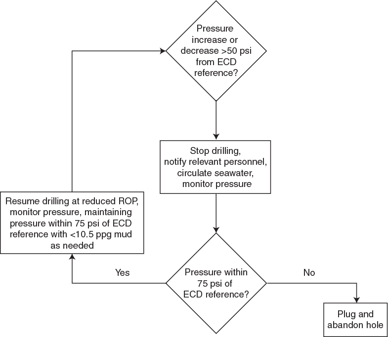
Figure F1. Safety decision tree for LWD/MWD pressure monitoring.
In addition to safety monitoring, we also analyzed the APWD to define whether annular conditions are below (negative APWD) or above (positive APWD) hydrostatic pressure. For comparison to driller’s mud weight and riserless drilling conditions, we relate the APWD to the ECD relative to the seafloor (ECDrsf) (in pounds per gallon or parts per gallon):
- PAPWD = APWD sensor reading (in pounds per square inch),
- Pwsf = hydrostatic pressure at seafloor (in pounds per square inch),
- DAPWD = true vertical depth of the APWD sensor referenced to the rig floor (in feet),
- Dw = water depth (in feet),
- RKB = distance from the sea level to the rig floor (in feet), and
- 0.0519 = conversion factor.
Hydrostatic pressure at the seafloor (Pwsf) can be calculated by the ECD of seawater (ECDsw) and the water depth (Dw):
where we assume an ECDsw of 8.54 lb/gal based on an average seawater density of 1024 kg/m3.
IODP depth conventions
The primary drilling and coring depth scales used during Expedition 375 were based on the length of the drill string deployed (e.g., drilling depth below rig floor [DRF] and drilling depth below seafloor [DSF]) and the length of core recovered (e.g., core depth below seafloor [CSF]) (see IODP Depth Scales Terminology at http://www.iodp.org/policies-and-guidelines). The logging depth scale used during Expedition 375 was based on the length of logging wireline deployed (e.g., wireline log depth below rig floor [WRF] and wireline log depth below seafloor [WSF]). In cases where multiple logging passes are made, wireline log depths are mapped to one reference pass, creating the wireline log matched depth below seafloor (WMSF) scale. During Expedition 372, LWD and MWD were measured on the LWD depth below seafloor (LSF) scale. LWD data are measured by time and are depth-corrected after data acquisition. All depths are in meters. The relationship between scales is defined either by protocol, such as the rules for computation of CSF from DSF, or by user-defined correlations, such as core-to-log correlation. The distinction in nomenclature should keep the reader aware that a nominal depth value in different depth scales usually does not refer to the exact same stratigraphic interval.
Depths of cored intervals are measured from the drill floor based on the length of drill pipe deployed beneath the rig floor (DRF scale). The depth of the cored interval is referenced to the seafloor (DSF scale) by subtracting the seafloor depth of the hole from the DRF depth of that interval. Standard depths of cores in meters below the seafloor (CSF-A scale) are determined based on the assumptions that (1) the top depth of a recovered core corresponds to the top depth of its cored interval (DSF scale) and (2) the recovered material is a contiguous section even if core segments are separated by voids when recovered. Standard depths of samples and associated measurements on the CSF-A scale are calculated by adding the offset of the sample or measurement from the top of its section and the lengths of all higher sections in the core to the top depth of the core.
If a core has <100% recovery, for curation purposes all cored material is assumed to originate from the top of the drilled interval as a continuous section. In addition, voids in the core are closed by pushing core segments together, if possible, during core handling at the core receiving area. Therefore, the true depth interval within the cored interval is unknown and should be considered a sampling uncertainty (e.g., in age-depth analysis or in correlation of core data with downhole logging data).
When core recovery is >100% (the length of the recovered core exceeds that of the cored interval), the depth of a sample or measurement taken from the bottom of a core will be deeper than that of a sample or measurement taken from the top of the subsequent core (i.e., the data associated with the two core intervals overlap on the CSF-A scale). This overlap can happen when a soft-sediment core expands upon recovery (e.g., due to release of gas or removal of overburden pressure) (typically by a few percent to as much as 15%). The CSF-B depth scale is a solution to the overlap problem. This method scales the recovered core length back into the interval cored from >100% to exactly 100% recovery.
In this volume, unless otherwise noted, depths below rig floor are reported as meters below rig floor (mbrf), core depths below seafloor are reported as meters below seafloor (mbsf) using the CSF-B depth scale, and wireline logging and LWD depths below seafloor are also reported as meters below seafloor.
Curatorial procedures and sample depth calculations
Numbering of sites, holes, cores, and samples followed standard IODP procedure. A full curatorial identifier for a sample consists of the following information: expedition, site, hole, core number, core type, section number, section half, piece number (hard rock only), and interval in centimeters measured from the top of the core section. For example, a sample identification of “375-U1518E-2H-5W, 80–85 cm” indicates a 5 cm sample removed from the interval between 80 and 85 cm below the top of Section 5 (“W” indicates the working half) of Core 2 (“H” designates that this core was taken with the APC system) of Hole E at Site U1518 during Expedition 375 (Figure F2). The “U” preceding the hole number indicates the hole was drilled by the United States platform, the JOIDES Resolution. The drilling system used to obtain a core is designated in the sample identifiers as follows:
Integers (instead of a letter) are used to denote the “core type” of drilled intervals (e.g., the drilled interval at the top of Hole U1520C is denoted as Core 11, and the first RCB core that follows it is denoted as Core 2R).
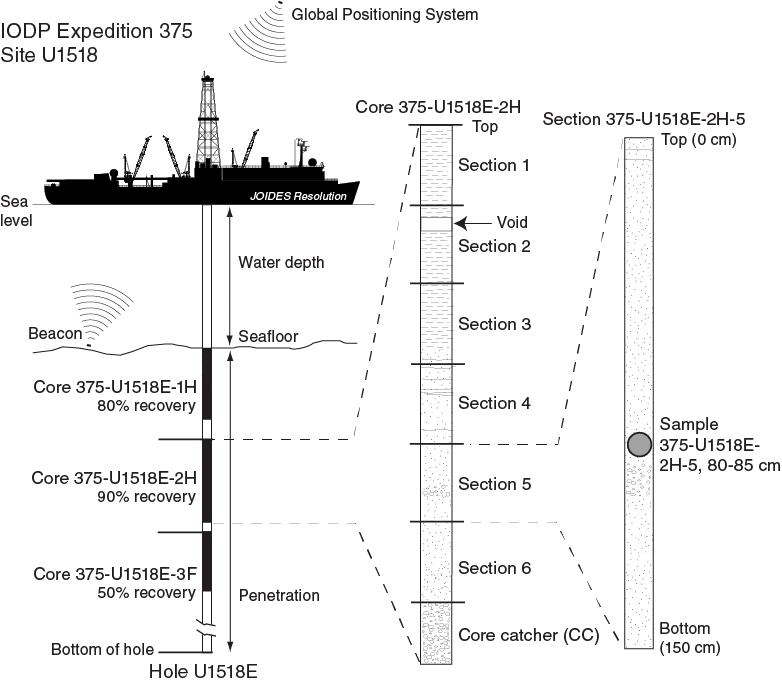
Figure F2. IODP naming convention.
Core handling and analysis
When the core barrel reached the rig floor, the core catcher from the bottom of the core was removed, and a short whole-round (WR) sample was typically extracted for paleontologic (PAL) analysis in sediment. Next, the core was extracted from the core barrel in its plastic liner. The liner was carried from the rig floor to the core receiving area on the catwalk outside the core laboratory, where it was curated.
Typically, the core was cut into ~1.5 m segments. In some cases, the lengths of sections were adjusted so that WR samples could be taken for interstitial water (IW) chemical analyses. At some sites where gas hydrate was anticipated, an infrared (IR) camera was used to examine the core for cold spots that would indicate the local presence of hydrate for two reasons: (1) to avoid hydrate-bearing intervals for routine IW sampling and (2) to target these intervals for calibrating shipboard chemical analyses or for collecting personal hydrate samples for post-expedition analyses. Next, syringe samples were taken for headspace gas analyses and personal microbiology samples, and occasionally vacuum tube samples were taken for additional gas analyses. Once all catwalk samples were collected, blue (uphole direction) and clear (downhole direction) liner caps were glued onto the cut liner sections with acetone. Yellow caps were used instead of clear caps to denote missing intervals where WR samples were removed.
Core sections were then placed in a core rack in the laboratory. When core sections reached equilibrium with laboratory temperature (typically after 4 h), they were run through the Whole-Round Multisensor Logger (WRMSL) for P-wave velocity (P-wave logger [PWL]), magnetic susceptibility (magnetic susceptibility logger [MSL]), and gamma ray attenuation (GRA) bulk density (see Physical properties). PWL was typically not measured for RCB cores. Core sections were also run through the Natural Gamma Radiation Logger (NGRL), and thermal conductivity measurements were taken when the material was suitable. Once all WR measurements were completed, additional WR personal samples were taken for post-expedition geotechnical, mechanical, and physical properties analyses.
Core sections were split lengthwise from bottom to top into working and archive halves. Investigators should note that deeper sedimentary material can be transported upward on the split face of each section during the splitting process. For hard rock, a diamond-impregnated saw was used to split sections.
The working half of each core was described by the structural geologists after discrete samples were taken for moisture and density (MAD) and personal biomarker analyses. Once description was complete, clustered samples were taken next to each WR sample for shipboard X-ray diffraction (XRD), carbonate (CARB) analyses, and a few shore-based studies. Paleomagnetic samples were then taken from undisturbed portions of the core, followed by all other personal samples based on the sampling plan agreed upon by the science party and shipboard curator. Discrete thermal conductivity and P-wave samples were also taken for lithified sediment or hard rock. Sampling of certain critical intervals (such as the fault zone at Site U1518) was delayed until all personal samples could be prioritized. Samples were not collected when the lithology was unsuitable or the core was severely deformed.
The archive half of each core section was scanned on the Section Half Imaging Logger (SHIL) and measured for point magnetic susceptibility (MSP) and reflectance spectroscopy and colorimetry (RSC) on the Section Half Multisensor Logger (SHMSL). Labeled foam pieces were used to denote missing WR intervals in the SHIL images. The archive halves were then described visually and with smear slides for sedimentology. Finally, the magnetization of archive-half sections and working-half discrete pieces was measured with the cryogenic magnetometer and spinner magnetometer, respectively.
When all steps were completed, cores were wrapped, sealed in plastic tubes, and transferred to cold storage space aboard the ship. At the end of the expedition, the cores were sent to cold storage at the IODP Gulf Coast Repository in College Station, Texas (USA).
Drilling and handling core disturbance
Cores may be significantly disturbed and contain extraneous material as a result of the coring and core handling process (Jutzeler et al., 2014). In formations with loose sand layers, sand from intervals higher in the hole may be washed down by drilling circulation, accumulate at the bottom of the hole, and be sampled with the next core. The uppermost 10–50 cm of each core must therefore be examined critically during description for potential “fall-in.”
Common coring-induced deformation in APC and HLAPC cores includes the concave-downward appearance of originally horizontal bedding. Piston action can result in fluidization (flow-in) at the bottom of the cores. Additionally, retrieval from depth to the surface can result in elastic rebound. Gas that is in solution at depth may become free and drive core segments apart in the liner. When gas content is high, pressure must be relieved for safety reasons before the cores are cut into segments. This is accomplished by drilling holes into the liner, which forces some sediment, as well as gas, out of the liner. These disturbances are described in each site chapter and graphically indicated on the visual core descriptions (see Core descriptions).
Authorship of chapters
The separate sections of the site chapters were written by the following scientists (authors are listed in alphabetical order; see Expedition 372 scientists and Expedition 375 scientists for contact information):
- Background and objectives: Barnes, Petronotis, Saffer, Wallace
- Operations: Grigar (Operations Superintendent), LeVay, Petronotis
- Lithostratigraphy: Engelmann de Oliveira, Hashimoto, Kutterolf, Meneghini, Noda, Rabinowitz, Underwood
- Biostratigraphy: Crundwell, LeVay, Shepherd, Woodhouse
- Paleomagnetism: Greve, Li, Petronotis
- Structural geology: Fagereng, Morgan, Savage, M. Wang
- Geochemistry: Hüpers, Luo, Malie, Solomon, Torres
- Physical properties and downhole measurements: Fulton, Harris, Ikari, Ito, Kitajima, Lee, Shreedharan
- Logging while drilling: Clennell, Cook, Dugan, Elger, Gamboa, Han, Kim, Koge, McNamara, Moore, Paganoni, Shankar, X. Wang, Wu
- Core-log-seismic integration: Barnes, Bell, Elger, Gamboa, Han, Moore
- Observatory: Fulton, Petronotis, Saffer, Solomon, Wallace
Lithostratigraphy
This section outlines the procedures used to document the composition, texture, and sedimentary structures of the sediments and sedimentary rocks recovered during Expedition 375. The strategy for description and interpretation of core disturbance, both drilling induced and tectonic, is discussed in Structural geology. The routine procedures for lithostratigraphy include visual core description, smear slide and thin section analysis of texture and composition, digital color imaging, color spectrophotometry, bulk powder XRD, and carbon/carbonate analysis. XRD samples were co-located in “clusters” with samples for carbon/carbonate (see Geochemistry) and MAD analyses (see Physical properties). Clusters were immediately adjacent to most WR sample intervals, including those for IW.
Archive halves were used for sedimentologic description and petrographic observation. Sections dominated by unlithified sediment were split using a thin wire held in high tension. The split surface of each archive half was assessed for quality (e.g., smearing or surface unevenness) and, if necessary, gently scraped with a glass slide. Harder sedimentary rock was split with a diamond-impregnated saw. For cores with significant water pooling, we dried the archive half with paper towels prior to imaging. The archive half was imaged by the SHIL and then analyzed for color reflectance and magnetic susceptibility using the SHMSL (see Physical properties).
Following imaging, the archive halves were described macroscopically for lithologic attributes and sedimentary structures, aided by use of a 20× wide-field hand lens and binocular microscope. We also enlarged digital images on a high-resolution monitor next to the description table. Visual inspection focused on textural variation, color, internal sedimentary structures (including soft-sediment deformation), and bed thickness. We also considered the severity of drilling/coring disturbance (see Structural geology for detailed assessment). Smear slide analysis, thin section petrography, and XRD were used to identify sedimentary constituents, including microfossils and minerals. For large clasts of igneous rocks, initial analysis focused on visual inspection of texture, grain size, color, contacts, and changes in primary and secondary mineralogy. All of the descriptive data were entered into DESClogik. All descriptions and sample locations were recorded using curated depths and documented on visual core description (VCD) graphic reports (Figure F3). We defined lithostratigraphic units and subunits using all forms of data. Units and unit boundaries were also correlated at the facies scale with logging unit designations from LWD logs (see Logging while drilling).
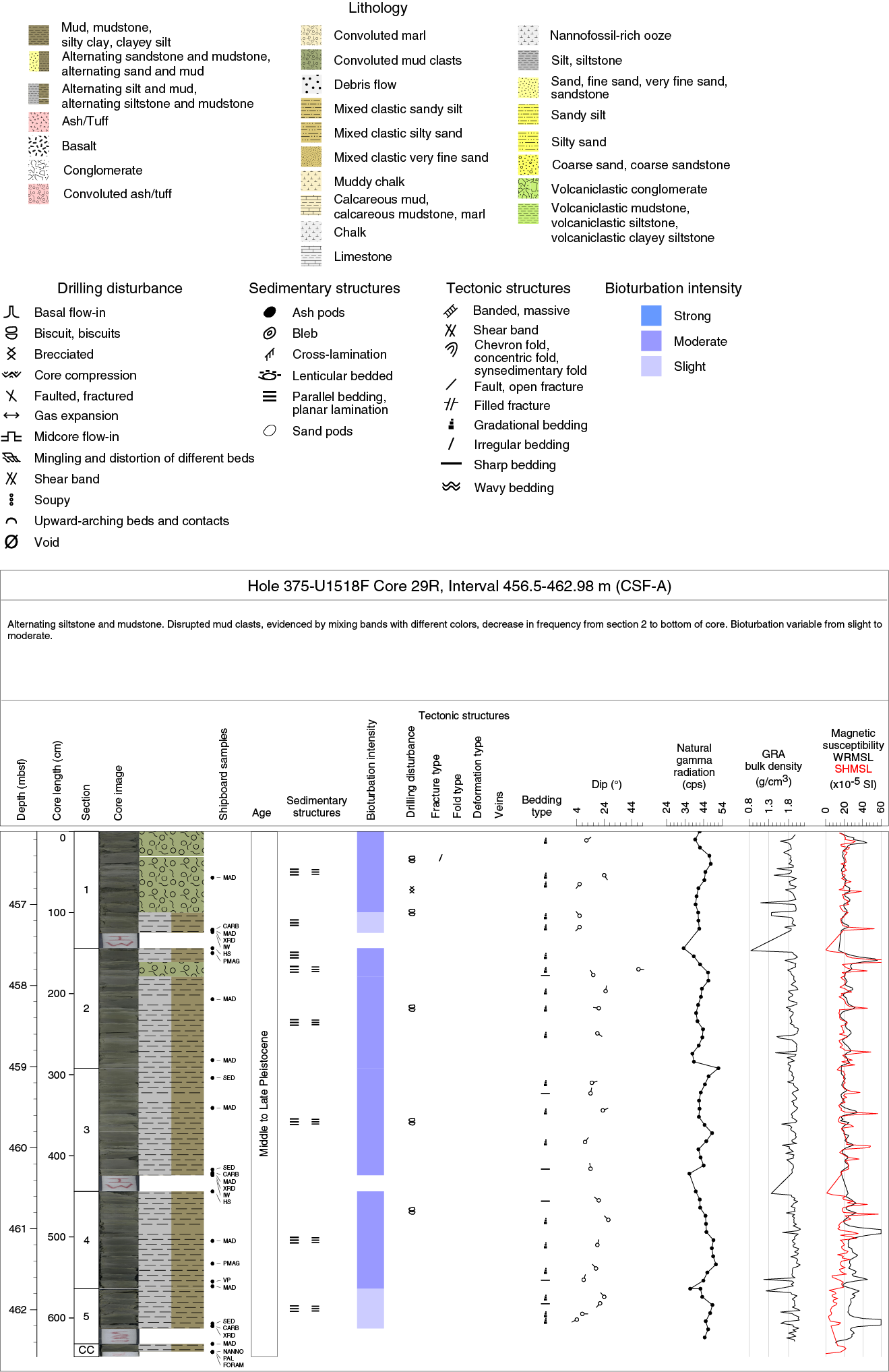
Figure F3. Graphic patterns and symbols and VCD sheet.
Visual core descriptions
Classification of lithology
We based each lithologic description on visual core description, supported by smear slide and thin section analysis of dominant and minor lithologies and bulk analysis of carbonate content. The following classification scheme, modified from Mazzullo and Graham (1988), emphasizes important descriptors that we recorded in DESClogik (Sediment tab in macroscopic spreadsheets; see DESC_WKB in Supplementary material). The modifications were tailored to the actual lithologies encountered during Expedition 375 and our desire to simplify terminology as much as possible. Lithologic names consist of a principal term based on texture, the dominant composition, and the degree of lithification.
The first discriminator (texture) follows the ternary scheme of Shepard (1954) (Figure F4). Ranges and boundaries for all grain size categories follow the conventional Wentworth (1922) definitions as used by Folk (1980), regardless of particle composition. The term “sand,” for example, refers to unconsolidated sediment with >75% sand-sized particles. Similarly, for cases in which silt-rich (>50%) sediment contains >25% sand, the term “sandy silt” is used. The lithology designations for siliciclastic material are based on grain size alone, although compositional modifiers can be added as desired (e.g., quartz-rich sand). Terminology for broader ranges of particle size can be cumbersome, so we grouped common mixtures. We apply the term “mud,” for example, to encompass the span of sizes from silty clay to clayey silt.
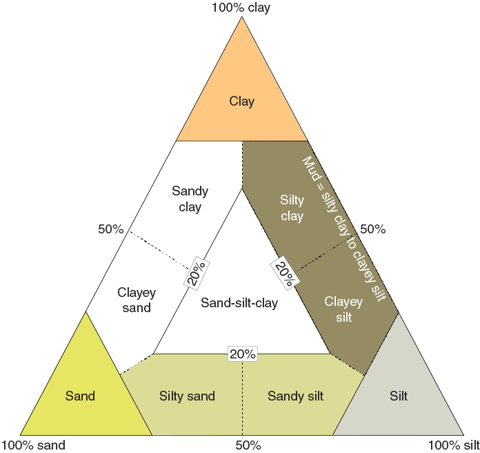
Figure F4. Classification of sediment.
Regardless of their particle size distributions, naturally occurring marine sediments usually contain mixtures of grain composition. Sediment with >75% biogenic debris is classified as pelagic, either biocalcareous or biosiliceous, based on the most abundant biogenic component (Figure F5). If the sediment contains <50% biogenic debris (calcareous or siliceous), then it is classified as either siliciclastic (implied terrigenous) or volcaniclastic based on the dominant nonbiogenic component (Figure F6). The classification for volcanic particles (Figure F7) is further guided by the scheme of Fisher and Schmincke (1984). In the broadest sense, “volcaniclasts” include the products of physical weathering and are commonly altered, heterogeneous assemblages of volcanic rock fragments, lava fragments, tuff fragments, crystals, and compositionally diverse glass shards and pumice. “Pyroclasts” constitute a subset of volcanic clasts and are defined here as fresh or relatively unaltered, compositionally homogeneous, unconsolidated particles (e.g., glass shards and pumice) that formed directly from magma fragmentation during explosive eruptions on land or effusive/explosive vents on the seafloor. If the volcanic clast population is >75% pyroclasts (tephra), then the sediment is divided further based on particle size: ash (<2 mm), lapilli (2–64 mm), bombs, or blocks (Fischer and Schmincke, 1984). In practice, our designations are meant to be purely descriptive, and it can be difficult to recognize each volcanic grain’s physical origin based on smear slide observations.
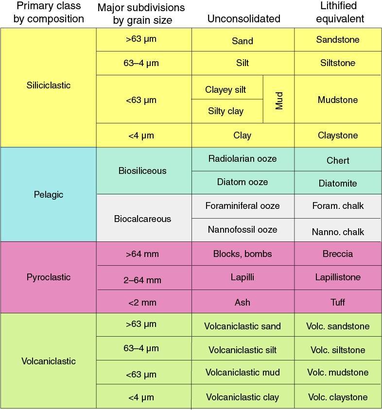
Figure F5. Classification of sediments and sedimentary rocks.
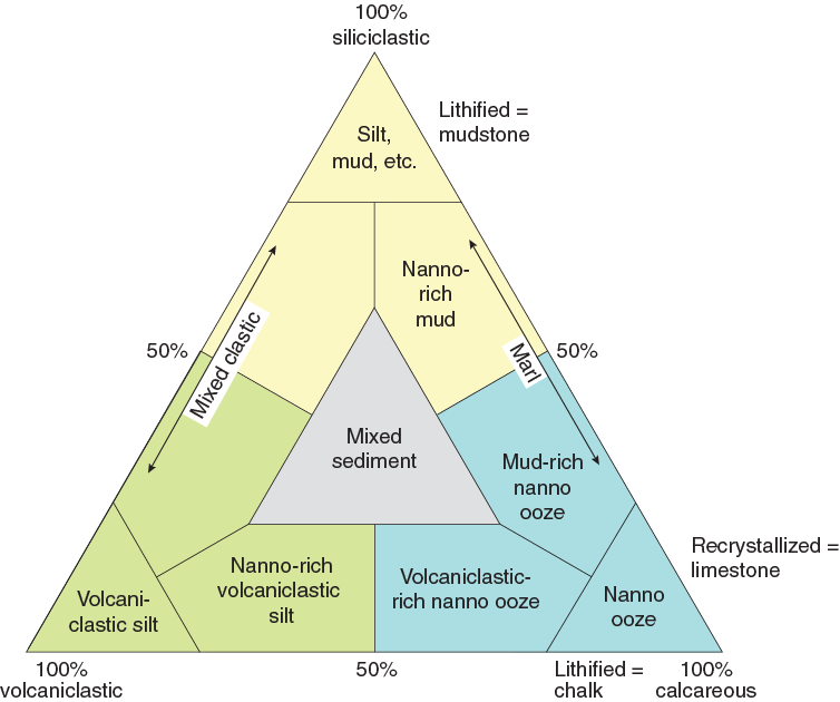
Figure F6. Continuum of compositional classes encountered.
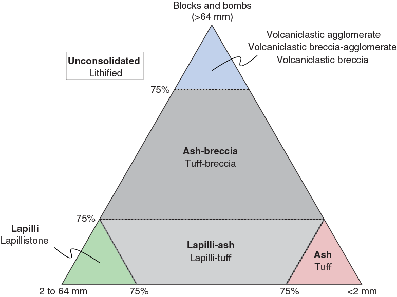
Figure F7. Classification of pyroclastic and volcaniclastic sediment and lithified rock.
The principal lithology name is typically preceded by major modifiers that refer to components making up 25%–50% of the sediment (e.g., calcareous or nannofossil-rich mud and volcaniclastic silty clay). Terms for the minor components (10%–25% of the total) follow the principal name (e.g., clayey silt with glauconite). As another example, an unconsolidated sediment containing 25% volcaniclastic grains, 10% nannofossils, 25% silt, and 40% clay would be termed “volcaniclastic silty clay with nannofossils.” Unconsolidated fine-grained pelagic sediment is classified as “ooze,” usually with a major modifier added to identify the dominant allochem (e.g., biosiliceous ooze and calcareous ooze). We insert additional modifiers to characterize specific microfossil categories (e.g., nannofossil ooze and foraminiferal ooze).
Inclusion of these additional criteria yields four compositional classes (Figure F5); each class carries the possibility of grain size distributions shown in Figure F4:
- Pyroclastic sediment (tephra) containing >75% volcanic particles of inferred primary eruptive origin,
- Volcaniclastic sediment containing >75% volcanic particles of detrital and/or primary eruptive origin,
- Siliciclastic sediment containing >75% terrigenous detritus, and
- Pelagic sediment (biosiliceous or biocalcareous) containing >75% biogenic particles.
End-member compositions are easy to recognize and classify using this approach. Difficulties arise with admixtures that are close to a dividing line between two compositional categories. To make the terminology as succinct as possible, we refer to roughly equal mixtures of siliciclastic silt (or sand) and volcaniclastic silt (or sand) as “mixed clastic” silt or sand (Figure F6). Similarly, we call roughly equal mixtures of fine-grained biocalcareous sediment and siliciclastic mud “muddy calcareous ooze” or “calcareous mud.”
Lithification
Lithification state can be inconsistent and dynamic, changing as a function of burial compaction, cementation, and localized tectonic consolidation. Perceptions of induration during core description can also be influenced by differential drying of the split core and differential coring disturbance between more cohesive and less cohesive interbeds. To be as objective as possible, our designations for all of the compositional and textural classes are based largely on the type of coring system. We routinely consider cores obtained with the APC or HLAPC system to be unconsolidated (e.g., sand, silty clay, volcanic ash, and biocalcareous ooze), whereas more consolidated siliciclastic sediment recovered with the XCB and RCB systems is designated as “-stone,” as in claystone, silty claystone, volcaniclastic sandstone, and so on (Figure F5).
For simplicity, we apply the general term “mudstone” to the broader range of lithified silty clay to clayey silt. Following the same rationale, lithified volcanic ash is designated “tuff.” Lithified biocalcareous ooze is termed “chalk,” and lithified biosiliceous ooze is called “chert” or “diatomite.” For lithified examples in which most or all of the biocalcareous particles have been replaced or obscured by small crystals of calcite, we use the term “limestone.” We assign the term “marl” to the broader range of lithified muddy calcareous ooze to lithified calcareous mud.
Color
Color was determined qualitatively during visual inspection using Munsell color charts. The archive halves were used to identify compositional and textural elements of the sediment and sedimentary rock, including rock fragments, sedimentary structures, and diagenetic features such as color mottling and the results of element mobility in diagenesis (e.g., manganese oxide segregation). Color reflectance spectral data were also collected, as outlined in Physical properties.
Sedimentary textures, structures, and fabric
For relatively coarse material (fine sand and larger), designations of grain size follow the Wentworth (1922) scale. Finer grained sediments require inspection at high magnification using smear slides (see below). In addition, the classifications for sorting and rounding follow the scheme of Folk (1980) (Figure F8).
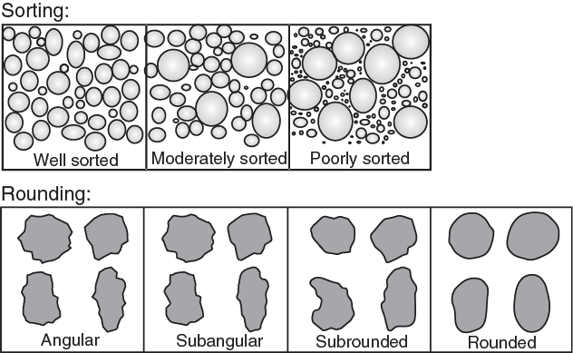
Figure F8. Classification of sediment sorting and roundness.
Sedimentary structures observed in the recovered cores (Figure F3) include bedding geometry, size grading (normal and reverse), plane-parallel laminae, soft-sediment deformation, bioturbation, and diagenetic effects. We assign bed thickness terms for recognizable event beds according to Ingram (1954):
- Very thick bedded = >100 cm.
- Thick bedded = >30–100 cm.
- Medium bedded = >10–30 cm.
- Thin bedded = >3–10 cm.
- Very thin bedded = 1–3 cm.
- Laminae = <1 cm.
Such designations are typically obscured by bioturbation in fine-grained sediments (see below) and distorted by drilling disturbance (e.g., biscuiting). In addition, picking the gradational tops of normally graded beds is usually subjective. Descriptions of the lower contacts of well-defined strata are based on geometry (irregular, planar, curviplanar, and wavy), shape or form (sharp and gradational), and orientation (subhorizontal, inclined, and horizontal). Sediment grading is described as nongraded, normally graded (fining upward), and reverse graded (coarsening upward). Contorted intervals and fragmentation of cohesive mud(stone) often result from gravitational soft-sediment deformation. Examples of such mass transport deposits (MTDs) can be difficult to discriminate with confidence from some types of coring disturbance and ductile tectonic deformation. Our designations of disturbed intervals are meant to be as descriptive as possible.
Bioturbation
Bioturbation intensity was recorded on the VCDs using a semiquantitative ichnofabric index (Figure F3) as described by Droser and Bottjer (1986, 1991), aided by visual comparative charts (Heard et al., 2014). The four-category index refers to the degree of biogenic disruption of primary depositional layering and grain fabric (e.g., laminae) by burrows, tracks, and trails, as summarized below:
- Nonbioturbated = no bioturbation recorded; all original sedimentary structures are preserved.
- Slight bioturbation = discrete, isolated trace fossils; as much as 10% of original bedding is disturbed.
- Moderate bioturbation = approximately 10%–60% of original bedding is disturbed; burrows largely overlap and are commonly poorly defined.
- Strong bioturbation = bedding is completely disturbed, but burrows can still be discerned in places; the fabric is not mixed, although the bedding may be nearly or totally homogenized.
Smear slides and thin sections
Smear slides are essential for identifying and reporting basic sediment attributes like textural and compositional constituents, but the results are semiquantitative at best (cf. Marsaglia et al., 2013, 2015). Most of the specimens during Expedition 375 were easily dispersed using a toothpick into their constituent detrital and biogenic particles for smear slide preparation. Some, but not all, of the lithified sediment designated as “-stone” disaggregated with more difficulty using a spatula but still sufficiently for smear slide examination. For highly indurated rocks, we used thin sections to verify composition and observe grain fabrics and potential mineral segregation associated with internal sedimentary structures and bioturbation.
Smear slides and thin sections were examined in transmitted polarized light using an Axioskop 40A polarizing microscope (Carl Zeiss) equipped with a Flex Spot digital camera. We estimated the abundance of biogenic, volcanogenic, and siliciclastic constituents using a visual comparison chart (Rothwell, 1989), with an emphasis on major lithologies. Particular attention was paid to the recognition of ash layers and mineral-rich sands. The results are summarized in the smear slides tables (see the microscopic spreadsheets in DESC_WKB in Supplementary material). We used reference images (Terry and Chilingar, 1955) to help guide visual estimates for normalized percentages of sand-, silt-, and clay-sized grains along with abundance for the individual grain types. The component categories are shown on the smear slide description sheet (Figure F9). Smear slides sampled from volcaniclastic layers were described in additional detail using a customized categorization of tephra components (Figure F10). Visual estimates of component abundance are reported as ranges of area percentage:
- T = trace (<0.1%).
- R = rare (0.1%–1%).
- P = present (1%–5%).
- C = common (5%–20%).
- A = abundant (20%–50%).
- D = dominant (>50%–80%).
- M = major (>80%).

Figure F9. Smear slide categories for sediment.
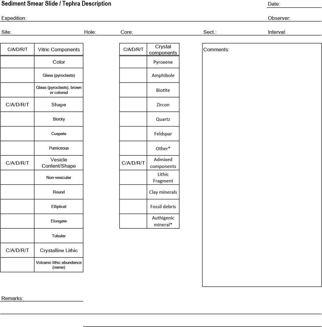
Figure F10. Smear slide categories for pyroclastic and volcaniclastic sediments.
Accurate estimates of area percentage can be difficult to make, especially in poorly sorted sediments. We validated the relative abundance of major to common components (quartz, feldspar, total clay, and calcite) by XRD (see below) and by the absolute weight percent of carbonate determined by coulometric analysis (see Geochemistry).
IODP use of DESClogik
Data for the macroscopic and microscopic descriptions of recovered cores were entered into the IODP Laboratory Information Management System (LIMS) database using the IODP data-entry software DESClogik. DESClogik is core description software used to store macroscopic and microscopic descriptions of cores. Core description data are available through the DESC LIMS Report (http://web.iodp.tamu.edu/DESCReport). A single row in DESClogik defines one descriptive interval, which is commonly one bed but may also be used, for example, to designate marked color variation that may be of diagenetic origin or thin interbeds that are too numerous or thin to subdivide. The same is true for disturbed intervals (possible MTDs). The minimum layer thickness for entry of a discrete lithology onto a VCD is 10 cm. For thin (<10 cm), repetitious interbeds of two lithologies (e.g., sandy silt and siliciclastic mud), the two individual graphics patterns are plotted side by side on the VCD (Figure F3). We recorded bed thickness for all volcaniclastic and siliciclastic event beds >1 cm on a separate spreadsheet to draft plots of occurrence frequency and thickness versus depth (see ash and silt layer spreadsheets in DESCRIPTION in Supplementary material). Those examples include intervals of alternating lithologies (e.g., thin interbeds of sandy silt and siliciclastic mud). In addition, the position of each smear slide is shown in the VCDs with a sample code of “SED.”
X-ray diffraction
Samples were selected from the working halves of core sections for analyses of bulk mineralogy by XRD. Sample depths are usually the same as for carbon/carbonate (see Geochemistry), MAD (see Physical properties), and shore-based clay-sized XRD. Most such clusters were positioned immediately adjacent to WR sample intervals, including those extracted for IW geochemistry (see Geochemistry). The bulk samples were freeze-dried and homogenized by grinding in a puck mill with tungsten carbide containers for 1 min to create fine powders. The randomly oriented powders were top mounted onto sample holders and scanned using a Bruker D4 Endeavor diffractometer mounted with a VANTEC-1 detector and nickel-filtered CuKα radiation. The routine locked-coupled scanning parameters were set as follows:
- Voltage = 40 kV.
- Current = 40 mA.
- Goniometer angle = 4°–40°2θ.
- Step size = 0.0166°2θ.
- Scan speed = 0.5 s/step.
- Divergence slit = 0.6 mm.
The XRD results for Expedition 375 provide relative abundances (in weight percent) of the most common mineral constituents spanning the range of lithologies: total clay minerals (smectite + illite + chlorite + kaolinite), quartz, feldspar (plagioclase + K-feldspar), and calcite.
The original plan for Expedition 375 was to process digital data on the JOIDES Resolution using the DIFFRAC.EVA software package; this software allows for baseline definition (set at enhanced, 1.000 curvature, and 1.000 threshold) and smoothing (set at smooth default factor = 0.124). Diagnostic peak areas (in units of counts/s × angle, measured above the baseline) for each mineral (or mineral group) can be determined using the “create area” function in DIFFRAC.EVA; this function accommodates manual adjustment of the upper and lower limits of the diagnostic peaks (Table T2). Failure of a circuit board on the diffractometer, however, necessitated its replacement and replacement of the detector during the port call at the end of Expedition 375. As a consequence, we were not able to process any of the XRD data during the expedition. Instead, all of the scans were finished during a transit to the Philippines following IODP Expedition 376 (July 2018), and the data were processed on shore using MacDiff software (version 4.2.5). We archived the data files for each analysis in the LIMS database (saved in RAW file format). The MacDiff software accommodates definition of the baseline, smoothing of counts, and small shifts in peak position to correct for misalignment of the detector and/or shifts in the height of the specimen surface relative to the X-ray beam. The units for peak intensity values are counts/step, and integrated peak areas are in units of total counts. Figure F11 shows a representative diffractogram generated by MacDiff, with identification of the diagnostic peaks for minerals of interest.
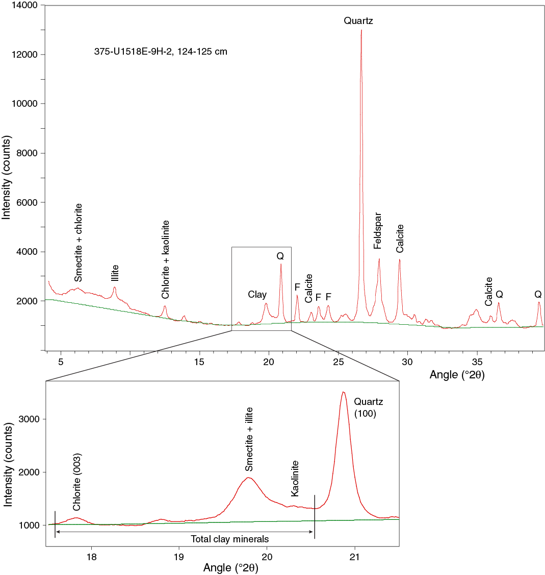
Figure F11. Representative X-ray diffractogram.
Comparisons between MacDiff and DIFFRAC.EVA versions of the diffractograms, and their sensitivities to different peak manipulation tools, are included in an assessment of error by M.B. Underwood and N. Lawler (unpubl. data). For quantitative analysis of composition, we computed relative mineral abundance using equations derived from calibrations using standard mineral mixtures. Twenty mixtures of standard minerals with known weight percentages were analyzed twice, both before and after the Bruker detector was replaced. Average peak area values were used to solve for polynomial regressions of the relation between integrated peak area and mineral abundance (Figure F12). Scans of nominally pure calcite (Cyprus chalk), quartz (St. Peter sandstone), feldspar (plagioclase mix), and smectite (Ca-montmorillonite + Na-montmorillonite) were included in the regression analyses to anchor the curves at high concentrations. The amounts of contamination in the nominally pure illite, smectite, and calcite standards were computed by iteration, and their absolute weight percentages in the total mixtures were recalculated. The regression curves are nonlinear because of asymmetric peak geometries and complex responses of peak intensity and peak broadening as concentrations of the individual minerals increase. Using the corrected values of weight percent for each major component in the mixtures, all of the correlation coefficients are approximately r = 0.99 (Figure F12).
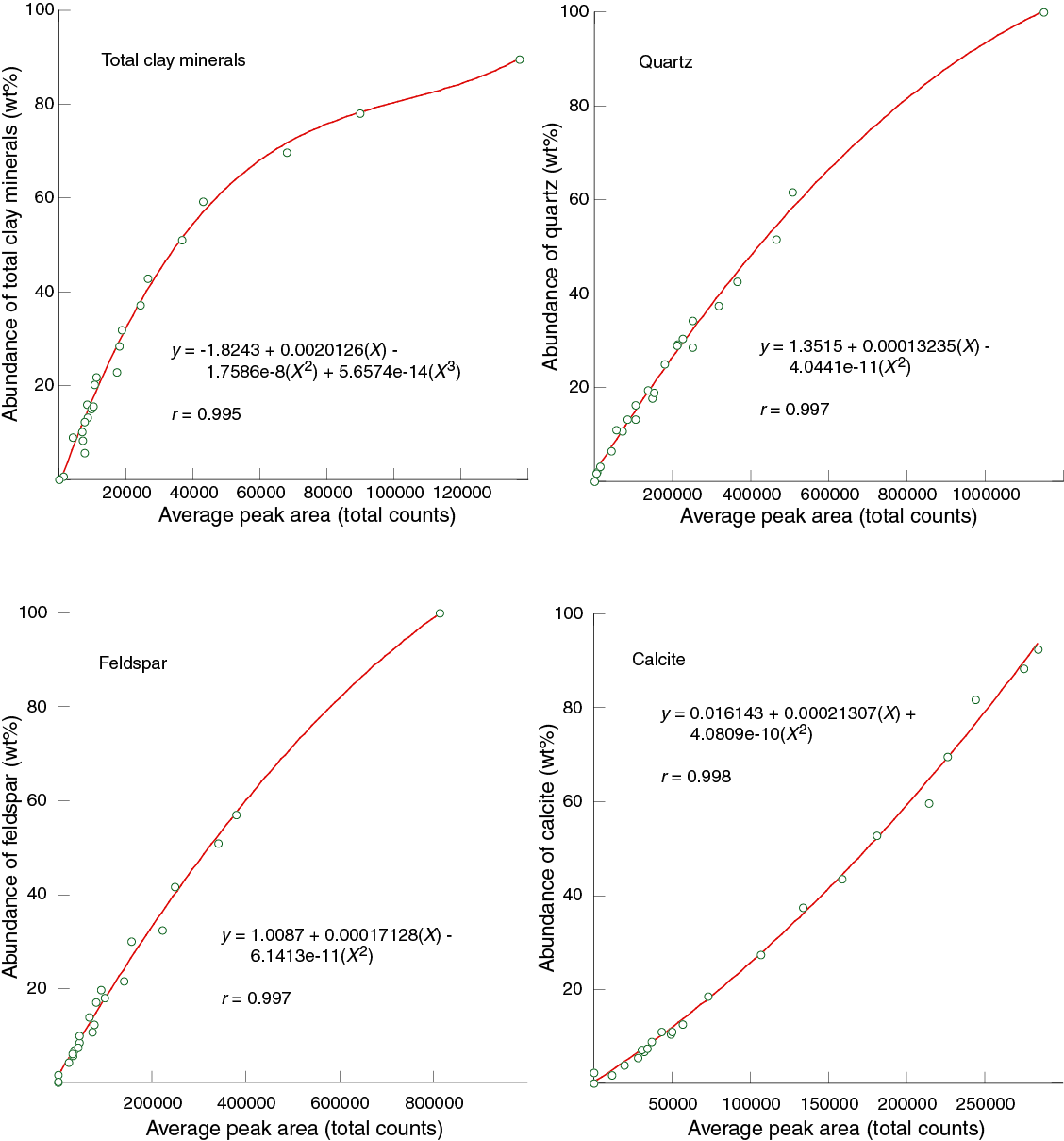
Figure F12. Regression curves.
In most cases, the computed weight percentages of the four common minerals (or mineral groups) add up to <100%, so the values were normalized to 100%. Accuracy errors were assessed by computing the difference between the measured weights of individual standard minerals in the freeze-dried powders and their normalized abundances calculated from the regression equations (Figure F12). The average errors for the standards are 1.32 wt% for total clay minerals, 1.25 wt% for quartz, 0.93 wt% for feldspar, and 1.02 wt% for calcite. We obtained an independent test of accuracy for calcite by comparing XRD-derived weight percent values with Ca carbonate values from shipboard coulometric analysis using the full range of data from Site U1520 (Figure F13). The usual expectation is for the normalized relative percentage of calcite to exceed the absolute value of CaCO3. This comparison, however, turned out to be flawed because of a mismatch between the calcite standard (nannofossil-rich Cyprus chalk) and variably recrystallized calcite in the lithified marls and chalks from Site U1520. Peaks intensity values for the recrystallized calcite are significantly higher than those generated by unaltered calcareous nannofossils. As a consequence, some of the computed weight percent values of calcite (XRD) exceed 100% of the bulk powder (Figure F13). Additional documentation of the standards, with representative diffractograms, is provided by M.B. Underwood and N. Lawler (unpubl. data). Their error analysis also includes intralaboratory comparisons between software and interlaboratory comparisons between data generated by the Bruker D4 Endeavor diffractometer on the JOIDES Resolution versus scans of the same standards using a Panalytical X’Pert Pro diffractometer at the New Mexico Bureau of Geology and Mineral Resources.
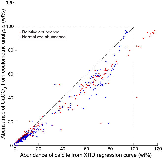
Figure F13. Statistical fits between relative and normalized abundance.
The main goal of the bulk powder XRD program during Expedition 375 was to provide reliable relative abundances of dominant minerals for a large number of specimens over a broad range of lithologies. Even though the error appears to be small for siliciclastic lithologies (Figure F12), the numerical results are only semiquantitative and should be interpreted with some caution. Fundamentally, the calculated mineral abundances represent relative percentages in a four-component system of total clay minerals + quartz + feldspar + calcite normalized to 100%. The closeness of those estimates to absolute percentages in the total solids depends largely on the abundance of dispersed amorphous solids (e.g., biogenic opal and volcanic glass) and the sum total of all other minerals that might occur in minor or trace quantities (e.g., pyroxene, pyrite, cristobalite, zeolites, and halite precipitated from interstitial water).
The mismatches between standards and natural specimens increase if their respective mineral mixtures differ significantly. For example, if other phyllosilicates (e.g., metamorphic white mica and coarse chlorite crystals) contribute to the peak area value for total clay minerals, especially in silt-rich sediments, their higher crystallinities will result in peak sharpening and skew results to larger estimates of total clay minerals. In addition, values of peak intensity and peak area for one individual mineral will be influenced not only by that mineral’s absolute abundance but also by the absolute abundances of all other minerals in the aggregate sample (Fisher and Underwood, 1995). Another factor to consider, although largely accommodated by the use of standards to calibrate regression equations, is the contrast in peak intensity response between peaks generated by small, poorly crystalline minerals at low diffraction angles (e.g., clay minerals) and those of highly crystalline minerals at higher diffraction angles (e.g., quartz and plagioclase).
All things considered, our accuracy errors for the widespread siliciclastic lithologies cored during Expedition 375 are smaller than those documented during other drilling expeditions that attempted “quantitative” XRD (e.g., Fisher and Underwood, 1995; Shipboard Scientific Party, 2001; McNeill et al., 2017). Among all of the factors to consider in the reduction of error, the most important is probably the accurate assessment of contaminants in the standards (e.g., percentage of quartz in illite standard) together with recalculation of all weight percentage values. For carbonate lithologies at Site U1520, we reduced the error shown in Figure F13 by substituting the value of CaCO3 from coulometric analyses for XRD-calcite. We then multiplied the residual (100% − CaCO3) by the relative abundances of total clay minerals, quartz, and feldspar from XRD. We also reduced errors by extending the peak area limits for total clay minerals to include the chlorite (003) reflection (Figure F11).
Biostratigraphy
The primary objectives of shipboard biostratigraphic analysis were to provide age models and develop an integrated biostratigraphy for all drill sites. Secondary objectives were to identify changes in paleowater depths and intervals of reworking to help elucidate the history of sedimentation and deformation along the Hikurangi margin.
Preliminary age assignments during Expedition 375 were based on biostratigraphic analyses using calcareous nannofossils, planktonic and benthic foraminifers, and bolboformids from 5–10 cm long WR samples. Most samples were from core catchers, or the bases of cores, but additional split-core samples were taken where appropriate to better define some datums and zonal boundaries. In addition to the abundance and preservation of the major microfossil groups, the presence of other microfossil groups, including shell fragments, micromollusks, ostracods, otoliths, bryozoan fragments, echinoid spines and plates, fish teeth and remains, radiolarians, diatoms, and sponge spicules, was routinely monitored.
The 2012 geologic timescale (GTS2012; Gradstein et al., 2012) was used during Expedition 375 in conjunction with the New Zealand geological timescale (Raine et al., 2015) to facilitate the integration of the Expedition 375 data with regional geological and seismic data (Figures F14, F15, F16, F17).
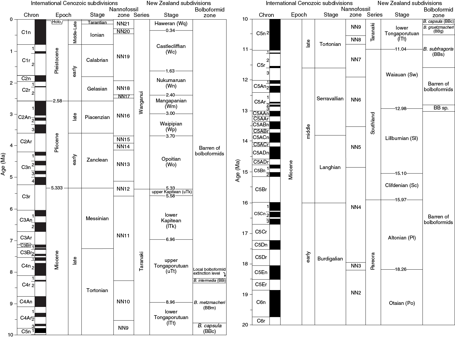
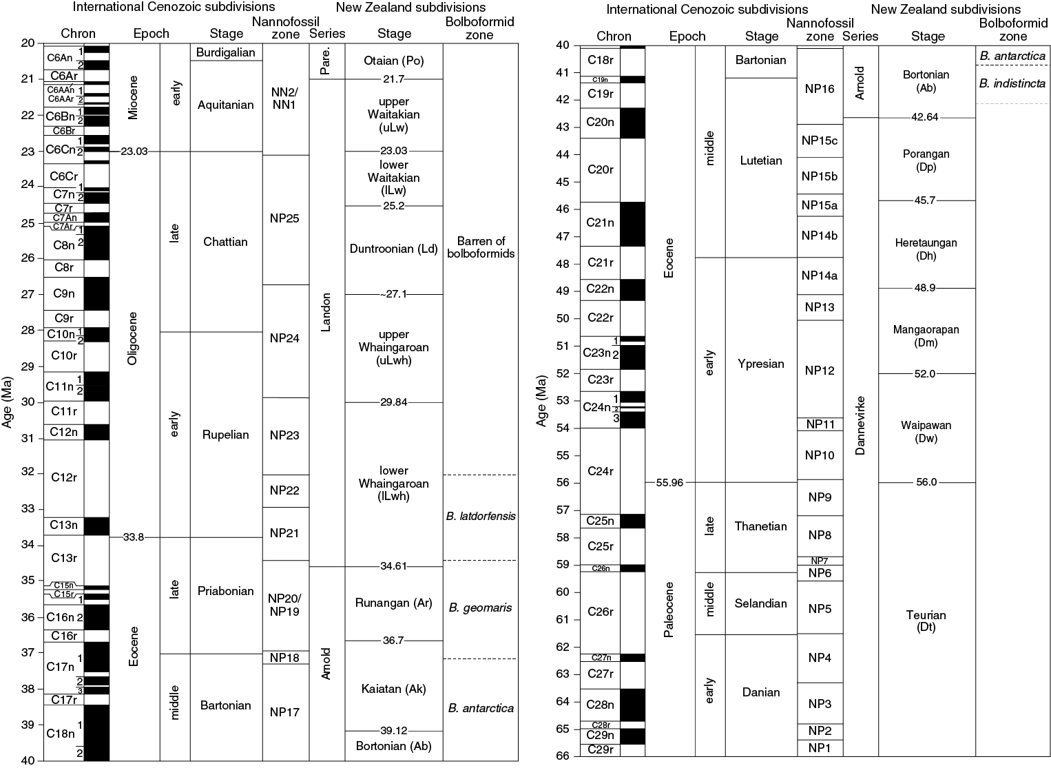
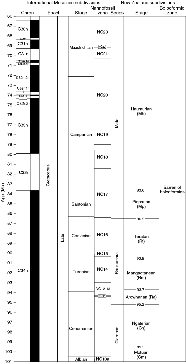
Figure F14. Cenozoic and Late Cretaceous chronostratigraphic units.
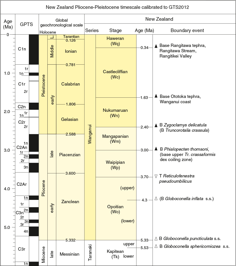
Figure F15. New Zealand Pliocene–Holocene timescale.
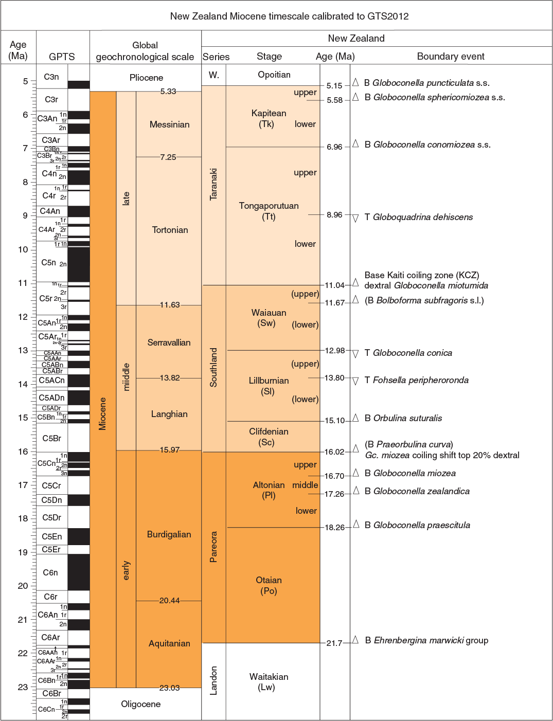
Figure F16. New Zealand Miocene timescale.
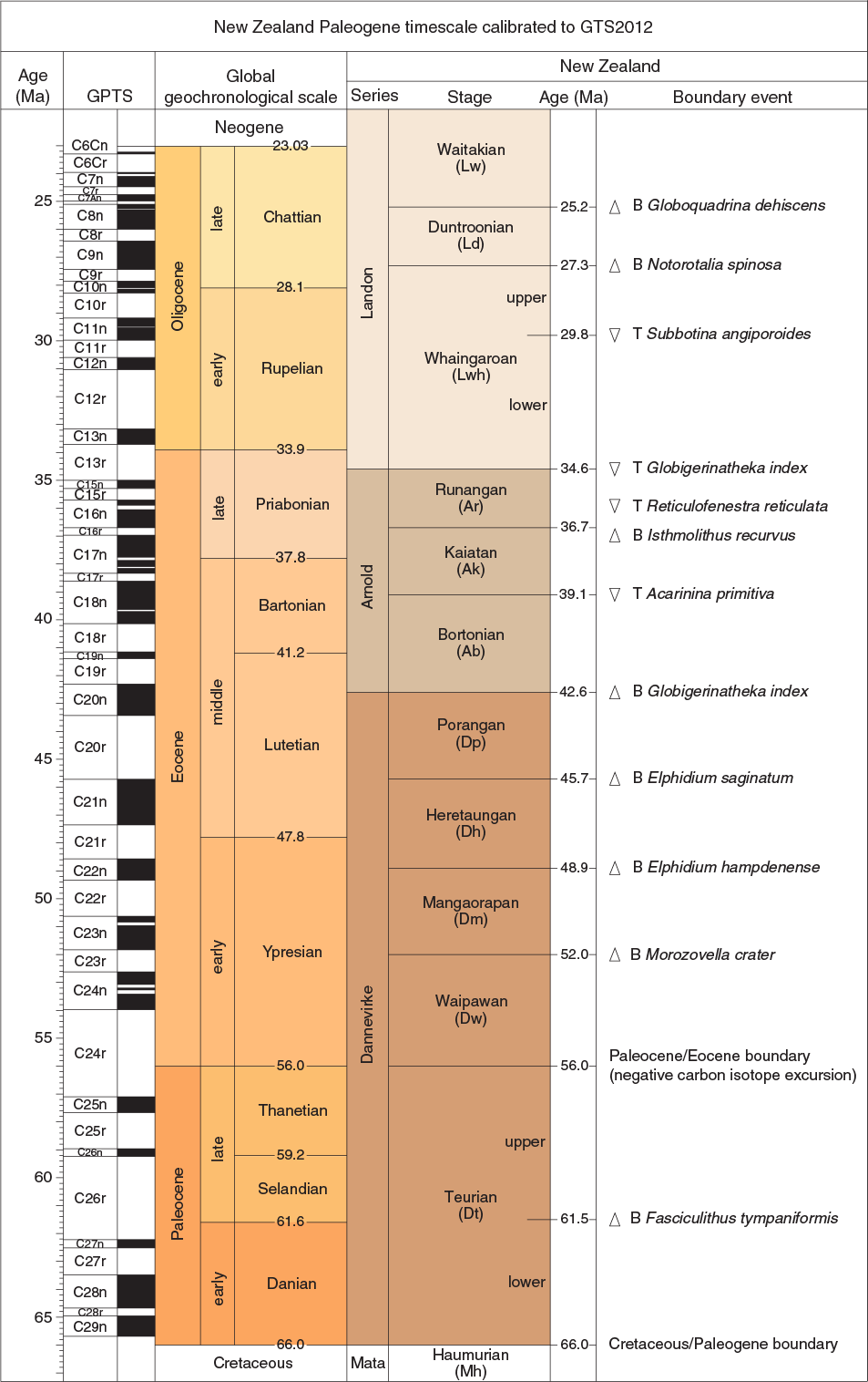
Figure F17. New Zealand Paleogene timescale.
Calcareous nannofossils
Calcareous nannofossil zones are based on the scheme of Martini (1971) (NN and NP) with ages calibrated to GTS2012 (Gradstein et al., 2012) (Table T3).
Considerable variation in the size and morphological features of species in the genus Gephyrocapsa, which are commonly used as Pleistocene biostratigraphic markers, often causes problems in identification (e.g., Samtleben, 1980; Su, 1996; Bollmann, 1997). We utilized size-defined morphological groups of this genus as event markers (Young, 1998; Maiorano and Marino, 2004; Lourens et al., 2004; Raffi et al., 2006), including small Gephyrocapsa spp. (<3.5 µm), medium Gephyrocapsa spp. (≥4 µm), and large Gephyrocapsa spp. (≥5.5 µm).
Differentiation in and between “species” of Reticulofenestra that are used as Cenozoic biostratigraphic markers is often problematic (e.g., Backman, 1980; Su 1996; Young, 1998). We adopt the definition of Reticulofenestra pseudoumbilicus by Young (1998) as having a maximum coccolith length >7 µm, with smaller forms recorded as R. pseudoumbilicus 5–7 µm.
Taxonomic concepts for other species follow those of Perch-Nielsen (1985), Bown (1998, 2005), Dunkley Jones et al. (2009), and Shamrock and Watkins (2012), as compiled in the online Nannotax3 database (http://www.mikrotax.org/Nannotax3).
Methods
Calcareous nannofossil smear slides were prepared from core catcher samples using standard techniques. In some instances, strewn slides were prepared by mixing a small amount of sediment in a buffered solution (pH = ~8.5), which was left for 10–15 s to allow larger particles to settle before the suspended sediment was transferred with a pipette to a coverslip and placed on a warming plate to dry. Once dry, the coverslip was affixed to a glass microscope slide using Norland optical adhesive Number 61 and cured under ultraviolet light.
Slides were analyzed using a Zeiss Axiophot microscope at 400× to 1250× magnification in plane-transmitted light, cross-polarized light, and phase-contrast light. All light microscope images were taken using a Spot RTS system with the IODP Image Capture and Spot commercial software. Selected samples were observed using a Hitachi TM3000 scanning electron microscope (SEM) to verify the presence of small forms.
Nannofossil preservation was noted as follows:
- G = good (little or no evidence of dissolution and/or overgrowth was observed, primary morphological features are slightly altered, and specimens were identifiable to the species level).
- M = moderate (specimens exhibit some dissolution and/or overgrowth, primary morphological features are somewhat altered, but most specimens were identifiable to the species level).
- P = poor (severe dissolution, fragmentation, and/or overgrowth was observed, primary morphological features are largely destroyed, and most specimens could not be identified at the species and/or generic level).
Intermediate categories (e.g., G/M or M/P) were used in some cases to better describe the state of preservation of calcareous nannofossil assemblages.
Total nannofossil abundance in the sediment was visually estimated at 1000× magnification and reported using the following categories:
- D = dominant (>90% of sediment particles).
- A = abundant (>50%–90% of sediment particles).
- C = common (>10%–50% of sediment particles).
- F = few (1%–10% of sediment particles).
- R = rare (<1% of sediment particles).
- B = barren (no calcareous nannofossils).
The relative abundance of individual calcareous nannofossil species or taxa groups was estimated at 1000× magnification and noted as follows:
- D = dominant (>100 specimens per field of view).
- A = abundant (>10–100 specimens per field of view).
- C = common (>1–10 specimens per field of view).
- F = few (1 specimen per 1–10 fields of view).
- R = rare (<1 specimen per 10 fields of view).
- * = reworked (presence of species interpreted to be reworked).
- ? = questionable (questionable specimen of that taxon).
Foraminifers and bolboformids
Locally calibrated ages were used for all Neogene and Quaternary planktonic foraminifer and bolboformid datums based on Cooper (2004), Crundwell (2004), Crundwell et al. (2004) (Figure F18), and Crundwell and Nelson (2007). The ages of other planktonic foraminifer datums are from Gradstein et al. (2012), and benthic foraminifer ages are emended after Cooper (2004) (Table T4). Foraminifer criteria for the adopted marine paleoenvironmental classification, modified after Hayward et al. (1999), are shown in Figure F19.
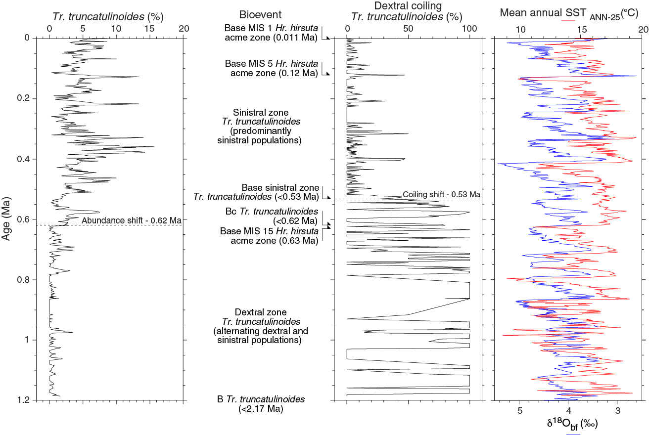
Figure F18. Site 1123 Truncorotalia truncatulinoides data.
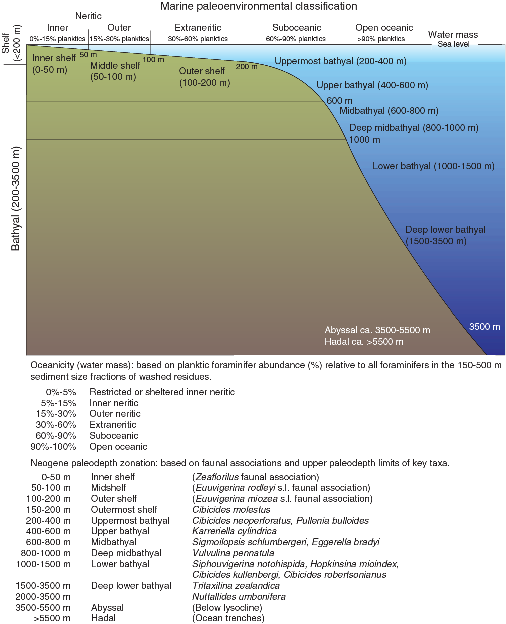
Figure F19. Marine paleoenvironmental classification.
The taxonomy of Quaternary and Neogene planktonic foraminifers follows a modified version of the phylogenetic classification of Kennett and Srinivasan (1983). Abbreviations for common genera and species qualifiers are given in Table T5. Species concepts are primarily based on Hornibrook (1981, 1982), Hornibrook et al. (1989), Scott et al. (1990), Hornibrook and Jenkins (1994), Crundwell and Nelson (2007), Crundwell (2015a, 2015b), and Schiebel and Hemleben (2017).
The taxonomy and biostratigraphy of Paleogene planktonic foraminifers follows Hornibrook et al. (1989), Spezzaferri (1994), Olsson et al. (1999), Pearson et al. (2006), and Pearson and Wade (2015). The taxonomy and biostratigraphy of Cretaceous planktonic foraminifers is based primarily on recent taxonomic and biostratigraphic discussions by Petrizzo and Huber (2006), Huber and Leckie (2011), Huber et al. (2017), and M.R. Petrizzo (pers. comm., 2017). The taxonomy and biostratigraphy of Cenozoic benthic foraminifers is based on Vella (1957), Hornibrook (1961), Hornibrook et al. (1989), Hayward et al. (1999, 2010, 2013), and Cooper (2004). The taxonomy and biostratigraphy of Neogene bolboformids is based on Spiegler and von Daniels (1991), Grützmacher (1993), Spiegler (1999), Spiegler and Spezzaferri (2005), Crundwell et al. (2005), and Crundwell and Nelson (2007).
Qualifiers for taxa identified in this study are as follows:
- cf. = confer (compare with).
- aff. = affinis (affinity with).
- sp. = unidentified species assigned to the genus.
- spp. = more than one unidentified species assigned to the genus.
- ? = identification uncertain.
Methods
Samples (typically 5–10 cm long whole rounds) were prepared by manually breaking the core into small pieces and soaking them in hot water with a few drops of detergent. After ~5–10 min, samples were disaggregated and sieved to 125 µm to remove mud and very fine sand. The washed residue retained on the sieve was dried at 150°C in an oven and divided with a microsplitter into equal aliquots for examination. As a precaution against cross-contamination, sieves were cleaned with jetted water and rinsed with methylene blue solution between successive samples.
The percentage of planktonic foraminifers relative to total foraminifers was determined quantitatively from random counts of 100 foraminifers in the 500–150 µm grain size fractions of the washed microfossil residues. This was done to determine oceanicity (qualitative measure of the extent to which the paleoenvironment recorded by the faunal assemblage represents open ocean conditions relative to a nearshore-influenced environment) and identify samples with reworked material (i.e., typically samples with planktonic abundance <90%). Age and depth markers were then picked from successive 500–300, 300–212, and 212–150 µm grain size fractions and mounted on 60-division faunal slides coated with gum tragacanth. As time allowed, other species and microfossils were also picked and mounted on the same slides. In most cases, the 500–212 µm grain size fraction was examined, although in samples where age diagnostic species were difficult to find and from stratigraphic levels where bolboformids were likely to be present, the 212–150 and 150–125 µm size fractions were also examined.
During the examination of microfossil samples, the abundance of foraminifers, bolboformids, and other fossil groups in the 150–500 µm grain size fractions of washed samples was determined visually and categorized as follows:
- D = dominant (foraminifers compose >50% of the washed sample).
- A = abundant (foraminifers compose >20%–50% of the washed sample).
- C = common (foraminifers compose >5%–20% of the washed sample).
- F = few (foraminifers compose 1%–5% of the washed sample).
- R = rare (foraminifers compose <1% of the washed sample).
- X = present (present in sample; abundance undetermined).
In addition, the preservation of foraminifers and bolboformids was categorized as follows:
- VG = very good (specimens were mostly whole, ornamentation and surface ultrastructure were very well preserved, and no visible modification of the test wall).
- G = good (specimens were often whole, ornamentation and surface ultrastructure were preserved but sometimes abraded or overgrown, and visible evidence of modification of the test wall).
- M = moderate (specimens were often etched or broken, ornamentation and surface ultrastructure were modified, and the majority of specimens were identifiable to species level).
- P = poor (most specimens were crushed or broken, recrystallized, diagenetically overgrown, or infilled with crystalline calcite and most specimens were difficult to identify to species level).
Planktonic foraminifers
Planktonic foraminifer dating was used in conjunction with calcareous nannofossil dating to determine biostratigraphic ages. Planktonic foraminifers were also used to identify changes in marine climate. To achieve this goal, globorotalid species and other planktonic foraminifers that are useful for biostratigraphic dating and warm-water taxa denoting inflows of subtropical water were preferentially picked during the examination of samples. As time allowed, representatives of other planktonic species were also picked.
Benthic foraminifers
Benthic foraminifers were the primary paleontological tool used for estimating paleowater depths (Figure F19). In some instances, they were also used as secondary markers for biostratigraphic dating. Paleowater depths were estimated on the basis of the deepest calibrated depth marker contained in each sample using the markers given in Figure F19. Displaced shallow-water species (e.g., Hayward et al., 1999) that had been reworked downslope were also noted to identify redeposited sediment.
Bolboformids
Bolboformids are an extinct group of calcareous microfossils that are used to supplement calcareous nannofossil and planktonic foraminifer zonations in mid- to high-latitude regions of Europe and the Atlantic, southern Indian, and southwest Pacific Oceans (Poag and Karowe, 1986; Spiegler and von Daniels, 1991; Spiegler and Müller, 1992; Grützmacher 1993; Spiegler and Spezzaferri, 2005). Bolboformid occurrences of early late Miocene age (8.23–11.67 Ma) from oceanic sites around New Zealand are unusual in that they are generally associated with a single species, often in very large numbers, and most intervals are associated with a different morphologically distinct species (Crundwell et al., 2005; Crundwell and Nelson, 2007). Bolboformid occurrences of Eocene and early Oligocene age have also been reported on the Campbell Plateau and in the southern Indian Ocean (Spiegler and Spezzaferri, 2005), but to date, no occurrence of this age has been found in New Zealand.
Paleomagnetism
The key aim of paleomagnetic analyses was to establish a preliminary magnetostratigraphy that could be combined with biostratigraphic datums to create a chronostratigraphic framework for the drill sites. In addition, the paleomagnetic data can be used to reorient core material with respect to geographic coordinates for interpretation of structural observations. The principal measurement routine was as follows:
- With a few exceptions, natural remanent magnetization (NRM) of archive halves was measured for all sections prior to and following alternating field (AF) demagnetization.
- A small number of discrete samples was extracted from sections of interest and subjected to anisotropy of magnetic susceptibility (AMS) measurements and more detailed thermal or AF demagnetization experiments.
- Selected samples were subjected to further rock magnetic analyses.
Archive halves
Archive halves were measured using a triaxial superconducting rock magnetometer (SRM; 2G Enterprises, model 760R-4K) coupled with a 2G sample degaussing system that allows automated AF demagnetization up to 100 mT (Figure F20). The system was designed for continuous measurement of sections as long as 1.5 m and has a chamber with an 8.2 cm wide entrance. The response curves for each of the superconducting quantum interference device sensors have a total width of ~8 cm (H. Oda and C. Xuan, unpubl. data). Automated and continuous demagnetization is controlled using the in-house IMS-SRM v. 9.2 software (SRM User Guide v. 371 available on the JOIDES Resolution). Prior to leaving port, a profile of the background field across the measurement chamber was constructed using a fluxgate magnetometer (Applied Physics, type 520), showing that the field in the x-, y-, and z-directions does not exceed 0.008 nT. To minimize noise caused by dirt trapped in the measurement chamber, the sample tray was demagnetized twice per day using an AF of 40 mT followed by measurement of the tray only. This background field usually yields magnetic moments between 4 × 10⁻¹² and 3 × 10⁻⁹ A/m2. Core sections were measured at a spacing of 2.5 cm. On each end of a section, an additional 10 cm was measured as a “header” and “trailer” to allow for deconvolution during future analysis. All data reported in the LIMS database are presented both in raw format and corrected for background field and magnetic drift of the sensors.
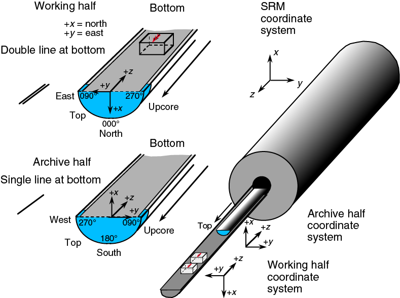
Figure F20. IODP coordinate systems.
NRM measurements usually yield anomalous components of magnetization along core due to a viscous remanent magnetization acquired during the drilling process. All cores were thus subjected to stepwise AF demagnetization using 4–5 steps up to a peak field of 40 mT or less, and NRM was measured following each demagnetization step. Calculated inclination, declination, and intensity were visually inspected using the IMS-SRM v. 9.2 software and, where necessary, carefully analyzed using vector component diagrams (Zijderveld, 1967) to verify whether the remanence directions and/or magnetic polarities determined were of primary origin. Subsequently, variations in declination, inclination, and intensity records and interpreted polarity sequences with respect to depth below seafloor were displayed using MATLAB.
Discrete samples
Oriented discrete cubes (7 cm3) were extracted from selected working halves by pushing a “Natsuhara-Giken” (Japanese) plastic container into the core with the z-arrow facing upward (Figures F20, F21). For more consolidated material or where the removal of the cubes resulted in extensive core damage, we first extruded the material from the cores using a similar shaped extraction device prior to moving them into the plastic containers while retaining the correct orientation. For thermal demagnetization, samples from moderately consolidated sediments were extracted using a 2 cm × 2 cm extruder, marked, and subsequently wrapped in parafilm to provide further stability during NRM and AMS measurements.
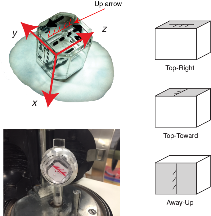
Figure F21. Coordinate convention, JR6A spinner magnetometer.
In well-consolidated or crystalline material, 2 cm × 2 cm cube samples were cut from the relevant sections using a 2-bladed ring saw. Discrete sample AMS was measured using an AGICO Kappabridge (model KLY 4) to investigate possible compaction-related inclination shallowing and to identify samples or sections that were disturbed during the drilling process. We display the orientations of the principal axes of magnetic susceptibility (χ1, χ2, and χ3) in equal-area stereoplots and calculate the anisotropy of foliation (F) = χ2/χ3 and the lineation (L) = χ1/χ2, where χ1 corresponds to the axis that aligns with the highest degree of magnetic susceptibility and χ1 > χ2 > χ3, using AGICO’s Anisoft software.
Subsequently, each specimen’s NRM was measured using a spinner magnetometer (AGICO model JR-6A; sensitivity: ~2 × 10⁶ A/m), followed by more detailed stepwise AF or thermal demagnetization up to 100 mT or 450°C, respectively. Demagnetization increments were matched to the coercivity or blocking temperature distributions of each sample, and experiments were completed when either a characteristic remanent magnetization (ChRM) direction could be clearly identified or when NRM intensity decreased below 10% of its initial value.
AF demagnetization was conducted along three axes using a DTECH (model D-2000) AF demagnetizer. During early AF demagnetization experiments at Site U1518, many samples acquired a remanence that is aligned roughly perpendicular to the last direction of the applied alternating current field (here: ±x-axis). We interpreted this behavior to be the acquisition of a gyroremanent magnetization (GRM) similar to that which has frequently been described in association with authigenic greigite (Fe3S4) in marine or lacustrine sediments (Dankers and Zijderveld, 1981; Hu et al., 2002; Pandey et al., 2016; Snowball, 1997). To correct for the effects of GRM, a small number of specimens were demagnetized following Stephenson (1993). For each demagnetization step, samples were first demagnetized along all three axes ending on +x, measured, subsequently demagnetized along −z, measured, and finally demagnetized along +y and measured. The average was calculated for each x, y, and z measurement, respectively, and the field vector was calculated.
Thermal demagnetization was conducted using ASC Scientific’s model TD-48SC thermal demagnetizer. Samples were heated and held at their respective temperature increments for 30 min, cooled, and subsequently measured. Bulk magnetic susceptibility was monitored following each heating increment using the Kappabridge to identify alteration of the magnetic remanence caused by the heating procedure.
Demagnetization data for all discrete specimens were displayed in vector component diagrams (Zijderveld, 1967), and ChRM directions were calculated from the best-fitting component by principal component analysis (Kirschvink, 1980) using PuffinPlot v. 1.0.3 (Lurcock and Wilson, 2012).
Following AF demagnetization and if time allowed, samples were further subjected to rock magnetic analysis with a focus on studying the distribution of populations of grains of different coercivity. We subjected samples to an impulse field along the +z-axis using an ASC impulse magnetizer (model IM-10), measured the IRM1T, applied an isothermal remanent magnetization (IRM) at a 300 mT impulse field along the −z-axis (IRM−300mT), and calculated S−300mT and IRM1T/χ ratios. The ratio S−300mT = [(IRM−300mT/IRM1T) + 1]/2 helps to isolate contributions of grains with high coercivity (e.g., hematite, goethite, and some iron sulfides), whereas the IRM1T/χ ratio is sensitive to the presence of authigenic greigite (Kars and Kodama, 2015; Liu et al., 2012).
Magnetostratigraphy
Magnetic polarity transitions were determined primarily based on inclination data. Assuming that the magnetic field resembles that of a geocentric axial dipole (GAD) field, the expected inclination can be calculated using (Butler, 2004)
where Inc is the inclination and lat is the site latitude. At 39°S latitude, we expect an inclination of −58° in a normal polarity field. Identified magnetozones were integrated with biostratigraphic datums (see Biostratigraphy) and mapped to the geomagnetic polarity timescale (GPTS) of Gradstein et al. (2012) where possible (Table T6). The GPTS of Gradstein et al. (2012) was chosen to be consistent with the calibration of the New Zealand geological timescale (Raine et al., 2015) used for the determination and correlation of New Zealand stratigraphic stages (de facto biozones).
Coordinate systems
The magnetic data sets presented are displayed relative to the standard IODP coordinate system (Figure F20) with +z pointing downcore and +x pointing toward the double lines at the bottom of the working half and thus away from the archive half. The SRM coordinate system is inverted with respect to IODP coordinates (+zIODP = −zSRM). Conversion from SRM to IODP coordinates is thus required prior to data display, which occurs prior to data upload into the LIMS database. All paleomagnetic data (declination and inclination) discussed here refer to this convention. The coordinate system of the discrete specimens follows the convention of the working halves.
Core reorientation
Two different tools (Icefield MI-5 multishot and FlexIT) allow for direct orientation of APC cores with an estimated accuracy of 20°–30° (McNeill et al., 2017). Unfortunately, the azimuthal data recovered during this expedition were inconclusive, thus requiring the orientation of the recovered cores based on paleomagnetic data sets. Reorientation using paleomagnetic data sets relies on three major assumptions:
- The reference paleomagnetic position of the drill site at the time of emplacement of the recovered sediment is known or the site has not experienced any vertical axis rotations since emplacement.
- The record is long enough to average out secular variation, thus averaging to a GAD direction (e.g., see Merill et al., 1996).
- The paleomagnetic records are not biased by incomplete core recovery or material disturbance caused during deposition and/or core recovery.
For the reorientation of APC cores to geographic coordinates, we calculate a mean and cone of 95% confidence (α95) following Fisher statistics (Fisher, 1953) for all measurements made at the peak demagnetization step for each of the cores independently. In a normal polarity field, dip directions that are provided in relation to the double lines on the core liner (+x-axis) can be corrected by subtracting the mean declination value. The error in declination (ΔDec) is calculated from the 95% confidence cone using
XCB and RCB cores were commonly dissected into a number of 5–20 cm long subhorizontal biscuits. In this case, we measured NRM directions with declinations that were systematically offset across biscuit boundaries, coherent with the azimuthal rotation of individual biscuits during drilling. For structural reorientation, we “handpicked” a mean declination for each individual biscuit. For samples from normal polarity intervals, we subtracted the mean declination from each biscuit; for samples from reversed polarity intervals, we subtracted the mean and added 180°. Note that the incomplete sampling of secular variation and data smearing due to the instrument response produces errors, probably in the range of 20°–40°. Reorientations were carried out only when measurements showed multiple consistent declinations.
Structural geology
Our principal objective was to record structures observed in the core and their orientations. These data will contribute to our aim of investigating the processes and in situ conditions of shallow subduction zone slow slip events. The structural data will also assist in interpretations of bedding and fracture orientations observed in Expedition 372 LWD data and integrating core, seismic, and downhole observations. These objectives were achieved by making detailed structural observations and measurements following methods used during previous expeditions, with modifications to more fully describe structures encountered during Expedition 375.
The methods for documenting structural features in Expedition 375 cores largely follow those of Integrated Ocean Drilling Program Expeditions 334 and 344 and IODP Expeditions 352, 360, and 362 (Expedition 334 Scientists, 2012; Harris et al., 2013; Reagan et al., 2015; MacLeod et al., 2017; McNeill et al., 2017). Blenkinsop and Doyle (2010) also provide a discussion of measuring planar structures in core. Structures observed in the split cores were classified and quantified in terms of depth extent, orientation, and if possible, sense and magnitude of displacement. Each structure was recorded manually on a description table sheet at the core table (scans are available in VCD_HAND in STRUCTURE in Supplementary material). For planar structures, the dip, strike, and dip direction were computed from apparent orientation measurements using trigonometric transformations applied in an Excel spreadsheet (see CALCULATION in STRUCTURE in Supplementary material). The resulting orientations defined in a core reference frame were then logged via the DESClogik interface to the LIMS database, together with other descriptive information about each structure and the material the structure occurs in (see Visual core descriptions; Figure F3).
Structural data acquisition and orientation measurements
The current basis for making quantitative measurements was defined during Expedition 334 (Expedition 334 Scientists, 2012) and further modified during Expeditions 344, 352, and 362 (Harris et al., 2013; Reagan et al., 2015; McNeill et al., 2017).
We used a plastic protractor for orientation measurements (Figure F22). This measurement process was performed on the working half because it provided greater flexibility in removing—and cutting, if necessary—pieces of the core for structural measurements. Orientations of planar and linear features in cores were determined relative to the core axis, which represents the vertical axis in the core reference frame, and to the split line marked on the working half of the split-core liner. The split line represents 000° (and 360°) in the plane perpendicular to the core axis (Figure F23); 000° was defined as perpendicular to the cut surface toward the working half of the core, and 180° was then defined toward the archive half of the core.
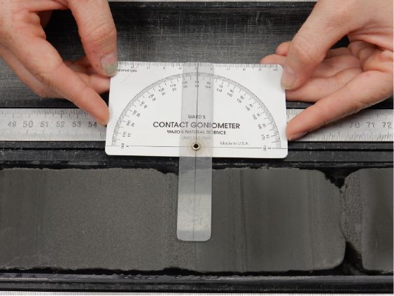
Figure F22. Protractor used.

Figure F23. Core reference frame.
To determine the orientation of a planar structural element, apparent dips were measured in two independent sections in the core reference frame. One apparent dip is represented by the intersection of the planar feature with the split face of the core and is quantified by measuring the plunge and trend of this line in the core reference frame (Figure F24). Such a measurement has a trend of either 090° or 270° and ranges in plunge from 0° to 90° (α1 and β1, respectively, Figure F24). A second apparent dip is represented by the intersection of the planar feature and a cut or fractured surface at a high angle to the split face of the core. In most cases, this surface lies either parallel or perpendicular to the core axis. When parallel, the apparent dip trace trends 000° or 180° and plunges from 0° to 90° (α2 and β2, respectively, Figure F24); when perpendicular, the trend ranges from 000° to 360° and plunges 0°. Linear features observed in cores are typically defined by a trend and plunge in the core reference frame, as for the apparent dips described above. Where appropriate, lines may also be associated with planar structures (e.g., a striation on a fault plane) and their orientations determined by measuring the rake on the associated plane. As an example, for a fault with striations, the apparent rake angle of the striation (ϕa) was measured on the fault surface from either the 090° or 270° direction of the split-core surface trace (Figure F25). Fault orientation was calculated from the two apparent dips as described above.
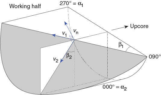
Figure F24. Calculation of plane orientation.
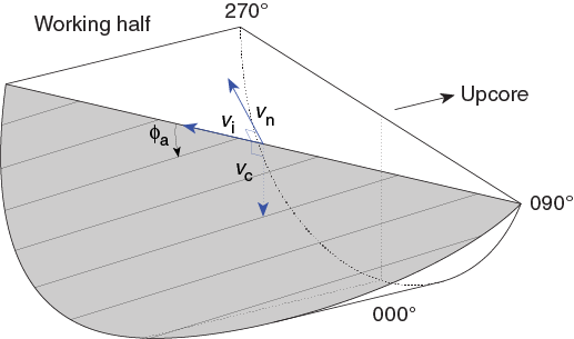
Figure F25. Rake measurement for striations on a fault surface.
For planar structures, the two apparent dips were converted to a plane in the core reference frame represented by a dip angle, a strike, and a dip direction using an Excel spreadsheet (see CALCULATION in STRUCTURE in Supplementary material) (Figure F26). A rake angle (ϕ) relative to the strike line in the core reference frame was similarly calculated trigonometrically in this Excel spreadsheet. Detailed methods for this are described by McNeill et al. (2017). We also confirmed conversions from apparent dips and rakes to orientations of planes and lines graphically using the Stereonet 9.8 software (Cardozo and Allmendinger, 2013) for selected examples.
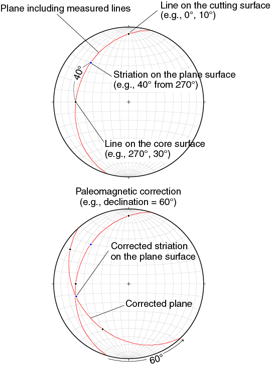
Figure F26. Procedure for converting 2-D measured data to 3-D data.
Registration of orientation data from the core reference frame to a true geographic reference frame using paleomagnetic data was possible for some intervals (Figure F26). For these calculations, we followed methods used during past IODP expeditions and detailed by McNeill et al. (2017). Azimuthal core orientation was determined based on paleomagnetic declination measurements obtained from the continuous magnetic remanence data collected for each core section, adjusted for geomagnetic polarity intervals (interpreted from correlations with the GPTS and biostratigraphic constraints) (see Paleomagnetism for details). Variability in both inclination and declination values introduces uncertainty in those orientation corrections. To be used for reorientations, declinations were required to be consistent (within ~30° range) over ~10 cm intervals in unbiscuited intervals containing no polarity reversals. The application of this method was not possible in intervals with severe core disturbance, including biscuiting on a centimeter scale or less, upwarped bedding, or midcore flow. The presence of MTDs or other zones of intense soft-sediment deformation also introduced challenges for core reorientations. However, many of these zones of sediment deformation occurred in coherent zones where relative rotations were minimal, in which case more reliable declination data from the bracketing zones could be used to reorient the structures.
Recognizing that it may be difficult to accurately measure orientations in cores, orientation measurements are accompanied by a confidence level from 1 to 3. A Level 3 measurement is one for which it was easy to define and measure the structure, it is unlikely to have been modified by drilling disturbance, and confidence is high. A Level 1 measurement is one for which it was difficult to define and/or measure the feature accurately and it is uncertain whether it has been modified by drilling disturbance. This confidence level also includes, where applicable, whether the sense of slip is uniquely determined by the observations. For faults and shear zones, the highest confidence is only assigned if offset marker horizons are visible in the core and/or if striations define slip direction (e.g., dip-slip versus strike-slip).
Description and classification of structures
We constructed a structural geology template for DESClogik that aids in the description and classification of observed structures. We define the terminology used to describe deformation structures, both for clarity and as the basis for differentiating natural structures from drilling-induced features. We adopt a descriptive hierarchy (see DESC_WKB in Supplementary material) for our structural classification in which we first define a structure type (e.g., fault, fracture, fold, deformation band, fabric, bedding, etc.) and then add a secondary descriptor to further classify the structure. Fractures are described as open or closed, and displacement sense is noted for faults and shear bands: normal, reverse, strike slip, or indeterminate. An indeterminate fault is one in which the surface has slickenlines that suggest displacement but without sufficient markers to define the sense of slip. We define deformation bands as continuous features that can be divided into shear bands (which show evidence of shear displacement), compaction bands, dilation bands, and indeterminate deformation bands for which it was not possible to determine the type of strain accommodated. Faults are distinguished from shear bands because they contain at least one discrete discontinuity along which shear displacement has occurred. Both faults and deformation bands, however, are tabular features and therefore have a thickness that was determined when possible. The internal structure of both faults and deformation bands is noted with additional qualifiers (Riedel shears, S-C structures, planar fabrics, gouge, cataclasite, and breccia) and a grain size if determined. For zones with a penetrative, spaced, or distributed fabric, a fabric type of planar, anastomosing, or stylolitic is recorded for that interval of the core. Additional geometrical descriptors used to define the morphology of the various features include planar, wavy, curved, or anastomosing planar features, open and tight folds, and en echelon and sigmoidal fractures.
Veins are recorded as filled fractures, and additional qualifying observations include their mineralogy and internal structure. Additional information, such as relations between vein and wall rock, are included in the comments section of the vein description. Orientations of veins, clastic dikes, distributed fabrics, and other structural features are part of the routine structural description.
Recognizing that uncertainty often occurs in objectively defining structures as either natural (sedimentary or tectonic) or drilling induced, we assign an interpretation probability level to each observation both to minimize the potential for any conflict and to identify all observations in the database that remain equivocal; the intent is to provide the means to include or exclude observations in post-expedition analyses based on confidence thresholds. The probability scale is defined from 0 to 1, where 0 is no confidence that the observed structure is natural (i.e., a fault is drilling induced with 100% certainty) and 1 is perfect confidence in a tectonic or synsedimentary origin (McNeill et al., 2017). In practice, probability values range from 0.1 to 0.9 to maintain some possibility that any individual structure may have a component of natural or drilling-induced deformation.
Fracture intensity assessment
The cores contain an abundance of brittle deformation, including fractures (both open and filled), faults, and brecciated zones. Because these features commonly denote distinct deformational domains or damage zones, we carried out a systematic first-order assessment of the abundance of such brittle features, which we refer to as fracture intensity. The assessment was conducted over 10 cm intervals, and the abundance of brittle features in each interval was logged independently of their orientations. Fracture counts were binned and assigned intensity values as follows (with effective fracture spacing also indicated):
- 1 = <1 fracture/m (>1 m spacing).
- 2 = 1–10 fractures/m (1 dm to 1 m spacing).
- 3 = >10–100 fractures/m (1 cm to 1 dm spacing).
- 4 = >100–1000 fractures/m (1 mm to 1 cm spacing).
- 5 = >1000 fractures/m (<1 mm spacing).
Thus, Fracture Intensity 1 records long unfractured sections of core and Fracture Intensity 5 denotes intensely brecciated zones. To define a continuous distribution of fracture intensities over longer intervals, fracture intensity assessments were then averaged over core sections (i.e., as long as 1.5 m). Fracture intensity is plotted as a function of depth for Sites U1518 and U1520 where coring was more continuous and where abundant brittle deformation occurred.
Drilling disturbance
Drilling disturbance was evident in many of the recovered cores and affected our ability to recognize and describe original sedimentary and tectonic structures. Drilling-induced folding and distortion of beds occurred in APC cores, including upward-arching and mingled and distorted beds caused by suction of the materials into the core barrel. XCB and RCB drilling led to induced faults, fractures, and breccias, as well as to biscuiting of cored intervals. Drilling-induced gouge is commonly formed between biscuits by relative rotation of drilling cuttings and injection of material. Other coring disturbances, such as fall-in, soupy texture, gas expansion, core extension, and voids, also occurred. Generally, we followed previous practice and terminology (e.g., Jutzeler et al., 2014; McNeill et al., 2017) in our description of drilling disturbance and categories of drilling disturbance intensity (slight, moderate, severe, and destroyed). These observations were logged during core description (see DESC_WKB in Supplementary material). Table T7 lists the criteria used.
DESClogik program
DESClogik is a program used to store a visual (macroscopic and/or microscopic) description of core structures at a given depth and to upload them to the LIMS database. During Expedition 375, only the locations of structural features, calculated orientations in the core reference frame, and restored orientations based on the paleomagnetic data were input into DESClogik alongside descriptive details. Calculation of 3-D orientations in the core reference frame from measured apparent dips were made with a spreadsheet as described above and are available as supplementary tables (see STRUCTURE in Supplementary material).
Geochemistry
The concentration of dissolved species in pore water and their isotopic composition provide data to identify fluid sources and flow pathways and to quantify fluid–rock reactions and the formation of authigenic minerals. In addition, pore water chemical profiles are essential for characterizing biogeochemical cycling and the distribution and concentration of methane hydrate. The distribution of pore water samples during Expedition 375 and the pore water analytical program are shown in Table T8.
Pore water collection
In general, pore water sampling was conducted on WR samples that were collected from recovered core at a resolution of six WR samples per core in the upper 20 m, three WR samples per core between 20 and 40 mbsf, and 1–2 WR samples per core from 40 mbsf to the bottom of the hole. WR length increased with depth from ~10 cm in the shallow cores to >40 cm in the deepest cores to account for the lower water content in more consolidated sediment at depth. Pore water samples were analyzed shipboard for a range of species and preserved for post-expedition research as detailed in Table T8. Details for the sampling protocol at each site are given in the corresponding site chapters.
For headspace analyses of gas composition and concentrations, sediment plugs were routinely collected in two sections per core immediately adjacent to the pore water WR sample. In addition, void gas samples were collected for shipboard hydrocarbon analyses when present. Starting at 30 mbsf, each core was scanned with an IR camera to identify the presence of methane hydrate, indicated by anomalously cold sections resulting from endothermic methane hydrate dissociation during core recovery. These IR anomalies guided the selection of pore water samples on the catwalk and ensured that we sampled sediments representing background conditions (not impacted by methane hydrate dissociation during core recovery). In addition, we collected a small number of WR samples for IW analysis where gas hydrates were inferred based on IR scans to quantify methane hydrate concentrations. These pore water–based estimates are useful for verifying the methane hydrate saturation calculations from LWD resistivity data collected during Expedition 372.
WR samples were cut on the catwalk, capped, and taken to the laboratory for processing. During high-resolution sampling, when there were too many IW WRs to process immediately, capped WRs were stored under a nitrogen atmosphere at 4°C until they were squeezed, which occurred no later than 4 h after core retrieval. After extrusion from the core liner, the surface of each WR was carefully scraped with a spatula to remove potential contamination from seawater and sediment smearing in the borehole. For APC cores, ~0.5 cm of material from the outer diameter, top, and bottom faces were removed, whereas for XCB and RCB cores where contamination is more prevalent, as much as two-thirds of the sediment was removed from each WR. The remaining sediment (~50–300 cm3) was placed into a titanium squeezer modified after the stainless steel squeezer of Manheim and Sayles (1974). Gauge forces to a maximum of 30,000 lb were applied using a laboratory hydraulic press to extract pore water. Pore water was passed through a prewashed Whatman Number 1 filter fitted above a titanium screen and extruded into a precleaned (10% HNO3) plastic syringe attached to the bottom of the squeezer assembly. Pore water was then dispensed from the syringe through a 0.2 µm Gelman polysulfone disposable filter into shipboard and shore-based sample containers and preserved for various analyses.
A few WR samples designated for He isotopic analysis were also cut on the catwalk and capped. Samples were immediately transferred to a special processing and squeezing station set up in the refrigerated core storage repository located on the lowermost deck of the JOIDES Resolution. This refrigerated repository is a He-free environment kept at 4°C, whereas the shipboard chemistry laboratory uses He as a carrier gas for the gas chromatographs (GCs) and carbon-hydrogen-nitrogen-sulfur (CHNS) elemental analyzer. The samples were cleaned in a glove bag, squeezed, and transferred into copper tubing that was previously flushed with ultrahigh-purity N2, and crimped.
Shipboard pore water analyses
We undertook key geochemical analyses on the ship and collected pore water samples for post-expedition studies. Sample allocation was determined based on the pore water volume recovered and analytical priorities based on the expedition objectives (Table T8). Pore water samples were analyzed on board following the protocols in Gieskes et al. (1991), Murray et al. (2000), and the IODP user manuals available on board.
Salinity, alkalinity, and pH
Salinity, alkalinity, and pH were measured immediately after squeezing following the procedures in Gieskes et al. (1991). Salinity was measured using a Fisher temperature-compensated handheld refractometer, pH was measured with a combination glass electrode, and alkalinity was determined by Gran titration with an autotitrator (Metrohm 794 basic Titrino) using 0.1 M HCl. International Association for the Physical Sciences of the Oceans (IAPSO) standard seawater and in-house 10, 20, and 40 mM NaHCO3 were used as calibration standards for the alkalinity determinations; in addition, an IAPSO sample was analyzed at the beginning and end of a set of samples for each site and after approximately every 10 samples. The average accuracy and precision of the alkalinity measurements based on repeat analysis of IAPSO standard seawater and the 20 mM reference standard were <2.5% and <2%, respectively.
Chloride measured by titration with AgNO3
High-precision chloride concentrations were measured with a Metrohm 785 DMP autotitrator via silver nitrate (AgNO3) titration and were calibrated against repeated titrations of IAPSO standard seawater. Each sample was analyzed twice by titration and averaged, and some samples were analyzed in triplicate. For each replicate, a 0.1 mL aliquot of sample was diluted with 4 mL of 2.2 M trace metal grade HNO3 and titrated with a 0.1 M AgNO3 solution. Repeated analyses of the IAPSO standard yielded a precision better than 0.3%.
Chloride, bromide, and sulfate measured by ion chromatography
Chloride (Cl−), bromide (Br−), and sulfate (SO42−) were analyzed by ion chromatograph (IC) on a Metrohm 850 Professional IC. Aliquots of 100 µL were diluted 1:100 with ultrapure water (18.2 MΩ·cm), and eluent solutions of 3.2 mM Na2CO3 and 1.0 mM NaHCO3 were used. Calibration standards had IAPSO dilution factors of 50, 67, 100, 150, 200, 350, 500, 750, 1000, 2000, 4000, 6000, and 8000. Samples were diluted 100 times. Calibration standards with dilution factors of 50–500 were used to construct a calibration curve for samples with higher sulfate concentrations (5–29 mM), and calibration standards with dilution factors between 750 and 8000 were used for samples close to the sulfate–methane transition zone (SMTZ) and below, where in situ sulfate concentrations are low. Thus, we used two separate calibration curves for the sulfate analyses but only used the higher concentration calibration curve for the Cl and Br analyses. A drift standard was measured after five samples for six cycles, after which three extra standards were analyzed as an accuracy check. For reproducibility, >5 sample replicates were analyzed during each run. The accuracy of the Cl, Br, and SO4 analyses via IC was <0.4%, <1%, and <1%, respectively. The precision of the Cl, Br, and SO4 analyses was <0.3%, <1%, and <1%, respectively. We report Cl values from both IC and titration but plot only the titration data, which yielded better precision. Likewise, we report sulfate concentrations from both the IC and inductively coupled plasma–atomic emission spectrometry (ICP-AES).
Below the SMTZ, sulfate is depleted in the pore water and any sulfate present in a sample is a result of contamination with surface seawater that was pumped downhole while drilling. Drilling fluid was sampled at every site and analyzed as part of the shipboard geochemical program. Based on the sulfate concentration of each IW sample below the SMTZ, we used the chemical composition of the drilling water to correct each analysis for contamination using the following equations:
- fSW = fraction of a pore fluid sample that is contaminated with drilling fluid,
- fPW = fraction of uncontaminated pore water in a sample,
- [X]corr = corrected value of a solute (e.g., Cl, Ca, Sr, etc.),
- [X]meas = measured concentration of that solute, and
- [X]SW = concentration of the solute in the drilling fluid.
Ammonium, phosphate, and silica by colorimetry
Ammonium, phosphate, and silica concentrations were determined by spectrophotometry using an Agilent Technologies Cary Series 100 UV-Vis spectrophotometer with an autosampler. Ammonium concentrations were determined using the method described in Solórzano (1969), and orthophosphate was measured using the ammonium molybdate method described in Gieskes et al. (1991). Dissolved silica was also measured spectrophotometrically using the method based on the production of a yellow silicomolybdate complex. The complex is reduced by ascorbic acid to form molybdenum blue and measured at 812 nm. In-house calibration standards were prepared for each of the colorimetric analyses that bracket the concentration range expected in the pore water. For the ammonium concentration analyses, standards ranged from 50 to 1000 µM, and the pore water samples were diluted into this range. Each batch of analyses also consisted of multiple check standards and drift standards analyzed after every 5 samples. The accuracy of the ammonium and silica analyses based on repeated analyses of the standards was <2.5% and <2%, respectively. The precision of the ammonium and silica analyses based on repeated analysis of drift standards spanning the anticipated in situ concentration range was <2.5% and <2%, respectively.
Calcium, magnesium, potassium, and sodium measured by ion chromatography
IC analyses were conducted using the same 1:100 aliquot dilutions with ultrapure water as those used for anions. The eluent solutions used for cation measurements were 3.2 mM Na2CO3 and 1.7 mM PDCA (pyridine-2,6-dicarboxylic acid) supplied by Metrohm (CAS#499-83-2). Check standards were run throughout each batch of analyses, and multiple drift standards bracketing the range of anticipated pore water concentrations were analyzed after every 5 samples. Standards were prepared by dilution of IAPSO standard seawater with dilution factors of 50, 67, 100 (same as the samples), 150, 200, and 350. Analytical precision based on repeated analysis of drift and check standards was <2.5%, <2%, <1%, and <0.8% for calcium, magnesium, potassium, and sodium, respectively. Accuracy of the analyses was <2.5%, <2%, <2%, and <0.7% for calcium, magnesium, potassium, and sodium, respectively.
Major and minor elements measured by ICP-AES
Dissolved major (Na, K, Ca, Mg, and total S) and minor (Li, Sr, B, Si, Mn, Fe, Ba, and total P) element concentrations were determined by an Agilent 5110 ICP-AES with an SPS4 autosampler.
For the shipboard ICP-AES analyses of IW samples, we modified the analytical procedures developed during IODP Expeditions 372 and 371. Each IW sample used for major element concentration analyses was diluted at 1:10 using 2% HNO3 and spiked with 100 µL of a 10 ppm Y, In, and Sc solution as an internal standard. For calibration, serial dilutions of IAPSO standard seawater (1%, 5%, 10%, 25%, 50%, 75%, 100%, and 200%) were prepared to bracket the range of concentrations anticipated in cores. Calibration standards for the minor element analyses were prepared from Spex Certiprep primary reference standards. Dilutions of the primary standard to bracket the range in anticipated pore water concentrations were matrix matched to achieve 3.5 g/L NaCl in each standard.
During each ICP-AES run, a complete set of all in-house and IAPSO dilutions were analyzed at the beginning and end of each batch. Furthermore, several standards that span the range of anticipated pore water concentrations were analyzed every 8–10 samples to monitor instrument drift and determine analytical precision and accuracy. The elemental concentrations reported for each sample were average values from three replicate integrations from each sample measured consecutively via continuous flow, as set by instrumental parameters. Analytical precision was based on repeat analysis of standards that span the range of anticipated in situ concentrations and is as follows for each element: Ca < 0.6%, Mg < 0.6%, K < 0.5%, Na < 1%, total S < 0.5%, Li < 0.7%, B < 2%, Sr < 0.5%, Ba < 0.4%, Fe < 0.8%, Mn < 0.7%, total P < 1%, and Si < 0.7%. Analytical accuracy for each element was based on repeat analysis of standards that span the range of anticipated in situ concentrations and is as follows: Ca < 0.4%, Mg < 0.3%, K < 0.8%, Na < 1.5%, total S < 1%, Li < 2.5%, B < 1.3%, Sr < 1.5%, Ba < 1%, Fe < 0.5%, Mn < 0.5%, total P < 1.2%, and Si < 0.5%.
Organic geochemistry
Expulsion of pore water and hydrocarbons produced by diagenetic and low-grade metamorphic reactions can provide useful tracers of fluid origin and subduction margin hydrogeologic processes (i.e., Kastner et al., 2014). Routine analysis of hydrocarbon gas in sediment cores is also a key element of IODP standard shipboard safety monitoring.
Analysis of gas samples obtained from sediment samples (headspace analysis) following the procedures described by Kvenvolden and McDonald (1986) is the most common method used for hydrocarbon monitoring during IODP expeditions. When gas pockets were detected, the free gas was sampled from the sediment void using a syringe attached to a hollow stainless steel tool used to puncture the core liner. The gas was then analyzed on a GC–flame ionization detector (GC-FID). For headspace analyses, a 3 cm3 sediment sample was collected from the freshly exposed top end of a core section and next to the IW sample immediately after core retrieval using a plastic syringe or brass boring tool. The sediment plug was placed in a 20 cm3 headspace vial and capped and sealed with a septum and aluminum crimp seal. The vial was then heated to 70°C for ~30 min to evolve hydrocarbon gases from the sediment. When consolidated or lithified samples were encountered, chips of material were placed in the vial and sealed. For gas chromatographic analyses, a 5 cm3 volume of headspace gas was extracted from the capped sample using a standard gas syringe and analyzed by gas chromatography.
Headspace and void gas samples were injected directly into the GC-FID or into the natural gas analyzer (NGA). The headspace samples were analyzed using an Agilent/HP 6890 Series II gas chromatograph (GC3) equipped with an 8 ft, 2.00 mm inside diameter × ⅛ inch outside diameter stainless steel column packed with 80/100 mesh HayeSep R and an FID set at 250°C. The GC3 oven was programmed to hold temperature at 80°C for 8.25 min, ramp at 40°C/min to 150°C, hold for 5 min, and return to 100°C postrun for a total of 15 min. Helium was used as the carrier gas. The GC3 system determines concentrations of methane (C1), ethane (C2), ethene (C2=), propane (C3), and propene (C3=).
Data were collected using the Hewlett Packard 3365 Chemstation data processing program. Chromatographic response is calibrated to nine different gas standards with variable quantities of low molecular weight hydrocarbons. The gas concentrations for required safety analyses are expressed as component parts per million by volume (ppmv) in the analyzed gas.
Sediment geochemistry
For the shipboard sediment geochemistry analyses, 3 cm3 of sediment was freeze-dried for ~24 h, crushed to a fine powder using a pestle and agate mortar, and sampled to analyze inorganic carbon, total carbon (TC), and total nitrogen (TN) and for source rock analyses.
Elemental analysis
The TC and TN of sediment samples were determined with a ThermoElectron Corporation FlashEA 1112 CHNS elemental analyzer equipped with a ThermoElectron CHNS/nitrogen-carbon-sulfur packed column and a thermal conductivity detector (TCD). Approximately 10–15 mg of freeze-dried, ground sediment was weighed in a tin cup, and the sample was combusted at 900°C in a stream of oxygen. The reaction gases were passed through a reduction chamber to reduce nitrogen oxides to nitrogen and were then separated by gas chromatography before detection by TCD. All measurements were calibrated to a standard sediment reference material (2704 Buffalo River Sediment; PWQR7837591) for TC and TN detection, which was run every 10 samples. The detection limit was 0.001% for TN (instrument limit) and 0.002% for TC (procedural blank; measured as an empty tin cup). Sample replicates (N = 10 for each of 5 samples) yielded precisions of <10% of measured values for TN and <7% of measured values for TC.
Inorganic and organic carbon content
Total inorganic carbon (TIC) concentrations were determined using a UIC CM5015 coulometer. Between 10 and 15 mg of freeze-dried, ground sediment was weighed and reacted with 2 M HCl. The liberated CO2 was titrated, and the end point was determined by a photodetector. Calcium carbonate content expressed as weight percent was calculated from the TIC content assuming that all evolved CO2 was derived from dissolution of CaCO3, using the following equation:
No correction was made for the presence of other carbonate minerals. Accuracy during individual batches of analyses was determined by running a carbonate standard (100 wt% CaCO3) every 10 samples. Typical precision, assessed using replicate analyses of a carbonate sample (N = 10 for each of 5 samples), was 2%. The detection limit for CaCO3, defined here as 3× the standard deviation of the blank (2 M HCl), was 0.1%. Total organic carbon (TOC) content was calculated as the difference between TC (measured on the elemental analyzer) and inorganic carbon (measured by coulometry):
Source rock analyses
Source rock analyses were conducted to identify the type and stage of maturation of organic matter, estimate TOC, and detect petroleum potential in sediments. Using source rock pyrolysis, free and adsorbed hydrocarbons released during programmed heating of a sample are recorded as the first peak in a pyrogram (S1) at low temperature. The second peak (S2) in the pyrogram represents hydrocarbons released by kerogen cracking. The temperature at the maximum of the S2 peak is defined as Tmax and is an indicator of rock maturity. CO2, shown as the third peak (S3) in the program, is also generated by kerogen degradation. When these components are normalized to the TOC content, the S2 peak becomes the hydrogen index (HI = S2 × 100/TOC) and the S3 peak becomes the oxygen index (OI = S3 × 100/TOC) (Tissot and Welte, 1984).
Source rock pyrolysis and TOC were determined using a Weatheford source rock analyzer. A crucible sample containing no material was included as a calibration blank and was run as the first measurement in each sequence. After this calibration blank, 90–100 mg of standard material was used to calibrate the instrument signals and allowed us to monitor instrument accuracy and precision. A pyrolysis program starting at 300°C with a heating rate of 25°C/min was used as a standard mode for the analysis of sediment with low maturity.
Physical properties
Physical properties measurements provide constraints on a range of sediment and rock physical characteristics to facilitate lithostratigraphic unit characterization and correlation of LWD, wireline logging, and seismic reflection data with core measurements and descriptions. After core recovery, whole-round core sections were thermally equilibrated to ambient room temperature (~20°C) over a period of ~4 h. Whole-round cores were then run through the WRMSL for GRA bulk density measurement, magnetic susceptibility measurement using a pass-through loop system (MSL), and P-wave velocity measurement using a P-wave logger (PWL). Following the WRMSL track, whole-round cores were analyzed with the NGRL) when the length of an individual section was >50 cm. Thermal conductivity (TCON) was measured on soft sediments before splitting using needle probes and on lithified sediments and rocks after splitting using a half-space probe. After the cores were split, the archive half was passed through the SHIL and then the SHMSL for RSC and MSP. Strength measurements (only for soft sediments) were made on the working half using the automated vane shear (AVS) and a pocket penetrometer. Discrete P-wave velocity measurements were made on either working halves for soft sediments or discrete cube samples for lithified materials using the P-wave velocity gantry. MAD measurements were conducted on discrete samples (generally two per section and adjacent to all WR samples). MAD discrete samples were taken from representative lithologies by using a syringe for soft sediments or by preparing oriented, discrete cube samples (1 cm × 1 cm × 2 cm and 2 cm × 2 cm × 2 cm) for lithified sediments and rocks. The oriented MAD cube samples and paleomagnetism (PMAG) cube samples (2 cm × 2 cm × 2 cm) were used for P-wave velocity measurements when possible.
Whole-Round Multisensor Logger measurements
The WRMSL was used to measure GRA density, magnetic susceptibility, and P-wave velocity nondestructively. The sampling interval for WRMSL measurements was set at 2 cm.
GRA bulk density
GRA density is an estimate of bulk density based on the attenuation of a gamma ray beam. The beam is produced by a 137Cs gamma ray source at a radiation level of 370 MBq in a lead shield with a 5 mm collimator, which is directed through the whole-round core. The gamma ray detector on the opposite side of the core from the source includes a scintillation detector and an integral photomultiplier tube to record the gamma radiation that passes through the core. The attenuation of gamma rays occurs primarily by Compton scattering, in which gamma rays are scattered by electrons in the formation; the degree of scattering is related to the material bulk density. Bulk density (ρ) determined with this method can be expressed as
- µ = Compton attenuation coefficient,
- d = sample diameter,
- I0 = gamma ray source intensity, and
- I = measured intensity of gamma rays passing through the sample.
The attenuation coefficient and gamma ray source intensity are treated as constants such that ρ can be calculated from I. The gamma ray detector was calibrated with a set of aluminum cylinders of various diameters surrounded by distilled water in a sealed core liner that is the same as that used during coring operations. The relationship between I and the product of µ and d can be expressed as
where B and C are coefficients determined during calibration. Gamma ray counts through each cylinder were determined for a period of 60 s, and the natural log of resulting intensity values was plotted as a function of µd. Here, the density of each aluminum cylinder is 2.7 g/cm3 and d is 1, 2, 3, 4, 5, or 6 cm. The WRMSL provided the values of I and µ, and ρ was calculated by the equation above. Recalibration was performed as needed if the deionized water standard run after every core deviated significantly (more than a few percent) from 1.0 g/cm3. The spatial resolution of the GRA densiometer is <1 cm.
GRA bulk density measured on WRMSL is dependent on core diameter. For some lithified RCB cores that do not completely fill the liner, corrections for core diameter are required to obtain meaningful bulk density values because GRA bulk density is calculated based on the assumption that core diameter is 66 mm (i.e., the inner diameter of the liner). We estimated the true core diameter from image analysis of photographs taken on archive halves. In the image analysis, the color image of core sections is first converted into a three-tone image so that any pixel on the image is either black (0), transitional (1), or white (2). An algorithm is then prepared to detect the edges of the core and calculate the core diameter by pixel size. Using the actual core diameter values, the GRA bulk density values were corrected by multiplying by a ratio of the liner diameter to the actual core diameter.
Magnetic susceptibility
Magnetic susceptibility (Κ) is a dimensionless measure of the degree to which a material can be magnetized by an external magnetic field:
where M is the magnetization induced in the material and H is the strength of an external field. Magnetic susceptibility varies in response to the type and concentration of magnetic grains and responds to variations in the magnetic composition of the sediment, which are both commonly related to variations in mineralogical composition (e.g., terrigenous versus biogenic materials) and diagenetic overprinting. Materials such as clay generally have a magnetic susceptibility several orders of magnitude lower than magnetite and some other iron oxides that are common constituents of igneous and volcanogenic material. Water and plastics (such as the core liner) have a slightly negative magnetic susceptibility.
The WRMSL measures volume magnetic susceptibility using a Bartington Instruments MS2 meter (Bartington Instruments, 2011), coupled to an MS2C sensor coil (88 mm diameter) and operates at an AF of 250 µT and a frequency of 565 Hz. During Expedition 375, the instrument was set to record an average of 3 measurements over a 1 s period. No correction was applied for volume effects caused by differing APC, XCB, and RCB core diameters. The spatial resolution of the MS2C sensor is 2 cm (Bartington Instruments, 2011), and tests using synthetic cores suggested a full width at half maximum response of 4.0–4.4 cm (Blum, 1997).
P-wave velocity
For soft sediments, the P-wave velocity sensor measures the ultrasonic P-wave velocity of the WR sample residing in the core liner. The PWL transmits a 500 kHz P-wave pulse across the core section at a repetition rate of 200 Hz. This signal is coupled to the sample by the plastic contacts of the ultrasonic transducers clamped to the sides of the core by a linear actuator. A small amount of water is applied to the contacts for each measurement to improve coupling between the transducers and the liner. The transmitting and receiving ultrasonic transducers are aligned so that wave propagation is perpendicular to the long axis of the core section.
Sonic velocity (V) is defined as
where d is the path length of the wave through the core and t is the traveltime. In addition to the traveltime through the sample, the total traveltime between the transducers includes three additional components:
- tdelay = time delay related to transducer faces and electronic circuitry,
- tpulse = delay related to the peak detection procedure, and
- tliner = transit time through the core liner.
For routine measurement on whole-round cores inside core liners, the corrected core velocity (Vcore) can be expressed by
- dʹcore = measured diameter of core and liner,
- dliner = liner wall thickness, and
- t0 = measured total traveltime.
The system was calibrated using an aluminum block of known P-wave velocity (6295 m/s) and length (76.2 mm), and measurement of water was used to verify the calibration and data quality during each section run.
Traveltime was determined by a signal processing software that automatically detects the first arrival of the P-wave signal. Because high background noise makes it challenging for an automated routine to pick the first arrival of a potentially low amplitude signal, the search method skips the first positive amplitude peak and detects a second positive amplitude using a detection threshold limit typically set to 30% of the maximum amplitude of the signal. The program then finds the preceding zero crossing and subtracts one wave period to define the first arrival. To avoid false detection of arrivals in the case of extremely weak signals, a minimum signal strength (typically 0.02 V) can be set and weaker signals are ignored. To avoid signal interference at the beginning of the record from the receiver, a delay (typically 0.01 ms) can be set to force the amplitude search to begin in the quiet interval preceding the first arrival. In addition, a trigger (typically 4 V) is selected to initiate the arrival search process, and the number of waveforms to be stacked (typically 50–100) can also be set. A laser measures the separation of the transducers to derive a signal path length (i.e., dʹcore). After corrections for system propagation delay, liner thickness, and liner material velocity, the ultrasonic P-wave velocity is calculated. The software removes any extremely unrealistic velocity values (<900 m/s or >6000 m/s).
Natural Gamma Radiation Logger
The NGRL measures gamma radiation emitted from whole-round core sections arising primarily from the radioactive decay of 238U, 232Th, and 40K isotopes. The main NGRL detector unit consists of 8 sodium iodide (NaI) scintillator detectors that are covered by 8 cm of lead shielding. In addition, lead separators (~7 cm of low-background lead) are positioned between the NaI detectors. Half of the lead shielding closest to the NaI detectors is composed of low-background lead, and the outer half is composed of regular (virgin) lead. In addition to passive lead shielding, the NGRL employs plastic scintillators to suppress the high-energy gamma and muon components of cosmic radiation by producing a canceling signal when these charged particles pass through the plastic scintillators. The NGRL was calibrated using a source consisting of 137Cs and 60Co and identifying the peaks at 662 (137Cs) and 1330 keV (60Co). The NGRL installed on the JOIDES Resolution was designed and built by the Integrated Ocean Drilling Program-US Implementing Organization at Texas A&M University (Vasiliev et al., 2011). Calibration materials are provided by Eckert & Ziegler Isotope Products, Valencia, California (USA). Background measurements of an empty core liner counted for 40,000 s (~10 h) at each measurement position were made when we arrived at the first site (U1518). Over the 100–3000 keV integration range, background levels averaged 4–5 counts/s.
A measurement run consisted of 8 measurements made simultaneously at 20 cm intervals for a normal (150 cm) section of core repeated with an offset of 10 cm to give a total of 16 measurements at 10 cm intervals for the section. Core liners were wiped dry prior to natural gamma radiation (NGR) measurement. The count time in each position was 5 min. For presentation purposes, the counts are summed over a range from 100 to 3000 keV. The quality of the energy spectrum measured in a core depends on the concentration of radionuclides in the sample but also on the counting time, with higher times yielding better spectra. Total NGRL counts are converted to potassium (K), thorium (Th), and uranium (U) contents from the characteristic gamma ray energies of isotopes in the 40K, 232Th, and 238U radioactive decay series using the procedure given by De Vleeschouwer et al. (2017).
Section Half Image Logger measurements
The SHIL scans the surface of archive halves and creates a digital image. The linescan camera contains three charge-coupled devices (CCDs); each CCD has 1024 arrays. Light reflection from the sample surface passes through the lens and is split into three paths (red, green, and blue) by a beam splitter inside the linescan camera. Each reflection was then detected by the corresponding CCD. Finally, the signals are combined and a digital image is produced. Optical distortion is avoided by precise movement of the camera. Spatial resolution is 100 pixels/cm.
Section Half Multisensor Logger measurements
The SHMSL measures magnetic susceptibility and spectral reflectance on archive halves. The archive half is placed on the system’s core track. An electronic platform moves along a track above the core section, recording the sample height with a laser sensor. The laser establishes the position of the cut face of the section, and the platform reverses the direction of movement, moving from bottom to top and taking MSP and spectral reflectance measurements at 2 cm intervals.
Reflectance spectrophotometry and colorimetry
Reflectance of visible light from the archive halves of sediment cores was measured using an Ocean Optics spectrophotometer mounted on the SHMSL. For sediment and sedimentary rock, freshly split cores were covered with clear plastic wrap. Spectral data were reduced to the L*a*b* color space for output and presentation. L* is lightness, ranging between 0 (black) and 100 (white); a* is the red–green value, ranging between −60 (green) and 60 (red); and b* is the yellow–blue value, ranging between −60 (blue) and 60 (yellow). The color reflectance spectrophotometer calibrates on two spectra, pure white (reference) and pure black (dark). Measurements were recorded every 2 cm in wide spectral bands from 380 to 900 nm in 2 nm steps. Each measurement took ~5 s.
Point magnetic susceptibility
MSP was measured on the SHMSL using a Bartington MS2K point sensor (high-resolution surface-scanning sensor) operating at an AF of 250 µT and a frequency of 930 Hz, similar to the MSL Bartington sensor on the WRMSL. The sensor takes and averages three measurements at 1 s intervals to an accuracy of 5%. Measurements were made on archive halves covered with clear plastic wrap.
Discrete P-wave velocity measurements
Discrete P-wave velocity measurements were obtained on soft-sediment cores at a typical frequency of one per section where conditions allowed using the P-wave velocity gantry. The frequency of the transducers is 500 kHz. Measurements along the x-axis (Figure F23) were acquired with a caliper-type contact probe with one transducer contact on the face of the working half and the other contact against the core liner. For the x-axis measurements, the distance between the transducers was measured by laser, and velocity values were corrected for traveltime through the single liner thickness. Deionized water was applied to the sample and transducer surfaces to improve contact with the transducers. Measurements along the y- and z-axes were acquired using two pairs of bayonet probes inserted perpendicular and parallel to the axis of the working half, respectively.
For lithified and semilithified cores, the caliper-type contact probe was used to measure P-wave velocity on discrete MAD cube samples (1 cm × 1 cm × 2 cm or 2 cm × 2 cm × 2 cm) and selected PMAG cube samples (2 cm × 2 cm × 2 cm) at a typical sampling frequency of 1–2 per core. P-wave velocity was measured across all three axes of the oriented cubes (x-, y-, and z-directions; Figure F23). Horizontal anisotropy (αI) and vertical anisotropy (αT) of P-wave velocity were calculated for 2 cm × 2 cm × 2 cm cubic samples as
where VPx, VPy, and VPz are the P-wave velocity in the x-, y-, and z-directions, respectively.
The signal received through the sample is recorded by the computer connected to the system, and the first arrival is chosen with autopicking software, as described in P-wave velocity above. In addition to the autopicked arrival, we manually picked the first arrival during the measurement or from the waveform data after the measurement. The caliper-type contact probe was calibrated each day with an aluminum block of known P-wave velocity. Deionized water was used to calibrate the bayonet probes.
Moisture and density measurements
MAD measurements on discrete samples provide several basic physical properties that can be used to characterize lithostratigraphic units and correlate cored material with logging data. The commonly used MAD properties are moisture content, bulk density, porosity, and void ratio. These properties are calculated based on the measured wet mass, dry mass, and dry volume of samples. As with most other expeditions, we used Method C of Blum (1997), described below.
Sampling procedure
Two samples were taken from each working half adjacent to each WR sample. The samples were collected using a plastic cylinder syringe (5–10 cm3) in soft sediments, and for indurated sediments, cubes (1 cm × 1 cm × 2 cm or 2 cm × 2 cm × 2 cm) were cut from the working halves with a saw. Each sample was placed in a labeled glass vial of known mass and volume (measured prior to the expedition). No vial was used for lithified cubes at Site U1526. The mass and volume of the samples were obtained by subtracting the vial mass and volume from the total mass and volume, respectively.
Measurement of wet and dry mass
The wet sample mass (Mwet) was measured using a Mettler-Toledo XS204 electric dual-balance system designed to compensate for ship heave. Both balances were initially “tared” or set to zero. The sample vial was then placed on the first (measuring) balance, and a reference with a mass within ~1 g of the sample vial was placed on the second (reference) balance. Once the mass was measured, the wet samples were dried in a convection oven for >24 h at 105° ± 5°C. The dry samples were then placed in a desiccator for at least 1 h for the samples to equilibrate to room temperature (~20°C) before the dry mass and volume were measured. The dry mass (Mdry) was determined using the same process as for the wet mass measurement.
Measurement of volume
The volume of the room-temperature dry samples was measured with a Micromeritics AccuPyc 1330TC helium-displacement pycnometer, an IODP custom-built system composed of six cell units, electronics, and control programs. The six cells are mounted in a chassis to protect the electronics and help provide temperature stability. The system measures dry sample volume using pressurized He-filled chambers with a precision of 0.04 cm3. For each measurement run, five of the six cells contained a sample and one cell contained stainless steel calibration spheres (3 and 7 cm3) with a total volume of ~10 cm3. Calibration spheres were cycled through the six cells sequentially with each progressive run to identify any systematic error and/or instrument drift. If the volumes of the calibration spheres deviated by >±1% of their known volume, then the relevant pycnometer cell was recalibrated. After we identified some uncertainty in dry volume measurements in certain cells for measurements on samples from Site U1518, we changed the method slightly for other sites; all cells were calibrated at least once every 24 h. For each measurement run, four of the six cells contained a sample and two cells contained stainless steel calibration spheres. If the volumes of the calibration spheres deviated by more than ±0.5%, then the pycnometer cell was recalibrated. For Site U1518 MAD data, we corrected the dry volume based on postmeasurement recalibration using standard spheres and calculated the associated MAD values (see Physical properties in the Site U1518 chapter [Saffer et al., 2019]).
Calculation of index properties
Saturated marine sediments are composed of fluid (water plus dissolved salt) and solid grains. From the direct measurements of Mwet, Mdry, and dry volume (Vdry) assuming known values for salinity and water density, we can obtain the mass and volume of each component: pore water mass (Mwater), pore fluid mass (Mf), salt mass (Msalt), mass of solids excluding salt (Ms), pore water volume (Vwater), pore fluid volume (Vf), salt volume (Vsalt), and volume of solids excluding salt (Vs):
- Mwet = total mass of the wet sample,
- Mdry = mass of the dried sample,
- s = salinity (0.035),
- ρf = density of pore fluid (1.024 g/cm3),
- ρsalt = density of salt (2.220 g/cm3), and
- ρwater = density of water (1.0 g/cm3).
Bulk density (ρb) is calculated as
and grain density (ρg) is calculated as
where Vwet is the bulk volume of the wet sample determined from the pycnometer measurements of dry volume (Vdry) and the calculated volume of the pore fluid (Vf) and salt (Vsalt). Porosity (ϕ) and void ratio (e) are calculated as
Undrained shear strength
The undrained shear strength of soft sediments was determined using a Giesa AVS system. The unconfined compressive strength of the sediments was determined using an ELE Soiltest CL-700A pocket penetrometer. These values were then converted to undrained shear strength values using empirical relations. The measurements were made as close as possible to MAD samples and in minimally disturbed and homogeneous sediments. All measurements were taken on working halves. Vane rotation axis and penetrometer axis were oriented in the x-direction (Figure F23).
Shear strength with AVS
Vane shear strength was determined for soft sediments using a Giesa AVS, which includes a four-bladed vane and the Giesa proprietary software GeoLAB. The vane has a blade height of 12.7 mm and blade width of 6.35 mm (Vane A) and was manually inserted into the section half using a hand crank until the top of the vane was flush with the top of the section half. The vane was subsequently rotated at an angular velocity of 1.5°/s until a maximum torque was observed. This torque at failure (T; newton meters) and a vane constant (Kv; cubic meters) can be used to estimate the vane shear strength of the sediment (S; newtons per square meter) as
The vane constant corresponding to Vane A is 233.09 m−3. Torque was measured every 5° via two spring-loaded analog sensors using the rotation angle of the torsional springs. Vane shear strength readings were most reliable only when the undrained shear strength of the sample was <150 kPa. Above this value, the sample experienced excessive cracking and separation. Hence, in cases where the strength exceeds this value, the AVS data were discarded. Additionally, if the sediment was too hard for the AVS to penetrate, a brass bushing at the top of the crank popped out, and no AVS measurement was taken.
Compressive strength with pocket penetrometer
The pocket penetrometer (model ELE Soiltest CL-700A) is a spring-loaded device used to measure the unconfined compressive strength of sediments. The device consists of a 6.4 mm diameter probe and is pushed 6.4 mm into a working half in the x-direction. The amount of deformation experienced by the spring in the penetrometer provides a direct measure of the compressive strength of the sediments. The unconfined compressive strength (σ) is calculated by multiplying the reading value on the penetrometer by gravitational acceleration (9.81 m/s2). This value is then converted to undrained shear strength (τ) by
The device with a standard foot (6.4 mm diameter) can measure compressive strengths as high as ~440 kPa (or shear strengths as high as ~220 kPa). To obtain accurate measurements in very soft sediments, a larger adaptor foot (25.4 or 12.7 mm) was attached to the penetrometer base; likewise, for stiff sediments with a compressive strength greater than ~440 kPa, a smaller (2.86 mm) foot was used. In these cases, the measured values were then divided by area ratios of 16, 4, or 0.2, respectively, before converting to unconfined compressive strength or undrained shear strength.
Thermal conductivity
At steady state, thermal conductivity (k; watts per meter Kelvin) is the coefficient of heat transfer that relates heat flow (q) and thermal gradient (dT/dz) by
Thermal conductivity is a material property that depends on type of saturating fluid, composition, porosity, and structure, distribution, and alignment of mineral phases, as well as (to a lesser extent) temperature and pressure.
The TK04 system measures thermal conductivity by transient heating of the sample with a needle of known heating power and geometry. The temperature of the superconductive needle probe has a quasilinear relationship with the natural logarithm of the time after the initiation of heating (Blum, 1997). Changes in temperature with time during heating are recorded and used to calculate thermal conductivity. Variable heating power is used for soft and lithified sediments. The measurement time depends on the dimensions of the probe (the larger the probe, the longer the required measuring time). The default measuring time for standard laboratory probes is 80 s. The software controlling the TK04 device uses an approximation method to calculate thermal conductivity and assess the fit of the heating curve. This method (Blum, 1997) fits discrete windows of the heating curve to a theoretical temperature (T) with time (t) function for a constantly heated line source:
where A1–A4 are constants calculated by linear regression over a series of different time windows. A1 is the initial temperature. A2, A3, and A4 are related to the geometry of the probe and material properties surrounding the probe. These constants define a time-dependent apparent thermal conductivity (ka) given by
where Q is the input heat flux. Each fit to the data provides a possible value of the true thermal conductivity (k) given by a local maximum in the function ka. The quality of each measurement is evaluated using the standard deviation of each least-squares fit, the number of valid solutions for k, and the time at which the maximum in ka occurs (tmax) in each case. The value of k output is that for which tmax is highest. The software also assesses contact resistance between the probe and the sample to ensure good thermal exchange.
All measurements were made after cores equilibrated to ambient laboratory temperature. The instrument measures temperature drift in the sample and does not begin a heating run until sufficient thermal stability is attained. The probe was checked every other day using the MACOR ceramic standard with a reported thermal conductivity of 1.626 W/(m·K).
For soft sediments, a full-space single-needle probe TeKa TK04 unit (Blum, 1997) is utilized to measure thermal conductivity of whole cores. To insert this probe, a hole was made in the core liner at a position based on visual inspection of the core that avoided disturbed regions. In most cases, three repeat measurements were made at the same location; typically the sample was left to equilibrate for 10 min between measurements. However, to facilitate core flow, sometimes less than three measurements were made. Initially, the heating power (W/m) was set in a range recommended for soft sediments, typically 3 W/m.
Thermal conductivity on samples too lithified for insertion of the probe was measured on the working half with the thermal conductivity meter in half-space mode using a needle probe embedded in the bottom of a Plexiglass block (Vacquier, 1985). Smooth and flat samples were coated with joint compound for adequate contact with the heating needle to ensure good heat transfer. The heating power was typically set to 1 W/m. The TK04 documentation indicates that heat flow through the Plexiglass block itself is only significant for samples with thermal conductivity values <1 W/(m·K).
For lithified rock, core pieces from the working half were measured at irregular intervals depending on the availability of homogeneous and relatively crack-free pieces long enough to be measured without edge effects (pieces >7 cm long; i.e., longer than the instrument needle). These pieces were first saturated in seawater under a vacuum for 4 h prior to measurement. At least three measurements were performed on each sample to verify the consistency of the results and define an average value.
In addition to the TK04, thermal conductivity measurements were also made in soft sediments in Hole U1518E using a third-party TPSYS02 system manufactured by Huskeflux Thermal Sensors and owned by Oregon State University (USA). The theory for this measurement is the same as for the TeKa system described above. Three repeat measurements were made at the same location; typically the sample was left to equilibrate for 10 min between measurements. Initially, the heating power was set in a range recommended for soft sediments, typically 3 W/m. An advantage of this system is that the full time series of temperatures during the drift and heating cycles are used to analyze the data. Each measurement was visually inspected, and thermal conductivity was estimated by computing a linear fit to the natural log of time during the heating phase of the measurement.
Downhole measurements
Formation temperature measurements
Downhole in situ temperature measurements were made using the APCT-3. The APCT-3 consists of three components: electronics, coring hardware, and computer software (Figure F27). During Expedition 375, downhole temperature measurements were made approximately every second or third core during APC coring when time and operational constraints allowed. The temperature sensors were calibrated for a working range of 0°–30°C. Prior to entering the hole for each deployment, the tool was held at the mudline for ~5 min to equilibrate with bottom water temperature. After bottom water temperature equilibration, the tool was lowered in the hole to penetrate the formation.

Figure F27. APCT-3 deployment.
The penetration of each tool into the formation generates a rise in temperature caused by frictional heating. Following the initial temperature rise, the temperature decreases along a decay curve to near equilibrium. During this decay phase, it is important that the temperature tool is not disturbed. A second rise in temperature marks the end of the measurement and is due to frictional heating as the tool is pulled out of the formation. Temperature data are sampled at 1 Hz and logged on a microprocessor in the APCT-3 coring shoe. Data are retrieved when the tool is recovered. The formation temperature is estimated from the recorded data by fitting model curves that are specific to the sensor and the tool geometry (Heesemann et al., 2006). Formation temperatures are used to estimate the geothermal gradient, which is combined with thermal conductivity measurements made on core samples (see Physical properties) to provide an estimate of the local vertical conductive heat flow.
Wireline logging
Wireline logs are measurements of physical, chemical, and structural properties of the formation around a borehole, made by lowering sondes with an electrical wireline into the hole after completion of drilling. The data are acquired continuously with depth (at vertical sampling intervals ranging from 2.5 mm to 15 cm) and are measured in situ.
Logs can be interpreted in terms of stratigraphy, lithology, mineralogy, physical properties, and geochemical composition. They also provide information on the status and size of the borehole and on possible deformation induced by drilling or formation stresses. In intervals where core recovery is incomplete, logging provides the continuous data needed to characterize the formation and can be used to determine the actual thickness of individual units or lithologies when contacts are not recovered, to pinpoint the depth of features in cores with incomplete recovery, or to identify and characterize intervals that were not recovered. Where core recovery is good, log and core data complement one another and may be interpreted jointly.
Logging operations
Logs are recorded with a variety of tools combined into strings. The measurements planned for Expedition 375 included gamma ray, resistivity, and sonic velocity. Because of concerns with borehole stability and time constraints, only a limited set of data was recorded at Site U1520 (Figure F28; Tables T9, T10).
Figure F28. Wireline logging string.
After completion of coring at Site U1520, the bottom of the drill string was set high enough above the bottom of the casing for the longest tool string to fit inside the casing before entering the open hole. The main data were recorded in the open hole section. The gamma ray tool (see below) is the only tool that provides meaningful (mostly qualitative) data inside the drill pipe or casing. Such data are used primarily to identify the seafloor and casing shoe depth but can also be used for stratigraphic characterization. Each deployment of a tool string is a logging run, starting with the assembly of the tools and the necessary calibrations. The tool string is then lowered to the bottom of the hole while recording a partial set of data and pulled back uphole at a constant speed, typically 250–500 m/h, to record the primary data set used for interpretation and core-log-seismic integration (CLSI). During the Site U1520 deployment, the tool strings were lowered and pulled up three times to assess repeatability and improve the quality or coverage of the data. Each lowering or raising of the tool string while collecting data constitutes a pass. During each pass, the data are monitored in real time and recorded on the surface.
Logged properties and tool measurement principles
The main logs recorded during Expedition 375 are listed in Table T9. More detailed information on individual tools and their geological applications may be found in Ellis and Singer (2007), Goldberg (1997), Rider (1996), Schlumberger (1989), and Serra (1984, 1986). A complete list of acronyms for the Schlumberger tools and measurement curves is available at http://www.apps.slb.com/cmd/index.aspx.
Natural radioactivity
The Enhanced Digital Telemetry Cartridge (EDTC; see Telemetry cartridges), which is used primarily to transmit data to the surface, includes a sodium iodide scintillation detector to measure the total natural gamma ray emission. It is not a spectral tool but it provides high-resolution total gamma ray measurements for each pass.
Caliper
The Hostile Environment Litho-Density Sonde (HLDS) normally uses a radioactive cesium (137Cs) gamma ray source to measure the formation density. Because of concerns about hole stability, the HLDS was run without the source in Hole U1520C, using its extended arm to provide a caliper log of the borehole size that can be used to assess data quality and the reliability of measurements that could be affected by an enlarged or irregular borehole.
Electrical resistivity
The High-Resolution Laterolog Array (HRLA) provides six resistivity measurements with different depths of investigation (including the borehole fluid or mud resistivity and five measurements of formation resistivity with increasing penetration into the formation). The sonde sends a focused current beam into the formation and measures the intensity necessary to maintain a constant drop in voltage across a fixed interval, providing a direct resistivity measurement. The array has one central source electrode and six electrodes above and below it, which serve alternately as focusing and returning current electrodes. By rapidly changing the role of these electrodes, a simultaneous resistivity measurement is achieved at six penetration depths (see Table T9).
Typically, minerals found in sedimentary and crustal rocks are electrical insulators, whereas ionic solutions like pore water are conductors. In most rocks, electrical conduction occurs primarily by ion transport through pore fluids and is strongly dependent on the porosity, the type of pores and connectivity, the permeability, and the pore fluid composition.
Acoustic velocity
The Dipole Shear Sonic Imager (DSI) generates acoustic pulses from various sonic transmitters and records the waveforms with an array of eight receivers. The waveforms are then used to calculate sonic velocity in the formation. The omnidirectional monopole transmitter emits high-frequency (5–15 kHz) pulses to measure the compressional velocity (VP) of the formation, as well as the shear velocity (VS) when it is faster than the sound velocity in the borehole fluid. The same transmitter can be fired in sequence at a lower frequency (0.5–1 kHz) to generate Stoneley waves that are sensitive to fractures and variations in permeability. The DSI also has two dipole transmitters generating flexural waves along the borehole that allow the measurement of shear wave velocity in formations for which VS is slower than the velocity in the borehole fluid.
Auxiliary logging equipment
Cablehead
The Schlumberger logging equipment head (or cablehead) measures tension at the top of the wireline tool string to diagnose difficulties in running the tool string up or down the borehole or when exiting or entering the drill string or casing.
Telemetry cartridges
Telemetry cartridges are used in each tool string to transmit the data in real time from the tools to the surface. The EDTC also includes a sodium iodide scintillation detector to measure the total natural gamma ray emission of the formation, which can be used to help match depths between the different passes and runs.
Joints and adapters
Because the tool strings combine tools of different generations and with various designs, they include several adapters and joints to allow communication, provide isolation, avoid interferences (mechanical and acoustic), terminate wirings, or position the tool properly in the borehole. Centralized knuckle joints were used to allow some of the tools, such as the HRLA, to remain centralized in the borehole while the HLDS was pressed against the borehole wall.
All of these components contribute to the total length and weight of the tool strings in Figure F28.
Log data quality
The principal factor in the quality of log data is the condition of the borehole. If the borehole diameter varies over short intervals because of washouts or ledges, the logs from tools that require good contact with the borehole wall may be degraded. Deep investigation measurements such as gamma ray, resistivity, and sonic velocity, which do not require contact with the borehole wall, are generally less sensitive to borehole conditions. Very narrow (“bridged”) sections will also cause irregular log results.
The accuracy of the logging depth depends on several factors. The depth of the logging measurements is determined from the length of the cable spooled out from the winch on the ship. Uncertainties in logging depth occur because of ship heave, cable stretch, cable slip, or even tidal changes. All of these factors generate some depth discrepancy between individual logging runs and passes. The gamma ray log recorded during each logging pass is used to match the logging depths (see below) and provide depth consistency across all logging data.
Wireline heave compensator
The wireline heave compensator (WHC) system is designed to compensate for the vertical motion of the ship and maintain a steady motion of the logging tools. It uses vertical acceleration measurements made by a motion reference unit located under the rig floor near the ship’s center of gravity to calculate the vertical motion of the ship. It then adjusts the length of the wireline by varying the distance between two sets of pulleys through which the wireline passes.
Logging data flow and processing
Data from each logging run were monitored in real time and recorded using the Schlumberger MAXIS 500 system. Shortly after logging, the data were transferred to the Lamont-Doherty Earth Observatory (LDEO) for standardized processing, formatting for the online logging database, and archiving. The processed data were returned to the ship and made available to the shipboard scientists within ~2 days.
The processing includes several stages. First, using the gamma ray logs, a visually interactive program is used to match the depths of recognizable features across all the passes to a reference curve; typically the gamma ray log of the longest upward pass serves as the reference. After depth matching, all logging depths are shifted to the seafloor based on the seafloor identified by a step in the gamma ray profile. All of the processed data are made available in ASCII and digital log information standard (DLIS) formats for most logs.
Logging while drilling
LWD well log data were collected at Sites U1518–U1520 as part of the gas safety monitoring protocol and to (1) facilitate lithologic interpretation; (2) guide interpretation of faults, fractures, and sediment deformation structures; (3) help constrain elastic moduli for integration with seismic data; and (4) provide guidance for observatories installed during Expedition 375 (see Observatory in the Site U1518 chapter and Observatory in the Site U1519 chapter [Saffer et al., 2019; Barnes et al., 2019]).
LWD tools are instrumented drill collars in the BHA (see Introduction). LWD and MWD tools are attached behind the bit and measure in situ formation properties. The MWD tool (TeleScope) provides electrical power and transmits data from other tools up the borehole. The TeleScope transmits limited LWD data channels, referred to as real-time data, using mud-pulse telemetry during drilling. The complete LWD data set is recorded in each tool and downloaded from memory after the tool is recovered on the rig floor, referred to as recorded-mode data. The term “LWD” is often used to refer to both LWD- and MWD-type measurements, tools, and systems, and we use that convention here.
LWD tools are powered by batteries or by pumping drilling fluid through a turbine. Each LWD tool has a memory chip to store recorded-mode data. The tools take measurements at regular time intervals. Drilling depth is measured using a geolograph, which is a spooled wire depth encoder attached to the top drive. Following drilling and the return of the tools to the drill floor, the recorded-mode data are downloaded and the data timestamps are synced with the geolograph depth file to provide data depths.
For Sites U1518–U1520, the six Schlumberger LWD tools assembled in order behind the 8½ inch drill bit from bottom to top were the geoVISION (electrical imaging), NeoScope (propagation resistivity and neutron porosity), StethoScope (formation pressure and fluid mobility), TeleScope (MWD), SonicScope (compressional and shear velocity), and proVISION Plus (nuclear magnetic resonance [NMR]) (Figure F29; Table T11). All tools were 6¾ inch (~17 cm) drill collars in the Schlumberger 675 series.
Figure F29. BHA used during LWD operations.
LWD tools
geoVISION
The geoVISION tool is a hybrid resistivity device that collects 1-D laterolog-type resistivity measurements, 360° azimuthal resistivity images, and natural gamma ray images of the borehole wall. The geoVISION tool was placed directly behind the bit (Figure F29) and is battery operated.
The resistivity measurements are performed by two transmitter electrodes that send signals to a series of receiver electrodes, providing three sets of information:
- Bit resistivity is measured using the lower portion of the geoVISION tool and the drill bit as the measurement electrode. Alternating current flows through the lower transmitter, the collar, and the drill bit and down into the formation before returning to the drill collar. Resistivity is derived from the axial current passing through the formation at a given induced voltage. The vertical resolution of the bit resistivity measurements ranges from ~30 to 60 cm with a depth of investigation of ~30 cm (Table T11).
- Ring resistivity is measured using the radial flow of current out of the collar. Current is approximately perpendicular to the tool, depending on the homogeneity of the formation. Resistivity is determined by measuring the current flowing out the tool at the 4 cm thick integral cylindrical electrode, located 90 cm from the bottom of the tool. Ring resistivity is a focused lateral resistivity measurement with a vertical resolution of ~5–8 cm and a depth of investigation of ~18 cm (Table T11).
- Button resistivity is measured by three longitudinally spaced, azimuthally focused, 2.5 cm thick button electrodes stacked in the upper portion of the tool, which provide resistivity data at various depths of investigation. Measurements acquired during tool rotation in the borehole provide data for generating 360° resistivity images of the borehole wall. The vertical resolution of the button resistivity measurements is ~5–8 cm, and the depth of investigation is of ~2.5, ~7.5, and ~13 cm for shallow, medium, and deep resistivity measurements, respectively (Table T11).
Gamma ray measurements are obtained with a scintillation gamma ray detector that has a vertical resolution of ~4 cm and records measurements in American Petroleum Institute gamma radiation units (gAPI; a standard for natural gamma ray measurements in a borehole) (Table T11). Similar to button resistivity, azimuthal gamma measurements are recorded during tool rotation allowing generation of a 360° gamma ray image log.
All geoVISION data were sampled every 5 s, resulting in data points every 0.042 m as long as the ROP remained below 30 m/h (Table T12).
NeoScope
The NeoScope tool (second LWD tool behind the bit) collects measurements of azimuthal natural gamma ray, a suite of electromagnetic wave propagation resistivity, neutron porosity, neutron-gamma bulk density, ultrasonic caliper, annular pressure, and annular temperature (Figure F29). Expedition 372 was the first time the NeoScope tool was used on the JOIDES Resolution; however, similar tools (EcoScope, adnVISION, and arcVISION) were used during Integrated Ocean Drilling Program Expeditions 308, 311, 314, 332, 334, 338, and 343 (Expedition 308 Scientists, 2006; Expedition 311 Scientists, 2006; Expedition 314 Scientists, 2009; Expedition 332 Scientists, 2011; Expedition 334 Scientists, 2012; Strasser et al., 2014; Expedition 343/343T Scientists, 2013).
Electromagnetic waves are attenuated and phase shifted when they propagate through a formation of finite conductivity, and the degree of attenuation and phase shift depends on the resistivity of the formation (Bonner et al., 1995). Propagation resistivity measurements on the NeoScope tool include attenuation resistivity and phase-shift resistivity at two frequencies (2 MHz and 400 kHz) and five transmitter–receiver spacings (16, 22, 28, 34, and 40 inches). The vertical resolution of these measurements is 0.5–1.5 m, which is significantly larger than most geoVISION resistivity measurements (Table T11). Phase-shift resistivity is more sensitive to vertical features (e.g., vertical fractures and borehole breakouts) and has a shallower depth of investigation (~0.3–0.8 m), whereas attenuation resistivity is more sensitive to horizontal features (e.g., bedding and shallow dipping fractures) and has a deeper depth of investigation (~0.5–1.0 m).
The NeoScope uses a high-energy, pulsed neutron generator and a variety of receivers to determine neutron porosity. Neutron porosity is determined by the amount of hydrogen in the formation (fluid and sediment), which is measured by accounting for the amount of scattered and slowed neutrons. Sediments with porosity >30% and high clay content usually lead to disproportionately high neutron porosity values, and readings of >50% should probably be disregarded (Ellis and Singer, 2007).
The secondary gamma rays produced in the formation from the neutron flux produced by the NeoScope source provide a measurement of formation density. This measurement, known as sourceless neutron-gamma density (as opposed to an active gamma ray source, which is usually used to measure bulk density) or RHON, is also degraded when the formation water content is high. Caution should be used when using RHON as a bulk density measurement because the accuracy of these measurements in high-porosity sediments in near-seafloor environments has not been evaluated.
The NeoScope also measures azimuthal gamma ray using a scintillation gamma ray detector in the same manner as the geoVISION tool. Annular pressure is measured by a Wheatstone bridge strain gauge in the tool that has an accuracy of ±25 psi (0.172 MPa). Annular temperature is measured by a platinum resistor in the tool that has an accuracy of ±1°C. Annular pressure and temperature data are used for safety monitoring during drilling and for environmental corrections.
The NeoScope tool has a measurement rate of every 2 s for the electromagnetic wave propagation resistivity measurements and 4 s for all other measurements (Table T12), which resulted in a sampling every 0.0167 m for the propagation resistivity and every 0.033 m for all other measurements as long as the ROP did not exceed 30 m/h.
StethoScope
The StethoScope (third tool behind the bit) uses pressure drawdown and recovery data to constrain pore pressure and fluid mobility. The StethoScope tool has never been deployed during IODP; however, similar wireline measurements were made using the Modular Formation Dynamics Tester during Integrated Ocean Drilling Program Expedition 319 (Expedition 319 Scientists, 2010). During Expedition 372, the StethoScope was deployed at Site U1518.
Unlike the other LWD tools that sample at regular time intervals, StethoScope measurements are only made at discrete intervals when drilling is paused (though mud pumps may be on or off). The tool uses a setting piston to push the BHA against the borehole wall to ensure good contact between the tool and the borehole wall. A probe is deployed opposite of the piston to create a seal with the borehole wall, ideally in a mud cake. The probe then uses another piston system to extract fluids by decreasing pressure. Once fluid extraction stops, the pressure recovers as it equilibrates with the pore pressure, ultimately providing a measure of the pore pressure. An advanced quartz gauge provides pressure data with an accuracy of ±2.2 psi (±0.015 MPa). To acquire quality pore pressure data, the probe must have a good seal against the borehole wall and the pore water mobility should be greater than 10 mD/cP, corresponding to a permeability of ~1 × 10⁻¹⁵ m2. In addition to the discrete pore pressure measurements, the StethoScope also records APWD using a strain gauge similar to that in the NeoScope. The strain gauge data have an accuracy of ±15 psi (±0.103 MPa).
TeleScope
The TeleScope tool (fourth LWD tool behind the bit) collects MWD data and transmits selected data channels from LWD tools to the ship. The TeleScope uses mud-pulse telemetry to transmit data uphole through the fluid in the drill pipe. A modulator in the tool generates a continuous pressure wave in the drilling fluid and changes the phase of this signal to transmit various measurements made by the MWD tool or by LWD tools in the BHA. The mud-pulsed pressure wave is read at two locations along the standpipe, which allows real-time monitoring of borehole conditions and drilling parameters and facilitates preliminary geological interpretation.
SonicScope
The SonicScope (fifth LWD tool behind the bit; Figure F29) is a multipole source tool that measures compressional and shear velocity and records full waveforms. We present velocity results in meters per second. These measurements enable a more complete characterization of the elastic moduli of the formation.
The SonicScope can work in a monopole or quadrupole mode. The monopole source generates a dilatational wave that travels out from the tool. The quadrupole source generates simultaneous dilation and compression in directions 90° apart. The transmitter has a frequency from 1 to 20 kHz. The arrival times of the compressional and shear waves are measured at the receiver section. The receiver station includes 48 digital sensors distributed among four 1.12 m long axial arrays that are each aligned with one of the transmitter quadrants.
The SonicScope has a vertical resolution of 10 cm (Table T11). The tool was configured to store waveform data at 10 s intervals, resulting in measurements every 0.083 m as long as the ROP remained below 30 m/h. Waveform data recorded from the SonicScope were sent to Schlumberger in Perth, Australia, during the expedition for the Leaky P and Leaky Q processing needed for the low-velocity sediments.
proVISION Plus
The proVISION Plus tool (sixth and last LWD tool behind the bit) is a NMR tool that provides formation information based on the relaxation time of the magnetically induced precession of polarized protons (hydrogen nuclei) in the pore and bound fluids (Ellis and Singer, 2007). Polarization of the nuclear spins in pore fluid is achieved by permanent magnets in the tool that produce a toroidal static magnetic field that is approximately parallel to the borehole wall and extends several tens of centimeters above and below the zone of measurement. Coils in the central region of the tool produce a magnetic field that, when energized at the resonant frequency, tips the spins through 90° and causes them to precess. Receiver antennae tuned to slightly different frequencies detect the signal radiating from the tipped spins in concentric annular shells a few millimeters thick in a sensitive zone ~76 cm in diameter around the tool axis that extends for 10 cm vertically.
A series of calibrated, very short magnetic pulses radiated from the tool antennae stimulate pore and bound fluids to generate a train of as many as several thousand spin echoes of decreasing magnitude. The time taken for the transverse magnetization to decay (T2 relaxation time) corresponds to the size of the pore space in which the fluid resides. When used in enhanced precision mode, a series of short, medium, and long pulse trains are combined, enabling the tool to measure the fluids in large- and medium-sized pores and the fast-relaxing spins in water bound to but not included in clay minerals. Thus, the total fluid-filled porosity and bound water content of the formation is measured, and the distribution of relaxation times provides an indication of the pore size distribution and clay content or hydration state. Secondary porosity (e.g., fractures and vugs) appear in the T2 distribution as very long relaxation times.
If proton spins decay too quickly to lie in the measurement range of the tool, then this part of the signal will not be detected. This applies to protons in solids, such as those found in hydroxyl groups in clay minerals, that are detected by the neutron porosity tool but not by NMR.
proVISION measurements have a vertical resolution of 25–51 cm (depending on the ROP) and a depth of penetration of 7 cm (Table T11). proVISION measurements were collected every 30 s for a data sampling rate of 0.125 m at an ROP of 15 m/h (Table T12).
After the data were collected, postprocessing and quality control were conducted onshore by Schlumberger. This processing produced total NMR porosity, bound water volume, logarithmic mean value of the relaxation time, and an estimate of permeability, although the latter is applicable only to sand and silt and typically requires laboratory calibration.
Tool activation
The geoVISION and SonicScope tools are battery powered, whereas the NeoScope, Telescope, StethoScope, and proVISION are activated by achieving a pump rate that turns on the tools via a turbine (Table T11). Pump rates used in each borehole to collect measurements from the turbine-powered tools varied based on water depth, although the lowest rate of tool activation was ~360 gal/min. In several holes, a pump rate below tool activation was maintained from 0 to 50 mbsf to preserve hole size and to collect high-quality, battery-powered data in recorded mode. Detailed spud-in procedures for each borehole can be found in the Operations section of each site chapter.
Analysis
Image analysis
Shipboard processing of geoVISION (GVR) resistivity images included orientation of the image log to magnetic north accounting for the magnetic declination at each well site, and static and dynamic (window size of 2 m) normalizations. Quality control assessment of the image logs was performed on acquisition parameters including tool movement (revolutions per minute), stick and slide, tool orientation, magnetometer readings, and identification of image log artifacts where present.
Each image log provided from the geoVISION tool was adjusted for orientation and depth of investigation (electrical penetration) parameters. Orientation for each image was set to north, and the orientation value was set to −3.21. This value is related to the fact that the first of the 56 bins that compose the GVR image logs are centered on the reference direction, and thus the edge of the first sector needs to be oriented a half sector counterclockwise to the reference direction (−[360/35]/2 = −3.21).
The geoVISION tool orients images using a magnetometer inside of the tool. The image is oriented by assigning one of the acquisition bins, Bin 21, to magnetic north and assigning Bin 0 as the Pad 1 North (P1NO), which is 225° from Bin 21. To correct for magnetic declination in vertical wells, the angle of declination must be added or subtracted (depending on global position) to the P1NO value (Figure F30). This correction is often already done by Schlumberger and should be checked prior to any attempt to correct for declination. If the P1NO values read anything other than 225°, it has already been adjusted. Schlumberger corrected the GVR image logs for magnetic declination at Sites U1518–U1520.
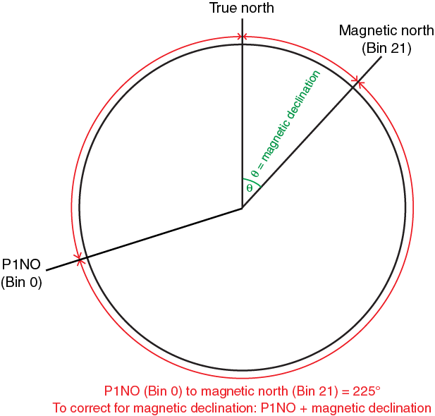
Figure F30. Image orientation to true north for geoVISION tool.
The final step to be able to accurately measure data on borehole features from GVR image logs is to assign the images with a value for the electrical penetration (referred to as depth of investigation in Schlumberger Techlog software). Each button (shallow, medium, and deep) has a fixed electrical penetration despite having different depths of investigation. The local response of the electrical signal is the part of the signal that is used to generate the resistivity images. This response is dependent on the size of the button and the standoff, which are similar for all three buttons on the geoVISION tool. The electrical penetration is 1.5 inches for the geoVISION tool, which corresponds to a percentage of the integrated geometrical radial response needed to resolve a resistivity contrast on the image. See Faivre and Catala (1995) for more detail.
A brief, descriptive, feature classification for GVR image logs was chosen to allow multiple subsequent interpretations and analyses (Trice, 1999). Classification included lithologic, structural, and stress-induced features (Figure F31; Table T13). The geometric and morphological interpretation of observed natural and stress-induced image log features can provide information on the lithology, stratigraphy, structure, and in situ stress character (Conin et al., 2014; Zoback, 2007; Massiot et al., 2015; Heidbach, 2016). Additionally, because gas hydrates are resistive, image logs also aided the interpretation of hydrate-bearing sediments in terms of vertical hydrate distribution and morphology with respect to the host sediments (e.g., Cook et al., 2008; Riedel et al., 2009; Collett et al., 2012; Kim et al., 2013; Kumar et al., 2014).

Figure F31. Resistivity image logs.
Core-log-seismic integration
LWD data were acquired during Expedition 372 at Sites U1518–U1520 across the continental margin and Hikurangi Trough (see Logging while drilling). Cores were collected from Sites U1518–U1520 and U1526 during Expedition 375. The cores and logs, together with high-quality regional seismic profiles, enabled CLSI during Expeditions 372 and 375.
Site U1518 LWD data were acquired from 0 to 600 mbsf across a lower slope thrust fault (Pāpaku fault), and cores were acquired (with varying degrees of recovery) from 0 to 494.9 mbsf. LWD data were acquired at Site U1519 (on the upper slope of the Tuaheni Basin) from 0 to 650 mbsf, and cores were acquired in several discrete intervals from 0 to 640 mbsf. LWD data were acquired within the incoming sedimentary section at Site U1520 from 0 to 750 mbsf, and wireline logs were acquired from 642 to 947 mbsf. Coring at Site U1520 took place from 0 to 1054.1 mbsf with varying degrees of recovery and some intervals that were drilled through without coring. Expedition 375 cored Site U1526 from 0 to 83.6 mbsf with varying degrees of recovery.
During Expedition 372, LWD data from Sites U1518–U1520 were tied to regional 2-D seismic profiles across the continental margin and Hikurangi Trough (e.g., Multiwave, unpubl. data; Barker et al., 2009; Bell et al., 2010; Pedley et al., 2010). This work was further advanced during Expedition 375 with integration of data from cores.
Expedition 372 LWD data, processing, and interpretation
The LWD BHA used during Expedition 372 included (in order from the bit up) the geoVISION, NeoScope, StethoScope, TeleScope, SonicScope, and proVISION Plus tools (Figure F29). For further details regarding the full suite of LWD tools, data types generated, techniques, and data processing, see Logging while drilling.
During the course of Expedition 372, various LWD data were processed on shore by Schlumberger logging scientists and then returned to the shipboard logging scientists for analysis. On the JOIDES Resolution, LWD data were loaded into the Techlog software (Schlumberger) for processing and interpretation. These data included a preliminary analysis of bedding, conductive and resistive fractures, and borehole breakouts identified in the GVR resistivity images.
All LWD data collected during Expedition 372 were interpreted on board and included in the site reports. These reports, their archived Techlog projects, and the results of real-time drilling safety monitoring and LWD-seismic integration were made available to the Expedition 375 scientists. In addition, a complete set of the final processed LWD data were compiled post-Expedition 372 in preparation for the Expedition 375 scientists.
Seismic reflection data and seismic stratigraphy
Data acquisition along the Expedition 372 and 375 drilling transect consisted of multiple cruises that collected 2-D seismic reflection data supporting Hikurangi subduction margin (HSM) Sites U1518–U1520 and U1526. The HSM sites are located on or close to 2-D Seismic Line 05CM-04 acquired in 2005 by the New Zealand government (Multiwave, unpubl. data; Barker et al., 2009, 2018). The 2005 data were acquired using a 4140 inch3 (67.8 L) air gun source array and a 12 km long streamer. The calculated source signature has a fairly flat amplitude spectrum across the range of ~6–100 Hz. Shot intervals were at 37.5 m, with a recording length of 12 s. These data were prestack time migrated with a 12.5 m common depth point (CDP) (Multiwave, unpubl. data; Barker et al., 2009; Bell et al., 2010).
The vertical resolution of Seismic Line 05CM-04 at Sites U1518–U1520, and U1526 can be determined as
Table T14 summarizes the vertical resolution for different depth intervals at each site using velocity information from the LWD logs.
Recently published prestack depth migration (PSDM) sections of Seismic Line 05CM-04 (Barker et al., 2018) and a preliminary full waveform inversion (FWI) P-wave velocity model were made available to both Expedition 372 and 375 scientists for onboard horizon depth estimates and CLSI. These data were made available by GNS Science, New Zealand (PSDM), and Imperial College London (FWI).
Seismic data from the 2005 05CM survey are supplemented by a suite of low-fold (48-channel) seismic data collected between 1993 and 2015 using 45–300 inch3 generator-injector (GI) gun sources. These data include the 1993 GeodyNZ survey on the R/V L’Atalante (e.g., Collot et al., 1996, 2001; Lewis et al., 1998); various R/V Tangaroa surveys in 2004, 2011, 2013, 2014, and 2015 (e.g., Pedley et al., 2010; Mountjoy and Barnes, 2011; National Institute of Water and Atmospheric Research [NIWA] [New Zealand], unpubl. data), and an R/V Roger Revelle survey in 2015 (Oregon State University, unpubl. data). In particular, the 2011 Survey TAN1114 undertaken by NIWA and GNS Science acquired drill site–specific seismic data with a source comprising two Sodera GI guns (300 inch3 total volume) operated in true GI mode at ~2000 psi pressure and recorded on a GeoEel 48-channel seismic streamer (~825 m long). These data were binned into a 6.25–12.5 m CDP spacing, bandpass filtered to 10, 35, 150, and 200 Hz, and poststack time migrated using a finite difference migration.
A seismic interpretation project developed at NIWA using IHS Kingdom Suite supported the predrilling interpretations of site geology and Expedition 372 and 375 drilling operations. The seismic project was developed from an initial data pack made available from the New Zealand Ministry of Business Innovation and Employment, in which all data are displayed with reversed polarity. Interpretations of seismic data from this project were exported to Petrel (Schlumberger) on the JOIDES Resolution during Expedition 372 and were available in active projects for the Expedition 375 scientists.
Seismic velocity models
Four sets of unpublished seismic P-wave velocity models for Seismic Line 05CM-04 were available to the Expedition 372 and 375 scientists for work on the JOIDES Resolution. These models include a high-resolution analysis of stacking velocity values and two PSDM models provided by GNS Science (Barker et al., 2018) and data from a preliminary FWI P-wave velocity model provided by Imperial College London. FWI is a technique that attempts to match the seismic waveforms trace by trace and differs from conventional velocity building techniques that use only arrival times (Warner et al., 2013). The Imperial College FWI velocity model uses a smoothed version of the GNS Science PSDM model as an initial velocity field, which is iteratively updated to produce synthetic waveforms to best match the real seismic data. Depth-converted seismic data derived from each of these models were used to evaluate the range of inferred depths to horizon and/or fault targets at each drilling site.
Integration of core and LWD data
Cores were collected from Sites U1518–U1520 and U1526 during Expedition 375 to characterize the age and lithologic, physical, thermal, geochemical, and structural properties of the sediment and rock sequences. Integrating these data with LWD data collected during Expedition 372 enabled calibration of the logging data, improved characterization of the sites, and refinement of LWD interpretations. Integration of core and log data sets was performed with the Techlog software and included the following:
- All LWD data sets were compared with lithostratigraphy as interpreted from retrieved cores, including high-resolution photographic images.
- Core measurements and LWD data of NGR were compared for consistency and calibration purposes.
- Porosity determined from MAD measurements on core samples was compared with LWD thermal neutron porosity and NMR porosity data.
- MAD bulk density measurements were compared with density measurements derived from the NeoScope tool (sourceless neutron-gamma density).
- P-wave velocity data measured on discrete core samples were compared with SonicScope VP data.
- Structural and bedding dip observations in the cores were compared with those interpreted from LWD resistivity images.
- Selected drilling parameters from different holes were evaluated to assist with correlations.
To aid the correlation of LWD data with core-based lithology, physical properties, and structural measurements from different holes at the same site, we used both the meters below rig floor and meters below seafloor depth scales.
Integration of core-log-seismic data: synthetic seismograms
We used LWD and core measurements to produce synthetic seismic traces at the drill site for comparison with observed traces in the seismic data. Their generation involved three steps:
- Producing a reflection coefficient model from LWD and core velocity and density measurements.
- Calculating vertical reflection times from LWD and core measurements.
- Convoluting the reflection coefficient model with a suitable source wavelet.
Generally, because of problems with logging data (e.g., washouts) and errors in seismic processing, a precise match between synthetic seismograms and seismic traces is rarely achieved. Instead, a suite of synthetic seismograms using different sonic calibrations and wavelets is constructed to see which best fits the seismic data and to provide a link between the core, geophysical logs, and seismic profiles.
Modeling of acoustic impedance and reflection coefficients was conducted using two different approaches with information from core, LWD, and wireline data. In the first approach, we calculated acoustic impedance and reflection coefficients using the sourceless neutron-gamma density log from the NeoScope tool, augmented where necessary by MAD density values spliced to the LWD density logs to produce a complete log. We used the compressional velocity log from the LWD SonicScope and from wireline data acquired in the deeper portion of Site U1520. The log measurements with high sampling rates were then averaged into intervals corresponding to the frequency range of seismic data. The second approach used physical properties information and interpretations of core data to build a log-lithologic model that highlighted major acoustic impedance changes at unit boundaries.
Conversion from depth to time is required during synthetic seismogram construction to allow correlation of depth-based LWD and wireline logs to traveltime-based seismic data. This conversion was performed using two different methods. First, LWD and wireline data were used to produce interval velocity logs that were used directly to convert depth data to time. However, poor log data quality (e.g., due to borehole washouts) result in poor time conversions. Secondly, lithostratigraphic units that could be confidently tied to reflection events provided “tie points” to further calibrate the time-depth relationship derived from compressional velocity and seismic velocity data.
Source wavelets can be obtained statistically or deterministically. Statistical determination involved recovery of the shape of the source wavelet from a horizontal area of the seafloor over a number of traces to produce a noise-free average wavelet. Deterministic source wavelet construction involved the calculation of a wavelet that produces the best fit between the synthetic trace and seismic data. Both approaches were applied using Schlumberger Petrel software and compared.
The wavelets were then convolved with a reflectivity series (R) expressed as the following:
where VP1 and VP2 and ρ1 and ρ2 are the acoustic velocity and density in the upper layer and lower layers, respectively.
Direct comparison was then made between all the available LWD and multichannel seismic (MCS) reflection data using Schlumberger’s Petrel software. This comparison enabled an overall assessment and integration of the unit boundaries and internal features determined during the analysis of each independent data set.
References
Backman, J., 1980. Miocene–Pliocene nannofossils and sedimentation rates in the Hatton-Rockall Basin, NE Atlantic Ocean. Acta Universitatis Stockholmiensis: Stockholm Contributions in Geology, 36(1):1–91.
Barker, D.H.N., Henrys, S., Caratori Tontini, F., Barnes, P.M., Bassett, D., Todd, E., and Wallace, L., 2018. Geophysical constraints on the relationship between seamount subduction, slow slip and tremor at the north Hikurangi subduction zone, New Zealand. Geophysical Research Letters, 45(23):12804–12813. https://doi.org/10.1029/2018GL080259
Barker, D.H.N., Sutherland, R., Henrys, S., and Bannister, S., 2009. Geometry of the Hikurangi subduction thrust and upper plate, North Island, New Zealand. Geochemistry, Geophysics, Geosystems, 10(2):Q02007. https://doi.org/10.1029/2008GC002153
Barnes, P.M., Wallace, L.M., Saffer, D.M., Pecher, I.A., Petronotis, K.E., LeVay, L.J., Bell, R.E., Crundwell, M.P., Engelmann de Oliveira, C.H., Fagereng, A., Fulton, P.M., Greve, A., Harris, R.N., Hashimoto, Y., Hüpers, A., Ikari, M.J., Ito, Y., Kitajima, H., Kutterolf, S., Lee, H., Li, X., Luo, M., Malie, P.R., Meneghini, F., Morgan, J.K., Noda, A., Rabinowitz, H.S., Savage, H.M., Shepherd, C.L., Shreedharan, S., Solomon, E.A., Underwood, M.B., Wang, M., Woodhouse, A.D., Bourlange, S.M., Brunet, M.M.Y., Cardona, S., Clennell, M.B., Cook, A.E., Dugan, B., Elger, J., Gamboa, D., Georgiopoulou, A., Han, S., Heeschen, K.U., Hu, G., Kim, G.Y., Koge, H., Machado, K.S., McNamara, D.D., Moore, G.F., Mountjoy, J.J., Nole, M.A., Owari, S., Paganoni, M., Rose, P.S., Screaton, E.J., Shankar, U., Torres, M.E., Wang, X., and Wu, H.-Y., 2019. Site U1519. In Wallace, L.M., Saffer, D.M., Barnes, P.M., Pecher, I.A., Petronotis, K.E., LeVay, L.J., and the Expedition 372/375 Scientists, Hikurangi Subduction Margin Coring, Logging, and Observatories. Proceedings of the International Ocean Discovery Program, 372B/375: College Station, TX (International Ocean Discovery Program). https://doi.org/10.14379/iodp.proc.372B375.104.2019
Bartington Instruments, Ltd., 2011. Operation Manual for MS2 Magnetic Susceptibility System: Oxford, United Kingdom (Bartington Instruments, Ltd.). https://www.gmw.com/magnetic_properties/pdf/BI-MAN-MS2-OM0408.pdf
Bell, R., Sutherland, R., Barker, D.H.N., Henrys, S., Bannister, S., Wallace, L., and Beavan, J., 2010. Seismic reflection character of the Hikurangi subduction interface, New Zealand, in the region of repeated Gisborne slow slip events. Geophysical Journal International, 180(1):34–48. https://doi.org/10.1111/j.1365-246X.2009.04401.x
Blenkinsop, T.G., and Doyle, M.G., 2010. A method for measuring the orientations of planar structures in cut core. Journal of Structural Geology, 32(6):741–745. https://doi.org/10.1016/j.jsg.2010.04.011
Blum, P., 1997. Technical Note 26: Physical Properties Handbook—A Guide to the Shipboard Measurement of Physical Properties of Deep-Sea Cores. Ocean Drilling Program. https://doi.org/10.2973/odp.tn.26.1997
Bollmann, J., 1997. Morphology and biogeography of Gephyrocapsa coccoliths in Holocene sediments. Marine Micropaleontology, 29(3–4):319–350. https://doi.org/10.1016/S0377-8398(96)00028-X
Bonner, S.D., Tabanou, J.R., Wu, P.T., Seydoux, J.P., Moriarty, K.A., Seal, B.K., Kwok, E.Y., and Kuchenbecker, M.W., 1995. New 2-MHz multiarray borehole-compensated resistivity tool developed for MWD in slim holes [paper presented at SPE Annual Technical Conference and Exhibition, Dallas, Texas, 22–25 October 1995]. (Abstract SPE-30547-MS) https://doi.org/10.2118/30547-MS
Bown, P.R. (Ed.), 1998. Calcareous Nannofossil Biostratigraphy: Dordrecht, The Netherlands (Kluwer Academic Publishing).
Bown, P.R., 2005. Palaeogene calcareous microfossils from the Kilwa and Lindi areas of coastal Tanzania (Tanzania Drilling Project 2003–4). Journal of Nannoplankton Research, 27(1):21–95. http://ina.tmsoc.org/JNR/online/27/Bown 2005_ JNR27-1_TDP.pdf
Butler, R.F., 2004. Paleomagnetism: Magnetic Domains to Geologic Terranes (electronic edition). https://www.geo.arizona.edu/Paleomag/
Cardozo, N., and Allmendinger, R.W., 2013. Spherical projections with OSXStereonet. Computers & Geosciences, 51:193–205. https://doi.org/10.1016/j.cageo.2012.07.021
Collett, T.S., Lee, M.W., Zyrianova, M.V., Mrozewski, S.A., Guerin, G., Cook, A.E., and Goldberg, D.S., 2012. Gulf of Mexico Gas Hydrate Joint Industry Project Leg II logging-while-drilling data acquisition and analysis. Marine and Petroleum Geology, 34(1):41–61. https://doi.org/10.1016/j.marpetgeo.2011.08.003
Collot, J.-Y., Delteil, J., Lewis, K.B., Davy, B., Lamarche, G., Audru, J.-C., Barnes, P., et al., 1996. From oblique subduction to intra-continental transpression: structures of the southern Kermadec-Hikurangi margin from multibeam bathymetry, side-scan sonar and seismic reflection. Marine Geophysical Research, 18(2–4):357–381. https://doi.org/10.1007/BF00286085
Collot, J.-Y., Lewis, K., Lamarche, G., and Lallemand, S., 2001. The giant Ruatoria debris avalanche on the northern Hikurangi margin, New Zealand; result of oblique seamount subduction. Journal of Geophysical Research: Solid Earth, 106(B9):19271–19297. https://doi.org/10.1029/2001JB900004
Conin, M., Bourlange, S., Henry, P., Boiselet, A., and Gaillot, P., 2014. Distribution of resistive and conductive structures in Nankai accretionary wedge reveals contrasting stress paths. Tectonophysics, 611:181–191. https://doi.org/10.1016/j.tecto.2013.11.025
Cook, A.E., Goldberg, D., and Kleinberg, R.L., 2008. Fracture-controlled gas hydrate systems in the northern Gulf of Mexico. Marine and Petroleum Geology, 25(9):932–941. https://doi.org/10.1016/j.marpetgeo.2008.01.013
Cooper, R.A., 2004. The New Zealand Geological Timescale. GNS Monograph, 22.
Crundwell, M., Scott, G., Naish, T., and Carter, L., 2008. Glacial–interglacial ocean climate variability from planktonic foraminifera during the Mid-Pleistocene transition in the temperate Southwest Pacific, ODP Site 1123. Palaeogeography, Palaeoclimatology, Palaeoecology, 260(1-2): 202–229. https://doi.org/10.1016/j.palaeo.2007.08.023
Crundwell, M.P., 2004. New Zealand late Miocene biostratigraphy and biochronology: studies of planktic foraminifers and bolboforms at oceanic Sites 593 and 1123 and selected onland sections [Ph.D. thesis]. University of Waikato, New Zealand. http://odp.georef.org/vufind/Record/2009082475/Details
Crundwell, M.P., 2015a. Pliocene and early Pleistocene planktic foraminifera: important taxa and bioevents in ODP Hole 1123B, Chatham Rise, New Zealand. GNS Science Report, 2015/51.
Crundwell, M.P., 2015b. Revised Pliocene and early Pleistocene planktonic foraminiferal biostratigraphy, DSDP Site 284, Challenger Plateau, New Zealand. GNS Science Internal Report, 2015\22.
Crundwell, M.P., Beu, A.G., Cooper, R.A., Morgans, H.E.G., Mildenhall, D.C., and Wilson, G.S., 2004. Miocene (Pareora, Southland and Taranaki Series). In Cooper R.A. (Ed.), The New Zealand Geological Timescale. GNS Science Monograph, 22:165–194.
Crundwell, M.P., Cooke, P.J., Nelson, C.S., and Spiegler, D., 2005. Intraspecific morphological variation in late Miocene Bolboforma, and implications for their classification, ecology, and biostratigraphic utility. Marine Micropaleontology, 56(3–4):161–176. https://doi.org/10.1016/j.marmicro.2005.05.003
Crundwell, M.P., and Nelson, C.S., 2007. A magnetostratigraphically constrained chronology for late Miocene bolboformids and planktic foraminifers in the temperate Southwest Pacific. Stratigraphy, 4(1):1–34. http://www.micropress.org/microaccess/check/1502
Crundwell, M.P., Scott, G.H., and Thrasher, G.P., 1994. Calibration of paleobathymetry indicators by integrated seismic and paleontological analysis of forest sequences, Taranaki Basin, New Zealand. In The Post Maui Challenge: Investment and Development Opportunities. New Zealand Petroleum Conference Proceedings, 169–178.
Dankers, P.H.M., and Zijderveld, J.D.A., 1981. Alternating field demagnetization of rocks, and the problem of gyromagnetic remanence. Earth and Planetary Science Letters, 53(1):89–92. https://doi.org/10.1016/0012-821X(81)90029-7
De Vleeschouwer, D., Dunlea, A.G., Auer, G., Anderson, C.H., Brumsack, H., de Loach, A., Gurnis, M., et al., 2017. Quantifying K, U, and Th contents of marine sediments using shipboard natural gamma radiation spectra measured on DV JOIDES Resolution. Geochemistry, Geophysics, Geosystems, 18(3):1053–1064. https://doi.org/10.1002/2016GC006715
Droser, M.L., and Bottjer, D.J., 1986. A semiquantitative field classification of ichnofabric. Journal of Sedimentary Research, 56(4):558–559. https://doi.org/10.1306/212F89C2-2B24-11D7-8648000102C1865D
Droser, M.L., and Bottjer, D.J., 1991. Trace fossils and ichnofabric in Leg 119 cores. In Barron, J., Larsen, B., et al., Proceedings of the Ocean Drilling Program, Scientific Results, 119: College Station, TX (Ocean Drilling Program), 635–641. https://doi.org/10.2973/odp.proc.sr.119.206.1991
Dunkley Jones, T., Bown, P.R., and Pearson, P.N., 2009. Exceptionally well preserved upper Eocene to lower Oligocene calcareous nannofossils (Prymnesiophycidae) from the Pande Formation (Kilwa Group), Tanzania. Journal of Systematic Palaeontology, 7(4):359–411. https://doi.org/10.1017/S1477201909990010
Ellis, D.V., and Singer, J.M., 2007. Well Logging for Earth Scientists (2nd edition): New York (Elsevier). https://doi.org/10.1007/978-1-4020-4602-5
Expedition 308 Scientists, 2006. Methods. In Flemings, P.B., Behrmann, J.H., John, C.M., and the Expedition 308 Scientists, Proceedings of the Integrated Ocean Drilling Program, 308: College Station, TX (Integrated Ocean Drilling Program Management International, Inc.). https://doi.org/10.2204/iodp.proc.308.102.2006
Expedition 311 Scientists, 2006. Methods. In Riedel, M., Collett, T.S., Malone, M.J., and the Expedition 311 Scientists, Proceedings of the Integrated Ocean Drilling Program, 311: Washington, DC (Integrated Ocean Drilling Program Management International, Inc.). https://doi.org/10.2204/iodp.proc.311.102.2006
Expedition 314 Scientists, 2009. Expedition 314 methods. In Kinoshita, M., Tobin, H., Ashi, J., Kimura, G., Lallemant, S., Screaton, E.J., Curewitz, D., Masago, H., Moe, K.T., and the Expedition 314/315/316 Scientists, Proceedings of the Integrated Ocean Drilling Program, 314/315/316: Washington, DC (Integrated Ocean Drilling Program Management International, Inc.). https://doi.org/10.2204/iodp.proc.314315316.112.2009
Expedition 319 Scientists, 2010. Methods. In Saffer, D., McNeill, L., Byrne, T., Araki, E., Toczko, S., Eguchi, N., Takahashi, K., and the Expedition 319 Scientists, Proceedings of the Integrated Ocean Drilling Program, 319: Tokyo (Integrated Ocean Drilling Program Management International, Inc.). https://doi.org/10.2204/iodp.proc.319.102.2010
Expedition 332 Scientists, 2011. Methods. In Kopf, A., Araki, E., Toczko, S., and the Expedition 332 Scientists, Proceedings of the Integrated Ocean Drilling Program, 332: Tokyo (Integrated Ocean Drilling Program Management International, Inc.). https://doi.org/10.2204/iodp.proc.332.102.2011
Expedition 334 Scientists, 2012. Methods. In Vannucchi, P., Ujiie, K., Stroncik, N., Malinverno, A., and the Expedition 334 Scientists, Proceedings of the Integrated Ocean Drilling Program, 334: Tokyo (Integrated Ocean Drilling Program Management International, Inc.). https://doi.org/10.2204/iodp.proc.334.102.2012
Expedition 343/343T Scientists, 2013. Methods. In Chester, F.M., Mori, J., Eguchi, N., Toczko, S., and the Expedition 343/343T Scientists, Proceedings of the Integrated Ocean Drilling Program, 343/343T: Tokyo (Integrated Ocean Drilling Program Management International, Inc.). https://doi.org/10.2204/iodp.proc.343343T.102.2013
Faivre, O., and Catala, G., 1995. Dip estimation from azimuthal laterolog tools [paper presented at the SPWLA 36th Annual Logging Symposium, Paris, France, 26–29 June 1995]. (Abstract SPWLA-1995-CC) https://www.onepetro.org/download/conference-paper/SPWLA-1995-CC?id=conference-paper%2FSPWLA-1995-CC
Fisher, A.T., and Underwood, M.B., 1995. Calibration of an X-ray diffraction method to determine relative mineral abundances in bulk powders using matrix singular value decomposition: a test from the Barbados accretionary complex. In Shipley, T.H., Ogawa, Y., Blum, P., et al., Proceedings of the Ocean Drilling Program, Initial Reports, 156: College Station, TX (Ocean Drilling Program), 29–37. https://doi.org/10.2973/odp.proc.ir.156.103.1995
Fisher, R., 1953. Dispersion on a sphere. Proceedings of the Royal Society of London, Series A: Mathematical, Physical and Engineering Sciences, 217(1130):295–305. https://doi.org/10.1098/rspa.1953.0064
Fisher, R.V., and Schmincke, H.-U., 1984. Pyroclastic Rocks: Berlin (Springer-Verlag). https://doi.org/10.1007/978-3-642-74864-6
Folk, R.L., 1980. Petrology of Sedimentary Rocks (2nd edition): Austin, TX (Hemphill Publishing Company). http://hdl.handle.net/2152/22930
Gieskes, J.M., Gamo, T., and Brumsack, H., 1991. Technical Note 15: Chemical Methods for Interstitial Water Analysis Aboard JOIDES Resolution. Ocean Drilling Program. https://doi.org/10.2973/odp.tn.15.1991
Goldberg, D., 1997. The role of downhole measurements in marine geology and geophysics. Reviews of Geophysics, 35(3):315–342. https://doi.org/10.1029/97RG00221
Gradstein, F.M., Ogg, J.G., Schmitz, M.D., and Ogg, G.M. (Eds.), 2012. The Geological Time Scale 2012: Amsterdam (Elsevier). https://doi.org/10.1016/C2011-1-08249-8
Grützmacher, U., 1993. Die Veränderungen der paläogeographischen Verbreitung von Bolboforma: ein Beitrag zur Rekonstruktion und Definition von Wassermassen im Tertiär. GEOMAR Reports, 22.
Harris, R.N., Sakaguchi, A., Petronotis, K., Baxter, A.T., Berg, R., Burkett, A., Charpentier, D., Choi, J., Diz Ferreiro, P., Hamahashi, M., Hashimoto, Y., Heydolph, K., Jovane, L., Kastner, M., Kurz, W., Kutterolf, S.O., Li, Y., Malinverno, A., Martin, K.M., Millan, C., Nascimento, D.B., Saito, S., Sandoval Gutierrez, M.I., Screaton, E.J., Smith-Duque, C.E., Solomon, E.A., Straub, S.M., Tanikawa, W., Torres, M.E., Uchimura, H., Vannucchi, P., Yamamoto, Y., Yan, Q., and Zhao, X., 2013. Methods. In Harris, R.N., Sakaguchi, A., Petronotis, K., and the Expedition 344 Scientists, Proceedings of the Integrated Ocean Drilling Program, 344: College Station, TX (Integrated Ocean Drilling Program). https://doi.org/10.2204/iodp.proc.344.102.2013
Hayward, B.W., Grenfell, H.R., Reid, C.M., and Hayward, K.A., 1999. Recent New Zealand shallow-water benthic foraminifera: taxonomy, ecologic distribution, biogeography, and use in paleoenvironmental assessment. New Zealand Geological Survey Bulletin, 75.
Hayward, B.W., Grenfell, H.R., Sabaa, A.T., Neil, H.L., and Buzas, M.A., 2010. Recent New Zealand Deep-Water Benthic Foraminifera: Taxonomy, Ecologic Distribution, Biogeography, and Use in Paleoenvironmental Assessment. GNS Science Monograph, 26.
Hayward, B.W., Sabaa, A.T., Grenfell, H.R., Neil, H., and Bostock, H., 2013. Ecological distribution of recent deep-water foraminifera around New Zealand. Journal of Foraminiferal Research, 43(4):415–442. https://doi.org/10.2113/gsjfr.43.4.415
Heard, T.G., Pickering, K.T., and Clark, J.D. 2014. Ichnofabric characterization of a deep-marine clastic system: a subsurface study of the middle Eocene Ainsa System, Spanish Pyrenees. Sedimentology, 61(5):1298–1331. https://doi.org/10.1111/sed.12101
Heesemann, M., Villinger, H., Fisher, A.T., Tréhu, A.M., and White, S., 2006. Data report: testing and deployment of the new APCT-3 tool to determine in situ temperatures while piston coring. In Riedel, M., Collett, T.S., Malone, M.J., and the Expedition 311 Scientists. Proceedings of the Integrated Ocean Drilling Program, 311: Washington, DC (Integrated Ocean Drilling Program Management International, Inc.). https://doi.org/10.2204/iodp.proc.311.108.2006
Heidbach, O. (Ed.), 2016. Scientific Technical Report 16-01:WSM Quality Ranking Scheme, Database and Analysis Guidelines for Stress Indicators. With contributions by A. Barth, B. Müller, J. Reinecker, O. Stephansson, M., Tingay, and A. Zhang. WSM World Stress Map. http://www.world-stress-map.org/fileadmin/wsm/pdfs/WSM_STR_16_01.pdf
Hornibrook, N.d.B., 1961. Tertiary foraminifera from Oamaru District (N. Z.), Part 1. Systematics and distribution. Palaeontological Bulletin, 34.
Hornibrook, N.d.B., 1981. Globorotalia (planktic Foraminiferida) in the late Pliocene and early Pleistocene of New Zealand. New Zealand Journal of Geology and Geophysics, 24(2):263–292. https://doi.org/10.1080/00288306.1981.10422717
Hornibrook, N.d.B., 1982. Late Miocene to Pleistocene Globorotalia (Foraminiferida) from DSDP Leg 29, Site 284, southwest Pacific. New Zealand Journal of Geology and Geophysics, 25(1):83–99. https://doi.org/10.1080/00288306.1982.10422507
Hornibrook, N.d.B., Brazier, R.C., and Strong, C.P., 1989. Manual of New Zealand Permian to Pleistocene foraminiferal biostratigraphy. New Zealand Geological Survey Paleontological Bulletin, 56.
Hornibrook, N.d.B., and Jenkins, D.G., 1994. DSDP 594, Chatham Rise, New Zealand—late Neogene planktonic foraminiferal biostratigraphy revisited. Journal of Micropalaeontology, 13(2):93–101. https://doi.org/10.1144/jm.13.2.93
Hu, S., Stephenson, A., and Appel, E., 2002. A study of gyroremanent magnetisation (GRM) and rotational remanent magnetisation (RRM) carried by greigite from lake sediments. Geophysical Journal International, 151(2):469–474. https://doi.org/10.1046/j.1365-246X.2002.01793.x
Huber, B.T., and Leckie, R.M., 2011. Planktic foraminiferal species turnover across deep-sea Aptian/Albian boundary sections. Journal of Foraminiferal Research, 41(1):53–95. https://doi.org/10.2113/gsjfr.41.1.53
Huber, B.T., Petrizzo, M.R., Watkins, D.K., Haynes, S.J., and MacLeod, K.G., 2017. Correlation of Turonian continental margin and deep-sea sequences in the subtropical Indian Ocean sediments by integrated planktonic foraminiferal and calcareous nannofossil biostratigraphy. Newsletters on Stratigraphy, 50(2):141–185. https://doi.org/10.1127/nos/2017/0373
Ingram, R.L., 1954. Terminology for the thickness of stratification and parting units in sedimentary rocks. Geological Society of America Bulletin, 65(9):937–938. https://doi.org/10.1130/0016-7606(1954)65[937:TFTTOS]2.0.CO;2
Jutzeler, M., White, J.D.L., Talling, P.J., McCanta, M., Morgan, S., Le Friant, A., and Ishizuka, O., 2014. Coring disturbances in IODP piston cores with implications for offshore record of volcanic events and the Missoula megafloods. Geochemistry, Geophysics, Geosystems, 15(9):3572–3590. https://doi.org/10.1002/2014GC005447
Kars, M., and Kodama, K., 2015. Rock magnetic characterization of ferrimagnetic iron sulfides in gas hydrate–bearing marine sediments at Site C0008, Nankai Trough, Pacific Ocean, off-coast Japan. Earth, Planets and Space, 67:118. https://doi.org/10.1186/s40623-015-0287-y
Kastner, M., Solomon, E.A., Harris, R.N., and Torres, M.E., 2014. Fluid origins, thermal regimes, and fluid and solute fluxes in the forearc of subduction zones. In Stein, R., Blackman, D., Inagaki, F., and Larsen, H.-C., Developments in Marine Geology (Volume 7): Earth and Life Processes Discovered from Subseafloor Environments: a Decade of Science Achieved by the Integrated Ocean Drilling Program (IODP). R. Stein (Series Ed.): Amsterdam (Elsevier B.V.), 671–733. https://doi.org/10.1016/B978-0-444-62617-2.00022-0
Kennett, J.P., and Srinivasan, M.S., 1983. Neogene Planktonic Foraminifera: A Phylogenetic Atlas: Stroudsburg, PA (Hutchinson Ross).
Kim, G.Y., Narantsetseg, B., Ryu, B.-J., Yoo, D.-G., Lee, J.Y., Kim, H.S., and Riedel, M., 2013. Fracture orientation and induced anisotropy of gas hydrate-bearing sediments in seismic chimney-like-structures of the Ulleung Basin, East Sea. Marine and Petroleum Geology, 47:182–194. https://doi.org/10.1016/j.marpetgeo.2013.06.001
Kirschvink, J.L., 1980. The least-squares line and plane and the analysis of palaeomagnetic data. Geophysical Journal of the Royal Astronomical Society, 62(3):699–718. https://doi.org/10.1111/j.1365-246X.1980.tb02601.x
Kumar, P., Collett, T.S., Boswell, R., Cochran, J.R., Lall, M., Mazumdar, A., Ramana, M.V., et al., 2014. Geologic implications of gas hydrates in the offshore of India: Krishna–Godavari Basin, Mahanadi Basin, Andaman Sea, Kerala–Konkan Basin. Marine and Petroleum Geology, 58:29–98. https://doi.org/10.1016/j.marpetgeo.2014.07.031
Kvenvolden, K.A., and McDonald, T.J., 1986. Technical Note 6: Organic Geochemistry on the JOIDES Resolution—An Assay. Ocean Drilling Program. https://doi.org/10.2973/odp.tn.6.1986
Lewis, K.B., Collot, J.-Y., and Lallemand, S.E., 1998. The dammed Hikurangi Trough: a channel-fed trench blocked by subducting seamounts and their wake avalanches (New Zealand–France GeodyNZ Project). Basin Research, 10(4):441–468. https://doi.org/10.1046/j.1365-2117.1998.00080.x
Liu, Q., Roberts, A.P., Larrasoaña, J.C., Banerjee, S.K., Guyodo, Y., Tauxe, L., and Oldfield, F., 2012. Environmental magnetism: principles and applications. Reviews of Geophysics, 50(4):RG4002. https://doi.org/10.1029/2012RG000393
Lourens, L., Hilgen, F., Shackleton, N.J., Laskar, J., and Wilson, D., 2004. The Neogene period. In Gradstein, F.M., Ogg, J.G., and Smith, A. (Eds.), A Geologic Time Scale 2004: Cambridge, United Kingdom (Cambridge University Press), 409–440. https://doi.org/10.1017/CBO9780511536045.022
Lurcock, P.C., and Wilson, G.S., 2012. PuffinPlot: a versatile, user-friendly program for paleomagnetic analysis. Geochemistry, Geophysics, Geosystems, 13(6):Q06Z45. https://doi.org/10.1029/2012GC004098
Maiorano, P., and Marino, M., 2004. Calcareous nannofossil bioevents and environmental control on temporal and spatial patterns at the early–middle Pleistocene. Marine Micropaleontology, 53(3–4):405–422. https://doi.org/10.1016/j.marmicro.2004.08.003
Manheim, F.T., and Sayles, F.L., 1974. Composition and origin of interstitial waters of marine sediments, based on deep sea drill cores. In Goldberg, E.D. (Ed.), The Sea (Volume 5): Marine Chemistry: The Sedimentary Cycle: New York (Wiley), 527–568.
Marsaglia, K., Milliken, K., and Doran, L., 2013. Technical Note 1: IODP digital reference for smear slide analysis of marine mud—Part 1: Methodology and atlas of siliciclastic and volcanogenic components. Integrated Ocean Drilling Program. https://doi.org/10.2204/iodp.tn.1.2013
Marsaglia, K., Milliken, K., Leckie, R.M., Tentori, D., and Doran, L., 2015. Technical Note 2: IODP smear slide digital reference for sediment analysis of marine mud, Part 2: Methodology and atlas of biogenic components. International Ocean Discovery Program. https://doi.org/10.2204/iodp.tn.2.2015
Martini, E., 1971. Standard Tertiary and Quaternary calcareous nannoplankton zonation. In Farinacci, A. (Ed.), Proceedings of the Second Planktonic Conference, Roma 1970: Rome (Edizioni Tecnoscienza), 2:739–785.
Massiot, C., McNamara, D.D., and Lewis, B., 2015. Processing and analysis of high temperature geothermal acoustic borehole image logs in the Taupo Volcanic Zone, New Zealand. Geothermics, 53:190–201. https://doi.org/10.1016/j.geothermics.2014.05.010
Mazzullo, J., and Graham, A.G. (Eds.), 1988. Technical Note 8: Handbook for shipboard sedimentologists. Ocean Drilling Program. https://doi.org/10.2973/odp.tn.8.1988
MacLeod, C.J., Dick, H.J.B., Blum, P., Abe, N., Blackman, D.K., Bowles, J.A., Cheadle, M.J., Cho, K., Ciążela, J., Deans, J.R., Edgcomb, V.P., Ferrando, C., France, L., Ghosh, B., Ildefonse, B.M., Kendrick, M.A., Koepke, J.H., Leong, J.A.M., Liu, C., Ma, Q., Morishita, T., Morris, A., Natland, J.H., Nozaka, T., Pluemper, O., Sanfilippo, A., Sylvan, J.B., Tivey, M.A., Tribuzio, R., and Viegas, L.G.F., 2017. Expedition 360 methods. In MacLeod, C.J., Dick, H.J.B., Blum, P., and the Expedition 360 Scientists, Southwest Indian Ridge Lower Crust and Moho. Proceedings of the International Ocean Discovery Program, 360: College Station, TX (International Ocean Discovery Program). https://doi.org/10.14379/iodp.proc.360.102.2017
McNeill, L.C., Dugan, B., Petronotis, K.E., Backman, J., Bourlange, S., Chemale, F., Chen, W., Colson, T.A., Frederik, M.C.G., Guèrin, G., Hamahashi, M., Henstock, T., House, B.M., Hüpers, A., Jeppson, T.N., Kachovich, S., Kenigsberg, A.R., Kuranaga, M., Kutterolf, S., Milliken, K.L., Mitchison, F.L., Mukoyoshi, H., Nair, N., Owari, S., Pickering, K.T., Pouderoux, H.F.A., Yehua, S., Song, I., Torres, M.E., Vannucchi, P., Vrolijk, P.J., Yang, T., and Zhao, X., 2017. Expedition 362 methods. In McNeill, L.C., Dugan, B., Petronotis, K.E., and the Expedition 362 Scientists, Sumatra Subduction Zone. Proceedings of the International Ocean Discovery Program, 362: College Station, TX (International Ocean Discovery Program). https://doi.org/10.14379/iodp.proc.362.102.2017
Merrill, R.T., McElhinny, M.W., and McFadden, P.L., 1996. The Magnetic Field of the Earth: Paleomagnetism, the Core and the Deep Mantle: San Diego (Academic).
Mountjoy, J.J., and Barnes, P., 2011. Active upper plate thrust faulting in regions of low plate interface coupling, repeated slow slip events, and coastal uplift: example from the Hikurangi margin, New Zealand. Geochemistry, Geophysics, Geosystems, 12(1):Q01005. https://doi.org/10.1029/2010GC003326
Murray, R.W., Miller, D.J., and Kryc, K.A., 2000. Technical Note 29: Analysis of Major and Trace Elements in Rocks, Sediments, and Interstitial Waters by Inductively Coupled Plasma–Atomic Emission Spectrometry (ICP-AES). Ocean Drilling Program. https://doi.org/10.2973/odp.tn.29.2000
Okada, H., and Bukry, D., 1980. Supplementary modification and introduction of code numbers to the low-latitude coccolith biostratigraphic zonation (Bukry, 1973; 1975). Marine Micropaleontology, 5:321–325. https://doi.org/10.1016/0377-8398(80)90016-X
Olsson, R.K., Hemleben, C., Berggren, W.A., and Huber, B.T. (Eds.), 1999. Atlas of Paleocene planktonic foraminifera. Smithsonian Contributions to Paleobiology, 85. https://doi.org/10.5479/si.00810266.85.1
Pandey, D.K., Clift, P.D., Kulhanek, D.K., Andò, S., Bendle, J.A.P., Bratenkov, S., Griffith, E.M., Gurumurthy, G.P., Hahn, A., Iwai, M., Khim, B.-K., Kumar, A., Kumar, A.G., Liddy, H.M., Lu, H., Lyle, M.W., Mishra, R., Radhakrishna, T., Routledge, C.M., Saraswat, R., Saxena, R., Scardia, G., Sharma, G.K., Singh, A.D., Steinke, S., Suzuki, K., Tauxe, L., Tiwari, M., Xu, Z., and Yu, Z., 2016. Site U1456. In Pandey, D.K., Clift, P.D., Kulhanek, D.K., and the Expedition 355 Scientists, Arabian Sea Monsoon. Proceedings of the International Ocean Discovery Program, 355: College Station, TX (International Ocean Discovery Program). https://doi.org/10.14379/iodp.proc.355.103.2016
Pearson, P.N., Olsson, R.K., Hemleben, C., Huber, B.T., and Berggren, W.A. (Eds.), 2006. Atlas of Eocene planktonic foraminifera. Special Publication - Cushman Foundation for Foraminiferal Research, 41.
Pearson, P.N., and Wade, B.S., 2015. Systematic taxonomy of exceptionally well-preserved planktonic foraminifera from the Eocene/Oligocene boundary of Tanzania. Special Publication - Cushman Foundation for Foraminiferal Research, 45.
Pedley, K.L., Barnes, P.M., Pettinga, J.R., and Lewis, K.B., 2010. Seafloor structural geomorphic evolution of the accretionary frontal wedge in response to seamount subduction, Poverty Indentation, New Zealand. Marine Geology, 270(1–4):119–138. https://doi.org/10.1016/j.margeo.2009.11.006
Perch-Nielsen, K., 1985. Cenozoic calcareous nannofossils. In Bolli, H.M., Saunders, J.B., and Perch-Nielsen, K. (Eds.), Plankton Stratigraphy: Cambridge, United Kingdom (Cambridge University Press), 427–554.
Petrizzo, M.R., and Huber, B.T., 2006. Biostratigraphy and taxonomy of late Albian planktonic foraminifer from ODP Leg 171B (western North Atlantic). Journal of Foraminiferal Research, 36(2):166–190. https://doi.org/10.2113/36.2.166
Poag, C.W., and Karowe, A.L., 1986. Stratigraphic potential of Bolboforma significantly increased by new finds in the North Atlantic and South Pacific. Palaios, 1(2):162–171. https://doi.org/10.2307/3514510
Raffi, I., Backman, J., Fornaciari, E., Pälike, H., Rio, D., Lourens, L., and Hilgen, F., 2006. A review of calcareous nannofossil astrobiochronology encompassing the past 25 million years. Quaternary Science Reviews, 25(23–24):3113–3137. https://doi.org/10.1016/j.quascirev.2006.07.007
Raine, J.I., Beu, A.G., Boyes, A., Campbell, H.J., Cooper, R.A., Crampton, J.S., Crundwell, M.P., Hollis, C.J., and Morgans, H.E., 2015. A revised calibration of the New Zealand Geological Timescale: NZGT2015 [paper presented at International Conference and Exhibition, Melbourne, Australia, 13–16 September 2015]. https://doi.org/10.1190/ice2015-2211449
Reagan, M.K., Pearce, J.A., Petronotis, K., Almeev, R., Avery, A.A., Carvallo, C., Chapman, T., Christeson, G.L., Ferré, E.C., Godard, M., Heaton, D.E., Kirchenbaur, M., Kurz, W., Kutterolf, S., Li, H.Y., Li, Y., Michibayashi, K., Morgan, S., Nelson, W.R., Prytulak, J., Python, M., Robertson, A.H.F., Ryan, J.G., Sager, W.W., Sakuyama, T., Shervais, J.W., Shimizu, K., and Whattam, S.A., 2015. Expedition 352 methods. In Reagan, M.K., Pearce, J.A., Petronotis, K., and the Expedition 352 Scientists, Izu-Bonin-Mariana Fore Arc. Proceedings of the International Ocean Discovery Program, 352: College Station, TX (International Ocean Discovery Program). https://doi.org/10.14379/iodp.proc.352.102.2015
Rider, M.H., 1996. The Geological Interpretation of Well Logs (2nd edition): Caithness, Scotland (Whittles Publishing).
Riedel, M., Collett, T., Malone, M.J., and IODP Expedition 311 Scientists, 2009. Gas hydrate drilling transect across northern Cascadia margin—IODP Expedition 311. Geological Society Special Publication, 319:11–19. https://doi.org/10.1144/SP319.2
Rothwell, R.G., 1989. Minerals and Mineraloids in Marine Sediments: An Optical Identification Guide: London (Elsevier). https://doi.org/10.1007/978-94-009-1133-8
Saffer, D.M., Wallace, L.M., Barnes, P.M., Pecher, I.A., Petronotis, K.E., LeVay, L.J., Bell, R.E., Crundwell, M.P., Engelmann de Oliveira, C.H., Fagereng, A., Fulton, P.M., Greve, A., Harris, R.N., Hashimoto, Y., Hüpers, A., Ikari, M.J., Ito, Y., Kitajima, H., Kutterolf, S., Lee, H., Li, X., Luo, M., Malie, P.R., Meneghini, F., Morgan, J.K., Noda, A., Rabinowitz, H.S., Savage, H.M., Shepherd, C.L., Shreedharan, S., Solomon, E.A., Underwood, M.B., Wang, M., Woodhouse, A.D., Bourlange, S.M., Brunet, M.M.Y., Cardona, S., Clennell, M.B., Cook, A.E., Dugan, B., Elger, J., Gamboa, D., Georgiopoulou, A., Han, S., Heeschen, K.U., Hu, G., Kim, G.Y., Koge, H., Machado, K.S., McNamara, D.D., Moore, G.F., Mountjoy, J.J., Nole, M.A., Owari, S., Paganoni, M., Rose, P.S., Screaton, E.J., Shankar, U., Torres, M.E., Wang, X., and Wu, H.-Y., 2019. Site U1518. In Wallace, L.M., Saffer, D.M., Barnes, P.M., Pecher, I.A., Petronotis, K.E., LeVay, L.J., and the Expedition 372/375 Scientists, Hikurangi Subduction Margin Coring, Logging, and Observatories. Proceedings of the International Ocean Discovery Program, 372B/375: College Station, TX (International Ocean Discovery Program). https://doi.org/10.14379/iodp.proc.372B375.103.2019
Samtleben, C., 1980. Die Evolution der Coccolithophoriden-Gattung Gephyrocapsa nach Befunden im Atlantik. Paläontologische Zeitschrift, 54(1–2):91–127. https://doi.org/10.1007/BF02985885
Scott, G.H., Bishop, S., and Burt, B.J., 1990. Guide to some Neogene Globotalids (Foraminiferida) from New Zealand. New Zealand Geological Survey Paleontological Bulletin, 61:1–135.
Schiebel, R., and Hemleben, C., 2017. Planktonic Foraminifers in the Modern Ocean: Berlin (Springer-Verlag). https://doi.org/10.1007/978-3-662-50297-6
Schlumberger, 1989. Log Interpretation Principles/Applications: Houston (Schlumberger Education Services), SMP–7017.
Serra, O., 1984. Fundamentals of Well-Log Interpretation (Volume 1): The Acquisition of Logging Data: Amsterdam (Elsevier).
Serra, O., 1986. Fundamentals of Well-Log Interpretation (Volume 2): The Interpretation of Logging Data: Amsterdam (Elsevier).
Shamrock, J.L., and Watkins, D.K., 2012. Eocene calcareous nannofossil biostratigraphy and community structure from Exmouth Plateau, Eastern Indian Ocean (ODP Site 762). Stratigraphy, 9(1):1–54. http://www.micropress.org/microaccess/stratigraphy/issue-292/article-1783
Shepard, F.P., 1954. Nomenclature based on sand-silt-clay ratios. Journal of Sedimentary Research, 24(3):151–158. https://doi.org/10.1306/D4269774-2B26-11D7-8648000102C1865D
Shipboard Scientific Party, 2001. Explanatory notes. In Moore, G.F., Taira, A., Klaus, A., et al., Proceedings of the Ocean Drilling Program, Initial Reports, 190: College Station, TX (Ocean Drilling Program), 1–51. https://doi.org/10.2973/odp.proc.ir.190.103.2001
Snowball, I.F., 1997. Gyroremanent magnetization and the magnetic properties of greigite-bearing clays in southern Sweden. Geophysical Journal International, 129(3):624–636. https://doi.org/10.1111/j.1365-246X.1997.tb04498.x
Solórzano, L., 1969. Determination of ammonia in natural waters by the phenolhypochlorite method. Limnology and Oceanography, 14(5):799–801. https://doi.org/10.4319/lo.1969.14.5.0799
Spezzaferri, S., 1994. Planktonic foraminiferal biostratigraphy and taxonomy of the Oligocene and lower Miocene in the oceanic record: an overview. Palaeontographica Italica, 81.
Spiegler, D., 1999. Bolboforma biostratigraphy from the Hatton-Rockall Basin (North Atlantic). In Raymo, M.E., Jansen, E., Blum, P., and Herbert, T.D. (Eds.), 1999. Proceedings of the Ocean Drilling Program, Scientific Results, 162: College Station, TX (Ocean Drilling Program), 35–49. https://doi.org/10.2973/odp.proc.sr.162.013.1999
Spiegler, D., and Müller, C., 1992. Correlation of Bolboforma zonation and nannoplankton stratigraphy in the Neogene of the North Atlantic: DSDP Sites 12-116, 49-408, 81-555 and 94-608. Marine Micropaleontology, 20(1):45–58. https://doi.org/10.1016/0377-8398(92)90008-8
Spiegler, D., and Spezzaferri, S., 2005. Bolboforma—an overview. Paläontologische Zeitschrift, 79(1):167–181. https://doi.org/10.1007/BF03021760
Spiegler, D., and von Daniels, C.H., 1991. A stratigraphic and taxonomic atlas of Bolboforma (Protophytes, incertae sedis, Tertiary). Journal of Foraminiferal Research, 21:126–158. https://doi.org/10.2113/gsjfr.21.2.126
Stephenson, A., 1993. Three-axis static alternating field demagnetization of rocks and the identification of natural remanent magnetization, gyroremanent magnetization, and anisotropy. Journal of Geophysical Research: Solid Earth, 98(B1):373–381. https://doi.org/10.1029/92JB01849
Strasser, M., Dugan, B., Kanagawa, K., Moore, G.F., Toczko, S., Maeda, L., Kido, Y., Moe, K.T., Sanada, Y., Esteban, L., Fabbri, O., Geersen, J., Hammerschmidt, S., Hayashi, H., Heirman, K., Hüpers, A., Jurado Rodriguez, M.J., Kameo, K., Kanamatsu, T., Kitajima, H., Masuda, H., Milliken, K., Mishra, R., Motoyama, I., Olcott, K., Oohashi, K., Pickering, K.T., Ramirez, S.G., Rashid, H., Sawyer, D., Schleicher, A., Shan, Y., Skarbek, R., Song, I., Takeshita, T., Toki, T., Tudge, J., Webb, S., Wilson, D.J., Wu, H.-Y., and Yamaguchi, A., 2014. Methods. In Strasser, M., Dugan, B., Kanagawa, K., Moore, G.F., Toczko, S., Maeda, L., and the Expedition 338 Scientists, Proceedings of the Integrated Ocean Drilling Program, 338: Yokohama, Japan (Integrated Ocean Drilling Program). https://doi.org/10.2204/iodp.proc.338.102.2014
Su, X., 1996. Development of late Tertiary and Quaternary coccolith assemblages in the northeast Atlantic. GEOMAR Report, 48. https://doi.org/10.3289/GEOMAR_Report_48_1996
Terry, R.D., and Chilingar, G.V., 1955. Summary of “Concerning some additional aids in studying sedimentary formations,” by M. S. Shvetsov. Journal of Sedimentary Research, 25(3):229–234. https://doi.org/10.1306/74D70466-2B21-11D7-8648000102C1865D
Tissot, B.P., and Welte, D.H., 1984. Petroleum Formation and Occurrence (2nd edition): Heidelberg (Springer-Verlag). https://doi.org/10.1007/978-3-642-87813-8
Trice, R., 1999. A methodology for applying a non unique, morphological classification to sine wave events picked from borehole image log data. In Lovell, M., Williamson, G., and Harvey, P. (Eds.), Borehole Imaging: Applications and Case Histories. Geological Society Special Publication, 159:77–90. https://doi.org/10.1144/GSL.SP.1999.159.01.04
Vacquier, V., 1985. The measurement of thermal conductivity of solids with a transient linear heat source on the plane surface of a poorly conducting body. Earth and Planetary Science Letters, 74(2–3):275–279. https://doi.org/10.1016/0012-821X(85)90027-5
Vasiliev, M.A., Blum, P., Chubarian, G., Olsen, R., Bennight, C., Cobine, T., Fackler, D., Hastedt, M., Houpt, D., Mateo, Z., and Vasilieva, Y.B., 2011. A new natural gamma radiation measurement system for marine sediment and rock analysis. Journal of Applied Geophysics, 75:455–463. https://doi.org/10.1016/j.jappgeo.2011.08.008
Vella, P., 1957. Studies in New Zealand foraminifera, Part I. Foraminifera from Cook Strait; Part II. Upper Miocene to recent species of the genus Notorotalia. Palaeontological Bulletin, 28.
Wallace, L.M., Saffer, D.M., Barnes, P.M., Pecher, I.A., Petronotis, K.E., LeVay, L.J., and the Expedition 372/375 Scientists, 2019. Supplementary material, https://doi.org/10.14379/iodp.proc.372B375supp.2019. Supplement to Wallace, L.M., Saffer, D.M., Barnes, P.M., Pecher, I.A., Petronotis, K.E., LeVay, L.J., and the Expedition 372/375 Scientists, 2019. Hikurangi Subduction Margin Coring, Logging, and Observatories. International Ocean Discovery Program, 372B/375: College Station, TX (International Ocean Discovery Program). https://doi.org/10.14379/iodp.proc.372B375.2019
Warner, M., Ratcliffe, A., Nangoo, T., Morgan, J., Umpleby, A., Shah, N., Vinje, V., et al., 2013. Anisotropic 3D full-waveform inversion. Geophysics, 78(2):R59–R80. https://doi.org/10.1190/geo2012-0338.1
Wentworth, C.K., 1922. A scale of grade and class terms for clastic sediments. Journal of Geology, 30(5):377–392. https://doi.org/10.1086/622910
Young, J.R., 1998. Neogene. In Bown, P.R. (Ed.), Calcareous Nannofossil Biostratigraphy: Dordrecht, The Netherlands (Kluwer Academic Publishing), 225–265.
Zijderveld, J.D.A., 1967. AC demagnetization of rocks: analysis of results. In Collinson, D.W., Creer, K.M., and Runcorn, S.K. (Eds.), Developments in Solid Earth Geophysics (Volume 3): Methods in Palaeomagnetism: Amsterdam (Elsevier), 254–286. https://doi.org/10.1016/B978-1-4832-2894-5.50049-5
Zoback, M.D., 2007. Reservoir Geomechanics: Cambridge, United Kingdom (Cambridge University Press). https://doi.org/10.1017/CBO9780511586477
1 Wallace, L.M., Saffer, D.M., Barnes, P.M., Pecher, I.A., Petronotis, K.E., LeVay, L.J., Bell, R.E., Crundwell, M.P., Engelmann de Oliveira, C.H., Fagereng, A., Fulton, P.M., Greve, A., Harris, R.N., Hashimoto, Y., Hüpers, A., Ikari, M.J., Ito, Y., Kitajima, H., Kutterolf, S., Lee, H., Li, X., Luo, M., Malie, P.R., Meneghini, F., Morgan, J.K., Noda, A., Rabinowitz, H.S., Savage, H.M., Shepherd, C.L., Shreedharan, S., Solomon, E.A., Underwood, M.B., Wang, M., Woodhouse, A.D., Bourlange, S.M., Brunet, M.M.Y., Cardona, S., Clennell, M.B., Cook, A.E., Dugan, B., Elger, J., Gamboa, D., Georgiopoulou, A., Han, S., Heeschen, K.U., Hu, G., Kim, G.Y., Koge, H., Machado, K.S., McNamara, D.D., Moore, G.F., Mountjoy, J.J., Nole, M.A., Owari, S., Paganoni, M., Rose, P.S., Screaton, E.J., Shankar, U., Torres, M.E., Wang, X., and Wu, H.-Y., 2019. Expedition 372B/375 methods. In Wallace, L.M., Saffer, D.M., Barnes, P.M., Pecher, I.A., Petronotis, K.E., LeVay, L.J., and the Expedition 372/375 Scientists, Hikurangi Subduction Margin Coring, Logging, and Observatories. Proceedings of the International Ocean Discovery Program, 372B/375: College Station, TX (International Ocean Discovery Program). https://doi.org/10.14379/iodp.proc.372B375.102.2019
2 Expedition 372B/375 Scientists’ affiliations.
This work is distributed under the Creative Commons Attribution 4.0 International (CC BY 4.0) license. 