McKay, R.M., De Santis, L., Kulhanek, D.K., and the Expedition 374 Scientists
Proceedings of the International Ocean Discovery Program Volume 374
publications.iodp.org

https://doi.org/10.14379/iodp.proc.374.103.2019
Site U15211
R.M. McKay, L. De Santis, D.K. Kulhanek, J.L. Ash, F. Beny, I.M. Browne, G. Cortese, I.M. Cordeiro de Sousa, J.P. Dodd, O.M. Esper, J.A. Gales, D.M. Harwood, S. Ishino, B.A. Keisling, S. Kim, S. Kim, J.S. Laberg, R.M. Leckie, J. Müller, M.O. Patterson, B.W. Romans, O.E. Romero, F. Sangiorgi, O. Seki, A.E. Shevenell, S.M. Singh, S.T. Sugisaki, T. van de Flierdt, T.E. van Peer, W. Xiao, and Z. Xiong2
Keywords: International Ocean Discovery Program, IODP, JOIDES Resolution, Expedition 374, Site U1521, Ross Sea, West Antarctic, ice sheet history, sea ice, Miocene, Pliocene, Quaternary, Antarctic Bottom Water, Antarctic water masses, turbidites, contourites, glaciomarine sediments, subglacial sediments, ice-rafted debris, paleobathymetry, seismic stratigraphy, paleoclimate, paleoceanography
MS 374-103: Published 10 August 2019
Background and objectives
International Ocean Discovery Program (IODP) Site U1521 is located in the Pennell Basin at 75°41.0351′S, 179°40.3108′W in 562 m of water (Figure F1). The site is on the mid- to outer continental shelf near a northeast–southwest-oriented Miocene paleotrough identified by mapping regional unconformities in seismic-reflection profiles (Figure F2). The primary objective of Site U1521 was to sample and date strata above and below Ross Sea Unconformity 4 (RSU4) (Figure F3), which was previously identified in seismic stratigraphic studies (Hinz and Block, 1984; Anderson and Bartek, 1992; Cooper et al., 1995). RSU4 has been mapped over most of the Ross Sea and is interpreted to represent a cross-shelf expansion of the East Antarctic Ice Sheet in the central regions of the Ross Sea in the Miocene (Brancolini et al., 1995; De Santis et al., 1995). Coring through RSU4 at Site U1521 should improve the broad age constraints provided by Deep Sea Drilling Project (DSDP) Sites 272 and 273 (Bart, 2003).
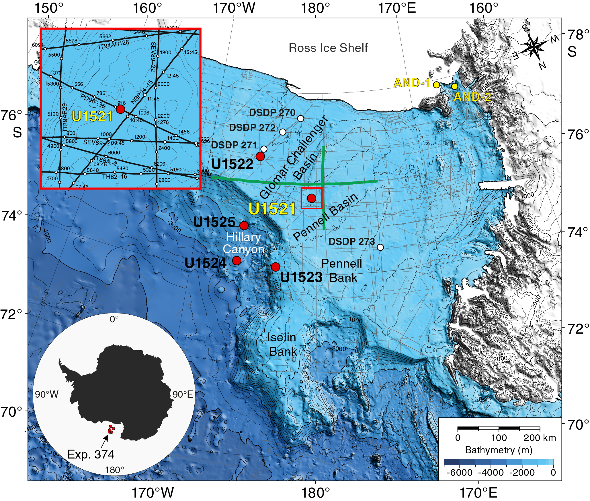
Figure F1. Bathymetry for RSU4 with site locations.
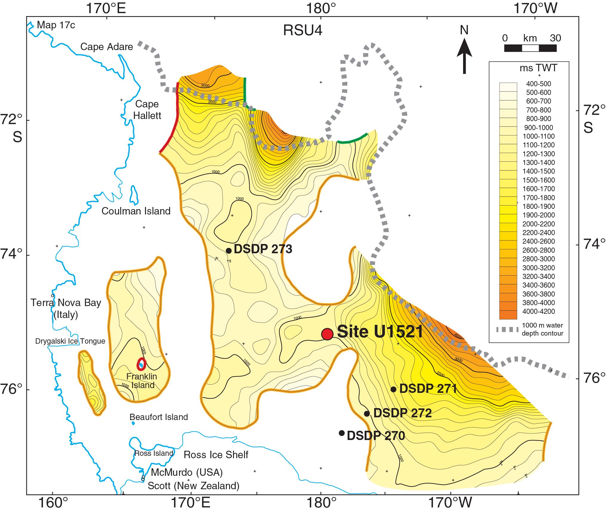
Figure F2. Depth contour map and site locations.
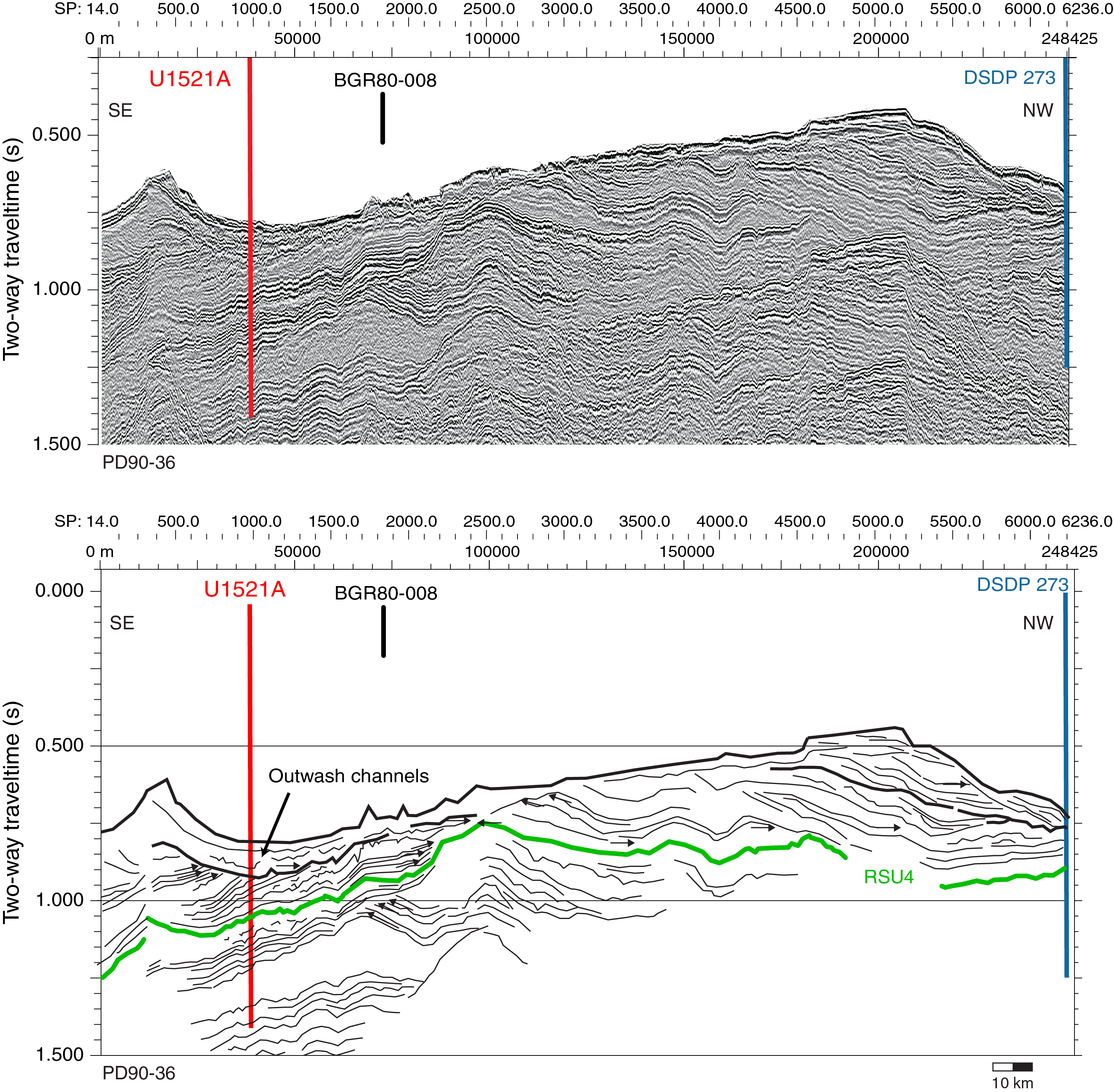
Figure F3. Seismic-reflection Profile PD90-36.
High-resolution single-channel seismic-reflection Profile PD90-36 shows numerous outwash channels above RSU4 (Figure F3) and as much as 250 m of till delta foresets and till tongue interbedded with aggrading bottomset strata below. This till delta progrades from the Central High (a basement high underlying the modern Ross Bank) onto stratified glaciomarine sediment (Figure F3; see also Figure F8 in the Expedition 374 summary chapter [McKay et al., 2019]) near Site U1521. A similar feature progrades from the Marie Byrd Land region in the easternmost Ross Sea. The presence of these features suggests a period of early to middle Miocene glaciation, culminating with the erosion of RSU4 by expansion of grounded ice on the Central High and over a shallow continental shelf in the central Ross Sea. RSU4 is also associated with ice stream expansion across the central Ross Sea to near the paleocontinental shelf edge of the Pennell Basin, where a glacial delta formed (Figures F4, F5).
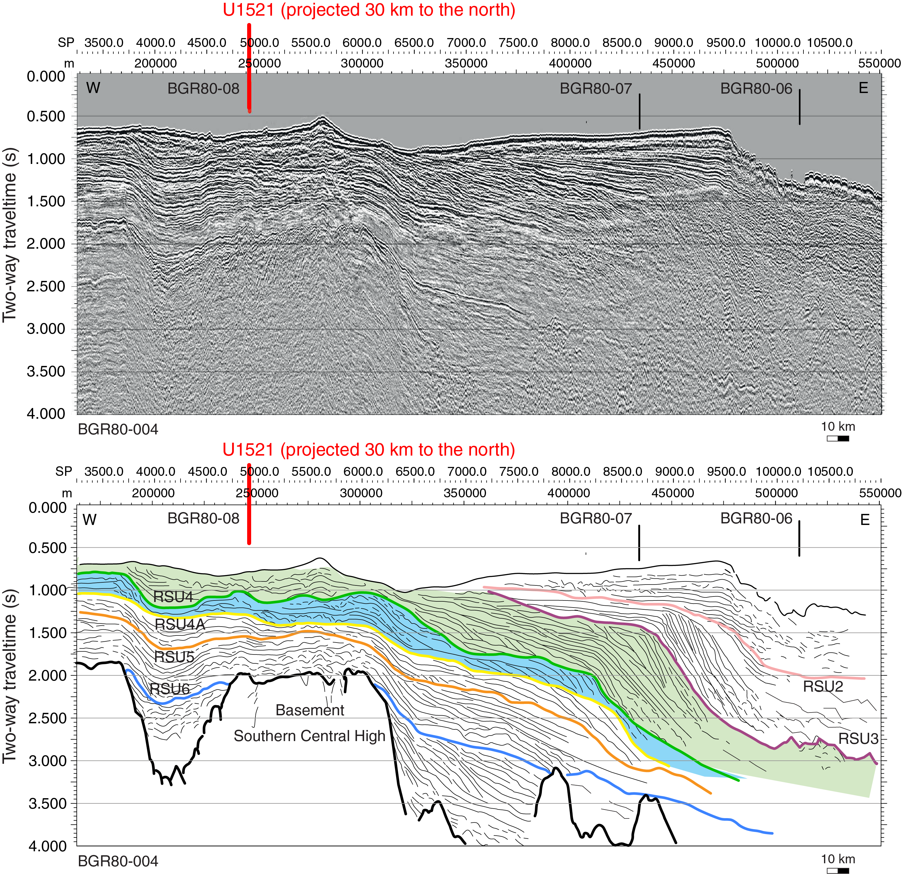
Figure F4. Seismic-reflection Profile BGR80-004.
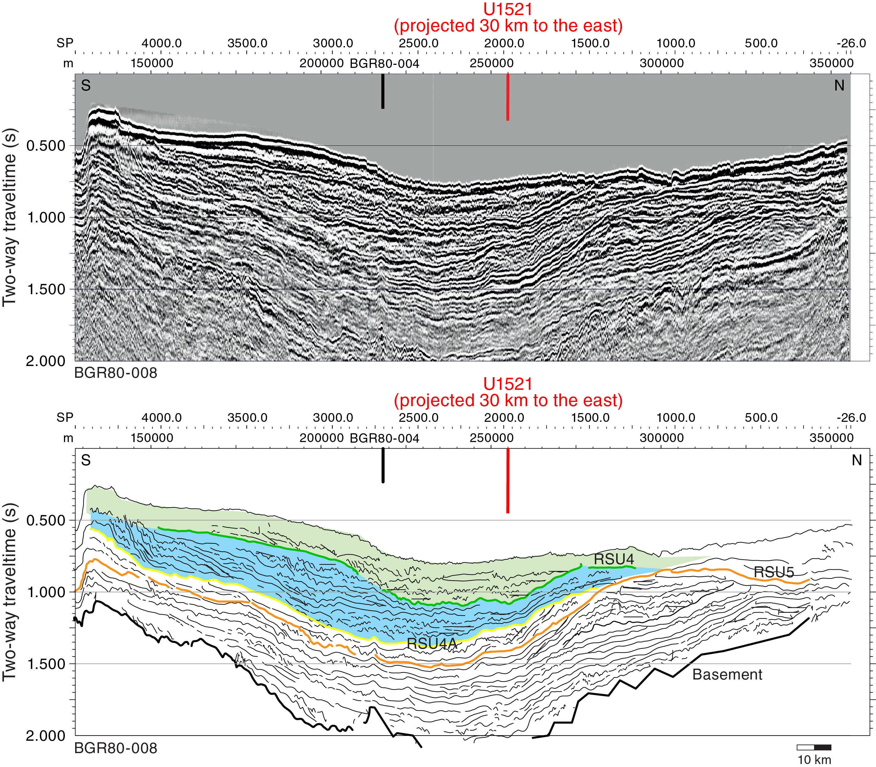
Figure F5. Seismic-reflection Profile BGR80-008.
Results from Site U1521 can be compared to those from the Ross Sea inner continental shelf (Antarctic Geological Drilling Project [ANDRILL] Site AND-2A) that record Antarctic Ice Sheet (AIS) minima in the Ross Sea and local Transantarctic Mountain outlet glacier activity. These two sites provide contemporaneous glacial records that will allow development of a transect of inner to outer continental shelf sedimentation. The outer continental shelf location of Site U1521 should allow development of a more complete assessment of oceanic forcings and response to AIS variability. This integrated framework will constrain the spatial extent of middle Miocene glacial advance and retreat events across the Ross Sea and associated erosional/depositional influences on the paleobathymetry of the Ross Sea continental shelf.
Records from Site U1521 will directly address all five primary objectives for Expedition 374 (see Scientific objectives in the Expedition 374 summary chapter [McKay et al., 2019]). The record of ice advance and retreat from Site U1521, when integrated with seismic stratigraphy, provenance studies, and numerical modeling, will allow a fuller assessment of Antarctic contributions to numerous inferred (~30 m amplitude) variations in far-field Miocene sea level (Objective 1) (Miller et al., 2005; John et al., 2011). The magnitude of polar amplification during the Miocene Climatic Optimum (MCO) will be assessed through proxies for atmospheric and marine temperatures derived from both in situ marine organic matter and terrestrial organic matter transported offshore by meltwater (e.g., micropaleontology and lipid biomarkers) (Objective 2). Insights into the oceanic drivers for retreat of middle Miocene marine terminating ice sheets and subsequent readvances in the late Miocene can be achieved by detailed lithofacies analysis to reconstruct physical changes in the paleoenvironment, and paleontological and geochemical proxies can identify the magnitude of the oceanic change through these intervals (Objective 3). Similarly, these methods will identify the sensitivity of middle Miocene ice sheets to orbital variability based on the presence of cyclicity in the open-marine, glaciomarine, and glacial-proximal sediments when combined with downhole logging results to complete the stratigraphy (Objective 4). Finally, a “backstripped” paleobathymetry can be done through accurate dating and depth estimates of the RSU4 surface and other unconformities at Site U1521 in combination with previous drilling constraints from other locations in the Ross Sea, which will allow for a fuller assessment of bathymetric controls on AIS evolution.
Operations
The original operations plan for Site U1521 (proposed Site EBOCS-01D) called for a single rotary core barrel (RCB) hole to 950 m drilling depth below seafloor (DSF) and downhole logging with the triple combination (triple combo), Formation MicroScanner (FMS)-sonic, and Vertical Seismic Imager (VSI) tool strings. We ultimately cored Hole U1521A to 650.1 m DSF (Cores 374-U1521A-1R through 71R) (Table T1). Coring proceeded without incident through Core 37R (0–352.5 m DSF); however, after poor recovery in Cores 32R through 37R (14.49 m; 25%) caused by chert and silica-cemented layers jamming the core barrel, we switched to cutting half-length cores to improve core recovery. Cores 38R through 43R (352.5–381.3 m DSF) were collected using a 4.8 m advance (instead of 9.6 m), significantly improving recovery (80%). We switched back to 9.6 m advances after the formation became less indurated and continued to core with the RCB system for Cores 44R through 71R (381.3–650.1 m DSF). We terminated coring at that depth after meeting the primary scientific objectives. At the end of coring operations, we displaced the hole with heavy (10.5 lb/gal) mud and logged with all three tool strings, all of which reached to within ~1 m of the bottom of the hole. Operations at Site U1521 concluded at 2245 h on 21 January 2018. A total of 132.75 h (5.5 days) were spent at Site U1521. RCB coring in Hole U1521A collected 71 cores and penetrated to 650.1 m DSF, recovering 411.50 m of core (63%).
Port call
Expedition 374, Ross Sea West Antarctic Ice Sheet History, began with the first line ashore at Berth No. 2 in Lyttelton, New Zealand, at 0706 h (all times are local ship time; UTC + 13 h) on 4 January 2018. After clearing immigration and customs, the R/V JOIDES Resolution Science Operator (JRSO) technical staff, Co-Chief Scientists, and Expedition Project Manager boarded the vessel. The IODP Expedition 372 science party moved off the vessel, and after a 5 h crossover the Expedition 372 JRSO technical staff moved off the vessel. After conducting a press conference, holding VIP and media tours, and loading IODP and Siem airfreight and some critical ocean freight, the vessel shifted from Berth No. 2 to Berth No. 7 to begin the remainder of port call operations. The following day, the Expedition 374 science party moved on board and the Siem Offshore crew change was completed. Local university faculty, staff, and students were given tours of the vessel. Most of the Schlumberger logging-while-drilling (LWD) tools were off-loaded, and bulk-loading operations began. We also received 41 short tons of barite and 135 short tons of sepiolite. On the third day of port call, the aft core line was removed in preparation for installing new coring line. Frozen food and dry stores were loaded, and the remaining Schlumberger LWD tools were off-loaded. After completing loading operations on 6 January, the vessel was shifted from Berth No. 7 to the Oil Berth for fueling. The last mooring line was released at 1735 h, and the first line ashore at the Oil Berth was secured at 1750 h, ending the very short passage.
After loading 640 metric tons of fuel oil, fuel operations were secured. At 0812 h on 7 January, the last line was released for the move back to Berth No. 7. The first line was secured at 0827 h, ending the brief transit. Loading operations resumed, and during the day fresh fruit and vegetables were loaded, the FMS tool was repaired and tested, and Polar Code training for the science party and technicians was completed. On 8 January, the final day of our 4.4 day port call, the vessel was inspected and issued a Polar Code certificate, all remaining trash was discharged, the last remaining items of freight were loaded or discharged, and immigration cleared the vessel for departure. After the vessel was secured for the sea passage to Antarctica, the harbor pilot came on board at 1552 h and two port tugs arrived to assist with departure. The mooring lines were released and pulled back on board, and the last line was released at 1624 h. The vessel proceeded to the pilot station, and the pilot departed the vessel at 1648 h after a 2 nmi transit. The vessel began its sea passage at 1648 h on 8 January.
Transit to Site U1521
The JOIDES Resolution met the R/V icebreaker Nathaniel B. Palmer at 1930 h on 14 January 2018. The Nathaniel B. Palmer acted as an escort through the sea ice into the Ross Sea polynya (ice-free area). At 1220 h on 15 January, the JOIDES Resolution cleared the southern edge of the sea ice, and the Nathaniel B. Palmer was released from escort duty at 1300 h. The JOIDES Resolution arrived at Site U1521 at 0954 h on 16 January after a 2014 nmi transit from Lyttelton that averaged 10.8 kt. The vessel switched to dynamic positioning at 0938 h, and the thrusters were lowered and secured. At 0957 h, the drill floor was cleared for operations, beginning Hole U1521A. At 1019 h, an acoustic beacon was deployed.
Hole U1521A
Initial operations consisted of picking up and assembling the RCB bottom-hole assembly and then deploying the drill string to 143.81 m drilling depth below rig floor (DRF). During deployment, the drill pipe was drifted (checked to ensure that the interior was clear) and strapped (measured). The nonmagnetic core barrels were spaced out after the outer core barrel was assembled. The top drive was picked up and spaced out, and a wiper pig was inserted into the drill string. The wiper pig was pumped through the drill string with two times the annular volume of the drill string to clean any loose rust or debris from the inside of the drill string. The precision depth recorder depth for the site was calculated as 573.4 m DRF. The core barrels were dressed with liners, and a core barrel was deployed.
The drill string was spaced out to spud and lowered slowly to tag the seafloor. Hole U1521A was started at 1845 h on 16 January 2018. The mudline core recovered 4.28 m of sediment, and the seafloor tag was measured at 573.0 m DRF (562.2 meters below sea level). RCB coring continued through Core 37R (352.5 m DSF). Because of reduced recovery starting with Core 31R, we proceeded to cut half cores (4.8 m advance instead of 9.6 m advance) for Cores 38R through 43R (352.5–381.3 m DSF) to improve core recovery. Coring with full 9.6 m advances continued for Cores 44R through 71R (381.3–650.1 m DSF), at which point coring was terminated when the science objectives had been met. High-viscosity mud sweeps (30 bbl) were pumped every two to four cores from Core 13R to Core 68R (113.0–611.7 m DSF).
To prepare for downhole logging after terminating coring in Hole U1521A, the hole was cleaned with a 40 bbl high viscosity–mud sweep. The rotary shifting tool (RST) was run in the hole on the coring line and released the RCB C-4 coring bit at 1505 h on 20 January. The RST was then run to reposition the bit shifting sleeve back to the circulating position in the mechanical bit release (MBR). After shifting the sleeve in the MBR, the RST was pulled back to the surface and the sinker bars were removed from the drill string. The hole was displaced with 217 bbl of 10.5 lb/gal mud from 650.1 m DSF to the seafloor. The top drive was set back, and the drill string was pulled back to logging depth (54.4 m DSF). After positioning the end of the pipe with knobbies through the guide horn, the circulating head was attached and the hole was top-displaced to the seafloor with 20 bbl of 10.5 lb/gal mud. The rig floor was then rigged up for logging.
A triple combo tool string was assembled with the following tools:
- Magnetic Susceptibility Sonde (MSS),
- High-Resolution Laterolog Array (HRLA; to measure resistivity),
- Hostile Environment Litho-Density Sonde (HLDS; with source),
- Hostile Environment Natural Gamma Ray Sonde (HNGS),
- Accelerator Porosity Sonde (APS), and
- Enhanced Digital Telemetry Cartridge (EDTC).
The tools were assembled and tested and then lowered into the hole at 2325 h on 20 January. The active heave compensator was switched on once the tools reached open hole. A downlog was performed from just above the seafloor to the total hole depth of 648 m wireline logging depth below seafloor (WSF). The hole was then logged up for a 126.5 m calibration pass. The triple combo tool string was lowered back to bottom (648 m WSF), and the hole was logged up. Before reaching the end of the drill pipe at 54.4 m DSF, the drill pipe was raised to 38.2 m DSF to provide additional log coverage of the upper part of the borehole before the caliper was closed and the tool string entered the pipe. The tools were pulled from the hole and were back at the surface at 0330 h on 21 January. By 0430 h, the triple combo was rigged down.
The FMS-sonic tool string was assembled with the following tools:
The FMS-sonic tool string was deployed at 0620 h. The tool string was lowered into the drill pipe, and a downlog with the FMS calipers closed began at 54.4 m WSF. Natural gamma radiation (NGR) was logged from above the seafloor to depth-match to the seafloor from the triple combo logging run. The tool string reached the bottom of the hole at 648 m WSF. The hole was logged up from 648 to 103 m WSF with the FMS calipers open. The calipers were then closed, and the tool string was lowered back to 648 m WSF. A second uplog was performed, and as the tool string approached the end of the drill string, it was again raised to ~38 m DSF to gain log coverage over the upper part of the borehole. The FMS calipers were closed just prior to entering the drill pipe. The FMS-sonic tool string was rigged down by 1245 h.
The VSI tool string for a vertical seismic profile experiment consisted of the VSI and EDTC. The VSI tool string was assembled, tested, and deployed at 1330 h. While lowering the tool string in the hole, the protected species watch was initiated, and the seismic source (two 250 inch3 Sercel G guns in parallel cluster) was lowered into the water and fired with increasing intensity according to the guidelines for a “soft start.” The VSI tool string was lowered to 648 m WSF for the first station test. The caliper was opened, and 18 stations were attempted, 16 with good results. At 1755 h, the last station was completed and the seismic source was secured. The logging tool string was at the rig floor at 1835 h, and by 1930 h all Schlumberger logging equipment was rigged down.
The drilling crew then began to secure the drilling equipment for transit. After laying out the knobbies, the drill string was pulled back to the rig floor, clearing the seafloor at 2020 h. The acoustic beacon was released during the pipe trip and recovered on deck at 2105 h. The rest of the pipe was pulled to the rig floor, three drill collar stands were racked back in the derrick, and the outer core barrel was disassembled and inspected. The rig floor was secured for transit at 2245 h on 21 January, ending Hole U1521A and Site U1521. A total of 132.75 h (5.5 days) were spent at Site U1521. We collected 71 RCB cores in Hole U1521A, recovering 411.50 m of sediment over 650.1 m of coring (63%).
Lithostratigraphy
Site U1521 consists of a single hole cored to 650.1 m DSF. The 411.50 m of recovered sediment is divided into seven lithostratigraphic units (Table T2).
A lithologic summary of Hole U1521A is shown in Figure F6. The dominant facies include diamictite, diatomite, diatom-rich mudstone, and mudstone, with intervals of chert and conglomerate. The upper ~85 m of Hole U1521A consists of interbedded massive diatom ooze, mud/sandy mud, diamictite, diatom-bearing/rich mudstone with dispersed clasts, and diatomite and is interpreted to represent truncated cycles of subglacial, glaciomarine, and open-marine sedimentation (lithostratigraphic Units I and II). Between ~85 and 210 m core depth below seafloor, Method A (CSF-A), a thick sequence of bioturbated diatom-bearing/rich mudstone (Unit III) containing whole bivalves and shell fragments is interpreted to reflect a prolonged interval of open-marine to ice-distal glaciomarine conditions. Deeper than ~210 m CSF-A, a series of interbedded massive to stratified diamictite, mudstone, and chert (Units IV–VII) was recovered. Unit VI is further divided into three subunits based on the character of interbedding, clast lithology, and diagenetic components, which are interpreted to reflect ice-proximal to ice-distal glaciomarine conditions. An interval of poor recovery and chert nodules (Unit V [280.72–324.20 m CSF-A]) marks the opal-CT transition. Photographs of primary lithologies, sedimentary structures, and accessories are shown in Figures F7 and F8 and summarized in Figure F9.
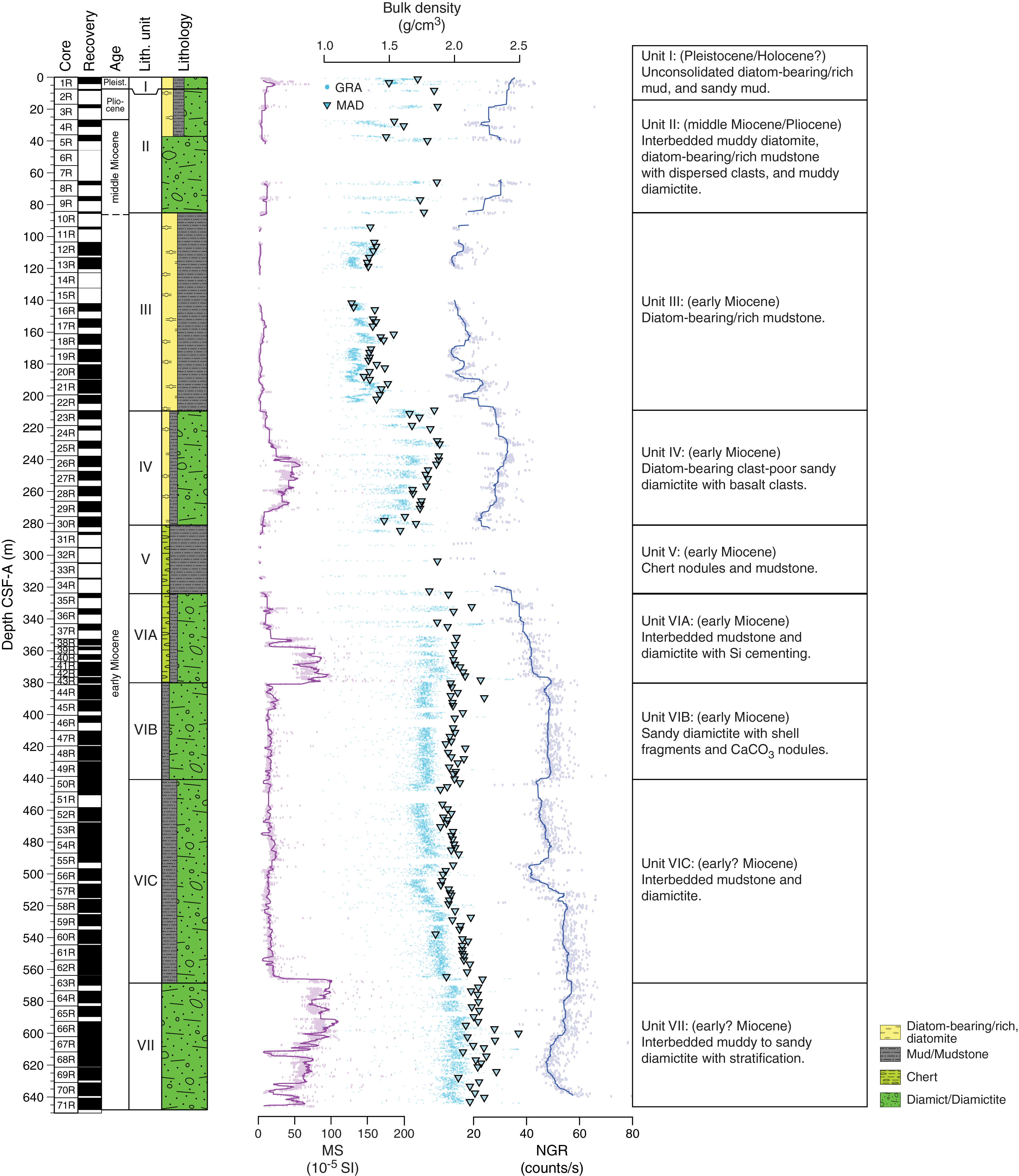
Figure F6. Lithostratigraphic summary.
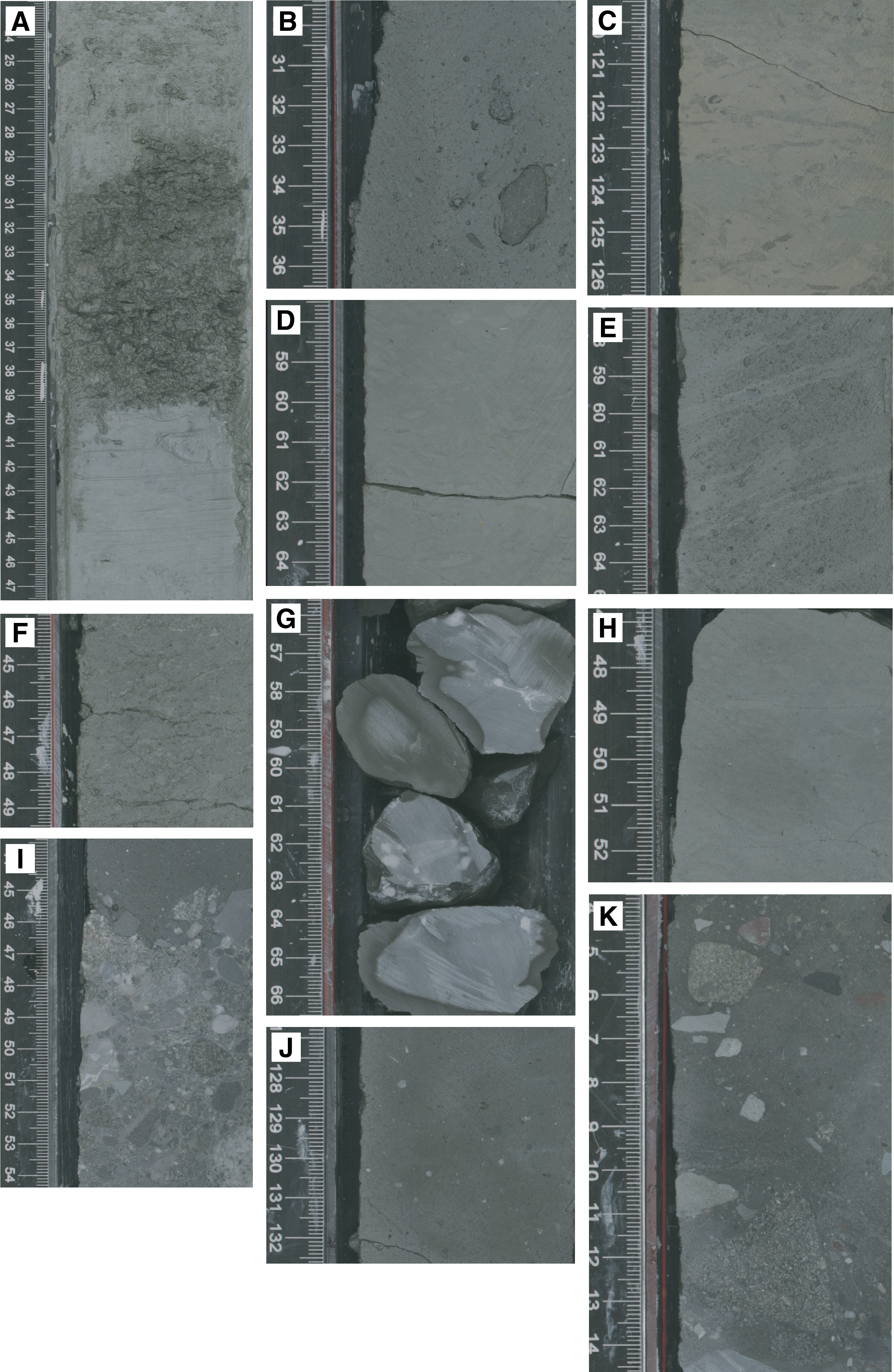
Figure F7. Major lithofacies.
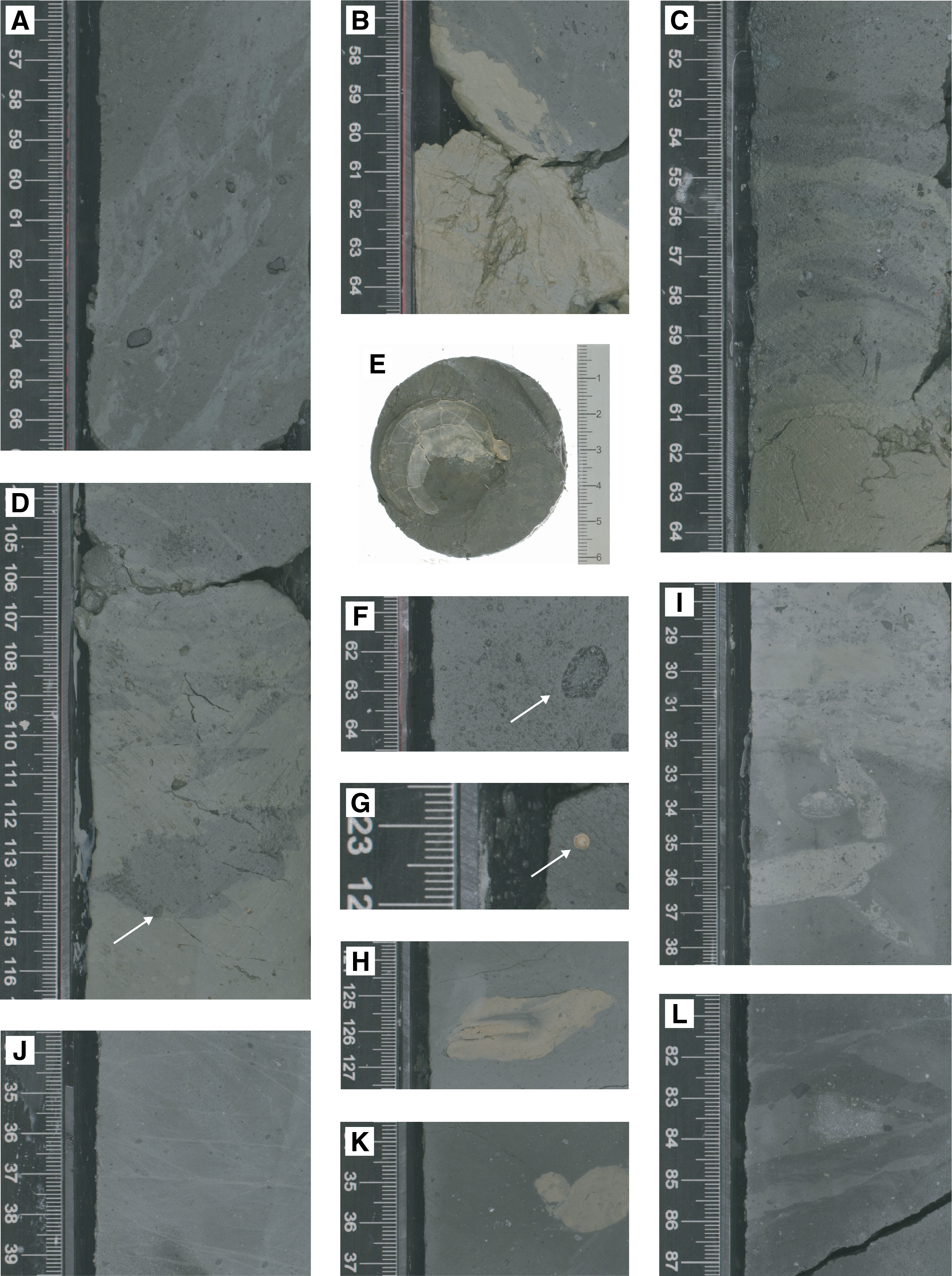
Figure F8. Sedimentary structures, unit contacts, and lithologic accessories.
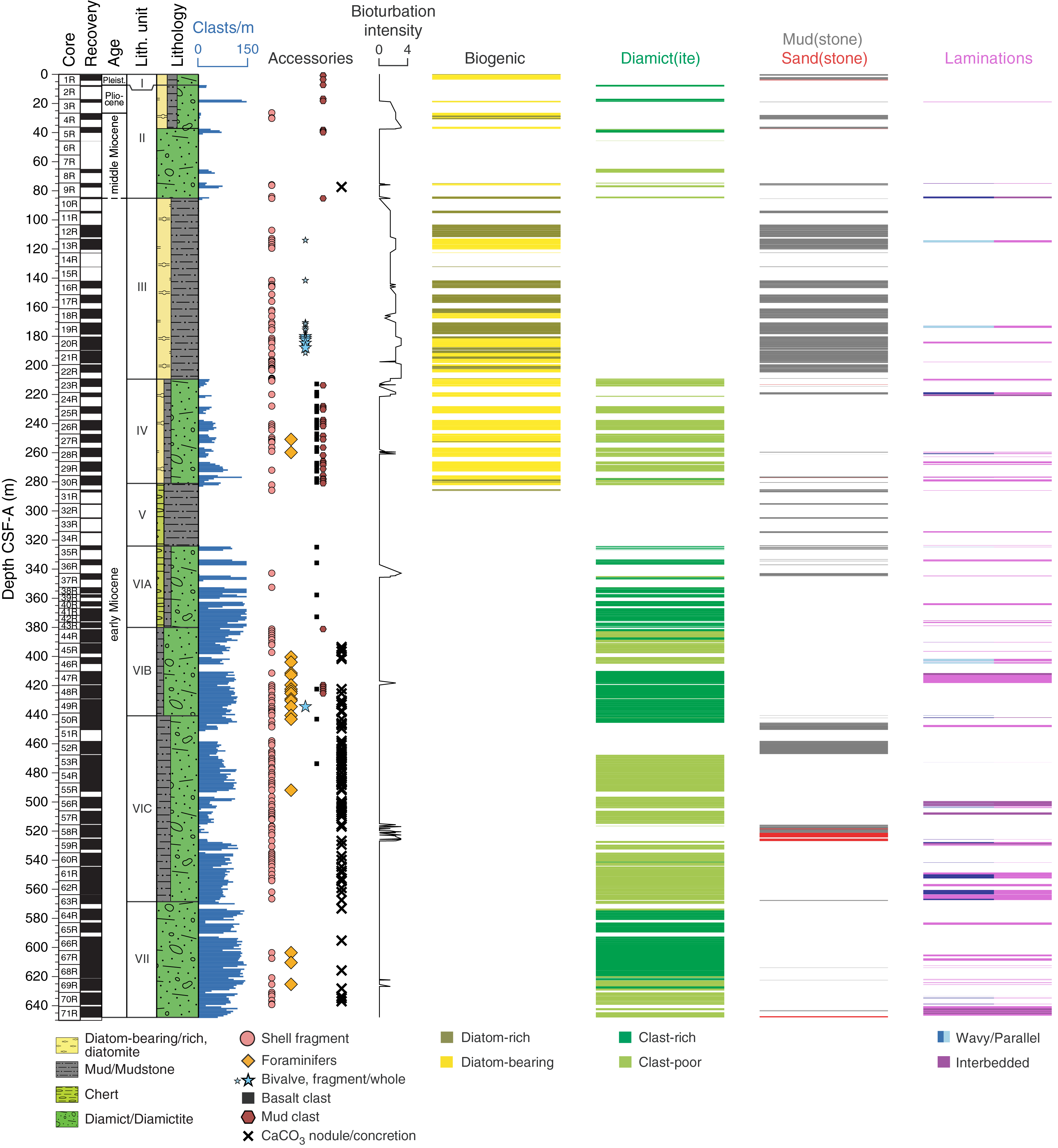
Figure F9. Lithology and sedimentary structures.
Unit descriptions
Site U1521 is divided into seven lithostratigraphic units (I–VII; youngest to oldest) on the basis of significant lithologic changes observed downhole (Figure F6) and determined using a combination of visual core description, microscopic examination of smear slides, color spectral observations, and bulk mineralogical analysis by X-ray diffraction (XRD) (see Lithostratigraphy in the Expedition 374 methods chapter [McKay et al., 2019a]). Unit VI is divided into three subunits (VIA–VIC; youngest to oldest). The criteria used to define the units and subunits are discussed below. Figure F9 represents core description data distilled from DESClogik that highlights lithologic variations and trends between and within lithostratigraphic units.
Unit I
- Interval: 374-U1521A-1R-1, 0 cm, to 2R-1, 0 cm
- Depth: 0–7.40 m CSF-A
- Thickness: 7.40 m
- Age: Pleistocene to Holocene?
- Lithology: diatom-bearing/rich mud with dispersed clasts, diatom-bearing sandy mud
Lithostratigraphic Unit I consists of unconsolidated olive to light olive gray diatom-rich mud to dark grayish brown diatom-bearing mud with dispersed clasts and two intervals of gray diatom-bearing sandy mud (Figures F6, F7A; Table T2). Recovery in Unit I is 4.28 m (58%).
Unit II
- Interval: 374-U1521A-2R-1, 0 cm, to 10R-1, 114 cm
- Depth: 7.40–85.34 m CSF-A
- Thickness: 77.94 m
- Age: late Pliocene to middle Miocene
- Lithology: diamictite, muddy diatomite, diatom-bearing/rich mudstone
Lithostratigraphic Unit II consists of interbedded lithified dark gray massive clast-poor muddy diamictite, muddy diatomite, and diatom-bearing/rich mudstone. The diamictite beds are as thick as ~6 m, whereas the muddy diatomite and diatom-bearing/rich mudstone beds are centimeters to decimeters thick, heavily bioturbated, and contain dispersed clasts, mud clasts, and shell fragments (Figures F6, F9; Table T2). The diamictite in Unit II is massive, with randomly distributed and oriented subangular to rounded clasts of various composition, including mudstone, granitoid rock, and metasedimentary rock (Figure F7B). In the diamictite are intervals of physically intermixed (Krissek et al., 2007) bioturbated muddy diatomite and diatom-bearing/rich mudstone with microfaults (Figure F8A). Physical intermixing occurs throughout (Figure F8A, F8B) but is most pronounced at the base of the unit (e.g., Section 374-U1521-10R-1A), where diamictite is intermixed with the underlying diatomite of Unit III on a decimeter scale (Figure F8D). Transitions are not always intermixed; they are sometimes laminated (e.g., Section 9R-1A; Figure F8C). The bottom of Unit II is defined as the last occurrence of diamictite in this interbedded sequence (Figures F8D, F9). Recovery in Unit II is 19.39 m (25%).
Unit III
- Interval: 374-U1521A-10R-1, 114 cm, to 23R-1, 17 cm
- Depth: 85.34–209.17 m CSF-A
- Thickness: 123.74 m
- Age: early Miocene
- Lithology: diatom-bearing/rich mudstone
Lithostratigraphic Unit III consists of moderately to highly bioturbated olive gray to greenish gray diatom-bearing/rich mudstone (Figures F6, F7C, F7D, F9; Table T2). Faint laminations, carbonate-cemented intervals, and pyrite staining are observed throughout. Disarticulated and articulated bivalves are present in Core 374-U1521A-20R (180.2–189.49 m CSF-A) (Figure F8E), and millimeter- to centimeter-scale shell fragments occur throughout the unit (Figure F9). Recovery in Unit III is 68.69 m (55%).
Unit IV
- Interval: 374-U1521A-23R-1, 17 cm, to 30R-4, 81 cm
- Depth: 209.17–280.72 m CSF-A
- Thickness: 71.55 m
- Age: early Miocene
- Lithology: diatom-bearing sandy diamictite
Lithostratigraphic Unit IV consists of dark gray massive to stratified diatom-bearing clast-poor sandy diamictite (Figures F6, F7E; Table T2). Centimeter- to decimeter-scale interbeds of mudstone and diamictite are observed at the top of Unit IV between 215 and 220 m CSF-A (interval 374-U1521A-23R-4A, 57–61 cm, to 24R-2A, 12 cm). In the diamictite, clast composition is diverse and includes basalt, granodiorite, and mudstone (Figures F8F, F9). Mud clasts, foraminifers, and shell fragments are randomly distributed throughout the unit (Figures F8G, F9). Carbonate concretions are observed throughout and often associated with shell fragments (Figure F8H). The sediment is bioturbated, and burrows are pyrite stained. At the base of the unit (interval 30R-1A, 90 cm, to 30R-4A, 81 cm), interbeds of laminated diatom-rich mudstone, mudstone with clasts, and clast-poor sandy diamictite with soft-sediment deformation features and intercalated contacts are observed (Figure F9). A conglomerate composed of elongated mudstone intraclasts is observed in Core 30R (Figure F7F). Recovery in Unit IV is 45.17 m (63%).
Unit V
- Interval: 374-U1521A-30R-4, 81 cm, to 35R-1, 50 cm
- Depth: 280.72–324.20 m CSF-A
- Thickness: 43.48 m
- Age: early Miocene
- Lithology: chert, mudstone, diatom-rich mudstone
Lithostratigraphic Unit V consists of gray chert nodules interbedded with dark gray silica-cemented mudstone (Figures F7G, F9; Table T2). Chert nodules are as long as 12 cm on their longest axis. Faint irregular laminae also occur in the mudstone. An ~1 m thick diatom-rich mudstone occurs in Section 374-U1521A-35R-1A. Recovery in Unit V is 7.14 m (16%). Drilling disturbance is high, and most cores consist of chert nodules that appear to have plugged the core barrel, reducing recovery (see Operations).
Unit VI
- Interval: 374-U1521A-35R-1, 50 cm, to 63R-4, 8 cm
- Depth: 324.20–567.95 m CSF-A
- Thickness: 243.75 m
- Age: early Miocene
- Lithology: diamictite, mudstone
Lithostratigraphic Unit VI is characterized by interbedded diamictite and mudstone and is divided into three subunits based on the style of interbedding (Figure F9; Table T2). Individual diamictite beds are decimeters (e.g., Section 374-U1521A-36R-1A) to tens of meters thick (e.g., Sections 37R-2A through 43R-3A) and are separated by sharply bounded centimeter-scale (e.g., Section 36R-1A) to meter-scale (e.g., Sections 37R-1A through 37R-2A) mudstone beds. Clasts are scattered, randomly oriented, and of various lithologies and range from angular to rounded. Recovery in Unit VI is 196.18 m (80%).
Subunit VIA
- Interval: 374-U1521A-35R-1, 50 cm, to 43R-3, 93 cm
- Depth: 324.20–380.04 m CSF-A
- Thickness: 55.84 m
- Age: early Miocene
- Lithology: mudstone, diamictite, silica-cemented diamictite, conglomerate, chert
Lithostratigraphic Subunit VIA consists of interbedded very dark gray to gray massive clast-rich sandy to clast-poor muddy diamictite and dark greenish gray mudstone (Figure F7H, F7I; Table T2). Clast-rich sandy diamictite and clast-poor muddy diamictite are physically intermixed at a centimeter to decimeter scale in Sections 374-U1521A-37R-2A through 38R-1A. Muddy diamictite is intermittently silica cemented in the upper part of the subunit. Shell fragments, large clasts, and intervals of moderate bioturbation are observed in the carbonate-cemented mudstone (Figures F8I, F9). Washed gray chert nodules occur in Sections 35R-2A through 35R-3A. Below Core 38R, the diamictite is weakly stratified with faint color changes, vein networks, mudstone laminae, and sandstone stringers. Diatoms are absent in most smear slides except in Sample 42R-2A, 111 cm, which contains trace numbers of diatom fragments. An ~160 cm interval of intermixed sandy diamictite and three clast-supported conglomerates (Section 43R-3A; Figure F7I) define the base of Subunit VIA. Recovery in Subunit VIA is 33.54 m (60%).
Subunit VIB
- Interval: 374-U1521A-43R-3, 93 cm, to 50R-2, 17 cm
- Depth: 380.04–440.58 m CSF-A
- Thickness: 60.54 m
- Age: early Miocene
- Lithology: diamictite, mudstone
Lithostratigraphic Subunit VIB consists of a massive to stratified very dark gray to dark greenish gray clast-rich to clast-poor sandy diamictite (Figure F6; Table T2). A faint vein network, shell fragments, foraminifers, and carbonate nodules/concretions are also present (Figures F8J, F9). The carbonate nodules/concretions have irregular edges and include sand and gravel clasts, indicating in situ formation in the diamictite. The base of Subunit VIB is defined as the first occurrence of mudstone at interval 374-U1521A-50R-2A, 17 cm. Recovery in Subunit VIB is 50.65 m (85%).
Subunit VIC
- Interval: 374-U1521A-50R-2, 17 cm, to 63R-4, 8 cm
- Depth: 440.58–567.95 m CSF-A
- Thickness: 127.37 m
- Age: early Miocene?
- Lithology: diamictite, mudstone
Lithostratigraphic Subunit VIC consists of interbedded very dark greenish gray mudstone and clast-poor diamictite (Figures F6, F7J; Table T2). In the upper part of Subunit VIC (Sections 374-U1521A-50R-2A through 50R-5A), centimeter-thick mudstone beds with sharp lower boundaries are interbedded with diamictite beds with sharp lower boundaries. A majority of the unit consists of thickly interbedded sandy mudstone to mudstone (Sections 50R-5A through 52R-CC and 58R-1A through 59R-2A) and muddy to sandy diamictite (Sections 53R-1A through 57R-7A and 59R-2A through 63R-3A). The sharp lower boundary of the subunit occurs at the base of a decimeter-thick bioturbated mudstone (interval 63R-4A, 11 cm) (Figure F9). Both the mudstone and diamictite contain faint vein networks, large clasts, carbonate concretions, and shell fragments (Figures F8K, F9). Recovery in Subunit VIC is 111.54 m (88%).
Unit VII
- Interval: 374-U1521A-63R-4, 8 cm, to 71R-CC, 16 cm
- Depth: 567.95–648.17 m CSF-A (total depth)
- Thickness: 80.22 m
- Age: early Miocene?
- Lithology: muddy diamictite, sandy diamictite
Lithostratigraphic Unit VII consists of very dark greenish gray interbedded clast-poor sandy to clast-rich muddy diamictite with intervals of fine wavy laminations, slight stratification, and sharp boundaries below Section 374-U1521A-69R-6A (Figures F6, F7K, F8L). A 6 cm thick carbonate-cemented mudstone is also observed in interval 70R-6A, 94–100 cm. Carbonate concretions, faint vein networks, and shell fragments are found throughout the unit. Granule- to pebble-sized clasts are observed throughout and sometimes oriented with the stratification/lamination. Recovery in Unit VII is 70.65 m (86%).
Facies description
At Site U1521, seven main lithofacies are identified based on common lithologic, sedimentary, and textural characteristics (Table T3). These lithofacies largely conform with the scheme for the ANDRILL AND-1B core (Krissek et al., 2007). Lithified forms (suffix “-stone” or “-ite”) are used in this scheme, although sediments in the upper ~7.5 m of the hole are unlithified. The association of facies is interpreted to reflect a range of marine, ice-distal to ice-proximal glaciomarine, and subglacial depositional environments. Facies are described in detail below, with the most common listed in order from ice proximal to ice distal.
Facies 1: massive diamictite
Facies 1 is clast-rich to clast-poor diamictite with a sandy to muddy matrix (Figure F7B, F7K; Table T3). Biogenic silica content is variable, ranging from absent to diatom-bearing (as much as 25% of the matrix). Clasts are subangular to subrounded and poorly sorted and contain a range of lithologies, including metasedimentary, sedimentary, basalt, dolerite, marble, granite, and mudstone. The relative abundances of these lithologies are variable, and some lithostratigraphic units reveal distinct shifts in clast provenance. Aligned faceted and/or outsized clasts are present in some intervals. Carbonate shell fragments (both macrofossils and microfossils) are observed (Figures F8G, F9). Silica cementing is often present in muddy diamictite below the opal-CT transition, whereas sandy diamictite is carbonate cemented. Carbonate concretions and pyrite nodules are common, particularly in lithostratigraphic Subunits VIB and VIC (Figures F8H, F9). Facies 1 often grades into or out of stratified diamictite (Facies 2) and diatomite/diatom-rich mudstone (Facies 5). Bioturbation is present in some intervals. Load features, bioturbation, brecciation, and faulting are visible at or near contacts.
Facies 1 likely represents ice-proximal glaciomarine deposits, rainout from floating ice, or subglacial deposition. Physical intermixing with underlying facies, a sharp basal contact, and evidence of ductile and/or brittle deformational structures in underlying facies may indicate past overriding by grounded ice.
Facies 2: stratified diamictite
The texture and composition of Facies 2 is similar to that of Facies 1, but stratification is evident and ranges from weak to well defined at the centimeter to meter scale. Stratification is identified by changes in color, matrix particle size, or clast concentration (Figure F7E).
Stratified diamictite intervals and beds may be associated with ice rafting and/or deposition in a glaciomarine environment. This facies may also contain indications of subglacial deformation, which is indicated by the presence of microfaulting and the displacement of laminae (Figure F8L). Traction or density currents may winnow clays in diamictite (Facies 1) deposited in grounding line–proximal settings, resulting in stratification defined by concentration of clasts and a sandier matrix.
Facies 3: mudstone
Facies 3 is massive to stratified/laminated mudstone, as indicated by a change in color or particle size (Figure F7H, F7J; Table T3). Diatom content may be as much as 25% (e.g., diatom-bearing). Laminae range from planar to wavy. Bioturbation intensity varies but tends to increase near contacts with diatomite or diatom-rich mudstone (Facies 5). In some intervals, burrows are filled/lined with pyrite. Soft-sediment deformation structures and carbonate shell fragments are common. At Site U1521, biosiliceous components (e.g., diatoms and sponge spicules) are rare deeper than ~280 m CSF-A, which is likely due to diagenetic transformation of biogenic silica to opal-CT.
Facies 3 represents hemipelagic suspension settling in ice-proximal to ice-distal glaciomarine environments. Bioturbated mudstone may reflect a more ice distal environment and/or lower sedimentation rates. Stratified intervals may reflect contributions from distal sediment gravity flows, episodic winnowing of fines by subglacial meltwater flux and/or bottom currents, or suspension settling from turbid meltwater plumes. Large clasts may be delivered by ice rafting, and soft-sediment deformation is sometimes observed below clasts.
Facies 4: mudstone with dispersed to common clasts
Facies 4 consists of mudstone containing <5% clasts (Table T3). Diatom content may be as high as 25% (e.g., diatom-bearing). Clasts are predominantly granule to pebble sized. This facies is commonly bioturbated and often associated with diamictite (Facies 1 and 2). The depositional setting of Facies 4 is likely similar to that of Facies 3, but ice rafting from floating ice shelves and/or icebergs results in clast deposition.
Facies 5: diatomite to diatom-rich mudstone
Facies 5 consists of heavily bioturbated to weakly laminated diatomite and diatom-rich mudstone (Figure F7C; Table T3). Bioturbation often obscures original stratification/lamination. Clasts are occasionally present to dispersed. Bivalves occur, and millimeter- to centimeter-scale shell fragments are common (Figures F8E, F9). Microfaulting is common throughout and often more pronounced in the upper parts of the diatomite/diatom-rich mudstone units, especially where overlain by diamictite (Figure F8D).
Facies 5 reflects pelagic to hemipelagic sedimentation in a marine environment. Where present, large clasts indicate ice rafting. Sediment loading, ploughing icebergs, and/or ice loading may induce microfaulting.
Facies 6: chert nodules
Facies 6 consists of chert nodules of diagenetically altered mudstone and/or diatomite indicative of the opal-CT boundary (Figure F7G; Table T3).
Facies 7: conglomerate
Facies 7 is a matrix- to clast-supported muddy to sandy conglomerate (Figure F7F, F7I). The conglomerate consists of clasts of various lithologies, including rounded to subrounded mudstone intraclasts, and can be weakly stratified. Lower contacts are sharp and irregular. One conglomerate consists of predominantly horizontally aligned elongate mudstone intraclasts (Core 374-U1521A-30R [~276 m CSF-A]). This facies is rare in the Site U1521 lithostratigraphic sequence.
Facies 7 likely represents either basal debris fallout proximal to the grounding line, submarine sediment redeposition and winnowing by currents, or channelized flow.
Diagenesis
Diagenetic features are common at Site U1521. Bacterial decomposition of organic matter results in sulfate reduction and the precipitation of pyrite. Pyrite cements, grain coatings, and nodules are common to abundant below lithostratigraphic Unit II, particularly in the diatom-bearing/rich mudstone of Unit III and mudstone/diamictite of Subunit VIC and Unit VII. Pyritized burrows are common to abundant in the Unit III diatom-bearing/rich mudstone and Subunit VIC mudstone/diamictite. Silica cements form faint vein networks and cement sandy diamictite and mudstone below the opal-CT transition (~280 m CSF-A). Authigenic carbonate precipitation is associated with intervals of sulfate reduction and leads to an increase in alkalinity and pH in interstitial water that provides the necessary conditions for carbonate precipitation (see Geochemistry and microbiology). Carbonate is observed in a variety of forms that include cement, concretions, and nodules. In general, carbonate cement is more abundant in mudstone and diamictite lithologies with visible calcium carbonate skeletal material (e.g., foraminifers and bivalve shell fragments), which act as nuclei for nodule/concretion growth. Deeper in the sequence (e.g., Unit VII), siderite forms rims around carbonate-rich clasts and/or concretions.
Bulk mineralogy
XRD analyses were performed on 26 powdered bulk samples from Hole U1521A to semiquantitatively estimate the relative abundances of the most common mineralogical components. Diffraction patterns are shown in Figure F10. The downhole mineralogy is relatively uniform, with slight variations in mineral content apparent in the relative peak intensities (Figure F10). Primary minerals include quartz and plagioclase, and minor components are associated with muscovite/illite, kaolinite/chlorite, and calcite (Figure F10). The relative abundance of calcite increases at the base of Unit II and in Unit III, which is consistent with the presence of intact bivalve shells, shell fragments, and foraminifers (Figures F8E, F9).
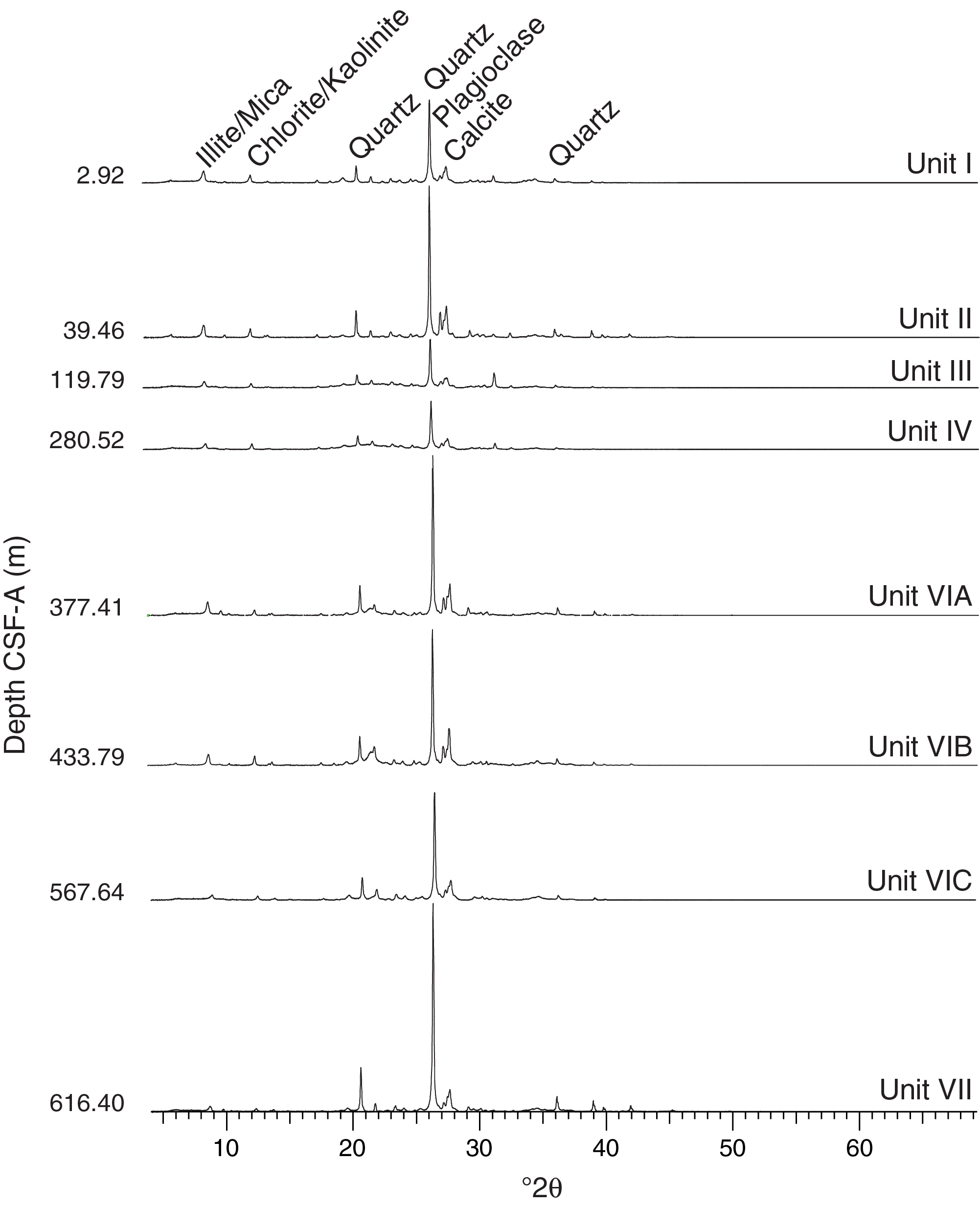
Figure F10. XRD patterns.
Preliminary depositional interpretation
Site U1521 recovered a sequence of lower Miocene to Holocene(?) sediments from the northern Central High of the Ross Sea outer continental shelf. Lithostratigraphic Units I and II, though incomplete, reveal a sequence of middle Miocene to Pleistocene glacial advances and retreats, indicated by interbedded diamictite, diatomite, and mudstone lithofacies, consistent with the results from the ANDRILL project (Fielding et al., 2008–2009; McKay et al., 2009). An expanded sequence of diatom-bearing/rich mudstone (Unit III) suggests a prolonged interval of productive open-marine conditions during the late early Miocene. Below this interval, interbedded massive diamictite and mudstone (Units VI and VII) indicate an ice-proximal to ice-distal glaciomarine depositional environment over the continental shelf.
Biostratigraphy and paleontology
The diverse microfossil assemblages recovered at Site U1521 comprise siliceous (diatoms, silicoflagellates, ebridians, and radiolarians), calcareous (foraminifers, nannofossils, and ostracods), and organic (dinoflagellate cysts [dinocysts] and other aquatic palynomorphs, pollen, and spores) remains. The presence and abundances of these microfossil groups vary significantly throughout the recovered sediment column. Rich assemblages of diatoms with rare silicoflagellates and ebridians occur in Samples 374-U1521A-1R-CC to 30R-CC (0–282.38 m CSF-A) (Figure F11). Deeper than 282.38 m CSF-A, diatoms and other siliceous microfossils are altered to opal-CT and offer only minimal information from shipboard analysis. Radiolarians are rare in the upper four cores (0–31.17 m CSF-A), and their numbers decrease significantly downhole. Foraminifers and palynomorphs are generally sparse. Calcareous nannofossils are present in trace numbers deeper than ~524 m CSF-A.

Figure F11. Micropaleontology summary.
Although all investigated microfossil groups supply valuable age and/or paleoenvironmental information, diatoms provide the best age constraint and indicate an ~500 m thick lower Miocene to middle Miocene interval that is unconformably overlain by a thin ~20 m thick Pliocene–Pleistocene interval. A late Pleistocene/recent age is assigned to Section 374-U1521A-1R-CC (0–4.28 m CSF-A) for the sediment recovered at the site (Figures F11, F12). The biostratigraphic utility of diatoms is hampered by reworking in the uppermost ~20 m CSF-A and in two barren intervals between ~282 and ~380 m CSF-A and from ~540 m CSF-A to the bottom of the hole. Radiolarians provide a suite of ages in the upper ~20 m CSF-A. Dinocysts confirm the age provided by diatoms in the interval between ~86 and ~273 m CSF-A. The foraminifer assemblages are not age diagnostic, but they do represent distinct biofacies that generally parallel the lithofacies of sediments recovered at Site U1521.
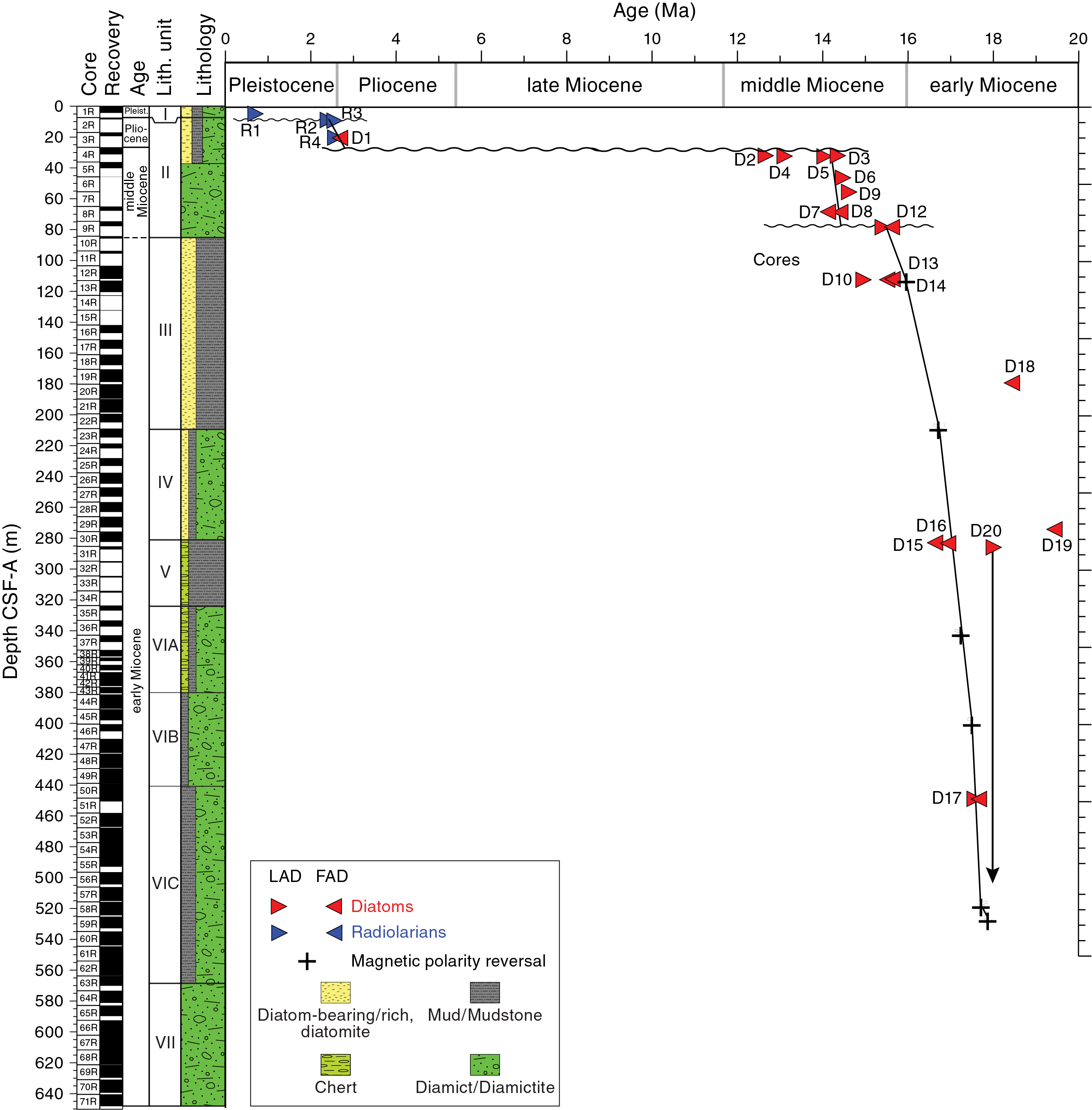
Figure F12. Shipboard age model.
Diatoms and other siliceous microfossils
The upper ~282 m at Site U1521 yields rich assemblages of diatoms with rare silicoflagellates and ebridians in all examined core catcher samples (Figures F11, F13; Table T4). Below Sample 374-U1521A-30R-CC (deeper than 282.38 m CSF-A), siliceous microfossils are altered to opal-CT and occur as replaced or silicified casts of the original diatom valves (Figure F13G), which are generally identifiable only to genus level. The upper part of this sequence is complex, with each core catcher sample representing a different combination of in situ and reworked taxa of different ages. The depth and age estimates of key biostratigraphic events are given in Table T5 and Figures F11 and F12.
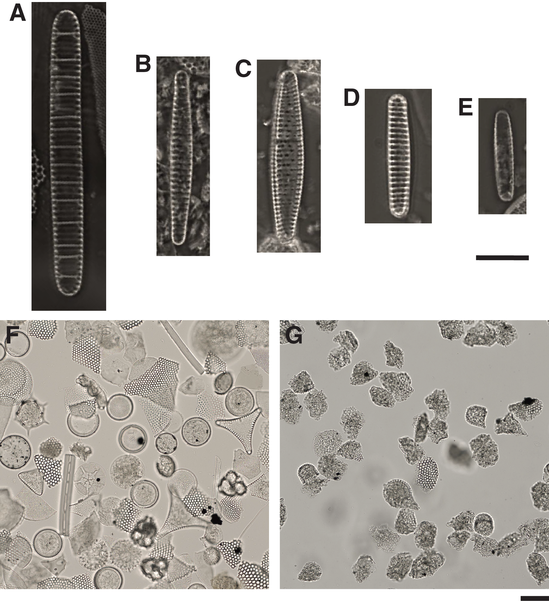
Figure F13. Diatoms.
Sample 374-U1521A-1R-CC (4.23 m CSF-A) contains a mixed assemblage sourced from material of several different ages, as indicated by the presence of Thalassiosira praefraga (early Miocene), Denticulopsis maccollumii (middle Miocene), Thalassiosira oliverana var. sparsa (late Miocene–early Pliocene), Thalassiosira vulnifica (Pliocene), and a modern/Pleistocene component indicated by the presence of Fragilariopsis curta, Fragilariopsis obliquecostata, and Thalassiosira antarctica, among others, which best reflects the true age of this interval. This combination of ages likely results from extensive mixing by a grounded ice sheet overriding the site during the Last Glacial Maximum and during prior Pliocene–Pleistocene advances. This sample cannot be assigned to the youngest diatom zone (Thalassiosira lentiginosa Zone) because it is not possible to determine whether the presence of Actinocyclus ingens in this sample is a natural occurrence or due to reworking by ice. However, the presence of T. antarctica and the absence of Thalassiosira elliptipora and Thalassiosira fasciculata suggest an age younger than 0.65 Ma in either the T. lentiginosa Zone or upper A. ingens Zone.
The stratigraphic interval represented by Sample 374-U1521A-2R-CC (8.51 m CSF-A) is assigned to the upper portion of the Thalassiosira complicata/T. vulnifica Concurrent Range Zone, as indicated by the co-occurrence of T. complicata and T. vulnifica. A reworked component from the upper Miocene is indicated by the presence of T. oliverana var. sparsa, which is abundant in the upper Miocene intervals of Hole U1521A.
Reworking of older taxa into younger sediments is also prevalent in Sample 374-U1521A-3R-CC (19.36 m CSF-A). The age of this sample is best constrained by the co-occurrence of Actinocyclus maccollumii (first appearance datum [FAD] at ~2.8 Ma) and T. complicata (last appearance datum [LAD] at 2.5 Ma), which indicates a position in the upper subzone of the T. complicata/T. vulnifica Zone.
An extended interval of middle and lower Miocene sediments is identified between Samples 374-U1521A-4R-CC and 30R-CC (31.17–282.38 m CSF-A), including portions of the Denticulopsis simonsenii Zone, A. ingens Zone, and D. maccollumii Zone (Figure F11). Samples 4R-CC to 8R-CC (31.17–67.75 m CSF-A) are assigned to the D. simonsenii Zone (middle Miocene). The upper boundary of the D. simonsenii Zone is not identified because of the absence of Nitzschia denticuloides (FAD at 13.5 Ma) in Sample 4R-CC; therefore, the interval comprising the upper portion of the D. simonsenii Zone was not recovered in Hole U1521A. Because Sample 3R-CC is Pliocene in age, there is a long hiatus between Samples 3R-CC (Pliocene) and 4R-CC (middle Miocene). The lower part of the D. simonsenii Zone is also missing, as indicated by the coincident FADs of D. simonsenii (14.2 Ma) and A. ingens var. nodus (14.4 Ma).
The lower part of the A. ingens Zone is identified only in Sample 374-U1521A-9R-CC (77.69 m CSF-A) as the stratigraphic interval below the coincident FADs of D. simonsenii and A. ingens var. nodus and LADs of Asteromphalus symmetricus and Cavitatus miocenicus (14.6 Ma) downhole to the FAD of A. ingens (16.2 Ma) (Figures F11, F12). The absence of A. ingens from Sample 10R-CC (85.67 m CSF-A) downhole and the continuing presence of D. maccollumii downhole to Sample 30R-CC (282.38 m CSF-A) identify the early Miocene D. maccollumii Zone (Figures F11, F12).
Below Sample 374-U1521A-30R-CC (282.38 m CSF-A), diatoms are poorly preserved and the assemblage consists of replaced or silica-infilled casts of diatoms that resulted from diagenetic transition of opal-A to opal-CT (Figure F13G). Diatoms occur discontinuously between Samples 46R-CC and 64R-CC (405.09–581.16 m CSF-A), with the highest abundances (rare to frequent) between Samples 49R-CC and 52R-CC (438.89–467.13 m CSF-A). In this interval, the diatom assemblages comprise specimens and fragments of Stephanopyxis spp. and Coscinodiscus spp. A diatom identified as Thalassiosira sp. cf. Thalassiosira bukryi in Ocean Drilling Program Hole 744A (Farmer, 2011) is also present in this assemblage. In Hole 744A, Thalassiosira sp. cf. T. bukryi is present between 74.99 and 89.12 meters composite depth (mcd), which is dated to ~17.4–18.5 Ma in Florindo et al. (2013) and could possibly suggest a similar age for the interval between Samples 49R-CC and 52R-CC in Hole U1521A. T. praefraga, an abundant and widespread diatom in lower Miocene Southern Ocean and Antarctic shelf sediments older than 18 Ma, was sought but not found in this interval. In well-preserved sediments, the absence of T. praefraga would suggest an age younger than 18 Ma, but because of the poor preservation of diatoms in sediments below Core 30R, its absence offers only weak constraint for an age less than 18.0 Ma for the deepest diatom-bearing sample (64R-CC [581.16 m CSF-A]) in Hole U1521A (Figures F11, F12).
Among the opaline-bearing microplankton, diatoms largely outnumber silicoflagellates and ebridians in Hole U1521A sediments. Approximately 80 species of diatoms are noted, whereas only two silicoflagellate and one ebridian species are noted. The rich and diverse diatom assemblages from Site U1521 will greatly contribute to our comprehension of the paleoceanography and paleoproductivity changes that occurred through the early to middle Miocene in the Ross Sea, especially during the MCO. Diatom preservation tends to be better (moderate to good) in samples where diatoms are common to abundant. Better preservation in Hole U1521A can be interpreted to reflect greater dissolved silica availability in the water column and/or decreased dissolution at the time of production and deposition.
Components of the diverse diatom community differ depending on the age of the sediment. A. ingens and a few other Actinocyclus species mainly occur in the uppermost ~70 m CSF-A (Cores 374-U1521A-1R through 8R). Chaetoceros resting spores appear as common components between Samples 18R-CC and 26R-CC (167.83–244.60 m CSF-A), matching a long interval of abundant to common diatoms with moderate to good preservation (Figure F11). Because of their well-silicified frustule, Chaetoceros resting spores have a relatively high sinking rate and therefore are subject to less dissolution than more weakly silicified valves (Crosta et al., 1997).
Radiolarians
Radiolarians are rare in the upper ~31 m CSF-A of Hole U1521A (Samples 374-U1521A-1R-CC to 4R-CC), with the exception of Sample 3R-CC (19.36 m CSF-A), in which radiolarians are abundant (Figure F11; Table T6). Their numbers decrease significantly downhole, and they are either barren or present only in trace amounts between Samples 5R-CC and 28R-CC (40.15–262.96 m CSF-A). Only Samples 13R-CC (120.45 m CSF-A), 20R-CC (189.42 m CSF-A), and 22R-CC (204.90 m CSF-A) have slightly elevated but still rare numbers of radiolarians. No radiolarian specimens are observed in Sample 28R-CC to the bottom of the drilled sequence (262.96–648.17 m CSF-A) (Figure F11). Photomicrographs of some of the observed radiolarian species are shown in Figure F14. Biostratigraphic events for radiolarians are listed, together with those for diatoms, in Table T5 and displayed in Figure F12 to produce an age-depth model.

Figure F14. Radiolarians.
Sample 374-U1521A-1R-CC (4.23 m CSF-A) contains Antarctissa denticulata, Spongotrochus glacialis, and Lithelius nautiloides (Table T6). These species are all extant and typical of the high-latitude Southern Ocean/Antarctic region, and their presence, along with the absence of any biostratigraphic marker species, suggests a late Pleistocene age (radiolarian Omega Zone) for this sample. The age is likely younger than 0.64 Ma based on the absence of Antarctissa cylindrica (LAD at 0.64 Ma), the youngest marker species usually observed in this region.
Sample 374-U1521A-2R-CC (8.51 m CSF-A) contains A. cylindrica, a secondary stratigraphic marker whose LAD is more easily recognized in the Southern Ocean (as noted in Lazarus, 1990) compared with the rarer Pterocanium charybdeum trilobum (the primary marker whose LAD defines the base of radiolarian Psi Zone). Several other species are also present, including Lychnocanium grande, which has a last common occurrence in the earliest Pliocene and is reworked from older sediments. Therefore, Sample 2R-CC is assigned to the Psi Zone or older (>0.64 Ma).
Sample 374-U1521A-3R-CC (19.36 m CSF-A) stands out as having the most abundant and well-preserved assemblage of radiolarians at this site. The presence of Phaeodaria suggests very favorable conditions for radiolarian preservation because this group is easily dissolved even in upper Pleistocene–Holocene sediments. The co-occurrence of Helotholus vema, Desmospyris spongiosa, and Cycladophora davisiana places this sample in the upper Upsilon Zone and suggests an age of 2.4–2.6 Ma. The occurrence of other species is consistent with this age determination: A. cylindrica (LAD at 0.64 Ma), Cycladophora pliocenica (LAD at 1.81 Ma), and Eucyrtidium calvertense (LAD at 1.92 Ma). The assemblage also includes species reworked from older (middle and upper Miocene) sediments: Antarctissa deflandrei (LAD in the latest Miocene), Cycladophora spongothorax (LAD in the late Miocene), Lithomelissa stigi (total range restricted to the late Miocene), and Cycladophora golli regipileus (LAD in the middle Miocene).
Below Sample 374-U1521A-4R-CC (31.17 m CSF-A), no age-diagnostic radiolarian species are found, with the exception of Phorticium polycladum, which is present in samples from Cores 15R through 22R (132.44–204.90 m CSF-A). P. polycladum is an extant species that has also been reported from the middle Miocene (Abelmann, 1990). This finding is consistent with the diatom age of 16.0–16.7 Ma (latest early Miocene) for the same interval.
Foraminifers
Foraminifers are generally sparse in Hole U1521A (Figure F11; Table T7). Most samples contain calcareous benthic foraminifers, whereas agglutinated species are a very minor component of the assemblages. Some samples did not yield any specimens during preliminary shipboard analysis. Planktonic foraminifers are observed in only one sample. The preliminary results suggest that the foraminifer assemblages represent distinct biofacies that generally parallel the lithofacies recovered at Site U1521.
Sample 374-U1521A-1R-CC (4.23 m CSF-A) contains abundant quartz sand with glauconite. No foraminifers were observed during preliminary scans of the >125 and >250 µm size fractions. However, common sponge spicules (some of which are glauconized) and radiolarians are present in the sample.
Benthic foraminifers are present in Sample 374-U1521A-2R-CC (8.51 m CSF-A; Figure F15). Twelve moderately to poorly preserved specimens were found during preliminary investigation, including Globocassidulina subglobosa, Elphidium sp. cf. Elphidium magellanicum, Cibicides lobatulus, Gyroidina sp. cf. Gyroidina orbicularis, and a broken miliolid (Quinqueloculina?). Common dark vesicular glass particles, sponge spicules, pyritized radiolarians, and bryozoans are also observed. Proximity to ice shelves or grounded ice may be indicated by the presence of the agglutinated taxon Miliammina arenacea (Osterman and Kellogg, 1979) in Sample 3R-CC (19.36 m CSF-A). Other benthic foraminifer species in this sample include calcareous species G. subglobosa, Globocassidulina sp. cf. Globocassidulina crassa, Elphidium sp. cf. E. magellanicum, Cribroelphidium sp., Angulogerina earlandi, Nonion germanicus, and Spheroidina bulloides.
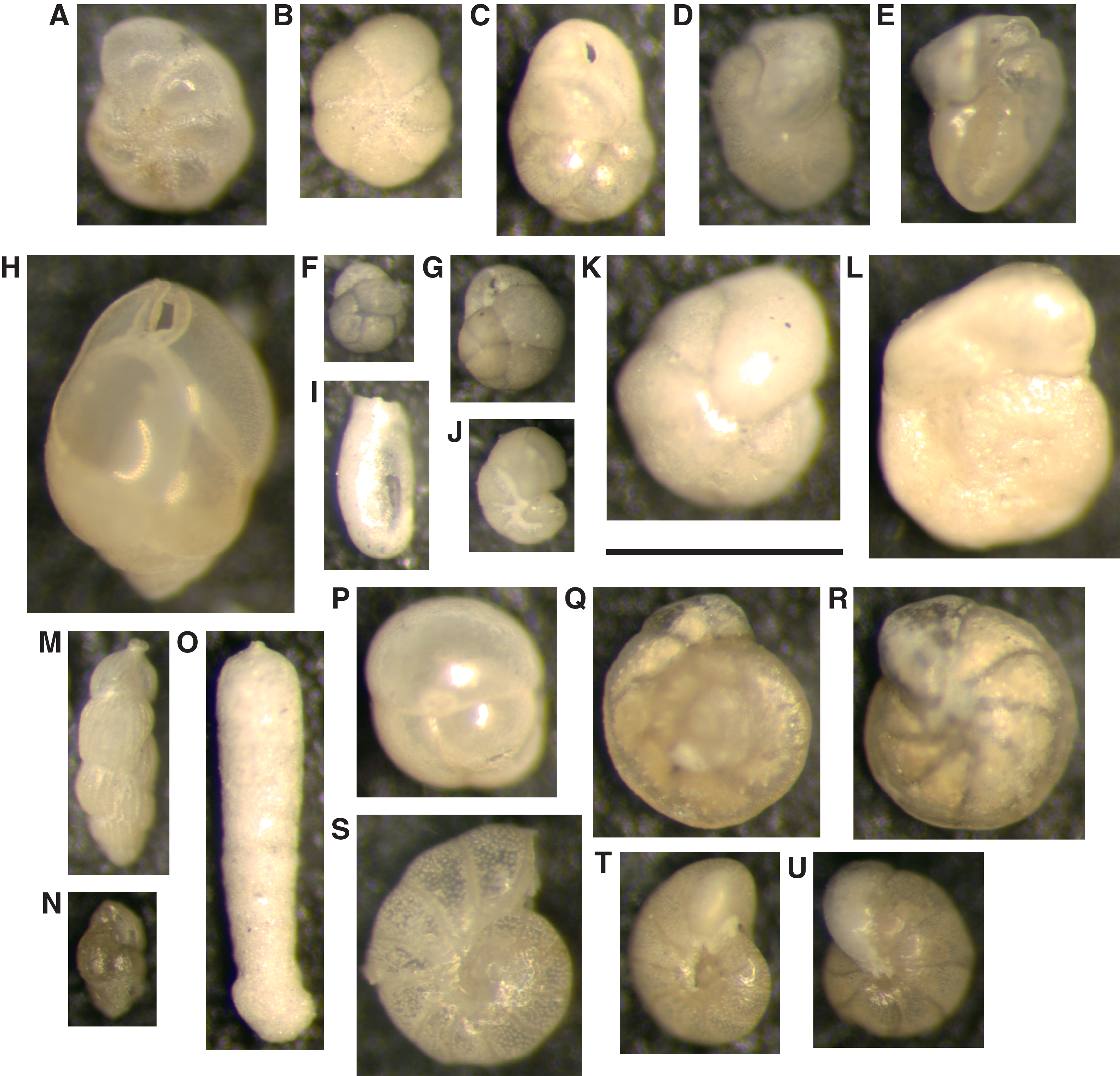
Figure F15. Benthic foraminifers.
Sample 374-U1521A-4R-CC (31.17 m CSF-A) contains a low-diversity assemblage consisting of small specimens of G. subglobosa with N. germanicus, Astrononion echolsi, and Cassidulinoides porrectus. This sample also contains diatoms (many are pyritized), sponge spicules, dark vesicular glass, pyrite, and small pyritized burrow fills. Similarly, G. subglobosa is the most common species in Sample 8R-CC (67.75 m CSF-A). Other taxa in this sparse assemblage include Melonis barleeanum, Nonionella iridea, E. magellanicum, Rosalina globularis, and Ammoelphidiella uniforamina. Grains of dark vesicular glass and coal are also noted. These taxa are all known from the lower to middle Miocene of DSDP Sites 270 and 272 in the central Ross Sea (e.g., Leckie and Webb, 1986; Steinhauff and Webb, 1987).
A significant change in foraminifer assemblages occurs below Core 374-U1521A-8R (Figure F11). An abundant and diverse benthic foraminifer assemblage is present in Sample 9R-CC (77.69 m CSF-A). At least 20 species of moderately to moderately well preserved calcareous benthic foraminifers plus one diagnostic lower to middle Miocene planktonic species, Antarcticella antarctica (Leckie and Webb, 1985), are identified in this sample. Representative benthic taxa include G. subglobosa, Uvigerina sp. cf. Uvigerina bifurcata, N. iridea, Nonionella bradii, Melonis barleeanus, Melonis sp. cf. Melonis pompiloides, Anomalinoides sp., Epistominella vitrea, Elphidium spp., Ehrenbergina glabra, S. bulloides, A. uniforamina, Ammoelphidiella pustulosa, Gavelinopsis lobatulus, and several species of nodosariids. In addition, fragments of mollusk shells, sponge spicules, echinoderm spines, and three ostracod species are present in this sample. Sample 10R-CC (85.67 m CSF-A) has a very similar diverse, abundant assemblage dominated by G. subglobosa, Melonis spp., Uvigerina sp. cf. U. bifurcata, and N. iridea, with echinoderms and ostracods. Quartz, lithic grains, coal, and dark vesicular glass particles are noted in Sample 9R-CC, but very few coarse (>125 µm) grains are present in Sample 10R-CC.
Sample 374-U1521A-14R-CC (122.86 m CSF-A) contains a calcareous benthic assemblage dominated by large, moderately well preserved specimens of Globobulimina sp. (Leckie and Webb, 1986) together with N. germanicus, E. magellanicum, and Lagena nebulosa and abundant diatoms. An elevated abundance of organic matter from highly productive surface water may be responsible for this unique biofacies. A very different moderately well preserved assemblage is recorded in Sample 20R-CC (189.42 m CSF-A), which is dominated by Nonionella spp. (N. iridea and N. bradii) together with S. bulloides, M. barleeanus, G. subglobosa, and C. lobatulus. Diatoms, radiolarians, sponge spicules, and pyritized burrows are also noted. The generally good preservational state and translucent foraminifer tests in samples from Sections 9R-CC through 22R-CC (77.69–204.90 m CSF-A) suggest that this interval contains in situ assemblages.
Foraminifers are generally sparse with few specimens per sample below Core 374-U1521A-22R (204.90 m CSF-A) (Figure F11), which is likely due in part to the difficulty in disaggregating the stiff mud. Sample 28R-CC (262.96 m CSF-A) contains a relatively diverse assemblage represented by M. barleeanus, M. pompiloides, C. lobatulus, G. subglobosa, S. bulloides, R. globularis, Martinottiella communis, and species of nodosariids. The sample also contains quartz, biotite, lithics, coal, and dark vesicular glass particles. However, most samples below Core 22R contain few specimens and fewer species of foraminifers. For example, one specimen of S. bulloides is found in Sample 33R-CC (305.24 m CSF-A), and no foraminifer specimens were found in the preliminary processing and scan of Sample 35R-CC (326.72 m CSF-A). Only three specimens are noted in Sample 41R-CC (371.71 m CSF-A): G. subglobosa, E. magellanicum, and Angulogerina sp. cf. Angulogerina fueguina. A single specimen of M. pompiloides is noted in Sample 45R-CC (397.94 m CSF-A), and no foraminifers are found in Samples 47R-CC (419.09 m CSF-A), 50R-CC (448.69 m CSF-A), and 54R-CC (487.35 m CSF-A). Sample 57R-CC (515.08 m CSF-A) is glauconitic and contains M. barleeanus, M. pompiloides, Uvigerina sp., and Haplophragmoides sp. Sample 60R-CC (543.89 m CSF-A) contains two specimens, including M. pompiloides. Five specimens are found in Sample 69R-CC (629.66 m CSF-A), Cibicides temperata, Cibicides refulgens, Uvigerina/Angulogerina sp., E. magellanicum, and M. pompiloides, whereas only two specimens of Cibicides and Melonis are found in Sample 71R-CC (648.12 m CSF-A).
Palynology
Thirty core catcher samples from Hole U1521A were processed for palynological investigation. Palynomorphs are found downhole in trace to rare numbers, with occasionally more frequent occurrences in Samples 374-U1521A-10R-CC to 29R-CC (85.67–272.98 m CSF-A) (Figure F11; Table T8). In these samples, dinocyst assemblages are of relatively high diversity and preservation varies from poor to good. The palynological assemblages contain both marine (primarily dinocysts) and terrestrial (pollen and spore) components. Other aquatic palynomorphs found include acritarchs, prasinophytes (e.g., Cymatiosphaera spp.), and foraminifer test linings. Pollen and spores are never abundant. Dinocyst occurrence and diversity vary significantly throughout the sequence.
Samples 374-U1521A-1R-CC to 8R-CC (4.23–67.75 m CSF-A) are nearly barren but contain specimens of modern dinocysts of the taxa Brigantedinium spp., Selenopemphix antarctica, and Impagidinium pallidum, as well as leiospheres (acritarchs), which are indicative of a sea ice–dominated environment (e.g., Prebble et al., 2013). Sample 3R-CC (19.36 m CSF-A) contains a notable assemblage of abundant dinocysts and other aquatic palynomorphs belonging to Brigantedinium pynei, Lejeunecysta spp., Operculodinium ?eirikianum, and four different morphotypes of Cymatiosphaera spp. Such an assemblage is comparable to that typically found in lower and middle Miocene circum-Antarctic sediments (e.g., Hannah et al., 1998, 2000; Hannah, 2006; Sangiorgi et al., 2018) and thus suggests reworking from Miocene sediments in this Pliocene sequence (Figure F11).
Samples 374-U1521A-10R-CC to 29R-CC (85.67–272.98 m CSF-A) yield the most diverse palynomorph assemblages of Hole U1521A (Figures F11, F16, F17). The assemblages include Brigantedinium spp., Brigantedinium pynei, Batiacasphaera minuta, Batiacasphaera sphaerica, I. pallidum, Impagidinium patulum, Lejeunecysta cowei, Lejeunecysta fallax, Lejeunecysta spp., Nematosphaeropsis labyrinthus, O. ?eirikianum, Operculodinium centrocarpum, Operculodinium janduchenei, S. antarctica, Selenopemphix nephroides, different species of Spiniferites, and three species of yet undescribed Protoperidinium (round, brown, and spiny). Two of these three species (Protoperidinium sp. 1 and sp. 2) are not present in or above Sample 14R-CC (122.86 m CSF-A) but become dominant in the assemblages of Samples 16R-CC and 18R-CC (147.02 and 167.83 m CSF-A). Different species of Cymatiosphaera spp. also occur abundantly together with Leiosphaeridia in all core catcher samples examined. The assemblages in this interval resemble those previously reported in lower and middle Miocene western Ross Sea drill cores from Cape Robert Projects Site CRP-1 and ANDRILL Site AND-2A (e.g., Hannah et al., 1998, 2000; Warny et al., 2009). In Hole U1521A, the dinocyst diversity is higher and contains a more diverse assemblage of neritic species. Pollen (mainly bisaccates) and spores are not abundant. The palynomorphs found in this interval indicate high-productivity marine waters that were warmer than today and seasonally stratified. Relatively high abundances of phototrophic taxa (e.g., Batiacasphaera spp., N. labyrinthus, Operculodinium spp., and Spiniferites spp.) are indicative of a reduced sea ice season compared with the present day. Modern samples are characterized by a dominance of nonphototrophic, heterotrophic species (Prebble et al., 2013; Sangiorgi et al., 2018).

Figure F16. Dinocysts.

Figure F17. Dinocysts.
Samples 374-U1521A-35R-CC to 71R-CC (326.72–648.12 m CSF-A) generally contain rare palynomorphs with poor preservation (Figure F11). Samples 35R-CC to 53R-CC (326.72–477.71 m CSF-A) are almost or completely barren, whereas Samples 53R-CC to 71R-CC (477.71–648.12 m CSF-A) yield sparse dinocysts and common pollen (saccate pollen and Nothofagus spp.). The dinocyst assemblages are characterized by the occurrence of spiny, round, brown dinocysts (Protoperidinium spp.) and a few specimens of Lejeunecysta cowiei, Lejeunecysta acuminata, and Arcticacysta spp., a species previously found in the (questionably) lower Miocene record of Integrated Ocean Drilling Program Expedition 302 (central Arctic Ocean; Sangiorgi et al., 2008, 2009). Some leiospheres and Cymatiosphaera sp. are also present sporadically. The dinocysts Distatodinium paradoxum, Spinidinium macmurdoense, and Vozzhennikovia apertura; fragments of Enneadocysta diktyostyla; Palaeocystodinium sp.; and inner bodies of cf. Deflandrea phosphoritica co-occur. Based on the stratigraphic occurrences of all these species (Bijl et al., 2015 [and references therein], 2018; Clowes et al., 2016), such an association indicates that at least part of the assemblage is likely reworked from Oligocene and Eocene strata.
Calcareous nannofossils
A total of 21 core catcher samples and 5 additional samples from the split-core sections were examined for calcareous nannofossils. Samples above Section 374-U1521A-58R-6 (524.40 m CSF-A) are almost entirely devoid of nannofossils (Figure F11; Table T9). A single fragment of the Eocene taxon Reticulofenestra umbilicus is found in Sample 14R-CC (122.9 m CSF-A), and an unidentifiable nannofossil fragment was also found in Sample 49R-CC (438.90 m CSF-A).
Moderately preserved calcareous nannofossils are sporadically present and very rare between Sections 374-U1521A-58R-6 and 65R-CC (524.40–589.70 m CSF-A) (Figures F11, F18; Table T9). The assemblage consists primarily of reticulofenestrids, including Reticulofenestra hampdenensis, Reticulofenestra lockeri, Reticulofenestra daviesii, Dictyococcites antarcticus, and Cyclicargolithus floridanus. All of these taxa first appear during the Paleogene and range into the Neogene. R. lockeri and R. daviesii have last appearances in the early Miocene (Young, 1998; Bown and Dunkley Jones, 2012), and C. floridanus goes extinct in the late middle Miocene (Raffi et al., 2006). Coccolithus pelagicus, a long-ranging extant taxon that evolved in the early Paleocene, is also present in the assemblage. Although this assemblage is consistent with an early Miocene age for the lower part of Hole U1521A, the presence of a probable fragment of a Chiasmolithus sp. rim suggests that there is at least some reworking in the section because the genus Chiasmolithus goes extinct in the late Oligocene (Perch-Nielsen, 1985). These findings, coupled with the lithology (predominantly diamictite), preclude confidently assigning an age to the interval based on calcareous nannofossils.
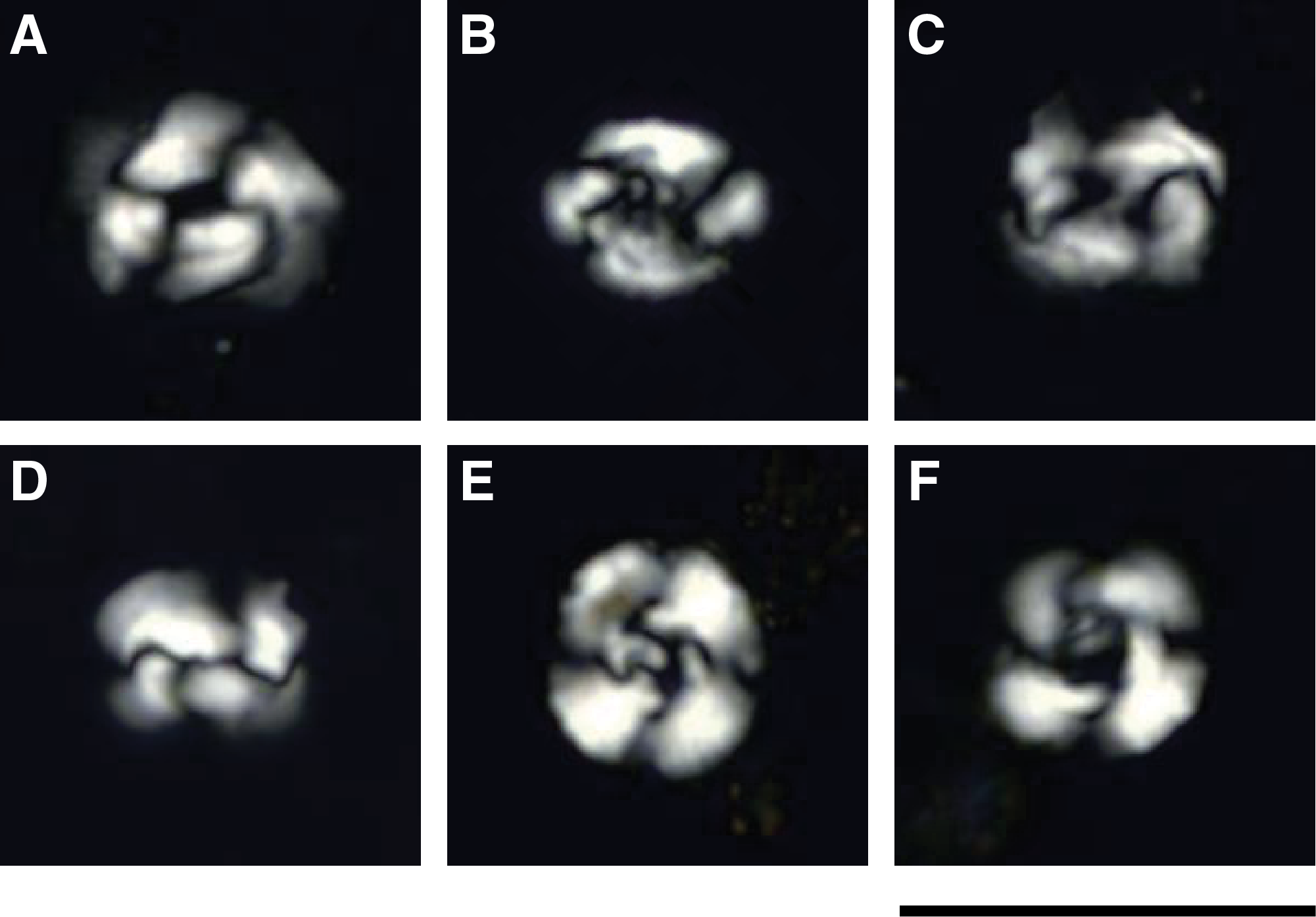
Figure F18. Calcareous nannofossils.
In addition to the calcareous nannofossil assemblage, fragments of calcareous dinoflagellates (Thoracosphaera and related taxa) are also present in samples from Sections 374-U1521A-60R-CC (543.90 m CSF-A) and 65R-CC (589.70 m CSF-A). A possible Thoracosphaera fragment is also noted in Sample 11R-CC, 0–5 cm (95.48 m CSF-A).
Macrofossils and ostracods
Fossil specimens of bivalves and echinoderm spines are identified in the sediment cores and residues washed from the foraminifer preparations, respectively. Disarticulated and articulated shells of a pecten are found in several section breaks in Core 374-U1521A-20R (see Lithostratigraphy). Ostracods were also noted in the foraminifer-washed residues of Samples 9R-CC and 10R-CC.
Age model
The age model for Site U1521 (Figure F12) is based on diatom and radiolarian events (Table T5) and magnetic polarity reversal events (see Paleomagnetism). At the top of the cored section, a thin interval of upper Pleistocene to recent sediments is present in Section 374-U1521A-1R-CC (0–4.32 m CSF-A). Samples 2R-CC and 3R-CC (8.51 and 19.41 m CSF-A) recovered an ~15 m thick interval of uppermost Pliocene to lower Pleistocene sediments that are dated by a combination of the diatom and radiolarian events described above. A disconformity representing a hiatus of ~11 My separates the Pliocene sediments from the underlying ~500 m thick interval of middle to lower Miocene sediments (~14 to <18 Ma), with age control based primarily on the diatom biostratigraphy described above and the magnetic polarity reversal events (Figure F12) described in Paleomagnetism. A shorter disconformity of ~1 My duration is denoted in Figure F12 between Samples 8R-C and 9R-CC.
Paleomagnetism
Paleomagnetic investigations at Site U1521 primarily contributed to the chronostratigraphy by constructing a magnetostratigraphy. Additional rock magnetic measurements were made to assess the stability and origin of the paleomagnetic record and to investigate the development of magnetic fabric from depositional and postdepositional processes.
Natural remanent magnetization (NRM) was measured on most archive-half core sections at 5 cm intervals before and after alternating field (AF) demagnetization in 5 mT steps up to 20 mT peak fields. The 15 mT step and occasionally the 5 mT step were omitted when core flow increased. The use of the RCB system frequently resulted in disturbed sediments, and special care was taken to either avoid measuring very disturbed sections or to exclude disturbed data points from analysis. Additionally, we masked data from the top and bottom 10 cm of each core because of edge effects (see Paleomagnetism in the Expedition 374 methods chapter [McKay et al., 2019a]). The processed data set was used to identify normal and reversed polarity zones that are correlated to the geomagnetic polarity timescale (GPTS) of Gradstein et al. (2012), with independent age control from biostratigraphic datums.
NRM measurements on a selection of oriented, discrete samples were used to test the fidelity of archive-half NRM data. Out of a total of 315 discrete samples (~1 per section), 21 samples were demagnetized using a 20-step AF demagnetization protocol (0–20 mT in 2 mT steps and 20–60 mT in 5 mT steps, followed by 70 and 80 mT peak AF demagnetization) to observe the potential overprint(s) and stable remanent carrier(s). Because of the nature of RCB coring, in which core pieces can rotate independently inside the core barrel, azimuthal orientation is not possible and all declinations are presented in sample coordinates.
In addition, we measured mean (bulk) magnetic susceptibility and anisotropy of magnetic susceptibility (AMS) on all discrete samples. The mean magnetic susceptibility served as a comparison to magnetic susceptibility measurements on the Whole-Round Multisensor Logger (WRMSL) and Section Half Multisensor Logger (SHMSL). The AMS measurements serve to reconstruct magnetic fabric.
NRM measurements
Archive-half measurements
Initial NRM inclinations on archive-half core sections are typically steep (Figure F19). As the samples are AF demagnetized, the direction usually changes little, remaining either steep upward or downward, presumably reflecting the normal or reversed polarity recorded in magnetically stable intervals (e.g., in lithostratigraphic Units III and IV). Other intervals (e.g., Unit VII) produced noisy results, with the inclinations starting steep downward and then becoming erratic as the samples are demagnetized. Presumably, the steep downward direction is a drilling overprint, although we cannot discount that it may have been a very low coercivity primary or secondary component unrelated to drilling (Figure F19). These intervals also contain elevated magnetic susceptibility values (collected on the WRMSL, SHMSL, and Kappabridge KLY 4S) and very low coercivity, which is demonstrated by the substantial NRM intensity decrease from about 10−2 A/m to <10−4 A/m after 20 mT peak AF demagnetization (Figure F19). Our working hypothesis is that these intervals contain coarse-grained magnetic minerals and are generally a poor record of the ancient deposition remanence.
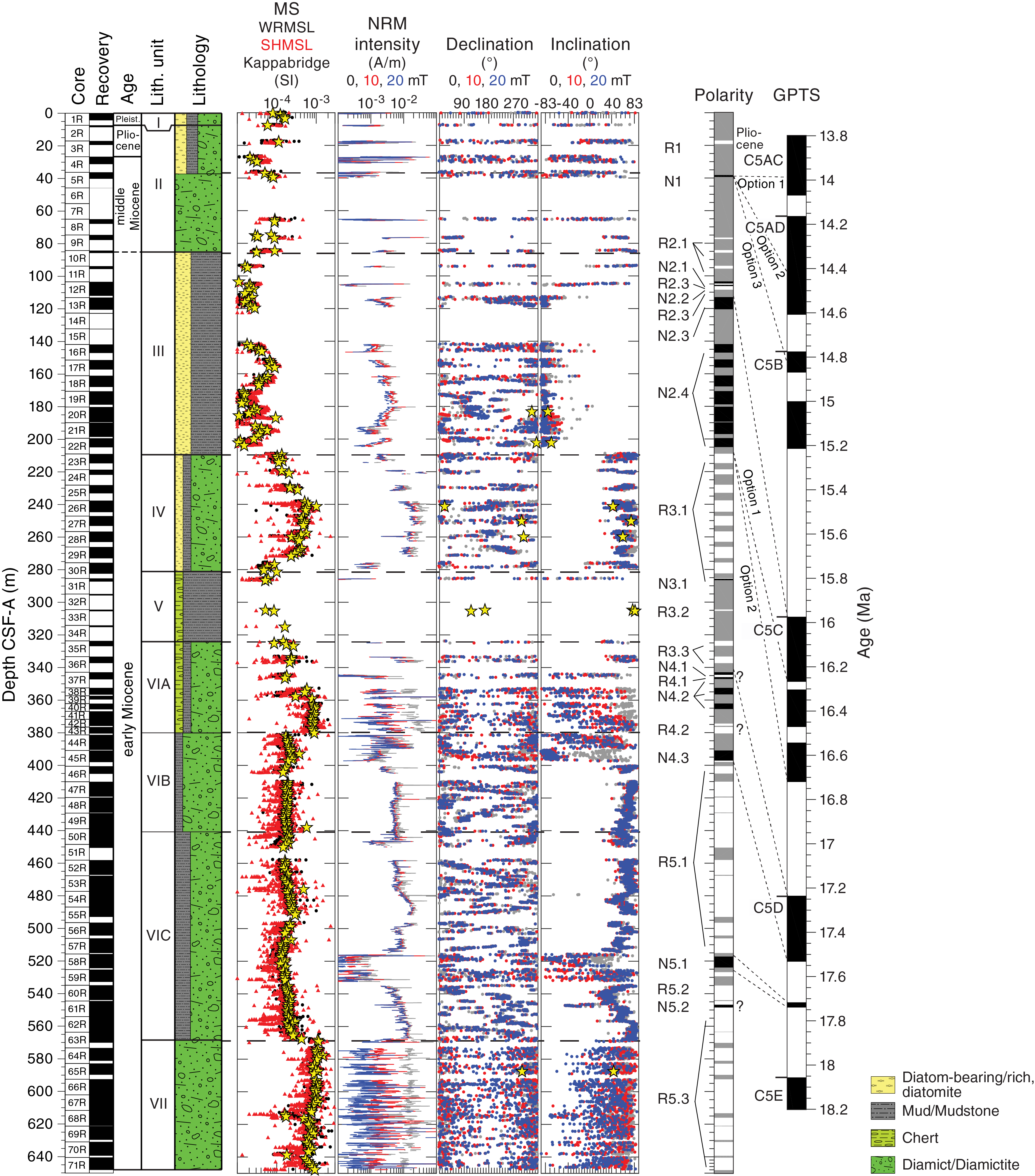
Figure F19. Paleomagnetic data.
For the magnetically stable intervals, the inclination following 20 mT AF demagnetization generally clusters around the expected value of ±82.7° for this site (present-day latitude of 75.7°S), assuming a geocentric axial dipole (e.g., lithostratigraphic Units III and IV and most of Subunits VIB and VIC).
Discrete sample measurements
One oriented discrete cube sample per section was collected at Site U1521, except from Cores 374-U1521A-6R, 7R, 14R, 15R, and 32R because of poor recovery (N = 315 samples). Similar to the archive-half core sections, initial NRM measurements on a subset of cube samples typically have steep upward or steep downward directions (representative examples shown in Figure F20). The drilling overprint, which is typically very evident in IODP cores, is not apparent in a majority of the samples. A small downward-directed low-coercivity component occurs in a few intervals (e.g., lithostratigraphic Subunit VIA and Unit VII). For example, most of the small overprint is removed with only 2 mT AF demagnetization in Sample 22R-3, 30 cm (Figure F20D). Progressive AF demagnetization reveals linear demagnetization paths for the most stable samples that have steep upward directions (normal polarity) or steep downward directions (reversed polarity) (Figure F20D). Extremely noisy demagnetization behavior occurs in intervals with low coercivity (Figure F20A), which often is associated with intervals of high magnetic susceptibility (e.g., Subunit VIA and Unit VII) and with intervals affected by coring disturbance. For the magnetostratigraphy, we only use NRM data of samples with a stable component that trends linearly toward the origin on Zijderveld diagrams (Figure F20C, F20D).
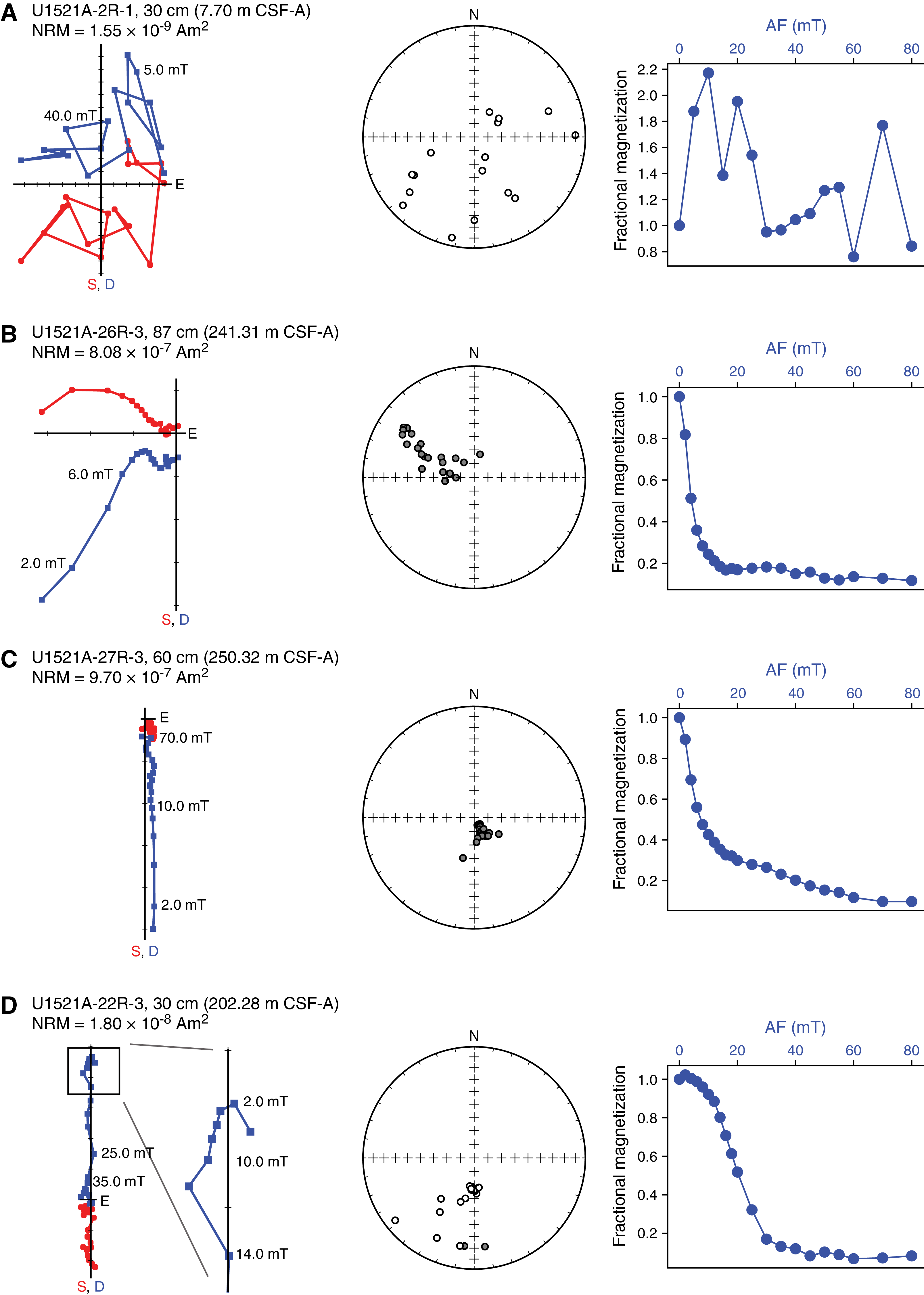
Figure F20. Representative AF demagnetization behavior.
Interestingly, Sample 374-U1521A-26R-3, 87 cm, reveals three components (Figure F20B): a low coercivity component (0–16 mT) with a steep downward direction, an intermediate coercivity component (16–35 mT) with a moderate upward direction, and a high-coercivity component (35–80 mT) with a moderate downward direction. Potentially, these components reflect an overprint; the incorporation of a small clast inside the cube, which is not visible on the cube surfaces; and a primary deposition magnetization. Alternatively, one of the components may reflect a diagenetic effect. Further shore-based analyses are required to disentangle these different components and to investigate their contributions to the NRM.
Magnetostratigraphy
Because this site is located at a high latitude in the Southern Hemisphere, the magnetostratigraphic interpretation for Hole U1521A relies on magnetically stable intervals with steep positive inclination values corresponding to reversed polarity and steep negative inclination values corresponding to normal polarity (Figure F19). Based on the normal and reversed polarity interpreted from both archive-half core sections and discrete samples, we define five major polarity zones (R1–R5; Figure F19). Where possible, each zone (except N1/R1) is divided into subzones, depending on recovery (all unrecovered intervals and intervals with low-quality directional data are indicated with gray shading in the Polarity column in Figure F19). Poor core recovery in Cores 374-U1521A-1R through 15R (0–132.49 m CSF-A) and 31R through 34R (285.30–315.20 m CSF-A) frequently yielded uncertain polarities.
Correlation of identified Zone R1 through Subzone R5.3 to the GPTS of Gradstein et al. (2012) strongly depends on independent age control. At Site U1521, this independent age control mainly comes from the first and last appearance datums of diatoms (see Biostratigraphy and paleontology). These datums indicate a middle Miocene to early Miocene age for Cores 374-U1521A-4R through 55R (26.60–492.96 m CSF-A), below which the sediments are barren of biostratigraphic index species. Our correlation of Site U1521 polarity zones to the GPTS is shown on Figure F19 and given in Table T10.
Cores 374-U1521A-1R through 3R (0–19.43 m CSF-A) are of Pliocene to recent(?) age (see Biostratigraphy and paleontology). Reversed polarity Zone R1 can correlate to various reversed (sub)chrons in the Pliocene to Pleistocene, and we thus refrain from correlating this zone to the GPTS without further biostratigraphic constraint. Diatom biostratigraphy provides good age control for Cores 4R through 8R (26.60–67.80 m CSF-A; Datums D4–D7 on Figure F12). Normal polarity Zone N1, identified in Core 5R, may therefore correlate to Chron C5ADn (14.163–14.609 Ma). However, given the uncertainties of the diatom ages, Zone N1 could also represent an interval deposited during Chron C5ACn (13.739–14.070 Ma) or Subchron C5Bn.1n (14.775–14.870 Ma) (Figure F19). Diatom biostratigraphy suggests an ~1 My hiatus between Samples 8R-CC and 9R-CC (67.75–77.69 m CSF-A; see Biostratigraphy and paleontology).
Subzone R2.1 may correlate to Chron C5Br (15.160–15.974 Ma), and our preference is to correlate the top of Subzone N2.3 to the top of Chron C5Cn (~16 Ma) and the base of Subzone N2.4 to the base of Chron C5Cn (~16.7 Ma) (Figure F19; Table T10). This correlation does not incorporate an identification of the reversed subchrons in Chron C5Cn, which may occur in the unrecovered intervals of Cores 374-U1521A-14R and 15R (122.60–132.49 m CSF-A). Alternatively, Subzones N2.3 and N2.4 may be correlated to Subchron C5Cn.1n (15.974–16.268 Ma), preceded by an ~0.5 My hiatus that covers at least the older half of Chron C5Cn. There is currently a lack of correlation of Subzones N2.1, R2.2, N2.2, and R2.3 to the GPTS, but they cannot be tied confidently unless there are substantial but spurious changes in sedimentation rate.
The correlation of Subzones R3.1–R5.3 to (sub)chrons of the GPTS is uncertain due to the paucity of biostratigraphic datums (see Biostratigraphy and paleontology). If we make the assumption that Subzones R3.1–R5.3 can be sequentially correlated to (sub)chrons of the GPTS, this correlation ties the thick, reversed interval of Zone R3 to Chron C5Cr (16.721–17.235 Ma), Zone N4 to Chron C5Dn (17.235–17.533 Ma), and Zone R5 to Subchrons C5Dr.1r (17.533–17.717 Ma) and C5Dr.2r (17.740–18.056 Ma), including thin Subzone N5.1 to the short-duration Subchron C5Dr.1n (17.717–17.740 Ma; Figure F19; Table T10). This correlation does not take into account the occurrence of the relatively thin Subzones N3.1, N4.1, R4.1, and N5.2, which could not be confidently correlated to the GPTS without introducing spurious sedimentation rate changes. We hypothesize that these thin polarity zones may potentially reflect undiagnosed diagenesis or unobserved geomagnetic field behavior, both of which will require additional shore-based analyses to evaluate the reliability of the observed NRM signal.
These correlations provide an estimate of the linear sedimentation rates, taking into account the incomplete recovery and corresponding uncertainties. Polarity Zone R5 (early Miocene) was deposited at ~62 cm/ky, which appears high but is not unrealistic for deposition of the diamictite in lithostratigraphic Subunit VIB through Unit VII. Sedimentation rates decreased to ~20 cm/ky during Chrons C5Cr and C5Dn (16.721–17.533 Ma; spanning Zones R3 and N4). The correlation of Subzones N2.3 and N2.4 to the entire Chron C5Cn (15.974–16.721 Ma) implies a sedimentation rate of ~13 cm/ky. If we correlate Subzones N2.3 and N2.4 to only Subchron C5Cn.1n (15.974–16.268 Ma), the sedimentation rate would be ~34 cm/ky.
Magnetic susceptibility and AMS
Mean magnetic susceptibility and AMS were measured on all cube samples. The Kappabridge KLY 4S controlled by the SUFAR software measures the magnetic susceptibility while rotating the sample. The program then stacks the data collected in three different orientations and calculates the best-fit second-order tensor. To interpret this tensor in terms of magnetic particle alignment and anisotropy, we use the orientation and the magnitude of the maximum susceptibility axis (kmax), intermediate susceptibility axis (kint), and minimum susceptibility axis (kmin).
A substantial separation between kmax and kmin highlights a greater degree of anisotropy. The kmax/kmin ratio approximates this degree of anisotropy (P), where P = 1 indicates no anisotropy and P > 1 indicates a high degree of anisotropy. When P is >1 (i.e., anisotropic sample) and kmin inclination is >60˚ (i.e., the orientation of the minimum susceptibility axis is steeply vertical), the anisotropy is most likely a result of sediment compaction, which is commonly observed in many sedimentary settings (e.g., Schwehr et al., 2006). This anisotropy is noted at Site U1521 in lithostratigraphic Units III and V (Figure F21). We observed scattered kmin inclination, high mean magnetic susceptibility, and high P (generally >1.05) at the bottom of Unit IV, in Subunit VIA, and throughout Unit VII. In contrast, we observed scattered kmin inclination but low mean magnetic susceptibility and low P (less than ~1.05) in the upper half of Unit IV and in Subunit VIB (Figure F21). Additionally, relatively steep kmin inclination, high P, and slightly elevated mean magnetic susceptibility values occur in the middle of Subunit VIC (Cores 374-U1521A-54R through 56R [~480–500 m CSF-A]). These differences between lithostratigraphic units and subunits potentially reflect variability in the sand-sized or coarser grained fraction of that unit, yielding variable compaction (reflected in P) orientation of the grains. Further postcruise work on the integration of sedimentological proxies such as magnetic fabric, grain size, and provenance are required to fully capture the variability in these diamictite units.
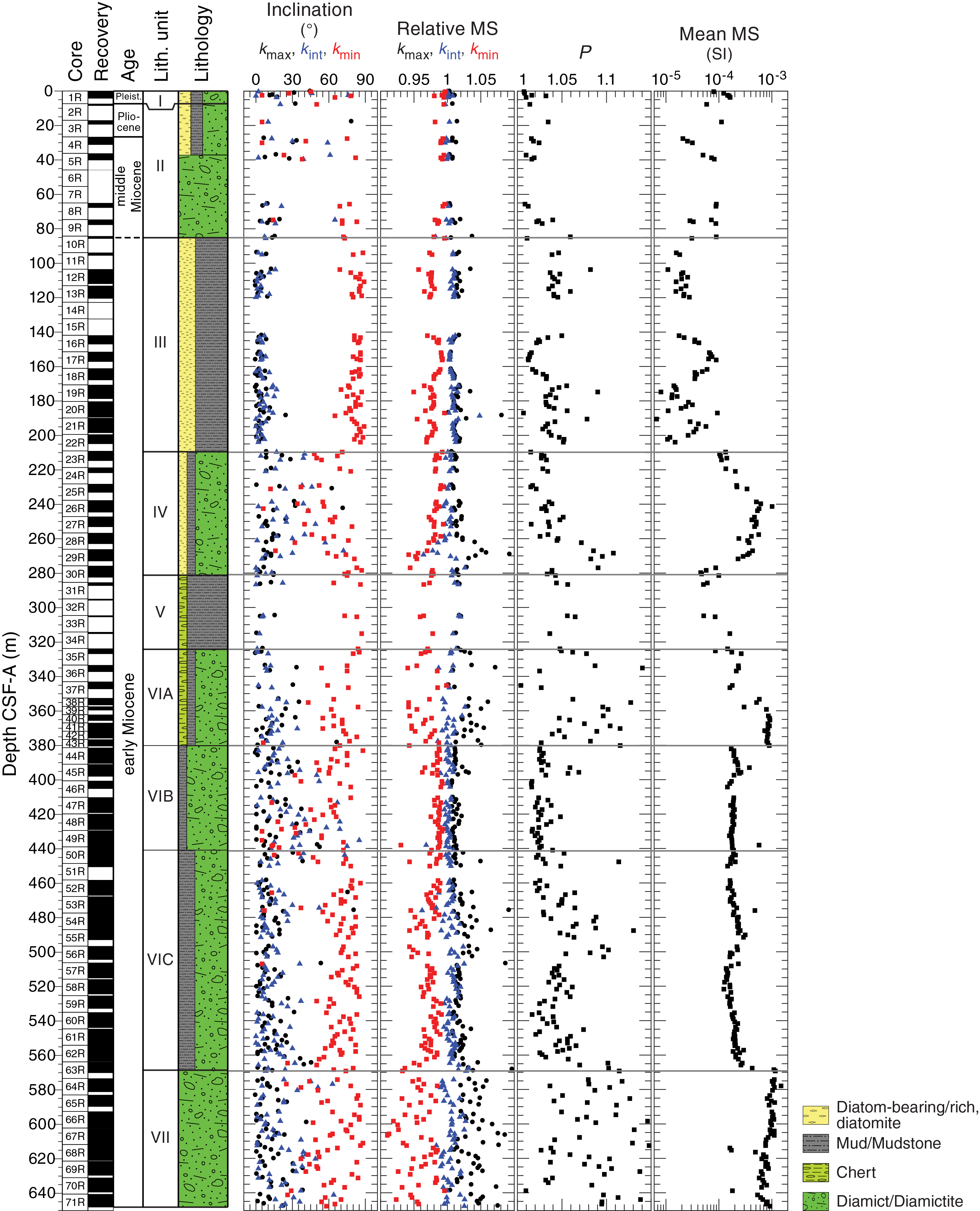
Figure F21. Anisotropy of magnetic susceptibility.
Physical properties
Physical property measurements for Hole U1521A were completed on whole-round sections, section halves, and discrete samples from Cores 374-U1521A-1R through 71R (0–648.17 m CSF-A). Prior to plotting, the measurement results were cleaned to exclude outliers and unreliable values (Table T11). Following thermal equilibration (~4 h), gamma ray attenuation (GRA) bulk density, magnetic susceptibility, compressional P-wave velocity, and NGR measurements were made on all whole-round sections using the Whole-Round Multisensor Logger (WRMSL) and the Natural Gamma Radiation Logger (NGRL). Sampling resolution for the WRMSL was 2.5 cm, and NGR was measured at 10 cm intervals with a measurement time of ~5 min at each position. P-wave velocity was measured on the WRMSL only for Core 1R (0–4.28 m CSF-A). Measurements were terminated deeper than 4.28 m CSF-A because of poor contact between the core liner and the sediment, which yields poor results (see Physical properties in the Expedition 374 methods chapter [McKay et al., 2019a]). Thermal conductivity measurements were mainly performed on working-half sections using a contact probe. Core 1R was measured on the whole-round section using a needle probe. Discrete samples from the working-half sections (typically from Sections 1, 3, 5, and 7) were taken for moisture and density (MAD) measurements. Discrete compressional wave velocity measurements were conducted on the working halves of each core section using the P-wave caliper (PWC) contact probe system on the Section Half Measurement Gantry (SHMG). Color reflectance and point magnetic susceptibility were collected on the archive-half sections using the Section Half Multisensor Logger (SHMSL). Red, green, and blue (RGB) were measured on the Section Half Imaging Logger (SHIL) (see Lithostratigraphy and Physical properties in the Expedition 374 methods chapter [McKay et al., 2019a]). Physical property measurements show distinct changes that are in good overall agreement with the defined lithostratigraphic units. All physical property data are available from the Laboratory Information Management System database (http://web.iodp.tamu.edu/LORE).
Magnetic susceptibility
Both whole-round measurements on the WRMSL and discrete point measurements on the SHMSL were used to characterize magnetic susceptibility at Site U1521 (Figure F22). Both methods yielded similar downhole variability and a similar range of values: 0–1000 × 10−5 SI for the WRMSL and −1 × 10⁻⁵ to 1388 × 10−5 SI for the SHMSL, respectively (see Physical properties in the Expedition 374 methods chapter [McKay et al., 2019a] for details on instrument units [IU; ~10−5 SI]). Measured values from the WRMSL that are <0 × 10−5 are likely due to uncertainty or error in zeroing the loop before measurement of slightly diamagnetic material and should not be used. Values >250 × 10−5 are attributed to individual outsized clasts (e.g., washed gravels and lonestones) and are not representative of the overall sediment composition. Magnetic susceptibility is generally low (~0 × 10−5 to 10 × 10−5 SI) in the upper 225 m CSF-A, which corresponds to lithostratigraphic Units I–III. Intervals of slightly higher magnetic susceptibility in this interval (3–4.5 and 70–80 m CSF-A) correspond to the presence of diamictite in Units I and II. Very low to slightly negative magnetic susceptibility values from Sections 374-U1521A-10R-2 through 26R-1 correspond to intervals of diatom-rich to diatom-bearing mudstone. Magnetic susceptibility is higher (30 × 10−5 to 65 × 10−5 SI) from 225 to 280 m CSF-A, which corresponds to an interval of sandy diamictite in Unit IV. Low magnetic susceptibility (0 × 10−5 to 20 × 10−5 SI) is found from 280 to 330 m CSF-A and corresponds to the chert-bearing intervals of Unit V. From 330 to 350 m CSF-A, higher values (2 × 10⁻⁵ to 40 × 10−5 SI) correspond to the interbedded mudstone and diamictite of Subunit VIA. A significant downhole increase in magnetic susceptibility (40 × 10−5 to 200 × 10−5 SI) observed from 355 to 380 m CSF-A in Subunit VIA suggests higher clast content and/or a change in the composition of the clasts. The transition between Subunits VIA and VIB (380 m CSF-A) shows a decrease in magnetic susceptibility, but the lithology appears to change from interbedded diamictite and diatom-bearing mudstone to sandy diamictite. Such a decrease in magnetic susceptibility is unexpected because sandy diamictite should have higher magnetic susceptibility than interbedded diatom-bearing mudstone and diamictite. From 385 to 565 m CSF-A, magnetic susceptibility is low again (5 × 10⁻⁵ to 40 × 10−5 SI), likely indicating lower clast content in Subunits VIB and VIC. From 565 m CSF-A to the bottom of the hole, magnetic susceptibility increases significantly (40 × 10−5 to 105 × 10−5 SI), corresponding to the sandy diamictite that dominates Unit VII. In this unit, lower magnetic susceptibility values most likely indicate muddier intervals. In general, magnetic susceptibility at this site is likely controlled by the proportion of biogenic versus detrital sediments and the size and abundance of lithogenic clasts.

Figure F22. MS, thermal conductivity, and NGR.
Natural gamma radiation
NGR measurements show downhole variations between ~10 and 65 counts/s in Hole U1521A (Figure F22). NGR values are lowest (10–30 counts/s) between Cores 374-U1521A-11R and 22R (93.8–204.95 m CSF-A), corresponding to diatom-bearing/rich mudstone (lithostratigraphic Unit III). NGR is higher and averages ~30 counts/s (25–50 counts/s) in Cores 23R through 30R (209–282.43 m CSF-A), corresponding to diatom-bearing clast-poor sandy diamictite in Unit IV. Deeper than 285 m CSF-A, NGR increases with depth in Cores 31R through 34R (285.3–315.2 m CSF-A), reaching a maximum of ~45 counts/s (Unit V and Subunit VIA). Cores 35R through 63R (323.7–570.13 m CSF-A) have generally increasing values downhole and have the highest NGR (~40–60 counts/s) at the site. This downhole increase is associated with the interbedded sandy diamictite and mudstone of Subunits VIB and VIC. In Cores 51R through 57R (448.5–515.13 m CSF-A), an interval of lower NGR (minima of ~30–35 counts/s) corresponds to mud-rich lithologies in Subunit VIC. NGR decreases downhole in Cores 64R through 69R (573.30–629.71 m CSF-A), followed by an increase at the bottom of the hole (Cores 70R through 71R [630.90–648.17 m CSF-A]). A similar pattern is present in the magnetic susceptibility record over this interval (Figure F22) and corresponds to Subunit VII, a clast-poor muddy and sandy diamictite.
Thermal conductivity
Thermal conductivity was measured, when possible, on Cores 374-U1521A-1R through 36R (2.95–335.18 CSF-A) (Figure F22). Measurements were attempted using a contact probe and were discontinued below Core 36R after repeated measurement attempts yielded invalid results. The quality of the thermal conductivity measurements was checked by evaluating two parameters: (1) the number of solutions acquired and (2) the shape of the curve formed on the temperature versus time plot of these points. A valid measurement must have a sufficient number of solutions to form an exponential curve. All measurements with a low number of solutions and/or a bad repartition of these values on the temperature versus time plot (i.e., forming two curves or no curve) were deleted, resulting in removal of 59% of the original data. Overall, thermal conductivity ranges from 0.8 to 1.9 W/(m·K) and generally corresponds with downhole changes in magnetic susceptibility (Figure F22). In general, diatom-bearing/rich mud/mudstone (lithostratigraphic Units I and III) is characterized by low thermal conductivity (<1 W/[m·K]) and diamictite (Units II and IV and Subunit VIA) is characterized by higher thermal conductivity (>1 W/[m·K]).
Bulk density, grain density, and porosity
Two methods were used to evaluate bulk density at Site U1521. The GRA method (see Physical properties in the Expedition 374 methods chapter [McKay et al., 2019a]) provides bulk density estimates measured on whole-round sections. MAD measurements on discrete samples provide a second independent measure of bulk density. GRA bulk density in Hole U1521A varies from 0.5 to ~2.5 g/cm3, whereas discrete MAD values exhibit a much narrower range, from 1.2 to 2.3 g/cm3 (Figure F23). Overall, bulk density calculated from discrete MAD samples is elevated compared to GRA bulk density measurements and generally matches the upper envelope of the GRA bulk density estimate. GRA bulk density is generally underestimated when measured on RCB cores because the instrument reports measurements based on the internal diameter of the core liner (66 mm), whereas RCB cores have a nominal diameter of 58 mm or less. The density measurements can be corrected to account for this bias (Jarrard and Kerneklian, 2007); however, we do not apply this correction here because of variations in the diameter of the RCB cores.
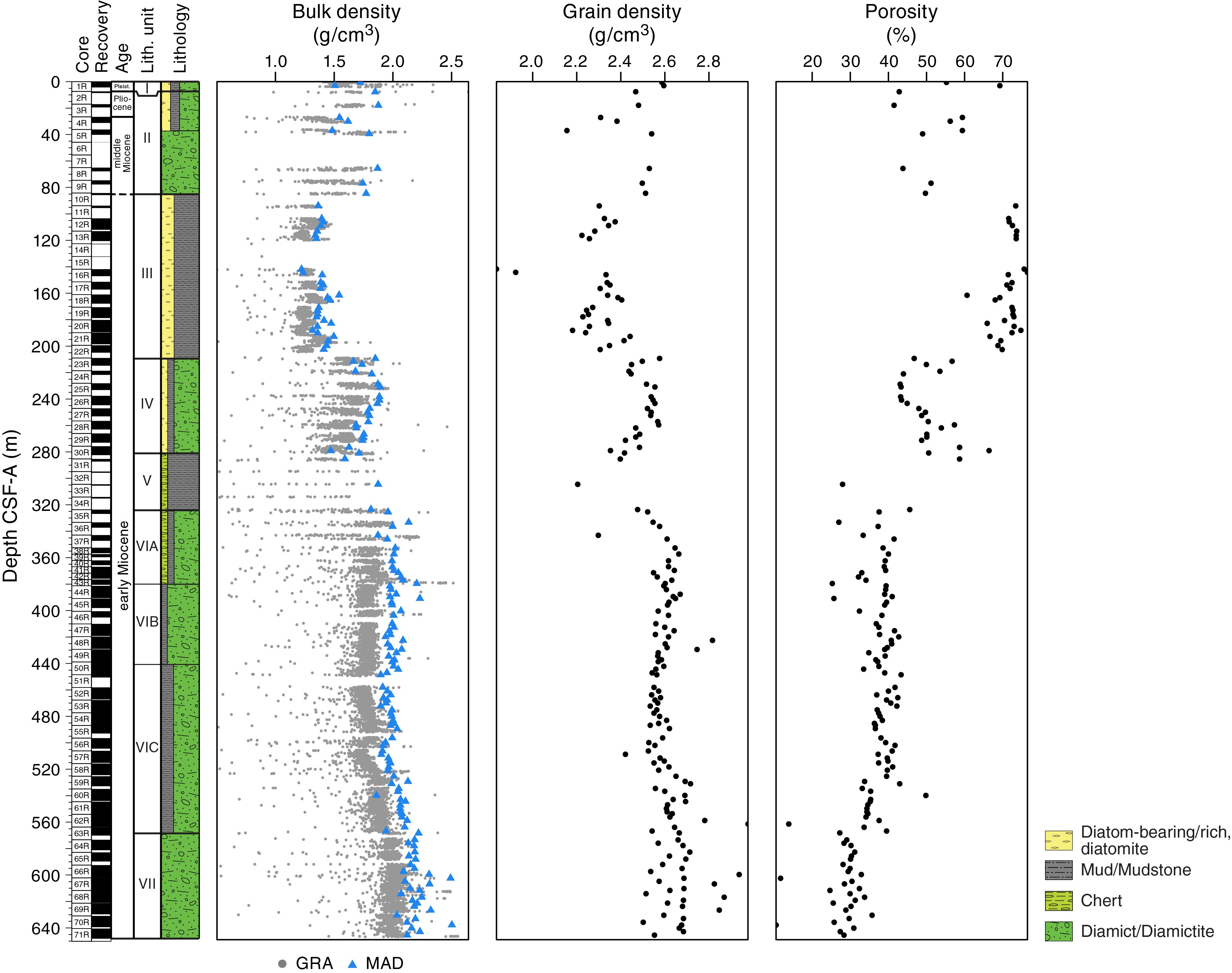
Figure F23. GRA and MAD bulk density, grain density, and porosity.
Both methods demonstrate similar trends downhole. Bulk density is initially high and variable in Cores 374-U1521A-1R through 10R (0–85.72 m CSF-A). The lowest values (~1.2–1.6 g/cm3) in the hole were recorded in Cores 11R through 22R (93.80–204.75 m CFS-A), corresponding to diatom-rich mudstone in lithostratigraphic Unit III. Bulk density increases abruptly in Core 23R (209.00 m CSF-A) and then gradually decreases downhole. From Core 31R to Core 71R (285.3–648.17 m CFS-A), bulk density is generally high (~1.7–2.2 g/cm3), and slight variations may be due to changes in grain size or cementing of the diamictite lithologies. In general, downhole variability in bulk density at this site is a function of both lithology and sediment compaction with depth.
In addition to bulk density, MAD measurements provide calculations of dry density, grain density, porosity, moisture content, void ratio, and several other properties that co-vary downhole. In general, bulk density and porosity are anticorrelated and increase and decrease downhole, respectively (Figure F23). Intervals of high porosity and low grain density correspond to diatom-rich mudstone (lithostratigraphic Unit III). Intervals of low porosity and high density correspond to diamictite-dominated lithologies (Units IV, VI, and VII). Porosity and density change abruptly at the Unit II/III, III/IV, IV/V, and VI/VII boundaries, indicating changes in grain size, matrix, or compaction. Higher grain densities in Unit VII may indicate a difference in clast composition compared with overlying units, but the data points are too few to draw a confident conclusion.
Compressional P-wave velocity
PWC-measured values in Cores 374-U1521A-1R through 10R (0–85.72 m CSF-A) are variable between ~1500 and 1900 m/s (Figure F24). Near-constant P-wave velocity (~1600 m/s) was measured in Cores 11R through 22R (93.80–204.95 m CSF-A), corresponding to the diatom-rich mudstone of lithostratigraphic Unit III. At the top of Core 23R, P-wave velocity abruptly increases to ~2000 m/s, which also corresponds to an abrupt increase in bulk density at the transition from diatom-rich mudstone (Unit III) to diamictite (Unit IV). P-wave velocity decreases with depth to 1800 m/s in Cores 23R through 30R (209.00–282.43 m CSF-A). Highly variable P-wave velocity values (~1800–4400 m/s) were measured in Cores 31R through 34R (285.30–315.2 m CSF-A), corresponding with an interval of low core recovery (~24%) and the presence of chert nodules or layers in Unit V. P-wave velocity increases from 2000 to 2400 m/s and is relatively stable in Cores 35R through 63R (323.7–570.13 m CSF-A), corresponding to interbedded diamictite and mudstone in Unit VI. In Core 63R, igneous boulders (>10 cm in diameter) were measured, giving very high P-wave velocities (5842 and 4854 m/s), but these values have been excluded from the plot in Figure F24. Below Core 63R (570.13 m CSF-A), P-wave velocity increases from 2400 to 3000 m/s, corresponding to the diamictite-dominated Unit VII. The overall P-wave velocity of the sediment in Unit VII is interpreted to represent a mix of measurements of the diamictite matrix with lower velocity and large clasts, which have significantly higher velocity.
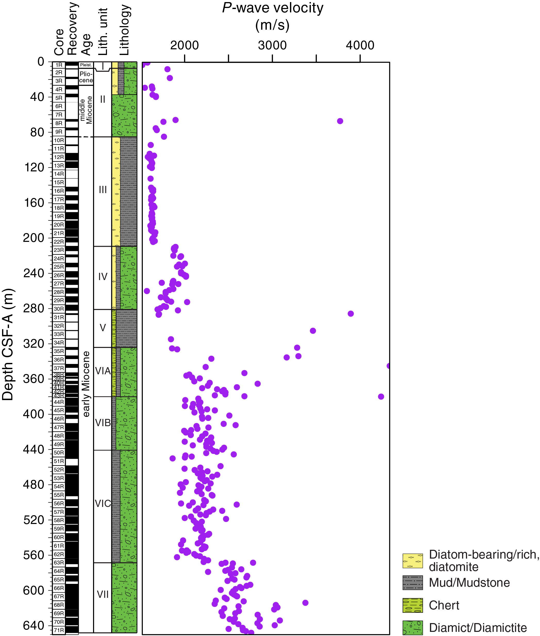
Figure F24. Discrete P-wave velocity.
Color reflectance spectroscopy
Color reflectance spectroscopy data were acquired on section halves using the SHMSL. At this site, L* and a* parameters vary and show little relationship with other physical parameters or lithostratigraphic units (Figure F25). This cyclicity apparently corresponds to differences in the data collection method between the two shifts (day shift/night shift), with one shift wetting the core surface prior to measurement and the other shift leaving the surface dry. As a consequence, these color reflectance data should be used with caution for this site. In contrast, b* appears to be less affected by shift-specific methodologies. The b* values are low for most of the hole (from −5 to 0) but higher (0–9) from 90 to 210 m CSF-A and may result from a greater proportion of diatoms in the sediment of lithostratigraphic Unit III.
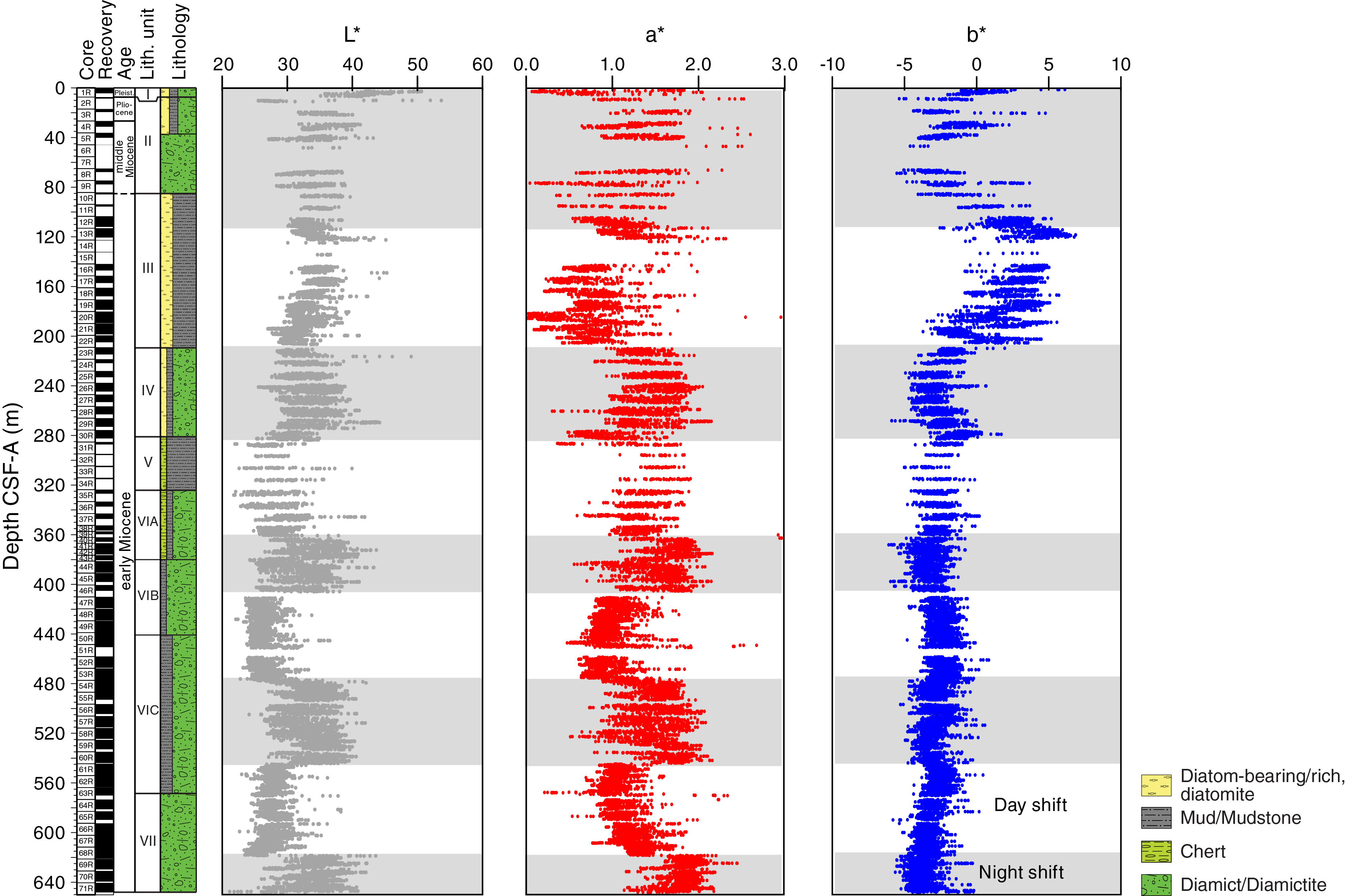
Figure F25. Color reflectance spectroscopy.
Summary
In general, data from whole-round measurements are in good agreement with those from split-core measurements (Figures F22, F23, F26). Discrete MAD samples and point magnetic susceptibility measurements on the section halves likely provide more accurate bulk density and magnetic susceptibility data compared with those from whole-round measurements because the whole-round measurements are dependent on the volume of core filling the liner (see Physical properties in the Expedition 374 methods chapter [McKay et al., 2019a]). In general, an increase in PWC values coincides with an increase in density and a decrease in porosity (Figure F26). Downhole variations in NGR also correlate well with changes in bulk density.
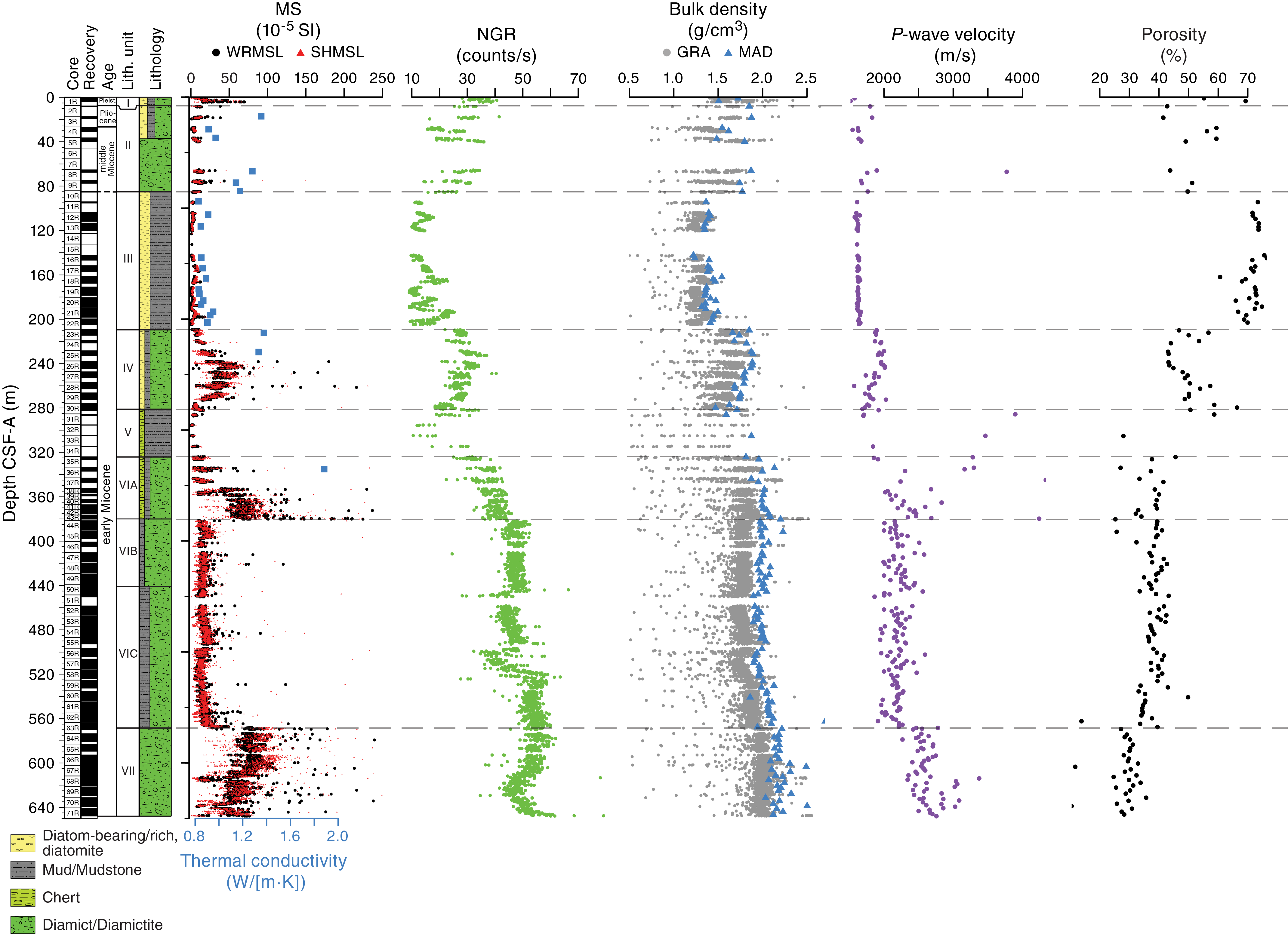
Figure F26. Physical property data summary.
Downhole changes in physical property characteristics overall are in good agreement with the defined lithostratigraphic units based on sedimentologic characteristics (see Lithostratigraphy; Figure F26; Table T12). In general, diatom ooze, diatom-rich mud/mudstone, and mudstone lithofacies (lithostratigraphic Units I, III, and V) correspond with low magnetic susceptibility, NGR, thermal conductivity (<1 W/[m·K]), and bulk density and high porosity (Figure F26). The lowest grain densities and highest porosities correspond with diatom-bearing/rich mudstone, which is the dominant facies in Unit III. In contrast, intervals that are predominantly diamictite (Units II, IV, VI, and VII) correspond with increased NGR; high bulk density, P-wave velocity, and thermal conductivity (>1 W/[m·K]); moderate to high magnetic susceptibility; and low to moderate porosity (Figure F26). The differences in magnetic susceptibility between clast-poor diamictite (low to moderate) and clast-rich diamictite (variable and generally high) suggest that magnetic susceptibility is a reliable indicator of the abundance or provenance of clasts and coarse sands.
Geochemistry and microbiology
Samples from Site U1521 were analyzed for headspace gas and interstitial water and bulk sediment geochemistry. Headspace gas methane and ethane concentrations are low in the upper 40 m of the hole and increase downhole, reaching 67,000 ppmv for methane (omitting one outlier) and 264 ppmv for ethane. Interstitial water analyses show a typical diagenetic profile with sulfate reduction in the uppermost 76 m CSF-A and elevated ammonium, alkalinity, and barium concentrations below this depth. Total organic carbon (TOC), total nitrogen (TN), and calcium carbonate (CaCO3) contents are generally low throughout the hole (0.1–1.2, ≤0.1, and 0.2–6 wt% [omitting one outlier], respectively). The TOC/TN ratio suggests a mixed input of terrestrial and marine-derived organic matter with no clear downhole trend. Elevated CaCO3 content is observed in the sandy diamictite of lithostratigraphic Unit IV, Subunit VIA, and Unit VII, which are also characterized by higher magnetic susceptibility. Elemental ratios obtained by handheld portable X-ray fluorescence (pXRF) scans show good agreement with major lithostratigraphic units but also suggest some deviations between chemical and lithologic boundaries.
Volatile hydrocarbons
Headspace gas analyses were performed at a resolution of one sample per core for full cores (9.6 m advance) or one sample every other core for half cores (4.8 m advance) throughout Hole U1521A (Cores 374-U1521A-1R through 71R) as part of the routine environmental protection and safety monitoring program. Methane (CH4) is the dominant hydrocarbon, although ethane (C2H6) is also present in low concentration. Methane concentration is low (2–112 ppmv) in the upper 40 m CSF-A but increases downhole with variable concentration generally ranging from 3,000 to 67,000 ppmv from 66 to 645 m CSF-A (Figure F27; Table T13). Ethane concentration remains low (<20 ppmv) in the upper 335 m CSF-A and increases to 264 ppmv between 300 and 620 m CSF-A (Figure F27). The methane/ethane ratio is correspondingly high (1500–2700) in the upper 100–335 m CSF-A and then decreases downhole to 165 at 645 m CSF-A (Figure F27). The methane and ethane are likely formed by methanogenic bacteria, which is documented for nearby DSDP Site 271 (Claypool and Kvenvolden, 1983).
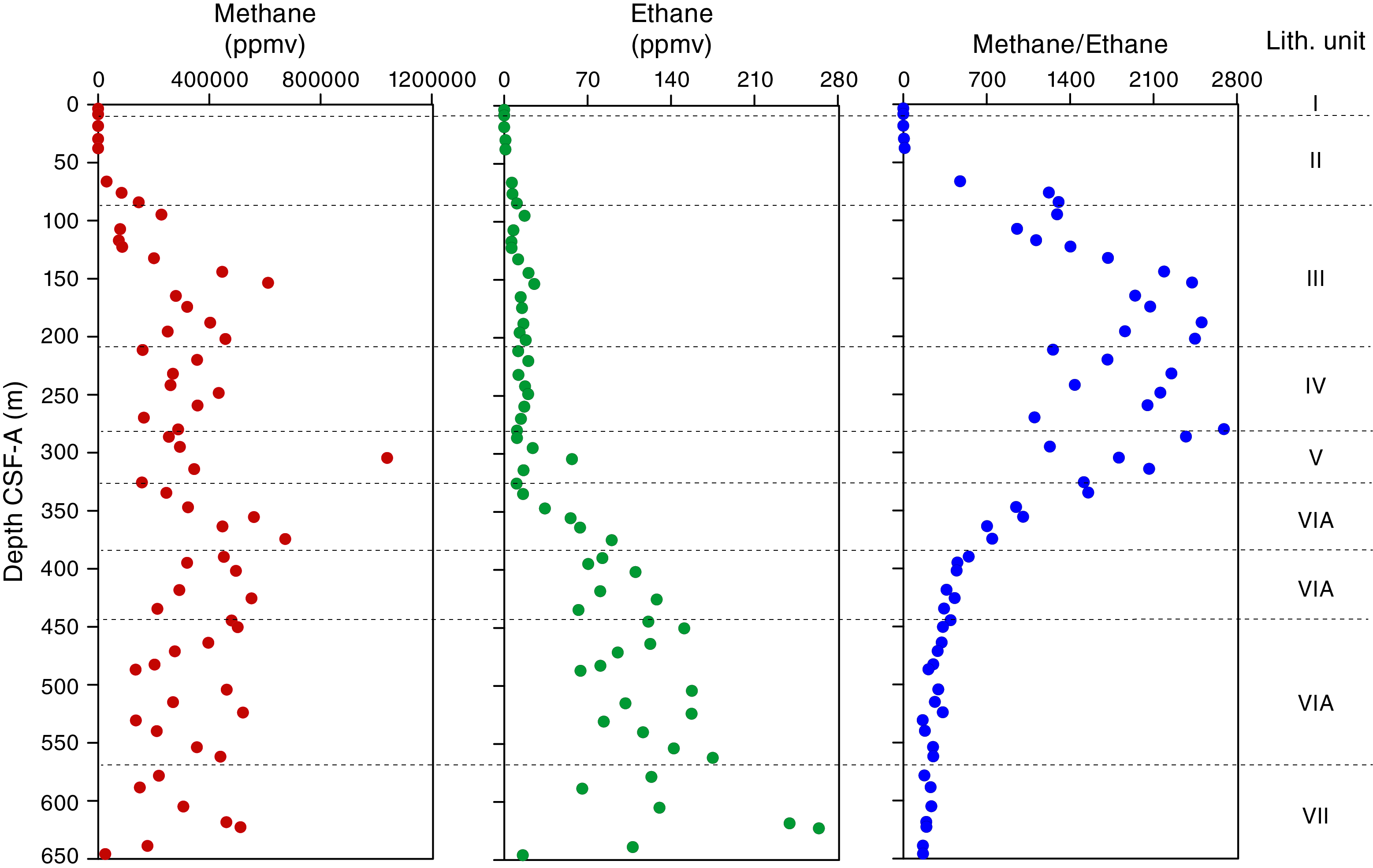
Figure F27. Headspace gas concentrations.
Interstitial water chemistry
A total of 15 interstitial water samples were squeezed from 10 cm whole-round samples from 3.40 to 353.88 m CSF-A, with sampling resolution dictated by core recovery and lithology. Deeper than 353.88 m CSF-A (Core 374-U1521A-38R), interstitial water extraction was no longer effective (<6 mL after 1.5 h of squeezing), and sampling was discontinued. Filtered subsamples of the interstitial water were prioritized in the order detailed in Geochemistry and microbiology in the Expedition 374 methods chapter (McKay et al., 2019a) for shipboard and shore-based analyses. For all but two samples (3R-1, 136–146 cm [18.36 m CSF-A], and 38R-1, 138–150 cm [353.88 m CSF-A]), interstitial water was present in sufficient volume to allow sampling for all planned analyses. Interstitial water data are reported in Table T14.
Salinity, sulfate, manganese, and ammonium
Interstitial water salinity is ~35, similar to ambient seawater, in the upper 40 m CSF-A and decreases to 31 deeper than 100 m CSF-A. Sulfate concentration decreases from a typical seawater value (~28 mM) at 3.40 m CSF-A to 2.2 mM at 75.94 m CSF-A. Average values below this depth are 1.5 ± 0.2 mM, with the exception of the lowermost sample at 353.88 m CSF-A (4.0 mM) (Figure F28). Manganese concentration in interstitial water is below the detection limit of inductively coupled plasma–optical emission spectroscopy (ICP-OES) throughout the sampled interval. Ammonium concentration increases from 156 µM near the seafloor (3.40 m CSF-A) to 2879 µM at 75.94 m CSF-A and is anticorrelated with sulfate concentration (Figure F28), probably marking the sulfate–methane transition zone (SMTZ) around 75 m CSF-A. Below this depth, ammonium values are high but somewhat variable, with an average of 3334 ± 985 µM (omitting one outlier with lower concentration at 164.79 m CSF-A) (Table T14). Both ammonium and sulfate profiles are consistent with pronounced reducing conditions deeper than ~75 m CSF-A.
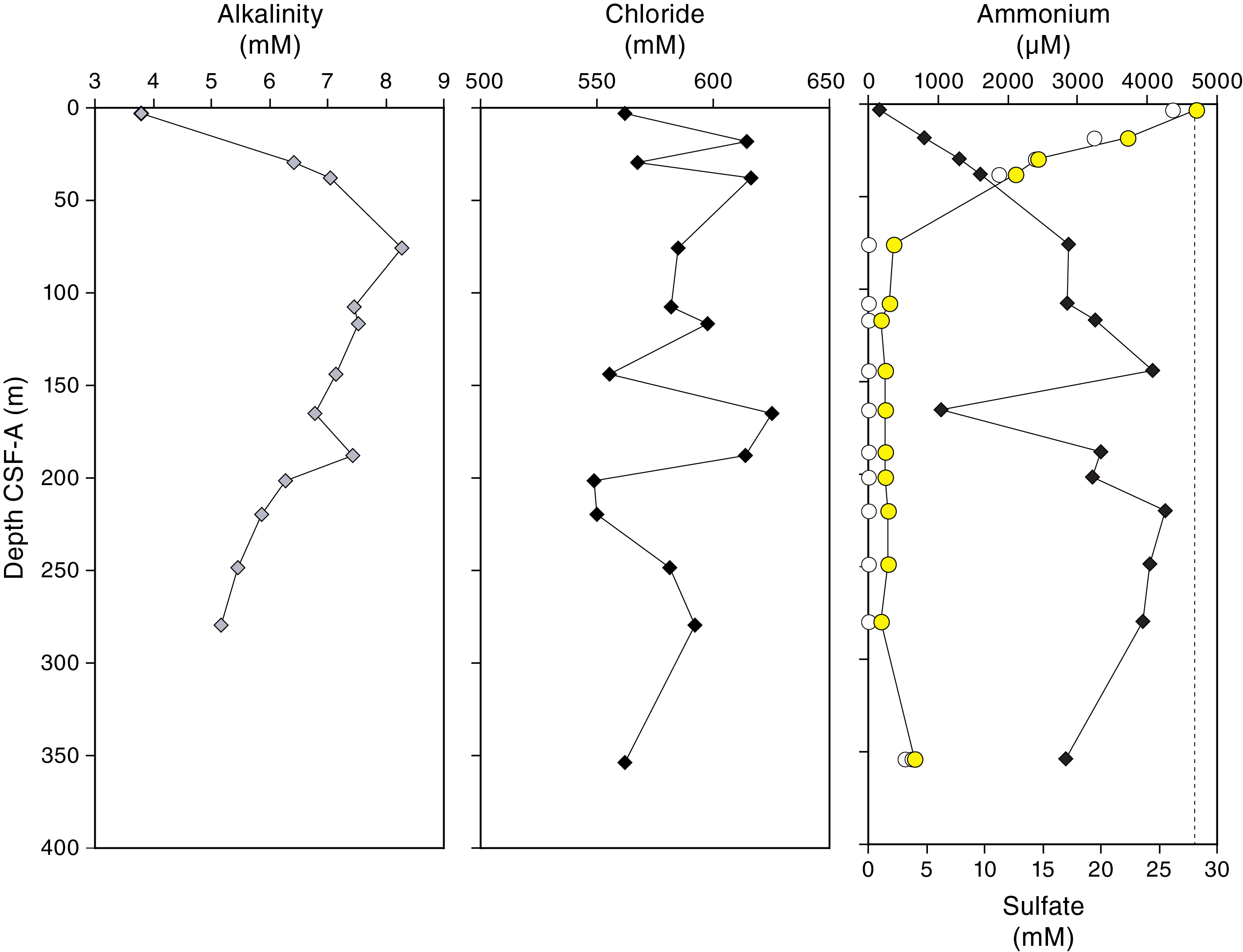
Figure F28. Interstitial water geochemistry.
Chloride, bromide, sodium, alkalinity, ammonium, and pH
Chloride, bromide, and sodium concentrations show similar and small downhole variations (within 5%). For simplicity, only chloride data are shown in Figure F28. A tentative interval of higher concentrations occurs between 150 and 200 m CSF-A for all three elements. This interval is characterized by diatom-rich mudstone in lithostratigraphic Unit III (see Lithostratigraphy). Other measured interstitial water properties do not show significant shifts in this interval (Figures F28, F29), nor do they correlate with the large shift in CaCO3 content observed at the bottom of Unit III (Figure F30). pH varies between 7.6 and 7.8, which is lower than average seawater (pH = 8.1), through the sampled interval. The alkalinity profile shows a similar downhole trend to the ammonium profile and is anticorrelated with sulfate in the upper part of the interstitial water profile. In detail, alkalinity increases from 3.8 mM at 3.40 m CSF-A to 8.3 mM at 75.94 m CSF-A. Below the tentative SMTZ, alkalinity decreases from 75.94 to 279.81 m CSF-A, reaching a value of 5.2 mM in the lowermost sample analyzed (279.81 m CSF-A) (Figure F28).

Figure F29. Interstitial water geochemistry.
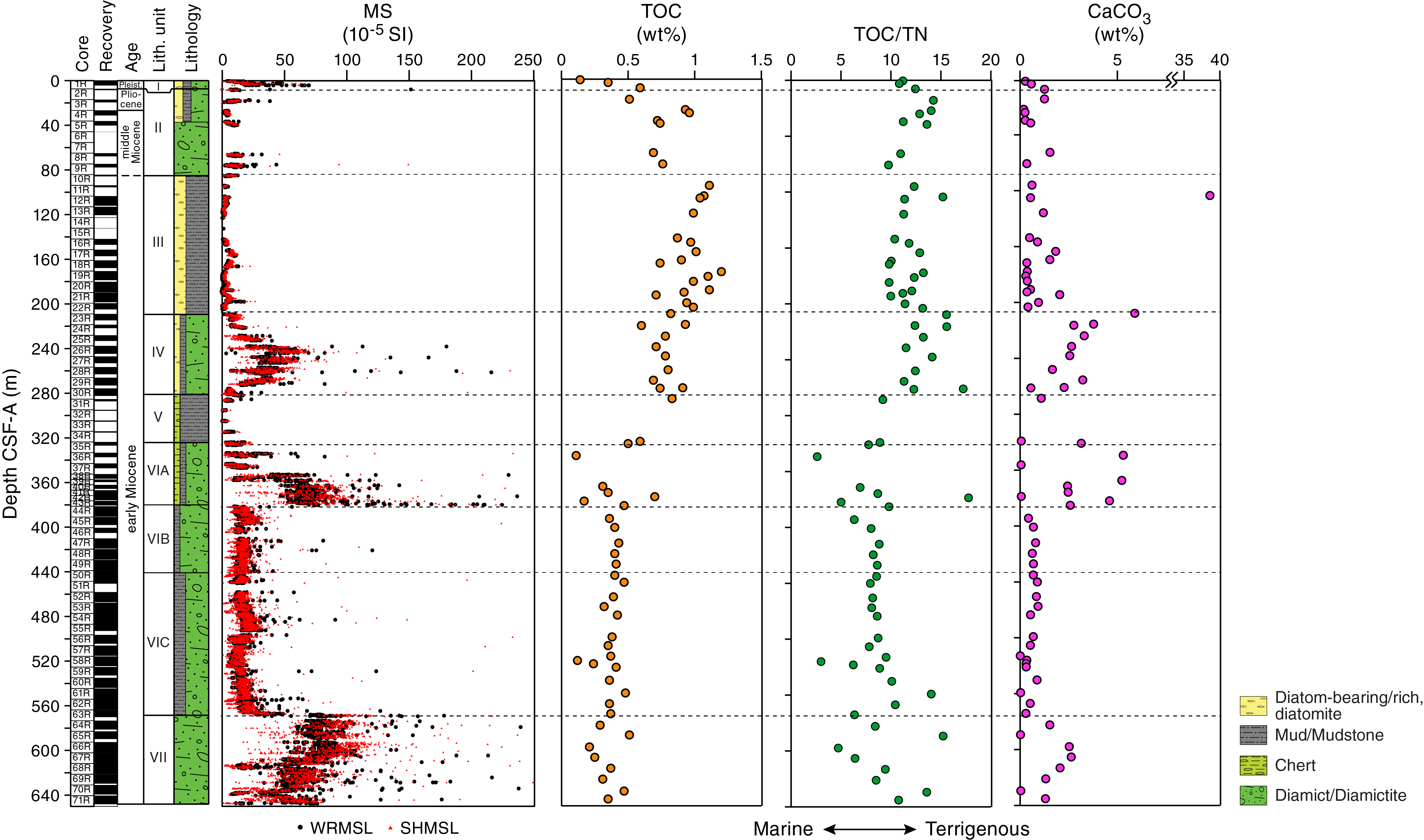
Figure F30. MS, carbon content, and TOC/TN.
Calcium, magnesium, silicon, barium, and other major and trace elements
Smooth downhole profiles are observed for many major and trace elements, including calcium, magnesium, silica/silicon, and barium (Figure F29). Similar downhole profiles are also observed for potassium, boron, sodium, sulfur, and strontium concentrations in interstitial water (not shown) (Table T14). Lithium concentration is below the detection limit of the ICP-OES. Calcium concentration decreases linearly from ~10 mM at 3.40 m CSF-A to 6 mM at 37.60 m CSF-A. Below this depth, calcium concentration linearly increases from 6 mM at 75.94 m CSF-A to 11 mM at 279.81 m CSF-A. Throughout this interval, potassium, magnesium, and sodium concentrations decrease (Figure F29). Silicon (also silica; see Geochemistry and microbiology in the Expedition 374 methods chapter [McKay et al., 2019a]) concentration increases from 677 µM near the seafloor to 1054 µM at 29.50 m CSF-A. From 75.94 to 279.81 m CSF-A, silicon concentration varies around an average value of 808 ± 129 µM (Figure F29). Total sulfur concentration strongly decreases in the uppermost part of the interstitial water profile (from 26 mM at 3.40 m CSF-A to 11 mM at 37.60 CSF-A) and is below the detection limit for the remainder of the profile. The sulfur profile is in good agreement with the sulfate-reduction profile previously described (Figure F28). The lowermost sample (353.88 m CSF-A) is distinct in most data sets, with elevated concentrations of calcium (27 mM) and strontium and low silicon, barium, potassium, and sodium concentrations. This observation could be related to generally higher CaCO3 content in sediments deeper than 200 m CSF-A (Figure F30), which are associated with carbonate-cemented diamictite (see Lithostratigraphy). Barium (Figure F29) and boron (not shown) concentrations generally increase downhole from low values near the seafloor. In detail, barium concentration is below the detection limit from just below the seafloor to 37.60 m CSF-A and then increases from 64 µM at 75.94 m CSF-A to a relative maximum of 108–109 µM at 187.83–201.88 m CSF-A. The increase in barium concentration occurs at a slightly shallower depth than the completion of sulfate reduction and the tentative SMTZ and is probably related to barite dissolution. Both barium and boron concentrations show a step toward lower values between 201.88 and 219.88 m CSF-A, which coincides with the boundary between lithostratigraphic Units III (diatom-rich mudstone) and IV (diamictite) (see Lithostratigraphy).
Bulk sediment geochemistry
Carbon, nitrogen, and carbonate
Discrete sediment samples (N = 77) from all major lithostratigraphic units identified at Site U1521 were analyzed for total carbon, TN, and total inorganic carbon. TOC and CaCO3 contents were subsequently calculated (Table T15). TOC content is generally low (0.1–1.2 wt%) (Figure F30). Slightly higher TOC content (0.4–1.2 wt%) is observed in the diatom-bearing and diatom-rich mudstone and diamictite of lithostratigraphic Units II–IV in the upper ~281 m CSF-A (see Lithostratigraphy). The TOC content of the chert, muddy to sandy diamictite, and mudstone of Units V–VII between 323.99 and 643.93 m CSF-A is lower and ranges between 0.1 and 0.7 wt%. TN content is very low (≤0.1 wt%), with slightly higher values in the upper ~281 m CSF-A. The TOC/TN ratio ranges between 10 and 18 (Figure F30), suggesting a mixed (i.e., marine and terrigenous) source of organic matter deposited at Site U1521. Except for a single sample from Core 374-U1521A-12R that has a carbonate content of 38.6 wt%, CaCO3 content is low (0.2 and 2.0 wt%) in the upper ~200 m CSF-A (Figure F30). CaCO3 content is higher (as high as 5.9 wt%) in the sandy diamictite of Unit IV, Subunit VIA, and Unit VII. These units also have higher magnetic susceptibility (Figure F30) (see Physical properties). On the other hand, the sandy diamictite of Subunit VIB, which contains visible shell fragments and carbonate nodules (see Lithostratigraphy), has low bulk CaCO3 content (0.4 to 0.8 wt%) between 393.03 and 433.791 m CSF-A. It should be noted that the CaCO3 content reported here reflects the typical diamictite of Subunit VIB because shell fragments and nodules were avoided during sampling.
pXRF and ICP-OES data
Sixteen discrete sediment samples were analyzed by ICP-OES (Table T16). Additionally, shipboard pXRF data were collected for Site U1521 from Sections 374-U1521A-1R-1 through 5R-2 (0–37.49 m CSF-A) and 24R-1 through 71R-3 (218.90–644.35 m CSF-A) (Figure F31) using two different methods (“geochem” and “soil”; see Lithostratigraphy in the Expedition 374 methods chapter [McKay et al., 2019a]). pXRF scanning was temporarily suspended for Cores 6R through 23R to keep up with core flow. Because of the higher resolution of pXRF data, only these results are discussed here. Downhole variability in the Si/Ti, Ba/Al, and Fe/Al ratios are given in Figure F31 and Table T17 and show some correlation to the major lithostratigraphic units. The Si/Ti ratio increases in the diatom-bearing and diatom-rich mudstone in the upper ~40 m CSF-A, with a notable step change between lithostratigraphic Units I and II. With the exception of one elevated value in Unit V, all of the highest Si/Ti ratios are observed in Unit II. In the diamictite-dominated intervals between 210 and 645 m CSF-A, the Si/Ti ratio remains relatively low, with the most uniform values in Subunit VIC and Unit VII (deeper than 538.12 m CSF-A) (Figure F31). In contrast, both the Ba/Al and Fe/Al ratios exhibit significant variability between 218.9 and 538.12 m CSF-A and low, relatively constant values from the deepest part of Subunit VIC to the bottom of the hole in Unit VII. Hence, geochemical data indicate some variations that are not apparent in the visual core descriptions or physical properties of the sediments of Subunit VIC. A significant positive correlation between the Ba/Al and Fe/Al ratio data has an r2 of 0.75, although the Ba/Al ratios show a clearer correlation with the lithostratigraphic units than the Fe/Al ratios.
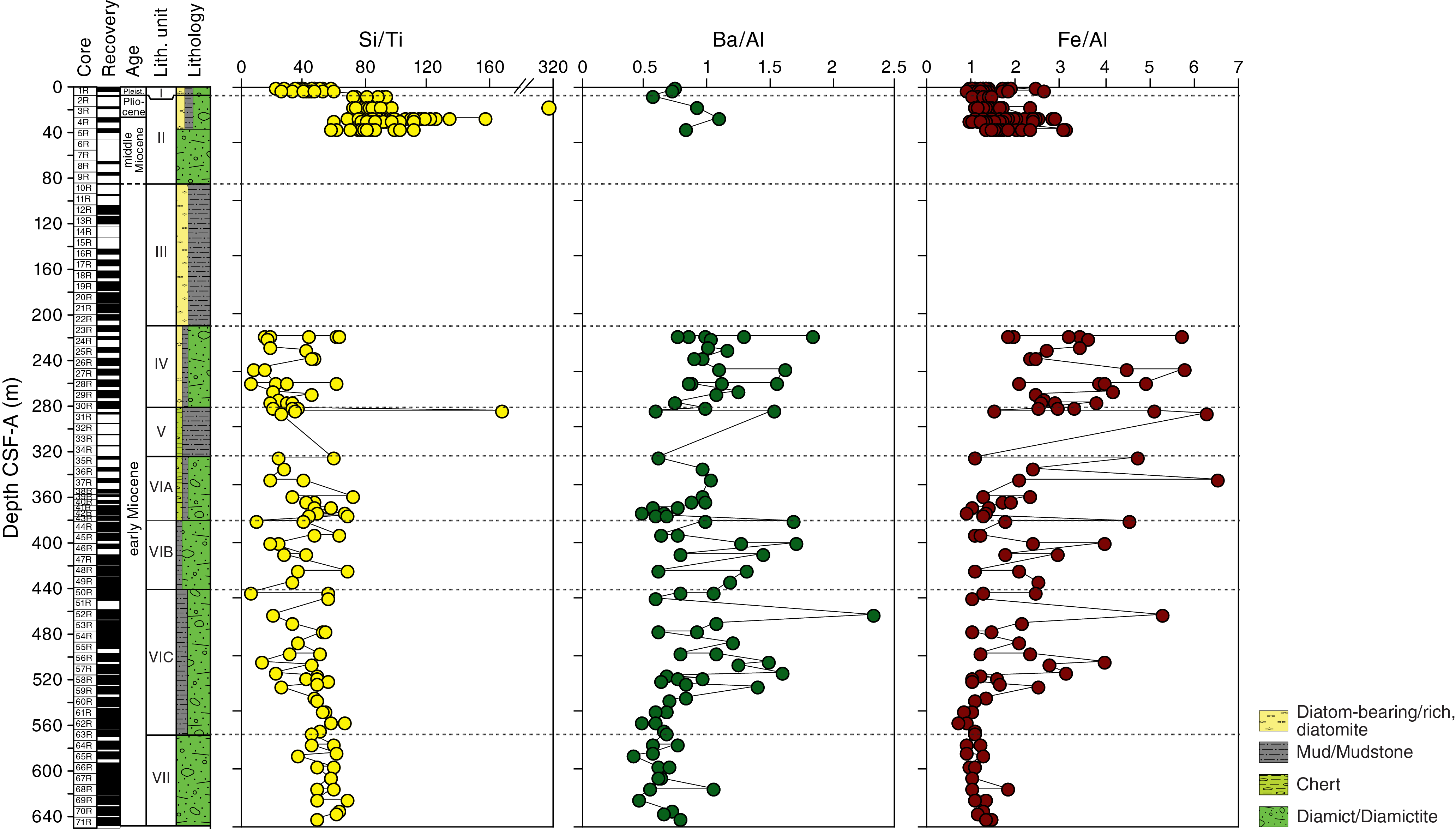
Figure F31. pXRF element ratios.
Microbiological sampling
Fifty samples for shore-based stable and clumped isotope analyses of methane and ethane were collected at Site U1521 from Cores 374-U1521A-1R through 71R. Additional samples for detailed analyses of metagenomics, cell counts, metabolomics, and cultures were also taken from Core 1R (see Geochemistry and microbiology in the Expedition 374 methods chapter [McKay et al., 2019a] for details).
Downhole measurements
Logging operations
The last core from Hole U1521A arrived on deck at 1440 h (UTC + 13 h) on 20 January 2018. Hole preparation for logging included a high-viscosity mud sweep followed by release of the RCB drill bit to the bottom of the hole at 1505 h and displacement with 217 bbl of heavy mud (10.5 lb/gal) from 650.1 m DSF to the seafloor. The end of the drill string was pulled up to a logging depth of 54.4 m DSF (~53 m wireline depth below seafloor [WSF]), and the top of the hole was displaced with an additional 20 bbl of heavy mud (10.5 lb/gal). The wireline heave compensator was used to reduce the effect of vertical ship motion on the wireline depth. An average heave of 0.3 m was estimated prior to logging. Rig up for downhole logging started at 2325 h on 20 January, and the triple combo tool string was assembled for the first run. The triple combo tool string consisted of the following tools (see Downhole measurements in the Expedition 374 methods chapter [McKay et al., 2019a]):
- Magnetic Susceptibility Sonde (MSS),
- High-Resolution Laterolog Array (HRLA; to measure resistivity),
- Hostile Environment Litho-Density Sonde (HLDS; with source),
- Hostile Environment Natural Gamma Ray Sonde (HNGS),
- Accelerator Porosity Sonde (APS), and
- Enhanced Digital Telemetry Cartridge (EDTC).
The triple combo tool string was lowered into the hole at 2325 h. All tools except the APS were run on the downlog, and the caliper arms were closed. All tools were run on the uplog. The base of the tool string reached the approximate bottom of the hole at 648 m WSF (to within ~2 m of the total depth of 650.1 m DSF), indicating that the bottom of the hole contained very little to no fall-in or debris. After reaching total depth, the APS tool was enabled, the caliper arms were opened, and the hole was logged up for a 126.5 m calibration pass. The tool was lowered back to total depth (648 m WSF), and the main uplog was collected. As the tool string approached the end of the pipe, it was raised to 38.2 m DSF to increase coverage of the upper part of the borehole. The triple combo tool string was returned to the rig floor at 0330 h on 21 January.
The second logging run used the FMS-sonic tool string (see Downhole measurements in the Expedition 374 methods chapter [McKay et al., 2019a]), which consisted of the following tools:
The FMS-sonic tool string was lowered into the hole at 0620 h on 21 January. While lowering the tools to the bottom of the hole, the DSI tool was enabled; however, the FMS caliper arms were kept closed. The tool string reached the base of the hole at 648 m WSF. After completing two upward logging passes, the tool string was returned to the rig floor at 1245 h.
The third logging run consisted of the Vertical Seismic Imager (VSI) tool string (see Downhole measurements in the Expedition 374 methods chapter [McKay et al., 2019a]). Observation for protected species began at 1300 h, and the seismic source (two 250 inch3 Sercel G guns in parallel array) was lowered into the water at 1400 h. The tool string was lowered into the hole at 1330 h on 21 January, and the first shot was fired at 1510 h (Table T18). A total of 18 stations, located at the depths of the main lithologic boundaries, were attempted (average spacing = 33 m) with the aim to obtain the best correlation with the seismic reflectors. Of these, 16 stations were successful (>1 good shot). Stations 14 (207.9 m WSF) and 18 (89.7 m WSF) failed because of problems with anchoring against the borehole wall. The last shot was fired at 1745 h, and the tool string returned to the surface at 1800 h. All logging equipment was rigged down by 1930 h.
Log data quality and comparison with shipboard physical properties
All logging curves were depth-matched using the total gamma ray log from the main pass of the triple combo tool string as the reference, which allowed a unified depth scale to be produced. Features in gamma ray logs from the other two tool string passes were aligned to the reference log to produce a complete depth-matched data set. Log data were then depth-shifted to the seafloor identified by a stepwise increase in the gamma ray value, which created the wireline log matched depth below seafloor (WMSF) depth scale. The triple combo main pass identified the seafloor at 572 m wireline depth below rig floor.
The main control on log data quality is the diameter of the borehole, which was measured by the caliper on the HLDS tool in the first and second logging runs (see Downhole measurements in the Expedition 374 methods chapter [McKay et al., 2019a]). Caliper data show that the borehole conditions in Hole U1521A during downhole logging were excellent (Figure F32), with one washed out interval (>4 inches deviation from drill bit diameter at 221–226 m WMSF) and an additional interval from 247 to 282 m WMSF where the borehole was slightly enlarged. During the VSI logging run, problems with tool anchoring because of the quality of the borehole walls occurred at ~90 and ~208 m WMSF. Other deviations from the bit diameter were minor, and most of the borehole wall was smooth.
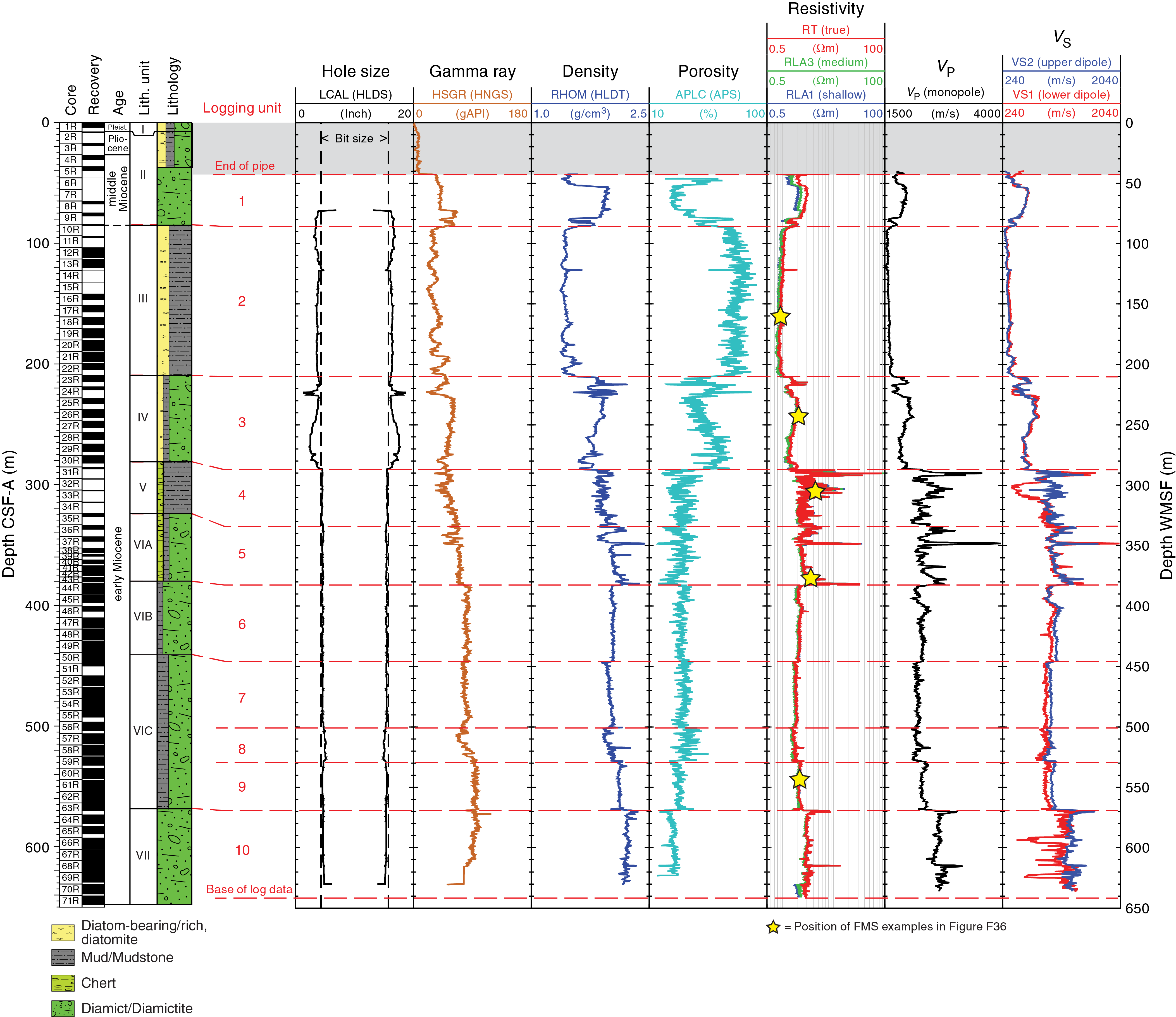
Figure F32. Downhole log data summary.
Log data quality can also be assessed by comparison with physical property measurements made on cores from Site U1521. Note that downhole logs are plotted on the WMSF depth scale, whereas physical property data are on the CSF-A depth scale. Depth offsets may exist between these two depth scales, but they are usually small (<2 m) and therefore still allow comparison of downhole trends. These minor differences in the WMSF and CSF-A scales can be correlated during postcruise research. In general, the gamma ray, bulk density, porosity, and P-wave velocity data show excellent correspondence between downhole and shipboard measurements throughout the borehole. Although the downhole gamma ray and shipboard NGR data are reported in different units (gAPI versus counts/s, respectively), the trends and relative magnitude of downhole shifts are comparable (Figure F33). The agreement between downhole P-wave velocity and shipboard PWC P-wave velocity is very good in lithologically homogeneous intervals (e.g., ~100–200 m WMSF) and fair to good in intervals with more lithologic heterogeneity (Figure F33). Intervals where downhole P-wave velocity is highly variable over meters to tens of meters (e.g., ~300–350 m WMSF) are not well represented by PWC velocities, likely because of poor core recovery and associated sparse measurements (Figure F33). The bulk density downhole log data, WRMSL GRA bulk density measurements, and discrete MAD sample bulk density estimates show excellent correlation (Figure F34), although WRMSL measurements routinely underestimate bulk density because of the smaller diameter of RCB core material relative to the core liner. Downhole porosity data show good overall agreement with laboratory MAD measurements, although the core-based measurements underestimate in situ porosity in the interval of very high porosity from ~100 to 200 m WMSF and slightly overestimate porosity in deeper intervals (Figure F34). Magnetic susceptibility data from both downhole and core (WRMSL and SHMSL) measurements also show reasonable correspondence throughout the borehole, but there is a clear downward drift to lower values in the downhole magnetic susceptibility data, likely because of tool temperature (Figure F35). Downhole magnetic susceptibility data delineate packages of sediment with different magnetic susceptibility character that is also seen in the core data (e.g., ~570–630 m WMSF). However, the overall amplitude and directionality of change between packages does not consistently match between the downhole and core data.
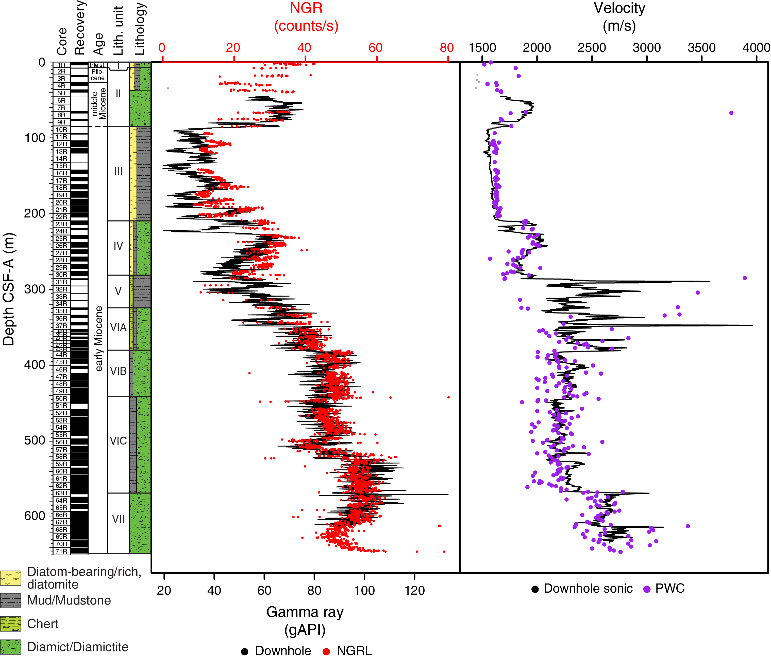
Figure F33. NGR and P-wave velocity data comparison.
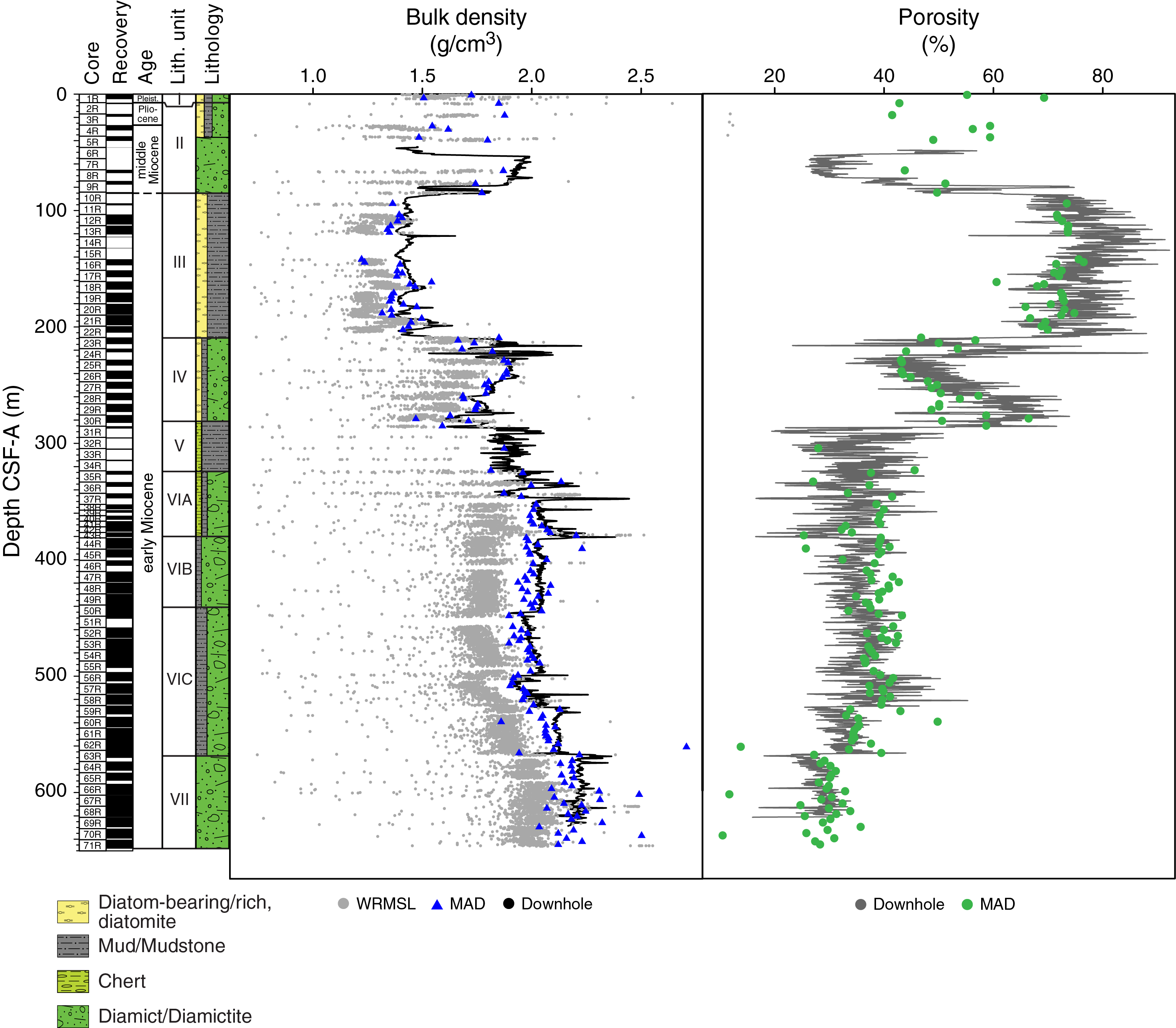
Figure F34. Bulk density and porosity data comparison.
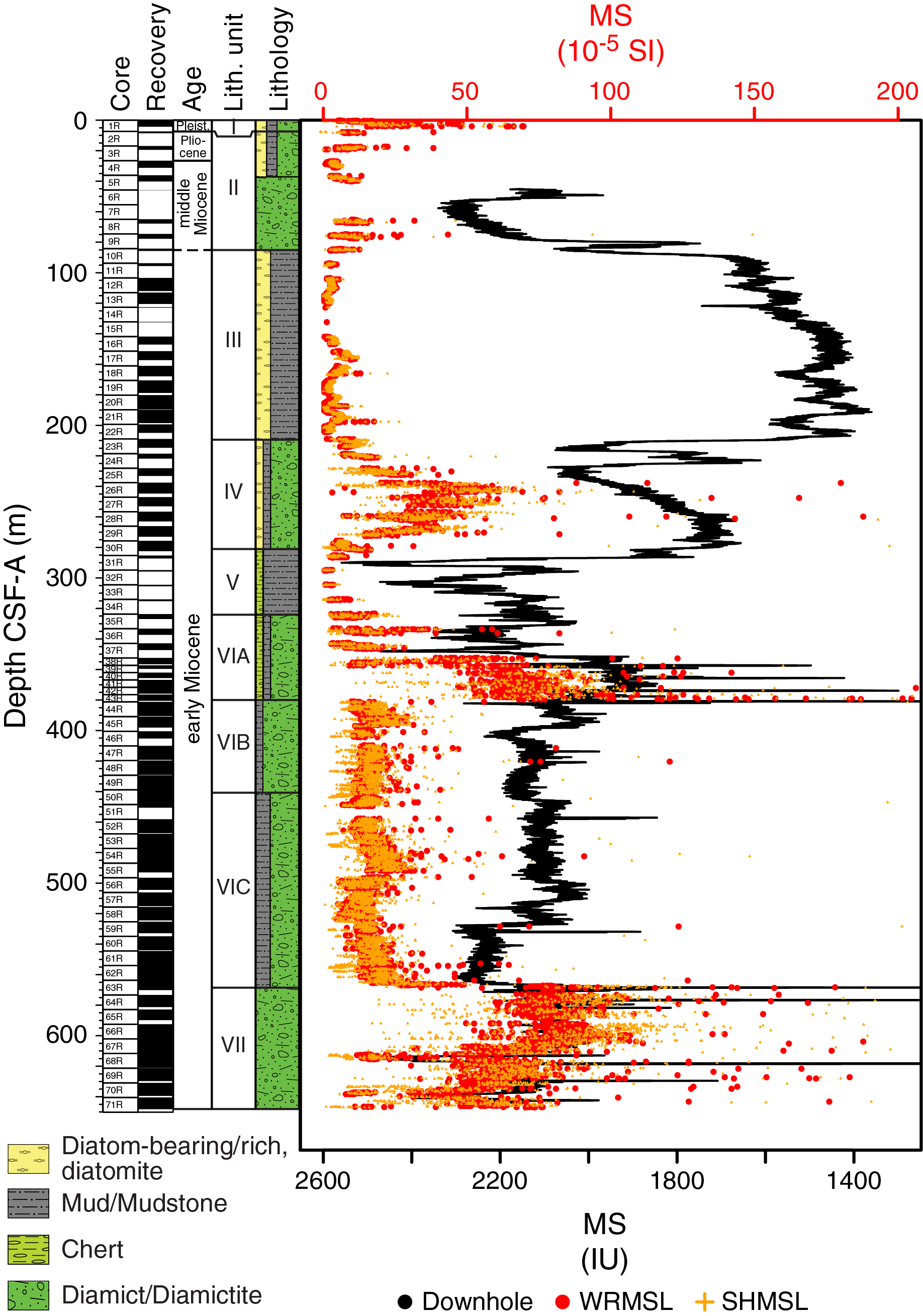
Figure F35. MS data comparison.
FMS image data quality is dependent on factors such as the quality of the borehole wall and good contact between the tool and the borehole. FMS images appear to be of overall excellent quality, indicating that the pads made good contact with the borehole walls (Figure F36). VSI data quality is very good (Table T18). Twelve of the successful stations collected at least five good shots for seismic waveform stacking. The other four stations used between one and four good shots.
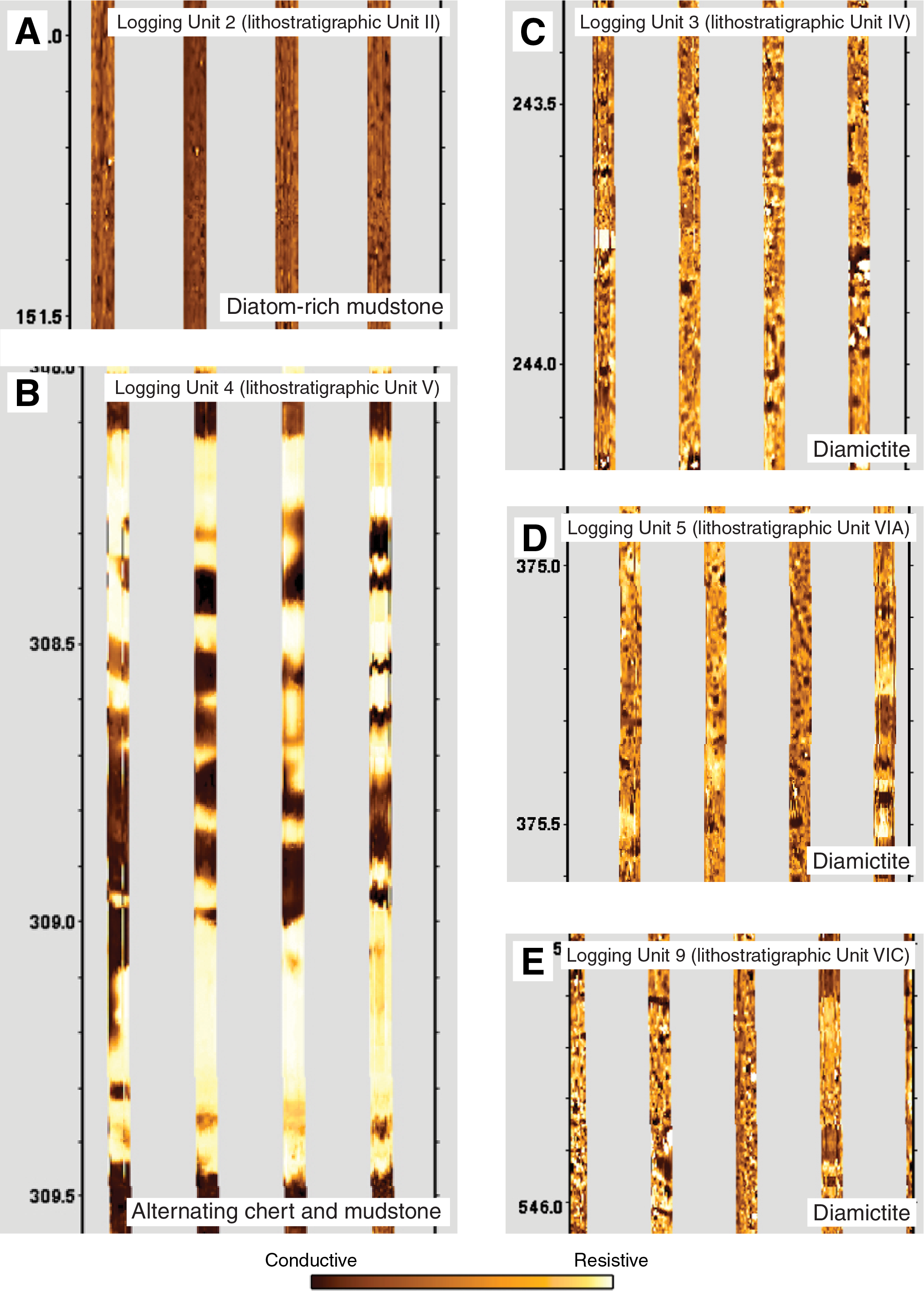
Figure F36. FMS image examples.
Logging units
Downhole logging data from Hole U1521A are summarized in Figure F32. The logged interval is divided into 10 logging units on the basis of distinctive features in the gamma ray, resistivity, density, porosity, magnetic susceptibility, and velocity (sonic) logs (Table T19). The units start from 42 m WMSF, which is the end-of-pipe depth below seafloor and where logging terminates.
Logging Unit 1: base of drill pipe (42 m WMSF) to 85.5 m WMSF
Logging Unit 1 is the uppermost unit logged in Hole U1521A and is characterized by relatively high density (as high as 2.0 g/cm3), variable porosity (18%–60%), variable magnetic susceptibility (1750–2300 IU), and high gamma radiation (as high as >68 gAPI). P-wave velocity reaches a peak value of 2100 m/s. Unit 1 corresponds to lithostratigraphic Unit II (7.40–85.34 m CSF-A; see Lithostratigraphy), which is composed of interbedded muddy diatomite, diatom-bearing/rich mudstone with dispersed clasts, and muddy diamictite (Figure F32; Table T19).
Logging Unit 2: 85.5–210.0 m WMSF
Logging Unit 2 is distinguished from Unit 1 by low gamma radiation (19–57 gAPI), low density (~1.4 g/cm3), high porosity (~75%), and low P-wave velocity (<1600 m/s). Magnetic susceptibility is low in this unit (peaking at 1400 IU). Unit 2 corresponds with lithostratigraphic Unit III (85.34–209.17 m CSF-A), which is composed of diatom-bearing/rich mudstone (Figure F32; Table T19).
Logging Unit 3: 210.0–287.0 m WMSF
Logging Unit 3 is characterized by high density (1.6–1.9 g/cm3), intermediate porosity (40%–60%), and high gamma radiation (30–70 gAPI). P-wave velocity is moderate (1700–2100 m/s). Unit 3 corresponds to lithostratigraphic Unit IV (209.17–280.72 m CSF-A), which is composed of diatom-bearing clast-poor sandy diamictite with basalt clasts. The lower boundary of the logging unit is slightly deeper than the lower boundary of lithostratigraphic Unit IV (Figure F32; Table T19).
Logging Unit 4: 287.0–334.0 m WMSF
Logging Unit 4 is marked by a distinctive increase in density (~2.0 g/cm3), an increase in gamma radiation (~50–70 gAPI), high P-wave velocity (as high as 4000 m/s; median >2300 m/s), low porosity (<40%), and high but variable magnetic susceptibility (~2400 IU). Unit 4 corresponds with lithostratigraphic Unit V (280.72–324.20 m CSF-A), which is an interval composed predominantly of interbedded chert and mudstone. The lower boundary of the logging unit is slightly deeper than the boundary of the lithostratigraphic unit (Figure F32; Table T19).
Logging Unit 5: 334.0–382.5 m WMSF
Logging Unit 5 is distinguished from Unit 4 by slightly lower porosity (~26%), high gamma radiation (60–80 gAPI), high density (2.0–2.2 g/cm3), and high P-wave velocity (~2400 m/s). Unit 5 corresponds with lithostratigraphic Subunit VIA (324.20–380.04 m CSF-A), which is composed of interbedded mudstone and diamictite with silica cement. The lower boundary of the logging unit is slightly deeper than the correlative lithostratigraphic subunit (Figure F32; Table T19).
Logging Unit 6: 382.5–446.0 m WMSF
Logging Unit 6 is characterized by high density (~2.0 g/cm3), high gamma radiation (80–90 gAPI), moderate porosity (~30%–40%), and moderate P-wave velocity (~2200 m/s). Unit 6 corresponds with lithostratigraphic Subunit VIB (380.04–440.58 m CSF-A), which is characterized by sandy diamictite with shell fragments and carbonate nodules. The lower boundary of the logging unit is slightly deeper than the lithostratigraphic subunit (Figure F32; Table T19).
Logging Unit 7: 446.0–501.0 m WMSF
Logging Unit 7 is characterized by high gamma radiation (~80–90 gAPI), high density (1.9–2.0 g/cm3), moderate porosity (~35%), and P-wave velocity of 2100–2200 m/s. Unit 7 corresponds with the upper part of lithostratigraphic Subunit VIC (440.58–567.95 m CSF-A), which is composed of interbedded mudstone and diamictite. The lower boundary of the logging unit is in the lithostratigraphic subunit (Figure F32; Table T19).
Logging Unit 8: 501.0–529.5 m WMSF
Compared with overlying logging Unit 7, Unit 8 is characterized by relatively lower gamma radiation (~80–90 gAPI), slightly lower density, slightly higher porosity, and higher resistivity but also by similar P-wave velocity. Although the differences in log values compared with Unit 7 are minor, the abruptness of the shift and consistency across all logs is the basis for this logging unit. Unit 8 is in the middle part of lithostratigraphic Subunit VIC (440.58–567.95 m CSF-A) but in a section described as containing layers of mudstone and sandy mudstone (see Lithostratigraphy) (Figure F32; Table T19).
Logging Unit 9: 529.5–569.5 m WMSF
The characteristics of logging Unit 9 are very similar to those of Unit 7. The lower boundary of Unit 9 correlates with the base of lithostratigraphic Subunit VIC. The lithologies in this logging unit are characterized by interbedded mudstone and diamictite (Figure F32; Table T19).
Logging Unit 10: 569.5–630.0 m WMSF
Logging Unit 10 is characterized by high density (>2.2 g/cm3), high gamma radiation (~85–100 gAPI), low porosity (<30%), and high P-wave velocity (as high as 2700 m/s). Unit 10 corresponds with lithostratigraphic Unit VII (567.95–648.17 m CSF-A), which is composed of interbedded muddy to sandy diamictite with stratification (Figure F32; Table T19).
FMS images
FMS resistivity images show differences in texture and lithology along the borehole at submeter scale (Figure F36). These features include intervals of very low resistivity diatom-rich mudstone-dominated sections (e.g., logging Unit 2), distinctly alternating intervals of very high and low-resistivity lithologies typical of the chert-rich unit (e.g., logging Unit 4), and intervals of mottled and patchy resistivity typical of the various diamictite lithologies, which include localized centimeter-scale high-resistivity spots interpreted as clasts in the diamictite (Figure F36).
Core-log-seismic integration
We combined log data, sediment core observations, physical property data, and seismic data from Site U1521 to evaluate whether the recovered cores reached the targeted seismic horizons and whether the observed sedimentary, physical property, logging, and seismic units could be integrated.
Velocity model construction
For the purposes of shipboard correlation of the core data (e.g., lithostratigraphic units and physical property data) and log data with features observed on the seismic data for Site U1521, we converted lithostratigraphic and logging unit boundaries from depth in meters to two-way traveltime (TWT) using three different methods:
- PWC point-source velocity data from physical property measurements (see Physical properties),
- First seismic waveform arrival times derived from the VSI for each of the 16 check shot stations, and
- Velocity data from the DSI log.
Discrete P-wave velocity laboratory measurements on cores gave the lowest velocity values, whereas the DSI gave the highest values. The velocity model used to convert the core data and depths to TWT shown in Figure F37 is based on the check shot–calibrated DSI log.
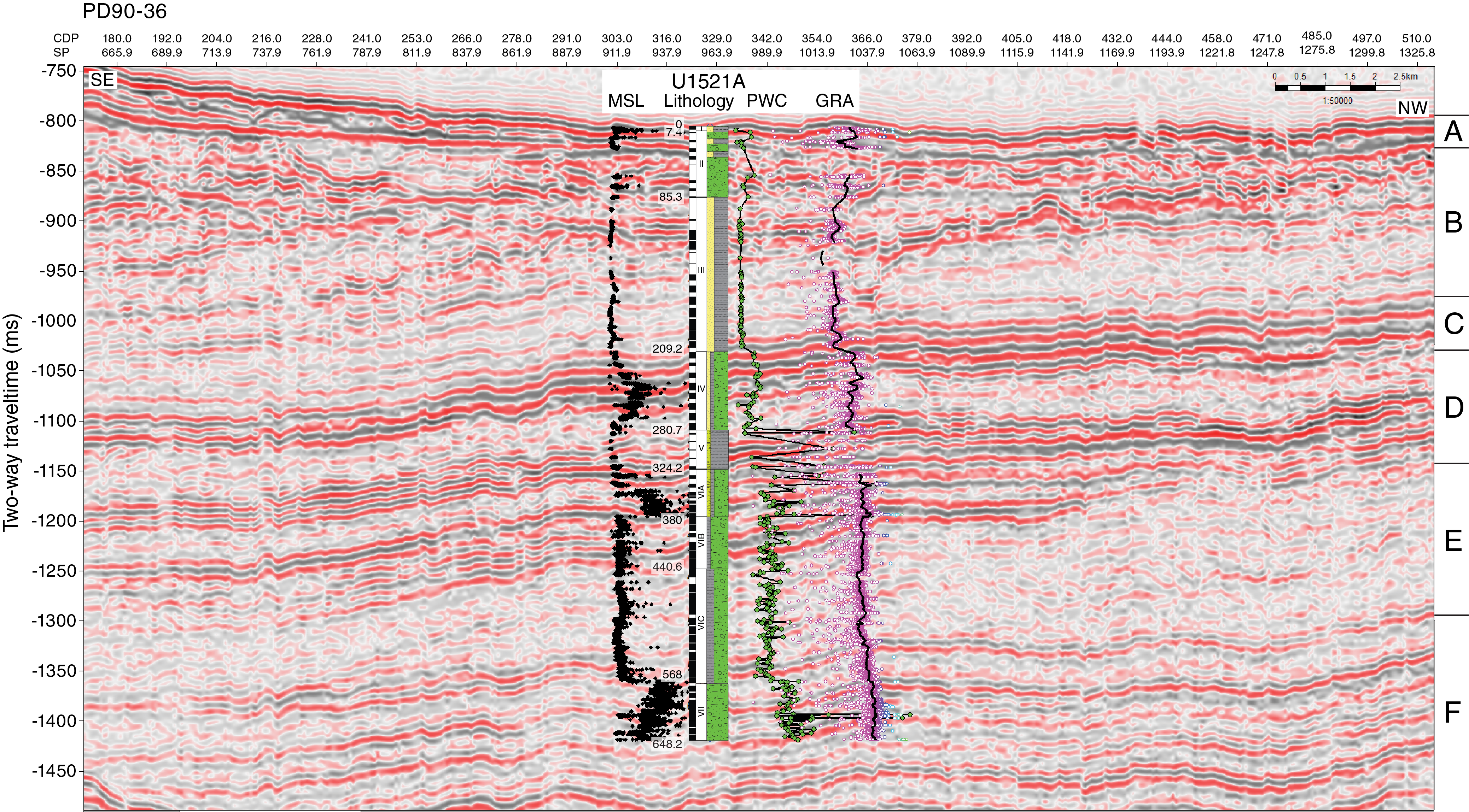
Figure F37. Core-log-seismic integration.
Seismic-downhole log correlation
Seismic-reflection Profile PD90-36, acquired in 1990 aboard the R/V Polar Duke, crosses Site U1521 (Figure F37) and was used for core-log-seismic integration. The primary seismic sequences are interpreted after Anderson and Bartek (1992) and De Santis et al. (1995). For core-log-seismic integration, the seismic-reflection profile was divided into six seismic units (A–F; Figure F37). Each of these units either defines a change in dominant seismic facies (relating to subglacial till, subglacial or outwash channels, and ice-proximal and ice-distal sediments) or is bounded by an interpreted erosional surface. The defined units are in good agreement with the logging and lithostratigraphic units. Drilling at Site U1521 reached and exceeded the targeted seismic horizon RSU4 (either in seismic Unit D or between Units D and E), which represents a boundary for sedimentary, physical property, log, and seismic units.
Seismic Unit A (815–890 ms TWT) comprises discontinuous high- to low-amplitude reflectors onlapping an irregular high-amplitude reflector and corresponds to logging Unit 1. Seismic Unit B (890–1020 ms TWT) is characterized by low-amplitude reflectors with sparse, internal, continuous reflectors inclined toward the south on top of a stratified package (seismic Unit C) and corresponds with logging Unit 2. Seismic Unit C (1020–1100 ms TWT) comprises a stratified package of high-amplitude continuous reflectors and corresponds with logging Unit 3. Seismic Unit D (1100–1240 ms TWT) comprises chaotic lenses (<100 ms thick) and horizontal high-amplitude, closely spaced, continuous reflectors and corresponds with logging Units 4–6. Seismic Unit E (1240–1345 ms TWT) is characterized by a low-amplitude chaotic wedge (part of a lens-shaped unit) pinching toward the south, with sparse, high-amplitude, discontinuous, irregular reflectors and corresponds to logging Unit 7. Seismic Unit F (>1345 ms TWT) is characterized by subhorizontal, subparallel, medium-amplitude, continuous reflectors interbedded with low-amplitude chaotic lenses and closely spaced reflector packages and corresponds to logging Units 8–10.
References
Abelmann, A., 1990. Oligocene to middle Miocene radiolarian stratigraphy of southern high latitudes from Leg 113, Sites 689 and 690, Maud Rise. In Barker, P.F., Kennett, J.P., et al., Proceedings of the Ocean Drilling Program, Scientific Results, 113: College Station, TX (Ocean Drilling Program), 675–708. https://doi.org/10.2973/odp.proc.sr.113.200.1990
Anderson, J.B., and Bartek, L.R., 1992. Cenozoic glacial history of the Ross Sea revealed by intermediate resolution seismic reflection data combined with drill site information. In Kennett J.P., and Warnke D. (Eds.), Antarctic Research Series (Volume 56): The Antarctic Paleoenvironment: A Perspective on Global Change: Part One: Washington, DC (American Geophysical Union), 231–263. https://agupubs.onlinelibrary.wiley.com/doi/pdf/10.1029/AR056p0231
Arndt, J.E., Schenke, H.W., Jakobsson, M., Nitsche, F.O., Buys, G., Goleby, B., Rebesco, M., et al., 2013. The International Bathymetric Chart of the Southern Ocean (IBCSO) Version 1.0—a new bathymetric compilation covering circum-Antarctic waters. Geophysical Research Letters, 40(12):3111–3117. https://doi.org/10.1002/grl.50413
Bart, P.J., 2003. Were West Antarctic Ice Sheet grounding events in the Ross Sea a consequence of East Antarctic Ice Sheet expansion during the middle Miocene? Earth and Planetary Science Letters, 216(1–2):93–107. https://doi.org/10.1016/S0012-821X(03)00509-0
Bijl, P.K., Houben, A.J.P., Bruls, A., Pross, J., and Sangiorgi, F., 2018. Stratigraphic calibration of Oligocene–Miocene organic-walled dinoflagellate cysts from offshore Wilkes Land, East Antarctica, and a zonation proposal. Journal of Micropaleontology, 37(1):105–138. https://doi.org/10.5194/jm-37-105-2018
Bijl, P.K., Sluijs, A., Head, M.J., Pross, J., Riding, J.B., and Schiøler, P., 2015. Advanced course in Jurassic-Cretaceous-Cenozoic organic-walled dinoflagellate cysts: morphology, stratigraphy, and palaeoecology [Heidelberg, Germany, 13–19 September 2015].
Bown, P.R., and Dunkley Jones, T., 2012. Calcareous nannofossils from the Paleogene equatorial Pacific (IODP Expedition 320 Sites U2331–1334). Journal of Nannoplankton Research, 32(2):3–51. http://ina.tmsoc.org/JNR/online/32/Bown%20&%20DunkleyJones%202012%20JNR%2032-2.pdf
Brancolini, G., Busetti, M., Marchetti, M., De Santis, L., Zanolla, C., Cooper, A.K., Cochrane, G.R., et al., 1995. Seismic stratigraphic atlas of the Ross Sea, Antarctica. In Cooper, A.K., Barker, P.F., and Brancolini, G. (Eds.), Antarctic Research Series (Volume 68): Geology and Seismic Stratigraphy of the Antarctic Margin: Washington, DC (American Geophysical Union), A271–A286.
Claypool, G.E., and Kvenvolden, K.A., 1983. Methane and other hydrocarbon gases in marine sediment. Annual Review of Earth and Planetary Sciences, 11(1):299–327. https://doi.org/10.1146/annurev.ea.11.050183.001503
Clowes, C.D., Hannah, M.J., Wilson, G.J., and Wrenn, J.H., 2016. Marine palynostratigraphy and new species from the Cape Roberts drill-holes, Victoria Land Basin, Antarctica. Marine Micropaleontology, 126:65–84. https://doi.org/10.1016/j.marmicro.2016.06.003
Cooper, A.K., Barker, P.F., and Brancolini, G. (Eds.), 1995. Antarctic Research Series (Volume 68): Geology and Seismic Stratigraphy of the Antarctic Margin: Washington, DC (American Geophysical Union). https://doi.org/10.1029/AR068
Crosta, X., Pichon, J.-J., and Labracherie, M., 1997. Distribution of Chaetoceros resting spores in modern peri-Antarctic sediments. Marine Micropaleontology, 29(3–4):283–299. https://doi.org/10.1016/S0377-8398(96)00033-3
De Santis, L., Anderson, J.B., Brancolini, G., Zayatz, I., 1995. Seismic record of the late Oligocene through Miocene glaciation on the central eastern continental shelf of the Ross Sea. In Cooper, A.K., Barker, P.F., and Brancolini, G. (Eds.), Antarctic Research Series (Volume 68): Geology and Seismic Stratigraphy of the Antarctic Margin: Washington, DC (American Geophysical Union), 235–260. https://doi.org/10.1029/AR068p0235
Farmer, R.K., 2011. The application of biostratigraphy and paleoecology at Southern Ocean drill sites to resolve early to middle Miocene paleoclimatic events [M.S. thesis]. University of Nebraska-Lincoln. https://digitalcommons.unl.edu/geoscidiss/19/
Fielding C.R., Atkins, C.B., Bassett, K.N., Browne, G.H., Dunbar, G.B., Field, B.D., Frank, T.D., et al., 2008-2009. Sedimentology and stratigraphy of the AND-2A core, ANDRILL Southern McMurdo Sound Project, Antarctica. Terra Antarctica, 15(1):77–112. http://www.mna.unisi.it/english/Publications/TAP/TA_pdfs/Volume_15/ TA_15_01_77_ANDRILL_SMS_Sedimentology.pdf
Florindo, F., Farmer, R.K., Harwood, D.M., Cody, R.D., Levy, R., Bohaty, S.M., Carter, L., and Winkler, A., 2013. Paleomagnetism and biostratigraphy of sediments from Southern Ocean ODP Site 744 (southern Kerguelen Plateau): implications for early-to-middle Miocene climate in Antarctica. Global and Planetary Change, 110(C):434–454. https://doi.org/10.1016/j.gloplacha.2013.05.004
Gradstein, F.M., Ogg, J.G., Schmitz, M.D., and Ogg, G.M. (Eds.), 2012. The Geological Time Scale 2012: Amsterdam (Elsevier).
Hannah, M.J., 2006. The palynology of ODP Site 1165, Prydz Bay, East Antarctica: a record of Miocene glacial advance and retreat. Palaeogeography, Palaeoclimatology, Palaeoecology, 231(1–2):120–133. https://doi.org/10.1016/j.palaeo.2005.07.029
Hannah, M.J., Wilson, G.J., and Wrenn, J.H., 2000. Oligocene and Miocene marine palynomorphs from CRP-2/2A, Victorialand Basin, Antarctica. Terra Antarctica, 7(4):503–511. http://epic.awi.de/27368/1/Han2000f.pdf
Hannah, M.J., Wrenn, J.H., and Wilson, G.J., 1998. Early Miocene and Quaternary marine palynomorphs from Cape Roberts Project CRP-1, McMurdo Sound, Antarctica. Terra Antarctica, 5(3):527–538. https://epic.awi.de/27440/1/Han1998g.pdf
Hinz, K., and Block, M., 1984. Results of geophysical investigations in the Weddell Sea and in the Ross Sea, Antarctica. Proceedings of the 11th World Petroleum Congress, 11(2):79–91.
Jarrard, R.D., and Kerneklian, M.J., 2007. Data report: physical properties of the upper oceanic crust of ODP Site 1256: multisensor track and moisture and density measurements. In Teagle, D.A.H., Wilson, D.S., Acton, G.D., and Vanko, D.A. (Eds.), Proceedings of the Ocean Drilling Program, Scientific Results, 206: College Station, TX (Ocean Drilling Program), 1–11. https://doi.org/10.2973/odp.proc.sr.206.011.2007
John, C.M., Karner, G.D., Browning, E., Leckie, R.M., Mateo, Z., Carson, B., and Lowery, C., 2011. Timing and magnitude of Miocene eustasy derived from the mixed siliciclastic-carbonate stratigraphic record of the northeastern Australian margin. Earth and Planetary Science Letters, 304(3–4):455–467. https://doi.org/10.1016/j.epsl.2011.02.013
Krissek, L., Browne, G., Carter, L., Cowan, E., Dunbar, G., McKay, R., Naish, T., et al., 2007. Sedimentology and stratigraphy of the AND-1B core, ANDRILL McMurdo Ice Shelf Project, Antarctica. Terra Antarctica, 14(3):185–222. http://www.mna.unisi.it/english/Publications/TAP/TA_pdfs/Volume_14/TA_14_185_Sedimentology.pdf
Lazarus, D., 1990. Middle Miocene to Recent radiolarians from the Weddell Sea, Antarctica, ODP Leg 113. In Barker, P.F., Kennett, J.P., et al., Proceedings of the Ocean Drilling Program, Scientific Results, 113: College Station, TX (Ocean Drilling Program), 709–727. https://doi.org/10.2973/odp.proc.sr.113.132.1990
Leckie, R.M., and Webb, P.-N., 1985. Candeina antarctica, n.sp., and the phylogenetic history and distribution of Candeina spp. in the Paleogene–early Neogene of the Southern Ocean. Journal of Foraminiferal Research, 15(2):65–78. https://doi.org/10.2113/gsjfr.15.2.65
Leckie, R.M., and Webb, P.-N., 1986. Late Paleogene and early Neogene foraminifers of Deep Sea Drilling Project Site 270, Ross Sea, Antarctica. In Kennett, J. P., von der Borch, C.C., et al., Initial Reports of the Deep Sea Drilling Project, 90: Washington, DC (U.S. Government Printing Office), 1093–1142. https://doi.org/10.2973/dsdp.proc.90.124.1986
McKay, R., Browne, G., Carter, L., Cowan, E., Dunbar, G., Krissek, L., Naish, T., et al., 2009. The stratigraphic signature of the late Cenozoic Antarctic Ice Sheets in the Ross Embayment. Geological Society of America Bulletin, 121(11–12):1537–1561. https://doi.org/10.1130/B26540.1
McKay, R.M., De Santis, L., Kulhanek, D.K., Ash, J.L., Beny, F., Browne, I.M., Cortese, G., Cordeiro de Sousa, I.M., Dodd, J.P., Esper, O.M., Gales, J.A., Harwood, D.M., Ishino, S., Keisling, B.A., Kim, S., Kim, S., Laberg, J.S., Leckie, R.M., Müller, J., Patterson, M.O., Romans, B.W., Romero, O.E., Sangiorgi, F., Seki, O., Shevenell, A.E., Singh, S.M., Sugisaki, S.T., van de Flierdt, T., van Peer, T.E., Xiao, W., and Xiong, Z., 2019a. Expedition 374 methods. In McKay, R.M., De Santis, L., Kulhanek, D.K., and the Expedition 374 Scientists, Ross Sea West Antarctic Ice Sheet History. Proceedings of the International Ocean Discovery Program, 374: College Station, TX (International Ocean Discovery Program). https://doi.org/10.14379/iodp.proc.374.102.2019
McKay, R.M., De Santis, L., Kulhanek, D.K., Ash, J.L., Beny, F., Browne, I.M., Cortese, G., Cordeiro de Sousa, I.M., Dodd, J.P., Esper, O.M., Gales, J.A., Harwood, D.M., Ishino, S., Keisling, B.A., Kim, S., Kim, S., Laberg, J.S., Leckie, R.M., Müller, J., Patterson, M.O., Romans, B.W., Romero, O.E., Sangiorgi, F., Seki, O., Shevenell, A.E., Singh, S.M., Sugisaki, S.T., van de Flierdt, T., van Peer, T.E., Xiao, W., and Xiong, Z., 2019b. Expedition 374 methods. In McKay, R.M., De Santis, L., Kulhanek, D.K., and the Expedition 374 Scientists, Ross Sea West Antarctic Ice Sheet History. Proceedings of the International Ocean Discovery Program, 374: College Station, TX (International Ocean Discovery Program). https://doi.org/10.14379/iodp.proc.374.101.2019
Miller, K.G., Kominz, M.A., Browning, J.V., Wright, J.D., Mountain, G.S., Katz, M.E., Sugarman, P.J., Cramer, B.S., Christie-Blick, N., and Pekar, S.F., 2005. The Phanerozoic record of global sea-level change. Science, 310(5752):1293–1298. https://doi.org/10.1126/science.1116412
Osterman, L.E., and Kellogg, T.B., 1979. Recent benthic foraminiferal distributions from the Ross Sea, Antarctica: relation to ecologic and oceanographic conditions. Journal of Foraminiferal Research, 9(3):250–269. https://doi.org/10.2113/gsjfr.9.3.250
Perch-Nielsen, K., 1985. Cenozoic calcareous nannofossils. In Bolli, H.M., Saunders, J.B., and Perch-Nielsen, K. (Eds.), Plankton Stratigraphy: Cambridge, United Kingdom (Cambridge University Press), 427–554.
Prebble, J.G., Crouch, E.M., Carter, L., Cortese, G., Bostock, H., and Neil, H., 2013. An expanded modern dinoflagellate cyst dataset for the Southwest Pacific and Southern Hemisphere with environmental associations. Marine Micropaleontology, 101:33–48. https://doi.org/10.1016/j.marmicro.2013.04.004
Raffi, I., Backman, J., Fornaciari, E., Pälike, H., Rio, D., Lourens, L., and Hilgen, F., 2006. A review of calcareous nannofossil astrobiochronology encompassing the past 25 million years. Quaternary Science Reviews, 25(23–24):3113–3137. https://doi.org/10.1016/j.quascirev.2006.07.007
Sangiorgi, F., Bijl, P.K., Passchier, S., Salzmann, U., Schouten, S., McKay, R., Cody, R.D., et al., 2018. Southern Ocean warming and Wilkes Land ice sheet retreat during the mid-Miocene. Nature Communications, 9(1):317. https://doi.org/10.1038/s41467-017-02609-7
Sangiorgi, F., Brinkhuis, H., and Damassa, S.P., 2009. Arcticacysta: a new organic-walled dinoflagellate cyst genus from the early Miocene? of the central Arctic Ocean. Micropaleontology, 55:249–258. http://www.micropress.org/microaccess/micropaleontology/issue-258/article-1628
Sangiorgi, F., Brumsack, H.-J., Willard, D.A., Schouten, S., Stickley, C.E., O’Regan, M., Reichart, G.-J., Sinninghe Damsté, J.S., and Brinkhuis, H., 2008. A 26 million year gap in the central Arctic record at the greenhouse–icehouse transition: looking for clues. Paleoceanography and Paleoclimatology, 23(1):PA1S04. https://doi.org/10.1029/2007PA001477
Schwehr, K., Tauxe, L., Driscoll, N., and Lee, H., 2006. Detecting compaction disequilibrium with anisotropy of magnetic susceptibility. Geochemistry, Geophysics, Geosystems, 7(11):Q11002. https://doi.org/10.1029/2006GC001378
Steinhauff, D.M., and Webb, P.-N., 1987. Miocene foraminifera from DSDP Site 272, Ross Sea. Antarctic Journal of the United States, 22(5):125–126.
Warny, S., Askin, R.A., Hannah, M.J., Mohr, B.A.R., Raine, J.I., Harwood, D.M., Florindo, F., and the SMS Science Team, 2009. Palynomorphs from a sediment core reveal a sudden remarkably warm Antarctica during the middle Miocene. Geology, 37(10):955–958. https://doi.org/10.1130/G30139A.1
Young, J.R., 1998. Neogene. In Bown, P.R. (Ed.), Calcareous Nannofossil Biostratigraphy: Dordrecht, The Netherlands (Kluwer Academic Publishing), 225–265.
1 McKay, R.M., De Santis, L., Kulhanek, D.K., Ash, J.L., Beny, F., Browne, I.M., Cortese, G., Cordeiro de Sousa, I.M., Dodd, J.P., Esper, O.M., Gales, J.A., Harwood, D.M., Ishino, S., Keisling, B.A., Kim, S., Kim, S., Laberg, J.S., Leckie, R.M., Müller, J., Patterson, M.O., Romans, B.W., Romero, O.E., Sangiorgi, F., Seki, O., Shevenell, A.E., Singh, S.M., Sugisaki, S.T., van de Flierdt, T., van Peer, T.E., Xiao, W., and Xiong, Z., 2019. Site U1521. In McKay, R.M., De Santis, L., Kulhanek, D.K., and the Expedition 374 Scientists, Ross Sea West Antarctic Ice Sheet History. Proceedings of the International Ocean Discovery Program, 374: College Station, TX (International Ocean Discovery Program). https://doi.org/10.14379/iodp.proc.374.103.2019
2 Expedition 374 Scientists’ affiliations.
This work is distributed under the Creative Commons Attribution 4.0 International (CC BY 4.0) license. 