McKay, R.M., De Santis, L., Kulhanek, D.K., and the Expedition 374 Scientists
Proceedings of the International Ocean Discovery Program Volume 374
publications.iodp.org

https://doi.org/10.14379/iodp.proc.374.102.2019
Expedition 374 methods1
R.M. McKay, L. De Santis, D.K. Kulhanek, J.L. Ash, F. Beny, I.M. Browne, G. Cortese, I.M. Cordeiro de Sousa, J.P. Dodd, O.M. Esper, J.A. Gales, D.M. Harwood, S. Ishino, B.A. Keisling, S. Kim, S. Kim, J.S. Laberg, R.M. Leckie, J. Müller, M.O. Patterson, B.W. Romans, O.E. Romero, F. Sangiorgi, O. Seki, A.E. Shevenell, S.M. Singh, S.T. Sugisaki, T. van de Flierdt, T.E. van Peer, W. Xiao, and Z. Xiong2
Keywords: International Ocean Discovery Program, IODP, JOIDES Resolution, Expedition 374, Site U1521, Site U1522, Site U1523, Site U1524, Site U1525, Ross Sea, West Antarctic, ice sheet history, sea ice, Miocene, Pliocene, Quaternary, Antarctic Bottom Water, Antarctic water masses, turbidites, contourites, glaciomarine sediments, subglacial sediments, ice-rafted debris, paleobathymetry, seismic stratigraphy, paleoclimate, paleoceanography
MS 374-102: Published 10 August 2019
Introduction
This chapter documents the procedures and methods employed during drilling operations and in the shipboard laboratories on the R/V JOIDES Resolution during International Ocean Discovery Program (IODP) Expedition 374. This information applies only to the shipboard work described in the Expedition Reports section of the Expedition 374 Proceedings of the International Ocean Discovery Program volume. Methods used by investigators for shore-based analyses of Expedition 374 data and samples will be described in separate individual publications. This introductory section provides an overview of drilling and coring operations, core handling, curatorial conventions, depth scale terminology, and the sequence of shipboard analyses. Subsequent sections of this chapter describe specific laboratory procedures and instruments in more detail.
The nomenclature of many geographic features on the Antarctic continent is aligned to the geographic coordinate system (e.g., the East and West Antarctic Ice Sheets), in which 0° of longitude represents grid north on a universal polar stereographic projection. However, in the Ross Sea, true direction is generally opposite to the geographic coordinates: the eastern Ross Sea is the area located between 160°W and 180° longitude (see Figure F2 in the Expedition 374 summary chapter [McKay et al., 2019a]), and the western Ross Sea is the area between 160°E and 180° of longitude (see Figure F2 in the Expedition 374 summary [McKay et al., 2019a]). In this volume, descriptors of directional orientation (e.g., west versus east) are based on true directions within the Ross Sea and not the geographical coordinate system.
Site locations
GPS coordinates from precruise site surveys were used to position the vessel at all Expedition 374 sites. A SyQuest Bathy 2010 CHIRP subbottom profiler was used to monitor seafloor depth on the approach to each site to reconfirm the depth profiles from precruise surveys. Once the vessel was positioned at a site, the thrusters were lowered and a positioning beacon was dropped to the seafloor at most sites. The dynamic positioning control of the vessel used navigational input from the GPS system and triangulation to the seafloor beacon weighted by the estimated positional accuracy. The final hole position was the mean position calculated from the GPS data collected over a portion of the time the hole was occupied.
When coring multiple holes at a site, the hole locations are typically offset from each other by ~20 m in a grid pattern. The second hole is offset 20 m east of the first hole, the third hole is offset 20 m south of the second hole, the fourth hole is offset 20 m west of the third hole, and so on.
Coring and drilling operations
All four standard coring systems, the advanced piston corer (APC), the half-length APC (HLAPC), the extended core barrel (XCB), and the rotary core barrel (RCB), were used during Expedition 374. We employed several different coring strategies during the expedition. For continental shelf Sites U1521 and U1522, we cored a single RCB hole to total depth. RCB coring was necessary on the continental shelf because of the presence of overconsolidated glaciomarine and subglacial diamictite, as well as large cobbles and boulders in surficial sediment. Although coring unconsolidated diamict is difficult and resulted in poor recovery, coring lithified glacial sediment with an indurated mud matrix resulted in much better core recovery. At Site U1523, located on the outermost continental shelf, we employed a different strategy that included piston coring with both the APC and HLAPC systems and using the XCB system to penetrate more indurated layers and unconsolidated gravel. By coring multiple holes at this site, we were able to use coring results from previous holes and drilling parameters (e.g., weight on bit and rate of penetration) to determine the location of unconsolidated gravel or indurated layers and then collect targeted HLAPC cores between these layers. In addition, we cored a single RCB hole primarily for downhole logging. At continental rise and slope Sites U1524 and U1525, our coring strategy consisted of APC coring to refusal followed by HLAPC coring to refusal and then deepening the hole with the XCB system. This strategy worked well at Site U1524; however, at Site U1525, an indurated layer at ~50 meters drilling depth below seafloor (DSF) resulted in HLAPC refusal at a very shallow depth. Based on our experience at Site U1523, we employed the XCB system to core through the hard layer and then resumed APC/HLAPC coring to refusal followed by additional XCB coring. At Site U1524, we also used the RCB system to core a deep hole.
JOIDES Resolution standard coring systems
The APC and HLAPC coring systems cut soft-sediment cores with minimal coring disturbance relative to other IODP coring systems. These coring systems are typically used in the upper portions of a hole where sediment is unconsolidated to obtain high-quality core. After the APC core barrel is lowered through the drill pipe and lands near the bit, the drill pipe is pressured up until the two shear pins holding the inner barrel attached to the outer barrel fail. The inner barrel then advances into the formation and cuts a core with a diameter of 66 mm (Figure F1). The driller can detect a successful cut, or “full stroke,” from the pressure gauge on the rig floor.
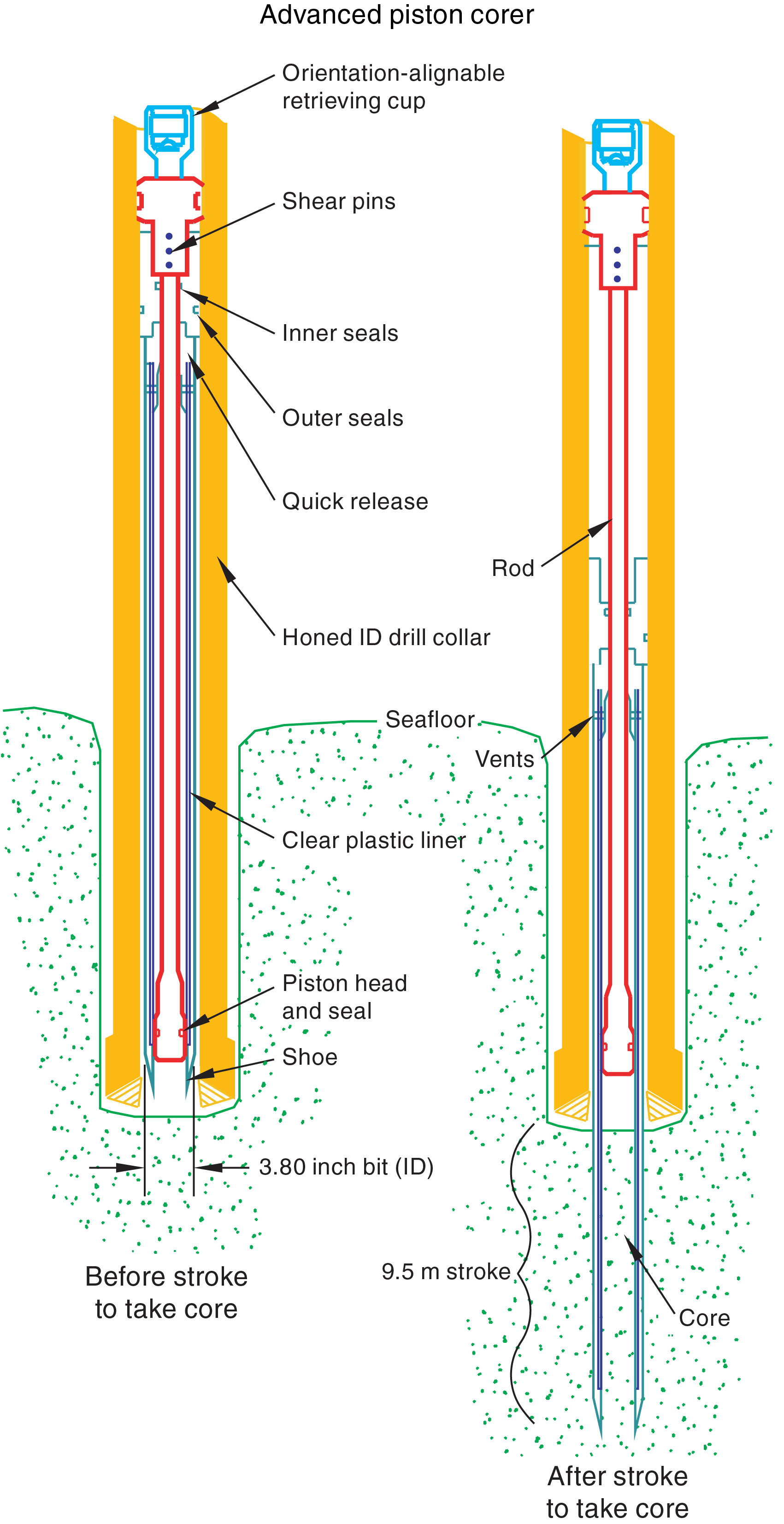
Figure F1. APC system.
The depth limit of the APC, referred to as APC refusal, is conventionally defined in two ways: (1) the piston fails to achieve a complete stroke (as determined from the pump pressure reading) because the formation is too hard or (2) excessive force (>60,000 lb; ~267 kN) is required to pull the core barrel out of the formation. When a full stroke cannot be achieved, additional attempts are typically made. With a partial stroke, the assumption is that the core barrel penetrated the formation by the length of core recovered (nominal recovery of ~100%), and the bit is advanced by that length before cutting the next core. The number of additional attempts is generally dictated by the length of recovery of the partial stroke core and the time available to advance the hole by piston coring. When a full or partial stroke is achieved but excessive force cannot retrieve the barrel, the core barrel is “drilled over,” meaning after the inner core barrel is successfully shot into the formation, the drill bit is advanced to free the APC barrel.
The standard (full) APC system contains a 9.5 m long core barrel, whereas the HLAPC system uses a 4.8 m core barrel. In most cases, the HLAPC system is deployed after the standard APC system reaches refusal. While using the HLAPC system, we applied the same criteria for refusal as with the standard APC system. This technology allowed for deeper continuous piston coring than would have been possible with the standard APC system. We also used the HLAPC system at Site U1523 to target piston cores between indurated layers and gravel beds that could not have been cored with the standard APC system.
Nonmagnetic core barrels were used during all APC and HLAPC coring to a pull force of ~40,000 lb. In addition, most full-length APC cores recovered at Sites U1523–U1525 were oriented using the Icefield MI-5 core orientation tool (see Paleomagnetism). We also used the advanced piston corer temperature tool (APCT-3) to obtain in situ formation temperatures at Site U1524 to determine the geothermal gradient and estimate heat flow (see Downhole measurements).
The XCB system was used to advance the hole when APC or HLAPC refusal occurred before the target depth was reached or when the formation became either too stiff for APC coring or hard substrate was encountered. The XCB is a rotary system with a small cutting shoe that extends below the large rotary APC/XCB bit. The smaller bit can cut a semi-indurated core with less torque and fluid circulation than the main bit, optimizing recovery. The XCB cutting shoe (bit) extends ~30.5 cm ahead of the main bit in soft sediments but retracts into the main bit when hard formations are encountered (Figure F2). XCB cores have a nominal diameter of 58 mm, which is less than the diameter of APC/HLAPC cores (66 mm). Steel core barrels are used for all XCB coring. XCB cores are often broken into “biscuits,” which are pieces of core that are a few to several centimeters in length with fluidized sediment and drilling slurry injected between them. This slurry can also fill the spaces between the cut core and the core liner, giving the impression that XCB cores have the same diameter as APC cores. Because the APC and XCB systems use the same bottom-hole assembly (BHA), it is possible to switch between them without having to trip the drill bit back to the vessel.
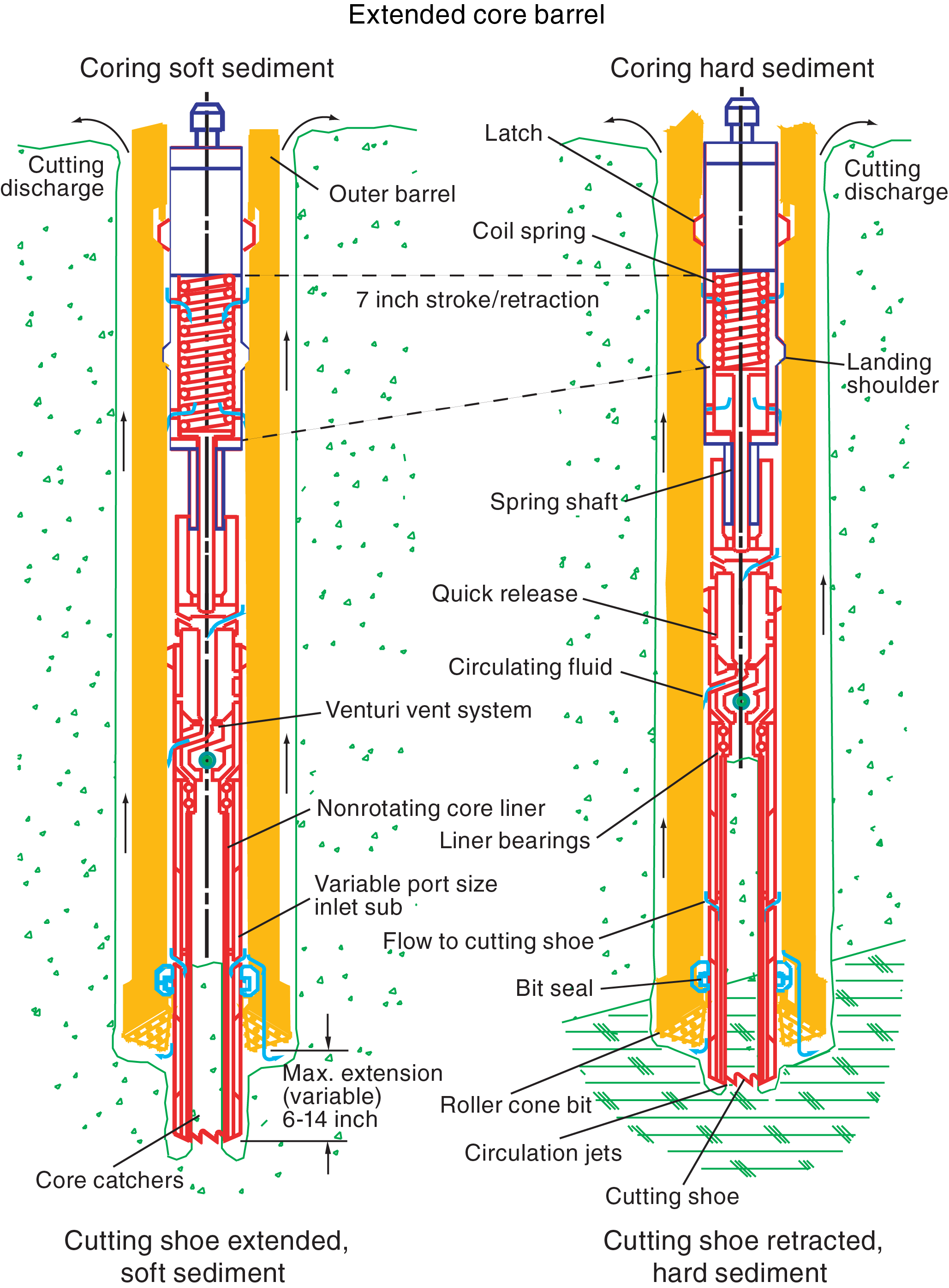
Figure F2. XCB system.
The BHA is the lowermost part of the drill string. A typical APC/XCB BHA consists of a drill bit (outer diameter = 11⁷⁄₁₆ inch), a bit sub, a seal bore drill collar, a landing saver sub, a modified top sub, a modified head sub, a nonmagnetic drill collar, a number of 8¼ inch (~20.32 cm) drill collars, a tapered drill collar, six joints (two stands) of 5½ inch (~13.97 cm) drill pipe, and one crossover sub. A lockable float valve was used in Hole U1523A so that downhole logs could be collected through the bit, but that hole was abandoned before logging took place. In some cases, the drill string was drilled or “washed” ahead without recovering sediment to advance the drill bit to a target depth and resume core recovery. Such intervals were typically drilled using a center bit installed on an XCB core barrel that was then latched into the APC/XCB bit.
The RCB system is typically used to core holes deeper than XCB refusal or to core hard rock. During Expedition 374, we used the RCB system to core continental shelf Sites U1521 and U1522 because of the presence of overconsolidated diamictite and large boulders. The RCB system was also deployed at Sites U1523 and U1524 to core deeper holes for downhole logging. The RCB system is the most conventional rotary coring system, and like the XCB system, it cuts a core with a nominal diameter of 58 mm (Figure F3). Unlike the XCB system, nonmagnetic core barrels can be used with the RCB coring system. The RCB system requires a dedicated RCB BHA and a dedicated RCB drilling bit. A typical RCB BHA includes a 9⅞ inch RCB drill bit, a mechanical bit release (to drop the bit prior to downhole logging), a modified head sub, an outer core barrel, a modified top sub, a modified head sub, 7–10 control-length drill collars, a tapered drill collar, two stands of 5½ inch drill pipe, and a crossover sub to the 5 inch drill pipe. Most intervals cored with the RCB system were ~9.6 m long, which is the length of a standard rotary core and approximately the length of a joint of drill pipe. In some cases, half cores (~4.8 m) were cut to improve core recovery when hard rocks (such as ice-rafted debris) clogged the drill bit throat. In some cases, the drill string was drilled or “washed” ahead with a center bit installed to advance the drill bit without coring to a target depth to resume core recovery.
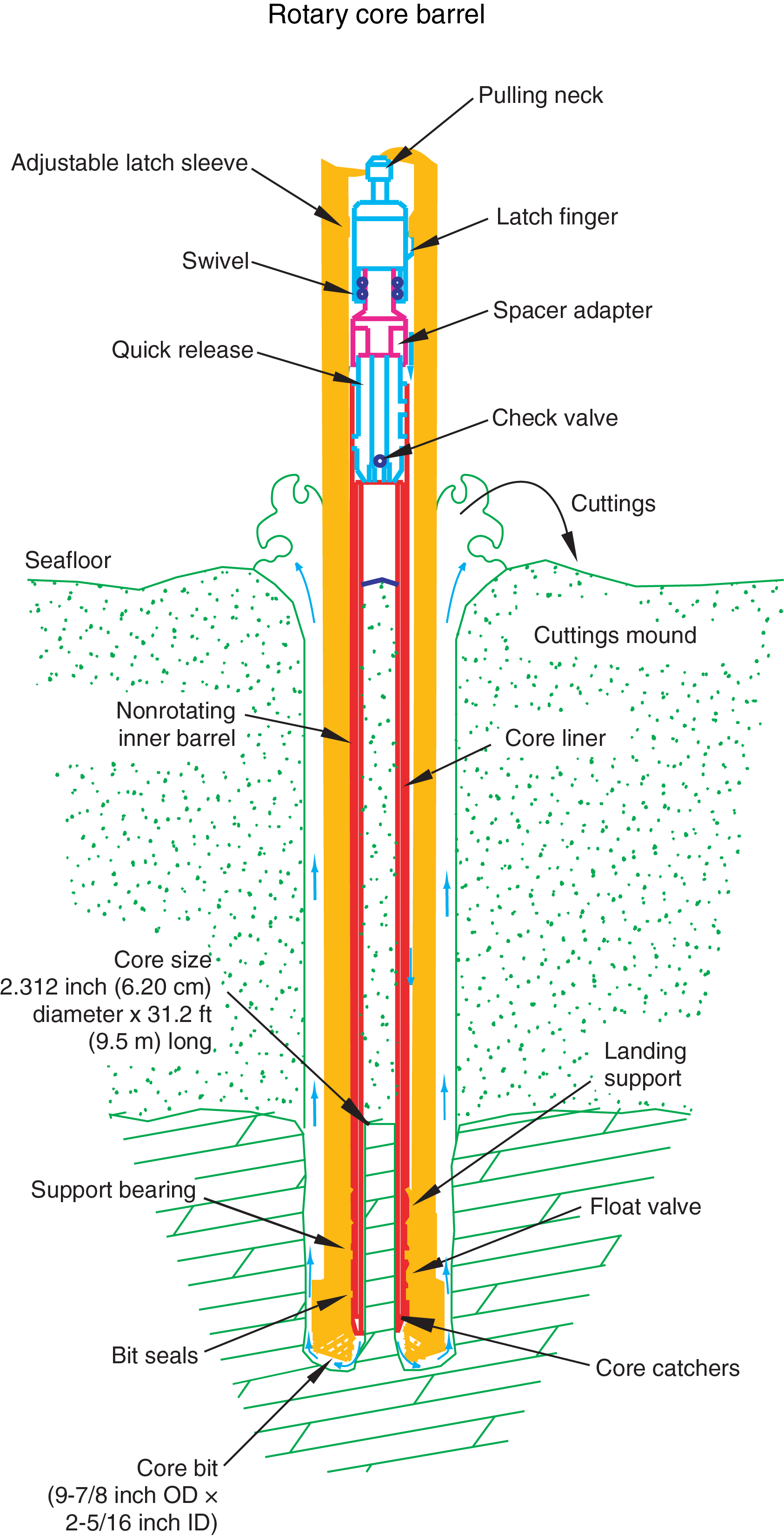
Figure F3. RCB system.
Core disturbance
Cores may be significantly disturbed by the drilling process and contain extraneous material as a result of the coring and core handling processes. In formations with loose sand or gravel layers, sand and gravel from intervals higher in the hole may be washed down by drilling circulation, accumulate at the bottom of the hole, and be sampled with the next core. The uppermost 10–50 cm of each core must therefore be examined critically during description for potential fall-in. Common coring-induced deformation includes the concave appearance of originally horizontal bedding. Piston action may result in fluidization (flow-in) at the bottom of or within APC and HLAPC cores. Retrieval of cores containing unconsolidated sediment from depth to the surface may result in elastic rebound. Gas that is in solution at depth may become free and drive core segments in the liner apart. Both elastic rebound and gas pressure can result in a total length for each core that is longer than the interval that was cored and thus a calculated recovery of >100%. If gas expansion or other coring disturbance results in a void in any particular core section, the void can be closed by moving material if very large, stabilized by a foam insert if moderately large, or left as is. When gas content is high, pressure must be relieved for safety reasons before the cores are cut into segments. Holes are drilled into the liner, which forces out some sediment, as well as gas. In extreme instances, core material can be ejected from the core barrel, sometimes violently, onto the rig floor by high pressure in the core or other coring problems. This core material is placed in the plastic core liners by hand and should not be considered to be in stratigraphic order; these core sections are denoted by a yellow label marked “disturbed,” and the nature of the disturbance is noted in the coring log. In more consolidated material, common coring disturbances include biscuiting, where fractured material (biscuits) rotates within the core barrel. Drilling slurry is often injected between the biscuits. This type of disturbance is particularly common with XCB coring but can also be seen in RCB cores. Fracturing, fragmentation, and brecciation as a result of the drilling process is common in indurated sediment and rock. Finally, some core liners can be broken or shattered, resulting in significant disturbance when extracted from the core barrel. This was particularly common with XCB coring during Expedition 374; 14 out of 22 XCB core liners shattered (64%). In some cases, broken liners could be patched; however, in many instances, material in shattered liners was placed by hand into new liners and should not be considered to be in stratigraphic order. These core sections were also indicated by a yellow label marked “disturbed.”
These disturbances are described in the Lithostratigraphy section in each site chapter and are graphically indicated on the core summary graphic reports (visual core descriptions [VCDs]).
Curatorial procedures and core handling
Cores recovered during Expedition 374 were extracted from the core barrel in 67 mm diameter plastic liners. These liners were carried from the rig floor to the core processing area on the catwalk outside the Core Laboratory, where they were split into ~1.5 m sections. Liner caps (blue = top; colorless = bottom; yellow = whole-round sample taken) were glued with acetone onto liner sections on the catwalk by the Marine Technicians. The length of each section was entered into the database as “created length” using the Sample Master application. This number was used to calculate core recovery.
Sample naming and identifiers
Numbering of sites, holes, cores, and samples follows standard IODP procedure (Figure F4). Drilling sites are numbered consecutively from the first site drilled by the D/V Glomar Challenger in 1968. Integrated Ocean Drilling Program Expedition 301 began using the prefix “U” to designate sites occupied by the United States Implementing Organization (USIO) platform, the JOIDES Resolution. For all IODP drill sites, a letter suffix distinguishes each hole drilled at the same site. The first hole drilled is assigned the site number modified by the suffix “A,” the second hole is assigned the site number and the suffix “B,” and so on.
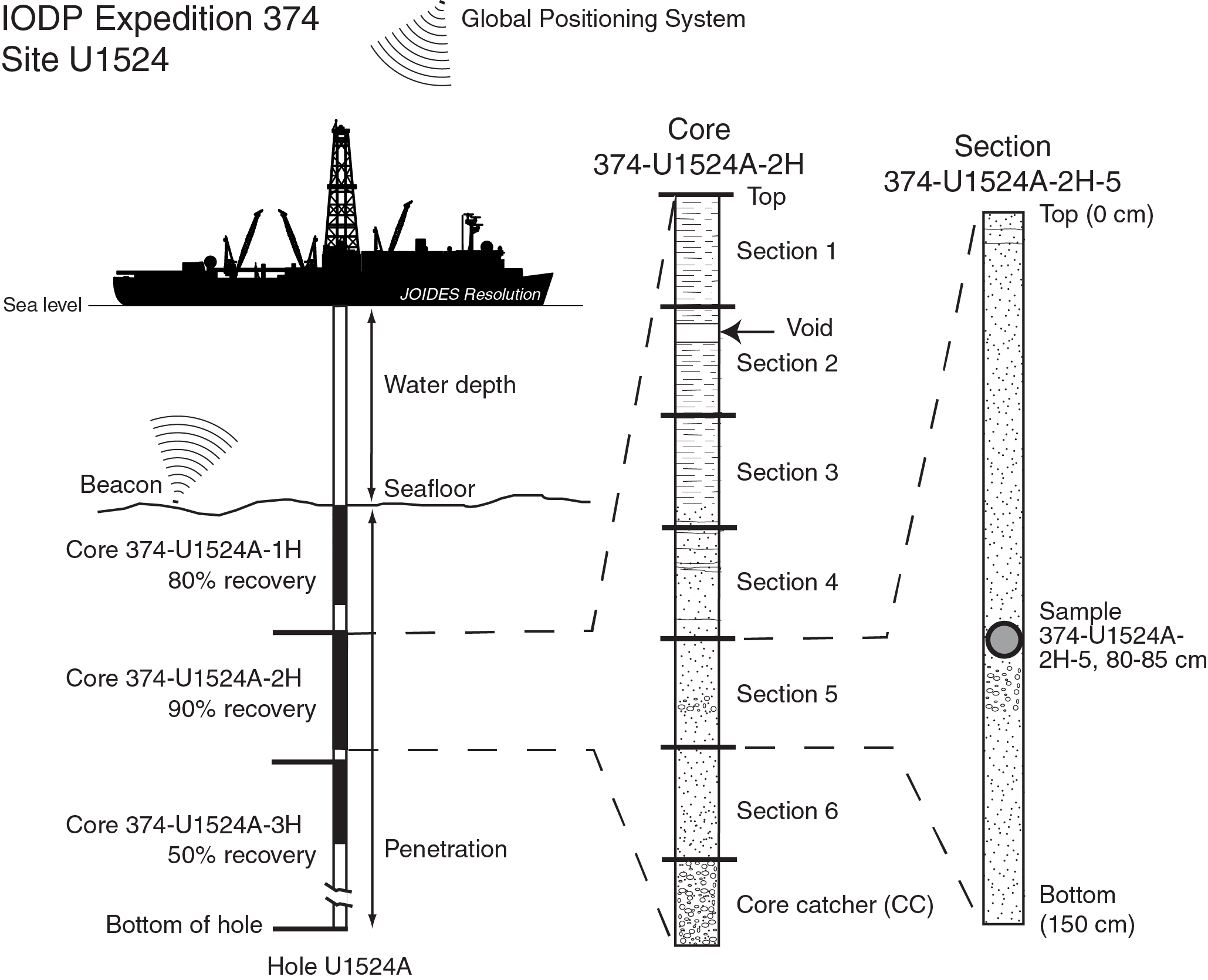
Figure F4. IODP naming conventions.
Cores taken from a hole are numbered sequentially from the top of the hole downward. When an interval is drilled down without coring, this interval is also numbered sequentially, and the drill down is designated by a “1” instead of a letter that designates the coring method used (e.g., 374-U1523B-21). Cores taken with the APC system are designated with “H,” “F” designates HLAPC cores, “X” designates XCB cores, and “R” designates RCB cores. Core numbers and their associated cored intervals are unique in a given hole. Generally, maximum recovery for a single core is 9.5 m of sediment (APC) or 9.7 m of sediment/rock (XCB and RCB) contained in a plastic liner (6.6 cm internal diameter) plus an additional ~0.2 m in the core catcher, which is a device at the bottom of the core barrel that prevents the core from sliding out when the barrel is retrieved from the hole. In certain situations, recovery may exceed the 9.5 or 9.7 m maximum. In soft sediment, this is normally caused by core expansion resulting from depressurization. High heave, tidal changes, and overdrilling can also result in an advance that differs from the planned 9.5 or 9.7 m.
Recovered cores are divided into ~1.5 m sections that are numbered serially from the top downward. When full recovery is obtained, the sections are numbered 1–7, and the last section is usually <1.5 m. Rarely, an unusually long core may require more than seven sections. When the recovered core is shorter than the cored interval, by convention the top of the core is deemed to be located at the top of the cored interval for the purpose of calculating (consistent) depths. In sedimentary cores, the core catcher section is treated as a separate section (“CC”). When the only recovered material is in the core catcher, it is placed at the top of the cored interval.
A full curatorial sample identifier consists of the following information: expedition, site, hole, core number, core type, section number, and interval in centimeters measured from the top of the core section. For example, a sample identification of “374-U1524A-2H-5, 80–85 cm,” represents a sample taken from the interval between 80 and 85 cm below the top of Section 5 of Core 2 (collected using the APC system) of Hole A of Site U1524 during Expedition 374 (Figure F4).
Depth scales
Primary depth scale types are based on the measurement of drill string length deployed beneath the rig floor (drilling depth below rig floor [DRF]) or seafloor (DSF), the length of core recovered (core depth below seafloor [CSF]), and the length of the logging wireline deployed (wireline log depth below rig floor [WRF], wireline log depth below seafloor [WSF], and wireline log matched depth below seafloor [WMSF]). All depths are in meters. The relationship between scales is defined either by protocol, such as the rules for computation of CSF from DSF, or by combinations of protocols with user-defined correlations. The distinction in nomenclature should keep the user aware that a nominal depth value at two different depth scales usually does not refer to exactly the same stratigraphic interval. For more information on depth scales, see “IODP Depth Scales Terminology” at http://www.iodp.org/policies-and-guidelines.
Depths of cored intervals are measured from the drill floor based on the length of drill pipe deployed beneath the rig floor (DRF scale). The depth of the cored interval is referenced to the seafloor (DSF scale) by subtracting the seafloor depth at the time of the first core from the DRF depth of the interval. Seafloor depth was calculated in several different ways during Expedition 374. For Sites U1521 and U1522, the seafloor depth was based on tagging the seafloor with the drill string when starting the hole. At Site U1523, we deployed the subsea camera for a seafloor survey and visually observed the seafloor tag to determine seafloor depth. For Sites U1524 and U1525, the seafloor depth is the length of pipe deployed minus the length of the mudline core recovered.
Standard depths of cores on the CSF, Method A (CSF-A), scale are determined based on the assumptions that (1) the top depth of a recovered core corresponds to the top depth of its cored interval (DSF scale) and (2) the recovered material is a contiguous section even if core segments are separated by voids when recovered. If possible, voids in the core are closed by pushing core segments together during core handling. This convention is also applied if a core has incomplete recovery, in which case the true position of the core within the cored interval is unknown and should be considered a sample depth uncertainty up to the length of the core barrel used when analyzing data associated with the core material. Standard depths of subsamples and associated measurements (CSF-A scale) are calculated by adding the offset of the subsample or measurement from the top of its section and the lengths of all higher sections in the core to the top depth of the cored interval.
A soft-sediment core from less than a few hundred meters below seafloor expands upon recovery (typically a few percent to as much as 15%), so the length of the recovered core can exceed that of the cored interval. Therefore, a stratigraphic interval may not have the same nominal depth at the DSF and CSF-A scales in the same hole. When core recovery (the ratio of recovered core to cored interval) is >100%, the CSF-A depth of a sample taken from the bottom of a core will be deeper than that of a sample from the top of the subsequent core (i.e., the data associated with the two core intervals overlap on the CSF-A scale). The core depth below seafloor, Method B (CSF-B), depth scale is a solution to the overlap problem. This method scales the recovered core length back into the interval cored, from >100% to exactly 100% recovery. If cores have <100% recovery to begin with, they are not scaled. When downloading data using the JOIDES Resolution Science Operator (JRSO) Laboratory Information Management System (LIMS) (http://web.iodp.tamu.edu/LORE/), depths for samples and measurements are presented on both the CSF-A and CSF-B scales by default. The CSF-B depth scale is primarily useful for data analysis and presentations in single-hole situations.
Wireline logging data are collected on the WRF scale, from which a seafloor measurement is subtracted to create a WSF scale. WSF depths were only used for preliminary data usage on the ship. Immediately after data collection was completed, the wireline logging data were transferred to the Lamont Doherty Earth Observatory (LDEO) Borehole Research Group, where multiple passes and runs were depth-matched using the natural gamma radiation (NGR) logs. The data were returned to the ship on the WMSF scale, which is the final logging depth scale type for investigators.
Shipboard core analysis
For sedimentary sections, as soon as cores arrived on deck, headspace samples were taken using a syringe or pieces of sediment were chipped off (for indurated samples) for immediate hydrocarbon analysis as part of the shipboard safety and pollution prevention program. Core catcher samples were taken for biostratigraphic analysis. Whole-round samples were taken from some core sections for shipboard and postcruise interstitial water analyses and shore-based microbiological studies.
After being cut on the catwalk, cores were brought into the core laboratory and placed on racks. After ~4 h of equilibration to laboratory temperature (~20°C), whole-round core sections were run through the Whole-Round Multisensor Logger (WRMSL; measuring P-wave velocity, gamma ray attenuation [GRA] bulk density, and magnetic susceptibility) and the Natural Gamma Radiation Logger (NGRL). Thermal conductivity measurements were typically taken at a rate of one per core (see Physical properties) for soft-sediment cores. The core sections were then split lengthwise from bottom to top into working and archive halves. Soft-sediment cores were split using a piano wire, whereas indurated cores were split with a saw blade. Investigators should note that older material may have been transported upward on the split face of each core section during splitting.
The working half of each sediment core was sampled for shipboard analyses (biostratigraphy, physical properties, paleomagnetism, X-ray diffraction [XRD], and bulk sediment geochemical parameters). The archive halves of all cores were scanned on the Section Half Imaging Logger (SHIL) with a line scan camera at 20 pixels/mm and measured for color reflectance and point magnetic susceptibility on the Section Half Multisensor Logger (SHMSL). At the same time, the archive halves were described visually and by means of smear slides and thin sections. In some cases, sedimentary description was aided by XRD analyses and handheld portable X-ray fluorescence (pXRF) analyses. All observations were recorded in the LIMS database using the DESClogik descriptive data capture application. After visual description, the archive halves were run through the cryogenic magnetometer. Finally, digital color close-up images were taken of particular features of the archive or working halves, as requested by individual scientists. Records of all samples taken are kept by the IODP curator. Sampling for personal postcruise research was deferred until a postcruise sampling meeting; however, shipboard residues were made available for scientists to request for postcruise analyses to guide personal sampling during the sampling meeting.
In preparation for storage, soft-sediment section-half cores were wrapped in plastic wrap. After wrapping, both halves of the core were put into labeled plastic tubes that were sealed and transferred to cold storage space aboard the ship. At the end of the expedition, the cores were transported from the ship to cold storage at the Gulf Coast Repository (GCR) at Texas A&M University in College Station, Texas (USA). Shore-based sampling of the cores for postcruise research took place while the cores were stored at the GCR. The GCR houses cores collected from the Pacific Ocean, Southern Ocean, Caribbean Sea, and Gulf of Mexico.
Authorship of site chapters
All shipboard scientists contributed to this volume. However, the separate sections of the site chapters and Expedition 374 methods chapter were written by the discipline-based groups of scientists listed below (authors are listed in alphabetical order; no seniority is implied):
- Background and objectives: L. De Santis, D.K. Kulhanek, R.M. McKay
- Operations: D.K. Kulhanek, S. Midgley
- Lithostratigraphy: J. Ash, I.M. Cordiero de Sousa, S. Ishino, B.A. Keisling, S. Kim, J.S. Laberg, R.M. McKay, M.O. Patterson, A.E. Shevenell, S.M. Singh
- Biostratigraphy and paleontology: G. Cortese, O.M. Esper, D.M. Harwood, D.K. Kulhanek, R.M. Leckie, O.E. Romero, F. Sangiorgi, W. Xiao
- Paleomagnetism: G.D. Acton, S.T. Sugisaki, T.E. van Peer
- Physical properties: F. Beny, I.M. Browne, J.A. Gales, S. Kim, B.W. Romans
- Geochemistry and microbiology: J.P. Dodd, J. Müller, O. Seki, T. van de Flierdt, Z. Xiong
- Downhole measurements: L. De Santis, J.A. Gales, B.W. Romans
Lithostratigraphy
Sediments and rocks recovered during Expedition 374 were described macroscopically from archive-half sections and microscopically from smear slides and thin sections. In some cases, sedimentary description was aided by XRD and pXRF analyses. Observations were recorded in separate macroscopic and microscopic DESClogik templates (version x.16.1.0.19; see the DESClogik user guide at http://iodp.tamu.edu/labs/documentation). Color spectrophotometry and point source magnetic susceptibility data acquired by the lithostratigraphy group during core description are described in detail in Physical properties. Descriptive data were uploaded to the LIMS database and were used to produce VCD standard graphic reports.
Core preparation
The technique used for splitting cores into working and archive halves (using either a piano wire or a saw and splitting from the bottom to the top; see Curatorial procedures and core handling) affects the appearance of the split-core surface. Prior to core description and high-resolution digital color imaging, the quality of the split-core surface of the archive half of each core was assessed, and when necessary (e.g., the surface was irregular or smeared), the split-core surface was scraped lightly with a glass microscope slide or stainless steel plate. Cleaned sections were then imaged on the SHIL, measured on the SHMSL (see Physical properties), and described visually.
Section-half images
After cleaning the core surface, the archive half was imaged with the SHIL as soon as possible to avoid sediment color changes caused by oxidation and drying. In cases of watery or soupy sediment, the surface was dried sufficiently to avoid light reflection prior to scanning. The SHIL uses three pairs of advanced illumination, high-current focused LED line lights to illuminate the features of the core. Each of the LED pairs has a color temperature of 6,500 K and emits 200,000 lux at 3 inches. Digital images were taken by a JAI line-scan camera at an interval of 10 lines/mm to create a high-resolution TIFF file. The camera height was set so that each pixel imaged a 0.1 mm2 section of the core surface; however, actual core width per pixel can vary because of slight differences in the section-half surface height. A high-resolution JPEG with grayscale and a depth ruler and a low-resolution cropped JPEG showing only the core section surface were created from the high-resolution TIFF files.
Visual core description
Macroscopic descriptions of each section (nominally 0–150 cm long) were recorded manually on core description (barrel) sheets. All handwritten sheets were digitally preserved as PDF files and are included in HANDBARREL in Supplementary material. Standard sedimentological observations of lithology, contacts/boundaries, primary and secondary (e.g., syn- and postsedimentary deformation) sedimentary structures, color (Munsell Color Company, Inc., 2010), bioturbation, and lithologic accessories were recorded with notes made on specific features. The Lithologic accessories column includes documentation of macroscopic biogenic remains (e.g., shells, worm tubes, bryozoa, mud clasts, and isolated lithic clasts >1 cm). When possible, clast lithology was noted. Consideration of physical property data (including whole-round core measurements of magnetic susceptibility, color reflectance, and NGR and split-core point magnetic susceptibility; see Physical properties) supported the identification and interpretation of distinct sedimentary features or intervals within the cores (e.g., reduced magnetic susceptibility and lower density often indicate the occurrence of diatom ooze/diatomite).
DESClogik data capture software
Data from core description sheets were compiled and entered into the LIMS database using the DESClogik software. A macroscopic spreadsheet template with five tabs was constructed and customized for Expedition 374:
- Drilling disturbance (type and intensity),
- General (major lithology, sedimentary structures, color, bioturbation intensity, clast abundance, diagenetic constituents/composition, biogenic material, lithologic accessories, etc.),
- Clasts (number of clasts),
- Core summary (written description of major lithologic findings by core), and
- Hole summary (lithostratigraphic unit and age).
A microscopic template with two tabs to capture texture and relative abundance of biogenic/mineralogic components was configured and used to record smear slide and thin section data, respectively. Data entered into DESClogik were then uploaded to the LIMS database and used to produce VCD standard graphical reports.
Standard graphical report
A one-page VCD of each core was generated using the Strater software package (Golden Software) (Figure F5). Hole, core, and interval are included at the top of each VCD, along with a summary core description. VCDs display the core depth below seafloor (m CSF-A), core length (in centimeters), sections, lithostratigraphic unit, location of shipboard samples, age, and SHIL digital color image to the left of the Graphic lithology column. Columns to the right of graphic lithology include type and intensity of drilling disturbance, bioturbation intensity, sedimentary structures, lithologic accessories (e.g., biogenic material, clasts, and diagenetic constituents), clast abundance (when appropriate for a given site), and physical property data (magnetic susceptibility, GRA bulk density, and NGR) collected by the WRMSL and SHMSL (see Physical properties) (Figure F5). Graphic lithologies, sedimentary structures, and other visual observations shown on the VCDs by graphic patterns and symbols are explained in Figure F6.
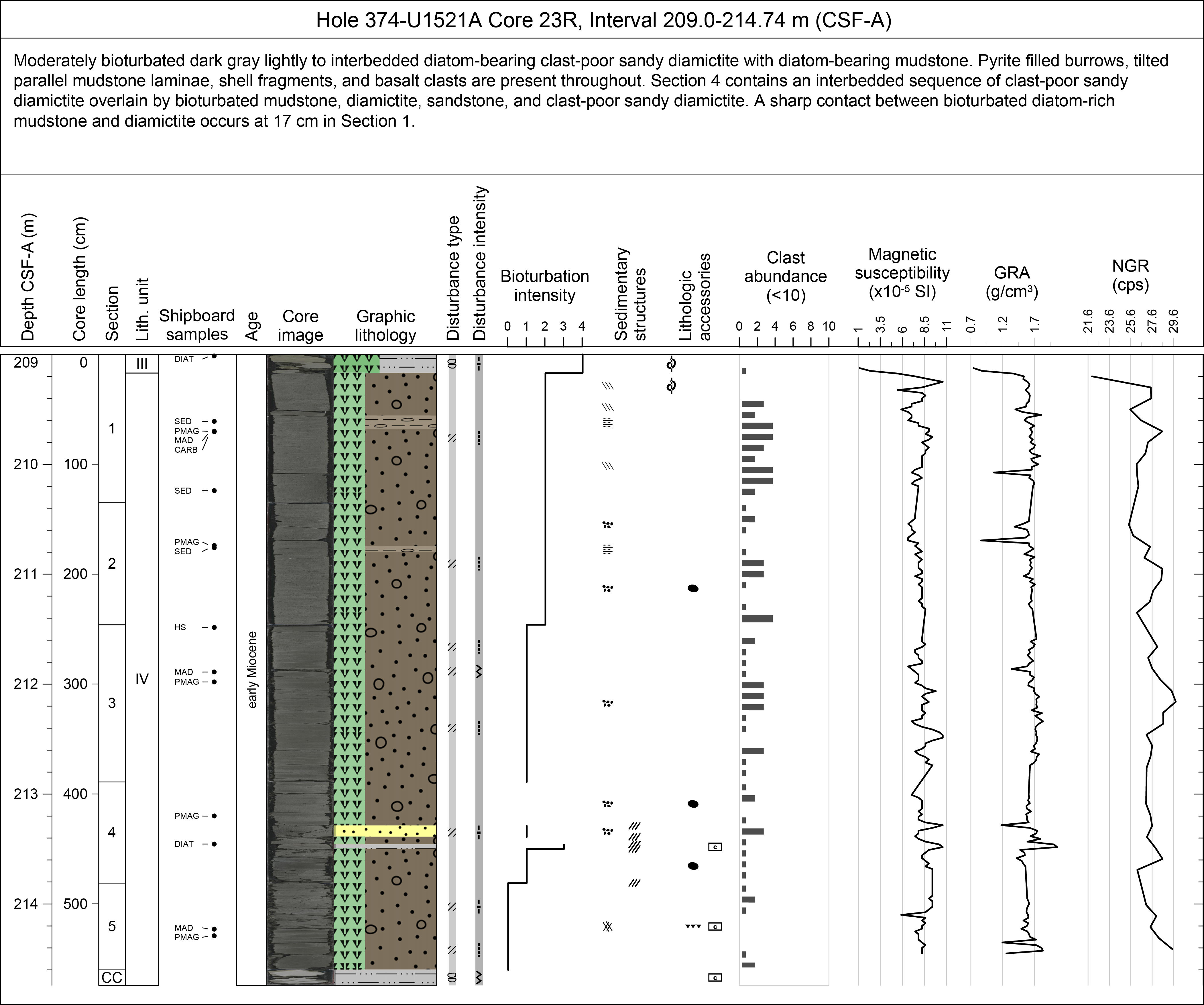
Figure F5. Example VCD.
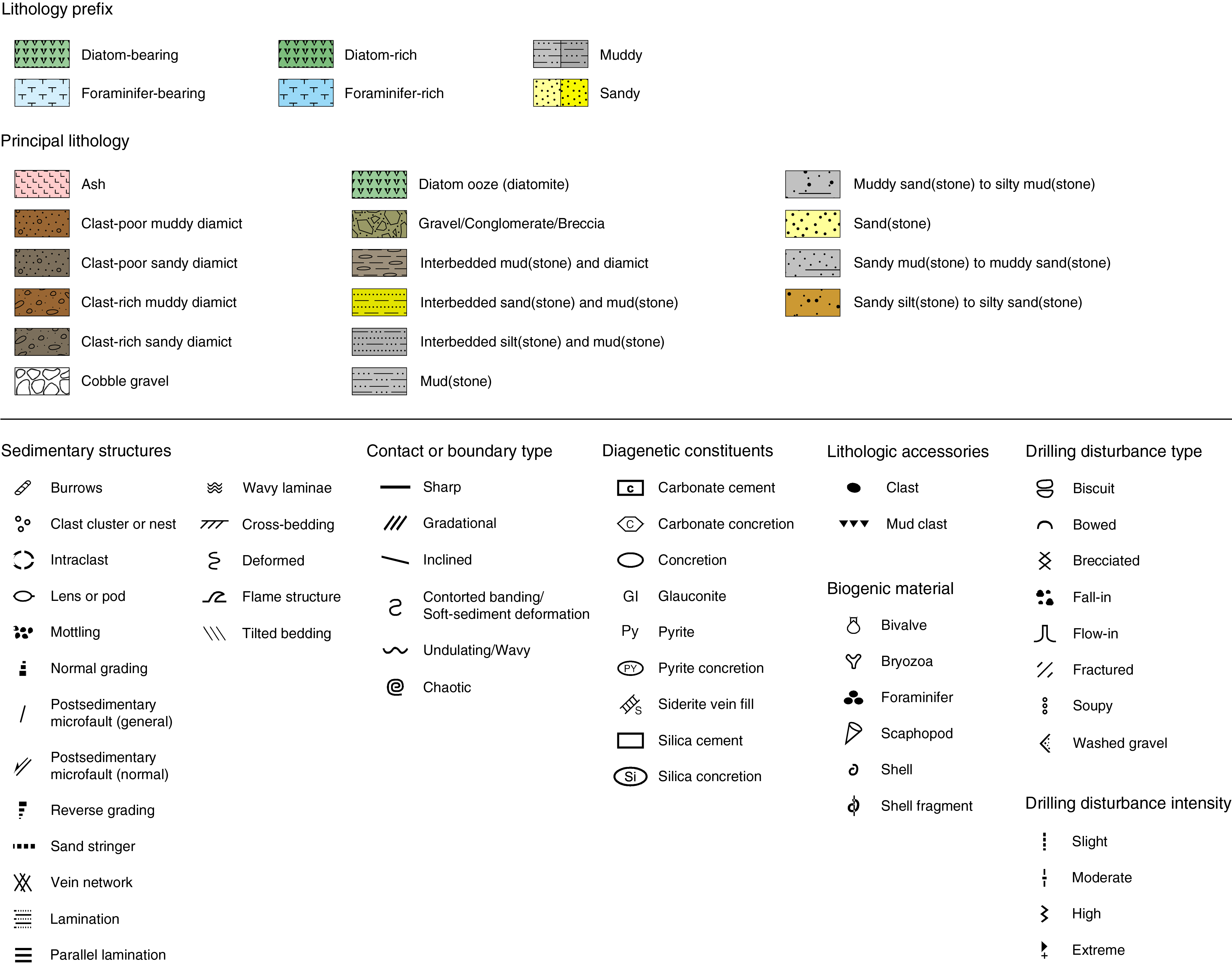
Figure F6. Symbols used for VCDs.
Lithologic classification scheme
Lithologic descriptions were based on the classification schemes used during Ocean Drilling Program (ODP) Leg 178 (Shipboard Scientific Party, 1999), the Cape Roberts Project (Hambrey et al., 1997), the Antarctic Geological Drilling Project (ANDRILL; Naish et al., 2006), and Integrated Ocean Drilling Program Expeditions 318 (Expedition 318 Scientists, 2011) and 341 (Jaeger et al., 2014).
Principal names and modifiers
The principal lithologic name was assigned based on the relative abundances of siliciclastic and biogenic grains (Figure F7). We note that it can be difficult to identify clast relative abundance based on visual description alone and that postcruise computed tomography (CT) scan and grain size analysis results may refine primary lithologies and clast abundance. The principal name is purely descriptive and does not include interpretive classifications relating to fragmentation, transport, deposition, or alteration processes. For each principal name, both a consolidated (i.e., semilithified to lithified) and a nonconsolidated term exist and are mutually exclusive.
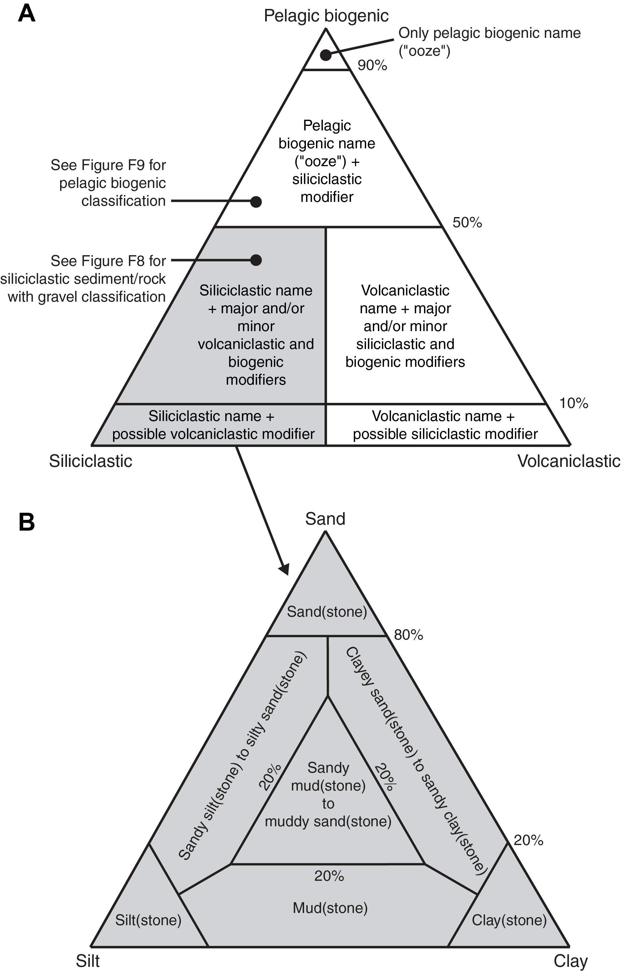
Figure F7. Classification for siliciclastic sediment/rock without gravel.
The principal name of a sediment/rock with >50% siliciclastic grains is based on an estimate of the grain sizes present (Figure F7A). The Wentworth (1922) scale was used to define size classes of clay, silt, sand, and gravel. If the sediment cannot be easily deformed with a finger, the suffix “-stone” is added to the grain size identifier (e.g., sandstone).
If no gravel is present, the principal sediment/rock name was determined based on the relative abundances of sand, silt, and clay (e.g., silt, sandy silt, silty sand, etc.; Naish et al., 2006, after Mazzullo et al., 1988, and Shepard, 1954; Figure F7B). For example, if any one of these components exceeds 80%, the lithology is defined by the primary grain size class (e.g., sand[stone]). The term “mud(stone)” is used to define sediments containing a mixture of silt and clay (these are difficult to separate using visual macroscopic inspection) in which neither component exceeds 80%. Sandy mud(stone) to muddy sand(stone) describes sediment composed of a mixture of at least 20% each of sand, silt, and clay (Figure F7B). The prefix was determined by the percentage >20% of sand versus mud in the matrix (Figure F7B).
If the sediment/rock contains siliciclastic gravel, then the principal name was determined from the relative abundance of gravel (>2 mm) and sand/mud ratio of the clastic matrix, following the textural classifications of Moncrieff (1989), with gravel percent estimated using the comparison chart of Terry and Chilingar (1955) (Figure F8). The term “diamict” is used as a nongenetic term for unsorted to poorly sorted terrigenous sediment that contains a wide range of particle sizes. Accordingly, a clast-poor muddy diamict includes 1%–5% gravel (>2 mm) and 25%–50% sand in matrix, whereas a clast-rich muddy diamict includes 5%–30% gravel and 25%–50% sand in matrix. A clast-poor sandy diamict has 1%–5% gravel and 50%–75% sand in matrix. For a clast-rich sandy diamict, gravel content is 5%–30%, sand content is 50–75%, and the remainder is mud. The term “conglomerate” is used when the matrix includes >30% gravel (Figure F8).

Figure F8. Classification scheme for siliciclastic sediments/rocks with gravel.
The principal name of nonlithified sediment with >50% biogenic grains is “ooze,” modified by the most abundant specific biogenic grain type (Figure F9). For example, if diatoms exceed 50%, then the sediment is called “diatom ooze.” However, if the sediment is composed of 40% diatoms and 15% sponge spicules, then the sediment is termed “biosiliceous ooze.” The same principle applies to calcareous microfossils. For example, if foraminifers exceed 50%, then the sediment is called a “foraminifer ooze,” whereas a mixture of 40% foraminifers and 15% calcareous nannofossils is termed a “calcareous ooze.” “Diatomite” is used for indurated diatom ooze. The term “chert” is used to describe biosiliceous rocks recovered from below the opal-CT transition, where the main biogenic component is not identifiable.
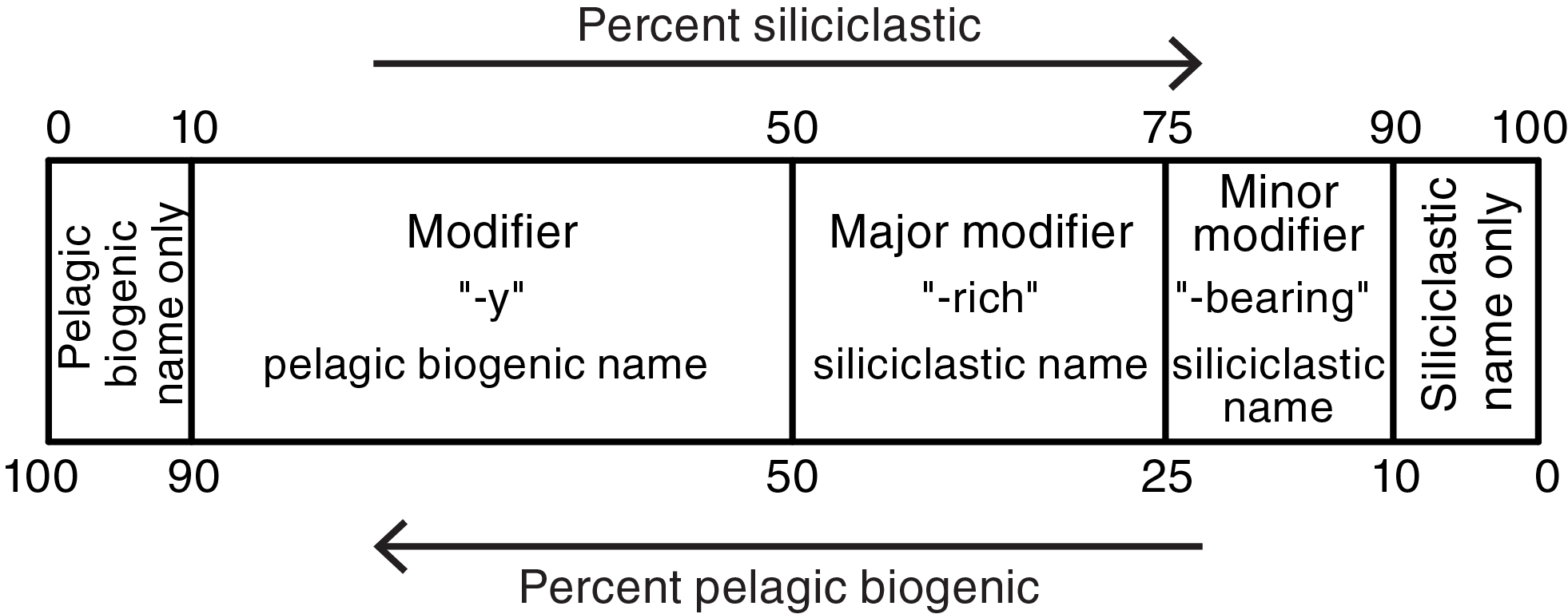
Figure F9. Classification scheme for mixed sediments.
For all lithologies, major and minor modifiers were applied to the principal sediment/rock names following a modified scheme of Expedition 318 (Expedition 318 Scientists, 2011) (Figure F9):
- Major biogenic modifiers are those components that comprise 25%–50% of the grains and are indicated by the suffix “-rich” (e.g., diatom-rich).
- Minor biogenic modifiers are those components with abundances of 10%–25% and are indicated by the suffix “-bearing” (e.g., diatom-bearing).
- Siliciclastic modifiers in biogenic oozes are those components with abundances of 10%–50% and are indicated by the suffix “-y” (e.g., silty, muddy, or sandy).
Lithostratigraphic units
At each site, units were assigned to highlight major lithologic changes downhole. Units were established where a prominent change in sediment lithology matched changes in other sediment characteristics (e.g., color reflectance and magnetic susceptibility). Units are numbered from the top of the stratigraphic succession using Roman numerals. When more subtle significant changes were observed, units were divided into subunits. Subunits are distinguished from the main lithologic units by adding a letter to the unit number (e.g., IA would indicate Unit I, Subunit A).
Sedimentary structures
The locations and types of sedimentary structures visible on the prepared surfaces of the archive-half sections were entered in the Sedimentary structures column of the General tab in the macroscopic DESClogik template. Boundaries between different lithologies are classified as sharp, gradational, inclined, contorted, undulating/wavy, or chaotic. Bedding and lamination were defined by thickness following Mazzullo et al. (1988):
- Thinly laminated (≤3 mm),
- Laminated (3 mm to 1 cm),
- Very thinly bedded (1–3 cm),
- Thinly bedded (3–10 cm),
- Medium bedded (10–30 cm),
- Thickly bedded (30–100 cm), and
- Very thickly bedded (>100 cm).
For units in which two lithologies are interbedded (individual beds are <15 cm thick and alternate between one lithology and another), the term “interbedded” is added before the lithology names and the lithology is considered primary (e.g., interbedded sand and mud, interbedded silt and mud, and interbedded mud and diamict). This terminology is for ease of data entry and graphic log display purposes for VCDs (Figure F6). When beds are distributed throughout a different lithology (e.g., centimeter- to decimeter-thick sand beds within a mud bed), they are logged individually, and the associated bed thickness and grain size ranges are described. The presence of graded beds is also noted. “Normal grading” corresponds to layers with an upward decrease in grain size, whereas “reverse grading” corresponds to layers with an upward increase in grain size.
Deformation of the core identified as unrelated to drilling is also recorded in the Sedimentary structures column using the symbols shown in Figure F6. Symbols include both synsedimentary deformation structures (e.g., flame structures), and postdepositional features (e.g., faults). When possible, direction of displacement (e.g., reverse or normal) is recorded in the comments section. Interval thickness is recorded from the uppermost to the lowermost extent of the described feature, as well as in the comments column of the core description sheet.
Where sediments are diagenetically altered (e.g., mottling or staining with manganese or pyrite, concretions, cement), the diagenetic constituent was entered in the Diagenetic constituent composition column of the General tab in the macroscopic DESClogik template. We define mottles (millimeter to centimeter scale) as spots or smears where material has a different color than the surrounding sediment.
Bioturbation
Ichnofabric description included the extent of bioturbation and notation of distinctive biogenic structures. To assess the degree of bioturbation semiquantitatively, the Droser and Bottjer (1986) ichnofabric index (0–4), modified by Savrda et al. (2001), was used (Figure F10):
- 0 = no apparent bioturbation (≤10%).
- 1 = slight bioturbation (>10%–30%).
- 2 = moderate bioturbation (>30%–60%).
- 3 = heavy bioturbation (>60%–90%).
- 4 = complete bioturbation (>90%).
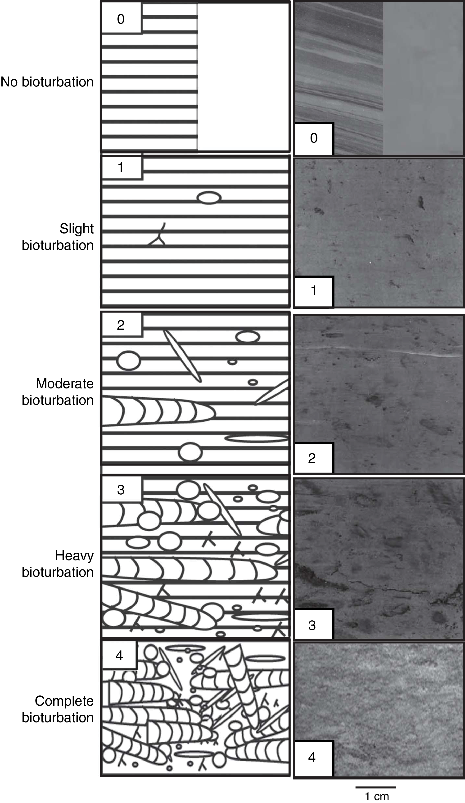
Figure F10. Ichnofabric index legend.
We note that massive muds may be deposited rapidly in glacial environments and record no evidence of bioturbation; they were assigned a value of 0. However, mud may also lack sedimentary structures due to complete bioturbation (e.g., 4 on the ichnofabric index), which may be accompanied by color mottling. This scenario is more likely for deeper water Sites U1523–U1525 than for shallower water continental shelf Sites U1521 and U1522. The ichnofabric index is graphed using the numerical scale in the Bioturbation intensity column of the VCD. When identifiable, ichnofacies (Ekdale et al., 1984) were noted and logged in the General tab of the macroscopic DESClogik template.
Lithologic accessories
Lithologic, paleontologic, and diagenetic features other than those delineated above were entered in the Lithologic accessories column and depicted as symbols in the VCDs (Figure F6). Accessories include macroscopic biogenic remains (e.g., shells, sponge spicules, and bryozoa) and clasts. When possible, clasts and concretions were described by composition.
Clast abundance
Clast abundance was determined on a site-specific basis by counting the clasts visible on the surface of the archive half. Where only holes or depressions caused by lithic or diamict clasts were observed, the working half was also examined to estimate clast abundance. Clasts larger than 2 mm were counted in 10 cm intervals of core. If between one and nine individual clasts were counted per 10 cm, the number of clasts per interval was entered into DESClogik. If 10 or more clasts were present in a 10 cm interval, the number 10 was entered into DESClogik. In these intervals, the modifiers “with dispersed” (<1% clasts; i.e., grains >2 mm), “clast-poor”/“with common” (1%–5% gravel), and “clast-rich”/“with abundant” (5%–30% gravel) were used to denote clast abundance following the Moncrieff (1989) classification (Figure F8). Details on lithology, size, shape, rounding, and surface texture (e.g., striae or faceted faces) are provided in the core description sheets and/or the General interval comments column in DESClogik. Clast counts were ambiguous for the unlithified sediment at Sites U1523 and U1524 and in Cores 374-U1525A-11F through 33X because clasts were sometimes pushed into the subsurface of the core during core splitting or cleaning of the split-core surface; therefore, clast counts for these sites and cores were not recorded.
Drilling disturbance
Core disturbance from the drilling process may alter the cores slightly (e.g., bent/bowed bedding contacts) or greatly (e.g., complete disruption of the stratigraphic sequence) (see Jutzeler et al., 2014, for examples). The style of drilling disturbance is described using the following terms:
- Fall-in: out-of-place material at the top of a core has fallen downhole onto the cored surface.
- Bowed: bedding contacts are slightly to moderately deformed but still subhorizontal and continuous.
- Flowage: severe soft-sediment stretching and/or compressional shearing attributed to coring/drilling. The particular type of deformation may also be noted (e.g., flow-in).
- Soupy: intervals are water saturated and have lost all aspects of original bedding.
- Gas expansion: part of the core is partitioned into pieces and voids due to expansion of interstitial gas. The particular type of deformation may also be noted (e.g., mousse-like).
- Biscuited: sediments of intermediate stiffness show vertical variations in the degree of disturbance. Softer intervals are washed and/or soupy, whereas firmer intervals are relatively undisturbed.
- Fractured: firm sediments are broken but not displaced or significantly rotated (including cracks).
- Fragmented: firm sediments are broken into pieces and rotated, and their stratigraphic position may not be preserved.
- Brecciated: firm sediments are pervasively broken into small and angular pieces with original orientation and stratigraphic position lost, often completely mixed with drilling slurry.
- Washed gravel: fine material was probably lost during drilling, with only washed coarse material, commonly pebbles or cobbles, remaining. Washed gravel often results when coring coarse-grained unconsolidated sediment (e.g., diamict).
The intensity of drilling disturbance (e.g., slight, moderate, high, extreme, or destroyed) was also described in the Drilling disturbance tab of DESClogik and displayed graphically on the VCDs.
Intensity of drilling disturbance of unconsolidated sediments was classified into four categories:
- Slightly disturbed: bedding contacts are slightly bent or bowed in a concave-downward appearance.
- Moderately disturbed: bedding contacts are moderately bent or bowed in a concave-downward appearance but are still visible.
- Highly disturbed: bedding contacts are bent or bowed in a concave-downward appearance but are still visible.
- Extremely disturbed: bedding is completely deformed and may show diapiric or minor flow structures.
Intensity of drilling disturbance of harder sediments (i.e., lithified by compaction or cementation) was classified into four categories:
- Slightly fractured: core pieces are in place and have very little drilling slurry or brecciation.
- Moderately fractured or biscuited: core pieces are from the cored interval and are probably in correct stratigraphic sequence (although the entire section may not be represented); intact core pieces are broken into rotated discs (or “biscuits”) as a result of the drilling process, and drilling mud has possibly flowed in.
- Highly fractured or brecciated: pieces are from the cored interval and are probably in the correct stratigraphic sequence (although the entire section may not be represented), but the original orientation is still visible and drilling mud has flowed in.
- Extremely fractured or brecciated: pieces are from the cored interval and are probably in the correct stratigraphic sequence (although the entire section may not be represented), but the original orientation is totally lost and drilling mud has flowed in.
In addition to drilling-related artifacts, disturbance also occurred during core handling. If a core liner shattered during coring, the pieces were brought onto the catwalk and transferred to a new core liner for curation. This process may result in pieces of core being out of stratigraphic order or inverted relative to their original position. These cores should be considered extremely/highly disturbed. Additionally, the split-core surface of lithologies with relatively high porosity was occasionally disturbed because of excess pressure applied by the point magnetic susceptibility instrument.
Microscopic descriptions
Smear slides
To aid in lithologic classification, the size, composition, and abundance of sediment constituents were estimated microscopically using smear slides (Figure F11). Toothpick samples were taken mostly from the primary lithologies, ideally at a frequency of at least one sample per core. For each smear slide, a small amount of sediment was removed from the section half using a wooden toothpick and put on a 22 mm × 30 mm glass cover glass. A drop of deionized water was added, and the sediment was homogenized and evenly spread across the cover glass. The dispersed sample was dried on a hot plate at a low setting (50°C). A drop of Norland optical adhesive Number 61 was added to a glass microscope slide that was then carefully placed on the dried sample to prevent air bubbles from being trapped in the adhesive. The smear slide was then placed in a UV light box for 5 min to cure the adhesive.
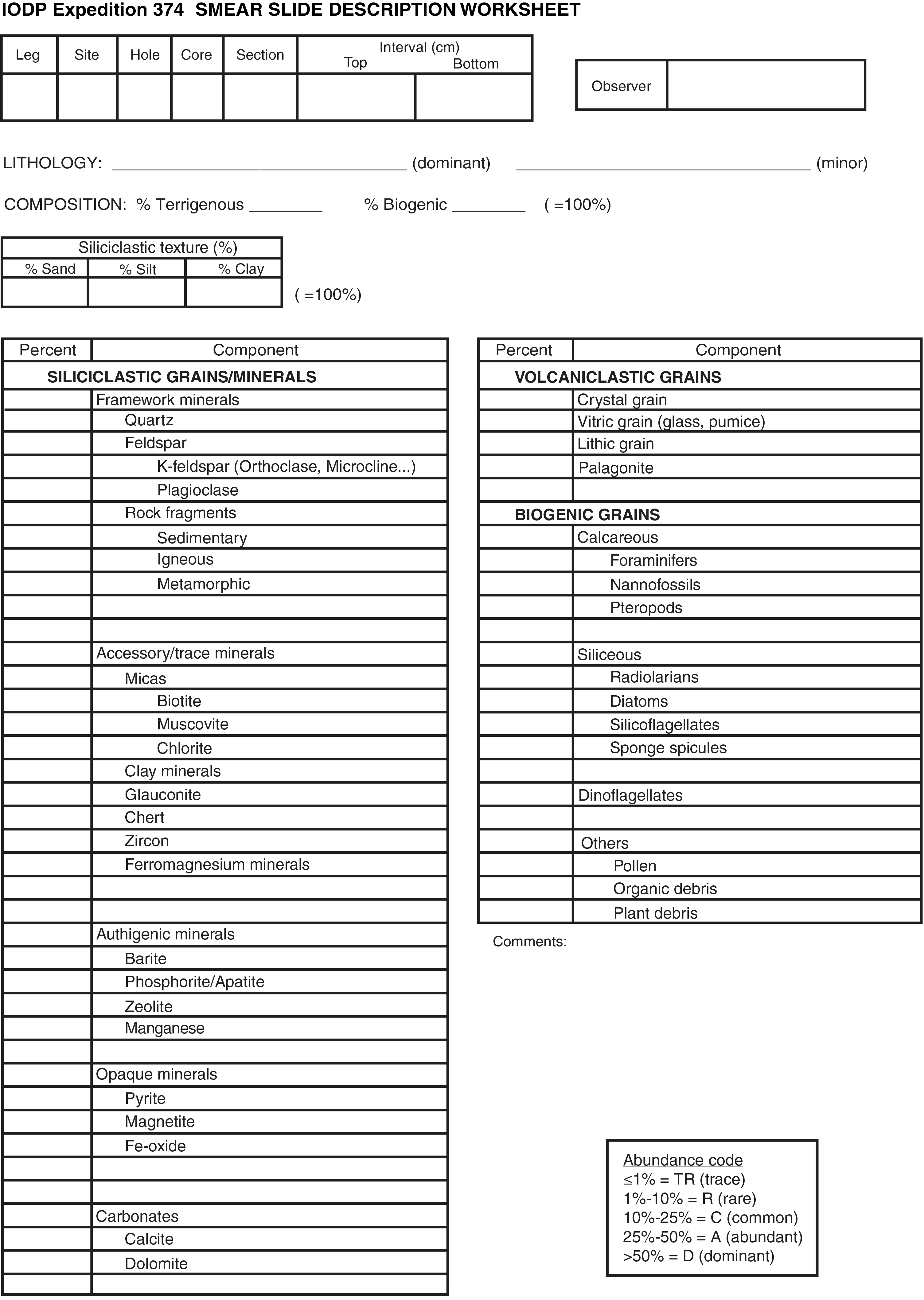
Figure F11. Smear slide description worksheet.
Smear slides were examined with a transmitted-light petrographic microscope equipped with a standard eyepiece micrometer. Biogenic and mineral components were identified following standard petrographic techniques as stated in Rothwell (1989) and Marsaglia et al. (2013, 2015). Several fields of view were examined at 100×, 200×, 400×, and 500× to assess the abundance of detrital, biogenic, and authigenic components. The relative abundance percentages of the sedimentary constituents were visually estimated using the techniques of Rothwell (1989). The texture of siliciclastic lithologies (e.g., relative abundance of sand-, silt-, and clay-sized grains) and the proportions and presence of biogenic and mineral components were recorded in the smear slide worksheet of the microscopic DESClogik template.
Components observed in smear slides were categorized as follows:
- TR = trace (≤1%).
- R = rare (>1%–10%).
- C = common (>10%–25%).
- A = abundant (>25%–50%).
- D = dominant (>50%).
Smear slides provide only a rough estimate of the relative abundance of sediment constituents. Occasionally, the lithologic name assigned based on smear slide observation does not match the name in the macroscopic lithology description because a small sample may not represent the macroscopic description of a much larger sediment interval. Additionally, very fine and coarse grains are difficult to observe in smear slides, and their relative proportions in the sediment can be affected during slide preparation. Therefore, intervals dominated by sand and larger sized constituents were examined by macroscopic comparison to grain size reference charts. Photomicrographs of some smear slides were taken and uploaded to the LIMS database.
Thin sections
Description of indurated sediments and hard rocks were complemented with thin section analysis. Standard and large-sized thin section billets were cut from selected intervals or features as needed, and thin sections prepared on board were examined with a transmitted-light petrographic microscope equipped with a standard eyepiece micrometer. Data were entered into the Thin section tab of the DESClogik microscopic template.
Spectrophotometry and colorimetry
The SHMSL employs multiple sensors to measure bulk physical properties in a motorized and computer-controlled section-half logging instrument. The sensors included in the SHMSL are a spectrophotometer, a point magnetic susceptibility sensor, and a laser surface analyzer. The resolution used for the SHMSL during Expedition 374 was 2.5 cm. Both the magnetic susceptibility sensor and the spectrophotometer require flush contact with the split-core surface, so the archive halves were covered with clear plastic wrap prior to measurement. A built-in laser surface analyzer aids in the recognition of irregularities in the split-core surface (e.g., cracks and voids), and data from this tool were recorded to provide an independent check on SHMSL measurement fidelity. Magnetic susceptibility was measured with a Bartington Instruments MS2 meter and a MS2K contact probe. Instrument details are given in Physical properties. Reflectance spectroscopy (spectrophotometry) was carried out using an Ocean Optics QE Pro detector, which measures the reflectance spectra of the split core from the ultraviolet to near-infrared range. Each measurement was recorded in 2 nm spectral bands from 390 to 732 nm. The data were converted to the L*a*b* color space system, which expresses color as a function of lightness (L*; grayscale) and color values a* and b*, where a* reflects the balance between red (positive a*) and green (negative a*) and b* reflects the balance between yellow (positive b*) and blue (negative b*).
X-ray fluorescence analysis
An Olympus Vanta “M” series pXRF was used on split-core sections to measure elemental composition with a 10–50 kV (10–50 µA) Rh X-ray tube and a high–count rate detector. Measurement time was set at 30 s. The instrument data-correction packages solve a series of nonlinear equations for each analyzed element. The measurement strategy for each site was based on lithologic variability. As a general rule, 2–4 measurements per core were taken in conjunction with carbonate samples (see Geochemistry and microbiology). The “Geochem” and “Soil” methods were used to examine the relative abundance of light and trace elements, respectively. Both methods were run for each measurement. pXRF measurements of standards were performed once per day to track instrument drift. In some cases, other analyses were coordinated with the pXRF measurements. At Sites U1521–U1523, XRD (see below) samples were taken at the same location as pXRF measurements. At Sites U1524 and U1525, pXRF measurements were not made because of instrument failure. The pXRF measurements acquired by the lithostratigraphy group during core description are described in detail in the Geochemistry and Microbiology sections in the site chapters.
XRD analysis
Samples for XRD analysis were selected from the working-half sections, generally at the same depth as sampling for solid-phase geochemistry and pXRF. In general, one 5 cm3 sample was taken per representative lithology for Sites U1521–U1523. Additional samples were occasionally taken and analyzed based on visual core observations (e.g., color variability, visual changes in lithology and texture, etc.) and smear slides. Prior to analysis, unlithified samples were freeze-dried or ground by hand, and lithified samples were ground in an agate ball mill. Prepared samples were top-mounted onto a sample holder and analyzed using a Bruker D-4 Endeavor X-ray diffractometer mounted with a Vantec-1 detector, using nickel-filtered CuKα radiation. The standard locked coupled scan was as follows:
- Voltage = 37 kV.
- Current = 40 mA.
- Goniometer scan = 4°–70°2θ.
- Step size = 0.016599°2θ.
- Scan speed = 1 s/step.
- Divergence slit = 0.3 mm.
Shipboard results yielded only qualitative results of the presence and relative abundances of the most common mineralogical components.
Bulk sample diffractograms were evaluated with the aid of the EVA software package, which allowed for mineral identification and basic peak characterization (e.g., baseline removal and maximum peak intensity identification). Files contain d-spacing values, diffraction angles, and peak intensities with and without the background removed. These files were scanned by the EVA software to find d-spacing values characteristic of a limited range of minerals using aluminum oxide as an external standard (Expedition 317 Scientists, 2011). Muscovite/illite and kaolinite/chlorite have similar diffraction patterns and were not distinguished on board. Digital files with the diffraction patterns are available from the LIMS database.
Biostratigraphy and paleontology
Fossil marine diatoms, radiolarians, planktonic and benthic foraminifers, organic-walled dinoflagellate cysts (dinocysts), and calcareous nannofossils provided preliminary shipboard biostratigraphic and paleoenvironmental information. All microfossil groups aided in characterizing paleoenvironmental conditions such as proximity to glacial influence, changes in water masses, relative water depth, and sea ice presence or absence and in identifying intervals reflecting sedimentation from open-marine biogenic productivity or intervals reflecting “glacial” influence with low microfossil abundance, poor preservation, fragmentation due to pervasive reworking (e.g., a mixture of ages), and other preservational impacts from bottom currents or dissolution. Shipboard biostratigraphic age assignments were based on analysis of microfossils from all mudline and core catcher sediment samples, which were shared among the micropaleontology groups. Where necessary, additional toothpick (and/or plug) samples from split-core sections were analyzed to refine biostratigraphic boundaries, examine critical intervals and distinct lithologies, or investigate the material above and below significant changes in lithology. At sites where two or more holes recovered the same stratigraphic interval, all core catcher samples were examined from all holes.
Biostratigraphic zonations for microfossil groups are presented individually in the representative sections below and integrated into Figure F12. Diatoms and radiolarians provided the most biostratigraphic control for all intervals cored during Expedition 374 (Miocene to recent; ~19 to 0 Ma). Ages assigned to datum levels for these two groups were guided by the composite ordering of events and model age output from constrained optimization (CONOP) analyses of Southern Hemisphere data sets (Cody et al., 2008), ANDRILL Core AND-1B (Cody et al., 2012), and ODP Site 744 (Florindo et al., 2013). The CONOP analysis presented in Florindo et al. (2013) benefitted from the inclusion of radiolarian biostratigraphic data in the Southern Ocean database managed by GNS Science (Wellington, New Zealand), which continues to add and integrate diatom, radiolarian, calcareous nannofossil, and foraminifer biostratigraphic events toward a digital composite sequence for the Neogene and late Paleogene. Elements of the diatom biostratigraphic zonations for the Southern Ocean (Harwood and Maruyama, 1992; Censarek and Gersonde, 2002, among others) and Antarctic continental shelf (Olney et al., 2007; Winter et al., 2012) are integrated in Figure F12. The radiolarian biostratigraphic zones are a combination of the middle Miocene to Pleistocene zonation defined and refined by Lazarus (1990, 1992) and supplemented by the early to middle Miocene zonation developed by Abelmann (1992) (Figure F12). Biostratigraphic zones of austral temperate planktonic foraminifers are based on Jenkins (1993) with datum ages derived from the New Zealand Geological Timescale and correlated with New Zealand Series and Stages from Crundwell et al. (2016). Correlation with the tropical–subtropical zonation and the Gradstein et al. (2012) geomagnetic polarity timescale (GTS2012) (Wade et al., 2011) is provided in Figure F12. Neogene dinocyst biostratigraphy is developing, and tentative placement of biostratigraphic datums for selected Southern and Northern Hemisphere high latitudes and Northern Hemisphere mid-latitudes is taken from Bijl et al. (2015) (Figure F12). Calcareous nannofossils are rare in Neogene southern high-latitude sections, with few biostratigraphic events. Consequently, the standard biostratigraphic zonations of Martini (1971) and Okada and Bukry (1980) are of limited usefulness. Instead, individual events correlated with the GTS2012 geomagnetic polarity timescale were applied when possible. Biostratigraphic events and zonal boundaries for these groups were compiled in reference to the GTS2012 and are presented in Figure F12.
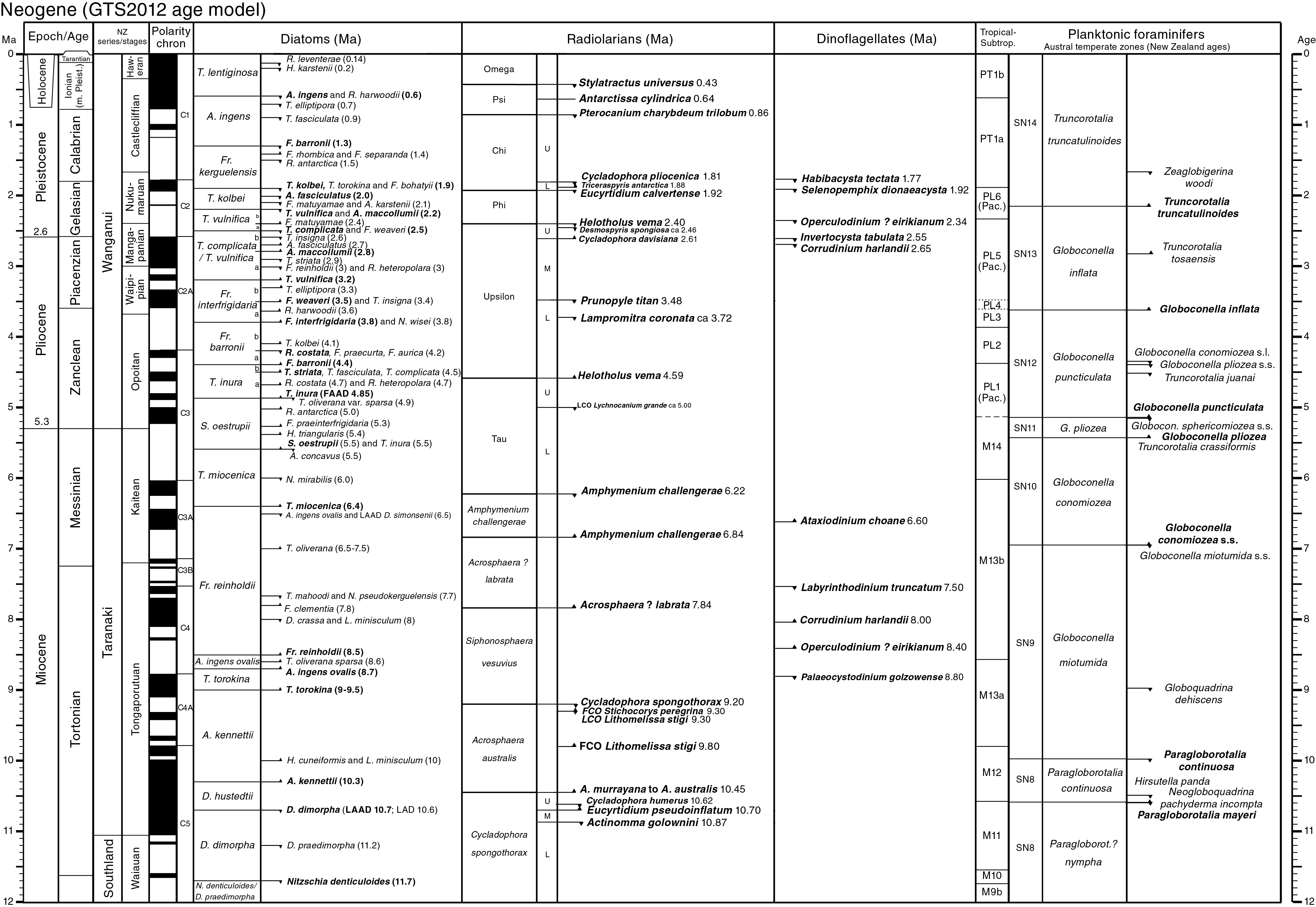

Figure F12. Global and New Zealand chronostratigraphy and microfossil datums.
Data for each microfossil group are presented in the form of taxonomic distribution charts that record occurrences by samples examined in each hole. Relative abundance and preservation data were entered through the DESClogik application into the LIMS database for all identified microfossil taxa and all paleontological data gathered during shipboard investigations. These data are available from the LIMS database. Taxonomic occurrence charts also record suspected upsection reworking or otherwise out-of-place species. The first figure in the Biostratigraphy and paleontology section of each site chapter presents a summary of biostratigraphical and paleoenvironmental information provided by each microfossil group. An age-depth figure based on selected biostratigraphic datum levels identified in an accompanying table is also included, and it identifies the location and approximate duration of unconformities.
Distribution charts for microfossil groups presented in each site chapter are based on shipboard study only. Shipboard biostratigraphic studies focused primarily on identifying biostratigraphic horizons (biohorizons) in the cores and are biased toward the reporting of age-diagnostic species and identifying intervals and ages of reworking. Reported events include the last appearance datum (LAD) or first appearance datum (FAD) of a taxon’s stratigraphic range, in some cases with modification to identify the last common occurrence or first common occurrence to in turn identify an abundance change within a taxon’s range if it is more reliable for correlation. Identification of a sequence of biohorizons in stratigraphic order allowed recognition of biostratigraphic zones and subzones using standard schemes. Tables in each site chapter present the depth and age of important bioevents for use in constructing age-depth plots in which biostratigraphic information is integrated with the magnetic polarity stratigraphy, if available, to produce an age model for each site. These age models are based on preliminary shipboard data and will be updated with postcruise research.
Diatoms
Diatom taxonomy
Taxonomic concepts for Neogene Antarctic diatoms, many of which are endemic to the southern high latitudes, have developed largely through the last 45 y of stratigraphic drilling by Deep Sea Drilling Project (DSDP) and ODP in the Southern Ocean and Antarctic shelf (McCollum, 1975; Schrader, 1976; Gombos, 1976; Ciesielski, 1983; Gersonde and Burckle, 1990; Gersonde, 1990, 1991; Fenner, 1991; Baldauf and Barron, 1991; Harwood and Maruyama, 1992; Mahood and Barron, 1996; Gersonde and Barcena, 1998; Iwai and Winter, 2002; Censarek and Gersonde, 2002; Zielinski and Gersonde, 2002; Arney et al., 2003; Bohaty et al., 2003; Whitehead and Bohaty, 2003). In parallel to the above efforts, ice platform drilling on the Antarctic margin recovered neritic diatom flora that serve as useful taxonomic references on the Antarctic shelf (Harwood 1986, 1989; Winter and Harwood, 1997; Harwood et al., 1998; Bohaty et al., 1998; Scherer et al., 2000; Olney et al., 2007, 2009; Winter et al., 2012; Sjunneskog et al., 2012). Other useful taxonomic references for Neogene and modern Antarctic marine diatoms include Fenner et al. (1976), Akiba (1982), Harwood et al. (1989), Yanagisawa and Akiba (1990), Medlin and Priddle (1990), Cremer et al. (2003), and Scott and Thomas (2005).
Methods for diatom study
Upon receipt of a core catcher sample, ~1 cm3 of sediment was placed in a disposable 15 mL centrifuge tube with a screw cap, and the tube was filled to ~13 mL with deionized water. Sediment and water in the centrifuge tube was mixed thoroughly with a pointed metal spatula and shaken repeatedly to aid disaggregation. This suspension of “raw” sediment from the core catcher samples was used as a “stock” suspension from which future preparation steps could be made. Slides made from this material represent an equivalent of smear slides but allow for a more uniform and random distribution of the sediment on the cover glass. Fossil marine diatoms were analyzed initially from strewn slides prepared by removing a random aliquot of suspended sediment from the thoroughly mixed stock suspension with a disposable pipette. One drop of suspended raw sediment from core catcher samples was dropped into a “bead” of water and ethanol (mixed at a 5:1 ratio) with a meniscus “dome” of water ~2 mm high that had been warming on a cover glass (30 mm × 20 mm). The temperature difference between the drop of sediment suspension (room temperature) and water-alcohol solution warming on the cover glass, as well as interaction between the suspended sediment and alcohol solution, led to rapid motion of particles on the cover glass and an even and random distribution of particles, which were allowed to dry completely on the cover glass on the hot plate. The cover glass was then mounted on a labeled glass slide with Norland optical adhesive Number 61 (refractive index = 1.56) and cured under a UV lamp until solid.
For samples in which siliceous microfossils are very rare or highly fragmented, which is common in glaciomarine shelf environments (e.g., Harwood et al., 1989; Sjunneskog and Scherer, 2005) and was the situation with most core catcher samples examined during Expedition 374, a process involving sieving the sediment suspension through a 20 µm sieve helped concentrate the diatoms and recover whole or nearly whole diatom valves that could be identified. Suspended sediment samples disaggregated during H2O2 and borax treatment for radiolarian and foraminifer study (see Radiolarians and Foraminifers) were provided for diatom study of their residual <63 µm size fraction. By making strewn slides in a similar fashion to that described above, examination of the <63 to >20 µm size fraction for diatoms allowed for the recovery of identifiable diatom specimens in most samples. However, this concentration effect, which is essential for providing a sufficient number of identifiable specimens to allow rapid age interpretations of core catcher samples, likely increased the presence of large, heavily silicified, and reworked species and removed or reduced the number of biostratigraphically important smaller diatoms from these slides.
To separate and concentrate these smaller diatoms from the abundant clay-sized suspension of clay, fine silt, and abundant small diatom fragments, a method of timed gravity settling was employed to concentrate more complete small diatoms. In this process, much of the clay-sized component remained in suspension and diatoms were concentrated by settling to the bottom of a 15 mL centrifuge tube. This process involved extracting ~2 mL of suspended raw sample from the thoroughly mixed suspension in the stock 15 mL centrifuge tube with a disposable pipette. After thorough shaking to mix the suspension, it was allowed to stand vertically for 30 s to allow coarse particles to settle to the bottom. Bubbles were then injected by pipette into the suspension at ~2 cm from the base of the tube to mix and randomize the suspension above that level. The 2 mL aliquot was introduced gently into the uppermost 2 cm of a 15 mL centrifuge tube filled with 12 mL of deionized water. The pipette end was moved in a gentle circular motion in the top of the water-filled tube as the 2 mL sample was slowly inserted into the upper water column. The resulting diluted suspension was allowed to settle undisturbed for 30 min. During this time, diatom valves of all sizes, including small diatoms, and sediment particles settled to or near the bottom. After 30 min of undisturbed settling, all material that settled to the bottom of the tube, as well as the lowest 2 cm of the water column, was extracted by a pipette and placed into a vial for storage. If additional diatom concentration and clay removal was required, the material extracted from the base of the tube was injected into another water-filled centrifuge tube to repeat this process of separating clay-sized suspension from settled diatoms. Strewn slides were made of the resuspended settled material with the strewn-slide approach described above. If necessary, the “bubble method” of Harwood (1986) was employed to further separate siliciclastic sediment grains and sediment particles from the hydrodynamically lighter diatoms in the >20 µm size fraction sample vial before extracting suspended material for preparation of strewn slides. In some cases, an additional concentration step was taken to remove clay and concentrate diatoms by allowing suspended sediment to settle for 15 to 30 s within the vertically held transfer pipette before adding the initial drops of sediment-laden suspension into the bead of water warming on the cover glass. Diatoms are preferentially concentrated in the lower portion of the suspended water column in the transfer pipette.
Samples were examined using a Zeiss Axioskop.A1 transmitted-light microscope. Photomicrographs were taken using a SPOT Flex 64 Mp digital camera and uploaded to the LIMS database. A Hitachi TM3000 tabletop scanning electron microscope (SEM) was used for higher magnification micrographs of selected specimens. Qualitative siliceous microfossil group abundances were determined from strewn slides using 630× magnification. Care was taken to ensure strewn slides were prepared with similar amounts of sediment. For each sample, the diatom abundance was qualitatively estimated by light-microscopic observations at 630× magnification with the examination of five random fields of view (FOVs) as follows:
- A = abundant (>5 complete valves per FOV).
- C = common (2 to 5 complete valves per FOV).
- F = frequent (1 complete valve in 1 to 5 FOVs).
- R = rare (1 complete valve in 6 to 30 FOVs).
- Tr = trace (very rare valves or diatom fragments).
- B = barren (no diatom valves or fragments observed).
Relative abundances of individual taxa were categorized in reference to their occurrence in FOVs or in reference to one traverse across a 30 mm wide cover glass (~55 FOVs) as follows:
- D = dominant (>10 valves per FOV).
- A = abundant (>5 and <10 valves FOV).
- C = common (1–5 valves per FOV).
- F = frequent (1 valve in every 10 FOVs).
- R = rare (<5 valves per traverse).
- X = trace (<1 valve per traverse or fragments noted).
Shipboard observations of diatom assemblages logged in DESClogik focused on the presence of age-diagnostic species, so the distribution data do not represent the full diatom assemblage. All diatom semiquantitative abundance data produced onboard were logged in DESClogik.
Preservation of individual siliceous microfossil groups was determined qualitatively and reported in the following terms of fragmentation and/or dissolution:
- G = good preservation (little or no evidence of dissolution/recrystallization or fragmentation; primary morphological characteristics were only slightly altered; specimens were identifiable to the species level).
- M = moderate preservation (specimens exhibit some etching/recrystallization and/or fragmentation; primary morphological characteristics were somewhat altered; most specimens were identifiable to the species level).
- P = poor preservation (specimens were severely dissolved/replaced and/or fragmented; primary morphological characteristics were largely destroyed; specimens were identified at the genus level, but species identification was often difficult).
Age assignment
Initial shipboard age assignment of individual Neogene samples was based on diatom biostratigraphy by applying the biostratigraphic zonation for Southern Ocean sites of Harwood and Maruyama (1992) (Oligocene to recent) and Censarek and Gersonde (2002) and for Antarctic continental shelf sites by applying the zonations of Winter et al. (2012) (Plio–Pleistocene) and Olney et al. (2007) (Oligocene to early Miocene). A wealth of biostratigraphic information is available from core-based studies listed in Diatom taxonomy and the integrated biochronological syntheses in the associated volumes for each leg/expedition (e.g., Gersonde et al., 1990; Barron et al., 1991; Harwood et al., 1992). Ages applied to specific diatom events and zonal boundaries were guided by successive iterations of the diatom biochronology afforded by CONOP analysis (Cody et al., 2008, 2012; Florindo et al., 2013) and are in general agreement with ages of appearance and extinction of Southern Ocean endemic planktonic diatoms presented in Barron (2003). Age assignments for diatom datum levels are presented in Figure F12 and Table T1.
Radiolarians
Radiolarian taxonomy and zonal schemes
The main taxonomic concepts for the Neogene radiolarians studied here are from Petrushevskaya (1975), Caulet (1991), Nigrini and Lombari (1984), Lombari and Lazarus (1988), Lazarus (1990, 1992), Abelmann (1992), Nigrini and Sanfilippo (2001), and Vigour and Lazarus (2002). All radiolarian semiquantitative abundance data produced on board were logged in DESClogik and are available in downloadable large-format tables for each site.
The Southern Ocean radiolarian zones introduced by Lazarus (1990, 1992) and Abelmann (1992) were collated and applied here, and the composite zonation is shown in Figure F12. Lazarus (1992) refined the middle Miocene to Pleistocene zonation previously established by Lazarus (1990) based on material recovered during ODP Legs 119 and 120. The early to middle Miocene is represented by the zonation developed by Abelmann (1992) based on Leg 120 material.
The original age estimates for Neogene radiolarian datums are based on their calibration to magnetostratigraphy according to Hays and Opdyke (1967), Gersonde et al. (1990), Barron et al. (1991), Caulet (1991), Abelmann (1992), Lazarus (1992), Harwood et al. (1992), Shackleton et al. (1995), and Kamikuri et al. (2004). To directly integrate radiolarian and diatom biostratigraphic results, we adopted the CONOP estimates for the ages of radiolarian events presented in Table T2 (Hybrid model column; for details see Florindo et al., 2013). The age estimates for the few radiolarian datums not included in Florindo et al. (2013) have been recalibrated to the GTS2012 using the Neptune Sandbox database (http://www.nsb-mfn-berlin.de) and are shown in the rightmost column in Table T2.
Methods for radiolarian study
A ~10 cm3 sediment sample was disaggregated in a beaker containing ~50 mL of water by adding a 10% solution of hydrogen peroxide together with an arbitrary amount of dilute borax and gently warming it on a hot plate. After effervescence subsided (typically after 30 min to 1 h), the suspension was washed through a 63 µm sieve. Two strewn slides per sample were prepared by pipetting the >63 µm residue onto a 22 mm × 50 mm microscope cover glass that was dried on a hot plate. Twelve drops of Norland optical adhesive Number 61 mounting medium was applied to the 25 mm × 75 mm glass slide. The cover glass with dried sediment was then inverted and placed gently on the slide. The mounting medium was fixed by placing the slide under an ultraviolet lamp for approximately 15 min. Species were identified, and their abundances were estimated using a Zeiss Axioplan microscope with bright-field illumination at 100× and 200× magnification. Photomicrographs were taken using a SPOT Flex 64 Mp digital camera and uploaded to the LIMS database. A Hitachi TM3000 tabletop SEM was used for higher magnification micrographs of selected specimens.
For each sample, the total abundance of radiolarians was estimated qualitatively by light-microscopic observations at 100× magnification along one horizontal traverse of the cover glass and recorded as follows:
- A = abundant (>100 specimens/traverse).
- C = common (51–100 specimens/traverse).
- F = frequent (11–50 specimens/traverse).
- R = rare (1–10 specimens/traverse).
- Tr = trace (1–10 specimens/slide).
- B = barren (absent).
Shipboard observations of radiolarian assemblages logged in DESClogik focused on the presence of age-diagnostic species, so the distribution data do not represent the full radiolarian assemblage.
Qualitative estimates of individual species abundances were also recorded by scanning through both slides at 100× magnification, according to the following scheme:
- A = abundant (≥2 specimens/FOV).
- C = common (1 specimen/FOV).
- F = frequent (1 specimen/2–5 FOVs).
- R = rare (1 specimen/5–30 FOVs).
- X = present (≤1 specimen/traverse).
Preservation of the radiolarian assemblages was recorded as follows:
- G = good (most specimens complete; fine structures preserved).
- M = moderate (minor dissolution and/or breakage).
- P = poor (common dissolution, recrystallization, and/or breakage).
Foraminifers
Planktonic foraminifer taxonomy and zonal schemes
Neogene planktonic foraminifer taxonomic concepts follow those of Jenkins (1971), Kennett (1973), Kennett and Vella (1975), Jenkins (1978), Hornibrook (1982), Kennett and Srinivasan (1983), Leckie and Webb (1985), Cifelli and Scott (1986), Hornibrook et al. (1989), Scott et al. (1990), Berggren (1992), and Majewski (2010), as well as those compiled in the online pforams@mikrotax database (http://www.mikrotax.org/pforams).
For sediment intervals deposited under the influence of tropical–subtropical water, the Cenozoic zonal scheme of Wade et al. (2011) with datum ages from Gradstein et al. (2012) are most appropriate. Given our southern high-latitude location, the Subantarctic zonal scheme of Berggren (1992; Leg 120, Kerguelen Plateau) and austral temperate zonal scheme of Jenkins (1993) were utilized with ages updated to the GTS2012, as well as datums used by GNS Science for planktonic foraminifer biostratigraphy (Crundwell et al., 2016). In addition, biostratigraphically important species used to define the base of New Zealand series and stages were also used (Raine et al., 2015) (Figure F12). Note that a magnetostratigraphically calibrated mid-latitude planktonic foraminifer zonal scheme for New Zealand and the Southwest Pacific region is currently lacking. Ages for planktonic foraminifer events used here are shown in Figure F12 and Table T3.
Benthic foraminifer taxonomy
The taxonomy of modern and Pleistocene benthic foraminifers of the Ross Sea continental shelf and slope follows McKnight (1962), Pflum (1966), Kennett (1968), Echols (1971), Fillon (1974), Anderson (1975), Osterman and Kellogg (1979), Ward and Webb (1986), Ward et al. (1987), Ishman and Domack (1994), Igarashi et al. (2001), and Majewski (2005, 2013). Key references for Oligocene–Neogene Ross Sea benthic foraminifers include D’Agostino (1980), Leckie and Webb (1986), Webb (1989), Coccioni and Galeotti (1997), Galeotti et al. (2000), Strong and Webb (2000, 2001), Webb and Strong (2006), Patterson (2010), Patterson and Ishman (2012), and Majewski et al. (2017). Taxonomic assignments of continental rise and slope Sites U1524 and U1525 mainly follow Mead (1985), Boersma (1986), van Morkhoven et al. (1986), Miller and Katz (1987), Hornibrook et al. (1989), Thomas (1990), Katz and Miller (1991), Nomura (1991, 1995), Mackensen (1992), and Holbourn et al. (2013). The classification of Loeblich and Tappan (1988) was followed for determinations at the genus level.
Foraminifer-based paleoenvironmental analysis
Planktonic foraminifers are rare on the Ross Sea continental shelf but become increasingly abundant in deeper water settings of the slope and rise. The distribution of planktonic foraminifers around Antarctica is strongly zonal (e.g., Bé, 1969) and is controlled by the distribution of surface water masses and dynamic oceanographic fronts, including the Antarctic Polar Front and Subantarctic Front (e.g., Nelson and Cooke, 2001; Sokolov and Rintoul, 2002). Incursions of subantarctic or temperate water taxa into the Ross Sea may be associated with changes in sea ice cover and productivity or times of extreme warmth, including superinterglacials of the late Neogene and Quaternary. Degree of test encrustation and ratio of left-coiling Neogloboquadrina pachyderma to right-coiling Neogloboquadrina incompta are also useful proxies of surface water mass properties (e.g., Asioli and Langone, 1997; Bergami et al., 2009).
The carbonate compensation depth (CCD) is much shallower in the Ross Sea today than in the open ocean (e.g., ~400–650 m; Kennett, 1966; also see Echols, 1971; Igarashi et al., 2001). The calcareous to agglutinated benthic foraminifer ratio was estimated to track changes in the CCD or water mass corrosiveness through time.
Quaternary benthic foraminifers have been found to track ice proximal, ice distal, and open-marine hemipelagic and pelagic lithofacies in the Ross Sea (e.g., Osterman and Kellogg, 1979; Ward et al., 1987; Melis and Salvi, 2009; Majewski et al., 2018). Benthic foraminiferal diversity, abundance, preservation, fragmentation, and reworking are additional proxies of paleoenvironmental conditions at the seafloor.
To assess benthic foraminiferal paleoecology, taxa were allocated into morphogroups following Corliss (1985, 1991), Jones and Charnock (1985), and Corliss and Chen (1988). Benthic foraminifers with planoconvex, biconvex, rounded trochospiral, tubular, coiled flattened, milioline, and palmate tests are inferred to have had an epifaunal mode of life (living at the sediment surface or in the upper centimeter of the sediment). Infaunal foraminifers living in the deeper layers of sediment have cylindrical or flattened tapered, spherical, rounded planispiral, flattened ovoid, globular unilocular, or elongate multilocular tests. The comparison between fossil and recent foraminifers is not straightforward, and for many taxa the close relationship between test morphology and microhabitat has not been observed but instead is extrapolated from data on other taxa (e.g., Jorissen, 1999), so the relationship between morphology and microhabitat may not always be certain (Buzas et al., 1993). Morphogroup analysis is used as a proxy for combined oxygenation and food availability in the deep ocean (Jorissen et al., 2007).
The comparison of fossil and recent assemblages and the occurrence and abundance of depth-related species and their upper depth limits (e.g., Hayward, 1986; van Morkhoven et al., 1986; Hayward et al., 2013) allowed us to infer a paleobathymetry for sediment intervals at each site. Antarctic margin species depth information is based on Kennett (1968), Echols (1971, for agglutinated taxa), Fillon (1974), Anderson (1975), Osterman and Kellogg (1979), and Patterson and Ishman (2012). Paleodepth zones follow van Morkhoven et al. (1986) using the following categories:
Methods for foraminifer study
Sediment was soaked in a solution of 10% hydrogen peroxide and borax (~5 tablespoons/L) for at least 30 min and then heated on a hot plate for 15–20 min. The sediment was then washed with tap water over a 63 µm wire mesh sieve. The <63 µm fraction was captured in a beaker for diatom strewn-slide and sieved preparations. Stiffer or semilithified sediments were chopped into smaller particles using a sharp-edged tool or crushed into pea-sized pieces using a hammer. All samples were dried on filter paper on a low-temperature hot plate with careful attention paid to not burn the sample.
Each dried >63 µm sample residue was sprinkled on a black-gridded picking tray and examined under a Zeiss Discovery V8 binocular light microscope for benthic and planktonic foraminifers. Photomicrographs were taken using a SPOT idea digital camera and uploaded to the LIMS database. Individual specimens were picked from the sample using a very fine brush and mounted on a gridded cardboard slide coated with a thin layer of water-soluble paste made from gum tragacanth powder. For samples that required further size separation, the >63 µm residue was dry-sieved through a series of sieves with 710, 250, and 125 μm wire mesh. Species identifications were generally made on the 250 to 710 μm and 125 to 250 μm size fractions; time permitting, the 63 to 125 μm size fraction was scanned for small or rare species.
The preservation state of planktonic and benthic foraminifers was estimated as follows:
- E = excellent (totally glassy specimens with no to very little evidence of overgrowth, dissolution, or abrasion).
- VG = very good (some minor evidence of overgrowth, dissolution, or abrasion).
- G = good (little evidence of overgrowth, dissolution, or abrasion).
- M = moderate (common but minor calcite overgrowth, dissolution, or abrasion).
- P = poor (substantial overgrowth, dissolution, or fragmentation).
The planktonic to benthic foraminifer ratio (P/B) was visually estimated as a first approximation of carbonate dissolution.
The following foraminifer group abundance categories relative to total sediment particles were estimated from visual examination of the dried sample in the >63 μm fraction:
- D = dominant (>50% of sediment particles).
- A = abundant (>25%–50% of sediment particles).
- C = common (>10%–25% of sediment particles).
- F = few (>5%–10% of sediment particles).
- R = rare (>1%–5% of sediment particles).
- P = present (<1% of sediment particles).
- B = barren.
For a given sample, the percentage of key planktonic and benthic foraminifer species in the >63 μm fraction were categorized as follows:
- D = dominant (>30% of species on the tray).
- A = abundant (>10%–30% of species on the tray).
- C = common (>10%–25% of species on the tray).
- F = few (>5%–10% of species on the tray).
- R = rare (>1%–5% of species on the tray).
- P = present (<1% of species on the tray).
Palynology
Dinocyst taxonomy and zonation scheme
Dinocyst taxonomy follows Williams et al. (2017), Clowes et al. (2016), and Bijl et al. (2018a). The most recent update of a globally integrated, magnetostratigraphically calibrated dinocyst stratigraphy for the Neogene is presented in Bijl et al. (2015). No complete integrated stratigraphic dinocyst framework exists currently for the Neogene of the Southwest Pacific. Biomagnetostratigraphic information for dinocysts from the Oligocene and early to middle Miocene are available from Integrated Ocean Drilling Program Expedition 318 Hole U1356A (Bijl et al., 2018a). Palynological records from DSDP Leg 28 (Kemp, 1975), ODP Leg 188 Site 1165 (Hannah, 2006), Cape Roberts Project drilling (Hannah et al., 2000; Clowes et al., 2016), and ODP Leg 178 (Harland and Pudsey, 2002) also serve as reference schemes. Here, we report the FADs and LADs for Neogene dinocyst taxa found in the Southern Hemisphere mid-latitudes, Northern Hemisphere mid-latitudes, and Northern Hemisphere high latitudes, all calibrated to the GTS2012 (Table T4) as reported in Bijl et al. (2015) and references therein. The dinocyst event data shown in Figure F12 are a selection based on species encountered during Expedition 318 of those reported in Table T4.
Methods for palynology study
Approximately 20 g of sediment was processed according to standard palynological laboratory protocols (e.g., Brinkhuis et al., 2003). Samples were digested with 30% HCl and cold 40% HF to dissolve carbonate and silicate materials, respectively, followed by 10% HCl leaching to remove silicate gels, with centrifuging and decanting after each step. Residues were sieved with nylon 250 and 10 μm sieves, put through an ultrasonic bath, and subsequently mounted on glass microscope slides using glycerine jelly. Species identification and data collection were carried out with a Zeiss Axiophot microscope using bright-field illumination at 400×, 630× (oil), and 1000× (oil) magnification. Photomicrography was conducted using a SPOT Flex 64 Mp digital camera, and images were uploaded to the LIMS database.
Palynomorph abundance and preservation
Palynofacies were grouped into the following broad categories:
- In situ marine organic-walled dinocysts,
- Reworked marine organic-walled dinocysts,
- Foraminifer test linings,
- Prasinophytes,
- Acritarchs,
- In situ sporomorphs (pollen and spores),
- Reworked sporomorphs (pollen and spores),
- Black phytoclasts,
- Brown phytoclasts,
- Fungal spores, and
- Amorphous organic matter.
For semiquantitative estimates of the abundance of these palynofacies groups, the following scale was used:
- D = dominant (>90% of palynomorphs).
- A = abundant (>50%–90% of palynomorphs).
- C = common (>10%–50% of palynomorphs).
- F = few (1%–10% of palynomorphs).
- R = rare (<1% of palynomorphs).
- BR = barren to rare (few specimens identified in two slides).
- B = barren (not present).
Dinocysts in each sample were identified at genus or species level. The following qualitative indication of their occurrence is given in the tables of each site chapter:
For biostratigraphic and paleoenvironmental purposes, shipboard analysis of palynomorphs focused primarily on determining the presence of age-diagnostic dinocyst taxa and characterizing the palynological assemblage in terms of paleoenvironment. When possible, given dinocyst yields and time, dinocyst counts were carried out per sample. For each sample, at least two slides were scanned or counted.
Terrestrial sporomorphs identified during these counts were also quantitatively registered, attributing them to the following four broad categories:
Palynomorph preservation was qualitatively classified as one of the following levels:
- G = good (little or no evidence of degradation or oxidation).
- M = moderate (some evidence of degradation or oxidation).
- P = poor (major degradation or oxidation has occurred).
Palynology-based paleoenvironmental analysis
The use of palynomorphs, in particular dinocysts, as paleoenvironmental indicators derives from information on the present-day global dinocyst distribution published in Zonneveld et al. (2013). Esper and Zonneveld (2007) and Prebble et al. (2013) provided detailed ecological indications for dinocysts in the Southern Ocean and the Pacific sector of the Southern Ocean, respectively. These indications can be used for paleoenvironmental reconstructions of Neogene and Quaternary sediments because many species are still extant. Previous investigations of circum-Antarctic Oligocene and Neogene sedimentary sequences (Hannah et al., 2000; Hannah, 2006; Warny et al., 2009; Houben et al., 2013; Clowes et al., 2016) yielded predominantly protoperidinioid dinocysts (the likely cyst of heterotrophic dinoflagellates), which are generally associated with a high-productivity, sea ice environment. More recent studies of Oligocene and Miocene sediments from Expedition 318 also revealed the presence of abundant phototrophic dinocysts (Bijl et al., 2018b; Sangiorgi et al., 2018). Based on this framework, the differential occurrence of taxa is used to reconstruct environmental parameters such as surface water productivity, surface water temperature, and the presence of sea ice.
Other aquatic palynomorphs, in particular acritarchs and prasinophytes, were used to obtain information on meltwater input/water stratification.
Calcareous nannofossils
Taxonomy and zonal framework
Calcareous nannofossils are very rare to absent in Neogene to recent sediments around Antarctica, and their presence in Neogene sediments is often associated with intervals of extreme warmth, such as superinterglacials. As a result, nannofossils are less useful for biostratigraphy in Neogene sediments from the southern high latitudes but can be used as paleoenvironmental indicators. Taxonomic concepts for calcareous nannofossils follow those given in Perch-Nielsen (1985) and Bown (1998). Calibrated ages for biostratigraphic events are from Gradstein et al. (2012).
Methods for calcareous nannofossil study
Smear slides prepared by the diatom and sedimentology shipboard scientists were examined for calcareous nannofossils on a semiregular basis. In intervals of coarser grained sediments, strewn slides were prepared by suspending a small amount of sediment in water, shaking to homogenize, and then allowing the coarse particles to settle out of the suspension for ~1 min. The suspension was then pipetted onto a cover glass on a hot plate. After the water evaporated, the cover glass was affixed to a glass microscope slide using Norland optical adhesive Number 61 and then cured under UV light. Strewn slides were sometimes prepared using the <20 µm fraction from the diatom preparations or the <63 µm fraction retained after sieving for foraminifers. Slides were examined on a Zeiss Axiophot or Axioskop.A1 microscope equipped with oil immersion objectives under cross-polarized and plane-transmitted light at 400× to 1600× magnification. Photomicrographs were taken using a SPOT Flex 64 Mp digital camera and uploaded to the LIMS database.
Total calcareous nannofossil abundance within the sediment was visually estimated at 630× magnification and reported using the following abundance categories:
- R = rare (1 or more specimens/traverse of a 30 mm cover glass).
- VR = very rare (<1 specimen/traverse).
- B = barren (no nannofossils present in two or more traverses).
The relative abundance of individual calcareous nannofossil species or taxa groups was estimated at 1000× magnification as follows:
- R = rare (1 or more specimens/traverse of a 30 mm cover glass).
- VR = very rare (<1 specimen/traverse).
- * = reworked (presence of species interpreted as reworked).
- ? = questionable (questionable specimen of that taxon).
Preservation of calcareous nannofossils was categorized as follows:
- G = good (little dissolution and/or overgrowth was observed, with no or only slightly altered primary morphological features).
- M = moderate (dissolution and/or overgrowth was evident and primary morphological features were somewhat altered, but most specimens were identifiable to the species level).
- P = poor (severe dissolution, fragmentation, and/or overgrowth was observed; primary morphological features have largely been destroyed; and most specimens cannot be identified at the species and/or generic level).
Paleomagnetism
Paleomagnetic investigations during Expedition 374 mainly focused on measuring the natural remanent magnetization (NRM) of archive-half core sections before and after alternating field (AF) demagnetization. The paleomagnetic and rock magnetic properties of the core, as well as the magnetic fabric, were further assessed on discrete samples (~7 or 8 cm3) taken from working-half core sections.
Samples and measurements
NRM measurements were made using a 2G Enterprises Model-760R-4K superconducting rock magnetometer (SRM) equipped with direct-current superconducting quantum interference devices (DC-SQUIDs) and an inline, automated AF demagnetizer capable of reaching a peak field of 80 mT. The spatial resolution is determined from the integrated response function (following Acton et al., 2017), with effective lengths of 7.30 cm for the x-axis, 7.30 cm for the y-axis, and 9.00 cm for the z-axis. The practical noise level of the SRM is ~2 × 10⁻⁹ Am2 and is primarily controlled by the magnetization of the core liner and the background magnetization of the measurement tray.
At the beginning of every working shift (approximately every 12 h), we physically cleaned the sample tray with window cleaner or isopropyl alcohol and wiped the tray with antistatic solution. The sample tray was then AF demagnetized with a peak field of 30 mT, and its remanence was measured to ensure accurate tray correction values.
NRM measurements of the archive-half core sections were made at 5 cm intervals with a 15 cm trailer and leader interval to monitor the background magnetic moment. Typically, we measured the initial NRM and the NRM after AF demagnetization with peak fields of 10 and 20 mT. When time permitted, we also measured the NRM after 5 and/or 15 mT peak AF demagnetization. The available time for measurements was primarily limited by core flow through the laboratory, equal to roughly 1–3 h per core.
During Expedition 374, low-field magnetic susceptibility was measured at 2.5 cm resolution on whole-round core sections using the WRMSL and on archive-half core sections using the SHMSL (see Physical properties). In figures, we use the instrument units of the WRMSL and label them as 10−5 SI volume units, which is a rough conversion factor. The Bartington user manual gives the conversion to SI units for a 66 mm diameter core measured with the 90 mm Bartington susceptibility loop as 1.36 × 10⁻⁵. Cores collected with the RCB and XCB coring systems have a nominal diameter of 58 mm and sometimes less, depending on the nature of the sediment. Therefore, the conversion factor for these cores is lower and likely between ~1 × 10⁻⁵ and 1.36 × 10⁻⁵.
We typically collected one oriented discrete sample per one or two sections from most working-half core sections of each hole, depending on site-specific characteristics such as lithologic changes or to refine the magnetostratigraphy. These discrete samples were used for measurements of mean bulk magnetic susceptibility, anisotropy of magnetic susceptibility (AMS), and NRM after stepwise AF demagnetization. We collected discrete samples from Hole A at each site, from the lower part of the stratigraphic section of any subsequent holes that cored deeper than Hole A, and from any intervals that were not recovered in previous holes. Discrete samples were collected by pushing plastic Natsuhara-Giken (“Japanese”) cubes (2 cm external edge length and internal volume of ~7 cm3) into working-half core sections with the arrow marker on the cube pointing upcore. The sample x-axis is toward the double lines on the working-half core sections, and the up arrow marks the negative z-axis (toward core top) (Figure F13A, F13C). When the sediment was more indurated, an extruder was pushed into the working half and the sample was placed into the plastic cubes. Alternatively, depending on the sediment firmness, the sediment was extruded onto a clean cutting board and the cube was placed on top. Additional care was taken to separate these two methods of sampling with the extruder because they yield different orientation schemes (see Coordinates). When the sediment (or hard rock) was too lithified to use the extruder, oriented cubes (~8 cm3) were cut and trimmed using a dual-blade saw.
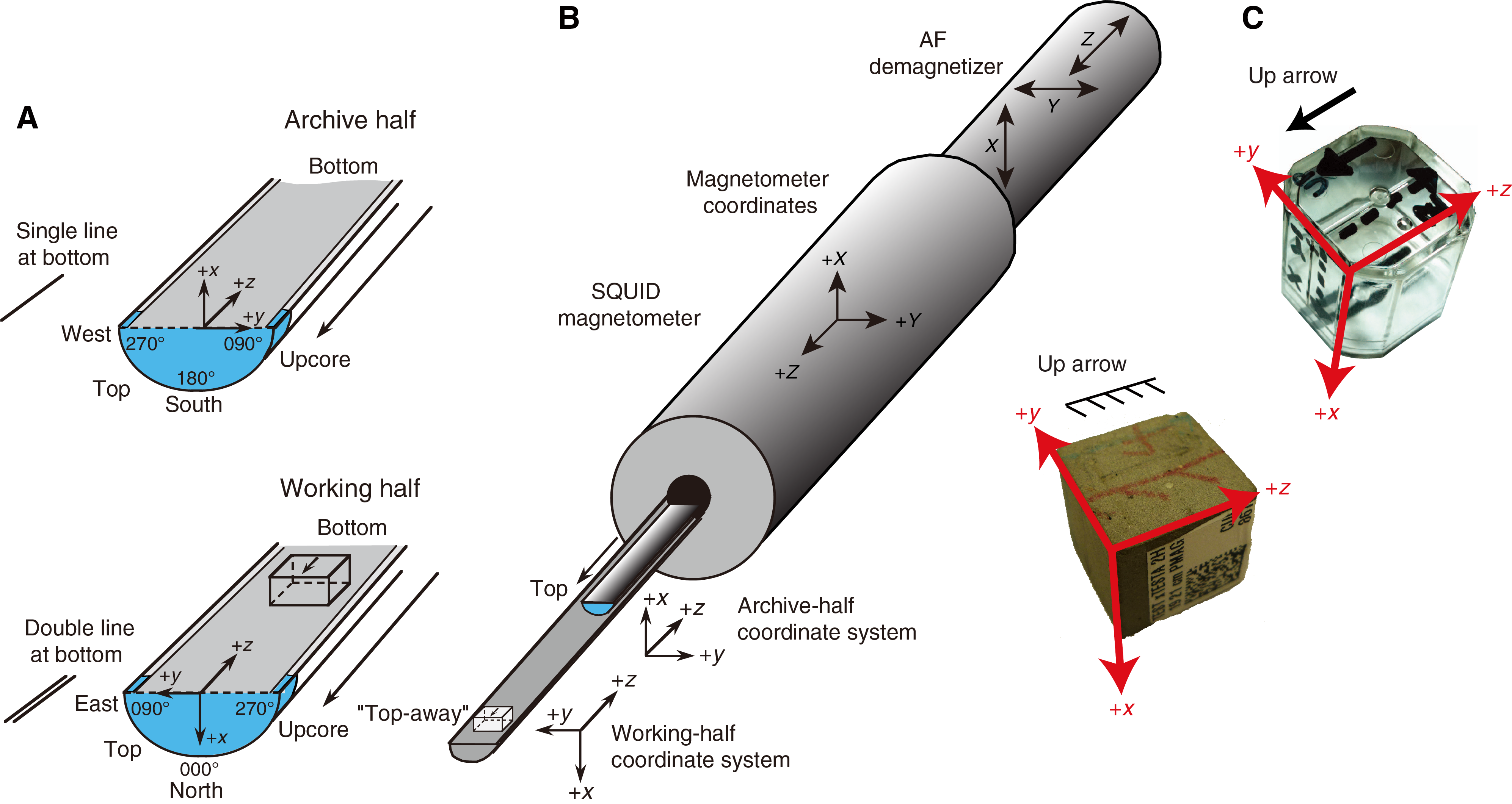
Figure F13. Paleomagnetism coordinate systems.
We measured the AMS and mean (bulk) magnetic susceptibility of the discrete samples on a KLY 4S Kappabridge. To ensure accurate susceptibility values, we calibrated the KLY 4S prior to each site using the standard provided by AGICO. The Kappabridge SUFAR software measures AMS by rotating the sample along three axes, stacking the data, and estimating the best-fit second-order tensor. The mean (bulk) magnetic susceptibility is calculated as the average of the magnetic susceptibilities in all three orientations, and we referred to this as mean magnetic susceptibility throughout Expedition 374. We only use the directions and (relative) amplitudes of the three principal axes, kmax (maximum susceptibility axis), kint (intermediate axis), and kmin (minimum axis), of the susceptibility tensor to approximate magnetic fabric (i.e., grain shape and orientation; Figure F14). When sediments are deposited in an undisturbed condition, sedimentary fabrics are oblate and the vertical axis has minimum susceptibility (e.g., Figure F14B). Disturbance by slumping or other deformation often yields triaxial fabrics (e.g., Figure F14D). Hence, we use the AMS as an indicator of disturbance.
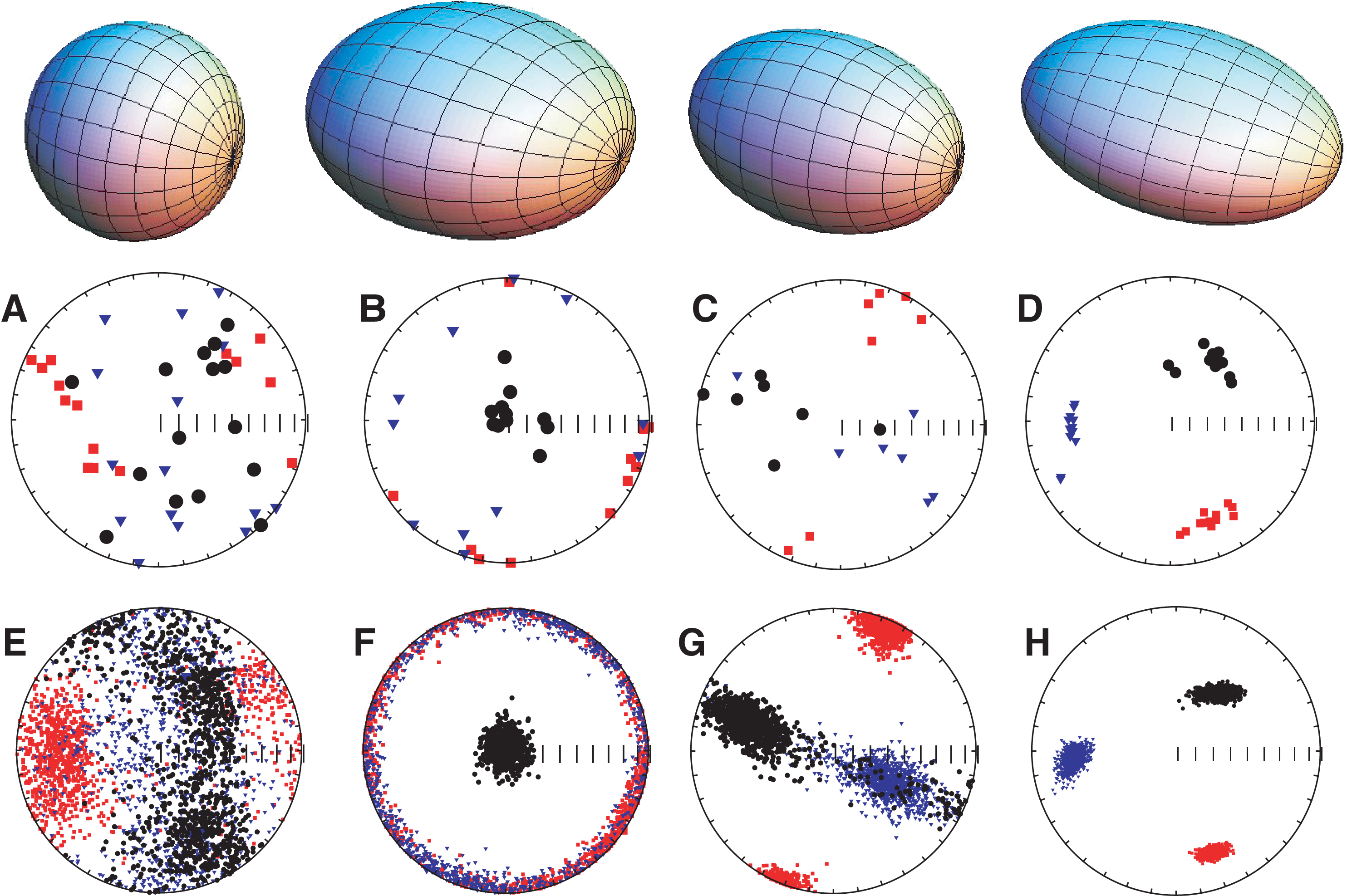
Figure F14. AMS data shape interpretation.
At each site, a selected group of discrete samples were used for NRM measurements. We used the SRM with inline AF demagnetizer to measure the NRM of discrete samples before and after AF demagnetization. Discrete samples were placed on a discrete sample tray with each sample separated from the adjacent ones by 20 cm to avoid convolution effects of the SRM sensor responses. Samples were measured with their orientation arrows facing upward and pointing out of the magnetometer (“top-away”), which equates to the −z-axis of the magnetometer (e.g., Figure F13B). After measuring the initial NRM, the discrete samples were subjected to progressive AF demagnetization and measured at 2 mT steps to a peak field of 20 mT, in 5 mT steps to 60 mT, and then at 70 and 80 mT to determine whether a characteristic remanent magnetization (ChRM) could be resolved and, if so, what level of demagnetization was required to resolve it.
To process the shipboard paleomagnetic measurement data, we exported formatted data files from the LIMS database. We used a combination of a modified version of the UPmag program (Xuan and Channell, 2009) and PmagPy software (Tauxe et al., 2010) to process all shipboard paleomagnetic data.
Coordinates
All magnetic data are reported relative to IODP orientation conventions: +x points into the face of the working half, +y points toward the left side of the working half when looking downcore, and +z is downcore (Figure F13A). The relationship between the SRM coordinates (X, Y, and Z) and the sample coordinates (x, y, and z) is +X = +x, +Y = +y, and +Z = −z for archive halves and +X = −x, +Y = −y, and +Z = −z for working halves (Figure F13). Note that the orientation of the SRM axes forms a left-handed coordinate system that is converted to a right-handed system within the SRM software by multiplying the calibration constant for the y-axis by −1.
The orientation of discrete samples depends on how the sample is collected. For samples collected by pushing the Japanese cube into the working half, the arrow on the sample points upcore along the z-axis and is along the face of the working half as in Figure F13A and F13C. For samples that are extruded into the plastic cube, we place a prominent red arrow on the lid that supersedes the embedded arrow that is in the base of all Japanese cubes. The orientation of sawed cubes and cubes placed on top of extruded sediment follows the orientation of the Japanese cubes.
Core collection and orientation (APC)
Cores were collected using nonmagnetic core barrels for the APC, HLAPC, and RCB coring systems. These nonmagnetic core barrels are more brittle and cannot be used in conjunction with the XCB system (see Coring and drilling operations). The BHA included a Monel (nonmagnetic) drill collar that was used for all APC and RCB cores. This collar is required when the Icefield MI-5 core orientation tool is used, but it was used for all (HL)APC/RCB cores during Expedition 374 (regardless of orientation tool use) because it can potentially reduce the magnetic field near where the core is cut and within the core barrel.
The Icefield MI-5 core orientation tool can only be used with APC core barrels. It uses three orthogonally mounted fluxgate magnetometers to record the orientation of the double lines scribed on the core liner with respect to magnetic north. The tool declination, inclination, total magnetic field, and temperature are recorded internally at a regular interval until the tool’s memory capacity is filled. For the measurement interval of 10 s used during Expedition 374, the tool can typically be run for more than a day, although we aimed to switch tools more frequently than that. Prior to firing the APC, the core barrel is held stationary (along with the pipe and BHA) for several minutes. During this time, data are recorded to constrain the core orientation. When the APC fires, the core barrel is assumed to maintain the same orientation. An antispiral key keeps the core barrel from rotating as it is fired. However, the core may rotate and/or the core liner can twist as it penetrates the sediments.
The Icefield MI-5 core orientation data collected during Expedition 374 are given in Table T5 along with the observed core mean paleomagnetic directions. The mean direction of each core is computed using Fisher statistics from the archive-half core section measurements. All directions with positive inclinations were inverted to their antipodal position by multiplying the inclination by −1 and adding 180° to the declination. We then computed the mean by using all directions with inclinations between −40° and −90°. We repeated this process after culling any directions that were more than four times the 95% confidence limits from the initial mean direction. This arbitrary cutoff was used to attempt to remove any outliers with declinations farthest from the majority of the data.
The orientation correction that converts the observed declination (Dobs) to a true declination (Dtrue) is given by
where MTF is the magnetic tool face angle from the Icefield MI-5 orientation tool and Damb is the ambient geomagnetic field declination obtained from geomagnetic field models. The World Magnetic Model 2015 gives a value of ~105° for the drill sites. Given that the Antarctic plate has not moved significantly over the past 20 My (Torsvik et al., 2012), the expected true declination is roughly 0°.
Neither the core mean directions nor the Icefield observations are ideal for use in core orientation. The steepness of the paleomagnetic field (with an inclination generally >70°) and the present-day geomagnetic field (inclination ≈ 80°) result in the horizontal component (declination) being only a very small part of the total vector field. For example, when the inclination is 80°, a measurement error of only 20° in angular distance of the geomagnetic field can yield a declination of 0° versus 180°.
Indeed, the corrected declinations do not cluster around the expected value of 0° but instead are virtually random (Table T5; Figure F15). For that reason, we did not use the correction during Expedition 374. In summary, the orientation tool clearly does not have the precision necessary to orient cores at such high latitudes.
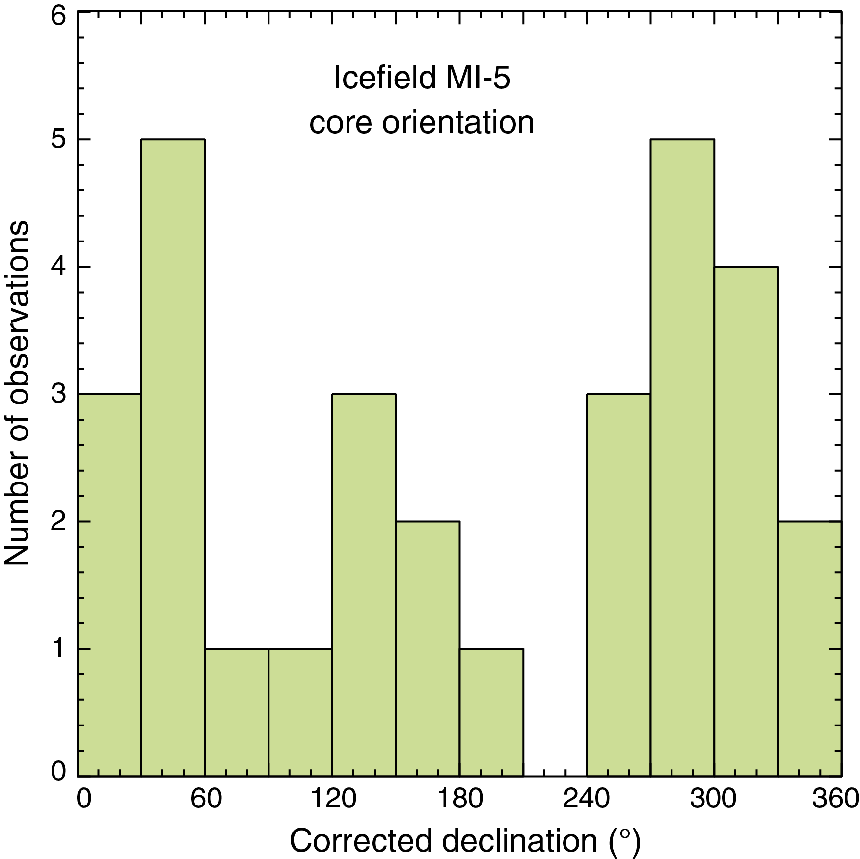
Figure F15. Declinations after orientation tool results.
Magnetostratigraphy
Magnetic polarity zones were predominantly assigned based on changes in inclination after 20 mT peak AF demagnetization and distinct ~180° alternations in declination that occur in undisturbed (HL)APC cores. Sediment disturbance caused by coring or geological processes (slumping, faulting, etc.) often leads to distorted and unreliable paleomagnetic directional records and largely altered sediment fabric. We examined the core face of each core section and the high-resolution shipboard core photographs (see Lithostratigraphy) to mark disturbed intervals and avoided using paleomagnetic data from those intervals.
Once a magnetostratigraphy was established for a given hole, we correlated the pattern to the GTS2012, summarized in Table T6 and illustrated in Figure F12, in close collaboration with the shipboard biostratigraphy team. The GTS2012 includes orbitally tuned reversals between Chron C1n and the base of Subchron C5r.2n (0–11.657 Ma) and between the base of Chron C5ABn and Subchron C5Bn.1n (13.608–15.215 Ma). The intervals between Subchron C5r.2n and Chron C5ABn and between Chrons C5Bn and C6Cn (11.657–13.608 and 15.215–23.030 Ma, respectively) are calibrated by spline fitting of marine magnetic anomaly profiles following Lourens et al. (2004) and Hilgen et al. (2012). We follow the chron terminology of Gradstein et al. (2012) and list several rarely observed polarity changes that were not formally classified as subchrons in the GTS2012 (remarks column in Table T6).
Measurement interference from flux jumps
Throughout the first half of Expedition 374, we noted a high occurrence of flux jumps in various circumstances. Flux jumps may occur due to a rapid change in magnetization in the sample, such that the SQUIDs cannot keep track of the number of counts. We determined that slowing the track speed is the best way to reduce the occurrence of this kind of flux jump.
Flux jumps also occurred when there was no sample inside the SRM, suggesting an external source. Acton et al. (2017) noted that mobile phones attempting to connect to a mobile network cause interference with the SQUIDs, yielding a large number of flux jumps. A large number of flux jumps on the y-axis was especially noticeable during measurements of sediments with higher water content, especially when the section was located between the SQUID sensor region and the AF coils. We hypothesize that this effect is similar to the antennae effect observed during previous expeditions (e.g., Expedition 342; Norris et al., 2014). We found this could be fixed by shielding the region near where the SQUID cables enter the magnetometer with aluminum foil.
Smaller numbers of flux jumps on all axes continued to occur even when no sample was in the magnetometer. These flux jumps occurred at intermittent moments of the day and could not be traced to any actively transmitting mobile phone. The jumps also occurred during background measurements (e.g., when the [empty] tray was outside the SRM SQUID region, thereby excluding a relation to measurements of samples and/or the tray). When these types of flux jumps occurred, they caused SRM downtime ranging from a few minutes to a few hours.
After thorough investigation, we found that devices that connect to WiFi and/or Bluetooth (e.g., wireless headphones, smartwatches, mobile phones, notebooks, etc.) have the potential to cause flux jumps when close to the entrance of the magnetometer. After disabling all such devices, we still noted one or two flux jumps that occurred with an apparent rhythmicity of ~65 s. These jumps were caused by a laptop ~3.5 m away from the entrance to the magnetometer connected to a temporary handheld pXRF device. The laptop uploaded its data to the LIMS database via a WiFi connection. As soon as this laptop was hardwired onto the network and its WiFi connection disabled, these regular flux jumps disappeared.
In summary, mobile phones are a source of flux jumps, but WiFi and Bluetooth devices can also interfere with the SRM system. We recommend that future expeditions remain vigilant of the occurrence of flux jumps and recognize that the SQUIDs are sensitive to radio frequency interference, most notably when in close proximity to devices that use Bluetooth, WiFi, and mobile reception.
Physical properties
During Expedition 374, high-resolution physical property measurements were made on recovered core material. Physical property data aided lithostratigraphic characterization and were used to link core observations with downhole measurements and seismic-reflection profiles. In particular, physical property data played a major role in the detection of lithologic discontinuities and heterogeneities, identification of changes in sediment composition and texture, and identification of major seismic reflectors. In addition, the thermal properties of the recovered material were measured and were used in conjunction with downhole temperature measurements to infer heat flow. A variety of techniques and methods were used on whole-round core sections, section halves, and discrete samples to characterize the physical properties of Expedition 374 cores.
General sampling and measurement sequence
A typical IODP core is 9.5–9.7 m long and cut into 1.5 m sections (see Coring and drilling operations and Curatorial procedures and core handling). Therefore, a core with ~100% recovery yields six sections plus a shorter seventh section. Physical property measurement intervals for Expedition 374 were selected to ensure that a full core could be analyzed without significantly impacting core flow through the laboratory. Prior to splitting, whole-round core sections were analyzed using two whole-round core logging systems: the WRMSL and the NGRL. We did not use the Special Task Multisensor Logger (STML) because we did not conduct real-time stratigraphic correlation at any site. Whole-round core sections from all holes were run on the WRMSL (Figure F16) at 2.5 cm resolution after equilibration for ~4 h to ambient room temperature (~20°C) and pressure. The WRMSL measures GRA bulk density, magnetic susceptibility, and compressional wave velocity on the P-wave logger (PWL). The PWL requires good contact between the sediment and core liner, which is usually the case for cores collected using the APC or HLAPC system. Cores recovered with the XCB or RCB system have a slightly smaller nominal diameter (58 mm) than those cored with the APC or HLAPC system (66 mm). As a result, sections cored with the XCB or RCB system typically have gaps between the liner and the core, and in these cases, P-wave velocity measurements with the WRMSL often fail or are outside the accepted velocity range (1000–4500 m/s). Therefore, the PWL was switched off for cores recovered using the XCB and RCB coring systems. Core sections were subsequently measured with the NGRL (Figure F17), which generates spectral gamma ray data. In one hole at each site, thermal conductivity measurement was attempted on one or two sections per core, and then repeat measurements were taken in subsequent holes as needed (Figure F18). For soft sediments, measurements were conducted with a needle probe inserted into the section through a small hole drilled through the plastic core liner close to the middle of the section. For lithified sediments, a contact probe method in a half-space configuration was used on split-core section halves for thermal conductivity measurements. After completion of whole-round measurements, the cores were split longitudinally, with one half designated as the archive section and one half as the working section (see Curatorial procedures and core handling) for sampling and additional analysis.
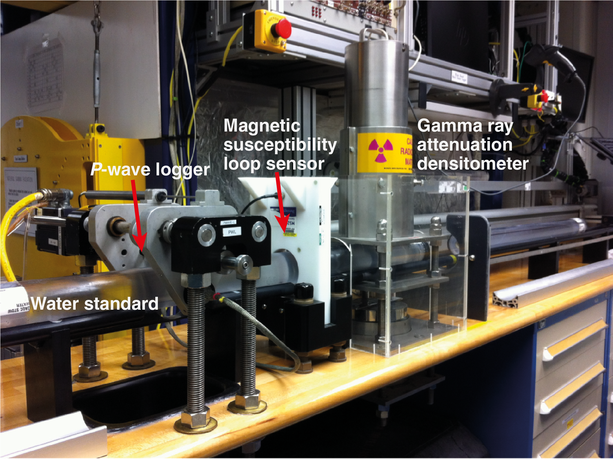
Figure F16. Whole-Round Multisensor Logger.
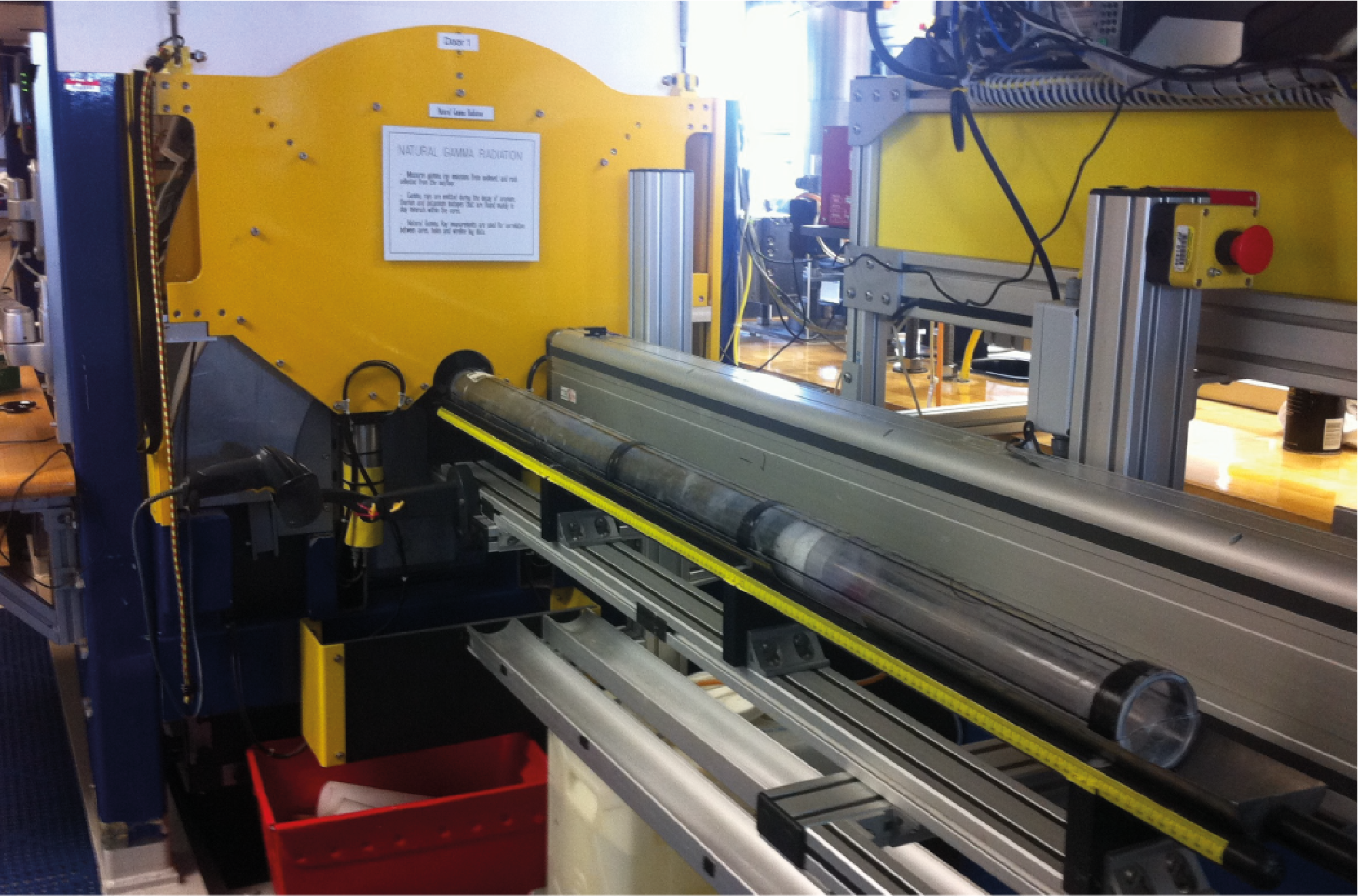
Figure F17. Natural Gamma Radiation Logger.
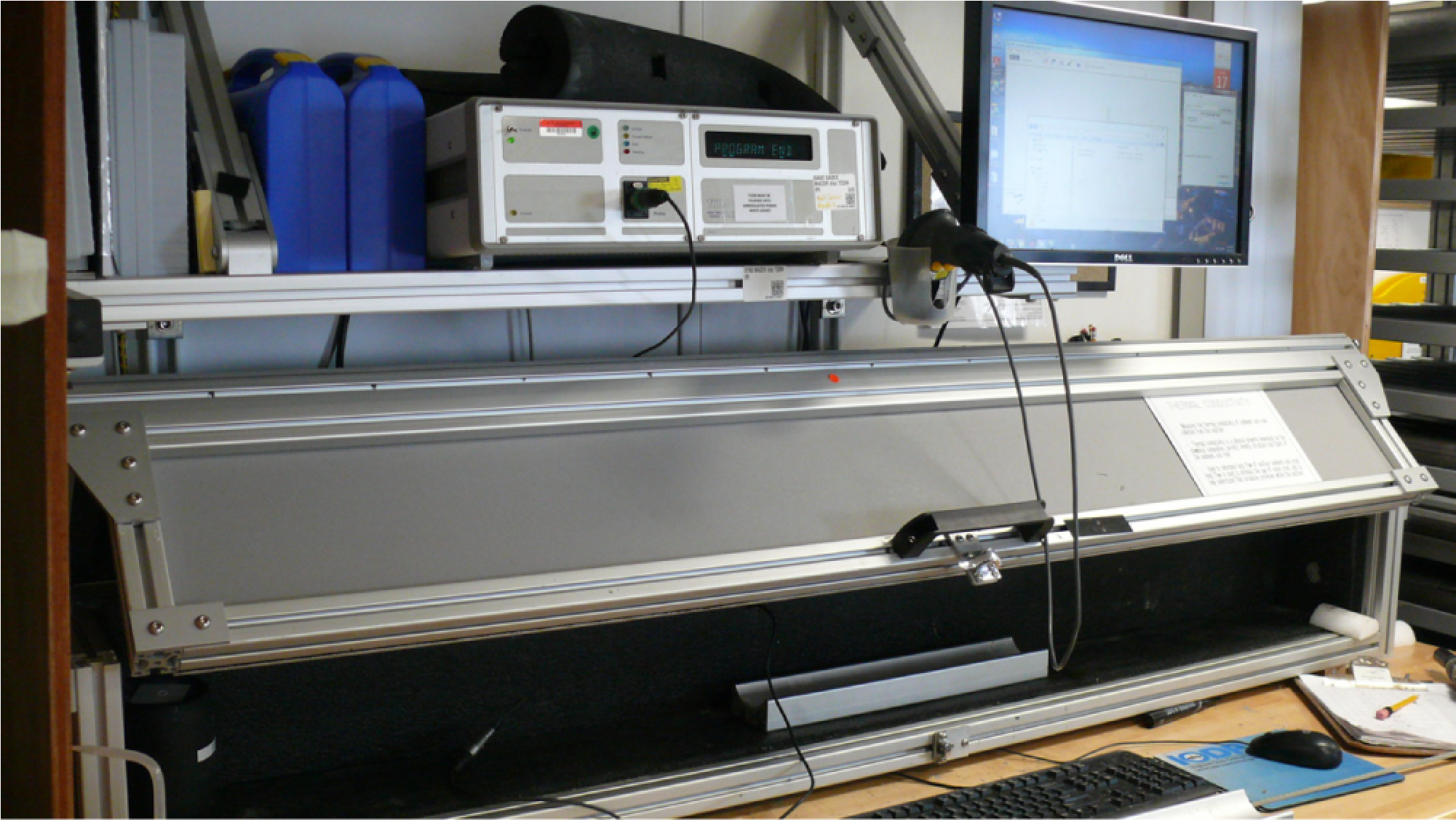
Figure F18. Shipboard station for thermal conductivity measurements.
Archive halves were measured with the SHMSL at 2.5 cm resolution for magnetic susceptibility using a discrete point-source Bartington probe and for color reflectance and colorimetry with an Ocean Optics spectrophotometer (Figure F19). For soft-sediment cores, P-wave velocity and shear strength measurements were performed on the section halves (generally every section or every other section). P-wave velocity measurements used the x-axis caliper contact probe transducer on the Section Half Measurement Gantry (SHMG), typically with one analysis per section (Figure F20). Discrete samples (~3 per core) for moisture and density (MAD) analysis were collected from the working halves, usually in Sections 1, 3, 5, and 7. These samples were then used to measure wet and dry mass and dry volume to calculate wet bulk density, dry bulk density, water content, porosity, and grain density using MAD procedures (Figure F21).
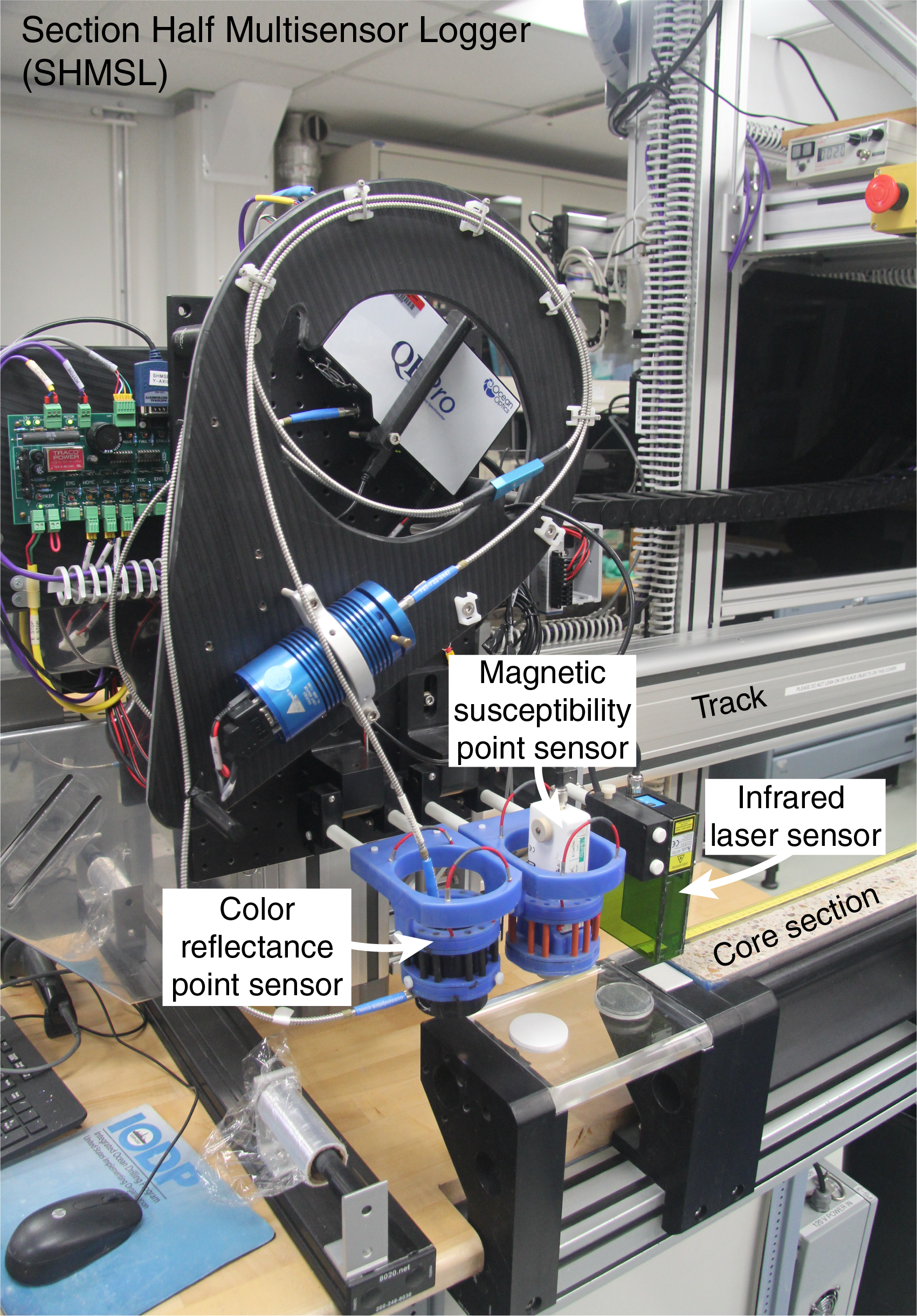
Figure F19. Section Half Multisensor Logger.
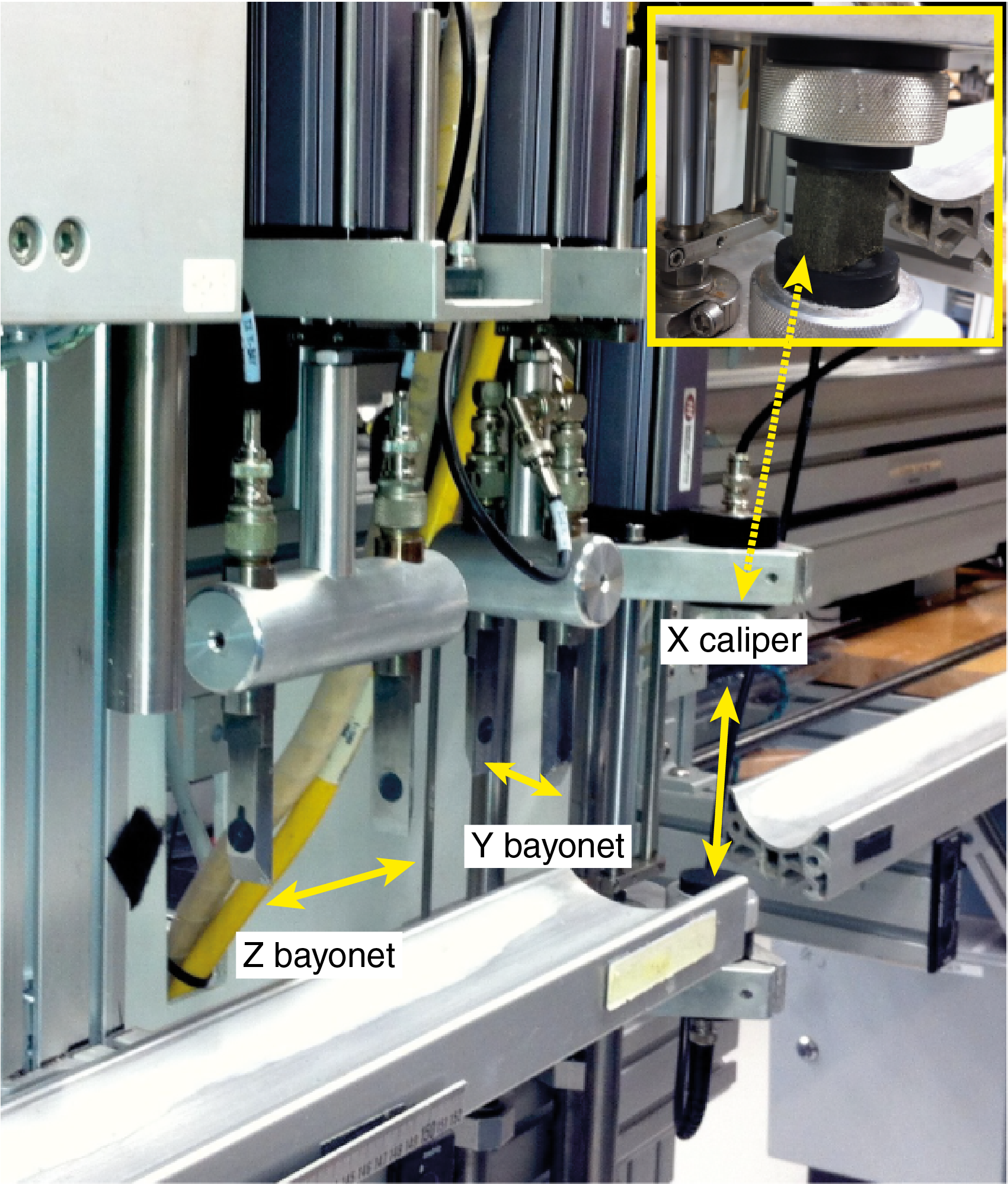
Figure F20. Section Half Measurement Gantry.

Figure F21. Equipment used for MAD analyses.
An overview of the sampling strategy for physical property measurements is given in Table T7. A full discussion of methodologies and calculations used on board the JOIDES Resolution in the physical properties laboratory is available in Blum (1997) and the shipboard user guides. Details and procedures for each physical property measurement are described below.
WRMSL measurements
During Expedition 374, GRA bulk density, magnetic susceptibility, and P-wave velocity were measured nondestructively on the WRMSL (Figure F16). To optimize the measurement process, sampling intervals and measurement times were the same for all sensors on each instrument. These sampling intervals are common denominators of the distances between the sensors installed on the WRMSL (30–50 cm), which allows sequential and simultaneous measurements. For the WRMSL, the sampling interval was 2.5 cm with an integration time of 3 s for each measurement. After measuring a core, calibration verification measurements were made by passing a single core liner filled with deionized water through the WRMSL.
GRA bulk density
GRA bulk density is a reflection of porosity, grain size, grain density (mineralogy), grain packing, and coring disturbance. These properties can be used to estimate the pore volume in sediment and evaluate the consolidation state. GRA density is an estimate of bulk density based on the attenuation of a gamma ray beam. The beam is produced by a 137Cs gamma ray source at a radiation level of ~370 MBq within a lead shield with a 5 mm collimator and directed through the whole-round core (Figure F16). The gamma ray detector on the opposite side of the core from the source includes a scintillator and integral photomultiplier tube to record the gamma radiation that passes through the core. The attenuation of gamma rays occurs primarily by Compton scattering, in which gamma rays are scattered by electrons in the formation; the degree of scattering is related to the material bulk density. Therefore, for a known thickness of sample, the density (ρ) is proportional to the intensity of the attenuated gamma rays and can be expressed as
- I = the measured intensity of gamma rays passing through the sample,
- I0 = gamma ray source intensity,
- μ = Compton attenuation coefficient, and
- d = sample diameter.
μ, d and I0 are treated as constants so ρ can be calculated from I.
In general, GRA bulk density measurements are most accurate when taken on a completely filled core liner with minimal drilling disturbance; otherwise, measurements tend to underestimate true values. By default, the instrument reports measurements using the internal diameter of the core liner (66 mm) as the assumed sample diameter. This assumption is suitable for most sediment cores obtained by the APC and HLAPC systems; however, for sediment and/or hard rock cored by the XCB or RCB systems, core diameter is usually ~58 mm or less. The spatial resolution of the GRA densitometer is less than ±1 cm. Calibration details can be found in Blum (1997).
Magnetic susceptibility (pass-through loop)
Magnetic susceptibility is measured on whole-round core sections using a pass-through loop on the WRMSL (Figure F16). Magnetic susceptibility (χ) is a dimensionless measure of the degree to which a material can be magnetized by an external magnetic field:
where M is the magnetization induced in the material by an external field of strength H. Magnetic susceptibility is primarily sensitive to the concentration of ferromagnetic minerals (e.g., magnetite, pyrite, and a few other iron oxides). It is also sensitive to magnetic mineralogy and can be related to the origin of the materials in the core and their subsequent diagenesis. Paramagnetic minerals such as clays have a specific magnetic susceptibility several orders of magnitude lower than ferromagnetic minerals. Diamagnetic minerals such as calcite/aragonite and opal, as well as water and plastic (core liner), have small to negative values of magnetic susceptibility. Thus, calcareous and siliceous biogenic deposits with very small amounts of clay and iron-bearing minerals have values approaching the detection limit of the magnetic susceptibility meters.
Magnetic susceptibility measurements were made using a Bartington Instruments MS2C loop sensor with a 90 mm diameter. An oscillator circuit in the sensor operates at a frequency of 565 Hz for the WRMSL (correction factor = 1.174) to avoid interference between the instruments. An ~140 A/m alternating field produces a low-intensity, nonsaturating alternating magnetic field. Sediment core sections going through the influence of this field cause a change in oscillator frequency. Frequency information returned in pulse form to the susceptometer is converted into magnetic susceptibility. The loop sensors have a spatial resolution of 20 mm and are accurate to within 5%, as indicated in Bartington specifications (Blum, 1997). The output of the magnetic susceptibility sensors can be set to centimeter-gram-second (cgs) units or dimensionless SI units. Approximate SI units (× 10−5) are used as the IODP standard and are reported as such in the LIMS database. See Paleomagnetism for a full discussion of the correction factor for conversion to SI units.
Compressional P-wave velocity
P-wave velocity varies with the material’s lithology, porosity, and bulk density, as well as state of stress, temperature, and fabric or degree of fracturing. In sediment and rock, velocity is controlled by the degree of consolidation, lithification, and fracturing, along with the occurrence and abundance of free gas and gas hydrate. P-wave velocity data can be used to assist in the correlation between the cores and seismic-reflection profiles, the correlation between downhole logging and core data, and the evaluation of porosity and cementation. P-wave (compressional) velocity (VP) is defined by the time required for a compressional wave to travel a specific distance:
where d is the path length of the wave across the core and tcore is the traveltime through the core. P-wave velocity was measured on whole-round core sections using the PWL on the WRMSL (Figure F16).
The PWL measures the traveltime of 500 kHz ultrasonic waves horizontally across the core while it resides in the core liner. Waves are transmitted to the core by transducer contacts connected to linear actuators. Pressure is applied to the actuators to ensure coupling between the transducers and the core liner, and the space between the core liner and transducers was kept wet to ensure good coupling. P-wave velocity transducers measure total traveltime of the compressional wave between transducers. The calibration of the PWL accounts for errors in the total distance (dtotal) and the total traveltime (ttotal). Errors on dtotal are assumed to come from the laser-distance measuring system. The core is surrounded by a core liner of assumed thickness (L), and the traveltime (tliner) is determined by measuring the traveltime through the core liner filled with distilled water of known velocity (corrected for the influence of temperature). A correction (tdelay; system delay) is measured using the traveltime through a standard block of aluminum with a known velocity (6295 m/s) and a known thickness. Arrival times are made on the second lobe of the waveform, giving a correction (tpulse) from the first arrival. During Expedition 374, tpulse was included within tdelay. Consequently, the velocity of the core is
- VP = velocity of the core,
- dtotal = measured diameter of core and liner,
- L = liner wall thickness,
- ttotal = total measured traveltime for pulse to travel through core and liner,
- tliner = traveltime through liner, and
- tdelay = delay related to transducer faces and electronic circuitry.
NGRL measurements
The NGRL measures NGR emitted from the decay of long-period isotopes uranium (238U), thorium (232Th), and potassium (40K) on whole-round cores using a system designed and built at Texas A&M University (USA) (Vasiliev et al., 2011; Dunlea et al., 2013). When 238U, 232Th, and 40K radioisotopes decay, they and their daughter products emit gamma radiation at specific energy levels unique to each isotope. NGR spectroscopy measures a wide energy spectrum that can be used to estimate the abundance of each isotope based on the strength of the signal at characteristic energies (Blum, 1997; Gilmore, 2008). In sediments and sedimentary rocks, Th and K are usually associated with particular clay minerals, whereas U is often encountered in either clay minerals or organic-rich material. Because minor changes in the abundance of clay minerals produces a relatively large variation in gamma radiation, the NGR data are useful as a lithologic indicator, aiding in core and/or downhole data set correlation in single or multiple holes.
The NGRL system consists of eight sodium iodide (NaI) detectors arranged along the core measurement axis at 20 cm intervals surrounding the lower half of the section (Vasiliev, et al., 2011) (Figure F22). The detector array has passive (layers of lead) and active (plastic scintillators) shielding to reduce the background environmental and cosmic radiation. The overlying plastic scintillators detect incoming high-energy gamma and muon cosmic radiation and cancel this signal from the total counted by the NaI detectors.
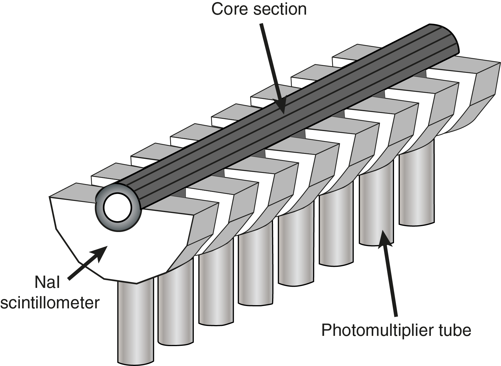
Figure F22. Interior of the NGRL.
The quality of the energy spectrum measured in a core depends on the concentration of radionuclides in the sample but also on the counting time, with greater times yielding better spectra. Therefore, a measurement run consisted of two sample positions located 10 cm apart. Measurements were conducted on each core section for 300 s at Position 1. After 300 s, the section was offset by 10 cm (Position 2) and measured again for 300 s. This yielded a total of 16 measurements (10 cm apart) per 150 cm section. Measurement times were 5 min per measurement cycle, or ~10 min per core section. These settings yielded statistically significant total counts.
Thermal conductivity
Thermal conductivity depends on the chemical composition, porosity, density, structure, and fabric of the material (e.g., Jumikis, 1966). Thermal conductivity is the measure of a material’s ability to transmit heat by molecular conduction. In marine geophysics, thermal conductivity profiles of sediment and rock sections are used along with in situ temperature measurements to determine heat flow (see Downhole measurements). Heat flow is not only characteristic of the material but is also an indicator of the type and age of ocean crust and the fluid circulation processes at both shallow and deep depths (Blum, 1997).
Thermal conductivity was measured on one or two sections per core (usually Sections 2 and 5) with the TK04 (Teka) system using a needle probe method in full-space configuration on whole-round cores for soft sediments (Von Herzen and Maxwell, 1959). A contact probe method in half-space configuration was conducted on section-half cores for lithified sediments and rocks. Some cores yielded no results for thermal conductivity because cracks caused bad coupling of the probe to the sediment. The probes contain a heater wire and calibrated thermistor. For soft sediment, the needle probe was inserted into a 2 mm hole drilled through the liner along one of the lines that later guided core splitting. To avoid interference from airflow in the laboratory, the core was placed in an enclosed box outfitted with foam (Figure F18). For lithified sediment cores, the section half was put in the enclosed box, and the contact probe was put on the cut face of the sample. The contact probe was embedded in the surface of an epoxy block with a low thermal conductivity (Vacquier, 1985).
The quality of thermal conductivity measurements was checked by evaluating two parameters: (1) the number of solutions acquired and (2) the shape of the curve formed on the temperature versus time plot of these points. A valid measurement must have a sufficient number of solutions to form an exponential curve. All measurements with a low number of solutions and/or a bad repartition of these values on the temperature versus time plot (i.e., forming two curves or no curve) were deleted.
The calibrated heat source of the probe was turned on, and the increase in temperature was recorded over 80 s for measurements with the needle probe and 60 s for measurements with the contact probe. A heating power of 2.5 W/m was typically used for soft sediment, and 0.5–2.5 W/m was typically used for lithified sediments. The solution to the heat conduction equation with a line source of heat was then fit to the temperature measurements to obtain the thermal conductivity. Because the probe is much more conductive than sediment, the probe is assumed to be a perfect conductor. Under this assumption, the temperature of the superconductive probe has a linear relationship with the natural logarithm of the time after the initiation of heat:
- T = temperature (K),
- q = heat input per unit length per unit time (J/m/s),
- k = thermal conductivity (W/[m·K]),
- t = time after the initiation of heat (s), and
- C = instrumental constant.
Three automatic measuring cycles were used to calculate average conductivity. A self-test, which included a drift study, was conducted at the beginning of each measurement cycle. Once the probe temperature stabilized, the heater circuit was closed and the temperature rise in the probe was recorded. Thermal conductivity was calculated from the rate of temperature rise while the heater current was flowing. Temperatures measured during the first 60 s of the heating cycles for the contact probe and 80 s of the heating cycles for the needle probe were fit to an approximate solution of a constantly heated line source (Kristiansen, 1982; Blum, 1997). Measurement errors were 5%–10%.
SHMSL measurements
Color reflectance and magnetic susceptibility were measured on archive section halves using the SHMSL. Because both sensors require flush contact with the split-core face, sections were covered with clear plastic and water was applied to the surface of the core prior to measurement. Foam inserts were also removed from the section-half cores before measurement, so the measured values represent those of the core material only. The archive half of the split core was placed on the core track, above which an electronic platform moves along a track and records the height of the split-core surface with a laser sensor. The laser establishes the surface topography of the section, and then the platform reverses the direction of movement, moving from the core section top (higher in the borehole) to bottom (lower in the borehole), making measurements of point magnetic susceptibility and color reflectance. During Expedition 374, point magnetic susceptibility and color reflectance data were collected at 2.5 cm intervals for each core.
Spectrophotometry
The color reflectance spectrometer uses an Ocean Optics QE Pro detector integrating sphere and associated light sources covering wavelengths from UV through visible to near infrared. Each measurement was recorded in 2 nm wide spectral bands from 390 to 732 nm. The approximate 3 s data acquisition offset was applied for the entire scan of the archive section half. Data are reported using the L*a*b* color system, in which L* is lightness, a* is redness (positive) versus greenness (negative), and b* is yellowness (positive) versus blueness (negative) of the sediment and rock. The color reflectance spectrometer calibrates on two spectra, pure white (reference) and pure black (dark). Color calibration was conducted approximately once every 6 h (twice per shift). Additional details regarding measurement and interpretation of spectral data can be found in Balsam et al. (1997), Balsam and Damuth (2000), and Giosan et al. (2002).
Point magnetic susceptibility
Point magnetic susceptibility was measured with a Bartington MS2 meter and an MS2K contact probe with a flat 15 mm diameter round sensor with a field of influence of 25 mm and an operation frequency of 930 Hz. The instrument averages three measurements from the sensor for each offset with an accuracy of ~5%. The spatial resolution of the point magnetic susceptibility instrument is ~3.8 mm. As with whole-round magnetic susceptibility loop measurements, the output displayed by the point magnetic susceptibility sensor is reported in instrument units (IU) and can be converted to approximate dimensionless SI units by multiplying by 10−5 (see Paleomagnetism for a full discussion of the correction factor). The probe is zeroed in air before each measurement to avoid influence from the metal track. The point magnetic susceptibility meter was calibrated by the manufacturer before installation on the ship and is quality checked every ~6 h at the same time as color reflectance sensor calibration.
SHMG measurements
P-wave velocity
P-wave velocity measurements on split-core sections were typically performed once per section using the SHMG (Figure F20). Measurements were taken at varying section intervals to accommodate lithologic variations, drilling disturbance, fractures, and general core quality. The system uses Panametrics-NDT Microscan delay line transducers, which transmit at 0.5 MHz. The signal received was recorded, and the peak (P-wave arrival) was chosen with autopicking software. In some cases, the peak was manually chosen to ensure that a consistent first arrival time was selected. For sections with highly variable core quality, different intervals within a section were tested to help choose an appropriate position to make the measurement. The distance between transducers was measured with a built-in linear voltage displacement transformer (LDVT).
Calibration was performed with a series of acrylic cylinders of differing thicknesses and a known P-wave velocity of 2750 ± 20 m/s. The determined system time delay from calibration was subtracted from the picked arrival time to give a traveltime of the P-wave through the sample. The thickness of the sample (calculated by LDVT in meters) was divided by the traveltime (in seconds) to calculate P-wave velocity in meters per second.
Shear strength
Shear strength is the resistance to failure of a material under shear. Shear stress in unconsolidated materials is resisted only by the network of solid particles. Shear strength (τf) can be expressed as a function of the effective normal stress at failure (σ′), the effective cohesion (c′), and friction angle (φ′):
where c′ and φ′ are the shear strength parameters that define a linear relationship between τf and φ′, according to the Mohr-Coulomb failure criterion.
Shear strength parameters can be determined by means of multiple laboratory tests. The c′ and φ′ are relevant for situations in which field drainage conditions correspond to test conditions. The shear strength of a soil under undrained conditions (interstitial water drainage does not occur during failure) is different from that under drained conditions (interstitial water drainage occurs). Undrained shear strength (Su) can be expressed in terms of total stress in the case of fully saturated materials of low permeability (e.g., clays). The most common strength tests in shipboard laboratories are the vane shear and penetrometer tests, which provide measurements of undrained shear strength (Blum, 1997).
During Expedition 374, Su was measured in undisturbed fine-grained sediment using the handheld Torvane shear device in working-half cores. Undrained shear strength was determined by inserting a four-bladed vane into the split core and putting it under shear stress, resulting in shearing of a cylindrical surface by the vane. This procedure provides a measurement of the peak shear strength expressed in kPa units. Measurements were made with the vane rotation axis perpendicular to the split surface. Shear strength was measured once in each core when sediments were within the instrument range. Measurements were stopped when they began to cause excessive disturbance. Shear strength measurements were not conducted for continental shelf Sites U1521 and U1522.
MAD measurements
Discrete samples were collected from the working halves to determine wet and dry bulk density, grain density, water content, and porosity. In soft sediment, ~10 cm3 samples were collected with a plastic or metal syringe. Generally, three samples were taken in each core from the first hole, and sampling continued in deeper intervals of successive holes. In shorter cores, only one or two samples were taken. When possible, the samples were taken from Sections 1, 3, 5, and, if present, 7. In lithified sediments, samples were taken adjacent to the cube samples sawed for paleomagnetism measurements.
Sediment samples were placed in numbered, preweighed ~16 mL Wheaton glass vials for wet and dry sediment weighing and drying and dry volume measurements. After wet sample analysis, samples were dried in a convection oven for at least 24 h at 105° ± 5°C. Dried samples were then cooled in a desiccator for at least 60 min before dry mass and volume were measured. The weights of wet and dry sample masses were determined to a precision of 0.005 g using two Mettler Toledo electronic balances (Figure F21A), with one acting as a reference. A standard weight of similar value to the sample was placed on the reference balance to increase accuracy. A computer averaging system was used to compensate for the ship’s motion. The default setting of the balances is 300 measurements over ~1 min.
Dry sample volume was determined using a six-celled custom-configured Micrometrics AccuPyc 1330TC helium-displacement pycnometer (hexapycnometer) (Figure F21B). The precision of each cell is 1% of the full-scale volume. Volume measurement was preceded by three purges of the sample chamber with helium warmed to ~28°C. Three measurement cycles were run for each sample. A reference volume (set of two calibration spheres) was placed sequentially in one of the chambers to check for instrument drift and systematic error. The volumes occupied by the numbered Wheaton vials were calculated before the expedition by multiplying each vial’s weight against the average density of the vial glass. Procedures for determining these physical properties comply with the American Society for Testing and Materials (ASTM) designation (D) 2216 (ASTM International, 1990). The fundamental relation and assumptions for the calculations of all physical property parameters are discussed in Blum (1997). MAD properties reported and plotted in the Physical properties sections of all site chapters were calculated with the MADMax shipboard program.
Mass and volume calculation
Wet mass (Mwet), dry mass (Mdry), and dry volume (Vdry) were measured in the laboratory. The mass ratio (rm) is a computational constant of 0.965 (i.e., 0.965 g of freshwater per 1 g of seawater). Salt precipitated in sediment pores during the drying process is included in the Mdry and Vdry values. The mass of the evaporated water (Mwater) and salt (Msalt) in the sample are given by
where s is the assumed saltwater salinity (0.035) corresponding to a pore water density (ρpw) of 1.024 g/cm3 (from experimental and empirical relations between salinity and density at laboratory conditions; Blum 1997) and a salt density (ρsalt) of 2.22 g/cm3. The corrected mass of pore water (Mpw), volume of pore water (Vpw), mass of solids excluding salt (Msolid), mass of salt (Msalt), volume of salt (Vsalt), wet volume (Vwet), and volume of solids excluding salt (Vsolid) are, respectively,
Wet (or total) volume (Vt), dry mass (Mdry), and dry volume (Vdry) were measured in the laboratory. Total mass, including freshwater in the pores, is calculated using a water density of 1 g/cm3 by
Assuming a pore water density of 1.024 g/cm3, the volume of the pore water is calculated as
Finally, the mass of the pore water is
Calculation of bulk properties
For all sediment samples, water content (w) is expressed as the ratio of the mass of pore water to the wet sediment (total) mass as
Wet bulk density (ρwet), dry bulk density (ρdry), sediment grain density (ρsolid), porosity (φ), and void ratio (VR) are calculated from
Geochemistry and microbiology
The shipboard geochemistry program for Expedition 374 included measurements of headspace gas content (hydrocarbons), interstitial water composition, and bulk sediment geochemical parameters. Samples for microbiology were collected and fixed for shore-based analyses of metagenomics, cell counts, metabolomics, and cultures.
Headspace gas geochemistry
Routine analysis of hydrocarbon gases in sediment cores is part of the standard IODP shipboard monitoring to ensure safe drilling operations. The most common method of hydrocarbon monitoring is headspace analysis (gas obtained from sediment/rock samples). One sediment plug (~5 cm3) was collected from each core from Hole A at each site for headspace gas analyses immediately after retrieval on deck. Additional samples were collected from other holes when depths exceeded those previously drilled. Headspace samples were collected from the top of a section from the middle of the core immediately adjacent to the interstitial water sample when possible (Figure F23). For soft sediments, plug samples were collected using a graduated syringe and extruded into a 21.5 cm3 glass serum vial with a crimped-seal metal cap and polytetrafluoroethylene septum. For consolidated or lithified samples, chips of material were placed in the vial and sealed. The vial was labeled with the core, section, and interval from which the sample was taken and then placed in an oven at 70°C for 30 min.

Figure F23. Schematic of catwalk sampling.
Headspace gas (5 cm3) was extracted through the septum with a gas-tight glass syringe and then injected into an Agilent 6890 gas chromatograph equipped with a flame ionization detector (FID) at 250°C to quantify concentrations of methane (C1), ethane (C2), ethylene (C2=), propane (C3), and propylene (C3=). A 2.4 m × 2.0 mm stainless steel column packed with 80/100 mesh HayeSep “R” is installed in the oven. The injector consists of a ¹⁄₁₆ inch Valco union with a 7 μm screen connected to a Valco-to-Luer lock syringe adaptor. This injector connects to a 10-port Valco valve that was switched pneumatically by a digital valve interface. The injector temperature was set at 120°C. Samples were introduced into the gas chromatograph through a 0.25 cm3 sample loop connected to the Valco valve. The valve can be switched automatically to back flush the column. The oven temperature was programmed to start at 80°C for 8.25 min and then increase to 150°C for 5 min at a rate of 40°C/min. Helium was used as the carrier gas. Initial helium flow in the column was 30 mL/min. Flow was then ramped to 60 mL/min after 8.25 min to accelerate elution of C3 and C3=. The run time was 15 min. The gas chromatograph was also equipped with an electronic pressure-control module to control the overall flow into the gas chromatograph. Data were collected and evaluated using the Agilent Chemstation software (2001–2006). The chromatographic response was calibrated against different preanalyzed gas standards with variable quantities of low–molecular weight hydrocarbons provided by Scott Specialty Gases (Air Liquide). Concentrations of hydrocarbon gases are reported in parts per million by volume (ppmv).
Interstitial water chemistry
Interstitial water samples for shipboard determination of salinity, alkalinity, pH, anions and cations, and major and trace elements, as well as for shore-based hydrogen sulfide, water isotope (δ18O, δ17O, and δ2H), and carbon isotope (δ13CDIC) analyses, were obtained by squeezing 5 or 10 cm whole-round sections cut from cores immediately after core retrieval (Figure F23). Whole-round samples were typically collected at a frequency of 1 sample per core (<100 m CSF-A) or every third core (>100 m CSF-A) to the bottom of the hole or until extraction produced <6 mL of interstitial water after 1.5 h of squeezing. Sampling frequency was reduced by half when using the HLAPC system or when cutting half cores with rotary coring systems. The exterior of the whole-round sample was carefully cleaned with a spatula to remove potential contamination from drilling fluid. For XCB and RCB cores, the intruded drilling mud between biscuits was also removed to eliminate contamination from drilling fluid. The cleaned sediment was transferred into an 8 cm inner diameter titanium squeezer that was then placed in a Carver hydraulic press (Manheim and Sayles, 1974) and squeezed with slowly increasing pressure up to 30,000 force pounds (1.335 × 10⁶ N). After discarding the initial drops to avoid contamination, the squeezed interstitial water was collected into a 60 mL water-washed (18 MΩ/cm) high-density polyethylene syringe attached to the squeezing assembly. If sample volume permitted, the interstitial water samples were split as outlined in the analytical workflow below. If interstitial water volume was limited (i.e., <20 mL but >6 mL), it was decided to either omit shore-based samples or shipboard alkalinity/inductively coupled plasma–optical emission spectroscopy (ICP-OES) analyses on a case-by-case basis.
The priority list for shipboard analyses and shore-based samples from interstitial water (from high to low priority) was as follows:
- Salinity (~100 μL): determined by optical refractometry immediately after squeezing.
- Anions and cations (~100 μL; Na+, K+, Ca2+, Mg2+, Cl−, Br−, SO42−): determined by ion chromatography.
- Silica (~400 μL) and ammonia (~200 μL): determined by spectrophotometry.
- Major and trace element analyses (~2 mL; B, Ba, Ca, Fe, K, Li, Mg, Mn, Na, S, Si, and Sr): determined by ICP-OES; addition of 30 µL concentrated trace metal–clean HNO3.
- Shore-based sample for δ18O, δ2H, δ17O (2 mL): no headspace in amber-colored glass crimp-top vial and stored at 4°C.
- Shore-based sample for δ13C and dissolved inorganic carbon (DIC) (2 mL): no headspace in amber-colored glass crimp-top vial; addition of 100 µL saturated HgCl solution (prepoisoned).
- pH and alkalinity (~3 mL): titrated/determined immediately after squeezing.
- Shore-based hydrogen sulfide (~4 mL): addition of 800 μm of zinc acetate.
- Duplicate (or triplicate) 2 mL samples for shore-based analysis (in case of excess interstitial water) of
For all above analyses, interstitial water was filtered through a 0.45 μm polysulfone disposable filter (Whatman). All shipboard analyses were carried out in batches.
Shipboard analysis
Interstitial water samples were analyzed on board following the protocols in Gieskes et al. (1991), Murray et al. (2000), and the IODP user manuals for shipboard instrumentation.
Alkalinity, pH, and salinity
Alkalinity and pH were measured using a Metrohm autotitrator (Model 794 Basic Titrino) equipped with a pH glass electrode and a stirrer (Model 728). The pH was obtained from the LabVIEW alkalinity program directly, and alkalinity was measured by titrating 3 mL of sample with 0.1 M HCl to reach an endpoint of pH = 4.2. Standardization for both measurements was achieved using the International Association of Physical Sciences of the Ocean (IAPSO) seawater standard, which was analyzed repeatedly during the expedition and reproduced within 1%. Salinity was analyzed using a Fisher Model S66366 refractometer calibrated using 18 MΩ millipore water. The known salinity of the IAPSO seawater standard was used for data quality control.
Ion chromatography
Aliquots of interstitial water were diluted at 1:100 with deionized water for analysis of Na+, K+, Ca2+, Mg2+, Cl−, Br−, and SO42− using a Metrohm 85 Professional ion chromatograph. The IAPSO seawater standard was used for standardization of measurements. Typical reproducibility was <5% for each ion.
Spectrophotometry
Aliquots of interstitial water samples were diluted with 18 MΩ millipore water for analysis of ammonium and dissolved silica using an Agilent Cary 100 UV-Vis spectrophotometer. Ammonium analyses were conducted by phenol diazotization and subsequent oxidization by sodium hypochlorite to yield a blue color measured spectrophotometrically at a wavelength of 640 nm. Ammonium chloride (NH4Cl) was used for calibration and standardization. Reproducibility of ammonium standards was typically better than 20%. Dissolved silica concentration was measured by reacting samples with ammonium molybdate tetrahydrate solution acidified with hydrochloric acid to form molybdosilicic acid. The complex was then reduced by ascorbic acid to form molybdenum blue, which was measured at a wavelength of 812 nm. Solutions of sodium silicofluoride (Na2SiF6) at 360 and 480 µM concentrations were used as standards with a reproducibility of better than 3%.
Inductively coupled plasma–optical emission spectroscopy
Dissolved major (Ca, K, Mg, and Na) and minor (B, Ba, Fe, Li, Mn, S, Si, and Sr) element concentrations were determined by an Agilent 5110 ICP-OES instrument with a SPS4 autosampler. Interstitial water samples were diluted 1:10 in 2% HNO3 and spiked with an internal standard to correct for atomic and ionic interferences. In detail, 100 μL of spike solution containing 100 ppm Be, In, and Sc and 200 ppm Sb was added to 500 µL of interstitial water sample and 4.4 mL of 2% HNO3. For calibration, serial dilutions of the IAPSO seawater standard (0%, 1%, 5%, 10%, 25%, 50%, 75%, and 100%) were prepared to cover interstitial water concentrations smaller than or equal to normal seawater. Additional calibration solutions for major and minor element concentrations exceeding that of seawater were prepared with 3.5% NaCl as a matrix. Calibration solutions for B, Ba, Ca, Fe, K, Li, Mg, Mn, P, Si, and Sr were spiked in the same way as interstitial water samples and run as serial dilutions of 0%, 1%, 5%, 10%, 25%, 50%, 75%, 100%, and 200%.
During each ICP-OES batch run, a complete set of in-house and IAPSO standard dilutions were analyzed at the beginning. Furthermore, known solutions of the IAPSO standard were run every 6–8 samples to monitor instrumental drift and accuracy. The elemental concentrations reported for each sample were average values from three replicate integrations for each sample. Reproducibility was typically better than 5% for all elements and mostly around 1%–3%.
All data produced on the Agilent 5110 ICP-OES was collected in atomic emission spectroscopy (AES) mode and is referred to as ICP-AES in the LIMS/LORE database. “ICP-OES” is used to refer to these data in the Expedition 374 Proceedings volume.
Comparative analysis of analytical methodologies for interstitial water
IODP standard shipboard analytical protocols produce multiple data sets for a number of elements. For example, B, Ba, Ca, Fe, K, Mg, Mn, Na, S, Si, and Sr were measured by ICP-OES using two or more wavelengths. Results for each wavelength were analyzed by evaluating shape and size of intensity peaks as well as interferences. Final chosen wavelengths are given in Table T8. In addition, Ca, Mg, K, Na, and SO42− were measured by ion chromatography, and dissolved silica was measured by spectrophotometry. Generally, these data are in good agreement with the ICP-OES results. Reproducibility between ion chromatography and ICP-OES analyses for K and Na is typically better than 10% and better than 15% for Ca and Mg. Total S (ICP-OES) and SO42− (ion chromatography) in the interstitial water samples for all sites were also in very good agreement; reproducibility between the two techniques is typically better than 10%. At Sites U1521–U1523, silica and silicon concentrations in interstitial water were measured by spectrophotometry and ICP-OES, respectively. There was good agreement between the two techniques for the majority of analyzed samples (differences are <5%), with consistently higher silica concentrations in the spectrophotometry analyses. The spectrophotometry method for silica was not conducted on interstitial water samples from Sites U1524 and U1525.
Sedimentary geochemistry
Typically, two 5 cm3 samples were taken from the working halves of split cores following identification of major lithologies in discussion with sedimentologists for on board bulk sediment analyses. The entire 5 cm3 sample was freeze-dried for ~12 h, crushed using an agate pestle and mortar, and aliquoted for the individual analyses. Bulk carbon, nitrogen, and calcium carbonate (CaCO3) content were determined on all samples.
Sedimentary inorganic and organic carbon, nitrogen, and carbonate content
Total carbon and total nitrogen content of sediment samples were determined with a ThermoElectron Corporation FlashEA 1112 CHNS elemental analyzer equipped with a ThermoElectron packed column CHNS/NCS gas chromatograph and a thermal conductivity detector (TCD). Approximately 10–15 mg of sediment was weighed into a tin cup and then combusted at 950°C in a stream of oxygen. The reaction gases were passed through a reduction chamber to reduce nitrogen oxides to nitrogen and then separated by the gas chromatograph before detection by the TCD. All measurements were calibrated to the NIST 2704 Buffalo River Sediment standard (soil reference material), which was run every 10 samples. Peak areas from the TCD were calculated to determine the total carbon and total nitrogen of the samples.
Total inorganic carbon (TIC) was determined using a Coulometrics 5015 CO2 coulometer. Approximately 10 mg of sediment was weighed into a glass vial and acidified with 2 M HCl. The liberated CO2 was titrated, and the corresponding change in light transmittance in the coulometric cell was monitored using a photodetection cell. The weight percent of CaCO3 was calculated from the inorganic carbon content using the following equation:
Standard CaCO3 (>99.9% CaCO3; Fisher Scientific) was used to confirm accuracy, and instrument performance was monitored by repeat analysis of the standard before, during, and after each run (target reproducibility is better than 2%).
Total organic carbon (TOC) content was calculated by subtracting inorganic carbon derived by coulometry from the total carbon derived by the CHNS elemental analyzer:
Major and minor elemental analysis by ICP-OES
Major (Al, Ca, Fe, K, Mg, Mn, Na, Si, and Ti) and selected minor (Ba, Sr, and Zr) elements were determined by an Agilent 5110 ICP-OES instrument with a SPS4 autosampler. Shipboard ICP-OES instrument analyses of samples followed methods described in principle by Murray et al. (2000). Because this specific instrument had not been used previously for sediment measurements, a range of reference standards were run first (BCR-2, BHVO-2, G-2, GSP-2, SO-1, LKSD-1, SDO-1, NBS-88b, STSD-2, PACS-3, MESS-4, and HISS-1) and compared in combusted and uncombusted form. Results for Al, Ba, Ca, Fe, K, Mg, Na, Si, Sr, Ti, and Zr revealed a loss on ignition (LOI) between 0% and 46%. In detail, average LOI values for all listed elements for basalt BCR-2 and BHVO-2 and granodiorite GSP-2 were <1%. Values for the sediment standards STSTD-2, MESS-4, and PACS-3 and soil standard SO-1 were between 9% and 15%, and lake sediment standard LKSD-1 and shale standard SDO-1 had 30%–31% LOI. The highest reference material LOI (46%) was for the carbonate standard NBS-88b. No combustion was performed on standards G-2 and HISS-1. Results corrected for LOI agreed within 3% for all but one standard (SDO-1; ~7%). No combustion was performed on actual samples from Site U1521 (the only site for which sediment ICP-OES analyses were performed).
Approximately 100 mg of ground and homogenized sediment sample (or reference material) was weighed (100 ± 0.5 mg) on the Cahn C-31 microbalance and placed in a vial containing 400 mg of preweighed lithium metaborate (LiBO2) to achieve a sample flux ratio of 1:4. After homogenization of sample and flux powders, the mixture was poured into a Pt-Au crucible and 10 μL of 0.172 M LiBr was added to prevent the cooled bead from sticking to the crucible. Samples were fused individually at 1050°C for ~12 min in an internal-rotating induction furnace (Bead Sampler NT-2100) and subsequently cooled to form a bead. After cooling, the bead was dissolved in 50 mL trace metal–grade 10% HNO3 (dilution factor 1:500) in acid-washed high-density polypropylene (HDPE) Nalgene wide-mouth bottles. Solutions were subsequently agitated on a Burrell wrist-action bottle shaker for 1.5 h. Aliquots (500 μL) of the filtered solutions were mixed with 4.4 mL 2% HNO3 and 100 μL of a spike solution containing 100 ppm Be, In, and Sc and 200 ppm Sb.
Microbiology
Microbiology sampling was carried out for shore-based analyses of metagenomics, cell counting, and metabolomics, as well as for fungal and anaerobic microbial culturing work. To support microbiology work, a headspace methane sample was taken in the same manner and adjacent to the routine headspace samples for methane for onshore stable and clumped isotope analysis of methane and higher hydrocarbons. Sediment for methane isotope work was extruded into 20 mL glass vials prepoisoned with 8 mL 1 M NaOH solution, immediately crimp-sealed, agitated, and stored upside down at 4°C.
Two sampling methods were employed for all other microbiological work. Dedicated holes for microbiology and interstitial water sampling were cored at Sites U1523 (Hole U1523B) and U1524 (Hole U1524B) (see Geochemistry and microbiology in the Site U1523 chapter and Geochemistry and microbiology in the Site U1524 chapter [McKay et al., 2019d, 2019e]). Sampling consisted of 10–20 cm whole rounds taken on the catwalk and placed into sterile Whirl-Pak bags. Isopropanol was used to sterilize the core cutter, spatula, and gloves to minimize contamination. Approximately half of the whole rounds was immediately placed in storage at −80°C for onshore analyses of metabolomics and tag amplicon sequencing. The remainder of the whole-round samples were stored at 4°C and subsampled within 12 to 18 h, operations permitting. Subsampling was carried out in a cold room (~4°–8°C) in a laminar flow hood. To minimize contamination, sterile gloves and spatulas were used to remove the outer layer of whole-round samples. Four 10 cm3 syringes were used to extract 5 cm3 from one side of each whole-round sample and were preserved in four different ways:
- One syringe was placed into a Whirl-Pak bag and stored at −20°C for culturing work.
- One syringe was transferred into a sterile centrifuge tube, covered with RNAlater to saturate sediment for 12 h at 4°C for incubation, and then stored at −80°C for shore-based metagenomic analyses.
- One syringe sample was placed in a sterile Whirl-Pak bag that was flushed with N2 and closed. The closed Whirl-Pak bag was placed in a silver wine bag with an oxygen scrubber that was flushed with N2, sealed, and then stored at −80°C for shore-based anaerobic microbial analyses.
- One 10 cm3 syringe was extruded into a 50 mL centrifuge tube. The extruded sediment was covered with glycerol to saturate for 12 h at 4°C and then moved to −20°C for shore-based culturing work.
The remainder of the whole-round samples were stored at −80°C for shore-based high-resolution subsampling.
The second sampling strategy was carried out on the catwalk by injecting sterile syringes into both sides of freshly cut core sections separated with a sterile spatula (Figure F23). Isopropanol was used to sterilize the core cutter, spatula, and gloves to minimize contamination. This sampling strategy was primarily used for low-resolution sampling (approximately every third core) during APC coring at Sites U1523–U1525 and in the uppermost core of Sites U1521 and U1522. Although RCB coring was performed at Sites U1521 and U1522, an effort was made to “push” rather than drill in the first core to capture the mudline and obtain microbiology samples in this uppermost interval with minimal risk of seawater or drilling mud contamination (see Operations in the Site U1521 chapter and Operations in the Site U1522 chapter [McKay et al., 2019b, 2019c]). Samples (15 cm3) of material were extracted using a 20 cm3 syringe below the fresh cut in the sediment core. Above the cut, one 10 cm3 syringe was filled to 6 cm3 and a second was filled to 10 cm3 (Figure F23). All syringes were covered in sterile foil on the catwalk and carried indoors for subsampling as described below. The 20 cm3 syringe was separated into three samples:
- 5 cm3 was extruded into a sterile 50 mL centrifuge tube and covered with RNAlater solution. This sample was agitated, inoculated for 12 h at 4°C, and then transferred to −80°C storage for shore-based analyses of metagenomics/DNA/polymerase chain reaction.
- 5 cm3 was placed in a sterile Whirl-Pak bag. The bag was flushed with N2 and then placed inside a silver wine bag with an oxygen scrubber. The wine bag was flushed with N2, sealed, and stored at −80°C for onshore anaerobic culturing work.
- 5 cm3 was placed in a Whirl-Pak bag, which was then sealed and stored at −20°C for onshore fungal culturing work.
The 10 cm3 syringe with 6 cm3 of sediment was separated into two samples. First, 1 cm3 was extruded into a 50 mL centrifuge tube and covered with a fixing solution of 2% (v/v) filter-sterilized (0.2 μm) formaldehyde in 2% (w/v) NaCl and then stored at 4°C for shore-based cell counting. The remaining 5 cm3 sample was extruded into a sterile Whirl-Pak bag that was then sealed and stored at −80°C for shore-based metabolomics analyses. Finally, the 10 cm3 syringe with 10 cm3 of sediment was placed into a sterile Whirl-Pak bag that was then sealed and stored at −80°C for shore-based tag-amplicon sequencing.
Throughout the expedition, seawater and drilling mud were sampled for contamination quality control.
Downhole measurements
Downhole logs are used to determine physical, chemical, and structural properties of the formation penetrated by a borehole. The data are rapidly collected, continuous with depth, and measured in situ, and they can be interpreted in terms of the stratigraphy, lithology, mineralogy, and geochemical composition of the penetrated formation. Where core recovery is incomplete or disturbed, log data may provide the only way to characterize the borehole section.
Where core recovery is good, log and core data complement one another and may be interpreted jointly. Downhole logs measure formation properties on a scale intermediate between those obtained from laboratory measurements on core samples and geophysical surveys. They are useful in calibrating the interpretation of geophysical survey data (e.g., downhole velocity values) and provide a necessary link for the integrated understanding of physical properties at all scales. In addition, formation temperature as a function of depth can be measured using the APCT-3, which allows heat flux to be estimated. Such estimations are important for assessing the viability of models governing tectonic subsidence regionally.
Wireline logging
During wireline logging operations, logs are recorded with a variety of Schlumberger logging tools combined into several tool strings (Figure F24; Tables T9, T10) that are lowered into the hole after completion of coring operations. Four tool strings were used during Expedition 374: the triple combination (triple combo), modified triple combo, Formation MicroScanner (FMS)-sonic, and Vertical Seismic Imager (VSI) tool strings.
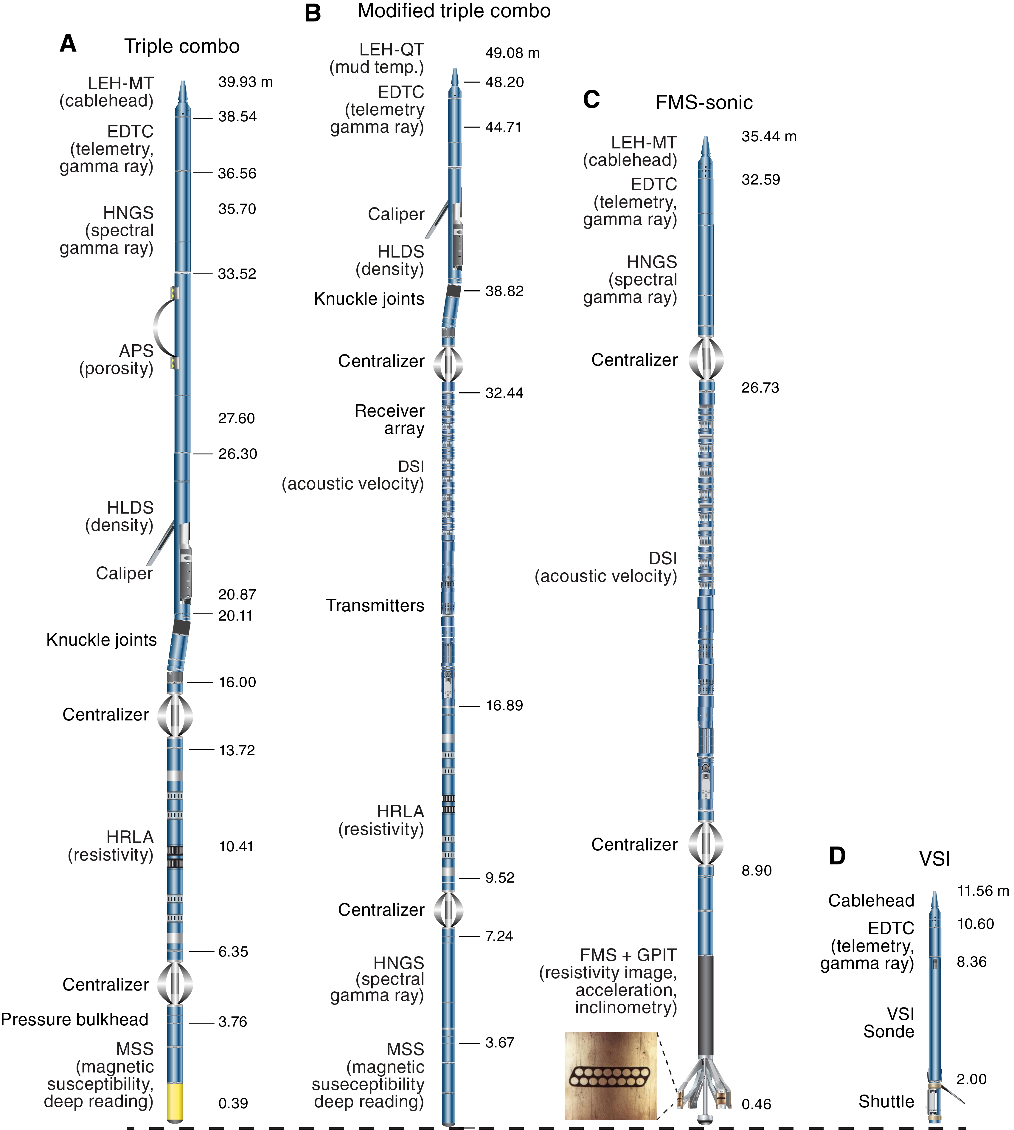
Figure F24. Downhole logging strings.
The triple combo tool string typically includes the following tools:
- Accelerator Porosity Sonde (APS),
- Hostile Environment Litho-Density Sonde (HLDS),
- Hostile Environment Natural Gamma Ray Sonde (HNGS),
- Enhanced Digital Telemetry Cartridge (EDTC-B),
- High-Resolution Laterolog Array (HRLA),
- Phasor Dual Induction-Spherically Focused Resistivity Tool (DIT), and
- Magnetic Susceptibility Sonde (MSS).
These tools are able to measure gamma radiation, porosity, density, resistivity, and magnetic susceptibility.
The FMS-sonic tool string typically includes the following tools:
The FMS gathers resistivity images of the borehole wall and the DSI collects sonic velocities.
The VSI tool string (for seismic “check shots”) (Table T9) includes the VSI and EDTC-B tools.
Each tool string contains a telemetry cartridge for communicating through the wireline to the Schlumberger data acquisition system (MAXIS unit) on the drillship. Total gamma radiation is also measured with each tool string to depth-match between logging runs. During Expedition 374, downhole logs were collected at Sites U1521–U1523. All three standard tool strings were run at Site U1521. The triple combo and FMS-sonic tool strings were reconfigured for logging at Sites U1522 and U1523 because of unstable borehole conditions. The radioactive source was left out of the HLDS, which was run solely for measuring borehole diameter using the caliper. The APS, which also includes a radioactive source, was not run because of the suboptimal conditions of the borehole that might have compromised recovery of the radioactive source. We included the DSI tool on the triple combo (referred to as the modified triple combo; Figure F24) because collection of downhole velocity data was a high priority. After successfully running the modified triple combo at both sites, we completed two additional logging runs at Site U1522 (VSI and FMS without sonic) and one additional logging run at Site U1523 (FMS without sonic) (Figure F24).
In preparation for logging, the boreholes were flushed of debris by circulating viscous drilling fluid and then filled with a seawater-based logging gel (sepiolite mud mixed with seawater and weighted with barite; approximate density = 10.5 lb/gal) to help stabilize the borehole walls. The BHA was pulled up to ~70–75 m DSF to cover the unstable upper part of the hole; this depth varied by site. The tool strings were then lowered downhole on a seven-conductor wireline cable before being pulled up at constant speed, typically 250–550 m/h, to provide continuous measurements of several properties simultaneously. A wireline heave compensator (WHC) was used when necessary to minimize the effect of ship’s heave on the tool position in the borehole (see below). During each logging run, incoming data were recorded and monitored in real time on the MCM MAXIS logging computer. At each site, the drill string was raised ~15 m as the tool string approached the end of pipe to increase log coverage of the upper portions of the borehole wall.
Logged sediment properties and tool measurement principles
The logged properties and the principles used in the tools to measure them are briefly described below. More detailed information on individual tools and their geological applications may be found in Serra (1984, 1986, 1989), Schlumberger (1989, 1994), Rider (1996), Goldberg (1997), Lovell et al. (1998), and Ellis and Singer (2007). A complete online list of acronyms for the Schlumberger tools and measurement curves is at http://www.apps.slb.com/cmd (Table T10).
Natural gamma radiation
The HNGS was used to measure NGR in the formation. The HNGS uses two bismuth germanate scintillation detectors and five-window spectroscopy to determine concentrations of K (in weight percent), Th, and U (both in parts per million) from the characteristic gamma ray energies of isotopes in the 40K, 232Th, and 238U radioactive decay series, which dominate the natural radiation spectrum. The computation of the elemental abundances uses a least-squares method of extracting U, Th, and K elemental concentrations from the spectral measurements. The HNGS filters out gamma ray energies below 500 keV, eliminating sensitivity to bentonite or KCl in the drilling mud and improving measurement accuracy. The HNGS also provides a measure of the total gamma ray emission (HSGR) and uranium-free or computed gamma ray (HCGR), which are both measured in American Petroleum Institute units (gAPI). The HNGS response is influenced by the borehole diameter; therefore, the HNGS data are corrected for borehole diameter variations during acquisition.
An additional gamma ray sensor was housed in the EDTC, which was used primarily to communicate data to the surface. The sensor includes a NaI scintillation detector that measures the total natural gamma ray emissions of the formation. It is not a spectral tool (i.e., does not provide U, Th, and K concentrations) but provides total gamma radiation for each pass. The inclusion of the EDTC in every tool string allowed us to use the gamma ray data for precise depth-match processing between logging strings and passes and for core-log integration.
Density and photoelectric factor
When borehole conditions were suitable, formation density was measured with the HLDS. The HLDS contains a cesium (137Cs) gamma ray source (662 keV) and far and near gamma ray detectors mounted on a shielded skid that is pressed against the borehole wall by a hydraulically activated decentralizing arm. Gamma radiation emitted by the source undergo Compton scattering, in which gamma rays are scattered by electrons in the formation. The number of scattered gamma rays that reach the detectors is proportional to the density of electrons in the formation, which is in turn related to bulk density. Porosity may also be derived from this bulk density if the matrix (grain) density is known.
The HLDS also computes the photoelectric effect (PEF), a measure of the photoelectric absorption of low-energy gamma radiation. Photoelectric absorption of gamma rays occurs when their energy falls below 150 keV as a result of being repeatedly scattered by electrons in the formation. PEF is determined by comparing the counts from the far detector in the high-energy region, where only Compton scattering occurs, with those in the low-energy region, where count rates depend on both reactions. Because PEF depends on the atomic number of the elements in the formation (heavier elements have higher PEF), it also varies according to the chemical composition of the minerals present; therefore, it can be used to identify the overall mineral make-up of the formation. For example, the PEF of calcite is 5.08 barn/e−, illite is 3.03 barn/e−, quartz is 1.81 barn/e−, and hematite is 21 barn/e− (Serra, 1984; Schlumberger, 1989).
Good contact between the tool and borehole wall is essential for good HLDS logs; poor contact results in underestimation of density values. To limit the possibility of losing an environmentally hazardous package during deployment, the HLDS was run without the 137Cs gamma ray source in Holes U1522A and U1523D. Both the density correction and caliper measurement of the hole are used to check the contact quality. In the deeper parts of the hole, the PEF log data should be used with caution, especially in washouts, because Ba in the logging mud swamps the signal despite a correction for the influence of mud.
Electrical resistivity
Resistivity is measured to aid in identifying poorly recovered sections of the hole because different materials have different electrical conductivities. Calcite, silica, and hydrocarbons are electrical insulators, whereas ionic solutions like interstitial water are conductors. Electrical resistivity can therefore be used to evaluate porosity for a given salinity and resistivity of interstitial water. Clay surface conduction also contributes to the resistivity values, but at high porosities this is a relatively minor effect.
The HRLA tool provides six resistivity measurements with different depths of investigation, including the borehole (mud) resistivity and five measurements of formation resistivity with increasing penetration into the formation. The tool sends a focused current into the formation and measures the intensity necessary to maintain a constant drop in voltage across a fixed interval, providing direct resistivity measurements. The array has one central (source) electrode and six electrodes above and below it that serve alternatively as focusing- and returning-current electrodes. By rapidly changing the roles of these electrodes, a simultaneous resistivity measurement at six penetration depths is achieved. The tool is designed to ensure that all signals are measured at exactly the same time and tool position to reduce the sensitivity to “shoulder bed” effects when crossing sharp beds thinner than the electrode spacing. The design of the HRLA, which eliminates the need for a surface reference electrode, improves formation resistivity evaluation compared with traditional dual induction and allows the full range of resistivity to be measured from low (e.g., in high-porosity sediments) to high (e.g., in basalt). The HRLA needs to be run centralized in the borehole for optimal results, so knuckle joints were used to centralize the HRLA while allowing the density and porosity tools to maintain good contact with the borehole wall.
Magnetic susceptibility
The MSS is a nonstandard wireline tool designed by LDEO that measures the ease with which formations are magnetized when subjected to a magnetic field. The ease of magnetization is ultimately related to the concentration and composition (size, shape, and mineralogy) of magnetic minerals (principally magnetite) in the formation. These measurements provide one of the best methods for investigating stratigraphic changes in mineralogy and lithology because the measurement is quick, repeatable, and nondestructive and because different lithologies often have strongly contrasting susceptibilities.
The MSS dual-coil sensor provides measurements with ~40 cm vertical resolution and ~20 cm depth of horizontal investigation. The MSS was run as the lowermost tool in the triple combo and modified triple combo tool strings and used a specially developed data translation cartridge to enable the MSS to be run in combination with the Schlumberger tools. The MSS also has an optional single-coil sensor to provide high-resolution measurements (~10 cm), but it was not used during Expedition 374 because it has a large bowspring that requires the MSS to be run higher in the tool string and because it is very sensitive to separation from the borehole wall.
Magnetic susceptibility data are plotted as uncalibrated instrument units. The MSS reading responses are affected by temperature and borehole size (higher temperatures lead to higher susceptibility measurements). The magnetic susceptibility values were not fully corrected for temperature during Expedition 374; therefore, values from deeper than several hundred meters were generally not interpretable. When the magnetic susceptibility signal in sediment is very low, the detection limits of the tool may be reached. For quality control and environmental correction, the MSS also measures internal tool temperature, z-axis acceleration, and low-resolution borehole conductivity.
Acoustic velocity
The DSI measures the transit times between sonic transmitters and an array of eight receivers. It combines replicate measurements, thus providing a direct measurement of sound velocity through formations that are relatively free from the effects of formation damage and an enlarged borehole (Schlumberger, 1989). Along with the monopole transmitters found on most sonic tools, the DSI also has two crossed-dipole transmitters that allow the measurement of shear wave velocity in addition to compressional wave velocity. Dipole measurements are necessary to measure shear velocities in slow formations with shear velocity less than the velocity of sound in the borehole fluid. Such slow formations are typically encountered in deep-ocean drilling.
Resistivity images (FMS)
The FMS provides high-resolution electrical resistivity–based images of borehole walls. The tool has four orthogonal arms and pads, each containing 16 button electrodes that are pressed against the borehole wall during logging. The electrodes are arranged in two diagonally offset rows of eight electrodes each (inset image in Figure F24). A focused current is emitted from the button electrodes into the formation, and there is a return electrode near the top of the tool. Resistivity of the formation at the button electrodes is derived from the intensity of current passing through the button electrodes.
Processing of the resistivity measurements offshore at LDEO generates oriented high-resolution images that reveal geologic structures of the borehole wall. Features such as bedding, stratification, fracturing, slump-related folding, and bioturbation can be resolved (Luthi, 1990; Salimullah and Stow, 1992; Lovell et al., 1998). Because the images are oriented to magnetic north, further analysis can provide measurement of the dip and direction (azimuth) of planar features in the formation. In addition, when the corresponding planar features can be identified in the recovered core samples, individual core pieces can be reoriented with respect to true north.
The maximum extension of the caliper arms is 40.6 cm (16 inches). In holes or sections of holes with a diameter greater than this maximum, the pad contact at the end of the caliper arms will be inconsistent, and the FMS images may appear out of focus and too conductive. Irregular (rough) borehole walls will also adversely affect the images if contact with the wall is poor. Approximately 30% of a borehole with a diameter of 25 cm is imaged during a single pass. The standard procedure is to make two full uphole passes with the FMS to maximize the chance of getting full borehole coverage with the pads.
Acceleration and inclinometer
Three-component acceleration and magnetic field measurements were made with the GPIT during logging. The primary purpose of this tool, which incorporates a three-component accelerometer and a three-component magnetometer, is to determine the acceleration and orientation of the FMS-sonic tool string. This information allows the FMS image to be corrected for irregular tool motion and to determine the dip and direction (azimuth) of features in the images. The GPIT has greater nonmagnetic insulation on the FMS-sonic tool string compared with other tool strings, which greatly reduces the effects on its magnetic measurements.
Vertical Seismic Imager
In a vertical seismic profile (VSP) experiment, a borehole VSI is anchored against the borehole wall at regularly spaced intervals to record the full waveform of elastic waves generated by a seismic source positioned just below the sea surface (Figure F25). These check shot measurements relate depth in the hole to traveltime in seismic-reflection profiles. The VSI used here contains a three-axis geophone and was anchored against the borehole wall at approximately 20–50 m spacing between stations (depending on borehole conditions), with 5–10 air gun shots typically taken at each station. The recorded waveforms were stacked, and a one-way traveltime was determined from the median of the first breaks for each station. The seismic sources used were two 250 inch3 Sercel G guns in parallel clusters 1 m apart and fired at 2000 psi. The source was positioned on the port side of the JOIDES Resolution at ~7–9 mbsl with a horizontal borehole offset of ~47 m.
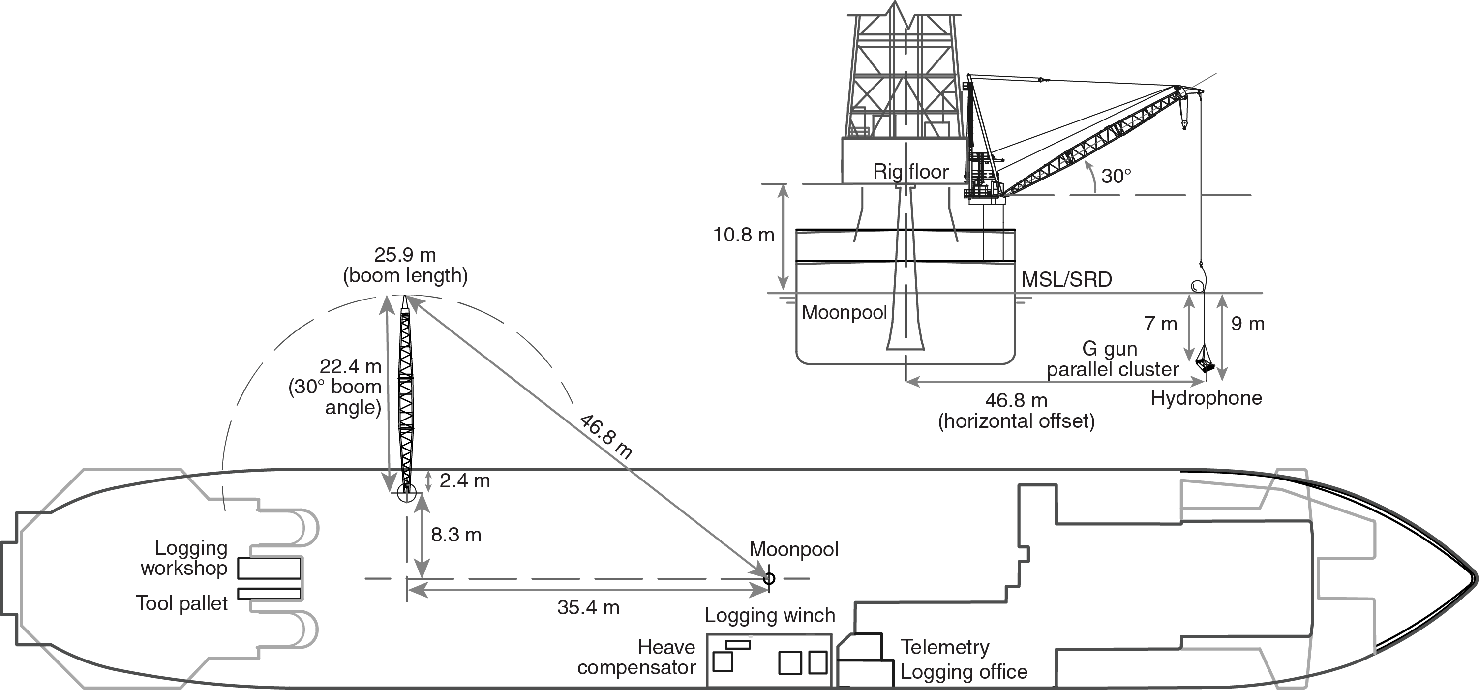
Figure F25. Sercel G gun deployment.
Precautions were taken to protect marine mammals and diving birds following the restrictions placed on seismic surveys in Antarctic waters. If there were no such fauna in or approaching the safety radius (940 m for water depths >1000 m and 1850 m for water depths between 100 and 1000 m), air gun operations commenced using a ramp-up or “soft start” procedure (gradually increasing the operational pressure and air gun firing interval) to provide time for undetected fauna to respond to the sounds and vacate the area. Once the guns were at full power, the check shot survey proceeded. Observations for relevant wildlife continued during the check shot survey, and the survey was suspended if marine mammals or diving birds entered the safety radius.
Wireline heave compensator
During wireline logging operations, the up and down motion of the ship (heave) causes a similar motion of the downhole logging tools. If the amplitude of this motion is large, depth discrepancies can be introduced into the logging data and the risk of damaging downhole instruments is increased. A WHC system was designed to compensate for the vertical motion of the ship and maintain a steady motion of the logging tools to ensure high-quality logging data acquisition (Liu et al., 2013; Iturrino et al., 2013). The WHC uses a vertical accelerometer (motion reference unit [MRU]) positioned under the rig floor near the ship’s center of gravity to calculate the vertical motion of the ship with respect to the seafloor. It then adjusts the length of the wireline by varying the distance between two sets of pulleys through which the cable passes to minimize downhole tool motion. Real-time measurements of uphole (surface) and downhole acceleration are made simultaneously by the MRU and the EDTC, respectively. An LDEO-developed software package allows these data to be analyzed and compared in real time, displaying the actual motion of the logging tool string and enabling monitoring of the efficiency of the compensator.
Logging data flow, data quality, and log depth scales
Data for each wireline logging run were monitored in real time and recorded using the Schlumberger MAXIS 500 system. Logging measurement depth is determined from the length of the cable payed out from the winch on the ship, and this depth scale is referred to as wireline depth below rig floor (WRF) (see “IODP Depth Scales Terminology” at http://www.iodp.org/policies-and-guidelines). The seafloor is identified on the HSGR (or EDTC) log by the abrupt upward reduction in gamma ray count at the water/sediment interface (mudline), and the seafloor depth is subtracted to give the wireline log depth below seafloor (WSF). Discrepancies between DSF and WSF may occur. For drilling depth, discrepancies are primarily due to incomplete heave compensation. In the case of log depth, discrepancies between successive runs occur because of incomplete heave compensation, incomplete correction for cable stretch, and cable slip.
Downhole log data were transferred onshore to LDEO for standardized data processing. The main part of the processing is depth matching to remove depth offsets between different logging runs, which results in a new depth scale, wireline log matched depth below seafloor (WMSF), which is the depth scale used for log data plots in the site chapters. Also, corrections are made to certain tools and logs, documentation for the logs (with an assessment of log quality) are prepared, and the data are converted to ASCII format for the conventional logs and GIF for the FMS images. Schlumberger GeoQuest’s GeoFrame software package is used for most of the processing. The data are transferred back to the ship within a few days of logging and made available (in ASCII and DLIS formats) to the science party.
A number of factors can influence log data quality. The main influence is the condition of the borehole wall. Where the borehole diameter varies over short intervals because of washouts of softer material or ledges of harder material, the logs from tools that require good contact with the borehole wall (i.e., density and porosity) may be degraded. Deep investigation measurements such as gamma radiation, resistivity, magnetic susceptibility, and sonic velocity that do not require contact with the borehole wall are generally less sensitive to borehole conditions. “Bridged” sections, where borehole diameter is significantly below the bit size, will also cause irregular log results. The quality of the borehole is improved by minimizing the circulation of drilling fluid while drilling, flushing the borehole to remove debris, and logging as soon as possible after drilling and conditioning are completed.
Log-core-seismic integration
A depth-traveltime relationship must be determined at each site to correlate log and core data that are acquired at depth with seismic-reflection profiles that are in two-way traveltime. A calibrated depth-traveltime relationship allows for correlation of the borehole stratigraphy with seismic-reflection features (e.g., assigning ages to prominent seismic reflectors that can then be correlated away from the drill site).
Wireline logging measurements of in situ P-wave velocity (from the sonic log) and density usually start at ~70 m DSF because the drill pipe is left in the top of the hole to prevent collapse. As a result, the uppermost ~70 m of the borehole lacks downhole data. If downhole logs were not acquired for a site, then core-based physical properties are the only data that can be used to establish a tie to the seismic-reflection data. Velocities required to convert core data to seismic traveltime were determined using P-wave caliper data (see Physical properties). These velocities are used to calculate a depth-traveltime relationship that can be used to display the core with the seismic-reflection data in the Petrel software package. For sites where downhole sonic logs and VSI data were acquired, a direct measurement of the depth-traveltime relationship is given by the first arrival times in the zero-offset VSP (see above). These initial depth-traveltime results are useful for a preliminary borehole-seismic tie and also serve as the foundation for postcruise analysis (e.g., generation of synthetic seismograms). Correlation of seismic and core data for the two sites where downhole logging was not conducted is presented in Physical properties in the Site U1524 chapter and Physical properties in the Site U1525 chapter (McKay et al., 2019e, 2019f).
In situ temperature measurements
In situ temperature measurements were made with the APCT-3 (Heesemann et al., 2006) at two sites (U1524 and U1525; only one measurement was made at Site U1525). The APCT-3 fits directly into the coring shoe of the APC system and consists of a battery pack, data logger, and platinum resistance-temperature device calibrated over a 0°–30°C temperature range. Before entering the borehole, the tool is first stopped at the mudline for 5 min to thermally equilibrate with bottom water. When the APCT-3 is plunged into the formation, frictional heating causes an instantaneous temperature rise. This heat gradually dissipates into the surrounding sediment as the temperature at the APCT-3 equilibrates toward the temperature of the sediment. After the APC penetrates the sediment, it is held in place for ~10 min while the APCT-3 records the temperature of the cutting shoe every 1 s.
The equilibrium temperature of the sediment is estimated by applying a heat-conduction model to the temperature decay record (Horai and Von Herzen, 1985). The synthetic thermal decay curve for the APCT-3 is a function of the geometry and thermal properties of the probe and the sediment (Bullard, 1954; Horai and Von Herzen, 1985). Equilibrium temperature is estimated by applying a fitting procedure (Pribnow et al., 2000). However, if the APC does not achieve a full stroke or if ship heave pulls the APC up from full penetration, the temperature equilibration curve is disturbed and temperature determination is less accurate. The nominal accuracy of the APCT-3 temperature measurements is ±0.05°C.
APCT-3 temperature data can be combined with thermal conductivity measurements (see Physical properties) obtained from whole-round core sections to obtain heat flow values. Heat flow can be calculated according to the Bullard method to be consistent with the synthesis of ODP heat flow data by Pribnow et al. (2000).
APCT-3 temperature measurements and heat flow calculations for the two sites where downhole logging was not conducted are presented in Physical properties in the Site U1524 chapter and Physical properties in the Site U1525 chapter (McKay et al., 2019e, 2019f).
References
Abelmann, A., 1992. Early to middle Miocene radiolarian stratigraphy of the Kerguelen Plateau, Leg 120. In Wise, S.W., Jr., Schlich, R., et al., Proceedings of the Ocean Drilling Program, Scientific Results, 120: College Station, TX (Ocean Drilling Program), 757–783. https://doi.org/10.2973/odp.proc.sr.120.165.1992
Acton, G., Morris, A., Musgrave, R., Zhao, X., and IODP SRM Personnel, 2017. Assessment of the New Superconducting Rock Magnetometer (SRM) on the JOIDES Resolution. http://iodp.tamu.edu/publications/JRSO/SRM_Workshop_2017.pdf
Akiba, F., 1982. Late Quaternary diatom biostratigraphy of the Bellingshausen Sea, Antarctic Ocean. Report of the Technology Research Center, Japan National Oil Corporation, 16:31–74.
Anderson, J.B., 1975. Ecology and distribution of foraminifera in the Weddell Sea of Antarctica. Micropaleontology, 21(1):69–96. https://doi.org/10.2307/1485156
Arney, J.E., McGonigal, K.L., Ladner, B.C., and Wise, S.W., Jr., 2003. Lower Oligocene to middle Miocene diatom biostratigraphy of ODP Site 1140, Kerguelen Plateau. In Frey, F.A., Coffin, M.F., Wallace, P.J., and Quilty, P.G. (Eds.), Proceedings of the Ocean Drilling Program, Scientific Results, 183: College Station, TX (Ocean Drilling Program), 1–21. https://doi.org/10.2973/odp.proc.sr.183.009.2003
Asioli, A., and Langone, L., 1997. Relationship between recent planktonic foraminifera and water mass properties in the western Ross Sea (Antarctica). Geografia Fisica e Dinamica Quaternaria, 20:193–198.
ASTM International, 1990. Standard method for laboratory determination of water (moisture) content of soil and rock (Standard D2216–90). In Annual Book of ASTM Standards for Soil and Rock (Volume 04.08): Philadelphia (American Society for Testing Materials). [revision of D2216-63, D2216-80]
Baldauf, J.G., and Barron, J.A., 1991. Diatom biostratigraphy: Kerguelen Plateau and Prydz Bay regions of the Southern Ocean. In Barron, J., Larsen, B., et al., Proceedings of the Ocean Drilling Program, Scientific Results, 119: College Station, TX (Ocean Drilling Program), 547–598. https://doi.org/10.2973/odp.proc.sr.119.135.1991
Balsam, W.L., and Damuth, J.E., 2000. Further investigations of shipboard vs. shore-based spectral data: implications for interpreting Leg 164 sediment composition. In Paull, C.K., Matsumoto, R., Wallace, P., and Dillon, W.P. (Eds.), Proceedings of the Ocean Drilling Program, Scientific Results, 164: College Station, TX (Ocean Drilling Program), 313–324. https://doi.org/10.2973/odp.proc.sr.164.222.2000
Balsam, W.L., Damuth, J.E., and Schneider, R.R., 1997. Comparison of shipboard vs. shore-based spectral data from Amazon Fan cores: implications for interpreting sediment composition. In Flood, R.D., Piper, D.J.W., Klaus, A., and Peterson, L.C. (Eds.), Proceedings of the Ocean Drilling Program, Scientific Results, 155: College Station, TX (Ocean Drilling Program), 193–215. https://doi.org/10.2973/odp.proc.sr.155.210.1997
Barron, J.A., 2003. Planktonic marine diatom record of the past 18 m.y.: appearances and extinctions in the Pacific and Southern Oceans. Diatom Research, 18(2):203–224. https://doi.org/10.1080/0269249X.2003.9705588
Barron, J.A., Baldauf, J.G., Barrera, E., Caulet, J.-P., Huber, B.T., Keating, B.H., Lazarus, D., Sakai, H., Thierstein, H.R., and Wei, W., 1991. Biochronologic and magnetochronologic synthesis of Leg 119 sediments from the Kerguelen Plateau and Prydz Bay, Antarctica. In Barron, J., Larsen, B., et al., Proceedings of the Ocean Drilling Program, Scientific Results, 119: College Station, TX (Ocean Drilling Program), 813–847. https://doi.org/10.2973/odp.proc.sr.119.188.1991
Bé, A.W.H., 1969. Planktonic foraminifera. In Cambell, C. (Ed.), AGS Antarctic Map Series (Folio 11): Distribution of Marine Invertebrates in Water South of 35°S Latitude: New York (American Geographical Society), 9–12.
Bergami, C., Capotondi, L., Langone, L., Giglio, F., and Ravaioli, M., 2009. Distribution of living planktonic foraminifera in the Ross Sea and the Pacific sector of the Southern Ocean (Antarctica). Marine Micropaleontology, 73(1–2):37–48. https://doi.org/10.1016/j.marmicro.2009.06.007
Berggren, W.A., 1992. Neogene planktonic foraminifer magnetobiostratigraphy of the southern Kerguelen Plateau (Sites 747, 748, and 751). In Wise, S.W., Jr., Schlich, R., et al., Proceedings of the Ocean Drilling Program, Scientific Results, 120: College Station, TX (Ocean Drilling Program), 631–647. https://dx.doi.org/10.2973.odp.proc.sr.120.153.1992
Bijl, P.K., Houben, A.J.P., Bruls, A., Pross, J., and Sangiorgi, F., 2018a. Stratigraphic calibration of Oligocene–Miocene organic-walled dinoflagellate cysts from offshore Wilkes Land, East Antarctica, and a zonation proposal. Journal of Micropaleontology, 37(1):105–138. https://doi.org/10.5194/jm-37-105-2018
Bijl, P.K., Houben, A.J.P., Hartman, J.D., Pross, J., Salabarnada, A., Escutia, C., and Sangiorgi, F., 2018b. Paleoceanography and ice sheet variability offshore Wilkes Land, Antarctica – Part 2: Insights from Oligocene–Miocene dinoflagellate cyst assemblages. Climate of the Past, 14:1015–1033. https://doi.org/10.5194/cp-14-1015-2018
Bijl, P.K., Sluijs, A., Head, M.J., Pross, J., Riding, J.B., and Schiøler, P., 2015. Advanced course in Jurassic-Cretaceous-Cenozoic organic-walled dinoflagellate cysts: morphology, stratigraphy, and palaeoecology [Heidelberg, Germany, 13–19 September 2015].
Blum, P., 1997. Technical Note 26: Physical Properties Handbook—A Guide to the Shipboard Measurement of Physical Properties of Deep-Sea Cores. Ocean Drilling Program. https://doi.org/10.2973/odp.tn.26.1997
Boersma, A., 1986. Biostratigraphy and biogeography of Tertiary bathyal benthic foraminifers: Tasman Sea, Coral Sea, and on the Chatham Rise (Deep Sea Drilling Project, Leg 90). In Kennett, J.P., von der Borch, C.C., et al., Initial Reports of the Deep Sea Drilling Project, 90: Washington, DC (U.S. Govt. Printing Office), 961–1037. https://doi.org/10.2973/dsdp.proc.90.120.1986
Bohaty, S.M., Scherer, R.P., and Harwood, D.M., 1998. Quaternary diatom biostratigraphy and palaeoenvironments of the CRP-1 drillcore, Ross Sea, Antarctica. Terra Antartica, 5(3):431–453. http://epic.awi.de/27451/1/Boh1998a.pdf
Bohaty, S.M., Wise, S.W., Jr., Duncan, R.A., Moore, C.L., and Wallace, P.J., 2003. Neogene diatom biostratigraphy, tephra stratigraphy, and chronology of ODP Hole 1138A, Kerguelen Plateau. In Frey, F.A., Coffin, M.F., Wallace, P.J., and Quilty, P.G. (Eds.), Proceedings of the Ocean Drilling Program, Scientific Results, 183: College Station, TX (Ocean Drilling Program), 1–53. https://doi.org/10.2973/odp.proc.sr.183.016.2003
Bown, P.R. (Ed.), 1998. Calcareous Nannofossil Biostratigraphy: Dordrecht, The Netherlands (Kluwer Academic Publishing).
Brinkhuis, H., Munsterman, D.K., Sengers, S., Sluijs, A., Warnaar, J., and Williams, G.L., 2003. Late Eocene–Quaternary dinoflagellate cysts from ODP Site 1168, off western Tasmania. In Exon, N.F., Kennett, J.P., and Malone, M.J. (Eds.), Proceedings of the Ocean Drilling Program, Scientific Results, 189: College Station, TX (Ocean Drilling Program), 1–36. https://doi.org/10.2973/odp.proc.sr.189.105.2003
Bullard, E.C., 1954. The flow of heat through the floor of the Atlantic Ocean. Proceedings of the Royal Society of London, Series A: Mathematical, Physical and Engineering Sciences, 222(1150):408–429. https://doi.org/10.1098/rspa.1954.0085
Buzas, M.A., Culver, S.J., and Jorissen, F.J., 1993. A statistical evaluation of the microhabitats of living (stained) infaunal benthic foraminifera. Marine Micropaleontology, 20(3–4):311–320. https://doi.org/10.1016/0377-8398(93)90040-5
Caulet, J.-P., 1991. Radiolarians from the Kerguelen Plateau, Leg 119. In Barron, J., Larsen, B., et al., Proceedings of the Ocean Drilling Program, Scientific Results, 119: College Station, TX (Ocean Drilling Program), 513–546. https://doi.org/10.2973/odp.proc.sr.119.137.1991
Censarek, B., and Gersonde, R., 2002. Miocene diatom biostratigraphy at ODP Sites 689, 690, 1088, 1092 (Atlantic sector of the Southern Ocean). Marine Micropaleontology, 45(3–4):309–356. https://doi.org/10.1016/S0377-8398(02)00034-8
Ciesielski, P.F., 1983. The Neogene and Quaternary diatom biostratigraphy of subantarctic sediments, Deep Sea Drilling Project Leg 71. In Ludwig, W.J., Krasheninnikov, V.A., et al., Initial Reports of the Deep Sea Drilling Project, 71: Washington, DC (U.S. Government Printing Office), 635–666. https://doi.org/10.2973/dsdp.proc.71.125.1983
Cifelli, R., and Scott, G., 1986. Stratigraphic record of the Neogene Globorotaliid radiation (planktonic Foraminiferida). Smithsonian Contributions to Paleobiologyy, 58. https://repository.si.edu/bitstream/handle/10088/1980/SCtP-0058-Lo_res.pdf
Clowes, C.D., Hannah, M.J., Wilson, G.J., and Wrenn, J.H., 2016. Marine palynostratigraphy and new species from the Cape Roberts drill-holes, Victoria Land Basin, Antarctica. Marine Micropaleontology, 126:65–84. https://doi.org/10.1016/j.marmicro.2016.06.003
Coccioni, R., and Galeotti, S., 1997. Foraminiferal biostratigraphy and palaeoecology of the CIROS-1 core from McMurdo Sound (Ross Sea, Antarctica). Terra Antartica, 4(2):103–117.
Cody, R., Levy, R., Crampton, J., Naish, T., Wilson, G., and Harwood, D., 2012. Selection and stability of quantitative stratigraphic age models: Plio–Pleistocene glaciomarine sediments in the ANDRILL 1B drillcore, McMurdo Ice Shelf. Global and Planetary Change, 96–97:143–156. https://doi.org/10.1016/j.gloplacha.2012.05.017
Cody, R.D., Levy, R.H., Harwood, D.M., and Sadler, P.M., 2008. Thinking outside the zone: high-resolution quantitative diatom biochronology for the Antarctic Neogene. Palaeogeography, Palaeoclimatology, Palaeoecology, 260(1–2):92–121. https://doi.org/10.1016/j.palaeo.2007.08.020
Corliss, B.H., 1985. Microhabitats of benthic foraminifera within deep-sea sediments. Nature, 314(6010):435–438. https://doi.org/10.1038/314435a0
Corliss, B.H., 1991. Morphology and microhabitat preferences of benthic foraminifera from the northwest Atlantic Ocean. Marine Micropaleontology, 17(3–4):195–236. https://doi.org/10.1016/0377-8398(91)90014-W
Corliss, B.H., and Chen, C., 1988. Morphotype patterns of Norwegian Sea deep-sea benthic foraminifera and ecological implications. Geology, 16(8):716–719. https://doi.org/10.1130/0091-7613(1988)016<0716:MPONSD>2.3.CO;2
Cremer, H., Roberts, D., McMinn, A., Gore, D., and Melles, M., 2003. The Holocene diatom flora of Marine Bays in the Windmill Islands, East Antarctica. Botanica Marina, 46(1):82–106. https://doi.org/10.1515/BOT.2003.010
Crundwell, M.P., Morgans, H.E.G., and Hollis, C.J., 2016. Micropaleontological report on dredge samples collected during the 2015 VESPA (Volcanic Evolution of South Pacific Arcs) expedition. GNS Science Internal Report.
D’Agostino, A., 1980. Foraminiferal biostratigraphy, paleoecology, and systematics of DSDP Site 273, Ross Sea, Antarctica [M.S. thesis]. Northern Illinois University. https://commons.lib.niu.edu/handle/10843/18050
Droser, M.L., and Bottjer, D.J., 1986. A semiquantitative field classification of ichnofabric. Journal of Sedimentary Research, 56(4):558–559. https://doi.org/10.1306/212F89C2-2B24-11D7-8648000102C1865D
Dunlea, A.G., Murray, R.W., Harris, R.N., Vasiliev, M.A., Evans, H., Spivack, A.J., and D’Hondt, S., 2013. Assessment and use of NGR instrumentation on the JOIDES Resolution to quantify U, Th, and K concentrations in marine sediment. Scientific Drilling, 15:57–63. https://doi.org/10.2204/iodp.sd.15.05.2013
Echols, R.J., 1971. Distribution of foraminifera in sediments of the Scotia Sea area, Antarctic waters. In Reid, J.L. (Ed.), Antarctic Oceanology I. Antarctic Research Series, 15:93–168. https://agupubs.onlinelibrary.wiley.com/doi/abs/10.1029/AR015p0093
Ekdale, A.A., Bromley, R.G., and Pemberton, S.G. (Eds.), 1984. Ichnology: The Use of Trace Fossils in Sedimentology and Stratigraphy. SEPM Short Course, 15.
Ellis, D.V., and Singer, J.M., 2007. Well Logging for Earth Scientists (2nd edition): New York (Elsevier).
Esper, O., and Zonneveld, K.A.F., 2007. The potential of organic-walled dinoflagellate cysts for the reconstruction of past sea-surface conditions in the Southern Ocean. Marine Micropaleontology, 65(3–4):185–212. https://doi.org/10.1016/j.marmicro.2007.07.002
Expedition 317 Scientists, 2011. Methods. In Fulthorpe, C.S., Hoyanagi, K., Blum, P., and the Expedition 317 Scientists, Proceedings of the Integrated Ocean Drilling Program, 317: Tokyo (Integrated Ocean Drilling Program Management International, Inc.). https://doi.org/10.2204/iodp.proc.317.102.2011
Expedition 318 Scientists, 2011. Methods. In Escutia, C., Brinkhuis, H., Klaus, A., and the Expedition 318 Scientists, Proceedings of the Integrated Ocean Drilling Program, 318: Tokyo (Integrated Ocean Drilling Program Management International, Inc.). https://doi.org/10.2204/iodp.proc.318.102.2011
Fenner, J., Schrader, H.-J., and Wienigk, H., 1976. Diatom phytoplankton studies in the southern Pacific Ocean: composition and correlation to the Antarctic Convergence and its paleoecological significance. In Hollister, C.D., Craddock, C., et al., Initial Reports of the Deep Sea Drilling Project, 35: Washington, DC (U.S. Government Printing Office), 757–813. https://doi.org/10.2973/dsdp.proc.35.app3.1976
Fenner, J.M., 1991. Late Pliocene–Quaternary diatom stratigraphy in the Atlantic sector of the Southern Ocean. In Ciesielski, P.F., Kristoffersen, Y., et al., Proceedings of the Ocean Drilling Program, Scientific Results, 114: College Station, TX (Ocean Drilling Program), 97–121. https://doi.org/10.2973/odp.proc.sr.114.133.1991
Fillon, R.H., 1974. Late Cenozoic foraminiferal paleoecology of the Ross Sea, Antarctica. Micropaleontology, 20(2):129–151. https://doi.org/10.2307/1485056
Florindo, F., Farmer, R.K., Harwood, D.M., Cody, R.D., Levy, R., Bohaty, S.M., Carter, L., and Winkler, A., 2013. Paleomagnetism and biostratigraphy of sediments from Southern Ocean ODP Site 744 (southern Kerguelen Plateau): implications for early-to-middle Miocene climate in Antarctica. Global and Planetary Change, 110(C):434–454. https://doi.org/10.1016/j.gloplacha.2013.05.004
Galeotti, S., Cita, M.B., and Coccioni, R., 2000. Foraminiferal biostratigraphy and paleoecology from two intervals of the CRP2/2A drillhole, Victoria Land Basin, Antarctica. Terra Antartica, 7(4):473–478. http://epic.awi.de/27371/1/Gal2000a.pdf
Gersonde, R., 1990. Taxonomy and morphostructure of Neogene diatoms from the Southern Ocean, ODP Leg 113. In Barker, P.F., Kennett, J.P., et al., Proceedings of the Ocean Drilling Program, Scientific Results, 113: College Station, TX (Ocean Drilling Program), 791–802. https://doi.org/10.2973/odp.proc.sr.113.128.1990
Gersonde, R., 1991. Taxonomy and morphostructure of late Neogene diatoms from the Maude Rise (Antarctic Ocean). Polarforschung, 59(3):141–171. http://epic.awi.de/28264/1/Polarforsch1989_3_4.pdf
Gersonde, R., Abelmann, A., Burckle, L.H., Hamilton, N., Lazarus, D., McCartney, K., O’Brien, P., Spieß, V., and Wise, S.W., Jr., 1990. Biostratigraphic synthesis of Neogene siliceous microfossils from the Antarctic Ocean, ODP Leg 113 (Weddell Sea). In Barker, P.F., Kennett, J.P., et al., Proceedings of the Ocean Drilling Program, Scientific Results, 113: College Station, TX (Ocean Drilling Program), 915–936. https://doi.org/10.2973/odp.proc.sr.113.209.1990
Gersonde, R., and Bárcena, M.A., 1998. Revision of the upper Pliocene: Pleistocene diatom biostratigraphy for the northern belt of the Southern Ocean. Micropaleontology, 44(1):84–98. https://doi.org/10.2307/1486086
Gersonde, R., and Burckle, L.H., 1990. Neogene diatom biostratigraphy of ODP Leg 113, Weddell Sea (Antarctic Ocean). In Barker, P.F., Kennett, J.P., et al., Proceedings of the Ocean Drilling Program, Scientific Results, 113: College Station, TX (Ocean Drilling Program), 761–789. https://doi.org/10.2973/odp.proc.sr.113.126.1990
Gieskes, J.M., Gamo, T., and Brumsack, H., 1991. Technical Note 15: Chemical Methods for Interstitial Water Analysis Aboard JOIDES Resolution. Ocean Drilling Program. https://doi.org/10.2973/odp.tn.15.1991
Gilmore, G.R., 2008. Practical Gamma-ray Spectrometry (2nd edition): Hoboken, NJ (John Wiley & Sons). https://doi.org/10.1002/9780470861981
Giosan, L., Flood, R.D., and Aller, R.C., 2002. Paleoceanographic significance of sediment color on western North Atlantic drifts: I. Origin of color. Marine Geology, 189(1–2):25–41. https://doi.org/10.1016/S0025-3227(02)00321-3
Goldberg, D., 1997. The role of downhole measurements in marine geology and geophysics. Reviews of Geophysics, 35(3):315–342. https://doi.org/10.1029/97RG00221
Gombos, A.M., Jr., 1976. Paleogene and Neogene diatoms from the Falkland Plateau and Malvinas Outer Basin: Leg 36, Deep Sea Drilling Project. In Barker, P.F., Dalziel, I.W.D. et al., Initial Reports of the Deep Sea Drilling Project, 36: Washington, DC (U.S. Government Printing Office), 575–687. https://doi.org/10.2973/dsdp.proc.36.111.1977
Gradstein, F.M., Ogg, J.G., Schmitz, M.D., and Ogg, G.M. (Eds.), 2012. The Geological Time Scale 2012: Amsterdam (Elsevier).
Hambrey, M., and Victoria University of Wellington Antarctic Research Centre, 1997. Cape Roberts Project Core Logging Manual: Coring for Antarctic Tectonic and Climatic History: Wellington, New Zealand (Antarctic Research Centre, Research School of Earth Sciences, Victoria University of Wellington). https://trove.nla.gov.au/version/8486761
Hannah, M.J., 2006. The palynology of ODP Site 1165, Prydz Bay, East Antarctica: a record of Miocene glacial advance and retreat. Palaeogeography, Palaeoclimatology, Palaeoecology, 231(1–2):120–133. https://doi.org/10.1016/j.palaeo.2005.07.029
Hannah, M.J., Wilson, G.J., and Wrenn, J.H., 2000. Oligocene and Miocene marine palynomorphs from CRP-2/2A, Victorialand Basin, Antarctica. Terra Antarctica, 7(4):503–511. http://epic.awi.de/27368/1/Han2000f.pdf
Harland, R., and Pudsey, C.J., 2002. Protoperidiniacean dinoflagellate cyst taxa from the upper Miocene of ODP Leg 178, Antarctic Peninsula. Review of Palaeobotany and Palynology, 120(3–4):263–284. https://doi.org/10.1016/S0034-6667(02)00080-5
Harwood, D.M., 1986. Diatoms. In Barrett, P.J. (Ed.), Antarctic Cenozoic History from the MSSTS-1 Drillhole, McMurdo Sound. DSIR Bulletin (New Zealand), 237:69–107.
Harwood, D.M., 1989. Siliceous microfossils. In Barrett, P.J. (Ed.), Antarctic Cenozoic History from the CIROS-1 Drillhole, McMurdo Sound. DSIR Bulletin (New Zealand), 245:67–97.
Harwood, D.M., Bohaty, S.M., and Scherer, R.P., 1998. Lower miocene diatom biostratigraphy of the CRP-1 drillcore, McMurdo Sound, Antarctica. Terra Antartica, 5(3):499–514. https://epic.awi.de/27445/1/Har1998d.pdf
Harwood, D.M., Lazarus, D.B., Abelmann, A., Aubry, M.-P., Berggren, W.A., Heider, F., Inokuchi, H., Maruyama, T., McCartney, K., Wei, W., and Wise, S.W., Jr., 1992. Neogene integrated magnetobiostratigraphy of the central Kerguelen Plateau, Leg 120. In Wise, S.W., Jr., Schlich, R., et al., Proceedings of the Ocean Drilling Program, Scientific Results, 120: College Station, TX (Ocean Drilling Program), 1031–1052. https://doi.org/10.2973/odp.proc.sr.120.185.1992
Harwood, D.M., and Maruyama, T., 1992. Middle Eocene to Pleistocene diatom biostratigraphy of Southern Ocean sediments from the Kerguelen Plateau, Leg 120. In Wise, S.W., Jr., Schlich, R., et al., Proceedings of the Ocean Drilling Program, Scientific Results, 120: College Station, TX (Ocean Drilling Program), 683–733. https://doi.org/10.2973/odp.proc.sr.120.160.1992
Harwood, D.M., Scherer, R.P., and Webb, P.-N., 1989. Multiple Miocene marine productivity events in West Antarctica as recorded in upper Miocene sediments beneath the Ross Ice Shelf (Site J-9). Marine Micropaleontology, 15(1–2):91–115. https://doi.org/10.1016/0377-8398(89)90006-6
Hays, J.D., and Opdyke, N.D., 1967. Antarctic radiolaria, magnetic reversals, and climate change. Science, 158(3804):1001–1011. http://www.jstor.org.lib-ezproxy.tamu.edu:2048/stable/1722956
Hayward, B.W., 1986. A guide to paleoenvironmental assessment using New Zealand Cenozoic foraminiferal faunas. New Zealand Geological Survey Report, 109.
Hayward, B.W., Sabaa, A.T., Grenfell, H.R., Neil, H., and Bostock, H., 2013. Ecological distribution of recent deep-water foraminifera around New Zealand. Journal of Foraminiferal Research, 43(4):415–442. https://doi.org/10.2113/gsjfr.43.4.415
Heesemann, M., Villinger, H., Fisher, A.T., Tréhu, A.M., and White, S., 2006. Data report: testing and deployment of the new APCT-3 tool to determine in situ temperatures while piston coring. In Riedel, M., Collett, T.S., Malone, M.J., and the Expedition 311 Scientists. Proceedings of the Integrated Ocean Drilling Program, 311: Washington, DC (Integrated Ocean Drilling Program Management International, Inc.). https://doi.org/10.2204/iodp.proc.311.108.2006
Hilgen, F.J., Lourens, L.J., and Van Dam, J.A., 2012. The Neogene period. With contributions by A.G. Beu, A.F. Boyes, R.A. Cooper, W. Krijgsman, J.G. Ogg, W.E. Piller, and D.S. Wilson. In Gradstein, F.M., Ogg, J.G., Schmitz, M.D., and Ogg, G.M. (Eds.), The Geologic Time Scale: Oxford, United Kingdom (Elsevier), 923–978. https://doi.org/10.1016/B978-0-444-59425-9.00029-9
Holbourn, A., Henderson, A.S., and MacLeod, N., 2013. Atlas of Benthic Foraminifera: Chichester, United Kingdom (John Wiley & Sons, Ltd.). https://doi.org/10.1002/9781118452493
Horai, K., and Von Herzen, R.P., 1985. Measurement of heat flow on Leg 86 of the Deep Sea Drilling Project. In Heath, G.R., Burckle, L.H., et al., Initial Reports of the Deep Sea Drilling Project, 86: Washington, DC (U.S. Government Printing Office), 759–777. https://doi.org/10.2973/dsdp.proc.86.135.1985
Hornibrook, N.d.B., 1982. Late Miocene to Pleistocene Globorotalia (Foraminiferida) from DSDP Leg 29, Site 284, southwest Pacific. New Zealand Journal of Geology and Geophysics, 25(1):83–99. https://doi.org/10.1080/00288306.1982.10422507
Hornibrook, N.d.B., Brazier, R.C., and Strong, C.P., 1989. Manual of New Zealand Permian to Pleistocene foraminiferal biostratigraphy. New Zealand Geological Survey Paleontological Bulletin, 56.
Houben, A.J.P., Bijl, P.K., Pross, J., Bohaty, S.M., Passchier, S., Stickley, C.E., Röhl, U., et al., 2013. Reorganization of Southern Ocean plankton ecosystem at the onset of Antarctic glaciation. Science, 340(6130):341–344. https://doi.org/10.1126/science.1223646
Igarashi, A., Numanami, H., Tsuchiya, Y., and Fukuchi, M., 2001. Bathymetric distribution of fossil foraminifera within marine sediment cores from the eastern part of Lützow-Holm Bay, East Antarctica, and its paleoceanographic implications. Marine Micropaleontology, 42(3–4):125–162. https://doi.org/10.1016/S0377-8398(01)00004-4
Ishman, S.E., and Domack, E.W., 1994. Oceanographic controls on benthic foraminifers from the Bellingshausen margin of the Antarctic Peninsula. Marine Micropaleontology, 24(2):119–155. https://doi.org/10.1016/0377-8398(94)90019-1
Iturrino, G., Liu, T., Goldberg, D., Anderson, L., Evans, H., Fehr, A., Guerin, G., et al., 2013. Performance of the wireline heave compensation system onboard D/V JOIDES Resolution. Scientific Drilling, 15:46–50. https://doi.org/10.2204/iodp.sd.15.08.2013
Iwai, M., and Winter, D., 2002. Data report: taxonomic notes of Neogene diatoms from the western Antarctic peninsula: Ocean Drilling Program Leg 178. In Barker, P.F., Camerlenghi, A., Acton, G.D., and Ramsay, A.T.S. (Eds.), Proceedings of the Ocean Drilling Program, Scientific Results, 178: College Station, TX (Ocean Drilling Program), 1–57. https://doi.org/10.2973/odp.proc.sr.178.239.2002
Jaeger, J.M., Gulick, S.P.S., LeVay, L.J., Asahi, H., Bahlburg, H., Belanger, C.L., Berbel, G.B.B., Childress, L.B., Cowan, E.A., Drab, L., Forwick, M., Fukumura, A., Ge, S., Gupta, S.M., Kioka, A., Konno, S., März, C.E., Matsuzaki, K.M., McClymont, E.L., Mix, A.C., Moy, C.M., Müller, J., Nakamura, A., Ojima, T., Ridgway, K.D., Rodrigues Ribeiro, F., Romero, O.E., Slagle, A.L., Stoner, J.S., St-Onge, G., Suto, I., Walczak, M.H., and Worthington, L.L., 2014. Methods. In Jaeger, J.M., Gulick, S.P.S., LeVay, L.J., and the Expedition 341 Scientists, Proceedings of the Integrated Ocean Drilling Program, 341: College Station, TX (Integrated Ocean Drilling Program). https://doi.org/10.2204/iodp.proc.341.102.2014
Jenkins, D.G., 1971. New Zealand Cenozoic planktonic foraminifera. New Zealand Geological Survey Paleontological Bulletin, 42.
Jenkins, D.G., 1978. Neogene planktonic foraminifers from DSDP Leg 40 Sites 360 and 362 in the southeastern Atlantic. In Bolli, H.M., Ryan, W.B.F., et al., Initial Reports of the Deep Sea Drilling Project, 40: Washington, DC (U.S. Govt. Printing Office), 723–738. https://doi.org/10.2973/dsdp.proc.40.116.1978
Jenkins, D.G., 1993. Cenozoic southern mid- and high-latitude biostratigraphy and chronostratigraphy based on planktonic foraminifera. In Kennett, J.P., and Warnke, D.A. (Eds.), The Antarctic Paleoenvironment: A Perspective on Global Change: Part Two. Antarctic Research Series, 60:125–144. https://agupubs.onlinelibrary.wiley.com/doi/abs/10.1002/9781118668061.ch7
Jones, R.W., and Charnock, M.A., 1985. “Morphogroups” of agglutinating foraminifera: their life positions and feeding habits and potential applicability in (paleo) ecological studies. Revue de Paleobiologie, 4(2):311–320.
Jorissen, F.J., 1999. Benthic foraminiferal microhabitats below the sediment-water interface. In Sen Gupta, B.K. (Ed.), Modern Foraminifera: Dordrecht (Kluwer), 161–179. https://doi.org/10.1007/0-306-48104-9_10
Jorissen, F.J., Fontanier, C., and Thomas, E., 2007. Paleoceanographical proxies based on deep-sea benthic foraminiferal assemblage characteristics. In Hillaire-Marcel, C., and De Vernal, A. (Eds.), Developments in Marine Geology (Volume 1): Proxies in Late Cenozoic Paleoceanography: Amsterdam (Elsevier), 263–325. https://doi.org/10.1016/S1572-5480(07)01012-3
Jumikis, A.R., 1966. Thermal Soil Mechanics: New Brunswick, N.J. (Rutgers University Press).
Jutzeler, M., White, J.D.L., Talling, P.J., McCanta, M., Morgan, S., Le Friant, A., and Ishizuka, O., 2014. Coring disturbances in IODP piston cores with implications for offshore record of volcanic events and the Missoula megafloods. Geochemistry, Geophysics, Geosystems, 15(9):3572–3590. https://doi.org/10.1002/2014GC005447
Kamikuri, S., Nishi, H., Motoyama, I., and Saito, S., 2004. Middle Miocene to Pleistocene radiolarian biostratigraphy in the northwest Pacific Ocean, ODP Leg 186. Island Arc, 13(1):191–226. https://doi.org/10.1111/j.1440-1738.2003.00421.x
Katz, M.E., and Miller, K.G., 1991. Early Paleogene benthic foraminiferal assemblages and stable isotopes in the Southern Ocean. In Ciesielski, P.F., Kristoffersen, Y., et al., Proceedings of the Ocean Drilling Program, Scientific Results, 114: College Station, TX (Ocean Drilling Program), 481–512. https://doi.org/10.2973/odp.proc.sr.114.147.1991
Kemp, E.M., 1975. Palynology of Leg 28 drill sites, Deep Sea Drilling Project. In Hayes, D.E., Frakes, L.A., et al., Initial Reports of the Deep Sea Drilling Project, 28: Washington, DC (U.S. Government Printing Office), 599–623. https://doi.org/10.2973/dsdp.proc.28.116.1975
Kennett, J.P., 1966. Foraminiferal evidence of a shallow calcium carbonate solution boundary, Ross Sea, Antarctica. Science, 153(3732):191–193. https://doi.org/10.1126/science.153.3732.191
Kennett, J.P., 1968. The fauna of the Ross Sea. Part 6: Ecology and distribution of foraminifera. New Zealand Department of Scientific and Industrial Research Bulletin, 186. http://docs.niwa.co.nz/library/public/Memoir%20046_Fauna%20of%20the%20Ross%20Sea%20(Part%206)_Foraminifera%20-%201968.pdf
Kennett, J.P., 1973. Middle and late Cenozoic planktonic foraminiferal biostratigraphy of the southwest Pacific—DSDP Leg 21. In Burns, R.E., Andrews, J.E., et al., Initial Reports of the Deep Sea Drilling Project, 21: Washington, DC (U.S. Government Printing Office), 575–639. https://doi.org/10.2973/dsdp.proc.21.117.1973
Kennett, J.P., and Srinivasan, M.S., 1983. Neogene Planktonic Foraminifera: A Phylogenetic Atlas: Stroudsburg, PA (Hutchinson Ross).
Kennett, J.P., and Vella, P., 1975. Late Cenozoic planktonic foraminifera and paleoceanography at DSDP Site 284 in the cool subtropical South Pacific. In Kennett, J.P., Houtz, R.E., et al., Initial Reports of the Deep Sea Drilling Project, 29: Washington, DC (U.S. Government Printing Office), 769–799. https://doi.org/10.2973/dsdp.proc.29.119.1975
Kristiansen, J.I., 1982. The transient cylindrical probe method for determination of thermal parameters of earth materials [Ph.D. dissertation]. Åarhus University, Åarhus, Denmark.
Lazarus, D., 1990. Middle Miocene to Recent radiolarians from the Weddell Sea, Antarctica, ODP Leg 113. In Barker, P.F., Kennett, J.P., et al., Proceedings of the Ocean Drilling Program, Scientific Results, 113: College Station, TX (Ocean Drilling Program), 709–727. https://doi.org/10.2973/odp.proc.sr.113.132.1990
Lazarus, D., 1992. Antarctic Neogene radiolarians from the Kerguelen Plateau, Legs 119 and 120. In Wise, S.W., Jr., Schlich, R., et al., Proceedings of the Ocean Drilling Program, Scientific Results, 120: College Station, TX (Ocean Drilling Program), 785–809. https://doi.org/10.2973/odp.proc.sr.120.192.1992
Leckie, R.M., and Webb, P.-N., 1985. Candeina antarctica, n.sp., and the phylogenetic history and distribution of Candeina spp. in the Paleogene–early Neogene of the Southern Ocean. Journal of Foraminiferal Research, 15(2):65–78. https://doi.org/10.2113/gsjfr.15.2.65
Leckie, R.M., and Webb, P.-N., 1986. Late Paleogene and early Neogene foraminifers of Deep Sea Drilling Project Site 270, Ross Sea, Antarctica. In Kennett, J. P., von der Borch, C.C., et al., Initial Reports of the Deep Sea Drilling Project, 90: Washington, DC (U.S. Government Printing Office), 1093–1142. https://doi.org/10.2973/dsdp.proc.90.124.1986
Liu, T., Iturrino, G., Goldberg, D., Meissner, E., Swain, K., Furman, C., Fitzgerald, P., Frisbee, N., Chlimoun, J., Van Hyfte, J., and Beyer, R., 2013. Performance evaluation of active wireline heave compensation systems in marine well logging environments. Geo-Marine Letters, 33(1):83–93. https://doi.org/10.1007/s00367-012-0309-8
Loeblich, A.R., Jr., and Tappan, H., 1988. Foraminiferal Genera and Their Classification: New York (Van Nostrand Reinhold).
Lombari, G., and Lazarus, D.B., 1988. Neogene cycladophorid radiolarians from North Atlantic, Antarctic, and North Pacific deep-sea sediments. Micropaleontology, 34(2):97–135. https://doi.org/10.2307/1485657
Lourens, L., Hilgen, F., Shackleton, N.J., Laskar, J., and Wilson, D., 2004. The Neogene period. In Gradstein, F.M., Ogg, J.G., and Smith, A. (Eds.), A Geologic Time Scale 2004: Cambridge, United Kingdom (Cambridge University Press), 409–440. https://doi.org/10.1017/CBO9780511536045.022
Lovell, M.A., Harvey, P.K., Brewer, T.S., Williams, C., Jackson, P.D., and Williamson, G., 1998. Application of FMS images in the Ocean Drilling Program: an overview. In Cramp, A., MacLeod, C.J., Lee, S.V., and Jones, E.J.W. (Eds.), Geological Evolution of Ocean Basins: Results from the Ocean Drilling Program. Geological Society Special Publication, 131(1):287–303. https://doi.org/10.1144/GSL.SP.1998.131.01.18
Luthi, S.M., 1990. Sedimentary structures of clastic rocks identified from electrical borehole images. In Hurst, A., Lovell, M.A., and Morton, A.C. (Eds.), Geological Applications of Wireline Logs. Geological Society Special Publication, 48:3–10. https://doi.org/10.1144/GSL.SP.1990.048.01.02
Mackensen, A., 1992. Neogene benthic foraminifers from the southern Indian Ocean (Kerguelen Plateau): biostratigraphy and paleoecology. In Wise, S.W., Jr., Schlich, R., et al., Proceedings of the Ocean Drilling Program, Scientific Results, 120: College Station, TX (Ocean Drilling Program), 649–673. https://doi.org/10.2973/odp.proc.sr.120.167.1992
Mahood, A.D., and Barron, J.A., 1996. Late Pliocene diatoms in a diatomite from Prydz Bay, East Antarctica. Micropaleontology, 42(3):285–302. https://doi.org/10.2307/1485876
Majewski, W., 2005. Benthic foraminiferal communities: distribution and ecology in Admiralty Bay, King George Island, West Antarctica. Polish Polar Research, 26(3):159–214. http://www.paleo.pan.pl/people/Majewski/Publications/Majewski%202005.pdf
Majewski, W., 2010. Planktonic foraminiferal response to middle Miocene cooling in the Southern Ocean (ODP Site 747, Kerguelen Plateau). Acta Palaeontologica Polonica, 55(3):541–560. https://doi.org/10.4202/app.2009.0088
Majewski, W., 2013. Benthic foraminifera from Pine Island and Ferrero Bays, Amundsen Sea. Polish Polar Research, 34 (2):169–200. https://doi.org/10.2478/popore-2013-0012
Majewski, W., Bart, P.J., and McGlannan, A.J., 2018. Foraminiferal assemblages from ice-proximal paleo-settings in the Whales Deep Basin, eastern Ross Sea, Antarctica. Palaeogeography, Palaeoclimatology, Palaeoecology, 493:64–81. https://doi.org/10.1016/j.palaeo.2017.12.041
Majewski, W., Tatur, A., Witkowski, J., and Gaździcki, A., 2017. Rich shallow-water benthic ecosystem in late Miocene East Antarctica (Fisher Bench Fm, Prince Charles Mountains). Marine Micropaleontology, 133:40–49. https://doi.org/10.1016/j.marmicro.2017.06.002
Manheim, F.T., and Sayles, F.L., 1974. Composition and origin of interstitial waters of marine sediments, based on deep sea drill cores. In Goldberg, E.D. (Ed.), The Sea (Volume 5): Marine Chemistry: The Sedimentary Cycle: New York (Wiley), 527–568.
Marsaglia, K., Milliken, K., and Doran, L., 2013. Technical Note 1: IODP digital reference for smear slide analysis of marine mud—Part 1: Methodology and atlas of siliciclastic and volcanogenic components. Integrated Ocean Drilling Program. https://doi.org/10.2204/iodp.tn.1.2013
Marsaglia, K., Milliken, K., Leckie, R.M., Tentori, D., and Doran, L., 2015. Technical Note 2: IODP smear slide digital reference for sediment analysis of marine mud, Part 2: Methodology and atlas of biogenic components. International Ocean Discovery Program. https://doi.org/10.2204/iodp.tn.2.2015
Martini, E., 1971. Standard Tertiary and Quaternary calcareous nannoplankton zonation. In Farinacci, A. (Ed.), Proceedings of the Second Planktonic Conference, Roma 1970: Rome (Edizioni Tecnoscienza), 2:739–785.
Mazzullo, J.M., Meyer, A., and Kidd, R.B., 1988. New sediment classification scheme for the Ocean Drilling Program. In Mazzullo, J., and Graham, A.G. (Eds.), Technical Note 8: Handbook for Shipboard Sedimentologists. Ocean Drilling Program, 44–67. https://doi.org/10.2973/odp.tn.8.1988
McCollum, D.W., 1975. Diatom stratigraphy of the Southern Ocean. In Hayes, D.E., Frakes, L.A., et al., Initial Reports of the Deep Sea Drilling Project, 28: Washington, DC (U.S. Government Printing Office), 515–571. https://doi.org/10.2973/dsdp.proc.28.112.1975
McKay, R.M., De Santis, L., Kulhanek, D.K., Ash, J.L., Beny, F., Browne, I.M., Cortese, G., Cordeiro de Sousa, I.M., Dodd, J.P., Esper, O.M., Gales, J.A., Harwood, D.M., Ishino, S., Keisling, B.A., Kim, S., Kim, S., Laberg, J.S., Leckie, R.M., Müller, J., Patterson, M.O., Romans, B.W., Romero, O.E., Sangiorgi, F., Seki, O., Shevenell, A., Singh, S.M., Sugisaki, S., van de Flierdt, T., van Peer, T.E., Xiao, W., and Xiong, Z., 2019a. Expedition 374 summary. In McKay, R.M., De Santis, L., Kulhanek, D.K., and the Expedition 374 Scientists, Ross Sea West Antarctic Ice Sheet History. Proceedings of the International Ocean Discovery Program, 374: College Station, TX (International Ocean Discovery Program). https://doi.org/10.14379/iodp.proc.374.101.2019
McKay, R.M., De Santis, L., Kulhanek, D.K., Ash, J.L., Beny, F., Browne, I.M., Cortese, G., Cordeiro de Sousa, I.M., Dodd, J.P., Esper, O.M., Gales, J.A., Harwood, D.M., Ishino, S., Keisling, B.A., Kim, S., Kim, S., Laberg, J.S., Leckie, R.M., Müller, J., Patterson, M.O., Romans, B.W., Romero, O.E., Sangiorgi, F., Seki, O., Shevenell, A., Singh, S.M., Sugisaki, S., van de Flierdt, T., van Peer, T.E., Xiao, W., and Xiong, Z., 2019b. Site U1521. In McKay, R.M., De Santis, L., Kulhanek, D.K., and the Expedition 374 Scientists, Ross Sea West Antarctic Ice Sheet History. Proceedings of the International Ocean Discovery Program, 374: College Station, TX (International Ocean Discovery Program). https://doi.org/10.14379/iodp.proc.374.103.2019
McKay, R.M., De Santis, L., Kulhanek, D.K., Ash, J.L., Beny, F., Browne, I.M., Cortese, G., Cordeiro de Sousa, I.M., Dodd, J.P., Esper, O.M., Gales, J.A., Harwood, D.M., Ishino, S., Keisling, B.A., Kim, S., Kim, S., Laberg, J.S., Leckie, R.M., Müller, J., Patterson, M.O., Romans, B.W., Romero, O.E., Sangiorgi, F., Seki, O., Shevenell, A., Singh, S.M., Sugisaki, S., van de Flierdt, T., van Peer, T.E., Xiao, W., and Xiong, Z., 2019c. Site U1522. In McKay, R.M., De Santis, L., Kulhanek, D.K., and the Expedition 374 Scientists, Ross Sea West Antarctic Ice Sheet History. Proceedings of the International Ocean Discovery Program, 374: College Station, TX (International Ocean Discovery Program). https://doi.org/10.14379/iodp.proc.374.104.2019
McKay, R.M., De Santis, L., Kulhanek, D.K., Ash, J.L., Beny, F., Browne, I.M., Cortese, G., Cordeiro de Sousa, I.M., Dodd, J.P., Esper, O.M., Gales, J.A., Harwood, D.M., Ishino, S., Keisling, B.A., Kim, S., Kim, S., Laberg, J.S., Leckie, R.M., Müller, J., Patterson, M.O., Romans, B.W., Romero, O.E., Sangiorgi, F., Seki, O., Shevenell, A., Singh, S.M., Sugisaki, S., van de Flierdt, T., van Peer, T.E., Xiao, W., and Xiong, Z., 2019d. Site U1523. In McKay, R.M., De Santis, L., Kulhanek, D.K., and the Expedition 374 Scientists, Ross Sea West Antarctic Ice Sheet History. Proceedings of the International Ocean Discovery Program, 374: College Station, TX (International Ocean Discovery Program). https://doi.org/10.14379/iodp.proc.374.105.2019
McKay, R.M., De Santis, L., Kulhanek, D.K., Ash, J.L., Beny, F., Browne, I.M., Cortese, G., Cordeiro de Sousa, I.M., Dodd, J.P., Esper, O.M., Gales, J.A., Harwood, D.M., Ishino, S., Keisling, B.A., Kim, S., Kim, S., Laberg, J.S., Leckie, R.M., Müller, J., Patterson, M.O., Romans, B.W., Romero, O.E., Sangiorgi, F., Seki, O., Shevenell, A., Singh, S.M., Sugisaki, S., van de Flierdt, T., van Peer, T.E., Xiao, W., and Xiong, Z., 2019e. Site U1524. In McKay, R.M., De Santis, L., Kulhanek, D.K., and the Expedition 374 Scientists, Ross Sea West Antarctic Ice Sheet History. Proceedings of the International Ocean Discovery Program, 374: College Station, TX (International Ocean Discovery Program). https://doi.org/10.14379/iodp.proc.374.106.2019
McKay, R.M., De Santis, L., Kulhanek, D.K., Ash, J.L., Beny, F., Browne, I.M., Cortese, G., Cordeiro de Sousa, I.M., Dodd, J.P., Esper, O.M., Gales, J.A., Harwood, D.M., Ishino, S., Keisling, B.A., Kim, S., Kim, S., Laberg, J.S., Leckie, R.M., Müller, J., Patterson, M.O., Romans, B.W., Romero, O.E., Sangiorgi, F., Seki, O., Shevenell, A., Singh, S.M., Sugisaki, S., van de Flierdt, T., van Peer, T.E., Xiao, W., and Xiong, Z., 2019f. Site U1525. In McKay, R.M., De Santis, L., Kulhanek, D.K., and the Expedition 374 Scientists, Ross Sea West Antarctic Ice Sheet History. Proceedings of the International Ocean Discovery Program, 374: College Station, TX (International Ocean Discovery Program). https://doi.org/10.14379/iodp.proc.374.107.2019
McKnight, W.M., Jr., 1962. The distribution of foraminifera off parts of the Antarctic coast. Bulletins of American Paleontology, 44:65–158.
Mead, G.A., 1985. Recent benthic foraminifera in the Polar Front region of the southwest Atlantic. Micropaleontology, 31(3):221–248. https://doi.org/10.2307/1485543
Medlin, L.K., and Priddle, J. (Eds.), 1990. Polar Marine Diatoms: Cambridge, United Kingdom (British Antarctic Survey).
Melis, R., and Salvi, G., 2009. Late Quaternary foraminiferal assemblages from western Ross Sea (Antarctica) in relation to the main glacial and marine lithofacies. Marine Micropaleontology, 70(1–2):39–53. https://doi.org/10.1016/j.marmicro.2008.10.003
Miller, K.G., and Katz, M.E., 1987. Oligocene to Miocene benthic foraminiferal and abyssal circulation changes in the North Atlantic. Micropaleontology, 33(2):97–149. https://doi.org/10.2307/1485489
Moncrieff, A.C.M., 1989. Classification of poorly-sorted sedimentary rocks. Sedimentary Geology, 65(1–2):191–194. https://doi.org/10.1016/0037-0738(89)90015-8
Munsell Color Company, Inc., 2010. Munsell Soil Color Chart: with genuine Munsell color chips: Grand Rapids, MI (Munsell Color Company, Inc.).
Murray, R.W., Miller, D.J., and Kryc, K.A., 2000. Technical Note 29: Analysis of Major and Trace Elements in Rocks, Sediments, and Interstitial Waters by Inductively Coupled Plasma–Atomic Emission Spectrometry (ICP-AES). Ocean Drilling Program. https://doi.org/10.2973/odp.tn.29.2000
Naish, T.R., Levy, R.H., Powell, R.D., and MIS Science and Operations Team Members, 2006. Scientific Logistics Implementation Plan for the ANDRILL McMurdo Ice Shelf Project, ANDRILL Contribution 7: Lincoln, NE (University of Nebraska, Lincoln). http://www.andrill.org/projects/mis
Nelson, C.S., and Cooke, P.J., 2001. History of oceanic front development in the New Zealand sector of the Southern Ocean during the Cenozoic—a synthesis. New Zealand Journal of Geology and Geophysics, 44(4):535–553. https://doi.org/10.1080/00288306.2001.9514954
Nigrini, C., and Lombari, G., 1984. A Guide to Miocene Radiolaria. Special Publication - Cushman Foundation for Foraminiferal Research, 22.
Nigrini, C., and Sanfilippo, A., 2001. Technical Note 27: Cenozoic radiolarian stratigraphy for low and middle latitudes with descriptions of biomarkers and stratigraphically useful species. Ocean Drilling Program. https://doi.org/10.2973/odp.tn.27.2001
Nomura, R., 1991. Oligocene to Pleistocene benthic foraminiferal assemblages at Sites 754 and 756, eastern Indian Ocean. In Weissel, J., Peirce, J., Taylor, E., Alt, J., et al., Proceedings of the Ocean Drilling Program, Scientific Results, 121: College Station, TX (Ocean Drilling Program), 31–75. https://doi.org/10.2973/odp.proc.sr.121.139.1991
Nomura, R., 1995. Paleogene to Neogene deep-sea paleoceanography in the eastern Indian Ocean: benthic foraminifera from ODP Sites 747, 757 and 758. Micropaleontology, 41(3):251–290. https://doi.org/10.2307/1485862
Norris, R.D., Wilson, P.A., Blum, P., Fehr, A., Agnini, C., Bornemann, A., Boulila, S., Bown, P.R., Cournede, C., Friedrich, O., Ghosh, A.K., Hollis, C.J., Hull, P.M., Jo, K., Junium, C.K., Kaneko, M., Liebrand, D., Lippert, P.C., Liu, Z., Matsui, H., Moriya, K., Nishi, H., Opdyke, B.N., Penman, D., Romans, B., Scher, H.D., Sexton, P., Takagi, H., Turner, S.K., Whiteside, J.H., Yamaguchi, T., and Yamamoto, Y., 2014. Site U1405. In Norris, R.D., Wilson, P.A., Blum, P., and the Expedition 342 Scientists, Proceedings of the Integrated Ocean Drilling Program, 342: College Station, TX (Integrated Ocean Drilling Program). https://doi.org/10.2204/iodp.proc.342.106.2014
Okada, H., and Bukry, D., 1980. Supplementary modification and introduction of code numbers to the low-latitude coccolith biostratigraphic zonation (Bukry, 1973; 1975). Marine Micropaleontology, 5:321–325. https://doi.org/10.1016/0377-8398(80)90016-X
Olney, M.P., Bohaty, S.M., Harwood, D.M., and Scherer, R.P., 2009. Creania lacyae gen. nov. et sp. nov. and Synedropsis cheethamii sp. nov., fossil indicators of Antarctic sea ice? Diatom Research, 24(2):357–375. https://doi.org/10.1080/0269249X.2009.9705807
Olney, M.P., Scherer, R.P., Harwood, D.M., and Bohaty, S.M., 2007. Oligocene–early Miocene Antarctic nearshore diatom biostratigraphy. Deep Sea Research, Part II: Topical Studies in Oceanography, 54(21–22):2325–2349. https://doi.org/10.1016/j.dsr2.2007.07.020
Osterman, L.E., and Kellogg, T.B., 1979. Recent benthic foraminiferal distributions from the Ross Sea, Antarctica: relation to ecologic and oceanographic conditions. Journal of Foraminiferal Research, 9(3):250–269. https://doi.org/10.2113/gsjfr.9.3.250
Patterson, M.O., 2010. Foraminifera fauna recovered from ANDRILL’s (Antarctica Geological Drilling Program) Southern McMurdo Sound (SMS) project [M.S. thesis]. Southern Illinois University, Carbondale. https://opensiuc.lib.siu.edu/theses/411/
Patterson, M.O., and Ishman, S.E., 2012. Neogene benthic foraminiferal assemblages and paleoenvironmental record for McMurdo Sound, Antarctica. Geosphere, 8(6):1331–1341. https://doi.org/10.1130/GES00771.1
Perch-Nielsen, K., 1985. Cenozoic calcareous nannofossils. In Bolli, H.M., Saunders, J.B., and Perch-Nielsen, K. (Eds.), Plankton Stratigraphy: Cambridge, United Kingdom (Cambridge University Press), 427–554.
Petrushevskaya, M.G., 1975. Cenozoic radiolarians of the Antarctic, Leg 29, DSDP. In Kennett, J.P., Houtz, R.E., et al., Initial Reports of the Deep Sea Drilling Project, 29: Washington, DC (U.S. Government Printing Office), 541–675. https://doi.org/10.2973/dsdp.proc.29.114.1975
Pflum, C.E., 1966. The distribution of foraminifera in the eastern Ross Sea, Amundsen Sea, and Bellingshausen Sea, Antarctica. Bulletins of American Paleontology, 50(226):151–209.
Prebble, J.G., Crouch, E.M., Carter, L., Cortese, G., Bostock, H., and Neil, H., 2013. An expanded modern dinoflagellate cyst dataset for the Southwest Pacific and Southern Hemisphere with environmental associations. Marine Micropaleontology, 101:33–48. https://doi.org/10.1016/j.marmicro.2013.04.004
Pribnow, D., Kinoshita, M., and Stein, C., 2000. Thermal Data Collection and Heat Flow Recalculations for Ocean Drilling Program Legs 101–180: Hanover, Germany (Institute for Joint Geoscientific Research, Institut für Geowissenschaftliche Gemeinschaftsaufgaben [GGA]). http://www-odp.tamu.edu/publications/heatflow/ODPReprt.pdf
Raine, J.I., Beu, A.G., Boyes, A., Campbell, H.J., Cooper, R.A., Crampton, J.S., Crundwell, M.P., Hollis, C.J., and Morgans, H.E., 2015. A revised calibration of the New Zealand Geological Timescale: NZGT2015 [paper presented at International Conference and Exhibition, Melbourne, Australia, 13–16 September 2015]. https://doi.org/10.1190/ice2015-2211449
Rider, M.H., 1996. The Geological Interpretation of Well Logs (2nd edition): Caithness, Scotland (Whittles Publishing).
Rothwell, R.G., 1989. Minerals and Mineraloids in Marine Sediments: An Optical Identification Guide: London (Elsevier). https://doi.org/10.1007/978-94-009-1133-8
Salimullah, A.R.M., and Stow, D.A.V., 1992. Application of FMS images in poorly recovered coring intervals: examples from ODP Leg 129. In Hurst, A., Griffiths, C.M., and Worthington, P.F. (Eds.), Geological Application of Wireline Logs II. Geological Society Special Publication, 65(1):71–86. https://doi.org/10.1144/GSL.SP.1992.065.01.06
Sangiorgi, F., Bijl, P.K., Passchier, S., Salzmann, U., Schouten, S., McKay, R., Cody, R.D., et al., 2018. Southern Ocean warming and Wilkes Land ice sheet retreat during the mid-Miocene. Nature Communications, 9(1):317. https://doi.org/10.1038/s41467-017-02609-7
Savrda, C.E., Krawinkel, H., McCarthy, F.M.G., McHugh, C.M.G., Olson, H.C., and Mountain, G., 2001. Ichnofabrics of a Pleistocene slope succession, New Jersey margin: relations to climate and sea-level dynamics. Palaeogeography, Palaeoclimatology, Palaeoecology,171(1–2):41–61. https://doi.org/10.1016/S0031-0182(01)00266-8
Scherer, R.P., Bohaty, S.M., and Harwood, D.M., 2000. Oligocene and lower Miocene siliceous microfossil biostratigraphy of Cape Roberts Project core CRP-2/2A, Victoria Land Basin, Antarctica. Terra Antartica, 7(4):417–442. http://epic.awi.de/27353/1/Sch2000w.pdf
Schlumberger, 1989. Log Interpretation Principles/Applications: Houston (Schlumberger Education Services), SMP–7017.
Schlumberger, 1994. IPL Integrated Porosity Lithology: Houston (Schlumberger Education Services), SMP-9270.
Schrader, H.-J., 1976. Cenozoic planktonic diatom biostratigraphy of the Southern Pacific Ocean. In Hollister, C.D., Craddock, C., et al., Initial Reports of the Deep Sea Drilling Project, 35: Washington, DC (U.S. Government Printing Office), 605–671. https://doi.org/10.2973/dsdp.proc.35.136.1976
Scott, F.J., and Thomas, D.P., 2005. Diatoms. In Scott, F.J., and Marchant, H.J. (Eds.), Antarctic Marine Protists: Canberra, ACT (Australian Biological Resources Study/Australian Antarctic Division), 13–201.
Scott, G.H., Bishop, S., and Burt, B.J., 1990. Guide to some Neogene Globotalids (Foraminiferida) from New Zealand. New Zealand Geological Survey Paleontological Bulletin, 61:1–135.
Serra, O., 1984. Fundamentals of Well-Log Interpretation (Volume 1): The Acquisition of Logging Data: Amsterdam (Elsevier).
Serra, O., 1986. Fundamentals of Well-Log Interpretation (Volume 2): The Interpretation of Logging Data: Amsterdam (Elsevier).
Serra, O., 1989. Formation MicroScanner Image Interpretation: Houston (Schlumberger Education Services), SMP-7028.
Shackleton, N.J., Baldauf, J.G., Flores, J.-A., Iwai, M., Moore, T.C., Jr., Raffi, I., and Vincent, E., 1995. Biostratigraphic summary for Leg 138. In Pisias, N.G., Mayer, L.A., Janecek, T.R., Palmer-Julson, A., and van Andel, T.H. (Eds.), Proceedings of the Ocean Drilling Program, Scientific Results, 138: College Station, TX (Ocean Drilling Program), 517–536. https://doi.org/10.2973/odp.proc.sr.138.127.1995
Shepard, F.P., 1954. Nomenclature based on sand-silt-clay ratios. Journal of Sedimentary Research, 24(3):151–158. https://doi.org/10.1306/D4269774-2B26-11D7-8648000102C1865D
Shipboard Scientific Party, 1999. Explanatory notes. In Barker, P.F., Camerlenghi, A., Acton, G.D., et al., Proceedings of the Ocean Drilling Program, Initial Reports, 178: College Station, TX (Ocean Drilling Program), 1–66. http://dx.doi.org/10.2973/odp.proc.ir.178.104.1999
Sjunneskog, C., Riesselman, C., Winter, D., and Scherer, R., 2012. Fragilariopsis diatom evolution in Pliocene and Pleistocene Antarctic shelf sediments. Micropaleontology, 58(3):273–289. http://www.micropress.org/microaccess/micropaleontology/issue-291/article-1781
Sjunneskog, C., and Scherer, R.P., 2005. Mixed diatom assemblages in glacigenic sediment from the central Ross Sea, Antarctica. Palaeogeography, Palaeoclimatology, Palaeoecology, 218(3–4):287–300. https://doi.org/10.1016/j.palaeo.2004.12.019
Sokolov, S., and Rintoul, S.R., 2002. Structure of Southern Ocean fronts at 140°E. Journal of Marine Systems, 37(1–3):151–184. https://doi.org/10.1016/S0924-7963(02)00200-2
Strong, C.P., and Webb, P.-N., 2000. Oligocene and Miocene foraminifera from CRP-2/2A, Victoria Land Basin, Antarctica. Terra Antarctica, 7(4):461–472. http://epic.awi.de/27372/1/Str2000j.pdf
Strong, C.P., and Webb, P.-N., 2001. Lower Oligocene foraminiferal fauna from CRP-3 drillhole, Victoria Land Basin, Antarctica. Terra Antarctica, 8(4):347–358. http://epic.awi.de/27350/1/Str2001b.pdf
Tauxe, L., Butler, R.F., Van der Voo, R., and Banerjee, S.K., 2010. Essentials of Paleomagnetism: Berkeley, CA (University of California Press).
Terry, R.D., and Chilingar, G.V., 1955. Summary of “Concerning some additional aids in studying sedimentary formations,” by M. S. Shvetsov. Journal of Sedimentary Research, 25(3):229–234. http://jsedres.geoscienceworld.org/cgi/content/abstract/25/3/229
Thomas, E., 1990. Late Cretaceous through Neogene deep-sea benthic foraminifers (Maud Rise, Weddell Sea, Antarctica). In Barker, P.F., Kennett, J.P., et al., Proceedings of the Ocean Drilling Program, Scientific Results, 113: College Station, TX (Integrated Ocean Drilling Program), 571–594. https://doi.org/10.2973/odp.proc.sr.113.123.1990
Torsvik, T.H., Van der Voo, R., Preeden, U., Mac Niocaill, C., Steinberger, B., Doubrovine, P.V., van Hinsbergen, D.J.J., et al., 2012. Phanerozoic polar wander, palaeogeography and dynamics. Earth-Science Reviews, 114(3–4):325–368. https://doi.org/10.1016/j.earscirev.2012.06.007
Vacquier, V., 1985. The measurement of thermal conductivity of solids with a transient linear heat source on the plane surface of a poorly conducting body. Earth and Planetary Science Letters, 74(2–3):275–279. https://doi.org/10.1016/0012-821X(85)90027-5
van Morkhoven, F.P.C.M., Berggren, W.A., Edwards, A.S., and Oertli, H.J., 1986. Cenozoic cosmopolitan deep-water benthic foraminifera. Bulletin des Centres de Recherches Exploration-Production Elf-Aquitaine: Mémoire, 11.
Vasiliev, M.A., Blum, P., Chubarian, G., Olsen, R., Bennight, C., Cobine, T., Fackler, D., Hastedt, M., Houpt, D., Mateo, Z., and Vasilieva, Y.B., 2011. A new natural gamma radiation measurement system for marine sediment and rock analysis. Journal of Applied Geophysics, 75:455–463. https://doi.org/10.1016/j.jappgeo.2011.08.008
Vigour, R., and Lazarus, D., 2002. Biostratigraphy of late Miocene–early Pliocene radiolarians from ODP Leg 183 Site 1138. In Frey, F.A., Coffin, M.F., Wallace, P.J., and Quilty, P.G. (Eds.), Proceedings of the Ocean Drilling Program, Scientific Results, 183: College Station, TX (Ocean Drilling Program), 1–17. https://doi.org/10.2973/odp.proc.sr.183.007.2002
Von Herzen, R., and Maxwell, A.E., 1959. The measurement of thermal conductivity of deep-sea sediments by a needle-probe method. Journal of Geophysical Research, 64(10):1557–1563. https://doi.org/10.1029/JZ064i010p01557
Wade, B.S., Pearson, P.N., Berggren, W.A., and Pälike, H., 2011. Review and revision of Cenozoic tropical planktonic foraminiferal biostratigraphy and calibration to the geomagnetic polarity and astronomical time scale. Earth-Science Reviews, 104(1–3):111–142. https://doi.org/10.1016/j.earscirev.2010.09.003
Ward, B.L., Barrett, P.J., and Vella, P., 1987. Distribution and ecology of benthic foraminifera in McMurdo Sound, Antarctica. Palaeogeography, Palaeoclimatology, Palaeoecology, 58(3–4):139–153. https://doi.org/10.1016/0031-0182(87)90057-5
Ward, B.L., and Webb, P.-N., 1986. Late Quaternary foraminifera from raised deposits of the Cape Royds-Cape Barne area, Ross Island, Antarctica. Journal of Foraminiferal Research, 16(3):176–200. https://doi.org/10.2113/gsjfr.16.3.176
Warny, S., Askin, R.A., Hannah, M.J., Mohr, B.A.R., Raine, J.I., Harwood, D.M., Florindo, F., and the SMS Science Team, 2009. Palynomorphs from a sediment core reveal a sudden remarkably warm Antarctica during the middle Miocene. Geology, 37(10):955–958. https://doi.org/10.1130/G30139A.1
Webb, P.N., 1989. Benthic foraminifera. In Barrett, P.J. (Ed.), Antarctic Cenozoic Hisory from the CIROS-1 Drillhole, McMurdo Sound. DSIR Bulletin (New Zealand), 245:99–118.
Webb, P.-N., and Strong, C.P., 2006. Foraminiferal biostratigraphy and palaeocology in upper Oligocene–lower Miocene glacial marine sequences 9, 10, and 11, CRP-2/2A drill hole, Victoria Land Basin, Antarctica. Palaeogeography, Palaeoclimatology, Palaeoecology, 231(1–2):71–100. https://doi.org/10.1016/j.palaeo.2005.07.036
Wentworth, C.K., 1922. A scale of grade and class terms for clastic sediments. Journal of Geology, 30(5):377–392. https://doi.org/10.1086/622910
Whitehead, J.M., and Bohaty, S.M., 2003. Data report: Quaternary–Pliocene diatom biostratigraphy of ODP Sites 1165 and 1166, Cooperation Sea and Prydz Bay. In Cooper, A.K., O'Brien, P.E., and Richter, C. (Eds.), Proceedings of the Ocean Drilling Program, Scientific Results, 188: College Station, TX (Ocean Drilling Program), 1–25. https://doi.org/10.2973/odp.proc.sr.188.008.2003
Williams, G.L., Fensome, R.A., and MacRae, R.A., 2017. The Lentin and Williams index of fossil dinoflagellates (2017 edition). AASP Contributions Series, 48. https://palynology.org/wp-content/uploads/2017/01/AASP-Contribution-Series-No.48.pdf
Winter, D., Sjunneskog, C., Scherer, R., Maffioli, P., and Harwood, D., 2012. Pliocene–Pleistocene diatom biostratigraphy of nearshore Antarctica from the AND-1B drillcore, McMurdo Sound. Global and Planetary Change, 96-97:59–74. https://doi.org/10.1016/j.gloplacha.2010.04.004
Winter, D.M., and Harwood, D.M., 1997. Integrated diatom biostratigraphy of late Neogene drillholes in Southern Victoria Land and correlation to Southern Ocean records. In Ricci, C.A. (Ed.), The Antarctic Region: Geological Evolution and Processes. Terra Antartica Publication, 985–992.
Xuan, C., and Channell, J.E.T., 2009. UPmag: MATLAB software for viewing and processing U channel or other pass-through paleomagnetic data. Geochemistry, Geophysics, Geosystems, 10(10):Q10Y07. https://doi.org/10.1029/2009GC002584
Yanagisawa, T., and Akiba, F., 1990. Taxonomy and phylogeny of the three marine diatom genera, Crucidenticula, Denticulopsis, and Neodenticula. Bulletin of the Geological Survey of Japan, 41(5):197–301. https://www.gsj.jp/data/bull-gsj/41-05_01.pdf
Zielinski, U., and Gersonde, R., 2002. Plio–Pleistocene diatom biostratigraphy from ODP Leg 177, Atlantic sector of the Southern Ocean. Marine Micropaleontology, 45(3–4):225–268. https://doi.org/10.1016/S0377-8398(02)00031-2
Zonneveld, K.A.F., Marret, F., Versteegh, G.J.M., Bogus, K., Bonnet, S., Bouimetarhan, I., Crouch, E., et al., 2013. Atlas of modern dinoflagellate cyst distribution based on 2405 data points. Review of Palaeobotany and Palynology, 191. https://doi.org/10.1016/j.revpalbo.2012.08.003
1 McKay, R.M., De Santis, L., Kulhanek, D.K., Ash, J.L., Beny, F., Browne, I.M., Cortese, G., Cordeiro de Sousa, I.M., Dodd, J.P., Esper, O.M., Gales, J.A., Harwood, D.M., Ishino, S., Keisling, B.A., Kim, S., Kim, S., Laberg, J.S., Leckie, R.M., Müller, J., Patterson, M.O., Romans, B.W., Romero, O.E., Sangiorgi, F., Seki, O., Shevenell, A.E., Singh, S.M., Sugisaki, S.T., van de Flierdt, T., van Peer, T.E., Xiao, W., and Xiong, Z., 2019. Expedition 374 methods. In McKay, R.M., De Santis, L., Kulhanek, D.K., and the Expedition 374 Scientists, Ross Sea West Antarctic Ice Sheet History. Proceedings of the International Ocean Discovery Program, 374: College Station, TX (International Ocean Discovery Program). https://doi.org/10.14379/iodp.proc.374.102.2019
2 Expedition 374 Scientists’ affiliations.
This work is distributed under the Creative Commons Attribution 4.0 International (CC BY 4.0) license. 
- F1. APC system.
- F2. XCB system.
- F3. RCB system.
- F4. IODP naming conventions.
- F5. Example VCD.
- F6. Symbols used for VCDs.
- F7. Classification for siliciclastic sediment/rock without gravel.
- F8. Classification scheme for siliciclastic sediments/rocks with gravel.
- F9. Classification scheme for mixed sediments.
- F10. Ichnofabric index legend.
- F11. Smear slide description worksheet.
- F12. Global and New Zealand chronostratigraphy and microfossil datums.
- F13. Paleomagnetism coordinate systems.
- F14. AMS data shape interpretation.
- F15. Declinations after orientation tool results.
- F16. Whole-Round Multisensor Logger.
- F17. Natural Gamma Radiation Logger.
- F18. Shipboard station for thermal conductivity measurements.
- F19. Section Half Multisensor Logger .
- F20. Section Half Measurement Gantry .
- F21. Equipment used for MAD analyses.
- F22. Interior of the NGRL.
- F23. Schematic of catwalk sampling.
- F24. Downhole logging strings.
- F25. Sercel G gun deployment.
- T1. Diatom events.
- T2. Radiolarian events.
- T3. Planktonic foraminifer events.
- T4. Dinocyst stratigraphic ranges.
- T5. Core orientation tool data.
- T6. Geomagnetic polarity timescale.
- T7. Physical properties sampling strategy.
- T8. ICP-OES wavelengths.
- T9. Downhole measurements.
- T10. Wireline tool acronyms.