McKay, R.M., De Santis, L., Kulhanek, D.K., and the Expedition 374 Scientists
Proceedings of the International Ocean Discovery Program Volume 374
publications.iodp.org

https://doi.org/10.14379/iodp.proc.374.107.2019
Site U15251
R.M. McKay, L. De Santis, D.K. Kulhanek, J.L. Ash, F. Beny, I.M. Browne, G. Cortese, I.M. Cordeiro de Sousa, J.P. Dodd, O.M. Esper, J.A. Gales, D.M. Harwood, S. Ishino, B.A. Keisling, S. Kim, S. Kim, J.S. Laberg, R.M. Leckie, J. Müller, M.O. Patterson, B.W. Romans, O.E. Romero, F. Sangiorgi, O. Seki, A.E. Shevenell, S.M. Singh, S.T. Sugisaki, T. van de Flierdt, T.E. van Peer, W. Xiao, and Z. Xiong2
Keywords: International Ocean Discovery Program, IODP, JOIDES Resolution, Expedition 374, Site U1525, Ross Sea, West Antarctic, ice sheet history, sea ice, Quaternary, Antarctic Bottom Water, Antarctic water masses, turbidites, contourites, glaciomarine sediments, subglacial sediments, ice-rafted debris, paleobathymetry, seismic stratigraphy, paleoclimate, paleoceanography
MS 374-107: Published 10 August 2019
Background and objectives
Site U1525 is located on the continental slope at 75°0.0603 ′S, 173°55.2028 ′W in 1776 m of water on the southwestern levee of the Hillary Canyon in a depositional setting similar to that of Site U1524 (~87 km to the northeast) (Figure F1). Site U1525 is closer to the continental shelf edge, which is ~60 km southwest of the site, and the mouths of the Pennell and Glomar Challenger Basins. The levee shows asymmetric flanks, with a steep erosional flank (~500 m relief) facing the canyon to the northwest and a less-steep southeastern flank (30 m relief). The northeast flank sharply truncates parallel, high-amplitude reflectors outcropping at the seafloor, and in the seismic-reflection profile chaotic seismic facies suggest that slope failure features affected the middle to lower units (Figure F2).

Figure F1. Bathymetric map with site locations.
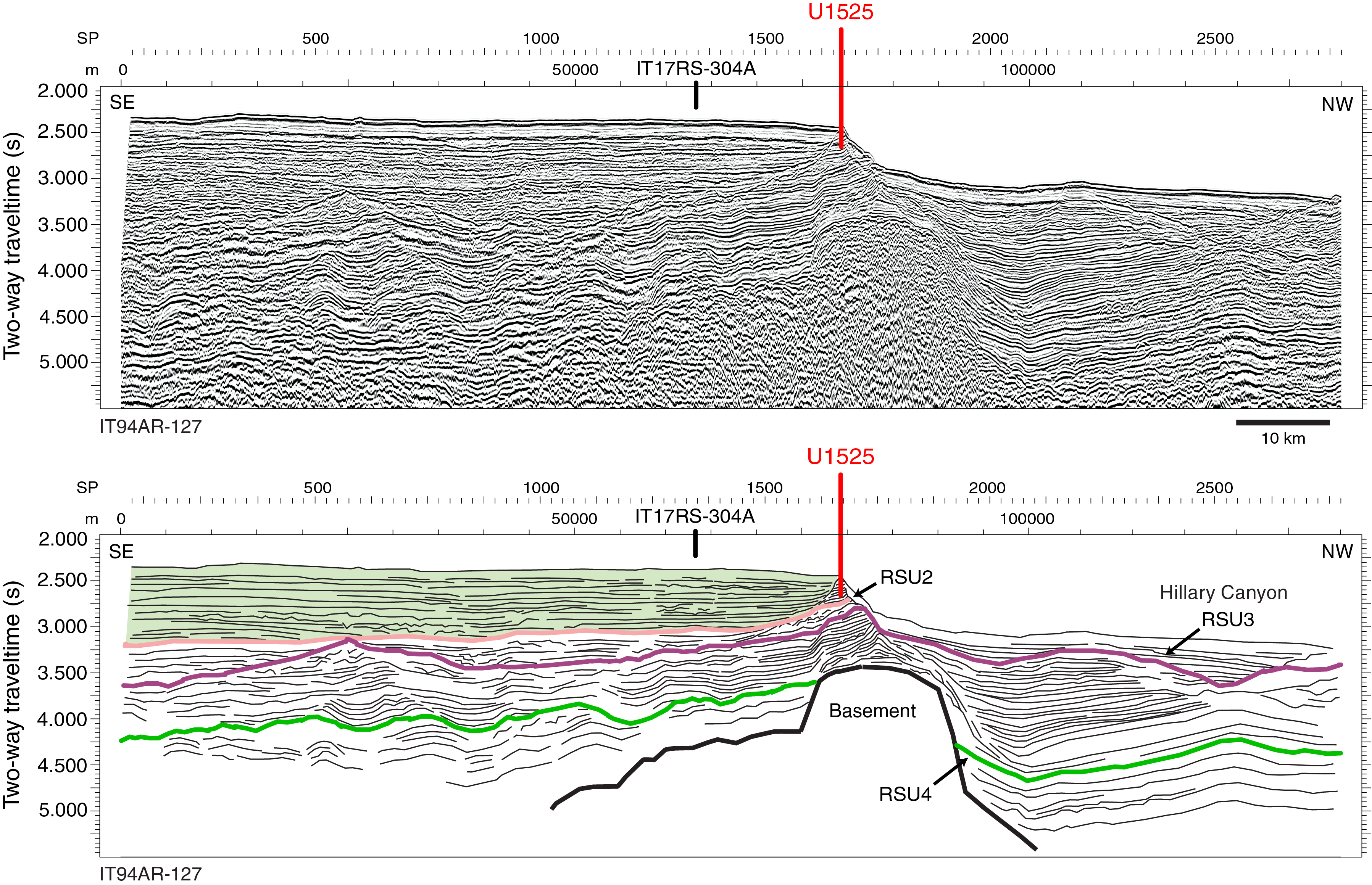
Figure F2. Seismic-reflection Profile IT94AR-127.
The Hillary Canyon is one of the largest conduits for newly formed Ross Sea Bottom Water (RSBW; a type of Antarctic Bottom Water [AABW]), which is focused in this channel by cascading dense water formed on the Ross Sea continental shelf passing down the continental rise (Bergamasco et al., 2002). The site also lies beneath the modern-day westward-flowing Antarctic Slope Current (ASC), which is thought to be stronger here than at the deeper water Site U1524 (Whitworth et al., 1998; Orsi and Wiederwohl, 2009). Seismic-reflection profiles indicate that the targeted sediments at Site U1525 are dominated by channel overspill and drift deposits characterized by stratified, parallel, high- to medium-amplitude seismic reflectors (Figure F2). Low-resolution multichannel seismic-reflection Profile IT94-127 (Figure F2) shows that the overall unit is stratified down to the acoustic basement at ~1 km below seafloor (3.5 s two-way traveltime [TWT]). Internal reflectors are spaced ~100 ms apart and are subparallel, laterally continuous, and subhorizontal. In the upper 50 m (0.7 s TWT), the reflectors onlap a highly angular unconformity that deepens and is likely older toward the southeast. These strata (green unit in Figure F2) are believed to be glacial debris flows interlayered with interglacial hemipelagic units of Pliocene to Pleistocene age that formed a prograding shelf margin fan at the mouth of the Glomar Challenger Basin coeval to or postdating Ross Sea Unconformity (RSU) 2.
The continental slope location of Site U1525 should allow for a more continuous assessment of oceanic forcings for (and response to) Antarctic Ice Sheet (AIS) variability than is possible from continental shelf records. The record of deposition at Site U1525 was anticipated to be primarily influenced by RSBW flowing down the Hillary Canyon but modified by an along-slope component associated with the westward-flowing ASC. Consequently, this site will enable assessment of the ocean drivers of ice sheet variability and bottom water production (see Objective 2 in Scientific objectives in the Expedition 374 summary chapter [McKay et al., 2019b]). The direct record of RSBW flow down the Hillary Canyon obtained at Site U1525 could potentially be extrapolated to high-fidelity paleoceanographic records farther afield in the abyssal Pacific Ocean to better constrain the Antarctic influences on the global oceanic deep circulation. The Hillary Canyon is also a main route for glacial sediments being eroded and transported by ice streams from the innermost continental shelf to its edge, and provenance studies of the terrigenous sediment may allow for identification of changing ice sheet drainage pathways through the Neogene and Quaternary.
Ice-rafted debris (IRD) could be sourced by icebergs from the Ross Sea or transported from the east by the ASC, providing a proxy for dynamic ice discharge from the Pacific Ocean coastline sector of the WAIS. Pelagic sediments would have been deposited during periods of high productivity or a lull in turbidity current–overspill deposition and will provide proxy records of surface water properties, including sea ice cover, sea-surface temperature, stratification, and salinity. These proxy records will enable an assessment of the magnitude of polar amplification during past warm climates (Objective 2) and the role of oceanic forcing on driving ice sheet fluctuations at those times (Objective 3). In addition, continuous deposition, anticipated at this site through much of the upper Neogene and Quaternary, will allow assessment of the orbital response of the WAIS and adjacent oceanic/biological system over a range of past climatic conditions (Objective 4). The upper Quaternary record in the uppermost 50 m of glacial strata can also shed light on the most recent ice sheet advances.
Operations
Site U1525 (proposed Site RSCR-03A) was added to the schedule when we were forced to temporarily leave Site U1524 because of encroaching sea ice. The operational plan for Site U1525 consisted of advanced piston corer (APC)/extended core barrel (XCB) coring in a single hole until sea ice moved away from Site U1524. Hole U1525A was cored to a total depth of 213.2 m drilling depth below seafloor (DSF) using a combination of APC, half-length APC (HLAPC), and XCB coring (Table T1). The XCB system was deployed in the upper part of the hole (43.0–55.7 m DSF) to core past an indurated interval. We then switched back to piston coring and continued to core using both the APC and HLAPC systems to 131.2 m DSF. After reaching HLAPC refusal, we continued coring with the XCB system to 213.2 m DSF. We terminated the hole at that depth after receiving confirmation that the sea ice was expected to clear from Site U1524 by the next day. The rig floor was secured for transit at 0535 h (local ship time; UTC + 13 h) on 9 February 2018 to return to Site U1524. A total of 51.25 h (2.1 days) was spent in Hole U1525.
We collected a total of 33 cores at Site U1525. The APC system was deployed 8 times, collecting 63.23 m of core (103%). The HLAPC system was deployed 14 times, recovering 52.64 m of core (92%). The XCB system was used 11 times and collected 42.83 m (45%) (Table T1).
Transit to Site U1525
The 50 nmi transit to Site U1525 was completed in 5.6 h at an average speed of 8.9 kt. A small deviation in course was required to navigate around sea ice. The vessel arrived at Site U1525 at 0200 h on 7 February 2018. The thrusters were lowered and secured at 0215 h, clearing the drill floor for operations. We did not deploy an acoustic positioning beacon at this site.
Hole U1525A
Operations for Hole U1525A began by preparing the APC/XCB bottom-hole assembly (BHA) and then lowering the drill string toward the seafloor. The calculated precision depth recorder depth for the site was 1790.8 m drilling depth below rig floor (DRF). We picked up the top drive and lowered the drill bit to tag the seafloor. Because the tag indicated that the seafloor was soft, we prepared a nonmagnetic APC core barrel and positioned the drill bit at 1786 m DRF. Hole U1525A was started at 1000 h on 7 February 2018. Core 374-U1525A-1H recovered 8.62 m of sediment, establishing a seafloor depth of 1776 meters below sea level. We continued to core with the APC system with nonmagnetic core barrels through Core 4H (28.9 m DSF), which was a partial stroke. We switched to the HLAPC system to collect Cores 5F through 8F (28.9–43.0 m DSF). Because Core 8F was a partial stroke with no recovery, we switched to the XCB system to cut Cores 9X and 10X (43.0–55.7 m DSF) to penetrate an indurated zone. We then switched back to the HLAPC system for Cores 11F through 15F (55.7–79.2 m DSF). With continued successful piston coring, we switched back to full-length APC core barrels and collected Cores 16H through 19H, which penetrated to 111.8 m DSF. Because Core 19H recorded a partial stroke, we advanced 4.1 m based on recovery and returned to the HLAPC system, collecting Cores 20F through 24F (111.8–131.2 m DSF). Core 24F also recorded a partial stroke, indicating HLAPC refusal. We switched to the XCB coring system for the remainder of the hole, cutting Cores 25X through 33X to a total depth of 213.2 m DSF. We experienced multiple shattered core liners (6 out of 11; 55%), which we suspect resulted from a combination of very cold seawater (−1.7°C) circulating through the drill string and the small space between the core liner and the core barrel, which allows vibration of the core liner. Ice conditions at Site U1524 were forecast to improve over the next 24 h, so we opted to terminate coring after Core 33X. We pulled the drill string out of the hole, clearing the seafloor at 2150 h on 8 February. After conducting routine rig maintenance (slip and cut 115 ft of drill line), the remainder of the drill string was retrieved, and the rig floor was secured at 0535 h on 9 February, ending operations at Site U1525. The total time spent at Site U1525 was 51.25 h (2.1 days).
Total recovery in Hole U1525A was 158.70 m over 213.2 m of coring (74%). The APC coring system was deployed 8 times, collecting 63.23 m of core over 61.5 m of coring (103%). The HLAPC was deployed 14 times, collecting 52.64 m of core over 57.0 m of coring (92%). The XCB was deployed 11 times, recovering 42.83 m of core over 94.7 m of coring (45%) (Table T1).
Lithostratigraphy
Site U1525 includes a single hole cored to 213.2 m DSF. The 158.70 m of sediment recovered from Site U1525 is divided into three lithostratigraphic units (Table T2). A lithologic summary of Hole U1525A is shown in Figure F3. The dominant facies throughout the hole are diatom-bearing/rich mud and muddy diatom ooze interbedded on the decimeter to meter scale with diatom-bearing/rich mud/sandy mud with dispersed to abundant clasts and muddy diamict (Table T3). The lithologic succession at Site U1525 consists of sandy mud with dispersed clasts and diamict in the upper 51.11 m core depth below seafloor, Method A (CSF-A) (Unit I), which overlies a 62.88 m thick sequence of interbedded massive/bioturbated diatom-bearing/rich mud and diatom-bearing/rich mud with silt laminae (Unit II). The lowermost 42.5 m consists of diatom-rich mud and muddy diatom ooze with fine laminae of silt and bioturbated diatom-rich sandy diamict (Unit III). Photographs of primary lithologies, sedimentary structures, and accessories are shown in Figures F4 and F5 and summarized in Figure F6, which highlights lithologic variations and trends based on data distilled from DESClogik.
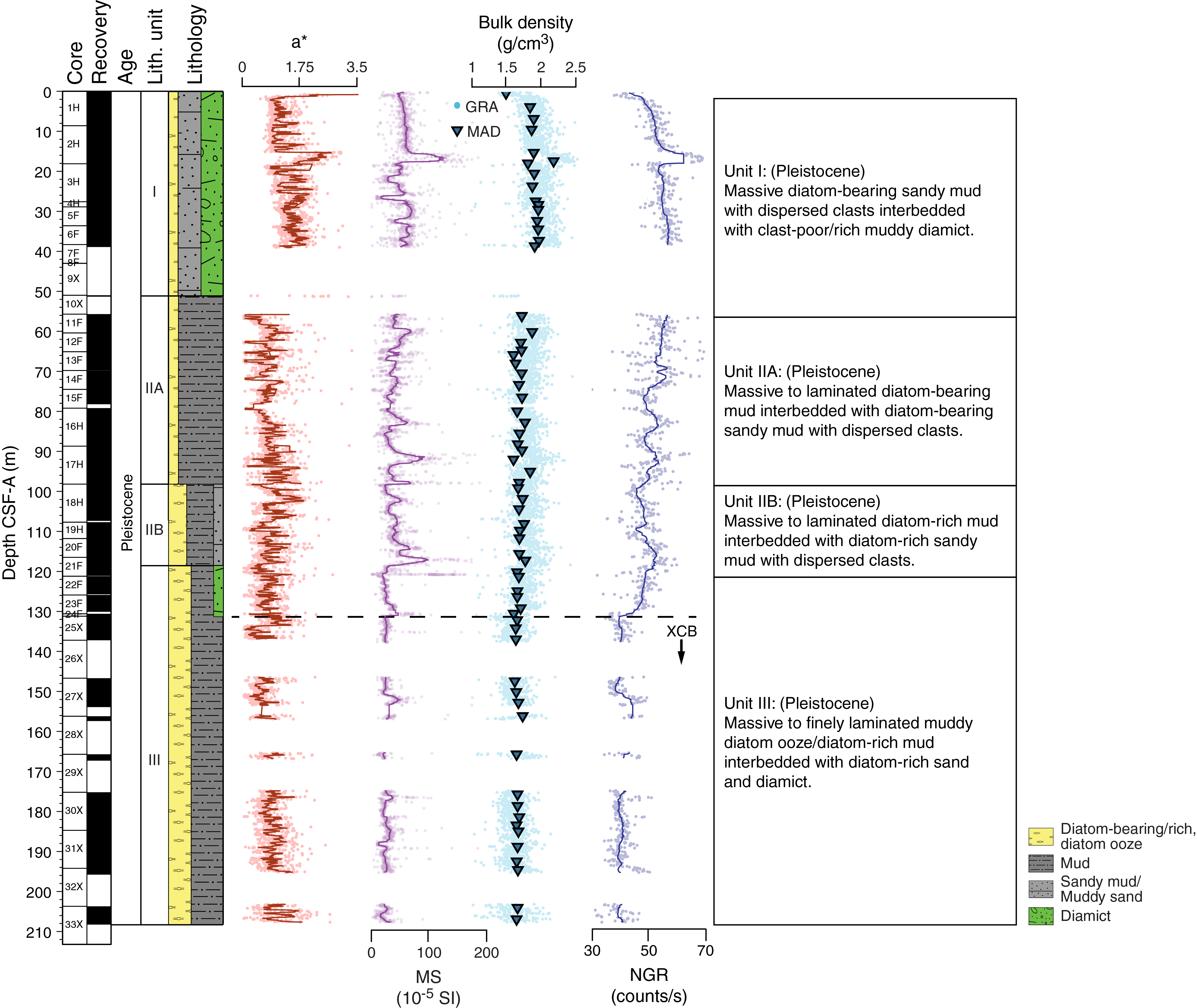
Figure F3. Lithostratigraphic summary.
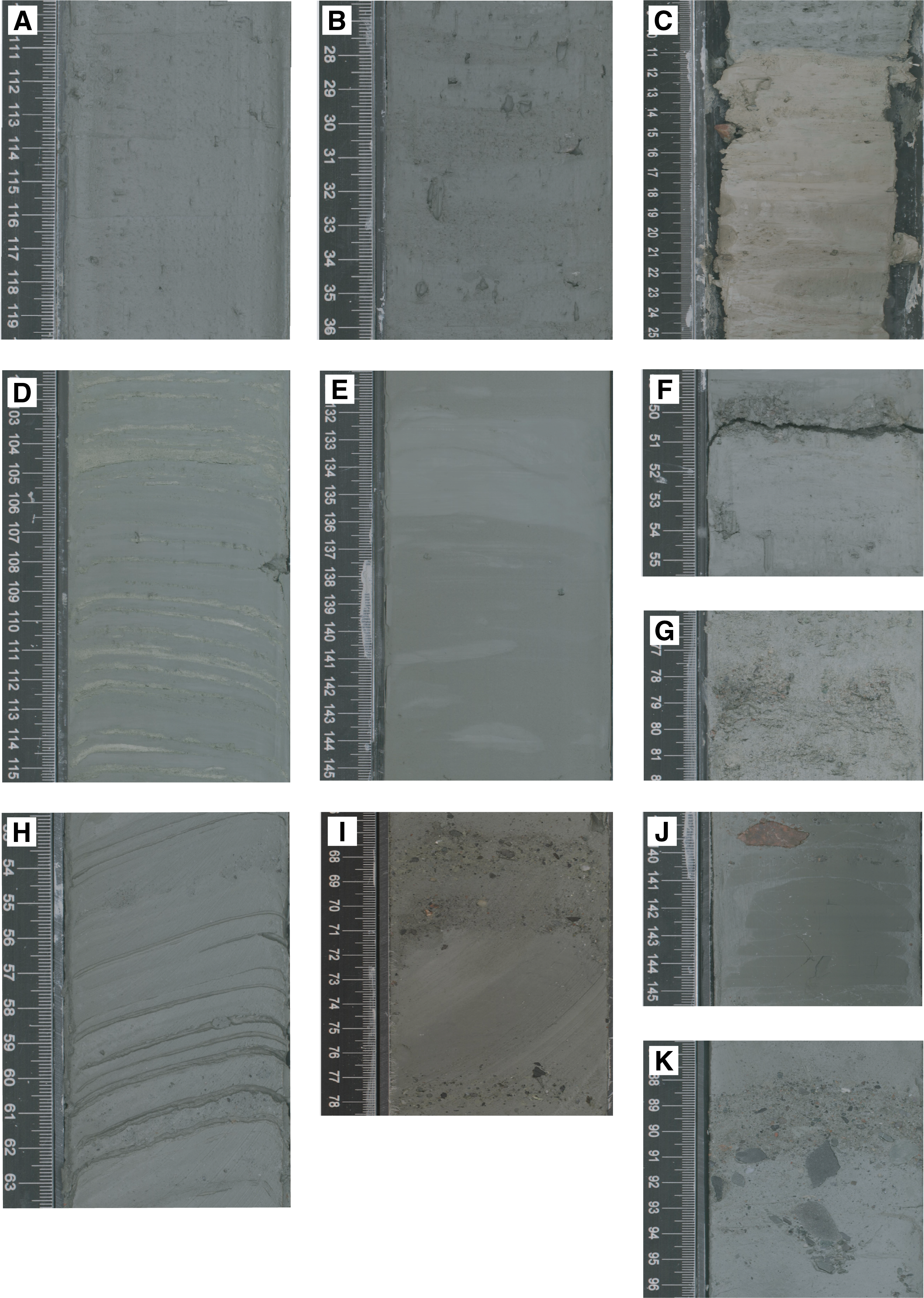
Figure F4. Primary lithologies.

Figure F5. Sedimentary structures and lithologic accessories.
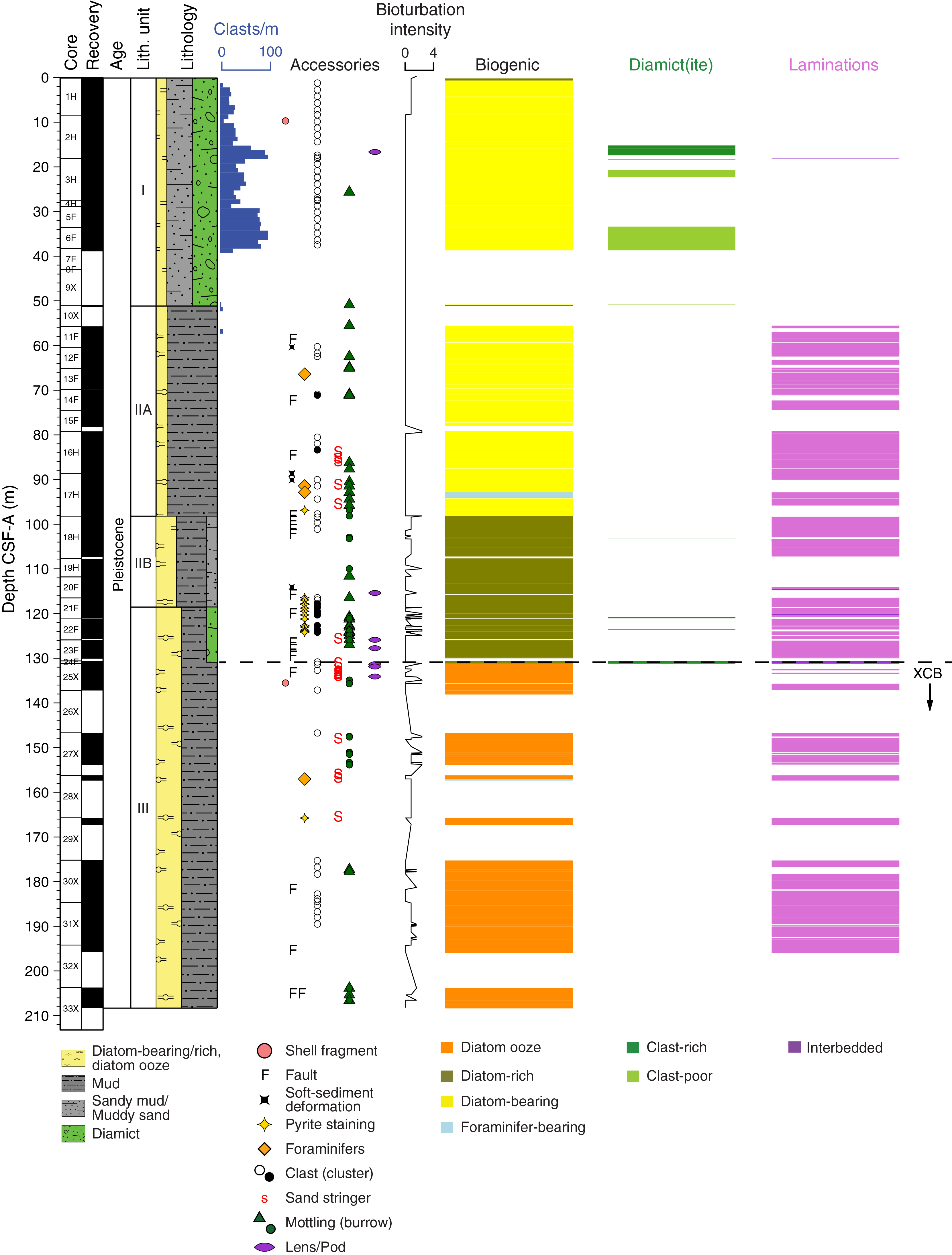
Figure F6. Lithology and sedimentary structures.
Unit descriptions
Site U1525 is divided into three lithostratigraphic units (I–III; youngest to oldest) based on lithologic changes observed downhole (Figure F3). The units were determined using a combination of visual core description, microscopic examination of smear slides, and color spectral observations (see Lithostratigraphy in the Expedition 374 methods chapter [McKay et al., 2019a]). Unit II is divided into two subunits (IIA and IIB; youngest to oldest).
Unit I
- Interval: 374-U1525A-1H-1, 0 cm, to 10X-1, 11 cm
- Depth: 0–51.11 m CSF-A
- Thickness: 51.11 m
- Age: Pleistocene
- Lithology: diamict, diatom-bearing sandy mud with dispersed clasts
Lithostratigraphic Unit I consists of unconsolidated massive bioturbated gray diatom-bearing/rich sandy mud with dispersed clasts interbedded on the meter scale with gray to light yellowish brown clast-poor/rich muddy diamict. Beds of diatom-bearing sandy mud with dispersed clasts (Figure F4A) are as thick as 8 m, and muddy diamict (Figure F4B) beds are as thick as 5 m. The beds are overcompacted (shear strength = 9.0 kg/cm2; see Physical properties) and contain randomly distributed, subrounded to subangular igneous and metamorphic clasts. Bedding contacts are sharp or gradational (Figure F5A). The lower boundary of Unit I (interval 374-U1525A-10X-1A, 11 cm) (Figure F4C) is a sharp contact between diatom-bearing/rich mud and diamict. This contact is in an interval of poor recovery that, based on the presence of muddy diamict in Section 7F-1 and piston core refusal in Core 8F (see Operations), likely consists of compacted diamict. The base of the unit was cored with the XCB system, with zero recovery in Core 9X and poor recovery in Core 10X that includes the contact between Units I and II. Recovery in Unit I is 40.78 m (80%).
Unit II
- Interval: 374-U1525A-10X-1, 11 cm, to 21F-2, 58 cm
- Depth: 51.11–118.58 m CSF-A
- Thickness: 67.47 m
- Age: Pleistocene
- Lithology: diatom-bearing/rich mud/sandy mud, diamict
Lithostratigraphic Unit II consists of massive greenish gray diatom-bearing/rich mud with dispersed clasts to diamict interbedded at the decimeter to meter scale with greenish gray diatom-bearing/rich mud containing silt and sand laminae. Unit II is divided into two subunits based on the structure and texture of laminations, very coarse sand and gravel clasts, centimeter-scale diamict beds, and diatom abundance (Figures F3, F6; Table T2). The lower contact of Unit II is defined by the increased thickness of bioturbated decimeter-scale sandy diamict beds, increased diatom content, and shifts in laminae frequency and clast content. Recovery in Unit II is 63.51 m (94%).
Subunit IIA
- Interval: 374-U1525A-10X-1, 11 cm, to 18H-1, 0 cm
- Depth: 51.11–98.20 m CSF-A
- Thickness: 47.09 m
- Age: Pleistocene
- Lithology: diatom-bearing mud/sandy mud
Lithostratigraphic Subunit IIA consists of massive to laminated greenish gray to dark greenish gray diatom-bearing mud interbedded at the decimeter to meter scale with diatom-bearing mud/sandy mud with dispersed clasts. In Subunit IIA, a typical decimeter- to meter-scale sequence consists of diatom-bearing mud with fine sand and silt laminae with sharp lower contacts and internal normal grading overlain by diatom-bearing mud with thin, more discontinuous laminae. This sequence is overlain by massive bioturbated diatom-bearing mud/sandy mud with clasts (Figure F4D–F4F). Soft-sediment deformation features and microfaulting are observed in the laminated sequences (Figures F5B, F5C, F6). Intervals of decimeter-scale bioturbated foraminifer-bearing sandy mud with dispersed clasts and sharp upper and lower contacts occur in some of the massive diatom-bearing mud beds (e.g., Section 374-U1525A-17H-4A; Figures F4G, F6). The Subunit IIA/IIB boundary is defined by a distinct change in the nature of the laminated mud beds, an increase in diatom content, and improved preservation of whole diatom frustules below Core 17H. Recovery in Subunit IIA is 43.21 m (92%).
Subunit IIB
- Interval: 374-U1525A-18H-1, 0 cm, to 21F-2, 58 cm
- Depth: 98.20–118.58 m CSF-A
- Thickness: 20.38 m
- Age: Pleistocene
- Lithology: diatom-rich mud/sandy mud, diamict
Lithostratigraphic Subunit IIB consists of laminated greenish gray diatom-rich mud (Figure F4H) interbedded at the decimeter to meter scale with massive bioturbated olive gray to greenish gray diatom-rich sandy mud with dispersed clasts and diamict beds (Figure F4H, F4I). The laminated diatom-rich mud beds are characterized by fine sand and silt laminae with sharp upper and lower contacts (Figure F5E, F5F) and internal planar to cross-bedding structures. Many laminated intervals contain coarse sand grains and gravel clasts that deform underlying silt laminae (Figure F5D). Clast composition varies and includes diamictite clasts. Sand pods, lenses, and stringers are observed, together with soft-sediment deformation (e.g., intervals 374-U1525A-20F-2A, 38–48 cm; 20F-2A, 90–106 cm; and 21F-1A, 137–143 cm; Figure F5G). Bioturbated diatom-rich sandy mud with dispersed clast beds sometimes contain sufficient clasts to be classified as muddy diamict. Recovery in Subunit IIB is 20.30 m (100%).
Unit III
- Interval: 374-U1525A-21F-2, 58 cm, to 33X-CC, 34 cm
- Depth: 118.58–208.27 m CSF-A
- Thickness: 89.69 m
- Age: Pleistocene
- Lithology: diatom-rich mud to muddy diatom ooze, diatom-rich sandy mud, diamict
Lithostratigraphic Unit III consists of laminated greenish gray diatom-rich mud to muddy diatom ooze (Figure F4J) interbedded at the decimeter scale with massive bioturbated light greenish gray diatom-rich sandy mud to muddy diatom ooze with dispersed clasts and diamict (Figure F4K). Beds of diatom-rich mud with dispersed clasts are faintly laminated, defined by submillimeter- to millimeter-scale silt laminae and millimeter- to centimeter-scale color variations. Laminae have sharp upper and lower contacts and sometimes appear rhythmic (e.g., interval 374-U1525A-23F-3A, 58–135 cm). Biogenic silica estimates from smear slides are variable, but some intervals are compositionally defined as muddy diatom ooze. However, the abundance of diatom fragments exceeds that of whole or partially fragmented diatom frustules. Sand to silt laminae are similar to those observed in Subunit IIB, but outsized clasts are less common (Figure F5I). Laminae occur sporadically downhole to Core 33X and often exhibit soft-sediment deformation and postdepositional faulting (Figures F5H, F6). Coarse sand pods, lenses, and laminae occur throughout (Figure F5J, F5K, F6). The bioturbated diatom-rich sandy mud with dispersed clasts coarsens upward into centimeter-scale diamict beds with bioturbated lower contacts (Figures F4K, F5L). Recovery in Unit III is 54.41 m (58%).
Facies distribution
At Site U1525, four main lithofacies are identified based on common lithologic and textural characteristics (Table T3). Although there are textural similarities between the shelf and slope sites, the depositional processes operating on the slope and rise are different from those on the shelf (Sites U1521, U1522, and U1523); therefore, we use an “r” to distinguish the slope/rise facies from the shelf facies. The lithofacies at Site U1525 largely conform with Lithofacies 1r, 2r, and 3r described at Site U1524 (see Lithostratigraphy in the Site U1524 chapter [McKay et al., 2019c]) but with some notable differences. At Site U1525, Lithofacies 1r (massive to stratified diamict) also includes a massive, overcompacted, poorly sorted clast-rich muddy diamict with subangular to rounded clasts of diverse lithologies. In lithostratigraphic Unit I, this facies likely represents mass flow deposits with rainout from ice rafting. The character of the laminae in Facies 2r and 3r also differs. For example, some laminae contain internal structures and sharp upper contacts that indicate reworking by bottom currents. One additional facies (4r; poorly sorted sand) is observed at Site U1525 and is described below.
Poorly sorted sand
Facies 4r consists of massive poorly sorted sand with dispersed clasts. This facies is diatom-bearing/rich and/or foraminifer-bearing/rich. Basal contacts are sharp, gradational, and/or bioturbated. Similar to the diamict facies, inverse grading is common. Facies 4r reflects sedimentation influenced by current winnowing, mass transport, and/or ice rafting.
Diagenesis
The presence of pyrite in laminated and bioturbated sediments indicates postdepositional diagenesis from bacterial decomposition of organic material in a sulfate-reducing environment.
Preliminary depositional interpretation
Coring at Site U1525 recovered a sequence of Pleistocene sediments from a channel levee complex on the upper continental slope of the Ross Sea. The depositional setting and lithostratigraphic units at Site U1525 reveal an interplay between downslope, along-slope (e.g., winnowing), hemipelagic, and pelagic processes. Clasts occur throughout, indicating the persistent influence of ice rafting. The mass transport deposits in lithostratigraphic Unit I may reflect changes in glacial dynamics on the outer continental shelf. Units II and III were deposited in a high-relief levee setting and therefore are influenced by the overspill of turbidity currents, winnowing by bottom currents, and ice rafting. Generally, siliciclastic content increases upsection. In Unit III, diatom fragments are observed in the diatom-rich mud/muddy diatom ooze intervals, suggesting that these deposits are not primary pelagic/hemipelagic ooze and mud. These sequences may be reworked from pelagic diatom ooze units originally deposited on the Ross Sea continental shelf or upper continental slope and subsequently transported downslope. In addition to downslope processes, internal structures in laminae and inverse grading of sand and diamict intervals in Units II and III may reflect winnowing related to temporal changes in the strength of the westward-flowing ASC. Thus, Site U1525 sediments record both down- and along-slope processes in a Pleistocene open-marine to glaciomarine environment.
Biostratigraphy and paleontology
Core catcher samples from Site U1525 were analyzed for siliceous (diatoms, radiolarians, silicoflagellates, and ebridians), calcareous (foraminifers and calcareous nannofossils), and organic (dinoflagellate cysts [dinocysts] and other aquatic palynomorphs, pollen, and spores) microfossils. Samples in the upper 111.84 m CSF-A (from Sample 374-U1525A-19H-CC and above) are either devoid of microfossils, contain only trace amounts, or include a “residual” assemblage of resistant forms that have likely been engaged in multiple phases of transport and reworking by ice and/or bottom currents. The character of this interval is defined by the abundance and persistence of reworked taxa (Table T4). These reworked specimens represent diatom taxa that were eroded and transported from discrete source beds of early Miocene, middle Miocene, and late Miocene to early Pliocene age into this interval at Site U1525. These older displaced diatoms co-occur in this interval with an assemblage of robust and heavily silicified diatoms. This combination likely reflects a concentration of taxa that survived multiple stages of transport and redeposition. This interval is problematic, and shipboard microfossil biostratigraphy is unable to resolve a reliable and defendable age profile with the ~5–10 m sample spacing available between core catchers. Future targeted sampling of intervals identified as having been deposited primarily by pelagic processes (e.g., interglacial intervals) in postcruise studies may provide additional age control. In this interval, Sample 4H-CC at 28.86 m CSF-A yields an age-diagnostic radiolarian event that indicates an age older than 0.65 Ma for this sample (Table T5; Figures F7, F8, F9).
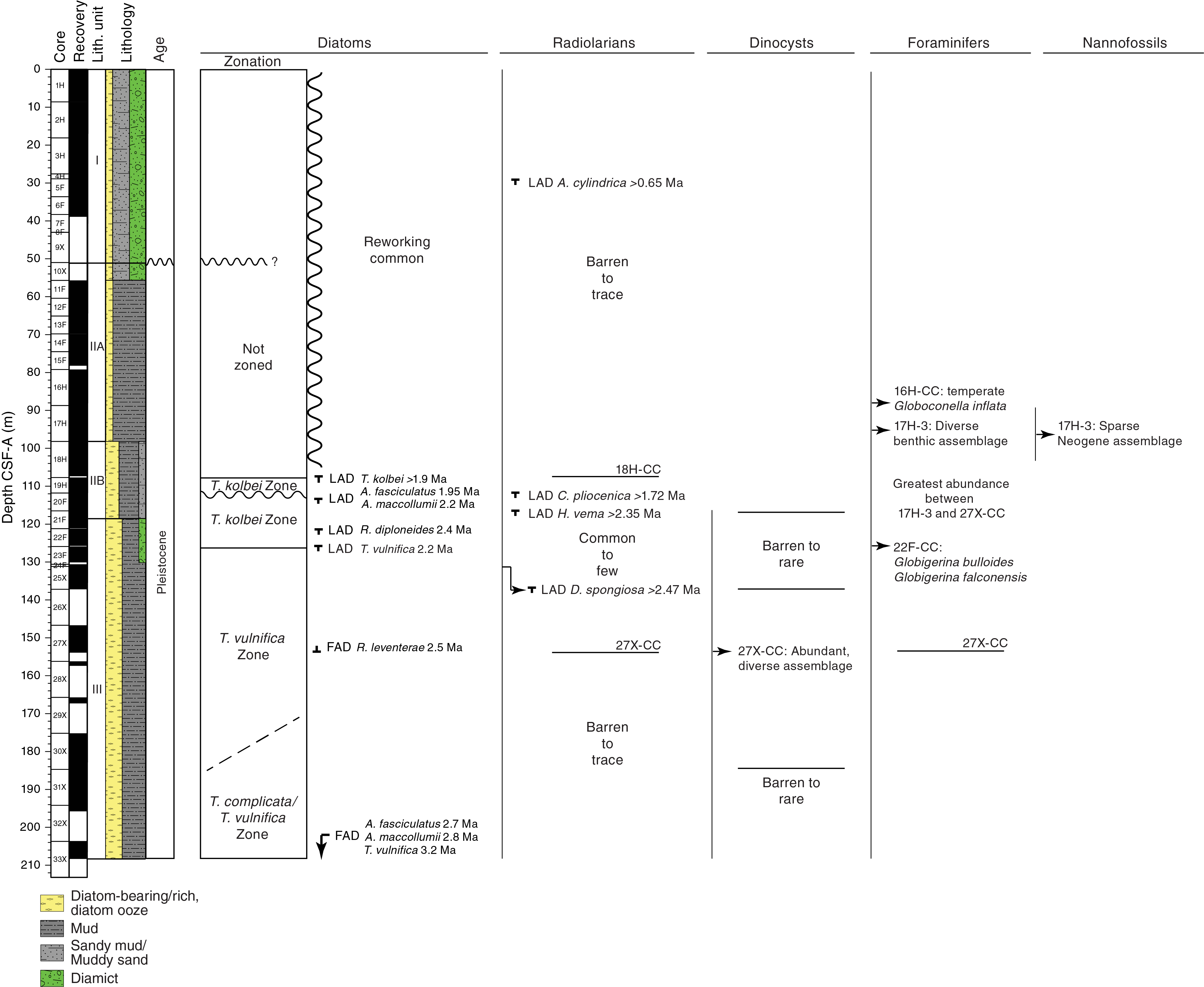
Figure F7. Micropaleontology summary.
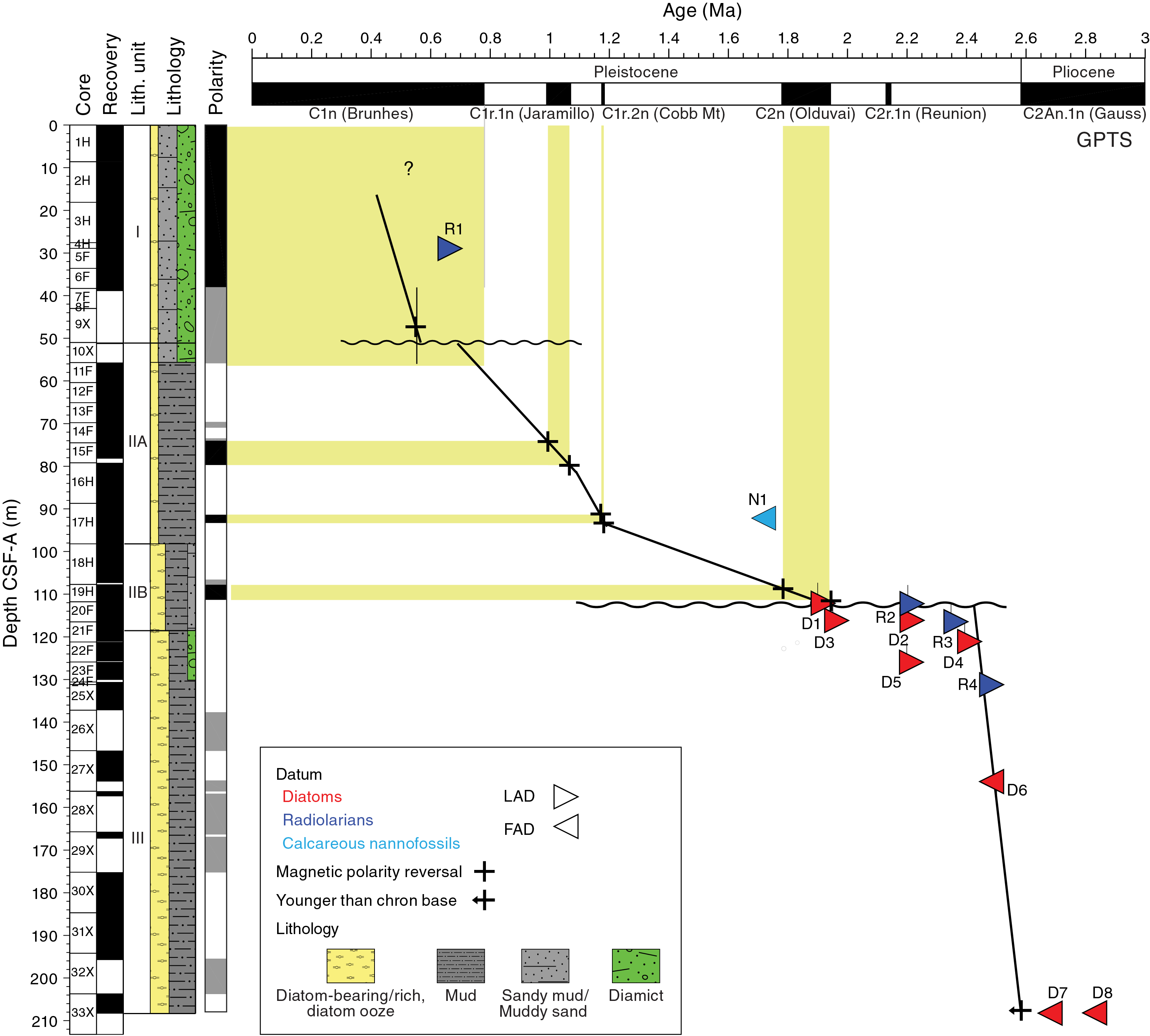
Figure F8. Shipboard age model.

Figure F9. Selected diatom and radiolarian distribution.
Microfossils in samples deeper than 111.84 m CSF-A (e.g., Sample 374-U1525A-19H-CC) are more abundant and well preserved, and several age diagnostic radiolarians and diatoms were encountered. Although a small background presence of reworked diatoms continues in this interval with the persistent presence of Thalassiosira oliverana var. sparsa (a late Miocene to early Pliocene diatom), an expected sequence of early Pleistocene first appearance datum (FAD) and last appearance datum (LAD) events is evident (Figures F7, F8, F9). Dinocysts are sparse in this interval, and only Sample 27X-CC (153.87 m CSF-A) in the lower Pleistocene yields abundant dinocysts (Figure F7). The assemblage comprises species known from the uppermost Quaternary sediments of the Atlantic sector of the Southern Ocean, south of the Polar Front. Planktonic and benthic foraminifers are also most abundant and diverse in the mid-Pleistocene section, and the occurrences of the planktonic species Globoconella inflata at 88.86 m CSF-A (Sample 16H-CC) and Globigerina bulloides and Globigerina falconensis at 125.67 m CSF-A (Sample 22F-CC) indicate the presence of warmer-than-present water (Figure F7). A sparse Neogene assemblage of calcareous nannofossils is present in Sample 17H-3A, 82 cm (92.34 m CSF-A) (Figure F7).
Diatoms
All core catcher samples from Site U1525 were examined for diatoms, and their distribution is shown in Figures F7 and F9 and Table T4. Samples 374-U1525A-1H-CC to 19H-CC (8.57–111.84 m CSF-A) are inferred to be late Pleistocene in age, although few diatoms characteristic of this age are identified in this interval. Assemblages comprise a mixture of reworked Miocene, Pliocene, and Pleistocene diatoms (Table T4; Figures F7, F9), which makes age assignment for this interval difficult. These reworked taxa are generally heavily silicified and include a persistent presence of T. oliverana var. sparsa (total range = 8.6–4.9 Ma), Trinacria spp. (generally common at >4.5 Ma), Stephanopyxis spp. (generally common at >4.5 Ma), Actinocyclus ingens var. nodus (14.5–12.6 Ma), Pseudammodocium lingii (a Miocene ebridian lorica common in Ross Sea sediment cores), and other robust taxa Paralia sulcata, Actinoptychus spp., Aulacodiscus brownei, and Coscinodiscus spp. fragments. Although there are very likely discrete stratigraphic intervals in the upper ~111 m CSF-A of Site U1525 that contain in situ assemblages of diatoms and other microfossils that reflect primary marine deposition, none of these intervals were identified during shipboard investigations of core catcher samples. Postcruise selective sampling may allow the identification of sedimentological facies where initial diatom production and final deposition ages are closely aligned, which may provide better age control through this interval.
The following discussion focuses on the lower half of Site U1525, which is interpreted to represent hemipelagic to pelagic environments. Some intervals record high diatom production in overlying water, and in other intervals diatoms were likely brought to the site by ocean currents with local modification and/or concentration of the diatom assemblage. Although diatom abundance is high in many intervals, diatoms are often present as finely fragmented remains and make up a large component of the clay-sized fraction of Site U1525 sediments.
Figures F7 and F9 present biostratigraphic datum events identified at Site U1525 that indicate age and zonal assignments. The top of the Thalassiosira kolbei Zone is identified by the last appearance of T. kolbei (1.9 Ma) in Sample 374-U1525A-19H-CC (111.84 m CSF-A). A disconformity is indicated between Samples 19H-CC and 20F-CC (between 111.84 and 116.52 m CSF-A), as indicated by biostratigraphic and magnetic polarity reversal constraints (Figure F8), which removed part of the T. kolbei Zone. The LADs of two distinctive diatoms are noted in this zone, Actinocyclus fasciculata (LAD at 1.95 Ma) and Actinocyclus maccollumi (LAD at 2.2 Ma) in the lower portion of the T. kolbei Zone in Sample 20F-CC (116.62 m CSF-A). These species are present downhole through the rest of the lower Pleistocene section at Site U1525, including the underlying T. vulnifica Zone, the top of which is identified by the LAD of T. vulnifica in Sample 22F-CC (125.67 m CSF-A).
A single occurrence of Rouxia leventerae (FAD at 2.5 Ma), noted in Sample 374-U1525A-27X-CC (153.87 m CSF-A), suggests an age of <2.5 Ma for this level. A rich and well-preserved assemblage of Rouxia spp., Fragilariopsis spp., and many spines and girdle bands of Corethron pennatum are also noted in Sample 27X-CC, revealing an interval of productive pelagic sedimentation at this site, with preservation of fine, lightly silicified diatoms.
The lower boundary of the T. vulnifica Zone and the upper boundary of the underlying Thalassiosira complicata/T. vulnifica Zone was not identifiable at Site U1525 because of the persistent reworking of T. complicata throughout this interval that prevents a clear identification of its highest occurrence, which defines this boundary. In the Ross Sea during Expedition 374, we use the LAD of T. complicata in place of the LAD of Thalassiosira insigna, whose LAD is used in the Southern Ocean biostratigraphic framework to define the top of the T. insigna/T. vulnifica Zone. For our use during Expedition 374, we recognize the LAD of T. complicata to define the top of the T. complicata/T. vulnifica Concurrent Range Zone (see Biostratigraphy and paleontology in the Expedition 374 methods chapter [McKay et al., 2019a]). This zone is identified to the base of Site U1525 in Sample 374-U1525A-33X-CC (208.22 m CSF-A), where T. vulnifica (whose FAD defines the base of the zone) is still present in the deepest sample examined. A. fasciculatus and A. maccollumi are also present, leading to the interpretation that the FAD of these taxa were not sampled and that they exist below the interval cored at Site U1525.
Radiolarians
All core catcher samples and the mudline sample from Site U1525 were analyzed for radiolarian content, and a distribution chart is given in Table T6. Radiolarians are barren or present in trace abundances and poorly preserved in the uppermost 107.27 m CSF-A (downhole to Sample 374-U1525A-18H-CC). Throughout this interval, only one radiolarian datum is observed, the LAD of Antarctissa cylindrica in Sample 4H-CC (28.86 m CSF-A) (Figures F7, F8, F9). Diatom biostratigraphy and seismic evidence suggest extensive mixing of sediments, probably linked to debris flow deposits, over this interval (see Background and objectives). This high input of terrigenous material could also cause dilution of radiolarian assemblages, which would explain the very low abundances observed for this group in this part of the section.
The interval from Sample 374-U1525A-19H-CC to Sample 27X-CC (111.84–153.87 m CSF-A) yields moderately to well-preserved radiolarians in frequent to common abundances. Three LADs are observed in this interval: Cycladophora pliocenica in Sample 19H-CC (111.84 m CSF-A), Helotholus vema in Sample 20F-CC (116.62 m CSF-A), and Desmospyris spongiosa in Sample 24F-CC (131.22 m CSF-A) (Figures F7, F8, F9). The high radiolarian abundance (particularly in Sample 27X-CC [153.87 m CSF-A]), together with the abundance patterns of planktonic foraminifers (Figures F7, F9) and dinoflagellates (also abundant in Sample 27X-CC), seem to suggest deposition in an open-marine environment with reduced influence of sea ice and/or terrigenous input. Disconformities, particularly slow sedimentation rates, and/or sharp changes in environmental conditions occur between Samples 17H-CC and 18H-CC (98.62–107.27 m CSF-A) and between Samples 19H-CC and 20H-CC (111.84–116.62 m CSF-A), where rapid age increases are observed downhole. A strong change in environmental conditions may additionally occur between Samples 27X-CC and 28X-CC (153.87–157.34 m CSF-A), where radiolarian abundances abruptly decrease from common to absent. This decrease makes the observed FAD for H. vema in Sample 27X-CC (153.87 m CSF-A) highly questionable, so this datum has not been used to constrain the age model at this site (Table T5 lists the retained diatom and radiolarian datums used to construct the age model in Figure F8). Between Sample 28X-CC (157.34 m CSF-A) and the bottom of the cored sequence (Sample 33X-CC [208.22 m CSF-A]), core catcher samples are barren or contain only trace abundances of radiolarians. Photomicrographs of a few radiolarian species from Sites U1525 and U1524 are shown in Figure F10.
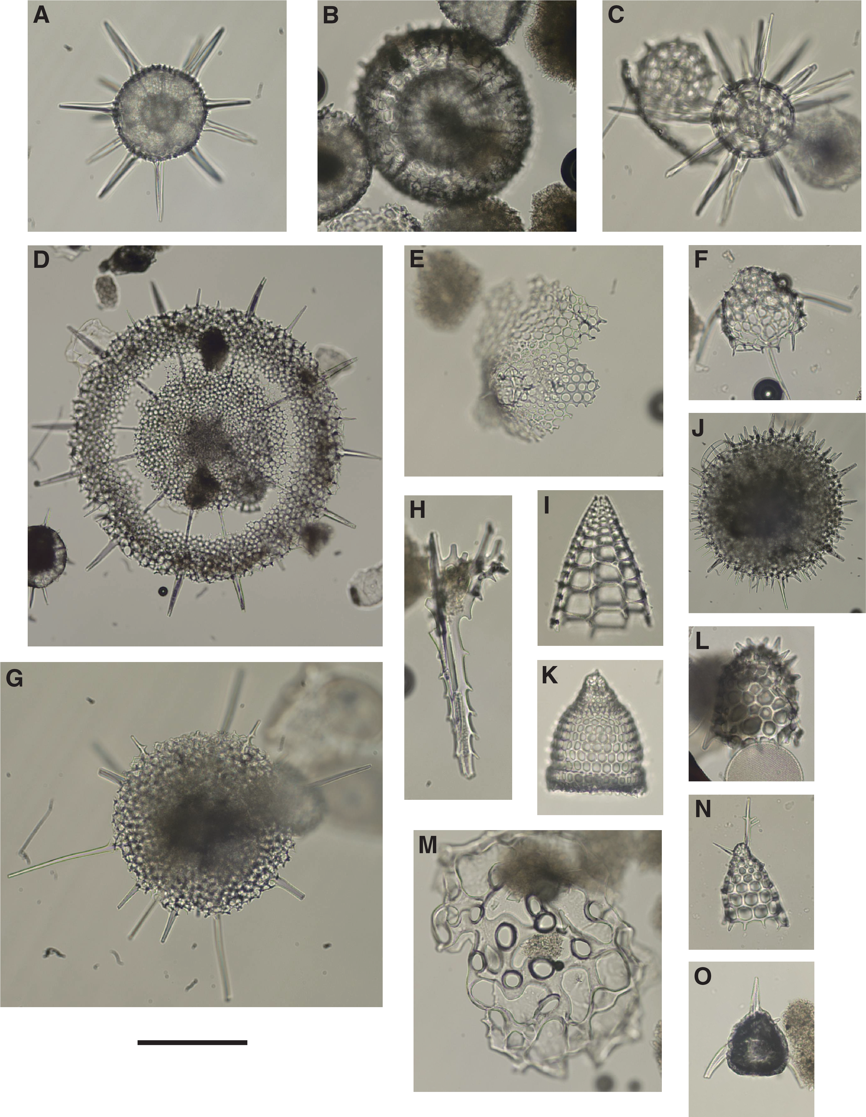
Figure F10. Radiolarians.
The primary marker species Stylatractus universus, Pterocanium charybdeum trilobum (both presumably living at much lower latitudes than the Ross Sea area), and Cycladophora davisiana (present in the mudline sample and therefore living at this location under modern conditions but absent in core material) are observed in core catcher samples from this site. The marker species Eucyrtidium calvertense was only found in the lowermost sample obtained at this site (Sample 374-U1525A-33X-CC [208.22 m CSF-A]), which is dated to >2.47 Ma based on the LAD of D. spongiosa in Sample 24F-CC (131.22 m CSF-A). This LAD is much older than the calibrated LAD at ~1.73 Ma (Florindo et al., 2013), which suggests that this event is probably slightly diachronous in different regions of the Southern Ocean and therefore not reliable in the Ross Sea area.
The mudline sample contains a very diverse, modern assemblage made up of 40 species, with significant contributions of Larcopyle pylomaticus, Stylatractus neptunus, Actinomma leptodermum, Actinomma boreale, and Antarctissa denticulata. The two taxa representative of Antarctic shelf/coastal assemblages (Rhizoplegma boreale and the Phormacantha hystrix/Plectacantha oikiskos group; Nishimura et al., 1997) are either absent or present in negligible numbers, respectively. Many of the species observed in significant numbers (e.g., A. boreale/leptodermum, Hexacontium pachydermum, and Pseudodictyophimus gracilipes) are typical components of Arctic/Subarctic assemblages (found in the Greenland Sea close to the summer sea ice edge, the Norwegian Sea, and the Arctic Ocean proper; Swanberg and Eide, 1992; Schröder-Ritzau, 1995; Bjørklund and Kruglikova, 2003). Thus, they may be considered to have a bipolar distribution with equatorial submergence and have probably been advected to the site through the Antarctic Divergence and upwelling of intermediate and deep-water masses. The latter process seems to also be confirmed by the presence of species known to live in intermediate- to deep-water masses (e.g., Cycladophora davisiana and Cornutella profunda).
Very high abundances of volcanic shards associated with abundant sponge spicules are observed in Sample 374-U1525A-21F-CC (121.05 m CSF-A) and strongly suggest the presence of a cryptic or partially reworked ash layer because a primary ash feature was not observed in the split cores. Such a layer might have been missed or unsampled because of its occurrence in the stratigraphic gaps that occur between cores (see Depth scales in the Expedition 374 methods chapter [McKay et al., 2019a]).
Foraminifers
Foraminifers have variable occurrence and abundance in the Pleistocene section cored at Site U1525 (Table T7). In general, the most clay rich samples are foraminifer poor or barren, whereas somewhat sandier mud samples contain planktonic and benthic foraminifers. Mud samples that at first examination appeared to be barren may contain planktonic and/or benthic taxa in the 63–125 µm fraction, which was not routinely examined shipboard. Sand-rich samples are likewise very poor in foraminifers, likely a consequence of dilution by the coarser terrigenous sediments (e.g., Samples 374-U1525A-1H-CC and 33X-CC [8.57 and 208.22 m CSF-A, respectively]) (Figure F7).
Sandy mud from Samples 374-U1525A-5F-CC (33.75 m CSF-A) and 7F-CC (38.87 m CSF-A) contains rare (<7) specimens of both planktonic and benthic foraminifers, including sinistrally coiled Neogloboquadrina pachyderma, Globocassidulina subglobosa, Angulogerina earlandi, Globocassidulina crassa, Bulimina aculeata, and Cibicides temperatus; the latter is a yellow-stained, reworked specimen.
A number of the clay-rich samples did not yield any foraminifers during shipboard examination, including Samples 374-U1525A-10X-1, 30–33 cm (51.30 m CSF-A), 12F-CC (65.46 m CSF-A), and 13F-CC (69.73 m CSF-A), whereas other clay-rich samples contain four or fewer specimens (Samples 14F-CC [74.68 m CSF-A], 28X-CC [157.34 m CSF-A]), 30X-CC [184.69 m CSF-A], and 32X-CC [195.84 m CSF-A]. In contrast, several clay-rich samples with small residues of >63 µm fraction material produced small assemblages of foraminifers with relatively numerous specimens (Samples 11F-CC [60.54 m CSF-A], which contains only N. pachyderma; 15H-CC to 20F-CC [78.16–116.62 m CSF-A]; 22F-CC [125.67 m CSF-A]; 23F-CC [130.03 m CSF-A]; and 27F-CC [153.87 m CSF-A]). The most common benthic species in most of these samples are G. subglobosa and Epistominella exigua. The specimens in some of these samples are very tiny and appear to be size sorted and winnowed by currents. Other specimens, particularly planktonic foraminifer N. pachyderma, have holes in chambers, suggesting etching by corrosive deep water. Sample 27X-CC, in contrast, looks more in situ than many samples because of the good preservation and dominance of the agglutinated benthic foraminifer Miliammina arenacea, which was found in abundance near the front edge of the Ross Ice Shelf (Osterman and Kellogg, 1979).
A particularly productive foraminifer-rich sandy interval was examined in Sample 374-U1525A-17H-3, 62–64 cm (92.14 m CSF-A). This sample contains abundant planktonic foraminifers (N. pachyderma) and nearly 30 species of benthic foraminifers, including G. subglobosa, A. earlandi, E. exigua, Brizalina sp. cf. Brizalina thalmanni, Pullenia bulloides, Pullenia subcarinata, Astrononion antarcticus, Melonis affinis, Gavelinopsis lobatulus, Cibicides refulgens, Cibicidoides spp., Fursenkoina fusiformis, Karreriella bradyi, and numerous species of nodosariids. This diverse, generally well preserved assemblage may represent colonization on a well-oxygenated, winnowed substrate. Alternatively, the broken chambers observed on some of the more delicate taxa suggest that this assemblage, or parts of it, were transported downslope more or less penecontemporaneously. Interestingly, all of the N. pachyderma in Sample 17H-3, 62–64 cm, are <250 µm in diameter, suggesting size sorting and winnowing by currents prior to deposition.
In summary, the greatest abundances of foraminifers are found in Samples 374-U1528A-11F-CC to 27X-CC (60.54–153.87 m CSF-A), but the greatest abundances of benthic foraminifers are found in Samples 15H-CC (78.16 m CSF-A) to 27X-CC (Figure F7). It is interesting to note that G. inflata occurs in Sample 16H-CC (88.86 m CSF-A), whereas G. bulloides and G. falconensis occur in Sample 22F-CC (125.67 m CSF-A), suggesting episodes of warmer, open, more highly productive surface water (Figure F11).

Figure F11. Planktonic foraminifers.
Palynology
Seven core catcher samples (374-U1525A-20F-CC to 31X-CC [116.62–194.38 m CSF-A]) were analyzed for palynomorph content (Table T8) below the interval of reworking identified by siliceous microfossils (Figure F7). In general, palynomorphs are moderately to well preserved and absent to rare in Samples 20F-CC (116.62 m CSF-A), 24F-CC (131.22 m CSF-A), 30X-CC (184.69 m CSF-A), and 31X-CC (194.38 m CSF-A); few in Samples 28X-CC (157.34 m CSF-A) and 29X-CC (167.25 m CSF-A); and abundant in Sample 27X-CC (153.87 m CSF-A) (Figure F7). The assemblages at Site U1525 are dominated by protoperidinioid dinocysts that are likely cysts of heterotrophic dinoflagellates (mostly Brigantedinium spp. and Selenopemphix spp.), which are indicative of highly productive water (Zonneveld et al., 2013). Few specimens of the phototrophic Batiacasphaera sp. are found. Representative photomicrographs of dinocysts are shown in Figure F12.
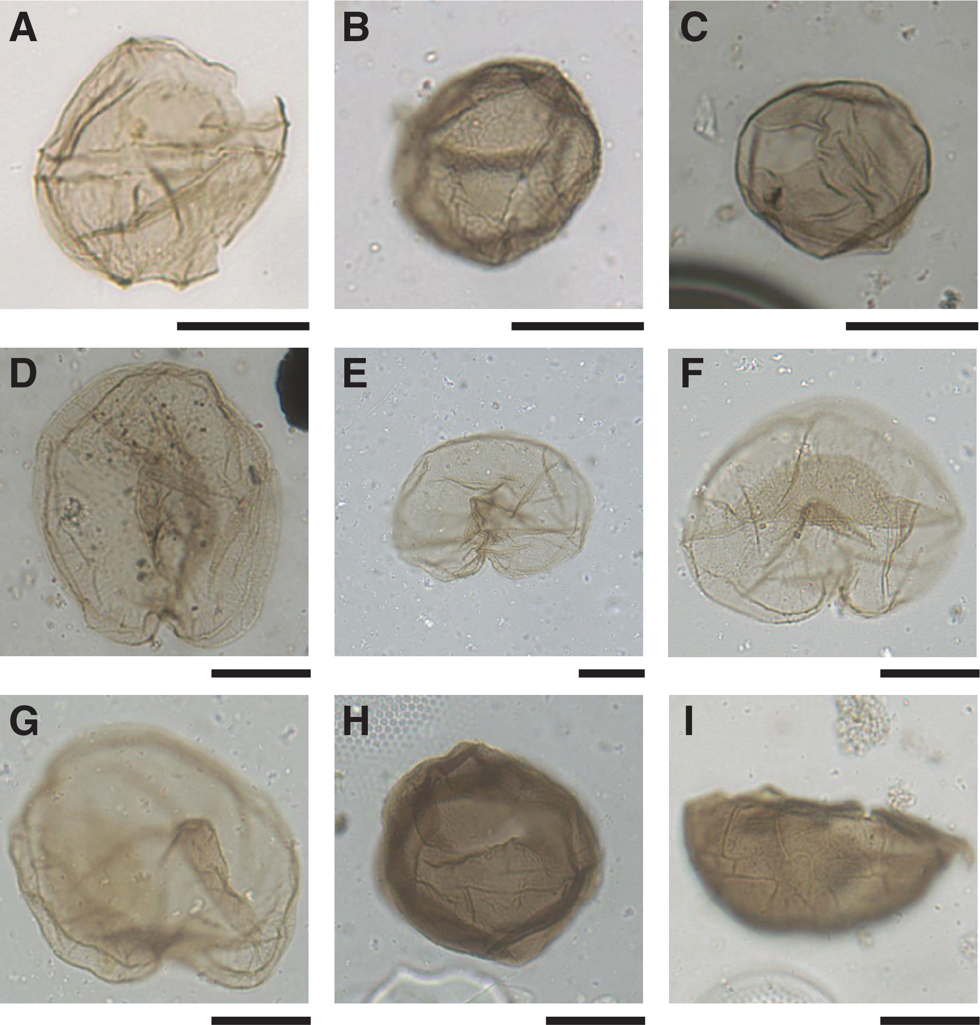
Figure F12. Dinocysts.
Sample 374-U1525A-20F-CC (116.62 m CSF-A) is almost devoid of dinocysts; only rare Brigantedinium spp. and very rare Lejeunecysta sp. are found (Figure F12; Table T8). The acritarch Leiosphaeridia is present in low numbers. Sample 24F-CC (131.22 m CSF-A) is barren of dinocysts, and only the acritarch Leiosphaeridia is present in very low numbers.
Sample 374-U1525A-27X-CC (153.87 m CSF-A) exhibits a low diversity dinocyst assemblage of dominant Brigantedinium spp., common Selenopemphix sp. 1 (Esper and Zonneveld, 2007), few Selenopemphix antarctica and Selenopemphix nephroides, and rare Batiacasphaera spp. The Brigantedinium spp. cysts are pigmented light brown, grayish brown, or dark brown and have smooth or granular to scabrate surfaces (Figure F12). Some Brigantedinium spp. exhibit a paratabulation-like pattern (Figure F12), with features resembling those of the genus Cryodinium described from the modern permanent open-ocean zone of the Atlantic Southern Ocean sector (Esper and Zonneveld, 2002); however, the Brigantedinium spp. here are generally larger and lack low sutures on a single layered wall. Assemblages composed mainly of Brigantedinium spp., S. antarctica, and Selenopemphix sp. 1 (Figure F12) were described from late Quaternary glacial sediments of the Atlantic Southern Ocean (Esper and Zonneveld, 2007) and might reflect productive open-water conditions during the summer season in the Ross Sea.
Samples 374-U1525A-28X-CC (157.34 m CSF-A) and 29X-CC (167.25 m CSF-A) exhibit few Brigantedinium spp. and S. nephroides and common specimens of the acritarch Leiosphaeridia. A few specimens of the transparent Cymatiosphaera sp. 1 are found in Sample 29X-CC only. In Samples 30X-CC (184.69 m CSF-A) and 31X-CC (194.38 m CSF-A), rare specimens of Brigantedinium spp., S. nephroides, and Batiacasphaera spp. are found. The acritarch Leiosphaeridia is common.
Although palynomorphs are very sparse in the sediments at Site U1525, the dinocyst assemblages point to a high-productivity environment. The low numbers encountered in these samples may be a consequence of high sediment accumulation rates and high input of terrigenous sediments, both of which dilute the biogenic (dinocyst) accumulation. Sample 374-U1525A-27X-CC (153.87 m CSF-A) is remarkable in that it contains abundant and well-preserved dinocysts that are as yet only known from modern circum-Antarctic sediments and open-ocean upper Quaternary Southern Ocean sediments from the Atlantic sector north of the Polar Front (Esper and Zonneveld, 2002, 2007). The occurrence of these dinocysts may imply that the typical recent to modern Southern Ocean dinocyst assemblage first appeared in the Ross Sea in the earliest Pleistocene and that environmental conditions were slightly warmer than at present, with longer seasons of open-water conditions. This aspect merits further postcruise investigation.
Calcareous nannofossils
Sample 374-U1525A-17H-3A, 82 cm (92.34 m CSF-A), was examined for calcareous nannofossils (Table T9). This sample contains a sparse assemblage of moderately preserved Neogene taxa (Figures F7, F13) that includes Reticulofenestra minuta, Reticulofenestra minutula, Calcidsicus leptoporus, and Coccolithus pelagicus. The absence of Gephyrocapsa spp. >4 µm is biostratigraphically significant because this group has a FAD at 1.73 Ma. However, additional work needs to be undertaken to support this interpretation because the absence of this group could be due to the sparse nature of the assemblage or the assemblage could be reworked from older sediment.
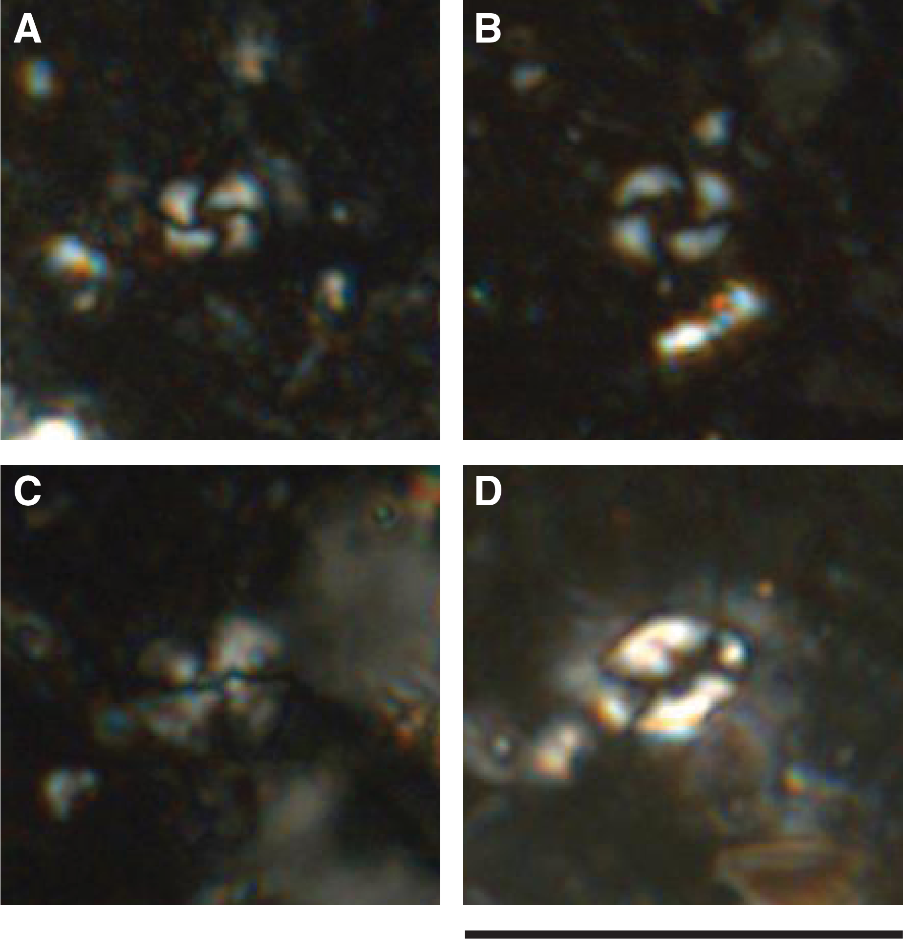
Figure F13. Calcareous nannofossils.
Age model
An age model for Site U1525 (Figure F8) was developed using a combination of radiolarian and diatom biostratigraphic events (Table T5; Figure F9) that constrain the age for the lowermost ~100 m of Site U1525 to between 2.4 and 2.6 Ma, with deposition under very high sediment accumulation rates. The entire sequence recovered from Site U1525 is Pleistocene in age based on the age model constructed from biostratigraphic FAD and LAD events (Table T5; Figure F8) and paleomagnetic reversal events (see Paleomagnetism).
Using only those biostratigraphic events that occur below the zone of reworking (deeper than ~100 m CSF-A), a disconformity is identified by the concentration of five diatom and radiolarian LAD events between Samples 374-U1525A-19H-CC and 20F-CC (111.84–116.62 m CSF-A). These five LAD events (D1, D2, D3, R2, and R4 in Figure F8 and Table T5) span from 1.9 to 2.35 Ma, constraining the age of sediments below the disconformity to older than 2.35 Ma and above the disconformity to younger than 1.9 Ma. This younger age control is based on the LAD of T. kolbei, a distinctive diatom with a well-documented range indicated as Event D1 in Table T5 and Figure F8. This diatom event provides an important constraint to guide interpretations of magnetic polarity reversals in the interval above this disconformity. The basal age in the early Pleistocene is supported by the FAD of diatoms A. fasciculatus and A. maccollumii (FADs at 2.7 and 2.8 Ma, respectively), which are present at the bottom of Site U1525. The age model indicates that the ~96 m thick lithostratigraphic Unit III is an expanded section with a sustained high sediment accumulation rate of >60 cm/ky.
Paleomagnetism
Paleomagnetic investigations focused on determining the characteristic remanent magnetization (ChRM) to construct the magnetostratigraphy of Site U1525, which provides chronological constraints when integrated with biostratigraphy. Additionally, a detailed demagnetization sequence was used to investigate the stability and origin of the magnetostratigraphy, and the magnetic fabric was determined to evaluate (post)depositional processes. Measurements of the natural remanent magnetization (NRM) of most archive-half core sections of Cores 374-U1525A-1H through 33X (0–208.27 m CSF-A) were conducted at 5 cm intervals before and after alternating field (AF) demagnetization in 10 mT increments between 0 and 20 mT peak fields.
Core recovery and coring disturbance were dependent on the coring method used. APC and HLAPC cores showed less disturbance and usually very good recovery, whereas XCB cores were more likely to have poorer recovery and drilling disturbance resulting from both the coring process and shattered core liners (see Operations). The latter cores are marked as “disturbed,” indicating that the orientation of individual core pieces and stratigraphic order is suspect (see Core disturbance in the Expedition 374 methods chapter [McKay et al., 2019a]). All cores with substantial drilling disturbance were excluded from the measurement sequence. Occasionally, the disturbance was not easily visible but only apparent in measurement results of the archive-half core sections or in the magnetic fabric data (e.g., parts of Sections 374-U1525A-14F-1 and 15F-1). The data from such intervals were excluded from analysis, as were data collected within 10 cm of section ends because of edge effects. The processed data were used for the construction of the magnetostratigraphy and subsequent correlation to the geomagnetic polarity timescale (GPTS) of Gradstein et al. (2012) using the available independent biostratigraphic age control (see Biostratigraphy and paleontology).
A total of 63 oriented discrete paleomagnetic samples (~1–3 per core) were collected to evaluate the coercivity of the magnetic minerals and the quality of the magnetostratigraphy based on measurements of archive-half sections. Seventeen samples were progressively demagnetized using a 20-step AF demagnetization protocol (0–20 mT in 2 mT steps and 20–60 mT in 5 mT steps, followed by 70 and 80 mT peak AF demagnetization) to determine the ChRM, the overprint(s), and their coercivities.
Mean (bulk) magnetic susceptibility and the anisotropy of magnetic susceptibility (AMS) were determined on discrete samples. Mean magnetic susceptibility is compared with magnetic susceptibility measurements made on archive-half core sections using the Section Half Multisensor Logger (SHMSL) and those made on whole-round core sections with the Whole-Round Multisensor Logger (WRMSL). Variability in the AMS data is used to determine magnetic fabric related to variable sedimentary compaction or geological disturbances.
NRM measurements
Archive-half measurements
Variations in initial NRM intensity correlate well with variations in Kappabridge, WRMSL, and SHMSL magnetic susceptibility, suggesting that magnetic concentration influences these parameters in a similar manner. In contrast, progressive AF demagnetization affects cores from different parts of the stratigraphic succession differently: the NRM intensity of Cores 374-U1525A-2H through 6F and 17H (8.60–38.54 and 88.70–98.67 m CSF-A, respectively) decreases as much as an order of magnitude after 10 mT AF demagnetization (Figure F14), whereas the NRM intensity of Cores 11F through 33X (55.70–208.27 m CSF-A), excluding Core 17H, decreases by 30%–50% after demagnetization. Two ~3 m thick intervals of maxima in magnetic susceptibility and initial NRM intensity at ~17 and ~93 m CSF-A (Figure F14) coincide with low-coercivity magnetic minerals, which could suggest a (transient) increase in abundance of coarse-grained magnetic material.
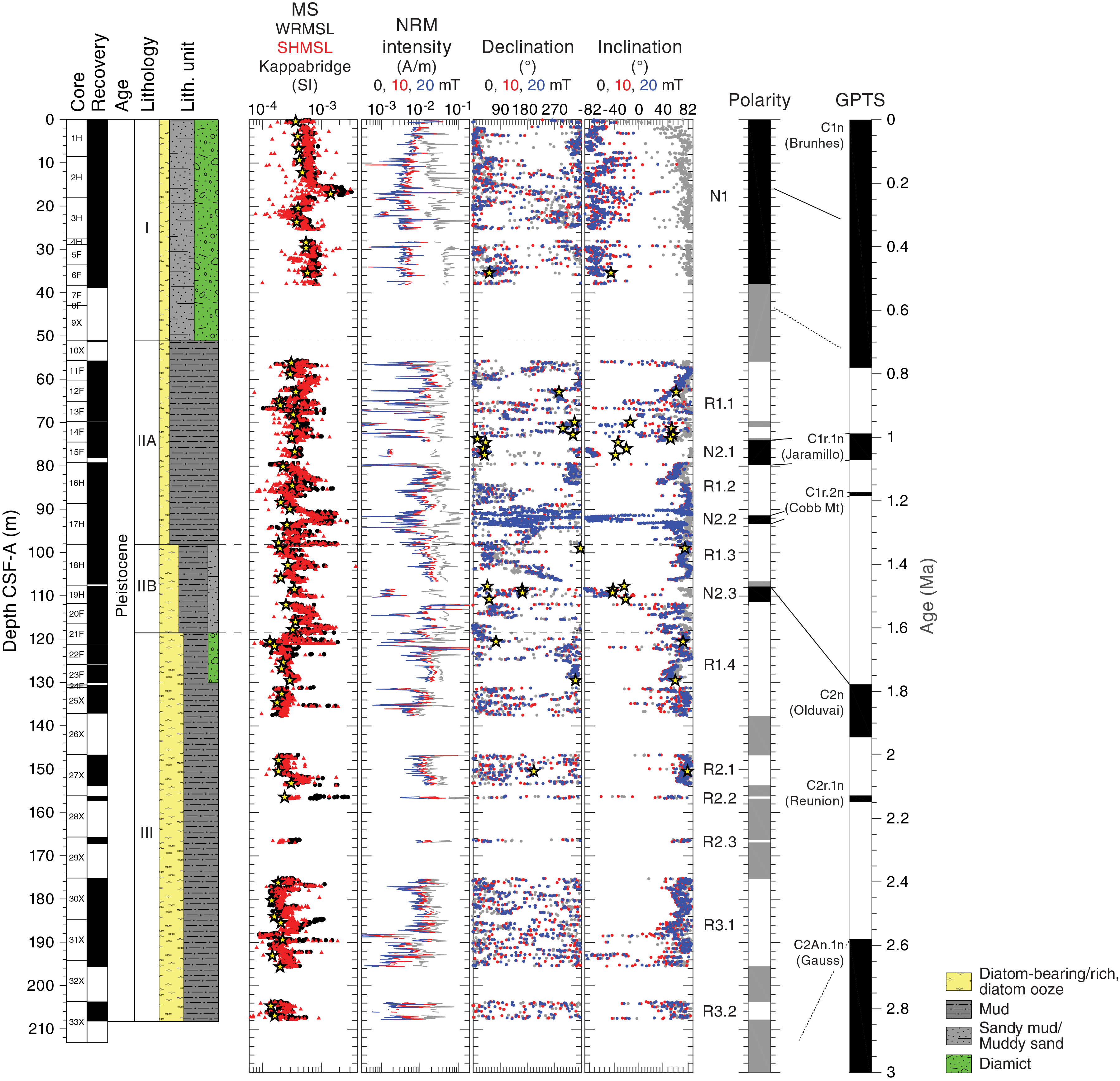
Figure F14. Paleomagnetic data.
NRM inclinations prior to AF demagnetization are steep and positive (Figure F14). After progressive AF demagnetization, both positive and negative inclinations occur. The initial positive inclination therefore presumably represents a low-coercivity downward-directed overprint, which is common to IODP coring operations. However, we cannot rule out the possibility that a low-coercivity component unrelated to drilling carries this positive inclination signal. The positive and negative inclinations after 20 mT peak AF demagnetization suggests that these intervals genuinely reflect reversed and normal polarity zones, respectively, because this site is located in the Southern Hemisphere. Inclination should cluster around ±82.4° (the present-day latitude of Site U1525 is 75.0°S) if a geocentric axial dipole is assumed. However, most negative inclinations are somewhat shallower than expected, whereas most positive inclinations are steep (Figure F14). The shallowing of negative inclinations may relate to a variety of factors, including (1) depositional processes that are not conducive to recording a primary magnetization, (2) relatively large magnetic grain sizes and associated low magnetic coercivities that make the sediments very susceptible to secondary remagnetization, and (3) drilling overprints that are not completely removed by demagnetization at 20 mT peak AF.
Discrete sample measurements
Results from the oriented discrete samples indicate that a peak AF of 10–16 mT is generally enough to remove a low-coercivity component (Figure F15) that may carry as much as 90% of the initial NRM (Figure F15C). Further AF demagnetization reveals an intermediate- to high-coercivity (~16–80 mT) ChRM component, which we interpret to be a primary depositional magnetization. For the normal polarity samples, the demagnetization paths on Zijderveld diagrams do not go directly toward the origin (Figure F15A, F15C). Instead, they overshoot the origin and become noisy. This could result from the existence of a high-coercivity secondary magnetization of unknown origin.
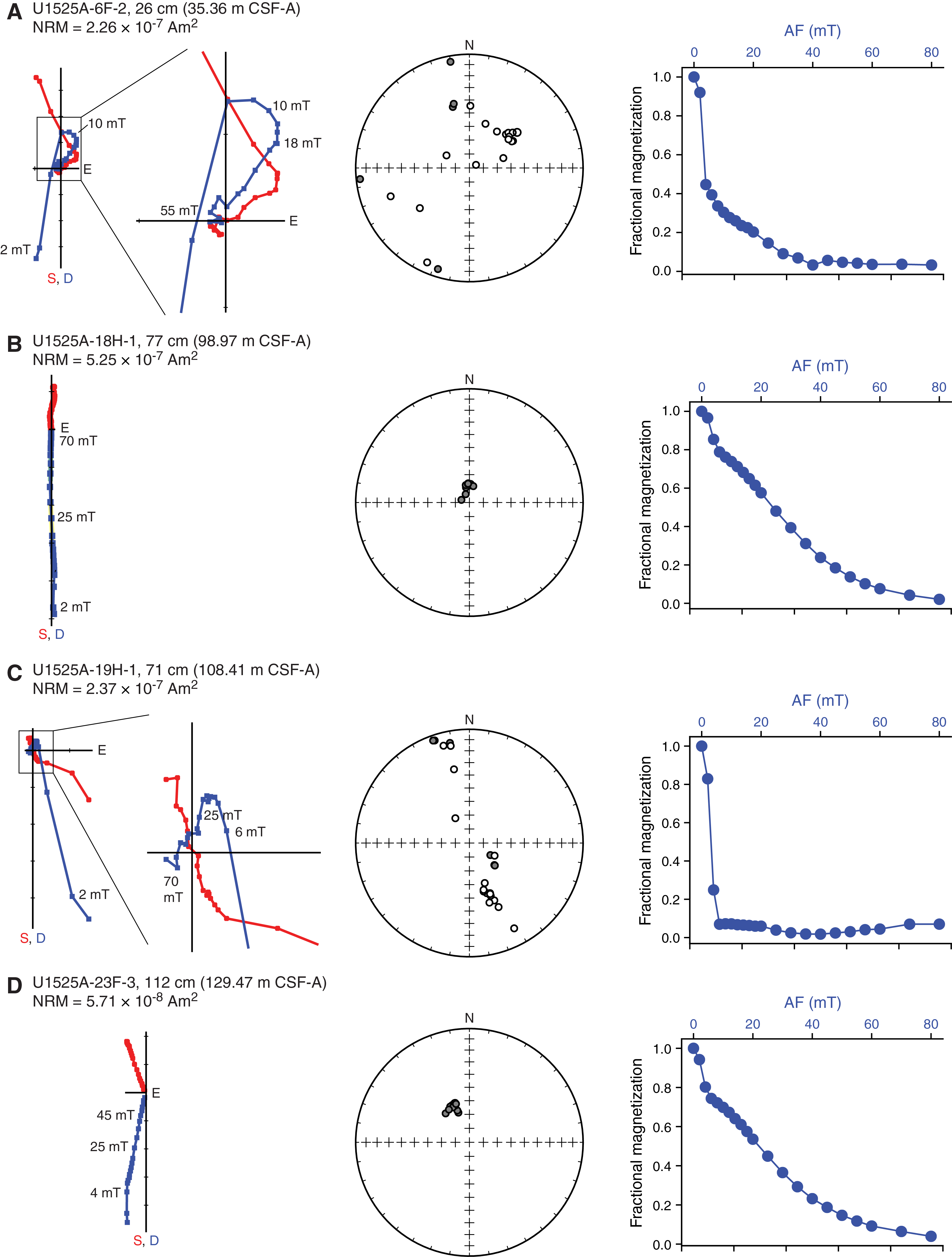
Figure F15. Representative AF demagnetization behavior.
Magnetostratigraphy
We define two major normal polarity zones (N1 and N2) and three major reversed polarity zones (R1–R3) that are further divided into subzones (e.g., N2.1 and R2.1) (Figure F14). The definition of these zones and subzones primarily depends on core recovery. For example, because there is no core recovery in Core 374-U1525A-26X, we chose to separate Zone R1 from Zone R2 rather than identifying only one zone of reversed polarity with many subzones. Cores 1H through 6F (0–38.54 m CSF-A) have normal polarity and make up Zone N1. The next interval with good recovery, Cores 11F through 25X (55.70–138.16 m CSF-A), has predominantly reversed polarity and is divided into four reversed subzones. Cores 15F, 17H, and 19H (74.50–78.21, 88.70–98.67, and 107.70–111.89 m CSF-A, respectively) contain thin intervals of normal polarity that we identify as Subzones N2.1–N2.3. We further identify reversed polarity Zone R2 in Cores 27X through 29X (146.70–167.30 m CSF-A) and Zone R3 in Cores 30X through 33X (175.20–208.27 m CSF-A).
The correlation of these polarity zones to the GPTS of Gradstein et al. (2012) requires independent biostratigraphic age control (see Biostratigraphy and paleontology). Biostratigraphy indicates that the upper ~90 m CSF-A contains significant proportions of reworked species and is therefore difficult to date. An angular unconformity at ~50 m CSF-A is inferred from seismic records and lithologic features, suggesting a stratigraphic break at this level (indicated as an unconformity on the preliminary age-depth model in Figure F8; see Background and objectives and Lithostratigraphy). Because core recovery is very good in the upper ~39 m CSF-A and the mudline sample contains an extant radiolarian fauna, we assume that Zone N1 is relatively continuous and can be tied fully to the Brunhes Chron (0–0.781 Ma) (Figure F14).
Excellent biostratigraphic tie points are available for Cores 374-U1525A-19H through 33X, and they indicate a latest Pliocene to earliest Pleistocene age (see Biostratigraphy and paleontology) (Figure F14; Table T10). We therefore tie reversed polarity Zones R2 and R3 to Subchron C2r.2r (2.148–2.581 Ma). The absence of a normal polarity zone implies that the lowermost cores at Site U1525 are of Pleistocene age. In addition, these biostratigraphic tie points imply a short hiatus between Cores 19H and 20F and provide an age of younger than ~1.9 Ma for Core 19H. The ages of normal polarity Subzones N2.1, N2.2, and N2.3 are therefore younger than 1.9 Ma, and we tie these to the Jaramillo Subchron (0.988–1.072 Ma), Cobb Mountain Subchron (1.173–1.185 Ma), and Olduvai Chron (1.778–1.945 Ma), respectively (Figure F14; Table T10).
Magnetic susceptibility and AMS
We measured the mean magnetic susceptibility and AMS tensor of all collected discrete samples. The orientation and magnitude of the maximum (kmax), intermediate (kint), and minimum (kmin) axes determines the shape of this AMS tensor. The degree of anisotropy (P) of each tensor is approximated by the kmax/kmin ratio, where P = 1 indicates no anisotropy (spherical shape) and P > 1 indicates a high degree of anisotropy (Figure F16). We observed a downhole increase toward higher P values (from ~1.1 in the upper 35 m CSF-A to ~1.2 at ~190 m CSF-A) (Figure F16).
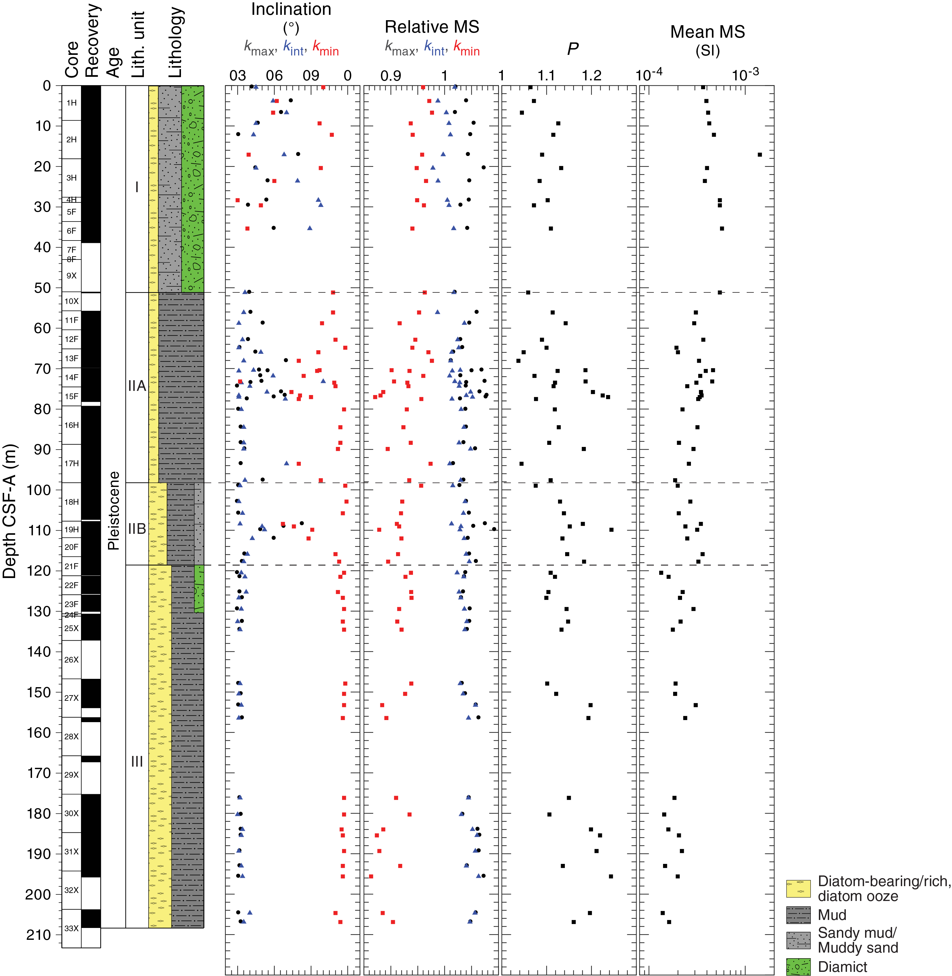
Figure F16. Anisotropy of magnetic susceptibility.
When P is >1 (i.e., anisotropic sample) and kmin inclination is >60° (i.e., minimum susceptibility axis is steep), compaction most likely causes the anisotropy. This compaction is common in sedimentary settings represented by the sediment deposited in lithostratigraphic Units II and III. The shallow kmin inclinations observed in Cores 374-U1525A-13F through 15F, 17H, 19H, and 20F may be related to subtle disturbances induced by either drilling or geological processes (e.g., turbidites). In Unit I, relatively subdued P values and scattered kmin inclinations indicate that these sediments are not compacted in the same way as those in Units II and III. This distinction correlates well with the sedimentary differences in lithostratigraphic units; the major lithologies of Unit I are sandy mud and muddy diamict, whereas Units II and III are predominantly mud-rich and diatom-bearing/rich lithologies.
Physical properties
Physical property measurements were completed on whole-round sections, section halves, and discrete samples from Site U1525. Some outliers and unreliable values were excluded from the plotted data (Table T11). Following thermal equilibration (~4 h), gamma ray attenuation (GRA) bulk density, magnetic susceptibility, P-wave velocity (P-wave logger [PWL]; on APC and HLAPC cores only), and natural gamma radiation (NGR) measurements were made on all whole-round sections using the WRMSL and Natural Gamma Radiation Logger (NGRL). Sampling resolution for the WRMSL was 2.5 cm, and NGR was measured at 10 cm intervals. Thermal conductivity measurements were conducted using the full-space needle probe for APC and HLAPC cores, typically on Sections 2 and 5.
Discrete samples from the working-half sections (typically from Sections 1, 3, 5, and 7) were taken for moisture and density (MAD) measurements for generating bulk and grain density and porosity data. Shear strength measurements were also taken on every other working-half section of APC and HLAPC cores using the Torvane shear device. Discrete compressional (P-wave) velocity measurements were conducted on the working-half sections of each core section using the P-wave caliper (PWC) contact probe system on the Section Half Measurement Gantry (SHMG). Color reflectance and point magnetic susceptibility data were collected on archive-half sections using the SHMSL. Red, green, and blue (RGB) were measured on the Section Half Imaging Logger (SHIL) (see Lithostratigraphy and Physical properties in the Expedition 374 methods chapter [McKay et al., 2019a]).
The physical property measurements are in good overall agreement with the defined lithostratigraphic units. In particular, a downhole increase in magnetic susceptibility and NGR in lithostratigraphic Unit I corresponds to lithologic variation in diatom-bearing sandy mud and muddy diamict. Fluctuating magnetic susceptibility and NGR values in Unit II correlate to interbedded intervals of diatom-bearing/rich mud and sandy mud. Relatively low magnetic susceptibility, NGR, and bulk and grain densities in Unit III are characteristic of diatom ooze and diatom-rich mud and sandy mud. Whole-round measurements on XCB cores often underestimate values for measurements that rely on volume (e.g., bulk density) because XCB cores do not completely fill the core liner. Therefore, the depth at which XCB coring initiated is shown on all figures for reference. Note that Cores 374-U1525A-9X and 10X were collected in the upper part of the hole, but core recovery was minimal, so these data are not specifically designated as being cored with the XCB coring system (see Operations). All physical property data are available from the Laboratory Information Management System (LIMS) database (http://web.iodp.tamu.edu/LORE).
Magnetic susceptibility
Whole-round measurements on the WRMSL and discrete point measurements on the SHMSL were used to characterize magnetic susceptibility at Site U1525 (Figure F17). Both methods yield similar downhole variability and a similar range of values from ~0 × 10−5 to ~330 × 10−5 SI. Low magnetic susceptibility values in the WRMSL data correspond to mud or clast-poor muddy diamict (e.g., Sections 374-U1525A-3H-3 and 16H-1). Poor recovery limited WRMSL measurements in several intervals of the hole, especially in Cores 7F through 10X (38.3–51.33 m CSF-A). Magnetic susceptibility in lithostratigraphic Unit I varies from ~30 × 10−5 to ~85 × 10−5 SI. Magnetic susceptibility increases slightly with depth, except in parts of Cores 2H and 3H. The exceptionally high peaks in Cores 2H and 3H (>200 × 10−5 SI) likely reflect the increase in abundance of individual clasts in this interval. In Unit II (51.11–118.58 m CSF-A), magnetic susceptibility varies downhole, predominantly between 20 × 10−5 and ~60 × 10−5 SI, and appears cyclic. These cyclic changes may reflect changes in composition of diatom-bearing mud and/or changes in clast composition. In Unit III, magnetic susceptibility is relatively low but varies from ~20 × 10−5 to ~40 × 10−5 SI. Lower average magnetic susceptibility values likely reflect an increased presence of diatom ooze and diatom-rich mud. In addition, incompletely filled XCB Cores 25X through 33X (131.2–208.27 m CSF-A) may cause lower magnetic susceptibility values compared with Units I and II.
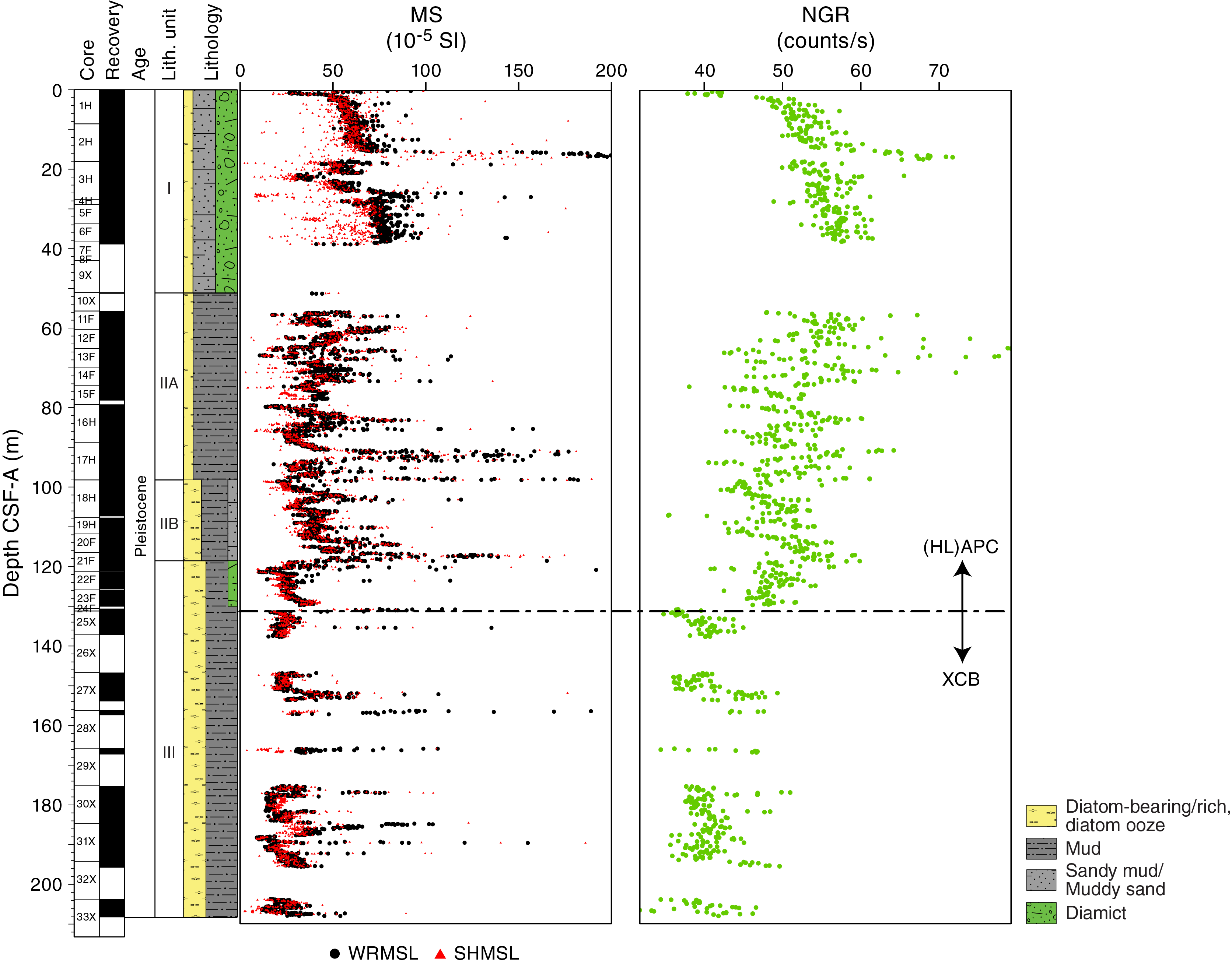
Figure F17. MS and NGR.
Natural gamma radiation
NGR varies between ~33 and 68 counts/s (Figure F17). NGR in lithostratigraphic Unit I (e.g., Cores 374-U1525A-1H through 10X [0.0–55.70 m CSF-A]) slightly increases downhole from ~40 to 58 counts/s, with a peak (~68 counts/s) in Sections 2H-5 and 2H-6. The peak correlates with high magnetic susceptibility and corresponds to diatom-bearing clast-rich muddy diamict. In Unit II (51.11–118.58 m CSF-A), NGR shows a downhole cyclic trend similar to magnetic susceptibility, varying between ~50 and 62 counts/s with ~6–12 m apparent cyclicity. These repetitions may reflect interbedded diatom-bearing to diatom-rich mud and/or sandy mud in Unit II. In general, NGR decreases downhole in Subunit IIA, whereas it increases downhole in Subunit IIB. NGR in the upper part of Unit III (Cores 22F through 24F [121.2–131.28 m CSF-A]) slightly decreases from ~50 to 45 counts/s, corresponding to diatom-rich mud. Overall, low values (33–46 counts/s) measured on the XCB cores (25X through 33X [131.2–208.27 m CSF-A]) are consistent with the presence of diatom ooze and diatom-rich mud and also are likely affected by incompletely filled core liners.
Bulk density, grain density, and porosity
Discrete MAD samples yielded bulk density values concentrated in a narrower range (~1.6–2.2 g/cm3) relative to GRA bulk density measurements (~1.0–2.6 g/cm3) (Figure F18). For APC and HLAPC cores (374-U1525A-1H through 24F [0–131 m CSF-A]), density measurements from discrete samples are generally lower than GRA bulk density measurements, whereas for XCB cores, it is the opposite. Furthermore, discrete-sample bulk density above and below the transition from APC/HLAPC to XCB coring remains unchanged, whereas whole-round density measurements decrease at the transition, likely because XCB cores do not completely fill the core liner and are usually more disturbed than APC/HLAPC cores.
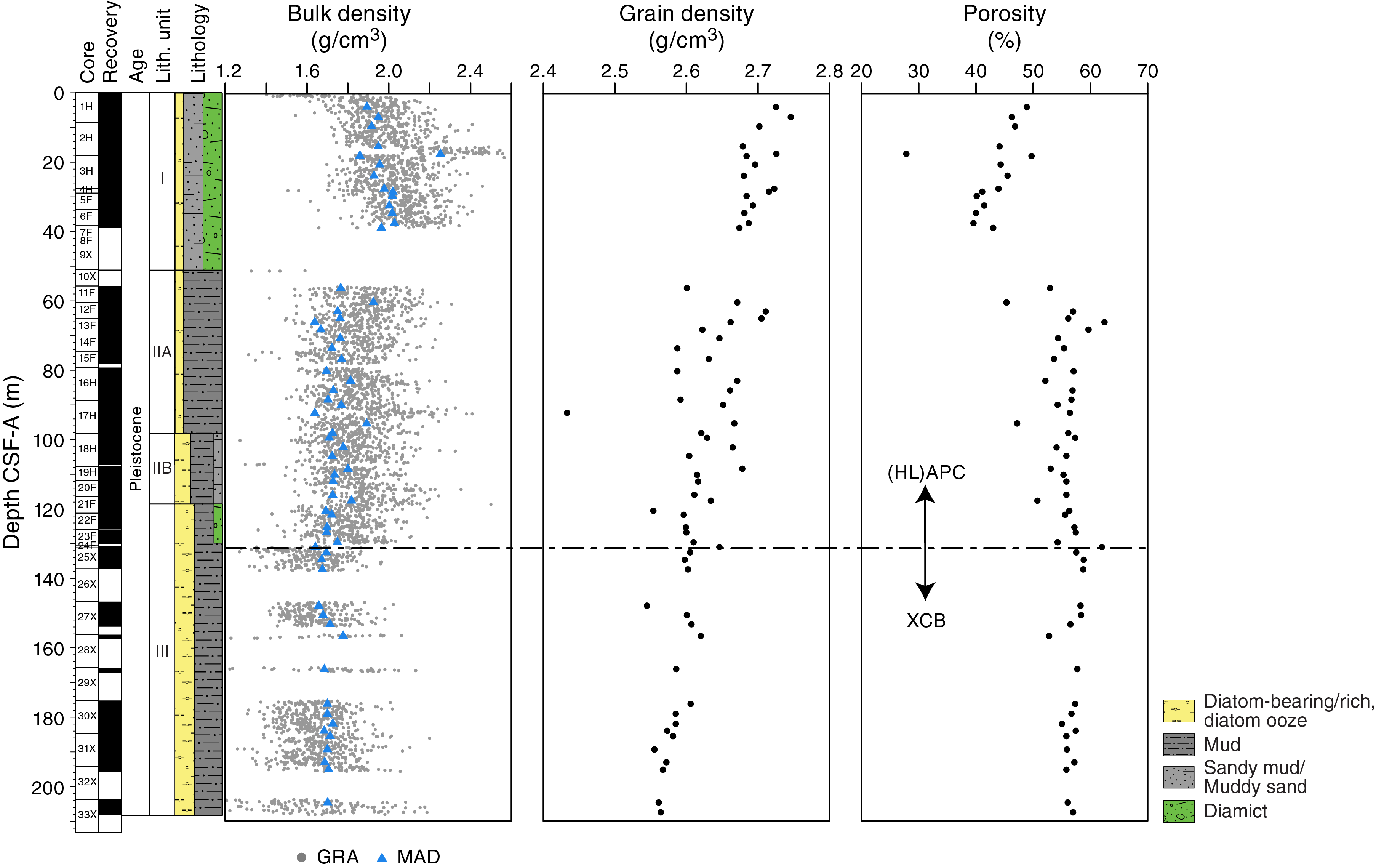
Figure F18. GRA and MAD bulk density, grain density, and porosity.
In lithostratigraphic Unit I, bulk density generally increases downhole, with peak density in Sections 374-U1525A-2H-5 and 2H-6 (~14.6–17.6 m CSF-A) corresponding to peaks in magnetic susceptibility and NGR that are related to clast-rich muddy diamict. Porosity decreases downhole in the upper ~40 m CSF-A, suggesting that compaction and/or lithology are controlling downhole variation in these properties. Grain density also decreases downhole through Unit I, indicating a change in lithologic composition or grain size. In Unit II, bulk density is lower relative to Unit I and is consistently ~1.7 g/cm3. Grain density is relatively low compared with Unit I, whereas porosity is relatively high. In Unit III, bulk density and grain density increase slightly from Section 27X-3 through Section 28X-1 (~152–157 m CSF-A), whereas porosity decreases, associated with increased clast abundance in this interval. Throughout the lower parts of Unit III, bulk density is ~1.7 g/cm3, and together with porosity does not significantly vary downhole, with values similar to Unit II, whereas grain density decreases downhole slightly. Overall, bulk and grain densities are the lowest in Unit III, reflecting increased diatom content.
Compressional P-wave velocity
P-wave velocity measurements range from ~1500 to 2800 m/s on the PWL and from ~1500 to 1900 m/s on the PWC and overall are in good agreement on the low end (Figure F19). PWL measurements were discontinued at Core 374-U1525A-25X (131 m CSF-A) because of the switch from HLAPC coring to XCB coring. In lithostratigraphic Unit I, P-wave velocity increases downhole from 1600 to 1800 m/s, which is consistent with compaction. A maximum P-wave velocity of ~2000 m/s occurs in Sections 2H-5 and 2H-6 (14.6–17.6 m CSF-A) and is related to a clast-rich diamict (see Lithostratigraphy). In Unit II, P-wave velocity from the PWC remains constant at ~1600 m/s and is relatively low compared with the overlying unit, likely because of increased abundance of diatoms in mud-dominated lithologies. A small decrease in velocity from 1600 to 1550 m/s occurs at the boundary between Units II and III, reflecting increased abundance of diatoms in Unit III. Slightly increased P-wave velocity in Section 28X-1 reflects an increased abundance of clasts in this section.
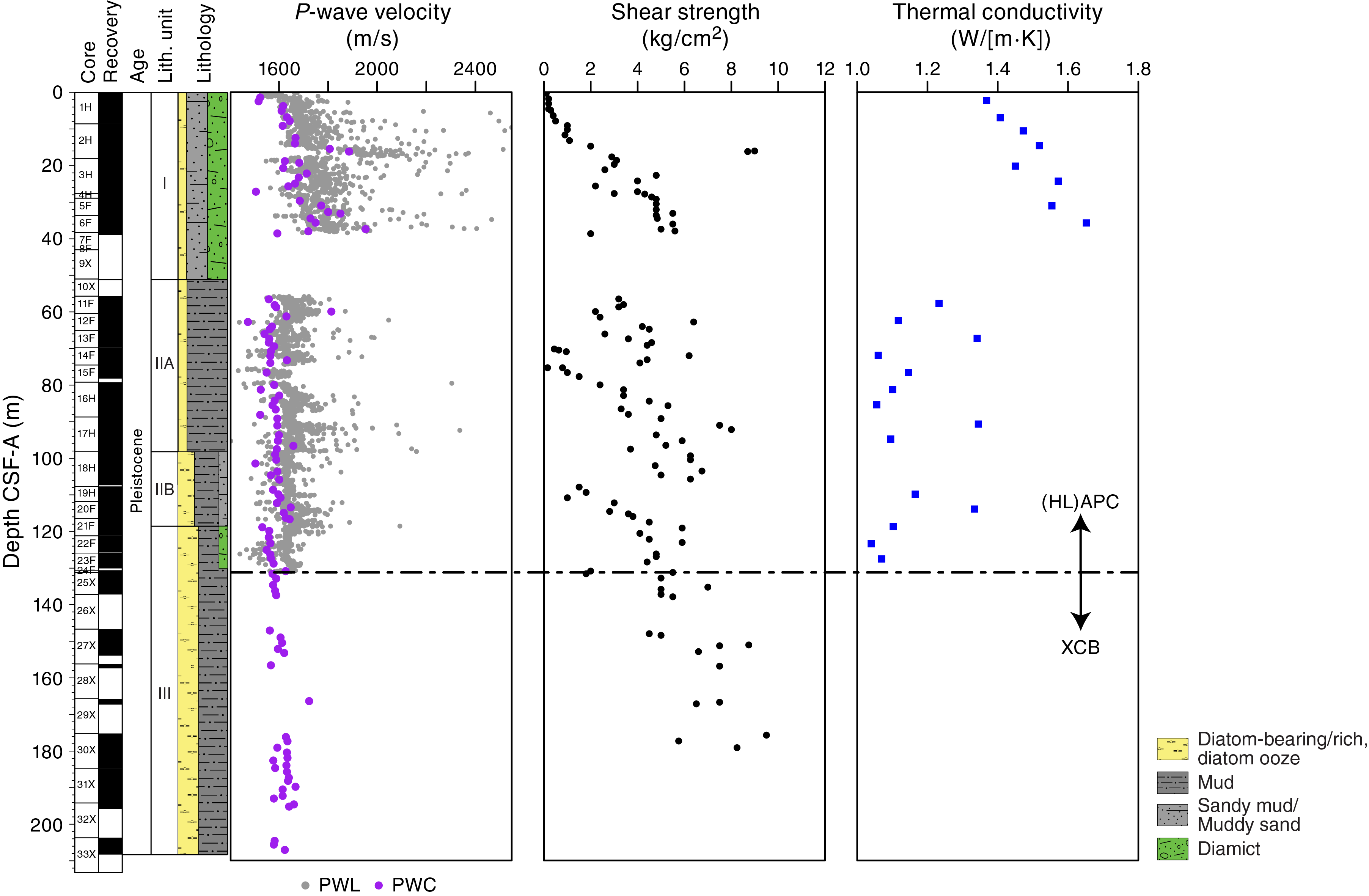
Figure F19. P-wave velocity, shear strength, and thermal conductivity.
Shear strength
Shear strength measurements vary from 0.1 to 9.5 kg/cm² (Figure F19). In lithostratigraphic Unit I, shear strength increases with depth from 0.1 to 5.6 kg/cm², likely because of compaction and decreasing moisture content with depth. A short interval (Sections 374-U1525A-2H-5 and 2H-6) has very high values (~8 kg/cm2) that correspond to a clast-rich muddy diamict also detected in other physical property measurements. In Unit II, shear strength increases from 2 to 6 kg/cm², likely because of increased compaction with depth. We note that the increase in this lower part of the hole is more gradual compared with the upper part of the hole, which might be explained by differing sedimentation rates between the two units and/or by different accumulation processes (event-bed dominated versus hemipelagic dominated). Low values (<2 kg/cm²) observed in Section 14H-1 correspond to sandy mud, with shear strength increasing from bottom to top. However, low shear strength observed in Cores 15H and 19H most likely reflects coring disturbance rather than lithologic change. In the upper part of Unit III, shear strength increases downhole from 5 to 10 kg/cm2, perhaps because of compaction. The cores below Core 30X were not measured because they are lithified.
Thermal conductivity
The quality of thermal conductivity measurements from APC and HLAPC cores was checked by evaluating two parameters: (1) the number of solutions acquired and (2) the shape of the curve formed on the temperature versus time plot of these points. A valid measurement must have a sufficient number of solutions to form an exponential curve. All measurements with a low number of solutions and/or a bad repartition of these values on the temperature versus time plot (i.e., forming two curves or no curve) were deleted, resulting in removal of 3% of the original data. In lithostratigraphic Unit I, thermal conductivity increases downhole from 1.4 to 1.7 W/(m·K) (Figure F19). In Unit II, thermal conductivity is generally lower than in Unit I, with measurements between 1.0 and 1.4 W/(m·K) and no systematic downhole trend. Thermal conductivity measurements were not carried out below Core 374-1525A-25X (131 m CSF-A) because of the switch to XCB coring in more lithified sediment.
Color reflectance spectroscopy
Color reflectance spectroscopy data were acquired on section halves using the SHMSL (Figure F20). In lithostratigraphic Unit I, L* and b* decrease, whereas a* increases downhole, suggesting that the sediment darkens and both yellow and green colors decrease with depth. In Subunit IIA, L* and a* increase slightly downhole, whereas b* remains unchanged, which indicates that the sediment becomes lighter and less green downhole. Relative to Unit I, a* is much lower, indicating that Subunit IIA is greener than Unit I, possibly reflecting increased diatom content. In Subunit IIB and the upper part of Unit III shallower than 131 m CSF-A, L* decreases slightly downhole and a* remains similar. In the lower part of Unit III, deeper than 131 m CSF-A, L* is lower overall but increases with depth, indicating downhole lightening of sediment. In this unit, a* remains unchanged and b* increases and then decreases toward the bottom of the hole, indicating increasing and then decreasing yellow color of the sediment.
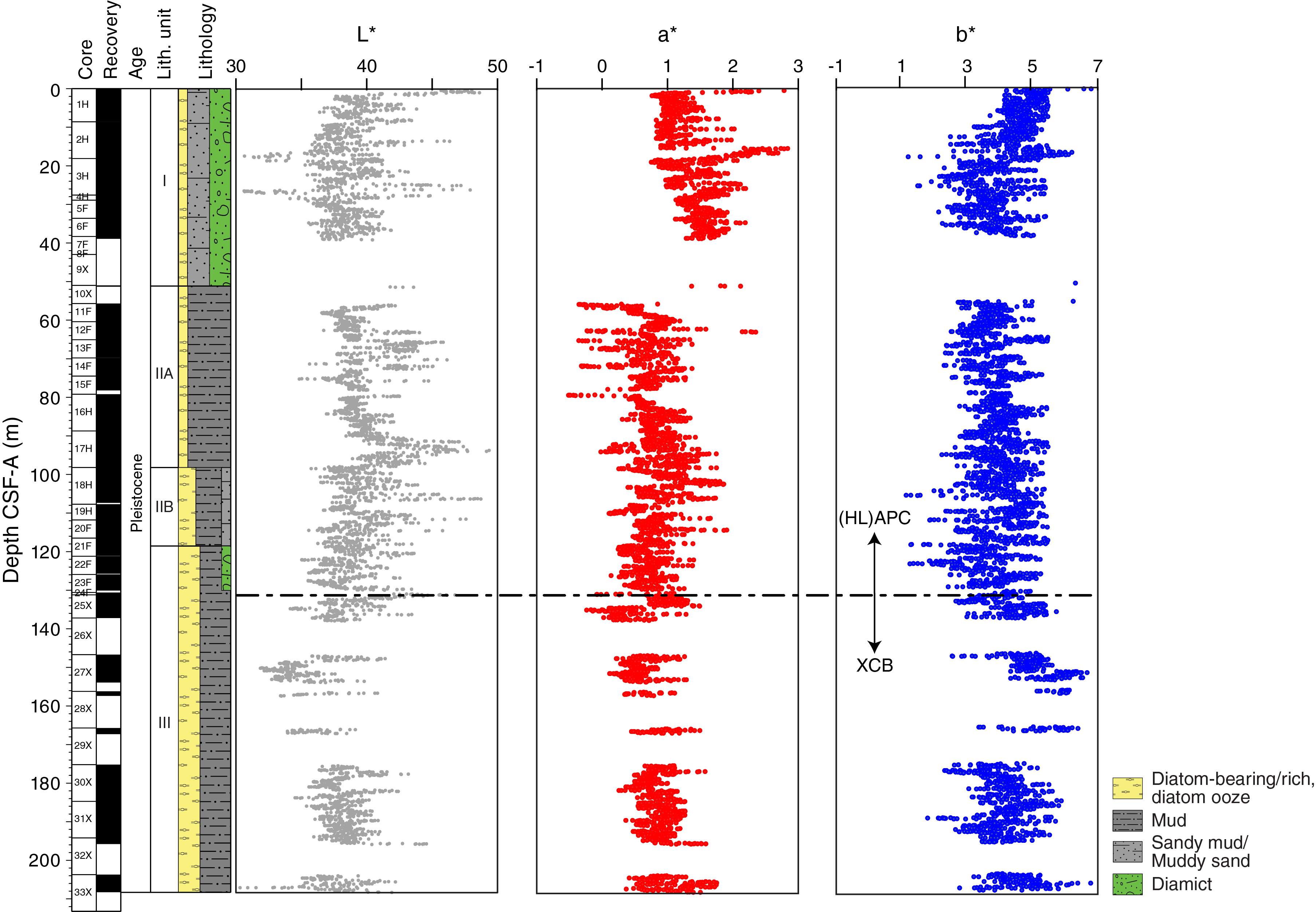
Figure F20. Color reflectance spectroscopy.
Summary
In general, data from whole-round measurements are in good agreement with those from split-core measurements (Figure F21). Downhole changes in physical properties are in good overall agreement with the defined lithostratigraphic units based on sedimentological characteristics (see Lithostratigraphy; Figure F21; Table T12), and changes in physical properties provide insight into lithologic changes in and seismic-reflection expression of (Figure F22) the units. Because of the lack of downhole sonic measurements, we relied on core-based P-wave measurements for depth-converting the lithostratigraphic and physical properties units and to correlate them with the seismic-reflection profile crossing Site U1525.
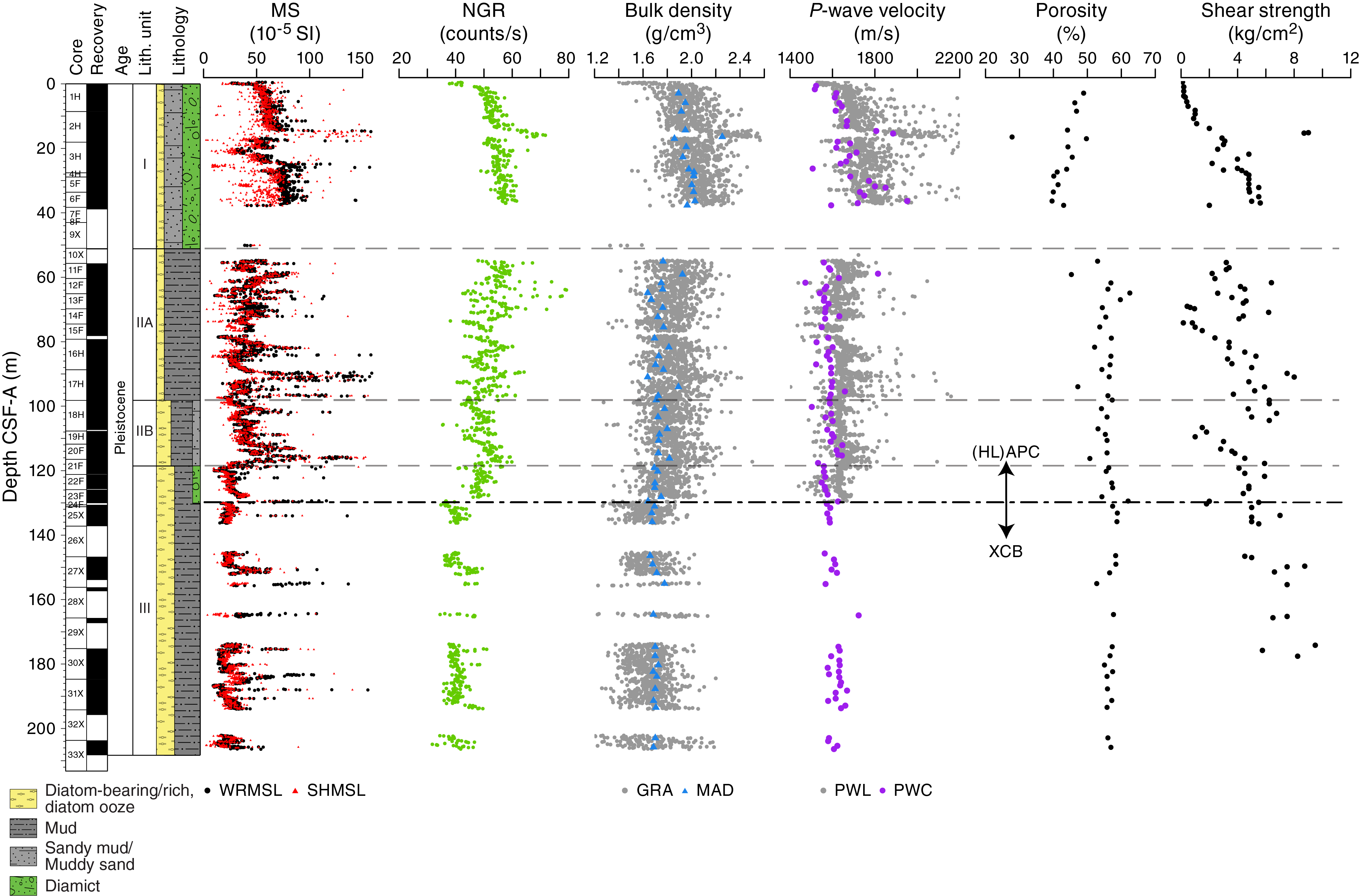
Figure F21. Physical properties summary.
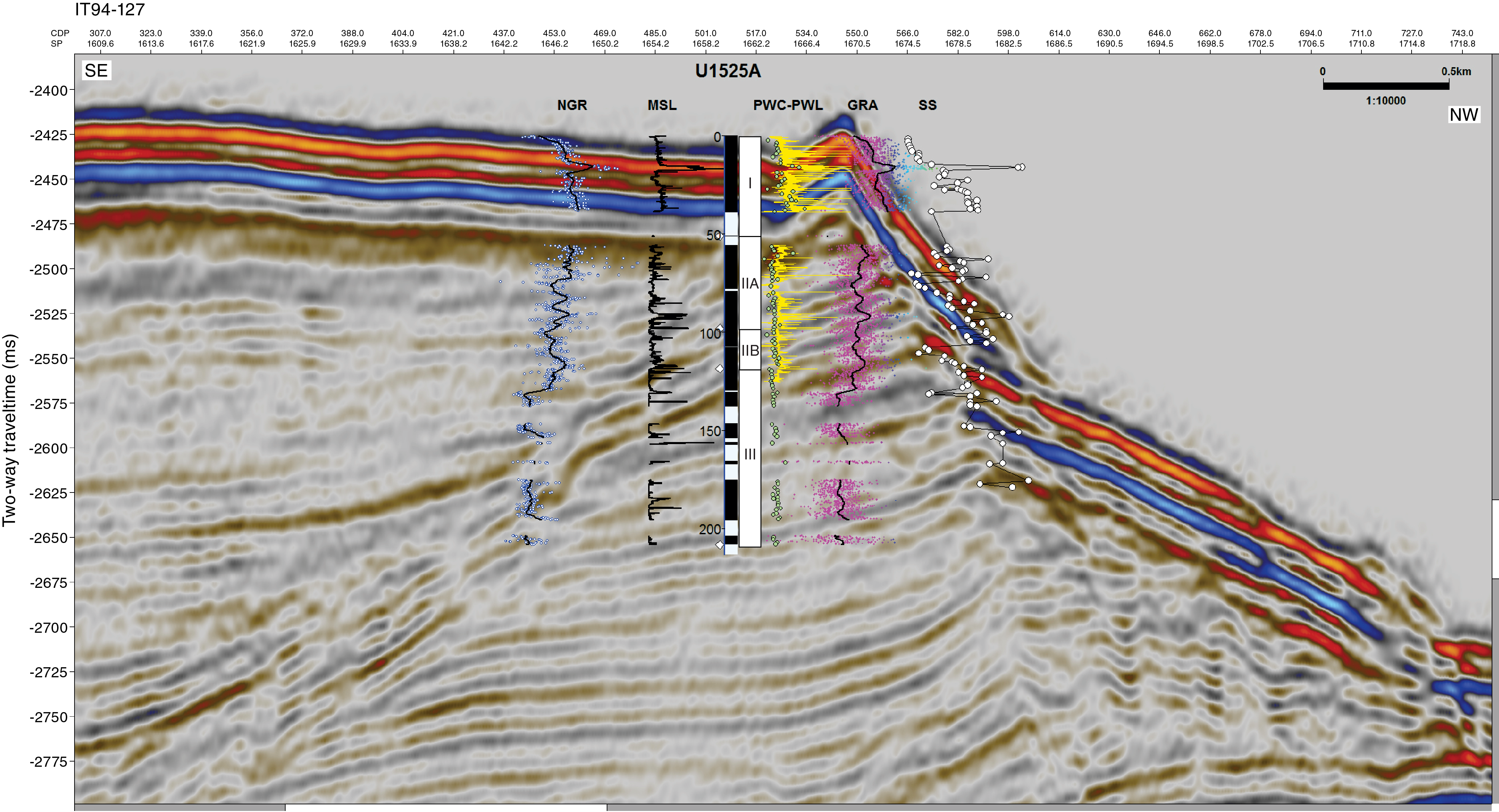
Figure F22. Core-seismic integration.
Lithostratigraphic Unit I records a downhole increase in magnetic susceptibility, NGR, density, P-wave velocity, and shear strength and a decrease in porosity. These changes reflect both compaction and changes in lithology in this unit of diatom-bearing sandy mud interbedded with clast-poor muddy diamict. In Unit I, Sections 374-U1525A-2H-5 and 2H-6 contain peaks in magnetic susceptibility, NGR, density, P-wave velocity, and shear strength and decreased porosity that reflect increased clast and clay content and compaction in this clast-rich diamict. In Unit II, multimeter-scale cyclicity apparent in magnetic susceptibility and NGR is likely related to downhole changes in lithology. In Unit II, relatively consistent density, P-wave velocity, and porosity indicate minimal changes in lithology in the diatom-bearing/rich mud and sandy mud beds. Shear strength in Unit II also demonstrates downhole changes that may be related to lithologic changes or compaction. Generally lower magnetic susceptibility, NGR, density, and P-wave velocity in Unit III reflect increased diatom content.
This unit division is also reflected by the seismic facies (Figure F22). Lithostratigraphic Unit I corresponds to a package of high-amplitude, subhorizontal reflectors partly covered by seafloor-ringing reflectors (Figure F22). These reflectors represent the top part of a wedge-shaped seismic unit with low-amplitude and discontinuous reflectors that pinches toward the northwest and onlaps on, or laterally interfingers with, an underlying sediment mound. The upper part of the mound recovered in Subunits IIA and IIB and Unit III is characterized by a stratified package of high-amplitude, subhorizontal reflectors that slightly dip toward the southeast (Figure F22). Hole U1525A was terminated before penetrating RSU3 (see Operations), which is inferred to be below the base of the hole. However, RSU2 was likely penetrated in Unit III.
Geochemistry and microbiology
Site U1525 samples were analyzed for headspace gas, interstitial water chemistry, and bulk sediment geochemistry. Headspace gas (methane and ethane) concentration is low in the upper ~120 m CSF-A and increases to 6640 and 7 ppmv, respectively, at ~194 m CSF-A. Interstitial water analyses of the mudline and 12 whole-round samples indicate biogeochemical zonation with sulfate reduction in the uppermost ~100 m CSF-A. Downhole variations in interstitial water elemental concentration (e.g., magnesium, calcium, silicon, and lithium) broadly correspond with lithologic changes and total organic carbon (TOC) and calcium carbonate (CaCO3) content. TOC and carbonate contents are low (<1% and <5%, respectively). The highest and most variable carbonate content and TOC/total nitrogen (TN) ratios occur in the upper ~35 m CSF-A (lithostratigraphic Unit I).
Volatile hydrocarbons
Headspace gas analyses were performed at a resolution of one sample per core (9.6 m advance) or one sample every other core for HLAPC cores (4.8 m advance) throughout Hole U1525A (Cores 374-U1525A-1H through 33X; N = 21) as part of the routine environmental protection and safety monitoring program. Methane is the dominant hydrocarbon, and ethane is present in low concentration. Methane concentration is low (≤11 ppmv) in the upper 124.20 m CSF-A and increases from 11 ppmv at 124.20 m CSF-A to 6641 ppmv at 193.81 m CSF-A (Figure F23; Table T13). Ethane concentration is below detection limit in the upper ~150 m CSF-A and increases to 10 ppmv at 206.37 m CSF-A (Figure F23). The methane/ethane ratio declines from 3162 at 151.21 m CSF-A to 608 at 206.37 m CSF-A (Figure F23).

Figure F23. Headspace gas concentrations.
Interstitial water chemistry
A total of 12 interstitial water samples were squeezed from 5 or 10 cm whole-round samples (Table T14) with a sampling resolution dictated by core recovery and lithology from 4.45 to 181.09 m CSF-A. Interstitial water sampling was not conducted deeper than 181.09 m CSF-A. An additional sample from the mudline was split and analyzed as a comparative sample for shipboard parameters and shore-based analyses.
Salinity, sulfate, sulfur, iron, manganese, alkalinity, and ammonium
Interstitial water salinity decreases from 35 at 4.45 m CSF-A to 33 at 181.09 m CSF-A. Water collected from the mudline of Site U1525 has a salinity of 36, and chloride, bromide, and sodium concentrations are higher than typical Ross Sea water. The mudline water likely reflects a mixture of in situ seawater and higher salinity water introduced by coring operations. Total sulfur and sulfate concentrations show identical downhole profiles. Sulfate decreases from >29 mM at the mudline, which is slightly elevated above typical seawater concentration, to close to the detection limit of inductively coupled plasma–optical emission spectroscopy (ICP-OES) deeper than ~130 m CSF-A (Figure F24). Iron concentration in the interstitial water is below the detection limit shallower than ~60 m CSF-A and at 94.35 and 181.09 m CSF-A. In most samples between 68.87 and 135.60 m CSF-A, iron was detected in interstitial water with concentrations up to ~5 µM. Manganese concentration is variable in the upper 31.85 m CSF-A from a very low value of 4 µM in the mudline sample to the highest value of 118 µM at 14.57 m CSF-A. From 59.43 m CSF-A, the manganese profile is better defined and shows a general decrease from 50 to 6 µM in the lowermost interstitial water sample (181.09 m CSF-A). Alkalinity increases nearly linearly from a low value of 2.5 mM in the mudline sample to 19.4 mM at 181.09 m CSF-A. This trend is paralleled by the ammonium concentration in interstitial water, which increases from ~6 µM in the mudline sample to 1017 µM at 181.09 m CSF-A (Figure F24). Downhole increase in ammonium concentration is likely the result of mineralization of organic carbon and is possibly associated with the anaerobic oxidation of methane by microbial activity. All downhole profiles described above are consistent with manganese and sulfate reduction in the suboxic to anoxic transition zone.
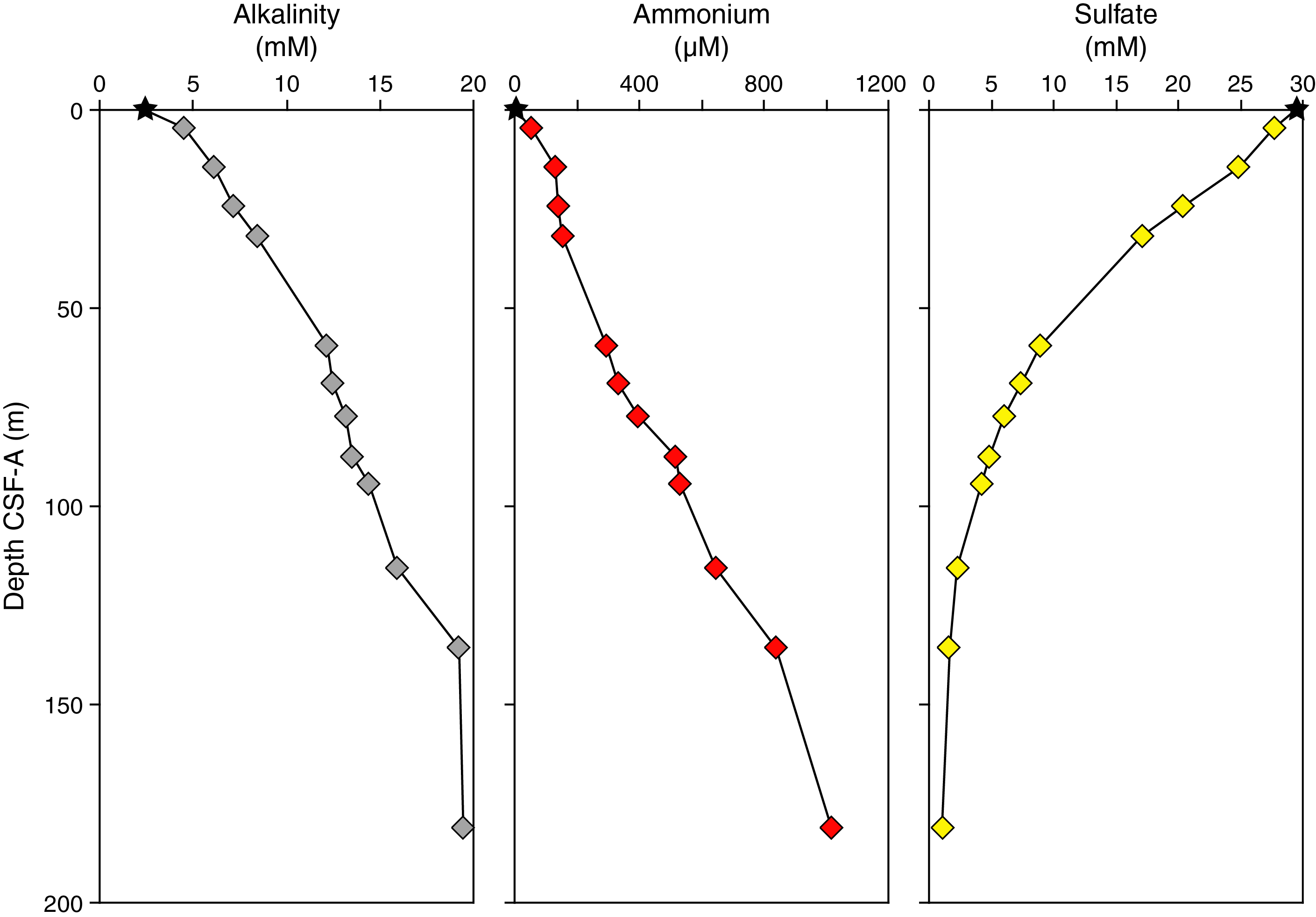
Figure F24. Interstitial water alkalinity, ammonium, and sulfate.
Lithium, calcium, magnesium, and silicon
Systematic downhole variability is observed for magnesium (34%), calcium (34%), and potassium (36%) (Figure F25). In detail, magnesium concentration decreases slightly downhole from 53 to 44 mM in the uppermost ~32 m CSF-A to an average concentration of 40 ± 1 mM from 59.43 to 135.60 m CSF-A (Figure F25). The bottommost sample shows slightly decreased magnesium concentration (35 mM). Calcium concentration exhibits a very smooth profile with values in the uppermost ~32 m CSF-A between 10 and 11 mM. Calcium concentration decreases linearly to 7 mM between 59.43 and 94.35 m CSF-A and remains essentially constant downhole to 181.09 m CSF-A (Figure F25). The lithium profile shows some similarities to downhole trends in calcium but also some deviations; lithium decreases in the uppermost ~32 m CSF-A from 30 µM in the mudline water sample to 19 µM at 31.85 m CSF-A. Deeper than 59.43 m CSF-A, lithium concentration more than doubles along a linear trend from 23 to 59 µM. Silicon concentration in interstitial water shows the closest relationship to lithostratigraphic units, with a peak value of 1006 µM at 77.32 m CSF-A possibly associated with higher biogenic silica (diatom) dissolution in the diatom-bearing mud of lithostratigraphic Subunit IIA (see Lithostratigraphy). Overall, silicon concentration increases from 169 µM in the mudline sample to 578 µM in the first interstitial water sample at 4.45 m CSF-A. Deeper than 14.57 m CSF-A, silicon concentration varies between 666 and 1006 µM, likely reflecting downhole changes in interstitial water silica saturation, which approaches equilibrium conditions at ~1000 µM (Figure F25).
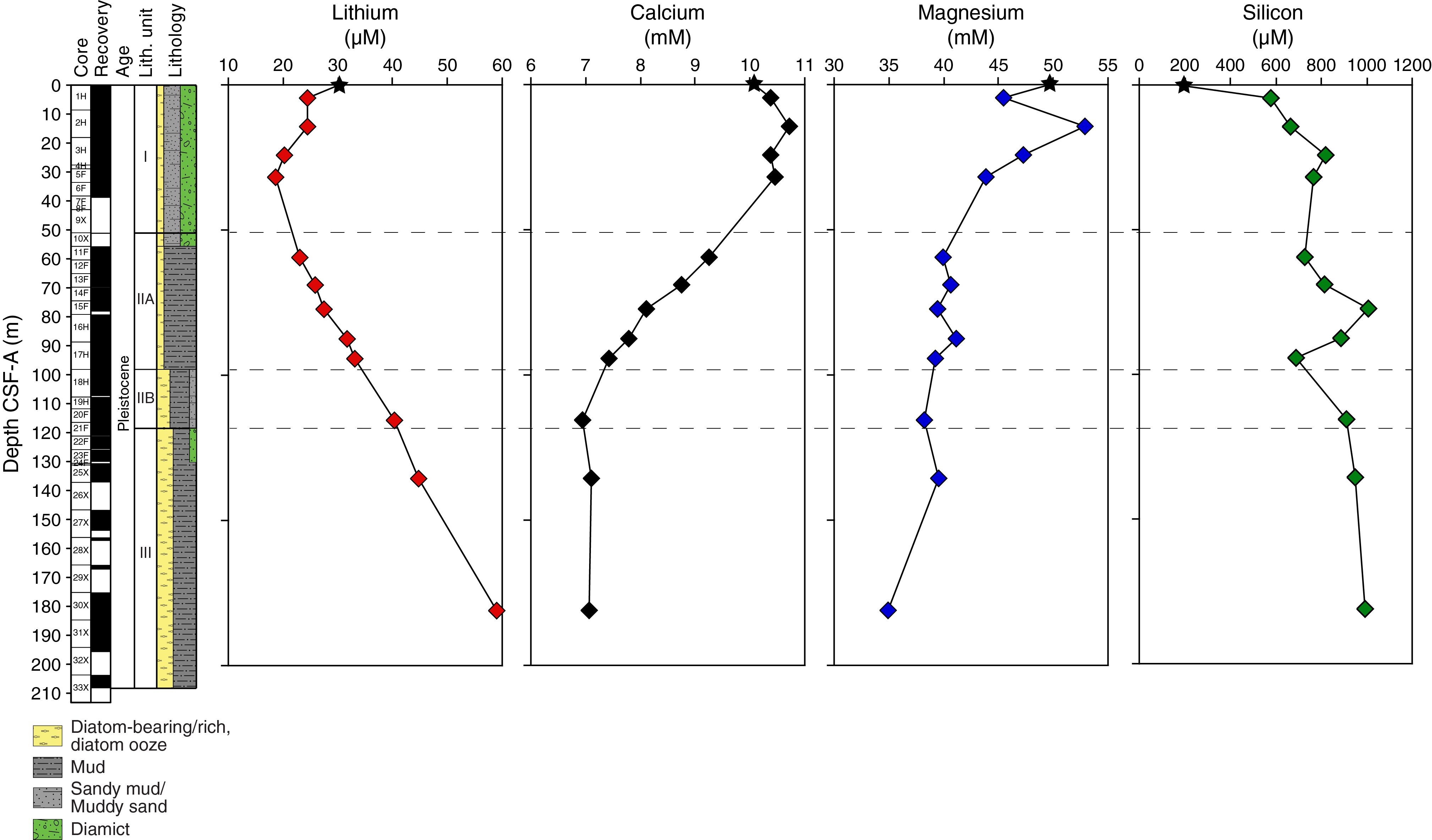
Figure F25. Interstitial water lithium, calcium, magnesium, and silicon.
Bulk sediment geochemistry
Carbon, nitrogen, and carbonate
A total of 47 sediment samples from the major lithostratigraphic units identified at Site U1525 were analyzed for total carbon, TN, and total inorganic carbon (Table T15). TOC and CaCO3 contents were subsequently calculated. TOC content is generally low (<0.6 wt%; Figure F26) and increases from minimum values (<0.2 wt%) in the upper 35 m CSF-A to maximum values (0.3–0.6 wt%) in the diatom-rich mud and sandy diamict of lithostratigraphic Units II and III between 68.46 and 206.89 m CSF-A (see Lithostratigraphy). TN content is very low (≤0.05 wt%) but increases downhole. Except for two samples from Sections 374-U1525A-6F-3 and 19H-1, the TOC/TN ratio ranges between 1 and 11 (Figure F26). These values are relatively low compared with those observed at continental shelf Sites U1521–U1523 and suggest a reduced input of terrigenous-derived organic matter at Site U1525. CaCO3 content is generally low, from 0.1 to 4.5 wt% (Figure F26). Slightly higher values (>2 wt%) are observed exclusively in the sandy mud and diamict of Unit I in the upper 34 m CSF-A. Although CaCO3 content is lower in the diatom-bearing to diatom-rich mud of Unit II (see Lithostratigraphy), it is also notably variable, with concentrations fluctuating between 0.1 and 1.5 wt%.
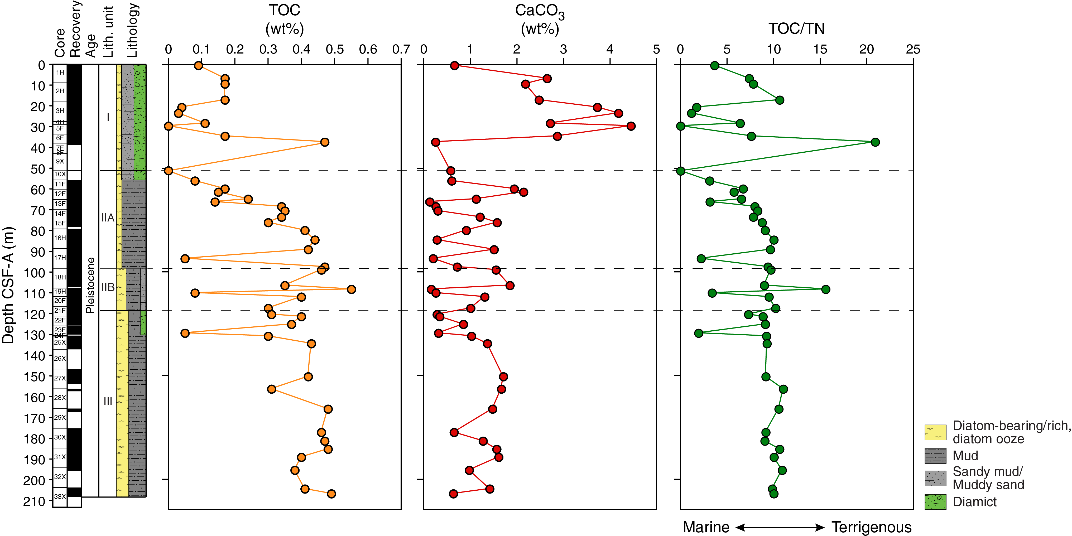
Figure F26. Bulk sediment carbon and TOC/TN ratio.
Microbiological sampling
In total, 20 samples for shore-based stable and clumped isotope analyses of methane and ethane were collected from Sections 374-U1525A-1H-4 through 33X-2. Additional samples for detailed analyses of metagenomics, cell counts, metabolomics, and cultures were taken from Cores 3H, 11F, 16H, and 20F (see Geochemistry and microbiology in the Expedition 374 methods chapter [McKay et al., 2019a] for details).
References
Arndt, J.E., Schenke, H.W., Jakobsson, M., Nitsche, F.O., Buys, G., Goleby, B., Rebesco, M., et al., 2013. The International Bathymetric Chart of the Southern Ocean (IBCSO) Version 1.0—a new bathymetric compilation covering circum-Antarctic waters. Geophysical Research Letters, 40(12):3111–3117. https://doi.org/10.1002/grl.50413
Bergamasco, A., Defendi, V., Zambianchi, E., and Spezie, G., 2002. Evidence of dense water overflow on the Ross Sea shelf-break. Antarctic Science, 14(3):271–277. https://doi.org/10.1017/S0954102002000068
Bjørklund, K.R., and Kruglikova, S.B., 2003. Polycystine radiolarians in surface sediments in the Arctic Ocean basins and marginal seas. Marine Micropaleontology, 49(3):231–273. https://doi.org/10.1016/S0377-8398(03)00036-7
Esper, O., and Zonneveld, K.A.F., 2002. Distribution of organic-walled dinoflagellate cysts in surface sediments of the Southern Ocean (eastern Atlantic sector) between the Subtropical Front and the Weddell Gyre. Marine Micropaleontology, 46(1–2):177–208. https://doi.org/10.1016/S0377-8398(02)00041-5
Esper, O., and Zonneveld, K.A.F., 2007. The potential of organic-walled dinoflagellate cysts for the reconstruction of past sea-surface conditions in the Southern Ocean. Marine Micropaleontology, 65(3–4):185–212. https://doi.org/10.1016/j.marmicro.2007.07.002
Florindo, F., Farmer, R.K., Harwood, D.M., Cody, R.D., Levy, R., Bohaty, S.M., Carter, L., and Winkler, A., 2013. Paleomagnetism and biostratigraphy of sediments from Southern Ocean ODP Site 744 (southern Kerguelen Plateau): implications for early-to-middle Miocene climate in Antarctica. Global and Planetary Change, 110(C):434–454. https://doi.org/10.1016/j.gloplacha.2013.05.004
Gradstein, F.M., Ogg, J.G., Schmitz, M.D., and Ogg, G.M. (Eds.), 2012. The Geological Time Scale 2012: Amsterdam (Elsevier). https://doi.org/10.1016/C2011-1-08249-8
McKay, R.M., De Santis, L., Kulhanek, D.K., Ash, J.L., Beny, F., Browne, I.M., Cortese, G., Cordeiro de Sousa, I.M., Dodd, J.P., Esper, O.M., Gales, J.A., Harwood, D.M., Ishino, S., Keisling, B.A., Kim, S., Kim, S., Laberg, J.S., Leckie, R.M., Müller, J., Patterson, M.O., Romans, B.W., Romero, O.E., Sangiorgi, F., Seki, O., Shevenell, A.E., Singh, S.M., Sugisaki, S.T., van de Flierdt, T., van Peer, T.E., Xiao, W., and Xiong, Z., 2019a. Expedition 374 methods. In McKay, R.M., De Santis, L., Kulhanek, D.K., and the Expedition 374 Scientists, Ross Sea West Antarctic Ice Sheet History. Proceedings of the International Ocean Discovery Program, 374: College Station, TX (International Ocean Discovery Program). https://doi.org/10.14379/iodp.proc.374.102.2019
McKay, R.M., De Santis, L., Kulhanek, D.K., Ash, J.L., Beny, F., Browne, I.M., Cortese, G., Cordeiro de Sousa, I.M., Dodd, J.P., Esper, O.M., Gales, J.A., Harwood, D.M., Ishino, S., Keisling, B.A., Kim, S., Kim, S., Laberg, J.S., Leckie, R.M., Müller, J., Patterson, M.O., Romans, B.W., Romero, O.E., Sangiorgi, F., Seki, O., Shevenell, A.E., Singh, S.M., Sugisaki, S.T., van de Flierdt, T., van Peer, T.E., Xiao, W., and Xiong, Z., 2019b. Expedition 374 summary. In McKay, R.M., De Santis, L., Kulhanek, D.K., and the Expedition 374 Scientists, Ross Sea West Antarctic Ice Sheet History. Proceedings of the International Ocean Discovery Program, 374: College Station, TX (International Ocean Discovery Program). https://doi.org/10.14379/iodp.proc.374.101.2019
McKay, R.M., De Santis, L., Kulhanek, D.K., Ash, J.L., Beny, F., Browne, I.M., Cortese, G., Cordeiro de Sousa, I.M., Dodd, J.P., Esper, O.M., Gales, J.A., Harwood, D.M., Ishino, S., Keisling, B.A., Kim, S., Kim, S., Laberg, J.S., Leckie, R.M., Müller, J., Patterson, M.O., Romans, B.W., Romero, O.E., Sangiorgi, F., Seki, O., Shevenell, A.E., Singh, S.M., Sugisaki, S.T., van de Flierdt, T., van Peer, T.E., Xiao, W., and Xiong, Z., 2019c. Site U1524. In McKay, R.M., De Santis, L., Kulhanek, D.K., and the Expedition 374 Scientists, Ross Sea West Antarctic Ice Sheet History. Proceedings of the International Ocean Discovery Program, 374: College Station, TX (International Ocean Discovery Program). https://doi.org/10.14379/iodp.proc.374.106.2019
Nishimura, A., Nakaseko, K., and Okuda, Y., 1997. A new coastal water radiolarian assemblage recovered from sediment samples from the Antarctic Ocean. Marine Micropaleontology, 30(1–3):29–44. https://doi.org/10.1016/S0377-8398(96)00019-9
Orsi, A.H., and Wiederwohl, C.L., 2009. A recount of Ross Sea waters. Deep Sea Research, Part II: Topical Studies in Oceanography, 56(13–14):778–795. https://doi.org/10.1016/j.dsr2.2008.10.033
Osterman, L.E., and Kellogg, T.B., 1979. Recent benthic foraminiferal distributions from the Ross Sea, Antarctica: relation to ecologic and oceanographic conditions. Journal of Foraminiferal Research, 9(3):250–269. https://doi.org/10.2113/gsjfr.9.3.250
Schröder-Ritzau, A., 1995. Aktuopaläontologische Untersuchung zu Verbreitung und Vertikalfluß von Radiolarien sowie ihre räumliche und zeitliche Entwicklung im Europäischen Nordmeer. Berichte aus dem Sonderforschungsbereich 313, Veränderungen der Umwelt - Der Nördliche Nordatlantik: Kiel, Germany (Christian-Albrechts-Universität), 52. https://doi.org/10.2312/reports-sfb313.1995.52
Swanberg, N.R., and Eide, L.K., 1992. The radiolarian fauna at the ice edge in the Greenland Sea during summer, 1988. Journal of Marine Research, 50(2):297–320. https://doi.org/10.1357/002224092784797674
Whitworth, T., III, Orsi, A.H., Kim, S.-J., Nowlin, W.D., Jr., and Locarnini, R.A., 1995. Water masses and mixing near the Antarctic slope front. In Jacobs, S.S., and Weiss, R.F. (Eds.), Antarctic Research Series (Volume 75): Ocean, Ice, and Atmosphere: Interactions at the Antarctic Continental Margin: Washington, DC (American Geophysical Union), 1–27. http://onlinelibrary.wiley.com/doi/10.1029/AR075p0001/summary
Zonneveld, K.A.F., Marret, F., Versteegh, G.J.M., Bogus, K., Bonnet, S., Bouimetarhan, I., Crouch, E., et al., 2013. Atlas of modern dinoflagellate cyst distribution based on 2405 data points. Review of Palaeobotany and Palynology, 191. https://doi.org/10.1016/j.revpalbo.2012.08.003
1 McKay, R.M., De Santis, L., Kulhanek, D.K., Ash, J.L., Beny, F., Browne, I.M., Cortese, G., Cordeiro de Sousa, I.M., Dodd, J.P., Esper, O.M., Gales, J.A., Harwood, D.M., Ishino, S., Keisling, B.A., Kim, S., Kim, S., Laberg, J.S., Leckie, R.M., Müller, J., Patterson, M.O., Romans, B.W., Romero, O.E., Sangiorgi, F., Seki, O., Shevenell, A.E., Singh, S.M., Sugisaki, S.T., van de Flierdt, T., van Peer, T.E., Xiao, W., and Xiong, Z., 2019. Site U1525. In McKay, R.M., De Santis, L., Kulhanek, D.K., and the Expedition 374 Scientists, Ross Sea West Antarctic Ice Sheet History. Proceedings of the International Ocean Discovery Program, 374: College Station, TX (International Ocean Discovery Program). https://doi.org/10.14379/iodp.proc.374.107.2019
2 Expedition 374 Scientists’ affiliations.
This work is distributed under the Creative Commons Attribution 4.0 International (CC BY 4.0) license. 