McKay, R.M., De Santis, L., Kulhanek, D.K., and the Expedition 374 Scientists
Proceedings of the International Ocean Discovery Program Volume 374
publications.iodp.org

https://doi.org/10.14379/iodp.proc.374.105.2019
Site U15231
R.M. McKay, L. De Santis, D.K. Kulhanek, J.L. Ash, F. Beny, I.M. Browne, G. Cortese, I.M. Cordeiro de Sousa, J.P. Dodd, O.M. Esper, J.A. Gales, D.M. Harwood, S. Ishino, B.A. Keisling, S. Kim, S. Kim, J.S. Laberg, R.M. Leckie, J. Müller, M.O. Patterson, B.W. Romans, O.E. Romero, F. Sangiorgi, O. Seki, A.E. Shevenell, S.M. Singh, S.T. Sugisaki, T. van de Flierdt, T.E. van Peer, W. Xiao, and Z. Xiong2
Keywords: International Ocean Discovery Program, IODP, JOIDES Resolution, Expedition 374, Site U1523, Ross Sea, West Antarctic, ice sheet history, sea ice, Miocene, Pliocene, Quaternary, Antarctic Bottom Water, Antarctic water masses, turbidites, contourites, glaciomarine sediments, subglacial sediments, ice-rafted debris, paleobathymetry, seismic stratigraphy, paleoclimate, paleoceanography
MS 374-105: Published 10 August 2019
Background and objectives
International Ocean Discovery Program (IODP) Site U1523 is located on the southeastern flank of the Iselin Bank, ~50 km northeast of the Pennell Basin, at 74°9.02′S, 176°47.70′W in 828 m of water (Figure F1). The site is on the outermost continental shelf (Figure F2) and lies beneath the modern-day Antarctic Slope Current (ASC) (Orsi and Wiederwohl., 2009). The targeted sediments are drift deposits characterized by stratified, parallel, high- to medium-amplitude seismic reflectors. High-resolution single-channel seismic-reflection Profile IT17RS-301 shows an unconformity at 1450 ms two-way traveltime (TWT) at Site U1523 between an onlapping wedge-shaped unit that pinches out toward the northern edge of the bank below (yellow wedge in Figure F2) and a more tabular shaped unit above. This wedge shape and its internal facies may suggest a change in the current flow pattern. A planar sheet-like flow over the bank may explain the tabular shape above the unconformity. Below the unconformity, the internally stratified, wedge-shaped unit downlaps and onlaps onto a reflector that is tentatively interpreted to be Ross Sea Unconformity (RSU) 4 on the basis of the correlation of seismic reflectors from the central Ross Sea to Site U1523. The lower units below this unconformity are lens shaped and pinch out or onlap toward the northern edge of the bank and upsection, suggesting a different depositional environment that was possibly influenced by local glacial ice caps forming on the Iselin Bank. Seismic-reflection Profile IT94-127A (Figure F3) shows wedge-shaped stratified units filling faulted continental basement basins (at 2000 ms TWT) that are ~5 km wide and 200 ms TWT deep.
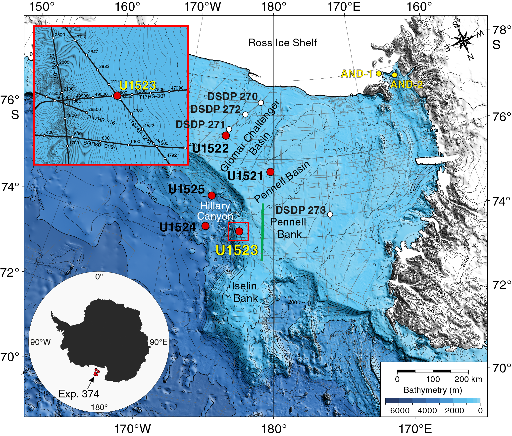
Figure F1. Bathymetric map and site locations.
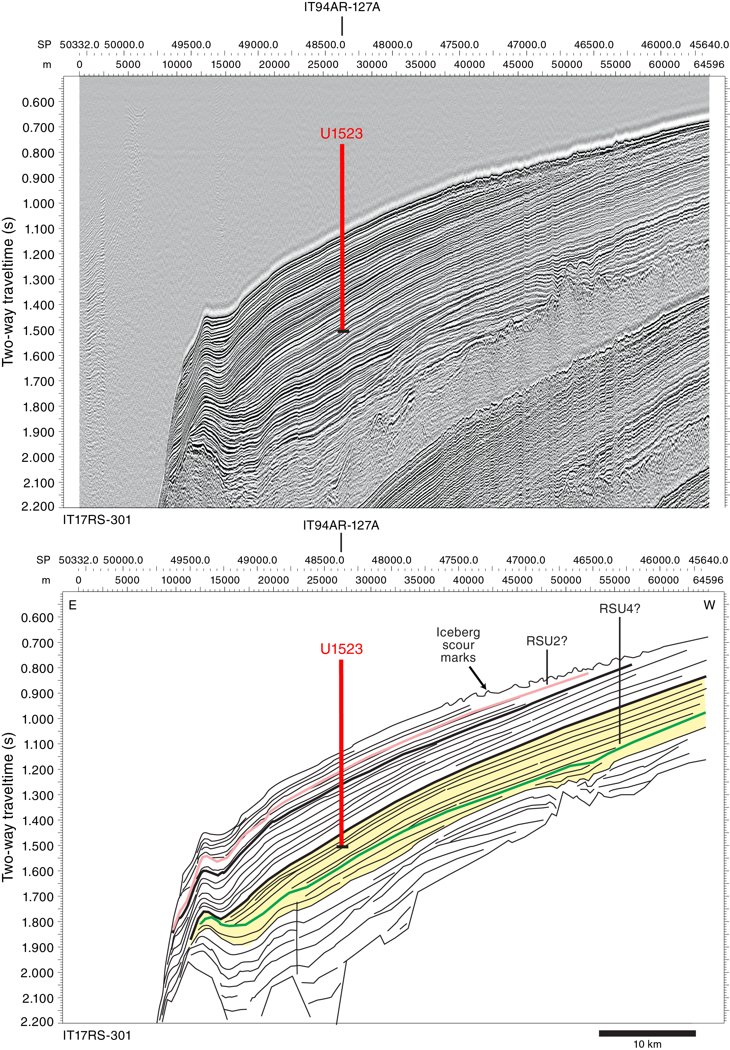
Figure F2. Seismic-reflection Profile IT17RS-301.
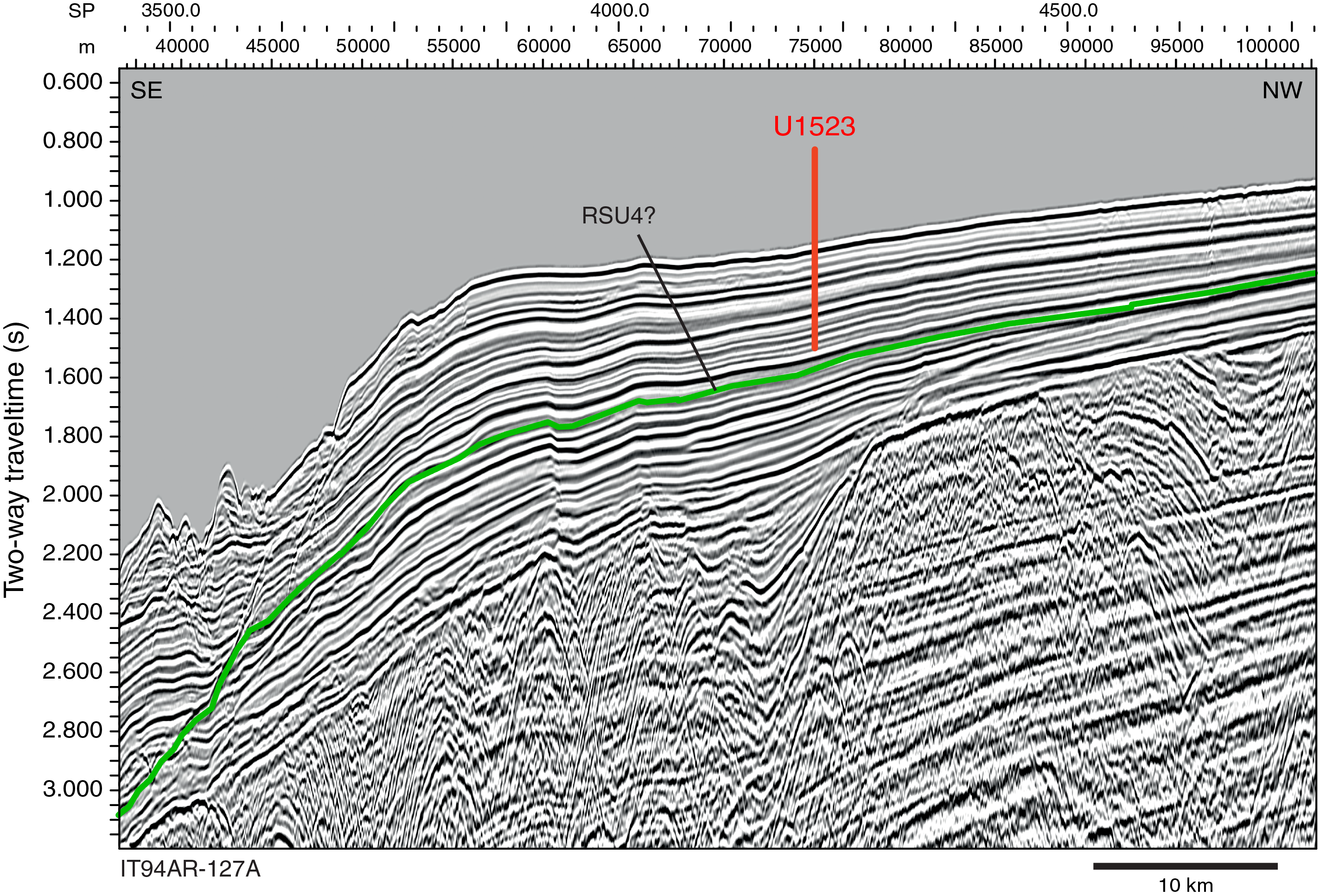
Figure F3. Seismic-reflection Profile IT94AR-127A.
Undulations in the seafloor and subseafloor reflectors occur toward the top of the bank, 12 km west of Site U1523, and are interpreted as iceberg scour marks (Figure F2). The scour marks crosscut into the youngest strata, and iceberg keels ploughing into the sediment would act to remobilize sediment deposited near the top of the bank. Higher on the bank, ~80 km west, seismic-reflection profiles show flat-topped ridges that are interpreted to represent grounding-zone wedges (green wedge in Figure F4). Ice sheet models suggest that during the Last Glacial Maximum (LGM), these wedges likely formed as a consequence of eastward ice flow and subglacial deposition from an ice divide on the bathymetric high of the Pennell Bank (Golledge et al., 2013). Consequently, sediment supply at Site U1523 could come from a combination of sources, including alongslope delivery of ice-rafted debris (IRD) and suspended sediment from the east via the ASC, downslope delivery from glacial outwash at the margin of an ice sheet grounded on the northernmost Pennell Bank west of the site, downslope delivery by suspended sediment scoured by icebergs west of the site, and/or pelagic sedimentation. Bottom currents associated with the ASC in this region are modeled to be between ~10 and 20 cm/s (Padman et al., 2003), and winnowing of fines is expected during periods of enhanced bottom-current flow. Jacobs et al. (1974) reported strong diurnal signals and average and maximum velocities of >17 and 40 cm/s, respectively, at 4 m above the seafloor in 527–1201 m water depth in the Ross Sea.
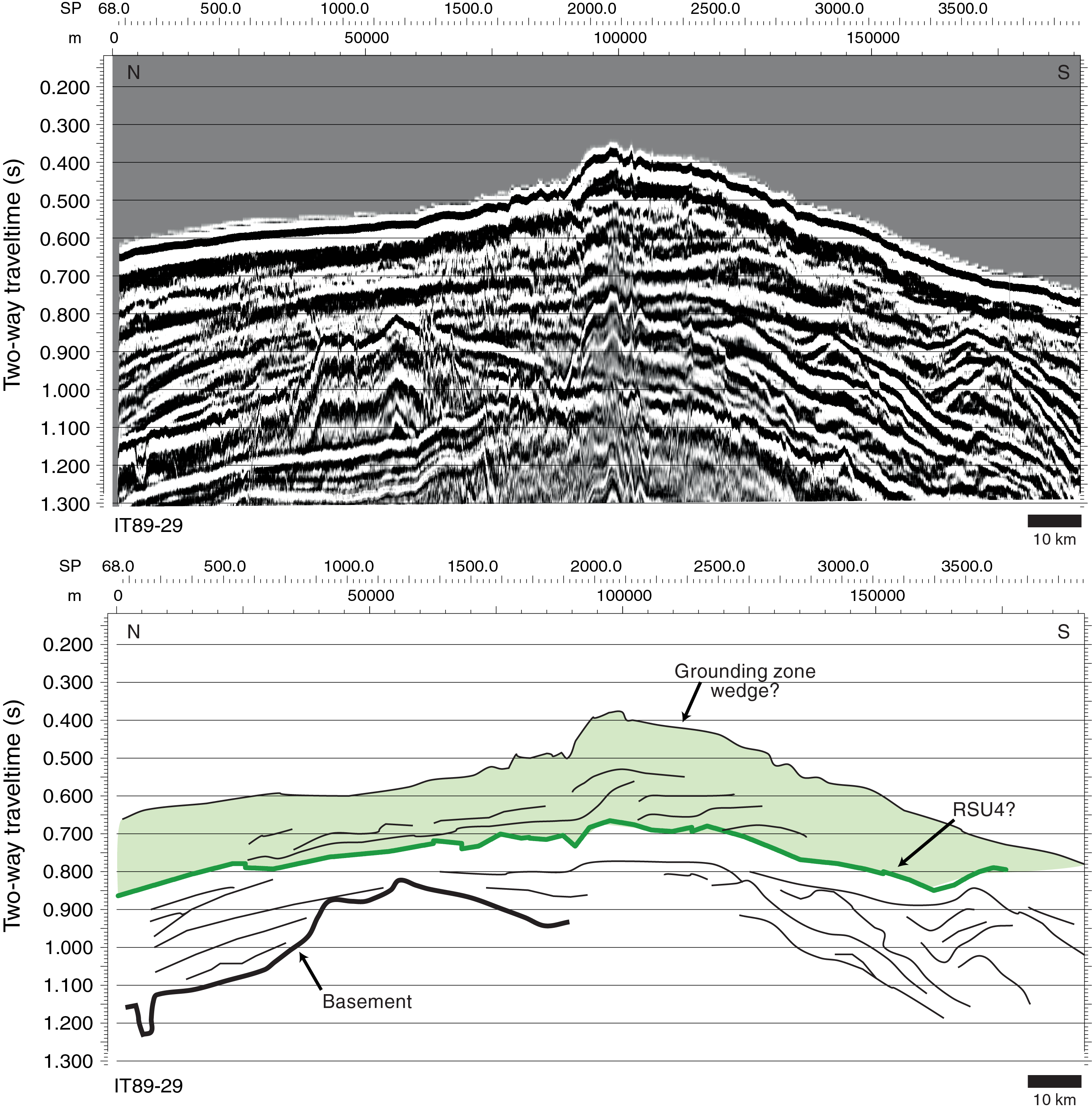
Figure F4. Seismic-reflection Profile IT89A-29.
The primary objectives at Site U1523 were to reconstruct fluctuations in the ASC vigor during the Neogene and Quaternary (Objective 3 in Scientific objectives in the Expedition 374 summary chapter [McKay et al., 2019b]) and to recover a high-resolution record that can be correlated to more direct records of ice sheet advance and retreat from the continental shelf (e.g., Site U1522 and Antarctic Geological Drilling Project [ANDRILL] Site AND-1B [Naish et al., 2009]). To achieve these objectives, coring at Site U1523 aimed to sample the upper sedimentary section above RSU4. The Site U1523 record of deposition and winnowing beneath the ASC will allow us to test the hypothesis that changes in the strength of this wind-driven ocean current regulated the southward transport of warm Circumpolar Deep Water onto the Ross Sea continental shelf during past ice sheet retreat events. Another objective is the reconstruction of ice-proximal oceanic temperatures and surface-water properties during periods of pelagic/hemipelagic sedimentation, thus constraining the magnitude of polar amplification during past warm periods of the Neogene and Quaternary (Objective 2). An additional objective is to identify processes that govern sediment transfer from the outermost continental shelf to the upper continental slope/rise.
Operations
Site U1523 (proposed Site RSCR-14A) is an alternate site that was occupied after coring at Site U1522 demonstrated that core recovery would likely be poor in the targeted upper interval of the original proposed primary Site EBOCS-04B. We planned to core two holes, one with the advanced piston corer (APC) system to refusal followed by an APC/extended core barrel (XCB) hole to 450 m drilling depth below seafloor (DSF). Instead, we ultimately cored five holes at Site U1523 because difficult coring conditions required additional holes to achieve the objectives (Table T1). Prior to coring, we conducted a seafloor camera survey to ensure we could avoid large rocks. The survey included tagging the seafloor at four potential hole locations.
Hole U1523A was cored with a combination of the APC and half-length APC (HLAPC) coring systems to 46.3 m DSF, where we were unable to land the HLAPC core barrel. The hole was terminated, and we pulled the drill string above the seafloor to try to clean out the bottom-hole assembly (BHA). After we were unable to reestablish circulation through the drill string, we had to pull the pipe back to the surface to clean the debris (rocks and sand/gravel) from the BHA. The debris was curated as a ghost core. The APC/XCB BHA was reassembled and run back to the seafloor, and Hole U1523B was cored to a final depth of 164.4 m DSF. Toward the end of coring operations in Hole U1523B, hole cleaning became a problem, and off-bottom torque steadily increased despite efforts to clean the hole. In addition, rotary coring with the XCB system yielded very poor recovery, so we terminated operations in Hole U1523B with the intention of using the HLAPC system in Hole U1523C to target specific stratigraphic gaps not recovered in Holes U1523A and U1523B. After pulling clear of the seafloor for Hole U1523B, our ability to circulate through the bit jets was apparently compromised. After attempting to clear the bit jets, we started Hole U1523C and drilled without coring to 43.3 m DSF. At that depth, we completely lost circulation through the drill string and were forced to terminate Hole U1523C. The drill string was pulled back to the rig floor.
We then decided to use the rotary core barrel (RCB) system to core and log to at least 300 m DSF. Hole U1523D was drilled without coring from the seafloor to 135.0 m DSF. RCB coring then penetrated from 130.5 m DSF to a final depth of 307.8 m DSF. We opted not to deepen the hole further because of very poor recovery (0.9 m; 0.5%). At the end of coring operations, the hole was displaced with heavy mud (10.5 lb/gal) and logged with two tool strings: a modified triple combination (triple combo) and the Formation MicroScanner (FMS). The Dipole Sonic Imager (DSI) was run on the triple combo tool string instead of the FMS tool string, and the Hostile Environment Litho-Density Sonde (HLDS) was run without the source for measurement of borehole diameter with the caliper only. After completion of logging, we used the APC and HLAPC systems to spot core in Hole U1523E to cover stratigraphic gaps from Holes U1523A and U1523B. Hole U1523E was successfully spot cored to 130.8 m DSF. After completion of coring, the drill string was recovered, and the rig floor was secured at 0547 h (all times are local ship time; UTC + 13 h) on 3 February 2018, ending Hole U1523E and Site U1523. A total of 147.5 h (6.15 days) were spent at Site U1523.
We collected a total of 64 cores at Site U1523. The APC coring system was deployed 5 times, recovering 41.57 m of sediment (91%). The HLAPC coring system was used 33 times, collecting 87.99 m (59%). The XCB coring system collected 3.16 m of core (5%) over 8 cores. The RCB system was deployed 18 times over 172.8 m, recovering 0.9 m (0.5%) (Table T1).
Transit to Site U1523
The 148 nmi transit to Site U1523 was completed in 12.9 h at an average speed of 11.5 kt. The vessel arrived at Site U1523 at 0158 h on 29 January 2018. The thrusters were lowered and secured at 0218 h, clearing the drill floor for operations. The acoustic positioning beacon was deployed at 1000 h after completing a seafloor survey.
Hole U1523A
Operations for Hole U1523A began with assembling an APC/XCB BHA and then lowering the drill string toward the seafloor. Because of uncertain seafloor conditions, we decided to survey the seafloor prior to starting the first hole. After the drill string reached 599.1 m drilling depth below rig floor (DRF), we pulled the upper guide horn to deploy the subsea camera for the seafloor survey to look for large rocks in the vicinity of the potential hole locations. While lowering the subsea camera, we also continued to lower the drill string. Because this site is in deeper water than the two previous sites (the precision depth recorder indicated 837 m DRF), some additional drill pipe had to be drifted (checked that it was clear of internal obstructions) and strapped (measured) as it was deployed. We picked up the top drive and prepared a nonmagnetic APC core barrel before conducting the seafloor survey, which included tagging the seafloor at four potential hole positions. All tag depths were 839 m DRF (828 meters below sea level). An acoustic positioning beacon was deployed at 1000 h after completing the survey. The vessel was moved back to the first tag location, and we left the subsea camera at the seafloor to observe the core barrel starting Hole U1523A.
After installing the sinker bars and orientation tool, the first APC core barrel was lowered into the drill string with the drill bit at 838.0 m DRF (1 m above the seafloor tag depth). Hole U1523A was started at 1050 h on 22 January 2018. The mudline core recovered 8.51 m of sediment. We continued to APC core with nonmagnetic core barrels and orientation through Core 374-U1523A-3H (0–25.2 m DSF). Because Core 3H was a partial stroke, we switched to the HLAPC system and continued coring through Core 7F (46.3 m DSF). While drilling out the cored interval, backflow of sand/gravel/stones into the BHA blocked the drill string. Because we were unable to land a core barrel or circulate, we abandoned Hole U1523A. We pulled the drill string out of the hole and attempted to clear the BHA while it was above the seafloor. We then dropped an XCB core barrel with a deplugger; however, this attempt to clear the BHA also failed. After the XCB core barrel was retrieved, the drill string was pulled to the rig floor, and the BHA was disassembled and cleaned of debris. The lockable float valve was damaged either by debris or the XCB core barrel. The bit cleared the rotary table at 0450 h, ending Hole U1523A. Total time spent in Hole U1523A was 26.5 h (1.1 days).
The APC coring system was deployed three times, recovering 23.22 m of core over 27.5 m of coring (84%). The HLAPC was deployed four times, collecting 10.29 m of core over 18.8 m of coring (55%). Total core recovered for the hole was 33.51 m (72%) (Table T1).
Hole U1523B
After clearing out the BHA, the outer core barrel was reassembled and the drill string was lowered toward the seafloor. The vessel was positioned 20 m east of Hole U1523A. After picking up the top drive, the drill bit was positioned at 838 m DRF (1 m above the seafloor) to start Hole U1523B. A nonmagnetic APC core barrel was deployed, and Hole U1523B was started at 1100 h on 30 January 2018. Core 374-U1523B-1H recovered 8.49 m of sediment. We then dropped an XCB center bit and advanced the hole without coring to 46.7 m DSF, observing a hard layer at 45.9 m DSF. After recovering the XCB center bit, we deployed a HLAPC core barrel. Coring continued with Cores 3F through 13F (46.7–93.8 m DSF). We pumped 20 or 30 bbl mud sweeps every few cores to maintain good hole conditions. Core 13F was a partial stroke, so we switched to the XCB coring system. Cores 14X through 16X penetrated from 93.8 to 103.3 m DSF with almost no recovery. Because Core 16X only advanced 0.1 m, we dropped the center bit and drilled ahead without coring for 5.0 m to try to advance past a very hard layer. We then resumed XCB coring and cut Cores 18X and 19X (108.3–127.5 m DSF), again with minimal recovery (3%). Because drilling parameters suggested we had successfully passed the hard layers, we switched back to the HLAPC coring system for Cores 20F and 21F (127.5–135.6 m DSF). We had to drillover Core 21F to release it from the formation because of excessive overpull, so we switched back to the XCB coring system. We cut Cores 22X through 24X (135.6–164.4 m DSF) with minimal recovery (9%). We terminated coring at 164.4 m DSF in Hole U1523B due to unstable hole conditions causing excessive torque. In addition, core liners used with the XCB system shattered at a high rate (63%) (Table T1), causing significant core disturbance. We pumped a 30 bbl mud sweep and pulled the drill string clear of the seafloor, ending Hole U1523B at 2120 h on 31 January. Total time spent in Hole U1523B was 37.0 h (1.5 days).
A single APC core recovered 8.49 m over an 8.5 m advance (100%). The HLAPC was deployed 13 times, recovering 33.48 m over 55.2 m of coring (61%). The XCB was deployed 8 times, collecting 3.16 m over 57.5 m of coring (5%). Total recovery for Hole U1523B was 45.13 m (37%) (Table T1).
Hole U1523C
After clearing the seafloor, the vessel was repositioned 20 m south of Hole U1523B. Hole U1523C was planned to selectively core intervals of poor recovery with the HLAPC system while avoiding hard layers encountered in previous holes. We dropped a center bit in preparation to start Hole U1523C and noticed high pump pressures, indicating clogged jets in the drill bit. After attempting to clear the jets, we started Hole U1523C at 1915 h on 31 January 2018 and drilled ahead without coring to 43.3 m DSF, where we lost circulation through the drill string, forcing us to abandon Hole U1523C. The bit cleared the seafloor at 2120 h and was retrieved to the rig floor at 0130 h on 1 February, ending Hole U1523C. Total time spent in Hole U1523C was 7.75 h (0.3 days) (Table T1).
Hole U1523D
After Hole U1523C, we decided to switch to the RCB coring system to core and log a deeper hole, intending to core a final APC/HLAPC hole if time permitted after logging. The RCB BHA was assembled and lowered toward the seafloor. After picking up the top drive, we prepared a core barrel with a center bit. Hole U1523D was started at 0725 h on 1 February 2018. The hole was advanced to 135.0 m DSF without coring. We pumped a 30 bbl high-viscosity mud sweep and retrieved the center bit. RCB coring continued with Cores 374-U1523D-2R through 19R (135.0–307.8 m DSF) with very poor recovery (0.90 m; 0.5%). We pumped 30 bbl high-viscosity mud sweeps every 2–3 cores to clear cuttings. We terminated coring after reaching our minimum target depth of ~300 m DSF and prepared the hole for downhole logging by circulating two 50 bbl high viscosity–mud sweeps to improve hole conditions. The rotary shifting tool (RST) was lowered on the coring line to release the RCB bit in the bottom of the hole at 0800 h on 2 February. After running the RST a second time to shift the sleeve in the mechanical bit release back to the circulating position, we displaced the hole with 94 bbl of 10.5 lb/gal mud from 307.8 m DSF to the seafloor. We then pulled the drill string to 258.5 m DSF, set back the top drive, and continued to pull the drill string up to a logging depth of 82.3 m DSF. After displacing the upper part of the hole with 20 bbl of 10.5 lb/gal mud, the drill floor was prepared for downhole logging operations at 1130 h on 2 February.
The first logging run consisted of a modified triple combo tool string assembled with the following tools:
- Magnetic Susceptibility Sonde (MSS),
- DSI,
- High-Resolution Laterolog Array (HRLA),
- HLDS (without source),
- Hostile Environment Natural Gamma Ray Sonde (HNGS), and
- Enhanced Digital Telemetry Cartridge (EDTC).
The triple combo tool string was lowered into the drill string at 1320 h on 2 February. The average heave was estimated to be 0.3 m just prior to logging. The active heave compensator was switched on when the tools reached open hole. A down log was performed from just above the seafloor to 292 m wireline logging depth below seafloor (WSF), with the tool string reaching to within 15 m of the bottom of the hole. The hole was logged up with a 136 m calibration pass. The tool string was lowered back to the bottom (288 m WSF), and the hole was logged up again. When the tool string neared the end of the pipe, it was raised to 67 m DSF to provide additional log coverage of the borehole. The tools were back at the surface at 1630 h on 2 February, and the triple combo tool string was disassembled by 1745 h.
The second logging run was with the FMS tool string, which was assembled with the FMS, HNGS, and EDTC. The FMS tool string was lowered into the hole at 1820 h. Natural gamma radiation (NGR) was logged from above the seafloor as the tool string was lowered to depth-match results to the first logging run. The FMS tool string reached a total depth of 289.6 m WSF, and two upward passes were logged. During the second uplog, the end of the pipe was raised to 67 m DSF to provide additional coverage of the borehole. The FMS tool string was returned to the rig floor at 2130 h, and all logging equipment was disassembled by 2245 h on 2 February. We then began to raise the drill string back toward the rig floor, clearing the seafloor at 2315 h on 2 February. After placing three stands of drill collars in the derrick, the outer core barrel was disassembled and inspected. The end of the drill string cleared the rotary table at 0240 h on 3 February, ending Hole U1523D. Total time spent in Hole U1523D was 49.25 h (2.1 days).
A total of 0.90 m of core was recovered over 172.8 m of RCB coring (0.5%) (Table T1).
Hole U1523E
We switched back to the APC/XCB coring system to target poorly recovered intervals in Holes U1523A and U1523B. The drill string was lowered toward the seafloor, and the bit was set at 830 m DRF for the first core. Hole U1523E was started at 0810 h on 3 February 2018, and Core 374-U1523E-1H recovered a full barrel (9.86 m). We drilled ahead 9.5 m without coring and then switched to the HLAPC coring system and proceeded with spot coring. Over the upper ~90 m DSF, spot coring consisted of collecting 1–3 HLAPC cores followed by a drilled interval ranging from 2.8 to 12.3 m in length (Table T1). Depths were chosen to avoid gravel encountered in Holes U1523A and U1523B. Deeper than ~90 m DSF, the coring plan included dropping a center bit to drill through hard layers encountered between 93 and 95, 104 and 108, and 116 and 117 m DSF, with HLAPC cores collected between the hard layers (Table T1). This technique proved particularly successful for the interval deeper than 100 m DSF, allowing us to fill in substantial gaps in the stratigraphy. The last core (25F) in Hole U1523E arrived on deck at 2350 h on 3 February. After pumping a 30 bbl mud sweep, we left the top drive installed while pulling the drill string out of the hole because unstable hole conditions caused excessive torque and overpull. After clearing the seafloor at 0150 h on 4 February, the top drive was set back, and the drill string was retrieved to the vessel. The acoustic beacon was released and recovered at 0450 h, and the rig floor was secured at 0547 h, ending operations in Hole U1523E and Site U1523. A total of 147.50 h (6.15 days) was spent at Site U1523.
A single APC core collected 9.86 m of core over 9.5 m of coring (104%). The HLAPC system was deployed 16 times, recovering 44.22 m of core over 75.2 m of coring (59%). Total recovery for Hole U1523E was 54.08 m (64%) (Table T1).
Lithostratigraphy
Site U1523 includes four holes with core recovery; the deepest hole was cored to 307.8 m DSF. The 133.62 m of sediment recovered from Site U1523 is divided into three lithostratigraphic units (Table T2). A lithologic summary of Holes U1523A, U1523B, and U1523E is shown in Figure F5. Hole U1523C was abandoned before any core was recovered. Hole U1523D is a RCB hole cored to 307.8 m DSF for downhole logging. Because of very poor recovery (0.5%), Hole U1523D is not described in this chapter.
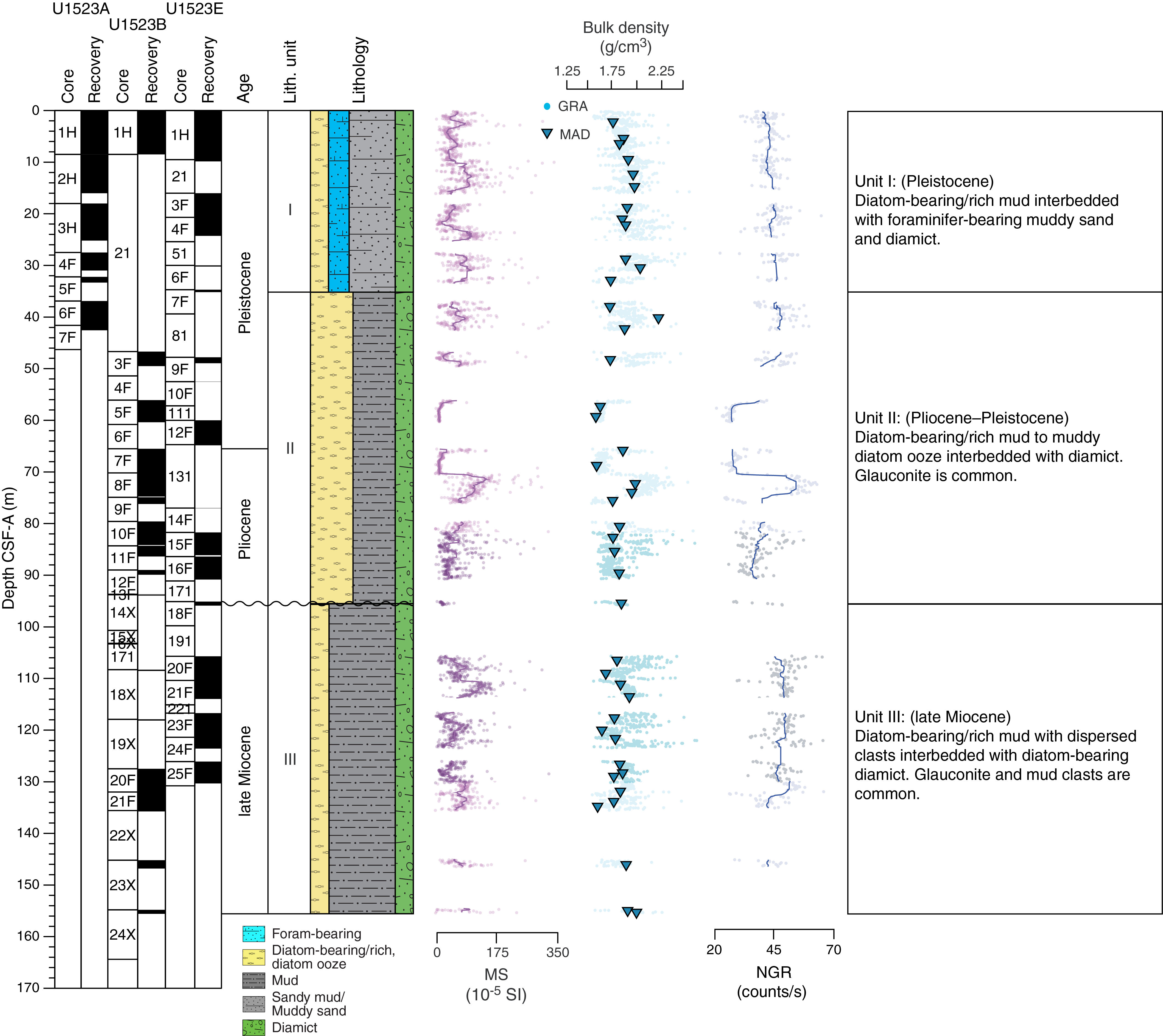
Figure F5. Lithostratigraphic summary.
In Hole U1523E, a targeted coring approach improved recovery by avoiding coarse-grained (e.g., gravel rich) and indurated layers identified by drilling parameters (e.g., penetration rate; see Operations) in Holes U1523A and U1523B. The dominant facies at this site are interbedded on the centimeter/decimeter to meter scale and include diatom-rich mud and diatom ooze with dispersed/common clasts, diatom-bearing mud/sandy mud, foraminifer-bearing sand, sand, and diamict. We define three lithostratigraphic units. Unit I is characterized by interbedded diatom-bearing/rich mud, foraminifer- and diatom-bearing muddy sand, and diamict. Unit II contains similar lithologies, but diatom content increases and foraminifer content decreases relative to Unit I. Unit III lithologies are predominantly siliciclastic with decreasing biogenic components downhole. All units contain intervals of poor recovery that are inferred to represent unconsolidated sand, gravel, and/or diamict layers not recovered by either the HLAPC or XCB coring systems. Photographs of primary lithologies and sedimentary structures/accessories are shown in Figures F6 and F7, respectively, and summarized in Figure F8.

Figure F6. Primary lithologies.
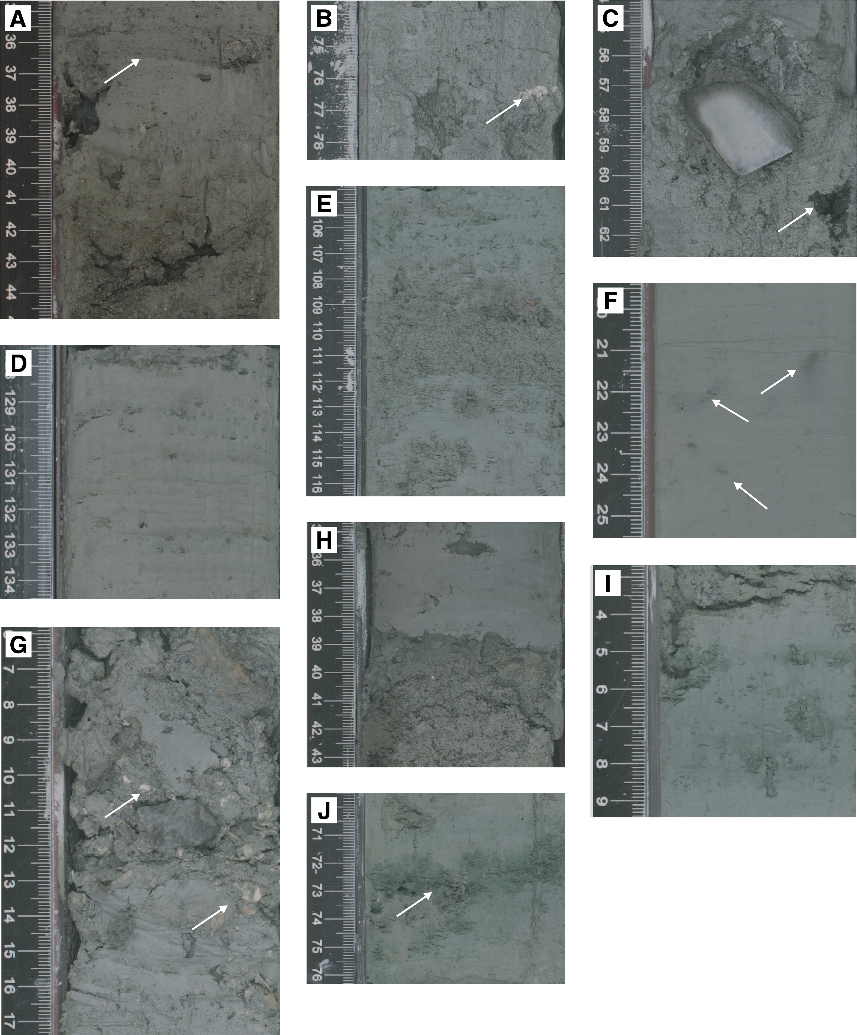
Figure F7. Sedimentary structures and diagenetic features.
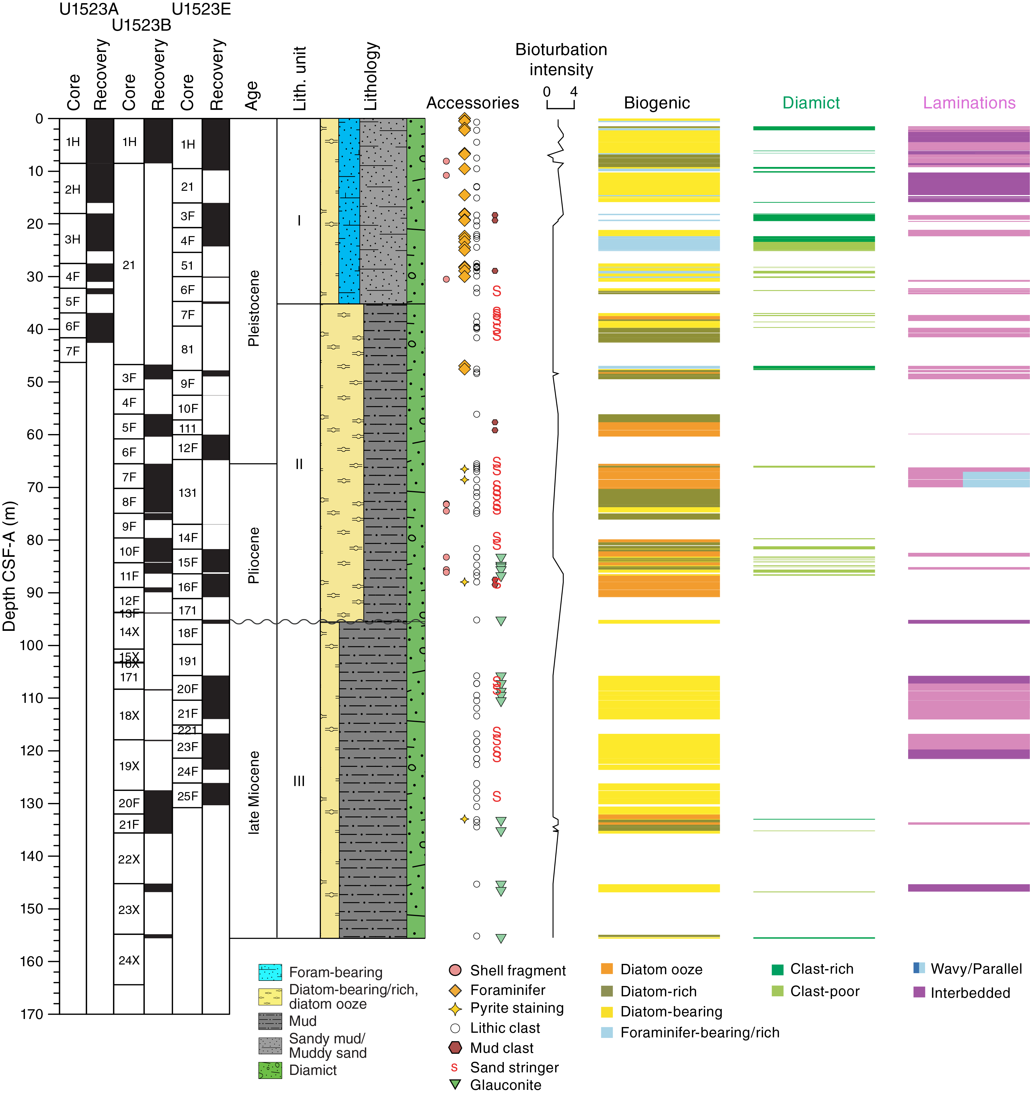
Figure F8. Lithology and sedimentary structures.
Unit descriptions
Site U1523 is divided into three lithostratigraphic units (I–III; youngest to oldest) based on lithologic changes observed downhole (Figure F5; Table T2) that were determined using a combination of visual core description, microscopic examination of smear slides, and color spectral observations (see Lithostratigraphy in the Expedition 374 methods chapter [McKay et al., 2019a]). In each hole, units are defined based on the first and last observation of the defining lithology (Table T2). On the summary log, the top of each unit is drawn as the uppermost depth observed across all holes on the core depth below seafloor (CSF-A) depth scale (Figure F5), although small differences exist between holes (see Depth scales in the Expedition 374 methods chapter [McKay et al., 2019a]). Missing stratigraphy resulting from nonrecovery creates greater uncertainty for some unit boundaries. A composite stratigraphy will be developed postcruise using core and downhole logging data.
Unit I
- Interval: 374-U1523A-1H-1, 0 cm, to 6F-1, 0 cm; 374-U1523E-1H-1, 0 cm, to 7F-1, 0 cm
- Depth: Hole U1523A = 0–36.90 m CSF-A; Hole U1523E = 0–34.70 m CSF-A
- Thickness: Hole U1523A = 36.90 m; Hole U1523E = 34.70 m
- Age: Pleistocene
- Lithology: diatom-bearing/rich mud, foraminifer-bearing muddy sand, diamict
Lithostratigraphic Unit I consists of massive bioturbated to laminated greenish gray to grayish brown diatom-bearing/rich mud interbedded at the decimeter scale with diatom-bearing and foraminifer-bearing muddy sand with dispersed clasts/diamict (Figures F5, F6A–F6C; Table T2). Laminae, distinguished by color and texture changes, are often bioturbated. Contacts vary between sharp, gradational, and bioturbated (Figures F7A, F8). Large lithic clasts, mud clasts, and pyrite staining occur throughout. Shell fragments are observed in Sections 374-U1523A-2H-2A and 374-U1523E-4F-1A (Figure F7B). A lignite clast is observed in interval 374-U1523E-4F-2A, 61 cm (Figure F7C). Drilling disturbance ranges from slight to extreme. Recovery is poor between ~25 and 35 m CSF-A, likely because of unconsolidated sand and gravel in the formation (see Operations). Recovery in Unit I is 27.68 m (75%) in Hole U1523A and 18.45 m (78%) in Hole U1523E. Targeted coring in Hole U1523E filled some of the gaps in recovery in Hole U1523A, resulting in an estimated combined recovery of ~86% for Unit I.
Unit II
- Intervals: 374-U1523A-6F-1, 0 cm, to 7F-CC, 12 cm (total depth); 374-U1523B-3F-1, 22 cm, to 14X-CC, 14 cm; 374-U1523E-7F-1, 0 cm, to 18F-1, 69 cm
- Depths: Hole U1523A = 36.90–42.55 m CSF-A (total depth); Hole U1523B = 46.92–93.94 m CSF-A; Hole U1523E = 34.70–95.79 m CSF-A
- Thicknesses: Hole U1523A = 5.65 m (minimum); Hole U1523B = 47.02 m (minimum); Hole U1523E = 61.09 m
- Age: Pliocene to Pleistocene
- Lithology: muddy diatom ooze, diatom-bearing/rich mud, diatom-bearing/rich diamict
Lithostratigraphic Unit II consists of massive bioturbated to laminated greenish gray diatom-bearing/rich mud and olive brown to gray diatom-rich mud to muddy diatom ooze interbedded at the decimeter to meter scale with massive bioturbated gray to greenish gray diamict (Figures F5, F6D–F6F, F7D). Diatom-rich mud and muddy diatom ooze lithologies define the unit. Contacts are sharp, gradational, and/or bioturbated (e.g., interval 374-U1523E-12F-2A, 108–116 cm; Figure F7E). Pyrite staining, glauconite, lithic clasts, and mud clasts are observed throughout. Shell fragments, bryozoa, foraminifers, and worm tubes are present between ~80 and 90 m CSF-A (Figure F7G). The base of Unit II is defined as the base of the deepest diatom-rich sandy mud bed (interval 18F-1A, 69 cm). Recovery in Unit II is 5.69 m (61%) in Hole U1523A, 25.21 m (47%) in Hole U1523B, and 15.39 m (46%) in Hole U1523E. Two large core gaps in the Hole U1523B record were filled with cores from Hole U1523E, resulting in an estimated combined recovery of ~66% for Unit II.
Unit III
- Intervals: 374-U1523B-18X-CC, 0 cm, to 24X-CC, 30 cm; 374-U1523E-18F-1, 69 cm, to 25F-CC, 27 cm
- Depths: Hole U1523B = 108.30–155.57 m CSF-A (total depth); Hole U1523E = 95.79–130.33 m CSF-A (total depth)
- Thicknesses: Hole U1523B = 47.27 m; Hole U1523E = 34.54 m (minimum)
- Age: late Miocene
- Lithology: diatom-bearing diamict, diatom-bearing/rich sandy mud/mud, muddy diatom ooze
Lithostratigraphic Unit III consists of massive bioturbated to laminated greenish gray to dark greenish gray diatom-bearing/rich mud and muddy diatom ooze interbedded at the decimeter scale with greenish gray diatom-bearing mud with dispersed clasts, sandy mud, and diamict (Figure F6G–F6J, F7H). Unit III is defined by a decrease in biogenic content and increased siliciclastics and glauconite relative to Unit II (Figure F8). Contacts are sharp, gradational, and/or bioturbated (Figure F7H). Large clasts, pyritized burrows, sand stringers, and glauconite are common (Figure F7F, F7I, F7J, F8). Diamictite is observed in two intervals deeper than 100 m CSF-A (intervals 374-U1523B-18X, 13–16 cm, and 24X, 22–25 cm; Figure F6G, F6H). Recovery in Unit III is 11.21 m (20%) in Hole U1523B and 19.55 m (71%) in Hole U1523E, where targeted HLAPC coring improved recovery. Thus, the estimated combined recovery for Unit III is ~61%.
Facies distribution
At Site U1523, three lithofacies are identified based on common lithologic, sedimentary, and textural characteristics (Table T3). Facies 3 (mud/mudstone) and 5 (diatom-rich mud to diatom ooze) largely conform to those previously described for Site U1521 (see Lithostratigraphy in the Site U1521 chapter [McKay et al., 2019c]). For consistency, we use the same facies numbering system used at Sites U1521 and U1522, but important site-specific differences are noted below. For example, at Site U1523, diamict is different in character and considered a separate facies (Facies 8; sand and diamict).
Mud/Mudstone
At Site U1523, Facies 3 (mud/mudstone) is predominately diatom bearing, with relatively good preservation of diatom frustules. Thus, this facies likely reflects both terrigenous input from suspension settling and pelagic biogenic sedimentation in a glaciomarine environment.
Diatom-rich mud to diatom ooze
Facies 5 (diatom-rich mud to diatom ooze) is largely comparable to Facies 5 at Site U1521 but is unlithified and bioturbated, with higher sand and clast content. This facies reflects pelagic biogenic to hemipelagic sedimentation, suspension settling, and ice rafting.
Sand and diamict
Facies 8 (sand and diamict) consists of massive bioturbated muddy sand/sand with dispersed clasts and diamict. This facies is commonly foraminifer bearing, glauconitic, and/or stratified (Figure F6A, F6E). Contacts are variable and may be sharp, gradational, and/or bioturbated (Figure F7E). Calcareous foraminifer presence (e.g., Unit I; Figure F6A) suggests either deposition above the local carbonate compensation depth (CCD) or downslope transport and rapid burial of foraminifer tests originally deposited at shallower depths above the local CCD. In the former case, foraminifers may be concentrated in sand/diamict intervals because of the winnowing of fines by bottom currents. Coarse sand and larger clasts may also be delivered by icebergs. Thus, Facies 8 reflects downslope transport, current winnowing, and ice rafting.
Diagenesis
Multiple indicators of postdepositional diagenesis are observed at Site U1523. Pyrite-filled burrows are observed in laminated beds (Figure F7F), indicating bacterial decomposition of organic matter in a sulfate-reducing environment. Glauconite, an authigenic mineral typically formed in low–sedimentation rate marine environments, is observed in Units II and III (Figure F7I, F7J).
Bulk mineralogy
X-ray diffraction (XRD) analyses were performed on powdered bulk samples from Holes U1523A (14 samples), U1523B (16 samples), and U1523E (1 sample) to semiquantitatively estimate the relative abundances of the most common mineralogical components. Relative mineral diffraction peak intensities are shown in Figure F9 (defined in Lithostratigraphy in the Expedition 374 methods chapter [McKay et al., 2019a]). Downhole mineralogy at Site U1523 is similar to that at Sites U1521 and U1522. Noticeable downhole variations in illite/mica may be associated with glauconite.
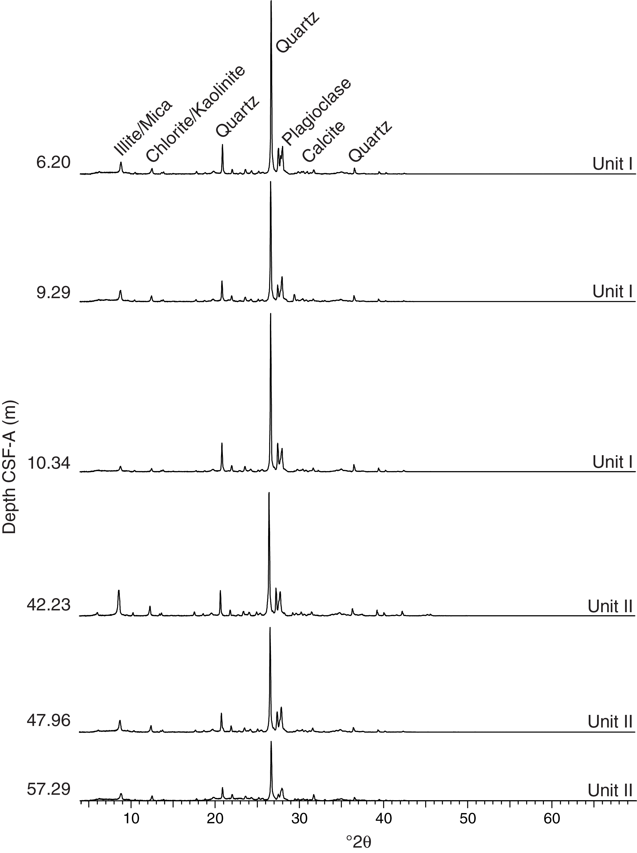
Figure F9. XRD patterns.
Preliminary depositional interpretation
Coring at Site U1523 recovered a sequence of late Miocene to Pleistocene sediments on the outermost continental shelf of the Ross Sea, Antarctica. This site contains diatom-bearing/rich mud, foraminifer-bearing muddy sand, diamict, and muddy diatom ooze interpreted to reflect deposition in a glaciomarine to open-marine environment influenced by downslope transport, bottom current processes, and ice rafting. Changes in the relative percentage of biogenic and siliciclastic components are likely related to ice proximity, with higher siliciclastic content associated with ice-proximal depositional environments and higher biogenic content associated with more ice distal to open-marine environments. Clasts, sand, and glauconite are typically concentrated at the top of the diatom-rich mud beds, suggesting winnowing of the finer fraction by changes in the strength and/or position of the westward-flowing Antarctic Coastal Current. Downslope transport also occurs at Site U1523, as indicated by sand beds with shell and bryzoan fragments (e.g., Unit II [60–90 m CSF-A]; Figure F7G). Processes associated with glaciation on the Pennell Bank could result in sediment loading at the ice sheet grounding line, iceberg ploughing, and isostatic adjustment, all of which may play a role in sediment destabilization on the outer continental shelf (e.g., Hesse et al., 1997; Lucchi et al., 2002; Carburlotto et al., 2010).
Biostratigraphy and paleontology
Core catcher samples from Holes U1523A, U1523B, U1523D, and U1523E were analyzed for siliceous (diatoms, radiolarians, silicoflagellates, ebridians, and chrysophycean cysts), calcareous (foraminifers), and organic (dinoflagellate cysts [dinocysts] and other aquatic palynomorphs, pollen, and spores) microfossils. Three broad stratigraphic intervals separated by disconformities correspond generally to lithostratigraphic units and represent deposition of (1) a Pleistocene interval with mixed and reworked microfossils, (2) an upper Pliocene interval (~2.5–2.8 Ma), and (3) an upper middle Miocene to lower upper Miocene interval (~8.5–13.5 Ma). All examined samples contain siliceous microfossils, although with varying abundance, composition, and state of preservation. The inferred depositional settings that produced these sequences ranged from pelagic to hemipelagic, with influence and mixing and sorting of microfossil assemblages by glaciomarine and bottom-current processes, respectively. Dinocysts are often rare except in the uppermost Pliocene and upper Miocene intervals. Foraminifers are most abundant in the upper Pleistocene at Site U1523. A unique monospecific assemblage of agglutinated benthic foraminifers is observed in the upper Miocene of Holes U1523B and U1523E.
Diatoms
All samples examined from Site U1523 contain diatoms and silicoflagellates (Table T4). The upper ~25 m CSF-A at Site U1523 (Samples 374-U1523A-1H-CC to 3H-CC [0–22.31 m CSF-A] and 374-U1523E-1H-CC to 4H-CC [0–24.23 m CSF-A]) contains rare and poorly preserved reworked diatoms of mixed middle Miocene through Pliocene ages. Preservation in this interval is generally poor, with selective preservation of robust, heavily silicified forms. Much of the clay-sized sediment fraction from this interval comprises highly fragmented diatom remains. Deeper than ~25 m CSF-A, diatoms are more abundant and allow for most of the sequence to be assigned to diatom zones (Figure F10). Biostratigraphically useful diatom events are listed in Table T5 and plotted in an age-depth model in Figure F11.
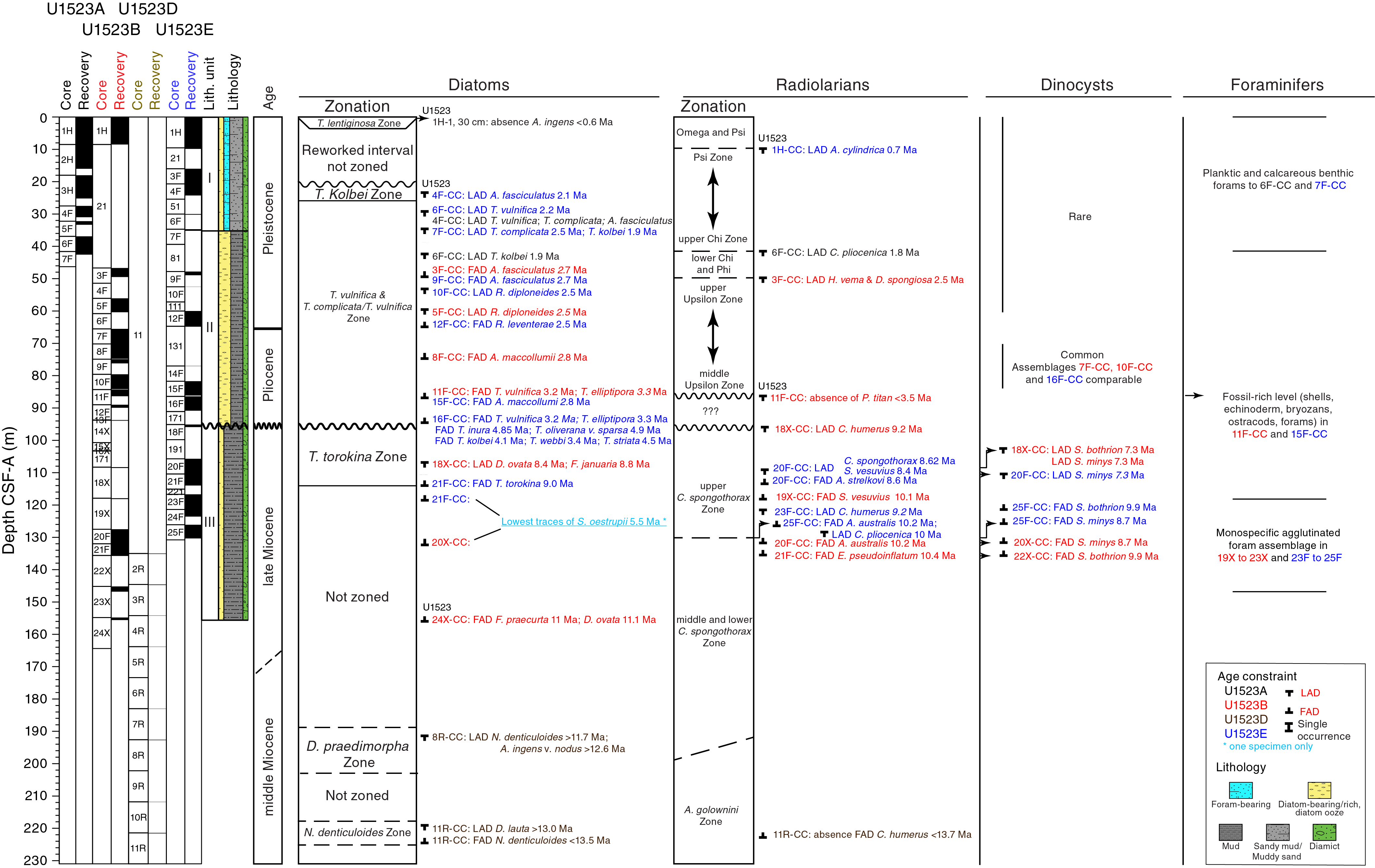
Figure F10. Micropaleontology summary.
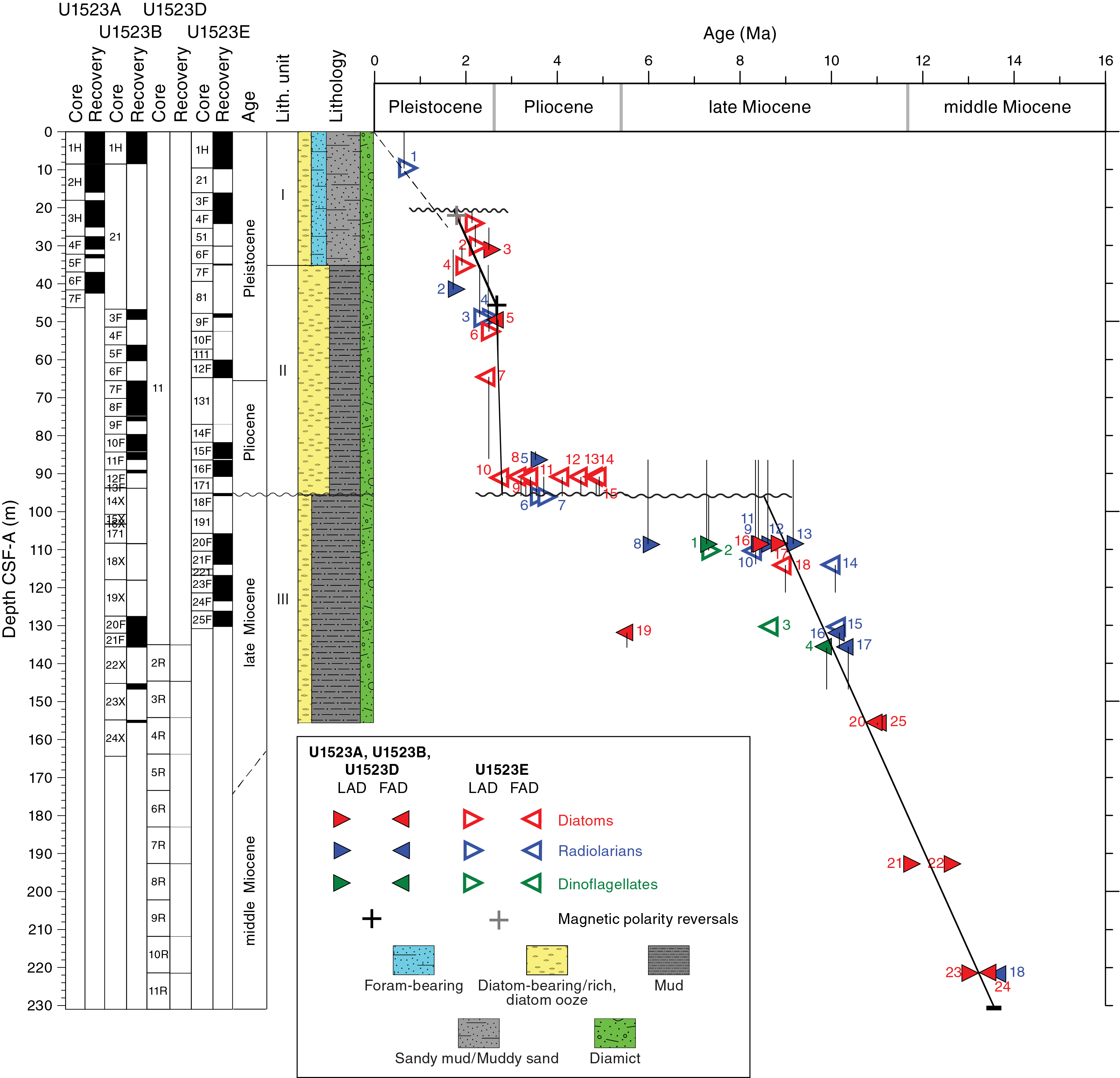
Figure F11. Shipboard age model.
An ~90 m interval of lower Pleistocene and upper Pliocene sediments (~25–95 m CSF-A) is assigned to the lower portion of the Thalassiosira kolbei Zone and the underlying Thalassiosira complicata/Thalassiosira vulnifica Zone. This package of sediment is bounded by unconformities (Figure F10). The lower unconformity coincides with the boundary between lithostratigraphic Units II and III. An age between 2.5 and 3.2 Ma is assigned to this interval based on the last appearance datum (LAD) of Actinocyclus fasciculatus in Core 374-U1523E-4F (24.23 m CSF-A), the LAD of T. complicata (2.5 Ma) in Samples 374-U1523A-4F-CC (30.93 m CSF-A) and 374-U1523E-7F-CC (34.05 m CSF-A), and the first appearance datum (FAD) of T. vulnifica (3.2 Ma) in Samples 374-U1523B-11F-CC (86.30 m CSF-A) and 374-U1523E-16F-CC (90.77 m CSF-A), which provide for the placement of zonal boundaries. Much of the mid- to lower Pliocene is missing in a disconformity.
Below the disconformity between lithostratigraphic Units II and III, an interval of middle to upper Miocene sediments was cored to ~230 m CSF-A. Core recovery over the upper part of this interval, between ~95 and 135 m CSF-A, is moderate, whereas deeper than ~135 m CSF-A, recovery in Holes U1523B and U1523D was very poor and provides only a few snapshots of the age and depositional environment. The FAD of Thalassiosira torokina (9.0 Ma) in Sample 374-U1523E-21F-CC (113.95 m CSF-A) allows assignment of the interval between this sample and the unconformity at ~95 m CSF-A to the T. torokina Zone. The LADs of Denticulopsis ovata (8.4 Ma) and Fragilariopsis januaria (8.8 Ma) in Sample 374-U1523B-18X-CC (108.47 m CSF-A) support the recognition of this zone. The interval below the T. torokina Zone, between ~114 and 190 m CSF-A, is not zoned because of the absence of diatoms used in existing Southern Ocean zonal schemes. Traces of Shionodiscus oestrupii are noted in two samples from this unzoned interval (Samples 374-U1523B-20F-CC [131.98 m CSF-A] and 374-U1523E-21F-CC [113.95 m CSF-A]). This species has a FAD at 5.5 Ma, so its presence in this much older interval requires additional investigation. Samples between ~110 and 120 m CSF-A contain abundant Denticulopsis, Trinacria, Chaetoceros, Coscinodiscus, and other taxa, indicating high-fertility water that resulted in high biosiliceous productivity and sedimentation.
Although core recovery was very poor in Hole U1523D, two samples from deeper than ~155 m CSF-A yielded sufficient material to date the lower part of this hole to ~13 Ma (Figures F10, F11). Sample 374-U1523D-8R-CC (192.71 m CSF-A) contains Nitzschia denticuloides (LAD at 11.7 Ma) and Actinocyclus ingens var. nodus (LAD at 12.7 Ma), which are indicative of the Denticulopsis praedimorpha Zone. Sample 11R-CC (221.55 m CSF-A) includes Denticulopsis lauta (LAD at 13.0 Ma) and N. denticuloides (FAD at 13.5 Ma), whose co-occurrence suggests an age between 13.0 and 13.5 Ma.
Radiolarians
All core catcher samples and the mudline sample were analyzed for radiolarian content (Table T6). Radiolarians are poorly to moderately preserved and present in trace to rare abundances in the upper ~90 m CSF-A of Site U1523 (Samples 374-U1523A-1H-CC to 6F-CC [0–41.59 m CSF-A], 374-U1523B-1H-CC to 11F-CC [0–86.30 m CSF-A], and 374-U1523E-1H-CC to 16F-CC [0–90.77 m CSF-A]), although they become slightly more abundant in Hole U1523E deeper than ~50 m CSF-A. From ~90 to 155 m CSF-A, radiolarians are better preserved and more abundant (Samples 374-U1523B-18X-CC to 24X-CC [108.47–155.52] and 374-U1523E-9F-1, 96.5–101.5 cm, to 25F-CC [48.77–130.28 m CSF-A]), with the exception of Samples 374-U1523E-15F-3, 133–135 cm, to 18F-CC (86.04–95.80 m CSF-A), in which radiolarians are moderately to poorly preserved and present in trace to rare abundances. Two samples from Hole U1523D (Samples 8R-CC [192.71 m CSF-A] and 11R-CC [221.55 m CSF-A]) yielded moderately preserved radiolarians in trace abundances. Plates illustrating some of the taxa identified at this site are presented in Figures F12 and F13. Recognized radiolarian biostratigraphic events are shown alongside diatom and dinoflagellate events in Table T5 and illustrated in Figure F11. The placement of radiolarian, diatom, and dinocyst events shows good agreement (Figures F10, F11).

Figure F12. Radiolarians.
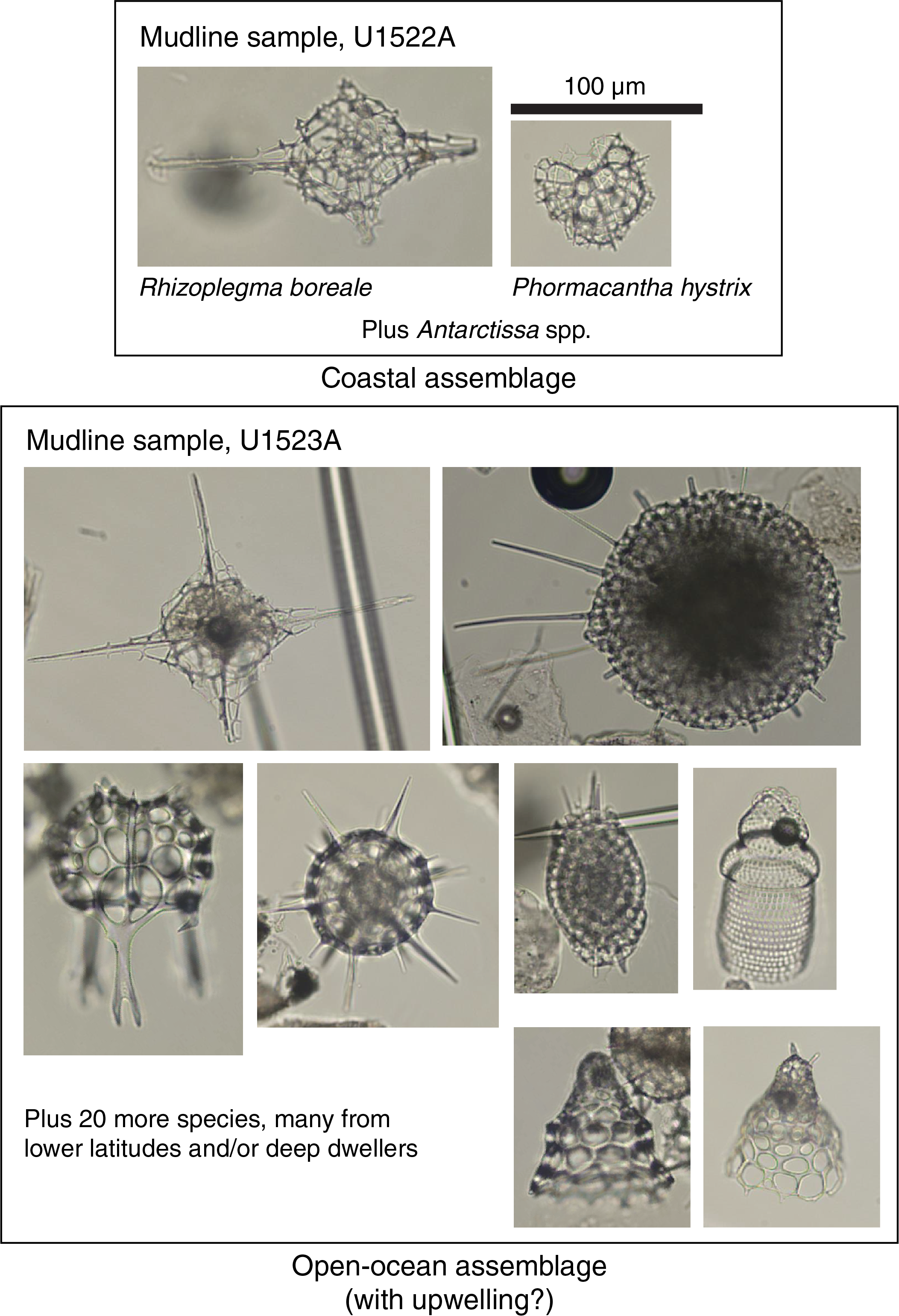
Figure F13. Radiolarians from mudline samples.
The absence of Prunopyle titan (LAD at 3.5 Ma) in Sample 374-U1523B-11F-CC (86.30 m CSF-A) indicates a Pliocene–Pleistocene age for the upper ~90 m CSF-A of this site (Samples 374-U1523A-1H-CC to 6F-CC [0–41.59 m CSF-A], 374-U1523B-1H-CC to 11F-CC [0–86.30 m CSF-A], and 374-U1523E-1H to 16F-CC [0–90.77 m CSF-A]). An unconformity occurs deeper than ~90 m CSF-A because Sample 374-U1523B-18X-CC (108.47 m CSF-A) is late Miocene in age based on the presence of Cycladophora humerus (LAD at 9.2 Ma), which is consistent with diatom biostratigraphy that suggests an age of 8.4–8.8 Ma. The presence of Antarctissa strelkovi (FAD at 8.6 Ma) and Cycladophora spongothorax (LAD at 8.6 Ma) in Sample 374-U1523E-20F-CC (110.35 m CSF-A) confirms this age assignment. Several other radiolarian events are recognized in the upper Miocene portion of the drilled sequence, with the deepest event being the presence of Eucyrtidium pseudoinflatum (FAD at 10.4 Ma) in Sample 374-U1523B-21F-CC (135.61 m CSF-A). The deepest sample at this site (Sample 374-U1523D-11R-CC [221.55 m CSF-A]) is younger than 13.7 Ma based on the absence of C. humerus (FAD at 13.7 Ma), which is in good agreement with the diatom age estimate (13–13.5 Ma) for the same sample.
Radiolarian zonal assignments are shown in detail in Figure F10. Samples above the observed Antarctissa cylindrica LAD (0.65 Ma; Sample 374-U1523E-1H-CC [9.81 m CSF-A]) belong to the radiolarian Omega Zone and part of the Psi Zone (Figure F10; Table T5). The interval from 9.81 m CSF-A downhole to Sample 374-U1523A-6F-CC (41.59 m CSF-A; LAD of Cycladophora pliocenica) is assigned to the remaining part of the Psi Zone and the upper Chi Zone. The lower Chi and Phi Zones are present from 41.59 m CSF-A downhole to Sample 374-U1523B-3F-CC (49.44 m CSF-A), where the LADs of Helotholus vema and Desmospyris spongiosa are recognized, thus marking the top of the upper Upsilon Zone. Samples from this depth to the last sample above the unconformity at ~90 m CSF-A (Sample 374-U1523B-11F-CC [86.3 m CSF-A]) belong to the upper to middle Upsilon Zone. The LAD of C. humerus at 108.47 m CSF-A (Sample 374-U1523E-18X-CC) allows assignment of this sample, the first one examined from below the hiatus, to the upper C. spongothorax Zone. The boundary between the upper and the middle to lower C. spongothorax Zone is defined by the Eucyrtidium pseudoinflatum FAD, located in Sample 374-U1523E-21F-CC (135.61 m CSF-A). Because neither the FAD of C. spongothorax nor the FAD of Actinomma golownini are observed, it is impossible to definitively assign the two deepest examined samples (374-U1523D-8R-CC [192.71 m CSF-A] and 11R-CC [221.55 m CSF-A]) to a specific zone, but they may tentatively be placed in the A. golownini Zone.
The species Stylatractus universus, Pterocanium charybdeum trilobum, Triceraspyris antarctica, Stichocorys peregrina, Lithomelissa stigi, A. golownini, and Dendrospyris megalocephalis represent primary, secondary, and accessory zonal markers in the Southern Ocean radiolarian biostratigraphic zonation (Lazarus, 1992), which is mainly based on Ocean Drilling Program (ODP) cores from the Indian Ocean sector. These species were not found in the Expedition 374 samples from the Ross Sea. In the Ross Sea region, very spotty occurrences of Eucyrtidium calvertense, Cycladophora davisiana, and Lychnocanium grande are of limited biostratigraphic usefulness, especially because they sometimes occur beyond their known ranges from other localities. A few other marker species (including Amphymenium challengerae and Acrosphaera? labrata) were not observed, probably because of the lack of recovered sediments of the appropriate age.
The mudline sample from Hole U1523A (from the outermost continental shelf) contains a much more diverse radiolarian assemblage than the one observed at Site U1522 on the continental shelf, which predominantly consists of three taxa, with both Rhizoplegma boreale and the Phormacantha hystrix/Plectacantha oikiskos group each making up ~5% of the total (Figure F13). These abundances are very close to those observed for the latter two species by Nishimura et al. (1997) in the Ross Sea continental shelf region. In other parts of coastal Antarctica (e.g., Scotia Sea, Antarctic Peninsula), their cumulative abundance can exceed 90% of the radiolarian assemblage, whereas in the open Southern Ocean they are essentially absent. The diverse assemblage in Hole U1523A contains a total of 21 taxa, including some known to be living at intermediate depths in the water column (e.g., Cycladophora davisiana), and may thus be interpreted as an open-ocean/upwelling assemblage when compared with the “coastal” assemblage observed at Site U1522. Documenting the relative abundance of these two assemblages through glacial–interglacial cycles at all Expedition 374 drill sites that recovered upper Pleistocene sequences can provide important information on changes in coastal versus open-ocean conditions through time for each of these locations.
Foraminifers
Samples from the upper 42 m CSF-A of Site U1523 contain a mix of planktonic and benthic foraminifers (Table T7; Figure F10). Typical calcareous benthic foraminifers include Globocassidulina subglobosa, Globocassidulina crassa, Angulogerina earlandi, Ehrenbergina glabra, Nonionella iridea, Cibicides lobatulus, and Astrononion antarcticus. Planktonic foraminifer assemblages are dominated by sinistrally coiled Neogloboquadrina pachyderma. Several samples contain Globigerina bulloides, including Sample 374-U1523A-6F-CC (41.59 m CSF-A). Planktonic foraminifers typically occur in greater numbers than benthic foraminifers in this part of the cored section. Variable foraminifer preservation of the benthic foraminifers suggests that some samples may represent a mix of in situ and penecontemporaneous reworking of specimens. For example, Sample 374-U1523E-4F-CC (24.23 m CSF-A) contains numerous specimens of N. pachyderma that are >250 µm in size, and benthic foraminifer preservation ranges from moderately poor to good.
Deeper than ~42 m CSF-A, foraminiferal abundance decreases sharply. Some samples contain a few tiny (<250 µm) planktonic foraminifers, suggesting penecontemporaneous reworking (e.g., Samples 374-U1523B-3F-CC [49.44 m CSF-A] and 5F-CC [60.32 m CSF-A]). Sample 10F-CC (84.10 m CSF-A) contains a possible in situ assemblage of planktonic and benthic foraminifers, including Miliammina arenacea, Epistominella exigua, Fursenkoina sp. cf. Fursenkoina fusiformis, and G. subglobosa.
An identical assemblage of calcareous benthic and planktonic foraminifers are found in Samples 374-U1523B-11F-CC (86.30 m CSF-A) and 374-U1523E-15F-3, 133–135 cm (86.04 m CSF-A) (Figure F10). These samples contain abundant foraminifers, as well as mollusk shell and bryozoan fragments, echinoderm spines, and ostracods. Typical benthic species include Cibicides refulgens, Cibicides subhaidingerii, C. lobatulus, G. crassa, G. subglobosa, Globocassidulina biora, A. earlandi, A. antarcticus, E. glabra, and numerous nodosariids. Abundant planktonic foraminifers are represented by N. pachyderma. More than 98% of the N. pachyderma are left-coiled (sinistral) forms. Benthic foraminifers show a range of preservation from moderately poor to good, with some specimens that are chalky white in appearance or have broken chambers and others that have translucent, unbroken tests. Benthic foraminifers do not show any evidence of size sorting. Planktonic foraminifers are concentrated in the <250 µm fraction in these samples, suggesting that this part of the foraminifer assemblage may have been winnowed.
A second foraminifer-poor interval extends from Sample 374-U1523E-16F-CC (90.77 m CSF-A) to Sample 21F-CC (113.95 m CSF-A). A monospecific agglutinated benthic foraminifer assemblage is recorded in the upper Miocene at Site U1523 (Figure F14). Martinottiella communis was reported from Samples 374-U1523B-19X-CC (118.11 m CSF-A) and 23X-CC (146.74 m CSF-A) and 374-U1523E-23F-CC (121.45 m CSF-A) and 25F-CC (130.28 m CSF-A). This taxon was previously reported from the Ross Sea as Martinottiella antarctica (Parr) by Kennett (1968) but never as a single-species occurrence. This unique assemblage that lacks calcareous benthic and planktonic foraminifers may indicate the presence of a past time interval of elevated CCD in the central Ross Sea, similar to Holocene conditions (e.g., Kennett, 1966; Osterman and Kellogg, 1979).
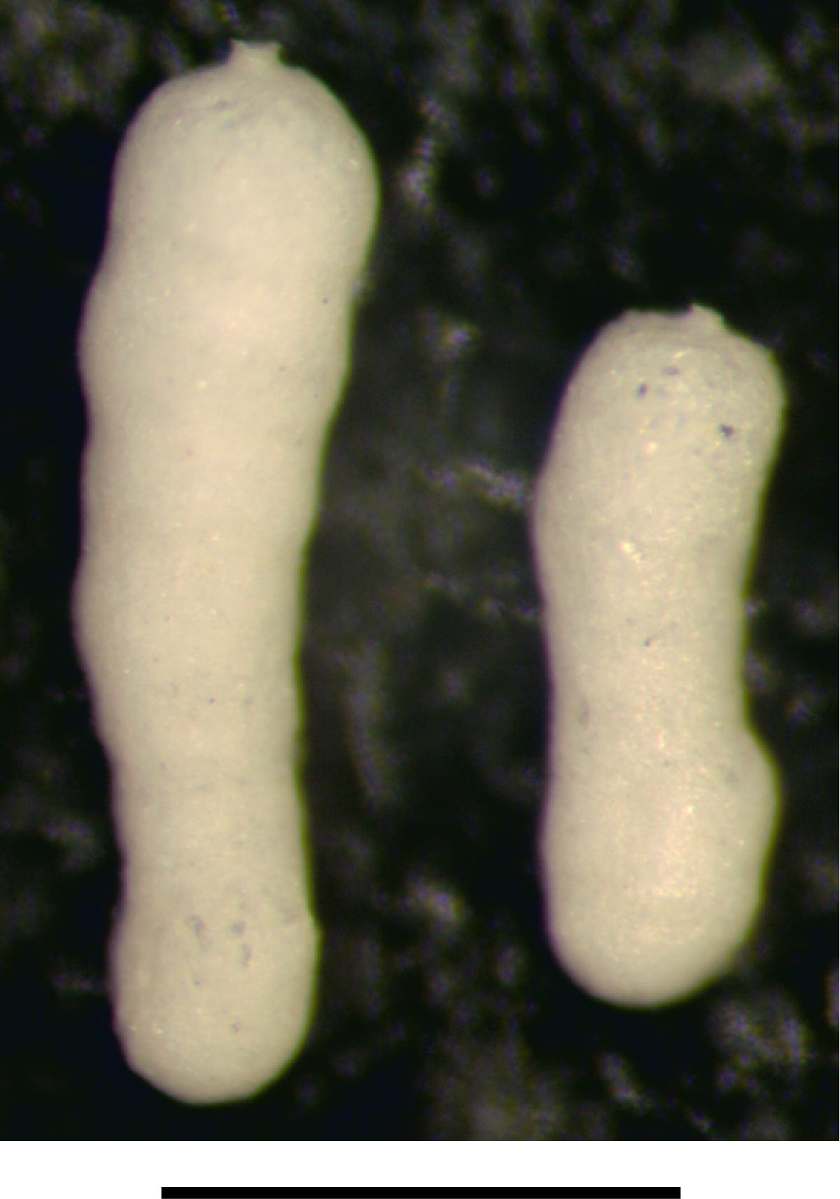
Figure F14. Agglutinated benthic foraminifer.
Palynology
Fourteen core catcher samples, one from Hole U1523A (1H-CC [8.46 m CSF-A]), seven from Hole U1523B (5F-CC to 22X-CC [60.32–135.61 m CSF-A]), and six from Hole U1523E (16F-CC to 25F-CC [90.77–130.28 m CSF-A]) were prepared and examined for palynomorphs (Table T8). In general, palynomorphs are moderately to well preserved and rare in the Pleistocene section but present in higher numbers in parts of the Pliocene and Miocene intervals (Figure F10). The Site U1523 assemblages are dominated by protoperidinioid dinocysts, likely cysts of heterotrophic dinoflagellates, and mostly Brigantedinium spp., Lejeunecysta spp., and Selenopemphix spp., a composition indicative of high-productivity water (Zonneveld et al., 2013). A few specimens of the phototrophic species Achomosphaera/Spiniferites spp., Batiacasphaera spp., Nematosphaeropsis labyrinthus, and Operculodinium sp. are also present. The occurrence of the Prasinophyta Cymatiosphaera (Table T8) may indicate periodic surface-water stratification.
Sample 374-U1523A-1H-CC (8.46 m CSF-A) is almost devoid of dinocysts, and only Brigantedinium spp. and some specimens of the autotrophic taxa Achomosphaera/Spiniferites are found. The acritarch Leiosphaeridia is present together with some remains of Cymatiosphaera. The sample contains common amorphous organic matter and a transparent “bag”-shaped palynomorph of indeterminate origin.
Palynomorph assemblages are comparable in Samples 374-U1523B-5F-CC (60.32 m CSF-A) to 10F-CC (84.10 m CSF-A) (Table T8). Few dinocysts are found in Sample 5F-CC (60.32 m CSF-A), mostly Brigantedinium spp. and a dinocyst resembling that produced by the dinoflagellate Gymnodinium spp. due to its round, brown body and finely microreticulated wall. Samples in this interval also yield abundant specimens of Leiosphaeridia. Selenopemphix species occur in higher numbers than Lejeunecysta taxa. Some specimens of a dinocyst resembling Eatonicysta ursulae (early Eocene) are found in this interval, although reworking is minimal. Sample 10F-CC (84.10 m CSF-A) contains abundant Cymatiosphaera sp. 3 of Hannah et al. (1998) and one yet undescribed species of Lejeunecysta, here called “reticulata” for its reticulate wall pattern. Sample 11F-CC (86.30 m CSF-A) is nearly devoid of palynomorphs, containing only poorly preserved specimens.
Samples 374-U1523B-18X-CC (108.47 m CSF-A) to 22X-CC (135.61 m CSF-A) show different degrees of preservation and palynomorph occurrences, but they all contain the species Selenopemphix bothrion and Selenopemphix minys (Figures F10, F11, F15), which were previously found in the upper Miocene of ODP Site 1095 (Harland and Pudsey, 2002) between 9.9 and 7.3 Ma and 8.7 and 7.3 Ma, respectively. Other than these two species, Brigantedinium spp., Selenopemphix nephroides, Selenopemphix antarctica (only found in Sample 22X-CC [135.61 m CSF-A]), cf. Gymnodinium sp., Lejeunecysta sp. cf. Lejeunecysta communis (Harland and Pudsey, 2002), and Protoperidinium sp. 2 (also found at Site U1521; see Biostratigraphy and paleontology in the Site U1521 chapter [McKay et al., 2019c]) characterize the dinocyst assemblages. Other palynomorphs found are Leiosphaeridia and Cymatiosphaera sp. 3 of Hannah et al. (1998), abundant foraminifer linings, a few reworked Eocene dinocysts (e.g., Spinidinium macmurdoense and Vozzhennikovia apertura), and some potentially in situ bisaccate pollen grains. In general, the assemblage indicates highly productive water.
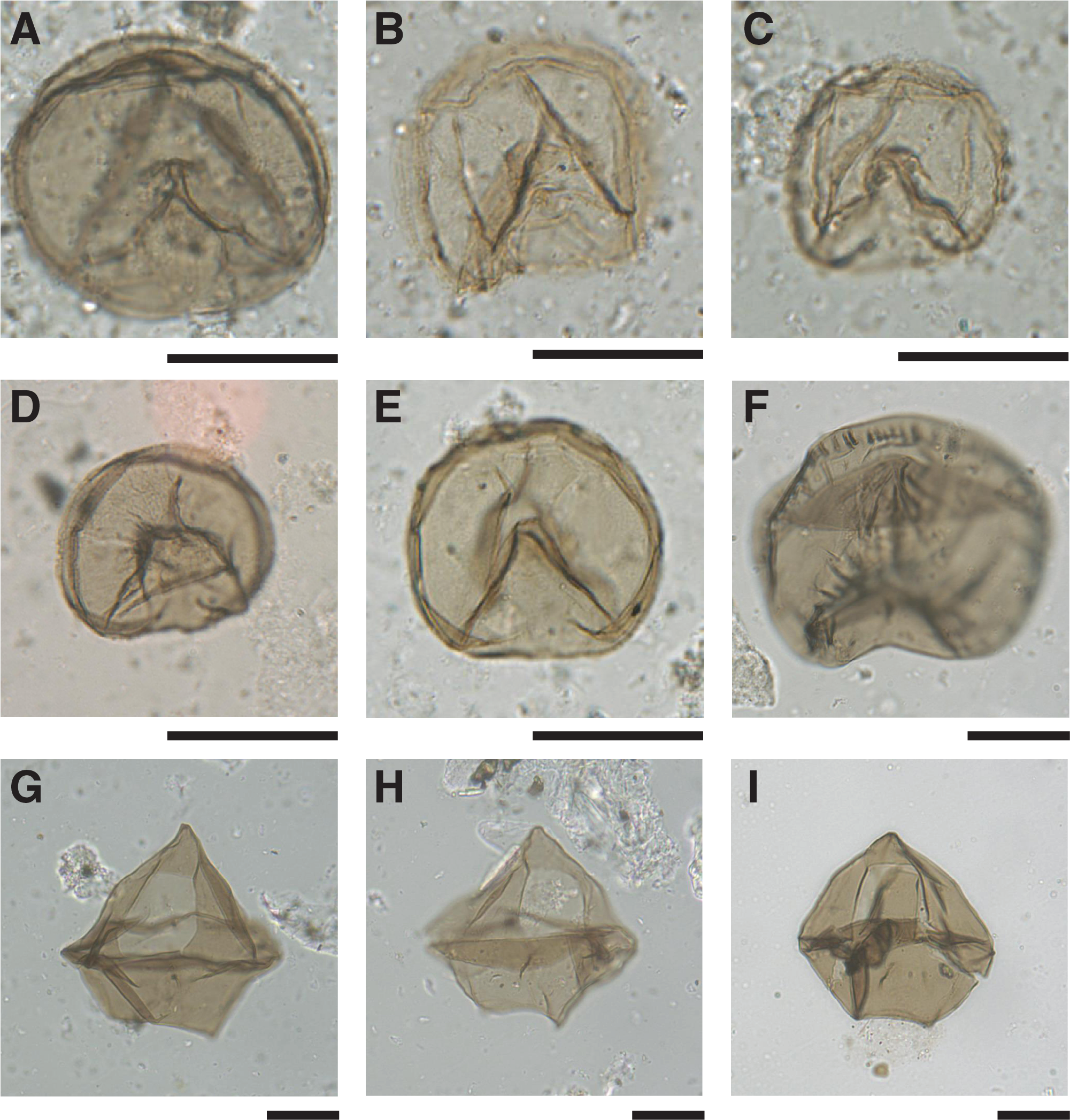
Figure F15. Dinocysts.
In Sample 374-U1523E-16F-CC (90.77 m CSF-A), dinocysts and palynomorphs are rare, but the palynomorph assemblage is similar to that of Sample 374-U1523B-10F-CC (84.10 m CSF-A) in that it contains the same Lejeunecysta “reticulata” morphotype together with Brigantedinium spp., Cymatiosphaera sp., Cymatiosphaera sp. 3 of Hannah et al. (1998), and many Leiosphaeridia acritarchs. Sample 374-U1523E-18F-CC (95.80 m CSF-A) is devoid of palynomorphs. In Sample 20F-CC (110.35 m CSF-A), palynomorphs are sparse, but this sample contains the dinocyst S. minys, which is present between 7.3 and 8.7 Ma in the ODP Site 1095 record (Harland and Pudsey, 2002).
Samples 374-U1523E-23F-CC (121.45 m CSF-A) to 25F-CC (130.28 m CSF-A) are richer in palynomorphs and dinocysts and include the dinocysts Brigantedinium spp., S. antarctica, S. minys, S. nephroides, and a few specimens of S. bothrion. Based on the occurrence of S. minys and S. bothrion, this interval is assigned an age of 7.3–9.9 Ma (Harland and Pudsey, 2002) (Figures F10, F11). Sample 23F-CC (121.45 m CSF-A) also yielded few specimens of the phototrophic dinocyst Batiacasphaera sphaerica and Lejeunecysta sp. cf. L. communis (Harland and Pudsey, 2002) (Figure F15). Some specimens of Cymatiosphaera sp. 3 of Hannah et al. (1998) and the Eocene dinocyst V. apertura are also present. Foraminifer linings are present throughout this interval. Some potentially in situ bisaccate pollen grains and Nothofagus sp. are noted in Samples 23F-CC (121.45 m CSF-A) and 24F-CC (123.52 m CSF-A).
When comparing dinocyst assemblages from Holes U1523B and U1523E, assemblages in Sample 374-U1523B-10F-CC (84.1 m CSF-A) are most similar to those in Sample 374-U1523E-16F-CC (90.77 m CSF-A). Although dinocysts are not abundant, this Pliocene interval shows potential for shore-based studies. Moreover, Samples 374-U1523B-18X-CC (108.47 m CSF-A) to 22X-CC (135.61 m CSF-A) contain assemblages comparable to those found in Samples 374-U1523E-20F-CC (110.35 m CSF-A) to 25F-CC (130.28 m CSF-A), as would be expected given the overlapping depth ranges. Postcruise work will include construction of a composite depth scale for this site, which will allow for more detailed comparison of assemblages among holes.
Age model
Holes U1523A and U1523B comprise a sequential depth series of cores, and coring in Hole U1523E used a targeted approach to fill in gaps in the stratigraphic records from the first two holes (see Operations). Hole U1523D was cored primarily for downhole logging, although a few core catcher samples from this hole provide additional biostratigraphic constraint toward the bottom of the drilled sequence. Sediment recovery in all holes was sporadic, with no core recovery through many cored intervals (Figure F10), but it was sufficient to guide construction of a composite age model. The diatom, radiolarian, and dinocyst biostratigraphic datum events presented in Table T5 were used to produce an age-depth model for this site (Figure F11). These events also helped tie magnetic polarity reversal events to the geomagnetic polarity timescale (GPTS) (see Paleomagnetism).
The age model identifies an expanded upper Pliocene section (Table T5; Figure F11) with sediment accumulation rates approaching 23 cm/ky of diatom-rich mud and diatom ooze. This rate is more than eight times higher than that of the middle to upper Miocene section (~2.7 cm/ky). A major disconformity representing ~6 My of missing record is identified across the Miocene/Pliocene boundary, which corresponds to the boundary between lithostratigraphic Units II and III. This boundary is identified biostratigraphically by a concurrence and concentration of first and last appearance datums (Figure F11) across the 5 m core recovery gap between Cores 374-U1523E-16F and 18F (90.77–95.8 m CSF-A).
Paleomagnetism
Paleomagnetic investigations at Site U1523 focused on determining the characteristic remanent magnetization (ChRM) for constructing a magnetostratigraphy that, combined with biostratigraphy, establishes the chronostratigraphy for the site. Additional rock magnetic measurements were made to assess the stability of the paleomagnetic record and to investigate magnetic fabrics that relate to depositional and postdepositional processes.
Our main observations come from measuring the natural remanent magnetization (NRM) of most archive-half core sections at 5 cm intervals before and after alternating field (AF) demagnetization. For archive-half sections of Cores 374-U1523A-1H through 7H (0–42.55 m CSF-A), 374-U1523B-3F through 23X (46.70–146.79 m CSF-A), and 374-U1523E-1H through 25F (0–130.33 m CSF-A), NRM measurements followed AF demagnetization in 5 mT steps between 0 and 20 mT. The XCB system frequently yielded sediments that were too disturbed to be used for paleomagnetic measurements (e.g., Core 374-U1523B-24X [154.80–155.57 m CSF-A]). Data from such disturbed intervals and those collected from in 10 cm of section ends were removed. The processed (relatively disturbance free) data set was subsequently used to determine the ChRM directions and construct a magnetostratigraphy. This magnetostratigraphy was correlated to the GPTS of Gradstein et al. (2012) and supplemented by independent biostratigraphic age control (see Biostratigraphy and paleontology).
To test the quality of the ChRM directions determined on archive-half core sections, 70 oriented discrete paleomagnetic samples were collected (~3–4 per core; 15 samples from Hole U1523A, 20 from Hole U1523B, and 35 from Hole U1523E). Ten samples were progressively demagnetized using a 20-step AF demagnetization protocol (0–20 mT in 2 mT steps and 20–60 mT in 5 mT steps followed by 70 and 80 mT peak AF demagnetization) to determine the ChRM, assess and remove potential overprint(s), and investigate the coercivity of the magnetic minerals that carry the remanent signal. The Icefield MI-5 core orientation tool was applied, but no accurate record of core orientation could be obtained because of the high latitude of the drill site (see Core collection and orientation (APC) in the Expedition 374 methods chapter [McKay et al., 2019a]). All (HL)APC cores are therefore presented in sample coordinates. Declinations of archive-half core sections and discrete samples from XCB cores have no azimuthal orientation because pieces of core can rotate independently inside the core barrel.
Mean (bulk) magnetic susceptibility on the discrete samples was compared with measurements made on archive-half core sections using the Section Half Multisensor Logger (SHMSL) and on whole-round core sections with the Whole-Round Multisensor Logger (WRMSL). Furthermore, the anisotropy of magnetic susceptibility (AMS) was determined and used to reconstruct magnetic fabric.
NRM measurements
Archive-half measurements
NRM intensities prior to demagnetization are mostly ~10−1 A/m, and their variations correlate well with variations in magnetic susceptibility from the WRMSL, SHMSL, and Kappabridge measurements (Figure F16). This agreement suggests that changes in magnetic mineral concentration similarly influence NRM intensity and magnetic susceptibility.
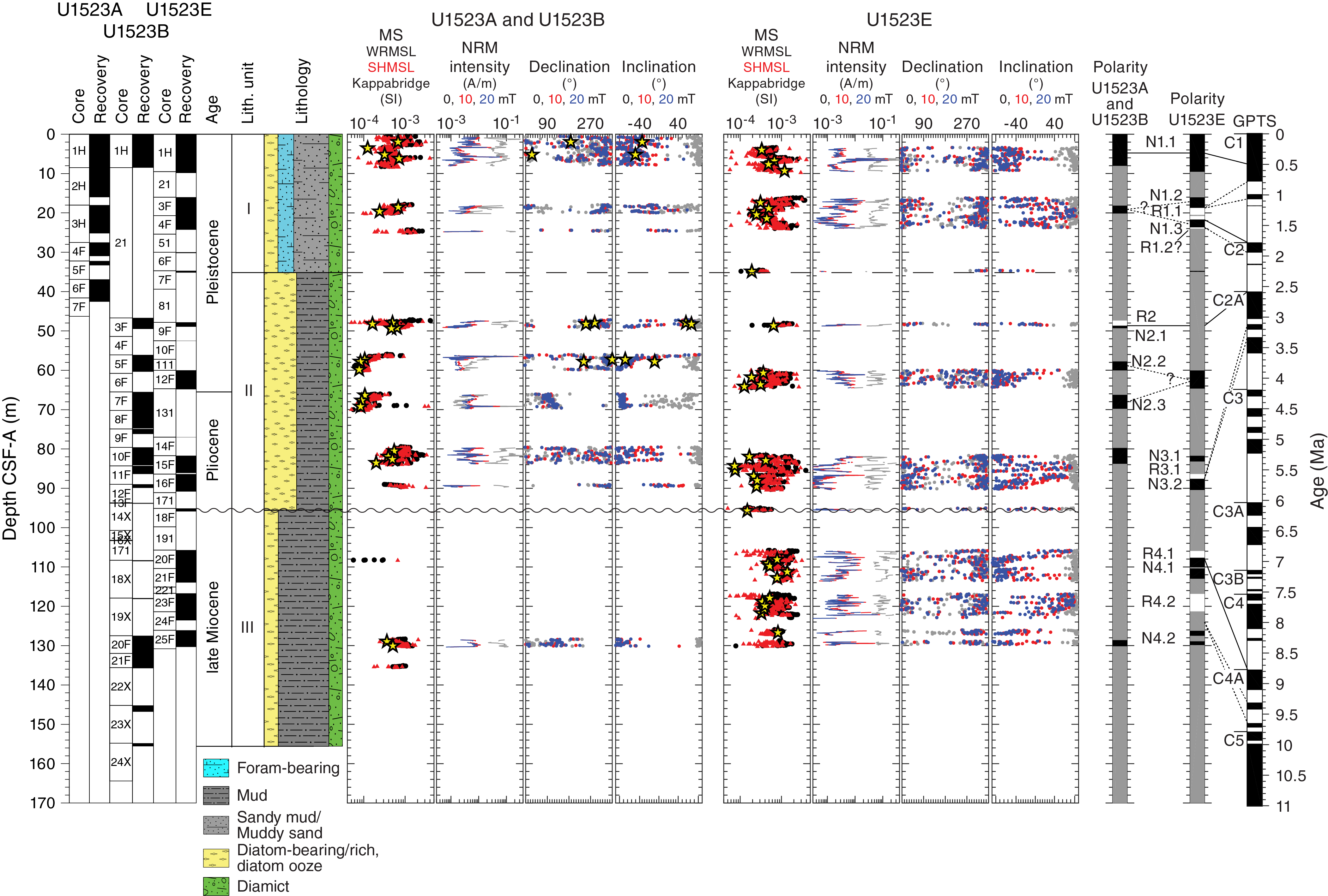
Figure F16. Paleomagnetic data.
NRM intensities are also influenced by the drilling overprint, which can add or subtract to the ChRM. For example, the initial NRM intensities of a few intervals with normal polarity (e.g., most of Core 374-U1523B-7F) increase following AF demagnetization because the low-coercivity drilling overprint has a direction nearly antipodal to the higher coercivity ChRM (Figure F16). The vector sum of these remanences tends to suppress the net size of the initial NRM. AF demagnetization in low fields preferentially removes this antipodal overprint, sometimes without significantly removing the ChRM, and hence the remaining magnetization is larger than the initial magnetization. In general, the overprint and a significant part of the ChRM is removed during demagnetization of these normal polarity intervals, which results in a net decrease in the intensity with AF demagnetization (e.g., Cores 374-U1523A-1H and 374-U1523E-1H).
After 10 and 20 mT peak AF demagnetization, inclinations generally cluster into two groups of steep-upward (negative) or steep-downward (positive) inclinations. These two groups may represent normal and reversed polarity zones, which should center at ±81.9° if a geocentric axial dipole is assumed (Site U1523 is located at 74.2°S). Most of the observed archive-half inclinations are shallower than ±81.9°, suggesting an influence of other factors such as (1) inclination flattening, (2) the presence of minerals that do not genuinely record the geomagnetic field, or (3) incomplete removal of the downward-directed drilling overprint in intervals with a negative inclination. Despite the shallow inclinations, we interpret these groups of upward- and downward-directed inclinations to reflect normal and reversed polarity zones, respectively, because Site U1523 is located in the Southern Hemisphere.
Discrete sample measurements
The NRM of oriented discrete samples was measured before and after progressive AF demagnetization. The 20-step AF demagnetization and measurement protocol shows the presence of multiple components (Figure F17) with variable coercivities. The first component is commonly present between 0 and 2 mT and has random orientations (Figure F17), suggesting that it is a viscous remanent magnetization. A steep downward-directed component has a coercivity of mostly <6 mT but sometimes up to 20 mT and is probably the drilling overprint originating from coring. A third component with higher coercivity is interpreted to be the ChRM. In the demagnetization diagrams, this component is represented by the nearly linear decay of magnetization toward the origin from ~20 to 80 mT. Components with coercivity higher than 80 mT may also be present and can be identified by some linear demagnetization paths not heading straight to the origin (e.g., Figure F17D). Postcruise work is required to disentangle these potential components and their influence on the NRM and ChRM. ChRM is assumed to be a reliable recorder of the paleomagnetic field, and ChRM directions are used to construct the magnetostratigraphy. Noisy demagnetization behavior (e.g., Figure F17C) occasionally occurs, and such data are excluded from further analysis.
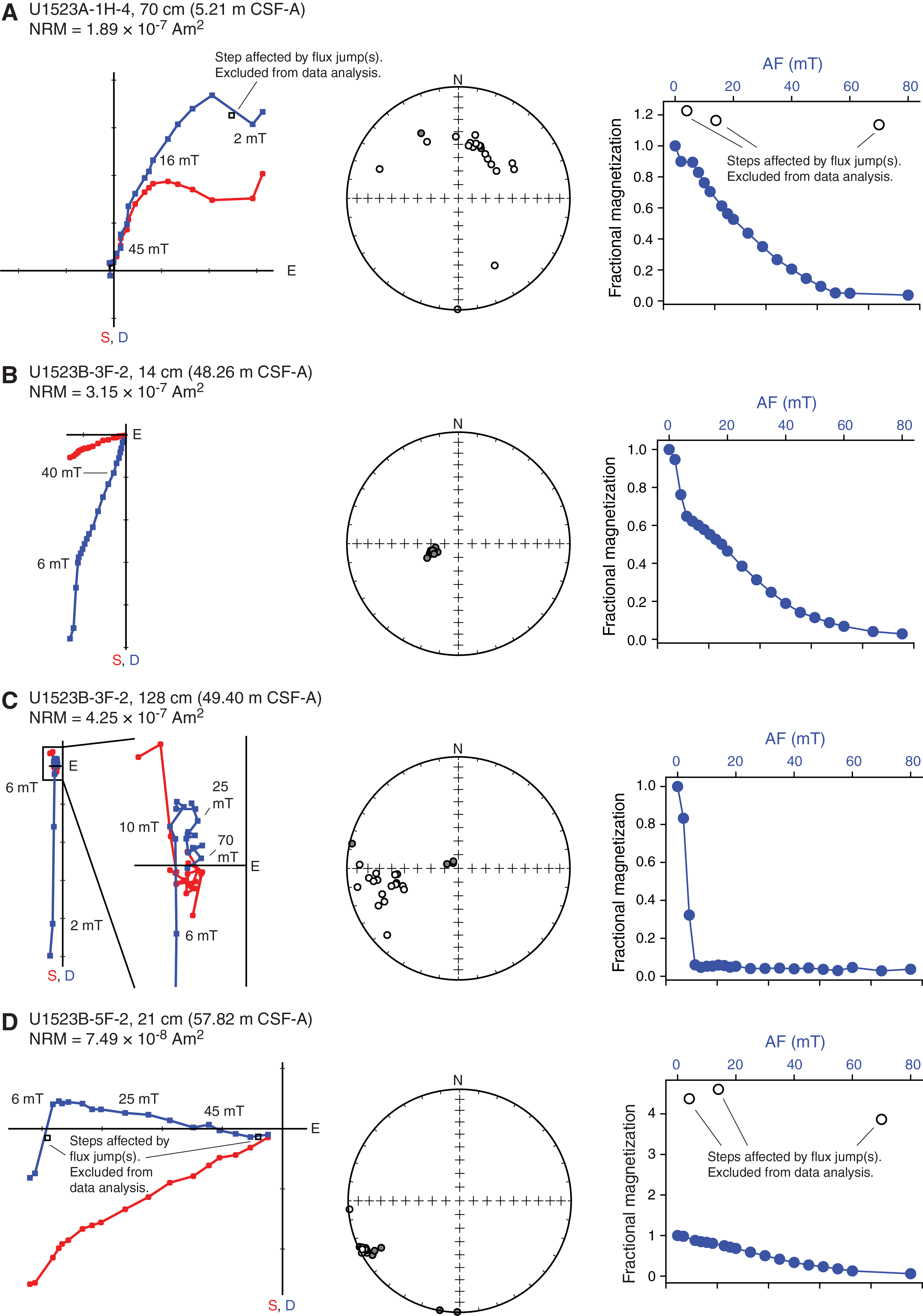
Figure F17. Representative AF demagnetization behavior.
Magnetostratigraphy
The inclination data from archive-half core sections and oriented cubes reveal stable intervals of positive and negative inclination, interpreted to be reversed and normal polarity zones, respectively (Figure F16). Four major polarity zones (N1–N4) are defined and divided into subzones (e.g., N1.1 and R1.1). Their exact definition is slightly arbitrary and depends on core recovery (e.g., Core 374-U1523E-6F consists of a 21 cm long core catcher that was not useful for magnetostratigraphic purposes) and data quality (e.g., shallow inclinations are present in Core 374-U1523E-9F, and we refrain from assigning a polarity to this core). An attempt was made to identify the same (sub)zone in each hole, which was possible in some cases (e.g., Subzone N1.1) but more difficult in others (Subzones N2.2 and N2.3). Further postcruise work on the integration of data from Holes U1523A, U1523B, and U1523E is required to generate a conclusive composite depth scale and magnetostratigraphy.
Normal polarity Subzone N1.1 is present in Cores 374-U1523A-1H and 374-U1523E-1H (0–8.51 and 0–9.86 m CSF-A, respectively) (Figure F16). Subzones N1.2, R1.1, N1.3, and R1.2 occur in Cores 374-U1523E-3F and 4F (16.0–24.28 m CSF-A). However, it is unclear whether the normal polarity zone in Core 374-U1523A-3H correlates to Subzone N1.2 or N1.3. Subzone R1.2 is only ~30 cm thick, and further postcruise work is required to test its reliability.
A second polarity zone (Figure F16) encompasses Zone R2 and Subzone N2.1 in Core 374-U1523B-3F (46.70–49.50 m CSF-A) and Subzones N2.2 and N2.3 in Cores 5F (56.10–60.37 m CSF-A) and 7F (65.50–70.30 m CSF-A), respectively. The normal polarity zone identified in Core 374-U1523E-12F (60.00–64.85 m CSF-A) probably represents Subzone N2.2 or N2.3. The third polarity zone (Figure F16) predominantly occurs in Cores 374-U1523E-15F and 16F (81.70–90.82 m CSF-A) and contains Subzones N3.1, R3.1, and N3.2, as well as a normal polarity zone in Core 374-U1523B-10F (79.60–84.15 m CSF-A) that may coincide with Subzones N3.1 or N3.2. Cores 374-U1523E-20F, 21F, 23F, and 25F (105.70–130.33 m CSF-A) and 374-U1523B-20F (127.50–132.03 m CSF-A) include a fourth polarity zone that contains Subzones R4.1 and N4.1–N4.3.
Confident correlation of Zones N1–N4 to the GPTS requires independent biostratigraphic age control (see Biostratigraphy and paleontology). However, limited biostratigraphic age control is available for the upper ~25 m CSF-A of Holes U1523A and U1523E. We hence tie the first polarity zone to the Brunhes Chron (C1n [0–0.781 Ma]) (Figure F16). Good biostratigraphic tie points at ~25 m CSF-A indicate an early Pleistocene age. Therefore, Subzone N1.3 is tied to the Olduvai Chron (C2n [1.778–1.945 Ma]) (Figure F16; Table T9). Biostratigraphic datums indicate a possible hiatus between Cores 374-U1523E-3F and 4F, so Subzone N1.2 could be tied to the Brunhes Chron (C1n [0–0.781 Ma]) or Jaramillo Subchron (C1r.1n [0.988–1.072 Ma]). Further work is required to differentiate between these two options.
Biostratigraphic datums suggest that the second and third polarity zones correlate with the early Pleistocene to late Pliocene. Zone R2 is therefore tied to Subchron C2r.2r (2.148–2.581 Ma), and Subzone N2.1 is tied to Subchron C2An.1n (2.581–3.032 Ma) (Figure F16; Table T9). Biostratigraphy also suggests that Subzone R3.1 can be tied to the Kaena Subchron (C2An.1r [3.032–3.116 Ma]), but the possibility that it corresponds to the Mammoth Subchron cannot be excluded (C2An.2r [3.207–3.330 Ma]). Either way, Subzones N2.2, N2.3, N3.1, and N3.2 are all part of the Gauss Chron (C2An [2.581–3.596 Ma]). Firm biostratigraphic tie points at ~110 m CSF-A suggest that polarity Subzones R4.1 and N4.1 should correlate with Subchron C4r.2r and Chron C4An, respectively (the C4r.2r/C4An reversal is at 8.771 Ma). The Subzone R4.2/N4.2 reversal cannot be tied with certainty to the GPTS and may represent the base of Subchron C4Ar.1r (9.311 Ma) or C4Ar.2r (9.647 Ma) (Figure F16; Table T9).
Magnetic susceptibility and AMS
We determined the mean magnetic susceptibility and AMS tensor of all collected discrete samples. The AMS tensor prescribes the orientation and magnitude of the maximum (kmax), intermediate (kint), and minimum (kmin) susceptibilities (Figure F18). The degree of anisotropy (P) is approximated by the kmax/kmin ratio, where P = 1 indicates no anisotropy and P > 1 indicates a high degree of anisotropy. High variability in P values, ranging from ~1.01 to >1.1, is observed in all lithostratigraphic units (Figure F18), which potentially reflects variations in grain size and/or compaction.
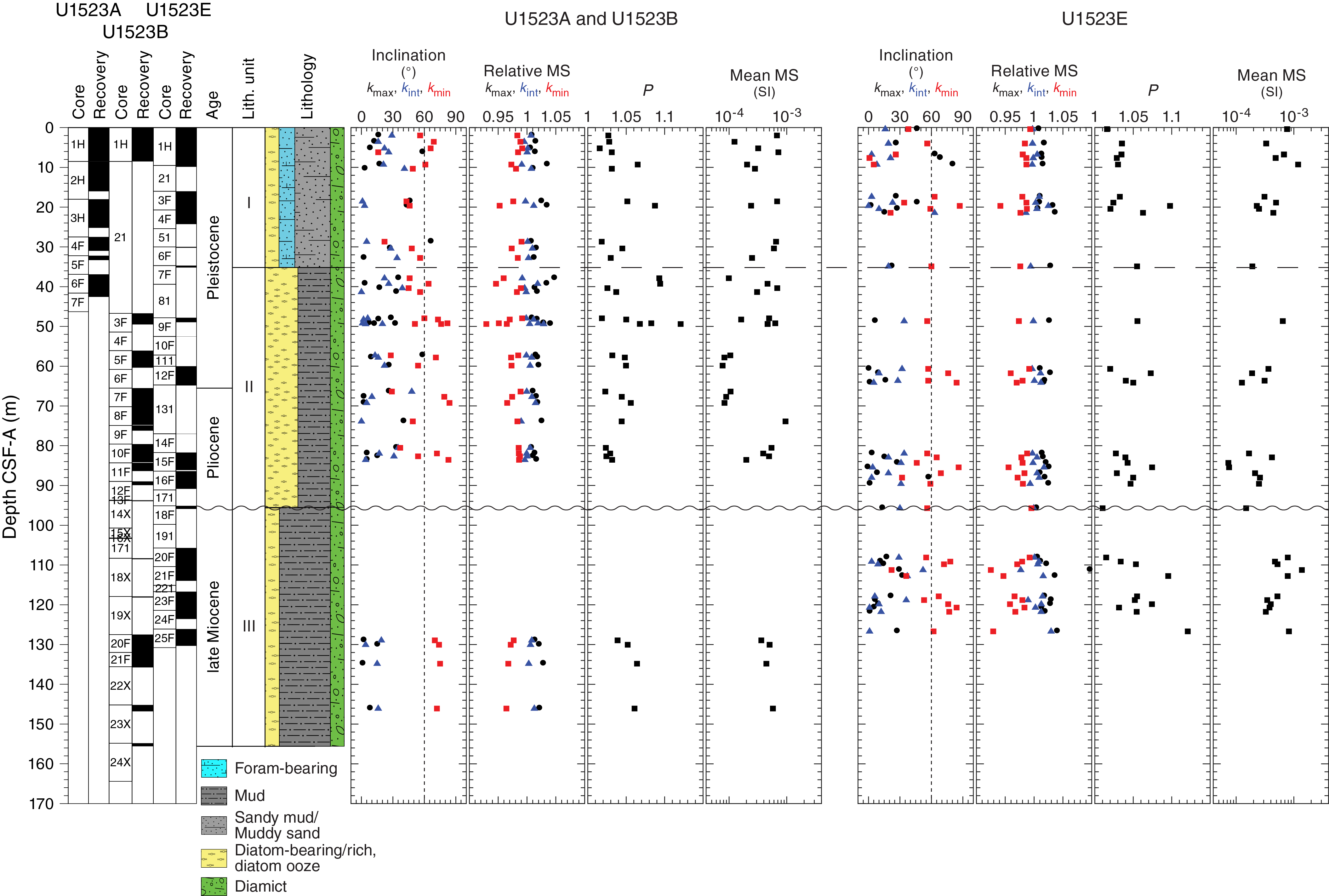
Figure F18. Anisotropy of magnetic susceptibility.
When P is >1 (i.e., anisotropic sample) and kmin is >60° (i.e., minimum susceptibility axis is steep), the anisotropy most likely arises from sediment compaction, as is commonly observed in many sedimentary settings. If the kmin inclination is <60°, the sediments may be disturbed for paleomagnetic purposes, even if that disturbance is not clearly visible in the core. At Site U1523, the kmin inclination of a majority of samples is shallower than 60° (Figure F18). These samples are usually from relatively coarse grained intervals (e.g., sandy lithologies or those incorporating small clasts) that may yield a different compaction than fine-grained muddy intervals. Further postcruise work is required to separate the contributions of disturbed and coarse-grained intervals. This evaluation of the AMS data will also test the reliability of the NRM data collected on both discrete samples and archive-half core sections.
Physical properties
Physical property measurements were completed on whole-round sections, section halves, and discrete samples from Cores 374-U1523A-1H through 7F (0–42.55 m CSF-A), 374-U1523B-3F through 24X (46.7–155.57 CSF-A), and 374-U1523E-1H through 25F (0–130.33 m CSF-A). Some outliers and unreliable values were excluded from the measured data (Table T10). Following thermal equilibration (~4 h), gamma ray attenuation (GRA) bulk density, magnetic susceptibility, P-wave velocity, and NGR measurements were made on all whole-round sections using the WRMSL and the Natural Gamma Radiation Logger (NGRL). Sampling resolution for the WRMSL was 2.5 cm, and NGR was measured at 10 cm intervals. Thermal conductivity measurements were made using the full-space needle probe. Discrete samples from the working-half sections (typically from Sections 1, 3, 5, and 7) were taken for moisture and density (MAD) measurements, generating bulk and grain density and porosity data. Shear strength measurements were also taken using the Torvane shear device. Discrete compressional wave velocity measurements were conducted on the working-half core sections of each core section using the P-wave caliper (PWC) contact probe system on the Section Half Measurement Gantry (SHMG). Color reflectance and point magnetic susceptibility data were collected on the archive-half sections using the SHMSL. Red, green, and blue (RGB) were measured on the Section Half Imaging Logger (SHIL) (see Lithostratigraphy and Physical properties in the Expedition 374 methods chapter [McKay et al., 2019a]). The physical property measurements are in good overall agreement with the defined lithostratigraphic units. All physical property data are available from the Laboratory Information Management System (LIMS) database (http://web.iodp.tamu.edu/LORE).
Magnetic susceptibility
Both whole-round measurements on the WRMSL and discrete point measurements on the SHMSL were used to characterize magnetic susceptibility at Site U1523 (Figure F19). Both methods yielded similar downhole variability with values ranging from 5 × 10⁻⁵ to 300 × 10−5 SI. From the top of Holes U1523A, U1523B, and U1523E to ~100 m CSF-A (Core 374-U1523E-18F), magnetic susceptibility is highly variable, corresponding to alternating sandy and muddy layers in lithostratigraphic Units I and II. A relatively thin interval in Cores 374-U1523B-5F through 7F (55–70 m CSF-A) has particularly low magnetic susceptibility (~5 × 10⁻⁵ SI) and corresponds to diatom-rich mud in Unit II. Magnetic susceptibility in Unit III is slightly elevated overall compared with overlying Unit II. This change may reflect decreased diatom/sand concentration and increased mud or clast content in Unit III.
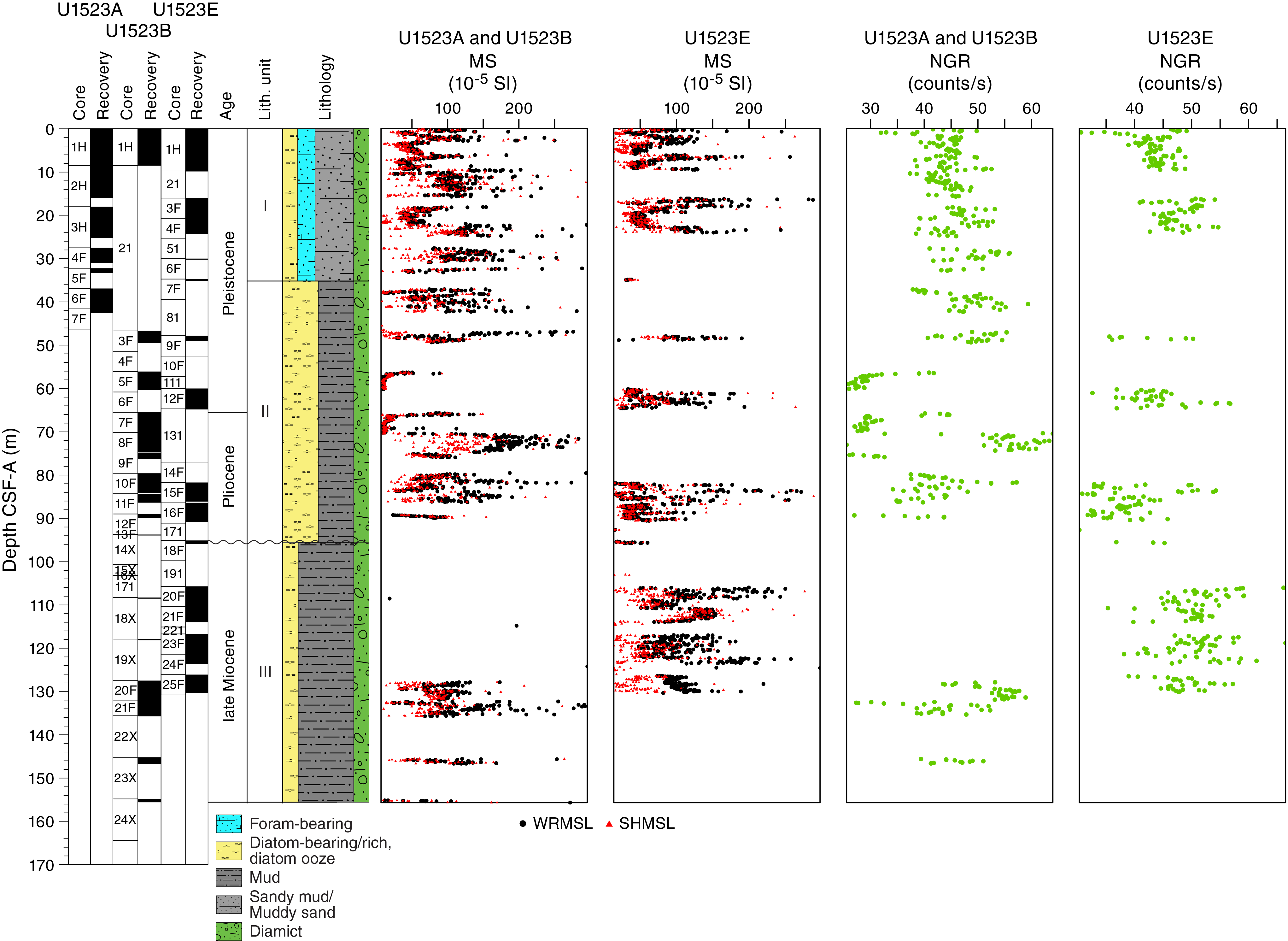
Figure F19. MS and NGR.
Natural gamma radiation
NGR measurements show downhole variations between ~20 and ~75 counts/s in Holes U1523A, U1523B, and U1523E (Figure F19). NGR increases slightly downhole from ~42 to ~48 counts/s in lithostratigraphic Unit I, which is composed of interbedded foraminifer-bearing muddy sand, diatom-bearing to diatom-rich diamict, and mud. In Unit II, NGR is highly variable in Hole U1523B, with low values (~30 counts/s) in Cores 374-U1523B-5F, 7F, 9F, and 12F that correspond to diatom-rich layers and high values (~55 counts/s) in Core 8F that are possibly related to clast or mud content. In Unit III, NGR is generally relatively high (~50 counts/s) compared with Unit II, except in Section 21F-1 where values are relatively low (30 counts/s) and correspond to diatom-rich mud with abundant clasts. Generally higher NGR values in Unit III may result from decreased diatom content and/or a subtle change in clay content.
Bulk density, grain density, and porosity
Discrete MAD samples yielded density values that are concentrated in a narrower range (~1.5–2.2 g/cm3) than that of GRA bulk density (~1.1–2.5 g/cm3) (Figure F20). Higher variability in density values obtained by the WRMSL is likely due to core disturbance. Overall, a similar downhole trend between GRA and MAD bulk densities is observed. Grain density also shows a similar trend to GRA and MAD bulk density, and porosity is inversely related.

Figure F20. GRA and MAD bulk density, grain density, and porosity.
In lithostratigraphic Unit I (0 to ~35 m CSF-A), a downhole increase in bulk density from 1.8 to 2.0 g/cm3 correlates with a porosity decrease from 55% to 45%. Downhole increase in density and decrease in porosity over this interval is likely due to variations in lithology and compaction downhole. In Unit II (~35–95 m CSF-A), bulk density varies downhole between ~1.4 and 1.8 g/cm3, corresponding to alternating muddy sand, diatom-rich mud, and diatom ooze. From 30 to 70 m CSF-A, a decrease in bulk density from 1.8 to 1.6 g/cm3 and grain density likely corresponds with a downhole increase in diatom content. In Unit II, porosity is relatively constant at ~55%. Downhole variations in GRA bulk density, porosity, and grain density in Unit III show overall similar variability to Unit II.
Compressional P-wave velocity
P-wave velocity measured with the P-wave logger (PWL) ranges from ~1300 to 2200 m/s and from ~1300 to 2000 m/s when measured with the PWC; the values from both measurement systems are in overall agreement and show similar downhole trends (Figure F21). From 0 to 15 m CSF-A in lithostratigraphic Unit I, P-wave velocity increases downhole from 1500 to 1800 m/s, which is likely a result of compaction. Deeper than ~15 m CSF-A, P-wave velocity is relatively constant at ~1600 m/s and lacks any significant downhole variations or trends. Sparse anomalously high P-wave velocity measurements are likely due to individual clasts in diamict(ite) intervals.
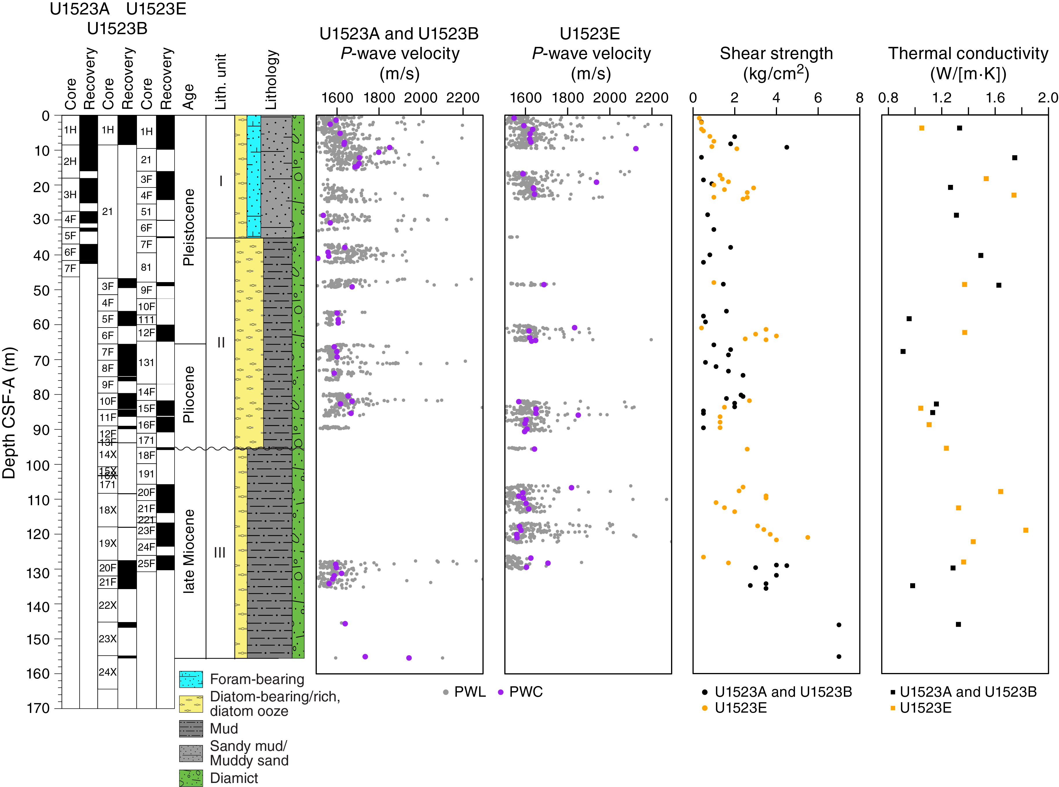
Figure F21. P-wave velocity, shear strength, and thermal conductivity.
Shear strength
Shear strength measurements from the Torvane shear device vary from 0.2 to 7 kg/cm2 (Figure F21). In lithostratigraphic Units I and II, shear strength is generally <4 kg/cm2. However, shear strength values are relatively high and increase downhole in Unit III. This increase in shear strength in Unit III relative to overlying Units I and II corresponds with a slight decrease in porosity and is likely related to sediment compaction.
Thermal conductivity
Thermal conductivity was measured once per core using the full-space needle probe on whole-round sections, typically in Section 3 for APC cores or Section 2 for HLAPC cores. The quality of thermal conductivity measurements was checked by evaluating two parameters: (1) the number of solutions acquired and (2) the shape of the curve formed on the temperature versus time plot of these points. A valid measurement must have a sufficient number of solutions to form an exponential curve. All measurements with a low number of solutions and/or a bad repartition of these values on the temperature versus time plot (i.e., forming two curves or no curve) were discarded, resulting in removal of 23% of the original data. Measurements range from 0.91 to 1.83 W/(m·K) from the top to the bottom of Holes U1523A, U1523B, and U1523E (Figure F21). Thermal conductivity generally decreases downhole from the top of lithostratigraphic Unit I to the middle of Unit II (0–70 m CSF-A), increases downhole to the middle of Unit III (~115 m CSF-A), and decreases downhole from there to the bottom of Unit III.
Color reflectance spectroscopy
Color reflectance spectroscopy data were acquired on section halves using the SHMSL. At this site, all parameters (L*, a*, and b*) exhibit very minor changes downhole (Figures F22). Overall, L* and a* vary slightly downhole, representing alternating diamict and mud lithologies. b* shows the same overall trend with notable higher values observed in Cores 374-U1523B-21F and 374-U1523E-15F and 16F (~80–90 m CSF-A) that correspond to diatom ooze identified in lithostratigraphic Unit II.
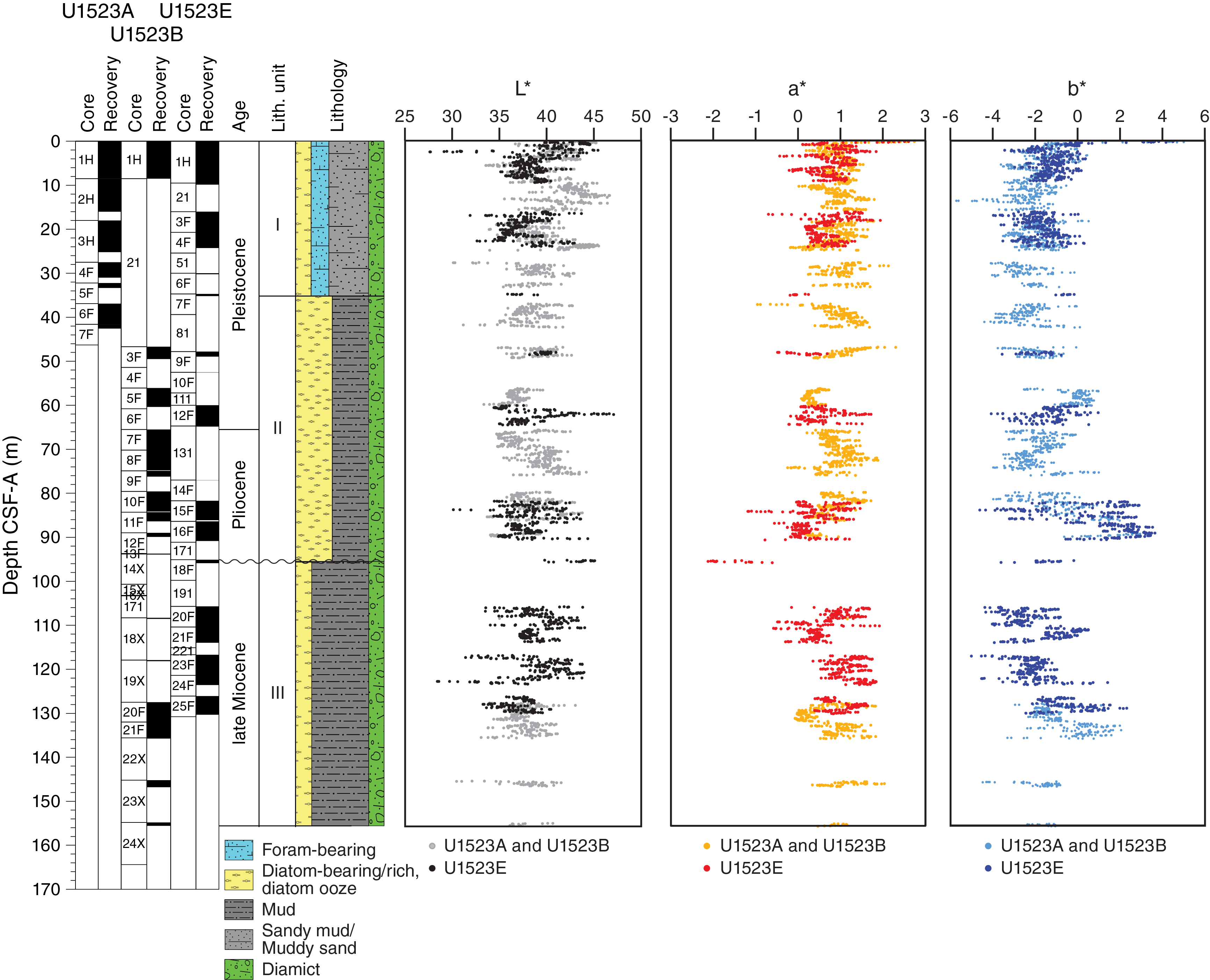
Figure F22. Color reflectance spectroscopy.
Summary
In general, data from whole-round measurements are in good agreement with those from split-core measurements (Figure F23). At Site U1523, data from Hole U1523E fills in missing intervals from Holes U1523A and U1523B (e.g., Cores 374-U1523A-2H and 374-U1523B-6F, 11F, 14X, 18X, and 19X). Downhole changes in physical properties are in good overall agreement with the defined lithostratigraphic units based on sedimentological characteristics (see Lithostratigraphy; Figure F23; Table T11), and changes in physical properties can provide insight into lithologic variations in each unit. Magnetic susceptibility is highly variable in lithostratigraphic Unit I, corresponding to alternating sandy and muddy layers with abundant clasts and muddy diamict. Low bulk density, magnetic susceptibility, and NGR values in the middle of Unit II (Cores 374-U1523B-5F and 7F) are correlated with diatom-rich mud intervals. Relatively high and consistent NGR values in Unit III indicate relatively high clay mineral content in the massive bioturbated to laminated diatom-bearing mud and sandy mud.
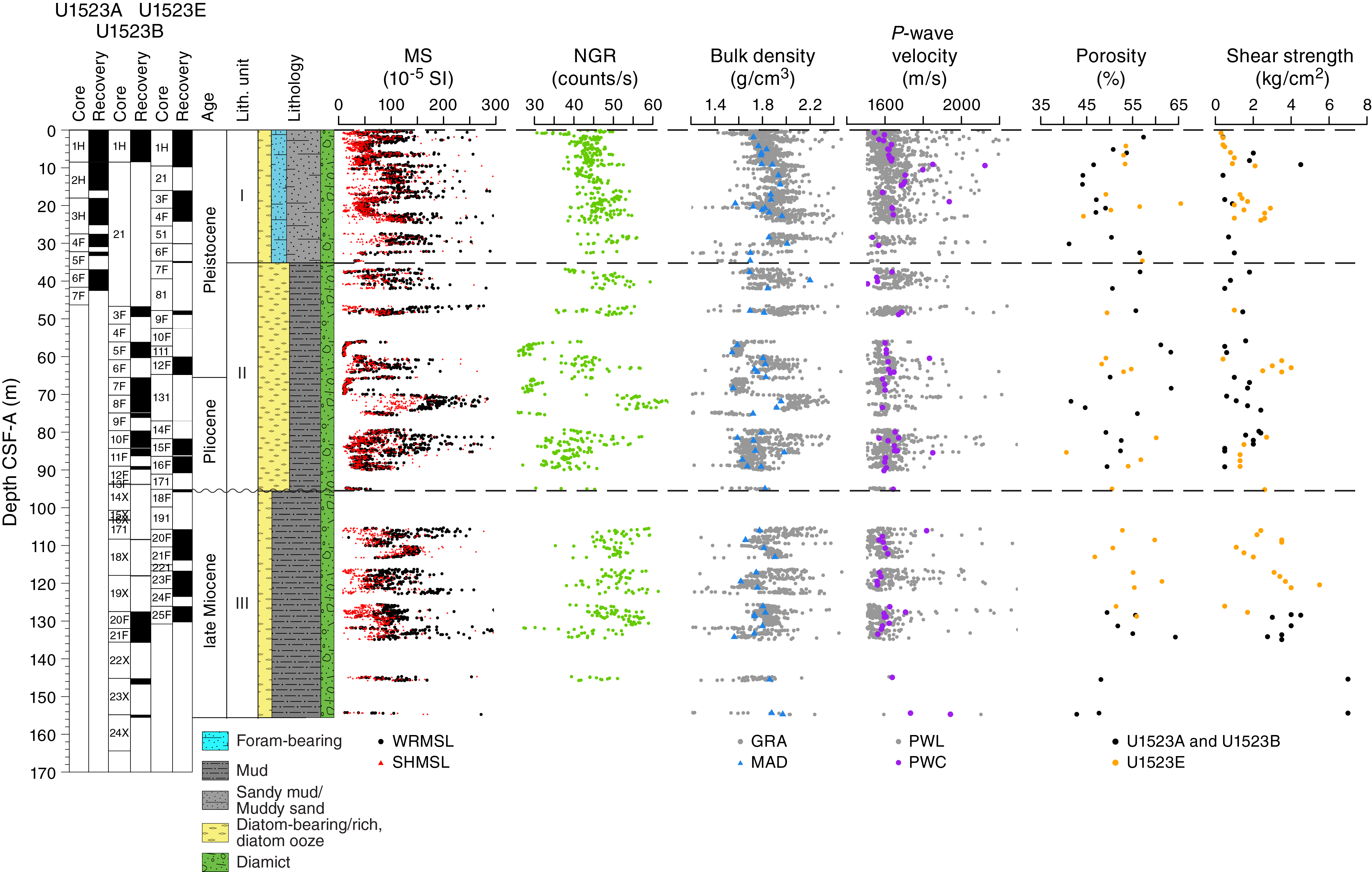
Figure F23. Physical properties summary.
Geochemistry and microbiology
Site U1523 samples were analyzed for headspace gas, interstitial water chemistry, and bulk sediment geochemistry. Methane and ethane concentrations are close to or below the detection limit, respectively. In addition to low-resolution interstitial water sampling throughout Holes U1523A, U1523B, and U1523E, a high-resolution profile of interstitial water chemistry was obtained for the upper 8.1 m CSF-A in Hole U1523B. Low-resolution downhole trends suggest manganese and sulfate reduction in the suboxic to anoxic transition zone. A rapid increase in silicon and manganese concentrations in the upper 2 m CSF-A probably reflect shallow diagenesis of silica. Bulk sediment total organic carbon (TOC) and calcium carbonate (CaCO3) contents are generally low throughout the site. Higher percentages in carbonate content are observed in foraminifer-bearing sandy mud in lithostratigraphic Units I and II. The TOC/total nitrogen (TN) ratio does not display a discernible trend, suggesting a mixed input of terrestrial and marine-derived organic matter. Handheld portable X-ray fluorescence (pXRF) scan data indicate a lower and more invariant Ba/Al ratio compared with Sites U1521 and U1522. In contrast, significant downhole variations are observed in ratios of refractory elements such as the Th/Ti ratio, which, with ratios like Fe/Ti, may serve as a provenance proxy at this site.
Volatile hydrocarbons
Headspace gas analyses were performed at a resolution of one sample per core (9.6 m advance) or one sample every other core for half cores (4.8 m advance) throughout Holes U1523A, U1523B, and U1523D as part of the routine environmental protection and safety monitoring program. Methane (CH4) is the only detectable hydrocarbon (Table T12). Methane concentration is very low (~2–3 ppmv) and does not show a discernible trend.
Interstitial water chemistry
A total of 61 interstitial water samples were squeezed from whole-round samples from 0 to 130.40 m CSF-A in Holes U1523A, U1523B, and U1523E (Table T13). In detail, a mudline sample and three interstitial water samples were taken from the upper 40.62 m CSF-A in Hole U1523A, four interstitial water samples were obtained between 59.08 and 130.40 m CSF-A in Hole U1523B, and four whole-round samples for interstitial water measurements were obtained between 18.96 and 127.41 m CSF-A in Hole U1523E. Together, these 12 samples constitute a low-resolution interstitial water profile.
Additionally, Core 374-U1523B-1H (0–8.49 m CSF-A) was selected for high-resolution interstitial water and microbiology sampling (N = 50; Figure F24). Interstitial water samples were collected from 10 cm whole-round samples from 0–30 cm (N = 3), 50–80 cm (N = 3), and 100–130 cm (N = 3) in Sections 1H-1 through 1H-5 and 0–20 cm (N = 2) and 40–70 cm (N = 3) in Section 1H-6. Filtered subsamples of all interstitial water samples were prioritized in the order detailed in Geochemistry and microbiology in the Expedition 374 methods chapter (McKay et al., 2019a) for shipboard and shore-based analyses. General downhole trends for all measured properties are described below, and the high-resolution interstitial water sampling results are presented in High-resolution sampling.
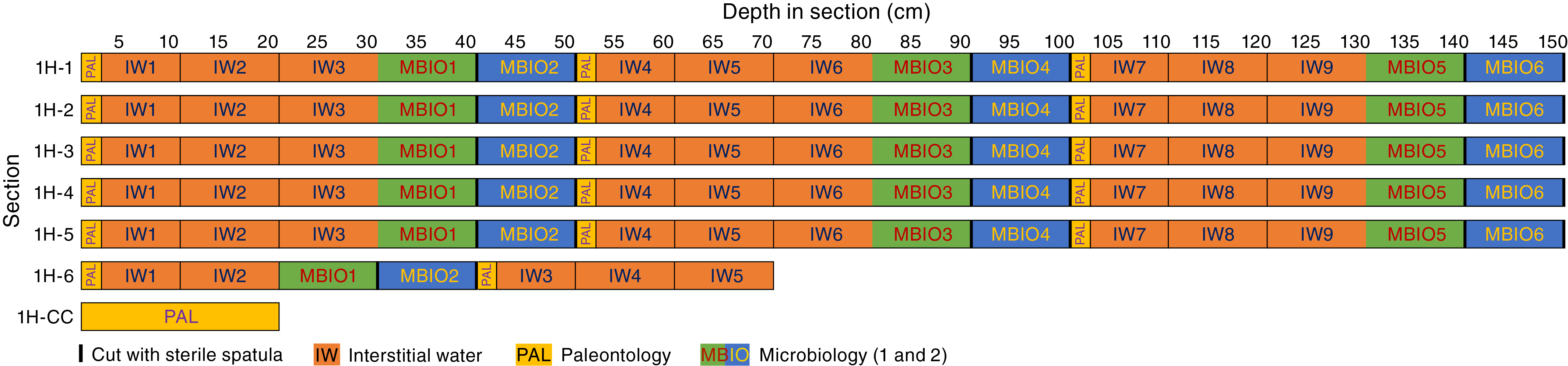
Figure F24. Interstitial water and microbiology sampling scheme.
Salinity, pH, ammonium, alkalinity, sulfate, and manganese
The average salinity for the mudline and all interstitial water samples across all holes is 35, similar to ambient seawater. The pH is 7.8 (±0.1) between 0 and 130.40 m CSF-A. Ammonium concentration increases linearly (r2 = 0.99) from 9 mM in the Hole U1523A mudline water to 692 mM in the deepest interstitial water sample taken at Site U1523 (130.40 m CSF-A in Hole U1523B). Alkalinity increases linearly from 2.7 to ~3.8 mM in the upper 8.1 m CSF-A of Holes U1523A and U1523B. Deeper than 8.1 m CSF-A, alkalinity increases to a peak of 7.5 mM at 68.41 m CSF-A, where it plateaus at 7.1–7.6 mM downhole to 130.40 m CSF-A (Figure F25). Sulfate decreases from typical seawater values of ~28 mM (0–0.1 m CSF-A) to ~13 mM at 130.40 m CSF-A. These results contrast with interstitial water profiles documented for Sites U1521 and U1522, where sulfate decreases to <10 mM by ~80 m CSF-A. Manganese concentration increases from values below detection limit in the Hole U1523A mudline sample to 37 µM at 89.35 m CSF-A but then decreases to 25–28 µM by 127.40–130.40 m CSF-A (Figure F25). All downhole profiles described above are consistent with manganese and sulfate reduction in the suboxic–anoxic transition zone.
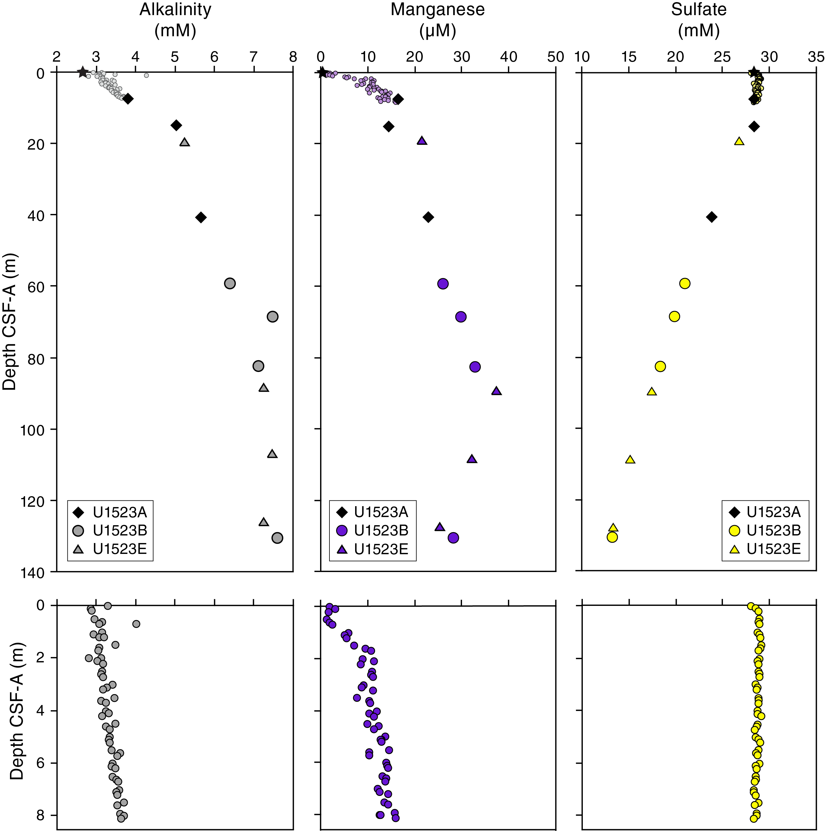
Figure F25. Interstitial water geochemistry.
Silicon, magnesium, and lithium
Silicon and dissolved silica, measured by inductively coupled plasma–optical emission spectroscopy (ICP-OES) and spectrophotometry, respectively (see Geochemistry and microbiology in the Expedition 374 methods chapter [McKay et al., 2019a]), are in very good agreement in interstitial water samples from Site U1523, indicating that the total silicon in the samples is primarily silicic acid. The mudline water sample from Hole U1523A has a low silicon concentration of 134 µM, which is common in the ambient water column. A pronounced silicon concentration increase to 329 µM is observed between the mudline sample and the uppermost interstitial water sample (374-U1523B-1H-1, 0–10 cm). A peak silicon concentration of 1019 µM is reached at 130.40 m CSF-A (Figure F26). Silicon concentration deeper than 40.62 m CSF-A is ~800–1000 µM and likely reflects equilibrium conditions between diagenesis/dissolution of biogenic silica and silica saturation in the interstitial water (Figure F26).
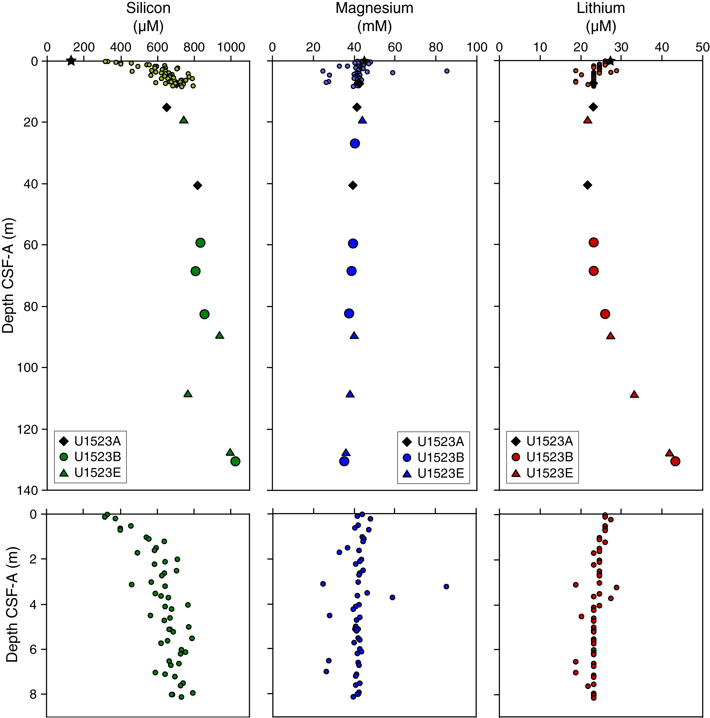
Figure F26. Interstitial water geochemistry.
Magnesium concentration shows low variability and ranges generally between 35 and 45 mM from the mudline downhole to 130.40 m CSF-A. Calcium and potassium downhole profiles are similar to that of magnesium. Lithium concentration is generally between 21 and 27 µM at 0–82.34 m CSF-A. Lithium increases downhole exponentially to a maximum concentration of 43 µM at 130.40 m CSF-A. Downhole variations in silicon, magnesium, and lithium (Figure F26) are very consistent between Holes U1523A, U1523B, and U1523E.
High-resolution sampling
High-resolution interstitial water data from Core 374-U1523B-1H (Table T13) are in excellent agreement with interstitial water measurements conducted at lower resolution in Holes U1523A, U1523B, and U1523E. Chloride concentration shows a slight increase of ~4% in the uppermost 0.2 m CSF-A of the high-resolution data set and stabilizes below this depth (560 ± 3 mM). Alkalinity linearly increases with a slope almost identical to that observed from low-resolution data in Hole U1523A (Figure F25). Increasing concentrations of silicon and manganese from Core 1H is in line with the lower resolution profiles. In detail, the most significant concentration increase in silicon, from ~300 to ~550 µM, occurs in the uppermost 1 m CSF-A (Figure F26). Between 1 and 8 m CSF-A, relatively constant concentration is observed, with some variability around a mean value of 657 ± 74 µM. Similarly, manganese concentration increases from low values (<3 µM) to ~10 µM in the uppermost 1.6 m CSF-A. These elemental profiles are consistent with shallow diagenesis of silica. Other elements (e.g., magnesium, calcium, potassium, sodium, and strontium) show very little variation in the high-resolution interstitial water samples.
Bulk sediment geochemistry
Carbon, nitrogen, and carbonate
Discrete sediment samples (N = 41) from all major lithostratigraphic units identified at Site U1523 were analyzed for total carbon, TN, and total inorganic carbon. TOC and CaCO3 contents were subsequently calculated (Table T14). TOC content is generally low (≤0.6 wt%) but increases slightly through the upper ~85 m CSF-A (Figure F27). Slightly lower values (0.02–0.39 wt%) occur in the mainly diatom-bearing mud and diamict of lithostratigraphic Unit III between 96 and 155 m CSF-A. TN content is very low (<0.1 wt%), with values increasing slightly downhole over the upper 85 m CSF-A. Except for three samples with significantly elevated ratios (29, 44, and 33) collected from Cores 374-U1523A-1H and 6F and Core 374-U1523E-4F, respectively, the TOC/TN ratio ranges between 2 and 17 (Figure F27), suggesting a mixed (i.e., marine and terrigenous) source of the organic matter deposited at Site U1523. CaCO3 content is generally low and ranges between 0.2 and 2.5 wt%, with slightly higher and more variable values occurring in the interbedded diatom-bearing sandy mud of Units I and II in the upper 76 m CSF-A. Three distinct CaCO3 maxima (as much as 15.5 wt%) are observed in samples from sandy foraminifer-bearing mud in Sections 374-U1523A-6F-3 and 374-U1523E-4F-2 and 15F-3. The upper two of these three samples also exhibit a significantly elevated TOC/TN ratio.
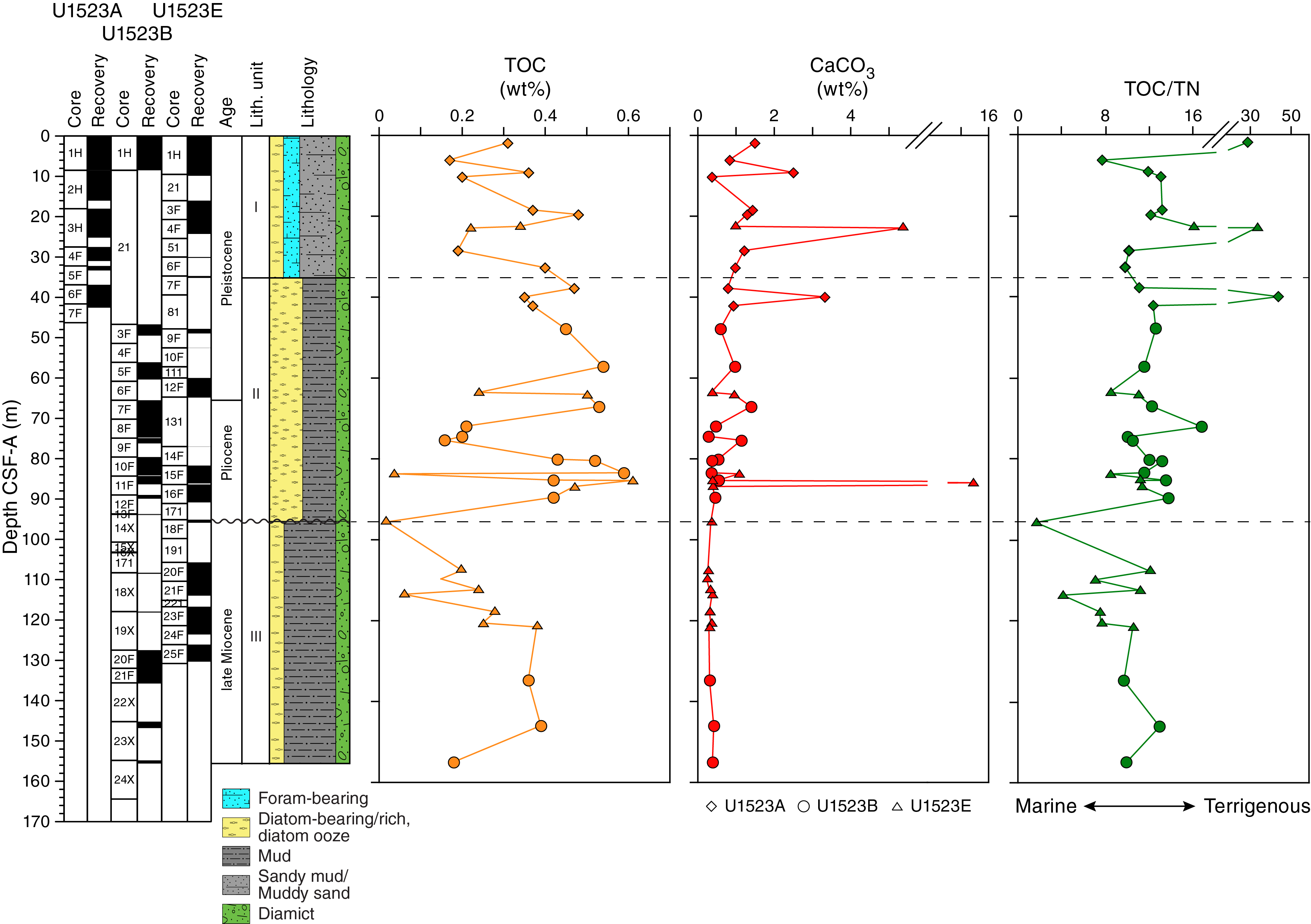
Figure F27. Bulk sediment carbon content and TOC/TN.
pXRF data
Shipboard pXRF data (Table T15) were collected from Holes U1523A, U1523B, and U1523E using two different methods (“geochem” and “soil”; see Lithostratigraphy and Geochemistry and microbiology in the Expedition 374 methods chapter [McKay et al., 2019a]). Data from all three holes are combined to illustrate downhole trends and show a positive relationship between the Ba/Al and Fe/Al ratios (r2 = 0.7). The Ba/Al ratios are relatively invariant, with the exception of data points at 22.61 and 22.91 m CSF-A in Hole U1523E and 75.61 m CSF-A in Hole U1523B (Figure F28). This observation contrasts with results for Sites U1521 and U1522, where the Ba/Al ratio varies cyclically over a larger range. More systematic downhole variations are observed in the Si/K and Si/Ti ratios, which are positively correlated (r2 = 0.87). Notably, the Si/K ratio is elevated in interbedded muddy sand and diatom-bearing/rich mud between ~50 and 90 m CSF-A in lithostratigraphic Unit II, an interval characterized by low NGR and magnetic susceptibility (see Physical properties) (Figure F28). The Ti/Th ratio fluctuates by a factor of four, with particularly low values in the samples that yielded an elevated Ba/Al ratio (Figure F28). The highest frequency fluctuations in the uppermost 90 m CSF-A are observed in the Fe/Ti ratio, which is likely to represent a good provenance indicator for the Ross Sea along with ratios of refractory elements such as the Ti/Th ratio.
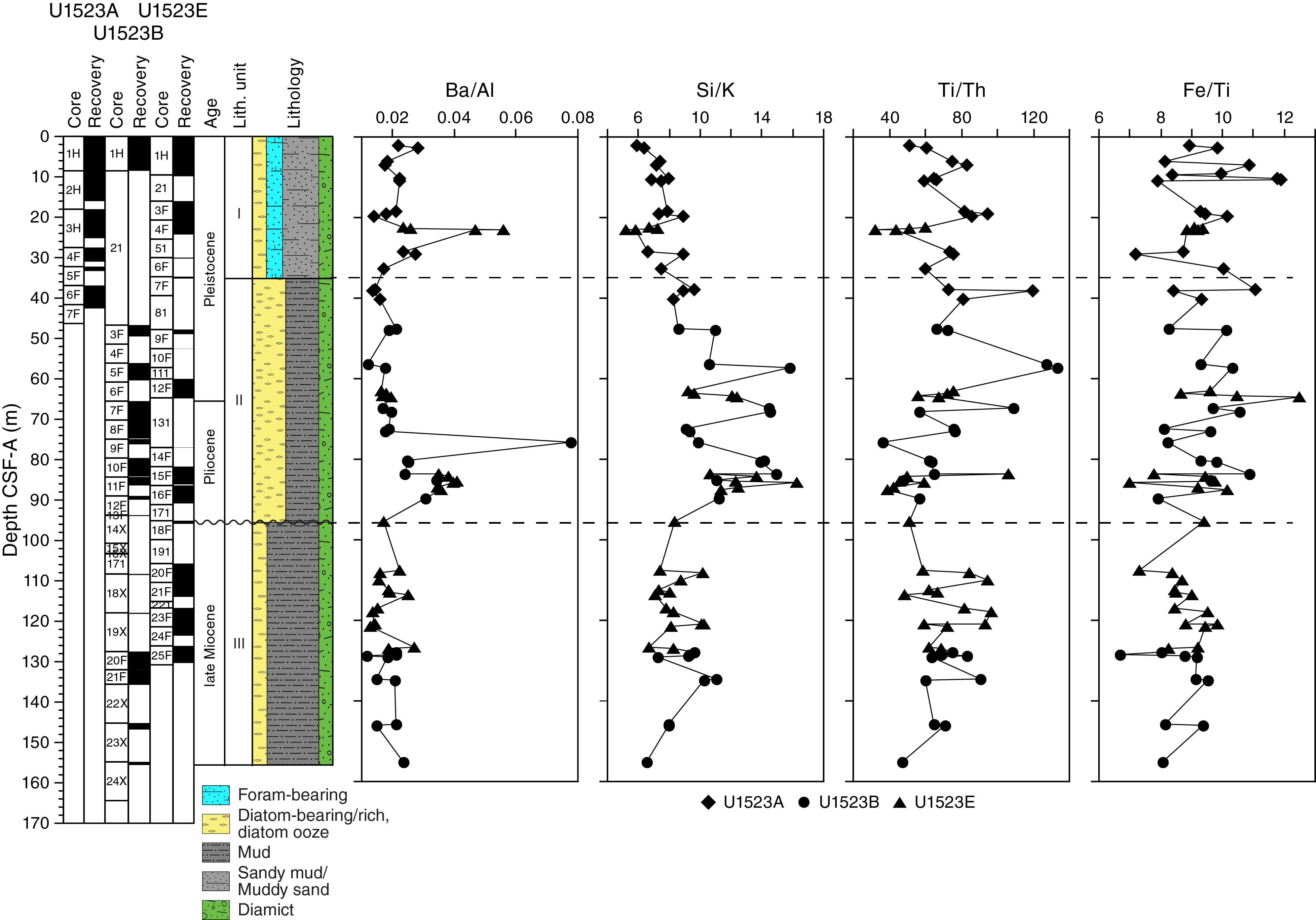
Figure F28. pXRF element ratios.
Microbiological sampling
In total, 11 samples were collected from Holes U1523A and U1523B for shore-based stable and clumped isotope analyses of methane and ethane. Syringe samples for detailed analyses of metagenomics, cell counts, metabolomics, and cultures were taken from Sections 374-U1523A-6F-2, 374-U1523B-5F-1 and 5F-2, and 374-U1523E-3F-1, 3F-2, 16F-1, 16F-2, 20F-1, and 20F-2 (see Geochemistry and microbiology in the Expedition 374 methods chapter [McKay et al., 2019a]).
High-resolution interstitial water sampling from Core 374-U1523B-1H was accompanied by higher resolution sampling for microbiology. In detail, 10 cm whole-round samples were collected at 30–50 cm (N = 2), 80–100 cm (N = 2), and 130–150 cm (N = 2) in Sections 1H-1 through 1H-5 and from 20–40 cm (N = 2) in Section 1H-6 (Figure F24). Half of these whole rounds were immediately stored at −80°C for onshore analyses of metabolomics and tag-amplicon sequencing. The other half was further subsampled (see Geochemistry and microbiology in the Expedition 374 methods chapter [McKay et al., 2019a] for details) for shore-based analyses of metagenomics and culturing.
Downhole measurements
Logging operations
Preparation of Hole U1523D for logging included release of the RCB drill bit at 0800 h on 2 February 2018 and cleaning the hole with two 50 bbl high-viscosity (10.5 lb/gal) mud sweeps to improve hole conditions. This was followed by an additional 20 bbl of heavy mud, and then the hole was displaced with 94 bbl of 10.5 lb/gal mud from 307.8 m DSF to the seafloor. The drill string was pulled up to a logging depth of 82.3 m DSF. After the end of the pipe was positioned, the hole was displaced with a further 20 bbl of heavy (10.5 lb/gal) mud.
The rig floor was prepared for logging at 1130 h on 2 February. An average heave of 0.3 m was estimated prior to logging, and the active heave compensator was switched on once the tools reached open hole. A modified triple combo tool string was assembled for the first run (see Downhole measurements in the Expedition 374 methods chapter [McKay et al., 2019a]). The triple combo tool string consisted of the following tools:
The triple combo tool string was assembled, tested, and lowered into the drill string at 1320 h. The HNGS and MSS were run while the tools were lowered to the bottom of the hole, and all tools were run during the upward logging run. The base of the tool reached 292 m WSF, ~15 m above the total depth of the hole at 307.8 m DSF. The caliper arms were opened, and the hole was then logged up with a 136 m calibration pass. The tool was run back to bottom, this time reaching 288 m WSF, and logged up with the modified triple combo tool string. Upon visual inspection, the curves from the two runs were identical. Before reaching the end of pipe at 82.3 m DSF, the end of pipe was raised to 67 m DSF. The caliper arms were closed before entering the BHA. The modified triple combo tool string was back at the rig floor at 1630 h and disassembled by 1745 h on 2 February.
The second logging run used the FMS tool string, which consisted of the following tools (see Downhole measurements in the Expedition 374 methods chapter [McKay et al., 2019a]):
The tool string was assembled and deployed into the drill string at 1820 h on 2 February. NGR was logged from above the seafloor and through the drill pipe to depth-match results to the first logging run. Total depth reached with the FMS tool string was 289.6 m WSF, and a first upward pass was logged to the end of pipe at 82.3 m DSF. After closing the calipers and lowering the tool back to 289.6 m WSF, a second upward pass was collected and the end of pipe was raised 15 m to increase logging coverage of the upper part of the borehole. The FMS tool string was returned to the rig floor, and all logging tools and equipment were disassembled by 2245 h.
Log data quality and comparison with shipboard physical properties
All log curves were depth-matched using the total gamma ray log from the main pass of the triple combo tool string as the reference, allowing a unified depth scale to be produced. Features in the gamma ray logs from the FMS tool string passes were aligned to the reference log to produce a complete depth-matched data set. Log data were then depth-shifted to the seafloor, as identified by a stepwise increase in the gamma ray value, leading to the wireline log matched depth below seafloor (WMSF) depth scale. The triple combo logging run identified the seafloor at 839 m wireline depth below rig floor (WRF).
Borehole quality in Hole U1523D was variable. Borehole diameter measured by the caliper varied widely, indicating numerous washed out intervals and multiple ledges. Caliper width ranged from 12.8 to 14.0 inches. The most significant washouts (more than ~4 inches on the caliper log) are at 110, 120, 145, 163, 177, 193, 203, and 207 m WMSF (Figure F29). Other deviations from the bit diameter were relatively minor, and most of the borehole wall had low to medium rugosity.
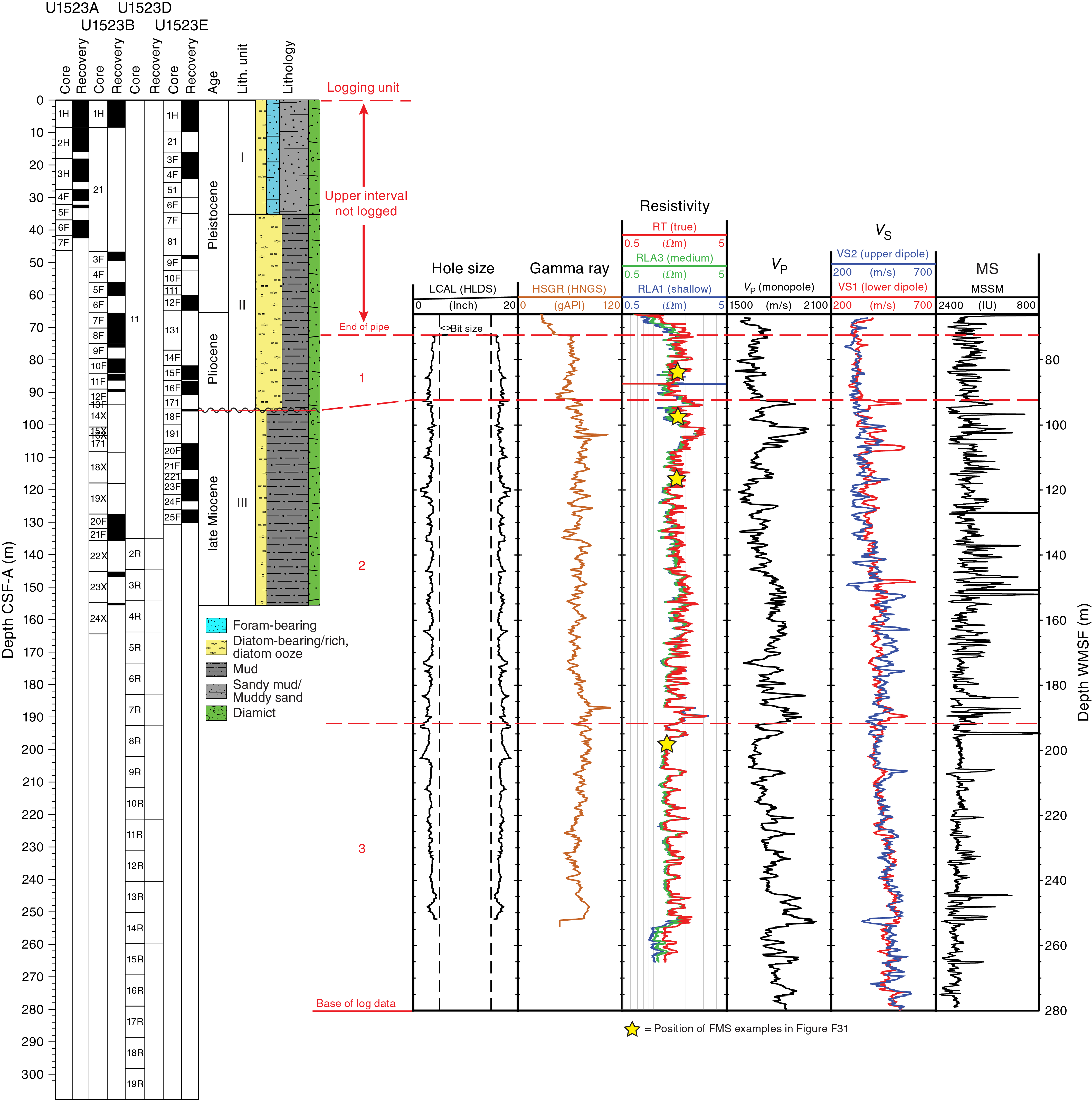
Figure F29. Downhole log data summary.
The quality of the logs can also be assessed by comparison with physical property measurements made on Site U1523 cores (see Physical properties). Because Hole U1523D was drilled without coring to 135 m DSF and core recovery with the RCB coring system was very low (0.5%) below that depth, correlation between log and core data from Hole U1523D was not possible. Three other holes were cored at this site (Hole U1523A from 0 to 46.3 m DSF, Hole U1523B from 0 to 164.4 m DSF, and Hole U1523E from 0 to 130.8 m DSF), and core recovery was adequate from these holes for comparison with logging data from the upper part of Hole U1523D. Note that downhole logs are shown on the WMSF depth scale, whereas physical property data are shown on the CSF-A depth scale on Figure F30. Offsets at the scale of the entire drilled/logged interval are minor (typically <2 m) and thus still allow comparison of downhole trends.
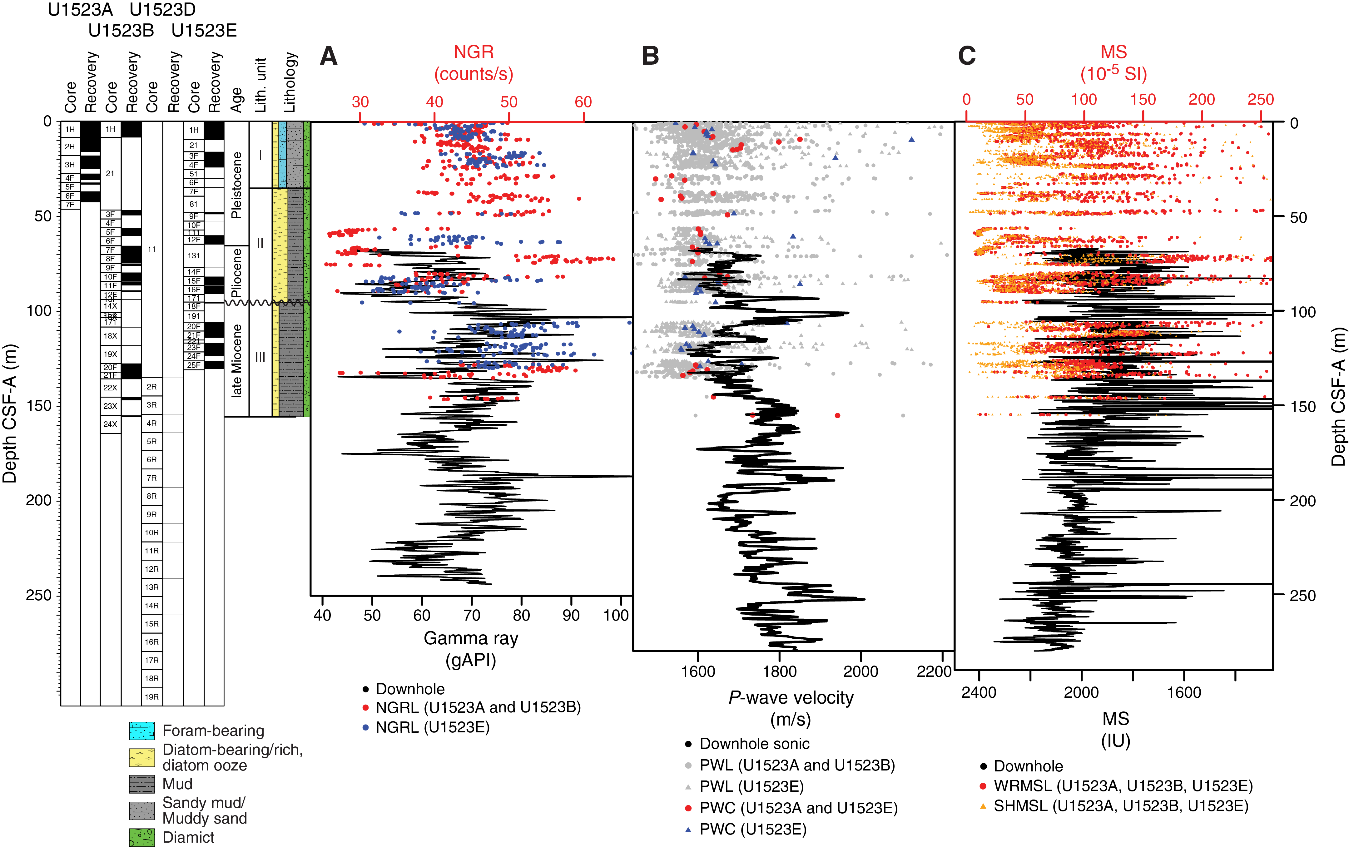
Figure F30. NGR, P-wave velocity, and MS data comparisons.
In general, the gamma ray and P-wave velocity data show good correspondence between overlapping downhole and shipboard measurements throughout the borehole, although the overlapping interval only spans ~80 m (Figure F30). Although the downhole gamma ray and shipboard NGR data have different units, the trends and relative magnitude of downhole shifts are comparable. Some discrepancies exist between downhole gamma ray and shipboard NGR data from Hole U1523B at ~75 m CSF-A, where laboratory measurements are much higher. Between 100 and 150 m CSF-A, laboratory measurements appear to overestimate gamma ray counts relative to the downhole measurements.
The agreement between downhole P-wave velocity from the sonic log and shipboard PWC P-wave velocity is fair in the overlapping section. Although general downhole trends are similar, the shipboard PWC consistently underestimates P-wave velocity relative to the downhole sonic log (Figure F30). Magnetic susceptibility data also show reasonable correspondence, although there is a wide range in values. A clear downhole drift in the magnetic susceptibility logging data is likely due to tool temperature (Figure F30).
FMS images appear to be overall of good quality, indicating that the pads made reasonable contact with the borehole walls (Figure F31). Data may be less reliable in the vicinity of significant washouts (more than ~4 inches on the caliper log) (e.g., at 110, 120, 145, 163, 177, 193, 203, and 207 m WMSF).
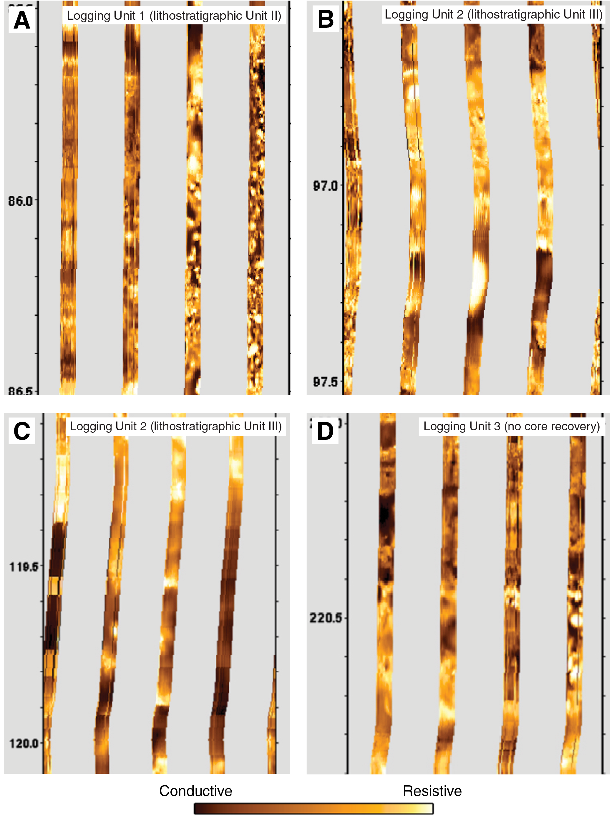
Figure F31. FMS image examples.
Logging units
Downhole logging data for Hole U1523D are summarized in Figure F29. Three logging units are defined on the basis of distinctive features in the gamma ray, resistivity, magnetic susceptibility, and velocity (sonic) logs (Table T16). The units start at 72 m WMSF (end of pipe depth below seafloor) and end at 280 m WMSF.
Logging Unit 1 (72.0–92.0 m WMSF)
Logging Unit 1 is the uppermost unit logged in Hole U1523D. It is characterized by relatively low gamma radiation (typically ~54–66 gAPI), moderate resistivity (1.48–1.91 Ωm), low to moderate velocity (~1630–1680 m/s), and variable magnetic susceptibility (~1790–2000 instrument units [IU]) (Figure F29). Unit 1 corresponds to the basal part of lithostratigraphic Unit II (~34.7–95.8 m CSF-A in Hole U1523E; see Lithostratigraphy), which is composed of diatom-bearing/rich mud to muddy diatom ooze interbedded with diamict. Glauconite is also common.
Logging Unit 2 (92.0–191.0 m WMSF)
Logging Unit 2 is characterized by relatively high gamma radiation (~64–66 gAPI) with peak values of ~74 gAPI. The unit has moderate resistivity (1.54–1.98 Ωm) and moderate velocity values (~1680–1790 m/s). Magnetic susceptibility varies significantly (~1780–2010 IU) (Figure F29), and these variations may correspond to lithologic changes in the interbedded (decimeter to meter scale) diatom-bearing/rich mud and diatom-bearing diamict of lithostratigraphic Unit III (95.8–130.3 m CSF-A in Hole U1523E).
Logging Unit 3 (191.0–280.0 m WMSF)
Logging Unit 3 is characterized by distinct intervals of low gamma radiation (~50 gAPI), high resistivity (~2.35 Ωm), high velocity (>2000 m/s), and high magnetic susceptibility (~2340 IU) (e.g., at 196, 209, 225 and 239 m WMSF). In between these intervals, gamma radiation is relatively high (63–74 gAPI), with low resistivity (1.33–1.65 Ωm), lower velocity (~1710–1810 m/s), and moderate magnetic susceptibility (~2010–2110 IU) (Figure F29). Because Unit 3 is below the depth of recovered core in Holes U1523A, U1523B, and U1523E (deeper than 155.57 m CSF-A in Hole U1523B), there are no lithostratigraphic units for comparison. Unit 3 is interpreted as alternating intervals of diatom-bearing mud, diamict, and gravel layers.
FMS images
FMS resistivity images show submeter variations in the texture and lithologies of the borehole walls (Figure F31). Logging Units 1 and 2 are characterized by variable resistivity with high-resistivity mottled and patchy textures, intervals of alternating high and low resistivity and distinct high-resistivity spots (Figure F31A–F31C). This corresponds to interbedded muddy sand, diatom-bearing/rich mud (occasionally with clasts), diatom ooze, and thin intervals of diamict in the cores. Localized, centimeter-scale high-resistivity spots are interpreted as clasts in the diamict. Unit 3 is characterized by distinct intervals of high and low resistivity, although resistivity continues to vary in these layers (Figure F31D). High-resistivity spots in FMS images below intervals of core recovery (Unit 3) suggests clasts are present, which is consistent with alternating intervals of diatom-bearing mud, diamict, and gravel layers.
Core-log-seismic integration
We combined log data from Hole U1523D; sediment core observations and physical property data from Holes U1523A, U1523B, and U1523E; and seismic-reflection data to evaluate whether the observed sedimentary, physical property, log, and seismic units could be integrated. Seismic-reflection Profile IT17RS301, acquired in 2017 aboard the OGS Explora, crosses Site U1523 and was used for core-log-seismic integration (Figure F32). To correlate the core and log data with features observed on the seismic-reflection data for Site U1523, we converted lithostratigraphic and logging unit boundaries from depth in meters to TWT using two different methods:
- PWC point-source velocity data from physical property measurements (see Physical properties) and
- Sonic velocity data from the DSI.
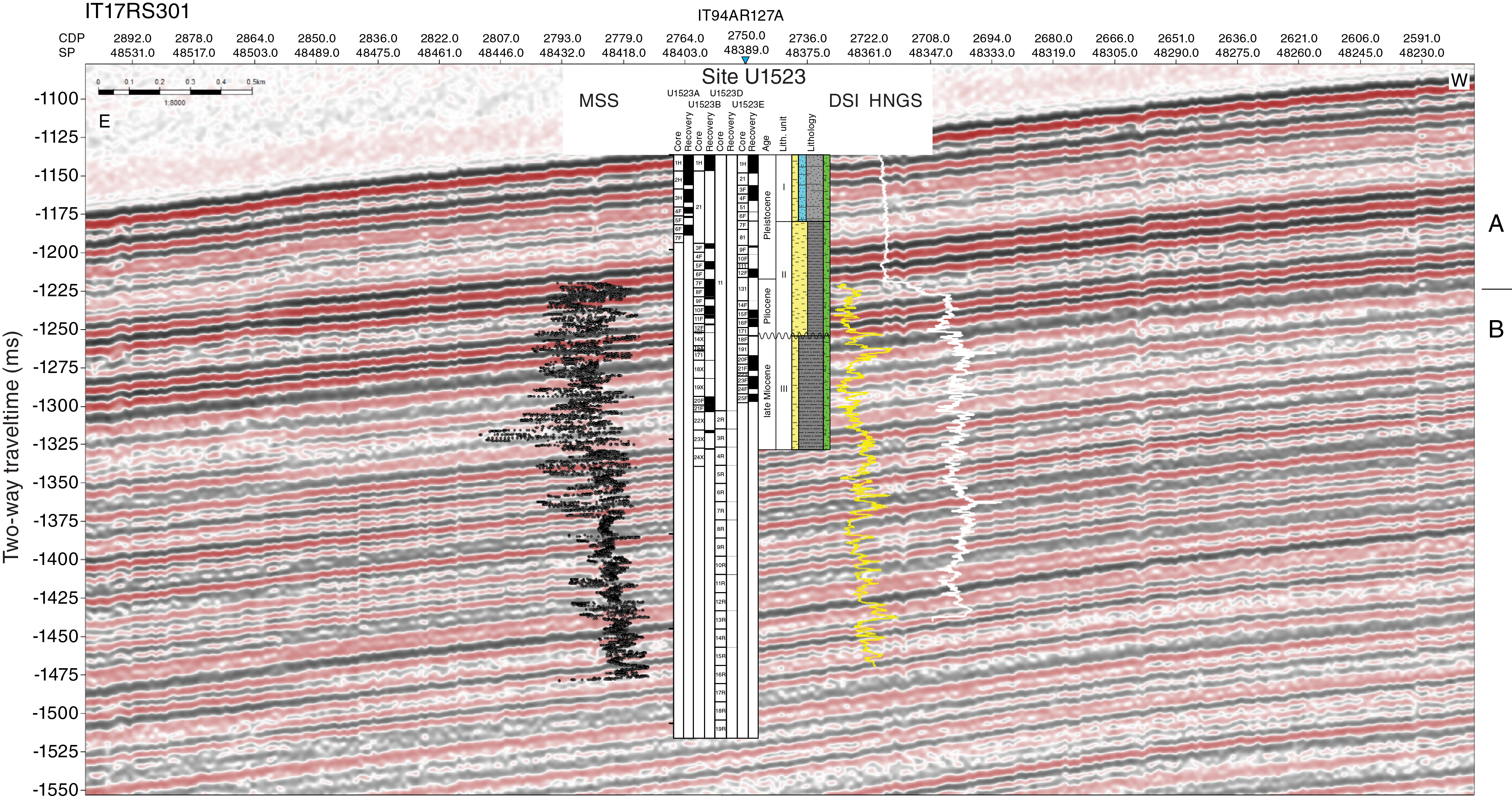
Figure F32. Core-log-seismic integration.
Discrete P-wave velocity laboratory measurements on cores gave relatively slow values, whereas the sonic log corresponds well with the stacking velocities. Core-log-seismic integration is limited by poor core recovery deeper than ~160 m CSF-A. Two seismic units are defined; Unit A (1150–1270 ms TWT) is characterized by moderate- to high-amplitude, parallel, continuous seismic reflectors, and Unit B (1270–1550 ms TWT) is characterized by reflectors with similar continuity and geometry but of low to moderate amplitude. The boundary between seismic Units A and B coincides with the boundary between logging Units 1 and 2 and lithostratigraphic Units II and III (Figure F32). Units A and B are interpreted as drift deposits.
References
Arndt, J.E., Schenke, H.W., Jakobsson, M., Nitsche, F.O., Buys, G., Goleby, B., Rebesco, M., et al., 2013. The International Bathymetric Chart of the Southern Ocean (IBCSO) Version 1.0—a new bathymetric compilation covering circum-Antarctic waters. Geophysical Research Letters, 40(12):3111–3117. https://doi.org/10.1002/grl.50413
Carburlotto, A., Lucchi, R.G., De Santis, L., Macrì, P., and Tolotti, R., 2010. Sedimentary processes on the Wilkes Land continental rise reflect changes in glacial dynamic and bottom water flow. International Journal of Earth Sciences, 99(4):909–926. https://doi.org/10.1007/s00531-009-0422-8
Golledge, N.R., Levy, R.H., McKay, R.M., Fogwill, C.J., White, D.A., Graham, A.C.C., Smith, J.A., et al., 2013. Glaciology and geological signature of the Last Glacial Maximum Antarctic Ice Sheet. Quaternary Science Reviews, 78:225–247. https://doi.org/10.1016/j.quascirev.2013.08.011
Gradstein, F.M., Ogg, J.G., Schmitz, M.D., and Ogg, G.M. (Eds.), 2012. The Geological Time Scale 2012: Amsterdam (Elsevier). https://doi.org/10.1016/C2011-1-08249-8
Hannah, M.J., Wrenn, J.H., and Wilson, G.J., 1998. Early Miocene and Quaternary marine palynomorphs from Cape Roberts Project CRP-1, McMurdo Sound, Antarctica. Terra Antarctica, 5(3):527–538. https://epic.awi.de/27440/1/Han1998g.pdf
Harland, R., and Pudsey, C.J., 2002. Protoperidiniacean dinoflagellate cyst taxa from the upper Miocene of ODP Leg 178, Antarctic Peninsula. Review of Palaeobotany and Palynology, 120(3–4):263–284. https://doi.org/10.1016/S0034-6667(02)00080-5
Hesse, R., Khodabakhsh, S., Klaucke, I., and Ryan, W.B.F., 1997. Asymmetrical turbid surface-plume deposition near ice-outlets of the Pleistocene Laurentide Ice Sheet in the Labrador Sea. Geo-Marine Letters 17(3):179–187. https://doi.org/10.1007/s003670050024
Jacobs, S.S., Bauer, E.B., Bruchhausen, P.M., Gordon, A.L., Root, T.F., and Rosselot, F.L., 1974. Eltanin Reports: Cruises 47–50, 1971, 52–55, 1972: Hydrographic Stations, Bottom Photographs, Current Measurements, Nephelometer Profiles: Palisades, NY (Lamont-Doherty Geological Observatory, Columbia University), CU-2-74.
Kennett, J.P., 1966. Foraminiferal evidence of a shallow calcium carbonate solution boundary, Ross Sea, Antarctica. Science, 153(3732):191–193. https://doi.org/10.1126/science.153.3732.191
Kennett, J.P., 1968. The fauna of the Ross Sea. Part 6: Ecology and distribution of foraminifera. New Zealand Department of Scientific and Industrial Research Bulletin, 186. http://docs.niwa.co.nz/library/public/Memoir%20046_Fauna%20of%20the%20Ross%20Sea%20(Part%206)_Foraminifera%20-%201968.pdf
Lazarus, D., 1992. Antarctic Neogene radiolarians from the Kerguelen Plateau, Legs 119 and 120. In Wise, S.W., Jr., Schlich, R., et al., Proceedings of the Ocean Drilling Program, Scientific Results, 120: College Station, TX (Ocean Drilling Program), 785–809. https://doi.org/10.2973/odp.proc.sr.120.192.1992
Lucchi, R.G., Rebesco, M., Camerlenghi, A., Busetti, M., Tomadin, L., Villa, G., Persico, D., Morigi, C., Bonci, M.C., and Giorgetti, G., 2002. Mid–late Pleistocene glacimarine sedimentary processes of a high-latitude, deep-sea sediment drift (Antarctica Peninsula Pacific margin). Marine Geology, 189(3–4):343–370. https://doi.org/10.1016/S0025-3227(02)00470-X
McKay, R.M., De Santis, L., Kulhanek, D.K., Ash, J.L., Beny, F., Browne, I.M., Cortese, G., Cordeiro de Sousa, I.M., Dodd, J.P., Esper, O.M., Gales, J.A., Harwood, D.M., Ishino, S., Keisling, B.A., Kim, S., Kim, S., Laberg, J.S., Leckie, R.M., Müller, J., Patterson, M.O., Romans, B.W., Romero, O.E., Sangiorgi, F., Seki, O., Shevenell, A.E., Singh, S.M., Sugisaki, S.T., van de Flierdt, T., van Peer, T.E., Xiao, W., and Xiong, Z., 2019a. Expedition 374 methods. In McKay, R.M., De Santis, L., Kulhanek, D.K., and the Expedition 374 Scientists, Ross Sea West Antarctic Ice Sheet History. Proceedings of the International Ocean Discovery Program, 374: College Station, TX (International Ocean Discovery Program). https://doi.org/10.14379/iodp.proc.374.102.2019
McKay, R.M., De Santis, L., Kulhanek, D.K., Ash, J.L., Beny, F., Browne, I.M., Cortese, G., Cordeiro de Sousa, I.M., Dodd, J.P., Esper, O.M., Gales, J.A., Harwood, D.M., Ishino, S., Keisling, B.A., Kim, S., Kim, S., Laberg, J.S., Leckie, R.M., Müller, J., Patterson, M.O., Romans, B.W., Romero, O.E., Sangiorgi, F., Seki, O., Shevenell, A.E., Singh, S.M., Sugisaki, S.T., van de Flierdt, T., van Peer, T.E., Xiao, W., and Xiong, Z., 2019b. Expedition 374 summary. In McKay, R.M., De Santis, L., Kulhanek, D.K., and the Expedition 374 Scientists, Ross Sea West Antarctic Ice Sheet History. Proceedings of the International Ocean Discovery Program, 374: College Station, TX (International Ocean Discovery Program). https://doi.org/10.14379/iodp.proc.374.101.2019
McKay, R.M., De Santis, L., Kulhanek, D.K., Ash, J.L., Beny, F., Browne, I.M., Cortese, G., Cordeiro de Sousa, I.M., Dodd, J.P., Esper, O.M., Gales, J.A., Harwood, D.M., Ishino, S., Keisling, B.A., Kim, S., Kim, S., Laberg, J.S., Leckie, R.M., Müller, J., Patterson, M.O., Romans, B.W., Romero, O.E., Sangiorgi, F., Seki, O., Shevenell, A.E., Singh, S.M., Sugisaki, S.T., van de Flierdt, T., van Peer, T.E., Xiao, W., and Xiong, Z., 2019c. Site U1521. In McKay, R.M., De Santis, L., Kulhanek, D.K., and the Expedition 374 Scientists, Ross Sea West Antarctic Ice Sheet History. Proceedings of the International Ocean Discovery Program, 374: College Station, TX (International Ocean Discovery Program). https://doi.org/10.14379/iodp.proc.374.103.2019
Naish, T.R., Powell, R., Levy, R., Wilson, G., Scherer, R., Talarico, F., Krissek, L., et al., 2009. Obliquity-paced Pliocene West Antarctic Ice Sheet oscillations. Nature, 458(7236):322–329. https://doi.org/10.1038/nature07867
Nishimura, A., Nakaseko, K., and Okuda, Y., 1997. A new coastal water radiolarian assemblage recovered from sediment samples from the Antarctic Ocean. Marine Micropaleontology, 30(1–3):29–44. https://doi.org/10.1016/S0377-8398(96)00019-9
Orsi, A.H., and Wiederwohl, C.L., 2009. A recount of Ross Sea waters. Deep Sea Research, Part II: Topical Studies in Oceanography, 56(13–14):778–795. https://doi.org/10.1016/j.dsr2.2008.10.033
Osterman, L.E., and Kellogg, T.B., 1979. Recent benthic foraminiferal distributions from the Ross Sea, Antarctica: relation to ecologic and oceanographic conditions. Journal of Foraminiferal Research, 9(3):250–269. https://doi.org/10.2113/gsjfr.9.3.250
Padman, L., Erofeeva, S., and Joughin, I., 2003. Tides of the Ross Sea and Ross Ice Shelf cavity. Antarctic Science, 15(1):31–40. https://doi.org/10.1017/S0954102003001032
Zonneveld, K.A.F., Marret, F., Versteegh, G.J.M., Bogus, K., Bonnet, S., Bouimetarhan, I., Crouch, E., et al., 2013. Atlas of modern dinoflagellate cyst distribution based on 2405 data points. Review of Palaeobotany and Palynology, 191. https://doi.org/10.1016/j.revpalbo.2012.08.003
1 McKay, R.M., De Santis, L., Kulhanek, D.K., Ash, J.L., Beny, F., Browne, I.M., Cortese, G., Cordeiro de Sousa, I.M., Dodd, J.P., Esper, O.M., Gales, J.A., Harwood, D.M., Ishino, S., Keisling, B.A., Kim, S., Kim, S., Laberg, J.S., Leckie, R.M., Müller, J., Patterson, M.O., Romans, B.W., Romero, O.E., Sangiorgi, F., Seki, O., Shevenell, A.E., Singh, S.M., Sugisaki, S.T., van de Flierdt, T., van Peer, T.E., Xiao, W., and Xiong, Z., 2019. Site U1523. In McKay, R.M., De Santis, L., Kulhanek, D.K., and the Expedition 374 Scientists, Ross Sea West Antarctic Ice Sheet History. Proceedings of the International Ocean Discovery Program, 374: College Station, TX (International Ocean Discovery Program). https://doi.org/10.14379/iodp.proc.374.105.2019
2 Expedition 374 Scientists’ affiliations.
This work is distributed under the Creative Commons Attribution 4.0 International (CC BY 4.0) license. 