McKay, R.M., De Santis, L., Kulhanek, D.K., and the Expedition 374 Scientists
Proceedings of the International Ocean Discovery Program Volume 374
publications.iodp.org

https://doi.org/10.14379/iodp.proc.374.104.2019
Site U15221
R.M. McKay, L. De Santis, D.K. Kulhanek, J.L. Ash, F. Beny, I.M. Browne, G. Cortese, I.M. Cordeiro de Sousa, J.P. Dodd, O.M. Esper, J.A. Gales, D.M. Harwood, S. Ishino, B.A. Keisling, S. Kim, S. Kim, J.S. Laberg, R.M. Leckie, J. Müller, M.O. Patterson, B.W. Romans, O.E. Romero, F. Sangiorgi, O. Seki, A.E. Shevenell, S.M. Singh, S.T. Sugisaki, T. van de Flierdt, T.E. van Peer, W. Xiao, and Z. Xiong2
Keywords: International Ocean Discovery Program, IODP, JOIDES Resolution, Expedition 374, Site U1522, Ross Sea, West Antarctic, ice sheet history, sea ice, Miocene, Pliocene, Quaternary, Antarctic Bottom Water, Antarctic water masses, turbidites, contourites, glaciomarine sediments, subglacial sediments, ice-rafted debris, paleobathymetry, seismic stratigraphy, paleoclimate, paleoceanography
MS 374-104: Published 10 August 2019
Background and objectives
International Ocean Discovery Program (IODP) Site U1522 is located in the Glomar Challenger Basin at 76°33.2262′S, 174°45.4652′W in 558 m of water (Figure F1). During the middle Miocene, this site was located near the eastern edge of a wide embayment ~80 km southeast of the paleoshelf break (see Figure F7 in the 374 Expedition summary chapter [McKay et al., 2019b]). Coring at this site was anticipated to recover a sedimentary sequence spanning the middle Miocene to the Pleistocene (Ross Sea Unconformities [RSU] 3 to RSU1). Coring also targeted laminated and massive acoustic facies interpreted to be interlayered stratified diamictite/mudstone and diatomite (glaciomarine/open marine) and massive diamictite (tills), respectively (Figure F2). The seismic-reflection profiles perpendicular to the continental shelf edge (Figure F3) (Anderson and Bartek, 1992) show the generally tabular shape of the sedimentary unit, with subparallel high- and medium-amplitude reflectors. The sequence between RSU4 and RSU3 appears to span several phases of erosion and deposition that resulted in several intervals of shelf margin aggradation and progradation (Figure F4). The sequence between RSU3 and RSU2 was mainly deposited on the slope, resulting in overall shelf margin progradation. The sequence between RSU2 and the seafloor is thicker on the outer shelf, and resulted in the development of a landward-deepening continental shelf profile. The sequence above RSU2 does not show significant shelf margin progradation, but slope slide features at the mouth of the Glomar Challenger Basin are evident.
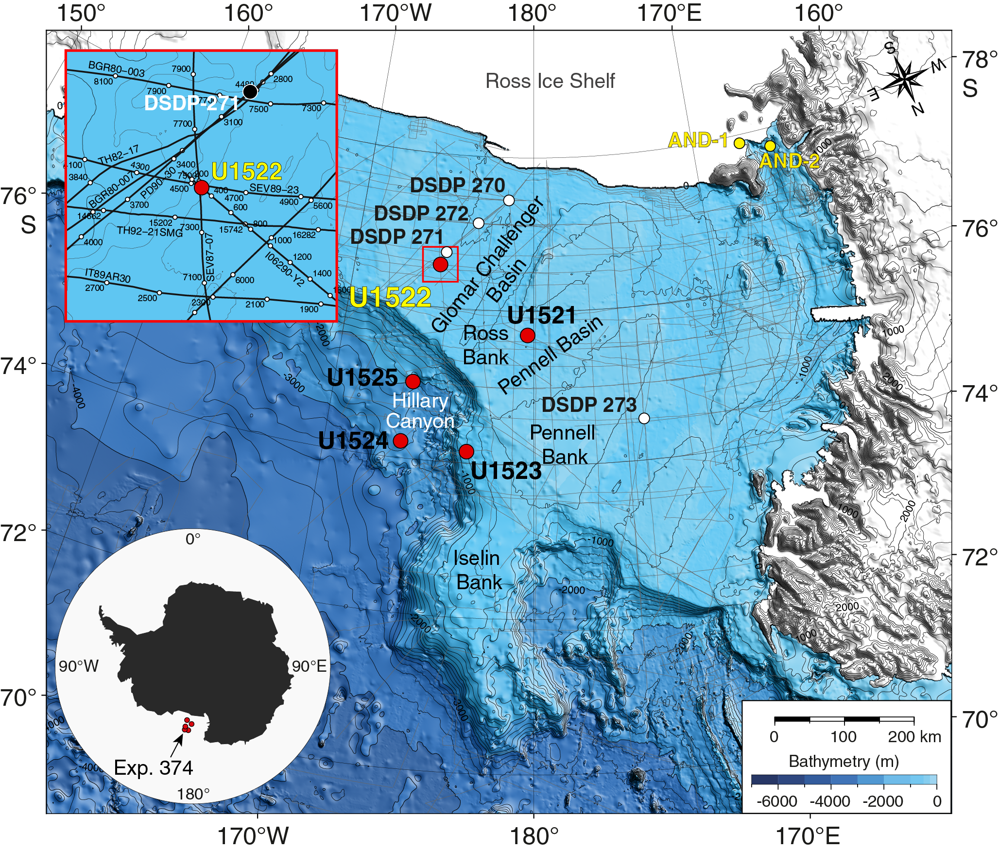
Figure F1. Bathymetric map and site locations.
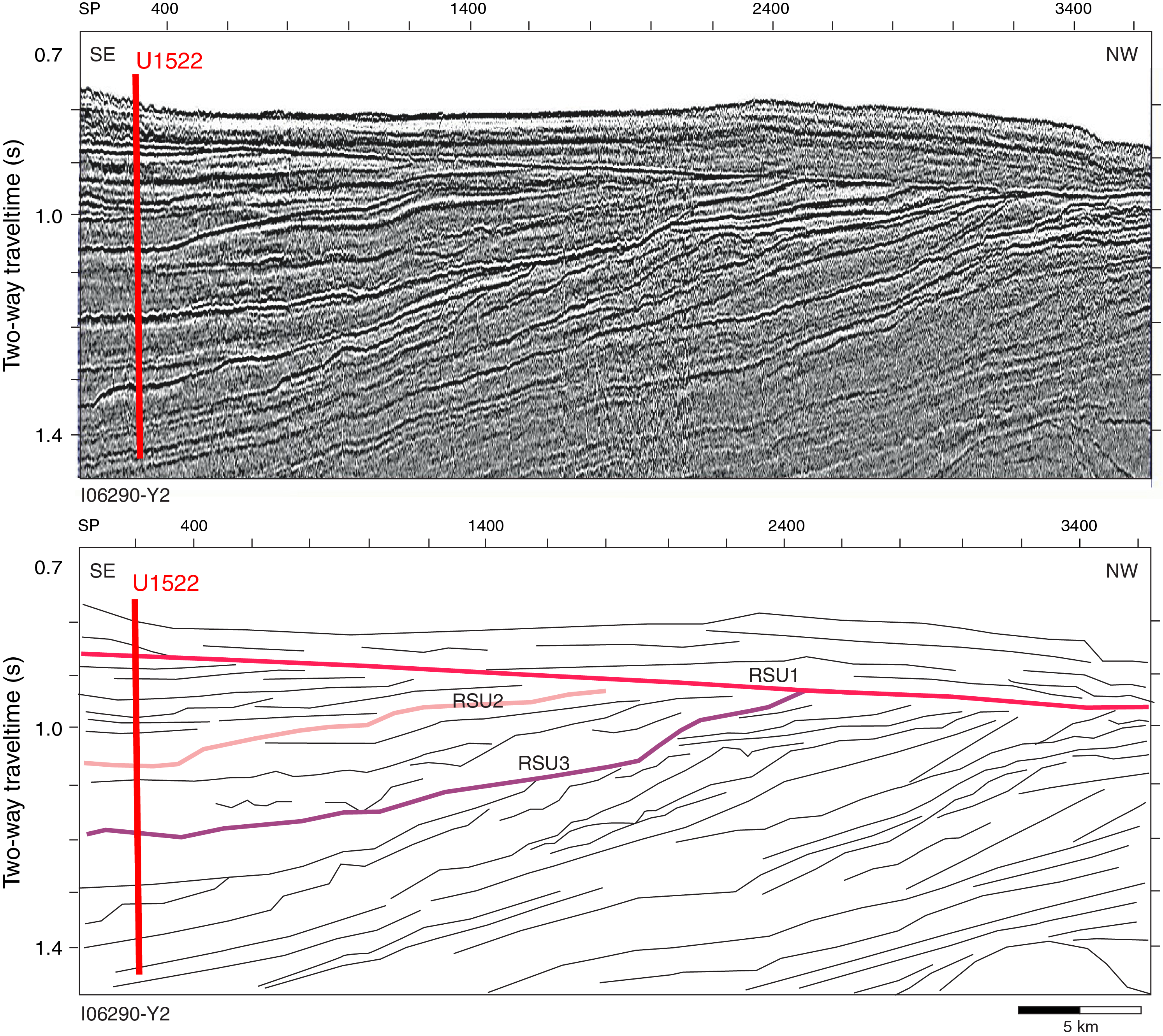
Figure F2. Seismic-reflection Profile I06290-Y2.

Figure F3. Seismic-reflection Profile PD90-30.
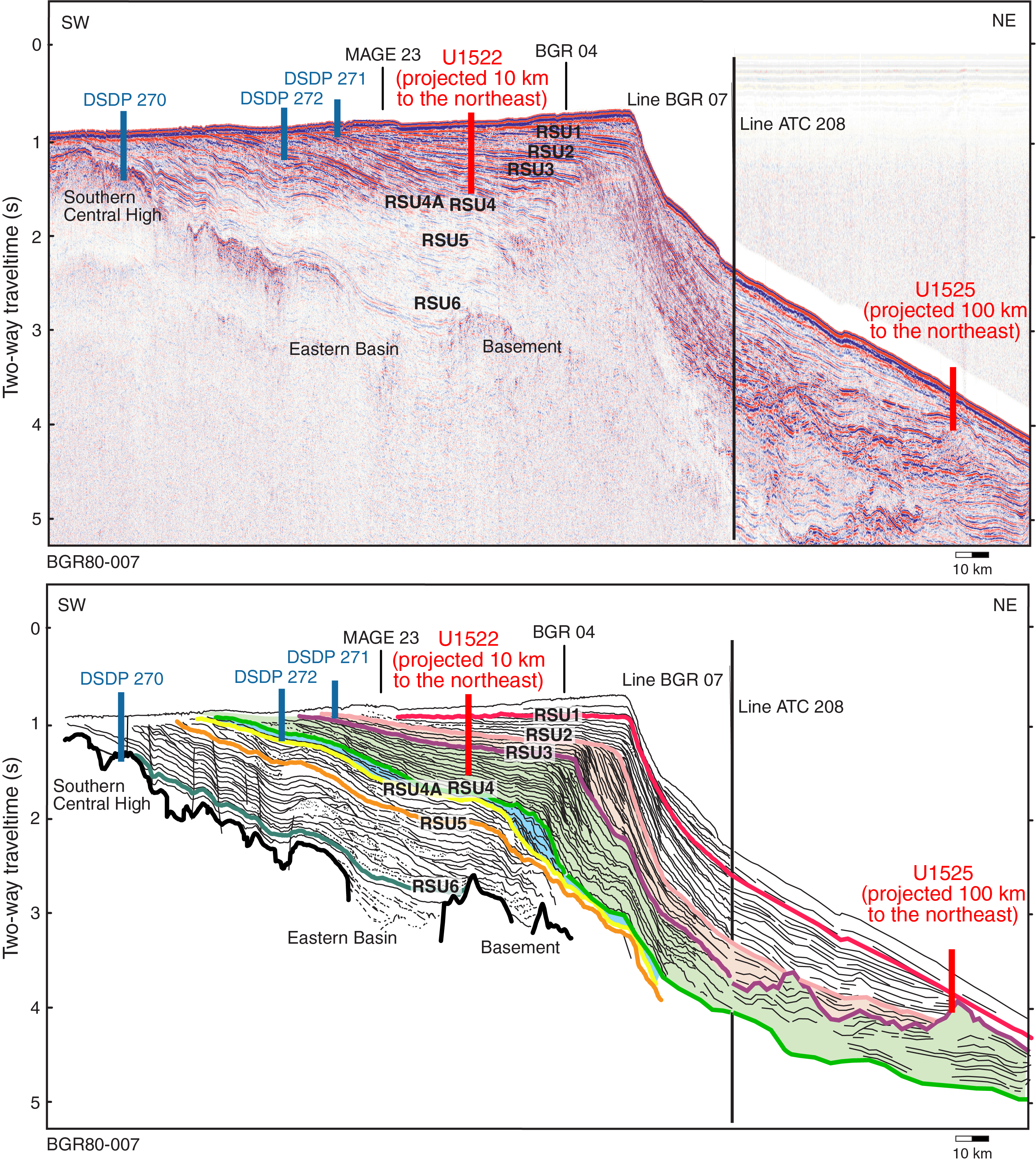
Figure F4. Seismic-reflection Profile BGR80-007.
On seismic-reflection profiles parallel to the continental shelf edge, the sequence lying below RSU3 displays wedge-like or channel structures near the flank of the Ross Bank that are consistent with deposition and erosion by streaming ice (Objectives 1 and 4 in Scientific objectives in the Expedition 374 summary chapter [McKay et al., 2019b]; Figure F2). The sequence above RSU3 shows cut and fill geometry and massive or chaotic seismic facies.
The primary objectives at this site were to date West Antarctic Ice Sheet advances associated with RSU3 and RSU2 (Objective 1) and to constrain the timing of the Ross Sea overdeepening (Objective 5). Deposits of glaciomarine mudstone were anticipated to be more biogenic rich than diamictite deposits, enabling paleoenvironmental reconstructions for late Miocene to Pleistocene interglacials (Objective 2).
The sediment above RSU3 (~1.25 s two-way traveltime [TWT]) consists of tabular units interpreted from the seismic-reflection profiles to be aggradational subglacial till sheets deposited by a grounded ice sheet and interlayered with glaciomarine/hemipelagic sediments of Miocene to late Pliocene age (Figure F3) (Alonso et al., 1992; De Santis et al., 1995). Underlying this succession is ~300 m (Figure F2) of acoustically laminated facies interbedded with more transparent lens-shaped layers, which are interpreted to be glaciomarine or hemipelagic sediments and ice proximal deposits (Böhm et al., 2009). This site will enable us to determine whether ice sheet–overriding events observed at Antarctic Geological Drilling Project (ANDRILL) Site AND-1B advanced to the shelf edge and will therefore help constrain the contribution of Antarctica’s ice sheets to Pliocene sea level lowstands (Objective 1; see Figure F4 in the Expedition 374 summary chapter [McKay et al., 2019b]; Naish et al., 2009; Miller et al., 2012). This site will also provide an opportunity to reconstruct the paleoceanographic and paleoecological conditions at the outermost Ross Sea continental shelf during periods of glaciomarine deposition (Objective 2). These sequences, combined with downhole logging to fill in unrecovered sections, may provide insights into the orbital controls on marine-based ice sheet extent (Objective 4).
Operations
The original operations plan for Site U1522 (proposed Site EBOCS-03C) consisted of a single rotary core barrel (RCB) hole to 545 m drilling depth below seafloor (DSF); however, after requesting and receiving approval from the Environmental Protection and Safety Panel and the Texas A&M Safety Panel, we ultimately cored Hole U1522A to 701.8 m DSF (Cores 374-U1522A-1R through 76R) (Table T1). Core recovery was very poor from 0 to 203.2 m DSF and moderate from 203.2 to 424.5 m DSF; recovery improved significantly below this depth. Hole cleaning became problematic near the end of coring operations, and off-bottom torque steadily increased despite multiple heavy mud sweeps to clean the hole. At the end of coring operations, the hole was displaced with heavy mud (10.5 lb/gal) and logged with three tool strings: a modified triple combination (triple combo), the Vertical Seismic Imager (VSI), and the Formation MicroScanner (FMS). The Dipole Sonic Imager (DSI) was run on the triple combo tool string instead of with the FMS, and the Hostile Environment Litho-Density Sonde (HLDS) was run without the source for measurement of borehole diameter with the caliper. Operations at Site U1522 concluded at 1311 h (all times are local ship time; UTC + 13 h) on 28 January 2018. A total of 149.25 h (6.2 days) were spent at Site U1522. RCB coring in Hole U1522A penetrated to 701.8 m DSF and recovered 279.57 m of core (40%) (Table T1).
Transit to Site U1522
The 88 nmi transit to Site U1522 was completed in 8.2 h at an average speed of 10.7 kt. The vessel arrived at Site U1522 at 0629 h on 22 January 2018. The thrusters were lowered and secured at 0654 h, clearing the drill floor for operations. We deployed the acoustic positioning beacon at 0720 h.
Hole U1522A
The RCB bottom-hole assembly (BHA) was assembled and lowered toward the seafloor to 143.82 m drilling depth below rig floor (DRF) before the top drive was picked up and spaced out and a RCB core barrel was deployed. The calculated precision depth recorder depth for the site was 567.5 m DRF; however, the final seafloor depth was measured at 568.5 m DRF (557.6 meters below sea level) based on the seafloor tag depth obtained while starting the hole. Hole U1522A was started at 1115 h on 22 January 2018, and the mudline core (1R) recovered 2.89 m of sediment. RCB coring continued through Core 35R (337.6 m DSF). We then switched to cutting half-length cores (4.8 m advance instead of 9.6 m advance) in an attempt to improve core recovery. After poor recovery in Core 36R (9%), this strategy worked for Cores 37R and 38R (70% recovery). However, this success was followed by almost no recovery in Cores 39R through 41R. We then switched back to full 9.6 m advances at Core 42R, with negligible core recovery until Core 45R. Coring continued to a total depth of 701.8 m DSF (Core 76R), when science objectives were met.
While coring, 30 bbl of high-viscosity mud were pumped every 2–4 cores between 145.2 and 501.3 m DSF. Because of deteriorating hole conditions, 90 bbl of high-viscosity mud were pumped at 520.5 m DSF. Deeper than 549.3 m DSF, mud was circulated on each core to try to improve hole cleaning and reduce the off-bottom torque. After terminating coring in Hole U1522A, the hole was cleaned with two 50 bbl high-viscosity mud sweeps followed by a third high-viscosity sweep in an effort to improve hole conditions for downhole logging. The rotary shifting tool (RST) was lowered into the hole on the coring line to release the RCB bit at 0645 h on 27 January. Several slugs of heavy mud were pumped to offset the high pressure in the annulus. The RST was then run again to reposition the bit shifting sleeve back to the circulating position in the mechanical bit release (MBR). After shifting the sleeve in the MBR, the RST was pulled back to the surface and the sinker bars were removed from the drill string. The end of the drill string was raised to 583.9 m DSF with the top drive installed because of the poor hole conditions. After a decrease in torque, the hole was displaced with 190 bbl of 10.5 lb/gal mud from 583.9 m DSF to the seafloor. The top drive was set back, and the end of the drill string was pulled up to a logging depth of 91.3 m DSF while monitoring for drag. After positioning the end of pipe, the circulating head was attached, and the hole was top displaced to the seafloor with 20 bbl of 10.5 lb/gal mud. The rig floor was then prepared for downhole logging.
A modified triple combo tool string was assembled with the following tools:
- Magnetic Susceptibility Sonde (MSS),
- High-Resolution Laterolog Array (HRLA),
- DSI,
- HLDS (without source),
- Hostile Environment Natural Gamma Ray Sonde (HNGS), and
- Enhanced Digital Telemetry Cartridge (EDTC).
The tools were tested and lowered into the drill string at 1630 h on 27 January. The average heave was estimated to be 0.3 m just prior to logging. The wireline active heave compensator was turned on once the tools reached open hole. A downlog was performed from just above seafloor to 650.3 m wireline logging depth below seafloor (WSF) (~50 m above the bottom of the hole). The hole was then logged up with a 143 m calibration pass, run back to bottom (650.3 m WSF), and logged up to the end of the drill pipe at 91.3 m DSF. Before reaching the end of pipe at 91.3 m DSF, the drill string was raised 15 m to 76.3 m DSF to increase log coverage of the borehole. The caliper was closed prior to the tool string being pulled into the end of the drill pipe. The tool string was back on the rig floor at 2035 h on 27 January, and by 2200 h the triple combo was disassembled.
The second tool string (VSI) was assembled with the VSI and EDTC. After the VSI tool string was tested, it was lowered into the pipe at 2245 h and lowered to 194.5 m WSF, where it was unable to pass a narrow area in the borehole. We retrieved the VSI tool string to the rig floor at 0025 h on 28 January and added a HNGS to the tool string to increase the weight. The VSI tool string was lowered into the drill string at 0055 h and again encountered the bridge at 203.5 m WSF; however, after working the tool string with the added weight up and down for 30 min, the tool string passed the bridge and reached 297.5 m WSF before encountering another bridge that could not be passed. Protected species observation started as the tool string was lowered in the hole. The seismic source was then deployed, and a soft start was initiated. Eight stations were selected and tested, and each yielded good results. During the logging run, several shut downs occurred when marine mammals (whales and seals) entered the exclusion zone during the vertical seismic profile (VSP) experiment. At 0600 h on 28 January, the last station was completed and the seismic source was secured. The VSI tool string returned to the rig floor at 0630 h and was secured by 0700 h.
The third logging tool string used in Hole U1522A was the FMS, which contained the FMS, HNGS, and EDTC. The FMS tool string was lowered into the hole at 0730 h. Natural gamma radiation (NGR) was logged from just above the seafloor while lowering the tool to depth-match the seafloor to the triple combo run. The FMS tool string reached 193.5 m WSF, and the first upward pass collected data with the FMS calipers open from 193.5 to 101.5 m WSF. The tool string was lowered back to 193.5 m WSF, and a second upward pass was collected. The end of the pipe was raised to 86.5 m DSF while the FMS tool approached to increase log coverage of the borehole. After completing the uplog, the calipers were closed, and the tool string was returned to the rig floor. All logging equipment was disassembled by 1030 h on 28 January.
We then retrieved the drill string back to the rig floor. The acoustic beacon was released while raising the drill string and was recovered to the deck at 1213 h. Three drill collar stands were racked in the derrick, and the outer core barrel was disassembled and inspected. The rig floor was secured for transit at 1311 h on 28 January, ending Hole U1522A and Site U1522. A total of 149.25 h (6.2 days) was spent at Site U1522. We collected a total of 76 RCB cores in Hole U1522A, recovering 279.57 m of sediment over 701.8 m of coring (40%) (Table T1).
Lithostratigraphy
Site U1522 includes a single hole cored to 701.8 m DSF. The 279.57 m of recovered sediment is divided into four lithostratigraphic units (Table T2). A lithologic summary of Hole U1522A is shown in Figure F5. Recovery is very poor in the upper 200 m core depth below seafloor, Method A (CSF-A), with most cores recovering only washed gravel and fall-in. Another poorly recovered interval exists between ~350 and 400 m CSF-A. Poor recovery compromises our ability to identify lithologic variations in these intervals, but it suggests the presence of unconsolidated sand- and/or gravel-rich beds. The dominant facies is massive bioturbated diatom-bearing diamictite with thin beds of laminated mudstone and muddy diatomite. Photographs of primary lithologies, sedimentary structures, and accessories are shown in Figures F6 and F7 and summarized in Figure F8.
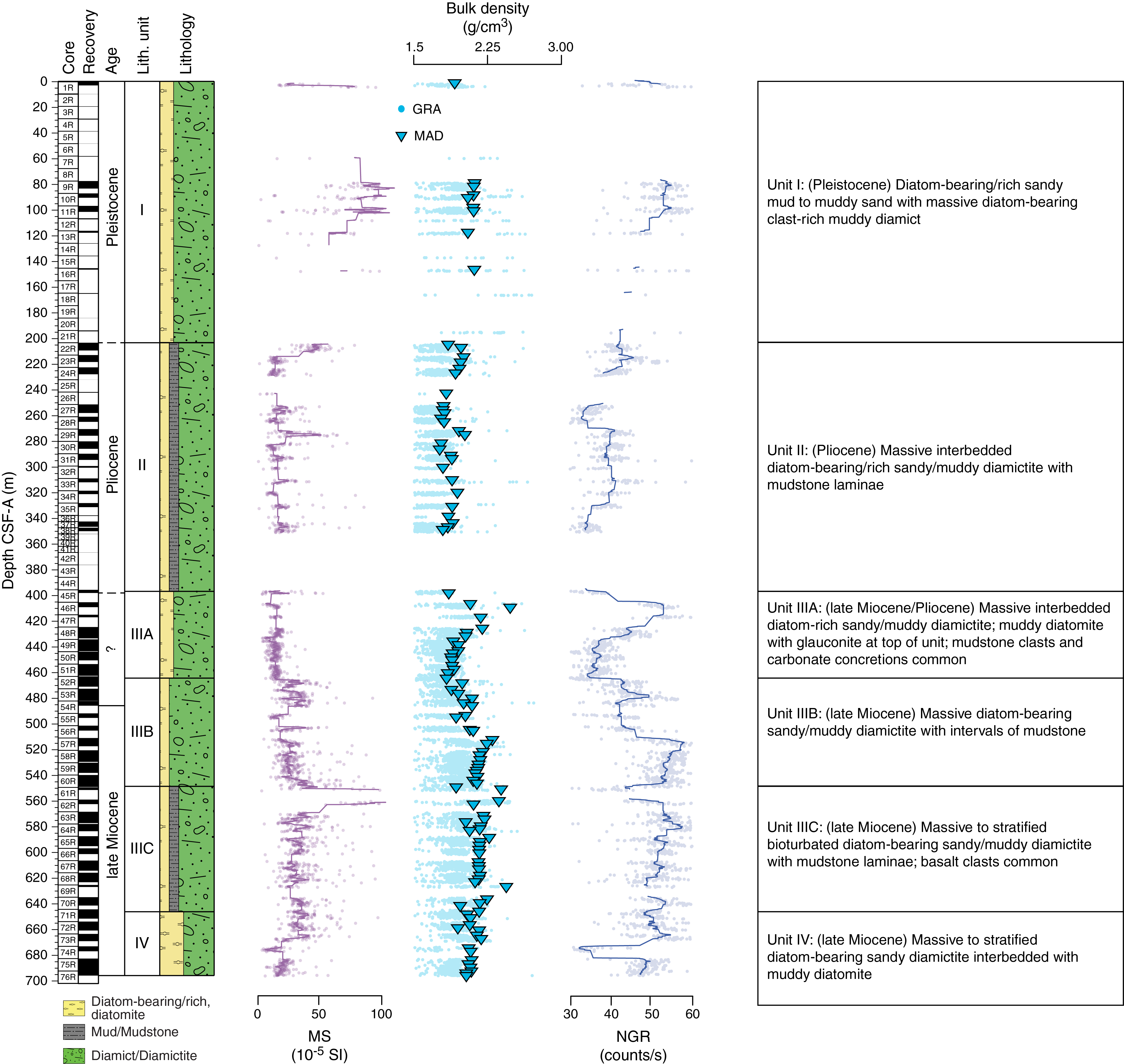
Figure F5. Lithostratigraphic summary.
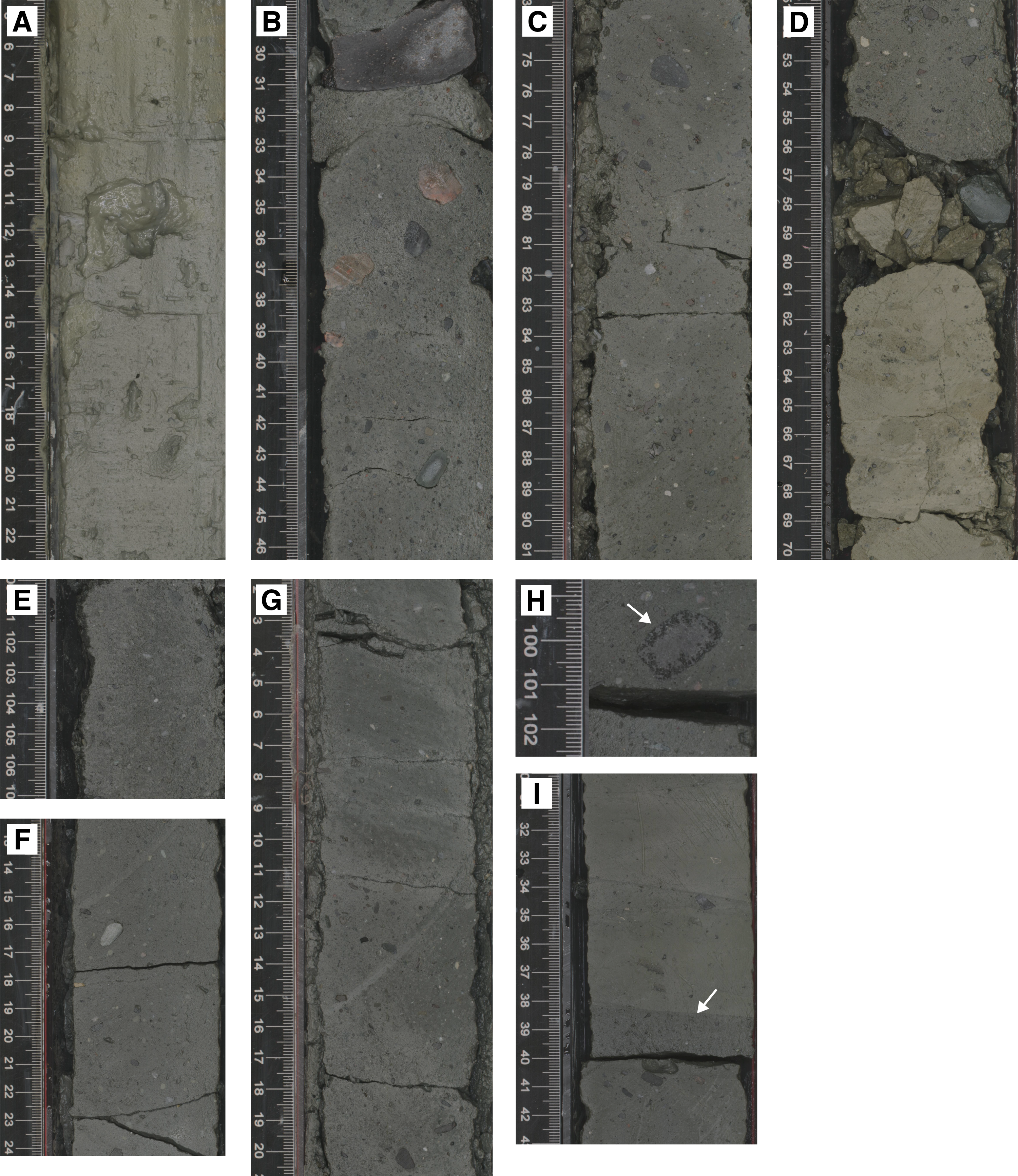
Figure F6. Primary lithologies.
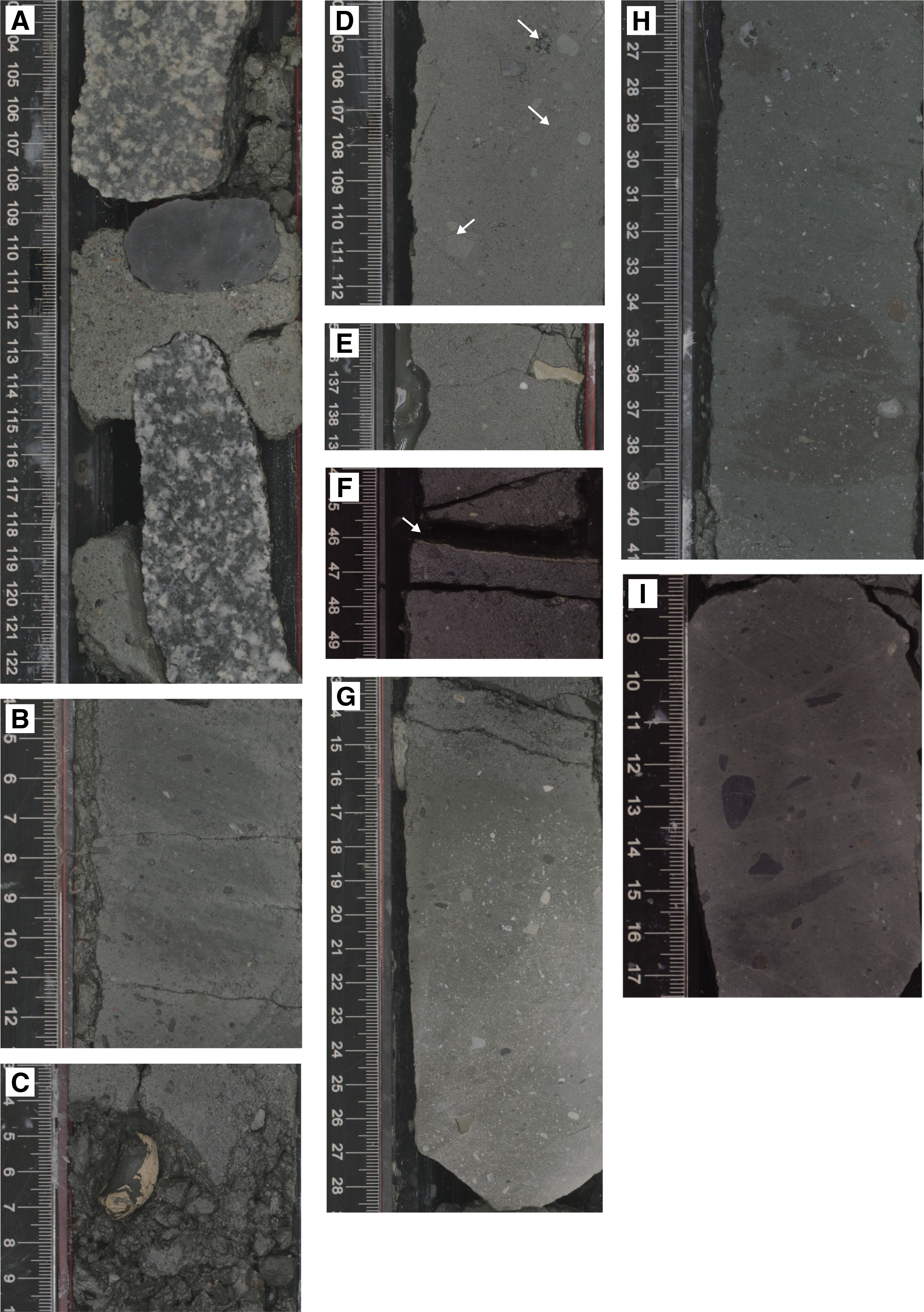
Figure F7. Sedimentary structures and diagenetic features.
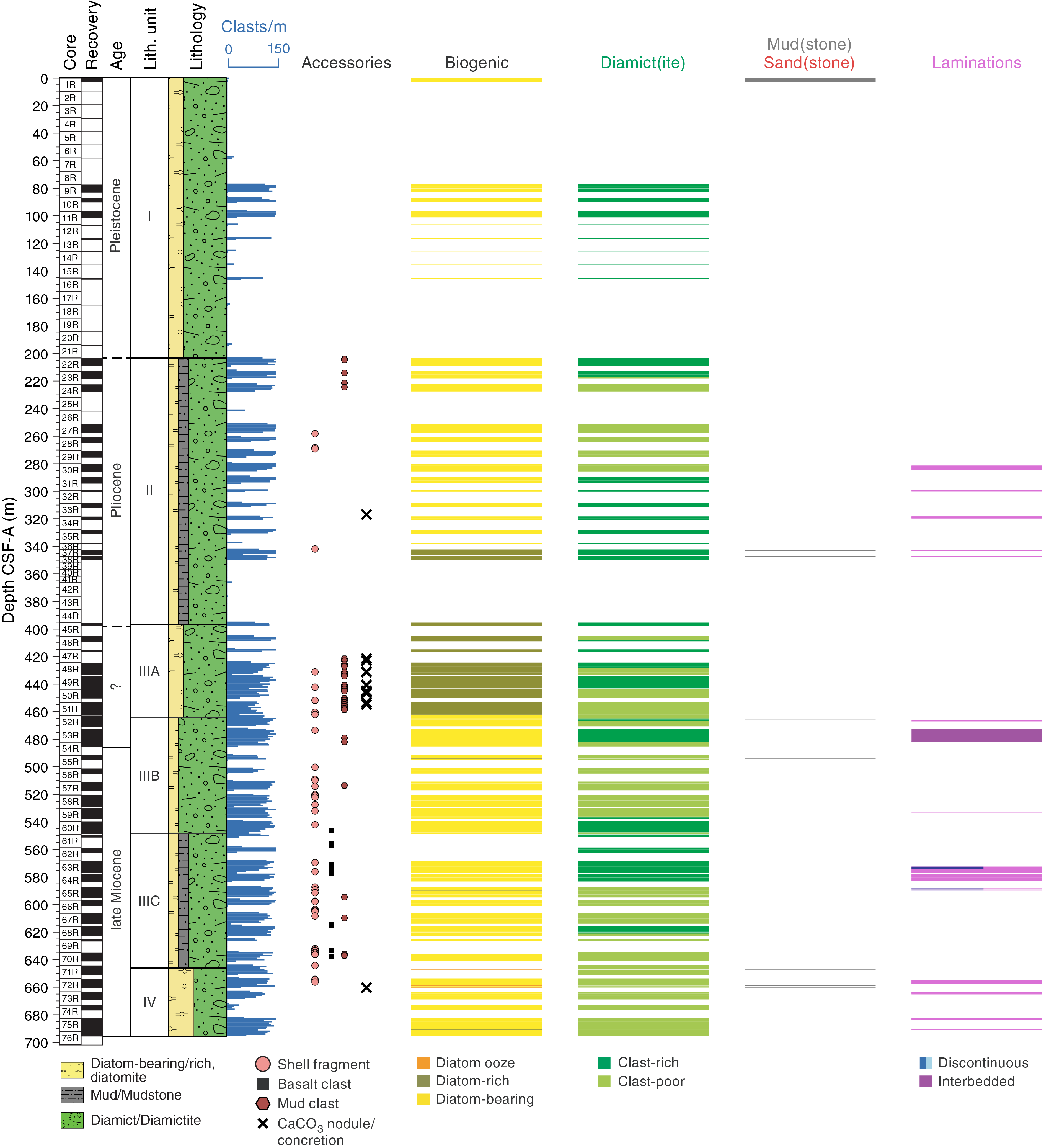
Figure F8. Lithology and sedimentary structures.
Unit descriptions
Site U1522 is dominated by massive diatom-bearing diamictite, but subtle lithologic changes downhole allow definition of four lithostratigraphic units (I–IV; youngest to oldest) (Figure F5; Table T2). These units are derived from a combination of visual core description, microscopic examination of smear slides, and color spectral observations (see Lithostratigraphy in the Expedition 374 methods chapter [McKay et al., 2019a]). Unit III is divided into three subunits (IIIA–IIIC; youngest to oldest).
Unit I
- Interval: 374-U1522A-1R-1, 0 cm, to 22R-1, 0 cm
- Depth: 0–203.20 m CSF-A
- Thickness: 203.20 m
- Age: Pleistocene
- Lithology: diatom-rich sandy mud to muddy sand with dispersed clasts, massive diatom-bearing diamict
The upper 2.83 m of lithostratigraphic Unit I consists of unconsolidated olive yellow to gray diatom-bearing/rich sandy mud to muddy sand with dispersed clasts and gray diatom-bearing clast-rich muddy to sandy diamict (Figures F5, F6A, F8; Table T2). Between 2.83 and 203.20 m CSF-A, recovery is poor and cores consist of washed cobble and gravel caused by drilling disturbance (Figure F7A). Although drilling disturbance precludes determination of primary unit lithology, the formation is likely coarse grained (sand to gravel size) and unconsolidated. A few cores recovered intervals of massive semilithified dark gray diatom-bearing clast-rich muddy diamict with lithologically diverse angular to rounded clasts. The clasts are randomly distributed, with no apparent orientation (Figure F6B). Thus, poor recovery in Unit I likely relates to the washing away of unlithified diamict and sand-, gravel-, and/or diatom-rich lithologies during rotary coring. The base of Unit I is defined by increased diamict lithification. Recovery in Unit I is 23.52 m (12%).
Unit II
- Interval: 374-U1522A-22R-1, 0 cm, to 45R-2, 56 cm
- Depth: 203.20–397.58 m CSF-A
- Thickness: 194.38 m
- Age: Pliocene
- Lithology: massive diatom-bearing/rich diamictite
Lithostratigraphic Unit II consists of massive dark greenish gray to greenish gray diatom-bearing/rich sandy and muddy diamictite with interbedded clast-rich and clast-poor intervals over tens of meters thick (Figures F5, F6C, F8; Table T2). Diatom-bearing mudstone and deformed (physically intermixed; Krissek et al., 2007) discontinuous mudstone laminae to thin (~1–2 cm) beds are occasionally observed in the muddy diamictite. Faint vein networks, distinguishable by matrix color variations, occur in the sandy diamictite. Clasts are diverse in size, lithology, and shape (rounded to angular). Mud and chert clasts occur in the upper ~60 m of Unit II (203.20–261.35 m CSF-A), and carbonate concretions and cements occur in the lower part of the unit (223.61–397.58 m CSF-A). Poor recovery in Cores 374-U1522A-25R and 26R (232.00–242.09 m CSF-A) and 39R through 44R (352.00–385.80 m CSF-A) is likely caused by large percentages of sand- to cobble-sized grains in the formation and washout during coring. The bottom of Unit II (397.58 m CSF-A) is defined by a sharp, brecciated contact between the massive clast-rich sandy diamictite of Unit II and diatomite at the top of Unit III (Figure F6D). Recovery in Unit II is 63.10 m (32%).
Unit III
- Interval: 374-U1522A-45R-2, 56 cm, to 71R-2, 131 cm
- Depth: 397.58–646.93 m CSF-A
- Thickness: 249.35 m
- Age: late Miocene
- Lithology: diatomite, diatom-bearing mudstone, massive diatom-bearing/rich diamictite
Lithostratigraphic Unit III consists of diatomite, diatom-bearing mudstone, and diatom-bearing/rich diamictite (Figures F5, F6D–F6H, F8; Table T2) and is divided into three subunits based on the style of interbedding and lithologic accessories (Figures F5, F8; Table T2). Clasts occur throughout, but clast assemblage and composition vary between subunits. Recovery in Unit III is 158.67 m (64%).
Subunit IIIA
- Interval: 374-U1522A-45R-2, 56 cm, to 52R-2, 72 cm
- Depth: 397.58–465.08 m CSF-A
- Thickness: 67.50 m
- Age: late Miocene to Pliocene?
- Lithology: muddy diatomite, massive diatom-rich diamictite
Lithostratigraphic Subunit IIIA consists of massive bioturbated greenish gray muddy diatomite with glauconite (interval 374-U1522A-45R-2, 56 cm, through Core 45R-CC) and interbedded massive dark greenish gray diatom-bearing/rich sandy and muddy diamictite with variable clast abundance (clast poor to clast rich) (Figures F5, F6D–F6F, F8; Table T2). Rounded to subrounded mudstone clasts 2 mm to >1 cm in diameter are common in the diamictite (Figure F7D). Carbonate cement, carbonate concretions, and shell fragments occur throughout (Figure F7E), and a distinct pyritized burrow occurs in interval 48R-1A, 46–47 cm (Figure F7F). The diversity of clast lithologies decreases in Subunit IIIA relative to Units I and II. The base of Subunit IIIA is characterized by a wavy (possibly physically intermixed) contact between massive dark greenish gray diatom-rich sandy diamictite and very dark greenish gray diatom-bearing sandy diamictite. Recovery in Subunit IIIA is 42.16 m (63%).
Subunit IIIB
- Interval: 374-U1522A-52R-2, 72 cm, to 60R-7, 57 cm
- Depth: 465.08–548.37 m CSF-A
- Thickness: 83.29 m
- Age: late Miocene
- Lithology: massive diatom-bearing diamictite, diatom-bearing/rich mudstone
Lithostratigraphic Subunit IIIB consists of interbedded very dark to dark greenish gray diatom-bearing sandy and muddy diamictite (Figures F5, F6G, F8; Table T2). The upper part of the subunit (Sections 374-U1522A-52R-2A through 52R-5A) is physically intermixed with Subunit IIIA. A distinct carbonate-cemented mudstone occurs in interval 52R-3A, 15–29 cm (Figure F7G). Soft-sediment deformation, faint laminations, shell fragments, and physical intermixing are common (Figure F7B, F7C, F7H). The base of Subunit IIIB is characterized by a sharp contact between sandy and muddy diamictite and color and clast lithology changes in interval 60R-7A, 57 cm. Recovery in Subunit IIIB is 58.00 m (70%).
Subunit IIIC
- Interval: 374-U1522A-60R-7, 57 cm, to 71R-2, 131 cm
- Depth: 548.37–646.93 m CSF-A
- Thickness: 98.56 m
- Age: late Miocene
- Lithology: massive to stratified diatom-bearing diamictite, mudstone
Lithostratigraphic Subunit IIIC consists of dark to very dark greenish gray diatom-bearing sandy to muddy diamictite (Figures F5, F8; Table T2). This subunit contains stratified diamictite with mudstone laminae and matrix color changes (faint in some places) and massive diamictite. Bioturbation occurs throughout. Basalt clasts are common (Figure F6H). The base of Subunit IIIC is defined by stratified diamictite, massive diamictite, and mudstone interbedded at the centimeter to decimeter scale. Recovery in Subunit IIIC is 58.51 m (59%).
Unit IV
- Interval: 374-U1522A-71R-2, 131 cm, to 76R-CC, 23 cm
- Depth: 646.93–695.74 m CSF-A
- Thickness: 48.81 m
- Age: late Miocene
- Lithology: massive to stratified diatom-bearing diamictite, diatom-rich mudstone, muddy diatomite
Lithostratigraphic Unit IV consists of massive very dark greenish gray diatom-bearing sandy diamictite (e.g., Section 374-U1522A-72R-4) and greenish gray diatom-rich mudstone to muddy diatomite interbedded at the decimeter to meter scale (Figures F5, F6I, F8; Table T2). Contacts vary from sharp planar (e.g., interval 71R-3A, 38 cm) to wavy (e.g., interval 72R-3A, 49–51 cm). Discontinuous mud laminae and vein networks are observed (Figure F7I). Bioturbation and shell fragments occur throughout. Recovery in Unit IV is 34.28 m (62%).
Facies distribution
At Site U1522, four main lithofacies are identified based on common lithologic, sedimentary, and textural characteristics. These lithofacies largely conform with Lithofacies 1–3 and 5 as described for Site U1521 (Table T3):
- Facies 1, massive diamictite;
- Facies 2, stratified diamictite;
- Facies 3, mudstone; and
- Facies 5, diatomite.
The facies scheme used here is described in detail in Lithostratigraphy in the Site U1521 chapter (McKay et al., 2019c) and modified from the scheme developed by Krissek et al. (2007).
Diagenesis
Silica cement fills faint vein networks, particularly in the diamictite and mudstone of Units II–IV. Bacterial decomposition of organic matter results in sulfate reduction and the precipitation of pyrite. Pyritized burrows are observed in Subunit IIIA (Figure F7F). Authigenic carbonate concretions and cements associated with sulfate reduction (see Geochemistry and microbiology) are also observed. In general, carbonate cement is more abundant in mudstone and concretions are present in diamictite. In some intervals (e.g., Subunit IIIA), siderite rims are observed around calcite-rich clasts and carbonate concretions.
Bulk mineralogy
X-ray diffraction (XRD) analyses of 13 powdered bulk samples from Hole U1522A were completed to semiquantitatively estimate the relative abundances of the most common mineralogical components. Diffraction patterns are shown in Figure F9, and the peak intensities (defined in Lithostratigraphy in the Expedition 374 methods chapter [McKay et al., 2019a]) reflect the relative presence/abundance of minerals. Generally, the Site U1522 downhole mineralogy is similar to that of Site U1521. Primary minerals include quartz and plagioclase; muscovite/illite, kaolinite/chlorite, and calcite are also present. The relative abundances of plagioclase and illite/mica vary downhole.
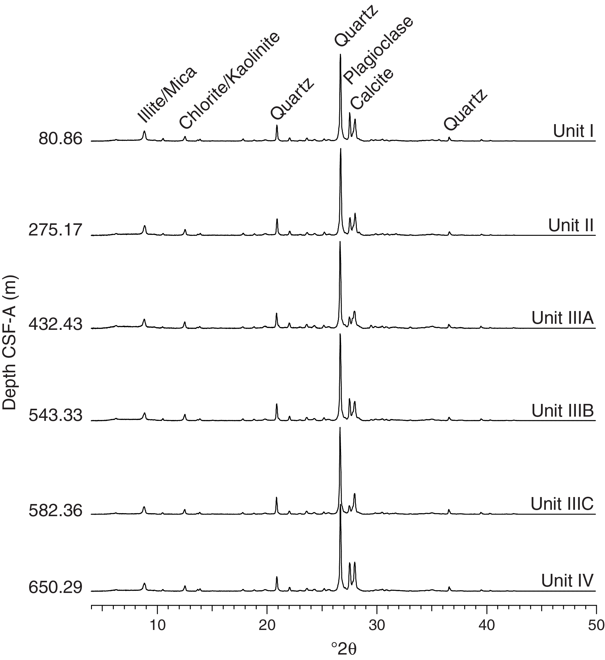
Figure F9. XRD patterns.
Preliminary depositional interpretation
Coring at Site U1522 recovered a discontinuous sequence of late Miocene to Pleistocene sediments and sedimentary rocks from the outer continental shelf of the Ross Sea (Figures F5, F8; Table T2), that indicates a series of glacial advances and retreats. Massive to stratified diamictite interbedded with diatomite (Unit IV) suggests an alternating sequence of grounding-line proximal to ice-distal glaciomarine deposition during the late Miocene. Units I–III contain diatom-bearing/rich massive/stratified diamictite interbedded with diatom-bearing/rich mudstone. The persistent diatom presence in the diamictite indicates glacial erosion and reworking of preexisting marine deposits, which may have been eroded by glacial advances across the outer continental shelf, and/or hemipelagic glaciomarine deposition. Core recovery may be biased toward lithified diamictite because softer or less consolidated facies (e.g., conglomerate/gravel, mud, and diatom ooze) are more susceptible to wash out during RCB coring, particularly when large clasts jam the drill bit. Poor core recovery and washed cobbles in Units I and II may indicate unconsolidated lithologies interbedded with more lithified diamictite facies. As such, Site U1522 records ice-proximal glaciomarine depositional environments associated with glacial advance and retreat across the Ross Sea continental shelf.
Biostratigraphy and paleontology
Microfossil assemblages at Site U1522 are represented by siliceous (diatoms, radiolarians, silicoflagellates, ebridians, and chrysophycean cysts), calcareous (foraminifers), and organic (dinoflagellate cysts [dinocysts] and other aquatic palynomorphs, pollen, and spores) remains. These occur in stratigraphic intervals dominated by (1) reworked assemblages of mixed ages, (2) modified assemblages altered by glacial and marine processes that concentrated robust taxa and removed fragile and weakly silicified taxa, or (3) in situ assemblages resulting from initial production and sedimentation (Figure F10). Features used to infer a primary or in situ (not reworked or modified) assemblage include state of preservation, continuity of taxon stratigraphic ranges, elevated abundance of delicate species relative to robust taxa, and short-ranging species relative to long-ranging taxa. These indexes help identify core intervals where fossil occurrences can be interpreted and applied with confidence in biostratigraphic, paleoenvironmental, and paleoceanographic analyses.
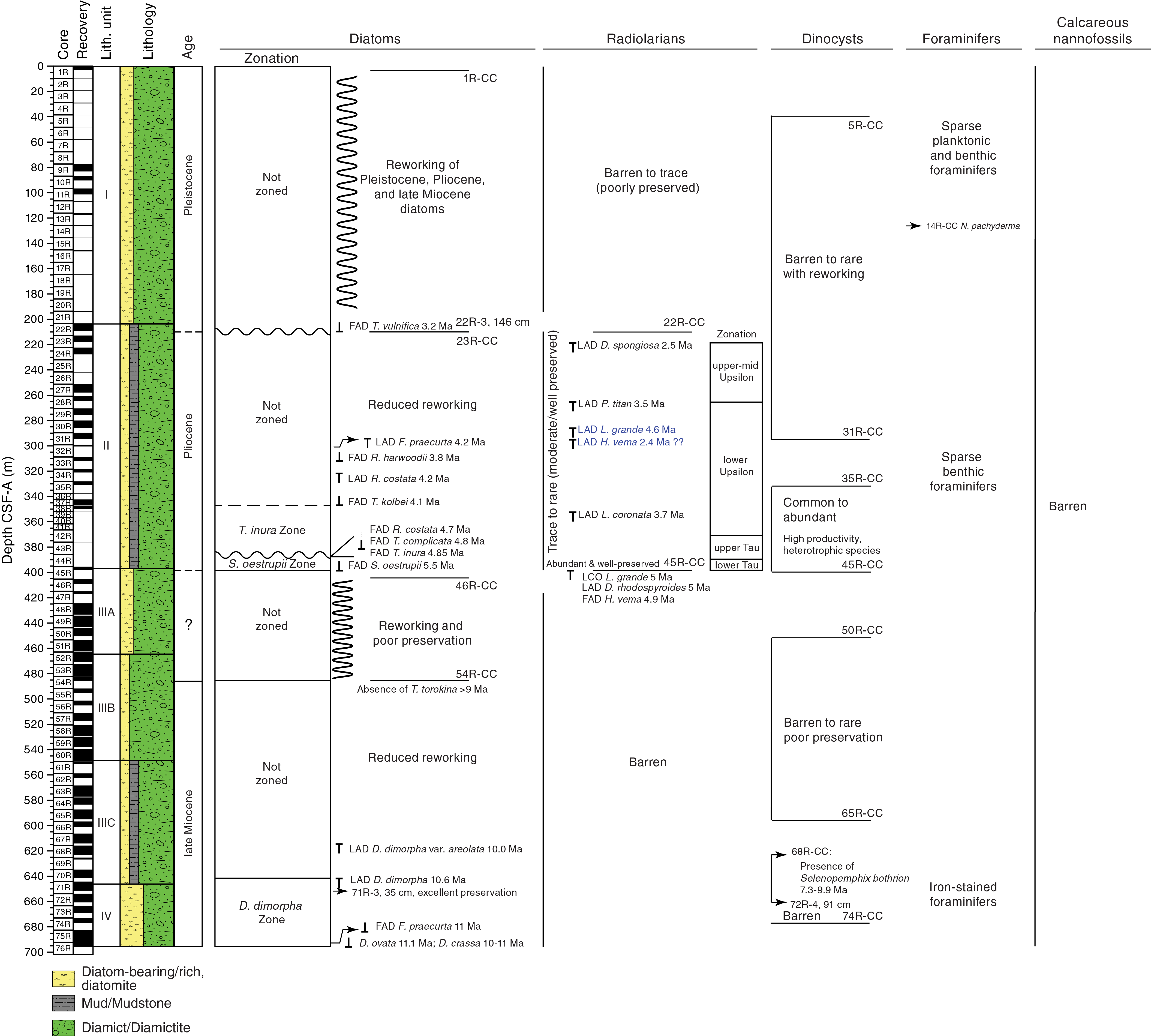
Figure F10. Micropaleontology summary.
Reworking of microfossils is pervasive through two intervals at Site U1522: Samples 374-U1522A-1R-CC to 22R-3, 146 cm (2.78–207.66 m CSF-A) and 46R-CC to 54R-CC (405.20–482.10 m CSF-A). As a means of demonstrating this reworking, Figure F11 presents the stratigraphic occurrence of selected microfossils from Site U1522 with the known ages for first appearance datum (FAD) and last appearance datum (LAD) events. Although a general downhole increase in age is indicated, reworking masks a clear interpretation of biostratigraphic-based age for this upper interval.
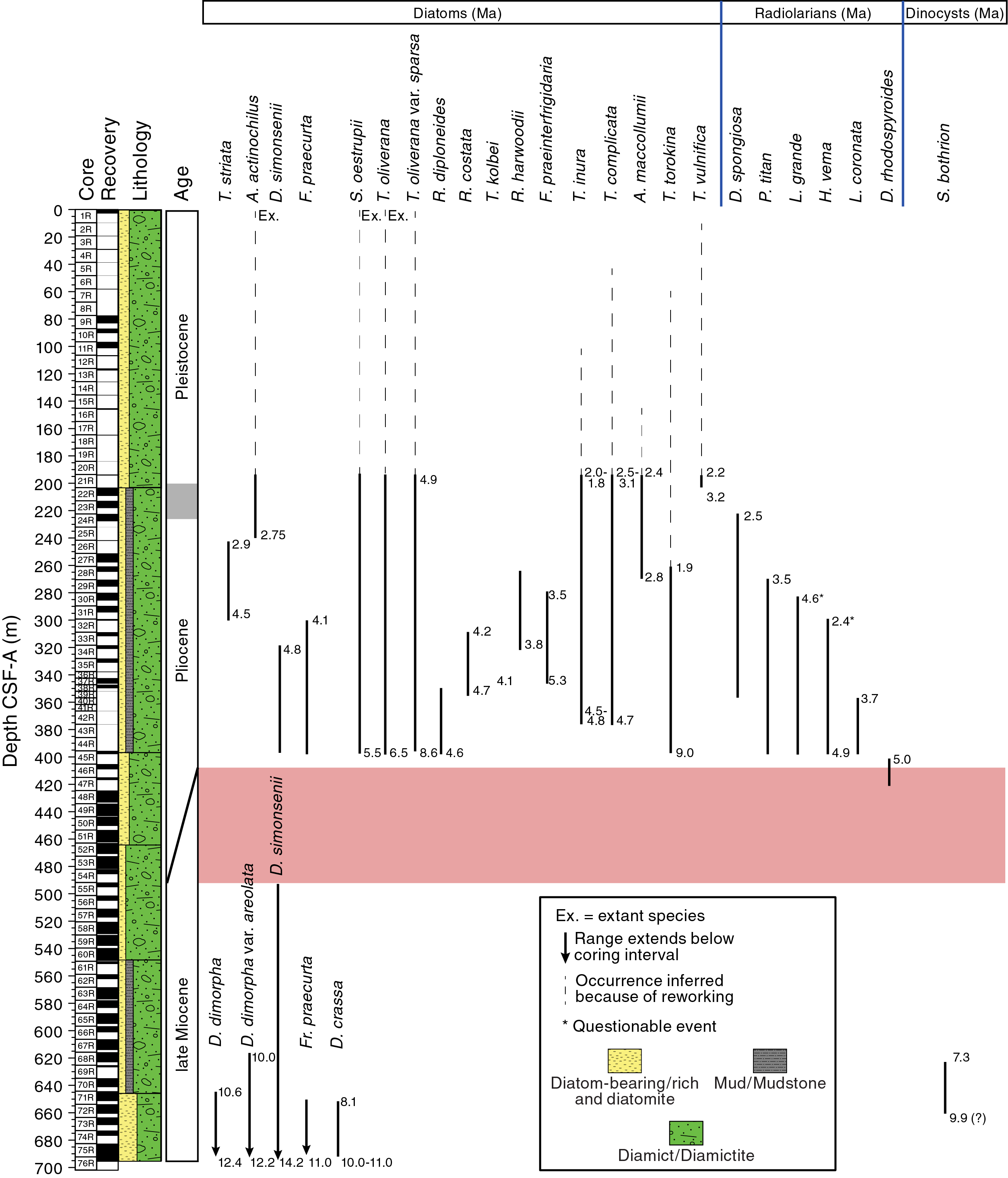
Figure F11. Selected diatom, radiolarian, and dinocyst distribution.
Site U1522 recovered an ~500 m thick discontinuous stratigraphic record from the upper Miocene (~11 Ma) to upper Pliocene (~2.5 Ma) with a disconformity of uncertain placement (between ~480 and ~400 m CSF-A) spanning from ~8.5 to ~5.5 Ma. The upper 200 m CSF-A comprises a poorly dated and poorly recovered interval of Pleistocene-age sediments.
Diatoms
Diatoms are present in all examined samples from Site U1522 (Table T4). Variation in assemblage abundance and composition reflects changes in the amount of diatoms supplied by glacial transportation or through original diatom production and sedimentation. Heavily silicified, robust diatoms that are dominant in some stratigraphic intervals are inferred to reflect modification and the mixing of different ages by glacial transport or marine bottom-current winnowing processes. This modification was described by Cunningham and Leventer (1998) and Cunningham et al. (1999) to explain the “extinct and/or heavily silicified assemblage,” which is composed of an assemblage that includes Paralia, Stephanopyxis, and other fossil taxa in Ross Sea surface and shallow sediments that were reworked by sedimentological processes. Similarly, Kellogg and Truesdale (1979) associated the concentration of Eucampia antarctica and Paralia sp. in their “transition assemblage” with the winnowing of small diatoms from older sediments by bottom currents during ice recession. Sjunneskog and Scherer (2005) distinguished different diamicton units in the Ross Sea, all of which are enriched in robust, reworked valves of long-ranging taxa such as Paralia, Stephanopyxis, and Stellarima, based on variable occurrence of shorter ranging diatom taxa.
The age of Site U1522 samples is established for intervals with prevalent reworking by invoking a “younger than” constraint: applying the FAD age of the youngest identifiable diatoms present. Common and distinctive taxa that proved useful in this regard are Thalassiosira vulnifica (FAD at 3.2 Ma) for intervals above Sample 374-U1522A-22R-3, 146–151 cm (207.66 m CSF-A), Thalassiosira complicata (FAD at 4.5 Ma) for intervals above Sample 43R-CC (376.10 m CSF-A), and Shionodiscus oestrupii (FAD at 5.5 Ma) and Thalassiosira oliverana var. sparsa (FAD at 8.7 Ma) for intervals above Sample 45R-CC (397.87 m CSF-A).
In contrast, several discrete intervals of diatom-bearing sediments are interpreted to represent primary in situ (not reworked) assemblages that can provide direct age constraint using standard biostratigraphic approaches. Several of these intervals are noted between Samples 374-U1522A-23R-CC and 45R-CC (218.12–397.87 m CSF-A) and between Samples 70R-5, 69–74 cm, and 76R-CC (641.27–695.69 m CSF-A). Exceptionally well preserved diatom assemblages are noted in Samples 45R-CC (397.87 m CSF-A) and 71R-3, 35 cm (647.38 m CSF-A).
Samples 374-U1522A-1R-CC to 22R-3, 146–151 cm (2.78–207.66 m CSF-A) contain a mixture of reworked and highly fragmented Pliocene and Miocene diatoms, silicoflagellates, and ebridian loricae mixed with Pleistocene taxa (Figure F10). The only definitive statement regarding the age of this interval is that it is younger than 3.2 Ma based on the persistent presence of reworked specimens of T. vulnifica, which first appears at ~3.2 Ma in Southern Ocean and Antarctic shelf records. Other Pliocene to Pleistocene diatoms present in this interval include T. complicata, Thalassiosira inura, Thalassiosira fasciculata, and Thalassiosira kolbei. A late Miocene to Pliocene diatom, T. oliverana var. sparsa, is dominant in this reworked flora, along with specimens of generally robust Paralia sulcata, Actinocyclus spp., Stephanopyxis spp., Thalassiosira torokina, E. antarctica, Coscinodiscus spp., Trinacria spp., Stellarima microtrias, and the silicified loricae of the ebridian Pseudammodochium lingii. Species of the genus Fragilariopsis, which usually make up a rich component of the diverse and abundant Antarctic Pleistocene and Pliocene diatom flora in the Southern Ocean and Antarctic continental shelf (Medlin and Priddle, 1990), are uncharacteristically absent from these assemblages, either because of environmental exclusion or their ease of winnowing or dissolution/diminution. It is not possible to determine what portion of the diatom flora might represent an in situ assemblage because any “native” assemblage that could be reflective of the age of the cored interval is masked by severe fragmentation or dissolution and by the flood of reworked specimens of older ages. A sufficient number of whole, identifiable specimens could only be recovered by sieving through a >20 µm screen. Raw, suspended sediment mounted on a “strewn slide” was routinely examined for the presence of smaller diatoms and to assess relative abundances and diatom occurrence. However, this material comprised largely unidentifiable clay- to very fine silt–sized particles and diatom fragments. The abundance of diatoms increases in Samples 13R-CC to 16R-CC (117.58–146.23 m CSF-A).
Sample 374-U1522A-22R-3, 146–151 cm (207.66 m CFS-A), contains a slightly different diatom assemblage with the addition of Actinocyclus fasciculatus, which may reflect either a different source of reworking or a brief window into a stratigraphic interval close to the 2.1–2.7 Ma range of A. fasciculatus. Two other intervals where age-diagnostic taxa make a brief appearance are noted. Rhizosolenia harwoodii (FAD 3.8 Ma) is present in Samples 28R-CC to 33R-CC (264.71–311.73 m CSF-A), suggesting a <3.8 Ma age based on its lowest occurrence. Rhizosolenia costata (4.2–4.7 Ma) is found in Samples 34R-CC to 43R-CC (318.4–376.1 m CSF-A), indicating an age of ~4.2 Ma for its highest occurrence and younger than 4.7 Ma for its lowest occurrence (Tables T4, T5; Figures F10, F11).
Diatom abundance is high in Samples 374-U1522A-23R-CC to 43R-CC (218.12–376.10 m CSF-A), and these assemblages contain fewer reworked elements. The base of the T. inura Zone is identified by the FAD of T. inura in Sample 43R-CC (376.10 m CSF-A); however, the coincident basal ranges of R. costata, T. complicata, and T. inura suggest the lower portion of this zone is missing because of a disconformity. The upper boundary of the T. inura Zone cannot be identified because Fragilariopsis barroni, which defines the upper boundary, is not identified at Site U1522. This boundary is tentatively drawn at the FAD of T. kolbei (FAD at 4.1 Ma) in Sample 37R-CC (346.42 m CSF-A) (Figure F10).
The Shionodiscus oestrupii Zone is identified in one sample, the interval from the FAD of S. oestrupii in Sample 374-U1522A-45R-CC (397.87 m CSF-A) up to the FAD of T. inura in Sample 43R-CC (376.10 m CSF-A). Sample 45R-CC (397.87 m CSF-A) contains a rich and extremely well preserved assemblage of lightly silicified diatoms, including Rouxia diploneides, Thalassiothrix, and abundant specimens of Fragilariopsis spp.
The interval between Samples 374-U1522A-46R-CC and 54R-CC (408.98–485.54 m CSF-A) contains poorly preserved, “residual” assemblages of reworked diatom valves comprising heavily silicified taxa of the genera Paralia, Coscinodiscus, Stephanopyxis, Actinoptychus, and Trinacria, as well as Actinocyclus ingens and ebridian Pseudammodochium lingii (Figure F10). The age of this interval is established only by the bracketing of dated intervals above and below because no biostratigraphic marker taxa are yet identified. The age of the source of reworked sediment is likely middle to late Miocene, as indicated by the presence of reworked specimens of Denticulopsis maccollumii (14.3–16.7 Ma).
Sample 374-U1522A-55R-CC (494.97 m CSF-A) contains a well-preserved and diverse assemblage of diatoms that are interpreted to be an in situ assemblage, but no biostratigraphic marker taxa are yet identified. Biostratigraphic control is sparse, even though diatoms are common and relatively well preserved. The absence of Thalassiosira torokina (FAD at 9.0 Ma), a diatom well represented in Antarctic continental shelf and Southern Ocean sites, suggests an age older than ~9.0 Ma for Sample 55R-CC (494.97 m CSF-A) and deeper and may indicate time missing in association with the above interval of reworked assemblages (Samples 46R-CC to 54R-CC [408.98–485.45 m CSF-A]). Diatoms are sparse and in some intervals poorly preserved downhole to Sample 67R-CC (614.07 m CSF-A), where the LAD of Denticulopsis dimorpha var. areolata (older than 10.0 Ma) is noted (Figure F10). A number of related species offer age constraint from this interval to the bottom of the hole, including recognition of the D. dimorpha Zone (10.6–11.1 Ma) by the occurrence of D. dimorpha (FAD at 12.4 Ma and LAD at 10.6 Ma in Samples 75R-3, 56 cm, to 70R-5, 69–74 cm [686.02–641.29 m CSF-A]) in the absence of Denticulopsis praedimorpha (LAD at 11.2 Ma). The presence of Denticulopsis ovata (FAD at 11.1 Ma) and Denticulopsis crassa (FAD at ~10.0–11.0 Ma) in Sample 76R-CC (695.69 m CSF-A), the deepest sample examined at this site, supports this age (Figure F10). In addition to these diatoms, the absence of D. praedimorpha (LAD at 11.2 Ma) and Nitzschia denticuloides (LAD at 11.75 Ma), which are common and widespread in Southern Ocean and Antarctic continental shelf sediments, also suggests the deepest cored interval at Site U1522 is younger than 11.2 Ma. Collectively, these data suggest an ~11.0 Ma age for sediments recovered at the bottom of Hole U1522.
The abundance and composition of the preserved diatom assemblages reflect changes in the amount of diatoms supplied by glacial or oceanographic current transportation or through production in overlying waters and subsequent sedimentation. The dominance of robust species of Paralia, Coscinodiscus, Stephanopyxis, Actinoptychus, Trinacria, and A. ingens might represent a paleoenvironmental signal strongly dependent on glacial transport and/or bottom current processes, whereas species such as resting spores of Chaetoceros, Actinocyclus actinochilus, Actinocyclus octonarius, and several species of Fragilariopsis and Thalassiosira reflect variations of in situ paleoproductivity, as described in Sjunneskog and Scherer (2005).
Radiolarians
All core catcher samples from Hole U1522A were analyzed for radiolarian content. Samples are barren or contain poorly preserved radiolarians from the seafloor downhole to 207.66 m CSF-A (Samples 374-U1522A-1R-CC to 22R-3, 146–151 cm), with only a few samples containing trace abundances (Figure F10; Table T6). Samples 23R-CC to 45R-CC (218.12–397.87 m CSF-A) consistently contain radiolarians in trace to rare abundances with moderate preservation. Samples 33R-CC (311.73 m CSF-A) and, particularly, 45R-CC (397.87 m CSF-A) stand out in this interval, with higher abundances and good preservation. From 408.98 m CSF-A (Sample 46R-CC) to the bottom of the drilled sequence, core catcher samples are barren of radiolarians, with very few exceptions containing trace abundances. Photomicrographs of some of the taxa identified at this site are shown in Figures F12 and F13.
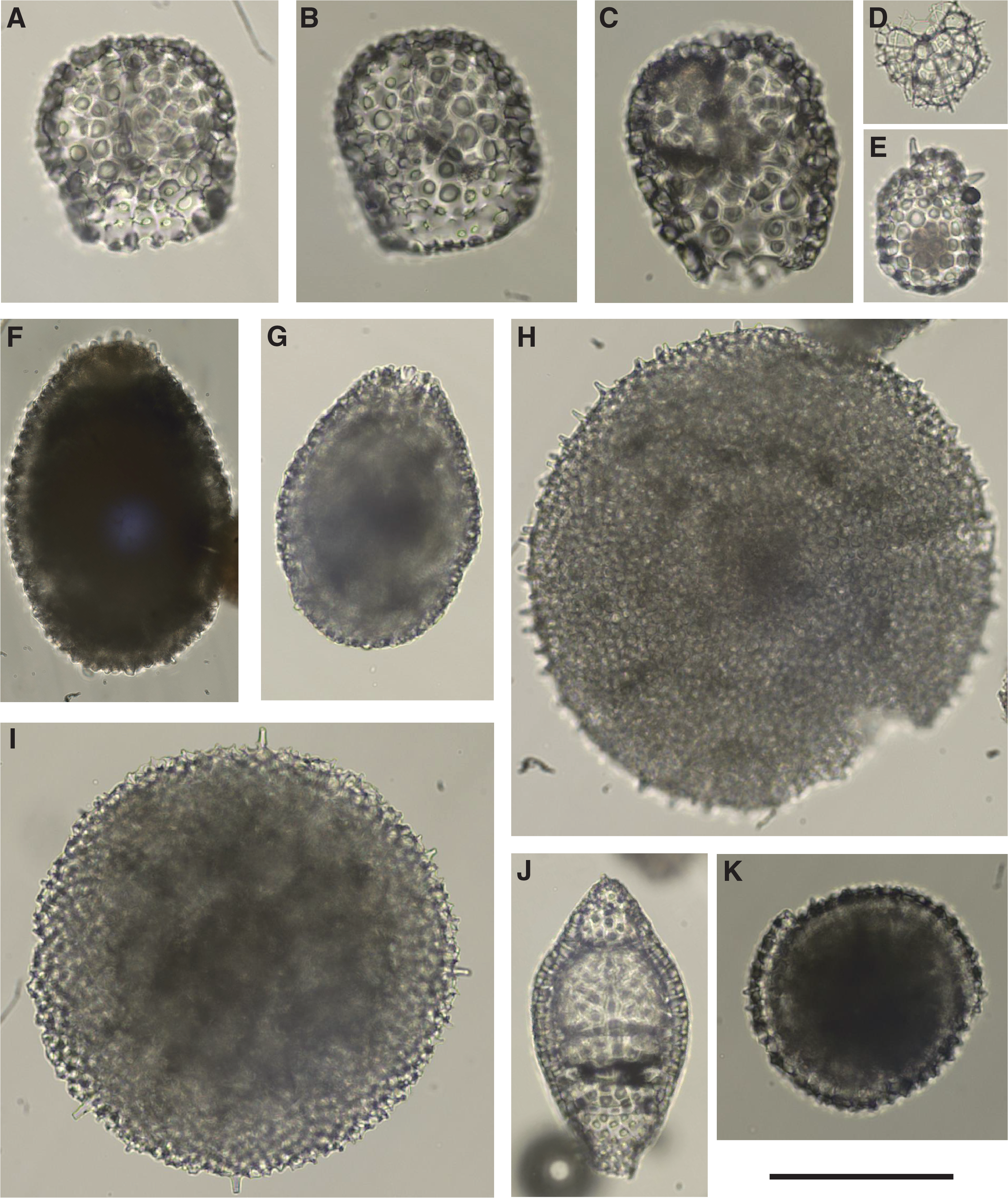
Figure F12. Radiolarians.
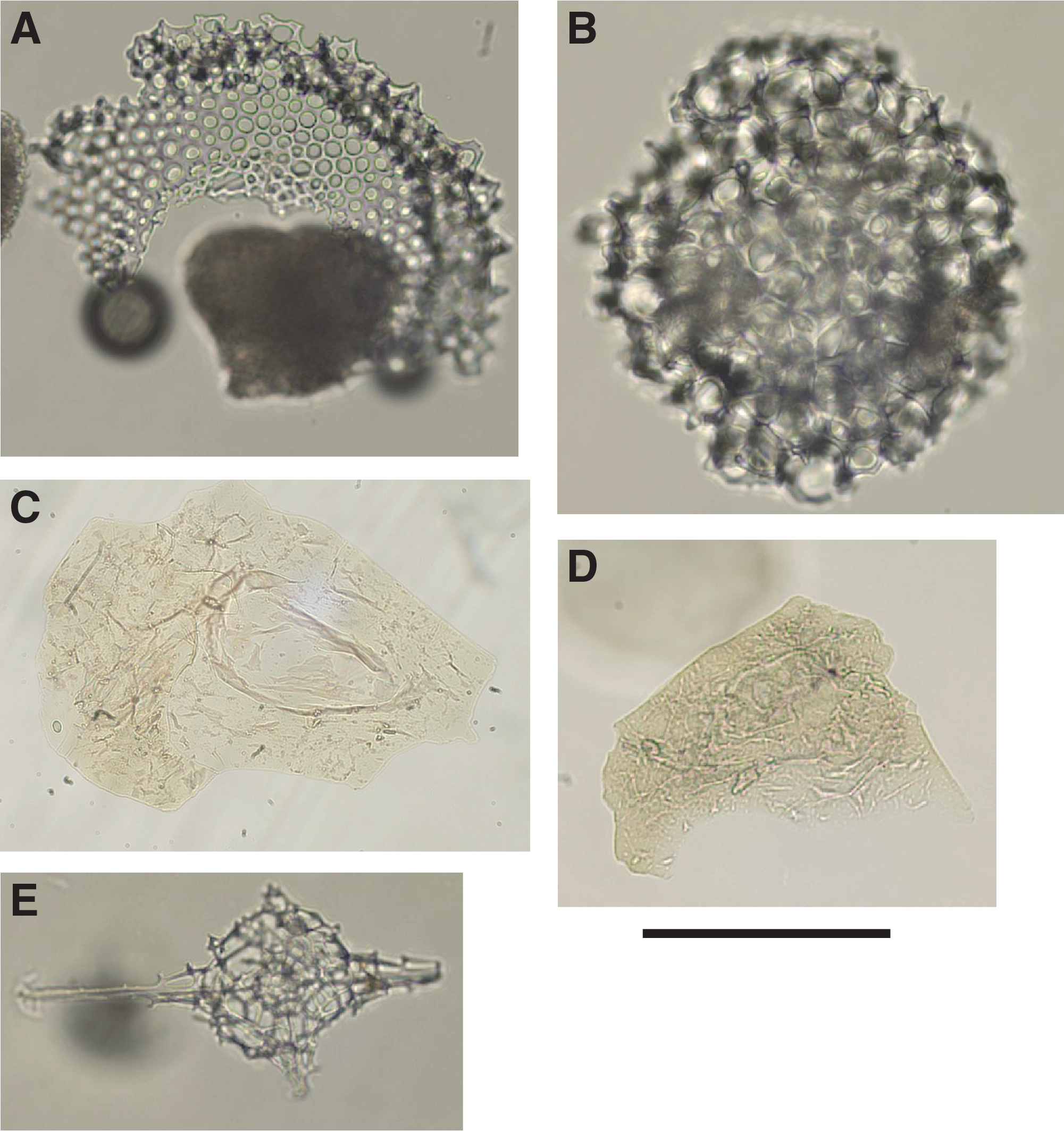
Figure F13. Radiolarians.
Age-diagnostic assemblages are noted in Sample 374-U1522A-1R-CC (2.78 m CSF-A; younger than 0.43 Ma?) and Samples 23R-CC to 45R-CC (218.12–397.87 m CSF-A), which contain radiolarian taxa that indicate an age range from 2.47 to 5.0 Ma (Pliocene) (Figures F10, F11). Noncellular membranes (phytoclasts), presumably derived from seaweed, are observed in the radiolarian residues between Samples 61R-CC (551.26 m CSF-A, where they are abundant) and 65R-CC (594.98 m CSF-A, where they are common) and in lower abundances downhole to the bottom of the drilled sequence.
The LAD of Lychnocanium grande is not included in the zonation of Lazarus (1992) but is calibrated by constrained optimization (CONOP) as one of the radiolarian datums used to develop an age model for Ocean Drilling Program (ODP) Site 744 (Florindo et al., 2013). At Site U1522, this biostratigraphic event is considered unreliable because in samples from shallower than 352.00 m CSF-A (Sample 39R-CC), only single specimens are observed and they might be reworked. The last common occurrence (LCO) of this species is preferred as a more reliably recognizable biostratigraphic event.
The utilization of the LAD of Helotholus vema (Sample 374-U1522A-31R-CC [294.37 m CSF-A]) is equally questionable at this site because the upper portion of the range of this species might be truncated based on the presence of only trace numbers of radiolarians in the analyzed samples in the upper Pliocene portion of the sequence. The LAD of H. vema usually only slightly predates the LAD of Desmospyris spongiosa, which occurs in Sample 23R-CC (218.12 m CSF-A). At Site U1522, the LAD of H. vema occurs well before the LAD of D. spongiosa. Moreover, the LAD of Prunopyle titan, which is used to divide the Upsilon Zone, occurs above (at or above Sample 28R-CC [264.71 m CSF-A]) the LAD of H. vema.
The interval from Core 374-U1522A-23R-CC through Core 45R-CC (218.12–397.87 m CSF-A) has good potential for shore-based sampling to refine the position of Pliocene radiolarian biostratigraphic events. Based on core catcher sample analyses, this interval was divided into the following subzones (as defined in Lazarus, 1992) (Figure F10):
- Upper/middle Upsilon Zone (2.47–3.53 Ma): Samples 23R-CC to 27R-CC (218.12–257.82 m CSF-A), based on the LAD of D. spongiosa;
- Lower Upsilon Zone (3.53–4.88 Ma): Samples 28R-CC to 39R-CC (264.71–352.00 m CSF-A), based on the co-occurrence of P. titan and H. vema;
- Upper Tau Zone (4.88–5.0 Ma): Sample 43R-CC (376.10 m CSF-A), based on its position above the LCO of L. grande; and
- Lower Tau Zone (>5.0 Ma): Sample 45R-CC (397.87 m CSF-A), based on the LAD of Desmospyris rhodospyroides and the LCO of L. grande.
Radiolarians are usually not preserved in the sediment at shallow-water locations, with the exception of specialized, low-diversity faunas that manage to thrive in such environments. In this respect, interesting evidence comes from microscopic examination of the mudline sample, which contains a modern assemblage, typical for the Antarctic continental shelf just outside the summer sea ice edge, as reported by Nishimura et al. (1997). This assemblage is made up almost exclusively of two radiolarian taxa: Rhizoplegma boreale and the Phormacantha hystrix/Plectacantha oikiskos group. The mudline sample at Site U1522 contains several specimens of R. boreale (~5% of the total radiolarian assemblage), a species which also occurs in high abundances (>9% of the total radiolarian assemblage) over a very short interval in piston Core MD95-2011 from the Norwegian Sea (Dolven and Bjørklund, 2001). This species has been associated with highly productive, coastal surface water from other high-latitude areas, including the Ross Sea, Antarctic Peninsula/Bransfield Strait, Prydz Bay, Dumont d’Urville Sea, Sea of Okhotsk, the Bering Sea, and the North Pacific Ocean. Nishimura et al. (1997) also report a more typical open-ocean radiolarian assemblage widely distributed around Antarctica, starting from just beyond the continental shelf break. This more diversified assemblage is indeed found in the mudline sample from Hole U1523A on the outermost continental shelf (see Biostratigraphy and paleontology in the Site U1523 chapter [McKay et al., 2019d] for further details). Detailed postcruise examination of late Pleistocene radiolarian occurrence and abundance data along a depth transect from the continental shelf to slope will therefore be interesting. This postcruise examination may potentially shed light on the utility of this group as indicators of open-ocean, complex food webs through time because such conditions will occur more frequently in deeper water locations compared with the continental shelf.
The evidence for phytoclasts/seaweed remains from Sample 374-U1522A-61R-CC (551.26 m CSF-A) and continuing downhole, if confirmed by other lines of evidence, might provide information on an abrupt change in provenance of coastal-derived sediment incorporated into diamictite over the deepest interval of the drilled sequence, deposited during the late Miocene (~10–11 Ma).
Foraminifers
Foraminifers are sparse in the section cored at Site U1522, and only a few of the samples examined shipboard are convincingly in situ based on the presence of well-preserved tests (Figure F10; Table T7). Many samples contain one or several variably preserved calcareous benthic foraminifer specimens. A significant number of samples did not yield any specimens during preliminary shipboard analysis. Agglutinated species are a minor component of the taxa recovered. Planktonic foraminifers are observed only in the Pleistocene interval of Site U1522. Preliminary results suggest that the foraminifer assemblages are mostly reworked at Site U1522.
The upper ~125 m of Site U1522 (from the seafloor to Sample 374-U1522A-14R-CC [0–125.97 m CSF-A]) contains very rare but generally well-preserved foraminifers (Figure F10). The presence of potassium feldspar as a common component of the sand residues throughout this interval is noteworthy. Glauconite is observed in Samples 1R-CC (2.78 m CSF-A) and 2R-CC (9.60 m CSF-A). Sample 14R-CC (125.97 m CSF-A) contains the largest in situ foraminifer assemblage recovered at Site U1522 and includes Angulogerina earlandi, Angulogerina pauperata, Astrononion antarcticus, Astrononion echolsi, Nonion germanicus, Elphidium magellanicum, Melonis barleeanus, Nonionella iridea, Lagena sp., and Oolina sp., as well as the planktonic foraminifers Neogloboquadrina pachyderma and Turborotalita quinqueloba.
Below Sample 374-U1522A-14R-CC (125.97 m CSF-A), grain provenance changes in the sand-sized fraction based on a decline in potassium feldspar and an increase in dark-colored chert and metamorphic grains. Foraminifers in this interval are represented by few specimens, which typically have broken final chambers, and tests that are chalky white or iron-stained. A quarter of the samples examined below Sample 14R-CC did not yield any foraminifer specimens during preliminary analysis. Possible in situ or mixed in situ and reworked assemblages are noted in Samples 29R-CC (275.49 m CSF-A), 55R-CC (494.97 m CSF-A), 68R-CC (623.11 m CSF-A), and 72R-4, 89–91 cm (658.93 m CSF-A), based on the nature of foraminifer preservation. The latter sample is from a diatom-rich interval. An abundance of glauconite is noted in Sample 45R-CC (397.87 m CSF-A) in association with abundant diatoms, radiolarians, and dinocysts.
Globocassidulina subglobosa is the most persistent foraminifer below Section 374-U1522A-14R-CC. Although represented by few specimens at Site U1522, other typical late Neogene calcareous benthic foraminifers known from the Ross Sea continental shelf include Cibicides temperatus, Cibicides refulgens, E. magellanicum, N. iridea, Ammoelphidiella uniforamina, Cassidulinoides porrectus, Ehrenbergina glabra, Epistominella exigua, Gavelinopsis lobatulus, and M. barleeanus (e.g., Fillon, 1974; Osterman and Kellogg, 1979; D’Agostino, 1980; Leckie and Webb, 1986; Patterson and Ishman, 2012). A few specimens of the agglutinated taxon Miliammina arenacea are noted in Samples 63R-CC (577.09 m CSF-A) and 72R-4, 89–91 cm (658.93 m CSF-A). This taxon has been associated with the Ross Ice Shelf front (Osterman and Kellogg, 1979). A reworked specimen of the endemic(?) Ross Sea Miocene planktonic foraminifer Antarcticella antarctica (Leckie and Webb, 1985) is noted in Sample 22R-3, 146–151 cm (207.66 m CSF-A).
Palynology
Nineteen sediment samples (from Sections 374-U1522A-5R-CC through 74R-CC [38.70–676.78 m CSF-A]) were analyzed for palynomorph content. Preservation varies from poor to good, and abundance varies substantially throughout the sequence (Table T8; Figure F10). Samples 374-U1522A-5R-CC to 31R-CC (38.70–294.37 m CSF-A) are devoid or almost devoid of palynomorphs (Figure F10). These samples contain only sparse numbers of Brigantedinium spp. cysts, some specimens of the dinocyst Vozzhennikovia sp. (reworked from older Eocene strata), and a more common occurrence of the acritarch Leiosphaeridia.
In Samples 374-U1522A-35R-CC (331.10 m CSF-A) and 45R-CC (397.87 m CSF-A), palynomorphs are common and abundant, respectively (Figure F10). Sample 45R-CC (397.87 m CSF-A) yields remarkably abundant dinocysts belonging to Brigantedinium spp., Brigantedinium sp. cf. Brigantedinium pynei, Islandinium sp., Impagidinium pallidum, Protoperidinium spp., Selenopemphix antarctica, and Selenopemphix nephroides. A single specimen of Achomosphaera sp. and one Invertocysta tabulata are also identified. A few specimens of Leiosphaeridia and Cymatiosphaera sp. are present. In general, the assemblage indicates environmental conditions similar to the present day (e.g., Prebble et al., 2013), with high primary productivity and the presence of sea ice. However, these assemblages have higher species diversity than in modern samples and include the presence of several phototrophic species, which may point to warmer waters and a shorter sea ice season.
The interval between Samples 374-U1522A-50R-CC and 65R-CC (450.36–594.98 m CSF-A) is characterized by poor preservation and rare occurrence of palynomorphs (Figure F10), with sparse Brigantedinium spp., Protoperidinium sp., S. nephroides, and the acritarch Leiosphaeridia.
In the interval between 623.11 and 660.65 m CSF-A, six samples were analyzed: three core catcher samples (374-U1522A-68R-CC, 70R-CC, and 72R-CC) and three additional samples: 70R-5, 69–74 cm (641.27 m CSF-A), 71R-3, 31–35 cm (647.34 m CSF-A), and 72R-4, 91–92 cm (658.95 m CSF-A). Palynomorphs are generally well preserved and occur in large numbers, except for Sample 70R-5, 69–74 cm, in which dinocyst abundance is remarkably low (Table T8; Figure F10). Palynomorphs include dinocysts, several morphotypes of foraminifer linings, pollen and spores, Prasinophytes (Cymatiosphaera sp.), and Leiosphaeridia (Figure F14). Dinocyst assemblages are dominated by heterotrophic species (Brigantedinium spp., Lejeunecysta spp., Protoperidinium spp., and Selenopemphix spp.), whereas phototrophic species are less diverse and abundant, only comprising some specimens of Operculodinium spp. and Batiacasphaera spp. The sea ice indicator species in modern Antarctic samples (e.g., Prebble et al., 2013; Zonneveld et al., 2013), S. antarctica, is rare. In general, the assemblage is suggestive of high productivity and probably reduced sea ice conditions compared to the present day. The occurrence of higher diversity in the Selenopemphix species at this site compared with Site U1521, together with the lower abundance and diversity of Lejeunecysta species, could potentially indicate a more distal marine paleoenvironment for Site U1522 than the more proximal environment (greater coastal influence) generally recorded for Site U1521.

Figure F14. Palynomorphs.
Samples 374-U1522A-68R-CC to 72R-4, 91–92 cm (623.11–658.95 m CSF-A), contain several specimens of the dinocyst Selenopemphix bothrion (Figures F10, F14), a species previously found exclusively in the sediment record of ODP Site 1095 between 7.3 and 9.9 Ma (Harland and Pudsey, 2002), therefore indicating a late Miocene age for this part of the Site U1522 sequence (Table T5). S. bothrion is not found in Samples 72R-CC and 74R-CC (660.65 and 676.78 m CSF-A). Sample 74R-CC (676.78 m CSF-A) contains rare and poorly preserved palynomorphs.
Calcareous nannofossils
Eleven samples between 125.97 and 660.65 m CSF-A (Samples 374-U1522A-14R-CC to 72R-CC) are barren of calcareous nannofossils (Table T9).
Age model
Important biostratigraphic events identified from diatom, radiolarian, and dinocyst analyses of Site U1522 sediments are compiled in Table T5. The depths and ages of FAD and LAD biostratigraphic events were used to construct the preliminary shipboard age-depth model for the site (Figure F15). The black lines in the figure represent the best fit for the available biostratigraphic events. An interval of uncertain age is identified in the pink rectangle, marking an interval where one or more disconformities are inferred but cannot be fully resolved. The majority of biostratigraphic events listed in Table T5 are accommodated by this interpretation, with only a few events (orange-outlined triangles in Figure F15) that may need further calibration to fit this age model interpretation for Site U1522.

Figure F15. Shipboard age model.
The upper 200 m of Site U1522 comprises a poorly dated and poorly recovered interval of Pleistocene age sediments downhole to Sample 374-U1522A-22R-CC (207.66 m CSF-A). This interval overlies an ~500 m thick interval of moderately well dated upper Pliocene to upper Miocene strata with a maximum age of ~11 Ma at the bottom of the section. A disconformity of uncertain placement (between ~480 and ~400 m CSF-A) spans from ~8.5 to ~5.5 Ma.
Paleomagnetism
Paleomagnetic investigations at Site U1522 focused on determining the characteristic remanent magnetization (ChRM) direction of the sediments to construct a magnetostratigraphy, with the goal of assisting with the chronostratigraphy for the site. Additional rock magnetic measurements were made to assess the stability and origin of the paleomagnetic record and to investigate the development of magnetic fabric from depositional and postdepositional processes.
Primary observations come from measuring the natural remanent magnetization (NRM) of most archive-half core sections at 5 cm intervals before and after alternating field (AF) demagnetization. For archive-half core sections from Cores 374-U1522A-1R through 55R (0–495.21 m CSF-A), NRM measurements followed AF demagnetization in 5 mT increments between 0 and 20 mT. To keep up with the core flow, the 15 mT peak AF demagnetization step was omitted beginning with Core 56R. The use of the RCB coring system to recover sediments at Site U1522 frequently yielded sediments (e.g., Cores 1R through 8R [0–67.60 m CSF-A]) that were too disturbed to be used for paleomagnetic purposes. Data were processed by removing disturbed intervals and data collected within 10 cm of section ends. The cleaned (relatively disturbance free) data set was used to construct a magnetostratigraphy, which was subsequently correlated to the geomagnetic polarity timescale (GPTS) of Gradstein et al. (2012), guided by independent biostratigraphic age control (see Biostratigraphy and paleontology).
To test the fidelity of the magnetostratigraphy generated on archive-half core sections, we also collected 107 oriented discrete paleomagnetic samples (~3 per core). Fourteen samples were progressively demagnetized using a 20-step AF demagnetization protocol (0–20 mT in 2 mT steps and 20–60 mT in 5 mT steps followed by 70 and 80 mT peak AF demagnetization) to determine the potential overprint(s) and stable remanent carrier(s). Declinations of archive-half core sections and discrete samples have no azimuthal orientation because RCB cores are unoriented and pieces of core commonly rotate inside the core barrel relative to each other.
Mean (bulk) magnetic susceptibility was measured on the discrete samples and compared with magnetic susceptibility measurements made on archive-half core sections using the Section Half Multisensor Logger (SHMSL) and on whole-round core sections with the Whole-Round Multisensor Logger (WRMSL). In addition, the anisotropy of magnetic susceptibility (AMS), which reflects changes in magnetic fabric that may be related to compaction, was determined (see Paleomagnetism in the Site U1521 chapter [McKay et al., 2019c]).
Natural remanent magnetization measurements
Archive-half measurements
In general, variations in the initial NRM intensity correlate well with variations in the WRMSL and SHMSL magnetic susceptibility, suggesting that these values all approximate variations in magnetic concentration. NRM inclinations prior to AF demagnetization are usually positive (Figure F16). After progressive AF demagnetization, both positive and negative inclinations occur and NRM intensity decreases by as much as one order of magnitude, with exceptions at the base of lithostratigraphic Subunit IIIB (Core 374-U1522A-60R [539.70–548.95 m CSF-A]) and the bottom of Unit IV (interval 75R-2, 20 cm, to 75R-3, 100 cm [684.24–686.46 m CSF-A]). The initial positive inclination, therefore, presumably represents a low-coercivity downward-directed overprint, which is common to IODP coring operations. However, we cannot exclude a low-coercivity primary or secondary component unrelated to drilling as carrier for the positive inclination signal.

Figure F16. Paleomagnetic data.
The positive and negative inclinations after 20 mT peak AF demagnetization suggest that at least some of these intervals may genuinely reflect normal and reversed polarity zones. If a geocentric axial dipole is assumed, the inclination should cluster around ±83.2° (the present-day latitude of Site U1522 is 76.5°S). The majority of the observed archive-half inclinations are somewhat shallower than expected, which is probably a reflection of suboptimal data quality at this site. Reasons could include depositional processes that are not conducive to recording a primary magnetization, relatively large magnetic grain sizes and associated low magnetic coercivities that make the sediments very susceptible to secondary remagnetization, and drilling overprints that are incompletely removed by AF demagnetization. We tentatively interpret the positive and negative inclination clusters as reversed and normal polarity zones and assess whether they provide credible correlations with the GPTS.
Discrete sample measurements
The oriented discrete samples were used to investigate the fidelity of the sediments in recording a primary magnetization. Despite the detailed 20-step AF demagnetization protocol, NRM directions become erratic after ~16 mT AF demagnetization, and very few samples have a demagnetization behavior that may correspond to a stable magnetic carrier (Figure F17). The first AF demagnetization step (2 mT peak AF) probably removes a small overprint. Progressive AF demagnetization up to 14–16 mT peak AF reveals scattered directions that retain their upward or downward directions (Figure F17A, F17C, F17D). Noisy demagnetization behavior occurs in intervals with low coercivity, often coinciding with high magnetic susceptibility values (Figure F17B), which is similar to observations made for Site U1521 (see Paleomagnetism in the Site U1521 chapter [McKay et al., 2019c]). We cautiously used samples with a potentially stable component (Figure F17A, F17C, F17D) for magnetostratigraphic interpretation and disregarded samples without a stable component (Figure F17B).

Figure F17. Representative AF demagnetization behavior.
Magnetostratigraphy
The inclination data from the relatively stable intervals have positive and negative inclinations that are tentatively interpreted as reversed and normal polarity zones, respectively (Figure F16), because Site U1522 is located in the Southern Hemisphere. We define five major reversed polarity zones (R1–R5) and five major normal polarity zones (N1–N5) that are divided into subzones (e.g., R5.1 and N4.1). The definition of these zones and subzones depends on core recovery and data quality. For example, no stable polarity could be identified between Zones R1 and R2. These zones are ~80 m apart, and we chose to separate them rather than speculatively identifying only one zone of reversed polarity. Note that poor core recovery and suboptimal data quality in the upper ~420 m CSF-A (Cores 374-U1522A-1R through 47R) frequently yield uncertain polarity (gray shading in the Polarity column of Figure F16).
From Core 374-U1522A-9R through Core 46R (77.30–409.03 m CSF-A), we identified reversed Zones R1 (Cores 9R through 13R [77.30–117.63 m CSF-A]) and R2 (Core 22R [203.20–209.24 m CSF-A]) and normal Zone N1 (Cores 27R through 46R [251.20–409.03 m CSF-A]). Below Core 47R (414.90 m CSF-A), we identified thick reversed Zone R3 (between Samples 48R-2, 95 cm, and 54R-3, 15 cm [426.90–485.03 m CSF-A]) and predominantly normal Zones N2, N3, N4, and N5 (Cores 57R through 60R [510.90–548.95 m CSF-A], 63R through 69R [568.30–626.78 m CSF-A], 71R through 73R [644.30–669.04 m CSF-A], and 75R and 76R [682.60–695.74 m CSF-A], respectively). Reversed Zone R4 occurs in partially disturbed Core 62R (558.80–562.36 m CSF-A) only. Thin reversed subzones occur in Cores 70R (Subzone R5.1) and 71R (Subzone R5.2). Further shore-based work is required to test whether the identified short reversed polarity subzones are genuine geomagnetic field behavior or artifacts of disturbance or overprinting.
Confident correlation of Zones R1–R5 to the GPTS requires independent age control, here provided by biostratigraphy (see Biostratigraphy and paleontology). Biostratigraphic datums indicate a Pleistocene to Pliocene age for lithostratigraphic Units I and II (0–397.58 m CSF-A). An interval of reworked diatoms precludes age assignment in Subunit IIIA and the upper part of Subunit IIIB (Cores 374-U1522A-46R through 54R [405.20–485.67 m CSF-A]), and a late Miocene age is suggested for the interval from the middle of Subunit IIIB to the base of Unit IV (491.7–695.74 m CSF-A). The poor recovery in Units I and II makes it difficult to confidently tie the magnetostratigraphy of the upper ~400 m CSF-A (Cores 1R through 45R) to the GPTS. The dominance of reworked species and subsequent lack of age control between Cores 46R and 54R also prohibits a confident correlation. Polarity Zone N2 is below the reworked interval but does not contain any definitive biostratigraphic markers, so its correlation to the GPTS is uncertain.
The available diatom age control between Cores 374-U1522A-66R and 76R suggests that the long normal polarity interval (Zones N3–N5) probably corresponds to Chron C5n (9.786–11.056 Ma) (Figure F16). Thin reversed polarity Subzones R5.1 and R5.2 can be correlated to the base of Chron C4Ar (9.105–9.786 Ma) if the diatom ages are assumed to be slightly too old, Subchron C5n.1r (9.937–9.984 Ma), or the rarely identified intervals of reversed polarity in Subchron C5n.2n (Evans et al., 2007). Further shore-based work is required to better constrain the ages so that we can confidently tie the thick normal intervals (Zones N3–N5) and the thin reversed intervals (Subzones R5.1 and R5.2) to the GPTS.
Magnetic susceptibility and AMS
We measured the mean magnetic susceptibility and determined the AMS tensor of all collected discrete samples. The inclination (vertical orientation) and magnitude of the maximum (kmax), intermediate (kint), and minimum (kmin) susceptibilities are plotted as a function of the core depth (Figure F18). The degree of anisotropy (P) is approximated by the kmax/kmin ratio, where P = 1 indicates no anisotropy and P > 1 indicates a high degree of anisotropy. We observed higher P values (greater than ~1.08; Figure F18) in lithostratigraphic Unit II, Subunit IIIC, and Unit IV and at the boundaries between Unit II and Subunit IIIA and between Subunit IIIC and Unit IV.
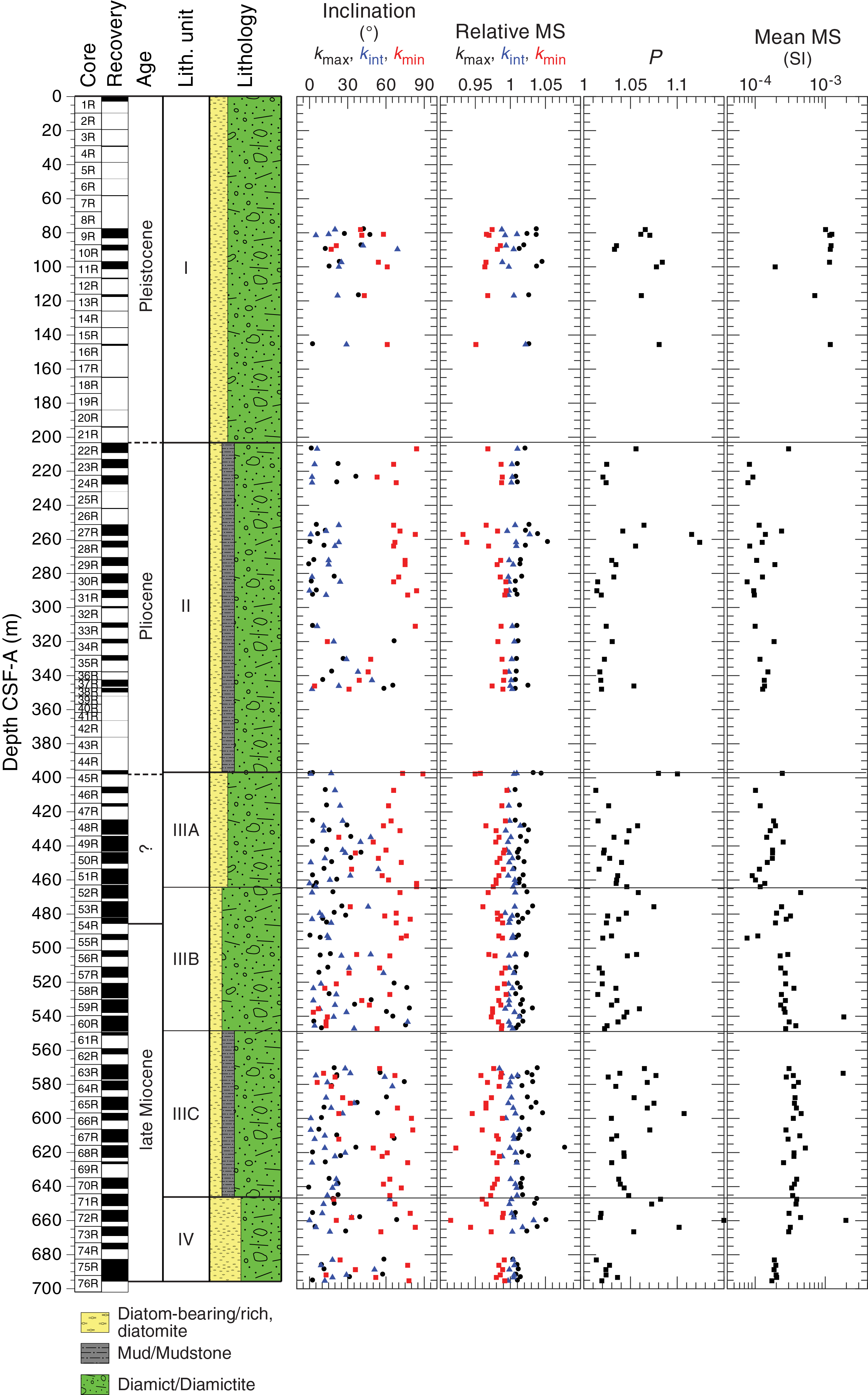
Figure F18. Anisotropy of magnetic susceptibility.
When P is >1 and kmin inclination is >60° (i.e., minimum susceptibility axis is steep), the anisotropy most likely arises from sediment compaction, as is commonly observed in many sedimentary settings. At Site U1522, this anisotropy is observed in the upper half of lithostratigraphic Unit II. In Unit I, the lower parts of Subunits IIIA and IIIB, and Unit IV, kmin inclinations are more scattered and generally shallower. We hypothesize that natural deformation (e.g., speculatively related to ice sheet loading or shearing under an ice sheet) may influence these values because these intervals lack visible drilling disturbance. Further postcruise work is required to better understand the origin and implications of the erratic orientations in the AMS fabric and whether they relate to ice sheet loading and shearing.
Physical properties
Physical property measurements were completed on whole-round sections, section halves, and discrete samples from Cores 374-U1522A-1R through 76R (0–695.74 m CSF-A). Some outliers and unreliable values were excluded from the measured data (Table T10). Following thermal equilibration (~4 h), gamma ray attenuation (GRA) bulk density, magnetic susceptibility, and NGR measurements were made on all whole-round sections using the WRMSL and the Natural Gamma Radiation Logger (NGRL). Sampling resolution for the WRMSL was set to 2.5 cm, and NGR was measured at 10 cm intervals. P-wave velocity was measured on the WRMSL for only Core 1R (0–2.89 m CSF-A) because of poor contact between the core liner and the lithified sediment of RCB cores, which yields poor and unreliable results (see Physical properties in the Expedition 374 methods chapter [McKay et al., 2019a]). Thermal conductivity measurements were not conducted at Site U1522 except on one section (1R-3) using the needle probe; therefore, the result is not reported here. Discrete samples from the working-half sections (typically from Sections 1, 3, 5, and 7) were taken for moisture and density (MAD) measurements, which generate porosity and grain density values. Discrete compressional wave velocity measurements were conducted on the working half of each core section using the P-wave caliper (PWC) contact probe system on the Section Half Measurement Gantry (SHMG). Color reflectance and point magnetic susceptibility were collected on the archive-half core sections using the SHMSL. Red, green, and blue (RGB) were measured on the Section Half Imaging Logger (SHIL) (see Lithostratigraphy and Physical properties in the Expedition 374 methods chapter [McKay et al., 2019a]). The physical property measurements are in good overall agreement with the defined lithostratigraphic units. However, some local variations of physical properties in a unit and at some unit boundaries may identify subtle shifts in lithologic composition or texture beyond those identified through visual core description. All physical property data are available from the Laboratory Information Management System (LIMS) database (http://web.iodp.tamu.edu/LORE).
Magnetic susceptibility
Both whole-round measurements on the WRMSL and discrete point measurements on the SHMSL were used to characterize magnetic susceptibility at Site U1522 (Figure F19). Both methods yield similar downhole variability and a similar range of values (~0–250 × 10−5 SI). Anomalously high values are attributed to individual clasts, and values >250 × 10-5 SI are not shown in Figure F19. Slightly negative magnetic susceptibility values that occur in the WRMSL data from Section 374-U1522A-18R-1 correspond to marble cobbles. Poor recovery limited WRMSL measurements in several intervals of the hole, especially in the upper 200 m CSF-A. Magnetic susceptibility in Cores 1R, 7R, and 9R through 13R averages around 100 × 10−5 SI and is highly variable, likely reflecting the abundance of individual clasts in this part of the hole. Below Core 22R (~200 m CSF-A), overall changes in average magnetic susceptibility are subtle and values generally vary between 10 × 10−5 and 60 × 10−5 SI. These minor changes in magnetic susceptibility may reflect changing composition of clasts downhole. For example, lower magnetic susceptibility values in lithostratigraphic Subunit IIIA (Sections 45R-2 through 52R-2 [397.58–465.08 m CSF-A]) correspond to a higher abundance of mud clasts, and increasing magnetic susceptibility throughout underlying Subunit IIIB (Sections 52R-2 through 60R-7 [645.08–548.37 m CSF-A]) is associated with the increasing dominance of basalt clasts (see Lithostratigraphy). A large increase in magnetic susceptibility to 180 × 10−5 SI in Cores 60R through 63R (~540–580 m CSF-A) corresponds to a sandy diamictite with coarse clasts in Subunit IIIC. In Unit IV, a downhole decrease in magnetic susceptibility likely reflects increased presence of muddy diatomite. Abnormally low magnetic susceptibility values in Core 4R are due to coring disturbance where the core liner was pumped out of the core barrel.
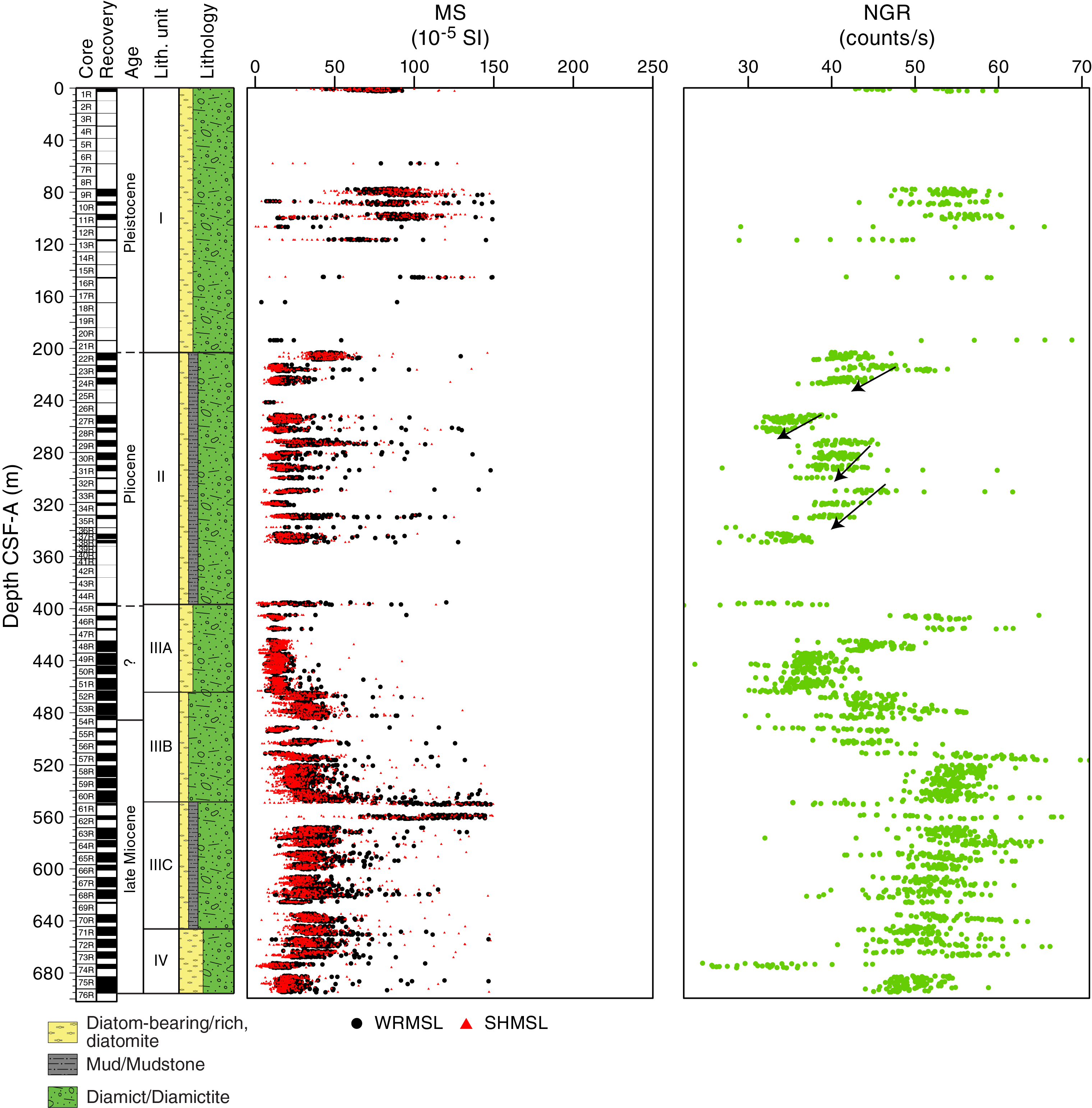
Figure F19. MS and NGR.
Natural gamma radiation
NGR measurements show downhole variations between ~25 and 65 counts/s in Hole U1522A (Figure F19). Because of poor recovery, NGR values from shallower than 200 m CSF-A are overprinted by anomalously high values from individual clasts, but in general, NGR is relatively high in cores that recovered both matrix and clasts in lithostratigraphic Unit I (e.g., Cores 374-U1522A-9R through 11R [~77–100 m CSF-A]). Between Cores 22R and 38R (~200–350 m CSF-A), NGR values show repeated downhole patterns of an ~20 counts/s decrease over a few tens of meters (arrows in Figure F19). These changes may reflect a systematic downhole decrease in clay content in the diamictite of Unit II. NGR increases from ~30 counts/s in the diamictite at the base of Unit II (Core 45R) to ~55 counts/s in the diamictite in Core 46R at the top of Subunit IIIA (~395–406 m CSF-A) without a corresponding change in magnetic susceptibility. These diamictite beds are separated by a 30 cm thick diatomite bed that defines the top of Unit III (interval 45R-2, 56 cm). The difference in NGR may indicate higher diatom content (or other reworked pelagic material) in the diamictite in the lower part of Unit II. From Core 52R through Core 60R (~465–550 m CSF-A), two successive cycles in NGR are visible, with abrupt downhole increases from 465 to 485 m CSF-A (Cores 52R through 53R) and from 500 to 512 m CSF-A (Cores 56R through 57R), where NGR reaches 55 and 65 counts/s, respectively. These variations are associated with increases in magnetic susceptibility and most likely reflect matrix grain size changes and clast composition changes in Subunit IIIB. From Core 58R to the bottom of the hole at 695 m CSF-A, NGR decreases to ~45 counts/s. This gradual decrease downhole may result from dilution of clays caused by the appearance of diatom-bearing lithologies in Unit IV. Exceptionally low NGR values measured in Core 74R were likely caused by core disturbance.
Bulk density, grain density, and porosity
Discrete MAD samples yielded bulk density values concentrated in a narrower range (~1.8–2.3 g/cm3) relative to GRA bulk density measurements (~1.4–2.2 g/cm3). Higher variability in density obtained by the WRMSL is due to the smaller diameter of the RCB cores relative to the core liner (see Physical properties in the Expedition 374 methods chapter [McKay et al., 2019a]) (Figure F20). Despite the different range of measured values, a similar downhole trend in GRA and MAD bulk density is observed. Grain density also shows an overall downhole trend similar to that of GRA and MAD bulk density. Downhole variations in porosity are inversely related to downhole variations in bulk and grain density.
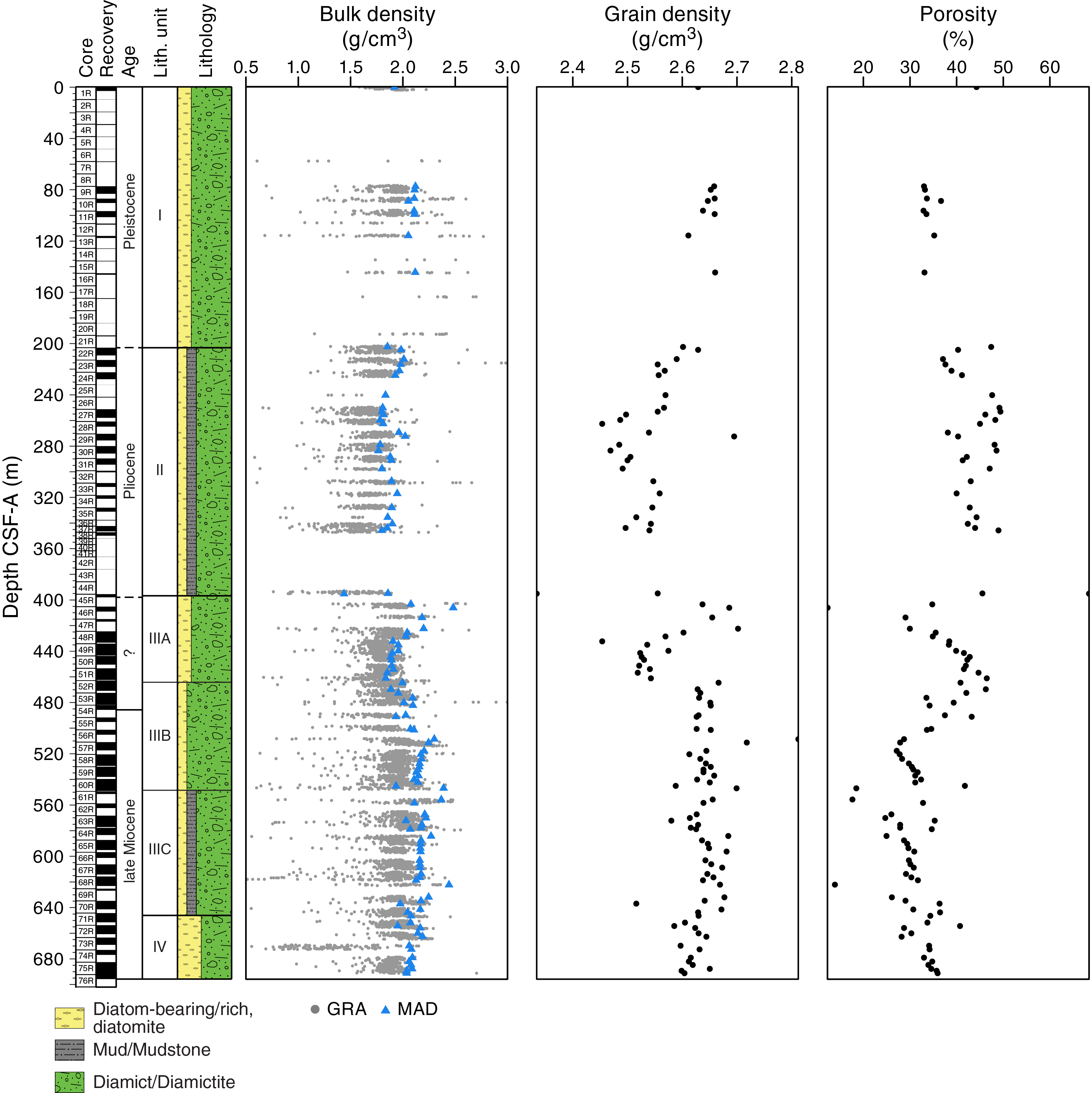
Figure F20. GRA and MAD bulk density, grain density, and porosity.
Not enough core was recovered to identify a general trend in the upper ~200 m CSF-A, but GRA and MAD bulk density values average ~2.1 g/cm3 in the sediments recovered between Cores 374-U1522A-2R and 21R, which corresponds to lithostratigraphic Unit I. Grain density and porosity values are relatively constant at ~2.65 g/cm3 and ~34% in this interval, respectively. The relatively high average bulk density might be related to an abundance of individual clasts in Unit I. GRA and MAD bulk density values (~1.8–2.0 g/cm3) in Cores 22R through 38R (~205–350 m CSF-A) in Unit II are generally lower than those in Unit I, suggesting overall clast content decreases with depth. Bulk and grain density values correspond to downhole repeating NGR cycles in Unit II, representing the alternation of clast-rich and clast-poor diamictite in Unit II. Bulk and grain densities increase and porosity decreases in Cores 45R and 46R, corresponding to the boundary between Units II and III (397.58 m CSF-A). Below this interval, bulk density and grain density decrease downhole and porosity increases in Cores 47R through 51R (~410–465 m CSF-A), corresponding to Subunit IIIA. Density increases downhole from Core 52R through Core 57R (~465–520 m CSF-A) and then decreases downhole to Core 60R at the base of Subunit IIIB. Bulk and grain densities and porosity remain relatively constant from Core 63R through Core 70R (~570–645 m CSF-A), corresponding to Subunit IIIC. Bulk and grain densities are slightly lower in Cores 71R through 76R (~645–695 m CSF-A) and correspond to the occurrence of mudstone laminae and muddy diatomite in Unit IV. GRA bulk density measured on highly disturbed Core 74R is exceptionally low, although MAD bulk density values are similar to those of adjacent core measurements.
Compressional P-wave velocity
Because of poor recovery, limited PWC measurements were acquired in Cores 374-U1522A-1R through 45R (0–396.7 m CSF-A). P-wave velocity in this interval ranges from ~1700 to 2000 m/s (Figure F21) and corresponds to diatom-bearing/rich sandy/muddy diamict(ite) in lithostratigraphic Units I and II. A downhole increase in P-wave velocity occurs at the boundary between Units II and III (~398 m CSF-A), with values ranging from ~1800 to 2200 m/s at the top of Unit III. In Unit III, P-wave velocity varies from 1700 to 2700 m/s, generally increases downhole to the base of Subunit IIIB, and then decreases to the base of Subunit IIIC. Higher P-wave velocities correspond to diminished diatom content in Subunit IIIB compared with Subunit IIIA and a change in clast lithology from mud clasts and carbonate concretions to basalt and metasedimentary clasts (see Lithostratigraphy). Lower P-wave velocities correspond to an increased presence of mudstone laminae in Subunit IIIC. In Unit IV, P-wave velocity is relatively high (2100–2500 m/s), and it decreases downhole, possibly because of the presence of mudstone laminae and interbedded muddy diatomite.
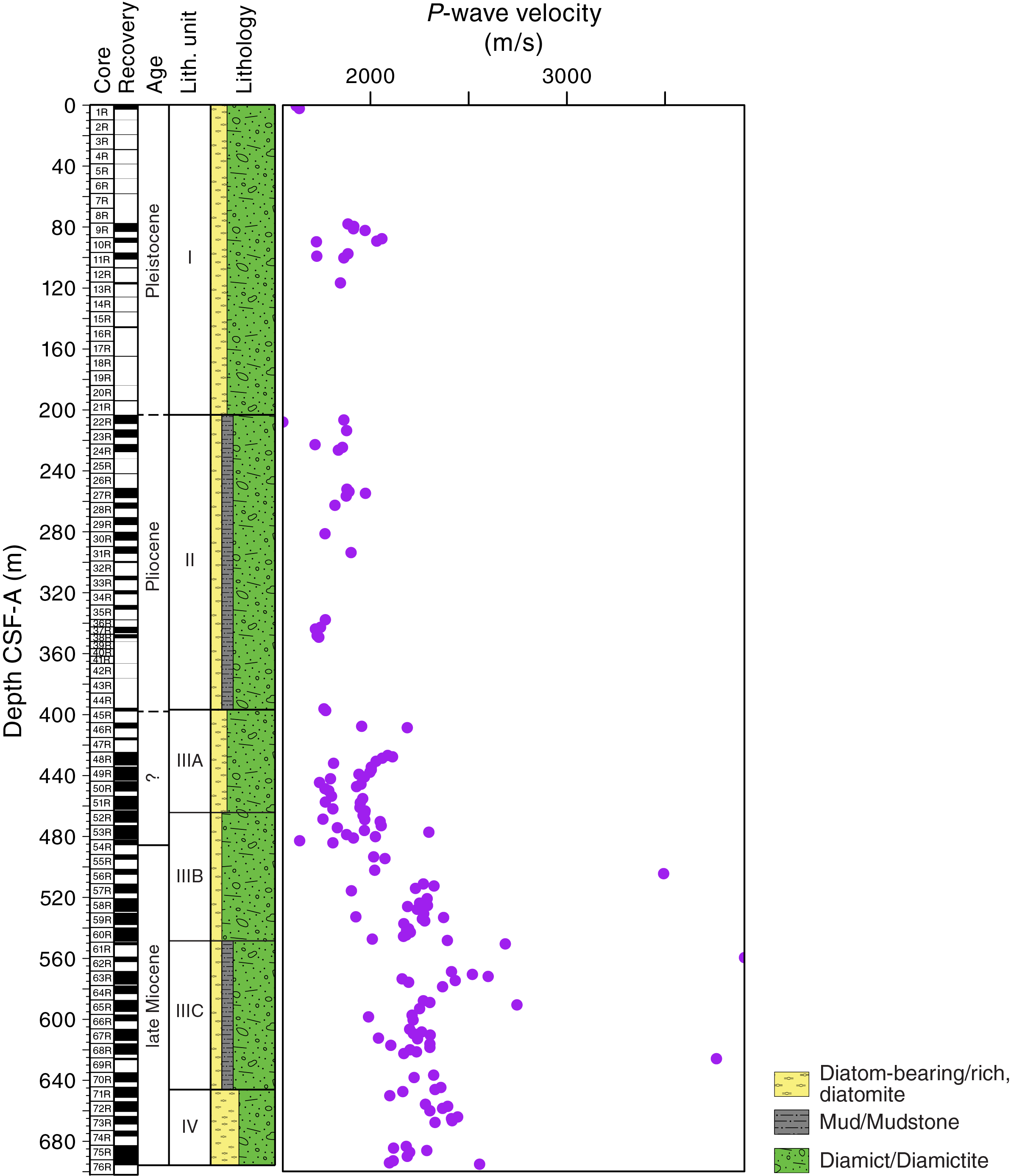
Figure F21. Discrete P-wave velocity.
Color reflectance spectroscopy
Color reflectance spectroscopy data were acquired on section halves using the SHMSL. At this site, all parameters (L*, a*, and b*) exhibit similar downhole changes (Figure F22). L* varies from 27 to 40 and shows a slight downhole increase (lightening) in lithostratigraphic Units I and II and then a downhole decrease (darkening) in Unit III. The ranges for a* and b* vary from 0 to 2.5 and −5 to 1, respectively. b* shows the most variation downhole, with sediment in Units I and II exhibiting more positive b* (yellower sediment) relative to Unit III, which has more negative b*.
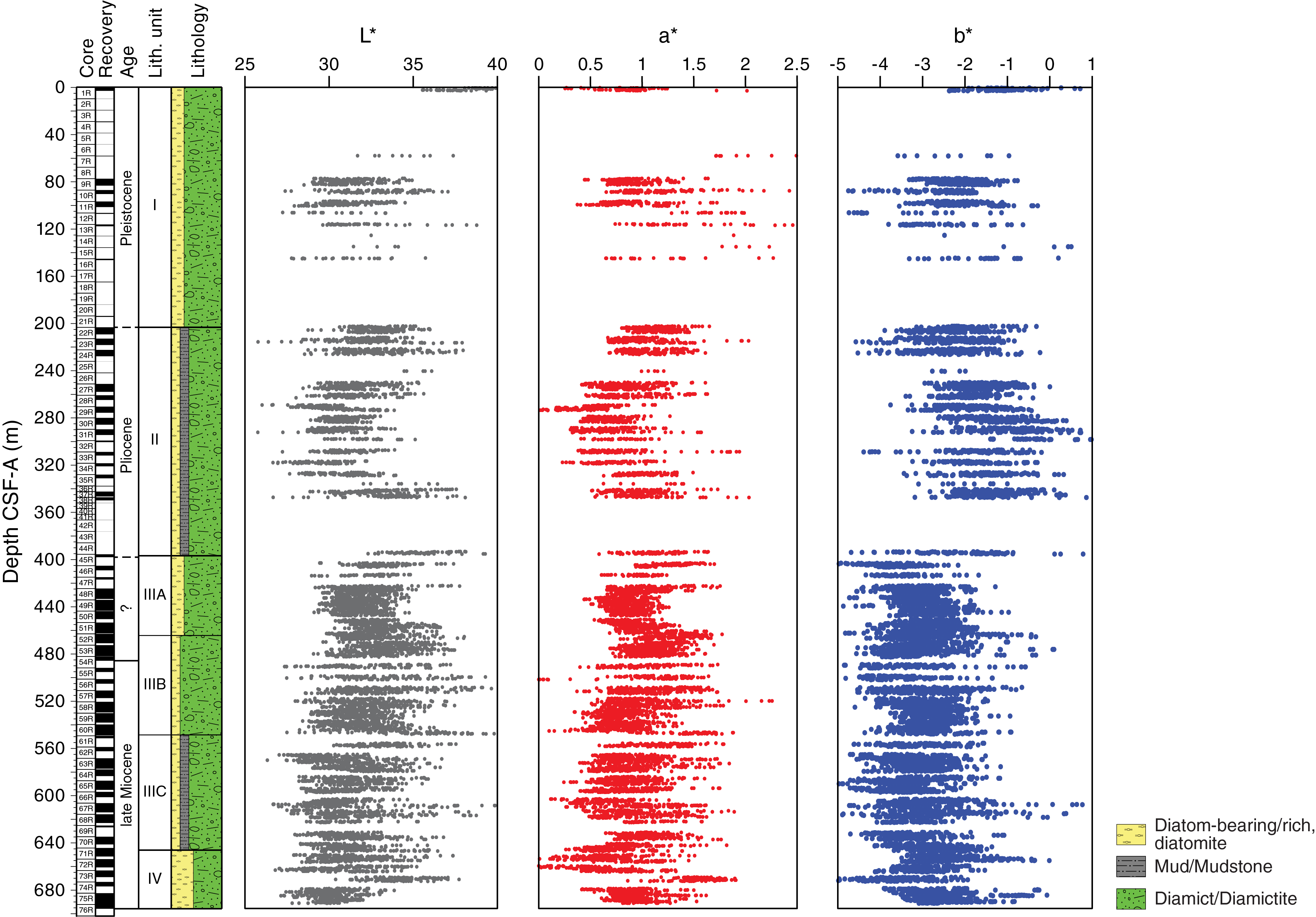
Figure F22. Color reflectance spectroscopy.
Summary
In general, data from whole-round measurements are in good agreement with those from split-core measurements (Figures F19, F20, F23). Discrete MAD samples and point magnetic susceptibility measurements on the section halves likely provide more accurate bulk density and magnetic susceptibility data compared with whole-round measurements because the whole-round measurements are dependent on the volume of core filling the liner (see Physical properties in the Expedition 374 methods chapter [McKay et al., 2019a]). Increases in P-wave velocity generally coincide with increases in GRA and MAD bulk density and magnetic susceptibility (to some extent) and decreases in porosity (Figure F23). Downhole variations in NGR also correlate well with changes in bulk density.

Figure F23. Physical properties summary.
Downhole changes in physical properties are in good overall agreement with the defined lithostratigraphic units based on sedimentological characteristics (see Lithostratigraphy; Figure F23; Table T11), and changes in physical properties can provide insight into lithologic changes in each unit. Downhole variations of magnetic susceptibility, NGR, and bulk density are observed in lithostratigraphic Unit II and are likely related to downhole decreases in clay content. In contrast, the description of Subunit IIIA (sand rich at the top and more clay rich at the bottom) is not consistent with the measured NGR, GRA and MAD bulk density, and porosity values, which suggests higher clay content at the top of Subunit IIIA and potentially more sand at the base. One plausible explanation for this discrepancy is that the sand contains abundant feldspars, thus increasing potassium radioactivity recorded in NGR.
Geochemistry and microbiology
Site U1522 samples were analyzed for headspace gas, interstitial water chemistry, and bulk sediment geochemistry. Headspace gases are low in the uppermost 100–200 m CSF-A and display variable methane and increasing ethane concentrations from 200 m CSF-A to the bottom of the hole at 700 m CSF-A. Interstitial water analyses of the mudline sample and five whole-round samples indicate early diagenesis immediately below the sediment/water interface, with sulfate reduction in the uppermost 100 m CSF-A and manganese reduction downhole to 215.40 m CSF-A. Total organic carbon (TOC) and calcium carbonate (CaCO3) content are generally low. Slightly elevated carbonate content and the decreasing TOC/total nitrogen (TN) ratios between 400 and 630 m CSF-A suggest more-marine conditions during deposition of the diamictite in lithostratigraphic Unit III. Systematic variations in handheld portable X-ray fluorescence (pXRF) scan data indicate the potential for detailed reconstruction of sediment provenance, particularly for Units II–IV.
Volatile hydrocarbons
Headspace gas analyses were performed at a resolution of one sample per core (9.6 m advance) or one sample every other core for half cores (4.8 m advance) throughout Hole U1522A (Cores 374-U1522A-1R through 76R; N = 63) as part of the routine environmental protection and safety monitoring program. Methane (CH4) is the dominant hydrocarbon, although ethane (C2H6) is also present in low concentration. Methane concentration is low (<4 ppmv) and variable in the upper 48.31 m CSF-A and generally ranges from 1,000 to 65,000 ppmv deeper than 80.31 m CSF-A (Figure F24; Table T12). Ethane concentration remains low (<2 ppmv) in the upper 200 m CSF-A and increases to 90 ppmv at 691.22 m CSF-A (Figure F24). The methane/ethane ratio is high (8,500–16,600) between 100 and 150 m CSF-A and then decreases downhole to 341 at 691.22 m CSF-A (Figure F24). The methane and ethane are likely formed by methanogenic bacteria, as documented for nearby Deep Sea Drilling Project (DSDP) Site 271 (Claypool and Kvenvolden, 1983).

Figure F24. Headspace gas concentrations.
Interstitial water chemistry
Five interstitial water samples were squeezed from 10 cm whole-round samples (Table T13), with sampling resolution dictated by core recovery and lithology from 1.42 to 215.40 m CSF-A. Squeezing the final sample for 1.5 h produced 2 mL of interstitial water, which was analyzed by ion chromatography and inductively coupled plasma–optical emission spectroscopy (ICP-OES) only to maximize data output. Interstitial water sampling was not conducted deeper than 215.40 m CSF-A because of low interstitial water content and low variability in lithology in the next cores. An additional sample from the mudline was split and analyzed as a comparative sample for shipboard parameters and shore-based analyses.
Salinity, sulfate, sulfur, iron, manganese, and ammonium
Interstitial water salinity is ~35 in the upper 1.42 m CSF-A, which is similar to ambient seawater and results for the mudline water sample (Figure F25). Salinity decreases to 32 at 80.21 m CSF-A and then to 30 from 88.40 to 215.40 m CSF-A. Similarly, sulfate concentration decreases from a typical seawater value of ~28 mM (within error, as is the sulfate concentration of the mudline water) at 1.42 m CSF-A to 8.5 mM at 80.21 m CSF-A. Below this depth, sulfate concentration is <4 mM (Figure F25). The total sulfur concentration profile is parallel to that of sulfate, with a decrease in the upper ~98 m CSF-A and low concentration from 98 to 215 m CSF-A. Iron concentration is below detection limit of the ICP-OES throughout the sampled interval. Manganese concentration increases from <1 µM at the mudline to 15–16 µM between 1.42 and 80.21 m CSF-A, with decreasing values below this depth to 2.4 µM at 215.40 m CSF-A. The decreasing manganese concentration is associated with increasing ammonium concentration, which increases from 75 µM at 1.42 m CSF-A to 1070 µM in the lowermost interstitial water sample (215.40 m CSF-A) (Figure F25). The downhole increase in ammonium concentration is possibly associated with anaerobic oxidation of methane by microbial activity. All downhole profiles described above are consistent with manganese and sulfate reduction in the suboxic to anoxic transition zone.
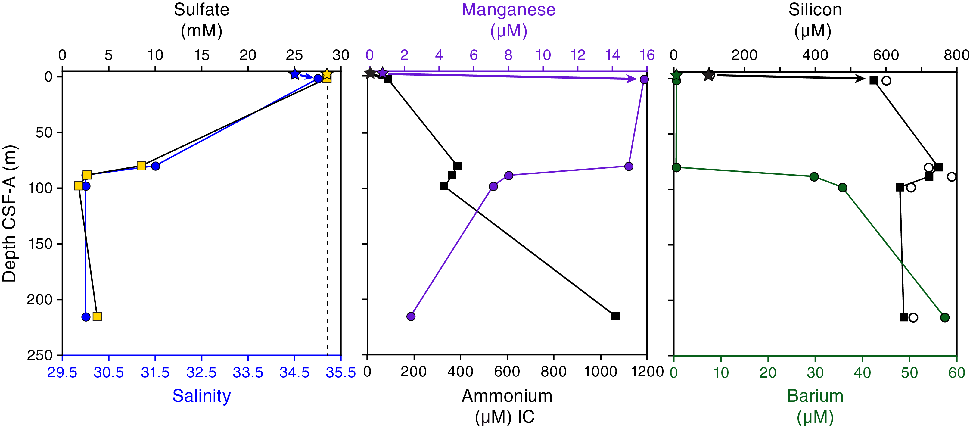
Figure F25. Interstitial and mudline water geochemistry.
Chloride, sodium, magnesium, calcium, potassium, alkalinity, and pH
Chloride and sodium concentrations show relatively small and similar downhole decreases (i.e., within 10%) that are paralleled by slightly larger downhole decreases in magnesium (15%), calcium (20%), and potassium (50%). Mudline water concentrations for all of these elements are within error of the first interstitial water sample taken at 1.42 m CSF-A. The low resolution of the interstitial water profile does not permit detailed interpretation of these elements. Deeper than 80.21 m CSF-A, interstitial water sample volume was less than the 12 mL required for all ship- and shore-based measurements. As a result, pH and alkalinity were only analyzed for two interstitial water samples (1.42 and 80.21 m CSF-A). Samples from the mudline and 1.42 m CSF-A have a lower pH (7.6–7.8) than average seawater (8.1). pH increases to 8.1 at 80.21 m CSF-A. Alkalinity follows a similar trend from a low value of 2.8 mM at 1.42 m CSF-A to a higher value of 9.4 mM at 80.21 m CSF-A.
Silica and barium
Barium concentration in interstitial water is below detection limit in the mudline sample and downhole to 80.21 m CSF-A and increases thereafter to 30–36 µM at 88.40 and 97.97 m CSF-A and 58 µM at 215.40 m CSF-A (Figure F25). The barium profile is mirrored by that of manganese. Silicon concentration varies between 572 and 759 µM with no clear downhole trend (Figure F25). An interesting (and expected) observation is that silicon concentration in the mudline water (94 µM) is significantly lower than in the first interstitial water sample at 1.42 m CSF-A (572 µM). A similar observation was made for manganese, which has a lower concentration in the mudline water relative to the first interstitial water sample at 1.42 m CSF-A. These results suggest that early diagenesis occurred in a closed system (i.e., relatively isolated from the water column) with high dissolved oxygen concentration in the uppermost few centimeters of the sediment close to the sediment/water interface.
Bulk sediment geochemistry
Carbon, nitrogen, and carbonate
A total of 74 sediment samples from the major lithostratigraphic units identified at Site U1522 were analyzed for total carbon, TN, and total inorganic carbon (Table T14). TOC and CaCO3 contents were subsequently calculated. TOC content is generally low and ranges from 0.1 to 0.8 wt% (Figure F26). Slightly higher TOC content (0.4–0.7 wt%) is observed in the diatom-bearing/rich diamictite of lithostratigraphic Units I and II in the uppermost ~400 m CSF-A, and a decreasing trend is noted between ~430 and ~620 m CSF-A. TN content is very low (≤0.05 wt%) but increases downhole. The TOC/TN ratio ranges between 3 and 42 (Figure F26), suggesting a mixed (i.e., marine and terrigenous) source of the organic matter deposited at this site. Overall, a downhole decrease in the TOC/TN ratio is observed, and an abundance of low TOC/TN ratios (3–7) in the diamictite of Subunits IIIB and IIIC (~520–620 m CSF-A) suggests a predominance of marine-derived organic matter in this depth interval. CaCO3 content is generally low and between 0.1 and 3.4 wt% when omitting one outlier of 32.4% from a carbonate-cemented unit at 625.98 m CSF-A (Figure F26). CaCO3 content is elevated in lithostratigraphic Unit III (407.36 –640.87 m CSF-A), reaching >3 wt%, and lower (<2 wt%) in lithostratigraphic Unit IV (645.25 and 693.36 m CSF-A).
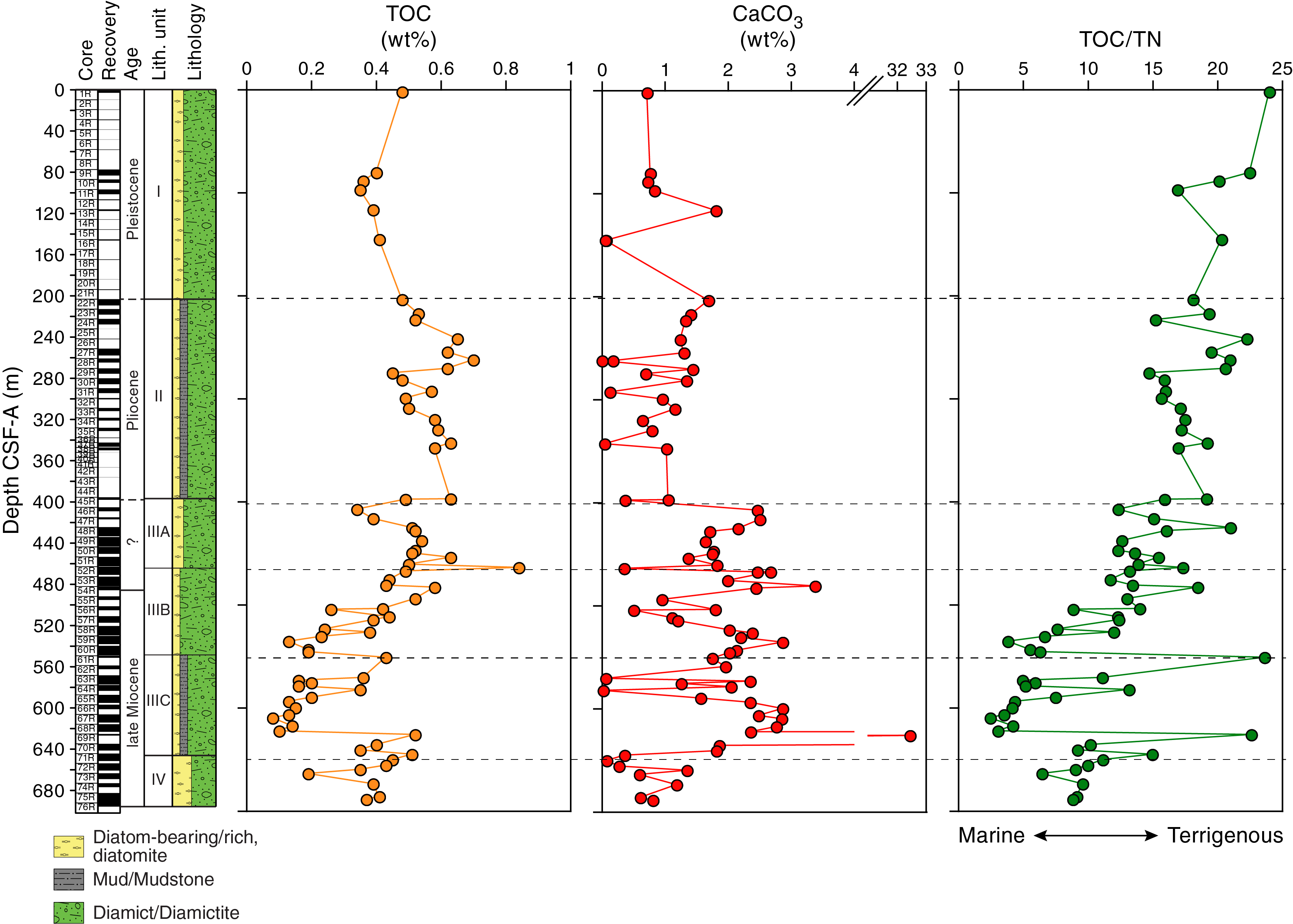
Figure F26. Bulk sediment carbon content and TOC/TN.
pXRF data
Shipboard pXRF data were collected for Cores 374-U1522A-1R through 76R (2.26–693.36 m CSF-A) (Table T15) using two different methods (“geochem” and “soil”; see Lithostratigraphy and Geochemistry and microbiology in the Expedition 374 methods chapter [McKay et al., 2019a]). The Ba/Al and Fe/Al ratios show a remarkably close positive correlation (r2 = 0.88; Figure F27). The ratios are low for the uppermost ~100 m CSF-A, and more elevated in lithostratigraphic Unit II between 203.8 and 347.93 m CSF-A. Recovery improved significantly deeper than ~400 m CSF-A, and the Ba/Al and Fe/Al ratios fluctuate cyclically over ~10 m intervals. The Si/Ti ratio indicates an exponential negative relationship with the Ba/Al ratio (r2 = 0.79; Figure F27). The Si/Ti ratio is more elevated from 2.26 to ~100 m CSF-A and generally lower between 203.80 and 347.93 m CSF-A, with the exception of one data point at 217.48 m CSF-A. The Si/Ti ratio also seems to vary cyclically over <10 to ~20 m intervals, especially deeper than ~400 m CSF-A. Higher resolution shore-based XRF scanning should help to identify the nature of the geochemical cyclicity in the Site U1522 record; however, there is good indication that different provenance sources and/or productivity regimes are preserved.
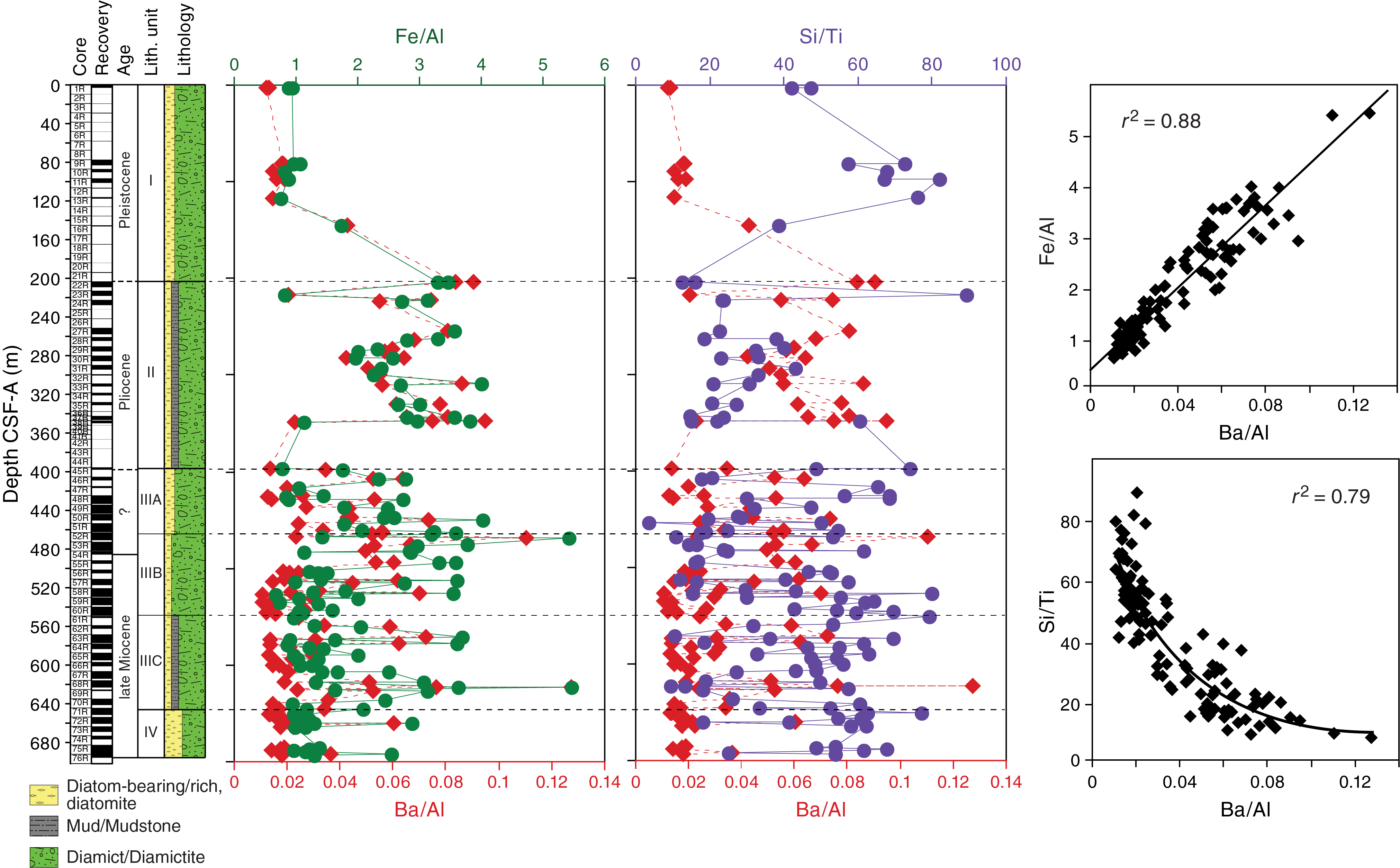
Figure F27. pXRF element ratios.
Microbiological sampling
In total, 52 samples for shore-based clumped isotope analyses were collected from Sections 374-U1522A-1R-2 through 76R-1. Additional samples for detailed analyses of metagenomics, cell counts, metabolomics, and cultures were also taken from Core 1R (see Geochemistry and microbiology in the Expedition 374 methods chapter [McKay et al., 2019a] for details).
Downhole measurements
Logging operations
Preparation of Hole U1522A for logging included release of the RCB drill bit at 0645 h on 27 January 2018 and multiple sweeps of high-viscosity (10.5 lb/gal) mud to improve the poor hole conditions. The drill string was pulled back to a logging depth of 91.3 m DSF. After the end of pipe was positioned, the hole was displaced with a further 20 bbl of heavy mud (10.5 lb/gal).
Preparation for downhole logging started at 1630 h on 27 January. An average heave of 0.3 m was estimated prior to logging, and the active heave compensator was switched on once the tools reached open hole. A modified triple combo tool string was assembled for the first run (see Downhole measurements in the Expedition 374 methods chapter [McKay et al., 2019a]). The triple combo tool string consisted of the following tools:
- Magnetic Susceptibility Sonde (MSS),
- High-Resolution Laterolog Array (HRLA),
- Dipole Sonic Imager (DSI),
- Hostile Environment Litho-Density Sonde (HLDS, without source),
- Hostile Environment Natural Gamma Ray Sonde (HNGS), and
- Enhanced Digital Telemetry Cartridge (EDTC).
The HNGS and MSS were run while lowering the tool string into the hole, and all the tools were run during the upward pass. The base of the tool string reached 650.3 m WSF, or approximately 50 m above the bottom of the hole, indicating that a significant amount of material had fallen into the hole. The caliper arms were opened, and the hole was logged up for a 143 m calibration pass. The tool string was then lowered back to bottom, again reaching 650.3 m WSF, and logged up. Upon visual inspection, the curves from the two runs were identical. Before reaching the end of pipe at 91.3 m WSF, the drill string was raised 15 m to 76.3 m DSF to increase log coverage of the borehole. The triple combo tool string was then returned to the rig floor at 2035 h.
The second run consisted of the VSI tool string, which included the following tools (see Downhole measurements in the Expedition 374 methods chapter [McKay et al., 2019a]):
The VSI tool string was lowered into the hole at 2245 h on 27 January but was unable to pass a bridge in the borehole at 194.5 m WSF, so the tool string was pulled back to surface to increase its weight. After adding the HNGS tool, the VSI tool string was again lowered into the hole, this time passing the bridge at 203.5 m WSF, but a second bridge at 297.5 m WSF could not be passed. Observation for protected species began prior to the air gun being lowered into the water and continued throughout the run. The VSP experiment included eight successful stations from 297.5 to 91.3 m WSF (Table T16). Operations were halted several times because of the presence of whales and seals. After completing the last station, the tool string was returned to the surface at 0630 h on 28 January.
The third logging run used the Formation MicroScanner (FMS) tool string, which consisted of the following tools (see Downhole measurements in the Expedition 374 methods chapter [McKay et al., 2019a]):
The FMS tool string was lowered into the drill string at 0730 h on 28 January. The HNGS was run while lowering the tool string to log natural gamma radiation across the water/sediment interface and the base of the drill pipe to depth-match results of the first logging run. The FMS reached 193.5 m WSF, and the hole was logged up to 101.5 m WSF. After closing the calipers and lowering the tool back to 193.5 m WSF, the main uplog pass was performed to the base of the pipe. All logging tools and equipment were disassembled by 1030 h.
Log data quality and comparison with shipboard physical properties
All log curves were depth-matched using the total gamma ray log from the main pass of the triple combo tool string as the reference, allowing a unified depth scale to be produced. Features in the gamma ray logs from the other two tool string passes (where data permitted) were aligned to the reference log to produce a complete depth-matched data set. Log data were then depth-shifted to the seafloor, as identified by a stepwise increase in the gamma ray value, producing the wireline log matched depth below seafloor (WMSF) depth scale. The seafloor is identified at 568 m wireline log depth below rig floor (WRF).
Hole U1522A data quality is variable. Borehole diameter, which was measured by the caliper, varies widely, indicating numerous washed out intervals and multiple ledges. The most significant washouts (more than ~4 inches on the caliper log; Figure F28) are at 85, 140, 170, 179, 195, 245, 260–270, 360–405, and 550 m WMSF. Other deviations from the bit diameter are relatively minor, and most of the borehole wall had low to medium rugosity. During the second and third logging runs, a narrow point (ledge) in the borehole at 297.5 m WSF prevented the VSI and FMS tool strings from being lowered below that depth.
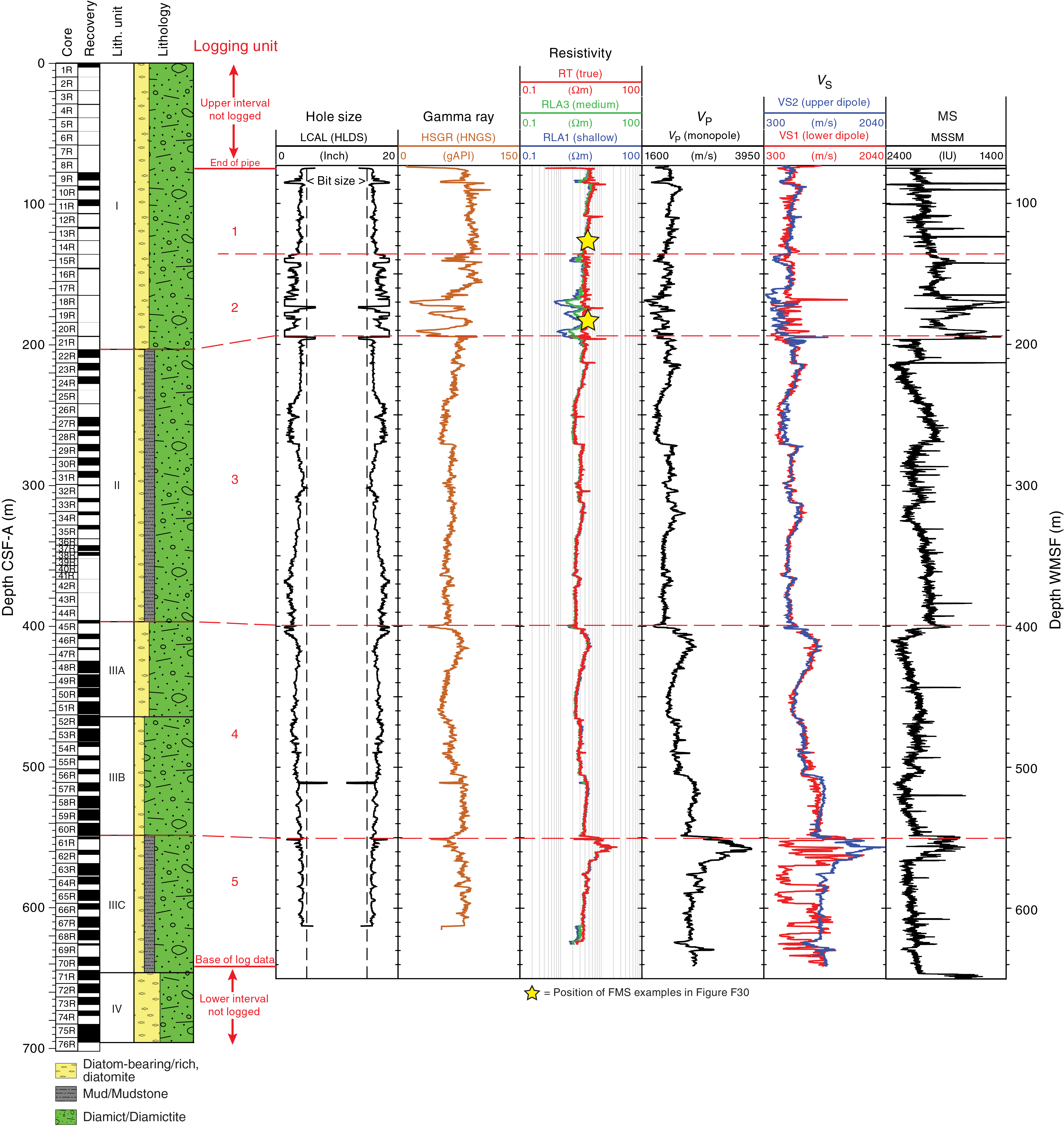
Figure F28. Downhole log data summary.
The quality of the logs can also be assessed by comparison with physical property measurements made on cores from Site U1522 (see Physical properties). Note that downhole logs are on the WMSF depth scale in Figure F29, whereas physical property data are on the CSF-A depth scale. Offsets at the scale of the entire drilled/logged interval are minor and thus still allow comparison of downhole trends.
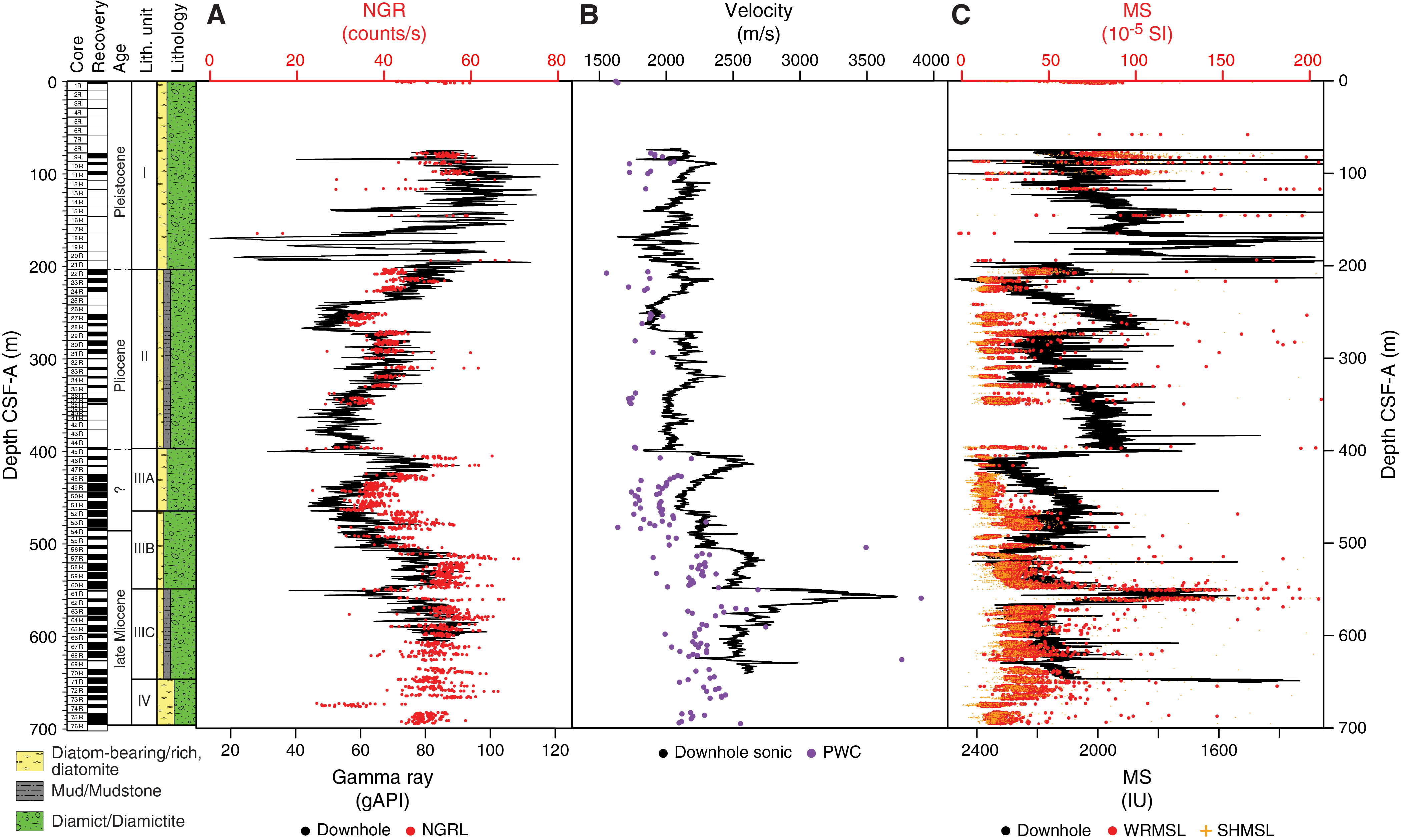
Figure F29. NGR, P-wave velocity, and MS data comparisons.
In general, gamma ray and P-wave velocity data show good correspondence between downhole and shipboard measurements throughout the borehole. Although downhole gamma ray and shipboard NGR data have different units, the trends and relative magnitude of downhole shifts are comparable (Figure F29). The agreement between downhole P-wave velocity from the sonic log and shipboard PWC P-wave velocity is fair. Although the general downhole trends are similar, the shipboard PWC measurements consistently underestimate P-wave velocity relative to the downhole sonic log by ~100–300 m/s (Figure F29). The magnetic susceptibility data also show reasonable correspondence, but a clear downhole drift in the magnetic susceptibility logging data is likely caused by tool temperature (Figure F29).
FMS and VSI data were only collected shallower than 193.5 m WSF because of poor borehole quality, which resulted in a narrow opening that the tool strings could not pass. FMS images appear to be of reasonably good quality, indicating that the pads made adequate contact with the borehole walls (Figure F30). Data may be less reliable in the vicinity of significant washouts (more than ~4 inches on the caliper log; Figure F28) at 85, 140, 170, and 179 m WMSF. The VSI data were also affected by the borehole quality; however, eight successful VSI stations with at least one good shot were collected and used for the seismic waveform stacking (Table T16).

Figure F30. FMS image examples.
Logging units
Downhole logging data for Hole U1522A are summarized in Figure F28. Five logging units are defined on the basis of distinctive features in the gamma ray, resistivity, magnetic susceptibility, and velocity (sonic) logs (Table T17). The units start from 75 m WMSF (end of pipe depth below seafloor) and end at 646 m WMSF.
Logging Unit 1 (75.0–139.0 m WMSF)
Logging Unit 1, the uppermost unit logged in Hole U1522A, is characterized by relatively high gamma radiation (typically ~87–97 gAPI with a maximum of 121 gAPI), high resistivity (>4.3 Ωm and as much as 13 Ωm), moderate velocity (~2090–2190 m/s), and variable magnetic susceptibility (~1990–2110 instrument units [IU]) (Figure F28). Unit 1 corresponds to the middle part of lithostratigraphic Unit I (~75–135 m CSF-A; see Lithostratigraphy), which is composed of diatom-bearing/rich sandy mud to muddy sand with massive diatom-bearing diamict.
Logging Unit 2 (139.0–195.0 m WMSF)
Logging Unit 2 is characterized by a relatively large degree of variability in gamma radiation (as little as 14 gAPI and as much as 107 gAPI), velocity (~1900–2100 m/s with numerous thin intervals of <1700 m/s), and magnetic susceptibility (<1660 IU to almost 2300 IU) (Figure F28). True resistivity is in a narrow range of 3.75–4.3 Ωm, but both medium and shallow resistivity deviate from true resistivity more than in any other logging unit. Unit 2 is distinguished by a markedly different log character compared with overlying and underlying intervals and corresponds with the lower part of lithostratigraphic Unit I. Poor core recovery in this interval of Unit I hampered identification of any significant lithologic variation based on visual core description associated with this interval. High variability in all logs in this unit likely reflects the rugosity of the borehole wall, as shown in the caliper log in Figure F28.
Logging Unit 3 (195.0–400.0 m WMSF)
Logging Unit 3 is characterized by ~30–60 m thick packages of downhole decreasing gamma ray, resistivity, velocity, and magnetic susceptibility values. The gamma ray data show three repeating packages with values from 55 to 71 gAPI. The resistivity data show four cycles with values from 2.37 to 3.36 Ωm. Velocity data show four intervals of decreasing velocity with depth in Unit 3. Velocity ranges from 2000 to 2144 m/s. Magnetic susceptibility data show four cycles of decreasing magnetic susceptibility with depth with values from ~1980 to 2170 IU. Unit 3 corresponds to lithostratigraphic Unit II (203–397 m CSF-A; see Lithostratigraphy), which consists of massive interbedded diatom-bearing/rich sandy/muddy diamictite with mudstone laminae.
Logging Unit 4 (400.0–551.0 m WMSF)
Logging Unit 4 is characterized by relatively high gamma radiation (66–75 gAPI). Similar to overlying Unit 3, there are ~50–60 m thick intervals of downhole decreasing resistivity values (2.85–4.02 Ωm) in the unit. Velocity values follow a similar trend of downward-decreasing intervals (2221–2520 m/s). Magnetic susceptibility values range from 2118 to 2252 IU. Unit 4 corresponds to lithostratigraphic Subunits IIIA and IIIB (397–548 m CSF-A; see Lithostratigraphy). Unit 4 encompasses both of these lithostratigraphic subunits because there is no significant change in log character throughout this section. Subunits IIIA and IIIB correspond to massive interbedded diatom-bearing/rich sandy/muddy diamictite with mudstone laminae, muddy diatomite with glauconite, and common mudstone clasts and carbonate concretions.
Logging Unit 5 (551.0–646.0 m WMSF)
Logging Unit 5, the lowermost unit, is characterized by high gamma radiation (75–86 gAPI). The unit has relatively high resistivity (3.65–5.05 Ωm), very high velocity (~2530–2780 m/s), and moderate to high magnetic susceptibility (2100–2220 IU). Unit 5 corresponds to lithostratigraphic Subunit IIIC (548–647 m CSF-A; see Lithostratigraphy), which is composed of massive to stratified bioturbated diatom-bearing sandy/muddy diamictite with mudstone laminae and common basalt clasts.
FMS images
FMS resistivity images show submeter-scale variations in the texture and lithologies of the borehole walls (Figure F30). FMS images are only available between 101.5 and 193.5 m WMSF; therefore, only logging Units 1 and 2 were imaged. Unit 1 is characterized by highly variable resistivity with high-resistivity mottled and patchy textures typical of various diamictite lithologies that include localized, centimeter-scale high-resistivity spots interpreted to be clasts in the diamictite. Unit 2 is characterized by intervals of very low resistivity diatom-rich mudstone-dominated sections and alternating intervals of very high resistivity with mottled and patchy textures typical of diamictite lithologies (Figure F30).
Core-log-seismic integration
We combined log data, sediment core observations, physical property data, and seismic data from Hole U1522A to evaluate whether the recovered cores had reached the targeted seismic horizons and whether the observed sedimentary, physical property, log, and seismic units could be integrated.
Velocity model construction and seismic-downhole log correlation
Seismic-reflection Profile IO6290-Y2A, acquired in 2005–2006 on board the R/V OGS Explora, crosses Site U1522 and was used for core-log-seismic integration (Figure F31). The primary seismic sequences are interpreted after Bohm et al., (2009). For the purposes of shipboard correlation of the core data (e.g., lithostratigraphic units and physical property data) and log data with features observed on the seismic-reflection profile for Site U1522, we converted lithostratigraphic and logging unit boundaries from depth in meters to TWT using three different methods:
- PWC point-source velocity data from physical property measurements (see Physical properties),
- First seismic waveform arrival times derived from the VSI for each of the eight check shot stations, and
- Sonic velocity data from the DSI.
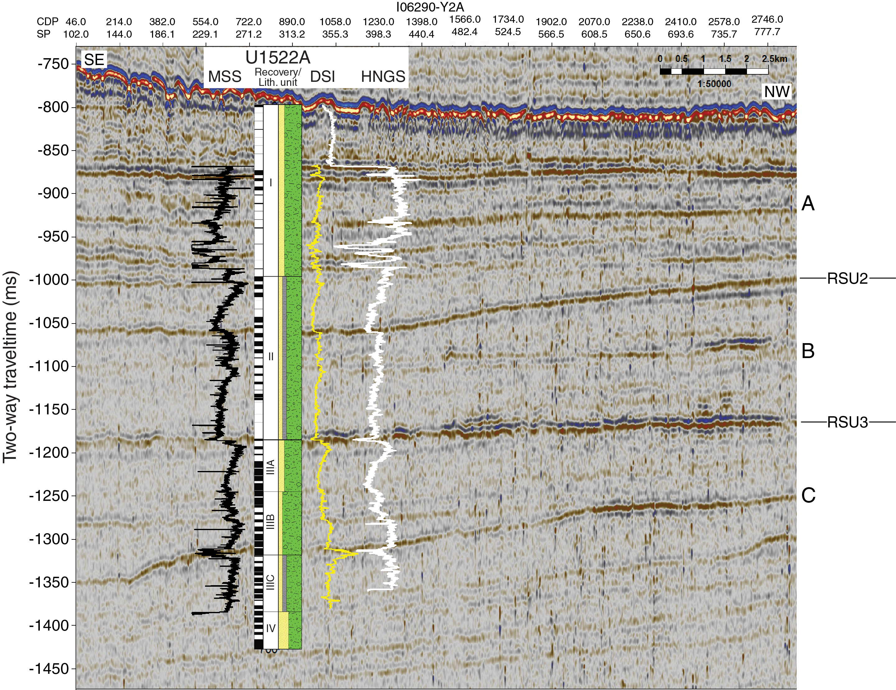
Figure F31. Core-log-seismic integration.
However, for VSI, velocity measurements were only available over the upper ~200 m of the borehole. Discrete P-wave velocity laboratory measurements on cores gave relatively slow values, whereas the VSI check shots and sonic log correspond well with each other and with stacking velocities. Coring at Site U1522 reached and drilled below the targeted RSU2 (in logging Unit 3) and RSU3 (between logging Units 3 and 4), which represent boundaries for sedimentary, physical property, log, and seismic units.
For core-log-seismic integration, the seismic-reflection profile was divided into three units (A–C) (Figure F31). Each of these units defines either a change in dominant seismic facies or is bounded by an interpreted erosional surface. Seismic Unit A (800–1050 ms TWT) is characterized by discontinuous high to medium amplitude, subhorizontal reflector packages interlayered with opaque lenses, the lowermost of which is onlapping RSU2. This unit corresponds with logging Units 1 and 2 and the upper part of Unit 3. Seismic Unit B (1050–1200 ms TWT) is characterized by sparse, very low amplitude, discontinuous reflectors bounded by two continuous high-amplitude reflectors (RSU2 and RSU3). RSU2 and RSU3 truncate the strata below. Seismic Unit B corresponds to logging Unit 3. Seismic Unit C (1200–1450 ms TWT) is characterized by discontinuous, mid- to high-amplitude reflectors that are subhorizontal or slightly dipping toward the southeast (left side of Figure F31) and correspond to logging Units 4 and 5. Seismic Units A, B, and C are interpreted as subglacial till, subglacial or outwash channel(s), and ice-proximal and ice-distal sediments, respectively, which is in good agreement with the logging and lithostratigraphic units.
References
Alonso, B., Anderson, J.B., Diaz, J.I., and Bartek, L.R., 1992. Pliocene–Pleistocene seismic stratigraphy of the Ross Sea: evidence for multiple ice sheet grounding episodes. In Elliot, D.H. (Ed.), Antarctic Research Series (Volume 57): Contributions to Antarctic Research III: Washington DC (American Geophysical Union), 93–103. https://agupubs.onlinelibrary.wiley.com/doi/10.1029/AR057p0093
Anderson, J.B., and Bartek, L.R., 1992. Cenozoic glacial history of the Ross Sea revealed by intermediate resolution seismic reflection data combined with drill site information. In Kennett J.P., and Warnke D. (Eds.), Antarctic Research Series (Volume 56): The Antarctic Paleoenvironment: A Perspective on Global Change: Part One: Washington DC (American Geophysical Union), 231–263. https://agupubs.onlinelibrary.wiley.com/doi/pdf/10.1029/AR056p0231
Arndt, J.E., Schenke, H.W., Jakobsson, M., Nitsche, F.O., Buys, G., Goleby, B., Rebesco, M., et al., 2013. The International Bathymetric Chart of the Southern Ocean (IBCSO) Version 1.0—a new bathymetric compilation covering circum-Antarctic waters. Geophysical Research Letters, 40(12):3111–3117. https://doi.org/10.1002/grl.50413
Böhm, G., Ocakoğlu, N., Picotti, S., and De Santis, L., 2009. West Antarctic Ice Sheet evolution: new insights from a seismic tomographic 3D depth model in the Eastern Ross Sea (Antarctica). Marine Geology, 266(1–4):109–128. https://doi.org/10.1016/j.margeo.2009.07.016
Claypool, G.E., and Kvenvolden, K.A., 1983. Methane and other hydrocarbon gases in marine sediment. Annual Review of Earth and Planetary Sciences, 11(1):299–327. https://doi.org/10.1146/annurev.ea.11.050183.001503
Cunningham, W.L., and Leventer, A., 1998. Diatom assemblages in surface sediments of the Ross Sea: relationship to present oceanographic conditions. Antarctic Science, 10(2):134–146. https://doi.org/10.1017/S0954102098000182
Cunningham, W.L., Leventer, A., Andrews, J.T., Jennings, A.E., and Licht, K.J., 1999. Late Pleistocene–Holocene marine conditions in the Ross Sea, Antarctica: evidence from the diatom record. The Holocene, 9(2):129–139. https://doi.org/10.1191/095968399675624796
D’Agostino, A.E., 1980. Foraminiferal biostratigraphy, paleoecology, and systematics of DSDP Site 273, Ross Sea, Antarctica [M.S. thesis]. Northern Illinois University. http://commons.lib.niu.edu/handle/10843/18050
De Santis, L., Anderson, J.B., Brancolini, G., and Zayatz, I., 1995. Seismic record of late Oligocene through Miocene glaciation on the Central and Eastern Continental Shelf of the Ross Sea. In Cooper, A.K., Barker, P.F., and Brancolini, G. (Eds.), Antarctic Research Series (Volume 68): Geology and Seismic Stratigraphy of the Antarctic Margin: Washington, DC (American Geophysical Union), 235–260. https://doi.org/10.1029/AR068p0235
Dolven, J.K., and Bjørklund, K.R., 2001. An early Holocene peak occurrence and recent distribution of Rhizoplegma boreale (Radiolaria): a biomarker in the Norwegian Sea. Marine Micropaleontology, 42(1–2):25–44. https://doi.org/10.1016/S0377-8398(01)00011-1
Evans, H.F., Westerhold, T., Paulsen, H., and Channell, J.E.T., 2007. Astronomical ages for Miocene polarity chrons C4Ar–C5r (9.3–11.2 Ma), and for three excursion chrons within C5n.2n. Earth and Planetary Science Letters, 256:455–465. http://dx.doi.org/10.1016/j.epsl.2007.02.001
Fillon, R.H., 1974. Late Cenozoic foraminiferal paleoecology of the Ross Sea, Antarctica. Micropaleontology, 20(2):129–151. https://doi.org/10.2307/1485056
Florindo, F., Farmer, R.K., Harwood, D.M., Cody, R.D., Levy, R., Bohaty, S.M., Carter, L., and Winkler, A., 2013. Paleomagnetism and biostratigraphy of sediments from Southern Ocean ODP Site 744 (southern Kerguelen Plateau): implications for early-to-middle Miocene climate in Antarctica. Global and Planetary Change, 110(C):434–454. https://doi.org/10.1016/j.gloplacha.2013.05.004
Gradstein, F.M., Ogg, J.G., Schmitz, M.D., and Ogg, G.M. (Eds.), 2012. The Geological Time Scale 2012: Amsterdam (Elsevier). https://doi.org/10.1016/C2011-1-08249-8
Harland, R., and Pudsey, C.J., 2002. Protoperidiniacean dinoflagellate cyst taxa from the upper Miocene of ODP Leg 178, Antarctic Peninsula. Review of Palaeobotany and Palynology, 120(3–4):263–284. https://doi.org/10.1016/S0034-6667(02)00080-5
Hinz, K., and Block, M., 1984. Results of geophysical investigations in the Weddell Sea and in the Ross Sea, Antarctica. Proceedings of the 11th World Petroleum Congress, 11(2):79–91.
Kellogg, T.B., and Truesdale, R.S., 1979. Late Quaternary paleoecology and paleoclimatology of the Ross Sea: the diatom record. Marine Micropaleontology, 4:137–158. https://doi.org/10.1016/0377-8398(79)90011-2
Krissek, L., Browne, G., Carter, L., Cowan, E., Dunbar, G., McKay, R., Naish, T., et al., 2007. Sedimentology and stratigraphy of the AND-1B core, ANDRILL McMurdo Ice Shelf Project, Antarctica. Terra Antarctica, 14(3):185–222. http://www.mna.unisi.it/english/Publications/TAP/TA_pdfs/Volume_14/TA_14_185_Sedimentology.pdf
Lazarus, D., 1992. Antarctic Neogene radiolarians from the Kerguelen Plateau, Legs 119 and 120. In Wise, S.W., Jr., Schlich, R., et al., Proceedings of the Ocean Drilling Program, Scientific Results, 120: College Station, TX (Ocean Drilling Program), 785–809. https://doi.org/10.2973/odp.proc.sr.120.192.1992
Leckie, R.M., and Webb, P.-N., 1985. Candeina antarctica, n.sp., and the phylogenetic history and distribution of Candeina spp. in the Paleogene–early Neogene of the Southern Ocean. Journal of Foraminiferal Research, 15(2):65–78. https://doi.org/10.2113/gsjfr.15.2.65
Leckie, R.M., and Webb, P.-N., 1986. Late Paleogene and early Neogene foraminifers of Deep Sea Drilling Project Site 270, Ross Sea, Antarctica. In Kennett, J. P., von der Borch, C.C., et al., Initial Reports of the Deep Sea Drilling Project, 90: Washington, DC (U.S. Government Printing Office), 1093–1142. https://doi.org/10.2973/dsdp.proc.90.124.1986
McKay, R.M., De Santis, L., Kulhanek, D.K., Ash, J.L., Beny, F., Browne, I.M., Cortese, G., Cordeiro de Sousa, I.M., Dodd, J.P., Esper, O.M., Gales, J.A., Harwood, D.M., Ishino, S., Keisling, B.A., Kim, S., Kim, S., Laberg, J.S., Leckie, R.M., Müller, J., Patterson, M.O., Romans, B.W., Romero, O.E., Sangiorgi, F., Seki, O., Shevenell, A.E., Singh, S.M., Sugisaki, S.T., van de Flierdt, T., van Peer, T.E., Xiao, W., and Xiong, Z., 2019a. Expedition 374 methods. In McKay, R.M., De Santis, L., Kulhanek, D.K., and the Expedition 374 Scientists, Ross Sea West Antarctic Ice Sheet History. Proceedings of the International Ocean Discovery Program, 374: College Station, TX (International Ocean Discovery Program). https://doi.org/10.14379/iodp.proc.374.102.2019
McKay, R.M., De Santis, L., Kulhanek, D.K., Ash, J.L., Beny, F., Browne, I.M., Cortese, G., Cordeiro de Sousa, I.M., Dodd, J.P., Esper, O.M., Gales, J.A., Harwood, D.M., Ishino, S., Keisling, B.A., Kim, S., Kim, S., Laberg, J.S., Leckie, R.M., Müller, J., Patterson, M.O., Romans, B.W., Romero, O.E., Sangiorgi, F., Seki, O., Shevenell, A.E., Singh, S.M., Sugisaki, S.T., van de Flierdt, T., van Peer, T.E., Xiao, W., and Xiong, Z., 2019b. Expedition 374 summary. In McKay, R.M., De Santis, L., Kulhanek, D.K., and the Expedition 374 Scientists, Ross Sea West Antarctic Ice Sheet History. Proceedings of the International Ocean Discovery Program, 374: College Station, TX (International Ocean Discovery Program). https://doi.org/10.14379/iodp.proc.374.101.2019
McKay, R.M., De Santis, L., Kulhanek, D.K., Ash, J.L., Beny, F., Browne, I.M., Cortese, G., Cordeiro de Sousa, I.M., Dodd, J.P., Esper, O.M., Gales, J.A., Harwood, D.M., Ishino, S., Keisling, B.A., Kim, S., Kim, S., Laberg, J.S., Leckie, R.M., Müller, J., Patterson, M.O., Romans, B.W., Romero, O.E., Sangiorgi, F., Seki, O., Shevenell, A.E., Singh, S.M., Sugisaki, S.T., van de Flierdt, T., van Peer, T.E., Xiao, W., and Xiong, Z., 2019c. Site U1521. In McKay, R.M., De Santis, L., Kulhanek, D.K., and the Expedition 374 Scientists, Ross Sea West Antarctic Ice Sheet History. Proceedings of the International Ocean Discovery Program, 374: College Station, TX (International Ocean Discovery Program). https://doi.org/10.14379/iodp.proc.374.103.2019
McKay, R.M., De Santis, L., Kulhanek, D.K., Ash, J.L., Beny, F., Browne, I.M., Cortese, G., Cordeiro de Sousa, I.M., Dodd, J.P., Esper, O.M., Gales, J.A., Harwood, D.M., Ishino, S., Keisling, B.A., Kim, S., Kim, S., Laberg, J.S., Leckie, R.M., Müller, J., Patterson, M.O., Romans, B.W., Romero, O.E., Sangiorgi, F., Seki, O., Shevenell, A.E., Singh, S.M., Sugisaki, S.T., van de Flierdt, T., van Peer, T.E., Xiao, W., and Xiong, Z., 2019d. Site U1523. In McKay, R.M., De Santis, L., Kulhanek, D.K., and the Expedition 374 Scientists, Ross Sea West Antarctic Ice Sheet History. Proceedings of the International Ocean Discovery Program, 374: College Station, TX (International Ocean Discovery Program). https://doi.org/10.14379/iodp.proc.374.105.2019
Medlin, L.K., and Priddle, J. (Eds.), 1990. Polar Marine Diatoms: Cambridge, United Kingdom (British Antarctic Survey).
Miller, K.G., Wright, J.D., Browning, J.V., Kulpecz, A., Kominz, M., Naish, T.R., Cramer, B.S., Rosenthal, Y., Peltier, W.R., and Sosdian, S., 2012. High tide of the warm Pliocene: implications of global sea level for Antarctic deglaciation. Geology, 40(5):407–410. https://doi.org/10.1130/G32869.1
Naish, T.R., Powell, R., Levy, R., Wilson, G., Scherer, R., Talarico, F., Krissek, L., et al., 2009. Obliquity-paced Pliocene West Antarctic Ice Sheet oscillations. Nature, 458(7236):322–329. https://doi.org/10.1038/nature07867
Nishimura, A., Nakaseko, K., and Okuda, Y., 1997. A new coastal water radiolarian assemblage recovered from sediment samples from the Antarctic Ocean. Marine Micropaleontology, 30(1–3):29–44. https://doi.org/10.1016/S0377-8398(96)00019-9
Osterman, L.E., and Kellogg, T.B., 1979. Recent benthic foraminiferal distributions from the Ross Sea, Antarctica: relation to ecologic and oceanographic conditions. Journal of Foraminiferal Research, 9(3):250–269. https://doi.org/10.2113/gsjfr.9.3.250
Patterson, M.O., and Ishman, S.E., 2012. Neogene benthic foraminiferal assemblages and paleoenvironmental record for McMurdo Sound, Antarctica. Geosphere, 8(6):1331–1341. https://doi.org/10.1130/GES00771.1
Prebble, J.G., Crouch, E.M., Carter, L., Cortese, G., Bostock, H., and Neil, H., 2013. An expanded modern dinoflagellate cyst dataset for the Southwest Pacific and Southern Hemisphere with environmental associations. Marine Micropaleontology, 101:33–48. https://doi.org/10.1016/j.marmicro.2013.04.004
Sjunnesskog, C., and Scherer, R.P., 2005. Mixed diatom assemblages in glacigenic sediment from the central Ross Sea, Antarctica. Palaeogeography, Palaeoclimatology, Palaeoecology, 218(3–4):287–300. https://doi.org/10.1016/j.palaeo.2004.12.019
Zonneveld, K.A.F., Marret, F., Versteegh, G.J.M., Bogus, K., Bonnet, S., Bouimetarhan, I., Crouch, E., et al., 2013. Atlas of modern dinoflagellate cyst distribution based on 2405 data points. Review of Palaeobotany and Palynology, 191. https://doi.org/10.1016/j.revpalbo.2012.08.003
1 McKay, R.M., De Santis, L., Kulhanek, D.K., Ash, J.L., Beny, F., Browne, I.M., Cortese, G., Cordeiro de Sousa, I.M., Dodd, J.P., Esper, O.M., Gales, J.A., Harwood, D.M., Ishino, S., Keisling, B.A., Kim, S., Kim, S., Laberg, J.S., Leckie, R.M., Müller, J., Patterson, M.O., Romans, B.W., Romero, O.E., Sangiorgi, F., Seki, O., Shevenell, A.E., Singh, S.M., Sugisaki, S.T., van de Flierdt, T., van Peer, T.E., Xiao, W., and Xiong, Z., 2019. Site U1522. In McKay, R.M., De Santis, L., Kulhanek, D.K., and the Expedition 374 Scientists, Ross Sea West Antarctic Ice Sheet History. Proceedings of the International Ocean Discovery Program, 374: College Station, TX (International Ocean Discovery Program). https://doi.org/10.14379/iodp.proc.374.104.2019
2 Expedition 374 Scientists’ affiliations.
This work is distributed under the Creative Commons Attribution 4.0 International (CC BY 4.0) license. 