McNeill, L.C., Shillington, D.J., Carter, G.D.O., and the Expedition 381 Participants
Proceedings of the International Ocean Discovery Program Volume 381
publications.iodp.org

https://doi.org/10.14379/iodp.proc.381.104.2019
Site M00781
L.C. McNeill, D.J. Shillington, G.D.O. Carter, J.D. Everest, E. Le Ber, R.E.Ll. Collier, A. Cvetkoska, G. De Gelder, P. Diz, M.-L. Doan, M. Ford, R.L. Gawthorpe, M. Geraga, J. Gillespie, R. Hemelsdaël, E. Herrero-Bervera, M. Ismaiel, L. Janikian, K. Kouli, S. Li, M.L. Machlus, M. Maffione, C. Mahoney, G. Michas, C. Miller, C.W. Nixon, S.A. Oflaz, A.P. Omale, K. Panagiotopoulos, S. Pechlivanidou, M.P. Phillips, S. Sauer, J. Seguin, S. Sergiou, and N.V. Zakharova2
Keywords: International Ocean Discovery Program, IODP, D/V Fugro Synergy, mission-specific platform, Expedition 381, Site M0078, Corinth rift, Gulf of Corinth, Alkyonides Gulf, Eastern Mediterranean Sea, Aegean Sea, continental rifting, extension, active rift, normal fault, earthquake, horst, fault growth, rift development, synrift stratigraphy, drainage evolution, surface processes, basin paleoenvironment, glacio-eustatic cycles, sea level, semi-isolated basin, marine basin, lacustrine, sediment flux, Quaternary, Pliocene, Miocene, carbon cycling, nutrient preservation, marine isotope stage
MS 381-104: Published 28 February 2019
Operations
During International Ocean Discovery Program (IODP) Expedition 381, cores were recovered from two holes at Site M0078 (Figures F1, F2). In total, 20.27 days were spent on station, with an average core recovery of 88% for the site (Table T1). Hole M0078A was drilled to 610.43 meters below seafloor (mbsf), and Hole M0078B was drilled to 55.85 mbsf.
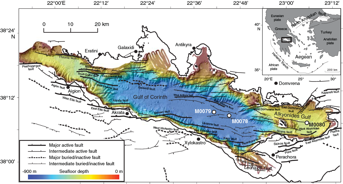
Figure F1. Corinth rift.
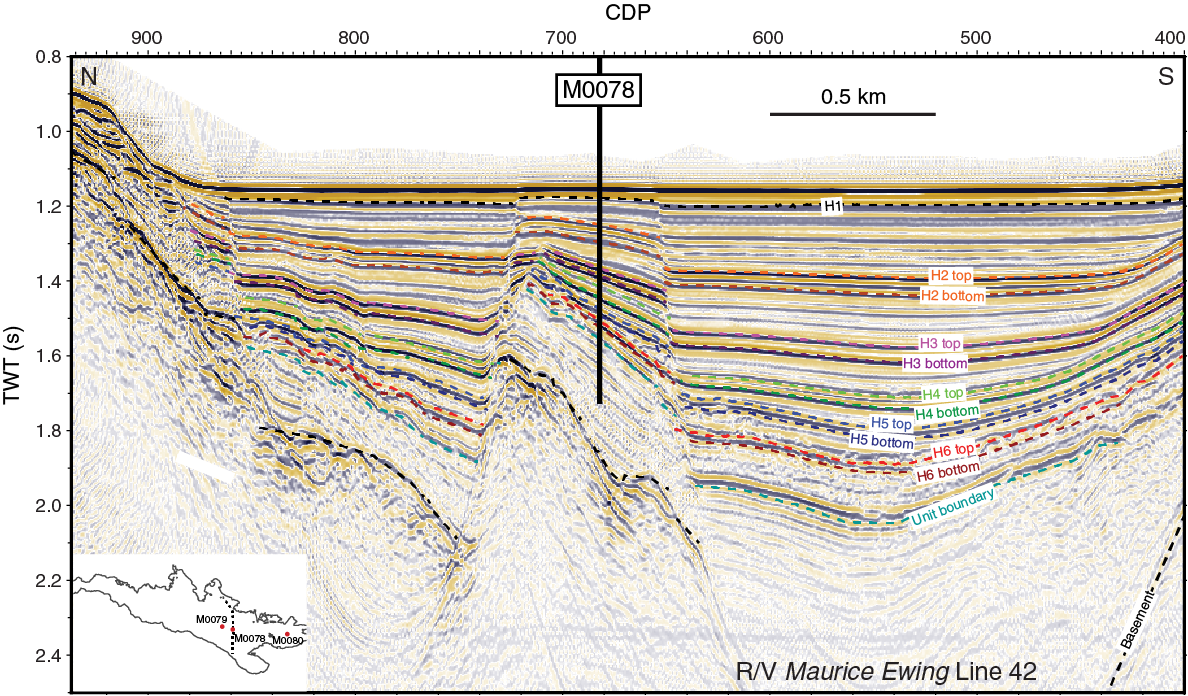
Figure F2. R/V Maurice Ewing Line 42.
In Hole M0078A, the Fugro Wison Extended Piston (WEP) system was used to core the upper 75 m, and the Fugro Corer in push mode was used for the next 124 m, followed by the same corer in percussive mode for 25 m. The Fugro Extended Marine Core Barrel (FXMCB) (rotary) was used to core the final 386 m of the borehole. In Hole M0078B, the Fugro Corer in push mode was used throughout to the base of the hole at 55.85 mbsf.
Transit to Hole M0078A
The D/V Fugro Synergy prepared to sail on the evening of 22 October 2017, and the vessel departed the Port of Corinth at 1955 h (local time) for the first coring site. At 2130 h, the Fugro Synergy arrived at Site M0078, and a dynamic positioning model was established. A reference beacon was deployed, and a sound velocity profile was conducted. Water depths for Holes M0078A and M0078B are 859.5 and 864 m, respectively.
Coring operations
Hole M0078A
At 0145 h (local time) on 23 October 2017, the seabed frame (SBF) was deployed, and the drilling crew began running pipe. However, running pipe took longer than anticipated because rust at the joints resulted in the need for a thorough cleaning prior to deployment.
During the evening of 23 October, the first cores were recovered with the first core on deck at 2135 h. The SEADEVIL (an addition to the standard seabed template) was used to accurately spud in and collect a seabed/water interface sample. The WEP system was lowered to approximately 10 cm above the seabed and energized. The first core was 2.65 m long. The next attempt at coring was unsuccessful, and the decision was made to wash through this interval. Following the wash through, coring continued throughout 23 and 24 October, generally with high recovery rates. On 25 October, recovery gradually worsened, prompting a switch to the Fugro Corer in push mode with flapper and finger catchers to optimize recovery. Initially, 3 m runs were conducted, but runs were extended to 4.7 m on the evening of 25 October.
At 2130 h on 25 October, a communication issue arose with the SEADEVIL, leading to its recovery on deck at 0300 h on 26 October for assessment. Further investigation identified a printed circuit board fault, and the board was replaced. At 1415 h, the SEADEVIL was redeployed to the seabed, and the drill pipe was extended to the base of the hole so that coring could recommence. The first core was recovered on deck at 1610 h. Coring paused briefly on 26 October to undertake an in situ temperature cone penetration test (CPT) measurement at 100 mbsf; temperature CPT measurements were also taken close to 200 and 300 mbsf in Hole M0078A. Coring with the Fugro Corer continued for the remainder of 26 October and through 28 October. At 0840 h, core Run 60 made no advance, and the run was repeated at the same interval (core Run 61). A 2 m advance was achieved, but no core was returned. Next, a 4.57 m run (core Run 62) was conducted with good recovery.
Recovery became more variable on 28 and 29 October, and some runs returned no core. As a result, in the early hours of 29 October it was decided to change the Fugro Corer from push mode to percussive mode. Despite this change, recovery continued to be highly variable, and at 2130 h, the operational decision was made to change from the Fugro Corer to the FXMCB system.
Coring continued with good rates of advance and recovery for the next 3 days until a communications and power issue arose with the SEADEVIL, resulting in its recovery on deck at 0530 h on 2 November for further assessment. It was concluded that this issue required a significant amount of time to resolve; therefore, it was agreed that coring would continue without the use of the SEADEVIL. From this point onward, the basic SBF was used for coring without the additional support of the SEADEVIL. Coring began again at 1645 h and progressed well through 7 November.
On 7 November, coring operations were paused because a slip clamp became jammed around the drill string. The clamp was eventually released after approximately 7 h. Coring then recommenced and continued through 8 November (apart from 1 h of downtime for lightning).
On the morning of 9 November, drill floor maintenance was required to repair some disk springs on the FXMCB. At ~0545 h, a slip clamp jammed around the drill string again, and it was not released until 0710 h, after which coring resumed. Coring paused again at 1135 h when the FXMCB was recovered on deck to undergo repairs. At 1600 h, coring resumed and progressed well through the morning of 10 November. At 1335 h, the final Hole M0078A core was on deck with a total penetration of 610.43 mbsf.
Throughout coring operations in Hole M0078A, seawater was used as the drilling medium, with the exception of four core runs where bentonite drilling mud was used to assist with hole conditioning (removal of cuttings and reducing any swelling of the borehole sidewall) (see Table T1).
Downhole logging operations in Hole M0078A commenced following coring and continued through 12 November. See Logging operations below for details.
Hole M0078B
Following unsuccessful downhole logging (see below), the decision was made to bump over 20 m to drill a short “B” hole to capture intervals of the upper 50 m of stratigraphy that were not recovered from Hole M0078A. Pipe was tripped, and the vessel moved 20 m south to the new coordinates (38°8′41.144″N, 22°45′30.242″E) (Figure F3).
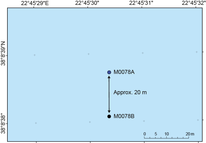
Figure F3. Hole M0078A and M0078B locations.
At midnight on 12 November 2017, the Fugro Synergy was settling on site. The first core was recovered at 0200 h using the Fugro Corer in push mode (a 1.31 m core that captured the seabed/water interface), and coring continued throughout the day with good recovery until 1640 h, when coring operations ended at 55.85 mbsf. Seawater was used as the drilling medium throughout coring operations in Hole M0078B. Following the completion of coring, tripping pipe commenced, and the SBF was recovered on deck in preparation for transit to the port call. At 0400 h on 13 November, the Fugro Synergy departed Site M0078 for the pilot station and was alongside and tied up by 0630 h at the Port of Corinth.
Logging operations
The following wireline logging tools were planned for deployment in two depth stages: magnetic susceptibility and conductivity (EM51), dual laterolog resistivity (DLL3), stacked natural gamma ray (QL40SGR), sonic (QL40FWS), acoustic borehole televiewer (QL40ABI), and spectral gamma ray (ASGR512).
Hole M0078A
Following completion of coring in Hole M0078A on 10 November 2017, preparations were made for downhole logging. Hole M0078A was stabilized with weighted bentonite mud, and then the drill pipe was raised to 296.54 mbsf for the first phase of logging.
Logging with the EM51 tool began at 0028 h on 11 November. The logging tools utilized for this expedition were super-slimline, and the tool strings were consequently relatively light. The light tool strings, coupled with the density of the mud that was ultimately used to stabilize the borehole, made it difficult for the tool string to descend in the borehole. Because of concerns surrounding hole stability, it was necessary to circulate heavier mud (8.5 lb/gal), which further impeded the descent of the tool string. After several failed attempts to deploy the tool, additional weight (~15 kg) was clamped to the wireline cable above the tool to make it heavier. The weighted tool started its descent more easily than before, but several losses of tension were observed, including at 297 m wireline log depth below seafloor (WSF), the depth of the drill bit, and between 337 and 347 m WSF. The total depth reached by the tool was believed to be 607 m WSF, and logging uphole commenced at a speed of 22 m/min. The difficulties encountered during the descent, including repeated attempts to pass various tight spots, led to the logging cable becoming entangled around the tool. As a result, 100 m of logging cable had to be cut from the primary winch (GV550). Data acquired during this first run are not depth accurate because of the entangling of the cable, and owing to the nature of the measurement (electrical and magnetic), the same entangled cable passing along the tool strongly affected the recorded data. Therefore, these data were not processed.
To save operational time, the backup winch (RG2000) was set up and used for the remainder of logging operations in Hole M0078A. To address the issues encountered during the first run, a heavier, centralized stacked tool string that included the QL40SGR, QL40FWS, and QL40ABI tools was deployed. No difficulties were encountered during the descent in the drill pipe. However, the tool string could not pass through the bit into the open hole, presumably because of the passive bowspring centralizers. The tool string was recovered, and a longer, heavier tool string was deployed in its place without the bowspring centralizers and with the QL40SGR, QL40FWS, caliper (QL40CAL), and magnetic susceptibility (QL40MSUS) tools. This tool string successfully reached 607 m WSF, and logging uphole started at 4 m/min. Unfortunately, the tool string became stuck in the open hole (356 m WSF) during its ascent. For 6 h, multiple attempts were made to free the tool string from the borehole, with increasing load applied to the cable in a step-wise fashion. Ultimately, it became clear that recovery of the tool string might not be possible, and the breaking load of the tool head was exceeded, resulting in the abandonment of the tool string in the hole. Fishing operations were not attempted, and logging operations in Hole M0078A were concluded at 1910 h on 11 November.
Data recorded during the final run indicate that the tool string became stuck on multiple occasions during its ascent, suggesting that borehole conditions were likely deteriorating as logging operations progressed. Owing to the difficulties encountered and erratic tool responses and in the absence of a meaningful depth reference, data lack context and are unusable.
Hole M0078B
Because of the shallow penetration (55.85 mbsf) in Hole M0078B, it was not logged.
Lithostratigraphy
Site M0078 is divided into two major lithostratigraphic units (1 and 2) based on a combination of the component facies associations (FA; see the Expedition 381 facies associations chapter [McNeill et al., 2019a]; Table T2), paleontology, seismic facies, and physical properties. In the following sections, we describe the units and subunits at Site M0078 and their boundaries (Table T3). The upper lithostratigraphic unit (1) is divided into 16 subunits that correlate with marine and isolated/semi-isolated intervals.
Unit and subunit description
Site M0078 was drilled into a horst block to sample the two main seismic stratigraphic units, here designated as lithostratigraphic Unit 1 (seismic Unit 2) and the underlying Unit 2 (seismic Unit 1) (Figure F2). Unit 1 is further divided into 16 subunits (Figure F4).
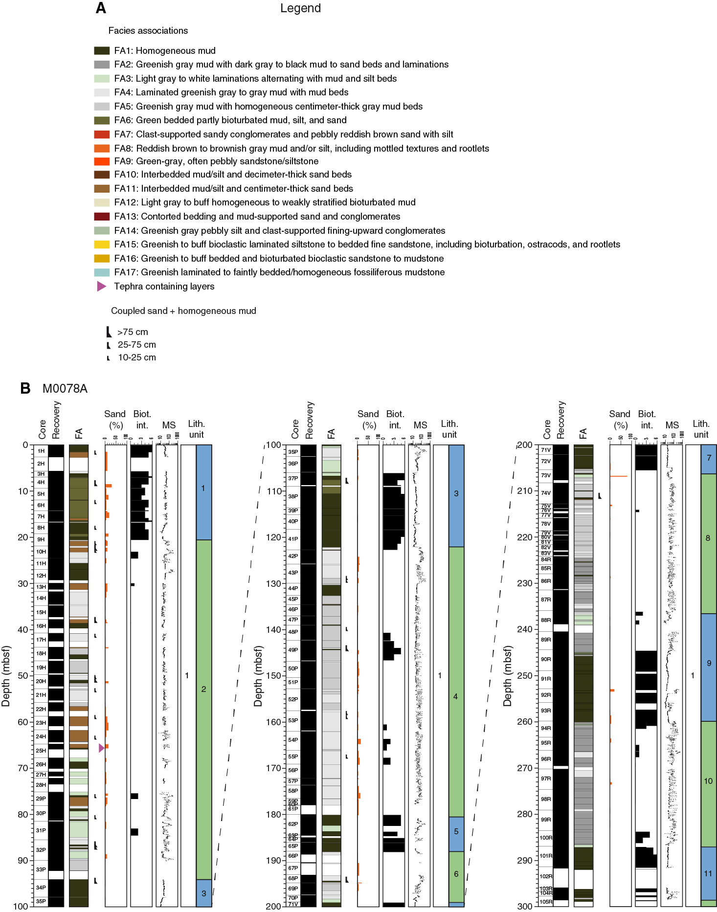
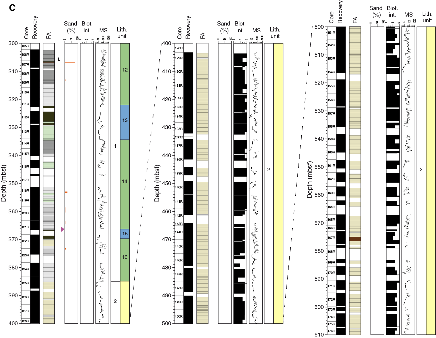
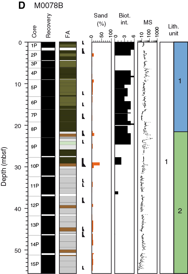
F4. Composite stratigraphic log.
Sediment composition for both Units 1 and 2 was determined from smear slide analysis and X-ray diffraction (XRD) data (Figure F5). Unit 1 sediment is dominated by detrital clay to clayey silt with calcite most abundant and with common to abundant quartz, feldspar, and phyllosilicates. Overall, carbonate content increases from the seafloor to the base of Hole M0078A (from <50 to >75 wt%), with a corresponding decrease in quartz and clay abundance. The upper 100 m of Hole M0078A displays particularly high mineral diversity, with dominant carbonate minerals, quartz, and phyllosilicates (clays and micas). Continuing downhole, carbonate minerals (mainly represented by calcite) gradually become more abundant with respect to other minerals. Biogenic material is common, where the major component is individual diatoms and diatom fragments (Figure F5C). Foraminifers, foraminiferal fragments, and calcareous nannofossils are common in the homogeneous fine-grained intervals of FA1 and FA6 mud (see Micropaleontology) but are rare to absent in other facies associations. A distinctive compositional feature is that well-sorted silt-sized aragonite needles dominate some of the FA3 white laminations (Figure F5B). However, it is important to note that white laminations can also be composed of calcite and thus are not always indicative of aragonite. Organic components and pyrite are also commonly present in smear slides, but their overall contribution to the mineral assemblage is negligible. In sandy intervals, subangular to subrounded, reworked detrital calcite grains dominate. Unit 2 has a similar overall composition to Unit 1, according to XRD analysis (Figure F5A), but with carbonate as the dominant component throughout and less quartz and fewer phyllosilicates. Smear slide analysis indicates that the carbonate is generally in the form of well-sorted clay (mud)-grade to very fine silt–sized detrital calcite (Figure F5D). Other detrital grains and organic and biogenic components are generally rare or absent in Unit 2.
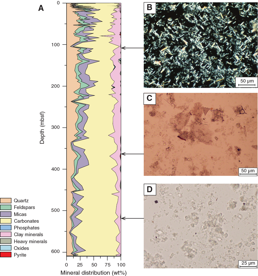
Figure F5. Downhole major mineral distribution.
Tephra and cryptotephra intervals were found in Site M0078 cores. These intervals were identified by a combination of visual inspection and physical properties. An increase in Multi-Sensor Core Logger (MSCL) natural gamma radiation (NGR) intensity was usually observed in association with both visible tephra layers and cryptotephra intervals, and this relationship was used as the primary method for targeting further investigation. Distinct and visible tephra layers (e.g., Section 381-M0078A-121R-3, 42.0–43.0 cm [366.52–366.53 mbsf]) were usually a subtly different color from the surrounding sediment, and very high concentrations of bubble-wall shards in these layers made the layers highly reflective under hand lens inspection. Cryptotephra intervals comprise the majority of tephra identified in the core and were identifiable only through methodical sampling of NGR intensity peaks and subsequent visual examination of sampled material via optical microscopy. Cryptotephra were also identified incidentally during routine micropaleontological work by the observation of glass shards.
Unit 1
- Intervals: 381-M0078A-1H-1, 0 cm, to 125R-2, 15 cm; 381-M0078B-1H-1, 0 cm, to 15P-CC, 15 cm
- Depths: Hole M0078A = 0–385.14 mbsf; Hole M0078B = 0–55.49 mbsf (base of Unit 1 not reached)
- Age: Pleistocene to Holocene
Subunit 1-1
- Intervals: 381-M0078A-1H-1, 0 cm, to 9H-2, 26 cm; 381-M0078B-1H-1, 0 cm, to 8H-2, 46 cm
- Depths: Hole M0078A = 0–20.78 mbsf (20.78 m thick including 3.22 m of missing core); Hole M0078B = 0–21.16 mbsf (21.16 m thick including 1.07 m of missing core)
In Hole M0078A, Subunit 1-1 extends from the seafloor to Section 9H-2, 26 cm (20.78 mbsf), where its base is marked by a change from mainly FA1 greenish gray homogeneous mud to FA4 laminated mud beds with greenish gray parallel laminations (Figure F4). In Hole M0078B, Subunit 1-1 extends from the seafloor to Section 8H-2, 46 cm, where its base is also marked by a transition from FA1 to FA4. In Subunit 1-1, four sand–homogeneous mud couplets >10 cm thick were identified in Hole M0078A and six were identified in Hole M0078B.
In Hole M0078A, Subunit 1-1 consists of FA1 and FA6 mud and minor FA11 interbedded mud/silt beds. The upper part comprises FA1 greenish gray homogeneous mud and FA6 mud with faint laminations and bedding, as well as high bioturbation intensity (BI = 4–6, including discrete Planolites and Palaeophycus). Subordinate centimeter-scale sand beds that fine upward, typically over 5–10 cm, also occur. The lower part is dominated by FA1 greenish gray homogeneous mud with shell fragments and intense bioturbation (BI = 4–6, with Zoophycos and Scolicia). Four prominent sand–homogeneous mud couplets were identified throughout Subunit 1-1 in Hole M0078A.
In Hole M0078B, Subunit 1-1 also comprises FA1 and FA6.
Subunit 1-2
- Intervals: 381-M0078A-9H-2, 26 cm, to 34P-1, 0 cm; 381-M0078B-8H-2, 46 cm, to 15P-CC, 15 cm
- Depths: Hole M0078A = 20.78–94.14 mbsf (73.36 m thick including 14.90 m of missing core); Hole M0078B = 21.16–55.49 mbsf (34.33 m penetrated including 2.57 m of missing core; base Subunit 1-2 not reached)
The top of Subunit 1-2 is marked by a change from FA1 (above) to FA4 (below). The lower boundary with Subunit 1-3 is transitional and occurs in FA1 homogeneous mud, and it is marked by the appearance of marine microfossils and shell fragments (Figure F4). In Hole M0078A, 15 sand–homogeneous mud couplets occur in Subunit 1-2. In Hole M0078B, 11 sand–homogeneous mud couplets are dispersed throughout Subunit 1-2, with a notable 4 m thick example from Section 9P-5, 16 cm, to Section 10P-2, 71 cm (25.81–19.86 mbsf).
In Hole M0078A, Subunit 1-2 consists of a complex succession of five facies associations and comprises three parts marked by changes in the dominant facies association. The upper part (Sections 9H-2, 26 cm, to 22H-2, 0 cm; 20.58–56.66 mbsf) is dominated by FA4 laminated mud beds with greenish gray parallel laminations that often alternate with FA5 greenish gray mud with homogeneous centimeter-scale mud beds and FA1 homogeneous mud. A smaller percentage of FA11 interbedded mud/silt beds and centimeter-thick sand beds (sometimes graded) occurs in the upper part of Subunit 1-2 (e.g., Section 13H-1, 36 cm; 30.3 mbsf). The middle part of Subunit 1-2 (Sections 22H-2, 0 cm, to 32P-3, 96 cm; 56.66–89.5 mbsf) is characterized by a general increase in sand proportion. It comprises predominantly FA3 bedded mud with gray to white submillimeter-scale laminations that are interbedded with FA11 mud and sand beds. The lower part of Subunit 1-2 (Sections 32P-3, 96 cm, to 34P-1, 0 cm; 89.5–94.14 mbsf) mainly consists of FA4 interbedded with short FA1 and FA3 intervals.
Subunit 1-2 is incomplete in Hole M0078B. The upper part consists of FA4, FA11, FA2, FA3, FA1, and FA10 intervals. Below Section 10P-3, 0 cm (24.65 mbsf), FA5 predominates. Some reddish mud appears in FA5 in Sections 381-M0078B-15P-2, 75 cm, to 15P-3, 68 cm (53.3–54.69 mbsf).
Subunit 1-3
- Interval: 381-M0078A-34P-1, 0 cm, to 41P-3, 84 cm
- Depth: 94.14–122.16 mbsf (28.02 m thick including 0.53 m of missing core)
The top of Subunit 1-3 is placed at the top of Core 381-M0078A-34P, where the uppermost part is composed of FA1 homogeneous mud. However, poor recovery in the overlying core means that the exact boundary location is poorly constrained. The base is marked by a change from FA1 (above) to FA4 (below) (Figure F4). Two sand–homogeneous mud couplets occur in Subunit 1-3.
Subunit 1-3 is divided into three parts. The upper part, to Section 381-M0078A-35P-2, 74 cm (100.19 mbsf), comprises FA1 greenish gray mud with abundant shell fragments and pyrite and sparse thin silty and sandy beds. Below, a transition to the second part includes mixed FA3 and FA4 laminated deposits and then a marked change to FA3 in Section 36P-1, 64 cm (103.28 mbsf). The FA3 laminations are regular and millimeter or submillimeter in scale and contain both marine and brackish diatom assemblages (see Micropaleontology), with aragonite dominating the whitish laminations (Figure F5B). An abrupt contact in Section 37P-1, 62 cm (106.66 mbsf), marks the top of the lower part of Subunit 1-3, which is dominated by FA1 homogeneous mud. The homogeneous character is due to a high degree of bioturbation destroying any bedding or lamination.
Subunit 1-4
- Interval: 381-M0078A-41P-3, 84 cm, to 62P-1, 0 cm
- Depth: 122.16–180.14 mbsf (57.98 m thick including 3.38 m of missing core)
The top of Subunit 1-4 is marked by a change from FA1 homogeneous mud to FA4 laminated mud. The lower boundary is marked by a change from FA4 to FA1 (Figure F4). Seven sand–homogeneous mud couplets occur in Subunit 1-4.
Subunit 1-4 comprises two parts, each dominated by one facies, with a transitional boundary between them in Section 381-M0078A-53P-1, 0 cm (157.74 mbsf). Below a package dominated by FA4, much of the upper part of Subunit 1-4 (128.84–157.74 mbsf) is dominated by FA5 but also includes FA1 occurrences of bioturbated mud as thick as 3 m. In the FA5 sediment, frequent centimeter-thick intervals consist of very poorly sorted silty sand with subangular to subrounded grains dominated by detrital lithics (mainly carbonates and quartz) and common organic material. The homogeneous mud beds (FA1) have gray to reddish gray (7.5Y 5/2 to 7.5Y 6/2) color variations. Shell fragments were also observed in the upper part of Subunit 1-4. The mud beds occasionally include darker gray organic-rich laminations. In the lower 5 m of the upper part of Subunit 1-4, bedded mud (FA5) is interbedded with laminated mud (FA4) on a meter scale.
The lower part of Subunit 1-4 (Sections 381-M0078A-53P-1, 0 cm, to 62P-1, 0 cm; 157.74–180.14 mbsf) mostly consists of FA4 with minor FA5 occurrences over intervals of tens of centimeters (165.89–166.24 mbsf; 172.16–172.34 mbsf).
Subunit 1-5
- Interval: 381-M0078A-62P-1, 0 cm, to 65P-CC, 8 cm
- Depth: 180.14–188.18 mbsf (8.18 m thick including 0.57 m of missing core)
FA1 homogeneous mud appears in Section 381-M0078A-62P-1, 0 cm (180.14 mbsf), marking the top of Subunit 1-5. However, approximately 2 m of core is missing immediately above this core, and therefore the top of Subunit 1-5 is poorly constrained. The lower boundary marks a change from greenish gray homogeneous mud (FA1) to laminated mud (FA4) (Figure F4).
The predominant facies association in Subunit 1-5 is greenish gray homogeneous mud (FA1) with high levels of bioturbation, scattered sparse small shell fragments, some rare faint laminations, and scattered pyrite. This facies association is interrupted by a 122 cm thick succession of FA3 gray and cream finely laminated mud with a few 1–2 cm beds of homogeneous mud that occurs with a disturbed top in Section 381-M0078A-62P-2, 147 cm, and a sharp base in Section 62P-3, 120 cm (182.3–183.52 mbsf). The laminations in this interval comprise well-sorted silt-grade aragonite crystals with abundant framboidal pyrite. Bioturbation intensity appears low.
Subunit 1-6
- Interval: 381-M0078A-66P-1, 0 cm, to 70P-1, 148 cm
- Depth: 188.18–199.14 mbsf (10.96 m thick including 4.29 m of missing core)
The top of Subunit 1-6 is marked by the disappearance of marine microfossils (see Micropaleontology) and a change from FA1 homogeneous mud (above) to FA4 laminated greenish gray mud (below) (Figure F4). The nature of the boundary is unclear because it falls in the ~8 cm gap (no recovery) between cores. The lower boundary is marked by the reappearance of marine microfossils and a change from FA3 creamy laminated mud (above) to FA1 homogeneous mud (below). One sand–homogeneous mud couplet occurs in Subunit 1-6.
The top part of Subunit 1-6 consists of FA4 centimeter-scale interbedded laminated and homogeneous mud beds. Black organic-rich silt layers (millimeter scale) are found occasionally throughout, whereas very fine sand beds are rare and thin (<1 cm thick) where present. Rare pyrite is scattered throughout. A 32 cm interval of FA1 homogeneous mud containing abundant pyrite beginning in Section 381-M0078A-68P-2, 20 cm (194.45 mbsf), separates the top part from the rest of the subunit. Below the homogeneous mud interval is another section of FA4 centimeter-scale interbedded laminated mud and homogeneous mud beds (70%) with lesser proportions of FA5 (30%). This interval also features rare 0.5–1.5 cm thick fine sand and millimeter-scale black organic-rich silt. Rare pyrite is scattered throughout this interval. The lower 78 cm of the subunit consists of FA3 creamy laminated mud interbedded with homogeneous mud beds.
Subunit 1-7
- Interval: 381-M0078A-71V-1, 0 cm, to 73V-1, 86 cm
- Depth: 199.14–206.40 mbsf (7.26 m thick including 0.06 m of missing core)
The top of Subunit 1-7 is marked by a distinct boundary between overlying FA3 creamy laminated mud and underlying FA1 homogeneous mud (Figure F4). The base is marked by the appearance of laminations that represent a return to FA3 creamy laminated mud at the top of the underlying Subunit 1-8 (Figure F6).
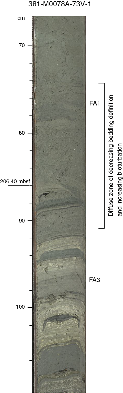
Figure F6. Transitional boundary from Subunit 1-7 to Subunit 1-8.
The upper part of Subunit 1-7 consists of greenish gray homogeneous mud (FA1) with shell fragments and bioclasts scattered throughout. The homogeneous mud is variably bioturbated and becomes completely bioturbated in Sections 381-M0078A-72V-2, 0 cm, to 72V-3, 24 cm (203.84–205.18 mbsf). The mud passes down into a more varied succession of centimeter- to decimeter-thick gray mud beds (FA5) between Sections 72V-3, 24 cm, and 73V-1, 54 cm (205.18–206.08 mbsf). The bedded mud includes shell fragments and is often moderately bioturbated with a slightly mottled appearance. The basal ~30 cm of Subunit 1-7 returns to FA1 completely bioturbated greenish gray homogeneous mud.
Subunit 1-8
- Interval: 381-M0078A-73V-1, 86 cm, to 87R-CC, 0 cm
- Depth: 206.40–236.18 mbsf (29.78 m thick including 2.72 m of missing core)
The top boundary of Subunit 1-8 is sharp and characterized by a change in facies from FA1 homogeneous mud (above) to FA3 white to gray finely laminated mud (below) (Figures F4, F6). The base is marked by a change from FA2 bedded mud with organic-rich silty to fine sand layers (above) to FA4 laminated mud (below) and is accompanied by the appearance of marine microfossils (see Micropaleontology). One sand–homogeneous mud couplet occurs in Subunit 1-8.
Subunit 1-8 dominantly comprises FA5 (60%) and FA2 (30%) and is divided into three parts. The top part (206.4–208.44 mbsf) is an interval of dominantly FA3 white to light gray finely laminated mud. The middle part (208.44–224.34 mbsf) is mainly composed of FA5 centimeter-thick bedded greenish gray mud with subordinate millimeter- to centimeter-thick silty layers that are occasionally black and contain possible organic material. Pyrite and slight bioturbation (BI = 1) are present in this middle part, and fine to very fine sand beds are sparsely distributed. The lower part (224.34–236.18 mbsf) is dominated by FA2 centimeter-thick bedded mud with frequent dark gray to black organic-rich silty to very fine sand layers with sparse pyrite.
Subunit 1-9
- Interval: 381-M0078A-87R-CC, 0 cm, to 93R-4, 21 cm
- Depth: 236.18–260.70 mbsf (24.52 m thick including 1.92 m of missing core)
The top of Subunit 1-9 appears sharp and is marked by a change from FA2 (above) to FA4 (below) but was picked on the basis of marine microfossils being present below this boundary (see Micropaleontology). The lower boundary occurs at a sharp contact between FA1 homogeneous mud (above) and FA4 (below) (Figure F4).
The upper part of Subunit 1-9 includes some intervals of FA4 but is dominated by FA3 light gray to white thin laminations and centimeter-thick homogeneous mud beds with sparse but locally intense bioturbation. FA2 greenish gray mud with dark gray to black centimeter-thick silty beds also occur. In contrast, the lower part (below Section 381-M0078A-90R-1, 110 cm; 245.69 mbsf) comprises FA1 greenish gray homogeneous mud that is intensely bioturbated (BI as high as 6) with high-diversity trace fossil assemblages, including Thalassinoides, Planolites, Chondrites, and Palaeophycus. Scattered shell fragments and pyrites also occur.
Subunit 1-10
- Interval: 381-M0078A-93R-4, 21 cm, to 101R-1, 0 cm
- Depth 260.70–287.12 mbsf (26.42 m thick including 0.70 m of missing core)
The top of Subunit 1-10 is marked by a sharp transition from FA1 homogeneous mud (above) to FA4 (below) followed by a downhole increase in organic material content. The lower boundary is marked by a change from FA3 light gray to white laminated mud (above) to FA1 homogeneous mud (below) and a corresponding appearance of scattered shell material. The lower boundary appears sharp but may be disturbed by drilling-induced deformation (DID) (Figure F4).
Subunit 1-10 mainly consists of FA2 centimeter-scale greenish gray bedded mud alternating with thin laminated (millimeter-scale) gray to black silt and sand. Darker beds are associated with the presence of organic material and are often pyritic. This succession is interrupted by short intervals (meter scale) of FA5 interbedded centimeter-scale homogeneous and laminated greenish gray to gray mud with subordinate laminated greenish gray to gray mud. Occasionally, FA3 light gray to white submillimeter laminated mud (<0.5 m thick) is also found in the upper and lowermost parts of Subunit 1-10.
Subunit 1-11
- Interval: 381-M0078A-101R-1, 0 cm, to 105R-1, 84 cm
- Depth: 287.12–298.84 mbsf (11.72 m thick including 4.21 m of missing core)
The upper boundary of Subunit 1-11 is marked by a change from FA3 laminated mud (above) to FA1 homogeneous mud (below). The lower boundary is marked by a change to FA4 laminated mud in Subunit 1-12 (Figure F4).
Subunit 1-11 is dominated by FA1 homogeneous mud (91%) with minor occurrences of FA4 and FA2 toward the base. FA1 is highly bioturbated mud with various bioclasts, abundant trace fossils (mainly identified as Chondrites, Palaeophycus, and Planolites), and pyrite. A 1.09 m thick FA4 and FA2 interval comprises organic-rich bedded and laminated mud in various greenish gray shades (Sections 381-M0078A-104R-2, 66 cm, to 105R-1, 33 cm; 295.36–298.33 mbsf). Below this interval, FA1 bioturbated homogeneous mud continues to the base of Subunit 1-11.
Subunit 1-12
- Interval: 381-M0078A-105R-1, 84 cm, to 111R-3, 3 cm
- Depth: 298.84–322.35 mbsf (23.51 m thick including 4.23 m of missing core)
The top of Subunit 1-12 is marked by a change from FA1 homogeneous mud (above) to FA2 laminated mud with frequent dark gray to black mud beds (below) and the disappearance downhole of marine microfossils. Poor recovery in Core 381-M0078A-105R (19%) prevents determination of the nature of the contact (abrupt or transitional). The lower boundary corresponds to a facies change from FA4 laminated mud (above) to FA1 homogeneous mud (below) (Figure F7). One sand–homogeneous mud couplet occurs in Subunit 1-12.
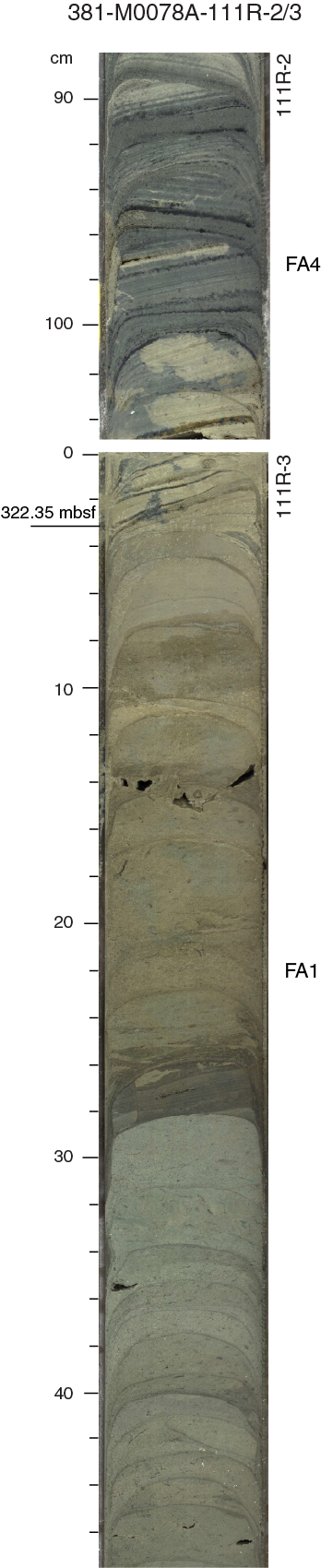
Figure F7. Transitional boundary from Subunit 1-12 to Subunit 1-13.
Subunit 1-12 comprises two parts, each one corresponding to one or two dominant facies associations. The upper part (Section 381-M0078A-106R-1, 0 cm, through Section 106R-3; 298.12–306.5 mbsf) is mainly composed of FA2 with thin organic-rich laminated mud beds, centimeter-thick organic-rich silt beds, and centimeter-thick homogeneous mud beds. Below this repetitive succession of FA2 is a fining-upward sand–homogeneous mud couplet (designated FA1 and FA10; Section 107R-1, 0–88 cm; 306.5–307.38 mbsf).
The lower part of Subunit 1-12 is characterized by further FA2 and then FA4 from Section 381-M0078A-109R-2, 0 cm, to Section 111R-3, 28 cm (314.35–322.35 mbsf), with laminated mud, centimeter-scale mud beds, and sparse organic-rich laminations.
Subunit 1-13
- Interval: 381-M0078A-111R-3, 3 cm, to 114R-1, 0 cm
- Depth: 322.35–334.40 mbsf (12.05 m thick including 1.6 m of missing core)
The top of Subunit 1-13 is marked by a gradational change from FA4 laminated mud (above) to FA1 homogeneous mud (below) (Figure F7) and a corresponding appearance of marine microfossils. The lower boundary occurs in FA3 finely laminated mud and is marked by the presence of bioturbation above the boundary, with discrete burrows descending from the drilling-disturbed boundary into otherwise unbioturbated laminated mud in Subunit 1-14 (Figure F4).
Subunit 1-13 comprises two parts with a boundary in Section 381-M0078A-113R-1, 0 cm (328.65 mbsf), marked by a change in the dominant facies association. The upper part is dominated by FA1 greenish gray homogeneous mud with some rare faint laminations, high levels of bioturbation, and scattered sparse small shell fragments and small disperse pyrite. This succession is interrupted by a short (61 cm) FA3 interval characterized by submillimeter-scale cream/gray laminated mud with strong bioturbation that notably includes Teichichnus burrows. The lower part comprises gray and cream finely (submillimeter) laminated mud with a few 1–2 cm beds of homogeneous mud (FA3). Strong bioturbation affects this FA3 interval, including oval millimeter-scale burrows that make laminations indistinct.
Subunit 1-14
- Interval: 381-M0078A-114R-1, 0 cm, to 121R-3, 38 cm
- Depth: 334.40–366.49 mbsf (32.09 m thick including 7.49 m of missing core)
The top of Subunit 1-14 is marked by the disappearance of bioturbation in FA3 finely laminated light mud and a transition from FA3 to FA2 downhole. The bottom of the subunit is marked by a sharp boundary from FA4 laminated mud (above) to FA5 bedded mud (below) (Figure F4) and the appearance of marine microfossils (see Micropaleontology).
Subunit 1-14 comprises three main parts with boundaries in Sections 381-M0078A-115R-1, 138 cm, and 119R-2, 52 cm (339.28 and 356.55 mbsf, respectively). The upper part features FA2 centimeter-thick organic-rich beds in centimeter-thick interbedded laminated mud (more common) and homogeneous mud (less common). Laminations are pale in color and very thin (<1 mm). The middle part consists predominantly of FA4 with occasional FA3 creamy laminated mud, with centimeter-thick homogeneous mud beds and rare organic-rich layers and very thin silt and sand beds. Sparse bioturbation and rare pyrite are present throughout. The lower part of the subunit is composed of centimeter-thick bedded and laminated mud of FA5 and FA4 with occasional millimeter- to centimeter-scale silt or very fine sand beds. Sparse to uncommon bioturbation is present throughout, with scattered rare pyrite. In the lower 1.8 m, strongly laminated mud (FA4) lies above a sharp boundary.
Subunit 1-15
- Interval: 381-M0078A-121R-3, 38 cm, to 122R-1, 106 cm
- Depth: 366.49–369.66 mbsf (3.17 m thick including 1.79 m of missing core)
The top of Subunit 1-15 appears sharp and is marked by a change from FA4 laminated mud (above) to FA5 mud beds (below) and a corresponding appearance of marine microfossils. The lower boundary is marked by a change from FA1 homogeneous mud (above) to FA3 laminated mud (below) (Figure F4).
Subunit 1-15 comprises an upper 10 cm interval of FA5 greenish gray centimeter-scale mud beds with abundant foraminifers, shell fragments, and bioclasts that contains distinct layers of millimeter-scale mud clasts. The rest of the subunit comprises FA1 greenish gray homogeneous mud that is highly to completely bioturbated with occasionally identifiable Planolites burrows and abundant shell fragments scattered throughout.
Subunit 1-16
- Interval: 381-M0078A-122R-1, 106 cm, to 125R-2, 15 cm
- Depth: 369.66–385.14 mbsf (15.48 m thick including 2.94 m of missing core)
The top boundary of Subunit 1-16 is moderately bioturbated and characterized by a change from FA1 homogeneous mud (above) to FA3 laminated mud (below). The bottom boundary is marked by an abrupt change from FA4 laminated gray mud to FA12 light gray homogeneous mud at the top of Unit 2 (Figures F4, F8).
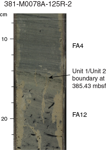
Figure F8. Unit 1/2 boundary.
Subunit 1-16 is mainly composed of FA4 with minor FA3 and FA12. Close to the upper boundary, the subunit contains both white to light gray thinly laminated mud (FA3) and centimeter-thick bedded gray mud (FA5) with pyrite and shell fragments. Directly below is a 2 m interval of FA12 highly bioturbated light gray to beige mud that is rich in pyrite. The bottommost 12.9 m is mainly composed of FA4 millimeter-scale laminated gray mud with some centimeter-thick beds and one interval with dominantly centimeter-thick bedded mud (FA5; 373.6–378.6 mbsf). Pyrite, millimeter-thick dark, probably organic-rich layers, and broken shell fragments are common, whereas bioturbation is sparse. Several intervals with centimeter-thick slumps or debris flows and centimeter-scale silty to sandy layers that fine upward also occur.
Unit 2
- Interval: 381-M0078A-125R-2, 15 cm, to 176R-3, 8 cm (base of hole)
- Depth: 385.14–610.43 mbsf (225.29 m thick including 43.19 m of missing core)
- Age: Pleistocene
The top of Unit 2 is a sharp boundary marked by an abrupt change from FA4 laminated greenish gray mud (above) to FA12 light gray homogeneous mud (below) (Figures F4, F8). The uppermost 15 cm of Unit 2 is characterized by abundant millimeter- to centimeter-scale pyritized burrows (mainly subhorizontal) (Figure F8). Unit 2 is composed almost entirely of FA12 (99%), with rare FA4, FA5, and FA11 occurrences. FA12 consists of light gray homogeneous mud with a high bioturbation intensity (BI = 4–6). Ichnological diversity is low to moderate, mainly including Planolites, Chondrites, and Teichichnus, but trace fossils are commonly undetermined because of the intense bioturbation. Sporadic framboidal and linear occurrences (infills of burrows?) of pyrite are common. A minor FA12 subfacies association comprises darker gray mud with faint bedding and black laminations associated with higher organic matter content and reduced bioturbation intensity (BI = ~4). The bedded and laminated mud of FA4 and FA5 occurs mainly in the uppermost 20 m of Unit 2, forming roughly 50–70 cm thick packages (391.10–391.59, 396.75–397.48, and 405.10–405.58 mbsf). The whole of Unit 2 is strongly affected by DID (biscuiting) (see Structural geology).
Interpretation of Site M0078
The Site M0078 lithostratigraphy is dominated by mud facies with minor sand and silt, indicating a distal subaqueous environment with low clastic input. Detrital calcite predominates throughout but with somewhat decreasing importance upward through the succession. Quartz, feldspar, and phyllosilicates represent subordinate minerals (in order of importance). Biogenic material is common, particularly in the marine subunits.
The most significant lithostratigraphic boundary (between Units 1 and 2) is marked by an abrupt uphole change from the highly monotonous FA12 succession in Unit 2 to a cyclical pattern of facies association changes in the overlying Unit 1. The 16 subunits in Unit 1 fall into two alternating types: those composed predominantly of the homogeneous green gray mud of FA1 and FA6 (odd-numbered subunits, Figure F4) and those composed predominantly of laminated and bedded mud of various facies associations, in particular FA5 (even-numbered subunits, Figure F4). These alternating types of subunits in Unit 1 are provisionally identified as representing marine and isolated/semi-isolated environments for odd- and even-numbered subunits, respectively, with good correlation with micropaleontology results (see Micropaleontology).
Marine subunits in Unit 1 (odd numbers) are moderately to highly bioturbated and dominated by homogeneous to poorly bedded greenish gray mud with scattered shell debris. Isolated/semi-isolated subunits (even numbers) are dominated by laminated to thinly bedded gray and greenish gray mud, some with black, organic-rich laminations and beds but with no, or only sparse, bioturbation or shell debris. In both the marine and isolated/semi-isolated subunits, sedimentary processes were dominated by deposition from fine-grained, low-concentration turbidity currents and hemipelagic suspension fallout. Sand–homogeneous mud couplets represent significant turbidite input, whereas centimeter- to millimeter-thick graded silt and sand represent a background of regular low-volume distal turbidite input. Compared with Site M0079, slumped units, mud-supported conglomerates, and sand–homogeneous mud couplets are relatively rare and thin in Holes M0078A and M0078B, suggesting a more stable environment or a location that was relatively well protected from incoming sediment derived from slope failure or sediment gravity flows sourced from the major catchments surrounding the rift, which is consistent with the position of Site M0078 on an intrabasinal horst (see Figure F2).
Unit 2 is dominated by monotonous FA12 light gray to buff homogeneous to weakly laminated highly bioturbated mud. The boundary with overlying Unit 1 is sharp, and the uppermost 15 cm of Unit 2 is characterized by abundant millimeter- to centimeter-scale subhorizontal pyritized burrows. These characteristics suggest a possible unconformity between Units 1 and 2. No compositional change was observed across this boundary in XRD or smear slide data (Figure F5).
Structural geology
DID and tectonic deformation were systematically recorded in Holes M0078A and M0078B. The north–south seismic reflection profile shows the tectonic location of Site M0078 on an uplifted horst block (Figure F2) with beds that are progressively tilted southward (as much as 13°) in the footwall of a major north-dipping normal fault. Because Site M0078 is located between two prominent faults, we did not expect to encounter any major structures in the borehole, and observations in the core confirm there are none.
Observed tectonic structures
Bedding attitude in the core is generally horizontal to subhorizontal through the core despite the gradual increase in dip of seismic reflection horizons around Site M0078. Locally, bedding can be tilted through full core sections (i.e., natural tilting rather than drilling induced) with apparent bedding dips as high as 24° (Section 381-M0078A-126R-3; 391.59–393.10 mbsf). These local dips are higher than those measured from the north–south seismic reflection profile, which could be due to the lower resolution of the individual seismic reflectors or the seismic profile not displaying the true dip.
Small-scale natural faulting was observed sporadically throughout the core, including frequent normal faults and rare suspected strike-slip faults (Figure F9). These natural faults were distinguished from DID by their planar geometries and the lack of influence by proximity to either the core liner, core axis (i.e., curving inward to become parallel to the core axis or curving into the core liner; conjugate fractures that are symmetrical on the core central axis), or other forms of DID. The shallowest observed natural fault is in Section 381-M0078A-9H-1 (19.21–20.52 mbsf), and faulting intensity per section (when observed) generally increases with depth (Figure F10A). Concentrated faulting in discrete intervals was also observed, such as in Core 113R (329.4–334.4 mbsf), where 20 small normal faults were recorded (Figures F10A, F11). In particular, abundant faulting was consistently recorded in Sections 113R-1 through 139R-2 (329.4–447.33 mbsf) (Figure F10A). Below this interval, no faulting was observed until Section 164R-1 (564.01 mbsf), where the deepest faults were observed. The apparent absence of small faults from Section 139R-2 through Section 164R-1 may be related to high-intensity rotary drilling–induced biscuiting throughout the interval (see below).
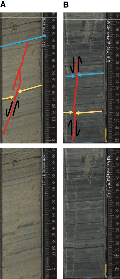
Figure F9. Small tectonic faults.

Figure F10. Preliminary analyses of natural faults.

Figure F11. Several small conjugate normal faults.
The vast majority of natural faults observed at Site M0078 have apparent normal displacements ranging from 1 to 350 mm. A total of 30 normal faults were sampled for orientation analysis. These faults appear to form conjugate sets throughout the core, as illustrated by the stereographic projection of several normal faults in the core reference frame in Core 381-M0078A-113R (329.4–334.4 mbsf) (Figures F10B, F11). The sampled normal faults show true dips ranging from 42° to 82° but with a clear modal average of 60°–70° and a mean fault dip of 66° (Figure F10C). The abundance and geometry of small normal faults are in agreement with the overall extensional nature of the rift deformation. Because cores were not oriented, the fault orientation measurements were not corrected to geographic north; this correction (using paleomagnetic data) will only be possible where the core has not been affected by DID (biscuiting).
Observed drilling-induced deformation
A range of drilling-induced structures was observed at Site M0078. The most common were biscuiting (Figure F12C), arching bedding, tilted panels, lensing, sediment smearing/flow along the core liner, voids, and open fractures. Other less frequently observed structures are listed in Table T1 in the Expedition 381 methods chapter (McNeill et al., 2019b). In general, DID intensity increases downhole, as in Hole M0078A (Figure F12A), and is particularly intense in rotary cores.
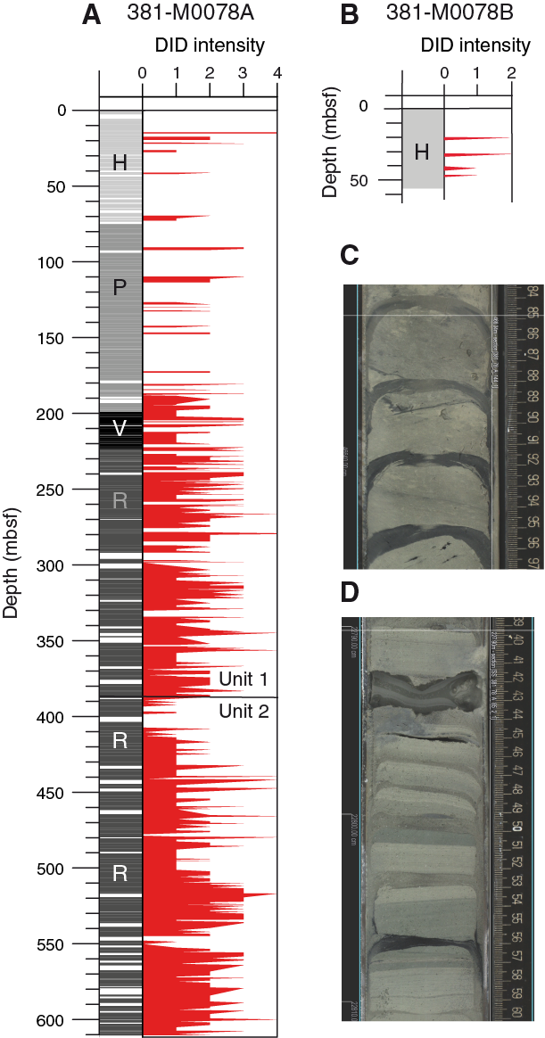
Figure F12. DID intensity.
The recording of DID through the upper part of Hole M0078A was patchy because our initial methodology was not robust. However, DID was correctly recorded in adjacent Hole M0078B (Figure F12B). Soupy texture was often found in the uppermost part of the hole through Core 381-M0078A-12H (29.94 mbsf). Hydraulic piston coring was used throughout Core 28H (75.19 mbsf), which generated sporadic, slight–moderate DID intensity that was mainly expressed by arching bedding and disrupted/mingled beds with rare axial flow and open fractures. For Cores 29P through 70P (75.19–99.14 mbsf), hydraulic push coring was used, producing sporadic, slight–moderate DID intensity characterized by arching bedding, lensing, and disrupted/mingled beds with rare voids and open fractures. Hydraulic percussive coring was used for a short interval from Core 71V through Core 83V (199.14–224.34 mbsf) and was associated with moderate–high DID intensity predominantly expressed by arching bedding and lenses.
Core 381-M0078A-84R (224.34 mbsf) marks the onset of rotary coring, which was used to the bottom of the hole. Rotary coring is associated with a marked and consistent increase in DID intensity (moderate–high). Deformation is dominated by biscuiting and sediment (and drilling fluid) inflow between biscuits. Notably, biscuiting is absent in Sections 125R-3 through 140R-1 (386.49–449.49 mbsf), coinciding with the upper part of lithostratigraphic Unit 2, but biscuiting returns again below this interval to the base of the hole. A wide variety of other DID types occur during rotary coring, in particular arching bedding, sediment flow along the core liner, lensing, tilted panels, and open fractures.
Because mud is the dominant lithology throughout the site, the main variations in drilling deformation are likely to be predominantly related to the coring method rather than lithology. A possible relation to style and intensity of drilling deformation should also be found with progressive compaction, lithification, and hence increasing strength with depth. Thus, comparison with physical properties results is also recommended; however, this comparison was not undertaken as part of the Expedition 381 “shipboard” analyses.
Micropaleontology
For Expedition 381, micropaleontological analysis included calcareous nannofossils, marine and nonmarine diatoms, planktonic and benthic foraminifers, and palynomorphs (including terrestrial and aquatic pollen grains, fern spores, dinoflagellate cysts, green algae coenobia and spores, fungal remains, foraminifer test linings, and microscopic charred particles). Calcareous nannofossils, marine and nonmarine diatoms, and planktonic and benthic foraminifers were prepared from core catcher samples offshore and examined at approximately 5 m intervals to a total depth of 610.38 mbsf. This combined examination of microfossil groups revealed alternating marine, mixed (marine with nonmarine), nonmarine, and undetermined (e.g., barren) microfossil assemblages resulting from complex environmental and depositional settings through time. See Micropaleontology in the Expedition 381 methods chapter (McNeill et al., 2019b) for a complete definition of these categories.
Shipboard micropaleontology work was divided among micropaleontology specialists, providing focused examinations of each microfossil group with the goal of understanding marine and terrestrial ecology and depositional environments and defining the boundaries across which the depositional environment shifted by integrating micropaleontological constraints with those from sedimentological information and physical properties. Another goal of shipboard micropaleontology is to obtain preliminary age information.
Hole M0078A is divided into two major lithostratigraphic units—1 (equivalent to seismic Unit 2) and 2 (equivalent to seismic Unit 1)—defined by a unit boundary and possible unconformity at approximately 385.14 mbsf (Section 125R-2). Unit 1 (0–385.14 mbsf) is further divided into 16 subunits by integration of lithologic and physical properties characteristics and observed microfossil assemblages. Fully marine microfossil assemblages occur in 8 of these 16 subunits. Unit 2 is not divided into subunits at this time because of the homogeneity of the lithology and the complexity revealed by initial micropaleontological investigations.
Calcareous nannofossils
Calcareous nannofossils were observed in almost every sample from lithostratigraphic Unit 1 in Hole M0078A, regardless of depositional environment. However, calcareous nannofossil assemblages observed in mixed microfossil assemblages have significantly lower total abundance and diversity than assemblages through the intervals that represent a fully marine environment (Tables T4, T5).
With the exception of Subunit 1-1, Gephyrocapsa “small” (<4 µm) is the most dominant species throughout Unit 1. Other observed species tend to be opportunistic types that display tolerance for elevated nutrients, terrigenous input, and adaptations to stressful environments (Dimiza et al., 2014, 2016; Wade and Bown, 2006; Perch-Nielsen, 1985).
The Subunit 1-1 marine interval (0–20.78 mbsf) is dominated by Emiliania huxleyi, which is the most dominant nannofossil in the modern ocean (Perch-Nielsen, 1985) and whose first appearance datum (FAD) marks 0.29 Ma (Backman et al., 2012). The last downhole occurrence (LDO) of E. huxleyi is noted at the bottom of Subunit 1-3 in Section 381-M0078A-41P-3 (121.82 mbsf). However, this occurrence is likely not the true FAD because E. huxleyi evolved during glacial marine isotope Stage (MIS) 8, a time when the Gulf of Corinth was presumably disconnected from the Mediterranean Sea. Consequently, the base of E. huxleyi should not be used as a geologic age marker here.
From Subunit 1-1 to Subunit 1-3, a conspicuous shift in dominance from E. huxleyi to Gephyrocapsa “small” occurs. The timing of this crossover in dominance was documented and discussed by Thierstein et al. (1977), Raffi et al. (2006), and Anthonissen and Ogg (2012), among others. The timing of this crossover appears to be time-transgressive depending on latitude and is not well calibrated (Thierstein et al., 1977), so one should proceed with caution when applying this datum. Anthonissen and Ogg (2012) documented this crossover at 0.07 Ma in the Mediterranean Sea, which corresponds to early MIS 4 (Lisiecki and Raymo, 2005). If this datum is applied to Hole M0078A in the Gulf of Corinth, then MIS 4 is represented by Subunit 1-2. Unfortunately, this crossover cannot be better characterized here because of the isolation/semi-isolation of the Gulf of Corinth during this period.
Although reworked nannofossils were observed in nearly every sample, a notably higher amount of reworking was observed in the Subunit 1-5 marine interval (180.14–188.15 mbsf). Calpionellids, a small group of late Tithonian to early Valanginian planktonic protozoans (Remane, 1985), were observed in this interval, along with an increased volume of Paleogene and Cretaceous nannofossils. The in situ nannofossil assemblage is composed of a significantly higher number of Helicosphaera carteri, a species commonly found in warm, nutrient-enriched waters and considered tolerant of lower salinity waters diluted by terrestrial runoff (Dimiza et al., 2014). The characteristics of this microfossil assemblage were not observed in any other marine subunit at this site.
The next oldest calcareous nannofossil marker, Pseudoemiliania lacunosa, whose last appearance datum (LAD) marks 0.43 Ma, was observed in Sample 381-M0078A-105R-1, 60 cm (298.6 mbsf), which was taken during the Onshore Science Party (OSP). This marker species was not observed in core catcher samples taken offshore immediately around this sample, nor was it observed in any of the deeper marine core catcher or core samples collected from Hole M0078A. In addition to being observed in only one sample, this occurrence is likely not the true LAD because the extinction of P. lacunosa occurs in glacial MIS 12, a time when the Gulf of Corinth was presumably disconnected from the Mediterranean Sea. Therefore, biostratigraphic application of P. lacunosa should be conservative.
If the observation of P. lacunosa is in fact the LAD, and if the stratigraphy is considered to be continuous, then an average sedimentation accumulation rate of 0.7 m/ky is implied. This estimate does not take into account compaction or attempt to remove gravity flow deposits. However, if this sedimentation rate is accurate, then the lowest occurrence of E. huxleyi should be at approximately 200 mbsf (Core 71V), further supporting the hypothesis that the LDO of E. huxleyi in Hole M0078A does not represent the FAD of the species.
Unit 2 is almost completely devoid of calcareous nannofossils, and most specimens that were observed are interpreted to be reworked. The few observed specimens that were not obviously reworked were not observed in abundances high enough to determine whether they were in place or the result of contamination.
Calcareous nannofossils in Hole M0078B (Table T5) were observed in Subunit 1-1 from 0 to 20.56 mbsf, which is stratigraphically equivalent to Subunit 1-1 in Hole M0078A.
Marine diatoms
Marine diatoms were observed in intervals with fully marine microfossil assemblages, except for Subunits 1-1 and 1-11 in Hole M0078A (Table T4). Marine diatoms were not observed in Hole M0078B. Marine diatoms were also observed in low abundances in Subunits 1-2 and 1-4, which were characterized as mixed microfossil assemblages by shipboard analyses.
The most abundant and diverse marine diatom assemblage was observed in Subunit 1-15 (Cores 381-M0078A-121R and 122R; 366.6–369.4 mbsf). This assemblage also includes other siliceous microfossils, such as radiolarians and silicoflagellates, and abundant calcareous nannofossils. A similar assemblage was observed in Hole M0079A in Subunit 1-16, just above the Unit 1/2 boundary (see Micropaleontology in the Site M0079 chapter [McNeill et al., 2019c]). Further quantitative analysis is required to determine whether these assemblages are correlative.
Nonmarine diatoms
Offshore, nonmarine diatoms were primarily examined in smear slides made from core catcher samples. Further examination of the nonmarine diatoms during the OSP sought to improve species identification (Tables T4, T6) and increase the understanding of ecology (Table T7). Onshore diatom analyses focused on selected intervals, aiming to identify the species and to describe the diatom assemblages according to the species’ environmental preferences. Analyses were conducted only on Hole M0078A samples; no samples from Hole M0078B were examined.
Diatom assemblage analyses were carried out on 45 samples from Cores 381-M0078A-10H through 158R (23.74–534.65 mbsf), targeting sections characterized as having mixed and nonmarine microfossil assemblages during the preliminary analyses conducted offshore. Diatoms are preserved throughout these sections at variable stages of dissolution, and 38 taxa, including morphological varieties, were identified. The preliminary diatom stratigraphy of the targeted sections is presented in Figure F13, and the data are annotated in Table T6.
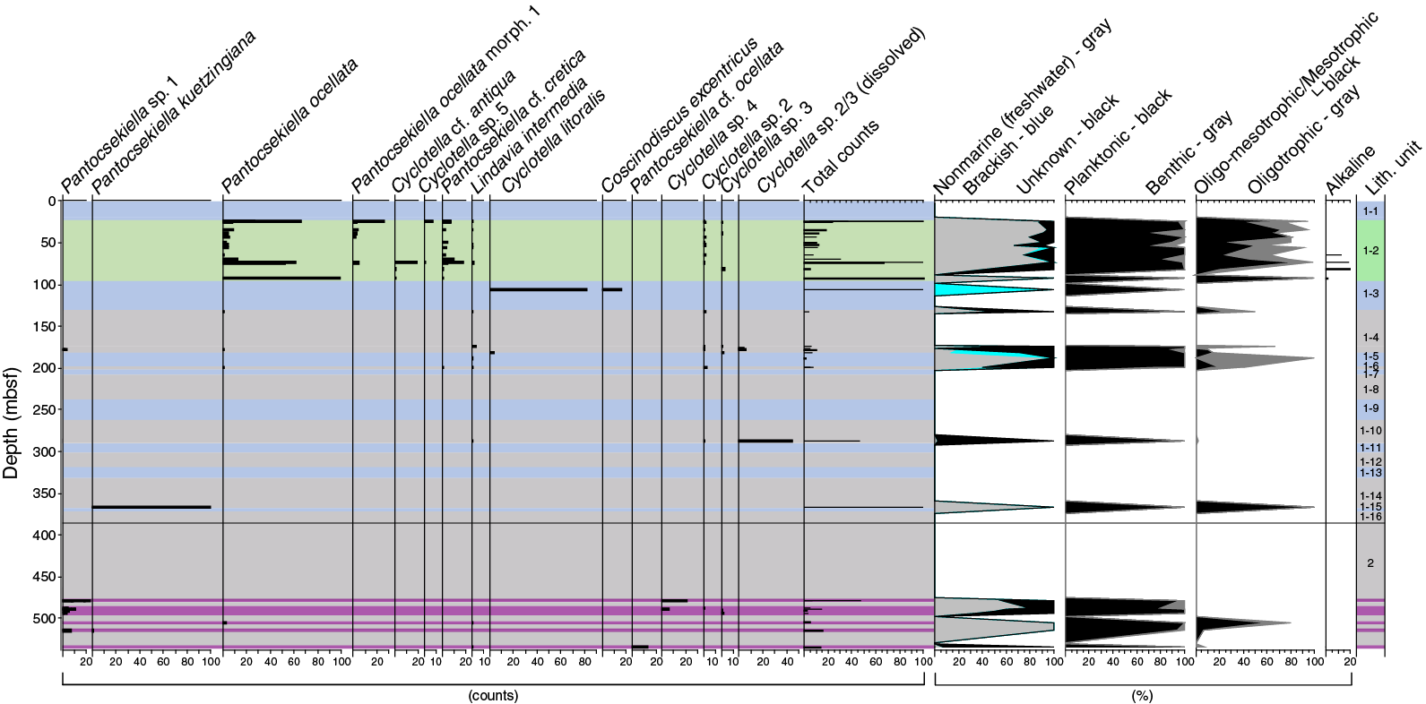
Figure F13. Most common nonmarine diatom taxa.
Unit 1 (Cores 381-M0078A-1P through 125R; 0–385.14 mbsf)
In the Unit 1 isolated/semi-isolated intervals, nonmarine diatoms are common to abundant with good to excellent preservation. Surprisingly, nonmarine diatoms in the isolated/semi-isolated intervals were typically observed co-occurring with low abundances of marine microfossils. When this combination was recognized and the fossils were interpreted to be in situ, the sample is described as having a mixed microfossil assemblage (see Micropaleontology in the Expedition 381 methods chapter [McNeill et al., 2019b]). Nonmarine diatoms observed in the Unit 1 isolated/semi-isolated intervals are not diverse and are dominated by species from the planktonic Pantocsekiella ocellata complex, including several morphotypes (Tables T4, T5, T6).
In the marine intervals, nonmarine diatoms were rarely observed. When nonmarine diatoms were observed in the marine intervals, their abundances are low and preservation poor, indicating that they are not in situ.
A total of 126 samples were analyzed offshore and an additional 29 samples were analyzed onshore from Unit 1. The mixed microfossil assemblage in Cores 381-M0078A-10H through 33P (Subunit 1-2; 23.74–92.22 mbsf) is characterized by planktonic assemblages with higher abundances and better preservation than was observed in mixed assemblages from deeper sections of Unit 1. The nonmarine planktonic taxa belonging to the P. ocellata complex dominate throughout these cores, with the highest peaks (>50 counts) in Cores 10H (24.09 mbsf), 26H–28H (69.12–73.09 mbsf), and 33P (92.22 mbsf) (Figure F13). P. ocellata is a widespread diatom species complex usually reported from the epilimnetic zone of the nonmarine ecosystems. Planktonic Pantocsekiella cf. cretica, Lindavia intermedia, and Cyclotella cf. antiqua simultaneously occur with the P. ocellata complex in these assemblages but in much lower abundances. Benthic nonmarine Cocconeis placentula, Encyonopsis microcephala, Staurosirella pinnata, and brackish taxa such as Diploneis cf. subovalis were observed only sporadically in these assemblages. A common planktonic taxon with unknown salinity and nutrient preferences in these samples is Cyclotella sp. 2.
The diatom assemblages in Cores 381-M0078A-44P through 100R (172.3–287.17 mbsf) are mostly characterized by low diatom counts (<20 valves per traverse) and moderate preservation. The nonmarine planktonic diatoms in these cores have low abundances, represented by Aulacoseira ambigua, P. ocellata, Pantocsekiella sp. 1, and L. intermedia, occurring at <5 valves per sample. Taxa with unknown salinity preferences, such as Cyclotella sp. 2, Cyclotella sp. 3, Cyclotella sp. 2/3 (dissolved), and Cyclotella sp. 4, are present in higher abundances. A unique assemblage in Core 100R (287.17 mbsf) is characterized by ~50 valves per traverse and a high abundance of dissolved valves, probably belonging to Cyclotella sp. 2 and Cyclotella sp. 3. High abundances of marine planktonic Cyclotella litoralis and Coscinodiscus spp. and benthic Diploneis bombus are present in Cores 62P (181.57 mbsf) and 71V (199.16 mbsf). The lowermost sample analyzed from this unit is in Core 121R (366.42 mbsf). It includes an assemblage characterized by a “bloom” of the nonmarine planktonic diatom Pantocsekiella kuetzingiana and marks the boundary between the marine microfossil assemblages that occur in the lowermost part of Unit 1 and the undetermined assemblages in Sections 113R-4 through 121R-3 (334.41–366.24 mbsf).
Unit 2 (Cores 381-M0078A-125R through 176R; 385.14–610.38 mbsf)
In Unit 2, nonmarine diatoms were observed in “unmixed” assemblages that are preliminarily classified here as freshwater assemblages (475.7–536.31 mbsf). Onshore, 16 additional samples were examined from Cores 381-M0078A-145R through 158R (474.13–534.65 mbsf). Planktonic diatoms from the genera Cyclotella, Pantocsekiella, and Lindavia dominate the assemblages observed in Unit 2. Diatoms are present in Samples 146R-3, 40 cm, to 149R-3, 67 cm (478.89–494.16 mbsf); 151R-3, 77 cm, to 153R-CC, 13 cm (504.78–514.66 mbsf); and 158R-1, 85 cm (534.65 mbsf). The total diatom counts are low (<20 valves per traverse), except for Section 146R-3 (479.02 mbsf), where a total of 48 valves were counted. The assemblages throughout these cores are dominated by planktonic Cyclotella sp. 2, Cyclotella sp. 3, and Cyclotella sp. 4, P. ocellata, Pantocsekiella cf. ocellata, Pantocsekiella sp. 1, Pantocsekiella sp. 2, and Pantocsekiella sp. 3. Freshwater benthic taxa such as Amphora pediculus, C. placentula, and Cocconeis pseudothumensis occur only sporadically.
In addition, the samples from Cores 145R (474.13, 474.44, and 475.12 mbsf), 150R (498.03 and 498.25 mbsf), 156R (528.55 mbsf), and 157R (530.43 mbsf) are barren of diatoms, thus indicating very poor diatom preservation and/or low productivity.
Planktonic taxa from the genera Cyclotella and Pantocsekiella are characterized by the high morphological variability of their external and internal valve features. Because of the complexity of these variations, additional scanning electron microscope analyses during postexpedition research are required to reveal the nature of the variability and improve species identification.
Foraminifers
Hole M0078A
A total of 168 samples were examined for planktonic and benthic foraminifers; 118 core catcher samples were taken offshore, and 50 additional core samples were taken from split-core sections during the OSP (Table T8).
Foraminifer specimens were observed in high abundances only in specific intervals in lithostratigraphic Unit 1 and always with variations in their composition. In Unit 1, sedimentary intervals with abundant foraminiferal fauna alternate with intervals where foraminifers are almost absent. These changes in the foraminifer records are almost in phase with Subunits 1-1 through 1-16. Eight of these subunits include intervals with relatively high abundances of benthic and/or planktonic foraminifer species, suggesting the prevalence of marine conditions:
- 0–20.31 mbsf, which corresponds to Subunit 1-1;
- 96.42–121.81 mbsf, which corresponds to Subunit 1-3;
- 180.16–186.16 mbsf, which corresponds to Subunit 1-5;
- 202.26–205.62 mbsf, which corresponds to the central part of Subunit 1-7;
- 245.16–260.56 mbsf, which corresponds to the central and lower parts of Subunit 1-9;
- 287.5–298.6 mbsf, which corresponds to the central part of Subunit 1-11;
- 322.64–329.04 mbsf, which corresponds to the central part of Subunit 1-13 and includes a short interval where foraminifers appear in low abundance (Sample 381-M0078A-112R-3, 75.5–77.5 cm; 328.155 mbsf); and
- 366.6–369.5 mbsf, which corresponds to Subunit 1-15.
In all the other intervals in Unit 1, which correspond to the remaining subunits (1-2, 1-4, 1-6, 1-8, 1-10, 1-12, 1-14, and 1-16), foraminifers appear in lower abundances or they are absent (Table T8). The low foraminiferal content in these intervals may suggest weakened marine conditions or nonmarine conditions. Two samples do not follow this trend: Sample 381-M0078A-44P-3CC, 3–4 cm (132.6 mbsf), from Subunit 1-3 and Sample 122R-5CC, 6–7 cm (373.7 mbsf), from Subunit 1-15, where foraminifers increase in abundance.
In the intervals with abundant foraminiferal fauna, benthic foraminifer associations are usually highly diversified and are mainly composed of shallow and deep infaunal species typical of normal salinity under moderate to high organic carbon inputs to the seafloor, such as species of genus Bulimina and Brizalina, as well as Melonis barleeanus and Cassidulina carinata (Goineau et al., 2011, and references therein) (Table T9). Samples containing moderate to high abundances of small species could imply input of labile organic material to the seafloor (i.e., exclusive of the 63–125 µm fraction), such as Nonionella cf. iridea, Eilohedra vitrea, and Cassidulina obtusa (Duchemin et al., 2007). In the intervals with abundant foraminiferal fauna, benthic foraminifer abundance is always higher than that of planktonic foraminifers, except for the intervals corresponding to Subunits 1-11 and 1-15, where planktonic foraminifer abundance is higher than that of benthic foraminifers (Table T10).
The planktonic foraminifer associations usually present low diversities, and when they appear in high abundance, they are usually represented by species that are interpreted to be indicative of relatively cool waters in the surficial or deeper water layers (Turborotalita quinqueloba, Neogloboquadrina pachyderma, Neogloboquadrina dutertrei, Globorotalia inflata, and Globigerinita glutinata) (Rohling et al., 1993; Pujol and Vergnaud Grazzini, 1995; Capotondi et al., 2016). The participation of the warm water species (Globigerinella spp., Globigerinoides ruber, Globigerinoides trilobus, Globoturborotalita spp., Hastigerina pelagica, and Orbulina universa) (Rohling et al., 1993; Pujol and Vergnaud Grazzini, 1995) in the planktonic associations is low (Table T10). Warm water species were obtained in the intervals corresponding to Subunits 1-9 and 1-11. In the samples with abundant planktonic foraminifers, the dominant planktonic species were often T. quinqueloba or N. pachyderma together with N. dutertrei or G. inflata. The dominance of planktonic species T. quinqueloba in some parts of Subunits 1-3, 1-5, 1-9, 1-11, and 1-15 could suggest the prevalence of surficial water with relatively low salinity and low temperature and/or enhanced fertility (Rohling et al., 1993; Pujol and Vergnaud Grazzini, 1995) in these intervals. Samples where the dominant planktonic species were N. pachyderma together with N. dutertrei, which were obtained in some parts of Subunits 1-3, 1-9, 1-11, and 1-15, could suggest the development of a deep chlorophyll maximum layer (Rohling and Gieskes, 1989; Rohling et al., 1993) in these intervals. The dominance of G. inflata obtained in one sample from Subunit 1-15 may suggest the development of a cool and deep mixed water layer (Rohling et al., 1993; Pujol and Vergnaud Grazzini, 1995) in this interval.
Benthic and planktonic foraminifers are absent throughout Samples 381-M0078A-124R-5, 0–1 cm, to 176R-1, 3–4 cm (all of which correspond to Unit 2), except for trace amounts of poorly preserved benthic foraminifers found in Sample 167R-2, 0–1 cm (575.03 mbsf) (Table T8).
Hole M0078B
Benthic foraminifers are generally abundant in Cores 381-M0078B-1P through 8P (1.3–20.55 mbsf), which correspond to Subunit 1-1, except for two samples containing low foraminiferal abundance: 3P-2CC, 14–15 cm (6.15 mbsf), and 7P-3CC, 6–7 cm (19.06 mbsf). Only trace abundances of planktonic foraminifers were observed in this interval (Table T11). The benthic foraminiferal species that characterize this interval are Bolivina spathulata, C. carinata, Bulimina marginata, Hyalinea balthica, M. barleeanus, Sigmoilina distorta, N. cf. iridea, and C. obtusa.
Benthic and planktonic foraminifers are in trace abundance in Samples 381-M0078B-8P-4CC, 0–1 cm, to 15P-4CC, 14–15 cm (22.68–55.63 mbsf), which correspond to Subunit 1-2, with the exception of Sample 10P-4CC, 32–33 cm (31.99 mbsf), which is especially rich in benthic and planktonic foraminiferal shells. The benthic foraminifer assemblage in Sample 10P-4CC, 32–33 cm, is diverse, and the most common species are C. carinata, H. balthica, M. barleeanus, and Bulimina aculeata (Tables T11, T12). N. pachyderma (dextral) is the most abundant planktonic species (Table T11).
Palynology
A total of 26 samples (24 from core catchers and 2 from split-core sections) were palynologically analyzed (Figure F14; Tables T13, T14); 13 samples are from lithostratigraphic Unit 1, and 13 are from lithostratigraphic Unit 2. Palynomorphs are abundant in most samples studied, and preservation is good; however, in some samples, a significant number of corroded pollen grains were encountered (e.g., Samples 381-M0078A-99R-CC, 4 cm [283.81 mbsf], and 134R-CC, 1 cm [428.64 mbsf]). It appears, though, that the high corroded pollen concentration does not correlate with a low concentration of well-preserved pollen grains. Corroded pollen grain concentration varies between a maximum of 7700 grains/g and a minimum of 41 grains/g with a mean value of 729 grains/g, and there appears to be a correlation between isolated/semi-isolated subunits and high corroded grain concentrations.
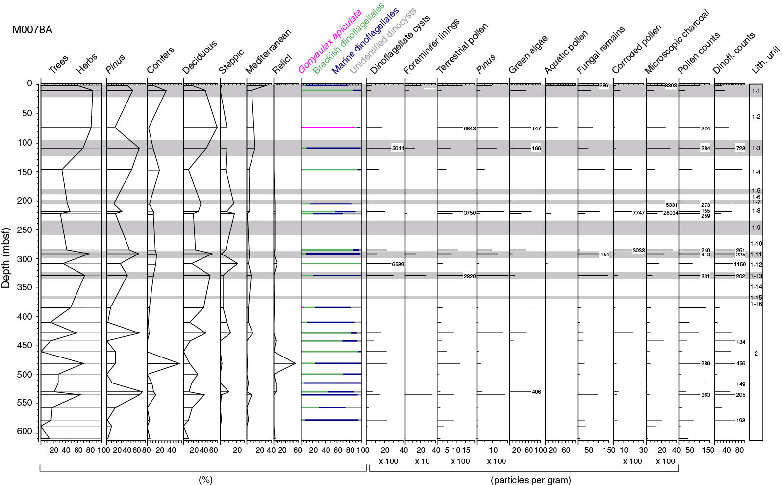
Figure F14. Palynomorphs.
Fungal remains consisting of ascospores and fruit bodies, aquatic vascular plant grains and spores, and charred microscopic particles have a higher concentration in Unit 1. Terrestrial pollen concentration, including trees and herbs, is also higher in Unit 1, with a mean value of 2500 grains/g, whereas Unit 2 has a mean value of 800 grains/g. Green algae concentration, which is mainly composed of Botryococcus sp., Pediastrum spp., and Zygnemataceae, has a maximum of 400 coenobia/spores per gram in Unit 2 (Sample 156R-CC, 9 cm; 528.86 mbsf).
The trees versus herbs percentage curve shows alternating periods dominated by forests or herb vegetation (Figure F14). Tree and herb concentrations confirm the occurrence of forested and open landscapes in the borderlands of the Gulf of Corinth inferred by the percentages curves. It appears that some peaks in tree percentages may correspond to marine intervals; however, further research is required for confirmation. High pine percentages (calculated on the Pollen Sum including pines) in the samples studied correspond to high tree percentages. These findings suggest that pines are not overrepresented in the pollen spectra and most likely form a constituent element of the local vegetation. Nevertheless, pines are excluded from the Pollen Sum to ensure compatibility with other marine regional records (see Micropaleontology in the Expedition 381 methods chapter [McNeill et al., 2019b]).
Quercus spp. dominates the deciduous trees percentages in all samples examined, but other mesophilous trees such as Corylus, Ulmus, Carpinus, Tilia, and Acer are present. Pollen grains of Carya, Pterocarya, and Liquidambar (relict species curve on Figure F14) are encountered in both lithostratigraphic units in low abundances (see Table T13). Conifer relative percentages have a mean of 9.7%; Cedrus is the dominant conifer species in Unit 2, and Abies is the dominant conifer species in Unit 1. In Sample 381-M0078A-146R-4, 9 cm (479.76 mbsf), Cedrus reaches a maximum of 50.7%. Steppic elements (e.g., Artemisia and Ephedra), suggesting the occurrence of open landscape, are more abundant in Unit 1 and correspond to isolated/semi-isolated intervals. Mediterranean sclerophyllous vegetation increases toward the top of the record, reaching a maximum of 12.6% in Sample 381-M0078B-1P-1, 0 cm (0 mbsf). These findings depict the significant role of Mediterranean maquis in the modern vegetation surrounding the Gulf of Corinth.
Dinoflagellate cysts have a mean concentration of 1885 cysts/g in Unit 1 and 985 cysts/g in Unit 2, whereas species diversity varies significantly throughout the core. Samples with a high diversity of marine dinoflagellate species (e.g., halophilic Mediterranean Spiniferites sp., Nematosphaeropsis labyrinthus, Lingulodinium machaerophorum, and Operculodinium centrocarpum) suggest deposition under fully marine conditions (Mudie et al., 2010) (e.g., Samples 381-M0078A-37P-CC, 11 cm [108.75 mbsf]; 101R-CC, 17 cm [291.92 mbsf]; and 157R-4, 54 cm [534.33 mbsf]). Samples with lower dinocyst diversity dominated by low-salinity indicators, such as Pyxidinopsis psilata, Spiniferites cruciformis, and L. machaerophorum, with low processes suggest deposition under low-salinity (brackish) conditions (Mertens et al., 2012; Mudie et al., 2017) (e.g., Samples 99R-CC, 4 cm [283.81 mbsf], and 134R-CC, 1 cm [428.64 mbsf]). Cysts of the freshwater species Gonyaulax apiculata (Evitt et al., 1985; Kouli et al., 2001) have a maximum of 1500 cysts/g (Table T14) and an abundance of 89% (Figure F14) in Sample 28H-CC, 10 cm (73.51 mbsf).
Biostratigraphy summary
Biostratigraphic age control is provided solely by calcareous nannofossils in Hole M0078A, and it should be applied cautiously given the complexity of the depositional environment (Table T15). Three biohorizons were recognized at this site. The first age datum is the crossover in dominance between E. huxleyi and Gephyrocapsa “small.” This crossover has been observed in multiple locations (Thierstein et al., 1977; Raffi et al., 2006; Anthonissen and Ogg, 2012), including the Mediterranean region, where it is calibrated at 0.07 Ma in MIS 4 (Anthonissen and Ogg, 2012). If this datum can be applied accurately in Hole M0078A, then it occurs in Subunit 1-2.
The LDO of E. huxleyi in Sample 381-M0078A-41P-3, 50–51 cm (121.82 mbsf), likely does not represent the true FAD (0.29 Ma) because this species evolved during glacial MIS 8, a time when the Gulf of Corinth was presumably disconnected from the Mediterranean Sea.
The oldest marker, P. lacunosa (LAD at 0.43 Ma), was observed in Sample 381-M0078A-105R-1, 60 cm (298.6 mbsf). In addition to only being observed in one sample, this occurrence is likely not the true LAD because the extinction of P. lacunosa occurs in glacial MIS 12, a time when the Gulf of Corinth was presumably disconnected from the Mediterranean Sea.
Micropaleontology summary
Micropaleontology at Site M0078 revealed a high level of complexity both in individual microfossil groups and collectively. Unit 1 alternates primarily between marine and undetermined assemblages but also includes several intervals with mixed and nonmarine assemblages. Unit 2 is devoid of marine calcareous and silicate microfossils and contains only nonmarine diatoms and terrestrial and aquatic pollen, dinoflagellate cysts, green algae coenobia and spores, fungal remains, and foraminifer test linings. However, a distinct horizon in Unit 2 is characterized by a predominantly marine dinoflagellate cyst assemblage, and foraminifer test linings were more abundant. In both units, alternating periods of forested and open landscapes are inferred in the borderlands of the Gulf of Corinth. See Figures F15 and F16 for a summary of the microfossil assemblages in Holes M0078A and M0078B by subunit.
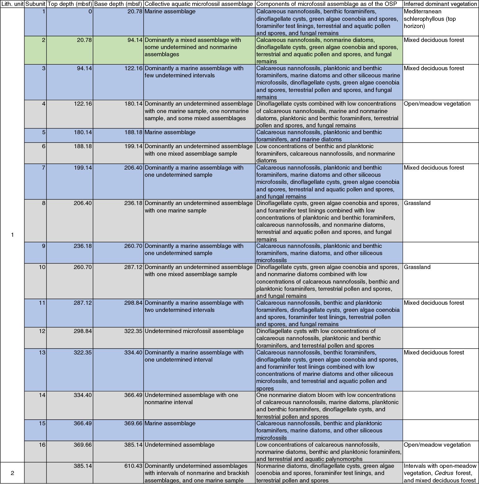
Figure F15. Micropaleontology assemblages, Hole M0078A.
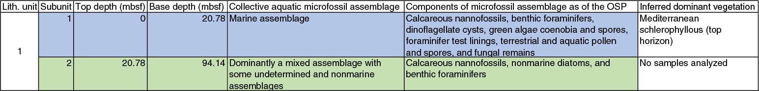
Figure F16. Micropaleontology assemblages, Hole M0078B.
Geochemistry
Interstitial water
At Site M0078, 82 interstitial water samples were collected using Rhizon samplers and whole-round squeeze cakes from both holes. Rhizons were used from 0.01 to 18.81 mbsf, and squeeze cakes were used from 11.78 to 608.80 mbsf in Hole M0078A. Hole M0078B penetrated 55.85 m, and Rhizons successfully collected pore water from the sediment/water interface to 8.56 mbsf. Five additional squeeze cakes were used to collect pore water from 12.00 to 52.51 mbsf in Hole M0078B (Table T16). Fluid geochemical results from both holes closely match for all analytes and are generally discussed together except where noted. Additionally, 14 drilling mud fluid samples were collected from discrete depths between 11.88 and 586.01 mbsf (see Geochemistry in the Expedition 381 methods chapter [McNeill et al., 2019b]) to identify the presence of any potential drilling contamination. No contamination was observed, as discussed below.
Pore water chemical compositions at Site M0078 reflect environmental changes in basin water chemistry, type and rate of organic matter burial, and dissolution/precipitation reactions with sediment. Two distinct geochemical regions were observed above and below the unit boundary (see Lithostratigraphy) at 385.14 mbsf. Cyclicity in the pore water signals is apparent in Unit 1 and may represent successive sea level fluctuations and basin water body isolation in the Gulf of Corinth. Unit 2 is broadly characterized by increasing concentrations of most solutes to the deepest sampled interval. These regions are described in detail below.
Salinity variations: salinity, sodium, and chloride
Salinity at Site M0078 decreases below the sediment/water interface from seawater values to 7.55 at 42.50 mbsf. Deeper than 42.50 mbsf, salinity values gradually decrease to a minimum of 1.95 at 340.34 mbsf then increase to 19.65 at 608.80 mbsf. These broad changes are superimposed by smaller scale fluctuations that coincide with identified lithologic changes (e.g., Figure F17A). Thus, these smaller scale changes are generally interpreted to be true geochemical signals rather than analytical scatter.
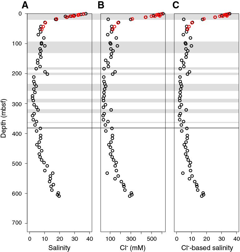
Figure F17. Pore water salinity, chloride, and Cl−-based salinity.
The chloride (Cl−) profile closely follows the salinity profile throughout Site M0078. Cl− concentration is highest (610.72 mM) close to the sediment/water interface (Figure F17B). Cl− decreases in the upper 30.45 m to 176.68 mM, followed by a more gradual decrease to 34.65 mM at 282.10 mbsf. This trend with depth may reflect the integrated result of varying basin water salinity conditions in the Gulf of Corinth. Deeper than 340.34 mbsf, Cl− increases to a maximum of 310.38 mM at 604.27 mbsf. As seen in Table T16, mud fluid salinity values throughout Hole M0078A are markedly different from sediment interstitial fluids, implying no contamination.
Figure F17C illustrates that salinity determined by refractometer (see Geochemistry in the Expedition 381 methods chapter [McNeill et al., 2019b]) is comparable with salinity calculated from Cl− (assuming a salinity of 35 has a Cl− concentration of 558 mM), which provides evidence that NaCl is the dominant dissolved salt and other salts are minor contributors to pore water salinity at Site M0078.
Organic matter degradation: alkalinity, ammonium, boron, bromide, iron, manganese, pH, phosphate, sulfate, inorganic carbon, and sulfide
Microbial mineralization of organic matter leads to distinct changes in pore water geochemistry, reflecting ongoing diagenetic redox reactions (Berner, 1980; C.M. Miller et al., unpubl. data). Shallow pore water profiles in Hole M0078A suggest the typical sequence of organic matter degradation in marine sediments through microbial oxidation (Froelich et al., 1979). Elevated manganese (Mn2+) concentration (as high as 67.04 µM) indicates Mn oxide reduction in the upper 8.36 m of Holes M0078A and M0078B (Figure F18A). Dissolved iron (Fe2+) concentration is elevated (as high as 172.25 µM) from 0.10 to 52.13 mbsf in Hole M0078A, suggesting the reduction of Fe (oxy)hydroxides. However, in this interval, a zone of lower Fe2+ concentration occurs between 9.10 and 19.19 mbsf (Figure F18B). Sulfate (SO42−) concentration decreases from seawater values near the seafloor to 0.04 mM at 11.78 mbsf, indicating SO42− reduction coupled to either organic matter degradation or anaerobic methane oxidation. Deeper than 11.78 mbsf, SO42− concentration generally stays between 0.02 and 4.85 mM, but multiple small peaks correspond to the previously described salinity fluctuations (Figure F18C). Sulfide (HS−) concentration values estimated by the difference between dissolved inorganic carbon (DIC) and alkalinity in Hole M0078A suggest the presence of HS− in the shallowest 200 m of the hole. HS− peaks at ~40 mbsf in Holes M0078A and M0078B and between 523.73 and 576.44 mbsf in Hole M0078A, where DIC is lower than alkalinity (Figure F19C).
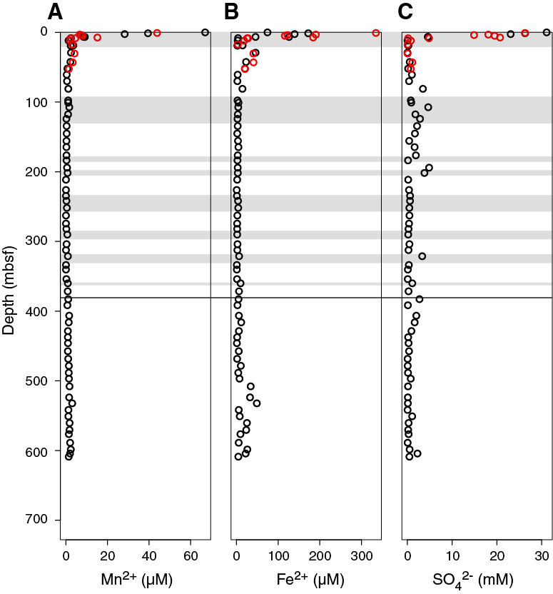
Figure F18. Pore water manganese, iron, and sulfate.
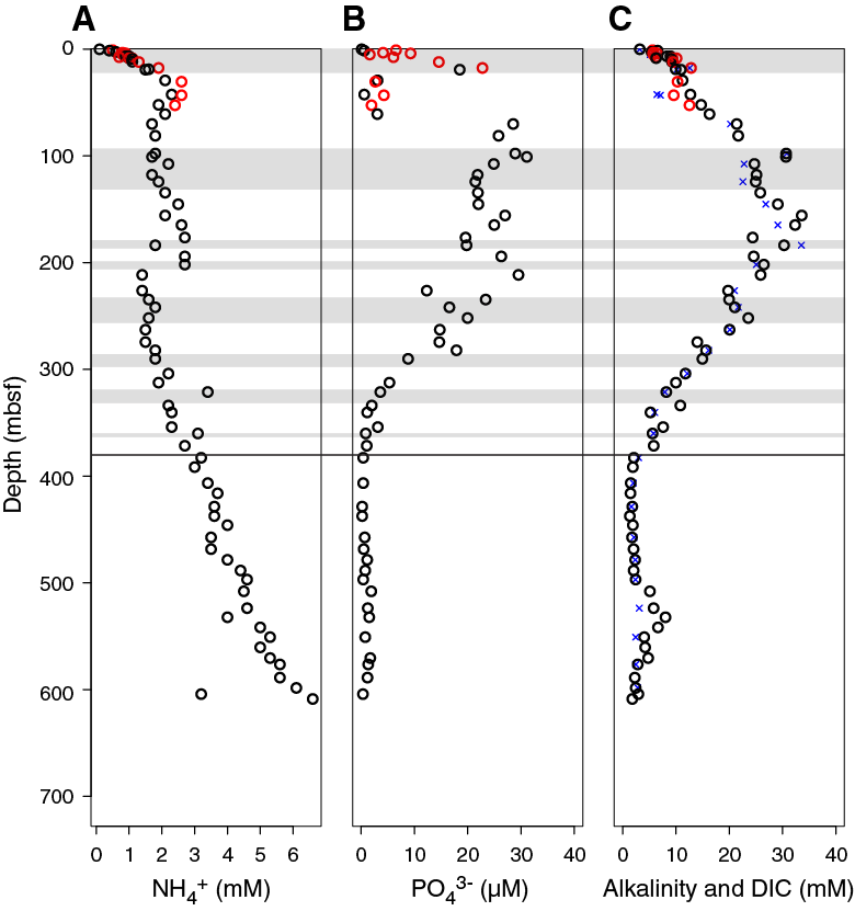
Figure F19. Pore water ammonium, phosphate, and alkalinity and DIC.
Microbial processes of organic matter degradation release bicarbonate (HCO3−), phosphate (PO43−), and ammonium (NH4+) to pore water. This process is apparent in the pore water results (Figure F19). NH4+ concentration increases from seafloor values (0.1 mM) to a local maximum of 2.6 mM at 30.45 mbsf. NH4+ then remains relatively constant (between 1.7 and 2.7 mM) to 211.47 mbsf and then steadily increases to the base of Hole M0078A, with a maximum of 6.6 mM. In contrast to NH4+, the PO43− increase in the uppermost portion of the core is more variable. Although PO43− concentration generally increases from 0.11 µM at the sediment/water interface to 31.09 µM at 100.91 mbsf, it is also low between 29.22 and 60.81 mbsf, which approximately corresponds to an isolated/semi-isolated subunit. At greater depths, PO43− decreases to 340.34 mbsf and then remains consistently low to the base of the hole, fluctuating between 0.21 and 1.91 µM. PO43− concentration values are at their lowest at the base of the hole.
Similar to PO43−, alkalinity increases with depth in the upper part of Hole M0078A, reaching a peak of 33.60 mM at 155.77 mbsf (Figure F19C). This peak is followed by decreasing alkalinity to 1.92 mM at 382.80 mbsf, approximately coincident with the lithostratigraphic Unit 1/2 boundary. An additional front occurs from 523.73 to 550.88 mbsf, reaching a maximum of 8.04 mM. Broadly, the changes in alkalinity are reflected in pH. Pore water pH at Site M0078 ranges from 7.0 to 8.9 with an average of 8.0 (Figure F20A). pH is generally higher above the Unit 1/2 boundary, with a maximum at 234.58 mbsf (deeper than the alkalinity peak), whereas pH is significantly lower below the unit boundary.
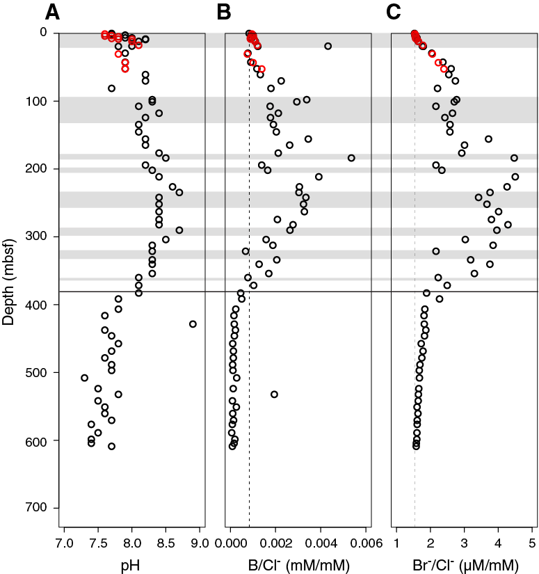
Figure F20. Pore water pH and B/Cl− and Br−/Cl− ratios.
Boron (B) and bromide (Br−) accumulate in organic matter and are useful when compared with Cl− to determine relative contributions of seawater and organic carbon oxidation to pore water chemistry. Disparity of the B/Cl− and Br−/Cl− ratios from seawater values can indicate production or removal of ions from solution. Both B/Cl− and Br−/Cl− values broadly follow the PO43− profile with depth, including a change to lower values at the approximate location of the Unit 1/2 boundary. The B/Cl− and Br−/Cl− peak values are located deeper than the PO43− peak at 211.47 mbsf (Figures F19, F20). Drilling fluid concentrations of Mn2+, NO3−, Fe2+, SO42−, HCO3−, PO43−, NH4+, B, and Br− are all dissimilar to those described above (Table T16), implying these samples are free of contamination.
Mineral reactions
Sodium, potassium, magnesium, calcium, strontium, and barium
Sodium (Na+), potassium (K+), magnesium (Mg2+), and calcium (Ca2+) are all major ions in seawater, and strontium (Sr2+) and barium (Ba2+) are minor components. Pore water solute concentration may be altered by ion exchange, mineral weathering, and formation of new minerals. The Na+ and K+ depth profiles resemble those of salinity and Cl−, indicating that salinity changes govern the overall pattern (Figure F21). However, the Na+/Cl− and K+/Cl− ratios show their concentrations may also be influenced by reactions with sediment because the ratios differ downhole and do not reflect the modern Gulf of Corinth seawater composition (vertical dashed lines, Figure F21). Between 60.84 and 290.15 mbsf, the Na+/Cl− and K+/Cl− ratios are higher than seawater, suggesting the release of Na+ and K+ to the pore water. Deeper than 354.04 mbsf (31 m above the Unit 1/2 boundary), the Na+/Cl− and K+/Cl− ratios are lower than in seawater. Ba2+ shows opposing trends to salinity in the uppermost 30 mbsf, increasing from 0.31 to 18.00 µM. However, from 340.34 mbsf (45 m above the Unit 1/2 boundary) downhole, Ba2+ increases alongside the increasing salinity to a maximum of 81.63 µM at 570.46 mbsf. This increase deeper than 340.34 mbsf appears to not entirely be governed by salinity, as emphasized in the Ba2+/Cl− ratio, which is higher than modern Gulf of Corinth seawater composition.
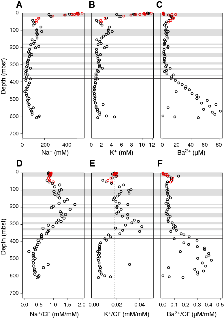
Figure F21. Pore water sodium, potassium, and barium.
The dissolved Ca2+, Mg2+, and Sr2+ depth profiles largely follow the Cl− curve (Figures F17B, F22A–F22C). Ca2+ decreases in the uppermost 11.78 mbsf from 9.37 to 1.83 mM. A peak at 30.45 mbsf may indicate an additional source from the depth at which Ca2+ is released. Between 100.91 and 312.42 mbsf, Ca2+ concentration stays lower than 1.6 mM. Mg2+ also decreases from the top of Site M0078 and stays between 1.35 and 11.60 mM from 100.91 to 312.42 mbsf. Sr2+ concentration also decreases in the upper 11.78 mbsf but has the same additional peak as Ca2+ at 30.45 mbsf. Sr2+ stays lower than 50 µM in the 100.91–312.42 mbsf interval. Deeper than 340.34 mbsf, all profiles increase. At the base of Hole M0078A, Mg2+ concentration returns to approximate seawater values, whereas Ca2+ and Sr2+ concentrations increase to several times higher than modern seawater values (vertical dashed lines, Figure F22).
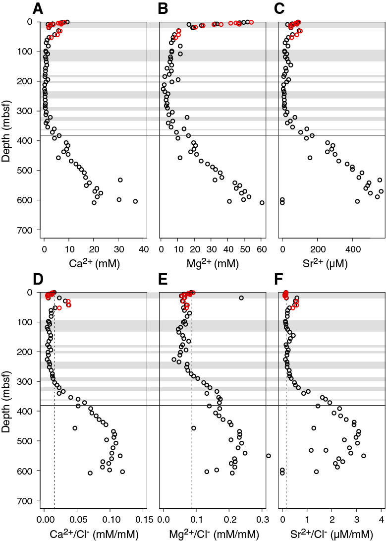
Figure F22. Pore water calcium, magnesium, and strontium.
The Ca2+/Cl− and Mg2+/Cl− ratios are mostly lower than seawater values from the sediment/water interface to 303.93 mbsf (Figure F22D–F22E). The Sr2+/Cl− ratio stays close to the seawater ratio in the upper 303.93 mbsf (Figure F22F). Deeper than 303.93 mbsf, the Ca2+/Cl−, Mg2+/Cl−, and Sr2+/Cl− ratios increase to values much higher than seawater, suggesting a source for Ca2+, Mg2+, and Sr2+ ions deeper than the cored section.
Silica and lithium
Silica accumulates in sediments from terrigenous silicate minerals and the remnants of siliceous organisms living in the water column (dominantly diatoms and radiolarians). Therefore, dissolved silica (H4SiO4) is typically released to pore water through dissolution of sediment components. H4SiO4 concentration is between 124.34 and 274.00 µM from below the sediment/water interface to 11.78 mbsf at Site M0078 (Figure F23A). Between 18.81 and 371.54 mbsf, H4SiO4 is higher with a maximum of 1227.88 µM at 97.74 mbsf. In this zone, dissolved Si content fluctuates, which may be a result of varying initial silicate content in the sediment. Between 382.80 and 468.43 mbsf, concentration is low (between 133.20 and 198.52 µM) and relatively steady before increasing again to higher values at 478.43 mbsf. In this lower portion of the hole, fluctuations are comparable in magnitude with those visible between 18.17 and 371.54 mbsf. Lithium (Li+) concentration is consistently low above the Unit 1/2 boundary and increases gradually below the boundary to 480.44 µM in the deepest sample (604.27 mbsf) (Figure F23B). This increase with depth suggests chemical weathering of the sediment.
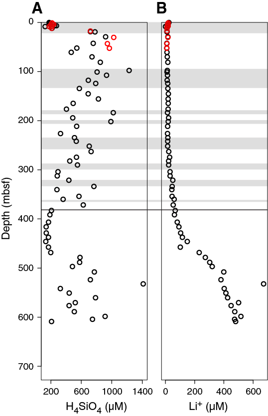
Figure F23. Pore water dissolved silica and lithium.
Sediment
Carbon content
At Site M0078, 127 total carbon (TC) and total organic carbon (TOC) content samples were collected and analyzed. Total inorganic carbon (TIC) was obtained by subtracting TOC from TC. The results are presented in Table T17 and plotted against depth in Figure F24. Site M0078 TC varies between 4.54 and 10.62 wt% with an average of 7.54 wt%. Values below the Unit 1/2 boundary are significantly higher, which is confirmed by the energy dispersive X-ray fluorescence (ED-XRF) discussed below and by XRD measurements (see Lithostratigraphy). TOC varies between 0.08 and 0.89 wt% with an average of 0.31 ± 0.12 wt% (standard deviation). Peaks in TOC at 104.70, 180.86, 203.08, 220.40, 236.91–253.79, 291.67, 325.1, and 368.7 mbsf correspond to the interpreted marine subunits (see Lithostratigraphy; gray bars, Figure F24B).
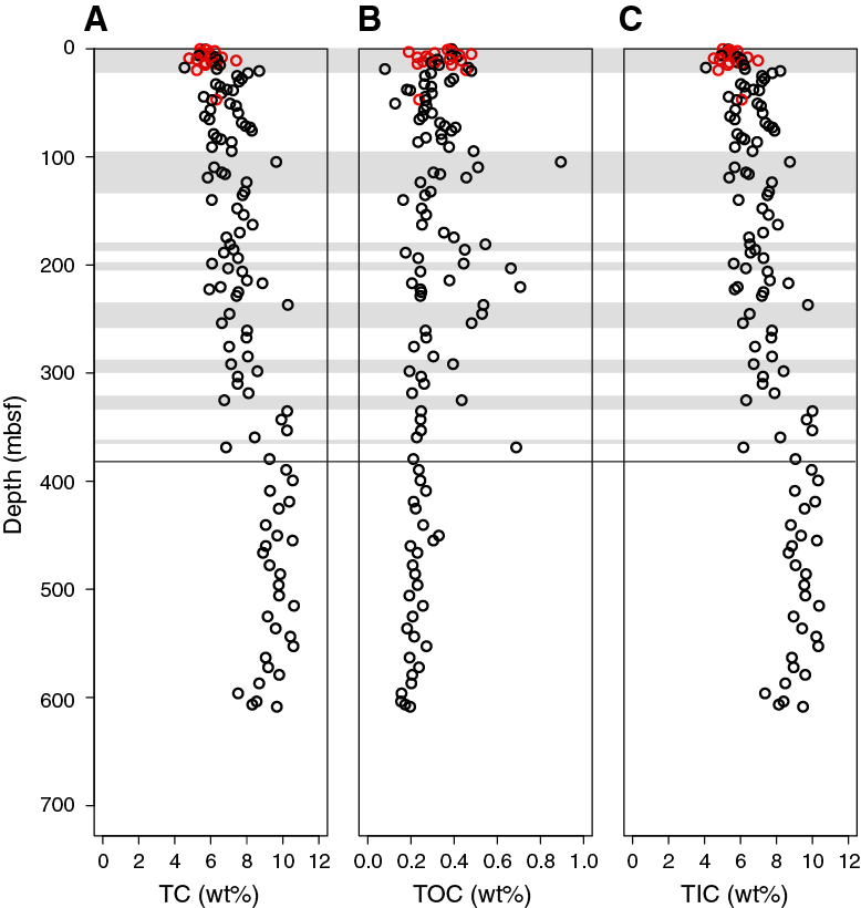
Figure F24. Solid-phase TC, TOC, and TIC.
ED-XRF
The concentrations of 24 elements were measured in the same 127 sediment samples collected for TC, TIC, and TOC from Site M0078 (109 samples from Hole M0078A and 18 samples from Hole M0078B). For 11 elements (Al, Ca, Fe, K, Mg, Mn, Si, Sr, Zr, Ni, and Rb), quantitative contents were measured (Table T17; Figures F25, F26, F27, and F28). For the other elements, either contents were too low or the measurement was imprecise because of interferences of the spectra. Hence, no precise, reliable results could be given for these elements. For all elements, considerable differences between Units 1 and 2 are apparent.
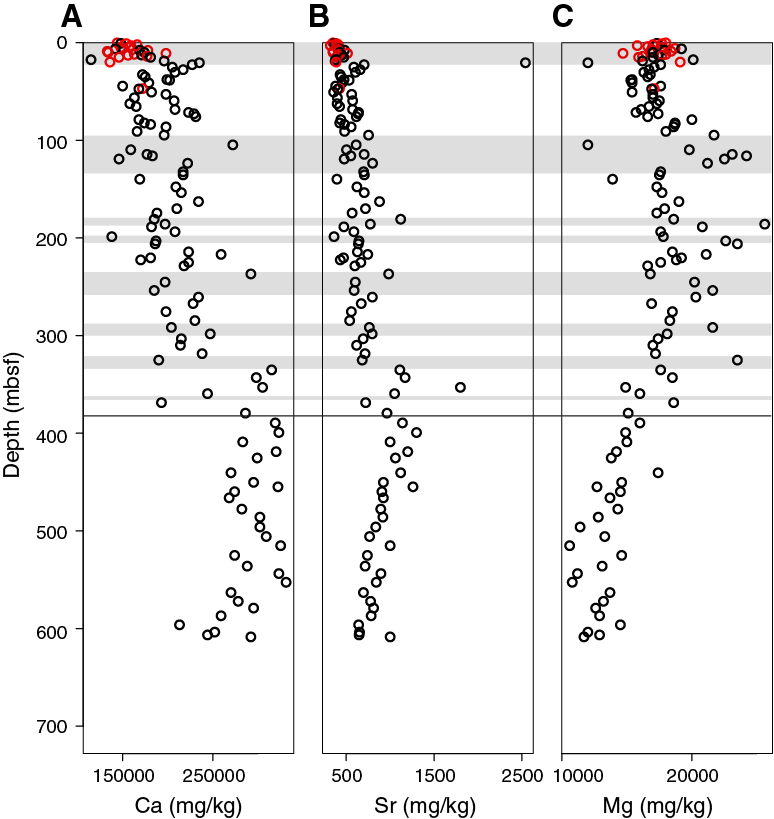
Figure F25. Solid-phase calcium, strontium, and magnesium.
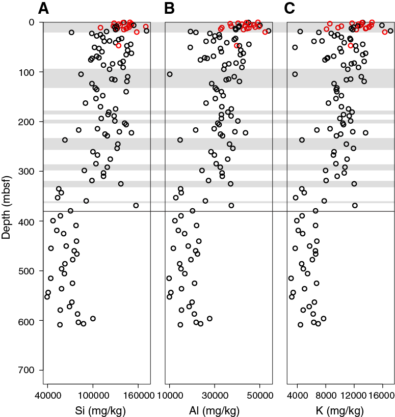
Figure F26. Solid-phase silicon, aluminum, and potassium.
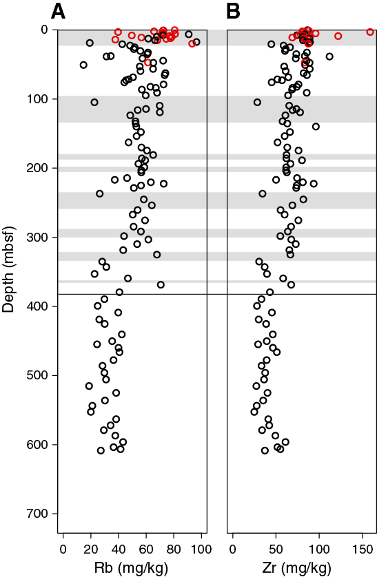
Figure F27. Solid-phase rubidium and zirconium.

Figure F28. Solid-phase manganese, iron, and nickel.
The highest elemental content was measured for calcium (Figure F25A). At Site M0078, an average Ca concentration of 214.3 g/kg was measured. Large differences were apparent between the two lithostratigraphic units: the average concentration in Unit 1 is 194 g/kg, whereas significantly higher values (289.3 g/kg) are detected in Unit 2. The second most abundant measured element was Si (mean = 119.7 g/kg) (Figure F26A). The Spearman Rho correlation between these two major elements shows an almost ideal negative correlation (R = −0.95, p < 0.05). Very strong positive correlations (R > 0.84) also exist between Si and Al, K, Rb, Zr, Fe, and Mn (Figures F26, F27, F28). The contents of these elements are all lower in Unit 2.
Mg and Ni, elements that do not show a strong correlation with Si, are also present at lower concentrations below the Unit 1/2 boundary (Figures F25, F28). Sr, which is commonly associated with carbonates, increases below the unit boundary, similar to Ca (Figure F25). Thus, an overall trend that is evident from the XRF data at Site M0078 is an increase in elements associated with carbonate minerals with depth, especially below the unit boundary, whereas elements normally associated with terrigenous input decrease with depth.
Physical properties
This section summarizes the preliminary physical properties results from Site M0078. Most data sets were collected at the sampling rates defined in Physical properties in the Expedition 381 methods chapter (McNeill et al., 2019b), except for P-wave velocity, thermal conductivity, and shear strength, where the nature of the sediment limited data acquisition (details below). Overall, the data sets collected reflect good correlations with changes in lithology and paleoenvironment, especially magnetic susceptibility, NGR, density, and color reflectance. A synthesis of physical properties for Hole M0078A is presented in Figures F29 and F30.
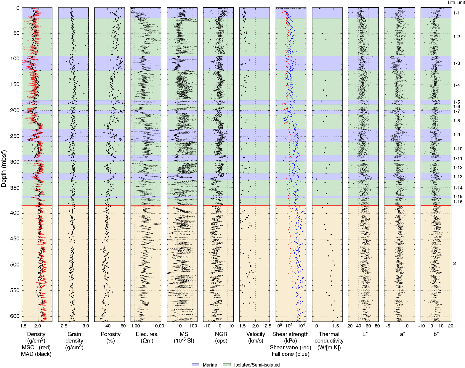
Figure F29. Physical properties with environmental interpretation.
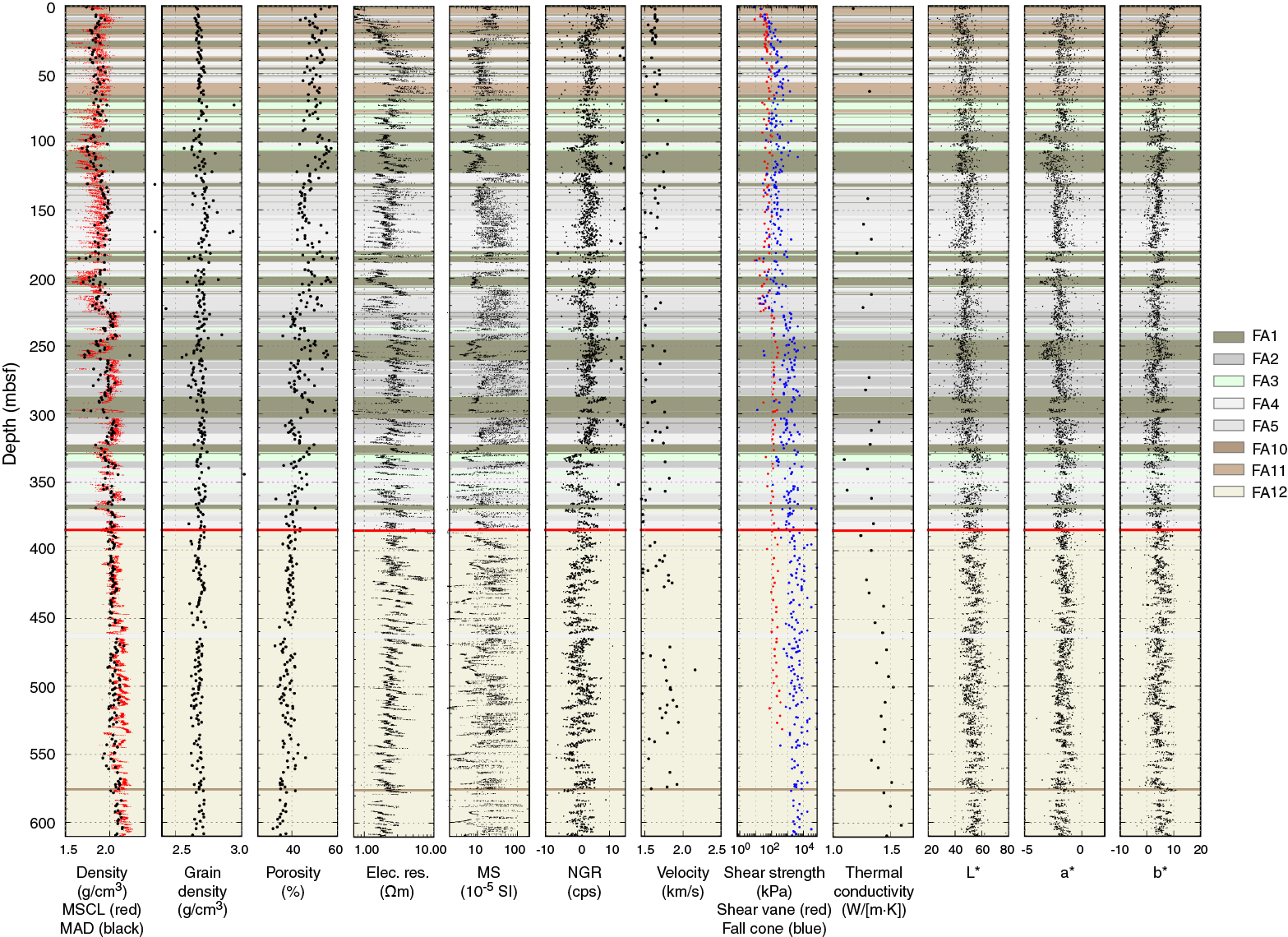
Figure F30. Physical properties with facies associations.
Shear strength
Sediment strength for Holes M0078A and M0078B was measured offshore using a handheld penetrometer and a temperature CPT and onshore using a fall cone and shear vane. Penetrometer and temperature CPT measurements were taken approximately every 20 and 100 m, respectively, whereas fall cone and shear vane measurements were taken one per core section and one per core, respectively.
The derived data using the four different methods differ significantly (Figure F31). Shallower than 400 mbsf, cone resistance derived from offshore handheld penetrometer measurements is consistently larger than other measurements, with a slight increase with depth from 1000 to ~4000 kPa at the base of Hole M0078A. Deeper than 400 mbsf, penetrometer values approximately coincide with fall cone shear strength values. CPT measurements provide minimum and maximum shear strength values (between the steady and peak state of cone resistivity) that increase from ~460 kPa at 102.64 mbsf to ~700 kPa at 303.03 mbsf, similar to fall cone measurements.
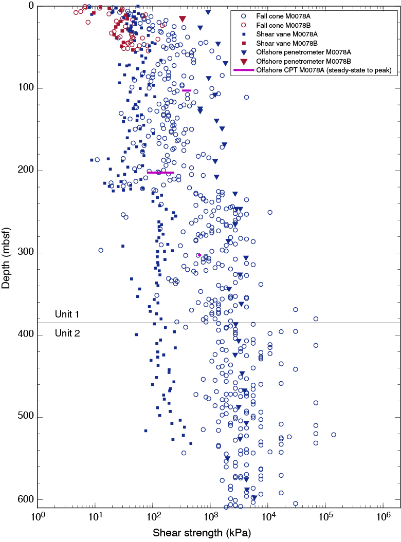
Figure F31. Shear strength.
Shear strength values derived from fall cone measurements vary over five orders of magnitude (Figure F31). In Hole M0078A, shear strength values increase from 0 to ~30 mbsf and remain relatively constant from ~30 to ~220 mbsf. At ~220 mbsf, shear strength increases sharply. Shear strength measured with the fall cone then increases downhole from ~1000 kPa at ~220 mbsf to ~6000 kPa at the bottom of the hole.
Shear strength values derived from shear vane measurements are much lower than those from fall cone measurements. In the upper 40 mbsf of Hole M0078A, spring stiffness was progressively increased, which had no impact on the measured shear strength. Deeper than 40 mbsf in both Holes M0078A and M0078B, the stiffest spring (4) was used (see Physical properties in the Expedition 381 methods chapter [McNeill et al., 2019b]). In Hole M0078A, shear strength values increase in the upper 30 mbsf and then remain relatively constant to ~225 mbsf, where they increase sharply. Deeper than 225 mbsf, shear strength values remain relatively constant to ~400 mbsf and then increase downhole. Shear vane measurements were stopped at 526.88 mbsf (Section 156R-2), where sediment strength exceeded the applied force capacity of the shear vane apparatus.
Shear strength values are lower in Hole M0078B than in Hole M0078A (Figure F31), although they exhibit a similar relationship between fall cone, shear vane, and penetrometer measurements and the same steady increase with depth.
The high cone resistance values (~1000 kPa) recorded by the handheld penetrometer may be misleading, especially in the shallower sections of Holes M0078A and M0078B, because the values are similar to the shear strength expected for extremely weak to very weak rocks. In all these sections, the shear vane could easily be inserted; hence, the sediment can be described as no stronger than stiff clay. Therefore, the maximum expected shear strength is ~500 kPa.
Shear vane measurements provide more realistic strength values than fall cone measurements. However, fall cone and shear vane measurements (taken at spots <10 cm apart) are correlated (Figure F32), indicating that fall cone measurements do provide a reliable indication of relative variations in shear strength.

Figure F32. Fall cone and shear vane correlations.
Despite the different ranges in shear strength values that the three measurements provide, they all follow similar patterns and indicate a general trend of increasing sediment strength with depth. The most abrupt increase occurs at approximately 228 mbsf (Section 381-M0078A-85R-2) and was observed in both fall cone and shear vane measurements (Figure F31). This strength increase, as well as an increase in density and electrical resistivity at a similar depth (Figure F29), coincides with both a change in coring method and with lithologic changes marked by a change in facies association. The coincidence with the change from FA5 to FA2 suggests an abrupt transition to more consolidated sediment driven by lithology change.
Natural gamma radiation
Overall low NGR values at Site M0078 indicate that K, Th, and U concentrations are depleted in the mud-dominated cores (Figures F29, F30). Note that the negative values result from the removal of the background during data processing, which was determined at the beginning of the expedition. Despite these negative values, gamma ray data acquired during downhole logging at other sites compare well with trends measured in cores from the same holes, suggesting these data faithfully capture NGR trends in the hole.
A significant change in the NGR trend occurs at 330 mbsf, 55 m above the Unit 1/2 boundary (Figure F33). The section shallower than 330 mbsf has on average distinctly higher values than the section deeper than 330 mbsf (Figure F34). Shallower than 330 mbsf, NGR values average 3.61 counts/s with a minimum of −6.44 counts/s and a maximum of 15.28 counts/s. NGR values in the marine intervals shallower than 330 mbsf often appear to be high (mean = 3.54 counts/s) relative to values in the isolated/semi-isolated intervals (mean = 0.89 counts/s).
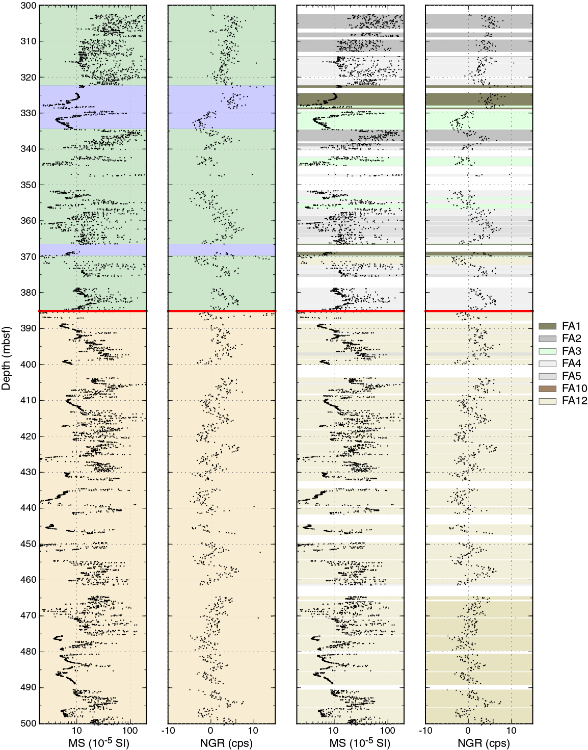
Figure F33. MSCL NGR and MS trends.
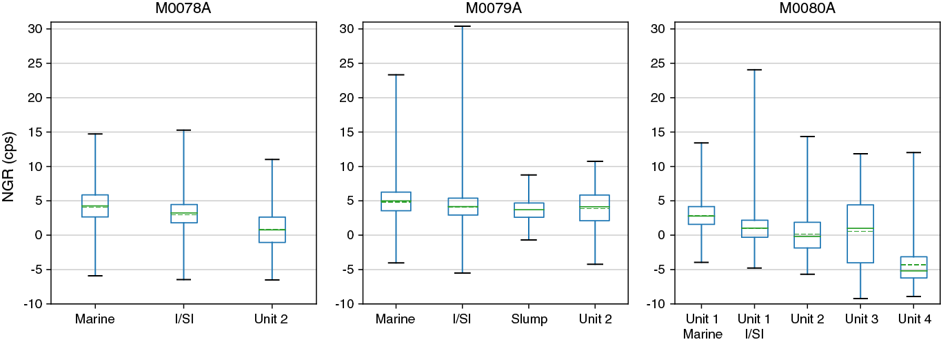
Figure F34. MSCL NGR box and whisker plots.
Deeper than 330 mbsf, NGR values average 0.92 counts/s with a minimum of −6.51 counts/s and a maximum of 14.71 counts/s (Figure F34). Variations in NGR deeper than 330 mbsf appear to occur at the scale length of ~10 m (Figure F33). Lithostratigraphic Unit 2 is associated with FA12 (light gray to gray homogeneous mud), has abundant bioturbation, and may be responsible for the variability in NGR values.
At 104 mbsf, a low in NGR occurs that is associated with FA3 (light gray/white thin laminations [calcite/aragonite] alternating with mud/silt beds). XRD results confirm that the total concentration of muscovite, K-feldspar, smectite, illite, and kaolinite in this layer is ~5%, whereas this concentration is typically >10% in the uppermost 200 m of the hole. At 330 mbsf, a low NGR value occurs in a section that is also associated with FA3 (Figure F33).
Magnetic susceptibility
Magnetic susceptibility appears to be a good indicator for lithology and basin environment at Site M0078 (Figure F29). In Unit 1, magnetic susceptibility values range from ~0 to ~200 × 10−5 SI. One of the distinct features of magnetic susceptibility is that it decreases abruptly in marine intervals/subunits (mostly associated with FA1; Figure F30), averaging 20 × 10−5 SI, and is higher but scattered in Unit 1 isolated/semi-isolated intervals/subunits (Figure F35). The scattered magnetic susceptibility behavior in isolated/semi-isolated intervals may be due to change in the terrigenous input during sedimentation, fluctuations in the quantity of fine detrital particles, and/or diagenetic processes. The thickness of lower value intervals associated with marine subunits increases upsection. Going downhole in Unit 1, sharp drops are seen in the magnetic susceptibility data at 98, 200, 238, and 253 mbsf, where the facies association changed from FA1 (homogeneous mud) to FA4 (laminated greenish gray to gray mud).
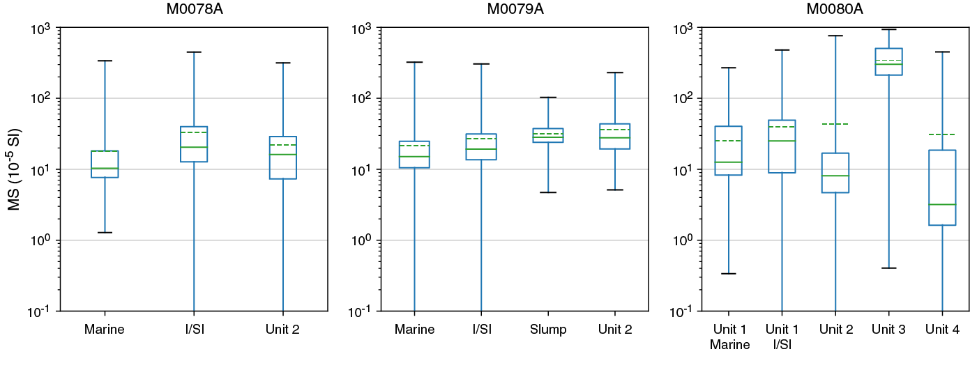
Figure F35. MSCL MS box and whisker plots.
In Unit 2, ~10 m thick intervals with values typically below 10 × 10−5 SI alternate with 10–20 m thick intervals, similar to NGR (Figure F33), with higher values ranging from ~10 × 10−5 to ~200 × 10−5 SI.
Magnetic susceptibility values sometimes drop below 0 SI (Figure F35). These values reflect sensor drift on some sections and are likely closer to 0.
P-wave velocity
P-wave velocity measurements were collected offshore using a Geotek MSCL. Onshore, they were collected on split cores using the MSCL track and on discrete samples using a Geotek P-wave logger for discrete samples (see Physical properties in the Expedition 381 methods chapter [McNeill et al., 2019b]).
Core quality (coring disturbances, the variable fill space between the sediment and the core liner, voids between and in the sediment layers, and/or the presence/absence of fluids in the core liner) strongly affected P-wave velocity measurements performed with the MSCL both onshore and offshore. Realistic values were only collected offshore in the upper few meters for both Holes M0078A and M0078B (0–12 and 0–10 mbsf, respectively), and they range between 1500 and 1515 m/s (Figure F36). P-wave velocity measurements on discrete samples were also strongly affected by the unconsolidated nature of the core samples in the upper part of Holes M0078A and M0078B. Downhole in Hole M0078A, the increase in stiffness led to more brittle behavior, and cracks in the samples likely affected P-wave signals, decreasing the reliability of velocity measurements. Realistic P-wave velocity values are between 1500 and 2161 m/s in Hole M0078A and between 1500 and 1769 m/s in Hole M0078B. In Hole M0078A, velocity values increase slightly with depth. However, these values are still smaller than what would be expected at 600 mbsf (see Core-log-seismic integration for velocity discussion). Low velocity values collected from discrete samples might also be due to the material not being in situ. P-wave velocity values are sparsely distributed with depth, so it was not possible to identify any potential downhole trends.
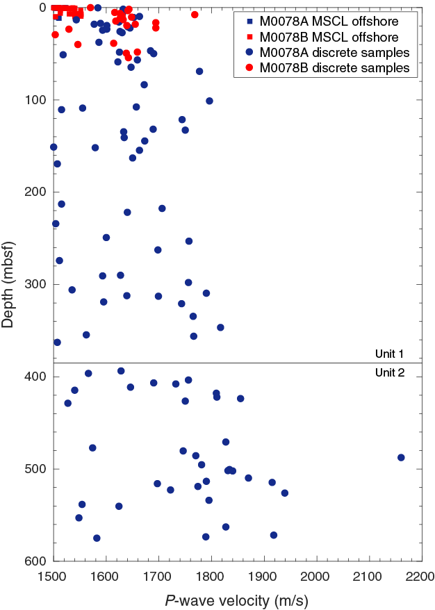
Figure F36. P-wave velocity data.
Density
Offshore, density data (bulk density) were obtained using the gamma ray attenuation (GRA) technique on the MSCL, whereas onshore, density data (bulk and grain density) were obtained using the moisture and density (MAD) analysis technique on discrete samples.
MSCL bulk density values range from 1 to 2.26 g/cm3 with ~96% above 1.70 g/cm3 (Figure F29). The results show a general increase in density with depth in Hole M0078A punctuated by a few intervals with drops in density that are followed by a return to the previous average values. The average MSCL density value is 1.97 g/cm3. Two notable increases in density occur at approximately 225 and 450 mbsf. The increase at 225 mbsf is relatively better defined and appears to occur at the same depth as an increase in shear strength. The average density is 1.84 g/cm3 from 0 to 225 mbsf, 2.0 g/cm3 from 225 to 450 mbsf, and 2.12 g/cm3 from 450 to 610 mbsf. Reduced density correlates with (parts of) the marine intervals/subunits (e.g., 195–205, 240–260, 290–300, 322–335, and ~370 mbsf).
Discrete bulk density values and trends from the MAD analysis match well with the MSCL data, ranging from 1.41 to 2.50 g/cm3 with 98% above 1.70 g/cm3, and generally increase with depth. The average density value from the MAD analysis is 1.96 g/cm3. Notable increases in density occur at approximately 136, 227, and 455 mbsf. The largest decreases in discrete bulk density are associated with the marine subunits, as is the case with MSCL GRA bulk density (in the same intervals noted above).
Sediment grain density values calculated from the MAD analysis range from 1.88 to 3.14 g/cm3 with an average of 2.6 g/cm3, and 93% of the values are between 2.6 and 2.8 g/cm3. These grain density values are between pure sandstone and pure limestone (Kennedy, 2015). Grain density generally increases with increasing bulk density and decreasing porosity. As with bulk density, low grain density correlates with some marine intervals/subunits (Figure F29).
Porosity
Porosity values calculated from the MAD analysis range from 14% to 65% with an average of 43%. Average porosity values in Units 1 and 2 are 46% and 38%, respectively. Porosity decreases with depth from an average of 50% in the uppermost 10 m of the hole to an average of 32% in the lowermost 10 m of the hole. Notable intervals of increased porosity with depth (e.g., ~195–205, ~250, and ~322–335 mbsf) correspond to noted intervals of decreased density that are associated with interpreted marine environments. Porosity decreases at ~224 mbsf, which coincides with an increase in density, resistivity, and shear strength and may be associated with a coring method change or increased consolidation linked to lithologic change, coincident with a facies association change (see Shear strength; Figures F29, F30). A further decrease occurs in Unit 2 at ~450 mbsf, also coincident with increased density. These two changes divide the borehole into three sections: 0–224 mbsf (average porosity = 48%), 224–450 mbsf (average porosity = 42%), and 450–610 mbsf (average porosity = 37%).
Resistivity
For Site M0078, electrical resistivity was measured offshore using the MSCL. The resistivity measured is low, ranging from 0.1 to 30 Ωm (Figure F37). The mean resistivity is 2.64 Ωm with a standard deviation of 1.45 Ωm.
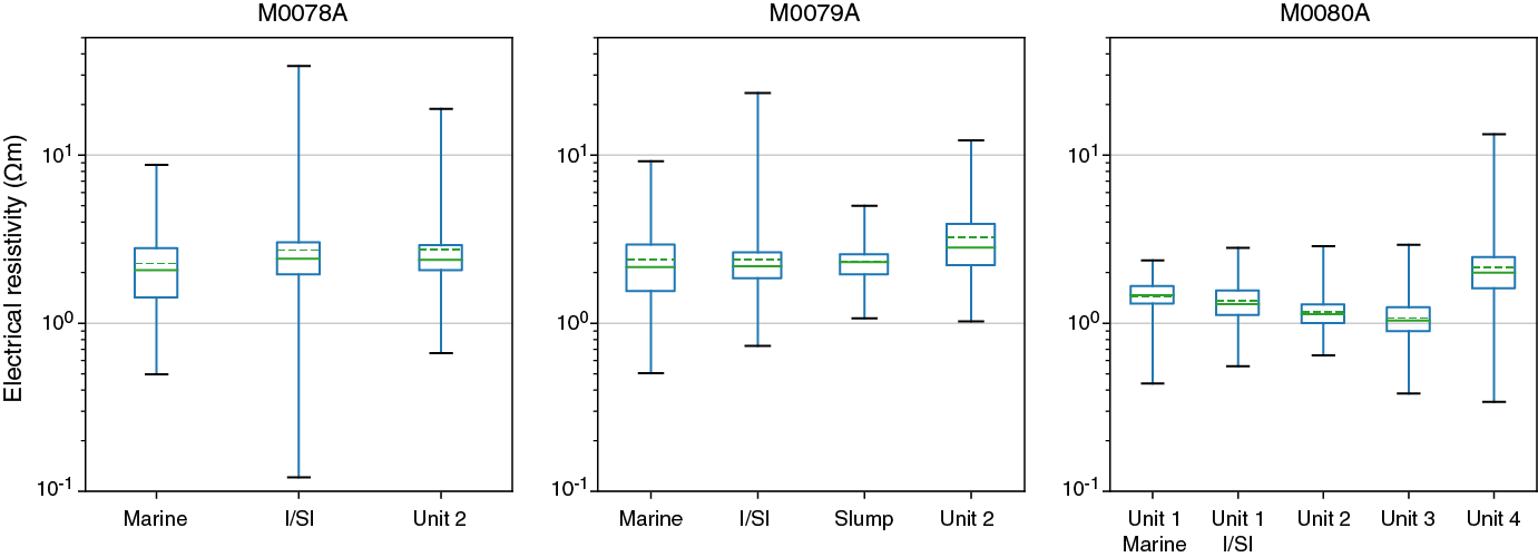
Figure F37. MSCL electrical resistivity box and whisker plots.
In each core, resistivity tends to increase from the top to the base, with a corresponding increase in density, especially in Unit 2 (Figure F38C, F38D). This tendency suggests an effect of drilling-induced disturbance. Electrical resistivity correlates well between Holes M0078B and M0078A, indicating reduced variations related to drilling disturbance in the shallow section of both holes (Figure F38).
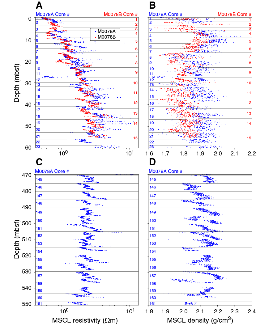
Figure F38. Resistivity and density trends observed in cores.
Low resistivity values are recorded in the shallower part of the hole, with an exponential increase with depth to 50 mbsf (note log scale on Figures F29 and F38). The mean resistivity value then remains almost constant to 380 mbsf, with values of 1–3 Ωm and larger variability in nonmarine subunits. Deeper than 400 mbsf, electrical resistivity decreases from 3 to 1 Ωm (Figure F29). This decrease, which is related to a decrease in porosity, suggests an increase in fluid conductivity at the bottom of the hole.
The low resistivity values recorded at Site M0078 are compatible with the values derived from the Archie equation for a porosity in the range of 35%–50% and a fluid conductivity equal to that of seawater.
Thermal conductivity
Thermal conductivity values range from 1.09 to 1.59 W/(m·K) with an average of 1.35 W/(m·K). Thermal conductivity averages 1.27 W/(m·K) in Unit 1 and 1.42 W/(m·K) in the underlying Unit 2. Increases in thermal conductivity occur at 62.5 and 440 mbsf, dividing the data downhole into three distinct sections. The average thermal conductivity is 1.21 W/(m·K) from 0 to 62.5 mbsf, 1.29 W/(m·K) from 62.5 to 440 mbsf, and 1.45 W/(m·K) from 440 to 610 mbsf. Thermal conductivity is lowest in intervals correlating with FA5 (light gray to white submillimeter laminations of calcite or aragonite alternating with mud–silt beds; see Lithostratigraphy). Relatively higher thermal conductivity values consistently occur in Unit 2. Laboratory values were corrected to in situ conditions because thermal conductivity is affected by temperature and pressure; the in situ thermal conductivity values range from 1.14 to 1.71 W/(m·K) and show a similar trend to the laboratory measurements (Figures F29, F39C). The correction to in situ conditions was done following Hyndman et al. (1974) (see Physical properties in the Expedition 381 methods chapter [McNeill et al., 2019b]).
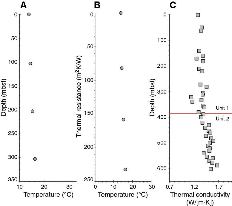
Figure F39. Temperature and thermal conductivity data, Hole M0078A.
Formation temperature and heat flow
Temperature measurements were collected offshore at four depths and plotted against depth to estimate the geothermal gradient (Figure F39C). The geothermal gradient is approximately 8°C/km, which like the temperature values is very low.
The temperature data were used with thermal conductivity to estimate heat flow using the Bullard method, which plots the thermal resistance against temperature (Figure F39B) and calculates heat flow from the slope of the best fitting line (see Physical properties in the Expedition 381 methods chapter [McNeill et al., 2019b]). The calculated heat flow is ~11 mW/m2.
The temperature at the seafloor can be determined from the intercept of a plot of temperature against depth using the three temperature measurements at 102.8, 202.8, and 303 mbsf (Figure F39A). The seafloor temperature estimated from temperature CPT data is 13.31°C, which is lower than the 13.75°C measured. Using this seafloor temperature of 13.31°C, the calculated geothermal gradient is 9°C/km and the heat flow from the Bullard plot is ~12 mW/m2.
Color reflectance
The mean color reflectance values ± standard deviations and minimum/maximum values of all depths in Hole M0078A are (Figure F40) 50 ± 7 and 0/77, respectively, for L*, −1.8 ± 0.9 and −10.9/0.7, respectively, for a*, and 4.0 ± 3.0 and −20/29, respectively, for b*. The main change in color reflectance occurs around 330–350 mbsf. Shallower than 330–350 mbsf, L*, a*, and b* values average 48, −2.0, and 3.4, respectively, and deeper than 330–350 mbsf, they average 53, −1.7, and 4.6, respectively. This division occurs above the Unit 1/2 boundary at 385.14 mbsf (Figures F29, F30).
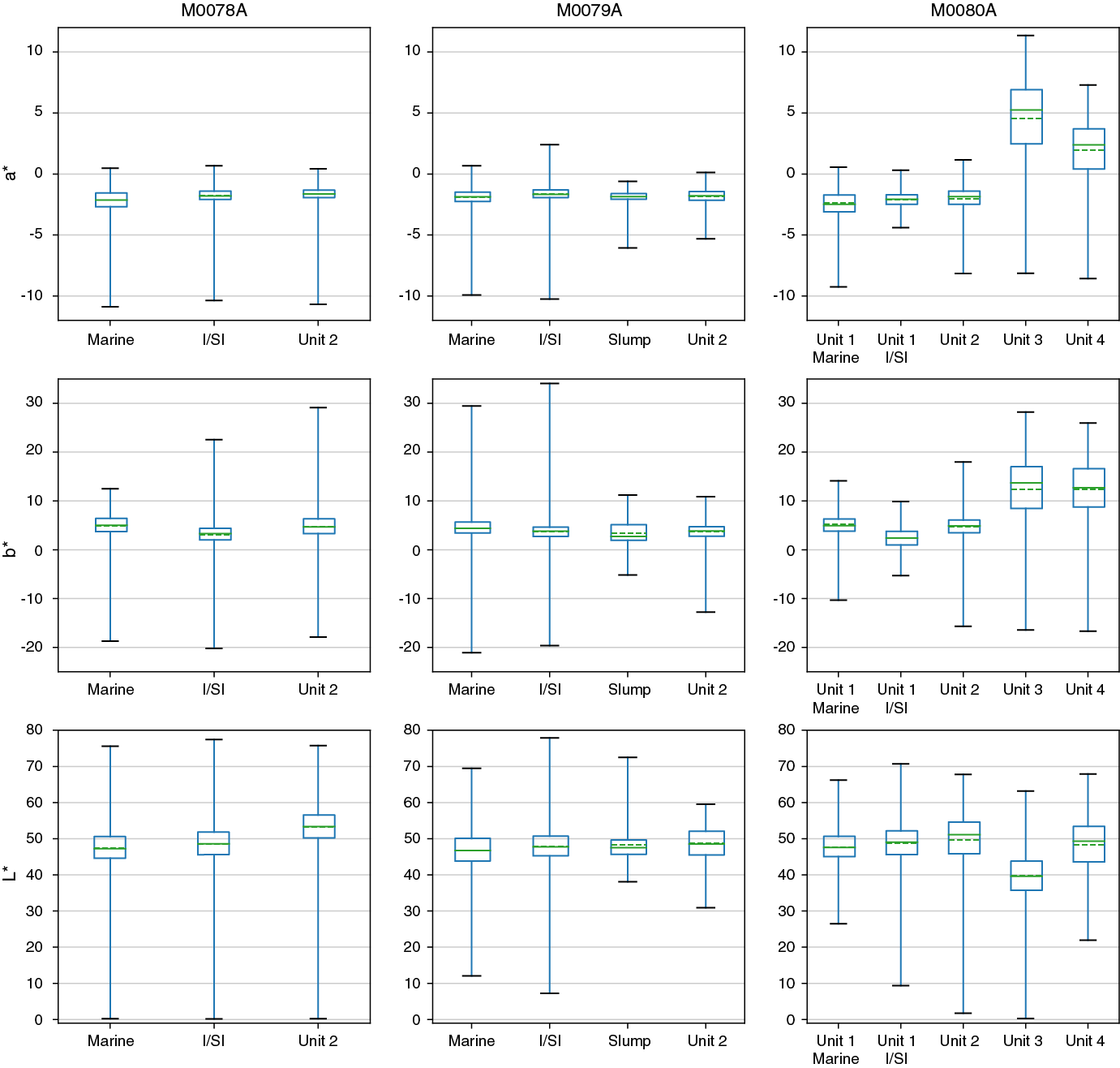
Figure F40. L*a*b* color reflectance data box and whisker plots.
Some color reflectance values deviate from the mean values for Hole M0078A when they occur in specific sedimentary facies associations (Figure F30). Most notable changes in color reflectance values occur mainly in two sedimentary facies associations. FA1 (homogeneous mud) is recorded in Unit 1 shallower than 370 mbsf and includes lower mean L* and a* values (47 and −2.4, respectively) and a slightly higher mean b* value (4.1) compared with mean values for the hole. The second sedimentary facies, FA12 (light gray to buff homogeneous to weakly stratified mud), includes higher mean L* and a* values (53 and −1.7, respectively) compared with mean values for the hole and a higher mean b* value (4.7) than the value in FA1 (4.1). This facies association and the associated color changes occur mainly in Unit 2. Color changes observed in FA10 and FA3 are similar to the changes observed in FA12 but are less prominent because they are thin and alternate with other facies associations, mainly in Unit 1.
Four sedimentary facies associations include L* values that are lower than the mean value for the hole: FA5 (greenish gray mud with dark gray to black [organic rich?] silty to sandy beds [centimeter scale]), FA2 (greenish gray mud with homogeneous centimeter-thick gray mud beds), FA11 (interbedded mud/silt and centimeter-thick sand beds), and FA4 (laminated greenish gray to gray mud with mud beds) (Figure F30). These facies associations are mostly confined to Unit 1.
Color reflectance values also vary between the two subunit environments (marine and isolated/semi-isolated) (Figures F29, F40). The marine subunits have lower mean L* and a* values (47 and −2.2, respectively) than the overall hole (50 and −1.9, respectively) and a higher mean b* value (4.7) than the overall hole (3.9). These values are similar to those associated with sedimentary FA1. The isolated/semi-isolated subunits have higher mean L* and a* values (51 and −1.8, respectively) than the overall hole (50 and −1.9, respectively) and a lower mean b* value (3.7) than the overall hole (3.9). The reduced L* values in FA1 and marine subunits correlate with reduced magnetic susceptibility values (Figure F41; also see Magnetic susceptibility). However, no strong correlation exists between other physical properties and color reflectance. Both magnetic susceptibility and NGR values show a change in variability and values at about 330 mbsf, which is slightly shallower than the observed change in color reflectance values at about 350 mbsf and above the Unit 1/2 boundary at 385.14 mbsf.
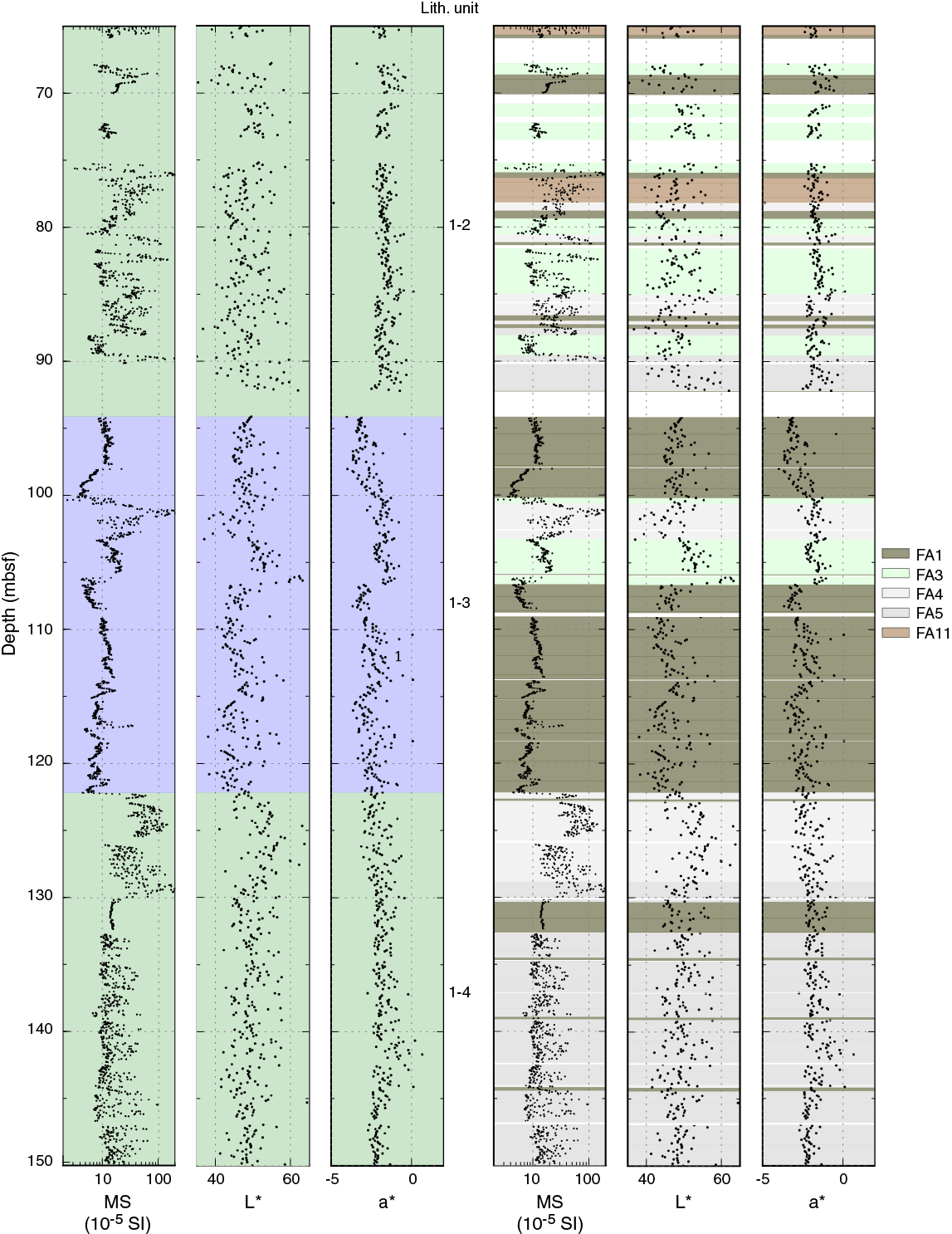
Figure F41. MS, L*, and a*.
Paleomagnetism
Magnetic susceptibility
A total of 454 and 47 discrete samples were analyzed from Holes M0078A and M0078B, respectively. Frequency distribution diagrams of magnetic susceptibility (k) from Hole M0078A and M0078B discrete samples, together with shipboard MSCL continuous data (2 cm interval) from whole core sections, are shown in Figure F42. Magnetic susceptibility in both Holes M0078A and M0078B shows a unimodal distribution with values that range between approximately 10 × 10−6 and 1000 × 10−6 SI. The maximum frequency of susceptibility values is between 50 and 100 × 10−6 SI (Figure F42B, F42C). A similar trend occurs in MSCL susceptibility data, where the most frequent values range between 50 and 150 × 10−6 SI (Figure F42A). Downhole distribution of magnetic susceptibility in Hole M0078A (Figure F43) shows a low variability to ~300 mbsf with values around ~100 ×10−6 SI (excluding a few samples with higher or lower susceptibility). Hole M0078B shows similar trends (Figure F44). Much higher variability occurs in Hole M0078A below ~300 mbsf, where susceptibility spans two orders of magnitude from 10 ×10−6 to 1000 ×10−6 SI. This trend is much clearer when onshore discrete and shipboard continuous susceptibility data are plotted together versus depth (Figure F43E). The increased scatter in magnetic susceptibility below ~300 mbsf observed at Site M0078 may be related to changes in concentration (possibly related to compaction), nature, or grain size of the magnetic minerals or to any combination of these factors.
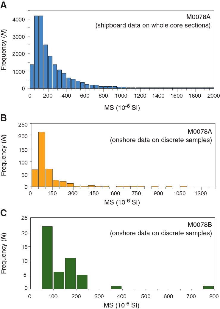
Figure F42. MS frequency distribution.
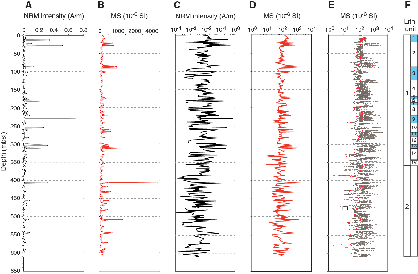
Figure F43. NRM intensity and MS, Hole M0078A.
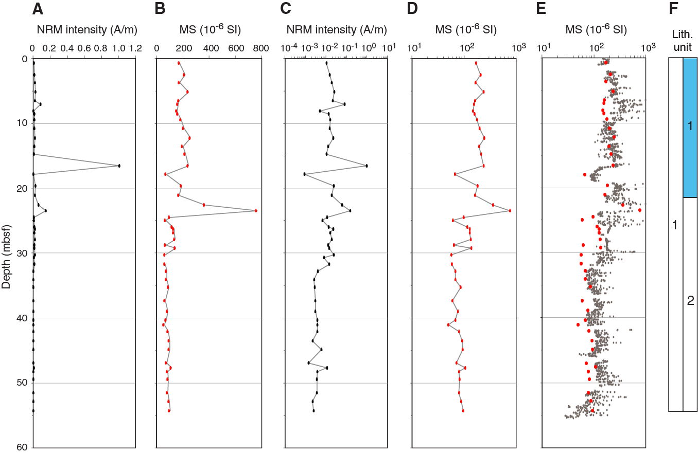
Figure F44. NRM intensity and MS, Hole M0078B.
Both magnetic susceptibility and natural remanent magnetization (NRM) change in a similar fashion downhole (Figures F43, F44), suggesting a correlation between these two parameters that is clearly demonstrated by the linear trend described by the data from Site M0078 when plotted on an NRM/k diagram (Figure F45). The direct relationship between NRM and k suggests that the susceptibility variation is mainly (but perhaps not exclusively) controlled by the change in concentration of a single magnetic phase in the sediment. However, the relationship between NRM and susceptibility in lithostratigraphic Unit 1 (red dots, Figure F45A) is perhaps more complex and forms both a linear trend and a small cluster localized at NRM intensity values <10−3 A/m and susceptibility values approximately between 50 × 10−6 and 80 × 10−6 SI. The samples belonging to this cluster appear to be mostly from the marine intervals/subunits of the sedimentary succession. Conversely, NRM and k follow a relatively well defined linear trend in lithostratigraphic Unit 2 (interpreted to be nonmarine), which is characterized by lower NRM values compared with Unit 1.
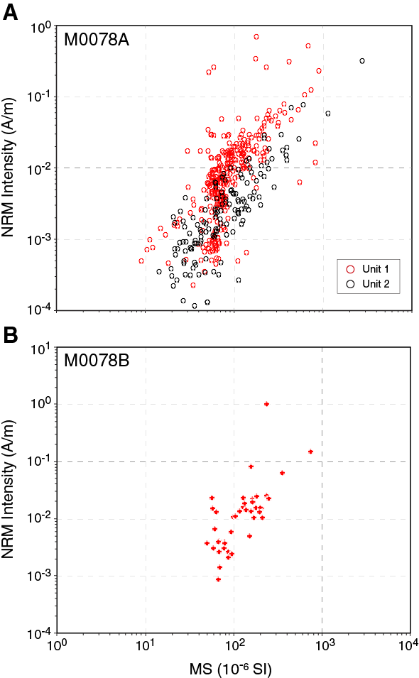
Figure F45. NRM intensity vs. MS.
Magnetic mineralogy
Thermal variation of low-field magnetic susceptibility was measured for five representative samples from Hole M0078A at the University of Hawaii (USA) prior to the OSP.
Susceptibility was measured during heating–cooling cycles from room temperature to 700°C and back to room temperature. No argon gas was used for these experiments. A heating–cooling rate of 9°C/min was used in all experiments. Figure F46 shows the results of the thermomagnetic experiments, revealing a wide range of Curie temperatures ranging between 171° and 630°C. However, most of the samples show a primary Curie temperature of 518°–577°C, indicating the occurrence of Ti-poor titanomagnetite. Other Curie temperatures around 320°–405°C may suggest the occurrence of iron sulfides (likely greigite). The variable magnetic susceptibility of greigite may be the cause of part of the observed downhole scatter in the magnetic susceptibility data.
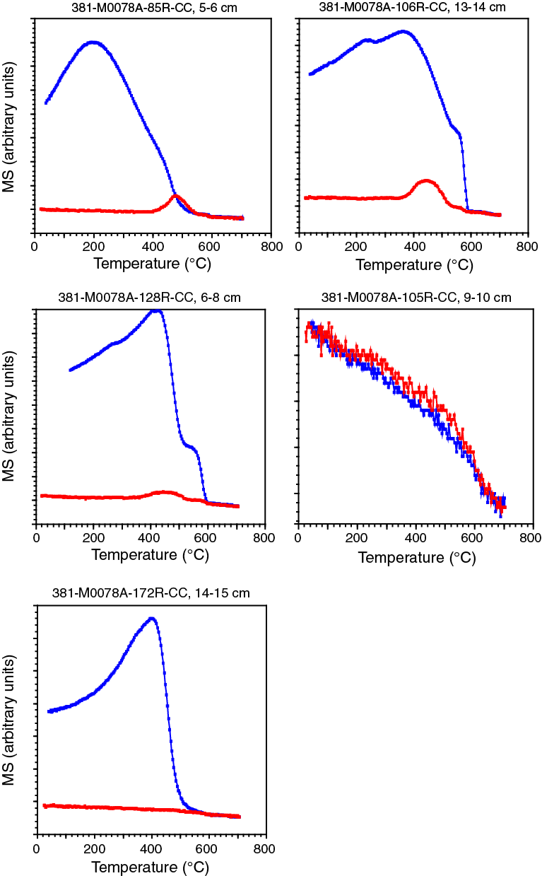
Figure F46. Low-field susceptibility vs. temperature experiment results.
Natural remanent magnetization
NRM direction and intensity of discrete samples were measured using the SRM 755–4000 cryogenic magnetometer (2G-Enterprises) at the University of Bremen (Germany). A total of 454 and 47 discrete cubic samples were analyzed from Holes M0078A and M0078B, respectively. All samples were stepwise demagnetized by alternating fields (AFs), and magnetization was measured after each demagnetization step. Magnetization decays steadily to nearly complete removal at the maximum AF (100 mT) in most of the samples (Figure F47A, F47B), indicating the occurrence of low-coercivity magnetic minerals, such as magnetite or titanomagnetite. Some samples still retain ~15%–20% of their initial magnetization after the application of the highest demagnetizing field (100 mT) (Figure F47C). In a few samples (<15%), remanence progressively decreased as larger demagnetizing fields were applied. Minimum values were reached at 50–60 mT, and then values increased again at higher demagnetizing fields (Figure F47D, F47E). This behavior is typical of sediment carrying diagenetic greigite (Fe3S4).
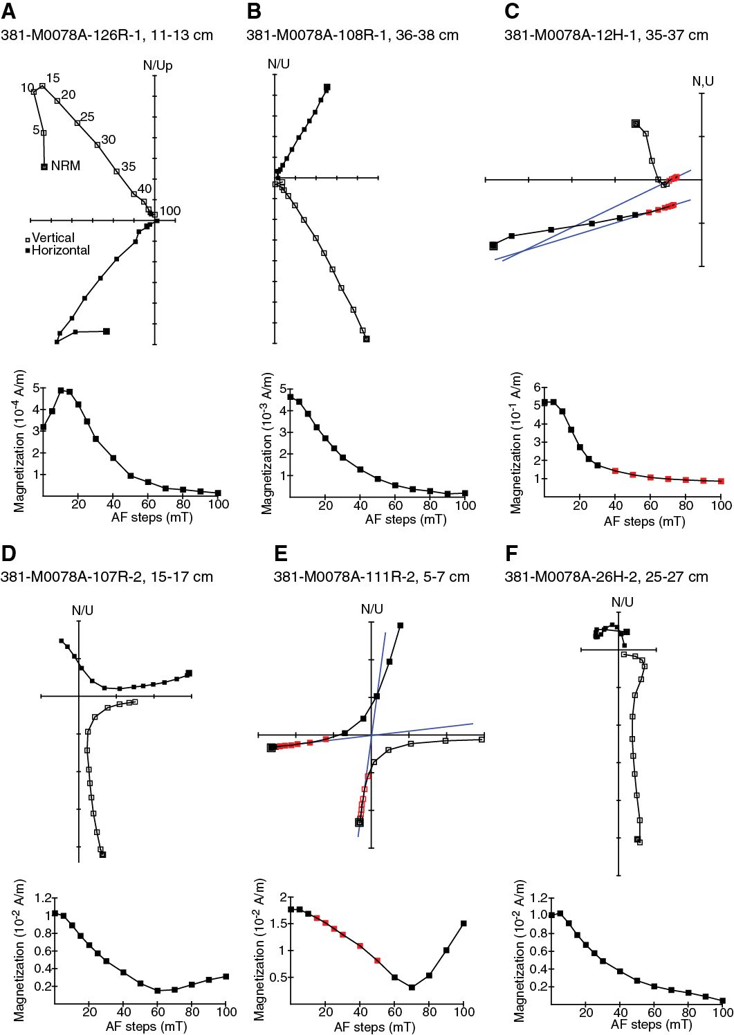
Figure F47. Orthogonal projections and relative decay paths.
Orthogonal demagnetization diagrams show that demagnetizing fields of 10–15 mT are sufficient to remove the weak viscous remanent magnetization and other secondary magnetization components. After removing these overprints, the samples displayed varied responses to the sequential demagnetization with two principal categories. Category 1 indicates the presence of NRM carried by magnetic minerals with high coercivity (median destructive field >40 mT). Category 1 samples occur in the upper 400 m of Hole M0078A and are characterized by magnetization vectors decaying toward the origin after the 10–15 mT AF step and more than 50% of the NRM intensity removed at 100 mT. Category 1 samples show both positive and negative inclinations (i.e., normal and reversed polarity) (Figure F47A, F47C). Category 2 samples show a relatively high susceptibility, a median destructive field of 60–70 mT, and about 20% of the initial magnetization still retained at the 100 mT AF step. The demagnetization diagrams for Category 2 samples form lines pointing toward the origin of the axes above the 10–15 mT AF step, and above 40 mT the data veer into a plane that is perpendicular to the last applied demagnetization axis (Figure F47D, F47E). This behavior is known as gyroremanent magnetization and is indicative of the occurrence of diagenetic greigite. A very small number of samples (<2%) do not belong to these two categories because they carry more complex magnetizations (Figure F47F) whose different components could not be straightforwardly interpreted, likely because of the occurrence of a mixture of different magnetic phases.
Samples do not seem to be strongly affected by drilling-induced magnetizations commonly present in cored sediments. This component is vertical, points downward, and is typically removed at 5–10 mT. NRM directions from Holes M0078A and M0078B do not carry this vertical component. Not only are these directions not vertical (or close to vertical), they are also close to the expected magnetic field inclination at the sampling locality (I = 57.5°) (Figure F48). After demagnetization at 40 mT, secondary magnetization components were removed in all the analyzed samples. For this reason, the remanence direction (declination and inclination) after demagnetization at 40 mT can be considered parallel to the characteristic remanent magnetization (ChRM) component in each sample.
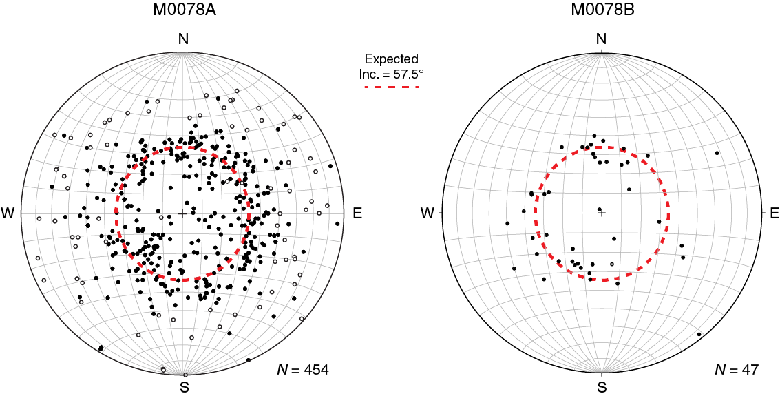
Figure F48. NRM directions.
The remanence inclination after demagnetization at 40 mT is consistent with the expected inclination in both Holes M0078A and M0078B (Figure F49). These data suggest that the ancient geomagnetic field has reliably been recorded by these sediments.
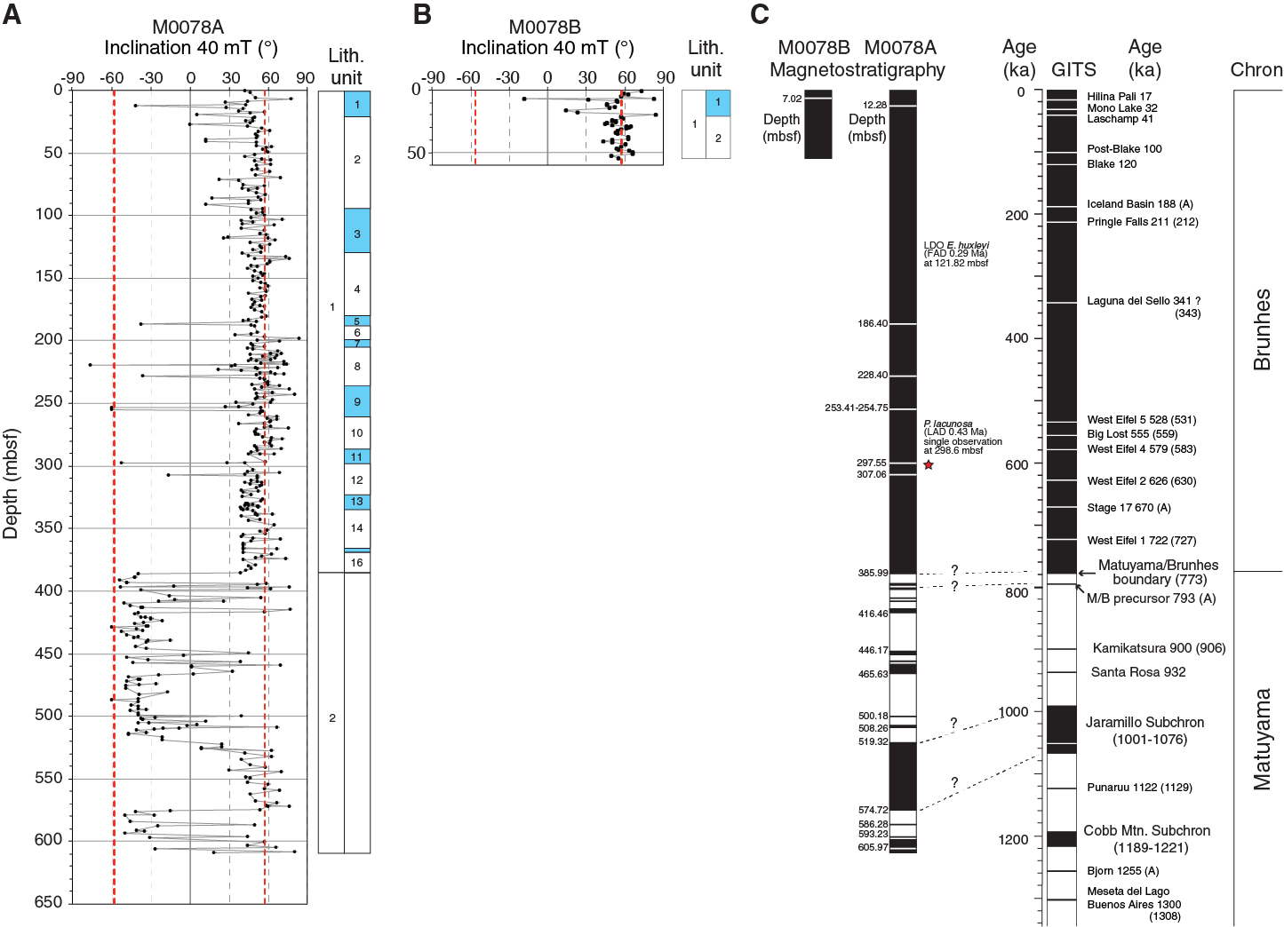
Figure F49. Inclination and magnetostratigraphic logs.
Magnetostratigraphy
Inclination values of the remanence after demagnetization at 40 mT (used here as representative of the ChRM components) show a downhole change from positive (normal polarity) to negative (reversed polarity) consistent with the expected magnetic field inclination values at the sampling latitude. Some of these inclination variations may represent geomagnetic field excursions rather than true reversals. One of the main objectives for the OSP paleomagnetic work was to produce magnetostratigraphic logs of the sedimentary sequences from Sites M0078, M0079, and M0080. The excellent magnetic stability of all the specimens will allow a potentially reliable magnetostratigraphic reconstruction. Figure F49 shows the inclination data for Holes M0078A and M0078B together with a preliminary magnetostratigraphy and its interpretative correlation with the geomagnetic instability timescale (GITS) of Singer (2014) (dashed lines with question marks). The produced magnetostratigraphy shows a predominantly normal polarity in the upper 385.11 m (Sample 381-M0078A-125R-2, 12–14 cm). Just below this sample at 385.14 mbsf, a major change in lithologic and chemical features marks the transition to Unit 2 (see Lithostratigraphy). In this uppermost interval characterized by a normal polarity, six Hole M0078A samples and one Hole M0078B sample have a reversed polarity consistent with the expected geomagnetic field inclination (i.e., −57.5°). These anomalous inclinations are marked with white lines in the magnetostratigraphic columns in Figure F49C. These samples may have recorded some of the geomagnetic field excursions that occurred during the Brunhes Chron (e.g., Singer, 2014). Additional rock magnetic experiments and biostratigraphic constraints will, however, be necessary to establish whether and which one of these inclination changes are actual magnetic field excursions.
From the “shipboard” work, two biomarkers were defined with moderate confidence in Unit 1 that could be used to tighten the proposed magnetostratigraphic correlations with the GITS. The LDO of E. huxleyi (FAD at 0.29 Ma) was observed at 121.82 mbsf, and the LAD of P. lacunosa (0.43 Ma) was observed at 298.6 mbsf (see Micropaleontology) (Figure F49). It is important to note that P. lacunosa was only observed in a single sample, and because of the punctuated nature of marine environments in the Corinth basin, the precision of both biohorizons is inherently low. These two biomarkers would suggest that the sediment shallower than 121.82 mbsf and deeper than 298.6 mbsf cannot be older than 0.29 Ma or younger than 0.43 Ma, respectively. These biomarkers would therefore imply that the potential excursion observed at 12.28 mbsf in Hole M0078A and 7.02 mbsf in Hole M0078B (Figure F49C), if indicative of true excursions, may only be correlated with one of the excursions younger than Pringle Falls (211 ka; Singer, 2014). Similarly, the potential excursion observed at 307.06 mbsf in Hole M0078A may only be correlated with one of the excursions older than West Eifel 5 (528 ka; Singer, 2014). However, given the lack of firm biostratigraphic constraints from Holes M0078A and M0078B, any correlation between the potential excursions observed in Holes M0078A and M0078B and those from the GITS currently remains highly speculative.
Sample 381-M0078A-125R-2, 100–102 cm (385.99 mbsf), at the top of Unit 2 yields a negative inclination (reversed polarity) and marks the boundary with a longer reversed polarity interval below. This major polarity transition might represent the Brunhes/Matuyama boundary (0.773 Ma; Singer, 2014). The interpretation of this polarity transition as the Brunhes/Matuyama boundary remains speculative. Below 385.99 mbsf, a number of samples with normal polarity occur too, including a relatively long normal polarity interval at 519.32–574.72 mbsf. The lack of biostratigraphic constraints from Unit 2, however, prevents us from drawing definitive conclusions on the real nature and age of the major polarity change at 385.99 mbsf or any of the deeper reversals observed. Between 519.32 and 574.72 mbsf, a relatively long interval characterized by a normal polarity occurs that might represent the Jaramillo Subchron (1.00–1.08 Ma).
Core-log-seismic integration
In the absence of new velocity information at Site M0078 from downhole logging or core measurements, MSCL density and a linear velocity function based on seismic data were used to generate synthetic seismograms. Unfortunately, neither MSCL nor discrete VP measurements produced reliable velocity data for Site M0078 (Figure F50), and downhole logging was not successful at this site. Therefore, the linear velocity model developed prior to the expedition (see Figure F18 in the Expedition 381 methods chapter [McNeill et al., 2019b]) and a slightly modified version from offshore core-seismic integration were used as a starting point for onshore synthetic seismograms. MSCL density values from Holes M0078A and M0078B were combined and thoroughly quality checked and filtered using the approach described in Core-log-seismic integration in the Expedition 381 methods chapter (McNeill et al., 2019b). The resulting density log was depth shifted to sea level (Figure F51; Table T18).
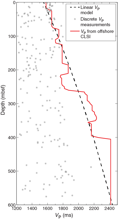
Figure F50. Discrete sample VP with pre-expedition model and offshore CLSI results.
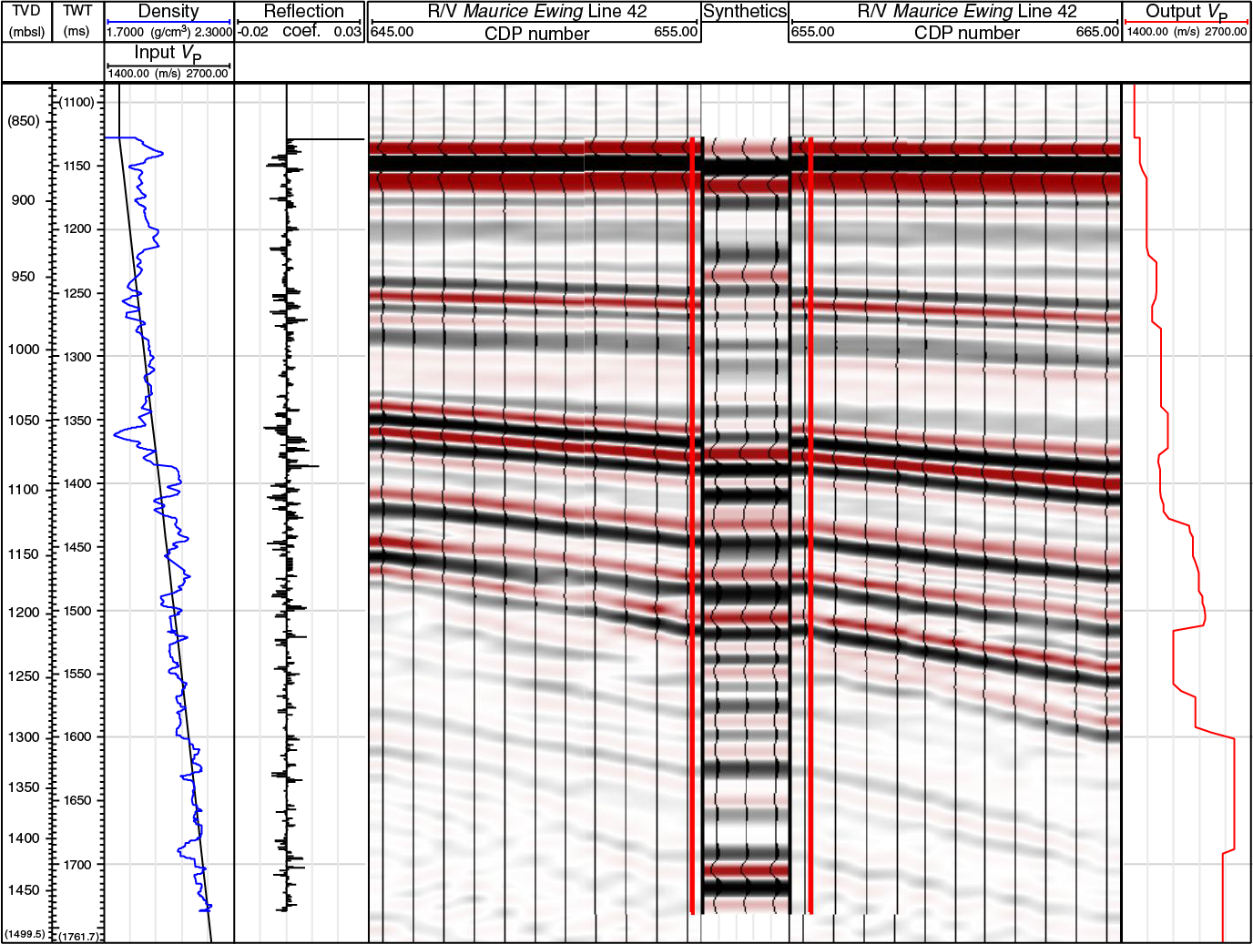
Figure F51. Synthetic seismogram.
Despite a lack of new downhole velocity information, the synthetic seismograms can be reliably tied to the seismic data with limited adjustments to the initial velocity profile (Figure F51). The main high-reflectivity horizons in seismic Unit 2 (lithostratigraphic Unit 1) match with the seismic data remarkably well. The lower reflectivity sequences in seismic Unit 1 (lithostratigraphic Unit 2) proved to be more challenging to match because of the lack of impedance contrasts in the core and seismic records. However, at least two low-reflectivity horizons in seismic Unit 1 can be potentially traced in the synthetic seismogram and tied to seismic data.
The output velocity profile from the synthetics generation (Table T19) suggests that VP often deviates from the linear velocity model but does not exhibit consistent variations with respect to the lithostratigraphic subunits (Figure F52). The resulting time-depth conversion function is shown in Figure F53, and the time-depth relationship (TDR) for the high-reflectivity seismic horizons is listed in Table T20 (full TDR is in M0078_TDR.xlsx in CLSI in Supplementary material).

Figure F52. Onshore CLSI VP profile with pre-expedition model and offshore CLSI results.
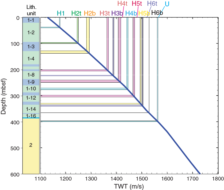
Figure F53. Time-depth conversion function.
One of the largest uncertainties in positioning seismic horizons in depth and correlating them with the core record proved to be the finite resolution of the seismic data. The interpretation by Nixon et al. (2016) placed seismic unit and sequence boundaries at the peak amplitude of a seismic reflection, whereas our analysis of synthetic seismograms indicates that the first break of a reflection provides a better estimate of the depth to the corresponding impedance contrast. Converted to depth, the time difference between picking “zero crossing” (wherever possible to identify) and the peak of a wavelet can reach 10–15 m, introducing significant uncertainty for core-seismic integration (Figure F53; Table T20). An estimated calculation of the vertical resolution for these seismic data agrees with this estimation. For example, the peak frequency of the source wavelet extracted from the data around the site is 30–40 Hz (see Figure F17 in the Expedition 381 methods chapter [McNeill et al., 2019b]). Assuming a vertical resolution of roughly a quarter of the wavelength (e.g., Widess, 1973) and an average velocity of 2000 m/s, this translates to a vertical resolution of 12–17 m.
The TDR established with synthetic seismograms at Site M0078 allows for direct comparison of major lithologic boundaries identified in the cores with the seismic data. Figure F54 shows a section of the seismic profile crossing Site M0078, the synthetic traces, and the unit and subunit boundaries identified from a combination of lithologic and paleontological observations. High-reflectivity horizons in the seismic profile clearly correspond to marine subunits in the core, confirming the interpretation of Nixon at el. (2016) and others before. For example, seismic Horizon H2 top and bottom clearly correspond to the lithostratigraphic Subunit 1-3 (marine) boundaries, and seismic Horizon H3 top and bottom correspond to thin marine intervals in Subunits 1-5 and 1-7, respectively. However, the subunit boundaries predominantly map onto the first break of a given seismic reflection, not the peak (Figure F53).
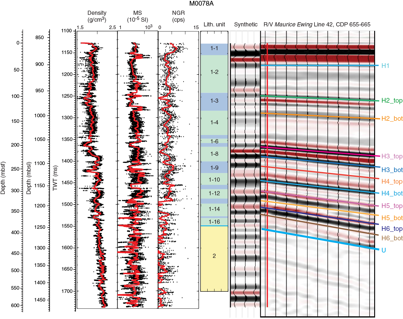
Figure F54. MSCL data converted to time with synthetic and seismic data.
Below ~250 mbsf, correlating seismic reflectors with subunit boundaries in Hole M0078A becomes more challenging because subunits are thinner and may be incomplete at the base of Unit 1 at this site. In this depth range, some of the seismic phases that correspond to the boundaries between the marine and isolated/semi-isolated subunits are different from the interpreted horizons (Figures F53, F54). For example, the Horizon H5 top corresponds to the top of isolated/semi-isolated lithostratigraphic Subunit 1-12, not a marine interval.
The depth of the unit boundary/unconformity (U) in the seismic data directly matches the lithostratigraphic Unit 1/2 boundary. Therefore, we interpreted seismic Unconformity U to represent the lithostratigraphic unit boundary identified in the core. Below the Unit 1/2 boundary, no bright reflectors were observed in the seismic record, consistent with the lack of lithostratigraphic boundaries in the core. However, two low-amplitude reflectors clearly correspond to changes in density and magnetic susceptibility at ~480 and ~545 mbsf. These boundaries may potentially correspond to paleoenvironmental changes, as suggested by preliminary “shipboard” micropaleontology, but the nature of these transitions and their expression in the sedimentary record and/or physical properties are not yet well characterized.
References
Anthonissen, D.E., and Ogg, J.G., 2012. Appendix 3—Cenozoic and Cretaceous biochronology of planktonic foraminifera and calcareous nannofossils. In Gradstein, F.M., Ogg, J.G., Schmitz, M.D., and Ogg, G.M., (Eds.), The Geologic Time Scale 2012: Amsterdam (Elsevier), 1083–1127. https://doi.org/10.1016/B978-0-444-59425-9.15003-6
Backman, J., Raffi, I., Rio, D., Fornaciari, E., and Pälike, H., 2012. Biozonation and biochronology of Miocene through Pleistocene calcareous nannofossils from low and middle latitudes. Newsletters on Stratigraphy, 45(3):221–244. https://doi.org/10.1127/0078-0421/2012/0022
Bell, R.E., McNeill, L.C., Bull, J.M., Henstock, T.J., Collier, R.E.L., and Leeder, M.R., 2009. Fault architecture, basin structure and evolution of the Gulf of Corinth Rift, central Greece. Basin Research, 21(6):824–855. https://doi.org/10.1111/j.1365-2117.2009.00401.x
Berner, R.A., 1980. Early Diagenesis: A Theoretical Approach: Princeton, NJ (Princeton University Press).
Capotondi, L., Girone, A., Lirer, F., Bergami, C., Verducci, M., Vallefuoco, M., Afferri, A., Ferraro, L., Pelosi, N., and De Lange, G.J., 2016. Central Mediterranean mid-Pleistocene paleoclimatic variability and its association with global climate. Palaeogeography, Palaeoclimatology, Palaeoecology, 442:72–83. https://doi.org/10.1016/j.palaeo.2015.11.009
Cvetkoska, A., Jovanovska, E., Francke, A., Tofilovska, S., Vogel, H., Levkov, Z., Donders, T.H., Wagner, B., and Wagner-Cremer, F., 2016. Ecosystem regimes and responses in a coupled ancient lake system from MIS 5b to present: the diatom record of lakes Ohrid and Prespa. Biogeosciences, 13(10):3147–3162. https://doi.org/10.5194/bg-13-3147-2016
Cvetkoska, A., Reed, J.M., and Levkov, Z., 2012. Diatoms as indicators of environmental change in ancient Lake Ohrid during the last glacial–interglacial cycle (ca. 140 ka). In Witkowski, A. (Ed.), Diatom Monographs: Königstein, Germany (Koeltz Scientific Books).
Dimiza, M.D., Triantaphyllou, M.V., and Malinverno, E., 2014. New evidence for the ecology of Helicosphaera carteri in polluted coastal environments (Elefsis Bay, Saronikos Gulf, Greece). Journal of Nannoplankton Research, 34:37–43. http://ina.tmsoc.org/JNR/online/34/Dimiza et al 2014 JNR Crete.pdf
Dimiza, M.D., Triantaphyllou, M.V., Malinverno, E., Psarra, S., Karatsolis, B.-T., Mara, P., Lagaria, A., and Gogou, A., 2016. The composition and distribution of living coccolithophores in the Aegean Sea (NE Mediterranean). Micropaleontology, 61(6):521–540. http://www.micropress.org/microaccess/micropaleontology/issue-321/article-1966
Duchemin, G., Fontanier, C., Jorissen, F.J., Barras, C., and Griveaud, C., 2007. Living small-sized (63–150 µm) foraminifera from the mid-shelf to mid-slope environments in the Bay of Biscay. Journal of Foraminiferal Research, 37(1):12–32. https://doi.org/10.2113/gsjfr.37.1.12
Evitt, W.R., Gocht, H., and Netzel, H., 1985. Gonyaulax cysts from Lake Zürich sediments. Review of Palaeobotany and Palynology, 45(1–2):35–46. https://doi.org/10.1016/0034-6667(85)90064-8
Ford, M., Rohais, S., Williams, E.A., Bourlange, S., Jousselin, D., Backert, N., and Malartre, F., 2013. Tectono-sedimentary evolution of the western Corinth Rift (central Greece). Basin Research, 25(1):3–25. https://doi.org/10.1111/j.1365-2117.2012.00550.x
Ford, M., Williams, E.A., Malartre, F., and Popescu, S.-M., 2007. Stratigraphic architecture, sedimentology and structure of the Vouraikos Gilbert-type fan delta, Gulf of Corinth, Greece. In Nichols, G., Paola, C., and Williams, E. (Eds.), Sedimentary Processes, Environments and Basins: A Tribute to Peter Friend. Jarvis, I. (Series Ed.). Special Publication of the International Association of Sedimentologists, 38:44–90. https://doi.org/10.1002/9781444304411.ch4
Froelich, P.N., Klinkhammer, G.P., Bender, M.L., Luedtke, N.A., Heath, G.R., Cullen, D., Dauphin, P., Hammond, D., Hartman, B., and Maynard, V., 1979. Early oxidation of organic matter in pelagic sediments of the eastern equatorial Atlantic: suboxic diagenesis. Geochimica et Cosmochimica Acta, 43(7):1075–1090. https://doi.org/10.1016/0016-7037(79)90095-4
Goineau, A., Fontanier, C., Jorissen, F.J., Lansard, B., Buscail, R., Mouret, A., Kerhervé, P., et al., 2011. Live (stained) benthic foraminifera from the Rhône prodelta (Gulf of Lion, NW Mediterranean): environmental controls on a river-dominated shelf. Journal of Sea Research, 65(1):58–75. https://doi.org/10.1016/j.seares.2010.07.007
Houk, V., Klee, R., and Tanaka, H., 2010. Atlas of Freshwater Centric Diatoms with a Brief Key and Descriptions: Part 3. Stephanodiscaceae A. Cyclotella, Tertiarius, Discostella: Praha, Czech Republic (Czech Phycological Society).
Hyndman, R.D., Erickson, A.J., and Von Herzen, R.P., 1974. Geothermal measurements on DSDP Leg 26. In Davies, T.A., Luyendyk, B.P., et al., Initial Reports of the Deep Sea Drilling Project, 26: Washington, DC (U.S. Government Printing Office), 451–463. https://doi.org/10.2973/dsdp.proc.26.113.1974
Kennedy, M. (Ed.), 2015. Practical Petrophysics (Volume 62): Developments in Petroleum Science. Cubitt, J. (Series Ed.): Amsterdam (Elsevier).
Kouli, K., Brinkhuis, H., and Dale, B., 2001. Spiniferites cruciformis: a fresh water dinoflagellate cyst? Review of Palaeobotany and Palynology, 113(4):273–286. https://doi.org/10.1016/S0034-6667(00)00064-6
Krammer, K., and Lange-Bertalot, H., 1991. Bacillariophyceae, Part 3. Centrales, Fragilariaceae, Eunotiaceae. In Ettl, H., Gerloff, J., Heynig, H., and Mollenhauer, D. (Eds.), Süßwaserflora von Mitteleuropa (Volume 2/3): Stuttgart, Germany (Gustav Fischer Verlag).
Lisiecki, L.E., and Raymo, M.E., 2005. A Pliocene–Pleistocene stack of 57 globally distributed benthic δ18O records. Paleoceanography, 20(1):PA1003. https://doi.org/10.1029/2004PA001071
Martini, E., 1971. Standard Tertiary and Quaternary calcareous nannoplankton zonation. In Farinacci, A. (Ed.), Proceedings of the Second Planktonic Conference, Roma 1970: Rome (Edizioni Tecnoscienza), 2:739–785.
McNeill, L.C., Shillington, D.J., Carter, G.D.O., Everest, J.D., Le Ber, E., Collier, R.E.Ll., Cvetkoska, A., De Gelder, G., Diz, P., Doan, M.-L., Ford, M., Gawthorpe, R.L., Geraga, M., Gillespie, J., Hemelsdaël, R., Herrero-Bervera, E., Ismaiel, M., Janikian, L., Kouli, K., Li, S., Machlus, M.L., Maffione, M., Mahoney, C., Michas, G., Miller, C., Nixon, C.W., Oflaz, S.A., Omale, A.P., Panagiotopoulos, K., Pechlivanidou, S., Phillips, M.P., Sauer, S., Seguin, J., Sergiou, S., and Zakharova, N.V., 2019a. Expedition 381 facies associations. In McNeill, L.C., Shillington, D.J., Carter, G.D.O., and the Expedition 381 Participants, Corinth Active Rift Development. Proceedings of the International Ocean Discovery Program, 381: College Station, TX (International Ocean Discovery Program). https://doi.org/10.14379/iodp.proc.381.103.2019
McNeill, L.C., Shillington, D.J., Carter, G.D.O., Everest, J.D., Le Ber, E., Collier, R.E.Ll., Cvetkoska, A., De Gelder, G., Diz, P., Doan, M.-L., Ford, M., Gawthorpe, R.L., Geraga, M., Gillespie, J., Hemelsdaël, R., Herrero-Bervera, E., Ismaiel, M., Janikian, L., Kouli, K., Li, S., Machlus, M.L., Maffione, M., Mahoney, C., Michas, G., Miller, C., Nixon, C.W., Oflaz, S.A., Omale, A.P., Panagiotopoulos, K., Pechlivanidou, S., Phillips, M.P., Sauer, S., Seguin, J., Sergiou, S., and Zakharova, N.V., 2019b. Expedition 381 methods. In McNeill, L.C., Shillington, D.J., Carter, G.D.O., and the Expedition 381 Participants, Corinth Active Rift Development. Proceedings of the International Ocean Discovery Program, 381: College Station, TX (International Ocean Discovery Program). https://doi.org/10.14379/iodp.proc.381.102.2019
McNeill, L.C., Shillington, D.J., Carter, G.D.O., Everest, J.D., Le Ber, E., Collier, R.E.Ll., Cvetkoska, A., De Gelder, G., Diz, P., Doan, M.-L., Ford, M., Gawthorpe, R.L., Geraga, M., Gillespie, J., Hemelsdaël, R., Herrero-Bervera, E., Ismaiel, M., Janikian, L., Kouli, K., Li, S., Machlus, M.L., Maffione, M., Mahoney, C., Michas, G., Miller, C., Nixon, C.W., Oflaz, S.A., Omale, A.P., Panagiotopoulos, K., Pechlivanidou, S., Phillips, M.P., Sauer, S., Seguin, J., Sergiou, S., and Zakharova, N.V., 2019c. Site M0079. In McNeill, L.C., Shillington, D.J., Carter, G.D.O., and the Expedition 381 Participants, Corinth Active Rift Development. Proceedings of the International Ocean Discovery Program, 381: College Station, TX (International Ocean Discovery Program). https://doi.org/10.14379/iodp.proc.381.105.2019
Mertens, K.N., Rengefors, K., Moestrup, Ø., and Ellegaard, M., 2012. A review of recent freshwater dinoflagellate cysts: taxonomy, phylogeny, ecology and palaeocology. Phycologia, 51(6):612–619. https://doi.org/10.2216/11-89.1
Mudie, P.J., Marret, F., Mertens, K.N., Shumilovskikh, L., and Leroy, S.A.G., 2017. Atlas of modern dinoflagellate cyst distributions in the Black Sea Corridor: from Aegean to Aral Seas, including Marmara, Black, Azov and Caspian Seas. Marine Micropaleontology, 134. https://doi.org/10.1016/j.marmicro.2017.05.004
Mudie, P.J., Marret, F., Rochon, A., and Aksu, A.E., 2010. Non-pollen palynomorphs in the Black Sea corridor. Vegetation History and Archaeobotany, 19(5–6):531–544. https://doi.org/10.1007/s00334-010-0268-9
Nixon, C.W., McNeill, L.C., Bull, J.M., Bell, R.E., Gawthorpe, R.L., Henstock, T.J., Christodoulou, D., et al., 2016. Rapid spatiotemporal variations in rift structure during development of the Corinth Rift, central Greece. Tectonics, 35(5):1225–1248. https://doi.org/10.1002/2015TC004026
Perch-Nielsen, K., 1985. Cenozoic calcareous nannofossils. In Bolli, H.M., Saunders, J.B., and Perch-Nielsen, K. (Eds.), Plankton Stratigraphy: Cambridge, United Kingdom (Cambridge University Press), 427–554.
Pujol, C., and Vergnaud Grazzini, C., 1995. Distribution patterns of live planktic foraminifers as related to regional hydrography and productive systems of the Mediterranean Sea. Marine Micropaleontology, 25(2–3):187–217. https://doi.org/10.1016/0377-8398(95)00002-I
Raffi, I., Backman, J., Fornaciari, E., Pälike, H., Rio, D., Lourens, L., and Hilgen, F., 2006. A review of calcareous nannofossil astrobiochronology encompassing the past 25 million years. Quaternary Science Reviews, 25(23–24):3113–3137. https://doi.org/10.1016/j.quascirev.2006.07.007
Reed, J.M., Cvetkoska, A., Levkov, Z., Vogel, H., and Wagner, B., 2010. The last glacial-interglacial cycle in Lake Ohrid (Macedonia/Albania): testing diatom response to climate. Biogeosciences, 7(10):3083–3094. https://doi.org/10.5194/bg-7-3083-2010
Remane, J., 1985. Calpionellids. In Bolli, H., Saunders, J., and Perch-Nielsen, K. (Eds.), Plankton Stratigraphy. Cambridge, United Kingdom (Cambridge University Press), 555–572.
Rohling, E.J., and Gieskes, W.W.C., 1989. Late Quaternary changes in Mediterranean intermediate water density and formation rate. Paleoceanography and Paleoclimatology, 4(5):531. https://doi.org/10.1029/PA004i005p00531
Rohling, E.J., Jorissen, F.J., Vergnaud Grazzini, C., and Zachariasse, W.J., 1993. Northern Levantine and Adriatic Quaternary planktic foraminifera; reconstruction of paleoenvironmental gradients. Marine Micropaleontology, 21(1–3):191–218. https://doi.org/10.1016/0377-8398(93)90015-P
Sakellariou, D., Lykousis, V., Alexandri, S., Kaberi, H., Rousakis, G., Nomikou, P., Georgiou, P., and Ballas, D., 2007. Faulting, seismic-stratigraphic architecture and Late Quaternary evolution of the Gulf of Alkyonides Basin–East Gulf of Corinth, Central Greece. Basin Research, 19(2):273–295. https://doi.org/10.1111/j.1365-2117.2007.00322.x
Singer, B.S., 2014. A Quaternary geomagnetic instability time scale. Quaternary Geochronology, 21:29–52. https://doi.org/10.1016/j.quageo.2013.10.003
Skourtsos, E., and Kranis, H., 2009. Structure and evolution of the western Corinth Rift, through new field data from the northern Peloponnesus. In Ring, U., and Wernicke, B. (Eds.), Extending a Continent: Architecture, Rheology and Heat Budget. Geological Society Special Publication, 321(1):119–138. https://doi.org/10.1144/SP321.6
Taylor, B., Weiss, J.R., Goodliffe, A.M., Sachpazi, M., Laigle, M., and Hirn, A., 2011. The structures, stratigraphy and evolution of the Gulf of Corinth Rift, Greece. Geophysical Journal International, 185(3):1189–1219. https://doi.org/10.1111/j.1365-246X.2011.05014.x
Thierstein, H.R., Geitzenauer, K.R., Molfino, B., and Shackleton, N.J., 1977. Global synchroneity of late Quaternary coccolith datum levels validation by oxygen isotopes. Geology, 5(7):400–404. https://doi.org/10.1130/0091-7613(1977)5<400:GSOLQC>2.0.CO;2
Van Dam, H., Mertens, A., and Sinkeldam, J., 1994. A coded checklist and ecological indicator values of freshwater diatoms from The Netherlands. Netherland Journal of Aquatic Ecology, 28(1):117–133. https://doi.org/10.1007/BF02334251
Wade, B.S., and Bown, P.R., 2006. Calcareous nannofossils in extreme environments: the Messinian salinity crisis, Polemi Basin, Cyprus. Palaeogeography, Palaeoclimatology, Palaeoecology, 233(3–4):271–286. https://doi.org/10.1016/j.palaeo.2005.10.007
Widess, M.B., 1973. How thin is a thin bed? Geophysics, 38(6):1176–1180. https://doi.org/10.1190/1.1440403
1 McNeill, L.C., Shillington, D.J., Carter, G.D.O., Everest, J.D., Le Ber, E., Collier, R.E.Ll., Cvetkoska, A., De Gelder, G., Diz, P., Doan, M.-L., Ford, M., Gawthorpe, R.L., Geraga, M., Gillespie, J., Hemelsdaël, R., Herrero-Bervera, E., Ismaiel, M., Janikian, L., Kouli, K., Li, S., Machlus, M.L., Maffione, M., Mahoney, C., Michas, G., Miller, C., Nixon, C.W., Oflaz, S.A., Omale, A.P., Panagiotopoulos, K., Pechlivanidou, S., Phillips, M.P., Sauer, S., Seguin, J., Sergiou, S., Zakharova, N.V., 2019. Site M0078. In McNeill, L.C., Shillington, D.J., Carter, G.D.O., and the Expedition 381 Participants, Corinth Active Rift Development. Proceedings of the International Ocean Discovery Program, 381: College Station, TX (International Ocean Discovery Program). https://doi.org/10.14379/iodp.proc.381.104.2019
2 Expedition 381 Participants’ affiliations.
This work is distributed under the Creative Commons Attribution 4.0 International (CC BY 4.0) license. 