McNeill, L.C., Shillington, D.J., Carter, G.D.O., and the Expedition 381 Participants
Proceedings of the International Ocean Discovery Program Volume 381
publications.iodp.org

https://doi.org/10.14379/iodp.proc.381.105.2019
Site M00791
L.C. McNeill, D.J. Shillington, G.D.O. Carter, J.D. Everest, E. Le Ber, R.E.Ll. Collier, A. Cvetkoska, G. De Gelder, P. Diz, M.-L. Doan, M. Ford, R.L. Gawthorpe, M. Geraga, J. Gillespie, R. Hemelsdaël, E. Herrero-Bervera, M. Ismaiel, L. Janikian, K. Kouli, S. Li, M.L. Machlus, M. Maffione, C. Mahoney, G. Michas, C. Miller, C.W. Nixon, S.A. Oflaz, A.P. Omale, K. Panagiotopoulos, S. Pechlivanidou, M.P. Phillips, S. Sauer, J. Seguin, S. Sergiou, and N.V. Zakharova2
Keywords: International Ocean Discovery Program, IODP, D/V Fugro Synergy, mission-specific platform, Expedition 381, Site M0079, Corinth rift, Gulf of Corinth, Alkyonides Gulf, Eastern Mediterranean Sea, Aegean Sea, continental rifting, extension, active rift, normal fault, earthquake, horst, fault growth, rift development, synrift stratigraphy, drainage evolution, surface processes, basin paleoenvironment, glacio-eustatic cycles, sea level, semi-isolated basin, marine basin, lacustrine, sediment flux, Quaternary, Pliocene, Miocene, carbon cycling, nutrient preservation, marine isotope stage
MS 381-105: Published 28 February 2019
Operations
During International Ocean Discovery Program (IODP) Expedition 381, cores were recovered from one hole at Site M0079 (Figures F1, F2). In total, 18 days were spent on station, with an average core recovery of 86.65% for the site (Table T1).
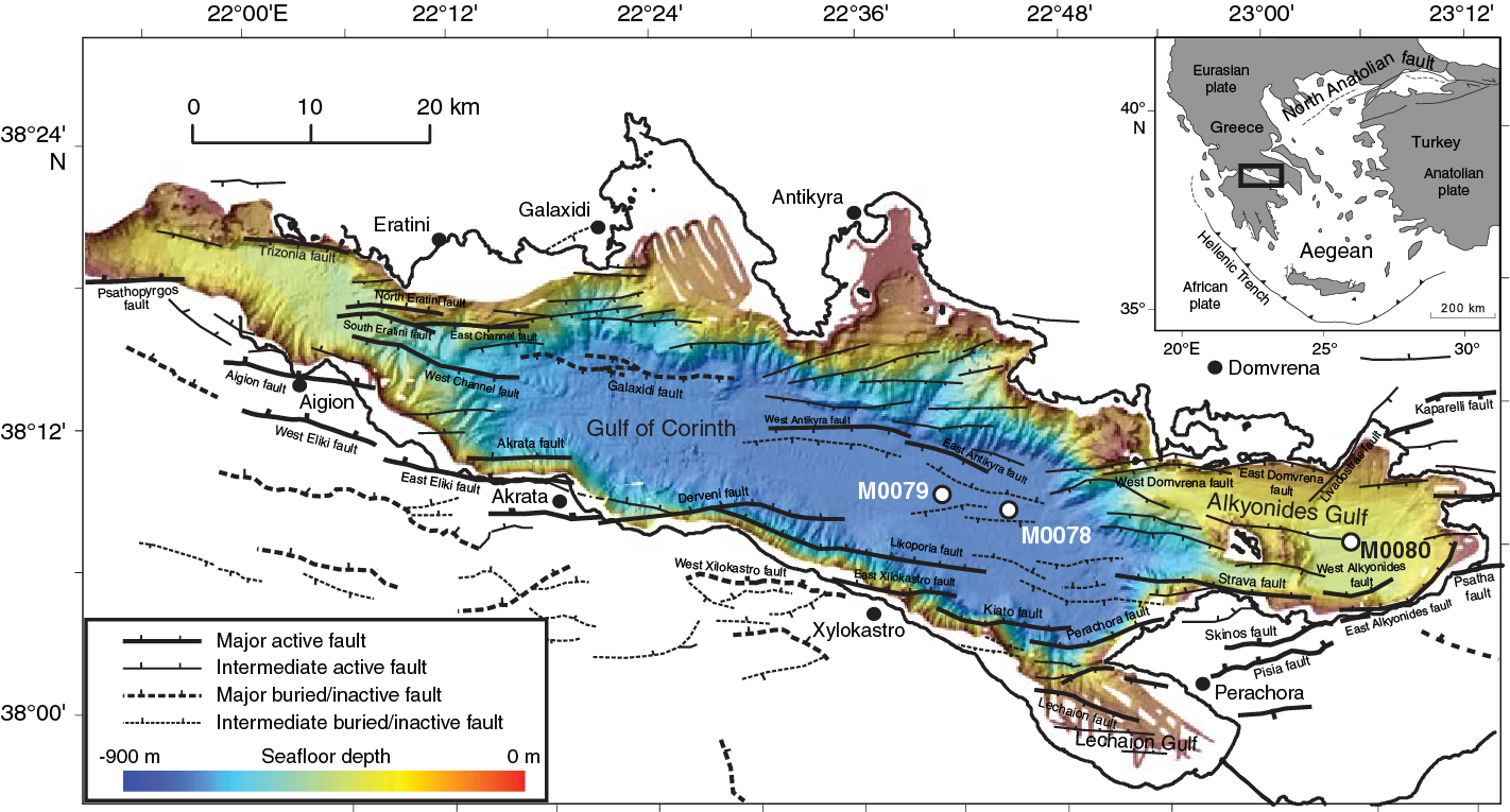
Figure F1. Corinth rift.
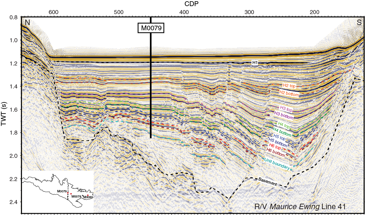
Figure F2. R/V Maurice Ewing Line 42.
Drilling and coring in Hole M0079A was completed to 704.9 meters below seafloor (mbsf) using two tools in 14 days. The Fugro Corer in push mode collected the upper 67 m of sediment, and the Fugro Corer in percussive mode collected the next 81 m. The Fugro Extended Marine Core Barrel (FXMCB) was then used to complete the lowermost 556 m of the borehole.
Port call and transit to Hole M0079A
On 13 November 2017 at 0630 h, the D/V Fugro Synergy made a port call in the Port of Corinth to load equipment and supplies and for a European Consortium for Ocean Research Drilling (ECORD) Science Operator (ESO) and Fugro crew change. At 2020 h, the vessel departed the Port of Corinth for Site M0079. At 2223 h, the vessel arrived on site and began settling on dynamic positioning (DP). At 0210 h on 14 November, a reference beacon was deployed, and a sound velocity profile (SVP) was conducted to ascertain water depth at the site.
Coring operations
Upon arrival at Site M0079, a water depth of 857.1 m was established following an SVP. Lowering the seabed frame (SBF) began at 0240 h on 14 November 2017 and was completed by 0410 h. However, at 0515 h communications were lost to the SBF, and it was therefore recovered on deck for maintenance. At 0718 h, the bottom-hole assembly (BHA) was recovered on deck, and the SBF was inspected in the moonpool before being lowered to the seafloor. At 1709 h on 14 November, coring commenced in Hole M0079A with the Fugro Corer in push mode. A seabed/water interface sample was collected by holding the Fugro Corer above the mudline, and 1 m of penetration was achieved, collecting 0.9 m of sediment.
Coring continued throughout the morning of 15 November until the Fugro Corer became stuck during a core run at 1045 h. Unsuccessful fishing attempts were made, therefore requiring tripping the pipe to recover the tool at 2209 h. Running pipe in the hole began at 0435 h on 16 November, and coring resumed at 1259 h. At 2223 h, coring paused briefly to undertake an in situ temperature cone penetration test (CPT) measurement at 100 mbsf.
Coring continued through 17 November using the Fugro Corer in percussive mode, with one core recovered in push mode (Core 38P). On the evening of 17 November, the operational decision was made to switch to the rotary coring method (FXMCB) because recovery had dropped because ground conditions had become firmer. From 18 to 23 November, coring progressed well with short pauses for high winds and three further temperature CPT measurements every ~100 m to ~400 mbsf.
At 0305 h on 24 November, repairs to the core barrel head were required, and coring resumed at 0700 h. As in Hole M0078A, it was found that penetrating to the full 5 m of the FXMCB and recovering high percentages of samples was difficult at times. It appears there may have been insufficient flush at the bit to lubricate the material being cored. Combined with the expanding nature of some of the intervals, this insufficient flush apparently caused the core to compress the liner, pushing it up the core barrel and creating a gap at the bottom that allowed a section of core to expand into the gap, making it too large to enter the liner. This expansion effectively blocked the liner, causing the remaining material to not be taken or a shorter core run to be completed. Coring progressed well until the terminal depth of the hole (704.9 mbsf) was achieved at 0045 h on 29 November.
Generally, seawater was used as the drilling medium, with the occasional use of bentonite drilling mud to assist with hole conditioning (removal of cuttings and reducing any swelling of the borehole sidewall), although bentonite was used for short runs earlier in Hole M0079A.
Logging operations
In preparation for logging, Hole M0079A was stabilized via displacement with weighted bentonite mud (8.9 lb/gal). Following the loss of a tool string in Hole M0078A, only standalone tools were available and used, and they were systematically run with a sinker bar fitted above the tool to help its descent. The planned logging program for Hole M0079A was to start by logging the entire borehole through pipe with the spectral gamma ray (ASGR512) tool and then log in the open hole in three depth stages (475–705 [base of the hole], 220–475, and 50–195 mbsf) using the following tools: magnetic susceptibility and conductivity (EM51), sonic (2PSA-1000), and dual induction (DIL45). The depths of the stages changed during logging operations.
Hole M0079A logging operations started on 29 November 2017 at 0345 h, with the drill bit at 699.5 m drilling depth below seafloor (DSF) (close to the bottom of the hole) to log with the ASGR512 tool through the pipe. The ASGR512 tool did not encounter any difficulty going down through the bentonite mud and in the pipe; it passed the drill bit to reach the bottom of the hole, and logging up started. After recovery of the tool, the drill bit was pulled up to 500 m DSF to start logging in the open hole for the first depth stage (500–705 m DSF). Bentonite mud (9 lb/gal) was circulated to stabilize the hole. Multiple attempts were made to send the EM51 tool down the hole, but the tension meter of the winch (GV550) appeared to be damaged. The fault could not be identified, so it was decided to use the backup winch (RG2000) and to move to the second depth stage (220–500 m DSF). Bentonite mud was recirculated, and the drill bit was pulled up to 220 m DSF. The EM51 tool was deployed successfully and passed the drill bit, but a loss of tension was observed at 297 m wireline log depth below seafloor (WSF). After multiple attempts to pass this obstruction, it was decided to start logging up from this depth and then move to the third depth stage (50–220 m DSF). In preparation for this third depth stage, the EM51 tool was recovered, the drill bit was pulled up to 50 m DSF, and bentonite mud (9 lb/gal) was circulated. The EM51 tool was deployed without any problem and reached 230 m WSF to allow ~10 m of overlap with the data collected during the previous stage. Logging up started, the tool was recovered, and the 2PSA-1000 tool was sent for the second run in this depth interval. The tool reached 230 m WSF, but no attempts were made to go deeper because the tool is fragile and deeper borehole conditions may have degraded with time between Stages 2 and 3. Data acquisition uphole was completed, and the tool was recovered on deck. Following this run, the dual laterolog resistivity (DLL3) tool was sent instead of the DIL45 tool because communication problems were observed with the latter during preparations on deck. The DLL3 tool was deployed successfully and reached 290 m WSF, just above the obstruction encountered during the second depth stage. Data acquisition uphole commenced, and the tool was recovered safely to terminate logging operations at Site M0079, with rigging down completed at 1740 h on 1 December.
After logging operations were completed, pulling pipe and recovering the SBF and DP transponder were completed by 2325 h on 1 December. At 2340 h, transit to Site M0080 began.
Lithostratigraphy
Site M0079 is divided into two major stratigraphic units based on a combination of the component facies associations (FA; see the Expedition 381 facies associations chapter [McNeill et al., 2019a]; Table T2), paleontology, seismic facies, and physical properties. In the following sections, we describe the main units and subunits in Hole M0079A (Table T3). In particular, the upper lithostratigraphic unit (1) is divided into subunits that correlate with “marine” and “isolated/semi-isolated” intervals.
Unit and subunit description
Site M0079 was drilled in an area with relatively thick stratigraphy in the upper seismic unit to provide an expanded Unit 1 succession compared with Site M0078. The cored succession largely comprises Unit 1, which is divided into 16 subunits, and the uppermost part of Unit 2 (Figure F3).
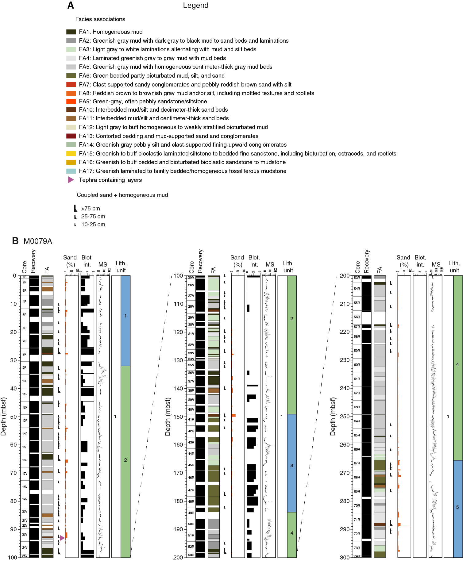
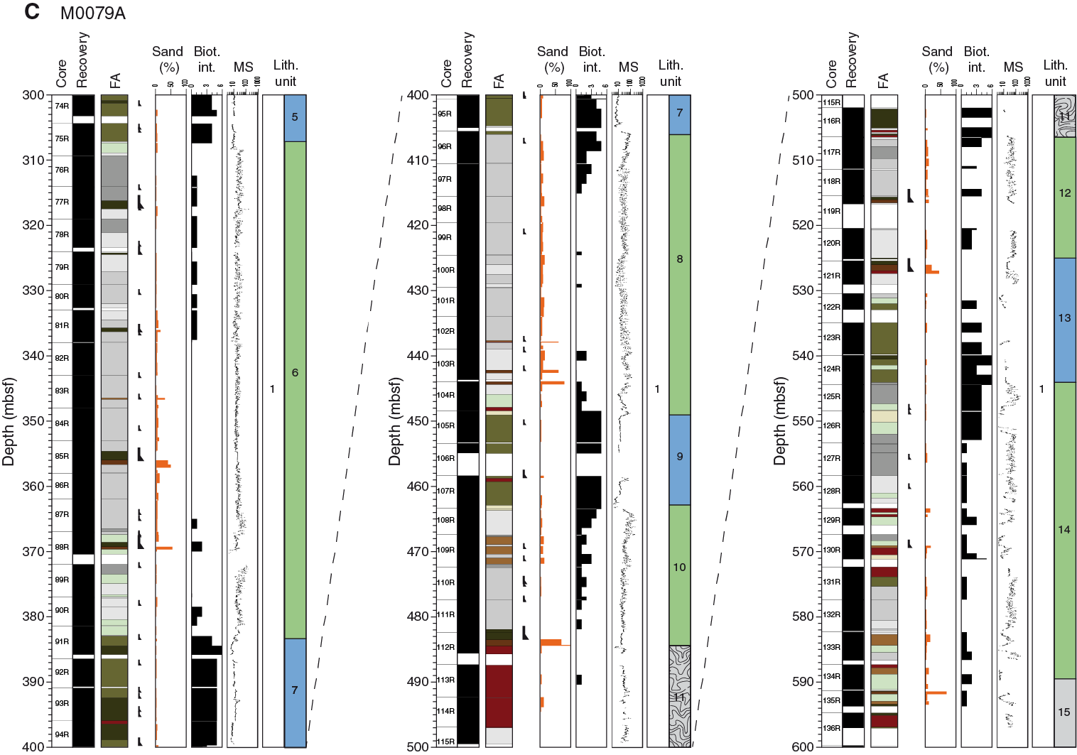
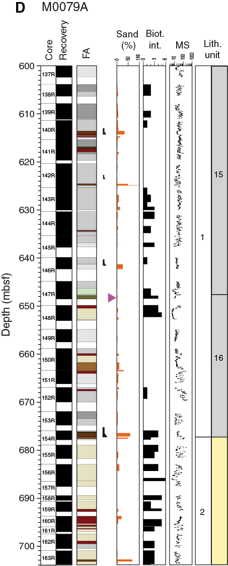
Figure F3. Composite stratigraphic log.
Unit 1 is dominated by fine-grained sediment with a similar composition to that found at Site M0078 (Figure F4). Carbonate minerals, phyllosilicates, feldspars, and quartz are the major mineral groups that dominate the sediment. Low occurrences of heavy minerals, pyrite, and Fe oxides were also identified. Calcite prevails in the overall mineralogical association as either single crystals or reworked carbonate fragments. Biogenic material is common and includes mainly individual fossils and fragments of diatoms and foraminifers. Locally, poorly sorted, detrital sand-sized carbonate grains appear in association with abundant amorphous organic components. In Unit 2, well sorted, fine mud- to silt-sized detrital calcite predominates, similar to Site M0078. Accordingly, in this unit the carbonate fraction increases significantly against the proportion of the other components (Figure F4).
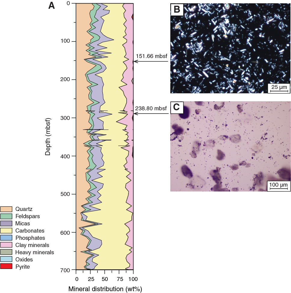
Figure F4. Downhole major mineral distribution.
Tephra and cryptotephra intervals were found in Site M0079 cores. These intervals were identified by a combination of visual inspection and physical properties. An increase in Multi-Sensor Core Logger (MSCL) natural gamma radiation (NGR) intensity was usually observed in association with both visible tephra layers and cryptotephra intervals, and this relationship was used as the primary method for identifying intervals for further investigation. A clear 2 cm thick tephra layer occurs at 91.37 mbsf (Section 381-M0079A-23V-2, 26 cm; Figure F3). Cryptic tephra intervals comprise the majority of tephra identified in the core. These tephra were identifiable only through methodical sampling of NGR intensity peaks and by subsequent visual examination of sampled material via optical microscopy using the presence of a high concentration of unusually reflective grains in an otherwise visually unremarkable interval of core (e.g., 75R-2, 25–40 cm [306.05–306.20 mbsf]). Cryptotephra were also identified incidentally during routine micropaleontological work by observation of glass shards.
Unit 1
- Interval: 381-M0079A-1P-1, 0 cm, to 154R-1, 133.0 cm
- Depth: 0–677.23 mbsf
- Age: Pleistocene to Holocene
Subunit 1-1
- Interval: 381-M0079A-1P-1, 0 cm, to 9P-2, 144 cm
- Depth: 0–31.94 mbsf (31.94 m thick including 8.30 m of missing core)
The top of Subunit 1-1 is at the seafloor. The lower boundary with Subunit 1-2 is transitional and occurs in FA1 homogeneous mud, marked by the downhole disappearance of marine microfossils and the appearance of faint lamination at the base of FA1. Eleven sand–homogeneous mud couplets occur in Subunit 1-1.
Subunit 1-1 is divided into three parts with a boundary in Section 381-M0079A-4P-1, 132 cm (8.22 mbsf), marked by a change from FA5 to FA2, and another boundary in Section 6P-2, 0 cm (17.81 mbsf), marked by a change from FA2 to FA4. The upper part is marked by a short interval (23 cm) of FA1 greenish gray homogeneous mud overlying FA5 bedded centimeter-thick greenish gray to gray and occasionally reddish gray mud. FA5 alternates with FA11 (interbedded mud/silt and centimeter-thick sand beds) intervals (<3 m). The middle part of the subunit mainly consists of FA2 greenish gray mud with dark gray to black centimeter-thick silty beds, which includes centimeter-thick very fine sand to silt fining-upward beds and interbedded greenish gray homogeneous mud (FA1). The lower part is marked by a 2.51 m thick interval of FA4 laminated and bedded greenish gray to gray mud overlying FA1 greenish gray homogeneous mud with meter-thick intercalations of FA4 and FA10.
Subunit 1-2
- Interval: 381-M0079A-9P-2, 144 cm, to 41R-1, 0 cm
- Depth: 31.94–149.10 mbsf (117.16 m thick including 16.61 m of missing core)
The top of Subunit 1-2 is marked by the disappearance of marine microfossils and the appearance of faint lamination at the base of FA1 preceding a change to FA3 in Section 381-M0079A-9P-3, 0 cm (32 mbsf). The lower boundary is placed between FA3 (above) and a sand–homogeneous mud couplet (93 cm thick). Subunit 1-2 includes 54 sand–homogeneous mud couplets.
Subunit 1-2 comprises a wide variety of facies associations (FA1, FA2, FA3, FA4, FA5, FA10, and FA11). The subunit is divided into three main parts with boundaries in Sections 24V-2, 84 cm (96.64 mbsf), and 25V-1, 40 cm (99.4 mbsf). The upper part is characterized by a mixture of FA5 bedded mud, FA4 laminated mud, FA1 homogeneous mud, and FA11 interbedded homogeneous mud and centimeter-thick fining-upward sand beds. Mud varies from gray (GLEY 1 6/N to 7/10Y) to reddish to brownish gray (5YR 5/1 to 6/2). The middle part is characterized by FA1 homogeneous greenish gray mud with marine microfossils (see Micropaleontology). The lower part is dominated by FA3 laminated mud, but some FA2 laminated mud with organic-rich silt, FA4 laminated and bedded mud, and FA5 bedded mud also occur. The lower part also contains homogeneous mud beds of FA1 and FA11 mud and centimeter-thick sand. Facies association changes are commonly gradational, without sharp contacts.
Subunit 1-3
- Interval: 381-M0079A-41R-1, 0 cm, to 49R-2, 58 cm
- Depth: 149.10–183.88 mbsf (34.78 m thick including 8.13 m of missing core)
The top of Subunit 1-3 is placed at a change from FA3 laminated sediment (above) to a sand–homogeneous mud couplet (Figure F5). The base is marked by a change from FA1 (above) to FA2 (below). Seven sand–homogeneous mud couplets occur throughout the subunit.
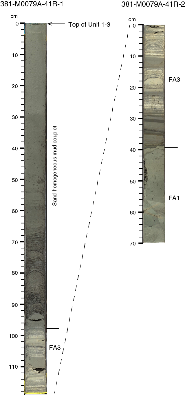
Figure F5. Uppermost part of marine Subunit 1-3.
Subunit 1-3 contains three distinct parts with boundaries in Sections 381-M0079A-43R-2, 95 cm (159.75 mbsf), and 45R-2, 56 cm (167.37 mbsf). The upper part comprises, in downhole order, FA10 (sand–homogeneous mud couplet) then FA3 mud with cream laminations (147.03–150.65 mbsf), followed by dominant FA6 faintly bedded greenish gray mud with some centimeter-scale silt and very fine sand. This sediment is variably bioturbated with a sporadic presence of shell fragments. The middle part is dominated by FA3 laminated mud but includes an interval of FA5 bedded to weakly laminated gray mud (159.75–163.67 mbsf). The lower part consists of FA6 greenish gray faintly bedded mud to the base of the subunit. These deposits are moderately to intensely bioturbated (typically bioturbation intensity [BI] = 4–6). A distinctive inclined or vertical burrow with U-shaped spreite occurs in the lower few meters. Abundant shell fragments and occasional millimeter- to centimeter-thick, graded very fine to fine sand beds occur.
Subunit 1-4
- Interval: 381-M0079A-49R-2, 58 cm, to 67R-1, 123 cm
- Depth: 183.88–265.53 mbsf (81.65 m thick including 8.84 m of missing core)
The top of Subunit 1-4 is in a core gap between 183.88 and 186.30 mbsf, marked by a change from FA6 (above) to FA2 (below). The lower boundary is marked by a sharp change from FA3 to FA6. Sixteen sand–homogeneous mud couplets are recorded in Subunit 1-4. The couplets are relatively small (10–25 cm) with a maximum thickness of 1.75 m (197–198.75 mbsf).
Subunit 1-4 comprises three parts. The dominant facies in the top part (183.88–202.30 mbsf) is gray bedded mud with black millimeter-scale silt layers and scattered pyrite fragments (FA2), with some intervals of FA5 with sparse bioturbation. FA5 dominates the middle part (202.30–259.30 mbsf), which also includes some FA4 intervals. Sparse organic layers and pyrite fragments were observed. Overall, bioturbation increases from slight to moderate downhole in this part of the subunit. Centimeter-scale reddish gray and reddish brown beds (2.5YR 6/2 to 7.5YR 6/1) occur from 198.75 to 230.80 mbsf and typically have sharp bases and sparsely bioturbated tops. The lower part (259.30–265.53 mbsf) mostly contains finely laminated, moderately bioturbated gray mud (FA4) and an interval of whitish laminated mud (FA3) directly above the transition to Subunit 1-5.
Subunit 1-5
- Interval: 381-M0079A-67R-1, 123 cm, to 75R-2, 138 cm
- Depth: 265.53–307.08 mbsf (41.65 m thick including 1.7 m of missing core)
The top of Subunit 1-5 appears sharp and is marked by a change from FA3 well-laminated gray mud to FA6. The lower boundary occurs 8 cm below a change from FA6 (above) to FA4 (below). Eleven sand–homogeneous mud couplets occur in Subunit 1-5.
Subunit 1-5 is dominated by laminated greenish gray to gray mud with muddy/sandy beds (FA4) (~50%) and greenish bedded mud with intense bioturbation (FA6) (~40%; BI = 5–6) and is divided into three main parts. The upper part is dominated by FA6 with intervals of greenish gray bedded mud (FA5) and greenish bedded mud with centimeter-thick silt (FA11). The middle part (276.83–297.30 mbsf) is dominated by FA4 occasionally interrupted by FA2 (greenish gray mud with dark gray to black silty beds). The lower part is dominated by FA6 with some white millimeter-scale laminated mud and silt beds (FA3).
Subunit 1-6
- Interval: 381-M0079A-75R-2, 138 cm, to 91R-2 at 0 cm
- Depth: 307.08–383.00 mbsf (75.92 m including 2.98 m of missing core)
The top of Subunit 1-6 lies 8 cm below a boundary between FA6 (above) and FA4 (below). The base of the subunit is marked by a transition from FA5 (above) to FA6 (below). A total of 19 sand–homogeneous mud couplets are recognized throughout the subunit, with the most notable in Sections 381-M0079A-77R-1, 69 cm, to 77R-3, 43 cm (316.19–317.43 mbsf).
Subunit 1-6 is divided into three parts with boundaries in Sections 381-M0079A-79R-3, 0 cm (327.0 mbsf), and 87R-4, 0 cm (366.5 mbsf). The upper part is dominated by greenish gray laminated mud (FA4) and bedded and laminated mud with dark gray to black laminations and beds (FA2) and intervals of creamy white laminated mud (FA3). This part of the subunit also contains scattered shell fragments and rare millimeter-scale discrete burrows, usually at the tops of homogeneous mud beds. The middle part is mostly bedded mud (FA5) with minor homogeneous (FA1) and laminated mud (FA4). Shell and wood fragments are scattered throughout this interval. The lower part is composed mostly of various laminated mud (FA2/FA3/FA4) and some bedded mud (FA5). The creamy white finely laminated mud of FA3 forms the most common component. Scattered pyrite and sparse bioturbation are found throughout the subunit.
Subunit 1-7
- Interval: 381-M0079A-91R-2, 0 cm, to 96R-1, 52 cm
- Depth: 383.00–406.02 mbsf (23.02 m thick including 1.43 m of missing core)
The top of Subunit 1-7 is marked by a change from FA5 (above) to FA6 (below) and a corresponding appearance of marine microfossils. The lower boundary is marked by a change from FA6 (above) to FA5 (below). Both boundaries are sharp. Nine sand–homogeneous mud couplets are recognized throughout the subunit, which overall contains approximately 2% sand.
Subunit 1-7 is composed almost exclusively of FA1 and FA6. FA1 is characterized by homogeneous greenish gray mud, high levels of bioturbation (BI = 6), and sparse and scattered shell fragments and pyrite throughout. Bioturbation includes Teichichnus, Planolites, and Skolithos burrows, although discrete burrows are often difficult to distinguish. FA6 is very similar to FA1 but is distinguished by the presence of bedding and/or lamination and a slightly lower degree of bioturbation. Isolated millimeter- and centimeter-thick fine sand or silt beds with graded or sharp tops and sharp bases occur throughout the succession. A short (42 cm) FA13 interval (Section 381-M0079A-94R-1, 11–53 cm) is characterized by a poorly sorted matrix-supported conglomerate, mainly with intraclasts of internally deformed light gray laminated mud and olive green bioturbated mud. The mud intraclasts can reach cobble grade (>8 cm), and the mud matrix also contains scattered coarse sand grains of limestone lithology.
Subunit 1-8
The top of Subunit 1-8 is marked by a sharp change from FA6 (above) to FA5 (below). The lower boundary with Subunit 1-9 is marked by a sharp change from pale bioturbated mud (FA12; above) to darker bedded mud (FA6; below) (Figure F6). Five sand–homogeneous mud couplets occur throughout Subunit 1-8.
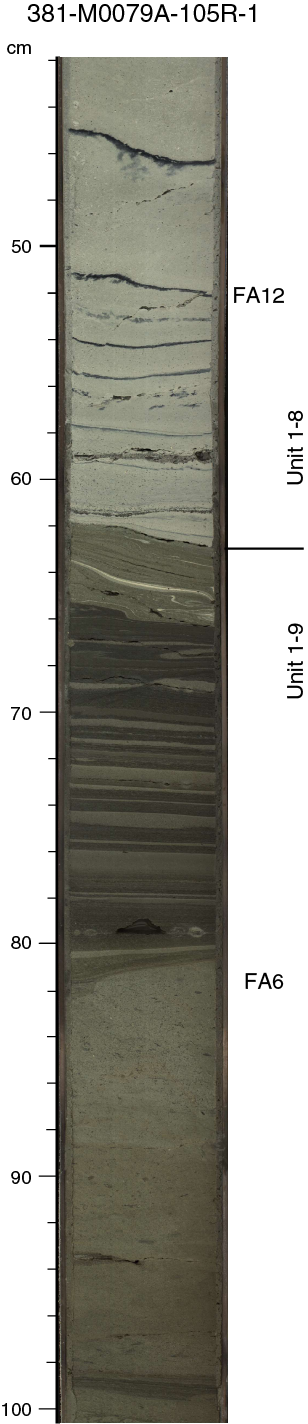
Figure F6. Upper boundary of Subunit 1-9 and lower part of Subunit 1-8.
Subunit 1-8 is divided into two parts with a boundary in Section 381-M0079A-102R-4, 52 cm (438.9 mbsf), marked by a change from FA5 to FA4. The upper part is dominated by FA5 greenish gray mud with homogeneous centimeter-thick gray mud beds. This succession is interrupted by a sharp based, approximately 8 cm thick zone of contorted bedding and mud-supported gravel (FA13) (Section 102R-3, 92–100 cm; 437.82–437.90 mbsf) and an overlying, approximately 20 cm thick fining-upward succession of centimeter-thick bedded sand and mud/silt beds (FA10). The lower part mainly consists of FA4 laminated greenish gray to gray mud beds passing at 445.85 mbsf into FA3 bedded mud with gray to white submillimeter-scale laminations and FA12 bioturbated pale green-gray mud. A deformed interval (FA13) occurs near the base of the subunit, comprising folded and sheared silty mud overlain by a pebble-sized mud intraclast conglomerate (Section 104R-3, 92–140 cm; 447.83–448.31 mbsf). Variable bedding dips in the FA12 section, 0.5 m below the FA13 folded and sheared interval, may also suggest this whole section is isoclinally folded.
Subunit 1-9
The top of Subunit 1-9 is marked by an abrupt change from FA12 above (pale green-gray bedded mud) to greenish bioturbated mud and silt below (FA6) (Figure F6). The lower boundary of Subunit 1-9 corresponds to a change from bioturbated mud (FA6) to finely laminated mud (FA3). The basal 70 cm of FA6 becomes progressively more laminated above this boundary. Two sand–homogeneous mud couplets occur in Subunit 1-9.
Subunit 1-9 is almost exclusively composed of bedded to homogeneous bioturbated mud and silt (FA6) that contain subvertical and horizontal burrows, one of which is filled with shelly and pelleted particles (Section 381-M0079A-106R-2, 22 cm). This succession is disrupted by a short FA13 interval (Section 107R-1; 458.73–459.22 mbsf) that comprises a mud-supported conglomerate with rounded intraclast pebbles and cobbles of mud. This interval is overlain by a 7 cm fining-upward sand bed with cross-laminations that is part of a sand–homogeneous mud couplet. One other couplet occurs in Subunit 1-9. The rest of the subunit is largely devoid of sand (<2%).
Subunit 1-10
The top of Subunit 1-10 corresponds to a gradual transition from FA6 intervals (above) to FA12 sediment (below). Seven sand–homogeneous mud couplets were identified throughout the subunit, and one marks the base of the subunit.
Subunit 1-10 consists of four parts. The first (upper) part (to Section 381-M0079A-109R-1, 0 cm; 467.4 mbsf) comprises FA12 homogeneous to weakly bedded light gray mud that passes downhole into laminated FA4 mud deposits with moderate to high bioturbation (mainly horizontal burrows) and thin sandy beds. The second part comprises alternations of layered FA5 bedded mud with FA11 sand-rich intervals to Section 110R-1, 0 cm (472.4 mbsf). This sediment displays moderate bioturbation and includes frequent thin (typically <1 cm) layers that appear organic rich. The third part comprises a ~10 m thick FA5 interval, marked by the occasional presence of slightly reddish centimeter-thick mud beds. The lower part comprises a sand–homogeneous mud couplet (FA1 and FA10) from Section 112R-2, 60 cm (483.49 mbsf), to the base of Subunit 1-10.
Subunit 1-11
- Interval: 381-M0079A-112R-3, 10 cm, to 116R-4, 50 cm
- Depth: 484.48–506.40 mbsf (21.92 m thick including 4.13 m of missing core)
The top of Subunit 1-11 is marked by a sharp change from the base of a sand bed in the overlying subunit (FA10) to an interval of contorted bedding below (FA13). The lower boundary lies between contorted mud beds above (FA13) and laminated mud below (FA4). Thus, Subunit 1-11 largely comprises an interval of contorted bedding and contains no sand–homogeneous mud couplets.
The upper part of Subunit 1-11 comprises a 12.51 m thick package of highly contorted beds (FA13) from Section 381-M0079A-112R-3, 10 cm, to Section 115R-1, 9 cm (484.48–496.99 mbsf). The contorted beds and clasts in this slump package consist of light gray to greenish gray mud, silt, and very fine sand beds of FA1, FA3, FA4, FA5, and FA6 with bioclasts scattered throughout, including shell and coral fragments. Isolated gravel- to pebble-sized clasts of creamy white mud and light gray limestone are also common. Bedded mud can form open to tight folds (wavelengths as high as 30 cm) and numerous small transposed folds (wavelengths as low as 4 cm). Laminated mud intervals sometimes show apparent shear fabrics, and occasional slip surfaces can separate clasts of original facies associations. The base of this large FA13 package is marked by a chaotic breccia that forms an irregular boundary with underlying laminated light to dark gray mud (FA4) (Sections 115R-1, 9 cm, to 116R-1, 19 cm; 496.99–502.09 mbsf).
The lowest part of Subunit 1-11 consists mainly of greenish gray homogeneous mud (FA1) (Sections 116R-1, 19 cm, to 116R-4, 21 cm; 502.09–506.11 mbsf) that is faintly bedded in places and heavily bioturbated. The FA1 mud is sometimes interrupted by short intervals of FA4 and FA13, with an FA13 interval at the base of the subunit.
Subunit 1-12
- Interval: 381-M0079A-116R-4, 50 cm, to 120R-4, 135 cm
- Depth: 506.40–524.98 mbsf (18.58 m thick including 3.88 m of missing core)
The top of Subunit 1-12 is marked by the downhole disappearance of marine microfossils (see Micropaleontology) and a change from FA13 above (slump deposits) to FA4 below (laminated mud beds). The lower boundary corresponds to a sharp planar contact between FA4 (above) and FA1 with marine microfossils (below). One sand–homogeneous mud couplet occurs in Subunit 1-12.
Subunit 1-12 is divided into two main parts with a boundary in Section 381-M0079A-119R-1, 110 cm (516.56 mbsf), that corresponds to the base of a meter-scale sand–homogeneous mud couplet (FA10 and FA1). The upper part is predominantly FA5 bedded mud but includes FA4 and FA2 intervals near the top. The lower part of Subunit 1-12 consists predominantly of FA4 centimeter-thick homogeneous and laminated mud beds with some organic-rich laminations and thin silt with a minor FA5 interval.
Subunit 1-13
- Interval: 381-M0079A-120R-4, 135 cm, to 124R-3, 90 cm
- Depth: 524.98–543.80 mbsf (18.82 m including 4.03 m of missing core)
The top of Subunit 1-13 is marked by a change from FA4 to FA1. The base of the subunit is marked by an abrupt increase in lamination and a corresponding decrease in bioturbation (Figure F7). One sand–homogeneous mud couplet occurs in Subunit 1-13.
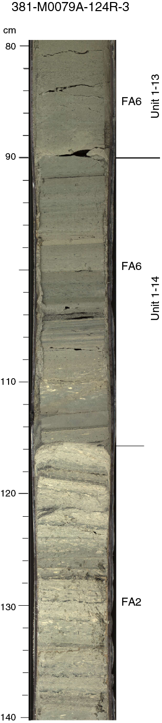
Figure F7. Lower boundary of Subunit 1-13 and Subunit 1-14.
Subunit 1-13 is divided into two main parts with a boundary in Section 381-M0079A-122R-3, 52 cm (323.0 mbsf). The upper part contains a wide variety of facies associations, including homogeneous mud (FA1), interbedded mud and sand (FA10), chaotic and contorted intervals (FA13), and a related sand–homogeneous mud couplet. This interval is underlain by laminated to bedded mud (FA4 and FA5) and, finally, white finely laminated mud (FA3). The lower part, in contrast, is fairly homogeneous, composed almost entirely of highly bioturbated homogeneous to bedded mud with rare silt and fine sand beds (FA1 and FA6). The bioturbation index is high (BI = 4–6), with individual traces including Teichichnus and Zoophycos(?). An additional white finely laminated FA3 interval occurs in Section 124R-2, 7–57 cm (541.47–541.97 mbsf).
Subunit 1-14
- Interval: 381-M0079A-124R-3, 90 cm, to 134R-2, 59 cm
- Depth: 543.80–589.45 mbsf (46.65 m thick including 4.6 m of missing core)
The top of Subunit 1-14 is marked by an abrupt increase in lamination and reduction in bioturbation followed by a change to FA2 (Figure F7). The lower boundary occurs in laminated mud (FA3) and is marked by the appearance of abundant Teichichnus burrows. Five sand–homogeneous mud couplets are recorded in Subunit 1-14.
Subunit 1-14 contains a wide variety of facies associations (FA2, FA3, FA4, FA5, FA11, FA12, and FA13). It is divided into three clear parts with boundaries at the tops of Sections 381-M0079A-129R-1 (563.5 mbsf) and 131R-2 (574 mbsf). The upper part is dominated by two packages of bedded and laminated greenish gray mud with black organic-rich beds of mud and silt (FA2) separated by an interval of FA12 and FA3. The middle part contains four intervals of FA13 (intraclast matrix-supported conglomerates with slump folds) separated by FA3 (finely laminated creamy mud and centimeter-scale gray mud) or FA12 (highly bioturbated pale gray mud with some millimeter-thick silt). The lower part (15.45 m thick) is dominated by centimeter-thick beds of laminated mud and homogeneous mud with low bioturbation and some millimeter-thick organic-rich layers (FA5), with subordinate FA3 and FA4 intervals and, notably, FA11 bedded mud with centimeter-scale beds of very fine sand and silt. In this lower part, a single occurrence of FA13 (48 cm thick; Section 134R-1, 0–48 cm; 587.40–587.88 mbsf) comprises silty mud with a range of scattered sand- and granule-grade clasts of limestone mud and sand.
Subunit 1-15
- Interval: 381-M0079A-134R-2, 59 cm, to 147R-2, 142 cm
- Depth: 589.45–647.72 mbsf (58.27 m thick including 13.18 m of missing core)
The upper boundary of Subunit 1-15 is transitional and occurs in FA3 sediments. It is marked by a distinctive increase in bioturbation intensity with the appearance of abundant Teichichnus burrows. The lower boundary is marked by a change from FA3 through a short interval of FA4 (17 cm; dark gray laminated mud) to FA6. Three sand–homogeneous mud couplets were observed in Subunit 1-15.
Subunit 1-15 consists of a complex succession of eight facies associations organized in three parts with boundaries in Sections 381-M0079A-138R-1, 0 cm (603.8 mbsf), and 141R-3, 0 cm (618.24 mbsf). The upper part is dominated by FA3 bedded mud with gray to white submillimeter-scale laminations and FA4 laminated greenish gray to gray mud beds. At 595.19 mbsf, the succession is interrupted by a ~2 m thick sharp-based interval of FA13 with sheared and contorted beds and folds. Short intervals (<1 m) of FA1 homogeneous mud, FA6 bedded green-gray mud, and bedded mud and silt with decimeter-thick sand beds (FA10) or centimeter-thick sand beds (FA11) occur. The middle part mainly consists of FA2 greenish gray mud with dark gray to black centimeter-scale organic-rich silty to sandy beds interspersed with FA5 greenish gray mud with centimeter-scale homogeneous mud beds. The succession is interrupted by short intervals (<0.3 m) of contorted bedding and mud with gravel clasts (FA13) (e.g., at 614.21, 614.62, and 617.16 mbsf). The lower part comprises predominantly FA5 greenish gray mud with centimeter-scale homogeneous mud beds with frequent bioturbation (BI = 2–3) that changes to FA3 at 646.22 mbsf.
Subunit 1-16
- Interval: 381-M0079A-147R-2, 142.0 cm, to 154R-1, 133.0 cm
- Depth: 647.72–677.23 mbsf (29.51 m thick including 5.88 m of missing core)
The top of Subunit 1-16 is marked by a change from FA3 through a short interval of FA4 (17 cm; dark gray laminated mud) to FA6 and corresponds to the appearance of marine microfossils (see Micropaleontology). The lower boundary of Subunit 1-16 is an abrupt bed contact between FA13 (above) and FA12 (below), corresponding to the top of Unit 2. One sand–homogeneous mud couplet occurs in Subunit 1-16.
Subunit 1-16 consists of a large variety of facies associations (FA4, FA5, FA6, FA11, FA12, and FA13) with no predominant facies association or repetitive pattern. The transitions between facies associations are sometimes inferred because of the lack of recovery of certain cores. Bioturbated mud beds (FA6 and FA12), laminated mud (FA4), and bedded mud successions (FA5) are commonly disrupted by meter-scale slump intervals of FA13 (659.87–660.30, 663.55–664.00, and 667.13–667.23 mbsf). The slump at 663.55–664.00 mbsf is overlain by a thin, fining-upward succession from fine sand to mud (decimeter scale) and laminated mud interbedded with centimeter-thick very fine sand (FA11). The base of Subunit 1-16 is a 10 cm thick FA13 interval comprising a mud-supported intraclast conglomerate overlain by a thin, coarse, and poorly sorted sand bed (2 cm thick) with a rafted mud clast (667.13–667.23 mbsf). This interval is overlain by a 1 m thick sand–homogeneous mud couplet.
Unit 2
- Interval: 381-M0079A-154R-1, 133 cm, to 163R-CC (base of Hole M0079A)
- Depth: 677.23–703.78 mbsf (26.55 m including 7.21 m of missing core)
- Age: Pleistocene
The top of Unit 2 is sharp and coincides with the likely erosive base of a slump/debrite interval (FA13; above) overlying FA12 mud. One sand–homogeneous mud couplet occurs in Unit 2.
Only 26.55 m of Unit 2 was penetrated by this borehole. The observed succession is divided into two parts with a boundary in Section 381-M0079A-159R-2, 10 cm (692.26 mbsf). The upper part is composed of faintly laminated highly bioturbated homogeneous mud (FA12), typically pale gray to buff (GLEY 1 6/5Y to 7/10Y) in color. The upper part contains occasional centimeter- to decimeter-scale (FA10) fining-upward sand horizons. The lower part is also mostly composed of FA12 faintly stratified highly bioturbated mud of pale gray to buff color but is frequently disturbed by FA13 large decimeter- to meter-scale slump structures and mud-supported intraclast conglomerate intervals that sometimes include coarse clastic sediment with granules of micritic limestone. Very coarse sand also occurs in a contorted FA10 interval in Section 163R-2, 36–76 cm (702.76–703.16 mbsf).
Interpretation
Site M0079 lithostratigraphy is dominated by fine-grained, carbonate-rich sediment and is lithostratigraphically similar to Site M0078 but with a much expanded Unit 1. Detrital calcite predominates with subordinate quartz, feldspar, and phyllosilicates (Figure F4). Biogenic material is common, particularly in the interpreted marine subunits. The alternating subunits are provisionally identified as representing alternating marine and isolated/semi-isolated basinal environments with good correlation with micropaleontology results (see Micropaleontology). In both the marine and isolated/semi-isolated subunits, sedimentary processes were dominated by deposition from fine-grained, low-concentration turbidity currents and hemipelagic suspension fallout.
Marine subunits in Unit 1 (odd numbers) are moderately to highly bioturbated and dominated by homogeneous to poorly bedded greenish gray mud with scattered shell debris. Isolated/semi-isolated subunits (even numbers) are dominated by laminated to thinly bedded gray and greenish gray mud, some with black, organic-rich laminations and beds, but with no or only sparse bioturbation or shell debris. In both marine and isolated/semi-isolated units, higher energy depositional processes are indicated by intervals of soft-sediment deformation and mud-supported intraclast conglomerates (FA13), as well as sand–homogeneous mud couplets. Overall, the occurrence of sand–homogeneous mud couplets and FA13 horizons increases with depth in Unit 1 and is higher overall than at Site M0078, with a particularly thick slumped interval occurring in Subunit 1-11. Such an increase in these deposit types with depth may reflect higher depositional gradients, higher sediment supply, and/or changing seismic intensity downhole.
Unit 2 is dominated by light gray to buff weakly laminated to homogeneous highly bioturbated mud (FA12). In contrast to Site M0078, the Unit 1/2 boundary is less distinct, with a gradual transition into the light gray to buff mud, suggesting that it may be diachronous between the two sites. Furthermore, Unit 2 at Site M0079 contains fining-upward sand, large decimeter- to meter-scale slumped horizons, and mud-supported intraclast conglomerates that are not present at Site M0078, suggesting episodically higher energy conditions compared with Unit 2 at Site M0078.
Structural geology
In Hole M0079A, tectonic deformation and drilling-induced deformation (DID) were systematically recorded during core description. The north–south seismic reflection profile through Site M0079 (Figure F2) shows an area of high basin subsidence with subhorizontal beds and no faults in the upper two thirds of the drilled section. The possibility of traversing small faults appears to increase in the deepest part of the drilled section.
Observed tectonic structures
Bedding attitude in the cores is generally horizontal to subhorizontal. Subhorizontal bedding persists at depth despite a very gentle increase in dip of seismic reflection horizons around Site M0079 (Figure F2).
Small-scale natural faulting was observed sporadically throughout the cores (Figure F8). Drilling-induced normal faulting was also well developed in this hole compared with Site M0078 (see below). Natural faults were distinguished, usually relatively easily, from drilling-induced faulting by their planar geometries and the lack of influence of proximity to either the core liner or core axis (see below). The first observed natural fault is in Section 381-M0079A-12P-4, 16.5 cm (47.68 mbsf), with measured faulting intensity per section downhole varying from 0.7 to 10 m−1 (Figure F9A). Concentrated faulting in discrete intervals was observed at 48–62, 259–278, 472–548, and 686–698 mbsf, where fracture intensity values greater than 3 m−1 were consistently recorded. All natural faults observed at Site M0079 have apparent normal displacements that range from 1 mm to >14 cm (“>” indicates displacement greater than the length of the fault trace in the core). A zone of significant normal faulting with offsets >3 mm and often greater than the length of the fault trace in the core (>8 cm) was recorded in and deeper than Section 125R-3 (547.34 mbsf) (Figure F8). This zone corresponds to the area on the seismic line where the borehole appears to traverse second-order normal faults (see Figure F9 in the Expedition 381 summary chapter [McNeill et al., 2019c]).
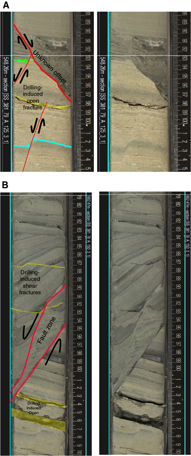
Figure F8. Tectonic faults.
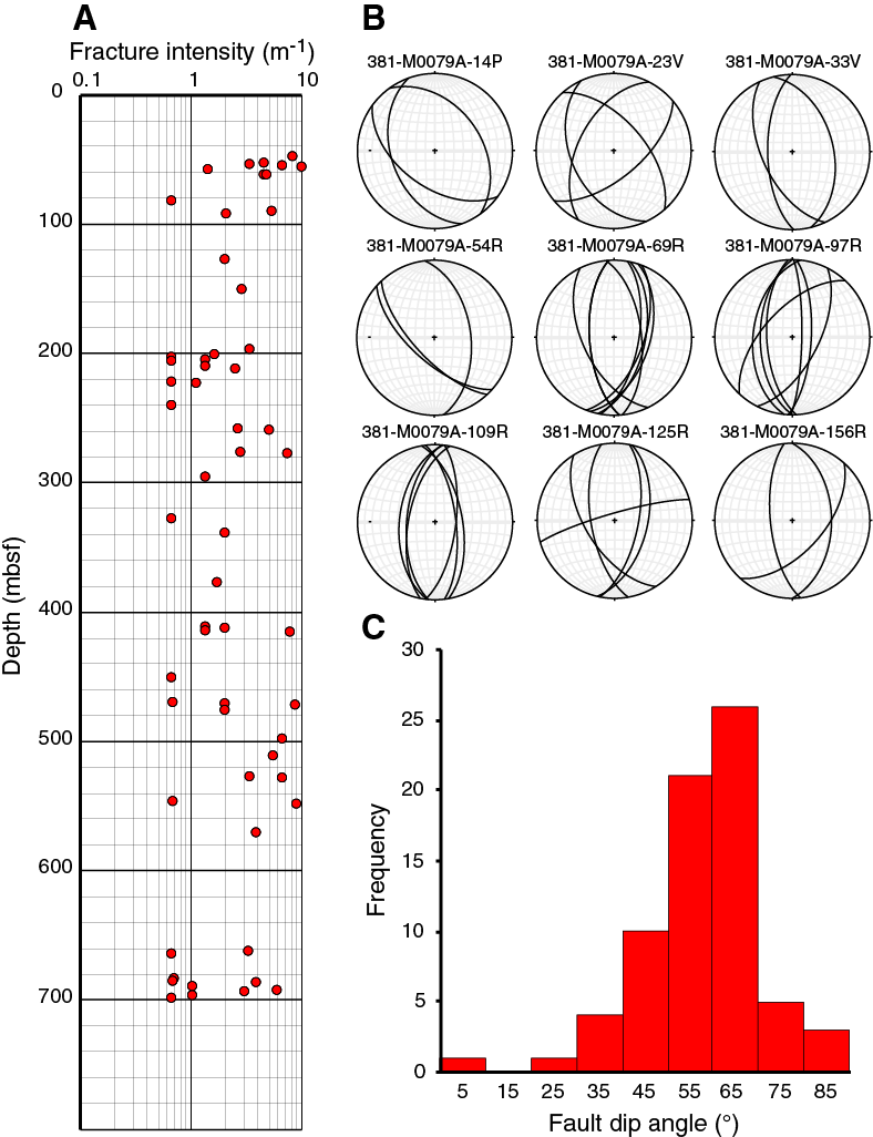
Figure F9. Preliminary analyses of faults.
In total, 71 normal faults were sampled for orientation analysis. These faults appear to mainly fall into a conjugate set with an average north–south strike in the core reference frame throughout the hole, as illustrated by the stereographic projection plots (Figure F9B). This consistency suggests that our sampling is biased because we are mainly able to observe faults when they are trending approximately perpendicular to the split-core surface. We are thus undersampling faults with other orientations. The sampled normal faults show true dips ranging from 9°–82° but with a clear modal average dip of 60° and a mean dip of 57° (Figure F9C). The subvertical and subhorizontal faults are thought to be drilling induced, and the data set clearly requires further filtering. Overall, the abundance and geometry of small normal faults are consistent with those observed at Site M0078 and in agreement with the overall extensional nature of the rift deformation.
Observed drilling-induced deformation
A wide range of drilling-induced structures was observed at Site M0079. The most common were biscuiting, shear fractures, arching bedding, disturbed bedding, sediment flow/smearing along the core liner, voids, and open fractures (examples in Figure F10). Other less frequently observed structures are listed in Table T1 in the Expedition 381 methods chapter (McNeill et al., 2019b).
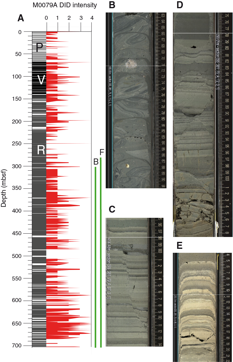
Figure F10. DID intensity.
Hydraulic piston coring was not used in this borehole; only push (P), percussive (V), and rotary (R) coring were used (Figure F10A). Overall, DID intensity is markedly lower than in Hole M0078A. Intensity remains low through push and percussive coring and through most of the rotary coring, only increasing downhole from Core 381-M0079A-132R (588 mbsf) and remaining moderate–high to the bottom of the hole. DID is nearly completely absent in Cores 58R–67R (224–269 mbsf).
The main DID type varies downhole. Through Core 381-M0079A-132R (588 mbsf), DID is mainly expressed by arching bedding, disrupted/mingled beds, sediment flow/smearing along the core liners, rare axial flow, and open fractures. Soupy texture is found in the uppermost cores and in Cores 14P and 15P. Axial fluid/sediment flow occurs sporadically (e.g., in the first section drilled by percussive coring [Core 17V; 63.3 mbsf]). A wide variety of other DID types occur in rotary cores, in particular arching bedding, sediment flow along the core liner, axial fluid/sediment flow, and open fractures. Biscuiting only occurs in rotary cores and first appears in Section 42R-3 (155 mbsf). Its presence is, however, sporadic until Core 74R (300 mbsf), after which biscuiting is regularly present. In the more intensely deformed cores deeper than Core 132R (574 mbsf), biscuiting is dominant, accompanied mainly by open fractures, voids, and distorted/disturbed bedding to the bottom of the hole.
Drilling-induced shear fracturing in the form of normal faulting is a characteristic and notable feature of Hole M0079A that was not observed at Site M0078 (Figure F10C, F10D). DID faulting first occurs at 198 mbsf (Section 381-M0079A-53R-1) and becomes a regular feature deeper than 276 mbsf (Section 59R-3). Intervals particularly affected by DID shear fractures are 276–296 mbsf (Cores 69R–73R), 335–344 mbsf (Cores 81R–83R), 364–377 mbsf (Cores 87R–90R), and finally 632–633 mbsf (Section 144R-2). These faults are usually easily distinguished from tectonic faults by a combination of the following:
- Their occurrence as conjugate pairs intersecting in the center of the core or as multiple conjugate pairs with complex intersections (Figure F10D),
- Dips that steepen toward vertical toward the center of the core and curve to lower angles near the core liner (Figure F10C),
- Offsets less than 1 cm, and
- Their association with small (<2 mm) trilete fracture holes on the surface of the cut core (along the fault and at fault tips) and pressure ridges along the faults themselves, both of which suggest stress release during the core cutting.
In conclusion, unlike Hole M0078A, we did not recognize a clear relationship between the drilling method and DID type or intensity, with two exceptions: (1) biscuiting, which only occurs in rotary cores, and (2) the presence of well-developed shear fractures in rotary cores. A possible relationship should be found between progressive compaction, lithification, and hence strength with depth. Thus, comparison with physical properties results is also recommended; however, this comparison was not undertaken as part of the Expedition 381 “shipboard” analyses.
Micropaleontology
Site M0079 is located 6 km from Site M0078 and is expected to be an equivalent expanded section of upper Hole M0078A. Calcareous nannofossils, marine and nonmarine diatoms, and benthic and planktonic foraminifers were prepared from core catcher samples offshore and examined at approximately 5 m intervals to a total depth of 703.78 mbsf. Selected samples were analyzed for palynomorphs (terrestrial and aquatic pollen and spores, dinoflagellate cysts, green algae coenobia and spores, fungal remains, foraminifer test linings, and microscopic charred particles) but at greater intervals. This combined examination of microfossil groups revealed alternating marine, mixed (marine with nonmarine), nonmarine, and undetermined (e.g., barren) microfossil assemblages constructed by complex environmental and depositional settings through time. Additionally, changes in terrestrial vegetation were inferred. See Micropaleontology in the Expedition 381 methods chapter (McNeill et al., 2019b) for a complete definition of these categories.
Onshore micropaleontology work provided focused examinations of each microfossil group. Additional core samples were taken during the onshore phase to better characterize this expanded section and to correlate between Sites M0078 and M0079.
Hole M0079A is divided into two major units (1 and 2) defined by a unit boundary at 677.23 mbsf (Sample 381-M0079A-154R-1, 133 cm) (see Lithostratigraphy). Unit 1 (0–677.23 mbsf) is further divided into 16 subunits by integration of lithologic and physical properties characteristics and observed microfossil assemblages. Fully marine microfossil assemblages define 7 of these 16 subunits. Inferred dominant terrestrial vegetation is also reported for the subunits. Unit 2 is not divided at this time because of the homogeneity of the lithology and the complexity revealed by initial paleontological investigations.
Calcareous nannofossils
Calcareous nannofossils were observed throughout Unit 1 in Hole M0079A, regardless of depositional environment. However, nannofossil assemblages observed through the isolated/semi-isolated intervals have significantly lower total abundances and diversity than assemblages observed through fully marine intervals (Table T4). The overall calcareous nannofossil assemblage observed in Hole M0079A is comparable to those in Holes M0078A and M0078B, and some of the most commonly observed species are Braarudosphaera bigelowii, Calcidiscus leptoporus, Gephyrocapsa spp., Helicosphaera carteri, Reticulofenestra spp., Rhabdosphaera clavigera, and Syracosphaera spp.
The Subunit 1-1 marine interval (0–31.94 mbsf) is dominated by Emiliania huxleyi, whose first appearance datum (FAD) marks 0.29 Ma (Backman et al., 2012). The last downhole occurrence (LDO) of E. huxleyi is noted at the bottom of Subunit 1-7 in Sample 381-M0079A-95R-3, 144–145 cm (404.94 mbsf). However, this occurrence is likely not the true FAD because E. huxleyi evolved during glacial marine isotope Stage (MIS) 8, a time when the Gulf of Corinth was presumably disconnected from the Mediterranean Sea. Consequently, the base of E. huxleyi should be applied conservatively as a geologic age marker here.
Gephyrocapsa “small” (<4 µm) is the most dominant species throughout Unit 1 (with the exception of Subunit 1-1), as in Hole M0078A. A shift in dominance from E. huxleyi in Subunit 1-1 to Gephyrocapsa “small” in Subunit 1-3 was observed in both Holes M0079A and M0078A, suggesting a stratigraphically correlative interval.
A slump was identified upon splitting Cores 381-M0079A-112R through 116R, and it is defined as Subunit 1-11 (see Lithostratigraphy). In the middle of this slump in Sample 114R-3, 68–69 cm (496.1 mbsf), Pseudoemiliania lacunosa, whose last appearance datum (LAD) marks 0.43 Ma, was observed. Although this marker species was observed in a slumped interval, the stratigraphy of the host unit appears to be intact, and P. lacunosa is interpreted to be in situ. However, in addition to only being observed in one sample, this occurrence is likely not the true LAD because the extinction of P. lacunosa occurs in glacial MIS 12, a time when the Gulf of Corinth was presumably disconnected from the Mediterranean Sea. Therefore, biostratigraphic application of P. lacunosa should be conservative. This marker was not observed in offshore core catcher samples immediately around this core sample, nor was it observed in any of the deeper marine core catcher or core samples collected from Hole M0079A.
A distinctly different nannofossil assemblage was observed in Samples 381-M0079A-123R-4, 34–35 cm (539.74 mbsf), and 124R-2, 72–73 cm (542.12 mbsf), in Subunit 1-13. Although the assemblage composition does not change relative to the rest of the hole, the abundances of particular species do. Here, a marked increase in reworked Cretaceous and Paleogene calcareous nannofossils and calpionellids (Late Jurassic–Early Cretaceous) was observed with an increase in relative abundance of H. carteri and Pontosphaera discopora and a decrease in Gephyrocapsa “small” abundance. This assemblage suggests a nearshore environment influenced by nutrient enrichment and freshening by terrestrial runoff. A comparable assemblage was observed in Hole M0078A (Sample 112R-4CC, 15–16 cm; 329.04 mbsf), but semiquantitative or quantitative counts will be required to confirm how comparable it is. The characteristics of this microfossil assemblage were not observed anywhere else in this hole.
Another distinct microfossil assemblage occurs in Sample 381-M0079A-147R-4CC, 2–4 cm (648.45 mbsf). This assemblage is composed of calcareous nannofossils, marine diatoms, and other siliceous microfossils that are each abundant and diverse, indicating warm, nutrient-rich (especially silica-rich) waters in a stable and well-established environment. A comparable assemblage was observed in Hole M0078A (Cores 381-M0078A-121R through 122R; 366.6–369.4 mbsf), but counts will be required for any potential correlation. At each site, this assemblage was observed just above the unit boundary, possibly indicating that the stratigraphic record does not preserve the development of the ecosystem indicated by this interval.
Unit 2 (677.78–703.78 mbsf) is not divided at this time. This unit is almost completely devoid of calcareous nannofossils, and most specimens that were observed are interpreted to be reworked. The few observed specimens that were not obviously reworked were not observed in abundances high enough to determine whether they were in situ or the result of contamination.
Marine diatoms
In Hole M0079A, marine diatoms were observed in intervals with fully marine microfossil assemblages, except for Subunits 1-1 and 1-11 (Table T4). Marine diatoms are most abundant in Subunits 1-3, 1-5 (lower half), and 1-7. Although diatoms are generally an indication of elevated nutrients, especially silica, they can also indicate sea-surface temperature (Phillips and Harwood, 2017). Several species known to be restricted to warm water environments were observed at this site, including Coscinodiscus marginatus, Pseudosolenia calcar-avis, and Shionodiscus oestrupii.
The marine diatom assemblage in Subunit 1-16, Sample 381-M0079A-147R-4CC, 2–4 cm (648.45 mbsf), although less robust, appears to be similar to the assemblage observed at Site M0078 in Subunit 1-15. Each assemblage is situated just above the Unit 1/2 boundary identified at each site and is potentially correlative; quantitative or semiquantitative data will be required to confirm this.
Nonmarine diatoms
Offshore, nonmarine diatoms were primarily examined in smear slides made from core catcher samples. In Unit 1, nonmarine diatoms are common to abundant with good to excellent preservation. Surprisingly, nonmarine diatoms in Unit 1 were typically observed co-occurring with low abundances of marine microfossils. When this combination is recognized and the fossils are interpreted to be in situ, the subunit is described as having a mixed microfossil assemblage. Sufficient information for understanding and interpreting the depositional environment responsible for the mixed microfossil assemblages is not available at this stage.
The nonmarine diatoms observed in mixed assemblage subunits in Unit 1 are not diverse and are dominated by species from the Pantocsekiella ocellata group, including several morphotypes (Tables T4, T5).
Nonmarine diatoms were rarely observed in intervals dominated by marine microfossils, which were interpreted to be of a marine depositional environment. When nonmarine diatoms were observed in marine intervals, their abundance was low and their preservation was poor, indicating that they were not in situ. Nonmarine diatoms were not observed in Unit 2.
During the Onshore Science Party (OSP), diatom assemblage analyses in Hole M0079A were carried out on 45 samples from Unit 1 only from Cores 9P through 148R (33.91–650.48 mbsf) (Table T5). The analyses focused on the “mixed” and “nonmarine” microfossil assemblage sections identified during the preliminary offshore analyses. The analyses of the selected samples focused exclusively on the diatom assemblages—calcareous nannofossil analyses were not performed on these samples. The onshore examination of the nonmarine diatom species sought to improve species identification and increase the understanding of their environmental preferences. See Table T6 for detailed information.
In total, 44 nonmarine and marine taxa, including morphological varieties, were identified (Tables T4, T5). Overall, diatom preservation is good, offering the potential for future high-resolution paleoenvironmental reconstruction of some of the isolated/semi-isolated subunits. The preliminary diatom stratigraphy for Hole M0079A is presented in Figure F11.
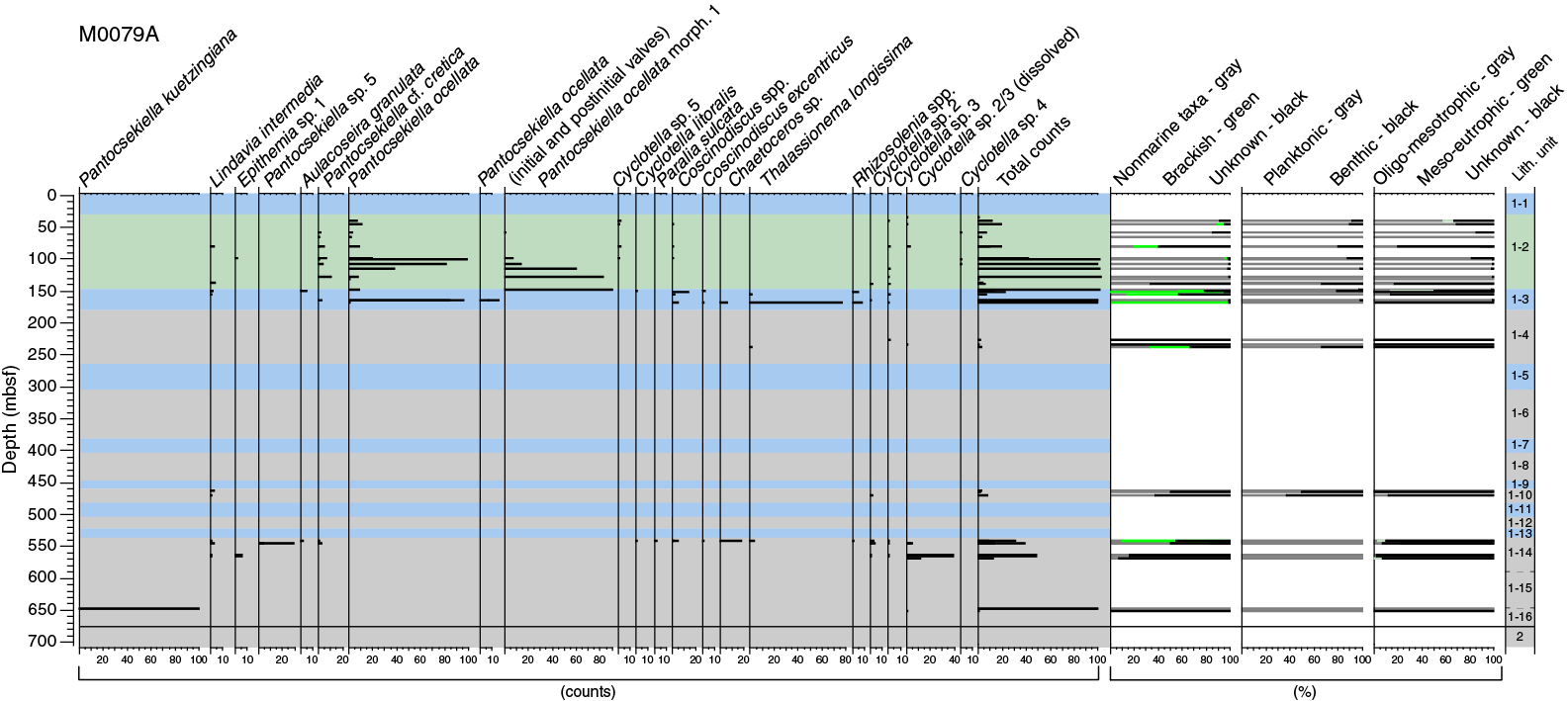
Figure F11. Most common diatom taxa.
Unit 1 (Cores 381-M0079A-1P through 154R; 0–677.23 mbsf)
Eighteen samples from Sections 381-M0079A-9P-4 through 41R-1 (33.91–149.1 mbsf) were analyzed from the isolated/semi-isolated Subunit 1-2. The nonmarine, planktonic, oligotrophic–mesotrophic P. ocellata complex dominates the diatom assemblages in this subunit, as observed in Hole M0078A (see Figure F13 in the Site M0078 chapter [McNeill et al., 2019d]). Nonmarine planktonic Pantocsekiella cf. cretica and Lindavia intermedia; benthic Cocconeis pseudothumensis, Diploneis spp., and Epithemia spp.; and planktonic taxa with unknown salinity preferences (Cyclotella sp. 2 and Cyclotella sp. 3) occur in the assemblages but at very low counts. Diatom blooms characterized by high counts of the P. ocellata complex are present in samples from Sections 381-M0079A-25V-1 through 33V-1 (99.49–126.93 mbsf) and in Section 40V-2 (147.58 mbsf). Two samples from Sections 9P-4 (33.91 mbsf) and 40V-1 (146.26 mbsf) appeared barren of nonmarine diatoms.
The samples analyzed from Subunit 1-3 (Cores 41R–49R; 149.1–183.88 mbsf) vary between marine- and nonmarine-dominated diatom assemblages. The marine diatom assemblages observed in samples from Cores 41R through 42R (150.85–154.25 mbsf) and in Core 45R (167.48 mbsf) are characterized by high counts of marine planktonic taxa, like Coscinodiscus spp., Chaetoceros spp., Thalassionema longissima, etc. The nonmarine diatom assemblages observed in samples from Sections 44R-2 through 44R-3 (163.95–164.83 mbsf) are characterized by blooms of the planktonic P. ocellata complex.
Nine samples were analyzed in Subunits 1-5 through 1-11 (Cores 67R–116R; 265.76–484.48 mbsf); however, the diatom counts in these samples are very low (<5) and/or the samples are barren. Planktonic taxa with unknown salinity preferences, such as Cyclotella sp. 2 and 3, and broken valves of benthic taxa were only sporadically observed in these samples, thereby limiting the reliability of the assemblage characterization. The sample from Core 109R (469.63 mbsf) is described as nonmarine based on the presence of planktonic L. intermedia and benthic Epithemia goeppertiana, although they were observed at low counts.
The two samples analyzed from Subunit 1-14 in Cores 124R and 125R (544.05 and 544.53 mbsf) are distinguished by the dominance of Pantocsekiella sp. 5, a planktonic taxon with unknown salinity preferences, which was observed for the first time in Holes M0078A and M0079A. The samples from Cores 381-M0079A-126R through 128R (548.51–562.01 mbsf) do not contain diatoms, except for some sporadically occurring broken valves of benthic taxa. The samples from Cores 129R and 130R (564.06–568.55 mbsf) are mainly dominated by dissolved valves of Cyclotella sp. 2 and Cyclotella sp. 3 (Figure F11). These two assemblages appear similar to the assemblage observed in a sample from Subunit 1-10 in Core 381-M0078A-100R (287.17 mbsf).
A bloom of the nonmarine planktonic diatom Pantocsekiella kuetzingiana occurs in two samples from Subunit 1-15 in Section 381-M0079A-147R-2 at 646.93 and 647.46 mbsf. A correlative bloom of the same taxon was also observed in a sample from Core 381-M0078A-121R (366.42 mbsf).
Foraminifers
At Site M0079, 209 samples were examined for foraminifer microfossils: 162 samples from core catchers taken offshore and 47 additional core samples from split-core sections during the onshore phase of the expedition (Table T7).
Unit 1 includes eight intervals in which benthic and/or planktonic foraminifer species appear in relatively high abundances, suggesting the prevalence of marine conditions:
- 0.89–31.86 mbsf (Subunit 1-1);
- 150.85–158.88 mbsf (Subunit 1-3);
- 167.47–183.87 mbsf (except in Sample 381-M0079A-48R-3, 76–77 cm; 181.49 mbsf), which corresponds to the lower part of Subunit 1-3;
- 265.84–275.43 mbsf (except in Sample 67R-4, 51–52 cm; 269.31 mbsf), which corresponds to the upper part of Subunit 1-5;
- 298.14–306.1 mbsf, which corresponds to the lower part of Subunit 1-5;
- 383.6–405.74 mbsf (Subunit 1-7);
- 449.09–462.15 mbsf (Subunit 1-9); and
- 532.86–539.74 mbsf, which corresponds to the middle of Subunit 1-13.
Periodic increases in foraminifer abundance occur in Subunits 1-2 and 1-4 and in the upper interval of Subunit 1-16 (648.45–666.08 mbsf). High abundances also occur in Subunit 1-11 from 484.73 to 504.84 mbsf, except in Sample 113R-4, 47–48 cm (492.37 mbsf), and from 496.92 to 499.53 mbsf, which corresponds to a slumped interval (see Lithostratigraphy), suggesting that this subunit includes material of marine origin. Foraminifers appear in low abundances or are absent in the remaining intervals of Subunits 1-2 and 1-4 and in Subunits 1-6, 1-8, 1-12, and 1-14, suggesting weakened marine conditions (Table T7).
Variability in foraminiferal abundance in and between the subunits suggests changes in the depositional and/or environmental patterns (Table T8). In general, the intervals containing abundant benthic foraminifers are characterized by species found in normal-salinity marine environments under moderate to high organic carbon inputs to the seafloor, including Bulimina (Bulimina aculeata, Bulimina striata, and Bulimina marginata) and species such as Bolivina spathulata, Melonis barleeanus, Cassidulina carinata, Hyalinea balthica, and Valvulineria bradyana (Goineau et al., 2011, 2015; Fontanier et al., 2003). Inputs of labile organic material to the seafloor could be inferred in samples containing moderate to high abundances of small species (i.e., exclusive of the 63–125 µm fraction) such as Nonionella cf. iridea, Eilohedra vitrea, Stainforthia fusiformis, and Cassidulina obtusa (Duchemin et al., 2007; Diz and Francés, 2008). The presence of few to common Articulina tubulosa and Chilostomella cf. ovoidea in some samples indicates low oxygenation levels in the water column and/or in the sediment (Nolet and Corliss, 1990).
In the intervals with abundant foraminiferal fauna, benthic foraminifer abundance is generally higher than that of planktonic foraminifers, and typically the planktonic foraminifer assemblages present low diversities. However, intervals where planktonic foraminifer abundance is higher than that of the benthic foraminifers occur in Subunits 1-3, 1-7, 1-9, and 1-16 (Tables T7, T9). When planktonic foraminifers appear in high abundance, species indicative of relatively cool waters in the surficial or deeper water layers were observed, including Turborotalita quinqueloba, Neogloboquadrina pachyderma, Neogloboquadrina dutertrei, Globorotalia inflata, and Globigerinita glutinata (Rohling et al., 1993; Pujol and Vergnaud Grazzini, 1995; Capotondi et al., 2016). The abundance of warm water species Globigerinella spp., Globigerinoides ruber, Globigerinoides trilobus, Globoturborotalita spp., Hastigerina pelagica, and Orbulina universa (Rohling et al., 1993; Pujol and Vergnaud Grazzini, 1995) in the planktonic assemblages is low (Table T9), but they were observed in intervals corresponding to Subunits 1-1, 1-3, 1-7, and 1-9. In the samples with abundant planktonic foraminifers, the dominant planktonic species appear to be T. quinqueloba or N. pachyderma together with N. dutertrei or G. inflata.
In Subunits 1-3, 1-9, 1-11, and 1-13, the dominant planktonic species is T. quinqueloba, suggesting surficial water of relatively low salinity and low temperature and/or enhanced fertility (Rohling et al., 1993; Pujol and Vergnaud Grazzini, 1995). In Subunit 1-11 (slumped deposit), T. quinqueloba appears in high abundance. Samples where the dominant planktonic species was N. pachyderma together with N. dutertrei, as observed in Subunits 1-3, 1-7, and 1-16, suggest the development of a deep chlorophyll maximum layer (Rohling and Gieskes, 1989; Rohling et al., 1993). The dominance of G. inflata, obtained in two samples from Subunits 1-3 and 1-4, suggests the development of a cool and deep mixed water layer (Rohling et al., 1993; Pujol and Vergnaud Grazzini, 1995).
Benthic and planktonic foraminifers are absent in Samples 381-M0079A-154R-3CC, 0–2 cm (677.78 mbsf), to 162R-3CC, 4–5 cm (700.43 mbsf), from Unit 2.
Palynology
A total of 23 samples were examined for palynomorphs (22 samples from Unit 1 and 1 sample from Unit 2) (Table T10). Eight samples yielded extremely low concentrations of palynomorphs and are listed as barren in Table T11. Sample 381-M0079A-134R-4, 11 cm (591.21 mbsf), was also excluded from the analyses because it originates from a core section where slumps were observed. A total of 14 samples are presented here, all from Unit 1 (7 samples in marine intervals and 7 samples in isolated/semi-isolated intervals).
Palynomorph preservation in Hole M0079A is good, and the mean concentration of corroded pollen grains is 274 grains/g with a maximum of 851 grains/g in Sample 99R-5, 0 cm (424.46 mbsf). In comparison, the mean concentration of corroded grains in Hole M0078A Unit 1 is higher.
The mean concentration of fungal remains is 30 per gram, and the mean concentration of charred microscopic particles is 3,250 per gram with a maximum of 10,142 per gram in Sample 73R-4, 49 cm (299.29 mbsf). Terrestrial pollen concentrations, including trees and herbs, have a mean value of 4,770 grains/g, which is similar to Hole M0078A; a maximum of 36,483 grains/g was recorded in Sample 381-M0079A-44R-3, 74 cm (165.04 mbsf). Maximum values of green algae concentrations (3,470 coenobia/g) were also recorded in the same sample.
Alternating periods of forest- and herb-dominated vegetation were observed in the samples examined (Tables T10, T11), confirming the occurrence of forested and open landscapes, respectively, in the borderlands of the Gulf of Corinth as inferred from Hole M0078A pollen spectra (see Micropaleontology in the Site M0078 chapter [McNeill et al., 2019d]). Maximum tree percentage and concentration values of 86.6% and 33,211 grains/g, respectively, were recorded in Sample 381-M0079A-44R-3, 74 cm (165.04 mbsf).
Oaks (Quercus spp.) continue to be the dominant deciduous tree, as observed in Hole M0078A; however, the occurrence of mixed deciduous forest in the area is inferred by the concomitant presence of Corylus, Acer, Carpinus, and Ulmus pollen grains. Pollen grains of relict species include Cedrus, Zelkova, Pterocarya, and Tricolpoporopollenites sibiricum. Cedrus reaches a maximum of 17% in Sample 381-M0079A-66R-4, 33 cm (264.13 mbsf), and Zelkova reaches a maximum of 6.5% in Sample 151R-3, 3 cm (666.08 mbsf). Artemisia, Ephedra, and Chenopodiaceae are more abundant in samples corresponding to isolated/semi-isolated intervals, whereas Mediterranean sclerophyllous vegetation reaches a maximum of 15% in Sample 44R-3, 74 cm (165.04 mbsf).
Dinoflagellate cysts have a mean concentration of 3,122 cysts/g, and the maximum (25,985 cysts/g) is recorded in Sample 15P-4, 11 cm (62.98 mbsf). As in Hole M0078A, dinoflagellate assemblages show alternating periods of marine and brackish paleoenvironments correlating with marine and isolated/semi-isolated intervals, respectively. In contrast to dinoflagellate assemblages observed in Hole M0078A, in two samples from Hole M0079A (Samples 15P-4, 11 cm [62.98 mbsf], and 44R-3, 74 cm [165.04 mbsf]), only specimens of Spiniferites cruciformis were encountered. Those two samples have the highest concentration of dinoflagellate cysts among the samples analyzed. In Sample 44R-3, 74 cm (165.04 mbsf), maximum concentrations of green algae and aquatic vascular plants are also recorded. The occurrence of S. cruciformis is generally associated with deposition under brackish conditions (Mudie et al., 2017); however, this species has also been reported from freshwater deposits in northwestern Greece (i.e., Lake Kastoria in Kouli et al., 2001).
Biostratigraphy summary
Age control is provided solely by the calcareous nannofossils in Hole M0079A (Table T12), and it should be applied cautiously given the complexity of the depositional environment (Figure F12). Three biohorizons were recognized at this site. The first age datum considered is that of the crossover in dominance between E. huxleyi and Gephyrocapsa “small.” This crossover has been observed in multiple locations (Thierstein et al., 1977; Raffi et al., 2006; Anthonissen and Ogg, 2012), including the Mediterranean Sea, where it is calibrated at 0.07 Ma in MIS 4 (Anthonissen and Ogg, 2012). If this datum is applied accurately in Hole M0079A, then it occurs in Subunit 1-2.
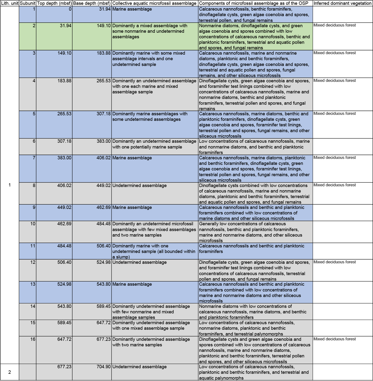
Figure F12. Micropaleontology assemblages.
The LDO of E. huxleyi was observed at 404.94 mbsf in Sample 95R-3, 144–145 cm, but this occurrence likely does not represent the true FAD (0.29 Ma) because this species evolved in glacial MIS 8, a time when the Gulf of Corinth was presumably disconnected from the Mediterranean Sea.
The oldest marker, P. lacunosa (LAD at 0.43 Ma), was observed in Sample 114R-3, 68–69 cm (496.1 mbsf). In addition to only being observed in one sample, this occurrence is likely not the true LAD because the extinction of P. lacunosa occurs in glacial MIS 12, a time when the Gulf of Corinth was presumably disconnected from the Mediterranean Sea. Additionally, it should be noted that the sample containing P. lacunosa comes from the slumped interval in Subunit 1-11 (see Lithostratigraphy); however, examination of the microfossils suggests that the assemblage is in situ regardless of its geographical displacement.
Micropaleontology summary
Micropaleontology at Site M0079 revealed a high level of complexity both in individual microfossil groups and collectively, as in Holes M0078A and M0078B. Unit 1 alternates primarily between marine and undetermined assemblages but also includes some mixed and nonmarine assemblages (Figure F12). Alternating periods of forested and open landscapes are inferred in the borderlands of the Gulf of Corinth. Unit 2 is nearly devoid of microfossils. See Figure F12 for a summary of the microfossil assemblages by subunit, and refer to individual data sets for details.
Geochemistry
Interstitial water
At Site M0079, 77 interstitial water samples were collected using Rhizon samplers and whole-round squeeze cakes. Rhizon sampling extended from the sediment/water interface to 8.65 mbsf, and whole-round squeeze samples were collected from 12.92 to 698.84 mbsf. Depth spacing of squeeze cakes was between 5.11 and 17.64 m with an average spacing of 9.94 m. Both Rhizon and whole-round squeeze cake methods generally provided adequate pore water volume for most analyses. Additionally, drilling mud fluid samples were taken from discrete depths approximately every 60 m throughout the hole to evaluate potential drilling contamination (see Geochemistry in the Expedition 381 methods chapter [McNeill et al., 2019b]).
Similar to Site M0078, pore water chemical compositions at Site M0079 reflect environmental changes in basin water chemistry, type and rate of organic matter burial, and dissolution/precipitation reactions with sediment. Cyclicity is apparent in many pore water signals that may represent successive eustatic sea level fluctuations impacting the basin water in the Gulf of Corinth (C.M. Miller et al., unpubl. data).
Salinity variations: salinity and chloride
Salinity decreases from seawater values near the sediment/water interface to 10.48 in the upper 41.56 m (Figure F13A). Salinity broadly remains around 10 to 504.84 mbsf but is punctuated by higher values at 199.94 mbsf (15.34), 320.45 mbsf (17.56), and 488.84 mbsf (14.64). Most of these peaks occur immediately below the interpreted marine intervals. Deeper than 504.84 mbsf, salinity is generally lower than 10, except between 621.74 and 660.24 mbsf.
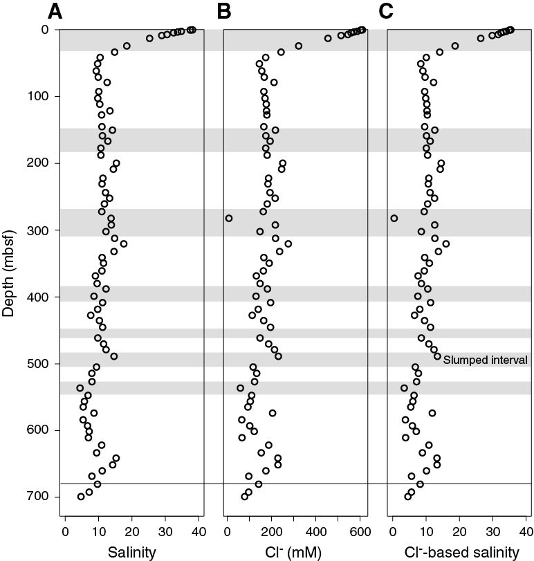
Figure F13. Pore water salinity, chloride, and Cl−-based salinity.
Chloride (Cl−) concentrations follow salinity. Values are highest (610.75 mM) close to the sediment/water interface and decrease to 145.33 mM at 51.00 mbsf (Figure F13B). From 51.00 to 427.43 mbsf, Cl− concentrations broadly increase to a local maximum of 275.87 mM at 320.45 mbsf and then decrease to 113.02 mM. Another broad peak occurs between 583.84 mbsf and the bottom of the hole and is centered at 651.24 mbsf (229.36 mM). Again, these distinct fluctuations occur at the same depths as the local salinity maxima, which may reflect the integrated result of varying salinity conditions across multiple marine isotope stages in the Gulf of Corinth. Figure F13C illustrates that salinity determined by refractometer (see Geochemistry in the Expedition 381 methods chapter [McNeill et al., 2019b]) is comparable to salinity calculated from Cl− (assuming a salinity of 35 is equivalent to a Cl− concentration of 558 mM), which provides evidence that NaCl is the dominant dissolved salt, with other salts making only a minor contribution to pore water salinity.
Drilling mud fluid salinity and Cl− concentrations throughout Site M0079 are either much higher than sediment interstitial fluids (when seawater was used) or much lower (when freshwater was used), implying no drilling contamination (Table T13).
Organic matter degradation: alkalinity, ammonium, boron, bromide, iron, manganese, pH, phosphate, sulfate, and dissolved inorganic carbon
Organic matter oxidation alters the geochemistry of both solid and liquid phases in sediment (Berner, 1980). These changes can be observed and quantified by measuring the degradation products of these reactions. Pore water profiles for the upper 24.25 m at Site M0079 suggest the typical sequence of organic matter degradation in marine sediments (Froelich et al., 1979). Elevated manganese (Mn2+) concentrations (as high as 71.52 µM) indicate Mn oxide reduction in the uppermost 7.18 m of Hole M0079A, with another smaller peak at 51.00 mbsf (Figure F14A). Dissolved iron (Fe2+) concentrations are elevated (as high as 318.50 µM) from the sediment/water interface to 121.42 mbsf, suggesting the reduction of Fe (oxy)hydroxides. Additionally, minor increases are found around 199.74, 252.25, 312.25, 573.84, and 641.19 mbsf (Figure F14B). These peaks generally occur with increased sulfate (SO42−) concentrations (Figure F14C). The dominant SO42− decrease from 28.40 mM below the seafloor to 0.84 mM at 8.65 mbsf implies organic matter degradation through SO42− reduction or anaerobic oxidation of methane in this zone. The presence of sulfide (HS−), a product of SO42− reduction, can be approximated by calculating the difference between dissolved inorganic carbon (DIC) and alkalinity. Figure F15C shows minor differences between DIC and alkalinity, suggesting HS− concentrations are low throughout the hole. Mn2+, Fe2+, and SO42− concentrations are highest right below the seabed, subsequently decrease, and are present at much lower concentrations throughout the remaining borehole (Figure F14).
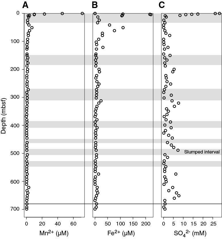
Figure F14. Pore water manganese, iron, and sulfate.
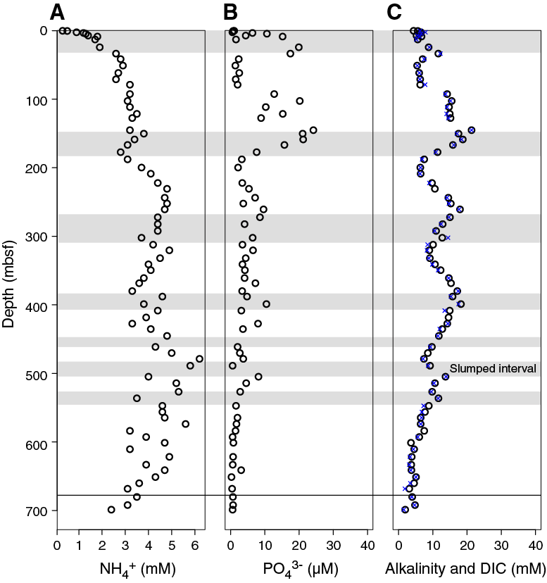
Figure F15. Pore water ammonium, phosphate, and alkalinity and DIC.
Microbial organic matter degradation in marine sediments releases bicarbonate (HCO3−; the main component of DIC), phosphate (PO43−), and ammonium (NH4+) to the pore water. NH4+ concentrations increase from 0.3 mM to a local maximum of 2.9 mM at 51.00 mbsf (Figure F15A). Deeper, NH4+ concentrations fluctuate but show a general increasing trend to 6.2 mM at 478.84 mbsf. From 51.00 mbsf to the base of Hole M0079A at 698.84 mbsf, NH4+ concentrations decrease to 2.4 mM. Both alkalinity and PO43− fluctuate downhole. Local maxima of these two parameters are at 33.50, 102.60, 145.18, 260.75, 398.89, and 504.84 mbsf, possibly indicating regions with enhanced organic matter degradation. The upper three peaks in PO43− concentrations are higher (as high as 24.2 µM) than the lower three peaks (as high as 10.5 µM) (Figure F15B). Alkalinity and DIC are very similar throughout the hole, implying alkalinity is composed almost exclusively of DIC (Figure F15C). Broadly, the changes in alkalinity are reflected in pH (Figure F16). Pore water pH at Site M0079 ranges from 7.5 to 8.3, with the highest values coinciding with the peaks in alkalinity.
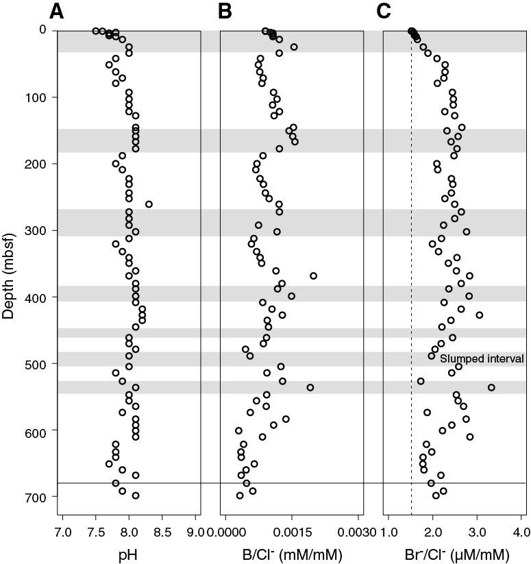
Figure F16. Pore water pH and B/Cl− and Br−/Cl− ratios.
Boron (B) and bromide (Br−) accumulate in organic matter. A common method to determine the relative contributions of seawater and organic carbon oxidation to pore water chemistry is to plot the ratios of B and Br− to Cl−. Although the Br−/Cl− depth profile does not always match the alkalinity profile, the B/Cl− ratio shows the same pattern as the alkalinity profile (Figure F16), supporting the interpretation that intervals of higher alkalinity concentration represent time periods of enhanced organic matter degradation.
Drilling fluid concentrations (IwrefMf and IwrefMl, Table T13) of Mn2+, Fe2+, DIC, PO43−, NH4+, and B are all low and therefore unlikely to contribute significantly to the pore water inventory in terms of potential contamination. SO42 and Br− are present in the drilling fluids; however, their trends with depth are dissimilar to the pore water trends (Table T13).
Mineral reactions
Barium, calcium, magnesium, potassium, sodium, and strontium
Calcium (Ca2+), magnesium (Mg2+), potassium (K+), and sodium (Na+) are all major ions in seawater, and barium (Ba2+) and strontium (Sr2+) are minor components. Their concentrations in pore water (Figure F17) may be altered by processes such as ion exchange, mineral weathering, and formation of new minerals. The Na+ depth profile matches the salinity and Cl− profiles. Furthermore, the Na+/Cl− ratio profile stays close to seawater values almost throughout the hole (vertical dashed line, Figure F17D), which suggests that Na+ is not significantly involved in mineral reactions. Deeper than approximately 500 mbsf, Na+/Cl− values decrease, resembling the trend in the lower part of Site M0078. K+ concentrations decrease significantly from 11.6 to 1.1 mM in the uppermost 51.00 m (Figure F17B). K+ concentrations then fluctuate between 4.8 and 0.7 mM to the base of the hole. These fluctuations were also observed in the K+/Cl− ratio profile, and the local maxima of K+/Cl− correspond roughly to the regions of high alkalinity (Figure F17E).
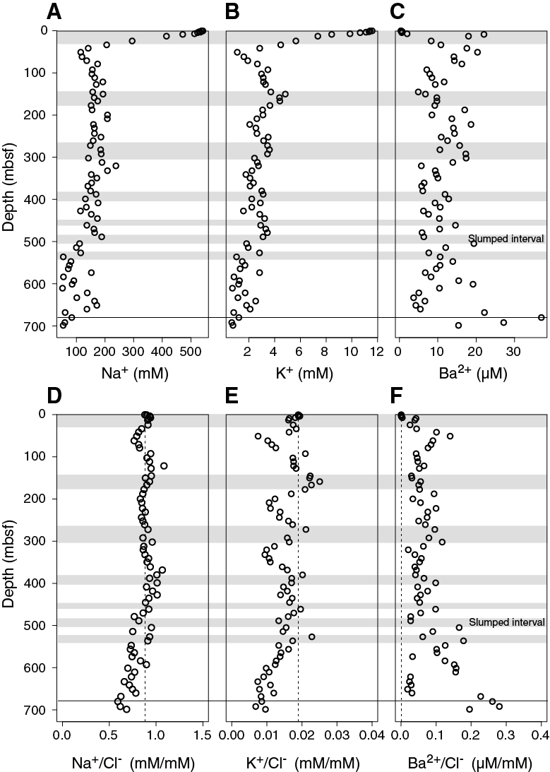
Figure F17. Pore water sodium, potassium, and barium.
The dissolved Ca2+, Mg2+, and Sr2+ depth profiles in Hole M0079A broadly follow the Cl− curve and show more distinct fluctuations than those observed in Hole M0078A (Figure F18). All three elements decrease in the uppermost 24.25 m of Hole M0079A, and they all have more or less pronounced peaks at 51.00, 208.74, 320.45, and 478.84 mbsf. Toward the base of Hole M0079A, the Ca2+/Cl−, Mg2+/Cl−, and Sr2+/Cl− ratios increase again to values much higher than seawater values, as seen in Hole M0078A, indicating a source of Ca2+, Mg2+, and Sr2+ at greater depths.
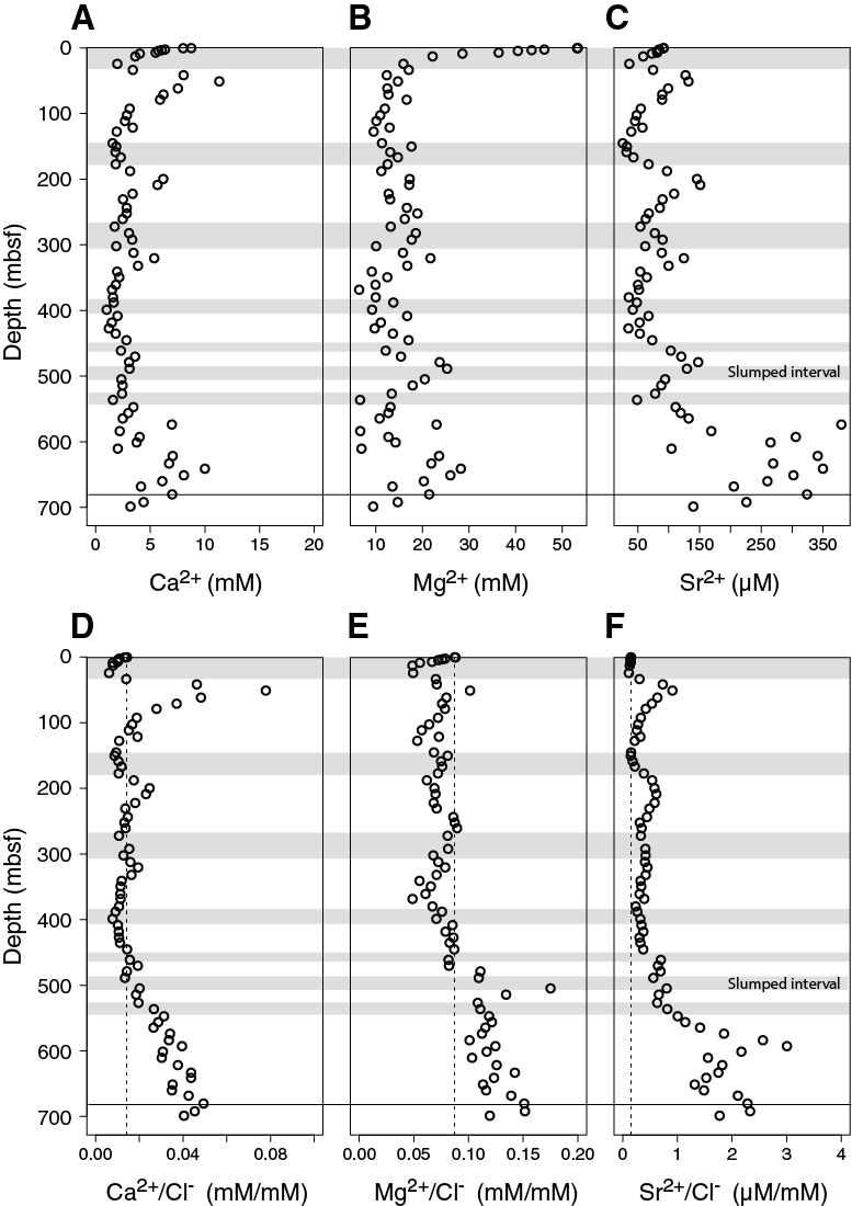
Figure F18. Pore water calcium, magnesium, and strontium.
Ba2+ concentrations appear more scattered than the other analytes (Figure F17C). Concentrations increase from 0.80 µM near the seafloor to 22.03 µM at 78.85 mbsf. Deeper than 78.85 mbsf, the concentrations fluctuate without showing a clear trend and are always higher than modern seawater composition, as emphasized by the dashed line in the Ba2+/Cl− ratio (Figure F17F). Between 621.74 and 660.24 mbsf, low concentrations of approximately 5 µM appear to coincide with a peak in salinity and SO42−. At the base of the hole, Ba2+ increases, comparable to the increase in Ca2+, Mg2+, and Sr2+. Na+, K+, Ca2+, Mg2+, and Sr2+ concentrations in drilling mud are variable but follow different trends with depth when compared with the pore water data (Table T13).
Silica and lithium
Silica accumulates in sediments as silicate minerals and the remnants of siliceous organisms. Dissolved silica (H4SiO4) is typically released to pore water through dissolution of these sediment components. H4SiO4 concentrations exhibit significant variability throughout Site M0079 (Figure F19A). Shallow H4SiO4 concentrations in the uppermost 24.25 m are consistently low and then increase to 1063.20 µM at 51.00 mbsf. Between 51.00 and 252.25 mbsf, H4SiO4 concentrations broadly decrease to 382.58 µM. From 252.25 to 601.24 mbsf, H4SiO4 concentrations exhibit significant scatter between 196.88 and 1274.66 µM. A broad front of 581.46 µM occurs from 601.24 to 698.84 mbsf and is centered at 651.24 mbsf. Overall, H4SiO4 peaks correspond to peaks in alkalinity.
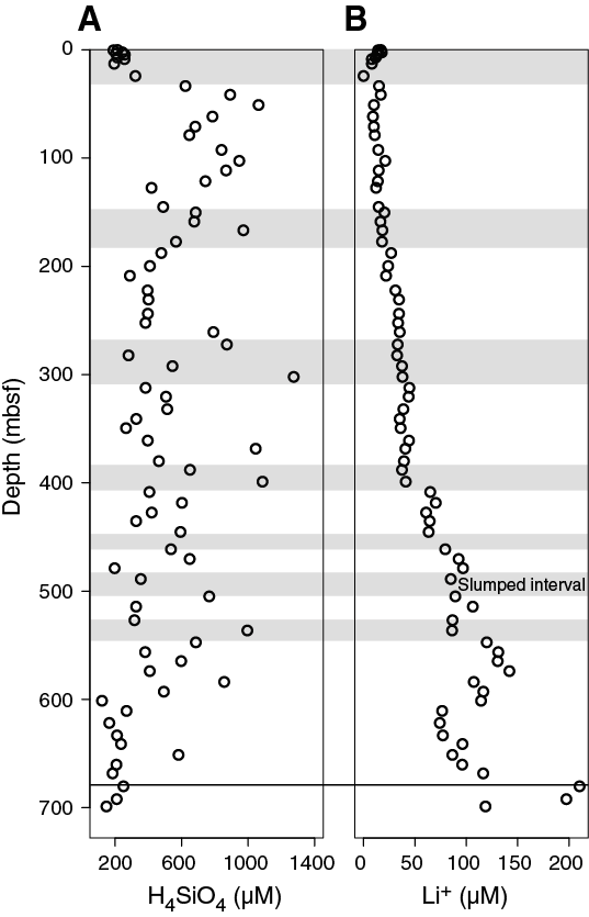
Figure F19. Pore water dissolved silica and lithium.
Lithium (Li+) concentrations are approximately 14 µM in the uppermost 7.18 m and drop to 8.01 µM followed by a steady increase with depth to 37.16 µM at 387.95 mbsf (Figure F19B). Deeper than 398.89 mbsf, Li+ concentrations continue to increase to 210.30 µM at 680.25 mbsf. Drilling mud fluids contain variable quantities of Si and Li; however, concentrations are in general much lower than those found in pore water (Table T13), and therefore drilling mud fluids are unlikely to contribute significantly to the pore water inventory.
Sediment
Carbon content
At Site M0079, a total of 112 samples were measured for total carbon (TC) and total organic carbon (TOC) in the sediment (Table T14; Figure F20). Total inorganic carbon (TIC) was obtained by subtracting TOC from TC. TC for Site M0079 varies between 4.31 and 10.92 wt% with an average of 7.13 wt%, which is very similar to Site M0078. TC and TIC values gradually increase with depth, comparable to the trend in solid-phase Ca (Figure F21A), indicating a higher calcite content in the lower part of the hole (see below). TOC varies between 0.18 and 0.51 wt% with an average of 0.31 ± 0.06 wt% (standard deviation). The average is the same as at Site M0078, but the range is narrower, implying a more homogeneous distribution of TOC throughout Site M0079. Local maxima at 26.40, 146.66, 260.00, 367.72, 387.23, and 540.69 mbsf may imply higher amounts of organic matter burial.
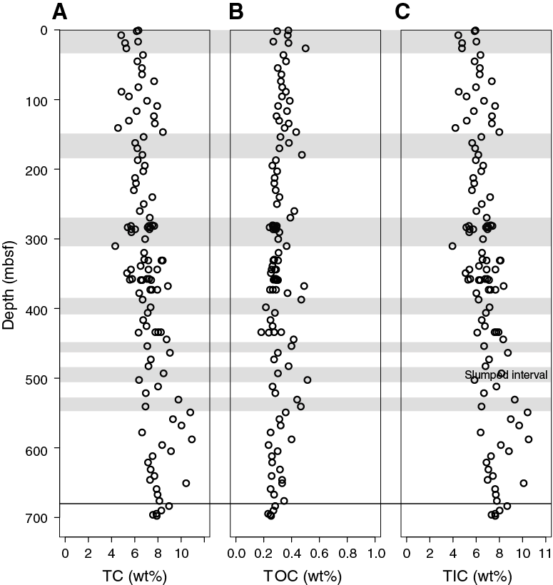
Figure F20. Solid-phase TC, TOC, and TIC.
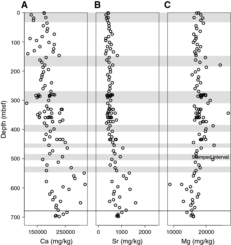
Figure F21. Solid-phase calcium, strontium, and magnesium.
ED-XRF
The concentrations of 24 elements were measured in 112 ground sediment samples using energy dispersive X-ray fluorescence (ED-XRF). Quantitative concentrations for 11 elements (Al, Ca, Fe, K, Mg, Mn, Si, Sr, Zr, Ni, and Rb) are presented in Table T14 and Figures F21, F22, F23, and F24. For the remaining elements, either concentrations were too low or the measurement was imprecise because of overlapping peaks in spectra. Concentrations of these elements are also included in Table T14, although they need to be treated with caution and are not discussed any further.
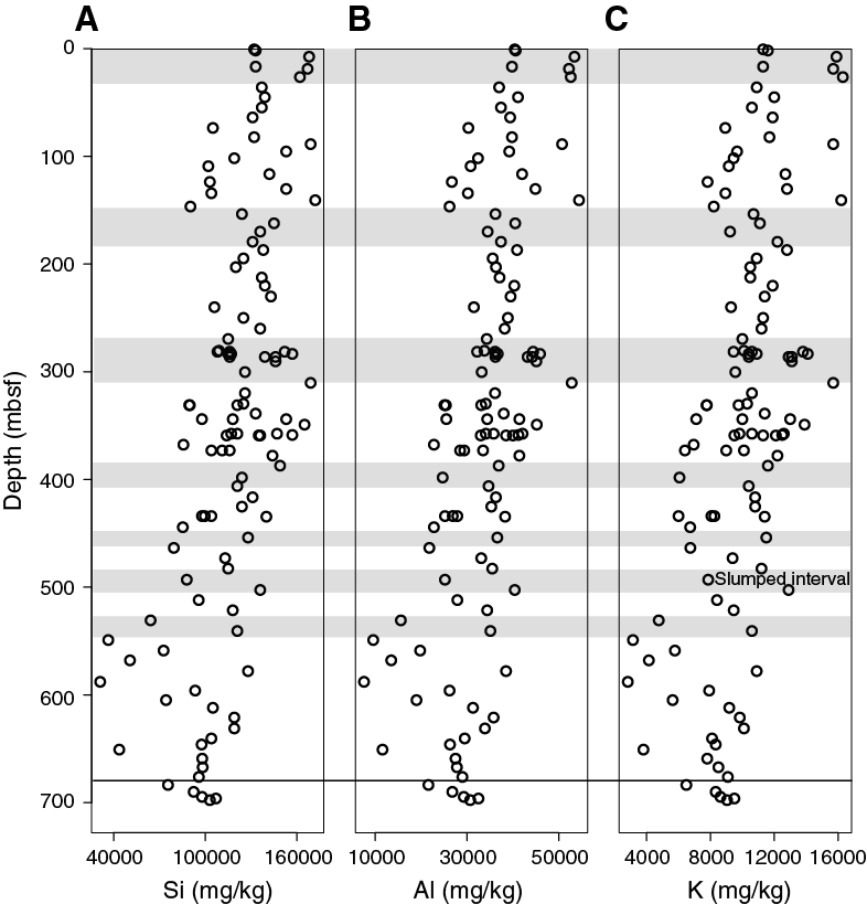
Figure F22. Solid-phase silicon, aluminum, and potassium.
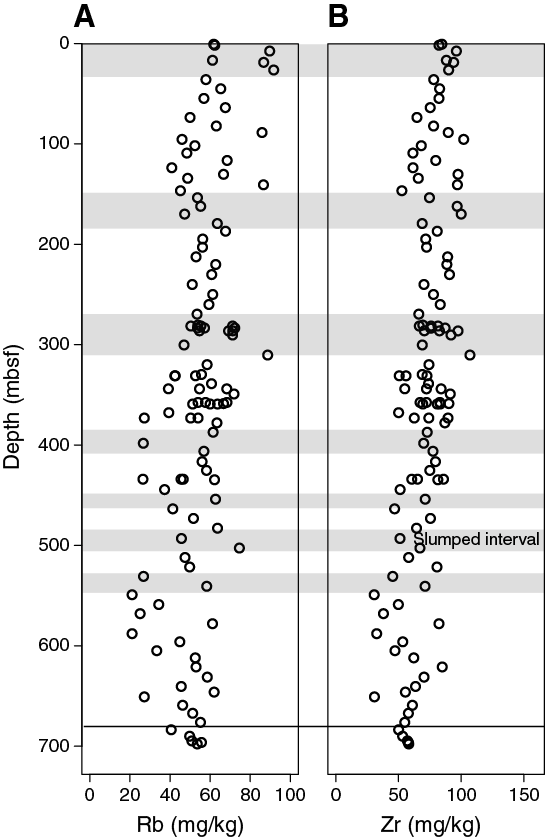
Figure F23. Solid-phase rubidium and zirconium.
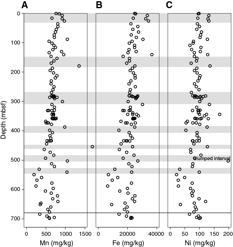
Figure F24. Solid-phase manganese, iron, and nickel.
The highest elemental content measured was calcium. At Site M0079, an average Ca concentration of 197.2 g/kg was measured (Figure F21A), which is slightly lower than at Site M0078. Ca gradually increases with depth. The second most abundant element is Si (mean = 119.7 g/kg) (Figure F22A). A Spearman Rho correlation for Ca and Si shows an almost ideal negative correlation (R = −0.97, ρ < 0.05). The average Si, Al, K, and Zr concentrations (Figures F22, F23) are all higher compared with Site M0078, implying a generally higher abundance of noncalcareous detrital material at Site M0079. The Mg and Sr profiles show relatively low scattering throughout the hole, with a slight decrease in Mg and an increase in Sr toward the bottom (Figure F21). However, Al, K, Rb, and Zr show higher fluctuations throughout the hole, especially between 398.22 and 650.83 mbsf. These fluctuations are superimposed on a decreasing trend toward the base of the hole (Figures F22, F23). The Mn, Fe, and Ni profiles likewise generally decrease with depth and show higher scattering between 398.22 and 650.83 mbsf (Figure F24). Ni also generally decreases with depth; however, much less variation occurs deeper than 377.89 mbsf.
Physical properties
This section summarizes the physical properties results from Site M0079, where one hole (M0079A) was drilled from 0 to 704.90 mbsf. Most data sets were collected at the sampling rates defined in Physical properties in the Expedition 381 methods chapter (McNeill et al., 2019b), except for P-wave velocity, thermal conductivity, and shear strength, where the nature of the sediment limited data acquisition. Overall, the data sets collected reflect good correlations between the sediment physical properties and the basin paleoenvironment and associated lithologic changes, especially magnetic susceptibility, NGR, density, porosity, and color reflectance. A synthesis of physical properties for Hole M0079A is presented in Figures F25 and F26, and a more detailed illustration of transitions between marine and isolated/semi-isolated subunits is presented in Figure F27.
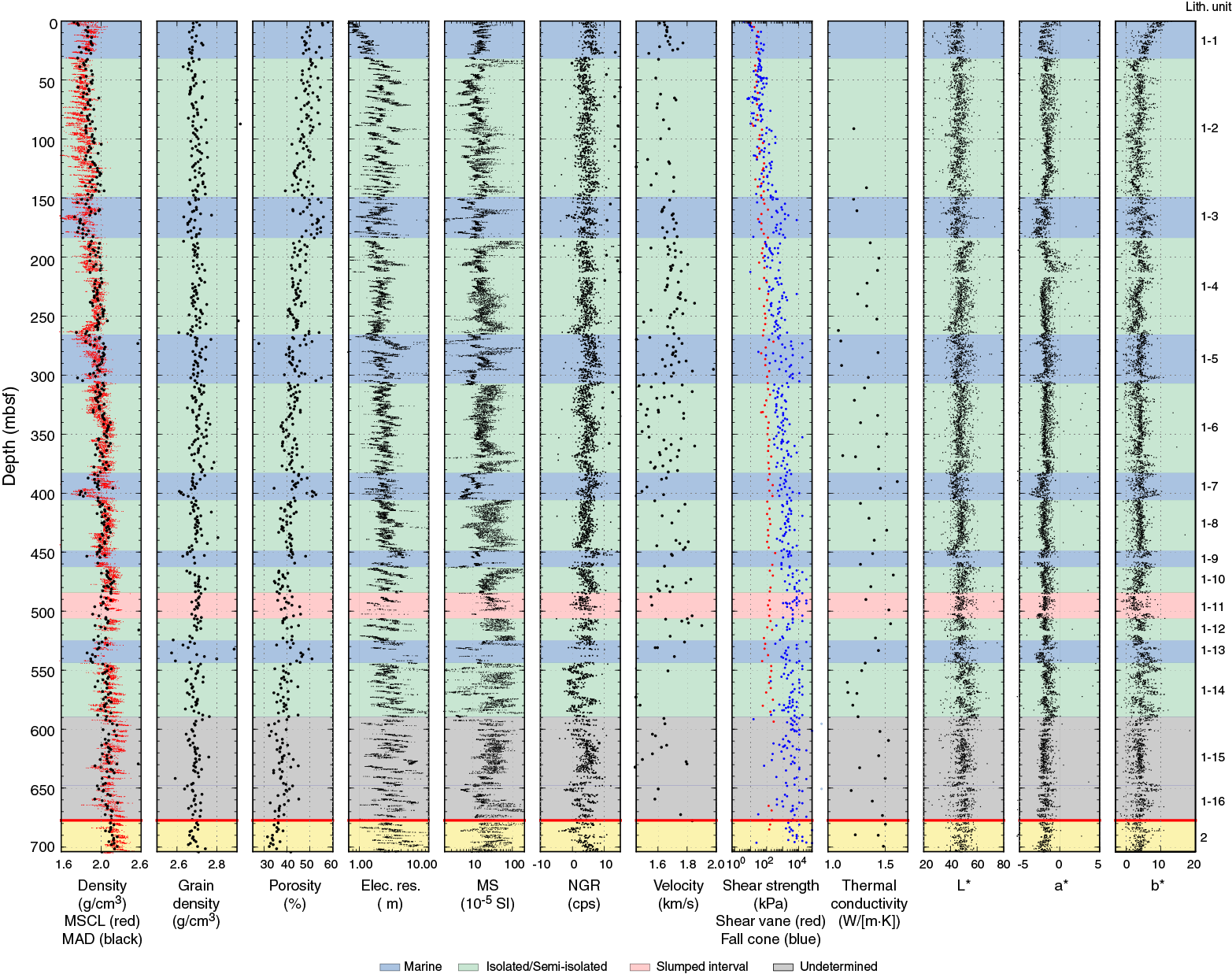
Figure F25. Physical properties with environmental interpretation.
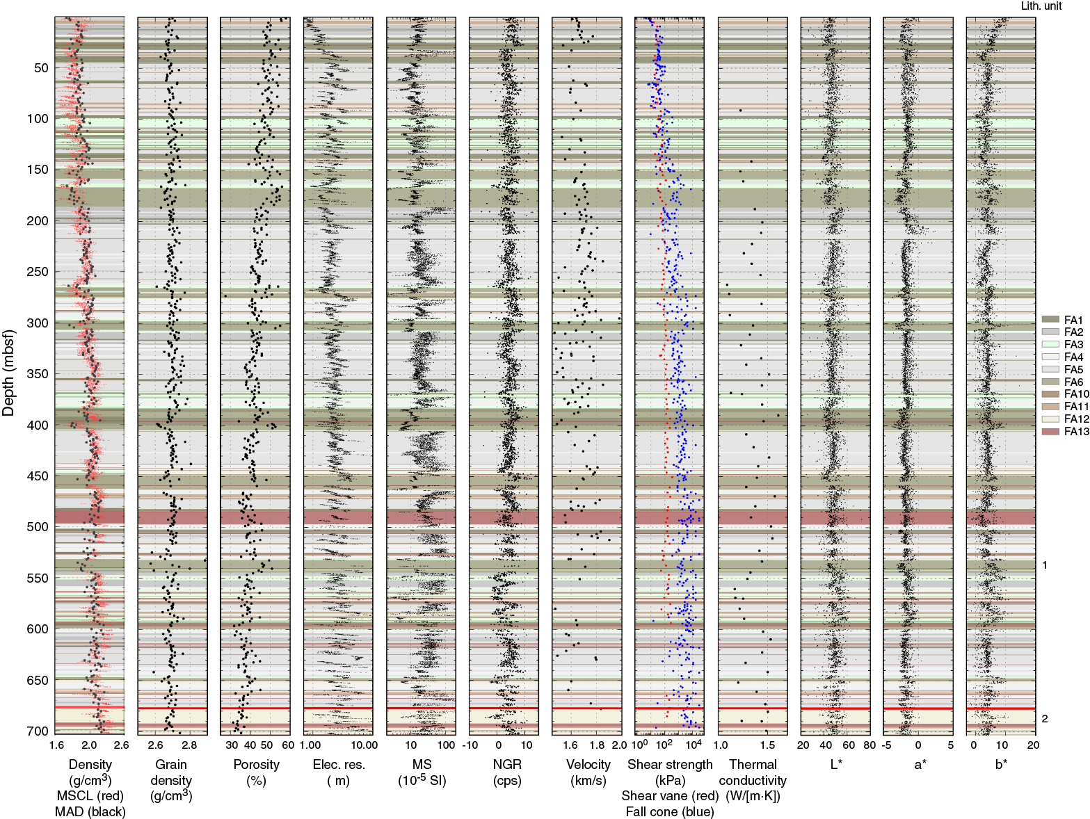
Figure F26. Physical properties with facies associations.
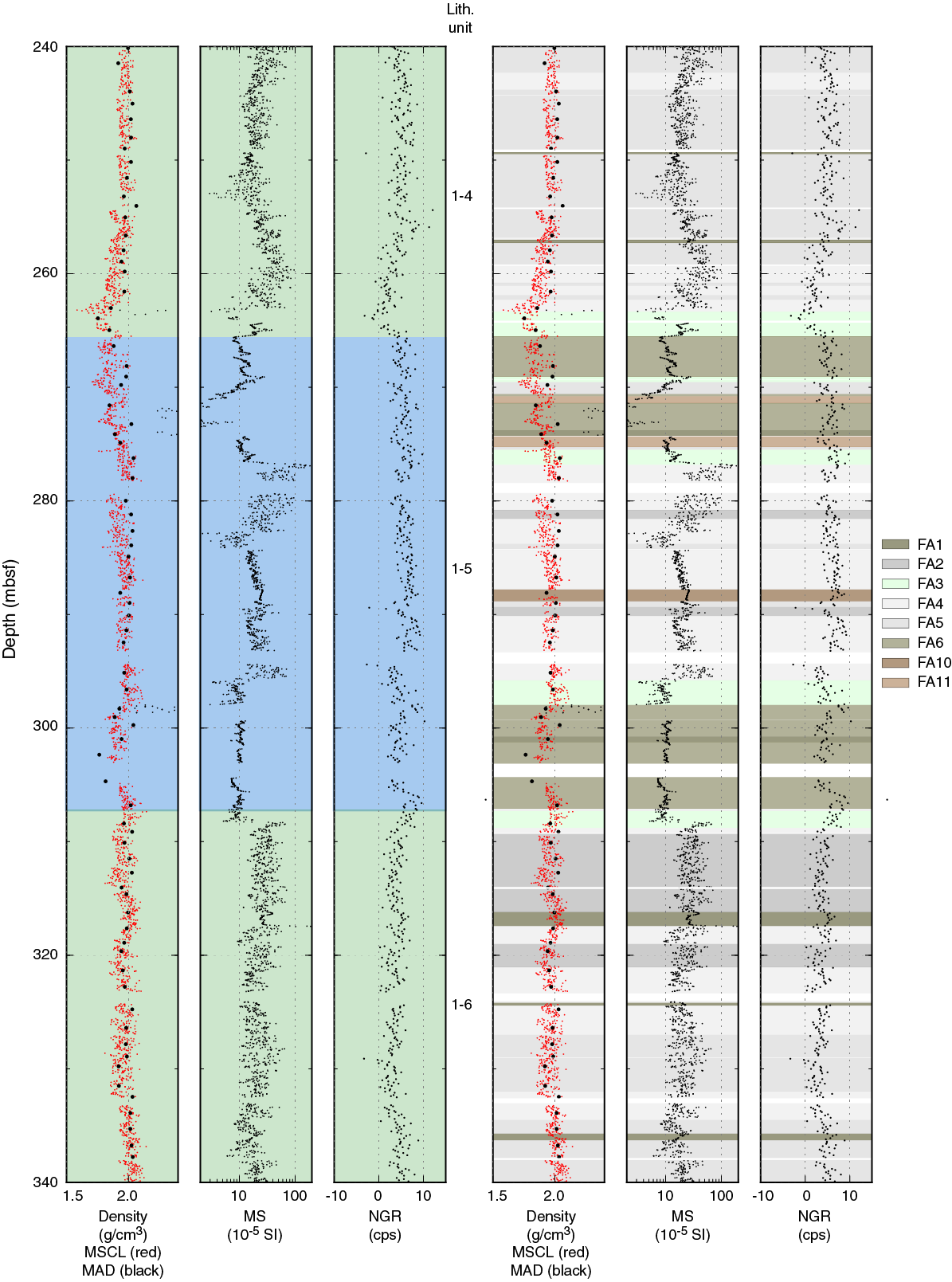
Figure F27. Changes from marine to isolated/semi-isolated subunits.
Shear strength
Sediment strength for Hole M0079A was measured offshore using a handheld penetrometer and a downhole CPT and onshore using a fall cone and a shear vane. Penetrometer and CPT measurements were taken approximately every 20 and 100 m, respectively, whereas fall cone and shear vane measurements were taken one per core section and one per core, respectively.
Strength values for Hole M0079A derived from the different methods differ significantly (Figure F28). Cone resistance values derived from handheld penetrometer measurements are consistently higher than shear strength values from fall cone and shear vane measurements in the upper ~150 mbsf. From 0 to ~115 mbsf, handheld penetrometer values increase from 180 to 490 kPa and then step up to 1120 kPa at ~137 mbsf and remain relatively constant to ~350 mbsf. From ~350 to ~692 mbsf, penetrometer values vary between 1590 and 5880 kPa. Deeper than ~150 mbsf, handheld penetrometer values approximately coincide with fall cone values.
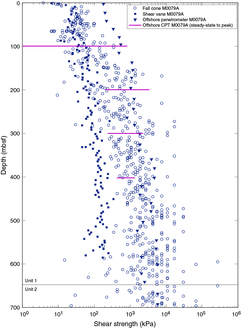
Figure F28. Shear strength.
Measured fall cone values are consistently higher than shear vane measurements deeper than ~100 mbsf. Fall cone strength values increase sharply from 0 to ~10 mbsf and then remain relatively constant below ~100 kPa to ~100 mbsf. From ~100 to ~500 mbsf, fall cone shear strength increases almost exponentially and reaches maximum values of ~31,000 kPa. In this depth interval, increases in shear strength appear downhole at ~150 and ~285 mbsf, which coincide with the tops of marine subunits (Figure F25). Another strength increase occurs at ~480 mbsf, which appears to coincide with the top of a slumped interval (Subunit 1-11; FA13; see Lithostratigraphy). From ~500 to ~540 mbsf, reduced strength values were observed, and from ~540 mbsf to the base of the hole, strength values are scattered, ranging from ~15 to ~17,300 kPa.
Shear vane measurements follow trends similar to those observed in the fall cone measurements but have lower values and are less scattered. Shear vane values increase linearly from ~10 to ~500 mbsf, ranging between ~30 and ~450 kPa. Deeper than ~500 mbsf, shear vane values show more variability, between ~58 and ~277 kPa. Shear vane measurements were taken to ~585 mbsf (Section 381-M0079A-133R-2), where sediment strength exceeded the maximum applied force capacity of the shear vane apparatus. Scattering of the values deeper than ~500 mbsf may reflect the equipment reaching its limit in increasingly indurated lithologies.
When inserting the CPT, a peak in cone resistance (qc) occurs followed by a decay to a steady-state value. Both peak and steady state were used to compute the in situ shear strength and bracket its actual value. The four in situ shear strength measurements from the CPT indicate an overall increase in sediment strength from 0 to ~400 mbsf, suggesting increased consolidation with depth, despite the different range in strength values they provide in comparison with the other strength measurements (Figure F28).
An overall increase in strength values was observed at ~150 mbsf (Section 41R-2) (Figure F25); however, any potential correlation with coring mode/drilling parameter or lithology as a function of basin environment (marine versus isolated/semi-isolated) remains unresolved. A similar shear strength increase at ~285 mbsf coincides with the downhole transition to a marine subunit. All three shear strength measurements on recovered cores (handheld penetrometer, shear vane, and fall cone) indicate smaller strength values and less variation between ~500 and ~540 mbsf, whereas deeper than ~540 mbsf and downhole, shear strength remains approximately constant.
Natural gamma radiation
Overall, the low NGR values at Site M0079 indicate that K, Th, and U concentrations are depleted in the mud-dominated cores (Figures F25, F29), as at Site M0078. Despite these low values, spectral gamma ray data acquired by downhole logging (see Downhole measurements) compare well with trends measured in the same intervals of the hole (Figure F45), suggesting the core MSCL data faithfully capture NGR trends in the hole. In lithostratigraphic Unit 1, NGR values average 4.59 counts/s with a minimum of −5.51 counts/s and a maximum of 30.39 counts/s (Figure F29). In Unit 2, NGR values average 3.68 counts/s with a minimum of −4.98 counts/s and a maximum of 23.31 counts/s.
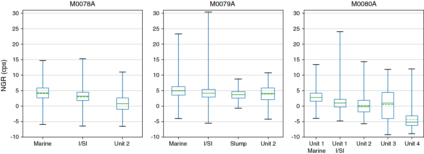
Figure F29. MSCL NGR.
A significant change in the NGR trend was observed at 485 mbsf, which is 195 m above the lithostratigraphic Unit 1/2 boundary (Figure F25). NGR values are distinctly higher and exhibit more scatter shallower than 485 mbsf than those deeper (Figure F29). Between 485 and 703 mbsf, NGR values appear to contain oscillations with a <10 m wavelength (Figure F25).
In marine subunits in Unit 1, NGR values vary from −4.01 to 23.31 counts/s with a mean of 4.83 counts/s. In isolated/semi-isolated subunits, NGR values vary from −5.51 to 30.38 counts/s with a mean of 4.09 counts/s and are thus are slightly lower overall in isolated/semi-isolated subunits than in the marine environment (Figure F29). In the slumped subunit (1-11), the mean NGR value is lower than in the marine and isolated/semi-isolated subunits, averaging 3.63 counts/s with minimum and maximum values of −0.68 and 8.75 counts/s, respectively. A distinct decrease in NGR values occurs at the boundary between Subunits 1-1 and 1-2 (at 32 mbsf; Figure F25), which is associated with a change from FA1 (homogeneous mud) to FA13 (contorted bedding and mud-supported gravel).
A decrease in NGR values occurs at 165 mbsf, where the facies association changes from greenish gray mud with homogeneous centimeter-thick gray mud beds (FA5) to light gray to white submillimeter laminations alternating with mud and silt beds (FA3) (Figure F26). At 308 mbsf, a change in NGR values (from low to high) is associated with a facies association change from light gray to white submillimeter laminations alternating with mud and silt beds (FA3) to greenish gray mud with dark gray to black mud to sand beds and laminations (FA2). A distinct increase in NGR values is noted at 450 mbsf, where a facies association change from light gray/white thin laminations (calcite/aragonite) alternating with beds of mud/silt (FA3) to homogeneous mud (FA1) occurs. At 250 mbsf, a sharp change in NGR values occurs, but no distinguishable variation is noticed in the facies association. Correlation between changes in NGR values with facies association is not straightforward, and the aforementioned examples are some of the locations where a clear relationship can be established. One of the main reasons for the correlations may be due to variation in mineral concentrations between the facies associations.
As at Site M0078, NGR values drop below 0 counts/s (Figure F29). These values were obtained after the background was subtracted from the raw count. Despite the negative values, the overall trend compares well with the downhole gamma ray log data (Figures F44, F45).
Magnetic susceptibility
Magnetic susceptibility appears to be a good indicator of lithology and basin environment at Site M0079 (Figures F25, F26), as at Site M0078. Magnetic susceptibility values range from 0 to 195.09 × 10⁻⁵ SI with a clear and relatively flat signal that averages 21.39 × 10⁻⁵ SI in the marine subunits. In the isolated/semi-isolated subunits, magnetic susceptibility varies from 0 to 198.41 × 10⁻⁵ SI with a mean of 26.89 × 10⁻⁵ SI. Average values are therefore higher and more scattered in the isolated/semi-isolated subunits relative to the marine subunits (Figures F25, F30). The scattered magnetic susceptibility in the isolated/semi-isolated subunits may be due to changes in the terrigenous input and fluctuations in the quantity of fine detrital particles. Paleomagnetic studies of discrete samples from Hole M0079A suggest that the variation in the magnetic susceptibility signal is mainly controlled by the concentration of magnetite and greigite minerals (see Paleomagnetism).
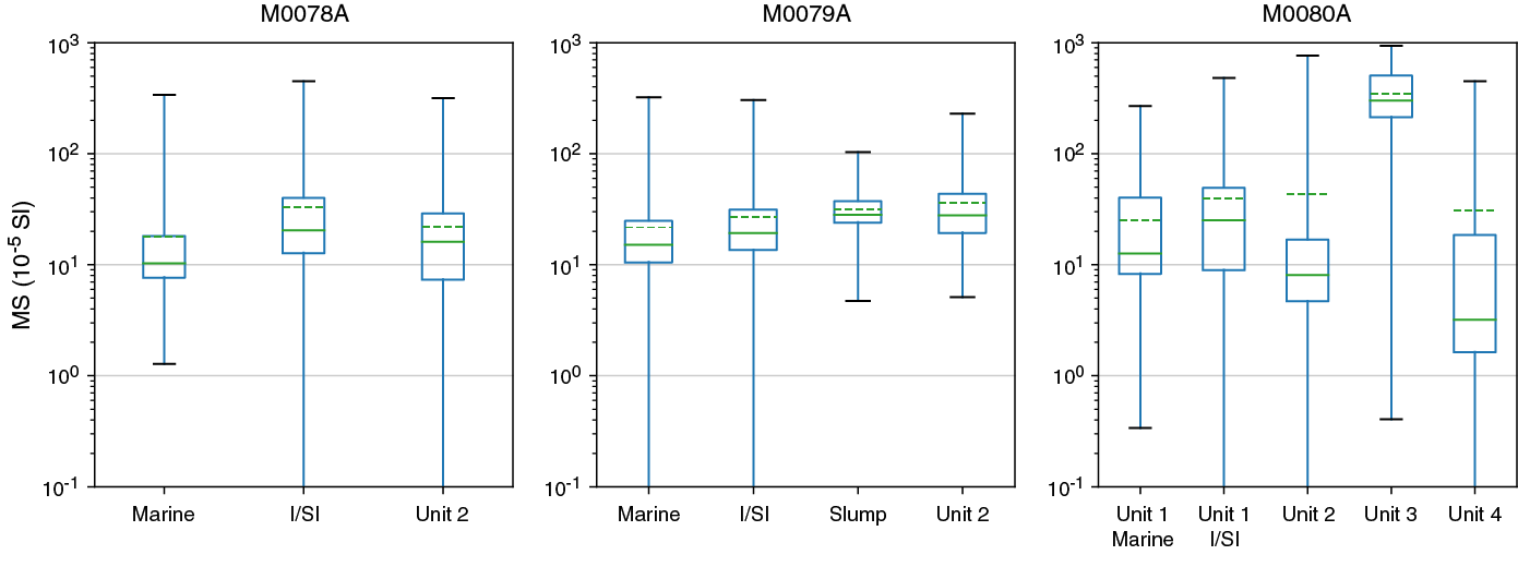
Figure F30. MSCL MS.
In the slumped subunit (484.48–506.40 mbsf), magnetic susceptibility varies from 4.7 × 10⁻⁵ to 103.30 × 10⁻⁵ SI with a mean of 31.86 × 10⁻⁵ SI. Magnetic susceptibility values are generally high for the greenish gray mud with homogeneous centimeter-thick gray mud beds (FA5) (e.g., 95, 160, and 260 mbsf) and interbedded mud–silt and centimeter-thick sand beds (FA11) (e.g., 38, 90, and 140 mbsf) compared with other facies associations (Figure F26). Magnetic susceptibility values sometimes drop below 0 SI. These values reflect sensor drift on some sections and are likely closer to 0.
P-wave velocity
P-wave velocity measurements for Hole M0079A were collected offshore using a Geotek MSCL and onshore on split cores using the MSCL track and on discrete samples with a Geotek P-wave logger for discrete samples (see Physical properties in the Expedition 381 methods chapter [McNeill et al., 2019b]).
The quality of the recovered cores strongly affected the quality of the P-wave velocity measurements. In Hole M0079A MSCL offshore data, realistic P-wave velocity values were only obtained in the upper few meters (0–10 mbsf), with values ranging between 1500 and 1600 m/s (Figure F31). Offshore MSCL measurements deeper than ~10 mbsf and onshore MSCL measurements were strongly affected by coring disturbances, variable fill space between the sediment and the core liner, cracks/voids in the core material, and/or the presence/absence of fluids in the core liner, so P-wave measurements were either not collected or were <1500 m/s and not considered realistic. Therefore, P-wave values >1500 m/s measured with the offshore MSCL are included on Figure F31, but no onshore MSCL data are plotted.
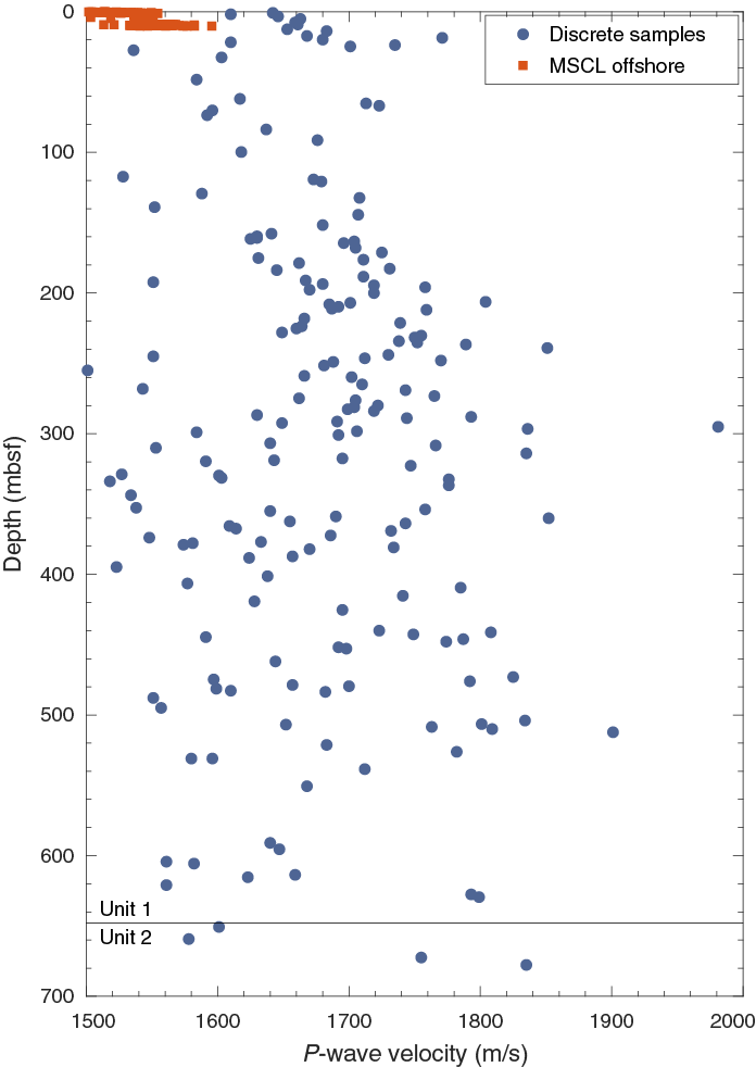
Figure F31. P-wave velocity data.
Onshore discrete sample P-wave velocity measurements for Hole M0079A provided a more realistic data set. From 0 to 10 mbsf, discrete velocity values are consistently higher than MSCL measurements, with values ranging between 1610 and 1663 m/s. Downhole to ~250 mbsf, these values agree with velocity values from sonic data acquired during downhole logging and with velocity values implied by core-log-seismic integration (CLSI) (see Downhole measurements and Core-log-seismic integration; Figures F45, F47). Deeper than ~250 mbsf, discrete P-wave velocity values vary between 1528 and 1851 m/s with an overall increasing trend and are lower than those evaluated by CLSI (Figure F47). The discrete velocity values are relatively low and imply limited compaction in this depth interval if they represent true values. It is more likely that P-wave signals deeper than ~250 mbsf were strongly affected by cracks in discrete samples induced by sampling (both by collection of the cores and by obtaining the discrete samples), potentially due to the increasing stiffness and brittle behavior of the sediment with depth (see also Core-log-seismic integration for velocity discussion).
Density
Gamma ray attenuation (GRA) bulk density values from offshore MSCL measurements range from 1.43 to 2.33 g/cm3 with an average of 1.97 g/cm3 (red, Figure F25), an average similar to that of Hole M0078A. Approximately 99% of the bulk density values are greater than 1.7 g/cm3, and only about 2% are greater than 2.2 g/cm3. Density gradually increases with depth with some intermittent intervals of decreasing density followed by a return to previous average values, which correlate with parts of the marine subunits (e.g., 149–158, 170–183, 266–270, 300–307, 395–405, and 524–543 mbsf), consistent with observations from Hole M0078A.
Bulk density from moisture and density (MAD) analysis of discrete samples has similar values and shows a similar trend to GRA bulk density (MAD black dots compared with MSCL red dots, Figure F25). MAD bulk density values range from 1.73 to 2.63 g/cm3 with an average of 1.98 g/cm3. All values are greater than 1.7 g/cm3, but only 0.4% of the values are greater than 2.2 g/cm3.
Sediment grain density ranges between 2.4 and 3.11 g/cm3 with an average of 2.7 g/cm3, and 97% of the values are between 2.6 and 2.8 g/cm3. These average and percentage values are slightly higher than those measured in Hole M0078A (0.1 g/cm3 and 4%, respectively). Grain density values are mostly between pure sandstone and pure limestone (Kennedy, 2015). Grain density generally increases with increasing bulk density and decreasing porosity, and, like bulk density, shows correlations of low grain density with some of the marine subunits, consistent with observations at Site M0078 (see Figure F29 in the Site M0078 chapter [McNeill et al., 2019d]; Figure F25).
Porosity
Porosity ranges from 58% to 17% with an average of 43%. Porosity decreases from an average of 50% in the upper 50 m of the hole to an average of 36% in the lower 50 m of the hole. Porosity values in the upper part of the hole are relatively high, consistent with the low bulk density and velocity. Relative increases in porosity occur at approximately 170–184, 260–280, 400–405, and 530–544 mbsf, and they mostly correlate with intervals of decreased bulk density in the marine subunits, similar to observations in Hole M0078A. An increase in porosity also occurs in the interval of slump deposits (Subunit 1-11; Figure F25).
Resistivity
The resistivity data in Hole M0079A were acquired both on cores with the MSCL and during downhole logging by both induction and dual induction tools (see Downhole measurements). As at Site M0078, MSCL electrical resistivity is low with a median resistivity value of 2.2 Ωm (Figure F25). It is compatible with the value derived from the Archie equation for porosity in the range of 35%–50% and fluid conductivity equal to that of seawater.
In the upper 50 m of the hole, MSCL resistivity increases linearly with depth from 0.5 to 2 Ωm (Figure F25). Resistivity stays constant at about 2 Ωm to the bottom of the hole but with larger excursions. It should be noted that these excursions are only seen in the MSCL data and not on the wireline logs, although their overall values are similar (see Downhole measurements; Figure F45).
Values are more scattered in the isolated/semi-isolated subunits than in the marine subunits in Unit 1 (Figure F25; also see whiskers in Figure F32), where large resistivity peaks regularly occur at the bases of cores (e.g., near 70, 285, and, in particular, 586 mbsf). The occurrence of these peaks is not correlated with specific facies associations (Figure F26).
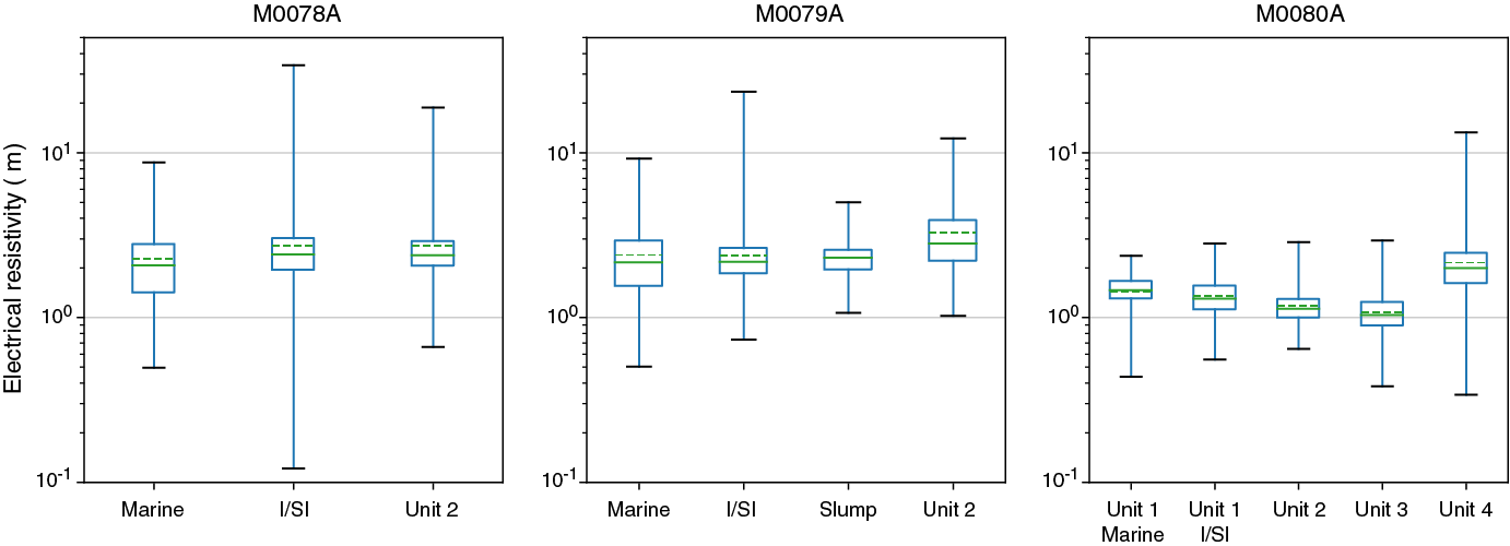
Figure F32. MSCL electrical resistivity.
Electrical resistivity is generally more stable/less variable in Unit 1 in the marine intervals than in the isolated/semi-isolated intervals (Figure F32). Noted increased instability occurs in Subunits 1-15 and 1-16 (Figure 25). Resistivity does not show major variation in the slumped subunit, but its median value increases in the deepest subunits of the hole. Unit 2 has generally slightly higher resistivity values relative to Unit 1 but the same electrical characteristics as the deepest subunits in Unit 1.
Thermal conductivity
Thermal conductivity data were not obtained from 0 to 140 mbsf (with the exception of one result at ~90 mbsf) because attempts to obtain measurements were unsuccessful, likely due to water content, cracks, compaction effects, or heterogeneous lithology. The measured thermal conductivity values range from 1.09 to 1.60 W/(m·K) with an average of 1.36 W/(m·K) (Figure F25). These measurements show variation in and between the marine and isolated/semi-isolated subunits but also a general increasing trend with depth. The measured laboratory values were also corrected to in situ conditions because thermal conductivity is affected by temperature and pressure (Hyndman et al., 1974). The corrected thermal conductivity values (following Hyndman et al., 1974) range from 1.14 to 1.69 W/(m·K) and show a similar trend to the original laboratory measurements (compare Figures F25 and F33C).
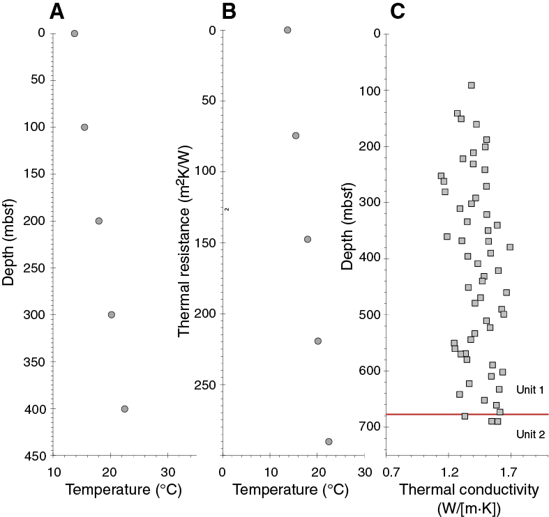
Figure F33. Temperature and thermal conductivity data.
Heat flow
In situ temperature measurements at five depths (four temperature CPT measurements and one seafloor measurement from an SVP) were collected offshore and plotted against depth to estimate the geothermal gradient (Figure F33A). The geothermal gradient is approximately 22°C/km, which is relatively low for a continental setting, particularly in a tectonically active region, but it is higher than the gradient calculated at Site M0078 (see Figure F39 in the Site M0078 chapter [McNeill et al., 2019d]).
The temperature data are used with thermal conductivity to estimate heat flow using the Bullard method, which involves plotting the thermal resistance against temperature (Figure F33B) and calculating heat flow from the slope of the best-fitting line (see Physical properties in the Expedition 381 methods chapter [McNeill et al., 2019b]). The heat flow calculated is ~31 mW/m2. This value is relatively low and may suggest that temperature is underestimated and should be further investigated.
Color reflectance
The mean values ± standard deviations and minimum/maximum color reflectance values from Hole M0079A (Figure F34) are 48 ± 5 and 7/78, respectively, for L*, −1.7 ± 0.8 and −10.3/2.4, respectively, for a*, and 3.9 ± 2.6 and −21/34, respectively, for b*.
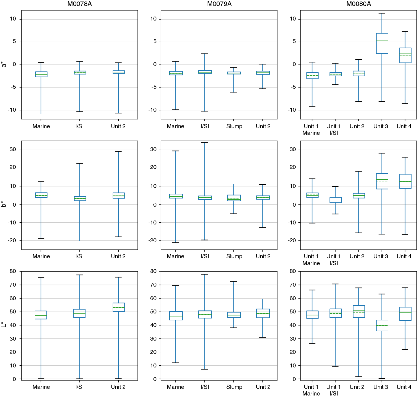
Figure F34. L*a*b* color reflectance data.
Color reflectance values change with depth in several intervals (Figure F25). In the upper part of the hole (0 to ~30 mbsf; Subunit 1-1), b* values are relatively high and decrease downhole and L* values are lower and less variable (mean = 44 ± 4; minimum/maximum = 27/58) compared with the entire hole (mean = 48 ± 5; minimum/maximum = 7/78) but a* values are similar to the rest of the hole. Changes in most other physical properties also occur in this 30 m thick uppermost interval/subunit (e.g., density, electrical resistivity, and velocity; Figure F25).
Additional changes in color reflectance values deeper than 30 mbsf occur mainly between the alternating marine and isolated/semi-isolated subunits in Unit 1 (Figures F25, F34). Marine subunits have slightly lower mean a* values and higher mean b* values (−1.9 and 4.5, respectively) compared with the mean a* and b* values in isolated/semi-isolated subunits (−1.6 and 3.6, respectively). L* values are similar although very slightly lower in the marine subunits, but greater scatter was observed for the isolated/semi-isolated subunits. The slumped interval in Unit 1 (Subunit 1-11) has color reflectance values (L* = 48, a* = −1.9, and b* = 3.4) that are lower for a* and b* than the average values for Unit 1 (L* = 48, a* = −1.7, and b* = 3.9) and do not match the values of either the marine or isolated/semi-isolated subunits.
Color reflectance values in Unit 2 are only slightly different when compared with the mean values for Unit 1 (Unit 2 mean L*, a*, and b* values of 49, −1.8, and 3.7, respectively, compared with Unit 1 mean values of 48, −1.7, and 3.9, respectively; Figure F34).
The observed change in mean values between the different subunits is also seen in color reflectance value changes associated with the dominant facies associations in each subunit, such as FA2 and FA3 in the isolated/semi-isolated subunits and FA6 in the marine subunits (Figure F26).
Paleomagnetism
Magnetic susceptibility
A total of 542 discrete samples from Hole M0079A were analyzed for magnetic susceptibility. Frequency distribution diagrams of magnetic susceptibility (k) from Hole M0079A discrete samples, together with shipboard MSCL continuous data collected at 2 cm intervals from whole cores, are shown in Figure F35. Discrete sample magnetic susceptibility in Hole M0079A shows a unimodal distribution peaking between 50 × 10−6 and 100 × 10−6 SI and values ranging between approximately 10 × 10−6 and 103 × 10−6 SI (Figure F36B, F36D). A similar trend is shown in MSCL susceptibility data, where the unimodal distribution peaks between 100 × 10−6 and 150 × 10−6 SI and values range between ~200 × 10−6 and 1000 × 10−6 SI (Figures F35B, F36E). The discrete sample susceptibility values are slightly lower compared with those from MSCL measurements on whole cores, which is likely due to the smaller volume and mass of the discrete samples. Downhole distribution of magnetic susceptibility in Hole M0079A shows a low variability between 0 and ~540 mbsf with values around ~100 × 10−6 SI (excluding a few outliers with higher or lower susceptibility) (Figure F36). Much higher variability occurs deeper than ~540 mbsf, where susceptibility spans two orders of magnitude from 10 × 10−6 to 1000 × 10−6 SI. This trend is much clearer when onshore discrete and MSCL continuous susceptibility data are plotted together against depth. The scatter in susceptibility values deeper than ~540 mbsf may suggest that sediment consolidation and dilution of one single magnetic component may not be the only factors controlling magnetic susceptibility. Other factors, including sediment provenance, magnetic grain size, and/or postdepositional precipitation of magnetic minerals, may contribute to such variability. The similar magnetic susceptibility and natural remanent magnetization (NRM) downhole variations (Figure F36A–F36D) seem to suggest that the variation in susceptibility is mainly (but not exclusively) controlled by the change in concentration of the magnetic phases in the sediment. In a few intervals, however, the increase in NRM does not correspond to an increase in susceptibility, suggesting the occurrence of mixtures of different magnetic minerals or a variable degree of drilling-induced magnetization. The relationship between NRM and susceptibility in Hole M0079A (Figure F37) is similar to that observed in Hole M0078A (see Figure F45 in the Site M0078 chapter [McNeill et al., 2019d]); however, in Hole M0079A, the presence of two linear trends is more marked. This pattern suggests the occurrence of two distinct magnetic minerals contributing to both NRM and magnetic susceptibility. In each trend, the variations of these two parameters are controlled primarily by the concentration of the magnetic minerals in the sediment. It seems likely that the steeper trend (green line) is associated with diagenetic greigite (Fe3S4) and the shallower trend (blue line) is associated with magnetite (Figure F37).
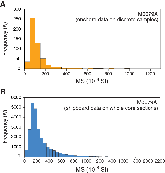
Figure F35. MS frequency distribution.
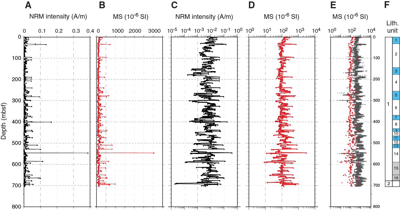
Figure F36. NRM intensity and MS.
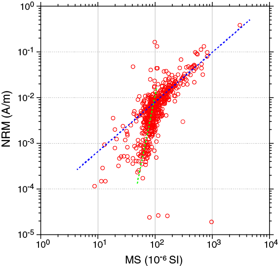
Figure F37. NRM intensity vs. MS.
Magnetic mineralogy
Thermal variation of the low-field magnetic susceptibility was determined for eight representative samples from Hole M0079A prior to the OSP (see Paleomagnetism in the Expedition 381 methods chapter [McNeill et al., 2019b] for more details). The results of the thermomagnetic experiments (Figure F38) reveal a wide range of Curie temperatures between 364° and 595°C. However, most of the samples show a primary Curie temperature between 502° and 585°C, which is typical of Ti-poor titanomagnetite. Other Curie temperatures between 365° and 486°C suggest the occurrence of Ti-rich titanomagnetite. The variable magnetic susceptibility of titanomagnetite and its occurrence in variable concentrations may be partly responsible for the observed downhole scatter in the magnetic susceptibility data.
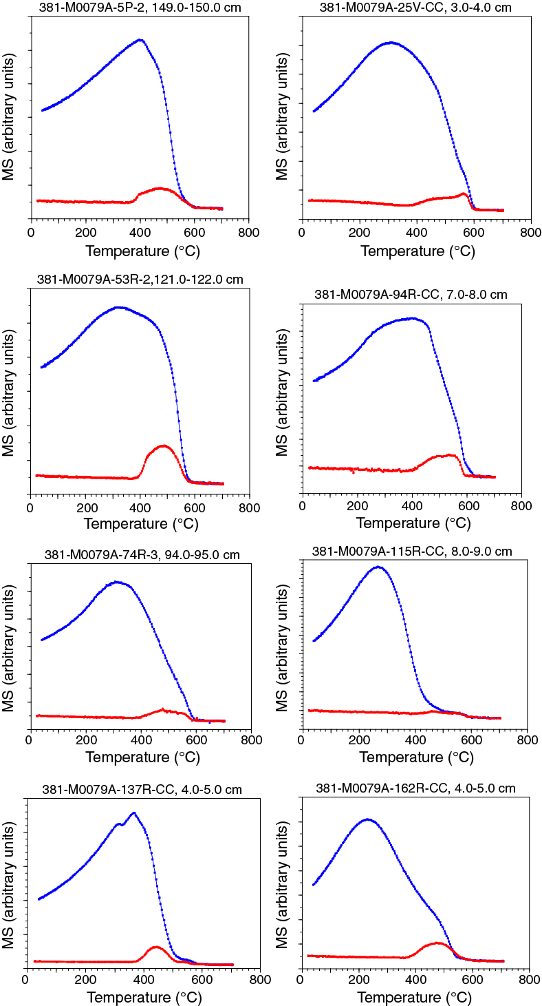
Figure F38. Low-field susceptibility vs. temperature experiment results.
Natural remanent magnetization
NRM direction and intensity of discrete samples were measured using the SRM 755–4000 cryogenic magnetometer (2G-Enterprises) at the University of Bremen (Germany). A total of 542 discrete cubic samples from Hole M0079A were analyzed. All samples were stepwise demagnetized by alternating fields (AFs) to determine the stability of the NRM during sequential demagnetization. Magnetization was measured after each demagnetization step, and in most of the samples it decays steadily to nearly complete removal at the maximum AF step of 100 mT (Figure F39A, F39B). This decay indicates the occurrence of low-coercivity magnetic minerals, such as magnetite or titanomagnetite. The shapes of the magnetization decay curves are typical of pseudosingle-domain grains. About 25% of the samples acquired a gyroremanent magnetization at AFs above 50–60 mT (Figure F39C, F39D). This spurious magnetization is typically acquired because of the occurrence of greigite. The magnetization of samples showing this behavior is therefore likely to be carried by a mixture of greigite, magnetite, and titanomagnetite, in agreement with what was inferred from the rock magnetic experiments shown in Figure F38. Greigite seems to occur more frequently in Hole M0079A than in Hole M0078A.
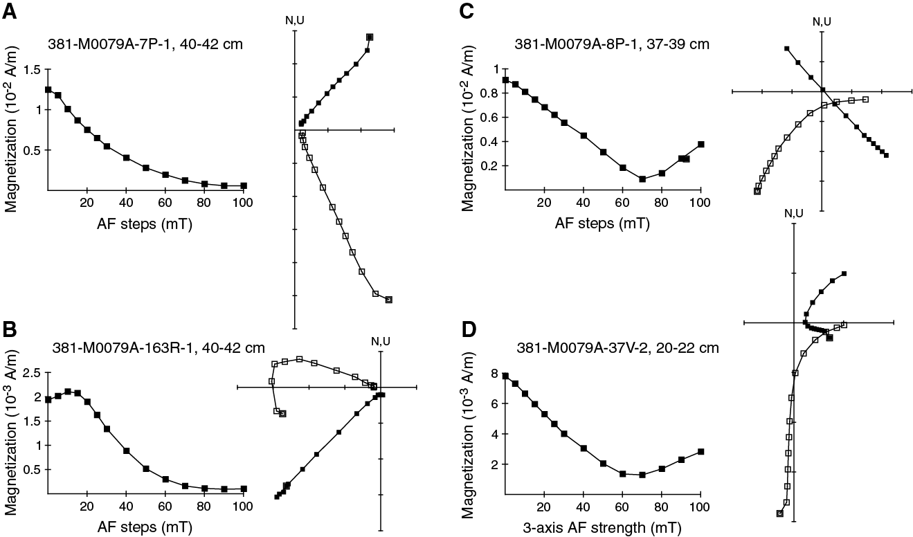
Figure F39. Orthogonal projections and relative decay paths.
Orthogonal demagnetization diagrams (Figure F39) show that demagnetizing fields of 10–15 mT are sufficient to remove the weak viscous remanent magnetization and other secondary components of magnetization. After the application of a 40 mT demagnetizing field, the majority of the samples (362 out of 542) show an inclination that is higher than expected (57.5°) for the site latitude (i.e., dots inside red circle, Figure F40). Out of these 362 samples, 87 show an inclination higher than 70°, which might be explained by the occurrence of a vertical drilling-induced magnetization that has partially overprinted the original magnetic remanence of the sample.
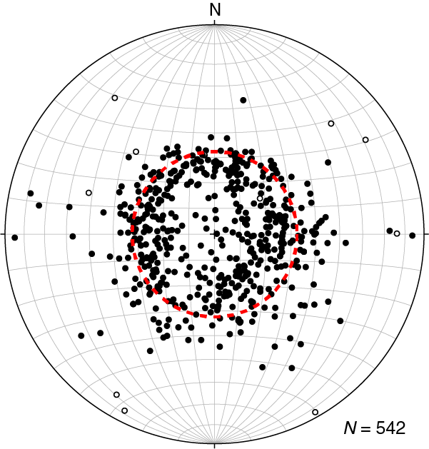
Figure F40. NRM directions.
The remanence direction after being demagnetized at 40 mT is parallel (within error) to the characteristic remanent magnetization (ChRM) computed on representative samples using standard principal component analysis. For this reason, we used the 40 mT step to build the magnetostratigraphy for Hole M0079A.
Slumping effect on remanence in Hole M0079A
Slumping appears to be quite pervasive at the base of lithostratigraphic Unit 1 in Hole M0079A (see Lithostratigraphy). To test the influence of slumping on the magnetic remanence stability of the Hole M0079A sediment, we performed a fold test on decimeter-scale folds in the interval most affected by slumping (Subunit 1-11). Two cubic samples were collected from the two limbs of a fold in Sections 381-M0079A-113R-2 (at 96–98 and 100–102 cm), 113R-3 (at 125–127 and 130–132 cm), and 114R-2 (at 58–60 and 64–66 cm) (Figure F41). The similar (within error) remanence directions after demagnetization at 40 mT in each fold indicate that the original magnetization may have been reset during or immediately after the slumping event because of remobilization of the sediment still rich in water. Soon after the slumping event, a new postdepositional remanent magnetization was acquired across the slumped beds. This test has important implications for the reliability of the remanence in the lowermost part of Hole M0079A. Based on this test, we assume that slumping has no effect on the remanence directions, and therefore these core intervals can still reliably be used to build the magnetostratigraphy for Hole M0079A.
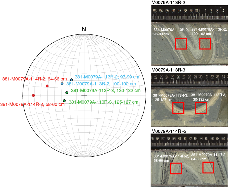
Figure F41. Fold test results.
Magnetostratigraphy
Figure F42 shows the inclination data (40 mT step) from Hole M0079A (interpreted to be indicative of the ChRM components) and a preliminary magnetostratigraphy for 200 m long intervals. These partial magnetostratigraphic logs are then combined into a composite magnetostratigraphy for the entire hole that is then tentatively compared with the geomagnetic instability timescale (GITS) of Singer (2014) (Figure F43). The polarity for the upper 665.95 m of Hole M0079A (to Sample 151R-2, 115–117 cm) is predominantly normal (i.e., positive inclinations). At 667.13 mbsf, the first sample with reversed polarity (Sample 152R-1, 23–25 cm) was observed, followed by a number of normal and reversed polarity samples to 692.43 mbsf. Because firm biostratigraphic constraints are absent from Hole M0079A, we can only speculate that the first reversed polarity sample at 667.13 mbsf may mark the Brunhes–Matuyama transition occurring at 0.773 Ma (Singer, 2014). According to this hypothesis, the location of the Brunhes/Matuyama boundary in Hole M0079A occurs just above the Unit 1/2 boundary, whereas in Hole M0078A it has been proposed to occur just below it (see Paleomagnetism in the Site M0078 chapter [McNeill et al., 2019d]).
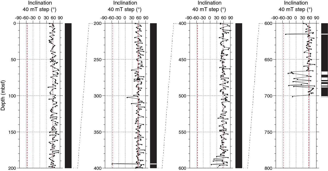
Figure F42. Inclination of remanence after demagnetization at 40 mT.
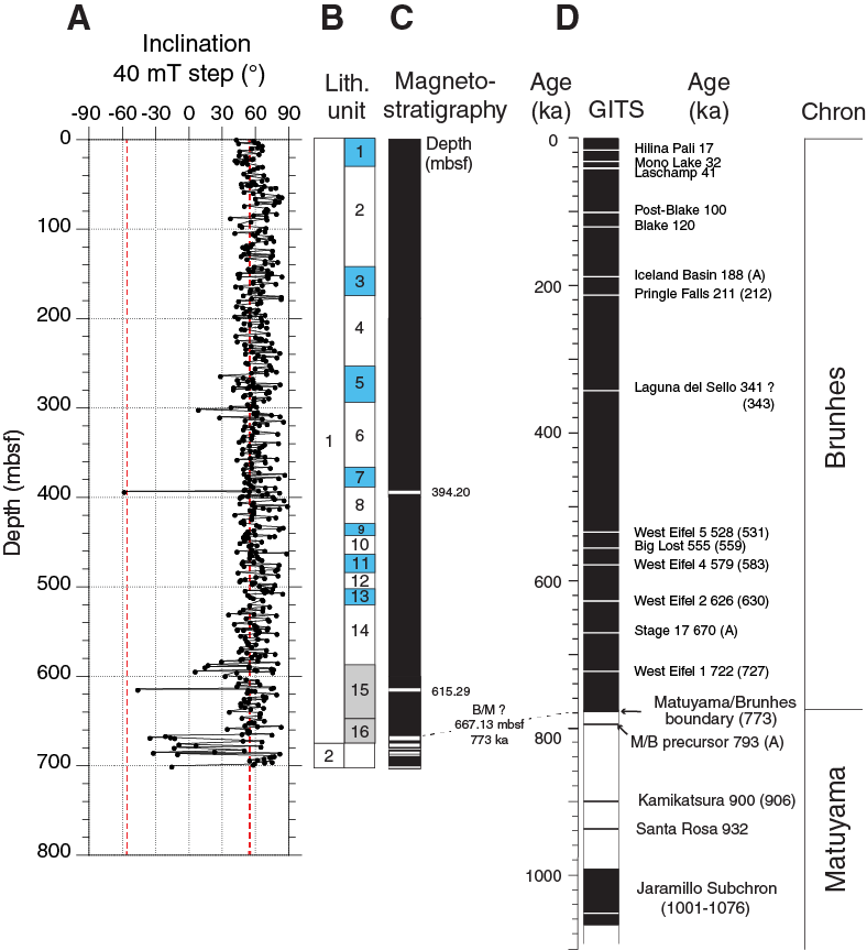
Figure F43. Composite magnetostratigraphy.
In the uppermost normal polarity interval (0–667.13 mbsf), two samples show a reversed polarity (negative inclination) with values consistent with the expected inclination of −57.5° (Figure F42A). These anomalous inclinations are marked with white lines in the magnetostratigraphic log in Figure F43C and may represent geomagnetic field excursions that occurred during the Brunhes Chron (Singer, 2014). Because firm biostratigraphic markers are absent from this hole, it is not possible at this stage to test whether this sample recorded one of the excursions of the Brunhes Chron. Additional rock magnetic experiments and other chronostratigraphic constraints will be necessary to establish which of these inclination changes are real magnetic field excursions and to test our preliminary interpretation.
Downhole measurements
At Site M0079, natural spectral gamma ray (ASGR512 tool) data were collected through the pipe over the full length of the hole. Magnetic susceptibility and conductivity (EM51 tool) were acquired in the open hole between ~220 and ~297 m WSF and between ~50 and ~230 m WSF, in two depth stages. Sonic (2PSA-1000 tool) data were acquired in the open hole between ~50 and ~230 m WSF, and dual laterolog resistivity (DLL3 tool) was acquired between ~50 and ~290 m WSF. Hole conditions and equipment problems prevented the acquisition of logging data at greater depths in the open hole. See Downhole measurements in the Expedition 381 methods chapter (McNeill et al., 2019b) for details on tools and acquisition parameters. Although the ranges in values are different, the collected logs compare well with MSCL data (Figures F44, F45).
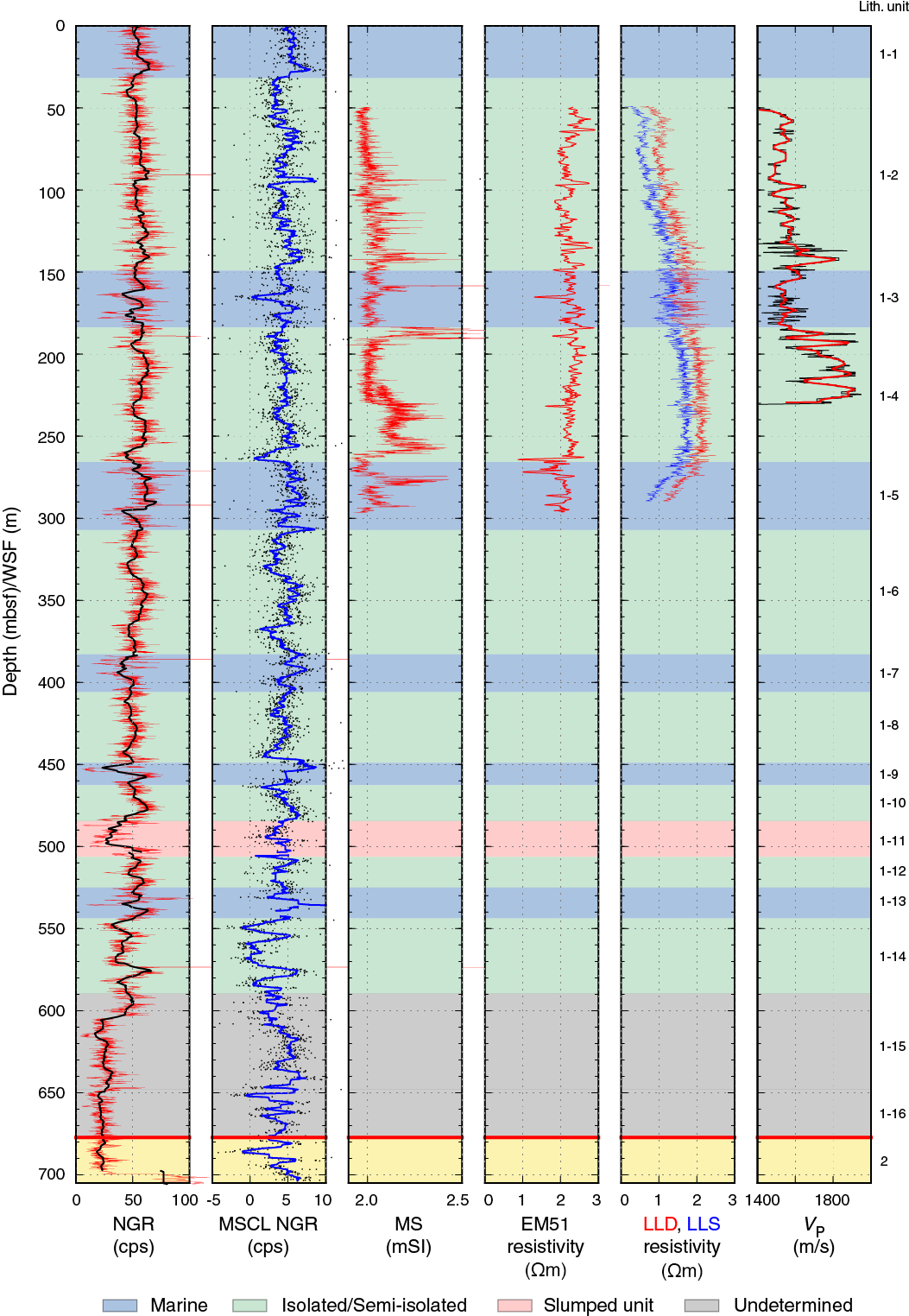
Figure F44. Downhole logging data and MSCL NGR.
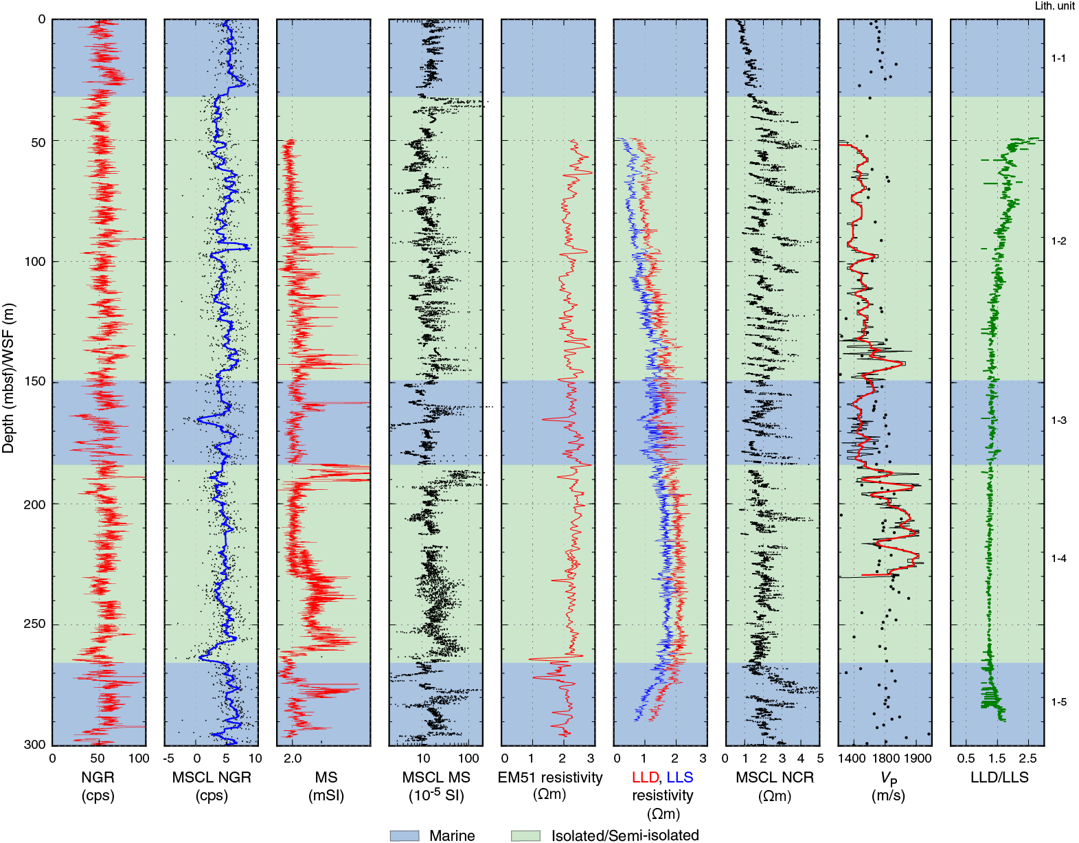
Figure F45. Downhole logging data, MSCL data, and discrete P-wave measurements.
Natural spectral gamma ray
Downhole gamma ray data collected through pipe can be used with NGR measured on cores to perform depth corrections and aid CLSI. Relatively low gamma ray counts from the cores compared with the downhole data can be interpreted to be a volume difference in the measured material (Figure F44). Even through the drill pipe, the logging tool is in situ and receives more gamma rays from the formation than the MSCL sensors receive from the ~6.7 cm diameter cores. The gamma ray log sharply decreases from 603 to 700 m WSF, averaging 24 counts/s in contrast to an average of 50 counts/s farther uphole. This signal attenuation is due to thicker drill collars used in the bottom ~100 m of the drill string. Between 700 and 704.9 m WSF, the tool measured in the open hole and the values here are consequently higher (>65 counts/s).
Going downhole, the upper 30 m of the hole (corresponding to a marine subunit) is characterized by an increase in gamma ray values from 50 to 60 counts/s. When transitioning to the first isolated/semi-isolated subunit at ~25 m WSF, gamma ray values decrease back to ~50 counts/s. Below this depth, in contrast to magnetic susceptibility (see below), the gamma ray log does not respond as clearly and consistently to marine and isolated/semi-isolated intervals, and the values vary between 40 and 60 counts/s throughout the rest of the hole. The sharp drop that occurs at 452 m WSF corresponds to an interval with low core recovery (e.g., Core 381-M0079A-106R; 30%) and could reflect a lithology emitting fewer gamma rays, an enlarged borehole reducing the volume of emitting material, or both. The slumped Subunit 1-11 (pink interval, Figure F44) shows a clear decrease in gamma ray values from >50 to ~25 counts/s. Below 605 m WSF, the thick collars of the drill string attenuate the signal, so values do not compare with NGR measured on cores.
Magnetic susceptibility
Downhole magnetic susceptibility values are lower than MSCL magnetic susceptibility values measured on cores, but the trend is similar (Figure F45). From 50 to 90 m WSF, the magnetic susceptibility signal has lower variability than was observed in core measurements. One explanation for this difference could be that the tool is in an oversized borehole and receives a weaker response from the formation. At greater depths in the hole, the magnetic susceptibility signal mirrors magnetic susceptibility derived from the core. As observed on cores, values tend to be lower and show less variability in marine subunits than in isolated/semi-isolated subunits.
Resistivity
Downhole resistivity was obtained from the DLL3 tool and calculated from the induction log of the EM51 tool. Overall, the resistivity recorded downhole is typically <3 Ωm, which is expected in this type of unconsolidated, fine-grained formation (Figure F45). Shallow resistivity (LLS) and deep resistivity (LLD) average 1.3 and 1.6 Ωm, respectively, whereas resistivity calculated from induction data averages 2.2 Ωm. Deep and shallow resistivity logs start at relatively lower values (0.5–1 Ωm) from 50 to 90 m WSF, progressively increase to 1.5–2.5 Ωm from 90 to 270 m WSF, and then decrease again from 270 to 290 m WSF. In addition to this trend, the deep and shallow resistivity curves drift apart in the upper and lower parts of the logged section. The LLD/LLS ratio is <1.5 in the main part of the logged section (100–270 m WSF), but it is >1.5 above 100 m WSF and below 270 m WSF. These observations most likely reflect borehole conditions, with a possible oversized hole from 50 to ~90 m WSF and from 270 to 290 m WSF, as also suggested by the magnetic susceptibility results. The induction log from the EM51 tool penetrated deeper in the formation and was less affected by borehole conditions; indeed, its overall trend is more stable than those from the DLL3 tool. Resistivity logs from the induction and DLL3 tools exhibit similar meter- to decimeter-scale variability, and their trends compare well with the MSCL noncontact electrical resistivity (NCR) measured on cores. Comparisons of the downhole and MSCL data suggest that the resistivity increases observed in the MSCL data from individual cores relate to changes in properties caused by the coring process and not in situ properties.
Sonic
Sonic data also support the interpretation that the borehole has a larger diameter from 50 to 90 m WSF; velocity values are close to 1500 m/s, which is lower than the velocity values measured on discrete samples. Note, however, that the quality of the collected signal led to uncertainties in first arrival picking (see manual picking compared with semblance, Figure F46) and consequently in the velocity calculation. The general trend is likely realistic, but values might not represent true formation velocity, notably from 125 to 150 m WSF, from 160 to 165 m WSF, and below 190 m WSF, where the first arrival of the acoustic signal was not observed as clearly as in the rest of the logged interval. In addition, physical properties measured on cores (density, porosity, and shear strength; see Physical properties) suggest that this part of the borehole has relatively low velocity. Below 100 m WSF, velocity values increase to ~1800 m/s at 142 m WSF, decrease again to ~1500 m/s when entering Subunit 1-3 (marine), and increase again to 1700–1900 m/s in Subunit 1-4 (isolated/semi-isolated). Higher velocity values are consistent with other physical properties; these intervals have a higher bulk density and a lower porosity than the marine intervals. The drop in values at ~220 m WSF matches a low recovery interval (Cores 381-M0079A-56R and 57R) and could correspond to a larger borehole that limited the propagation of the acoustic pulse. Interpretation of velocity data is further developed in Core-log-seismic integration.
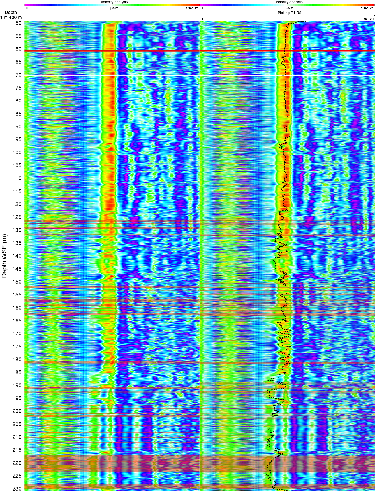
Figure F46. Sonic semblance compared with manual picking.
Core-log-seismic integration
CLSI at Site M0079 incorporated MSCL density measurements, new velocity information from downhole logging in the upper part of the hole and measurements on discrete samples, a pre-expedition linear velocity model, and the primary seismic profile Maurice Ewing Line 41 (Figure F2).
Velocity data integration
Downhole sonic velocity data were acquired between ~50 and 225 m WSF in Hole M0079A and were incorporated into the input velocity model for synthetics generation. Figure F47 presents a compilation of all available velocity information in Hole M0079A, including a linear velocity model from seismic data, the velocity model from offshore CLSI, downhole logging measurements, and onshore measurements on discrete samples. Remarkable agreement occurs between the latter three data sets, particularly between the velocity model from offshore CLSI (which did not use any logging data) and the downhole sonic log. Both suggest rather low VP values of around 1540–1580 m/s on average at 60–180 mbsf, which are potentially due to the high porosity of the shallow sediment (Figure F25). The discrete VP measurements have a similar range of values and match the preliminary synthetic model in the upper ~225 mbsf. Deeper than ~225 mbsf, unlike other data sets, the discrete values do not increase with depth. Given the prevalence of cracks in discrete samples (see Physical properties), the unconfined discrete measurements can be expected to yield low VP values, whereas velocity values recorded in situ increase with depth because of closing of fractures and compaction.
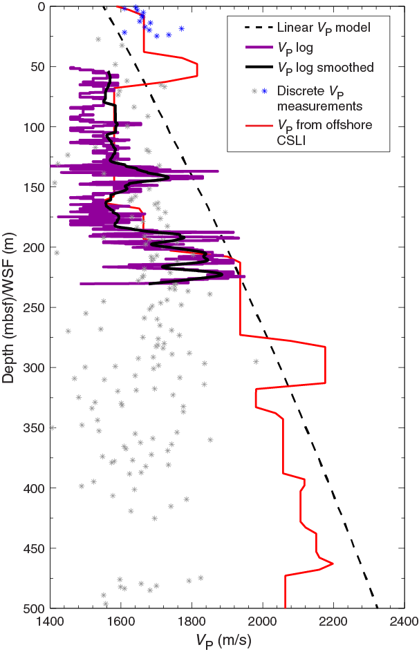
Figure F47. VP data.
To maximize the use of available VP measurements for synthetics generation, the following combination of input data sets was utilized: a 7-point average of discrete velocity data in the top 25 m of Hole M0079A, linearly interpolated values from discrete samples to downhole logging sonic data between 25 and 50 mbsf to avoid introducing sharp artificial changes between data sets, and then smoothed sonic log data from 50 to 220 mbsf. Deeper than 220 mbsf, where no further new velocity information was available, the velocity model developed by offshore CLSI was used (Table T15). Alternative smoothing windows for the downhole VP log were tested, but in all cases the resulting synthetic seismograms had multiple bright reflectors corresponding to VP variability in the 190–220 mbsf interval that were not observed in the seismic data. For the synthetics presented and discussed below, all VP values <1500 m/s were removed and a 10 m wide smoothing window was used, which allowed the preservation of major velocity contrasts but eliminated meter-scale variations attributed to poor borehole conditions that resulted in challenging picking of velocity logs (see Downhole measurements). The resulting velocity profile is in Table T15. The density profile for synthetics generation was produced from filtered and smoothed MSCL data depth shifted to sea level (Table T16) (see Core-log-seismic integration in the Expedition 381 methods chapter [McNeill et al., 2019b]).
Synthetic-to-seismic comparison
The synthetic seismogram at Site M0079 was tied to the seismic data with moderate adjustments to the initial velocity profile (Figure F48). The high-amplitude reflectors in synthetics seismograms associated with subunits in lithostratigraphic Unit 1 match well with the seismic data. Reproducing lower reflectivity features in the seismic reflection data between the high-reflectivity sequences proved to be more challenging because of a combination of the lack of impedance contrasts in core physical properties in some intervals and strong impedance contrasts introduced by the downhole data between 1250 and 1450 ms two-way traveltime (TWT).
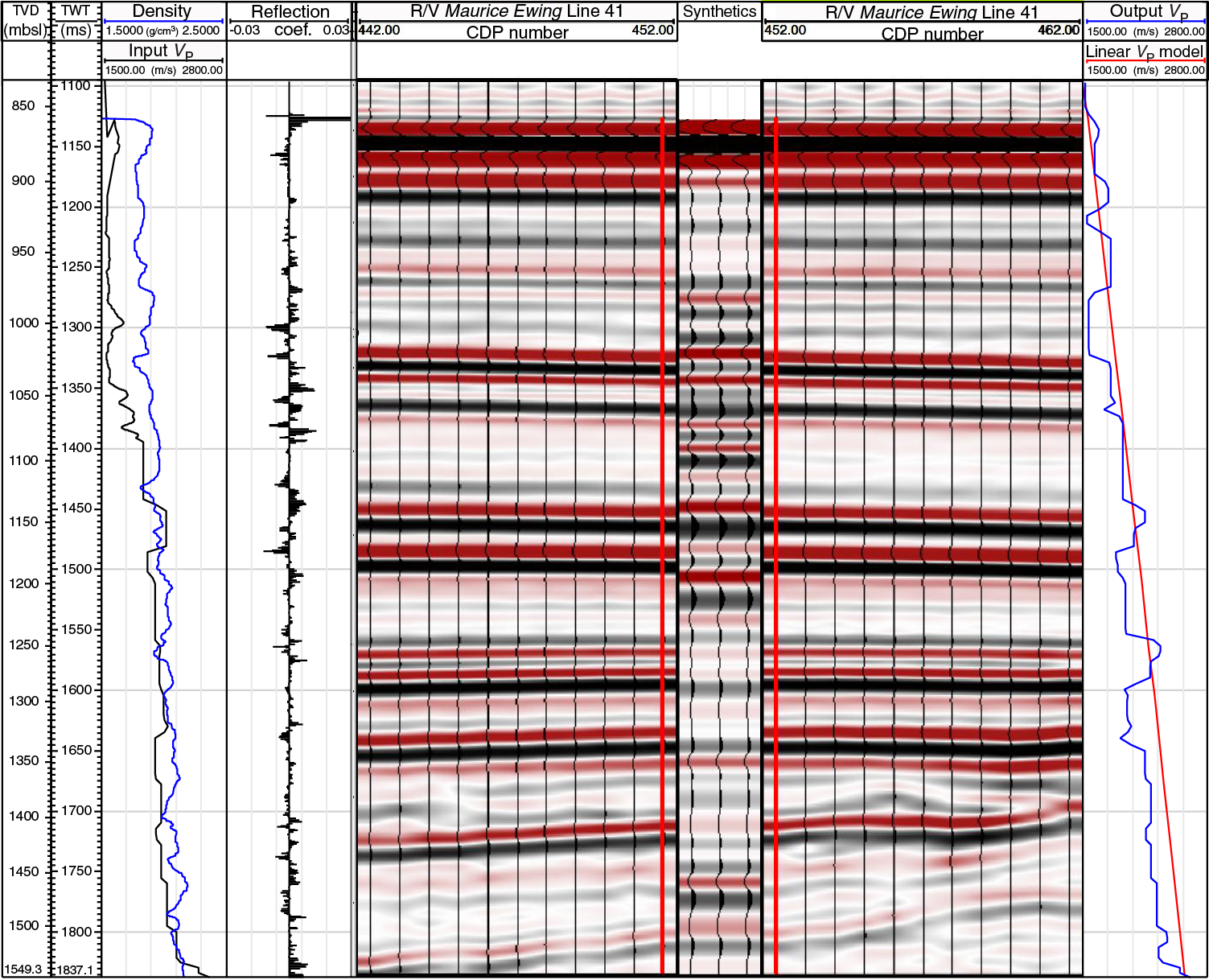
Figure F48. Synthetic seismogram.
The output velocity profile from the synthetics generation (Table T17) suggests that VP deviates from the pre-expedition linear velocity model (see Core-log-seismic integration in the Expedition 381 methods chapter [McNeill et al., 2019b]) toward predominantly lower velocity values. Velocity values appear to increase in some marine subunits (Figure F49), possibly consistent with increasing shear strength in these intervals (Figure F25). The resulting time-depth relationship (TDR) (Figure F50) is listed for the main horizons in Table T18 (the full TDR table is available in M0079_TDR.xlsx in CLSI in Supplementary material).
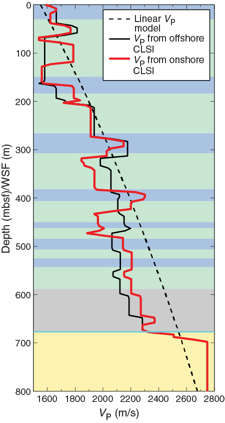
Figure F49. Onshore CLSI VP profile and offshore CLSI results.
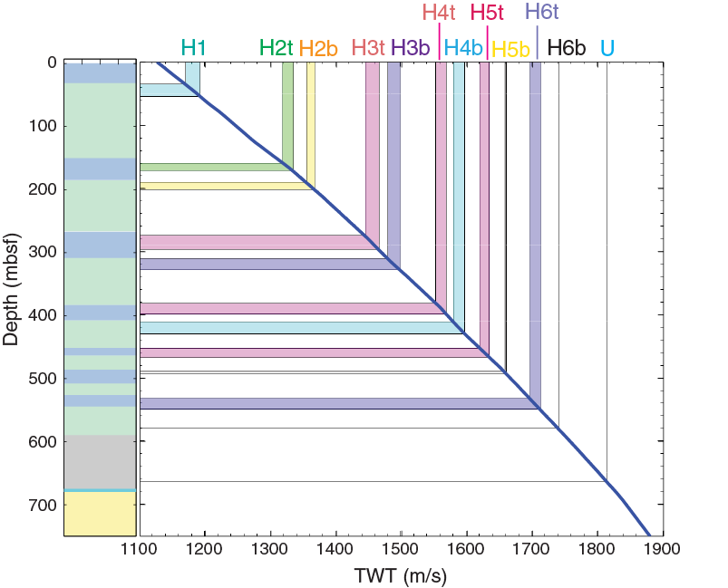
Figure F50. Time-depth conversion function.
The TDR established with synthetic seismograms at Site M0079 allows for direct comparison of major lithologic boundaries identified in the cores with the seismic data. Figure F51 shows a section of the seismic profile crossing Site M0079, the synthetic traces, and lithostratigraphic unit and subunit boundaries. Similar to Site M0078, high-reflectivity horizons in the seismic profile clearly correspond to the marine subunits in the core, confirming the prior interpretation by Nixon at el. (2016) and others. However, the subunit boundaries predominantly map onto the first break, not the peak, of a given seismic reflection, and the depth to individual subunits was therefore previously overestimated in the seismic record (Figures F50, F51). In the deeper part of Unit 1 (e.g., Subunits 1-8 through 1-14), the relationship between reflections and marine subunits is more complex, likely due to the small thicknesses of these subunits. The Unit 1/2 boundary depth is underestimated in the seismic data, and the bright horizon interpreted to be the boundary may instead correspond to the last marine transition in Unit 1. However, this level of detail is beyond the resolution of the seismic data, which at Site M0079 is estimated to be roughly ~20 m.
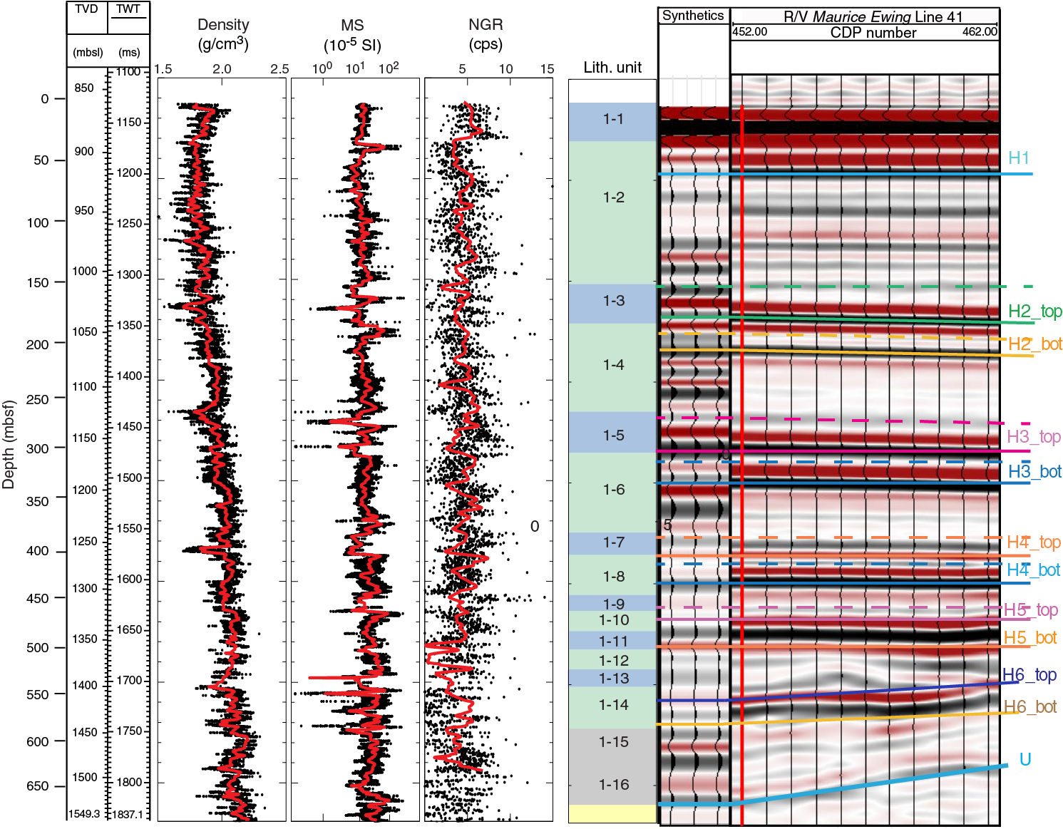
Figure F51. MSCL data converted to time with synthetic and seismic data.
References
Anthonissen, D.E., and Ogg, J.G., 2012. Appendix 3—Cenozoic and Cretaceous biochronology of planktonic foraminifera and calcareous nannofossils. In Gradstein, F.M., Ogg, J.G., Schmitz, M.D., and Ogg, G.M., (Eds.), The Geologic Time Scale 2012: Amsterdam (Elsevier), 1083–1127. https://doi.org/10.1016/B978-0-444-59425-9.15003-6
Backman, J., Raffi, I., Rio, D., Fornaciari, E., and Pälike, H., 2012. Biozonation and biochronology of Miocene through Pleistocene calcareous nannofossils from low and middle latitudes. Newsletters on Stratigraphy, 45(3):221–244. https://doi.org/10.1127/0078-0421/2012/0022
Bell, R.E., McNeill, L.C., Bull, J.M., Henstock, T.J., Collier, R.E.L., and Leeder, M.R., 2009. Fault architecture, basin structure and evolution of the Gulf of Corinth Rift, central Greece. Basin Research, 21(6):824–855. https://doi.org/10.1111/j.1365-2117.2009.00401.x
Berner, R.A., 1980. Early Diagenesis: A Theoretical Approach: Princeton, NJ (Princeton University Press).
Capotondi, L., Girone, A., Lirer, F., Bergami, C., Verducci, M., Vallefuoco, M., Afferri, A., Ferraro, L., Pelosi, N., and De Lange, G.J., 2016. Central Mediterranean mid-Pleistocene paleoclimatic variability and its association with global climate. Palaeogeography, Palaeoclimatology, Palaeoecology, 442:72–83. https://doi.org/10.1016/j.palaeo.2015.11.009
Cvetkoska, A., Jovanovska, E., Francke, A., Tofilovska, S., Vogel, H., Levkov, Z., Donders, T.H., Wagner, B., and Wagner-Cremer, F., 2016. Ecosystem regimes and responses in a coupled ancient lake system from MIS 5b to present: the diatom record of lakes Ohrid and Prespa. Biogeosciences, 13(10):3147–3162. https://doi.org/10.5194/bg-13-3147-2016
Cvetkoska, A., Reed, J.M., and Levkov, Z., 2012. Diatoms as indicators of environmental change in ancient Lake Ohrid during the last glacial–interglacial cycle (ca. 140 ka). In Witkowski, A. (Ed.), Diatom Monographs: Königstein, Germany (Koeltz Scientific Books).
Diz, P., and Francés, G., 2008. Distribution of live benthic foraminifera in the Ría de Vigo (NW Spain). Marine Micropaleontology, 66(3–4):165–191. https://doi.org/10.1016/j.marmicro.2007.09.001
Duchemin, G., Fontanier, C., Jorissen, F.J., Barras, C., and Griveaud, C., 2007. Living small-sized (63–150 µm) foraminifera from the mid-shelf to mid-slope environments in the Bay of Biscay. Journal of Foraminiferal Research, 37(1):12–32. https://doi.org/10.2113/gsjfr.37.1.12
Fontanier, C., Jorissen, F.J., Chaillou, G., David, C., Anschutz, P., and Lafon, V., 2003. Seasonal and interannual variability of benthic foraminiferal faunas at 550 m depth in the Bay of Biscay. Deep-Sea Research, Part I: Oceanographic Research Papers, 50(4):457–494. https://doi.org/10.1016/S0967-0637(02)00167-X
Ford, M., Rohais, S., Williams, E.A., Bourlange, S., Jousselin, D., Backert, N., and Malartre, F., 2013. Tectono-sedimentary evolution of the western Corinth Rift (central Greece). Basin Research, 25(1):3–25. https://doi.org/10.1111/j.1365-2117.2012.00550.x
Ford, M., Williams, E.A., Malartre, F., and Popescu, S.-M., 2007. Stratigraphic architecture, sedimentology and structure of the Vouraikos Gilbert-type fan delta, Gulf of Corinth, Greece. In Nichols, G., Paola, C., and Williams, E. (Eds.), Sedimentary Processes, Environments and Basins: A Tribute to Peter Friend. Jarvis, I. (Series Ed.). Special Publication of the International Association of Sedimentologists, 38:44–90. https://doi.org/10.1002/9781444304411.ch4
Froelich, P.N., Klinkhammer, G.P., Bender, M.L., Luedtke, N.A., Heath, G.R., Cullen, D., Dauphin, P., Hammond, D., Hartman, B., and Maynard, V., 1979. Early oxidation of organic matter in pelagic sediments of the eastern equatorial Atlantic: suboxic diagenesis. Geochimica et Cosmochimica Acta, 43(7):1075–1090. https://doi.org/10.1016/0016-7037(79)90095-4
Goineau, A., Fontanier, C., Jorissen, F.J., Lansard, B., Buscail, R., Mouret, A., Kerhervé, P., et al., 2011. Live (stained) benthic foraminifera from the Rhône prodelta (Gulf of Lion, NW Mediterranean): environmental controls on a river-dominated shelf. Journal of Sea Research, 65(1):58–75. https://doi.org/10.1016/j.seares.2010.07.007
Goineau, A., Fontanier, C., Mojtahid, M., Fanget, A.-S., Bassetti, M.-A., Berné, S., and Jorissen, F., 2015. Live–dead comparison of benthic foraminiferal faunas from the Rhône prodelta (Gulf of Lions, NW Mediterranean): development of a proxy for palaeoenvironmental reconstructions. Marine Micropaleontology, 119:17–33. https://doi.org/10.1016/j.marmicro.2015.07.002
Houk, V., Klee, R., and Tanaka, H., 2010. Atlas of Freshwater Centric Diatoms with a Brief Key and Descriptions: Part 3. Stephanodiscaceae A. Cyclotella, Tertiarius, Discostella: Praha, Czech Republic (Czech Phycological Society).
Hyndman, R.D., Erickson, A.J., and Von Herzen, R.P., 1974. Geothermal measurements on DSDP Leg 26. In Davies, T.A., Luyendyk, B.P., et al., Initial Reports of the Deep Sea Drilling Project, 26: Washington, DC (U.S. Govt. Printing Office), 451–463. https://doi.org/10.2973/dsdp.proc.26.113.1974
Kennedy, M. (Ed.), 2015. Developments in Petroleum Science (Volume 62): Practical Petrophysics. Cubitt, J. (Series Ed.): Amsterdam (Elsevier).
Kouli, K., Brinkhuis, H., and Dale, B., 2001. Spiniferites cruciformis: a fresh water dinoflagellate cyst? Review of Palaeobotany and Palynology, 113(4):273–286. https://doi.org/10.1016/S0034-6667(00)00064-6
Krammer, K., and Lange-Bertalot, H., 1991. Bacillariophyceae, Part 3. Centrales, Fragilariaceae, Eunotiaceae. In Ettl, H., Gerloff, J., Heynig, H., and Mollenhauer, D. (Eds.), Süßwaserflora von Mitteleuropa (Volume 2/3): Stuttgart, Germany (Gustav Fischer Verlag).
Martini, E., 1971. Standard Tertiary and Quaternary calcareous nannoplankton zonation. In Farinacci, A. (Ed.), Proceedings of the Second Planktonic Conference, Roma 1970: Rome (Edizioni Tecnoscienza), 2:739–785.
McNeill, L.C., Shillington, D.J., Carter, G.D.O., Everest, J.D., Le Ber, E., Collier, R.E.Ll., Cvetkoska, A., De Gelder, G., Diz, P., Doan, M.-L., Ford, M., Gawthorpe, R.L., Geraga, M., Gillespie, J., Hemelsdaël, R., Herrero-Bervera, E., Ismaiel, M., Janikian, L., Kouli, K., Li, S., Machlus, M.L., Maffione, M., Mahoney, C., Michas, G., Miller, C., Nixon, C.W., Oflaz, S.A., Omale, A.P., Panagiotopoulos, K., Pechlivanidou, S., Phillips, M.P., Sauer, S., Seguin, J., Sergiou, S., and Zakharova, N.V., 2019a. Expedition 381 facies associations. In McNeill, L.C., Shillington, D.J., Carter, G.D.O., and the Expedition 381 Participants, Corinth Active Rift Development. Proceedings of the International Ocean Discovery Program, 381: College Station, TX (International Ocean Discovery Program). https://doi.org/10.14379/iodp.proc.381.103.2019
McNeill, L.C., Shillington, D.J., Carter, G.D.O., Everest, J.D., Le Ber, E., Collier, R.E.Ll., Cvetkoska, A., De Gelder, G., Diz, P., Doan, M.-L., Ford, M., Gawthorpe, R.L., Geraga, M., Gillespie, J., Hemelsdaël, R., Herrero-Bervera, E., Ismaiel, M., Janikian, L., Kouli, K., Li, S., Machlus, M.L., Maffione, M., Mahoney, C., Michas, G., Miller, C., Nixon, C.W., Oflaz, S.A., Omale, A.P., Panagiotopoulos, K., Pechlivanidou, S., Phillips, M.P., Sauer, S., Seguin, J., Sergiou, S., and Zakharova, N.V., 2019b. Expedition 381 methods. In McNeill, L.C., Shillington, D.J., Carter, G.D.O., and the Expedition 381 Participants, Corinth Active Rift Development. Proceedings of the International Ocean Discovery Program, 381: College Station, TX (International Ocean Discovery Program). https://doi.org/10.14379/iodp.proc.381.102.2019
McNeill, L.C., Shillington, D.J., Carter, G.D.O., Everest, J.D., Le Ber, E., Collier, R.E.Ll., Cvetkoska, A., De Gelder, G., Diz, P., Doan, M.-L., Ford, M., Gawthorpe, R.L., Geraga, M., Gillespie, J., Hemelsdaël, R., Herrero-Bervera, E., Ismaiel, M., Janikian, L., Kouli, K., Li, S., Machlus, M.L., Maffione, M., Mahoney, C., Michas, G., Miller, C., Nixon, C.W., Oflaz, S.A., Omale, A.P., Panagiotopoulos, K., Pechlivanidou, S., Phillips, M.P., Sauer, S., Seguin, J., Sergiou, S., and Zakharova, N.V., 2019c. Expedition 381 summary. In McNeill, L.C., Shillington, D.J., Carter, G.D.O., and the Expedition 381 Participants, Corinth Active Rift Development. Proceedings of the International Ocean Discovery Program, 381: College Station, TX (International Ocean Discovery Program). https://doi.org/10.14379/iodp.proc.381.101.2019
McNeill, L.C., Shillington, D.J., Carter, G.D.O., Everest, J.D., Le Ber, E., Collier, R.E.Ll., Cvetkoska, A., De Gelder, G., Diz, P., Doan, M.-L., Ford, M., Gawthorpe, R.L., Geraga, M., Gillespie, J., Hemelsdaël, R., Herrero-Bervera, E., Ismaiel, M., Janikian, L., Kouli, K., Li, S., Machlus, M.L., Maffione, M., Mahoney, C., Michas, G., Miller, C., Nixon, C.W., Oflaz, S.A., Omale, A.P., Panagiotopoulos, K., Pechlivanidou, S., Phillips, M.P., Sauer, S., Seguin, J., Sergiou, S., and Zakharova, N.V., 2019d. Site M0078. In McNeill, L.C., Shillington, D.J., Carter, G.D.O., and the Expedition 381 Participants, Corinth Active Rift Development. Proceedings of the International Ocean Discovery Program, 381: College Station, TX (International Ocean Discovery Program). https://doi.org/10.14379/iodp.proc.381.104.2019
Mudie, P.J., Marret, F., Mertens, K.N., Shumilovskikh, L., and Leroy, S.A.G., 2017. Atlas of modern dinoflagellate cyst distributions in the Black Sea Corridor: from Aegean to Aral Seas, including Marmara, Black, Azov and Caspian Seas. Marine Micropaleontology, 134. https://doi.org/10.1016/j.marmicro.2017.05.004
Nixon, C.W., McNeill, L.C., Bull, J.M., Bell, R.E., Gawthorpe, R.L., Henstock, T.J., Christodoulou, D., et al., 2016. Rapid spatiotemporal variations in rift structure during development of the Corinth Rift, central Greece. Tectonics, 35(5):1225–1248. https://doi.org/10.1002/2015TC004026
Nolet, G.J., and Corliss, B.H., 1990. Benthic foraminiferal evidence for reduced deep-water circulation during sapropel deposition in the eastern Mediterranean. Marine Geology, 94(1–2):109–130. https://doi.org/10.1016/0025-3227(90)90106-T
Phillips, M.P., and Harwood, D.M., 2017. Marine diatom assemblage variation across Pleistocene glacial–interglacial transitions from Integrated Ocean Drilling Program Site C9001, Northwest Pacific. Palaeogeography, Palaeoclimatology, Palaeoecology, 483:172–187. https://doi.org/10.1016/j.palaeo.2016.07.040
Pujol, C., and Vergnaud Grazzini, C., 1995. Distribution patterns of live planktic foraminifers as related to regional hydrography and productive systems of the Mediterranean Sea. Marine Micropaleontology, 25(2–3):187–217. https://doi.org/10.1016/0377-8398(95)00002-I
Raffi, I., Backman, J., Fornaciari, E., Pälike, H., Rio, D., Lourens, L., and Hilgen, F., 2006. A review of calcareous nannofossil astrobiochronology encompassing the past 25 million years. Quaternary Science Reviews, 25(23–24):3113–3137. https://doi.org/10.1016/j.quascirev.2006.07.007
Reed, J.M., Cvetkoska, A., Levkov, Z., Vogel, H., and Wagner, B., 2010. The last glacial-interglacial cycle in Lake Ohrid (Macedonia/Albania): testing diatom response to climate. Biogeosciences, 7(10):3083–3094. https://doi.org/10.5194/bg-7-3083-2010
Rohling, E.J., and Gieskes, W.W.C., 1989. Late Quaternary changes in Mediterranean intermediate water density and formation rate. Paleoceanography and Paleoclimatology, 4(5):531. https://doi.org/10.1029/PA004i005p00531
Rohling, E.J., Jorissen, F.J., Vergnaud Grazzini, C., and Zachariasse, W.J., 1993. Northern Levantine and Adriatic Quaternary planktic foraminifera; reconstruction of paleoenvironmental gradients. Marine Micropaleontology, 21(1–3):191–218. https://doi.org/10.1016/0377-8398(93)90015-P
Sakellariou, D., Lykousis, V., Alexandri, S., Kaberi, H., Rousakis, G., Nomikou, P., Georgiou, P., and Ballas, D., 2007. Faulting, seismic-stratigraphic architecture and Late Quaternary evolution of the Gulf of Alkyonides Basin–East Gulf of Corinth, Central Greece. Basin Research, 19(2):273–295. https://doi.org/10.1111/j.1365-2117.2007.00322.x
Singer, B.S., 2014. A Quaternary geomagnetic instability time scale. Quaternary Geochronology, 21:29–52. https://doi.org/10.1016/j.quageo.2013.10.003
Skourtsos, E., and Kranis, H., 2009. Structure and evolution of the western Corinth Rift, through new field data from the northern Peloponnesus. In Ring, U., and Wernicke, B. (Eds.), Extending a Continent: Architecture, Rheology and Heat Budget. Geological Society Special Publication, 321(1):119–138. https://doi.org/10.1144/SP321.6
Taylor, B., Weiss, J.R., Goodliffe, A.M., Sachpazi, M., Laigle, M., and Hirn, A., 2011. The structures, stratigraphy and evolution of the Gulf of Corinth Rift, Greece. Geophysical Journal International, 185(3):1189–1219. https://doi.org/10.1111/j.1365-246X.2011.05014.x
Thierstein, H.R., Geitzenauer, K.R., Molfino, B., and Shackleton, N.J., 1977. Global synchroneity of late Quaternary coccolith datum levels validation by oxygen isotopes. Geology, 5(7):400–404. https://doi.org/10.1130/0091-7613(1977)5<400:GSOLQC>2.0.CO;2
Van Dam, H., Mertens, A., and Sinkeldam, J., 1994. A coded checklist and ecological indicator values of freshwater diatoms from The Netherlands. Netherland Journal of Aquatic Ecology, 28(1):117–133. https://doi.org/10.1007/BF02334251
1 McNeill, L.C., Shillington, D.J., Carter, G.D.O., Everest, J.D., Le Ber, E., Collier, R.E.Ll., Cvetkoska, A., De Gelder, G., Diz, P., Doan, M.-L., Ford, M., Gawthorpe, R.L., Geraga, M., Gillespie, J., Hemelsdaël, R., Herrero-Bervera, E., Ismaiel, M., Janikian, L., Kouli, K., Li, S., Machlus, M.L., Maffione, M., Mahoney, C., Michas, G., Miller, C., Nixon, C.W., Oflaz, S.A., Omale, A.P., Panagiotopoulos, K., Pechlivanidou, S., Phillips, M.P., Sauer, S., Seguin, J., Sergiou, S., Zakharova, N.V., 2019. Site M0079. In McNeill, L.C., Shillington, D.J., Carter, G.D.O., and the Expedition 381 Participants, Corinth Active Rift Development. Proceedings of the International Ocean Discovery Program, 381: College Station, TX (International Ocean Discovery Program). https://doi.org/10.14379/iodp.proc.381.105.2019
2 Expedition 381 Participants’ affiliations.
This work is distributed under the Creative Commons Attribution 4.0 International (CC BY 4.0) license. 