Lamy, F., Winckler, G., Alvarez Zarikian, C.A., and the Expedition 383 Scientists
Proceedings of the International Ocean Discovery Program Volume 383
publications.iodp.org

https://doi.org/10.14379/iodp.proc.383.103.2021
Site U15391
G. Winckler, F. Lamy, C.A. Alvarez Zarikian, H.W. Arz, C. Basak, A. Brombacher, O.M. Esper, J.R. Farmer, J. Gottschalk, L.C. Herbert, S. Iwasaki, V.J. Lawson, L. Lembke-Jene, L. Lo, E. Malinverno, E. Michel, J.L. Middleton, S. Moretti, C.M. Moy, A.C. Ravelo, C.R. Riesselman, M. Saavedra-Pellitero, I. Seo, R.K. Singh, R.A. Smith, A.L. Souza, J.S. Stoner, I.M. Venancio, S. Wan, X. Zhao, and N. Foucher McColl2
Keywords: International Ocean Discovery Program, IODP, JOIDES Resolution, Expedition 383, Dynamics of the Pacific Antarctic Circumpolar Current, Site U1539, Southern Ocean, South Pacific, Chilean margin, paleoceanography, Antarctic Circumpolar Current, oceanic fronts, Circumpolar Deep Water, Antarctic Intermediate Water, marine carbon cycle, dust, biological productivity, iron fertilization, southern westerly winds, Patagonian ice sheet, West Antarctic ice sheet
MS 383-103: Published 18 July 2021
Background and objectives
Site U1539 (proposed Site CSP-2B) is located in the central South Pacific at 56°09.0655′S, 115°08.038′W, ~1600 nmi west of the Strait of Magellan at 4070 m water depth (Figure F1). The site sits on the eastern flank of the southernmost East Pacific Rise (EPR) ~220 nmi from the modern seafloor spreading axis and is underlain by oceanic crust formed at the EPR at ~10–12 Ma (Eagles, 2006). Assuming overall constant seafloor half-spreading rates of ~4.5 cm (Pitman and Heirtzler 1966), the plate tectonic backtrack path of Site U1539 moves the site westward. This translates to an early Pliocene position ~100 nmi closer to the crest of the EPR at a water depth shallower by several hundred meters. On a smaller scale, the site is located in a northeast–southwest oriented, ~5 nmi wide trough that parallels the orientation of the EPR. The adjacent ridges rise to ~3000 m water depth northwest of the site and ~3500 m water depth southeast.
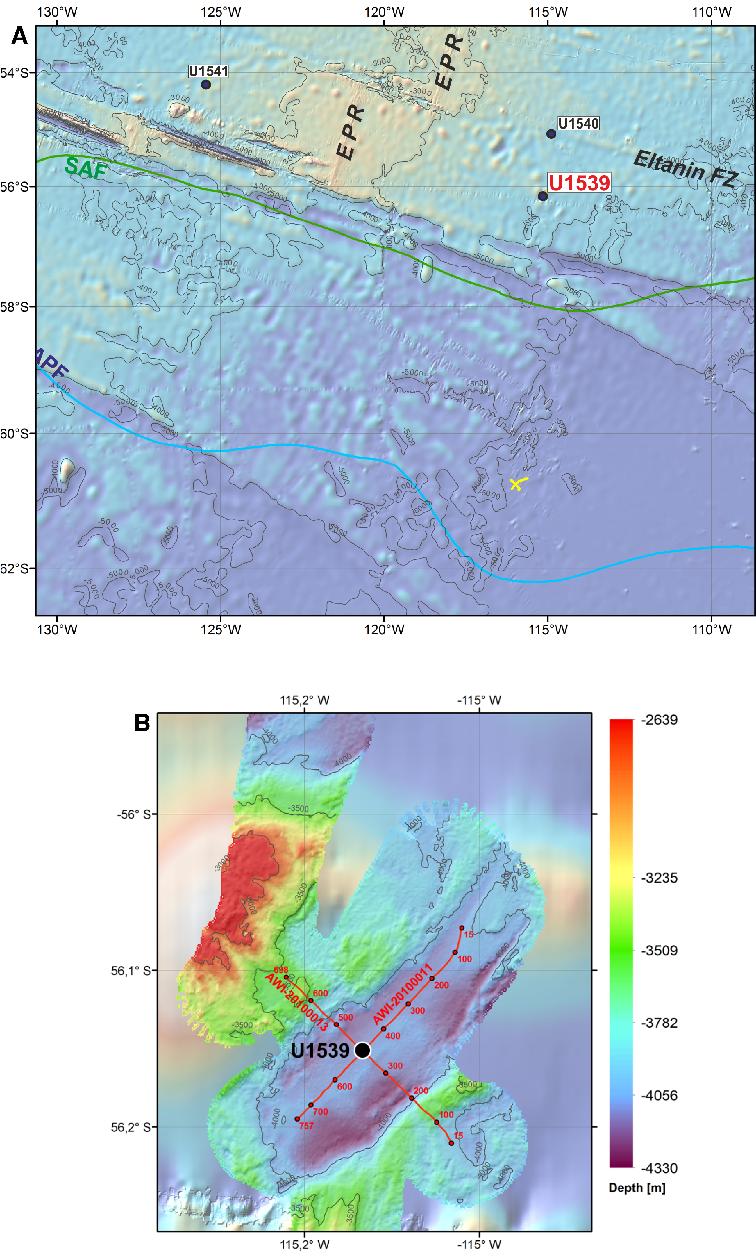
Figure F1. Oceanographic and bathymetric setting.
Site U1539 is located on Multichannel Seismic Line AWI-201000013 close to the intersection with Line AWI-2010000011 (Figure F2) (Gersonde, 2011). The seismic cross-lines indicate ~650 m thick sediments above oceanic basement. The sediments are mostly well stratified and have flat-lying reflectors. Low to moderately reflecting layers become stronger below ~100–120 m sediment depth. Sediment echo sound (Parasound) profiles (Gersonde, 2011) reveal excellent penetration (>150 m) and distinct layering, suggesting a succession of fine-grained soft sediments with varying lithologic composition.
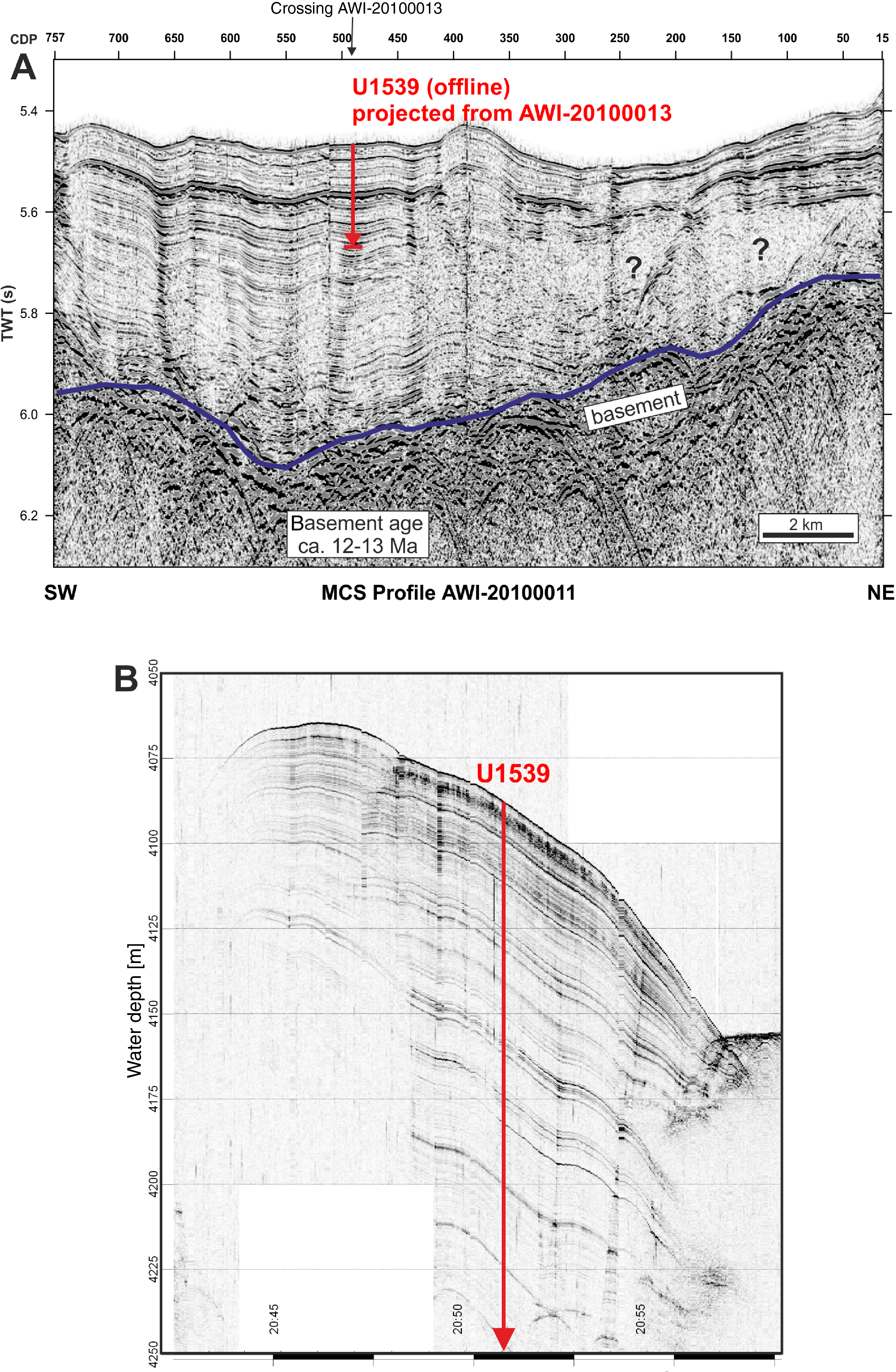
Figure F2. Site U1539 seismic profiles.
A ~22 m long piston core (PS75/054-1) covering the past ~165 ky at Site U1539 contains an alternation of diatom ooze during glacial intervals (~10–20 wt% CaCO3, ~50–80 wt% opal, and ~10–25 wt% siliciclastics) and diatomaceous calcareous ooze during interglacial intervals (~50–70 wt% CaCO3, ~20–25 wt% opal, and ~5–10 wt% siliciclastics). Sedimentation rates vary between ~5 cm/ky during the Holocene and Marine Isotope Stage (MIS) 5 and ~25 cm/ky during most of the glacial section and late MIS 5 (Basak et al., 2018).
Site U1539 lies in the pathway of the Subantarctic Pacific section of the Antarctic Circumpolar Current (ACC) ~100 nmi north of the modern average Subantarctic Front in a zonal transition zone of the ACC. West of the site, the ACC and the associated fronts are strongly steered by the topography of seafloor spreading systems (Udintsev and Eltanin-Tharp Fracture Zone systems), whereas to the east the vast Amundsen Sea Basin does not strongly influence the ACC.
Sea-surface temperatures vary seasonally between ~2°C (July–September) and ~6.5°C (January–March). The area is located west of the main Antarctic Intermediate and Mode Water formation regions in the Southeast Pacific. The water depth of 4070 m places Site U1539 within Lower Circumpolar Deep Water (Figure F3).
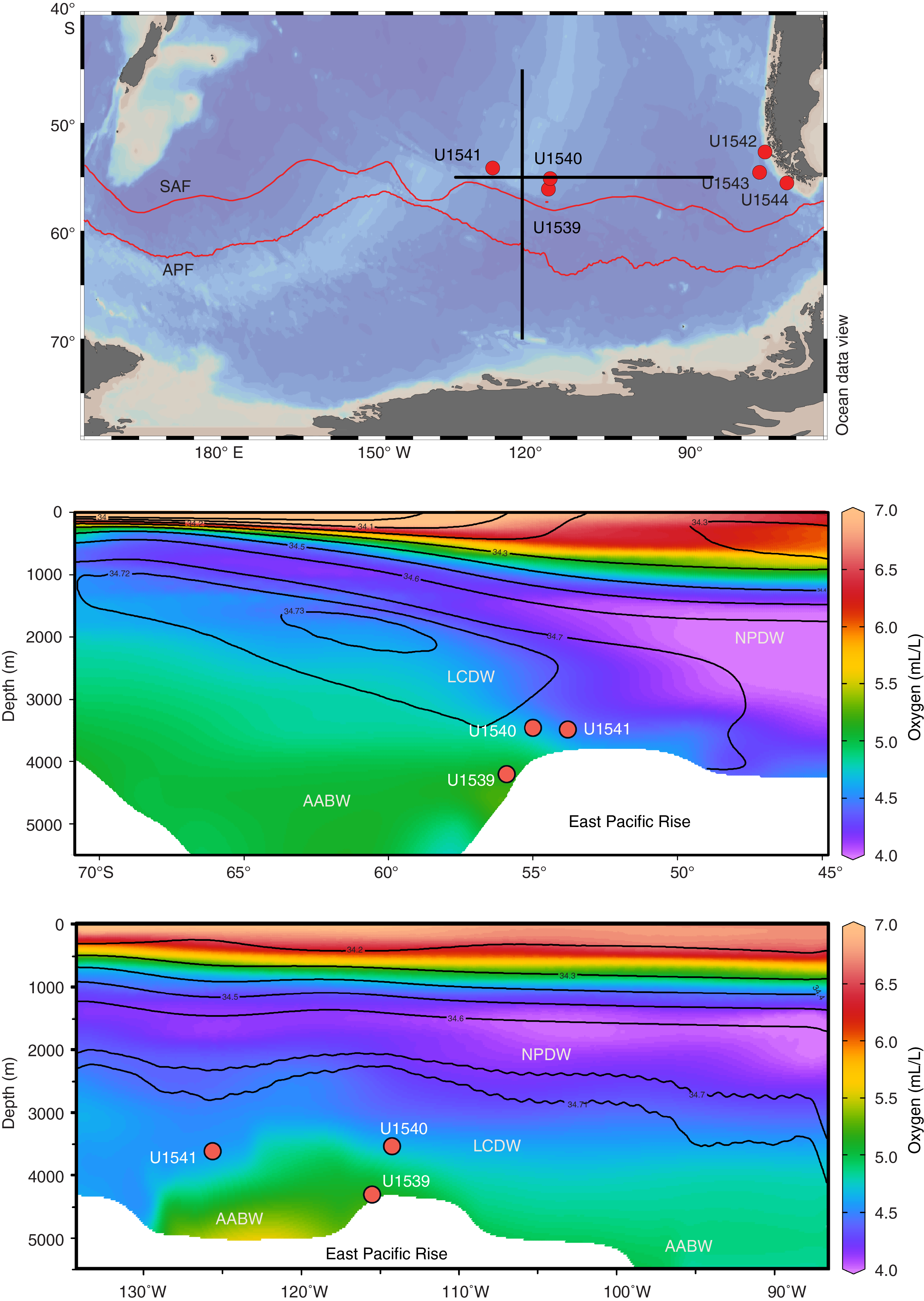
Figure F3. Modern South Pacific salinity and oxygen distribution.
Scientific objectives
The main objectives at Site U1539 were to
- Recover a moderate- to high-resolution Subantarctic Pliocene–Quaternary sediment record close to the Subantarctic Front;
- Investigate the sequencing of siliceous and calcareous oozes, allowing for a wide range of paleoceanographic reconstructions;
- Reconstruct high-amplitude Subantarctic sea-surface temperatures and sea ice variations;
- Provide a record of lowermost Circumpolar Deep Water and glacial Antarctic Bottom Water;
- Reconstruct productivity (opal versus carbonate), nutrient distribution, and dust productivity coupling; and
- Recover a potential far-field record of West Antarctic Ice Sheet variability.
Operations
The original operations plan for Site U1539 consisted of coring three holes with the advanced piston corer (APC) system to 300 m core depth below seafloor, Method A (CSF-A). Instead, because of rough seas and high winds, we cored four holes to shallower depths. The first hole was cored to 107.6 m CSF-A (104.75 m recovered; 97.4%). The second hole was cored to 28.2 m CSF-A (21.92 m recovered; 77.73%). The third hole was cored to 268.1 m CSF-A (247.5 m recovered; 92.3%). The fourth hole was cored to 129.3 m CSF-A (128.2 m recovered; 99.13%).
Punta Arenas, Chile, port call
Expedition 383, Dynamics of the Pacific Antarctic Circumpolar Current (DYNAPACC), officially started at 0930 h on 20 May 2019 when the Co-Chief Scientists and International Ocean Discovery Program (IODP) JOIDES Resolution Science Operator (JRSO) staff boarded the ship. The JRSO staff conducted their crossover with the departing staff, who left later in the afternoon, and the Co-Chief Scientists and Expedition Project Manager (EPM) met with members of the off-going science party from Expedition 382. Port call activities continued throughout the day, but all on-loading and off-loading of freight was postponed until the afternoon because of high winds.
The expedition scientists boarded the ship on the morning of 21 May. After getting settled in their rooms, the scientists were introduced to life on board the R/V JOIDES Resolution, general laboratory safety, and information technology resources/services. The following day and during the rest of the week, the scientists received training and familiarized themselves with the ship laboratories, instrumentation, and software applications. They attended presentations on the expedition scientific and operational objectives and coring operations on board JOIDES Resolution and received information and training on ship safety. The Education and Outreach officer gave a presentation on the education and outreach plans for the expedition, and two cinematographers from Maylo Films, Inc., presented details for the production of a science film/documentary about the expedition. Afterward, the Expedition 383 scientists started to work on preparing their laboratory procedures and developing the shipboard sampling plan.
On 22 May, a press conference was held by the Co-Chief Scientists and the EPM for members of the Chilean national and regional press, followed by a tour of the ship’s laboratories for the journalists. The visit by the press was coordinated by the Columbia Global Center in Santiago, Chile. Throughout the rest of the morning, ship tours and presentations were also provided for students and teachers from the American Corner and Colegio Alemán de Punta Arenas. In the afternoon, the Co-Chief Scientists and the EPM hosted a dozen researchers from the Instituto Antárctico Chileno and the Centro de Investigación GAIA Antártica from the Universidad de Magallanes for a presentation on the expedition objectives and gave them a tour of the vessel. A Chilean Coastal Observer boarded the ship on the fourth day of port call and was given an orientation. The observer sailed during Expedition 383 because three of the sites are located in waters within Chile’s exclusive economic zone.
Other port call activities included loading drilling mud, JRSO air freight and surface freight, fresh and frozen food, and other catering supplies. The Expedition 382 cores were loaded into two 40 ft refrigerated containers for shipment, and all off-going freight was off-loaded and prepared for shipment.
On 24 May, the vessel transited 19.5 nmi to the Cabo Negro fuel terminal for refueling. While taking on fuel, the vessel was informed that approval to occupy the sites in Chilean waters had not yet been granted. This forced us to change our operations plan, as stated in the addendum to the Scientific Prospectus, by prioritizing first the sites in the central South Pacific to give us more time to attain approval for the Chilean sites. After fueling was complete, and after being cleared for departure by the Servicio Hidrográfico y Oceanográfico de la Armada (SHOA) de Chile and the Punta Arenas Maritime Authority, JOIDES Resolution departed from the Cabo Negro fuel terminal in Punta Arenas after the last line was brought aboard and anchors were secured at 0100 h on 25 May. The ship took the western route through the Strait of Magellan, averaging 10.9 kt in good weather. By 2400 h on 25 May, the vessel had cleared the Strait of Magellan and entered the South Pacific Ocean on its way to Site U1539 in the central South Pacific.
Site U1539
Hole U1539A
JOIDES Resolution completed the 1634 nmi sea voyage to the first drill site in 6.4 days and arrived at Site U1539 at 1142 h on 31 May 2019. Upon arrival, all thrusters were lowered, and the vessel was placed under dynamic positioning mode at 1211 h. No positioning beacon was deployed. An APC/extended core barrel (XCB) bottom-hole assembly was made up with an 11⁷⁄₁₆ inch C-3 drill bit and deployed to 4050 meters below rig floor (mbrf). The top drive was picked up, and the bit was spaced out to 4077 mbrf for spudding. Hole U1539A (56°09.06′S, 115°08.0461′W) was spudded at 0445 h on 1 June, and Core 383-U1539A-1H recovered 4.56 m of sediment, establishing a seafloor depth of 4081.9 mbrf (or 4071.1 meters below sea level [mbsl]). APC coring continued to 90.1 m CSF-A with advanced piston corer temperature (APCT-3) tool measurements taken on Cores 4H (33.1 m CSF-A), 7H (61.6 m CSF-A), and 10H (90.1 m CSF-A). Coring was stopped at that point to allow the rig crew time to repair a leak in the aft core winch line load cell. This repair took approximately 3.75 h, and coring resumed with Cores 11H and 12H (90.1–107.6 m CSF-A). Coring was terminated after Core 12H because of rough weather and sea conditions. The bit was pulled back to 3885.6 mbrf, clearing the seafloor at 0225 h on 2 June and ending Hole U1539A at a total depth of 108.6 m CSF-A. Shattered liners were recorded on Cores 5H and 11H. Shear pins were sheared prematurely on Cores 1H, 11H, and 12H.
Hole U1539B
After 27 h on stand-by waiting on weather, the seas had calmed enough to attempt spudding Hole U1539B. The vessel was offset 20 m east of Hole U1539A, and the bit was set at 4081 mbrf. Once the sinker bars and orientation tool were installed, Hole U1539B was spudded at 0540 h on 3 June 2019. The seafloor was calculated at 4070.5 mbsl based on the Core 383-U1539B-1H recovery of 9.21 m. Coring continued to 28.2 m CSF-A, but Cores 2H and 3H were misfires. It was decided to terminate the hole and wait for seas to improve before continuing operations. The bit was pulled to 4060 mbrf, clearing the seafloor at 1000 h on 3 June and ending Hole U1539B. By 1245 h, heave had fallen to 3.0 m, and it was decided to attempt coring again.
Hole U1539C
The vessel was moved 20 m south of Hole U1539B, and the bit was spaced out to 4081 mbrf for spudding. Core 383-U1539C-1H returned a full core barrel. This allowed us to determine a seafloor depth of 4070.2 mbsl. Full-length APC coring continued to refusal at 240.1 m CSF-A (Core 26H). Half-length APC (HLAPC) coring was then used to deepen the hole, and coring terminated after Core 32F at 268.1 m CSF-A. The bit was pulled back to 4050 mbrf, clearing the seafloor at 1230 h and ending Hole U1539C. A total of 32 cores were taken using the APC and HLAPC coring tools. APCT-3 formation temperature measurements were taken with Cores 4H, 13H, and 16H. Partial strokes were recorded on Cores 24H–27F, and there was high overpull on Cores 17H–26H. A misfire was recorded on Core 31F.
Hole U1539D
Hole U1539D was spot cored to fill in coring gaps from the previous holes. The vessel was moved 20 m west of Hole U1539C, and a wash barrel was dropped. Hole U1539D was spudded at 1405 h on 5 June 2019 and drilled ahead without recovery to 47.5 m CSF-A. The wash barrel was pulled, and coring began. The hole was advanced to 198 m CSF-A with seven drilled intervals totaling 68.7 m. A total of 14 APC cores were taken over the 129.3 m cored interval with a recovery of 128.15 m (99%). The hole reached its total depth of 198 m CSF-A at 1500 h on 6 June, and the drill string was recovered. The bit cleared the rotary table at 0115 h, ending Hole U1539D and Site U1539. Misfires were recorded on Cores 383-U1539D-2H, 3H, 6H, 8H, and 9H, and a partial stroke was recorded on Core 18H. No temperature or orientation measurements were taken in this hole. After recovering the drill string, the rig floor was secured for transit at 0130 h. The thrusters were raised, and the sea voyage to Site U1540 began at 0224 h.
A total of 61 cores were taken at this site. The full-length APC system was deployed 55 times. The HLAPC system was deployed six times. A total of 68.7 m was drilled ahead without recovery. The interval cored with the APC system was 533.2 m. Total core recovered at Site U1539 is 502.35 m (94%). Total time spent at Site U1539 was 156 h (6.5 days). Coring summaries for Holes U1539A–U1539D are shown in Table T1.
Sedimentology
Site U1539 is located about 100 nmi north of the modern Subantarctic Front at 56°09.06′S, 115°08.05′W at approximately 4110 m water depth. The hydrographic setting makes it ideal to evaluate past changes in frontal position, associated export production, Antarctic Circumpolar Current current speed and position, and eolian dust and ice-rafted debris (IRD) input during the Pleistocene. Four holes (U1539A–U1539D) were drilled at Site U1539, and Hole U1539C recovered the deepest cored sediments at 268.31 m CSF-A. The recovered 293 m CCSF-A of core spans one lithostratigraphic unit with two subunits that consist of interbedded calcareous and siliceous biogenic ooze (Figure F4). Site U1539 sediments can broadly be divided into two categories: diatom ooze with varying amounts of calcareous and biosiliceous components and calcareous ooze with varying amounts of biosiliceous components. Based on core descriptions and smear slide analyses, we have identified five unique sedimentary facies based on lithology, sedimentary structures, color, and diatom species distribution. Lithofacies 1–4 are found throughout the sedimentary sequence, but their distribution and arrangement differ in the two lithologic subunits. Lithofacies 5 is limited to two discrete intervals in Subunit IB and represents a different depositional process (see below).

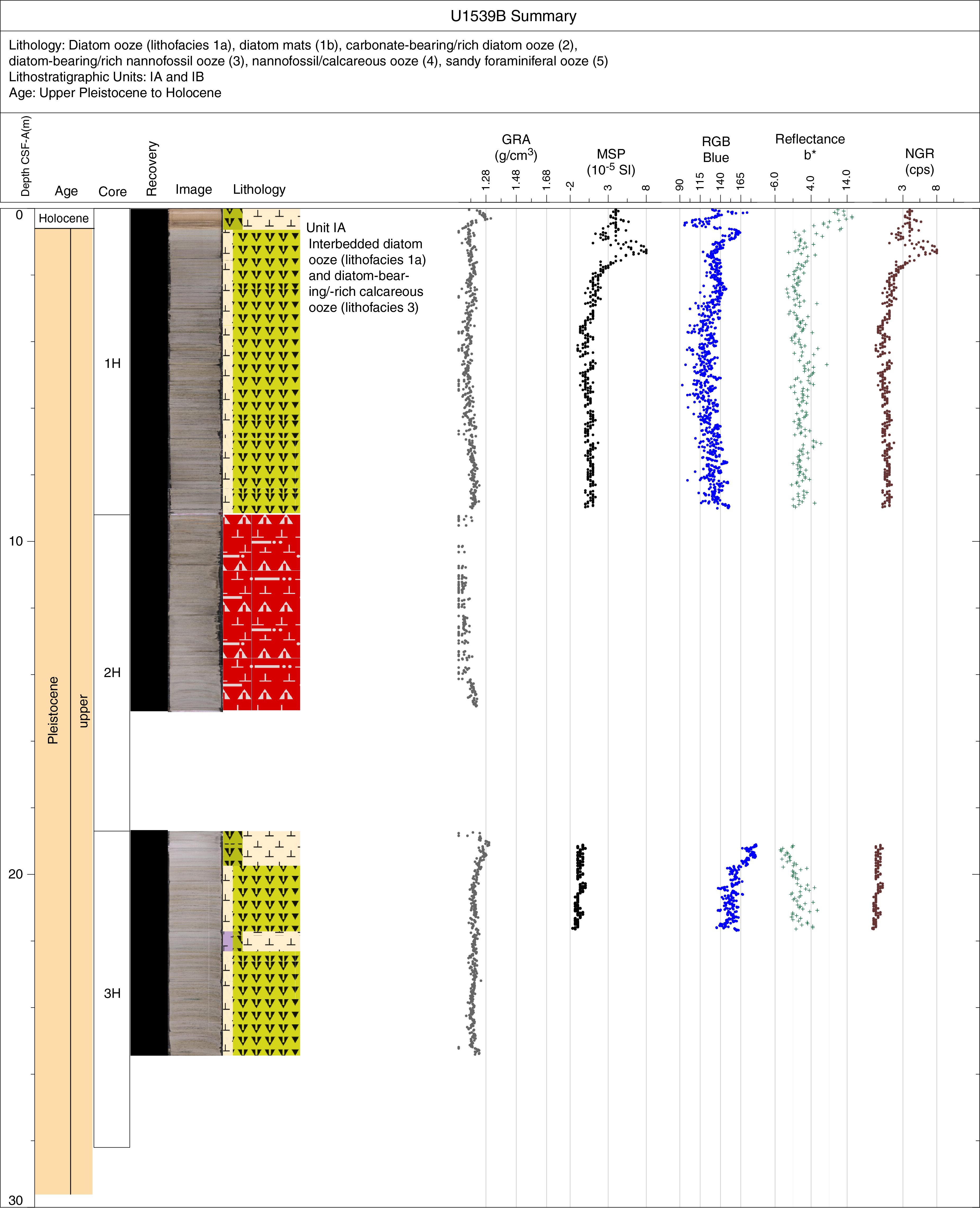
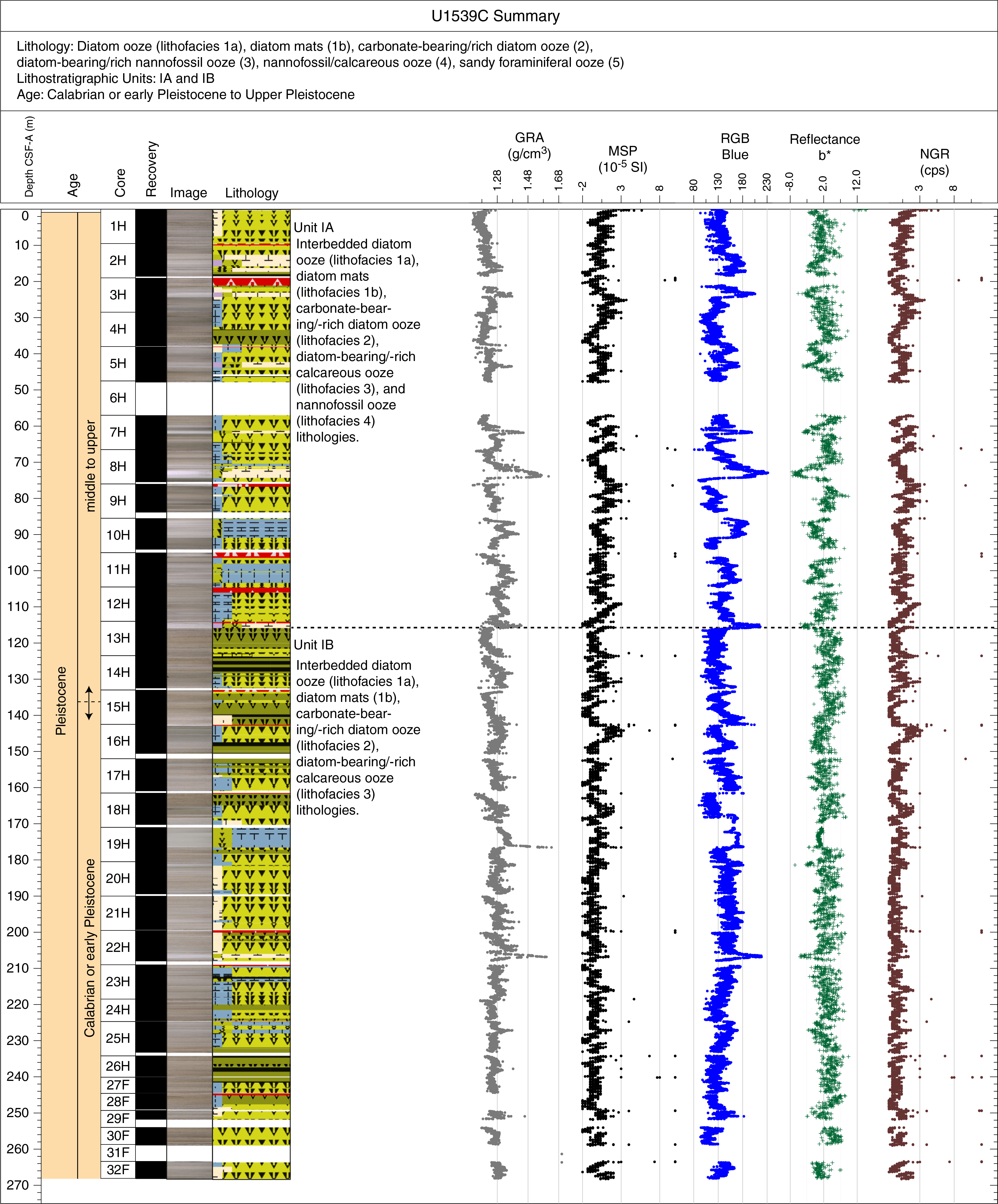
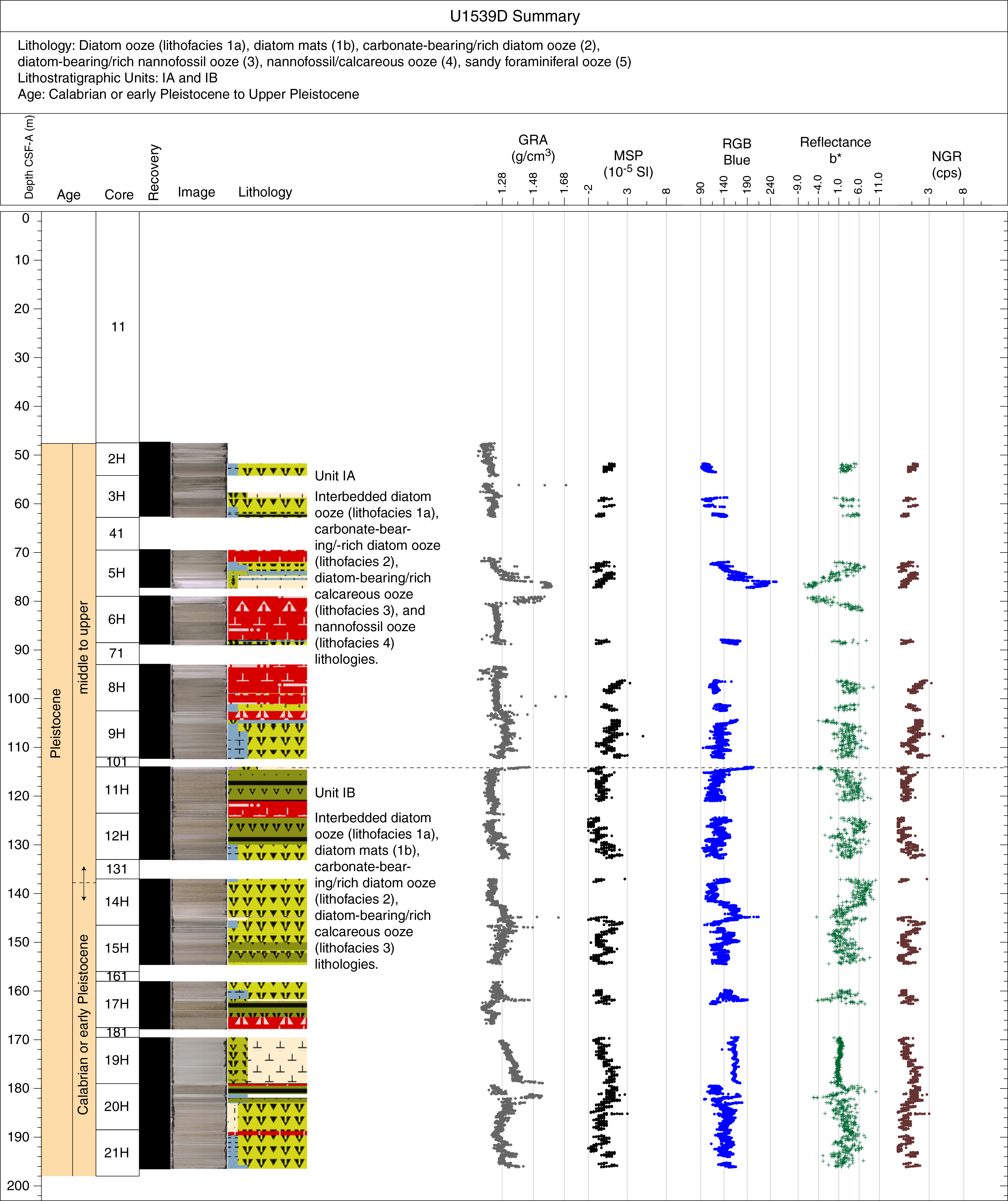
Figure F4. Hole summaries.
Cores were recovered from Holes U1539A–U1539D (Figure F4). Holes U1539A and U1539C provide much of the stratigraphy, and Holes U1539B and U1539D were drilled to fill gaps between adjacent cores in Holes U1539A and U1539C. Strong winds and high seas impacted the amount and quality of sediment cores recovered. Cores from all holes have at least one occurrence of fall-in (mostly in the uppermost one or two sections) and suck-in (often in the lower sections of the core), drilling disturbances that were most likely caused by high heave on the drill string. Drilling disturbance was identified in split core sections and in X-ray images of the archive-half sections by comparison with common disturbance features shown in Jutzeler et al. (2014) and was reported in the visual core descriptions (VCDs) (see Sedimentology in the Expedition 383 methods chapter [Winckler et al., 2021a]). Soupy, fall-in mixed sediment at the top of some cores was classified as mixed biogenic ooze and flagged as high drilling disturbance in the VCDs. Upward arching of centimeter-scale bedded facies and diatom mats were also used as an indicator of slight to heavy sediment drilling disturbance. Examples of such disturbed sediments are found in Sections 383-U1539A-2H-1, 383-U1539C-9H-1, and 383-U1539D-6H-1 and 6H-2.
Lithofacies description
Five primary lithofacies were identified at Site U1539 (Table T2; see Table T2 in the Expedition 383 summary chapter [Winckler et al., 2021b]). They mostly differ in their proportions of calcareous and biosiliceous components, but they also differ in grain size, diagenetic alteration, and degree of bioturbation. Lithofacies 1 is diatom ooze with two different appearances. Lithofacies 1a is composed of distinct diatom mats in a fine-grained diatom ooze matrix and can be distinguished from sequences with more pronounced and stacked diatom mats and a near absence of the diatom ooze matrix (Lithofacies 1b). Although carbonate-bearing or carbonate-rich diatomaceous oozes dominate the sedimentary record at Site U1539 (Lithofacies 2), biosilica-bearing or biosilica-rich calcareous oozes occur as thin beds generally less than 3 m thick throughout the sequence (Lithofacies 3). Lithofacies 4 is nannofossil ooze with only traces of other components. Occasionally, foraminiferal oozes occur with sharp contacts to surrounding lithologies (Lithofacies 5).
Lithofacies 1
Lithofacies 1a
Lithofacies 1a is composed of diatom oozes that include sporadic centimeter-thick diatom mats in beds that range in thickness from 0.2 to 8.2 m. The diatom mats are gray and have a texture and appearance similar to wet newspaper (Figure F5). In some instances, these single mats could be used as stratigraphic markers to identify potential tie points between holes. The diatom mats strongly resemble those found in Lithofacies 1b. The main matrix of Lithofacies 1a is composed of light to dark greenish gray to gray (10Y 7/1 and 10Y 6/1) moderately bioturbated diatom oozes that may show wavy or discontinuous centimeter-scale bedding. Accessory components (<10%) found in this lithofacies include radiolarians, silicoflagellates, sponge spicules, and undifferentiated calcareous debris. The diatom assemblages are dominated by Fragilariopsis kerguelensis and have common to few occurrences of Thalassiosira lentiginosa for the last 0.64 My and Actinocyclus ingens for the time span older than 0.64 Ma (see Biostratigraphy). Lithofacies 1a occurs frequently throughout the sedimentary record at Site U1539. Typical examples are found in Sections 383-U1539A-7H-6 and 9H-2 and 383-U1539D-12H-5.
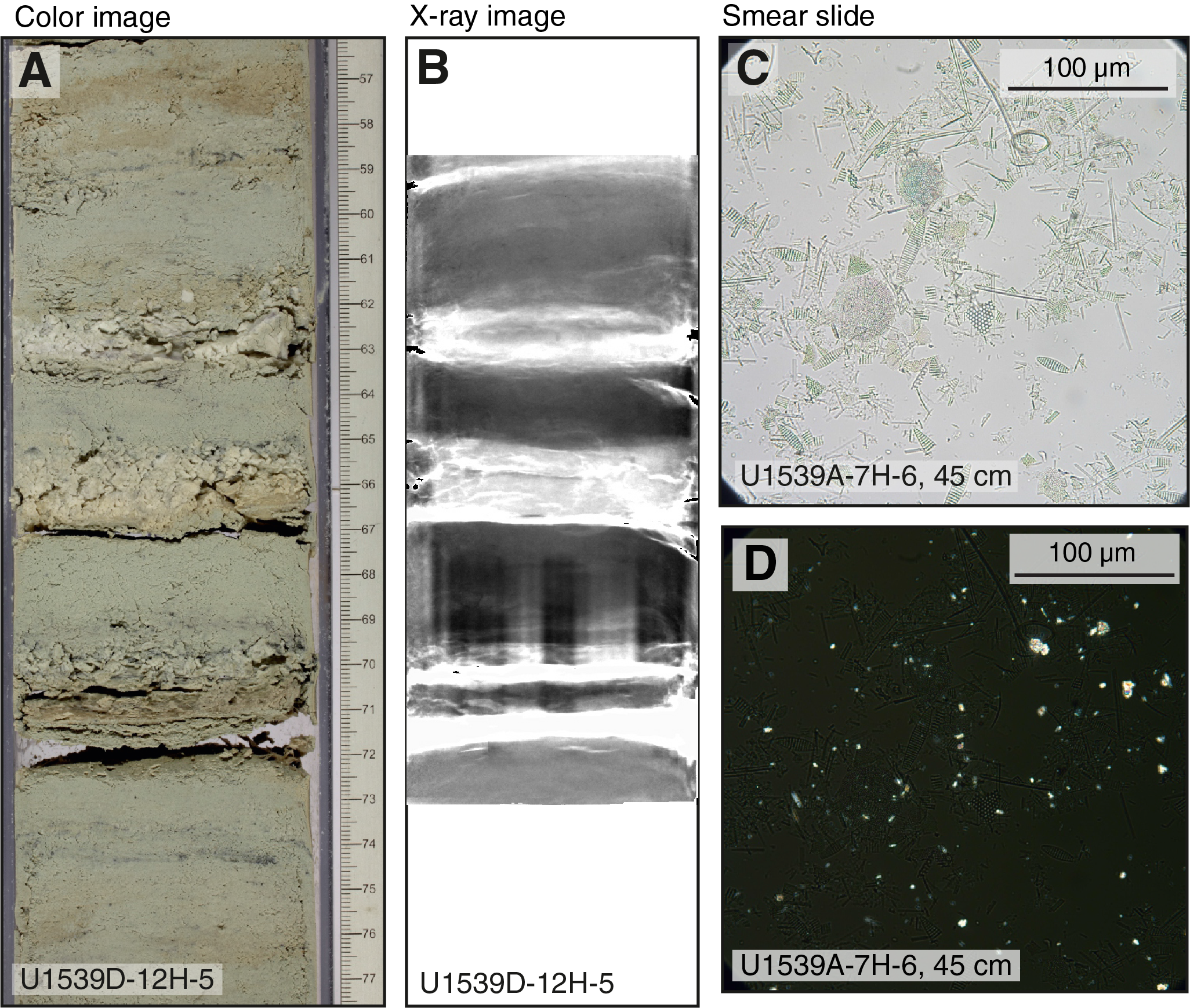
Figure F5. Representative images.
Lithofacies 1b
Lithofacies 1b is attributed to beds approximately 1.5 to 10 m thick and made up of densely stacked diatom mats (Figure F6). These slightly white, light gray to pale yellow (5Y 7/1, 5Y 6/1, and 5Y 7/3) diatom mats are nearly entirely dominated by diatoms, in particular by the species Thalassiothrix antarctica (see Biostratigraphy), with traces of calcareous and other biosiliceous components. They are mostly planar to wavy bedded, without any or with only slight bioturbation. Accessory components (<10%) found in this lithofacies include radiolarians, silicoflagellates, sponge spicules, and traces of undifferentiated calcareous debris. Examples of this lithofacies are found in Sections 383-U1539A-3H-6 and 383-U1539C-4H-6 and 4H-7.
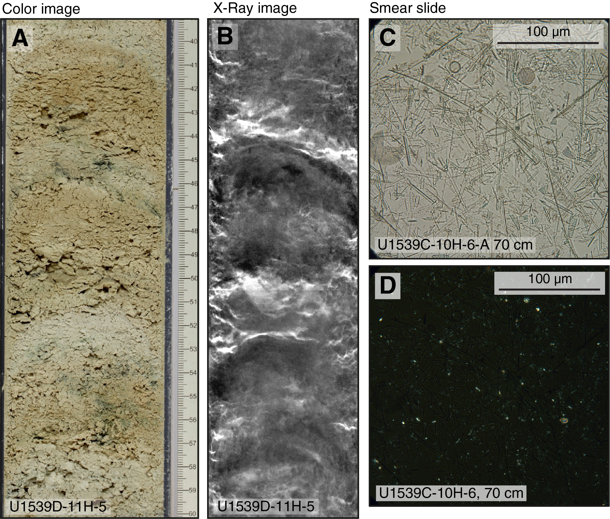
Figure F6. Lithofacies 1b mineral properties.
Lithofacies 2
Lithofacies 2 is light greenish gray to gray (10Y 7/1 and 2.5Y 5/1) carbonate-bearing to carbonate-rich diatom ooze (Figure F7) that exhibits moderate to heavy bioturbation. The minor component (10%–49%) consists of nannofossils and calcareous debris of mostly foraminiferal shells. Accessory components (<10%) include radiolarians, silicoflagellates, and sponge spicules. A high abundance of dropstones >0.5 cm was identified through macroscopic visual inspection of the section halves and X-radiograph images. Sporadic diatom mats are also a defining characteristic of this lithofacies. X-ray images reveal thin and elongated, centimeter-scale burrows in this lithofacies, some of which are filled with denser material, presumably pyrite and/or iron-oxide minerals. Lithofacies 2 is observed as extensive beds throughout the sedimentary sequence at Site U1539. Examples of this lithofacies are found in Sections 383-U1539C-8H-4, 383-U1539D-11H-2, and 383-U1539A-11H-5.
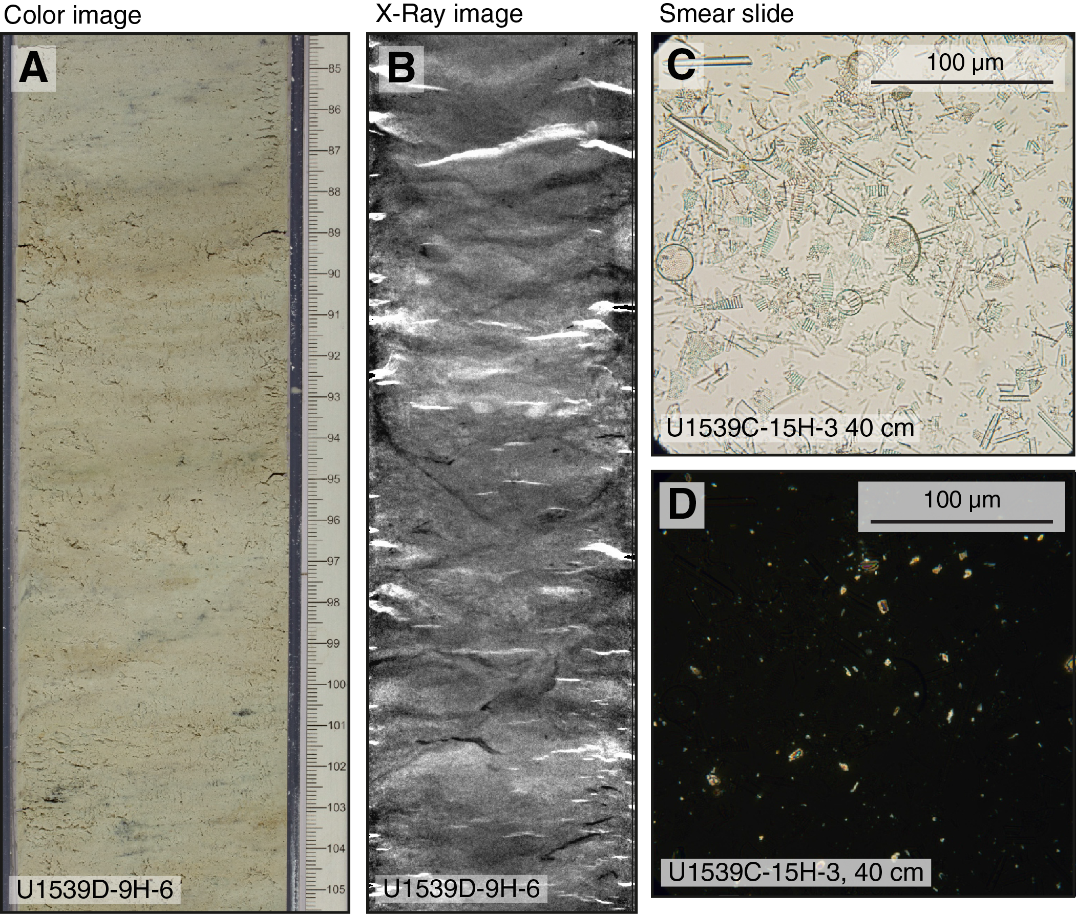
Figure F7. Lithofacies 2 mineral properties.
Lithofacies 3
Lithofacies 3 is diatom-bearing to diatom-rich nannofossil or calcareous ooze (Figure F8). This lithofacies is characterized by white or light gray/greenish gray (N 8/ and 5Y 7/1) nannofossil (and/or calcareous) oozes that often show weak wavy centimeter-scale bedding. The oozes have a mottled light yellow and light brown appearance in some places, likely from diagenetic overprints. Lithofacies 3 is moderately to heavily bioturbated. Examination of smear slides indicate a varying degree of a minor component (10%–50%) mainly comprised of diatoms. In this lithofacies, X-ray images reveal only minor abundances of dropstones and some indications of thin and elongated, centimeter-scale burrows, which are filled with denser material, presumably composed of pyrite and/or iron-oxide minerals. Along with whole foraminifers, radiolarians, and silicoflagellates, Lithofacies 3 also includes undifferentiated calcareous debris as an accessory component (<10%), most likely fragmented foraminiferal shells. Nannofossil and calcareous oozes appear as less dominant facies in the sedimentary record at Site U1539, mainly as thin beds <2–3 m. Examples of this lithofacies are found in Sections 383-U1539A-7H-1, 383-U1539B-3H-1, 383-U1539C-13H-2, and 383-U1539D-19H-6.
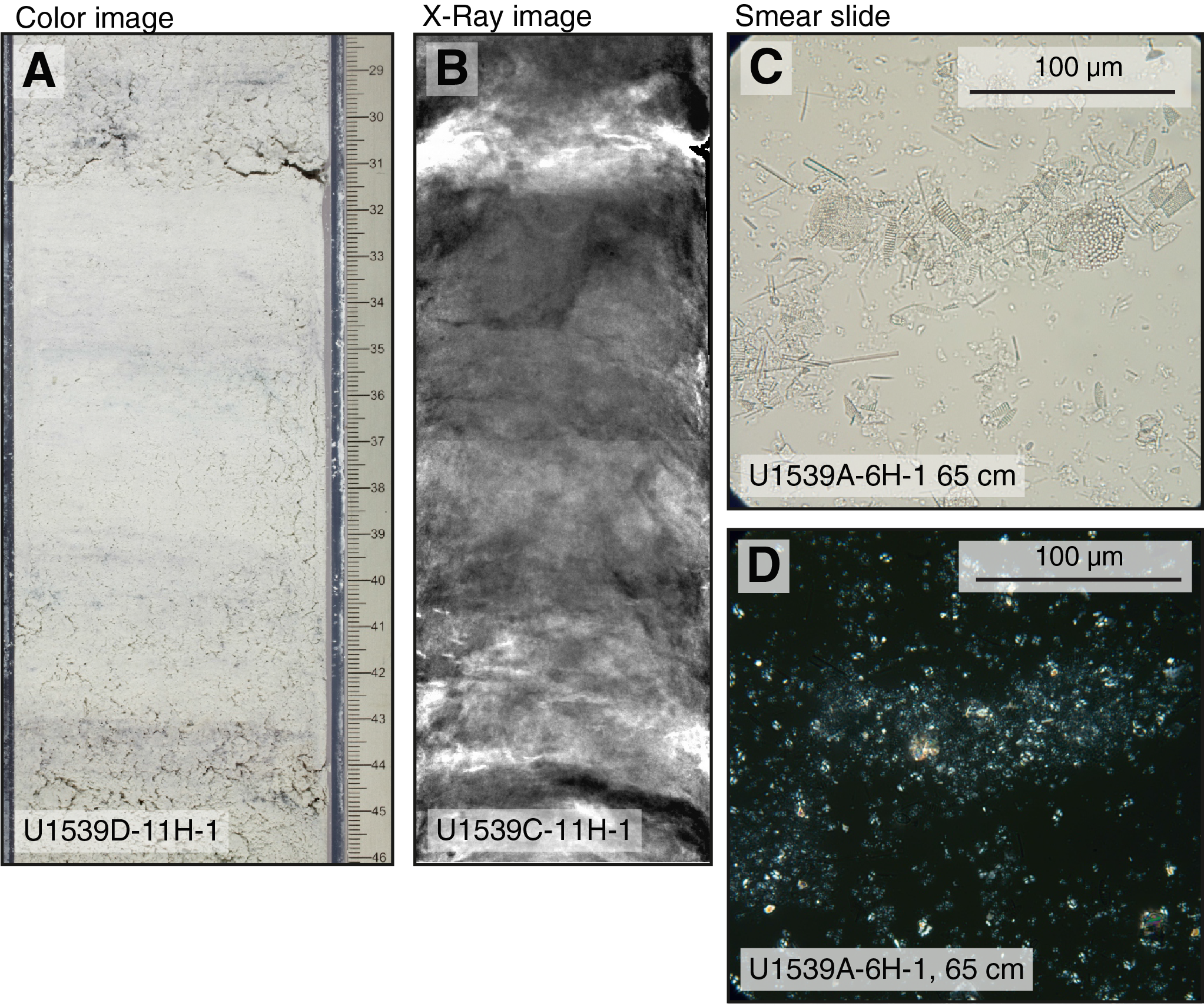
Figure F8. Lithofacies 3 mineral properties.
Lithofacies 4
Lithofacies 4 is nannofossil ooze that is heavily bioturbated and often has a massive appearance. Its color may range from white to very light gray (N 9/ and N 7/). It is characterized by only rare occurrences of carbonate (foraminifers) and various biosiliceous components. Mottled patches of darker grayish colors due to diagenetic iron sulfide overprints are found in this lithofacies. The only occurrence of Lithofacies 4 at Site U1539 consists of a bed approximately 3 m thick. This bed can be found in Sections 383-U1539A-9H-1 and 9H-2, 383-U1539C-8H-5, and 383-U1539D-5H-7.
Lithofacies 5
Lithofacies 5 corresponds to foraminiferal oozes and sands that occur as two centimeter- to decimeter-scale layers. This lithofacies is characterized by light gray colors and is most often homogeneous with a sharp basal contact indicative of rapid deposition by a turbidite or gravity-driven flow (Figure F9). X-ray images reveal distinct cross-bedding in this lithofacies. Accessory components (<10%) of this lithofacies include radiolarians and few lithic grains. Bed thickness can range from 1 to 80 cm, and examples are found in Sections 383-U1539C-1H-2 and 16H-2 as well as 383-U1539D-12H-7.
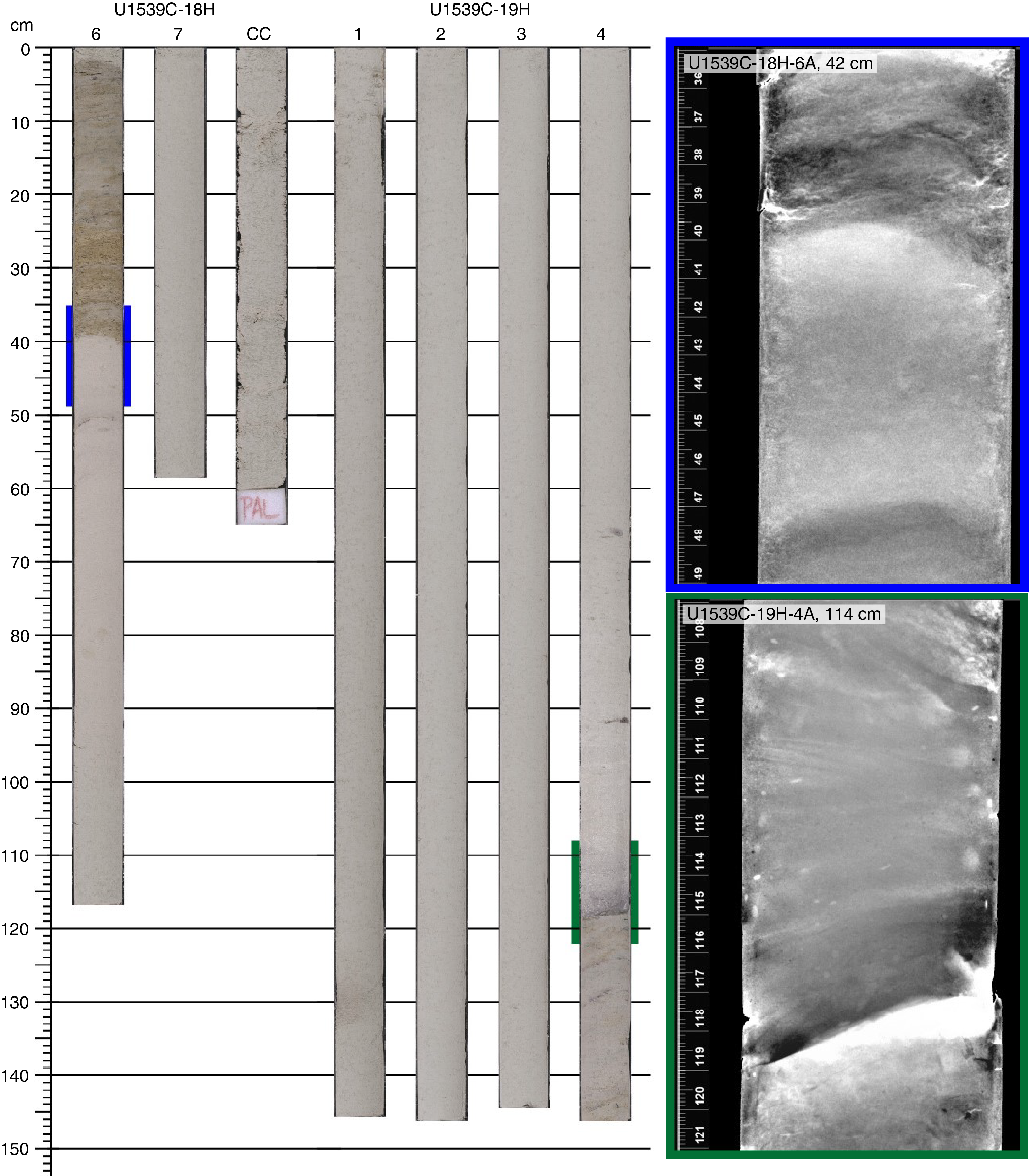
Figure F9. Lithofacies 5 mineral properties.
Site U1539 lithofacies can be plotted on a ternary diagram where Lithofacies 1a/1b and 4 are the two end-members and Lithofacies 2 and 3 occupy the mixing areas in between them (Figure F10). Accordingly, the mixed Lithofacies 2 and 3 are most common, making up 58.4% and 13.8%, respectively, of the entire sequence. The diatom Lithofacies 1a and 1b are 8.7% and 18.5%, respectively, and the carbonate-dominated Lithofacies 4 comprises only 0.6% of the record. Because of its limited distribution and different inferred depositional process, Lithofacies 5 is omitted from the above calculations.
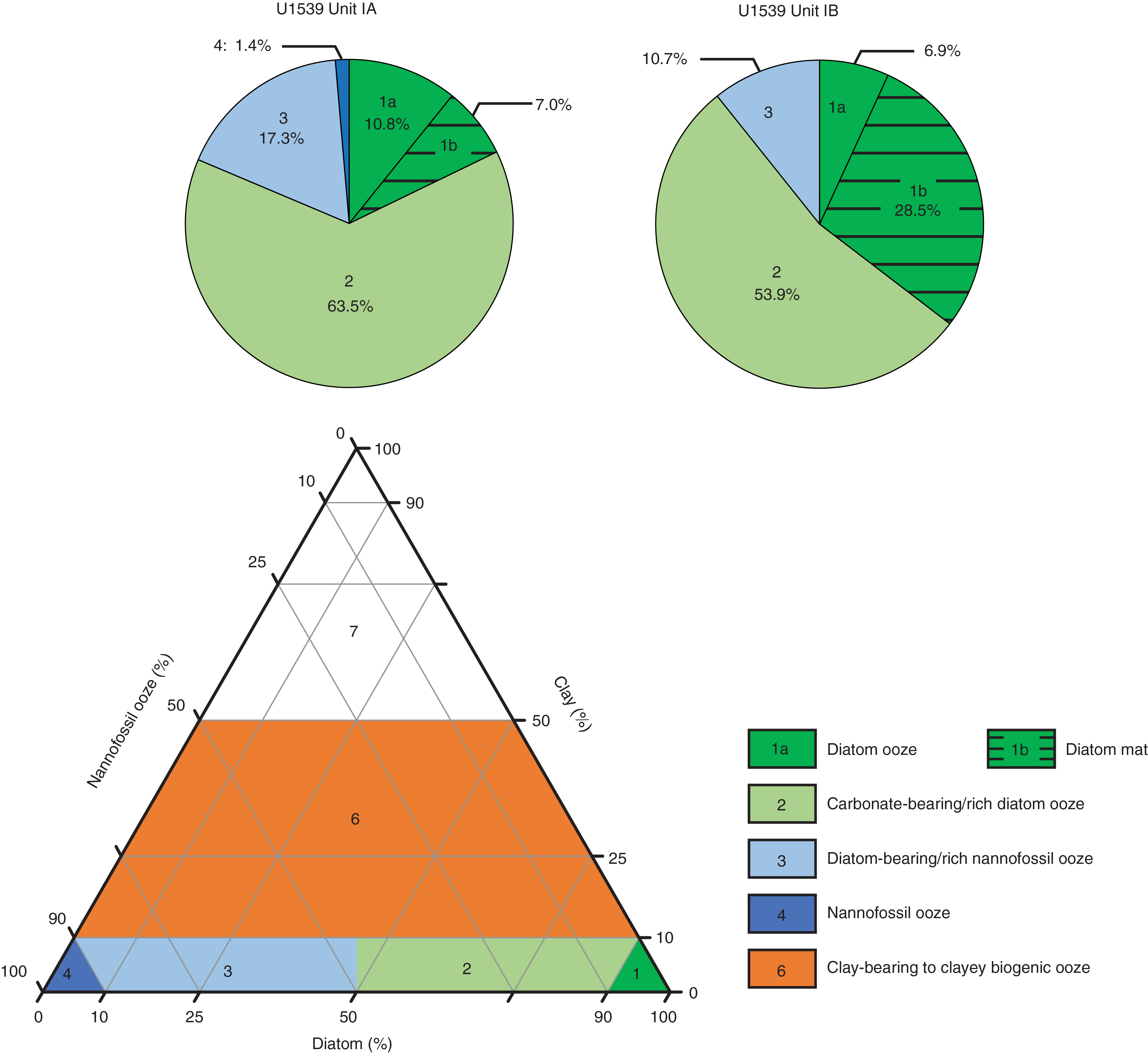
Figure F10. Primary lithofacies lithologies.
Lithostratigraphic units
Based on the distribution of the lithofacies, the sedimentary sequence of Site U1539 is divided into one lithostratigraphic unit with two subunits, IA and IB. The criteria used to define unit boundaries are discussed below and are highlighted in Figures F10 and F11. Key unit characteristics, including depths within the Site U1539 sedimentary sequence and corresponding ages according to the preliminary shipboard age model, are also discussed below.
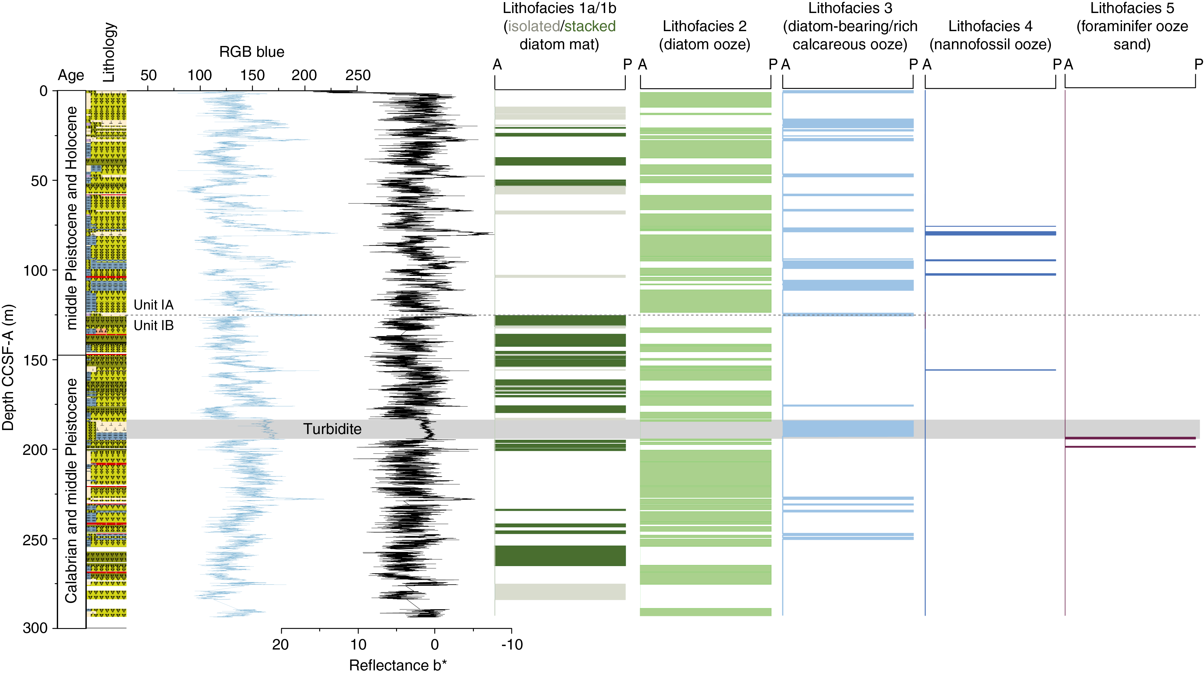
Figure F11. Primary lithostratigraphic variations.
Unit I
Subunit IA
- Intervals: 383-U1539A-1H-1, 0 cm, to 12H-CC, 12 cm; 383-U1539B-1H-1, 0 cm, to 3H-CC, 5 cm; 383-U1539C-1H-1, 0 cm, to 13H-2, 35 cm; 383-U1539D-1H-1, 0 cm, to 11H-1, 56 cm
- Depths: Hole U1539A = 0–107.54 m CSF-A, Hole U1539B = 0–25.44 m CSF-A, Hole U1539C = 0–115.86 m CSF-A, Hole U1539D = 0–114.56 m CSF-A, Site U1539 composite section = 0–125 m CCSF-A
- Thickness: 125 m
- Age: Holocene to middle Pleistocene (younger than 0.78 Ma)
- Lithology: diatom ooze to carbonate-bearing/rich diatom ooze, diatom-bearing/rich nannofossil ooze to nannofossil/calcareous ooze
Lithostratigraphic Subunit IA is characterized by the frequent occurrence of ~1.5 m thick beds of light greenish gray to gray carbonate-bearing to carbonate-rich diatom ooze (Lithofacies 2), which contributes 63.5% to the lithologic sequence, interbedded with diatom-bearing/rich calcareous/nannofossil ooze (17.3%) and including a limited occurrence of light gray to pale yellow diatom mats (Lithofacies 1b; 7%), diatom ooze (Lithofacies 1a; 10.8%), and white to light gray nannofossil ooze (Lithofacies 4; 1.4%). Dropstone abundance is generally higher in this subunit, and the alternating lithofacies drive the high-amplitude, low-frequency variations in red-green-blue color space (RGB) blue and L* (Figure F11).
- Intervals: 383-U1539C-13H-2, 35 cm, to 32F-CC, 13 cm; 383-U1539D-11H-1, 56 cm, to 21H-CC, 26 cm
- Depths: Hole U1539C = 115.86–268.26 m CSF-A, Hole U1539D = 114.56–196.46 m CSF-A, Site U1539 composite section = 125–293 m CCSF-A
- Thickness: 168.9 m
- Age: middle Pleistocene (older than 0.78 Ma) and Calabrian (younger than 1.4 Ma)
- Lithology: diatom mats, diatom ooze to carbonate-bearing/rich diatom ooze, diatom-bearing/rich nannofossil ooze
Subunit IB
Lithostratigraphic Subunit IB is characterized by a larger proportion of beds of thick and continuous diatom mats (Lithofacies 1b; 28.5% of the total lithologic sequence) and a moderate decrease in the occurrence and thickness of the still dominant carbonate-bearing/rich diatom ooze lithofacies (53.9%) and diatom-bearing/rich nannofossil/carbonate ooze (10.7%). One massive homogeneous bed of diatom-rich nannofossil ooze (~10.7 m thick; 184–194.7 m CCSF-A) with erosive foraminifer sands at the base (Lithofacies 5) interrupts the normal depositional sequence and most likely represents a depositional event (Figure F9). Dropstone abundance is generally lower in Subunit IB than in Subunit IA, and the lithofacies alternations reflected in RGB blue and L* are of higher frequency and lower amplitude (Figure F11).
Complementary analyses
Dropstone distribution
Dropstone observations were part of the visual sediment core description and provide a preliminary account of the presence and abundance record of IRD in the core (see Sedimentology in the Expedition 383 methods chapter [Winckler et al., 2021a]). Figure F12 shows examples of X-ray images with no, rare, and more frequent dropstone occurrence. Subunit IA documents significant variability between 0 and ~150 dropstones per image with no or rare occurrence in the carbonate-rich Lithofacies 3 and 4. Dropstone variability is much lower in Subunit IB, varying between 0 and ~20 dropstones per image.
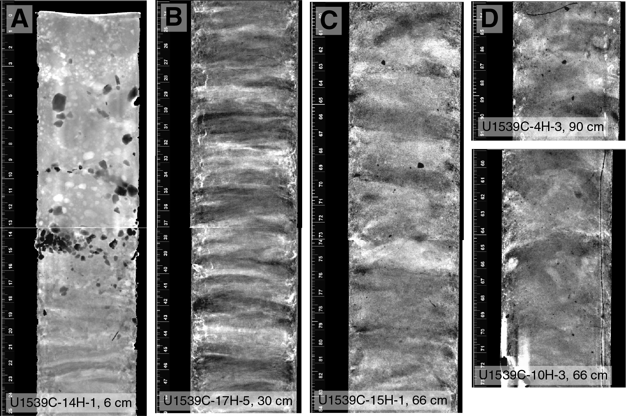
Figure F12. Dropstones.
X-ray diffraction clay mineralogy
X-ray diffraction analyses were performed on 35 powdered samples from Holes U1539A and U1539C to identify the mineralogy and downcore variations in the composition of the lithogenic fraction of the sediment (Figure F13). As expected from the dominance of diatom oozes in the sedimentary sequence at Site U1539 (Lithofacies 1a and 2), a wide peak between 18° and 30°2θ occurs in the diffractogram of all measured samples and can be associated with amorphous biogenic silica (i.e., opal). However, the amplitude of the peak is dependent on the relative proportions of biogenic (i.e., biosiliceous) versus lithogenic sedimentary material in the samples. Peaks in the diffractogram characteristic for calcite at 29.5°2θ are observed in four samples obtained from diatom-bearing to diatom-rich nannofossil oozes (Lithofacies 3). The characteristic calcite peaks are likely the result of incomplete carbonate dissolution during sample preparation.
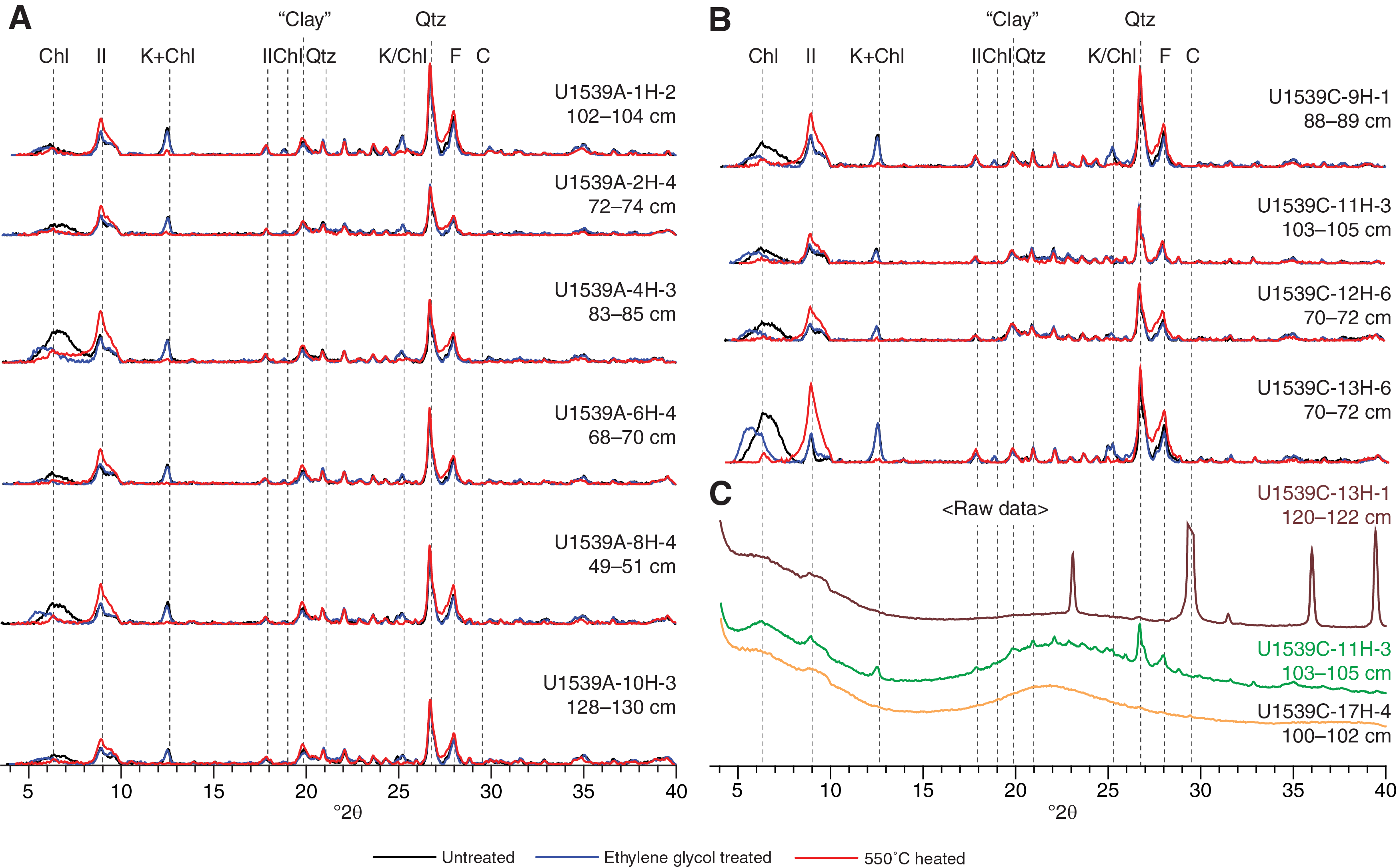
Figure F13. X-ray diffractograms.
We refrain from discussing the diffraction pattern of biosiliceous material further because of its dominance in all samples and focus instead on the composition of the lithogenic fraction. Diffraction patterns of 10 representative samples are shown in Figure F13 after subtraction of the background (i.e., opal) signal and for different preparation techniques. The lithogenic sediment fraction is dominated by detrital minerals such as quartz, feldspar (plagioclase), and phyllosilicates including illite, chlorite, and kaolinite. In samples heated to 550°C, peak heights of kaolinite [001]/chlorite [002] at 7.1 Å (12.7°2θ) and kaolinite [002]/chlorite [004] at 3.54–3.58 Å (24.9°2θ) are significantly lower (or absent) than in untreated samples. The decrease in these clay ratios are likely the result of the destruction of the kaolinite mineral structure upon heating (Brindley, 1980). The illite [001] peak at 10 Å (9°2θ) appears in most samples, but it is not prominent because of a broad, low-amplitude baseline peak at 8–10°2θ. However, this peak and the 4.478 Å (19.8°2θ) “clay composite” peak increases in most samples after heating, which may indicate the presence of hydrated minerals. In the absence of any identifiable smectite peak at 17 Å, the small shift of the 14.2 Å peak (6.5°2θ) to the left in the diffractogram in samples that were processed with ethylene glycol solvation may point to the presence of small amounts of mixed-layer clay minerals. The downhole variation of the relative contribution of each clay mineral phase may be evaluated in biogenic silica–free samples, although an additional pretreatment that includes opal dissolution will be necessary.
Bioturbation
Sediments at Site U1539 are slightly to heavily affected by bioturbation. For example, the presumably fast-depositing diatom mat Lithofacies 1b is sometimes barely affected by bioturbation and shows distinct centimeter-scale wavy bedding (Figure F12). Lithofacies 2 is mostly moderately bioturbated and shows only a weak wavy bedding. Lithologic transitions to the generally more heavily bioturbated to homogeneous lithofacies 3 and 4 are frequently mottled by larger centimeter-scale burrows.
Integrating physical property measurements with lithofacies observations
As described above, the lithology of Site U1539 is characterized by dominant greenish gray to gray biosiliceous oozes (Lithofacies 1–3) and the occasional occurrence of white or light gray/greenish gray calcareous ooze (Lithofacies 4). These lithofacies alternations are identified by downcore physical properties and spectrophotometry measurements, as exemplified by Cores 383-U1539A-7H through 10H (52–90 m CSF-A) (Figure F14). In this interval, a prominent bed of light-colored (white) nannofossil ooze in Core 9H is characterized by lower natural gamma radiation (NGR), higher gamma ray attenuation (GRA) bulk density, higher color reflectance (L*) obtained using the Section Half Multisensor Logger (SHMSL), and higher blue intensity generated from RGB intensity obtained from the Section Half Imaging Logger (SHIL) (see Physical properties in the Expedition 383 methods chapter [Winckler et al., 2021a]).
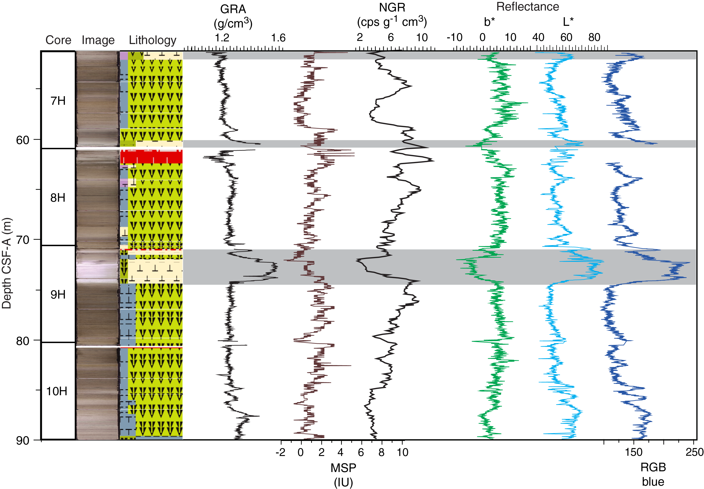
Figure F14. Major lithologies and physical properties.
The strong correspondence between L*, RGB (particularly blue), and alternations between biosiliceous and carbonate lithofacies is further supported by shipboard measurements of weight percent calcium carbonate (CaCO3). L* and RGB blue intensity are tightly correlated to weight percent CaCO3 at Site U1539 (Figure F15), with higher L* and RGB blue intensity corresponding to higher carbonate concentrations.
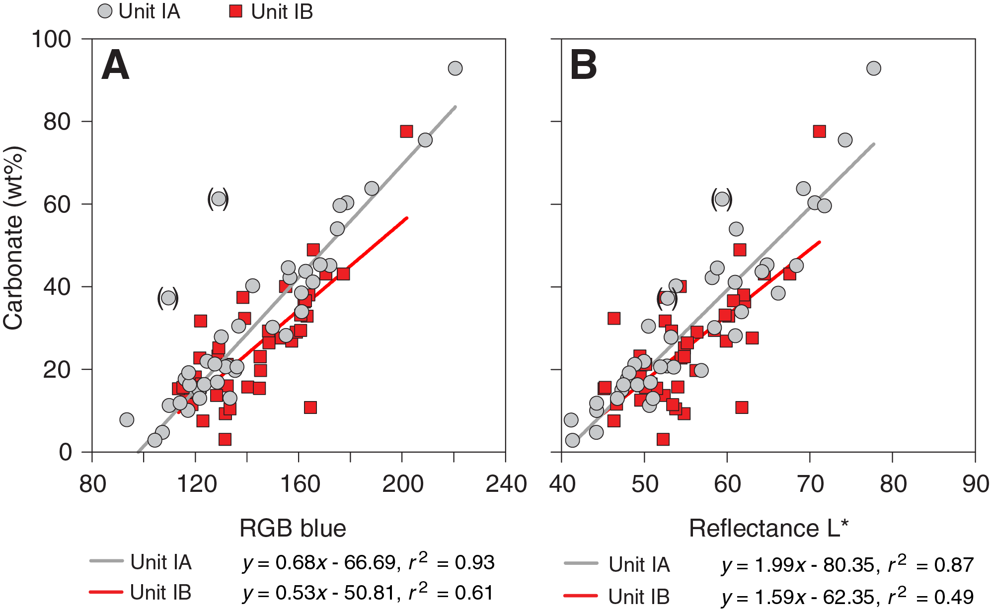
Figure F15. Carbonate content with RGB blue and RSC L*.
Summary and preliminary site interpretation
Two lithostratigraphic subunits are identified in Site U1539 sediments based on the relative abundances of diatom mats, nannofossil/calcareous oozes, and dropstones. Subunit IA consists of generally more abundant nannofossil/calcareous oozes (Lithofacies 4) and dropstones and a lower abundance of beds with pronounced and stacked diatom mats (Lithofacies 2). Conversely, the lower Subunit IB consists of generally more abundant beds of diatom mats (Lithofacies 2), less abundant nannofossil/calcareous oozes (Lithofacies 4), and fewer dropstones observed in X-radiographs (Figure F11). One massive, 10.7 m bed interrupts normal sedimentation and most likely represents a depositional event.
Variations between the relative proportions of Lithofacies 1a/1b/2 and Lithofacies 3/4 drive the RGB blue intensity signal (Figure F14), which correlates with shipboard measurements of sedimentary carbonate percentages (Figure F15). In Subunit IA, the RGB blue intensity record appears to record the characteristic “sawtooth” pattern of late Pleistocene 100,000 y glacial cycles, suggesting higher carbonate export production and/or preservation during interglacial periods and stronger opal export production during glacial intervals (Figure F11). In this context, we interpret higher RGB blue intensity (Lithofacies 3 and 4) to represent interglacial periods and lower RGB blue intensity (Lithofacies 1 and 2) to represent glacial periods. This sedimentation pattern resembles glacial–interglacial sedimentation and sediment composition patterns found in the Subantarctic Atlantic sector of the Southern Ocean at Ocean Drilling Program Sites 1090 and 1092, which bracket the modern-day position of the Subantarctic Front in this region (Diekmann and Kuhn, 2002; Gersonde et al., 2003; Hodell et al., 2001).
The increase in dropstone counts in Subunit IA relative to Subunit IB implies a higher frequency of icebergs passing over Site U1539 combined with a greater amount of dropstones delivered to the seafloor, but it may also reflect a change in sedimentation rates between units and thus variations in the dilution effect of the dropstones by other sedimentary components. For instance, in Subunit IA, we observe relatively lower sedimentation rates and therefore less dilution of dropstones by diatom mat Lithofacies 1b. However, the timing of the Site U1539 lithostratigraphic boundary (i.e., 0.78 Ma based on the shipboard age model; see Stratigraphic correlation) is approximately coeval with the onset of stronger glaciations in the mid-Pleistocene, expressed as well-developed 100 ky glacial cycles, and therefore supports a climate driver of the observed IRD variability at Site U1539. This climate driver can be further explored at millennial to orbital timescales with proxy reconstructions of ocean conditions from Site U1539 sediments.
Biostratigraphy
Biostratigraphic results were consistent among diatoms, radiolarians, nannofossils, and planktonic foraminifers for all samples from Holes U1539A and U1539C. A total of 32 biostratigraphic constraints were identified (Table T3; Figures F16, F17). Based on these events, we estimate an age of ~1.3 Ma at the base of Hole U1539C, which indicates an average sedimentation rate of ~20 cm/ky over 268.3 m CSF-A. Diatom, radiolarian, and nannofossil biostratigraphy detected no major hiatuses, indicating that the material recovered from Site U1539 represents a continuous stratigraphic sequence from the middle Pleistocene through the Holocene. Between 167.8 and 176.6 m CSF-A in Hole U1539C, trace abundances of early Pleistocene and Pliocene diatom and nannofossil taxa co-occur with diverse late Pleistocene flora, indicating reworking of sediments with an age older than 2 Ma into the regular strata (see Sedimentology).
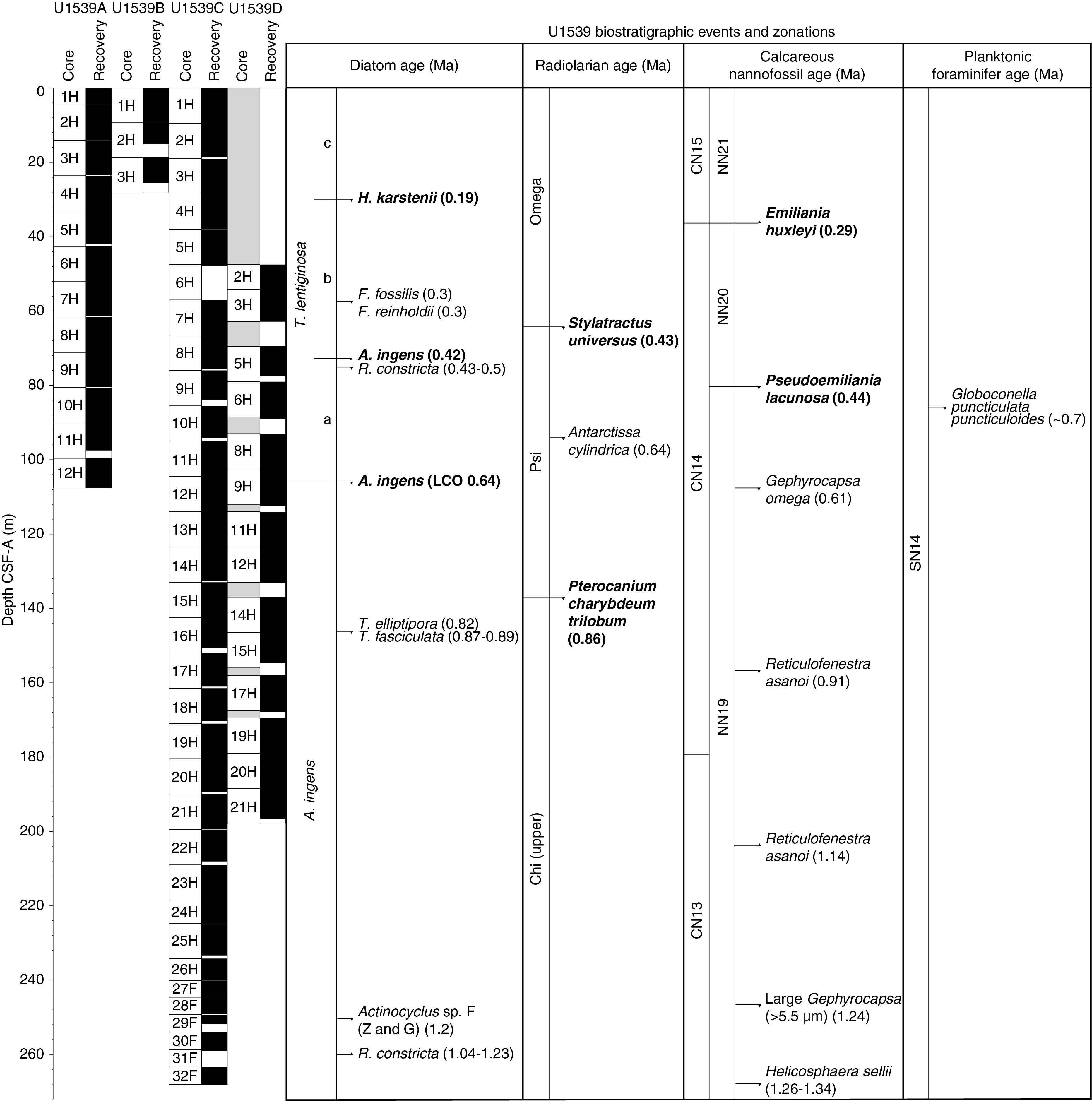
Figure F16. Biozonations and biostratigraphic events.
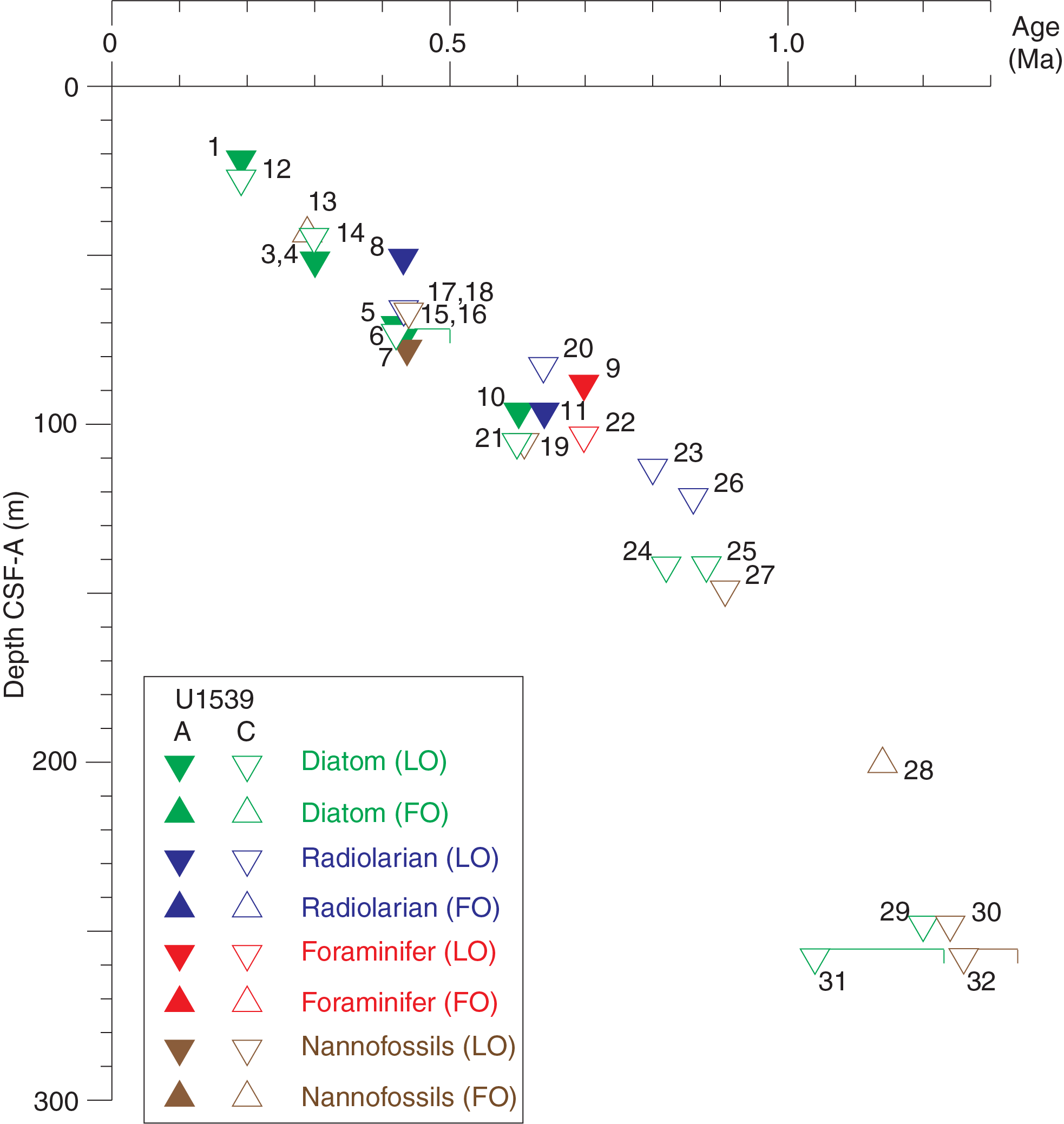
Figure F17. Age-depth plot.
Overall preservation of siliceous microfossil is relatively good in all samples, and fragmentation is more common than dissolution. Several sequences of diatom mats composed mainly of the needle-shaped diatom Thalassiothrix antarctica, which contribute significantly to the high sedimentation rates, were noted between 190 and 252 m CSF-A. Silicoflagellates are rare to common in most samples throughout the entire succession and are occasionally abundant. Calcareous microfossils were identified throughout the entire sequence with significant variations in abundance; these groups become dominant in discrete depth intervals and are interpreted to record interglacial periods. Preservation of calcareous nannofossils is variable, which made some biostratigraphic marker species (e.g., Emiliania huxleyi) difficult to recognize. Planktonic foraminifers are generally present in low abundances and moderately preserved at Site U1539; assemblages are dominated by the cold-water species Neogloboquadrina pachyderma (sinistral). Benthic foraminifer abundance is very low, but assemblages are diverse; Melonis barleeanum, Oridorsalis umbonatus, Pullenia bulloides, and Cibicidoides mundulus are present in most samples, and specimens are moderately preserved. Radiolarians are generally abundant and well preserved throughout the cored section. Three radiolarian marker species were identified at Site U1539 from the Psi Zone (late/middle Pleistocene) and Chi Zone (middle Pleistocene).
Diatoms
Diatom biostratigraphy at Site U1539 is based on the analysis of 57 smear slides from 1 mudline sample, 44 core catcher samples, and 12 working-half toothpick samples taken from Holes U1539A and U1539C. Diatoms are abundant and assemblages are diverse in all core catcher samples and in most of the working-half samples examined (Figures F18, F19; Table T4). Two samples have few diatoms: Sample 383-U1539C-8H-5, 140 cm, which is dominated by nannofossils and interpreted to be from MIS 11, and Sample 19H-4, 100 cm, which is sandy and interpreted to be the base of a gravity-driven flow deposit (see Sedimentology). Preservation is good overall, and most samples exhibit low to moderate fragmentation and dissolution.
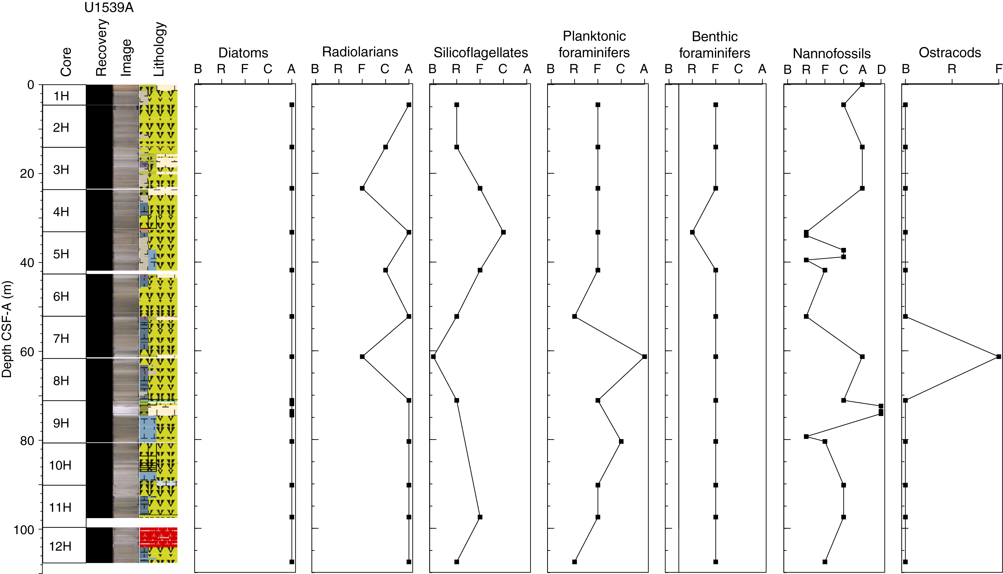
Figure F18. Siliceous and calcareous microfossils, Hole U1539A.

Figure F19. Siliceous and calcareous microfossils, Hole U1539C.
The assemblages of the mudline sample, 12 core catcher samples, and 3 working-half samples from Hole U1539A are in good agreement with the species composition of the upper part of Hole U1539C. In Hole U1539C, Samples 383-U1539C-1H-CC through 17H-CC preserve a well-established sequence of Southern Ocean diatom bioevents (Table T3) and age increases steadily with depth. Samples from Sections 18H-6 through 19H-4 contain trace occurrences of diatoms with early Pleistocene and Pliocene ages mixed into the normal diatom succession, indicating that older sediments have been reworked into this 8 m long interval. Assemblages in Samples 20H-CC through 29F-CC are characterized by abundant to dominant Thalassiothrix antarctica, a needle-shaped mat-forming taxon that contributes to higher sedimentation rates compared to the overlying sequences. In Samples 30F-CC through 32F-CC, diatom assemblages exhibit a more diverse composition with less abundant Thalassiothrix antarctica frustules. The depth and age estimates of 10 key diatom biostratigraphic events identified at Site U1539 are described below (Table T3; Figure F16).
Hole U1539A
In Hole U1539A, the species composition of nearly all assemblages is characterized by the dominance of F. kerguelensis and common to few occurrences of T. lentiginosa and Thalassiothrix antarctica. Fragilariopsis separanda and Fragilariopsis rhombica are also common to rare in most of the samples from Hole U1539A.
The mudline sample from Hole U1539A is further characterized by the appearance of few to rare Hemidiscus cuneiformis, Shionodiscus oestrupii, Thalassionema nitzschioides var. lanceolata, Thalassiosira oliverana, and T. trifulta and no extinct or reworked species. Rare to common abundances of Hemidiscus karstenii were noted between Samples 383-U1539A-4H-CC (33.25–33.30 m CSF-A) and 9H-2, 108 cm (73.65 m CSF-A). The last occurrence (LO) of H. karstenii in Sample 4H-CC constrains the age at 33.25–33.30 m CSF-A to older than 0.19 Ma in MIS 7 and marks the base of T. lentiginosa Subzone C following the Northern Antarctic Circumpolar Current Diatom Zonation scheme of Zielinski and Gersonde (2002) (Figure F16).
The published last appearance datums (LADs) for Fragilariopsis fossilis and Fragilariopsis reinholdii are 0.7 and 0.6 Ma, respectively (e.g., Zielinski and Gersonde, 2002; Cody et al., 2008). However, both species were identified at Site U1539 in younger intervals that are rich in carbonate (see Sedimentology). Sample 383-U1539A-7H-CC, 19–24 cm (61.29–31.34 m CSF-A), which contains both F. fossilis and F. reinholdii, is correlated to MIS 9 (see Stratigraphic correlation), providing a revised regional LAD of 0.3 Ma for both species (Table T3). F. fossilis was also identified in Sample 9H-2, 108 cm, which might be correlated to MIS 11 but does not occur in the two carbonate-poor samples examined in between the two samples mentioned above (Table T4). Furthermore, the diatom assemblages in both Hole U1539A samples that contain F. fossilis also include common to few occurrences of Thalassionema nitzschioides var. parva, an indicator of relatively warm sea-surface conditions (e.g., Esper and Gersonde, 2014). We therefore propose that the discrepancy between Site U1539 LADs and published LADs for both F. fossilis and F. reinholdii reflects an environmentally controlled diachronous extinction.
A single apex of Rouxia constricta identified in Sample 383-U1539A-6H-CC (52.23–52.28 m CSF-A) is judged to be reworked; the species is rare in Samples 9H-CC (80.40–80.45 cm CSF-A) and 10H-CC (90.25–90.30 m CSF-A), providing an age older than 0.43–0.5 Ma at 80.40 m CSF-A (Table T3).
A. ingens is present in trace occurrences in Sections 383-U1539A-7H-CC (61.29–31.34 m CSF-A) to 9H-1, 86 cm (71.96 m CSF-A), is rare from Section 9H-2, 108 cm (73.65 m CSF-A) through Sample 11H-CC (97.45–97.50 m CSF-A), and is common in Sample 12H-CC (107.55–107.60 m CSF-A). The shallowest rare occurrence of A. ingens in Sample 9H-2, 108 cm (73.65 m CSF-A), constrains the age of the sample above, 9H-1, 86 cm (71.96 m CSF-A), to 0.42 Ma, whereas the shallowest abundant occurrence of A. ingens in Sample 12H-CC places the boundary dividing the T. lentiginosa Zone from the A. ingens Zone at 0.64 Ma between 97.45 and 107.6 m CSF-A (Tables T3, T4; Figure F16).
The diatom assemblages in Hole U1539A generally reflect a late to middle Pleistocene sequence of fluctuating environmental conditions. Samples 383-U1539A-6H-CC (52.23–52.28 m CSF-A) and 9H-3, 47 cm (74.49 m CSF-A), and similar samples reflect warmer-than-present surface water during the time of deposition, and Sample 9H-1, 86 cm (71.96 m CSF-A), and similar samples point to colder surface water conditions than those reported for the modern Subantarctic Zone (Esper and Gersonde, 2014).
Hole U1539C
The biostratigraphy of Cores 383-U1539C-1H through 12H is consistent with Hole U1539A (Table T3). Assemblages in Samples 1H-CC through 17H-CC are characterized by the dominance of F. kerguelensis and common to few occurrences of T. lentiginosa and Thalassiothrix antarctica. In contrast, Samples 18H-CC through 32F-CC exhibit higher relative abundances of Thalassiothrix antarctica, even dominant occurrences, that dilute the abundance of the other species and are consistent with the prevalence of diatom mats in the lithologic descriptions (see Sedimentology). Frustules of Eucampia antarctica appear mostly in Samples 1H-CC through 16H-CC, whereas F. rhombica and F. separanda are identified in few to trace abundance down to Sample 23H-CC. H. karstenii is rare in Samples 2H-CC and 3H-CC and then common to few in Samples 4H-CC to 8H-4, 115 cm, constraining the LO of H. karstenii, which defines the base of T. lentiginosa Subzone C (0.19 Ma) to between 28.62 and 37.88 m CSF-A. The LO of F. fossilis during MIS 9, identified in Hole U1539A, is also seen in Sample 383-U1539C-6H-CC (47.72–47.77 m CSF-A). The species is also present in Sample 8H-5, 140 cm, which is interpreted to be MIS 11, and again in association with T. nitzschioides var. parva. R. constricta appears between Samples 8H-CC (75.50–75.55 m CSF-A) and 30F-CC in rare to trace abundance, placing the LO (0.43–0.5 Ma) between 73.83 and 75.50 m CSF-A. The first occurrence (FO) of R. constricta (1.04–1.23 Ma) is tentatively placed between 258.92 and 259.91 m CSF-A. However, occurrences of the species are discontinuous below Sample 18H-CC and the observed FO is near the base of the hole, so it is possible that the true FO of R. constricta lies below the recovered sequence.
A. ingens is present in trace abundance between Sections 383-U1539C-7H-4, 16 cm (61.66 m CSF-A) and 8H-5, 140 cm (73.83 m CSF-A) and in rare to few abundance between Samples 8H-CC (75.50–75.55 m CSF-A) and 11H-CC (104.62–104.67 m CSF-A). It is common to abundant between Samples 12H-CC (114.11–114.16 m CSF-A) and 32F-CC (268.26–268.31 m CSF-A). The rare occurrence of A. ingens at 73.83 m CSF-A constrains the age of this sample to older than 0.42 Ma, whereas the last abundant occurrence of A. ingens at 144.11 m CSF-A constrains this depth to older than 0.64 Ma and marks the boundary between the T. lentiginosa Zone and the A. ingens Zone (Figure F16; Table T3).
The LO of Thalassiosira elliptipora in Sample 383-U1539C-16H-CC (150.60–150.65 m CSF-A) constrains this horizon to older than 0.82 Ma, and few to rare occurrences were observed down to Sample 23H-CC (218.97–219.02 m CSF-A). The LO of Thalassiosira fasciculata, which has a LAD age of 0.87–0.89 Ma, is also identified in Sample 16H-CC. This species persists in few to rare abundance down to Sample 20H-CC (189.46–189.51 m CSF-A), is absent from the interval dominated by Thalassiothrix antarctica, and then returns in few to rare occurrences from Sample 29F-CC (251.83–251.88 m CSF-A) to the bottom of the hole.
A small centric species resembling Shionodiscus tetraoestrupii var. reimerii occurs in rare or trace abundance in Samples 383-U1539C-16H-CC (150.60–150.65 m CSF-A) through 31F-CC (259.01–259.06 m CSF-A) (Table T3). This taxon appears to have a single process in a central divot on the valve face, but moderate dissolution and fragmentation made it difficult to determine whether the distinctive margin characteristic of S. tetraoestrupii var. reimerii (Mahood and Barron, 1996) was present. Because the taxon was found at a higher stratigraphic position than expected and we could not confirm that its form adheres to the sensu stricto taxonomic definition of the variety, it was not used as stratigraphic indicator for Hole U1539C.
Trace occurrences of seven Pliocene and early Pleistocene species are reworked into the primary assemblage in Sections 383-U1539C-18H-6, 38 cm (168.27 m CSF-A) to 19H-4, 100 cm (176.39 m CSF-A). Sedimentologically, this interval is homogeneous with a sandy base and a sharp basal contact and is likely the product of rapid deposition by a turbidite or gravity-driven flow (see Sedimentology).
Starting in Sample 383-U1539C-18H-CC (170.27–170.32 m CSF-A), transitional forms between F. kerguelensis and Fragilariopsis barronii were identified in rare to trace abundance. However, these transitional morphologies are without clear age assignment (Zielinski and Gersonde, 2002) and thus were not used for chronographic constraint.
The diatom mat interval between Samples 383-U1539C-20H-CC and 29F-CC, which is dominated by needle-shaped Thalassiothrix antarctica frustules, contributes to higher sedimentation rates in this sequence. These mats may preserve a series of glacial–interglacial cycles because the diatom assemblages of different core catcher samples reflect varying glacial to interglacial surface water conditions according to the ecological study of Esper and Gersonde (2014). For example, Sample 24H-CC exhibits a relatively high proportion (common abundance) of the relatively “warm” Azpeitia tabularis (temperature range = 6°–14°C) compared to adjacent samples that show only rare abundance of this species. In contrast, the diatoms in Samples 10H-CC and 29F-CC point to deposition during cooler glacial intervals, indicated by the common abundance of E. antarctica in only these two samples and its rather rare occurrence in the neighboring samples. However, the density of core catcher samples alone is not sufficient to determine true glacial–interglacial cyclicity.
Finally, few occurrences of Actinocyclus sp. F of Zielinski and Gersonde (2002) were identified in Sample 383-U1539C-29F-CC (251.83–251.88 m CSF-A). Although this species was only observed in a single sample, its LAD is tentatively applied to Hole U1539C, providing an age older than 1.2 Ma at 251.83 m CSF-A, near the base of the recovered sequence.
Radiolarians
Core catcher samples from Holes U1539A and U1539C were processed and analyzed for the occurrence of radiolarians (Samples 383-U1539A-1H-CC through 12H-CC [4.5–107.5 m CSF-A] and 383-U1539C-1H-CC through 32F-CC [9.6–268.28 m CSF-A]). Shipboard observations focused mainly on the presence of age diagnostic species. Therefore, the distribution data do not fully represent the true radiolarian assemblage (Table T5). Radiolarians are moderately to well preserved and common to abundant in most of the samples from Site U1539 (Figures F18, F19). Two samples from Hole U1539A (383-U1539A-3H-CC [23.30m CSF-A] and 7H-CC [61.9 m CSF-A]) have few radiolarians. Photomicrographs of some of the taxa identified at this site are presented in Figure F20.

Figure F20. Radiolarians.
A typical high-latitude Southern Ocean/Antarctic region radiolarian assemblage characterized by Antarctissa denticulata, Antarctissa strelkovi, Spongotrochus glacialis, and Cycladophora davisiana is present in Samples 383-U1539A-1H-CC through 6H-CC (4.5–52.23 m CSF-A) and 383-U1539C-1H-CC through 7H-CC (9.6–66.97 m CSF-A). Their presence, along with the absence of any biostratigraphic marker species, suggests a late Pleistocene age (Omega Zone) for this interval. The age is likely younger than 0.43 Ma based on the absence of Stylatractus universus (LAD at 0.43 Ma) (Figure F16).
The top of the Psi Zone was assigned at ~75.50 m CSF-A (Samples 383-U1539A-7H-CC and 383-U1539C-8H-CC) by the presence of S. universus. The following interval, to Samples 383-U1539A-12H-CC (107.55 m CSF-A) and 383-U1539C-10H-CC (94.09 m CSF-A), where the last appearance of Antarctissa cylindrica (0.64 Ma) is located, is assigned to the remaining part of the Psi Zone. The last appearance of Pterocanium charybdeum trilobum (0.86 Ma), which marks the base of the Psi Zone, is frequently rare and not easy to identify (Hays and Opdyke, 1967; Lazarus, 1990). At Site U1539, P. charybdeum trilobum occurs only in Sample 383-U1539A-15H-CC. Chen (1975) suggested using the last appearance of Saturnalis circularis as the zonal marker between the Psi and Chi Zones. Therefore, the base of the Psi Zone was placed between the top occurrence of S. circularis at 124.10 m CSF-A (Sample 383-U1539C-13H-CC) and the occurrence of P. charybdeum trilobum at 142.84 m CSF-A (Sample 15H-CC).
The Chi Zone was recognized below Sample 383-U1539C-15H-CC (142.84 m CSF-A) and continues through Sample 32F-CC (268.26 m CSF-A). This entire interval contains a similar radiolarian assemblage and is therefore inferred to be of similar age. The Chi Zone is divided into two subzones (lower/upper) by the LAD of Cycladophora pliocenica (1.81 Ma). Because this subzone marker was not observed in any core catcher samples from this site, we assign the lower 125 m of Hole U1539C to the upper Chi Zone. Furthermore, the occurrence of Triceraspyris antarctica (first appearance datum at 1.88 Ma) down to Sample 32F-CC (268.26 m CSF-A) and absence of Eucyrtidium calvertense (1.92 Ma), which marks the base of this zone, support an age younger than 1.81 Ma for the base of the core.
Finally, several morphologies of the phaeodarian family Challengeridae picked from the coarse fractions prepared for benthic foraminifer analysis are presented in Figure F21.

Figure F21. Unknown microfossils.
Silicoflagellates
Silicoflagellates from 10 core catcher samples from Hole U1539A and 32 core catcher samples from Hole U1539C were analyzed. Silicoflagellates are present throughout the core, except for one sample that is barren (Table T6). They range from rare to common in most samples and are abundant in a few samples.
The silicoflagellate assemblage at Site U1539 consists of four species: Dictyocha stapedia, Dictyocha aculeata, Stephanocha speculum, and Octactis pulchra (Figure F22). D. stapedia and D. aculeata are present sporadically in a few samples. S. speculum is present in all samples and has large morphological variability, including specimens with long and short corner spines, specimens with variable apical ring features (S. speculum var. monospicata, S. speculum var. bispicata, S. speculum var. coronata, S. speculum var. minuta, S. speculum var. binocula, and S. speculum var. pseudofibula), and specimens with different numbers of basal ring sides (S. speculum var. pentagona, S. speculum var. septenaria, S. speculum var. octonaria, S. speculum var. nonarius, and a large [≥30 µm] variety similar to the S. speculum Group B described by Tsutsui et al. [2009] from water samples). O. pulchra is consistently present or common from 150.6 m CSF-A (Sample 383-U1539C-16H-CC) to 268.26 m CSF-A (Sample 32F-CC).
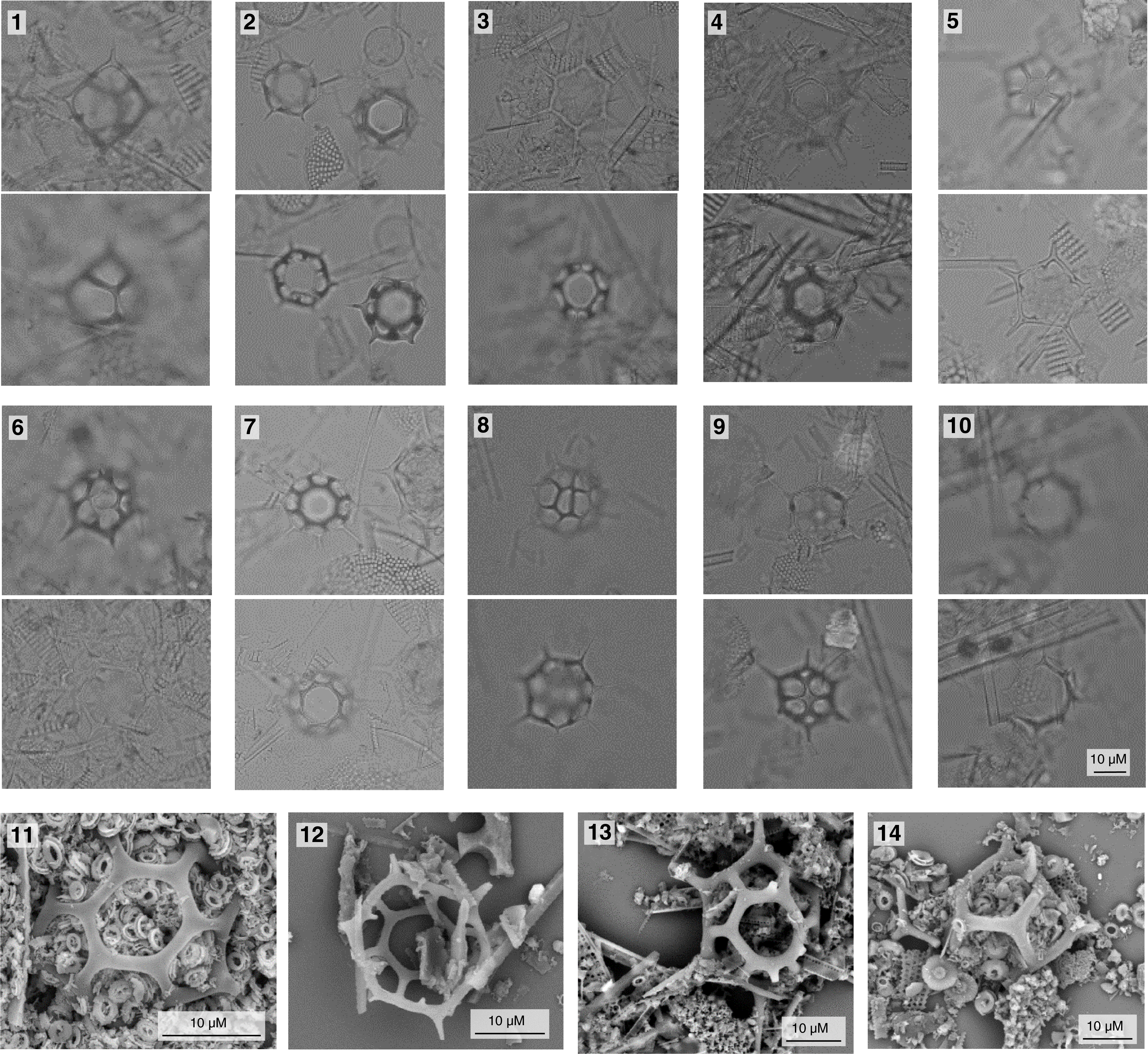
Figure F22. Silicoflagellates.
All samples fall within the D. speculum A Zone developed for the Southern Ocean (Ciesielski 1975), which spans the middle–late Pleistocene. Changes in abundance of the different S. speculum varieties indicate different climatic conditions, and complicated morphologies (specimens with multiple sides or with an apical structure having multiple windows or spines) increase in cold periods. The presence of Dictyocha species and of O. pulchra coincides with intervals of warmer waters.
Calcareous nannofossils
Calcareous nannofossil biostratigraphy is based on the analysis of 83 samples: 1 mudline, 12 core catcher, and 8 split core section samples from Hole U1539A (21 samples); 3 core catcher samples (shallower than 25.49 m CSF-A) from Hole U1539B; and 1 mudline, 32 core catcher, and 24 split-core samples from Hole U1539C (57 samples). Nannofossils are generally present throughout the sedimentary sequence except in a few barren intervals (Table T7; Figure F23). Calcareous nannofossils show significant variations in abundance at Site U1539 (Figures F18, F19), ranging from rare to abundant, becoming dominant in specific intervals, and forming nannofossil oozes, which were observed, for example, in Samples 383-U1539A-7H-4, 16 cm (61.66 m CSF-A), and 8H-5, 29 cm (72.72 m CSF-A); 383-U1539C-13H-1, 92 cm (114.92 m CSF-A); and 383-U1539C-15H-CC (142.84 m CSF-A), coincident with what has been interpreted to be interglacial periods (see Sedimentology). Preservation of calcareous nannofossils was variable, which made it challenging to recognize some of the smaller and more delicate species markers (e.g., E. huxleyi) at this site (Figure F24).

Figure F23. Calcareous nannofossils.
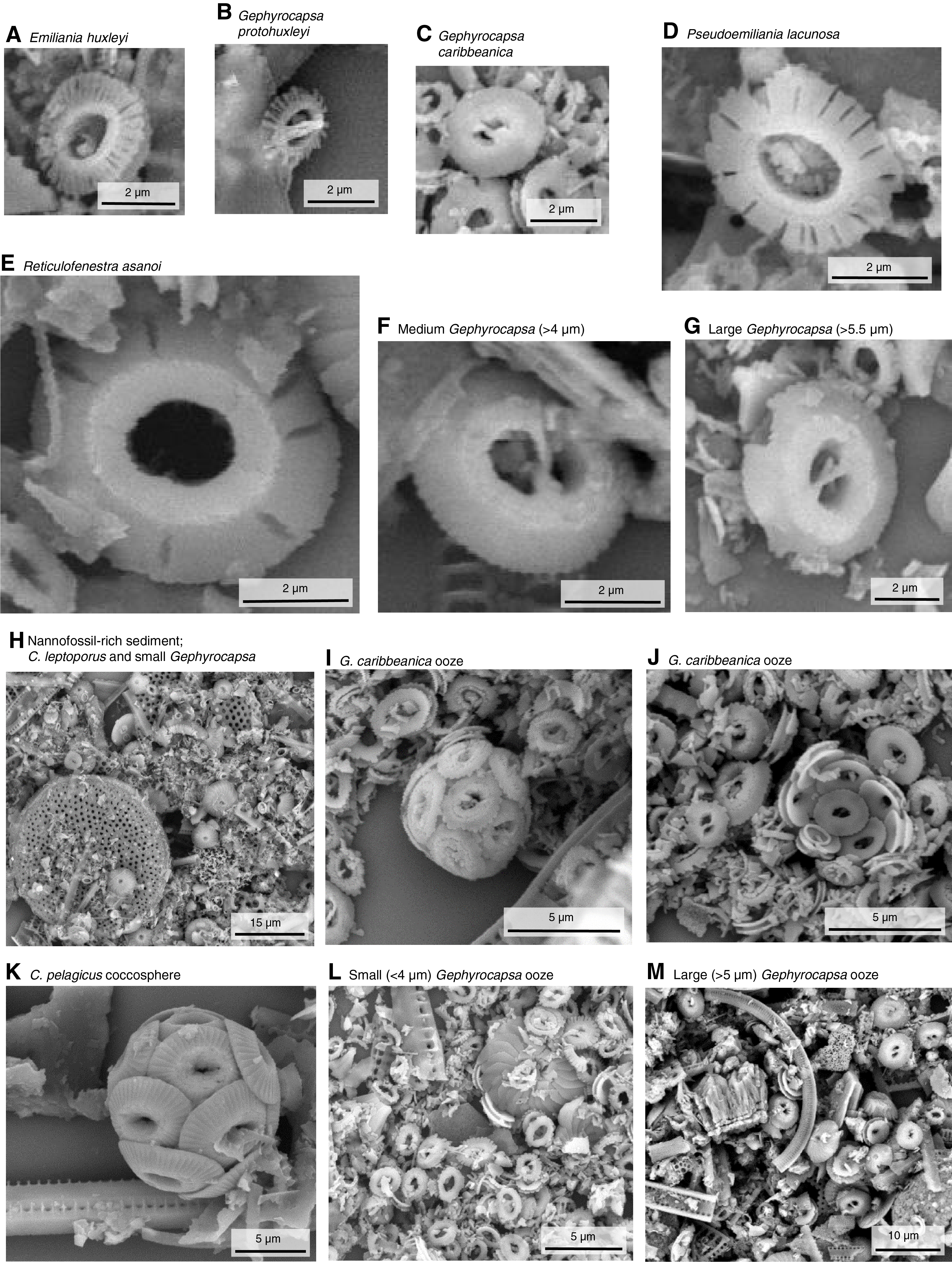
Figure F24. Calcareous nannofossils under SEM.
The nannofossil assemblage at Site U1539 consists of 22 groups/taxa, including E. huxleyi, Gephyrocapsa margerelii/muellerae, Gephyrocapsa caribbeanica, Gephyrocapsa oceanica, Gephyrocapsa spp. (<4 µm, closed >4 µm, medium, and large), Gephyrocapsa omega, Pseudoemiliania lacunosa, Reticulofenestra (<3, 3–5, 5–7, and >7 µm), Reticulofenestra asanoi, Coccolithus pelagicus, Calcidiscus leptoporus, Helicosphaera carteri, and Helicosphaera sellii as well as rare Pontosphaera japonica, Syracosphaera spp., and Rhabdosphaera spp. Occasionally, reworked specimens were found in samples from Holes U1539A and U1539C (Table T7); these include Reticulofenestra umbilica, Reticulofenestra pseudoumbilica, Discoaster sp., and Dictyococcites spp.
Nannofossil Zones CN15/NN21 through CN13b/NN19 were recognized (Figure F16) based on the FO of E. huxleyi (Sample 383-U1539C-5H-4, 16 cm; 42.66 m CSF-A) and the LO of P. lacunosa (Samples 383-U1539A-9H-CC [80.40–80.45 m CSF-A] and 383-U1539C-9H-CC [83.84–83.89 m CSF-A]). Additionally, the rare occurrence of G. omega in one sample (383-U1539C-12H-4, 50 cm; 109.51 m CSF-A), the LO of R. asanoi (Sample 383-U1539C-17H-CC; 160.96–161.01 m CSF-A), the base common occurrence (Bc) of R. asanoi (Sample 21H-CC; 199.36–199.41 m CSF-A), the LO of Gephyrocapsa spp. large (>5.5 µm) (Sample 28F-CC; 249.06–249.11 m CSF-A), and the LO of H. sellii (Sample 32F-CC; 268.26–268.31 m CSF-A) provide good age control for the Pleistocene sequence.
Foraminifers
Planktonic foraminifers
Planktonic foraminifers were analyzed in core catcher samples from all 12 cores from Hole U1539A and Cores 383-U1539C-6H through 26H, 28F, 30F, and 32F (Table T8). Abundance of foraminifers relative to the total >150 µm sieved and dried sediment fraction varies throughout Holes U1539A and U1539C (Figures F18, F19). Foraminifers typically make up less than 25% of coarse fraction residues in Hole U1539A, and Samples 383-U1539A-10H-CC through 12H-CC in particular consist of diatom- and radiolarian-rich residue with few planktonic foraminifers. The only exception is Sample 7H-CC, in which foraminifers make up >50% of the coarse fraction and include many large and well-preserved specimens. Foraminifer abundance in Hole U1539C is variable in Sections 383-U1539C-6H-CC through 19H-CC and low in deeper cores. The assemblages are characterized by species that are typical of temperate to high latitudes: N. pachyderma (sinistral) dominates the assemblage in the majority of samples, and Globigerina bulloides, Truncorotalia crassaformis, Globoconella inflata, and Turborotalita quinqueloba frequently occur in lower abundance. Globoconella puncticulata puncticuloides, a subspecies of Globoconella puncticulata that persisted in the western South Pacific long after the global extinction of G. puncticulata (Hornibrook, 1981; Scott et al., 2007), occurs regularly in Samples 383-U1539C-15H-CC to 32F-CC. Occasionally, species such as Globigerina falconensis, Neogloboquadrina incompta, Globigerinita uvula, Truncorotalia crassaformis hessi, Hirsutella hirsuta, Globigerinita glutinata, and Hirsutella scitula were found. Examples of major foraminifer taxa found at Site U1539 are displayed in Figure F25.
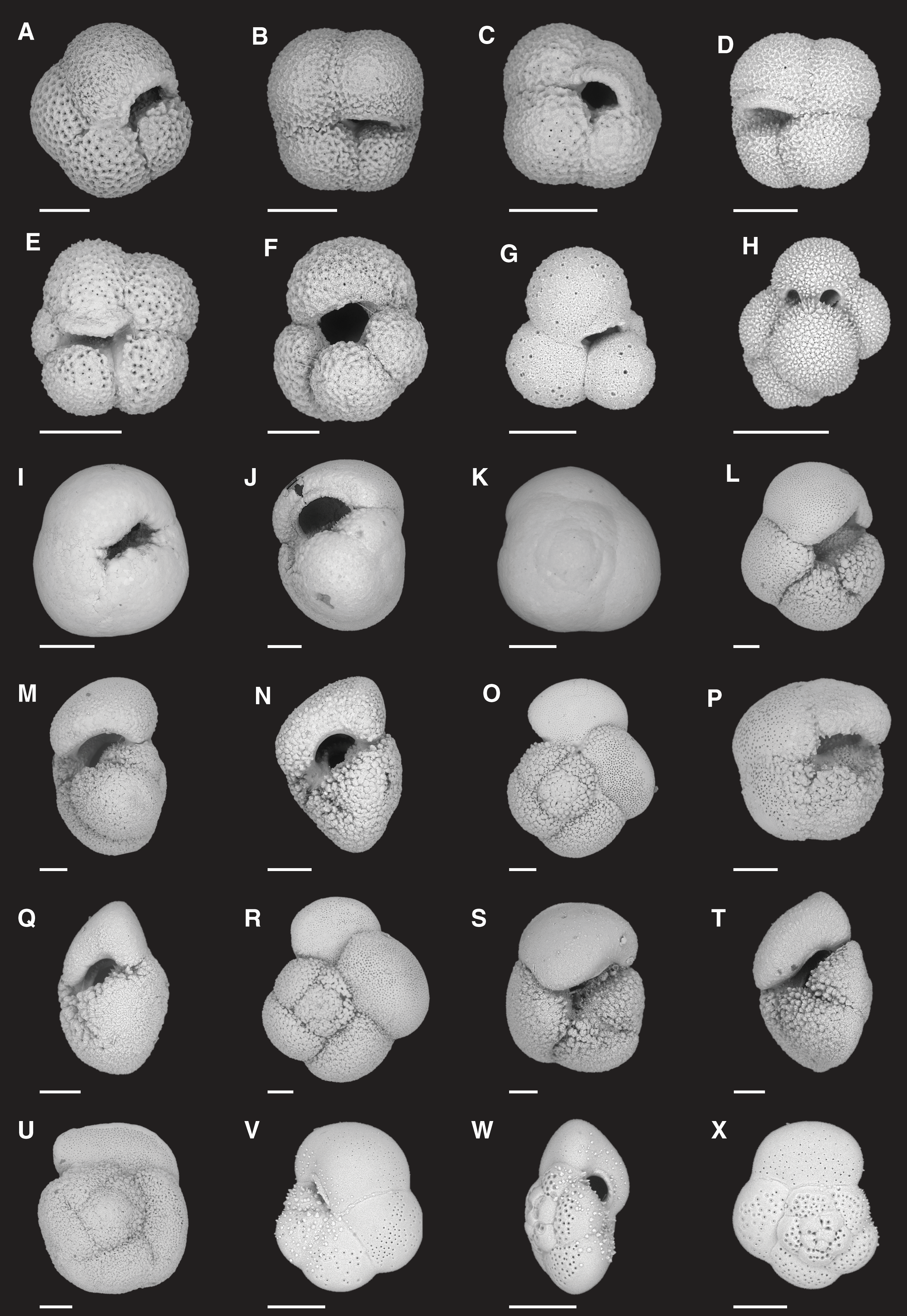
Figure F25. Planktonic foraminifers.
G. inflata is the only biomarker species present in Site U1539 planktonic foraminiferal assemblages. It is found throughout the sequence and gives an age younger than 2.39–3.13 Ma (Wei, 1994) to Sample 383-U1539C-28F-CC. Additionally, G. puncticulata puncticuloides has been reported to occur exclusively in early to middle Pleistocene sediments (Hornibrook, 1981; Scott et al., 2007), suggesting a similar age constraint for Samples 11H-CC through 32F-CC. Both age estimates are consistent with radiolarian, diatom, and nannofossil ages.
Preservation state was generally moderate to good in samples from Hole U1539C, but several tests in Sample 383-U1539A-9H-CC show clear signs of dissolution. We also observed the presence of pyrite framboids attached to foraminiferal tests (Figure F26). Throughout Holes U1539A and U1539C, many species exhibit secondary encrustation, most notably N. pachyderma, G. inflata, G. puncticulata puncticuloides, and T. crassaformis. This may have implications for stable isotope or trace element analyses because the chemical composition of crusts is known to deviate from that of the lamellar calcite (Jonkers et al., 2012; Steinhardt et al., 2015).
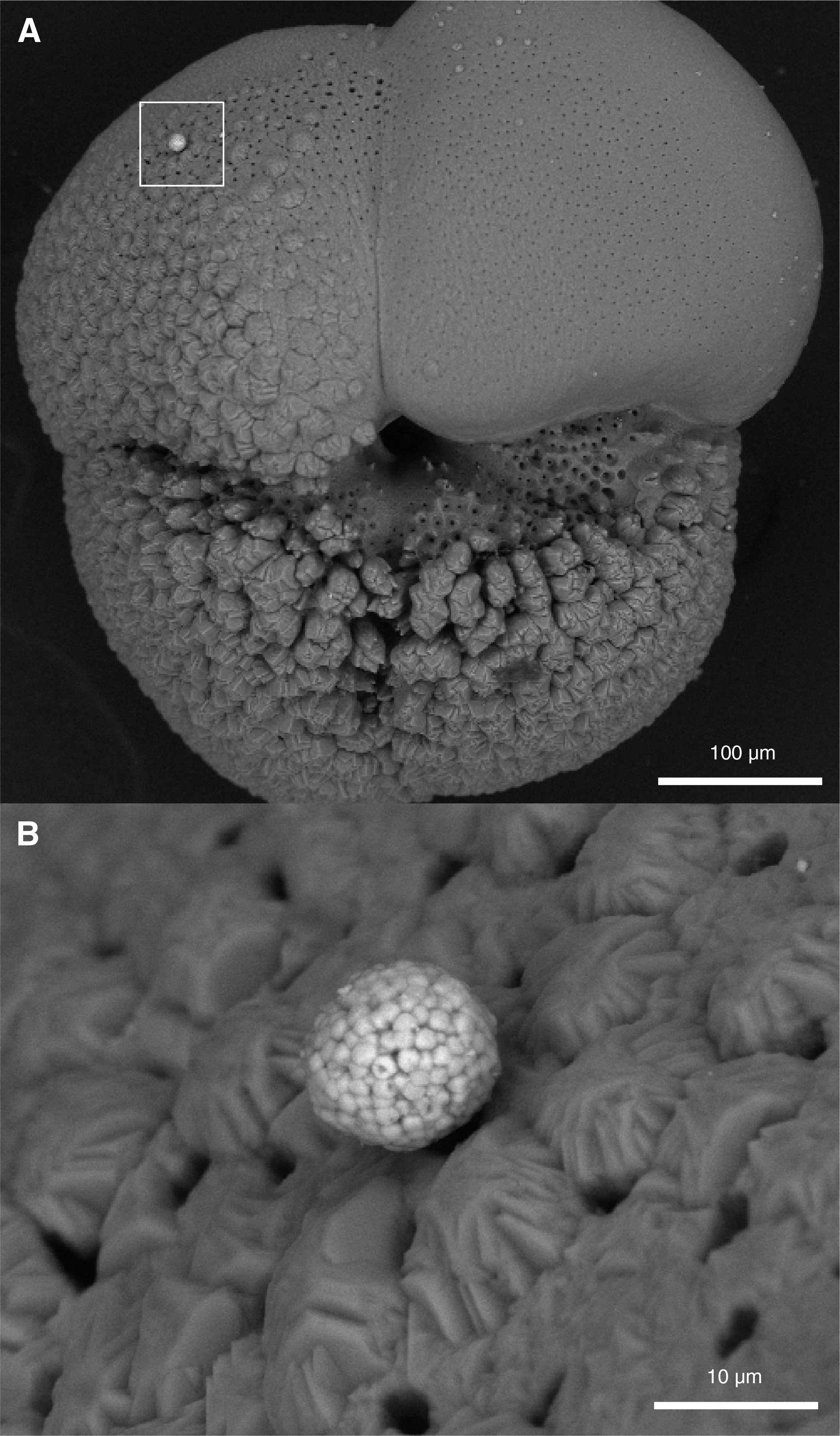
Figure F26. Pyrite framboid.
Benthic foraminifers
Benthic foraminifers were examined in core catcher samples from Hole U1539A (12 samples) and U1539C (21 samples). The mudline samples recovered in Holes U1539A and U1539B were also examined, although systematic counts were not collected for mudline assemblages. To assess assemblage composition and variability in core catcher samples, ~100 specimens from the >125 µm fraction were picked and transferred to slides for identification and counting. The presence and distribution of benthic foraminifers was additionally checked in the 125–63 µm fraction to ensure that assemblages in the >125 µm fraction were representative and that small species such as phytodetritus feeders or small infaunal taxa were not overlooked.
Benthic foraminifer abundance is generally very low, and foraminifers are moderately preserved throughout the ~270 m thick early Pleistocene to Holocene succession recovered in Holes U1539A and U1539C (Figures F18, F19, F27; Table T9). Sample 383-U1539C-18H-CC is the only sample barren of benthic foraminifers; they are rare in Samples 383-U1539A-4H-CC (33.35 m CSF-A), 383-U1539C-27F-CC (244.52 m CSF-A), and 31F-CC (259.0 m CSF-A) (Figures F18, F19).

Figure F27. Benthic foraminifer abundance and diversity.
A total of 62 benthic foraminiferal taxa were identified. Table T9 summarizes the downcore distribution of benthic foraminifers in core catcher samples from Holes U1539A and U1539C. Figure F28 illustrates characteristic taxa found at this site.
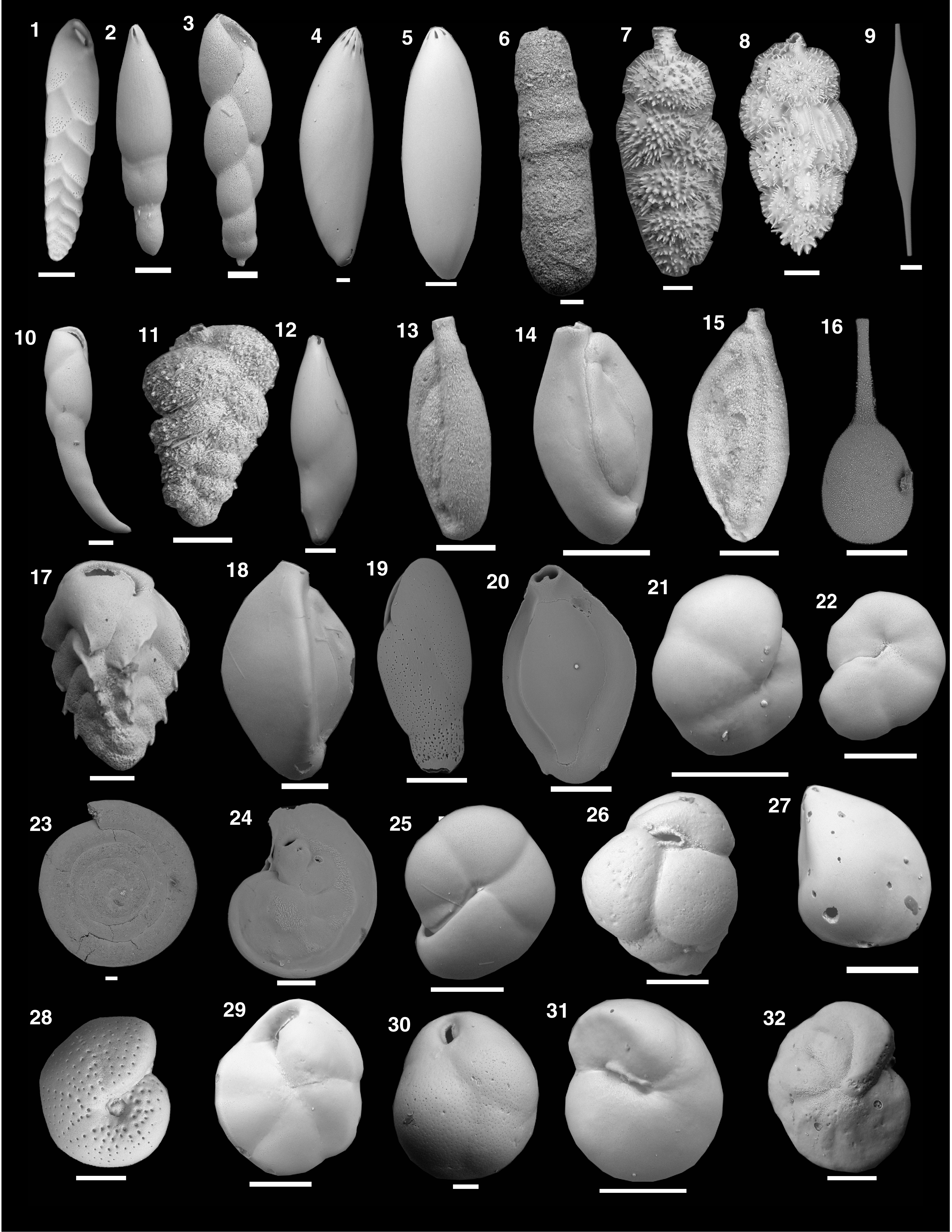
Figure F28. Benthic foraminifers.
The overall composition of assemblages indicates an abyssal paleodepth above the carbonate compensation depth (CCD) throughout the early Pleistocene to Holocene. Species commonly recorded through the succession are C. mundulus, Epistominella exigua, Globocassidulina subglobosa, M. barleeanum, O. umbonatus, P. bulloides, and Pullenia quinqueloba, which overall indicate varying oxygen conditions, low to intermediate carbon flux, and cold deep water with occasionally strongly pulsed food supply and oligotrophic conditions (Gupta et al., 2004; Singh and Gupta, 2004; Singh et al., 2012; Verma et al., 2013). High abundances of M. barleeanum and P. bulloides are found in core catcher samples from deeper than ~180 m CSF-A. These two species are associated with intermediate to high flux of organic matter in different oceans (Rathburn and Corliss, 1994; Gupta and Thomas, 1999; Singh and Gupta, 2004; Verma et al., 2013) in low oxygen conditions (Corliss, 1985; Fontanier et al., 2005) and are reported as high productivity taxa from the Pacific (Loubere, 1991). G. subglobosa is a cosmopolitan species that occurs within the depth range of Circumpolar Deep Water and is associated with Antarctic Bottom Water (Corliss, 1979; Singh and Gupta, 2004, 2010; Singh et al., 2012). It is abundant in Samples 383-U1539C-19H-CC and 32F-CC, suggesting enhanced influence of Antarctic Bottom Water at Site U1539 during this interval. The upper part of the succession (above ~100 m CSF-A) is characterized by E. exigua and O. umbonatus. E. exigua is a cosmopolitan species that feeds opportunistically on phytodetritus deposited seasonally on the seafloor (Gooday, 1988; Thomas, et al., 1995; Singh and Gupta, 2004, 2010). O. umbonatus is a cosmopolitan abyssal taxon associated with Antarctic Bottom Water in the Indian Ocean (Corliss, 1979; Singh and Gupta, 2010), the Atlantic Ocean (Streeter and Shackleton, 1979), and the Antarctic (Uchio, 1960). It is capable of surviving under food-limited and low oxygen conditions (Singh and Gupta, 2010). C. mundulus occurs sporadically throughout the record and reaches its maximum abundance in Samples 383-U1539C-12H-CC, 21H-CC, and 22H-CC, suggesting strongly pulsed cold water with low to intermediate organic flux.
Downcore changes in assemblage composition at Site U1539 reflect changes in paleoenvironmental conditions that are probably linked to distinct phases of glacial–interglacial changes during the Pleistocene. Overall, samples with low species diversity are typical for glacial intervals and samples with high species diversity occur during interglacial periods (Singh and Gupta, 2005; Gupta et al., 2013). However, the analyzed sample resolution is not high enough to capture all of the glacial–interglacial changes in the South Pacific.
The mudline sample from Hole U1539A has stained agglutinated and calcareous benthic foraminifers, whereas the mudline sample from Hole U1539B does not have any stained benthic foraminifers. This suggests that the core top sample from Hole U1539A collected modern seafloor sediments, which were not observed in the mudline sample from Hole U1539B. The stained mudline assemblage from Hole U1539A includes specimens of the agglutinated species Reophax scorpiurus, Reophax spiculifer, and Siphotextularia rolshauseni and calcareous taxa including Bolivina pacifica, Fursenkoina complanata, E. exigua, Fissurina spp., C. mundulus, Gyroidinoides sp., G. subglobosa, P. quinqueloba, O. umbonatus, Quinqueloculina venusta, and Quinqueloculina oblonga (Figure F29). A few more species in addition to the species mentioned above were found unstained. The mudline samples from both holes are dominated by unstained planktonic foraminifers and radiolarians.
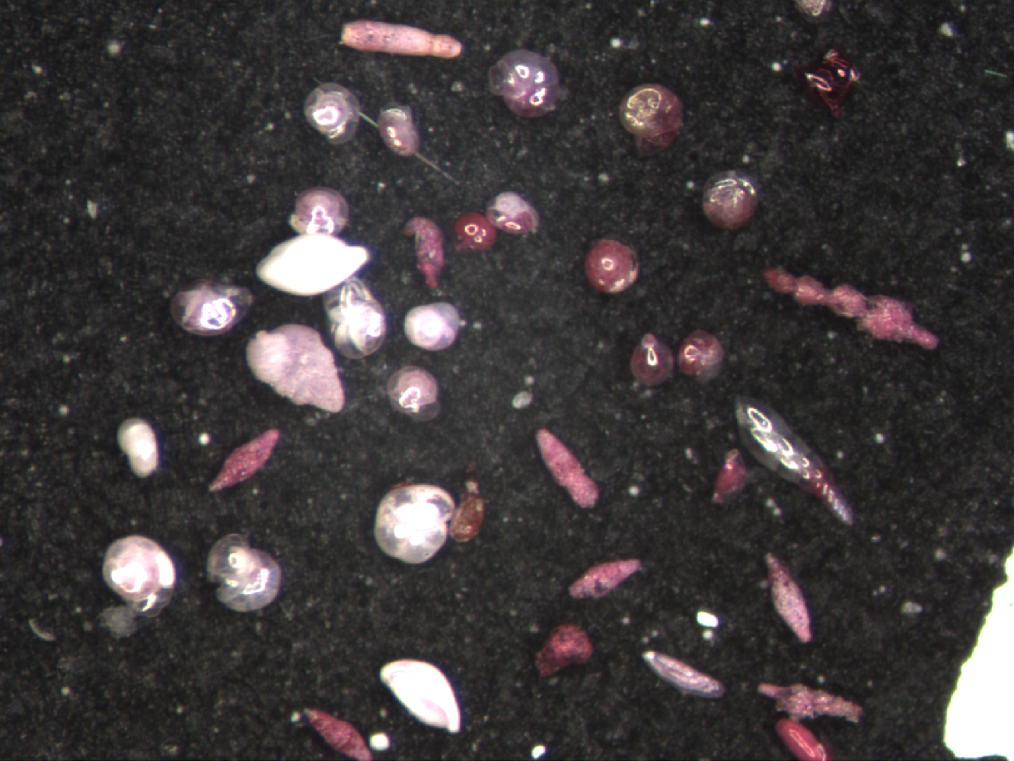
Figure F29. Stained benthic foraminifers in mudline.
Ostracods
All core catcher samples from Holes U1539A, U1539C, and U1539D were scanned for the presence of ostracods during shipboard examination of benthic foraminifers. Ostracods are rare (≤10 valves) to barren in most samples, and only five samples yielded a few specimens (Table T10). Six genera were identified: Bradleya, Krithe, Henryhowella, Legitimocythere, Pelecocythere, and Pennyella. All of them have a predominantly abyssal distribution (Alvarez Zarikian, 2015; Stepanova and Lyle, 2014). The highest abundance (8 valves) was observed in Sample 383-U1539C-15H-CC, which was interpreted to represent MIS 31. See Biostratigraphy in the Site U1540 chapter (Winckler et al., 2021c) for an image of ostracods found at Site U1539.
Paleomagnetism
The natural remanent magnetization (NRM) of archive-half core sections from Site U1539 was measured and remeasured after alternating field (AF) demagnetization at 2 cm increments. Peak AFs were restricted to a maximum of 15 mT for all sections recovered using the APC/HLAPC system with standard full and half-length nonmagnetic and steel core barrels (see Operations). The number of demagnetization steps and the peak fields used reflect the severity of the drill string and natural overprints, the desire to use low peak fields to preserve the magnetization for future shore-based studies, and the need to maintain core flow through the laboratory. When time permitted, demagnetization steps were added to facilitate interpretation of the paleomagnetic record. Cores from Holes U1539A and U1539B were mostly demagnetized at AFs of 5, 10, and 15 mT. Cores from Holes U1539C and U1539D were demagnetized at AFs of 10 and 15 mT. All samples were, at the very least, measured before and after 15 mT AF demagnetization. See Table T11 for a list of AF demagnetization steps employed. To maintain core flow, sections completely affected by drilling disturbance (see Sedimentology) were not measured. Data associated with intervals affected by obvious drilling deformation or measurement errors were culled prior to uploading or during data processing.
Sediments recovered from Holes U1539A–U1539D had NRM intensities that vary over approximately six orders of magnitude from 10–1 to 10–6 A/m (Figure F30). Intensities and overall variability are slightly reduced after peak AF demagnetization at 15 mT. Much of this variability can be attributed to the combined effect of drill string overprints, core disturbance, and dropstones intermixed in a lithology dominated by weakly magnetic biogenic oozes that vary in their magnetic behavior depending on whether they are dominantly siliceous or carbonate (see Sedimentology).
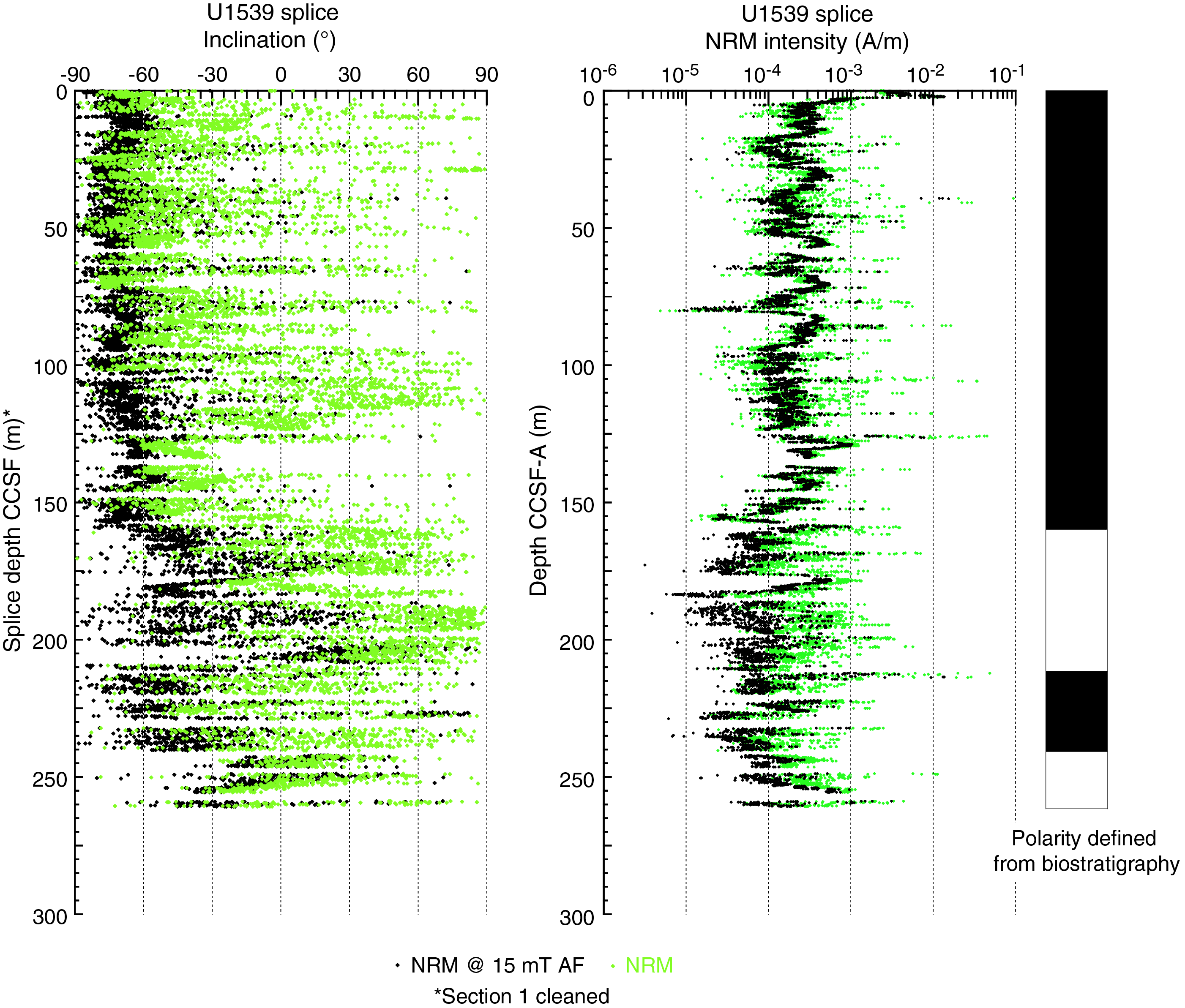
Figure F30. Inclination and NRM intensity.
NRM intensities were relatively high (10–2 to 10–3 A/m) before and after AF demagnetization in the upper two sections of the mudline core recovered in Hole U1539A (Figure F30). Below ~3 m core composite depth below seafloor, Method A (CCSF-A), starting at and continuing below the brown to gray color transition (see Sedimentology), intensities drop by about an order of magnitude and oscillate in the mid 10–3 to mid 10–4 A/m range to ~150 m CCSF-A (Figure F30). Intensities in the 3 to ~150 m CCSF-A interval vary on a tens of meters scale, and occasional intensity spikes are often significantly reduced by AF demagnetization. A few discrete intervals of extremely low intensities in the 10–6 A/m range are associated with carbonate oozes. In contrast, diatom oozes are often associated with higher intensities, well-defined directions (described in more detail below), and well-behaved demagnetization behaviors. This somewhat surprising observation may result from a secondary magnetization induced by preferential alignment during coring, although postcruise studies would be needed to more fully investigate these observations. Below 160 m CCSF-A, mean intensities drop (approximately half an order of magnitude) and variability increases after peak AF demagnetization. There is little change in intensity and variability prior to demagnetization. This pattern is less pronounced in the ~225–245 m CCSF-A interval, but it is more clearly observed again below (Figure F30).
Above 160 m CCSF-A, inclinations prior to demagnetization are quite variable, dominantly negative (as expected for Brunhes age sediment), but also commonly positive. After peak AF demagnetization of 15 mT, inclinations are generally more steeply negative (Figure F30) and generally near values expected for a geocentric axial dipole (approximately ±71.5°) at the latitude of Site U1539 (~56°S). Although many intervals of shallower than expected or even positive inclinations are observed, they are often associated with extremely low intensity <10–5 A/m and are therefore intervals of low signal-to-noise ratios. Below 160 m CCSF-A, the pattern changes. Prior to demagnetization, inclinations are more positive than above, and after peak AF at 15 mT, inclinations are positive and shallowly negative. Although a clear record of polarity changes that could be interpreted and tuned to the geomagnetic polarity timescale (GPTS) (Cande and Kent, 1995) and The Geological Timescale 2012 (GTS2012) (Hilgen et al., 2012) was not preserved, predicted polarities were based upon biostratigraphic age assignments (see Biostratigraphy). Figure F30 demonstrates the impacts of polarity on the magnetic record at Site U1539. Postcruise research will be needed to tease apart the relationships between polarity, remanence intensity, and lithology to further understand the dynamics of sediment magnetism in the Southern Ocean and the information that it captures about the Earth system.
Geochemistry
Sediment gas sampling
Routine safety hydrocarbon measurements were collected at Site U1539 in headspace gastight vials at a resolution of approximately one 5 cm3 sample per core for Cores 383-U1539A-1H through 12H (2.99–105.57 m CSF-A) and 383-U1539C-9H through 28F, 30F, and 32F (81.98–266.41 m CSF-A) (see Geochemistry in the Expedition 383 methods chapter [Winckler et al., 2021a]). Headspace samples were not collected from HLAPC cores (383-U1539C-29F and 31F). Methane concentrations are low at this site overall and gradually increase downhole, averaging 12.3 ppmv and never exceeding 18.4 ppmv (Figure F31; see U1539-T1.xlsx in GEOCHEM in Supplementary material). Ethane and propane remain below detection limit throughout the entire hole.

Figure F31. Headspace methane concentrations.
Interstitial water chemistry
At Site U1539, 63 whole rounds were collected for interstitial water (IW) samples from Holes U1539A (31 samples; 0–105 m CSF-A) and U1539C (32 samples; 78.9–266.36 m CSF-A) at a resolution of three per core from 0 to 120 m CSF-A, two per core from 120 to 150 m CSF-A, and one per core from 150 m CSF-A to the bottom of Hole U1539C. A mudline sample collected from Hole U1539A was allowed to settle for several hours and subsequently filtered through a 0.45 µm syringe-tip filter. Filtered mudline water was subjected to all standard shipboard chemistry analyses.
Each whole round was placed in a glove bag filled with nitrogen gas and trimmed on all sides to remove contamination from drilling fluid as well as any sediment that may have been oxidized by contact with the atmosphere. The squeezers were also assembled in the glove bag to prevent further oxidation. The whole rounds were then squeezed for IW, and extracted volumes ranged from 50 to 60 mL in the upper portions of the hole and from 20 to 30 mL at greater depths. After taking 8 mL of extracted IW for shipboard analyses, the remaining IW was split and preserved according to requests for postcruise shore-based analyses (see Geochemistry in the Expedition 383 methods chapter [Winckler et al., 2021a]).
Alkalinity and pH
Alkalinity increases to ~5 mM in the uppermost 10.6 m, but no appreciable change is observed below that depth (Figure F32; see U1539-T2.xlsx in GEOCHEM in Supplementary material). The surface increase in alkalinity is likely caused by anaerobic organic matter remineralization. pH values also increase from 7.7 at the surface to ~8 at 2.94 m CSF-A and remain constant with depth at an average value of 8.0 ± 0.1 (±1σ).
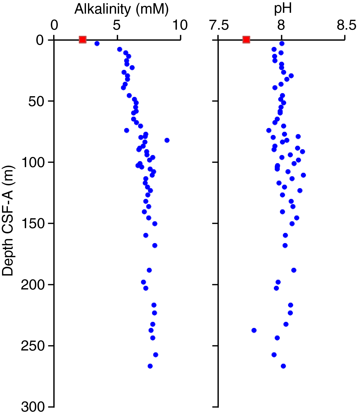
Figure F32. IW alkalinity and pH.
Salinity, chlorinity, sodium, and bromide
Salinity values for all IW samples are constant at 35 throughout the core. Chlorinity measured using titration is in good agreement with chloride concentrations obtained through ion chromatography. Chlorinity exhibits a gradual increase from surface values of 556 ± 2 mM to 565 ± 4 mM at ~50 m CSF-A and then remains fairly constant below this depth (Figure F33). Sodium (Na) and bromide (Br−) increase slightly over the uppermost 50 m; Na increases from 467 to ~480 mM, and Br− increases from 0.85 to 0.88 mM. Otherwise, Na and Br- remain relatively constant throughout the core at average values of 483 ± 10 mM and 0.87 ± 0.10 mM, respectively (Figure F33).
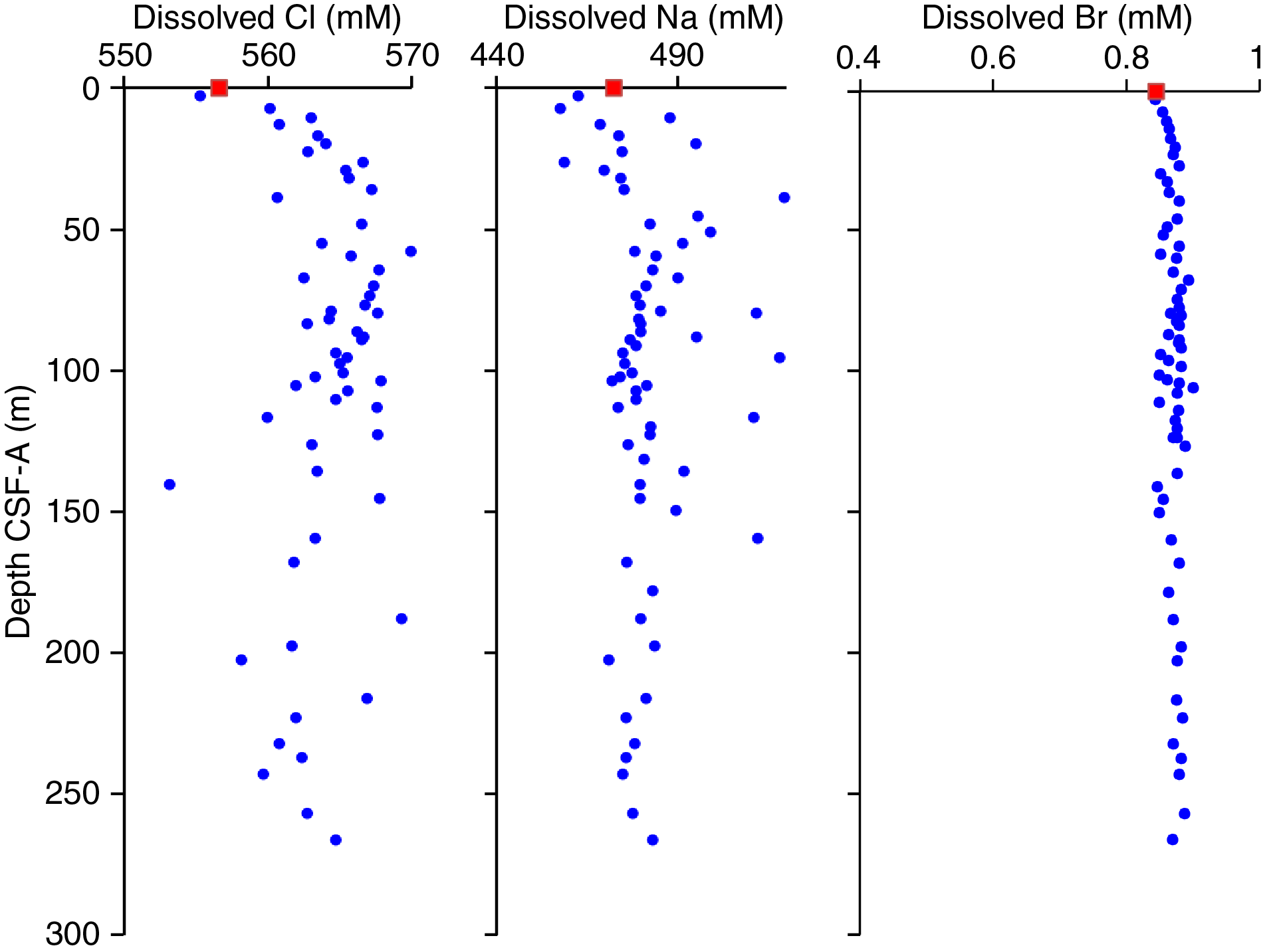
Figure F33. IW chloride, sodium, and bromide.
Magnesium and lithium
Magnesium (Mg) and lithium (Li) appear conservative throughout the sediment column, with some scatter. Average values (±1σ) are 53.0 ± 1.2 mM for Mg and 20.3 ± 0.6 µM for Li (Figure F34).
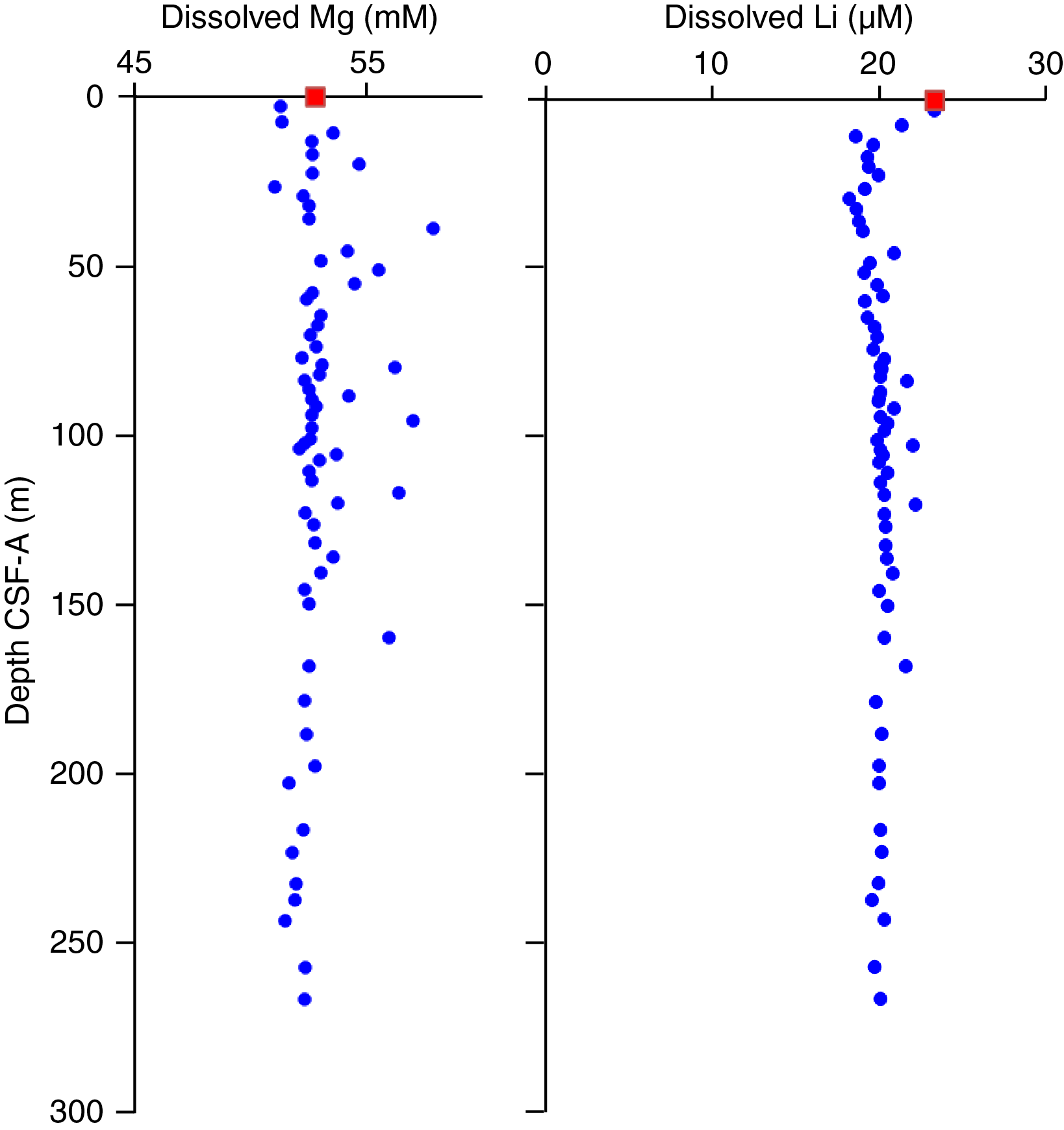
Figure F34. IW magnesium and lithium.
Iron, manganese, calcium, and strontium
Iron (Fe) concentrations in most IW samples are below detection limit and hence not plotted. Manganese (Mn) concentrations increase sharply from below detection limit in the mudline sample to a maximum of 60 µM at 7.57 m CSF-A, indicating anaerobic, reductive dissolution of Mn oxides in the upper 3 m of the sediment column. Mn concentrations drop again at ~20 m CSF-A before increasing to a second local maximum of 72 µM at 32.35 m CSF-A (Figure F35). Following these shallow peaks, Mn concentrations steadily decrease to 13 µM at 126 m CSF-A, below which depth concentrations remain steady to 237 m CSF-A. Small increases in Mn concentrations are observed in the bottom two samples (383-U1539C-30F-2, 142–147 cm, and 32F-2, 146–151 cm).
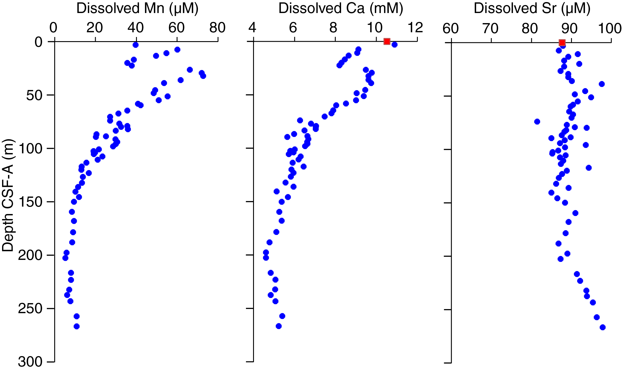
Figure F35. IW manganese, calcium, and strontium.
Calcium (Ca) concentrations decrease consistently in the uppermost 20 m and reach 8.5 mM. They then increase to a concentration maximum at 35.9 m CSF-A and subsequently decrease to 4.6 mM at ~197 m CSF-A (Figure F35). This decrease in Ca concentrations occurs at the same depth where Mn concentrations decrease. Precipitation of authigenic carbonate minerals could explain this observation. The deeper part of the record exhibits slight increases in Ca concentrations to ~5.3 mM.
Strontium (Sr) concentrations to ~200 m CSF-A scatter around an average value of 89.6 ± 3.2 µM (Figure F35). Below 200 m CSF-A, the concentration progressively increases to a maximum value of 97.8 µM in the bottom sample. The increase in Sr concentrations with concomitant small increases in Ca concentrations suggest dissolution of carbonate minerals.
Phosphate, sulfate, and ammonium
Phosphate (PO43−) concentrations increase in the uppermost few meters below the seafloor and reach values of ~41 µM at 10.6 m CSF-A. Concentrations of PO43− below this initial maximum vary around a mean of 33 ± 7 µM (Figure F36).
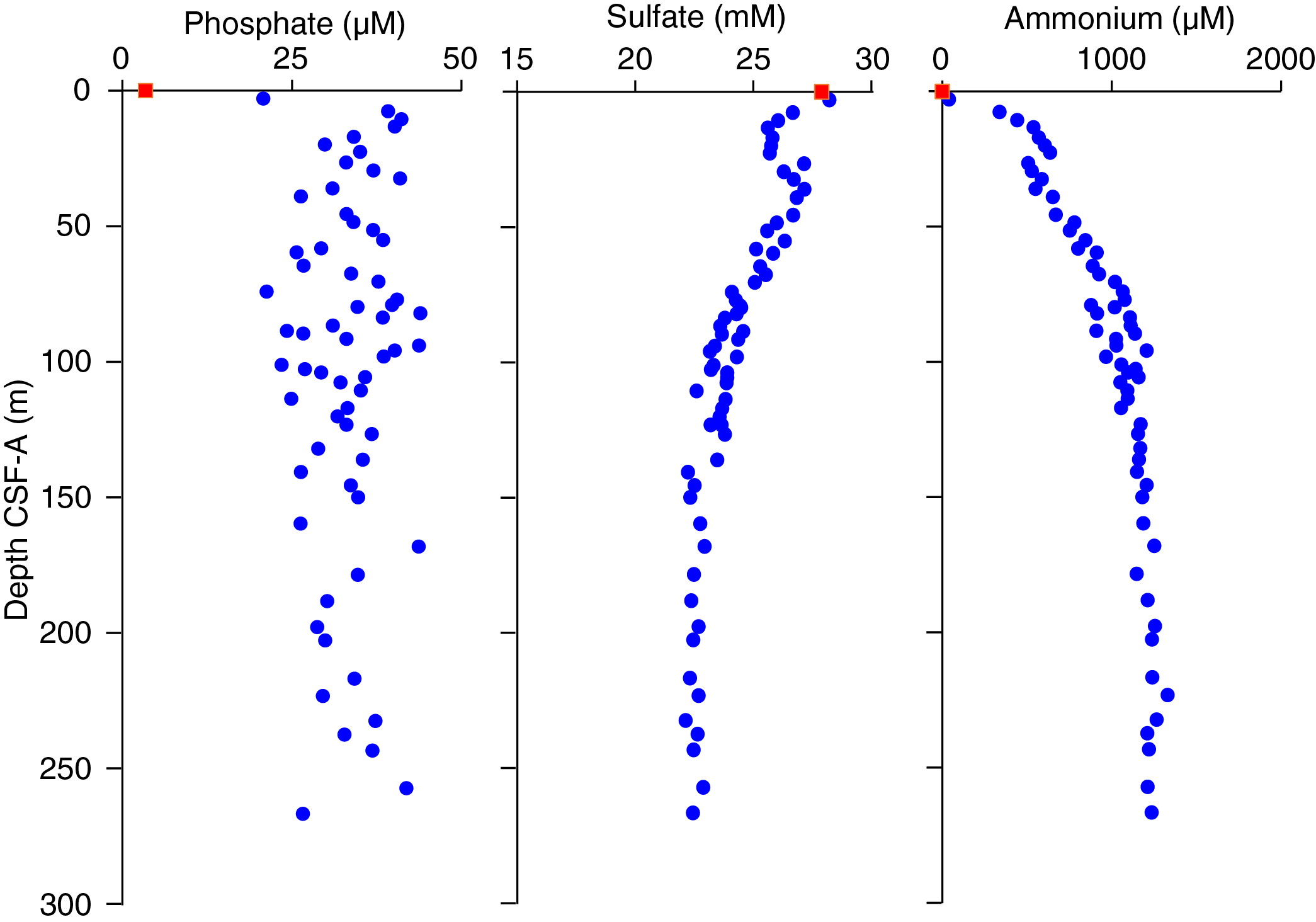
Figure F36. IW phosphate, sulfate, and ammonium.
Sulfate (SO42−) concentrations show a decreasing trend with increasing depth and reach 22 mM at 140 m CSF-A (Figure F36). This steady decrease is interrupted by a return to near-surface values (27.1 mM) at 26.49 m CSF-A, which could be related to past changes in salinity because SO42− is conservative in the water column.
Ammonium (NH4+) increases steadily from below detection limit in the mudline sample to 1207 µM at 95.76 m CSF-A (Figure F36). Below this depth, concentrations continue to increase at a slower rate and reach a maximum value of 1265 µM at 232.14 m CSF-A. Most likely, NH4+ is most likely produced during organic matter remineralization and accumulates in the IW downhole.
Potassium, silicon, boron, and barium
Potassium (K) shows a slight increase from the surface value of 10.3 mM to a maximum of 11.9 µM at 50 m CSF-A, below which depth it remains constant at 11.1 ± 0.4 mM (Figure F37). Silicon (Si) and boron (B) concentrations increase over the uppermost ~10–20 m from 187 to 843 µM for silicon and from 411 to 523 µM for boron. Below this depth, both elements remain roughly constant with depth. Barium (Ba) is only present at low concentrations (~0.5 µM), and in many samples it is below detection limit (Figure F37).
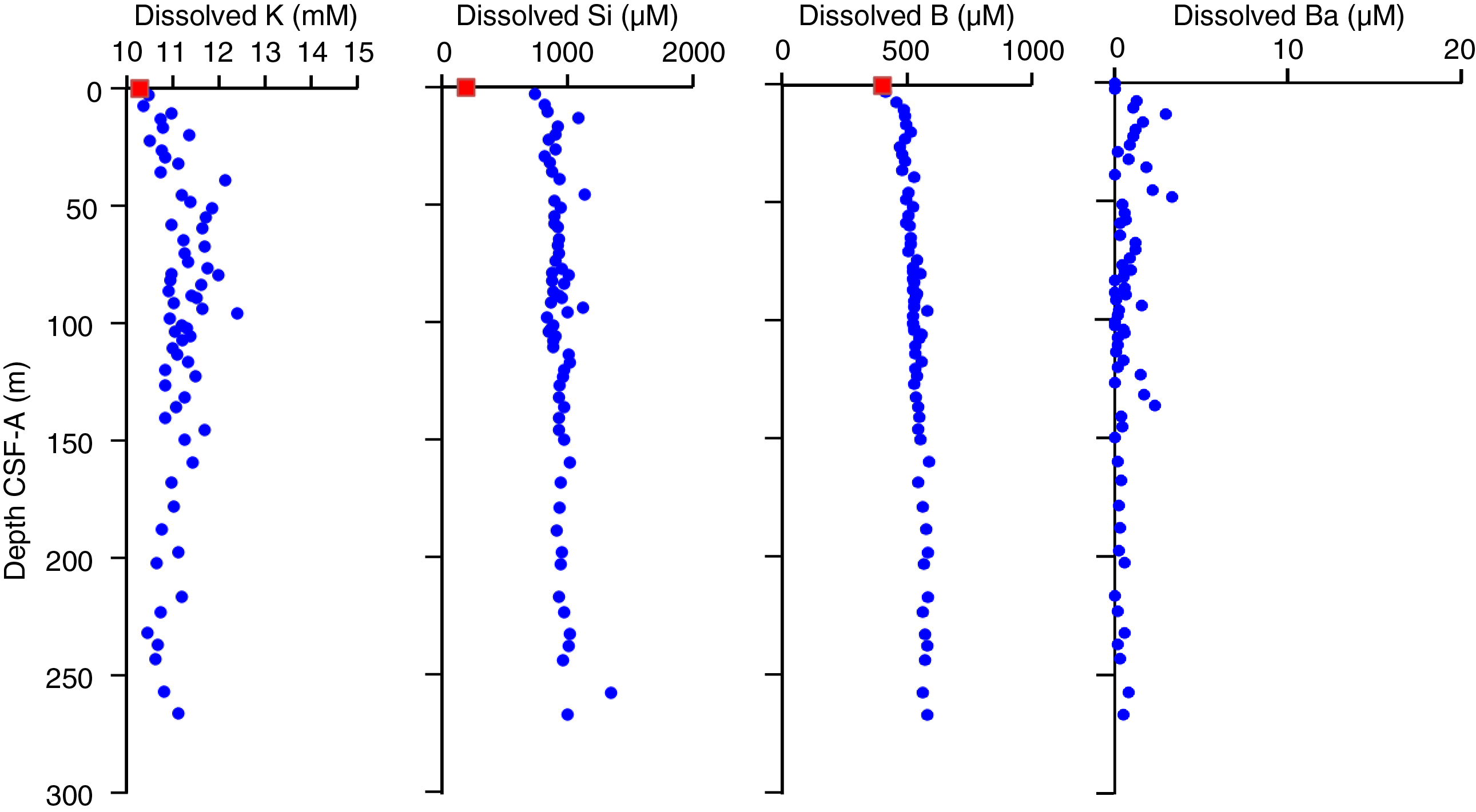
Figure F37. IW potassium, silica, boron, and barium.
Bulk sediment
Calcium carbonate
Calcium carbonate (CaCO3) concentration measurements for Hole U1539A were obtained with a resolution of four samples per core in Cores 383-U1539A-1H, 2H, and 9H and generally three samples in every other core. For Hole U1539C, samples from Cores 383-U1539C-9H through 32F were measured, providing 90 samples for this site. The composite CaCO3 record of Holes U1539A and U1539C shows downhole variability ranging from 2.85 to 92.84 wt% (Figure F38; see U1539-T3.xlsx in GEOCHEM in Supplementary material). The CaCO3 record of Hole U1539A is generally consistent with the CaCO3 record of Hole U1539C from 77.44 to 105.97 m CSF-A. The disagreement between the two CaCO3 records observed in the overlapping part between 97.03 and 105.97 m CSF-A can be explained by the high core disturbance in Cores 383-U1539A-11H and 12H (see Sedimentology). CaCO3 measurements show a strong correlation with RGB blue and color reflectance L* measurements (see Sedimentology).
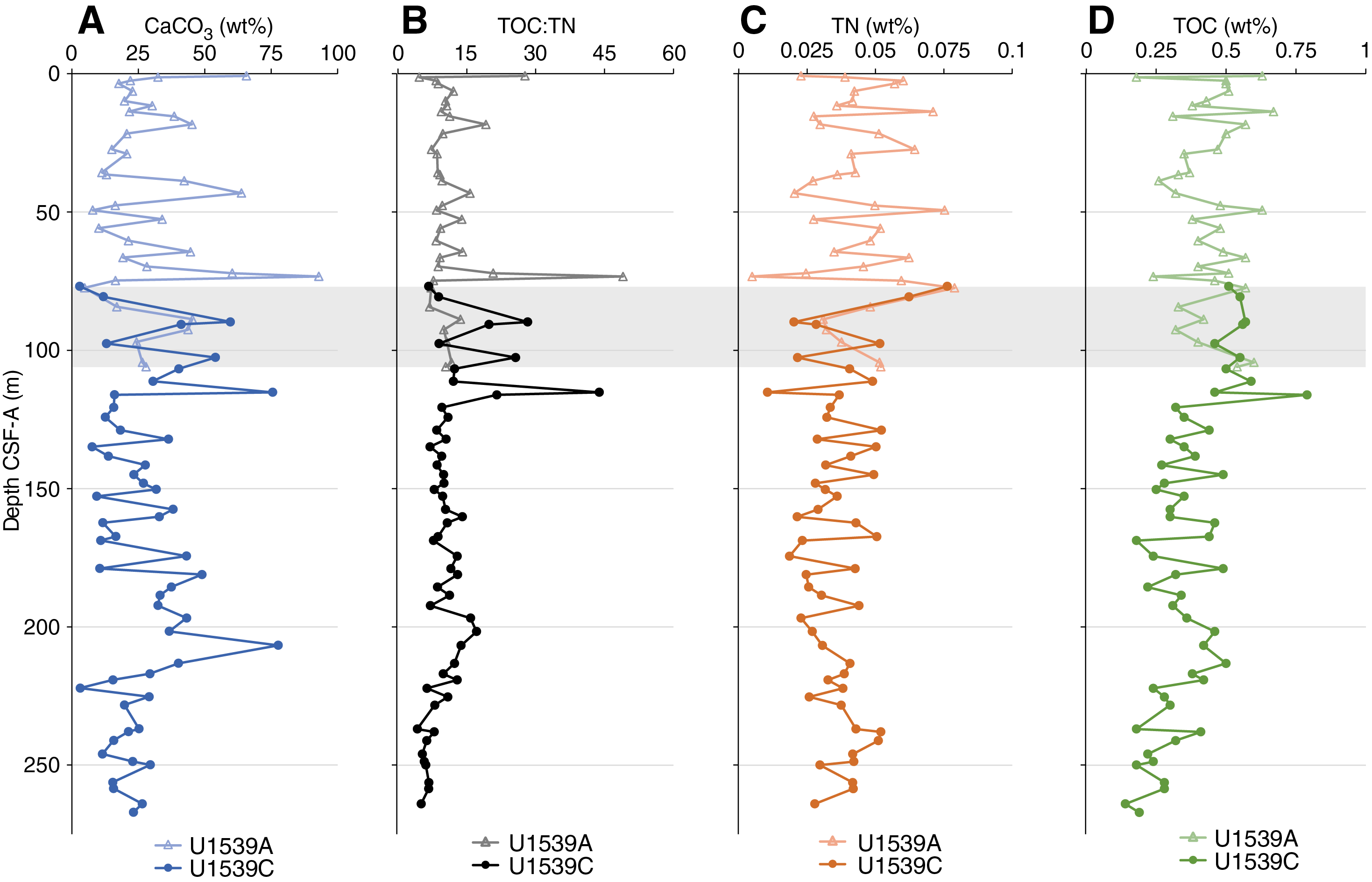
Figure F38. Solid-phase carbon and nitrogen.
Major and trace elements
A total of 32 samples taken for CaCO3 analyses from Holes U1539A and U1539C were also analyzed for major and minor element concentrations using inductively coupled plasma–atomic emission spectroscopy (ICP-AES) (see U1539-T4.xlsx in GEOCHEM in Supplementary material). Elemental oxides (namely MgO, K2O, Fe2O3, and TiO2) show a strong positive correlation with aluminum (Al) oxides (Figure F39). This correlation could indicate the presence of micaceous/clay minerals. Clay minerals in pelagic marine sediments can be formed in situ or delivered by wind-blown dust from continental sources. SiO2 and CaO do not exhibit any well-defined pattern when plotted against Al2O3 (Figure F39). Diatoms, foraminifers, and calcareous nannofossils dominate different sections of the core, so dilution of lithogenic material by these biogenic constituents might explain the weak relationship between these elements and Al2O3. Phosphorous and Mn oxides also do not show any distinct relationship when plotted against Al2O3, possibly due to redox changes and authigenic phosphate and carbonate formation.
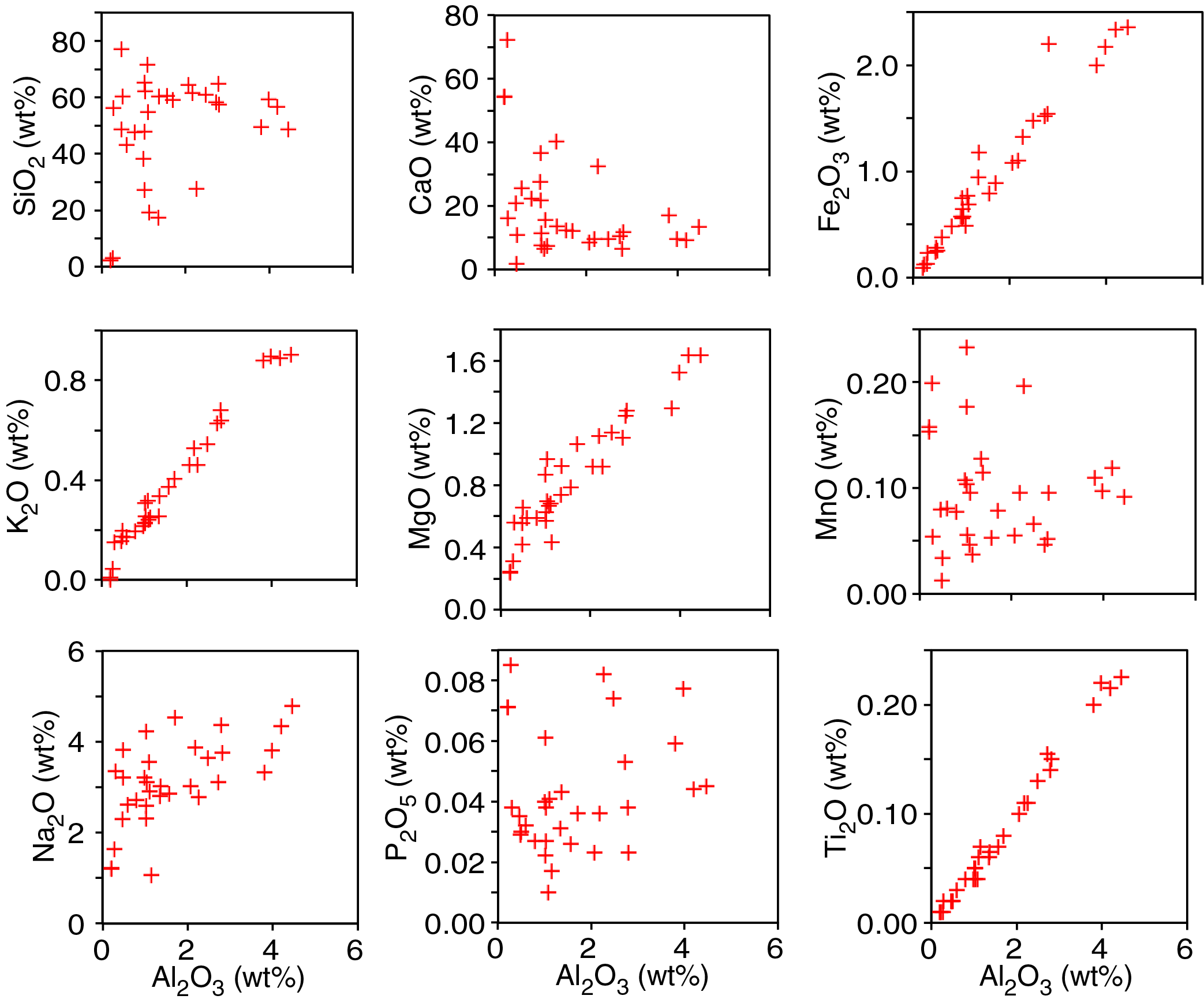
Figure F39. Bulk sediment elemental oxides vs. aluminum oxide.
Downcore major and minor elemental concentrations exhibit variability that changes with depth. In the uppermost 150 m, Al, Fe, Ba, K, titanium (Ti), zinc (Zn), and zircon (Zr) exhibit similar high variability (Figure F40). Although the absolute concentrations vary between elements, the peaks and troughs match for each of these elements. Below 150 m CSF-A, the variability decreases significantly. The high variability above 150 m CSF-A could be due to increased dust levels in the later Pleistocene and/or variable dilution by other sedimentary components. Sr contents show an inverse relationship with Al and co-vary with the Ca content of the bulk sediment. Bulk sediment Ca is primarily controlled by biogenic CaCO3; hence, covariation of Sr and Ca can be attributed to incorporation of Sr in biogenic CaCO3. Based on the preliminary age model, ~73 m CSF-A represents MIS 11. This interval is marked by ~92 wt% CaCO3 (dominated by foraminifers) and the highest bulk sediment Sr concentration for this site, further attesting that Sr in the bulk sediment is correlated to biogenic CaCO3.
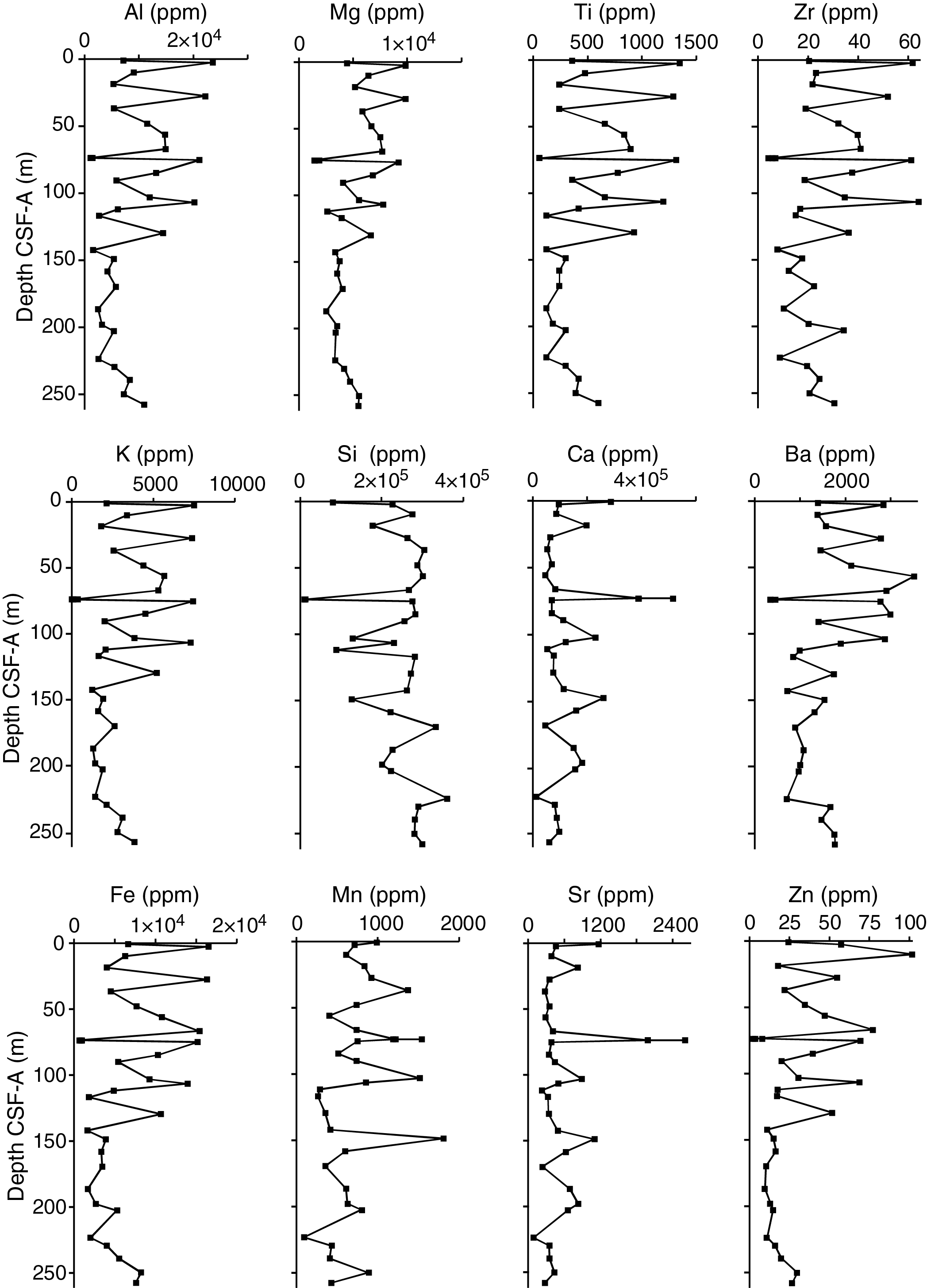
Figure F40. Bulk sediment major and minor element concentrations.
Organic carbon
All samples analyzed for CaCO3 were additionally subsampled for total carbon (TC) analysis. Total organic carbon (TOC) estimates were obtained by measuring the TC and subtracting the contribution of inorganic CaCO3 (see Sedimentary inorganic and organic carbon, nitrogen, and carbonate content in the Expedition 383 methods chapter [Winckler et al., 2021a]). The composite TOC record of Holes U1539A and U1539C has a mean of 0.398 wt% and shows downhole variability ranging from 0.14 to 0.79 wt% (Figure F38; see U1539-T3.xlsx in GEOCHEM in Supplementary material). In the upper portion of the composite core between 0.8 and 116.11 m CSF-A, mean TOC is 0.47 ± 0.12 wt%. Farther downhole between 116.11 and 120.64 m CSF-A, TOC decreases from 0.79 to 0.32 wt%. From 120.64 m CSF-A to the bottom of the core at 267.11 m CSF-A, mean TOC is lower and slightly less variable with a value of 0.32 ± 0.10 wt%. The TOC record shows no correlation to the CaCO3 record (r2 = 0.0002) downhole.
Total nitrogen
Samples were measured for total nitrogen (TN) simultaneously with TC. It was assumed that all the nitrogen detected in the sediment was organic in origin. The composite TN record of Holes U1539A and U1539C has a mean of 0.039 wt% and shows downhole variability ranging from 0.005 to 0.079 wt% (Figure F38; see U1539-T3.xlsx in GEOCHEM in Supplementary material). In the upper portion of the composite core between 0.8 and 116.11 m CSF-A, mean TN is 0.043 ± 0.017 wt%. Farther downhole between 120.64 and 264 m CSF-A, mean TN is lower and slightly less variable with a value of 0.036 ± 0.009 wt%. The change in amplitude of TN variability between 116.11 and 120.63 m CSF-A coincides in depth with the change in amplitude of TOC variability previously described. However, interpretations of TN variability are tentative because duplicate TN analyses yield poor reproducibility of results with as much as 25% difference in TN between identical samples.
Organic carbon to organic nitrogen ratios
The ratio of TOC to TN from the composite record of Holes U1539A and U1539C has a mean value of 11.6 and shows downhole variability ranging from 4.2 to 49.0 (Figure F38; see U1539-T3.xlsx in GEOCHEM in Supplementary material).
TOC:TN values remain relatively constant at <20 throughout the record with the exception of four distinct peaks of elevated values between 75 and 130 m CSF-A. This suggests a predominance of marine derived organic matter with an increase of terrigenous organic matter input in the aforementioned interval (Meyers, 1994, 1997).
Summary
The IW composition at this site is likely predominantly controlled by both organic matter degradation and dissolution/precipitation of carbonate minerals. The increase in alkalinity and pH in the uppermost ~10 m may be caused by anaerobic organic matter oxidation through reduction of Mn oxides, Fe oxides, or SO42− (Soetaert et al., 2007), which also explains the peak in dissolved Mn concentration in the surface and the gradual decrease in sulfate downhole. The reduction of Fe oxides may be occurring, but Fe2+ does not accumulate in the IW because of the presence of abundant hydrogen sulfide (indicated by scent during core processing) and the precipitation of Fe-S minerals such as pyrite (observed in framboidal form in smear slides). The increase in NH4+ concentrations downhole is also likely due to heterotrophic activity because NH4+ is a by-product of respiration (Zehr and Ward, 2002). The removal of Mn and Ca from the IW at the middle depths may be due to adsorption to or precipitation of carbonate minerals in the sediment, whereas the increase in dissolved Mn, Ca, and Sr at the bottom of the core may indicate predominant dissolution of carbonates. Neither dissolution nor precipitation of carbonates is apparent in the bulk sediment Ca, Mn, or Sr contents, likely due to the fact that the bulk sediment pools of these elements are orders of magnitude greater than the IW pools and are therefore less sensitive to alteration.
The CaCO3 record indicates numerous occurrences of CaCO3-rich layers that likely correspond to interglacial periods and closely correlate to the RGB blue data. Organic carbon contributes a maximum of 0.8 wt% to the TC pool throughout this site and has no correlation to CaCO3 content. TN never exceeds 0.08 wt%, and low concentrations yield poor reproducibility of samples due to instrumental detection limits. The ratio of TOC:TN, which can be used to differentiate algal versus terrestrially derived organic material, increases significantly between 75 and 130 m CSF-A. This interval may therefore roughly coincide to a time at which Site U1539 experienced an influx of continental dust material. However, given the very low amounts of TN detected at this site, the interpretation of the TOC:TN ratio should be treated with caution.
The bulk sediment elemental composition shows broad variation to 150 m CSF-A, below which depth the variability decreases significantly. This could indicate a change in deposition or a postdepositional homogenization of the sediment. Oxide contents of Fe, Mg, K, and Ti co-vary strongly with Al oxides, suggesting that these elements are present primarily in clay minerals. The weak relationships of Mn, Si, and Ca to Al indicate that these elements are controlled by factors other than clay content: biogenic silica and CaCO3 content for Si and Ca and redox changes or CaCO3 adsorption for Mn.
Physical properties
Shipboard physical properties at Site U1539 comprise nondestructive whole-round measurements of GRA bulk density, magnetic susceptibility (MS), and P-wave velocity using the Whole-Round Multisensor Logger (WRMSL) and NGR measurements on core sections from Holes U1539A–U1539D. Thermal conductivity measurements were made using a needle probe on whole-round core sections from Holes U1539B–U1539D. To support stratigraphic correlation and determine the best overlaps to cover coring gaps in Hole U1539A, MS and GRA data were acquired while drilling Holes U1539B–U1539D before temperature equilibration using the Special Task Multisensor Logger (STMSL) at a 3 cm resolution. These data were stored in the IODP Laboratory Information Management System (LIMS) but are not further evaluated and reported; further use is discouraged because WRMSL and SHMSL data from all core sections are available in LIMS. Measurements were carried out on all recovered sections, including sections with incompletely filled liners or partially water-filled sections (see Sedimentology).
After splitting the core sections, discrete samples were taken from the working halves with representative lithostratigraphic units for moisture and density (MAD) measurements to determine porosity and bulk, dry, and grain density values from Holes U1539A and U1539C. Discrete compressional wave velocity measurements were conducted on at least one working-half section from each core using the P-wave caliper (PWC) contact probe system on the Section Half Measurement Gantry (SHMG). Archive halves were measured with the SHMSL for MS and color reflectance.
Physical property data were used for hole-to-hole stratigraphic correlation and splicing (see Stratigraphic correlation). In line with the pelagic lithology at Site U1539, multiple physical property parameters display long-term cyclic changes and variability throughout the recovered strata. They generally correlate well with the alternating lithologies at Site U1539 over both short and longer timescales. Because of the relatively high sedimentation rates, the effect of increased compaction with depth is minimal at this site.
Discrete thermal conductivity measurements were carried out on one section per core on average and on two sections in Holes U1539C and U1539D. In total, 107 samples with three measurements each were taken, including multiple samplings with different heating power adjustments, from 0.7 to 0.3. Because of the soft and water-rich nature of the upper sections, a number of measurements did not yield sufficient results to be usable. In total, about 70 sample intervals yielded one or more thermal conductivity values that underwent further quality control.
Magnetic susceptibility
Both whole-round measurements on the WRMSL and discrete point measurements on the SHMSL were used to characterize MS at Site U1539 (Figures F41, F42). Both methods yielded a similar range of values and similar downhole variability. Values range from −2 to 12 instrument units (IU) for the WRMSL and from −1 to 10 IU for the SHMSL (see Physical properties in the Expedition 383 methods chapter [Authorship, 2021] for details on instrument units [~10–5 SI]). MS values are very low in all holes, often leading to negative instrument readings on both the WRMSL and the SHMSL logging banks, especially in the upper sections of all cores. These low values lead to low signal-to-noise ratios and a high influence of secondary factors on the primary sedimentary signal, mostly through APC-related artifacts like water or air bubbles or voids in the core liners. Generally, uncorrected MS values at Site U1539 reach minima between −2.5 and −3.5 IU throughout Holes U1539A–U1539D on both instruments (Figures F41, F42). High values of >5 IU are attributed to individual outsized clasts, dropstones, and so on and are not representative of the overall sediment composition. At the top of some cores (e.g., high MS values are associated with visually identified dropstones that are inferred to have fallen into the borehole during the coring process and accumulated at the top of some cores; see Sedimentology). Intervals of slightly elevated MS in all holes mainly correspond to carbonate Lithofacies IV and V and carbonate-bearing diatomaceous Lithofacies III. In turn, Lithofacies I and II are mostly correlated to low MS values, bordering on the instrumental sensitivity, which also implies a small to negligible input of nonclay terrigenous components. Despite their low MS values, Holes U1539A and U1539C yield noticeable cycles in the MS records, with lengths of 10–15 m on average and more pronounced amplitudes in the upper sections of Hole U1539C (Core 383-U1539C-1H through Section 19H-4), whereas Hole U1539D yields cyclic MS changes across the entire downhole record.

Figure F41. K%, K/Th, MS, and MSP, Hole U1539A.
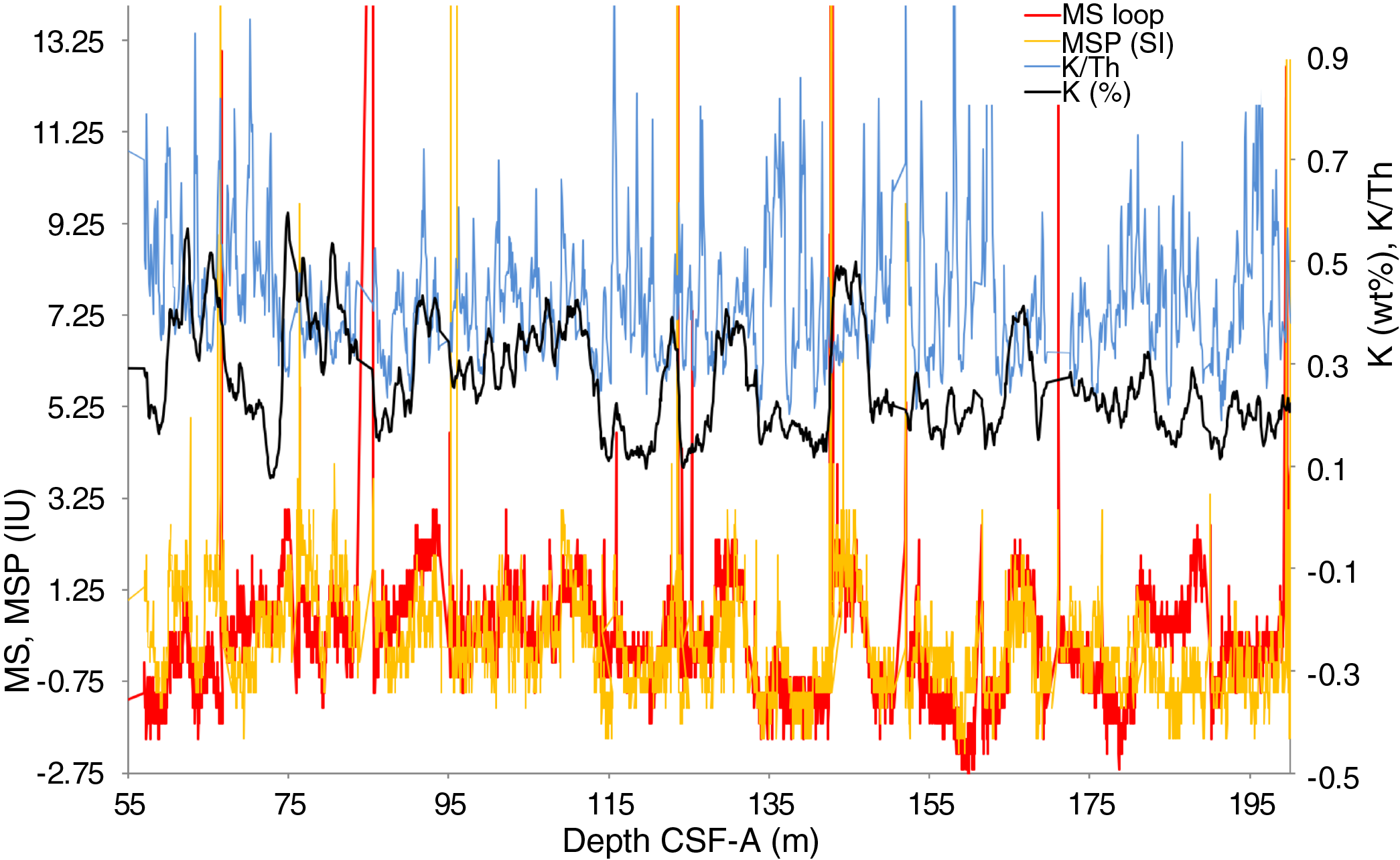
Figure F42. K%, K/Th, MS, and MSP, Hole U1539C.
Natural gamma radiation
NGR measurements show downhole variations from about 4 to 50 counts/s in Holes U1539A–U1539D and similar variability between all holes in range and amplitude variations (Figure F43). Holes U1539A and U1539C show corresponding exponential downhole trends of decreasing counts with depth in the uppermost ~30 m. Hole U1539B shows a similar pattern. Because coring in Hole U1539D started at 47 m CSF-A, no comparable trend in total NGR counts can be identified in this hole.
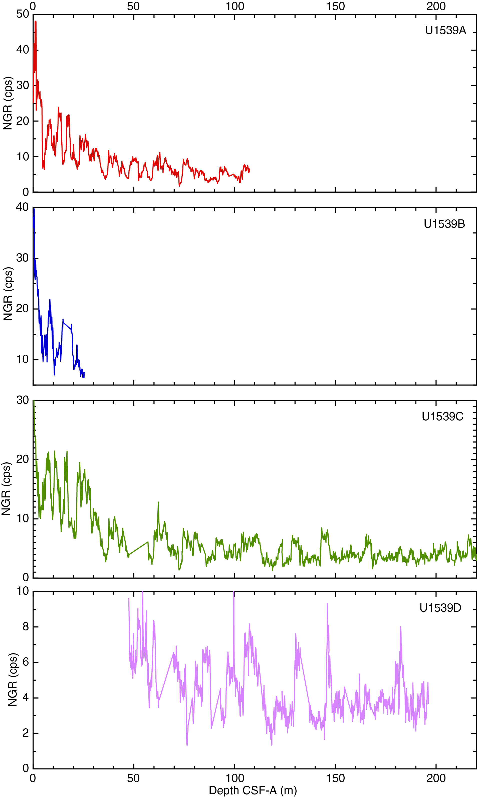
Figure F43. NGR total counts.
We deconvolved the NGR record into low-resolution, (semi)quantitative concentrations for the elements potassium (K), uranium (U), and thorium (Th) (Figure F44) following the methods of Dunlea et al. (2013) and De Vleeschouwer et al. (2017). All three elements follow identical patterns, and their values exhibit clear cyclic peaks in Holes U1539A and U1539C (Figures F41, F42) that are paced on 10 to 15 m intervals and correlate well with MS values, principally providing a clearer signal of terrigenous sediment content than the partially compromised MS series. U and Th show weaker peaks than K due to their lower concentrations and attainable resolution with the NGR data but may provide initial information about sedimentation regime changes (Jacobel et al., 2017). Higher total NGR counts, as well as the individual elemental data which most likely indicate higher contents of siliciclastic material (primarily clay minerals), correlate with maxima in MS and often minima in GRA density values. This pattern is evident in intervals with high carbonate content (Lithofacies 4 and 5) where anticorrelation to GRA density and P-wave velocity values appears (e.g., Sections 383-U1539A-9H-1 through 9H-3).
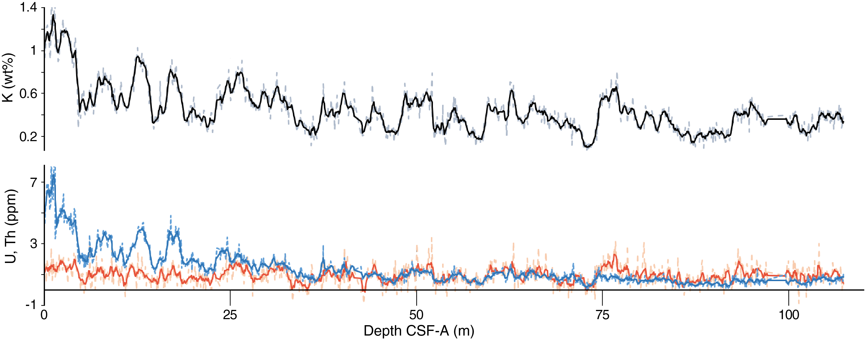
Figure F44. K, U, and Th from NGR.
Bulk density, grain density, and porosity
We used GRA measurements at 2 cm spacing and discrete MAD values (157 samples) to evaluate changes in bulk density at Site U1539. GRA bulk density values in Holes U1539A and U1539C vary from ~1.16 to ~1.65 g/cm3, and discrete MAD values exhibit a similar range (Figure F45). Bulk density calculated from discrete MAD samples matches the envelope of the GRA estimate and displays similar downhole trends in both holes, leading to a high correlation coefficient between both methods of r2 = 0.859 across all encountered lithofacies (Figure F45). Bulk density values remain highly variable throughout all holes. Subtle changes in GRA bulk density may correspond to the major components of the main lithofacies (see Sedimentology) and are mostly related to changes in the relative proportions of calcareous versus biosiliceous oozes in the lithofacies. Potential secondary contributing changes are made by terrigenous modifiers through either eolian deposition or lateral transport by ocean currents. GRA bulk density remains fairly consistent across the upper cores from all holes (i.e., from the seafloor to ~20–40 m CSF-A), where usually high initial densification, particularly of biogenic oozes, is expected. GRA bulk density at this site displays pronounced recurring 10–15 m long cycles, particularly evident in the upper 175 m CSF-A of Hole U1539C. Below 180 m CSF-A, GRA bulk density shows significantly lower amplitude variability, ranging between 1.35 and 1.5 g/cm3.
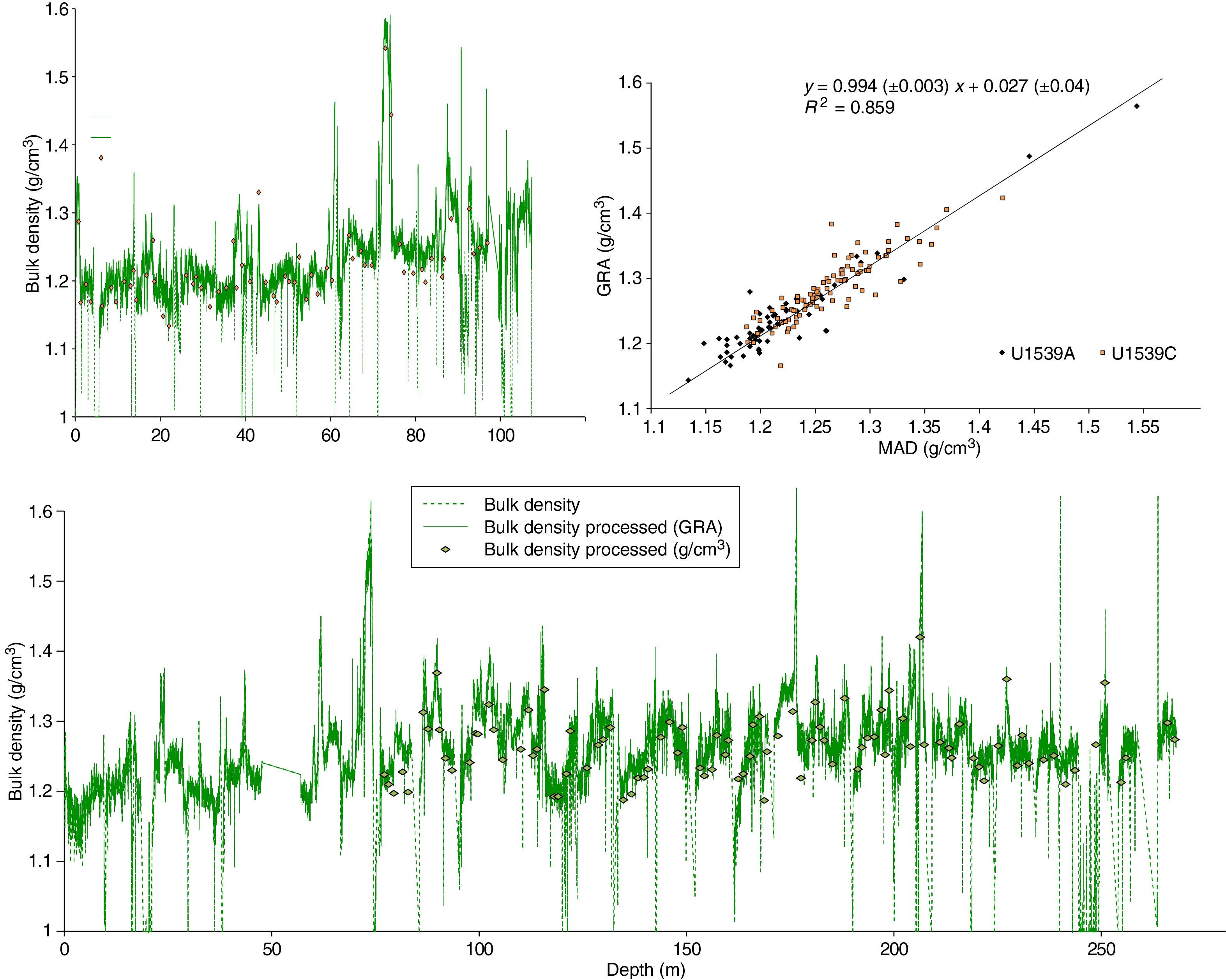
Figure F45. GRA and discrete bulk density.
In addition to bulk density, MAD measurements provide estimates of dry density, grain density, porosity, moisture content, void ratio, and several other properties that co-vary downhole. In general, bulk density and porosity are anticorrelated and increase and decrease downhole, respectively. Intervals of high porosity and low grain density correspond to diatom-rich oozes (Lithofacies 1 and 2). Intervals of low porosity and high density correspond to carbonate-bearing and carbonate-dominated lithologies (Lithofacies 3 and 4). Although not entirely consistent in Holes U1539A–U1539D, density often changes at the boundaries of lithofacies, indicating changes in grain size, matrix, or, on longer intervals across holes, compaction. Higher grain density values in Lithostratigraphic Unit IV may indicate a difference in composition compared with overlying units, but the data are too few and scattered to draw reliable conclusions.
Compressional P-wave velocity
P-wave measurements from the WRMSL indicate moderate variations from 1480 to 1580 m/s (Figure F46). Measurements carried out using the PWC on working halves vary from 1515 to 1570 m/s and show higher velocity values than the measurements made on whole-round core sections, but a consistent linear relationship is observed between the whole- and half-core analyses. Lower velocity values are associated with nannofossil oozes with reduced water content (e.g., Sections 383-U1539A-9H-2 and 383-U1539D-19H-1 through 19H-6), whereas higher velocity values are associated with water-rich diatom ooze facies. This suggests that mainly the grain size is determining the P-wave velocity values in Site U1539 cores and not the water content or density. The highest P-wave velocity maxima (1550–1570 m/s) occur in lithofacies with diatom mats (e.g., Lithofacies II; Sections 383-U1539C-13H-4 through 13H-6). These appear to be distinct, even within single sections of a single core (e.g., Sections 383-U1539B-11H and 12H).

Figure F46. GRA bulk density and P-wave velocity.
Thermal conductivity
Thermal conductivity was measured for all holes at a resolution of one or more measurements per retrieved core (Figure F47). Measurements were carried out using the needle probe on whole-round sections; however, a number of measurements in the upper sections of Holes U1539A, U1539C, and U1539D failed due to low thermal conductivity, likely from high water content in these sections. In the lower parts of the holes, thermal conductivity measurements were partially compromised by frequent coring disturbances, evidenced by cracks in the sediment and partially filled liners (see Sedimentology). The quality of the thermal conductivity measurements was checked by evaluating two parameters: (1) the number of solutions acquired and (2) the shape of the curve formed on the temperature versus time plot of these points. A valid measurement should have a sufficient number of solutions to form an exponential curve. If strictly assessed, about 30%–50% of thermal conductivity measurements should be excluded from further evaluation. Nonetheless, measurements with a relatively low number of solutions and/or a bad repartition of these values on the temperature versus time plot (i.e., forming two or no curve) were kept until further sites are addressed for comparison and because observed patterns followed expected thermal conductivity behavior along lithologic facies.
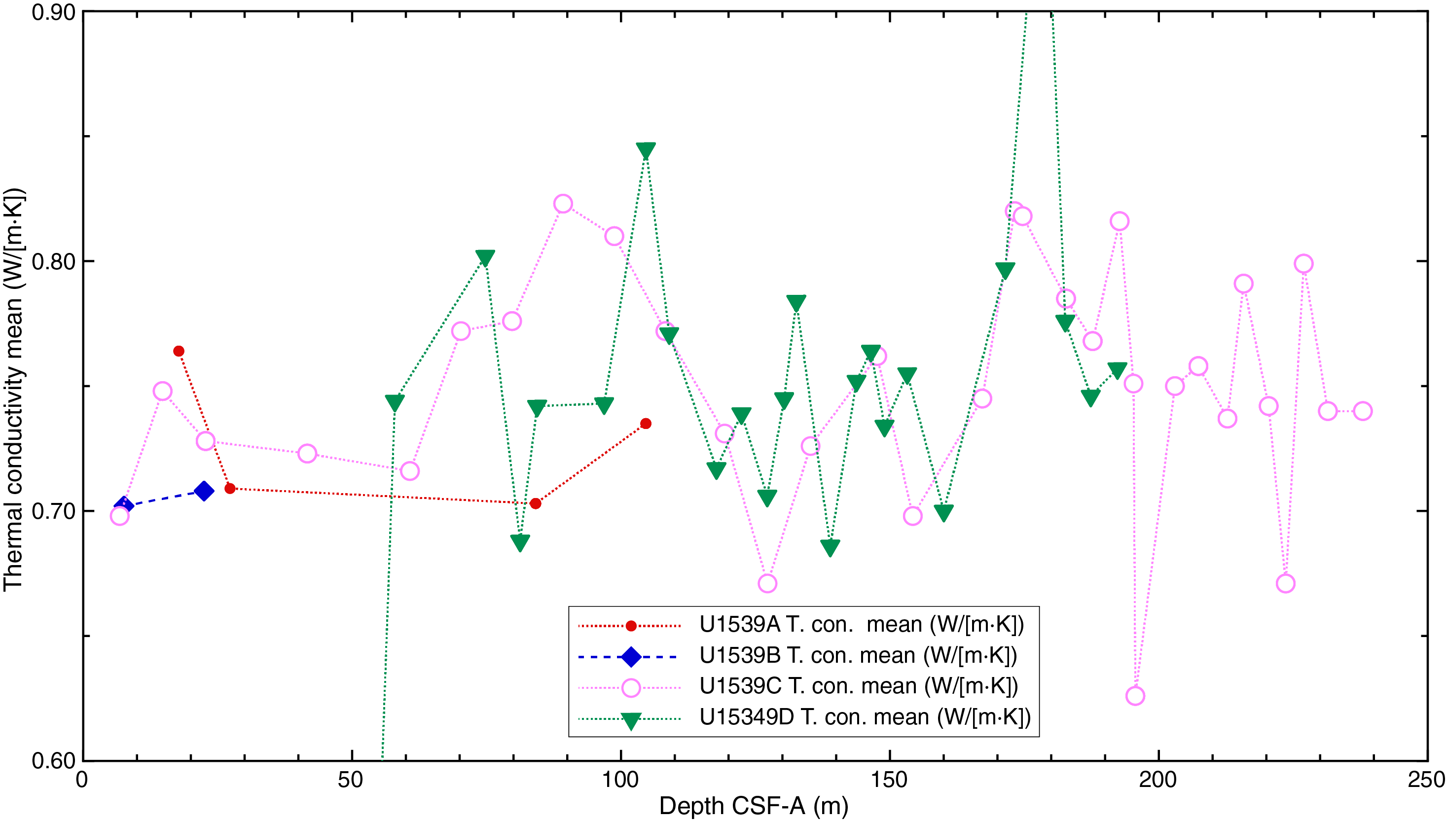
Figure F47. Thermal conductivity data.
Throughout all of the holes, thermal conductivity ranges from ~0.68 to 0.82 W/(m·K) and generally corresponds to downhole changes in MS (Figure F47). In general, diatom-rich oozes (Lithostratigraphic Units I and II) are characterized by low thermal conductivity and diatom oozes with higher carbonate contents or carbonate facies (Lithostratigraphic Units III and IV) are characterized by higher thermal conductivity. Despite their low resolution and scatter, thermal conductivity mean values may follow a long-time cyclic pattern (Figure F47) that probably corresponds to orbital-scale variations in lithology at this site, a presumption to be tested at subsequent sites with lower temporal resolution and longer stratigraphic coverage.
Summary
Data acquired from whole-round measurements for Site U1539 are generally in good agreement with those from split-core measurements (Figures F41, F42). In particular, discrete MAD samples and GRA-derived density values correlate well (Figure F45). Bulk density values follow established patterns and reflect the respective proportions of relatively low density, more biosiliceous facies versus higher density calcareous biogenic components, and distal terrigenous sediment supply.
Although both WRMSL and SHMSL point MS measurements provide some information and variations, overall values are low and should be interpreted with caution. MS values are consistently low from 0 to <20 IU. However, MS shows surprisingly clear 10–15 m scale cyclicity, similar to the GRA bulk density and NGR records, and values range from −2 to 10 IU. NGR counts range between ~10 and 40 cps, and the lower values correspond to nannofossil ooze intervals richer in carbonates, although this relationship is not constant throughout Site U1539.
In general, a decrease in PWC values coincides with an increase in density and a decrease in porosity (Figure F46). Downhole variations in NGR also correlate well with inverse changes in bulk density (Figures F50, F51), and both were used to supplement color data in the construction of the spliced record.
Downhole changes in physical property characteristics overall are in good agreement with the defined lithofacies based on sedimentologic characteristics (Figure F4; see Sedimentology). In general, diatom ooze lithofacies (Lithostratigraphic Units I and II) correspond to high MS, low bulk density, and high porosity. The lowest density values and highest porosity values occur in diatom mats within the diatom ooze that is a recurring dominant Lithofacies 2. In contrast, intervals that are predominantly calcareous nannofossil ooze (Lithostratigraphic Units IV and V) correspond to decreased NGR, high bulk density, low P-wave velocity, low to moderate MS, and low to moderate porosity. Over most of the record, GRA bulk density shows an anticorrelation with the NGR percent potassium (K%) and MS. The NGR record also exhibits 10–15 m scale cyclicity, particularly from ~10 to 135 m CSF-A. NGR data also imply that the total counts and derived K% can be used as low-resolution proxy for the abundance of terrigenous material delivered by dust or iceberg transport.
Downhole measurements
In situ temperature and heat flow
We carried out APCT-3 downhole temperature measurements in Hole U1539A at three depths on Cores 383-U1539A-4H, 7H, and 10H. Calculated in situ temperatures were 1.22°C at 33.1 m CSF-A, 1.84°C at 61.6 m CSF-A, and 1.7°C at 90.1 m CSF-A (Table T12). The relatively linear downhole temperature increase indicates that the temperature gradient is fairly uniform with depth, albeit with scatter due to the small number of measurements (Figure F48).
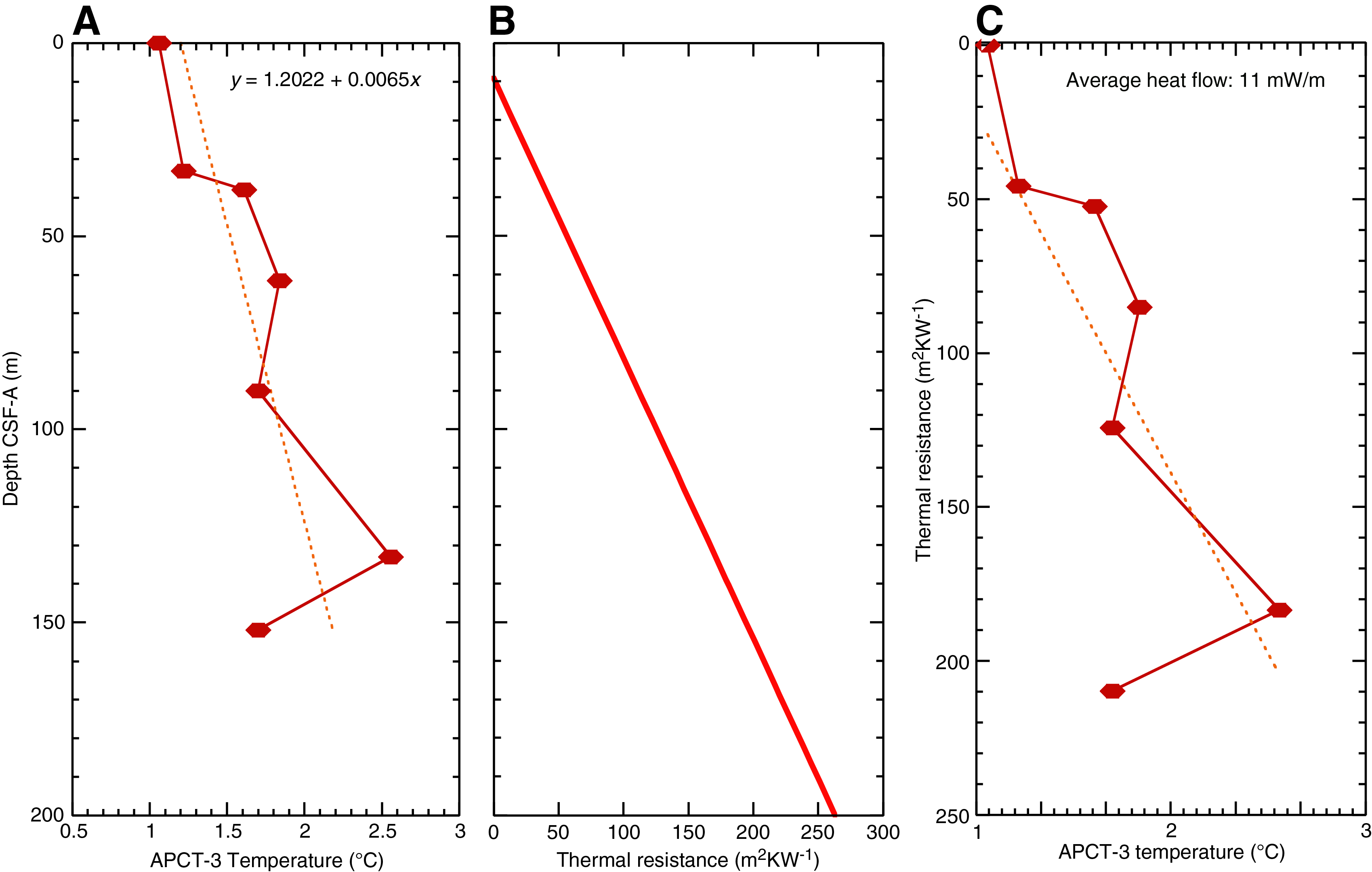
Figure F48. Heat flow calculations.
In addition, we carried out three additional APCT-3 downhole temperature measurements in Hole U1539C at three depths on Cores 383-U1539C-4H, 13H, and 16H. Calculated in situ temperatures were 1.61°C at 38.0 mbsf, 2.56°C at 133.0 mbsf, and 2.87°C at 152.0 mbsf (Table T12). The relatively linear downhole increase indicates that the temperature gradient is reasonably uniform with depth, albeit with significant scatter due to the small number of measurements and the combination of data from two different holes (Figure F48).
Bottom water temperature was calculated to be 1.07°C for Hole U1539A and 1.06°C for Hole U1539C. These values are based on APCT-3 logging at the mudline for about 5 min while stopping with pumps switched off in the hole before lowering the tool to target depth. Values are the mean of averages of the three APCT-3 measurements in each hole. These temperature values are in agreement with the expected temperature based on previous conductivity-temperature-depth (Gersonde, 2011) and World Ocean Atlas 2009 data (Locarnini et al., 2010) from Site U1539 and provide support for comparable conditions through two holes.
Thermal conductivity under in situ conditions was estimated from laboratory-determined thermal conductivity using established methods (Pribnow et al., 2000; Hyndman et al., 1974) (see Physical properties in the Expedition 383 methods chapter [Authorship, 2021]). Thermal resistance was calculated by cumulatively adding the inverse of the in situ thermal conductivity values over depth intervals downhole (Figure F48). A calculated heat flow of 11 mW/m2 for the combined data from both holes was obtained from the slope of the linear fit between in situ temperature and thermal resistance (Pribnow et al., 2000). Values for Hole U1539A are 11 and 14 mW/m2, respectively, if calculated separately. A geothermal gradient (dT/dz) for the site is estimated at ~65°C/km within the total measured depth interval based on a linear fit of temperature versus depth, in which T is temperature at depth z.
Stratigraphic correlation
Correlations between holes at Site U1539 were accomplished using the Correlator software (version 3.0). Tie points were established mostly using the blue channel extracted from the images (red-green-blue [RGB] blue) (Figure F49), but in many cases a combination of measurements was used (Table T13). We constructed a splice for the upper portion of the site (0–219.80 m CCSF-A) using Holes U1539A–U1539D (Table T14; Figures F49, F50, F51). However, the splice contains several gaps (Figure F49), detailed below. Below 219.80 m CCSF-A, only a single hole (U1539C) was drilled; thus, Cores 383-U1539C-22H through 32F were appended to the splice with gaps set between each core to the bottom of the hole.
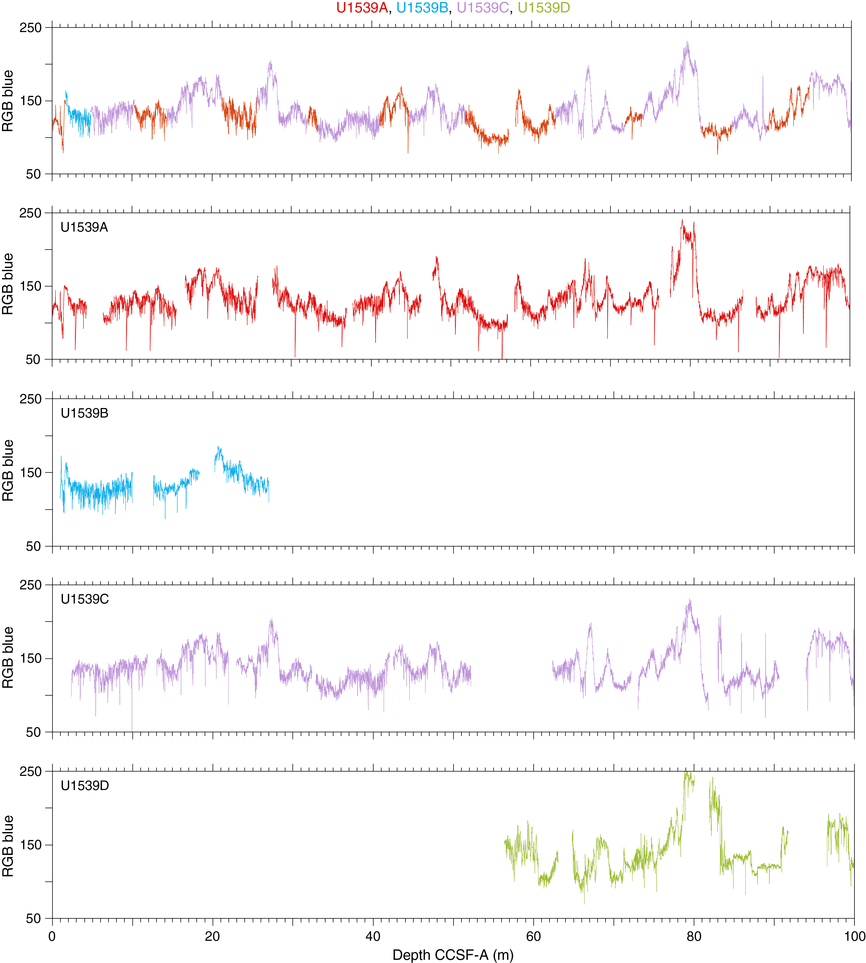
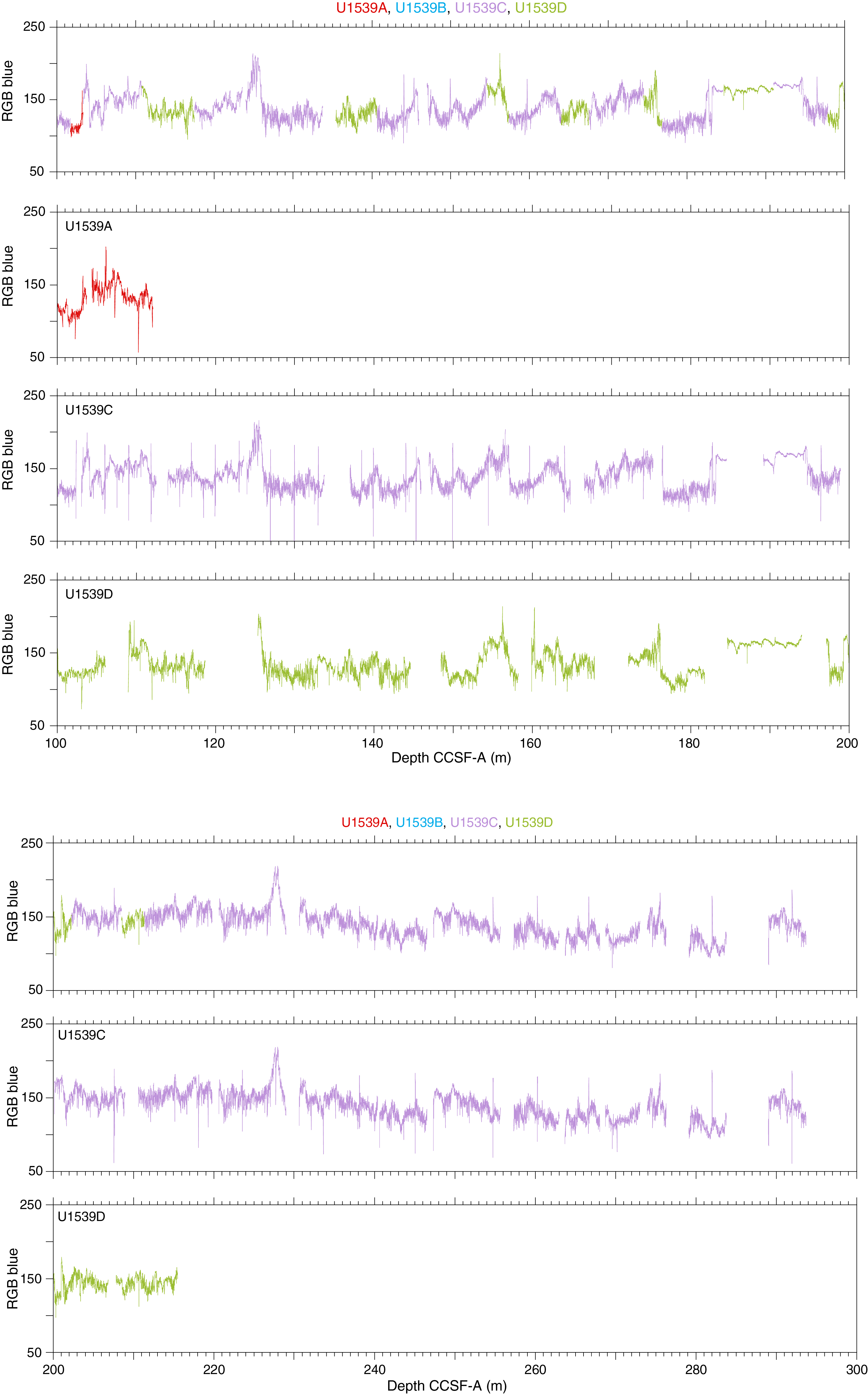
Figure F49. RGB blue vs. composite depth.
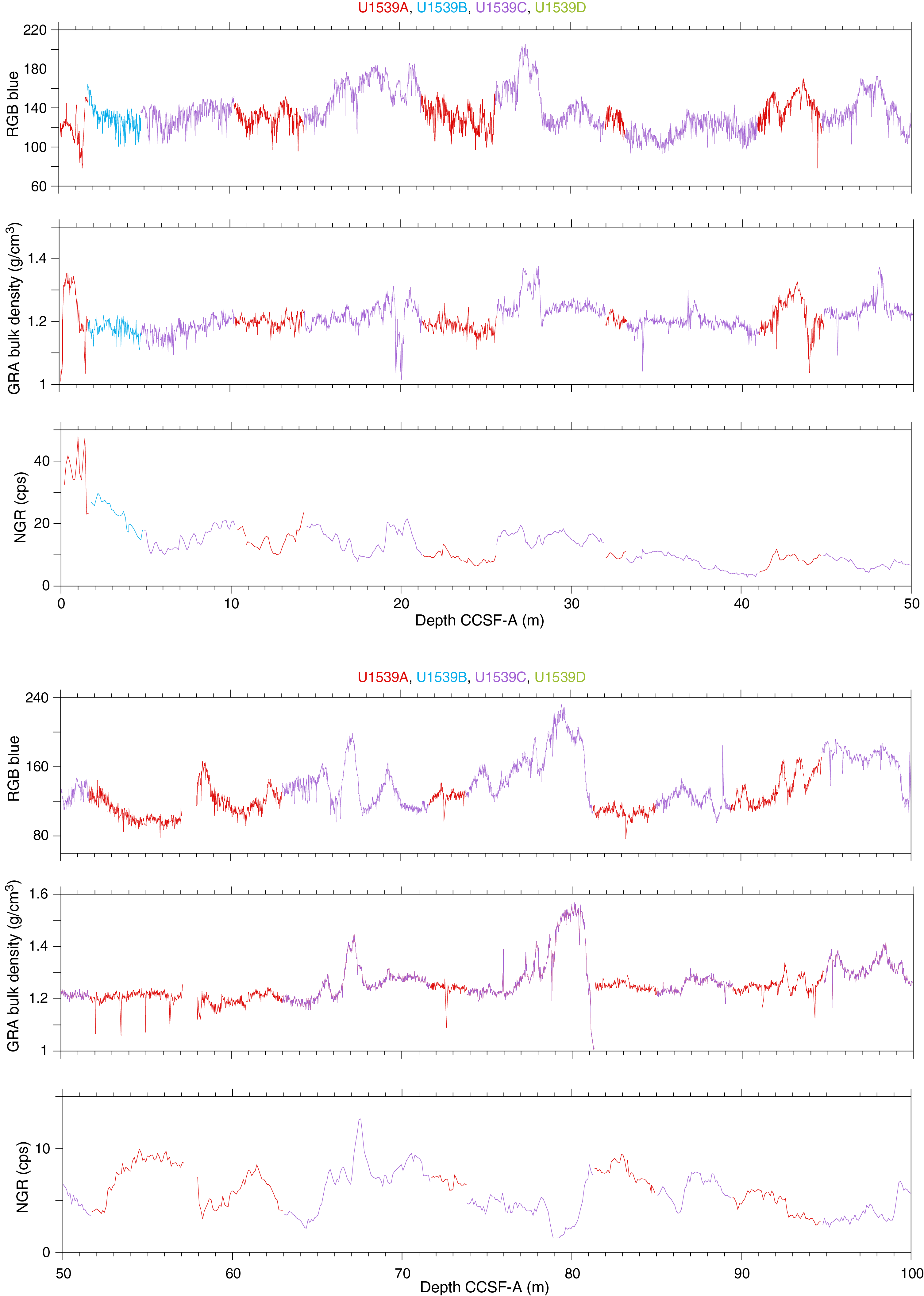

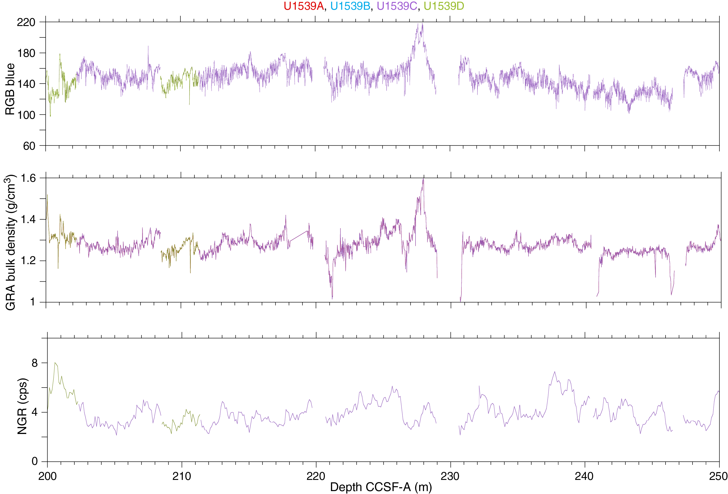
Figure F50. Spliced data: RGB blue, GRA bulk density, and NGR.
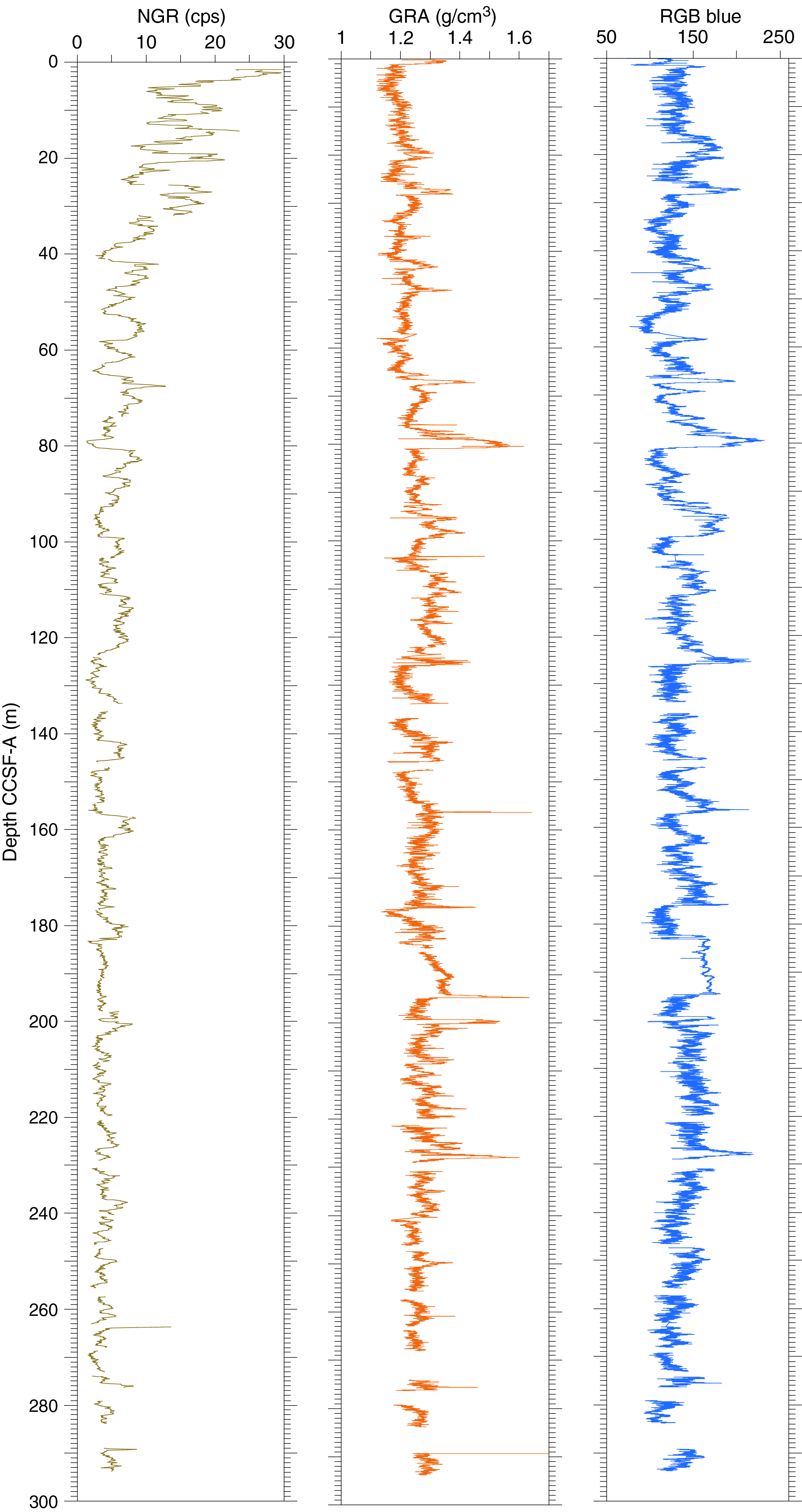
Figure F51. Cleaned spliced data: RGB blue, GRA bulk density, and NGR.
The CCSF-A scale is anchored to the mudline of Core 383-U1539A-1H, which is assigned the depth of 0 m CCSF-A. From this anchor, we worked downhole using Correlator to establish a composite stratigraphy on a core-by-core basis. IW sampling and shipboard measurement sampling was done on Cores 383-U1539A-1H and 12H and 383-U1539C-9H through 32F; thus, our general approach was to avoid using material from these cores. However, because of poor recovery or coring disturbance in a few intervals, we had to piece together the splice using all four holes. Hole U1539B recovered only three cores (383-U1539B-1H through 3H); we used the uppermost core (1H) in the splice. Below this point, we used Hole U1539C as the backbone of the splice. We filled gaps between cores and avoided any disturbed intervals by including cores from Holes U1539A and U1539D in the splice. The splice is continuous and has no gaps from 0 to 57.17 m CCSF-A. At that depth, Core 383-U1539A-7H was appended to the splice by setting the affine offset using the growth factor of 1.112, which is the growth factor of Core 6H. Below this first gap, the splice is continuous from 57.94 m CCSF-A to the bottom of Core 383-U1539C-12H at 123.58 m CCSF. Below 123.58 m CCSF, the splice has four gaps; at each of these gaps, the top of the underlying core was appended to the bottom of the previous core using an offset consistent with an increasing cumulative affine offset of 0.5 m CCSF-A per core. The four gaps occur where the tops of Cores 383-U1539C-13H, 383-U1539D-12H, 383-U1539C-15H, and 383-U1539D-19H were appended (Table T14). The bottom of the splice is the bottom of Core 383-U1539C-21H at 219.80 m CCSF-A; it was not possible to construct a splice below this depth because only one hole (U1539C) was drilled deeper. For this reason, all cores deeper than Core 383-U1539C-21H were appended to the splice using an offset consistent with an increasing cumulative affine offset of 0.5 m CCSF-A per core (Tables T13, T14).
The cumulative offset between the CSF-A and CCSF-A depth scales is nearly linear (Figure F52A). The growth factor varies from ~4% to 38%; this large range includes offsets due to ship heave and misfired APC cores. Drilling in Hole U1539C occurred with the best sea conditions, and therefore the growth factor of ~7% in this hole is most representative of the behavior of the sediment. This growth factor is expected from sediments that expand due to release of overburden but have minimal gas expansion due to low concentrations of methane and other gases (see Geochemistry). There are small changes in the growth factor, and therefore in the cumulative offset with depth (Figure F52B), because of core disturbance due to bad weather conditions and misfired APC coring in a few instances at the top of Hole U1539D and the bottom of Holes U1539B and U1539A. The CSF-A depth of the tops of those cores are set to the drilling depth below seafloor (DSF) scale, which is based on the position of the drill string below the seafloor, but the process of correlation moved them to a position on the CCSF-A scale that may not represent sediment expansion. Calculation of mass accumulation rates based on the CCSF-A scale should account for differential expansion by dividing apparent depth intervals by the appropriate growth factor.
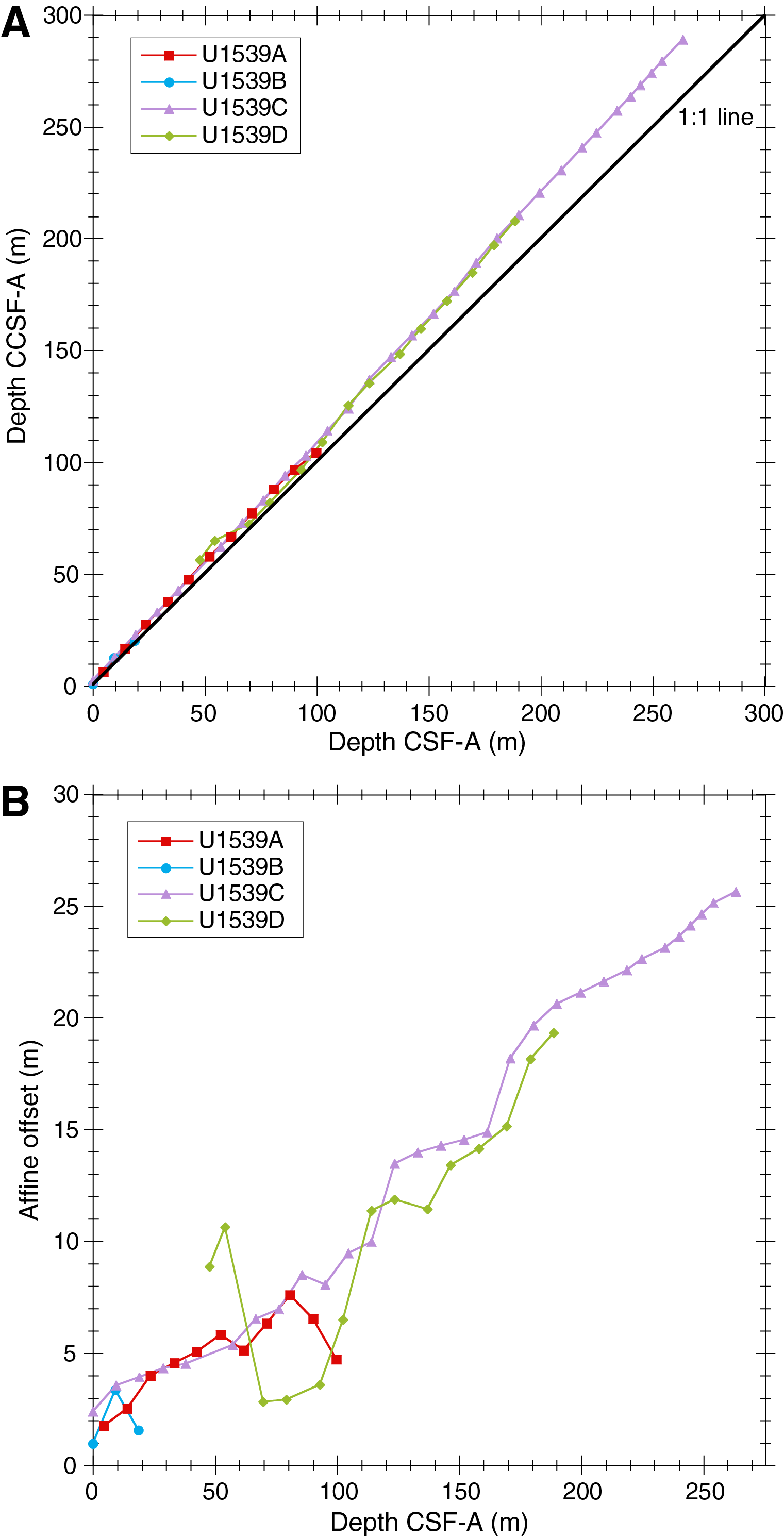
Figure F52. Depth scales and offsets in the splice.
References
Alvarez Zarikian, C.A., 2015. Cenozoic bathyal and abyssal ostracods beneath the South Pacific Gyre (IODP Expedition 329 Sites U1367, U1368 and U1370). Palaeogeography, Palaeoclimatology, Palaeoecology, 419:115–142. https://doi.org/
Anthonissen, D.E., and Ogg, J.G., 2012. Appendix 3—Cenozoic and Cretaceous biochronology of planktonic foraminifera and calcareous nannofossils. In Gradstein, F.M., Ogg, J.G., Schmitz, M.D., and Ogg, G.M., (Eds.), The Geologic Time Scale 2012: Amsterdam (Elsevier), 1083–1127. https://doi.org/
Basak, C., Fröllje, H., Lamy, F., Gersonde, R., Benz, V., Anderson, R.F., Molina-Kescher, M., and Pahnke, K., 2018. Breakup of last glacial deep stratification in the South Pacific. Science, 359(6378):900–904. https://doi.org/
Brindley, G., 1990. Quantitative X-ray mineral analysis of clays. In Brindley, G.W., and Brown, G. (Eds.), Crystal Structures of Clay Minerals and Their X-ray Identification. Mineralogical Society Monograph, 5:411–438. https://doi.org/
Cande, S.C., and Kent, D.V., 1995. Revised calibration of the geomagnetic polarity timescale for the Late Cretaceous and Cenozoic. Journal of Geophysical Research: Solid Earth, 100(B4):6093–6095. https://doi.org/
Chen, P.-H., 1975. Antarctic radiolaria. In Hayes, D.E., Frakes, L.A., et al., Initial Reports of the Deep Sea Drilling Project, 28: Washington, DC (U.S. Government Printing Office), 437–513. https://doi.org/
Ciesielski, P.F., 1975. Biostratigraphy and paleoecology of Neogene and Oligocene silicoflagellates from cores recovered during Antarctic Leg 28, Deep Sea Drilling Project. In Hayes, D.E., Frakes, L.A., et al., Initial Reports of the Deep Sea Drilling Project, 28: Washington, DC (U.S. Government Printing Office), 625–691. https://doi.org/
Cody, R.D., Levy, R.H., Harwood, D.M., and Sadler, P.M., 2008. Thinking outside the zone: high-resolution quantitative diatom biochronology for the Antarctic Neogene. Palaeogeography, Palaeoclimatology, Palaeoecology, 260(1–2):92–121. https://doi.org/
Corliss, B.H., 1979. Quaternary Antarctic bottom-water history: deep sea benthonic foraminiferal evidence from the southeast Indian Ocean. Quaternary Research, 12(2):271–289. https://doi.org/
Corliss, B.H., 1985. Microhabitats of benthic foraminifera within deep-sea sediments. Nature, 314(6010):435–438. https://doi.org/
De Vleeschouwer, D., Dunlea, A.G., Auer, G., Anderson, C.H., Brumsack, H., de Loach, A., Gurnis, M., et al., 2017. Quantifying K, U, and Th contents of marine sediments using shipboard natural gamma radiation spectra measured on DV JOIDES Resolution. Geochemistry, Geophysics, Geosystems, 18(3):1053–1064. https://doi.org/
Diekmann, B., and Kuhn, G. 2002. Sedimentary record of the mid-Pleistocene climate transition in the southeastern South Atlantic (ODP Site 1090). Palaeogeography, Palaeoclimatology, Palaeoecology, 182(3–4):241–258. https://doi.org/
Dunlea, A.G., Murray, R.W., Harris, R.N., Vasiliev, M.A., Evans, H., Spivack, A.J., and D’Hondt, S., 2013. Assessment and use of NGR instrumentation on the JOIDES Resolution to quantify U, Th, and K concentrations in marine sediment. Scientific Drilling, 15:57–63. https://doi.org/
Eagles, G., 2006. Deviations from an ideal thermal subsidence surface in the southern Pacific Ocean. Terra Antarctica Reports, 12:109–118.
Esper, O., and Gersonde, R., 2014. Quaternary surface water temperature estimations: new diatom transfer functions for the Southern Ocean. Palaeogeography, Palaeoclimatology, Palaeoecology, 414:1–19. https://doi.org/
Fontanier, C., Jorissen, F.J., Chaillou, G., Anschutz, P., Grémare, A., and Griveaud, C., 2005. Live foraminiferal faunas from a 2800 m deep lower canyon station from the Bay of Biscay: faunal response to focusing of refractory organic matter. Deep-Sea Research, Part I: Oceanographic Research Papers, 52(7):1189–1227. https://doi.org/
Gersonde, R., 2011. The expedition of the research vessel “Polarstern” to the polar South Pacific Sea in 2009/2010 (ANT-XXVI/2-BIPOMAC). Berichte zur Polar und Meeresforschung, 632. https://doi.org/
Gersonde, R., Hodell, D.A., and Blum, P. (Eds.), 2003. Proceedings of the Ocean Drilling Program, Scientific Results, 177: College Station, TX (Ocean Drilling Program). https://doi.org/
Gooday, A.J., 1988. A response by benthic foraminifera to the deposition of phytodetritus in the deep sea. Nature, 332(6159):70–73. https://doi.org/
Gupta, A.K., Singh, R.K., Joseph, S., and Thomas, E., 2004. Indian Ocean high-productivity event (10–8 Ma): linked to global cooling or to the initiation of the Indian monsoons? Geology, 32(9):753–756. https://doi.org/
Gupta, A.K., Singh, R.K., and Verma, S., 2013. Deep-sea palaeoceanographic evolution of the eastern Indian Ocean during the late Oligocene–Pleistocene: species diversity trends in benthic foraminifera. Current Science, 104(7):904–910. http://www.currentscience.ac.in/
Gupta, A.K., and Thomas, E., 1999. Latest Miocene–Pleistocene productivity and deep‐sea ventilation in the northwestern Indian Ocean (Deep Sea Drilling Project Site 219). Paleoceanography and Paleoclimatology, 14(1):62–73. https://doi.org/
Harwood, D.M., and Maruyama, T., 1992. Middle Eocene to Pleistocene diatom biostratigraphy of Southern Ocean sediments from the Kerguelen Plateau, Leg 120. In Wise, S.W., Jr., Schlich, R., et al., Proceedings of the Ocean Drilling Program, Scientific Results, 120: College Station, TX (Ocean Drilling Program), 683–733. https://doi.org/
Hays, J.D., and Opdyke, N.D., 1967. Antarctic radiolaria, magnetic reversals, and climate change. Science, 158(3804):1001–1011. http://www.jstor.org.lib-ezproxy.tamu.edu:2048/
Hilgen, F.J., Lourens, L.J., and Van Dam, J.A., 2012. The Neogene period. With contributions by A.G. Beu, A.F. Boyes, R.A. Cooper, W. Krijgsman, J.G. Ogg, W.E. Piller, and D.S. Wilson. In Gradstein, F.M., Ogg, J.G., Schmitz, M.D., and Ogg, G.M. (Eds.), The Geologic Time Scale: Oxford, United Kingdom (Elsevier), 923–978. https://doi.org/
Hodell, D.A., Charles, C.D., and Sierro, F.J., 2001. Late Pleistocene evolution of the ocean’s carbonate system. Earth and Planetary Science Letters, 192(2):109–124. https://doi.org/
Hornibrook, N.d.B., 1981. Globorotalia (planktic Foraminiferida) in the late Pliocene and early Pleistocene of New Zealand. New Zealand Journal of Geology and Geophysics, 24(2):263–292. https://doi.org/
Hyndman, R.D., Erickson, A.J., and Von Herzen, R.P., 1974. Geothermal measurements on DSDP Leg 26. In Davies, T.A., Luyendyk, B.P., et al., Initial Reports of the Deep Sea Drilling Project, 26: Washington, DC (U.S. Govt. Printing Office), 451–463. https://doi.org/
Jacobel, A.W., McManus, J.F., Anderson, R.F., and Winckler, G., 2017. Repeated storage of respired carbon in the equatorial Pacific Ocean over the last three glacial cycles. Nature Communications, 8:1727. https://doi.org/
Jonkers, L., De Nooijer, L.J., Reichart, G.-J., Zahn, R., and Brummer, G.-J.A., 2012. Encrustation and trace element composition of Neogloboquadrina dutertrei assessed from single chamber analyses - implications for paleotemperature estimates. Biogeosciences, 9(11):4851–4860. https://doi.org/
Jutzeler, M., White, J.D.L., Talling, P.J., McCanta, M., Morgan, S., Le Friant, A., and Ishizuka, O., 2014. Coring disturbances in IODP piston cores with implications for offshore record of volcanic events and the Missoula megafloods. Geochemistry, Geophysics, Geosystems, 15(9):3572–3590. https://doi.org/
Lamy, F., Winckler, G., Alvarez Zarikian, C.A., and the Expedition 383 Scientists, 2021. Supplementary material, https://doi.org/
Lazarus, D., 1990. Middle Miocene to Recent radiolarians from the Weddell Sea, Antarctica, ODP Leg 113. In Barker, P.F., Kennett, J.P., et al., Proceedings of the Ocean Drilling Program, Scientific Results, 113: College Station, TX (Ocean Drilling Program), 709–727. https://doi.org/
Lazarus, D., 1992. Antarctic Neogene radiolarians from the Kerguelen Plateau, Legs 119 and 120. In Wise, S.W., Jr., Schlich, R., et al., Proceedings of the Ocean Drilling Program, Scientific Results, 120: College Station, TX (Ocean Drilling Program), 785–809. https://doi.org/
Locarnini, R.A., Mishonov, A.V., Antonov, J.I., Boyer, T.P., Garcia, H.E., Baranova, O.K., Zweng, M.M., and Johnson, D.R., 2010. World Ocean Atlas 2009 (Volume 1): Temperature. In Levitus, S. (Ed.), NOAA Atlas NESDIS 68: Washington, DC (U.S. Government Printing Office). ftp://ftp.nodc.noaa.gov/
Loubere, P., 1991. Deep-sea benthic foraminiferal assemblage response to a surface ocean productivity gradient: a test. Paleoceanography and Paleoclimatology, 6(2):193–204. https://doi.org/
Mahood, A.D., and Barron, J.A., 1996. Late Pliocene diatoms in a diatomite from Prydz Bay, East Antarctica. Micropaleontology, 42(3):285–302. https://doi.org/
Meyers, P.A., 1994. Preservation of elemental and isotopic source identification of sedimentary organic matter. Chemical Geology, 114(3–4):289–302. https://doi.org/
Meyers, P.A., 1997. Organic geochemical proxies of paleoceanographic, paleolimnologic, and paleoclimatic processes. Organic Geochemistry, 27(5–6):213–250. https://doi.org/
Orsi, A.H., Whitworth III, T., and Nowlin, W.D., Jr., 1995. On the meridional extent and fronts of the Antarctic Circumpolar Current. Deep-Sea Research, Part I: Oceanographic Research Papers, 42(5):641–673. https://doi.org/
Pitman, W.C., and Heirtzler, J.R., 1966. Magnetic anomalies over the Pacific-Antarctic Ridge. Science, 154(3753):1164–1171. https://doi.org/10.1126/science.154.3753.1164
Pribnow, D., Kinoshita, M., and Stein, C., 2000. Thermal Data Collection and Heat Flow Recalculations for Ocean Drilling Program Legs 101–180: Hanover, Germany (Institute for Joint Geoscientific Research, Institut für Geowissenschaftliche Gemeinschaftsaufgaben [GGA]). http://www-odp.tamu.edu/
Rathburn, A.E., and Corliss, B.H., 1994. The ecology of living (stained) deep-sea benthic foraminifera from the Sulu Sea. Paleoceanography and Paleoclimatology, 9(1):87–150. https://doi.org/
Scott, G.H., Kennett, J.P., Wilson, K.J., and Hayward, B.W., 2007. Globorotalia puncticulata: population divergence, dispersal and extinction related to Pliocene–Quaternary water masses. Marine Micropaleontology, 62(4):235–253. https://doi.org/
Singh, R.K., and Gupta, A.K., 2004. Late Oligocene-Miocene paleoceanographic evolution of the southeastern Indian Ocean: Evidence from deep-sea benthic foraminifera (ODP Site 757). Marine Micropaleontology, 51(1–2):153–170. https://doi.org/
Singh, R.K., and Gupta, A.K., 2005. Systematic decline in benthic foraminiferal species diversity linked to productivity increases over the last 26 Ma in the Indian Ocean. Journal of Foraminiferal Research, 35(3):219–227. http://dx.doi.org/
Singh, R.K., and Gupta A.K., 2010. Deep-sea benthic foraminiferal changes in the eastern Indian Ocean (ODP Hole 757B): their links to deep Indonesian (Pacific) flow and high latitude glaciation during the Neogene. Episodes, 33(2):74–82.
Singh, R.K., Gupta, A.K., and Das, M., 2012. Paleoceanographic significance of deep-sea benthic foraminiferal species diversity at southeastern Indian Ocean Hole 752A during the Neogene. Palaeogeography, Palaeoclimatology, Palaeoecology, 361–362:94–103. https://doi.org/
Soetaert, K., Hofmann, A.F., Middelburg, J.J., Meysman, F.J.R., and Greenwood, J., 2007. The effect of biogeochemical processes on pH. Marine Geochemistry, 105(1–2):30-51. https://doi.org/
Steinhardt, J., de Nooijer, L.L., Brummer, G.-J., and Reichart, G.-J., 2015. Profiling planktonic foraminiferal crust formation. Geochemistry, Geophysics, Geosystems, 16(7):2409–2430. https://doi.org/
Stepanova, A., and Lyle, M., 2014. Deep-sea ostracoda from the eastern equatorial Pacific (ODP Site 1238) over the last 460 ka. Marine Micropaleontology, 111:100–117. https://doi.org/
Streeter, S.S., and Shackleton, N.J., 1979. Paleocirculation of the deep North Atlantic: 150,000-yr record of benthic foraminifera and oxygen-18. Science, 203(4376):168–170. https//doi.org/
Thomas, E., Booth, L., Maslin, M., and Shackleton, N.J., 1995. Northeastern Atlantic benthic foraminifera during the last 45,000 years: changes in productivity seen from the bottom up. Paleoceanography and Paleoclimatology, 10(3):545–562. https://doi.org/
Tsutsui, H., Takahashi, K., Nishida, N., and Nishiwaki, S., 2009. Intraspecific morphological variation with biometry of Distephanus speculum (Silicoflagellata). Marine Micropaleontology, 72(3–4):239–250. https://doi.org
Uchio, T., 1960. Ecology of living benthic foraminifera from the San Diego, California, area. Special Publication - Cushman Foundation for Foraminiferal Research, 5. https://cushmanfoundation.allenpress.com/
Verma, S., Gupta, A.K., and Singh, R.K., 2013. Variations in deep-sea benthic foraminifera at ODP Hole 756B, southeastern Indian Ocean: evidence for changes in deep ocean circulation. Palaeogeography, Palaeoclimatology, Palaeoecology, 376:172–183. https://doi.org/
Wei, K.-Y., 1994. Stratophenetic tracing of phylogeny using SIMCA pattern recognition technique: a case study of the late Neogene planktonic foraminifera Globoconella clade. Paleobiology, 20(1):52–65. https://doi.org/
Winckler, G., Lamy, F., Alvarez Zarikian, C.A., Arz, H.W., Basak, C., Brombacher, A., Esper, O.M., Farmer, J.R., Gottschalk, J., Herbert, L.C., Iwasaki, S., Lawson, V.J., Lembke-Jene, L., Lo, L., Malinverno, E., Michel, E., Middleton, J.L., Moretti, S., Moy, C.M., Ravelo, A.C., Riesselman, C.R., Saavedra-Pellitero, M., Seo, I., Singh, R.K., Smith, R.A., Souza, A.L., Stoner, J.S., Venancio, I.M., Wan, S., Zhao, X., and Foucher McColl, N., 2021a. Expedition 383 methods. In Lamy, F., Winckler, G., Alvarez Zarikian, C.A., and the Expedition 383 Scientists, Dynamics of the Pacific Antarctic Circumpolar Current. Proceedings of the International Ocean Discovery Program, 383: College Station, TX (International Ocean Discovery Program). https://doi.org/
Winckler, G., Lamy, F., Alvarez Zarikian, C.A., Arz, H.W., Basak, C., Brombacher, A., Esper, O.M., Farmer, J.R., Gottschalk, J., Herbert, L.C., Iwasaki, S., Lawson, V.J., Lembke-Jene, L., Lo, L., Malinverno, E., Michel, E., Middleton, J.L., Moretti, S., Moy, C.M., Ravelo, A.C., Riesselman, C.R., Saavedra-Pellitero, M., Seo, I., Singh, R.K., Smith, R.A., Souza, A.L., Stoner, J.S., Venancio, I.M., Wan, S., Zhao, X., and Foucher McColl, N., 2021b. Expedition 383 summary. In Lamy, F., Winckler, G., Alvarez Zarikian, C.A., and the Expedition 383 Scientists, Dynamics of the Pacific Antarctic Circumpolar Current. Proceedings of the International Ocean Discovery Program, 383: College Station, TX (International Ocean Discovery Program). https://doi.org/
Winckler, G., Lamy, F., Alvarez Zarikian, C.A., Arz, H.W., Basak, C., Brombacher, A., Esper, O.M., Farmer, J.R., Gottschalk, J., Herbert, L.C., Iwasaki, S., Lawson, V.J., Lembke-Jene, L., Lo, L., Malinverno, E., Michel, E., Middleton, J.L., Moretti, S., Moy, C.M., Ravelo, A.C., Riesselman, C.R., Saavedra-Pellitero, M., Seo, I., Singh, R.K., Smith, R.A., Souza, A.L., Stoner, J.S., Venancio, I.M., Wan, S., Zhao, X., and Foucher McColl, N., 2021c. Site U1540. In Lamy, F., Winckler, G., Alvarez Zarikian, C.A., and the Expedition 383 Scientists, Dynamics of the Pacific Antarctic Circumpolar Current. Proceedings of the International Ocean Discovery Program, 383: College Station, TX (International Ocean Discovery Program). https://doi.org/
Zehr, J.P., and Ward, B.B., 2002. Nitrogen cycling in the ocean: new perspectives and paradigms. Applied and Environmental Microbiology, 68(3):1015–1024. https://doi.org/
Zielinski, U., and Gersonde, R., 2002. Plio–Pleistocene diatom biostratigraphy from ODP Leg 177, Atlantic sector of the Southern Ocean. Marine Micropaleontology, 45(3–4):225–268. https://doi.org/
1 Winckler, G., Lamy, F., Alvarez Zarikian, C.A., Arz, H.W., Basak, C., Brombacher, A., Esper, O.M., Farmer, J.R., Gottschalk, J., Herbert, L.C., Iwasaki, S., Lawson, V.J., Lembke-Jene, L., Lo, L., Malinverno, E., Michel, E., Middleton, J.L., Moretti, S., Moy, C.M., Ravelo, A.C., Riesselman, C.R., Saavedra-Pellitero, M., Seo, I., Singh, R.K., Smith, R.A., Souza, A.L., Stoner, J.S., Venancio, I.M., Wan, S., Zhao, X., and Foucher McColl, N., 2021. Site U1539. In Lamy, F., Winckler, G., Alvarez Zarikian, C.A., and the Expedition 383 Scientists, Dynamics of the Pacific Antarctic Circumpolar Current. Proceedings of the International Ocean Discovery Program, 383: College Station, TX (International Ocean Discovery Program). https://doi.org/10.14379/iodp.proc.383.103.2021
2 Expedition 383 Scientists’ affiliations.
This work is distributed under the Creative Commons Attribution 4.0 International (CC BY 4.0) license. 