Strasser, M., Ikehara, K., Everest, J., and the Expedition 386 Scientists
Proceedings of the International Ocean Discovery Program Volume 386
publications.iodp.org
https://doi.org/10.14379/iodp.proc.386.102.2023
Expedition 386 methods1
![]() M. Strasser,
M. Strasser,
![]() K. Ikehara,
K. Ikehara,
![]() J. Everest,
J. Everest,
![]() L. Maeda,
L. Maeda,
![]() K. Hochmuth,
K. Hochmuth,
![]() H. Grant,
H. Grant,
![]() M. Stewart,
M. Stewart,
![]() N. Okutsu,
N. Okutsu,
![]() N. Sakurai,
N. Sakurai,
![]() T. Yokoyama,
T. Yokoyama,
![]() R. Bao,
R. Bao,
![]() P. Bellanova,
P. Bellanova,
![]() M. Brunet,
M. Brunet,
![]() Z. Cai,
Z. Cai,
![]() A. Cattaneo,
A. Cattaneo,
![]() K.-H. Hsiung,
K.-H. Hsiung,
![]() J.-J. Huang,
J.-J. Huang,
![]() T. Ishizawa,
T. Ishizawa,
![]() T. Itaki,
T. Itaki,
![]() K. Jitsuno,
K. Jitsuno,
![]() J.E. Johnson,
J.E. Johnson,
![]() T. Kanamatsu,
T. Kanamatsu,
![]() M. Keep,
M. Keep,
![]() A. Kioka,
M. Kölling,
A. Kioka,
M. Kölling,
![]() M. Luo,
M. Luo,
![]() C. März,
C. März,
![]() C. McHugh,
C. McHugh,
![]() A. Micallef,
A. Micallef,
![]() Y. Nagahashi,
Y. Nagahashi,
![]() D.K. Pandey,
D.K. Pandey,
![]() J.-N. Proust,
J.-N. Proust,
![]() E.T. Rasbury,
E.T. Rasbury,
![]() N. Riedinger,
N. Riedinger,
![]() Y. Satoguchi,
Y. Satoguchi,
![]() D.E. Sawyer,
D.E. Sawyer,
![]() C. Seibert,
C. Seibert,
![]() M. Silver,
M. Silver,
![]() S.M. Straub,
S.M. Straub,
![]() J. Virtasolo,
J. Virtasolo,
![]() Y. Wang,
Y. Wang,
![]() T.-W. Wu, and
T.-W. Wu, and
![]() S.D. Zellers2
S.D. Zellers2
1 Strasser, M., Ikehara, K., Everest, J., Maeda, L., Hochmuth, K., Grant, H., Stewart, M., Okutsu, N., Sakurai, N., Yokoyama, T., Bao, R., Bellanova, P., Brunet, M., Cai, Z., Cattaneo, A., Hsiung, K.-H., Huang, J.-J., Ishizawa, T., Itaki, T., Jitsuno, K., Johnson, J.E., Kanamatsu, T., Keep, M., Kioka, A., Kölling, M., Luo, M., März, C., McHugh, C., Micallef, A., Nagahashi, Y., Pandey, D.K., Proust, J.-N., Rasbury, E.T., Riedinger, N., Satoguchi, Y., Sawyer, D.E., Seibert, C., Silver, M., Straub, S.M., Virtasalo, J., Wang, Y., Wu, T.-W., and Zellers, S.D., 2023. Expedition 386 methods. In Strasser, M., Ikehara, K., Everest, J., and the Expedition 386 Scientists, Japan Trench Paleoseismology. Proceedings of the International Ocean Discovery Program, 386: College Station, TX (International Ocean Discovery Program). https://doi.org/10.14379/iodp.proc.386.102.2023
2 Expedition 386 Scientists’ affiliations.
1. Introduction
This chapter documents the primary shipboard procedures and methods employed by various operational and scientific groups during the offshore and the Onshore Science Party (OSP) phases of Expedition 386. Methods for postexpedition research conducted on Expedition 386 samples and data will be described in individual scientific contributions published after the expedition.
1.1. Site location and order
The ordering of Expedition 386 sites was based on a combination of scientific priorities and operational decisions while offshore. In total, cores were collected from 15 sites (2–6 holes each) located in 11 individual trench-fill basins along a Japan Trench axis-parallel transect from 36°N to 40.4°N between 7445 and 8023 meters below sea level (mbsl) (Figure F1; Table T1). In this volume, site results are presented in chapters organized by trench basins from south to north and subsequently numbered with the prefix of the geographic location in the southern (S1–S3), central (C1 and C2), boundary area between the central and northern (C/N1–C/N3), and northern (N1–N3) Japan Trench (Table T2). According to the principal coring strategy of the expedition, as described in the Expedition 386 Scientific Prospectus (Strasser et al., 2019; i.e., in key priority basins), an expanded stratigraphic succession was recovered in the main depocenter of the basin, and a correlative condensed stratigraphic succession was recovered from topographic highs within the same basin. Principal results for coupled sites within a basin are reported in one combined chapter.
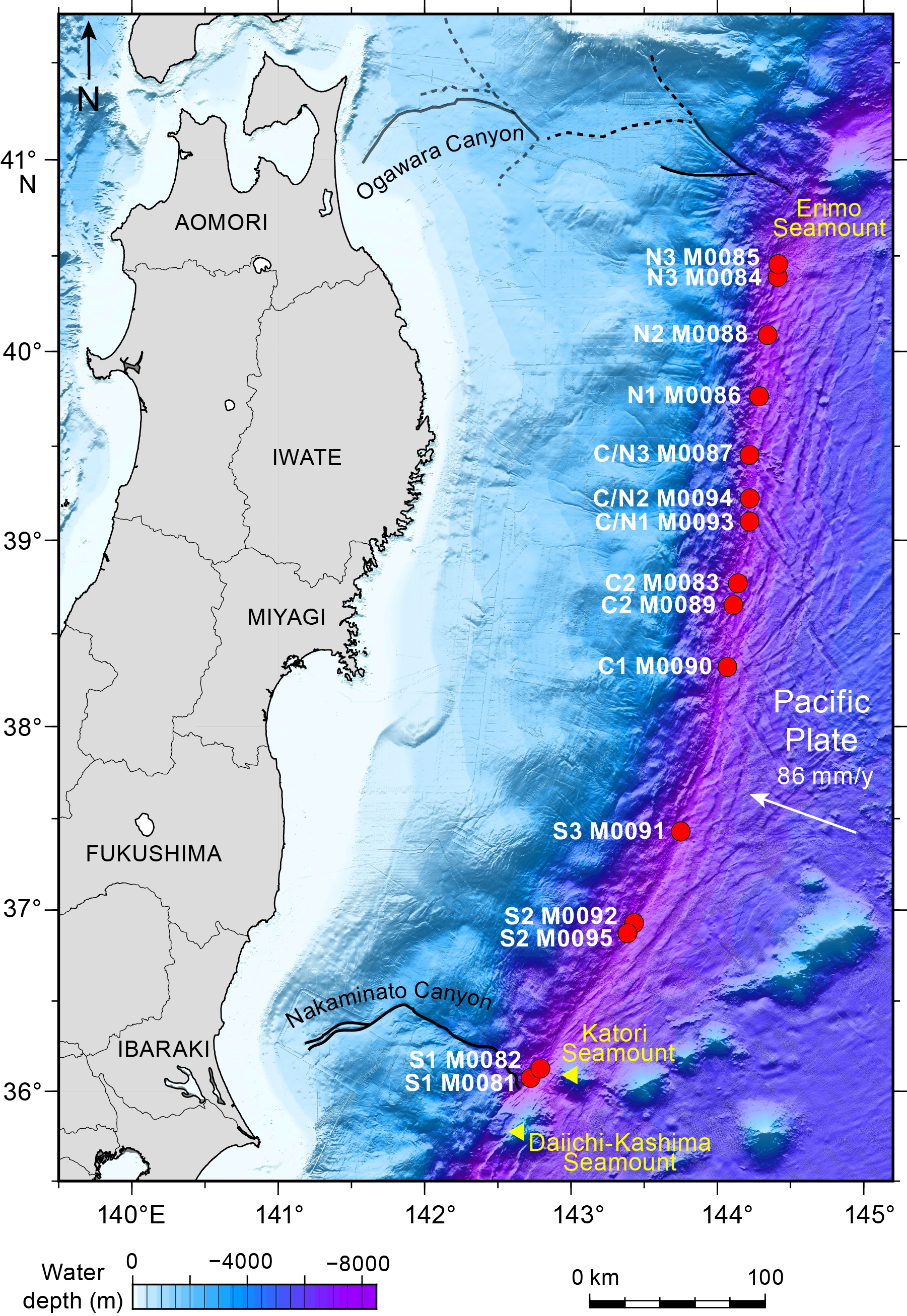
Figure F1. Site locations.
1.2. Site survey
At all Expedition 386 sites, the proposed site locations were first surveyed by at least one site-crossing multibeam swath bathymetry and high-resolution subbottom profile (see Hydroacoustics) to confirm that the seafloor and subseafloor sediment targets were free of large solid obstructions, which can bend the piston corer barrel on impact (see Coring methodology). Sound velocity profiles to calibrate the hydroacoustic data were obtained from expendable bathythermograph (XBT) probes, deployed at least once per working area (Table T5). Upon confirmation of a suitable site location, the GPS coordinates for the proposed sites were used to position the vessel on site (Strasser et al., 2019). After the ship was positioned at a site, a dynamic positioning system model was established. Coordinates for the position of the Giant Piston Corer (GPC) system deployments at the seabed were calculated from a combination of the corrected ship’s position and the position of a transponder mounted on a cable 50 m above the GPC. The accuracy of the actual positioning of the GPC system at the seabed is estimated to be ~200 m. In some incidences, the exact position at the seabed could not be calculated due to malfunctioning of the GPC transponder. In this case, the ship’s GPS position was applied for the positioning of holes. The accuracy of hole positioning in these cases is lower (on the order of 300 m).
Detailed descriptions and time breakdowns of operational activities are complicated by the decision to leave and return to sites dependent on highly changeable weather and variations in surface ocean currents on a daily basis. Summaries of time spent on operations and transit are therefore presented weekly (see OPS in Supplementary material).
1.3. Platform
The coring platform used for Expedition 386 was the R/V Kaimei (100.5 m long; 5747 tonnes; https://www.jamstec.go.jp/e/about/equipment/ships/kaimei.html), operated by the Japan Agency for Marine-Earth Science and Technology (JAMSTEC) (Figure F2). This dynamically positioned vessel has onboard laboratory facilities adaptable to a wide range of scientific applications. For the purpose of Expedition 386, the usual suite of European Consortium for Ocean Research Drilling (ECORD) containerized laboratories were not required, and the onboard laboratories were adapted to accommodate all analytical equipment required to carry out International Ocean Discovery Program (IODP) shipboard and time-critical Science Party sampling and analysis. A GPC releaser was used during the expedition, including a barrel and bit manufactured by NuStart Technologies Pte Ltd and a weighthead from Ocean Scientific International Ltd (OSIL), enabling deployment of a 20, 30, or 40 m GPC using its 12,000 m cable. The anticipated depth below sea level of coring sites was in excess of 8000 m. Core barrels are 5 m in length and have an internal diameter of 129 mm and an external diameter of 168 mm; core barrel thickness is 39 mm (details provided by NuStart Technologies).
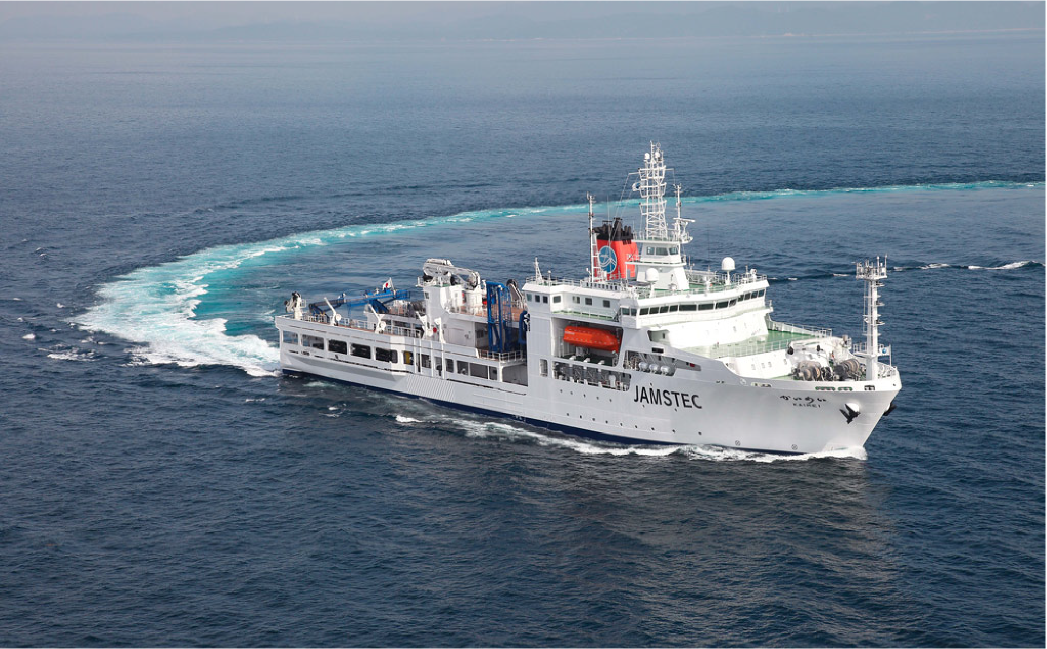
Figure F2. R/V Kaimei.
1.4. Coring methodology
Giant piston coring is an established technique, and it is used by many oceanographic research institutes around the world (e.g., Curry et al., 2008; Chen et al., 2013; Govin et al., 2016). This deployment for Expedition 386, however, was its first use as part of IODP drilling. The extreme water depths of the sites (>7300 mbsl), combined with the relatively shallow sampling targets (<50 meters below seafloor [mbsf]), made GPC sampling an attractive economic alternative to a typical IODP drilling expedition using a traditional drillship.
The GPC system consists of a set of coring barrels (a piston corer and a trigger corer), connected by a trigger line, that are lowered from the ship (Figure F3). A transponder was attached 50 m above the trigger corer and used to track the GPC system position. An azimuth inclinometer was attached to the piston corer weighthead to obtain information about geographic orientation of the core (Figure F4) and monitor potential deviation from vertical or rotation of the piston corer barrel during penetration (Figure F5). After the piston corer barrel has sunk to its target sampling depth, the entire system is winched back to the surface for recovery.
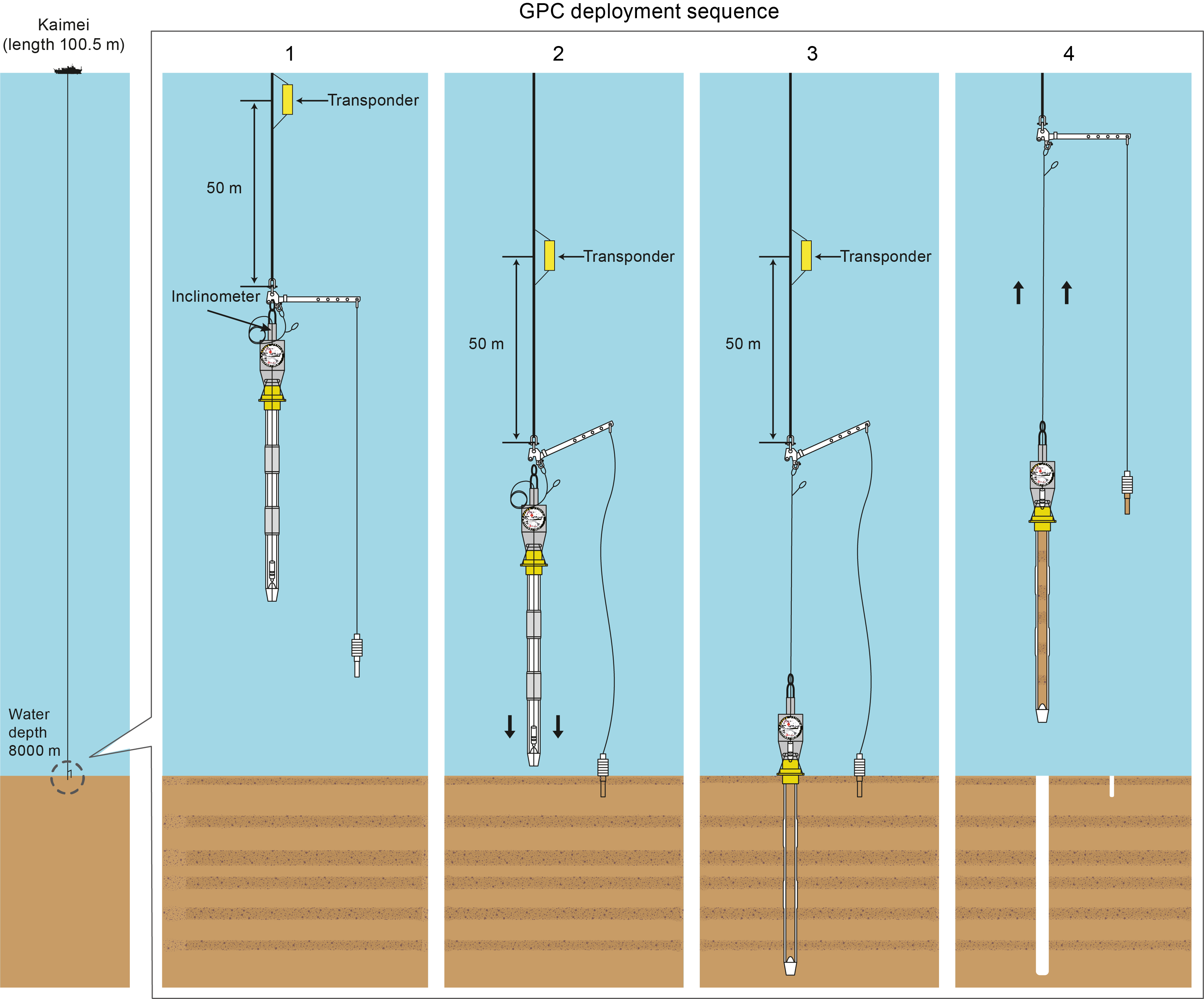
Figure F3. GPC deployment sequence.

Figure F4. Azimuth-inclinometer.
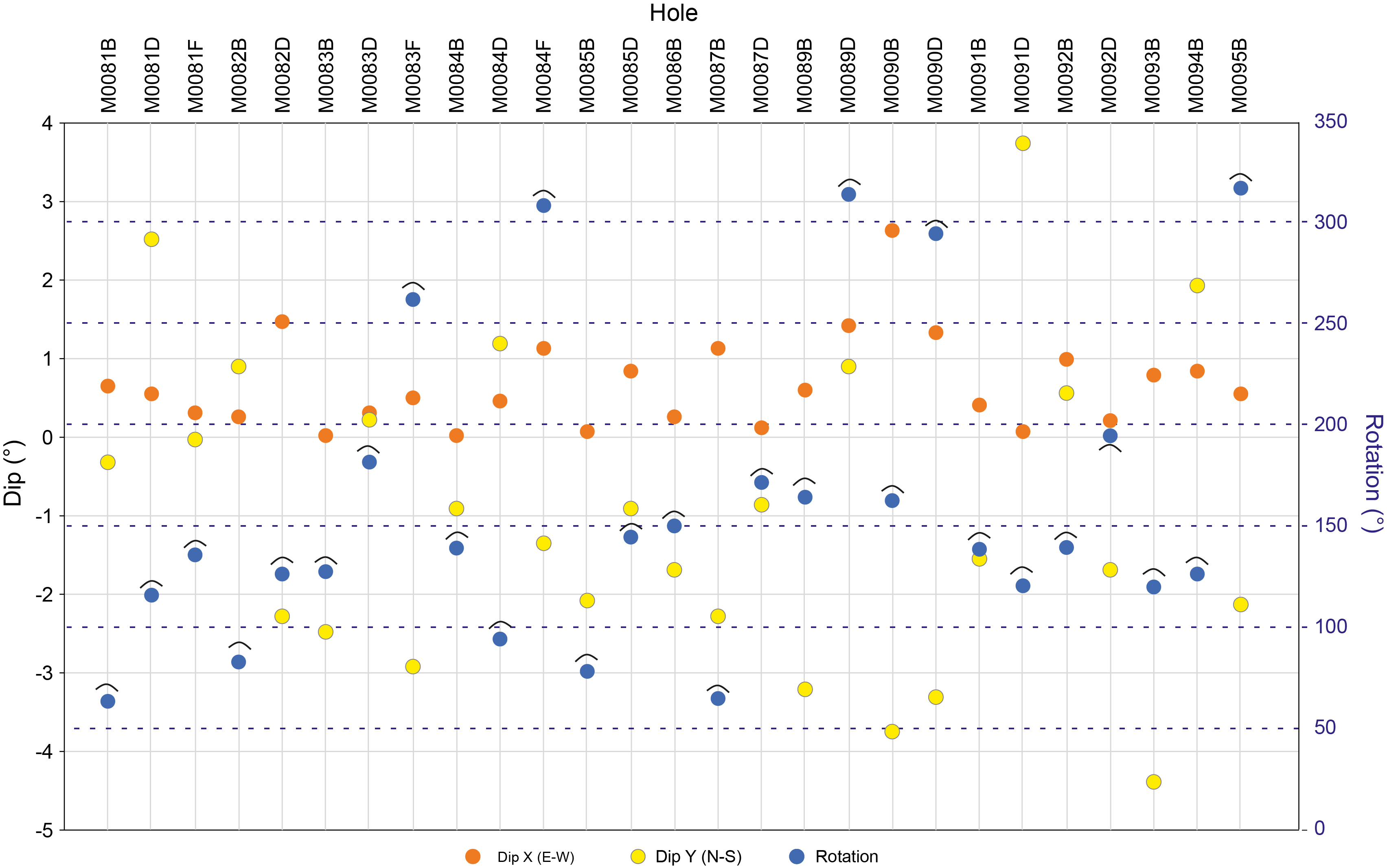
Figure F5. Azimuth-inclinometer measurements.
In detail, the GPC deployment sequence is as follows:
- The GPC system is lowered by winch toward the seafloor, with a small trigger corer suspended below the piston coring system. To improve core collection, the winch is stopped 100 m from the seabed to ensure the corer (transponder) is positioned correctly on the target point and allow stabilization before it is lowered again toward the seabed.
- The trigger corer hits the seafloor, triggering the release of the lever arm and the excess winch wire holding the piston corer system, which allows it to free fall to the seabed and penetrate into the seafloor sediments because of the heavy weight of the head and the main coring barrel.
- As the piston corer barrel enters the sediment, a piston inside the piston corer barrel, which is initially located at the bottom of the corer and is fixed at seafloor when penetration of the corer starts, moves up as the sediment enters, coming to rest at the maximum penetration point and forming an airtight cap at the top of the barrel.
- After penetration is completed, the GPC system is pulled out of the seabed and the piston remains stationary, ensuring the core remains in the barrel. The entire system is then hauled back to the surface.
- On board, the core barrel sections are opened and the core sections are cut, metadata is recorded, and cut core sections are moved to the laboratory for measurement and storage.
Different combinations of barrel lengths were applied for different GPC deployment sequences during Expedition 386. The length of the barrel of the trigger corer was 1.5 m for all 29 GPC deployments. To test safe penetration of the seabed and recovery, the first GPC deployment at each site used a 20 or 30 m long piston corer barrel. After the shorter barrels were successfully deployed and recovered, a 40 m barrel was used for subsequent holes at each site.
During operations, the cable tension during the GPC deployment sequence was monitored. The cable tension curve at spud-in (seabed penetration) to recovery of the GPC system follows a similar pattern for all sites (Figure F6). The tension on the cable falls rapidly at spud-in, taking only a few seconds to achieve maximum penetration before it is recovered. To ensure the piston coring system does not fall over and bend if full penetration is not achieved, recovery commences immediately. As the piston coring system is raised, the tension increases until the sediment at the base of the corer shears. A dip in the tension is noted at this point. The tension caused by the squeezing of the sediment against the piston corer barrel increases the tension as it is recovered until it is clear of the seabed, and this point is also identified on the tension graph. The average tension on recovery is greater than that during deployment due to the recovered sediment.

Figure F6. Winch log.
The cable tension curve for the first 20 or 30 m long piston corer was assessed at each site to decide whether to deploy the maximum piston corer length for the second (and third) deployment. In most cases, this allowed for deployment of the 40 m piston corer barrel.
1.5. Azimuth and inclinometer
Two azimuth-inclinometers were attached to the GPC during deployment, one on the hoist cable and the other secured in the weighted body of the GPC. The location of the instruments allowed the rotation of the GPC barrel and cable to be recorded. These data are required to calibrate results acquired from paleomagnetic analysis (Figure F4).
Data collected from the instrument in the body of the GPC was graphed to visualize the movement and rotation of the GPC as the barrel penetrated the seabed (Figures F4, F5). Although the azimuth-inclinometers measured continually during deployment and recovery, the most important measurements scientifically are those taken during core collection. For each site, the rotation direction and value (in degrees) and dip (north–south and east–west in degrees) are shown at the estimated seabed penetration (see TRANSPONDER in Supplementary material). Rotation and dip measurements were obtained from graphing the continuous measurements and the values taken from the point of the estimated seabed, which was calculated by subtracting the length of the core recovered from the maximum water depth recorded by the instruments at each site. There is no allowance for core loss or compression, which builds an error into the calculated depths. Therefore, depths are estimated and should not be taken as precise, meaning that the resulting values for barrel rotation and dip may not be at the exact moment of seabed penetration. Unfortunately, the clock in the azimuth-inclinometers was not calibrated to the GPC winch logs, so direct correlations of sediment penetration and the total depth of the GPC cannot be made. The overall difference appears to be around 9 h, but this is not always consistent between sites.
Inclinometer data from the GPC instrument reveal that, as expected, the GPC rotates as it is deployed and recovered through the water column. Inclinometer data also confirm that the corer continues to rotate as it penetrates the seabed. The extent of the rotation varied at each location and could be affected by the initial angle of contact with the seabed, the seabed current, and the speed of penetration, among other factors. The GPC angle of penetration may be exaggerated by the current if the rate of penetration was less than the speed of cable payout; similarly, the weight of the GPC body may also cause the barrel to tilt slightly without any effect from the current.
1.6. Numbering holes, cores, samples, and core depth scale terminology
The hole naming convention for IODP drill sites is that cored holes are labeled with capital letters in the sequence of drilling. Therefore, Hole A is the trigger core hole and Hole B is the main hole cored using the piston corer. For the second (and third) GPC deployment, Hole C is cored using the trigger corer, Hole D using the piston corer, Hole E using the trigger corer, and Hole F using the piston corer. For each hole, one core was recovered.
The recovered core from each hole is divided into 1 m long sections (a few exceptions have a maximum length of 1.36 m) that are numbered sequentially from the top, starting at 1. Following IODP convention, material recovered from the core catcher of a sedimentary core is treated as a separate section labeled CC for core catcher and placed below the last section recovered in the liner. Most core catcher sections were placed in a bag due to their consistency.
Any sample removed from a core is designated by the distance measured in centimeters from the top of the section to the top and bottom of the sample removed. A full identification number for an IODP sample consists of the following information: expedition, site, hole, core number, core type, section number, and interval in centimeters within a section measured from the top of section. For example, a sample identification of “386-M0081D-1H-24W, 95–100 cm,” represents a sample removed from the working half (W; “A” indicates the archive half) from the interval 95–100 cm below the top of Section 24, Core 1H (“H” [for hydraulic piston corer] indicates GPC cores, and “P” [for push corer] indicates trigger corer cores; see Coring methodology), from Hole M0081D during Expedition 386. These IODP identifiers for sample positions and/or measurement points are kept in all data files in the volume and in all data files during postexpedition and postmoratorium research.
Throughout this volume, we use meters below seafloor (mbsf) for the core depth below seafloor scale. With the definition of the core depth top datum at 0 mbsf, the mbsf scale is equivalent to the core depth below seafloor, Method A (CSF-A), scale from IODP Depth Scale Terminology 2011 (https://www.iodp.org/policies-and-guidelines/142-iodp-depth-scales-terminology-april-2011/file). The core depth below seafloor of a sample is calculated by adding the depth of the sample below the section top and the lengths of all higher sections in the core to the core top datum. This follows standard IODP practice to place the top of the recovered core at the top depth of the cored interval. Note that this IODP terminology was adapted for the deployment procedure of a GPC system, used for the first time during Expedition 386, by defining 0 m core depth below seafloor at the core top of the curated core (for cores recovered from both the trigger corer and the GPC; Figure F7).
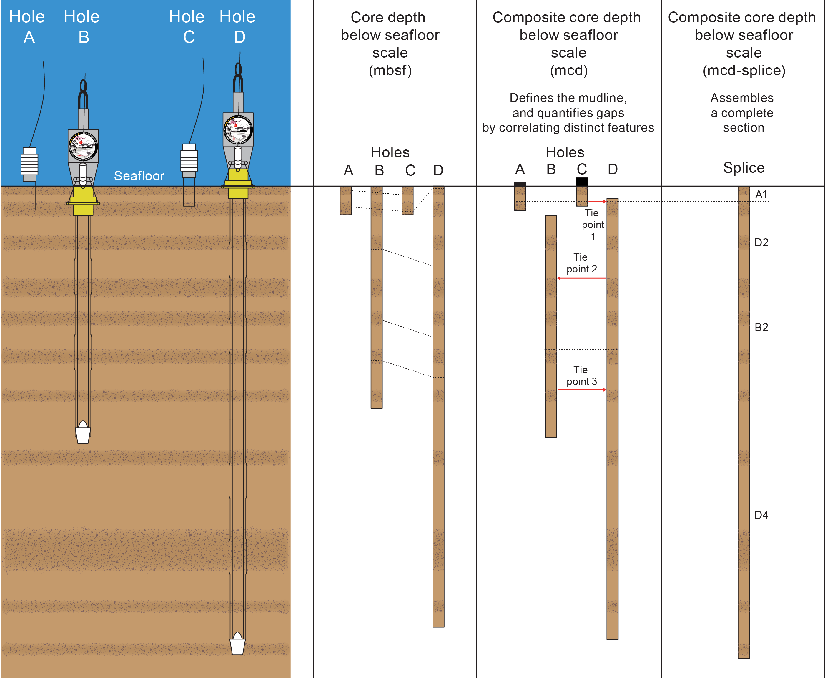
Figure F7. Depth scales.
The core depth below seafloor scale is established by adding the curated core length to the curated core top. As such, this depth scale does not yet correct for incomplete recovery of the uppermost subseafloor section, which is typically disturbed upon penetration of the heavy weight of the head and the main coring barrel of the piston corer. It also does not account for core expansion/contraction as a result of gas expansion and elastic rebound and coring disturbance or artificial voids filled by foam at the top or bottom of the sections, especially at the top part of the curated first section of trigger cores to keep the mudline (Figure F7). Therefore, it is important to be aware of the following:
- The mudline (water/sediment contact at the actual seafloor) recovered by the trigger corer can occur a few to several centimeters into the section because often the mudline is not at 0 mbsf. However, based on observation of the sediment/water interface on the ship, the mudline was well preserved in all trigger cores. Therefore, surface loss is considered minimal.
- Free fall to the seabed and penetration into the seafloor by the heavy weight of the head and the main coring barrel of the piston corer disturbs the seabed and the uppermost subseafloor section, resulting in nonrecovery of the first few decimeters to 2–3 mbsf and/or coring disturbance, a common phenomenon for such piston coring operations (e.g., Stow and Aksu, 1978; Buckley et al., 1994; Széréméta et al., 2004; Jutzeler et al., 2014). Larger loss of the surface mostly occurred during the GPC system deployment using the shorter, 20 m long piston corer barrel, likely caused by the comparably heavier weight of the head compared to the total length of the barrels and to deployment using a 40 m piston corer barrel.
To correlate cores between holes and to mitigate mudline definition and coring gap problems at the top of each trigger core and giant piston core, a core composite depth below seafloor scale was constructed based on sequential identification of distinct horizons (including the mudline) identified in multiple holes at a given site, working from the top of the section downward. Throughout this volume, we use meters composite depth (mcd) for the core composite depth below seafloor depth scale. The mcd scale is equivalent to the core composite depth below seafloor (CCSF) scale from IODP Depth Scale Terminology 2011 (https://www.iodp.org/policies-and-guidelines/142-iodp-depth-scales-terminology-april-2011/file). Before compositing holes, artificial and/or natural voids at the ends of sections were measured and the void length was subtracted from curated section length to obtain sediment length in each section (neglecting core catchers that were sampled in bags). Tables with corrected section lengths and section top and bottom depths of all sections are presented as part of Stratigraphic correlation in each site chapter.
To correlate cores, shipboard Multi-Sensor Core Logger (MSCL) data and onshore X-ray computed tomography (CT) images taken on board the D/V Chikyu were compared and initially aligned to define tie points, which were verified with visual core description and digital core linescan images. By doing this, core depths in adjacent holes at a given site are vertically shifted to line up with features found in cores recovered in adjacent holes. The correlation process results in tables that indicate the vertical shift of cores on the mcd scale relative to the mbsf scale (Figure F7; see Stratigraphic correlation).
The core composite depth below seafloor scale is constructed based on sequential identification of distinct horizons identified in multiple holes at a given site, working from the top of the section downward. The composite section, also called the splice, is constructed by combining selected intervals between tie points such that coring gaps and disturbed sections are excluded, resulting in a complete stratigraphic section (less any natural, sedimentologic hiatuses). The splice therefore represents the maximum stratigraphic record that could be recovered at a site by including the best portions of individual sections of the core from each hole. Because of gas expansion, which differs between cores from different holes, mcd depth designations for intervals in the splice are not necessarily equivalent to mcd depths for intervals not included in the splice.
The definition of these depth scale types and the distinction in nomenclature should inform the user that a nominal depth value on different depth scales usually does not refer to exactly the same stratigraphic interval in a hole.
1.7. Core handling and analysis
The following sections describe the flow of core, samples, and measurements from the deck through the laboratories during the different phases of Expedition 386. The specific steps in core processing, sampling, measurement, and data flow are illustrated in Figure F8.
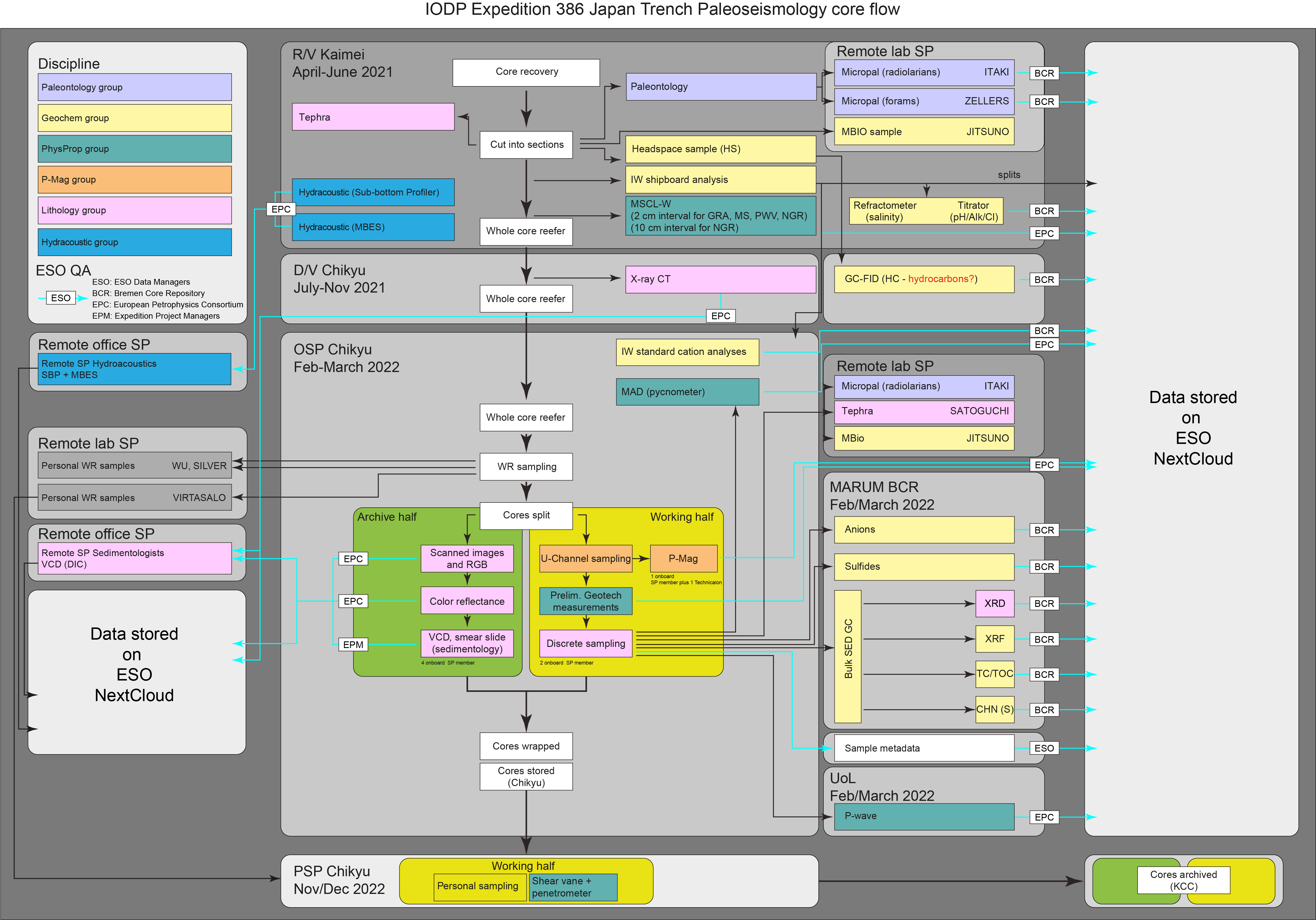
Figure F8. Core processing and measurement flow.
1.7.1. Offshore phase
After the trigger core assembly was recovered to deck, it was kept in an upright position to allow sampling of bottom water (BW). This sample was taken from inside the core liner above the mudline and siphoned into sample bottles for microbiological and geochemical analyses (see Microbiology).
After recovering the GPC system to deck, the core was initially extracted from the GPC barrel and cut into 5 m sections for easier handling. Sampling the bottom ends of these 5 m sections took place for IODP shipboard micropaleontology samples. Each of these sections was then cut into 1 m sections, and blue end caps were added to the top of each section. The 1 m sections were sampled on deck for IODP headspace samples (see Geochemistry) and Science Party microbiology and paleontology samples (see Microbiology and Micropaleontology).
Each 1 m section was then sealed at the top and bottom with color-coded plastic caps and tape: blue at the top of a section and white/clear at the bottom. The length of the core section and the core catcher sample were measured to the nearest centimeter and logged into Drilling Information System (DIS) spreadsheet templates by Institute for Marine-Earth Exploration and Engineering (MarE3) staff on board. These were uploaded to the ECORD Science Operator (ESO)-IODP Cloud and then entered into ESO’s Expedition DIS (ExpeditionDIS) by the ESO Database Managers onshore. No core splitting took place during the offshore phase. After end caps were added and curation was completed, the 1 m sections were transferred to the shipboard laboratory.
Interstitial water (IW) sampling for IODP shipboard geochemistry was completed using one to two Rhizon sampler syringes per section at decreasing resolution with depth. Ephemeral properties were measured for the BW and IW samples during the offshore phase (pH, alkalinity, and NH3) (see Geochemistry). All IODP shipboard analytical data and water samples reserved for IW standard analysis were stored on board Chikyu after the offshore phase of the expedition.
At Sites M0081, M0083, and M0084, all E and F holes were vacuum sealed in Escal neo foil and flushed with nitrogen to preserve core material from oxidation for microbiological analyses proposed for the OSP. All core sections, including trigger cores, were allowed to thermally equilibrate for 6 h and then scanned using the Geotek MSCL for physical property measurements (magnetic susceptibility, gamma attenuation, P-wave velocity, NCR, and natural gamma radiation [NGR]) (see Physical properties).
Smear slide samples were prepared from IODP micropaleontology samples taken from the 5 m cut section ends, but no observation was conducted on board due to time limitations.
After MSCL measurements were complete, cores were moved to refrigerated storage.
1.7.2. Between the offshore and onshore phases
A number of analyses were completed in the period between the offshore and onshore phases of the expedition.
X-ray CT scans were carried out on all sections, including trigger cores, using the X-ray CT scanner on board Chikyu (GE Yokogawa Medical Systems Discovery CT 750HD) (see Lithostratigraphy). These scans provided several functions:
- To provide an assessment of core recovery and liner integrity;
- To provide a data archive of core sections taken for whole-round samples prior to preparing the hand drawn visual core descriptions (VCDs);
- To determine appropriate locations for whole-round core samples by avoiding important structural and sedimentologic features;
- To identify the location of subtle features in cores that warranted detailed study or special handling during visual core description and sampling; and
- To determine the 3-D geometry, orientation, and crosscutting relationships of sedimentary, tectonic, and drilling-induced structures.
All data generated by both X-ray CT scanners are stored as Digital Imaging and Communication in Medicine (DICOM) formatted files.
Headspace samples taken offshore were analyzed on board Chikyu for gas chromatography with flame-ionization detection (GC-FID) (see Geochemistry).
Smear slides taken offshore were described and entered into the DIS spreadsheet template by Co-Chief Scientist Ken Ikehara and then entered into the ExpeditionDIS by the ESO Database Managers (see Lithostratigraphy).
1.7.3. Hybrid Onshore Science Party
The global situation resulting from the COVID-19 pandemic necessitated changes in the structure and operation of the OSP, which was held on board Chikyu on 14 February–15 March 2022. Because of travel and entry restrictions to Japan, only Japanese resident Science Party members and Operator staff were able to attend. This forced a number of significant changes to be made to the core flow prior to, during, and after the OSP. The most significant change was the decision to conduct only microbiological and IODP shipboard sampling and analysis during the OSP. A further restriction forced upon the operators was the limitation on the number of staff allowed to attend the OSP in person. As a result, a complicated core flow was designed (Figure F8), ensuring that analyses that could not be completed on board Chikyu were carried out at ESO laboratories at the Bremen Core Repository (BCR; Germany) and the European Petrophysics Consortium (EPC) at the University of Leicester (UK). Data derived from analyses conducted in Japan and Europe were shared with the full Science Party as they were produced, including the Japanese participants on board Chikyu and the remaining 26 scientists around the world, after a full QA/QC process conducted by ESO and MarE3 operator staff.
After cores were taken out of refrigerated storage, they were split lengthwise into working and archive halves. Splitting was carried out using horizontal wire cutters and steel plates to keep soupy material intact while the liner was cut. The cores were split from bottom to top, so investigators should be aware of the potential for older material to have been dragged up the core on the split face of each section. During section splitting, a few incidences occurred when sediment moved slightly into void spaces. Therefore, in some instances there may be a slight discrepancy between the whole-round depth (X-ray CT and MSCL) and the hand drawn VCD and linescan image. Whenever possible, the original depth of the whole-round data was referenced before core splitting. Each archive-half section was scanned for color reflectance measurements and high-resolution and linescan imagery.
The sedimentologists described the archive halves visually, aided by smear slides (see Lithostratigraphy), and recorded their observations on hand drawn VCDs. After undergoing full QA/QC by ESO staff, these sheets were then scanned and uploaded each day to the ESO-IODP Cloud for the remote sedimentologists to check, enhance where necessary, and then enter all observations into the DIS Section unit description spreadsheet template. The ESO Database Managers then entered this information into the ExpeditionDIS. Digital images of archive halves were made with a digital imaging system (see Physical properties). Specific areas of interest on the archive halves were occasionally photographed using a color digital camera.
Prior to sampling, penetrometer measurements were made on the working half of the core (Figure F8). Sampling was then routinely carried out for shipboard measurements and analysis (see Physical properties, Geochemistry, Paleomagnetism, and Micropaleontology) and logged into the JAMSTEC Kochi Core Center (KCC) Harumon System (see Data handling, database structure, and access). Sample metadata were then entered into the DIS samples spreadsheet template, uploaded to the ESO-IODP Cloud, and then entered into the ExpeditionDIS. Samples were generally sealed in plastic bags, labeled, and stored as appropriate. Some samples were shipped to ESO laboratories at the BCR and EPC (Table T3).
Because the GPC cores were too large (diameter = 11 cm) to fit the paleomagnetism superconductor on board Chikyu, 2 cm × 2 cm U-channel samples were taken from the centerline of all sections of most cores for IODP standard paleomagnetic measurements (see Paleomagnetism) and postexpedition research for X-ray fluorescence (XRF) analysis (some were shifted slightly to one side to accommodate a small number of high volume slab samples). Although it was understood this may impact later physical properties measurements (see Physical properties in this chapter and in each site chapter), this compromise was made to enable the fullest suite of IODP standard measurements to be taken, given the staffing and timing constraints placed upon sampling at the OSP.
IW samples taken from cores offshore were analyzed for cations (major and trace elements) on board Chikyu at the start of the OSP. Nonacidified IW samples were shipped to the BCR, where analysis for anions (chloride, bromide, sulfate, and phosphate), dissolved inorganic carbon, and phosphate (using spectrophotometry) were completed (see Geochemistry).
Following visual core description, initial measurements, and sampling, both halves of the cores were wrapped in cling film, vacuum sealed with Escal neo foil, placed in labeled plastic D-tubes, and transferred to a 4°C refrigerated container on board Chikyu.
1.7.4. Personal Sampling Party
The relaxation of travel restrictions and the opening of Japan’s borders to overseas visitors in September 2022 enabled the final phase of the onshore portion of the expedition to take place. The Personal Sampling Party (PSP) took place on board Chikyu on 15–30 November 2022. All 33 Science Party members and 3 shore-based scientists were invited to attend, and MarE3 and ESO operators finalized planning for sampling expedition cores to satisfy individual research proposals and complete IODP standard physical properties measurements. ESO operator staff traveled to Japan to help coordinate and assist MarE3 staff with Science Party logistics and the PSP workflow. A total of 22 Science Party members and 2 shore-based scientists attended either for all or part of the PSP. Over the course of 2 weeks, all samples and measurements were completed, fulfilling the sample requirements for 44 Science Party sample requests and completing IODP penetrometer and shear vane measurements for those core sections not already measured during the OSP.
Whole-round samples that had been requested for nondestructive analyses prior to splitting for the OSP were returned, split, scanned, and reintroduced to the core flow for sampling during the PSP. Before sampling, sedimentologists described the split section visually, recording their observations on hand drawn VCDs, and these were subsequently recorded into the DIS. Note that the images of the VCDs of material sampled during the PSP appear slightly different to those originally described due to the time interval between splitting and description (hand drawn VCDs are available in HANDDRAWNVCD in Supplementary material).
Sampling planning was coordinated by ESO over several months in close communication with scientists. Sample labeling and any additional required curation (e.g., deletion or addition of samples) was implemented using the JAMSTEC KCC Harumon sample curation system on board Chikyu. All samples, once taken, were packed, labeled, and stored according to agreed protocols and were shipped to scientists’ home institutions after the conclusion of the PSP. Sample information held in the Harumon system underwent full QA/QC and was then integrated into the ExpeditionDIS by the ESO Database Managers.
1.8. Data handling, database structure, and access
Data management comprised two overlapping stages. The first stage was the capture of metadata and data during the expedition (offshore, pre-OSP, OSP, and PSP). Data and metadata were uploaded to and exchanged on the ESO-IODP Cloud.
The ExpeditionDIS is a flexible and scalable database system originally developed for the International Continental Scientific Drilling Project (ICDP) and adapted for ESO so that it is compatible with the databases of the other IODP implementing organizations and ICDP. During Expedition 386, the ExpeditionDIS was used to store coring information, core curation information, core images, sample information, section unit descriptions, smear slide descriptions, X-ray CT core images, slabbed section linescan images, smear slide images, and split core closeup images. All other data were captured in files and stored on the shared file server.
During this expedition, several intermediate steps were necessary. Information was entered into DIS spreadsheet templates, checked, and then entered into the ExpeditionDIS. The second stage was the longer term postexpedition archiving of Expedition 386 data sets, core material, and samples. This function was performed by the World Data Center (PANGAEA; http://www.pangaea.de), the BCR, and the KCC.
All cores, sections, and samples entered into the ExpeditionDIS automatically receive an individual International Generic Sample Number (IGSN). The IGSN is a unique persistent identifier for physical samples. After the end of the moratorium, all data are transferred from the ExpeditionDIS to the CurationDIS in the long-term BCR core curation system; contemporaneously, the IGSNs are registered and can be accessed at http://www.igsn.org (to navigate to a particular IGSN, add the IGSN to the end of this link [e.g., http://www.igsn.org/IBCR0381EXI3001]).
All long-term archiving and publishing of IODP data was performed by ESO. The data captured in the Expedition 386 ExpeditionDIS and the shipboard expedition data stored in the shared file server were transferred to PANGAEA. PANGAEA is a member of the International Council of Scientific Unions World Data Center system and is used for processing, long-term storage, and publication of georeferenced data related to earth sciences. Until the end of the moratorium period, data access was restricted to the expedition scientists. Following the moratorium, all shipboard expedition data were published online in PANGAEA, and PANGAEA will continue to acquire, archive, and publish new results derived from Expedition 386 samples and data sets.
The central portal for all IODP data, including Expedition 386 data, is the Scientific Earth Drilling Information Service (SEDIS; http://sedis.iodp.org). IODP mission specific platform (MSP) data are also downloadable from the MSP Data Portal at PANGAEA.
In addition, JAMSTEC will also publish the following offshore data through the JAMSTEC database after the moratorium:
- Cruise tracking map,
- Navigation data (SQJ and SOQ),
- Multibeam echo sounder data (MBES),
- Three-component magnetometer data (STCM),
- XBT,
- Acoustic doppler current profiler (ADCP),
- Inertial navigation data (PHINS),
- Weather and maritime meteorology monitoring data (JAMMET),
- Radar wave height data (WAVE) (Leg 1 only),
- Photosynthetically active radiation data,
- Ceilometer data,
- Sea surface water continuous monitoring data (temperature, salinity, chlorophyll, and dissolved oxygen) (EPCS/TSG),
- Radiation thermometer data (THERMO), and
- Water vapor content monitoring data (VAPOR).
1.9. Core, section, and sample curation
Expedition 386 followed IODP procedures and naming conventions in core, section, and sample handling (see Numbering holes, cores, samples, and core depth scale terminology). Metadata were captured in spreadsheets by MarE3 and uploaded to the ESO-IODP Cloud. Curation metadata includes the following and was transferred to the ExpeditionDIS by ESO:
- Expedition information,
- Site information (latitude, longitude, water depth, start date, and end date),
- Hole information (hole naming by letter, latitude, longitude, water depth, start date, and end date),
- Core data (core number, core type, top depth, bottom depth, number of sections, core catcher where present, curator name, core on deck date and time, core recovery, core diameter, core temperature at time of recovery, and additional remarks),
- Section data (section number, section length, curated length, curated top depth of section, and additional remarks),
- Sample information (sampling location, requester code, sampler code, expedition, site, hole, core, section, half [working or archive], sample top, sample bottom, sample volume, and additional remarks).
Note that core recovery percentage is set as 100% because the GPC was used. Top and bottom depths of the section were calculated on the basis of the core top depth. Section and sample label formats follow the standard IODP convention. The sample labels include barcodes of the section ID (expedition-site-hole-core-core type-section) and sample depth interval (top and bottom depth in section). This standardization guarantees data exchange between the repositories and enables information flow between the implementing organizations.
2. Hydroacoustics
2.1. Aims
The aims of the hydroacoustic surveying during the offshore phase of Expedition 386 were as follows:
- To generate detailed bathymetric maps of the basins of interest and allow comparison along strike of both the condensed and full sections at each site,
- To collect additional 2-D hydroacoustic data in sedimentary infill basins,
- To confirm proposed coring site locations as selected based on data from previous site survey cruises (e.g., Strasser et al., 2019) to verify intact stratigraphy and confirm the seafloor and subseafloor sediment targets are free of large solid obstructions that can bend the piston corer barrel on impact (see Site survey),
- To compare the newly collected survey data with previously acquired site survey data,
- To facilitate integration of physical properties data into sediment echo sounder data, and
- To provide regional information and context for each site.
2.2. Systems
2.2.1. Multibeam
Kaimei is equipped with a Kongsberg EM122 multibeam echo sounder with a nominal frequency of 12 kHz. The depth range encompasses the full ocean depth, and the swath consists of 432 beams.
2.2.2. TOPAS subbottom profiling
Kaimei is equipped with a Kongsberg TOPAS PS18 parametric subbottom profiling system, which enabled high-resolution data acquisition from less than 20 mbsl to full ocean depth. At +80% relative bandwidth, a secondary low-frequency signal of 0.5 kHz is generated in the water column by nonlinear interaction between two high-frequency signals (centered symmetrically around 18 kHz). Only the secondary low-frequency signal is used for subbottom profiling.
Given the deep water of the study area, the TOPAS system was operated in Chirp mode for acquisition of the subbottom profiles because this allows for high penetration of the acoustic signal. Acquisition parameters for all lines are given in Table T4.
2.3. Data acquisition
Hydroacoustic systems on board Kaimei were operated by the Nippon Marine Enterprise engineer and the ship’s crew. Hydroacoustic data collection occurred between GPC deployments or during weather downtime when hydroacoustics could be acquired but the GPC assembly could not be safely launched. Subbottom profiler surveys were generally conducted at a speed of 3–6 kt, depending on the weather and current.
2.3.1. Multibeam data
In addition to multibeam bathymetric data acquisition, XBT measurements, which record depth sound velocity profiles, were implemented in the acoustic data set (Figure F9). This was done to ensure accurate sound velocity representation of the water column for ray path correction of the acoustic pulse. XBT Type T5 probes were used. Acquisition of water column profiles with the XBT probes up to 1830 mbsl was conducted at least once at each of the 11 basins and more than once in Basins S1, C2, N3, S2, and C/N3 (Table T5). Data were integrated into the acquisition system during data collection.

Figure F9. XBT profiles.
Acquired multibeam data (Figure F10) were cleaned and corrected with XBT measurements during the acquisition phase. Final data products include measured point data (KM21-EXP386.xyz) and a gridded data set (KM21-EXP.386.grd) (see HYDROACOUSTIC in Supplementary material).
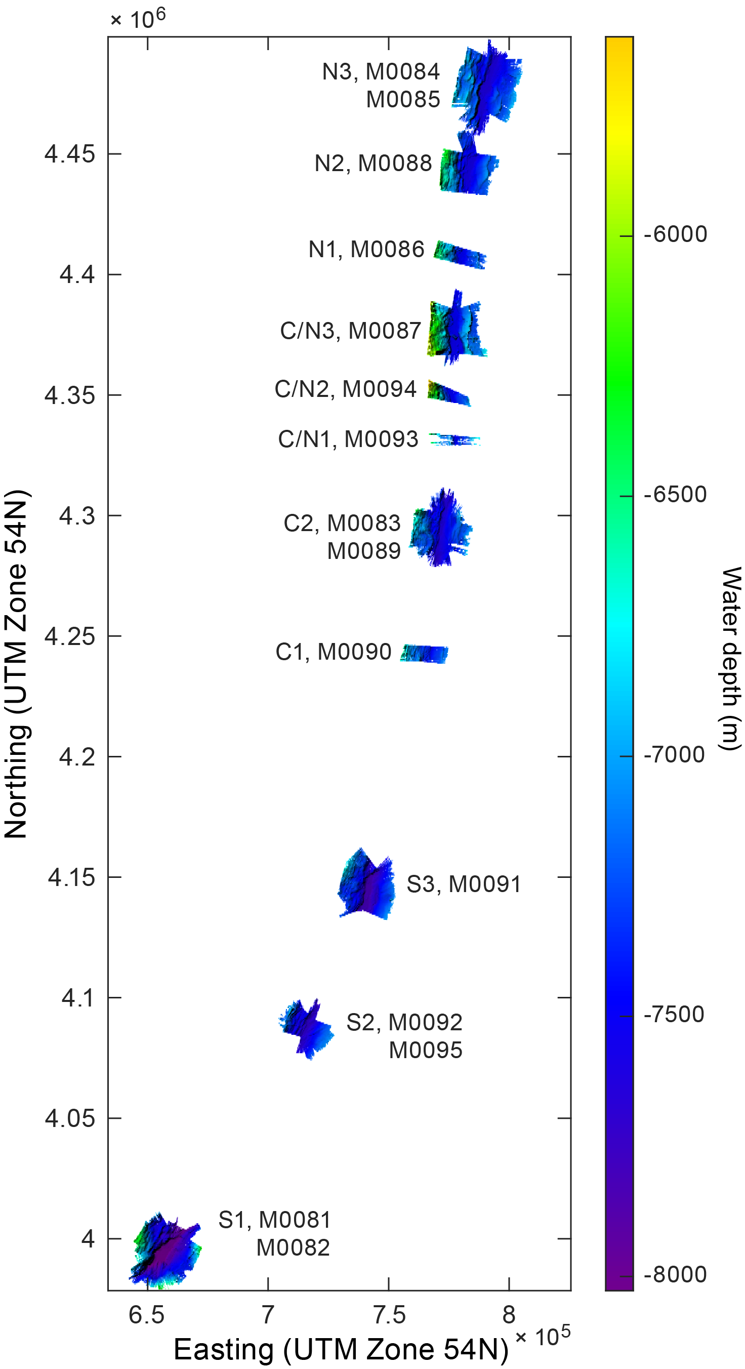
Figure F10. Bathymetric data.
2.3.2. Subbottom profiler data
Echo sounding used the Chirp mode, operated by using a linearly coded chirp pulse wavelet, where the frequency changes linearly with time (2–5 kHz), and with a chirp length of 10 ms. The ping interval was 12,000 ms, and the trace length was 200–300 ms. The gain for each line varies between 27 and 30 db. Frequency filtering was done through a high-pass filter at 2 kHz. TOPAS data were recorded mostly at 20–40 m per shotpoint depending on the ship’s velocity. Acquisition parameters are shown in Table T4. Raw data include a header of text regarding acquisition parameters for the processing flow of data sets (Table T6) and are stored in TOPAS’s native format raw files and converted SEG-Y files. Table T7 shows all of the information regarding trace headers for the TOPAS data.
The offshore file names for each individual line are a reflection of the date and time of start of acquisition in the format Year_Month_Day_Hours_Minutes_Seconds. For example, acquisition of Strike Line 20210416052623_1 started on 16 April 2021 at 05:26:23 h (the full list is shown in Table T4). The final line names are numbered in order of acquisition and are referred to as Lines 386_Underway_001 to 386_Underway_103. Because of the deep water depths, raw data recordings included time lags depending on water depth. This time lag is stored in Byte 109 on the SEG-Y header of each line. Shifts in time lag sometimes occurred within a single survey line when water depth abruptly changed (e.g., at the margin of a nearly flat trench fill basin floor to the steep trench slope). These lags can be corrected using the information at Byte 109 of the header when loading the original SEG-Y files in an appropriate software package. In this case, original data were loaded and corrected in SeismicUnix and exported from there as lag time shift–corrected SEG-Y files. The resulting uniform lag time per line is stored in Byte 109-110 (“delrt”) of the SEG-Y header.
Trench axis–perpendicular (dip) lines were generally shot either from east to west or from west to east, whereas trench axis–parallel (strike) lines were usually acquired north to south or south to north. Some basins where the trench axis does not quite strike south to north have oblique strike lines parallel to the trench basin axis. Some lines are extremely short where the data acquisition commenced, abruptly stopped, and then a new line commenced. In total, there are 103 discrete lines collected as grids or individual lines for each basin (Table T8; see HYDROACOUSTIC in Supplementary material).
2.4. Data analyses and reporting
2.4.1. Multibeam data
Coordinates in the original multibeam data are recorded in milliarcseconds. For analyzing and reporting this data, bathymetric grid data were converted to UTM coordinates (UTM Zone 54N). UTM grid data were then exported as GeoTiff data using the program gdal_translate (available from the Geospatial Data Abstraction Library). The bathymetric image was generated using a hillshading algorithm with azimuth-altitude illuminations and 4× elevation exaggeration. The final GeoTiff of the bathymetric data were exported as a PDF (Figure F10; for GeoTiff, .XYZ, and .GRD files, see HYDROACOUSTIC in Supplementary material).
2.4.2. Subbottom profiler data
The seismic interpretation package IHS Kingdom (2020) was used to upload, collate, and view the bathymetric and hydroacoustic data. All subbottom profile images were loaded using their navigation and header data and corrected for the time shift as given in Byte 109 (Table T6). This enabled visualization of each line/basin relative to underlying bathymetry. Amplitude images of each of the 103 lines were exported as PDFs (see HYDROACOUSTIC in Supplementary material).
2.5. Data interpretation
Visual interpretation of the subbottom profiles serves to identify layers or packages with distinct acoustic properties. In particular, seismically transparent, often ponded facies, likely representing event deposition (Ikehara et al., 2016), may be interbedded or in contact with less transparent, sometimes higher amplitude reflections from other geological events (Kioka et al., 2019). Following previous methodology (Ikehara et al., 2016; Kioka et al., 2019), the seismic character of the 11 basins in the study were characterized in terms of the thickness and morphology of any acoustically transparent packages and their relationships to other facies above and below them, as well as the character of other facies in the basin. For example, basal layers from the subbottom profiles commonly show disrupted reflection patterns, sometimes with irregular top morphologies. Basin-fill packages commonly show acoustically laminated packages of varying thicknesses, and packages or reflections with high amplitudes occur at various horizons. An overview of the types of acoustic facies identified is given in Figure F11. For each basin, all of the lines were examined to determine the acoustic character of the basin and how it varied both along the basin axis and perpendicular to the basin axis. Results are documented in the site chapters. In addition, for each basin, the relationship of seafloor topography and bathymetric data was determined because elevation changes within the basins can drive sediment depositional patterns.
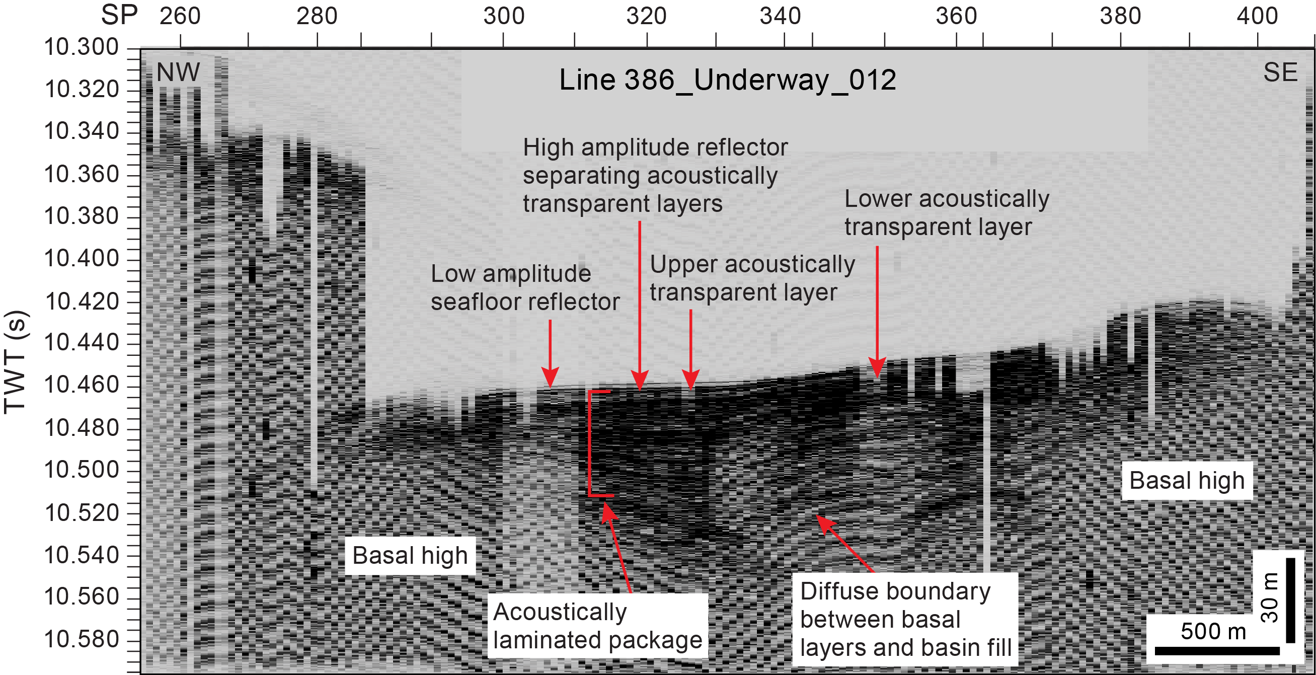
Figure F11. Acoustic facies interpretation of subbottom profile line.
2.6. Acknowledgments
We acknowledge IHS Markit for the provision of the IHS Kingdom software as part of an academic software donation to the University of Leicester, the EPC, and The University of Western Australia.
3. Lithostratigraphy
The techniques and procedures used to describe, analyze, and identify lithologies are described below. They are based on the methodologies employed during previous IODP expeditions and were adapted to the specific conditions and equipment available during Expedition 386. Because of international COVID-19 travel restrictions, the onshore Lithostratigraphy team consisted of a Chikyu team who worked in the onboard core description laboratory and a remote team that worked via video conference and synthesized and input the data. The techniques and procedures described here include (1) the methodology of core description and the procedures used to condense these data into computer-generated summary sheets (DIS) for each section; (2) the sediment classification schemes and terms used in the descriptions for the Expedition 386 cores; (3) smear slide methods, petrography, and data types; (4) X-ray diffraction (XRD) methods used to analyze bulk sediment mineralogy; (5) digital linescan imagery acquisition and equipment characteristics; and (6) X-ray CT data acquisition, analysis, and outputs. Information presented here concerns onshore operations and analyses described in the site chapters.
Because of the limited time and manpower on board Kaimei, shipboard descriptions of some core section cutting surfaces were limited to brief notes on sediment color and grain size for IODP paleontology samples. When available, these notes were introduced in the section description and recorded with the label “CC.” Any significant deviations from the procedures outlined here are discussed in the site chapters.
Sediments recovered from the Japan Trench are generally mixed siliciclastic and biosiliceous but contain a significant volcaniclastic component. The dominant grain sizes are silt and clay with a minor sand component. Generally, silt and clay sediments are dominated by diatoms and sponge spicules with minor quantities of other biogenic components. Lithogenic grains dominate the composition in coarse-grained sediment intervals. Diagenetic phases include iron monosulfides, pyrite, and authigenic carbonate in dispersed and nodular forms.
3.1. Visual core description
Unsampled archive halves of split cores arrived on the core table after linescan imaging (see Linescan split core imaging) along with pre-prepared paper copies of description forms (hand drawn VCDs; Figure F12) that included the X-ray CT image of the accompanying core section on the left side of the sheet. Before the visual inspections, the split core surfaces were scraped smooth again to emphasize sedimentary structures and compositional and/or textural changes in cores. The archive half was then examined, and visual observations were recorded manually on the hand drawn VCDs by the onboard sedimentologists. The VCDs were then scanned, and the resulting PDFs were uploaded before being sent in a batch every 24 h to the ESO server. The ESO staff performed quality control checks to confirm all files were present, the filenames were correct, and the scan quality was suitable. Scanned VCDs were then released for data input into the DIS and synthesis by the remote sedimentologists.

Figure F12. Hand drawn VCD template.
The lithology of each core section is represented on the hand drawn VCDs by graphic patterns next to the X-ray CT image of the archive-half core section (Figure F12). A wide variety of features that characterize the sediment are indicated in the columns to the right of image, including coring disturbance, unit bounding surfaces, grain size, smear slide sample and close-up photo locations, primary sedimentary structures, body and trace fossils, bioturbation intensity, grain sorting and roundness, color, and an additional free text description that may include handwritten depths of contacts, accessories, and iron monosulfide abundance.
This information was later condensed using specific codes and entered online in an Excel spreadsheet by the remote sedimentologists. The data was then uploaded to the Expedition DIS by the ESO Database Managers to generate a simplified database for each described core section. Digital lithologic columns were generated from the information entered in the Expedition DIS using Strater (Golden Software). These composite lithologic figures are referred to as lithostratigraphic summaries (Figure F13) in the site chapters. The main symbols used to represent the lithologies are presented in Figure F14. Recovery of core catcher materials was not consistent during the expedition, so they only appear in some of the lithostratigraphic summaries. Core close-up photos, linescan images of each section, X-ray CT composite and section images, XRD data used in figures, hand drawn VCDs, and smear slide photos are available in CORECLOSEUP, LINESCAN, XRAYCT, XRD, HANDDRAWNVCD, and SMEARSLD, respectively, in Supplementary material. The 3 m scale barrel sheets, smear slide tables, and linescan composite plots are available in Core descriptions.
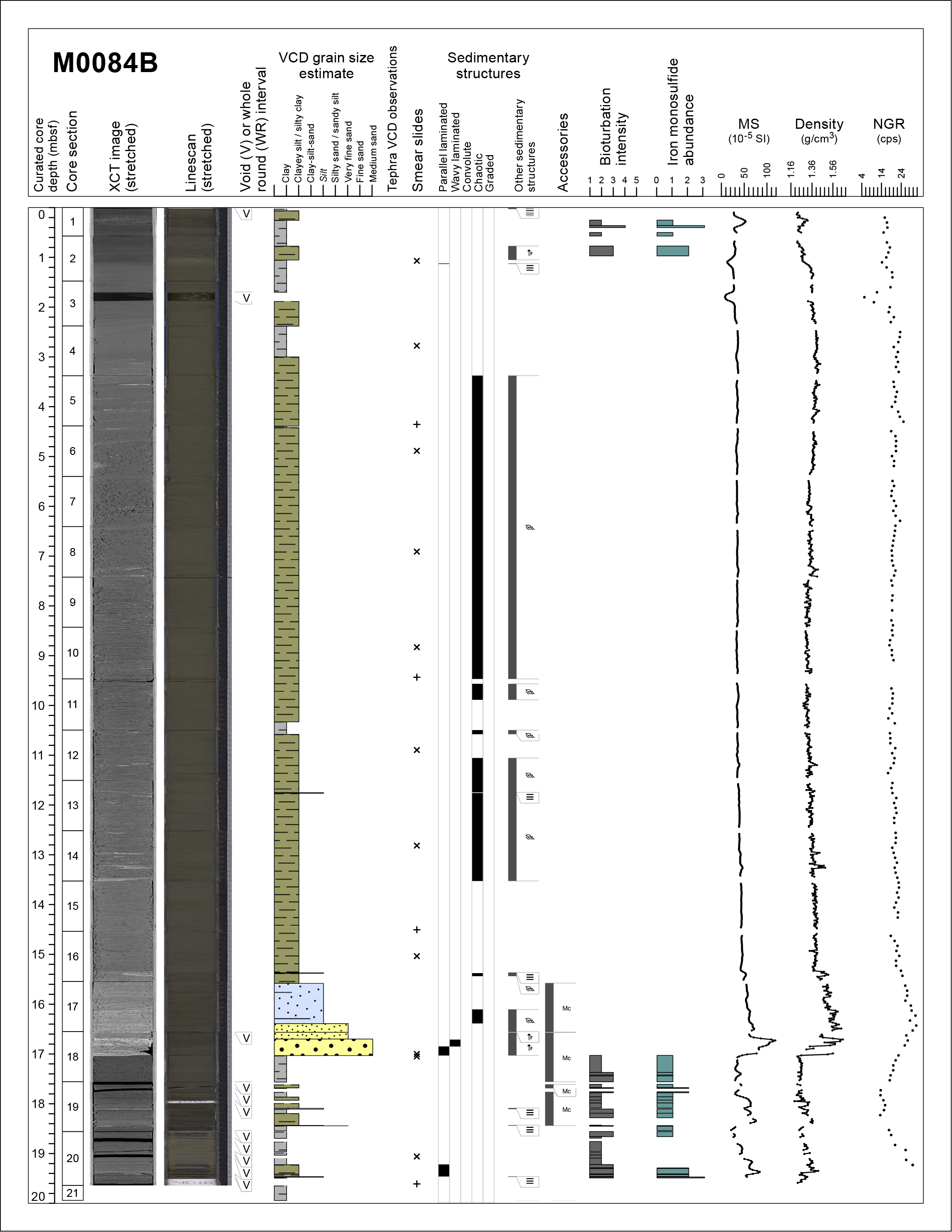
Figure F13. Example lithostratigraphic summary.
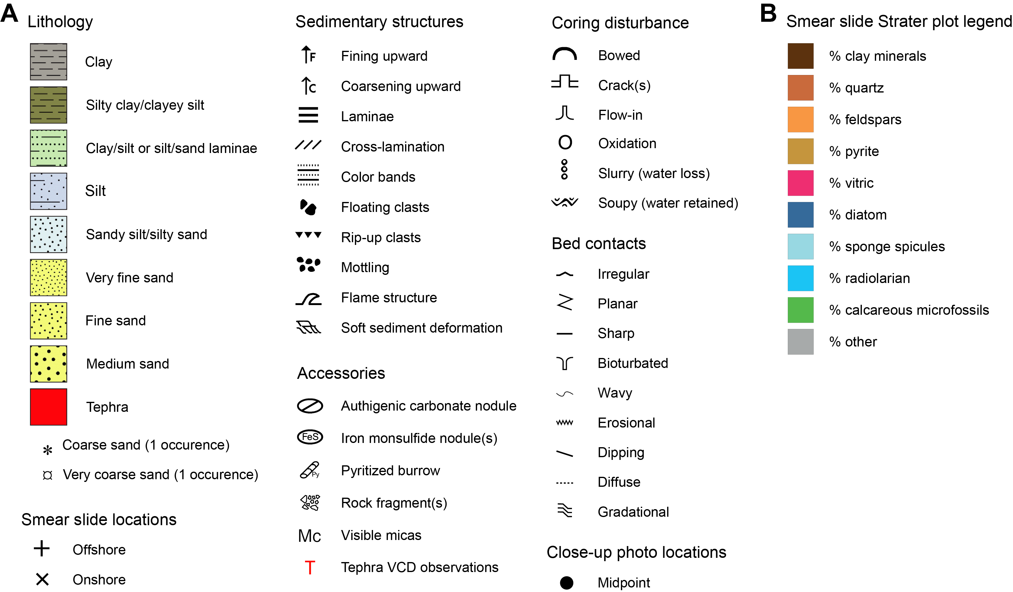
Figure F14. Lithostratigraphic summary, 3 m barrel sheet, and smear slide summary plot legend.
Composition, structure, and texture are the only criteria used to define lithology. Genetic/interpretative terms such as pelagic, hemipelagic, turbidite, debrite, and so on do not appear in this classification. The sediment type and major lithology follow Shepard’s (1954) textural classification scheme and are represented as a ternary diagram with three grain size end-members (sand, silt, and clay; Figure F15). This definition of the sediment texture obtained with a hand lens on split cores is complemented by a description of the composition and texture of sediment obtained every 2 m from smear slides observed under an optical microscope (see Smear slides). Slight differences in assessment between macro- and microscopic observations may occur in some cases. When volcanic ash is the dominant lithology, it is distinguished as a red layer with a red “T” for tephra in the lithostratigraphic summaries. Additional occurrences of volcanic material, such as ash patches and reworked glasses, are reported in Tephra.
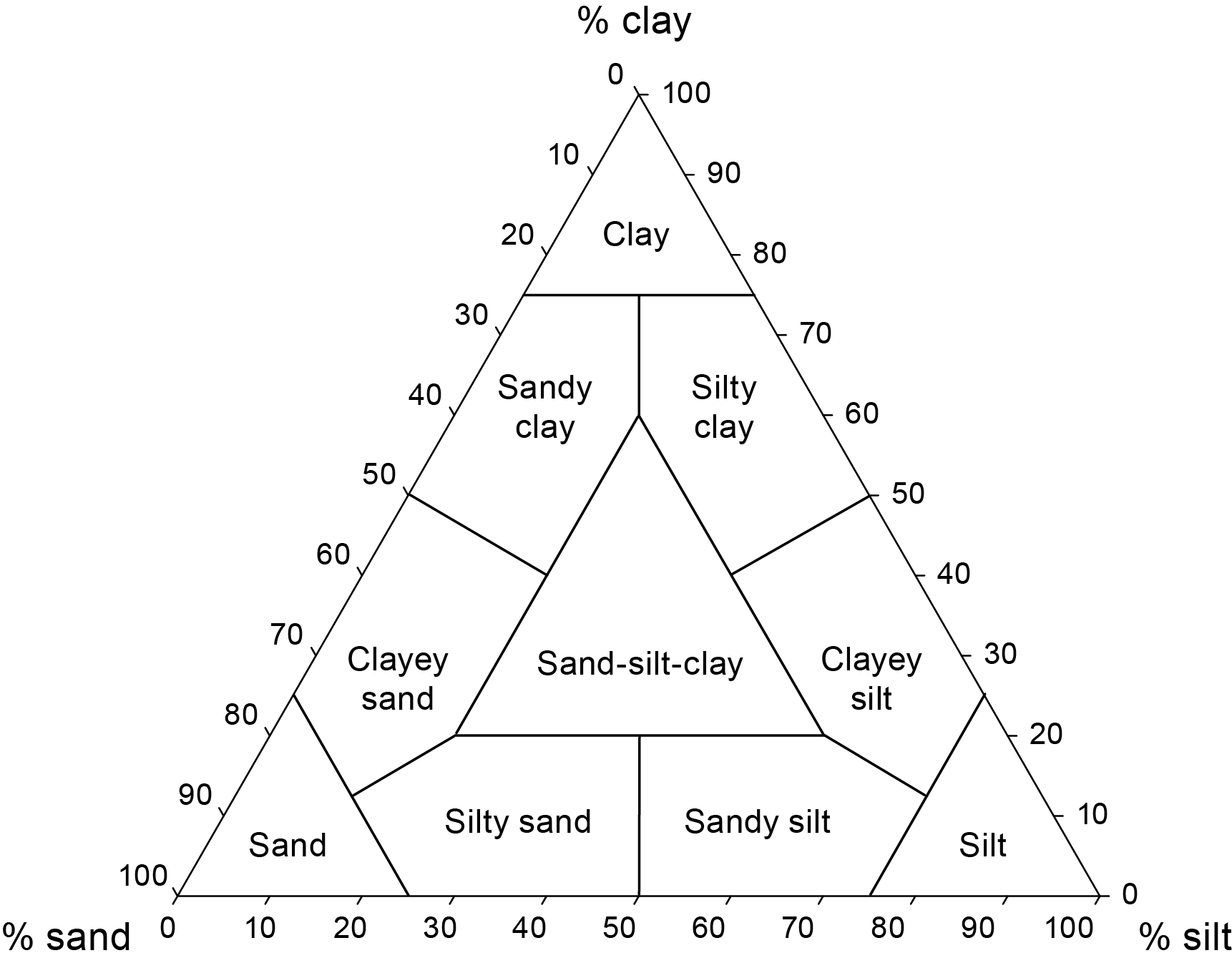
Figure F15. Sediment textures.
3.1.1. Bedding
Bedding terminology is after McKee and Weir (1953):
- Very thick bed = >100 cm.
- Thick bedded = >30–100 cm.
- Medium bedded = >10–30 cm.
- Thin bedded = >3–10 cm.
- Very thin bedded = 1–3 cm.
- Laminae = <1 cm.
The most commonly observed bedding structure in Expedition 386 cores is lamina.
3.1.2. Contacts
Contacts between different sediment beds are described as gradational, bioturbated, irregular, sharp, erosional, wavy, planar, dipping, and diffuse. These contacts are described for both the lower and upper portions of an interval.
3.1.3. Grain size
Grain size divisions on the lithostratigraphic summaries for clay, silt (very fine, fine, medium, and coarse), sand (very fine, fine, medium, coarse, and very coarse), gravel (very fine, fine, medium, coarse, and very coarse), and cobble follow Wentworth (1922) and Lane (1947) and were assessed using hand lenses and grain size cards. The term “clay” is used for both clay minerals and other siliciclastic material <4 µm in size. If sand, silt, or clay is >50% of the sediment, the principal name is determined by the relative proportions of sand, silt, and clay sizes when plotted on a modified Shepard (1954) classification diagram (Figure F15). Examples of principal names are clay, silty clay, silt, sandy silt, or sand. On the lithostratigraphic summaries, grain size variations are represented as clay, clayey silt/silty clay, clay-silt-sand, silt, silty sand/sandy silt, and sand (very fine, fine, and medium) (Figure F13).
3.1.4. Deformation and disturbance
Deformation and disturbance of sediment that clearly resulted from the coring process are illustrated in the Drilling disturbance column on the 3 m barrel sheets. Blank regions indicate the absence of apparent disturbance. Disturbances include cracks (these become more abundant with depth in the core and are related to gas expansion upon core recovery gas expulsion), slurry/soupy (water saturated), and flow-in and bowed disturbances (both of which are associated with piston coring techniques). Bowed disturbance is evident in sedimentary structures such as lamina. The term “void” is used to document empty spaces related to the coring process or whole-round core sampling. In the latter case, a specific note is added to the lithostratigraphic summaries and in the DIS because some whole-round samples were split and described during the PSP. Secondary oxidation of the sediment after core cutting at core section ends or sides is indicated as well.
3.1.5. Primary sedimentary structures
Description of primary sedimentary structures was kept as simple as possible to capture the most frequent observations. Small sedimentary features are usually fining or coarsening upward; parallel-, wavy-, or cross-laminated; and structureless, chaotic, or mottled and in some places exhibit some rip-up clasts and soft-sediment deformation such as microfolding. We define lithologies as structureless when they lack any primary sedimentary structures (e.g., lamination, parallel bedding, etc.). Structureless lithologies, however, may show secondary structures such as bioturbation. A free text column on the lithostratigraphic summaries shows complementary information that captures other features, including faults, fractures, tilted bedding, clastic dikes, flame, dish, water escape, or convolute structures.
3.1.6. Accessories
Accessories (i.e., macroscopically identified authigenic or diagenetic minerals) are minor components of the cores, and the relative abundance of some of them is assessed using the standard visual composition chart of Rothwell (1989). The captured accessories are micas (hand lens scale), rock fragments, authigenic carbonate concretions, iron monosulfides, nodules, and pyritized burrows. The intensity of the presence of iron monosulfides in the cores was assessed using a semiquantitative scale: 1 = sparse, 2 = moderate, and 3 = abundant (Figure F16).
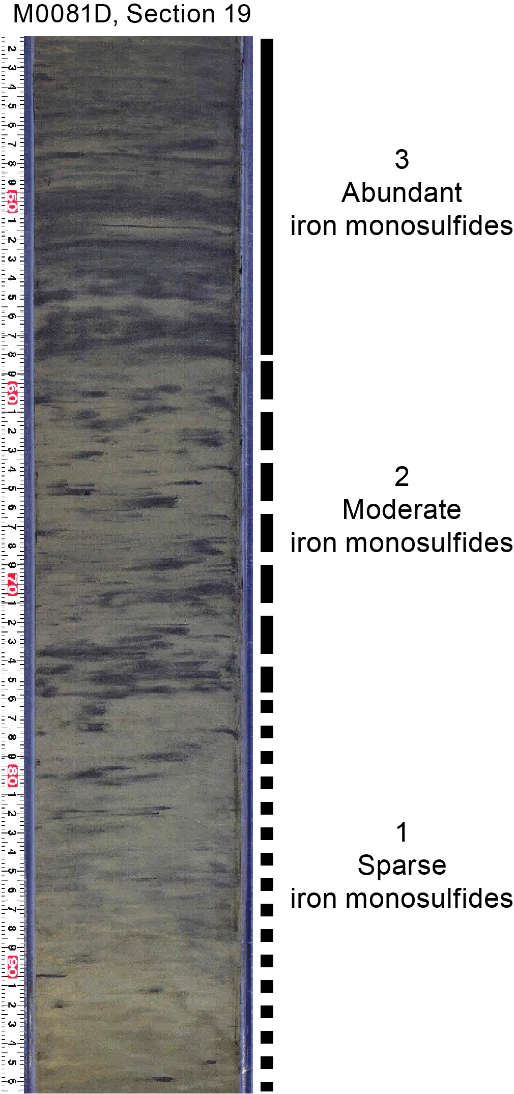
Figure F16. Iron monosulfide intensity.
3.1.7. Biogenic content
Macrofossils are quasi-absent in the core sections due to the very deep marine conditions. Most of the fauna and flora is represented by microfossils (e.g., diatoms, radiolaria, silicoflagellates, siliceous sponge spicules, foraminifera, and calcareous nannofossils) that were only observed in smear slides or in micropaleontology samples. A first assessment is presented in the smear slides section of each site chapter. However, macroscale wood and plant debris and shell fragments are reported on the lithostratigraphic summaries and in the DIS.
3.1.8. Trace fossils and bioturbation
Trace fossils largely produced by soft-bodied faunas are abundant and in many places overprint fine structures (laminae and contacts). Our ichnological analysis included both evaluation of the intensity of bioturbation and identification of trace fossil types. To assess the degree of bioturbation semiquantitatively, a modified version of the Droser and Bottjer (1991) ichnofabric index (ii = 1–5) scheme was employed. The different degrees of bioturbation are: (1) no bioturbation, (2) slight, (3) moderate, (4) abundant, and (5) homogenized by bioturbation (Figure F17). Slight bioturbation is manifested by discrete burrows and trace fossils covering ~10% of the core surface. Moderate bioturbation includes 10%–50% of the core surface disturbed by burrows or trace fossils. If more than 50% of the core surface is disturbed by burrowing or trace fossils, it is abundant.
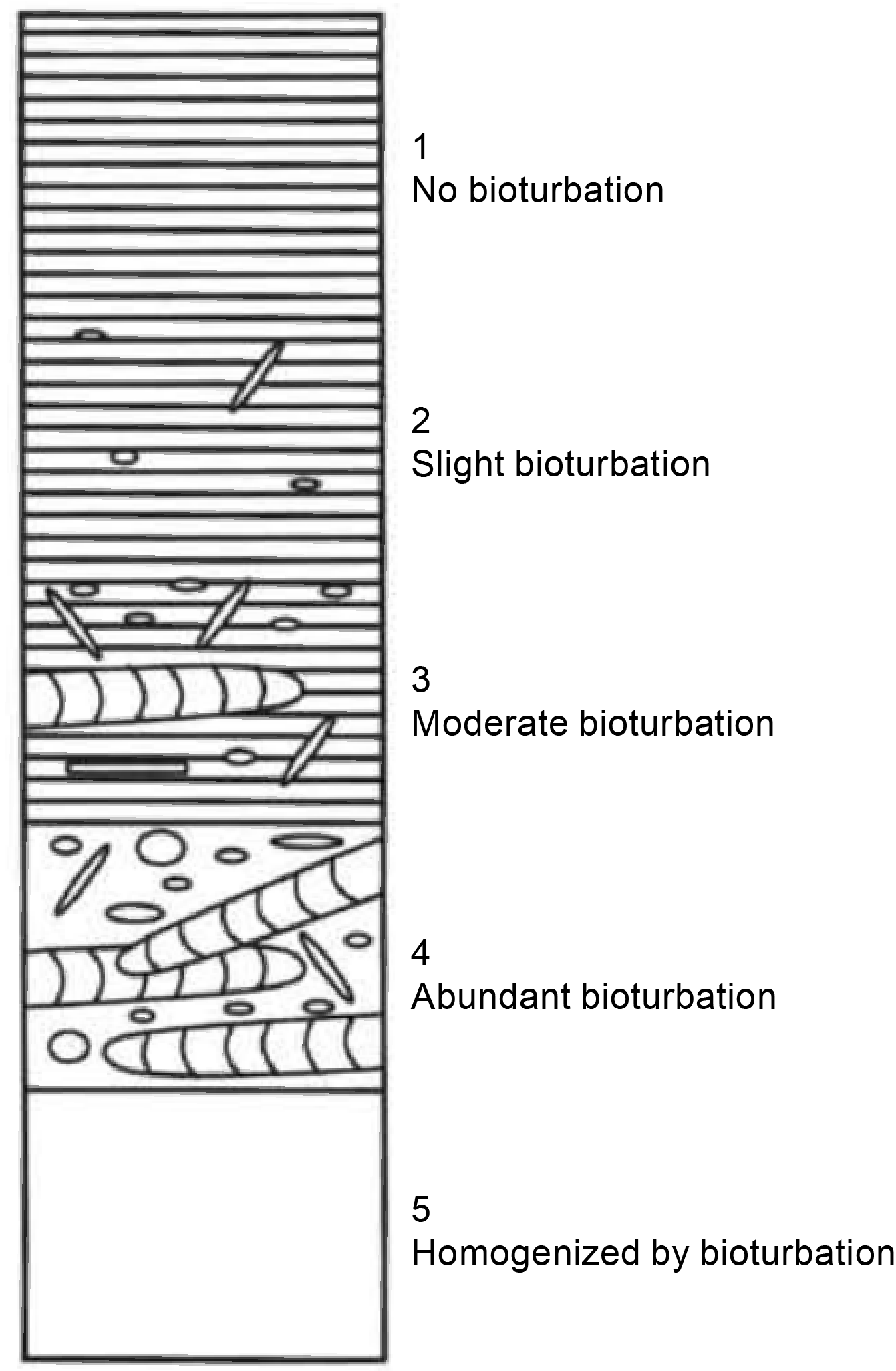
Figure F17. Degree of bioturbation.
The photographic atlas of Gérard and Bromley (2008) was used as a basis for trace fossil identification, and the name of the trace fossil genus was reported in the free text description column of the lithostratigraphic summaries and entered in the DIS.
3.1.9. Sediment color
Hue and chroma attributes of sediment color were determined visually using the Revised Standard Soil Color Chart (Oyama and Takehara, 1967). Color was coded by a combination of hue, which represents the dominant spectral value, such as red, yellow, green, or blue value, which represents the relative lightness of color, and chroma, which represents the relative purity or strength of the spectral color. Hue is composed of five major colors—red (R), yellow (Y), green (G), blue (B), and purple (P)—and the respective complement colors–yellow red (YR), green yellow (GY), blue green (BG), purple blue (PB), and red purple (RP). These colors are arranged on a loop, and each one is divided by a decimal system from 0 to 10. Thus, whole hues are assigned values between 1 and 100, R to RP. Value consists of numbers, from 0 for absolute black to 10 for absolute white, and neutral, which has no depth in color. The colors between 0 and 10 are arranged so that they become successively lighter in visually equal steps. The chroma values of each color gradually change with increases in vividness. When the hue and value are systematically arranged, the chroma value increases with increasing vividness starting at 0 (neutral gray). A color of 7.5Y in hue, 6 in value, and 4 in chroma is noted as 7.5Y 6/4.
3.2. Smear slides
During the offshore phase of Expedition 386, smear slides were prepared from paleontology samples collected with a tip-cut syringe from section ends every 5 m on board Kaimei. Before making smear slides, the samples were visually inspected for grain size determination and sediment color assessment with the Revised Standard Soil Color Chart (Oyama and Takehara, 1967). During the onshore phase, smear slides samples were collected every 2 m to complement visual core description observations and identify the composition of fine-grained sediment. This helps confirm the major lithology and adds compositional information for fine-grained sediment when the observer noted a marked change in sedimentary facies. A specific assigned symbol indicates the location of the offshore smear slide samples on the lithostratigraphic summaries (Figures F13, F14). The smear slide was prepared by putting a small amount of sediment on a glass slide mixed with distilled water. The slide was evaporated on a hot plate, and the dried sample was mounted in Norland Optical Adhesive 61 using ultraviolet light.
Sediment grain size and composition were examined under a polarized light petrographic microscope (Zeiss Axio Imager A1m POL-1) with an ocular micrometer. The adopted sediment nomenclature is derived from Mazzullo et al. (1988). The textural description is based on the sand-silt-clay ratio for granular sediments (Figure F15; Shepard, 1954), and the compositional description as a percentage of lithic, biogenic, and volcanic components is estimated semiquantitatively using a standard visual composition chart (Rothwell, 1989), although clay-sized grains tend to be underestimated using this method.
Major minerals identified during this preliminary petrographic analysis of sediments include quartz, feldspar, mica, pyrite, and volcanic glass shards. Rock fragments were also recognized. Positive identification requires additional microscopic analysis, however. Identifiable whole microfossils and fragments include diatoms, radiolaria, silicoflagellates, siliceous sponge spicules, and rare foraminifera and calcareous nannofossils.
Descriptions were recorded in data tables (see smear slide tables in Core descriptions). These tables include information about the sample location in the Japan Trench, a description of where the sample was taken in the core, the estimated percentages of texture (i.e., sand, silt, and clay), and the estimated percentages of composition (i.e., volcaniclastics, siliciclastics, detrital carbonate, biogenic carbonate, and biogenic silica). Offshore, because of a relatively abundant occurrence of siliceous microfossils such as diatoms, radiolaria, silicoflagellates, and siliceous sponge spicules, the term “siliceous” was used for mixed siliceous microfossil assemblages. Offshore smear slide descriptions are available in SMEARSLD in Supplementary material.
Onshore, the sediment nomenclature was refined. The sediment is named in an orderly fashion according to the proportions of its major constituents. The main name is that of the component that represents more than 50% of the sediment, and associated modifiers such as “rich” (25%–50%), “bearing” (10%–25%), and “with” (5%–10%) are added. A silica-rich example would be siliceous-bearing lithogenic-rich vitric clayey silt with nannofossils, and a calcareous-rich example would be lithogenic-bearing calcareous nannofossil–rich siliceous ooze with pyrite. Sediment composed of 50% or more biogenic components is named “ooze,” and sediment composed of 50% or more volcaniclastic material is named “ash.”
The results are summarized for each hole at each site in two different plot types:
- Two Sigma plot ternary diagrams (Figure F18) show the grain size distribution (percent clay, percent silt, and percent sand) and the composition of the sediment (percent volcanics, percent biogenics, and percent lithics). Lithics in this diagram are quartz, clay, feldspar, pyrite, heavy minerals, and rock fragments.
- A smear slide summary plot presents the different percentages of the main components as observed in each smear slide along the stratigraphic column (Figure F19). The most abundant lithogenics (clay, quartz, feldspar, and pyrite) are given in a brown color gradient, the volcaniclastic/vitrics are pink, and the biogenics are in a blue gradient for siliceous biogenics (diatoms, sponge spicules, and radiolaria) and are green for calcareous microfossils (Figure F14). Gray represents uncommon accessory components such as mica, heavy minerals, lithic grains, and plant and wood fragments. Raw data for all smear slides are presented in SMEARSLD in Supplementary material.
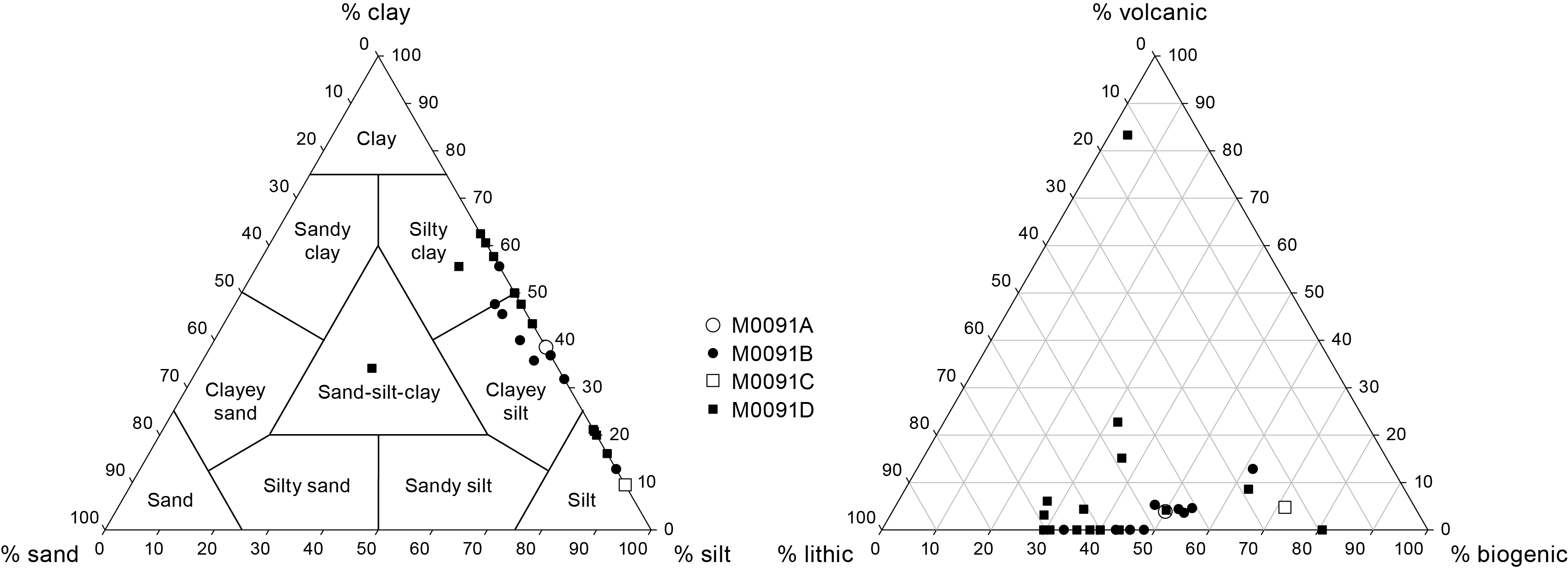
Figure F18. Texture and composition of sediment.
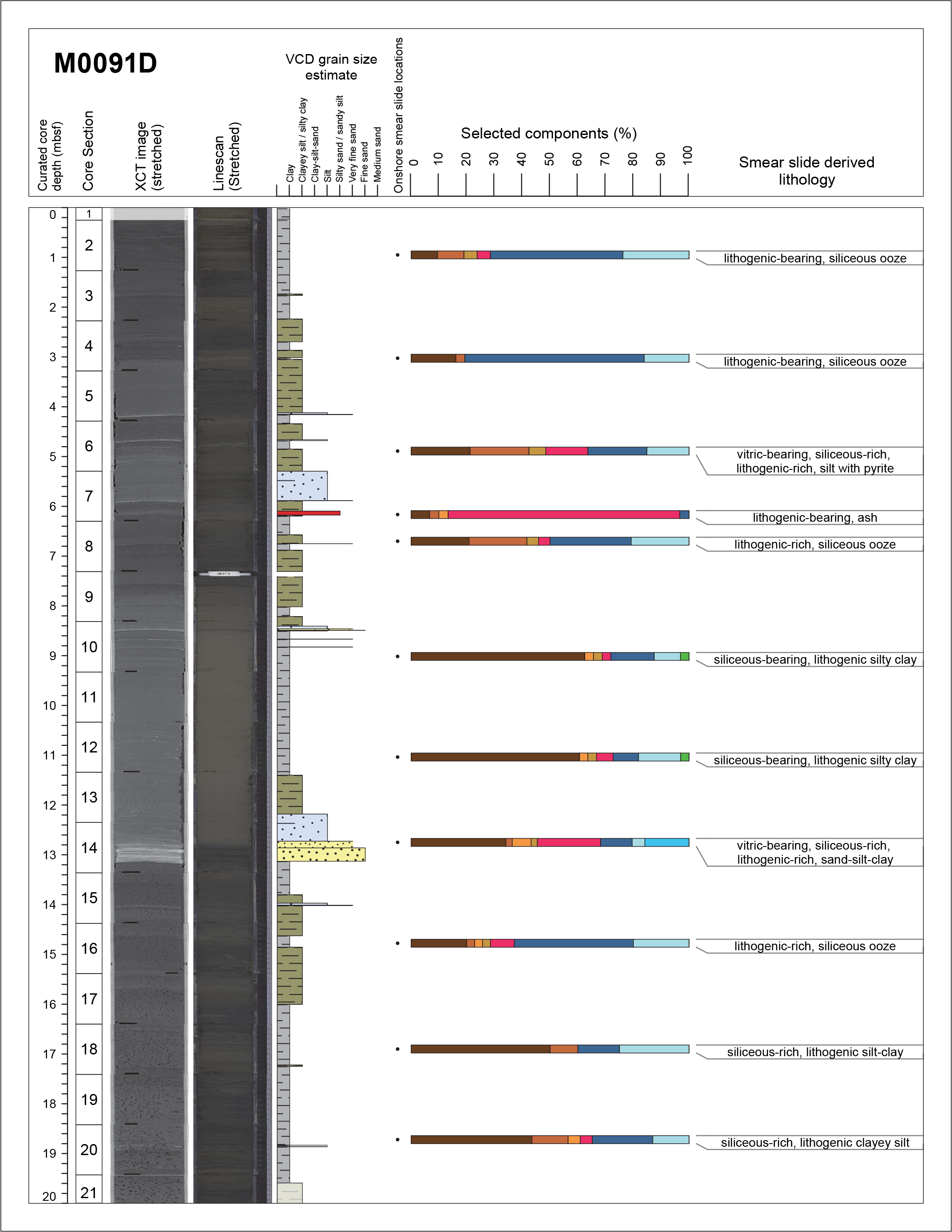
Figure F19. Example smear slide summary.
3.3. X-ray diffraction analyses
XRD analyses were used as a diagnostic tool to identify and semiquantitatively document the relative content of mineral phases in bulk samples. Samples for XRD analyses with a volume of 10 cm3 were selected every 2 m from the working half at the same depth as sampling for solid phase geochemistry. Bulk powder samples were sent to the BCR and analyzed by ESO staff during the hybrid OSP. Samples for bulk mineralogical analyses were freeze-dried and ground to a fine powder by hand. Dried and ground (<20 µm particle size) bulk samples were prepared with the Philips backloading system in the Crystallography and Geomaterials Research laboratories of the Geoscience Department at the University of Bremen (Germany). A thorough preparation commonly increases reproducibility of the results; however, the standard deviation given by Moore and Reynolds Jr. (1989) of ±5% can be considered as a general guideline for mineral groups with >20% clay fraction. In addition, the determination of well-crystallized minerals like quartz, calcite, or aragonite can be done with better standard deviations (±1%–3%) (Tucker, 1988; Vogt et al., 2002).
X-ray diffractograms were measured on a Bruker D8 Discover diffractometer equipped with a Cu-tube (kα 1.541 Å, 40 kV, 40 mA), a fixed divergence slit of 0.25°, a 90 samples changer, and a monochromatization by way of energy discrimination on the highest resolution Linxeye detector system. To maximize the sample throughflow the Philips X’Pert Pro multipurpose diffractometer with a Cu-tube (kα 1.541 Å, 45 kV, 40 mA), a fixed divergence slit of 0.25°, a 16 samples changer, a secondary Ni-filter and the X’Celerator detector system was also utilized from 30 March to 6 April 2022. XRD data used to make the lithostratigraphic summaries identify which diffractometer was used for each sample measurement (see XRD in Supplementary material). For all other XRD measurements, the Bruker D8 Discover diffractometer was used. Measurements were done as a continuous scan from 3° to 65°2θ (Bruker D8 Discover) or 4° to 85°2θ (Philips X’Pert Pro multipurpose) with a calculated step size of 0.016°2θ and 0.0167°2θ, respectively. Mineral identification was done using the Philips software X’Pert HighScore Version 1.2 (Degen et al., 2014). Semiquantification X’Pert HighScore follows concepts of Vogt (2009) and former IODP Bremen OSPs.
Summary plots of the major minerals and/or groups of minerals are included in the site chapters for the longest core at each site. The data used to make these figures are available in XRD in Supplementary material. For systematic comparison across sites, these plots contain the cumulative weight percent of the following: quartz, total feldspar (K-feldspar and plagioclase), total carbonates (calcite, Mg-rich calcite, aragonite, dolomite, ankerite, siderite/magnesite, and other carbonate minerals), total clays (smectite/montmorillonite, illite, kaolinite, and chlorite), palygorskite, total micas (biotite and muscovite), total heavy minerals (rutile, anatase, zircon, magnetite, Fe-oxides and hydroxides, and manganite), pyroxene, amphiboles (Amp)/cordierite (Cord)/sillimanite (Sill)/andalusite (And), and pyrite.
3.4. Linescan split core imaging
High-resolution (100 pixels/cm) images of the archive half of each core section were obtained on board Chikyu using the Tri-Sensor Core Logger (TSCL; NS Design) before visual core description and sampling were completed. After core splitting and prior to imaging, the split core surfaces were scraped smooth to emphasize sedimentary structures and compositional and/or textural changes in the cores. The TSCL is used to take a digital photo using a linescan camera while simultaneously measuring color reflectance spectrophotometry and colorimetry using a noncontact imaging spectrophotometer (MetaVue VS300; X-Rite) on split core sections. During this expedition, only the linescan imagery and color spectrophotometer data were collected. The linescan images are presented and discussed in Lithostratigraphy in the site chapters. The color spectrophotometer data are presented and discussed in Physical properties in the site chapters. To acquire the linescan images, the camera moves over the split core sections. The core table allows the operator to measure up to four sections in a single operation. The split core digital photography is categorized as the IODP minimum measurement, and the split core color reflectance spectrophotometry is categorized as the IODP standard measurement.
The camera has three complementary metal oxide semiconductor (CMOS) sensors and provides a 16 bit red-green-blue (RGB) color (48 bit) TIFF file. The camera has two resolution modes; the 2K spatial resolution is ~100 pixels/cm, and the 4K spatial resolution is ~200 pixels/cm. In a single IODP measurement, two shots (gamma correction 0.45 and 1.0) with 2K resolution are taken. The camera system (SW-4000T-MCL; 3CMOS prism linescan camera, JAI) has three CMOS sensors, the Otus 1.4/55, ZEISS lens, and two LED lights (LNSP-300W50-BTSP; CCS). The light reflection from a sample surface is split into three paths (red, green, and blue) by a prism inside the camera. The RGB data derived from each image for each section are presented and discussed in Physical properties in the site chapters.
Linescan images of all core sections are presented in LINESCAN in Supplementary material.
3.5. X-ray computed tomography
During Expedition 386, X-ray CT scanning was performed on whole-round sections on board Chikyu in July 2021, after the offshore phase and prior to the OSP. X-ray CT images are used to identify 3-D sedimentary and structural features that are not visible on the split core surface, such as bioturbation, bedding planes, faults, fractures, mineral inclusions, erosion surfaces, and sedimentary laminae successions. X-ray CT scanning collects a series of X‐ray images or slices from a 360° perspective, creating 2-D and 3-D density-sensitive renderings of the core (Brooks and Di Chiro, 1976; Cnudde and Boone, 2013; McKetty, 1998). The technique can be completed on half- or whole-round core sections, providing 3-D images of sediment prior to core splitting. This nondestructive technique allows discrimination between sediment volumes with a different X-ray attenuation, which is a function of the material composition (effective atomic number) and density (Cnudde et al., 2004), and can be used to image subtle changes in the composition of soft sediments (Goldfinger et al., 2012). X-ray CT data from Expedition 386 were processed for visualization and analyses with the open-source Fiji image processing package (LOCI University ImageJ). X-ray CT images are displayed on a gray-level viewing system, with the brighter parts representing higher CT numbers (i.e., mineral or biogenic components) and the darker parts representing lower CT numbers (i.e., organic matter or air/fractures). Each image is defined by a unique file name that refers to expedition, site, core number, core type, and section.
The X-ray CT instrument on board Chikyu is a Discovery CT 750HD (GE Medical Systems) that produces 32 0.625 mm thick slice images every 0.4 s, the time for one revolution of the X-ray source around the sample. Data generated for each core consist of core-axis-normal planes of X-ray attenuation values that are 512 × 512 pixels in size. Data were stored on the server as DICOM formatted files. The DICOM files were restructured to create 3-D images for further investigation.
The theory behind X-ray CT has been well established through medical research and is very briefly outlined here. X-ray intensity varies as a function of X-ray path length and the linear attenuation coefficient (LAC) of the target material:
- I = transmitted X-ray intensity,
- I0 = initial X-ray intensity,
- μ = LAC of the target material, and
- L = X-ray path length through the material.
LAC is a physical index of X-ray beam reduction during translation of target materials. It is led from the relationship between physical properties of target materials (i.e., chemical composition, density, and state). The basic measure of attenuation, or radiodensity, is the CT number given in Hounsfield units (HU):
The distribution of attenuation values mapped to an individual slice comprises the raw data used for subsequent image processing. Successive 2-D slices yield a representation of attenuation values in 3-D pixels (voxels). The analytical standards used during Expedition 386 were air (CT number = −1000), water (CT number = 0), and aluminum (2477 < CT number < 2487) in an acrylic core mock-up. All three standards were run once daily after air calibration. For each standard analysis, the CT number was determined for a 24.85 mm2 area at fixed coordinates near the center of the cylinder.
X-ray CT images of all core sections are presented in XRAYCT in Supplementary material.
3.6. Event beds and stratigraphic intervals
Certain lithologic features appear regularly along the stratigraphic columns. These show recurrent sedimentary patterns or events driven by specific depositional processes. Although the thicknesses of these event beds vary from a few centimeters to several meters, other characteristics are very similar. Event beds are usually characterized by a sharp base surface, a basal part with coarse sediments whose grain size decreases progressively upward, and a top with traces of bioturbation (Figure F20). In some locations, event beds are identified only by structureless clay, bioturbated at the top, or rounded to subrounded mud clasts and lithoclasts in a muddy matrix with a sharp top and basal surfaces. These events are either directly superimposed on each other or interbedded with highly bioturbated clays or silty clays with abundant planktonic microfossils.
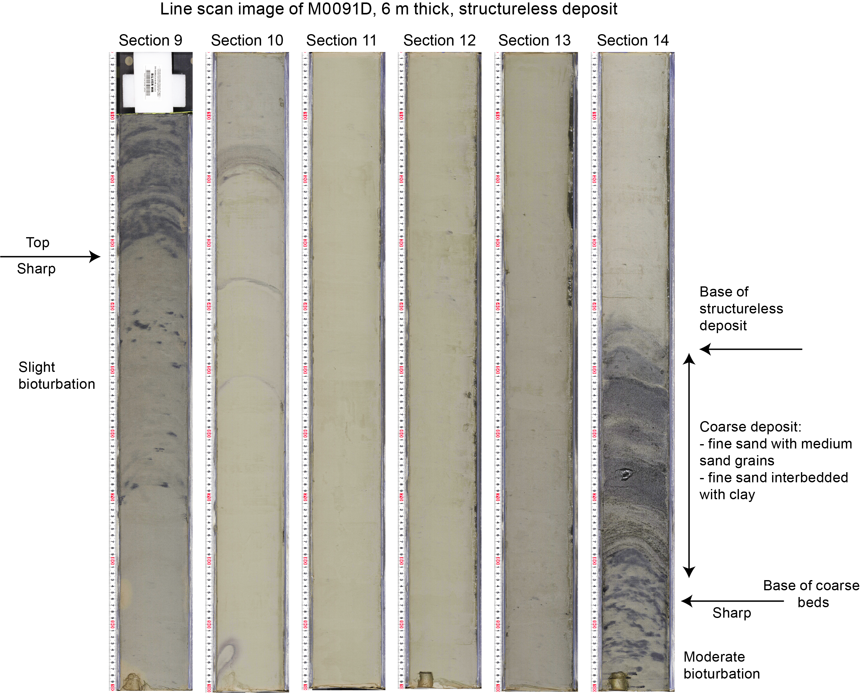
Figure F20. Event bed.
To make reading easier, core descriptions in the Lithostratigraphy section in each site chapter are divided into stratigraphic intervals. These intervals are defined by sediments that have the same physical characteristics on the lithostratigraphic summaries and occupy a particular place in the core. The physical characteristics of each interval (grain size, color, composition, bed thickness and frequency, sedimentary structures, bioturbation, iron monosulfide overprint, etc.) are described in the text. These intervals are defined in each core and cannot be used for correlations between holes without extreme caution.
4. Tephra
The term “tephra,” defined as pyroclastic material regardless of grain size, was used during Expedition 386, although pyroclastic materials with a less than 2 mm grain size are named volcanic ash. Procedures used to describe tephra during Expedition 386 include visual core description, smear slide observation, and analysis of chemical composition. Tephra layers were named according to their site and position in the core section: hole, core, core type, section, and bottom depth of the layer in centimeters. For example, the tephra in interval 35.3–36.5 cm in Section 8 of Core 1H from Hole M0081B was labeled M0081B-1H-8, 36.5 cm.
4.1. Tephra description
The key characteristics of sediments composed of pyroclastic materials, including color, grain size, thickness, and structures, were described and recorded on the hand drawn VCDs during the onshore phase of Expedition 386 (see Lithostratigraphy). The structure of each tephra layer in the core was described using the categories (1) bed, (2) lenticular, (3) block, and (4) patch (Figure F21). After close-up photos were taken, approximately 1–2 mm3 of each tephra deposit was picked from archive halves using a wooden toothpick, and smear slides were made using the method described in Smear slides. Their characteristic components, such as the shape of volcanic glass shards and heavy mineral content (e.g., hornblende and orthopyroxene), were observed.

Figure F21. Tephra layers.
Volcanic glass shard classification focuses on vesicle size and elongation, although several classifications of glass morphology exist. Three main types of glass morphology were described by Lowe (2011). It is most appropriate to use the Japanese classification method to examine tephra described during this expedition to most effectively correlate with accepted Japanese tephras. Descriptions of volcanic glass shard shape were made based on the well-used classification schemes of Yoshikawa (1976) and Machida and Arai (1978). Although the two methods are similar, the number of the shape classifications is somewhat different. The following morphology of volcanic glass shards was adopted here: (1) platy type, (2) bubble-wall type, (3) moderate vesicularity type, (4) pumiceous type, and (5) fibrous type (Figure F22). Types 1, 2, 4, and 5 are almost identical to the classification scheme of Machida and Arai (1978), and Type 3 is roughly equivalent to the combined Henpei-b and Chukan-b types of Yoshikawa (1976). In the classification of Yoshikawa (1976), Types 1, 2, 4, and 5 are identical to Henpei-a and Chukan-a with parts of Henpei-b, Takoushitsu-a, and Takoushitsu-b, respectively.
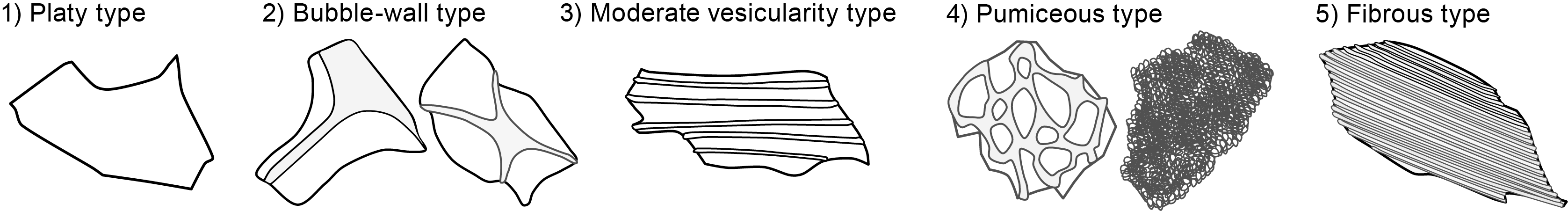
Figure F22. Volcanic glass shard shape types.
Heavy minerals are important characteristics for tephra correlations. Each tephra, as a magma product of an eruption from a volcano, has its own unique petrological characteristics. Heavy mineral compositions have been described for many tephras in Japan as one of the important indicators of their characteristics. It is important to describe the heavy mineral composition of tephras for examination of the correlation with the widely known tephras in Japan. Of course, it is also important for interhole and intersite correlations, but it is difficult to describe heavy mineral composition from smear slide observations because of their low abundances. In those instances where more than a few dozen grains of heavy minerals were observed and were not heavily weathered, their abundance ratio is indicated by an inequality sign.
4.2. Tephra identification
Pyroclastic materials on the seafloor are emplaced not only by volcanic eruptions but also as part of a remobilized sediment layer that is transported as flows. Therefore, a distinction was made between tephra beds that were identified as primary tephra layers, excluding reworked tephra, and those deposited through reworking of seabed sediments. The reworked tephras were characterized as (1) a layer with sedimentary structures and/or (2) rounded grains without chemical alteration. These observations were made using visual core description and smear slides, respectively. Sediments identified as reworked tephras were described as reworked tephra or volcanic glass–rich sand.
4.3. Chemical composition analysis
Two section-bottom samples were taken during the offshore phase of Expedition 386. These pyroclastic sediments or pyroclastic-rich sediments, which might be tephras, were sampled from the bottom of Sections 386-M0085D-1H-33 and 386-M0094B-1H-19 to establish the chemical composition of any potential volcanic glass shards. Tephras with a high potential for intersite correlations and/or correlation with widely known tephras in Japan will be analyzed for their chemical composition during postexpedition research.
Major element compositions of volcanic glass shards were analyzed using energy dispersion–type electron probe microanalysis (EPMA) at Fukushima University. The analytical equipment was an INCA x-act1x-stream (Oxford, London, UK) energy dispersive spectrometer (EDS) attached to a JSM-6610LV scanning electron microscope (JEOL, Tokyo, Japan). Tephra samples were sieved using 0.25 and 0.0625 mm mesh-sized sieves and washed using an ultrasonic bath; dried samples were mounted in an epoxy resin on a slide glass. The resin surface was polished until glass shards were exposed, and the carbon was coated by vacuum deposition after the glass shard mount was cleaned once more using an ultrasonic bath and dried before analysis. Sample measurement parameters are 15 kV accelerating voltage, 0.5 nA electric current on a Faraday cup, and a 5 µm × 5 µm beam scanning area. The analyzed major element compositions were recalibrated by normalizing the results to the well-known dacite to rhyolite volcanic glasses analyzed during the same session (Baegdusan-Oga [B-Og], Aso-1, Kamiizumi-4 [Km-4], Oga, Aira-Tn [AT], and Ikezuki tephra), after quantitative calibrations were completed, using synthetic and natural mineral standards. Major element compositions of the in-house standard volcanic glasses were determined by XRF spectrometry (Nagahashi et al., 2003).
5. Micropaleontology
Preliminary age assignments for Expedition 386 sediments were based on biostratigraphic analyses of radiolaria using samples taken during the offshore and onshore phases of Expedition 386. Benthic foraminifera were examined to estimate the paleoenvironment at the source of displaced gravity flows into the Japan Trench.
5.1. Radiolaria
5.1.1. Zonal scheme
Radiolaria are a group of oceanic plankton with siliceous skeletons that are well preserved in marine sediments as microfossils, even in sediments from the Japan Trench below the calcite compensation depth (CCD). Because many first and last occurrence datums generally used in biostratigraphic work are not recognized here, stratigraphic changes of relative abundance for three radiolarian species or species groups—Cycladophora davisiana Ehrenberg, Tetrapyle circularis/fruticosa group sensu Matsuzaki et al. (2020), and Lithomelissa setosa Jørgensen—are used as the main radiolarian zonal scheme for Expedition 386 (Figure F23).
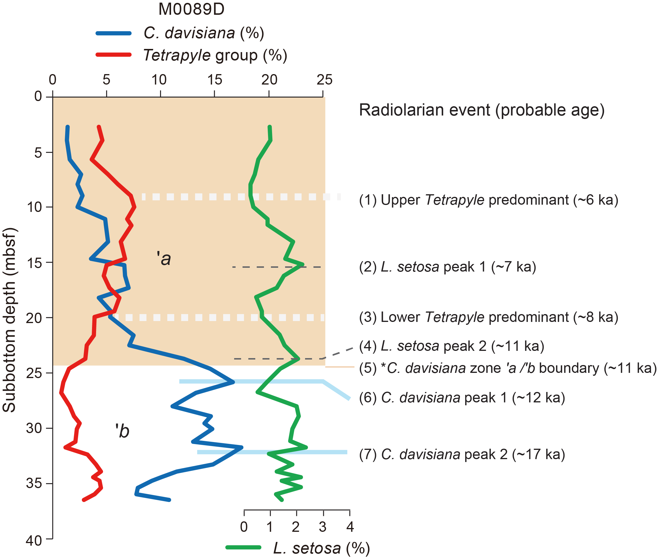
Figure F23. Relative abundance for main radiolarian zonal scheme.
It is known that C. davisiana is one of the most important species at high latitudes in both hemispheres (e.g., Morley et al., 1982, 1995). The relative abundance of this species is higher during glacial periods and lower during interglacial periods. This relationship is used as a tool for the late Pleistocene high-resolution stratigraphy in carbonate-poor sediments and as a substitution for Marine isotope stages (MISs) in the Southern Ocean (e.g., Hays et al., 1976), the North Atlantic Ocean (e.g., Morley and Hays, 1979) and the North Pacific Ocean (e.g., Morley et al., 1982, 1995; Ohkushi et al., 2003; Itaki et al., 2009; Yasudomi et al., 2014; Matsuzaki, et al., 2014). C. davisiana Zones ‘a and ‘b correspond to the Holocene and late Pleistocene, respectively, and are based on the North Pacific standard curve of Morley et al. (1982). The boundary between Zones ‘a and ‘b (~11 ka; calendar age based on planktonic radiocarbon dating by Itaki et al., 2009) is shown as Event 5 in Figure F23. In addition, two significant peaks of C. davisiana in Zone ‘b (Events 6 and 7) could be correlated to Davisiana Event (DAE)-2 (~12 ka) and DAE-3 (~17 ka) of Matsuzaki et al. (2014), respectively.
The T. circularis/fruticosa group is a predominant species in subtropical areas related to the Kuroshio Current in the northwestern Pacific Ocean (e.g., Matsuzaki et al., 2020). The working area of Expedition 386 is located within the mixing zone of the warm Kuroshio and cold Oyashio Currents (Figure F24), so the radiolarian assemblage sensitively responded with the Kuroshio oscillations and millennial-scale climatic changes during the Holocene period, as demonstrated by Chinzei et al. (1987). Thus, it is expected that the T. circularis/fruticosa group can provide detailed correlation between sites during the Holocene. An interval of continuous high abundance of this species group is likely related to a mid-Holocene climatic optimum known as the hypsithermal event, and its upper and lower limit might be correlated to roughly 6 and 8 ka (Events 1 and 3 in Figure F23), respectively.
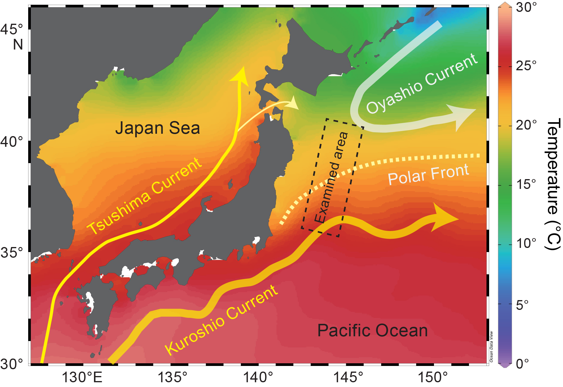
Figure F24. Sea-surface temperature.
In addition, abundance patterns of L. setosa, which were found in this examination, could be correlated between most of the sites and is regarded as a potential key marker. In Figure F23, two small peaks of this species are shown as Events 2 and 4, and the ages of these events are tentatively estimated to roughly 7 and 11 ka, respectively, according to interpolation between Events 1, 3, and 5. Because the sedimentation rate between these events may potentially not be linear, event ages should be reconsidered based on future well-dated cores.
5.1.2. Method of study
A total of 311 samples were collected for radiolarian analysis during both the offshore and onshore phases of the expedition, and 203 samples, except for samples from event layers identified on X-ray CT images, were processed (see tables in each site chapter). Samples (~10 cm3) collected during the offshore phase, using a tip-cut syringe, were routinely taken from 240 section bases at 2 m intervals. A total of 108 samples were from the event layers. Most of the offshore samples from Holes M0087D, M0093B, and M0094B were taken from event layers, so radiolarian analyses were not conducted due to the expected large numbers of reworked specimens. In addition, 71 samples (~10 cm3) from hemipelagic deposits from Holes M0082D, M0085D, and M0089D were collected using a scoop during the OSP to detect more detailed changes; these sites serve as references for the southern, northern, and central basins of the Japan Trench, respectively.
Sample preparation for light microscopy observation was conducted as follows: approximately 1 cm3 of wet sediments was sieved and rinsed with tap water using a 45 µm mesh sieve. Residues were then mounted with Norland Optical Adhesive 61 and covered with a 24 mm × 36 mm (for offshore samples) or 40 mm (for OSP samples) cover glass. The adhesive was solidified by placing the slide under ultraviolet light for approximately 15 min. Slides were partially examined at 50× to 400× using an optical microscope (Zeiss Axio Imager.A1m POL-1) on board Chikyu.
Abundance estimates of the radiolarian assemblage are qualitative estimates of the concentration of total radiolaria in individual sediment samples using the following categories:
- A = abundant (>10,000 specimens in a sample).
- C = common (2,000–10,000 specimens in a sample).
- F = few (500–2,000 specimens in a sample).
- R = rare (50–500 specimens in a sample).
- VR = very rare (<50 specimens in a sample).
- B = barren (0 specimens in a sample).
Preservation of the radiolarian assemblage was recorded as follows:
- G = good (majority of specimens complete, with no or minor dissolution, recrystallization, and/or breakage).
- M = moderate (minor but common dissolution, with a small amount of breakage of specimens).
- P = poor (strong dissolution, recrystallization, or breakage; many specimens unidentifiable).
Relative abundances (in percentages) of C. davisiana, the T. circularis/fruticosa group, and L. setosa in the assemblage were estimated from counts of more than 200 specimens of radiolaria based on observation under the microscope. In addition, Dictyocoryne truncatum (Ehrenberg)/Dictyocoryne profunda Ehrenberg and Didymocyrtis tetrathalamus (Haeckel) groups (including the young form) were counted as the Kuroshio warm water species, and Stylochlamydium venustum (Bailey) was also counted as a Oyashio cold water species.
5.2. Foraminifera
Foraminifera are a group of marine animals that have either calcareous, agglutinated, or organic-walled skeletons; planktonic foraminifera float within the water column, and benthic foraminifera live on or within the sediment. All Expedition 386 sites occur below the modern CCD, so calcareous foraminifera assemblages are considered allochthonous and thus do not provide chronostratigraphic control. Benthic foraminifera, however, can supply provenance information for displaced faunas, including water depth, productivity, and oxygenation (van Morkhoven et al. 1986; Gooday, 2003; Murray, 2006; Jorissen et al., 2007). Several authors have used benthic foraminifera to understand the provenance of mass transport deposits in shallow sediments in the Japan Trench (Usami et al., 2017, 2021; Tsujimoto et al., 2020).
Paleodepth estimates of displaced fauna were based on selected benthic foraminifera noted and described by van Morkhoven et al. (1986) using the following categories:
5.2.1. Method of study
During the offshore phase, micropaleontology (IODP PAL) samples were taken from the end of split cores at 5 m intervals. During the OSP, approximately 2 cm3 of sediment from each of these samples were analyzed for foraminifera. After drying overnight in a ~40°C oven, samples were disaggregated in a solution of deionized water, Calgon, and H2O2 to ensure removal of clay-sized particles. Samples were then wet sieved through a 63 µm mesh sieve and rinsed with deionized water. The coarse fraction was placed on filter paper in an oven at ~40°C until it dried completely.
Faunal identifications were made using a Meiji Techno RZ binocular light microscope. Taxonomic composition, abundance, and preservation state were observed in the >63 µm size fraction. All foraminifera observed during a visual scan of the entire sample were counted; representatives of each taxa found were picked for reference. Benthic foraminiferal taxonomy follows Smith (1973), Matoba (1976), van Morkhoven et al. (1986), Loeblich and Tappan (1988), and Scott et al. (2000). The World Foraminifera Database was consulted for taxonomic revisions (e.g., https://www.marinespecies.org/aphia.php?p=taxdetails&id=113491). Planktonic foraminifera were not included in the faunal identification, but their abundance was estimated and preservation was indicated. For a species list and examples of foraminifera recovered, see MICROPAL in Supplementary material.
Preservation of foraminiferal tests was ranked as follows:
- VG = very good (no breakage or visible dissolution).
- G = good (minor dissolution or pitting on calcareous taxa and no recrystallization; <10% of specimens are broken).
- M = moderate (frequent etching of calcareous taxa; 10%–30% of specimens are broken).
- P = poor (frequent dissolution and recrystallization; >30% of specimens are broken).
Samples with a clearly bimodal distribution of preservation were noted with a slash separating two of the above ranks (e.g., VG/M). When one or more orange-stained specimens are observed, an “S” is used in conjunction with the above ranks (e.g., VG/MS).
Semiquantitative estimates of abundances of foraminifera in relation to the total >63 µm size fraction are given as follows:
- A = abundant (>200 specimens in a sample).
- C = common (between 50 and 200 specimens in a sample).
- F = few (between 30 and 50 specimens in a sample).
- R = rare (between 10 and 30 specimens in a sample).
- P = present (<10 specimens in a sample).
- B = barren (no foraminifera present).
Because of the low number of foraminifera (average of 20 specimens/sample), actual counts rather than estimates are provided in the occurrence tables in the site chapters. The presence of other microfossils, iron monosulfides, heavy minerals, volcanic glass, and discolored sediment clumps are noted.
6. Geochemistry
6.1. Offshore sampling and analysis
There are offsets in the initial geochemical data sets due to overshooting the GPC. Corrections for this are calculated in Stratigraphic correlation, and more information is given in the Introduction.
6.1.1. Interstitial water sampling
Cores were sampled for IW immediately on recovery using Rhizon samplers (CSS 19.21.23F; Rhizosphere Research Products, Netherlands) consisting of a microporous tube (2.5 mm diameter; 5 cm length) supported by a nylon/PEEK wire and attached to PVC tubing with a female Luer lock connector (Seeberg-Elverfeldt et al., 2005; Dickens et al., 2007). Before use, each Rhizon sampler was soaked in purified laboratory water for approximately 60 min. A 3.8 mm hole was drilled into the plastic core liner using a drill bit, and a Rhizon sampler with the same diameter as the hole was inserted into the sediment. Negative pressure was applied by attaching a 24 mL plastic back syringe to the Rhizon sampler. Sampling frequency was approximately every 50 cm for the first 5 m and about 1 m for the remainder of the core. The sediment cores remained capped throughout this process to minimize contamination by the ambient atmosphere. The first 0.1 mL (1–2 drops) were discarded to remove any purified laboratory water, and then the sample syringes were reattached to the Rhizon sampler, which remained in the cores for a maximum of 6 h for IW sampling. The total amount of approximately 15 mL of IW samples were subsequently split into as many as seven fractions for the following IODP standard measurements: sulfide (1.5 mL IW + 0.6 mL ZnAc 2.5%), salinity (0.5–1.5 mL), pH and alkalinity (3–4 mL), ammonium (0.5–1.5 mL), cations (3 mL IW + 0.03 mL HNO3), and anions (3 mL). In addition to the standard measurements, all requested IW samples were split from the IW gained during the 6 h sampling time frame for customized sampling schemes. All split samples were stored at +4°C.
6.1.2. Bottom water sampling
BW samples from each trigger core were collected using a BW sampling system consisting of a Duran bottle and vacuum pump unit connected by tubes. Negative pressure was generated by the pump, and samples were sucked into the Duran bottle through the tube placed in the overlying water of the trigger core. After filtering using a Rhizon sampler, a total of 15 mL of BW was collected and subsequently subsampled and stored at +4°C before further offshore IODP standard measurements were conducted, as detailed below.
6.1.3. Bottom water and interstitial water analysis
The IW from all holes was analyzed onboard for alkalinity, ammonium, and salinity. Immediately following IW extraction, alkalinity and pH were determined with a pH electrode and an autotitrator (Metrohm 888 Titrando, except for samples from Site M0095). An aliquot of 1.0–3.0 mL IW adjusted to 3.0 mL with 0.7 M KCl solution was titrated with nominal 0.1 M HCl at 25°C. A 100 mM Na2CO3 solution was used for calibration of the acid each week during the offshore phase. Quality checks were conducted once per day using a 50 mM solution of NaHCO3 and 0.1 M HCl. For samples from Site M0095, a 100 μL subsample was measured for pH using a B-712 LAQUA-twin compact pH meter (HORIBA Ltd.). Standard solutions, one with a pH of 4.01 and another with a pH of 6.86 at 25°C, were used for a two-point calibration every 24 h. Quality checks were conducted as the first and last daily measurement using a standard solution (pH = 6.86).
A refractometer (Atago RX-5000i) was used to determine salinity based on the refractive index. The refractive index was converted to salinity by referral to analytical results of ultrapure water and International Association of Physical Sciences of the Oceans (IAPSO) standard seawater (salinity = 34.993). Pure water measurements were made between each sample analysis.
Ammonium was measured by colorimetry using an automated spectrophotometer (SEAL Analytical AQ2 discrete analyzer) within 24 h of IW sampling. The AQ2 has a sampling probe with a stepper motor–driven syringe, a quartz-halogen lamp, a flow-through cuvette (50 μL), and a photodiode. The analytical procedure is based on absorption spectroscopy of indophenol blue. Indophenol blue is formed by reaction of ammonium with the diazotization of phenol and subsequent oxidation of the diazo compound by sodium hypochlorite. Samples and reagents were taken into reaction segments with the sampling probe and warmed to 37°C for 8 min to enhance color development. The colored solution was then transferred to the cuvette, and absorbance at 620 nm was measured. All operations, including sample dilution, color development, measurement, and calculation, were automated and controlled by equipment software. Concentrations were calculated based on a standard curve determined before each analytical run. A drift standard solution was measured before the first sample and after every five samples to obtain the analytical precision (QC). The standard deviation of replicate analyses of the 0.071 μM QC standard was between 2.3% and 9.0%.
6.1.4. Headspace gas sampling
Following standard protocols for headspace sampling, all headspace samples were collected onboard from the base of each section immediately after section cutting following core recovery on deck. Two parallel headspace samples (IODP standard and requested samples) were collected from the bottom of every GPC core section, the longest core from each site, and the respective shorter trigger core. For each headspace double sample, ~5 cm³ of sediment was collected (using two 2.5 cm³ tip-cut syringes). Each 2.5 cm³ headspace sample was then added to a 20 mL crimp vial with 5 mL of 1 M NaOH. After sealing, the samples were preserved at 4°C until analysis.
6.2. Analyses between offshore and Onshore Science Party phases
6.2.1. Preparation and GC-FID measurements
Concentrations and relative abundance of light hydrocarbon gases including methane (C1 or CH4), ethene/ethylene (C2=), ethane (C2), propene/propylene (C3=), propane (C3), i-butane (i-C4), and n-butane (n-C4) were monitored following standard procedures for headspace gas sampling and analysis (Kvenvolden and McDonald, 1986).
The IODP standard headspace samples from the longest GPC core from each site were measured between the offshore phase and the OSP on board Chikyu, and measurement results are reported in the site chapters. All other samples were analyzed during and after the OSP and are only reported in GEOCHEM in Supplementary material.
Each sample was vigorously shaken by hand for 2 min and then shaken in a laboratory shaker for 1 h and left for 23 h at room temperature. Each vial was placed in an Agilent 7697A headspace sampler, where it was heated to 70°C for 30 min before an aliquot of the headspace gas was automatically injected (split mode) into an Agilent 7890B gas chromatograph (GC) equipped with a packed column (HP PLOT-Q) and linked to a flame ionization detector. The carrier gas helium flow rate was at 10 cm³/min. The oven temperature was programmed to start at 60°C and ramp up to 150°C at a rate of 10°C/min. The GC can detect seven hydrocarbon compounds (C1, C2=, C2, C3=, C3, i-C4, and n-C4) and was calibrated for the chromatographic response with commercial standards (Types VIII–XII, GL Sciences, Japan). Quantification of hydrocarbon gases was achieved by comparison of the chromatographic response with a three-point calibration curve.
6.3. Onshore science party sampling and analyses
6.3.1. Onshore sampling
Samples for carbon, nitrogen, sulfur, and bulk element analyses were taken during the OSP. Solid-phase samples (10 cm3) were collected at about one sample per meter on average. For further analyses, the bulk sediment samples were shipped to the Center for Marine Environmental Sciences (MARUM) at the University of Bremen (Germany), where they were freeze-dried and then ground and homogenized to a fine powder using a pestle and an agate mortar. Total nitrogen (TN) was analyzed with a Vario EL3 CHNS analyzer by Elementar. Approximately 30 mg of dry sample was weighed out into a zinc capsule and combusted at 950°C. The evolved NO2 was measured using a thermal conductivity detector and/or infrared detection. Because of technical issues, TN was only measured on samples from Sites M0081 and M0082. All data are reported in weight percentage per dry sample with an analytical precision <8% relative standard deviation (RSD) for total sulfur (TS) based on replicate sample analysis.
6.3.2. Interstitial water analysis
Filtered (0.2 μm) and acidified (10 µL of concentrated HNO3 per milliliter) IW sample splits were analyzed for cations and trace metals using analytical equipment on board Chikyu prior to the OSP. Minor elements in IW, including Li, B, Ba, Mn, Fe, Sr, and Si, were analyzed using an inductively coupled plasma–atomic emission spectrometer (ICP-AES; ULTIMA 2, Horiba Jobin Yvon). IW samples are subjected to 10-fold dilution using 1% HNO3 and spiked with 10 ppm Y as an internal standard. Trace elements (V, Cu, Zn, Rb, Mo, Cs, Pb, and U) were analyzed on an ICP–mass spectrometer (ICP-MS; Agilent 7500ce). Samples were acidified and diluted at a ratio of 1:20 with purified (double deionized) water. Ultrapure primary standards (SPC Science PlasmaCAL) were prepared with a matrix solution of sulfate-free artificial seawater to fit the sample matrix, and indium was used as an internal standard. Calibration standards were prepared using IAPSO seawater and National Institute of Standards and Technology Certified Reference Materials. Analytical precision was ±3% for major elements and ±5% for trace elements. In contrast to Rb, Mo, V, and U, trace element analyses for Cu, Pb, Cs, and Zn were either at or below the detection limit or showed contamination; therefore, these elements are not reported for all sites. A cation column was used on an ion chromatograph to analyze major cations (Na, K, Mg, and Ca) on acidified (4% of 6 M HCl, trace metal grade) IW samples diluted at a ratio of 1:200 to 1:800, depending on the concentrations of the analyzed cations. The IAPSO standard was used for calibration, and dilutions of IAPSO were used for internal quality controls of the instrument. Analytical precisions were ±1.28% for Na, ±0.96% for K, ±1.92% for Mg, and ±1.69% for Ca (1σ). The data are only presented in GEOCHEM in Supplementary material because the samples require postexpedition analysis for validation of absolute values (analytical accuracy).
IW splits were shipped to MARUM, where analyses for sulfate (SO42−), bromide (Br−), and chloride (Cl−) concentrations were determined using a Metrohm 882 compact ion chromatograph. A 40-fold dilution of IAPSO seawater and standards prepared from commercial single anion standards was used for calibration. Analytical precisions were ±0.95% for SO42−, ±2.7% for Br−, and ±2.6% for Cl− (1σ). Total sulfide (S2−, HS−, and H2S) was measured spectrophotometrically by applying the methylene blue method of Cline (1969) using a DR 3900 HachLange (Berlin, Germany) spectrophotometer. Total sulfide is referred to as H2S throughout the text for simplicity, although H2S was not quantified. The detection limit of H2S using the Cline method is approximately 0.1 mg/L (for samples with H2S lower than 200 µM the limit is about ~1.5 µM; Sakamoto‐Arnold et al., 1986).
6.3.3. Bulk geochemical analysis of sediments
Total carbon (TC), total organic carbon (TOC) and TS of sediments were measured using a CS744 LECO carbon-sulfur analyzer. Approximately 100 mg of the homogenized sample was weighed in a ceramic cup and heated in a furnace. The evolved CO2 and SO2 provide a measure of the sedimentary TC and TS content and were measured with a nondispersive infrared detector calibrated with commercial CRM and certified one-use reference pieces. To determine the TOC content, aliquots of the sediment (~100 mg) were leached in 12.5% HCl to remove calcium carbonate and analyzed as described above. Total inorganic carbon (TIC) was determined by subtracting TOC from TC. All data are reported in weight percentage per dry sample with an analytical precision <8% RSD for TS based on replicate sample analysis.
6.3.4. Bulk sediment element analyses
To measure the elemental composition of sediment samples using energy dispersive XRF (ED-XRF), 4 g (±0.2 g) of freeze-dried, ground, homogenized sediment was weighed into a plastic cuvette with a Mylar foil bottom covered with polypropylene film. The sample in the cuvette was then compacted twice manually, applying a force of approximately 25 kg/cm² on a plastic piston to obtain a smooth surface with limited void space, consistent density, and sufficient sample thickness. Elemental concentrations were determined by ED-XRF spectroscopy using a PANalytical Epsilon 3-XLE benchtop ED-XRF spectrometer at the MARUM sediment geochemistry laboratory. ED-XRF calibration is based on eight certified or in-house natural and synthetic reference materials (Table T9). Standard MESS-4, which was remeasured six times during the run and again after the remaining samples, showed no significant drift during the run.
For XRF analysis, the following elements were measured with a precision of <1% and an accuracy of better than 10%: Al, Br, Ca, Fe, K, Mg, Mn, Si, Sr, Ti, V, and Zn. At the same accuracy of <10%, the precision was less for Cr (4.3%), Cu (2.9%), Ni (3.0%), and P (1.5%). The accuracy for Ba and Zr is better than 25% at a precision of 3.7% (Ba) and 1.0% (Zr). Analysis of elements Rb, As, Cl, Na, Pb, and S was attempted, but results are not reported because the accuracy exceeded >25% or the element was not suitably represented by the reference materials to calculate reliable analytical errors.
7. Physical properties
High-resolution physical properties measurements on board facilitate rapid characterization of different lithologic units as well as hole-to-hole and site-to-site stratigraphic correlation. Physical properties data are also used to tie core descriptions to available borehole measurements and geophysical observations. Therefore, such physical properties data sets offer vital proxies toward the detection of discontinuities and heterogeneities, compositional and textural differences, and construction of synthetic seismic profiles. Physical properties measured during Expedition 386 comprise the following data sets: MSCL, moisture and density (MAD), P-wave velocity, undrained shear strength (measured with a handheld penetrometer, automated vane shear [AVS], and fall cone penetrometer), RGB extracted from linescan images, and color spectrometry.
7.1. Multi-Sensor Core Logger
Core logging to obtain physical properties data was performed on board Kaimei during the offshore phase using a Geotek MSCL with five sensors for measuring gamma ray attenuation (GRA) density, P-wave velocity, noncontact resistivity (NCR), magnetic susceptibility, and NGR.
After arriving on deck, cores equilibrated for at least 6 h to bring them to a relatively constant temperature (see Core handling and analysis) and facilitate consistent measurements of physical properties, which are sensitive to temperature.
Physical properties measurements are affected by core quality. Core sections that do not fill the core liner and/or have cracks can result in anomalous measurements. Prior to measurement, the MSCL operators took note of the core quality and lithology with an emphasis on cracks, gaps, voids, incomplete filling of the core liner, and fluid contents. When processing data, data points from low-quality core intervals were removed (although all raw data are archived).
At the start of the expedition, the MSCL sensors were fully calibrated, and calibration checks were performed approximately every 6 h to check instrument drift for all sensors except the NGR sensor, which was checked biweekly for any drift in the calibration. A full calibration was also performed whenever the system was restarted. Following full calibration, processing parameters were obtained for each instrument; during the expedition, physical properties measured from each core were processed with the parameters generated from the most recent full calibration, as described in detail below.
The core physical properties were measured at predetermined optimal instrument-based spatial and temporal sampling intervals. GRA density, P-wave velocity, NCR, and magnetic susceptibility were measured every 2 cm, and NGR measurements were obtained every 10 cm.
7.1.1. Gamma ray densiometry
The GRA densiometry technique was used to obtain bulk density measurements by passing medium-energy gamma rays from a 137Cs source with a principal energy of 0.662 MeV through a whole-round core. These medium-energy gamma rays pass through the core and are attenuated mainly by Compton scattering. The degree of scattering and consequent attenuation is a function of the electron density of the material, which is also related to bulk density. Most elements of rock-forming minerals have similar Compton mass attenuation (Blum, 1997). The relationship between electron density and bulk density is given by
- ρb = bulk density,
- ρe = electron density,
- NAV = Avogadro number,
- Z = atomic number of elements in the material, and
- A = atomic mass of the material.
Further derivation (Blum, 1997) results in
- Yt = transmitted gamma ray energy,
- Yi = incident gamma ray energy (0.662 MeV),
- µ = Compton gamma ray mass attenuation coefficient (~0.10 cm2/g for medium-energy gamma rays and most common rock-forming minerals), and
- d = sample (scatterer) thickness, which is the core thickness.
The standard sampling interval was set at 2 cm, and the count time was set to 10 s. The resolution with this setup was 0.5 cm. Initial full calibration was performed using a standard core liner containing a stepped aluminum calibration piece centered inside the liner, which was filled with distilled water. Gamma ray counts were taken for 60 s through each of the five aluminum steps of known thicknesses (8, 7, 6, 4, and 3 cm). In addition, the gamma ray count of the liner filled with only distilled water was recorded. All data were handled using the processing parameters from these wet calibrations. Calibration checks were made by logging the distilled water calibration piece approximately every 6 h during the core logging process.
7.1.2. P-wave velocity
P-wave velocity (measured in meters per second) is the rate at which compressional waves pass through a medium. These velocities vary with the lithology, porosity, and bulk density of the material; stress state; and the fabric or degree of fracturing. In marine sediment and rocks, P-wave velocities are also affected by the degree of consolidation and lithification, fracturing, and the occurrence and abundance of free gas and gas hydrates. P-wave velocity is used together with density measurements to calculate acoustic impedance and reflection coefficients to link cores and wells to geophysical profiles. Velocity measurements are also used to estimate the depth of reflectors observed in seismic profiles and to construct synthetic seismograms (McNeill et al., 2019).
Transverse P-wave velocity was measured using two P-wave transducers (a transmitter and a receiver) aligned perpendicular to the core axis with P-waves passing through the core horizontally by way of a Geotek Velocimeter on the MSCL. Compressional wave pulses centered on a frequency of 230 kHz were transmitted through the core every 50 ns. Signal processing software identified the first arrival of the wave at the receiver. The processing routine also corrected for the thickness of the liner. The P-wave transducers functioned as displacement transducers, monitoring the small variations of the outside diameter of the liner over which the traveltime was measured. These variations were used in processing GRA density and magnetic susceptibility in addition to velocity. P-wave velocity was affected by the quality of the core; incomplete filling of the liner reduced the ability to obtain reliable P-wave data. Air between the liner and core reduced the coupling between the core liner and core and prohibited successful P-wave measurements in the deeper parts of cores (deeper than ~10 mbsf). P-wave data points affected by these issues have been excluded. It should be noted that discrepancies between MSCL and discrete sample P-wave measurements were observed (see Discrete sample P-wave velocity), making the comparability of these measurements difficult. The P-wave measurements on the MSCL were obtained ~12 h after coring, and the discrete samples were extracted after approximately 9–10 months of storage and core settling as well as transport of the cores and samples. Taking these factors into consideration, this process might have contributed to more consolidated samples and therefore higher velocities.
Standard measurement spacing was set at 2 cm, and measurements were instantaneous. Initial calibration was performed using a core liner filled with distilled water and measured at a known temperature. Calibration checks were made by logging the distilled water calibration piece approximately every 6 h during the core logging process.
7.1.3. Noncontact electrical resistivity
NCR is based on conductivity (inversely proportional to resistivity) measurements from the core. A transmitter coil induces a high-frequency magnetic field, which in turn generates electrical currents that are proportional to the core’s conductivity. During resistivity measurements, readings obtained from the core by one set of coils were compared with readings taken in air by a second set of coils. The very small magnetic fields regenerated by these electrical currents were measured by a receiver coil and normalized with the set of identical coils operating in air. The spatial resolution of this method was ~2 cm, which was set as the measurement interval. The measurement time was 5 s. Prior to initial measurement of each core, the resistivity sensor was zeroed.
Initial calibration was performed using six standard core liner sections containing water of known but varying salinity. Six standards were made with NaCl concentrations of 35, 17.5, 8.75, 3.5, 1.75, and 0.35 g/L, respectively. Calibration checks were performed approximately every 6 h by relogging the 8.75 g/L saline standard.
7.1.4. Magnetic susceptibility
Magnetic susceptibility (κ) is a dimensionless measure of the degree to which a material can be magnetized by an external magnetic field:
where M = magnetization induced in the material and H = strength of the external field.
Magnetic susceptibility varies in response to the type and concentration of magnetic grains, making it useful for identifying compositional variations. Whole-round core magnetic susceptibility was measured on the MSCL using a Bartington MS2 meter coupled to a MS2C sensor coil. The loop sensor had an internal diameter of 140 mm.
A standard loop was used during the expedition, operating at a frequency of 565 Hz. The MS2C system operated on two fixed sensitivity levels, ×0.1 and ×1, corresponding to 10 and 1 s sampling integration periods, respectively, with the 10 s (×0.1) setting used. Magnetic susceptibility measurements were made at a sampling interval of 2 cm. The actual resolution depends on the diameter of the loop sensor because each measurement integrates over several centimeters. The sensor automatically zeroed and took a free-air reading at the start and end of each run to account for instrument drift by subtraction of a linear interpolation between readings. Magnetic susceptibility data were recorded as corrected volume-specific units (× 10−5 SI). The accuracy of the magnetic susceptibility sensor was checked using a calibration standard made of impregnated resin, and calibration checks were carried out approximately every 6 h to check the consistency of the sensor.
7.1.5. Natural gamma radiation
NGR is emitted from rock and sediment primarily as a result of the radioactive decay of 40K and the decay of isotopes in the 238U and 232Th series (primeval emitters). Measurement of NGR from the recovered core provides an indication of the concentration of these elements. The principle behind NGR is that the primeval emitters are in secular equilibrium (Blum, 1997). The sensor comprises three NaI(Tl) detectors housed in 6 inch diameter lead shields. Emitted gamma rays hit the NaI(Tl) crystals, which produces a pulse of light. This pulse of light then strikes the photomultiplier tube, producing a small electrical current to give a voltage pulse, which is related to the energy of the gamma emission. Three detectors are used to increase the recorded signal level because natural rocks and sediment have very low natural radioactivity; combining data collected with multiple detectors improves the data quality. NGR total counts refer to the integration of all emission counts over the gamma ray energy range between 0 and 3 MeV, with a spatial resolution of 10 cm and a count time of 30 s. A NGR background measurement was acquired when at sea before logging the first core. This background was subtracted from the NGR readings of the cores. No calibration was made on this sensor. Instead, a calibration check was performed weekly by placing a calibration standard of potassium sulfate and making sure that the potassium peak did not deviate by more than 5%.
7.1.6. QA/QC
During the offshore phase of the expedition, QA/QC was performed by repeating measurements on the best quality section of every 10 cores. QA/QC involved core quality description using the hard copy and electronic MSCL log sheets prepared during the original core logging and processing the repeat measurements with the same processing parameters as the original measurement to check for consistency.
7.2. Moisture and density
MAD properties (bulk density, dry density, grain density, water content, porosity, and void ratio) of the sediment were calculated based on measurement of the wet and dry masses of discrete core sediment samples and their dry volume.
Sediment samples were collected on the working halves with a plastic syringe (10 cm3), approximately every 2 m, in tandem with other physical properties samples such as P-wave velocity and strength data. These sampling depths were adapted and slightly modified for layers of special interest, such as tephras. The samples were transferred to glass beakers whose weight and volume (8.5 cm3) had been previously measured. The samples (total mass = wet sediment and glass beakers) were weighed using an electric balance system with an acceptable accuracy within ± 0.005 g. The balance was calibrated every 12 h with several standard weights.
The samples were dried in a constant temperature oven at 105°C for 24 h and then kept in an autodry desiccator for 1 h. The dry samples (dry mass = dry sediment and glass beaker) were successively weighed, and volume measurements (dry volume = dry sediment and glass beaker) were performed using a pentapycnometer with a precision of ±0.06 cm3. The instrument allowed the simultaneous measurement of four samples and the calibration sphere. The volume measurements were repeated five times for each cell and averaged per sample. The wet volume of the samples was not measured.
The dry volume (Vd) is given by
The mass of pore water (Mpw) and volume of pore water (Vpw) are given by
where s is the salinity of pore water (0.035) and Dpw is the density of pore water (1.024 g/cm3).
The mass of salt (Msalt) and the volume of salt (Vsalt) are given by
where Dsalt is the density of salt (2.22 g/cm3).
The volume of solids (Vs) and mass of solids (Ms) are given by
The total volume (Vt) is given by
From the previous equation, the wet water content (WW) and dry water content (WD), bulk density (BD), dry density (DD), grain density (GD), porosity (PO), and void ratio (VR) are calculated as follows:
7.3. Discrete sample P-wave velocity
Core samples were also taken from the working halves of split cores for discrete measurements and transported at 4°C to the EPC laboratory. Samples were removed from cores every 2 m during core sampling on board Chikyu using syringes with an inner diameter of 2 cm. Samples measured 2.5–3 cm long for a sample volume of ~10 cm3. The sampling frequency (2 m) resulted in an average of a single sample per trigger core and one sample per odd-numbered GPC core section. P-wave samples were extracted with a syringe directly next to MAD and undrained shear strength sampling points. Samples were removed from their respective syringes and analyzed for P-wave velocity following MSP-IODP measuring standards. Discrete P-wave velocity measurements were attempted. However, the measurement apparatus was not suitable for measuring the unconsolidated samples because it did not provide any means of confinement for those samples. Clay-rich sediments tended to be too soft for sampling, and silty sediments cracked when placed between the two transducers.
Despite arriving at the EPC in a fresh condition, most samples dried quickly after protective wrappings were removed and were disturbed due to the pressure of the transducers, which made additional measurements during later runs impossible.
Measurements were performed with a Geotek P-wave logger for discrete samples (PWL-D), which consists of a mechanical section containing the transducers (between which the sample is placed), an electronic panel, and a laptop. Acoustic coupling through solid neoprene surfaces (pads on the transducers) is improved by applying downward pressure on the sample between transducers and wetting the neoprene with distilled water. A laser distance transducer measures the thickness of the sample. The PWL-D can measure velocity on cubic or cylindrical, consolidated, semi-consolidated, or lithified core specimens.
The basic velocity (v) equation is
where d is the distance traveled through the material and t is traveltime (in seconds).
The PWL-D was calibrated using a standard of known length and P-wave velocity provided by Geotek. At the start of each set of samples measured, a calibration check was performed using the same standard.
Traveltimes are corrected for delays related to the latency of transducers and electronics (tdelay) and to the peak detection procedure (tpulse). Delays were determined during calibration with zero distance. For routine measurements on discrete samples with the PWL-D, the equation for velocity is
- vsample = velocity through the sample (m/s),
- dsample = measured thickness of the sample (mm),
- TOT = measured total traveltime (µs), and
- PTO = delay correction (µs).
A pulse is sent to the transmitter sensor, which generates an ultrasonic compressional pulse at ~230 kHz that propagates through the sample and is received by the receiver sensor. The received signal is processed through an analog-to-digital converter before appearing in the software display. The signal is digitized at a sampling frequency of 12.5 MHz.
In the software, a threshold detector determines the first positive or negative excursion on the received pulse; this can be adjusted by the operator. The traveltime is determined by measuring the time to the first zero crossing after the threshold has been exceeded. In this way, the traveltime measured is approximately one-half of the wavelength after the start of the pulse but is measured without any errors caused by signal amplitude. A delay can be used to define the point at which the software should start its threshold detection. A delay should be set before the arrival of the signal.
P-wave velocity is also sensitive to temperature (Leroy, 1969) and increases with increasing temperature. Temperature was recorded during every measurement and was found to be uniform, so no temperature corrections were applied.
7.4. Undrained shear strength
As a result of the OSP operating in a hybrid mode, only handheld penetrometer derived strength measurements were conducted. They were taken immediately after core splitting and were typically performed every second section (~2 m interval). AVS and fall cone penetrometer measurements were postponed to the PSP in November and December 2022. For both methods, the measurements were co-located at the same depth. The direct centerline (y-axis) of each core section was unavailable because of previous sampling with a U-channel for paleomagnetic measurement (see Paleomagnetism). Therefore, at each measurement point, the fall cone measurement was taken on one side of the U-channel and the AVS measurement was taken on the other side. Both measurements were centered between the U-channel and the respective core liner wall. Fall cone measurements were acquired once per section. An AVS measurement was acquired every other section. Both measurements were typically acquired at 25.5 cm; however, sampling points were adjusted to avoid voids, cracks, or other discontinuities.
7.4.1. Handheld penetrometer
A handheld (pocket) penetrometer is a flat-footed, cylindrical probe that provides a measure of the unconfined compressive strength (qu) of the sediment, which is a measure of the major principal stress (σ1) at failure for the condition of zero minor principal stress (σ3 = 0) and with no drainage allowed. Undrained shear strength (Su) is calculated by dividing the measured compressive strength (qu) by two.
During the OSP, the 10 mm diameter tip was attached to the penetrometer and measurements were done on undisturbed, fine-grained sediments. The penetrometer was pushed 6.3 mm perpendicular to the split core surface with the measuring pin downward until the groove marked on the tip was even with the level of the core surface. The resulting resistance is the unconfined compressive strength (qu), which corresponds to twice the value of Su. Therefore, Su is obtained by
- Su = undrained shear strength (kPa),
- qu = unconfined compressive strength (kg/cm2), and
- g = acceleration due to gravity (9.81 m/s2).
At each measurement depth, measurements were conducted three times and an average Su was calculated. In the case of major discrepancies between the three measurements, the team verified the results by repeating the measurements.
7.4.2. Fall cone penetrometer
The fall cone penetrometer measures the penetration of a cone as it free falls and embeds itself in the sediment. During testing, the cone (pointing downward) was lowered so that it just touched the surface of the split core before it was locked in place with the dial gauge reading noted. The cone was then released for a total of 5 s to penetrate the sample. A single cone with an apex angle of 30° and a mass of 79.96 g was used.
Undrained shear strength (Su) is determined using the empirical formula determined by Hansbo (1957):
- Su = undrained shear strength (kPa),
- K = empirical factor related to the cone angle and sediment type,
- M = mass of the cone (g),
- g = acceleration due to gravity (m/s2), and
- d = penetration depth of cone (mm).
The K factor is dependent on the apex angle of the cone and the degree of remolding (Wood, 1985; Leroueil and Le Bihan, 1996; Zreik et al., 1995). A K factor of 1.05 was used based on Hansbo (1957) for intact clays, and the cone angle was 30°.
The accuracy of the measurement is very dependent on correctly determining the position of the cone above the split surface of the core. The error induced by the initial location of the cone is approximately 0.2 mm. In addition, the analog dial used to read the cone position before and after the release leads to a typical error of 0.05 mm. Hence, the maximum resolution of the measurement of the penetration distance of the cone is estimated to be 0.3 mm. More cohesive and stiff sediment, where cone penetration is less than 2 mm, can result in as much as a 15% error. In addition, the formula of Hansbo (1957) may be inadequate for silty sediment (present in some Expedition 386 cores); therefore, fall cone measurements were obtained in clay-dominated intervals.
In this condition, the values recovered are considered to be relative qualitative measurements; they are compensated by the high number of measurements that can be performed because each measurement is very quick and results in minimal disturbance of the core. In the experiments performed during Expedition 386, the cone left a 2–10 mm diameter mark.
7.4.3. Automated vane shear
AVS testing is a more quantitative way to estimate the undrained shear strength of cohesive sediment. The AVS consists of four vanes perpendicular to each other that are inserted in the sediment to their full length while attempting to minimize disturbance to the sediment.
A Wykeham-Farrance AVS was used during Expedition 386. A motor loads a helical torsion spring by rotating its upper end, inducing a deflection on its upper end (θu) that is accompanied by the rotation of an inner dial. The bottom of the spring is united to the vane; therefore, the bottom deflection (θb) also records the angular displacement of the sediment. It can be directly read from an outer dial (fixed) because it is set on the frame of the apparatus. Hence, the same pointer coupled to the vane reads (1) the angular displacement (θb) of the sediment on the fixed outer dial attached to the frame of the apparatus and (2) the actual angular twist on the loading spring (θu − θb) from the inner dial that rotates with the motor. Because the loading spring is elastic with a stiffness (B), the torque (T) applied is calculated as T = B × (θu − θb). Four springs of different stiffness are available, and the most compliant ones are more appropriate for softer sediment because they allow a lower loading rate and more resolution for strength determination. During Expedition 386, Spring 1 was suitable for nearly all core sections. When total rotation exceeded 180°, Spring 2 was used.
Undrained shear strength (Su) is calculated by
- Su = undrained shear strength (kPa),
- Tmax = maximum torque measured (Nm), and
- K = geometrical factor (m3) that depends on the diameter (D) and height (H) of the vane.
where D is the diameter of the vane (mm) and H is the height of the vane (mm). The vane used for Expedition 386 was the standard small vane (12.7 mm in height and width). The corresponding K for this vane is 0.00429 m3.
A number of assumptions are made in calculating the shear strength:
- The sediment is not disturbed during the insertion of the vane.
- Isotropic strength conditions exist in the sediment.
- The remolded zone around the vane is very small.
- There is no progressive failure so that the maximum applied torque overcomes the shear strength along the cylindrical surface.
During the insertion, the blades were oriented along the y- and z-axes of the split surface.
An observation noted measurements during the PSP was that the shear zone created by the AVS measurement was influenced by the presence of the central U-channel and the sidewall of the core. In particular, the fractures that evolve during the vane rotation would typically propagate toward the U-channel and the sidewall of the core. This may result in lower strength values than would be obtained if the U-channel was not present. This should be taken into consideration when interpreting the absolute values of these vane shear strength data.
7.5. Color reflectance and RGB values
During the onshore phase, the working halves of split cores were measured using the TSCL. The TSCL was used to take a continuous digital photo using a linescan camera (SW-4000T-MCL; 3 CMOS prism linescan camera; JAI) and measure color reflectance spectrophotometry and colorimetry using a noncontact imaging spectrophotometer (MetaVue VS3200; X-Rite) of split core sections at a 2 cm sampling interval. The extracted RGB values from the linescan image are available at 1 and 5 mm resolutions. Munsell color notation is based on the visual observation of color during core description, and the color data collected with the track system is represented in RGB and L*a*b* color spaces.
The obtained color reflectance spectrometry data (2 cm interval) is represented in the L*a*b* color coordinate system, where L* is a total reflectance index ranging 0%–100%, a* is green (<0) to red (>0) chromaticity, and b* is blue (<0) to yellow (>0) chromaticity. L*a*b* values were transferred into RGB values using the MATLAB routine lab2rgb. Both data sets are used as proxies for color changes in lithology or depositional environment and for intercore correlation.
White calibration of the spectrophotometer was carried out once per day using a white Spectralon (SRT-99-050). A color chart (Color Checker Classic Mini; X-Rite) was placed at the top of each core sample as a color reference. A calibration for zero was performed once per day when starting up the machine. Measurement quality is affected by the degree and uniformity of sediment fill in the split liner, such as cracks or other core disturbance. Core samples were thus prepared by removing bumps and dust from the sample surface. Depth was calculated based on the section depths. It should be noted that the color of the core changed dramatically after exposure to air. Prior to the measurements, the core surfaces were scraped to overcome the color change caused by oxidation; however, the oxidation was ongoing while the core sections were on the track system.
Addition values were extracted from the linescan images for every pixel downcore across a 4.5 cm section using a Python routine provided by the EPC resulting in 1 and 5 mm resolution data sets. The RGB values of both methods show small differences, which can be attributed to the different acquisition approaches.
Both data sets were cleaned to remove data representing sponges, larger core gaps, and the end caps.
8. Paleomagnetism
The main objective of the OSP paleomagnetic study was to obtain an initial paleomagnetic record on U-channel samples from 15 sites, with the ultimate goal to establish a detailed stratigraphy using paleomagnetic secular variation for the correlation of turbidite units laterally along the Japan Trench. OSP paleomagnetism measurements were limited to natural remanent magnetization (NRM) with 5 mT demagnetization due to time constraints. Intensity, declination, and inclination were investigated in all holes.
The paleomagnetism laboratory on board Chikyu is located on the starboard side of the core processing deck. Most of the equipment is housed in a large magnetically shielded room (7.3 m × 2.8 m × 1.9 m) with a long axis parallel to the ship transverse. The total magnetic field inside the room generally equals 1% of Earth’s magnetic field. The room is large enough to comfortably handle standard IODP core sections (~150 cm length). The shielded room houses the equipment, instruments, and ancillary items described in this section.
8.1. Superconducting rock magnetometer
The long-core superconducting rock magnetometer (SRM) (2G Enterprises, model 760) is coupled to a 4 K SRM liquid helium–free cooling system. The 4 K SRM uses a Cryomech pulse tube cryocooler to achieve the required 4 K operating temperature without the use of liquid helium. The SRM system is ~6 m long with an 8.1 cm diameter access bore. A 1.5 m split core liner can pass through the magnetometer and an alternating field demagnetizer. The system includes three sets of superconducting pickup coils: two for transverse moment measurements (Mx and My) and one for axial moment measurements (Mz). Inclination and declination are given by the following formulas (e.g., Butler, 1992):
The noise level of the magnetometer is <10−7 A/m for a 10 cm3 volume of rock. The magnetometer includes an automated sample handling system (2G804) consisting of aluminum and fiberglass channels designated to support and guide long-core movement. The core itself is positioned in a nonmagnetic fiberglass carriage that is pulled through the channels by a rope attached to a geared high-torque stepper motor. A 2G600 sample degaussing system is coupled to the SRM to allow automatic demagnetization of samples up to 100 mT. The system is controlled by an external computer and enables programming of a complete sequence of measurements and degauss cycles without removing the long core from the holder.
8.2. Methods
Because the diameter of the split section (12.5 cm) is larger than the magnetometer entrance (8.1 cm), U-channel samples were taken from the center of each working half by inserting a long, rectangular plastic tube closed on three sides and open on the other into the split surface of the section half. The inside cross section area of the U-channel is 2 cm × 2 cm. Plastic fishing line was used to separate the U-channel from the section (Figure F25).
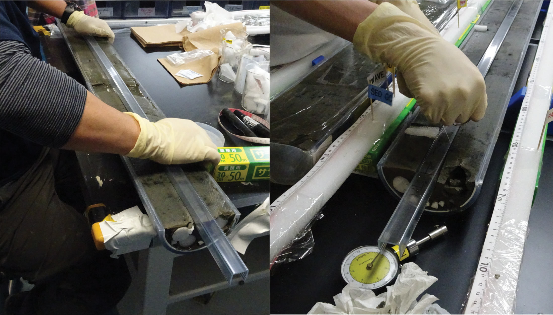
Figure F25. U-channel sampling.
The NRM of the U-channel sample was measured using the SRM, with measurements typically made at 2 cm intervals. Only one iteration of these measurements was taken after demagnetization at 5 mT due to the strict time constraints of the hybrid OSP, and routine demagnetization to calculate more detailed directions are planned for postcruise work. We used 20 cm long leaders and trailers because the response curve from the sensor coils of the cryogenic magnetometer corresponds to a region ~20 cm wide.
8.2.1. Sample coordinates
The standard IODP core coordinate system was used, where +x is the vertically upward direction when the archive half is on its curved side, +y is the direction to the left along the split core surface when looking upcore (on the archive half), and +z is the downcore direction (Figure F26). The coordination of U-channel samples follows that of the working half.

Figure F26. Paleomagnetism coordinate systems.
8.2.2. Orientation correction
Rotational movement of the GPC during penetration of the seabed can cause relative motion of the core sample along the vertical axis. Because this rotational movement is known (e.g., McCoy, 1980), the recorded declination can be modified from the original linear trend of the cores. Azimuth inclinometer data show rotational motion around an axis perpendicular to the horizontal plane during GPC penetration of the seafloor (Figure F5; see PALEOMAG in Supplementary material). This rotational motion suggests that the sediment core was inserted while rotating against the core liner, although detailed analysis of the directional inclinometer data will occur postcruise. We applied only a simple correction to reconstruct the original variation of declination trends and assumed that the amount of rotation is regarded as a linear function of core depth. We anticipate that segmentation of the core into pieces may cause sudden declination shifts. Declinations of intervals are shifted to fit those of the upper interval. Inclination and declination profiles will be compared with those of the master curves of paleomagnetic secular variation (such as BIWA SV-3 [Ali et al., 1999] and ARCH3k.1 [Korte et al., 2009]) to obtain age information.
9. Microbiology
During Expedition 386, microbiological sampling along the Japan Trench was performed to secure samples for postexpedition research that will explore the microbial communities and functional changes in response to massive sediment transport events, especially those triggered by subduction zone earthquakes. This section describes the shipboard sampling and handling procedures employed for microbiological sampling during the offshore and OSP phases. The shore-based methodology and analytical methods for postexpedition research conducted on these samples and data will be described in individual scientific contributions published after the expedition.
9.1. Offshore sampling
9.1.1. Sediment sampling
For microbiological studies, offshore sampling occurred on board Kaimei immediately after recovery of the GPC assembly on deck from the selected holes described (Table T10). Sampling used syringes to avoid any alteration or contamination introduced by sample handling before and during the core sectioning process. Time sensitive samples that required rapid processing within 30 min were taken from near the center of the freshly cut end of each core section using a sterile 2 mL syringe for cell counts and a sterile 50 mL syringe for DNA analysis. Seafloor sediment samples were also taken from the top of the trigger core (0 mbsf). Sediment samples for cell counting were transferred to a 15 mL centrifuge tube containing 50% paraformaldehyde suspended in a fixing solution and stored in the cold room (~4°C). Sediments for DNA analysis were transferred to a 207 mL Whirl-Pak bag and stored in the deep freezer (~80°C). All Hole E and F cores from Sites M0081, M0083, and M0084 were sealed in gas-tight aluminum (Escal) bags and flushed with nitrogen to preserve core material from oxidation for further microbiological analyses.
9.1.2. Bottom water sampling
In addition to sediment cores, BW samples for single-cell genome analysis were obtained from trigger cores (Table T10). Bottom seawater (3 L) was sampled from the top of trigger cores using a BW sampling system with two 1.2 L sterilized bottles (Figure F27). The single-cell amplified genome in gel (SAG-gel) approach was applied (Figure F28). BW samples were filtered within 24 h of sampling using 5 and 0.22 µm pore size filters, and microbial cells collected on the filter surface were then suspended with phosphate-buffered saline (PBS) in a 25 mL tube. Cell suspensions were diluted to an optimized concentration (0.1 cells/bead) to prevent the encapsulation of multiple cells in single beads. Using the droplet generator, single microbial cells were encapsulated in droplets and collected in a 1.5 mL tube that was chilled on ice for 15 min to form the gel matrix. After solidification, the collected droplets were broken with 1H,1H,2H,2H-perfluoro-1-octanol to collect the beads. The gel beads were then washed with 500 μL acetone, and the solution was mixed vigorously and centrifuged at 6000 rpm for 20 s. The acetone supernatant was removed, 500 µL isopropanol was added, and the solution was mixed vigorously and centrifuged again at 6000 rpm for 20 s. The isopropanol supernatant was removed, and the gel beads were washed three times with 500 μL PBS. Next, individual cells in beads were lysed by submerging the gel beads in three types of lysis solutions: (1) 50 U/μL Ready-lyse Lysozyme Solution, 2 U/mL Zymolyase, 22 U/mL lysostaphin, and 250 U/mL mutanolysin in PBS at 37°C overnight; (2) 0.5 mg/mL achromopeptidase in PBS at 37°C for 8 h; and (3) 1 mg/mL Proteinase K with 0.5% sodium dodecyl sulphate (SDS) in PBS at 40°C overnight. At each reagent replacement step, the gel beads were washed three times with PBS and then resuspended in the next solution. After lysis, the gel beads were washed with PBS five times and the supernatant was removed. The beads were then suspended in Buffer D2 and subjected to multiple displacement amplification using a reference protocol in REPLI-g Single Cell Kit. After whole genome amplification at 30°C for 2 h, the gel beads were washed three times with 500 μL PBS. The gel beads were then stored at 4°C in a 1.5 mL tube.

Figure F27. Bottom water sampling system.
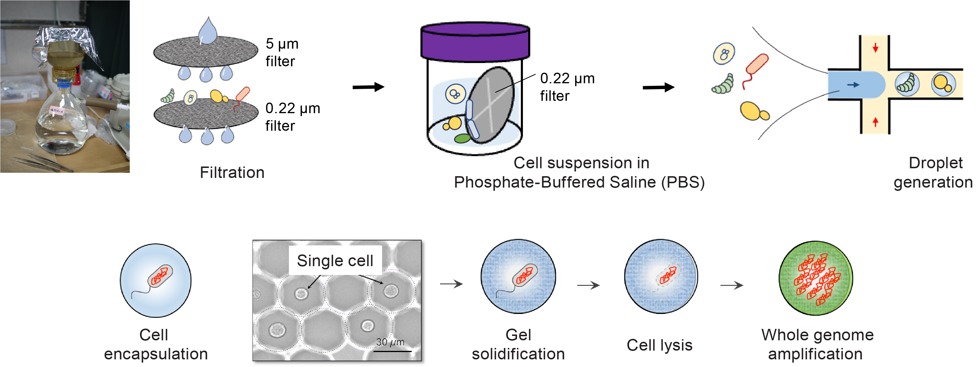
Figure F28. Massively parallel single-cell genome amplification.
9.2. Onshore sampling
Sediment samples for postcruise research to evaluate changes in microbial diversity were taken from event layers identified by sedimentologists performing visual core description during the OSP. Sediment sampling for DNA analysis was conducted on samples from cores that had been vacuum packed with nitrogen gas in Escal bags and stored at 4°C. Sampling occurred within 30 min of core splitting to minimize changes in microbial compositions. Sediment (10 mL) was taken from event layers with a sterile 50 mL syringe and transferred to a 207 mL Whirl-Pak bag and frozen at −80°C within 30 min of sampling (Figure F29). Sediment was also taken above and below the event layer and from the section bottom near the offshore sampling locations to evaluate the shift of microbial community composition during storage after coring. The sampling frequency depended on the number of the event layers retrieved (Table T11).

Figure F29. Microbiology sediment sampling.
10. Stratigraphic correlation
Meeting the scientific objectives of Expedition 386 required recovery of complete stratigraphic sections. Such sections cannot be constructed from a single GPC hole because core recovery gaps of up to 2–3 m can occur in the top part of the GPC core and significant voids and cracks exist, especially in the lower part of GPC cores. The construction of a complete stratigraphic section, referred to as a splice, requires combining stratigraphic intervals from two or more offset holes cored at the same site.
10.1. Core depth below seafloor depth scale
The depth to a given position in a core is determined by adding the distance at which that position occurs from the top of the core (curated to be 0 mbsf). The distance from the top of the core includes expansion due to relief of overburden as well as gas expansion and artificial voids filled by foam at the top or bottom of the sections. This depth scale is referred to as core depth below seafloor (or meters below seafloor [mbsf]) and is equivalent to the core depth below seafloor, Method A (CSF-A), scale described in IODP Depth Scale Terminology 2011 (https://www.iodp.org/policies-and-guidelines/142-iodp-depth-scales-terminology-april-2011/file). Errors in the mbsf scale include incomplete recovery and core expansion as a result of elastic rebound and gas. In any case, the goal of avoiding core gap alignment at the top of GPC cores can be difficult to achieve with just two holes and sometimes even with three. Furthermore, for some trigger cores and GPC cores (especially when using a 20 m piston corer barrel), the core catcher was sampled in a bag. Although the length of the core catcher (0.05–0.3 m) was included to record the total core length, this length is not included on the mbsf depth scale.
10.2. Core composite depth below seafloor depth scale
The ultimate goal of constructing a composite depth scale for a given site is to place specific coeval, laterally continuous features identified in all holes into a common frame of reference by depth shifting individual cores (each starting at 0 mbsf). The resulting core composite depth below seafloor (or mcd) scale is equivalent to the core composite depth below seafloor, Method A (CCSF-A), scale described in IODP Depth Scale Terminology 2011 (https://www.iodp.org/policies-and-guidelines/142-iodp-depth-scales-terminology-april-2011/file). In constructing the mcd scale, the depths of the individual cores are shifted by a constant amount (there is no stretching or squeezing within individual cores). This provides good first-order correlation between cores from different holes, estimated lengths of coring gaps, and a basis upon which higher order composite depth scales can be constructed; compositing is a prerequisite to developing the core composite depth below seafloor, Method D (CCSF-D), scale (spliced record; as defined in IODP Depth Scale Terminology 2011.
The mcd scale is built by correlating features downhole from the sedimentologic mudline. Based on observation of the sediment/water interface on board Kaimei, the mudline is well preserved in all trigger cores. Hence, the top of the sediment below the artificially added foam in the top part of the curated first section of trigger cores was determined to be the mudline and anchored as 0 mcd (seafloor). This establishes the top of the stratigraphic section and anchors the entire composite depth scale for all cores from all holes at a site. In practice, compositing is accomplished sequentially by establishing specific tie points among the various holes, working from the mudline (anchor) trigger cores to the longer GPC cores (red tie point arrows in Figure F7). The mcd scale very rarely (if ever) results in alignment of all features because of the differing effects of coring-induced stretching and squeezing within and between cores as well as hole-to-hole sedimentologic differences.
The revised length of sections, correcting for artificial voids filled by foam at the top or bottom of the sections and the vertical depth offset of every core in every hole, is tabulated in an affine table (included in each site chapter). Conceptually, it should be possible to correlate (tie) each core in one hole to a core from an adjacent hole, provided that the core length of the trigger core is long enough to recover the uppermost part of the subseafloor section not recovered or disturbed at the top of the GPC core. In the case of several tie points occurring in the trigger cores, the core with the longest length between the mudline and the stratigraphically first tie point was selected for the composite section. If this situation does not arise, aligned coring gaps across all holes cored at a site may still occur, in which case cores below the gap are no longer tied to the mudline trigger core but can often still be tied to one another. Such intervals are commonly referred to as floating sections. In the event of such a coring gap of unknown extension, we defined a floating anchor point between GPC cores to calculate the relative depth offset. The meters composite depth of the trigger core with the longest length between the mudline or stratigraphically last tie point and the core bottom is then added to calculate vertical depth offsets for each GPC core (speculatively assuming that there is no gap between the base of the longest trigger cores and the top of the GPC core with the highest recovery at the core top).
During the process of constructing the composite section, the core composite depth (mcd scale) becomes systematically larger than that of the curated core depth (mbsf scale) at equivalent horizons. This expansion, which is typically ~1%–5%, is mostly caused by decompression of the cores as they are brought to the surface, gas expansion, stretching that occurs as part of the coring process, and/or curation, when, for example, gas expansion voids are curated as part of the core. The established core composite depth scale (mcd) includes both natural and artificial voids except those of the trigger core and GPC core tops.
10.3. Core composite depth below seafloor within the splice
After the core composite depth scale (mcd) has been developed and the between-core gaps identified, a complete stratigraphic section (splice) or a floating splice (in the event the coring gap could not be quantified) is constructed by combining selected intervals between tie points that were either (1) previously established and used to identify and quantifying coring gaps at the tops of GPC cores or (2) defined additionally in the lower part of the GPC core. Special care was taken to choose tie points such that disturbed intervals are avoided. The depth scale of the splice is given in meters composite depth below seafloor in splice (mcd-splice) (Figure F7).
Although it is a subset of the mcd scale, the mcd-splice scale applies only to intervals included in the splice. Intervals not included in the primary splice, including any alternate splice(s), retain the mcd scale. For sites where coring gaps happen to align across all holes at that site, the spliced sections, as established by tie points between piston cores below, are appended to those from the trigger core above and referred to as floating splice sections (i.e., not tied to the mudline). This amount of missing material between floating sections may later be estimated during postexpedition correlation work that will establish (1) correlation with up to 10 m long continuous piston and gravity cores retrieved during the previous site survey cruise (summarized in Strasser et al., 2019) and (2) alignment of geochemical profiles from IW analyses (see Geochemistry) such as alkalinity, Ba, NH4, and/or uranium that show distinct downhole features at correlative subseafloor depth.
10.4. Methods for correlation
Zero-order compositing and splicing prior to the OSP was tentatively based on visual correlation of marker horizons on X-ray CT images, guided by visual inspection of trends and spikes in magnetic susceptibility and GRA data from the MSCL measured at 2 cm intervals (see Physical properties). At this early stage, thin but clear marker beds visible on X-ray CT images were tentatively used because large (coarse and thick) event beds may have eroded the underlying sediments.
During the OSP, tie points were updated according to core characterization by visual core description (lithology, sedimentary structures, and linescan images), identification of visible air fall tephra layers and their characteristic composition as observed in smear slide observation (preferred, most robust tie points), and physical properties, including color reflectance and RGB values (see Lithostratigraphy, Tephra, and Physical properties). Examples of different types of tie points used in this first-order stratigraphic correlation between holes are presented in Figure F30.
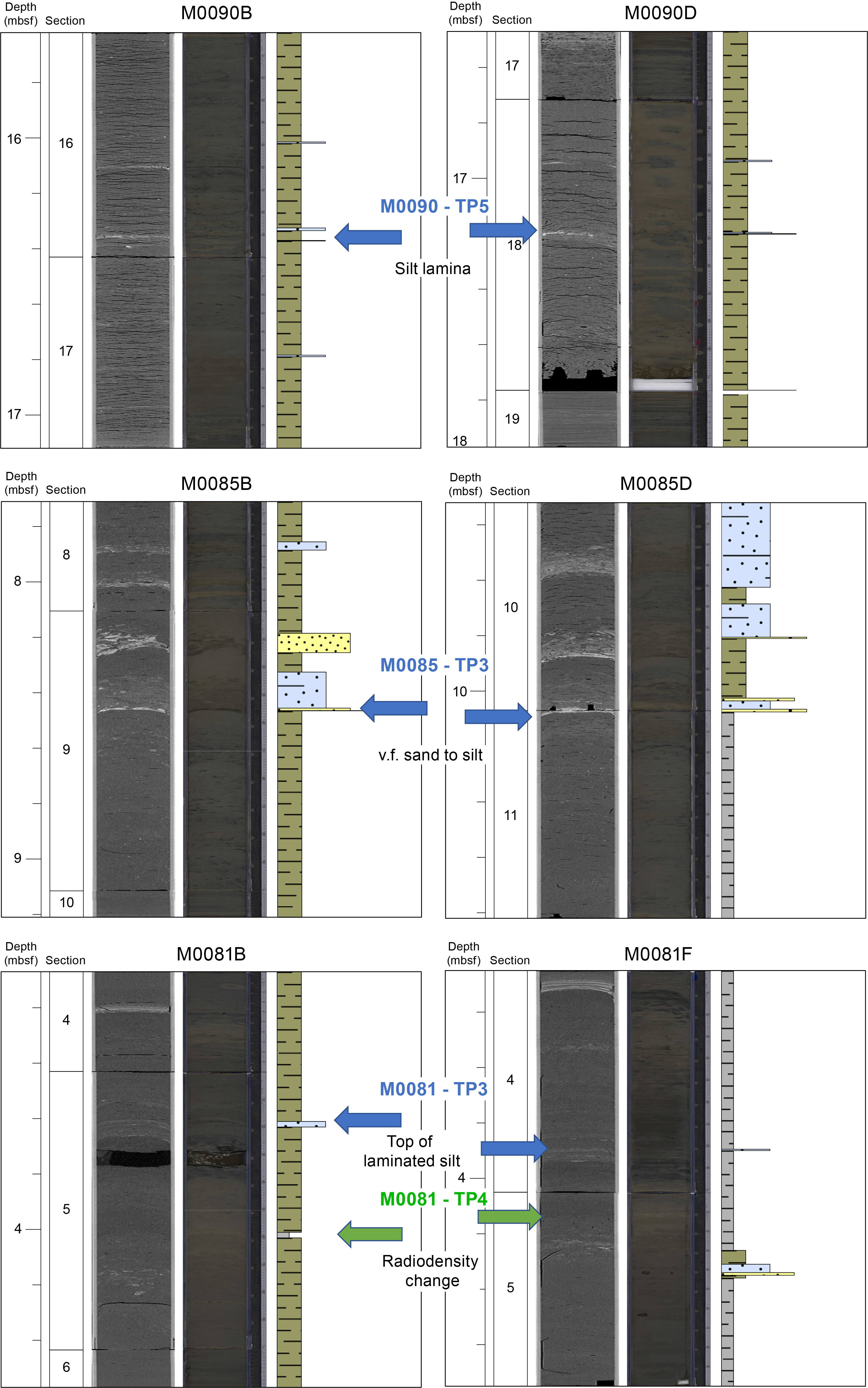

Figure F30. Tie points.
OSP-based first-order generation of standard affine tables and tie point tables were constructed manually from visually reading section depths and manually editing the table. In each site chapter, the first table shows the revised lengths of sections, correcting for artificial void filled by foam at the top or bottom, the second table shows the vertical offset (in meters) added to each core to generate the core composite depth scales, and the third table lists tie points between holes, intervals used to construct the splice, and the respective mcd-splice depth scale. Figures showing X-ray CT and linescan images of all tie points used are presented in STRATCORR in Supplementary material.
References
Ali, M., Oda, H., Hayashida, A., Takemura, K., and Torii, M., 1999. Holocene palaeomagnetic secular variation at Lake Biwa, central Japan. Geophysical Journal International, 136(1):218–228.
https://doi.org/
Blum, P., 1997. Physical properties handbook: a guide to the shipboard measurement of physical properties of deep-sea cores. Ocean Drilling Program Technical Note, 26. https://doi.org/
Brooks, R.A., and Di Chiro, G., 1976. Principles of computer assisted tomography (CAT) in radiographic and radioisotopic imaging. Physics in Medicine and Biology, 21(5):689–732. https://doi.org/
Buckley, D.E., MacKinnon, W.G., Cranston, R.E., and Christian, H.A., 1994. Problems with piston core sampling: mechanical and geochemical diagnosis. Marine Geology, 117(1–4):95–106.
https://doi.org/
Butler, R.F., 1992. Paleomagnetism: Magnetic Domains to Geologic Terranes: Boston (Blackwell Science Publishing). https://www.geo.arizona.edu/
Chen, J.-W., Fan, W., Bingham, B., Chen, Y., Gu, L.-Y., and Li, S.-L., 2013. A long gravity-piston corer developed for seafloor gas hydrate coring utilizing an in situ pressure-retained method. Energies, 6(7):3353–3372. https://doi.org/
Chinzei, K., Fujioka, K., Kitazato, H., Koizumi, I., Oba, T., Oda, M., Okada, H., Sakai, T., and Tanimura, Y., 1987. Postglacial environmental change of the Pacific Ocean off the coasts of central Japan. Marine Micropaleontology, 11(4):273–291. https://doi.org/
Cline, J.D., 1969. Spectrophotometric determination of hydrogen sulfide in natural waters. Limnology and Oceanography, 14(3):454–458. https://doi.org/
Cnudde, V., and Boone, M.N., 2013. High-resolution X-ray computed tomography in geosciences: a review of the current technology and applications. Earth-Science Reviews, 123:1–17.
https://doi.org/
Cnudde, V., Cnudde, J.P., Dupuis, C., and Jacobs, P.J.S., 2004. X-ray micro-CT used for the localization of water repellents and consolidants inside natural building stones. Materials Characterization, 53(2):259–271. https://doi.org/
Curry, W., Broda, J., Keigwin, L., Mountain, G., and Pisias, N., 2008. A new long coring system for R/V Knorr. Eos, Transactions of the American Geophysical Union, 89(15):142–143. https://doi.org/
Degen, T., Sadki, M., Bron, E., König, U., and Nénert, G., 2014. The HighScore suite. Powder Diffraction, 29(S2):S13–S18. https://doi.org/
Dickens, G.R., Koelling, M., Smith, D.C., Schnieders, L., and the IODP Expedition 302 Scientists, 2007. Rhizon sampling of pore waters on scientific drilling expeditions: an example from the IODP Expedition 302, Arctic Coring Expedition (ACEX). Scientific Drilling, 4:22–25. https://doi.org/
Droser, M.L., and Bottjer, D.J., 1991. Trace fossils and ichnofabric in Leg 119 cores. In Barron, J., Larsen, B., et al., Proceedings of the Ocean Drilling Program, Scientific Results, 119: College Station, TX (Ocean Drilling Program), 635–641. https://doi.org/
Gérard, J., and Bromley, R.G., 2008. Ichnofabrics in Clastic Sediments: Applications to Sedimentological Core Studies: a Practical Guide: Madrid, Spain (Jean Gérard). http://lib.ugent.be/
Goldfinger, C., Nelson, C.H., Morey, A.E., Johnson, J.E., Patton, J.R., Karabanov, E.B., Gutierrez-Pastor, J., Eriksson, A.T., Gracia, E., Dunhill, G., Enkin, R.J., Dallimore, A., and Vallier, T., 2012. Turbidite event history—methods and implications for Holocene paleoseismicity of the Cascadia subduction zone. USGS Professional Paper, 1661-F. https://doi.org/
Gooday, A.J., 2003. Benthic Foraminifera (protista) as tools in deep-water palaeoceanography: environmental influences on faunal characteristics. In Advances in Marine Biology. 46: 1–90.
https://doi.org/
Govin, A., Vázquez Riveiros, N., Réaud, Y., Waelbroeck, C., and Giraudeau, J., 2016. Unprecedented coring performance with the upgraded Research Vessel Marion Dufresne. Past Global Changes Magazine, 24(1):27. https://doi.org/
Hansbo, S., 1957. A new approach to the determination of the shear strength of clay by the fall-cone test. SGI Proceedings:46. http://urn.kb.se/
Hays, J.D., Lozano, J.A., Shackleton, N., Irving, G., Cune, R.M., and Hays, J.D., 1976. Reconstruction of the Atlantic and Western Indian Ocean sectors of the 18,000 B.P. Antarctic Ocean. In Cune, R.M., and Hays, J.D. (Eds.), Investigation of Late Quaternary Paleoceanography and Paleoclimatology. Geological Society of America Memoirs, 145: (Geological Society of America). https://doi.org/
Ikehara, K., Kanamatsu, T., Nagahashi, Y., Strasser, M., Fink, H., Usami, K., Irino, T., and Wefer, G., 2016. Documenting large earthquakes similar to the 2011 Tohoku-oki earthquake from sediments deposited in the Japan Trench over the past 1500 years. Earth and Planetary Science Letters, 445:48–56. https://doi.org/
Itaki, T., Uchida, M., Kim, S., Shin, H.-S., Tada, R., and Khim, B.-K., 2009. Late Pleistocene stratigraphy and palaeoceanographic implications in northern Bering Sea slope sediments: evidence from the radiolarian species Cycladophora davisiana. Journal of Quaternary Science, 24(8):856–865. https://doi.org/
Jorissen, F.J., Fontanier, C., and Thomas, E., 2007. Paleoceanographical proxies based on deep-sea benthic foraminiferal assemblage characteristics. In Hillaire–Marcel, C., and De Vernal, A. (Eds.), Developments in Marine Geology (Volume 7): Earth and Life Processes Discovered from Subseafloor Environments: A Decade of Science Achieved by the Integrated Ocean Drilling Program (IODP). R. Stein (Series Ed.). Amsterdam (Elsevier), 263–325.
https://doi.org/
Jutzeler, M., White, J.D.L., Talling, P.J., McCanta, M., Morgan, S., Le Friant, A., and Ishizuka, O., 2014. Coring disturbances in IODP piston cores with implications for offshore record of volcanic events and the Missoula megafloods. Geochemistry, Geophysics, Geosystems, 15(9):3572–3590. https://doi.org/
Kioka, A., Schwestermann, T., Moernaut, J., Ikehara, K., Kanamatsu, T., Eglinton, T.I., and Strasser, M., 2019. Event stratigraphy in a hadal oceanic trench: the Japan Trench as sedimentary archive recording recurrent giant subduction zone earthquakes and their role in organic carbon export to the deep sea. Frontiers in Earth Science, 7:319. https://doi.org/
Korte, M., Donadini, F., and Constable, C.G., 2009. Geomagnetic field for 0–3 ka: 2. A new series of time-varying global models. Geochemistry, Geophysics, Geosystems, 10(6):Q06008. https://doi.org/
Kvenvolden, K.A., and McDonald, T.J., 1986. Organic geochemistry on the JOIDES Resolution—an assay. Ocean Drilling Program Technical Note, 6. https://doi.org/
Lane, E.W., 1947. Report of the Subcommittee on Sediment Terminology. Eos, Transactions of the American Geophysical Union, 28(6):936–938. https://doi.org/
Leroueil, S., and Bihan, J.-P.L., 1996. Liquid limits and fall cones. Canadian Geotechnical Journal, 33(5):793–798. https://doi.org/
Leroy, C.C., 1969. Development of simple equations for accurate and more realistic calculation of the speed of sound in seawater. The Journal of the Acoustical Society of America, 46(1B):216–226. https://doi.org/
Loeblich, A.R., and Tappan, H.N., 1988. Foraminiferal Genera and Their Classification: New York (Van Nostrand Reinhold Company). https://doi.org/
Lowe, D.J., 2011. Tephrochronology and its application: a review. Quaternary Geochronology, 6(2):107–153. https://doi.org/
Machida, H., and Arai, F., 1978. Akahoya ash—a Holocene widespread tephra erupted from the Kikai Caldera, South Kyushu, Japan. The Quaternary Research (Daiyonki-Kenkyu), 17(3):143–163. https://doi.org/
Matoba, Y., 1976. Recent foraminiferal assemblages off Sendai, northeast Japan. Maritime Sediments, Spec. Pub. A:205–220. https://cir.nii.ac.jp/
Matsuzaki, K.M., Itaki, T., and Sugisaki, S., 2020. Polycystine radiolarians vertical distribution in the subtropical Northwest Pacific during spring 2015 (KS15-4). Paleontological Research, 24(2):113–133. https://doi.org/
Matsuzaki, K.M., Nishi, H., Suzuki, N., Kawate, Y., Takashima, R., and Sakai, T., 2014. Cycladophora davisiana abundances as a paleoceanographic and stratigraphic tool in high latitude siliciceous sediments. Marine Micropaleontology, 106:1–9. https://doi.org/
Mazzullo, J., Meyer, A., and Kidd, R., 1988. Appendix I: New sediment classification scheme for the Ocean Drilling Program. In Mazzullo, J., and Graham, A.G. , Handbook for shipboard sedimentologists. Ocean Drilling Program Technical Note. 8: 44–67. https://doi.org/
McCoy, F.W., 1980. Photographic analysis of coring. Marine Geology, 38(1–3):263–282. https://doi.org/
McKee, E.D., and Weir, G.W., 1953. Terminology for stratification and cross-stratification in sedimentary rocks. Geological Society of America Bulletin, 64(4):381–390.
https://doi.org/
McKetty, M.H., 1998. The AAPM/RSNA physics tutorial for residents. X-ray attenuation. RadioGraphics, 18(1):151–163. https://pubs.rsna.org/
McNeill, L.C., Shillington, D.J., Carter, G.D.O., Everest, J.D., Le Ber, E., Collier, R.E.Ll., Cvetkoska, A., De Gelder, G., Diz, P., Doan, M.-L., Ford, M., Gawthorpe, R.L., Geraga, M., Gillespie, J., Hemelsdaël, R., Herrero-Bervera, E., Ismaiel, M., Janikian, L., Kouli, K., Li, S., Machlus, M.L., Maffione, M., Mahoney, C., Michas, G., Miller, C., Nixon, C.W., Oflaz, S.A., Omale, A.P., Panagiotopoulos, K., Pechlivanidou, S., Phillips, M.P., Sauer, S., Seguin, J., Sergiou, S., and Zakharova, N.V., 2019. Expedition 381 methods. In McNeill, L.C., Shillington, D.J., Carter, G.D.O., and the Expedition 381 Participants, Corinth Active Rift Development. Proceedings of the International Ocean Discovery Program, 381. https://doi.org/
Moore, D.M., and Reynolds, R.C., Jr., 1989. X-Ray Diffraction and the Identification and Analysis of Clay Minerals: Oxford, United Kingdom (Oxford University Press).
Morley, J.J., and Hays, J.D., 1979. Cycladophora davisiana: a stratigraphic tool for Pleistocene North Atlantic and interhemispheric correlation. Earth and Planetary Science Letters, 44(3):383–389.
https://doi.org/
Morley, J.J., Hays, J.D., and Robertson, J.H., 1982. Stratigraphic framework for the late Pleistocene in the northwest Pacific Ocean. Deep Sea Research, Part A: Oceanographic Research Papers, 29(12):1485–1499.
https://doi.org/
Morley, J.J., Tiase, V.L., Ashby, M.M., and Kashgarian, M., 1995. A high-resolution stratigraphy for Pleistocene sediments from North Pacific Sites 881, 883, and 887 based on abundance variations of the radiolarian Cycladophora davisiana. In Rea, D.K., Basov, LA., Scholl, D.W., and Allan, J.F. (Eds.), Proceedings of the Ocean Drilling Program, Scientific Results. 145: College Station, TX (Ocean Drilling Program), 133–140. https://doi.org/
Murray, J.W., 2006. Ecology and Applications of Benthic Foraminifera: Cambridge, UK (Cambridge University Press). https://doi.org/
Nagahashi, Y., Yoshida, T., Nakai, S., and Okudaira, T., 2003. Evaluation and correction of EDS results of the glass shards from some representative tephra by comparison with XRF analysis. The Quaternary Research (Daiyonki-Kenkyu), 42(4):265–277. https://doi.org/
Ohkushi, K.i., Itaki, T., and Nemoto, N., 2003. Last Glacial–Holocene change in intermediate-water ventilation in the Northwestern Pacific. Quaternary Science Reviews, 22(14):1477–1484.
https://doi.org/
Oyama, M., and Takehara, H., 1967. Revised Standard Soil Color Charts: Shiga, Japan (Japan Color Enterprise).
Rothwell, R.G., 1989. Minerals and Mineraloids in Marine Sediments: An Optical Identification Guide: London (Elsevier). https://doi.org/
Sakamoto-Arnold, C.M., Johnson, K.S., and Beehler, C.L., 1986. Determination of hydrogen sulfide in seawater using flow injection analysis and flow analysis. Limnology and Oceanography, 31(4):894–900. https://doi.org/
Scott, D.B., Takayanagi, Y., Hasegawa, S., and Saito, T., 2000. Illustration and reevaluation of affinities of Neogene Foraminifera described From Japan. Palaeontologia Electronica, 3(2):1–41.
https://palaeontologia-electronica.earthsci.carleton.ca/
Seeberg-Elverfeldt, J., Schlüter, M., Feseker, T., and Kölling, M., 2005. Rhizon sampling of porewaters near the sediment-water interface of aquatic systems. Limnology and Oceanography: Methods, 3(8):361-371. https://doi.org/
Shepard, F.P., 1954. Nomenclature based on sand-silt-clay ratios. Journal of Sedimentary Research, 24(3):151–158. https://doi.org/
Smith, P.B., 1973. Foraminifera of the North Pacific Ocean. U.S. Geological Survey Professional Paper, 766. http://pubs.usgs.gov/
Stow, D.A.V., and Aksu, A.E., 1978. Disturbances in soft sediments due to piston coring. Marine Geology, 28(1–2):135–144. https://doi.org/
Strasser, M., Ikehara, K., and Cotterill, C., 2019. Expedition 386 Scientific Prospectus: Japan Trench Paleoseismology. International Ocean Discovery Program. https://doi.org/
Strasser, M., Ikehara, K., Everest, J., and the Expedition 386 Scientists, 2023. Supplementary material, https://doi.org/10.14379/iodp.proc.386supp.2023. In Strasser, M., Ikehara, K., Everest, J., and the Expedition 386 Scientists, Japan Trench Paleoseismology. Proceedings of the International Ocean Discovery Program, 386: College Station, TX (International Ocean Discovery Program).
Széréméta, N., Bassinot, F., Balut, Y., Labeyrie, L., and Pagel, M., 2004. Oversampling of sedimentary series collected by giant piston corer: Evidence and corrections based on 3.5-kHz chirp profiles. Paleoceanography, 19(1):PA1005. https://doi.org/
Tsujimoto, A., Nomura, R., Arai, K., Nomaki, H., Inoue, M., and Fujikura, K., 2020. Changes in deep-sea benthic foraminiferal fauna caused by turbidites deposited after the 2011 Tohoku-oki earthquake. Marine Geology, 419:106045. https://doi.org/
Tucker, M.E., 1988. Techniques in Sedimentology: Oxford, United Kingdom (Blackwell Science Publishing).
Usami, K., Ikehara, K., Jenkins, R.G., and Ashi, J., 2017. Benthic foraminiferal evidence of deep-sea sediment transport by the 2011 Tohoku-Oki earthquake and tsunami. Marine Geology, 384:214–224.
https://doi.org/
Usami, K., Ikehara, K., Kanamatsu, T., Kioka, A., Schwestermann, T., and Strasser, M., 2021. The link between upper-slope submarine landslides and mass transport deposits in the hadal trenche. In Sassa, K., Mikoš, M., Sassa, S., Bobrowsky, P.T., Takara, K., and Dang, K. (Eds.), Sendai Landslide Partnerships and Kyoto Landslide Commitment. Understanding and Reducing Landslide Disaster Risk, 1. https://doi.org/
van Morkhoven, F.M., Berggren, W.A., and Edwards, A.S., 1986. Cenozoic cosmopolitan deep-water benthic foraminifera. Bulletin des centres de Recherches exploration-production elf-aquitaine, 11.
Vogt, C., 2009. Data report: semiquantitative determination of detrital input to ACEX sites based on bulk sample X-ray diffraction data. In Backman, J., Moran, K., McInroy, D.B., Mayer, L.A., and the Expedition 302 Scientists, Proceedings of the Integrated Ocean Drilling Program 302: Edinburgh (Integrated Ocean Drilling Program Management International, Inc.). https://doi.org/
Vogt, C., Lauterjung, J., and Fischer, R.X., 2002. Investigation of the clay fraction (<2 µm) of the clay minerals society reference clays. Clays and Clay Minerals, 50(3):388–400. https://doi.org/
Wentworth, C.K., 1922. A scale of grade and class terms for clastic sediments. The Journal of Geology, 30(5):377–392. https://doi.org/
Wood, D.M., 1985. Some fall-cone tests. Geotechnique, 35(1):64–68. https://doi.org/
Yasudomi, Y., Motoyama, I., Oba, T., and Anma, R., 2014. Environmental fluctuations in the northwestern Pacific Ocean during the last interglacial period: evidence from radiolarian assemblages. Marine Micropaleontology, 108:1–12. https://doi.org/
Yoshikawa, S., 1976. On the volcanic ash layers of the Osaka Group. Geological Journal, 82(8):497–515. https://doi.org/
Zreik, D., Ladd, C., and Germaine, J., 1995. A new fall cone device for measuring the undrained strength of very weak cohesive soils. Geotechnical Testing Journal, 18(4):472–482. https://doi.org/