Parnell-Turner, R.E., Briais, A., LeVay, L.J., and the Expedition 395 Scientists
Proceedings of the International Ocean Discovery Program Volume 395
publications.iodp.org
https://doi.org/10.14379/iodp.proc.395.108.2025
Site U16021
![]() R.E. Parnell-Turner,
R.E. Parnell-Turner,
![]() A. Briais,
A. Briais,
![]() L.J. LeVay,
L.J. LeVay,
![]() Y. Cui,
Y. Cui,
![]() A. Di Chiara,
A. Di Chiara,
![]() J.P. Dodd,
J.P. Dodd,
![]() T. Dunkley Jones,
T. Dunkley Jones,
![]() D. Dwyer,
D. Dwyer,
![]() D.E. Eason,
D.E. Eason,
![]() S.A. Friedman,
S.A. Friedman,
![]() S.R. Hemming,
S.R. Hemming,
![]() K. Hochmuth,
K. Hochmuth,
![]() H. Ibrahim,
H. Ibrahim,
![]() C. Jasper,
C. Jasper,
![]() B.T. Karatsolis,
B.T. Karatsolis,
![]() S. Lee,
S. Lee,
![]() D.E. LeBlanc,
D.E. LeBlanc,
![]() M.R. Lindsay,
M.R. Lindsay,
![]() D.D. McNamara,
D.D. McNamara,
![]() S.E. Modestou,
S.E. Modestou,
![]() B. Murton,
B. Murton,
![]() S. OConnell,
S. OConnell,
![]() G.T. Pasquet,
G.T. Pasquet,
![]() P.N. Pearson,
S.P. Qian,
P.N. Pearson,
S.P. Qian,
![]() Y. Rosenthal,
Y. Rosenthal,
![]() S. Satolli,
S. Satolli,
![]() M. Sinnesael,
T. Suzuki,
M. Sinnesael,
T. Suzuki,
![]() T. Thulasi Doss,
T. Thulasi Doss,
![]() N.J. White,
N.J. White,
![]() T. Wu, and
T. Wu, and
![]() A. Yang Yang2
A. Yang Yang2
1 Parnell-Turner, R.E., Briais, A., LeVay, L.J., Cui, Y., Di Chiara, A., Dodd, J.P., Dunkley Jones, T., Dwyer, D., Eason, D.E., Friedman, S.A., Hemming, S.R., Hochmuth, K., Ibrahim, H., Jasper, C., Karatsolis, B.T., Lee, S., LeBlanc, D.E., Lindsay, M.R., McNamara, D.D., Modestou, S.E., Murton, B., OConnell, S., Pasquet, G.T., Pearson, P.N., Qian, S.P., Rosenthal, Y., Satolli, S., Sinnesael, M., Suzuki, T., Thulasi Doss, T., White, N.J., Wu, T., and Yang Yang, A., 2025. Site U1602. In Parnell-Turner, R.E., Briais, A., LeVay, L.J., and the Expedition 395 Scientists, Reykjanes Mantle Convection and Climate. Proceedings of the International Ocean Discovery Program, 395: College Station, TX (International Ocean Discovery Program). https://doi.org/10.14379/iodp.proc.395.108.2025
2 Expedition 395 Scientists' affiliations.
1. Background and objectives
Site U1602 is located east of the Greenland continental margin in the North Atlantic Ocean, coinciding with the northern portion of Eirik drift (Figure F1). Site U1602 is also located on a tentatively identified crustal V-shaped ridge (VSR) marked by a northeast-southwest trending linear high in the free-air gravity anomaly map and the reflection seismic profile (Figures F1, F2). This is one of the V-shaped structures that straddle the Reykjanes ridge flanks and whose origin in relation to the Iceland hotspot is debated. The site sits on oceanic crust with an age of 49.8 Ma, estimated from magnetic anomalies and plate reconstruction models.
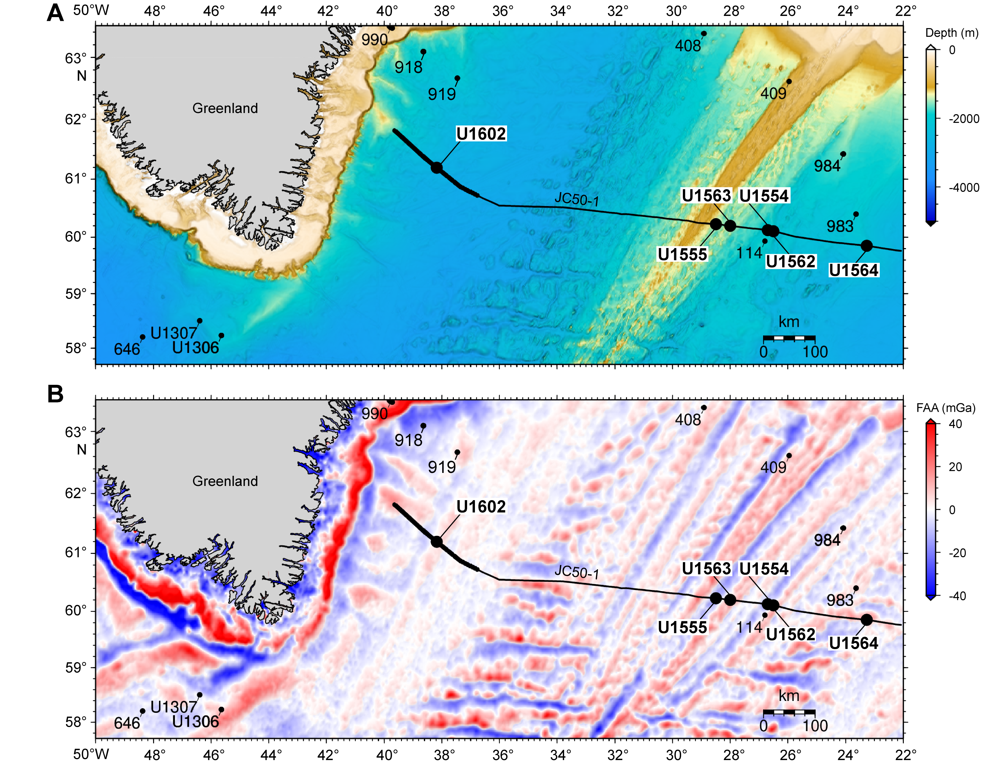
Figure F1. Bathymetry and free-air gravity anomaly maps.

Figure F2. Seismic Profile JC50-1 near Site U1602.
The Reykjanes Ridge flanks are the site of major contourite drift deposits, and two of them, Björn and Gardar drifts, are located on the eastern flank of the ridge. In contrast, Eirik drift consists of an elongate, mounded contourite deposit that is plastered along the East Greenland margin. These rapidly accumulated contourite drift sediments have the potential to record variations in past climate and ocean circulation on millennial timescales. The sedimentation rate of the drifts can serve as a proxy for deepwater current strength, providing information on oceanic gateways to the Norwegian Sea and their potential ties to Iceland mantle plume behavior. The sedimentary section at Site U1602 on Eirik drift has the potential to preserve detailed records of the evolution of the Greenland and Iceland ice sheets and of variations in the Western Boundary Undercurrent (WBUC). Site U1602 complements the sites on the eastern side of the Reykjanes Ridge drilled through Björn and Gardar drifts and also allowed the recovery of much older sediment, potentially providing insights into the North Atlantic ocean circulation and sedimentation deep into the Cenozoic. Site U1602 is located on Seismic Line JC50-1 (Common Midpoint [CMP] 148300) (Figure F2), obtained in 2010 during RRS James Cook Cruise JC50 (Parnell-Turner et al., 2017). Sediment thickness at Site U1602 was expected to be ~1376 m (5.03 s two-way traveltime [TWT]) based on seismic imagery (Figure F2). The main goal for Site U1602 was to obtain a continuous sedimentary record of Eirik drift. Another goal was to obtain a sedimentary record throughout the middle Miocene warm period. A final goal, time permitting, was to core into basement, although this was not achieved. Cores and data from this site will address two of the three expedition primary science objectives: (1) crustal accretion and mantle behavior and (2) ocean circulation, gateways, and sedimentation.
The operational objectives for this site were to core the sedimentary section using the advanced piston corer (APC), extended core barrel (XCB), and rotary core barrel (RCB) systems as deep as time permitted outside of the primary sites operations and use downhole wireline tools to log the borehole. The possibility was open to reach the sediment/basement interface and to core and log ~130 m into the basement. However, the time remaining in the expedition did not allow for these final operations to take place.
2. Operations
Site U1602 (61°11.7138′N, 38°10.8186′W) consists of five holes drilled during Expedition 395 that extend to 8.8–1365.2 m drilling depth below seafloor (DSF) (Table T1). A total of 230 cores were recovered from Site U1602 (see Table T1 in the Expedition 395 summary chapter [Parnell-Turner et al., 2025b]). These cores collected 1444.65 m of sediment over a 1903.8 m cored interval (76% recovery) (Table T1).
The APC system was used to collect 55 cores over a 510.3 m interval with 524.93 m of core recovered (103% recovery). The half-length APC (HLAPC) was deployed for 59 cores and recovered 291.43 m of sediment from a 277.3 m interval (105% recovery). The XCB system was deployed over a 280.3 m interval. The 29 XCB cores recovered 177.9 m of sediment (63% recovery). The RCB system was deployed over an 835.9 m interval with 450.39 m of core recovered (54% recovery). A total of 87 cores were collected with the RCB system. Two drilled intervals were recorded over a 531.3 m interval. Downhole wireline logging operations were attempted in Hole U1602E and were partly successful.
The total time spent at Site U1602 was 19.5 days.
2.1. Hole U1602A
The ship completed the 350 nmi transit, averaging 11.0 kt, from Site U1562 to Site U1602 at 1701 h UTC on 4 July 2023. At that time, the thrusters were lowered, and the ship was in dynamic positioning (DP) mode at 1718 h, marking the start of Site U1602. The APC/XCB bottom-hole assembly (BHA) and drill string were assembled, 105 feet of drill line was cut off, and the top drive was picked up. The bit was spaced out to initiate Hole U1602A (61°11.7138′N, 38°10.8186′W), which was spudded at 0425 h on 5 July. Core 1H recovered 8.8 m of core, establishing a seafloor depth of 2708.6 meters below sea level (mbsl). However, Core 1H also recovered part of the pig, a foam device with metal bristles used to clean rust from the inside of the drill pipe, which disturbed the mudline interval. Hole U1602A was terminated to recover an undisturbed mudline. A total of 8.81 m of core was recovered over an 8.8 m interval (100% recovery). Core 1H was oriented using the Icefield MI-5 core orientation tool and was taken with a nonmagnetic core barrel.
2.2. Hole U1602B
Hole U1602B (61°11.7144′N, 38°10.8184′W; 2709.2 mbsl) was spudded at 0535 h on 5 July 2023 from the same ship position, and Core 1H recovered 5.15 m of core with a good mudline. Coring continued with Cores 2H–16H (5.2–147.7 m DSF). Core 16H required 100,000 lb of overpull to extract the core barrel from the sediment. The HLAPC was deployed for Cores 17F–38F (147.7–251.1 m DSF). Cores 18F and 26F had partial strokes. Piston coring refusal was reached with Core 38F, which required 80,000 lb of overpull to free the barrel from the formation. The drill string was pulled from the hole, and the bit cleared the seafloor at 1600 h on 6 July, marking the end of Hole U1602B.
A total of 38 cores were collected in Hole U1602B, with 262.37 m of core recovered over a 251.1 m interval (104% recovery). All APC cores were oriented using the Icefield MI-5, and all APC and HLAPC cores were collected using nonmagnetic core barrels. Temperature measurements using the third-generation advanced piston corer temperature (APCT-3) tool were collected on Cores 395-U1602B-4H, 7H, 10H, and 13H.
2.3. Hole U1602C
Following operations in Hole U1602B, the vessel was offset 20 m north. After performing maintenance on the rig and cutting off 150 m of core winch line, the top drive was picked up and the bit was spaced out to 2719 meters below rig floor (mbrf). Hole U1602C (61°11.7253′N, 38°10.8193′W) was spudded at 1920 h on 6 July 2023. Core 1H recovered 7.07 m of core, placing the seafloor at 2710.0 mbsl. Cores 1H–20H (0–180.0 m DSF) were recovered. In this cored interval, an interval of 2 m was drilled without recovery (64.0–66.0 m DSF; drilled interval 81) to offset coring gaps for stratigraphic correlation. After three partial strokes using the APC system, the HLAPC system was deployed for Cores 21F–39F (180.0–269.3 m DSF). Partial strokes were recorded on Cores 23F and 39F, and the overpull on Core 38F was 100,000 lb. Piston coring refusal was reached at 269.3 m DSF, and the hole was ended. The drill pipe was pulled out of the hole, and the bit cleared the seafloor at 0525 h on 8 July, ending Hole U1602C.
A total of 38 cores were recovered in Hole U1602C, with 272.63 m of sediment recovered from a 267.3 m cored interval (102% recovery). All APC cores were oriented using the Icefield MI-5, and all APC and HLAPC cores were taken using nonmagnetic core barrels.
2.4. Hole U1602D
The vessel was offset 20 m east of Hole U1602C, the rig was serviced, and 100 m of core line was removed. Hole U1602D (61°11.7259′N, 38°10.7967′W; 2709.1 mbsl) was spudded at 0805 h on 8 July 2023. The seafloor depth was determined based on the recovery of Core 1H, which was 9.6 m. Cores 1H–19H advanced from 0 to 175.8 m DSF. Partial strokes were recorded on Cores 17H and 19H, and Core 18H required 100,000 lb of overpull to free it from the formation. APC refusal was reached at 175.8 m DSF, and the HLAPC system was deployed for Cores 20F–37F and advanced to 260.4 m DSF. Piston coring refusal was reached on Core 37F with a partial stroke. The XCB system was used to cut Cores 38X–66X (260.4–540.7 m DSF). The cutting of Core 66X was very slow compared to the other XCB cores. When the core barrel was retrieved, the XCB cutting shoe was immediately deemed to be severely damaged, with large pieces missing. Coring could not continue because the location of the broken metal from the cutting shoe was unknown, and Hole U1602D was terminated at 540.7 m DSF. The drill string was pulled from the hole, and the bit cleared the seafloor at 1130 h on 11 July. The vessel was offset 20 m south of Hole U1602D, and the drill pipe and BHA continued to be pulled up to the rig. At 1645 h, the bit cleared the rig floor, ending Hole U1602D. The RCB BHA was made up in anticipation of RCB coring.
A total of 450.45 m of sediment was recovered from a 540.7 m cored interval (83% recovery) in Hole U1602D. Core recovery for the XCB cored section was highly variable, ranging 0%–101%. All APC cores were oriented using the Icefield MI-5, and all APC and HLAPC cores used nonmagnetic core barrels.
2.5. Hole U1602E
The drill string with an RCB BHA and C-4 drill bit was deployed to the seafloor, and Hole U1602E (61°11.7150′N, 38°10.7961′W) was spudded at 0630 h on 12 July 2023. A seafloor depth of 2709.2 mbsl was used based on the offset of Hole U1602B, which recovered the best-preserved mudline core. The hole was advanced without recovery to 529.3 m DSF, the center bit was retrieved, and coring with the RCB system began. Cores 395-U1602E-2R through 88R (529.3–1365.2 m DSF) were recovered. Drilling breaks while coring were noted by the drillers, and their depths were entered into the Laboratory Information Management System (LIMS) database. The drill bit had 101.8 h of use at the end of Hole U1602E.
Because of expedition time constraints, coring in Hole U1602E was terminated following the recovery of Core 88R, and the rig floor began to prepare for downhole wireline logging operations.
The hole was cleaned with 40 bbl of high-viscosity mud. After releasing the RCB bit at the bottom of the hole, the drill pipe was pulled up to 77.8 m DSF. The triple combination (triple combo) tool string was made up. The triple combo measures porosity, gamma log, magnetic susceptibility (MS), density, and resistivity (see Downhole measurements; see also Downhole measurements in the Expedition 395 methods chapter [Parnell-Turner et al., 2025a]). At 0600 h on 22 July, the triple combo was deployed, and the tools were run to a maximum depth of 1270 m wireline log depth below seafloor (WSF), at which point the tool string was unable to descend farther into the hole. The calipers were opened for the first pass up the hole, and the tool string immediately became stuck. The calipers were closed, but the tool remained trapped in the hole. The Hostile Environment Litho-Density Sonde (HLDS) on the triple combo contains a radioactive 137Cs source, making it necessary to recover the tool string.
After attempting to free the tool for more than 1 h, the wireline cable was cut at the surface and connected to the core winch line to pull on the line with more force. The tool string was briefly freed and ascended 160 m before getting stuck again. The decision was made to run the drill pipe back down the hole and to move the drill pipe over and around the stuck tool string.
At 0430 h on 23 July, the pipe became stuck at 742 m DSF. After nearly 1.5 h of working the drill string and circulating water, the drill pipe was freed. The hole was cleaned with heavy mud, and operations resumed while pumping water. At 1300 h, the end of the pipe reached the triple combo tool string at 1079 m DSF. The drill pipe was maneuvered around the tool sting, which was then pulled into the pipe. The rig floor crew prepared the rig to pull up the tools using the core winch line while water continued to be pumped down the pipe using a circulating sub. The tools arrived at the rig floor at 1645 h. The top drive was made up to circulate water and rotate the drill pipe while the triple combo tool string was broken down. After pumping a mud sweep, the drill string was pulled from the hole with the end of the pipe, clearing the seafloor at 2135 h. At 0345 h on 24 July, the end of the pipe cleared the rig floor. The drill floor was secured for transit, and the vessel was put into cruise mode at 0409 h, marking the end of Site U1602. At 0423 h, the thrusters were secured, and the vessel began the 448 nmi transit to Site U1564.
A total of 87 RCB cores collected 450.39 m of sediment from an 835.9 m cored interval (54% recovery) in Hole U1602E. A 529.3 m drilled interval was recorded for the hole. The final depth of Hole U1602E is 1365.2 m, to our knowledge making it the twelfth deepest hole drilled by JOIDES Resolution and the second deepest hole drilled with a single bit.
3. Lithostratigraphy
The sediments at Site U1602 are primarily composed of silty clay, silty clay with nannofossils, and nannofossil silty clay, with pervasively interbedded thin beds (a few to ~10 cm in thickness) of silt and sand that are often laminated or graded. The base of the cored sedimentary sequence includes nannofossil chalk and sandstone. Lithostratigraphic unit definitions are based primarily on Holes U1602B, U1602D, and U1602E because they include the longest and most complete sedimentary records recovered (Figure F3). Stratigraphic horizons and lithology are assumed to be equivalent depths in each hole for comparative purposes in this initial report.
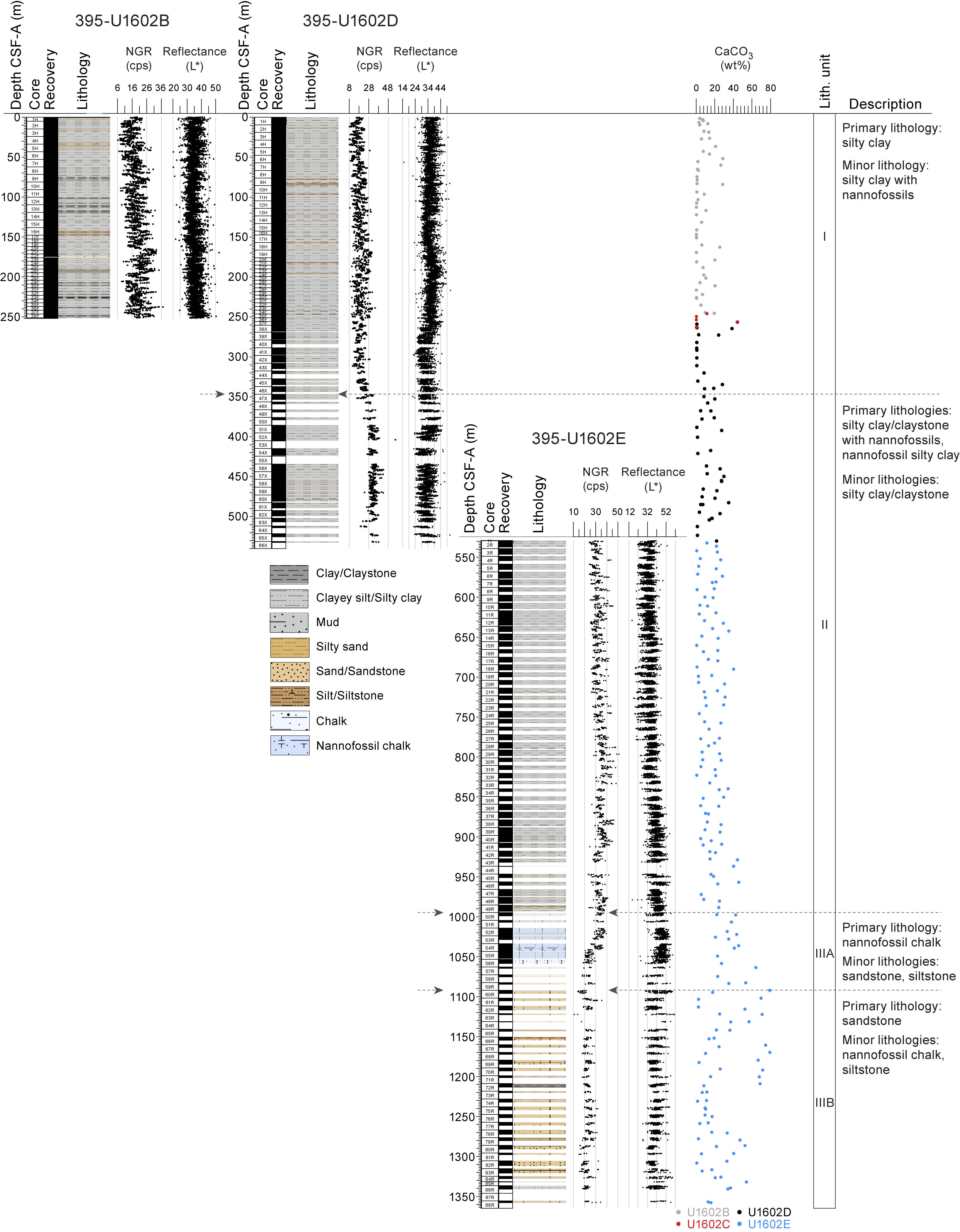
Figure F3. Lithostratigraphic summary, Site U1602.
Three lithostratigraphic units are observed at this site (Units I–III); Unit III is divided into Subunits IIIA and IIIB (Table T2). Core photographs of representative lithologies for the various units are shown in Figure F4. Unit and subunit boundaries were identified based on five parameters: (1) visual core description, (2) natural gamma radiation (NGR), (3) color reflectance L*, (4) smear slide examination, and (5) bulk CaCO3 measurements. Unit boundaries and corresponding physical properties data are shown in Figures F3 and F5. To assist in understanding the sedimentologic patterns at this site, NGR and color reflectance data were smoothed using an eighth-order lowpass Butterworth filter with a cutoff of 0.125 times the Nyquist frequency (Figure F5; this was applied to data that had undergone cleaning; see Physical properties in the Expedition 395 methods chapter [Parnell-Turner et al., 2025a]). This bidirectional linear digital filter avoids phase shift, maintaining correct peak positions (Butterworth, 1930; Lyons, 2011).
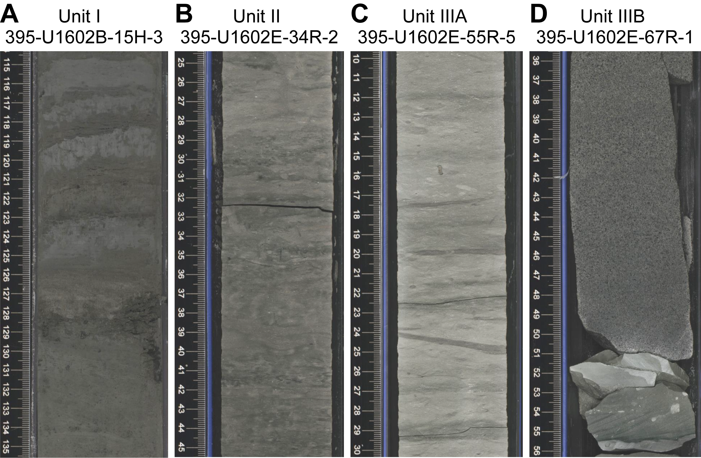
Figure F4. Primary lithologies.
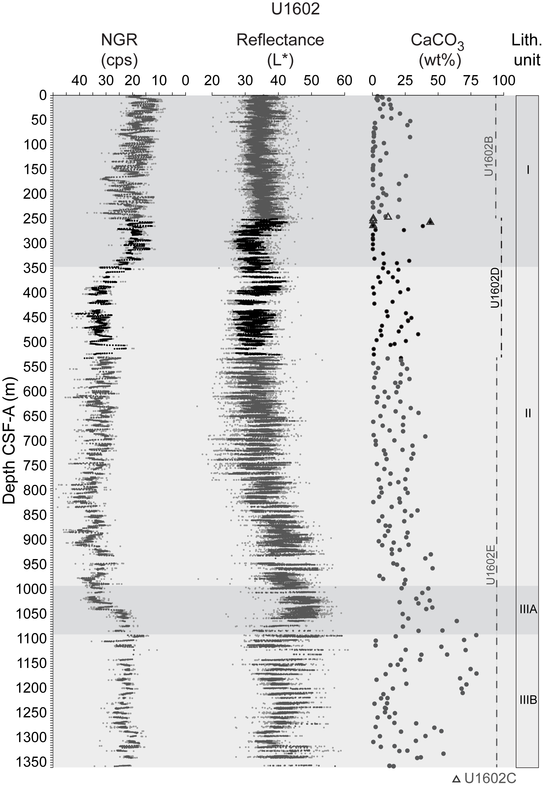
Figure F5. Lithologic unit definition parameters.
Numerous centimeter- to decimeter-scale graded beds and laminations were identified throughout Site U1602 sediments; in Units I and II, these features are prominent in most cores. Because of time constraints and the prevalence of the laminations and graded beds throughout the site, detailed descriptions of each feature were not conducted, and their occurrence is not consistently documented in the VCDs. Unit boundaries are transitional and not characterized by obvious lithologic changes; therefore, boundaries are placed at the top of core sections in which the transition occurs. Calcium carbonate (CaCO3) measurements (n = 268) were obtained for Holes U1602B–U1602E. Clasts are only present in Unit I, and clasts >2 cm observed on the split core surface are listed in Table T3.
3.1. Lithostratigraphic Unit I
- Intervals: 395-U1602A-1H-1, 0 cm, to end of hole; 395-U1602B-1H-1, 0 cm, to end of hole; 395-U1602C-1H-1, 0 cm, to end of hole; 395-U1602D-1H-1, 0 cm, to 47X-1, 0 cm
- Depths: Hole U1602A = 0–8.81 m core depth below seafloor, Method A (CSF-A); Hole U1602B = 0–251.43 m CSF-A; Hole U1602C = 0–269.19 m CSF-A; Hole U1602D = 0–346.70 m CSF-A
- Thickness: Hole U1602A = 8.81 m; Hole U1602B = 251.43 m; Hole U1602C = 269.19 m; Hole U1602D = 346.70 m
- Age: Holocene to late Pliocene
- Lithology: silty clay
In Unit I, the primary lithology of the sediments is dark gray to black silty clay (Figure F4A). The minor lithologies of Unit I include gray to dark greenish gray silty clay with biogenics and dark gray silt with sand. In general, biogenics are less than 30% of the sediment composition; however, the relative abundance of nannofossils is abundant to dominant, foraminifers are rare to common, and biosilica (diatoms, radiolarians, and sponge spicules) is rare to abundant. CaCO3 ranges 0–44 wt% (average = 9 wt%). The terrigenous component is primarily quartz, feldspar, and glass with smaller amounts of opaque grains and pyrite (Figure F6A). Glauconite is consistently observed in minor amounts throughout this unit. Several glass layers are found from 75 to 107 m CSF-A (Figure F7A). In addition to clasts, gravel beds are also present in Unit I (Table T3). Well-sorted, laminated silt or fine sand laminations (centimeter to ~0.5 m thick) are present throughout the unit, typically fining upward with a sharp boundary at the base and sometimes displaying cross-bedding (Figure F7E). Thin laminated beds (centimeter-scale) alternate with greenish gray clay. Bioturbation is primarily sparse to moderate. There is slight to moderate drilling deformation at the uppermost portions of the cores. In Hole U1602D, moderate to strong biscuiting is observed from Core 38X to the base of the unit (Section 47X-1, 0 cm).
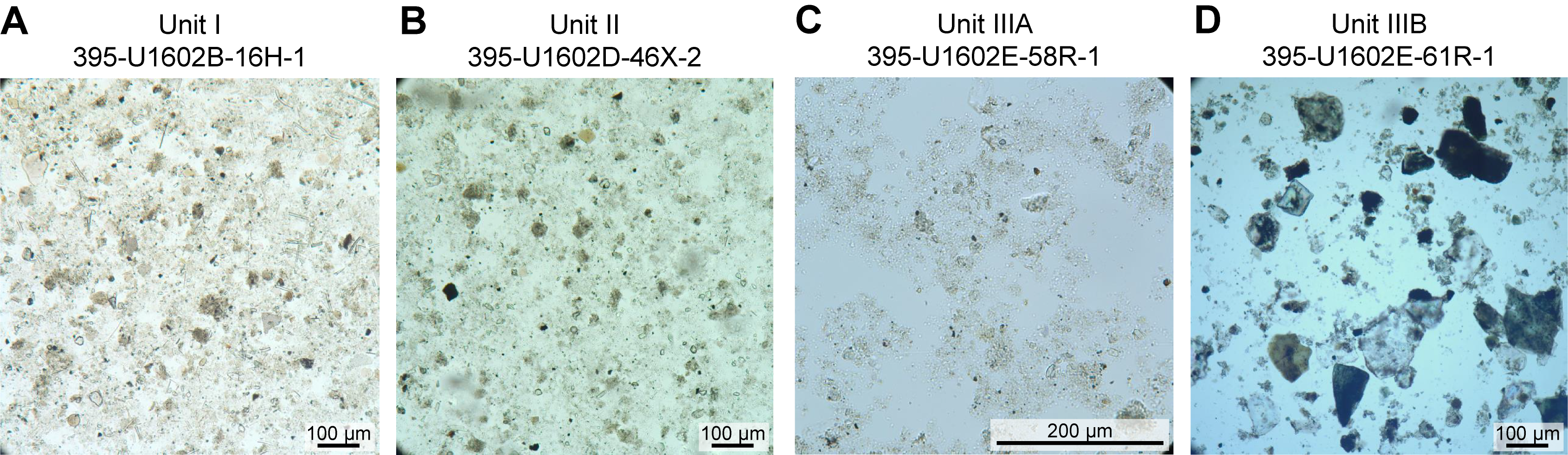
Figure F6. Representative lithologies of silty clay, nannofossil chalk, and sand and silt.
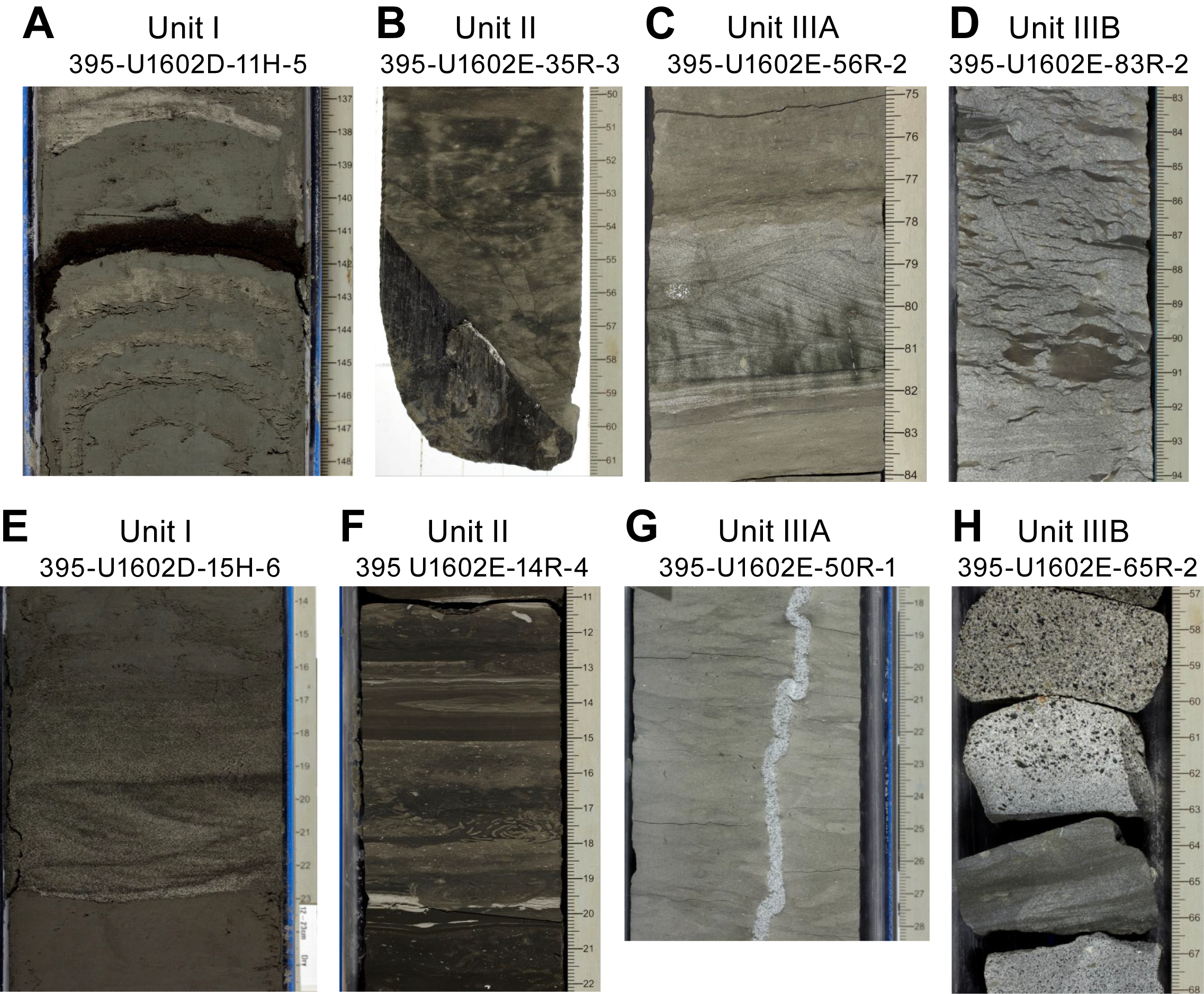
Figure F7. Sedimentary textures and features.
3.2. Lithostratigraphic Unit II
- Intervals: 395-U1602D-47X-1, 0 cm, to end of hole; 395-U1602E-2R-1, 0 cm, to 50R-1, 0 cm
- Depths: Hole U1602D = 346.70–532.36 m CSF-A; Hole U1602E = 529.30–994.80 m CSF-A
- Thickness: Hole U1602D = 185.66 m; Hole U1602E = 465.5 m
- Age: late Pliocene to Miocene
- Lithology: silty clay/claystone with nannofossils and nannofossil silty clay/claystone
In Unit II, lithification increases downhole. The primary lithologies are gray to dark gray silty clay/claystone with nannofossils and nannofossil silty clay/claystone (Figure F4B). The minor lithologies are dark gray to black silty clay/claystone and silt with sand/sandstone. Similar well-sorted, graded laminated layers continue through this unit, still composed of silt and/or fine sand and accompanied by sharp boundaries at their base. Some laminations are cross-cut by bioturbation (Figure F7F). Pyritized burrows and green mottling are observed throughout. Fractures with slickensides are occasionally present from Core 395-U1602E-31R to the base of the unit (see Lithostratigraphic Unit III) (Figure F7B). Biogenics generally comprise less than 50% of the sediment composition; these are primarily nannofossils, with trace foraminifers (Figure F6B). Biosilica is absent throughout Unit II. This observation is coincident with low pore water silicon measurements throughout this unit. CaCO3 ranges 0–35 wt% (average = 14 wt%). The terrigenous component is primarily quartz, feldspar, glass, opaque grains, and pyrite with smaller amounts of glauconite, chlorite and Fe/Mn oxides. Bioturbation is primarily sparse to moderate.
Throughout Unit II, there is moderate to severe biscuiting in Hole U1602D. Moderate to severe biscuiting in Hole U1602E is confined to Cores 2R–27R. From Core 27R to base of unit, the cores are slightly to severely fragmented. Overall, core recovery begins to decline in Unit II, with an average recovery of 63% (range = 0%–101%).
3.3. Lithostratigraphic Unit III
- Interval: 395-U1602E-50R-1, 0 cm, to end of hole
- Depth: 994.8–1357.99 m CSF-A
- Thickness: 362.3 m
- Age: Miocene to late Eocene
- Lithology: nannofossil chalk and sandstone
In Unit III, the primary lithology of the sediments is gray to dark greenish gray nannofossil chalk and sandstone (Figure F4). Short (centimeter to ~10 cm) intervals of siltstone and mudstone are present. The sandstone and siltstone intervals are generally graded and well sorted. Unit III contains a wide variety of sedimentary structures, including fractures with slickensides, laminations, cross bedding, sand injection features, mud drapes, and flaser bedding (Figure F7). The sand injection features are interpreted as soft-sediment deformation (Figure F7G).
The biogenics in this unit are primarily nannofossils, and biosilica is absent. The terrigenous component is primarily quartz, feldspar, glass, opaque grains, pyrite, and glauconite with smaller amounts of chlorite, biotite, and Fe/Mn oxides observed in smear slides. Burrows, where present, appear vertically compressed and are commonly pyritized. CaCO3 concentration in this subunit ranges 1–79 wt% (average = 30 wt%). CaCO3 measurements targeted both the lightest and darkest intervals per core, especially those most and least likely to contain carbonate; therefore, these data should contain the most extreme values downcore. This sampling approach was followed regardless of recovery of each lithology to document the range of variability in CaCO3. Unit III is divided into two subunits.
3.3.1. Lithostratigraphic Subunit IIIA
- Interval: 395-U1602E-50R-1, 0 cm, to 60R-1, 0 cm
- Depth: 994.80–1092.10 m CSF-A
- Thickness: 97.3 m
- Age: Miocene
- Lithology: nannofossil chalk
Subunit IIIA is composed primarily of gray to greenish gray nannofossil chalk (Figure F4C). The minor lithology is gray to dark gray sandstone. Small intervals of siltstone are also present. The upper boundary of this subunit is defined by the transition from nannofossil silty claystone to nannofossil chalk. Subunit IIIA is characterized by small intervals of sandstone between large intervals of nannofossil chalk, although recovery of sandstone beds may have been poorer than that of nannofossil chalk. CaCO3 concentration ranges 23–79 wt% (average = 43 wt%). Bioturbation is generally abundant in the chalk, with a wide variety of trace fossils, but absent to sparse in the sandstone intervals.
The nannofossil chalk in this subunit hosts sand injection features, flaser bedding, and mud drapes. The relationship between nannofossil chalk and sandstone cannot be determined because of poor core recovery. The sandstone beds are commonly graded, displaying fining- or coarsening-upward sequences, lamination and cross bedding. The sandstone grains range from coarse to very fine and commonly grade into siltstone. Siltstone beds exhibit features similar to the sandstone beds (Figure F7C).
Biogenics comprise ~50% of the sediment composition, and are primarily nannofossils. The terrigenous component is primarily quartz, feldspar, glass, opaque grains, pyrite and glauconite with smaller amounts of chlorite, biotite, and Fe/Mn oxides (Figure F6C). Drilling disturbance is relatively pervasive and consists of predominantly slight to moderate fragmentation. Core recovery in this unit ranges 18%–94% (average = 51%).
3.3.2. Lithostratigraphic Subunit IIIB
- Interval: 395-U1602E-60R-1, 0 cm, to end of hole
- Depth: 1092.10–1357.99 m CSF-A
- Thickness: 265.89 m
- Age: Miocene to late Eocene
- Lithology: sandstone
Subunit IIIB is composed primarily of thin intervals (~5–20 cm) of gray to greenish gray nannofossil chalk between thick intervals (~1–4 m) of gray to dark greenish gray sandstone. The upper boundary of this subunit is defined by the transition from less than 50% sandstone (Subunit IIIA) to more than 50% sandstone (Subunit IIIB). Thinner intervals of gray siltstone are also present. Flaser bedding is commonly observed in the sandstone, particularly near the tops of beds. Some chalk beds in this subunit contain sand injection features, similar to Subunit IIIA. Also similar to Subunit IIIA, sandstones range from very fine grained to coarse grained. Massive bedding, fining- and coarsening-upward sequences, lamination, and cross bedding are commonly present in both the sandstone and siltstone beds (Figure F7). Alternating grading (coarsening-fining-coarsening cycles in a single bed, not separated by bedding planes) is also observed, although less commonly.
CaCO3 concentration ranges 1–79 wt% (average = 29 wt%), a large range resulting from the sampling procedure. Intervals with high CaCO3 content are from the thin intervals of nannofossil chalk and the lowest values are from the sandstone. Bioturbation is mainly absent to sparse in this subunit, with the exception of the thin intervals of chalk which appear moderately to abundantly bioturbated. Smear slides were mainly taken from the nannofossil chalk layers in this subunit and show similar composition to those from Subunit IIIA, with a slightly higher percentage of nannofossils, consistent with the higher CaCO3 weight percent in this subunit. The smear slides taken from sandstones and siltstones show almost 100% terrigenous components; nannofossils are occasionally present in these beds but are rare (Figure F6D). Quartz, feldspar, glass, glauconite, and opaque grains are the major components, with minor amounts of pyrite. Drilling disturbance is relatively pervasive, and consists of predominantly slight to moderate fragmentation. Core recovery in Subunit IIIB ranges 0%–61% (average = 36%).
3.4. XRD results
A subset of squeeze cake residues and other samples (n = 27) were analyzed for X-ray diffraction (XRD). The minerals identified are generally consistent with smear slide, thin section (see next section), and macroscopic observations (Figure F8; Table T4). One important exception is the identification of several minerals from the zeolite family (including phillipsite, stilbite, analcime, and clinoptilolite). Zeolites are difficult to identify in smear slides, and this discrepancy is not surprising. The primary minerals identified include quartz, calcite, assorted feldspar, K-feldspar, pyroxene, and amphibole, mica, pyrite, and chlorite, in addition to zeolite. Cordierite was identified in two samples, and it is likely that high-grade metamorphic rocks from Greenland provide a proximal source for the mineral. The amount of calcite implied by the diffraction patterns is variable but consistent with CaCO3 measurements. Because shipboard processing does not include the requisite preparation for clay mineral analysis, peaks observed with a 2θ of <15° should be treated with caution. Nonetheless, the primary peaks for glauconite, zeolite, and chlorite are also observed in this range. For these cases, glauconite was commonly observed in smear slides as well as thin sections. Zeolite (analcime) was identified from a separate sample taken for XRD analysis from a fracture (not shown); this mineral-specific analysis was very clearly dominated by analcime (sample taken from interval 395-U1602E-35R-3, 85–93 cm, and carefully scraped from slickensided surface). Finally, chlorite was also identified from smear slide analysis. Consequently, the identification of these three minerals is supported by several other lines of evidence. Future analysis specifically addressing the clay mineralogy in these samples will be useful for determining shifts in deposition processes and sediment sources.
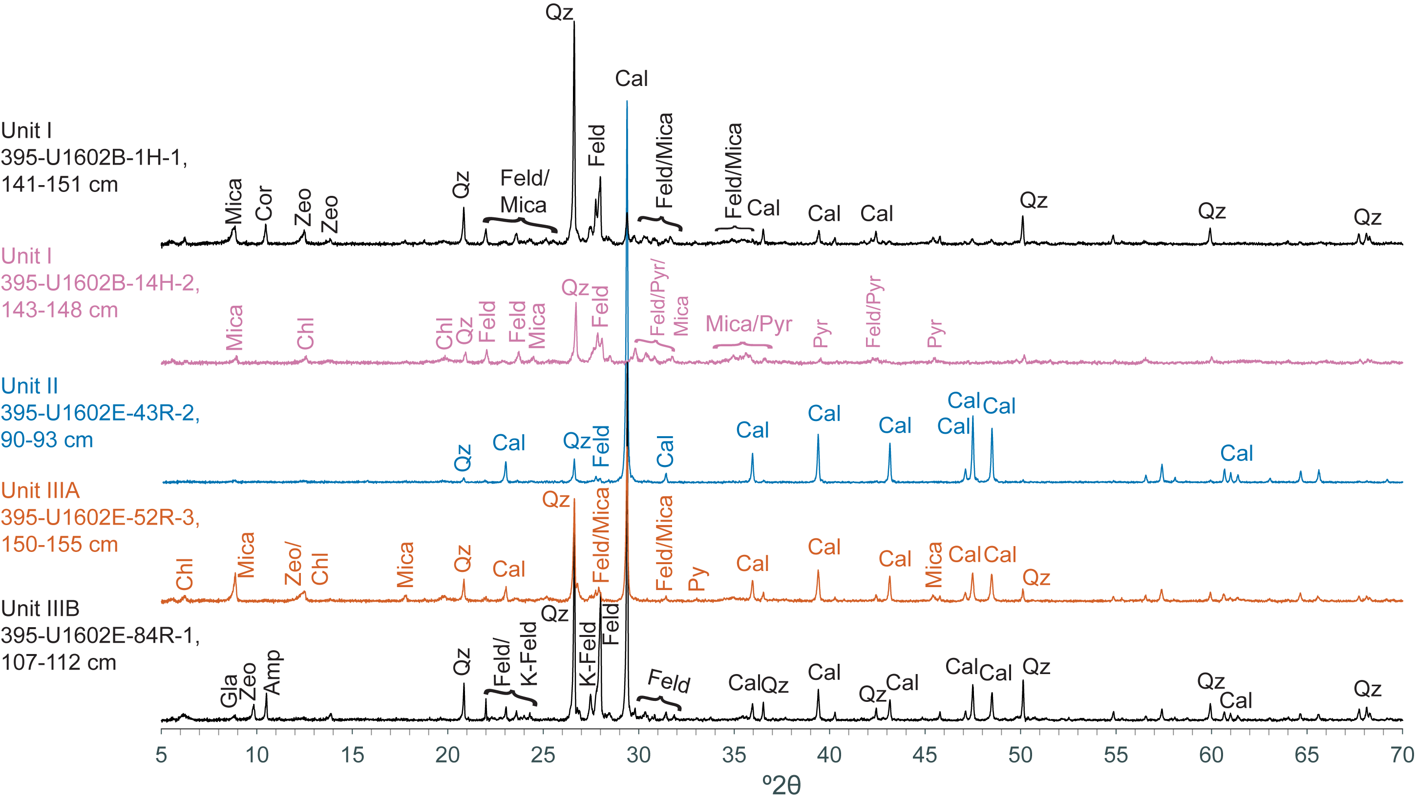
Figure F8. Powder XRD results.
3.5. Thin section analysis
With the addition of hornblende, a similar mineralogical assemblage is observed in thin sections of sandstones from Unit II compared to observations made with smear slide analysis. Grains are generally subangular to subrounded. Most grains are cemented with calcite, although some clay is also present. The calcite is sufficiently pervasive that most of the grains are not in contact. Sorting ranges from well to poorly sorted, and silt is common in the calcite and mud matrix and cement (Figure F9A, F9B). Note that although laminations, cross-bedding, and grading are readily recognizable in the cores, such features are difficult to recognize in thin section (Figure F9C, F9D).
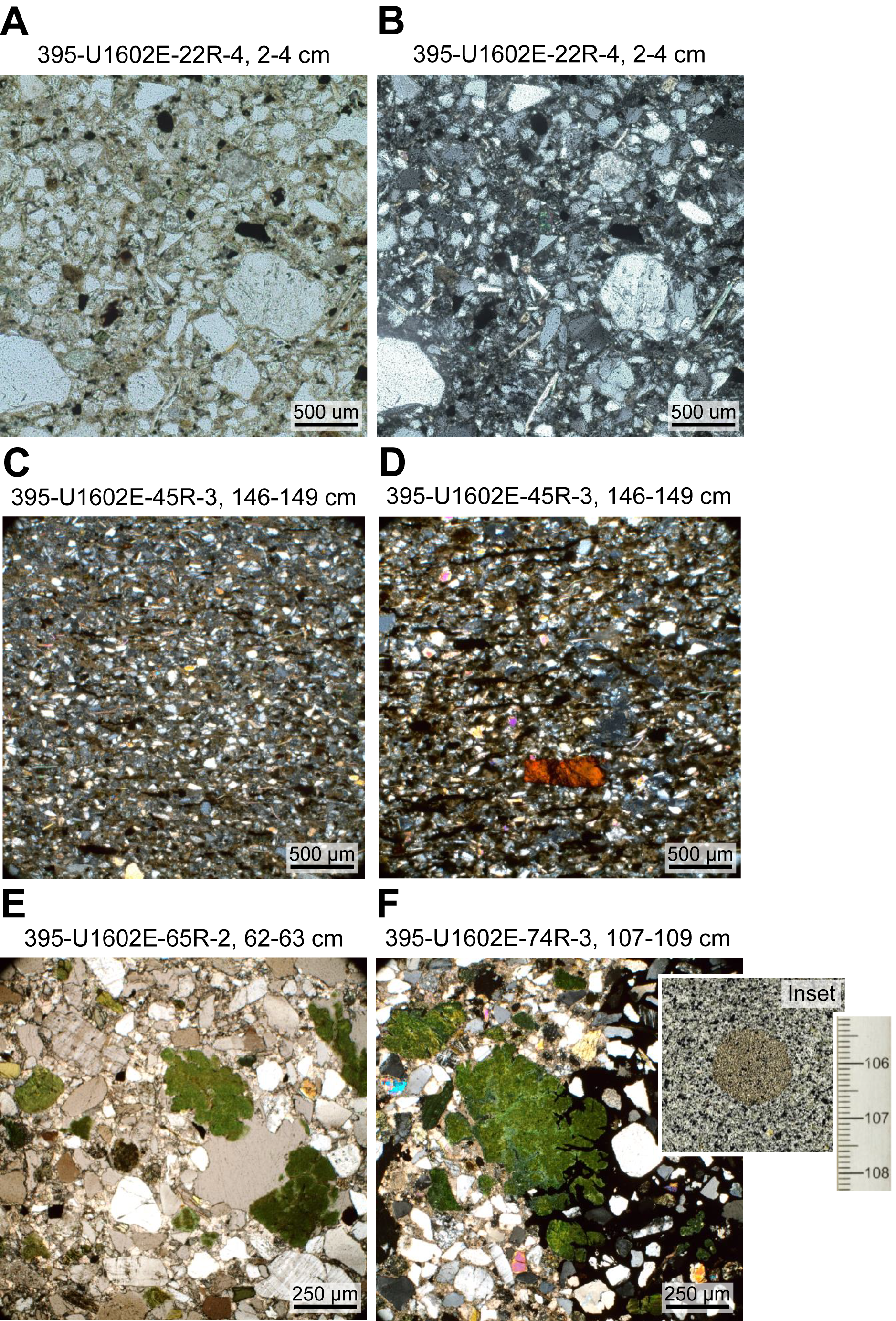
Figure F9. Selected specimens.
Thin sections from sandstones in Unit III are predominantly subangular to subrounded quartz. Feldspars are abundant, and mica, glauconite, chlorite, pyrite, and hornblende are present. Most grains are cemented with calcite, although some clay is also present. The calcite is sufficiently pervasive that most of the grains are not in contact. Sorting ranges from well to poorly sorted, and silt is common in the calcite and mud matrix and cement.
4. Micropaleontology
At Site U1602, a 1357.99 m long interval of upper Eocene/lower Oligocene to upper Pleistocene succession was recovered across multiple holes. Lithologies of the recovered sediments are mostly silty clay, with some nannofossil chalk and sandstone toward the base. Micropaleontological analyses were undertaken on samples from Holes U1602B (0–251.43 m CSF-A), U1602C (255.43–264.9 m CSF-A), U1602D (250.31–532.36 m CSF-A) and U1602E (537.07–1357.99 m CSF-A). Biohorizons used in the age model are based on calcareous nannoplankton, planktonic foraminifers, and bolboforms, which are present in varying abundances through the succession from barren or nearly barren samples to those with very high abundances. Extensive intervals were barren of planktonic foraminifers but still yielded calcareous nannofossil assemblages with low to moderate abundance, especially the Oligocene and lower Miocene sandstone and siltstone horizons.
4.1. Calcareous nannofossils
A total of 294 core catcher samples and working half section samples from all studied holes at Site U1602 were investigated for calcareous nannofossils. Observations were undertaken using plane-polarized light, cross-polarized light, and circular-polarized light. Table T5 provides a list of calcareous nannofossil bioevents that are mostly based on Hole U1602B for the Pleistocene, Hole U1602D for the Pliocene, and Hole U1602E for the Miocene and Oligocene. Calcareous nannofossils are present in most samples, with distinctly differing abundances alternating in intervals downcore from few (1–5 per field of view [FOV]) to dominant (hundreds per FOV). There is one uppermost Pliocene to lower Pleistocene interval where barren samples are more frequent in Samples 395-U1602B-12H-2, 68 cm (102.40 m CSF-A), to 395-U1602D-41X-CC (297.07 m CSF-A), although sequences of barren samples are broken up by short intervals where samples yield high calcareous nannofossil abundances with good preservation (e.g., Samples 395-U1602B-27F-3, 49 cm [198.06 m CSF-A], to 28F-CC [204.20 m CSF-A]).
Overall preservation worsens with depth. Where nannofossils are present in the interval from the top of Hole U1602B (Sample 1H-CC; 5.10 m CSF-A) to Sample 15H-6, 75 cm (136.85 m CSF-A), they show good preservation with intervals of very good preservation. Below this depth, in Samples 15H-6, 75 cm (136.85 m CSF-A), to 30R-CC (805.91 m CSF-A), preservation varies between moderate and good. Preservation worsens in the interval from Sample 395-U1602E-30R-CC (805.91 m CSF-A) to the base of Hole U1602E (Sample 88R-2, 87 cm; 1357.97 m CSF-A), varying between poor and good. In this interval, the standard smear slide preparation technique was altered to improve the quality of slides prepared from coarse silt and fine sand lithologies. Prior to smear slide preparation, an approximately 2 cm3 bulk sediment sample was disaggregated with mortar and pestle and a small amount of deionized water. This sediment was then transferred to an 80 mm diameter 38 µm sieve placed over a watch glass. The suspended fine fraction was gently washed through the sieve using as small a volume of deionized water as possible. The suspension of fine fraction (<38 µm) sediment collected in the watch glass was then gently agitated with the tip of a disposable pipette to resuspend and homogenize the sediment, and then a small amount was transferred with the pipette to a microscope slide warming on a hot plate. As the suspension dried out, further sediment drops were added until a sufficient concentration of sediment was present to make a standard smear slide. Where nannofossil chalks or nannofossil-bearing claystones were sampled, the standard smear slide technique was employed.
Using the above technique, nannofossil assemblages with good preservation were recovered, even in the deepest sample of Hole U1602E (88R-1, 102 cm), from nonlaminated, greenish, poorly consolidated coarse silt to fine sand lithologies. In these lithologies, there is still a small clay to fine silt matrix that bears well-preserved nannofossils. In contrast, hard nannofossil chalks and nannofossil-bearing claystones in the same interval typically yielded somewhat fragmented and substantially overgrown nannofossils, often outweighed in smear slide preparations by an abundance of diagenetic inorganic calcite within the nannofossil chalks. Siltstones with visible laminations are mostly barren or have very few to no nannofossils, which is consistent with more rapid deposition of clastic material by bottom currents. Samples from split cores were mostly targeted toward softer unlaminated greenish silts. Nannofossil chalks, claystones and laminated silt, and sandstones were avoided.
Seven biohorizons spanning the Pleistocene were identified (Table T5), providing an excellent biochronology from base common Emiliania huxleyi (0.09 Ma) between Samples 395-U1602B-1H-CC (5.10 m CSF-A) and 2H-CC (15.15 m CSF-A) to base Gephyrocapsa >4 µm (1.71 Ma) between Samples 22F-1, 60 cm (171.8 m CSF-A), and 23F-2, 80 cm (178.18 m CSF-A). Although one sample showed rare nannofossil abundance (Sample 3H-CC [24.22 m CSF-A]), most of the samples down to Sample 9H-CC (81.64 m CSF-A) vary from few to abundant nannofossils, all with good or very good preservation. It is likely that variations in abundance correlate with glacial (low abundance) and interglacial (high abundance conditions) intervals, with assemblages dominated by small Gephyrocapsa, Gephyrocapsa caribbeanica, and E. huxleyi. From Sample 10H-CC (91.15 m CSF-A) into the low abundance lower Pleistocene interval noted above, the mean nannofossil abundance appears to decrease with more samples yielding no, rare, or few nannofossils. This change in abundance appears to coincide with the mid-Pleistocene transition from glacial cycles dominated by 40–100 ky periodicities.
The placement accuracy of the Pleistocene biohorizon top Helicosphaera sellii (1.24 Ma) is limited by several barren samples above its last observed occurrence and is placed between Samples 395-U1602B-12H-CC (109.89 m CSF-A) and 14H-3, 48 cm (122.64 m CSF-A).
Although calcareous nannofossils are almost consistently present with moderate to good preservation in the Pliocene sediments of Hole U1602D and at the top of Hole U1602E, except for barren Sample 395-U1602D-51X-CC (395.27 m CSF-A), only one calcareous nannofossil biohorizon was identified for this interval. This biohorizon is top Reticulofenestra pseudoumbilicus (3.82 Ma) between Samples 50X-1, 110 cm (376.90 m CSF-A), and 50X-CC (378.87 m CSF-A). The placement of this biohorizon is complicated by the rare occurrences of reworked R. pseudoumbilicus (or potentially Reticulofenestra dictyoda, Paleogene equivalents) morphotypes between Samples 42X-4, 24 cm (302.93 m CSF-A), and 46X-CC (343.60 m CSF-A). In this interval, there is also some rare but characteristic reworking of other Paleogene reticulofenestrids, including Cyclicargolithus abisectus and Reticulofenestra bisecta. Below this interval, there is a consistent absence of R. pseudoumbilicus morphologies between Samples 46X-1, 53 cm (347.23 m CSF-A), and 50X-1, 110 cm (376.90 m CSF-A), before it is observed with frequent abundance in Sample 50X-CC (378.87 m CSF-A), which we pick as the true top of this species. Other standard Pliocene biohorizons (Raffi et al., 2020) are not recognized because of the absence or very low abundance of Discoaster marker species in the Pliocene sediments at Site U1602, along with the complete absence of Amaurolithus and Ceratolithus.
Discoasters become more consistently present in the cored Miocene interval, roughly from the top of Hole U1602E (Sample 2R-CC [537.07 m CSF-A]) downward, with the most common being the six-rayed Discoaster variabilis. These occurrences include the marker species Discoaster quinqueramus, which has both biohorizon top (5.53 Ma) and base (8.1 Ma) that are useful in biostratigraphy. The occurrence of this species is sporadic and usually occurs as a single occurrence in 2–4 transects of a standard smear slide. Because of this low abundance, we used the first downhole observed occurrence to constrain the maximum depth of the top (the top must be this sample or shallower) in Sample 11R-CC (626.06 m CSF-A). Likewise, we use the last downhole observation to constrain a minimum depth of base D. quinqueramus (must be this sample or deeper) in Sample 26R-CC (766.61 m CSF-A).
The abundance distribution of R. pseudoumbilicus through the Miocene is also complex and makes identification of the paracme of this species (7.1–8.8 Ma) difficult. The distinctive late Miocene size reduction of R. pseudoumbilicus was described in the tropical Indian Ocean by Young (1990) and now has entered biostratigraphic schemes; it is defined as a period of absence of morphotypes larger than 7 µm (Raffi et al., 2020). However, Young (1990) originally noted that its biostratigraphic application to high-latitude successions may not be reliable because of diachrony, different patterns of size changes through time, and the complexities of distinguishing between R. pseudoumbilicus and large specimens of Reticulofenestra perplexa. Here, we have applied an 8 µm size threshold rather than the 7 µm size threshold of the original paper because this higher threshold is preferred by experienced industry-sector biostratigraphers (https://www.mikrotax.org/Nannotax3/cenozoic/Reticulofenestra_pseudoumbilicus). It is also clear that larger morphotypes of R. perplexa in Holes U1602D and U1602E do regularly show a somewhat open central area even though a more fully closed central area morphology is dominant. As a result, true R. pseudoumbilicus morphologies must be carefully distinguished and characterized by their wide central area, which is typically wider than the shield width.
Downcore, this taxonomic complexity is compounded by multiple prolonged intervals of absent R. pseudoumbilicus interspersed with intervals where they are rare to frequent (Table T6). These patterns downcore present multiple intervals that could be identified as the biostratigraphically identified R. pseudoumbilicus acme. In particular, Interval 4, between Samples 395-U1602D-61X-1, 64 cm (483.14 m CSF-A), and 395-U1602E-6R-CC (576.29 m CSF-A), could be confused with the paracme; however, given other age constraints within the succession it is more likely correlated to the ~Miocene/Pliocene boundary size reduction in R. pseudoumbilicus noted by Young (1990). Below this depth, the top of the paracme is placed between Samples 395-U1602E-25R-CC (757.61 m CSF-A) and 26R-CC (766.61 m CSF-A) at the top of a prolonged interval with no and then rare (downcore) occurrences of R. pseudoumbilicus. The biohorizon base paracme could be picked between Samples 31R-1, 88 cm (811.58 m CSF-A), and 31R-4, 51 cm (815.66 m CSF-A), which marks the reentry of rare specimens of R. pseudoumbilicus >8 µm (Interval 7). However, there is then a further period of near absence (Interval 8) with R. pseudoumbilicus >8 µm only observed as two specimens in 2 out of 17 samples. The first reappearance of frequent R. pseudoumbilicus is at the top of Interval 9 in Sample 43R-CC (931.88 m CSF-A). The patterns described in Young (1990) show that the base of the paracme is characterized by the rapid loss of large forms (equivalent to the rapid reentry of large forms downcore) and would be more comparable with the base of Interval 8 in Hole U1602E. Based on the similarities between Young (1990) and our observations, base paracme of R. pseudoumbilicus is placed between Samples 42R-1, 46 cm (918.06 m CSF-A), and 43R-CC (931.88 m CSF-A). Again, based on the paleomagnetic constraints of the age model, the base paracme is likely to be this base of Interval 8 rather than the base of Interval 6. With such expanded successions and potentially good independent age control, Site U1602 has great potential for studies of the dynamics of R. pseudoumbilicus size changes in the high northern latitudes, the taxonomic differentiation from R. perplexa, and the biostratigraphic use of the paracme interval in this region.
Toward the base of the upper Miocene, the biohorizon top Coccolithus miopelagicus (11.04 Ma) is placed between Samples 395-U1602E-48R-4, 74 cm (980.57 m CSF-A), and 48R-CC (983.34 m CSF-A). C. miopelagicus is always rare in this succession, but the biohorizon top is placed at the top of a run of samples in which at least one specimen of C. miopelagicus that exceeds 14 µm in length is observed (Samples 48R-CC [983.34 m CSF-A] to 50R-CC [998.87 m CSF-A]). Below this interval, large (>14 µm) C. miopelagicus are only observed sporadically and are always very rare.
A series of biohorizons with calibrated ages around 13 Ma cluster around ~1080–1100 m CSF-A, providing confidence in the age of this interval. Most reliable in placement are top common Cyclicargolithus floridanus (13.33 Ma) and top Sphenolithus heteromorphus (13.60 Ma), which are both placed between Samples 395-U1602E-59R-2, 109 cm (1084.61 m CSF-A), and 60R-CC (1096.10 m CSF-A). Below this level, medium to large C. floridanus are frequent to common in most samples, and although rare, a number of specimens of S. heteromorphus are consistently observed per sample. In contrast, only single occurrences are observed of Calcidiscus premacintyrei in Samples 59R-2, 16 cm (1083.68 m CSF-A), and 59R-2, 109 cm (1084.61 m CSF-A). As a result of the uncertainty associated with such rare occurrences, these two samples are used as the maximum depth of the top (12.57 Ma; the top must be this sample or shallower) and the minimum depth of the base (13.16 Ma; the base must be this sample or deeper) of C. premacintyrei. Likewise, although Coronocyclus nitescens is rare in Sample 60R-CC (1096.10 m CSF-A), outside of this sample it is only recorded in one other sample (62R-1, 92 cm; 1112.52 m CSF-A) and then as a singleton. Therefore, consistent with the treatment of other very rare marker species, top C. nitescens (12.45 Ma) is placed with a maximum depth in Sample 60R-CC (1096.10 m CSF-A).
At the base of the middle Miocene, the distinctive Helicosphaera ampliaperta is recognized with rare but consistent abundances in a number of samples, with a top (14.86 Ma) placed between Samples 395-U1602E-61R-CC (1105.38 m CSF-A) and 62R-1, 92 cm (1112.52 m CSF-A). The base of the middle Miocene is then constrained to be between the above biohorizon and base common S. heteromorphus (17.65 Ma), which is placed between Samples 64R-1, 40 cm (1131.5 m CSF-A), and 64R-1, 64 cm (1131.74 m CSF-A). The placement of other lower Miocene biohorizons is more uncertain. The crossover in abundance between Helicosphaera carteri (younger) and Helicosphaera euphratis (older; 20.98 Ma) is identified between Samples 67R-2, 76 cm (1162.09 m CSF-A), and 69R-1, 139 cm (1180.89 m CSF-A), based on five H. carteri and one H. euphratis observed in the top sample versus no H. carteri and three H. euphratis observed in the lower sample. Above and below this interval, the presence of Helicosphaera species is sporadic, but where specimens are present they support the dominance of H. carteri above and H. euphratis below this interval. Finally, Sphenolithus disbelemnos was only observed in Samples 64R-1, 40 cm (1131.50 m CSF-A), and 76R-3, 113 cm (1251.3 m CSF-A), and we use the latter sample as minimum depth constraint on the base (22.90 Ma) of this species.
The Oligocene/Miocene boundary (23.04 Ma) is approximated by the combined downhole appearance (tops) of R. bisecta and C. abisectus (>11 µm) between Samples 395-U1602E-76R-3, 113 cm (1251.3 m CSF-A), and 76R-3, 135 cm (1251.52 m CSF-A), below which both taxa are frequent to common in occurrence and constitute a significant component of Oligocene assemblages. Although these assemblages are not calibrated biohorizons, they are widely considered to have tops within the top Oligocene to basal Miocene nannofossil Zone NN1 (Young, 1998) with an estimated age range of 23.73–24.35 Ma (see Micropaleontology in the Expedition 395 methods chapter [Parnell-Turner et al., 2025a]).
Oligocene assemblages are uniformly dominated by a few taxa: C. floridanus across a range of sizes (3–11 µm), C. abisectus, R. bisecta, R. dictyoda, and Reticulofenestra lockeri with frequent Chiasmolithus altus and Sphenolithus moriformis. None of the age diagnostic Furcatolithus or Triquetrorhabdulus species were observed in any Oligocene samples, making the placement of any late Oligocene biohorizons impossible. In the deepest core at Site U1602 (Core 395-U1602E-88R), Reticulofenestra umbilicus was observed, allowing the placement of the biohorizon top of this species (32.02 Ma) between Samples 87R-CC (1346.10 m CSF-A) and 88R-1, 102 cm (1356.62 m CSF-A) and constraining the base of the hole to be older than 32.02 Ma.
4.2. Planktonic foraminifers
Planktonic foraminifers at Site U1602 were studied in Holes U1602A (a mudline sample and Sample 1H-CC), U1602B (25 core catcher samples from near the seafloor to Sample 38F-CC [251.4 m CSF-A], plus four samples from within split cores), U1602C (two core catcher samples from 255.43 and 264.85 m CSF-A), U1602D (32 core catcher samples from 251.28 m CSF-A to the near bottom of the hole [532.31 m CSF-A], plus one sample from Section 37F-1 [256.08 m CSF-A]), and U1602E (59 core catcher samples from 537.07 m CSF-A to near the bottom of the hole [1357.02 m CSF-A], plus four samples from split cores). Together, these samples provide good coverage of the recovered sedimentary succession at the site.
In general, preservation declines with depth, but there is much variability in both preservation and abundance. Below ~100 m CSF-A, the sediment becomes increasingly hard and difficult to process. Below ~350 m CSF-A, the samples are mostly lithified and were cut into discs with a saw and freeze-dried for 48 h before soaking in water. From ~1050 m CSF-A downward, only every fifth core catcher sample was studied, most of which proved to be barren, although additional samples were taken from the split cores where foraminifers were observed on the sediment surface.
A list of planktonic foraminifer biohorizons is given in Table T7. Excellently preserved Holocene planktonic foraminifers dominate Sample 395-U1602A-1H-1, 0 cm, from the mudline. Neogloboquadrina pachyderma is dominant in this sample, as is expected from the oceanographic setting influenced by the cold East Greenland Current, and Neogloboquadrina incompta is frequent. Globigerina bulloides is also abundant, but the closely related morphospecies Globigerina umbilicata and Globigerina cariacoensis are absent.
Samples 395-U1602A-1H-CC (8.76 m CSF-A) and 395-U1602B-1H-CC (5.15 m CSF-A) are dominated by N. pachyderma with a few sinistral Neogloboquadrina dutertrei present and are assigned to the N. pachyderma Zone. Similar low-diversity assemblages dominated by neogloboquadrinids occur in all samples to Sample 395-U1602B-11H-CC (100.43 m CSF-A), although G. bulloides, Turborotalita quinqueloba, and Globoconella inflata are occasionally present and there are variable amounts of quartz and rock fragments in the residues, which are interpreted as ice-rafted debris. Samples 12H-CC (109.89 m CSF-A) and 13H-CC (119.61 m CSF-A) are barren with abundant rock fragments and quartz, but Sample 14H-CC (129.17 m CSF-A) is once again dominated by N. pachyderma. The base of common encrusted sinistral N. pachyderma, marking the base of the N. pachyderma Zone (1.82 Ma), is in a long interval that is mostly barren of planktonic foraminifers between Samples 14H-CC (129.17 m CSF-A) and 28F-CC (204.20 m CSF-A).
The interval from Samples 395-U1602B-28F-CC to 32F-CC (204.20–223.24 m CSF-A) varies from barren to abundant and includes four samples taken from the split cores where concentrations of foraminifers were observed with the hand lens; where present, the preservation is excellent and glassy. Assemblages are variable with N. incompta and T. quinqueloba abundant in some samples and small transparent Globorotalia scitula common in Sample 32F-3, 69–71 cm (221.92 m CSF-A). This sample contains the lowest occurrence of G. inflata, denoting the base of the G. inflata Zone (2.06 Ma), but the biohorizon has low confidence because the marker species at Site U1602 is discontinuous and always rare.
Top Neogloboquadrina atlantica, which marks the base of the G. bulloides Zone (2.26 Ma), is constrained by sampling across Holes U1602B–U1602D. Sample 395-U1602B-32F-CC (223.24 m CSF-A) lacks N. atlantica, and the three samples taken from below that depth in the same hole are all barren, as is the shallowest sample examined in Hole U1602D (Sample 35F-CC; 251.28 m CSF-A). Sample 36F-CC (256.01 m CSF-A), also from Hole U1602D, has abundant N. atlantica with excellent preservation. Another sample taken from a slightly lower depth in Hole U1602C, Sample 38F-CC (264.85 m CSF-A), has a similar assemblage with abundant N. atlantica. The top N. atlantica is thus placed between Samples 395-U1602B-32F-CC (223.24 m CSF-A) and 395-U1602D-36F-CC (256.01 m CSF-A).
N. atlantica is the most common planktonic foraminifer species in most of the succession throughout the rest of Hole U1602D and most of Hole U1602E, although preservation deteriorates markedly with depth and many samples are barren. Biostratigraphic control is limited because the zonal marker Globoconella puncticulata was not found at the site and Globorotalia cibaoensis is rare and sporadic. Many samples contain a high proportion of deformed and flattened individuals. An interesting diagenetic feature is observed in Sample 395-U1602E-25R-CC (757.61 m CSF-A), in which many broken chambers contain well-formed crystals of the zeolite group mineral analcime (identified using scanning electron microscope–energy dispersive spectrometry [SEM-EDS]) (Figure F10). The same mineral was found infilling foraminifers at two other depths (Samples 48R-CC [993.05 m CSF-A] and 74R-2, 54 cm [1230.02 m CSF-A]) and in multiple fractures in the succession (see Lithostratigraphy).

Figure F10. Deformed and broken planktonic foraminifer shells.
The base of G. cibaoensis, marking the base of the undifferentiated G. puncticulata and G. cibaoensis Zones (9.44 Ma), is located between Samples 395-U1602E-33R-CC (833.77 m CSF-A) and 36R-CC (866.08 m CSF-A) but with low confidence because of the rarity of the species and difficulty with its identification, especially when poorly preserved. Coiling directions in N. atlantica were measured whenever the species was recorded, although some samples yielded just a few crushed specimens (Table T8; Figure F11). The dextral to sinistral (upcore) switch in the dominant coiling direction (9.23 Ma) is located between Samples 33R-CC (833.77 m CSF-A) and 36R-CC (866.08 m CSF-A).
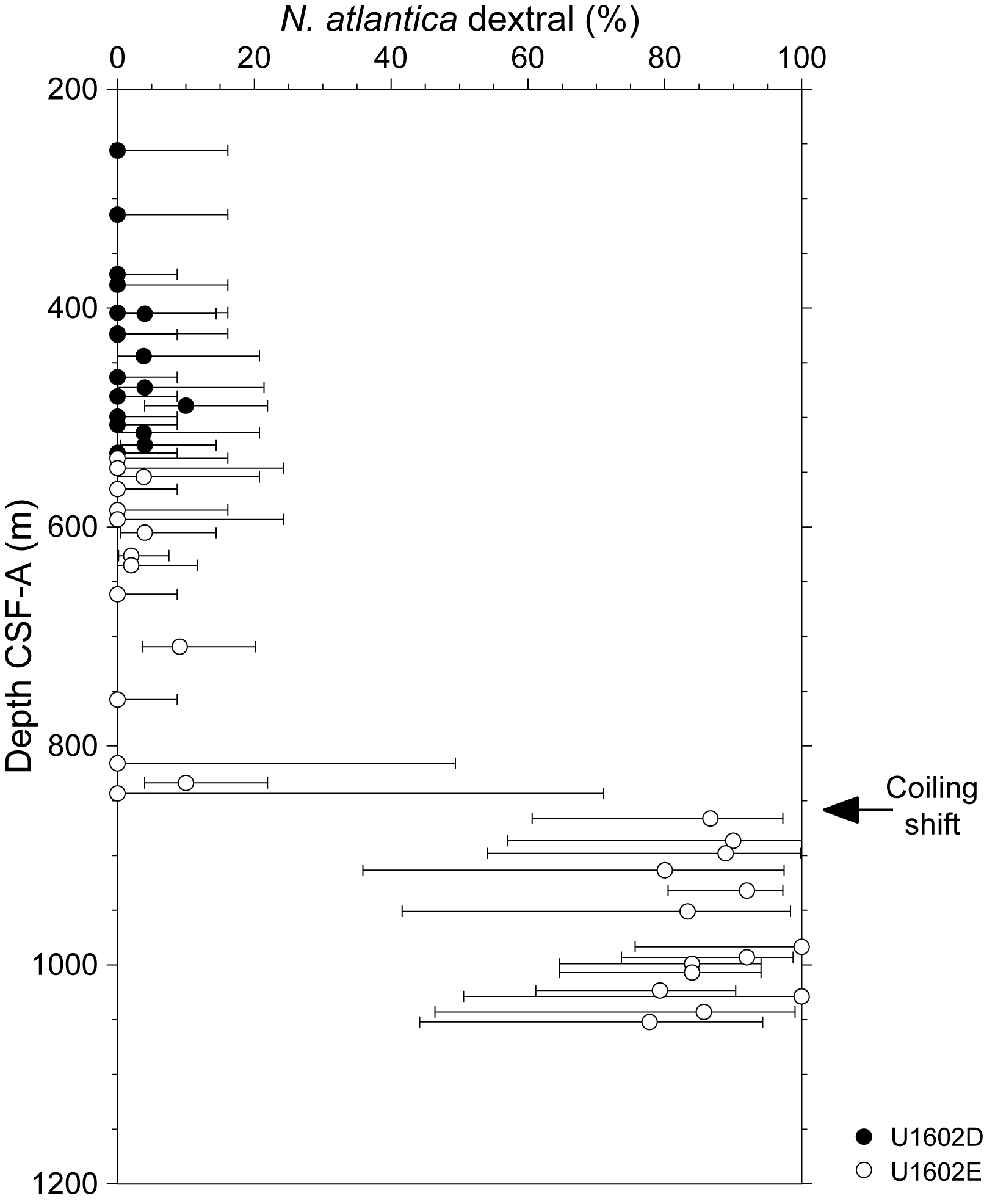
Figure F11. N. atlantica coiling ratios.
Below this depth, the foraminifer biostratigraphy is increasingly challenging because of poor preservation in hard, lithified sediment that is often barren. Orbulina universa (which first appeared globally at 15.12 Ma) was found in several samples down to Sample 395-U1602E-50R-CC (1006.89 m CSF-A), providing some age constraint, but its absence below that may be due to poor preservation rather than representing a genuine first appearance. A single specimen of Paragloborotalia mayeri (which disappeared at 10.54 Ma) was found in Sample 53R-CC (1028.67 m CSF-A), and this also provides some age constraint.
Small numbers of nondiagnostic, poorly preserved planktonic foraminifers are present in various samples down to Sample 395-U1602E-55R-CC (1052.05 m CSF-A). Below this sample is a long interval of core catcher samples that are mostly sandstones barren of foraminifers. However, planktonic foraminifers are common in Sample 88R-1, 142–144 cm (1357.02 m CSF-A), which was taken from the split core. Foraminifers are infilled and mostly flattened but well enough preserved to tentatively identify an upper Eocene assemblage containing Globigerinatheka index, Globigerinatheka sp., Catapsydrax unicavus, Subbotina angiporoides, and probable Subbotina gortanii. Top G. index (34.5 Ma) provides a minimum age constraint for this sample.
4.3. Bolboforms
Bolboforms were studied in the same sample set as planktonic foraminifers. The only interval where bolboforms are sufficiently abundant to study for biostratigraphy is between Samples 395-U1602E-48R-CC (993.05 m CSF-A) and 65R-CC (1143.35 m CSF-A). Preservation varies from good (showing the test shape and the broad ornamentation pattern but without preservation of fine details) to poor (recrystallized and deformed, with ornamentation difficult to discern). Abundance and taxonomic composition differ markedly, suggesting that there is significant ecological as well as evolutionary variability between samples.
Sample 395-U1602E-48R-CC (993.05 m CSF-A) has an assemblage of mostly flat-bottomed flask-shaped tests with reticulate ornamentation identified as Bolboforma metzmacheri. Sample 49R-CC (998.87 m CSF-A) contains very abundant bolboforms in a roughly equal mixture of just two identifiable species, B. metzmacheri and smooth-walled Bolboforma laevis. The bottom occurrence of B. metzmacheri (9.90 Ma) is between this sample and Sample 50R-CC (1006.89 m CSF-A), in which bolboforms are still abundant but which contains only B. laevis. A similar monospecific assemblage of B. laevis, although more poorly preserved, occurs in Sample 52R-CC (1023.25 m CSF-A). Below that level, the record is sparse except in Sample 65R-CC (1143.35 m CSF-A), where frequent very poorly preserved bolboforms were found, possibly belonging to Bolboforma fragori or morphologically similar species.
5. Physical properties
The suite of physical properties measurements acquired at Site U1602 is documented in Table T9. Physical properties data were collected on all cores, with the exception of moisture and density (MAD) data and P-wave velocity (VP) caliper (PWC) data for Hole U1602A, Whole-Round Multisensor Logger (WRMSL) P-wave logger (PWL) data for Hole U1602E, and thermal conductivity data for Holes U1602A and U1602C. Furthermore, discrete measurements of MAD and PWC were acquired only for specific cored intervals in each hole at Site U1602 (Table T10). Physical properties data were cleaned for half the response function corresponding to the instruments at the top and bottom of each section, and values deemed artifacts were removed from the respective figures (Table T11). All raw data are retained in the LIMS database.
5.1. Whole-round measurements
Data measured using the WRMSL and Natural Gamma Radiation Logger (NGRL) on cores from Holes U1602B (Figure F12), U1602C (Figure F13), U1602D (Figure F14), U1602E (Figure F15), and a composite of Holes U1602D and U1602E (Figure F16) correspond well with lithologic variations and expected trends with depth. In the upper 270 m of Holes U1602B–U1602D (Figures F12, F13, F14), the gamma ray attenuation (GRA) bulk density data vary between 1.3 and 2.2 g/cm3, with slightly higher amplitude variations observed in Hole U1602B. WRMSL MS measurements dominantly range 300–700 IU with a few excursions to higher values (e.g., ~33 m CSF-A). VP ranges 1400–1600 m/s, higher in Hole U1602C from 0 to 75 m CSF-A than recorded over the same depth interval in Holes U1602B and U1602D, with a marked difference at ~15 m CSF-A, where VP values reach ~1700 m/s. PWC measurements from samples from Hole U1602B over this depth interval broadly agree with PWL measurements from the same hole. NGR values range 10–30 counts/s and show fluctuations on the meter to decimeter scale. Fluctuations in each of the WRMSL measurements in this interval appear to coincide with each other (Figures F12, F13, F14).

Figure F12. Physical properties measurements, Hole U1602B.
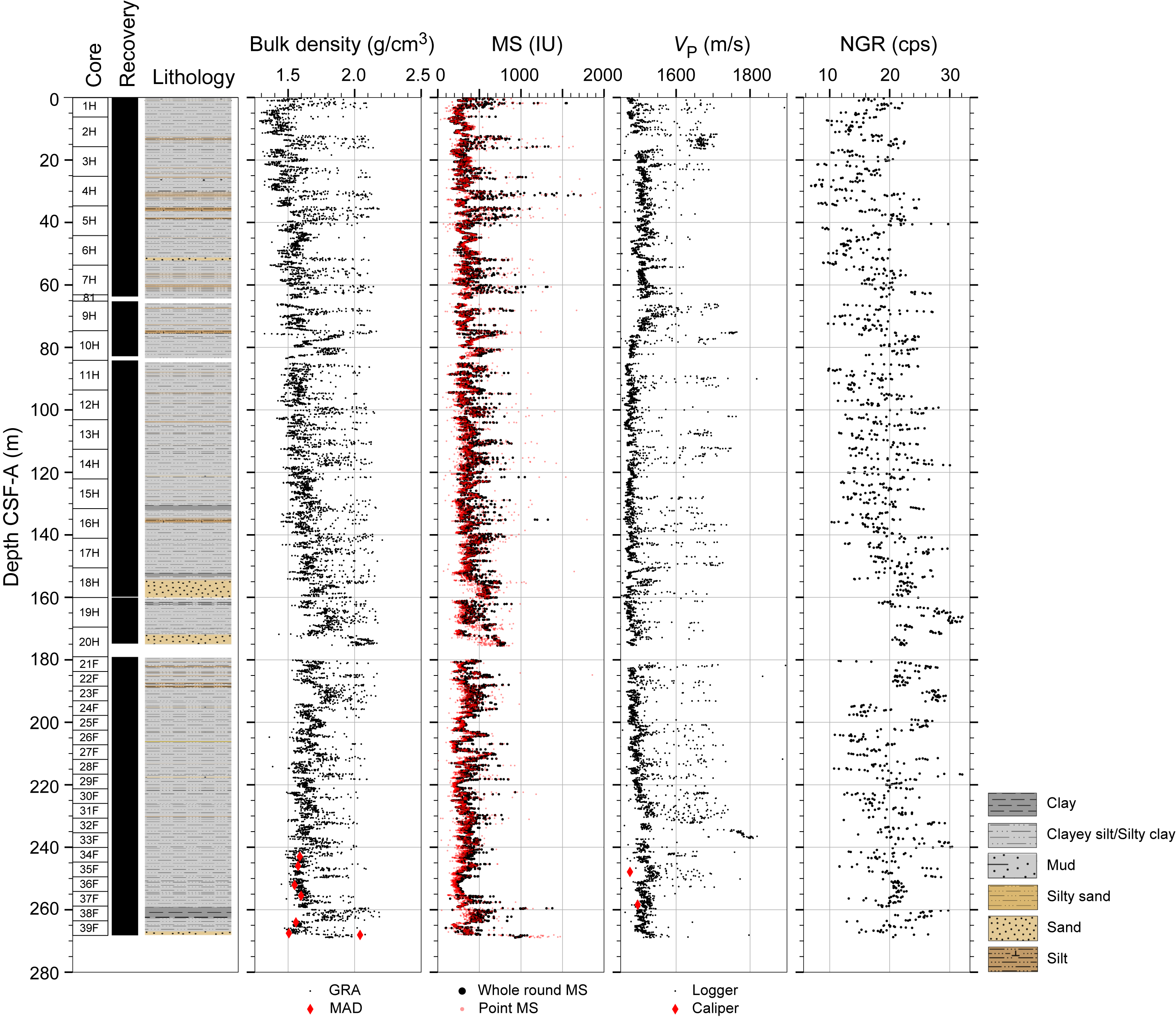
Figure F13. Physical properties measurements, Hole U1602C.
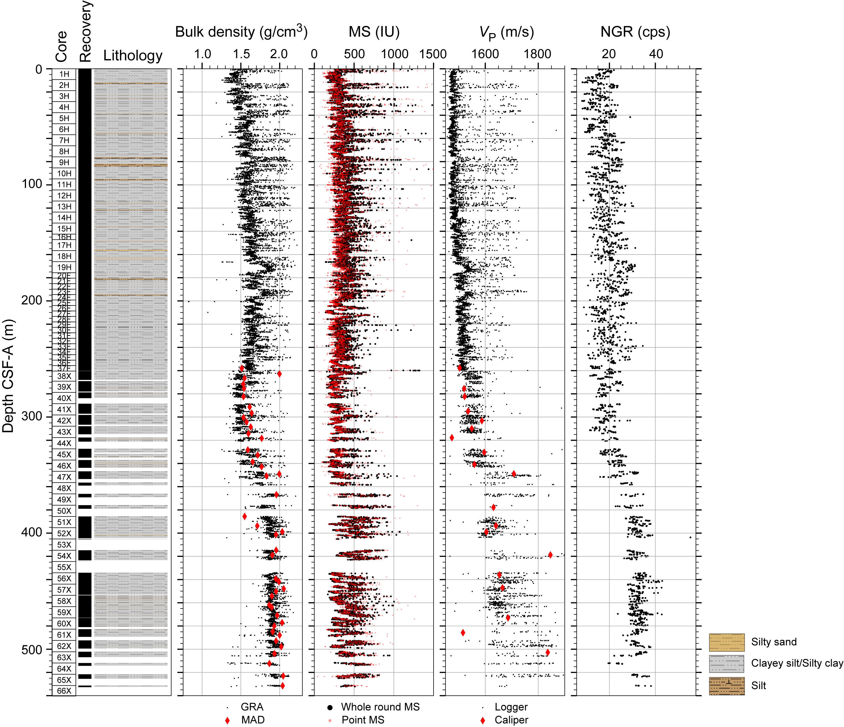
Figure F14. Physical properties measurements, Hole U1602D.

Figure F15. Physical properties measurements, Hole U1602E.
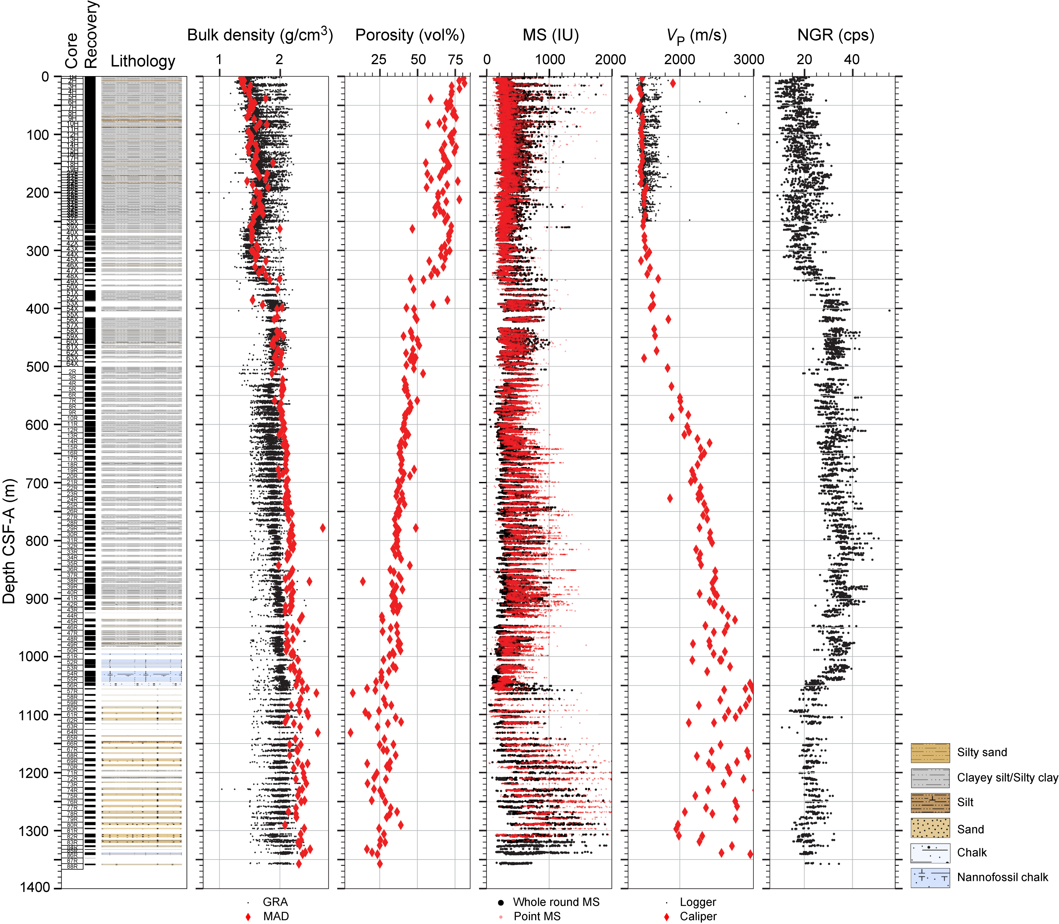
Figure F16. Physical properties measurements composite.
Cores from Holes U1602D (to 540 m CSF-A) and U1602E (520–1367 m CSF-A) collected material between 270 and 1367 m CSF-A (Figures F14, F15, F16). At ~260 m CSF-A, GRA bulk density values initially decrease and then begin to increase from ~1.5 to ~2 g/cm3 with depth to ~360 m CSF-A. From ~360 m CSF-A, GRA bulk density remains invariant at ~2 g/cm3 to ~540 m CSF-A. From ~540 m CSF-A, GRA bulk density averages around ~2 g/cm3 with varying spread in the data. From ~520 m CSF-A, in RCB drilled Hole U1602E, GRA bulk density consistently reports lower than density measured from discrete MAD samples due to the smaller diameter of cores not filling the liner. MS measurements in Hole U1602D display the same behavior reported from 0 to 270 m CSF-A in Holes U1602B and U1602C to ~320 m CSF-A, where the data show an initial increase and then decrease before remaining relatively low at ~440 m CSF-A. From 440 to ~530 m CSF-A, MS fluctuates on meter to decimeter depth scales. From ~530 to ~620 m CSF-A, MS is predominantly below ~500 IU. From ~620 to 940 m CSF, MS varies between ~200 and ~1000 IU. This sequence is followed by a sharp decrease in the maximum MS values to ~500 IU to ~1040 m CSF-A. From ~1040 to ~1360 m CSF-A (bottom depth of Hole U1602E), the range of MS values increases to a maximum of ~2000 IU. Similar transitions in MS are observed in downhole logs from Hole U1602E (see Downhole measurements).
VP was measured on whole-round cores from Hole U1602D from 0 to ~540 m CSF-A, and then, because of incomplete fill of the core liner in Hole U1602E, only PWC measurements were acquired over the 520–1380 m CSF-A interval. PWL measurements show an increase in VP at ~260 m CSF-A (from ~1550 to ~1575 m/s) and a larger increase at 350 m CSF-A (from ~1575 to an average of 1750 m/s). From 350 to 540 m CSF-A, PWL measurements show a greater range of VP than for shallower intervals, and further changes in this physical property are reported from discrete PWC measurements. Between 320 and 360 m CSF-A, NGR values gradually increase from around ~20 counts/s to around ~35 counts/s. From 360 to ~1040 m CSF-A, NGR varies from 30 to 40 counts/s, showing meter- to decimeter-scale fluctuations, particularly between 840 and 1040 m CSF-A. At ~1040 m CSF-A, the average NGR decreases to ~22 counts/s to ~1280 m CSF-A, where decreases in NGR create further observed oscillating behavior to 1380 m CSF-A.
5.2. Split core measurements
Point MS (MSP) data acquired using the Section Half Multisensor Logger (SHMSL) are displayed in Figures F12, F13, F14, F15, and F16. Both types of MS measurements show the same relative variations, and the absolute values for the sediments are very close to each other. MSP displays higher values than WRMSL MS from ~1060 to 1300 m CSF-A because of the smaller core diameter.
Figure F17 summarizes the reflectance and colorimetry data collected on the archive halves as measured using the SHMSL for Holes U1602D and U1602E. Graphs display long (>100 m) fluctuations from 0 to 920 m CSF-A with values of R, G, and B ranging 50–100. Below 920 m CSF-A, the R, G, and B values display a wider measurement spread, corresponding to lithologic variability (see Lithostratigraphy). L* and a* values vary with depth with similar increases and decreases. L* values follow similar fluctuations to those displayed by R, G, and B values, and a* measurements increase values where L* decreases (e.g., 420–920 m CSF-A). The b* measurements are relatively invariant with depth at Site U1602 with values averaging between 0 and −6, although below ~1050 m CSF-A this range decreases.
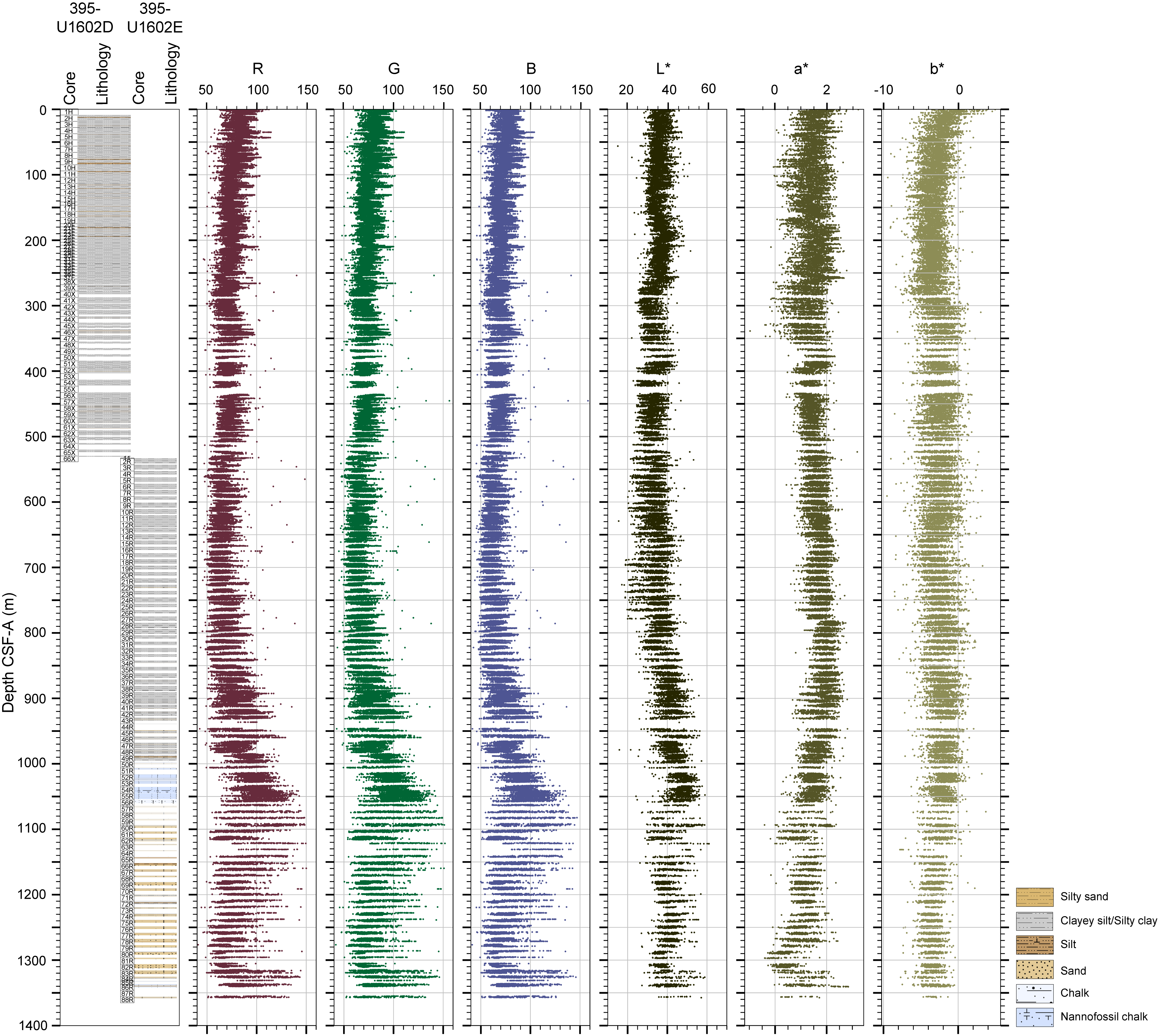
Figure F17. Archive-half colorimetry and reflectance measurements.
5.3. Discrete measurements
5.3.1. P-wave velocity
PWC measurements were made at approximately 10 m spacing using the caliper (x-direction) on the Section Half Measurement Gantry (SHMG) on core from Holes U1602B–U1602E. VP values average ~1500 m/s to ~300 m CSF-A. Between 300 and 540 m CSF-A, VP increases to ~2400 m/s and increases again at ~850 m CSF-A to ~2500 m/s. From ~940 to 1380 m CSF-A, PWC values show a wide range of measurements (2000–4000 m/s), reflecting the variety of sediment types observed in the core drilled from this interval at Site U1602 (see Lithostratigraphy).
5.3.2. Moisture and density
MAD measurements were taken on sediment cores, approximately one per 5 m in Holes U1602B–U1602E across variable depth intervals. MAD density data accord with WRMSL GRA bulk density values to ~500 m CSF-A, where they then show consistently higher density values than GRA bulk density. This divergence between the two differently derived density data is likely due to underestimations of density using the GRA bulk density method for RCB-cored sections. Core from ~500 m CSF-A (starting with Core 395-U1602E-2R) was drilled using the RCB system, whereas core from above this interval was drilled using the APC or XCB system. RCB core tends to be narrower than the core liner and does not fill the core liner as completely as XCB core does. This means the GRA bulk density measurement averages the density of the core and the air around it within the liner, thereby producing underestimations of the core density. MAD density values range from ~2.1 g/cm3 at 500 m CSF-A to 2.6 g/cm3 at ~1350 m CSF-A and show a slightly wider range of values below ~930 m CSF-A than above. Porosity data derived as part of the MAD method using a pycnometer displays a matching but opposite increase and decrease trend to the density data.
5.3.3. Thermal conductivity
Thermal conductivity measurements were made on selected working-half sections, approximately one per 10 m, in Holes U1602B, U1602D, and U1602E. Combining these measurements with five temperature measurements from the APCT-3 tool allowed a calculation of heat flow at Site U1602 (Figure F39; see Downhole measurements).
5.3.4. X-ray scans
Section halves from Holes U1602A–U1602E were imaged using the X-Ray Linescan Logger (XSCAN). Energy settings used to obtain the raw image included 90–100 kV and 0.9 mA. Figure F18 shows examples of features in XSCAN images.
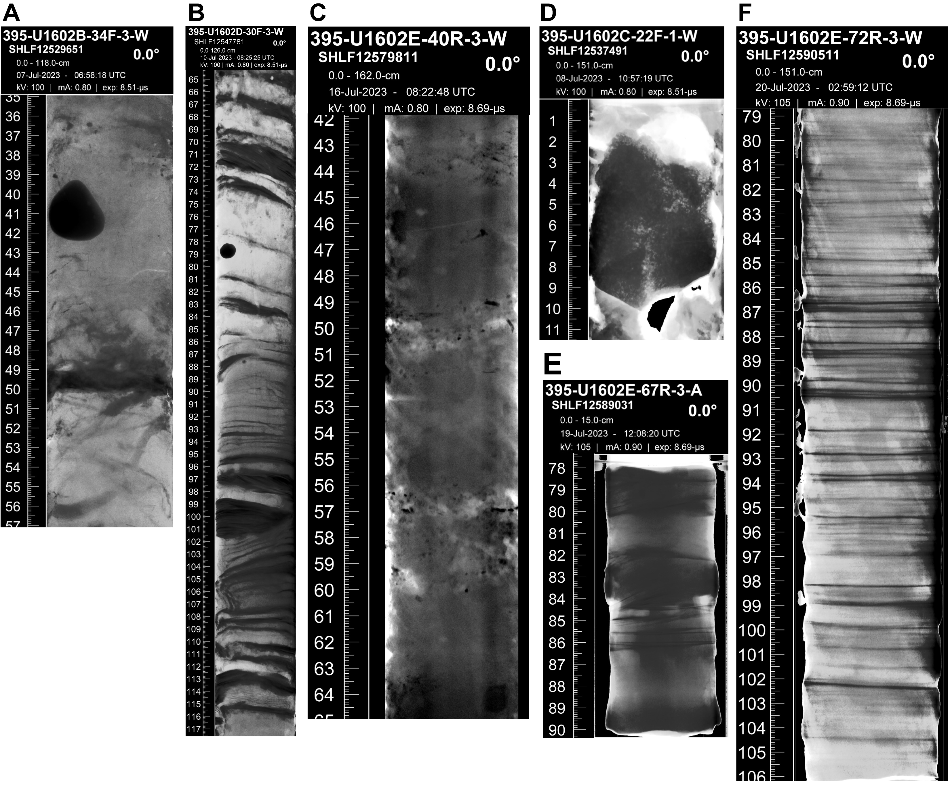
Figure F18. Archive-half XSCAN images.
6. Stratigraphic correlation
The stratigraphic correlation reported here includes the main sedimentary targets of stratigraphically overlapping cores from Holes U1602B–U1602D (Table T12). MS data from whole-round measurements were used for near real-time correlation because they often reveal strong contrasts between lithologic sequences. These data were obtained shortly after the core was recovered on deck at 5.0 cm resolution using the Special Task Multisensor Logger (STMSL) to guide operational decisions. The whole-round MS data collected at 2.5 cm resolution using the WRMSL were used to construct the final shipboard splices. An overview of the MS data from Holes U1602B–U1602D and the MS data from Hole U1602E that was not included in the splice is presented in Figure F19.
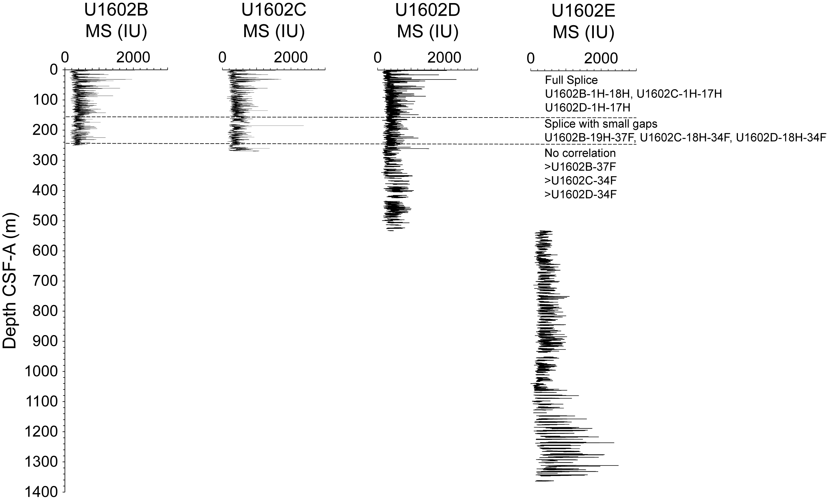
Figure F19. WRMSL MS.
6.1. Correlation between holes
The upper 140 m core composite depth below seafloor, Method A (CCSF-A), is shown in Figure F20, and the interval from 140 to 270 m CCSF-A is shown in Figure F21. Correlation was achieved without gaps starting at the mudline for Cores 395-U1602B-1H through 18H, 395-U1602C-1H through 17H, and 395-U1602D-1H through 17H (156.50 m CSF-A; 169.45 m CCSF-A) (Figure F22). The patterns in MS at the lower extent of these cores were too variable to confidently make a tie with any of the next cores, leading to a correlation gap. In contrast to other Expedition 395 sites, the downhole logging MS record was not straightforward enough to correlate with the MS point data measured on the cores and was therefore not used to assess the size of potential gaps in the recovered cores. Comparison of the lower resolution NGR signals from the downhole logging and core measurements suggests that there are no large stratigraphic recovery gaps for the spliced interval at Site U1602. However, because of the relatively low resolution of both NGR records and the edge effect for NGR as measured on cores, it was difficult to quantify the sizes of the gaps in correlation. Consequently, when a gap was suspected, the next core was simply appended without modifying the distance between cores. Another gap occurs between Cores 395-U1602B-21F and 22F, 395-U1602C-19H and 20H, and 395-U1602D-19H and 20F around 189 m CCSF-A. Penetration was difficult for this interval in all holes, possibly due to the presence of a sand layer, resulting in the switch from APC to HLAPC coring in Holes U1602B–U1602D. In Cores 395-U1602B-23F through 37F, 395-U1602C-21F through 34F, and 395-U1602D-20F through 34F, ties can be made to ~270 m CCSF-A (Figure F21). One exception is the contact between Cores 395-U1602B-35F and 36F, 395-U1602C-32F and 33F, and 395-U1602D-32F and 33F, where the cores are too close to alignment for the stratigraphic correlators to be able to tie on to any of the next cores, leading to a correlation gap. Below Cores 395-U1602B-37F, 395-U1602C-34F, and 395-U1602D-34F, correlation between holes was not attempted because of the lack of similarity in MS variations with depth between holes.
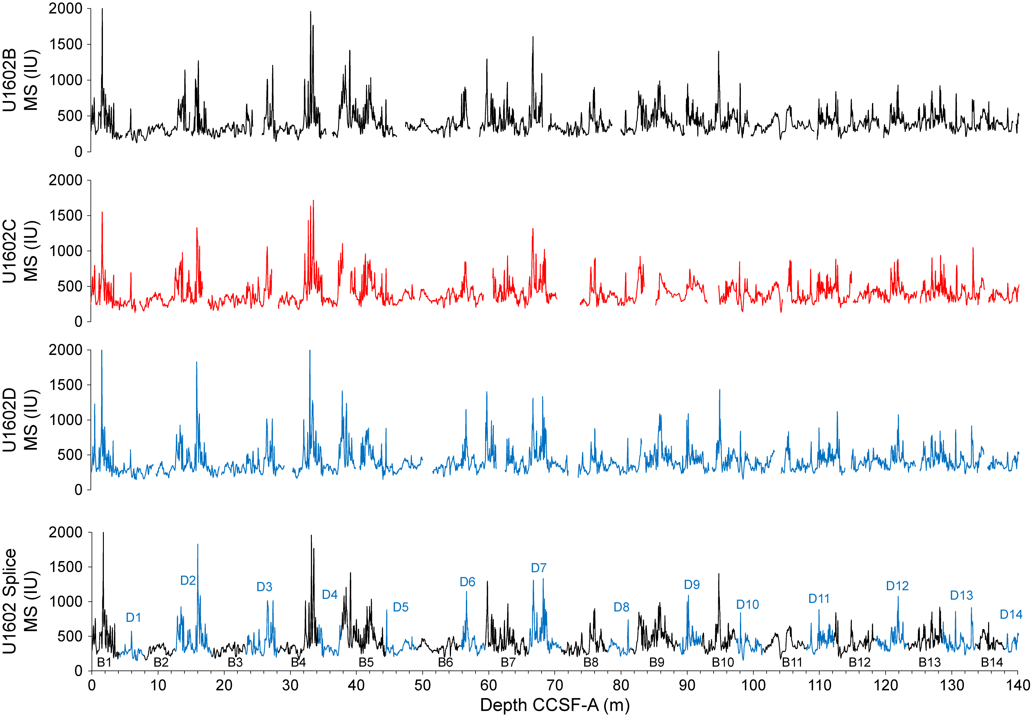
Figure F20. Splice for 0–140 m CCSF-A.
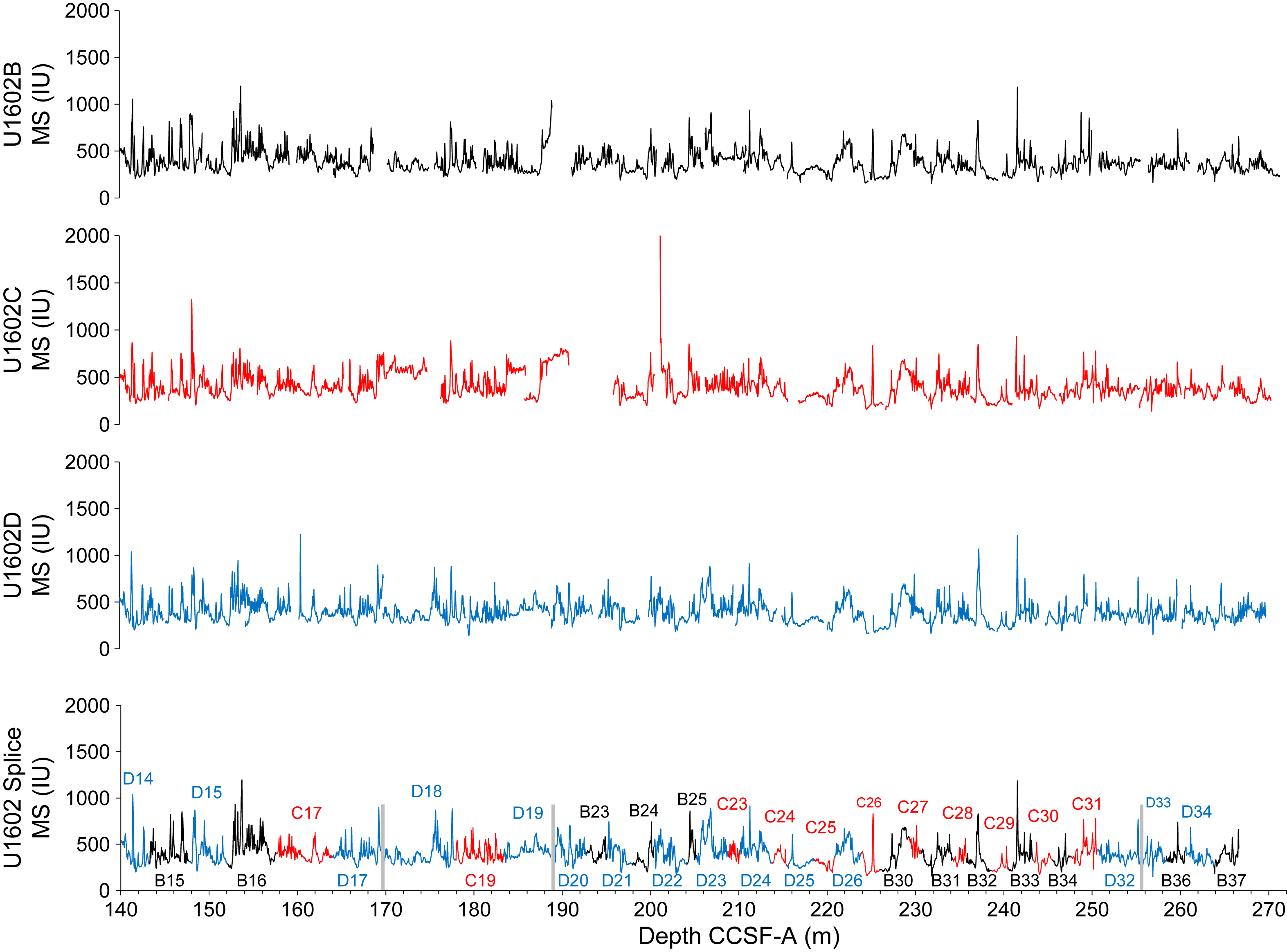
Figure F21. Splice for 140–270 m CCSF-A.
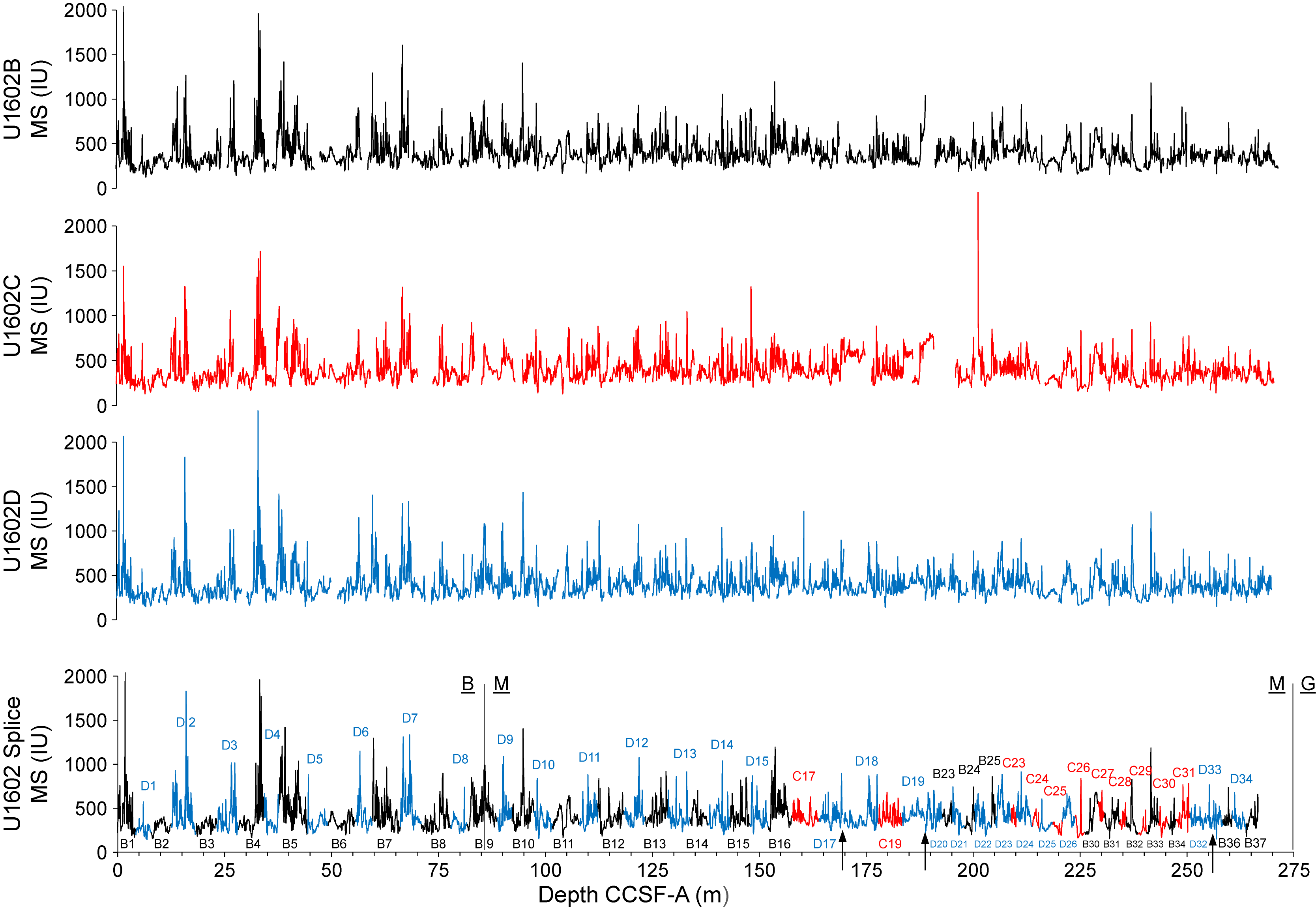
Figure F22. Splice.
6.2. Construction of the splice
The continuous splice for the upper 169.45 m CCSF-A is based on Holes U1602B and U1602D (Figure F22). The splice is further extended to Cores 395-U1602B-37F, 395-U1602C-34F, and 395-U1602D-34F by appending Cores 395-U1602D-17H and 18H, 395-U1602D-19H and 20H, and 395-U1602D-32F and 33F where small (<1–2 m) gaps in correlation occurred (Figure F21). The splice figures do not show core catcher measurements.
7. Paleomagnetism
7.1. Shipboard measurements
Shipboard paleomagnetic investigations were conducted on the archive-half cores from all holes at Site U1602 (see Paleomagnetism in the Expedition 395 methods chapter [Parnell-Turner et al., 2025a]). For Holes U1602A and U1602B, four alternating field (AF) demagnetization steps (0, 10, 15, and 20 mT) were performed at 2.5 cm resolution. Hole U1602C cores were measured for natural remanent magnetization (NRM) only at 2.5 cm spacing in Sections 1H-1 through 33F-4 and deeper cores were demagnetized with five steps (0, 10, 15, 20, and 25 mT) to the bottom of the hole. Measurements on cores from Hole U1602D started with four steps (0, 10, 15, and 20 mT), and then steps were increased to five (0, 10, 15, 20, and 25 mT) at Section 52X-6 all with a 2.5 cm spacing. Three different treatments were applied to cores from Hole U1602E at 2.5 cm spacing. These include demagnetization of five steps (0, 10, 15, 20, and 25 mT) and two sequences of six steps (0, 5, 10, 15, 20, and 30 mT and 0, 10, 15, 20, 25, and 30 mT) (see Table T7 in the Expedition 395 methods chapter [Parnell-Turner et al., 2025a]). A set of discrete oriented cubes was collected from the working halves of cores from Holes U1602B through U1602E (Figure F23, orange circles). We collected two cubes from every 10 m of core in nonoverlapping intervals from the entire 240 m of core from Hole U1602B (54 paleomagnetic oriented cubes), the lowest 30 m in Hole U1602C from 240 to 270 m CSF-A (six samples), from about 250 to 500 m CSF-A in Hole U1602D (66 samples), and the entire Hole U1602E (141 samples). For all discrete samples, the anisotropy of magnetic susceptibility (AMS) (Figure F24) was measured before NRM and AF demagnetization (Figure F25) up to 100 mT, if needed, with a stepwise sequence of 5, 10, 15, 20, 25, 30, 40, 50, 60, 80, and 100 mT. Discrete cubes from Holes U1602B and U1602C were also analyzed for anhysteretic remanent magnetization (ARM) (DC field = 100 mT; AC field = 50 µT) and isothermal remanent magnetization (IRM) (at 100, 300, and 500 mT and 1T) and then demagnetized using the same steps as the AF of the NRM.
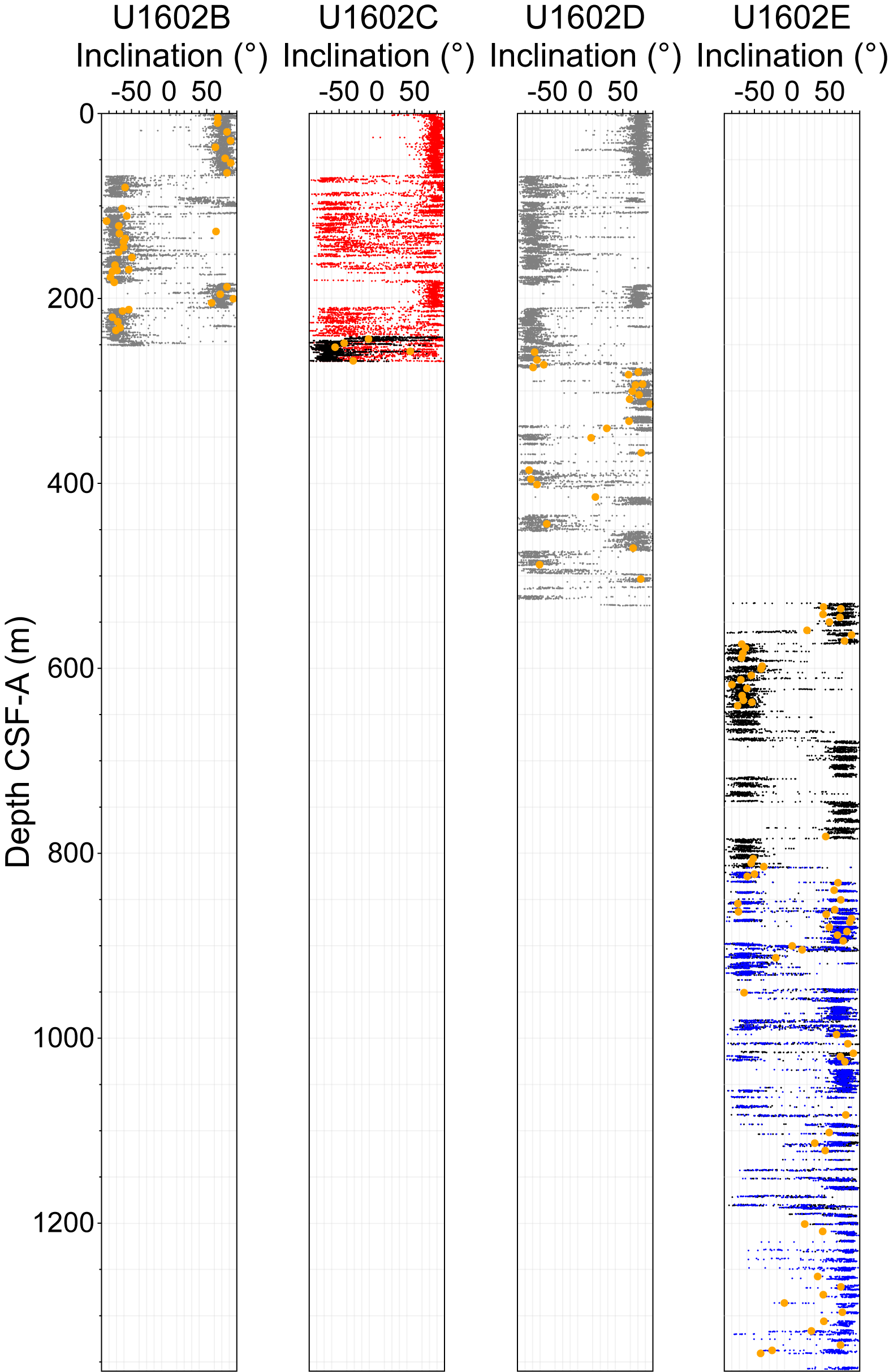
Figure F23. Inclination.
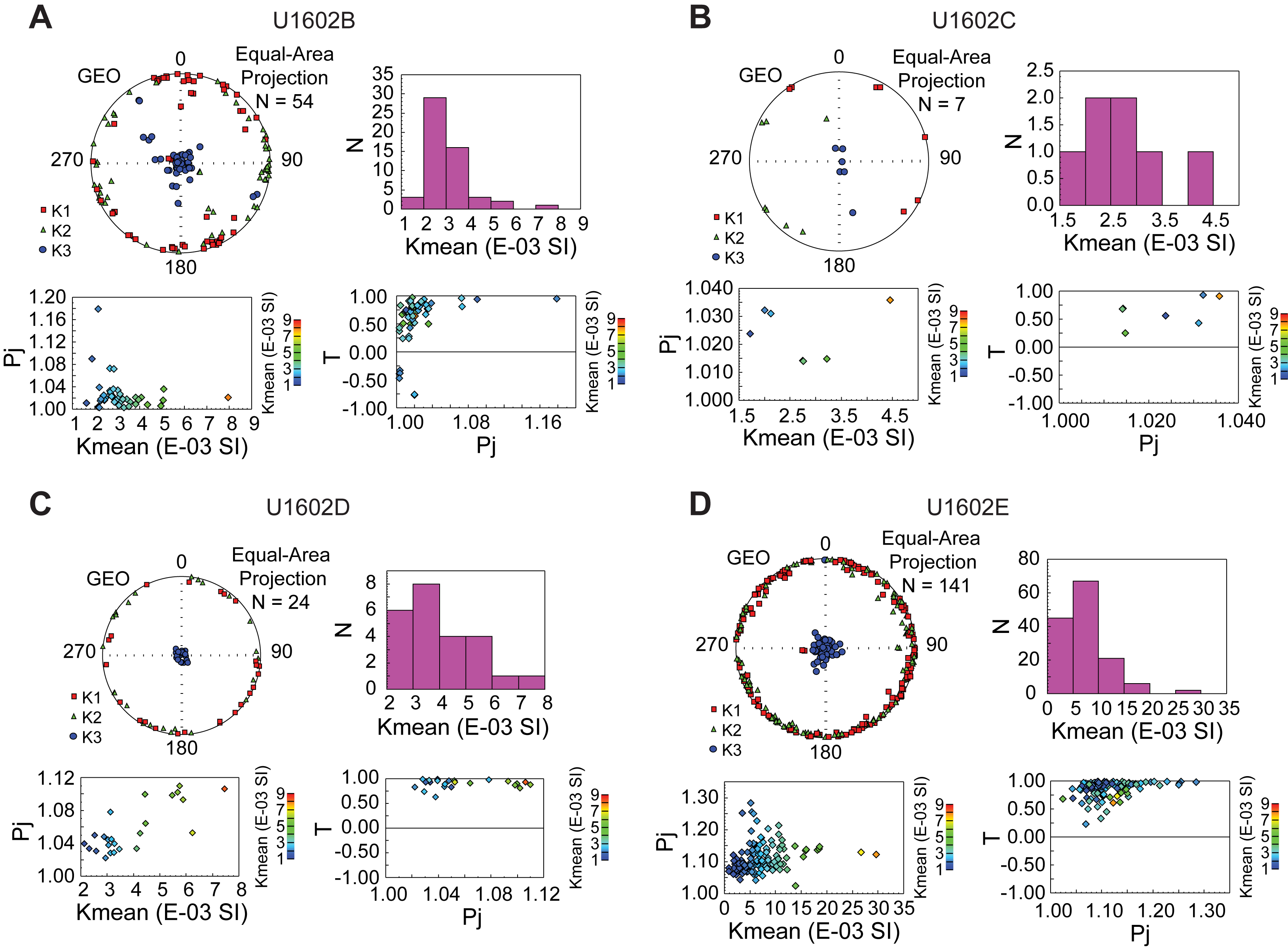
Figure F24. AMS.
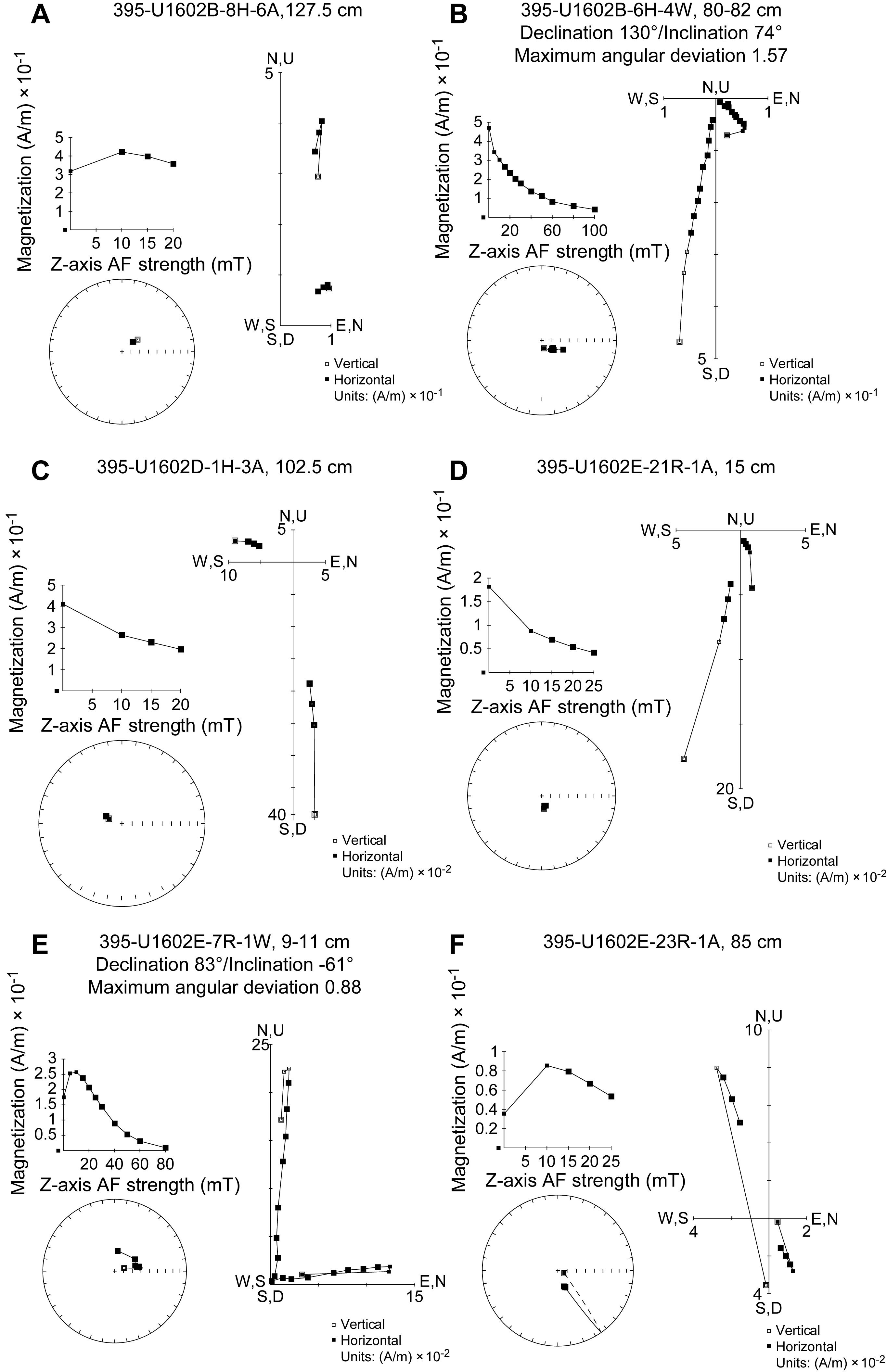
Figure F25. Demagnetization of sediments.
Inclinations from archive-half sections measured after the in-line AF demagnetization step (maximum step of demagnetization of 20, 25, or 30 mT) were used to interpret magnetic polarities in Holes U1602B, U1602D, and U1602E. Directional data were analyzed using Zijderveld diagrams (Zijderveld, 1967), and characteristic remanent magnetization (ChRM) direction(s) were calculated using principal component analysis (PCA) (Kirschvink, 1980) using PuffinPlot software (Version 1.4.1; Lurcock and Florindo, 2019) for the discrete samples.
7.2. Paleomagnetic and rock magnetic results
After the removal of an overprint up to 10 mT, stepwise AF demagnetization performed up to 20, 25, or 30 mT (or up to 100 mT for the discrete samples) successfully isolated a stable ChRM directed to the origin of the Zijderveld plot, even if samples were not completely demagnetized (Figure F25A, F25F). Normal and reversed polarities were identified in cores from Holes U1602B (Figure F25A, F25B), U1602C, U1602D (Figure F25C), and U1602E (Figure F25D–F25F). In some cases, the NRM was fully demagnetized by the 10 mT step. Inclinations from Hole U1602A, which are not shown in Figure F23, all display a normal polarity. The paleomagnetic results from the discrete samples replicate the data obtained with the downcore semicontinuous measurements collected with the SRM.
In Hole U1602A, NRM intensity varies from 8 × 10⁻² to 7.1 × 10⁻¹ A/m (average = 3.8 × 10⁻¹ A/m), and in Hole U1602B it varies from 2.9 × 10⁻³ to 1.7 A/m (average = 3.2 × 10⁻¹ A/m) (Figure F26). In Hole U1602C, NRM intensity varies from 4.85 × 10⁻³ to 3.13 A/m (average = 3.3 × 10⁻¹ A/m) (Figure F27), and in Hole U1602D it varies from 2.8 × 10⁻³ to 2.9 A/m (average = 3.5 × 10⁻¹ A/m) (Figure F28). Finally, in Hole U1602E, NRM intensity varies from 6.3 × 10⁻⁵ to 70.1 A/m (average = 7.9 × 10⁻¹ A/m) (Figure F29). In Hole U1602E, NRM intensity shows cyclical patterns between ~530 and ~1070 m CSF-A. Below this depth, NRM intensity decreases considerably, likely as a result of the mainly sandstone lithology.
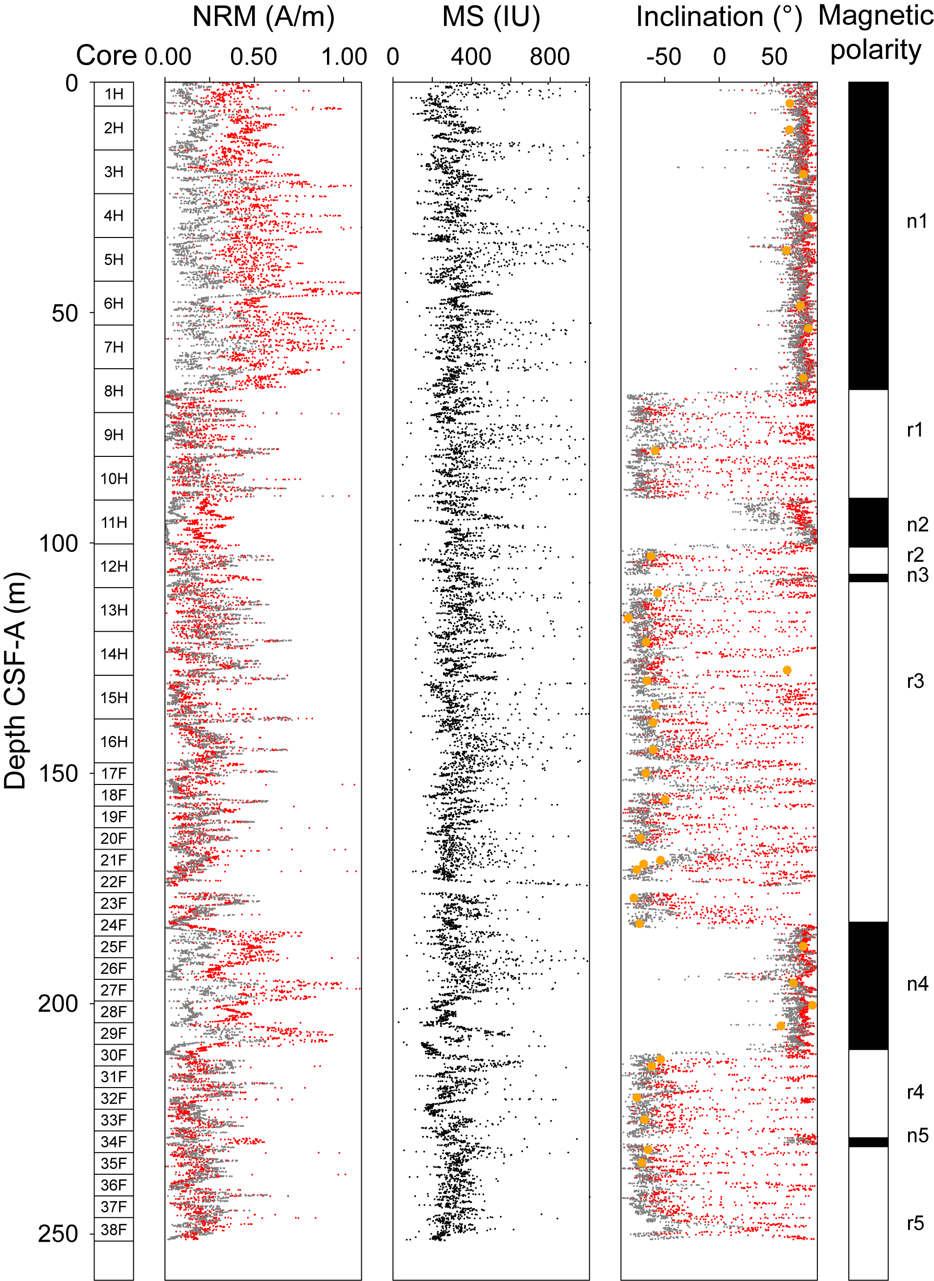
Figure F26. Paleomagnetic results from sediments, Hole U1602B.

Figure F27. Paleomagnetic results from sediments, Hole U1602C.
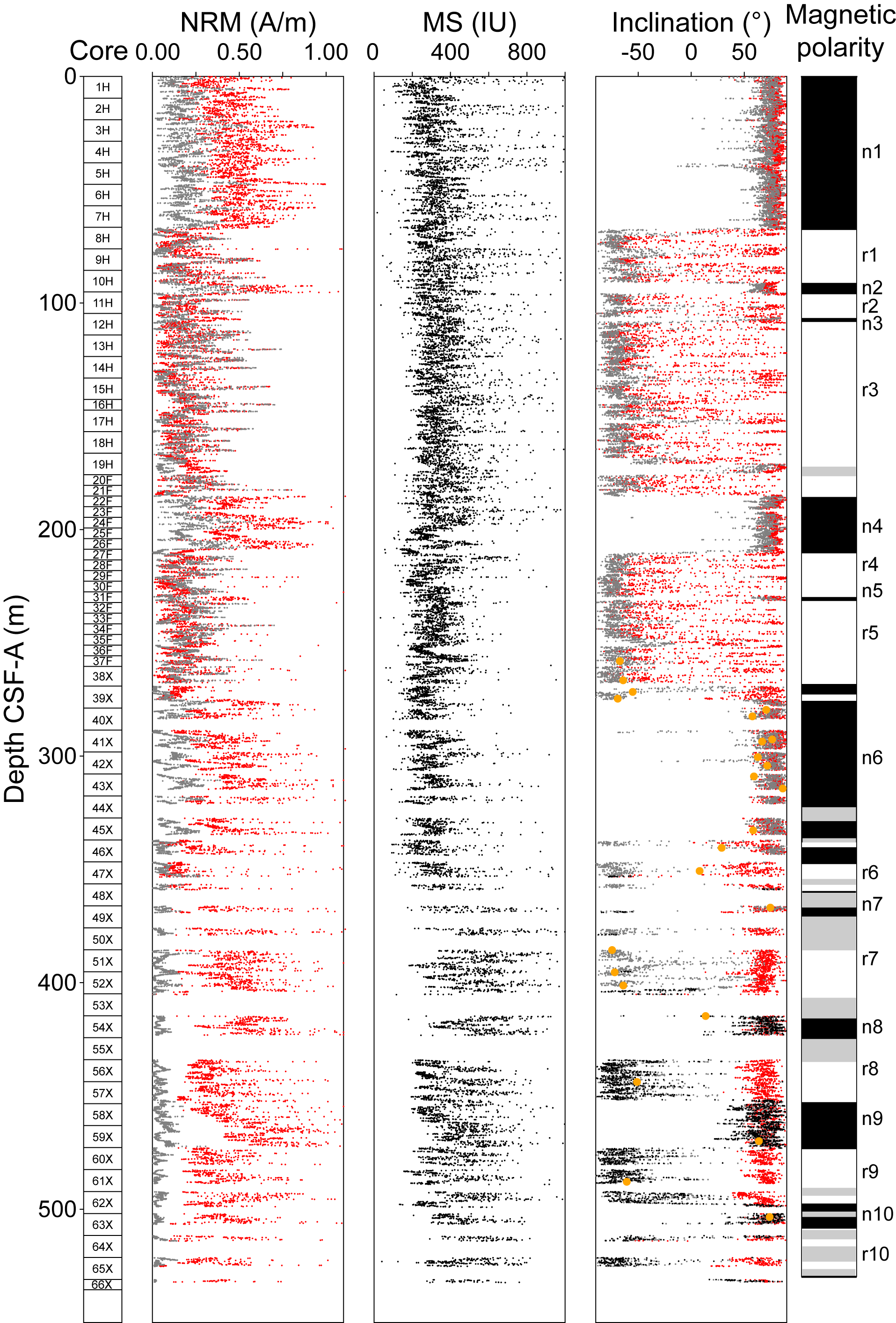
Figure F28. Paleomagnetic results from sediments, Hole U1602D.
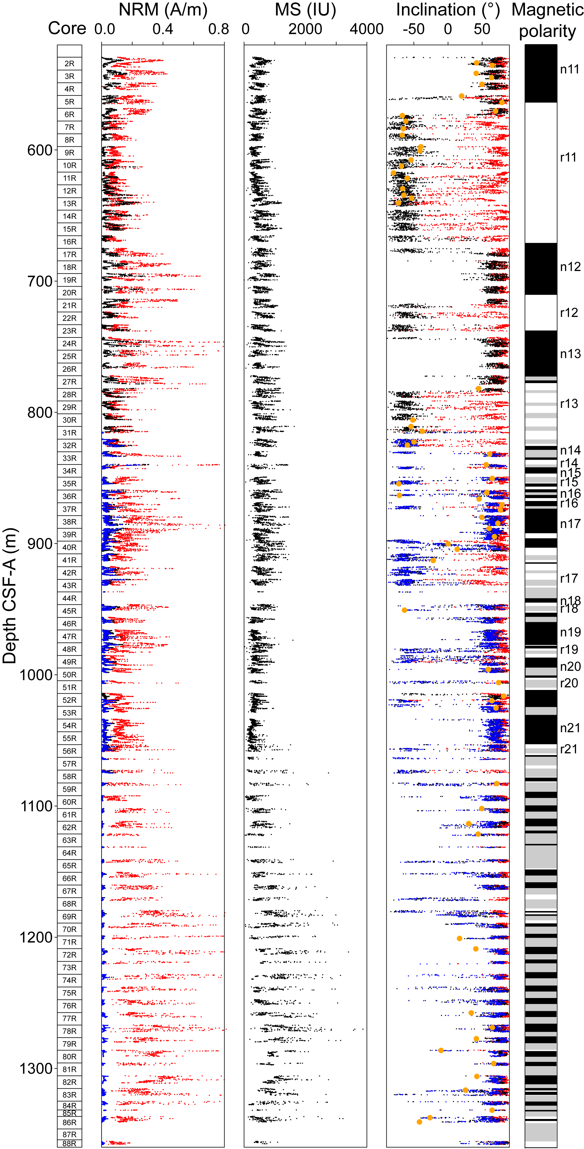
Figure F29. Paleomagnetic results from sediments, Hole U1602E.
MS obtained by point measurement on section halves (see Physical properties) ranges 28.7–5010.0 IU (average = 367.9 IU) in Hole U1602B (Figure F26), 3.9–4058.9 IU (average = 372.8 IU) in Hole U1602C (Figure F27), 16.7–5051.8 IU (average = 380.9 IU) in Hole U1602D (Figure F28), and 1.7–5459.6 (average = 574.7 IU) in Hole U1602E (Figure F29). Both NRM and MS show considerable variability with depth. These variations are most likely due to changes in carbonate and silica content in sedimentary units (see Lithostratigraphy).
Paleomagnetic results are summarized in Figure F23, where the variations in inclination reflect changes in the magnetic polarities and are replicated in all the holes. In Figure F30, data from Holes U1602D and U1602E are combined to interpret the magnetostratigraphy of Site U1602. Normal polarities (in black) are characterized by positive inclinations with short secular variations around present-day field inclination value of 73° at Site U1602.
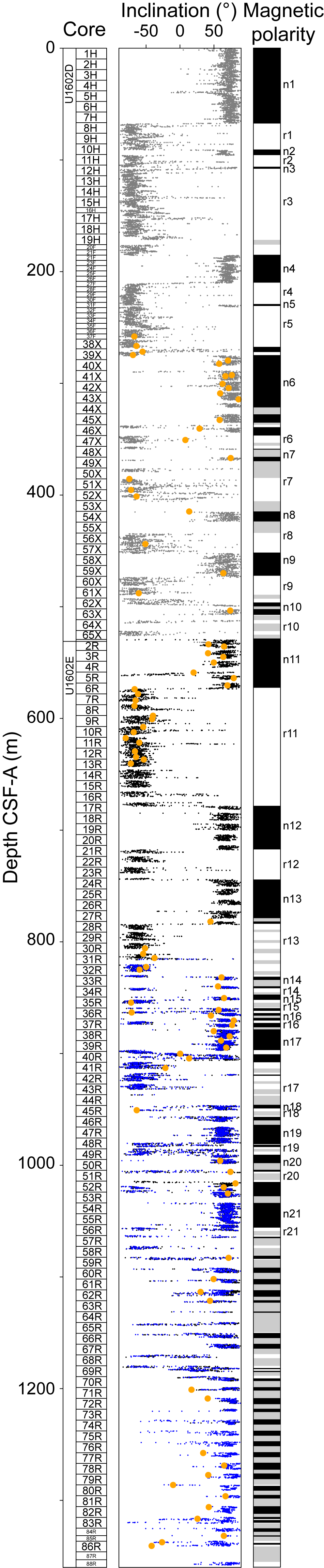
Figure F30. Inclinations and interpreted downcore magnetic polarities.
The AMS shows an anisotropy tensor compatible with a predominantly sedimentary fabric with a vertical minimum axis of anisotropy (blue circles in the stereonet of Figure F24).
The ARM at 0 mT and IRM at 100 mT are shown downhole in Figure F31. From 0 to ~500 m CSF-A, the ARM has a linear pattern around an average ARM intensity of 0.8 A/m. From 530 to 900 m CSF-A, the average ARM intensity has an increasing trend and then decreases to around 1110 m CSF-A. Below 1110 m CSF-A, this increasing trend reappears. IRM intensity after the 100 mT acquisition step has a slightly different pattern: from 0 to ~130 m CSF-A, the IRM intensity increases and below that the intensity averages out to a more linear trend (with average intensities around 38 mT).
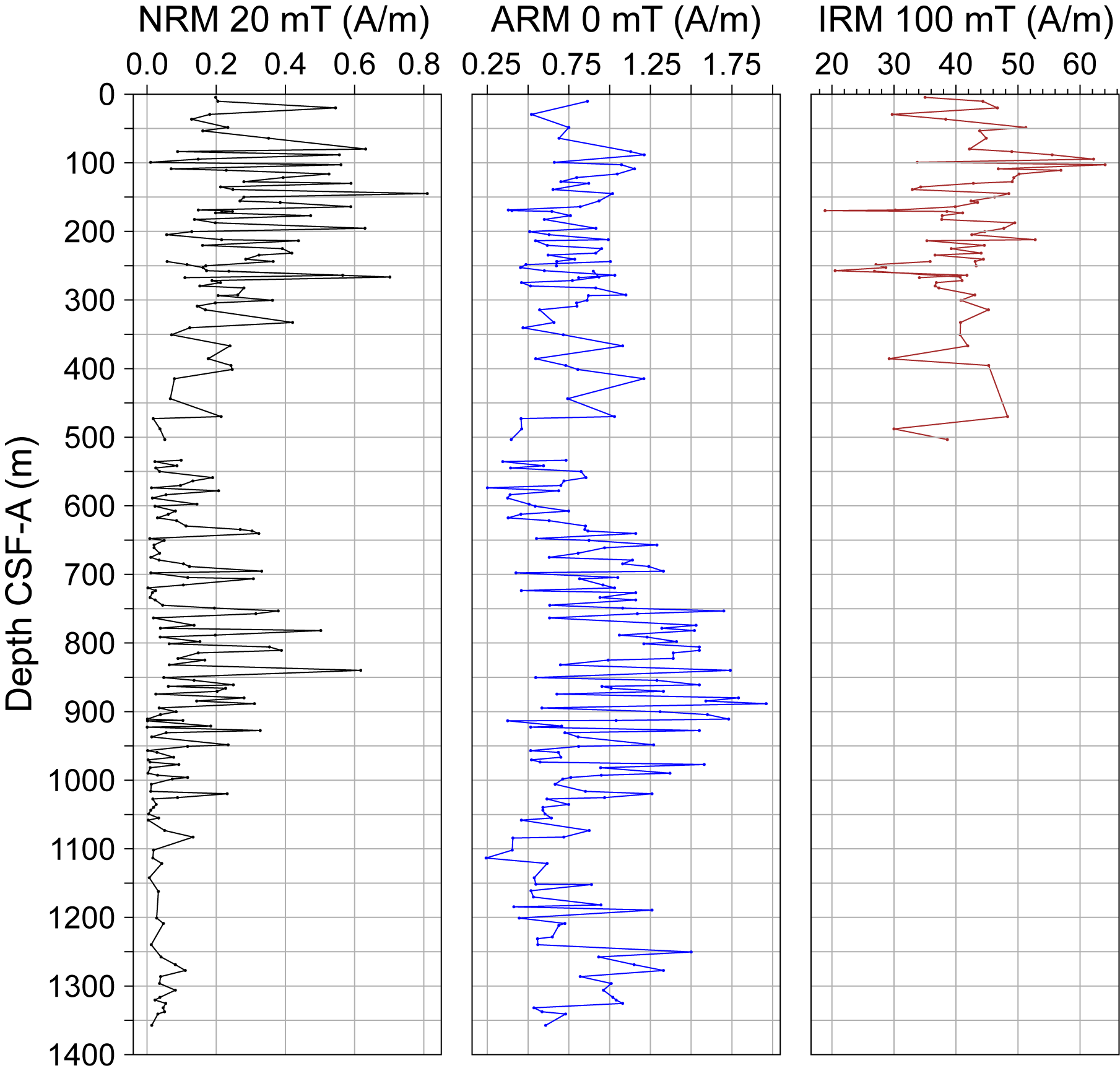
Figure F31. NRM, ARM, and IRM.
7.3. Magnetostratigraphy
The magnetostratigraphy of Site U1602 is based on the correlation of the polarity assigned to the archive-half cores from Holes U1602D and U1602E, using inclinations at the highest step of demagnetization (20, 25, and 30 mT) and the polarities reported in Ogg (2020) (Table T13). Importantly, the magnetic events recognized in Hole U1602D (Figure F28) are also identified in Hole U1602B (Figure F26). A succession of 21 normal and 21 reversed intervals was recognized (Figure F30) and correlated to the geomagnetic polarity timescale of Ogg (2020). Below 1060 m CSF-A, deterioration of the magnetic signal and the poor core recovery hamper the recognition of magnetic polarities. The magnetostratigraphic tie points are plotted along with the tie points from the shipboard microfossil ages to contribute to a preliminary age model (see Age model).
8. Geochemistry and microbiology
Cores taken at Site U1602 (Holes 395-U1602B through 395-U1602E) were analyzed for headspace gas, interstitial water (IW) chemistry, and bulk sediment geochemistry. Headspace methane concentrations range 0–328 ppmv (n = 143). Low ethane concentrations (<4.6 ppmv) were detected in a subset of the headspace samples (n = 21). Alkalinity is near seawater values (3.68 mM) in the uppermost IW sample (395-U1602A-1H-1, 141–151 cm) and increases to 6.1 mM at ~103 m CSF-A (Sample 12H-2, 146–151cm), before decreasing to low values (<1.0 mM) below ~320 m CSF-A (Sample 395-U1602D-44X-2, 123–130 cm). In contrast, pH is approximately constant in the upper ~340 m (7.9 ± 0.1), increases downhole to 8.9 at ~400 m CSF-A, and remains similarly elevated to ~786 m CSF-A (Sample 395-U1602E-28R-3, 119–131 cm). Below 786 m CSF-A, limited volumes of IW extracted from the sediment prevented additional pH measurements.
IW calcium ion (Ca2+) concentrations increase with depth; the highest Ca2+ concentrations occur at ~871 m CSF-A (Sample 395-U1602E-37R-2, 103–108 cm). Magnesium ion (Mg2+) concentrations decrease with depth; the highest Mg2+ concentrations (51.6 mM) occur at the top of the sediment column (Sample 395-U1602B-1H-1, 141–151 cm; 1.4 m CSF-A). Sulfate ion (SO42−) concentrations decrease downhole from seawater values at the sediment/water interface and reach a minimum at ~240 m CSF-A (Sample 35F-2, 145–150 cm). SO42− concentrations increase slightly below ~600 m CSF-A to between 5 and 9 mM. Downhole trends in other dissolved elements, including barium (Ba), lithium (Li), potassium (K), and silicon (Si) indicate a change in concentrations at around 388 m CSF-A.
CaCO3 generally increases downhole from ~0 to 30 wt% in the uppermost 100 m to as high as ~80 wt% near the bottom of Hole U1602E (Sample 60R-1, 3–4 cm). Bulk sediment generally exhibits low total organic carbon (TOC) (<0.7 wt%), total nitrogen (TN) (<0.2 wt%), and total sulfur (TS) (≤1.0 wt%). Bulk sediment major and minor element concentrations were also analyzed using inductively coupled plasma–atomic emission spectroscopy (ICP-AES) on select samples. Downhole variations in major oxides (e.g., SiO2, Al2O3, TiO2 K2O, MgO, and CaO) and trace elements (e.g., S and Sr) show variable concentrations that likely reflect changing lithologies.
8.1. Volatile hydrocarbons
Methane concentrations throughout the sedimentary section of Site U1602 (Holes U1602B–U1602E) increase from 0 ppmv at the sediment/water interface to a peak of 327.7 ppmv at 485.5 m CSF-A and then drop back to ~39 ppmv near the bottom of Hole U1602E (Figure F32). There are three methane peaks at 291.5, 327.7, and 1308.4 m CSF-A, indicating elevated methane production, which could be due to biological methanogenesis.
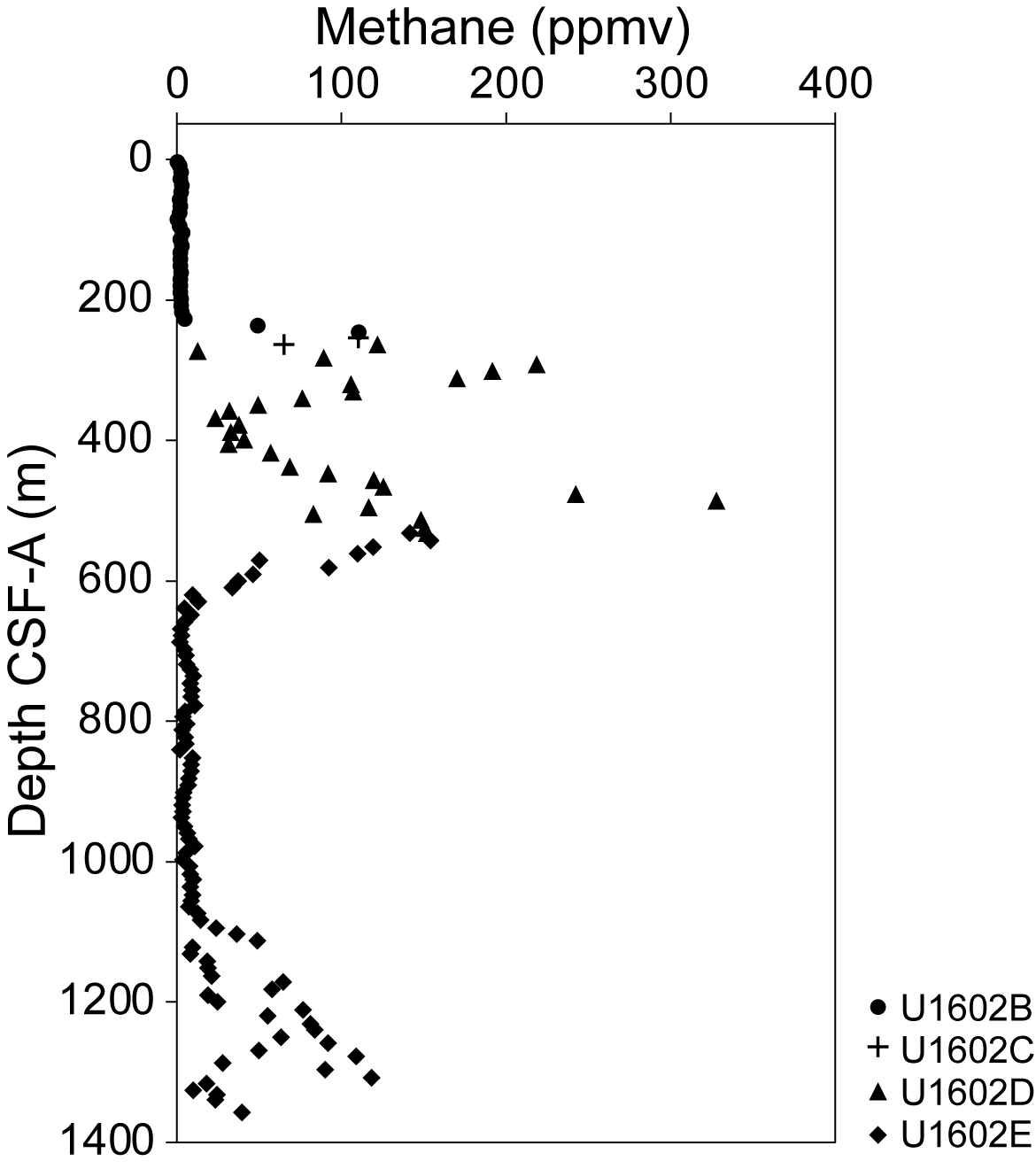
Figure F32. Composite gas analyses of methane concentrations.
8.2. Interstitial water chemistry
A total of 102 IW samples were squeezed from 5, 10, or 12 cm long whole-round samples from 1.4 to 978.3 m CSF-A at Site U1602 (Cores 395-U1602B-1H through 37F, 395-U1602C-36F through 38F, 395-U1602D-37F through 65X, and 395-U1602E-2R through 40R, 47R, and 48R). Selected data acquired from analysis of IW in Holes U1602B–U1602E are shown in Figure F33. pH is generally constant in the upper ~340 m and then increases downhole from ~340 to 777 m CSF-A (the deepest pH measurement possible due to low water yield from squeeze cakes). Alkalinity values are near seawater in the uppermost sediments (Section 395-U1602A-1H-1) and increases slightly to 6.1 mM at 103 m CSF-A; below 310.83 m CSF-A, alkalinity remains low (≤1 mM). IW Mg2+ concentrations display a decreasing trend with depth from 51.6 mM in the uppermost sediments to below detection limit at greater depths, and values are consistently close to the limit of detection below 398 m CSF-A. SO42− concentrations range from 28.3 mM at the top of the sediments to 0.52 mM at 259 m CSF-A and decrease with depth. Ca2+ concentrations are 8.03 mM at 46.16 m CSF-A before increasing to high concentrations with a maximum of 96.6 mM at 706.65 m CSF-A. Sr2+ concentrations range from 81.0 µM at 27.17 m CSF-A to 1602.27 µM at the deepest depth sampled (978.3 m CSF-A) with a general increase in concentration with depth.
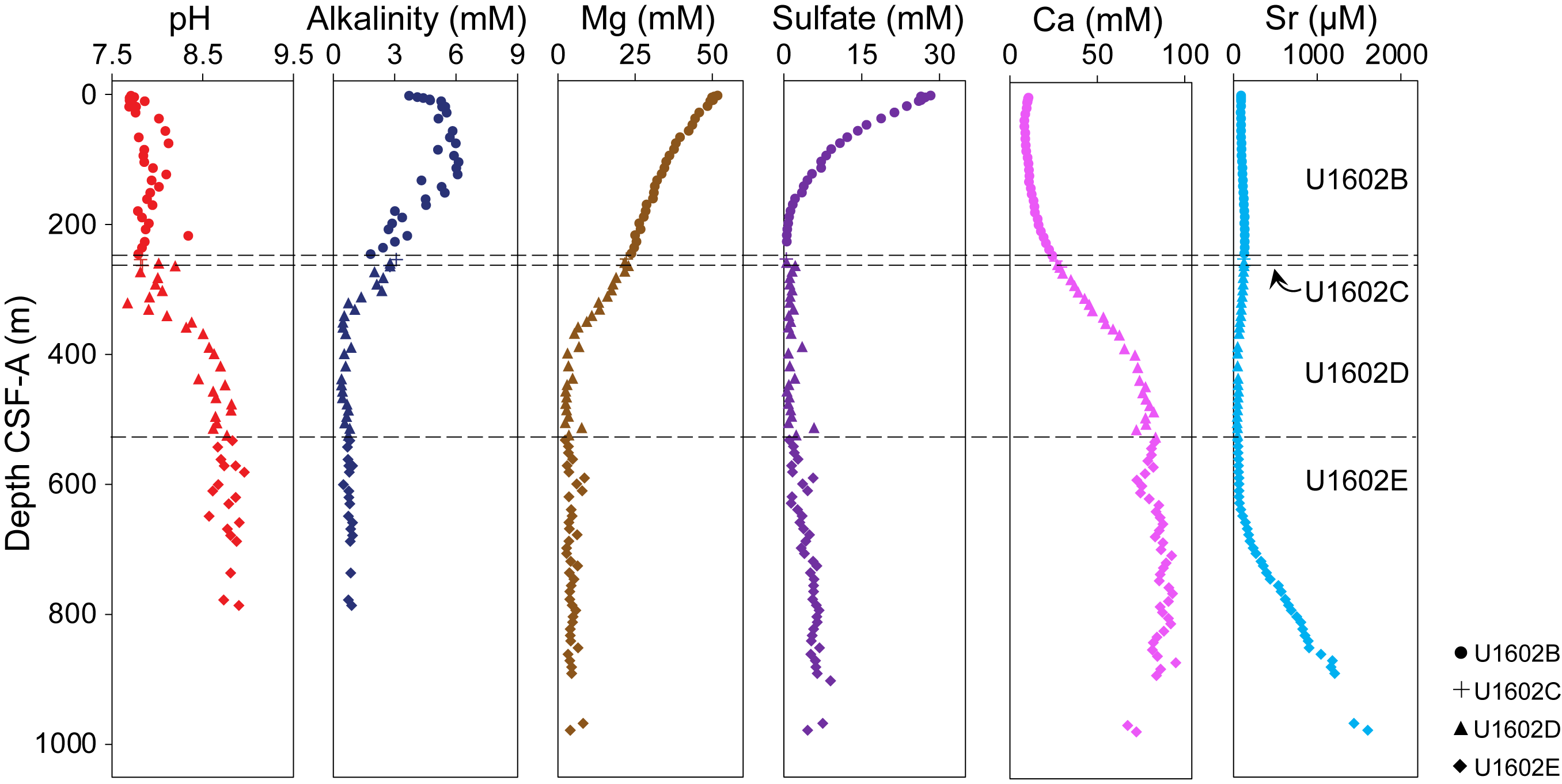
Figure F33. IW pH, alkalinity, and concentrations of selected ions.
Downhole trends in dissolved lithium (Li), potassium (K), silicon (Si), and barium (Ba) are shown in Figure F34. IW Li concentrations generally increase with depth, with a slight decrease from 357.82 to 561.29 m CSF-A before increasing to the bottom of the hole. K concentrations decrease downhole from a high value of 11.5 mM at 9.64 m CSF-A to consistently between 1 and 2 mM at 388.43 m CSF-A to the bottom of the hole. Si also decreases with depth with a steep decrease from 709.5 to 243.8 µM between 339.91 and 349.63 m CSF-A. Interestingly, Ba has a large peak in concentration at 188.24 m CSF-A, where it increases to 18.1 µM before decreasing sharply at 388.43 m CSF-A.
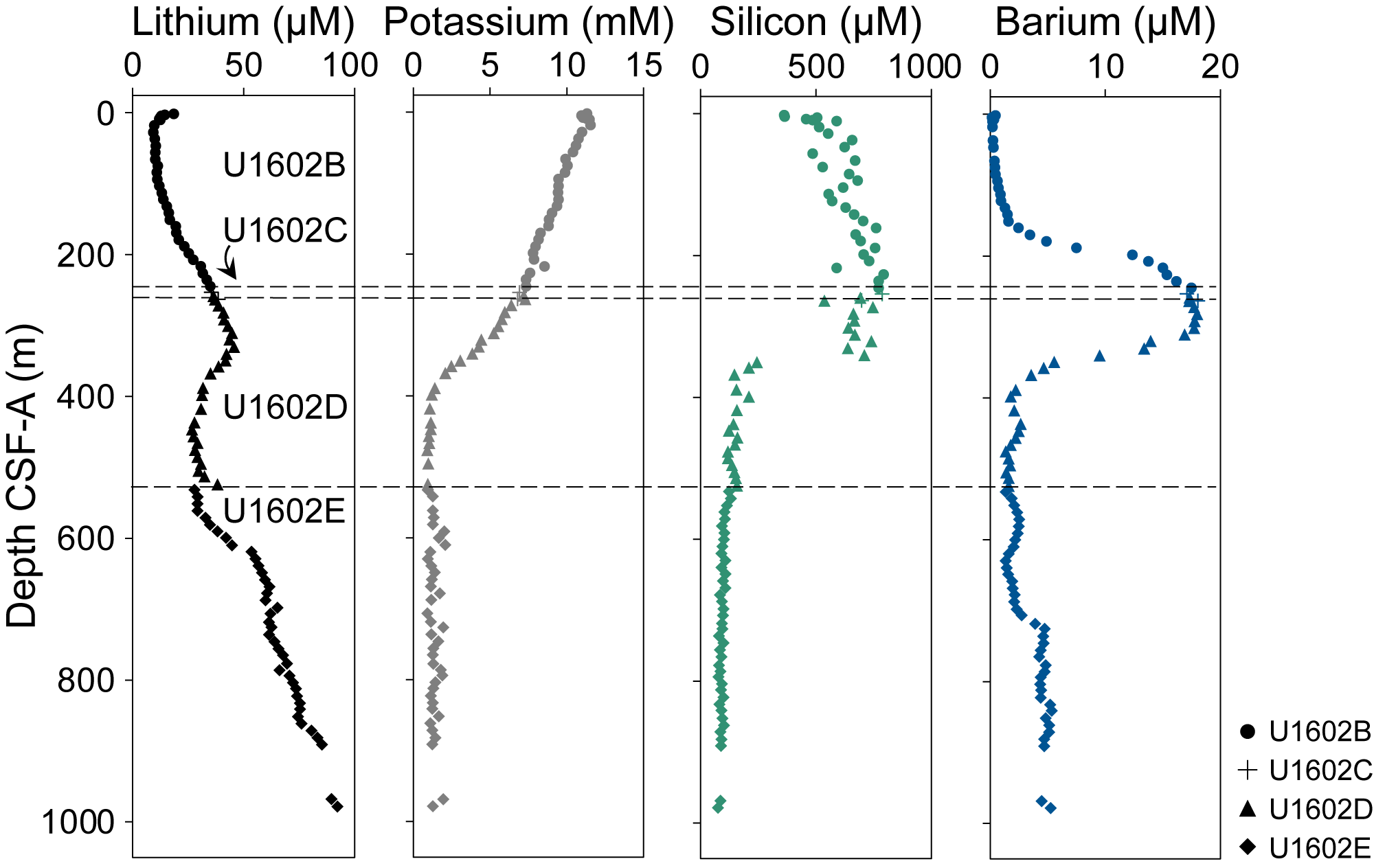
Figure F34. IW Li, K, Si, and Ba.
8.2.1. Bulk sediment geochemistry
8.2.1.1. Carbonate, nitrogen, carbon, and sulfur
Discrete sediment samples (n = 268) were collected from squeeze cake residues and working halves during sediment description in Cores 395-U1602B-1H through 395-U1602E-88R (1.41–1357.1 m CSF-A). TOC content is generally low (average = 0.22 ± 0.11 wt%). CaCO3 content is variable (total range = 27–79.80 wt%) with the highest CaCO3 content at 1092.13 m CSF-A (Sample 60R-1, 3–4 cm) (Figure F35). Additional sediment samples were chosen so that the resulting geochemical information (e.g., CaCO3 content) could be used to aid in lithologic description. Differences in the CaCO3 content between the sampling strategies (Figure F35, open versus solid circles) reflects the sampling bias and variable sedimentary CaCO3 content in different lithologic layers. TN ranges 0–0.08 wt% (average = 0.43 ± 0.23 wt%). TS is mostly below detection (average = 0.36 ± 0.25 wt%).
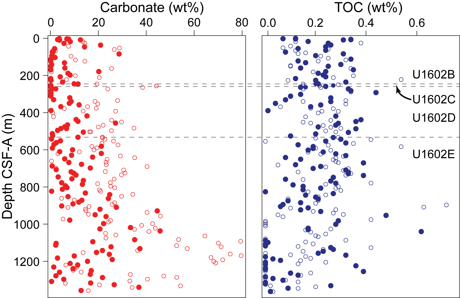
Figure F35. CaCO3 and TOC.
8.2.1.2. Major oxide and minor elements
A subset of carbonate residue samples (n = 53) from Holes U1602B–U6202E were analyzed for bulk sediment major oxide and minor element concentrations using ICP-AES. Downhole variations in major oxides (e.g., SiO2, Al2O3, TiO2 K2O, MgO, and CaO) and minor elements (e.g., S and Sr) show variable concentrations that likely reflect changing sediment lithologies. Sedimentary ICP-AES data define three geochemical units (Figure F36). Although sedimentary geochemical units were defined with ICP-AES data alone, there is general agreement with lithostratigraphic unit boundaries (see Lithostratigraphy). Above 398.4 m CSF-A (Sample 395-U1602D-52X-2, 143–150 cm), most major and trace elements and oxides display more variability. Between 398.4 and 968.25 m CSF-A, most oxide and element data have a lower degree of variability, and concentrations generally transition between the average values in the upper and lower intervals. Below 968.25 m CSF-A, all oxides and elements display the largest point-to-point variability, which likely reflects variable silicate/carbonate lithologies present in the lower portion of Site U1602. Sr concentrations are notable in that they display the most coherent downhole trend, showing low concentrations in the upper part of the core (e.g., Sample 41X-2, 142–149 cm; 167 ppm) and the highest concentrations near the bottom of the sampled core (e.g., Sample 395-U1602E-80R-1, 140–145 cm; 1084 ppm).
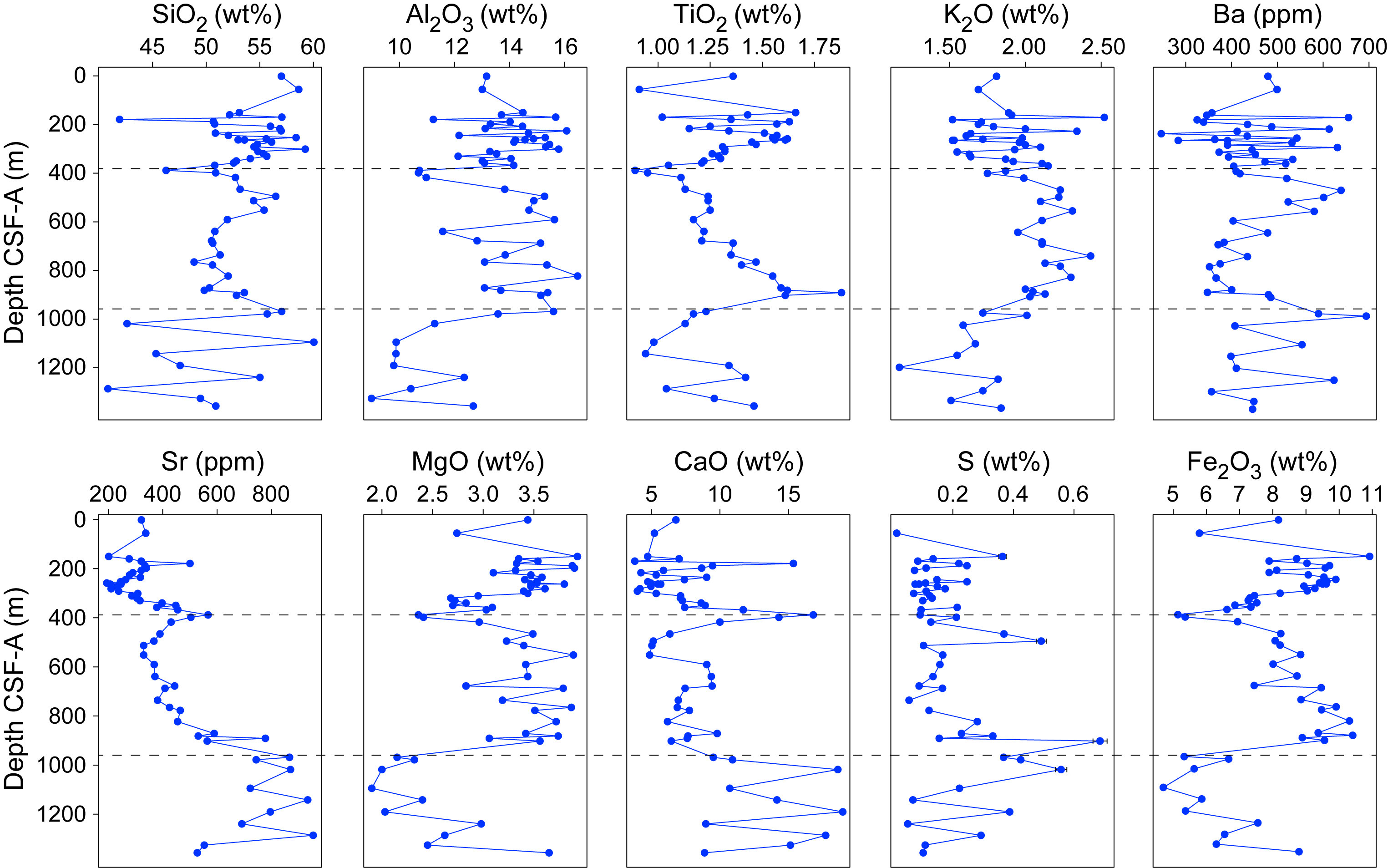
Figure F36. Major oxide and trace element data.
8.3. Microbiology
Microbiological sampling of sediments from Holes U1602B–U1602E was focused on collecting samples for culture-independent approaches. A total of 136 sediment samples, each 5 cm3, were collected with a sterile cut-end syringe (Holes U1602B and U1602C) or were aseptically sampled from the interior portion of IW whole-round samples (Holes U1602D and U1602E) for shore-based analyses. For samples where IW analyses were not conducted because of a lack of available pore water, a 5 cm whole-round sample was collected for microbiological analysis.
9. Downhole measurements
Details on tools and logging procedures can be found in Downhole measurements in the Expedition 395 methods chapter (Parnell-Turner et al., 2025a), and only hole specific procedures are detailed here. Downhole logging operations at Site U1602 were conducted in Hole U1602E, which was logged with the triple combo tool string only (Magnetic Susceptibility Sonde [MSS], High-Resolution Laterolog Array [HRLA], Accelerator Porosity Sonde [APS], HLDS, and Hostile Environment Natural Gamma Ray Sonde [HNGS]). While coring Hole U1602B, formation temperature measurements were acquired at four depths (33.7, 62.2, 90.7, and 119.2 m DSF) using the APCT-3 tool (Table T14).
9.1. Logging procedure and log data processing
After coring operations in Hole U1602E concluded, the hole was prepared for logging by performing a sweep and replacing the heavy drilling mud (sepiolite and barite) with seawater. The drill pipe was raised to 76 m WSF. A triple combo tool string downhole logging downhole pass (Data Set 017PUP) collected data from ~32 to 1278 m WSF depth. The calipers were closed during the downhole logging pass, precluding data acquisition with the APS tool and creating unreliable and uncorrectable measurements with the HLDS tool. At 1278 m WSF, the triple combo tool string became stuck, and tool recovery operations were initiated (see Operations). The tool string was successfully recovered, and further logging operations at this site were canceled. The downhole logging pass did not capture a seafloor signal because tool recording began below seafloor. Because this single downhole pass is the only logging data set available from Site U1602, the logger's seafloor depth is assumed to be equal to the driller's seafloor depth (2720.7 m drilling depth below rig floor [DRF]). The signal attenuation of the drill pipe in the subsurface is clear in the logging data (Figure F37), which shows the bottom of the drill pipe at ~76 m WSF, providing confidence in the logger's seafloor depth estimate. The HRLA data were corrected for environmental conditions during logging. Below ~1250 m WSF, the MS measurements show a large degree of variability that may be caused by a narrowing borehole diameter and should therefore be interpreted with caution. The wireline heave compensator (WHC) was used in the open hole interval to counter the ship heave (~0.5 m) during downhole logging.

Figure F37. Downhole logging data.
9.2. Logging units
Seven logging units and multiple subunits are defined in Hole U1602E (Table T15). The units are primarily defined based on the logging response of gamma log and subsequently from their logging response in other parameters, especially MS (Figure F37).
9.2.1. Logging Unit L1
Logging Unit L1 is defined by the topmost measured logging data (~32 m WSF) to 162 m WSF. The bottom depth is marked by an increase in gamma log. Unit L1 corresponds to the upper 162 m of Lithostratigraphic Unit I at Site U1602 (see Lithostratigraphy).
9.2.1.1. Logging Subunit L1a
Logging Subunit L1a (32–76 m WSF) corresponds to the portion of Unit L1 that was measured through the drill pipe. Because logging data from this interval were collected through the drill pipe, only gamma log can be used to assess hole geology, and then only qualitatively due to attenuation of the incoming signal by the pipe. The gamma log and spectral gamma logs (U, Th, and K) show a similar character to that observed in Subunit L1b and are therefore grouped with Subunit L1b into Unit L1.
9.2.1.2. Logging Subunit L1b
Logging Subunit L1b shows gamma log measurements of ~27.7 ± 5.3 American Petroleum Institute gamma radiation units (gAPI) with fluctuations ranging from highs of up to 44.3 gAPI to lows of 5 gAPI. High gamma peaks correspond to increases in the Th (up to ~6 ppm) and K (up to 1.5%) spectral gamma counts. U counts show a weak negative correlation with Th but not K. Deep formation resistivity values range 0.5–1.8 Ωm in Subunit L1b, and subtle variations can be observed with depth. Between 104 and 113 m WSF, resistivity shows multiple sharp peaks that may be related to poor hole conditions and should therefore be interpreted with caution. MS fluctuates between 85 and 890 SI from 76 to 141 m WSF, after which it becomes relatively invariant (average = 249 ± 37 SI) to the bottom of Unit L1. There is a positive correlation between gamma log and MS in Subunit L1b.
9.2.2. Logging Unit L2
The top of Logging Unit L2 is defined by a step increase in gamma log from Subunit L1b to an average around 35 ± 6 gAPI. Gamma measurements fluctuate between values as high as 57.6 gAPI and as low as 17.9 gAPI over 2–6 m thick depth intervals. These fluctuations are more pronounced between 162 and 300 m WSF. From 300 to 347 m WSF, gamma log shows a gradual increase and less pronounced fluctuations. Like Unit L1, increases in gamma radiation observed in Unit L2 correlate with increases in the Th and K counts measured from spectral gamma logging, and Th counts show a weak negative correlation with U counts. The bottom of Unit L2 is defined by an increase in the formation resistivity into Unit L3 and an increase and distinct change in character in MS. Formation resistivity is ~0.75 Ωm with very small fluctuations occurring over 2–3 m depth intervals. MS in Unit L2 has an average measurement of 259 ± 65 SI and contains 2–3 m thick intervals ranging 34–494 SI. Unit L2 correlates to the bottom portion of Lithostratigraphic Unit I (0–346 m CSF-A) (see Lithostratigraphy).
9.2.3. Logging Unit L3
The boundary between Logging Units L2 and L3 at ~340 m WSF is marked by an increase in gamma log, formation resistivity, and MS. Gamma log in Unit L3 averages 47 ± 6 gAPI and shows meter- to decameter-scale depth cycles of high (~65 gAPI) and low (~25 gAPI) values throughout. High gamma radiation values correspond to higher counts of Th, K, and U in Unit L3, as measured from spectral gamma logging. A negative correlation between Th and U counts is observed for Unit L3 but is less pronounced compared to that observed in Subunit L1b and Unit L2. Several distinct intervals with decreased gamma log are observed (e.g., ~437, ~490, ~544, ~556, and ~567 m WSF), which correspond to increases in MS. From 340 to 355 m WSF, formation resistivity displays a gradual increase to an average of 1.3 ± 0.2 Ωm with low-amplitude meter-scale fluctuations throughout. MS initially increases at the top of Unit L3 compared to Unit L2, but it gradually decreases with depth to the bottom of Unit L3. Unit L3 MS shows high-amplitude fluctuations on a meter scale from as high as 772 SI to as low as 15 SI. Unit L3 approximately corresponds to the upper 243 m of Lithostratigraphic Unit II (see Lithostratigraphy).
9.2.4. Logging Unit L4
Logging Unit L4 is distinguished from Units L3 and L5 by a notable ~42 m thick perturbation in gamma log and a pronounced decrease in MS. Throughout Unit L4, natural gamma increases from ~48 gAPI to a maximum of ~67 gAPI at ~610 m WSF before decreasing again toward the top of Unit L5. Within this larger gamma radiation pattern, there are 1–2 m long cycles. In Unit L4, natural gamma increases correspond to increases in Th and K counts from spectral gamma logging but not to increases in U counts. Spectral gamma log U measurements in Unit L4 are, on average, higher than in Units L3 and L5, and there is a negative correlation between U and Th in Unit L4. Deep formation resistivity in Unit L4 averages 1.5 ± 0.2 Ωm with subtle meter-scale fluctuations. MS in Unit L4 decreases compared to Units L3 and L5, with an average of 229 ± 88 SI. Similar to the logging units above and below Unit L4, MS fluctuates on 1–2 m wavelengths, although the fluctuations are less pronounced (ranging 95–532 SI). There is a weak negative correlation between MS and gamma log. Unit L4 corresponds to Lithostratigraphic Unit II (see Lithostratigraphy).
9.2.5. Logging Unit L5
The top of Logging Unit L5 is defined by an initial decrease in gamma log and an increase in MS compared to Unit L4. The boundary between Units L5 and L6 is defined by decreasing gamma log and increased deep formation resistivity in Subunit L6a. The depth interval defined as Unit L5 shows fluctuations in gamma log at meter, decameter, and hectometer scales, within which values range 19–73.5 gAPI. From 630 to 848 m WSF, gamma log is characterized by meter- to decameter-thick fluctuations. These smaller scale fluctuations are also present from 848 to 1039 m WSF, but this interval also contains two ~100 m thick features at ~848–936 and ~936–1039 m WSF. The transition between these two hectometer-scale fluctuations is marked by a ~10 m interval of lower gamma log. Increased gamma log in Unit L5 positively correlates with increasing Th, K, and U spectral gamma log counts, although U shows a weaker correlation than K and Th. The top of Unit L5 shows a change in the character of formation resistivity from Unit L4, with increased amplitude variability that persists throughout Unit L5. From 630 to 848 m WSF, these formation resistivity fluctuations have a range of 2.5 Ωm, and between 848 and 1039 m WSF their amplitude decreases to ~1.8 Ωm. The deeper interval correlates with the lower 100 m long fluctuation observed in gamma log. Across Unit L5, formation resistivity shows a gradual increase with depth from ~1.5 to ~2.3 Ωm. A weak positive correlation exists between deep formation resistivity and gamma log. After an initial increase in MS at the top of Unit L5, three hectometer-scale fluctuations are observed with depth to ~906 m WSF, where a gradual increase is observed toward the bottom of the unit. Large-amplitude fluctuations occur at the meter to decameter scale across the entire interval of Unit L5 to as low as 13 SI and as high as 1376 SI. Unit L5 corresponds to the lower part of Lithostratigraphic Unit II (346.70–994.80 m CSF-A) and most of Lithostratigraphic Unit IIIA (994.80–1092.10 m CSF-A) (see Lithostratigraphy).
9.2.6. Logging Unit L6
Logging Unit L6 is characterized by highly variable logging responses that are separated into five subunits based predominantly on gamma log character. The top of Unit L6 is defined by an abrupt decrease in gamma log, with lower gamma radiation than Unit L5. The base of Unit L6 is marked by a change to a cyclical gamma log response in Unit L7. Unit L6 is distinguished by lower Th and U spectral gamma counts than Unit L5. Unit L6 is entirely within Lithostratigraphic Unit III (see Lithostratigraphy).
9.2.6.1. Logging Subunit L6a
Logging Subunit L6a displays a decreasing gamma log measurement with depth (from ~40 to ~25 gAPI) with some irregularly spaced meter-scale fluctuations. Peaks in gamma log correlate with increased Th and K spectral gamma counts. Formation resistivity in Subunit L6a is ~2.4 ± 0.4 Ωm and displays small meter-scale variability. MS in Subunit L6a is lower than that observed in Unit L5 and Subunit L6b, although it exhibits several submeter-scale peaks up to ~700 SI.
9.2.6.2. Logging Subunit L6b
Logging responses change abruptly between Logging Subunits L6a and L6b. Gamma log initially increases and then decreases with depth throughout the subunit, and resistivity initially starts to decrease before increasing again toward the bottom of Subunit L6b. MS is higher than in Subunit L6a and exhibits meter-scale fluctuations down to 42 SI. U spectral gamma counts are, on average, slightly lower in Subunit L6b compared to Subunit L6a.
9.2.6.3. Logging Subunit L6c
Logging Subunit L6c shows an initial sharp decrease in gamma log compared to Subunit L6b, which then increases with depth (from ~25 to ~50 gAPI) before dropping again at ~1118 m WSF. Spectral gamma counts of Th and U fluctuate in this subunit, although not always synchronously. Resistivity decreases from the top of Subunit L6c to ~1112 m WSF, where it starts to increase with depth to the boundary with Subunit L6d. MS shows a sharp decrease at the top of Subunit L6c and then increases with depth, fluctuating in meter-scale cycles.
9.2.6.4. Logging Subunit L6d
Logging Subunit L6d is the most distinct subunit in Unit L6. It is marked by a prominent decrease in gamma log (average = 19 ± 3 gAPI), a sharp decrease in MS (average = 128 ± 50 SI), and a slight increase in resistivity (average = 2.2± Ωm) compared to the subunits above and below. Logging responses are mostly invariable within Subunit L6d.
9.2.6.5. Logging Subunit L6e
The top of Logging Subunit L6e is marked by an abrupt increase in gamma log and MS. Gamma, formation resistivity, and MS fluctuate slightly in Subunit L6e. Spectral gamma Th and U counts fluctuate, matching the gamma log response.
9.2.7. Logging Unit L7
Logging Unit L7 is distinguished from Unit L6 by a clear cyclic character in gamma log, which shows meter-scale fluctuations (as high as 44 gAPI and as low as 16 gAPI). Spectral gamma Th, K, and U counts correlate positively with the natural gamma log. Formation resistivity has an average of 2 Ωm and shows submeter fluctuations with depth. MS has numerous meter-scale fluctuations to ~1250 m WSF that measure between 19 and 1192 SI. Below ~1250 m WSF, MS increases; however, this could be a measurement artifact caused by deteriorating hole conditions. Unit L7 is entirely within Lithostratigraphic Unit IIIB (see Lithostratigraphy).
9.3. Downhole temperature and thermal conductivity
While drilling Hole U1602B, downhole temperature measurements were taken with the APCT-3 tool in Unit L1. The tool provided equilibration temperatures ranging from 3.22°C at 33.7 m DSF to 10.43°C at 116 m DSF (Figures F38, F39A; Table T16). These observations indicate a thermal gradient in the upper sediment section of 79°C/km. Thermal conductivity under in situ conditions (K) was estimated from laboratory-determined thermal conductivity from Hole U1602B using the method of Hyndman et al. (1974). Thermal conductivity shows a slight increase with depth and values between 0.8 and 1.2 W/m·K (Figure F39B). A linear function for depth-dependent thermal resistance (R) was obtained by integrating the inverse of the thermal conductivity over depth and applying a linear least-squares fit (Figure F39C). This function was used to estimate thermal resistance at each corresponding APCT-3 downhole temperature measurement depth. A heat flow of 78.9 mW/m2 was obtained from a linear least-squares fit of the relationship between temperature and thermal resistance (Bullard, 1939), whose slope is the vertical heat flow (Figure F39D).
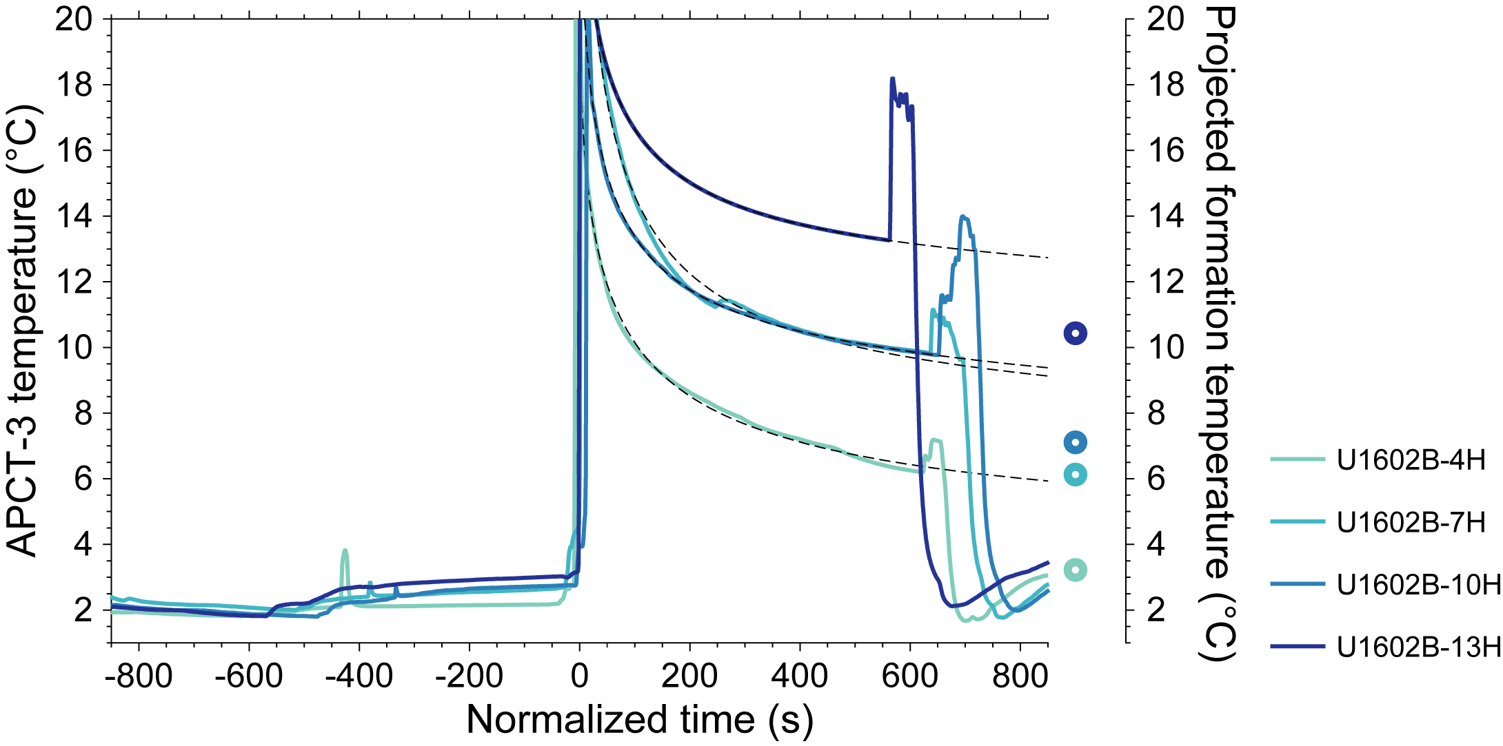
Figure F38. APCT-3 temperature-time series and projected formation temperature estimates.
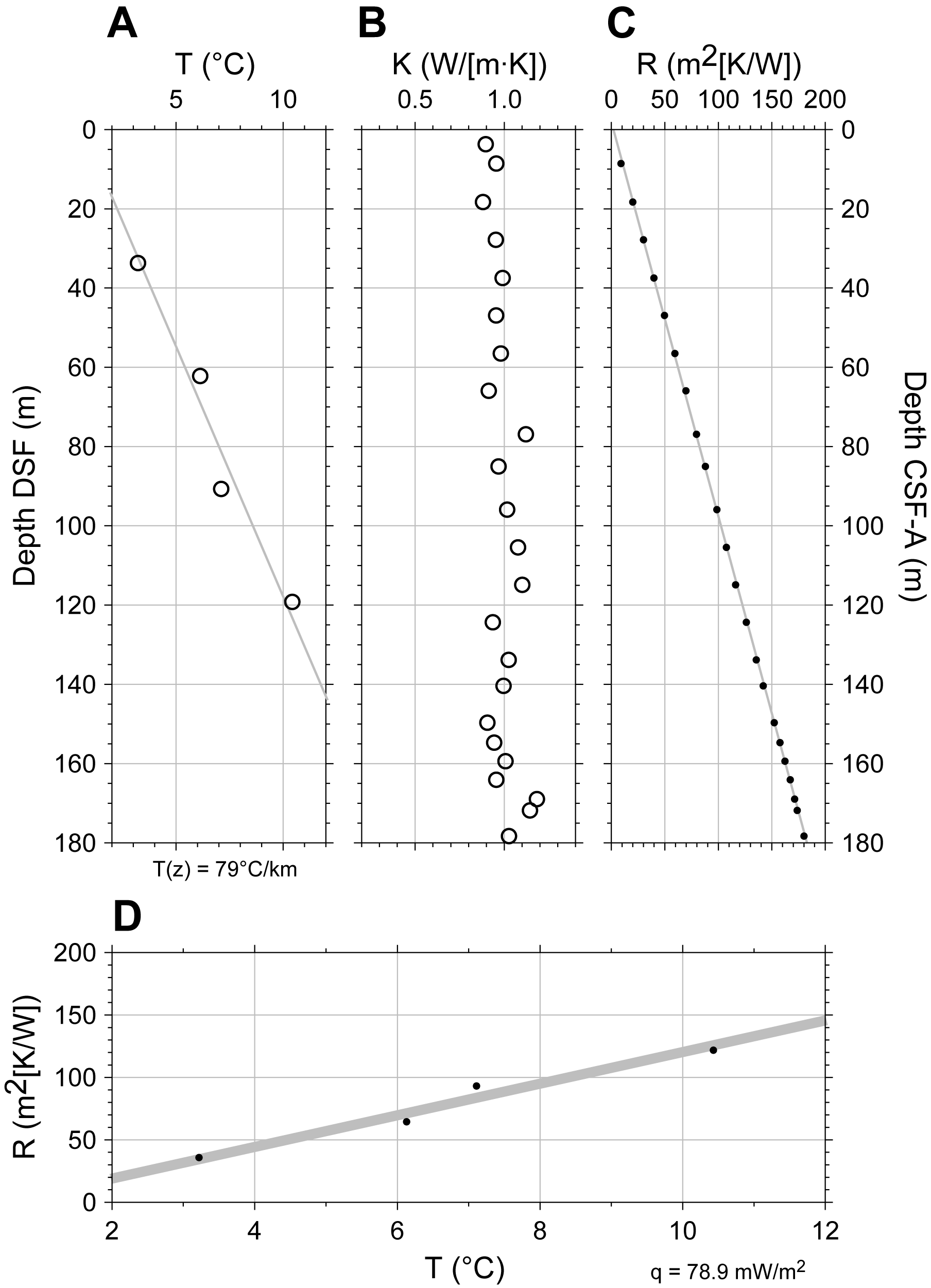
Figure F39. Thermal gradient and heat flow estimates.
10. Age model
Site survey seismic reflection profiles show a relatively flat and laterally continuous series of reflections at Site U1602 (see Background and objectives). The age model (Figure F40) is based on a combination of paleomagnetic and biostratigraphic age determinations (see Paleomagnetism and Micropaleontology). Some of the biostratigraphic data are only upper or lower depth constraints because rarity and/or variable preservation makes them difficult to locate precisely. Age constraints are listed in Table T17 with interpolated ages of selected epoch and subepoch boundaries and estimated ages for selected lithostratigraphic units.
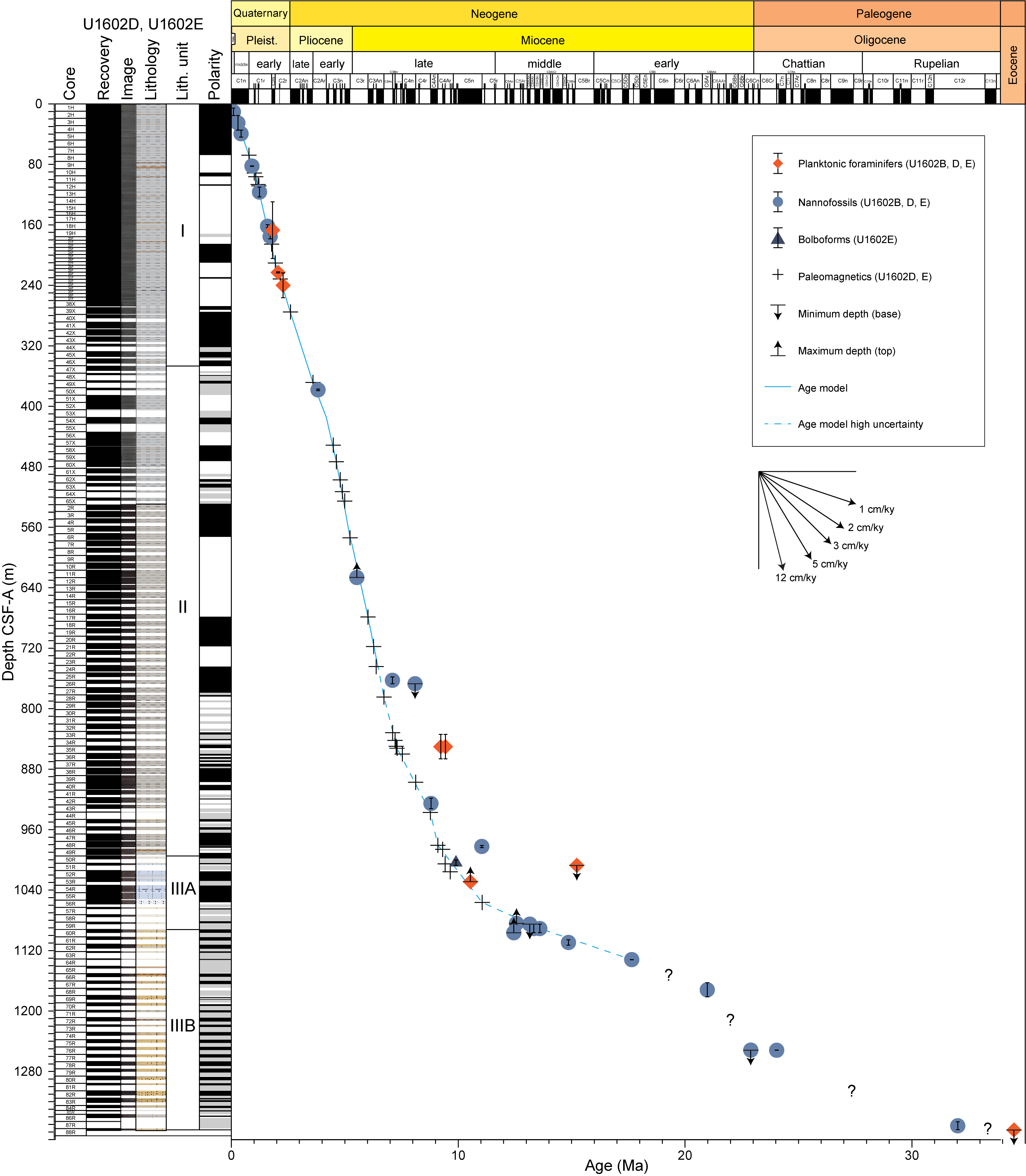
Figure F40. Age model for the sedimentary succession.
There is a very good agreement between the paleomagnetic and biostratigraphic data sources to the base of Gilbert Chron C3r (6.023 Ma) at 678.5 m CSF-A. Below this depth, the paleomagnetic record continues to follow the expected reversal sequence to the interpreted base of Subchron C5n.2n (11.056 Ma) at 1056.10 m CSF-A, which is consistent with a sedimentation rate similar to the sequence above. However, the biostratigraphic data appear to depart from this trend; hence, the age model in Figure F40 is indicated with a dashed line in this interval. Some of the apparent discrepancies can be explained by problems associated with diachrony, reworking, and/or poor preservation of the fossils. The dextral to sinistral coiling direction shift in N. atlantica (one of the planktonic foraminifer events at ~850 m CSF-A), which is calibrated at 9.23 Ma, is particularly difficult to reconcile with the paleomagnetic interpretation. A possible explanation is that a dextral subpopulation of N. atlantica may have persisted in the area of Site U1602 after the main coiling shift elsewhere. However, this explanation is problematic because the bioevent was calibrated at Deep Sea Drilling Project (DSDP) Site 646 on Eirik drift and was therefore likely to have sampled the same population of plankton from surface water currents flowing east of Greenland.
The average sedimentation rate for Lithostratigraphic Unit I from the top of Site U1602 to the base of this unit at 346.7 m CSF-A is ~10.3 cm/ky. For the upper part of Unit II to the base of Subchron C3Br.1n at 852 m CSF-A, the average sedimentation rate is ~12.8 cm/ky. For the lower part of Unit II to 994.8 m CSF-A, the rate is apparently lower (~6.6 cm/ky).
The age model becomes increasingly uncertain below the base of Lithostratigraphic Unit II. The top (13.60 Ma) and bottom (17.65 Ma) common occurrences of S. heteromorphus at 1090.36 and 1131.62 m CSF-A, respectively, provide age constraints near the base of Subunit IIIA. Below that, the paleomagnetic record is not readily interpretable likely because of drilling overprint (see Paleomagnetism). Widely spaced nannofossil age constraints hint at nonuniform episodic sedimentation in the sandstones of Subunit IIIB. Planktonic foraminifers suggest that Hole U1602E terminated in the upper Eocene (>34.5 Ma), but that interpretation is based on a very poorly preserved assemblage from just one sample near the bottom of the hole at 1357.02 m CSF-A (see Micropaleontology). The estimated depth of the basement from site survey seismic reflection profiles is 1375 m CSF-A, and the estimated age of the basement from regional magnetic surveys and plate reconstructions is 49.8 Ma (see Background and objectives). Although both estimates are only approximate, the age model implies that there is only space for a relatively thin and slowly accumulated and/or stratigraphically discontinuous body of sediment between the basement and the bottom of the drilled interval, or that true basement depth is deeper than estimated from seismic reflection profiles.
References
Bullard, E.C., 1939. Heat flow in South Africa. Proceedings of the Royal Society of London, A: Mathematical and Physical Sciences, 173(955):474–502. https://doi.org/10.1098/rspa.1939.0159
Butterworth, S., 1930. On the theory of filter amplifiers. Experimental Wireless and the Wireless Engineer, 7:536–541. https://www.gonascent.com/papers/butter.pdf
Hartmann, A., and Villinger, H., 2002. Inversion of marine heat flow measurements by expansion of the temperature decay function. Geophysical Journal International, 148(3):628–636. https://doi.org/10.1046/j.1365-246X.2002.01600.x
Hyndman, R.D., Erickson, A.J., and Von Herzen, R.P., 1974. Geothermal measurements on DSDP Leg 26. In Davies, T.A., Luyendyk, B.P., et al., Initial Reports of the Deep Sea Drilling Project. 26: Washington, DC (US Government Printing Office), 451–463. https://doi.org/10.2973/dsdp.proc.26.113.1974
Kirschvink, J.L., 1980. The least-squares line and plane and the analysis of palaeomagnetic data. Geophysical Journal International, 62(3):699–718. https://doi.org/10.1111/j.1365-246X.1980.tb02601.x
Lurcock, P.C., and Florindo, F., 2019. New developments in the PuffinPlot paleomagnetic data analysis program. Geochemistry, Geophysics, Geosystems, 20(11):5578–5587. https://doi.org/10.1029/2019GC008537
Lyons, R.G., 2011. Understanding Digital Signal Processing (Third edition): Upper Saddle River, NJ (Prentice Hall). https://www.iro.umontreal.ca/~mignotte/IFT3205/Documents/UnderstandingDigitalSignalProcessing.pdf
Müller-Michaelis, A., Uenzelmann-Neben, G., and Stein, R., 2013. A revised early Miocene age for the instigation of the Eirik Drift, offshore southern Greenland: evidence from high-resolution seismic reflection data. Marine Geology, 340:1–15. https://doi.org/10.1016/j.margeo.2013.04.012
Ogg, J.G., 2020. Geomagnetic Polarity Time Scale. In Gradstein, F.M., Ogg, J.G., Schmitz, M., and Ogg, G. (Eds.), Geologic Time Scale 2020. Amsterdam (Elsevier), 159–192. https://doi.org/10.1016/B978-0-12-824360-2.00005-X
Parnell-Turner, R., White, N., Henstock, T.J., Jones, S.M., Maclennan, J., and Murton, B.J., 2017. Causes and consequences of diachronous v-shaped ridges in the North Atlantic Ocean. Journal of Geophysical Research: Solid Earth, 122(11):8675–8708. https://doi.org/10.1002/2017JB014225
Parnell-Turner, R.E., Briais, A., LeVay, L.J., Cui, Y., Di Chiara, A., Dodd, J.P., Dunkley Jones, T., Dwyer, D., Eason, D.E., Friedman, S.A., Hemming, S.R., Hochmuth, K., Ibrahim, H., Jasper, C., Karatsolis, B.T., Lee, S., LeBlanc, D.E., Lindsay, M.R., McNamara, D.D., Modestou, S.E., Murton, B., OConnell, S., Pasquet, G.T., Pearson, P.N., Qian, S.P., Rosenthal, Y., Satolli, S., Sinnesael, M., Suzuki, T., Thulasi Doss, T., White, N.J., Wu, T., and Yang Yang, A., 2025a. Expedition 395 methods. In Parnell-Turner, R.E., Briais, A., LeVay, L.J., and the Expedition 395 Scientists, Reykjanes Mantle Convection and Climate. Proceedings of the International Ocean Discovery Program, 395: College Station, TX (International Ocean Discovery Program). https://doi.org/10.14379/iodp.proc.395.102.2025
Parnell-Turner, R.E., Briais, A., LeVay, L.J., Cui, Y., Di Chiara, A., Dodd, J.P., Dunkley Jones, T., Dwyer, D., Eason, D.E., Friedman, S.A., Hemming, S.R., Hochmuth, K., Ibrahim, H., Jasper, C., Karatsolis, B.T., Lee, S., LeBlanc, D.E., Lindsay, M.R., McNamara, D.D., Modestou, S.E., Murton, B., OConnell, S., Pasquet, G.T., Pearson, P.N., Qian, S.P., Rosenthal, Y., Satolli, S., Sinnesael, M., Suzuki, T., Thulasi Doss, T., White, N.J., Wu, T., Yang Yang, A., dos Santos Rocha, V., Pearman, C., and Tian, C.Y., 2025b. Expedition 395 summary. In Parnell-Turner, R.E., Briais, A., LeVay, L.J., and the Expedition 395 Scientists, Reykjanes Mantle Convection and Climate. Proceedings of the International Ocean Discovery Program, 395: College Station, TX (International Ocean Discovery Program). https://doi.org/10.14379/iodp.proc.395.101.2025
Parnell-Turner, R.E., Briais, A., LeVay, L.J., and the Expedition 395 Scientists, 2025c. Supplementary material, https://doi.org/10.14379/iodp.proc.395supp.2025. In Parnell-Turner, R.E., Briais, A., LeVay, L.J., and the Expedition 395 Scientists, Reykjanes Mantle Convection and Climate. Proceedings of the International Ocean Discovery Program, 395: College Station, TX (International Ocean Discovery Program).
Parnell-Turner, R., White, N.J., McCave, I.N., Henstock, T.J., Murton, B., and Jones, S.M., 2015. Architecture of North Atlantic contourite drifts modified by transient circulation of the Icelandic mantle plume. Geochemistry, Geophysics, Geosystems, 16(10):3414–3435. https://doi.org/10.1002/2015GC005947
Raffi, I., Wade, B.S., Pälike, H., Beu, A.G., Cooper, R., Crundwell, M.P., Krijgsman, W., Moore, T., Raine, I., Sardella, R., and Vernyhorova, Y.V., 2020. The Neogene Period. In Gradstein, F.M., Ogg, J.G., Schmitz, M.D., and Ogg, G. (Eds.), Geologic Time Scale 2020. (Elsevier), 1141–1215. https://doi.org/10.1016/B978-0-12-824360-2.00029-2
Young, J.R., 1990. Size variation of Neogene Reticulofenestra coccoliths from Indian Ocean DSDP cores. Journal of Micropalaeontology, 9(1):71–85. https://doi.org/10.1144/jm.9.1.71
Young, J.R., 1998. Neogene. In Bown, P.R., Calcareous Nannofossil Biostratigraphy. Dordrecht, Netherlands (Kluwer Academic Publishing), 225–265.
Zijderveld, J.D.A., 1967. AC demagnetization of rocks: analysis of results. In Runcorn, S.K.C., Creer, K.M., and Collinson, D.W. (Eds.), Methods in Palaeomagnetism. Developments in Solid Earth Geophysics, 3: 254–286. https://doi.org/10.1016/B978-1-4832-2894-5.50049-5