Hodell, D.A., Abrantes, F., Alvarez Zarikian, C.A., and the Expedition 397 Scientists
Proceedings of the International Ocean Discovery Program Volume 397
publications.iodp.org
https://doi.org/10.14379/iodp.proc.397.103.2024
Site U15861
![]() F. Abrantes,
F. Abrantes,
![]() D.A. Hodell,
D.A. Hodell,
![]() C.A. Alvarez Zarikian,
C.A. Alvarez Zarikian,
![]() H.L. Brooks,
H.L. Brooks,
![]() W.B. Clark,
W.B. Clark,
![]() L.F.B. Dauchy-Tric,
L.F.B. Dauchy-Tric,
![]() V. dos Santos Rocha,
V. dos Santos Rocha,
![]() J.-A. Flores,
J.-A. Flores,
![]() T.D. Herbert,
T.D. Herbert,
![]() S.K.V. Hines,
S.K.V. Hines,
![]() H.-H.M. Huang,
H.-H.M. Huang,
![]() H. Ikeda,
H. Ikeda,
![]() S. Kaboth-Bahr,
S. Kaboth-Bahr,
![]() J. Kuroda,
J. Kuroda,
![]() J.M. Link,
J.M. Link,
![]() J.F. McManus,
J.F. McManus,
![]() B.A. Mitsunaga,
B.A. Mitsunaga,
![]() L. Nana Yobo,
L. Nana Yobo,
![]() C.T. Pallone,
C.T. Pallone,
![]() X. Pang,
X. Pang,
![]() M.Y. Peral,
M.Y. Peral,
![]() E. Salgueiro,
E. Salgueiro,
![]() S. Sanchez,
S. Sanchez,
![]() K. Verma,
K. Verma,
![]() J. Wu,
J. Wu,
![]() C. Xuan, and
C. Xuan, and
![]() J. Yu2
J. Yu2
1 Abrantes, F., Hodell, D.A., Alvarez Zarikian, C.A., Brooks, H.L., Clark, W.B., Dauchy-Tric, L.F.B., dos Santos Rocha, V., Flores, J.-A., Herbert, T.D., Hines, S.K.V., Huang, H.-H.M., Ikeda, H., Kaboth-Bahr, S., Kuroda, J., Link, J.M., McManus, J.F., Mitsunaga, B.A., Nana Yobo, L., Pallone, C.T., Pang, X., Peral, M.Y., Salgueiro, E., Sanchez, S., Verma, K., Wu, J., Xuan, C., and Yu, J., 2024. Site U1586. In Hodell, D.A., Abrantes, F., Alvarez Zarikian, C.A., and the Expedition 397 Scientists, Iberian Margin Paleoclimate. Proceedings of the International Ocean Discovery Program, 397: College Station, TX (International Ocean Discovery Program). https://doi.org/10.14379/iodp.proc.397.103.2024
2 Expedition 397 Scientists' affiliations.
1. Background and objectives
Site U1586 is the deepest (4692 meters below sea level [mbsl]) and farthest site from shore (170 km) drilled during Expedition 397 (Figures F1, F2, F3). It is located near the toe of the Promontório dos Príncipes de Avis at Common Midpoint (CMP) 1330 on Cruise JC89 Seismic Line 2 near the intersection of Cruise JC089 Line 3 (Figures F4, F5, F6). The continental slope environment is prone to failure and mass transport deposits (MTDs), and large disturbances are recognizable features on seismic profiles. For example, Site U1586 is between two MTDs or disturbed intervals at about 6.3 and 6.5 s two-way traveltime (TWT) on Cruise JC089 Seismic Line 2 near CMPs 1170–1250 and around CMP 1350 (Figure F5). Site U1586 is located where there is good continuity of reflectors to avoid these MTDs, but disturbances may still occur on a shorter length scale than the resolution of the seismic profiles. The target drilling depth of 350 meters below seafloor (mbsf) corresponds to the top of a package of chaotic high-amplitude reflections at 6.6 s TWT that was initially estimated to be late Miocene (~7 Ma) but was later determined biostratigraphically to be middle Miocene (~14 Ma) on the basis of shipboard micropaleontological analyses.
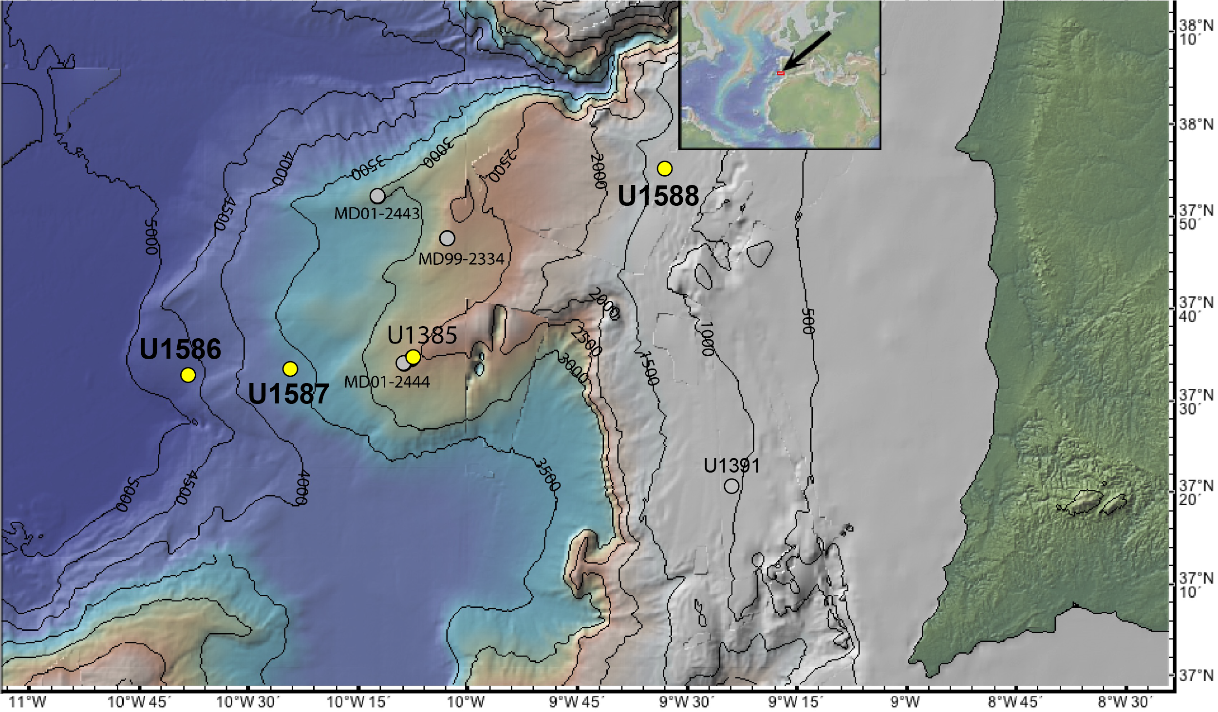
Figure F1. PPA bathymetry.
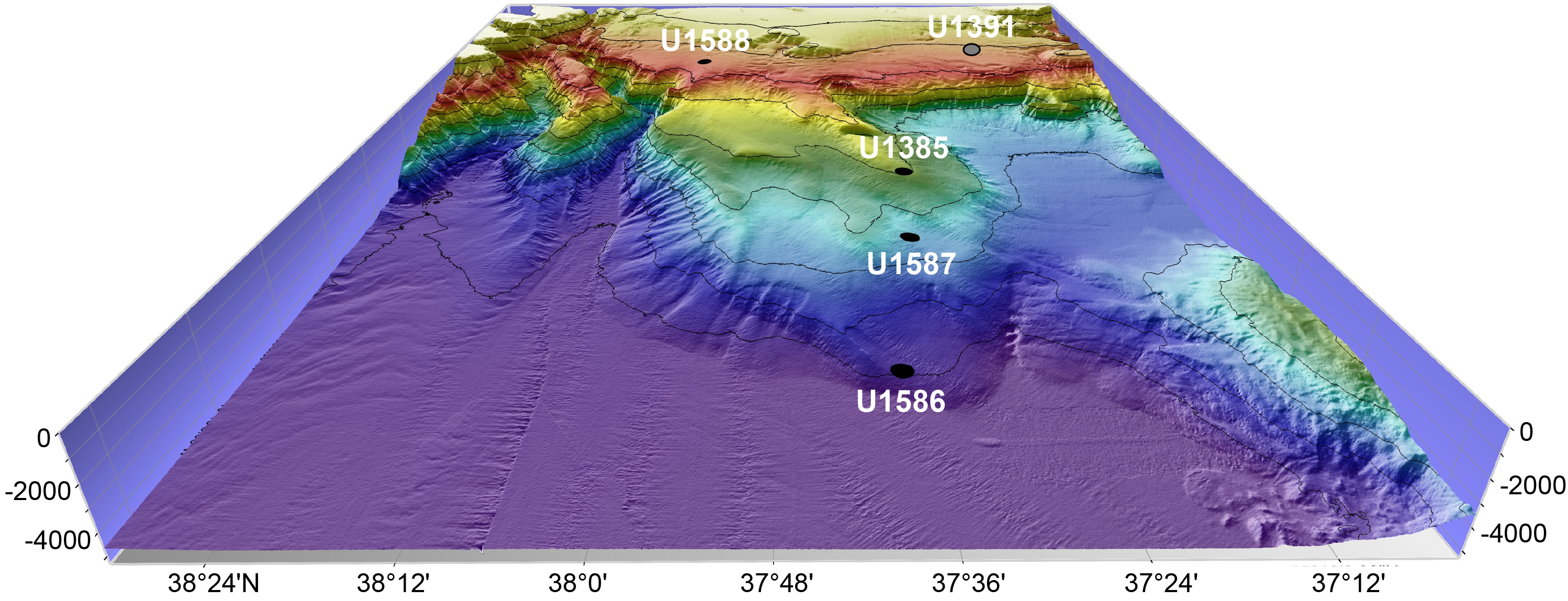
Figure F2. Expedition 397 drill site depth distribution.
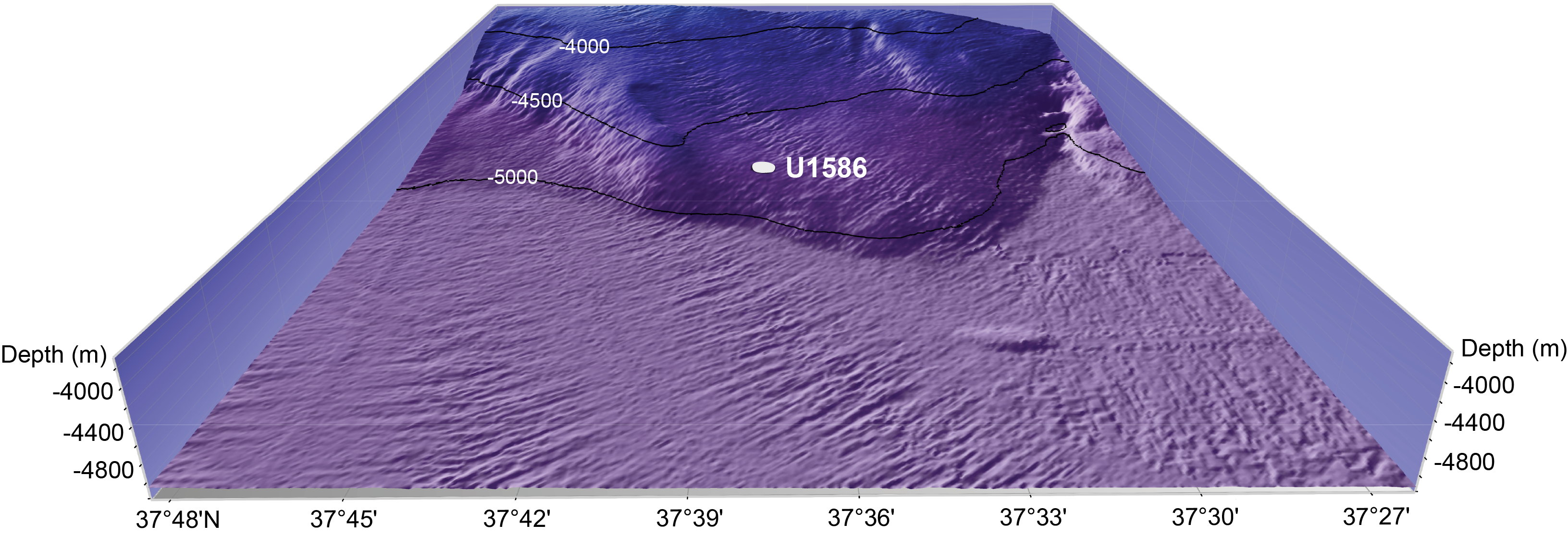
Figure F3. Site U1586 location.
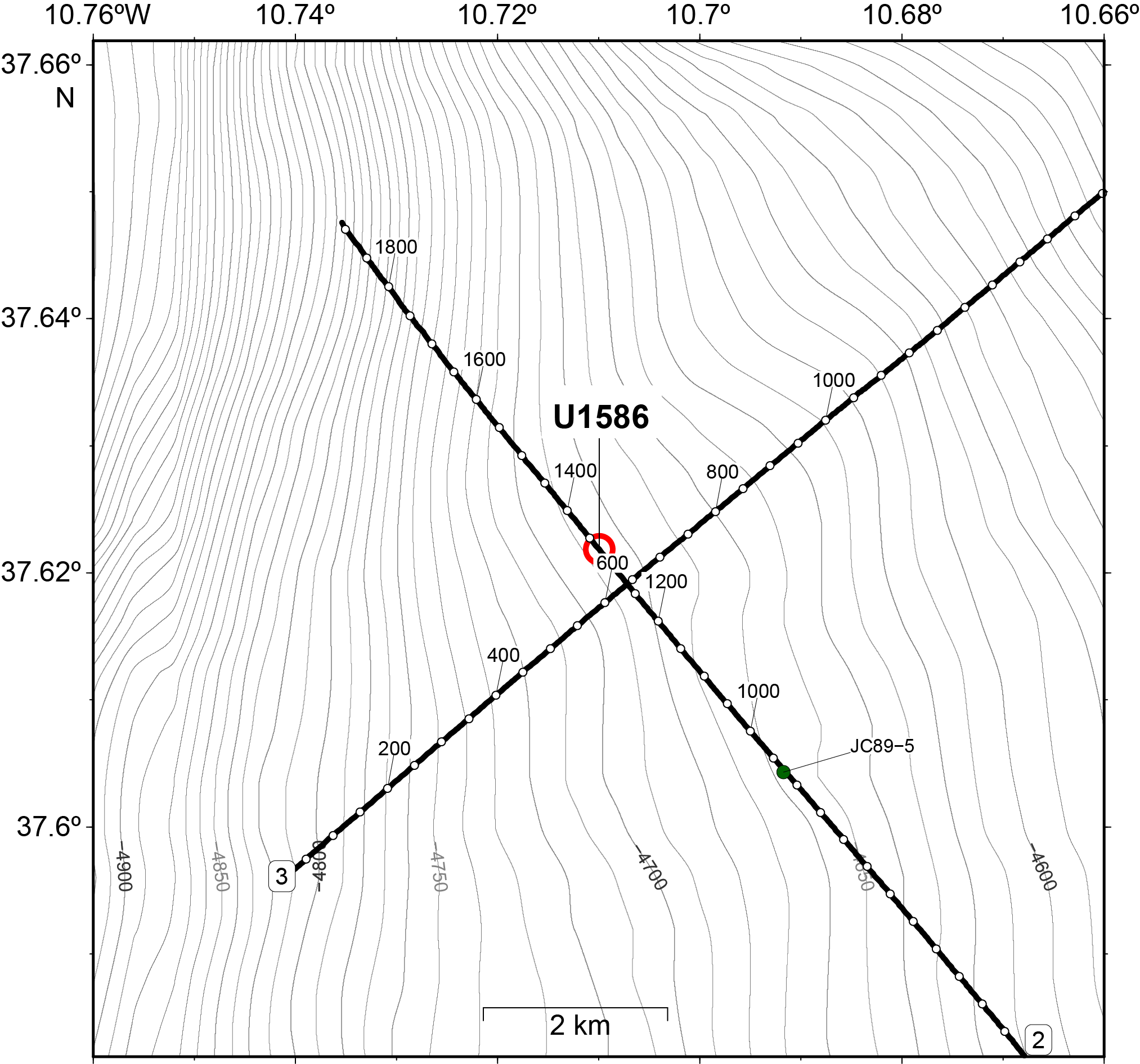
Figure F4. Bathymetric map.
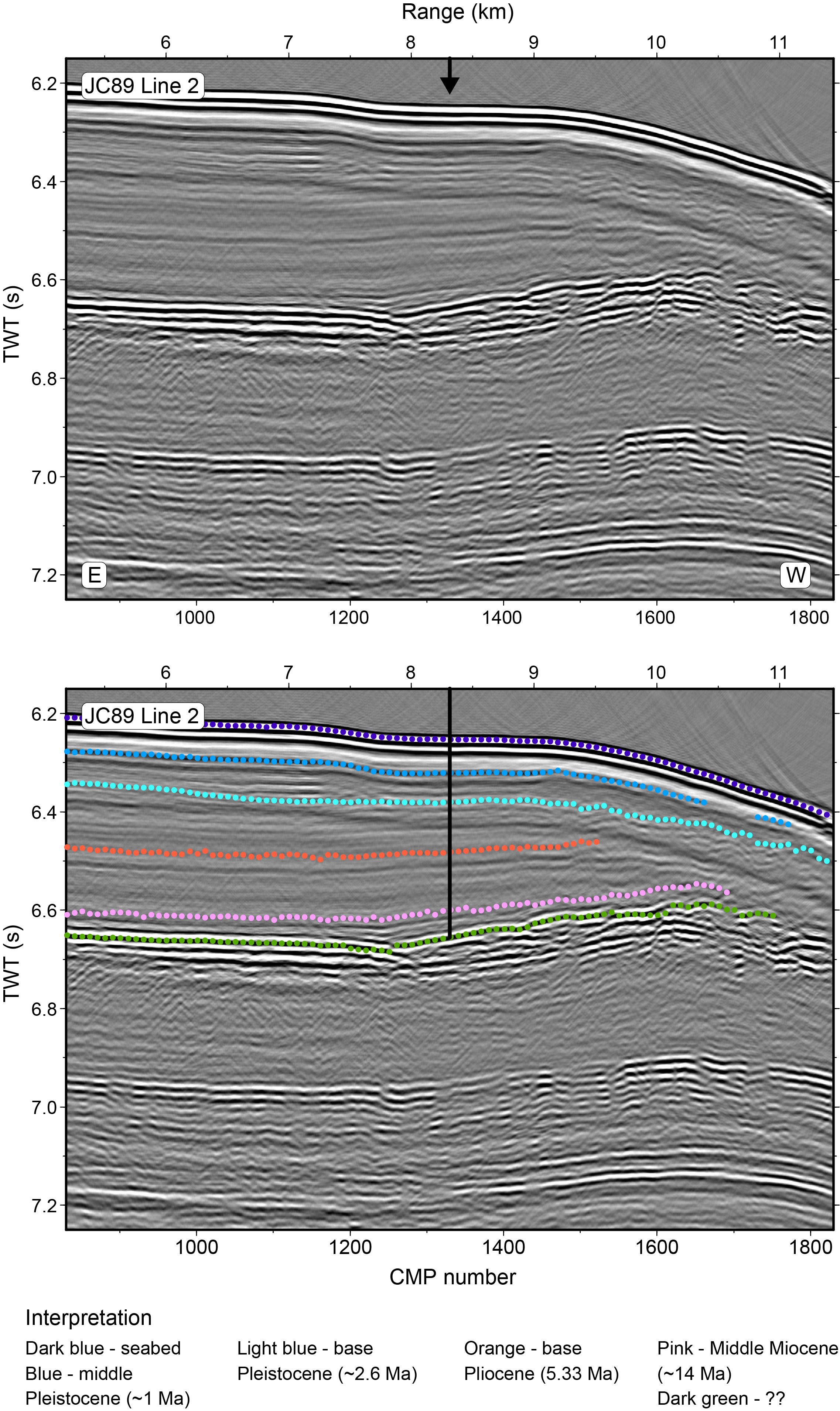
Figure F5. Seismic Profile JC89-2.
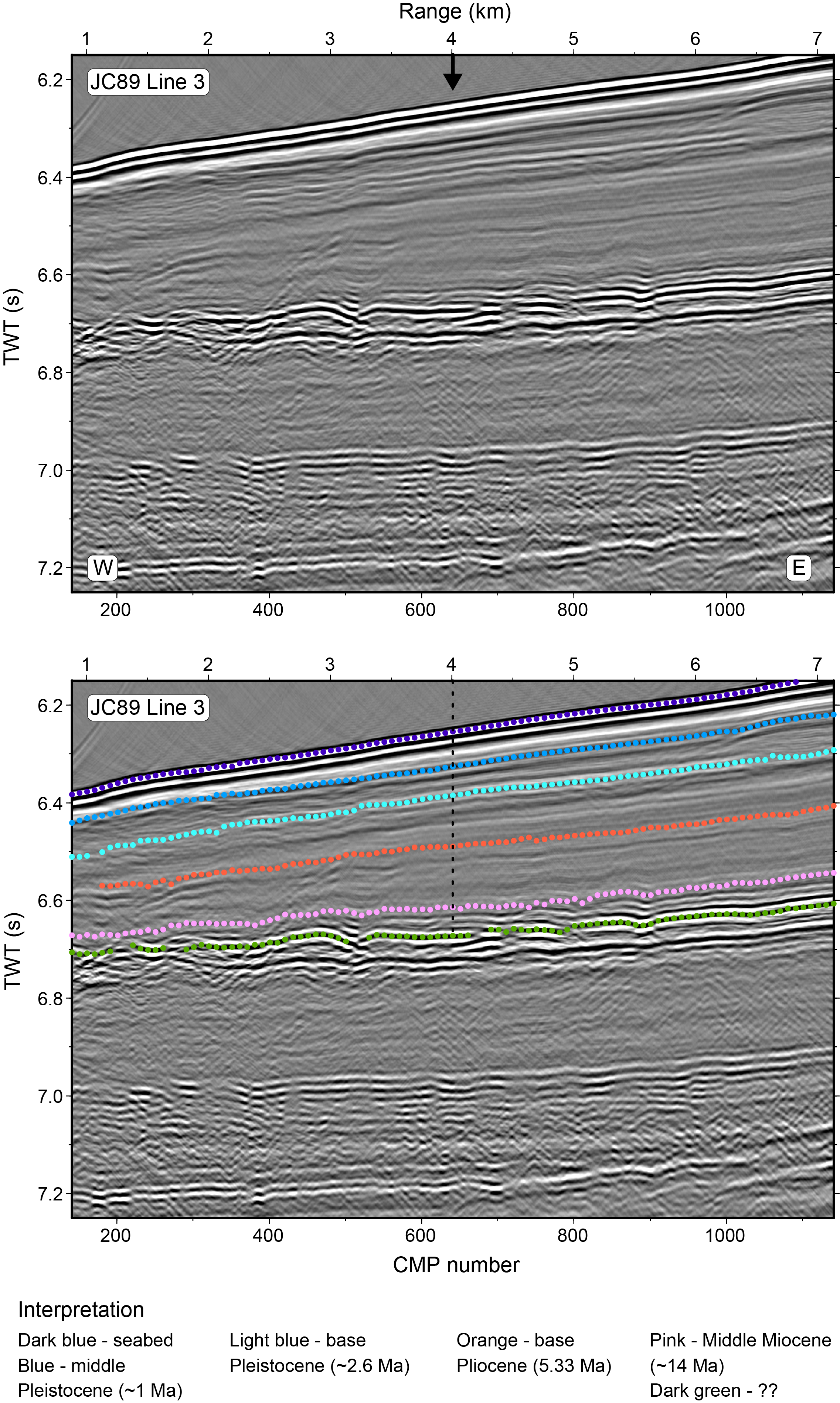
Figure F6. Seismic Profile JC89-3.
The primary scientific objective of Site U1586 was to recover a deep distal record from a water depth of ~4690 mbsl. The sediment thickness thins toward the toe of the Promontório dos Príncipes de Avis owing to lower sedimentation rates with increased distance from shore. Interpretation of the seismic profiles suggests the sequence spans the late Miocene to Quaternary with an average sedimentation rate of 5 cm/ky. Recovery of late Miocene sediment at this site will complement sequences to be drilled during International Ocean Discovery Program (IODP) Expedition 401 to study the exchange between the Mediterranean and Atlantic for the period before, during, and after the Messinian Salinity Crisis (5.96–5.33 Ma) (Flecker et al., 2023). The sediments will also provide a history of surface and deepwater conditions through the Pliocene, including the mid-Pliocene warm period, when atmospheric CO2 was similar to today (400 ppm). Sediments recovered at Site U1586 will also be useful for studying how surface and deep oceanographic conditions responded to the intensification of Northern Hemisphere glaciation in the late Pliocene (~2.9 Ma).
Site U1586 is under the influence of Lower Deep Water (LDW), which consists of Antarctic Bottom Water whose properties have been modified significantly from its origin in the high-latitude South Atlantic (Figure F7). This site's great depth may result in carbonate microfossil dissolution, although a 7.45 m piston core (JC089-5-3P) and 4.68 m kasten core (JC089-5-3K) recovered at the same location show continuous preservation of foraminifers during the last glacial stage and Holocene. Results from shipboard analyses during Expedition 397 further show that carbonate preservation and abundance of calcareous microfossils extends back to the Miocene (see Biostratigraphy). Sedimentation rates in the piston core average 11 cm/ky. The Ca/Ti and Zr/Sr measured using core scanning X-ray fluorescence (XRF) show distinct millennial events (Channell et al., 2018), with particularly notable peaks in Zr/Sr marking each of the Heinrich stadials of the last glacial period (Figure F8).
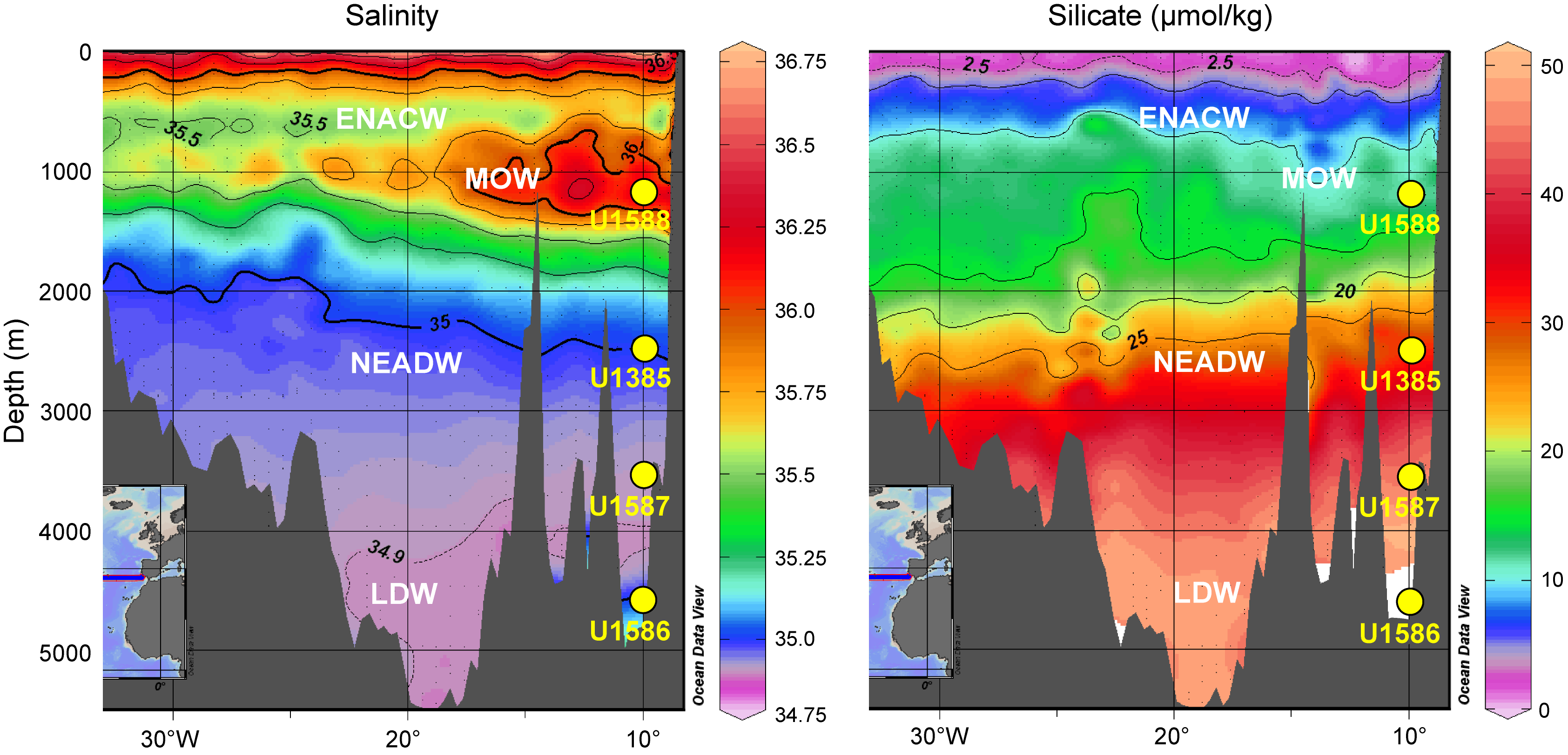
Figure F7. Salinity and silicate profiles.
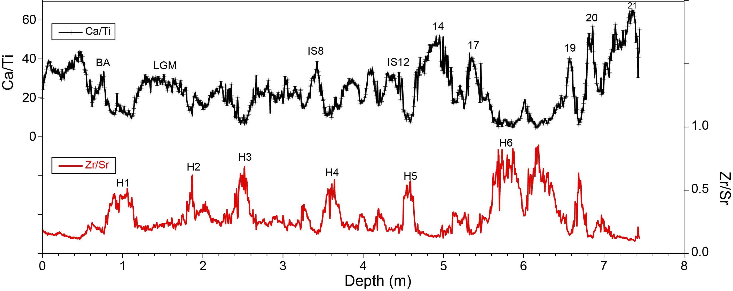
Figure F8. Ca/Ti and Zr/Sr on Piston Core JC089-5-3P.
Study of Site U1586 cores will permit the reconstruction of changes in ventilation and carbon storage in the deepest Atlantic on glacial–interglacial and millennial timescales with potential implications for atmospheric CO2 changes. Preservation of terrestrial biomarkers and pollen will permit reconstruction of vegetation changes in Europe. Lastly, it should be possible to correlate physical properties at Site U1586 into the Mediterranean cyclostratigraphy, thereby permitting regional climate change to be placed into a global context.
2. Operations
2.1. Lisbon port call
IODP Expedition 397, Iberian Margin Paleoclimate, began on 11 October 2022 at 1045 h (UTC + 1 h) upon arrival of the R/V JOIDES Resolution at Rocha Pier in Lisbon, Portugal, at the end of Expedition 397T. The ship cleared customs and immigration and began port call operations. All oncoming Expedition 397 personnel, including 25 scientists, 25 JOIDES Resolution Science Operator (JRSO) staff, 1 outreach officer, and a Portuguese observer moved onto the ship on 13 October following a 4 day quarantine in a Lisbon hotel. The quarantine included a PCR and an antigen test according to the JRSO COVID-19 mitigation protocol. All personnel tested negative before boarding. Once aboard, and over the next 2 days, all expedition participants received another antigen and PCR COVID-19 test. Four IODP Staff and one crew member tested positive after the PCR test on the second day after boarding and were quarantined in single person cabins for 5 days and until they recovered and tested negative two consecutive times. COVID-19 mitigation measures, which included mandatory mask wearing, social distancing, and daily antigen testing of all personnel, were followed until 29 October, which was the fifth day after the last isolated person recovered and came out of quarantine.
Port call activities included the offloading of freight and Expedition 397T cores and samples and the loading of supplies, fresh food, and catering consumables. Fuel was also pumped on board by two barges tied up alongside the ship over 2 days (one each day). At 0800 on 16 October, the harbor pilot came aboard, two tugboats arrived to assist with the departure, and the mooring lines were released at 0830 h. The vessel proceeded to the pilot station at the mouth of the Tagus River, and the pilot departed at 0902 h. JOIDES Resolution continued the sea passage and completed the 93 nmi transit to Site U1586 at 1834 h on the same day.
2.2. Site U1586
The plan for Site U1586 was to core five holes. Holes U1586A–U1586C were to be cored with the advanced piston corer (APC) and half-length APC (HLAPC) to refusal (estimated at approximately 250 m core depth below seafloor, Method A [CSF-A]) and then cored to a maximum depth of 350 mbsf using the extended core barrel (XCB) system. Holes U1586D and U1586E were to be cored to APC/HLAPC refusal. Temperature measurements were planned for the first hole using the advanced piston corer temperature (APCT-3) tool, and orientation was planned for all APC cores in all five holes. Logging with the triple combination (triple combo) tool string was also planned for Hole U1586C.
Once on site, weather conditions and high seas caused ~48 h of delay over the planned 14.8 days of operations, and the coring strategy was adjusted. The high core quality produced using the XCB system with a polycrystalline diamond compact (PDC) bit and cutting shoe in Hole U1586A allowed for it to be deployed earlier than normal, eliminating the need for the HLAPC to be used in Holes U1586B–U1586D. Therefore, a revised strategy was derived to use the APC system until the first partial stroke and extend the hole to its total depth using the XCB system. Site U1586 ended up consisting of four holes to 350 m CSF-A (Table T1). Hole U1586D was logged using the triple combo tool string.
All APC and HLAPC cores used nonmagnetic core barrels, and APC cores were oriented using the Icefield MI-5 core orientation tool. In total, 1399.1 m were cored using all three coring systems (96% recovery). Operations at Site U1586 took 349.5 h (14.6 days) to complete.
2.2.1. Hole U1586A
A depth reading with the ship's precision depth recorder (PDR) was taken as the vessel approached the site coordinates (37°37.7108′N, 10°42.6987′W), obtaining a seafloor depth of 4702.4 meters below rig floor (mbrf) (4691.4 mbsl). The thrusters were deployed, and the drill string was made up with 5 inch drill pipe and an APC/XCB bottom-hole assembly (BHA) with a PDC bit and lowered to the seafloor. Wind and sea conditions were calm.
At 0900 h on 17 October 2022, we installed the sinker bars and the Icefield MI-5, picked up the top drive, and positioned the drill bit at 4692.4 mbrf to take the first core, but the core barrel was retrieved empty. The bit was repositioned to 4699 mbrf, and a second core barrel was deployed, this time successfully spudding Hole U1586A at 1235 h. Based on recovery from Core 1H, the seafloor depth was calculated at 4702.1 mbrf (4691.1 mbsl). Coring continued with the APC system through Core 19H at 177.5 mbsf. APC refusal was reached on Core 19H (177.4 mbsf) after recording partial strokes on Cores 16H–19H, and excessive force (20,000 lb) was required to pull the last core barrel out of the formation. The HLAPC system was then deployed for Cores 20F–26F (177.4–205.8 mbsf). Because Cores 24F–26F registered partial strokes, the XCB system was deployed for Cores 27X–42X (205.8–350 mbsf), which was the Environmental Protection and Safety Panel (EPSP) approved penetration depth for the site. The drill string was then raised, clearing the seafloor at 0930 h on 20 October, and ending Hole U1586A. With high seas moving in, the drill string was pulled back ~45 m above the seafloor to wait for the seas to subside.
Total recovery for Hole U1586A was 339.5 m (97%). Formation temperature measurements were taken on Cores 4H (34.9 mbsf; 4.27°C), 7H (63.4 mbsf; 4.45°C), 10H (91.9 mbsf; 5.74°C), and 13H (120.4 mbsf; 5.77°C). The rate of penetration for the XCB system averaged 28 m/h.
2.2.2. Hole U1586B
While waiting for calmer seas, the vessel was moved ~100 m northeast from Hole U1586A to the coordinates for Hole U1586B (37°37.3478′N, 10°42.5506′W). By 1000 h on 21 October 2022, heave had subsided to under 3.5 m and operations began on Hole U1586B. Based on the PDR reading, 4693.0 mbrf (4682 mbsl) was chosen to shoot the first core, and Hole U1586B was spudded at 1145 h on 21 October. Based on recovery in Core 1H, the seafloor depth was calculated at 2690.5 mbsl. Hole U1586B was cored to 139.5 mbsf (Core 16H) using the APC system. This depth was almost the same as that where the first partial stroke for the APC in Hole U1586A was registered. With the aim of improving core recovery and quality, we changed to the XCB system, and an XCB core barrel was deployed, but while making the pipe connection, the stabbing guide was damaged and two pieces of plastic were thought to fall into the pipe, blocking the GS fishing tool from latching onto the core barrel. On the second attempt to recover Core 17X, the drill crew mounted a custom-made fishing tool to the bottom of a rotary core barrel (RCB) and deployed it. This tool latched around the outside of the core barrel, allowing us to successfully retrieve the XCB barrel and Core 17X at 1450 h on 22 October. Coring resumed with the XCB system and continued to 209.4 mbsf (Core 24X) at 0045 h on 23 October, when coring was paused because of high seas. The drill bit was pulled two stands off bottom, and an extra knobby was run through the guide horn. The bit was set at 146.2 mbsf at 0500 h on 23 October, and we began waiting for the seas to calm down.
By 0645 h on 24 October, the sea conditions had improved enough to restart rig floor operations. The drillers washed down to 209.4 mbsf, where approximately 2 m of fill was encountered. When the hole was cleared of fill, an XCB barrel was deployed, and coring resumed at 0900 h on 24 October with Core 397-U1586B-25X to 219.1 mbsf. Coring continued thereafter, deepening the hole to 308.4 mbsf (Core 35X) by midnight. Core 30X was advanced only 2 m to reestablish a good core offset with Hole U1586A. Coring operations and laboratory activities were suspended at ~2130 h on 24 October due to smoke and fumes from the overheating of the degassing coils on the superconducting rock magnetometer (SRM) in the core laboratory. The SRM was isolated, and the situation was dealt with by JRSO technical staff and Siem personnel. Coring resumed, and the scientists returned to their stations. Coring continued to 350 mbsf (Core 40X). The drill string was pulled back, and the bit cleared the seafloor at 1320 h on 25 October, ending Hole U1586B. The rate of penetration for the XCB system averaged 34 m/h.
At 1300 h on 25 October, the seagoing tugboat Spartacus arrived alongside JOIDES Resolution and took two expedition participants (a scientist and an Entier crew member) to shore for compassionate evacuation.
2.2.3. Hole U1586C
The vessel was offset 150 m southeast to the location of Hole U1586C (37°37.2911′N, 010°42.6216′W). While repositioning the vessel, the drill crew started servicing the rig, which comprised slipping and cutting the drill line, and the JRSO staff obtained a water depth reading with the PDR. Based on the PDR depth, the bit was spaced to 1698 mbrf, and Hole U1586C was spudded at 1825 h on 25 October 2022. The seafloor depth then was calculated as 4703.5 mbrf (4692.4 mbsl) based on recovery from Core 1H. APC coring continued to 118.0 mbsf, where there was a partial stroke on Core 13H. The XCB tools were then deployed over a 231.1 m interval (Cores 14X–38X [118.0–349.1 mbsf]; 91% recovery). The rate of penetration with the XCB system was 39 m/h.
2.2.4. Hole U1586D
The vessel was offset 20 m southeast from Hole U1586C, the bit was spaced to 4702 mbrf, and Hole U1586D was spudded at 1120 h on 28 October 2022 at 37°37.2835′N, 10°42.6289′W. Based on recovery from Core 1H, the seafloor was calculated at 4704.7 mbrf (4693.6 mbsl). APC coring continued through Core 12H (to 111.3 mbsf) under increasing heave by midnight on 28 October. Owing to the high heave, various APC cores were triggered unintentionally during orientation (Cores 5H and 6H), causing incomplete strokes and heavy drilling disturbance in the cores. At 0100 h, with the aim to improve core quality, the Co-Chief Scientists requested to stop coring operations until heave had lessened. At 0700 h on 29 October, with the heave down to ~2 m and continuing to decrease, we changed to the XCB system and resumed coring. Cores 13X–38X were retrieved from 111.3 to 350 mbsf and recovered 223.55 m, with recovery ranging 48%–130% (average = 96%). Overall core recovered in Hole U1586D is 337.79 m (97%). The rate of penetration with the XCB system averaged 49 m/h.
After reaching a total depth of 350.0 mbsf, the driller pumped a 30 bbl sweep of high-viscosity mud to clean the hole and the bit was pulled to 84.6 mbsf for logging. After a safety meeting between the rig crew and the Schlumberger engineer, the drill floor was rigged for logging and the triple combo tool string was assembled and deployed at 0445 h on 31 October.
Because a new logging surface equipment was installed during a recent tie-up period, a short test of the wireline active heave compensator was performed while the tool string was still in the drill pipe. The test was successful, and the tools were lowered out of the drill pipe and into the open hole, reaching a total depth of 4690 mbrf (255.3 mbsf), approximately 100 m above the total depth of the hole. Attempts to open the caliper were unsuccessful until the tool string reached 4945 mbrf (240.3 mbsf), and the upward pass, which collected magnetic susceptibility (MS), resistivity, density (with caliper), neutron porosity, temperature, and natural gamma radiation (NGR) data, began from there to 2843 mbrf (125.3 mbsf). Attempts to close the caliper so that a second pass could be performed were unsuccessful, and it was decided to bring the tools to surface. The tools were pulled into the drill string but became stuck with the top of the tools about 18 m above the bit. Attempts to free the tools were unsuccessful. The Kinley crimper and cutter were deployed to cut the logging cable and keep the tools in the drill pipe.
After the severing operation, the wireline was recovered to the drill floor, followed by the drill pipe, and the BHA cleared the seafloor at 1820 h on 31 October and reached the rig floor at 0145 h on 1 November. Three stands of drill collars were racked back in the derrick so the crew could work on freeing the stuck logging tools. The tools were free and laid down at 0630 h. The rig floor was then secured, and the vessel was readied for transit to Site U1587 at 0810 h on 1 November, ending Hole U1586D and Site U1586.
3. Lithostratigraphy
Three primary lithofacies were defined from visual descriptions, smear slides, and thin sections. Lithofacies 1 and 2 can be represented by a mixed ratio of two end-members: Lithofacies 1, which is 100% nannofossil ooze, and Lithofacies 2, which is 100% clay/silt. Lithofacies 3 consists of very fine to coarse sand that is dominantly calcareous. Three lithostratigraphic units were defined at Site U1586 based on the frequency and occurrence of the three lithofacies and on changes in states of deformation. Lithostratigraphic Unit I spans 0–197 m CSF-A in Holes U1586A–U1586D. Unit I consists predominantly of Lithofacies 1, with cyclically varying amounts of clay downcore. Bioturbation is sparse to heavy and dark patches are extensive in the upper 17 m in all holes. Unit II spans mostly 197–245 m CSF-A in the same holes and consists of sediment from Lithofacies 1 (66% sediment) and 2 (34% sediment), presenting a clear cyclicity. Bioturbation varies from absent to complete disturbance of sedimentary layers, and pyrite nodules are occasionally observed. The abundance of nannofossil ooze with varying amounts of clay in Units I and II indicates the dominance of hemipelagic sedimentation at Site U1586 from the Pleistocene through the late Miocene. Lithostratigraphic Units I and II were further divided into deformed (slumped or convoluted) and nondeformed intervals. The frequent occurrence of slump intervals suggests repeated periods of slope instability. Lithostratigraphic Unit III consists of sediment from Lithofacies 1 (60% sediment), 2 (35% sediment), and 3 (5% sediment). The lithofacies in Subunit IIIA alternate between nannofossil ooze (Lithofacies 1) and clay (Lithofacies 2), and those in Subunit IIIB alternate between clay (Lithofacies 2) and sand (Lithofacies 3). Sandy intervals in Subunit IIIB likely resulted from sediment gravity flows. Drilling disturbance is present in most cores in all holes, varies from slight to severe, and is influenced by the drilling type and operation conditions.
3.1. Introduction
Three lithofacies were identified using visual observation of sediments, microscopic examination of smear slides and thin sections, X-ray diffraction (XRD), and carbonate analyses; they were also compared to the sediment physical properties. Sediments are categorized into three lithofacies according to their primary lithologies, which include nannofossil ooze, clay, and sand. Two smear slides, two CaCO3 samples, and one XRD sample were taken per core in Hole U1586A, and additional smear slides were taken in other holes to confirm lithologies. Site U1586 consists of three lithostratigraphic units spanning the Quaternary to the early Miocene. Units I and II consist primarily of Lithofacies 1 (nannofossil ooze) and 2 (clay), and Unit III also includes Lithofacies 3 (sand).
Based on constraints from biostratigraphy and paleomagnetic data, the ages of the bases of Holes U1586A–U1586D are estimated at approximately 13.6 Ma, or early/middle Miocene. It is likely that multiple sedimentation hiatuses occurred throughout the recovered sequence. Using onboard age models, sedimentation rates at Site U1568 were estimated at 5 cm/ky from 0 to 100 m CSF-A, 3.2 cm/ky from 100 to 230 m CSF-A, and 1 cm/ky from 230 to 300 m CSF-A (see Biostratigraphy). Slumps ranging 1–12 m thick were observed over five depth intervals between 45 and 207 m CSF-A. Drilling disturbance is present in many cores in all holes, is slight to strong, and varies with the type of drilling system.
3.2. Lithofacies description
Three lithofacies were identified at Site U1586 (Table T2). Lithofacies 1 and 2 can be represented as a mixing ratio between two end-members: 100% nannofossils and 100% clay/silt comprising of siliciclastics.
3.2.1. Lithofacies 1
Lithofacies 1 is a pale beige to light brown nannofossil ooze (Figure F9) with distinctive color banding throughout. Color banding is generally on the 0.5–3 cm scale and alternates from light to dark with some minor green banding. No grain size difference is noted between bands of different colors. Contacts between bands vary from sharp to gradational to straight to irregular. Nannofossil ooze is deposited as continuous units of many tens of meters in thickness. The major modifying component (>25%–50%) is clay, and the minor modifying components (>10%–25%) are silt and clay (as siliciclastic grains), foraminifers (as the biogenic component), detrital carbonate, and authigenic grains. Bioturbation varies from sparse to heavy; Chondrites, Thalassinoides, and Planolites are the most common trace fossils, and Zoophycos and Ophiomorpha are less abundant. Black patches and black stained burrows are noted throughout this lithofacies, and black pyritized nodules are occasionally present.
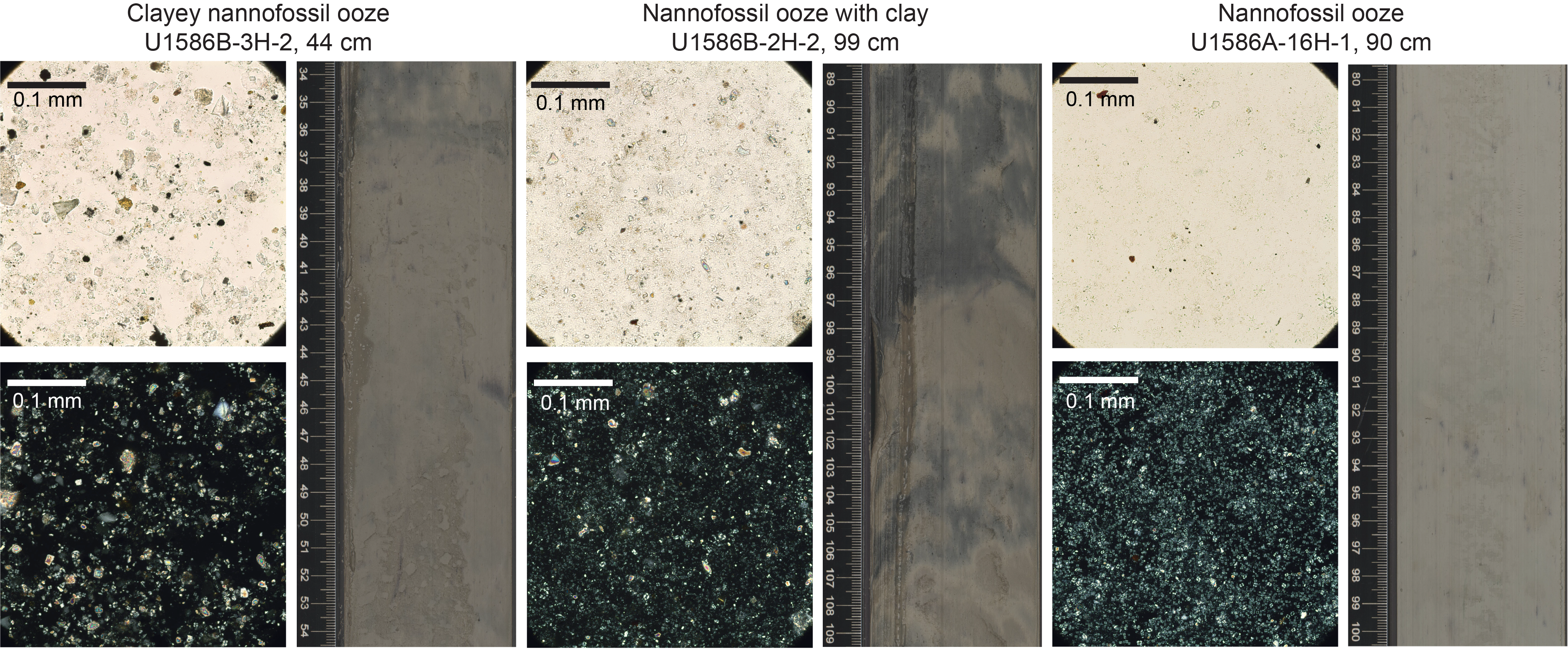
Figure F9. Lithofacies 1.
3.2.1.1. Smear slides
Nannofossils are the dominant component (>50%) in this lithofacies. The siliciclastic component of smear slides varies from rare to abundant and is predominantly in the clay-size fraction (>70%). Other minor components (>1%–10%) are foraminifers, detrital carbonate, sponge spicules, radiolarians, and authigenic minerals such as glauconite and iron oxides. For all (biogenic and siliciclastic) components, 20%–98% of grains are in the clay-size fraction, 2%–60% are in the silt-size fraction, and 0%–50% are in the sand-size fraction.
3.2.2. Lithofacies 2
Lithofacies 2 is mostly dark brown but can vary in color between green, blue-gray, and red. This lithofacies often contains distinctive 0.5–3 cm color banding throughout but can also be homogeneous. It is dominated by siliciclastic clay and minor silt grains, although there are a few examples of clayey silt where silt dominates lithology (>50%) (Figure F10). Clay intervals vary from 1 cm to 1.5 m and rarely span up to 3 m. Most clay intervals are 10–20 cm thick, and minor cases are thinly (<0.3 cm) to thickly (0.3–1 cm) laminated. The major modifying components (>25%–50%) are silt (as siliciclastic grains) and nannofossils (as the biogenic component). The minor modifying components (>10%–25%) are sand (as siliciclastic grains), foraminifers and nannofossils (as the biogenic component), carbonate, and authigenic grains. Where sand is present, it can occur as diffuse patches 2–5 cm in length and is often discontinuous with irregular shaped bases. Bioturbation ranges from absent to complete, and Planolites, Chondrites, Thalassinoides, Zoophycos, and Ophiomorpha are the most common trace fossils. Black patches and black stained burrows are noted throughout this lithofacies, and black pyritized nodules are occasionally present.
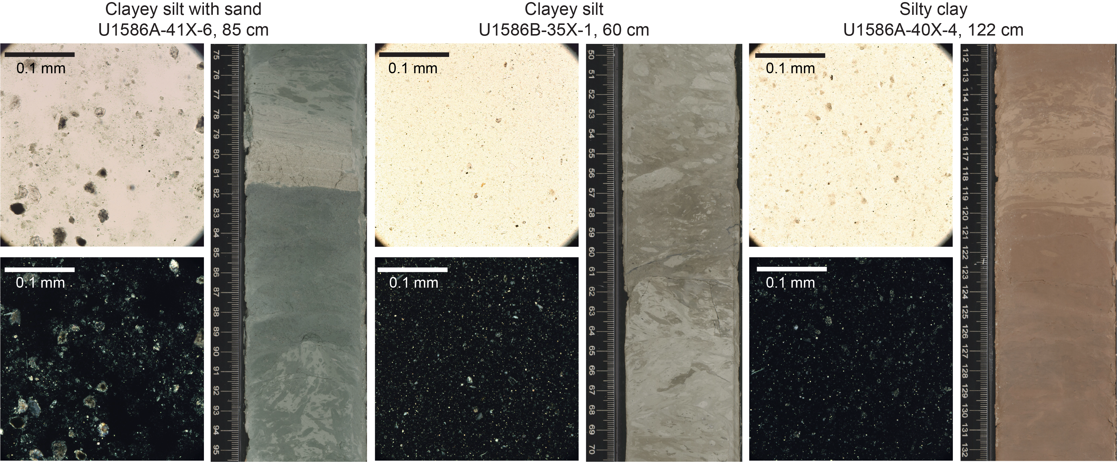
Figure F10. Lithofacies 2.
3.2.2.1. Smear slides
Siliciclastic grains are the dominant component (>50%) in this lithofacies. They occur in the clay- (50%–90%) and silt-size (15%–40%) fractions. Nannofossil abundance ranges from rare (>1%–10%) to abundant (>25%–50%). Detrital carbonate ranges from rare (>1%–10%) to common (>10%–25%). Other minor components (>1%–10%) include foraminifers, sponge spicules, and authigenic minerals such as glauconite and iron oxides. For all (biogenic and siliciclastic) components, 15%–94% of grains are in the clay-size fraction, 5%–70% are in the silt-size fraction, and 0%–35% are in the sand-size fraction.
3.2.3. Lithofacies 3
Lithofacies 3 varies greatly in color from white/light brown to gray, brown, and green. Sediment can also be altered to black. Grains appear dominantly calcareous, and foraminifers can be recognized with a hand lens. Grain size ranges from very fine to coarse sand and sometimes can be as fine as silt/clay sizes (Figure F11). Beds are 2–50 cm thick with sharp erosional bases, with minor scouring or loading. Sand beds can be structureless or planar/unidirectional ripple laminated. Grains in this lithofacies consist of broken foraminifer shells and other calcareous grains with various amount of micrite. Bioturbation is generally absent to sparse and, where present, includes Planolites and Thalassinoides in the coarser fractions of beds and Chondrites and Zoophycos in silty layers located at the tops of beds.
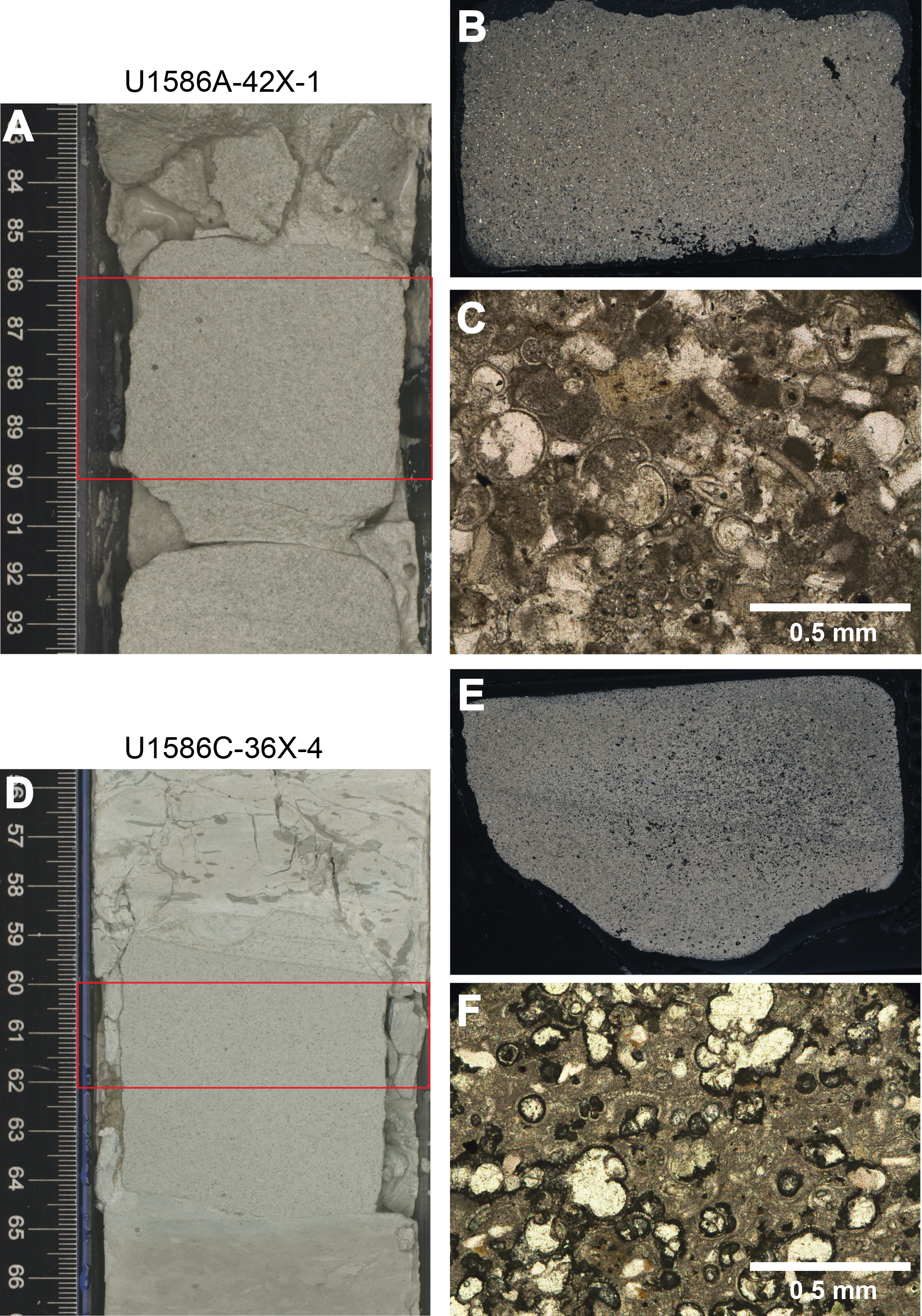
Figure F11. Lithofacies 3.
3.2.3.1. Smear slides
Smear slides significantly underrepresent coarser grain sizes, so only three were made for this lithofacies. Sandy foraminifer ooze with nannofossils is observed in Section 397-U1586B-31X-3, 23 cm, and sandy silt with clay, carbonate, and foraminifers is observed in Section 36X-5, 70 cm. In the calcareous sand from Section 397-U1586C-36X-6, 119 cm, calcite grains seem to be recrystallized or reprecipitated.
3.2.3.2. Thin sections
Thin sections (Samples 397-U1586A-42X-1, 86–90 cm, and 397-U1586C-36X-4, 60–62 cm) from this lithofacies contain broken foraminifer shells, corals, coralline red algae, green algae, bivalve shells, brachiopod shell fragments, echinoderm spines, and fish teeth. The thin sections consist of dominant biogenic grains (>75%), rare to common micrite (5%–12%), rare to common quartz grains (5%–12%), and trace mica grains (<1%) (Figure F11). For all (biogenic and siliciclastic) components, 10%–30% of grains are in the clay-size fraction, 3%–5% are in the silt-size fraction, and 65%–85% are in the sand-size fraction. Following the carbonate classification scheme of Dunham (1962), this facies is classified as a packstone.
3.3. Lithostratigraphic units
The sedimentary sequence at Site U1586 was divided into three lithostratigraphic units based on the frequency and occurrence of the three lithofacies and changes in the state of deformation. Lithostratigraphic units were further divided where deformed intervals are present (Table T3). The associated criteria used are outlined below, along with the depths in each hole at Site U1586 and the corresponding ages according to the onboard age model based on biostratigraphy and magnetostratigraphy.
3.3.1. Unit I
- Intervals: 397-U1586A-1H-1, 0 cm, to 24F-1, 67 cm; 397-U1586B-1H-1, 0 cm, to 23X-5, 70 cm; 397-U1586C-1H-1, 0 cm, to 23X-2, 26 cm; 397-U1586D-1H-1, 0 cm, to 22X-1, 51 cm
- Depths: Hole U1586A = 0–196.95 m CSF-A; Hole U1586B = 0–196.90 m CSF-A; Hole U1586C = 0–195.75 m CSF-A; Hole U1586D = 0–196.50 m CSF-A
- Thicknesses: Hole U1586A = 196.6 m; Hole U1586B = 196.9 m; Hole U1586C = 195.75 m; Hole U1586D = 196.50 m
- Age: Holocene (~0 ka) to late Miocene (~5.5 Ma)
- Primary lithofacies: 1, 2
Lithostratigraphic Unit I spans sediments from 0 to 197 m CSF-A in Holes U1586A–U1586D and consists largely of Lithofacies 1, which represents, on average, 96% of the sequence. Lithofacies 2 occurs in the remaining 4% of sediment depths (Figure F12). Minor components in smear slides from Lithofacies 1 include rare to common foraminifers (>1%–25%) and rare detrital carbonate (>1%–10%), authigenic minerals (glauconite and iron oxides), and sponge spicules (in Subunits IA and IC). Minor components in smear slides from Lithofacies 2 show common to abundant nannofossils (>10%–50%), rare (>1%–10%) detrital carbonate in Subunit IA, common (>10%–25%) detrital carbonate in Subunits IC and IE, and rare (>1%–10%) foraminifers, authigenic minerals (glauconite and iron oxides), and sponge spicules.
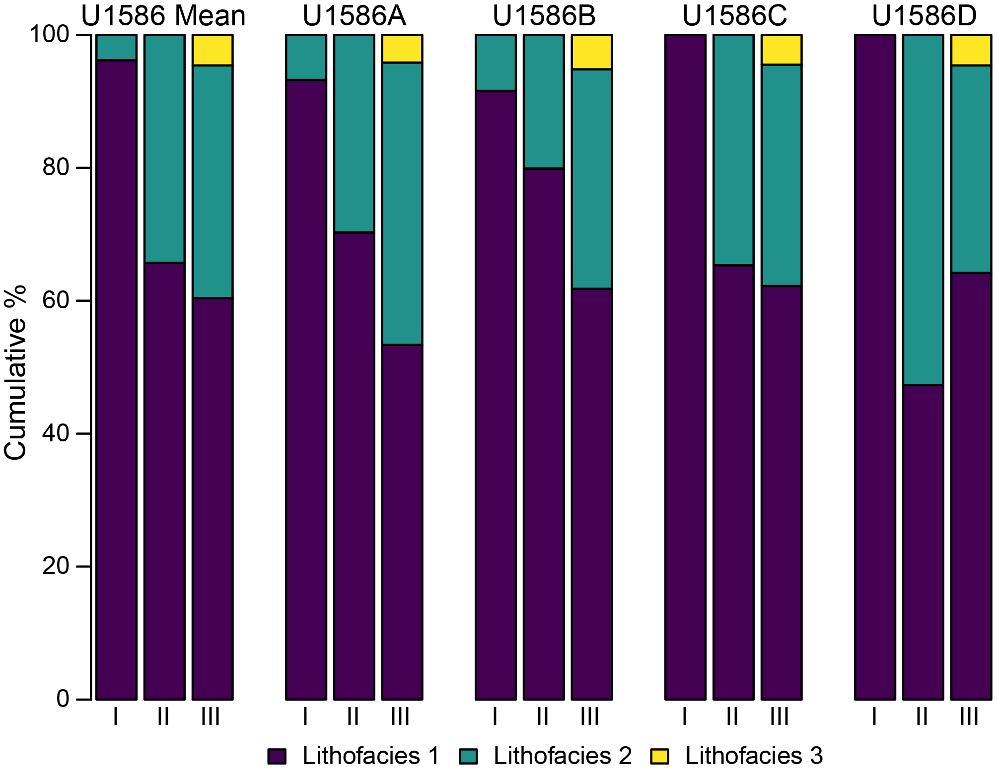
Figure F12. Distribution of lithofacies in lithostratigraphic unit.
Core 1 Section 1 in Holes U1586A–U1586D contains fine-grained brown sediments toward the top and gray sediments toward the bottom, separated by a coarser orange-brown layer with relatively sharp upper and lower contacts. Sediments shallower than 12–17 m CSF-A in all holes are characterized by extensive black patches (Figure F13). Downcore in Unit I, a distinctive pattern of thicker (generally 20–30 cm) white to light beige nannofossil ooze (Lithofacies 1) and thinner (5–10 cm) nannofossil ooze with clay or clayey nannofossil ooze (Lithofacies 1) repeats. A small number of cores show few color changes and do not show variations in minor clay components.
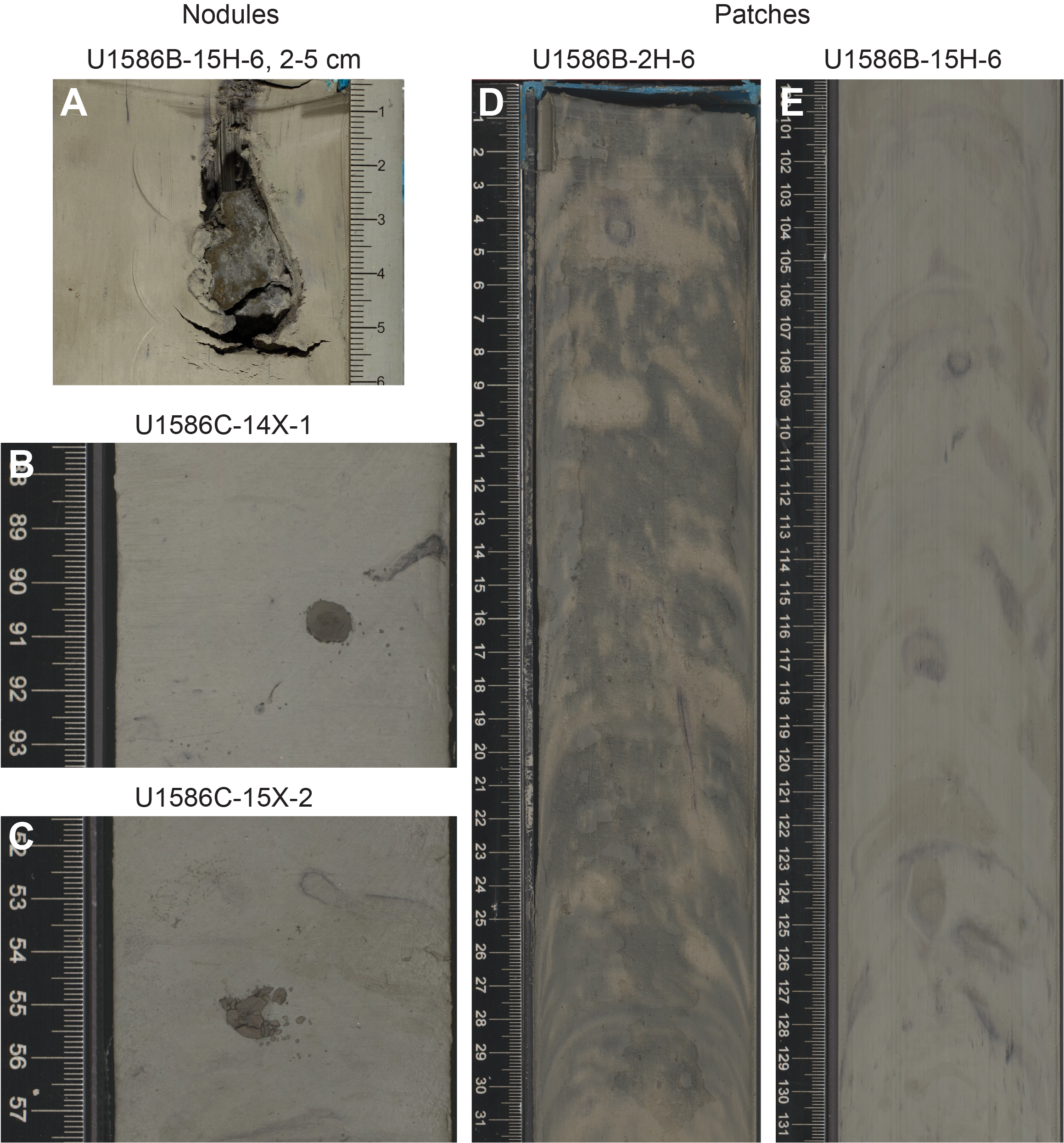
Figure F13. Diagenetic features.
Foraminifers were observed in many cores in Unit I (Hole U1586A = 35–76 m CSF-A; Hole U1586B = 39–104 m CSF-A; Hole U1586C = 17–118 m CSF-A; Hole U1586D = 64–92 m CSF-A). Microspherules were observed in smear slides (Figure F14) from cores with large MS anomalies (Figure F15), including Cores 397-U1586B-18X, 397-U1586C-18X, and 397-U1586D-17X. Deep-sea corals were observed in Cores 397-U1586A-20F and 21F and 397-U1586B-16H (Figure F16). Unit I is divided into nine subunits with undisturbed intervals interrupted by slumped intervals.
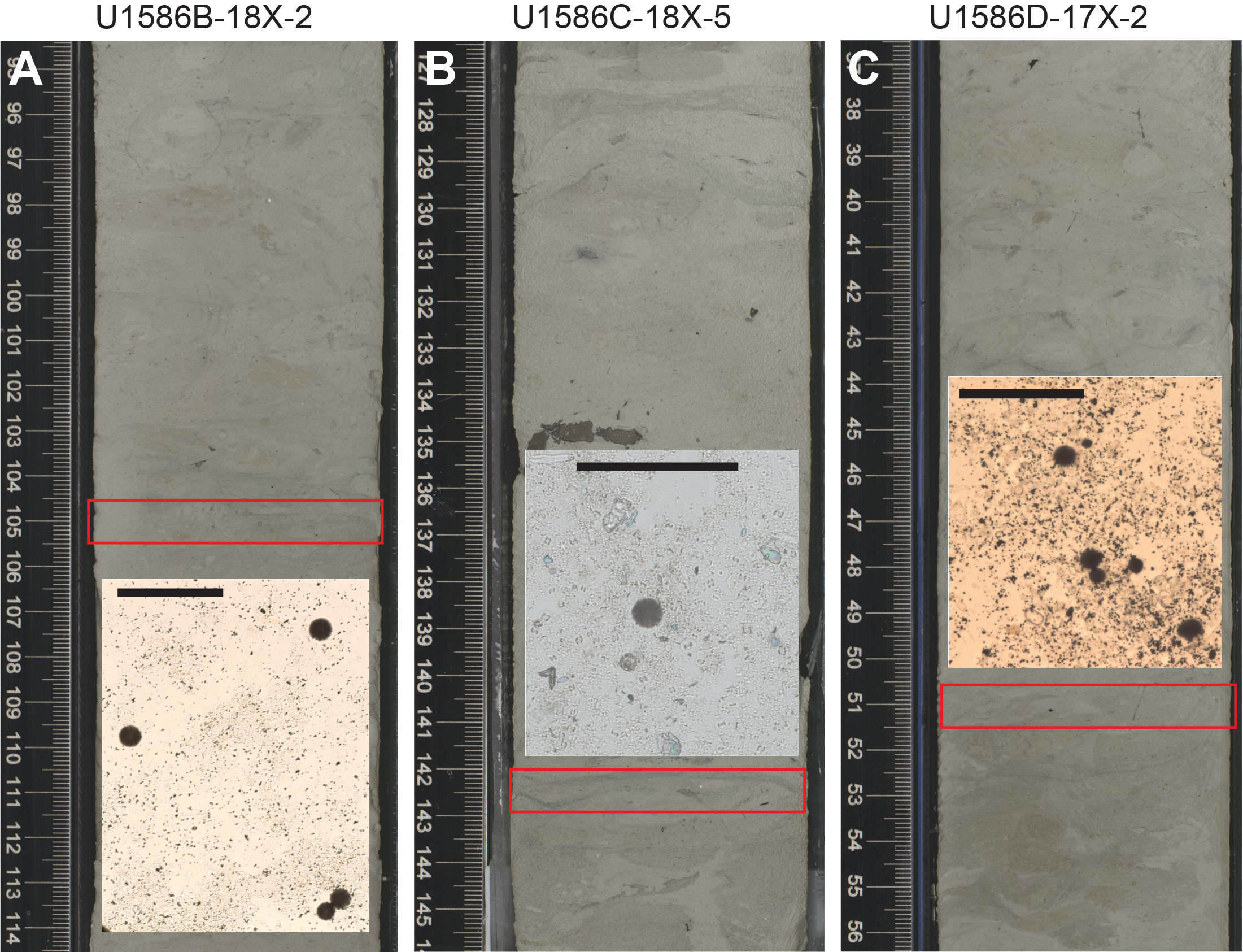
Figure F14. Section halves.
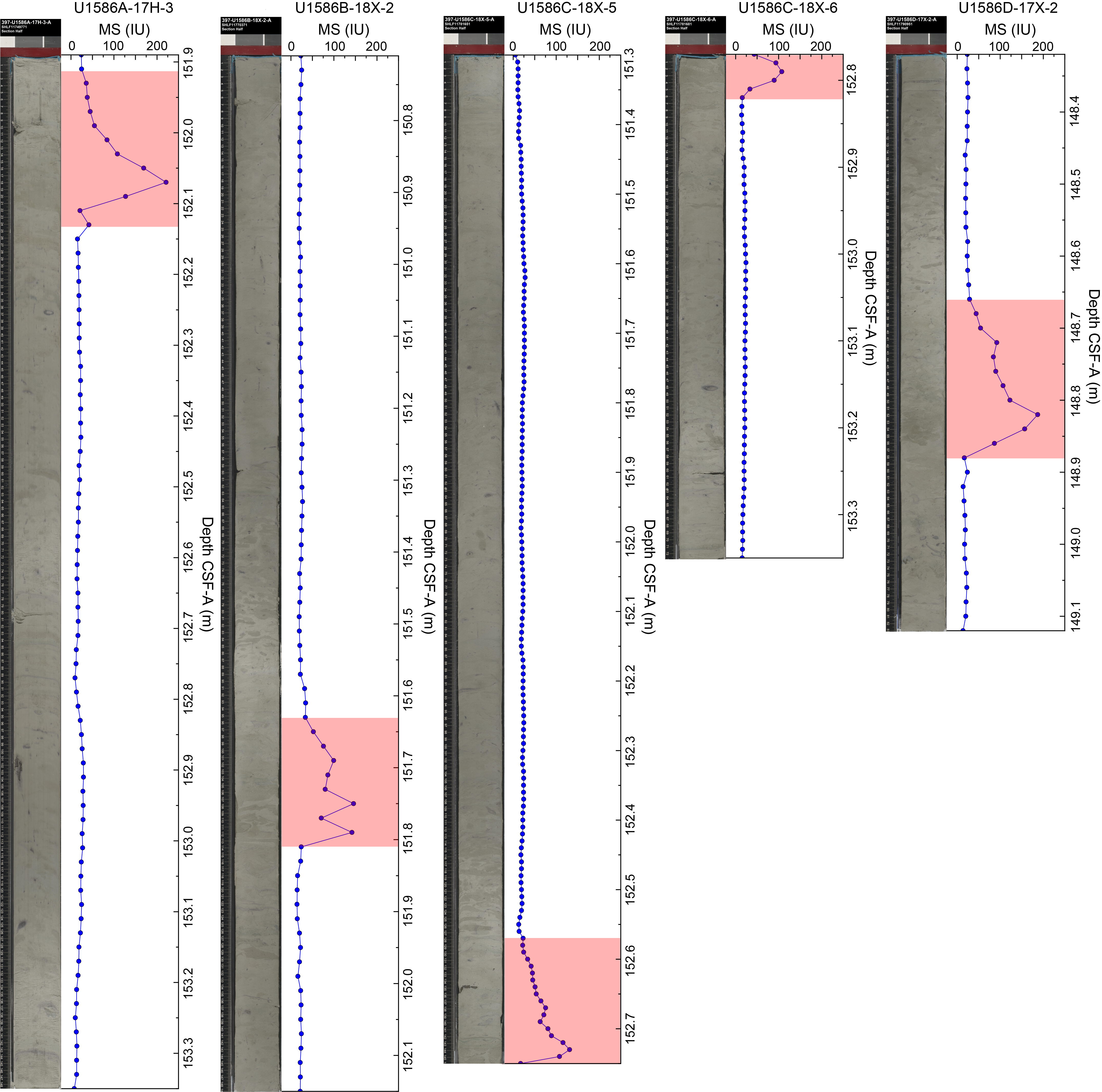
Figure F15. Section halves and MS.
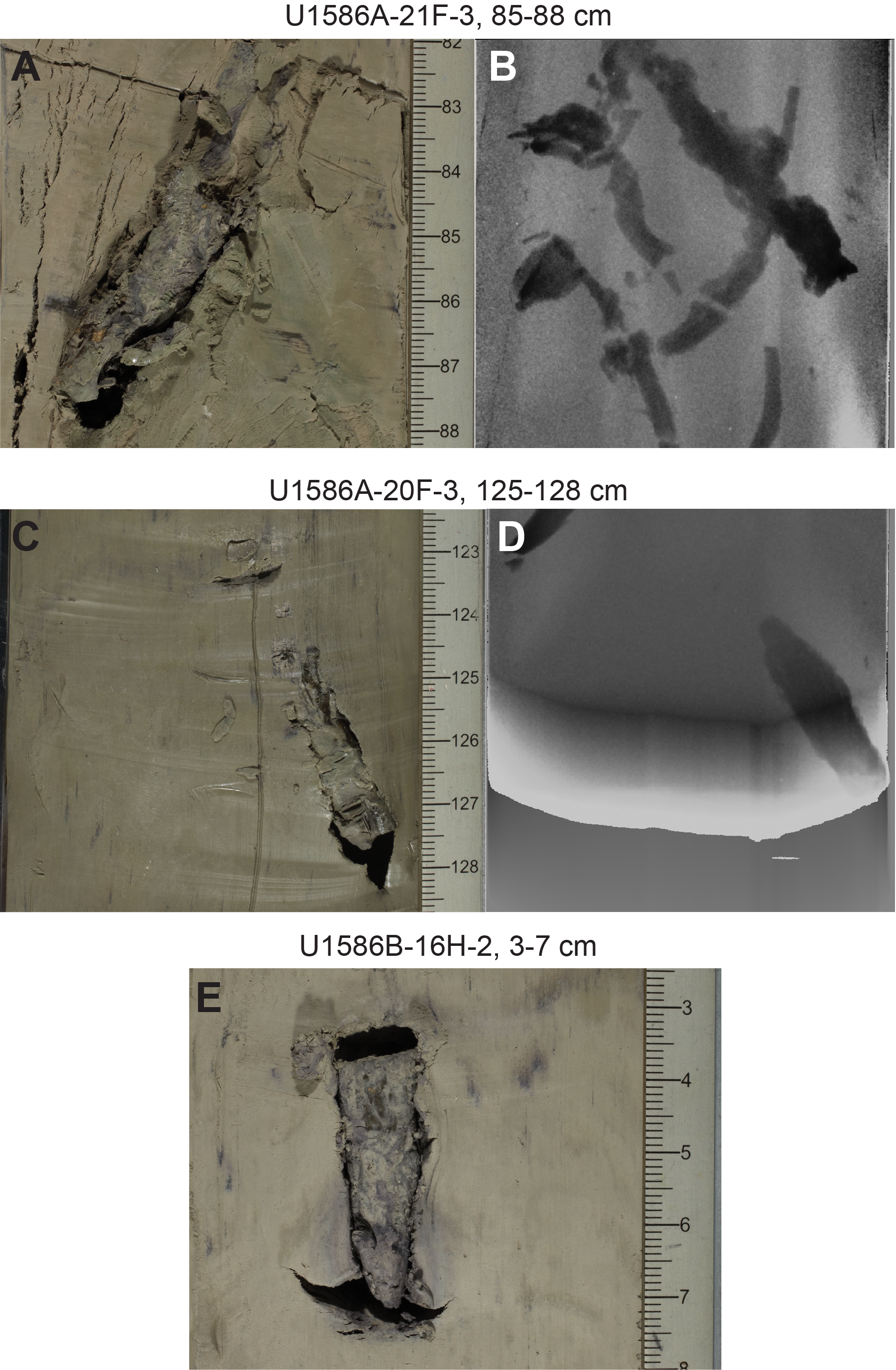
Figure F16. Deep sea corals.
3.3.1.1. Undisturbed Subunits IA, IC, IE, and IG and Unit II
These subunits consist of strata that show indications of cyclicity and are conformable across all holes (Table T3; see Stratigraphic correlation). In these subunits, layers of Lithofacies 1 are characterized by the absence of major deformational structures. Minor soft-sediment deformation observed in these subunits includes microfaulting and very minor convoluted laminations. Bioturbation is slight to moderate, with Thalassinoides, Planolites, and Chondrites as major trace fossils and less abundant Zoophycos and Ophiomorpha.
3.3.1.2. Slumped Subunits IB, ID, IF, and IH
These subunits consist of strata that show no evidence of cyclicity, are unconformable (Figure F17; Table T3; see Stratigraphic correlation), and are correlated across all holes. These subunits are defined by deformational structures characterized as slump folds, convoluted bedding, and contorted beds (Figure F17). Beds can show more distinctive banding that is thinner (1–3 cm) than in the undisturbed subunits. Bioturbation is generally absent to sparse but can be moderate.
Figure F17. Slumped interval.
3.3.2. Unit II
- Intervals: 397-U1586A-24F-1, 67 cm, to 31X-CC, 45 cm; 397-U1586B-23X-5, 70 cm, to 28X-5, 77 cm; 397-U1586C-23X-2, 26 cm, to 28X-2, 150 cm; 397-U1586D-22X-1, 55cm, to 28X-1, 20 cm
- Depths: Hole U1586A = 196.95–245.4 m CSF-A; Hole U1586B = 196.90–245.50 m CSF-A; Hole U1586C = 195.75–245.35 m CSF-A; Hole U1586D = 196.5–242.5 m CSF-A
- Thicknesses: Hole U1586A = 48.45 m; Hole U1586B = 48.6 m; Hole U1586C = 49.60 m; Hole U1586D = 46.00 m
- Age: late Miocene (~5.5–7.78 Ma)
- Primary lithofacies: 1, 2
Unit II spans sediments from ~196 to 245 m CSF-A in the four holes drilled at Site U1586 and consists largely of Lithofacies 1 (66% of sediment depths) and Lithofacies 2 in the remaining sediment depths (average = 34%) (Figure F12). Minor components in Lithofacies 1 and 2 recognized in smear slides include trace to rare (>1%–10%) glauconite and iron oxides. The top of Unit II is characterized by the appearance of 10–20 cm thick dark brown layers of silty clay (Lithofacies 2), which are interstratified with increasingly lighter 20–30 cm layers of nannofossil ooze. White and light to dark brown color banding occurs in Unit II, with occasional 2–5 cm green bands. Black nodules and pyrite are observed throughout the unit.
Unit II is divided into Subunits IIA, IIB, and IIC. Subunits IIA and IIC are undisturbed intervals, interrupted by the slumped interval Subunit IIB. In Subunits IIA and IIC, bioturbation ranges from sparse to heavy and increases downcore. Trace fossils include widespread Planolites, Chondrites, Thalassinoides, and Ophiomorpha; an increase in Zoophycos; and the addition of minor Teichichnus (Figure F18). Based on its occurrences in Holes U1586A–U1586D, Subunit IIB thickens from 3.87 to 5 m downslope. However, drilling disturbance and gaps in the strata of Holes U1586B–U1586D preclude correlation to Hole U1586A. Subunit IIB shows slump folds, contorted bedding, and chaotic strata. Bioturbation in Subunit IIB is absent to moderate.
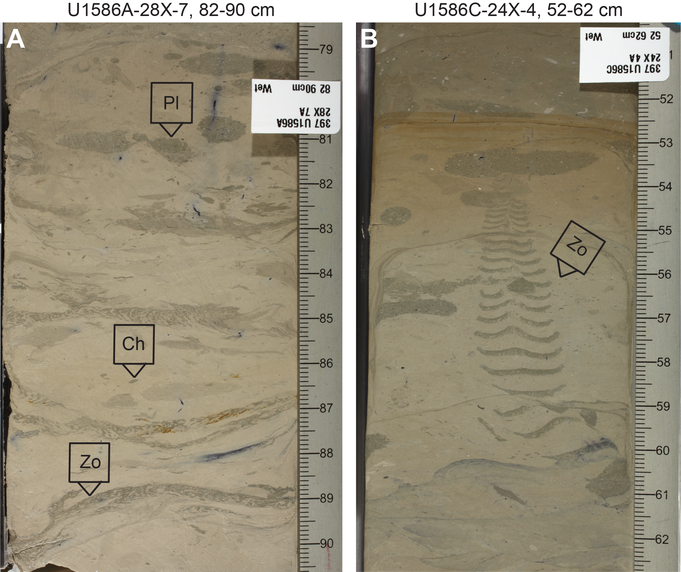
Figure F18. Trace fossils found in Lithofacies 2.
3.3.3. Unit III
- Intervals: 397-U1586A-31X-CC, 45 cm, to 42X-2, 59 cm; 397-U1586B-28X-5, 77 cm, to 40X-CC, 39 cm; 397-U1586C-28X-2, 150 cm, to 38X-CC, 23 cm; 397-U1586D-28X-1, 20 cm, to 38X-CC, 24 cm
- Depths: Hole U1586A = 245.4–346.32 m CSF-A; Hole U1586B = 245.50–350.25 m CSF-A; Hole U1586C = 245.35–341.90 m CSF-A; Hole U1586D = 242.50–347.20 m CSF-A
- Thicknesses: Hole U1586A = 100.92 m; Hole U1586B = 104.75 m; Hole U1586C = 104.75 m; Hole U1586D = 104.7 m
- Age: late to middle/early Miocene (~7.8–17.9 Ma)
- Primary lithofacies: 1, 2, 3
Lithofacies 1 (nannofossil ooze) dominates Unit III but is reduced to, on average, 60% of the strata. Lithofacies 2 (clay) makes up around 35% of the strata, and Lithofacies 3 (sand) constitutes the remaining 5% (Figure F12). Minor components of Lithofacies 1 recognized in smear slides include rare (>1%–10%) foraminifers, detrital carbonate, authigenic minerals (glauconite and iron oxides), sponge spicules (Subunits IIIA and IIIB), and radiolarians (Subunit IIIB). Minor components of Lithofacies 2 recognized in smear slides include common (>10%–25%) detrital carbonate and rare (>1%–10%) foraminifers, sponge spicules, and authigenic minerals (glauconite and iron oxides). In smear slides from Lithofacies 2, nannofossils range from common to abundant (>10%–50%) in Subunit IIIA and are rare (>1%–10%) in Subunit IIIB.
Color banding is present in Unit III as light to dark brown and occasionally green bands 2–5 cm thick. Layers vary from lighter nannofossil ooze (Lithofacies 1) bands 20–30 cm thick to dark brown silty clay (Lithofacies 2) bands. The color of clay changes downcore in Unit III from brown to gray-blue and green. Sediments are moderately to heavily bioturbated, with widespread Planolites, Chondrites, Zoophycos, and Thalassinoides and minor Ophiomorpha. Unit III is divided into Subunits IIIA and IIIB.
3.3.3.1. Subunit IIIA
Throughout Subunit IIIA, Lithofacies 1 (nannofossil ooze) becomes progressively lighter in color downcore. Silty clay becomes predominant (Lithofacies 2) and is dark chocolate brown. Clay starts to occur as greenish sediments in some intervals just above the boundary with Subunit IIIB.
3.3.3.2. Subunit IIIB
The top of Subunit IIIB is marked by the first occurrence of sand in Holes U1586A–U1586D. The shallowest meters of Subunit IIIB are dominated by brown clay with green patches or layers where rare (>1%–10%) silt and sand are present. Upcore in Subunit IIIB, sand layers are thin (centimeter scale) and discontinuous. Downcore in Subunit IIIB, sand layers are bedded and range 2–50 cm thick with sharp, sometimes erosional, bases with occasional loading or scouring. Beds can be structureless or planar/cross-laminated and can be normally graded, in rare cases up to silt and clay. Information about the primarily biogenic grains constituting the sand is given in the Lithofacies 3 description.
3.4. Complementary analysis
3.4.1. Drilling disturbance
The most common drilling disturbances were basal flow-in, up-arching, and soupiness in the APC cores and biscuiting, fragmentation, and fall-in in the XCB cores (Figure F19). Drilling disturbance data for Holes U1586A–U1586D are summarized in Tables T4, T5, T6, and T7 with all slightly disturbed strata omitted.
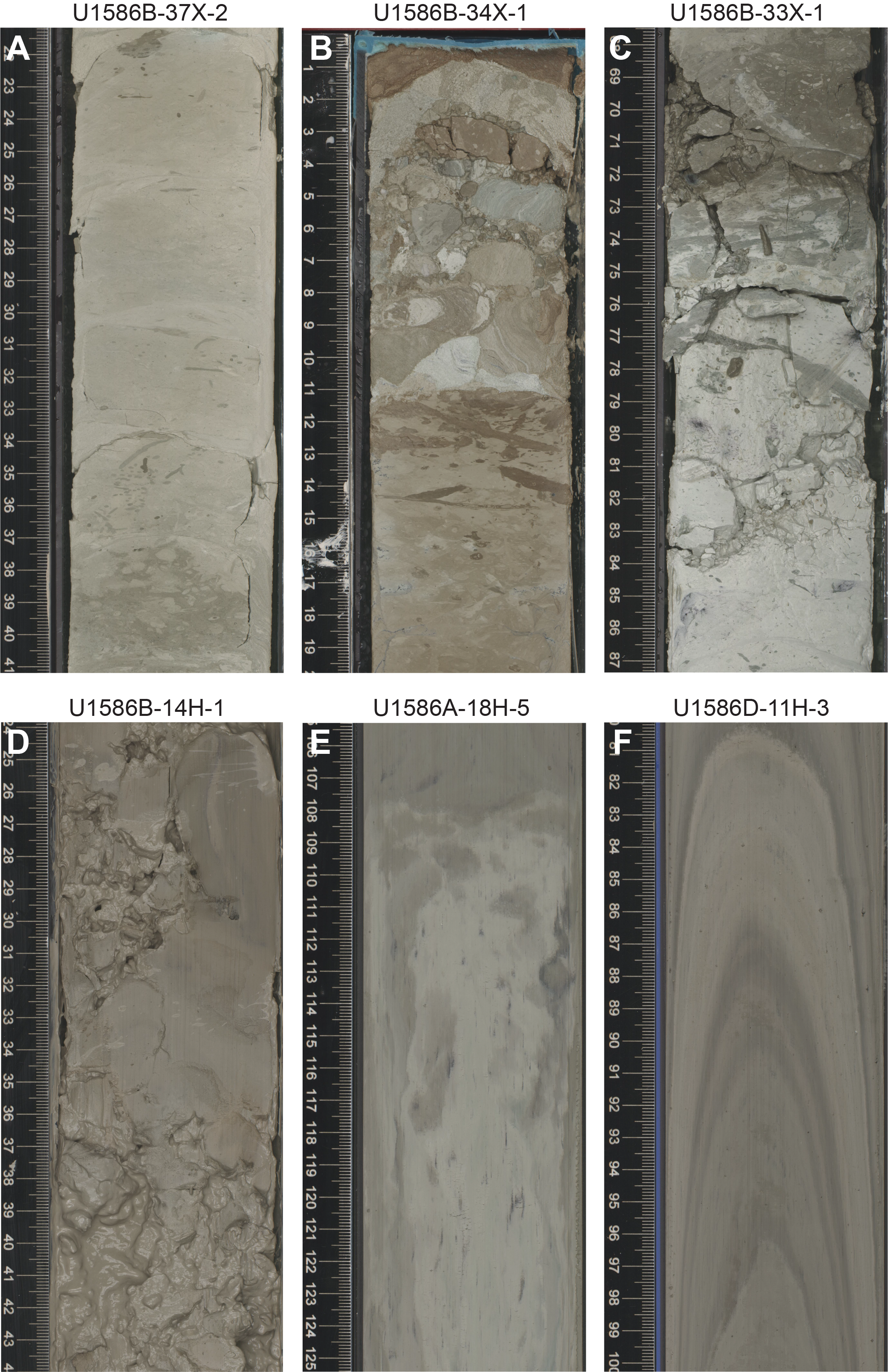
Figure F19. Examples of drilling disturbances.
3.4.2. X-ray diffraction mineralogy
The most abundant minerals observed in XRD analysis in Hole U1586A are calcite, quartz, feldspar, and various clay minerals (i.e., illite, kaolinite, smectite, and chlorite), followed by dolomite, muscovite, glauconite, and pyrite as minor components. The results agree with the mineral composition of the lithologies identified during core description, smear slide, and thin section observations. Iron oxides, glauconite, pyrite, and other iron sulfides are the most common authigenic minerals observed in smear slides from all holes. In the XRD data, glauconite is present occasionally in sediments from different depths in Hole U1586A (intervals 11H-5, 114–115 cm; 22F-2, 135–136 cm; 27X-3, 40–41 cm; 30X-5, 41–42 cm; and 37X-2, 38–39 cm) and pyrite is present rarely (interval 10H-3, 45–46 cm). In Subunit IIIB, dolomite, glauconite, and chlorite were observed in smear slides in dark green silty clay (e.g., Section 397-U1586B-39X-4, 59 cm). XRD analysis also showed that dark green clayey silt with sand (e.g., interval 41X-6, 85–86 cm) contains smectites, Fe-bearing chlorite, quartz, and K-bearing albite.
3.4.3. Carbonate content
Changes in sediment carbonate content (CaCO3) in Hole U1586A are concurrent with lithostratigraphic unit boundaries (Figure F20; see Geochemistry). An overall decrease in CaCO3 occurs downcore from Unit I to Unit II, which is consistent with a decrease in the cumulative percent of Lithofacies 1 (Figure F12). An overall increase in CaCO3 occurs downcore through Subunit IIIA, which indicates that weight percent CaCO3 is not directly proportional to the cumulative percent occurrence of Lithofacies 1. CaCO3 is highly variable in Subunit IIIB, which may reflect the variable lithologies in this subunit or sampling bias/resolution.
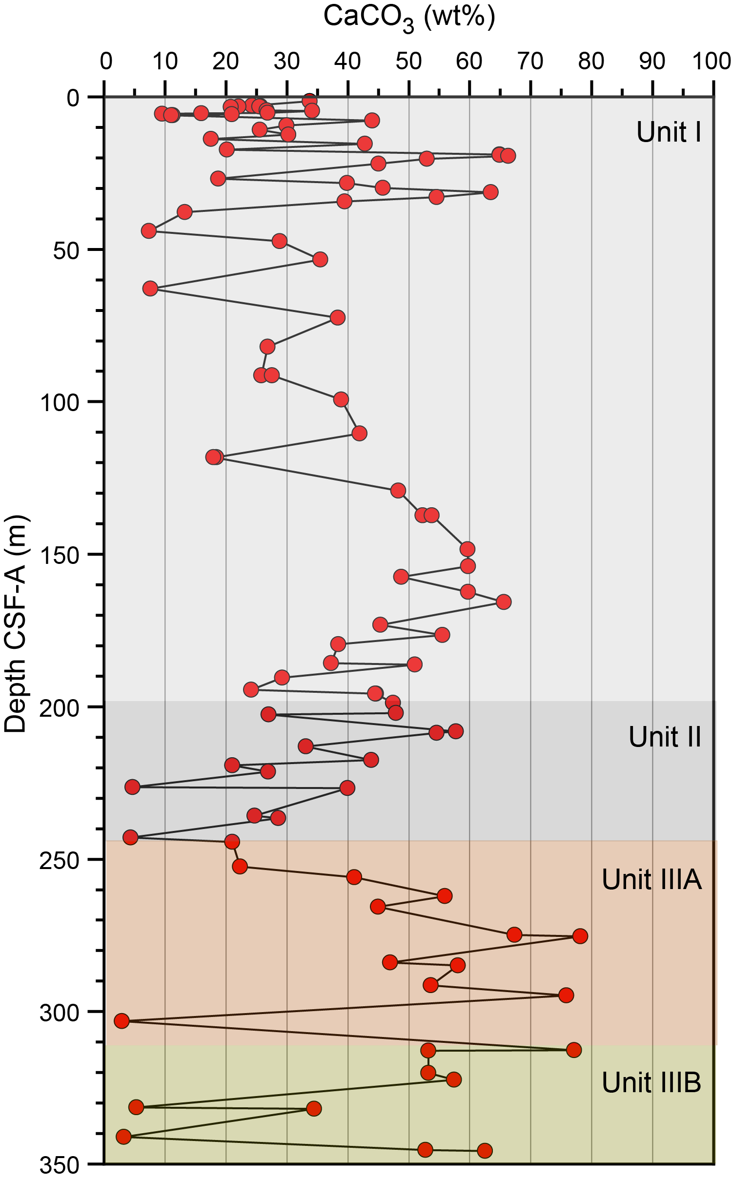
Figure F20. CaCO3.
3.4.4. Integrating physical properties measurements with lithofacies observations
The occurrences of different lithologies at Site U1586 were compared to downcore physical properties measurements including gamma ray attenuation (GRA) bulk density, MS from both loop (Whole-Round Multisensor Logger [WRMSL]) and point (Section Half Multisensor Logger [SHMSL]) detectors, NGR intensity, RGB intensity, and color reflectance L*a*b* (see Physical properties).
Changes in physical properties are associated with lithofacies of various lithostratigraphic units. Unit I is generally characterized by lower GRA bulk density, higher porosity, lower thermal conductivity, intermediate a* and b*, and variable MS that reaches repeated peaks above 60 IU. GRA bulk density increases downcore over the uppermost 100 m and remains nearly constant through the lower half of Unit I, and porosity decreases sharply downcore over the uppermost 100 m and then continues to decrease to the bottom of the unit. NGR displays variable signals and generally declines downcore throughout the unit. Downcore, a* declines modestly throughout Unit I with slight high-frequency variation, whereas b* displays higher frequency variability without a systematic trend downcore in the unit. The WRMSL MS loop and the SHMSL point detector data display strong coherence in the upper half of the unit with repeated peaks that rise above the background of lower values that generally decrease downcore.
Several physical properties vary substantially in Unit II. MS increases downcore throughout the unit from ~20 to ~60 IU. NGR displays a systematic and marked doubling from the top to the bottom of the unit. Reflectance color a* ceases its downcore decline and stabilizes at a near-constant value throughout Unit II, with excursions to higher values and back at the top and bottom of the unit. Moisture and density (MAD) increases slightly, porosity declines variably, and thermal conductivity increases sharply.
MS and NGR decline sharply in Subunit IIIA and remain low throughout Subunit IIIB. L* shifts substantially higher in Subunit IIIA and generally remains high with substantial variability to the bottom of the unit. Both a* and b* also display increased variability throughout the unit, particularly in Subunit IIIB. Throughout Unit III, high NGR is accompanied by high values in MS, a*, and b*. NGR and L* signals tend to vary in antiphase within the unit. The associated changes in NGR, MS, and color reflect the repeated alternation of nannofossil ooze, clay, and sand lithologies in Unit III.
The downcore changes in physical properties and color reflectance correspond to the observed variation of lithologies and identified units in general, although not in every aspect. For example, L* is largely related to calcium carbonate content (see Geochemistry), which varies along with nannofossil ooze and inorganic carbonate and inversely with clay content at Site U1586. Departures from the downcore increase in GRA bulk density and decrease in MAD porosity expected by sediment compaction are due to alternating intervals of nannofossil ooze containing more and less clay in Unit I and repeated layers containing sand in Unit III.
3.5. Discussion
The abundance of Lithofacies 1 indicates dominant hemipelagic sedimentation throughout Units I and II (Figure F21). In Unit II, an increased abundance of Lithofacies 2 indicates increasing terrigenous input (Figure F21). Visual observation of the rhythmic variations between layers of Lithofacies 1 and 2 in Units I and II and Subunit IIIA on a scale of tens of centimeters suggests orbital cyclicity (see Stratigraphic correlation). To evaluate this more fully, a refined age model derived from high-resolution oxygen isotope stratigraphy and/or XRF analyses of sediments is necessary. Sandy intervals (Lithofacies 3) in Subunit IIIB are considered to have been transported as sediment gravity flows. Sharp erosive bases, loading structures, and fining upward from sand to silt to clay are common traits of turbidites (Bouma et al., 1962). The calcareous organisms comprising the sand are typically found in shallow marine settings (Flügel, 2004), and the fragmentation indicates reworking and redeposition. Therefore, these beds are interpreted as the result of turbidity currents that source material from the continental shelf and transport it down the slope to this location (Figure F21). An interpretation supported by the micropaleontological analyses of some of these beds revealed the presence of shallow marine benthic foraminifers and ostracods (see Biostratigraphy). Intervals of 1–3 beds are observed in immediate sequence separated by intervals of silty clay, suggesting periods of relative quiescence between flow events. Reworking of bioclasts precludes accurate age determination, but it is at least 13.6 Ma. Similarities in composition and texture are noted in the Miocene Lagos-Portimão Formation, onshore Portugal (Armenteros et al., 2019), and the early to middle Miocene Pakhna Formation in southern Cyprus (Hüneke et al., 2021), where a mixed turbidite-contourite system is recognized. Some sand beds noted in Holes U1586A–U1586D could be contourites, but this would need to be confirmed by subsequent microfacies analysis.
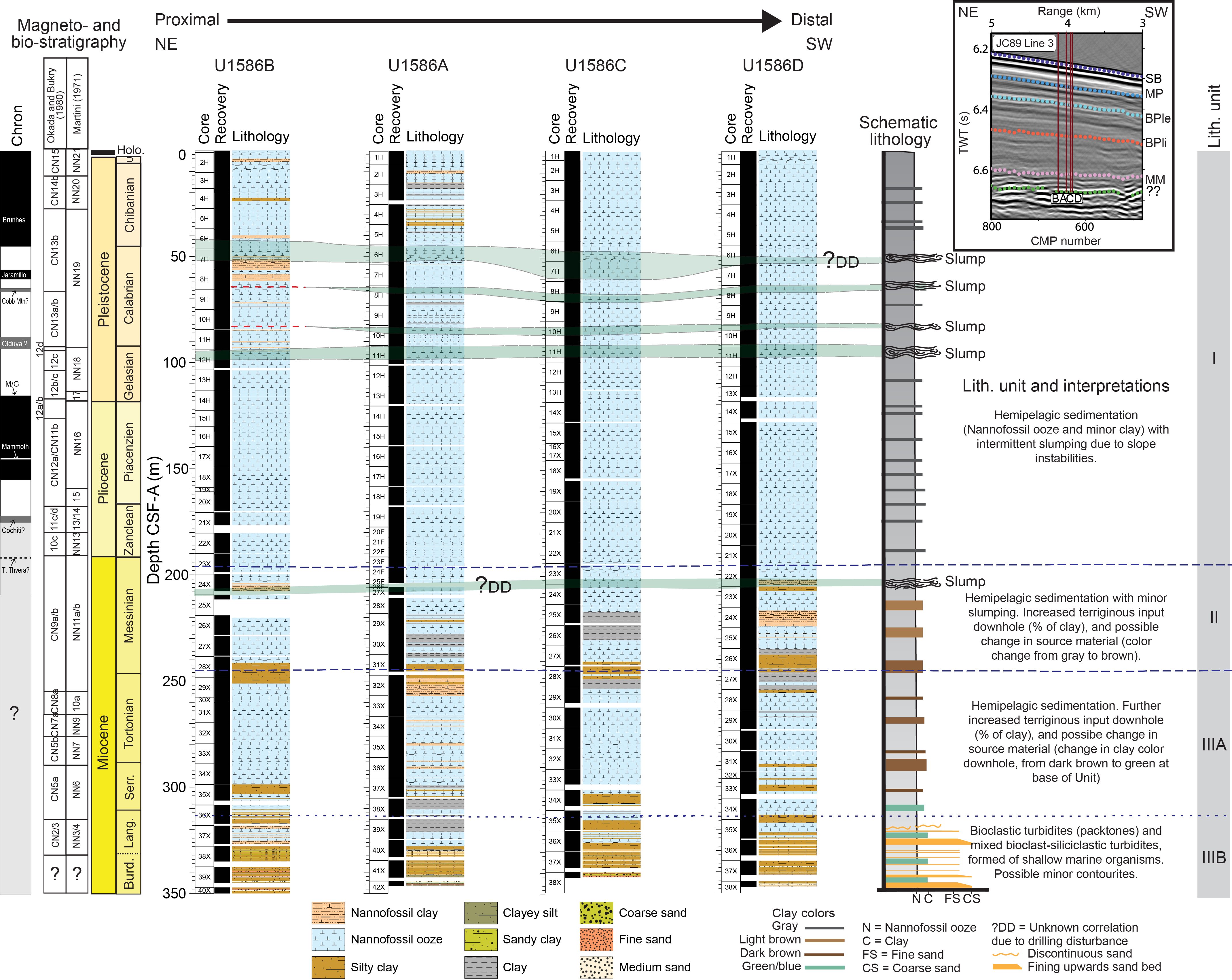
Figure F21. Lithologic summary.
The upper layer in the shallowest section of all holes is interpreted to be influenced by the penetration of oxygen into the sediment from the overlying ocean and its eventual depletion by organic respiration in the upper tens of centimeters. The brown sediments are inferred to be oxidizing and the gray sediments to be reducing, leading to the mobilization in solution of redox-sensitive elements, including iron and manganese. These diffuse upward and precipitate out at the boundary with the oxic layer above, forming an orange-brown redox horizon that may migrate upward as sediment accumulates under stable conditions and may migrate upward or downward over time relative to the seafloor as ocean ventilation and organic carbon export vary, as occurred during glacial–interglacial cycles at Site U1586.
Iron sulfides are common throughout Lithostratigraphic Unit I, occurring primarily as amorphous iron monosulfides (FeS) in the upper part of the unit and as pyrite (FeS2) in various forms, often as burrow fill, in the lower half of the unit. The iron monosulfides are evident as widespread dark smudges along the surface of darker intervals containing more clay and presumably representing glacial intervals and are particularly ephemeral, oxidizing, and fading away within minutes to hours. Pyrite occurs as discrete elongated burrow fill and isolated nodules evident along the face of the split core and in X-ray images and is more persistent. Both iron sulfides suggest relatively reducing environments on, or more likely beneath, the seafloor. Such conditions may result from limited ventilation of the bottom waters, enhanced organic carbon export from the near-surface ocean and subsequent respiration at depth or in pore waters, or some combination of those phenomena. Pervasive monosulfides are indicative of generally reducing conditions in the sediment, and the discrete occurrence of pyrite suggests local microenvironments typically associated with benthic organisms. The pattern of alternating iron sulfide deposition in what is interpreted as glacial intervals and nondeposition (or less deposition) during interglacial intervals suggests that the former was characterized by diminished deep-ocean ventilation, enhanced biological productivity, or both.
Deep-sea coral fragments are observed in Unit I at 165–187 m CSF-A in Hole U1586A and 133–139 m CSF-A in Hole U1586B with estimated ages of at least 2.65 Ma and 5.5 Ma, respectively. Given the need for hardgrounds for corals to grow, these corals were likely transported as clasts to the Site U1586 location from sources upslope. Layers containing microspherules in Unit I (148–152 m CSF-A; Holes U1586B–U1586D) are associated with exceptionally strong MS anomalies. Because no smear slide sample was taken in Hole U1586A at the location of the extreme MS anomaly (152 m CSF-A), no microspherules were identified in that hole. The microspherules are micrometer scale with distinctive spherical, opaque, and magnetic characteristics. Preliminary investigation suggests that these microspherules may be attributed to extraterrestrial origin. However, micrometer-scale (5–10 µm) grains of magnetite (Figure F22) were also found in the samples, and a conclusive inference awaits additional evidence. Based on onboard stratigraphy, the layers are dated at ~3.6 Ma (see Stratigraphic correlation). If confirmed to be cosmic in origin and regionally widespread, the associated exceptionally high MS signal may serve as a useful new stratigraphic marker.
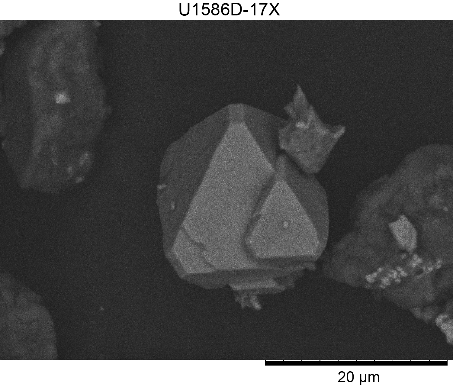
Figure F22. Magnetite grain.
The occurrence of slumped intervals in Units I and II indicates periods of slope instability (Figure F21). In the slumped interval, thinner, more distinct sharper boundaries between banding may suggest compression of the source material before or during remobilization, with low bioturbation possibly due to rapid en masse deposition of slumps and contorted bedding. All slumped intervals are less than 10 m thick, and most are less than 5 m. The subintervals are relatively uniform in thickness across all holes apart from Subunits ID and IF, which are erosive in the proximal Hole U1586B, with deposits slightly thickening downslope or remaining uniform in thickness (Figure F21; Table T3). The abundance of slumped intervals throughout Unit I and into Unit II suggests ongoing instabilities on the lower slope. The sediment source for the slumps is likely local or from a similar environment upslope because the slumped material consists of Lithofacies 1 and 2. Trigger mechanisms may include a periodic overstepping of slope due to uplift or periodic seismic activity in the region. There is currently no evidence of large-scale instabilities farther upslope, and no material sourced from the shelf or upper slope is recognized, both of which would indicate slumping caused by sea level variations.
Carbonate content significantly decreases throughout Unit II in all holes, and L* data suggest a trough at ~260–185 m CSF-A (Sections 397-U1586A-32X-5 through 21F-3). Given the strong positive correlation between CaCO3 and L*, this trough possibly suggests poor CaCO3 preservation. The low CaCO3 can be visually identified as dark layers. Based on the onboard stratigraphy, the associated depth range corresponds to the late Miocene around 12–5 Ma, roughly coeval with the time of the Miocene carbonate crash (Farrell et al., 1995; Lyle et al., 1995). Previous observations are primarily based on sediments from tropical oceans, with some observations in the South Atlantic (e.g., Diester-Haass et al., 2004). Because Site U1586 is located at 37°N, the onboard CaCO3 estimates suggest a wider occurrence of reduced carbonate burial during the middle–late Miocene. However, more work is needed to confirm inferences of CaCO3 changes from L*. If confirmed, this observation increases the priority of exploring the associated causes with implications for the global carbon cycle and climate change during the late Miocene.
Unit III shows characteristic changes in the coloration of clay from red to green and blue and the commencement of the bioclastic turbidites formed by shallow marine fauna. Although nannofossils from this interval do not allow continuous dating, the age of the top of Unit III suggests that these turbidites might be from mixed Eocene–Oligocene sources with minor Cretaceous–Triassic components (see Biostratigraphy). The deposition of Unit III possibly coincided with periods of tectonic activity and significant climatic changes on the Iberian Peninsula. Landmass rotation was associated with a series of tectonic events resulting in the opening of the North Atlantic, the gradual narrowing of the Mediterranean gateway, and the formation of various depositional basins across the Iberian continental margin (Ramos et al., 2017) between 110 and 35 Ma (Andeweg, 2002). A series of regional hiatuses in the Middle–Late Jurassic, Late Cretaceous, middle Eocene, and Eocene–Oligocene, along with uplift (Pena dos Reis et al., 2010), might lead to exposure and erosion of sediments on land. Throughout the late to middle Miocene, the Lower Tagus Basin in the Lisbon area shows a series of reddish conglomerates, white sand, and blue shales (Pais et al., 2010). Within the Betic Corridor (modern-day southern Spain and Portugal) and Rifian Corridor (modern-day Morocco), bioclastic sand and conglomerates are common and thought to be related to the uplift during the late Miocene. Sediments in the South Rifian Trough also show blue marls overlain by reddish clay-rich marls, similar to those described in Unit III. From 11.6 Ma, these marls were interbedded with sand sources from the basin margin (Flecker et al., 2015). Therefore, the distinctive colored clay and bioclastic sands in Unit III may be related to similar uplifting events, causing the remobilization of terrigenous and shallow water sediments of mixed ages. The turbidite flows may have been triggered when deltaic deposits on the shelf were remobilized downslope during periods of relative sea level fall; this may coincide with a period of climatic cooling during the Eocene/Oligocene boundary and the Middle Miocene Climate Transition (Westerhold et al., 2020).
4. Biostratigraphy
At Site U1586, the ~350 m cored sedimentary succession spans the Holocene to middle Miocene. Using calcareous nannofossils and samples taken from split-core and core catchers, approximately 50 bioevents were identified. Nannofossils are very abundant to common, with moderate to good preservation, and are generally well distributed throughout the succession, except for a 44 m interval (218–262 m CSF-A).
Planktonic foraminifer assemblages examined in the core catcher samples and two split core samples from Hole U1586A allow the identification of eight bioevents. Planktonic foraminifers are abundant and well preserved in the uppermost 250 m over the Pleistocene and Pliocene, but their abundance varies from rare to dominant in the Miocene. Below 260 m CSF-A, planktonic foraminifer preservation decreases with increasing depth and shells show strong signs of dissolution.
Holocene and Pleistocene biostratigraphic markers are identified in Samples 397-U1586A-1H-2, 74 cm, through 14H-4, 78 cm. Pliocene markers are identified in Samples 14H-4, 78 cm, through 23F-CC, 22–29 cm. The middle to late Miocene is identified in Samples 23F-CC, 22–29 cm, through 38X-4, 66 cm. Lithostratigraphic evidence suggests the occurrence of slumped intervals close to the middle to late Miocene bioevents; therefore, these age assignments are provisional. Samples 41X-CC and 42X-CC at the bottom of the hole contain mixed early Oligocene to late Eocene nannofossils.
The zonal schemes of calcareous nannofossils and planktonic foraminifers generally agree, although they diverge by as much as 3 My at 260–350 m CSF-A. Integrated calcareous microfossil bioevents are provided in Figure F23, with nannofossil and planktonic foraminifer datums reported in Tables T8 and T9.
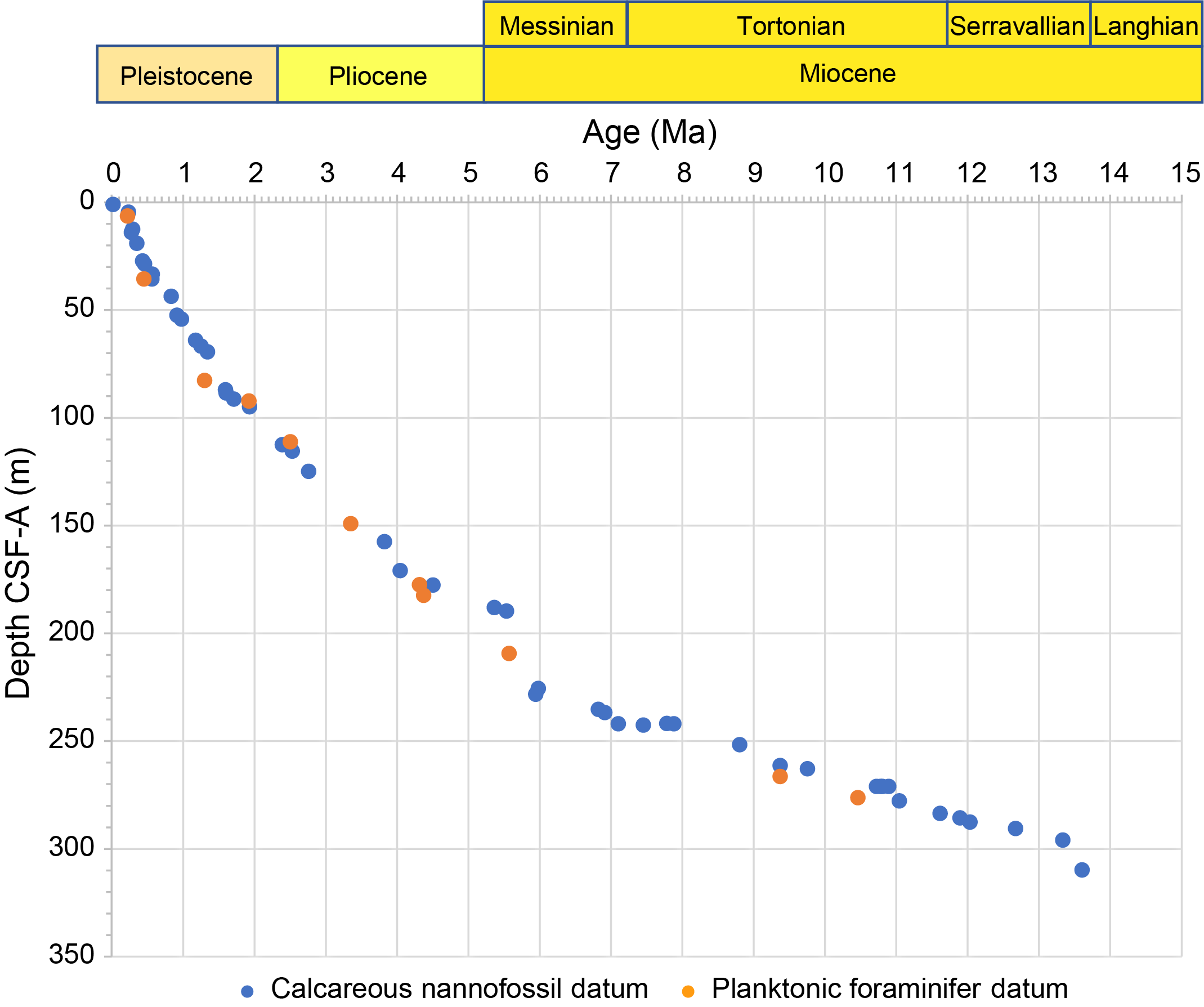
Figure F23. Preliminary age model.
4.1. Calcareous nannofossils
Calcareous nannofossil biostratigraphy at Site U1586 is based on 42 core catcher samples and 280 split-core samples taken from Holes U1586A–U1586C in selected intervals. All the samples were processed into smear slides using standard techniques. Calcareous nannofossils are shown in Plate P1.
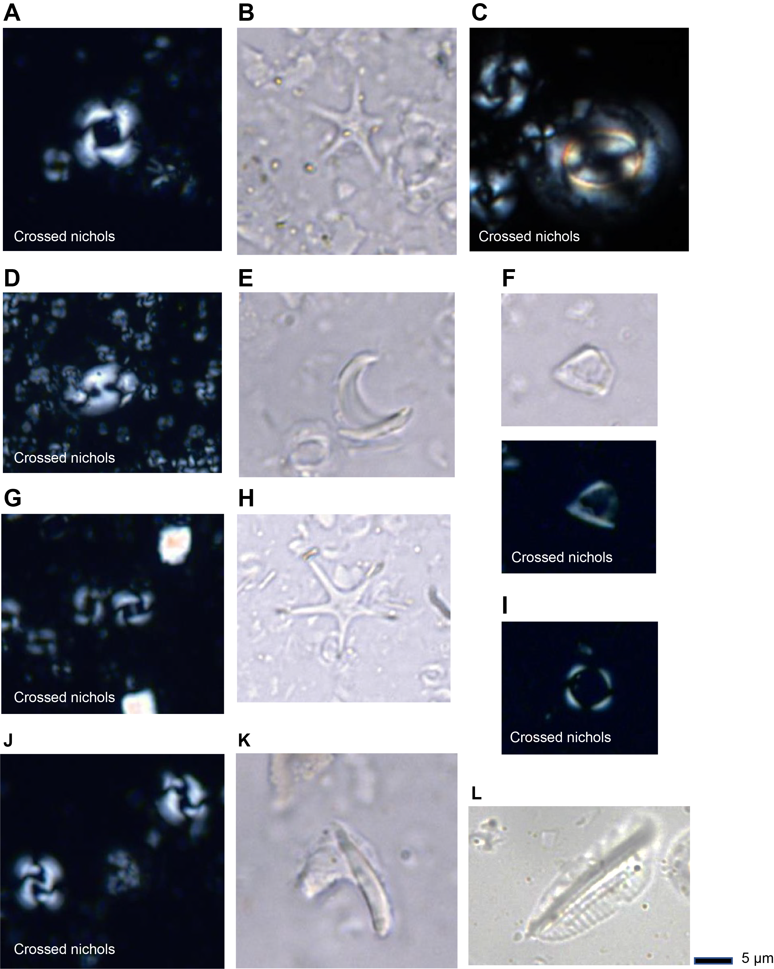
Plate P1. Calcareous nannofossils.
The nannofossil assemblage from Holes U1586A–U1586C is defined by 42 groups/taxa-morphotypes including Emiliania huxleyi, Gephyrocapsa caribbeanica gr., Gephyrocapsa spp. (small <4 µm, medium, and large >5.5 µm), Gephyrocapsa omega, Pseudoemiliania lacunosa, Reticulofenestra (<3, 3–5, 5–7, and >7 µm), Reticulofenestra asanoi, Reticulofenestra minuta, Reticulofenestra pseudoumbilicus, Reticulofenestra perplexa, Reticulofenestra rotaria, Coccolithus pelagicus, Coccolithus miopelagicus, Calcidiscus leptoporus, Calcidiscus macintyrei, Catinaster coalitus, Catinaster calyculus, Ceratolithus armatus, Cyclicargolithus floridanus, Helicosphaera carteri, Helicosphaera inversa, Helicosphaera sellii, Minylitha convallis, Nicklithus amplificus, Orthorhabdus rugosus, Pontosphaera multipora, Rhabdosphaera clavigera, Sphenolithus abies/neoabies, Sphenolithus heteromorphus, Sphenolithus belemnos, Syracosphaera spp., Scyphosphaera spp., Discoaster spp., Discoaster variabilis, Discoaster brouweri, Discoaster pentaradiatus, Discoaster surculus, Discoaster tamalis, Discoaster asymmetricus, Discoaster bellus, Discoaster kugleri, Amaurolithus primus, and Amaurolithus delicatus and occasionally less abundant taxa.
A total of 50 calcareous nannofossil events were identified within the core and dated using the age calibrations of Balestra et al. (2015), Raffi et al. (2006), and Gradstein et al. (2020) (Table T8). Additionally, the standard biozones of Martini (1971) and Okada and Bukry (1980) were identified. For these analyses, only taxa or morphotypes with biostratigraphic significance were considered (Table T10).
4.1.1. Pleistocene
Nannofossils are very abundant and show good preservation throughout the Pleistocene interval (0–124 m CSF-A; from Sample 397-U1586A-1H-1, 67 cm, to 14H-4, 78 cm). The Holocene is identified from above Sample 397-U1586A-1H-2, 74 cm, through the top of the core, after the highest occurrence (HO) of E. huxleyi >4 µm (Flores et al., 2010).
Zone CN14-15/NN20-21 is identified based on the lowest occurrence (LO) of E. huxleyi above Sample 397-U1586A-2H-5, 78 cm. Zone CN14b-14a/NN19-20 is placed based on the HO of P. lacunosa above Sample 4H-2, 49 cm. Zone CN14a/NN19 is identified based on the highest common occurrence (HcO) R. asanoi above Sample 6H-6, 117 cm. Zone CN13b/NN19 is placed based on the HOs of large Gephyrocapsa (>5.5 µm), H. sellii, and C. macintyrei above Samples 8H-3, 74 cm, 8H-5, 73 cm, and 10H-5, 82 cm, respectively. Zone CN13a-12d/NN18 is placed based on the HO of D. brouweri above Sample 11H-3, 75 cm. Zone CN12c/NN17-18 is placed based on the HO of D. pentaradiatus in Sample 13H-2, 79 cm. Zone CN12c-12b/NN16-17 is based on the HO of D. surculus in Sample 13H-4, 77 cm. Zone CN12b-12a/NN16 is based on the HO of D. tamalis in Sample 14H-4, 78 cm. These later three events characterize the Gelasian Stage, approaching the Pleistocene/Pliocene boundary.
4.1.2. Pliocene
The Pliocene interval (124–189 m CSF-A; Samples 397-U1586A-14H-4, 78 cm, through 23F-CC, 22–29 cm) contains abundant to common calcareous nannofossils with good preservation. Zone CN12a-11b/NN15-16 is based on the HO of R. pseudoumbilicus >7 µm in Sample 397-U1586A-17H-7, 9 cm. This event is normally synchronous with the HO of Sphenolithus spp. (Raffi et al., 2006); intriguingly, these taxa are absent or sporadic in the Iberian margin. Zones CN11a-11b/NN13-14 are based on the lowest common occurrence (LcO) of D. asymmetricus in Sample 397-U1586A-19H-3, 50 cm. Calcareous nannofossil marker species for the Miocene/Pliocene boundary (189 m CSF-A; 397-U1586A-22F-3, 43 cm), such as Discoaster quinqueramus and C. armatus, have sporadic distribution and are few to common in abundance, making Zone CN10a-9b/NN11b-12 difficult to place.
4.1.3. Miocene
The Miocene interval covers 189–310 m CSF-A (Samples 397-U1586A-23F-CC, 22–29 cm, through 38X-4, 66 cm). Nannofossils in the Miocene were found in very high to high abundance with generally good preservation. The Messinian/Tortonian boundary is approximated by the LO of Amaurolithus spp. The LO of R. rotaria and the HO (paracme) of R. pseudoumbilicus > 7 µm are identified close to the LO of Amaurolithus spp. Zone CN9a-9b/NN11a-11b is based on the LO of A. primus up to Sample 31X-4, 61 cm. Because of the slump in this interval, these events should be considered tentative. The Tortonian is characterized by several events defined by Discoaster species as well as the absence (paracme) of specimens of R. pseudoumbilicus > 7 µm in the upper part. Zone CN9a/NN11a is based on the HcO of M. convallis and the LcO of D. surculus found in Samples 31X-1, 76 cm, and 31X-4, 61 cm. Zone CN8a-7b/NN10-9 is based on the LO of D. pentaradiatus in Sample 33X-4, 70 cm.
Zone CN5b-6/NN7-8 is based on the LO of C. coalitus identified in Sample 397-U1586A-34X-4, 63 cm. Multiple taxa (LO M. convallis, LO D. brouweri, and LO C. calyculus) of Zone CN7a/NN9 were also identified in Sample 34X-4, 63 cm, and their simultaneous identification may be due to a high sedimentation rate and low sample resolution. Zone CN5a/NN6 is based on the HcO of C. floridanus found in Sample 37X-1, 67 cm. Zone CN4-5a/NN5-6 is based on the HO of S. heteromorphus in Sample 38X-4, 66 cm. This species is intermittent in Core 38X to Sample 39X-6, 69 cm.
Between Samples 397-U1586A-40X-1, 70 cm, and 40X-2, 83 cm, the presence of S. belemnos is observed, marking the Zone CN2-3/NN3-4 boundary in the Burdigalian. This taxon is recorded in a sequence mostly barren of calcareous nannofossils, which is why the event should be considered provisional.
Below Sample 397-U1586A-40X-2, 83 cm, and in Core 42X, taxa of early Oligocene to late Eocene age were identified (e.g., Chiasmolithus altus, Chiasmolithus grandis, Discoaster saipanensis, Discoaster barbadiensis, Sphenolithus intercalaris, Reticulofenestra umbilicus, Zygrhablithus bijugatus, Helicosphaera lophota, Isthmolithus recurvus, Reticulofenestra stavensis) with sparse to common abundance and moderate to poor preservation, interspersed with samples rich in silty calcareous sand.
4.2. Planktonic foraminifers
Planktonic foraminifers from the mudline, all 42 core catchers from Hole U1586A, and Sections 41X-6 and 42X-1 were examined. The relative abundance of taxa and estimation of assemblage preservation are presented in Table T11. Planktonic foraminifers are dominant and well preserved in the Pleistocene and Pliocene sections. In the Miocene, the abundance varies between rare and dominant. Preservation decreases with depth, and Miocene foraminifers are dissolved, recrystallized, and difficult to identify. No relative abundance is provided. The main biostratigraphic planktonic species are shown in Plate P2.
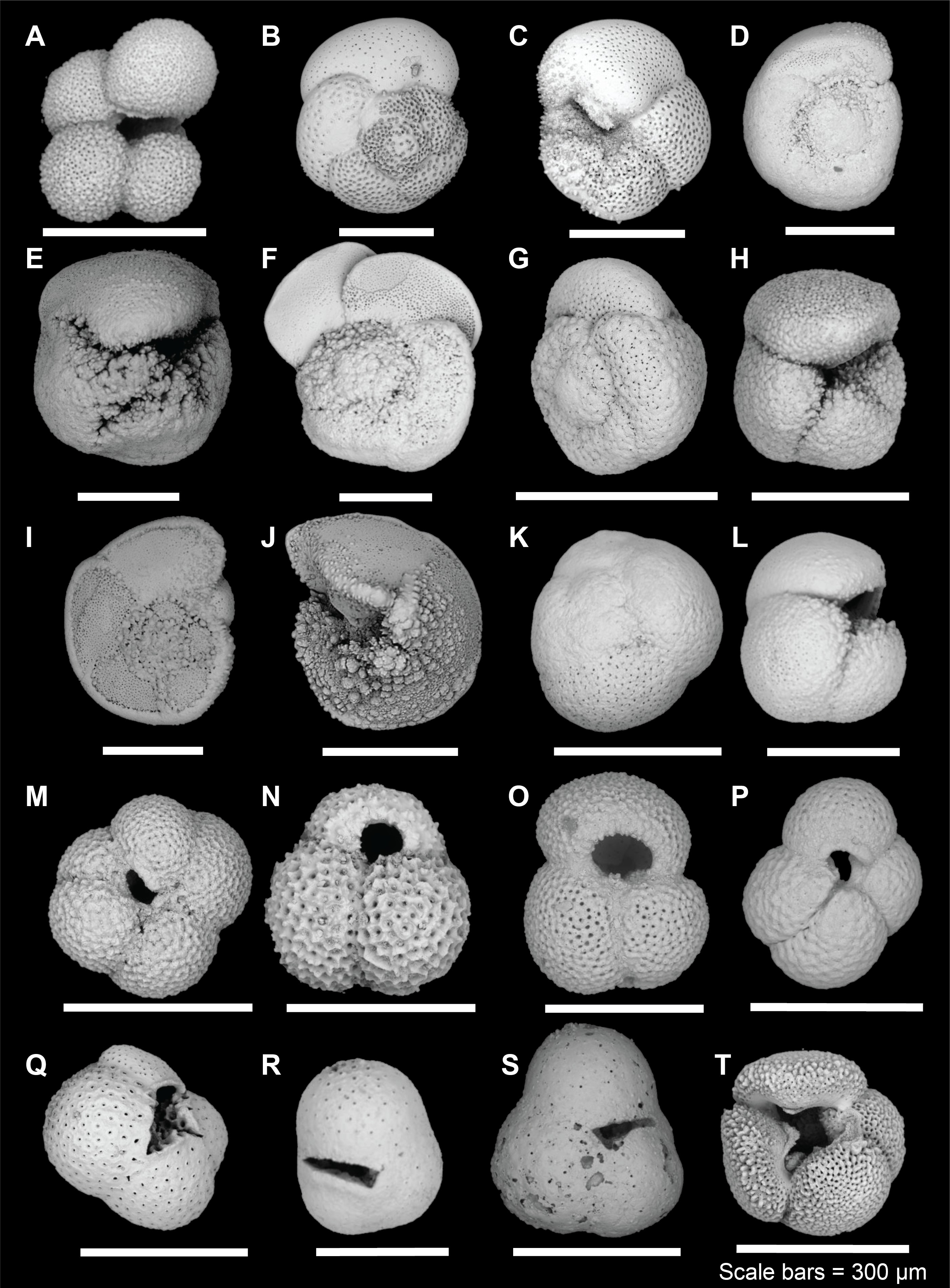
Plate P2. Planktonic foraminifers.
Key biostratigraphic species are given in Table T9 with identification of eight bioevents calibrated by Kennett and Srinivasan (1983), Chaisson and Pearson (1997), Wade et al. (2011), and Spezzaferri et al. (2018). The age of the upper part of the section, in Samples 397-U1586A-1H-CC through 4H-CC, is assigned to the late middle Pleistocene (0.45 Ma) based on the LO of Globorotalia hirsuta. The interval in Samples 4H-CC through 9H-CC belongs to the Calabrian Stage (1.3 Ma), as evidenced by the HO of Globigerinoides obliquus. The HO of Globigerinoides bollii is recorded during the Piacenzian Stage (3.3 Ma) in Sample 16H-CC.
The interval between Samples 397-U1586A-16H-CC and 19H-CC is assigned to the early late Pliocene (4.31 Ma) based on the LO of Globorotalia crassaformis, and the age for Sample 20F-CC is 4.36 Ma based on the HO of Globoturborotalita nepenthes. From Sample 21F-CC downhole, biostratigraphic ages could not be assigned because of the low abundance and poor preservation of planktonic foraminifers.
The interval between Samples 397-U1586A-27X-CC and 34X-CC is assigned to the late Miocene based on the LO of Globigerinoides ruber (Table T9). The base of Hole U1586A is estimated to be of late Miocene age; however, the poor preservation of the foraminifers makes this assignment difficult.
The mudline is dominated by well-preserved planktonic foraminifers. The assemblage is characterized by a typical temperate North Atlantic fauna including Globorotalia inflata, Neogloboquadrina pachyderma, Globigerina bulloides, Globorotalia truncatulinoides, Globigerinita glutinata, and G. crassaformis. G. ruber and Orbulina universa are also present (Table T11).
The Pleistocene assemblages are also typical of temperate waters from the North Atlantic, containing a mixture of surface- and deep-dwelling foraminifers. G. bulloides, N. pachyderma, and G. inflata are the dominant species, with Globigerinella siphonifera, G. truncatulinoides, G. crassaformis, and Turborotalita quinqueloba in lower abundance and G. hirsuta also occasionally contributing to the deep-dwelling fauna. G. ruber and O. universa are also continuously present (Table T11) and increase in abundance through time, whereas the abundance of typical North Atlantic species decreases at the end of the Pleistocene (Figure F24).
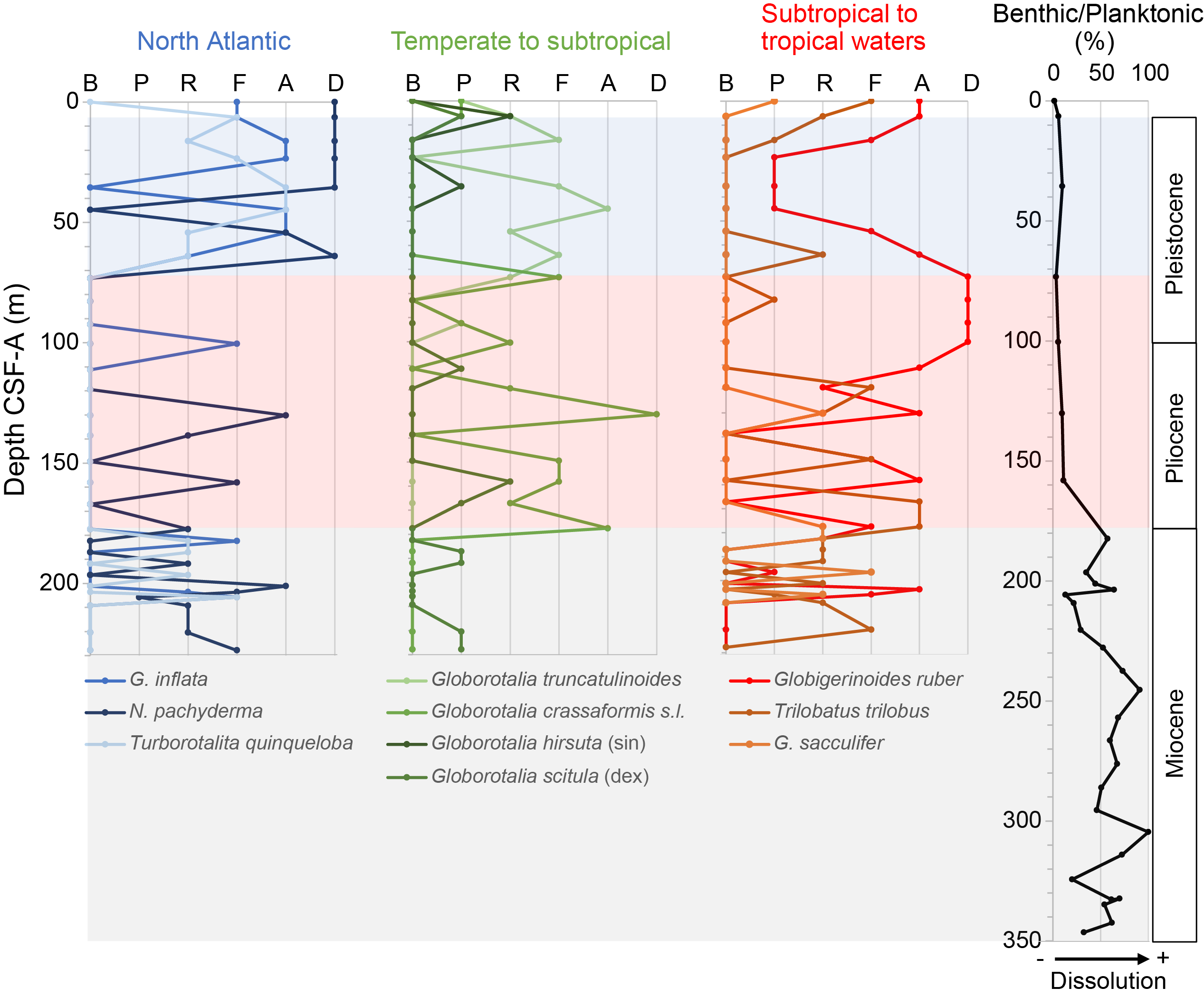
Figure F24. Key ecological planktonic foraminifer species distribution and benthic/planktonic foraminifer ratio.
In the Pliocene, subtropical to tropical species such as Trilobatus sacculifer plexus, G. ruber, O. universa, and G. nepenthes are common. In addition, G. bulloides and G. glutinata are present in lower abundance. G. siphonifera, Neogloboquadrina acostaensis, and G. crassaformis are also observed in several samples from Hole U1586A (Figure F24; Table T11). Despite the low resolution of the core catcher samples, variations in the planktonic foraminifer assemblages generally agree with the global temperature trend (e.g., Zachos et al., 2001): a warm Pliocene with dominance of warmer-water species, followed by progressively colder conditions thereafter to the mid- and late Pleistocene (decrease of the warm-water species associated with an increase of the colder-water species) (Figure F24).
The late Miocene is marked by an increase in the dissolution of planktonic foraminifers (Figure F24). The ratio between benthic and planktonic foraminifers is a dissolution index (more benthic than planktonic foraminifers may indicate more dissolution). This ratio is high throughout the Miocene. In addition, both planktonic and benthic foraminifers demonstrate visual evidence of dissolution, complicating species identification (Figure F24). The late Miocene is characterized by dominance of temperate to subtropical species including the occurrence of Globorotalia scitula, G. bulloides, Trilobatus sacculifer plexus, O. universa, N. acostaensis, Globoturborotalita apertura, G. glutinata, Sphaeroidinellopsis seminulina, and G. nepenthes.
4.3. Benthic foraminifers
Benthic foraminifers were examined in core catcher samples from Hole U1586A. They vary markedly in abundance but are generally well preserved throughout the sequence, except in the lowermost samples (397-U1586A-40X-CC and 41X-CC). Benthic foraminifer species are shown in Plates P3 and P4.
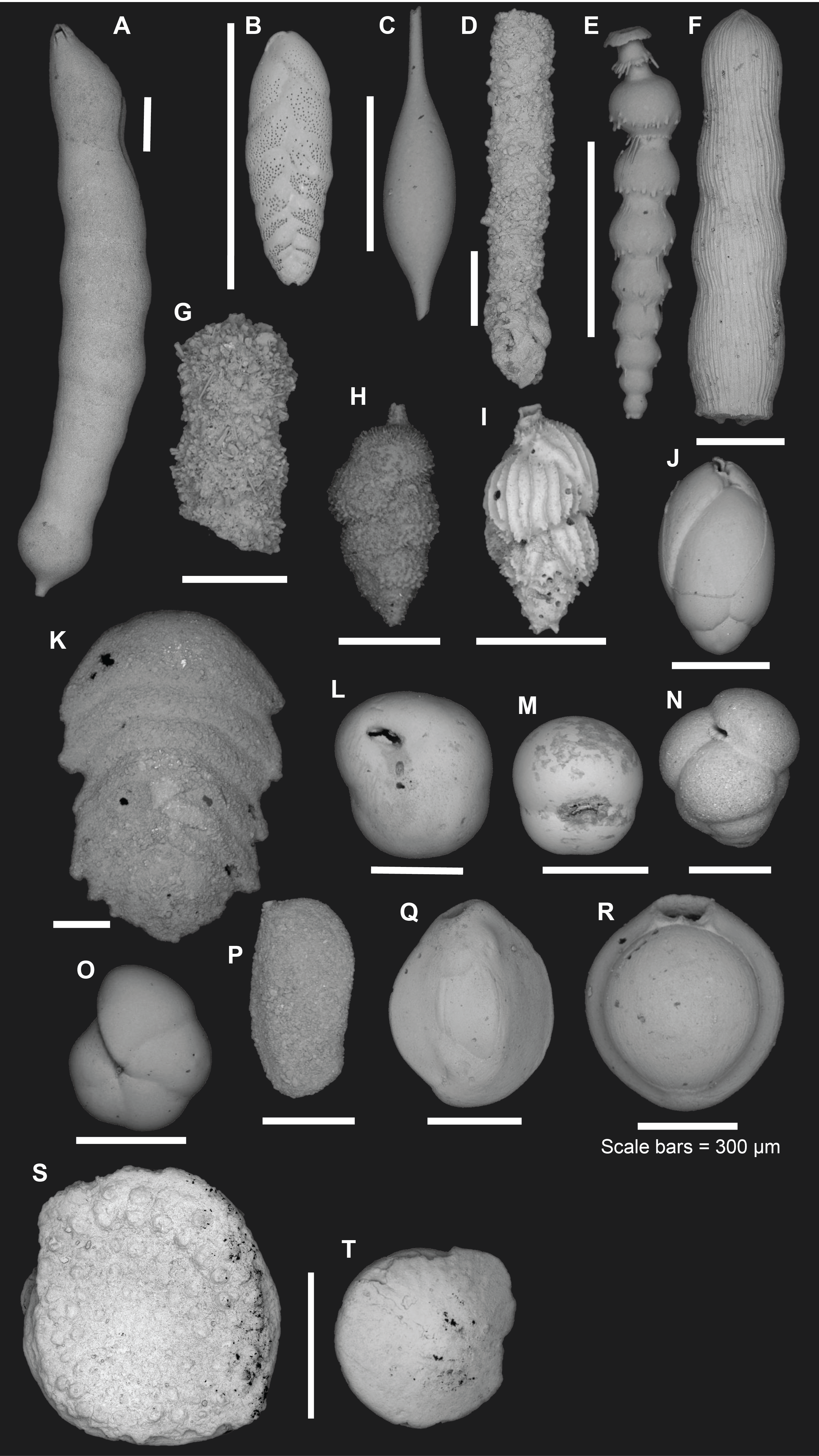
Plate P3. Benthic foraminifers, Expedition 397.
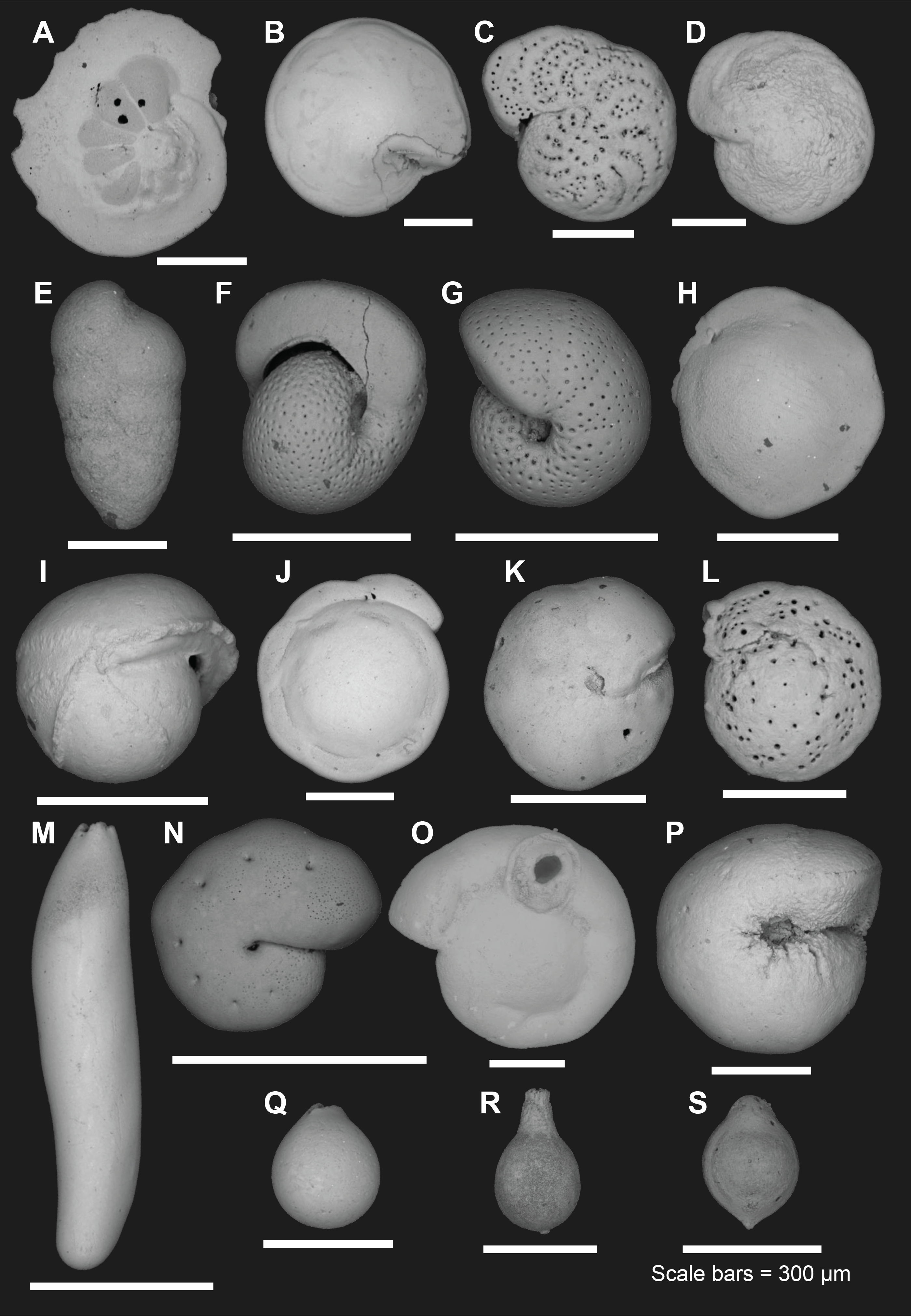
Plate P4. Benthic foraminifers, Hole U1587A.
The overall benthic foraminifer assemblage composition indicates a lower bathyal to abyssal paleodepth throughout the late Miocene to Holocene, as indicated by the common presence of Laticarinina pauperata, Eggerella bradyi, Triloculina spp., Chilostomella spp., and Bolivina spp. Other species such as Bolivina spp., Bulimina spp., Cibicidoides spp., Melonis spp., Oridorsalis umbonatus, Pullenia spp., Pyrgo spp., Biloculina spp., Quinqueloculina spp., and Uvigerina spp., as well as the agglutinated species Textularia spp. and Martinotiella spp., are frequently recorded through the succession. In contrast, Samples 397-U1586A-40X-6, 40–42 cm, and 41X-1, 29–31 cm, contain shallow-water and larger marine benthic foraminifers such as Spirillina sp., Dentoplanispirinella sp., and Calcarina sp. (Plate P3). This observation agrees with the ostracod assemblages (see Ostracods), suggesting reworking and redeposition of shallow sediments resulting from sea level variations or tectonic events.
4.4. Ostracods
The sediment fraction ≥250 µm of all 42 core catcher samples from Hole U1586A, Sample 397-U1586A-41X-1, 29–31 cm, and the mudline samples from all four holes were examined for ostracods. Ostracods are absent from most samples except for the mudline sample and Samples 1H-CC; 2H-CC; 6H-CC; 7H-CC; 9H-CC; 33X-CC; 40X-CC; 41X-1, 29–31 cm; and 41X-CC. The younger samples only yielded single to a few valves of typical deep-sea North Atlantic genera such as Krithe, Henryhowella, Poseidonamicus, Pseudobosquetina, Dutoitella, and Legitimocythere (Alvarez Zarikian, 2009; Yasuhara and Okahashi, 2014, 2015). In contrast, the three lowermost samples from the Miocene section yielded shelf marine ostracods Hermanites sp., Aurila spp., Pokornyella deformis, Pseudopsammocythere kollmanni, Triebelina sp., and Neonesidea sp. (Faranda et al., 2008; Ruiz et al., 2008), indicating redeposition associated with slope instability resulting from possible sea level fluctuations or tectonic activity. The ostracod range chart is shown in Table T12, and representative species are shown in Plate P5.
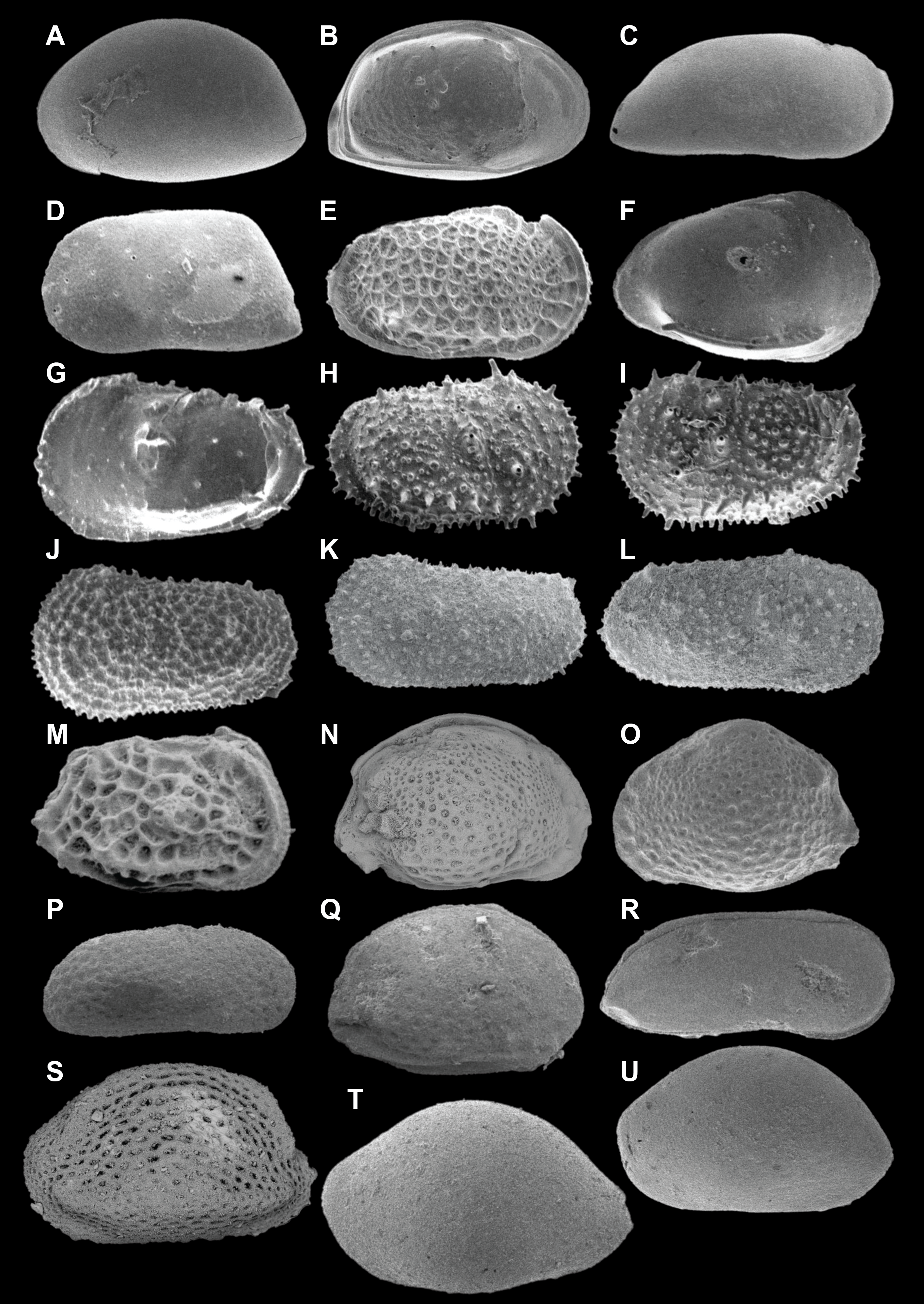
Plate P5. Deep-sea Ostracoda.
5. Paleomagnetism
Paleomagnetic investigations at Site U1586 focused on the measurement of the natural remanent magnetization (NRM) of archive-half sections from the four holes recovered at the site at 2 cm intervals. Depending on core flow, we measured the NRM of core sections after a varying number of alternating field (AF) demagnetization steps (Table T13), with NRM for most of the core sections measured before and after 20 mT AF demagnetization. We measured most core catcher sections from Hole U1586A and Cores 397-U1586B-1H through 4H. Data from core catcher sections were found to be typically noisy, and we stopped measuring core catcher sections of all other cores from the site. We also did not measure Sections 397-U1586D-6H-1 through 6H-3, 7H-1, and 7H-2 because they were heavily disturbed during coring. The Icefield MI-5 (see Paleomagnetism in the Expedition 397 methods chapter [Abrantes et al., 2024]) was used to orient Cores 397-U1586A-1H through 19H, 397-U1586B-1H through 16H, 397-U1586C-1H through 13H, and 397-U1586D-1H through 6H. The APC core orientation data for all holes are reported in Table T14.
We collected 110 discrete cube samples from Hole U1586A (see Paleomagnetism in the Expedition 397 methods chapter [Abrantes et al., 2024]). One cube sample was taken from every section (except core catchers) of Cores 1H–5H, and from about every two sections of other cores in Hole U1586A. We also collected 7 cubes from Hole U1586B, 7 cubes from Hole U1586C, and 12 cubes from Hole U1586D. Depth levels where the cubes were taken are marked by squares in Figures F25, F26, F27, and F28. Demagnetization steps used for the NRM measurements of the cubes depend on the core flow and what instrument was used (i.e., the SRM or the JR-6A spinner magnetometer) and are summarized in Table T13. SRM appears to produce generally less noisy data than the JR-6A for cube sample measurements (Figure F29). The NRM of the cube samples from Holes U1586A and U1586B was measured before and after stepwise AF demagnetization with peak fields up to 80 mT. A software and hardware communication issue caused the SRM in-line degauss coils to overheat. No samples were being measured when the issue occurred. Tests conducted after the coils cooled down suggested the coils were performing normally, but the maximum peak field for AF demagnetization was limited to 50 mT to avoid potential damage to the coils. Therefore, the NRM of cube samples from Holes U1586C and U1586D was measured before and after stepwise AF demagnetization with peak fields up to 50 mT.
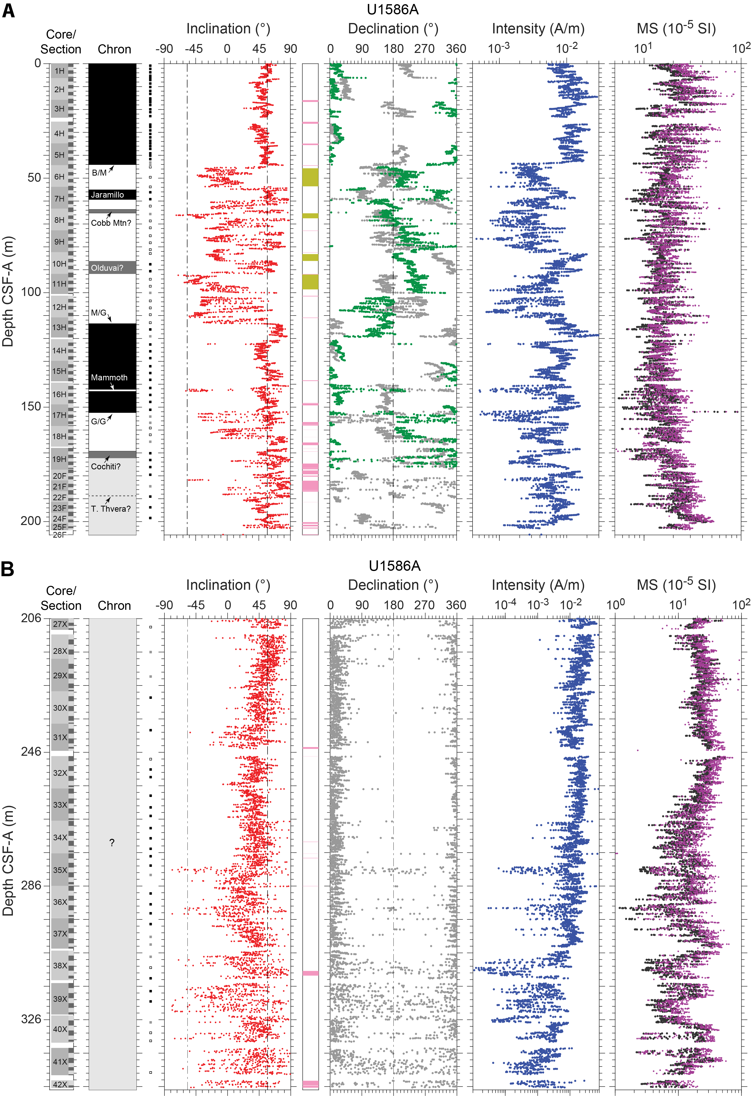
Figure F25. Paleomagnetism data, Hole U1586A.
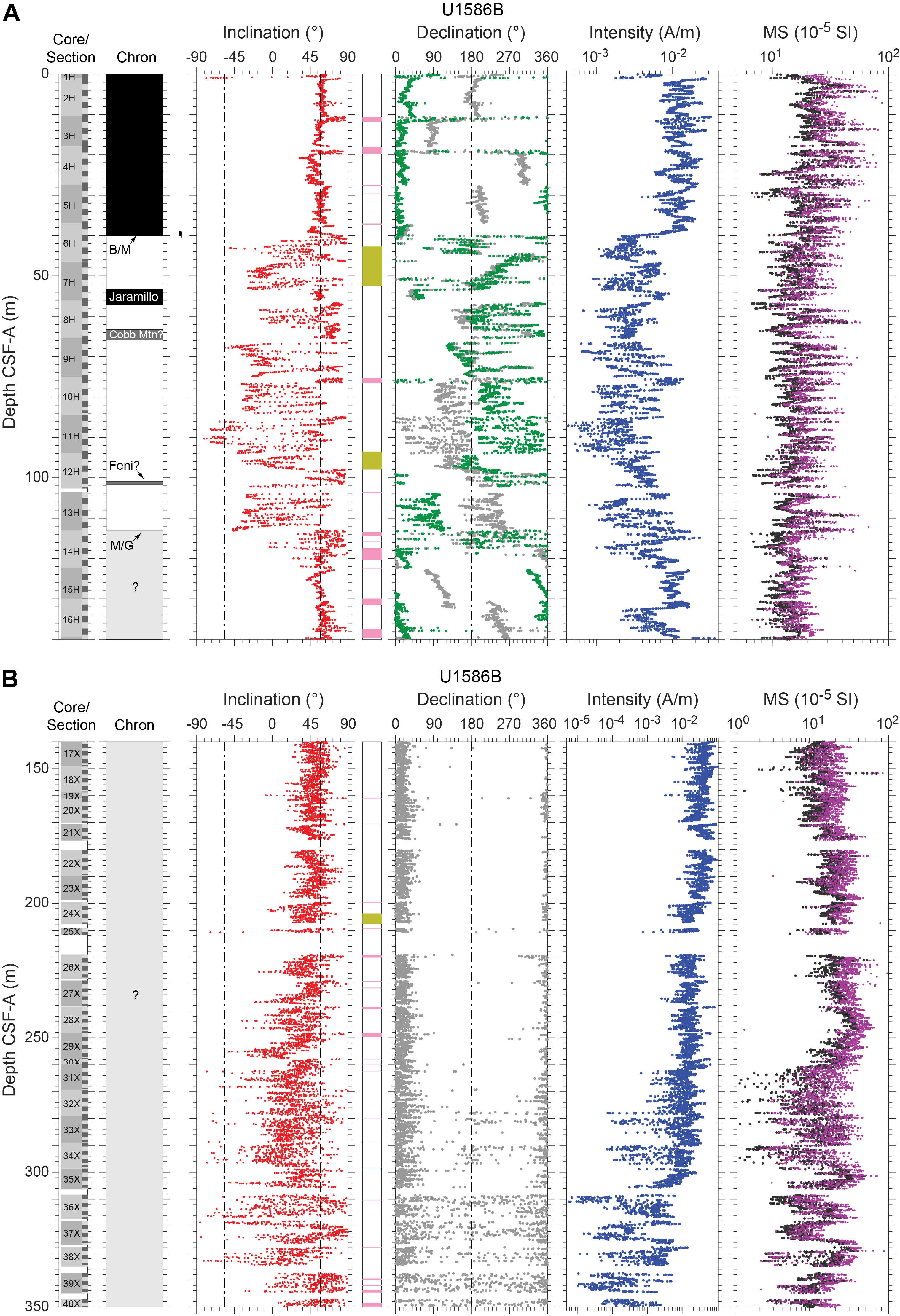
Figure F26. Paleomagnetism data, Hole U1586B.
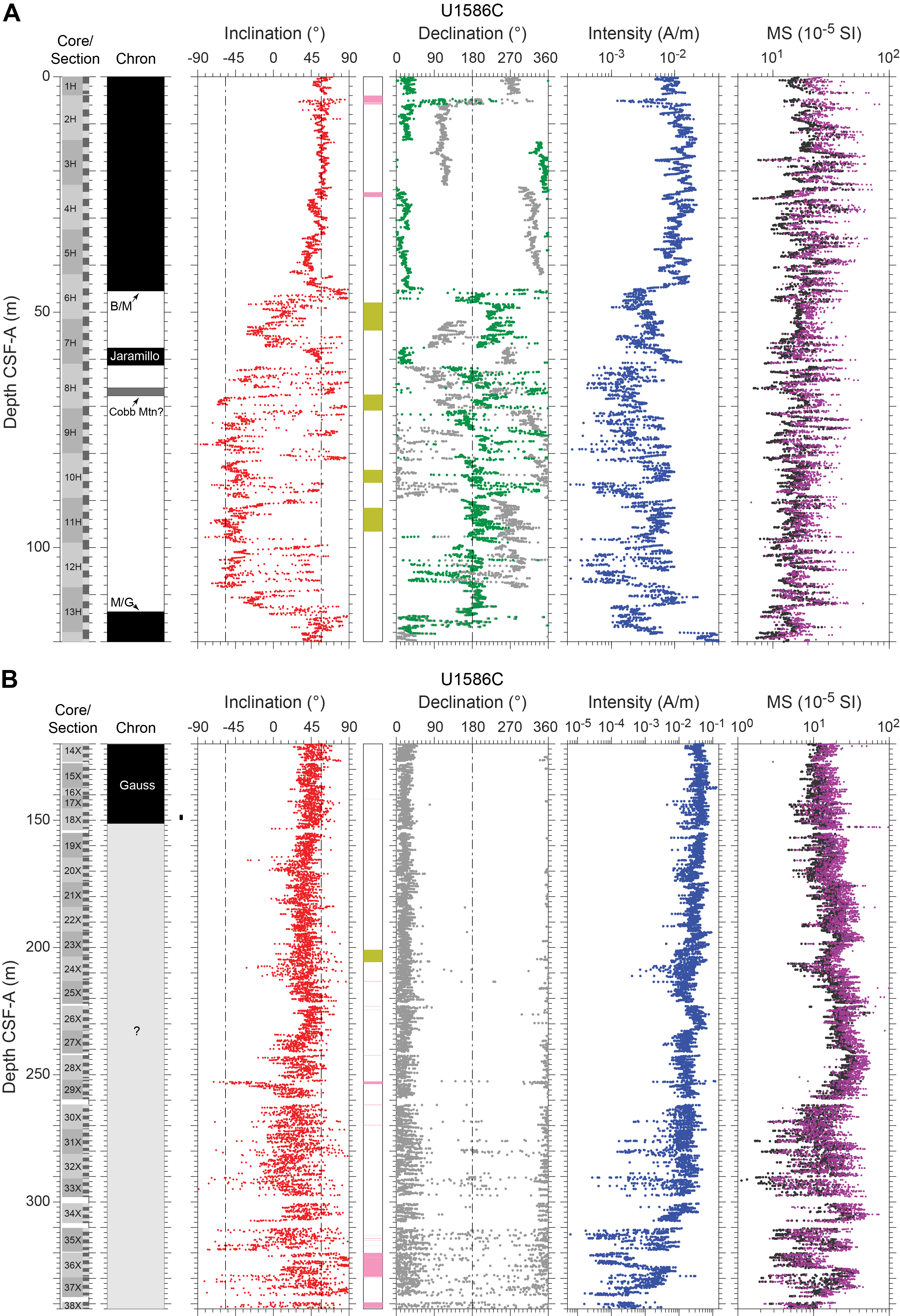
Figure F27. Paleomagnetism data, Hole U1586C.
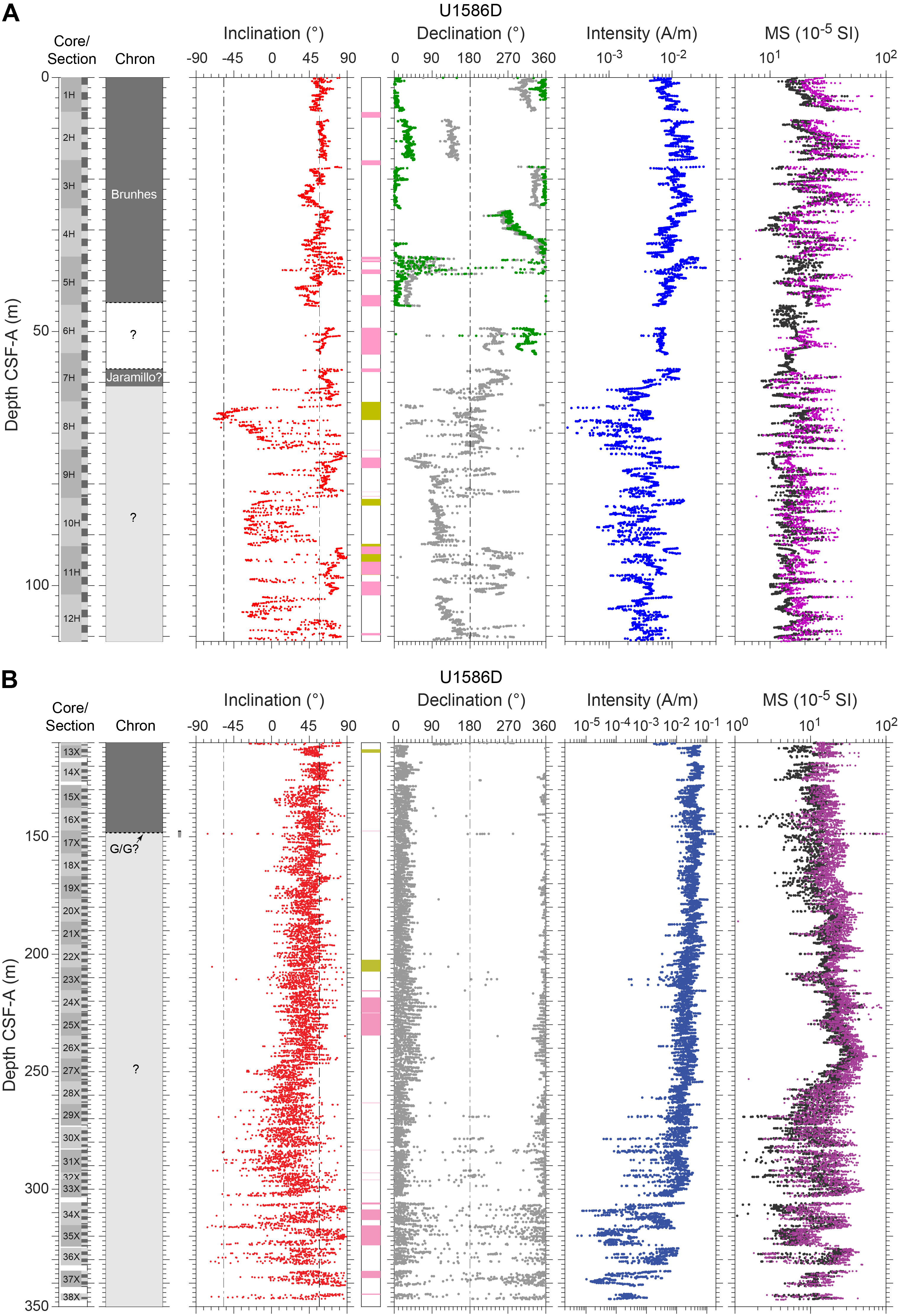
Figure F28. Paleomagnetism data, Hole U1586D.
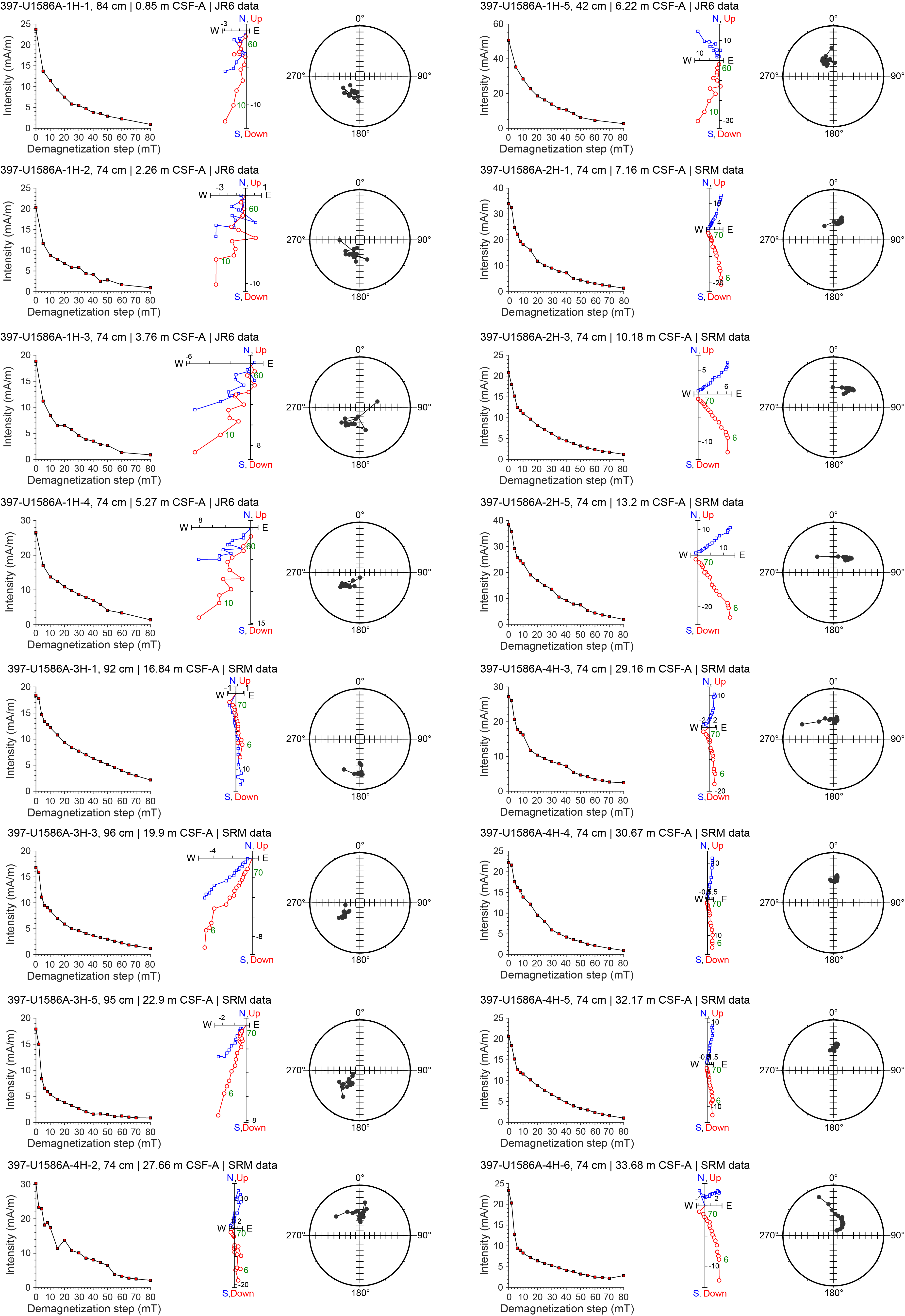
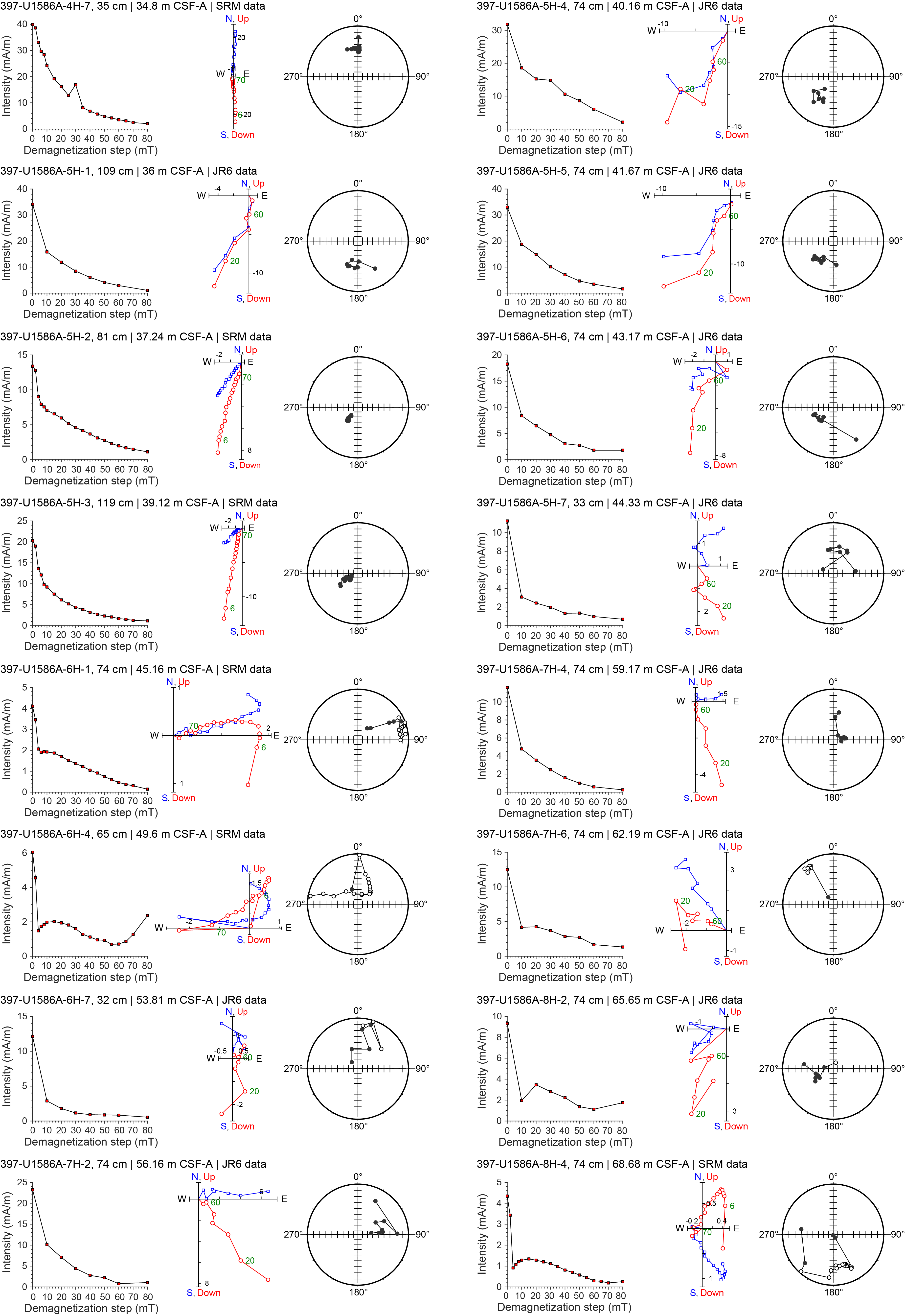
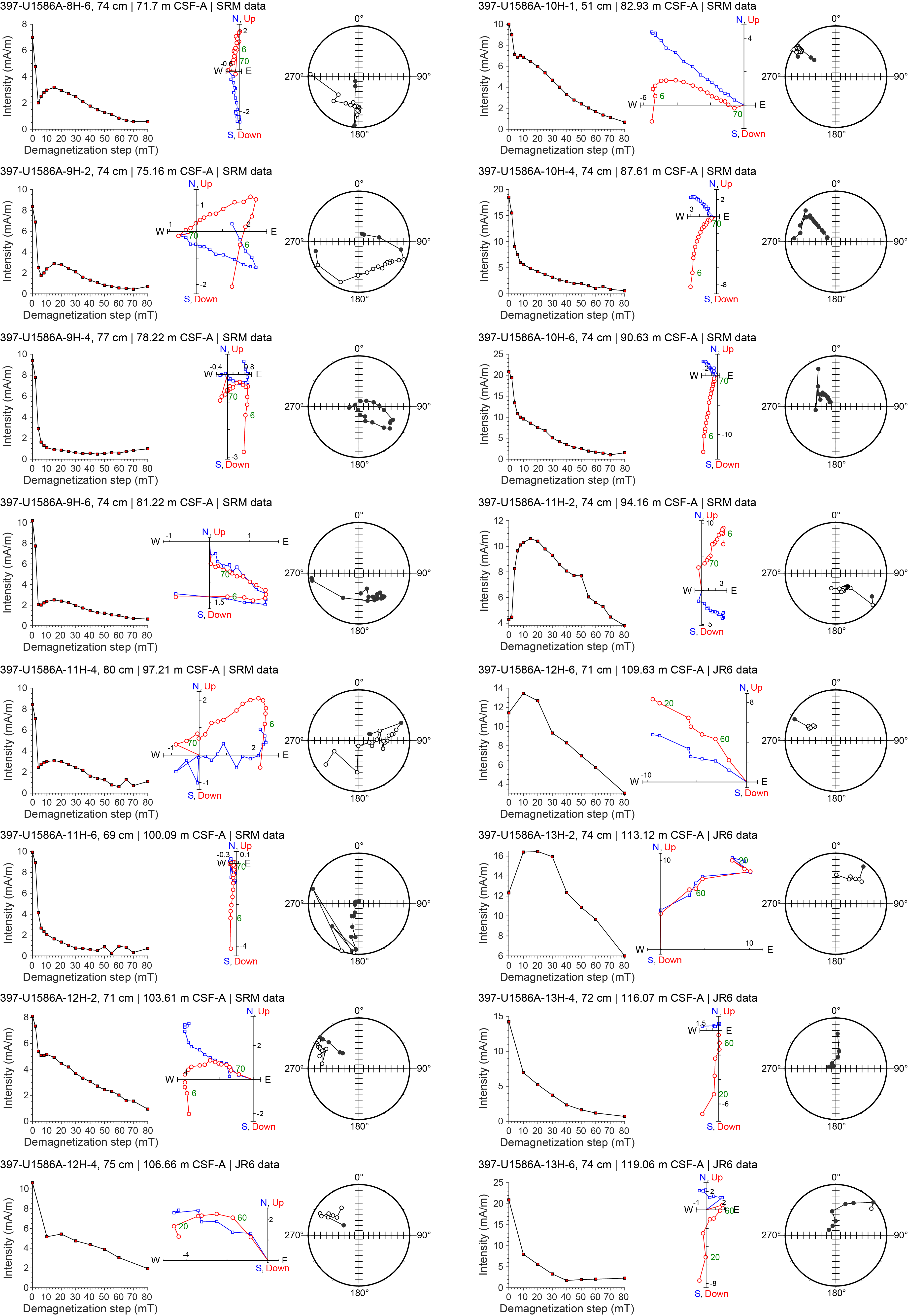
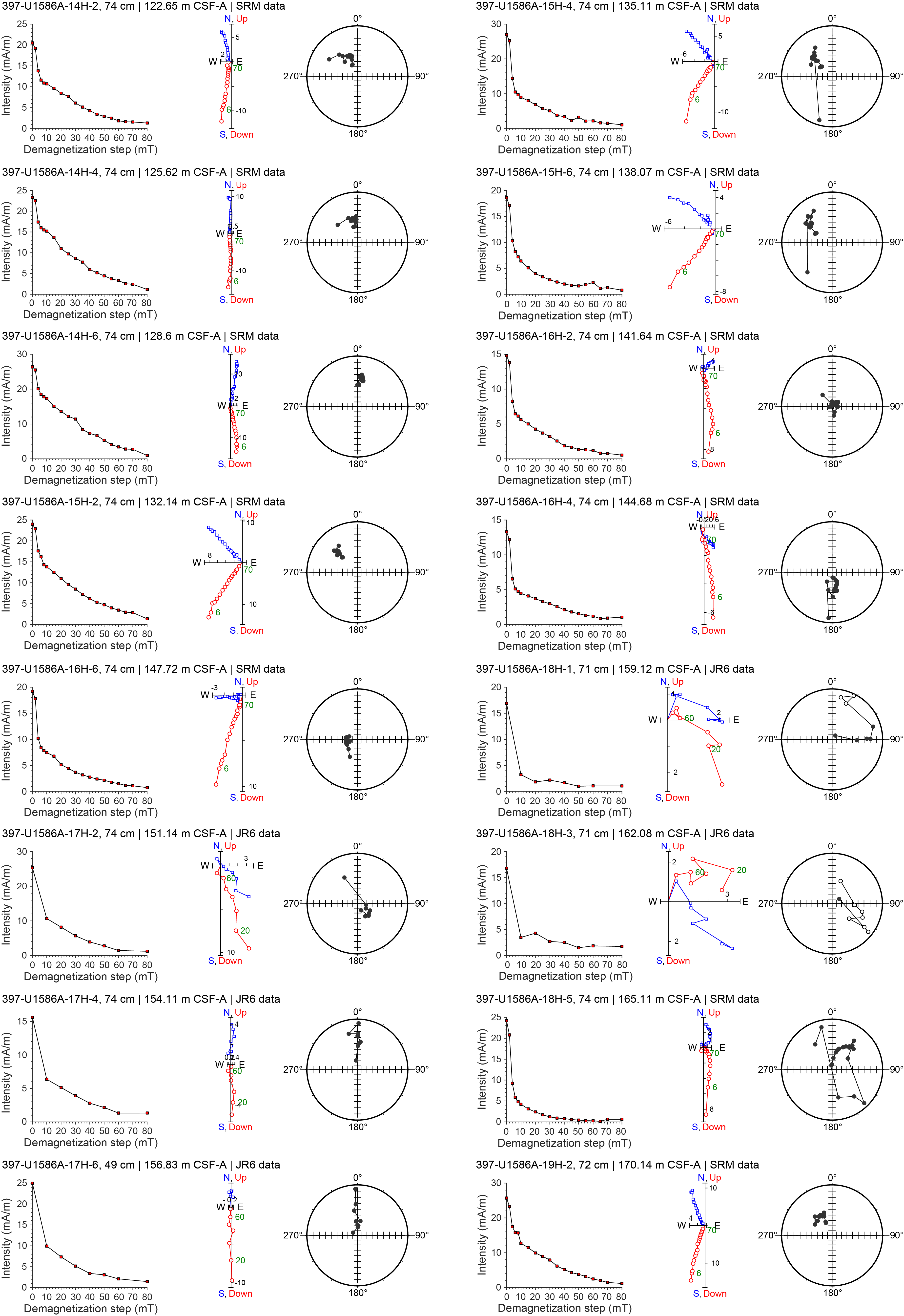
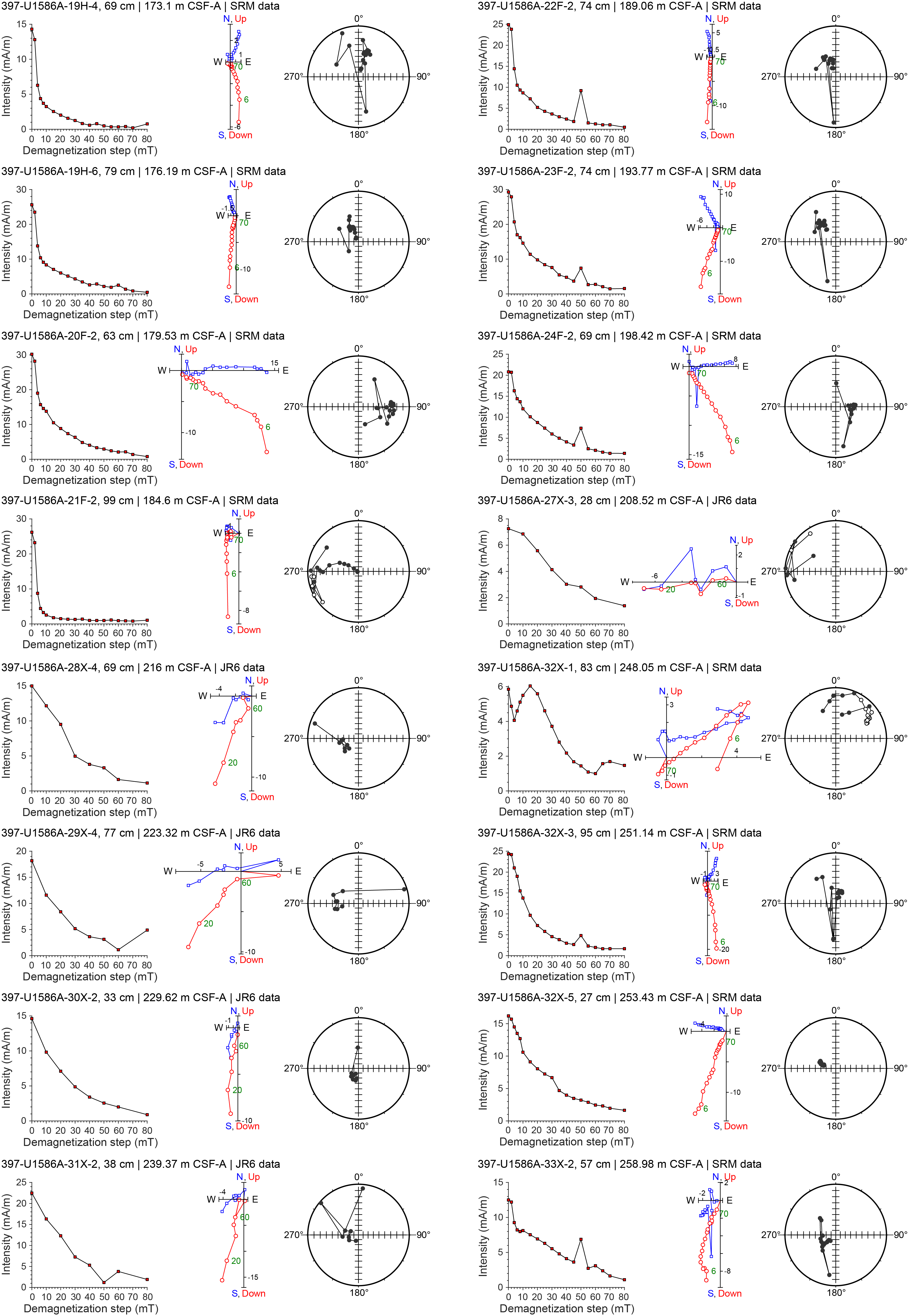
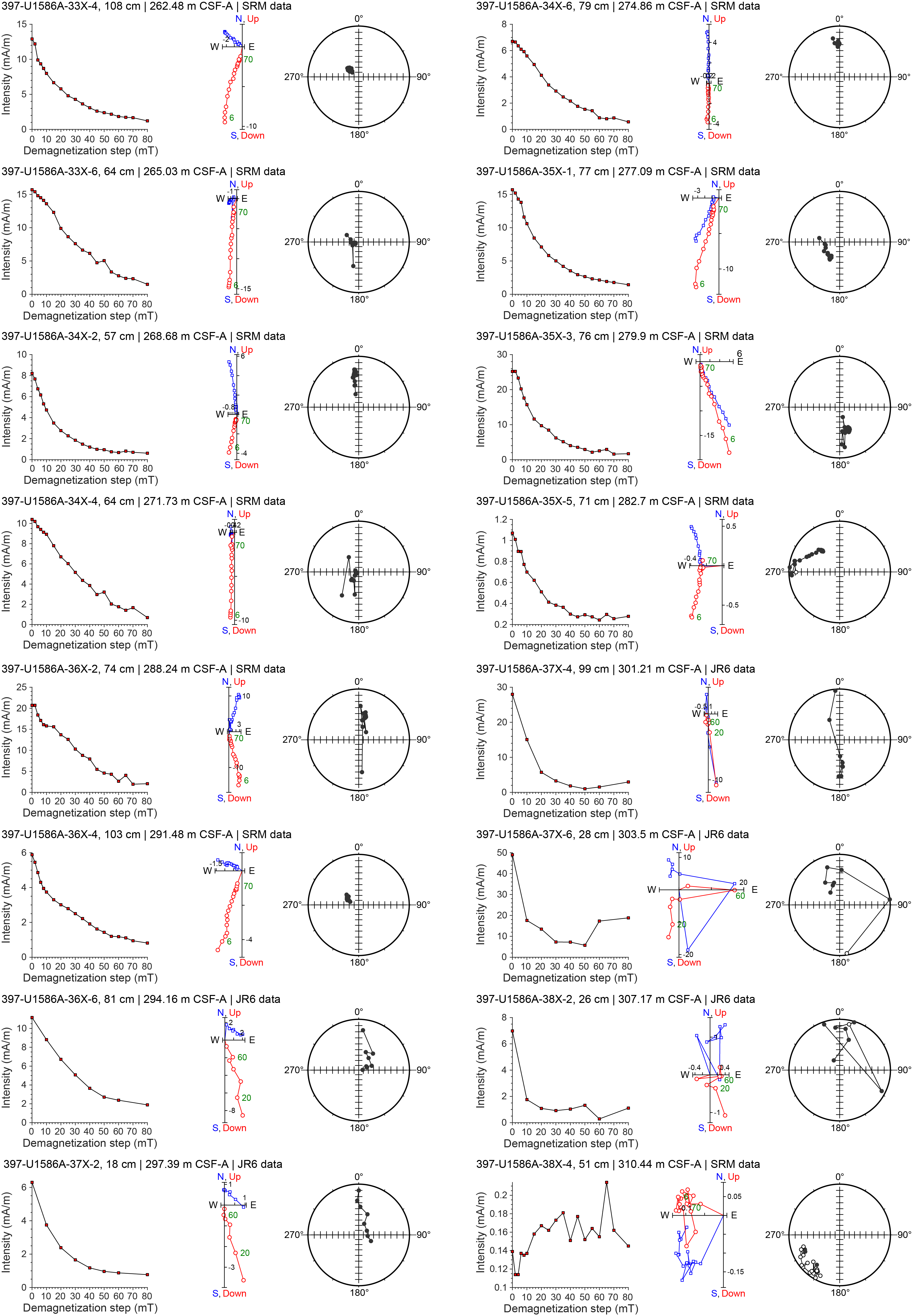
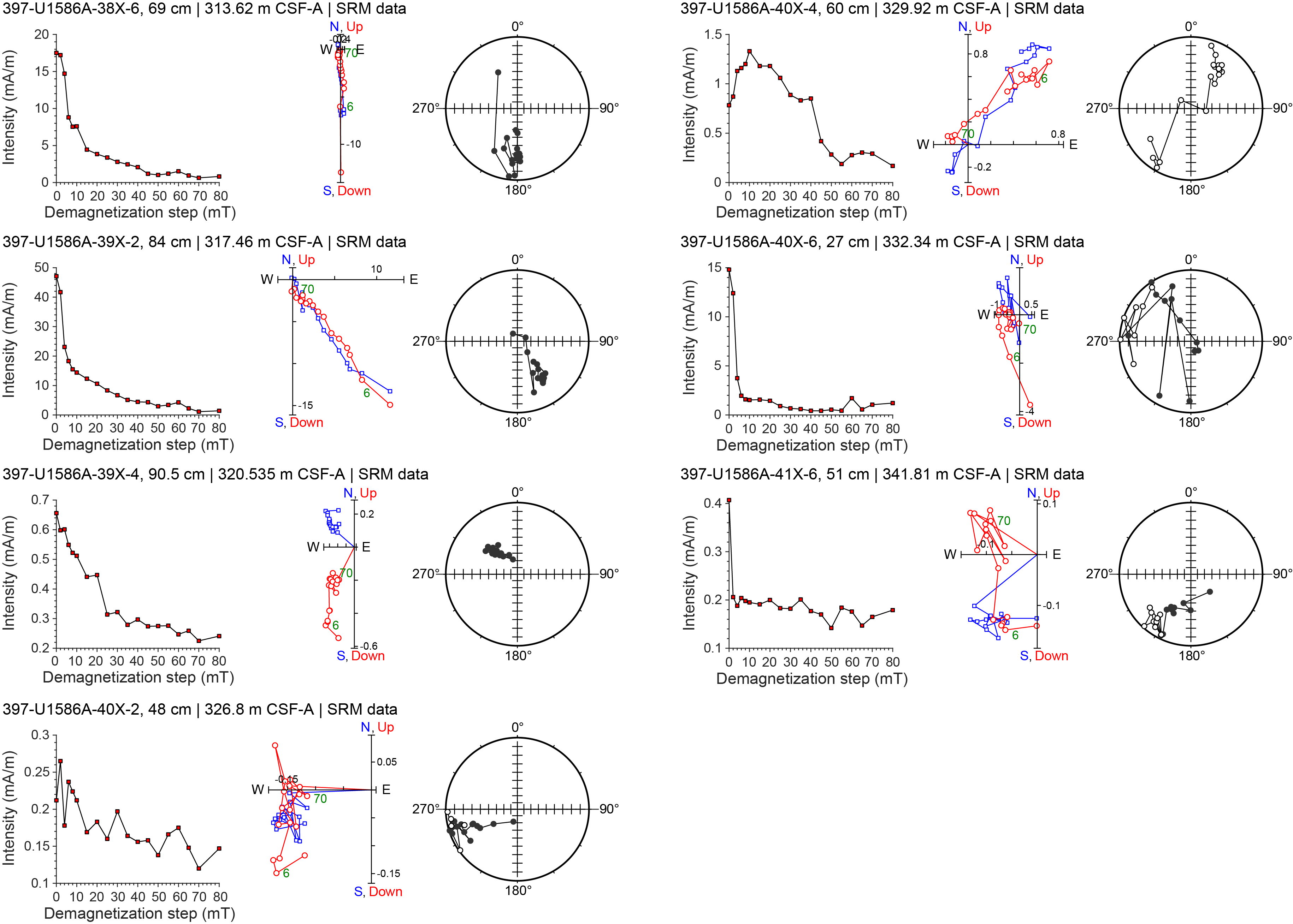
Figure F29. Discrete cube sample AF demagnetization, Hole U1586A.
We processed archive-half data extracted from the shipboard Laboratory Information Management System (LIMS) database by removing all measurements collected from (1) void intervals caused by whole-round sampling (i.e., interstitial water [IW] and paleontology [PAL] samples), (2) disturbed core top intervals in APC cores (Table T15), and (3) the top and bottom 6 cm of each section and an extra 6 cm to the void and disturbed core top intervals. Intervals in each hole that are either slumped or were strongly disturbed during coring (see Lithostratigraphy) are indicated in Figures F25, F26, F27, and F28, and data from these intervals are typically not used for magnetostratigraphic interpretation. Declination data from APC cores where Icefield MI-5 orientation data are available were corrected for each core using the estimated orientation angles and the current declination value at the site according to the 2020 International Geomagnetic Reference Field (IGRF2020) (see Paleomagnetism in the Expedition 397 methods chapter [Abrantes et al., 2024]). To analyze the NRM data of both the section-half and the discrete cube samples, we used a modified version of the UPmag software (Xuan and Channell, 2009). The processed NRM inclination, declination (including orientation-corrected declination where available), and intensity data after 20 mT AF demagnetization are shown in Figures F25, F26, F27, and F28.
5.1. Natural remanent magnetization intensity and magnetic susceptibility
Intensities of NRM after 20 mT AF demagnetization (NRM20mT) for APC and HLAPC cores from the four holes are similar in magnitude for overlapping intervals. There is an apparent drop of NRM20mT intensity from mostly ~10−2 A/m to ~10−3 to 10−2 A/m at ~43, ~39, and ~44.5 m CSF-A in Holes U1586A, U1586B, and U1586C, respectively. This intensity drop appears to coincide with directional changes associated with the Brunhes/Matuyama (B/M) boundary (see Magnetostratigraphy). This intensity drop is not shown in Hole U1586D, possibly due to strong coring disturbance in APC cores of the hole near the relevant depths. NRM20mT intensity of the XCB cores is typically on the order of 10−2 A/m with a downhole decreasing trend to ~308, ~304, ~308, and ~304 m CSF-A in Holes U1586A, U1586B, U1586C, and U1586D, respectively, below which depths intensity drops to the order of 10−4 to 10−3 A/m. NRM20mT intensity of the XCB cores are significantly (often up to one order of magnitude) higher than those from the overlapping APC cores in Hole U1586A, suggesting strong overprint of the XCB cores that are not completely removed after 20 mT demagnetization.
Figures F25, F26, F27, and F28 show MS measured on whole-round cores using the WRMSL and on archive-half sections using the SHMSL (see Physical properties). The WRMSL and SHMSL acquired susceptibility values were multiplied by 0.68 × 10⁻⁵ and (67/80) × 10−5, respectively, to convert to the dimensionless volume SI unit (Blum, 1997). MS measurements are generally consistent between the two instruments and across the different holes for overlapping intervals and vary mostly between 10 × 10−5 and 100 × 10−5 SI. A susceptibility peak of ~150 × 10−5 SI is visible in all four holes at ~150 m CSF-A. MS of sediments generally mimics NRM20mT intensity on a few tens of centimeters to meter scales, suggesting that magnetic minerals that carry NRM are at least similar to those that dominate MS. However, there is an apparent difference in the trend of NRM20mT intensity and MS on the tens of meters scale, possibly due to greater influence of incompletely removed overprint on NRM, reversed polarity interval sediments, and/or diagenesis on (typically finer) remanence carrying magnetic grains of the sediments.
5.2. Magnetostratigraphy
We combined NRM (after 20 mT demagnetization) inclination and orientation-corrected declination data from archive-half sections and stepwise NRM demagnetization (up to 50 or 80 mT) data from cube samples to make magnetostratigraphic interpretations. The geomagnetic field at the latitude of Site U1586 (37.62°N) has an expected inclination of 57° (−57°) during normal (reversed) polarity, assuming a geocentric axial dipole (GAD) field model. The AF demagnetization behavior of cube samples is illustrated in Figures F29, F30, F31, and F32. A steep normal overprint appears to be largely removed after AF demagnetization with peak fields of ~5–20 mT (but potentially incompletely removed at even higher demagnetization steps). Polarity information determined based on the cube data is indicated by black (normal), white (reversed), and gray (uncertain) squares in Figures F25, F26, F27, and F28. Identified polarity reversals at Site U1586 are shown in the Chron column in Figures F25, F26, F27, and F28 and summarized in Table T16. The interpreted magnetostratigraphy is generally consistent with the biostratigraphy of the site (see Biostratigraphy).
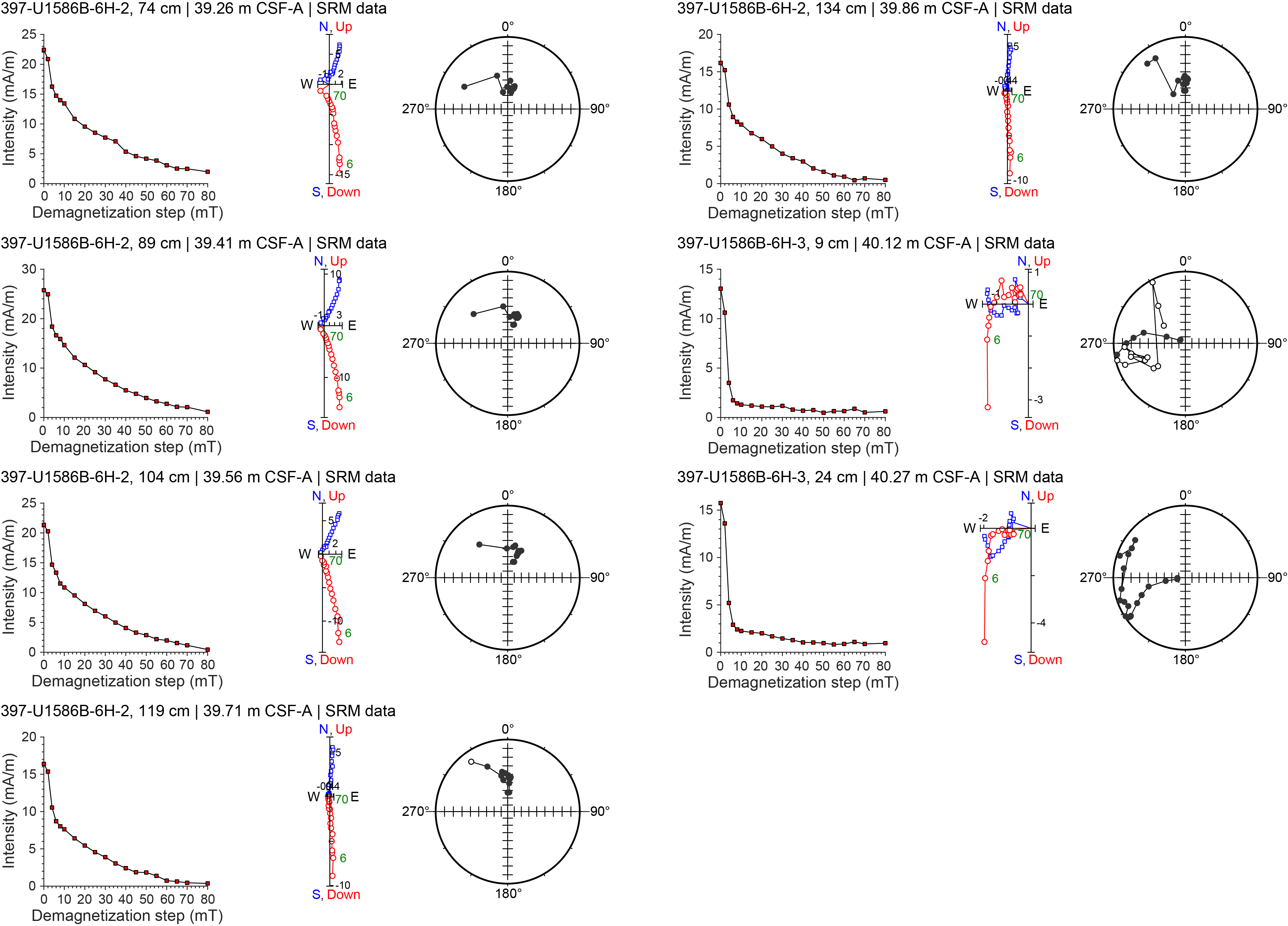
Figure F30. Discrete cube sample AF demagnetization, Hole U1586B.
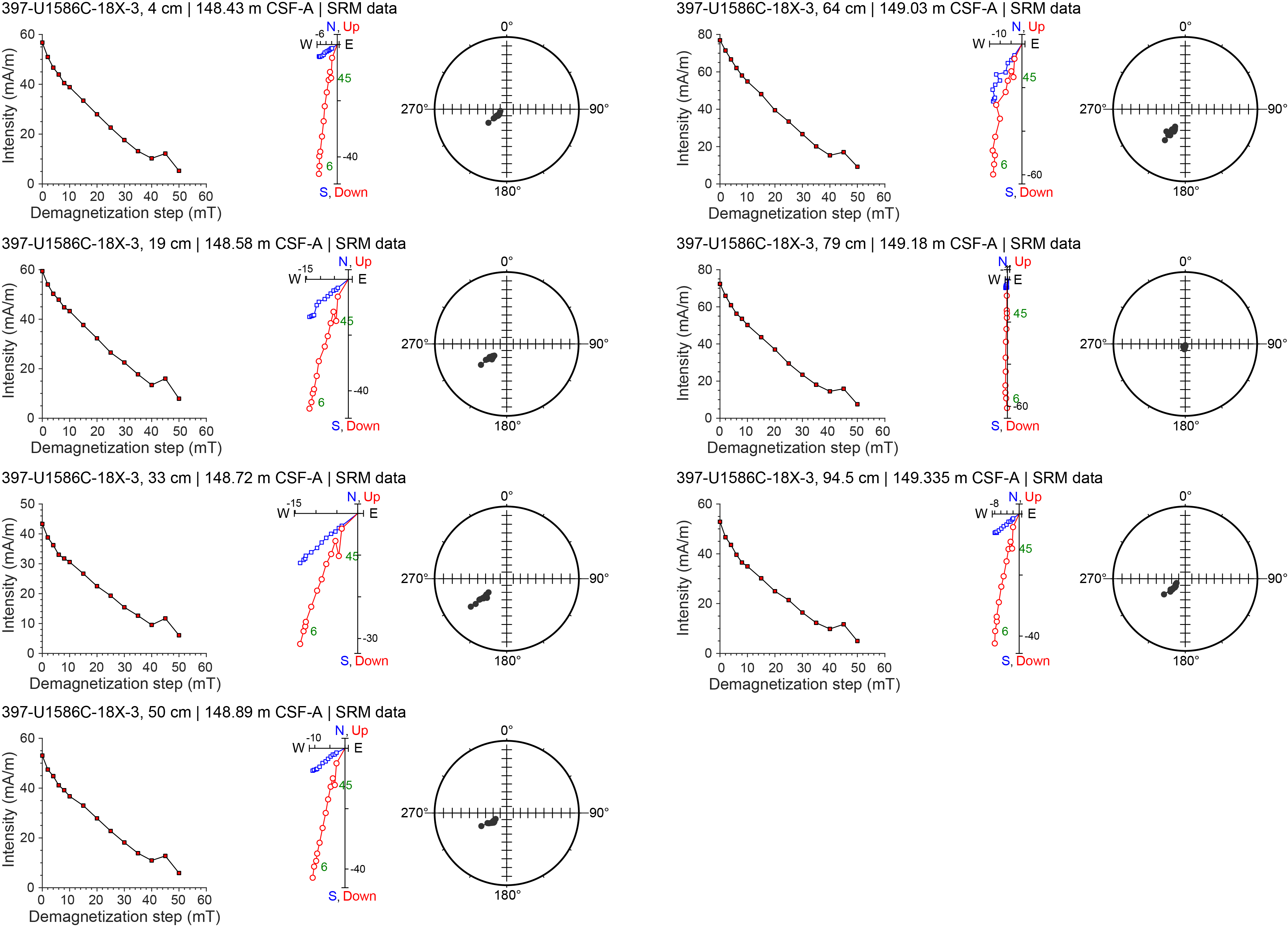
Figure F31. Discrete cube sample AF demagnetization, Hole U1586C.
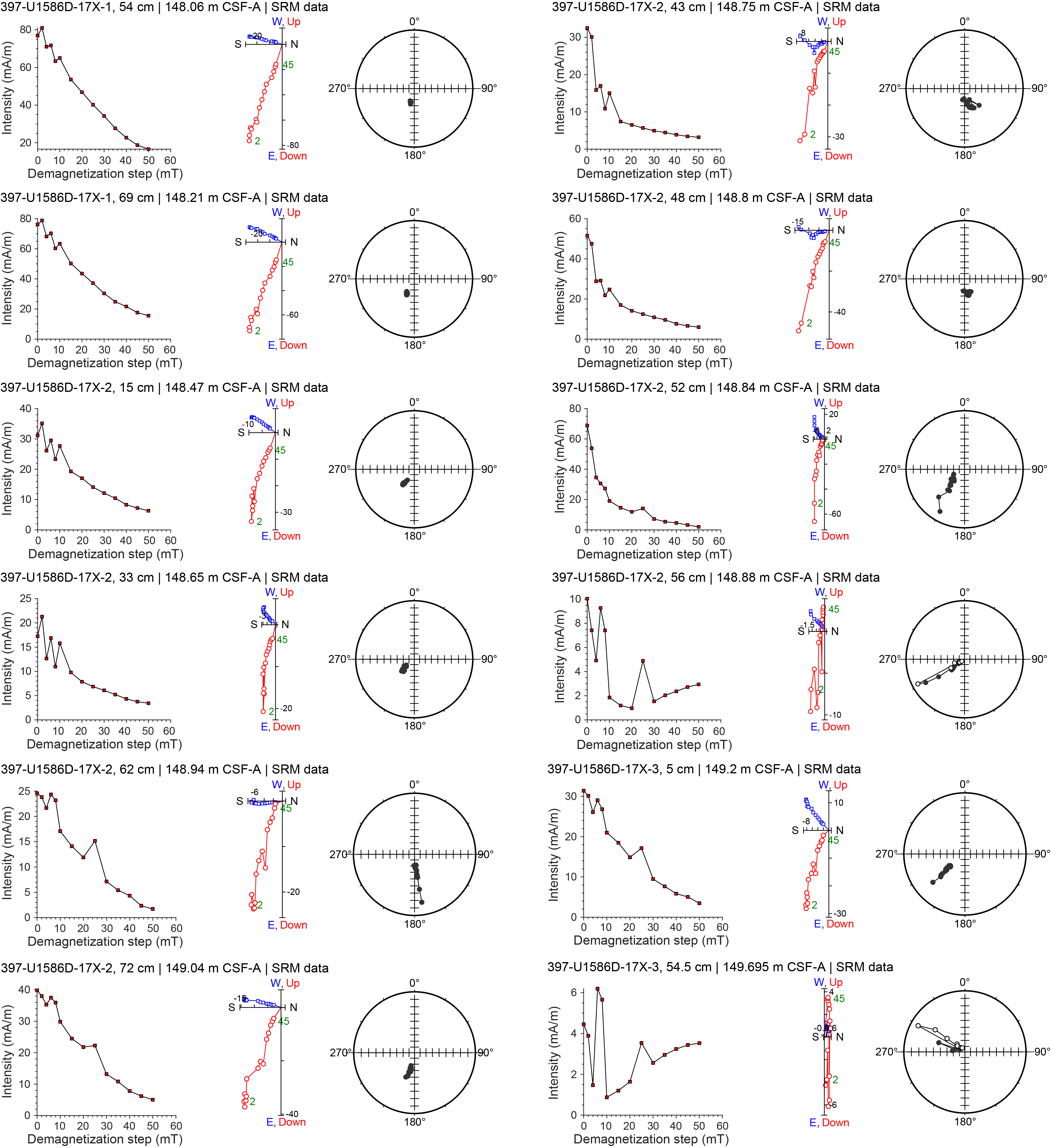
Figure F32. Discrete cube sample AF demagnetization, Hole U1586D.
The B/M boundary (0.773 Ma) is recorded at ~44, ~40, and ~45.5 m CSF-A in Holes U1586A, U1586B, and U1586C, respectively, and is not identified in Hole U1586D because of heavy coring disturbance of APC cores near this depth level. This boundary should be below 42 m CSF-A in Hole U1586D. Above the B/M boundary, NRM20mT inclination of all holes varies closely around the expected GAD inclination of ~57° (Figures F25A, F26A, F27A, F28A). Below the B/M boundary, the NRM of sections from Holes U1586A–U1586C is dominated by shallow/negative inclinations. Inclinations during the reversed polarity intervals are generally shallower than the expected dipole inclination of −57°, possibly due to incompletely removed drilling overprint that orients vertically down. In Holes U1586A–U1586C, the shift in NRM20mT from positive to shallow/negative inclinations is accompanied by changes in corrected declination values from ~0° to ~180°. Our interpretation of the B/M boundary is supported by the results of cube samples from Holes U1586A and U1586B. Cube samples from above the boundary show well-defined characteristic remanence with positive inclinations, whereas cube samples from below the B/M boundary apparently have shallow/negative inclinations at high demagnetization steps (Figures F29, F30). The seven cube samples collected at ~15 cm spacing in Sections 397-U1586B-6H-2 and 6H-3 constrained the B/M boundary to between 39.86 and 40.12 m CSF-A in Hole U1586B, consistent with the ~40 m CSF-A depth determined from the archive-half sample data.
The Jaramillo Subchron (0.99–1.07 Ma) is identified at ~55–59, ~53–57, and ~57–61 m CSF-A in Holes U1586A, U1586B, and U1586C, respectively. These intervals are characterized by positive inclinations varying around 57° and orientation-corrected declinations close to ~0° or ~360°. The NRM of sections from the top and bottom of these intervals is characterized by downhole shifts of negative/positive inclinations to shallow/opposite direction inclinations and ~180° changes in declinations. Results from cube samples in Hole U1586A are consistent with this interpretation (Figure F25A). Cube samples from 56.16 and 59.17 m CSF-A in Hole U1586A show well-defined positive inclination components, and cube samples from above and below these samples show reversed components (Figure F29). The Jaramillo Subchron is not clearly identified in Hole U1586D. The bottom of the Jaramillo Subchron could be located at ~61 m CSF-A in Hole U1586D.
Inclination from the interval between the interpreted bottom of the Jaramillo Subchron and the Matuyama/Gauss (M/G) boundary (see paragraph below) shows frequent alternations between positive and negative values (Figures F25A, F26A, F27A). Comparison of the NRM20mT directional data with the section-half images shows that most of the apparent positive inclination intervals coincide with light-colored nannofossil ooze. It is possible that sediments dominated by nannofossil ooze are more prone to drilling overprint. Data from cube samples taken from some of these intervals show reversed components after >20 mT demagnetization steps (e.g., cube sample from 78.22 m CSF-A in Figure F29). We interpret the positive inclination intervals with corrected declinations around 0° or 360° at ~63.7–65.2, ~63.3–65.8, and ~66.1–67.7 m CSF-A in Holes U1586A, U1586B, and U1586C, respectively, as the Cobb Mountain Subchron (1.18–1.215 Ma). Compared with the light-colored nannofossil ooze, these intervals are richer in clay, and this interpretation is generally consistent with the biostratigraphy. We speculate that the dominantly positive (~57°) inclination interval at ~86–91 m CSF-A in Hole U1586A represents the Olduvai Subchron (1.775–1.934 Ma). Two cube samples from this interval show shallow positive inclination components, and we note that this interval is dominated by calcareous/nannofossil ooze. The Feni Subchron (2.116–2.14 Ma) could be recorded at ~100.9–101.7 m CSF-A in Hole U1586B.
We place the M/G boundary (2.595 Ma) at ~113.5, ~113, and ~113.7 m CSF-A in Holes U1586A, U1586B, and U1586C, respectively. This interpretation is supported by a downhole inclination pattern change from dominantly negative/shallow to positive inclinations. In Hole U1586C, this inclination pattern change is accompanied by changes in corrected declinations from ~180° to ~0°. Changes in declination are less clear in Holes U1586A and U1586B around this boundary. Discrete cube samples from above and below this boundary (e.g., from 113.12 and 116.07 m CSF-A) in Hole U1586A appear to show reversed and normal components, respectively (Figure F29), which is consistent with the interpretation.
In Core 397-U1586A-16H, at ~142.2–143.1 m CSF-A, a short interval with reversed polarity is identified by both negative inclinations close to −57° and corrected declinations around 180° (Figure F25A). This reversed interval is not observed in other holes, possibly because of heavy drilling overprint associated with the XCB coring at similar depths in those holes. We interpret this interval as the Mammoth Subchron (3.207–3.33 Ma) based on its relative position in the interpreted Gauss Chron. This interpretation suggests the Keana Subchron (3.032–3.116 Ma) is missing/not well recorded at least in Hole U1586A.
The Gauss/Gilbert (G/G) boundary (3.596 Ma) is identified at ~152 m CSF-A in Hole U1586A, where dominantly positive inclinations shift to shallow/negative inclinations and corrected declinations change from values around 0° or 360° to ~180°. Cube sample data from Hole U1586A are generally consistent with this interpretation (Figure F29). The G/G boundary in Hole U1586A appears to coincide with the MS spike (Figure F25A). The G/G boundary is not observed in Hole U1586B because of heavy drilling overprint of XCB cores at similar depth. Measurements of the seven cube samples from Section 397-U1586C-18X-3 (~148.4–149.3 m CSF-A), above the MS spike (~152.7 m CSF-A), show well-defined normal polarity components (Figure F31), suggesting that Section 18X-3 is likely still in the Gauss Chron. A total of 12 cube samples were taken in Hole U1586D near the MS peak (~148.8 m CSF-A). The top six samples (~148.06–148.8 m CSF-A) show well-defined normal components, and samples from below this appear to show shallow/negative components (Figure F32), suggesting the G/G boundary could be located at ~148.8 m CSF-A in Hole U1586D, again coinciding with the MS spike.
At ~169–172 and ~188.6 m CSF-A in Hole U1586A, we observe a short interval of normal polarity and a possible reversal. The former is dominated by positive inclinations with corrected declinations close to 0° or 360°, and the latter appears to be a shift (downhole) of shallow inclinations to steeper positive inclinations accompanied by a ~180° change in declinations. Based on their relative depth levels and biostratigraphy we tentatively interpret them as the Cochiti Subchron (1.187–4.3 Ma) and the top of the Thvera Subchron (4.997 Ma). Results from cube samples show some support for this interpretation. For example, a cube sample from ~170.14 m CSF-A yields well-defined normal component, and cube samples from ~184.6 and ~189.06 m CSF-A appear to show reversed and normal components, respectively (Figure F29).
XCB coring started at ~206, ~140, ~120, and ~110 m CSF-A in Holes U1586A, U1586B, U1586C, and U1586D, respectively (Figures F25B, F26B, F27B, F28B). The NRM20mT data of the XCB cores are dominated by positive inclinations with declinations centered close to 0°. As mentioned, NRM20mT intensity of XCB cores is also significantly (often up to one order of magnitude) stronger than APC cores from overlapping depth intervals. These observations suggest that XCB cores are heavily influenced by drilling overprint, and it is difficult to make magnetostratigraphic interpretations using section-half measurements for the XCB cores. Results from the cube samples taken from the undisturbed center parts of the XCB cores in Holes U1586A–U1586D often show reasonably well defined normal or reversed components (Figure F29). However, because of the low sampling rate aboard ship and generally low and (likely) varying sediment accumulation rates, it is difficult to make magnetostratigraphic interpretations for the XCB cores based only on the shipboard cube sample data. Polarity information from these cubes could be used to help verify biostratigraphy.
6. Geochemistry
Geochemistry analysis at Site U1586 included the collection and measurement of IW samples for salinity, alkalinity, pH, major ions (Na, K, Ca, Cl, and SO4), nutrients (NH4 and PO4), and trace elements (Sr, Li, Fe, Mn, B, and Ba); headspace gases for methane (CH4) concentrations; and bulk sediment samples for total organic carbon (TOC), total inorganic carbon (TIC)/calcium carbonate (CaCO3), total nitrogen (TN), total sulfur (TS), and bulk mineralogical abundance (by XRD) and elemental composition (by inductively coupled plasma–atomic emission spectrometry [ICP-AES]). In total, 56 IW samples were taken from Hole U1586A, as described in Geochemistry in the Expedition 397 methods chapter (Abrantes et al., 2024). For each core, a 5 cm sample was taken from the base of every section in the upper 34 m, at the base of Sections 2 and 6 to 47 m CSF-A, and then at the base of Section 6 (i.e., the second to last section recovered from every core) for the remainder of the hole. Squeeze cake samples and select discrete samples from the working half of split cores were measured for sedimentary total carbon (TC), TN, TS, and TIC. TOC is calculated as the difference between TC and TIC. Samples for bulk elemental and mineralogical composition were also selected from the working half of split cores for paired ICP-AES and XRD analyses at a resolution of two samples per core.
IW alkalinity, NH4, and PO4 increase and SO4 decreases in the upper 100 m of the hole, indicative of organic matter respiration. However, SO4 reduction likely did not occur at a high intensity, given that its concentrations never reach zero and CH4 concentrations never exceed 15 ppmv. Similarly, peaks in redox-sensitive elements such as Fe and Mn are indicative of microbially mediated respiration reactions within the sediment. The CH4 trend implies peak anaerobic respiration around 100–150 m CSF-A. IW samples show evidence of microbially mediated respiration and other diagenetic reactions.
CaCO3 content ranges 2.9–78.1 wt% (average = 37.4 wt%). Coulometer-determined CaCO3 content results are consistent with stoichiometrically calculated CaCO3 from elemental Ca concentrations measured using ICP-AES. CaCO3 correlates positively with L* and negatively with NGR. TOC, TN, and TS values in Hole U1586A are generally low, ranging 0–2.02 wt% TOC (mean = 0.48 wt%), 0–0.022 wt% TN (mean = 0.095 wt%), and 0–0.37 wt% TS (mean = 0.03 wt%). Organic C/N ratios (0–86.7; mean = 20.0) suggest that organic matter has both marine and terrestrial sources.
Bulk sediment concentrations of SiO2, K2O, Fe2O3, MgO, and TiO2 show strong positive correlations with Al2O3, indicating the dominance of terrigenous detritus. This correlation is also observed for minor elements, including Zn, Cr, V, Sc, Y, and Zr. Na shows a correlation with Al, but the nonzero intercept is likely caused by NaCl precipitated from seawater. Bulk sediment Ca primarily represents biogenic CaCO3, and because of incorporation of Sr into biogenic CaCO3, both elements show an inverse relationship with Al. Ba is weakly correlated with Al or Ca, likely due to the presence of barite (BaSO4). Mn shows no relationship with Al, indicating a process other than end-member mixing. Elemental ratios of Si/Al, K/Al, Si/Al, Sr/Ca, and estimated biogenic Ba are identified as useful proxies for provenance, weathering, and productivity.
Part of the recovered sequence contains slumped intervals (as described in Lithostratigraphy), but these slumps did not seem to have any significant effect on the major or minor elemental composition of pore water (although only two IW samples were taken from a potential slumped interval: 397-U1586A-6H-2, 146–151 cm, and 6H-6, 146–151 cm). The squeezed cakes of these two samples were measured for bulk sediment composition, and their results also show no significant effect in the overall bulk sediment composition.
6.1. Headspace hydrocarbon gases
One headspace sample was collected from the last section of each core (or every other HLAPC core) in Hole U1586A. Ethene, ethane, propane, and propene are below detection limits, and CH4 concentrations remain low (0–14.10 ppmv; average = 6.91 ppmv). The measured CH4 concentrations are around 4 ppmv in Core 1H, peak at ~14 ppmv between 100 and 150 m CSF-A, and decline to ~2 ppmv by 350 m CSF-A (Figure F33; Table T17). Undetectable C2H6 levels indicate that C1/C2 (i.e., CH4/C2H6) ratios remain high and that there is no danger to drilling.
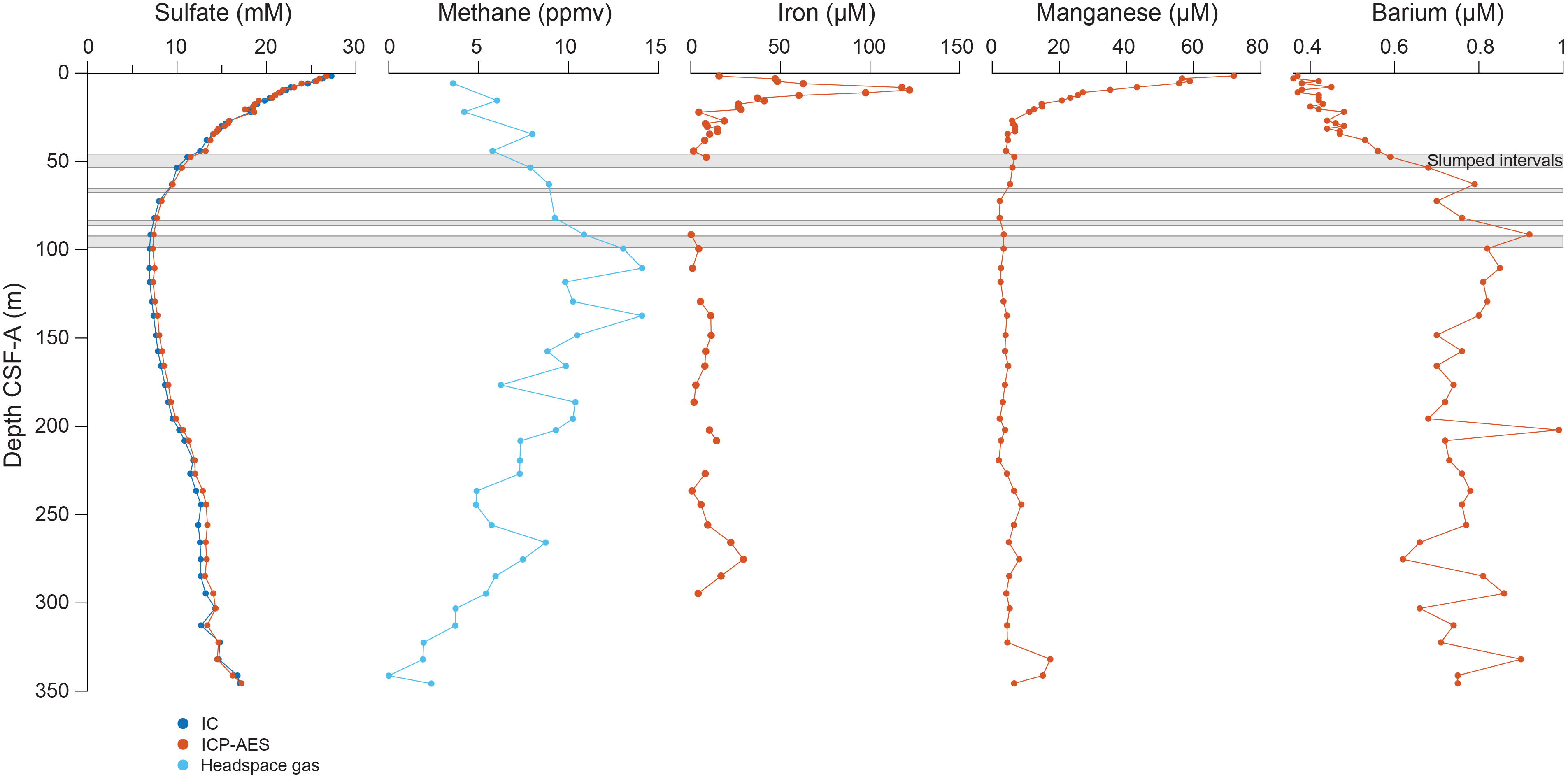
Figure F33. Dissolved SO4, Fe, Mn, and Ba with headspace CH4 concentration.
6.2. Interstitial water geochemistry
Shortly after extracting IW, aliquots of the recovered water were designated for salinity, chlorinity, alkalinity, and pH analysis. In addition, both major and minor elemental compositions were measured using ion chromatography (IC) and ICP-AES and for NH4 and PO4 by spectrophotometry (Table T18). Some of the major trends are highlighted below.
6.2.1. Salinity, sodium, potassium, and chloride
Salinity, Na, and Cl concentrations are relatively constant in Hole U1586A, with values close to seawater (Figure F34). Na has a mean value of 476.7 ± 6.5 mM, and Cl measured by IC has a mean value of 564.2 ± 7.8 mM (ICP-AES data were more variable than IC data, but mean values were nearly identical). Cl measured by AgNO3 titration has a similar mean value (562.2 mM) but is much more variable, with a 1σ (standard deviation) of 23.4 mM and two outliers (>3σ from the mean). K declines at a relatively constant downhole rate from a value of 12 mM in the uppermost sample (397-U1586A-1H-1, 146–151 cm) to 8 mM in the lowermost sample (42X-1, 144–154 cm).
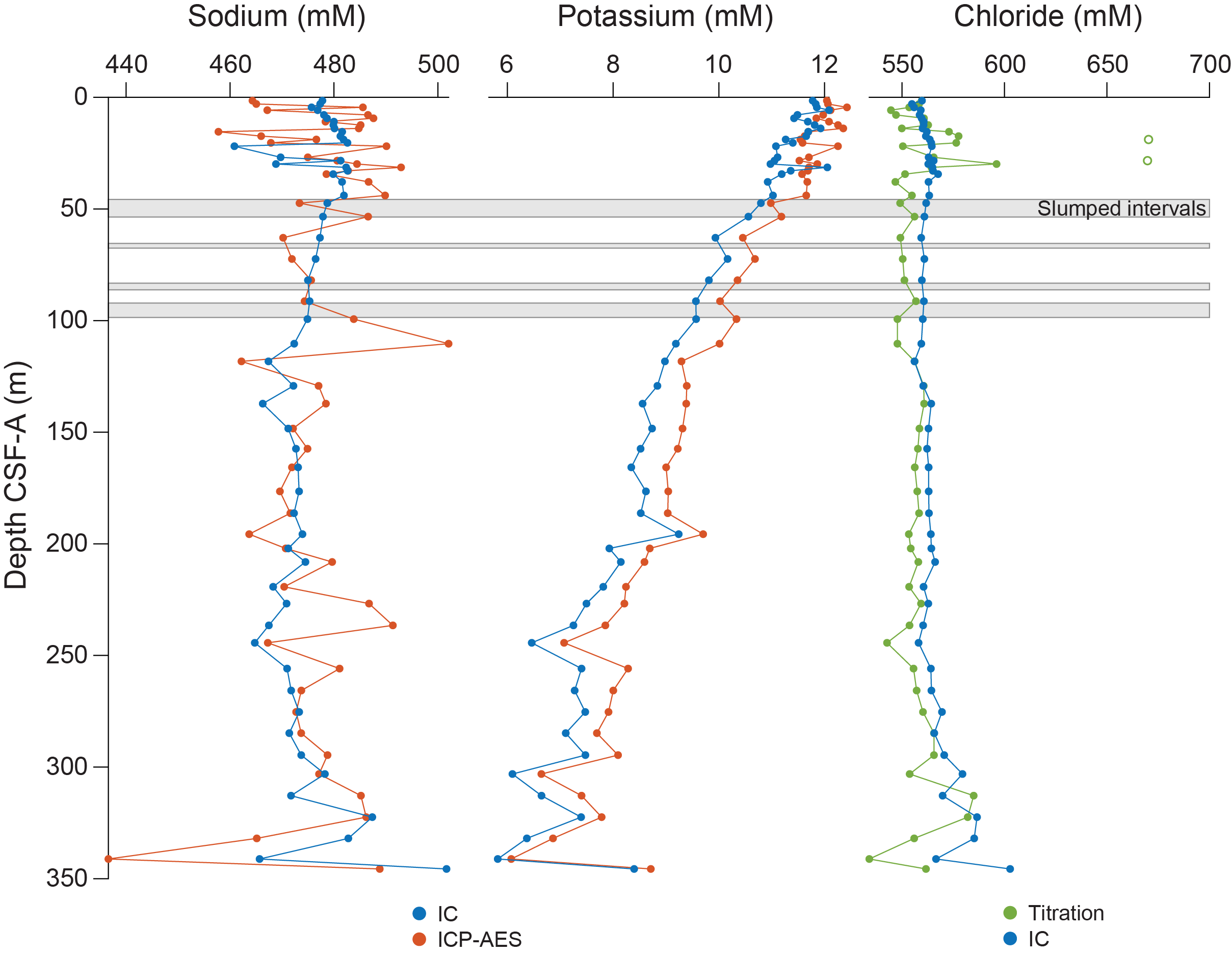
Figure F34. Dissolved concentrations of Na, K, and Cl.
6.2.2. Alkalinity, pH, ammonium, and phosphate
Alkalinity, pH, NH4, and PO4 concentrations increase in the upper part of the hole, peaking at ~70 m CSF-A, and then decline toward the bottom of the hole (Figure F35). Alkalinity is 3.9 mM in the uppermost sample (397-U1586A-1H-1, 146–151 cm), increases to a maximum of 9.2 mM at 62.89 m CSF-A, and then returns to values of 4 ± 0.5 mM by 208.13 m CSF-A. pH values are more variable than alkalinity but follow a similar pattern. The uppermost sample (1H-1, 146–151 cm) has a pH of 7.77; a maximum of 7.95 occurs at 62.89 m CSF-A, and then pH decreases to ~7.64 to ~284.8 m CSF-A. NH4 concentrations are near zero in the uppermost sample (30.77 µM), increase to 1236.75 µM at 99.33 m CSF-A, and then decrease to 503.77 µM at 345.64 m CSF-A. PO4 concentrations are lower and more variable than NH4: 6.52 µM in the uppermost sample, decreasing slightly in the upper 10 m to a minimum value of 4.35 µM at 7.86 m CSF-A, increasing to 10.75 µM at 62.89 m CSF-A, and then decreasing to 5.22 µM at 176.5 m CSF-A. Below ~175 m CSF-A, PO4 concentrations are relatively constant at 5.90 ± 0.47 µM. The deepest four samples (Cores 39X–42X and repeat measurement of 38X) are offset to slightly higher PO4; however, these samples were measured during a different analytical session so this offset is likely an analytical artifact.
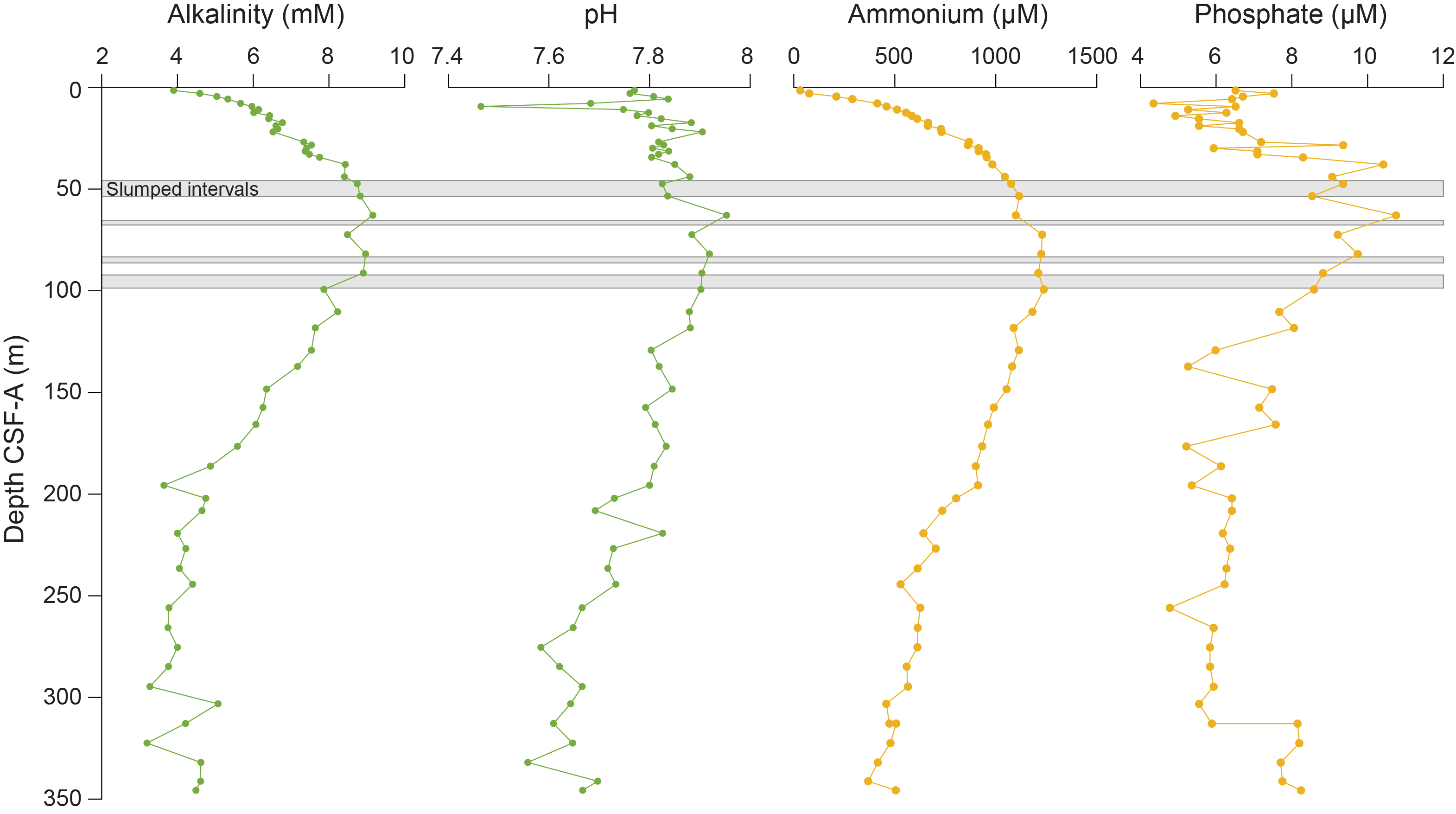
Figure F35. Alkalinity, pH, NH4, and PO4.
The increase in alkalinity, NH4, and PO4 in the upper 70 m are likely the result of organic matter respiration, assuming a generic composition of (CH2O)106(NH3)16(H2PO4), which produces alkalinity (in the form of HCO3−), PO4, and NH4. Alkalinity is also related to the charge balance in seawater, so changes in the major anion and cation composition (e.g., Ca2+, Mg2+, and SO42−) will also affect alkalinity.
6.2.3. Sulfate, iron, manganese, and barium
SO4 concentrations are near seawater value (27.26 mM) in the uppermost sample (397-U1586A-1H-1, 146–151 cm), decrease to a minimum of 6.90 mM at 110.35 m CSF-A, and then increase to 17.03 mM at the bottom of the hole (Figure F33). The SO4 minimum coincides with the CH4 maximum, although the CH4 data are more variable. There is a well-resolved peak in dissolved Fe near the top of the hole, with maximum values of 121.93 µM at 9.37 m CSF-A. Below ~20 m CSF-A, Fe concentrations are near the detection limit. The maximum in dissolved Mn occurs in the uppermost sample (71.96 µM). Mn then declines to near zero to 16.85 m CSF-A. At the very base of the hole, two samples have higher Mn concentrations (17.3 µM in 40X-5, 114–124 cm, and 15.07 µM in 41X-5, 92–102 cm). Ba concentrations increase as SO4 decreases in the upper part of the hole from values of around 0.4 µM at the top to 0.82 µM at 99.33 m CSF-A. Below 100 m CSF-A, Ba concentrations are highly variable but roughly constant around 8 µM.
Decreasing SO4 concentrations indicate organic matter respiration via SO4 reduction; however, SO4 never reaches zero and CH4 concentrations never exceed 15 ppmv. Therefore, these reactions were likely not occurring at high intensity. Peaks in redox-sensitive elements such as Fe and Mn are similarly indicative of microbially mediated respiration reactions within the sediment. Dissolved Fe likely derives in part from the dissolution of magnetite, which contributes to the reduction in MS in the upper part of the hole (see Paleomagnetism). X-ray images of cores show evidence of pyritized burrows resulting from organic carbon remineralization via SO4 reduction, which produces HS− and reacts with dissolved Fe to form pyrite. Increasing Ba concentrations in the upper 100 m could be the result of BaSO4 dissolution.
6.2.4. Calcium, magnesium, and strontium
Ca concentrations in IW decrease in the upper 50 m from a value of 10.39 mM in the uppermost sample (397-U1586A-1H-1, 146–151 cm) to 4.62 mM at 72.39 m CSF-A and then increase to around 20 mM at the bottom of the hole (Figure F36). Mg concentrations are more variable than Ca, and IC values are offset ~2.5 mM greater than ICP-AES. Mg concentrations also decrease in the upper part of the hole from ~50 mM in the uppermost sample to ~45 mM at 62.89 m CSF-A. Between ~60 and 220 m CSF-A, Mg is roughly constant, decreasing again to ~40 mM at the bottom of the hole. Sr concentrations are around 80 µM to ~70 m CSF-A, followed by an increase toward a maximum of 461.29 µM at 303.11 m CSF-A, after which concentrations decrease slightly to the bottom of the hole.
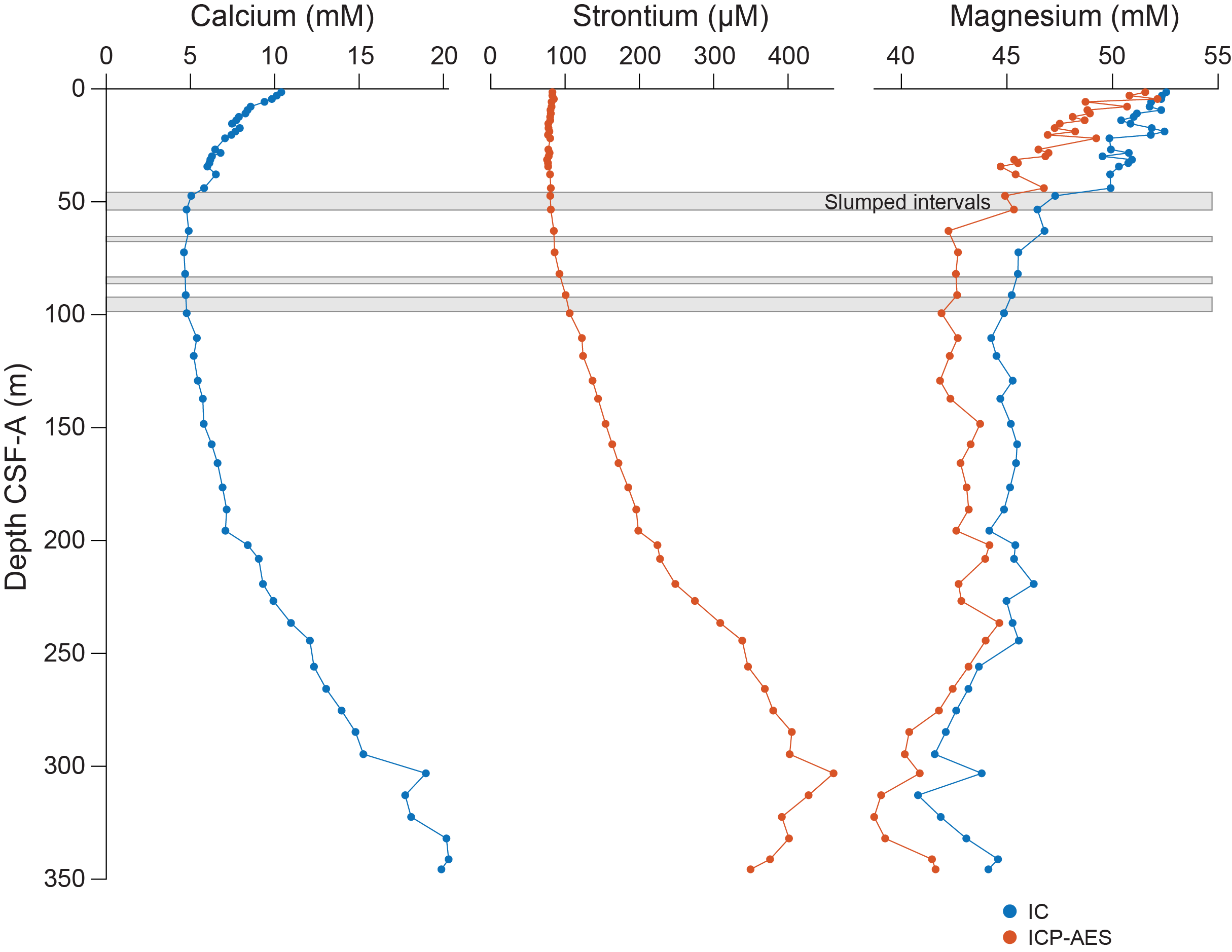
Figure F36. Dissolved Ca, Mg, and Sr.
The decrease in Ca and Mg concentrations in the upper 50 m could be the result of authigenic carbonate precipitation driven by high pore water alkalinity associated with SO4 reduction. As alkalinity and pH decrease deeper in the hole, CaCO3 dissolution could drive up Ca concentrations. Below 200 m CSF-A, possible dolomitization may be taking up Mg and liberating Ca and Sr.
6.2.5. Silicon, lithium, and boron
Si concentrations are nearly constant (average = 179.5 ± 25 µM) between 1.46 and 294.4 m CSF-A (Figure F37). From 294.64 to 312.81 m CSF-A, Si increases to a maximum of 913.46 µM and then decreases to 680.81 µM in the lowermost sample (397-U1586A-42X-1 144–154 cm). Li concentrations show a linear increase downhole from a value of 23.44 µM in the uppermost sample (1H-1, 146–151 cm) to 123.53 µM in the lowermost sample (42X-1, 144–154 cm). B data are highly variable at the top of the hole; B concentrations are ~600 µM and decrease to ~460 µM at ~100 m CSF-A, followed by a renewed increase to ~650 µM at ~250 m CSF-A and a decrease to ~550 µM at the bottom of the hole.
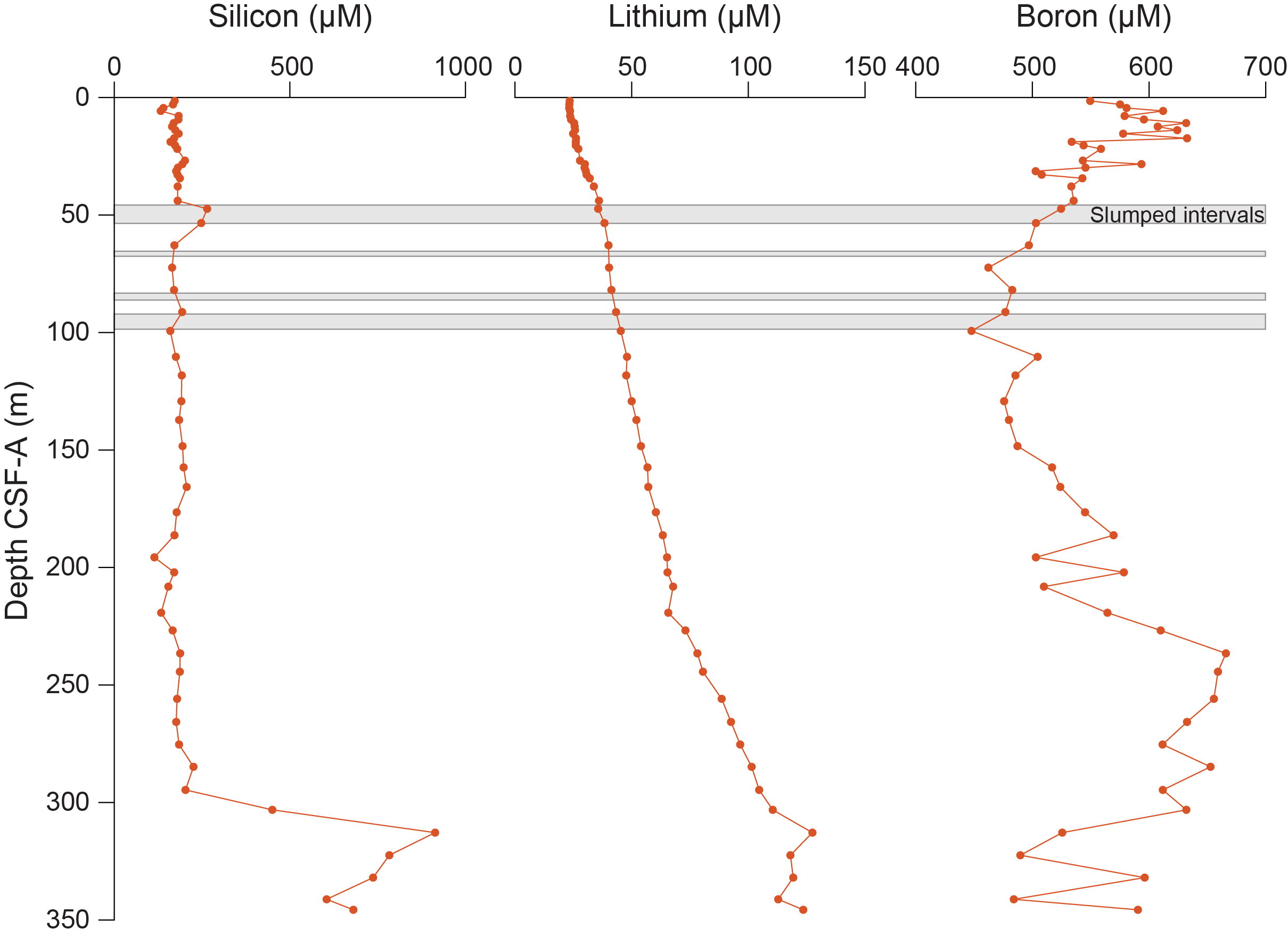
Figure F37. Dissolved Si, Li, and B.
High Si concentrations near the bottom of the hole coincide with the start of Lithostratigraphic Unit III; the peak in Si corresponds to the observed silty clay layers (Tables T2, T3).
6.3. Bulk sediment geochemistry
6.3.1. Calcium carbonate (total inorganic carbon)
In Hole U1586A, splits for CaCO3/TIC quantification were taken from the sedimentary residue of every IW sample. Separate discrete TIC samples were also taken throughout the hole at a resolution of approximately 1 per 3.5 m, or ~3 measurements per core.
A 100% CaCO3 standard was analyzed every ~10 samples (mean = 99.24 ± 1.09 wt%; n = 15) (Tables T19, T20). Samples were not measured until the standard was within ~1.5% of 100 wt%. Four samples were duplicated to assess analytical error; interduplicate differences ranged 0.22–1.75 wt% CaCO3 (Table T21).
Mean CaCO3 content is 37.4 wt%, but variability is high (±1σ = 18.7 wt%; range = 2.9–78.1 wt%). CaCO3 increases steadily but nonmonotonically, with local maxima of ~65 wt% around 20 m CSF-A, ~65 wt% around 165 m CSF-A, and ~78 wt% between 275 and 315 m CSF-A (Figures F38, F39; Table T22). CaCO3 correlates positively with L* (adjusted R2 = 0.787) and negatively with NGR (adjusted R2 = 0.597) (Figures F38, F39, F40, F41). Correlations are slightly weaker if samples from squeeze cakes are included, but this requires extrapolation of L* and NGR data to sediment adjacent to IW samples. Using the measured elemental Ca concentrations from the ICP-AES data, the stoichiometric CaCO3 was compared to the shipboard calculated total CaCO3 weight measured using the coulometer (Figures F38, F39). Although the absolute numbers are not the same, the data show a similar overall trend.
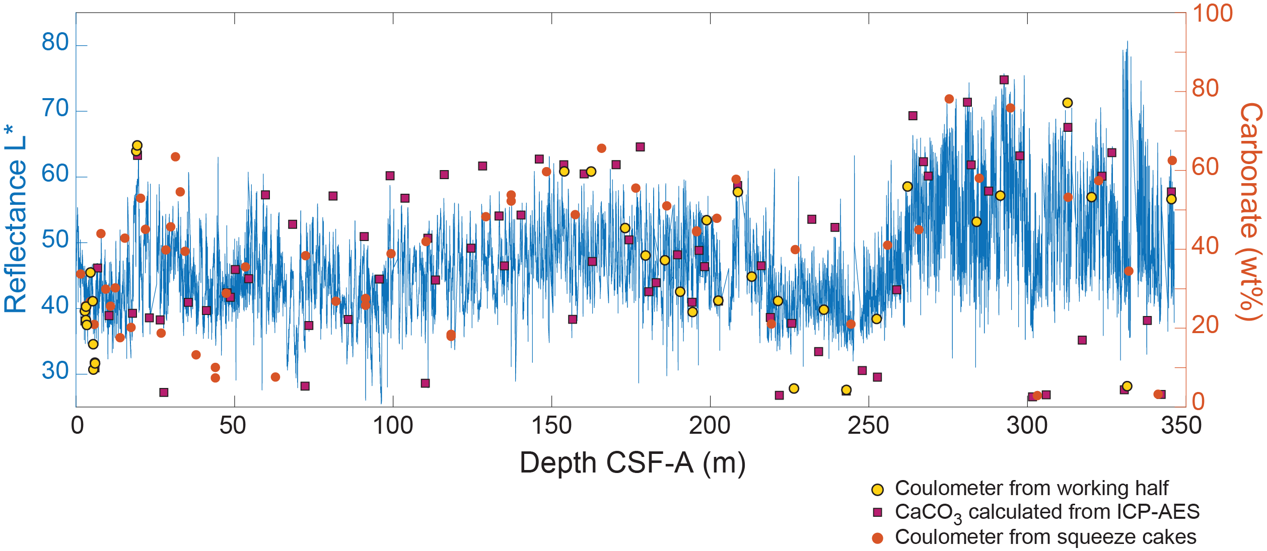
Figure F38. CaCO3 and L* reflectance.
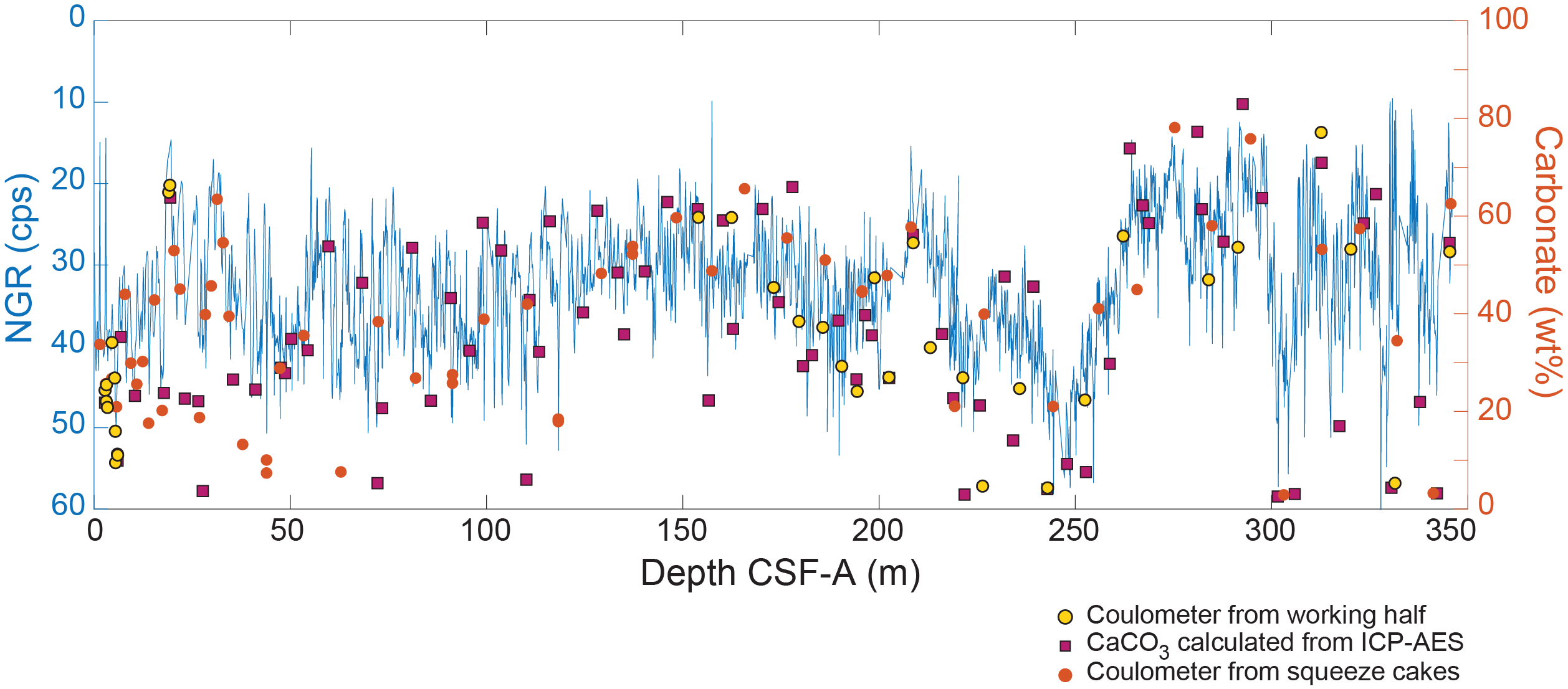
Figure F39. CaCO3 and NGR.
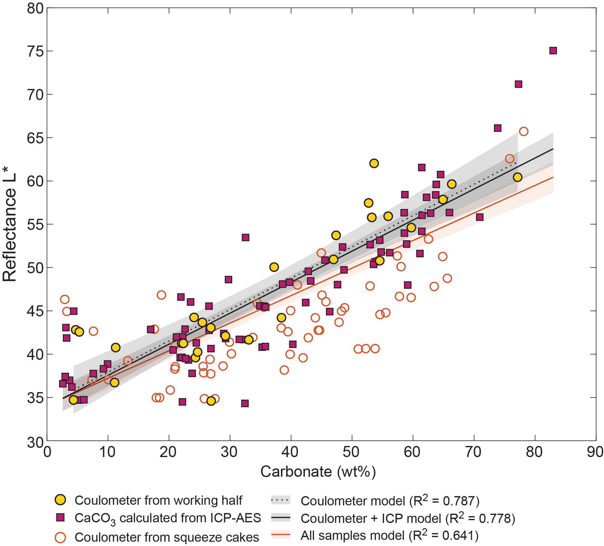
Figure F40. Crossplot and linear regression of CaCO3 and L* reflectance.
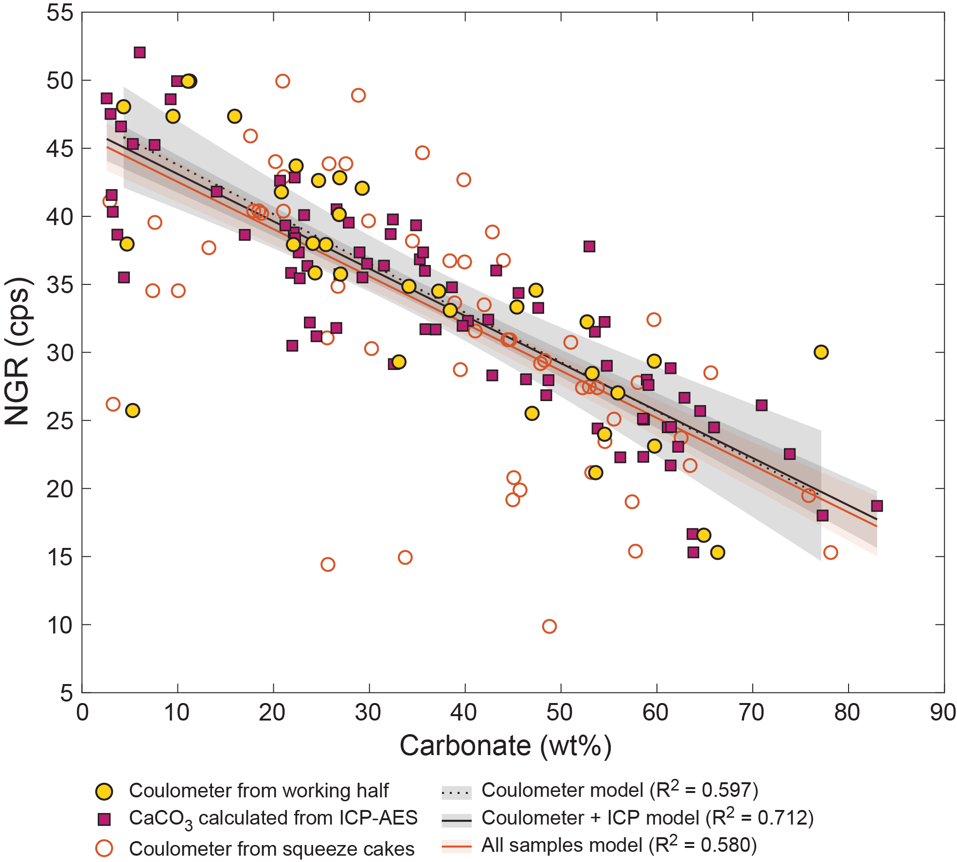
Figure F41. Crossplot and linear regression of CaCO3 vs. NGR.
6.3.2. Total organic carbon
All samples were simultaneously analyzed for TC alongside TIC, TN, and TS (Figure F42). TOC is defined as the difference between TC and TIC.
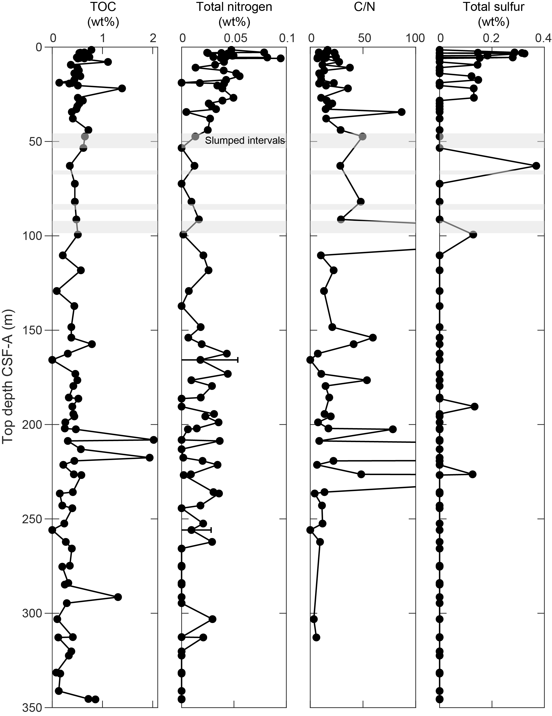
Figure F42. Sedimentary TOC, TN, C/N, and TS vs. top depth.
Two different internal standards were used to calibrate the elemental analyzer and assess reproducibility of TC, TN, and TS and were run at least every ~10 samples: the 1σ of TC in NIST Buffalo River Sediment (BRS) (n = 19) and sulfanilamide (n = 4) is 0.068 and 0.326 wt%, respectively (Table T23). Two samples were duplicated to assess analytical error; interduplicate differences ranged 0.127–0.268 wt% TC (Table T21).
TOC content in Hole U1586A is generally low (mean = 0.48 ± 0.32 wt%; range = 0–2.02 wt%); it is highest in the upper 50 m (0.57 ± 0.21 wt%) and steadily declines with depth (0.33 ± 0.27 wt% in the lowermost 50 m) (Figure F42; Table T24); however, CaCO3 and TOC show little correlation (R2 = 0.05). The light (n = 3) and dark (n = 7) intervals were targeted to improve correlations with other physical properties. However, there was no significant difference in TOC between dark and light layers (0.60 ± 0.09 and 0.57 ± 0.08 wt%, respectively).
6.3.3. Total nitrogen
All sedimentary nitrogen is assumed to be organic. The 1σ of TN for NIST BRS (n = 19) and sulfanilamide (n = 4) are 0.019 and 0.003 wt%, respectively (Table T23). Two samples were duplicated to assess analytical error; interduplicate differences ranged 0.019–0.036 wt% TN (Table T21).
TN contents are also very low (mean = 0.022 ± 0.020 wt%; range = 0–0.095 wt%) (Table T25). TN is highest near the top of the hole, averaging 0.045 ± 0.021 wt% in the upper 10 m and declining to a stable 0.017 ± 0.016 wt% by 40–50 m CSF-A (Figure F42).
6.3.4. Organic C/N ratios
The ratio of sedimentary TOC/TN (C/N) can fingerprint particulate organic matter: marine and lacustrine algae have ratios of 0–10, whereas terrestrial plants exist in a much broader C/N space (25–75) (Meyers 1994, 1997).
Samples with 0 wt% TN were excluded from C/N calculations. Of the remaining values, mean C/N = 45.5 ± 151 (range = 0–1210), but this is driven by several samples with low TN (Table T26). Removing 3 samples with C/N values > 200 yields a more realistic mean of 20.0 ± 17.0 (range = 0–86.7). C/N averages 18.2 (± 14.6) between 0 and 38 m CSF-A, increases to 36.8 (± 11.0) between 43 and 91 m CSF-A, and decreases to ~5 by ~300 m CSF-A. This suggests that TOC and TN were primarily marine-sourced in the upper core, were replaced by a greater percentage of terrestrial origin, and gradually shifted back toward predominantly marine sources, punctuated by short intervals of significant terrestrial organic matter delivery.
6.3.5. Total sulfur
The 1σ of TS in NIST BRS (n = 19) and sulfanilamide (n = 4) are 0.019 and 0.072 wt%, respectively (Table T23). Two samples were duplicated to assess analytical error, but TS was below detection limits in both (Table T21).
Similar to TOC and TN, TS contents were very low (mean = 0.033 ± 0.081 wt%; range = 0–0.369 wt%) (Table T27). TS levels were below detection limits for the majority of samples from Hole U1586A. TS was highest in the upper 9.5 m of the hole (0.114 ± 0.130 wt%) and from 9.5 to 27 m CSF-A (0.048 ± 0.067 wt%); below this, only four samples had detectable amounts.
6.3.6. Major and minor elements
Major and minor element concentrations were measured on 80 samples taken from Hole U1586A using ICP-AES (Table T28). Replicate analyses of eight international reference standards (n = 24) show relative standard deviation (RSD) < 3% for all major elements (except for P2O5) and <10% for most of the minor elements reported.
Elemental oxides SiO2, K2O, Fe2O3, MgO, and TiO2 show strong positive correlations with Al2O3, with a near-zero intercept indicating the dominance of terrigenous detritus (Figure F43). This is also observed for the minor elements including Zn, Cr, V, Sc, Y, and Zr. Na shows a correlation with Al, but the nonzero intercept is likely caused by NaCl (~0.5%) precipitated from seawater. Bulk sediment Ca primarily represents biogenic CaCO3, and because of incorporation of Sr into biogenic CaCO3, both elements show an inverse relationship with Al. Ba is weakly correlated with Al or Ca, likely due to the presence of BaSO4. Mn shows no relationship with Al, indicating processes other than end-member mixing, such as the precipitation of Mn CaCO3 in the upper 200 m (above Core 28H), may be occurring.
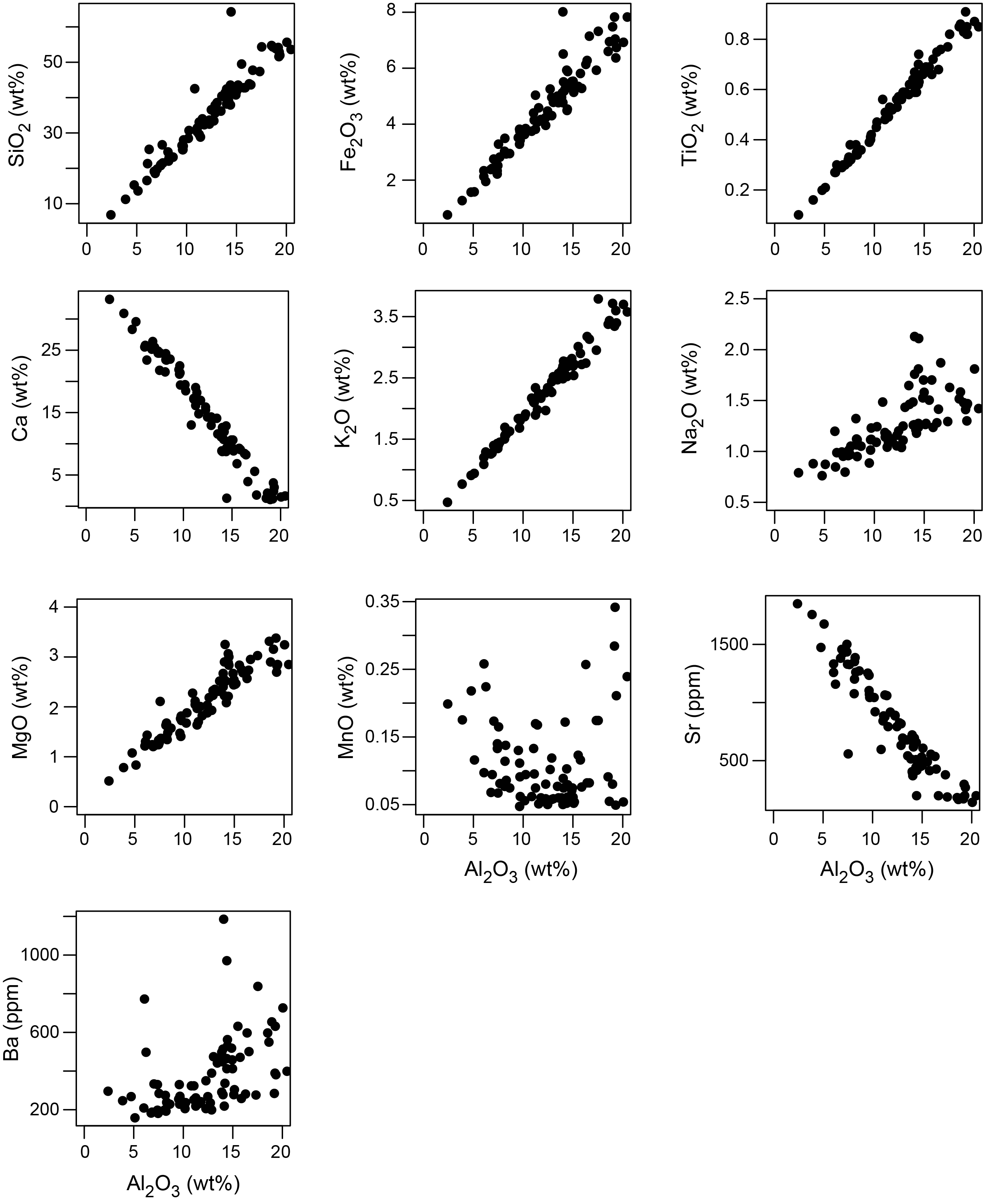
Figure F43. Sedimentary major and minor element concentrations vs. Al2O3.
The Ca/Ti ratio, which reflects the relative contributions of CaCO3 versus terrigenous detritus, shows larger variations below 200 m CSF-A than above (Figure F44). Selected lithogenic elements are normalized to Al as a proxy for provenance, weathering, and productivity. The Si/Al ratio may serve as a proxy of grain size, mainly reflecting the abundance of quartz versus clay minerals. In Hole U1586A (Figure F44) Si/Al ratios are relatively constant (~2.6) to about 300 m CSF-A, where the values increase to a maximum of about 3.6 at the bottom of the core. The interval in which the ratios increase corresponds with the change in lithology from dominantly carbonate to sand-rich layers (see Lithostratigraphy) as well as the increase in Si concentration seen in the IW profile (Figure F37). The K/Al ratio is often used to reflect the input of river-borne material and associated chemical weathering intensity (here, K/Al shows a consistent downhole profile as the chemical index of alteration; not shown). The Ti/Al ratio in this region is widely recognized as an indicator of North African dust (Wu et al., 2016). The K/Al and Ti/Al ratios show similar trends to about 150 m CSF-A and then diverge. The K/Al ratio decreases to about 230 m CSF-A (~0.26), followed by an increase to about 0.32 at the bottom of the hole. Ti/Al values remain relatively constant (~0.051) to about 230 m CSF-A, where they gradually decrease to 0.046 at about 300 m CSF-A. Afterward, the Ti/Al ratio steadily increases to 0.06 to the bottom of the hole.
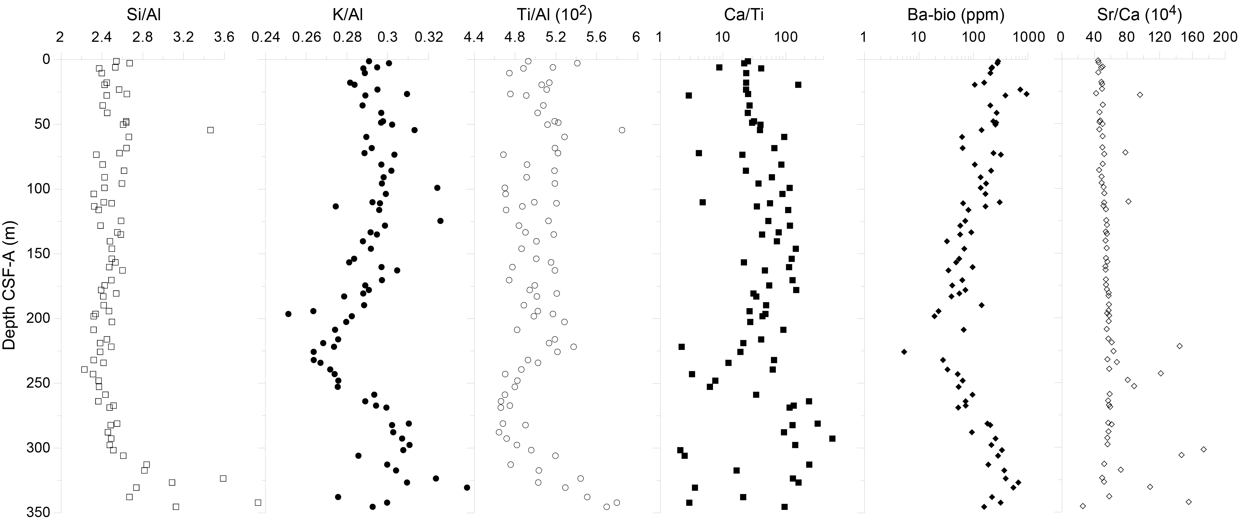
Figure F44. Bulk sedimentary Si/Al, K/Al, Ti/Al, Ca/Ti, biogenic Ba, and Sr/Ca.
Assuming a constant Ba/Al ratio of 0.0037 for the terrigenous aluminosilicate component (Reitz et al., 2004), the biogenic Ba (i.e., Ba-bio, mostly BaSO4) can be estimated. BaSO4 content in marine sediments is a widely recognized proxy for export productivity (Paytan and Griffith, 2007). Ba-bio progressively decreases from 400 ppm to 0 ppm at ~225 m CSF-A, followed by a gradual increase to the bottom of the hole; however, there is no significant shift in TOC downhole. The Sr/Ca ratio shows a nearly constant value of about 50 downhole with short increases below 200 m CSF-A depth.
7. Physical properties
Physical properties were characterized through a set of measurements on whole-round cores, split cores, and discrete samples. High-resolution (2 cm steps) nondestructive measurements of GRA bulk density and MS were carried out on whole-round sections from all holes. P-wave velocity was measured using the P-wave logger (PWL) at 2 cm steps on the whole-round sections of Cores 397-U1586A-1H through 27X only. NGR was measured at 10 cm resolution for each whole-round section, except Cores 1H–5H where NGR was measured at 20 cm resolution. To support stratigraphic correlation and optimize drilling depths at subsequent holes to cover coring gaps, MS and GRA bulk density data were acquired while drilling Holes U1586B–U1586D before temperature equilibration via fast-track logging at 2 or 4 cm resolution. Thermal conductivity was measured once for each core in Hole U1586A. One to three measurements of P-wave velocity per core were made using the P-wave caliper (PWC) on section halves from Hole U1586A. MAD samples were measured using 10 cm3 discrete samples taken at a sampling resolution of one per core in Hole U1586A. Color reflectance spectrophotometry and split core point MS (MSP) measurements were carried out at 2 cm steps on every core section from all holes at Site U1586. X-ray images of whole-round sections were taken of every section in Hole U1586A. In addition, X-ray images were taken for selected section halves.
7.1. Gamma ray attenuation bulk density
GRA bulk density was measured on all whole-round sections from all holes at a 2 cm interval using the WRMSL. Measured GRA bulk density gradually increased from 1.5 g/cm3 at the top of the holes to ~1.9 g/cm3 around 110 m CSF-A (Figure F45). The downhole trend of GRA bulk density could reflect variations in lithology, consolidation, cementation, and porosity. In general, GRA bulk density decreases where there is drilling disturbance such as core expansion, cracks, voids, soupy textures, and basal flow-ins (see Lithostratigraphy). GRA bulk density also decreases by 0.1–1.2 g/cm3 at depths where the coring system was switched from the APC or HLAPC to the XCB system (Figure F45) because of the change in diameter of the cores recovered. GRA bulk density is significantly higher (>2.0 g/cm3) in the thin sandy layers at 330–347 m CSF-A (bottom of the hole) in Hole U1586A (Figure F45).
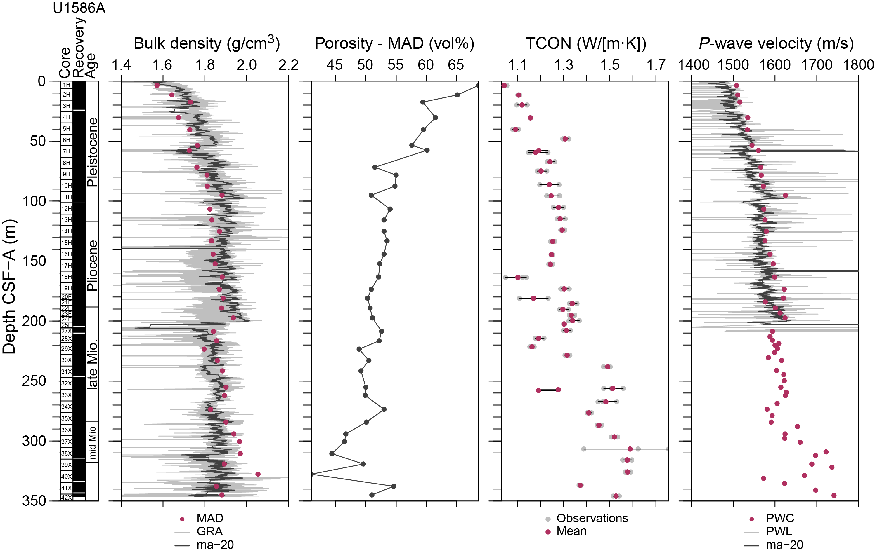
Figure F45. GRA and MAD bulk density, porosity, thermal conductivity, and P-wave velocity.
7.2. Magnetic susceptibility
MS was measured on whole-round sections at 2 cm intervals using the WRMSL (Figure F46), and those values are in good agreement with the MS values measured on archive halves using the SHMSL. The measured MS values are characterized by cyclic variations on the order of a few tens of centimeters to a few meters. The overall downhole trends at Site U1586 include (1) a gradual downhole reduction of MS values with decreasing amplitude of the cyclic variations in the upper 140 m and (2) several broad peaks of MS values in the deeper part of the holes, which are recognized around ~200, ~250 and ~300 m CSF-A. The cyclic variation of MS is synchronous with NGR measurements and a* and b* values and mirrors L* values.
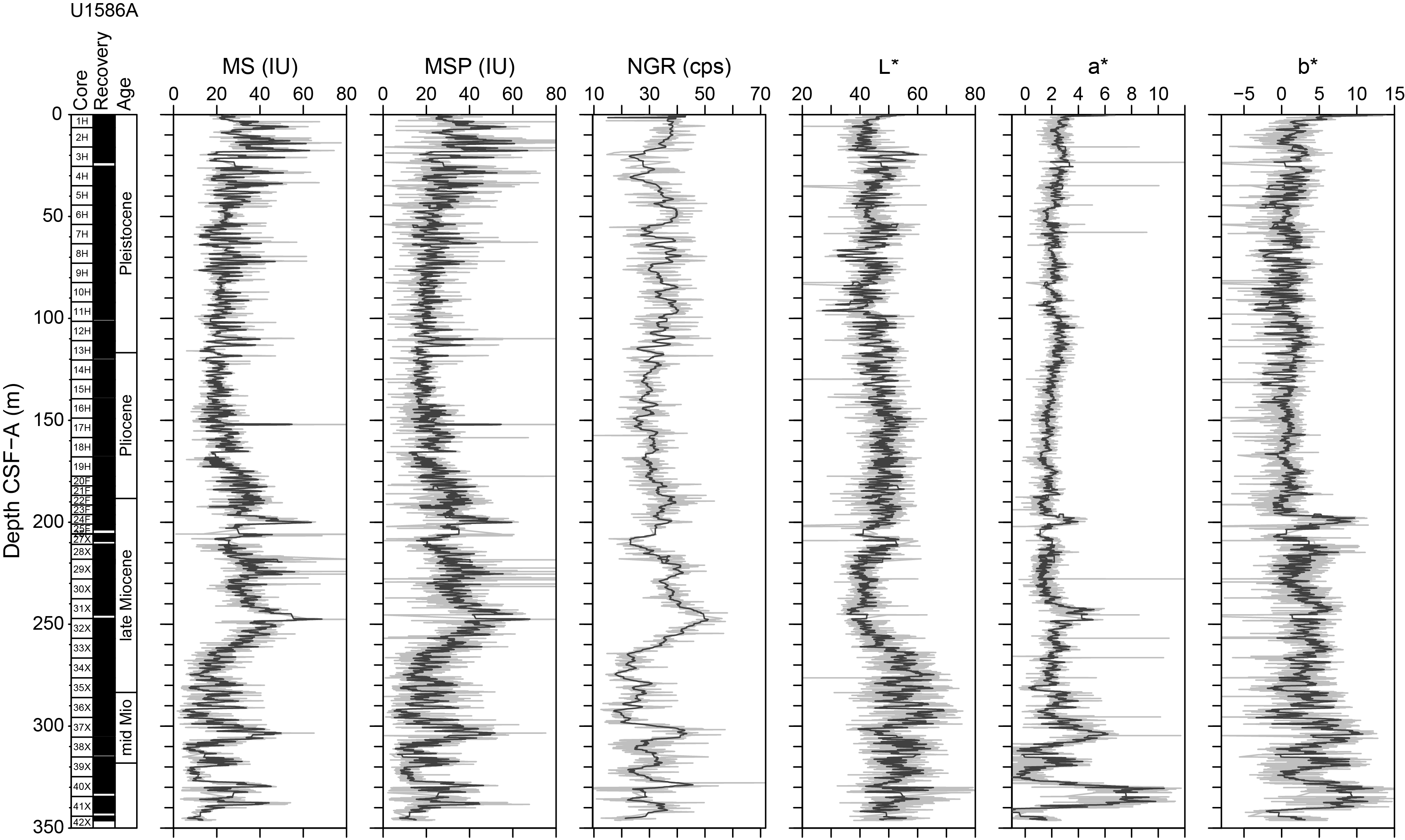
Figure F46. MS, MSP, NGR, and L*a*b* values.
In addition to the overall trends, sharp peaks of MS were identified, one of which occurs around ~150 m CSF-A in all holes. Although X-ray images of the sediments around this peak did not show resolvable-sized magnetic mineral grains or foreign objects (e.g., pieces of the cutting shoe or shear pin) (Figure F47), silt-sized grains of magnetite were isolated from Sample 397-U1586D-17X-2, 53 cm (see Lithostratigraphy).
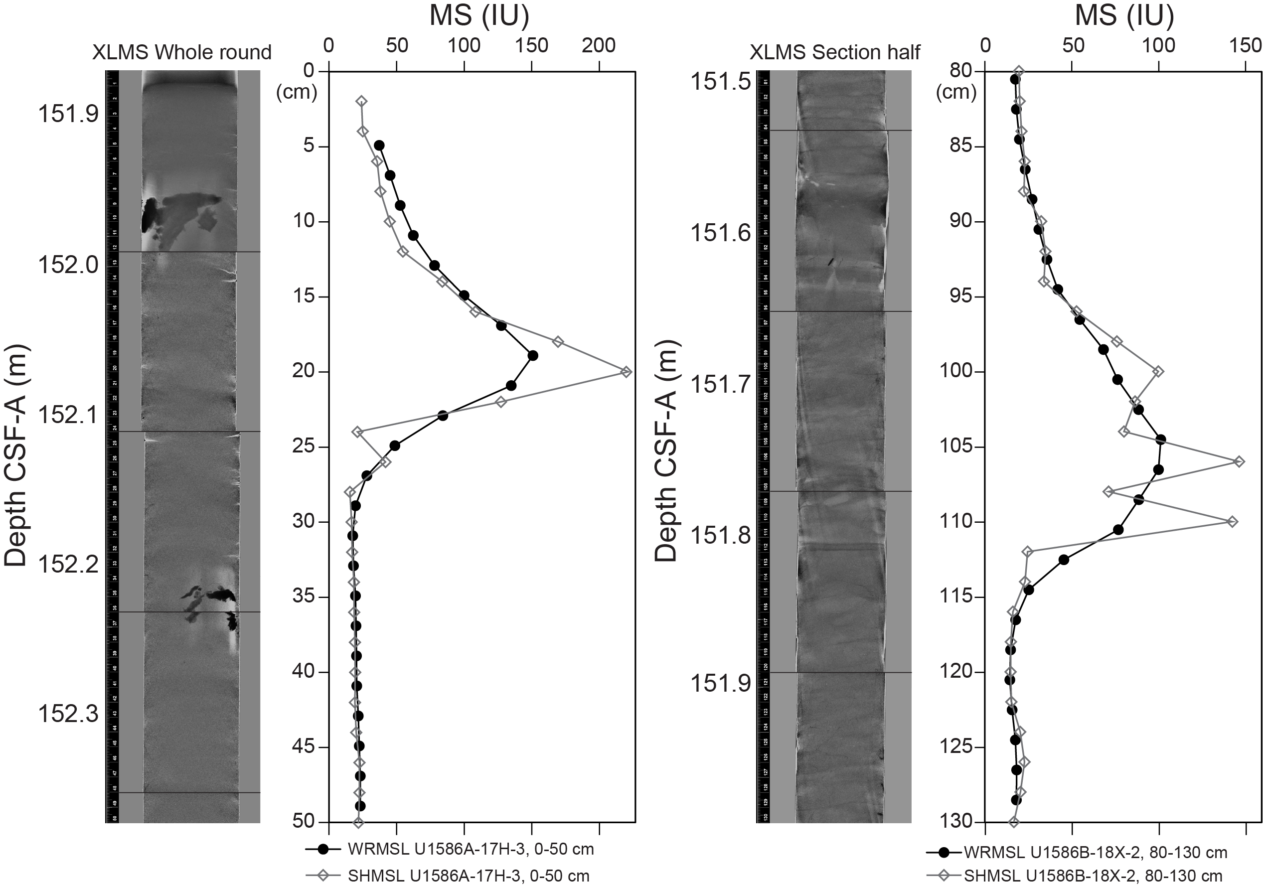
Figure F47. X-ray images and MS.
MS values were largely homogenized in at least three intervals in Hole U1586A: 45.8–54.3, 65.5–67.5, and 83.2–86.1 m CSF-A, where contorted or convoluted strata were observed (see Lithostratigraphy). Also characterized by low MS values are the thinly bedded sand layers at 330–347 m CSF-A.
Whole-round MS data for Holes U1586B–U1586D were collected before the cores equilibrated with room temperature, which may have affected the loop sensor, resulting in an underestimation of absolute values of MS. The reason for measuring whole-round MS data before temperature equilibration was to aid rapid stratigraphic correlation needed to check the offset of core breaks among holes. We therefore highly recommend that for any future quantitative analyses, scientists use section-half MS data (MSP) from Holes U1586B–U1586D because they are the most equilibrated to room temperature and provide the most accurate measurements of MS.
7.3. P-wave velocity
P-wave velocity was measured for all core sections taken with the APC and HLAPC systems in Hole U1586A at 2 cm intervals on the WRMSL (Figure F45). The whole-round PWL on the WRMSL system could not measure reasonable P-wave velocity from core sections taken using the XCB system because of poor coupling between the liner and the sediment core diameter, and thus P-wave velocity was not measured on XCB cores. P-wave velocity shows a gradual increase from ~1490 m/s at the top of Hole U1586A to ~1600 m/s at 160 m CSF-A. The overall downhole trend of the whole-round P-wave velocity is superimposed by cyclic variation similar to the MS and NGR intensity. Whole-round P-wave velocity is highly variable in some cores, such as Core 397-U1586A-7H, which is most likely a result of drilling disturbances (see Lithostratigraphy).
Split core P-wave velocity data were obtained at 56 depths throughout Hole U1586A using the PWC. The data show a steady increase from 1806 m/s at 3.7 m CSF-A to 1599 m/s at 163.3 m CSF-A, and the values become highly variable (1570–1740 m/s) below 173 m CSF-A (Figure F45). The whole-round P-wave velocity values match well with those obtained using the PWC, assuring the reliability of the whole-round data.
7.4. Natural gamma radiation
Measurements of NGR were made using the Natural Gamma Radiation Logger (NGRL) on all core sections from all holes at two positions with 10 cm spacing and analyzed with a measurement time of 10 min per section (300 s/measurement). It should be noted that NGR measurements were carried out at one position (i.e., 20 cm spacing) on Cores 397-U1586A-1H through 5H.
Overall, NGR ranges 15–55 counts/s with clear cyclicity in intensity for most of the cores (Figure F46). A broad peak of NGR intensity is seen at ~250 m CSF-A. The cyclic variation of NGR intensity correlates with that of MS and mirrors L* values. Because L* is often related to carbonate content (see Geochemistry), dilution of potassium- and thorium-bearing detrital material (clay) by higher carbonate contents likely explains the low NGR and MS signals. This suggests that the physical properties parameters such as MS and NGR are closely tied to changes in lithology. Lower values of NGR and MS are interpreted as sediments dominated by calcareous microfossils (nannofossil ooze), whereas higher NGR and MS are interpreted as sediments with higher clay content (e.g., clayey nannofossil ooze).
Concentrations of K, Th, and U were extracted from the NGR spectra using a method provided by De Vleeschouwer et al. (2017). Downhole trends of K and Th are similar to that of NGR, and U concentrations decrease in the uppermost 30 m of Hole U1586A (Figure F48). U/Th ratios also decrease in the uppermost 30 m and are typically ~0.2–0.4 below 30 m CSF-A. K/Th ratios are constant throughout the hole.
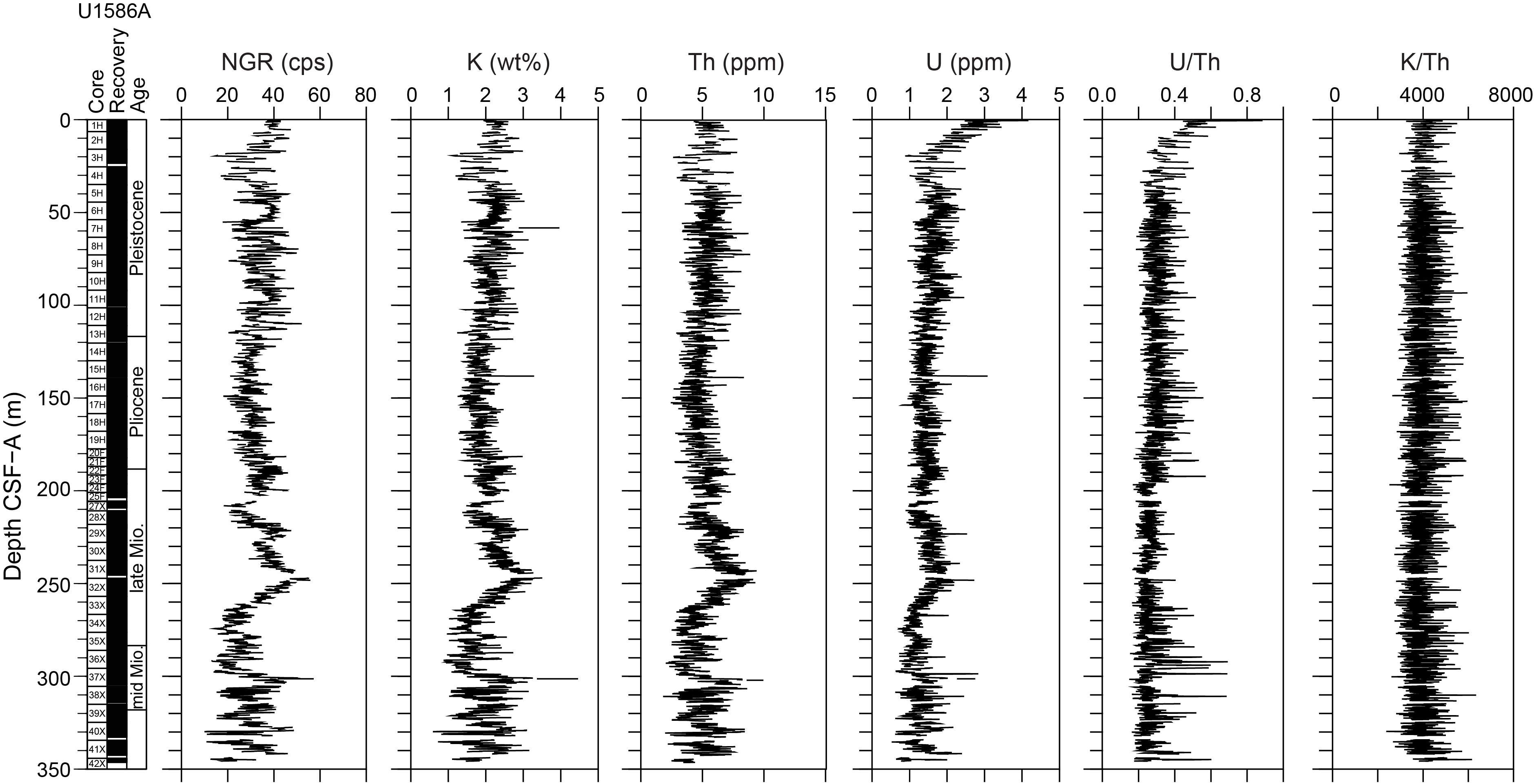
Figure F48. NGR; K, Th, and U deconvolved and extracted from NGR spectra; and U/Th and K/Th ratios.
Similar to MS, the cyclicity of NGR values becomes less prominent in four intervals in Hole U1586A: 45.8–54.3, 65.5–67.5, 83.2–86.1, and 91.9–98.6 m CSF-A. These intervals are associated with contorted or convoluted bedding interpreted to represent slump deposits (see Lithostratigraphy).
7.5. Moisture and density
Measurements of density, porosity, and grain density were taken on 38 samples from Hole U1586A, typically one sample per core. MAD samples were taken from fine-grained sections, and care was taken to avoid locations of obvious drilling disturbance. These samples were measured for wet mass, dry mass, and dry volume to calculate bulk density, dry density, grain density, porosity, and void ratio.
The bulk densities from the discrete samples range 1.57–2.05 g/cm3 (Figure F45). The bulk densities of the discrete samples increase with depth from 1.57 g/cm3 at 3.6 m CSF-A to >1.8 g/cm3 below 78.4 m CSF-A. Although the overall trend is similar to that of the MAD bulk densities, the sharp decrease in GRA bulk densities at ~200 m CSF-A is much larger than estimated from discrete measurements (Figure F45). Because the GRA bulk densities are affected by the decrease in core diameter at 200 m CSF-A, where coring switched from the APC to the XCB system, we think that the discrete samples provide more accurate bulk density values below ~200 m CSF-A.
Grain densities mostly range 2.7–2.8 g/cm3 with no particular depth trend. This could be explained by the mixture of calcite (2.71 g/cm3) and sheet silicate minerals (variable but generally 2.6–2.8 g/cm3) in the cores.
Porosity ranges 41%–69% and gradually decreases with depth. Porosity is 69% at the top of the hole (3.6 m CSF-A) and falls to <50% below 220 m CSF-A (Figure F45). The downhole increasing trend of bulk and dry densities and the decreasing trend of porosities with depth primarily reflect the compaction and dewatering of the sediment.
7.6. Thermal conductivity
Thermal conductivity was measured once per core throughout Hole U1586A. For the shallower cores with soft sediment (Cores 1H–29X), thermal conductivity was measured using the needle probe. For the deeper cores with firm sediment (Cores 30X–42X), it was measured using the puck probe. Measurements were carried out at 41 depths from 3.7 to 345.9 m CSF-A, and two or three measurements were conducted at each depth. Thermal conductivity ranges 1.04–1.45 W/(m·K) and shows an increasing trend with depth (Figure F45), which is similar to the patterns of bulk density and P-wave velocity. The downhole trend of the thermal conductivity values may thus reflect the compaction and consolidation of sediments with depth.
7.7. Color reflectance
Color reflectance data were collected at 2 cm intervals using the SHMSL. L*a*b* values showed a major shift below 240 mbsf, where the sections recorded higher amplitudes of color changes, reflecting more intervals with higher L*a*b* values in the middle Miocene than in younger periods (Figure F46). L* values are negatively correlated with MS and NGR. Calcium carbonate concentrations (see Geochemistry) are high in intervals where L* values are high, suggesting that the change in sediment lightness is related to the carbonate content. Thinly bedded sandy layers below 320 m CSF-A are characterized by high L* values.
7.8. X-ray imaging
X-ray images were taken for all whole-round sections from Hole U1586A on the X-ray Logger (XMAN). For the preceding holes, X-ray images were taken on selected archive-half sections at the request of the sedimentologists. The X-ray images revealed the presence of authigenic mineral grains, the morphology of lithologic contacts, burrows, and drilling disturbances such as biscuiting. Authigenic mineral grains and nodules, probably pyrite, were found from ~2 to ~250 m CSF-A in Hole U1586A and were more common from 20 to 200 m CSF-A. Grains and nodules were generally a few millimeters to 2 cm in size with burrow fillings up to 12 cm in length (Figure F49). Mineral-filled burrows appear to be broken brittlely into segments, probably from the forces experienced during sediment coring and/or drilling.
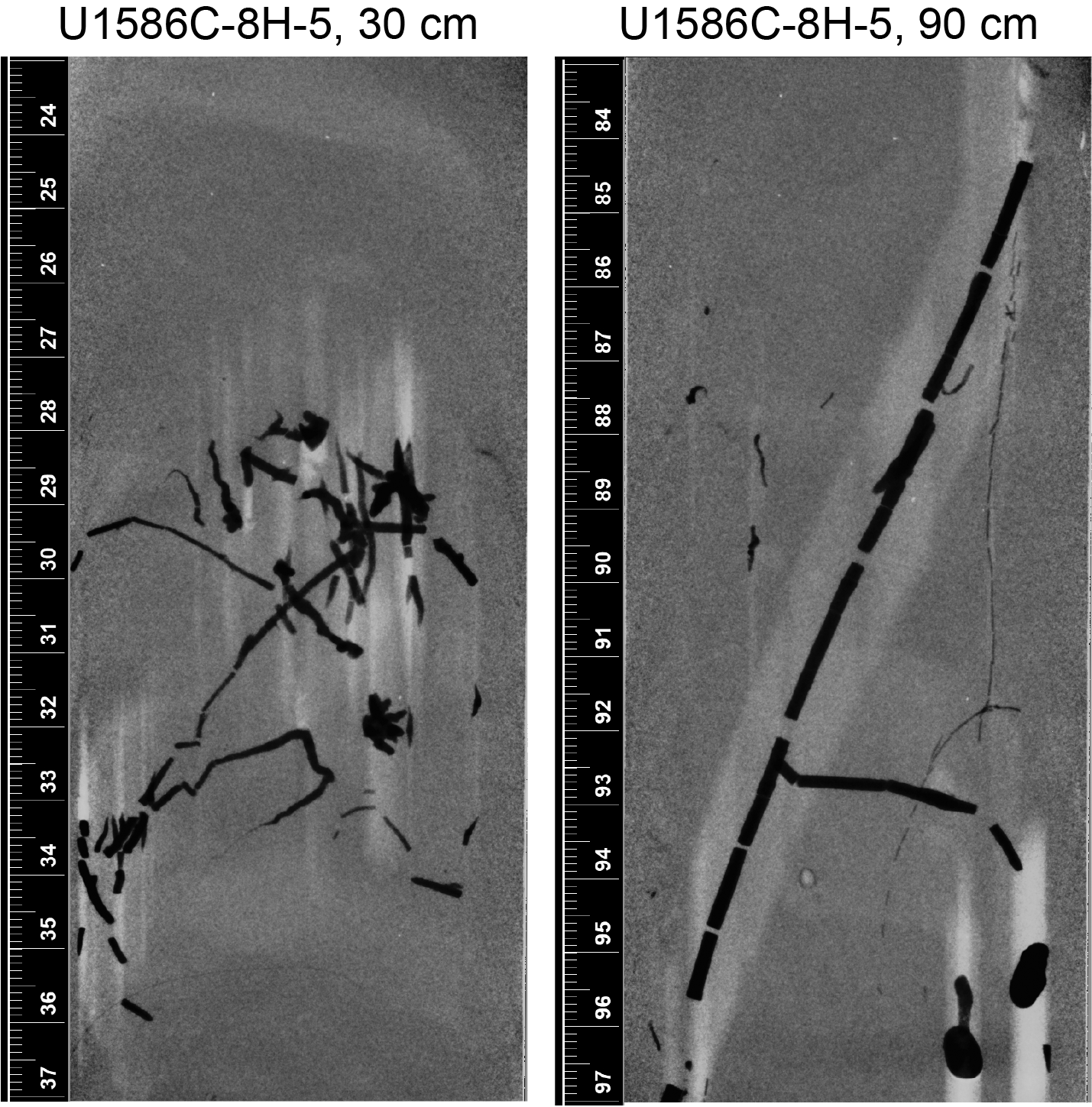
Figure F49. Authigenic mineral grains.
8. Downhole measurements
8.1. Downhole logging data processing and quality check
After the completion of coring operations in Hole U1586D, the triple combo tool string, consisting of the Hostile Environment Natural Gamma Ray Sonde (HNGS), Hostile Environment Litho-Density Sonde (HLDS), High-Resolution Laterolog Array (HRLA), Magnetic Susceptibility Sonde version B (MSS-B), and Enhanced Digital Telemetry Cartridge (EDTC), was deployed for downhole logging (see Operations). The raw logging data were sent to the Lamont-Doherty Earth Observatory Borehole Research Group (LDEO-BRG) for processing, quality control, and depth matching. The raw logs were first depth-matched using the total spectral gamma ray (HSGR) log from the downlog pass as a reference log and then shifted to a seafloor depth reference, resulting in a unified wireline log matched depth below seafloor (WMSF) depth scale. In Hole U1586D, the seafloor depth was determined using the gamma ray (GR) step observed at 4704.7 m wireline log depth below rig floor (WRF). This depth matches the seafloor depth of 4704.7 m drilling depth below rig floor (DRF) given by the drillers.
The borehole diameter was recorded using the hydraulic caliper on the HLDS tool. In Hole U1586D, the borehole diameter was around 12 inches for most of the logged interval (115–220 m WMSF) with variations reaching up to 16 inches (Figure F50). Above 115 m WMSF, the hole size varied widely between 5 and 14 inches. The caliper was closed at 105 m WMSF while logging up into the drill pipe. Log data that require decentralization or a good contact with the borehole wall (e.g., GR, density, and MS) could be affected by the caliper closure above 105 m WMSF. Here we report the logging data from 220 to 115 m WMSF, where the borehole diameter was nearly constant.
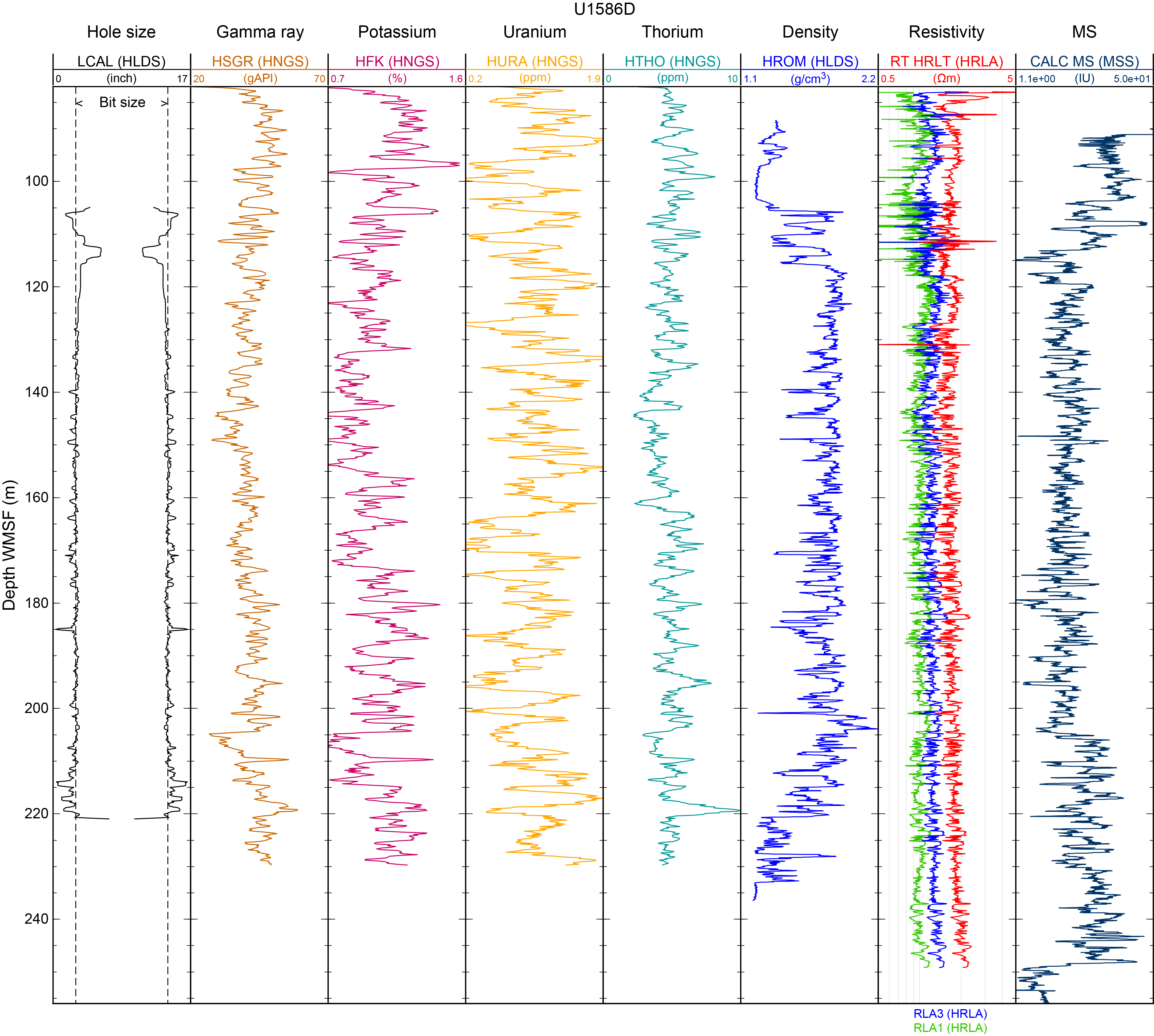
Figure F50. Downhole logging data.
8.2. Magnetic susceptibility
Downhole MS mostly ranges 10–35 IU (Figure F50). The overall trend of the downhole logging MS is not well correlated to the core MS data (Figure F51). For example, the cyclic variations of MS values were clear in the core sections (wavelengths were typically ~0.6–1.5 m), but such variations were not detected in the downhole logging MS data. This may suggest that the downhole logging MS signal has been aliased, although the MSS-B has a vertical resolution of ~12 cm.
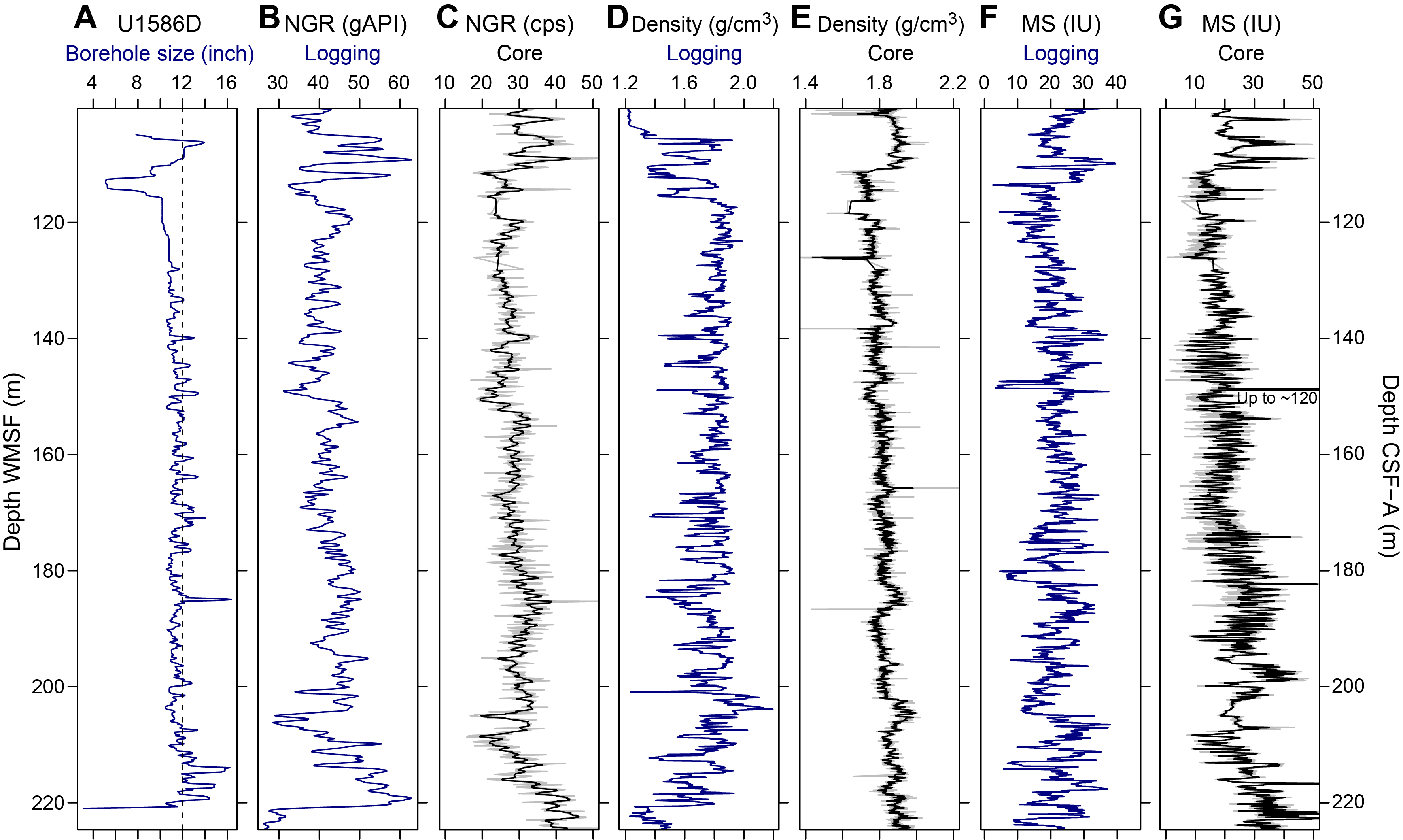
Figure F51. Downhole logs and core physical properties data.
Nevertheless, a peak of downhole MS occurs at 149 m WMSF, which is correlated to a sharp and prominent peak in MS in Section 397-U1586D-17X-2 at 148.8 m CSF-A (Figure F51). The sharp peak in MS was also observed at ~150 m CSF-A in all holes at Site U1586 (i.e., Cores 397-U1586A-17H, 397-U1586B-18X, 397-U1586C-18X, and 397-U1586D-17X; see Physical properties) and is likely to be a key marker for stratigraphic correlation between downhole logging data and cores, although the peak in downhole logging MS (~38 IU) is not as high as the maximum in the recovered cores (~110 IU).
8.3. Gamma ray
GR values obtained during wireline logging in Hole U1586D ranged 30–60 American Petroleum Institute gamma radiation units (gAPI) (Figure F51). Downhole variations of GR are in good agreement with NGR values from cores recovered from Hole U1586D. For example, (1) a sharp increase in GR from 32 to 45 gAPI downward at around 150 m WMSF and (2) a gradual increase from 30 to 60 gAPI from 205 to 220 m WMSF are well correlated with the NGR data obtained from whole-round sections (Figure F51).
The five-window spectroscopy of the HNGS tool also allowed determination of approximate K, Th, and U contents. K and Th contents range 0.6%–1.6% and 3–8 ppm, respectively, and correspond with the overall downhole GR trend (Figure F50). The overall K and Th concentration trends are similar between downhole log and core measurements (Figure F52). However, high frequency cycles that are commonly observed in core data (typically wavelengths of 0.6–1.5 m) are not visible in the downhole logging data. U contents from cores ranges 0.2–1.9 ppm, and their downhole profile is independent from the U estimates from the NGR data of core sections. Quasiperiodic variations in the U content is particularly apparent over the logged interval. However, such variations are not obvious in the U data in core sections (Figure F52). The cause of the discrepancies between downhole logging and core measurements is unknown, but it may be attributed either to instrumental-specific aliases, differences in integration time (300 s for core measurement versus ~1.5 s for downhole logging), or borehole conditions (morphology and diameter).
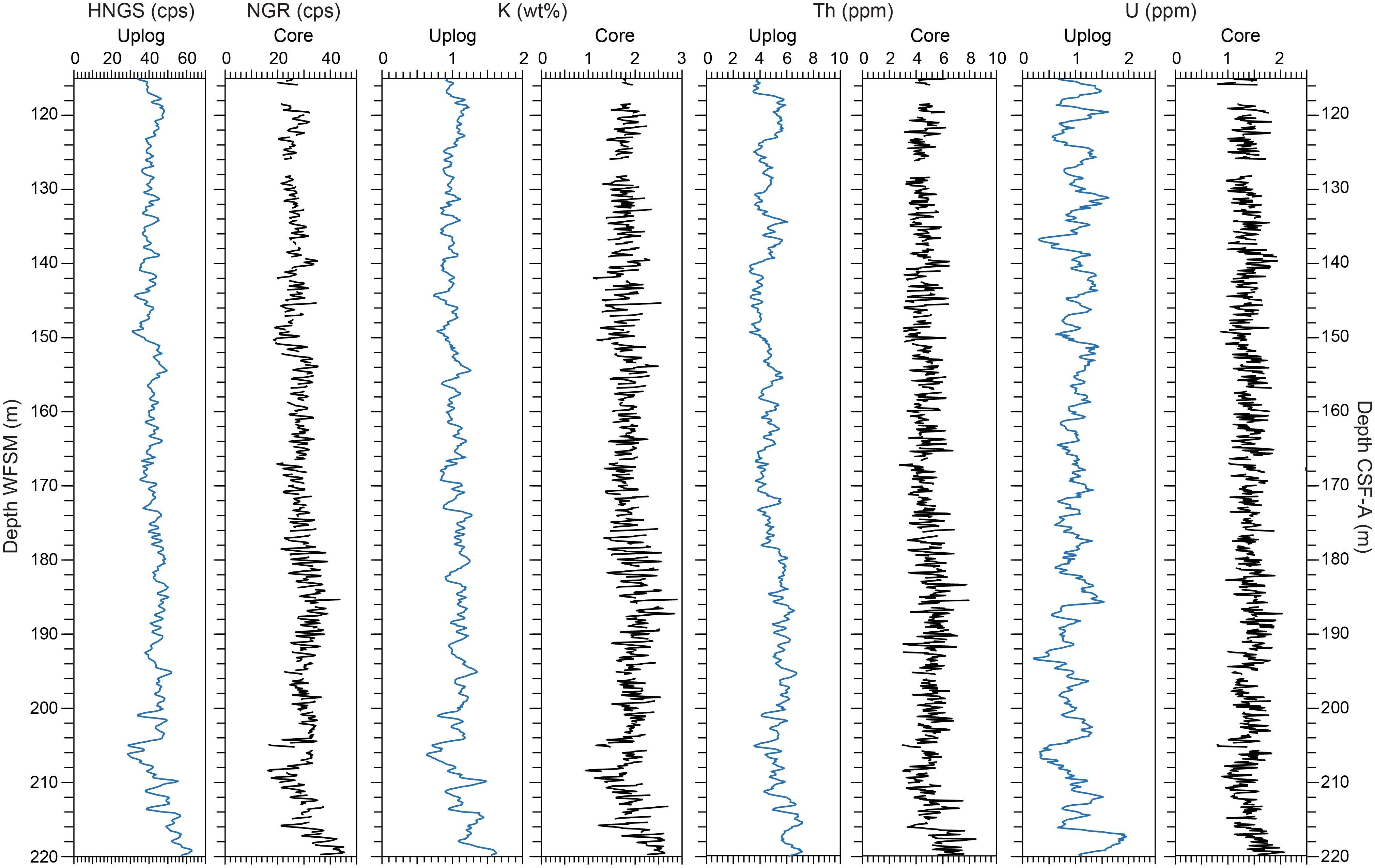
Figure F52. GR and K, Th, and U concentrations.
8.4. Density
Downhole density values from wireline logging show a plateau of 1.8–1.9 g/cm3 between 120 and 200 m WMSF, with sporadic decreases to <1.4 g/cm3 (Figure F50). Below 200 m WMSF, downhole density shows a broad peak, reaching the maximum value of ~2.2 g/cm3 at ~203 m WMSF before decreasing gradually to <1.6 g/cm3 around 220 m WMSF. The downhole trend of the wireline logging densities differs from that of the variation of GRA bulk densities obtained from the whole-round sections, which shows a slight increasing trend from 1.7 to 1.9 g/cm3 from 115 to 220 m CSF-A with small-scale variations (~10 m) superimposed on the general trend (Figure F51). Nevertheless, the broad peak of wireline logging density at ~203 m WMSF may be correlated to a peak of GRA bulk density (reaching ~2.0 g/cm3) found at ~202–206 m CSF-A. This broad peak occurs in Sections 397-U1586D-22X-5 through 22X-CC, where contorted strata (slump) were identified.
8.5. Resistivity
Most resistivity values throughout the logged interval range 1.5–2 Ωm, showing a slight increasing trend with depth (Figure F50). The downhole trend to higher resistivity may reflect the compaction of sediment.
8.6. In situ temperature and heat flow
Four APCT-3 downhole formation temperature measurements were made in Hole U1586A. Calculated in situ sediment temperatures ranged from 4.27°C at 34.9 m CSF-A to 5.77°C at 120.4 m CSF-A (Table T29), resulting in a geothermal gradient of 26.9°C/km (Figure F53). The bottom water temperature (mudline temperature) was 2.58°C and was calculated by taking the average of the minimum temperatures of the four APCT-3 temperature profiles. In situ thermal conductivity was estimated using laboratory-determined thermal conductivity established methods (Pribnow et al., 2000; Hyndman et al., 1974; see Physical properties in the Expedition 397 methods chapter [Abrantes et al., 2024]). Thermal resistance was calculated by cumulatively adding the inverse of the in situ thermal conductivity values from 0 to 124 m CSF-A (Figure F53). A calculated heat flow of 32.0 mW/m2 for Hole U1586A was obtained from the slope of the linear fit between in situ temperature and thermal resistance (Figure F53) (cf. Pribnow et al., 2000). This value is slightly lower than the heat flow of 47.5 mW/m2 obtained at Site U1385 (water depth = 2587 mbsl) during Expedition 339 (Expedition 339 Scientists, 2013) and is lower than but of the same order of magnitude as the normal range of heat flow on the Portuguese margin (45–76 mW/m2) (Grevemeyer et al., 2009).
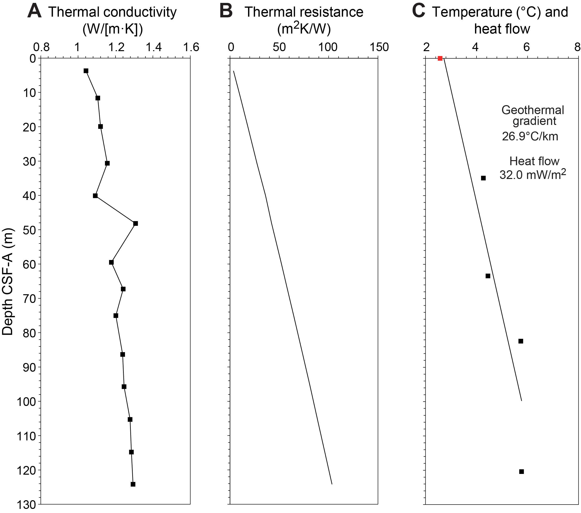
Figure F53. APCT-3 heat flow calculations.
9. Stratigraphic correlation
Correlations between holes at Site U1586 were accomplished using Correlator software (version 4.0.1). Tie points were established using L* color reflectance, MS from the WRMSL, and the blue channel extracted from the color images (RGB blue) (Figure F54; Table T30). We constructed a splice from 0 to 378 m core composite depth below seafloor, Method A (CCSF-A), using Holes U1586A–U1586D (Figures F54, F55, F56; Table T31). Slump intervals (four in the Middle to Upper Pleistocene sequence and two adjacent in the Upper Miocene section) noted by the sedimentology group were correlated between all holes along with disturbed or removed variable amounts of intact stratigraphy. Gaps in core recovery were evident when offset holes were compared and seemed to correlate with sea state. The HLAPC section of Hole U1586A was so strongly distorted by drilling that it was not used in correlation or deployed again for the remainder of the expedition. However, the use of multiple holes allowed us to define a composite section to ~378 m CCSF-A with complete overlap and only one potential small gap in the Upper Pliocene where overlap is equivocal.
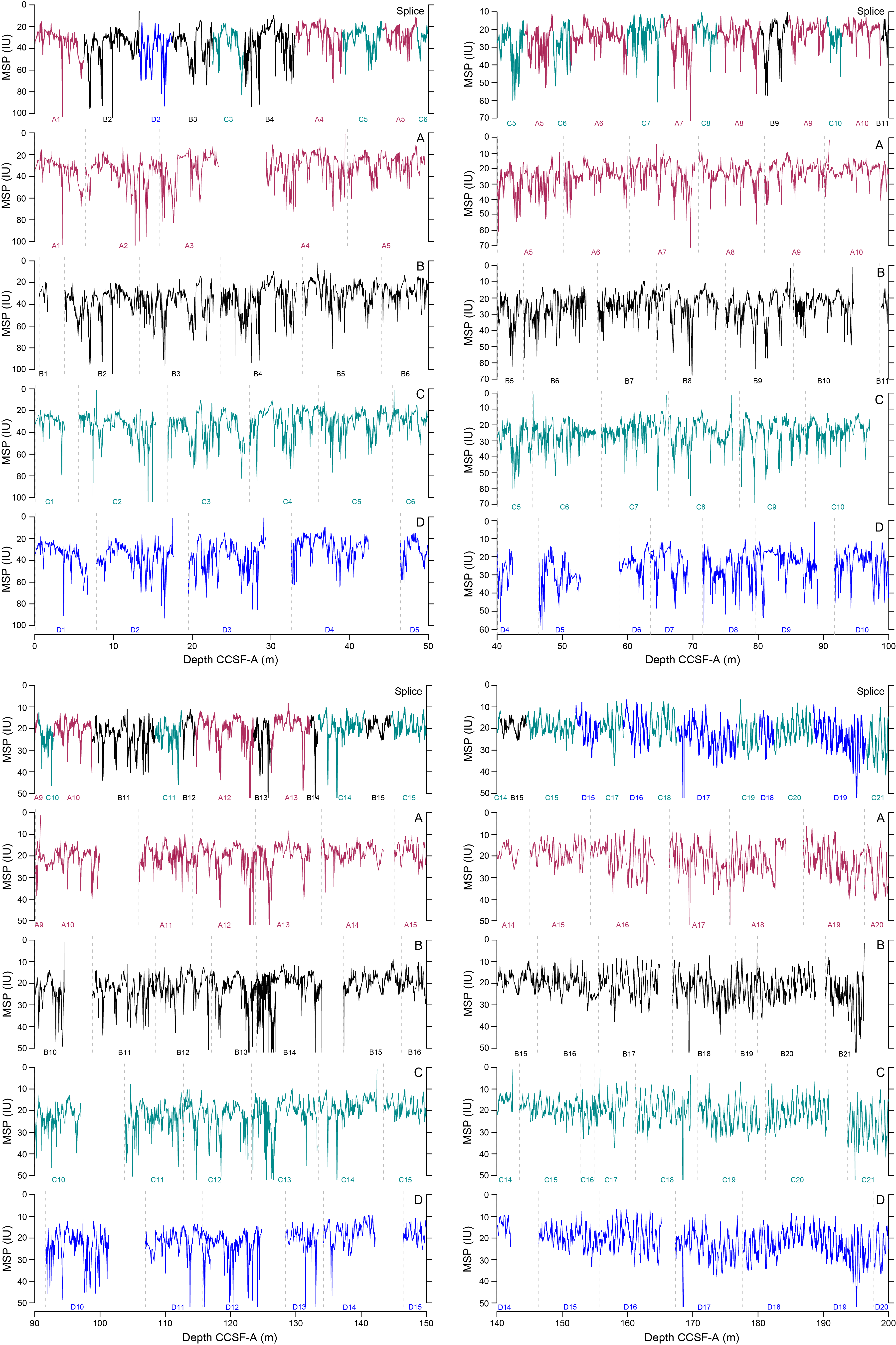
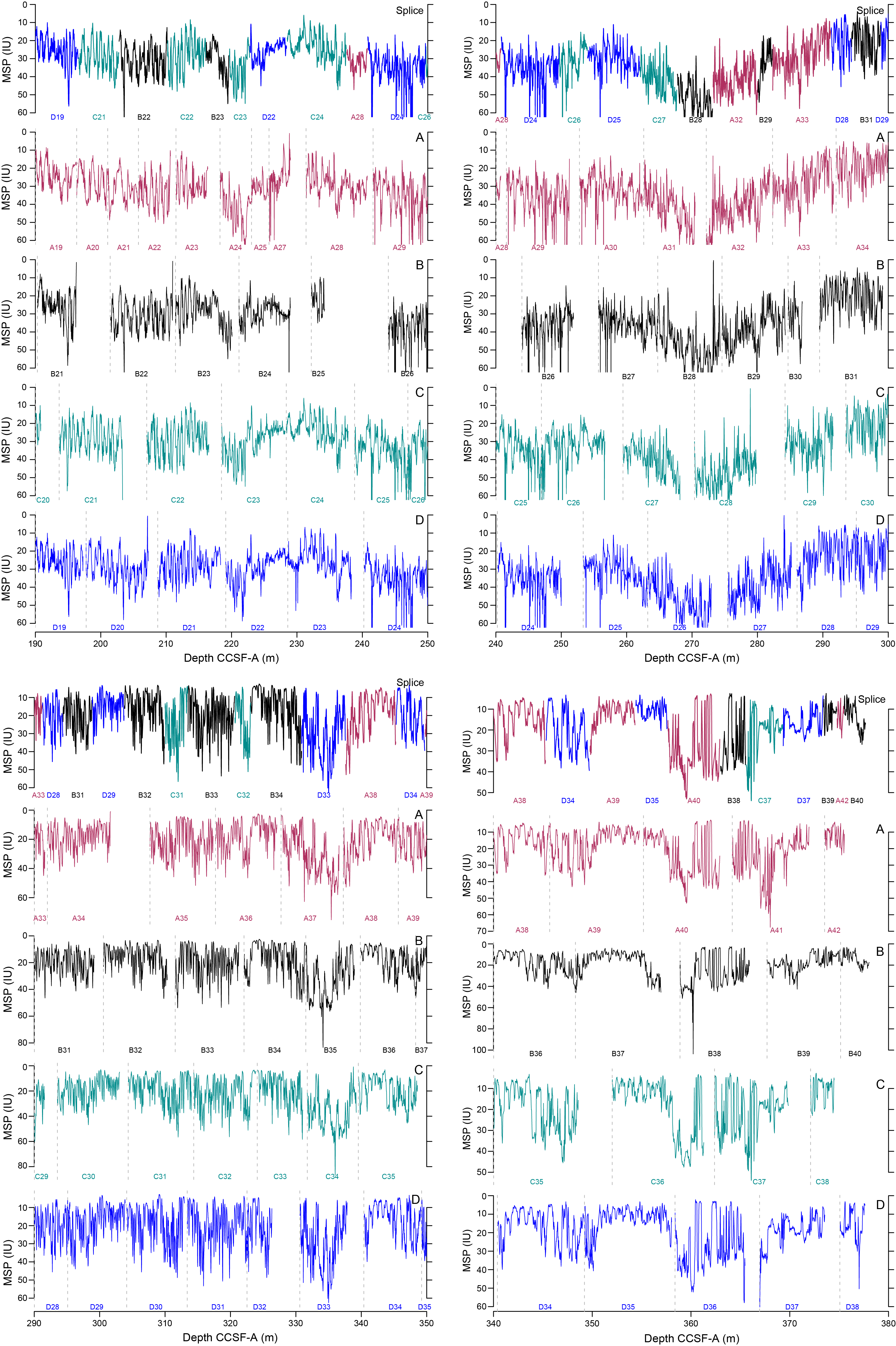
Figure F54. Composite section construction.
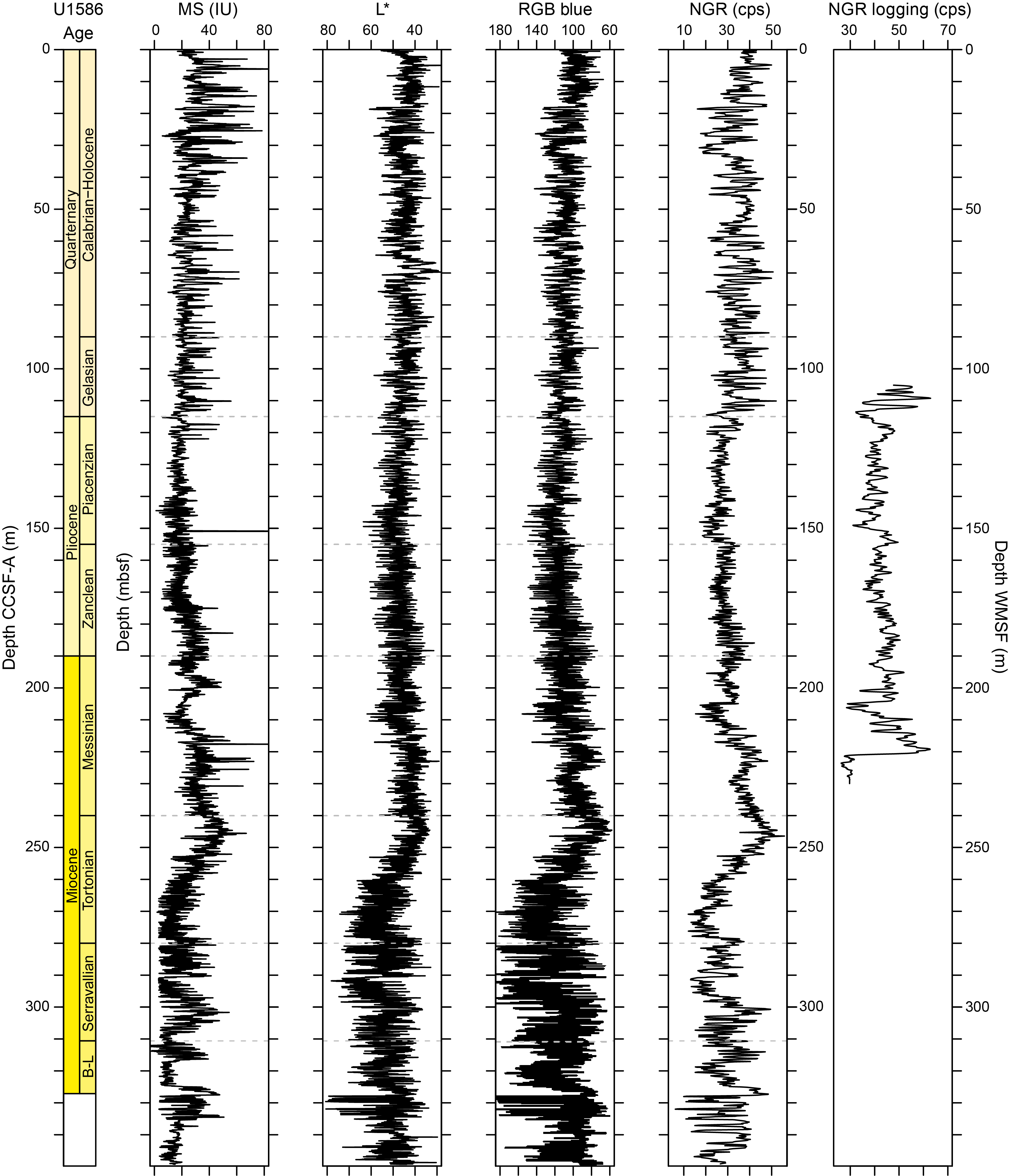
Figure F55. Spliced composite records of MS, L* color reflectance, RGB blue, and NGR and wireline GR.
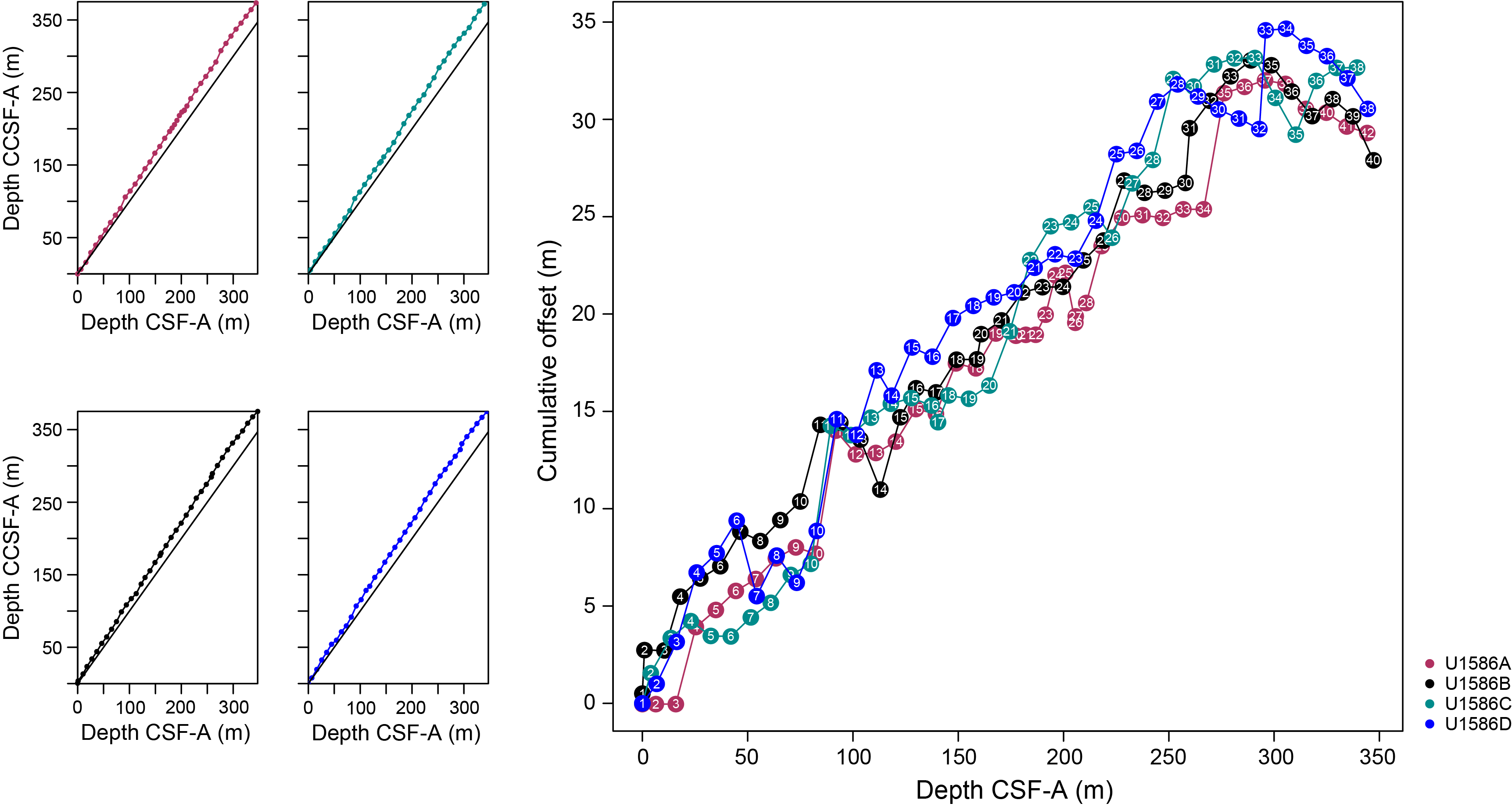
Figure F56. Depth scale comparison.
9.1. Approach
The CCSF-A depth scale is anchored to the mudline of Core 397-U1586A-1H, which is assigned the depth of 0 m CCSF-A. From this anchor, we worked downhole using Correlator to establish a composite stratigraphy on a core-by-core basis. Our general approach was to avoid placing ties (1) near section breaks as much as possible and (2) in sections where whole-round samples were taken for IW samples (only done on cores in Hole U1586A). We mainly used Hole U1586C as the backbone of the splice because this hole was drilled under better weather conditions. Core breaks in Hole U1586C are filled with sediment recovered from Holes U1586A, U1586B, and U1586D. Strong drilling distortion is observed in much of the Miocene sequence because of variable compression/expansion of low carbonate (mechanically weak) beds that occur frequently in that interval.
A major aid in correlation came from strong, high-frequency variability in all physical properties signals (MS, NGR, and color reflectance) (Figure F55). Fundamentally, all are controlled by calcium carbonate content. In the Pleistocene, this led to a recognizable sequence of variations that are tentatively correlated to marine isotope stages (Figure F57). In the Pliocene and Miocene, strong amplitude modulation was observed, likely from lithologic variations controlled by eccentricity-modulated precession (Figure F58). The modulations led to diagnostic packets of higher and lower amplitude lithologic cycles that aided correlations between offset holes.
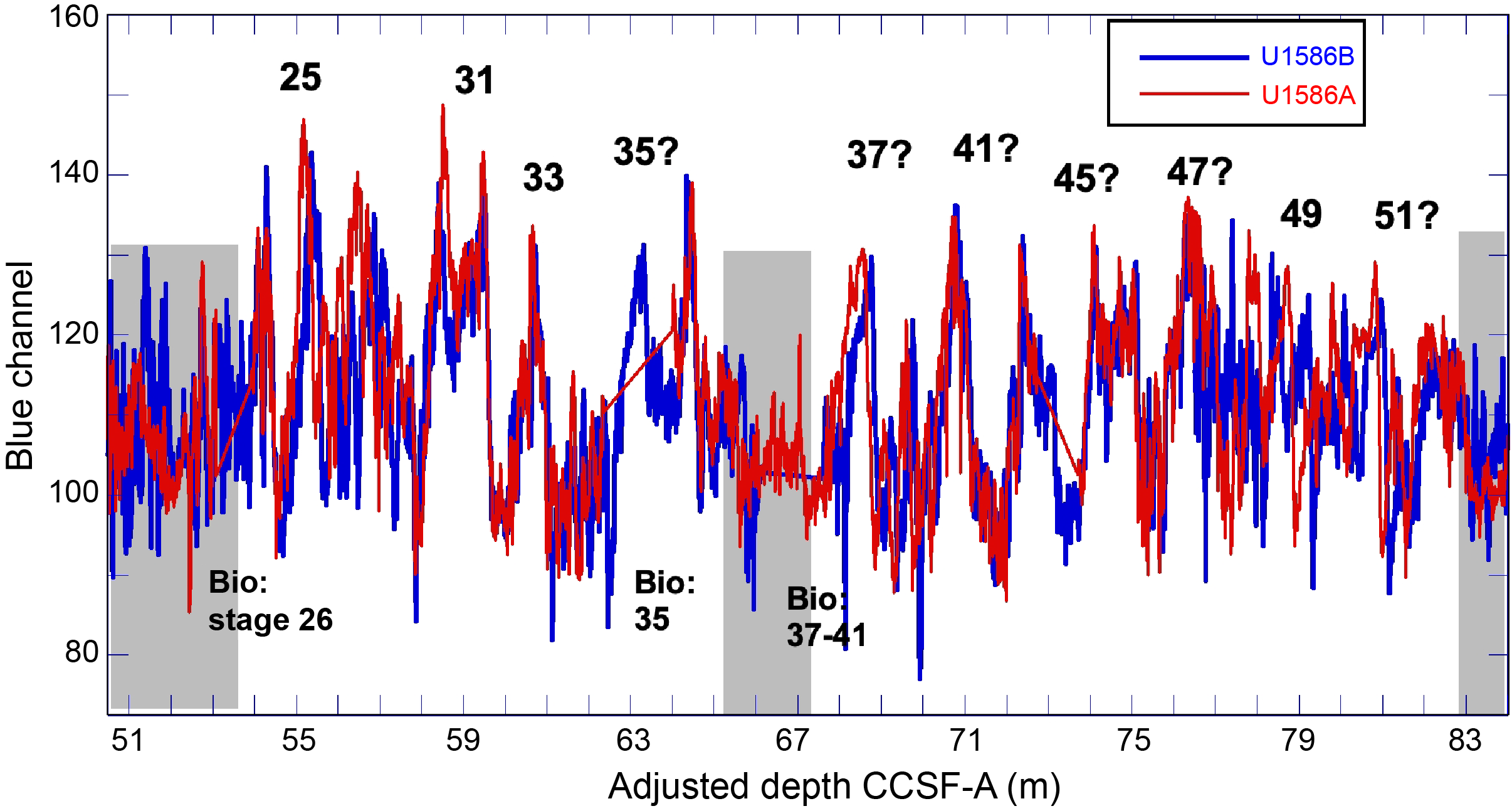
Figure F57. Blue channel color reflectance splice.
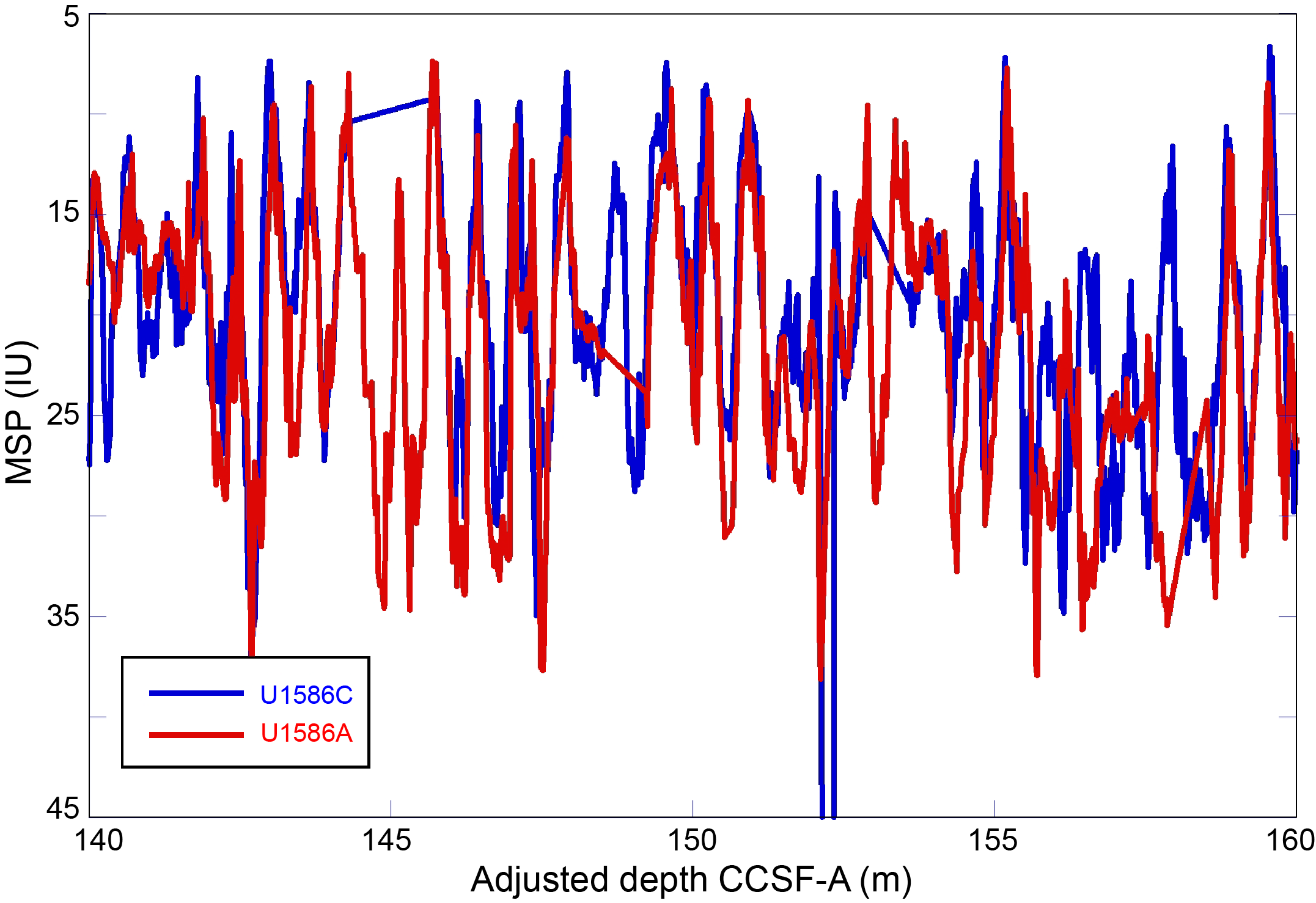
Figure F58. Pliocene amplitude modulated cycles.
NGR measurements showed similar patterns between holes, but absolute values differed when the same stratigraphic sequence was compared between holes. The most likely explanation comes from the fact that NGR counts are a volume measurement (as is the measurement of MS in the whole-round MS loop). When we compared GRA bulk density logs, the reason for most of the discrepancy became apparent: changing from using the APC system to the XCB system reduced the diameter of recovered section, as shown by a step drop in GRA bulk density estimates (Figure F59); hence, there are lower NGR and MS counts in the XCB section. In detail, the diameter of XCB cores probably varies downhole as well. A more accurate calibration of mass- and volume-dependent measurements will require standardizing to volume as estimated by GRA bulk density logging and discrete MAD results.
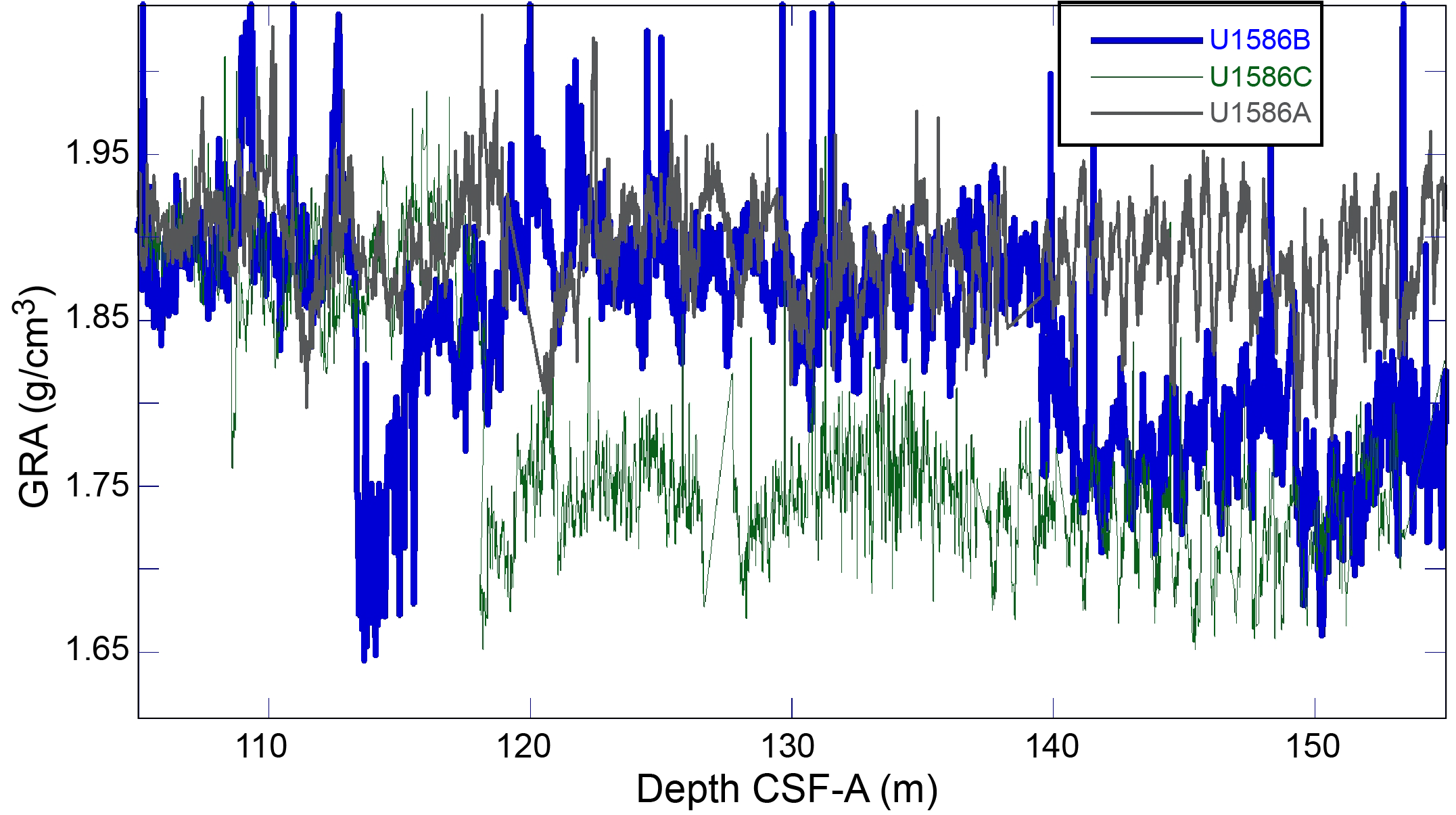
Figure F59. GRA bulk density.
9.2. Gaps
The upper portion of the splice is continuous except for two potential gaps. A lack of tie between Cores 397-U1586A-13H and 14H, 397-U1586C-13 and 14H, and 397-U1586D-13H and 14H is potentially filled by the top of Core 397-U1586B-14H. For the time being, Core 14H was tied to its reference, Core 397-U1586C-13H. Below ~118 m CCSF-A, the splice appears continuous to ~355 m CCSF-A, corresponding to the contact with the shallow water Oligocene(?) section with sandy intervals. The only exception to continuity in this deeper sequence lies in the slumped Upper Miocene sequence (Cores 397-U1586A-25X through 27X, 397-U1586B-24X through 25X, 397-U1586C-23X through 24X, and 397-U1586D-22X through 23X).
9.3. Growth rate and cumulative offset
The cumulative offset between the CSF-A and CCSF-A depth scales grows nearly linearly for Holes U1586A–U1586D to ~250 m CSF-A (Figure F56, left). The growth factor averages 1.115% but varies by core and hole because of variable sea state conditions and misfired APC coring in a few instances, particularly in the upper 80 m CCSF-A (see Operations). Such changes in the growth factor are reflected/summed in the cumulative offset with depth (Figure F56, right), particularly in the upper 80 m CCSF-A. The CSF-A depth for the top of each core is set to the drilling depth below seafloor (DSF) depth scale, which is based on the position of the drill string below the seafloor. However, the process of correlation moved each core top depth to a position on the CCSF-A depth scale that reflects significant expansion. As a closer approximation to true stratigraphic depth, we follow a similar procedure to Expedition 339 (which created the mbsf* scale used in the original Site U1385 report) to convert the splice depths to a scale closely approximating driller's depths, referred to as CCSF-A*. This conversion required a sixth-order polynomial to pass through the zero depth point; the coefficients are reported in Figure F60 and Table T32. Calculation of mass accumulation rates based on the CCSF-A depth scale should account for differential expansion by dividing apparent depth intervals by the appropriate growth factor or by converting to the CCSF-A* scale.
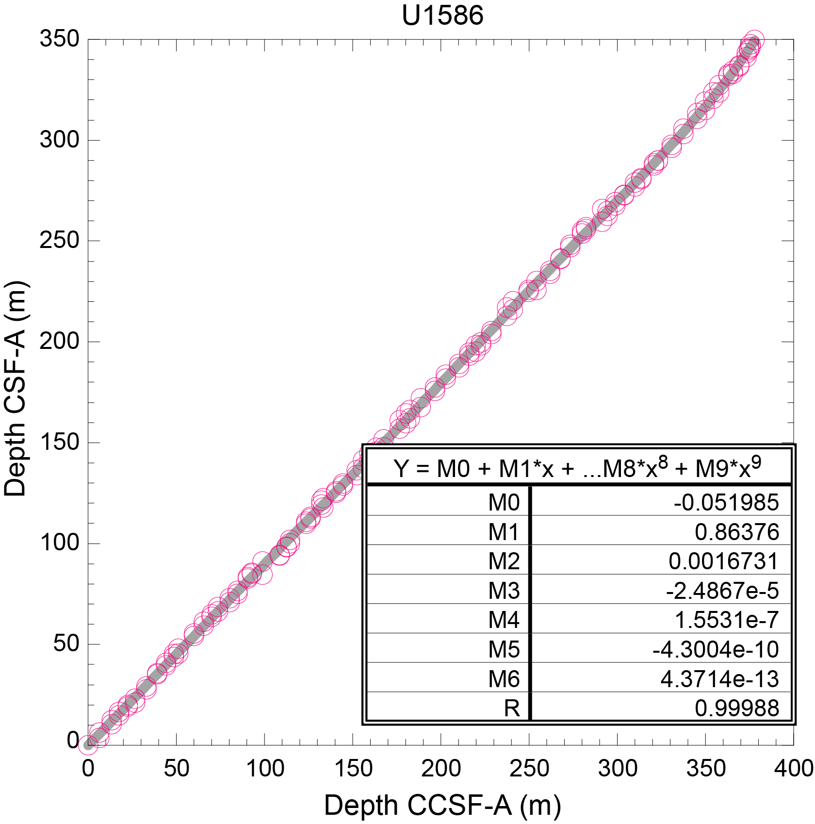
Figure F60. Correlation of splice depth to driller's depth for tie points used in splice construction.
The correlation between MS records from core measurements and wireline logging in Hole U1586D shows that the CCSF-A* depth scale closely resembles the WMSF scale (Figure F55).
References
Abrantes, F., Hodell, D.A., Alvarez Zarikian, C.A., Brooks, H.L., Clark, W.B., Dauchy-Tric, L.F.B., dos Santos Rocha, V., Flores, J.-A., Herbert, T.D., Hines, S.K.V., Huang, H.-H.M., Ikeda, H., Kaboth-Bahr, S., Kuroda, J., Link, J.M., McManus, J.F., Mitsunaga, B.A., Nana Yobo, L., Pallone, C.T., Pang, X., Peral, M.Y., Salgueiro, E., Sanchez, S., Verma, K., Wu, J., Xuan, C., and Yu, J., 2024. Expedition 397 methods. In Hodell, D.A., Abrantes, F., Alvarez Zarikian, C.A., and the Expedition 397 Scientists, Iberian Margin Paleoclimate. Proceedings of the International Ocean Discovery Program, 397: College Station, TX (International Ocean Discovery Program). https://doi.org/10.14379/iodp.proc.397.102.2024
Alvarez Zarikian, C.A., 2009. Data report: late Quaternary ostracodes at IODP Site U1314 (North Atlantic Ocean). In Channell, J.E.T., Kanamatsu, T., Sato, T., Stein, R., Alvarez Zarikian, C.A., Malone, M.J., and the Expedition 303/306 Scientists, Proceedings of the Integrated Ocean Drilling Program. 303/306: College Station, TX (Integrated Ocean Drilling Program Management International, Inc.). https://doi.org/10.2204/iodp.proc.303306.213.2009
Andeweg, B., 2002. Cenozoic tectonic evolution of the Iberian Peninsula: effects and causes of changing stress fields [PhD dissertation]. Vrije Universiteit, Amsterdam. https://www.researchgate.net/publication/315450294
Armenteros, I., Dabrio, C.J., Legoinha, P., González-Delgado, J.A., Martínez-Graña, A., Alonso-Gavilán, G., Civis, J., and Pais, J., 2019. Facies and sequence analysis of Miocene open-shelf warm-temperate carbonates in Portimão (Lagos-Portimão Formation, Portugal). Facies, 65(3):33. https://doi.org/10.1007/s10347-019-0575-2
Balestra, B., Flores, J.A., Hodell, D.A., Hernández Molina, F.J., and Stow, D.A.V., 2015. Pleistocene calcareous nannofossil biochronology at IODP Site U1385 (Expedition 339). Global and Planetary Change, 135:57–65. https://doi.org/10.1016/j.gloplacha.2015.10.004
Blum, P., 1997. Physical properties handbook: a guide to the shipboard measurement of physical properties of deep-sea cores. Ocean Drilling Program Technical Note, 26. https://doi.org/10.2973/odp.tn.26.1997
Bouma, A.H., Keunen, P.H., and Shepard, F.P., 1962. Sedimentology of Some Flysch Deposits: a Graphic Approach to Facies Interpretation: Amsterdam (Elsevier).
Chaisson, W.P., and Pearson, P.N., 1997. Planktonic foraminifer biostratigraphy at Site 925: middle Miocene-Pleistocene. In Shackleton, N.J., Curry, W.B., Richter, C., and Bralower, T.J. (Eds.), Proceedings of the Ocean Drilling Program, Scientific Results. 154: College Station, TX (Ocean Drilling Program), 3–31. https://doi.org/10.2973/odp.proc.sr.154.104.1997
Channell, J.E.T., Hodell, D.A., Crowhurst, S.J., Skinner, L.C., and Muscheler, R., 2018. Relative paleointensity (RPI) in the latest Pleistocene (10–45 ka) and implications for deglacial atmospheric radiocarbon. Quaternary Science Reviews, 191:57–72. https://doi.org/10.1016/j.quascirev.2018.05.007
De Vleeschouwer, D., Dunlea, A.G., Auer, G., Anderson, C.H., Brumsack, H., de Loach, A., Gurnis, M.C., Huh, Y., Ishiwa, T., Jang, K., Kominz, M.A., März, C., Schnetger, B., Murray, R.W., Pälike, H., and Expedition 356 Shipboard Scientists, 2017. Quantifying K, U, and Th contents of marine sediments using shipboard natural gamma radiation spectra measured on DV JOIDES Resolution. Geochemistry, Geophysics, Geosystems, 18(3):1053–1064. https://doi.org/10.1002/2016GC006715
Diester-Haass, L., Meyers, P.A., and Bickert, T., 2004. Carbonate crash and biogenic bloom in the Late Miocene: evidence from ODP Sites 1085, 1086, and 1087 in the Cape Basin, southeast Atlantic Ocean. Paleoceanography, 19(1):PA1007. https://doi.org/10.1029/2003PA000933
Dunham, R.J., 1962. Classification of carbonate rocks according to depositional texture. In Ham, W.E., Classification of Carbonate Rocks. AAPG Memoir, 1.
Expedition 339 Scientists, 2013. Site U1385. In Stow, D.A.V., Hernández-Molina, F.J., Alvarez Zarikian, C.A., and the Expedition 339 Scientists, Proceedings of the Integrated Ocean Drilling Program. 339: Tokyo (Integrated Ocean Drilling Program Management International, Inc.). https://doi.org/doi:10.2204/iodp.proc.339.103.2013
Faranda, C., Cipollari, P., Cosentino, D., Gliozzi, E., and Pipponzi, G., 2008. Late Miocene ostracod assemblages from eastern Mediterranean coral reef complexes (central Crete, Greece). Revue de Micropaléontologie, 51(4):287–308. https://doi.org/10.1016/j.revmic.2007.06.002
Farrell, J.W., Raffi, I., Janecek, T.R., Murray, D.W., Levitan, M., Dadey, K.A., Emeis, K.-C., Lyle, M., Flores, J.-A., and Hovan, S., 1995. Late Neogene sedimentation patterns in the eastern equatorial Pacific Ocean. In Pisias, N.G., Mayer, L.A., Janecek, T.R., Palmer-Julson, A., and van Andel, T.H. (Eds.), Proceedings of the Ocean Drilling Program, Scientific Results. 138: College Station, TX (Ocean Drilling Program), 717–756. https://doi.org/10.2973/odp.proc.sr.138.143.1995
Flecker, R., Ducassou, E., and Williams, T., 2023. Expedition 401 Scientific Prospectus: Mediterranean Atlantic Gateway Exchange. International Ocean Discovery Program. https://doi.org/10.14379/iodp.sp.401.2023
Flecker, R., Krijgsman, W., Capella, W., de Castro Martíns, C., Dmitrieva, E., Mayser, J.P., Marzocchi, A., Modestou, S., Ochoa, D., Simon, D., Tulbure, M., van den Berg, B., van der Schee, M., de Lange, G., Ellam, R., Govers, R., Gutjahr, M., Hilgen, F., Kouwenhoven, T., Lofi, J., Meijer, P., Sierro, F.J., Bachiri, N., Barhoun, N., Alami, A.C., Chacon, B., Flores, J.A., Gregory, J., Howard, J., Lunt, D., Ochoa, M., Pancost, R., Vincent, S., and Yousfi, M.Z., 2015. Evolution of the Late Miocene Mediterranean–Atlantic gateways and their impact on regional and global environmental change. Earth-Science Reviews, 150:365–392. https://doi.org/10.1016/j.earscirev.2015.08.007
Flores, J.-A., Colmenero-Hidalgo, E., Mejía-Molina, A.E., Baumann, K.-H., Henderiks, J., Larsson, K., Prabhu, C.N., Sierro, F.J., and Rodrigues, T., 2010. Distribution of large Emiliania huxleyi in the central and Northeast Atlantic as a tracer of surface ocean dynamics during the last 25,000 years. Marine Micropaleontology, 76(3–4):53–66. https://doi.org/10.1016/j.marmicro.2010.05.001
Flügel, E., 2004. Microfacies of carbonate rocks: analysis, interpretation and application: Berlin (Springer Science & Business Media). https://doi.org/10.1007/978-3-662-08726-8
Gradstein, F.M., Ogg, J.G., Schmitz, M.D., and Ogg, G.M. (Eds.), 2020. The Geologic Time Scale 2020: Amsterdam (Elsevier BV). https://doi.org/10.1016/C2020-1-02369-3
Grevemeyer, I., Kaul, N., and Kopf, A., 2009. Heat flow anomalies in the Gulf of Cadiz and off Cape San Vincente, Portugal. Marine and Petroleum Geology, 26(6):795–804. https://doi.org/10.1016/j.marpetgeo.2008.08.006
Hüneke, H., Hernández-Molina, F.J., Rodríguez-Tovar, F.J., Llave, E., Chiarella, D., Mena, A., and Stow, D.A.V., 2021. Diagnostic criteria using microfacies for calcareous contourites, turbidites and pelagites in the Eocene–Miocene slope succession, southern Cyprus. Sedimentology, 68(2):557–592. https://doi.org/10.1111/sed.12792
Hyndman, R.D., Erickson, A.J., and Von Herzen, R.P., 1974. Geothermal measurements on DSDP Leg 26. In Davies, T.A., Luyendyk, B.P., et al., Initial Reports of the Deep Sea Drilling Project. 26: Washington, DC (US Government Printing Office), 451–463. https://doi.org/10.2973/dsdp.proc.26.113.1974
Kennett, J.P., and Srinivasan, M.S., 1983. Neogene Planktonic Foraminifera: A Phylogenetic Atlas: London (Hutchinson Ross).
Lyle, M., Dadey, K.A., and Farrell, J.W., 1995. The late Miocene (11–8 Ma) eastern Pacific carbonate crash; evidence for reorganization of deep-water circulation by the closure of the Panama Gateway. In Pisias, N.G., Mayer, L.A., Janecek, T.R., Palmer-Julson, A., and van Andel, T.H. (Eds.), Proceedings of the Ocean Drilling Program, Scientific Results, 138: College Station, TX (Ocean Drilling Program), 821–838. https://doi.org/10.2973/odp.proc.sr.138.157.1995
Martini, E., 1971. Standard Tertiary and Quaternary calcareous nannoplankton zonation. Proceedings of the Second Planktonic Conference, Roma, 1970:739–785.
Meyers, P.A., 1994. Preservation of elemental and isotopic source identification of sedimentary organic matter. Chemical Geology, 114(3–4):289–302. https://doi.org/10.1016/0009-2541(94)90059-0
Meyers, P.A., 1997. Organic geochemical proxies of paleoceanographic, paleolimnologic, and paleoclimatic processes. Organic Geochemistry, 27(5–6):213–250. https://doi.org/10.1016/S0146-6380(97)00049-1
Okada, H., and Bukry, D., 1980. Supplementary modification and introduction of code numbers to the low-latitude coccolith biostratigraphic zonation (Bukry, 1973; 1975). Marine Micropaleontology, 5(3):321–325. https://doi.org/10.1016/0377-8398(80)90016-X
Pais, J., Cunha, P.P., and Legoinha, P. , 2010. Lithostratigraphy of the Cenozoic of Portugal. In Neiva, J.M.C., Ribeiro, A., Victor, L.M., Noronha, F., and Ramalho, M. (Eds.) Geological Sciences: Teaching and Research. 365–376.
Paytan, A., and Griffith, E.M., 2007. Marine barite: recorder of variations in ocean export productivity. Deep Sea Research, Part II: Topical Studies in Oceanography, 54(5–7):687–705. https://doi.org/10.1016/j.dsr2.2007.01.007
Pena dos Reis, R., Pimentel, N., and Garcia, A.J.V., 2010. The Lusitanian Basin (Portugal): stratigraphic analysis and geodynamic evolution. Boletim de Geociências da Petrobrás, 19:23–52.
Pribnow, D.F.C., Kinoshita, M., and Stein, C.A., 2000. Thermal data collection and heat flow recalculations for ODP Legs 101–180: Hannover, Germany (Institute for Joint Geoscientific Research, GGA). http://www-odp.tamu.edu/publications/heatflow/
Raffi, I., Backman, J., Fornaciari, E., Pälike, H., Rio, D., Lourens, L., and Hilgen, F., 2006. A review of calcareous nannofossil astrobiochronology encompassing the past 25 million years. Quaternary Science Reviews, 25(23):3113–3137. https://doi.org/10.1016/j.quascirev.2006.07.007
Ramos, A., Fernández, O., Terrinha, P., and Muñoz, J.A., 2017. Neogene to recent contraction and basin inversion along the Nubia-Iberia boundary in SW Iberia. Tectonics, 36(2):257–286. https://doi.org/10.1002/2016TC004262
Reitz, A., Pfeifer, K., de Lange, G.J., and Klump, J., 2004. Biogenic barium and the detrital Ba/Al ratio: a comparison of their direct and indirect determination. Marine Geology, 204(3–4):289–300. https://doi.org/10.1016/S0025-3227(04)00004-0
Ruiz, F., González-Regalado, M.L., Abad, M., Civis, J., Delgado, J.Á.G., García, E.X.M., Prudêncio, M.I., and Dias, M.I., 2008. Pliocene ostracods of Southwestern Europe. Geobios, 41(6):845–859. https://doi.org/10.1016/j.geobios.2007.07.004
Spezzaferri, S., Olsson, R.K., Hemleben, C., Wade, B.S., Olsson, R.K., Pearson, P.N., Huber, B.T., and Berggren, W.A., 2018. Taxonomy, biostratigraphy, and phylogeny of Oligocene to lower Miocene Globigerinoides and Trilobatus. In Atlas of Oligocene planktonic Foraminifera. Cushman Special Publications, 46.
Wade, B.S., Pearson, P.N., Berggren, W.A., and Pälike, H., 2011. Review and revision of Cenozoic tropical planktonic foraminiferal biostratigraphy and calibration to the geomagnetic polarity and astronomical time scale. Earth-Science Reviews, 104(1–3):111–142. https://doi.org/10.1016/j.earscirev.2010.09.003
Westerhold, T., Marwan, N., Drury, A.J., Liebrand, D., Agnini, C., Anagnostou, E., Barnet, J.S.K., Bohaty, S.M., De Vleeschouwer, D., Florindo, F., Frederichs, T., Hodell, D.A., Holbourn, A.E., Kroon, D., Lauretano, V., Littler, K., Lourens, L.J., Lyle, M., Pälike, H., Röhl, U., Tian, J., Wilkens, R.H., Wilson, P.A., and Zachos, J.C., 2020. An astronomically dated record of Earth's climate and its predictability over the last 66 million years. Science, 369(6509):1383–1387. https://doi.org/10.1126/science.aba6853
Wu, J., Böning, P., Pahnke, K., Tachikawa, K., and de Lange, G.J., 2016. Unraveling North-African riverine and eolian contributions to central Mediterranean sediments during Holocene sapropel S1 formation. Quaternary Science Reviews, 152:31–48. https://doi.org/10.1016/j.quascirev.2016.09.029
Xuan, C., and Channell, J.E.T., 2009. UPmag: MATLAB software for viewing and processing u channel or other pass-through paleomagnetic data. Geochemistry Geophysics Geosystems, 10:Q10Y10. https://doi.org/10.1029/2009GC002584
Yasuhara, M., and Okahashi, H., 2014. Quaternary deep-sea ostracode taxonomy of Ocean Drilling Program Site 980, eastern North Atlantic Ocean. Journal of Paleontology, 88(4):770–785. https://doi.org/10.1666/13-125
Yasuhara, M., and Okahashi, H., 2015. Late Quaternary deep-sea ostracod taxonomy of the eastern North Atlantic Ocean. Journal of Micropalaeontology, 34(1):21–49. https://doi.org/10.1144/jmpaleo2013-022
Zachos, J., Pagani, M., Sloan, L., Thomas, E., and Billups, K., 2001. Trends, rhythms, and aberrations in global climate 65 Ma to Present. Science, 292(5517):686–693. https://doi.org/10.1126/science.1059412