Hodell, D.A., Abrantes, F., Alvarez Zarikian, C.A., and the Expedition 397 Scientists
Proceedings of the International Ocean Discovery Program Volume 397
publications.iodp.org
https://doi.org/10.14379/iodp.proc.397.102.2024
Expedition 397 methods1
![]() F. Abrantes,
F. Abrantes,
![]() D.A. Hodell,
D.A. Hodell,
![]() C.A. Alvarez Zarikian,
C.A. Alvarez Zarikian,
![]() H.L. Brooks,
H.L. Brooks,
![]() W.B. Clark,
W.B. Clark,
![]() L.F.B. Dauchy-Tric,
L.F.B. Dauchy-Tric,
![]() V. dos Santos Rocha,
V. dos Santos Rocha,
![]() J.A. Flores,
J.A. Flores,
![]() T.D. Herbert,
T.D. Herbert,
![]() S.K.V. Hines,
S.K.V. Hines,
![]() H.-H.M. Huang,
H.-H.M. Huang,
![]() H. Ikeda,
H. Ikeda,
![]() S. Kaboth-Bahr,
S. Kaboth-Bahr,
![]() J. Kuroda,
J. Kuroda,
![]() J.M. Link,
J.M. Link,
![]() J. McManus,
J. McManus,
![]() B.A. Mitsunaga,
B.A. Mitsunaga,
![]() L. Nana Yobo,
L. Nana Yobo,
![]() C.T. Pallone,
C.T. Pallone,
![]() X. Pang,
X. Pang,
![]() M.Y. Peral,
M.Y. Peral,
![]() E. Salgueiro,
E. Salgueiro,
![]() S. Sanchez,
S. Sanchez,
![]() K. Verma,
K. Verma,
![]() J. Wu,
J. Wu,
![]() C. Xuan, and
C. Xuan, and
![]() J. Yu2
J. Yu2
1 Abrantes, F., Hodell, D.A., Alvarez Zarikian, C.A., Brooks, H.L., Clark, W.B., Dauchy-Tric, L.F.B., dos Santos Rocha, V., Flores, J.-A., Herbert, T.D., Hines, S.K.V., Huang, H.-H.M., Ikeda, H., Kaboth-Bahr, S., Kuroda, J., Link, J.M., McManus, J.F., Mitsunaga, B.A., Nana Yobo, L., Pallone, C.T., Pang, X., Peral, M.Y., Salgueiro, E., Sanchez, S., Verma, K., Wu, J., Xuan, C., and Yu, J., 2024. Expedition 397 methods. In Hodell, D.A., Abrantes, F., Alvarez Zarikian, C.A., and the Expedition 397 Scientists, Iberian Margin Paleoclimate. Proceedings of the International Ocean Discovery Program, 397: College Station, TX (International Ocean Discovery Program). https://doi.org/10.14379/iodp.proc.397.102.2024
2 Expedition 397 Scientists’ affiliations.
1. Introduction
This chapter provides an overview of the procedures and methods employed for coring operations and in the shipboard laboratories of the R/V JOIDES Resolution during International Ocean Discovery Program (IODP) Expedition 397. The laboratory information applies only to shipboard work described in the Expedition Report section of the Expedition 397 Proceedings of the International Ocean Discovery Program volume that includes the shipboard sample registry, imaging and analytical instruments, core description tools, and the Laboratory Information Management System (LIMS) database. The shipboard workflow followed standard IODP procedures (as previously described by, e.g., Huber et al., 2019; Winckler et al., 2021; Planke et al., 2023), with revisions and refinements as described in this chapter. Methods used by investigators for shore-based analyses of Expedition 397 data will be documented in separate publications.
All shipboard scientists contributed to this volume with the following primary responsibilities (authors are listed in alphabetical order; see Expedition 397 scientists for contact information):
Summary chapter: Expedition 397 Scientists
- Background and objectives: F. Abrantes, D. Hodell
- Operations: C.A. Alvarez Zarikian, K. Grigar
- Lithostratigraphy: H.L. Brooks, J.M. Link, J. McManus, C. Pallone, X. Pang, E. Salgueiro, V. dos Santos Rocha, J. Yu
- Biostratigraphy: C.A. Alvarez Zarikian, W. Clark, J.-A. Flores, M. Peral, K. Verma
- Paleomagnetism: L. Dauchy-Tric, C. Xuan
- Geochemistry: S. Hines, B. Mitsunaga, L. Nana Yobo, J. Wu
- Physical properties and downhole measurements: H.-H.M. Huang, H. Ikeda, J. Kuroda, S. Sanchez
- Stratigraphic correlation: T. Herbert, H.-H.M. Huang, S. Kaboth-Bahr
This introductory section provides an overview of drilling and coring operations, core handling, curatorial conventions, depth scale terminology, and the sequence of shipboard analyses. Subsequent sections of this chapter document specific laboratory instruments and methods in detail.
1.1. Operations
The IODP Environmental Protection and Safety Panel (EPSP) approved four primary and two alternate drilling sites for Expedition 397 as described in the expedition Scientific Prospectus (Hodell et al., 2022). The proposed sites encompass a depth transect (1304–4686 meters below sea level [mbsl]) off the Portuguese margin across the Promontório dos Principes de Avis. The shipboard GPS navigation system (WGS84 datum) was used to position the vessel at Expedition 397 sites. A SyQwest Bathy 2010 CHIRP subbottom profiler was used to monitor seafloor depth during the approach to each site to confirm the seafloor depth once on site. Once the vessel was positioned at a site, the thrusters were lowered and a seafloor positioning beacon was prepared for deployment in case it was needed. Dynamic positioning control of the vessel was constrained by the navigational input from the GPS system (Figure F1). No seafloor positioning beacons were deployed during this expedition. The final hole position was calculated as the mean position of at least 1000 GPS position fixes since the hole was occupied. The ship’s position is better than 1 m, but the exact position of the hole is less certain because of the deviation of the pipe below the ship, which can vary depending on water currents, tides, and water depth; the hole position is thus known typically within 10 m accuracy.
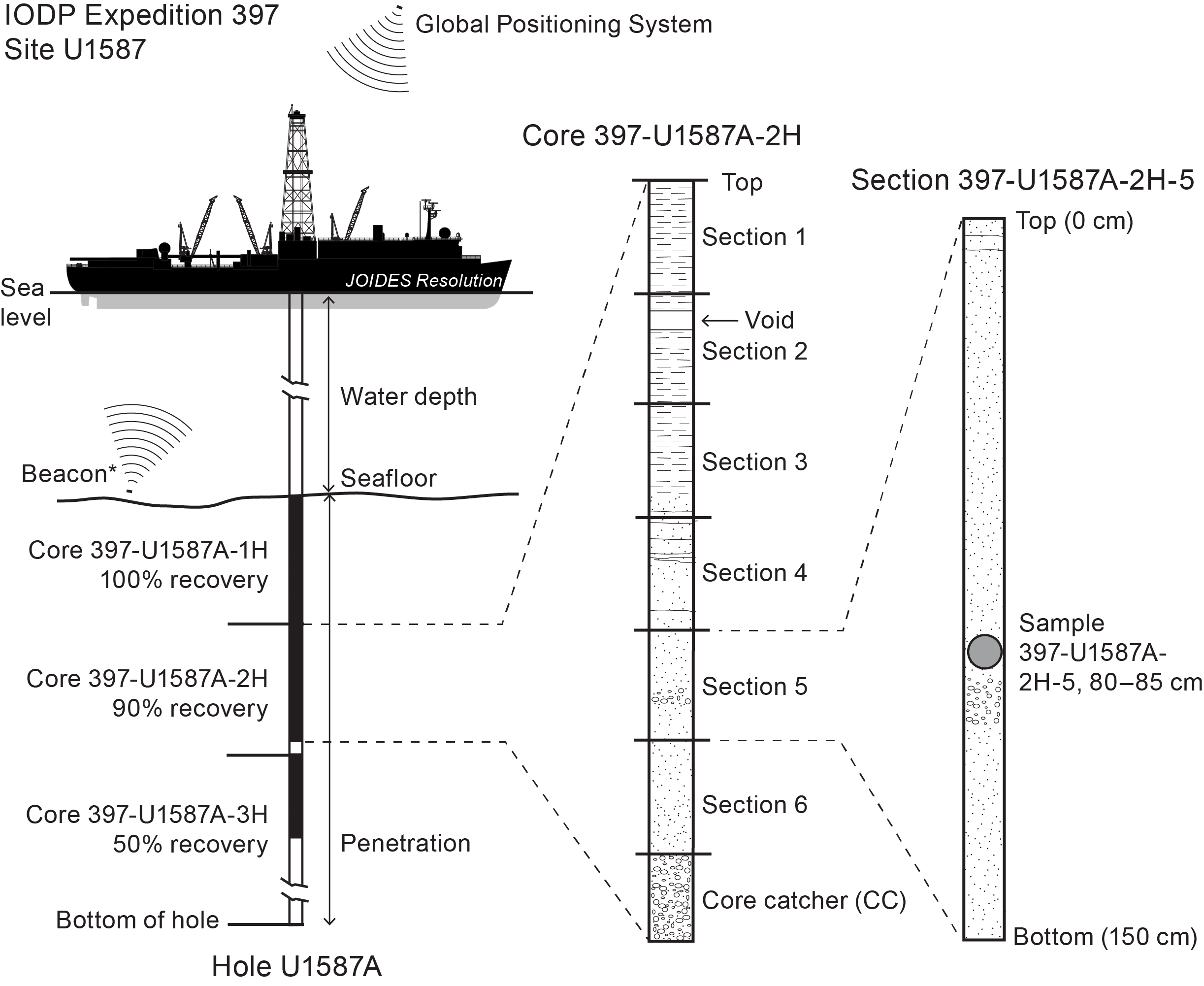
Figure F1. Naming convention for sites, holes, cores, sections, and samples.
Drilling sites were numbered according to the series that began with the first site drilled by the D/V Glomar Challenger in 1968. Starting with Integrated Ocean Drilling Program Expedition 301, the prefix “U” designates sites occupied by JOIDES Resolution. When drilling multiple holes at a site, hole locations were offset from each other by ~20–100 m. A letter suffix distinguishes each hole drilled at the same site. The first hole drilled is assigned the site number modified by the suffix “A,” the second hole takes the site number and the suffix “B,” and so forth. During Expedition 397, we occupied three new sites, U1586, U1587, U1588, and reoccupied Integrated Ocean Drilling Program Expedition 339 Site U1385 and drilled 16 new holes.
1.2. JOIDES Resolution standard coring systems
The advanced piston corer (APC), half-length APC (HLAPC), and extended core barrel (XCB) systems were used during Expedition 397 (Figures F2, F3). These tools and other drilling technology are documented in Graber et al. (2002).
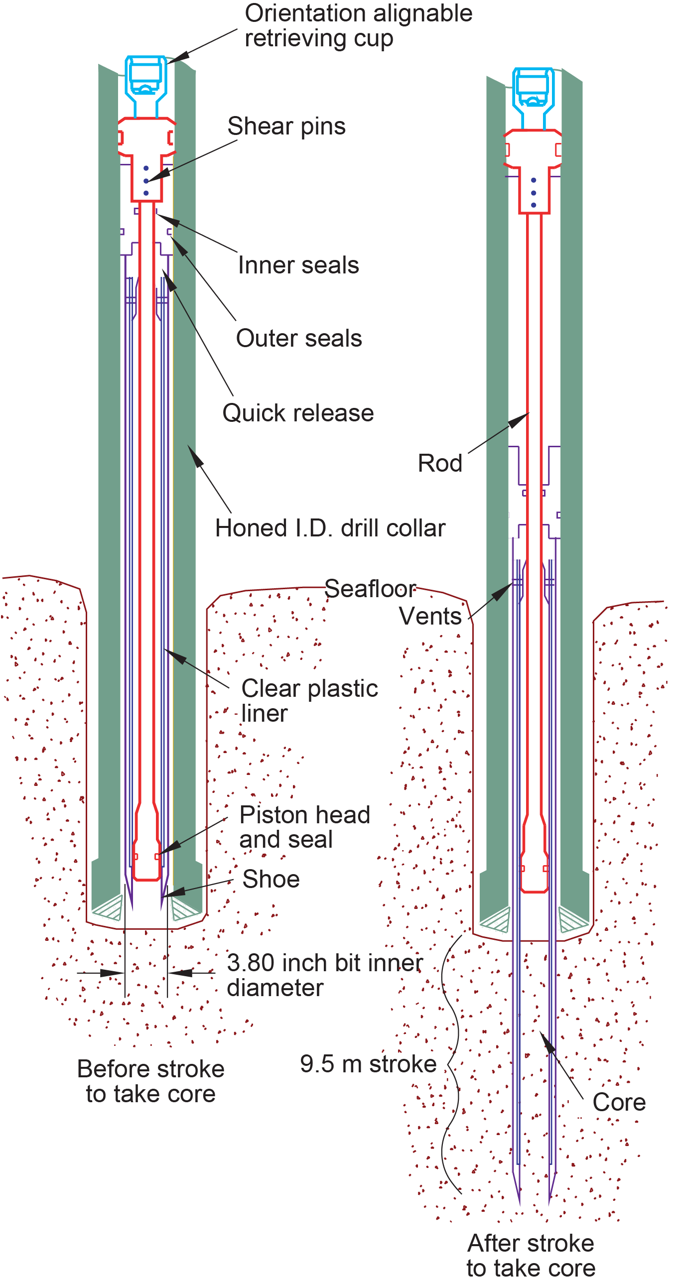
Figure F2. APC system.
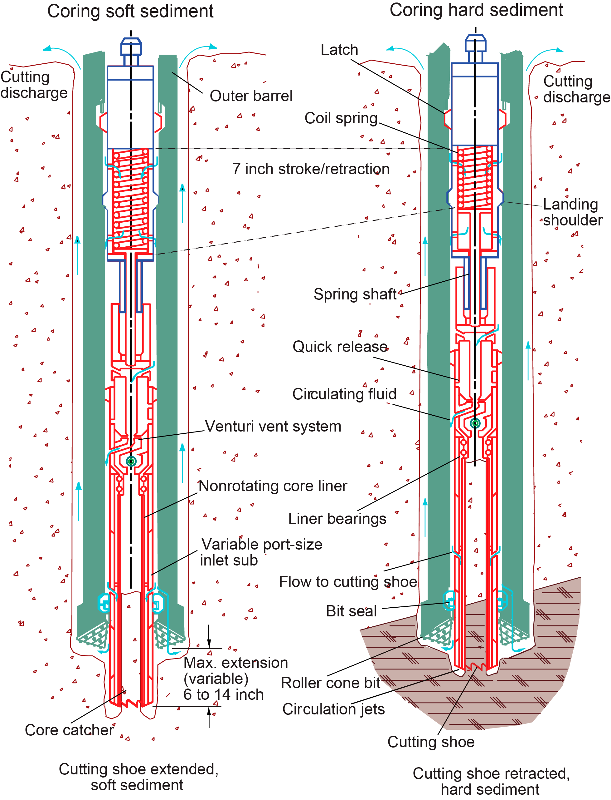
Figure F3. XCB system.
The APC and HLAPC systems cut soft-sediment cores with minimal coring disturbance relative to other IODP coring systems. After the APC/HLAPC core barrel is lowered through the drill pipe and lands above the bit, the inside of the drill pipe is pressured up until one or two shear pins that hold the inner barrel attached to the outer barrel fail. The inner barrel then advances into the formation at high speed and cuts a core with a diameter of 66 mm (2.6 inches) (Figure F2). The driller can detect a successful cut, or full stroke, from the pressure gauge on the rig floor because the excess pressure accumulated prior to the stroke drops rapidly. The depth limit of the APC system, often referred to as APC refusal, is indicated in two ways: (1) the piston fails to achieve a complete stroke (as determined from the pump pressure and recovery reading) because the formation is too hard, or (2) excessive force (>60,000 lb) is required to pull the core barrel out of the formation. When a full stroke cannot be achieved, one or more additional attempts are typically made, and each time the bit is advanced by the length of the core recovered (note that for these cores, this results in a nominal recovery of ~100%). When a full or partial stroke is achieved but excessive force is insufficient to retrieve the core barrel, it can be drilled over, meaning that after the inner core barrel was successfully shot into the formation the drill bit is advanced to total depth to free the APC barrel.
The standard APC system uses a 9.6 m long core barrel, whereas the HLAPC system uses a 4.7 m long core barrel. The HLAPC typically is deployed after the standard APC has repeated partial strokes. During use of the HLAPC, the same criteria is applied in terms of refusal as for the APC system. Nonmagnetic core barrels were used for all APC and HLAPC coring. APC cores were oriented using the Icefield MI-5 core orientation tool when coring conditions allowed.
The XCB system is typically used when the APC/HLAPC system has difficulty penetrating the formation and/or damages the core liner or core. The XCB system can also be used to either initiate holes where the seafloor is not suitable for APC coring or interchanged with the APC/HLAPC when dictated by changing formation conditions. The XCB system is used to advance the hole when APC or HLAPC refusal occurs before the target depth is reached or when drilling conditions require it.
The XCB system has a small cutting shoe that extends below the large rotary APC/XCB bit (Figure F3). The smaller bit can cut a semi-indurated core with less torque and fluid circulation than the main bit, optimizing recovery. The XCB cutting shoe (bit) extends ~30.5 cm ahead of the main bit in soft sediment but retracts into the main bit when hard formations are encountered. It cuts cores with a nominal diameter of 5.87 cm (2.31 inches), slightly less than the 6.6 cm diameter of APC cores. XCB cores are often broken (torqued) into biscuits, which are disc-shaped pieces a few to several centimeters long with remolded sediment (including some drilling slurry) interlayering the discs in a horizontal direction and packing the space between the discs and the core liner in a vertical direction. This type of drilling disturbance may give the impression that the XCB cores have the same thickness (66 mm) as the APC cores.
The bottom-hole assembly (BHA) used for APC and XCB coring during Expedition 397 was composed of an 11⁷⁄₁₆ inch (~29.05 cm) polycrystalline diamond compact (PDC) bit, a bit sub, a seal bore drill collar, a landing saver sub, a modified top sub, a modified head sub, 8¼ inch control length drill collars, a tapered drill collar, two stands of 5½ inch transition drill pipe, and a crossover sub to the drill pipe that extended to the surface.
During Expedition 397, the HLAPC was only used at Site U1586 because the cores retrieved with this system showed severe coring disturbance. Instead, we opted to use the XCB rotary system to advance the holes when the full APC system reached refusal because the XCB performed significantly better than expected with a PDC bit and cutting shoe; biscuiting was typically light to moderate, and the core quality was superior to that obtained with the HLAPC.
1.3. Drilling disturbance
Cores may be significantly disturbed by the drilling process and contain extraneous material because of the coring and core handling process. In formations with loose granular layers (sand, ash, foraminifer ooze, chert fragments, shell hash, etc.), granular material from intervals higher in the hole may settle and accumulate in the bottom of the hole because of drilling circulation and be sampled with the next core. The uppermost 10–50 cm of each core must therefore be examined critically for potential fall-in.
Common coring-induced deformation includes the concave-downward appearance of originally horizontal bedding. Piston action may result in fluidization (flow-in) at the bottom of, or sometimes in, APC cores. Retrieval of unconsolidated (APC) cores from depth to the surface typically results to some degree in elastic rebound, and gas that is in solution at depth may become free and drive core segments in the liner apart. When gas content is high, pressure must be relieved for safety reasons before the cores are cut into segments. Holes are drilled into the liner, which forces some sediment and gas out of the liner. As noted above, XCB coring typically results in biscuits mixed with drilling slurry. During Expedition 397, the main drilling disturbance observed was APC-induced flow-in and XCB coring–induced biscuiting. Severe gas expansion at Site U1588 prompted us to adopt a strategy of half advances of the XCB system and allowing the sediment to expand in the empty liner. We refer to this method as half XCB. Drilling disturbances are described in the Lithostratigraphy section of each site chapter and are indicated on graphic core summary reports, also referred to as visual core descriptions (VCDs).
1.4. Downhole measurements
1.4.1. Formation temperature
Formation temperature measurements were taken at specified intervals with the advanced piston corer temperature (APCT-3) tool (see Downhole measurements) embedded in the APC coring shoe. These measurements were used to obtain temperature gradients and heat flow estimates. During Expedition 397, formation temperature measurements were taken in Holes U1586A, U1587A, and U1588A. No temperature measurements were taken at Site U1385 because they were previously taken during Expedition 339. Information on downhole tool deployments is provided in the Operations, Physical properties, and Downhole measurements sections of each site chapter.
1.4.2. Wireline logging
During wireline logging operations, downhole logs are recorded with Schlumberger and IODP logging tools combined into tool strings, which are lowered into the hole after the completion of coring operations. Only the modified triple combination (triple combo) tool string was used during Expedition 397. It included the Hostile Environment Litho-Density Sonde (HLDS), Hostile Environment Natural Gamma Ray Sonde (HNGS), Enhanced Digital Telemetry Cartridge (EDTC), High-Resolution Laterolog Array (HRLA), Magnetic Susceptibility Sonde version B (MSS-B), and Dipole Sonic Imager (DSI). These tools measure gamma radiation, porosity, density, resistivity, magnetic susceptibility (MS), and P- and S-wave velocity. The tool string contains a telemetry cartridge for communicating through the wireline to the Schlumberger multitasking acquisition and imaging system (MAXIS) on the ship.
In preparation for logging, the boreholes were flushed of debris by circulating drilling fluid and were at least partially filled with seawater-based logging gel (sepiolite mud mixed with seawater) to help stabilize the borehole walls in sections where instability was expected from drilling and coring disturbance. The BHA was pulled up to ~80 m drilling depth below seafloor (DSF), where it protected the unstable upper part of the hole. The triple combo tool string was then lowered downhole on a seven-conductor wireline cable before being pulled up at a constant speed of 550 m/h to provide continuous log measurements of several properties simultaneously. Further details on the logging operations are described in the Downhole measurements sections of each site.
1.5. Core and section handling
1.5.1. Whole-round cores
When a core barrel reached the rig floor, the core catcher from the bottom of the core was removed and taken to the core receiving platform (catwalk), and a sample was extracted for paleontological analysis. Next, the sediment core was extracted from the core barrel in its plastic liner. The liner was carried from the rig floor to the core processing area on the catwalk outside the core laboratory, where it was split into ~1.5 m sections. The exact section length was noted and entered into the database as created length using the Sample Master application. This number was used to calculate core recovery.
Once the core was cut into sections, whole-round samples were immediately taken for interstitial water (IW) chemical analyses from the bottom of selected core sections and headspace samples were taken from the top of a selected section (typically one per core) using a syringe for immediate gas analyses according to the IODP hydrocarbon safety monitoring protocol. When catwalk sampling was complete, liner caps (blue = top; colorless = bottom; yellow = bottom if a whole-round sample was removed from the section) were glued with acetone onto liner sections and sections were placed in core racks for analysis. IW samples also were taken with Rhizon samplers (Seeberg-Elverfeldt et al., 2005) from whole-round cores at selected sites (see Geochemistry for details on the Rhizon sampling program).
The curated length of the sediment cores was set equal to the created length and was updated very rarely (e.g., in cases of data entry errors or when section length kept expanding by more than ~2 cm). Depth in hole calculations are based on the curated section length (see Depth calculations).
The core sections then were placed in a core rack in the laboratory, core information was entered into the database, and the sections were labeled. All core sections were run through the Whole-Round Multisensor Logger (WRMSL) for MS and gamma ray attenuation (GRA) bulk density (see Physical properties). The core sections were also run through the Natural Gamma Radiation Logger (NGRL), and thermal conductivity measurements were taken once per core when the material was suitable.
1.5.2. Core section halves
After completion of whole-round section analyses, the sections were split lengthwise from bottom to top into working and archive halves. Cores were split with a wire or saw. Investigators should note that older material can be transported upward on the split face of a section during splitting. This was particularly true of pyritized burrows that can be dragged upward by the wire. The overall flow of cores, sections, analyses, and sampling implemented during Expedition 397 is shown in Figure F4.
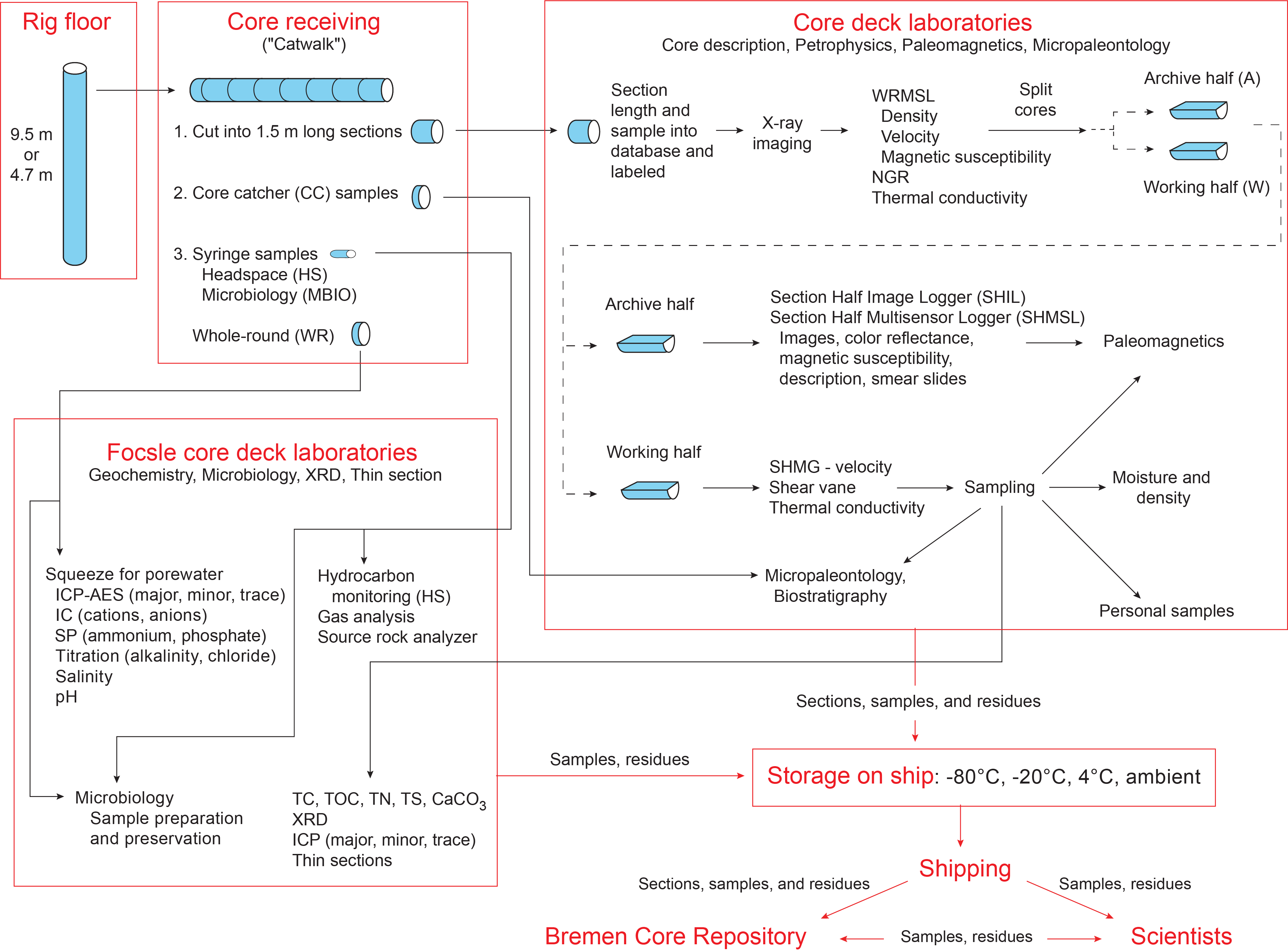
Figure F4. Cores, section, analysis, and sampling workflow implemented during Expedition 397.
Discrete samples were then taken from the working half of each core for moisture and density (MAD), paleomagnetic (PMAG), X-ray diffraction (XRD), carbonate (CARB), and inductively coupled plasma–atomic emission spectroscopy (ICP-AES) analyses. Samples were not collected when the core lithology was a high-priority interval for expedition or postcruise research, the core material was unsuitable, or the core was severely deformed. During the expedition, samples for personal postcruise research were taken where they concerned ephemeral properties (e.g., IW). We also took a limited number of personal or shared pilot samples (1) to determine if an analytical method works and yields interpretable results and how much sample is needed to guide postcruise sampling and (2) to generate low spatial resolution pilot data sets that can be incorporated in proposals and, potentially, increase their chances of being funded.
The archive half of each core was scanned on the Section Half Imaging Logger (SHIL) to provide line-scan images and then measured for point MS (MSP) and reflectance spectroscopy and colorimetry on the Section Half Multisensor Logger (SHMSL). Selected archive-half core sections were X-ray imaged. Labeled foam pieces were used to denote missing whole-round intervals in the SHIL images. The archive-half sections were then described visually and by means of smear slides for sedimentology. Finally, the magnetization of archive-half sections and working-half discrete pieces was measured with the cryogenic magnetometer and spinner magnetometer.
When all steps were completed, the cores were wrapped, sealed in plastic D-tubes, boxed, and transferred to cold storage space aboard the ship. At the end of the expedition, all working halves were shipped to the IODP Bremen Core Repository at the Center for Marine Environmental Sciences (MARUM) (Germany). The archive halves of the cores were sent to various institutions for X-ray fluorescence (XRF) analysis: Site U1586 (Lisbon), Site U1385 (Cambridge), Site U1587 (Texas A&M), and Site U1588 (Bremen). Once core scanning XRF is completed, all cores will be returned to the IODP Bremen Core Repository for permanent storage.
1.6. Sample naming
1.6.1. Editorial practice
Sample naming in this volume follows standard IODP procedure. A full sample identifier consists of the following information: expedition, site, hole, core number, core type, section number, section half, and offset in centimeters measured from the top of the core section. For example, a sample identification of “397-U1586A-1H-2W, 10–12 cm,” represents a sample taken from the interval between 10 and 12 cm below the top of the working half of Section 2 of Core 1 (“H” designates that this core was taken using the APC system) of Hole U1586A during Expedition 397.
The drilling system used to obtain a core is designated in the sample identifiers as follows: H = APC, F = HLAPC, and X = XCB. Integers are used to denote the core type of drilled intervals (e.g., a drilled interval between Cores 2H and 4H would be denoted by Core 31).
When working with data downloaded from the LIMS database or physical samples that were labeled on the ship, three additional sample naming concepts may be encountered: text ID, label ID, and printed labels.
1.6.2. Text ID
Samples taken on JOIDES Resolution are uniquely identified for use by software applications using the text ID, which combines two elements:
- Sample type designation (e.g., SHLF for section half) and
- A unique sequential number for any sample and sample type added to the sample type code (e.g., SHLF30495837).
The text ID is not particularly helpful to most users but is critical for machine reading and troubleshooting.
1.6.3. Label ID
The label ID is used throughout the JOIDES Resolution workflows as a convenient, human-readable sample identity. However, a label ID is not necessarily unique. The label ID is made up of two parts: primary sample identifier and sample name.
1.6.3.1. Primary sample identifier
The primary sample identifier is very similar to the editorial sample name described above, with two notable exceptions:
- Section halves always carry the appropriate identifier (397-U1587B-20X-2A and 397-U1587B-20X-2W for archive and working half, respectively).
- Sample top and bottom offsets, relative to the parent section, are indicated as “35/37” rather than “35–37 cm.”
1.7. Depth calculations
Sample and measurement depth calculations were based on the methods described in IODP Depth Scales Terminology v.2 (https://www.iodp.org/policies-and-guidelines/142-iodp-depth-scalesterminology-april-2011/file) (Table T1). The definition of multiple depth scale types and their distinction in nomenclature should keep the user aware that a nominal depth value at two different depth scale types (and even two different depth scales of the same type) generally does not refer to exactly the same stratigraphic interval in a hole. The SI unit for all depth scales is meters (m).
Depths of cored intervals were measured from the drill floor based on the length of drill pipe deployed beneath the rig floor and referred to as drilling depth below rig floor (DRF), which is traditionally referred to as meters below rig floor (mbrf). The depth of each cored interval, measured on the DRF scale, can be referenced to the seafloor by subtracting the seafloor depth measurement (on the DRF scale) from the cored interval (on the DRF scale). This seafloor referenced depth of the cored interval is reported on the DSF scale, which is traditionally referred to as meters below seafloor (mbsf). In the case of APC coring, the seafloor depth was the length of pipe deployed minus the length of the mudline core recovered.
Depths of samples and measurements in each core were computed based on a set of rules that result in the core depth below seafloor, Method A (CSF-A), depth scale. The two fundamental rules for this scale are that (1) the top depth of a recovered core corresponds to the top depth of its cored interval (top DSF depth = top CSF-A depth) regardless of type of material recovered or drilling disturbance observed and (2) the recovered material is a contiguous stratigraphic representation even when core segments are separated by voids when recovered, the core is shorter than the cored interval, or it is unknown how much material is missing between core pieces. When voids were present in the core on the catwalk, they were closed by pushing core segments together whenever possible. The length of missing core should be considered a depth uncertainty when analyzing data associated with core material.
When core sections were given their curated lengths, they were also given a top and a bottom depth based on the core top depth and the section length. Depths of samples and measurements on the CSF-A scale were calculated by adding the offset of the sample (or measurement from the top of its section) to the top depth of the section.
Per IODP policy established after the introduction of the IODP Depth Scales Terminology v.2, sample and measurement depths on the CSF-A depth scale are commonly referred to with the custom unit mbsf, just like depths on the DSF scale. The reader should be aware, however, that the use of mbsf for different depth scales can cause confusion in specific cases because different mbsf depths may be assigned to the same stratigraphic interval. For example, a soft-sediment core from less than a few hundred meters below seafloor often expands upon recovery (typically by a few percent to as much as 15%), and the length of the recovered core exceeds that of the cored interval. Therefore, a stratigraphic interval in a particular hole may not have the same depth on the DSF and CSF-A scales. When recovery in a core exceeds 100%, the CSF-A depth of a sample taken from the bottom of the core will be deeper than that of a sample from the top of the subsequent core (i.e., some data associated with the two cores overlap on the CSF-A scale). To overcome the overlap problem, core intervals can be placed on the core depth below seafloor, Method B (CSF-B), depth scale. The CSF-B approach scales the recovered core length back into the interval cored, from >100% to exactly 100% recovery. If cores had <100% recovery to begin with, they are not scaled. When downloading data using the JOIDES Resolution Science Operator (JRSO) LIMS Reports (https://web.iodp.tamu.edu/LORE), depths for samples and measurements are by default presented on both the CSF-A and CSF-B scales. The CSF-B depth scale was particularly useful for Site U1588, which had severe gas expansion issues, prompting the use of the half XCB method to allow sediment to expand into empty liner.
Wireline logging data are collected at the wireline log depth below rig floor (WRF) scale, from which a seafloor measurement is subtracted to create the wireline log depth below seafloor (WSF) scale. For Expedition 397, the WSF depth scale was only used for preliminary data usage on the ship. Immediately after data collection was completed, the wireline logging data were transferred to the Lamont-Doherty Earth Observatory Borehole Research Group (LDEO-BRG), where multiple passes and runs were depth matched using the natural gamma radiation (NGR) logs. The data were returned to the ship using the wireline log matched depth below seafloor (WMSF) scale, which is the final and official logging depth scale type for investigators.
During Expedition 397, all core depths below seafloor were initially calculated according to the CSF-A depth scale. Unless otherwise noted, all depths presented are core depths below seafloor calculated as CSF-A and reported in meters on the CSF-A scale. For Site U1588, depths are reported in meters on the CSF-B scale.
Core composite depth below seafloor (CCSF) depth scales are constructed for sites with two or more holes to create as continuous a stratigraphic record as possible. This also helps to mitigate the CSF-A core overlap problem and the coring gap problem. Using shipboard core logger–based physical properties data verified with core photos, core depths in adjacent holes at a site are vertically shifted to correlate between cores recovered in adjacent holes. This process produces the CCSF depth scale. The correlation process is achieved using the Correlator program (version 4.0 was used during Expedition 397) and results in affine tables that indicate the vertical shift of cores on the CCSF scale relative to the CSF-A scale or CSF-B scale in the case of Site U1588. Once the CCSF scale is constructed, a splice that best represents the stratigraphy of a site by utilizing and splicing the best portions of individual sections and cores from each hole is defined. Because of core expansion, the CCSF depths of stratigraphic intervals are typically 10%–15% deeper than their CSF-A depths. CCSF depth scale construction also reveals that coring gaps on the order of 1.0–1.5 m typically occur between two subsequent cores, despite the apparent >100% recovery. For more details on construction of the CCSF depth scale, see Stratigraphic correlation.
2. Lithostratigraphy
This section outlines the procedures for documenting the sedimentology of cores recovered during Expedition 397, including core description, sediment classification, smear slide preparation and description, and portable X-ray fluorescence spectrometry (pXRF) measurements. Only general procedures are outlined. All observations and data were uploaded directly into the IODP LIMS database using the GEODESC application. LIMS Information Viewer (LIVE) is a graphic display for core data (e.g., digital images of section halves, principal lithology, and drilling disturbance) that was used for quality control of the uploaded data sets.
2.1. Core preparation and digital color imaging
Prior to core description and high-resolution digital color imaging, the quality of the split surface of the archive half of each core was assessed and the surface was scraped lightly with a flexible metallic plate as needed. Cleaned core sections were then described in conjunction with images obtained using the SHIL, smear slide analysis, and measurements obtained using the SHMSL (see Physical properties).
The cleaned archive half was imaged with the SHIL as soon as possible to avoid sediment color changes caused by oxidation and drying. In cases of watery or soupy sediment, the surface was dried sufficiently to avoid light reflection prior to scanning. A high-resolution JPEG with a grayscale and depth ruler and a low-resolution cropped JPEG showing only the core section surface were created from the high-resolution TIFF files. These images were uploaded in LORE as Images > Core sections (LSIMG), and the RGB data were uploaded in LORE under Physical properties > RGB channels (RGB).
2.2. Smear slides
Smear slide microscopic analysis was used to determine biogenic and terrigenous components and abundance to aid in lithologic classification. For the first hole of each site, toothpick samples were taken at a frequency of at least two samples per core, or one sample per core in the case of HLAPC drilling. When sediments were highly disturbed, the number of smear slides per core was optionally reduced or nonexistent. For slide preparation, the sediment was mixed with distilled water, spread on a glass coverslip or glass slide, and dried on a hot plate at 120°C. The dried sample was then mounted with Norland optical adhesive Number 61 and fixed with ultraviolet light. Smear slides were examined with a transmitted-light petrographic microscope equipped with a standard eyepiece micrometer. Several fields of view (FOVs) were examined at some combination of 5×, 10×, 20×, and 40× along a transversal section to assess the abundance of detrital, biogenic, and authigenic components following standard petrographic techniques as stated in Rothwell (1989) and Marsaglia et al. (2013, 2015). The relative percent abundance of the sedimentary constituents was visually estimated using the techniques of Rothwell (1989). The texture of siliciclastic lithologies (e.g., relative abundance of sand-, silt-, and clay-sized grains) and the proportions and presence of biogenic and mineral components were recorded in the smear slide worksheet in GEODESC Data Capture. Components observed in smear slides were categorized as follows:
- TR = trace (≤1%).
- R = rare (>1%–10%).
- C = common (>10%–25%).
- A = abundant (>25%–50%).
- D = dominant (>50%).
Smear slides provide only a rough estimate of the relative abundance of sediment constituents. Occasionally, the lithologic name assigned on the basis of smear slide observation does not match the macroscopic designation because a small sample may not be representative of a much larger sediment interval. Additionally, very fine and coarse grains are difficult to observe in smear slides, and their relative proportions in the sediment can be altered during slide preparation. Therefore, intervals dominated by sand and larger sized components were examined by macroscopic comparison to grain size reference charts. Photomicrographs of all smear slides were taken and uploaded to the LIMS database.
2.3. Visual core description and standard graphic report
Macroscopic descriptions of each section (nominally 0–150 cm long) were input into GEODESC Data Capture. Two templates were constructed (drilling disturbance and macroscopic sediment), and columns were customized to include relevant descriptive information categories. For the macroscopic sediment template, these include lithology, sedimentary structures, diagenetic features, bioturbation intensity, deformational structures, and trace and macro fossils. A summary description was created for each core.
A simplified one page graphical representation of each core, or VCD (Figure F5), was generated using the LIMS2Excel application and a commercial program (Strater, Golden Software). VCDs are presented with the core depth below seafloor (CSF) depth scale, split-core photographs, graphic lithology, and columns for core disturbance, deformational structures, average grain size, sedimentary structures, diagenetic features, bioturbation, shipboard samples, age, MS, NGR counts, and color reflectance (L*a*b*). The graphic lithologies, sedimentary structures, and other visual observations are represented on the VCDs by graphic patterns and symbols (Figure F6). Each VCD also contains the summary description for the core. Only major lithologies are shown on the summary figure for each chapter.
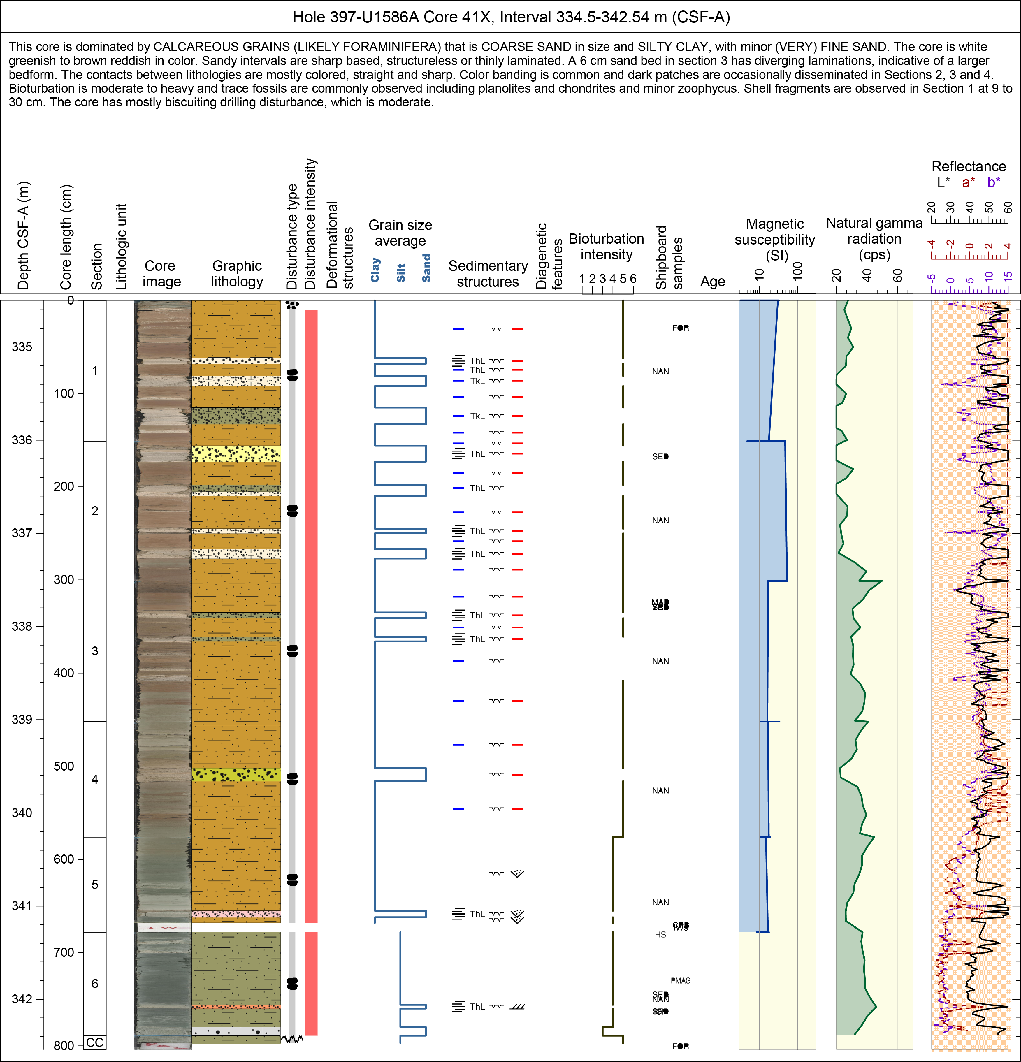
Figure F5. Example VCD.
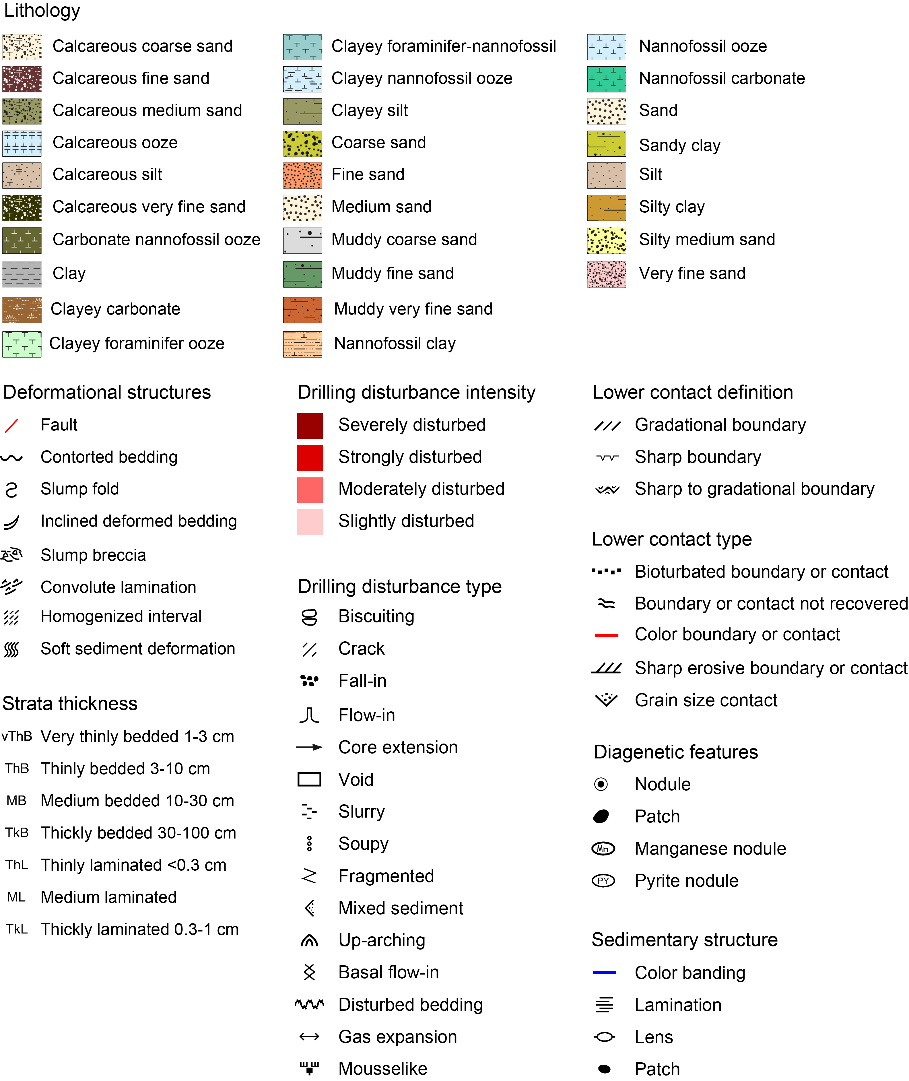
Figure F6. VCD legend.
2.4. Drilling disturbance
Drilling disturbances were described in a separate template in GEODESC Data Capture. The definitions of terms are paraphrased or taken from GEODESC and are consistent with the nomenclature of Jutzeler et al. (2014) and the methods described in Expedition 339 Scientists (2013) unless otherwise noted.
- Fall-in: debris in the top of a core that fell into the borehole from shallower depths during the coring process.
- Up-arching: soft-sediment layers in the plastic core liner bending down around the cut periphery due to friction when the core barrel is shot in sediment.
- Basal flow-in: flow structures and fabrics dominated by vertical banding in the lower portion of a piston core, which are interpreted to have flown or been sucked in by the piston action.
- Flow-in: identified based on vertical flow banding in the bottom of a piston core, caused by the suction action if the core fails to separate from the formation.
- Along-core gravel/sand contamination: gravel/sand is dragged or washed up or down between the in situ core material and the core liner.
- Gas expansion: may be indicated in piston cores (1) by voids several centimeters long that are observed in the core liner before the core is sectioned and curated, which are closed in processing and not accounted for in core recovery, or (2) when core recovery exceeds 110%, which is unlikely to be caused by elastic rebound and mechanical stretching alone.
- Soupy: intervals are water saturated and have lost all aspects of original bedding.
- Slurry: intervals are water saturated but maintain some aspects of original bedding.
- Mousse-like: very soft sediment, typically ooze, apparently remolded by the coring process through flowage with the core liner.
- Biscuiting: breakage of semilithified core into disc-shaped pieces, often separated by remolded mud that is a mixture of ground up sediment and drill fluid, resembling a macaroon biscuit.
- Crack: firm sediments that are broken but not displaced or rotated significantly.
- Brecciated: firm sediments that are pervasively broken and may be displaced or rotated.
- Void: an interval that has no core material, typically with a Styrofoam spacer with the word VOID marked on it.
- Disturbed bedding: sediments visibly mixed by the coring process.
- Fractured or fragmented: sediment displaying breakage.
- Core extension: a piston core that is extended or expanded to some degree by a combination of elastic rebound, gas expansion, and friction along the core liner.
- Punctured: displaying damage in the form of holes or slots.
- Mixed sediment: sediments are visibly mixed by the coring process.
- Sediment flowage: a collective term for structures resulting from the act of sediment flowing. Flowage is typically a result of piston coring action.
Drilling disturbances were also classified into four categories:
- Slightly disturbed (<1%),
- Moderately disturbed (1%–10%),
- Strongly disturbed (10%–50%), and
- Severely disturbed (50%–100%).
If a core or interval did not present any drilling disturbance type, a comment in the core summary was written to inform that drilling disturbance was absent and no description was entered into the GEODESC Data Capture spreadsheet.
2.5. Lithologic classification scheme
The principal lithologic name was assigned on the basis of the relative abundances of biogenic and terrigenous clastic grains and was noted in the microscopic and macroscopic sediment templates in GEODESC Data Capture. The Wentworth (1922) scale was used to define grain-size classes:
- The principal name of sediment with <50% biogenic grains was based on the dominant grain size of both the terrigenous and biogenic grains. This grain size was largely determined by analysis of smear slides.
- The principal name of sediment with ≥50% biogenic grains was classified as an ooze, modified by the most abundant specific biogenic grain type that forms 50% or more of the sediment. For example, if nannofossils exceed 50%, then the sediment was classified as nannofossil ooze. Biogenic constituents of similar composition were grouped together to exceed this 50% abundance threshold. For example, if nannofossils are 40% of the sediment and foraminifers are 20%, then the sediment was termed calcareous ooze or, in the case where the two components were clearly distinguishable, foraminifer-nannofossil ooze.
Major and minor modifiers were applied to any of the principal granular sediment names. Minor modifiers were those components with abundances >10% and <25% and were used in the lithology suffix followed by “with.” When more than one minor modifier is present, the component with the higher abundance is followed by the component with less abundance and so forth and linked with “and.” Major modifiers are those components with abundances >25% and <50% and were used in the lithology prefix. If the dominant component was siliciclastics, the modifier was based on the grain-size characteristics of both the terrigenous clastic and the biogenic grains. For example, if the sediments were dominantly (>50%) siliciclastic and contained (for all grains) 60% clay, 30% silt, and 10% sand, the lithology would be silty clay. If the component was biogenic, then the most specific biogenic grain type that exceeds the percentage threshold was used. The term “mud” or “muddy” was only used when clay and silt were mixed or could not be determined (i.e., not distinguishable without a smear slide).
Lower contacts between lithologies within sections were also described in the macroscopic sediment template in GEODESC Data Capture. Bioturbation, color, cut-and-fill, firmground, grain size, and sharp erosive contacts or boundaries were described. Contact shapes were described as curved, irregular, straight to irregular, straight, or wavy. Contacts were described as gradational, sharp to gradational, or sharp.
2.6. Stratification and sedimentary structures
The presence of sedimentary structures was noted in the macroscopic sediment template in GEODESC Data Capture. The definitions of terms were paraphrased from GEODESC:
- Lamination: a formation of lamina or laminae.
- Color banding: bands of different colors caused by layers of alternating textures or compositions, possibly emphasized by diagenetic alteration.
- Graded bedding: each layer displays a gradual and progressive change in particle size, usually from coarse at the base of the bed to fine at the top.
- Lens: a geologic deposit bounded by converging surfaces (at least one of which is curved), thick in the middle and thinning out toward the edges, resembling a convex lens.
- Patch: a section of sediment distinct from its surroundings, often due to lithology or color.
Stratification and sedimentary structures were characterized by the following thicknesses, similar to Stow (2005):
- Thin lamination (<0.3 cm),
- Thick lamination (0.3–1 cm),
- Very thin bed (1–3 cm),
- Thin bed (3–10 cm),
- Medium bed (10–30 cm),
- Thick bed (30–100 cm), and
- Very thick bed (>100 cm).
2.7. Deformational structures
The presence of deformational structures was noted in the macroscopic sediment template in GEODESC Data Capture. The definitions of terms were paraphrased from GEODESC:
- Churned or chaotic strata: soft-sediment deformation; irregular or unordered set of layers due to postdepositional processes.
- Contorted bedding: wavy, extremely disorganized, markedly and intricately crumpled, twisted, or folded beds that are overlain and underlain by parallel undisturbed layers.
- Contorted bedding: disorganized bedding that is not confined to a single uniform layer.
- Convolute lamination: wavy, extremely disorganized, markedly and intricately crumpled, twisted, or folded laminae that are confined within a single, relatively thin, well-defined, undeformed layer that die out both upward and downward and that are overlain and underlain by parallel undisturbed layers.
- Fault: a discrete surface or zone of discrete surfaces separating two sedimentary units across which one mass has slid past the other.
- Slump breccia: a contorted sedimentary bed produced by slumping and exhibiting brecciation (disaggregation in angular clasts).
- Slump fold: an intraformational fold produced by slumping (ductile movement) of soft sediments.
- Inclined deformed bedding: bedding that is inclined at an angle, rather than parallel.
- Homogenized interval: sediment that contains no clear structure or bedding or that appears mixed.
- Soft-sediment deformation: sediment that appears disturbed by ductile deformation and may exhibit a wavy structure or be otherwise deformed.
2.8. Bioturbation and trace fossils
Bioturbation was noted in the macroscopic sediment template in GEODESC Data Capture. Six levels of bioturbation are recognized using a scheme like that of Droser and Bottjer (1986). Bioturbation intensity is classified as follows:
- Complete (100%),
- Heavy (>60%),
- Moderate (40%–60%),
- Slight (10%–40%),
- Sparse (<10%), and
- Absent (none).
Trace fossil types were also identified where possible.
2.9. Other features
Diagenetic features, including nodules (of distinct or indistinct composition), pyrite, and dark patches were described. Macrofossil abundance was described as none, rare, few, common, or abundant (see Smear slides for quantification of these terms), and the type or species was identified when possible. Clast (>2 mm) counts and characteristics were described. These features were noted in the macroscopic sediment template in GEODESC Data Capture.
2.10. Spectrophotometry and colorimetry
The SHMSL employs multiple sensors for the measurement of bulk physical properties in a motorized and computer-controlled section-half logging machine. The sensors on the SHMSL include a spectrophotometer that measures reflectance spectroscopy and colorimetry, a point susceptibility meter that measures MS, and a laser surface analyzer. Spectrophotometry and MS were measured at 2 cm resolution for Sites U1586, U1587, and U1385 and Cores 397-U1588A-1H through 49X and 397-U1588B-1H through 9H. Measurements were taken at 4 cm resolution for Sections 397-U1588B-10X-1 through 10X-3 and 5 cm resolution for Sections 10X-4 through 64X-CC and Holes U1588C and U1588D. Reflectance spectroscopy (spectrophotometry) was carried out using an Ocean Insight QE-Pro spectrophotometer. This instrument measures the reflectance spectra of the split core from the ultraviolet to near-infrared range. Colorimetric information is extracted from the reflectance data to the L*a*b* color space system. The L*a*b* color space expresses color as a function of lightness (L*) and color values a* and b*, where a* reflects the balance between red (positive a*) and green (negative a*) and b* reflects the balance between yellow (positive b*) and blue (negative b*). When a* and b* are 0, there is no color and L* determines grayscale. On the SHMSL, MS was measured with a Bartington MS2 meter and MS2K contact probe (see Physical properties).
Accurate spectrophotometry using the SHMSL demands a direct and level contact between the instrument sensors and the split core surface. A built-in laser surface analyzer aids the recognition of irregularities in the split core surface (e.g., cracks and voids), and data from this tool were recorded to provide an independent check on the fidelity of SHMSL measurements.
2.11. Portable X-ray fluorescence spectrometry
pXRF scanning was performed on selected sections to generate high-resolution element percentages and elemental ratios in bulk sediments. Individual measurements made with a Bruker Tracer 5 pXRF device take 135 s and consist of three measurement steps performed with beam energies of 30, 50, and 15 keV, each with 45 s of integration time. The spot size of the measurements was 8 mm.
The relative intensity of each element is calculated with the internal calibration GeoExploration using the Oxide3phase method. Reference materials (CS-M2 provided by Bruker, USGS BHVO-2, and USGS BCR-2) were measured before and after each measurement session to assure the quality of the data. During Expedition 397, pXRF measurements were conducted to investigate (1) sections with relatively high MS compared to surrounding sections and (2) intervals of cores in which the core catcher showed distinctive faunal assemblages.
2.12. Lithofacies classification
Lithofacies are qualitatively defined groups primarily based on lithology as well as all other criteria outlined above. The lithofacies characterized cover all sites, and therefore not all lithofacies are present at each site.
2.13. Lithostratigraphic units
Lithostratigraphic units are divided based on the frequency and occurrence of the lithofacies, additional information from smear slides, and other visual descriptions such as color and are generally corroborated with changes in physical properties data. Lithostratigraphic subunits are divided based on more subtle changes and where deformed intervals could be traced through the whole site.
3. Biostratigraphy
Preliminary shipboard biostratigraphic and paleoenvironmental information for Expedition 397 is provided by studying marine fossils. Paleontological studies are based on qualitative and semiquantitative analyses of calcareous nannofossils and foraminifer (planktonic and benthic) and ostracod assemblages. The studied microfossils are from mudline and core catcher samples from Hole A at each site. As needed, core samples from subsequent holes at a site were analyzed when the holes penetrated deeper strata than Hole A. At Site U1385, the first hole was designated Hole U1385F because Holes U1385A–U1385E were drilled previously during IODP Expedition 339. Similarly, only core catcher samples from Holes U1385F–U1385J were analyzed for biostratigraphy. To refine biostratigraphic boundaries, examine critical intervals, or study compositional variations in assemblages above and below significant changes in lithology, additional toothpick and/or cylinder samples were taken from split-core sections and analyzed as needed.
A taxonomic distribution table recording occurrences within each sample examined is presented along with the data for each group of microfossils. Relative abundance and preservation data were entered into the GEODESC application for all identified microfossil taxa and all paleontological data collected on board. In accordance with IODP policy, all data are available in the IODP LIMS database.
Shipboard biostratigraphic age assignments were based on analysis of the calcareous nannofossils and planktonic foraminifers using their biostratigraphic zonations and the ages of the highest occurrence (HO) and lowest occurrence (LO) of age-diagnostic species for all Sites (U1586, U1587, U1385, and U1588). Calcareous nannofossil and foraminifer age events from the middle Miocene to the Holocene were estimated by correlation to the geomagnetic polarity timescale (GPTS) of Lourens et al. (2004). The biozonation of Balestra et al. (2015) was used for calcareous nannofossil events for the late Pleistocene. Other zonations and calcareous nannofossil events used are summarized in Figure F7. Nannofossil and foraminifer bioevents are categorized by the following terminology:
- HO = highest occurrence.
- LO = lowest occurrence.
- CO = common occurrence.
- HcO = highest common occurrence.
- LcO = lowest common occurrence.
- HaO = highest abundant occurrence.
- LaO = lowest abundant occurrence.
- LrO = lowest regular occurrence.
- T = top.
- B = bottom.
- AB = acme bottom.
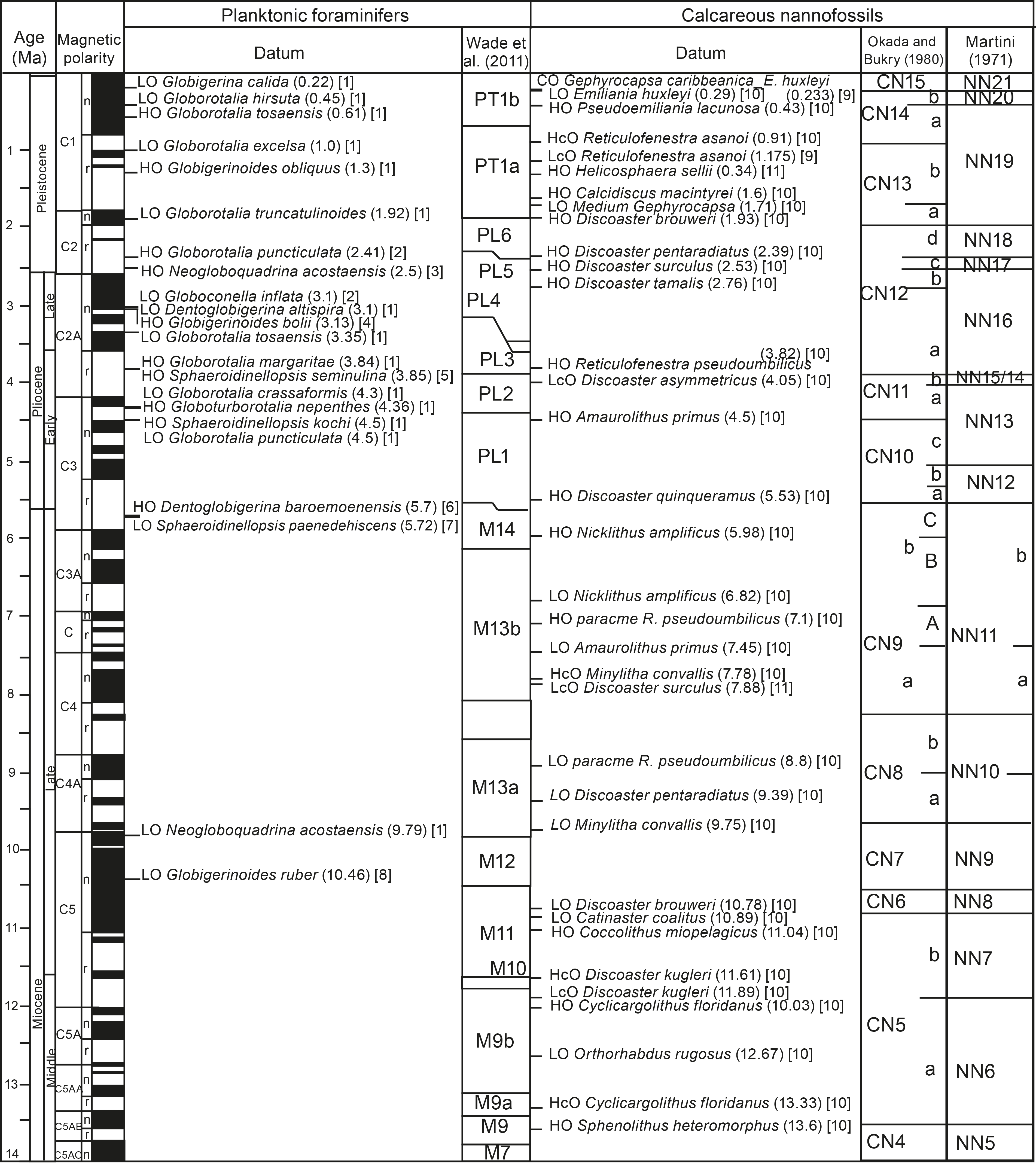
Figure F7. Correlation of GPTS, biostratigraphic zonation, and biohorizons used during Expedition 397.
The concept of acme (dominance interval) and paracme (absence interval) was also applied.
Details of the shipboard methods are described below for each microfossil group.
3.1. Calcareous nannofossils
Calcareous nannofossil bioevent ages were assigned based on the occurrence of calcareous nannofossils (relative abundance) in core catcher samples and in selected depths of all sections. Calibration of the identified events was derived mainly from Raffi et al. (2006). Additionally, Martini (1971) and Okada and Bukry (1980) standard zonal schemes were adopted.
The change in abundance of large Emiliania huxleyi (>4 µm), which characterizes Termination 1 in mid- to low-latitude water masses in the northeast Atlantic Ocean (Flores et al., 2010), was utilized.
Gephyrocapsa and Reticulofenestra species are grouped in several size categories (see Table T2). Specimens of Reticulofenestra that are <3 µm in size are referred to as “small Reticulofenestra;” specimens that are 3–5 µm in size are referred to as “medium Reticulofenestra.” Reticulofenestra specimens that are >6 µm in size are considered “large Reticulofenestra.”
Morphometric subdivision within Calcidiscus leptoporus s.l. and Coccolithus pelagicus s.l. complexes is used according to the taxonomy of Klejine (1993), Knappertsbusch et al. (1997), Steel (2001), Geisen et al. (2002), Quinn et al. (2003, 2004), and Parente et al. (2004).
Pliocene and Miocene events are mainly characterized by ceratolith and discoaster species, as well as variability in size of Reticulofenestra morphotypes (Raffi et al., 2006). Otherwise, taxonomic concepts for Neogene taxa were adopted from Perch-Nielsen (1985) and Young et al. (2022).
The Miocene/Pliocene boundary is a remarkable event in the Mediterranean Sea because it marks the Pliocene flooding after the Messinian Salinity Crisis, astronomically dated at 5.33 Ma (Hilgen, 1991), and the recovery of open marine deep-sea microfauna in the Mediterranean. However, its identification in the Atlantic Ocean is problematic because no major environmental change occurred in this area at this time. The location of this boundary is not well constrained because no bioevent has been identified within this time interval. Nevertheless, the biohorizons of the LO of Ceratolithus acutus and the HO of Discoaster quinqueramus, occurring at 5.34 and 5.54 Ma, respectively, may be used to approximate the boundary in the Atlantic.
The Pliocene/Pleistocene boundary has been formally established at 2.588 Ma at the boundary between the Piacenzian and Gelasian, located just above the Matuyama/Gauss magnetic reversal within Marine Isotope Stage 103 (Gibbard et al., 2010). The boundary can be approximated by the HO of Discoaster surculus (2.53 Ma) and the HO of Globorotalia puncticulata (2.41 Ma) (Figure F7).
3.2. Foraminifers
Foraminifer biostratigraphic events and their designations are derived mainly from Wade et al. (2011, 2018), BouDagher-Fadel (2015), King et al. (2020), and Gradstein et al. (2020) and references therein (Figure F7).
The taxonomic concepts of planktonic foraminifer species are based on Kennett and Srinivasan (1983), Hemleben et al. (1989), Spezzaferri et al. (2018), Schiebel and Hemleben (2017), and Poole and Wade (2019). Globigerinoides extremus is lumped into Globigerinoides obliquus because of the difficulty of distinguishing the two species in sediments from Atlantic regions. We also decided to use Neogloboquadrina pachyderma (dextral) instead of Neogloboquadrina incompta.
Benthic foraminifers provide limited control of biostratigraphic age. Only “Stilostomella extinction” can potentially be used. This extinction is marked by the disappearance from the world ocean of a large number of species of deep-sea foraminifers of Stilostomellidae, Pleurostomellidae, and Nodosariidae. A pulsed decline of these foraminifer groups would have started at ~1.2 Ma, and the final extinction of Stilostomella would have occurred between 0.7 and 0.58 Ma (e.g., Hayward, 2002; Kawagata et al., 2005). Generic-level taxonomic assignments of benthic foraminifer species are based on Loeblich and Tappan (1988) with updates from Hayward (2002).
3.3. Ostracoda
Ostracods provided no biostratigraphic control but were examined and recorded at every site for paleobathymetric an paleoenvironmental purposes. Taxonomic assignments follow Breman (1978), Colalongo and Pasini (1980), Faranda et al. (2008), Alvarez Zarikian (2009), and Yasuhara and Okahashi (2014, 2015).
3.4. Sample preparation methods
3.4.1. Calcareous nannofossils
Calcareous nannofossil samples were prepared following the standard smear slide technique with Norland optical adhesive. Calcareous nannofossils were examined with a Zeiss polarized microscope at 1000× magnification.
Preservation includes effects of dissolution and overgrowth. Preservation of calcareous nannofossils was categorized as follows:
- G = good (little or no evidence of dissolution and/or overgrowth; specimens are identifiable to the species level).
- M = moderate (minor to moderate dissolution and/or overgrowth; most specimens are identifiable to the species level).
- P = poor (extreme dissolution and overgrowth; some specimens are identifiable to the species level).
Total abundance of calcareous nannofossils was categorized as follows:
- VA = very abundant (>100 specimens per FOV).
- A = abundant (11–100 specimens per FOV).
- C = common (1–10 specimens per FOV).
- F = few (1 specimen per 2–10 FOVs).
- R = rare (1 specimen per ≥11 FOVs).
- B = barren.
Abundances of individual taxa or groups of calcareous nannofossils were categorized as follows:
- D = dominant (>20 specimens per FOV).
- A = abundant (11–20 specimens per FOV).
- C = common (1–10 specimens per FOV).
- F = few (1 specimen per 2–10 FOVs).
- R = rare (1 specimen per ≥11 FOVs).
- P = present (abundance not quantitatively determined).
3.4.2. Foraminifers
For counting planktonic and benthic foraminifers, 20–30 cm3 of sediment from each core catcher was analyzed. Unlithified sediment samples were soaked in tap water and washed through a 63 µm sieve. In addition, mudline samples were taken from most of the holes and used for ecological study. These samples were collected by emptying the sediment/water material from the top casing of the core from each hole into a bucket. Rose bengal was used to detect living foraminifers.
The washed samples were dried at 60°C. Dry residues larger than 63 µm were sieved again over a 150 µm screen. Samples were split into subsamples to obtain at least 300 specimens of planktonic foraminifers. The entire sample was examined when it contained fewer planktonic foraminifer specimens.
The samples were analyzed under Zeiss Discovery V8 and Zeiss Stemi SV11 stereomicroscopes. To avoid contamination between successive samples, the sieves used for wet sieving were cleaned in an ultrasonic bath for several minutes, and those used for dry sieving were cleaned with compressed air.
Planktonic and benthic foraminifer abundance in the >150 µm fraction in relation to the total residue of each sample was categorized as follows:
- D = dominant (>30%).
- A = abundant (>10%–30%).
- F = few (>5%–10%).
- R = rare (1%–5%).
- P = present (<1%).
- B = barren.
Relative abundance of individual taxa or groups of foraminifers was characterized as follows:
- D = dominant (>30%).
- A = abundant (>10%–30%).
- F = few (>5%–10%).
- R = rare (1%–5%).
- P = present (<1%).
The state of preservation is defined including the effects of diagenesis, epigenesis, abrasion, encrustation, and/or dissolution. The preservation of planktonic and benthic foraminifers was classified as follows:
- VG = very good (no evidence of breakage or dissolution).
- G = good (only very minor dissolution and no recrystallization; <10% of specimens broken).
- M = moderate (frequent etching and partial breakage; 30%–90% of specimens unbroken).
- P = poor (much dissolution and recrystallization; broken specimens dominate).
Scanning electron microscopy (SEM) is used to confirm and document the potential dissolution of some specimens.
3.4.3. Ostracoda
Ostracods were picked, counted, and identified only in the >250 µm sediment grain size fraction of all samples analyzed for foraminifers using a Zeiss Discovery V8 stereomicroscope. Ostracod abundance was defined by the number of valves (carapaces were counted as 2 valves) per sample as follows:
- A = abundant (>50 valves).
- C = common (≥20–50 valves).
- F = few (5–20 valves).
- R = rare (<5 valves).
- B = barren (no specimens in the entire sample).
Ostracod preservation was defined as follows:
- VG = very good (valves translucent; no evidence of overgrowth, dissolution, or abrasion).
- G = good (valves semitranslucent; slight evidence of overgrowth, dissolution, or abrasion).
- M = moderate (common but minor calcite overgrowth, dissolution, or abrasion).
- P = poor (substantial overgrowth, dissolution, or fragmentation of the valves).
3.5. Paleoenvironment
All examined microfossil groups allow characterization of paleoenvironmental conditions such as changes in water masses, water depth, and seawater temperature and to identify intervals of varying marine productivity (e.g., Colmenero-Hidalgo et al., 2004; Baumann et al., 2005; Narciso et al., 2006; Kucera, 2007; Salgueiro et al., 2010; Ruiz et al., 2008; Alvarez Zarikian et al., 2009). Changes in abundance and preservation of assemblages are related to hydrographic parameters such as salinity, temperature, and oxygen saturation conditions. Variations in benthic foraminifer assemblages are very useful as proxies for deepwater circulation, food availability, oxygen content, water depth, and other physicochemical properties (e.g., Murray, 2006; Jorissen et al., 2007). In particular, their variations along the Iberian continental margin may have been controlled by the interplay between surface productivity and changes in the relative proportions of deepwater masses prevailing in the area (i.e., North Atlantic Deep Water, Antarctic Bottom Water, or Mediterranean Outflow Water) (e.g., Schönfeld and Zahn, 2000).
4. Paleomagnetism
Paleomagnetic studies during Expedition 397 focused on measuring the natural remanent magnetization (NRM) of archive-half sections before and after alternating field (AF) demagnetization using the shipboard 2G Enterprises Model 760R-4K superconducting rock magnetometer (SRM). We used AF with peak fields up to 20 mT to remove drilling-induced overprint and identify the direction of characteristic remanent magnetization (ChRM). The acquired paleomagnetic directional data (excluding those from disturbed/void intervals and section ends) were matched to a GPTS (Ogg, 2020) to construct magnetostratigraphy for the cored sediment sequences.
We collected discrete cube samples from working-half sections, typically two to four samples per core in selected holes from Sites U1586 and U1587 and about one sample per core in selected holes from Sites U1385 and U1588. NRM of discrete samples was measured before and after stepwise AF demagnetization with peak fields up to 50 or 80 mT using either the SRM with in-line AF demagnetizer or the AGICO JR-6A spinner magnetometer with a D-Tech Model D-2000 AF demagnetizer. The detailed and more complete NRM demagnetization data of the cube samples were used to help verify and improve the archive-half data-based magnetostratigraphy.
4.1. Instrumentation tests
Prior to coring operations, we conducted tests to check the spatial resolution and response function of the SRM and compare background noise levels and measurements made on the SRM and the JR-6A spinner magnetometer. Our tests included (1) calibrating the JR-6A spinner magnetometer and using it to repeatedly measure the calibration sample and a random selection of 10 empty plastic cubes used for discrete sampling (i.e., 7 cm3 Natsuhara-Giken sampling cubes), (2) repeatedly measuring the continuous sample tray as an archive-half sample using the SRM, (3) repeatedly measuring the discrete sample tray with empty cubes as working-half cube samples using the SRM, and (4) repeatedly measuring the JR-6A calibration sample on the SRM over a 50 cm interval at every 0.2 cm resolution while it is oriented parallel/antiparallel to each of the three SRM measurement axes.
The JR-6A calibration sample from AGICO is a magnetized thin wire embedded in the center of an 8 cm3 transparent cube. It contains a dipole-like remanence (intensity = 7.99 A/m) pointing toward the center of one of the cube surfaces. We calibrated the JR-6A using the calibration sample and then repeatedly measured the calibration sample five times. This was followed by measurement of 10 randomly selected empty cubes (the type we used for discrete sampling). The repeated measurements of the calibration sample yielded a mean intensity of 8.01 A/m with standard deviation of 1.17 × 10⁻² A/m. The empty cube measurements yielded a mean intensity of 1.99 × 10⁻⁵ A/m with standard deviation of 1.85 × 10⁻⁵ A/m, suggesting the practical noise level of sample measurements on the JR-6A is probably on the 10−5 A/m level or above (e.g., due to inaccuracy in positioning the samples in the holder).
For the SRM continuous tray measurement test, we cleaned the tray using glass cleaner, AF demagnetized the tray with 80 mT peak field, and conducted a background measurement. We then measured the empty continuous tray as a 1.5 m long archive-half sample five times. Measurements were made at 2 cm intervals and used a leader and trailer length of 14 cm (same as that used for most core section measurements during the expedition). Drift- and background-corrected magnetic moment along the three axes is within ±1 × 10⁻⁹ Am2 and mostly varies around ±0.3 × 10⁻⁹ Am2 (Figure F8). The Z-axis measurement appears to be noisier than those of the X- and Y-axis. Using a standard section-half cross area of 17.5 cm2 and effective lengths of 7.30, 7.30, and 9.00 cm along the X-, Y-, and Z-axis measurements, the intensity of the repeated empty tray measurements (after drift and background correction) is mostly <0.4 × 10⁻⁵ A/m and reaches up to ~1 × 10⁻⁵ A/m. The practical SRM measurement noise level is therefore on the 10−5 A/m level for section-half measurements.
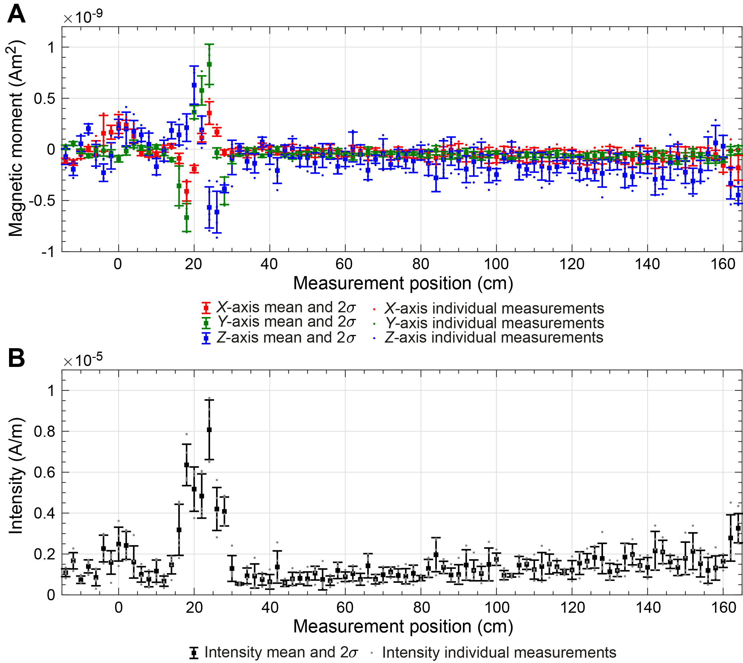
Figure F8. Section-half SRM noise level.
Prior to the SRM discrete tray measurement test, we cleaned and AF demagnetized the discrete tray (with 80 mT peak field) and conducted a background measurement. We then placed empty cubes at the seven measurement positions on the discrete tray (i.e., at 13, 33, 53, 73, 93, 113, and 133 cm) and repeatedly measured each of the seven empty cubes 10 times. In total, 3 out of the 10 repeated measurements experienced flux jumps on the Z-axis (~4 × 10⁻⁸ Am2 level) and were not used for further analysis. Drift- and background-corrected magnetic moment of the remaining measurements is within ±1 × 10⁻⁹ Am2 (Figure F9A), similar to those of the continuous tray test. The intensity of the repeated discrete tray with empty cubes measurement is mostly <1.5 × 10⁻⁴ A/m (Figure F9B), which should be the approximate noise level for cube measurement on the SRM.
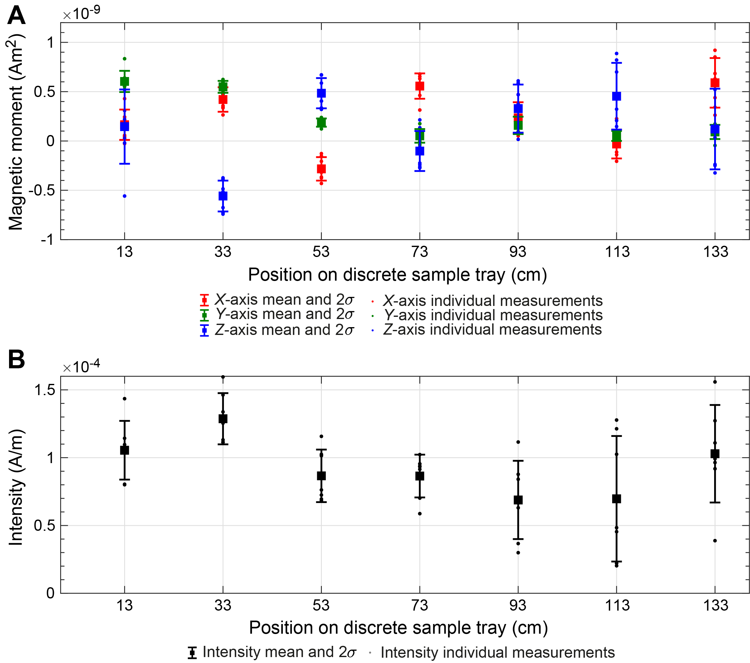
Figure F9. Discrete cube SRM noise level.
To facilitate measurement of the JR-6A calibration sample on the SRM, we 3-D printed a holder (see Figure F10A, F10B) to position the calibration sample so that its center is 20 cm away from the SRM measurement start line and 2.1 cm above the bottom of the tray (i.e., center of mass on the cross-section of a half-round core with 7.2 cm diameter). The 3-D printed holder allows accurate orientation of the remanence signal parallel/antiparallel to each of the three SRM measurement axes. We measured the calibration sample as a 40 cm long archive-half section with leader and trailer length of 5 cm (total = 50 cm) at every 0.2 cm resolution. We repeatedly measured the sample while orienting its remanence signal toward/opposite to the +X-, +Y-, and +Z-directions (total = six orientations) of the archive-half measurement coordinates of the SRM (Figure F10A). For each of the six orientations, we collected measurements four times after rotating the sample in 90° steps using that orientation as the rotation axis. We flipped data measured while the sample was oriented toward the −X-, −Y-, and −Z-directions and plotted all 24 runs of data as gray dots in Figure F10C. As a result, each of the nine terms of the SRM sensor response (i.e., XX, XY, XZ, YX, YY, YZ, ZX, ZY, and ZZ, where AB means B-axis response while remanence signal is oriented toward A-axis; A, B = X, Y, or Z) has eight runs of data. These data fall close to one another, and we use the mean of these data (colored curves in Figure F10C) as an estimate of the SRM sensor response function.
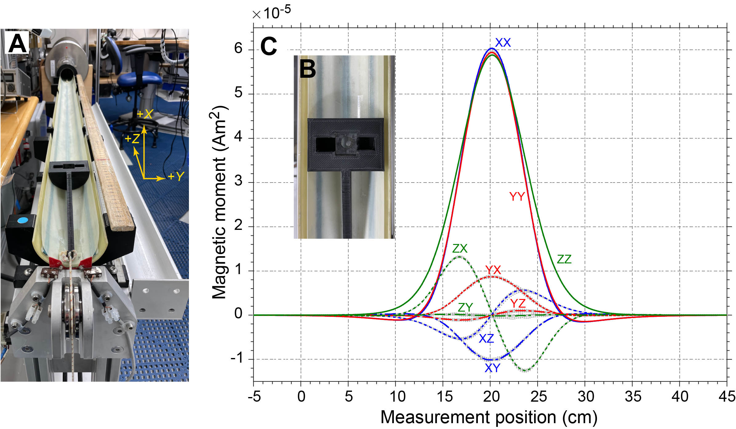
Figure F10. SRM sensor response function.
The peaks of XX, YY, and ZZ response terms occur at 20.2 cm, suggesting the SRM track positions are fairly accurate. Peak magnetic moment of XX, YY, and ZZ terms are 6.04 × 10⁻⁵, 5.94 × 10⁻⁵, and 5.88 × 10⁻⁵ Am2, which are about 5.5%, 7.0%, and 8.0% smaller than the expected values of 6.39 × 10⁻⁵ Am2 (i.e., 7.99 A/m × 8 × 10⁻⁶ m3), respectively. Full widths at half maximum for XX, YY, and ZZ terms are 7.23, 7.25, and 8.17 cm, respectively. Cross-term responses appear to be significant (Figure F10C). The effective lengths for XX, XY, XZ, YX, YY, YZ, ZX, ZY, and ZZ terms are 7.09, −1.15, 0.03, 1.05, 7.15, −0.01, 0.09, 0.01, and 8.90 cm, respectively. More accurate estimates of the SRM sensor response will require the integration of repeated measurements of a magnetic point source while placing it at different positions on the cross-section of a half-round core (see Xuan and Oda, 2019).
4.2. Core collection and orientation
Cores were collected using nonmagnetic core barrels for the APC and HLAPC systems. Nonmagnetic core barrels are more brittle than standard core barrels and are not used with the XCB system (see JOIDES Resolution standard coring systems). The BHA included a monel (nonmagnetic) drill collar. This collar is required when the Icefield MI-5 core orientation tool is used. During Expedition 397, this collar was used for all APC, HLAPC, and XCB cores (even when the Icefield MI-5 was not used) because it can potentially reduce the magnetic field in the core barrel and near where the core is cut.
The Icefield MI-5 can only be used with APC core barrels. It uses three orthogonally mounted fluxgate magnetometers to record the orientation of the multiple toolface (MTF) with respect to magnetic north. The MTF is aligned with the double lines scribed on the core liner. The tool declination, inclination, total magnetic field, and temperature are recorded internally at regular intervals until the tool’s memory capacity is filled. For a measurement interval of 10 s, which was used during Expedition 397, the tool can typically be run for ~24 h, although we aimed to switch tools every ~12 h. Prior to firing the APC, the core barrel is held stationary (along with the pipe and BHA) for several minutes. During this time, data are recorded to constrain the core orientation. When the APC fires, the core barrel is assumed to maintain the same orientation, although the core barrel can rotate and/or the core liner can twist as it penetrates the sediment. The orientation correction that converts the observed declination (Dobs) to a true declination (Dtrue) is given by the following formula:
where MTF is the magnetic tool face angle from the Icefield MI-5 and Damb is the ambient geomagnetic field declination at the drill sites.
The 2020 International Geomagnetic Reference Field (IGRF) declination values for Sites U1385, U1586, U1587, and U1588 are −1.78°, −1.97°, −1.86°, and −1.59°, respectively. We report orientation angle estimated from the Icefield MI-5 (MTF) for all oriented cores of each site as a table in the site chapters.
4.3. Archive-half measurements
NRM measurement of the archive-half sections using the SRM was controlled by the shipboard Integrated Measurement System (IMS) software (version 13). We cleaned the SRM sample tray with glass cleaner at the beginning of every working shift (every ~12 h), at the start of new holes, or as deemed necessary. The sample tray was then AF demagnetized and measured using the section background routine to maintain accurate tray correction values that were applied to each measured core section. We used AF with an 80 mT peak field to demagnetize the tray at the beginning of Expedition 397. A software and hardware communication issue caused the SRM in-line degauss coils to overheat. Tests conducted after the coils cooled down suggested the coils were performing normally, but the maximum peak field for AF demagnetization was limited to 50 mT to avoid potential damage to the SRM in-line degauss coils. We used AF with a 40 mT peak field to demagnetize the SRM sample tray afterward. For all section-half measurements, track speed was set to 10 cm/s, data acquisition was set for no averaging, and 1 Hz data filtering with 1000 ms settling time was used.
For archive halves from most of the holes recovered during Expedition 397 (i.e., all holes at Sites U1586 and U1587 and Holes U1385F, U1385G, and U1588A), SRM measurements were made at 2 cm resolution along the core section and for a 14 cm leader interval and a 14 cm trailer interval. Measurements from the leader and trailer intervals immediately before and after the sample serve the dual function of monitoring the background magnetic moment and allowing for future deconvolution analysis. We typically measured the NRM of archive halves before and after AF demagnetization with a peak field of 20 mT. Some sections were measured using more detailed (3–5) demagnetization steps (e.g., 0, [5], 10, [15], and 20 mT [steps in brackets are not always carried out]) to check if a lower demagnetization level would be sufficient to remove the drilling-induced overprint. Measurement of a 1.5 m long core section at 2 cm resolution (with 14 cm leader and trailer intervals) before and after 20 mT demagnetization takes ~9 min and 20 s. The core flow (the analysis of one core after the other) through the laboratory dictates the available time for measurements. When core flow increased, we either prioritized and only measured NRM after the 20 mT demagnetization step at 2 cm resolution (e.g., for some cores from the low sedimentation rate sites) or we measured NRM before and after 20 mT demagnetization at 4 cm resolution (e.g., for some cores from the higher sedimentation rate sites). For a 1.5 m core section, it takes ~6 min to measure NRM at 2 cm resolution (with 14 cm leader and trailer intervals) after only 20 mT demagnetization and ~6 min and 40 s to measure NRM at 4 cm resolution (with 12 cm leader and trailer intervals) before and after 20 mT demagnetization.
SRM data are reported relative to IODP orientation conventions: +X-orientation points into the face of the working half (toward the double line or away from the single line), +Y-orientation points toward the left (right) side of the working (archive) half when looking downcore, and +Z-orientation is downcore (see Figure F11A, F11B). The shipboard IMS software registers the orientation of the archive- and working-half samples and automatically converts the SRM measurement coordinates accordingly (see Figure F11C). SRM data were stored using the standard IODP file format and automatically uploaded to the LIMS database.
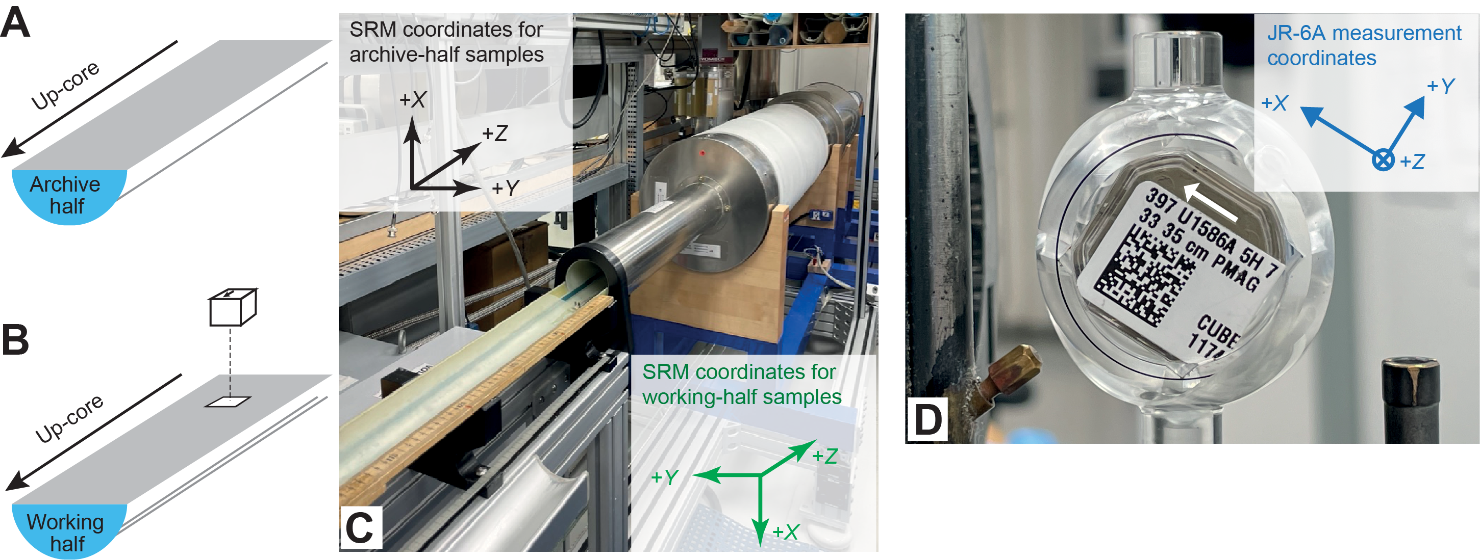
Figure F11. SRM and JR-6A spinner magnetometer sample measurement coordinates.
4.4. Discrete cube samples and measurements
During Expedition 397, we collected oriented discrete cube samples from working-half sections from selected holes at each site for detailed and more complete AF demagnetization experiments to help verify and improve the archive-half data-based magnetostratigraphy. We typically collected two to four cube samples per core from selected holes at Sites U1586 and U1587 and one cube sample per core from selected holes at Sites U1385 and U1588. Samples were taken using plastic Natsuhara-Giken sampling cubes, which have a 2 cm external edge length and an internal volume of ~7 cm3. Cube samples were taken from the center of working halves and away from disturbed sediments near the core liner. We avoided sampling sections and intervals that were visually disturbed. For biscuited XCB cores (see Lithostratigraphy), cube samples were taken from the centers of biscuits. For the top few cores from the selected holes where sediments are soft, we pushed the cubes directly into the section with the arrow marker on the cube pointing toward the stratigraphic up direction. We collected most cube samples by pushing a hollow metal tube into the working-half section and then extruding the sample onto a clean flat surface before we fit the sample into the cube. This ensures cube samples collected using either method (i.e., directly pushed into the section or extruded from the hollow metal tube) have consistent orientation.
Depending on the core flow and availability of the SRM, we used either the SRM with in-line AF demagnetizer or the JR-6A spinner magnetometer with a D-Tech Model D-2000 AF demagnetizer for NRM measurement of the cubes before and after stepwise AF demagnetization with peak fields up to 50 or 80 mT. For measurement using the JR-6A spinner magnetometer, NRM of cube samples was measured after stepwise demagnetization with peak fields of 0, (5), (8), 10, (15), 20, (25), 30, (35), 40, (45), 50, 60, (70), and 80 mT. Demagnetization was carried out manually in three axes using a D-Tech Model D-2000 AF demagnetizer. Demagnetization steps in parentheses were not always included for all samples depending on sample demagnetization behavior and/or time available. For measurement on the JR-6A spinner magnetometer, cubes were positioned in the sample holder so that the surface with the arrow marker faced the user and the arrow marker pointed toward the top left (Figure F11D). Measurements on the JR-6A were controlled by AGICO Remasoft (version 6.0) using the following settings for all cube measurements:
JR-6A data were manually uploaded to the LIMS database.
The majority of cube samples were measured on the SRM after stepwise AF demagnetization with peak fields of 0, 2, 4, 6, 8, 10, (12) 15, (18), 20, (22), 25, (28), 30, (32), 35, (38), 40, (42), 45, (48), 50, (55), (60), (70), and (80) mT (steps in parentheses were not always included). The cube samples were placed on the SRM discrete sample tray so that the surface with the arrow mark (also the surface of working-half sections) was on top and the arrow mark pointed away from the SRM (Figure F11B, F11C). The NRM of some cube samples (i.e., those from Holes U1586A and U1586B) was measured on the SRM with demagnetization up to 80 mT, and the rest of the cube samples measurements on the SRM only used demagnetization up to 50 mT. Measurements on the SRM appear to be frequently compromised by flux jumps along the Z-axis just before sample measurements start (potentially because of antenna effect when the sample tray was moving into the SRM sensor area). The jumped values occur on all seven cube samples measured in the same batch and are usually ~4 × 10⁻⁸ Am2 (possibly due to the jump of one flux count on the SRM Z-axis that is equivalent to 3.8825 × 10⁻⁸ Am2). These flux jumps can significantly affect the measurement of samples that carry weak magnetization. We removed SRM measurements compromised by flux jumps from further analyses. For samples measured with demagnetization up to 50 mT, we used a demagnetization sequence with 22 steps to ensure enough measurement data remained after removing those influenced by flux jumps (two to six steps of data often need to be removed).
4.5. Data filtering and magnetostratigraphy
We processed archive-half data extracted from the shipboard LIMS database by removing all measurements collected from (1) void intervals caused by whole-round core sampling (i.e., IW and paleontology [PAL] samples), (2) disturbed core top intervals in APC cores, and (3) the top and bottom 6 cm of each section and an extra 6 cm for the void and disturbed core top intervals, which are subjected to edge effects due to convolution of the SRM sensor response with the sample remanence signal (Figure F10C; see Instrumentation tests). The disturbed core top intervals were recognized based on inspection of the section-half image and NRM (after 20 mT demagnetization) directional and intensity data. Disturbed intervals are often characterized by sudden large increases in intensity accompanied by abnormal changes in declination and/or inclination and are often longer than what is apparent from the section image. We summarize the disturbed core top intervals in a table in each site chapter. Sediment disturbance due to coring or geologic processes (slumping, faulting, etc.) often leads to distorted and unreliable paleomagnetic directions. We mark intervals described as slump or severely/strongly disturbed during coring (see Lithostratigraphy) and do not use data from these intervals for magnetostratigraphic interpretations.
We combine NRM (after 20 mT demagnetization) inclination and declination data from archive-half sections and stepwise NRM demagnetization (up to 50 or 80 mT) data from cube samples to make magnetostratigraphic interpretations. For cores with Icefield MI-5 orientation data, declinations were first corrected for core orientation. Magnetostratigraphy for each site was constructed by matching the magnetozones with the GPTS (Ogg, 2020) of the Geologic Time Scale 2020 (GTS2020) (Gradstein et al., 2020). We summarized GPTS over the last 40 My in Figure F12. Correlation to the GPTS was assisted by discussion with the shipboard biostratigraphy team, and stratigraphic correlation enabled the assessment of magnetostratigraphic results across holes at each site.
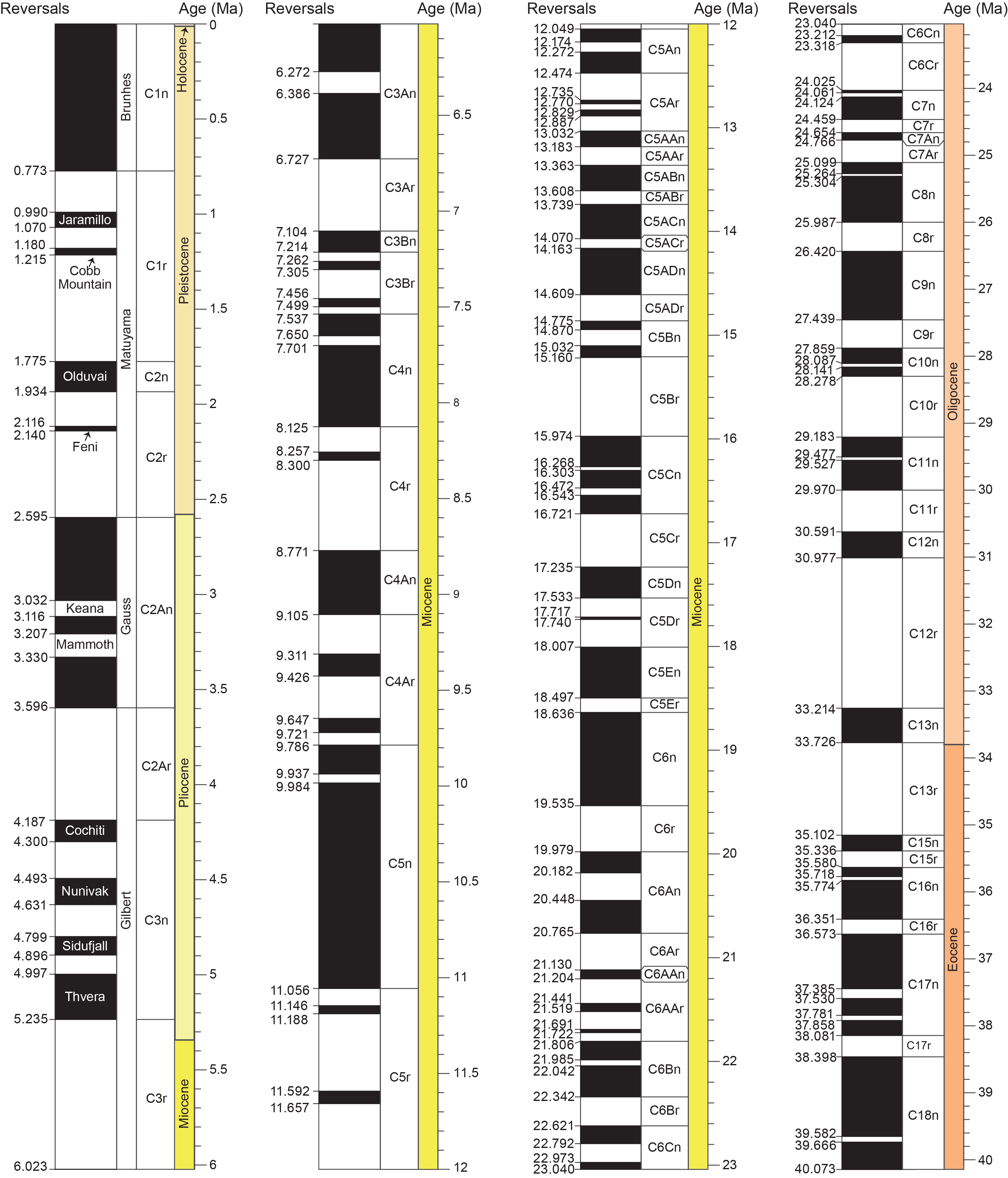
Figure F12. GPTS used during Expedition 397.
5. Geochemistry
The shipboard geochemistry program for Expedition 397 included analyses of headspace gases (hydrocarbons), IW (pH, alkalinity, chlorinity, major and minor anions and cations, and nutrients), and bulk sediment (major and minor element concentrations, total inorganic carbon [TIC] and total organic carbon [TOC], total nitrogen [TN], total sulfur [TS], and C/N values). The purpose of these analyses is for routine shipboard safety as well as characterization of sedimentary geochemistry. Additionally, pore water samples were taken using Rhizon samplers for dedicated shore-based analysis.
5.1. Sedimentary hydrocarbon gases
In the first hole at each site (U1586A, U1587A, U1385F, U1588A), volatile hydrocarbons (C1–C6) were sampled approximately once per core (or once every other half core) at the top of the last section (Figure F13) to ensure their concentrations did not exceed safe limits while drilling. If a subsequent hole that extended deeper than the first hole was drilled, additional gas sampling was conducted starting from the basal depth of the previous hole(s). Immediately following core retrieval, ~5 cm3 of retrieved sediment was sealed in a 21.5 cm3 glass serum vial using a Teflon/silicone septum and aluminum crimp cap and heated at 70°C for 30 min to exsolve gases. If expansion voids or pockets appeared in the core while it was still in the liner, the liner was punctured and a heavy-duty syringe was used to extract gas.
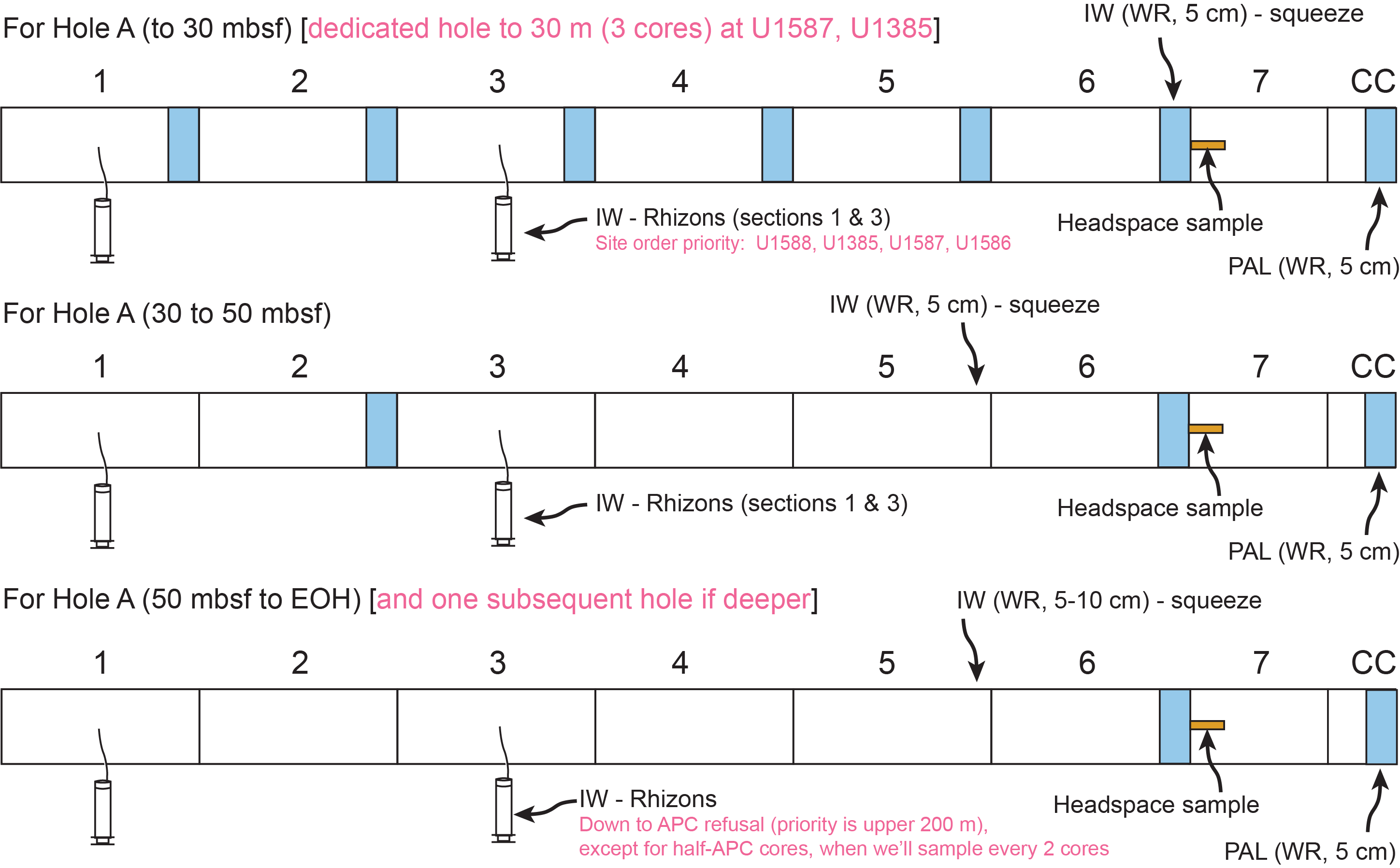
Figure F13. Catwalk geochemistry sampling.
A 5 cm3 aliquot of gas was removed from the headspace vial with a gas-tight glass syringe and injected onto an Agilent 6890 gas chromatograph with a flame ionization detector (250°C) equipped with a stainless-steel column (2.4 m × 3.2 mm internal diameter) packed with HayeSep R, 80/100 mesh, using helium as carrier gas. The oven temperature program was as follows: hold for 8.25 min at 80°C, increase to 150°C at 40°C/min, and hold for 5 min at 150°C (15 min total). Helium flow began at 30 mL/min and increased to 60 mL/min after 8.25 min to accelerate elution of propane and propylene.
Standards with known concentrations of methane (C1), ethane (C2), ethene (C2=), propane (C3), and propene (C3=) produced by Scott Specialty Gases (Air Liquide) were injected at the start of the expedition to quantify concentrations (parts per million by volume [ppmv]) of headspace gases. Peak areas were quantified using Agilent Chemstation software.
5.2. Interstitial water sampling
5.2.1. Whole-round squeeze sampling
Standard IW sampling was performed on 5–10 cm whole rounds with higher-resolution sampling near the top of the hole. Samples were taken at the bottom of each section in the uppermost 3 cores (down to ~30 mbsf), then at the bottom of Sections 2 and 6 in the proceeding 2 cores (~30–50 mbsf), and finally at the bottom of Section 6 to the end of hole (Figure F13). Sampling was performed in Hole A and in any subsequent hole that extended deeper than Hole A, except for Site U1385, which was sampled in Hole G (due to previous occupation of the site during Expedition 339 that drilled Holes U1385A–U1385E). No acetone was used to seal end caps until whole rounds were removed from the catwalk.
In the geochemistry laboratory, sediment from the whole-round sections was extruded from core liners and the outermost ~1 cm of sediment was removed from all sides to minimize potential contamination from drill fluid. Cleaned sediment was placed into Manheim titanium squeezers and compressed at ambient temperature using a Carver hydraulic press (Manheim and Sayles, 1974), typically reaching pressures up to 200 MPa and occasionally as high as 300 MPa, if needed. IW samples discharged from the squeezer were passed through 0.45 µm polyethersulfone membrane filters, collected in acid-cleaned plastic syringes, and stored in plastic sample tubes for shipboard analyses. IW was divided as follows in order of priority for shipboard and shore-based analysis:
- Shipboard analyses:
- 30 µL for salinity determined by optical refractometry immediately after squeezing.
- 3 mL for pH and alkalinity determined by hydrochloric acid (HCl) titration immediately after squeezing.
- 150 µL for chlorinity determined by AgNO3 titration immediately after squeezing.
- 100 µL for major and minor cations/anions (SO42−, Mg2+, Ca2+, Na+, K+, Br−, and Cl−) by ion chromatography (IC).
- 600 µL for phosphate (PO43−) and 200 µL for ammonium (NH4+) determined by spectrophotometry.
- 2 mL for major (Ca2+, K+, Mg2+, and Na+) and minor (B, Ba2+, Fe2+, Li+, Mn2+, P, Si, Sr2+, and S) element analysis using ICP-AES. This aliquot was preserved with trace metal HNO3 to ensure all elements remained in solution.
- Postcruise onshore analyses (volume permitting):
- 10 mL for rare earth element (REE) analysis. This aliquot was acidified with 30 µL optima HCl and stored in acid-cleaned high-density polyethylene (HDPE) bottles.
- 4 mL for Si isotope analysis. This aliquot was acidified with 20 µL optima HCl and stored in acid-cleaned HDPE bottles.
- 2 mL for paired stable Sr and Ca isotopes analysis. This aliquot was acidified with 10 µL optima HNO3 and stored in an acid-cleaned HDPE bottle.
- 2 mL for sulfur (S) and possibly carbon isotope analysis. This aliquot was fixed with 10 µL of 100% HgCl2 and flame-sealed into glass ampoules for storage.
If total volume collected was <26 mL, the shore-based REE sample was omitted to prioritize shipboard data collection.
Following squeezing, 10–25 cm3 of sediment was removed from the squeeze cake (~¼ of the squeeze cake), placed in a heat-sealed bag that was flushed with nitrogen, and stored frozen for dedicated shore-based analysis. If a sample was taken for REEs, another 10–25 cm3 of sediment (~¼ of the squeeze cake) was also collected for shore-based analysis. Two additional 10–25 cm3 aliquots of sediment (~¼ of the squeeze cake each) were taken for postcruise analyses for barite contents and organic biomarker concentrations.
5.2.2. Rhizon sampling
Rhizon samples were taken for shore-based analysis by suction filtration through inert porous polymer filters (mean pore diameter = 0.15 µm) into 10 mL syringes. Rhizon samplers were inserted directly into the sediment through holes drilled in the core liner along the core splitting line at the midpoint of Sections 3 and 5 from Hole B, C, or D. Rhizon samplers were connected to syringes using a Luer-lock syringe, which was pulled to create a vacuum, held open using a wood spacer, and left in sediment until at least 2 mL of fluid was extracted. Sampling targeted the upper 200 m of sediment, but Rhizon samples were taken until the depth at which sediment compaction prevented the acquisition of 2 mL of pore water.
Following sampling, retrieved pore water was fixed with 10 µL of 100% HgCl2 and flame-sealed into glass ampoules for storage.
5.3. Shipboard interstitial water analysis
Pore fluid samples were analyzed on board the ship following the protocols in Gieskes et al. (1991), Murray et al. (2000), and the IODP user manuals for new shipboard instrumentation.
5.3.1. Alkalinity, pH, salinity, and chloride
Alkalinity, pH, salinity, and Cl− were measured immediately after squeezing. pH and alkalinity were analyzed on the same aliquot of pore water. First, pH was measured with a combined glass electrode, then alkalinity was determined by Gran titration using an autotitrator (Metrohm 794 Basic Titrino) against 0.1 M HCl at 25°C to an endpoint pH of 4.2. A 3 mL aliquot of pore water was used for each titration. International Association for the Physical Sciences of the Oceans (IAPSO) standard seawater was used for calibration and was analyzed at the beginning and end of a set of samples for each site.
Salinity was measured using a Fisher Model S66366 refractometer. The handheld refractometer was calibrated with 18 MΩ deionized water and standardized using IAPSO standard seawater of known salinity.
Cl concentrations were measured by titration using a Metrohm 785 DMP autotitrator and silver nitrate (AgNO3) solution calibrated against repeated titrations of an IAPSO standard. A 0.15 mL aliquot of sample was diluted with 30 mL of 0.1 M HNO3 and titrated with 0.02 M AgNO3. Repeated analyses of an IAPSO standard yielded a precision better than 2%.
5.3.2. Ion chromatography analysis of sulfate and other major elements
Sulfate (SO42−) and other major elements (Mg2+, Ca2+, K+, Na+, Cl−, and Br−) were analyzed on a Metrohm 850 Professional IC using ~100 µL of pore water that was diluted 1:100 with Milli-Q water. Measurements were standardized using a calibration curve made with serial dilutions of IAPSO seawater.
5.3.3. Nutrients (phosphate and ammonium)
PO4 and NH4 were measured using an Agilent Cary 100 UV-Vis spectrophotometer following the methods of Gieskes et al. (1991).
PO4 concentrations were determined using an antimony-phosphomolybdate complex. A mixed reagent containing ammonium molybdate, sulfuric acid, ascorbic acid, and potassium antimonyl tartrate was added to each sample and left for a few minutes to allow blue color to develop. The color (proportional to PO4 concentration) was then measured at 885 nm. Concentrations were determined using a calibration curve made with serial dilutions of a potassium phosphate monobasic standard (KH2PO4).
NH4 concentrations were determined using an oxidized phenol diazotization method. Samples were diluted with Milli-Q water, mixed with phenol-alcohol and sodium nitroprusside, and then oxidized. After waiting approximately an hour for the color to develop, sample absorbance was measured at 640 nm. Concentrations were determined using a calibration curve made with serial dilutions of an ammonium chloride standard.
5.3.4. ICP-AES measurement of major and minor elements
Dissolved major (Ca2+, K+, Mg2+, and Na+) and minor (B, Ba2+, Fe2+, Li+, Mn2+, P, Si, Sr2+, and S) elemental concentrations were determined using an Agilent 5110 ICP-AES with a SPS4 autosampler following the methods of Murray et al. (2000). The IW aliquot for ICP-AES analysis was diluted 1:10 (v/v) with 2% HNO3 and an internal standard to account for drift during the measurement period as well as any interferences. The internal standard contained 100 ppm beryllium (Be), indium (In), and scandium (Sc) and 200 ppm antimony (Sb). Serial dilutions of IAPSO seawater were run, spanning the concentration range expected for IW up to seawater. A multielement synthetic in-house standard prepared from single-element standards was used to calibrate the ICP-AES for minor elements Mn2+, Fe2+, B, Si, Sr2+, Ba2+, and Li+. Calibrations with IAPSO and in-house standards were performed at the beginning and end of every run. Known concentrations of IAPSO and in-house standards were also run every 8–10 samples to monitor drift and accuracy throughout the measurement period.
Typical internal precision was <3% (standard deviation [σ]). External precision was <3% based on four replicates of the multielement standard. Detection limits for the minor elements are defined here as 3.3 times the σ of the blank intensities converted to concentrations. Multiple wavelengths were measured for each element, and the wavelength reported was chosen based on possible interferences, the linearity of the calibration curve, and the precision and accuracy of IAPSO and in-house standards measured.
5.4. Bulk sediment geochemistry
5.4.1. Total carbon, nitrogen, sulfur, and inorganic and organic carbon content
Total carbon (TC), TN, and TS contents were determined on TIC sample splits using a Thermo Electron Flash EA 1112 CHNS/NCS elemental analyzer with a Thermo Electron packed gas chromatography column (polytetrafluoroethylene; length = 2 m; internal diameter = 6 mm × 5 mm) and thermal conductivity detector (TCD). Approximately 10 mg of sediment was sampled from the working half of split cores following the identification of major lithologies by the sedimentology group. Samples were then freeze-dried, ground, weighed into tin cups into which 1–3 mg of vanadium oxide was added to enhance the oxidation of sulfurous compounds, and combusted in the elemental analyzer reactor oven (1800°C) with a pulse of O2. Nitrogen oxides were reduced to N2, and the resultant gases (N2, CO2, H2O, and SO2) were separated by gas chromatography at 65°C and analyzed by TCD. All materials were calibrated to pure sulfanilamide and NIST Buffalo River Sediment (BRS) standards, run upon arrival at each site. Sulfanilamide and/or BRS were run every 10 samples to test for instrumental accuracy and drift.
Per-site reproducibility of BRS TC, TN, and TS measurements (n = 10–22) was ±0.052 to ±0.074 wt% (±1σ), ±0.009 to ±0.019 wt%, and ±0.073 to ±0.151 wt%, respectively.
TIC content was determined using a UIC Inc. CM 5011 CO2 coulometer coupled with a UIC Inc. CM 5130 acidification module. Approximately 10 mg sediment aliquots were freeze-dried, ground, and reacted with ~5 mL of 2 M HCl. Evolved CO2 was absorbed by a solution containing a colorimetric pH indicator, and the color change was measured by a photodetector for end-point determination. Calcium carbonate (CaCO3) content (expressed as weight percent) was calculated from inorganic carbon content assuming that all CO2 produced was from the dissolution of CaCO3:
A 100% CaCO3 standard was run every 10 samples to test for instrumental accuracy and drift. Per-site reproducibility of CaCO3 measurements was ±0.98 to ±1.81 wt% (1σ; n = 11–19).
TOC content is defined as the difference between TC and TIC:
5.4.2. Major and minor element analysis using ICP-AES
Major (Al, Ca, Fe, K, Mg, Mn, Na, Si, Ti, and P) and minor (Ba, Sr, Zr, Cu, Co, Cr, Ni, V, and Zn) elements in bulk sediment were analyzed using an Agilent 5110 ICP-AES with an SPS4 autosampler using a lithium metaborate flux-fusion method. Several sediment reference materials were also measured during each analytical session.
The homogenized, dried, and ground sediment (100 ± 0.5 mg) was mixed with 400 ± 0.5 mg of lithium metaborate (LiBO2), transferred to a Pt-Au crucible, mixed with 10 mL of 0.172 M LiBr, and fused for 10–12 min at 1050°C in a furnace. After fusion, the resultant bead was cooled and dissolved in 50 mL of 10% trace-metal grade HNO3. A 500 mL aliquot of this solution was diluted in 4.4 mL of 2% HNO3 and spiked with 100 mL of an internal standard containing 100 ppm Be, In, and Sc and 200 ppm Sb prior to analysis with ICP-AES. An aliquot of LiBO2 was processed alone as a procedural blank with each batch of samples. Typical reproducibility was <5% for major elements and <10% for minor elements.
6. Physical properties
Physical properties measurements were made on cores including whole rounds, section halves, and discrete samples. The main objectives include (1) assisting hole-to-hole and site-to-site stratigraphic correlation by detecting discontinuities, heterogeneities, cyclicity, and major seismic reflectors; (2) measuring the lithology- and depth-dependent physical properties to tie paleoenvironmental observations with age models and astronomical cycles; (3) combining thermal properties measured from recovered cores and downhole temperature measurements to infer heat flow; and (4) improving regional lithostratigraphy by integrating new and previous data collected from cores, wireline logging, and seismic survey. Physical properties measurements include NGR; P-wave velocity; bulk, grain, and dry densities; porosity; MS; thermal conductivity; X-ray and photo imaging; and color reflectance.
6.1. General sampling and measurement sequence
The details of core measurements from the equipment used during Expedition 397 are explained in the following sections. Here, we explain the general procedure used to measure physical properties. Only when whole-round P-wave and thermal conductivity were measured were whole-round cores allowed to equilibrate at ambient room temperature (~20°C) and pressure for about 3–4 h prior to analyses. X-ray images of the whole rounds were taken with the X-ray Logger (XMAN), and NGR was determined using the NGRL. Core sections were run through the WRMSL for GRA bulk density and MS. Compressional P-wave velocity was measured using the P-wave logger (PWL). The PWL was disabled for XCB cores and/or cores with severe gas expansion because sediment does not fill the core liner in those cases, which results in poor data. Thermal conductivity was measured on one section per core, typically chosen from the center of APC cores and from Section 1 of XCB cores.
For all holes following Hole A (and Hole U1385F), the WRMSL continued to measure GRA bulk density and MS every 2 cm but the PWL was disabled. X-ray images of whole-round sections were also not taken for every core section but made on request of the scientific team. All core sections continued to be measured for NGR. If requested by the stratigraphic correlators, core sections were run for GRA bulk density and MS through the Special Task Multisensor Logger (STMSL) fast track every 4 cm. Thermal conductivity measurements were not performed on core sections from depth ranges in which sediment had already been recovered.
The archive halves of all cores from all holes were passed through the SHMSL for measurements of MSP and color reflectance.
P-wave velocity was measured on the working-half sections of Hole A cores (or cores from depth ranges recovered for the first time) using the Section Half Measurement Gantry (SHMG). P-wave velocity measurements were made on 1–3 working-half sections per core and were typically chosen from undisturbed areas close to MAD samples, other sections of interest based on lithology variations, and XCB cores for which adequate whole-round measurements were not possible using the PWL.
Discrete samples were collected from Hole A (or cores from depth ranges recovered for the first time) working-half sections with a sampling resolution of typically one per core. These samples were used to measure wet and dry mass and dry volume and to calculate wet bulk density, dry density, void ratio, porosity, and grain density following MAD procedures.
Only raw data, as retrieved from the physical properties instruments, were deposited in the LIMS database. Processing the data according to the information in Processing and data availability is recommended to retain only high-confidence data. Details on the physical properties measurement systems and theory in this section benefited significantly from the extensive methodologies published for previous IODP expeditions (e.g., Tamura et al., 2015; Sun et al., 2018; Sutherland et al., 2019).
6.2. Whole-Round Multisensor Logger measurements
GRA bulk density and MS were measured for all whole-round cores using the WRMSL. Compressional P-wave velocity was also measured using the WRMSL only for cores recovered using the APC system. To optimize the measurement process and for consistency, uniform sampling intervals (2 or 4 cm) and measurement integration times (GRA bulk density = 3 s/measurement; MS = 1 s/measurement) were set for all sensors of the WRMSL. These sampling intervals are common factors for the distances between the sensors installed on the WRMSL (30–50 cm), which allows sequential and simultaneous measurements. Quality control was ensured by running a single core liner filled with deionized water through the WRMSL after every core run. Where deviations from expected values were observed, recalibrations were applied as needed. Both GRA bulk density and MS were also measured under similar analytical conditions using the STMSL, which is equipped in the same line with the XMAN.
6.2.1. Gamma ray attenuation bulk density
Bulk density is a fundamental rock property that can be used to estimate the pore volume in rocks where grain density is either measured or can be reasonably estimated. It is integral to rock physics and core-log-seismic applications. GRA bulk density is an estimate of bulk density based on the attenuation of a gamma ray beam. The beam is produced using a 137Cs gamma ray source at a radiation level of 370 MBq within a lead shield with a 5 mm collimator that is directed through the whole-round core. The gamma ray detector on the opposite side of the core from the source includes a scintillation detector and an integral photomultiplier tube to record the gamma radiation that passes through the core. The attenuation of gamma rays occurs primarily by Compton scattering, in which gamma rays are scattered by electrons in the sample, and the degree of scattering is related to the material bulk density. Therefore, for a known thickness of sample, the density (ρ) is related to the intensity of the attenuated gamma rays and can be expressed as follows:
- I = measured intensity of gamma rays passing through the sample,
- I0 = gamma ray source intensity,
- µ = Compton attenuation coefficient, and
- d = sample diameter.
µ and I0 are treated as constants, such that ρ can be calculated from I.
The spatial resolution of the GRA densitometer is less than ±1 cm. The gamma ray detector is calibrated with sealed calibration cores (one standard core liner filled with distilled water and aluminum cylinders of various diameters). To establish the calibration curves, gamma ray counts were taken through each aluminum cylinder for 60 s. Each aluminum cylinder has a density of 2.7 g/cm3, and d is 1, 2, 3, 4, 5, or 6 cm. The relationship between I and µd is as follows:
where A, B, and C are coefficients determined from the calibration. Recalibration was performed as needed when the deionized water quality control standard density deviated significantly (more than a few percent) from 1 g/cm3.
6.2.2. Magnetic susceptibility
MS (χ) is a dimensionless measure of the degree to which a material can be magnetized by an external magnetic field:
where M is the magnetization induced in the material by an external field of strength H. MS is primarily sensitive to the concentration of ferrimagnetic minerals (e.g., magnetite and maghemite). MS can also give insights into magnetic mineral origins and subsequent diagenetic processes.
MS was measured using a Bartington MS3 susceptometer coupled with a Bartington MS2C loop sensor with an 8 cm internal diameter that comes precalibrated. An oscillator circuit in the sensor, which operates at a frequency of 0.565 kHz and an AF of ~140 A/m, produces a low-intensity, nonsaturating alternating magnetic field. Sediment core sections passing through this field cause a change in oscillator frequency. Frequency information returned in pulse form to the susceptibility meter can then be converted into MS.
During Expedition 397, we examined the response function of the loop sensor by running a straightened staple through the WRMSL, and its MS values were measured at every 2 mm. Through this experiment, we obtained an effective length of ~6.4 cm.
6.2.3 Compressional P-wave velocity
Core measurements of sonic P-wave (compressional) velocity form a vital link for core-log-seismic integration and for the associated scaling up of lithofacies inferences. P-wave velocity can also be used to estimate porosity, especially where downhole conditions are poor (e.g., caved sections), and forms a vital component of geomechanical and stress state calculations. P-wave velocity (VP) is defined by the time required for a compressional wave to travel a specific distance:
where dcore is the path length of the wave across the core and tcore is the traveltime through the core. P-wave velocity was measured on whole-round cores using the PWL. The P-wave velocity systems use Panametrics-NDT Microscan delay line transducers, which transmit a 500 kHz pulse.
The PWL measures the traveltime of 500 kHz ultrasonic waves horizontally across the whole-round core at 2 cm intervals with the core still in the liner. Waves are transmitted to the core by transducer contacts connected to linear actuators. Pressure is applied to the actuators to ensure coupling between the transducers and the core liner, and the space between the core liner and transducers is kept wet to ensure good coupling. P-wave velocity transducers measure total traveltime (t) of the compressional wave between transducers separated by the total distance (d) measured using a laser beam. By measuring the traveltime through a standard block of aluminum with a known velocity (6295 m/s), a system delay correction (δt) is defined. The core is surrounded by a core liner of known thickness (δL), and a traveltime correction (δtL) is determined by measuring the traveltime through the core liner filled with distilled water of known velocity, which is corrected for the influence of temperature. Arrival times are taken for the second lobe of the waveform, requiring a correction (δtpulse) to get the first arrival. The velocity in the core is as follows:
P-wave measurements are not typically made on the WRMSL for cores drilled with the XCB systems because the smaller core diameters generally result in poor contacts and noise.
6.3. Natural Gamma Radiation Logger measurements
NGR data are critical for several aspects of borehole studies, including identification of various lithostratigraphic units, stratigraphic correlation, core-log calibration, and chemical/mineralogic appraisal.
NGR is emitted from the decay of 238U, 232Th, and 40K in the core sample. The NGRL measures gamma emissions on whole-round cores using a system designed and built at Texas A&M University (USA) (Vasiliev et al., 2011; Dunlea et al., 2013). When 238U, 232Th, and 40K radioisotopes decay, NGR is emitted at specific energy levels. NGR spectroscopy measures a wide energy spectrum that can be used to estimate the abundance of each isotope based on the strength of the signal at characteristic energies (Blum, 1997; Gilmore, 2008). NGR spectral data were deconvolved to estimate K, Th, and U concentrations using the Matlab scripts modified after De Vleeschouwer et al. (2017).
The main NGRL detector unit consists of eight sodium iodide (NaI) detectors arranged along the core measurement axis at 20 cm intervals surrounding the lower half of the section (Vasiliev et al., 2011). The detector array has passive (layers of lead) and active (plastic scintillators) shielding to reduce the background environmental and cosmic radiation. The overlying plastic scintillators detect incoming high-energy NGR and cosmic radiation and cancel this signal from the total counted by the NaI detectors. The quality of the energy spectrum measured in a core depends on the concentration of radionuclides in the sample but also on the counting time, with higher times yielding better spectra. During Expedition 397, integration time of gamma ray counting was fixed to 300 s, and the number of measurement positions was switched flexibly between 1 (20 cm resolution) and 2 (10 cm resolution), depending on the frequency of the cores on deck.
The axial length of the response function (visible range) of a NaI detector is ~20 cm (Vasiliev et al., 2011; De Vleeschouwer et al., 2017). When a detector’s visible range is not fully covered by cored material, an edge correction needs to be applied for every section. The edge correction coefficient depends on the distance between a core section’s edge and the center of the last detector directly covered by cored material. For example, when this distance is 0 cm, the NGR spectrum count is multiplied by the edge effect correction coefficient of 2 because only half of the visible range of the detector is covered by cored material. For distances between 0 and 20 cm, the correction factors were empirically determined at 1 cm intervals (Vasiliev et al., 2011). This edge correction is automatically calculated by the IMS. Care should be taken to ensure that the edge effect is accurately corrected because errors can be large when the detector is close to the section edge.
6.4. Thermal conductivity measurements
Thermal conductivity was measured with the TK-04 (Teka Bolin) system. Thermal conductivity defines how material conducts heat and is essential to determine heat flow and geothermal gradient. Thermal conductivity was measured once per core in all Hole A cores (or cores from depth ranges recovered for the first time). To avoid interference from air flow in the laboratory, thermal conductivity measurements were all done in an enclosed foam insulated box.
For soft sediments, thermal conductivity was measured using a needle probe inserted into the whole-round core through a small hole (diameter = 2 mm) drilled into the plastic core liner in the middle of the section (Von Herzen and Maxwell, 1959) along one of the lines that guided later core splitting. The probes contain a heater wire and a calibrated thermistor. A contact probe method with the puck tool was used on section halves for lithified sediments that were selected from the working-half sections. The contact probe was embedded in the surface of an epoxy block with a low thermal conductivity (Vacquier, 1985) and was maintained in contact with the sample.
After the calibrated heat source of the probe was turned on, the increase in temperature was recorded for 80 (needle probe and puck) or 60 s (small-sized puck). A heating power of 2.0–2.5 W/m was typically used. The solution to the heat conduction equation with a line source of heat was then fitted to the temperature measurements to obtain the thermal conductivity. Because the probe is much more conductive than sediment, the probe is assumed to be a perfect conductor. Under this assumption, the temperature of the superconductive probe has a linear relationship with the natural logarithm of the time after the initiation of the heat:
- T = temperature (K),
- q = heat input per unit length per unit time (J/m/s),
- k = thermal conductivity (W/[m·K]),
- t = time after the initiation of the heat (s), and
- C = instrumental constant.
Three measuring cycles were automatically performed to calculate average conductivity. A self-test, which included a drift study, was conducted at the beginning of each measurement cycle. Once the probe temperature stabilized, the heater circuit was closed and the temperature rise in the probe was recorded. Thermal conductivity was calculated from the rate of temperature rise while the heater current was flowing. Temperatures measured during the first heating cycle were fitted to an approximate solution of a constantly heated line source (Kristiansen, 1982; Blum, 1997). Measurement errors were typically 5%–10%. Thermal conductivity measurements were routinely taken in one section per core (usually the third section of each core).
6.5. X-Ray Logger images
X-ray imaging provides a powerful tool for appraising internal features of core samples from either whole-round or section-half cores. X-ray images can give insights into features such as fractures, bedding, shells, dropstones, clast variations, and burrows in sediments. The XMAN aboard the R/V JOIDES Resolution is composed of a 120 kV, 1 mA constant potential X-ray source and a detector unit. The source is a Teledyne ICM CP120B portable X-ray generator with a 0.8 mm × 0.5 mm focal spot. The beam angle is 50° × 50°, generating a directional cone onto the detector, which is located 65 cm from the source. The detector is a Go-Scan 1510 H unit composed of an array of complementary metal oxide semiconductor sensors with an active area of 102 mm × 153 mm and a resolution of 99 µm. A voltage is established between the filament and the material used for X-ray generation (kVp), and a current is run through a filament, heating it up and emitting electrons. The number of electrons is controlled by the current (mA), and the electrons collide with the anode material (e.g., Rh or W), leading to the generation of broad-spectrum X-rays that exit the tube through a window of thin metal (typically Be) to minimize absorption. The XMAN is run using the IMS XMAN software application, which can optimize acquisition and image processing. Typically, 20 images are collected and stacked to create a composite 2-D image. These images are processed using the Image Processing Utility to optimize observed features.
During Expedition 397, X-ray images were acquired for the whole-round cores of Hole A at each site (or cores from depth ranges recovered for the first time) at 80 kV and 0.7 mA source condition and 300 ms acquisition time. X-ray images were also taken as requested for section halves, which were taken with 120 ms acquisition time.
6.6. Section Half Multisensor Logger measurements
MS and color reflectance were measured on archive-half sections using the SHMSL. The archive half of the split core was placed on the core holder under a track-mounted electronic platform that moves along the core recording the height of the split core surface with a laser sensor. MSP and color reflectance are measured. All foam inserts were removed from the section halves before measurement to restrict the measurements to the core material only. Typically, MSP and color reflectance data were collected every 2.0 cm along each core section.
6.6.1. Point magnetic susceptibility
MSP was measured with a Bartington MS2 meter and an MS2K contact probe with a flat 15 mm diameter round sensor with a field of influence of 25 mm and an operation frequency of 930 Hz. The instrument averages three measurements from the sensor for each offset, leading to an accuracy of ~5%. The spatial resolution of the MSP instrument is ~3.8 mm, which is significantly higher than that of the whole-round MS at 23–27 mm. This resolution is useful for core sections containing smaller broken pieces. The output displayed by the MSP sensor must be converted to dimensionless SI units by multiplying by 10−5. The probe was zeroed in air before each measurement to avoid influence from the metal track. The MSP meter was calibrated by the manufacturer before installation on the ship and is quality checked approximately every 6 h simultaneously with color reflectance sensor calibration.
6.6.2. Color reflectance
The color reflectance spectrometer uses an Ocean Optics 30 mm integrating sphere with both halogen and LED light sources covering wavelengths from ultraviolet through visible to near infrared. Measurements were taken from 380 to 900 nm wavelengths at 2 nm intervals. The approximate 3 s data acquisition offset was applied for the entire scan of the archive-half section. The data are reported using the L*a*b* color system, in which L* is lightness, a* is redness (positive) versus greenness (negative), and b* is yellowness (positive) versus blueness (negative) of the sediment. The color reflectance spectrometer calibrates on two spectra: pure white (reference) and pure black (dark). Color calibration was conducted automatically approximately once every 6 h (twice per shift).
6.7. Section Half Imaging Logger
The SHIL captures continuous high-resolution images of the archive-half surface to aid analysis and description. The system was used to image both dry and wet sections and uses a commercial line-scan camera lens (AF Micro Nikon; 60 mm; 1:2.8 D). Illumination is provided by a custom assembly of three pairs of light-emitting diode strip lights that provide constant illumination over a range of surface elevations. Each pair of lights has a color temperature of 6,500 K and emits 90,000 lux at 3 inches. The resolution of the line-scan camera was set at 10 pixels/mm. The focus area for analyses is targeted by cropping the analytical field to optimize operations. Images are saved as high-resolution TIFF files along with a grayscale and ruler and reduced JPEG images cropped to show only the section-half surfaces.
6.8. Section Half Measurement Gantry measurements
P-wave velocity measurements were taken from 1–3 sections per core using the x-axis P-wave caliper (PWC) on the SHMG. Measurements were usually taken from the least disturbed parts of the section depending on core recovery because good core/transducer coupling is a requirement for viable data. XCB cores sometimes did not provide usable data because of bad sediment/liner contact and disturbed sediment. In Hole U1588A, cores below Core 8H could not also be measured even with the APC core because of severe gas expansion.
The PWC measures the traveltime of 500 kHz ultrasonic waves vertically across the section half. The distance between transducers is measured with a built-in linear voltage displacement transformer, and regular calibration was performed using acrylic cylinders of differing thicknesses with a known P-wave velocity of 2730 ± 20 m/s. The calibration-derived system time delay was subtracted from the picked arrival time to give the traveltime of the P-wave through the sample. The thickness of the sample after appropriate subtraction of the liner thickness was divided by the traveltime to calculate P-wave velocity in meters per second. All first arrival picks for P-wave measurements were manually quality controlled and revised from the automatic picking function, which often underestimated the first-break arrival by ~50–300 m/s for fresh samples with a good signal and often became unreliable for noisier signals.
6.9. Discrete sample measurements
Discrete samples were collected from the working-half sections from Hole A (or cores from depth ranges recovered for the first time) to measure wet mass, dry mass, and dry volume, which are all used to calculate wet bulk density, dry bulk density, water content, porosity, and grain density using MAD procedures. Soft-sediment samples were collected in ~10 cm3 volume plastic syringes. Samples were typically taken once from every core.
Soft-sediment samples were placed in numbered, preweighed ~16 mL Wheaton glass vials for wet and dry sediment weighing, drying, and dry volume measurements. Immediately after the discrete sampling, the samples were weighed (wet mass) and then dried in a convection oven for at least 24 h at 105° ± 5°C, followed by cooling of the dried samples in a desiccator for at least 2 h before the dry mass and the volume were measured.
Weights of wet and dry samples were determined to a precision of 0.005 g using two Mettler Toledo electronic balances, with one acting as a reference. A standard weight of 30 g, a weight similar value to the sample, was placed upon the reference balance to increase accuracy. The ship’s motion was compensated for using a computer averaging system, with the default setting of the balances collecting 300 measurements and taking approximately 1.5 min.
The volume of dry samples was determined using the hexapycnometer system of a six-celled, custom-configured Micromeritics AccuPyc 1330TC helium-displacement pycnometer. The precision of each cell is 1% of the full-scale volume. The sample chamber was purged three times with helium warmed to ~28°C prior to volume measurement, and three measurement cycles were run for each sample. A reference volume (a set of two calibration spheres) was placed sequentially in one of the chambers to check for instrument drift and systematic error. The volumes occupied by the numbered Wheaton vials were calculated before the cruise by multiplying each vial’s weight against the average density of the vial glass. The procedures for the determination of these physical properties comply with the American Society for Testing and Materials (ASTM) designation (D) 2216 (ASTM International, 1990). The fundamental relation and assumptions for the calculations of all physical properties parameters are discussed by Blum (1997) and summarized below.
MAD properties reported and plotted in the physical properties section of each site chapter were calculated with the MADMax shipboard program (version 2.0.0.7). Submethod C was applied to calculate mass and volume of the sample, which is suitable for fine-grained, saturated sediments. It requires known wet mass (Mwet), dry mass (Mdry), and dry volume (Vdry) to calculate densities and porosities. Salt precipitated in sediment pores during the drying process is included in the Mdry and Vdry values. The mass of the evaporated water (Mwater) and salt (Msalt) in the sample are given as follows:
where s is the assumed saltwater salinity (35) corresponding to a pore water density (ρpw) of 1.024 g/cm3 and a salt density (ρsalt) of 2.22 g/cm3. The corrected mass of pore water (Mpw), volume of pore water (Vpw), mass of solids excluding salt (Msolid), volume of salt (Vsalt), volume of solids excluding salt (Vsolid), and wet volume (Vwet) are as follows:
Water content (w) is expressed as the ratio of mass of pore water to wet sediment (total) mass:
Wet bulk density (ρwet), dry bulk density (ρdry), sediment grain density (ρsolid), porosity (ϕ), and void ratio (VR) are calculated as follows:
6.10. Processing and data availability
All acquired data and metadata have been archived in the LIMS database without further processing aside from instrument-specific acquisition parameters. Data appraisal and filtering of these data were applied to the results described in the site chapters. Data appraisal did not include removal of data associated with intervals interpreted as fall-in (see Lithostratigraphy).
WRMSL measurement accuracy is affected by both the core diameter and competence (degree of core disturbance/breakages), with thin diameter or damaged cores often leading to measurement underestimates compared to true values. As a standard, the instrument reports measurements using the internal diameter of the common core liner (66 mm) as the assumed sample diameter. This assumption is suitable for typical sediment cores obtained using the APC system. However, for sediment cored using the XCB system, the core diameter is smaller than 66 mm. Partially filled core liners could influence GRA bulk density, MS, and NGR measurements because the instrument assumes a volume of sediment in its detector windows equivalent to that present in a perfectly full core liner (volumetric bias). The volumetric bias is particularly critical for XCB cores or those with severe gas expansion. Therefore, for quantitative usage of the shipboard physical properties data, a correction with algorithm provided by Walczak et al. (2015) is highly recommended to minimize the bias associated with variable sediment volume in the detector windows of the WRMSL and NGRL.
To address scatter in the WRMSL data, any values measured within ±2.5 cm of the core piece dividers (recorded during curation; see LIMS database) were filtered out of the WRMSL GRA bulk density, MS, and P-wave velocity data.
7. Downhole measurements
Wireline logging tools were deployed at all Expedition 397 sites to determine the physical, chemical, and structural properties of the drilled formations (Tables T3, T4). These included the triple combo wireline tool string and the APCT-3 tool. The triple combo tool string was only deployed at Sites U1586, U1587, and U1385 (no useful data were obtained for Site U1385). The APCT-3 tool was deployed at Sites U1586, U1587, and U1588. Formation temperatures at Site U1385 were measured during Expedition 339. Wireline-deployed logging tools collect continuous data series at logging speeds up to several hundreds of meters per hour and measure the in situ properties of the drilled formations. Wireline logging data have several advantages over core measurements because core recovery is often incomplete or distorted and the cores are variably damaged and nonuniformly spaced because of partial recovery. In addition, cores undergo changes due to extraction such as pressure release, cooling, and drying, which can have a potentially significant influence on surface measurements. Together with core-based data calibration, logging data enables drilled holes to be interpreted in terms of the continuous stratigraphy, lithology, mineralogy, magnetic characteristics, and geochemical composition of the penetrated formation. Logging data are also integral to the accurate depth matching and stratigraphic interpretation of boreholes with incomplete core recovery.
Downhole logs measure formation properties on a scale that is intermediate between those obtained from laboratory measurements on core samples and those from geophysical surveys such as seismic-gravity-magnetics and therefore form a critical component for accurate core-log-seismic integration. Details on the wireline logging tool instrumentation and background measurement theory in this chapter are compiled based on extensive previous IODP expedition methodologies (e.g., Tamura et al., 2015; Sun et al., 2018; Sutherland et al., 2019).
7.1. Logging tool strings
The triple combo tool string was used to measure spectral gamma ray (GR), density, resistivity, and MS (Figure F14). The tool string is composed of the logging equipment head-Q tension (LEH-QT), EDTC, HNGS, HLDS, HRLA, and MSS-B. A mechanical caliper arm (decentralizing arm) is equipped in the triple combo HLDS (LCAL) to diagnose borehole conditions and hole sizes and to sustain good contact between the HLDS pads and the borehole wall.
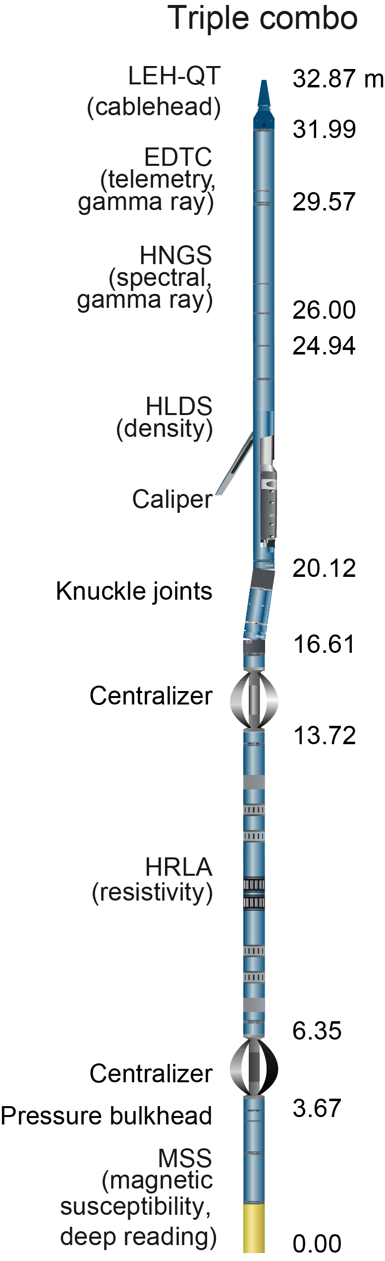
Figure F14. Downhole logging string schematics.
7.2. Wireline logging operations
In preparation for logging, the boreholes were reamed in their lower sections, flushed of debris by circulating drilling fluid, and filled with seawater-based logging gel (i.e., sepiolite mud mixed with seawater) to help stabilize the borehole walls. The BHA was pulled up to a logging depth determined by the borehole conditions (typically around 80 m DSF). Tool handling, deployment, and field data collection were undertaken by the onboard Schlumberger wireline logging engineer prior to the data being sent onshore for processing. GR log data was typically collected while running the tool string into the hole from just above seafloor for quality control and in case of any downhole logging problems, such as a stuck tool, which could render the main logging pass impossible. The bottom of the open hole was confirmed during the triple combo logging run and was typically a few meters higher than the final coring depth because of cave-ins and the onset of hole collapse above. The upward triple combo logging run also served to assess the hole conditions using the single arm HLDS caliper. In some cases, the borehole had already collapsed or bridged off by the time logging tools could be run into the hole, resulting in limited logging recovery. The primary data logging run was collected while raising the tool string upward at a constant speed, typically around 300 m/h for the triple combo tool string.
During wireline logging operations, the ship’s heave and ocean conditions affect the wireline tension and tool position in the well. A wireline heave compensator (WHC) is used in conditions of increased swell to maintain a steady motion of the logging tools and to ensure high-quality logging data acquisition (Liu et al., 2013; Iturrino et al., 2013). The WHC was used for all open hole logging operations regardless of sea state. The WHC uses a vertical accelerometer (motion reference unit [MRU]) positioned under the rig floor near the ship’s center of gravity to calculate the vertical motion of the ship with respect to the seafloor. The length of the wireline is adjusted by varying the distance between two sets of pulleys through which the cable passes to minimize downhole tool motion. Real-time measurements of uphole (surface) and downhole acceleration are made simultaneously with the MRU and EDTC, respectively, and software analyzes and compares the real-time data to monitor the efficiency of the compensator.
7.3. Data processing
Collected wireline data were sent for onshore processing by the LDEO-BRG. All original logging data was first depth matched to the total GR logging value from the main pass of the triple combo logging run. Prominent features were matched manually between GR within all tool runs and the reference GR log, and then all logging data within the same tool run were depth shifted by the same set of corrections. All depth-matched logs were then shifted to the seafloor (0 m) as defined by the clear increase in GR for this transition, resulting in the common depth reference WMSF in meters. The Schlumberger Techlog software package was used for most of the wireline log data processing.
Standard borehole size environmental corrections were applied to the HNGS (GR), HRLA (resistivity), and HLDS (density/photoelectric effect [PEF]) of the triple combo tool string automatically during acquisition and quality checked by the Schlumberger wireline engineer onboard.
7.4. Quality control and data presentation
The quality of the wireline data was assessed during both acquisition and processing by checking recorded values against reference values for the logged lithologies, evaluating repeatability between different passes of the same tool (downlog and main uplog), and assessing the correspondence between logs affected by the same formation property (e.g., the resistivity log should show similar features to the sonic velocity log). In general, very good correlation exists between density and resistivity for logged intervals. Wireline GR and MSS-B logs also generally reveal good quality data, in most cases matching well with equivalent core-based values. GR logs recorded through the BHA and drill pipe are influenced by significant attenuation of the incoming signal, resulting in reduced absolute GR values that should be used only qualitatively. Detailed comparison between these sections and the open hole data are restricted for this reason.
A wide (>12 inches) or irregular borehole affects most wireline logging recordings, in particular those that require decentralization and good contact with the borehole wall, such as the HLDS. To potentially improve hole conditions for logging, a PDC bit, which drills an 11 inch diameter hole, was used.
The mechanical caliper arm in the triple combo HLDS (LCAL) logging runs can be often closed from 3 to 10 m or sometimes greater distances below the end of the drill string casing. Closure of the calipers causes nongeologic changes in caliper-calibrated wireline measurements such as density, PEF, and GR.
Data received back on board were uploaded into the WellCAD software along with associated core-derived physical properties data. WellCAD templates were developed for consistent data presentation and used for all Expedition 397 sites.
7.5. Measurement principles
7.5.1. Gamma ray
The HNGS measures the GR of a formation. Standard (total) GR is reported as total spectral gamma ray (HSGR) in American Petroleum Institute gamma radiation units (gAPI) throughout the Downhole measurements section in each site chapter. The HNGS response is influenced by borehole diameter and requires borehole diameter corrections (caliper-derived) during acquisition. Two bismuth germanate scintillation detectors in the HNGS tool string measure potassium (weight percent), thorium (parts per million), and uranium (parts per million) concentrations from the characteristic GR energies of isotopes in the 40K, 232Th, and 238U radioactive decay series that dominate the natural radiation spectrum.
In addition to the HNGS, the EDTC also houses an HSGR sensor. The inclusion of a GR tool in every tool string allows the use of GR data for precise depth matching between logging runs, aids core-log integration, and enables precise identification of the seafloor.
7.5.2. Density and photoelectric effect
Formation density is measured using the HLDS. The HLDS contains a radioactive cesium (137Cs) GR source (622 keV) and far and near GR detectors mounted on a shielded skid that is pressed against the borehole wall by a decentralizing arm. The tool emits gamma radiation, which undergoes Compton scattering, and the GR signal received by the detectors is proportional to the density of electrons in the formation, which is in turn related to bulk density. Throughout this volume, wireline bulk density is presented as the HLDS-corrected bulk density (RHOM) in grams per cubic centimeter. The density log is commonly the best downhole tool for assessing porosity where the matrix (grain) density is known or can be accurately estimated and is particularly important for clay-bearing rocks, which suffer from poor neutron porosity determinations because of clay-bound water (Broglia and Ellis, 1990).
PEF gives a measure of the photoelectric absorption of low-energy GR and is also measured using the HLDS. Photoelectric absorption occurs when GR energy falls below 150 keV as a result of scattering by electrons in the formation. PEF is determined by comparing the counts from the far detector in the high-energy region, where only Compton scattering occurs, to those in the low-energy region, where count rates depend on both reactions. Because PEF depends on the atomic number of the elements in the formation (heavier elements have higher PEF), it also varies according to the chemical composition of the minerals present and can aid assessment of the matrix mineralogy. The PEF delivers data in barn/e− units and requires good contact between the tool and the borehole wall; poor contact results in underestimation of density values. Both the density correction and caliper measurement of the hole are used to check hole conditions and assess likely contact quality.
7.5.3. Electrical resistivity
The HRLA tool records six resistivity measurements with different depths of investigation (including the borehole fluid resistivity and five progressively deeper measurements of formation resistivity). The HRLA tool sends a focused current into the formation and measures the intensity necessary to maintain a constant drop in voltage across a fixed interval, providing direct resistivity measurement. Three depths of investigation, including shallow (RLA1), medium (RLA3), and true (RT_HRLT) resistivity measurements are presented in the Downhole measurements section in each site chapter, with RT_HRLT representing an estimate of the true formation from the area least influenced by drilling fluid invasion. The tool is designed to ensure that all signals are measured at the same time and tool position and to reduce the sensitivity to shoulder bed effects when crossing beds thinner than the electrode spacing. The HRLA is run centralized in the borehole for optimal results. Knuckle joints are used to centralize the HRLA while allowing the density tool to maintain good contact with the borehole wall. The HRLA gives an effective measurement of formation resistivity, allowing the full range of resistivity to be measured, from high-porosity brine saturated sediments (low resistivity) to hard dense rock formations (high resistivity).
7.5.4. Magnetic susceptibility
The MSS-B uses a single-coil sensor to measure borehole MS in approximate SI units, referred to here as noncalibrated instrument units (IU), at a vertical resolution of ~12 cm with shallow (~3 cm) depth of penetration. A lower resolution (~36 cm) but greater depth of penetration (36 cm) is also collected (LSUSR), which provides a quality check for the higher resolution reading. MS is the ease with which formations are magnetized when subjected to a magnetic field. The ease of magnetization is related to the size, distribution, and composition of magnetic minerals in the formation (e.g., magnetite). These measurements are useful both for stratigraphic correlation with the recovered cores and geophysical/geochemical analyses of the recovered sediments. The MSS-B is run as the lowest logging tool in the triple combo tool string and therefore collects one of the largest open hole coverages of all the logging tools. The sensor is an electric inductor constructed such that when positioned against the borehole wall its inductance is affected by the volume susceptibility of the formation within the measured formation rock volume.
The tool is calibrated to a 9⅞ inch borehole diameter, and larger or washed out holes will result in lower susceptibility measurements, whereas higher temperatures lead to higher susceptibility measurements. Temperature measurements were not run alongside the MSS-B. For quality control and environmental corrections, the MSS-B also measures internal tool temperature, z-axis acceleration, and low-resolution borehole conductivity.
7.5.5. Downhole temperature measurement
In situ temperature measurements were made using the APCT-3 tool when the APC system was deployed in Holes U1586A, U1587A, and U1588A. The APCT-3 tool fits into the APC coring shoe and includes a battery pack, data logger, and platinum resistance-temperature device calibrated over a temperature range of 0°–30°C. During deployment, the tool is first stopped at the mudline to thermally equilibrate with bottom water for 5 min. When the APC system is deployed into the formation, there is an instantaneous temperature rise from frictional heating. This heat gradually dissipates into the surrounding formation as the temperature at the APCT-3 tool equilibrates toward the temperature of the sediment. After the APC system penetrates the sediment, it is held in place for 5 min while the APCT-3 tool records the temperature of the cutting shoe every second.
A preliminary APCT-3 tool measurement evaluation was carried out onboard using the TP-Fit software (v. 3) (Heesemann, 2008). This involved picking the entry time and two points on the temperature equilibration path to capture the temperature decay after the frictional heating caused by lance entry and the second frictional heat pulse caused by lance retrieval. APCT-3 tool temperature data is combined with thermal conductivity measurements on the core.
8. Stratigraphic correlation
Most of the Expedition 397 scientific objectives depend on the recovery of complete stratigraphic sedimentary sequences. A complete stratigraphic sequence cannot be recovered from a single borehole because core recovery gaps occur between successive cores despite 100% or more nominal recovery (e.g., Ruddiman, Kidd, Thomas, et al., 1987; Hagelberg et al., 1995; Acton et al., 2002). The construction of a complete composite section, referred to as a splice, thus requires the combination of stratigraphic intervals from two or more holes cored at the same site. To maximize the probability of bridging gaps between successive cores in individual holes, the starting depths below seafloor from which cores are recovered are offset between holes and corrections are made if the core breaks between holes become aligned. This practice ensures that most missing sedimentary sections from intercore gaps in a given hole are recovered in one or more adjacent holes. Usually at least three holes must be cored to recover a complete section at a site. Additional holes are cored to allow for the construction of alternate splices, where possible.
The composite section and splice construction methodology employed during Expedition 397 follows the basic strategy originally developed during Ocean Drilling Program (ODP) Leg 138 (e.g., Hagelberg et al., 1992, 1995) and later refined during many other expeditions. This strategy is now common practice on all high-resolution paleoceanographic expeditions. Assembly and verification of a complete composite stratigraphic section requires construction of a composite depth scale, referred to as the core composite depth below seafloor, Method A (CCSF-A), scale. The composite depth scale provides a common depth scale for the holes at a site, unlike the original CSF-A depth scale, which is based on drill string measurements that are unique to each hole.
8.1. Core depth below seafloor, Method A, depth scale
The depth to the top of each core is based on a drill string measurement that is determined by the length of drill string below the rig floor to the top of the cored interval minus the length of drill string from the rig floor to the mudline (assumed to be the seafloor). The depth to a point along the core is determined by adding the distance at which the point occurs from the top of the core to the core top depth. This depth scale is referred to as the CSF-A depth scale and is equivalent to the ODP mbsf depth scale.
The zero-depth point of the CSF-A depth scale is defined by the mudline in the first core of each hole. However, it is often difficult to tell whether this empirical mudline recovers the true sediment/water interface. Some holes are inadvertently (or purposely) started below the sediment/water interface. In this case, the zero-depth point in CSF-A depth scale units may be substantially offset from the zero-depth point in adjacent holes that successfully recover the sediment/water interface.
The CSF-A depth scale may also be inaccurate because of ship heave, tidal variations in sea level, coring distortion, and other sources of error. Tidal influence on depth was first predicted during ODP Leg 138 (Hagelberg et al., 1995) and was proven by correlation of affine offset changes and tide height during ODP Leg 202 (Mix, Tiedemann, Blum, et al., 2003). Tidal variations were thus the largest source of variation in the CSF-A depth scale from one hole to the next. Because these are predictable, pipe offsets could be adjusted with the goal of avoiding core gap alignment. For a variety of practical reasons, such as failure to get a complete 9.6 m stroke with the APC system for one or more cores from each hole, the goal can be difficult to achieve with just two holes and sometimes even more.
8.2. Core composite depth below seafloor, Method A, depth scale
The goal of constructing a composite depth scale is to place coeval, laterally continuous stratigraphic features into a common frame of reference by depth. This is achieved by shifting the CSF-A depth scales of individual cores to maximize correlation between holes. In the CCSF-A scale, the depths of the individual cores can only be shifted by a constant amount, without permitting expansion or contraction of the relative depth scale within any core. Ultimately, this provides a good first-order correlation between cores from different holes and also avoids more subjective, and potentially erroneous, interpretations that might arise without applying this restriction first. The CCSF-A scale, once established, provides a basis upon which higher order depth composite scales can be built onshore.
In essence, the CCSF-A scale overcomes many of the inadequacies of the CSF-A depth scale, which is unique to each hole and may be inaccurate as discussed above. Rather than using a drill string measurement, the CCSF-A scale is built by correlating features downhole from the mudline. The mudline is not merely taken as the top of the first core in a hole but is the top of the first core with the most representative or best-preserved mudline. This mudline establishes the top of the stratigraphic section, and the core with this mudline becomes the anchor in the composite depth scale. It is typically the only core in which the depths are the same for both the CSF-A and CCSF-A scales. Each core downhole is tied to the composite section by adding or subtracting a depth offset (a constant) that best aligns the observed lithologic variations to the correlative variations for cores from adjacent holes. Provided that gaps between cores do not occur at the same stratigraphic position in offset holes and recovery is high, it should be possible to correlate each successive core downhole to a core from an adjacent hole. Gaps common to all holes cored at a site can occur, in which case cores downhole can be appended to the composite section. In such cases, the depth offset for the appended core can be adjusted to convey an estimate of the true size of the coring gap. For example, one could use the average growth factor (i.e., expansion) of the CCSF-A depth scale relative to the CSF-A depth scale or could use continuous logging data from a hole at the site or observations from other nearby sites.
8.3. Adjusting composites to driller’s depth (CCSF-A* and CCSF-B*)
In the process of constructing the composite section, the CCSF-A depth scale is virtually always expanded relative to the CSF-A depth scale. The expansion, which is typically ~5%–15%, is mostly caused by stretching that occurs as part of the coring process, decompression of the cores as they are brought to the surface, and/or curation practice, in which material that has fallen downhole or gas expansion voids are curated as part of the core (e.g., Hagelberg et al., 1995; Acton et al., 2002). To generate a physically plausible match of the composite stratigraphy to in situ stratigraphy, we adopted a similar strategy to that used during Expedition 339: inverting the CCSF-A depth scale to the CSF-A depth scale to bring measurements back to a scale closely approximating driller’s depth, referred to as the CCSF-A* depth scale (similar to the mbsf* scale used for Site U1385 by Expedition 339 Scientists [2013]). Because of the significant curvature in the relationship between the CCSF-A and CSF-A depth scales, polynomial fits were required to achieve a good relationship that ran through the zero depth (mudline) at the top of each site. The fits are presented in each site chapter (see Figures F50 in the Site U1385 chapter [Hodell et al., 2024a], F60 in the Site U1586 chapter [Abrantes et al., 2024a], F47 in the Site U1587 chapter [Hodell et al., 2024b], and F39 in the Site U1588 chapter [Abrantes et al., 2024b]). The CCSF-A* depth scale is used in stratigraphic summary Figures F48 in the Site U1385 chapter (Hodell et al., 2024a) and F55 in the Site U1586 chapter (Abrantes et al., 2024a) because it represents the closest match of the spliced sequences to data presented elsewhere in the CSF-A depth scale. In the case of Site U1588, severe gas expansion required us to build a composite based on the CSF-B, convention, whereby core thickness is compressed to 100% recovery. The core composite depth below seafloor, Method B (CCSF-B), is then corrected to approximate driller’s depth on the CCSF-B* scale. Tables for conversion of CCSF-A depths to the CCSF-A* depth scale are given in Tables T32 in the Site U1385 chapter (Hodell et al., 2024a), T32 in the Site U1586 chapter (Abrantes et al., 2024a), and T32 in the Site U1587 chapter (Hodell et al., 2024b).
8.4. Goals
The goals for stratigraphic correlation for Expedition 397, in order of priority, were as follows:
- Guide the drilling process to ensure recovery of a complete stratigraphic section;
- Establish a composite depth scale; and
- Define a stratigraphically complete and representative sampling splice and, if possible, one or more alternate splices.
This first-order ship-based correlation is expected to be refined postcruise with the generation of XRF scanning data (e.g., Ca/Ti) that will be used to construct a revised composite depth scale, which may include correction for distortion within individual cores by stretching and squeezing of cored intervals to match the composite splice, similar to that done for Expedition 339 Site U1385 (Hodell et al., 2015). The revised composite sections can also be linked to logging depths at site where downhole logging was successful.
8.5. Measurements and methods specific to Expedition 397
The composite sections and splices are based on the stratigraphic correlation of data from the shipboard logging systems that measure physical and magnetic properties. Initial correlation was based primarily on MS from the WRMSL, STMSL, and SHMSL. The WRMSL and STMSL have identical capacity to measure MS and density, and the WRMSL additionally measures P-wave velocity. The WRMSL is used primarily to take higher resolution measurements and the STMSL is used to take lower resolution and thus rapid measurements for the purpose of quick correlation. These measurements were done after the core temperature had equilibrated to laboratory temperature for the first holes of Sites U1586, U1587, and U1385, whereas all measurements were done as soon as the machines were available for other holes (see Physical properties). Final correlation involves multiple proxies, including whole-round MS, whole-round NGR, section-half MSP, color reflectance L*, and RGB blue channel.
Hole-to-hole and site-to-site correlations were accomplished using the Correlator software (version 4.0.1), as well as several other software packages such as Match (Lisiecki and Lisiecki, 2002), Autocomp (Lisiecki and Herbert, 2007), AnalySeries (Paillard et al., 1996), and KaleidaGraph. Utilizing Correlator, we generated standard affine tables, which list the offset that is added to each core to place it on the CCSF-A scale, and splice tables, which give the intervals that comprise the splice. The tables were uploaded into the LIMS database using the Stratigraphic Correlation Support (SCORS) application. The affine and splice tables provide all the necessary information to place any of the Expedition 397 data into the CCSF-A or CCSF-B scale and to generate spliced data sets for each site.
Upon completion of the site splice using Correlator, we recognized two aspects of core measurements that will require correction of raw data values of whole-round MS, MSP, and NGR. The first comes from the reduced diameter and volume of XCB cores relative to APC cores. We observed a step drop by ~0.2 g/cm3 in the GRA bulk density when coring was switched to the XCB system. This reduction in core volume will affect the values of all mass/volume-dependent measurements. Although MSP measurements may be slightly less sensitive to core diameter changes than whole-round MS measurements, they generally fall close to the whole-round values, suggesting that they average over a nearly equivalent volume/distance and also need correction for the reduced diameter of XCB cores. A comparison of the NGR measurements also shows an abrupt drop at the transition from APC to XCB coring; values in equivalent sections of XCB cores are comparable between offset holes but noticeably lower than for the equivalent sections cored using the APC system. The possibility of correcting mass/volume-dependent measurements using the GRA bulk density logs will be explored postcruise.
The second artifact in initial data comes from the effect of core temperature on MS readings taken with the WRMSL. The temperature of the cores significantly affects the sensitivity of the MS sensor; experiments showed differences between cores run before and after thermal equilibration. The raw values of whole-round MS logs are therefore much less consistent between holes than MSP measurements. As above, we hope to correct raw pass-through MS measurements by reference to the MSP measurements on the same cores.
References
Abrantes, F., Hodell, D.A., Alvarez Zarikian, C.A., Brooks, H.L., Clark, W.B., Dauchy-Tric, L.F.B., dos Santos Rocha, V., Flores, J.-A., Herbert, T.D., Hines, S.K.V., Huang, H.-H.M., Ikeda, H., Kaboth-Bahr, S., Kuroda, J., Link, J.M., McManus, J.F., Mitsunaga, B.A., Nana Yobo, L., Pallone, C.T., Pang, X., Peral, M.Y., Salgueiro, E., Sanchez, S., Verma, K., Wu, J., Xuan, C., and Yu, J., 2024a. Site U1586. In Hodell, D.A., Abrantes, F., Alvarez Zarikian, C.A., and the Expedition 397 Scientists, Iberian Margin Paleoclimate. Proceedings of the International Ocean Discovery Program, 397: College Station, TX (International Ocean Discovery Program). https://doi.org/
Abrantes, F., Hodell, D.A., Alvarez Zarikian, C.A., Brooks, H.L., Clark, W.B., Dauchy-Tric, L.F.B., dos Santos Rocha, V., Flores, J.-A., Herbert, T.D., Hines, S.K.V., Huang, H.-H.M., Ikeda, H., Kaboth-Bahr, S., Kuroda, J., Link, J.M., McManus, J.F., Mitsunaga, B.A., Nana Yobo, L., Pallone, C.T., Pang, X., Peral, M.Y., Salgueiro, E., Sanchez, S., Verma, K., Wu, J., Xuan, C., and Yu, J., 2024b. Site U1588. In Hodell, D.A., Abrantes, F., Alvarez Zarikian, C.A., and the Expedition 397 Scientists, Iberian Margin Paleoclimate. Proceedings of the International Ocean Discovery Program, 397: College Station, TX (International Ocean Discovery Program). https://doi.org/
Acton, G.D., Borton, C.J., and the Leg 178 Shipboard Scientific Party, 2002. Palmer Deep composite depth scales for Leg 178 sites 1098 and 1099. In Barker, P.F., Camerlenghi, A., Acton, G.D., and Ramsay, A.T.S. (Eds.), Proceedings of the Ocean Drilling Program, Scientific Results. 178: College Station, TX (Ocean Drilling Program), 1–35. https://doi.org/
Alvarez Zarikian, C.A., 2009. Data report: late Quaternary ostracodes at IODP Site U1314 (North Atlantic Ocean). In Channell, J.E.T., Kanamatsu, T., Sato, T., Stein, R., Alvarez Zarikian, C.A., Malone, M.J., and the Expedition 303/306 Scientists, Proceedings of the Integrated Ocean Drilling Program. 303/306: College Station, TX (Integrated Ocean Drilling Program Management International, Inc.). https://doi.org/
Alvarez Zarikian, C.A., Stepanova, A.Y., and Grutzner, J., 2009. Glacial–interglacial variability in deep sea ostracod assemblage composition at IODP Site U1314 in the subpolar North Atlantic. Marine Geology, 258(1–4):69–87. https://doi.org/
ASTM International, 1990. Standard method for laboratory determination of water (moisture) content of soil and rock (Standard D2216–90). In Annual Book of ASTM Standards for Soil and Rock Philadelphia (American Society for Testing Materials).
Balestra, B., Flores, J.A., Hodell, D.A., Hernández Molina, F.J., and Stow, D.A.V., 2015. Pleistocene calcareous nannofossil biochronology at IODP Site U1385 (Expedition 339). Global and Planetary Change, 135:57–65. https://doi.org/
Baumann, K.-H., Andruleit, H., Böckel, B., Geisen, M., and Kinkel, H., 2005. The significance of extant coccolithophores as indicators of ocean water masses, surface water temperature, and palaeoproductivity: a review. Paläontologische Zeitschrift, 79(1):93–112. https://doi.org/
Blum, P., 1997. Physical properties handbook: a guide to the shipboard measurement of physical properties of deep-sea cores. Ocean Drilling Program Technical Note, 26. https://doi.org/10.2973/odp.tn.26.1997
BouDagher-Fadel, M.K., 2015. Biostratigraphic and Geological Significance of Planktonic Foraminifera: London (UCL Press). https://doi.org/
Breman, E., 1978. Krithe keyi nom. nov., revision of an ostracode species name. Journal of Paleontology, 52:580.
Broglia, C., and Ellis, D.V., 1990. Effect of alteration, formation absorption, and standoff on the response of the thermal neutron porosity log in gabbros and basalts; examples from Deep Sea Drilling Project-Ocean Drilling Program sites. Journal of Geophysical Research: Solid Earth, 95(B6):9171–9188. https://doi.org/
Chaisson, W.P., and Pearson, P.N., 1997. Planktonic foraminifer biostratigraphy at Site 925: middle Miocene-Pleistocene. In Shackleton, N.J., Curry, W.B., Richter, C., and Bralower, T.J. (Eds.), Proceedings of the Ocean Drilling Program, Scientific Results. 154: College Station, TX (Ocean Drilling Program), 3–31. https://doi.org/
Colalongo, M.L., and Pasini, G., 1980. La Ostracofauna plio-pleistocenica della Sezione Vrica in Calabria (con considerazioni sul limite Neogene/Quaternario). Bollettino della Società Paleontologica Italiana, 19(1–2):84–126.
Colmenero-Hidalgo, E., Flores, J.-A., Sierro, F.J., Bárcena, M.Á., Löwemark, L., Schönfeld, J., and Grimalt, J.O., 2004. Ocean surface water response to short-term climate changes revealed by coccolithophores from the Gulf of Cadiz (NE Atlantic) and Alboran Sea (W Mediterranean). Palaeogeography, Palaeoclimatology, Palaeoecology, 205(3–4):317–336. https://doi.org/
De Vleeschouwer, D., Dunlea, A.G., Auer, G., Anderson, C.H., Brumsack, H., de Loach, A., Gurnis, M.C., Huh, Y., Ishiwa, T., Jang, K., Kominz, M.A., März, C., Schnetger, B., Murray, R.W., Pälike, H., and Expedition 356 Shipboard Scientists, 2017. Quantifying K, U, and Th contents of marine sediments using shipboard natural gamma radiation spectra measured on DV JOIDES Resolution. Geochemistry, Geophysics, Geosystems, 18(3):1053–1064. https://doi.org/
Droser, M.L., and Bottjer, D.J., 1986. A semiquantitative field classification of ichnofabric. Journal of Sedimentary Research, 56(4):558–559. https://doi.org/
Dunlea, A.G., Murray, R.W., Harris, R.N., Vasiliev, M.A., Evans, H., Spivack, A.J., and D’Hondt, S., 2013. Assessment and use of NGR instrumentation on the JOIDES Resolution to quantify U, Th, and K concentrations in marine sediment. Scientific Drilling, 15:57–63. https://doi.org/
Expedition 339 Scientists, 2013. Methods. In Stow, D.A.V., Hernández-Molina, F.J., Alvarez Zarikian, C.A., and the Expedition 339 Scientists, Proceedings of the Integrated Ocean Drilling Program. 339: Tokyo (Integrated Ocean Drilling Program Management International, Inc.). https://doi.org/
Expedition 339 Scientists, 2013. Site U1385. In Stow, D.A.V., Hernández-Molina, F.J., Alvarez Zarikian, C.A., and the Expedition 339 Scientists, Proceedings of the Integrated Ocean Drilling Program. 339: Tokyo (Integrated Ocean Drilling Program Management International, Inc.). https://doi.org/
Faranda, C., Cipollari, P., Cosentino, D., Gliozzi, E., and Pipponzi, G., 2008. Late Miocene ostracod assemblages from eastern Mediterranean coral reef complexes (central Crete, Greece). Revue de Micropaléontologie, 51(4):287–308. https://doi.org/
Flores, J.-A., Colmenero-Hidalgo, E., Mejía-Molina, A.E., Baumann, K.-H., Henderiks, J., Larsson, K., Prabhu, C.N., Sierro, F.J., and Rodrigues, T., 2010. Distribution of large Emiliania huxleyi in the central and Northeast Atlantic as a tracer of surface ocean dynamics during the last 25,000 years. Marine Micropaleontology, 76(3–4):53–66. https://doi.org/
Geisen, M., Billard, C., Broerse, A., Cros, L., Probert, I., and Young, J., 2002. Life-cycle associations involving pairs of holococcolithophorid species: intraspecific variation or cryptic speciation? European Journal of Phycology, 37(4):531–550. https://doi.org/
Gibbard, P.L., Head, M.J., Walker, M.J.C., and the Subcommission on Quaternary Stratigraphy, 2010. Formal ratification of the Quaternary system/period and the Pleistocene series/epoch with a base at 2.58 Ma. Journal of Quaternary Science, 25(2):96–102. https://doi.org/
Gieskes, J.M., Gamo, T., and Brumsack, H.J., 1991. Chemical methods for interstitial water analysis aboard JOIDES Resolution. Ocean Drilling Program Technical Note, 15. https://doi.org/
Gilmore, G.R., 2008. Practical Gamma-Ray Spectrometry, 2nd Edition: New York (Wiley). https://doi.org/
Graber, K.K., Pollard, E., Jonasson, B., and Schulte, E. (Eds.), 2002. Overview of Ocean Drilling Program engineering tools and hardware. Ocean Drilling Program Technical Note, 31. https://doi.org/
Gradstein, F.M., Ogg, J.G., Schmitz, M.D., and Ogg, G.M. (Eds.), 2020. The Geologic Time Scale 2020: Amsterdam (Elsevier BV). https://doi.org/
Hagelberg, T., Shackleton, N., Pisias, N., and the Shipboard Scientific Party, 1992. Development of composite depth sections for Sites 844 through 854. In Mayer, L., Pisias, N., Janecek, T., et al., Proceedings of the Ocean Drilling Program, Initial Reports. 138: College Station, TX (Ocean Drilling Program), 79–85. https://doi.org/
Hagelberg, T.K., Pisias, N.G., Shackleton, N.J., Mix, A.C., and Harris, S., 1995. Refinement of a high-resolution, continuous sedimentary section for studying equatorial Pacific Ocean paleoceanography, Leg 138. In Pisias, N.G., Mayer, L.A., Janecek, T.R., Palmer-Julson, A., and van Andel, T.H. (Eds.), Proceedings of the Ocean Drilling Program, Scientific Results. 138: College Station, TX (Ocean Drilling Program). https://doi.org/
Hayward, B.W., 2002. Late Pliocene to middle Pleistocene extinctions of deep-sea benthic Foraminifera (“Stilostomella extinction”) in the Southwest Pacific. Journal of Foraminiferal Research, 32(3):274–307. https://doi.org/
Heesemann, M., 2008. Advances in the acquisition and processing of subseafloor temperature and pressure data and their interpretation in the context of convergent margin processes [PhD dissertation]. University of Bremen, Bremen, Germany.
Hemleben, C., Spindler, M., and Anderson, O.R., 1989. Modern Planktonic Foraminifera: New York (Springer-Verlag).
Hilgen, F.J., 1991. Extension of the astronomically calibrated (polarity) time scale to the Miocene/Pliocene boundary. Earth and Planetary Science Letters, 107(2):349–368. https://doi.org/
Hodell, D.A., Abrantes, F., and Alvarez Zarikian, C.A., 2022. Expedition 397 Scientific Prospectus: Iberian Margin Paleoclimate. International Ocean Discovery Program. https://doi.org/
Hodell, D.A., Abrantes, F., Alvarez Zarikian, C.A., Brooks, H.L., Clark, W.B., Dauchy-Tric, L.F.B., dos Santos Rocha, V., Flores, J.-A., Herbert, T.D., Hines, S.K.V., Huang, H.-H.M., Ikeda, H., Kaboth-Bahr, S., Kuroda, J., Link, J.M., McManus, J.F., Mitsunaga, B.A., Nana Yobo, L., Pallone, C.T., Pang, X., Peral, M.Y., Salgueiro, E., Sanchez, S., Verma, K., Wu, J., Xuan, C., and Yu, J., 2024a. Site U1385. In Hodell, D.A., Abrantes, F., Alvarez Zarikian, C.A., and the Expedition 397 Scientists, Iberian Margin Paleoclimate. Proceedings of the International Ocean Discovery Program, 397: College Station, TX (International Ocean Discovery Program). https://doi.org/
Hodell, D.A., Abrantes, F., Alvarez Zarikian, C.A., Brooks, H.L., Clark, W.B., Dauchy-Tric, L.F.B., dos Santos Rocha, V., Flores, J.-A., Herbert, T.D., Hines, S.K.V., Huang, H.-H.M., Ikeda, H., Kaboth-Bahr, S., Kuroda, J., Link, J.M., McManus, J.F., Mitsunaga, B.A., Nana Yobo, L., Pallone, C.T., Pang, X., Peral, M.Y., Salgueiro, E., Sanchez, S., Verma, K., Wu, J., Xuan, C., and Yu, J., 2024b. Site U1587. In Hodell, D.A., Abrantes, F., Alvarez Zarikian, C.A., and the Expedition 397 Scientists, Iberian Margin Paleoclimate. Proceedings of the International Ocean Discovery Program, 397: College Station, TX (International Ocean Discovery Program). https://doi.org/
Hodell, D., Lourens, L., Crowhurst, S., Konijnendijk, T., Tjallingii, R., Jiménez-Espejo, F., Skinner, L., Tzedakis, P.C., and the Shackleton Site Project Members, 2015. A reference time scale for Site U1385 (Shackleton Site) on the SW Iberian Margin. Global and Planetary Change, 133:49–64. https://doi.org/
Huber, B.T., Hobbs, R.W., Bogus, K.A., Batenburg, S.J., Brumsack, H.-J., do Monte Guerra, R., Edgar, K.M., Edvardsen, T., Garcia Tejada, M.L., Harry, D.L., Hasegawa, T., Haynes, S.J., Jiang, T., Jones, M.M., Kuroda, J., Lee, E.Y., Li, Y.-X., MacLeod, K.G., Maritati, A., Martinez, M., O’Connor, L.K., Petrizzo, M.R., Quan, T.M., Richter, C., Riquier, L., Tagliaro, G.T., Wainman, C.C., Watkins, D.K., White, L.T., Wolfgring, E., and Xu, Z., 2019. Expedition 369 methods. In Hobbs, R.W., Huber, B.T., Bogus, K.A., and the Expedition 369 Scientists, Australia Cretaceous climate and tectonics. Proceedings of the International Ocean Discovery Program, 369: College Station, TX (International Ocean Discovery Program). https://doi.org/
Iturrino, G., Liu, T., Goldberg, D., Anderson, L., Evans, H., Fehr, A., Guerin, G., Inwood, J., Lofi, J., Malinverno, A., Morgan, S., Mrozewski, S., Slagle, A., and Williams, T., 2013. Performance of the wireline heave compensation system onboard D/V JOIDES Resolution. Scientific Drilling, 15:46–50. https://doi.org/
Jorissen, F.J., Fontanier, C., and Thomas, E., 2007. Paleoceanographical proxies based on deep-sea benthic foraminiferal assemblage characteristics. In Hillaire–Marcel, C., and De Vernal, A. (Eds.), Developments in Marine Geology (Volume 7): Earth and Life Processes Discovered from Subseafloor Environments: A Decade of Science Achieved by the Integrated Ocean Drilling Program (IODP). R. Stein (Series Ed.). Amsterdam (Elsevier), 263–325. https://doi.org/
Jutzeler, M., White, J.D.L., Talling, P.J., McCanta, M., Morgan, S., Le Friant, A., and Ishizuka, O., 2014. Coring disturbances in IODP piston cores with implications for offshore record of volcanic events and the Missoula megafloods. Geochemistry, Geophysics, Geosystems, 15(9):3572–3590. https://doi.org/
Kawagata, S., Hayward, B.W., Grenfell, H.R., and Sabaa, A., 2005. Mid-Pleistocene extinction of deep-sea foraminifera in the North Atlantic Gateway (ODP Sites 980 and 982). Palaeogeography, Palaeoclimatology, Palaeoecology, 221(3):267–291. https://doi.org/
Kennett, J.P., and Srinivasan, M.S., 1983. Neogene Planktonic Foraminifera: A Phylogenetic Atlas: London (Hutchinson Ross).
King, D.J., Wade, B.S., Liska, R.D., and Miller, C.G., 2020. A review of the importance of the Caribbean region in Oligo-Miocene low latitude planktonic foraminiferal biostratigraphy and the implications for modern biogeochronological schemes. Earth-Science Reviews, 202:102968. https://doi.org/
Klejine, A., 1993. Morphology, taxonomy, and distribution of extant coccolithophorids (calcareous nannoplankton) [PhD dissertation]. Vrije University, Amsterdam.
Knappertsbusch, M., Cortes, M.Y., and Thierstein, H.R., 1997. Morphologic variability of the coccolithophorid Calcidiscus leptoporus in the plankton, surface sediments and from the early Pleistocene. Marine Micropaleontology, 30(4):293–317. https://doi.org/
Kristiansen, J.I., 1982. The transient cylindrical probe method for determination of thermal parameters of earth materials [PhD dissertation]. Åarhus University, Åarhus, Denmark. http://digitallib.oit.edu/
Kucera, M., 2007. Planktonic foraminifera as tracers of past oceanic environments. In Hillaire–Marcel, C., and De Vernal, A. (Eds.), Proxies in Late Cenozoic Paleoceanography Developments in Marine Geology. R. Stein (Series Ed.), 1: 213–262. https://doi.org/
Lisiecki, L.E., and Herbert, T.D., 2007. Automated composite depth scale construction and estimates of sediment core extension. Paleoceanography and Paleoclimatology, 22(4):PA4213. https://doi.org/
Lisiecki, L.E., and Lisiecki, P.A., 2002. Application of dynamic programming to the correlation of paleoclimate records. Paleoceanography, 17(4):1049. https://doi.org/
Liu, T., Iturrino, G., Goldberg, D., Meissner, E., Swain, K., Furman, C., Fitzgerald, P., Frisbee, N., Chlimoun, J., Van Hyfte, J., and Beyer, R., 2013. Performance evaluation of active wireline heave compensation systems in marine well logging environments. Geo-Marine Letters, 33(1):83–93. https://doi.org/
Loeblich, A.R., and Tappan, H.N., 1988. Foraminiferal Genera and Their Classification: Plates: (Van Nostrand Reinhold Company).
Lourens, L., Hilgen, F., Shackleton, N.J., Laskar, J., and Wilson, D., 2004. The Neogene period. In Smith, A.G., Gradstein, F.M. and Ogg, J.G., A Geologic Time Scale 2004. Cambridge, UK (Cambridge University Press), 409–440. https://doi.org/
Manheim, F.T., and Sayles, F.L., 1974. Composition and origin of interstitial waters of marine sediments, based on deep sea drill cores. In Goldberg, E.D., The Sea (Volume 5): Marine Chemistry: The Sedimentary Cycle. New York (Wiley), 527–568. http://pubs.er.usgs.gov/
Marsaglia, K., Milliken, K., and Doran, L., 2013. IODP digital reference for smear slide analysis of marine mud, Part 1: Methodology and atlas of siliciclastic and volcanogenic components. Integrated Ocean Drilling Program Technical Note, 1. https://doi.org/
Marsaglia, K., Milliken, K., Leckie, R., Tentori, D., and Doran, L., 2015. IODP smear slide digital reference for sediment analysis of marine mud, Part 2: Methodology and atlas of biogenic components. Integrated Ocean Drilling Program Technical Note, 2. https://doi.org/
Martini, E., 1971. Standard Tertiary and Quaternary calcareous nannoplankton zonation. Proceedings of the Second Planktonic Conference, Roma, 1970:739–785.
Mix, A.C., Tiedemann, R., Blum, P., et al., 2003. Proceedings of the Ocean Drilling Program, Initial Reports, 202: College Station, TX (Ocean Drilling Program). https://doi.org/
Murray, J.W., 2006. Ecology and Applications of Benthic Foraminifera: Cambridge, UK (Cambridge University Press). https://doi.org/
Murray, R.W., Miller, D.J., and Kryc, K.A., 2000. Analysis of major and trace elements in rocks, sediments, and interstitial waters by inductively coupled plasma–atomic emission spectrometry (ICP-AES). Ocean Drilling Program Technical Note, 29. https://doi.org/
Narciso, A., Cachão, M., and de Abreu, L., 2006. Coccolithus pelagicus subsp. pelagicus versus Coccolithus pelagicus subsp. braarudii (Coccolithophore, Haptophyta): a proxy for surface subarctic Atlantic waters off Iberia during the last 200 kyr. Marine Micropaleontology, 59(1):15–34. https://doi.org/
Ogg, J.G., 2020. Geomagnetic Polarity Time Scale. In Gradstein, F.M., Ogg, J.G., Schmitz, M., and Ogg, G. (Eds.), Geologic Time Scale 2020. Amsterdam (Elsevier), 159–192. https://doi.org/
Okada, H., and Bukry, D., 1980. Supplementary modification and introduction of code numbers to the low-latitude coccolith biostratigraphic zonation (Bukry, 1973; 1975). Marine Micropaleontology, 5(3):321–325. https://doi.org/
Paillard, D., Labeyrie, L., and Yiou, P., 1996. Macintosh Program performs time-series analysis. Eos, Transactions of the American Geophysical Union, 77(39):379. https://doi.org/
Parente, A., Cachão, M., Baumann, K.-H., de Abreu, L., and Ferreira, J., 2004. Morphometry of Coccolithus pelagicus s.l. (Coccolithophore, Haptophyta) from offshore Portugal, during the last 200 kyr. Micropaleontology, 50(Suppl_1):107–120. https://doi.org/10.2113/50.Suppl_1.107
Perch-Nielsen, K., 1985. Cenozoic calcareous nannofossils. In Bolli, H.M., Saunders, J.B., and Perch-Nielsen, K. (Eds.), Plankton Stratigraphy (Volume 1). Cambridge, UK (Cambridge University Press), 427–554.
Planke, S., Berndt, C., Alvarez Zarikian, C.A., Agarwal, A., Andrews, G.D.M., Betlem, P., Bhattacharya, J., Brinkhuis, H., Chatterjee, S., Christopoulou, M., Clementi, V.J., Ferré, E.C., Filina, I.Y., Frieling, J., Guo, P., Harper, D.T., Jones, M.T., Lambart, S., Longman, J., Millett, J.M., Mohn, G., Nakaoka, R., Scherer, R.P., Tegner, C., Varela, N., Wang, M., Xu, W., and Yager S.L., 2023. Expedition 396 methods. In Planke, S., Berndt, C., Alvarez Zarikian, C.A., and the Expedition 396 Scientists, Mid-Norwegian Margin Magmatism and Paleoclimate Implications. Proceedings of the International Ocean Discovery Program, 396: College Station, TX (International Ocean Discovery Program). https://doi.org/
Poole, C.R., and Wade, B.S., 2019. Systematic taxonomy of the Trilobatus sacculifer plexus and descendant Globigerinoidesella fistulosa (planktonic foraminifera). Journal of Systematic Palaeontology, 17(23):1989–2030. https://doi.org/
Quinn, P., Thierstein, H.R., Brand, L., and Winter, A., 2003. Experimental evidence for the species character of Calcidiscus leptoporus morphotypes. Journal of Paleontology, 77(5):825–830. https://doi.org/
Quinn, P.S., Sáez, A.G., Baumann, K.-H., Steel, B.A., Sprengel, C., and Medlin, L.K., 2004. Coccolithophorid biodiversity: evidence from the cosmopolitan species Calcidiscus leptoporus. In Thierstein, H.R., and Young, J.R. (Eds.), Coccolithophores: From Molecular Processes to Global Impact. Berlin, Heidelberg (Springer), 299–326. https://doi.org/
Raffi, I., Backman, J., Fornaciari, E., Pälike, H., Rio, D., Lourens, L., and Hilgen, F., 2006. A review of calcareous nannofossil astrobiochronology encompassing the past 25 million years. Quaternary Science Reviews, 25(23):3113–3137. https://doi.org/
Rothwell, R.G., 1989. Minerals and Mineraloids in Marine Sediments: An Optical Identification Guide: London (Elsevier). https://doi.org/
Ruddiman, W.F., Kidd, R.B., Baldauf, J.G., Clement, B.M., Dolan, J.F., Eggers, M.R., Hill, P.R., Keigwin, L.D., Jr., Mitchell, M., Philipps, I., Robinson, F., Salehipour, S.A., Takayama, T., Thomas, E., Unsold, G., and Weaver, P.P.E., 1987. Initial Reports of the Deep Sea Drilling Project, 94: Washington, DC (US Government Printing Office). https://doi.org/
Ruiz, F., González-Regalado, M.L., Abad, M., Civis, J., Delgado, J.Á.G., García, E.X.M., Prudêncio, M.I., and Dias, M.I., 2008. Pliocene ostracods of Southwestern Europe. Geobios, 41(6):845–859. https://doi.org/
Salgueiro, E., Voelker, A.H.L., de Abreu, L., Abrantes, F., Meggers, H., and Wefer, G., 2010. Temperature and productivity changes off the western Iberian margin during the last 150 ky. Quaternary Science Reviews, 29(5–6):680–695. https://doi.org/
Schiebel, R., and Hemleben, C., 2017. Planktic Foraminifers in the Modern Ocean: Berlin (Springer). https://doi.org/
Schönfeld, J., and Zahn, R., 2000. Late Glacial to Holocene history of the Mediterranean Outflow. Evidence from benthic foraminiferal assemblages and stable isotopes at the Portuguese margin. Palaeogeography, Palaeoclimatology, Palaeoecology, 159(1–2):85–111. https://doi.org/10.1016/S0031-0182(00)00035-3
Seeberg-Elverfeldt, J., Schlüter, M., Feseker, T., and Kölling, M., 2005. Rhizon sampling of porewaters near the sediment-water interface of aquatic systems. Limnology and Oceanography: Methods, 3(8):361-371. https://doi.org/
Spezzaferri, S., Olsson, R.K., Hemleben, C., Wade, B.S., Olsson, R.K., Pearson, P.N., Huber, B.T., and Berggren, W.A., 2018. Taxonomy, biostratigraphy, and phylogeny of Oligocene to lower Miocene Globigerinoides and Trilobatus. In Atlas of Oligocene planktonic Foraminifera. Cushman Special Publications, 46.
Steel, B.A., 2001. Physiology, growth, and morphometry of selected extant coccolithophorids, with particular reference to Calcidiscus leptoporus (Murray and Blackman, 1889) (Loeblich and Tappan, 1987). [MS thesis]. University College London, London.
Stow, D.A.V., 2005. Sedimentary Rocks in the Field. A Colour Guide: London (Manson Publishing).
Sun, Z., Jian, Z., Stock, J.M., Larsen, H.C., Klaus, A., Alvarez Zarikian, C.A., Boaga, J., Bowden, S.A., Briais, A., Chen, Y., Cukur, D., Dadd, K.A., Ding, W., Dorais, M.J., Ferré, E.C., Ferreira, F., Furusawa, A., Gewecke, A.J., Hinojosa, J.L., Höfig, T.W., Hsiung, K.-H., Huang, B., Huang, E., Huang, X.-L., Jiang, S., Jin, H., Johnson, B.G., Kurzawski, R.M., Lei, C., Li, B., Li, L., Li, Y., Lin, J., Liu, C., Liu, C., Liu, Z., Luna, A., Lupi, C., McCarthy, A.J., Mohn, G., Ningthoujam, L.S., Nirrengarten, M., Osono, N., Peate, D.W., Persaud, P., Qiu, N., Robinson, C.M., Satolli, S., Sauermilch, I., Schindlbeck, J.C., Skinner, S.M., Straub, S.M., Su, X., Tian, L., Van der Zwan, F.M., Wan, S., Wu, H., Xiang, R., Yadav, R., Yi, L., Zhang, C., Zhang, J., Zhang, Y., Zhao, N., Zhong, G., and Zhong, L., 2018. Expedition 367/368 methods. In Sun, Z., Jian, Z., Stock, J.M., Larsen, H.C., Klaus, A., Alvarez Zarikian, C.A., and the Expedition 367/368 Scientists, South China Sea Rifted Margin. Proceedings of the International Ocean Discovery Program, 367/368: College Station, TX (International Ocean Discovery Program). https://doi.org/
Sutherland, R., Dickens, G.R., Blum, P., Agnini, C., Alegret, L., Asatryan, G., Bhattacharya, J., Bordenave, A., Chang, L., Collot, J., Cramwinckel, M.J., Dallanave, E., Drake, M.K., Etienne, S.J.G., Giorgioni, M., Gurnis, M., Harper, D.T., Huang, H.-H.M., Keller, A.L., Lam, A.R., Li, H., Matsui, H., Morgans, H.E.G., Newsam, C., Park, Y.-H., Pascher, K.M., Pekar, S.F., Penman, D.E., Saito, S., Stratford, W.R., Westerhold, T., and Zhou, X., 2019. Expedition 371 methods. In Sutherland, R., Dickens, G.R., Blum, P., and the Expedition 371 Scientists, Tasman Frontier Subduction Initiation and Paleogene Climate. Proceedings of the International Ocean Discovery Program, 371: (International Ocean Discovery Program). https://doi.org/
Tamura, Y., Busby, C.J., Blum, P., Guèrin, G., Andrews, G.D.M., Barker, A.K., Berger, J.L.R., Bongiolo, E.M., Bordiga, M., DeBari, S.M., Gill, J.B., Hamelin, C., Jia, J., John, E.H., Jonas, A.-S., Jutzeler, M., Kars, M.A.C., Kita, Z.A., Konrad, K., Mahony, S.H., Martini, M., Miyazaki, T., Musgrave, R.J., Nascimento, D.B., Nichols, A.R.L., Ribeiro, J.M., Sato, T., Schindlbeck, J.C., Schmitt, A.K., Straub, S.M., Vautravers, M.J., and Yang, Y., 2015. Expedition 350 summary. In Tamura, Y., Busby, C.J., Blum, P., and the Expedition 350 Scientists, Izu-Bonin-Mariana Rear Arc. Proceedings of the International Ocean Discovery Program, 350: College Station, TX (International Ocean Discovery Program). https://doi.org/
Vacquier, V., 1985. The measurement of thermal conductivity of solids with a transient linear heat source on the plane surface of a poorly conducting body. Earth and Planetary Science Letters, 74(2–3):275–279. https://doi.org/
Vasiliev, M.A., Blum, P., Chubarian, G., Olsen, R., Bennight, C., Cobine, T., Fackler, D., Hastedt, M., Houpt, D., Mateo, Z., and Vasilieva, Y.B., 2011. A new natural gamma radiation measurement system for marine sediment and rock analysis. Journal of Applied Geophysics, 75(3):455–463. https://doi.org/
Von Herzen, R., and Maxwell, A.E., 1959. The measurement of thermal conductivity of deep-sea sediments by a needle-probe method. Journal of Geophysical Research, 64(10):1557–1563. https://doi.org/
Wade, B.S., Pearson, P.N., Berggren, W.A., and Pälike, H., 2011. Review and revision of Cenozoic tropical planktonic foraminiferal biostratigraphy and calibration to the geomagnetic polarity and astronomical time scale. Earth-Science Reviews, 104(1–3):111–142. https://doi.org/
Wade, B.S., Pearson, P.N., Olsson, R.K., Fraass, A.J., Leckie, R.M., and Hemleben, C., 2018. Taxonomy, biostratigraphy, and phylogeny of Oligocene and lower Miocene Dentoglobigerina and Globoquadrina. In Wade, B.S., Olsson, R.K., Pearson, P.N., Huber, B.T., and Berggren, W.A. (Eds.), Atlas of Oligocene planktonic Foraminifera. Cushman Foundation Special Publication, 46: 331–384. https://www.ucl.ac.uk/
Walczak, M.H., Mix, A.C., Willse, T., Slagle, A., Stoner, J.S., Jaeger, J., Gulick, S., LeVay, L., and Kioka, A., 2015. Correction of non-intrusive drill core physical properties data for variability in recovered sediment volume. Geophysical Journal International, 202(2):1317–1323. https://doi.org/
Wei, K.-Y., 1994. Stratophenetic tracing of phylogeny using SIMCA pattern recognition technique: a case study of the late Neogene planktic foraminifera Globoconella clade. Paleobiology, 20(1):52–65. https://www.jstor.org/
Wentworth, C.K., 1922. A scale of grade and class terms for clastic sediments. The Journal of Geology, 30(5):377–392. https://doi.org/
Winckler, G., Lamy, F., Alvarez Zarikian, C.A., Arz, H.W., Basak, C., Brombacher, A., Esper, O.M., Farmer, J.R., Gottschalk, J., Herbert, L.C., Iwasaki, S., Lawson, V.J., Lembke-Jene, L., Lo, L., Malinverno, E., Michel, E., Middleton, J.L., Moretti, S., Moy, C.M., Ravelo, A.C., Riesselman, C.R., Saavedra-Pellitero, M., Seo, I., Singh, R.K., Smith, R.A., Souza, A.L., Stoner, J.S., Venancio, I.M., Wan, S., Zhao, X., and Foucher McColl, N., 2021. Expedition 383 methods. In Lamy, F., Winckler, G., Alvarez Zarikian, C.A., and the Expedition 383 Scientists, Dynamics of the Pacific Antarctic Circumpolar Current. Proceedings of the International Ocean Discovery Program, 383: College Station, TX (International Ocean Discovery Program). https://doi.org/
Xuan, C., and Oda, H., 2019. Sensor response estimate and cross calibration of paleomagnetic measurements on pass-through superconducting rock magnetometers. Geochemistry, Geophysics, Geosystems, 20(11):4676–4692. https://doi.org/
Yasuhara, M., and Okahashi, H., 2014. Quaternary deep-sea ostracode taxonomy of Ocean Drilling Program Site 980, eastern North Atlantic Ocean. Journal of Paleontology, 88(4):770–785. https://doi.org/
Yasuhara, M., and Okahashi, H., 2015. Late Quaternary deep-sea ostracod taxonomy of the eastern North Atlantic Ocean. Journal of Micropalaeontology, 34(1):21–49. https://doi.org/
Young, J.R., Bown, P.R., and Lees, J.A., 2022. Nannotax3 website. International Nannoplankton Association. https://www.mikrotax.org/