Druitt, T.H., Kutterolf, S., Ronge, T.A., and the Expedition 398 Scientists
Proceedings of the International Ocean Discovery Program Volume 398
publications.iodp.org
https://doi.org/10.14379/iodp.proc.398.102.2024
Expedition 398 methods1
![]() S. Kutterolf,
S. Kutterolf,
![]() T.H. Druitt,
T.H. Druitt,
![]() T.A. Ronge,
T.A. Ronge,
![]() S. Beethe,
S. Beethe,
![]() A. Bernard,
A. Bernard,
![]() C. Berthod,
C. Berthod,
![]() H. Chen,
H. Chen,
![]() S. Chiyonobu,
S. Chiyonobu,
![]() A. Clark,
A. Clark,
![]() S. DeBari,
S. DeBari,
![]() T.I. Fernandez Perez,
T.I. Fernandez Perez,
![]() R. Gertisser,
R. Gertisser,
![]() C. Hübscher,
C. Hübscher,
![]() R.M. Johnston,
R.M. Johnston,
![]() C. Jones,
C. Jones,
![]() K.B. Joshi,
K.B. Joshi,
![]() G. Kletetschka,
G. Kletetschka,
![]() O. Koukousioura,
O. Koukousioura,
![]() X. Li,
X. Li,
![]() M. Manga,
M. Manga,
![]() M. McCanta,
M. McCanta,
![]() I. McIntosh,
I. McIntosh,
![]() A. Morris,
A. Morris,
![]() P. Nomikou,
P. Nomikou,
![]() K. Pank,
K. Pank,
![]() A. Peccia,
A. Peccia,
![]() P.N. Polymenakou,
P.N. Polymenakou,
![]() J. Preine,
J. Preine,
![]() M. Tominaga,
M. Tominaga,
![]() A. Woodhouse, and
A. Woodhouse, and
![]() Y. Yamamoto2
Y. Yamamoto2
1 Kutterolf, S., Druitt, T.H., Ronge, T.A., Beethe, S., Bernard, A., Berthod, C., Chen, H., Chiyonobu, S., Clark, A., DeBari, S., Fernandez Perez, T.I., Gertisser, R., Hübscher, C., Johnston, R.M., Jones, C., Joshi, K.B., Kletetschka, G., Koukousioura, O., Li, X., Manga, M., McCanta, M., McIntosh, I., Morris, A., Nomikou, P., Pank, K., Peccia, A., Polymenakou, P.N., Preine, J., Tominaga, M., Woodhouse, A., and Yamamoto, Y., 2024. Expedition 398 methods. In Druitt, T.H., Kutterolf, S., Ronge, T.A., and the Expedition 398 Scientists, Hellenic Arc Volcanic Field. Proceedings of the International Ocean Discovery Program, 398: College Station, TX (International Ocean Discovery Program). https://doi.org/10.14379/iodp.proc.398.102.2024
2 Expedition 398 Scientists’ affiliations
1. Operations
This section provides an overview of operations, depth conventions, core handling, curatorial procedures, and analyses performed on the R/V JOIDES Resolution during International Ocean Discovery Program (IODP) Expedition 398, Hellenic Arc Volcanic Field. This information applies only to shipboard work described in the Expedition reports section of the Expedition 398 Proceedings of the IODP volume. Methods used by investigators for shore-based analyses of Expedition 398 data will be described in separate individual postcruise research publications.
1.1. Site locations
Global Positioning System (GPS) coordinates (WGS84 datum) from precruise site surveys were used to position the vessel at Expedition 398 sites. A SyQwest Bathy 2010 CHIRP subbottom profiler was used to monitor seafloor depth during the approach to each site and to confirm the seafloor depth once on site. Once the vessel was positioned at a site, the thrusters were lowered. Dynamic positioning control of the vessel primarily used navigational input from the GPS (Figure F1). The final hole position is the mean position calculated from the GPS data collected over a significant portion of the time during which the hole was occupied.
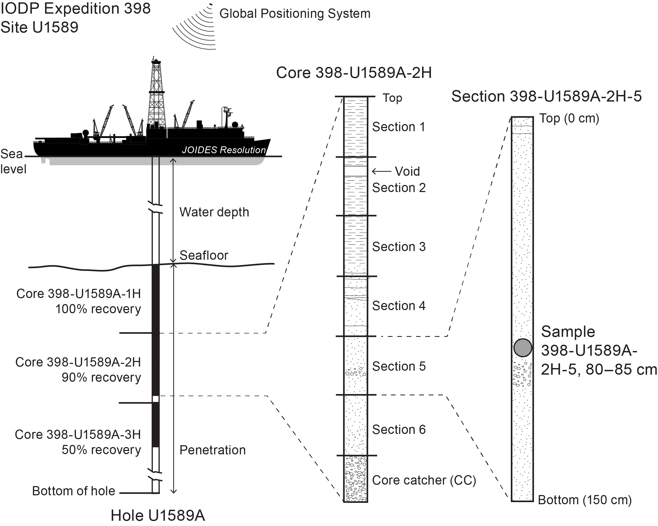
Figure F1. IODP naming convention.
1.2. Drilling operations
The advanced piston corer (APC), half-length APC (HLAPC), extended core barrel (XCB), and rotary core barrel (RCB) systems were all used during Expedition 398 (Figures F2, F3, F4). These tools and other drilling technology are documented in Graber et al. (2002). The APC and HLAPC systems cut soft-sediment cores with minimal coring disturbance relative to other IODP coring systems. After the APC/HLAPC core barrel is lowered through the drill pipe and lands above the bit, the drill pipe is pressured up until the two shear pins that hold the inner barrel attached to the outer barrel fail. The inner barrel then advances into the formation and cuts the core (Figure F2). The driller can detect a successful cut, or “full stroke,” by observing the pressure gauge on the rig floor because the excess pressure accumulated prior to the stroke drops rapidly.
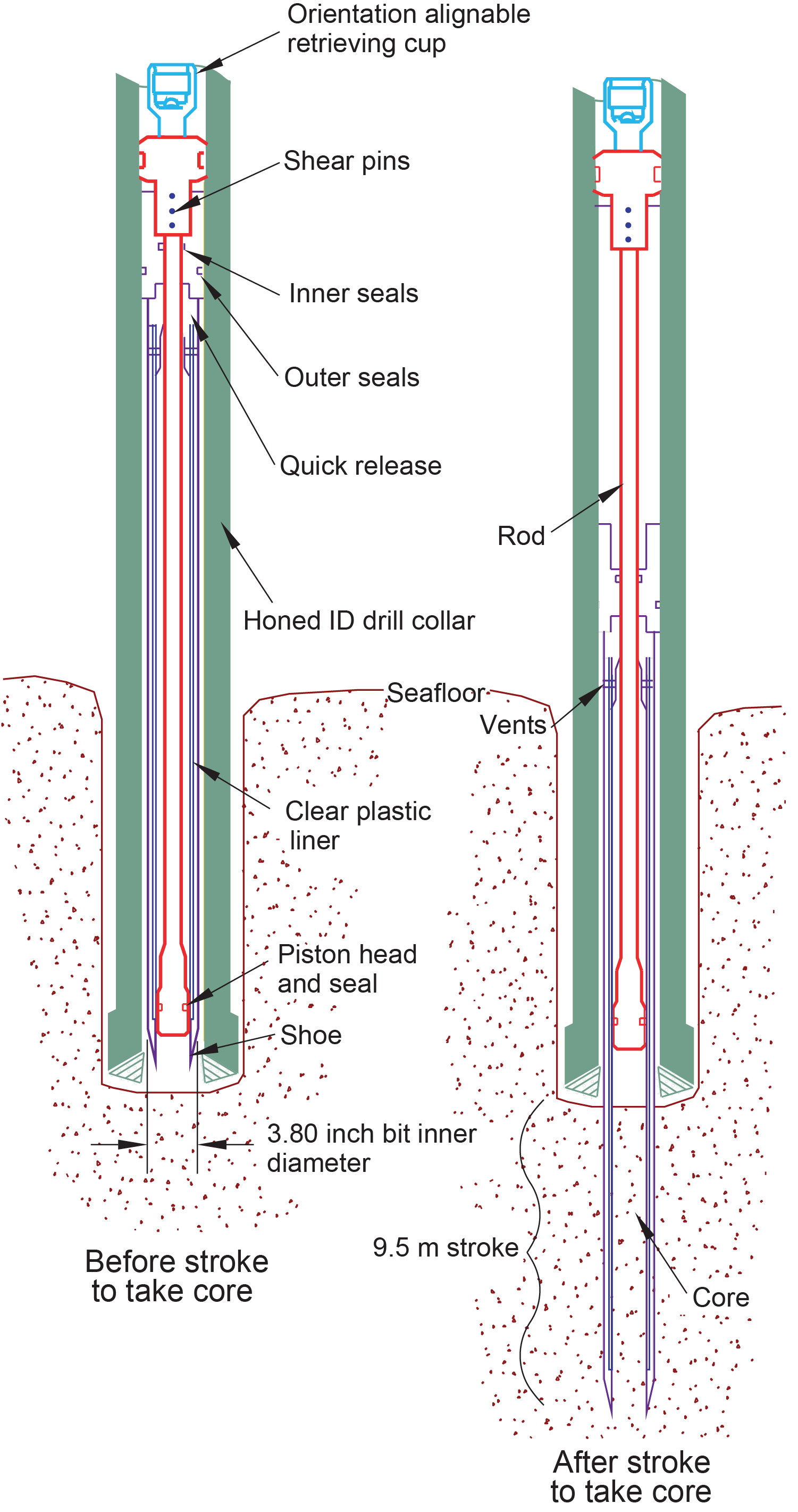
Figure F2. APC system.
APC refusal is conventionally defined in one of two ways: (1) the piston fails to achieve a complete stroke (as determined from the pump pressure and recovery reading) because the formation is too hard, or (2) excessive force “overpull” (>60,000 lb) is required to pull the core barrel out of the formation. For APC cores that do not achieve a full stroke, the next core can be taken after advancing to a depth determined by the recovery of the previous core (i.e., advance by recovery) or to the depth of a full APC core (typically 9.5 m). When a full stroke is not achieved, one or more additional attempts are typically made, and each time the bit is advanced by the length of the core recovered (note that for these cores, this results in a nominal recovery of ~100%). When a full or partial stroke is achieved but excessive force is not able to retrieve the barrel, the core barrel can be “drilled over,” meaning that after the inner core barrel is successfully shot into the formation, the drill bit is advanced to total depth to free the APC barrel.
The standard APC system uses a 9.5 m long core barrel, whereas the HLAPC system uses a 4.7 m long core barrel. In most instances, the HLAPC system is deployed after the standard APC system has repeated partial strokes and/or the core liners are damaged. During use of the HLAPC system, the same criteria are applied in terms of refusal as for the APC system. Use of the HLAPC system allowed for significantly greater APC sampling depths to be attained than would have otherwise been possible.
The XCB system is typically used when the APC/HLAPC system has difficulty penetrating the formation and/or damages the core liner or core. The XCB system can also be used either to initiate holes where the seafloor is not suitable (e.g., Site U1599) for APC coring or be interchanged with the APC/HLAPC system when dictated by changing formation conditions. The XCB system is used to advance the hole when HLAPC refusal occurs before the target depth is reached or when drilling conditions require it. The XCB system is a rotary system with a small cutting shoe that extends below the large rotary APC/XCB bit (Figure F3). The smaller bit can cut a semi-indurated core with less torque and fluid circulation than the main bit, potentially improving recovery. The XCB cutting shoe typically extends ~30.5 cm ahead of the main bit in soft sediments, but a spring allows it to retract into the main bit when hard formations are encountered. Shorter XCB cutting shoes can also be used.
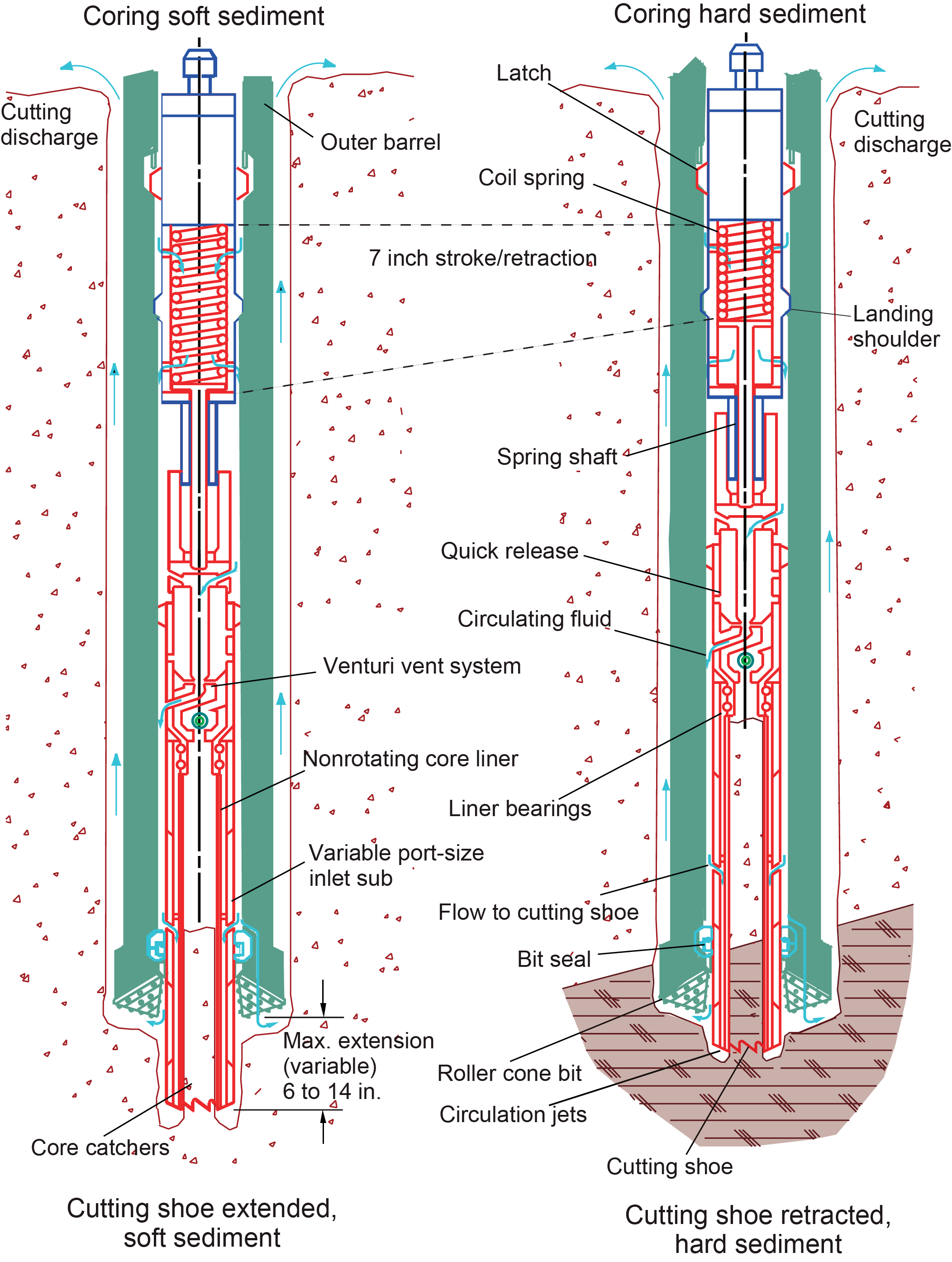
Figure F3. XCB system.
The bottom-hole assembly (BHA) used for APC/XCB coring is typically composed of an 11⁷⁄₁₆ inch (~29.05 cm) roller cone drill bit, a bit sub, a seal bore drill collar, a landing saver sub, a modified top sub, a modified head sub, 8¼ inch control length drill collars, a tapered drill collar, two stands of 5½ inch transition drill pipe, and a crossover sub to the drill pipe that extends to the surface.
The RCB system is a rotary system designed to recover firm to hard sediments and basement rocks. The BHA, including the bit and outer core barrel, is rotated with the drill string while bearings allow the inner core barrel to remain stationary (Figure F4).
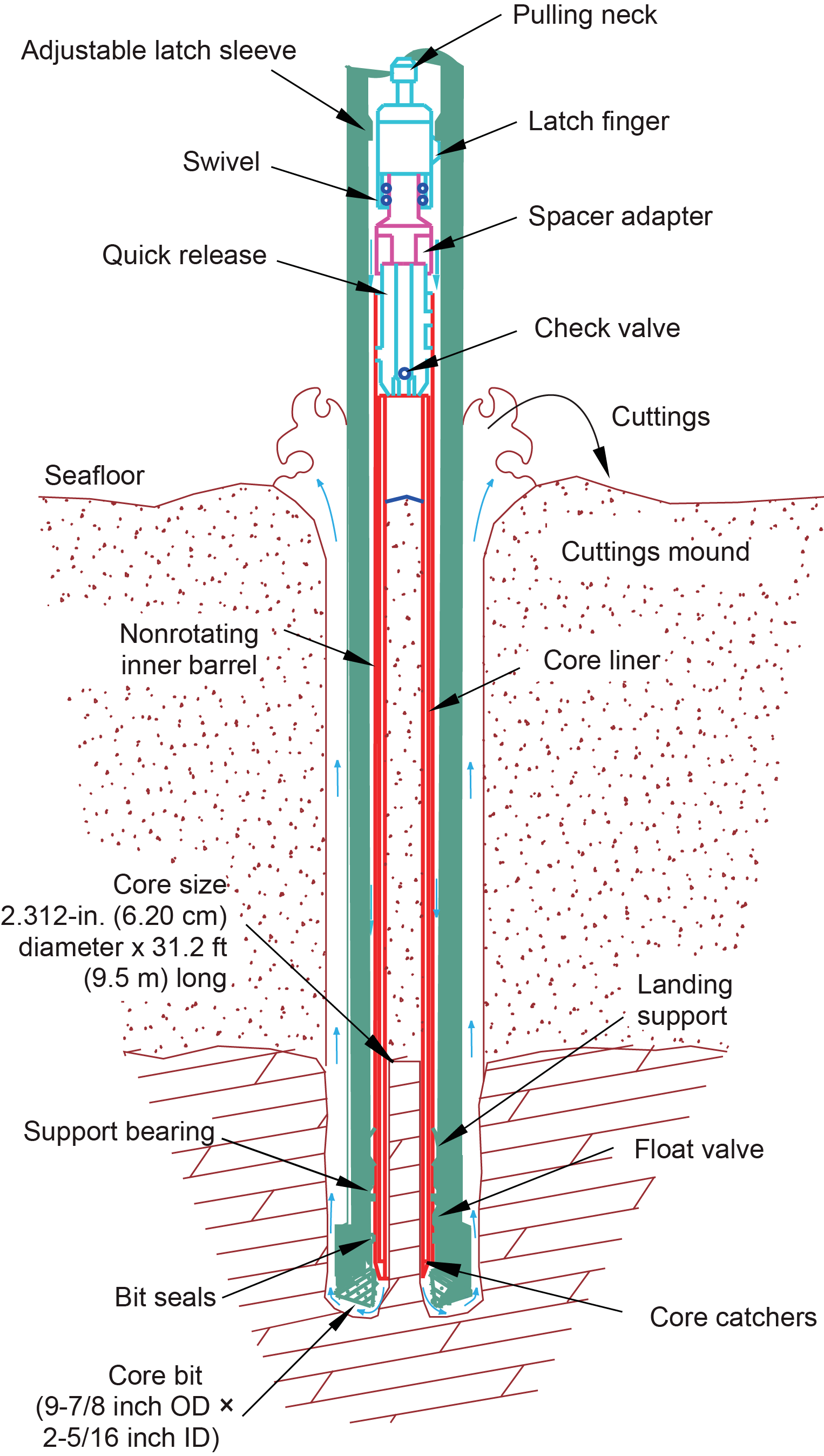
Figure F4. RCB system.
A typical RCB BHA includes a 9⅞ inch drill bit, a bit sub, an outer core barrel, a modified top sub, a modified head sub, a variable number of 8¼ inch control length drill collars, a tapered drill collar, two stands of 5½ inch drill pipe, and a crossover sub to the drill pipe that extends to the surface.
Nonmagnetic core barrels were used only at Sites U1589 and U1590 and Hole U1591A for APC, HLAPC, and RCB coring. APC cores were oriented with the Icefield MI-5 core orientation tool when coring conditions allowed. Formation temperature measurements were taken with the advanced piston corer temperature (APCT-3) tool (see Downhole temperature measurements). Information on recovered cores, drilled intervals, downhole tool deployments, and related information are provided in the Operations, Paleomagnetism, and Downhole measurements sections of each site chapter. Having severed the drill string at Sites U1589 and U1590 and becoming stuck in Hole U1591A, the decision was made to assemble and run simplified BHAs from Hole U1591B forward. These BHAs had no tapered collars, no nonmagnetic collars, and no Icefield MI-5 core orientation tool. In addition, temperature measurements were discontinued.
1.3. IODP depth conventions
The primary depth scales used by IODP are based on the measurement of the following:
- The drill string length deployed beneath the rig floor (drilling depth below rig floor [DRF] and drilling depth below seafloor [DSF]),
- The length of core recovered (core depth below seafloor [CSF] and core composite depth below seafloor [CCSF]), and
- The length of logging wireline deployed (wireline log depth below rig floor [WRF], wireline log depth below seafloor [WSF], and wireline log matched depth below seafloor [WMSF]).
All depths are in meters. The relationship between scales is defined either by protocol, such as the rules for computation of CSF depths from DSF depths, or by combinations of protocols with user-defined correlations (e.g., CCSF scale). The distinction in nomenclature should keep the user aware that a nominal depth value in two different depth scales usually does not refer to exactly the same stratigraphic interval (see Curatorial procedures and sample depth calculations). For more information on depth scales, see IODP Depth Scales Terminology at http://www.iodp.org/policies-and-guidelines. To more easily communicate shipboard results, CSF, Method A (CSF-A), depths in this volume are reported as meters below seafloor (mbsf) unless otherwise noted.
Depths of cored intervals are measured from the rig floor based on the length of drill pipe deployed beneath the rig floor (DRF scale; Figure F1). The depth of the cored interval is referenced to the seafloor (DSF scale) by subtracting the seafloor depth of the hole from the DRF depth of the interval. Standard depths of cores in meters below seafloor (CSF-A scale) are determined based on the assumption that the top depth of a recovered core corresponds to the top depth of its cored interval (DSF scale). Standard depths of samples and associated measurements (CSF-A scale) are calculated by adding the offset of the sample or measurement from the top of its section and the lengths of all higher sections in the core to the top depth of the core.
If a core has <100% recovery, for curation purposes all cored material is assumed to originate from the top of the drilled interval as a continuous section. In addition, voids in the core are closed by pushing core segments together, if possible, during core handling. If the core pieces cannot be pushed together to eliminate the voids, then foam spacers are inserted and clearly labeled “void.” Therefore, the true depth interval within the cored interval is only partially constrained. This should be considered a sampling uncertainty in age-depth analysis or correlation of core data with downhole logging data.
When core recovery is >100% (i.e., the length of the recovered core exceeds that of the cored interval), the CSF-A depth of a sample or measurement taken from the bottom of a core will be deeper than that of a sample or measurement taken from the top of the subsequent core (i.e., the data associated with the two core intervals overlap at the CSF-A scale). This overlap can happen when a soft to semisoft sediment core recovered from a few hundred meters below seafloor expands upon recovery (typically by a few percent to as much as 15%). Therefore, a stratigraphic interval may not have the same nominal depth on the DSF and CSF-A scales in the same hole.
1.4. Curatorial procedures and sample depth calculations
Numbering of sites, holes, cores, and samples followed standard IODP procedure (Figure F1). A full curatorial identifier for a sample consists of the following information: expedition, site, hole, core number, core type, section number, section half, piece number (hard rocks only), and interval in centimeters measured from the top of the core section. For example, a sample identification of “398-U1589A-2H-5W, 80–85 cm,” indicates a 5 cm sample removed from the interval between 80 and 85 cm below the top of Section 5 (working half) of Core 2 (“H” designates that this core was taken with the APC system) of Hole A at Site U1589 during Expedition 398 (Figure F1). The “U” preceding the hole number indicates the hole was drilled by the US IODP platform, JOIDES Resolution. The drilling system used to obtain a core is designated in the sample identifiers as follows:
Integers are used to denote the core type of drilled intervals (e.g., a drilled interval between Cores 2H and 4H would be denoted by Core 31).
1.5. Core handling and analysis
The overall flow of cores, sections, analyses, and sampling implemented during Expedition 398 is shown in Figure F5.
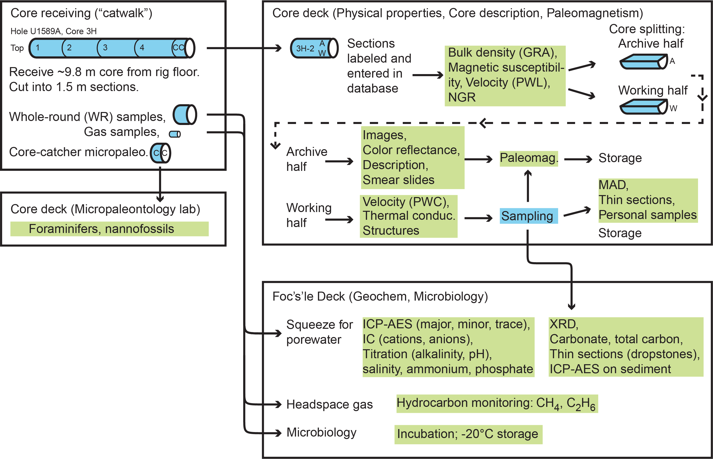
Figure F5. Work flow for Expedition 398.
1.6. Sediment
When the core barrel reached the rig floor, the core catcher (CC) from the bottom of the core was removed and taken to the core receiving platform (i.e., the catwalk), and a sample was extracted for paleontological (PAL) analysis. Next, the sediment core was extracted from the core barrel in its plastic liner. The liner was carried from the rig floor to the core processing area on the catwalk outside the core laboratory, where it was cut into ~1.5 m sections. If the core material was too soupy and sloshed within the core liner, decantation was achieved either by compressing the sediment and draining off the seawater or by vertical density segregation. Blue (uphole direction) and clear (downhole direction) liner caps were glued with acetone onto the cut liner sections.
Once the core was cut into sections, whole-round samples were taken for interstitial water (IW) chemical and microbiological analyses. When a whole-round sample was removed, a yellow cap was used to indicate it was taken. Syringe samples were taken for gas analyses according to the IODP hydrocarbon safety monitoring protocol. Syringe and whole-round samples were taken for microbiology culturing and postcruise analyses.
The core sections were placed in a core rack in the laboratory, core information was entered into the database, and the sections were labeled. When the core sections reached equilibrium with laboratory temperature (typically after 4 h), they were run through the Whole-Round Multisensor Logger (WRMSL) for P-wave velocity, magnetic susceptibility (MS), and gamma ray attenuation (GRA) bulk density (see Physical properties). The core sections were also run through the Natural Gamma Radiation Logger (NGRL), often prior to temperature equilibration because that does not affect the natural gamma radiation (NGR) data, and thermal conductivity measurements were taken once per core when the material was suitable.
The core sections were then split lengthwise from bottom to top into working and archive halves. Investigators should note that older material can be transported upward on the split face of each section during splitting.
Discrete samples were then taken for moisture and density (MAD) and paleomagnetic (PMAG) analyses and for remaining shipboard analyses such as X-ray diffraction (XRD), carbonate (CARB), and inductively coupled plasma–atomic emission spectroscopy (ICP-AES). Samples were not collected when the lithology was a high priority interval for expedition or postcruise research, the core material was unsuitable, or the core was severely deformed. During the expedition, samples for personal postcruise research were only taken in the form of a limited number of personal or shared “pilot” samples for three reasons: (1) to determine whether an analytical method works and yields interpretable results and how much sample is needed to guide postcruise sampling, (2) to generate low spatial resolution pilot data sets that can be incorporated in proposals and potentially increase chances of being funded, and (3) to generate early results to help with high impact publications before the Expedition 398 sampling party.
The archive half of each core was scanned on the Section Half Imaging Logger (SHIL) to provide linescan images, and then it was measured for point magnetic susceptibility (MSP) and reflectance spectroscopy and colorimetry (RSC) on the Section Half Multisensor Logger (SHMSL). Labeled foam pieces were used to denote missing whole-round intervals in the SHIL images. The archive halves were then described visually and by means of smear slides for sedimentology. Finally, the magnetization of archive halves and working-half discrete pieces was measured with the cryogenic magnetometer and spinner magnetometer.
When all steps were completed, cores were wrapped, sealed in plastic tubes, and transferred to the cold storage space aboard the ship. At the end of the expedition, the working halves of the cores were sent to the IODP Bremen Core Repository (Center for Marine Environmental Sciences [MARUM], Bremen, Germany), where samples for postcruise research were taken in July 2023. The archive halves of the cores were first sent to the IODP Gulf Coast Repository (Texas A&M University, College Station, Texas, USA), where a subset was analyzed by X-ray fluorescence (XRF) scanning before being forwarded to the Bremen Core Repository for long-term archive.
1.7. Drilling and handling core disturbance
Cores may be significantly disturbed and contain extraneous material as a result of the coring and core handling process (Jutzeler et al., 2014). For example, in formations with loose lapilli pumice, clasts from intervals higher in the hole may be washed down by drilling circulation, accumulate at the bottom of the hole, and be sampled with the next core. The uppermost 10–50 cm of each core must therefore be examined critically during description for potential “fall-in.” Common coring-induced deformation includes the concave-downward appearance of originally horizontal bedding. Piston action can result in liquefaction (i.e., “flow-in”) at the bottom of APC cores and/or especially when coarse loose material is penetrated, as well as disruption and shearing of the core material and subsequent midcore flow-in. The rotation and fluid circulation used during XCB and RCB coring can also cause core pieces to rotate relative to each other as well as introduce fluids into the core and/or cause liquefaction and remobilization of poorly consolidated/cemented sediments. In addition, extending APC or HLAPC coring into deeper, firmer formations can also induce core deformation. Retrieval from depth to the surface can result in elastic rebound. Gas that is in solution at depth may exsolve and drive apart core segments in the liner. When gas content is high, pressure must be relieved for safety reasons before the cores are cut into segments. This is accomplished by drilling holes into the liner, which forces some sediment as well as gas out of the liner. These disturbances are described in each site chapter and graphically indicated on the visual core descriptions (VCDs).
2. Lithostratigraphy
This section outlines procedures used to document the composition, texture, and structures of the volcanic, tuffaceous, and nonvolcanic sediments and sedimentary rocks recovered during Expedition 398. The procedures include VCD, smear slide and petrographic thin section analysis, digital color imaging, color spectrophotometry, and XRD.
Cores were split into working and archive halves, with sedimentologic and petrographic observations described on the archive halves. Soft-sediment cores were split with a wire, and lithified cores were split with a diamond-impregnated saw. The exposed surface of the archive half was evaluated for quality (e.g., smearing or surface unevenness) and, if necessary, gently scraped perpendicular to the core with a glass or stainless-steel slide to ensure a smooth, uncontaminated surface. After splitting, the archive half was imaged on the SHIL and then analyzed for color reflectance and MS using the SHMSL (see Physical properties). The archive-half sections were in some cases reimaged when visibility of sedimentary structures or fabrics improved following treatment of the split core surface.
Following imaging, the archive-half sections of the sediment cores were macroscopically described for lithologic and sedimentary features aided by use of a 20× wide-field hand lens, a binocular microscope, and 10% and 20% HCl solutions. Based on preliminary observations, toothpick samples from the archive-half sections were used to make smear slides, whereas thin sections and XRD samples were taken from the working-half sections. Lithostratigraphic units were defined following visual inspection, assisted by smear slide analysis; XRD analysis; and, where useful, thin section analysis, as well as physical properties.
Visual inspection of volcanic, tuffaceous, and nonvolcanic sediments and their lithified equivalents (e.g., tuff, mudstone, sandstone, marl, limestone) yielded macroscopic information such as sedimentary structures, lithologic variation, clast componentry, color, contacts, and core disturbance (e.g., drilling or tectonic disturbances; see Structural geology), whereas smear slide, thin section (i.e., microscopic), and XRD analyses were used to better identify volcanic, tuffaceous, and nonvolcanic sedimentary constituents including clasts, minerals, glass, and microfossils. Igneous rocks were found only as clasts in sediments or sedimentary rocks and were characterized macroscopically only as volcanic or plutonic. Varied types of metamorphic rocks were found as clasts in sediments, whereas metamorphic rocks from the basement consisted of marble or peridotite. Where applicable, thin sections of selected descriptive intervals and clasts provided more detail on mineralogy, variations in primary and secondary mineralogy, and the texture of these rocks. The descriptive data were entered into the GEODESC application (see GEODESC for details). All descriptions and sample locations were recorded using curated depths and documented on VCD graphic reports (e.g., Figure F6).
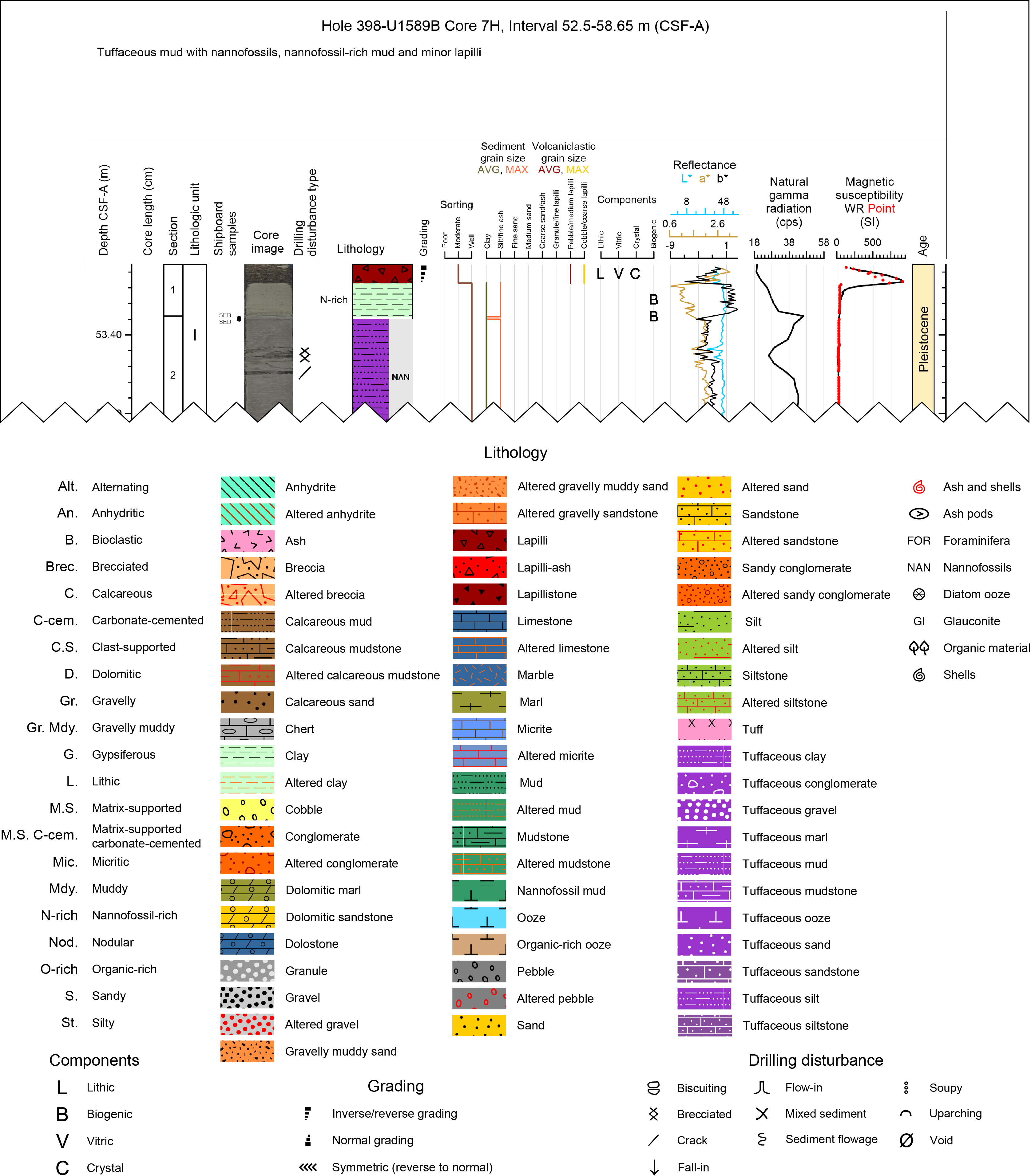
Figure F6. Example VCD and key for lithologies and features.
2.1. GEODESC
Data for the macroscopic and microscopic (i.e., smear slide and thin section) descriptions of recovered cores were entered into the IODP descriptive database using the IODP application GEODESC. GEODESC is description software that stores macroscopic and/or microscopic descriptions of cores. Data were entered into GEODESC through templates specific to different lithologies (i.e., sediments, intrusive igneous rocks, extrusive igneous rocks, and metamorphic rocks) for both macroscopic and microscopic observations. Core description data are available through LIMS Reports - Descriptive Information (http://web.iodp.tamu.edu/DESCReport). A single row in GEODESC defines one descriptive interval, where the material in that interval has similar characteristics with no major visual breaks. In volcanic sedimentary environments, an interval is commonly related to an eruptive or depositional event that punctuates background sedimentation intervals (Table T1).
This expedition collected volcanic material that was deposited by multiple possible processes (e.g., air fall, pyroclastic density current, turbidity current, debris flow, and so on) and as such are sediments and sedimentary rocks. The descriptive protocol employed during this expedition is rigorously nongenetic and integrates volcanic particles into GEODESC’s sedimentary descriptive schemes. As such, we have followed but adapted the methods used during Expeditions 350 and 376 (Tamura et al., 2015; de Ronde et al., 2019)
A capability in the new rollout of GEODESC is that multiselection lists allow multiple characteristics to be listed within one column, separated by commas in the output files. This feature was particularly useful for Expedition 398 because it allows for easy identification of multiple types of lithic clasts, glass shards, and crystals in volcanic lithologies for which no further description is needed. The order of selection in the multiselection list can be used to order the components in the output list by abundance. The same is true for alteration features.
The position of each smear slide or petrographic thin section is shown in the VCDs with a sample code of “SED” or “TS,” respectively.
2.2. Core disturbance
The coring and core handling processes may induce various types of core disturbance (Jutzeler et al., 2014), affecting our ability to recognize and describe original sedimentary and tectonic structures. The severity of core disturbance was rated as slight, moderate, severe, or destroyed, depending on the intensity of disturbance. Common types of core disturbance are described below:
- Fall-in core disturbance in unconsolidated units (e.g., ash, lapilli-ash, and lapilli) occurs when granular material from the top of the hole may fall in and accumulate at the bottom until the next core is recovered. As a result, fall-in material may reoccur in the uppermost part of the recovery of the next core, and original lithofacies and sedimentary structures are not present in these intervals. Thus, the uppermost part of each core section must be examined critically during description for potential fall-in (Figure F7A).
- Up- and downarching core disturbance results from slight to moderate coring-induced shear between the sediment and core liner and is recognized from bedding uniformly dragged downward along the core margins (Figure F7B). In these intervals, the original lithofacies and sedimentary structures are usually slightly to severely disturbed but can still be recognized visually.
- Soupy core disturbance is typically restricted to water-saturated intervals of unconsolidated ash overprinting original sedimentary or depositional structures (Figure F7C).
- Sediment flowage is caused by high shearing rates between cored sediments and the core liner, leaving a smear or thin trail of displaced sediment along the inside of the core liner (Figure F7D). Contamination by sediment flowage along the core liner may occur over long sections of the core and should be considered when further measurements and sampling of core material are conducted.
- Midcore flow-in disturbance may occur in water-saturated, granular core sections where grains and clasts flow and mix, producing mixed sediment and moderately to severely disturbed original sedimentary structures and stratigraphy (Figure F7E).
- Brecciated core disturbance results from drilling-related brittle rock failure (Figure F7F). Slight brecciation produces cracks in the original lithologies (Figure F7G), whereas moderate to severe brecciation disturbs original lithofacies and sedimentary structures more severely, though they usually remain readily recognizable.
- Biscuiting of recovered cores produces fractured disc-shaped pieces ranging in size from a few to more than 10 cm, often packed with sheared and remolded core material mixed with drill slurry, filling gaps between brittle “biscuits” (Figure F7H). Depending on the size of the biscuits, the degree of biscuiting was rated as slight (>5 cm biscuits), moderate (2–5 cm), severe (<2 cm), and destroyed (brecciated biscuits).
- Core voids up to ~25 cm in the original lithologies were observed in a few instances, for example in cores that experienced basal flow-in (Jutzeler et al., 2014), core extension, or low recovery (Figure F7I). Original lithofacies and sedimentary structures are fully destroyed in these intervals. Artificial size and density segregation of sediments is likely to occur during drilling or within postrecovery core handling processes on board (e.g., inclining, shaking, and plunging cores on the catwalk to compact sediments).
- Pseudohorizontal density grading, also described by Jutzeler et al. (2014), may occur while a core is lying flat on deck, resulting in vertical structures once the core is turned upright. Such core disturbances are observed most often in volcanic sediments, as increased porosity allows sucking in of seawater during hydraulic piston coring. The resulting soupy texture allows material to flow within the core liner. Secondary normal or reverse grading, or density separation of clasts, may occur as a result of this disturbance and obscure primary sedimentary features (Figure F8).
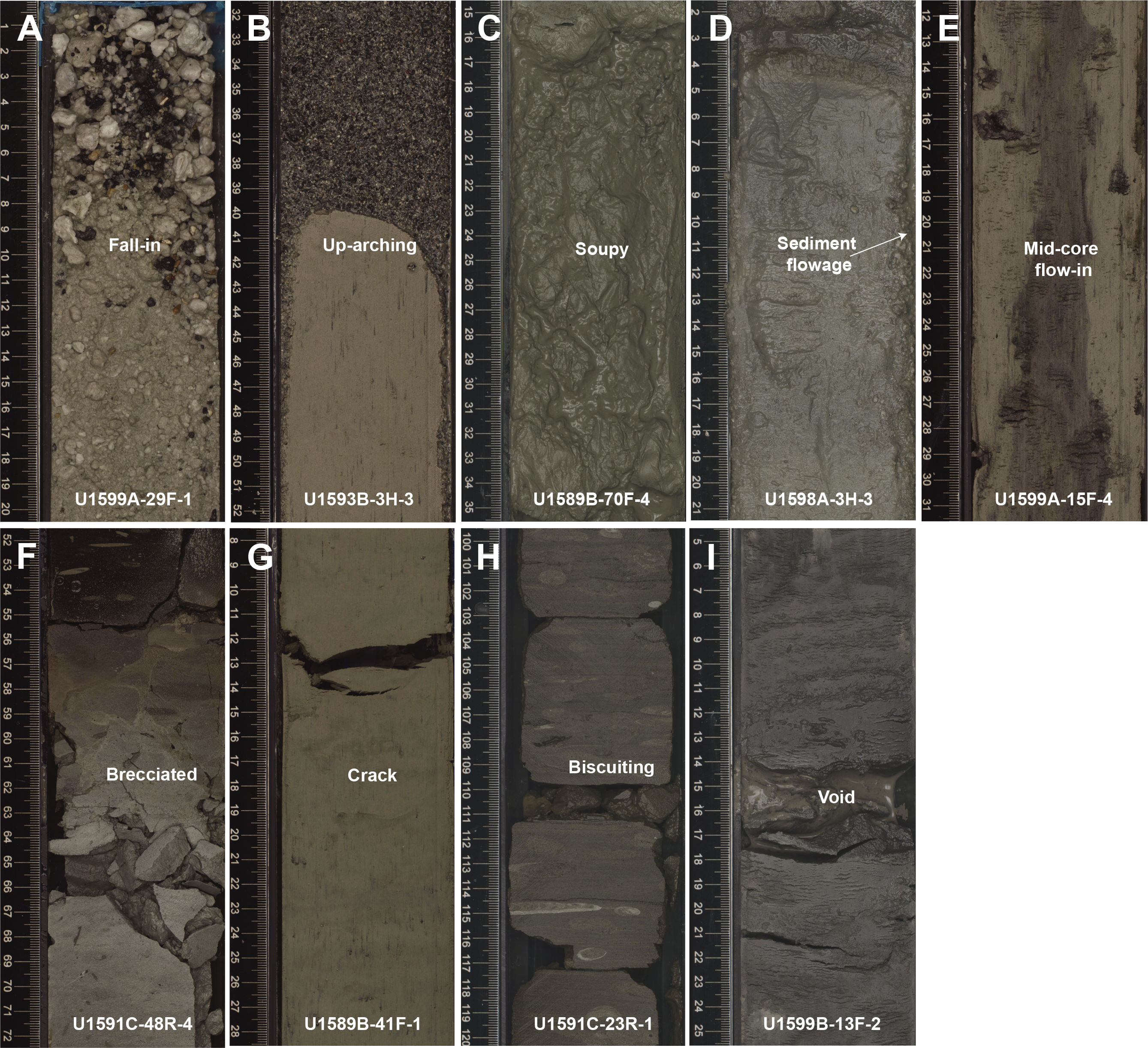
Figure F7. Examples of deformation and disturbance.
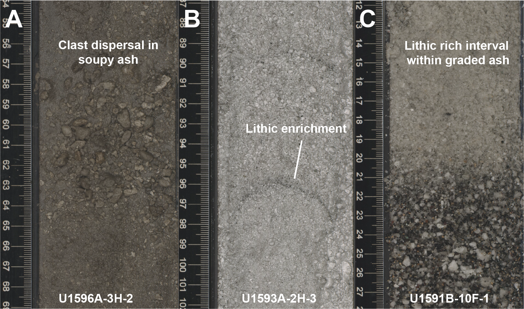
Figure F8. Examples of artificial and primary grain size and density segregation.
Identified disturbance parameters are recorded in GEODESC, and some of them are only associated with specific coring techniques. For example, APC and HLAPC coring may induce core expansion (stratification destroyed and layer thickness artificially increased), sediment flowage disturbance (leaving a smear of exotic sediment along the inside of the core barrel), shearing and sediment flowage along the margin of the core liner, and basal flow-in (false stratigraphy, commonly composed of soupy, polymictic, density-graded sediment that generally lacks horizontal laminations). RCB and XCB coring typically cause torquing of the consolidated units (e.g., sedimentary and volcanic lithologies), resulting in biscuiting and brecciation (see above).
2.3. Core description workflow
Several procedures were used to document the composition, texture, and structures in material recovered during Expedition 398, including visual core description (both macroscopic and microscopic), digital color imaging, scanning electron microscope (SEM) imaging, X-ray imaging, and XRD analysis.
To describe the cores with as much detail and efficiency as possible, the core describers of Expedition 398 established the following description workflow:
- Macroscopic identification and logging of intervals (see Table T1 for interval definition): macroscopic description of material color, texture, structure (e.g., bottom contacts, grain size, bedding, grading, and so on), componentry, and alteration (e.g., disseminated sulfides). Componentry refers to clasts > 2 mm and crystals; these were logged separately as vitric clasts (e.g., pumice, scoria), lithic clasts (e.g., volcanic rock, metamorphic rock), and biogenic clasts.
- Microscopic analyses of interval characteristics: smear slides were critical for identifying components and mineralogy of volcanic, tuffaceous, and nonvolcanic sediments. Thin sections were important for identifying components and mineralogy of sedimentary rock igneous clasts and metamorphic basement rock (marble only). In the event of recurring layers in sediments and neighboring holes, smear slides were prepared only for representative layers, due to limited capacities/personnel on board.
- Based on the descriptions from (1), supported by (2), and assisted by physical properties analysis (see Physical properties), intervals were grouped into sequential lithostratigraphic units and subunits (see Table T1 for lithostratigraphic unit and subunit definitions).
2.4. Units
The materials retrieved during Expedition 398 include sediment and their lithified equivalents (including igneous rock clasts), and metamorphic (i.e., marble or peridotite) basement rocks. They are described at the following levels:
- The descriptive interval (a single descriptive row in the GEODESC spreadsheet),
- The lithostratigraphic unit, and
- The subunit.
2.4.1. Descriptive intervals
A descriptive interval is a sediment or rock interval defined by macroscopic features such as color, texture, and grain size that are distinct from features in the lithologies above or below and may continue across core sections. They are analogous to beds, and thicknesses can be classified in the same way.
Multiple lithologies are sometimes intercalated and repetitive (e.g., alternating mud and sand beds), and these are usually grouped within one descriptive interval. This was accomplished by adding a suffix of “with alternating…” to the principal name of the most abundant facies for the subordinate facies (e.g., “organic-rich mud with alternating sand”; Figure F9). Alternatively, although not used during this expedition, it is possible to use the domain classifier in GEODESC for this purpose, where the alternating interval is identified as Domain 0 for the dominant lithology and the subordinate part is identified as Domain 1 (and 2, 3, if necessary). In GEODESC, each subordinate domain is then described beneath the composite descriptive interval as if it were its own descriptive interval.
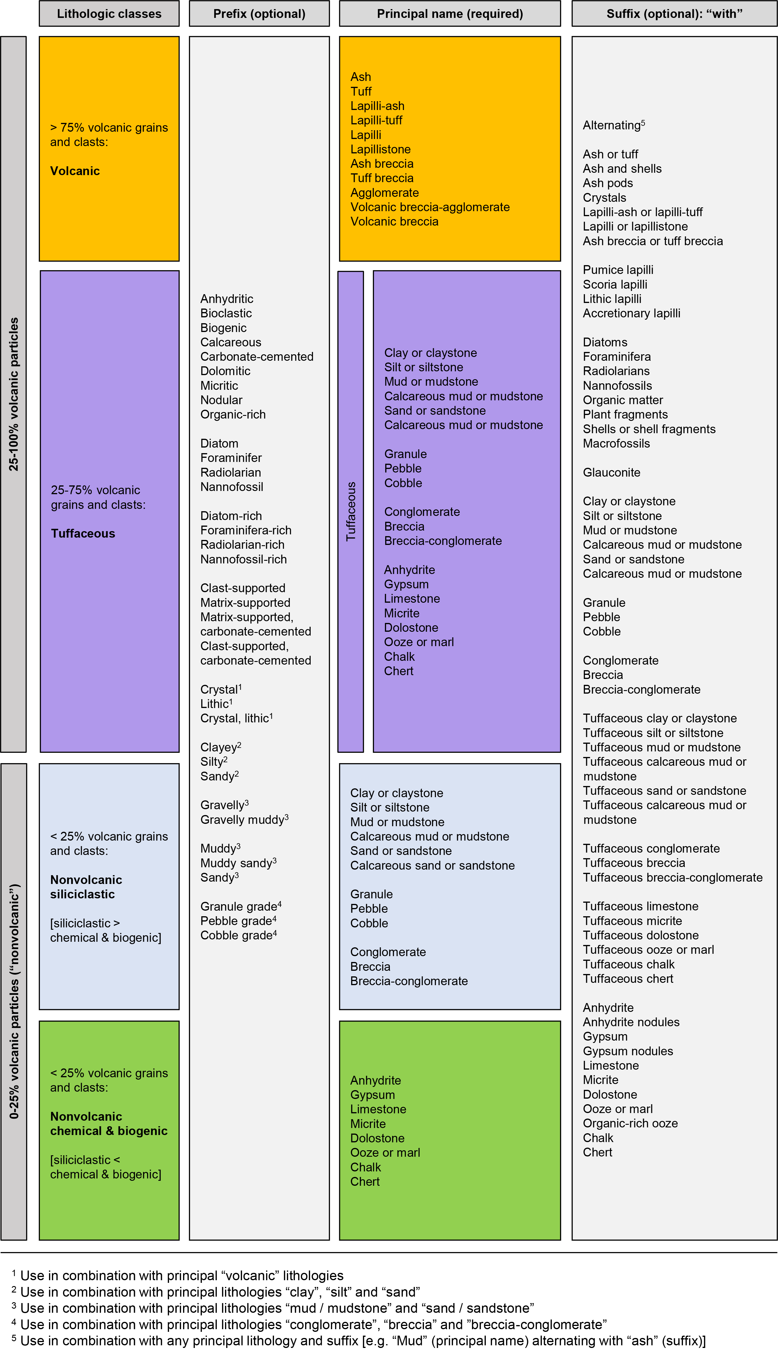
Figure F9. Sedimentary lithology naming conventions.
Description of alternating lithologies was generally avoided for intervals containing volcanic sediments with >75% volcanic material, as these volcanic sediments must be associated with specific depth intervals for tephrostratigraphic purposes. Therefore, these lithologies were typically added using GEODESC’s “split interval” function so that background sediments could be described across an entire larger interval with smaller split intervals added incrementally (e.g., at the appearance of discrete volcanic ash layers).
2.4.2. Lithostratigraphic units
Lithostratigraphic units are assemblages, tens to hundreds of meters thick, of similar principal lithologies and facies. They can include subunits (Table T1). Units are numbered sequentially (e.g., Lithostratigraphic Unit I, II, III) from top to bottom. They are clearly distinguishable from each other by several observable characteristics (e.g., relative proportion of principal lithologies, composition, bed thickness, grain size class). They can be considered analogous to formations. Changes in age, geochemistry, physical properties, or paleontology may coincide with, or inform placements of, boundaries between lithostratigraphic units.
2.4.3. Subunits
Subunits are made up of many descriptive intervals and capture lithologic trends on the scale of one to hundreds of meters. They are distinguished by more subtle shifts within the overall lithologic context, such as a subunit of ooze containing a much higher frequency of volcanic layers than a previous subunit. Subunits are numbered sequentially within the main units with an alphabetical suffix (e.g., Subunit Ia, Ib, Ic), from top to bottom.
2.5. Sediments and sedimentary rocks
2.5.1. Lithologic description
2.5.1.1. Principal lithology
Principal lithologies were assigned by the proportion of four main sedimentary lithologic classes (Figure F9), based on composition:
- Volcanic (>75% volcanic particles).
- Tuffaceous (25%–75% volcanic particles).
- Nonvolcanic siliciclastic (<25% volcanic particles, where siliciclastic particles are dominant compared to chemical and biogenic components).
- Nonvolcanic chemical and biogenic (<25% volcanic particles, where chemical and biogenic components are dominant compared to siliciclastic particles).
The volcanic principal lithology names are from Fisher and Schmincke (1984) based on particle size and proportions (Figures F10, F11).
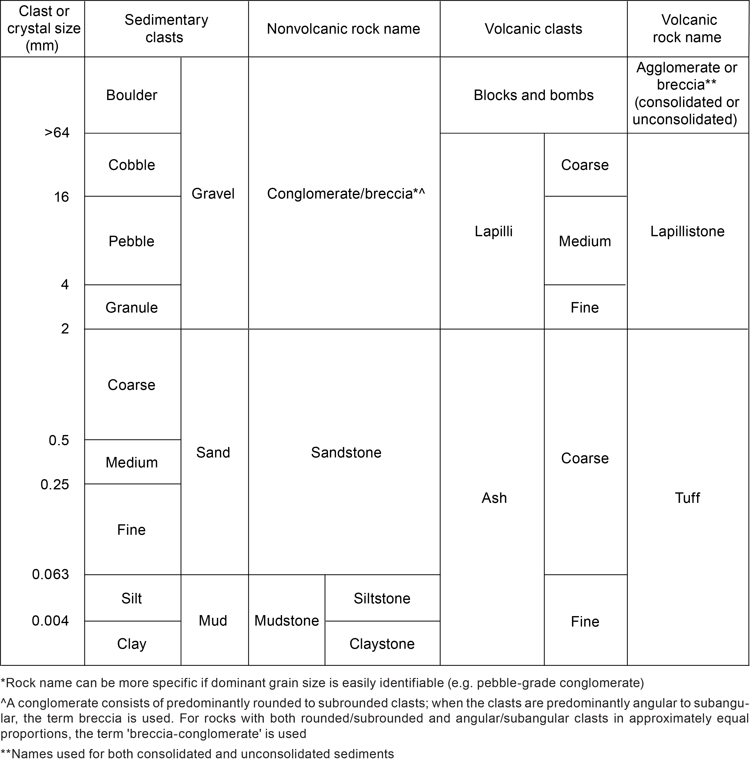
Figure F10. Grain size scheme.
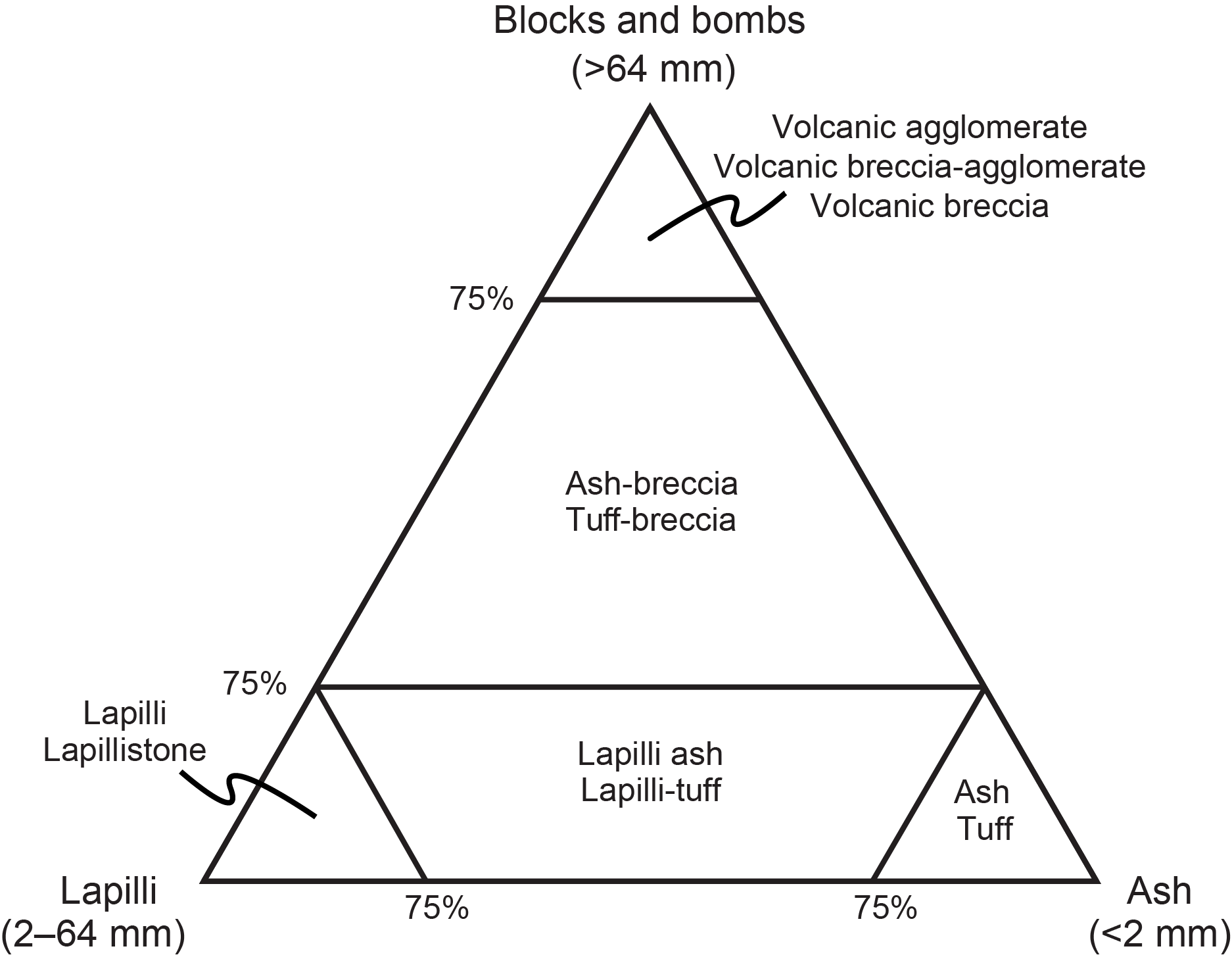
Figure F11. Volcanic grain size terms and classification.
The term “tuffaceous” describes sediments consisting of 25%–75% volcanic grains and clasts mixed with another principal lithology (e.g., Fisher and Schmincke, 1984), often identified with microscopic smear slide observation (e.g., tuffaceous ooze; Figure F9). We chose to include tuffaceous lithologies as independent principal lithologies to preserve the use of prefixes for further description.
Nonvolcanic sediments contain <25% volcanic particles and are classed as either “siliciclastic,” where siliciclastic particles are dominant compared to chemical and biogenic components, or “chemical and biogenic,” where chemical and biogenic sedimentary components are dominant compared to siliciclastic particles.
Within these lithologic classes, the principal lithology name is based on particle size and lithification (unconsolidated versus consolidated) (Figure F11). Tuffaceous and nonvolcanic lithologies were further categorized based on the proportions of sand-, silt-, and clay-sized grains (for lithologies with grain sizes < 2 mm) (Figure F12) or based on the proportions of mud-, sand-, and gravel-sized grains and clasts (for lithologies that contain clasts > 2 mm) (Figure F13). For tuffaceous and nonvolcanic lithologies with a biogenic component, a simplified and adapted classification scheme based on Shepard (1954) was used (Figure F14). This scheme uses abundance of biogenic components (e.g., foraminifera, diatoms, nannofossils, and radiolarians) to name nonvolcanic sediments. See Other parameters for more detail.

Figure F12. Sand, silt, clay classification scheme.
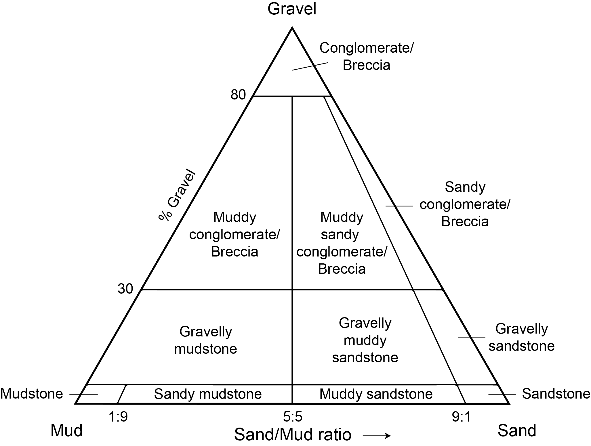
Figure F13. Sand, gravel, mud classification scheme.
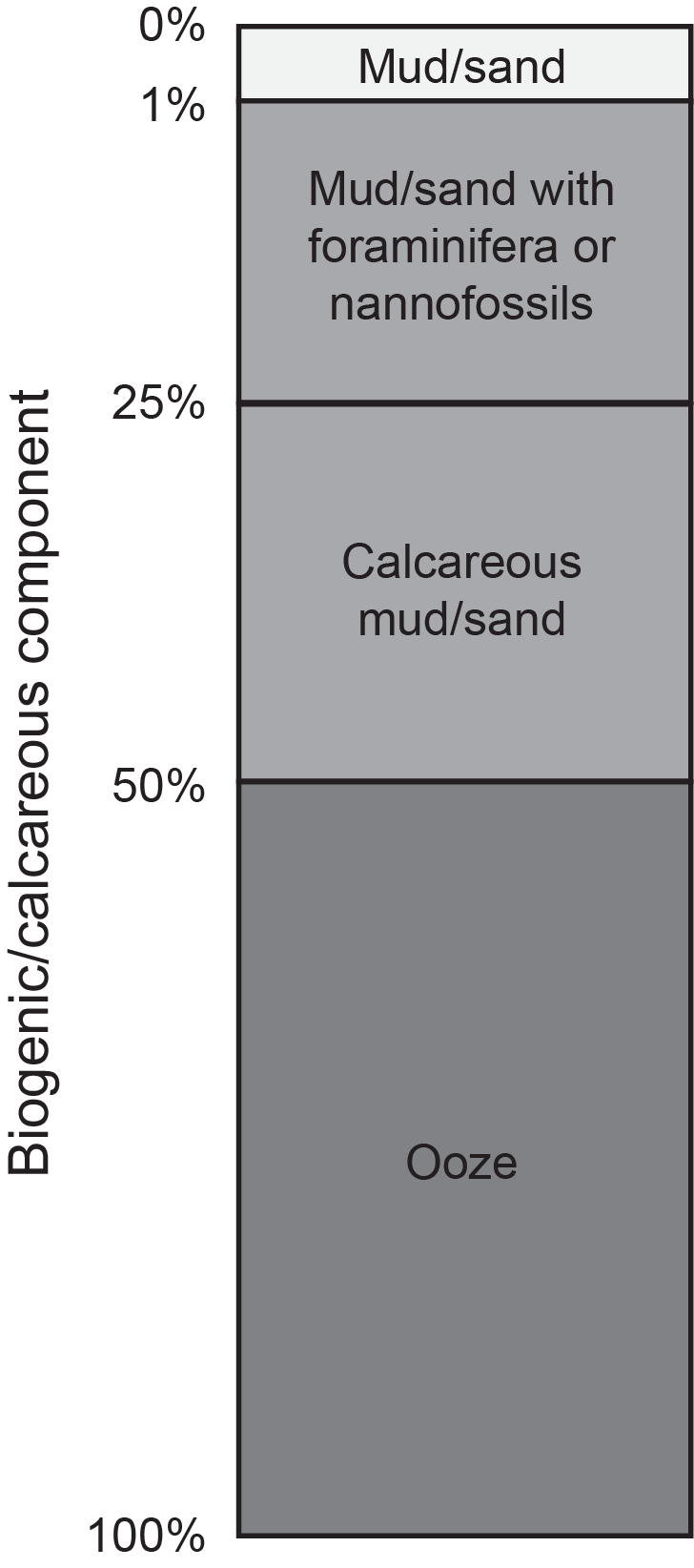
Figure F14. Biogenic sediments and sedimentary rocks classification.
Carbonate lithologies are typically calcium carbonate based (i.e., calcite) and, in some cases, contain a proportion of dolomite (i.e., calcium magnesium carbonate). In such a case, we added the prefix “dolomitic” to the principal lithology name (e.g., dolomitic sand). Mineralogy was determined by color, mineral hardness, smear slide observation, and HCl acid test (using both 10% and 20% HCl)—the latter is particularly useful for the distinction of calcitic and dolomitic lithologies—and was subsequently confirmed by XRD analyses on selected samples. Evaporitic chemical sediments encountered at Site U1591, and maybe at Site U1599 (micritic sediment), were characterized based on mineralogy, macroscopic observations of texture, and XRD. Anhydrite lithologies often occur as nodular varieties (>0.5 cm growths) described in the literature as “chicken wire” anhydrite (e.g., Hsü et al., 1973) or as laminated sheets (<0.5 cm growths) interbedded with micrite, and thus were assigned the “nodular” or “laminated” prefix. If the abundance of nodules was <25%, the suffix “with anhydrite nodules” was used. Thin section analysis also allowed observation of algal mats within evaporitic lithologies.
Lithification of sediments was determined by visual observation of relative hardness and compaction of sediments and corroborated by increasing P-wave velocity and bulk density and decreasing porosity (see Physical properties). As sediments often transitioned gradually from unconsolidated sediment to sedimentary rock with increasing depth, the point of transition to lithified principal lithology nomenclature (e.g., “mudstone” instead of “mud”) was determined based on overall downcore trends.
2.5.1.1.1. Prefix
Prefixes are used to describe lithologies and features that are present but not captured by principal lithology names. They can refer to observable characteristics, such as “clast-supported” versus “matrix-supported,” or “nodular.” They can also be assigned to components that appear in 25%–50% abundance, for example, “silty” as a prefix to sand, “calcareous” as a prefix to mud, or “microfossil-rich” as a prefix to limestone.
2.5.1.1.2. Suffix
The suffix is used for a subordinate component within a given sediment or sedimentary rock that deserves to be highlighted. Suffixes were assigned to lithologies with 1%–25% abundance. They are always in the form of “with” added to the dominant principal lithology, for example, “with ash,” “with clay,” or “with foraminifera.” Suffixes are also used with alternating units as described previously, and these can be up to 50% abundance. For example, suffixes for principal lithologies with alternating units might read “with alternating mudstone.”
2.5.2. Definitions of descriptive terms
2.5.2.1. Grain versus clast
The term “particle” is used to describe fragments (i.e., grains and clasts) that comprise volcanic-rich and nonvolcanic sediments, regardless of size. We use the term “clast” to describe particles > 2 mm and “grain” to describe particles < 2 mm. This follows the practice of IODP Expedition 350, with combined size divisions of particles from Wentworth (1992), Fisher (1961), Fisher and Schmincke (1984), Cas and Wright (1987), McPhie et al. (1993), and White and Houghton (2006).
Volcanic particles were defined by Fisher and Schmincke (1984), and we adapt their scheme based on grain size and the relative abundance of ash-sized (<2 mm) and lapilli-sized (2–64 mm) particles (Figure F10) rather than particle type. For example, the terms “ash” and “lapilli” are used when the proportion of one size was >75%, and “lapilli-ash” describes when both grain sizes were present but each at <75% abundance (Fisher and Schmincke, 1984). The term “ash” is used to imply a composition of predominantly vitric grains (glass shards), unless specified otherwise, using “lithic,” “crystal,” or “lithic, crystal” prefixes in cases where these are dominant components, as confirmed, for example, by smear slide analysis. Equally, lapilli are implied to consist predominantly of vitric clasts (e.g., pumice or scoria) unless a lithic, crystal, or lithic, crystal prefix is used, suggesting that these are dominant components. For example, we use the term “lithic lapilli” when an interval is dominantly composed of lithics sized 2–64 mm rather than vitric clasts. Types of vitric clasts are further defined in the GEODESC interval under Type of vitric clasts.
Lithic clast types are listed in the componentry columns of GEODESC (see Componentry).
2.5.2.2. Monomictic versus polymictic
The term “monomictic” is used for sediments with only one clast type (i.e., lithic or vitric), whereas “polymictic” is used when sediments have multiple clast types. We restrict our use of these terms to particles >2 mm in size (referred to as clasts in our scheme) and do not use the term for particles <2 mm in size (referred to as grains in our scheme). Variations within a single volcanic parent rock (e.g., a collapsing lava dome) may produce a deposit referred to as monomictic, which is composed of fragments of the same composition. In contrast, a debris flow or turbidity current may remobilize a region that contains multiple source-rock types, therefore producing a deposit that is polymictic.
2.5.2.3. Clast-supported versus matrix-supported
We define clast-supported sediments as sediment intervals with clasts >2 mm that are in direct physical contact with each other. In contrast, matrix-supported sediments have clasts >2 mm surrounded by an interstitial fine-grained matrix with very few clast/clast contacts. The matrix is not specifically defined by a grain size (i.e., it is not restricted to grains, which are <2 mm in size). For example, a matrix-supported volcanic breccia could have clasts supported in a matrix of lapilli.
2.5.2.4. Lithic, crystal, and crystal, lithic prefixes
Volcanic lithologies (e.g., ash, lapilli-ash, lapilli) were sometimes modified with the prefix “lithic,” “crystal,” or “crystal, lithic” to denote component enrichment (in a proportion of 25%–50%) within a descriptive interval. Volcanic lithologies described without a lithic, crystal, or crystal, lithic prefix are implied to be dominantly vitric. The type of vitric clast (e.g., pumice or scoria) is defined in GEODESC for that interval under Type of vitric clasts.
2.5.2.5. Ooze versus calcareous mud
Nonvolcanic sediments (i.e., sediments with <25% volcanic grains and clasts) containing a significant proportion of biogenic and calcareous components relative to siliciclastic components were commonly recovered during Expedition 398. These sediments were classified as “ooze” if the proportion of biogenic and calcareous components (e.g., calcareous nannofossils, foraminifera, diatoms, radiolarians) was >50% and as “calcareous mud” or “calcareous sand” if biogenic and calcareous components were 25%–50% abundance (Figure F14). A suffix, for example “with foraminifera” or “with nannofossils,” was used for lithologies that contain 1%–25% biogenic and calcareous components. Such lithologies and calcareous muds and sands are implied to contain a greater proportion of siliciclastic material than oozes and were distinguished from ooze by intensity of reaction with HCl and confirmed by microscopic smear slide observation, where necessary. Although most recovered oozes consist dominantly of calcareous microfossils, rare instances of siliceous oozes, dominated, for example, by diatoms or radiolarians, were noted in the GEODESC descriptions.
2.5.2.6. “Organic-rich” prefix and “with organic material” suffix
Nonvolcanic ooze-dominated units and subunits display cyclical transitions from green-hued ooze to olive-gray-brown oozes and calcareous muds, representing cyclical variations in proportions of organic matter. This organic matter also presented a telltale odor. When these color variations and odors were present, the “organic-rich” prefix was employed. If only a slight color change was observed and ooze was still recognizable, the suffix “with organic material” was employed.
2.5.3. Sedimentary structures, textures, and fabric
Sediment grain size was determined using the Wentworth scale (Wentworth, 1922) (Figure F10). The determination of grain sizes of loose volcanic-dominated deposits (i.e., fine to coarse ash/lapilli) simplifies the classification schemes of Fisher and Schmincke (1984) and Schmid (1981).
2.5.3.1. Structures
Sedimentary structures observed in the recovered cores included stratification (i.e., bedding or lamination), grading, soft-sediment deformation, and bioturbation. The lower contacts of stratification features were described based on geometry (i.e., irregular, planar, curviplanar, covered, or not recovered), definition (i.e., sharp, diffuse, scoured, wavy, continuous, discontinuous, and gradational), and orientation (i.e., horizontal, subhorizontal, inclined, subvertical, and vertical).
2.5.3.2. Bedding
Bed thickness was defined according to Ingram (1954) and included the following units:
- Very thickly bedded = >100 cm.
- Thickly bedded = 30–100 cm.
- Medium bedded = 10–30 cm.
- Thinly bedded = 3–10 cm.
- Very thinly bedded = 1–3 cm.
- Thickly laminated = 0.3–1 cm.
- Thinly laminated = <0.3 cm.
Bedding type was also described as either planar, wavy, lenticular, or cross-bedded.
2.5.3.3. Grading, sorting, and roundness
Sediment grading was described as either normal (i.e., fining upward), reverse, symmetric (i.e., normal to reverse), symmetric (i.e., reverse to normal), multiple normal, or multiple reverse (Fisher and Schmincke, 1984). Descriptions of sorting and rounding followed the scheme of Folk (1980) as shown in Figure F15.
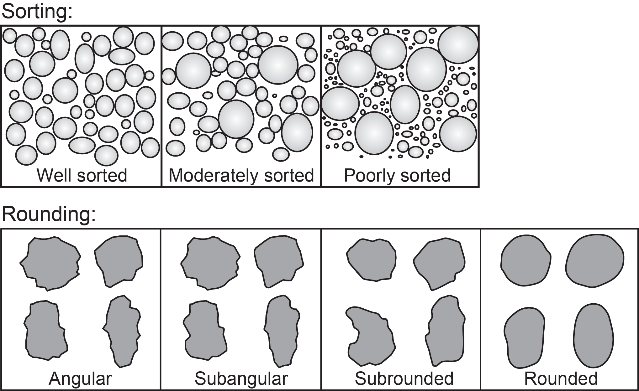
Figure F15. Terms for sorting and rounding of grains and clasts.
2.5.4. Bioturbation
Bioturbation intensity in deposits was measured and shown on the VCDs using the semiquantitative ichnofabric index described by Droser and Bottjer (1986, 1991), aided by visual comparative charts (Heard et al., 2014). The several indexes shown in these charts refer to the degree of biogenic disruption of primary fabric such as laminations and range from nonbioturbated sediment to total homogenization. Here, the indexes are simplified and summarized into categories as below:
- None = no bioturbation recorded; all original sedimentary structures preserved.
- Slight bioturbation = discrete, isolated trace fossils; up to 10% of original bedding disturbed.
- Moderate bioturbation = approximately 10%–60% of original bedding disturbed; burrows largely overlap and are commonly poorly defined.
- High bioturbation = bedding is completely disturbed, but burrows can still be discerned in places; the fabric is not mixed although the bedding may be nearly or totally homogenized.
2.5.5. Componentry
Volcanic, tuffaceous, and nonvolcanic sediments and their lithified equivalents were further described by their respective components including lithic clasts, vitric clasts, biogenic clasts, free crystals, and matrix. Clast components must be >2 mm (following the definition of clasts vs. grains), whereas matrix may be composed of both clasts and grains. Lithic clasts were described by their composition (i.e., volcanic, carbonate, sedimentary, and so on). Vitric clasts were characterized by texture (e.g., scoria, pumice) and roundness (i.e., angular, subangular, subrounded, rounded) (Figure F15). Free crystals visible macroscopically were identified regardless of size, though most crystals were grains (<2 mm). Biogenic components were identified and specified by type if possible (e.g., gastropod, echinoderm, bivalve, and so on).
2.6. Alteration
2.6.1. Macroscopic description
Alteration observed macroscopically was classified by feature (e.g., vein, disseminated) and secondary mineral type. Noted alteration features include background alteration, concretion, disseminated secondary mineral phases, layered alteration, nodular alteration, or vein infills.
Macroscopic observation of several secondary minerals was recorded in terms of abundance (i.e., dropdown multiselect list by order of abundance) to indicate prevalence of mineralization for each type. Comments were allowed for further description of observed alteration (e.g., “quartz-chlorite veins may indicate hydrothermal alteration”).
2.6.2. Microscopic description
Microscopic descriptions of alteration are contained within the microscopic descriptions of the major rock type (i.e., sedimentary, igneous, metamorphic). The intensity of replacement of original rock components is based on visual estimations of proportions relative to the total area of the thin section. Microscopic descriptions are made in terms of replacing phases for minerals, groundmass/matrix, clasts, glass, and patches of alteration. Comments are used to provide further specific information where available. Descriptive terms used for alteration extent follow:
2.7. Other parameters
Several additional parameters were recorded in macroscopic core descriptions to further delineate units. Color was recorded using standardized Munsell color charts (Munsell Color Company, Inc., 2009). Organic-rich (sapropelic) muds and oozes were recognized by their dark color and occasional sulfuric odor and characterized using the terms “homogeneous” or “color-banded.”
2.8. Smear slides
Smear slides are useful for identifying and reporting basic sediment attributes like textural, mineralogical, and compositional features, as well as microfossils. They were prepared to confirm macroscopic descriptions of distinct lithology changes at the core section level, such as identification of vitric particles in tuffaceous lithologies or crystals in ash layers. They confirmed the presence of specific minerals such as biotite, amphibole, feldspar, and pyroxene. Smear slide components supported designation of boundaries of units and subunits, but the results are semiquantitative at best (cf. Marsaglia et al., 2013, 2015). Finer grained sediments (<2 mm) required inspection at high magnification to accurately determine lithic, crystal, and biogenic type and abundance. We estimated the abundance of volcanic, tuffaceous, siliciclastic, and biogenic components using a visual comparison chart (Rothwell, 1989), with an emphasis on major lithologies. Particular attention was paid to recognition of ash layers and tuffaceous lithologies through observation of glass and crystals. Glass shape and vesicularity as well as vesicle shape were quantified as well.
Visual estimates for normalized percentages of sand, silt, and clay (Terry and Chilingar, 1955) were recorded along with abundance for the individual observed grain types. The component categorization applied to smear slides is shown in Figure F16. For all smear slides, visual estimates of component abundance were made semiquantitatively, and defined as follows:
- T = trace (<1 vol%).
- R = rare (1–5 vol%).
- C = common (5–20 vol%).
- A = abundant (20–50 vol%).
- D = dominant (>50%).
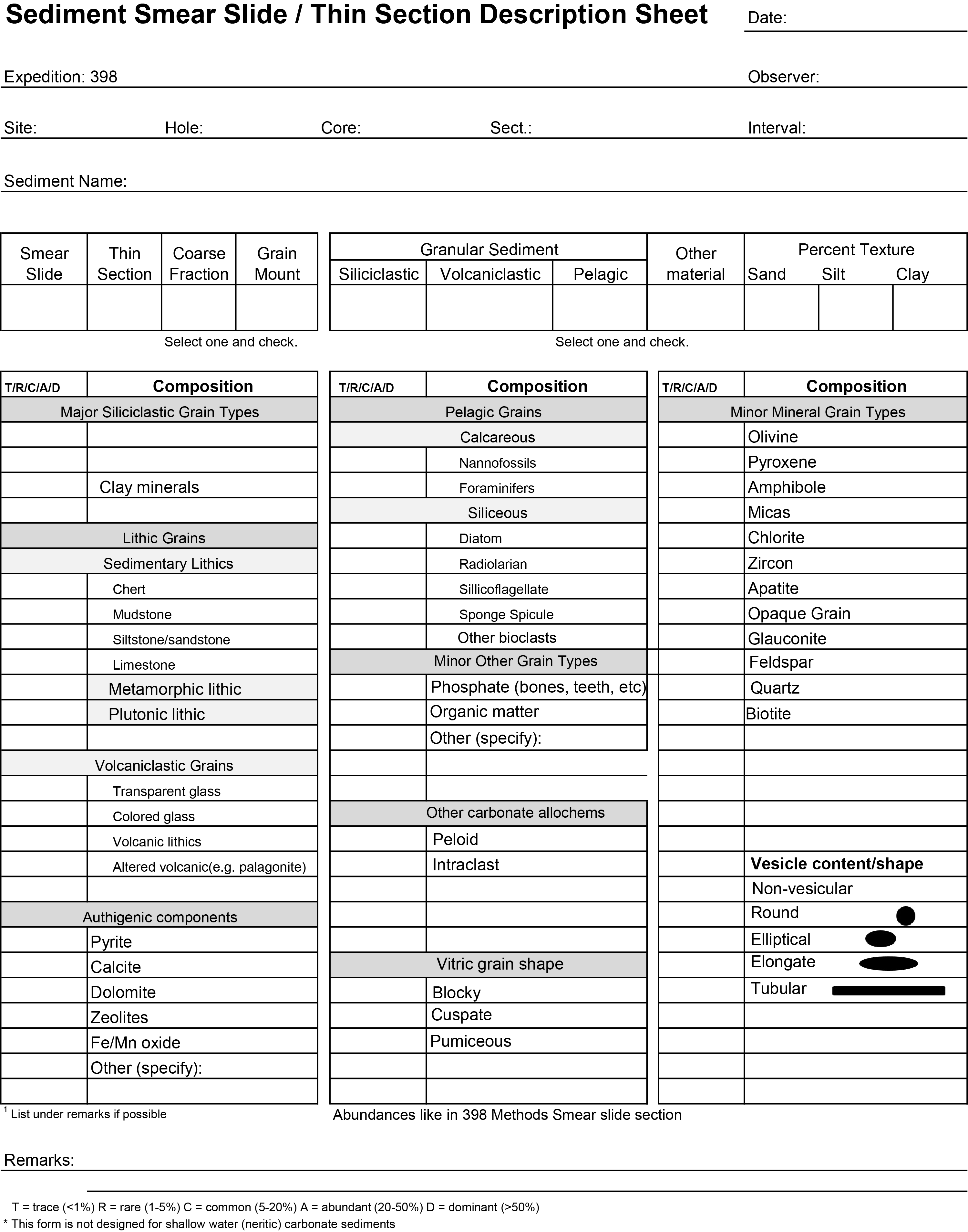
Figure F16. Template for characterization of smear slides.
Smear slides were observed and photographed in transmitted light, plane-polarized light (PPL), and cross-polarized light (XPL) using an Axioskop 40A polarizing microscope (Carl Zeiss) equipped with a FlexSpot digital camera (Figure F17).
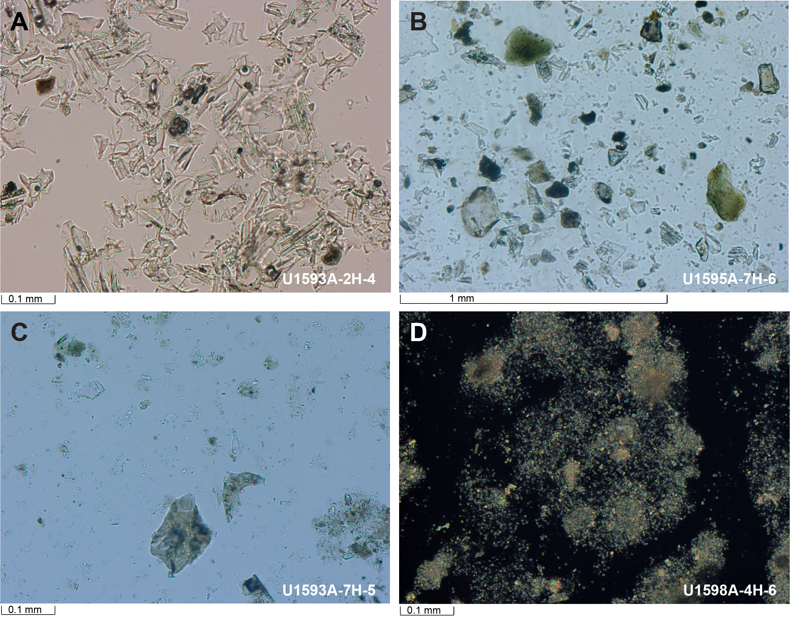
Figure F17. Smear slide images showing lithologic units or subunits.
2.9. Thin sections
Description of thin sections followed standard protocols as described in IODP Expedition 344 (Harris et al., 2013). Thin section descriptions were used to refine the initial macroscopic observations of sedimentary, igneous (clast only), and metamorphic lithologies. The composition and proportion (modal) of primary and secondary (altered/hydrothermal) minerals and other rock-forming components in these lithologies were better defined by using microscopic examination. The microscopic description of sedimentary lithologies followed closely that of our macroscopic characterization, with additional detail provided on the grain size, texture, and proportions of rock components. Textural domains of igneous rocks (identified only as clasts for Expedition 398) were defined after MacKenzie et al. (1982). We also described the crystallinity (i.e., holocrystalline, hypocrystalline, and holohyaline) and the vesicularity (i.e., degree, shape, and size) of our samples. In our description, “phenocryst” was used as a shape term describing relatively large and generally conspicuous crystals distinctly larger than the groundmass of a volcanic rock. A preliminary name for volcanic rock (e.g., basalt, andesite, dacite, and rhyolite) was given based on color, phenocryst content, and literature data (Table T2).
Eruptive products from Christiana, Kolumbo, and ancient Santorini (>550 ka) contain amphibole and zircon (e.g., Huijsmans, 1985; Druitt et al., 1999; Francalanci et al., 2005; Cantner et al., 2014; Higgins et al., 2021) (Table T3), which are essentially absent in the younger Santorini series (Francalanci and Zellmer, 2019). In addition, biotite has so far only been identified in quantity in the Kolumbo eruptive products (e.g., Cantner et al., 2014) (Table T3). These mineralogical differences helped us to correlate the volcanic layers between cores collected during this expedition and between source volcanoes. We also compared our samples with the parageneses of the eruptive products of Milos and Eastern Aegean arc volcanoes that could be present in our cores.
Metamorphic rocks were only encountered as occasional lithic clasts in volcanic intervals and in crystalline basement rocks of the south Aegean region that were recovered at some sites. The nomenclature used for naming metamorphic rocks was based on directly observable features at the macroscopic scale (i.e., mineral content and rock structure) rather than genetic terms, following the recommendations by the IUGS Subcommission on the Systematics of Metamorphic Rocks (Schmid et al., 2004).
Thin sections were observed and photographed in transmitted light, PPL, and XPL using an Axioskop 40A polarizing microscope (Carl Zeiss) equipped with a FlexSpot digital camera (Figure F18).
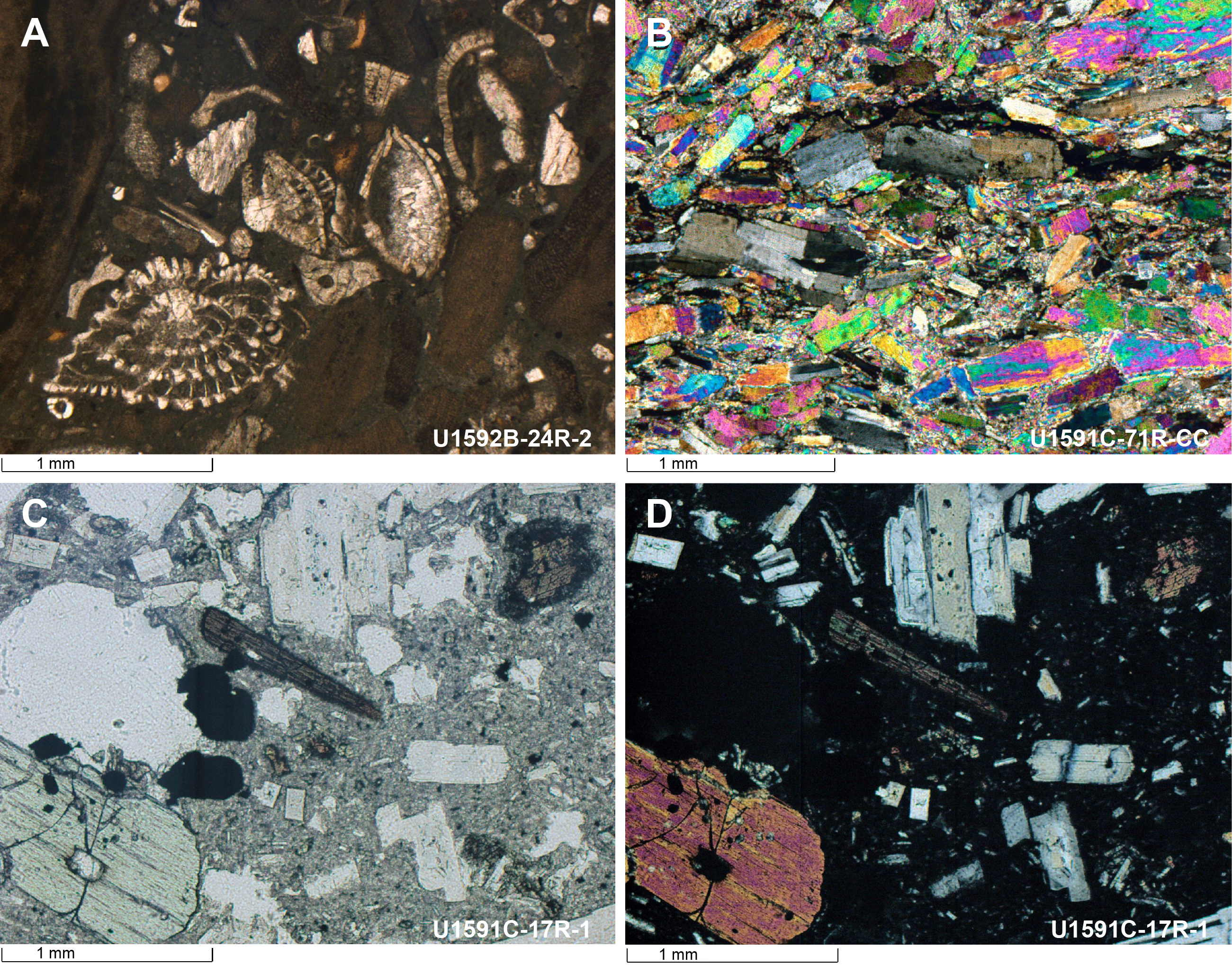
Figure F18. Thin section images showing mineral phases and rock texture.
2.10. Visual core description graphic summary reports
VCDs were generated from descriptive data input to GEODESC to summarize each core. Patterns, symbols, and colors used correspond to individual descriptors, as shown in Figure F6. Each core is graphically displayed with its lithologic units next to the high-resolution image. A typical example is shown in Figure F6.
2.11. X-ray diffraction
Samples for XRD analysis were obtained routinely from IW squeeze cake sediment residues and selected other core samples. Typically, 5 cm3 samples were processed for XRD analysis. All samples were vacuum-dried, crushed for 3 min with a ball mill, and mounted as randomly oriented bulk powders. Routine XRD analyses of bulk powders were performed using a Malvern Panalytical Aeris X-ray diffractometer equipped with a PIXcel1D detector, which allows standardless quantification of mixtures of phases. XRD instrument settings were as follows:
- Voltage = 40 kV.
- Current = 15 mA.
- Goniometer angle = 5°–70°2θ.
- Step size = 0.0108664°2θ.
- Scan speed = 49.725 s/step.
- Divergence slit = 0.25 mm.
The principal goal of XRD analysis was to determine bulk sample mineralogy from characteristic peaks in the XRD spectra (Figure F19) to complement the macroscopic core description and geochemical analysis. Identification of all phases was carried out using Malvern Panalytical’s software package, HighScore Plus, based on characteristic mineral peaks and peak intensities (i.e., counts). Relative phase proportions were determined in selected samples using the Rietveld method implemented in HighScore Plus.
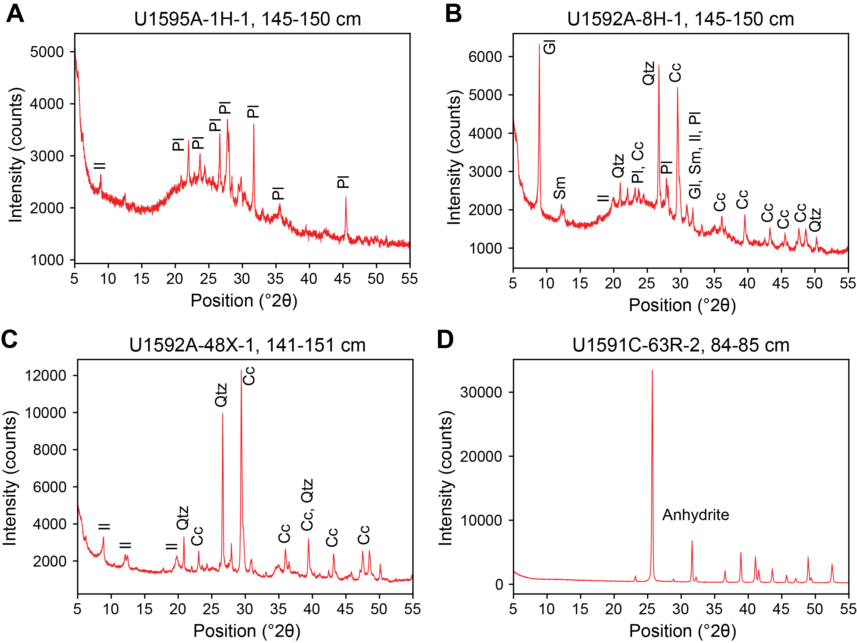
Figure F19. XRD spectra of various sediments.
2.12. Interpretation
Core description was intentionally restricted to observable characteristics of the recovered materials. However, we allowed for optional preliminary interpretation of lithologic origin based on the observable characteristics recorded (i.e., fallout, debris flow, basement). Initial interpretation was largely for ease of internal communication among the onboard science party and is not included in the final VCDs subject to review by the core description scientists and co-chief scientists.
3. Stratigraphic correlation
The scientific objectives of Expedition 398 required recovery of complete stratigraphic intervals with continuity at a centimeter scale. With a single IODP hole, such recovery is impossible to achieve because of coring gaps that occur between successive cores during the drilling process, even when 100% or more nominal recovery is attained (Ruddiman et al., 1987; Hagelberg et al., 1995). In addition, contamination by sediments that might have fallen into the hole introduces stratigraphic noise within any core. Therefore, it was important to generate a “splice,” whereby we combined stratigraphic intervals from two or more closely spaced holes at the same site, such that the depths of core gaps are staggered between holes. To minimize gaps between cores, we attempted to offset the depths of coring between adjacent holes and intended to apply near real-time correlations to check while coring.
The stratigraphic correlators aboard JOIDES Resolution during Expedition 398 focused mainly on three tasks: (1) use the correlation of sediment physical properties (MS and GRA density) acquired from fast whole-round tracks between holes that were scanned immediately upon retrieval of cores as a rapid-response guide while drilling to minimize gap alignment; (2) construct a composite depth scale for all holes; and (3) reconstruct the most representative single continuous sedimentary section by splicing intervals from multiple holes.
The results from the stratigraphic correlation effort involved consideration of several different depth scales, for which we followed IODP conventions, as outlined below (see IODP Depth Scales Terminology at https://www.iodp.org/policies-and-guidelines) (Figure F20).
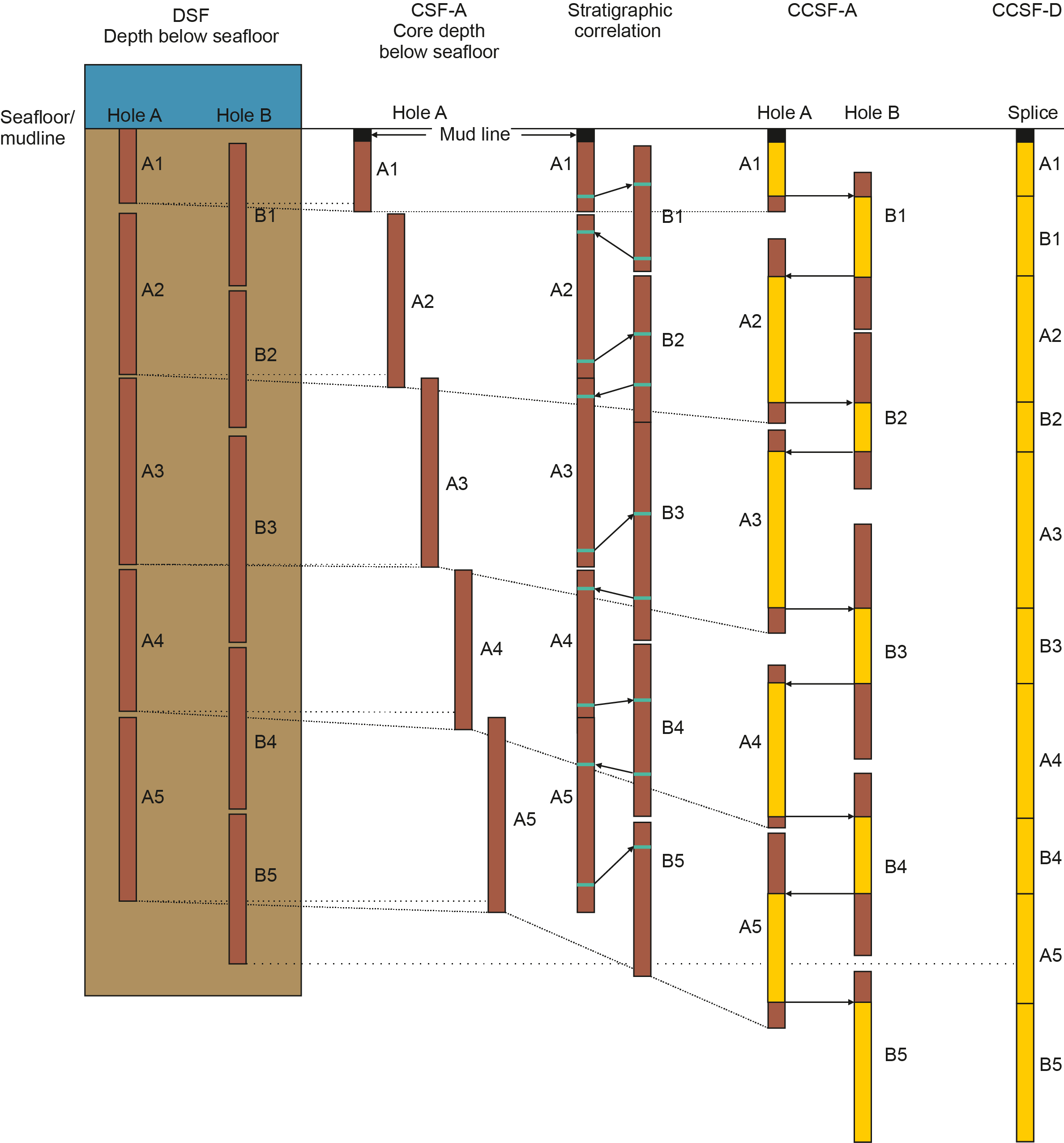
Figure F20. Relationships between cored material and the depth scales.
3.1. Drilling depth below seafloor scale
The starting point for the process of building a composite section was to assign a depth to the top of each core, which is initially based on DSF. This value is determined as the difference between the length of the drill string below the rig floor to the top of the cored interval and the length of the drill string from the rig floor to the mudline, which is, by IODP convention, assumed to be the seafloor (Figure F20). DSF is influenced by tidal variations in sea level, uncompensated ship heave, and other sources of error.
3.2. Core depth below seafloor scale
The depth of a given position within any core is determined relative to the DSF core top depth. The CSF scale combines the DSF core top depth with the curated depth within a core after retrieval (Figure F20).
CSF does not necessarily correspond to the actual depth below the seafloor for several reasons. Technical reasons can prevent the mudline from being cored, especially if the precise water depth is not accurately known, for instance, due to tides or swell and resulting heave. It may turn out that even if the mudline was cored in Hole A, the mudline was not cored in Hole B because the APC stroke was shot from beneath the sediment surface. Such an example is shown in Figure F20.
Other factors combine to further influence CSF. Sediment loss at the ends of the core may shorten the core. Core expansion resulting from the piston coring technique, which develops underpressure at the top of the core, is one of the most common effects. Overpressurized fluids or trapped gas within the pore space of the core may also result in expansion. Therefore, core expansion may result in an overlap of cores when plotted on the CSF scale (CSF-A).
If the APC core barrel, for example, penetrates the seafloor by 8 m including the mudline (Hole A Core 1H), the entire ~10 m long core may be filled due to expansion. However, because the top of the next core is at 8 m DSF, the resulting CSF-A scale will indicate a 2 m overlap. Thus, errors in the CSF-A scale include both drilling effects and core expansion effects, and, as a consequence, the CSF-A scale permits overlap between successive cores that are stratigraphically impossible.
3.3. Core composite depth below seafloor scale
Before a splice can be constructed, the cores from adjacent holes must be stratigraphically correlated with each other (Figure F20). Such correlation transfers the CSF-A scale into the CCSF, Method A (CCSF-A), scale that should, in principle, correct stratigraphic artifacts contained in the CSF-A scale. The CCSF scale is based on locating features common to cores in multiple holes at a given site and working from the top of the site downward to select tie points (arrows in Figure F20) that correlate strata in one hole with those in another. Because of core expansion and the unavoidable absence of complete recovery at the tops and bottoms of cores, Holes A and B on the CCSF scale are potentially longer than they are on the CSF-A scale.
By correlating distinct features, such as prominent waveforms in physical properties or distinct layers in core images, between cores from adjacent holes, we shifted the depth of individual cores relative to CSF-A in that hole to align those features on a common depth scale (Figure F20). The construction of a CCSF-A scale requires that each individual core is offset by a constant value without stretching or squeezing individual cores. This resulting composite depth scale provides good estimates of the length of coring gaps and provides the basis for the development of the spliced record (CCSF-D scale, see below). We summarized the vertical depth offset of every core in every hole in an affine table, one of the principal deliverables of the stratigraphic correlation effort.
In practice, we constructed the CCSF-A scale using Correlator software (version 4.0) (see more below), which allowed correlation of distinct strata or corresponding physical properties downhole from the mudline. The mudline marks the top of the stratigraphic section and was typically taken from the first core. We used the core including the uppermost strata as the “anchor” in the composite depth scale. This core (Core A in Figure F20) is usually the only one in which the depths are the same on the CSF-A and CCSF-A scales.
Next, we identified corresponding signatures (i.e., prominent waveforms in physical properties or distinctive layers in core images) and established tie points among adjacent holes. MS was the most suitable physical parameter and was used most often. The decision regarding which core from which hole should be shifted against the corresponding core in the neighboring hole was not always easy to make. As a rule, however, cores were shifted downward because an upward shift usually increased the vertical overlap of two cores in the same hole, which is usually not plausible. Whenever we encountered gaps in the correlation (e.g., due to low recovery or when no correlations could be identified), we used the “SET” function in Correlator software to offset the cores below the gaps by the same amount as the cores above.
As a consequence of the downward shift, the summed length of all cores in the CCSF-A scale is usually longer than the sum of all cores in the DSF or CSF-A scale. We calculated the systematic increase for each site by comparing the deviation from the CCSF-A scale from the CSF-A scale. The final length of all cores in the CCSF-A scale is therefore greater than the maximum drilling depth due to postrecovery expansion of the cores.
After establishing the CCSF-A scale and identifying all between-core gaps, we constructed a complete stratigraphic section—the splice—by combining selected intervals between aligned adjacent cores. The resulting depth section is the CCSF-D scale, which can be considered a subset of the CCSF-A scale (Figure F20). The corresponding splice interval table contains listings of the specific core intervals used to construct the splice and is the other principal deliverable of the stratigraphic correlation effort. No correction of the core expansion was applied on board.
3.4. Measurements and methods for correlation
Our workflow for compositing and splicing using Correlator software (version 4.0) comprised two steps:
- During core retrieval from Hole B, we anticipated using the Special Task Multisensor Logger (STMSL) to rapidly measure GRA density and MS as soon as possible after core retrieval. This allowed stratigraphic correlation to be conducted in near real time so that bit depths could be adjusted to avoid alignment of core gaps between holes.
- After retrieval of cores from both Holes A and B, we used all available data to develop composite sections (CCSF-A scale) based on the stratigraphic correlation of NGR, MS, and GRA density acquired from the WRMSL and STMSL, as well as digitized color reflectance data and photos. We accomplished compositing and splicing using Correlator software, from which we generated standard affine tables (i.e., listings of the vertical offset in meters added to each core to generate the CCSF-A scales) and splice interval tables (i.e., listings of the specific core intervals used to construct the splice). Once the stratigraphic correlation was finalized, we uploaded finalized tables into the IODP LIMS database with “-USE THIS” remarks, which then affixes the appropriate depth scale to any associated data set.
4. Structural geology
The Christiana-Santorini-Kolumbo (CSK) volcanic field and surrounding marine rift basins on the Hellenic volcanic arc form a unique system that records rich archives of volcanic products, tectonic evolution, and magma genesis. The principal objective of the structural geology team during Expedition 398 was to record deformation structures observed both in volcanic and clastic packages in cores, which are the basic data for evaluating the links between tectonic evolution and volcanism, and corresponding event deposits in the basin.
Our methods for documenting the structural geology of Expedition 398 cores largely followed those given by Expedition 334 structural geologists (see Structural geology in the Expedition 334 methods chapter [Expedition 334 Scientists, 2012]). We documented deformation observed in the split cores by classifying structures, determining the depth interval, measuring orientation data, and recording the sense of displacement. The collected data were hand logged onto a printed form at the core table and then typed into both a spreadsheet and the GEODESC database.
4.1. Structural data acquisition and orientation measurements
Each structure was recorded manually on a description table sheet modified from that used during Expeditions 315 and 316 (Figure F21). Core measurements followed those made during Expeditions 315, 316, and 376 (Expedition 315 Scientists, 2009; Expedition 316 Scientists, 2009; de Ronde et al., 2019), which in turn were based on previous Ocean Drilling Program (ODP) procedures developed at the Nankai accretionary margin (i.e., ODP Legs 131 and 190; Shipboard Scientific Party, 1991; Shipboard Scientific Party, 2001). The distance from the top of the section (0 cm) to the top and bottom of the feature was recorded, and the mean distance between the top and bottom of the feature was used as the depth of the structure on the plot (Figure F22). We used a plastic protractor for orientation measurements (Figure F23). Using the working half of the split cores provided greater flexibility in removing—and cutting, if necessary—pieces of the core for measurements.
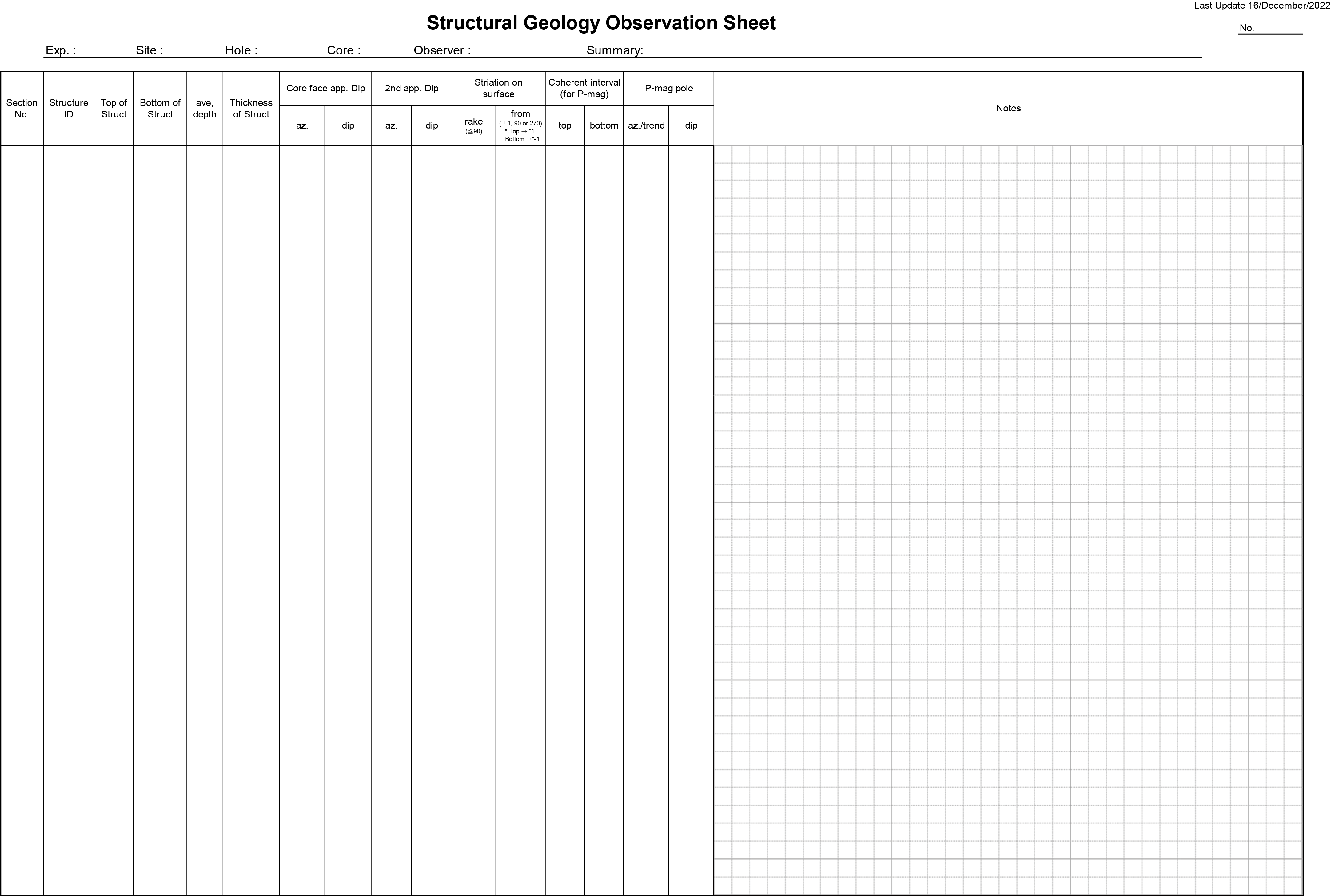
Figure F21. Structural geology log sheet.
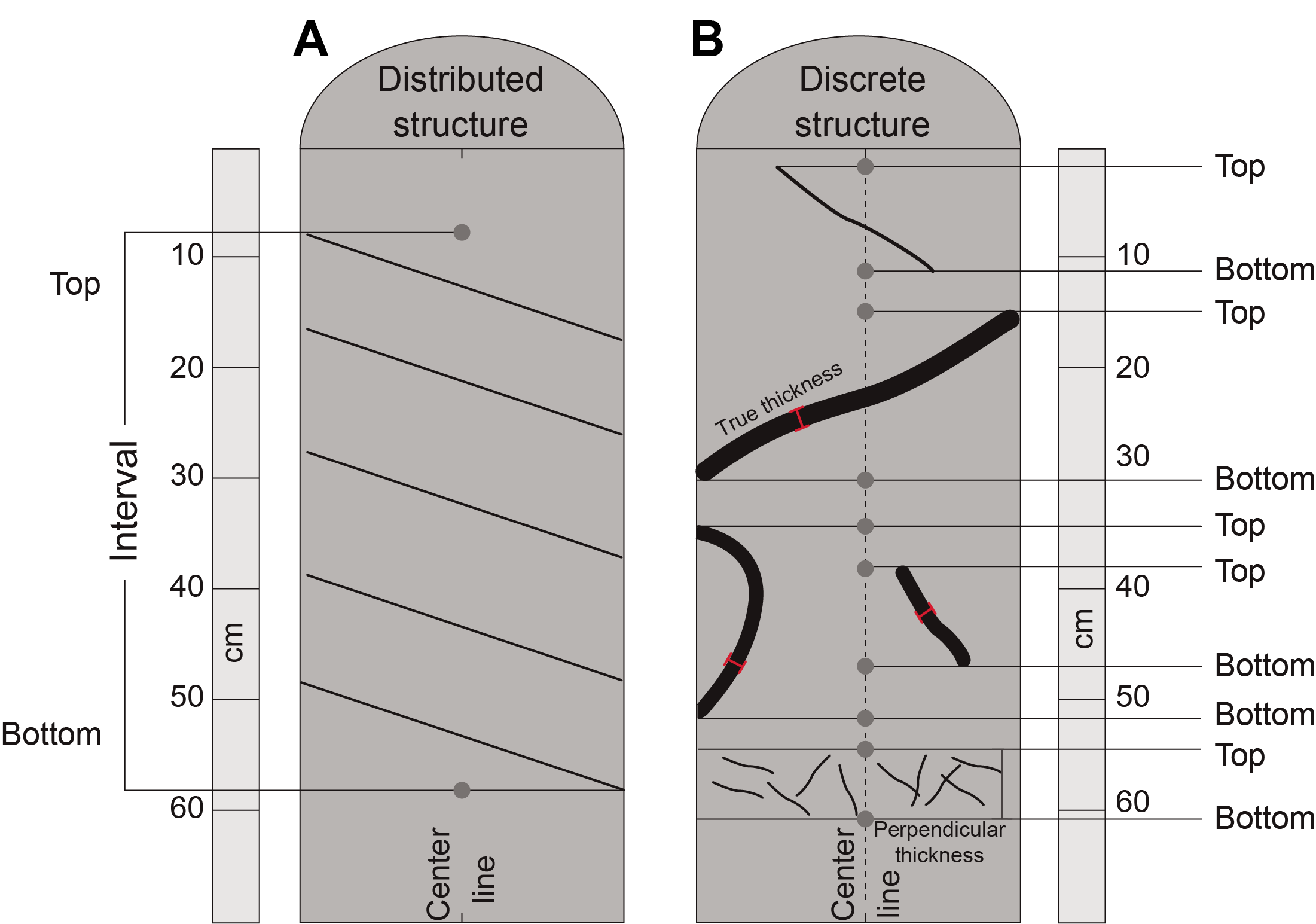
Figure F22. Method for logging structures.
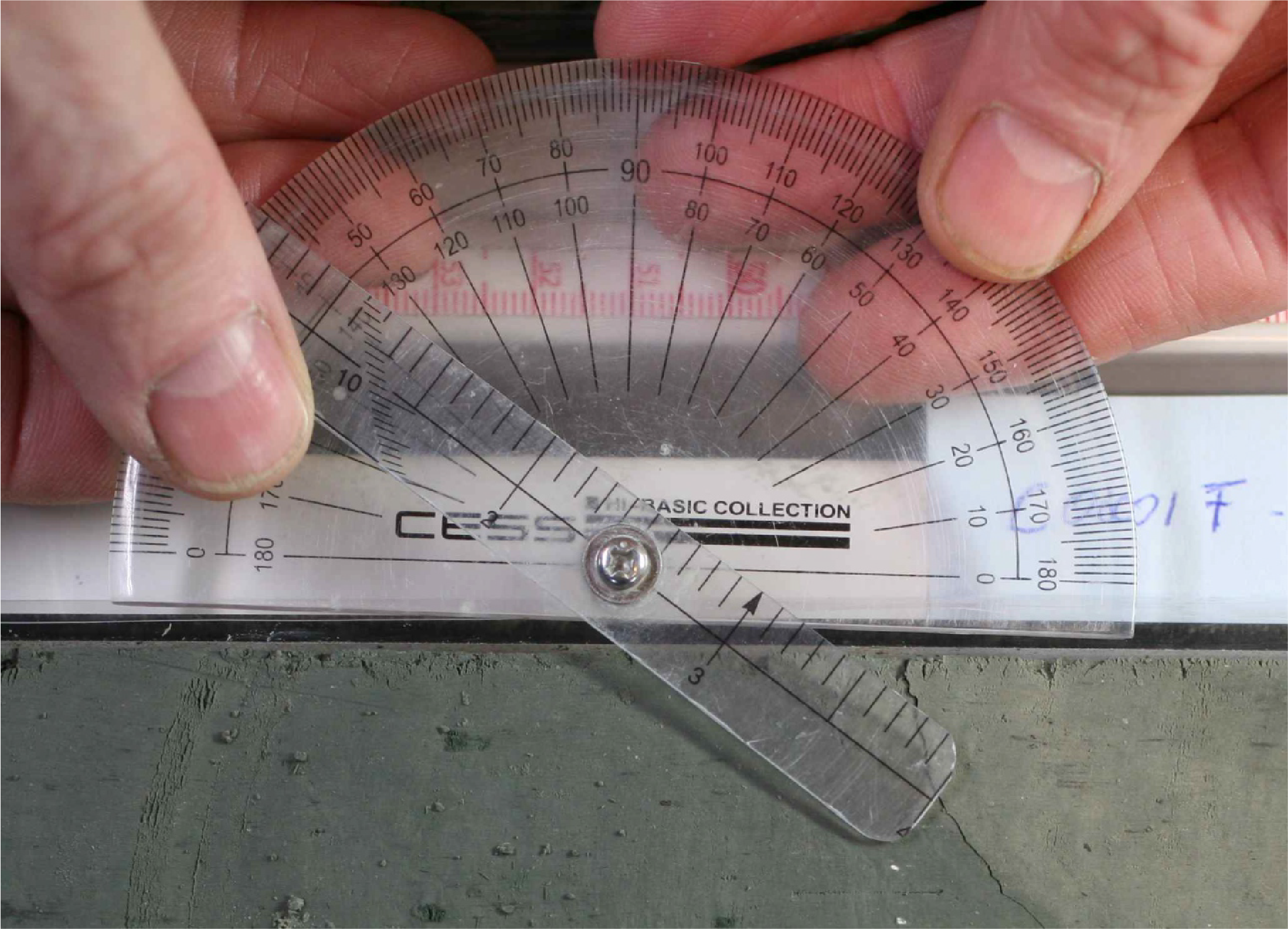
Figure F23. Protractor.
Orientations of planar and linear features in cored materials were determined relative to the core axis, which represents the vertical axis in the core reference frame, and the “double line” marked on the working half of the split core liner, which represents 0° (and 360°) in the plane perpendicular to the core axis (Figure F24). For the RCB cores, orientation measurements were conducted only on core pieces longer than ~5 cm to ensure that a piece did not rotate around a horizontal axis resulting in an uncertain upcore orientation).
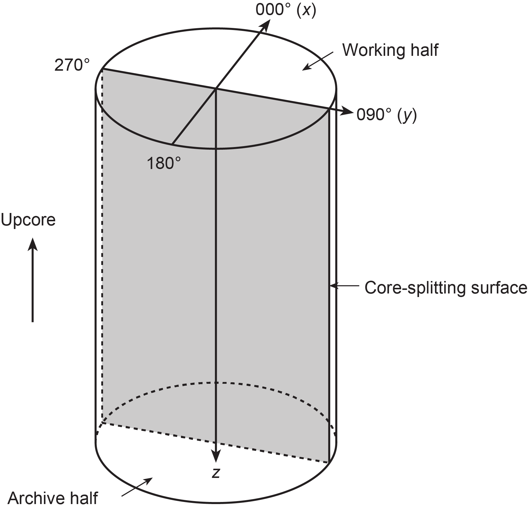
Figure F24. Core reference frame and coordinates for orientation.
To determine the orientation of a planar structural element, two apparent dips of this element were measured in the core reference frame and converted to a plane represented by the dip angle and either a strike or dip direction (Figure F25). One apparent dip is usually represented by the intersection of the planar feature with the split face of the core and is quantified by measuring the dip direction and angle in the core reference frame (β1; Figure F25). Typical apparent dip measurements have a trend of 90° or 270° and range in plunge from 0° to 90° (β2; Figure F25). The second apparent dip is usually represented by the intersection of the planar feature and a cut or fractured surface at a high angle to the split face of the core. In most cases, this was a surface either parallel or perpendicular to the core axis. In the former cases, the apparent dip lineation would trend 0° or 180° and plunge from 0° to 90°; in the latter cases, the trend would range from 0° to 360° and plunge at 0°. Linear features observed in the cores were always associated with planar structures (e.g., striations on faults), and their orientations were determined by measuring either the rake (or pitch) on the associated plane or the trend and plunge in the core reference frame. During Expedition 398, we measured rake for striations on fault surfaces (Figure F26) but azimuth and plunge for other lineation (e.g., fold axes). All data were recorded on the log sheet with appropriate depths and descriptive information.
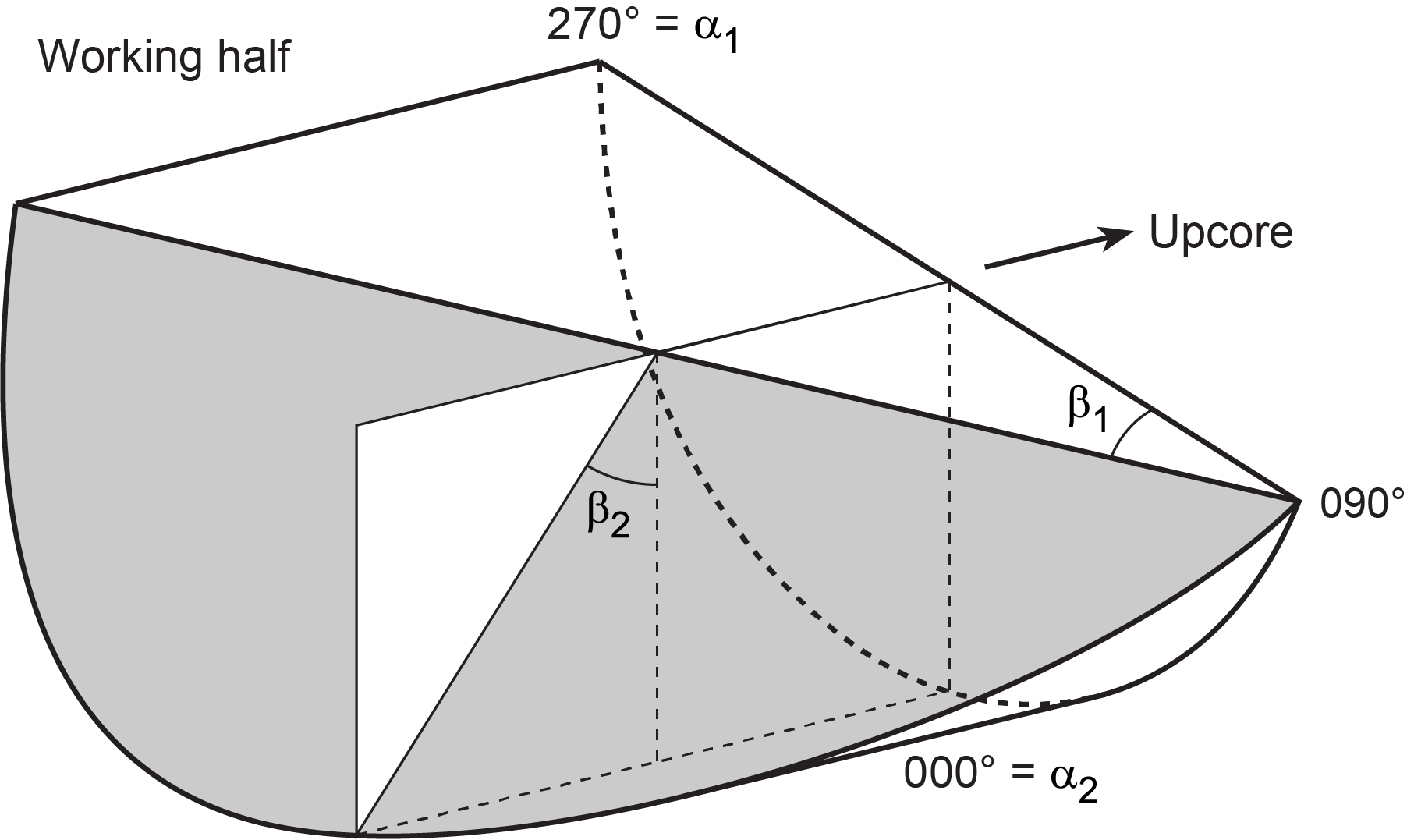
Figure F25. Calculation of plane orientation.
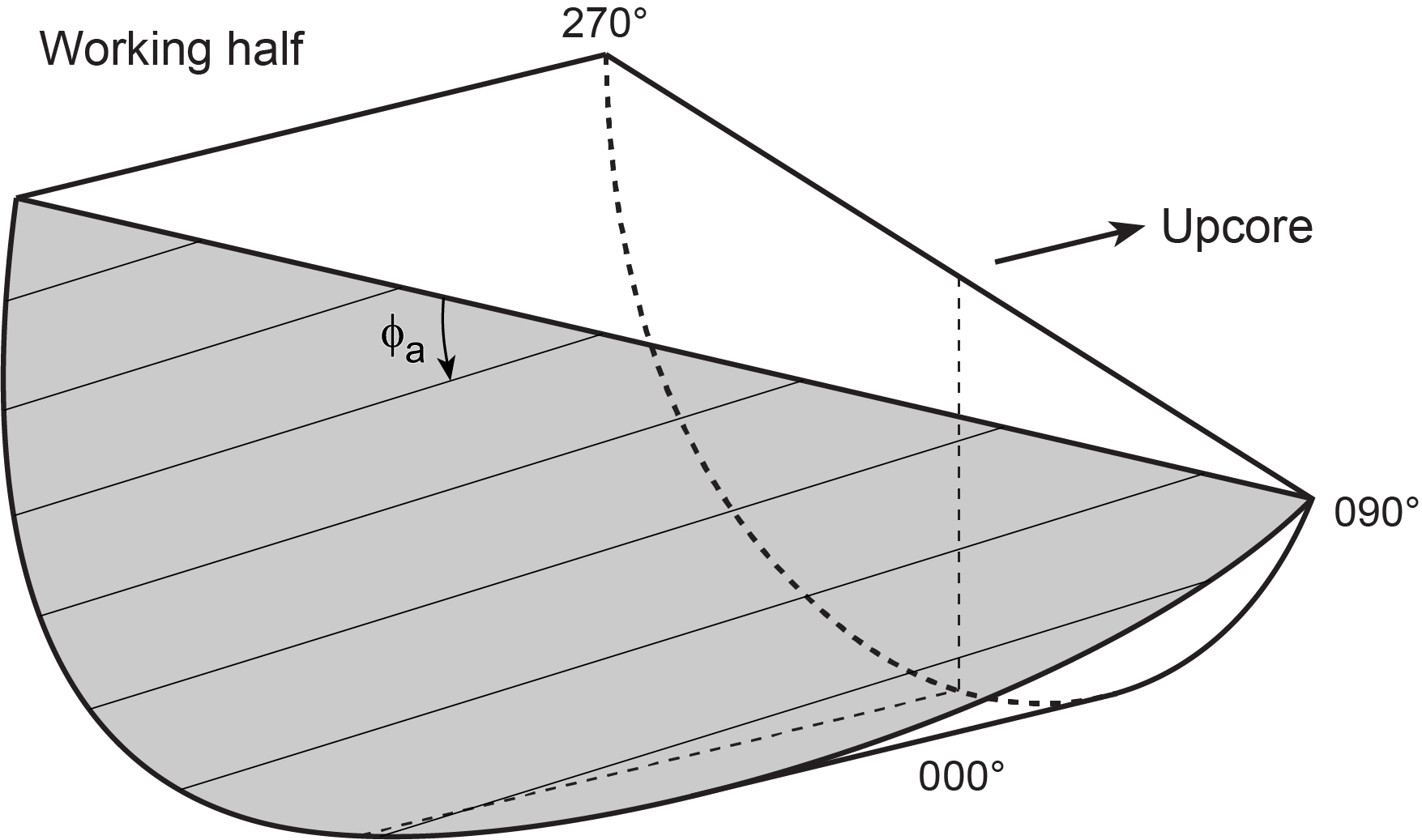
Figure F26. Apparent rake measurement of striations on a fault surface.
4.2. Description and classification of structures
We constructed a structural geology template for GEODESC to facilitate the description and classification of observed structures. For clarity, we defined the terminology used to describe fault-related rocks as well as the basis for differentiating natural structures from drilling-induced features.
Faults were classified into several categories based on the sense of fault slip and their structural characteristics. The sense of fault slip was identified using offsets of markers (e.g., bedding and older faults) across the fault plane and predominantly by slicken steps. A fault with cohesiveness across the fault zone was described as a “healed fault.”
For the igneous rock intervals, whereas lithology and mineralogy of the vein minerals were described by the petrologists, the orientations of the veins, foliations, and other structural features were measured by the structural geologists.
Structural data can sometimes be disturbed by drilling-induced structures such as flow-in structures in APC and HLAPC cores and biscuiting, fracturing, faulting, and rotation of fragments in XCB and RCB cores. If structures have been disturbed by flow-in on >60% of the cross section of the core, we excluded measurements because of the intense disturbance (e.g., bending, rotation, and so on) of these structures.
4.3. X-ray image logger
X-ray imaging provides information about structural and sedimentary features and quality in cores. Furthermore, structures such as shear zones could be imaged related to porosity changes or chemical alteration within shear zones. X-ray imaging was supplemental to visual core description during Expedition 398.
The X-ray Logger (XMAN) on JOIDES Resolution is a Teledyne ICM CP120B. Imaging was performed on selected core sections with complex fractures/microfaults during core descriptions. The XMAN scans a 1.5 m core section in ~8 min. It scans the upper half of the core section in the first 4 min; a plastic pusher is then added behind the core section, and the instrument runs for another 4 min to scan the lower half of the core section. The images are then processed.
The images were transferred from the XMAN host PC to the server using a script that copies the output from the XMAN to the server automatically every 30 min as executed via a task scheduler. The X-ray imaging parameters (i.e., voltage, current, time, and stack) were added at the top of each processed image for further reference.
4.4. Calculation of plane orientation
For planar structures (e.g., bedding or faults), two apparent dips on two different surfaces (e.g., one being the split core surface, which is east–west vertical, and the other being the horizontal or north–south vertical surface) were measured in the core reference frame as azimuths (measured clockwise from north, looking down) and plunges (Figure F25). A coordinate system was defined in such a way that the positive x-, y-, and z-directions coincide with north, east, and vertical downward, respectively. If the azimuths and plunges of the two apparent dips are given as (α1, β1) and (α2, β2), respectively, as in Figure F25, then the unit vectors representing these two lines, v1 and v2, are
The unit vector normal to the plane, vn (Figure F27), is then defined as
The azimuth, αn, and plunge, βn, of vn are given by
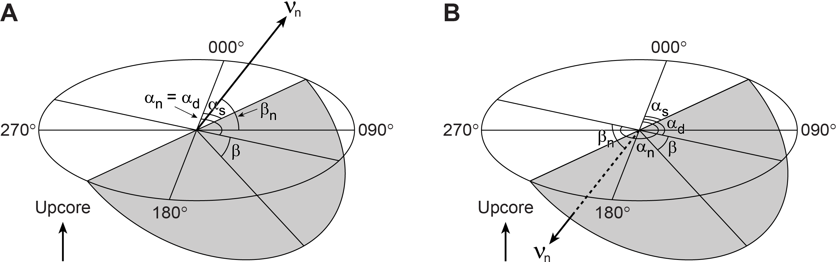
Figure F27. Dip direction, right-hand rule strike, and dip of a plane.
The dip direction, αd, and dip angle, β, of this plane are αn and 90° + βn, respectively, when βn < 0° (Figure F27A). They are αn ± 180° and 90° − βn, respectively, when βn ≥ 0° (Figure F27B). The right-hand rule strike of this plane, αs, is then given by αd − 90° (Figure F27).
4.5. Calculation of slickenline rake
For a fault with striations, the apparent rake angle of the striation, ϕa, was measured on the fault surface from either the 90° or 270° direction of the split-core surface trace (Figures F26, F27). The fault orientation was measured as described above. Provided that vn and vc are unit vectors normal to the fault and split core surfaces, respectively, the unit vector of the intersection line, vi, is perpendicular to both vn and vc (Figure F28) and is therefore defined as
Knowing the right-hand rule strike of the fault plane, αs, the unit vector, vs, toward this direction is then
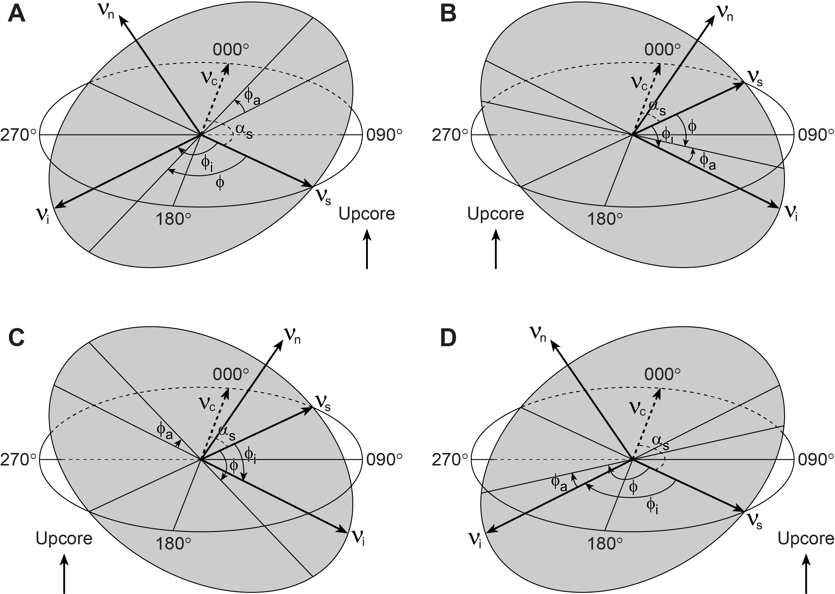
Figure F28. Diagrams of rake of striations.
The rake angle of the intersection line, ϕi, measured from the strike direction is given by
The rake angle of the striation, ϕ, from the strike direction is ϕi ± ϕa, depending on the direction from which the apparent rake was measured and on the dip direction of the fault: ϕa should be subtracted from ϕi when the fault plane dips to the west and ϕa was measured from either the top or 90° direction (Figure F28A) or when the fault plane dips toward the east and ϕa was measured from either the bottom or 90° direction (Figure F28B). On the other hand, ϕa should be added to ϕi when the fault plane dips toward the east and ϕa was measured from either the top or 270° direction (Figure F28C) or when the fault plane dips toward the west and ϕa was measured from either the bottom or 270° direction (Figure F28D).
4.6. GEODESC structural database
The GEODESC database is a program used to store visual (i.e., macroscopic and/or microscopic) descriptions of core structures at a given section index. During this expedition, orientation data were first recorded on the printed Structure VCD and then logged in a spreadsheet as described above. Then all the orientation data, locations of structural features, and calculated orientations in the core reference frame were input into GEODESC.
5. Biostratigraphy
The primary biostratigraphic objectives were to provide biostratigraphic ages to develop an integrated biostratigraphy and magnetostratigraphy for all drill sites. Secondary objectives were to identify changes in paleowater depth ranges and intervals of reworking to help elucidate the history of sedimentation and volcano-tectonic processes within the Hellenic arc volcanic field.
Preliminary age assignments during Expedition 398 were based on biostratigraphic analyses using calcareous nannofossils and planktonic and benthic foraminifera from 5–10 cm whole-round samples cored with the APC, HLAPC, XCB, and RCB systems. Most samples were taken from CCs or from the base of cores where CCs were not recovered, but where appropriate, additional split-core samples were taken to better define certain datums and zonal boundaries. Moreover, mudline samples from all cores were preserved in an ethanol (70%) and rose bengal solution (2 g/L) according to Walton’s (1952) technique to analyze the present-day environmental conditions. In addition to the abundance and preservation of the age-diagnostic microfossil groups, the presence of other sedimentary remains including tephra, shell fragments, phytoliths, micromollusks, ostracods, otoliths, bryozoan fragments, echinoid spines and plates, fish teeth and remains, radiolarians, diatoms, and sponge spicules was also routinely monitored.
The Geologic Time Scale 2020 (GTS 2020) (Gibbard and Head, 2020; Gradstein et al., 2020; Raffi et al., 2020) was used during Expedition 398 and supplemented with regional Mediterranean biostratigraphic schemes and datums (e.g., Rio et al., 1990; Lirer et al., 2019) to facilitate the integration of the Expedition 398 data with regional geological and seismic data (Figure F29). Where identified, uncertainties within microfossil datums that appear diachronous with the utilized Mediterranean biostratigraphic schemes, potentially due to local oceanographic differences, were noted for future calibration.
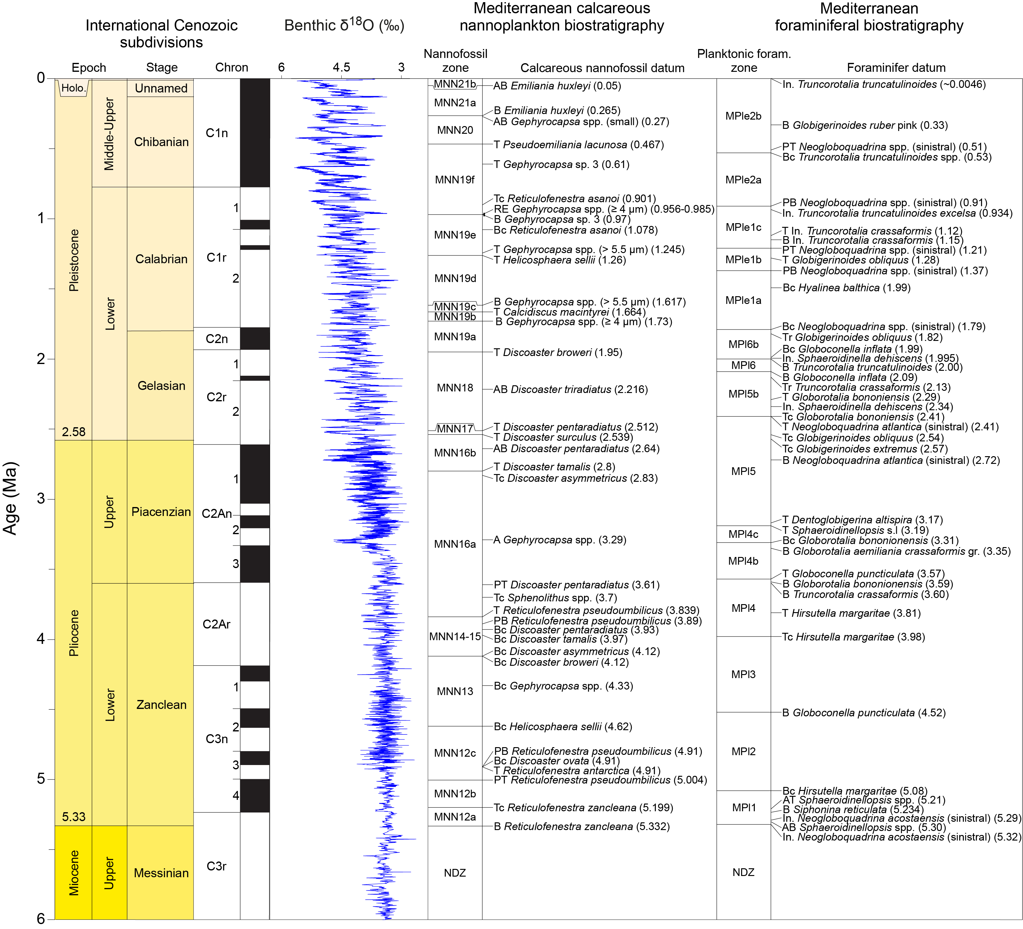
Figure F29. Biostratigraphic scheme.
5.1. Calcareous nannofossils
The taxonomic criteria of calcareous nannofossils follows Perch-Nielsen (1985) and Raffi et al. (2006). The calcareous nannofossil biostratigraphic classification of sedimentary sequences follows the recent reviews by Raffi et al. (2006) and Backman et al. (2012). Based on this classification, the calcareous nannofossil zonal scheme established by Martini (1971) and Okada and Bukry (1980), and modified by Young (1998) and Backman et al. (2012), was used for Neogene to Quaternary sequences encountered during Expedition 398. In addition, the Neogene to Quaternary biohorizons defined by Sato and Takayama (1992), modified by Raffi et al. (2006), were used for more detailed correlation of the sedimentary sequences. The Mediterranean scheme of Rio et al. (1990) was also utilized and updated with regional biostratigraphic markers (e.g., Lourens et al., 2004; Raffi et al., 2006; Di Stefano and Sturiale, 2010).
Astronomically tuned age estimates for the Neogene to Quaternary global chronostratigraphic units were based on the GTS 2020 (Gibbard and Head, 2020; Gradstein et al., 2020; Raffi et al., 2020). Specimens of the genera Reticulofenestra were assigned to size categories as proposed by Young (1998). For gephyrocapsids, we adopted the concept of Raffi et al. (2006), and the morphological terminology used here is summarized in Perch-Nielsen (1985) and Takayama and Sato (1987). Accordingly, Gephyrocapsa is divided into four major groups by maximum coccolith length:
- Small Gephyrocapsa (<4 µm).
- Medium Gephyrocapsa (G. caribbeanica and G. oceanica; ≥4 but <5.5 µm).
- Gephyrocapsa sp. 3 (G. parallela; ≥4 but <5.5 µm).
- Large Gephyrocapsa (G. caribbeanica and G. oceanica ≥5.5 µm).
All zonal schemes and nannofossil biohorizons are shown in Figure F29 and Tables T4 and T5.
5.1.1. Sampling, sample preparation, and analysis
For nannofossil analyses, the CC section or the base of each recovered core was sampled. Samples from other sections were included from split-core samples to better define biostratigraphic datums or when nannofossils were not abundant in the analyzed material. Standard smear slide methods were used for all samples, using optical adhesive as a mounting medium. Calcareous nannofossils were examined under a polarizing light microscope at 1250× magnification. Abundance, preservation, and zonal data for each sample investigated were recorded in the GEODESC database.
We followed the taxonomic concepts summarized in Takayama and Sato (1987). Calcareous nannofossil preservation was assessed as follows:
- G (good) = little or no evidence of dissolution and/or overgrowth.
- M (moderate) = minor dissolution or crystal overgrowth observed.
- P (poor) = strong dissolution or crystal overgrowth, many specimens unidentifiable.
Total abundance of calcareous nannofossils for each sample was estimated as follows:
- A (very abundant) = >50 specimens per field of view.
- C (common) = >10–50 specimens per field of view.
- F (few) = 1–10 specimens per field of view.
- R (rare) = 1 specimen per 2 or more fields of view.
Nannofossil abundances of individual species were recorded as follows:
- A (abundant) = 1–10 specimens per field of view.
- C (common) = 1 specimen per 2–10 fields of view.
- R (rare) = 1 specimen per >10 fields of view.
5.2. Planktonic and benthic foraminifera
The taxonomy for planktonic foraminifera follows a modified version of the phylogenetic classification of Kennett and Srinivasan (1983). Additional species concepts are based on Iaccarino (1985), Huber et al. (2016), Schiebel and Hemleben (2017), Wade et al. (2018), and Lam and Leckie (2020). Abundance, preservation, and zonal data for each sample investigated were recorded in the GEODESC database.
Locally calibrated ages were used for all foraminiferal datums based on Lirer et al. (2019) and were supplemented with additional regional datums sourced from Lourens et al. (1996), Farouk et al. (2022), and Margaritelli et al. (2022). The ages of other planktonic foraminiferal datums are from the GTS 2020 (Gibbard and Head, 2020; Gradstein et al., 2020; Raffi et al., 2020), as given in Table T6.
Taxonomy and biostratigraphy of Cenozoic benthic foraminifera are based on Loeblich and Tappan (1988), Cimerman and Langer (1991), Sgarella and Moncharmont Zei (1993), Rasmussen et al. (2005), Holbourn et al. (2013), and the World Register of Marine Species (WoRMS) database (WoRMS Editorial Board, 2021).
Qualifiers for foraminiferal taxa identified in this study are as follows:
- cf. = confer (compare with).
- aff. = affinis (affinity with).
- sp. = unidentified species assigned to the genus.
- spp. = more than one unidentified species assigned to the genus.
- s.l. = sensu lato.
- ? = identification uncertain.
5.2.1. Sampling, sample preparation, and analysis
Samples (5–10 cm whole rounds) were prepared by manually breaking the core into small pieces followed by disaggregation and washing over a 63 µm mesh sieve to remove all mud and silt. More lithified sediments were soaked in a solution of hot water and hydrogen peroxide (H2O2; 30%) to chemically disaggregate the microfossils from the sediments, and then additionally were manually broken down using a mortar and pestle if necessary. The washed microfossil residue retained on the sieve was dried at low temperature (~50°C) in a thermostatically controlled drying cabinet and divided with a microsplitter into equal aliquots for examination. As a precaution against cross contamination, sieves were cleaned with jetted water, placed in an ultrasonic bath for 15 min, dried with compressed air, and thoroughly inspected between samples.
During examination of samples, the percentage of planktonic foraminifera relative to total foraminifera was determined quantitatively from random counts of 100 foraminifera in the 150–500 µm grain-size fractions of washed microfossil residues. This was done to determine relative oceanicity (greater planktonic percent corresponds to greater oceanicity; Hayward et al., 1999) (Figure F30) to identify samples with reworked material (i.e., dependent on the water depth). For planktonic foraminifera, age-diagnostic markers were picked from the 150–500 µm grain-size fraction and mounted onto 60-division faunal slides coated with gum tragacanth. Additionally, during intervals biostratigraphically subdivided by abundances shifts in Neogloboquadrina spp. (sinistral), the population ratios of sinistral and dextral coiled specimens within this genus were semiquantitatively assessed. For benthic foraminifera, the >125 µm grain-size fraction was examined and ~100 specimens were obtained and identified for environmental and paleowater depth estimations. As time allowed, other species and biogenic remains of microfossils were also picked and mounted onto the same slides.
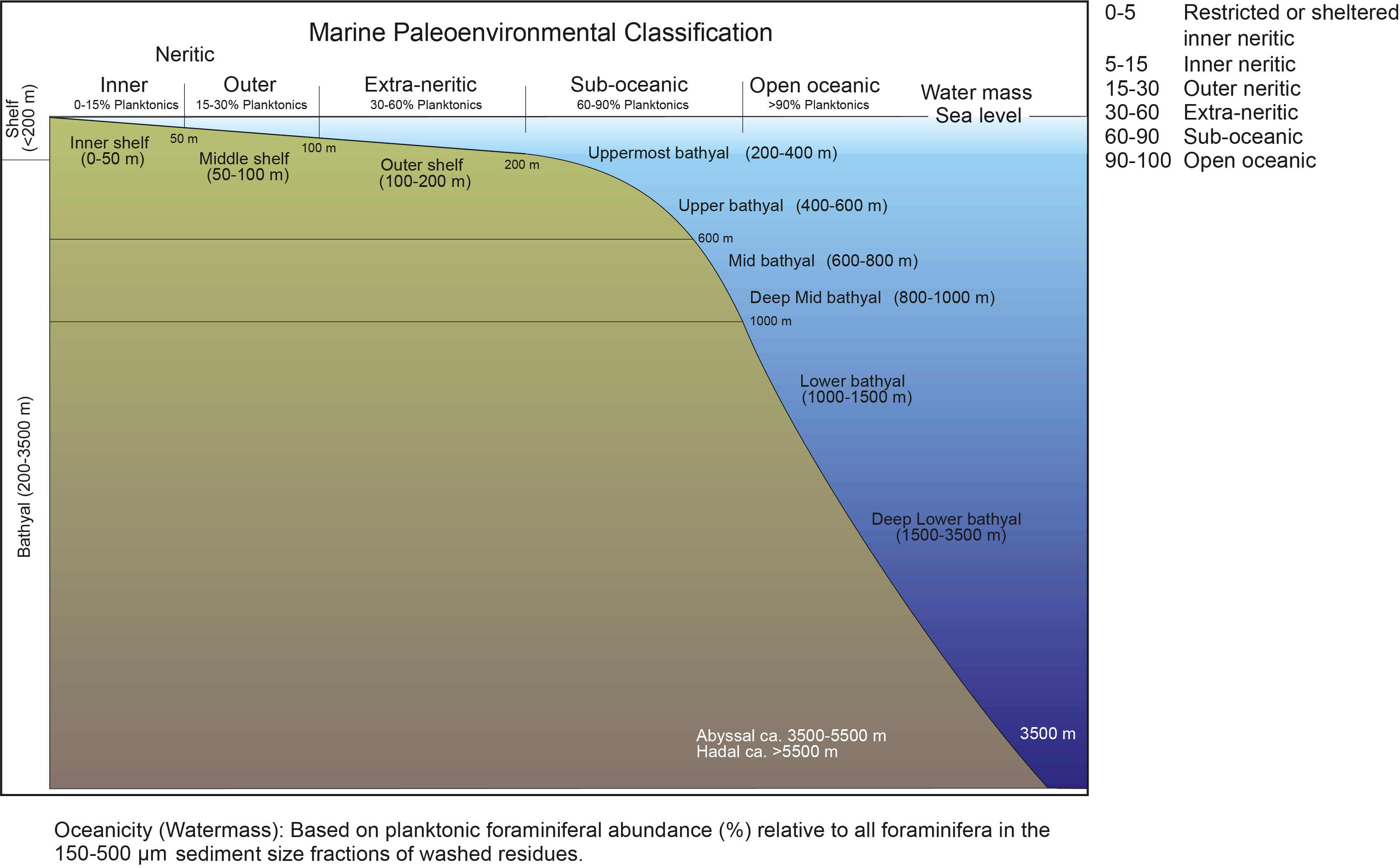
Figure F30. Marine paleoenvironmental classification and oceanicity.
Specimen images were taken using a camera-mounted Zeiss SteREO Discovery V8 microscope, or scanning electron micrographs were acquired by mounting the specimens on an SEM stub, sputter-coating them with gold-palladium alloy, and imaging them using a Hitachi TM3000 tabletop microscope and an SNE-4500M Plus SEM.
During examination of microfossil samples, the abundance of foraminifera and other fossil groups in the 150–500 µm grain-size fractions of washed samples was determined visually and categorized as follows:
- D = dominant (foraminifera compose >50% of the washed sample).
- A = abundant (foraminifera compose >20%–50% of the washed sample).
- C = common (foraminifera compose >5%–20% of the washed sample).
- F = few (foraminifera compose 1%–5% of the washed sample).
- R = rare (foraminifera compose <1% of the washed sample).
- X = present (foraminifera present in sample, abundance undetermined).
In addition, the preservation of foraminifera was categorized as follows:
- VG = very good (specimens mostly whole, very well preserved ornamentation and surface ultrastructure, no visible modification of the test wall).
- G = good (specimens often whole, ornamentation and surface ultrastructure preserved but sometimes abraded or overgrown, visible evidence of modification of the test wall).
- M = moderate (specimens often etched or broken, ornamentation and surface ultrastructure modified, majority of specimens identifiable to species level).
- P = poor (most specimens crushed or broken, recrystallized, diagenetically overgrown, or infilled with crystalline calcite; most specimens difficult to identify to species level).
- VP = very poor (all specimens crushed or broken, recrystallized, diagenetically overgrown, or infilled with secondary minerals; most specimens difficult to identify to genus level).
Additionally, benthic and planktonic foraminifera were examined in thin sections of lithified calcareous rock samples. Specimen images were taken using a camera-mounted Zeiss Axioplan.
5.2.2. Planktonic foraminifera
Planktonic foraminiferal dating was used in conjunction with calcareous nannofossil dating to determine biostratigraphic ages. Planktonic foraminifera were also used to identify changes in marine conditions. To achieve this goal within the available time, species with documented affinity for warm- or cold water masses (see Crundwell et al. 2008; Aze et al. 2011; Crundwell and Woodhouse, 2022; Woodhouse et al. 2023) were used to assign tentative boundaries of marine isotope stages to supplement biostratigraphic analyses.
5.2.3. Benthic foraminifera
Benthic foraminifera were the primary paleontological tool used for estimating paleowater depths during the examination of samples, in collaboration with planktonic foraminiferal assemblage abundance. Additionally, they were also used as secondary markers for biostratigraphic dating. Paleowater depth ranges were estimated on the basis of the deepest calibrated depth marker contained in each sample based on Wright (1978), van Morkhoven et al. (1986), de Stigter et al. (1998), De Rijk et al. (1999), Rasmussen et al. (2005), Spezzaferri and Tamburini (2007), and Milker et al. (2017). These analyses contributed to understanding the complex sedimentary and volcano-tectonic sediments sampled during Expedition 398 that can result in uncertainties in paleowater depth reconstructions through sediment remobilization and downslope displacement of shallow-water species (e.g., Cimerman and Langer, 1991).
6. Paleomagnetism
Paleomagnetic analyses during Expedition 398 focused on measurement of the remanent magnetization of archive-half sections on the superconducting rock magnetometer (SRM) before and after alternating field (AF) demagnetization. Our aim was to determine magnetostratigraphic age constraints to combine with micropaleontological datums to yield an age model for each site.
Analyses of the archive-half sections were complemented by experiments on discrete cubic specimens taken from working-half core sections. These were subjected to stepwise AF demagnetization (usually up to 50 mT), although a limited number of samples were thermally demagnetized (up to 700°C) or subjected to a combination of low-temperature demagnetization (down to 77 K using liquid nitrogen) followed by either AF or thermal treatment.
6.1. Archive-half section remanent magnetizations
Measurements of natural remanent magnetization (NRM) and remanences following stepwise AF demagnetization were conducted on archive-half sections using the automated pass-through 2G Enterprises Model 760R-4K SRM interfaced to Integrated Measurement System (IMS) SRM software (version 13.0). The SRM is equipped with direct-current superconducting quantum interference devices (DC-SQUIDs) and an in-line automated three-axis AF demagnetizer capable of reaching a maximum peak field of 80 mT (frequency 200 Hz). The spatial resolution of remanence measurements is determined from the integrated response function of the SQUID sensors with effective widths of 7.3 cm for the x- and y-axes and 9.0 cm for the z-axis (Acton et al., 2017). The practical noise level of the SRM is ~2 × 10⁻⁹ Am2 and is primarily controlled by the magnetization of the core liner and the background magnetization of the measurement tray.
The sample tray was cleaned every 24 h, the AF demagnetized at a peak field of 30 mT, and its remanence measured to monitor any changes during the expedition and to ensure accurate tray correction values. The measurement interval and speed for processing archive-half sections were set to 2.0 cm and 10 cm/s, respectively. A 12 cm long interval of empty track was measured before the start of the section passed the center of the pickup coils of the SQUID sensors, and an equal interval of empty track was measured after the end of the section had passed through it. These header and trailer measurements serve the dual functions of monitoring the background magnetic moment and enabling future deconvolution analysis (Xuan and Oda, 2015).
Following an initial period of experimentation at the start of the expedition to establish the most appropriate demagnetization sequence to use for routine analysis, archive-half sections were demagnetized in AF fields of 15, 20, and 25 mT, sufficient to allow the biasing effects of any drilling-induced magnetization on magnetic polarity to be determined to aid identification of the distribution of magnetozones downhole. This limited demagnetization sequence fulfilled the following requirements: (1) allowed more rapid throughput of sections through the SRM to keep up with core flow; (2) provided sufficient data to allow principal components of magnetization to be calculated for each measurement interval; and (3) avoided recently reported overheating problems with one of the demagnetization coils when used to produce high demagnetizing fields (up to 80 mT).
Data collected near the ends of core sections and piece boundaries are significantly affected by edge effects due to the width of the SQUID sensor response functions. Consequently, data points within 8 cm of section ends and piece boundaries were filtered out prior to further processing. To further reduce artifacts when measuring core samples collected by RCB drilling, any pieces smaller than 8 cm were removed from section trays prior to measuring/demagnetizing and replaced afterward.
Data from individual measurement points were examined on orthogonal vector plots (Zijderveld, 2013) and analyzed using the PuffinPlot software (Lurcock and Wilson, 2012). This allowed us to automate the calculation of principal component directions of magnetization downhole to aid determination of the distribution of magnetozones. In addition, Fisher mean directions of magnetization were calculated for each measurement interval (from the directions after demagnetization at 15, 20, and 25 mT) to estimate inclinations in samples where only minor changes in intensity occurred. Both principal component and Fisher mean directions were subject to statistical filtering to establish the most appropriate estimate of inclination, and the inclination at 25 mT was used when no statistically acceptable alternative measure was available. This process is described in detail in the Site U1591 chapter (see Paleomagnetism in the Site U1591 chapter [Druitt et al., 2024]).
Mean inclinations and associated Fisher statistics were calculated using the incfish.py program in the PmagPy package (Tauxe et al., 2016). In addition, median destructive fields (i.e., the demagnetization treatment levels at which the sample intensity is reduced to 50% of its NRM value) were calculated using PuffinPlot (Lurcock and Wilson, 2012) to give further information on the coercivity of magnetic minerals present in the samples.
6.2. Discrete sample remanent magnetizations
Remanent magnetizations of discrete samples were measured exclusively with the AGICO JR-6A spinner magnetometer using the automated sample holder, providing the most accurate discrete sample remanent magnetization directions and intensities. Measurements of the empty automatic sample holder after subtracting the stored holder magnetization yielded intensities on the order of 9.0 × 10⁻⁶ A/m, representing the practical noise limit of the system.
Where sediments were sufficiently soft, we collected discrete 7 cm3 samples in plastic Natsuhara-Giken sampling boxes pushed into the working half of the core by hand through a plastic 3-D printed jig designed to align samples with the core reference framework, with the “up” arrow on the box pointing upsection in the core. In stiffer sediments, a stainless steel cutter was hammered into the sediment through a second custom-made plastic 3-D printed jig, and the resulting sample was then extruded onto a flat surface and placed inside a Natsuhara-Giken sampling box. These samples were subject to stepwise AF demagnetization.
In more indurated sediment and hard rocks, we cut 8 cm3 cubes with orthogonal passes of a rock saw with two parallel blades spaced 2 cm apart. These were marked with an upcore orientation arrow on the split core face of the cubic sample and wrapped in plastic to prevent desiccation. These lithified samples without a plastic container were suitable for both AF and thermal demagnetization.
Stepwise AF demagnetization of discrete samples was performed using a DTech D-2000 AF demagnetizer. Samples selected for AF demagnetization were usually treated at peak fields of 10, 15, 20, 30, and 50 mT. Thermal demagnetization of some discrete samples was performed using an ASC Scientific TD-48 SC thermal demagnetizer capable of heating samples up to 700°C. During use, samples were located in the innermost 26 cm of the sample chamber where the field was <50 nT, avoiding a significant field gradient toward its mouth (reaching a maximum of 120 nT).
MS was measured using the AGICO MFK2 Kappabridge after every heating step to monitor thermal alteration of magnetic minerals during heating. Low-temperature demagnetization (LTD) was performed on a limited number of discrete samples (Dunlop, 2003) prior to subsequent AF or thermal demagnetization to remove secondary magnetizations. LTD involves cooling samples in a liquid nitrogen bath (77 K) and allowing them to warm back up to room temperature in a low-field environment. A suitable low-field environment was provided by a three-layer cylindrical mu-metal shield.
Characteristic remanent magnetization directions of the discrete samples were determined using principal component analysis (Kirschvink, 1980) using the PuffinPlot software, version 1.4.1 (Lurcock and Wilson, 2012).
6.3. Anisotropy of low-field magnetic susceptibility
In addition to standard paleomagnetic measurements, the anisotropy of low-field magnetic susceptibility (AMS) was determined for all discrete samples using an AGICO MFK2 Kappabridge operated via AGICO SAFYR 7.5.01 software. AMS reflects the shape- or crystallographic-preferred orientations of minerals and grains (e.g., Tarling and Hrouda, 1993; Borradaile and Jackson, 2004) or the distribution anisotropy of ferromagnetic grains (Stephenson, 1994), providing quantitative constraints on petrofabric development even in weakly deformed sediments and rocks. Described by a second-order tensor, AMS is represented by a susceptibility ellipsoid specified by the magnitude and orientation of its principal axes (kmax, kint, and kmin, corresponding to its maximum, intermediate, and minimum susceptibility axes, respectively). AMS in a rock results from contributions from all its constituent minerals but is usually dominated by the signal from ferromagnetic phases, when present, because of their high susceptibilities. The shape of the AMS ellipsoid is defined by the relative magnitude of the principal susceptibility axes and can be
- Isotropic (kmin = kint = kmax) with no preferred alignment,
- Oblate (kmin ≪ kint ≈ kmax) defining a planar magnetic fabric (foliation),
- Prolate (kmin ≈ kint ≪ kmax) defining a linear magnetic fabric (lineation), or
- Triaxial (kmin < kint < kmax).
AMS ellipsoid shapes were quantified using the Jelínek and Kropáček (1978) shape parameter (T) where −1.0 < T < 1.0, with positive/negative values of T indicating oblate/prolate fabrics, respectively. The magnitude of anisotropy is described using the corrected anisotropy degree, PJ (Jelínek and Kropáček, 1978), where PJ = 1.0 indicates an isotropic fabric and, for example, PJ = 1.05 indicates 5% anisotropy.
6.4. Sample coordinates and core orientation
All magnetic data were initially acquired relative to the IODP core reference frame. In this system, +x points into the working half, +z is downcore, and +y is orthogonal to x and z in a right-hand sense. Therefore, +x corresponds to 000° and +y to 090° in the core reference frame. For some APC sediment cores, the magnetization directions and AMS principal axes were subsequently restored to a geographic reference frame using the Icefield MI-5 core orientation tool. This tool uses three orthogonally mounted fluxgate magnetometers to record the orientation of the magnetic tool face (which is collinear with the double line scribed on the core liner) relative to magnetic north. The tool is run on the APC BHA in a nonmagnetic core barrel. The tool declination, inclination, total magnetic field, and temperature are recorded on internal memory at a regular interval (typically 10 s). The core barrel, pipe, and BHA is kept steady for several minutes just prior to when the core is taken. Data recorded during this time are used to determine the core orientation. Rotation of the core barrel is prevented using an anti-spiral key, although the core and/or core liner may twist as it penetrates the sediments. The Icefield MI-5 tool data then provide orientation correction for the core barrel that converts observed magnetic declinations measured in the core reference frame (Dobs) to true declinations (Dtrue) as follows:
where MTF is the magnetic tool face angle from the Icefield MI-5 tool and Damb is the ambient geomagnetic field declination obtained from geomagnetic field models (Weber et al., 2021). The International Geomagnetic Reference Field (13th generation, Alken et al., 2021) declination for all drill sites is +5.0°.
6.5. Magnetostratigraphic dating
Expedition 398 sites are all located at ~36.3°–36.7°N and have not undergone significant latitudinal motion, and hence reversals of the Earth’s magnetic field recorded by sampled sequences can be easily identified by distinct changes in inclination. Assuming a geocentric axial dipole (GAD) geometry for the field, it is possible to calculate the field inclination, I, as tan(I) = 2 tan(lat), where lat is the latitude. The time-averaged GAD field at a latitude of 36.5°N is therefore expected to have a positive (downward) inclination of ~56°. Negative inclinations indicate reversed polarity. Magnetozones identified from the shipboard data were correlated with the geomagnetic polarity timescale (GPTS; Gradstein et al., 2020) with the aid of biostratigraphic datums.
7. Physical properties
The primary objectives of the Expedition 398 physical properties program are to collect various high-resolution physical properties data on cored materials that (1) identify major volcaniclastic deposits and mass transport events; (2) constrain geothermal, geomechanical, and seismic properties of the deposits; and (3) construct composite stratigraphic correlations. In addition, physical properties measurements provide data that assist in the characterization of lithologic units, heat flow, fluid flow, and consolidation history. They also help with the interpretation of seismic reflection profiles and downhole geophysical logging data.
7.1. Laboratory core flow
Physical properties measurements were made in the following sequence:
- The pocket penetrometer (PP) was used to measure undrained compressive strength on fine-grained cohesive sediment; typically, but not always, the bottom of the second to last section of each core was measured while the core was on the catwalk.
- Whole-round cores were measured with the NGR detector when the length of an individual section was >50 cm.
- Whole-round cores were measured on the WRMSL, which includes a GRA bulk densitometer, an MS pass-through loop system, and a P-wave velocity logger (PWAVE_L). The default sampling interval was set to 2.5 cm. APC cores were analyzed after equilibrating on the core deck for at least 4 h to reach thermal equilibrium with the laboratory (a necessary condition for P-wave velocity analysis). P-wave velocity was not measured on XCB and RCB cores because they do not fill the core liners; these cores could therefore be analyzed without waiting for thermal equilibrium to be reached.
- Whole-round cores were split.
- Thermal conductivity on the working half was measured with a TeKa TK04 half-space needle probe (HLQ) puck.
- Shear strength was measured with the automatic vane shear (AVS) system at representative locations along the working half.
- Discrete P-wave velocity measurements were made along the working half in its core liner using the P-wave gantry system. For consolidated rock, P-wave velocity was measured on seawater-saturated cube samples in the x-, y-, and z-directions.
- Discrete samples for shipboard moisture and density (MAD) measurements were collected from representative locations along the working half. Wet mass was measured before samples were dried at 105°C for 24 h and then cooled to room temperature in a desiccator for 3 h, after which their dry mass was obtained. Sample volumes were then obtained by helium pycnometry.
During Expedition 398, all raw data were uploaded to the LIMS database.
7.2. Whole-Round Multisensor Logger
PWAVE_L, GRA density, and MS were measured on the WRMSL, and NGR was measured using the NGRL. These measurements are all nonintrusive and nondestructive. APC sections were passed through the WRMSL after equilibrating to laboratory temperature for at least 4 h.
The sampling interval for all WRMSL measurements was 2.5 cm, with an integration time of 3 s for each measurement. The reliabilities of WRMSL measurements were assessed by passing a single core liner filled with deionized (DI) water through the WRMSL after every core. The core liner was assumed to be completely full. Bulk density values obtained from the GRA and the MS measurements may underestimate true values if the liner is not completely full. This was the case for many core sections, particularly when the recovered material was sand/volcaniclastic rich. Anomalously low values of P-wave velocity, MS, and bulk density also occur where there are cracks and gaps in the core. To limit data manipulation, anomalous values were left in the raw data.
During Expedition 398, the STMSL (i.e., “fast-track”; see Stratigraphic correlation) was only used at Site U1589. To enable rapid stratigraphic correlation for Hole B against Hole A, sections were run through the STMSL, measuring GRA density and MS as soon as possible. These sections then equilibrated to laboratory temperature and were remeasured with the full set of WRMSL instruments.
7.2.1. Gamma ray attenuation bulk density
Bulk density is calculated by measuring the attenuation of gamma rays as they pass through the core. Attenuation of these rays is dominated by Compton scattering and depends on the density and thickness of the sample. Gamma rays with energy of 0.662 MeV are generated by a 137Cs source core (Evans, 1965; Harms and Choquette, 1965) and pass through the entire diameter of the core. The GRA detector records these gamma rays on a 75 mm × 75 mm NaI detector. The spatial resolution of the GRA detector is <1 cm.
Bulk density, ρ, is proportional to the gamma ray count,
- µ = Compton attenuation coefficient,
- d = sample diameter,
- I0 = gamma ray source intensity, and
- I = measured intensity of gamma rays passing through the sample.
µ and I0 are treated as constants obtained by calibrating the gamma ray detector with a set of aligned aluminum cylinders of various diameters surrounded by distilled water in a sealed core liner that is the same as that used during coring operations. The relationship between I, µ, and d is
where A, B, and C are coefficients obtained from the calibration. Gamma ray counts through each cylinder were determined for a period of 60 s. The density, ρ, of each aluminum cylinder was 2.7 g/cm3, and the diameter, d, was 1, 2, 3, 4, 5, or 6 cm.
Drift was assessed by running a water standard after every core. Calibrations were performed if deviations from the standard exceeded 2%.
7.2.2. Magnetic susceptibility
The bulk MS of a material indicates its ability to produce a magnetic response to an applied external magnetic field. The relationship between the magnetic response, that is, the magnetization or normalized magnetic moment, M (unit: Am2), and the external field, H (unit: Am2), is
where κ is the bulk volume MS and is dimensionless. (We report measurement values in “SI” to indicate that the values in this equation are in SI units as opposed to CGS units, for which the volume MS is a factor ¼π smaller).
The strength and distribution of MS can indicate the composition and properties of magnetic minerals and thus can be related to the origins of cored materials and impacts of diagenesis. Igneous materials typically have an MS a couple orders of magnitude greater than background organic sediments and clay.
A Bartington Instruments MS2C sensor coil with an operating frequency of 565 Hz was used in WRMSL instrumentation. Calibration of the instrument was preset. Spatial resolution is 4 cm; thus, if the core is not continuous over an interval greater than 8 cm, κ will be underestimated.
7.2.3. Compressional P-wave velocity
The compressional wave velocity sensor measures the traveltime of 500 kHz ultrasonic waves across the whole core while it remains in the core liner. The waves are transmitted to the core by plastic transducer contacts connected to linear actuators. Pressure is applied to the actuators to ensure coupling between the transducers and the core liner. Water is dripped along the outside of the core liners to enhance the physical connection with the actuators. P-wave velocity, V, is calculated by V = d/t where d is the path length of the wave through the core and t is the traveltime. The total traveltime between the transducers includes the time delay related to transducer faces and electronic circuitry, the delay in the peak detection procedure, and the transit time through the core liner.
Traveltime is calculated by automated signal processing that detects the arrivals of P-wave signals to a precision of 50 ns. The search method skips the first positive amplitude and finds the second positive amplitude using a detection threshold limit, typically set to 30% of the maximum amplitude of the signal. It then finds the preceding zero crossing and subtracts one wave period to determine the first arrival. To avoid extremely weak signals, minimum signal strength can be set (typically 0.02 V) and weaker signals are ignored. To avoid signal interference at the beginning of the record from the receiver, a delay (typically 0.01 ms) can be set to force the amplitude search to begin in the quiet interval preceding the first arrival. In addition, a trigger (typically 4 V) is selected to initiate the arrival search process, and the number of waveforms to be stacked (typically 5) can also be set. A linear voltage differential transformer measures the separation of the transducer to derive a signal path length (i.e., the core diameter). The P-wave velocity is finally calculated after correction for system propagation delay, liner thickness, and liner material velocity. The gain was adjusted throughout the expedition to maximize the number of good measurements.
The system was calibrated with a set of plastic cylinders with a range of diameters. A water standard was run after each core to ensure the measurements remained reliable. PWAVE_L velocities always remained within 2% of the room temperature value.
7.2.4. Natural Gamma Radiation Logger
Gamma rays are emitted from decay of 238-uranium (238U), 232-thorium (232Th), and 40-potassium (40K). The NGRL measures this natural emission on whole-round cores using a system designed and built at IODP Texas A&M University between 2006 and 2008 (Vasiliev et al., 2011). This system was also used on all expeditions since Expedition 320.
The NGR detection unit contains 8 NaI scintillator detectors, 7 plastic scintillator detectors, and 22 photomultipliers. Lead is used for passive shielding. The NaI detectors are covered by 8 cm of lead shielding. Half of the lead shielding closest to the NaI detectors is composed of low-background lead, whereas the outer half is composed of regular (i.e., virgin) lead. Low-background lead of thickness 7 cm separates each NaI detector. The NGRL uses a plastic scintillator to suppress high-energy gamma and muon components of cosmic radiation by producing a canceling signal when these charged particles pass through the plastic scintillators. The NGRL was calibrated with 137Cs and 60Co sources and identifying peaks at 662 keV (137Cs) and 1330 keV (60Co) and using the 1170 keV peak for verification. Calibration materials are provided by Eckert and Ziegler Isotope Products (Valencia, California, USA).
Gamma ray counts are summed over the range of 100–3000 keV and are thus comparable with data collected from previous expeditions and can be directly compared with downhole logging data.
The characterization of each section consisted of 8 measurements at 2 positions for a total of 16 measurements at 10 cm intervals. Intrinsic spatial resolution, defined by the full-width at half-maximum, is 17 cm and an edge correction was applied to measurements within 20 cm of the ends of each section (Vasiliev et al., 2011). The quality of the energy spectrum depends on the concentration of radionuclides in the sample, but also on the counting time, with higher times yielding better spectra. A previous study on pelagic sediments (i.e., very little gamma radiation activity) with minor amounts of siliciclastic material used the same apparatus; with counting times of 5 min at each position, spatial variations in natural radiation could be identified reliably and then used for stratigraphic correlation (Vasiliev et al., 2011). Thus, we used counting times of 5 min at each position to ensure reliable counting statistics. Measurements made at the ends of each section appear to be systematically different from adjacent measurements, even after end corrections are made, likely due to a combination of uncertainty in the actual position of the end of the material in the core liner and spatial variations in the abundance of radiogenic elements.
7.3. Discrete measurements
7.3.1. Sediment strength
During Expedition 398, an undrained shear strength (Su) measurement was attempted in undisturbed fine-grained sediments using a PP at the base of one section per core when the core was on the core deck to minimize drainage and provide an estimate of the undrained shear strength. The AVS system was used to measure strength on the working half.
The shear strength is the resistance of a material to failure in shear. Shear stress in unconsolidated materials is resisted only by the contact network of solid particles. Shear strength (τf) is expressed as a function of the effective normal stress at failure (σ′), with shear strength parameters being the effective cohesion (c′) and friction angle (ϕ′):
The shear strength parameters can be determined by means of multiple laboratory tests. c′ and ϕ′ are relevant in situations where the field drainage conditions correspond to the test conditions. The shear strength of a sediment under undrained conditions (i.e., pore fluid drainage does not occur during failure) is different from that under drained conditions (i.e., pore fluid drainage occurs).
The undrained shear strength can be expressed in terms of total stress in the case of fully saturated materials of low permeability (e.g., clays). The most common strength tests in shipboard laboratories are the AVS test and the penetrometer, which provide measurement of the undrained shear strength Su (Blum, 1997).
7.3.1.1. Pocket penetrometer
A Humboldt Manufacturing PP with three different foot adapter types was used to estimate the compressional strength of cored materials. The force required to push a cylindrical probe into sediment was measured at the bottom of a section of each core when the core arrived on the core deck. There were three probe adapter foot types available: 25.35, 6.4, or 2.85 mm diameters. We selected the foot type depending on the stiffness of the cored materials. The instrument was inserted parallel to the core in the z-direction. Three to seven measurements were made ~1 cm from each other, and the mean was reported. The mechanical scale of compressive strength (Δσ) is in units of kilograms per square centimeter, which are converted into units of kilopascals for reporting as follows:
Unconfined shear strength, Su(penet), is approximately related to compressive strength by (e.g., Blum, 1997)
Shear strengths up to ~220 kPa and 1.1 MPa could be measured with the 6.4 or 2.85 mm diameter adapters, respectively. The smallest diameter adapter was available from Hole U1589B and onward. In the LIMS database we indicate adapter type: PP_L, NA, and PP_PT, for 25.35, 6.4, or 2.85 mm diameters, respectively.
7.3.1.2. Automatic vane shear system
The AVS test is used to measure the undrained strength of fully saturated homogeneous fine-grained sediment. The undrained shear strength was determined by inserting a four-bladed vane into the split core and rotating at a constant 9.0°/min to determine the torque required to shear a cylindrical surface by the vane, which provides a measure of the peak shear strength. The vane has a rotation axis perpendicular to the surface of the split core. The difference in rotational strain between the top and the bottom of a linear spring is measured using digital shaft encoders. The residual shear strength was taken to be the constant and lowest measured shear strength after reaching the peak value during the test cycle. Sampling rates were limited to one per core section unless the sediment was too firm for instrument penetration or the sediment was disturbed during coring.
Vane shear strength, Su(v) (Pa), is calculated as follows:
- T = torque required to induce material failure (N·m),
- Kv = constant depending on vane dimensions (m3),
- Δ = the maximum torque angle (°) at failure, and
- B = the spring constant that relates the deflection angle to the torque (° N∙m) (Blum, 1997).
All measurements used a vane with blade height and diameter of 12.7 mm. Failure torque was determined by measuring the degrees of rotation of one of four torsional springs. A linear calibration equation (specified by the manufacturer) relates the rotation angle to the torque for the particular spring being used. Selection of the appropriate spring was based on the anticipated shear strength of the material. Vane shear results were generally considered reliable for shear strength values less than ~150 kPa, above which excessive cracking and separation of the core material occurred. To avoid data gaps, locations where sediment strength prevented successful insertion of the vane (hence, no measurement was made) are recorded in the LIMS database with a shear strength value of 150 kPa. These 150 kPa database values thus indicate real shear strength values that may be equal to or greater than 150 kPa.
7.3.2. Compressional wave velocity
The measurement of compressional wave (P-wave) velocity was carried out on wet sediment and rock in the working half of the split cores using the P-wave gantry system. Measurements were conducted perpendicular to the split core surface (x-axis) using the caliper transducers for every section unless core quality was compromised. X-axis measurements could be performed in most core sections. Measurements parallel to the core (z-axis) and across the core (y-axis) were made by insertion of bayonet transducers and could therefore only occasionally be carried out in loose, fine-grained sediments. Sandy sediments tend to fracture when the bayonet transducers are inserted, preventing P-wave measurement, and thus there are few y- and z-axis data.
For more efficient contact, DI water was applied on the lower transducer in contact with the core liner during x-axis measurements. To protect the upper x-axis caliper transducer from dirt and damage, a piece of plastic film was placed on the split core surface.
The system uses Panametrics-NDT Microscan delay line transducers with a frequency of 500 kHz. The distance between the two transducers was measured with a built-in linear variable differential transformer (LVDT). The P-wave passing through the sample was recorded and first arrivals were picked as the initial rise of the first peak using an automated procedure. Velocities were manually picked only in circumstances where the automated thresholds did not align with the observed first arrival. The x-axis measurement of section halves includes an adjustment for the core liner of known thickness.
7.3.3. Moisture and density
Several basic quantities of interest (e.g., water content, bulk density, grain density, porosity, and void ratio) are measured most accurately through mass and volume determinations on discrete samples. MAD data are also used for comparison with GRA bulk density data from the WRMSL. The shipboard MAD facility on JOIDES Resolution includes a dual balance system and a hexapycnometer (i.e., six pycnometers in a single instrument).
In undisturbed cores, 1–3 MAD samples were typically collected from each core. From APC cores, cylindrical MAD samples were extracted with a plastic syringe or metal corer, depending on the degree of sediment consolidation. In XCB and RCB cores, fragmented domains produced by the coring processes were sampled with forceps to minimize further core destruction. Occasionally, samples were cut from the working half of RCB cores with a saw.
7.3.3.1. Dual balance system
The dual balance system was used to measure both wet and dry masses. The two coupled analytical balances, Mettler Toledo XS204, were used to compensate for ship motion; one acted as a reference and the other for measurement of the unknown. Before weighing sample-standard pairs, the balances were “tared” to zero based on the mean of 300 measurements; this procedure was performed every 6 h. Standard weights of similar value to the sample’s weight were placed on the reference balance and the sample was placed on the “unknown” balance. Each reported sample mass is the mean of 300 measurements. If the reference and sample masses differed by more than 2 g, the measurement was aborted and then repeated after adjusting the weights on the reference balance.
7.3.3.2. Wet and dry mass
Immediately after sediment samples were collected (or hard rock samples were saturated with seawater), the wet sample mass (Mw) was measured. Dry sample mass (Md) and volume (Vd) were measured after drying the samples in a convection oven for 24 h at a temperature of 105° ± 5°C and then cooling them in a desiccator for 3 h. Dry volume was measured using a helium-displacement pycnometer with a nominal precision of ±0.04 cm3. Each reported volume value consists of an average of three measurements.
7.3.3.3. Hexapycnometer system
The hexapycnometer system measures dry sample volume using pressurized, helium-filled chambers. At the start of the expedition and whenever the helium gas tank was changed, shipboard technicians performed a calibration using stainless steel spheres of known volume. A batch of samples consisted of five cells with unknowns and one cell with two stainless steel spheres (3 and 7 cm3). The spheres were cycled through the cells to identify any systematic error and/or instrument drift requiring recalibration. Samples should be close to 10 cm3 because the larger the sample, the higher the precision of the method. During Expedition 398, we also performed MAD analyses on a small number of individual intact pumice clasts. To improve accuracy when measuring the volumes of the smallest (<1 cm3) of these pumice clasts, a 3 cm3 calibration sphere was added to the sample container and its volume subsequently subtracted from the measured value. Individual volume measurements were preceded by three purges of the sample chambers with research grade (i.e., 99.995% or better) helium heated to 28°C, followed by three data acquisition cycles.
7.3.3.4. Calculation of densities and porosity
For calculation of sediment bulk density, dry density, grain density, porosity, and void ratio, the traditional ODP method is used (“Method C,” Blum [1997]). Water content, porosity, and void ratio are defined by the mass or volume of extracted water before and after removal of interstitial pore water through the drying process.
Water content was determined following the methods of the American Society for Testing and Materials (ASTM) designation D2216 (ASTM, 1990). Corrections are required for salt when measuring the water content of marine samples. For these, a pore water salinity, S, of 0.035‰ and density of 1.024 g/cm3 were used. The salt content of the pore fluid is calculated as follows:
Grain density, ρg, is obtained from the dry mass and dry volume measurements:
where ρsalt = density of salt (2.22 g/cm3).
The mass of pore water, Mpw, removing the mass of salt, is
The volume of pore water, Vpw, is then
where ρpw is the density of pore water (assumed to be 1.024 g/cm3).
The bulk volume of the wet sample is Vb = Vd + Vpw, so that the bulk density is
and the (connected) porosity is
7.3.4. Thermal conductivity
Thermal conductivity measures the ability of a material to transfer heat by conduction. It is used, in combination with measurements of temperature, to calculate heat flow. Its value also depends on composition, porosity, and structure and thus complements the other physical property measurements.
All measurements were made after the core had equilibrated with the ambient temperature in the laboratory. Thermal conductivity was measured on seawater-saturated split cores from the working half (sample size ≥6 cm) using the TeKa TK04 system described in Blum (1997). Half-space determinations of thermal conductivity were made using standard HLQ pucks (number H11060) and mini needle probe pucks (number H51033). The mini-puck was used when the samples were cracked into pieces that were too small for the standard puck or did not sufficiently fill the core liner to enable good contact between the puck and the sample. The pucks, which are designed for planar surfaces, consist of a Plexiglas block (k = 0.184 W/[m·K]) with a needle probe embedded in its base. Heat is assumed to be transferred through the sample, and the TeKa TK04 documentation indicates that heat flow through the Plexiglas block itself is only significant for samples with thermal conductivities <1 W/(m·K). Heating power can be adjusted for each sample depending on the type of HLQ puck being used; heating power can be varied from 1 to 1.6 W/m for a standard puck and from 0.5 to 1.2 W/m for a mini-puck. For most samples, a heating power close to 1.2 W/m for a standard puck and 0.8 W/m for a mini-puck were used. These values were adjusted as needed to ensure stable measurements. Prior to measurements, a test was performed on a standard of MACOR plastic with k = 1.626 W/(m·K) ± 2%. Measured values were within 3%.
At steady state, thermal conductivity (k) is the coefficient of heat transfer (q) across a steady-state temperature difference (ΔT) over a distance (Δx):
The temperature of the superconductive needle probe has a quasilinear relationship with the natural logarithm of the time after the initiation of heating (Blum, 1997). The TeKa TK04 device uses a special approximation method to calculate conductivity and to assess the fit of the heating curve. This method fits discrete windows to the theoretical function of temperature (T) with time (t) for a constantly heated line source (Kristiansen, 1982):
where A1–4 are constants that are calculated by linear regression. A1, A3, and A4 are related to the sample geometry and the material properties surrounding the needle probe, and A2 is related to the heating power and thermal conductivity. Having determined these constants (and how well they fit the data), the apparent conductivity, kα, for the fitted curve is time dependent:
where Q is the input heat flux. The maximum value of kα and the time (tmax) at which it occurs on the fitted curve are used to assess the validity of that time window for calculating the thermal conductivity. The best solutions are those where tmax is greatest, and these solutions are selected for use. Data are considered good if kα has a maximum value, tmax is large, and the standard deviation of the least-squares fit is low. For each heating cycle, several output values can be used to assess the quality of the data, including the natural logarithm of tmax, which should be large, and the contact value, which assesses contact resistance between the probe and the sample and should be small and uniform for repeated measurements. For each sample, three thermal conductivity measurements (and occasionally two when one was of insufficient quality) were made, and the reported values are the mean of all measurements on the sample.
Reported data are not corrected to in situ conditions. The effect of increasing pressure is to increase thermal conductivity, k. The pressure correction is about +1% for each 1800 m, assuming a hydrostatic pressure gradient (Ratcliffe, 1960). The effect of temperature is more complicated. The thermal conductivity of the matrix solids is inversely proportional to temperature (Zoth and Haenel, 1988). In contrast, the thermal conductivity of water increases with temperature (Keenan et al., 1978). The temperature correction for each +20°C change in temperature can be as high as +5% for a high-porosity, water-saturated sediment (Ratcliffe, 1960), and −3% for hard rocks (Clark, 1966). These corrections are similar to the TeKa TK04 measurement uncertainty of 5% during routine evaluation.
7.4. Downhole temperature measurements
Depending on the coring system being used, one of two temperature measurement tools were deployed. In situ temperature measurements were made with the APCT-3 tool when the APC system was deployed. In consolidated sediments, the Sediment Temperature 2 (SET2) tool was used. Downhole temperature measurements helped to determine which logging tool string suites could be safely deployed.
7.4.1. Advanced piston corer temperature tool
The APCT-3 thermistor tool fits directly into the coring shoe of the APC coring system and can therefore be used to measure formation temperatures during regular piston coring. The tool consists of a battery pack, a data logger, and a platinum thermistor probe (Model YSI 55032) calibrated over a temperature range from −5° to 55°C with an accuracy of ±0.02°C. Before entering the borehole, the tool is first held at the mudline for 5 min to thermally equilibrate and to estimate the bottom water temperature. However, the lowest temperature recorded during the run was occasionally used as an estimate of the bottom water temperature instead of the average temperature at the mudline because (1) it was more repeatable and (2) the bottom water is expected to have the lowest temperature in the profile. When the APCT-3 tool is inserted into the formation, there is a rapid temperature rise from frictional heating. This heat gradually dissipates into the surrounding sediment as the temperature within the APCT-3 tool and adjacent sediment equilibrate to the temperature of the surrounding sediment volume. After the APCT-3 tool penetrates the sediment, it is held in place for ~10 min while it records the temperature of the cutting shoe every 1 s. Details of its calibration and testing are described by Heesemann et al. (2006).
The recorded evolution of temperature is fit to a theoretical solution to the temperature evolution using TP-Fit software (Fisher et al., 2007). The calculated temperature depends on thermal conductivity, density, and specific heat capacity of the surroundings. Uncertainties in these thermal properties dominate the uncertainty in the recovered temperature. Typical uncertainties in temperature are <0.15°C.
7.4.2. Sediment temperature tool
Formation temperatures are measured using a thermistor in the SET2 tool that records actual in situ temperature and is located ~1 cm from the probe tip. The thermistor is calibrated for a temperature range of −2° to 50°C with an accuracy of ±0.002°C. Once the tool is retrieved, the data are downloaded and processed on the ship using TP-Fit software (Fisher et al., 2007). The probe tip contains both the data logger and the thermistor string and is designed to enter the sediment with minimal disturbance. The probe tip design and high-strength stainless steel construction survives penetration into highly consolidated sediment and contact with igneous rock. The 8 mm spherical probe tip tapers upward at an angle of 5° to minimize mechanical disturbance of the soil and the tendency to crack the formation upon penetration by the tool. The SET2 tool is deployed by the motion decoupled hydraulic delivery system (MDHDS).
8. Geochemistry
8.1. Headspace gas analysis
One sample per sediment core (9.5 m advance) or one sample every other core for half-length cores (4.7 m advance) was routinely taken for headspace hydrocarbon gas analysis as part of the standard shipboard safety monitoring procedure as described in Kvenvolden and McDonald (1986) and updated by Pimmel and Claypool (2001). Regular shipboard monitoring of the hydrocarbon content of the cores ensured an assessment of the probable risks of an uncontrolled release of hydrocarbons while drilling. This risk assessment is determined by the C1/C2 ratio (methane/ethane) and the temperature of the sediments at depth, measured by temperature sensors during coring (Figure F31).
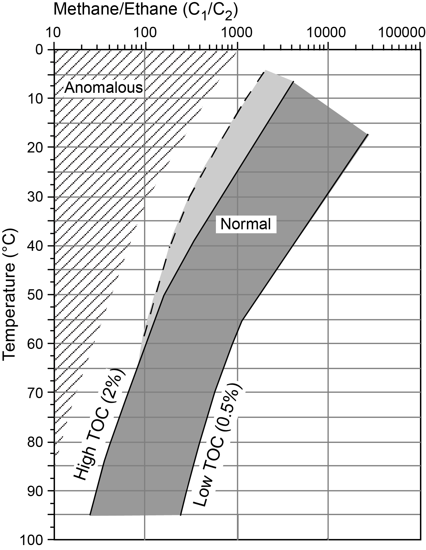
Figure F31. Hydrocarbon content risk assessment.
About 5 cm3 of sediment was collected from cores immediately after sectioning on the catwalk using a cork borer in soft sediments and a metal spatula for harder material. The samples were usually taken at the top of the section adjacent to the IW whole-round sample (cf. IW whole-round sample in Figure F32). After sampling, the sediments were placed in a 20 cm3 glass vial and sealed with a polytetrafluoroethylene (PTFE)/silicon septum and a crimped aluminum cap. Each vial containing a headspace sample was placed in an oven at 70°C for 30 min. A 5 cm3 aliquot of the released hydrocarbon gases was then extracted from the headspace vial with a gas-tight syringe and manually injected into an Agilent 7890A gas chromatograph (GC) equipped with a flame ionization detector (FID) set at 300°C for rapid estimation of methane (C1), ethane (C2), ethene (C2=), propane (C3), and propene (C3=) content. For these analyses, capillary columns DB-1 (123-1015, DB-1, 5.0 m × 0.32 mm × 1.0 µm) and AL/S (19091P-S12, HP-AL/S, 25 m × 0.32 mm × 8.0 µm) were used. The GC oven program was set to remain at 35°C for 4 min with a subsequent rise to 200°C at 25°C/min, and then was kept isothermal for 5 min, resulting in a total run time of 15.6 min. For these analyses, helium was used as the carrier gas. The results were processed using the Agilent ChemStation data software package.
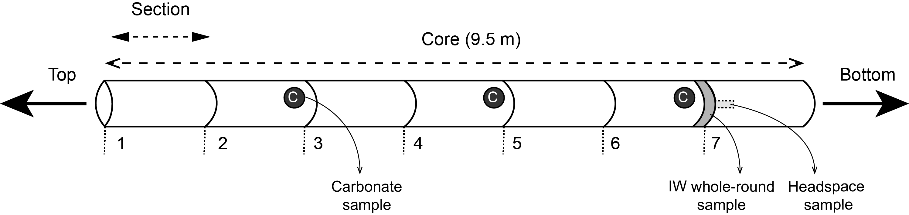
Figure F32. Proposed sampling locations.
The chromatographic response was calibrated using nine different gas standards containing known variable concentrations of low molecular weight hydrocarbons. One of these standards was checked every day before headspace gas analysis to ensure correct response from the FID. This standard measurement was also preceded by a blank analysis to verify the absence of a residual signal from the GC. Concentrations of hydrocarbon gases are reported as parts per million by volume (ppmv). The detection limit of the FID detector is ~1 ppmv, and the measurement uncertainty is ~2% of the measured value.
8.2. Interstitial water geochemistry
8.2.1. Shipboard processing
Whole-round core samples of unconsolidated materials, generally 5–10 cm long (IW whole-round sample in Figure F32), were partitioned immediately after the core was brought on deck, capped, and taken to the laboratory for pore fluid processing. After extrusion from the core liner, contamination from seawater and sediment smearing was removed by scraping the sample surface with a spatula. The sample was placed into a titanium squeezer (modified after Manheim and Sayles, 1974) and compressed using a laboratory hydraulic press. The squeezed pore fluids were filtered through a prewashed Whatman No. 1 filter placed in the squeezers above a titanium mesh screen. Approximately 40 mL of pore fluid was collected in precleaned plastic syringes attached to the squeezing assembly and subsequently filtered through a 0.45 µm Whatman Puradisc polyethersulfone (PES) disposable filter. For several samples, such as samples with high ash and water content, Rhizon samplers were used instead of titanium squeezers (Rhizosphere Research Products, Wageningen, The Netherlands). Rhizon samplers were presoaked in DI water and inserted into the sediment, and the first 1 mL of extracted IW was discarded as waste to remove potential contaminants or residual DI in the sampler.
After fluids were extracted, the squeezer parts were cleaned with shipboard water and rinsed with DI water. Parts were dried thoroughly with compressed air prior to reuse.
Sample allocation was determined based on the pore fluid volume recovered and on analytical priorities based on the expedition objectives. The IW extracted from the compressed sediment sample was divided into aliquots (in priority order) for the following analyses:
- 3 mL for salinity, alkalinity, and pH;
- 100 µL for ion chromatography (IC) analysis of major anions and cations;
- 500 µL for ICP-AES analysis of major, minor, and trace elements; and
- 5–10+ mL for postexpedition analysis.
8.2.2. Shipboard interstitial water analyses
8.2.2.1. Salinity, alkalinity, and pH
Salinity, alkalinity, and pH were measured immediately after IW extraction, following the procedures in Gieskes et al. (1991). Salinity was measured using a Fisher temperature-compensated handheld refractometer (Fisher Model S66366). A transfer pipette was used to transfer 2 drops of IW to the salinity refractometer, and the corresponding salinity was recorded in the log book.
The pH was measured with a combination glass electrode, and alkalinity was determined by Gran titration with an autotitrator (Metrohm 794 Basic Titrino) using 0.1 M HCl at 25°C. International Association for the Physical Sciences of the Oceans (IAPSO) standard seawater was used as a check standard and was analyzed at the beginning and end of the sample set for each site and after every 10 samples. Repeated measurements of IAPSO standard seawater alkalinity yielded a precision <0.8%.
8.2.2.2. Ion chromatography
Interstitial water samples were analyzed on board for major anions (i.e., Cl−, SO42−, and Br−) and major cations (i.e., Ca2+, Na+, Mg2+, and K+) using a Metrohm 850 ion chromatograph equipped with a Metrohm 858 Professional sample processor as an autosampler following the protocols in Gieskes et al. (1991), Murray et al. (2000), and the IODP user manuals for shipboard instrumentation. Interstitial water was diluted 1:100 with 18.2 MΩ·cm DI water prior to ion chromatography analysis. Precision and accuracy were monitored using IAPSO standard seawater with the following composition: alkalinity (2.353 mM), Ca (10.54 mM), Mg (54.1 mM), K (10.46 mM), Sr (93.0 µM), sulfate (28.94 mM), Cl (559.6 mM), Na (480.7 mM), and Li (26.4 µM). Diluted IAPSO standard seawater was analyzed every 10 unknown samples as a check standard. During Expedition 398, repeated values for check standards were generally within 4%.
8.2.2.3. ICP-AES major and minor elements
A 500 µL aliquot of interstitial water from each sample was acidified immediately with 2 drops of ultrapure HNO3 after squeezing and analyzed on an Agilent Technologies 5110 spectrometer ICP-AES for major (i.e., S, Ca, Mg, K, and Na) and minor (i.e., B, Ba, Fe, Li, Mn, P, Si, and Sr) elements. The general method for shipboard ICP-AES analysis is described in ODP Technical Note 29 (Murray et al., 2000) and the user manuals for shipboard instrumentation, with modifications as indicated.
The ICP-AES plasma was ignited at least 20 min before each sample run to allow the instrument to warm up and stabilize. Blanks and standard solutions of known concentrations were added to each analytical run. The raw intensity values were corrected for instrument drift and blank values. Drift correction was applied to each element by linear interpolation between the drift-monitoring solutions. Whenever possible, multiple wavelength analyses of an element were performed, and wavelengths generating the least scatter and smallest deviations from the certified standard values were selected. The wavelengths performed for each major and minor element in the IW samples and the wavelength selected for reporting the analytical data of each element are shown in Table T7. Major and minor elements were run in triplicate for both unknowns and standards.
Splits of 500 µL of samples and standards were diluted with a 100 µL internal standard (i.e., Be, In, Sb, and Sc) and 4.4 mL 2% trace-metal grade HNO3. With every batch run for major elements (i.e., S, Ca, Mg, K, and Na), a 7-point calibration curve was created using different dilution levels of IAPSO seawater. For minor elements (i.e., B, Ba, Fe, Li, Mn, P, Si, and Sr), an 8-point calibration curve was created using synthetic, acidified seawater spiked with minor elements from SPEX CertiPrep stock solutions diluted to varying degrees. Calibration curves were used to convert background-corrected intensities to concentrations. The IAPSO dilutions for the major element calibration curve were also included in the trace element calibration curve for the trace elements with detectable concentrations. All standards were analyzed at the beginning of the run to construct a calibration curve using the Agilent software. Four standards (IAPSO and in-house) were run every 10 samples to monitor drift and precision of each element throughout the run. During Expedition 398, relative standard deviation (RSD) for repeated check standards was better than 3% for the majority of elements. Iron and phosphorus were below the detection limit in a majority of samples.
8.3. Sediment bulk geochemistry
8.3.1. Shipboard processing
A portion of the squeeze cakes produced when compressing the sediments for interstitial water extraction were freeze-dried for ~24 h to remove water and then ground to powder to ensure homogenization. This powder aliquot was used for sediment bulk geochemical analyses.
8.3.2. Sapropel Identification
For units described as organic rich and suspected to be sapropels (e.g., Kroon et al., 1998), samples were collected from the working half of the core for bulk geochemical analyses to calculate total organic carbon (TOC) values. Following Kidd et al. (1978), units with TOC values > 2 wt% were termed “sapropels” and TOC values of 0.5–2 wt% were termed “sapropelitic.” TOC values were used to identify organic-rich units as sapropels.
8.3.3. Sediment geochemistry
8.3.3.1. Carbonate content
The carbonate-associated carbon content of the samples (also referred to as total inorganic carbon [TIC]) was determined using a Metrohm CM5017 coulometer. About 11 mg of sediment was placed in a heated glass vial and reacted with 5 mL of 1 M HCl at 50°C. The evolved CO2 was backtitrated to a colorimetric end point. Analytical reproducibility was determined by replicate measurements of selected samples. A verification external standard (i.e., 100 wt% CaCO3) was run every 10 samples. Analyses would only continue if standard values were 98–102 wt%. Carbonate content, reported as weight percent, was calculated from the TIC content based on the assumption that all TIC exists as CaCO3:
All CO2 was assumed to derive from dissolution of CaCO3. No corrections were made for other carbonate minerals.
8.3.3.2. Total carbon, total organic carbon, and nitrogen
Total carbon (TC) and nitrogen (N) content was determined using a Thermo Electron Flash EA-1112 Series elemental analyzer equipped with a Thermo Electron packed GC column carbon-hydrogen-nitrogen-sulfur (CHNS)/nitrogen-carbon-sulfur (NCS) analyzer and a thermal conductivity detector (TCD). Bulk powder, ~12 mg, was weighed into a tin capsule and combusted in an oxygen gas stream at 950°C. After the reduction of nitrogen oxides to N2, the mixture of gases (i.e., N2, CO2, H2O, SO2) was separated by gas chromatography and detected by TCD.
Calibration for the elemental analyzer was based on Standard 2704, Buffalo River sediment (C = 3.35%, N = 0.172%–0.18%). Analytical reproducibility was determined by replicate measurements of this standard every 10 samples. During Expedition 398, RSD for repeated check standards was better than 10% for N and better than 1.7% for C. TOC was determined as the difference between TC and TIC measured by coulometry:
8.4. Igneous and volcaniclastic bulk geochemistry
8.4.1. Shipboard processing
Volcaniclastic sediments and ash layers identified as regions of interest were sampled by scooping, whereas lapilli-sized pumice clasts were hand-picked, targeting a total sample volume of ~5 cm3. Volcaniclastic sediments and ashes were freeze-dried (10–12 h). The samples were ground to a fine powder in the SPEX 8530 Shatterbox.
Each sample and standard was weighed on a Cahn C-31 microbalance to make 100.0 ± 0.5 mg splits; weighing errors were estimated to be ±0.05 mg under relatively smooth sea-surface conditions. Splits of ignited whole-rock powders were mixed with 400.0 ± 0.5 mg of LiBO2 flux (preweighed on shore). During each ICP-AES analysis, standard rock powders and full procedural blanks were interspersed with unknowns (among the elements reported, contamination from the tungsten carbide mills is negligible) (Shipboard Scientific Party, 2003).
Aqueous LiBr solution (10 µL of 0.172 mM LiBr) was added to the flux and rock powder mixture as a nonwetting agent prior to sample fusion to prevent the fused bead from sticking to the crucible during cooling. Samples were fused individually in Pt-Au (95:5) crucibles for ~12 min at a maximum temperature of 1050°C in an internally rotating induction furnace (Bead Sampler TK-4100).
The beads were transferred into 125 mL high-density polyethylene (HDPE) bottles and dissolved in a 50 mL solution containing 10% HNO3. The solution bottle was placed in a Burrell wrist-action shaker for 1 h to aid dissolution. Next, 20 mL increments of the solution were passed through a 0.45 µm filter into a clean 60 mL wide-mouth HDPE bottle. From the filtered solution, 500 µL was pipetted into a scintillation vial and diluted with 4.4 mL of dissolution solution containing 10% HNO3. Internal standard solution containing Be, In, and Sb (100 µL) was added into each vial. The final solution-to-sample dilution factor was 5000; this solution was used to analyze both major and trace elements.
8.4.2. ICP-AES major and trace elements
Major and trace element concentrations of standards and samples were determined using an Agilent 5110 ICP-AES instrument. Certified international rock reference materials, calibration and drift solutions, and chemical procedure blanks were included with the unknown samples for each sample run (Table T7). Detection limits were calculated as three times the standard deviation of the mean for blank solution measurements.
The ICP-AES plasma was ignited at least 20 min before each sample run to allow the instrument to warm up and stabilize. The ICP-AES data presented in the rock geochemistry sections for each site were acquired using Agilent’s ICP Expert software. The intensity curve for each element is defined by 20 measurements within the designated wavelength window. The ICP Expert software integrates the area delineated by the baseline and the intensity curve. Each sample was analyzed three times from the same dilute solution in a given sample run.
A set of six certified rock standards were chosen for their wide range in composition to calibrate the analyses (Table T8; Figures F33, F34): basalts BHVO-2 and BCR-2; andesites JA-1 and AGV-1; and rhyolites JR-1 and RGM-1. As many as 25 unknown samples were analyzed during a single run. A 10% HNO3 wash solution was run for 90 s between each sample analysis. Estimates of accuracy and precision of major and trace element analyses were based on replicate analyses of two international standards, basalt BHVO-2 and granodiorite JG-3, run every four samples. During Expedition 398, run-to-run RSD by ICP-AES was typically ±1% for major elements and ±5%–10% for trace elements. Repeated procedural blanks were used to determine detection limits.
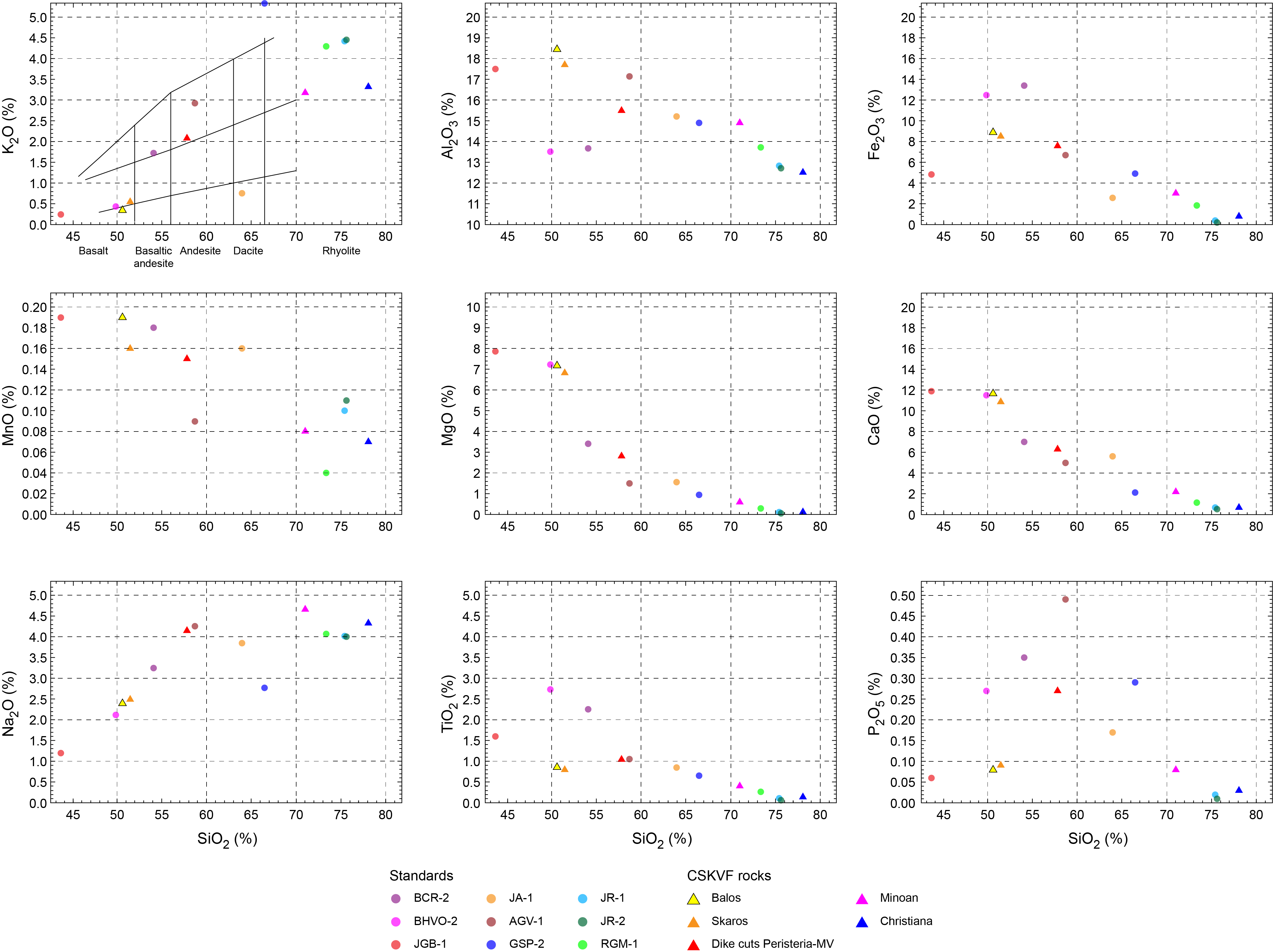
Figure F33. Major element compositions.
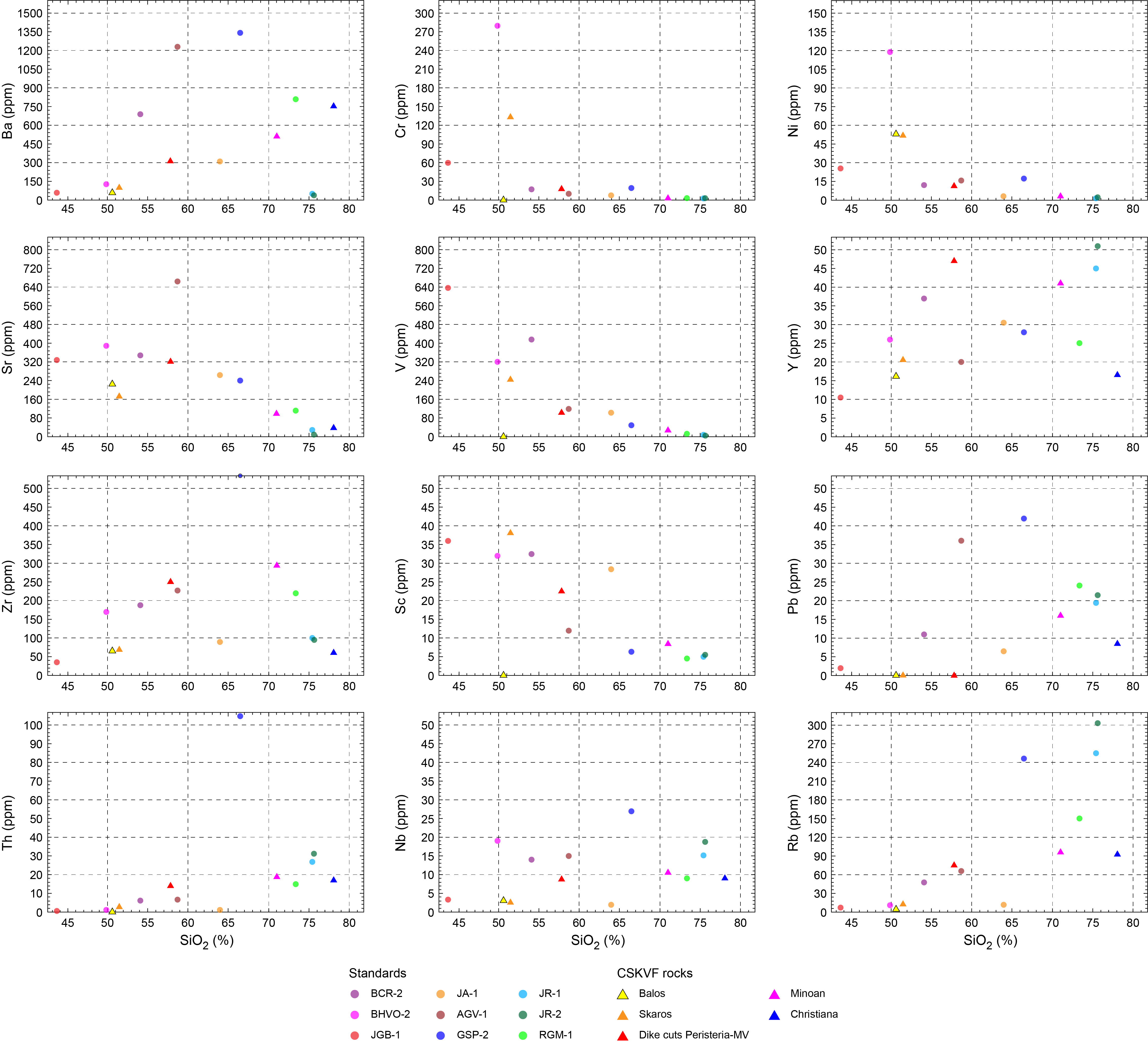
Figure F34. Minor and trace element compositions.
8.4.3. ICP-AES data reduction
All analyses were corrected first for drift. A drift correction was applied to each element based on the internal standard containing Be, In, and Sb. Concentrations used for the calibrations were compiled values from the literature. Total iron oxide concentrations were reported as Fe2O3t. Element concentrations in the samples were calculated from the relevant calibration lines.
9. Microbiology
The microbiology team collected samples from the deep subsurface of the Santorini caldera at Sites U1595 and U1596 and from the Anafi Basin at Sites U1599 and U1600. Because sampling for microbiology is delicate in terms of identifying suitable sampling material and avoiding contamination, we focused on samples showing specific geochemical and physicochemical characteristics (e.g., differences in color, temperature, and so on) and made ad hoc decisions while the core was being delivered to the core receiving platform (i.e., catwalk). Special emphasis was placed on dark black-green and red, iron-rich layers. In total, we collected 50 samples for all four sites.
During Expedition 398, we collected samples from sediments and volcaniclastics. Εmphasis was placed on sediment sampling. Some representative pumice samples were collected.
Samples were processed and prepared for shore-based molecular-based phylogenetic studies and metagenomic analysis (DNA), cultivation assays (prokaryote cultivation experiments), microscopic observation of cells and cell counts, and contamination tests. Our efforts were dedicated to collecting and preserving an adequate number of samples for further shore-based studies; no shipboard analyses were performed.
9.1. Sampling
For the most part, the sampling strategy was based on the methods of Expedition 376 (de Ronde et al., 2019). Microorganisms collected were expected to be sensitive to chemical and physical changes when brought to the surface. Changes in oxygen concentration and temperature are two important factors that were considered. Thus, the following procedures were followed to minimize harm to subsurface microorganisms.
For microbiological studies, whole-round samples were required to have sufficient material to work with to enable proper cleaning and avoid contamination introduced by sample handling before and during the core splitting process. Gloves and face masks were used when sampling whole rounds from the catwalk, and the split core liner was sprayed with 70% ethanol to minimize the chances of contamination. The microbiologists and the geologists taking part in sample selection wore gloves sprayed with ethanol to limit possible contamination of the sample from human contact. The microbiologists wore closed-sleeve laboratory coats. The lead microbiologist selected a whole-round section for sampling in accordance with the Co-Chief Scientist on shift or the Staff Scientist. An ideal sample was one that consisted largely of intense dark green-black or red sediments that had not split apart during recovery and did not have a unique lithology that would be critical to the core description team. The whole-round core sample chosen for microbiology was transferred immediately into a sterile Whirl-Pak bag and transported to the microbiology laboratory for further processing. In the microbiology laboratory, the whole-round sample was transferred immediately into the hard-shell anaerobic chamber (COY anaerobic chamber rigid glove box with purge airlock, COY Laboratory Products Inc.) (Figure F35). The outside of each core was sprayed three times with 70% ethanol.
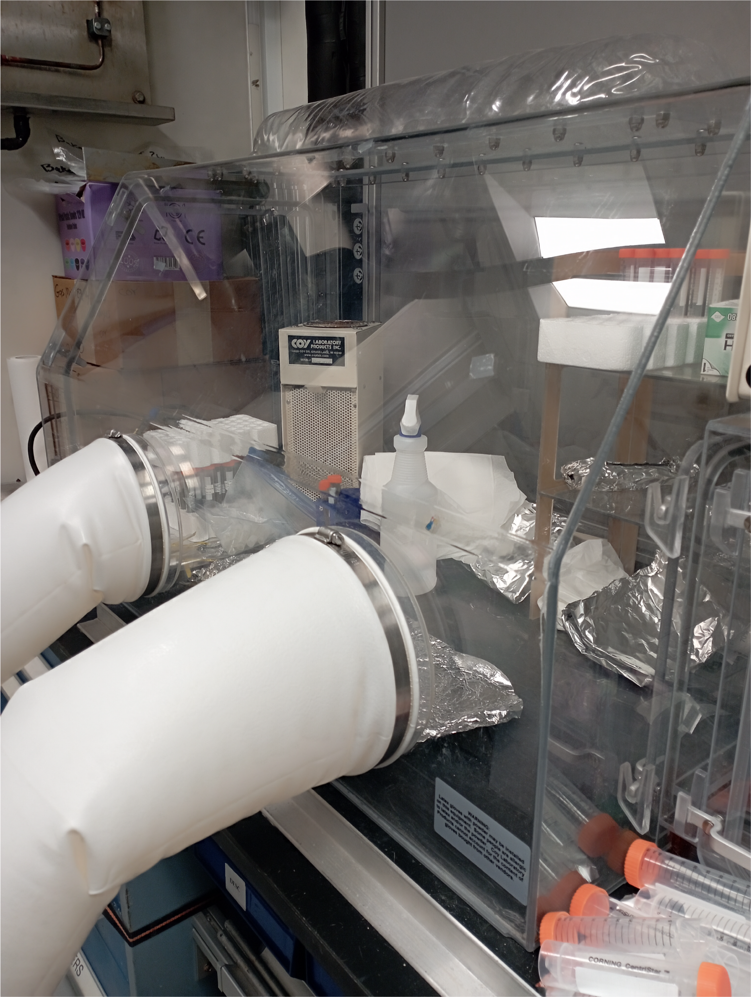
Figure F35. COY anaerobic chamber.
Prior work has shown that the interior of rock cores is generally free from contamination (Lever et al., 2006). Therefore, efforts were made to sample only the interior of the cores. Sections that displayed soft material or were organically enriched were chosen because these were the most likely locations to support microbial life.
On average, microbiology samples were ~5 cm long. Sample material was divided into subsamples for a variety of tests, which included the following:
- DNA-based metagenetic analysis,
- DNA-based metagenomic analysis,
- Cell counts,
- Microscopy,
- Aerobic cultures in liquid medium and agar plates, and
- Anaerobic cultures.
After cleaning the exterior of whole-round samples, the core interiors were subsampled for the above-mentioned tests using either sterile syringes of 60 cm3 and 20 cm3 or ethanol-sterilized stainless-steel spatula, chisel, and hammer (Figures F36 and F37). The whole-round core remaining after subsampling was stored at 4°C.
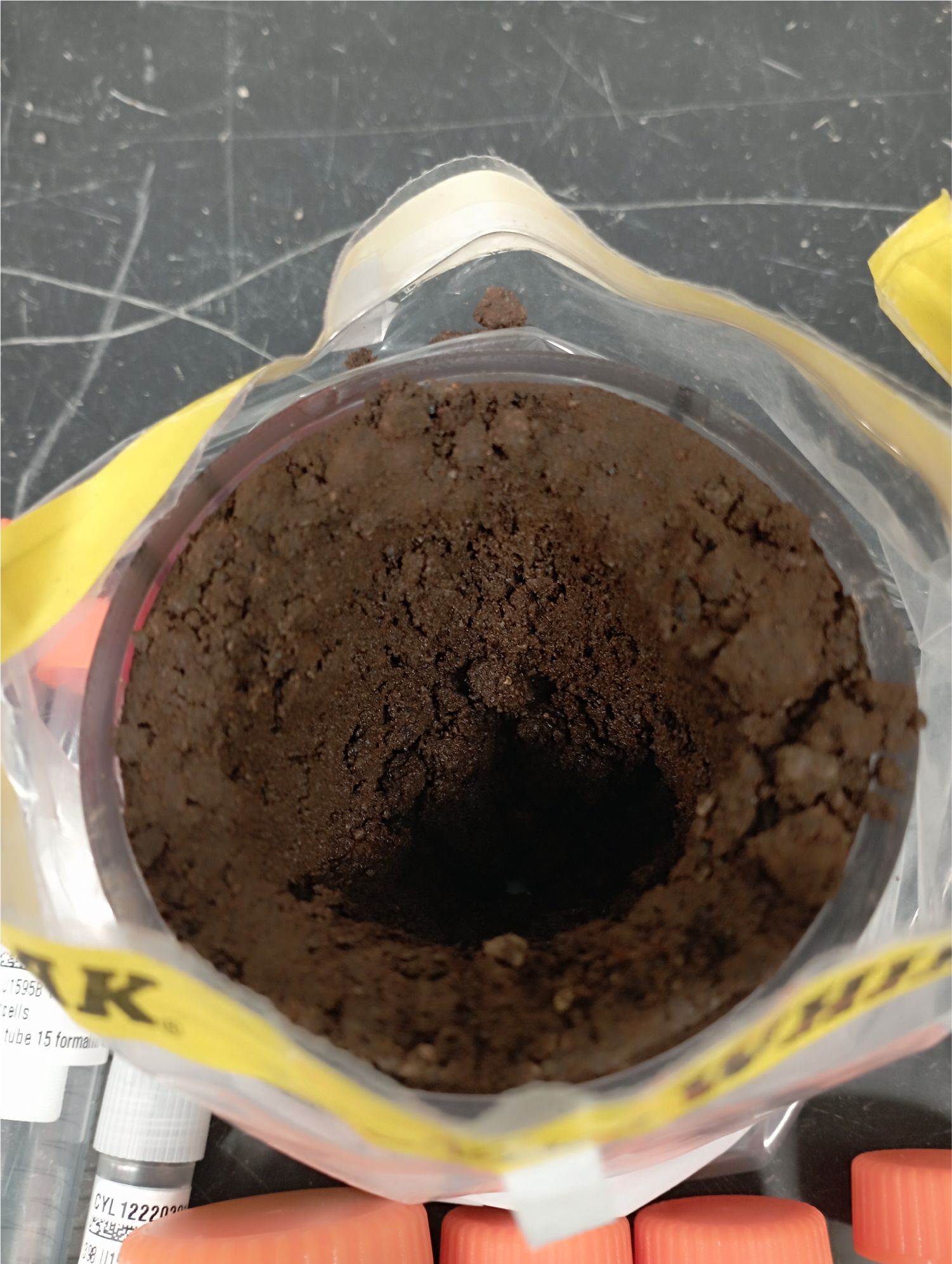
Figure F36. Whole-round sample after subsampling of interior.
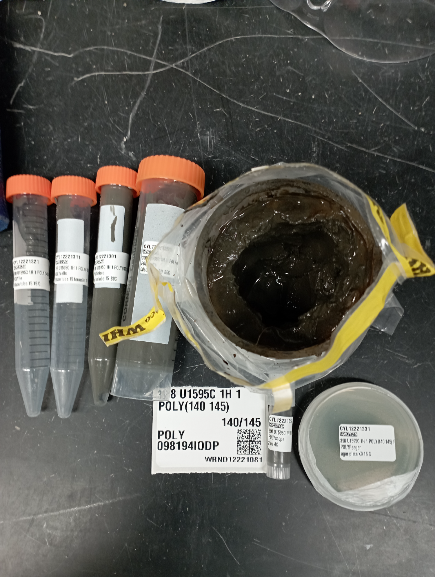
Figure F37. Whole-round sample and labeled samples.
Following completion of sample processing, all tools and the chamber were cleaned with DI water, sprayed with 75% ethanol, wiped with Kimwipes, sprayed with 75% ethanol again, and allowed to air dry.
9.2. Contamination testing of drilling fluid
Samples of the drilling fluid were collected for microbial community small subunit ribosomal RNA gene diversity analysis during drilling. These samples were collected directly from the injection pipe on the rig floor into sterile bottles. Any organisms found to be present in both the drilling fluid and rock samples will be considered a sign of contamination.
The Aegean Sea is an oligotrophic environment, and the microbial abundances in the surface waters are extremely low, so we do not expect contamination issues. However, in the case that some organisms are present in the drilling fluid and are observed during postcruise analyses, they will be excluded from further analysis. Following previous expedition methodology (i.e., Expedition 376), this conservative approach is the most appropriate one.
To measure contamination, ~500 mL of drilling fluid was collected and filtered on board onto 45 mm 0.22 µm pore-sized polycarbonate membrane filters and kept frozen at −80°C for shore-based DNA extraction and analysis.
Samples of drilling mud (i.e., sepiolite) were also collected on the rig floor prior to injection into the drill pipe in two sterile 50 mL polypropylene centrifuge tubes and frozen at −80°C for shore-based DNA extraction.
9.3. Subsample preparation
9.3.1. Cell counts and microscopic examination
A subsample of ~1.5 cm3 was placed into a 15 mL plastic tube (Falcon type) with 8.5 mL of filtered sterile seawater collected from the drilling site, fixed with 3% (v/v) buffered formalin (final concentration), and stored at 4°C until analysis in the laboratory for total microbial cell counts. A subsample of ~1.5 cm3 was placed in small 2 mL vials and frozen at 4°C for further electron microscopy investigation of microbial cells on shore.
9.3.2. Cultivation experiments
Culture-based techniques using different substrates and conditions were also applied in an attempt to isolate microorganisms from the deeper layers of Santorini caldera (Figure F38). Special emphasis was given to iron-related bacteria to further investigate their potential in the biological Fe cycling. Both aerobic and anaerobic conditions were investigated. From each round core, a subsample of ~12 cm3 was placed into a 15 mL sterile Falcon tube and anaerobically stored at 4°C for shore-based analysis. A subsample of 1.5 mL was used for aerobic cultivation on board using a laminar flow hood. The material was placed into 15 mL Falcon tubes containing sterile 9K medium, which is rich in Fe+2 and stored at 16°C for onboard and shore-based cultivation experiments. Onboard experiments were performed using sterile Petri dishes with 9K agar medium already prepared by the Hellenic Centre for Marine Research (HCMR) using the streak plate method.
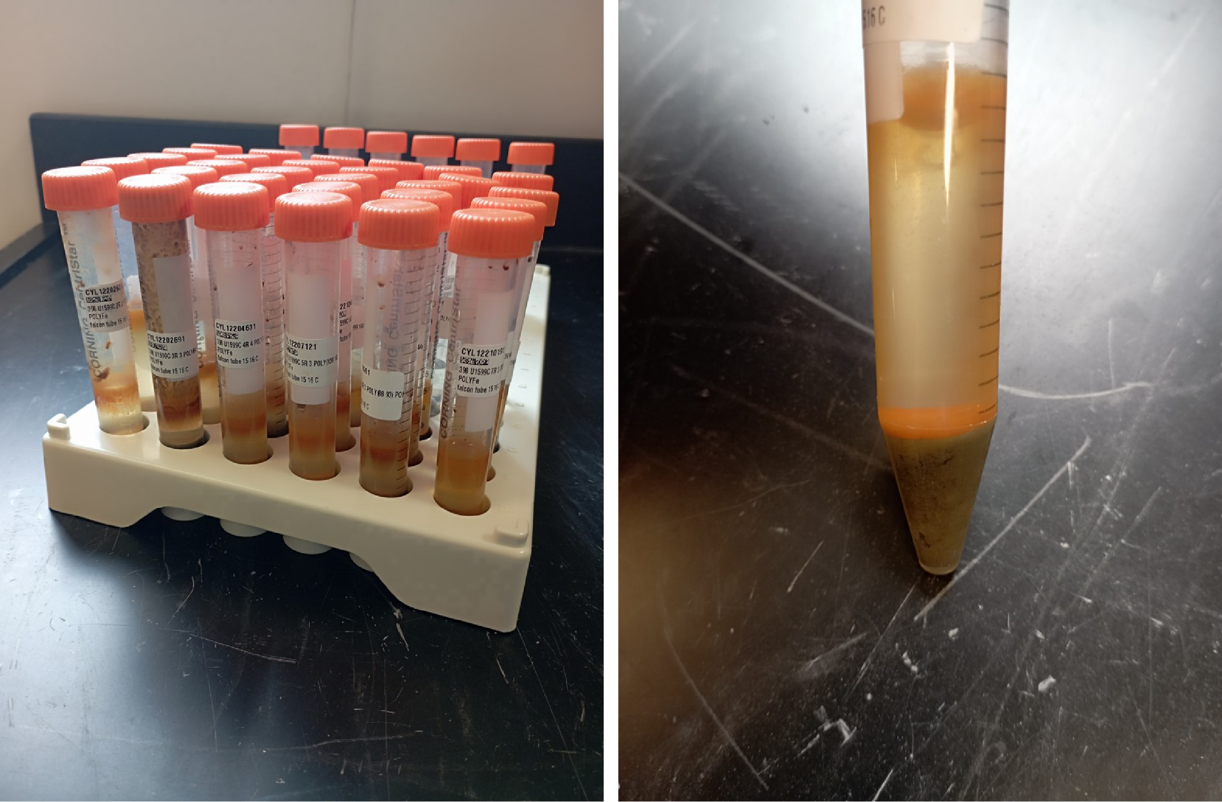
Figure F38. Culture-based samples.
9.3.3. Molecular biology-DNA
For DNA analyses, we collected 50 cm3 of sediment and froze it at −80°C. These samples will be analyzed during postcruise research for molecular-based phylogenetic studies and metagenomic analysis. In addition, in some cases, mudline water was collected for microbial community analysis to be used for comparison.
9.4. Storage and shipment conditions
All sediment cores and rocks for molecular analyses were placed in sterile tubes and bags and stored at −80°C. The slurry samples for aerobic cultivation were stored at room temperature. The slurry samples for anaerobic cultivation were stored under anaerobic conditions at 4°C.
10. Downhole logging
Downhole wireline logging data help characterize subseafloor lithologies and their structures. It is especially useful to fill gaps at depth intervals where recovery is poor (e.g., lapilli-rich units or depths cored with XCB and RCB coring) and to compare shipboard and in situ measurements. A suite of downhole logging tools provides continuous physical properties data in situ at sampling intervals ranging from 2.5 mm to 0.15 m. The acquired data help with interpretation of whole-hole lithostratigraphy, formation fluid properties, and measured temperatures. Downhole logging data are ultimately used to conduct multiscale correlations of data acquired throughout and beyond Expedition 398 by bridging measurements on discrete sample/whole and/or half core and various regional-scale data, including seismic reflection records.
During Expedition 398, one wireline logging run was conducted in Hole U1589C, which yielded three paths. We adhered to a standard open-hole logging approach established by Schlumberger and throughout scientific ocean drilling on JOIDES Resolution. Prior to the logging operations, the formation temperature was deemed sufficiently low for logging. This was checked by the following tools:
- APCT-3 (soft sediments) and
- SET2/sediment temperature pressure tool (SETP) (consolidated sediments).
In Hole U1589C, we deployed the standard suites of downhole logging tools (http://iodp.tamu.edu/tools/logging). The triple combination (triple combo) tool string deployed in Hole U1589C consisted of the following tools (top to bottom) (also see Table T9):
- LEH-QT (logging equipment head-Q tension).
- EDTC (Enhanced Digital Telemetry Cartridge).
- HNGS (Hostile Environment Natural Gamma Ray Sonde).
- HLDS (Hostile Environment Litho-Density Sonde with source and caliper).
- HRLA (High-Resolution Laterolog Array).
- MSS (Magnetic Susceptibility Sonde—third-party tool from Lamont Doherty Earth Observatory [LDEO]).
10.1. Logging data flow and depth scales
In Hole U1589C, the triple combo tool string was pulled up at a constant speed of ~9 m/min to provide a continuous set of measurements in each logging path. Downhole data during the logging run were monitored in real time and recorded by the Schlumberger MAXIS 500 system.
Initially, the logging data depths were referenced to the rig floor; the data depths are then post-processed using a combination of the tool locations during operations, including stuck-and-slip motion data. The Schlumberger logging tool head (or cable head) measures tension at the very top of the wireline tool string. These measurements detect and can diagnose difficulties in running the tool string up or down the borehole when exiting or entering the drill string or casing. The EDTC includes an accelerometer from which the data are used to evaluate the efficiency of the wireline heave compensator (WHC) (see Wireline heave compensator). The EDTC also includes a scintillation gamma ray detector to aid correlation between various passes and detect when the tool passes the seafloor. A clearer indication of the seafloor is provided by the HNGS. Because the tool strings combine tools of different generations and various designs, they include several adapters and joints between individual tools to allow communication, provide isolation, avoid interference (i.e., mechanical or acoustic), terminate wirings, or position the tool properly in the borehole.
After completion of logging operations, the downhole logging data were sent to the LDEO Borehole Research Group at Columbia University (New York, USA) for processing during the expedition and returned to the shipboard downhole logging scientists for interpretation.
Postprocessing primarily involves depth-matching to provide consistency in the depth scale between the different logging passes. Similar to the depth shift to the seafloor datum, this depth matching was undertaken primarily by utilizing the gamma ray data. In addition, corrections were made to certain tools and logs (e.g., speed and voltage corrections to microresistivity images), documentation for the logs (including an assessment of log data quality) was prepared, and the data were converted to ASCII format for the conventional logs.
10.2. Log data quality
The condition of a borehole is the principal factor contributing to log data quality. The ideal conditions for logging include a consistent borehole diameter of the size of the bit with no washouts (i.e., enlarged borehole) or bridges (i.e., narrowed borehole). Oversized borehole diameter can have a significant impact on measurements, especially those that require tool eccentering (e.g., HLDS). Direct contact of the eccentered tools with the formation is essential for acquisition of high-quality data sets. Borehole wall contact is lost beyond a 20 inch (50.80 cm) borehole diameter for the HLDS. Certain measurements (notably, spectral gamma ray [HNGS], resistivity [HRLA], and acoustic velocity [Dipole Sonic Imager (DSI)]) taken during Expedition 398 are still representative of the formation in larger borehole diameters. Consequently, these measurements are less affected by borehole conditions, although data are optimized in boreholes where the tools can be centralized (as large as ~20 inch diameter).
If the borehole diameter changes over short intervals due to washouts or ledges, logging results may be irregular. Bridged sections will also cause irregular log results. The quality of the borehole can be improved by minimizing the circulation of drilling fluid, flushing the borehole to remove debris prior to logging, performing a full wiper trip, and starting logging as soon as possible after drilling and hole conditioning.
The quality of logging depth determination is dependent on a number of factors, including ship’s heave, cable stretch, cable slip, and tidal changes. An important reference datum in wireline logging is the seafloor/mudline, which is determined from the gamma ray logs acquired during each logging pass. Discrepancies between the drilling core depth and the wireline logging depth occur because of incomplete core recovery, core expansion, incomplete heave compensation, and drill pipe stretch. Reconciling the differences between the two data sets is possible through comparison of the common data sets acquired in situ and on the core (e.g., NGR and MS).
10.3. Logged properties and tool measurement principles
The properties of the formations logged and the methods by which they were measured are described below. Further information regarding individual and/or combinations of logging tools and their applications are widely available (e.g., Ellis and Singer, 2007; Goldberg, 1997; Lovell et al., 1998; Rider and Kennedy, 2011; Schlumberger, 1989; Serra, 1984, 1986, 1989). In addition, a complete list of acronyms for Schlumberger tools and logs is available at http://www.odplegacy.org/PDF/Operations/Engineering/Logging_Tools/Acronyms_Comprehensive.pdf.
10.3.1. Physical properties wireline tools
During Expedition 398, a standard triple combo tool string in Hole U1589C recorded bulk density and photoelectric effect (PEF; HLDS), porosity (Accelerator Porosity Sonde [APS]), spectral (HNGS) and total count (EDTC) natural gamma ray, resistivity (HRLA), and fluid temperature (logging equipment head-mud temperature [LEH-MT]). Each tool string also included a telemetry cartridge in the EDTC that transmitted the data in real time from the tools to the MAXIS unit on the ship through the wireline cable.
10.3.2. Caliper
The borehole diameter measured by the caliper provides an indication of formation strength and borehole wall conditions after drilling operations. Displaying caliper measurements along depth can provide evidence of breakouts or borehole ellipticity that can be interpreted in terms of maximum and minimum plane stresses. A breakout signal typically shows an increase in diameter in one of the orthogonal calipers, whereas the other caliper remains close to the bit size. These caliper measurements can provide information on the present-day stress field inferred from the ellipticity of borehole deformation induced by downhole operations.
10.3.3. Natural gamma radioactivity
Total and spectral gamma ray measurements were acquired using the HNGS. This tool utilizes two bismuth germanate scintillation detectors and five-window spectroscopy to determine concentrations of 40K, 232Th, and 238U in the formation. Sensitivity to any additives in the drilling fluid (notably sepiolite-based drilling mud clay) is eliminated because the HNGS filters out gamma ray energies <500 keV, thus improving measurement accuracy. The inclusion of HNGS in all tool strings allows the use of gamma ray data for depth correlation between consecutive tool string runs and individual tool string passes (up- and down-logs).
10.3.4. Photoelectric effect
The HLDS also measures photoelectric absorption (i.e., PEF). After repeated Compton scattering resulting from collision with formation electrons, gamma radiation reaches an energy that is low enough (<150 keV) to be photoelectrically absorbed. The PEF is dependent on the atomic number of the elements in the formation and therefore varies according to the mineralogical composition of the lithologies encountered. As such, the PEF can be used to identify the presence of some minerals. Bartetzko et al. (2003), for example, interpret values >6 b/e− as a general indicator for sulfide or oxide mineralization.
10.3.5. Density
The HLDS measures formation density utilizing a cesium (137Cs) gamma ray source and far- and near-gamma ray detectors mounted on a shielded skid. This skid is pressed against the borehole wall using a hydraulically activated eccentering arm. The gamma rays emitted from the source are attenuated through the process of Compton scattering, which involves a partial energy loss resulting from elastic collision with electrons in the formation. The quantity of gamma radiation that reaches the detectors is directly related to the density of electrons in the formation, which in turn is related to the bulk density. Good tool/borehole contact is essential for effective HLDS measurements, whereas poor contact results in underestimation of formation density values.
10.3.6. Porosity
The formation porosity sonde includes a minitron neutron generator that produces fast neutrons and five detectors positioned at different spacings from the minitron. The tool’s detectors count neutrons that arrive after being scattered and slowed by collisions with atomic nuclei in the formation. The highest energy loss occurs when neutrons collide with hydrogen nuclei, which have essentially the same mass as the neutron. Therefore, the tool provides a measure of hydrogen content, which is most commonly found in water in the pore fluid and can be directly related to porosity. However, hydrogen may be present in sedimentary, igneous, and alteration minerals, including clay minerals, which can result in overestimation of actual porosity.
Upon reaching thermal energies (0.025 eV), the neutrons are captured by the nuclei of Cl, Si, B, and other elements, resulting in gamma ray emission. This neutron capture cross section (Σf) is also measured by the tool and can be used to identify these elements (Broglia and Ellis, 1990; Brewer et al., 1996).
10.3.7. Magnetic susceptibility
The MSS is a nonstandard wireline tool designed by LDEO (see Specialty Wireline Tools at https://iodp.tamu.edu/tools/logging/SPECIAL/mss-b.html). It measures the ease with which formations are magnetized when subjected to a magnetic field. The ease of magnetization is ultimately related to the concentration and composition (i.e., size, shape, and mineralogy) of magnetic minerals (principally magnetite) in the formation. These measurements provide one of the best methods for investigating stratigraphic changes in mineralogy and lithology because the measurement is quick, repeatable, and nondestructive and because different lithologies often have strongly contrasting magnetic susceptibilities.
The MSS dual-coil sensor provides ~40 cm resolution measurements with ~20 cm depth of horizontal investigation. The MSS was operated as the lowermost tool in the triple combo tool string with a data translation cartridge to be combined with the Schlumberger tools. MS data from the MSS are plotted as noncalibrated units and are affected by temperature and borehole size (e.g., higher temperatures lead to higher susceptibility measurements). For quality control and environmental correction, the MSS also measures internal tool temperature, z-axis acceleration, and low-resolution borehole conductivity.
10.3.8. Electrical resistivity
Six resistivity measurements with different depths of investigation (including one borehole fluid measurement and five formation measurements) were acquired with the HRLA. The array provides direct resistivity measurements by emitting a focused current into the formation and measuring the intensity necessary to maintain a constant drop in voltage across a fixed interval. The HRLA has one central (i.e., source) electrode and six electrodes above and below it that alternate as transmitting and receiving current electrodes. Simultaneous resistivity measurements at six penetration depths are possible because of the rapid alternation in roles of these electrodes.
10.3.9. Acoustic velocity
The DSI measures the transit time of acoustic pulses between sonic transmitters and an array of eight receivers. The resulting waveforms are used to calculate the sonic velocity of the formation. High-frequency (5–15 kHz) pulses emitted by an omnidirectional monopole transmitter are used to extract the compressional velocity (VP) of the formation. It is possible to extract the shear wave velocity (VS) from these data in the event that it is faster than the acoustic velocity in the borehole fluid. The monopole transmitter can also be fired in sequence at a lower frequency (0.5–1.0 kHz) to generate Stoneley waves, which are sensitive to fractures and variations in formation permeability. The DSI has two cross-dipole transmitters that facilitate the acquisition of shear wave velocity data in slow formations where the formation VS is less than that of the borehole fluid. In fast formations, VS measurements from the monopole waveforms are possible and have sharper arrivals and more accurate VS estimates than the equivalent cross-dipole data. However, the cross-dipole–derived shear velocities can be useful in identifying any sonic anisotropy associated with the local stress regime.
10.4. Wireline heave compensator
The WHC is designed to compensate for the ship’s vertical motion to help maintain the steady movement of the logging tools in the borehole. Vertical acceleration measurements made by the motion reference unit (MRU), located under the rig floor near the ship’s center of gravity, are used to calculate the vertical motion of the ship. The WHC then adjusts the length of the wireline by varying the distance between two sets of pulleys through which the cable passes. The actual motion of the tool string is displayed, enabling evaluation of the compensator’s efficiency. The WHC was used during logging operations in Hole U1589C with favorable sea conditions (<1 m peak-to-peak heave). Real-time measurements of uphole (i.e., surface) and downhole acceleration are made simultaneously by the MRU and the EDTC, respectively.
References
Acton, G., Morris, A., Musgrave, R., Zhao, X., and IODP SRM Personnel, 2017. Assessment of the New Superconducting Rock Magnetometer (SRM) on the JOIDES Resolution. http://iodp.tamu.edu/publications/JRSO/SRM_Workshop_2017.pdf
Alken, P., Thébault, E., Beggan, C.D., Amit, H., Aubert, J., Baerenzung, J., Bondar, T.N., Brown, W.J., Califf, S., Chambodut, A., Chulliat, A., Cox, G.A., Finlay, C.C., Fournier, A., Gillet, N., Grayver, A., Hammer, M.D., Holschneider, M., Huder, L., Hulot, G., Jager, T., Kloss, C., Korte, M., Kuang, W., Kuvshinov, A., Langlais, B., Léger, J.M., Lesur, V., Livermore, P.W., Lowes, F.J., Macmillan, S., Magnes, W., Mandea, M., Marsal, S., Matzka, J., Metman, M.C., Minami, T., Morschhauser, A., Mound, J.E., Nair, M., Nakano, S., Olsen, N., Pavón-Carrasco, F.J., Petrov, V.G., Ropp, G., Rother, M., Sabaka, T.J., Sanchez, S., Saturnino, D., Schnepf, N.R., Shen, X., Stolle, C., Tangborn, A., Tøffner-Clausen, L., Toh, H., Torta, J.M., Varner, J., Vervelidou, F., Vigneron, P., Wardinski, I., Wicht, J., Woods, A., Yang, Y., Zeren, Z., and Zhou, B., 2021. International Geomagnetic Reference Field: the thirteenth generation. Earth, Planets and Space, 73(1):49. https://doi.org/10.1186/s40623-020-01288-x
ASTM International, 1990. Standard method for laboratory determination of water (moisture) content of soil and rock (Standard D2216–90). In Annual Book of ASTM Standards for Soil and Rock Philadelphia (American Society for Testing Materials).
Aze, T., Ezard, T.H.G., Purvis, A., Coxall, H.K., Stewart, D.R.M., Wade, B.S., and Pearson, P.N., 2011. A phylogeny of Cenozoic macroperforate planktonic foraminifera from fossil data. Biological Reviews, 86(4):900–927. https://doi.org/10.1111/j.1469-185X.2011.00178.x
Backman, J., Raffi, I., Rio, D., Fornaciari, E., and Pälike, H., 2012. Biozonation and biochronology of Miocene through Pleistocene calcareous nannofossils from low and middle latitudes. Newsletters on Stratigraphy, 45(3):221–244. https://doi.org/10.1127/0078-0421/2012/0022
Bartetzko, A., Paulick, H., Iturrino, G., and Arnold, J., 2003. Facies reconstruction of a hydrothermally altered dacite extrusive sequence; evidence from geophysical downhole logging data (ODP Leg 193). Geochemistry, Geophysics, Geosystems, 4(10):1087. https://doi.org/10.1029/2003GC000575
Blum, P., 1997. Physical properties handbook: a guide to the shipboard measurement of physical properties of deep-sea cores. Ocean Drilling Program Technical Note, 26. https://doi.org/10.2973/odp.tn.26.1997
Borradaile, G.J., and Jackson, M., 2004. Anisotropy of magnetic susceptibility (AMS): magnetic petrofabrics of deformed rocks. Geological Society, London, Special Publications, 238(1):299–360. https://doi.org/10.1144/GSL.SP.2004.238.01.18
Braschi, E., Mastroianni, F., Di Salvo, S., Casalini, M., Agostini, S., Vougioukalakis, G., and Francalanci, L., 2022. Unveiling the occurrence of transient, multi-contaminated mafic magmas inside a rhyolitic reservoir feeding an explosive eruption (Nisyros, Greece). Lithos, 410–411:106574. https://doi.org/10.1016/j.lithos.2021.106574
Brewer, T.S., Harvey, P.K., Locke, J., and Lovell, M.A., 1996. Neutron absorption cross section (Ε) of basaltic basement samples from Hole 896A, Costa Rica Rift. In Alt, J.C., Kinoshita, H., Stokking, L.B., and Michael, P.J. (Eds.), Proceedings of the Ocean Drilling Program, Scientific Results. 148: College Station, TX (Ocean Drilling Program). https://doi.org/10.2973/odp.proc.sr.148.154.1996
Broglia, C., and Ellis, D.V., 1990. Effect of alteration, formation absorption, and standoff on the response of the thermal neutron porosity log in gabbros and basalts; examples from Deep Sea Drilling Project-Ocean Drilling Program sites. Journal of Geophysical Research: Solid Earth, 95(B6):9171–9188. https://doi.org/10.1029/JB095iB06p09171
Cantner, K., Carey, S., and Nomikou, P., 2014. Integrated volcanologic and petrologic analysis of the 1650AD eruption of Kolumbo submarine volcano, Greece. Journal of Volcanology and Geothermal Research, 269:28–43. https://doi.org/10.1016/j.jvolgeores.2013.10.004
Cas, R.A.F., and Wright, J.V., 1987. Volcanic Successions, Modern and Ancient: a Geological Approach to Processes, Products and Successions: London (Allen and Unwin).
Cimerman, F., and Langer, M., 1991. Mediterranean Foraminifera: Ljubljana, Slovenia (Academia Scientiarum et Artium Slovenica).
Clark, S.P., Jr., 1966. Handbook of Physical Constants: Boulder, CO (Geological Society of America). https://doi.org/10.1130/MEM97
Crundwell, M., Scott, G., Naish, T., and Carter, L., 2008. Glacial–interglacial ocean climate variability from planktonic foraminifera during the mid-Pleistocene transition in the temperate southwest Pacific, ODP Site 1123. Palaeogeography, Palaeoclimatology, Palaeoecology, 260(1–2):202–229. https://doi.org/10.1016/j.palaeo.2007.08.023
Crundwell, M.P., and Woodhouse, A., 2022. A detailed biostratigraphic framework for 0–1.2 Ma Quaternary sediments of north-eastern Zealandia. New Zealand Journal of Geology and Geophysics. https://doi.org/10.1080/00288306.2022.2054828
De Rijk, S., Troelstra, S.R., and Rohling, E.J., 1999. Benthic foraminiferal distribution in the Mediterranean Sea. Journal of Foraminiferal Research, 29(2):93–103. https://doi.org/10.2113/gsjfr.29.2.93
de Ronde, C.E.J., Humphris, S.E., Höfig, T.W., Brandl, P.A., Cai, L., Cai, Y., Caratori Tontini, F., Deans, J.R., Farough, A., Jamieson, J.W., Kolandaivelu, K.P., Kutovaya, A., Labonté, J.M., Martin, A.J., Massiot, C., McDermott, J.M., McIntosh, I.M., Nozaki, T., Pellizari, V.H., Reyes, A.G., Roberts, S., Rouxel, O., Schlicht, L.E.M., Seo, J.H., Straub, S.M., Strehlow, K., Takai, K., Tanner, D., Tepley III, F.J., and Zhang, C., 2019. Expedition 376 methods. In de Ronde, C.E.J., Humphris, S.E., Höfig, T.W., and the Expedition 376 Scientists, Brothers Arc Flux. Proceedings of the International Ocean Discovery Program, 376: College Station, TX (International Ocean Discovery Program). https://doi.org/10.14379/iodp.proc.376.102.2019
de Stigter, H.C., Jorissen, F.J., and van der Zwaan, G.J., 1998. Bathymetric distribution and microhabitat partitioning of live (Rose Bengal stained) benthic Foraminifera along a shelf to bathyal transect in the southern Adriatic Sea. Journal of Foraminiferal Research, 28(1):40–65.
Di Stefano, A., and Sturiale, G., 2010. Refinements of calcareous nannofossil biostratigraphy at the Miocene/Pliocene Boundary in the Mediterranean region. Geobios, 43(1):5–20. https://doi.org/10.1016/j.geobios.2009.06.007
Droser, M.L., and Bottjer, D.J., 1986. A semiquantitative field classification of ichnofabric. Journal of Sedimentary Research, 56(4):558–559. https://doi.org/10.1306/212F89C2-2B24-11D7-8648000102C1865D
Droser, M.L., and Bottjer, D.J., 1991. Trace fossils and ichnofabric in Leg 119 cores. In Barron, J., Larsen, B., et al., Proceedings of the Ocean Drilling Program, Scientific Results. 119: College Station, TX (Ocean Drilling Program), 635–641. https://doi.org/10.2973/odp.proc.sr.119.206.1991
Druitt, T.H., Edwards, L., Mellors, R.M., Pyle, D.M., Sparks, R.S.J., Lanphere, M., Davies, M., and Barreirio, B., 1999. Santorini Volcano. Memoir - Geological Society of London, 19. http://pubs.er.usgs.gov/publication/70094778
Druitt, T.H., Kutterolf, S., Ronge, T.A., Beethe, S., Bernard, A., Berthod, C., Chen, H., Chiyonobu, S., Clark, A., DeBari, S., Fernandez Perez, T.I., Gertisser, R., Hübscher, C., Johnston, R.M., Jones, C., Joshi, K.B., Kletetschka, G., Koukousioura, O., Li, X., Manga, M., McCanta, M., McIntosh, I., Morris, A., Nomikou, P., Pank, K., Peccia, A., Polymenakou, P.N., Preine, J., Tominaga, M., Woodhouse, A., and Yamamoto, Y., 2024. Site U1591. In Druitt, T.H., Kutterolf, S., Ronge, T.A., and the Expedition 398 Scientists, Hellenic Arc Volcanic Field. Proceedings of the International Ocean Discovery Program, 398: College Station, TX (International Ocean Discovery Program). https://doi.org/10.14379/iodp.proc.398.105.2024
Dunlop, D.J., 2003. Stepwise and continuous low-temperature demagnetization. Geophysical Research Letters, 30(11):1582. https://doi.org/10.1029/2003GL017268
Ellis, D.V., and Singer, J.M., 2007. Well Logging for Earth Scientists (2nd edition): New York (Elsevier). https://doi.org/10.1007/978-1-4020-4602-5
Evans, H.B., 1965. GRAPE* - A Device For Continuous Determination Of Material Density And Porosity. Presented at the SPWLA 6th Annual Logging Symposium (Volume II).
Expedition 315 Scientists, 2009. Expedition 315 methods. In Kinoshita, M., Tobin, H., Ashi, J., Kimura, G., Lallemant, S., Screaton, E.J., Curewitz, D., Masago, H., Moe, K.T., and the Expedition 314/315/316 Scientists, Proceedings of the Integrated Ocean Drilling Program,. 314/315/316: Washington, DC (Integrated Ocean Drilling Program Management International, Inc.). https://doi.org/10.2204/iodp.proc.314315316.122.2009
Expedition 316 Scientists, 2009. Expedition 316 methods. In Kinoshita, M., Tobin, H., Ashi, J., Kimura, G., Lallemant, S., Screaton, E.J., Curewitz, D., Masago, H., Moe, K.T., and the Expedition 314/315/316 Scientists, Proceedings of the Integrated Ocean Drilling Program. 314/315/316: Washington, DC (Integrated Ocean Drilling Program Management International, Inc.). https://doi.org/10.2204/iodp.proc.314315316.132.2009
Expedition 334 Scientists, 2012. Methods. In Vannucchi, P., Ujiie, K., Stroncik, N., and the Expedition 334 Scientists, Proceedings of the Integrated Ocean Drilling Program. 334: Tokyo (Integrated Ocean Drilling Program Management International, Inc.). https://doi.org/10.2204/iodp.proc.334.102.2012
Farouk, S., Ren, C., Abdeldaim, A., Salama, A., Wu, H., El-Kahtany, K., and Zaky, A.S., 2022. An astronomical time scale of early Pliocene from the Mediterranean Sea, Egypt. Global and Planetary Change, 215:103869. https://doi.org/10.1016/j.gloplacha.2022.103869
Fisher, A.T., Villinger, H., and Heesemann, M., 2007. User Manual for the Third-Generation, Advanced Piston Corer Temperature Tool (APCT-3).
Fisher, R.V., 1961. Proposed classification of volcaniclastic sediments and rocks. Geological Society of America Bulletin, 72(9):1409–1414. https://doi.org/10.1130/0016-7606(1961)72[1409:PCOVSA]2.0.CO;2
Fisher, R.V., and Schmincke, H.-U., 1984. Pyroclastic Rocks: Berlin (Springer). https://doi.org/10.1007/978-3-642-74864-6
Folk, R.L., 1980. Petrology of Sedimentary Rocks: Austin, TX (Hemphill Publishing Company). http://hdl.handle.net/2152/22930
Francalanci, L., Vougioukalakis, G.E., Perini, G., and Manetti, P., 2005. A West-East traverse along the magmatism of the south Aegean volcanic arc in the light of volcanological, chemical and isotope data. In Fytikas, M., and Vougioukalakis, G.E. (Eds.), The South Aegean Active Volcanic Arc: Present Knowledge and Future Perspectives. Developments in Volcanology, 7: (Elsevier), 65–111. https://doi.org/10.1016/S1871-644X(05)80033-6
Francalanci, L., and Zellmer, G.F., 2019. Magma genesis at the south Aegean volcanic arc. Elements, 15(3):165–170. https://doi.org/10.2138/gselements.15.3.165
Gibbard, P.L., and Head, M.J., 2020. The Quaternary period. In Gradstein, F.M., Ogg, J.G., Schmitz, M.D., and Ogg, G.M. (Eds.), Geologic Time Scale 2020. Dordrecht, Netherlands (Elsevier), 1217–1255. https://doi.org/10.1016/B978-0-12-824360-2.00030-9
Gieskes, J.M., Gamo, T., and Brumsack, H.J., 1991. Chemical methods for interstitial water analysis aboard JOIDES Resolution. Ocean Drilling Program Technical Note, 15. https://doi.org/10.2973/odp.tn.15.1991
Goldberg, D., 1997. The role of downhole measurements in marine geology and geophysics. Reviews of Geophysics, 35(3):315–342. https://doi.org/10.1029/97RG00221
Graber, K.K., Pollard, E., Jonasson, B., and Schulte, E. (Eds.), 2002. Overview of Ocean Drilling Program engineering tools and hardware. Ocean Drilling Program Technical Note, 31. https://doi.org/10.2973/odp.tn.31.2002
Gradstein, F.M., Ogg, J.G., Schmitz, M.D., and Ogg, G.M. (Eds.), 2020. The Geologic Time Scale 2020: Amsterdam (Elsevier BV). https://doi.org/10.1016/C2020-1-02369-3
Hagelberg, T.K., Pisias, N.G., Shackleton, N.J., Mix, A.C., and Harris, S., 1995. Refinement of a high-resolution, continuous sedimentary section for studying equatorial Pacific Ocean paleoceanography, Leg 138. In Pisias, N.G., Mayer, L.A., Janecek, T.R., Palmer-Julson, A., and van Andel, T.H. (Eds.), Proceedings of the Ocean Drilling Program, Scientific Results. 138: College Station, TX (Ocean Drilling Program). https://doi.org/10.2973/odp.proc.sr.138.103.1995
Harms, J.C., and Choquette, P.W., 1965. Geologic evaluation of a gamma-ray porosity device. Presented at the SPWLA 6th Annual Logging Symposium, Dallas, TX, May 1965.
Harris, R.N., Sakaguchi, A., Petronotis, K., Baxter, A.T., Berg, R., Burkett, A., Charpentier, D., Choi, J., Diz Ferreiro, P., Hamahashi, M., Hashimoto, Y., Heydolph, K., Jovane, L., Kastner, M., Kurz, W., Kutterolf, S.O., Li, Y., Malinverno, A., Martin, K.M., Millan, C., Nascimento, D.B., Saito, S., Sandoval Gutierrez, M.I., Screaton, E.J., Smith-Duque, C.E., Solomon, E.A., Straub, S.M., Tanikawa, W., Torres, M.E., Uchimura, H., Vannucchi, P., Yamamoto, Y., Yan, Q., and Xhao, X., 2013. Methods. In Harris, R.N., Sakaguchi, A., Petronotis, K., and the Expedition 344 Scientists, Proceedings of the Integrated Ocean Drilling Program. 344: College Station, TX (Integrated Ocean Drilling Program). https://doi.org/10.2204/iodp.proc.344.102.2013
Hayward, B.W., Grenfell, H.R., Reid, C.M., and Hayward, K.A., 1999. Recent New Zealand shallow-water benthic foraminifera: taxonomy, ecologic distribution, biogeography, and use in paleoenvironmental assessment. In Institute of Geological & Nuclear Sciences Monograph, 21: Lower Hutt, NZ.
Heard, T.G., Pickering, K.T., and Clark, J.D., 2014. Ichnofabric characterization of a deep-marine clastic system: a subsurface study of the middle Eocene Ainsa System, Spanish Pyrenees. Sedimentology, 61(5):1298–1331. https://doi.org/10.1111/sed.12101
Heesemann, M., Villinger, H.W., Tréhu, A.T.F.M., and White, S., 2006. Data report: testing and deployment of the new APCT-3 tool to determine in situ temperatures while piston coring. In Riedel, M., Collett, T.S., Malone, M.J., and the Expedition 311 Scientists, Proceedings of the Integrated Ocean Drilling Program. 311: Washington, DC (Integrated Ocean Drilling Program Management International, Inc.). https://doi.org/10.2204/iodp.proc.311.108.2006
Higgins, M.D., Debecq, A., Vander Auwera, J., and Nomikou, P., 2021. Chemical and textural diversity of Kameni (Greece) dacites: role of vesiculation in juvenile and mature basal crystal masses. Contributions to Mineralogy and Petrology, 176(2):13. https://doi.org/10.1007/s00410-020-01764-3
Holbourn, A., Henderson, A.S., and MacLeod, N., 2013. Atlas of Benthic Foraminifera: United Kingdom (John Wiley & Sons, Ltd.). https://doi.org/10.1002/9781118452493
Hsü, K.J., Ryan, W.B.F., and Cita, M.B., 1973. Late Miocene desiccation of the Mediterranean. Nature, 242(5395):240–244. https://doi.org/10.1038/242240a0
Huber, B.T., Petrizzo, M.R., Young, J.R., Falzoni, F., Gilardoni, S.E., Bown, P.R., and Wade, B.S., 2016. Pforams@microtax: a new online taxonomic database for planktonic foraminifera. Micropaleontology, 62(6):429–438. https://www.jstor.org/stable/26645533
Huijsmans, J.P.P., 1985. Calc-alkaline lavas from the volcanic complex of Santorini, Aegean Sea, Greece. A petrological, geochemical and stratigraphic study. Geologica Ultraiectina, 41.
Iaccarino, S., 1985. Mediterranean Miocene and Pliocene planktonic foraminifera. In Bolli, H.M., Saunders, J.B., and Perch-Nielsen, K. (Eds.), Plankton stratigraphy. 1: New York (Cambridge University Press).
Ingram, R.L., 1954. Terminology for the thickness of stratification and parting units in sedimentary rocks. Geological Society of America Bulletin, 65(9):937–938. https://doi.org/10.1130/0016-7606(1954)65[937:TFTTOS]2.0.CO;2
Jelínek, V., and Kropáček, V., 1978. Statistical processing of anisotropy of magnetic susceptibility measured on groups of specimens. Studia Geophysica et Geodaetica, 22(1):50–62. https://doi.org/10.1007/BF01613632
Jutzeler, M., White, J.D.L., Talling, P.J., McCanta, M., Morgan, S., Le Friant, A., and Ishizuka, O., 2014. Coring disturbances in IODP piston cores with implications for offshore record of volcanic events and the Missoula megafloods. Geochemistry, Geophysics, Geosystems, 15(9):3572–3590. https://doi.org/10.1002/2014GC005447
Keenan, J.H., Keyes, F.G., Hill, P.G., and Moore, J.G., 1978. Steam Tables: Thermodynamic Properties of Water, Including Vapor, Liquid, and Solid Phases: New York (John Wiley & Sons).
Kennett, J.P., and Srinivasan, M.S., 1983. Neogene Planktonic Foraminifera: A Phylogenetic Atlas: London (Hutchinson Ross).
Kidd, R.B., Cita, M.B., and Ryan, W.B.F., 1978. Stratigraphy of eastern Mediterranean sapropel sequences recovered during DSDP Leg 42A and their paleoenvironmental significance. In Hsü, K., Montadert, L., et al., Initial Reports of the Deep Sea Drilling Project. 42(1): Washington, DC (US Government Printing Office), 421–443. https://doi.org/10.2973/dsdp.proc.42-1.113-1.1978
Kirschvink, J.L., 1980. The least-squares line and plane and the analysis of palaeomagnetic data. Geophysical Journal International, 62(3):699–718. https://doi.org/10.1111/j.1365-246X.1980.tb02601.x
Kristiansen, J.I., 1982. The transient cylindrical probe method for determination of thermal parameters of earth materials [PhD dissertation]. Åarhus University, Åarhus, Denmark. http://digitallib.oit.edu/digital/collection/geoheat/id/2103/
Kroon, D., Alexander, I., Little, M., Lourens, L.J., Matthewson, A., Robertson, A.H.F., and Sakamoto, T., 1998. Oxygen isotope and sapropel stratigraphy in the eastern Mediterranean during the last 3.2 million years. In Robertson, A.H.F., Emeis, K.-C., Richter, C., and Camerlenghi, A. (Eds.), Proceedings of the Ocean Drilling Program, Scientific Results. 160: College Station, TX (Ocean Drilling Program), 181–189. https://doi.org/10.2973/odp.proc.sr.160.071.1998
Kvenvolden, K.A., and McDonald, T.J., 1986. Organic geochemistry on the JOIDES Resolution—an assay. Ocean Drilling Program Technical Note, 6. https://doi.org/10.2973/odp.tn.6.1986
Lam, A.R., and Leckie, R.M., 2020. Late Neogene and Quaternary diversity and taxonomy of subtropical to temperate planktic foraminifera across the Kuroshio Current Extension, northwest Pacific Ocean. Micropaleontology, 66(3):177–268. https://doi.org/10.47894/mpal.66.3.01
Lever, M.A., Alperin, M., Engelen, B., Inagaki, F., Nakagawa, S., Steinsbu, B.O., and Teske, A., 2006. Trends in basalt and sediment core contamination during IODP Expedition 301. Geomicrobiology Journal, 23(7):517–530. https://doi.org/10.1080/01490450600897245
Lirer, F., Foresi, L.M., Iaccarino, S.M., Salvatorini, G., Turco, E., Cosentino, C., Sierro, F.J., and Caruso, A., 2019. Mediterranean Neogene planktonic foraminifer biozonation and biochronology. Earth-Science Reviews, 196:102869. https://doi.org/10.1016/j.earscirev.2019.05.013
Loeblich, A.R., and Tappan, H.N., 1988. Foraminiferal Genera and Their Classification: New York (Van Nostrand Reinhold Company). https://doi.org/10.1007/978-1-4899-5760-3
Lourens, L., Hilgen, F., Shackleton, N.J., Laskar, J., and Wilson, D., 2004. The Neogene period. In Smith, A.G., Gradstein, F.M. and Ogg, J.G., A Geologic Time Scale 2004. Cambridge, UK (Cambridge University Press), 409–440. https://doi.org/10.1017/CBO9780511536045.022
Lourens, L.J., Antonarakou, A., Hilgen, F.J., Van Hoof, A.A.M., Vergnaud-Grazzini, C., and Zachariasse, W.J., 1996. Evaluation of the Plio-Pleistocene astronomical timescale. Paleoceanography, 11(4):391–413. https://doi.org/10.1029/96PA01125
Lourens, L.J., Hilgen, F.J., and Raffi, I., 1998. Base of large Gephyrocapsa and astronomical calibration of early Pleistocene sapropels in Site 967 and Hole 969D: solving the chronology of the Vrica Section (Calabria, Italy). In Robertson, A.H.F., Emeis, K.-C., Richter, C., and Camerlenghi, A. (Eds.), Proceedings of the Ocean Drilling Program, Scientific Results. 160: College Station, TX (Ocean Drilling Program), 191. https://doi.org/10.2973/odp.proc.sr.160.017.1998
Lovell, M.A., Harvey, P.K., Brewer, T.S., Williams, C., Jackson, P.D., and Williamson, G., 1998. Application of FMS images in the Ocean Drilling Program: an overview. Geological Society Special Publication, 131:287–303. https://doi.org/10.1144/GSL.SP.1998.131.01.18
Lurcock, P.C., and Wilson, G.S., 2012. PuffinPlot: a versatile, user-friendly program for paleomagnetic analysis. Geochemistry, Geophysics, Geosystems, 13(6):Q06Z45. https://doi.org/10.1029/2012GC004098
MacKenzie, W.S., Donaldson, C.H., and Guilford, C., 1982. Atlas of Igneous Rocks and Their Textures: Essex, UK (Longman Group UK Limited).
Manheim, F.T., and Sayles, F.L., 1974. Composition and origin of interstitial waters of marine sediments, based on deep sea drill cores. In Goldberg, E.D., The Sea (Volume 5): Marine Chemistry: The Sedimentary Cycle. New York (Wiley), 527–568. http://pubs.er.usgs.gov/publication/70207491
Margaritelli, G., Lirer, F., Schroeder, K., Cloke-Hayes, A., Caruso, A., Capotondi, L., Broggy, T., Cacho, I., and Sierro, F.J., 2022. Globorotalia truncatulinoides in the Mediterranean Basin during the Middle–Late Holocene: bio-chronological and oceanographic indicator. Geosciences, 12(6):244. https://doi.org/10.3390/geosciences12060244
Marsaglia, K., Milliken, K., and Doran, L., 2013. IODP digital reference for smear slide analysis of marine mud, Part 1: Methodology and atlas of siliciclastic and volcanogenic components. Integrated Ocean Drilling Program Technical Note, 1. https://doi.org/10.2204/iodp.tn.1.2013
Marsaglia, K., Milliken, K., Leckie, R., Tentori, D., and Doran, L., 2015. IODP smear slide digital reference for sediment analysis of marine mud, Part 2: Methodology and atlas of biogenic components. Integrated Ocean Drilling Program Technical Note, 2. https://doi.org/10.2204/iodp.tn.2.2015
Martini, E., 1971. Standard Tertiary and Quaternary calcareous nannoplankton zonation. Proceedings of the Second Planktonic Conference, Roma, 1970:739–785.
McPhie, J., Doyle, M., and Allen, R., 1993. Volcanic Textures: A Guide to the Interpretation of Textures in Volcanic Rocks: Hobart, Tasmania (Centre for Ore Deposit and Exploration Studies, University of Tasmania).
Milker, Y., Weinkauf, M.F.G., Titschack, J., Freiwald, A., Krüger, S., Jorissen, F.J., and Schmiedl, G., 2017. Testing the applicability of a benthic foraminiferal-based transfer function for the reconstruction of paleowater depth changes in Rhodes (Greece) during the early Pleistocene. PloS One, 12(11):e0188447. https://doi.org/10.1371/journal.pone.0188447
Munsell Color Company, Inc., 2009. Munsell Rock Color Book: Grand Rapids, MI (Munsell Color Co. Inc.).
Murray, R.W., Miller, D.J., and Kryc, K.A., 2000. Analysis of major and trace elements in rocks, sediments, and interstitial waters by inductively coupled plasma–atomic emission spectrometry (ICP-AES). Ocean Drilling Program Technical Note, 29. https://doi.org/10.2973/odp.tn.29.2000
Okada, H., and Bukry, D., 1980. Supplementary modification and introduction of code numbers to the low-latitude coccolith biostratigraphic zonation (Bukry, 1973; 1975). Marine Micropaleontology, 5(3):321–325. https://doi.org/10.1016/0377-8398(80)90016-X
Perch-Nielsen, K., 1985. Cenozoic calcareous nannofossils. In Bolli, H.M., Saunders, J.B., and Perch-Nielsen, K. (Eds.), Plankton Stratigraphy (Volume 1). Cambridge, UK (Cambridge University Press), 427–554.
Pimmel, A., and Claypool, G., 2001. Introduction to shipboard organic geochemistry on the JOIDES Resolution. Ocean Drilling Program Technical Note, 30. https://doi.org/10.2973/odp.tn.30.2001
Raffi, I., Backman, J., Fornaciari, E., Pälike, H., Rio, D., Lourens, L., and Hilgen, F., 2006. A review of calcareous nannofossil astrobiochronology encompassing the past 25 million years. Quaternary Science Reviews, 25(23):3113–3137. https://doi.org/10.1016/j.quascirev.2006.07.007
Raffi, I., Wade, B.S., Pälike, H., Beu, A.G., Cooper, R., Crundwell, M.P., Krijgsman, W., Moore, T., Raine, I., Sardella, R., and Vernyhorova, Y.V., 2020. The Neogene Period. In Gradstein, F.M., Ogg, J.G., Schmitz, M.D., and Ogg, G. (Eds.), Geologic Time Scale 2020. (Elsevier), 1141–1215. https://doi.org/10.1016/B978-0-12-824360-2.00029-2
Rasmussen, T.L., Thomsen, E., Rasmussen, T.L., Hastrup, A., and Thomsen, E., 2005. Foraminifera and paleoenvironment of the Plio-Pleistocene Kallithea Bay section, Rhodes, Greece: evidence for cyclic sedimentation and shallow-water sapropels. In Rasmussen, T.L., Hastrup, A., and Thomsen, E. (Eds.), Lagoon to Deep-Water Foraminifera and Ostracods from the Plio-Pleistocene Kallithea Bay Section, Rhodes, Greece. 39: (Cushman Foundation for Foraminiferal Research Special Publication), 15–51.
Ratcliffe, E.H., 1960. The thermal conductivities of ocean sediments. Journal of Geophysical Research, 65(5):1535–1541. https://doi.org/10.1029/JZ065i005p01535
Rider, M., and Kennedy, M., 2011. The Geological Interpretation of Well Logs: Devon, UK (Rider-French Consulting Ltd).
Rio, D., Raffi, I., and Villa, G., 1990. Pliocene-Pleistocene calcareous nannofossil distribution patterns in the western Mediterranean. In Kastens, K.A., Mascle, J., et al., Proceedings of the Ocean Drilling Program, Scientific Results. 107: College Station, TX (Ocean Drilling Program), 513–533. https://doi.org/10.2973/odp.proc.sr.107.164.1990
Rothwell, R.G., 1989. Minerals and Mineraloids in Marine Sediments: An Optical Identification Guide: London (Elsevier). https://doi.org/10.1007/978-94-009-1133-8
Ruddiman, W.F., Cameron, D., and Clement, B.M., 1987. Sediment disturbance and correlation of offset holes drilled with the hydraulic piston corer - Leg 94. In Ruddiman, W.F., Kidd, R. B., Thomas, E., et al., Initial Reports of the Deep Sea Drilling Project. 94: Washington, DC (US Government Printing Office), 615–634. https://doi.org/10.2973/dsdp.proc.94.111.1987
Sato, T., and Takayama, T., 1992. A stratigraphically significant new species of the calcareous nannofossil Reticulofenestra asanoi. In Ishizaki, K., and Saito, T. (Eds.), Centenary of Japanese Micropaleontology. Tokyo (Terra Scientific Publishing Company), 457–460.
Schiebel, R., and Hemleben, C., 2017. Planktic Foraminifers in the Modern Ocean: Berlin (Springer). https://doi.org/10.1007/978-3-662-50297-6
Schlumberger, 1989. Log Interpretation Principles/Applications, SMP-7017: Houston (Schlumberger Education Services).
Schmid, R., 1981. Descriptive nomenclature and classification of pyroclastic deposits and fragments: Recommendations of the IUGS Subcommission on the Systematics of Igneous Rocks. Geology, 9(1):41–43. https://doi.org/10.1130/0091-7613(1981)9<41:DNACOP>2.0.CO;2
Schmid, R., Fettes, D., Harte, B., Davis, E., Desmons, J., Meyer-Marsilius, H.-J., and Siivola, J., 2004. A systematic nomenclature for metamorphic rocks: 1. How to name a metamorphic rock. In Recommendations by the IUGS Subcommission on the Systematics of Metamorphic Rocks.
Serra, O., 1984. Fundamentals of Well-log Interpretation: The acquisition of logging data: (Elsevier).
Serra, O., 1986. Fundamentals of Well-Log Interpretation (Volume 2): The Interpretation of Logging Data: Amsterdam (Elsevier).
Serra, O., 1989. Formation MicroScanner Image Interpretation, SMP-7028: Houston (Schlumberger Education Services).
Sgarella, F., and Moncharmont Zei, M., 1993. Benthic foraminifera in the Gulf of Naples (Italy): systematics and autoecology. Bollettino della Società Paleontologica Italiana, 32(2):145–264.
Shepard, F.P., 1954. Nomenclature based on sand-silt-clay ratios. Journal of Sedimentary Research, 24(3):151–158. https://doi.org/10.1306/D4269774-2B26-11D7-8648000102C1865D
Shipboard Scientific Party, 1991. Explanatory notes. In Taira, A., Hill, I., Firth, J.V., et al., Proceedings of the Ocean Drilling Program, Initial Reports, 131. College Station, TX (Ocean Drilling Program), 25–60. https://doi.org/10.2973/odp.proc.ir.131.104.1991
Shipboard Scientific Party, 2001. Explanatory notes. In Moore, G.F., Taira, A., Klaus, A., et al., Proceedings of the Ocean Drilling Program, Initial Reports, 190. College Station, TX (Ocean Drilling Program), 1–51. https://doi.org/10.2973/odp.proc.ir.190.103.2001
Shipboard Scientific Party, 2003. Explanatory notes. In Wilson, D.S., Teagle, D.A.H., Acton, G.D., et al., Proceedings of the Ocean Drilling Program, Initial Reports. 206: College Station, TX (Ocean Drilling Program). https://doi.org/10.2973/odp.proc.ir.206.102.2003
Spezzaferri, S., and Tamburini, F., 2007. Paleodepth variations on the Eratosthenes Seamount (Eastern Mediterranean): sea-level changes or subsidence? eEarth Discussions, 2(3):115–132.
Stephenson, A., 1994. Distribution anisotropy: two simple models for magnetic lineation and foliation. Physics of the Earth and Planetary Interiors, 82(1):49–53. https://doi.org/10.1016/0031-9201(94)90101-5
Stewart, A.L., and McPhie, J., 2006. Facies architecture and Late Pliocene–Pleistocene evolution of a felsic volcanic island, Milos, Greece. Bulletin of Volcanology, 68(7):703–726. https://doi.org/10.1007/s00445-005-0045-2
Takayama, T., and Sato, T., 1987. Coccolith biostratigraphy of the North Atlantic Ocean, Deep Sea Drilling Project Leg 94. In Ruddiman, W.E., Kidd, R. B., Thomas, E., et al., Initial Reports of the Deep Sea Drilling Project. 1, 94: Washington, DC (US Government Printing Office), 651–702. https://doi.org/10.2973/dsdp.proc.94.113.1987
Tamura, Y., Busby, C.J., Blum, P., Guèrin, G., Andrews, G.D.M., Barker, A.K., Berger, J.L.R., Bongiolo, E.M., Bordiga, M., DeBari, S.M., Gill, J.B., Hamelin, C., Jia, J., John, E.H., Jonas, A.-S., Jutzeler, M., Kars, M.A.C., Kita, Z.A., Konrad, K., Mahony, S.H., Martini, M., Miyazaki, T., Musgrave, R.J., Nascimento, D.B., Nichols, A.R.L., Ribeiro, J.M., Sato, T., Schindlbeck, J.C., Schmitt, A.K., Straub, S.M., Vautravers, M.J., and Yang, Y., 2015. Expedition 350 methods. In Tamura, Y., Busby, C.J., Blum, P., and the Expedition 350 Scientists, Izu-Bonin-Mariana Rear Arc. Proceedings of the International Ocean Discovery Program, 350: College Station, TX (Proceedings of the International Ocean Discovery Program). https://doi.org/10.14379/iodp.proc.350.102.2015
Tarling, D.H., and Hrouda, F., 1993. The Magnetic Anisotropy of Rocks: London (Chapman and Hall).
Tauxe, L., Shaar, R., Jonestrask, L., Swanson-Hysell, N.L., Minnett, R., Koppers, A.A.P., Constable, C.G., Jarboe, N., Gaastra, K., and Fairchild, L., 2016. PmagPy: software package for paleomagnetic data analysis and a bridge to the Magnetics Information Consortium (MagIC) Database. Geochemistry, Geophysics, Geosystems, 17(6):2450–2463. https://doi.org/10.1002/2016GC006307
Terry, R.D., and Chilingar, G.V., 1955. Summary of “Concerning some additional aids in studying sedimentary formations,” by M. S. Shvetsov. Journal of Sedimentary Research, 25(3):229–234. https://doi.org/10.1306/74D70466-2B21-11D7-8648000102C1865D
van Morkhoven, F.M., Berggren, W.A., and Edwards, A.S., 1986. Cenozoic cosmopolitan deep-water benthic foraminifera. Bulletin des centres de Recherches exploration-production elf-aquitaine, 11.
Vasiliev, M.A., Blum, P., Chubarian, G., Olsen, R., Bennight, C., Cobine, T., Fackler, D., Hastedt, M., Houpt, D., Mateo, Z., and Vasilieva, Y.B., 2011. A new natural gamma radiation measurement system for marine sediment and rock analysis. Journal of Applied Geophysics, 75(3):455–463. https://doi.org/10.1016/j.jappgeo.2011.08.008
Wade, B.S., Olsson, R.K., Pearson, P.N., Huber, B.T., and Berggren, W.A., 2018. Atlas of Oligocene Planktonic Foraminifera. Special Publication - Cushman Foundation for Foraminiferal Research, 46.
Wallace, L.M., Saffer, D.M., Barnes, P.M., Pecher, I.A., Petronotis, K.E., LeVay, L.J., Bell, R.E., Crundwell, M.P., Engelmann de Oliveira, C.H., Fagereng, A., Fulton, P.M., Greve, A., Harris, R.N., Hashimoto, Y., Hüpers, A., Ikari, M.J., Ito, Y., Kitajima, H., Kutterolf, S., Lee, H., Li, X., Luo, M., Malie, P.R., Meneghini, F., Morgan, J.K., Noda, A., Rabinowitz, H.S., Savage, H.M., Shepherd, C.L., Shreedharan, S., Solomon, E.A., Underwood, M.B., Wang, M., Woodhouse, A.D., Bourlange, S.M., Brunet, M.M.Y., Cardona, S., Clennell, M.B., Cook, A.E., Dugan, B., Elger, J., Gamboa, D., Georgiopoulou, A., Han, S., Heeschen, K.U., Hu, G., Kim, G.Y., Koge, H., Machado, K.S., McNamara, D.D., Moore, G.F., Mountjoy, J.J., Nole, M.A., Owari, S., Paganoni, M., Rose, P.S., Screaton, E.J., Shankar, U., Torres, M.E., Wang, X., and Wu, H.-Y., 2019. Expedition 372B/375 methods. In Wallace, L.M., Saffer, D.M., Barnes, P.M., Pecher, I.A., Petronotis, K.E., LeVay, L.J., and the Expedition 372/375 Scientists, Hikurangi Subduction Margin Coring, Logging, and Observatories. Proceedings of the International Ocean Discovery Program, 372B/375: College Station, TX (International Ocean Discovery Program). https://doi.org/10.14379/iodp.proc.372B375.102.2019
Walton, W.R., 1952. Techniques for recognition of living foraminifera. Contributions from the Cushman Foundation for Foraminiferal Research, 3(2):56–60. https://eurekamag.com/research/025/641/025641728.php
Weber, M.E., Raymo, M.E., Peck, V.L., Williams, T., Armbrecht, L.H., Bailey, I., Brachfeld, S.A., Cardillo, F.G., Du, Z., Fauth, G., García, M., Glüder, A., Guitard, M.E., Gutjahr, M., Hemming, S.R., Hernández-Almeida, I., Hoem, F.S., Hwang, J.-H., Iizuka, M., Kato, Y., Kenlee, B., Martos, Y.M., O’Connell, S., Pérez, L.F., Reilly, B.T., Ronge, T.A., Seki, O., Tauxe, L., Tripathi, S., Warnock, J.P., and Zheng, X., 2021. Expedition 382 methods. In Weber, M.E., Raymo, M.E., Peck, V.L., Williams, T., and the Expedition 382 Scientists, Iceberg Alley and Subantarctic Ice and Ocean Dynamics. Proceedings of the International Ocean Discovery Program, 382: College Station, TX (International Ocean Discovery Program). https://doi.org/10.14379/iodp.proc.382.102.2021
Wentworth, C.K., 1922. A scale of grade and class terms for clastic sediments. The Journal of Geology, 30(5):377–392. https://doi.org/10.1086/622910
White, J.D.L., and Houghton, B.F., 2006. Primary volcaniclastic rocks. Geology, 34(8):677–680. https://doi.org/10.1130/G22346.1
Woodhouse, A., Procter, F.A., Jackson, S.L., Jamieson, R.A., Newton, R.J., Sexton, P.F., and Aze, T., 2023. Paleoecology and evolutionary response of planktonic foraminifera to the mid-Pliocene Warm Period and Plio-Pleistocene bipolar ice sheet expansion. Biogeosciences, 20(1):121–139. https://doi.org/10.5194/bg-20-121-2023
WoRMS Editorial Board, 2021. WoRMS: World Register of Marine Species. https://doi.org/10.14284/170
Wright, R.C., 1978. Neogene paleobathymetry of the Mediterranean based on benthic foraminifers from DSDP Leg 42A. In Hsü, K., Montadert, L., et al., Initial Reports of the Deep Sea Drilling Project. 42(1): 837–846. https://doi.org/10.2973/dsdp.proc.42-1.141.1978
Xuan, C., and Oda, H., 2015. UDECON: deconvolution optimization software for restoring high-resolution records from pass-through paleomagnetic measurements. Earth, Planets and Space, 67(1):183. https://doi.org/10.1186/s40623-015-0332-x
Young, J.R., 1998. Neogene. In Bown, P.R., Calcareous Nannofossil Biostratigraphy. Dordrecht, Netherlands (Kluwer Academic Publishing), 225–265.
Zijderveld, J.D.A., 2013. A. C. demagnetization of rocks: analysis of results. In Collinson, D.W., Creer, K.M., and Runcorn, S.K. (Eds.), Methods in Paleomagnetism. Developments in Solid Earth Geophysics, 3: New York (Elsevier), 254–286. https://doi.org/10.1016/B978-1-4832-2894-5.50049-5
Zoth, G., and Haenel, R., 1988. Appendix 1. In Haenel, R., Rybach, L., and Stegena, L. (Eds.), Handbook of Terrestrial Heat-Flow Density Determination with Guidelines and Recommendations of the International Heat Flow Commission. Dordrecht, Netherlands (Kluwer Academic Publishing), 449–468. https://doi.org/10.1007/978-94-009-2847-3_10