Druitt, T.H., Kutterolf, S., Ronge, T.A., and the Expedition 398 Scientists
Proceedings of the International Ocean Discovery Program Volume 398
publications.iodp.org
https://doi.org/10.14379/iodp.proc.398.103.2024
Site U15891
![]() T.H. Druitt,
T.H. Druitt,
![]() S. Kutterolf,
S. Kutterolf,
![]() T.A. Ronge,
T.A. Ronge,
![]() S. Beethe,
S. Beethe,
![]() A. Bernard,
A. Bernard,
![]() C. Berthod,
C. Berthod,
![]() H. Chen,
H. Chen,
![]() S. Chiyonobu,
S. Chiyonobu,
![]() A. Clark,
A. Clark,
![]() S. DeBari,
S. DeBari,
![]() T.I. Fernandez Perez,
T.I. Fernandez Perez,
![]() R. Gertisser,
R. Gertisser,
![]() C. Hübscher,
C. Hübscher,
![]() R.M. Johnston,
R.M. Johnston,
![]() C. Jones,
C. Jones,
![]() K.B. Joshi,
K.B. Joshi,
![]() G. Kletetschka,
G. Kletetschka,
![]() O. Koukousioura,
O. Koukousioura,
![]() X. Li,
X. Li,
![]() M. Manga,
M. Manga,
![]() M. McCanta,
M. McCanta,
![]() I. McIntosh,
I. McIntosh,
![]() A. Morris,
A. Morris,
![]() P. Nomikou,
P. Nomikou,
![]() K. Pank,
K. Pank,
![]() A. Peccia,
A. Peccia,
![]() P.N. Polymenakou,
P.N. Polymenakou,
![]() J. Preine,
J. Preine,
![]() M. Tominaga,
M. Tominaga,
![]() A. Woodhouse, and
A. Woodhouse, and
![]() Y. Yamamoto2
Y. Yamamoto2
1 Druitt, T.H., Kutterolf, S., Ronge, T.A., Beethe, S., Bernard, A., Berthod, C., Chen, H., Chiyonobu, S., Clark, A., DeBari, S., Fernandez Perez, T.I., Gertisser, R., Hübscher, C., Johnston, R.M., Jones, C., Joshi, K.B., Kletetschka, G., Koukousioura, O., Li, X., Manga, M., McCanta, M., McIntosh, I., Morris, A., Nomikou, P., Pank, K., Peccia, A., Polymenakou, P.N., Preine, J., Tominaga, M., Woodhouse, A., and Yamamoto, Y., 2024. Site U1589. In Druitt, T.H., Kutterolf, S., Ronge, T.A., and the Expedition 398 Scientists, Hellenic Arc Volcanic Field. Proceedings of the International Ocean Discovery Program, 398: College Station, TX (International Ocean Discovery Program). https://doi.org/10.14379/iodp.proc.398.103.2024
2 Expedition 398 Scientists’ affiliations.
1. Background and objectives
The principal aim at Site U1589 (proposed Site CSK-01A) was to reconstruct the evolution of the Anhydros Basin, including its history of subsidence, as well as to document the presence of volcanic event layers in the basin sediments and draw conclusions regarding the links between volcanism and crustal tectonics. The site is located about 10 km southwest of Amorgos Island at 484 meters below sea level (mbsl) (Figure F1). The drill site targeted the volcano-sedimentary fill of the Anhydros Basin. We received permission from the International Ocean Discovery Program (IODP) Environmental Protection and Safety Panel to touch the Alpine basement using an advanced piston corer/extended core barrel/rotary core barrel (APC/XCB/RCB) drilling strategy. The site involved three holes (U1589A–U1589C) and terminated in basement limestone at 612.4 meters below seafloor (mbsf) (all depths below seafloor are given using the core depth below seafloor, Method A [CSF-A] scale, except in Operations, where the drilling depth below seafloor [DSF] scale is used). Core recovery was good in Holes U1589A (78%) and U1589B (87%) and poor in Hole U1589C (24%).
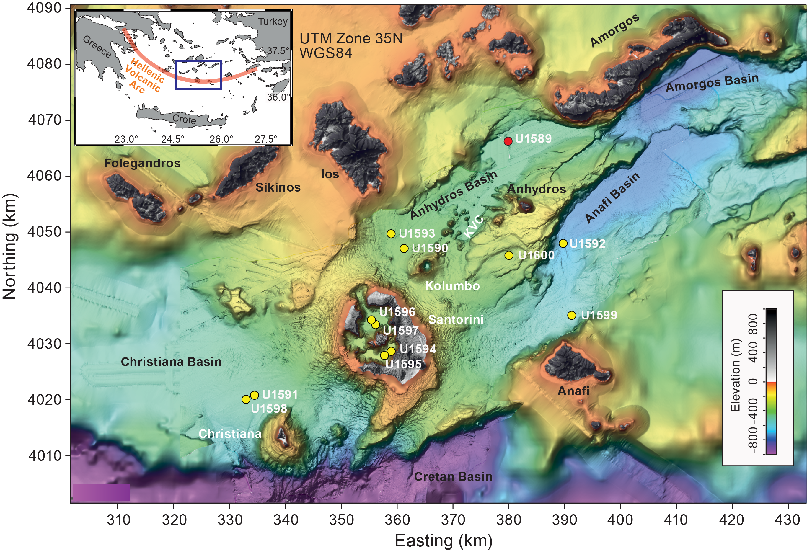
Figure F1. Site map.
Site U1589 was chosen to sample the eruptive histories of both Santorini and the Kolumbo chain and was expected to yield volcaniclastics from many Kolumbo eruptions and the major Santorini eruptions. Many deposits from smaller Santorini eruptions were not expected at this distance from the volcano, in part due to flow blocking by the Kolumbo volcanic chain. Santorini has been active since 0.65 Ma, with many large explosive eruptions since about 0.36 Ma (Druitt et al., 2016). Kolumbo Volcano was known from seismic profiles to have had at least five eruptions (Hübscher et al., 2015), the last of which was in 1650 Common Era (CE) and killed 70 people on Santorini (Fuller et al., 2018). Seismic profiles provided constraints on the relative ages of the Kolumbo cones (Preine et al., 2022c) but not on the absolute ages. The site offered a near-continuous time series of volcanism in the area since rift inception.
The site was also chosen to develop a core-log-seismic integration stratigraphy and compare it with the recently published seismic stratigraphy for the basin (Preine et al., 2022a) and the paleotectonic reconstruction of the region (Nomikou et al., 2016, 2018) to promote a holistic view of the Anhydros Basin evolution (Figure F2). The site transects all six seismic packages of the Anhydros rift basin, as well as the onlap surfaces between them (Nomikou et al., 2016, 2018; Preine et al., 2022a). The anticipated lithologies were undisturbed hemipelagic muds, volcaniclastics, turbidites, and finally continental basement rocks. A gravity core recovered 7 km to the east indicated that the uppermost sediments on site would consist of hemipelagic muds and volcaniclastic layers, as well as sapropels (Kutterolf et al., 2021).
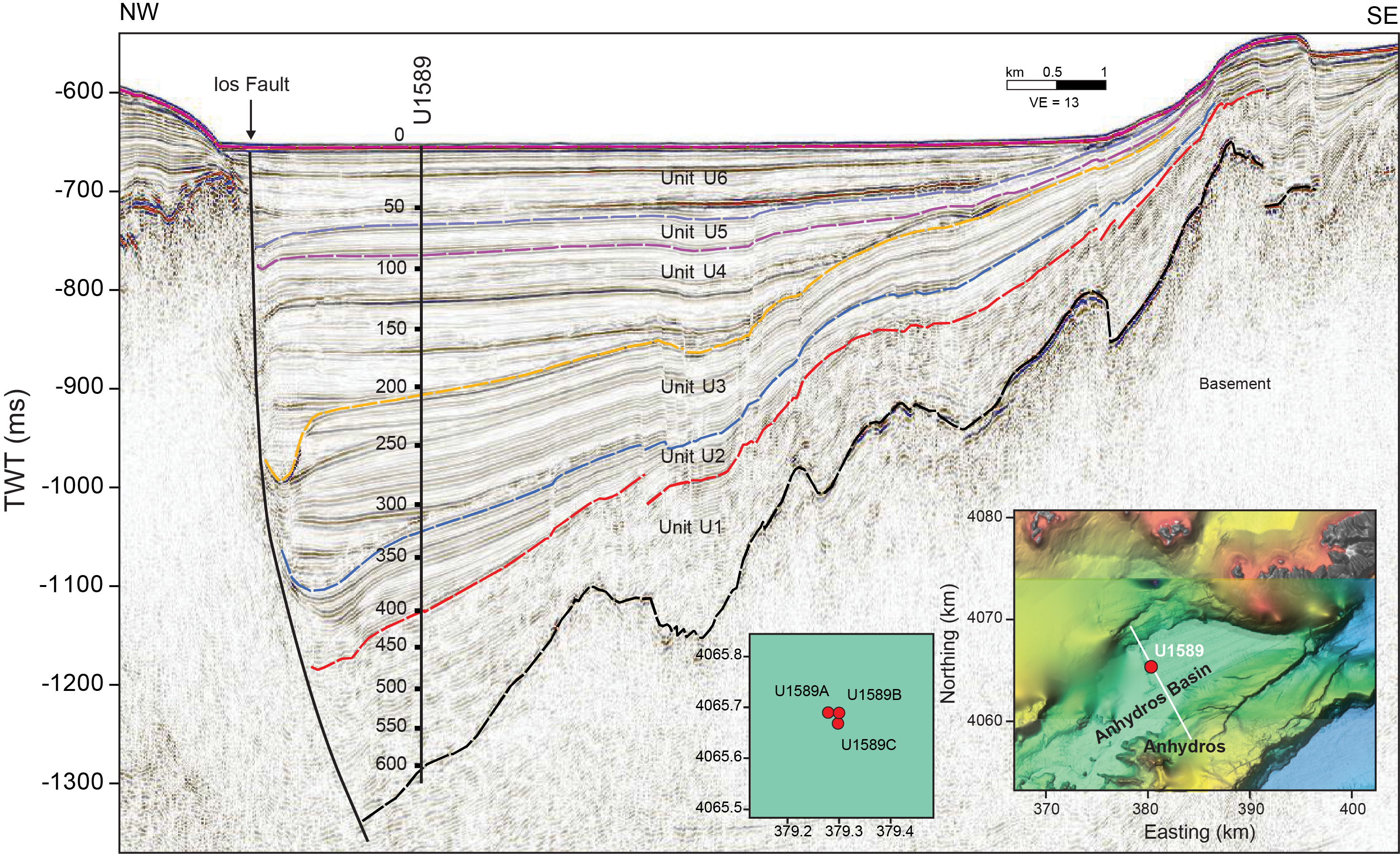
Figure F2. Seismic profile.
The Anhydros Basin is crossed by many seismic profiles obtained in campaigns between 2006 and 2019, many of them multichannel (Hübscher et al., 2015; Nomikou et al., 2016, 2018), and its southwestern part is included within the area of the 2015 PROTEUS seismic tomography experiment, during which subbottom profiling, gravity, and magnetic data were also recorded (Hooft et al., 2017). The basin bathymetry had been studied in several marine campaigns, and fault distributions and throws had been mapped (Nomikou et al., 2016; Hooft et al., 2017). Previously published analyses of the seismic data suggested the following possible interpretations (from the bottom up; Preine et al., 2022b, 2022c):
- Units U1 and U2: sediment packages predating Santorini and Kolumbo volcanism;
- Unit U3: sediments and the products of the early Kolumbo volcanism and some of the Kolumbo cones;
- Unit U4: sediments associated with a major rift pulse; and
- Units U5 and U6: sediments and the products of Santorini activity, some of the Kolumbo cones, and the later eruptions of Kolumbo including the 1650 CE eruption.
Units U3–U6 were believed to be of Pleistocene age, and Units U1 and U2 were believed to be of possible Pliocene age.
The site enabled us to test these interpretations by using the cores to reconstruct a near-complete volcanic stratigraphy consistent with both onshore and offshore constraints and pinned by chronological markers from biostratigraphy, magnetostratigraphy, and sapropel records. Benthic foraminifera from fine-grained sediments provided estimates of paleowater depths and, via integration with seismic profiles and chronologic data, of time-integrated basin subsidence rates.
Coring at Site U1589 in the Anhydros Basin addressed scientific Objectives 1–4 and 6 of the Expedition 398 Scientific Prospectus (Druitt et al., 2022). It was complemented by Site U1592 in the Anafi Basin because each basin taps a different sediment distributary branch of the Christiana-Santorini-Kolumbo volcanic system.
2. Operations
We started our 1241 nmi voyage across the Mediterranean to Aegean Sea Site U1589 at 1254 h local time (all times local; 2 h ahead of UTC) on 16 December 2022 in Tarragona, Spain. Throughout the transit, all groups familiarized themselves with their respective laboratories and worked on writing their methods sections. The COVID mitigation protocol was followed until 19 December when it ended at 1810 h after no one tested positive for nine consecutive days. We completed the transit on 21 December at 0715 h at an average speed of 10.9 kt.
2.1. Hole U1589A
The bottom-hole assembly (BHA) and drill string were assembled and lowered at Site U1589. A pig was pumped down to remove rust and minor irregularities inside the pipes. The nonmagnetic sinker bar assembly was picked up, the Icefield MI-5 core orientation tool was loaded, and the sinker bars were installed. Using the APC system, Hole U1589A was spudded at 1435 h with Core 1H recovering 2.2 m (Table T1) and a good mudline, establishing the seafloor depth at 495.3 meters below rig floor (mbrf) or 484.3 mbsf. The advanced piston corer temperature (APCT-3) tool was run on Cores 4H, 7H, 10H, and 13H (see Physical properties). APC coring continued into 22 December 2022, when 45,000 lb of overpull was observed following Core 15H at 125.7 mbsf. The core was drilled over and retrieved at 0500 h. Subsequently, coring was switched to the half-length advanced piston corer (HLAPC) system with Core 16F. HLAPC coring continued through Core 65F at 360.8 mbsf at 1130 h on 23 December. After firing, the core became stuck with an overpull of 40,000–50,000 lb. It took drillover of ~4 m to free the barrel. In the following, coring was switched to the XCB with Core 66X. Coring continued into 24 December with the final XCB core, 76X, retrieved. Hole U1589A cored an interval of 446.7 m, recovering 350.55 m of volcaniclastic and hemipelagic to pelagic sediments.
2.2. Hole U1589B
After clearing Hole U1589A, the vessel moved 20 m east. Hole U1589B was spudded at 482.6 mbsl with Core 1H at 0950 h on 24 December 2022. Coring continued through Core 12H. Cores 5H and 11H were shot from a higher position to account for a stratigraphic gap in this interval of Hole U1589A. The APCT-3 tool was run with Cores 398-U1589B-5H, 6H, and 11H. As the lithology became more compacted again, operations were switched to the HLAPC system for Cores 13F–70F. In total, Hole U1589B recovered 331.46 m of volcaniclastic sediments and reached a maximum depth of 359.58 mbsf. At the base of Core 70F, the Sediment Temperature 2 (SET2) tool was deployed to analyze the formation temperature at the bottom of Hole U1589B. After completion, the drill string was tripped back up to the vessel.
2.3. Hole U1589C
The ship offset 20 m south, and the BHA for RCB coring was assembled and tripped back down to the mudline, spudding Hole U1589C at 482.6 mbsl at 2304 h on 26 December 2022. The uppermost 360 m of Hole U1589C was drilled without recovery and continued to a depth 20 m above the base of Hole U1589B with recovery from Cores 2R–28R. In Core 25R, we began to recover pebbles of limestone. Coring continued through Core 28R, with all cores containing limestone pebbles. Thus, the basement depth was determined to be recovered in Core 25R (recovery = 48%) and tentatively set at 589 mbsf. Following Core 28R, coring in Hole U1589C was ended. In total, Hole U1589C recovered 62.08 m of sediments, volcaniclastic rocks, and limestone basement, reaching a total depth of 621.9 mbsf. The drill string was tripped up to 66.5 mbsf.
2.4. Downhole logging
Hole U1589C was prepared for downhole logging, and the triple combo tool string was equipped with natural gamma radiation (NGR; Hostile Environment Natural Gamma Ray Sonde [HNGS]), litho-density (Hostile Environment Litho-Density Sonde [HLDS]), electrical resistivity (High-Resolution Laterolog Array [HRLA]), and magnetic susceptibility (MS; Magnetic Susceptibility Sonde [MSS]) sensors.
The tool string was assembled, and logging began at 1340 h on 29 December 2022. During logging Run 1, the tools encountered an obstruction at 544.9 mbsf that could not be passed. After the tool string made up-log and down-log passes again, it became stuck at 227.7 mbsf. The remainder of the operations time was spent retrieving the logging tools.
The tool was lowered, the calipers were closed, and the winch was worked, but the tool became stuck again. In working the pipe up and down, it was discovered the drill string was stuck. The hole was circulated and 45,000 lb overpull was applied to work it free. The drill pipe was worked and circulated while we rigged up the wireline retrieval tools. On 30 December, the drill string was broken out and a T-bar was installed on the logging line. Ultimately, 19 single pipes were picked up, washing down to just above the triple combo tool string. The BHA was washed over the logging tool for ~4 m until 10,000 lb was observed on the weight indicator. Simultaneously, there was a tension loss on the core winch line. The Assistant Driller pulled up with the coring line, and the logging tools appeared to come free. The tools were picked up and slacked down to verify. The drill string was pulled up to 224.7 mbsf, with the coring winch in unison.
Starting the trip out of the hole, the drill string was found to be stuck. Applying 50,000 lb overpull and 1100 A managed to free it. Because of the tight hole conditions, singles were pulled with the top drive from 224.7 mbsf. There were again tight hole conditions at 195.9 and 186.3 mbsf. Once more, at 115.5 mbsf the BHA became stuck. Parameters were increased to 110,000 lb overpull without success. A sepiolite mud sweep and heavy barite mud were pumped in short succession, both at 118.0 mbsf. The pipe remained stuck. The decision was made to sever the string during the late evening on 30 December, and the preparations to sever continued into the next day. On 31 December at 0930 h, the line was successfully severed. At 1800 h, the rig floor was secured for transit. The thrusters were lifted. The vessel was out of dynamic positioning mode and under bridge control at 1805 h. All thrusters were up and secured, and passage to Site U1590 started at 1818 h.
3. Lithostratigraphy/sedimentology
Cores from three consecutively cored holes at Site U1589 (U1589A–U1589C) recovered a coherent stratigraphy from 0 to 612.4 mbsf (Figure F3). Hole U1589A consists of Cores 1H–76X (0–446.1 mbsf), Hole U1589B contains Cores 1H–70F (0–360 mbsf), and Hole U1589C encompasses Cores 2R–28R (372.3–612.4 mbsf).
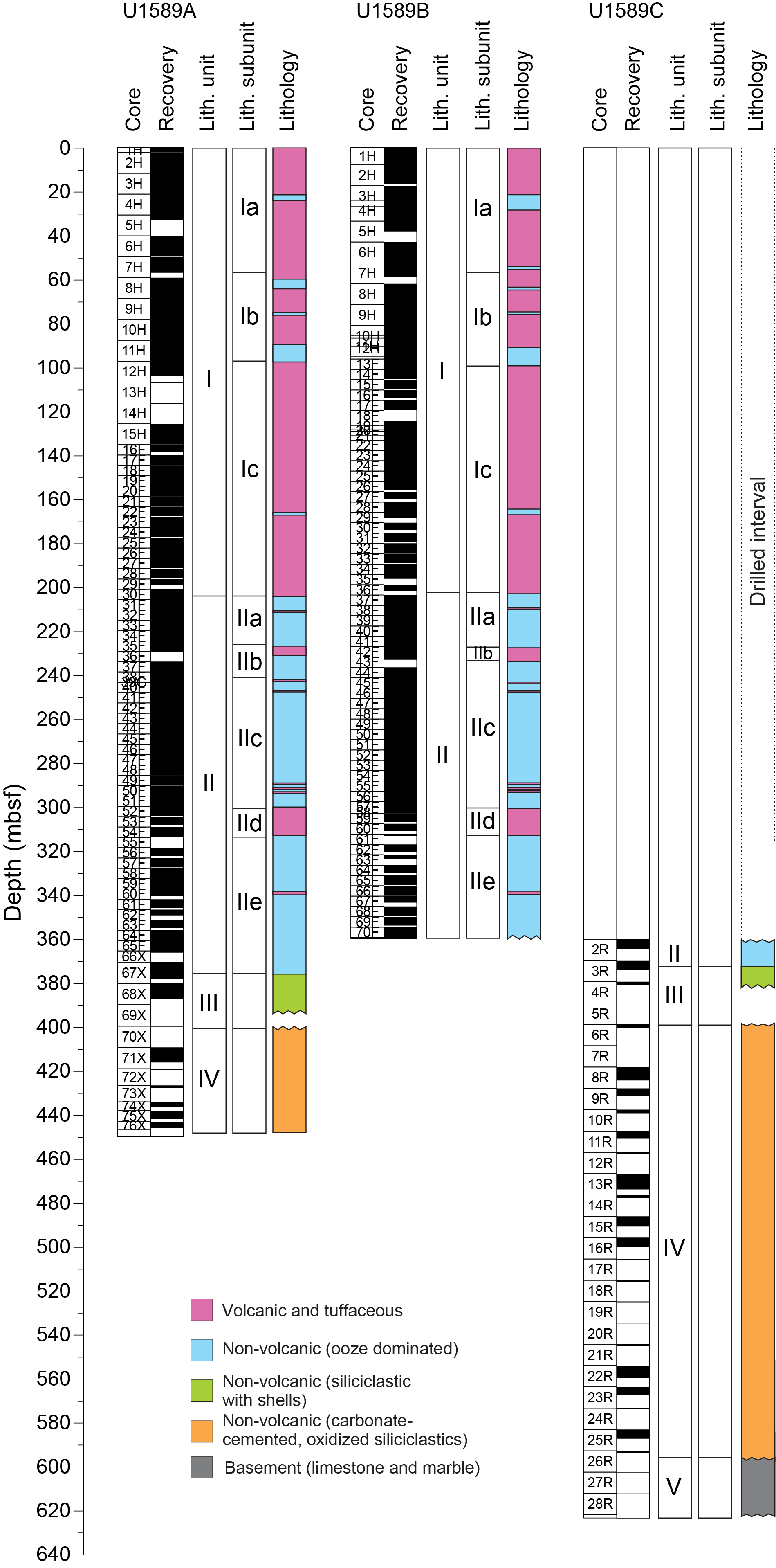
Figure F3. Lithostratigraphy.
There is very good overlap between Holes U1589A and U1589B. Hole U1589C begins near the bottom of Holes U1589A and U1589B, and overlap is minimal, with penetration to basement. The majority of the recovered materials are sedimentary, dominated by ash, lapilli, lapilli-ash, and tuffaceous mud in the uppermost 200 m (Unit I), oozes and muds from 200 to ~370 mbsf (Unit II), shell-bearing siliciclastic units from ~370 to ~390 mbsf (Unit III), oxidized and carbonated sands and conglomerates/breccias below 400 mbsf (Unit IV), and limestone basement below 590 mbsf (Unit V).
The first four lithostratigraphic units (I–IV) are distinguished from each other based on the presence or absence of volcanic material, calcareous nannofossils, and shell fragments and the level of red-hued oxidation and matrix carbonation. Smear slides for microscopic analysis were prepared often to confirm macroscopic observation of distinct lithology changes at the section level, such as identification of vitric ash particles in tuffaceous lithologies. The upper and lower boundaries of each lithostratigraphic unit are defined by lithologic changes that are usually accompanied by a change in physical properties (e.g., MS). The fifth lithostratigraphic unit is a limestone unit that is the basement rock on which the above-lying sediments were deposited.
Subunits in Units I and II are defined by the relative proportion of volcanic lithologies (i.e., lapilli, lapilli-ash, ash, and tuffaceous sediment) in each unit. Although volcanic lithologies are dominant in Unit I (Subunits Ia and Ic), there is a short break in which nontuffaceous muds and oozes become relatively more abundant (Subunit Ib) (Figure F4). Conversely, Unit II is dominated by nontuffaceous muds and oozes; thus, subunits are distinguished by intervals with a relatively high proportion of volcanic lithologies.
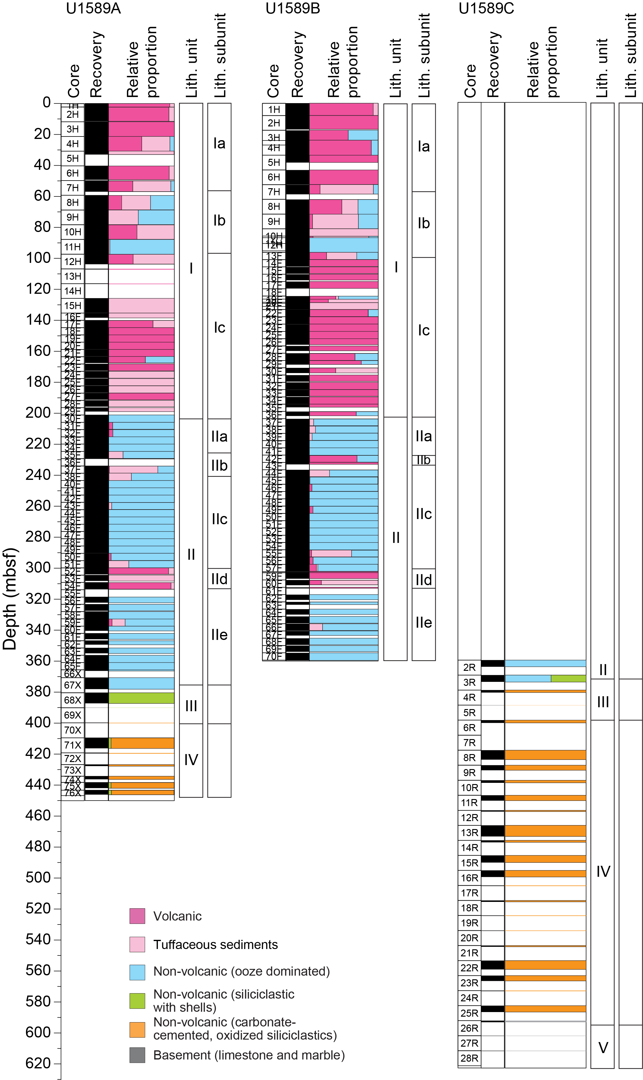
Figure F4. Volcanic, tuffaceous, and nonvolcanic lithologies.
Figure F3 summarizes the complete lithostratigraphy of Site U1589. Table T2 provides the upper and lower boundaries of each lithostratigraphic unit, stratigraphic ages, and a summary of lithologies in each unit. Figure F4 graphically presents the relative proportions of volcanic, tuffaceous, and nonvolcanic lithologies in Hole U1589A. Figure F5 shows the grain size distribution of lithologies in Units I–III in more detail. Figure F6 displays representative images of volcanic and nonvolcanic lithologies in Holes U1589A–U1589C.
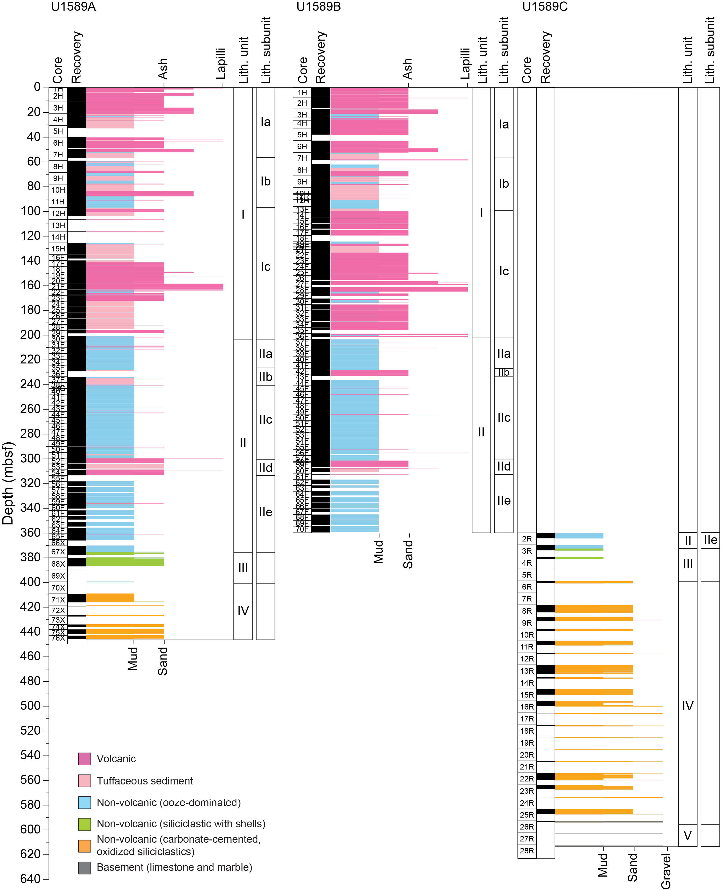
Figure F5. Average grain size distribution.
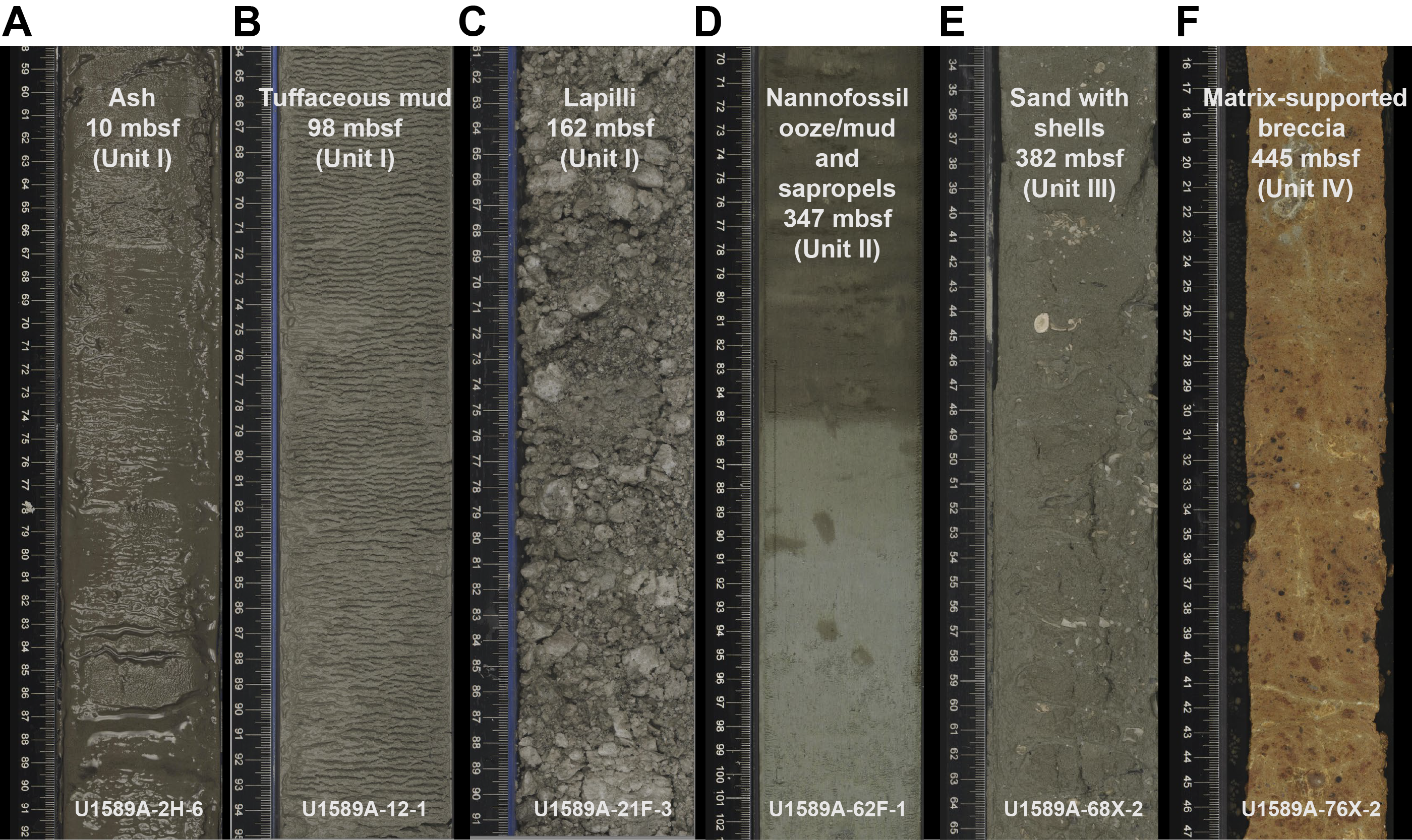
Figure F6. Representative lithologies.
The following sections describe (1) the effects of core disturbance; (2) the five lithostratigraphic units and subunits; (3) correlations between Holes U1589A, U1589B, and U1589C; and (4) X-ray diffraction (XRD) analysis.
3.1. Core disturbance
Several types of core disturbance disrupt the lithostratigraphy at Site U1589 (Figure F7):
- Biscuiting of recovered cores produces fractured disc-shaped pieces ranging in size from a few to more than 10 cm thick, often packed with sheared and remolded core material mixed with drill slurry, filling gaps between brittle biscuits (Figure F7A, F7B). The degree of biscuiting ranges from slight to severe, depending on the size of the biscuits and the proportion of biscuits to infill material.
- Brecciated core disturbance results from core extension that disturbs the core until it becomes sheared or, in the case of brittle failure, brecciated (Figure F7C). Slight brecciation produces cracks in the original lithologies (Figure F7D), whereas moderate to severe brecciation disturbs original lithofacies and sedimentary structures more severely, although they usually remain readily recognizable. In contrast, the contacts between intervals and stratifications in granular layers may be lost due to brecciation.
- Fall-in occurs at the top of cores, where it is recognized by coarse clast-supported intervals at the tops of many cores (Figure F7E). We exclude these intervals from lithostratigraphy interpretations.
- Soupy core disturbance is typically restricted to water-saturated intervals of unconsolidated ash, overprinting original sedimentary or depositional structures (Figure F7F).
- Sediment flowage is produced by high shearing rates between cored sediments and the core liner. This process typically leaves a smear or thin trail of displaced sediment along the outside rim of the core (Figure F7G).
- Mixed sediment core disturbance occurs in water-saturated, granular core sections where grains and clasts flow and mix, producing moderately to severely disturbed original sedimentary structures and stratigraphy (Figure F7H).
- Uparching results from slight to moderate coring-induced shear between the sediment and core liner and is recognized as bedding uniformly dragged downward along the core margins (Figure F7I). In these intervals, original lithofacies and sedimentary structures are usually slightly to severely disturbed but can still be recognized visually.
- Core voids up to ~25 cm in the original lithologies were observed in a few instances (Figure F7J), for example in cores that experienced basal flow-in (Jutzeler et al., 2014), core extension, or low recovery. Original lithofacies and sedimentary structures are fully destroyed in these intervals.
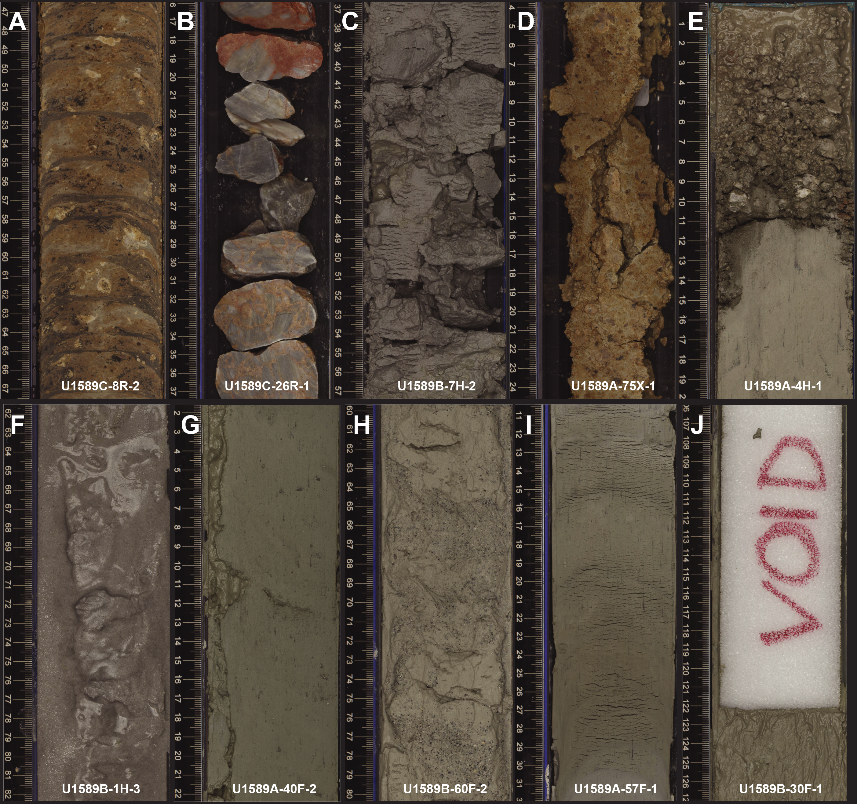
Figure F7. Core disturbances.
3.2. Description of units
Cores recovered from Holes U1589A–U1589C are divided into four volcano-sedimentary lithostratigraphic units and one basement unit (Figure F3; Table T2). The volcano-sedimentary units comprise the 589 m cover sequence above the limestone basement.
3.2.1. Unit I
- Intervals: 398-U1589A-1H-1, 0 cm, to 29F-CC, 13 cm; 398-U1589B-1H-1, 0 cm, to 36F-CC, 15 cm
- Thicknesses: Hole U1589A = 198.9 m; Hole U1589B = 201.8 m
- Depths: Hole U1589A = 0–198.9 mbsf; Hole U1589B = 0–201.8 mbsf
- Age: Holocene to Middle Pleistocene
- Lithology: volcanic (ash, lapilli, lapilli-ash, and tuffaceous mud) and lesser ash-poor or organic-rich oozes and muds
Unit I extends from 0 to ~200 mbsf (Table T2) and primarily consists of tuffaceous mud intercalated with intervals of ash, lapilli-ash, and lapilli punctuated by less abundant nontuffaceous mud and ooze intervals (Figures F4, F5). Thicknesses of the volcanic intervals in Unit I vary from thin ash layers in nonvolcanic lithologies (e.g., ash layer; interval 398-U1589A-19F-2, 43–44 cm; 126.32 mbsf) to distinct volcanic intervals that span across several cores (e.g., ash and lapilli interval; interval 398-U1589B-4H-2, 0 cm, to 7H-1, 24 cm; 25.5–52.74 mbsf). These intervals commonly have sharp bottom contacts with tuffaceous or biogenic lithologies. The relative proportions of volcanic, tuffaceous, and nonvolcanic lithologies for Hole U1589A are presented in Figure F4.
Lithologies consisting of >75% volcanic particles (e.g., glass shards, pumice, and crystals) comprise ash, lapilli-ash, and lapilli. Description of ash, lapilli-ash, and lapilli in volcanic intervals was based on the relative abundance of ash-sized (<2 mm) and lapilli-sized (2–64 mm) particles, as described in Lithostratigraphy in the Expedition 398 methods chapter (Kutterolf et al., 2024), with ash and lapilli used when the proportion of one size was >75%, and lapilli-ash used when both sizes were present but in <75% abundance (Fisher and Schmincke, 1984). Macroscopically, ash layers are typically white to dark gray, well sorted, ranging from fine ash to coarse ash, and variably admixed with mud at the top. Ash layers are typically nongraded or normally graded and are frequently characterized by a sharp, commonly crystal-rich base and a more diffuse and often bioturbated upper boundary that grades into tuffaceous mud. Microscopically, ash layers are characterized by colorless angular glass shards with or without crystals (Figure F8). Some ash layers have distinct crystal/lithic-rich lags at their bases. Microscopic observations of smear slides were useful for identification of specific minerals (e.g., biotite, feldspar, and pyroxene) in ash. The coarser volcanic intervals in Unit I are dominantly monomictic lapilli and lapilli-ash containing white to gray pumice lapilli with varying proportions of ash matrix (Figure F6). Less common are lithic-rich lapilli-ash layers. Where recovered, the bottom contacts of these coarser intervals are sharp or bioturbated but commonly affected by uparching drilling disturbance.
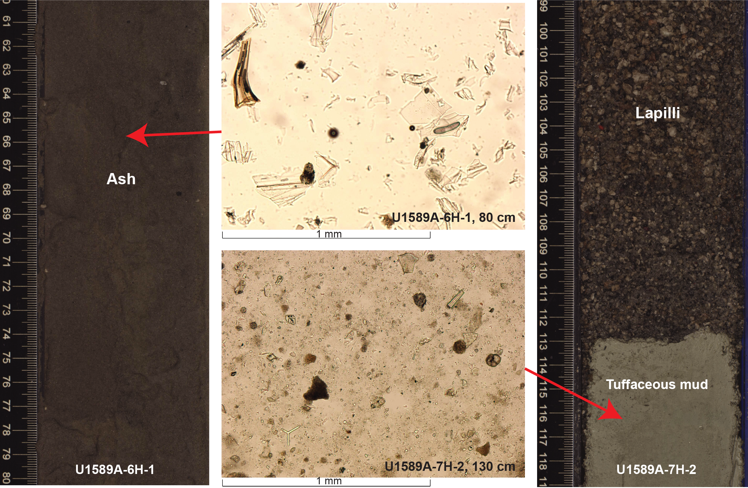
Figure F8. Volcanic lithologies, Unit I.
Lithologies consisting of 25%–75% volcanic particles are characterized as tuffaceous muds or oozes. Tuffaceous mud (and silt or clay) is white to dark gray-brown and contains abundant fine, colorless glass shards and rare crystals. Isolated pumice lapilli dropstones occur in some intervals but are uncommon. These tuffaceous muds and oozes commonly contain sedimentary lithics, clay minerals, authigenic calcite, and micro-/nannofossils in addition to their volcanic components.
Lithologies consisting of <25% volcanic materials in Unit I include calcareous mud, nannofossil-rich clays/muds, ooze, and organic-rich (sapropelic) oozes, often with foraminifera and disseminated sulfides. These intervals of ooze and calcareous muds are generally several meters thick and are commonly punctuated by volcanic intervals (e.g., ooze with small ash; interval 398-U1589B-12H-2A, 106–108 cm; 88.2–89.7 mbsf). These nonvolcanic muds and oozes appear to cluster between ~70 and 100 mbsf in Holes U1589A and U1589B and were significant enough to merit a subunit designation (Ia–Ic) (Figures F4, F5).
3.2.1.1. Subunit Ia
Subunit Ia (0–57.5 mbsf) is dominated by volcanic-rich lithologies with only sparse breaks of fine-grained ash-free muds or oozes (Figures F4, F5). The uppermost 20 m in Holes U1589A and U1589B consist of interbedded ash, lapilli-ash, and tuffaceous mud separated from the next deeper set of the same lithologies by less than 5 m of ash-poor mud. Ash intervals typically grade upward into tuffaceous mud. One distinctive polymictic, lithic-rich lapilli-ash and ash interval occurs at ~47–52 mbsf in both holes. This pattern of interbedding continues through the end of a large ash and lapilli interval ending at 57.0 mbsf in Hole U1589A (Section 7H-CC, 28 cm) and 58.6 mbsf in Hole U1589B (Section 7H-5, 132 cm). This latter interval was poorly recovered at its lapilli-rich base. This subunit is generally characterized by high MS, with the highest peak at the bottom of Subunit Ia, probably caused by the lapilli-rich base interval (see Physical properties; Figure F46).
3.2.1.2. Subunit Ib
Subunit Ib (60–99 mbsf) is defined by thicker and more extensive intervals of nontuffaceous calcareous muds and oozes. In addition to lithology, this subunit is marked by distinct pore water geochemical characteristics (see Geochemistry), including a sharp increase in alkalinity and potassium and a decrease in calcium, magnesium, and sulfate (see Geochemistry; Figures F54, F55). MS is generally high in this subunit but decreases with depth, whereas NGR slightly increases (see Physical properties; Figure F46). This subunit begins with nannofossil-rich mud in Core 8H of Holes U1589A and U1589B at ~59 mbsf (Sections 398-U1589A-8H-1, 0 cm, and 398-U1589B-8H-1, 0 cm). This mud is interbedded with ashes and tuffaceous muds for the next 19 m until a very thick, 12 m interval of tuffaceous mud and ash (± lapilli) is encountered at ~78 mbsf, leading to a strong peak in MS (see Physical properties; Figure F46). Below this is another thick interval of ooze that ends at 98.4 mbsf in Hole U1589A and 99.8 mbsf in Hole U1589B (Sections 398-U1589A-12H-1, 119 cm, and 398-U1589B-13H-3, 61 cm).
3.2.1.3. Subunit Ic
Subunit Ic (99–200 mbsf) begins with the first appearance of a thick ash layer beneath an ooze described in Subunit Ib. This subunit is lithologically similar to Subunit Ia. The lithologic change from Subunit Ib to Ic is accompanied by a change in pore water geochemical characteristics to lower potassium and alkalinity and higher calcium, magnesium, and sulfate values that characterize Subunit Ia (see Geochemistry; Figures F54, F55). In this subunit, MS profiles of some tuffaceous mud intervals show a clearly decreasing trend from an ash-rich base to an ash-poor top, indicating progressive dilution of settling of dispersed ash by background mud sedimentation (e.g., see MS profile for the tuffaceous interval from ~129 to 135 mbsf in Cores 398-U1589A-15H and 398-U1589B-21F). A distinctive polymictic, lithic-rich lapilli/lapilli-ash marks the base of Unit I in Cores 398-U1589A-21F and 398-U1589B-27F (~197–202 mbsf).
3.2.2. Unit II
- Intervals: 398-U1589A-30F-1, 0 cm, to 67X-4, 40 cm; 398-U1589B-37F-1, 0 cm, to the bottom of the hole; 398-U1589C-2R-1, 0 cm, to 3R-2, 115 cm
- Thicknesses: Hole U1589A = 172.6 m; Hole U1589B = 155.9 m; Hole U1589C = 12.3 m
- Depth: 201–375.1 mbsf
- Age: Middle Pleistocene to Early Pleistocene
- Lithology: calcareous and nannofossil oozes and muds with intermittent volcanic layers (ash, lapilli, and tuffaceous sediments) and sapropels
Unit II is distinct from Unit I in that it primarily consists of oozes (>50% nannofossils) and nonvolcanic muds interspersed with intermittent volcanic intervals and distinctly colored organic-rich (sapropelic) oozes (Figures F3, F4, F5, F6). The unit was observed entirely in Hole U1589A and partially in Holes U1589B (lower contact not reached) and U1589C (uppermost section not recovered). In addition to lithology, the beginning of Unit II is marked by significant changes in physical properties and geochemistry such as higher shear strengths and grain densities (see Physical properties; Figures F48, F50) and higher methane and total organic carbon (TOC) but lower lithium (see Geochemistry; Figures F56, F57, F58).
A distinctive shift in sediment color marks this boundary with the oozes; oozes range from dark gray, olive-gray, and greenish gray to white. Muds are generally darker and range from very dark gray, dark greenish gray, and dark olive-gray to greenish gray and several pale yellow layers. The volcanic intervals are also mostly dark and range from gray and greenish gray to black; however, a package of white and light gray ash layers is present in interval 398-U1589A-51F-4, 56 cm, to 54F CC, 8 cm (300–313.4 mbsf). Organic-rich (sapropelic) intervals are very distinct; they have a restricted color range and are typically dark gray to dark grayish brown or greenish brown.
Oozes and organic-rich (sapropelic) oozes are the most cohesive lithologies, followed by muds and tuffaceous sediments. The ash- and lapilli-dominated layers are the least cohesive.
Sharp boundaries are observed between oozes and muds and overlying volcanic intervals, whereas the uppermost portions of the volcanic intervals grade into the overlying sediment. Boundaries with organic-rich intervals are generally diffuse and grade into the overlying and underlying sediment.
The grain size of the oozes, muds, and tuffaceous sediments ranges from clay to silt (<0.004–0.63 mm) and are referred to as muds. The ash layers have a grain size range of fine to coarse ash (<0.63 mm and 0.63–2 mm, respectively), and the lapilli-ash and lapilli layers range in grain size from fine to medium lapilli (2–16 mm).
Oozes and muds contain abundant nannofossils and clay minerals (Figure F9, bottom center). Sedimentary lithics and other biogenic material (foraminifera, diatoms, radiolarians, and sponge spicules) are common. Shell fragments (>2 mm) are present in the bottom ~20 m of Unit II. Discrete ash pods, centimeters thick, occur throughout the oozes and muds.
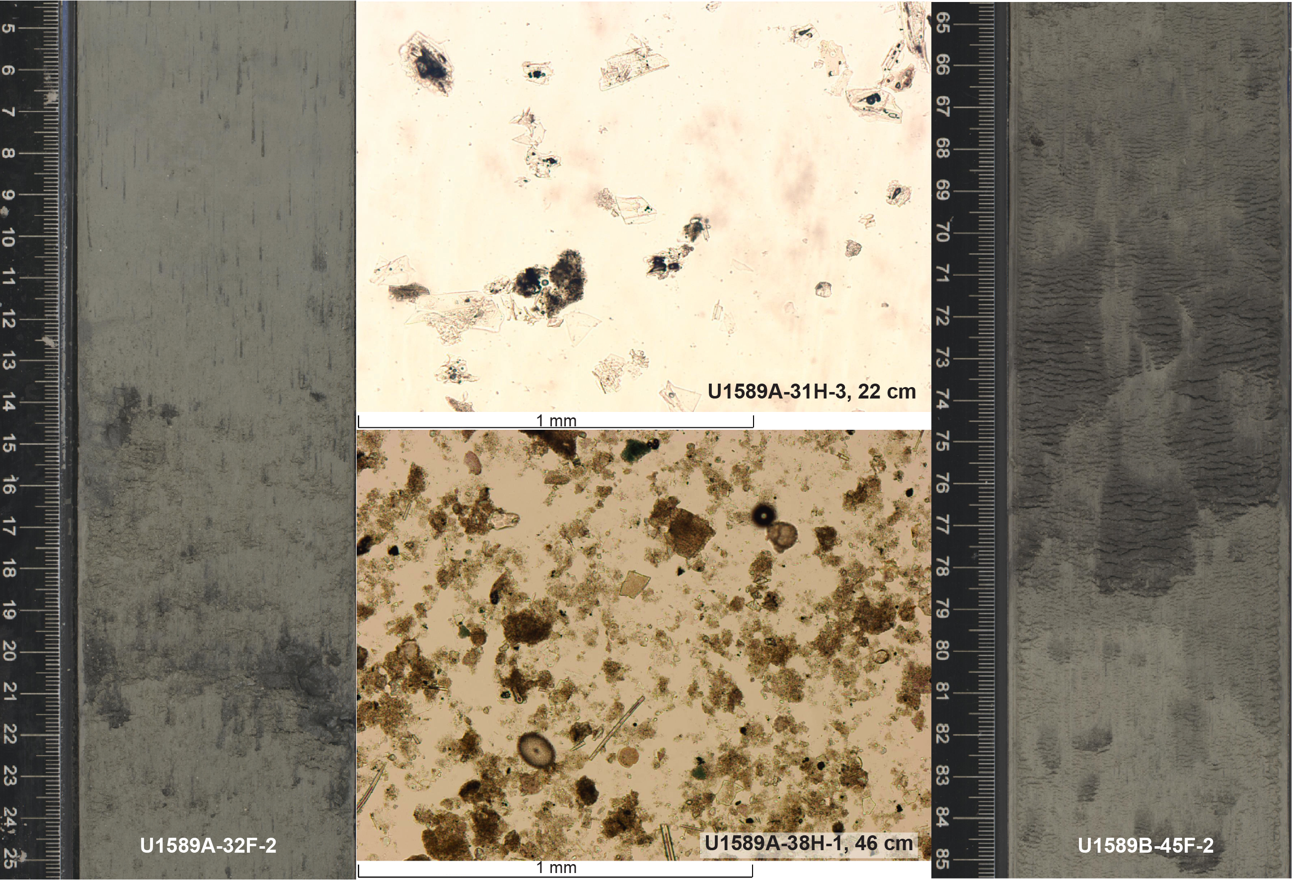
Figure F9. Nannofossil ooze, Unit II.
Bioturbation occurs throughout Unit II regardless of lithology, although in general it is observed less in the volcanic layers. In the uppermost part of the unit (~50 m), the bioturbation intensity is overall slight with few intervals of moderate disturbance. Bioturbation intensity increases in the following ~35 m (moderate to high) and decreases to slight to moderate with few discrete intervals of high intensity for the remainder of the unit. Exceptions where no bioturbation is observed are within thick volcanic intervals.
Volcanic intervals in Unit II are intermittent and range in thickness from a centimeter to several tens of centimeters. They consist of ash layers, ash with lapilli, lapilli, and tuffaceous sediments (volcanic particle abundances from 25% to 75%). Glass shards within volcanic layers are dominantly transparent, nonvesicular to vesicular and blocky, cuspate, or pumiceous in shape (Figure F9, top center). A thick tuffaceous mud interval and a thick ash interval are distinct enough to warrant subunit designation, as described below.
Smear slides taken throughout Unit II show trace to rare mineral components of feldspar, pyroxene, quartz, glauconite, and opaques.
In Unit II, five subunits were identified and distinguished based on (1) the major lithology present in the interval, (2) physical properties (i.e., MS; see Physical properties), and (3) geochemistry of pore fluids (see Geochemistry). Subunits consist of ooze- and mud-dominated layers (Subunits IIa, IIc, and IId, with intermittent thin volcanic or tuffaceous layers in Subunits IIb and IIc) (Figures F4, F5). The physical properties of Unit II, in particular MS, differ from those of Unit I, and peaks often correspond to described volcanic-rich intervals (see Physical properties; Figure F46). Interestingly, volcanic-rich Subunit IIb is clearly distinguishable based on its MS, which displays peaks between ~228 and 240 mbsf (Subunit IIb); however, there are no similar peaks in volcanic-rich Subunit IId between ~300 and 313 mbsf (see Physical properties; Figure F46).
3.2.2.1. Subunit IIa
Subunit IIa (~200–228 mbsf) consists primarily of muds, calcareous muds, and oozes interbedded with intermittent volcanic layers. Five thin (millimeter to several centimeters in thickness) ash layers separated by muds are present in the uppermost 8 m. Two consecutive ash layers with lapilli are present at 209 mbsf and extend vertically for ~20 cm. Two thicker ash layers (20 and 9 cm) separated by ooze with ash pods are present at 201 and 212 mbsf. The lowermost 16 m of this subunit contains several intervals of ooze with ash pods. At ~220 mbsf, an organic-rich (sapropelic) ooze was observed. Because this layer extends over two core sections (398-U1589A-35F-4 and 35F-CC), it is likely one continuous lithology.
3.2.2.2. Subunit IIb
Tuffaceous ooze is the dominant lithology in Subunit IIb (~228–240 mbsf), which is clearly shown by higher MS and a concomitant drop in gamma ray attenuation (GRA) bulk density (see Physical properties; Figure F49). Two thin ash units (3 and 1.5 cm) are separated by a 19.5 cm tuffaceous ooze. One ash layer (3 cm) is crystal rich (235 mbsf). One 7 cm thick potential sapropel was observed at ~235 mbsf.
3.2.2.3. Subunit IIc
Subunit IIC (~240–300 mbsf) is characterized by intermittent ash layers and organic-rich (sapropelic) oozes throughout calcareous muds and oozes. The lowermost 10 m contains several tuffaceous oozes. The ash layers are all thin, only several centimeters thick, whereas the majority of the potential sapropels are tens of centimeters thick. Ash layers are dispersed throughout the subunit, but organic-rich (sapropelic) layers are only observed from 266 mbsf downward.
3.2.2.4. Subunit IId
Subunit IId (~300–313 mbsf) is the thinnest subunit in Unit II, and it contains an interval of tuffaceous sand capped by lapilli and ash layers. This subunit is distinguished by sharp changes in pore water geochemistry, including sharp increases in salinity, bromide, chlorite, sodium, calcium, magnesium, potassium, and sulfate and decreases in alkalinity (see Geochemistry; Figures F54, F55, F56). Interestingly, there is no concomitant change in MS (see Physical properties; Figure F48). In comparison to the other subunits in Unit II, the majority of the ash layers in this subunit are several tens of centimeters thick. The tuffaceous sand is a continuous layer, although it extends across several core sections and is ~4 m thick.
3.2.2.5. Subunit IIe
Oozes and muds are the dominant lithologies in the uppermost ~27 m of Subunit IIe (~318–375 mbsf). The remainder of the subunit comprises these lithologies alternating with organic-rich (sapropelic) intervals. Only two volcanic layers exist in the upper part of this subunit. A lithic ash (7 cm thick) with minor amounts of clay is present at 336 mbsf, followed by a 51 cm thick tuffaceous ooze.
3.2.3. Unit III
- Intervals: 398-U1589A-67X-3, 0 cm, to 68X-CC, 13 cm; 398-U1589C-3R-2, 115 cm, to 4R-1, 1 cm
- Thicknesses: Hole U1589A = 13.6 m; Hole U1589C = 8.6 m
- Depths: Hole U1589A = 373.6–387.2 mbsf; Hole U1589C = 372.3–380.9 mbsf
- Age: Early Pleistocene
- Lithology: sandy silt and calcareous mud with shells
Unit III is distinguished from Unit II by a gradual increase in both grain size and shell content. It consists primarily of sand with ash and shells (Figure F10) interspersed with calcareous mud and organic-rich (sapropelic) ooze. The unit was largely observed in Hole U1589A and only partially in Hole U1589C. A gradual change in the color of the sediments from pale yellow in the overlying calcareous muds to olive-gray in sandy silts to light olive-gray to greenish gray in sand with shells marks the transition between the units. Within the unit, irregular sharp to gradational boundaries are observed between sands, sandy silts, and mud layers. The sands contain abundant shells and shell fragments, are poorly to moderately well sorted, and contain evidence of moderate to high bioturbation. Sand intervals commonly show normal grading, whereas shell fragments within sections generally coarsen upward. Volcanic and tuffaceous lithologies in Unit III are confined to Section 398-U1589A-68X-1 and are a minor constituent of the sands between 380.3 and 381.8 mbsf. The bottom contact of Unit III with Unit IV was not recovered.
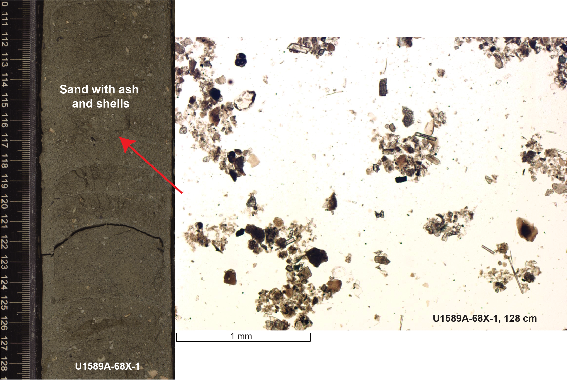
Figure F10. Typical interval, Unit III.
3.2.4. Unit IV
- Intervals: 398-U1589A-70X-CC, 0 cm, to 76X-CC (bottom of the hole); 398-U1589C-6R-1, 3 cm, to 25R-CC, 148 cm
- Thicknesses: Hole U1589A = >46.45 m; Hole U1589C = >188.2 m
- Depths: Hole U1589A = 399.7–446.15 mbsf; Hole U1589C = 398.8–587 mbsf
- Age: Early Pleistocene
- Lithology: oxidized and carbonate-altered sands and matrix-supported conglomerate/breccia
Unit IV, observed in Holes U1589A and U1589C, consists of intercalated sand and matrix-supported conglomerate and breccia showing brown to reddish colors (Figures F6F, F11). Neither the top nor the bottom contact of this unit was recovered in Holes U1589A or U1589C. The recovered lithologies extend from 399.7 to 446.15 mbsf in Hole U1589A and from 398.8 to 587 mbsf in Hole U1589C (Table T2). The unit is marked by significantly lower porosity and higher bulk density and P-wave velocity than any of the above units (see Physical properties; Figures F46, F50) and significantly lower Sr content (see Geochemistry; Figure F56). The upper part of Unit IV is also characterized by higher Mn contents than any other unit and may be linked to the presence of pisolites, described below.
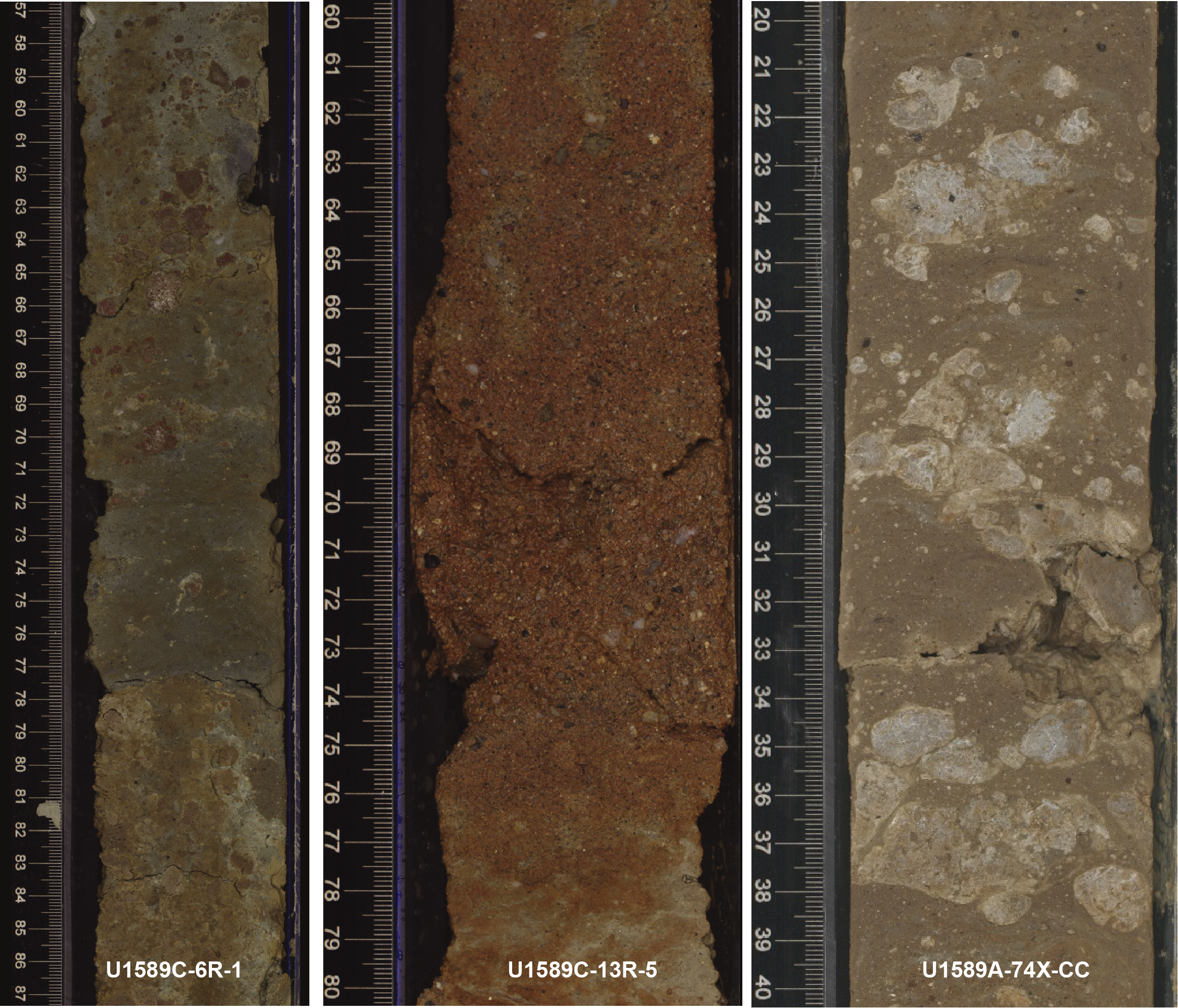
Figure F11. Representative lithologies, Unit IV.
In both Holes U1589A and U1589C, the first recovered lithology in Unit IV is a matrix-supported sandy conglomerate that has a gray color similar to the lithologies of Unit III. However, within 0.1 m a gradational transition to highly oxidized, reddish-hued sediment occurs. This reddish, oxidized hue continues throughout the unit, with sporadic nonoxidized sections (Figure F11).
Matrix-supported or clast-supported conglomerate or breccia is interbedded with centimeter to multidecimeter layers of sand, muddy sand, gravelly muddy sand, gravelly sand, and sandy conglomerate. In these poorly sorted and polymictic lithologies, the matrix is typically silty to sandy, with rounded grains, including quartz. Clasts are typically carbonate or quartzite (chert or obsidian), with lesser light and dark volcanic, metamorphic, and mudstone fragments displaying variable degrees of oxidation and carbonation. Carbonate clasts are typically more oxidized than others. They also commonly display an irregularly shaped brecciated carbonated rim. This lithology is also characterized by the presence of carbonate concretions and black, millimeter-sized pisolites. Intervals commonly display shearing and layering features (Figure F7) likely related to coring disturbance (see Structural geology and Core disturbance).
Several decimeter- to pluridecimeter-thick layers of sand are intercalated with and dispersed throughout Unit IV. The contact between these clast-poor and clast-rich lithologies can be sharp, diffuse, or gradational. Sand layers are moderately sorted and have a grain size varying from silt to medium sand (0.25–0.5 mm). These include a few isolated millimeter- to centimeter-sized clasts, as described above. Some sand layers are characterized by normal grading.
No organic-rich (sapropelic) lithologies or volcanic intervals were observed in this unit.
3.2.5. Unit V
- Interval: 398-U1589C-26R-1, 0 cm, to the bottom of the hole
- Thickness: not determined
- Depth: >592.8 mbsf
- Age: probable middle Eocene to Cretaceous
- Lithology: limestone, marble
Unit V was encountered in Hole U1589C and extends from 592.8 mbsf to the end of the hole, where drilling ceased (612.4 mbsf; Table T2). As a consequence of the termination of drilling, only the superficial part of this unit was sampled. Because Hole U1589C was drilled with the RCB system, core sections of this unit are characterized by brittle deformation. The samples collected from Unit V consist of pluridecimetric fragments of brecciated, carbonate-cemented and nonbrecciated limestone/marble (Figure F12) with spectacular large foraminifera (nummulites) observable in thin section (see Biostratigraphy; Figure F31). Unit V is interpreted as the basement to the overlying sedimentary packages in Units I–IV.
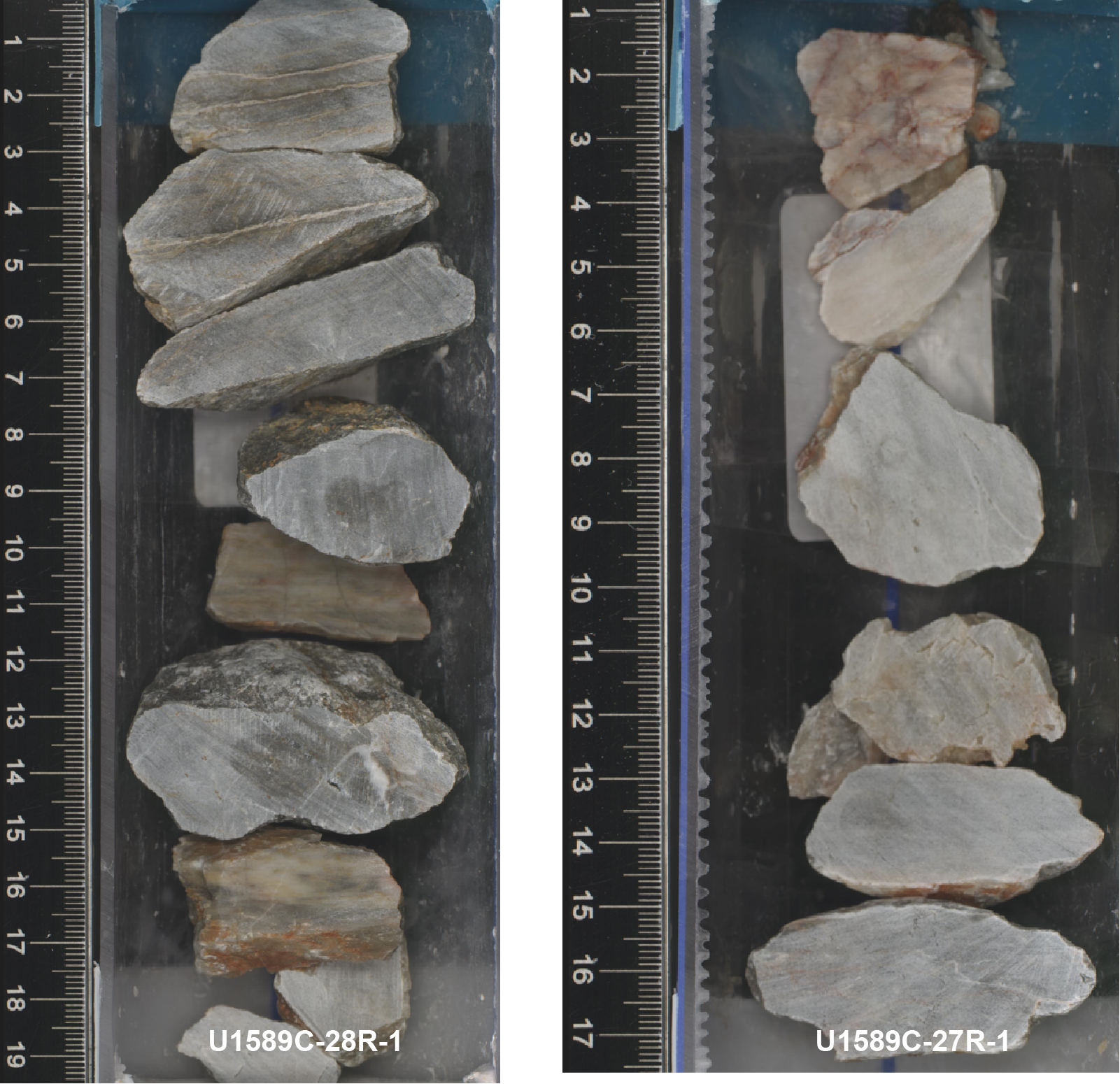
Figure F12. Limestone and marble clasts.
3.3. Correlations between holes
The recovered sediments from Holes U1589A–U1589C allow for correlation of sediment-specific features such as volcanic layers (e.g., discrete ash or lapilli layers) or organic-rich (sapropelic) horizons. Holes U1589A and U1589B largely overlap in an effort to fill gaps in recovery, whereas Hole U1589C extends the lithology to the basement, with some overlap between the lowermost recovered sediments from Hole U1589B (see Stratigraphic correlation). Here, we highlight notable lithologic correlations between Holes U1589A–U1589C.
3.3.1. Notable volcanic deposits
- Sections 398-U1589A-7H-2 (bottom depth = 52.33 mbsf) and 398-U1589B-7H-1 (bottom depth = 52.74 mbsf) (~42–52.5 mbsf): this ~10 m thick, brown lapilli-ash is characterized by a high amount of vitric and lithic-rich lapilli-sized clasts. Toward the top of this interval, areas of concentrated lapilli-sized pumice clasts occur. These pumices do not form a discrete layer but are intermixed with the surrounding finer grained sediments, likely due to sloshing inside the core liner before splitting.
- Cores 398-U1589A-21F through 22F (~5 m; bottom depth = 164.14 mbsf) and 398-U1589B-27F through 28F (~6.5 m; bottom depth = 164.85 mbsf) (~157–164 mbsf): this interval of lapilli with ash is characterized by a high amount of lapilli-sized pumice clasts with minor ash, reaching up to coarse lapilli in grain size. In Hole U1589B, a 2 cm thick lithic-crystal-rich ash was identified at the bottom of the layer, which is also present in Hole U1589A, although less discrete. Larger pumice clasts (medium to coarse lapilli) are generally concentrated at the bottom of the interval and decrease in grain size toward the top to fine lapilli or coarse ash, indicating a normal grading of this volcanic deposit.
- Sections 398-U1589A-29F-CC (bottom depth = 198.81 mbsf) and 398-U1589B-36F-1 (bottom depth = 199.94 mbsf) (~197–198 mbsf): this ~1 m thick lithic ash volcanic deposit is characterized by a dark gray color and high amounts of lithic clasts at the bottom of the interval. Toward the top, this deposit grades into an ash with lithics, described as a normally graded depositional interval.
- Sections 398-U1589A-50F-1 (bottom depth = 291.6 mbsf) and 398-U1589B-55F-4 (bottom depth = 292.8 mbsf) (~292 mbsf): this ~5 cm thick ash layer is described as coarse-grained crystal ash (with lithics). It has a relatively sharp lower boundary, although slightly wavy, whereas the upper boundary of this ash layer is diffuse and gradational.
3.3.2. Notable organic-rich (sapropelic) muds
- Sections 398-U1589A-46F-3 (bottom depth = 274.8 mbsf) and 398-U1589B-52F-1 (275.6 mbsf) (~275 mbsf): this ~25 cm thick organic-rich (sapropelic) horizon is moderately to highly bioturbated and olive-brown to dark brown. It is characterized by a relatively sharp lower boundary, whereas the upper boundary is gradational in Hole U1589B and was not recovered in Hole U1589A.
- Sections 398-U1589A-50F-3 (bottom depth = 293.8 mbsf) and 398-U1589B-56F-2 (294.8 mbsf) (~294 mbsf): this ~15 cm thick organic-rich (sapropelic) horizon is characterized by a dark color (brown–greenish gray) with a relatively sharp lower boundary and a gradational upper boundary.
3.4. X-ray diffraction analysis
XRD data were collected systematically from the interstitial water (IW) squeeze cake sediment residues from Holes U1589A–U1589C to complement macroscopic core description and geochemical analysis. XRD spectra obtained from representative principal lithologies of Hole U1589A are shown in Figure F13. The spectra show characteristic XRD patterns of glass-rich volcanic rocks from Unit I, with major peaks diagnostic of mainly anorthite (with Na solid solution), a silica phase (quartz), glauconite, and halite in tuffaceous mud (Figure F13A) and mainly anorthite (with Na solid solution) with minor glauconite in volcanic ash (Figure F13B). The spectra obtained on an organic-rich ooze (Figure F13C) and ooze (Figure F13D) from Unit II identify calcium carbonate (calcite and aragonite), a silica phase (quartz), and clay minerals typically from the illite and smectite groups. The spectrum in Figure F13E is characteristic of samples of siliciclastic sand with shell fragments from Unit III, with a silica phase (quartz), calcium carbonate (calcite and aragonite), and clay minerals (illite group) present in addition to minor anorthite (with Na solid solution). A breccia from Unit IV (Figure F13F) is dominated by a silica phase (quartz) with minor amounts of albite (with Ca solid solution) and clay minerals (illite group).
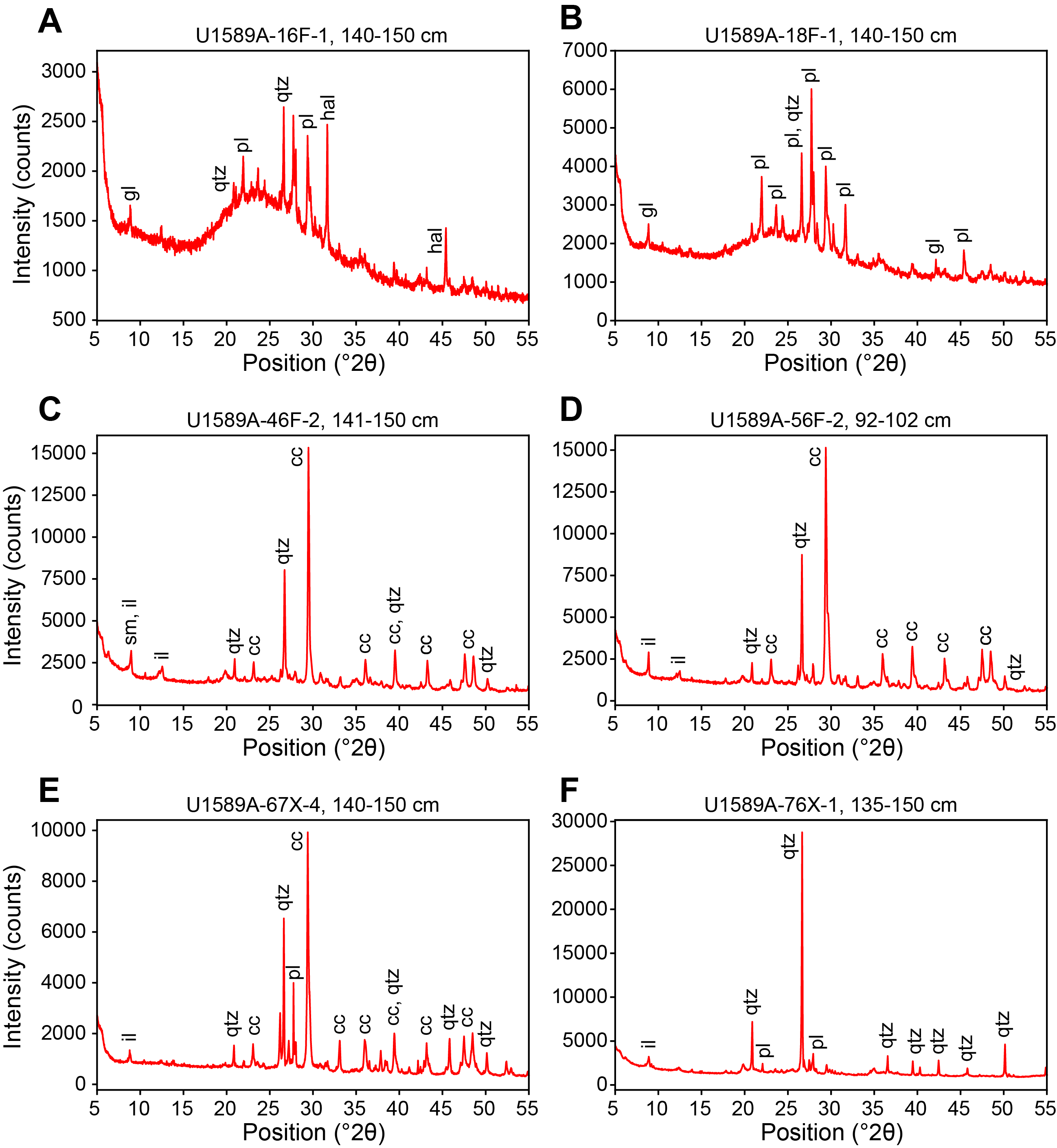
Figure F13. XRD spectra.
4. Stratigraphic correlation
To achieve the expedition research objectives, two holes (U1589A and U1589B) were drilled at Site U1589 using the APC, HLAPC, and XCB coring systems; these were complemented by Hole U1589C, where the RCB system was used. The mudline was recovered in Hole U1589A with the APC system. Using the APC/HLAPC/XCB approach in Hole U1589A, 76 cores were recovered to 446.15 mbsf, and in Hole U1589B, 70 cores were recovered to 359.58 mbsf. In both cases, the uppermost strata (135.12/96.68 mbsf) were cored using the full-length APC system until the first major overpull was encountered. Then we switched to HLAPC coring to better recover the sediment formation. In Hole U1589A, we switched to XCB coring at 365.5 mbsf (Core 66X) when the sediment became too stiff; we refrained from using the XCB coring system in Hole U1589B. In Hole U1589C, we drilled down with the RCB drill bit to 360 mbsf without recovery; thereafter, we cored to 612.4 mbsf and recovered 28 cores with low recovery.
4.1. Correlation during coring
To gain experience with Correlator software, we measured the cores from Hole U1589A with the Special Task Multisensor Logger (STMSL) to get an impression of how STMSL and Whole-Round Multisensor Logger (WRMSL) measurements compare and to get used to the workflow. A comparison of MS measured with both tools is provided in Figure F14. This comparison confirmed that both tools measured the same trends and that the STMSL resolves small-scale events well. The STMSL resolution for Hole U1589B was set to 10 cm, which took less than 2 min per section and provided sufficient quality to enable fast stratigraphic correlation.
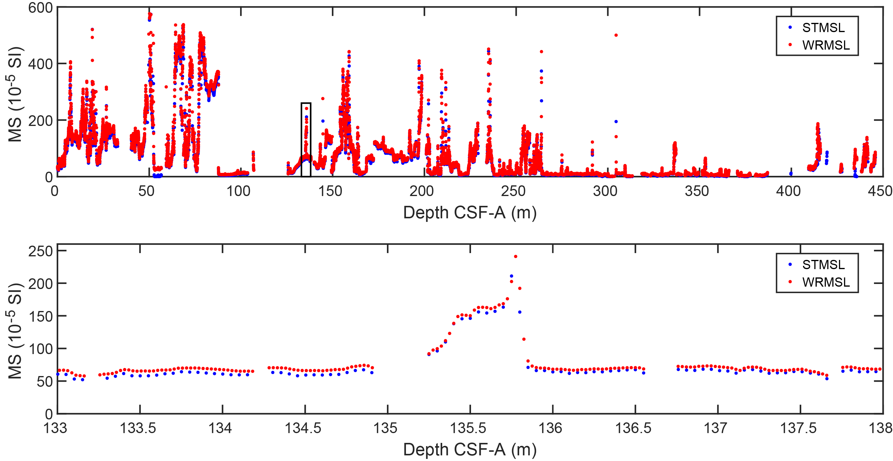
Figure F14. MS measurements.
After the end of coring in Hole U1589A, we evaluated the continuity of the stratigraphic record and identified gaps. We calculated the base of each core by adding the curated length of each core (taken from the core laboratory whiteboard) to its top and estimated the difference to the top of the following core. This gave a rough estimate of the occurrence of larger gaps in the CSF-A scale, as illustrated in Figure F15 (blue dots). Positive values indicate potential gaps, and negative values indicate potential overlap. We identified two major gaps in Hole U1589A, in Core 5H (a gap of ~7 m) and in Cores 11H and 12H, which had nearly no recovery (Figure F15). More frequent gaps occurred in cores obtained with the XCB system (e.g., Cores 70X–75X). We anticipated closing these gaps as much as possible in Hole U1589B.
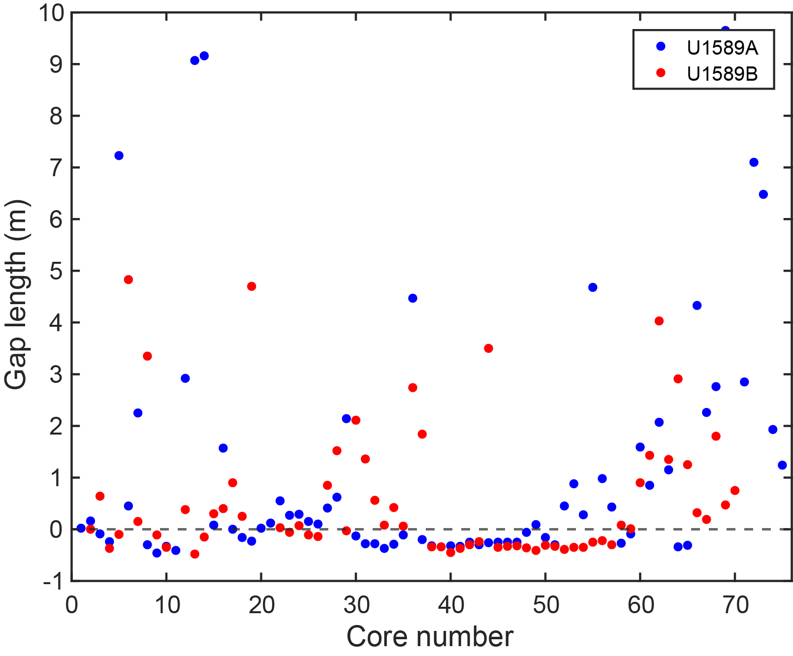
Figure F15. Major gaps in cores.
During core retrieval in Hole U1589B, we used the STMSL to rapidly measure density (using the GRA densitometer) and MS on each recovered core section as soon as possible after core retrieval. This allowed stratigraphic correlation to the WRMSL-derived GRA density and MS from Hole U1589A to be conducted in near real time, enabling effective communication with the drill floor to proceed (or introduce offsets) in subsequent coring.
We were able to fill the largest parts of the identified gaps in the Hole U1589A cored stratigraphy with coring in Hole U1589B, but we also identified intervals that had not been covered completely due to incomplete and low recovery during coring in Hole U1589B of the respective depth intervals. This most probably indicates coarser grained lithologies (e.g., sand, ash) in these intervals (Figure F15).
During coring of Hole U1589B, immediate stratigraphic correlation revealed the need for real-time adjustments of the drilling depth at two intervals to be able to close the major gaps encountered in Hole U1589A that resulted in minor overlaps of base and top of subsequent cores. However, problems arose when these modifications of the drill depths were applied, resulting in mismatches of the drillers depth and the depth in the LIMS database, which led to implausible overlaps in the CSF-A scale.
4.2. Correlation for establishing CCSF-A depth scale
To establish the core composite depth below seafloor, Method A (CCSF-A), depth scale, we analyzed Holes U1589A and U1589B with Correlator software by matching characteristic signals within their downhole physical properties characters. We used the data measured on the WRMSL (for MS, GRA density, and P-wave velocity), the Natural Gamma Radiation Logger (NGRL; for NGR intensity), and the Section Half Multisensor Logger (SHMSL; for MS and color reflectance), as well as photos once the cores were split into working and archive halves (see Physical properties; also see Physical properties in the Expedition 398 methods chapter [Kutterolf et al., 2024]). Hole U1589C started with a 2 m overlap in relation to Hole U1589B at greater depths, and sparse recovery (24% on average) of the subsequent coring resulted in unreliable correlations with the other two holes.
In general, we found that MS was the most reliable physical parameter for correlations, whereas NGR and GRA density measurements were often significantly overprinted by the irregular distribution of core material in cores with low recovery and high water contents. An important observation was that tilting the cores during core handling (e.g., when cores were retrieved from the core rack) led to uneven distribution of core material, with one end having more material than the other. This led to a characteristic sawtooth pattern both in the GRA density and NGR distribution (Figure F16).
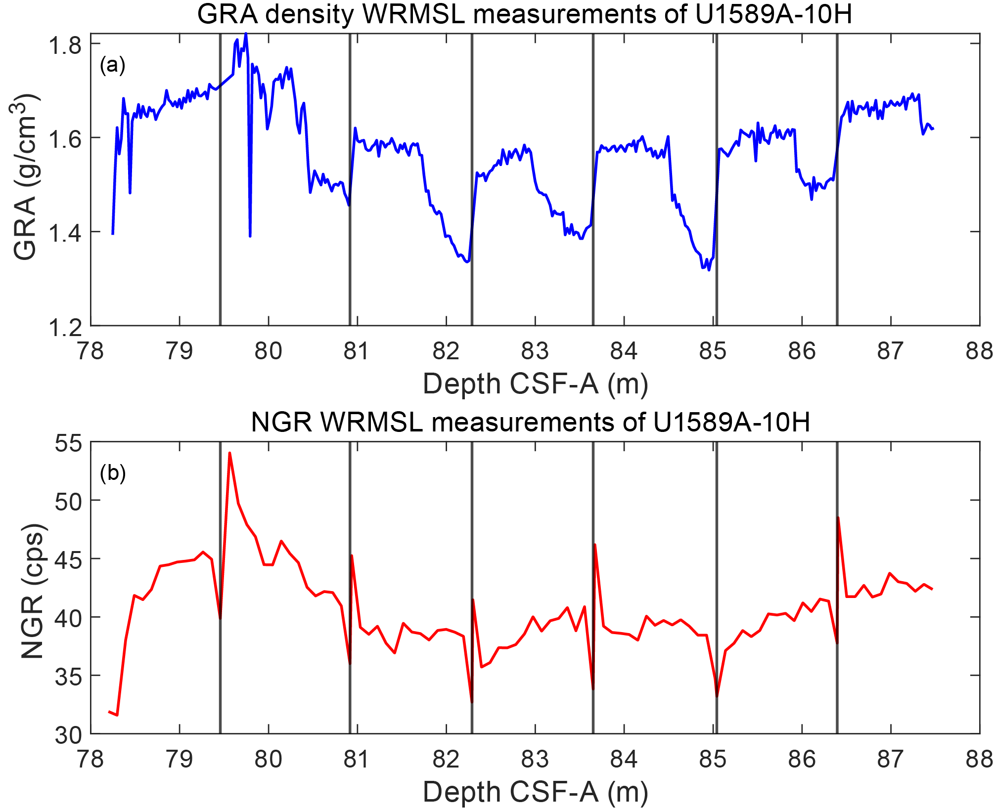
Figure F16. GRA and NGR sawtooth pattern.
The top of Hole U1589A preserved the mudline and served as the anchor (zero-depth point) for the generation of the CCSF-A depth scale (see Stratigraphic correlation in the Expedition 398 methods chapter [Kutterolf et al., 2024]). Using this anchor core, we attempted to determine the relative depth offset of each core by establishing affine ties between the holes based on the maximum correlation of all measured physical properties. These depth offsets are reported in Table T3. Figure F17 shows the MS of all the holes on the resulting CCSF-A depth scale, in which individual cores were shifted according to the identified correlations. This figure highlights the vertical alignment of characteristic events in the adjacent holes.
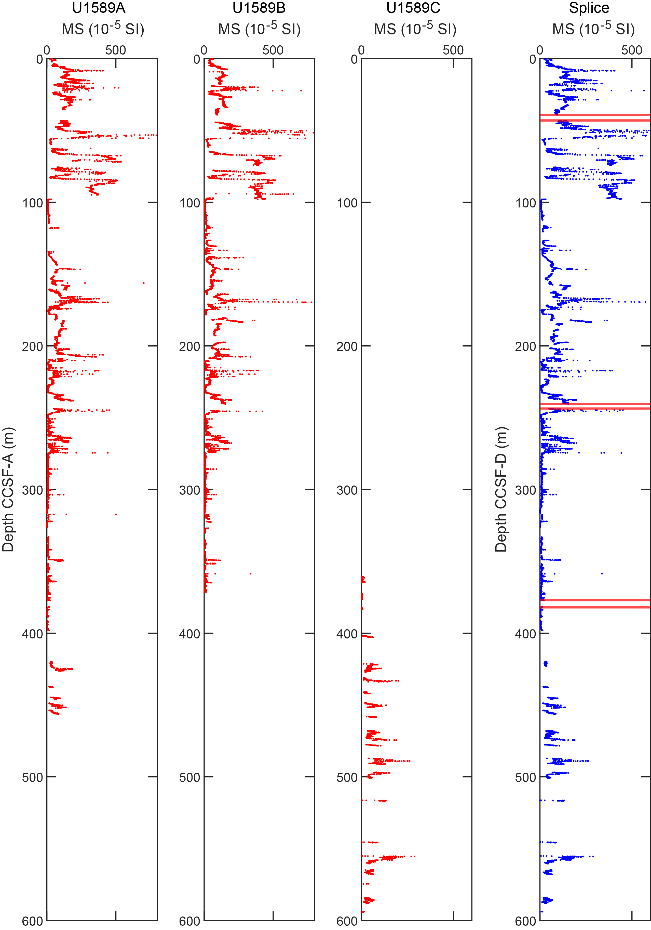
Figure F17. WRMSL-derived MS data.
In general, we were able to identify reliable correlations between most cores of Holes U1589A and U1589B. However, low recovery in several areas, as well as strong lithologic variations (especially in the uppermost 30 m) and the soupy nature of the recovered material led to the occurrence of interruptions in the stratigraphic correlation of Site U1589. For each of these interruptions, we used the relative offset between untied (uncorrelated) cores derived from the CSF-A scale to keep the composite depth scale as close to the original CSF-A scale as possible. Figure F17 shows MS plotted on the constructed CCSF-A scale for Holes U1589A and U1589B.
4.3. Construction of the splice
Once we established the composite depth scale, we spliced selected sequences from Holes U1589A and U1589B and added additional but scattered parts of Hole U1589C to create the most complete and representative section possible. The end product of this process is reported in Table T4 and illustrated in Figure F18. Down to 370 m CCSF-A (Figure F17), gaps in the splice are mostly <1 m, whereas three larger gaps occur (39.3–43.0, 240.5–243.6, and 330.2–333.1 mbsf). Below 370 mbsf, gaps occurred more often because Hole U1589B was only drilled to this depth and recovery in Holes U1589A and U1589C was low.
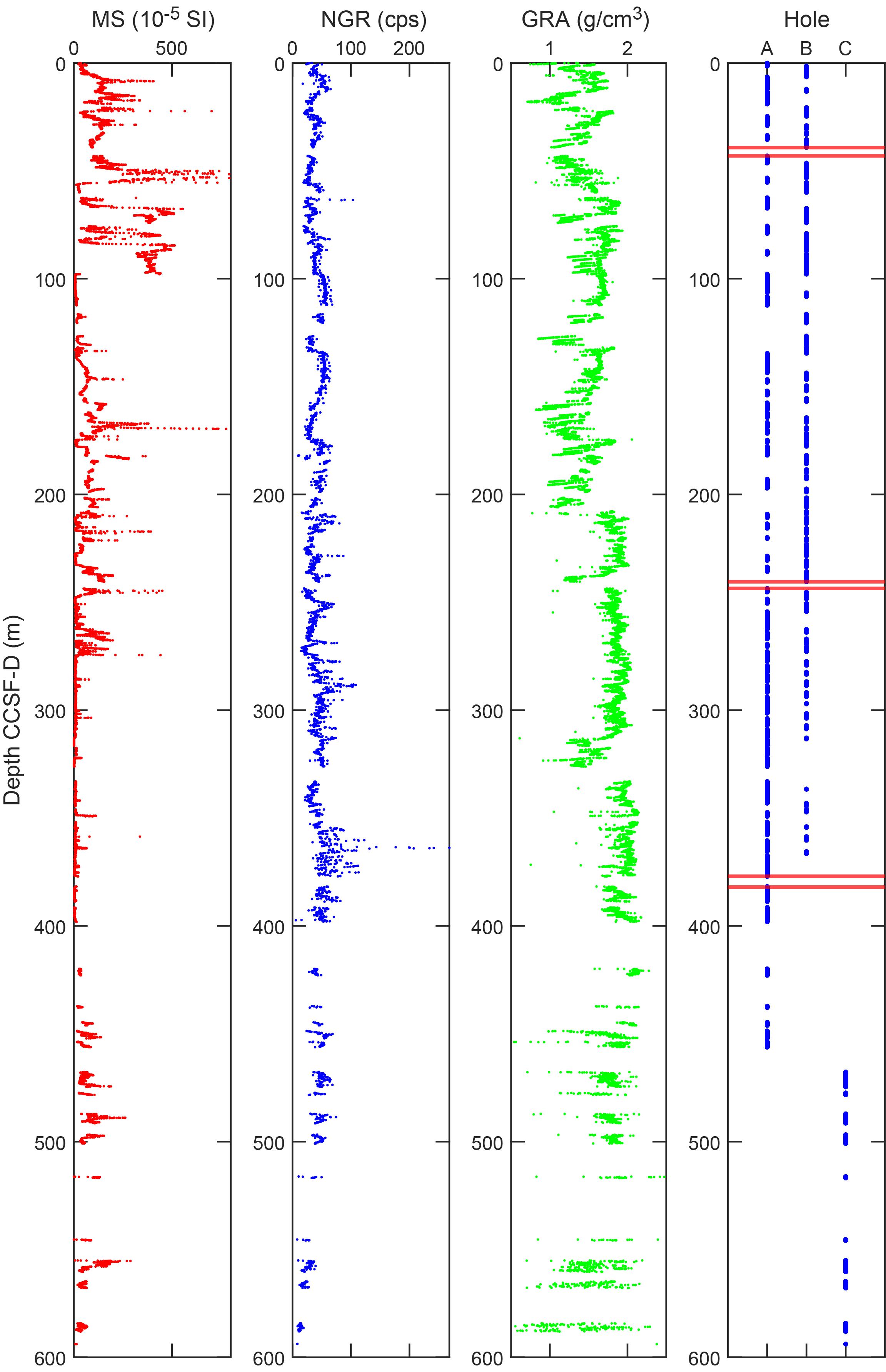
Figure F18. Splice, Site U1589.
In general, no significant core expansion was observed during curation and handling of the cores. Figure F19 shows a plot comparing the CSF-A and CCSF-A scales for Holes U1589A and U1589B and a linear regression curve calculated for both holes together. The deviation from the dotted line indicates an affine growth factor of 4%, although gaps in the correlation add uncertainty to this value.
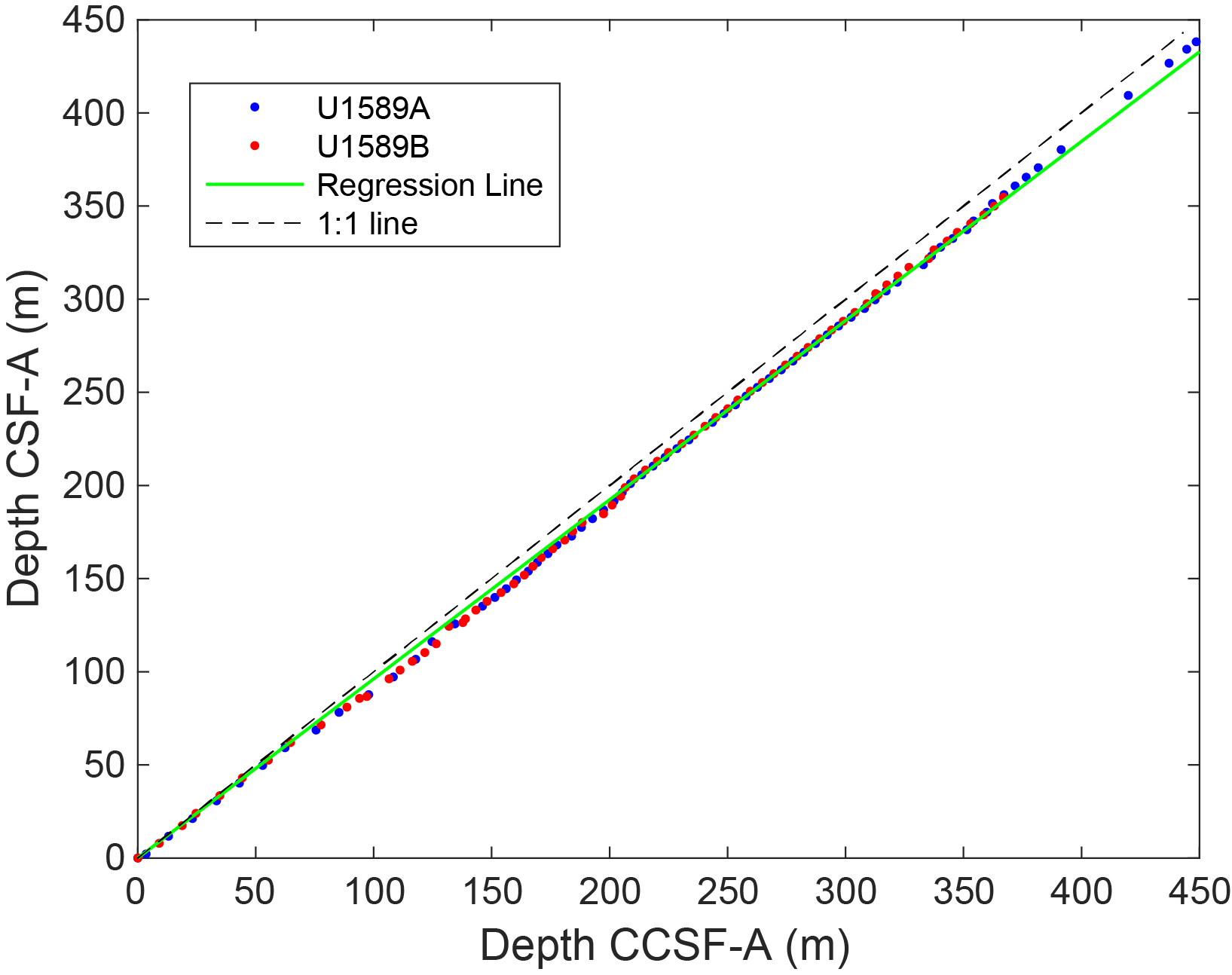
Figure F19. Core top depths.
5. Structural geology
Structural geology analyses at Site U1589 included description of cores retrieved from Holes U1589A–U1589C. A total of 230 structures were observed, and their orientations were measured (to an estimated accuracy of ±2°) in the cores. These included bedding planes (89.5%), faults (7%), and carbonate veins and breccias (3.5%). The distributions and dip angles of planar structures are shown in Figure F20. Deformation related to drilling and core recovery was noted on the log sheet but not recorded in GEODESC. Here, we describe and provide examples of each of the features that were recorded.
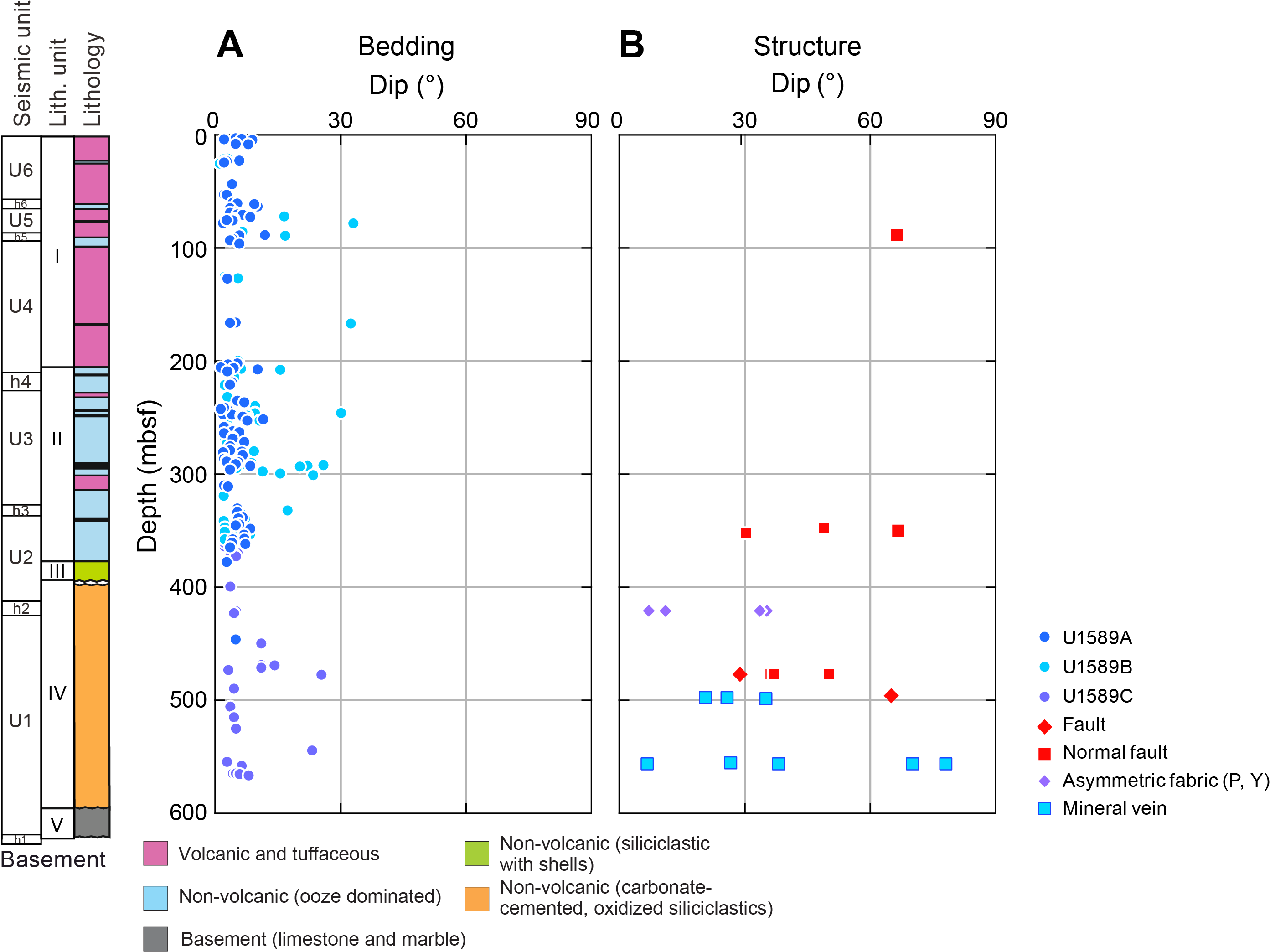
Figure F20. Dip data.
5.1. Bedding
Bedding planes (n = 206) were measured mainly on thin sand beds/laminae, sapropels, and calcareous/siliciclastic mud boundaries. They exhibit horizontal to sub-subhorizontal dips throughout the boreholes (mostly ≤ 10°; mean dip = 6.0°; standard deviation = 5.3°; median dip = 4.2°) (Figure F20), with steeper dips only identified around 80, 300, and 480 mbsf in contrast to dips in the rest of the depth interval (Figure F20).
To further characterize the variation of bedding dips, we constructed box plots (Figure F21). In these plots, each box indicates the range of dips between the lower and upper quartiles of the observed distributions, which is statistically meaningful. Median values (i.e., the fiftieth percentiles of each data set) were also plotted. First, we divided the dip measurements into the five lithostratigraphic units identified from core description (see Lithostratigraphy) (Figure F21A). Measurements were mostly concentrated in Lithostratigraphic Units I, II, and IV and limited by the scarcity of bedding in Units III and V (only one measurement was made in Unit III; Figure F21A). The bedding dip decreases from the bottom to the top; the median dip decreases from 5.0° in Unit IV to 4.2° in Unit I (Figure F21A), with the range of dips also decreasing. The most prominent change of the bedding dip distribution was identified between Units II and III. There is no significant variation between Units I and II (Figure F21A).
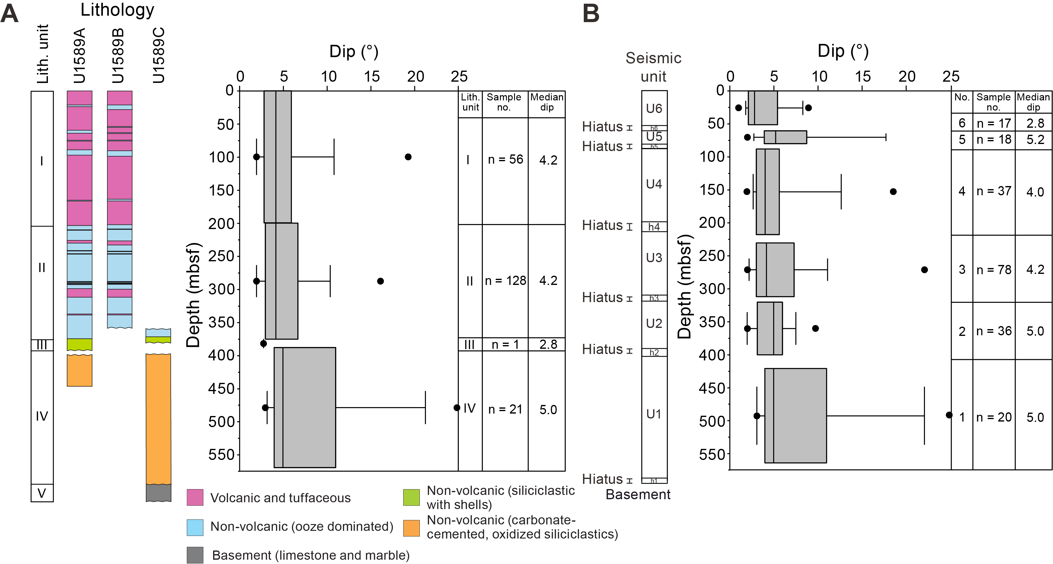
Figure F21. Bedding dip.
To explore the dip variance between different rift intervals, the bedding data were divided into six units corresponding to the six seismic units defined by core-seismic correlation (see Stratigraphic correlation) (Figure F21B). Each seismic unit comprises the respective sediment package (e.g., Seismic Unit U6) underlain by a basal onlap surface or hiatus (e.g., h6) (Figure F21B). From the bottom to top, the median dip gradually decreased from 5.0° in Unit U1 to 4.0° in Unit U4 (Figure F21B), indicating the tectonic tilt in Anhydros Basin decreases from Unit U1 to Unit U4. Because the median dip in Unit U6 (2.8°) is clearly shallower than in Unit U4 (4.0°), a small tilting event and associated disturbance of the bedding in Unit U5 might be expected (Figure F21B).
5.2. Faults
Minor small-displacement faults are apparent on split core surfaces (Figure F22). They are developed mainly in the lower part of the cores (470–612 mbsf). Faults show apparent displacements from a few millimeters to a centimeter. Minor faults at Site U1589 have a normal sense of displacement and represent cohesive (healed) fault planes with closed fault planes. The sense and/or amount of displacement is defined where faults cut bioturbation or sedimentary structures and by asymmetric fabrics within the faults. Normal faults developed, particularly in Lithostratigraphic Units I and III, show faint slip planes and are apparently characterized by independent particulate flow, grain boundary slipping. On the other hand, faults and normal faults developed in Unit IV exhibit grain size reduction identified clearly under hand lens. Therefore, the deformation style of the faults in Unit IV was characterized as cataclastic deformation. On X-ray images, fault planes were identified based on the offset of dense/less dense intervals extending linearly from the edge to the center of split core surfaces (Figure F22). No density variations were identified along the faults, apparently because the density change associated with faulting could not be resolved.
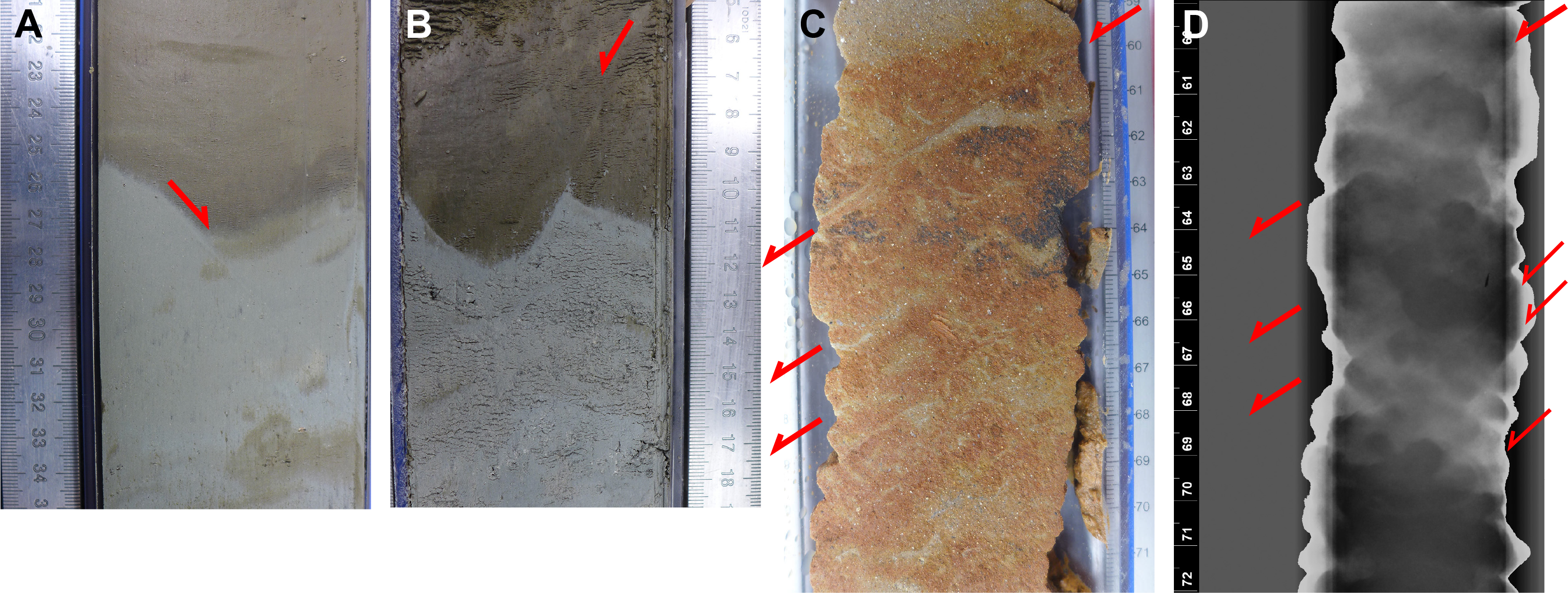
Figure F22. Minor faults.
5.3. Carbonate veins and breccias
Carbonate veins and breccias were identified only in the lower part of Lithostratigraphic Units IV and V (>497 mbsf). The occurrences of the veins in Unit IV were furrowed, intermittent, and narrow (~1 mm width) (Figure F23). Intergranular vein minerals crystallized in the open spaces of the coarse sandstone. Although some of the veins show preferred orientation, the orientations of most are random. Frequently, the earlier stage veins were cut and dislocated a few millimeters, indicative of hybrid failure mode (open and shear). Therefore, these veins formed under small differential stress soon after sedimentation. On X-ray images, the carbonate veins could not be identified (Figure F23). The porous sandy media outside the vein indicates that no cementation occurred along the veins.
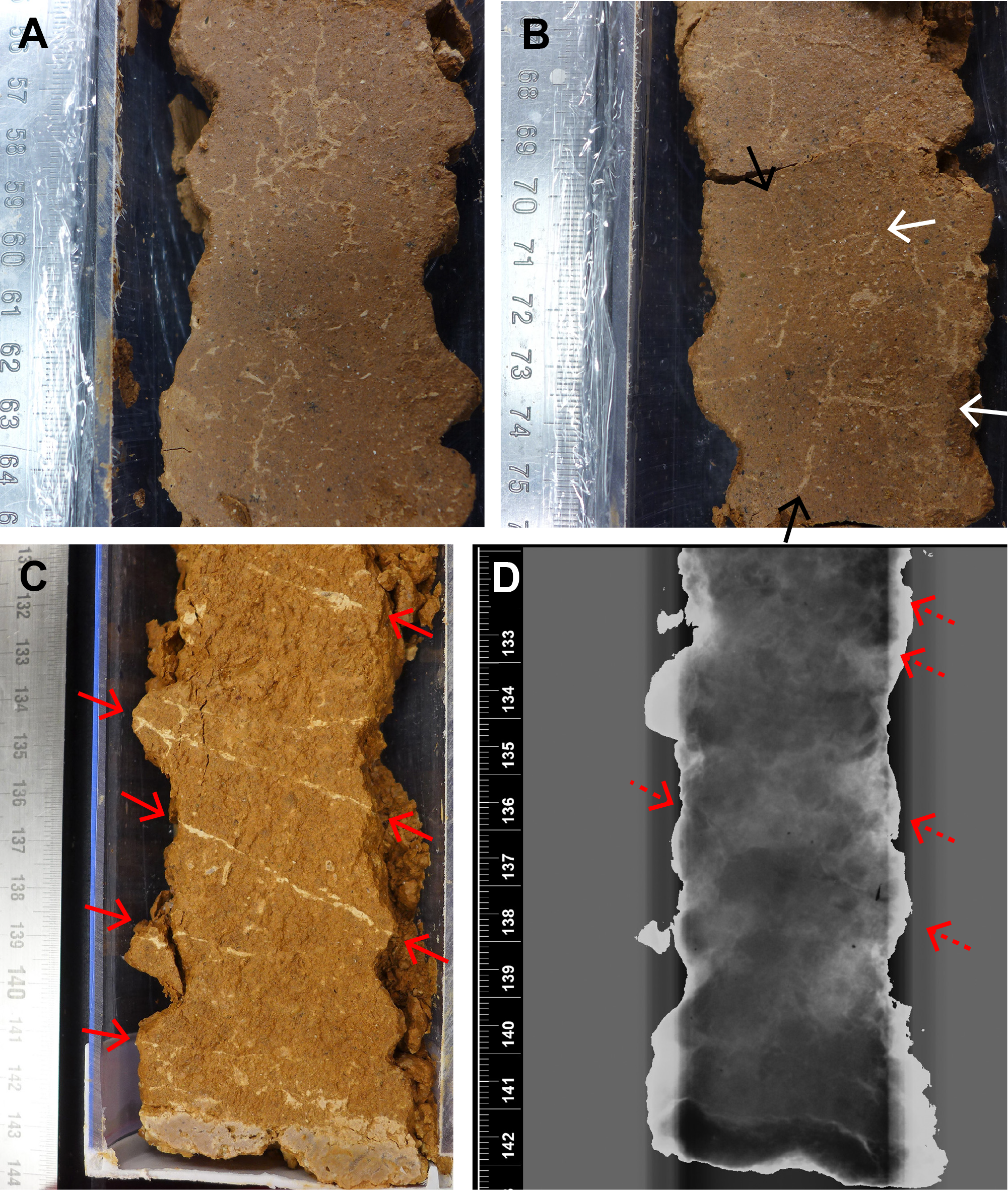
Figure F23. Carbonate vein and breccia, Unit IV.
Breccia composed of limestone clasts in a carbonate matrix was observed in Lithostratigraphic Unit V (Figure F24). Because the retrieved core samples from this unit were heavily biscuited (<5 cm), no structural data were measured (see Structural geology in the Expedition 398 methods chapter [Kutterolf et al., 2024]). However, some of the breccias showed preferred orientation of clasts at the hand-specimen scale (Figure F24). On the split core surface of interval 398-U1589C-26R-1, 34–53 cm, some pieces of the breccia are composed of angular-shaped, foliated limestone clasts (Figure F24). The foliations in the brecciated clasts were all oriented in the same direction. In addition, a biscuited core exhibited systematic orientations of breccia fractures, with one set parallel to the foliation of the limestone clasts and the other at a high angle (approximately perpendicular) to the foliation. Therefore, the breccia in Unit V formed by in situ brecciation.
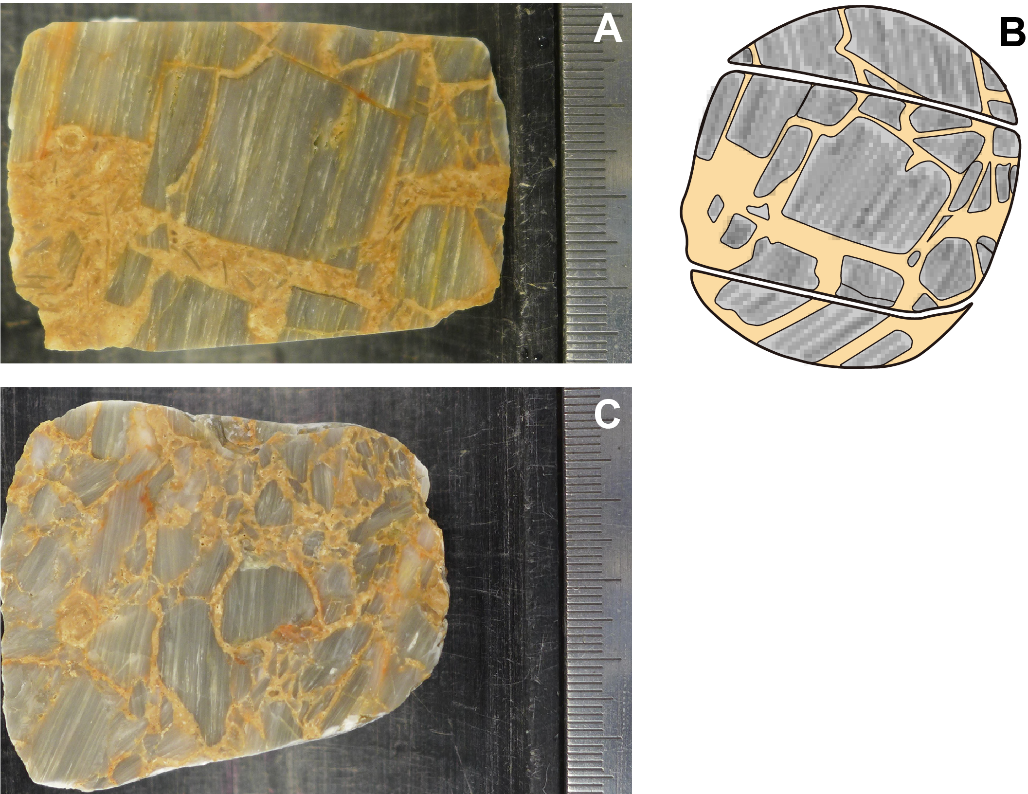
Figure F24. Carbonate breccia, Unit V.
6. Biostratigraphy
Calcareous nannofossils and planktonic and benthic foraminifera were examined from core catcher samples and additional split core samples from Holes U1589A–U1589C to develop a shipboard biostratigraphic framework for Site U1589. Planktonic and benthic foraminifera additionally provided data on paleowater depths, downslope reworking, and possible dissolution.
Site U1589 cored the Anhydros Basin sedimentary sequence and the upper portion of limestone basement. A ~589 m thick Holocene to Pleistocene sequence comprising several hiatus-bound packages was recovered. Calcareous nannofossils and planktonic foraminifera provided good age resolution throughout the Pleistocene sediments. Ages provided by benthic foraminifera were consistent with those of calcareous nannofossils and planktonic foraminifera. Additionally, because of high sedimentation rates through much of the cored section, semiquantitative planktonic foraminiferal assemblage data were used in conjunction with calcareous nannofossil and planktonic foraminiferal biostratigraphic datums to tentatively assign marine isotope stage (MIS) boundaries. These boundaries are based primarily on fluctuations of the warm-water species Globigerinoides ruber, Globigerinoides elongatus, and Globigerinoides pyramidalis (see Crundwell et al., 2008; Aze et al., 2011; Crundwell and Woodhouse, 2022; Woodhouse et al., 2023). Biostratigraphic datums recognized at Site U1589 are given in Tables T5 and T6, and an age-depth plot is shown in Figure F25.
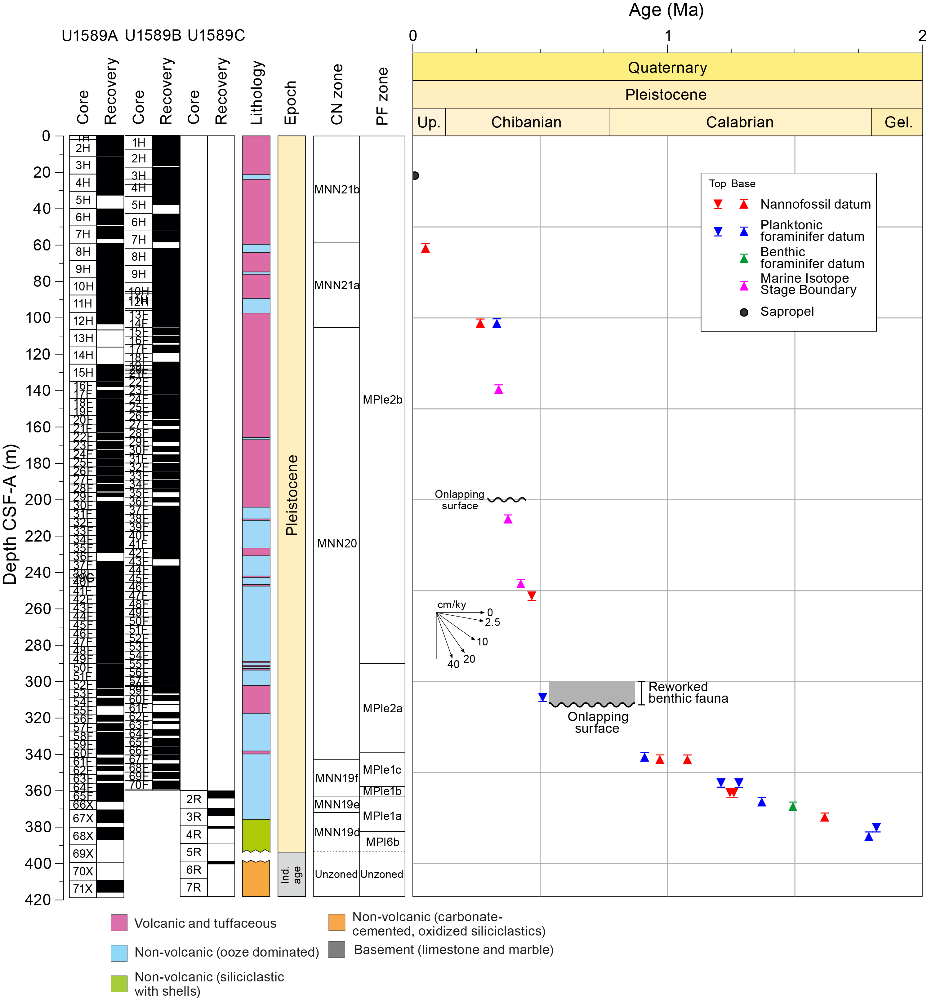
Figure F25. Age-depth plot.
Holocene–Pleistocene age sediments (<1.8 Ma) were recovered in Hole U1589A from Samples 1H-CC, 54–59 cm, through 68X-CC, 12–15 cm (2.13–387.24 mbsf), and sediments of indeterminate age were recovered from Samples 68X-CC, 12–15 cm, through 76X-CC, 25–30 cm (387.24–446.15 mbsf). In Hole U1589B, Holocene–Pleistocene age sediments (<1.8 Ma) were recovered from Samples 1H-CC, 14–19 cm, through 70F-CC, 8–10 cm (7.83–359.58 mbsf). In Hole U1589C, sediments of indeterminate age were recovered from Samples 2R-CC, 4–7 cm, through 27R-1, 0–5 cm (364.29–602.55 mbsf). Several carbonate clasts of middle Eocene and Cretaceous age were recovered in Samples 398-U1589C-22R-1, 0–3 cm (554.03 mbsf), and 26R-1, 77–80 cm (593.6 mbsf), respectively.
6.1. Calcareous nannofossils
Calcareous nannofossil biostratigraphy in Holes U1589A and U1589B was established through analysis of core catcher samples or, alternatively, samples from the base of recovered cores where core catchers were missing. Nannofossils are common to abundant in samples from the Middle–Late Pleistocene sequence (Hole U1589A: 2.18–387.24 mbsf; Hole U1589B: 7.88–359.58 mbsf). Preservation is generally good to moderate with sporadically poor intervals throughout the sequence (Figure F26); however, there is significant reworking of older material in most of the Pleistocene samples. The assemblages are characterized by the occurrence of warm-water species such as Rhabdosphaera clavigera and Umbilicosphaera sibogae throughout the sequence in Holes U1589A and U1589B.
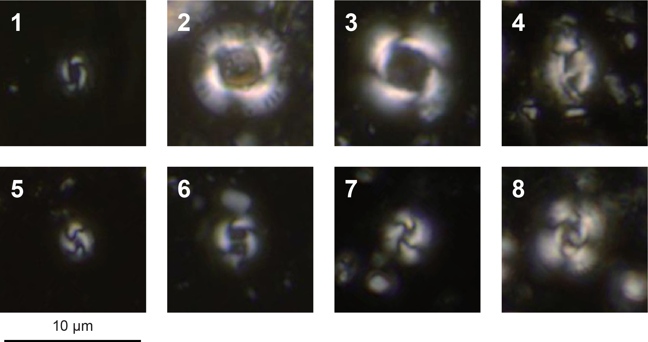
Figure F26. Calcareous nannofossils.
Nine nannofossil biostratigraphic datums recognized at Site U1589 represent a continuous Middle–Late Pleistocene sedimentary sequence. Sampling resolution through Hole U1589B was lower than that in Hole U1589A due to time constraints, and only a few select core catcher samples were examined. Postexpedition analysis of additional samples will help to constrain datums through the Pleistocene interval. The distribution of calcareous nannofossil taxa is shown in Table T7, and biostratigraphic datums are given in Table T5.
The presence of Emiliania huxleyi in Samples 398-U1589A-1H-CC, 54–59 cm, through 12H-CC, 0–5 cm (2.18–103.78 mbsf), and 398-U1589B-1H-CC, 14–19 cm, through 13F-CC, 0–5 cm (7.88–101.05 mbsf), indicates a Holocene to Middle Pleistocene age (≤0.265 Ma) within Zones MNN21a and 21b (CNPL11, Backman et al., 2012; NN21, Martini, 1971; CN15, Okada and Bukry, 1980) of Rio et al. (1990) and Di Stefano and Sturiale (2010). The acme base of E. huxleyi, which correlates with the MNN21a/b boundary and MIS 4–5a (0.05 Ma) of Rio et al. (1990), Castradori (1993), and Lourens et al. (2004) in the eastern Mediterranean, is interpreted to occur in Samples 398-U1589A-6H-CC, 11–16 cm, and 8H-CC, 0–5 cm (49.25–69 mbsf), and 398-U1589B-7H-CC, 0–2 cm, and 8H-CC, 11–13 cm (58.65–71.61 mbsf). The top/last appearance datum of Pseudoemiliania lacunosa defines the MNN20/21a (CNPL10/11, NN19/20, CN14a/CN14b) boundary. The top consistent appearance of P. lacunosa occurs in Samples 398-U1589A-42F-CC, 20–25 cm (257.625 mbsf), and 398-U1589B-47F-CC, 28–30 cm (255.66 mbsf). Therefore, Samples 398-U1589A-41F-CC, 21–26 cm, and 42F-CC, 20–25 cm (253.005–257.625 mbsf) and 398-U1589B-46F-CC, 22–24 cm, and 47F-CC, 28–30 cm (250.92–255.66 mbsf), are assigned to the MNN20/21a boundary. The top occurrence of Reticulofenestra asanoi (0.901 Ma), situated at the top of the Jaramillo Subchronozone of the Matuyama Chronozone in Zone MNN19e, is recognized at the boundary between Samples 398-U1589A-59F-CC, 17–22 cm, and 60F-CC, 19–24 cm (337.39–340.41 mbsf), and between Samples 398-U1589B-66F-CC, 14–16 cm, and 67F-CC, 0–5 cm (340.4–343.5 mbsf). The basal occurrence of Gephyrocapsa sp. 3 (0.97 Ma), situated between the top of the Jaramillo Subchronozone of the Matuyama Chronozone in Zone MNN19e, is found between Samples 398-U1589A-60F-CC, 19–24 cm, and 61F-CC, 19–24 cm (340.36–345.83 mbsf), and between Samples 398-U1589B-67F-CC, 0–5 cm, and 68F-CC, 11–13 cm (343.5–349.53 mbsf). The basal occurrence of R. asanoi (1.078 Ma), which lies just below the Jaramillo Subchronozone of the Matuyama Chronozone in the Zone MNN19e, is found between Samples 398-U1589A-60F-CC, 19–24 cm, and 61F-CC, 19–24 cm (340.38–345.83 mbsf), and between Samples 398-U1589B-66F-CC, 14–16 cm, and 67F-CC, 0–5 cm (340.39–343.48 mbsf). The large form of Gephyrocapsa spp. (>5.5 µm) that appears between 1.245 and 1.617 Ma (Zones MNN19d, CNPL8, NN19, and CN13b) occurs in Samples 398-U1589A-65F-CC, 19–24 cm, and 66X-CC, 14–19 cm (365.79–366.25 mbsf).
6.2. Foraminifera
Planktonic and benthic foraminifera were examined from core catcher samples, split core samples, and thin sections from Holes U1589A–U1589C (Tables T8, T9). Absolute ages assigned to biostratigraphic datums follow those listed in Table T6 in the Expedition 398 methods chapter (Kutterolf et al., 2024). Planktonic and benthic foraminifer datums for Site U1589 are given in Table T6. Planktonic foraminifer abundances and indications of oceanicity (e.g., Hayward et al., 1999) and benthic foraminifer paleowater depth estimations are shown in Figures F27 and F28.
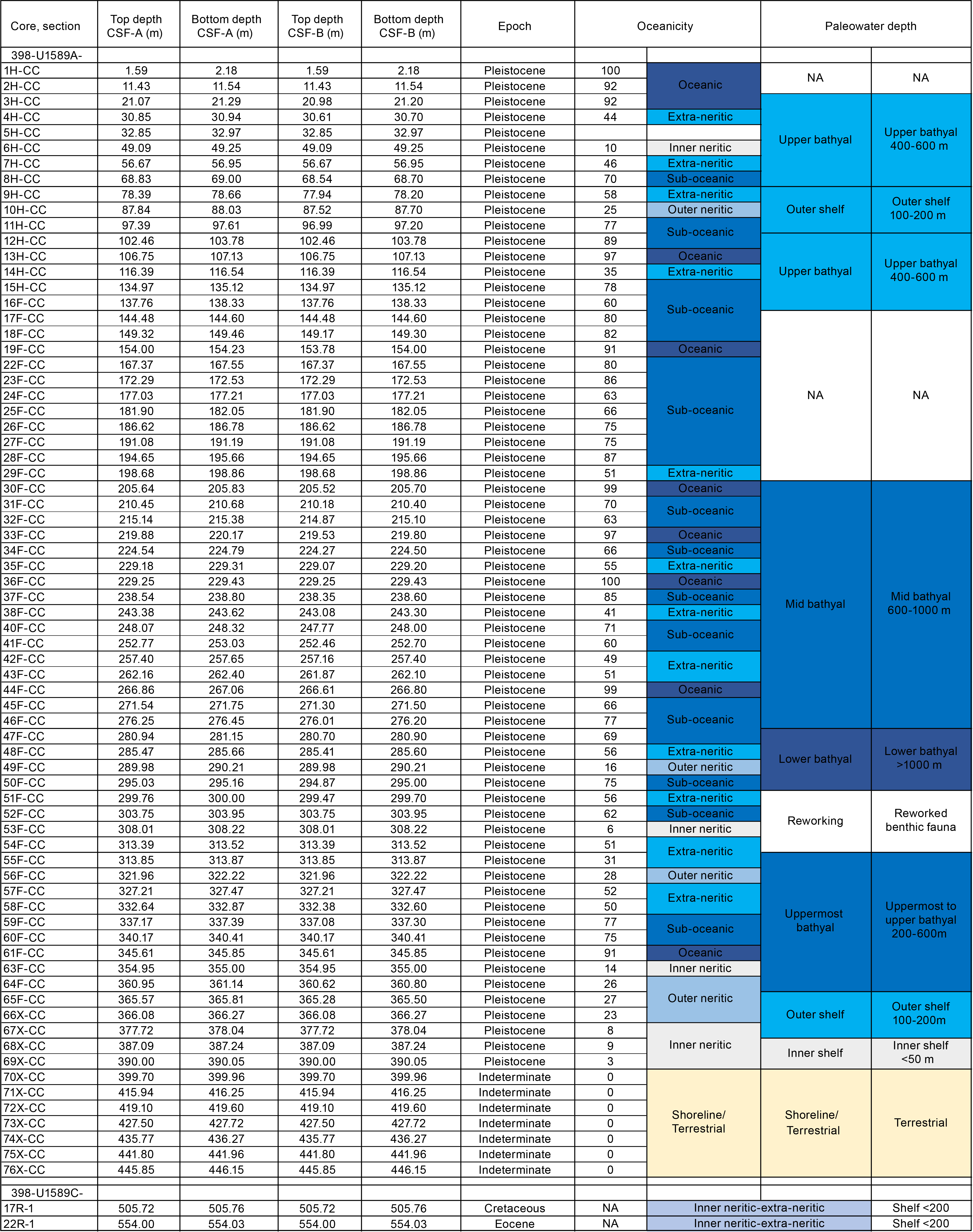
Figure F27. Foraminiferal oceanicity and paleowater depth estimates.
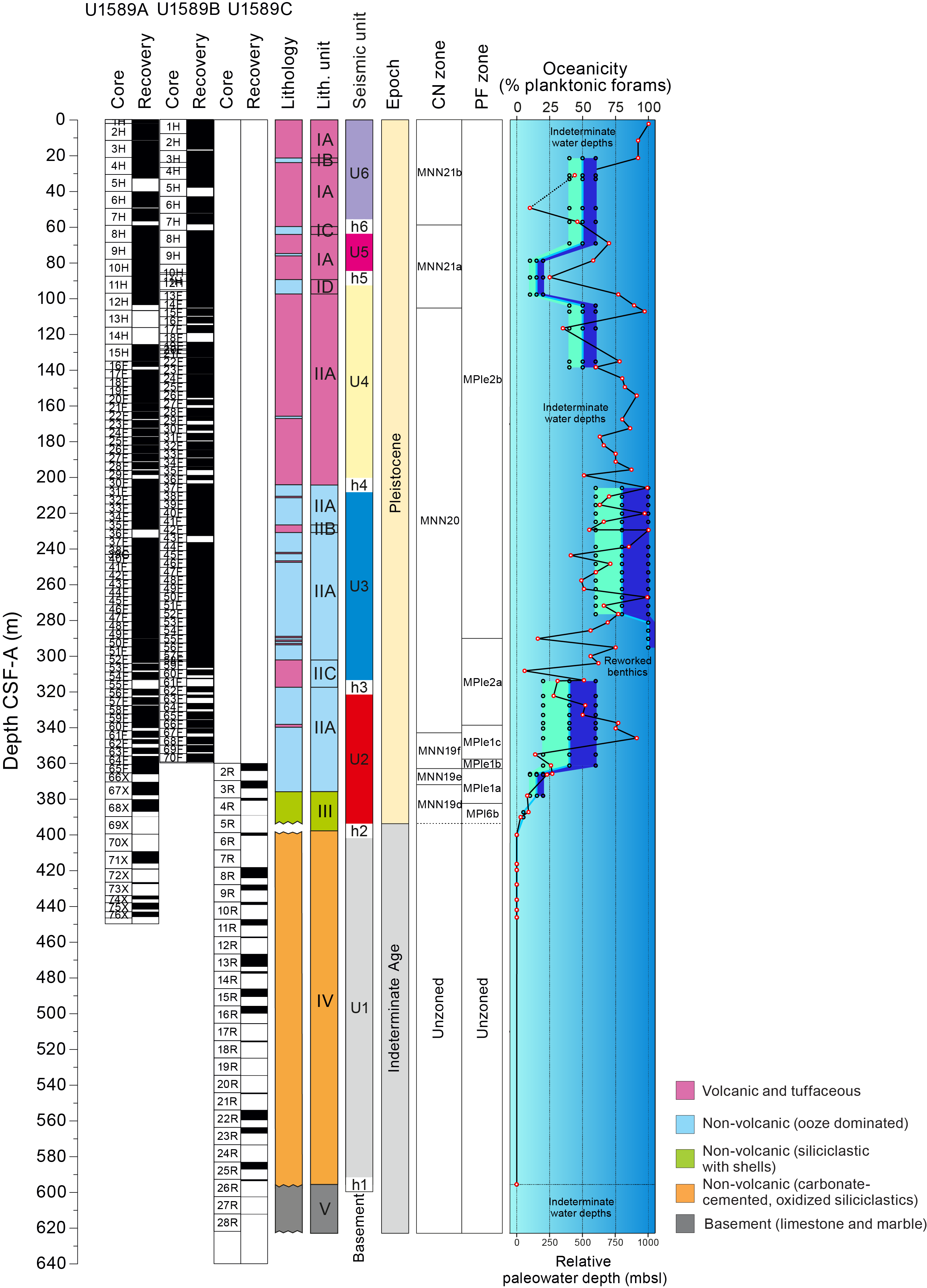
Figure F28. Biostratigraphic summary.
Because of the volcanogenic nature of the cored sedimentary sequence, residues (>125 µm) from washed samples were often significantly composed of volcaniclastic particles such as pumice, scoria, and ash that often diluted the microfossil component of the residues. Foraminifera dominated the biogenic component of the residues, however, and age markers were present in sufficient numbers to date most samples reliably. As well as volcanic material, clastic grains, minor pyrite, carbonaceous plant-derived matter, and other fossil material including shells and fragments (Bivalvia and Gastropoda), Pteropoda, Scaphopoda, Bryozoa, Arthropoda (Balanus), echinoid spines and plate fragments, radiolarians, ostracods, and otoliths, as well as fish teeth and vertebrae were also present in variable amounts in most samples. In addition, reworked Pliocene foraminifera were often present.
In the Holocene–Pleistocene section, foraminifera with very good to poor preservation are present in siliciclastic and volcaniclastic sediments. Foraminifer abundances are also highly variable, commonly making up the primary sedimentary component (>125 µm) in nannofossil oozes, notably rare in tuffaceous oozes likely due to sedimentary dilution, whereas coarser volcaniclastic intervals (>2 mm median grain size) were sometimes barren altogether of biogenic remains.
6.2.1. Holocene–Pleistocene biostratigraphy
Because of explosive volcanic events and rapid deposition related to the upper sedimentary section, it is not possible to accurately assign the base of the Holocene. Planktonic foraminifer assemblages from the Holocene–Pleistocene section of Holes U1589A and U1589B are mostly well preserved, with specimens rarely broken or exhibiting partially dissolved shell walls.
Holocene–Pleistocene foraminifer faunas indicate large fluctuations in relative paleowater depth and oceanicity with highly variable planktonic abundances that range 3%–100% when foraminifera were present (Figure F28). The fauna is typical of Mediterranean biostratigraphic Zones MPle2–MPl6, primarily composed of Neogloboquadrina incompta, Globigerina bulloides, Globigerina falconensis, Globigerina umbilicata, Globigerinella siphonifera, Globigerinita glutinata, G. elongatus, G. pyramidalis, Trilobatus trilobus group, G. ruber var. white, G. ruber var. pink, Globoconella inflata, Hirsutella scitula, Truncorotalia truncatulinoides s.l. (sinistral and dextral coiling), Neogloboquadrina pachyderma, Orbulina universa, Turborotalita quinqueloba, and Globigerinella calida (Figure F29). Rare reworked Pliocene specimens of Globoconella puncticulata and Globoturborotalita woodi were often present.
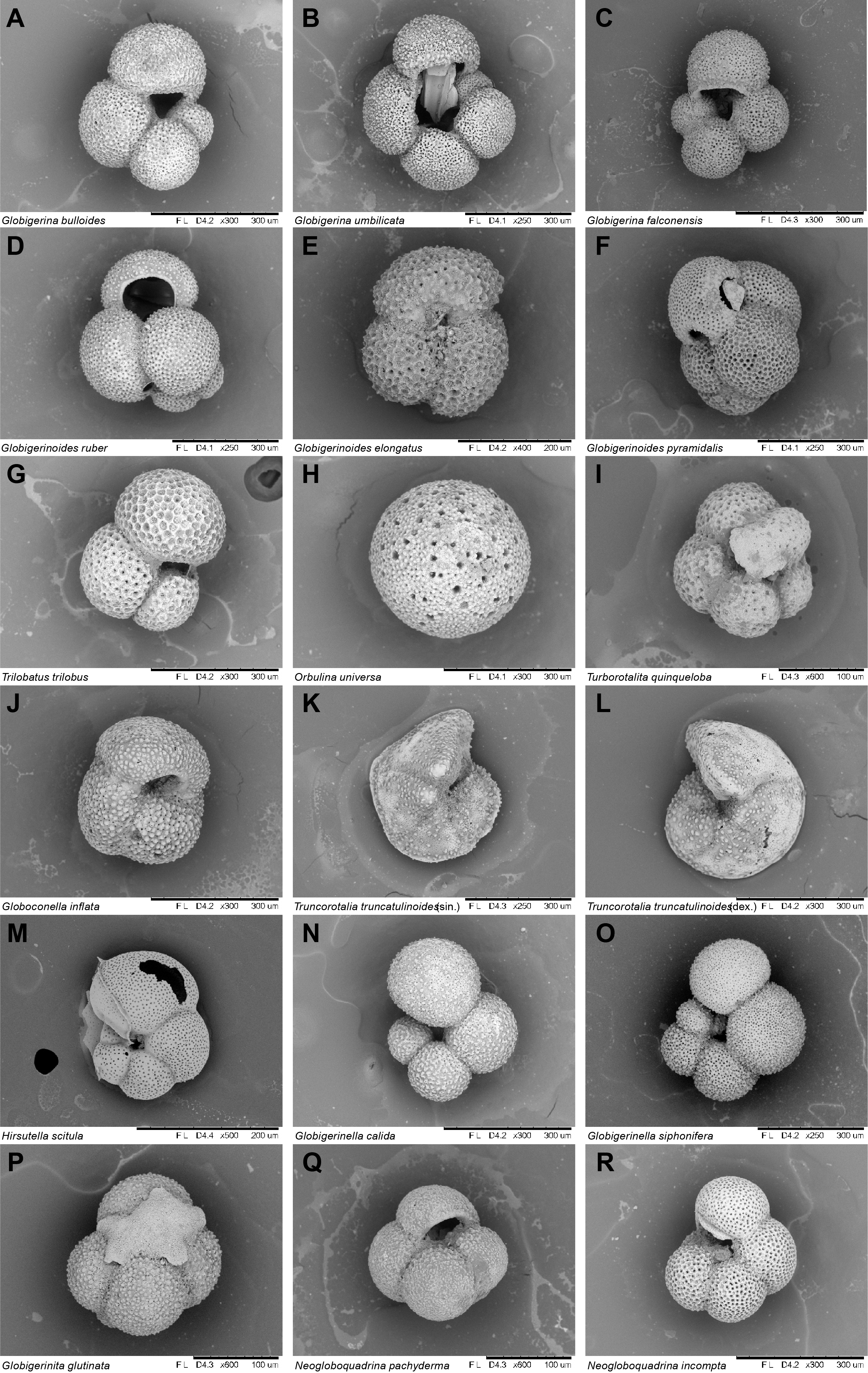
Figure F29. Planktonic foraminifera.
Foraminiferal faunas are sufficiently common to biostratigraphically divide the Pleistocene into six Mediterranean planktonic foraminiferal biostratigraphic zones (Lirer et al., 2019) separated by several sedimentary hiatuses:
- Zone MPle2b (0.00–0.53 Ma): 2.18–313.52 mbsf.
- Zone MPle2a (0.53–0.94 Ma): 313.82–340.41 mbsf.
- Zone MPle1c (0.94–1.21 Ma): 345.95–355.00 mbsf.
- Zone MPle1b (1.21–1.37 Ma): 361.14 mbsf.
- Zone MPle1a (1.37–1.79 Ma): 365.81–378.04 mbsf.
- Zone MPl6b (1.79–2.00 Ma): 387.24–390.05 mbsf.
The faunal criteria on which these age assignments are based are given below.
6.2.1.1. Zone MPle2b (0.00–0.53 Ma)
Samples 398-U1589A-1H-CC, 54–59 cm, through 54F-CC, 8–13 cm (2.18–313.52 mbsf), are assigned to Zone MPle2b based on the paracme top of sinistrally coiled Neogloboquadrina spp. (<0.51 Ma) in Sample 54F-CC, 8–13 cm (313.53 mbsf), above which this species is continuously present. Furthermore, within this interval are variable occurrences of T. truncatulinoides (<0.51 Ma), and the first occurrence of G. ruber var. pink (<0.33 Ma) occurs in Sample 11H-CC, 17–22 cm. The presence of an onlapping surface identified between Seismic Units U3 and U4 (see Stratigraphic correlation) indicates the base of this biostratigraphic zone is likely missing.
6.2.1.2. Zone MPle2a (0.53–0.94 Ma)
Samples 398-U1589A-55F-CC, 0–2 cm, through 59F-CC, 17–22 cm (313.82–337.39 mbsf), are assigned to Zone MPle2a based on the absence of T. truncatulinoides s.l. (0.53–0.934 Ma) and the scattered low abundances of sinistrally coiled Neogloboquadrina spp. (0.51–0.91 Ma) throughout the interval. The presence of an onlapping surface identified between Seismic stratigraphic Units U2 and U3 indicates the top of this biostratigraphic zone is likely missing.
6.2.1.3. Zone MPle1c (0.94–1.21 Ma)
Samples 398-U1589A-60F-CC, 19–24 cm, through 63F-CC, 0–5 cm (340.41–355.00 mbsf), are assigned to Zone MPle1c based on the consistently high abundances of sinistrally coiled Neogloboquadrina spp. (0.91–1.21 Ma) throughout this interval.
6.2.1.4. Zone MPle1b (1.21–1.37 Ma)
Sample 398-U1589A-64F-CC, 14–19 cm (361.14 mbsf), is assigned to Zone MPle1b based on the low abundances of sinistrally coiled Neogloboquadrina spp. (1.21–1.37 Ma) in this sample.
6.2.1.5. Zone MPle1a (1.37–1.79 Ma)
Samples 398-U1589A-65F-CC, 19–24 cm, through 67X-CC, 29–32 cm (365.81–378.04 mbsf), are assigned to Zone MPle1a based on the first common occurrence of sinistrally coiled Neogloboquadrina spp. (1.37–1.79 Ma) through this interval. Additionally, Sample 65F-CC marks the first common occurrence of the benthic foraminifer Hyalinea balthica (1.492 Ma; Lourens et al., 1998).
6.2.1.6. Zone MPl6b (1.79–2.00 Ma)
Samples 398-U1589A-68X-CC, 12–15 cm, through 69X-CC, 0–5 cm (387.24–390.05 mbsf), are assigned to Zone MPl6b or older based on the less than common abundance of sinistrally coiled Neogloboquadrina spp (>1.79 Ma) and the occurrence of rare Globigerinoides obliquus (>1.82 Ma) and Globoturborotalita decoraperta (~1.8 Ma) through this interval.
6.2.2. Pre-Pleistocene biostratigraphy
Several lithified carbonate clasts containing biogenic material were recovered from Lithostratigraphic Unit IV and investigated in thin section. The first clast (Sample 398-U1589C-17R-1, 22–26 cm; 505.76 mbsf) can be assigned to the Cretaceous as indicated by the scarce presence of Orbitoides sp. (Figure F30). The second clast (Sample 22R-1, 0–3 cm; 554.03 mbsf) can be assigned to the middle Eocene based on the possible presence of Nummulites ex. gr. perforatus, Assilina sp., Discocyclina sp., Sphaerogypsina sp., and various undetermined rotaloid forms (Figure F31), as well as planktonic foraminifer specimens attributable to Morozovella spp. (Figure F32).
Figure F30. Limestone clast.
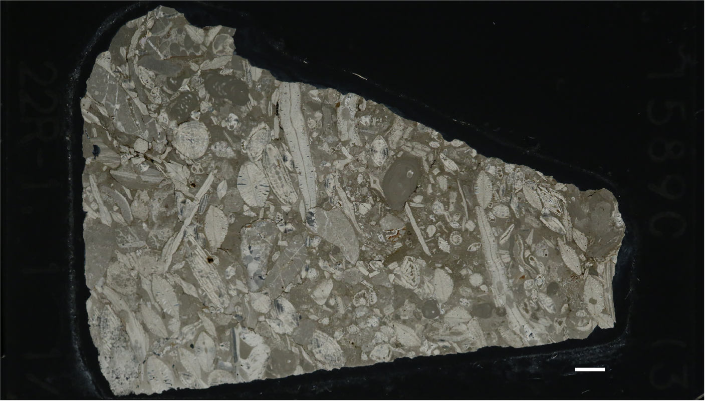
Figure F31. Nummulitic limestone.
Figure F32. Nummilitic limestone with possible Morozovella spp.
6.2.3. Planktonic foraminiferal oceanicity
Planktonic foraminifer abundances are highly variable, ranging 3%–100% when foraminifera were present (Figure F28). Oceanicity values are generally in agreement with benthic foraminiferal paleowater depth indicators (Figure F28). Because of the position of Site U1589 on the shallow bathymetric high of the Aegean Sea, low planktonic foraminifer abundances that suggest oceanicity indicative of shallower depths than those calculated through benthic foraminiferal paleowater depth markers are likely not associated with depth-related dissolution (Figure F27). These samples are more likely indicative of downslope reworking (e.g., Samples 398-U1589A-51F-CC, 19–24 cm, through 54F-CC, 8–13 cm; 300–313.52 mbsf) or environmental change and sediment dilution associated within the rapid onset of explosive volcaniclastic sedimentation (e.g., Samples 4H-CC, 6–11 cm, through 7H-CC, 0–5 cm; 30.94–56.95 mbsf). In general, the oceanicity data of Site U1589 indicate that relatively consistent suboceanic conditions (200–1000 mbsl) prevailed in Samples 1H-CC, 54–59 cm, through 48F-CC, 16–19 cm (2.18–285.66 mbsf). Samples 49F-CC, 20–23 cm, through 53F-CC, 16–21 cm (290.21–308.22 mbsf), indicate large fluctuations in oceanicity from suboceanic (200–1000 mbsl) to inner neritic conditions (0–50 mbsl), and Sample 53F-CC, 16–21 cm (308.22 mbsf), records the lowest oceanicity values (6% planktonic foraminifera) observed downhole so far (Figure F28). Samples 54F-CC, 8–13 cm, through 61F-CC, 19–24 cm (313.52–345.85 mbsf), then indicate increasing oceanicity values downhole, after which oceanicity values decrease relatively consistently from Samples 63F-CC, 8–13 cm, through 69X-CC, 19–24 cm (355–390.05 mbsf), reaching the minimum oceanicity value for the whole section (where foraminifera are present) with 3% planktonic foraminifera in Sample 69X-CC, 19–24 cm (355–390.05 mbsf).
6.2.4. Benthic foraminifera paleowater depths
Benthic foraminiferal distributions are highly variable, indicating paleowater depths from inner shelf (<50 mbsl) to lower bathyal (>1000 mbsl) (Figure F28). The low abundances or complete absence of benthic foraminiferal faunas in some samples (e.g., 398-U1589A-17F-CC, 7–12 cm, through 29F-CC, 13–18 cm [144.6–198.86 mbsf], and 398-U1589B-31F-CC, 5–10 cm, through 35F-CC, 10–13 cm [177.5–196.55 mbsf]), are possibly correlated with rapid emplacement of volcaniclastic sediments and/or related inhospitable environmental conditions (e.g., Samples 398-U1589A-70X-CC, 21–26 cm, through 76X-CC, 25–30 cm; 399.96–446.15 mbsf). Samples 398-U1589A-3H-CC, 17–22 cm, through 16F-CC, 0–5 cm (21.29–138.33 mbsf), record a large paleowater depth fluctuation from outer shelf (100–200 mbsl) to upper bathyal (400–600 mbsl), as indicated by the common presence of typical shelf species (e.g., Cibicides spp., Neoconorbina terquemi, and miliolids) and Cibicides pachyderma and Gyroidina spp., respectively (Figure F33). Samples 30F-CC, 14–19 cm, through 46F-CC, 17–20 cm (205.83–276.45 mbsf), exhibit mid-bathyal (600–1000 mbsl) paleowater depths as indicated by the presence of Oridorsalis umbonatus, whereas lower bathyal markers including Cibicidoides wuellerstorfi and rare occurrences of Articulina tubulosa are present in Samples 47F-CC, 18–21 cm, through 50F-CC, 8–13 cm (281.15–295.16 mbsf), and 398-U1589B-53F-CC, 24–26 cm, through 56F-CC, 20–25 cm (281.15–295.25 mbsf), indicating deposition in paleowater depths >1000 mbsl (Figures F28, F33). Commonly reworked outer shelf benthic foraminifera in Samples 398-U1589A-51F-CC, 19–24 cm, through 55F-CC, 0–2 cm (300–313.87 mbsf), likely represent downslope reworking, whereas Samples 56F-CC, 23–26 cm, through 69X-CC, 0–5 cm (322.22–390.05 mbsf), record gradual shallowing of the paleowater depth from uppermost–upper bathyal (200–600 mbsl) to outer shelf (100–200 mbsl) and finally to inner shelf (<50 mbsl). This is indicated by a change in fauna from species such as O. umbonatus and Nuttallides sp. to typical shelf species and finally to mainly reworked shelf benthic foraminifer fauna.
Figure F33. Benthic foraminifera.
7. Paleomagnetism
Paleomagnetic analysis at Site U1589 focused on measurement and demagnetization of archive-half sections to determine magnetostratigraphic age controls. However, the data suggest the presence of authigenic greigite that greatly complicates the use of the cores for creating a geomagnetic timescale. The core interval shallower than 300 mbsf can be confidently assigned to the Brunhes Chron, but recognition of the Brunhes/Matuyama and Matuyama/Jaramillo reversals is problematic.
7.1. Bulk magnetic properties
The bulk magnetic parameters of intensities of magnetization and low-field MS typically have log normal (geometric) distributions in natural samples (Tarling, 1983). Table T10 provides the geometric means and ranges of these parameters observed at the same measurement points in archive-half sections for all three holes cored at Site U1589, whereas the histograms of Figure F34 show their overall distributions for the entire site (plotted as log10 values). Natural remanent magnetism (NRM) intensities are broadly normally distributed, but low-field susceptibilities display a bimodal distribution with peaks at ~10 × 10−5 and ~60 × 10−5 SI that suggests contributions from two distinct lithologic sources and/or magnetic minerals and/or magnetic grain sizes.
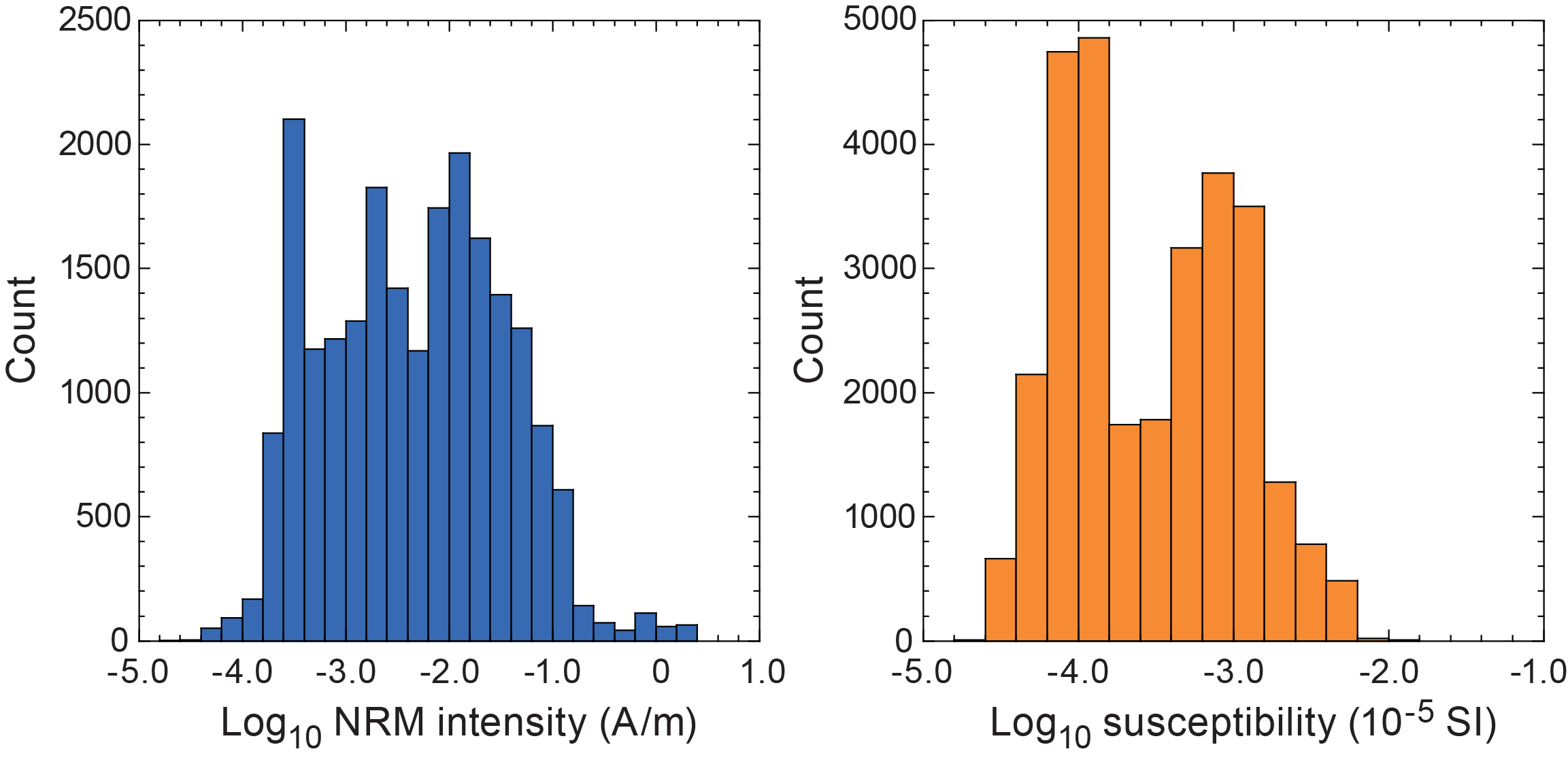
Figure F34. NRM intensity and low-field MS.
To further explore these distributions of bulk magnetic parameters, the lithologies recovered at Site U1589 were grouped into seven categories based on composition: (1) tuffaceous sediments, (2) volcaniclastic sediments, (3) sediments containing visible organic material, (4) organic-rich sediments (including suspected sapropels), (5) sediments with organic material, (6) muds and nannofossil oozes, and (7) siliciclastic sediments (seen only in Holes U1589A and U1589C). Plots of NRM intensity against low-field MS (Figure F35) show two overlapping linear trends. Linear relationships between these parameters indicate variations in the concentration of magnetic minerals in samples in the absence of variations in magnetic mineralogy (and variations in geomagnetic field strength in the case of NRM intensities). The distributions seen in Figure F35 therefore support the presence of two populations of magnetic grain assemblages in the sequences sampled at Site U1589, demarcated by susceptibilities above and below ~20 × 10−5 SI. We suspect that the low-susceptibility group includes samples containing the diagenetic authigenic ferrimagnetic sulfide mineral greigite (Fe3S4) in lower intervals of the sampled section deeper than ~300 mbsf.
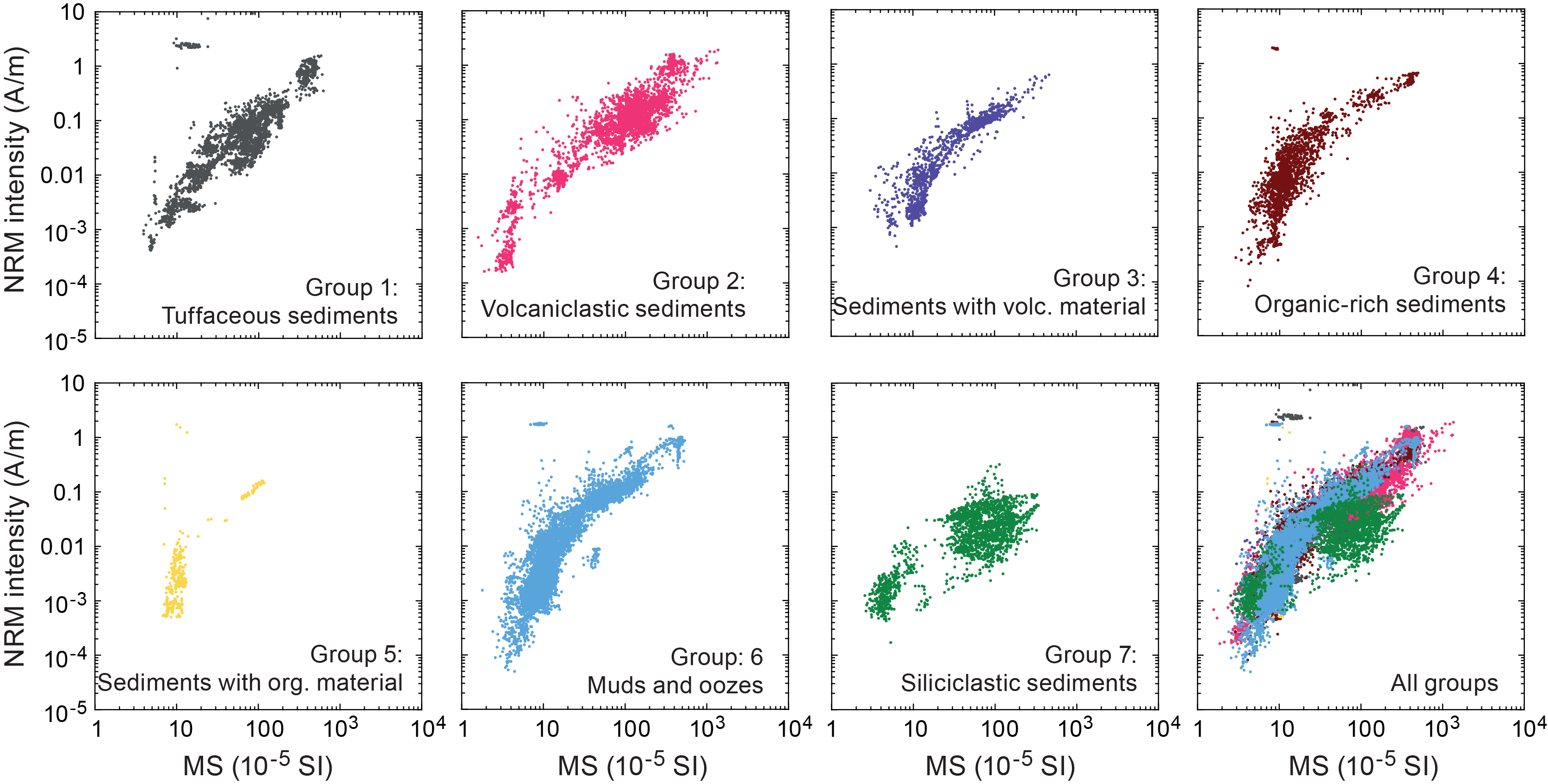
Figure F35. Low-field MS vs. NRM intensity.
7.2. Remanence characteristics
Remanence measurements were made on archive-half sections recovered by APC and XCB coring in Hole U1589A, APC coring in Hole U1589B, and RCB coring in Hole U1589C using the 2G Enterprise superconducting rock magnetometer (SRM) system. Remanence was measured every 2 cm, and the resulting data were filtered to reject measurement points within 8 cm of section ends. Point susceptibility data obtained from the archive-half sections were also filtered to preserve only data corresponding to the intervals where remanence measurements were made. A limited number of discrete samples were fully demagnetized and found to exhibit the same remanence characteristics observed in archive-half section measurements.
The majority of archive-half sections and discrete samples have a large drilling-induced remanence magnetization (DIRM) that is largely removed by alternating field (AF) demagnetization treatment at low applied fields (typically 5 mT) and that represents >70% of the NRM in many cases. DIRMs of this type have been reported previously during nearly all IODP expeditions, and their acquisition is usually reduced but not eliminated by the use of nonmagnetic core barrels. These artificial remanences imparted during coring and drilling operations are typically directed downward along the axes of the cores and result in NRM directions that are subvertical in the core reference frame. This is illustrated in the stereographic equal-area projections of NRM directions observed in archive-half sections recovered from all three holes at Site U1589 (Figure F36). However, a notable additional feature of NRM directions from archive-half sections measured in Hole U1589A is dispersion of directions away from vertical toward shallower inclinations and the −X direction in the core reference frame (Figure F36), representing NRMs that are directed into the archive half. This must reflect reorientation of magnetic particles in water-saturated sections containing unconsolidated sediments that have undergone redeposition in the core liner during recovery to the catwalk that subsequently acquired artificially induced depositional remanences in the generally downward-directed magnetic field on the R/V JOIDES Resolution during processing and archiving. This effect is not seen in data from Hole U1589B because visibly redeposited/disturbed core sections were not measured.
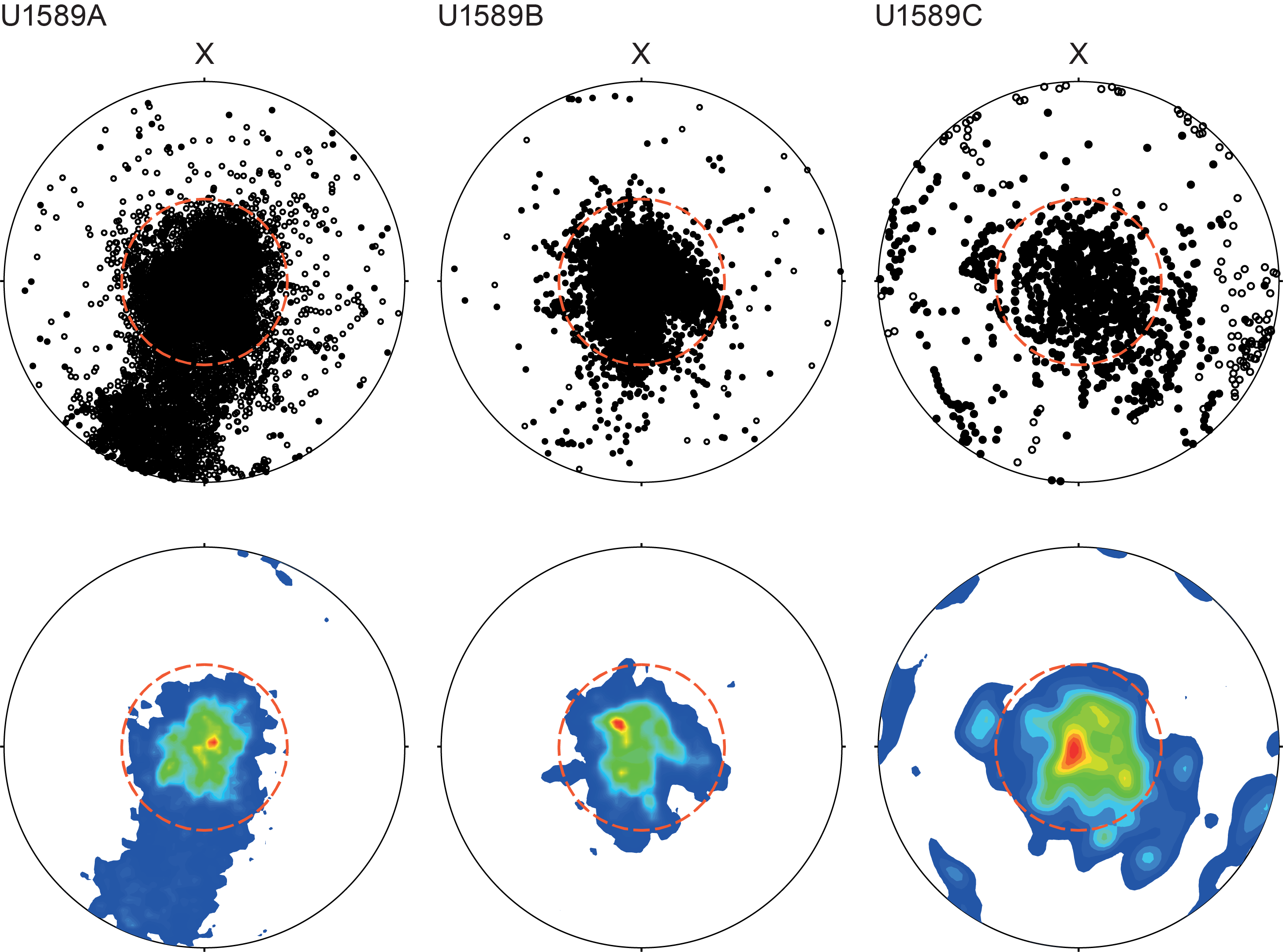
Figure F36. Projections of NRM directions.
After removal of the DIRM at low applied fields, AF demagnetization experiments then reveal two distinct behaviors during stepwise demagnetization of archive-half sections and discrete samples, illustrated here with examples from Hole U1589B: (1) samples that reach stable endpoint directions of magnetization that decay toward the origin on orthogonal vector plots and that can be used for magnetostratigraphic purposes (Figure F37) and (2) samples that exhibit a range of deviations from linear demagnetization behavior at applied fields >20 mT (Figure F38). These include samples in which intensities of magnetization begin to increase after demagnetization at fields >30 mT, leading to movement away from the origin on orthogonal vector plots (e.g., Sample 398-U1589B-66F-1, 24 cm). These complex behaviors are observed in all lithologies but become increasingly prevalent deeper than 230 mbsf, dominate below 300 mbsf, and suggest acquisition of a spurious laboratory-imparted remanence during progressive static AF demagnetization. Such behavior is a characteristic of the presence of greigite, which is known to form as a precursor to pyrite in anoxic sulfate-reducing sedimentary environments and has been previously reported from globally distributed localities (Roberts et al., 2011). Greigite-bearing sediments typically acquire a spurious gyroremanent magnetization (GRM) during AF demagnetization (especially during static AF demagnetization as performed on board JOIDES Resolution), with the GRM commonly acquired perpendicular to the last axis along which a static AF was applied (Stephenson and Snowball, 2001; Snowball, 1997a, 1997b; Roberts et al., 2011; Maffione and Herrerro-Bervera, 2022). The suspected presence of greigite in samples from Site U1589 can account for the unusual demagnetization behaviors seen in many cored intervals at deeper depths and undermines efforts to identify primary depositional remanences using stepwise demagnetization experiments as, after removal of the DIRM at low fields, a GRM begins to be acquired before the characteristic remanent magnetization (ChRM) direction of the samples can be determined. However, in some instances (e.g., Sample 398-U1589B-67F-1, 22 cm), demagnetization paths defined by lower applied field steps indicate migration of remanence directions toward upper hemisphere negative inclinations, providing some evidence of reversed magnetizations in some intervals.
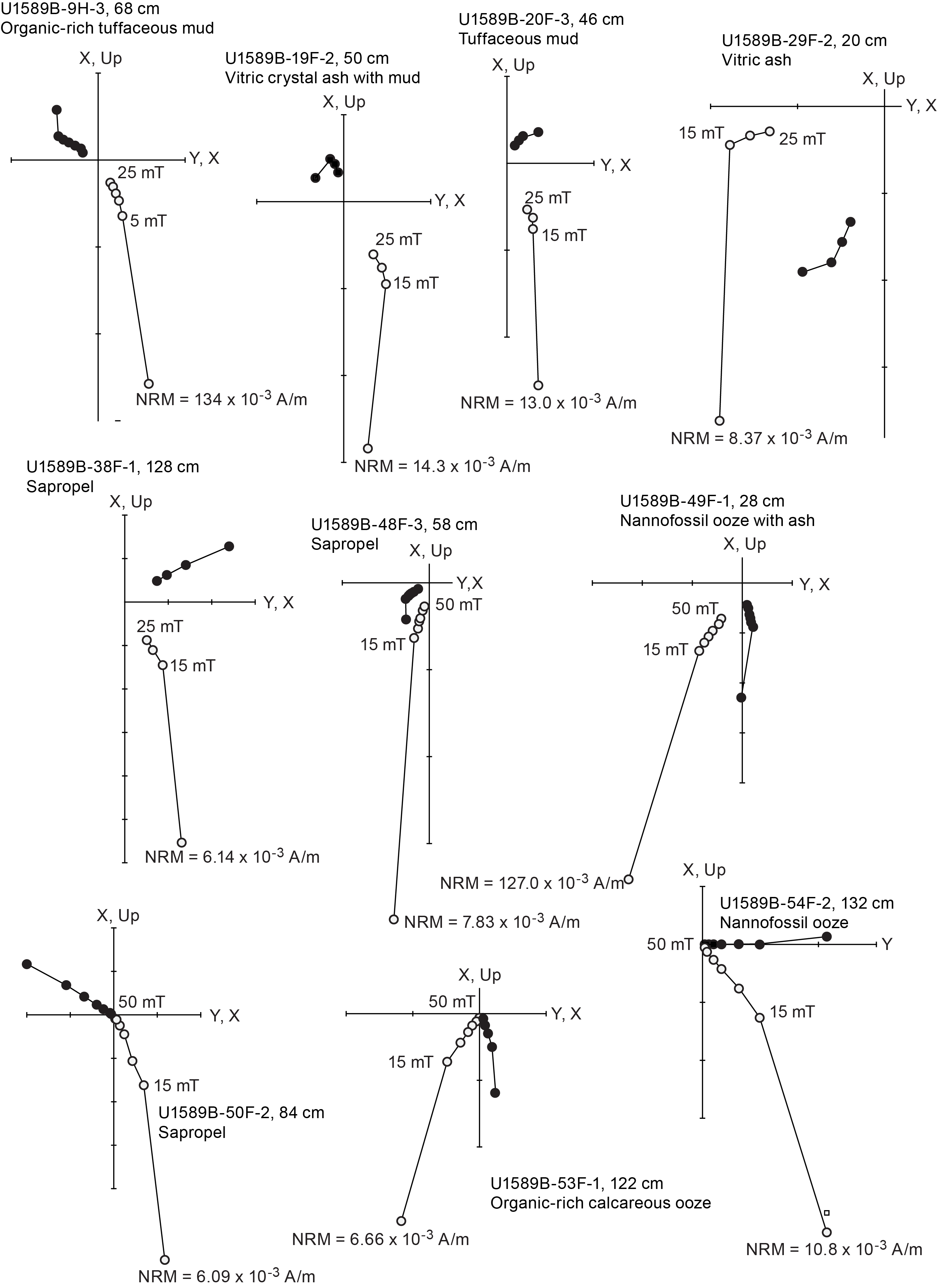
Figure F37. AF demagnetization showing clear linear trends.
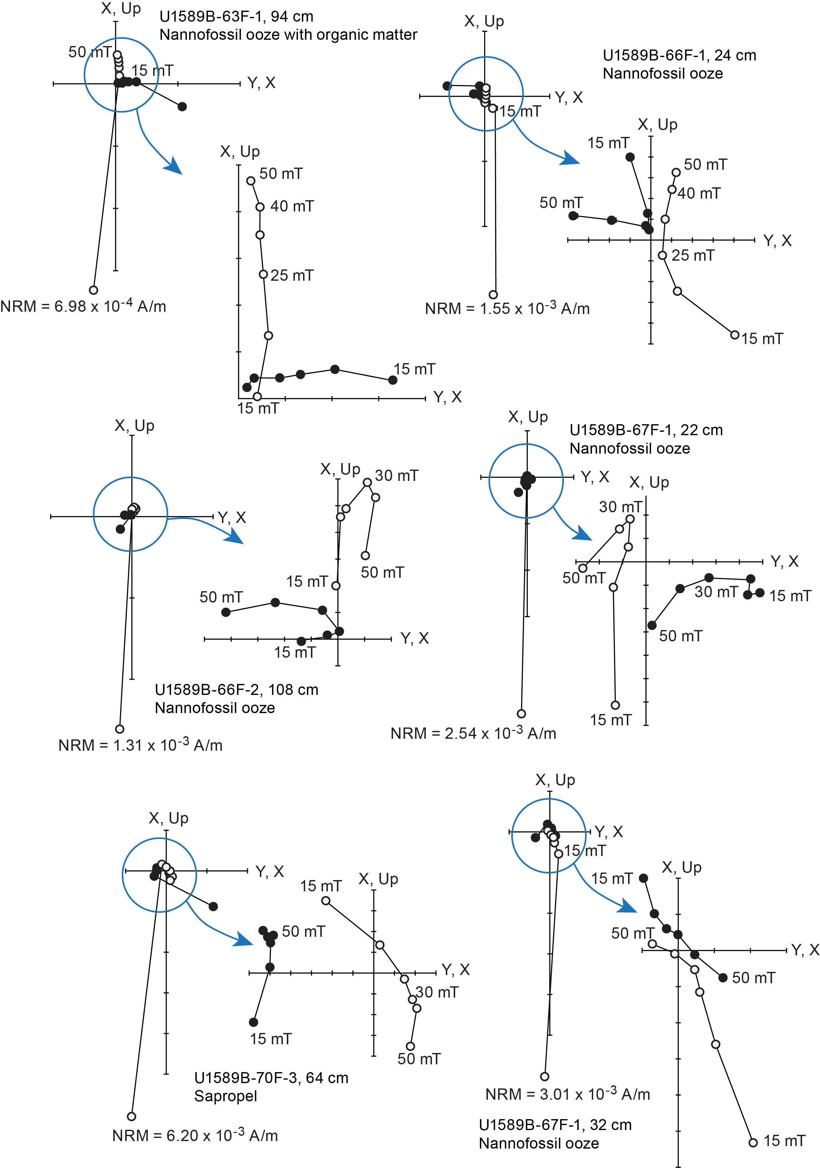
Figure F38. AF demagnetization showing complex directional behavior.
7.3. Downhole variations in magnetic characteristics
Downhole variations in magnetic properties are shown in Figure F39 for Hole U1589A and in Figure F40 for Holes U1589B and U1589C combined. Declinations of magnetizations are azimuthally unconstrained and show wide variations between cores as expected (see below for a discussion of reorientation of APC cores using the Icefield tool). Systematic variations in declination within cores are seen in many cored intervals, typically undergoing a clockwise change in declination with offset that may indicate significant disturbance of cored intervals during sampling. This effect is more pronounced in sections measured in Hole U1589A than those in Hole U1589B and probably reflects measurement of significant numbers of core sections containing easily remobilized/deformed unconsolidated sediments that were omitted from SRM measurements in Hole U1589B. Inclinations are observed to become shallower than the NRM directions following demagnetization at 20 mT, reflecting removal of the DIRM discussed above. Inclinations are consistently positive down to ~320 mbsf in Holes U1589A and U1589B and become more variable in deeper formations, with both shallow and negative inclinations. This change coincides with a distinctive decrease in the median destructive field (defined as the applied AF that reduces magnetization intensities to 50% of their NRM values), indicative of a change in bulk magnetic mineralogy to include lower coercivity minerals. This change also correlates with a decrease in the parameter Int20mT/k (i.e., intensity of magnetization after demagnetization at 20 mT normalized by MS), which is also indicative of a change in magnetic assemblages. Inclinations in the deepest parts of the section (sampled in Hole U1589C), within the siliciclastic units, remain very variable, but low core recovery here makes the magnetic record patchy and difficult to interpret.
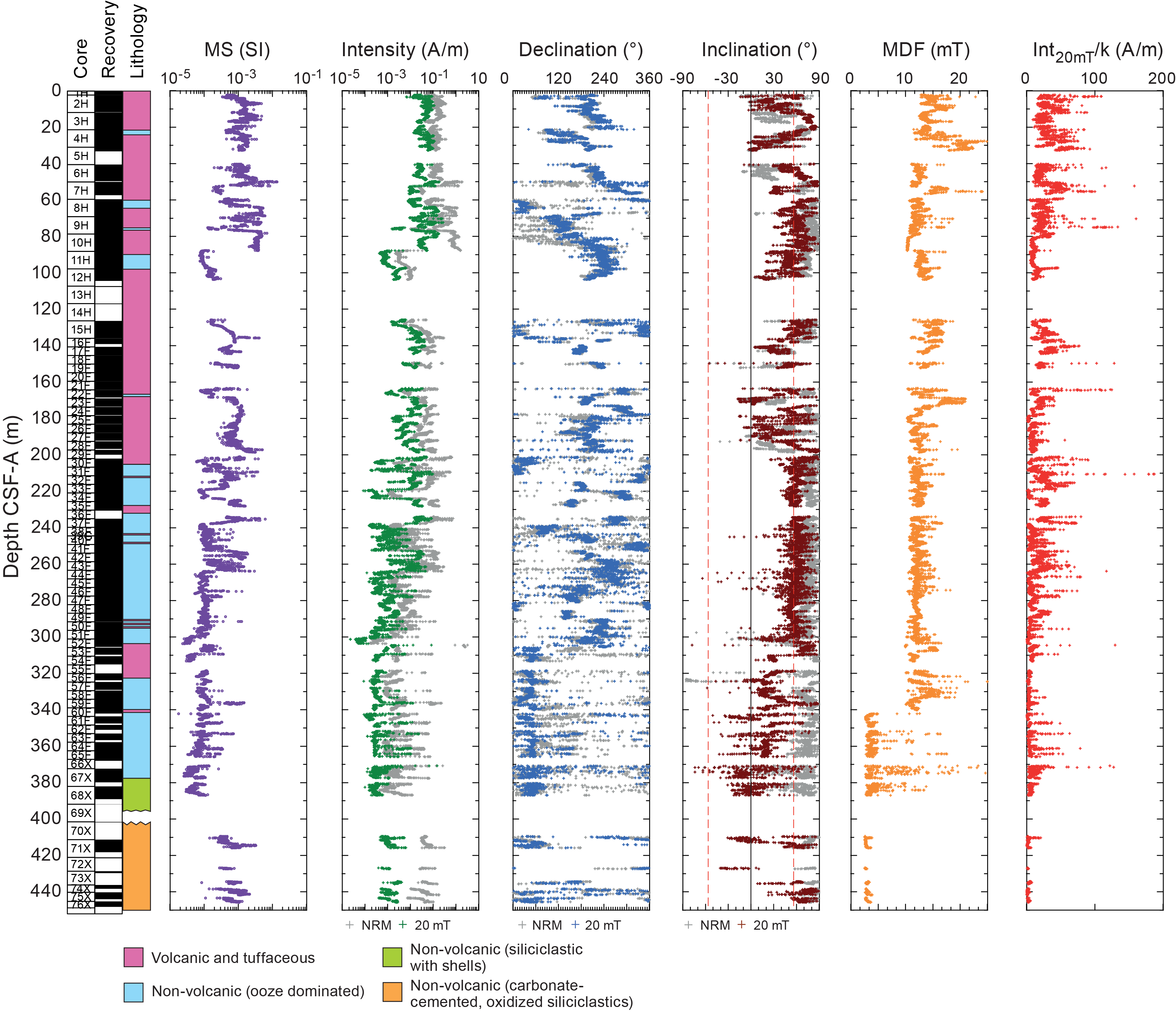
Figure F39. Magnetic data, Hole U1589A.
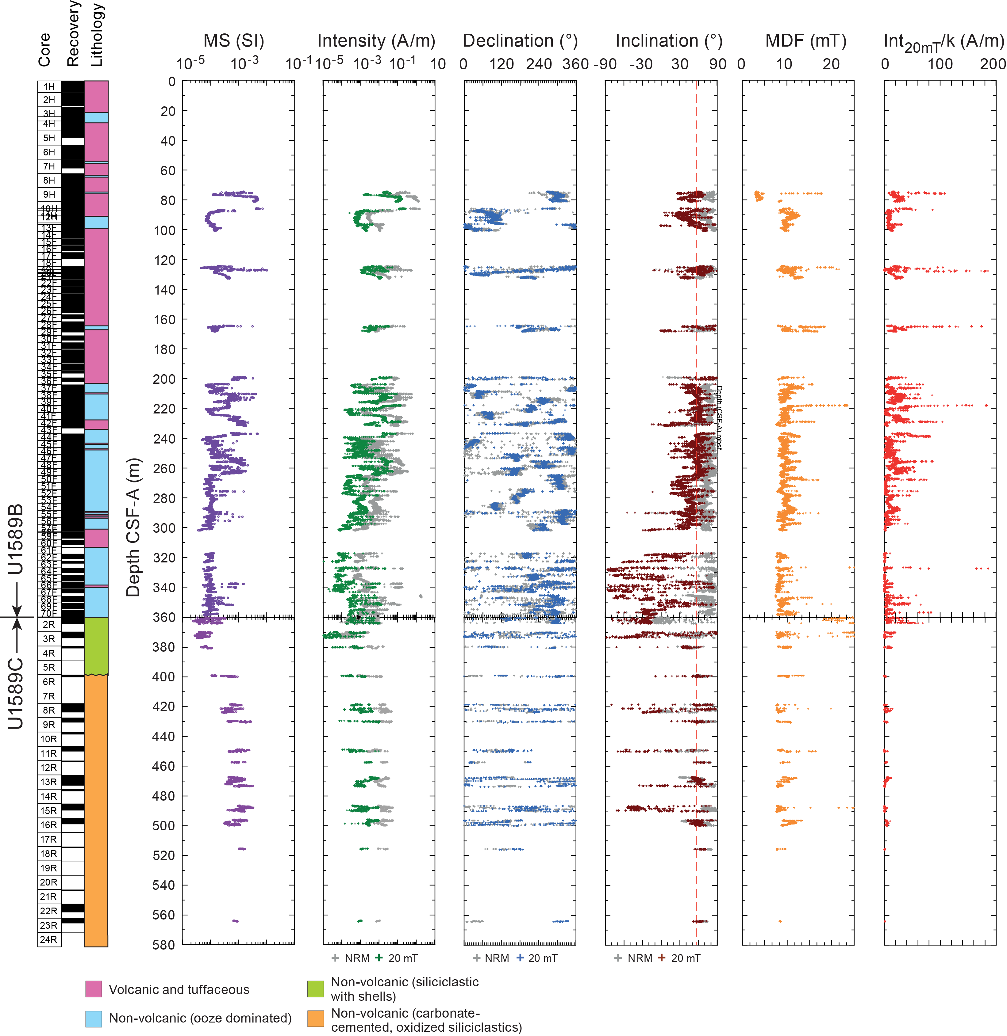
Figure F40. Magnetic data, Holes U1589B and U1589C.
Remanence directions for APC-cored intervals in Holes U1589A and U1589B have been reoriented using constraints from the Icefield tool to restore them to a true geographic reference frame. Figure F41 shows the results of reorienting both NRM and 20 mT demagnetization step directions in both holes. Successful reorientation at this site should result in restoration of declinations to ~000°/360° (or 180° for reversely magnetized samples), and this is only apparent in Hole U1589B, with much more variable restored declinations seen in Hole U1589A. This again could result from coring-related disturbance of some intervals as discussed above.
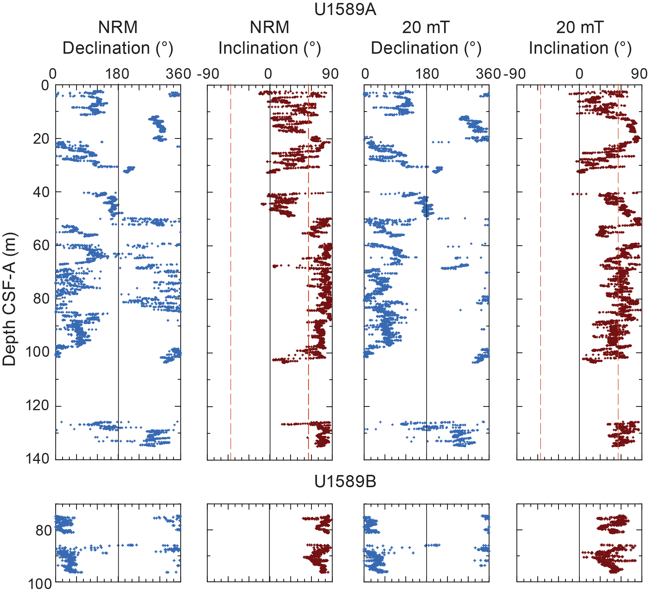
Figure F41. NRM, declination, and inclination.
Demagnetization of archive-half sections at Site U1589 generated a data set consisting of 21,199 individual orthogonal vector plots that could be subject to principal component analysis (PCA) to determine ChRM directions. A common approach to interpretation of such large IODP paleomagnetic data sets is to plot data from a single demagnetization level that is representative of the ChRMs observed downhole (Figures F39, F40). The complex nature of demagnetization paths in many intervals at Site U1589, attributed to the suspected presence of diagenetic greigite, invalidates use of this approach to defining magnetic polarities because the sign of the inclination of the magnetization after any individual treatment level can be contaminated by spurious GRMs. However, manual inspection and analysis of all >21,000 orthogonal vector plots is clearly impossible to achieve given time constraints, so an automated approach to picking directions for magnetostratigraphic purposes has been adopted instead. To minimize the contaminating effects of GRMs acquired at higher field steps, we focused on analysis of remanence directions measured after demagnetization at 15, 20, and 25 mT (note only the 20 and 25 mT steps were used in the upper 340 m of Hole U1589A, prior to an increase in the number of demagnetization steps used thereafter). To automate identification of samples displaying linear decay toward the origin during demagnetization at these treatment levels, we used PuffinPlot software to automatically determine PCAs downhole to produce two alternative sets of least-squares PCA directions, one anchored to the origin and one free of constraints. We then determined the angular difference between the two alternative directions at each measurement point and selectively filtered the resulting downhole data sets to reject all measurements for which this angular difference exceeded 10° and/or the calculated maximum angular deviation of the free-fit line exceeded 10° (Figure F42). Finally, we produced downhole plots of the inclinations of the filtered free-fitting PCAs, representing the highest quality data obtained in each of the three holes sampled at Site U1589.
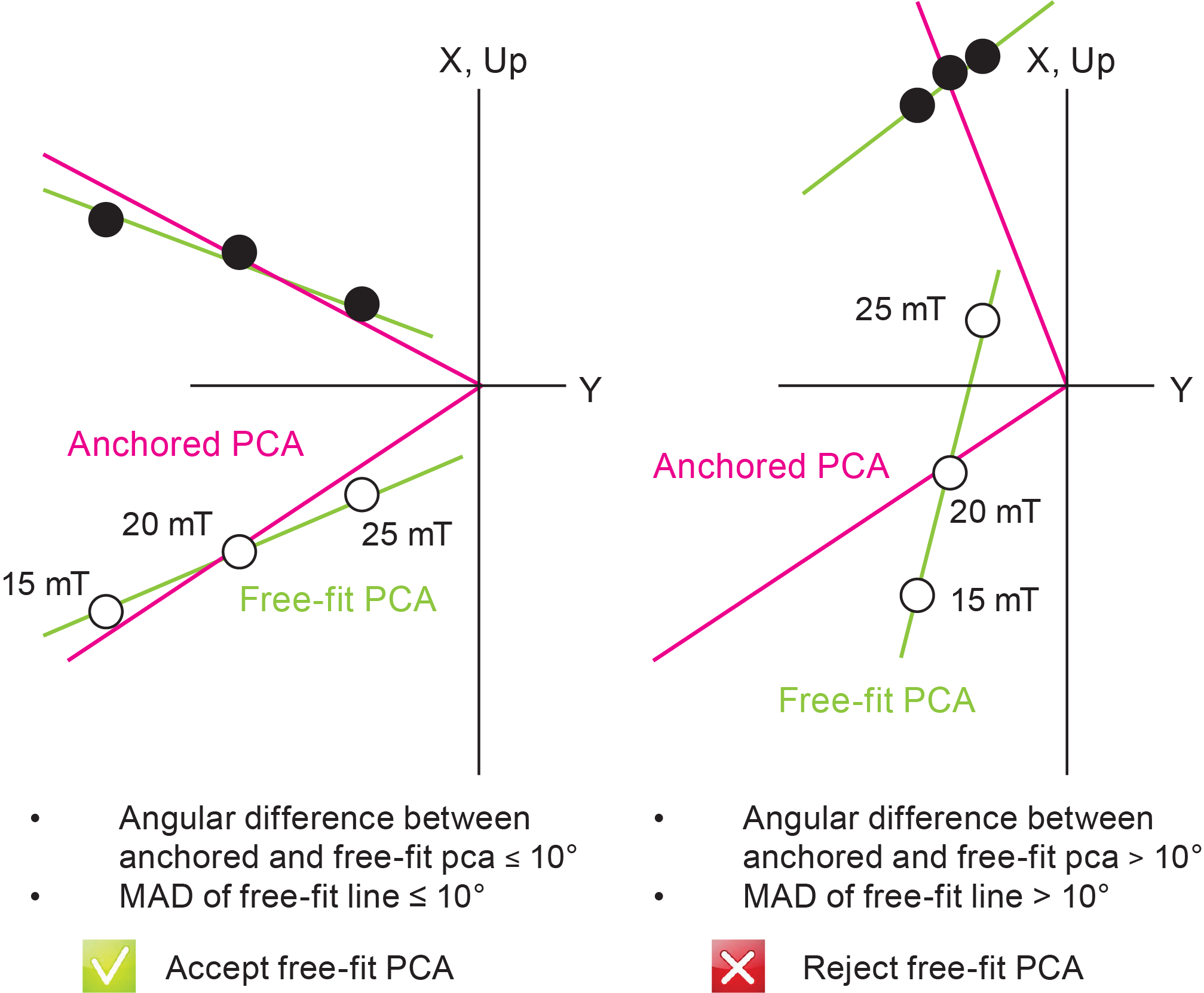
Figure F42. Automated PCA determination process.
Results of this automated PCA selection process are shown in Figure F43. The majority of the highest quality samples occur shallower than 300 mbsf, with only very limited, narrow intervals passing the selection criteria in the interval below this, where we suspect the presence of spurious GRMs carried by diagenetic greigite. The Fisher mean inclination of these data points down to 300 mbsf is 57.3° (k = 21; α95 = 2.2; n = 5099) in Hole U1589A and 58.1° (k = 19.8; α95 = 2.4; n = 3216) in Hole U1589B. These are in good agreement with the geocentric axial dipole (GAD) field inclination of 56° at Site U1589, confirming that the interval from 0 to 360 mbsf carries a normal polarity magnetization acquired in the Brunhes Chron. The scatter in inclinations across this interval (Figure F43) is entirely consistent with the variations expected from paleosecular variation of the geomagnetic field. For comparison, a synthetic data set of field inclinations calculated using the statistical field model TK03.GAD of Tauxe and Kent (2004) for a site at 36.5°N yields mean inclination statistics (mean inclination = 55°; k = 2.21; α95 = 2.0; n = 5099) indistinguishable from those observed in Hole U1589A, confirming that paleosecular variation is adequately sampled down to 300 mbsf at this site.
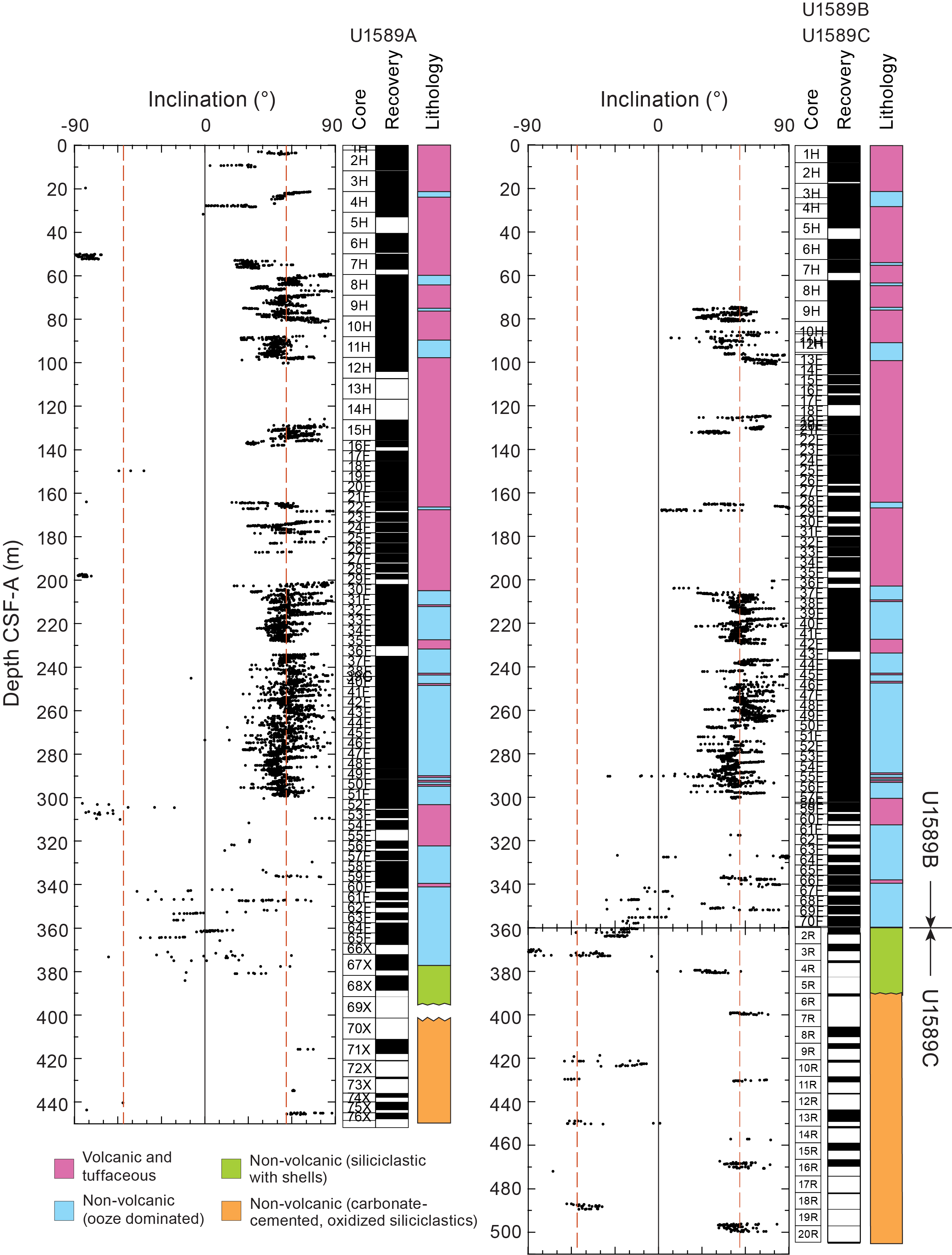
Figure F43. Inclinations of automated PCA free-fit components.
Data from deeper intervals in all three holes at Site U1589 that meet the selection criteria for the automated PCA process are too sparse to draw definitive conclusions concerning magnetic polarity, especially in the siliciclastic units below 380 and 360 mbsf in Holes U1589A and U1589C, respectively.
7.4. Additional tentative correlations with the geomagnetic polarity timescale
As discussed above, the interval above 300 mbsf can be confidently assigned to the Brunhes Chron based on the automated PCA data set, as well as using the single 20 mT demagnetization step data (Figures F40, F44). The scattered inclinations and lack of continuous intervals with acceptable automated PCAs below this depth make confident independent determinations of the magnetostratigraphy impossible. However, reference to the biostratigraphically determined age model for the site makes some further tentative interpretation of part of this deeper interval possible. Figure F44 shows the downhole distribution of automated PCA and 25 mT demagnetization step inclinations for Hole U1589B alongside part of the geomagnetic polarity timescale (Gradstein et al., 2020) converted to the Hole U1589B depth scale using the biostratigraphic age model. In the time period across the Brunhes/Matuyama and Matuyama/Jaramillo reversal boundaries, the age model shows a linear trend (reflecting a constant deposition rate) that is sufficiently well defined to allow prediction of the meters below seafloor depths of these reversals at the site. Specifically, this predicts that the Brunhes/Matuyama reversal should be seen at 330 mbsf and the Matuyama/Jaramillo reversal at 342 mbsf (Figure F44). This places the Matuyama/Jaramillo reversal at the precise depth where a change to consistently shallowly negative to positive 25 mT inclinations is observed (Figure F45). However, the inferred depth of the Brunhes/Matuyama reversal falls in an interval where only negative and unrealistically steep (>80°) 25 mT inclinations are observed. Visual inspection of orthogonal vector plots in this region shows a complete lack of interpretable linear demagnetization trends, suggesting that this reversal is obscured by the effects of spurious magnetizations carried by greigite. Given the quality of the biostratigraphy age controls for this part of the sequence sampled at Site U1589, further investigation of the polarity across this interval is not recommended.
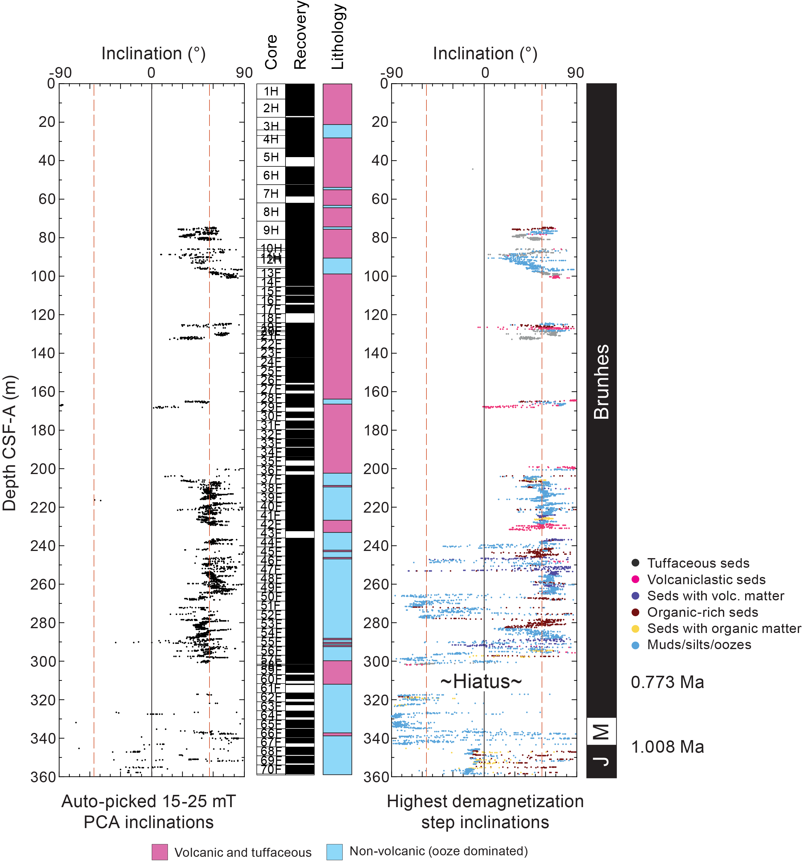
Figure F44. Inclinations before and after 25 mT demagnetization.
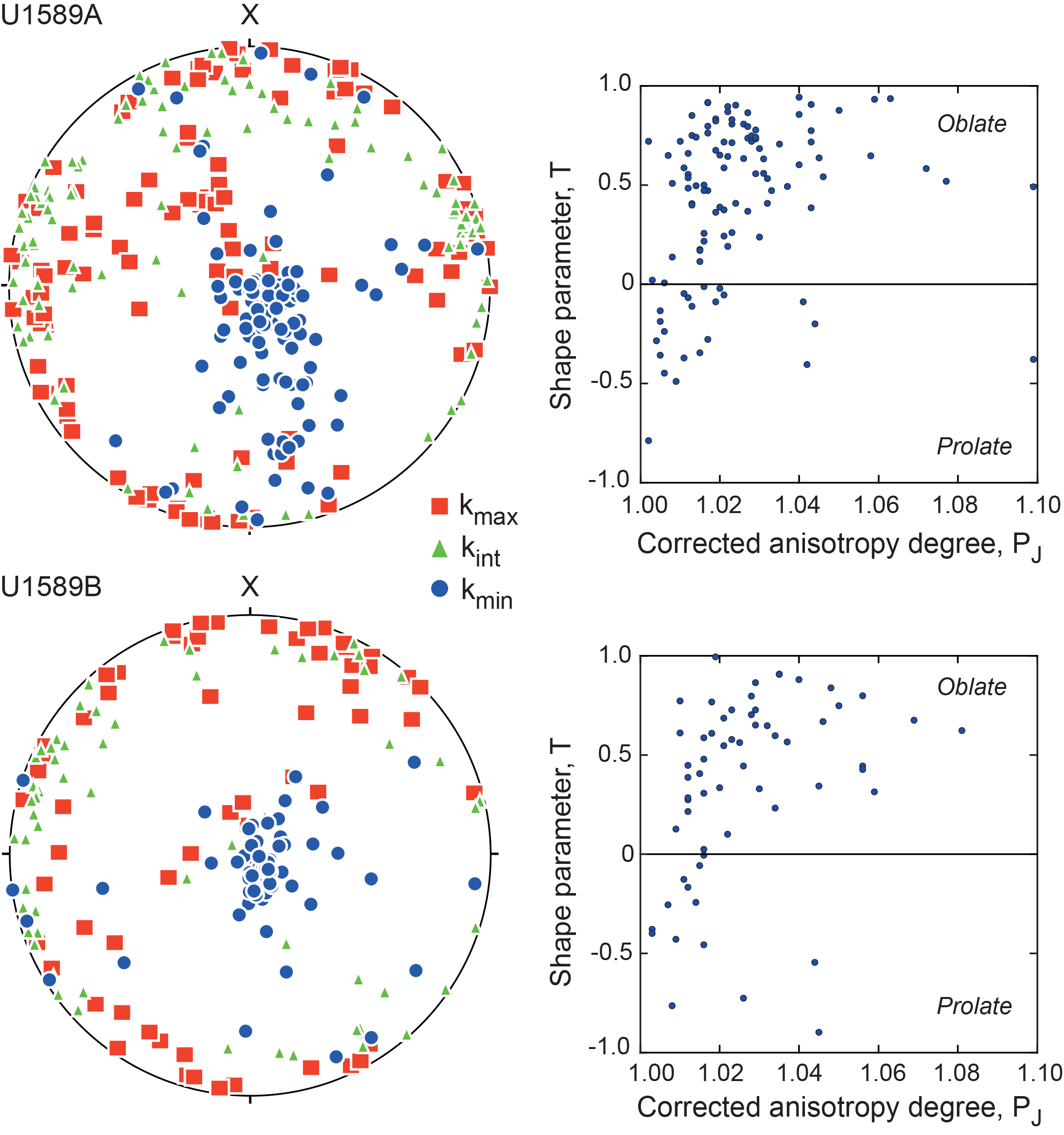
Figure F45. Discrete sample anisotropy.
An interval that may benefit from shore-based paleomagnetic analysis, however, is seen between 240 and 300 mbsf in Hole U1589B. This interval is biostratigraphically dated to be within the Brunhes Chron but exhibits numerous subintervals with negative 25 mT inclinations that occur in close proximity to organic-rich sediments (Figure F45). Detailed paleomagnetic and rock magnetic analysis across this interval may therefore lead to better understanding of the relationships between lithology, the presence/absence of authigenic greigite, and remanence characteristics.
7.5. Anisotropy of low-field magnetic susceptibility
Anisotropy of magnetic susceptibility (AMS) was measured on 171 discrete samples from Holes U1589A and U1589B (Figure F45). In both holes, the distribution of the majority of sample minimum principal susceptibility (kmin) axes is subvertical with subhorizontal girdle distributions of intermediate (kint) and maximum (kmax) axes. Corrected anisotropy degrees, PJ, reach maximum values of 1.10 (i.e., 10% anisotropy), but the majority of samples have moderate anisotropies of ~1.01–1.04. Shape parameters are mainly positive, indicating dominance of oblate anisotropy ellipsoids. These distributions are characteristic of primary depositional fabrics, with kmin principal axes oriented normal to bedding. Such fabrics could also potentially result from compaction, but this would be accompanied by a shallowing of observed inclinations away from the expected GAD inclination, which is not seen here. Without reorientation parameters for all samples, it is impossible to determine whether there is a consistent preferred magnetic lineation present that may be indicative of flow. A subset of samples display markedly different magnetic fabric with steeply inclined kmax principal axes and subhorizontal kmin principal axes (Figure F45). This suggests the presence of inverse magnetic fabrics (Potter and Stephenson, 1988), which may potentially be due to the presence of authigenic greigite. Such fabrics have previously been reported in AMS analyses of greigite-enhanced organic-rich sapropel layers from the eastern Mediterranean Sea (Roberts et al., 1999, 2011).
8. Physical properties
Downhole variations in physical properties arise from changes in lithology, compaction, and other diagenetic processes. The drilled formations at Site U1589 fall into three main groups that can be related to their physical properties:
- Volcaniclastic (Lithostratigraphic Unit I),
- Oozes and muds (Unit II), and
- Siliciclastic and terrigenous sediments and basement rocks (Units III–V).
Differences between volcanic and other lithologies are most prominent in MS because of the abundance of ferromagnetic minerals (e.g., magnetite) in volcanic sediments (high) and oozes and muds (low). Density is expected to increase progressively with increasing depth owing to compaction, but low-density pumice deposits and unconsolidated ash layers between compacted biogenic ooze create a more complex porosity structure throughout the drilled formation. Similarly, shear strength and thermal conductivity both increase with depth but are often reduced in volcaniclastic units relative to adjacent materials.
In general, at this site volcaniclastic units have higher MS, lower P-wave velocity, and lower density than other sediments at the same depth. Thus, physical property measurements can be used to interpret downhole logging data and to help identify thin ash and pumice layers in mostly biogenic compacted sediment. All depths in this section reference the CSF-A depth scale.
8.1. Whole-round GRA density, MS, P-wave velocity, and NGR
Figure F46 summarizes data collected on whole-round cores measured using the GRA densitometer, MS loop, and P-wave logger on the WRMSL and NGR on the NGRL. These data should be interpreted with care, based on the following considerations:
- For GRA density and P-wave velocity, depth-dependence (with either increasing or decreasing trends) in physical property values in a core or individual section can be an artifact from redistribution of water-rich cored materials in the core liner (producing, for example, downhole zigzag patterns of measured properties; e.g., density values at 100–200 mbsf).
- Discrepancies between MS values measured on the WRMSL and STMSL versus the SHMSL (see Lithostratigraphy) are due mainly to the loop versus contact methods that calculate measured volume susceptibility by assuming the core liner is filled with cored materials.
- Recovered cores of unconsolidated materials can contain large amounts of extra water that can lower the values of all physical property measurements made on whole-round cores. Thus, there are some inaccurate groups of density and P-wave velocity data (and sometimes unfeasible data such as values less than those for seawater) in the measured whole-round data sets. Whole-round P-wave velocity data were not collected for Hole U1589C because the recovered RCB cores do not fill the core liner.
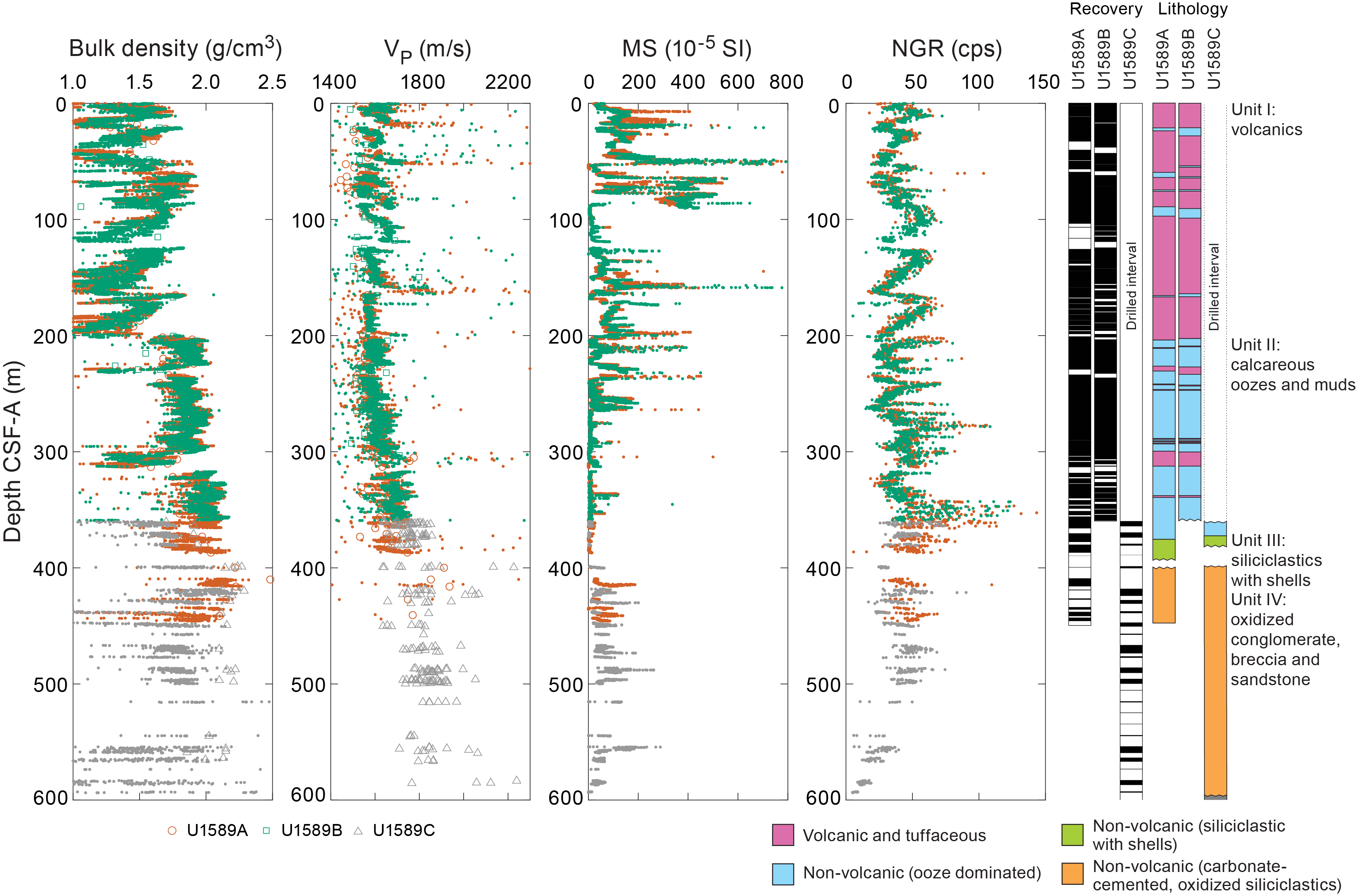
Figure F46. GRA bulk density, P-wave velocity, MS, and NGR.
Changes in MS correlate with changes in major lithostratigraphic units (Figure F46). Where volcaniclastic sediments exist, MS is high. MS reaches maximum values of 1000 × 10−5 to 1225 × 10−5 SI between 51.2 and 51.6 mbsf. To ease visualization, only MS values up to 800 × 10−5 SI are shown on the figure. At all depths where MS values are high, we observe volcaniclastic materials (see Lithostratigraphy). In oozes and muds, MS values remain low (mostly <100 × 10−5 SI). In Lithostratigraphic Units III–V, whole-round MS values are also low (<300 × 10−5 SI). Bulk density also correlates with the type of cored material, showing high values (2.1 g/cm3) in compacted biogenic sediments to values sometimes <1.3 g/cm3 in pumice layers. P-wave velocity increases with depth, from typically ~1.5 km/s in the uppermost 100–200 m to ~1.7 km/s in the compacted biogenic sediments. The highest P-wave velocities, closer to 2.0 km/s, occur in Unit III and deeper. Most of the lowest P-wave velocities are observed in formations that correspond to porous cored materials such as volcaniclastic layers with lapilli (i.e., 2–64 mm diameter pumices; see Lithostratigraphy in the Expedition 398 methods chapter [Kutterolf et al., 2024]). NGR shows less variability than MS (Figure F46).
A more detailed illustrative example of correlations between lithology and physical properties, Figure F47 shows physical property measurements for one example interval of recovered core (Sections 398-U1589B-66F-1 through 66F-3). Relative to background sediment, the two volcaniclastic layers, composed of tuffaceous nannofossil ooze, have higher MS and lower bulk density and P-wave velocity. There is no consistent signature in the NGR data. The organic-rich layer in this core has lower bulk density, higher NGR, and low MS.
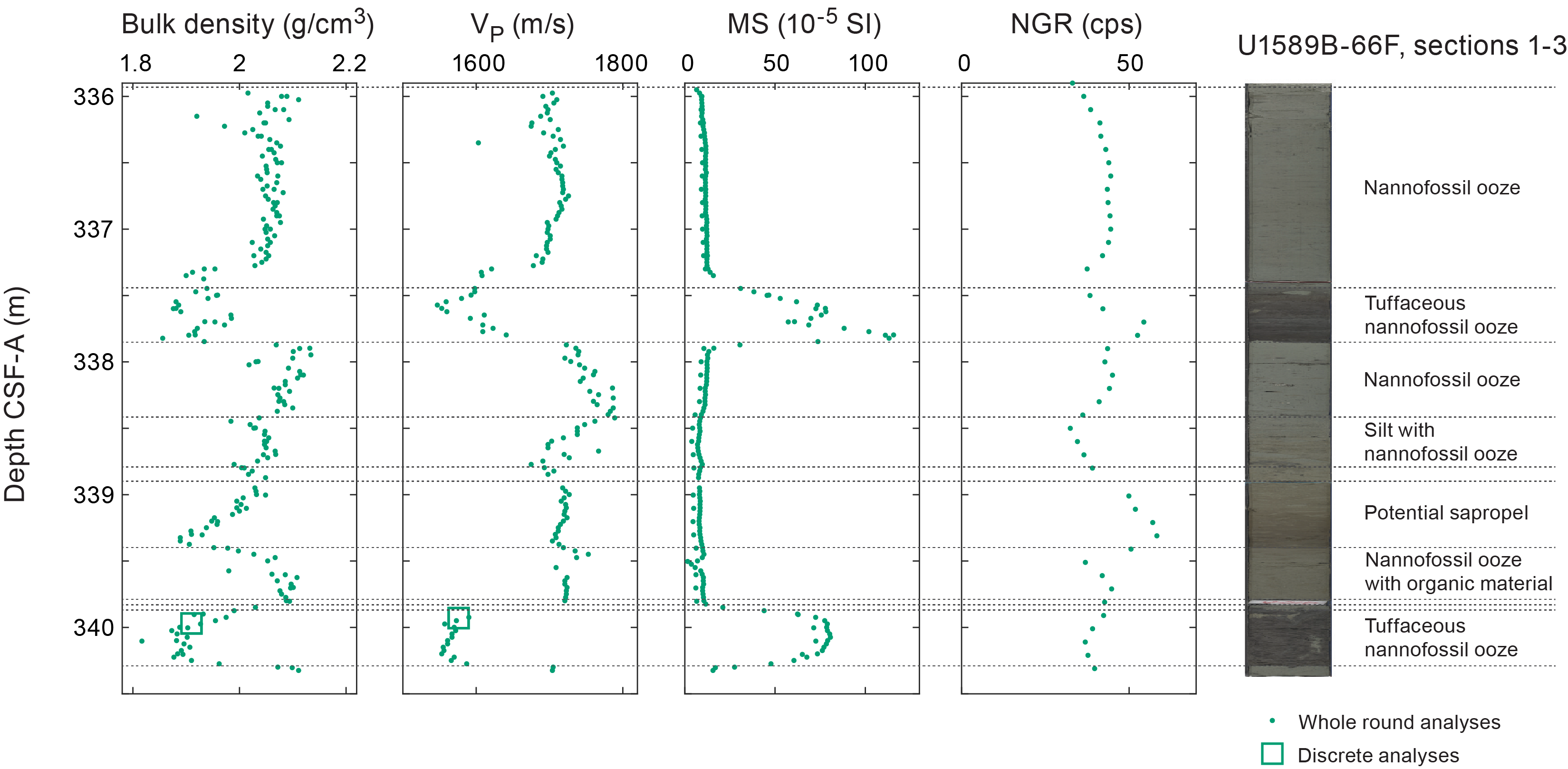
Figure F47. Lithology and physical properties measurements.
8.2. Discrete measurements
8.2.1. Material strength
Sediment strength was measured with a pocket penetrometer (PP) on the catwalk immediately after section splitting. Automated vane shear (AVS) strength measurements were made on working-half sections. Totals of 49 and 47 AVS measurements were made on working-half sections in Holes U1589A and U1589B, respectively (Table T11). AVS measurements were not made in Hole U1589C because recovered materials were consolidated or solid rocks with strengths beyond the detection limit of AVS. The compressional strength measured using the PP is divided by 2 as an estimate of shear strength and converted to kilopascals from the force measurement (see Physical properties in the Expedition 398 methods chapter [Kutterolf et al., 2024]). A total of 19, 41, and 1 PP measurements were made on cored materials from Holes U1589A, U1589B, and U1589C, respectively (Table T11). Measurements were only made in fine-grained materials that remained intact (i.e., not liquified) in core liners upon recovery on the catwalk.
Figure F48 shows shear strength as a function of depth and lithology. During measurement of material from Hole U1589A, the adapters used for the PP measurements only enabled measurements up to 220 kPa. In general, shear strength increases with increasing depth. There are several depths, however, with large decreases in shear strength (e.g., ~40, 100, 150, 210, and 300 mbsf) that correspond to volcaniclastic-rich lithologies or contacts between volcaniclastic and other lithology types. The origins of these decreases in shear strength remain uncertain because of the uncertainty of whether material weakness documents in situ conditions or is affected by coring and sample recovery.
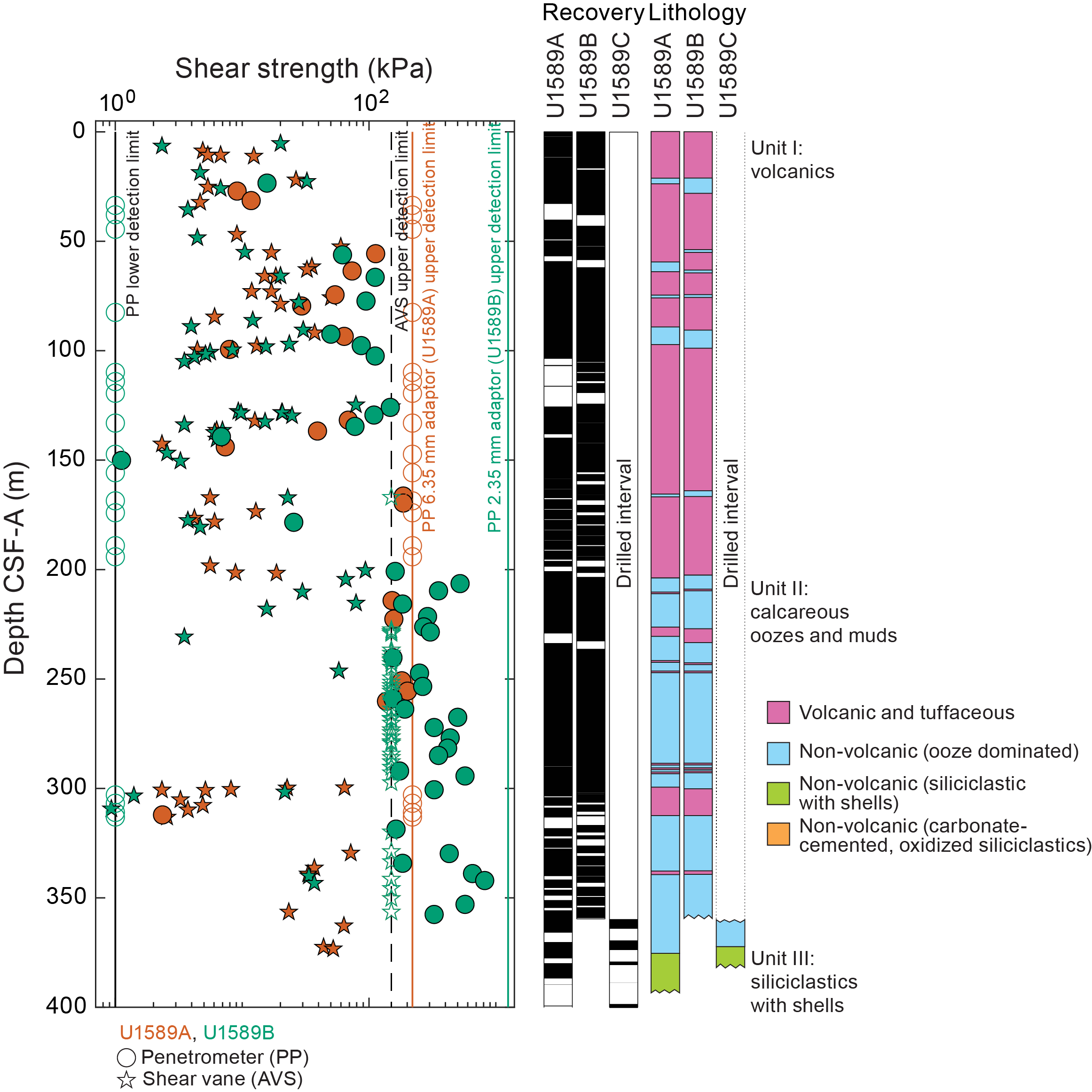
Figure F48. AVS shear strength and PP compressional strength.
Below 400 mbsf (with one exception at 468.2 mbsf in Hole U1589C with a shear strength of 1.08 MPa, not plotted in Figure F48), shear strength measurements taken with the PP consistently exceeded the measured values using AVS, indicating that shear strength is >1.3 MPa. Open symbols plotted on a line at 150 or 1.25 MPa for the AVS and PP measurements, respectively, indicate shear strengths greater than those that could be measured. When values were too low to measure, an open symbol is plotted on a line at 1 kPa.
8.2.2. P-wave velocity
Discrete measurements of P-wave velocity on working-half sections follow the trend observed by WRMSL measurements on whole-round cores (Figures F46, F49; Table T12). Discrete measurements should be more reliable than WRMSL measurements because the calipers measure the P-wave velocity of cored materials by direct contact, whereas the WRMSL measures core liners that contain water pockets, fractures, and other gaps in the recovered materials.
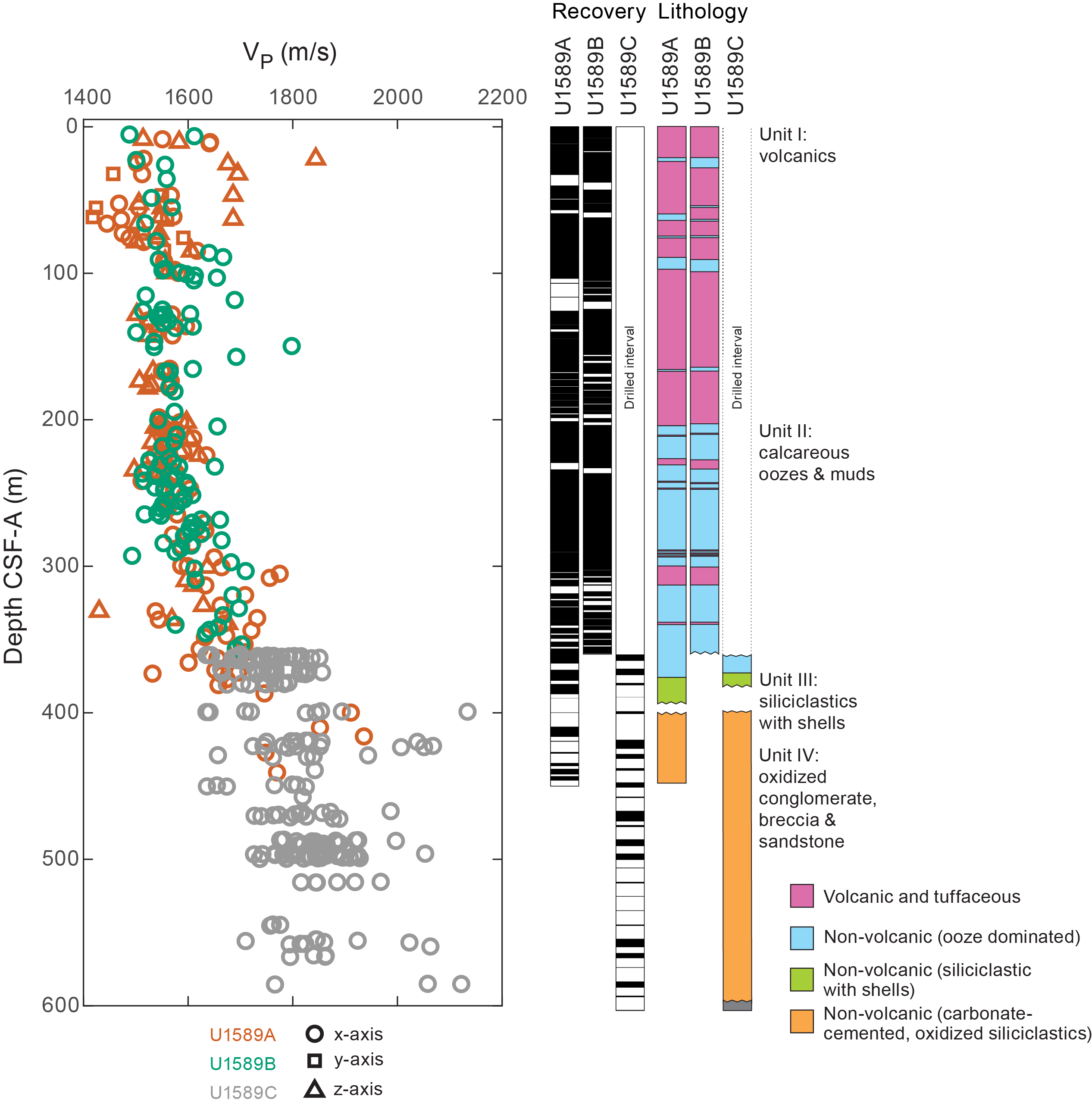
Figure F49. P-wave velocity.
Totals of 94, 104, and 206 discrete P-wave velocity measurements were made in Holes U1589A, U1589B, and U1589C, respectively (Table T12). Samples with measured P-wave velocities > 2.2 km/s are listed in Table T12 but not plotted in Figure F49 to highlight variations in the vast majority of cored lithologies. In Hole U1589A, when sediments were soft enough to be penetrated without fracture using P-wave bayonets, velocities in the y- and z-directions were measured. No systematic difference between the x-, y-, and z-directions were observed; thus, there is no clear sign of anisotropy. We therefore only measured x-direction P-wave velocity in Hole U1589B. In Hole U1589C, only one sample was measured in all three directions. Measurements on this 2 cm cube of basement limestone from volcanic Unit IV had the highest P-wave velocity of >4.5 km/s (Table T12).
8.2.3. Moisture and density
Totals of 114, 46, and 28 discrete samples were collected from Holes U1589A, U1589B, and U1589C, respectively, to conduct moisture and density (MAD) measurements (Figure F50; Table T13). Bulk density derived by MAD measurements on discrete samples should be more reliable than GRA density from WRMSL on whole-round cores. Primary measured values are mass and volume of sampled materials. Porosity and bulk density are derived from these measurements (see Physical properties in the Expedition 398 methods chapter [Kutterolf et al., 2024]).
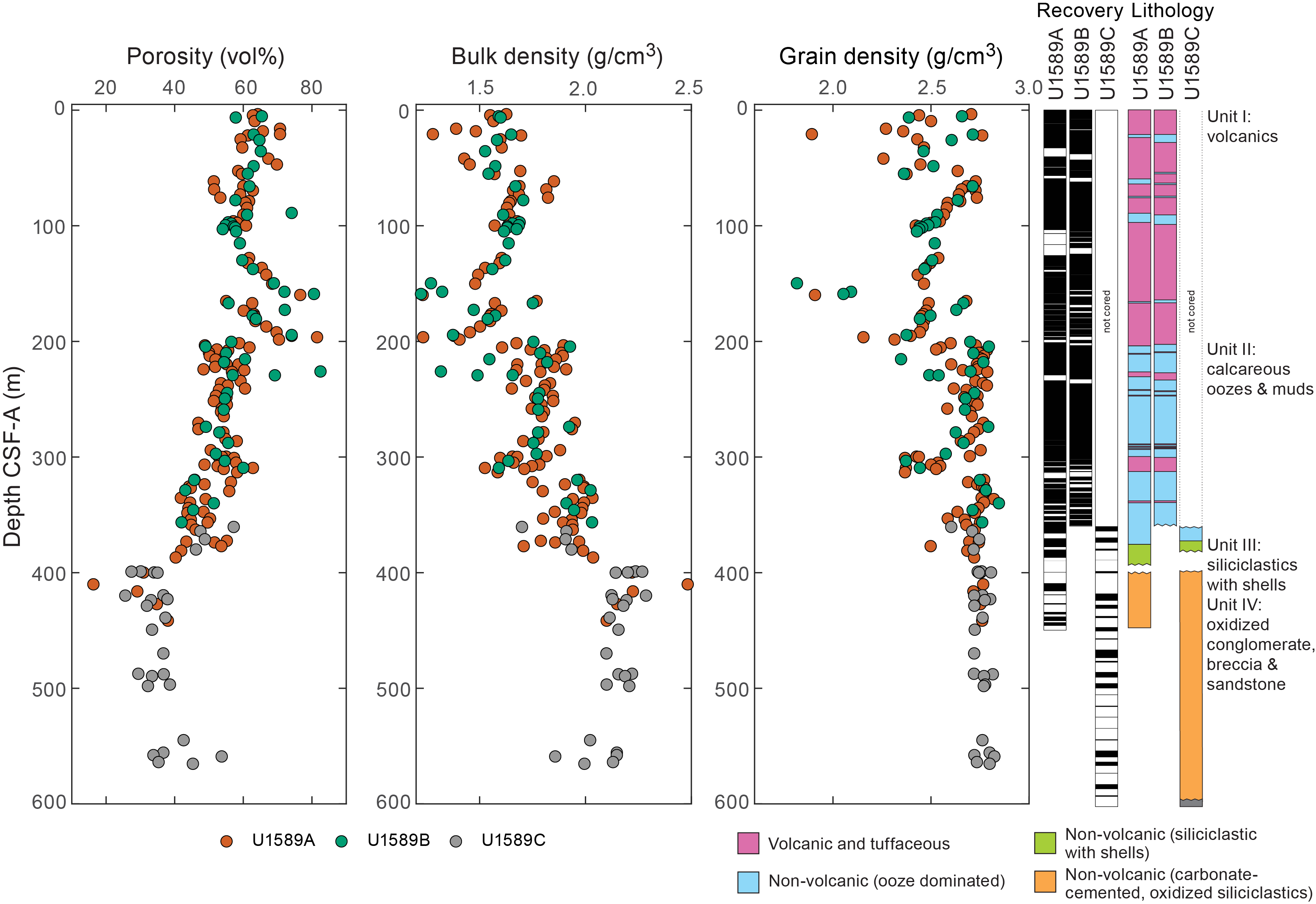
Figure F50. Porosity, bulk density, and grain density.
Porosity ranges 16–83 vol%. Volcanic lithologies generally have higher porosity than other recovered materials. At Site U1589, porosity decreases with increasing depth except for Lithostratigraphic Unit IV, where porosity increases with depth.
Bulk density ranges 1.2–2.5 g/cm3. Bulk density is lowest in volcaniclastic units and increases with depth, with a jump at the top of Unit IV.
Grain density in volcaniclastic units averages ~2.5 g/cm3 and increases to ~2.7 g/cm3 in pelagic and hemipelagic sediments.
8.2.4. Thermal conductivity
A total of 91 thermal conductivity measurements were made on selected working-half sections from Holes U1589A–U1589C. Overall, thermal conductivity increases with depth (Figure F51; Table T14). The mean value in the uppermost 50 m is 0.895 ± 0.088 W/(m·K) compared to a mean of 1.50 ± 0.28 W/(m·K) deeper than 300 mbsf. A least-squares linear fit to the thermal conductivity data is k(z) = (0.804 ± 0.032) + (0.00167 ± 0.00013)z W/(m·K) (with z in m and k in W/[m·K]), with large scatter about the trend. In measured sections, thermal conductivity is lower in volcaniclastic-rich sediment compared with volcaniclastic-poor sediment. The lowest value of 0.66 W/(m·K) is found in a pumice layer in Section 398-U1589B-5F-2 at 149.6 mbsf. The highest thermal conductivities of >1.5 W/(m·K) are found in dense measured sections from Lithostratigraphic Units III and IV below 370 mbsf. Thermal conductivity could not be measured on very coarse, permeable samples. Thus, an inherent sampling bias may affect mean values, variability, and trends.
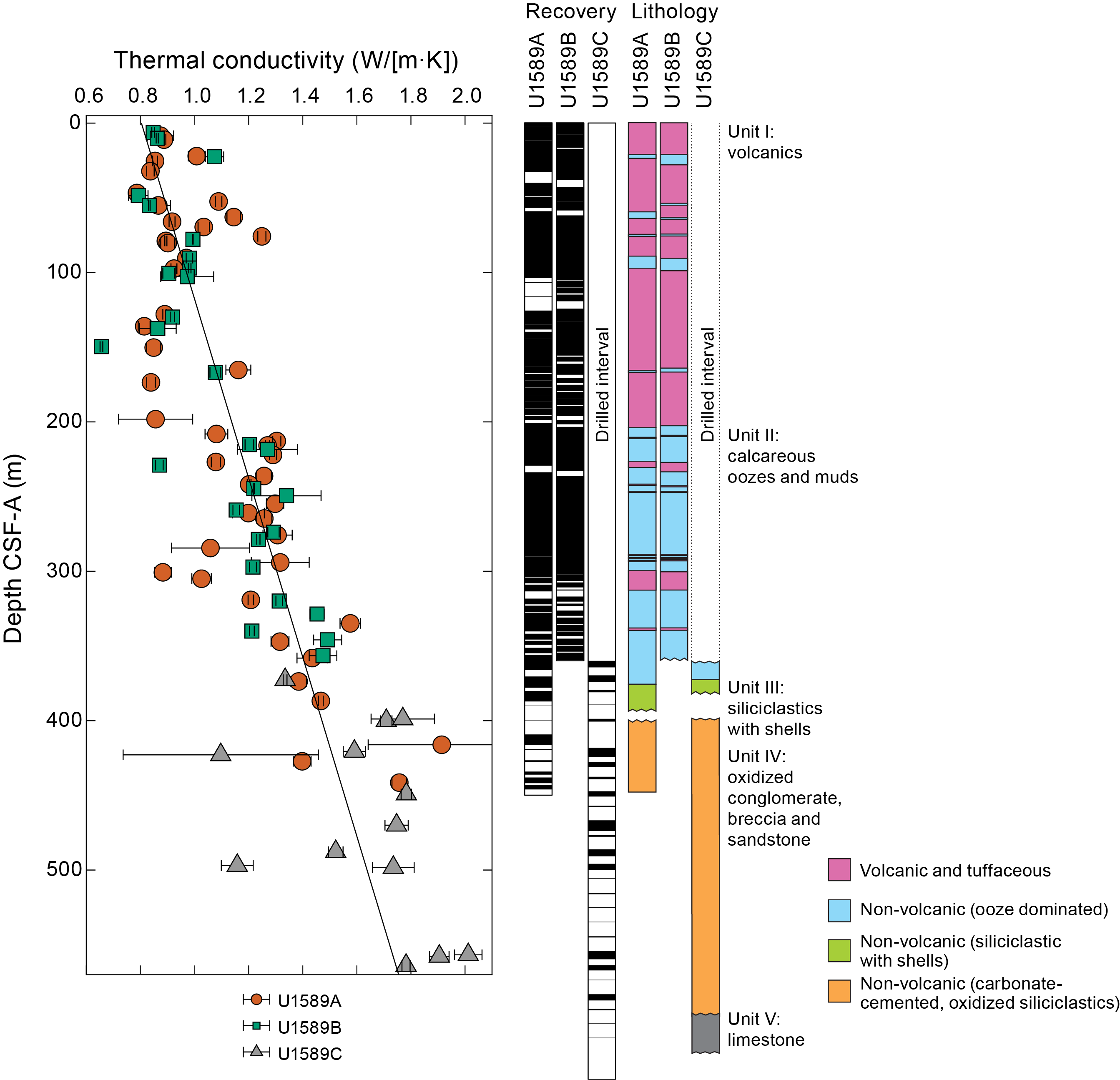
Figure F51. Thermal conductivity.
8.3. Downhole temperature measurement
Downhole temperature was measured using the APCT-3 tool at the bottom of Hole U1589A (Cores 4H, 7H, 10H, and 13H; 30.7, 59.2, 87.7. and 116.3 mbsf, respectively) and the bottom of Hole U1589B (Cores 5H, 6H, 8H, 11H, and 14F; 43.0, 52.5, 71.5, 85.7, and 105.6 mbsf, respectively). Additionally, the SET2 tool was deployed at the bottom of Hole U1589B (Cores 54F and 70F). The temperature of ocean water at the seafloor was 15.47 ± 0.05°C based on mudline temperature measurements from Core 14H.
Temperature was modeled from time-series measurements using TP-Fit software (see Physical properties in the Expedition 398 methods chapter [Kutterolf et al., 2024]). In modeling, a thermal conductivity of k = 1.0 W/(m·K) and a product of density and specific heat of ρC = 3.7 × 10⁶ J/(m3·K) were assumed for APCT-3 measurements, whereas k = 1.2 W/(m·K) and ρC = 3.7 × 10⁶ J/(m3·K) were assumed for SET2 measurements at greater depths. An uncertainty in k of ±0.15 W/(m·K) (based on our measurements) and in ρC of ±0.3 × 10⁶ J/(m3·K) were also assumed to calculate the uncertainty in temperature.
Time-series temperature measurements from Cores 398-U1589A-4H, 7H, and 10H, and 398-U1589B-11H did not show monotonic decreases in temperature after inserting the APCT-3 tool. Instead, the time-series measurements showed multiple jogs attributed to tool motion. To extrapolate the measured temperature time series to the formation temperature, the model assumes that heat is generated only during the initial insertion of the tool into the formation. Hence, we do not calculate formation temperatures or interpret their values when temperature measurements show clear disruptions in the time series.
There is little change in temperature with depth (Figure F52; Table T15). For reference, we plot a temperature gradient of 100°C/km, which, assuming a thermal conductivity of 1 W/(m·K) for sediment at Site U1589, would lead to a heat flow similar to other rifting environments such as the Basin and Range, USA (e.g., Blackwell, 1983). The best-fit linear relationship for the four deepest measurements in Hole U1589B is 4.0 ± 0.2°C/km.
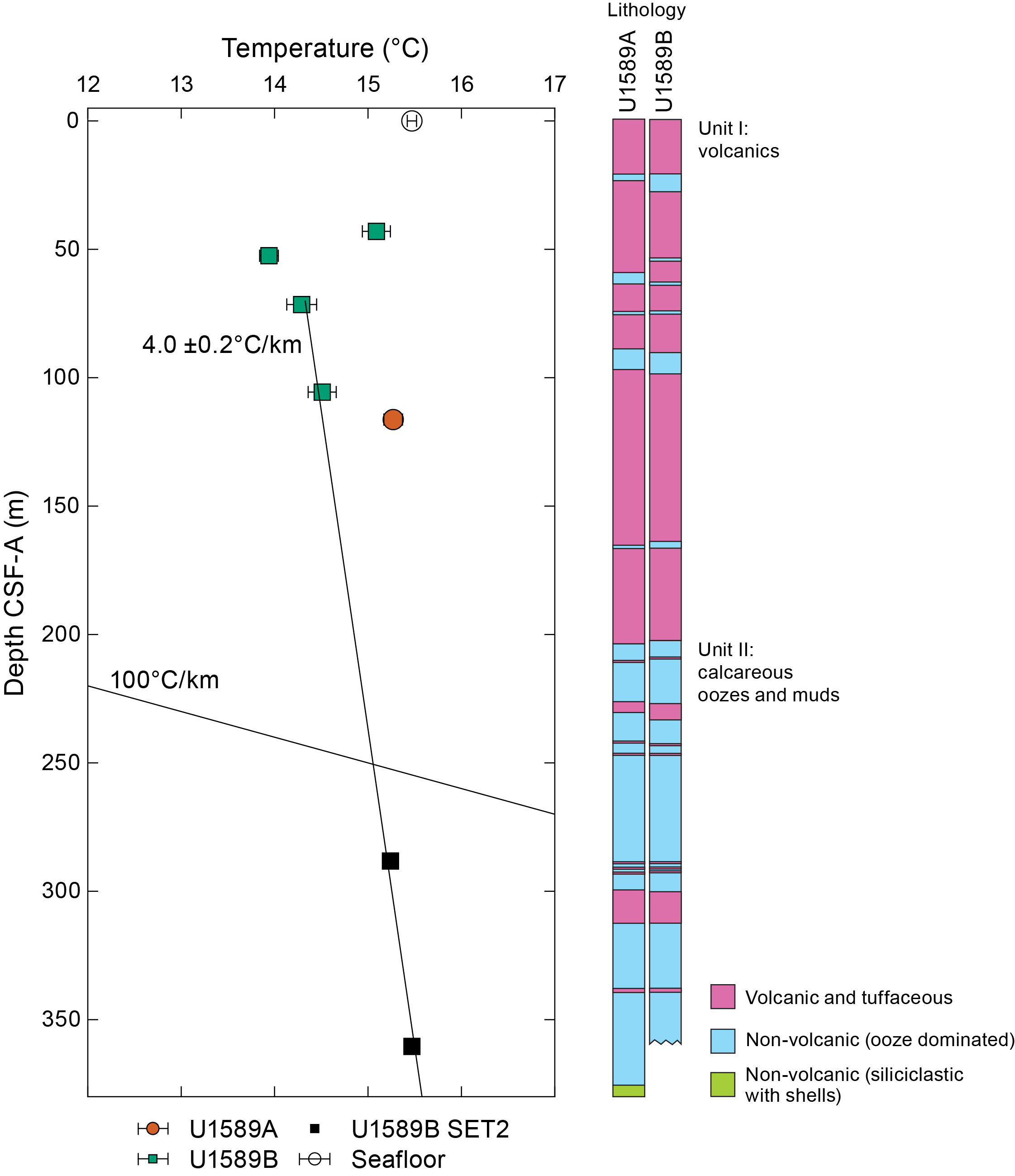
Figure F52. Downhole temperature.
9. Geochemistry
9.1. Volcaniclastic bulk geochemistry
To determine the geochemistry of the volcanic and tuffaceous materials, 17 pumice and ash samples were handpicked from various layers in Hole U1589A. Following cleaning, grinding, fusion, and dissolution, the volcaniclastic material was analyzed shipboard for major (Si, Al, Fe, Mg, and Ca), minor (Ti, Mn, Na, K, and P), and trace (Sc, V, Cr, Co, Ni, Cu, Zn, Rb, Sr, Y, Zr, Nb, Ba, Ce, and Nd) elements using inductively coupled plasma–atomic emission spectroscopy (ICP-AES) (see Geochemistry in the Expedition 398 methods chapter [Kutterolf et al., 2024] for analytical technique). Several unknown samples were run multiple times to determine analytical reproducibility.
9.1.1. ICP-AES: major, minor, and trace elements
Of the volcaniclastic units sampled, 2 were classified as basaltic andesites or basaltic trachyandesites, 4 as andesites or trachyandesites, 11 as dacites or trachydacites, and 3 as rhyolites (Table T16; Figure F53). Bulk chemistry values are less evolved than glass chemistry reported in Kutterolf et al. (2021), as expected due to bulk analyses including both minerals and glass. One section (398-U1589A-2H-3) was discarded because low totals indicated it was not purely volcanic.
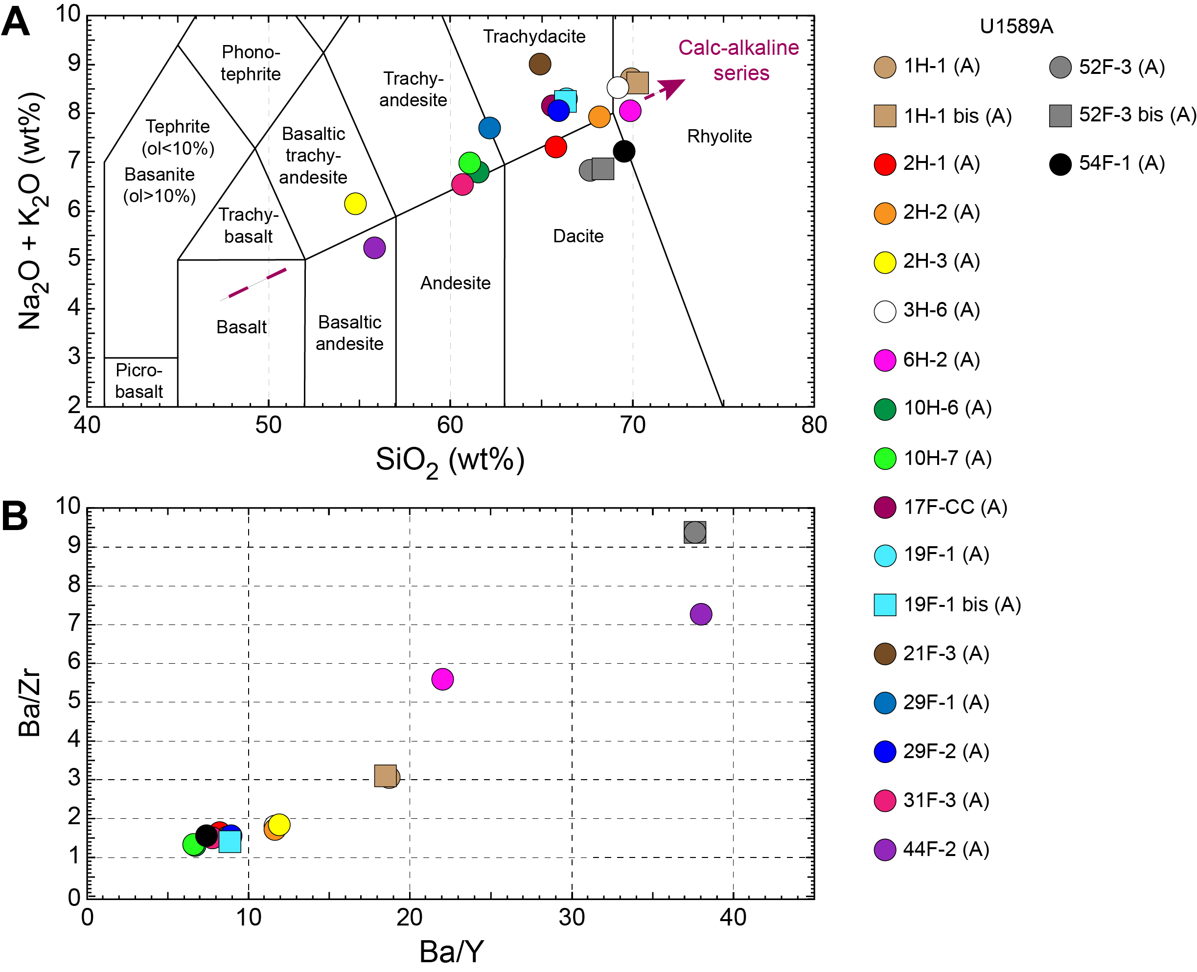
Figure F53. ICP-AES analyses of volcaniclastic units.
Concentrations are reported for all analyzed trace elements, but Ce, Cr, Cu, Nb, Ni, P, Rb, S, and V were below detection limits in the majority of samples and are not shown in Table T16. Trace element ratios were used to broadly discriminate between the volcanic centers of Kolumbo, Santorini, and Christiana.
9.2. Interstitial water geochemistry
To determine the inorganic constituents of IW, a total of 47 water samples were taken from whole-round squeezing of sediment intervals from Holes U1589A (36 samples), U1589B (8 samples), and U1589C (3 samples). Aliquots of IW were used for shipboard analyses, and the remaining water was retained for shore-based analysis, following protocols specified by individual scientists. The retrieved pore waters were subsequently analyzed shipboard for salinity, alkalinity, pH, major anions (Cl−, SO42−, and Br−), major cations (Ca2+, Na+, Mg2+, and K+), and major (S, Ca, Mg, K, and Na) and minor (B, Ba, Fe, Li, Mn, P, Si, and Sr) elements by the methods described in Geochemistry in the Expedition 398 methods chapter (Kutterolf et al., 2024).
9.2.1. Salinity, alkalinity, and pH
Salinity varies from 34 to 40 throughout the hole, which corresponds to current average Aegean salinity value of 39. Several anomalously high salinity values were recorded in six sections (398-U1589A-54F-2, 56F-2, and 68X-4; 398-U1589B-57F-2 and 60F-2; 398-U1589C-13R-3), with a maximum value of 50 at 320 mbsf (Section 398-U1589A-54F-2). Slight variations in the salinity are observed below 250 mbsf (Table T17; Figure F54).
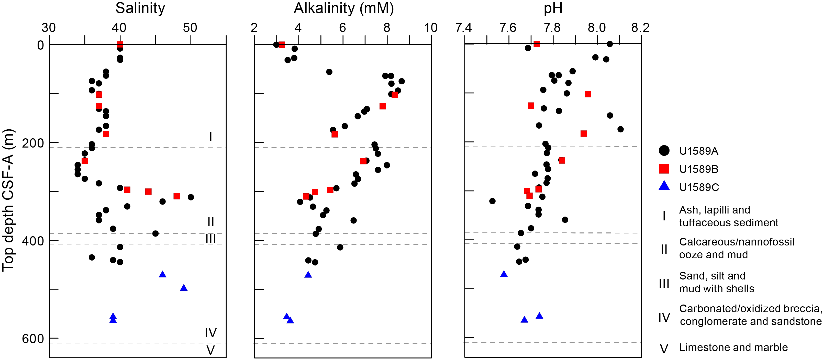
Figure F54. IW salinity, alkalinity, and pH.
Total alkalinity increases from ~3 mM at the seafloor to a maximum of ~9 mM at 75 mbsf. Outside of the maximum and minimum values, alkalinity fluctuates from ~3 to ~8 mM downhole, with higher values occurring in hemipelagic sediments (Table T17; Figure F54).
Values for pH show some variation within the sampled depths, ranging 7.5–8.1 (average = 7.8 ± 0.1).
9.2.2. Bromide, chloride, sodium, and boron
Bromide, Cl−, Na+, and B covary downcore with limited or no variation to 280 mbsf, where two sharp peaks (312 and 386 mbsf) are noted, similar to trends observed in salinity (Table T18; Figure F55).
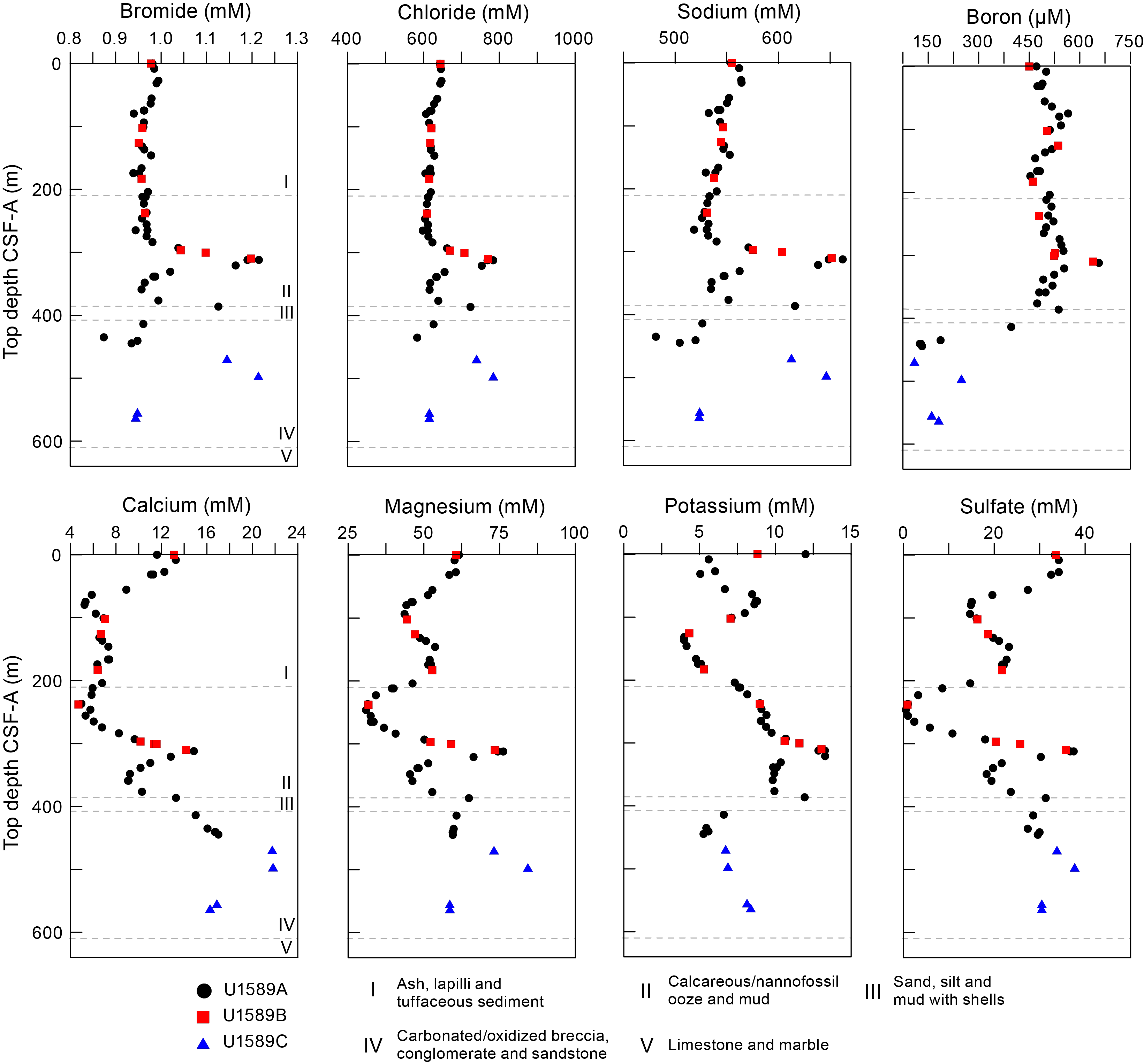
Figure F55. IW Br−, Cl−, Na, B, Ca, Mg, K, and SO42−.
9.2.3. Calcium, magnesium, potassium, and sulfate
IW Ca, Mg, K, and SO42− concentrations show downhole variations that strongly correlate with lithology (Table T18; Figure F55). Calcium, Mg, and SO42− display high concentrations in volcanic-dominated lithologies and decrease in sedimentary calcareous ooze lithologies. Potassium concentration inversely correlates with Ca, Mg, and SO42− in the uppermost ~300 m and also strongly correlates with lithology, displaying low concentrations in the volcanic-dominated lithologies and high concentrations in sedimentary calcareous ooze lithologies.
At 312 mbsf within a volcanic-dominated layer, Ca, Mg, SO42−, and K all sharply increase in concentration. This directly correlates with the anomalous high salinity values described above (Sections 398-U1589A-54F-2 and 56F-2; 398-U1589B-57F-2 and 60F-2) (Table T18; Figure F55). The change in element correlation may be related to volcanic ash alteration (e.g., Cerling et al., 1985; Ogawa et al., 2005; Schacht et al., 2008). Below this depth, all five elements increase through siliciclastic Lithostratigraphic Unit III, increasing to another concentration high correlated with an anomalous salinity high at 386 mbsf, although both are lower values than those at 312 mbsf. Within the terrigenous materials in Unit IV, below ~400 mbsf, Ca concentration slightly increases and Mg, K, and SO42− decrease slightly or stay relatively constant.
9.2.4. Lithium, silicon, and strontium
Lithium, Si, and Sr show different and/or weaker trends than Ca, Mg, K, and SO42− (Table T18; Figure F56). Lithium concentrations are highest in volcaniclastic lithologies with significant scatter, and they reach a maximum at 101 mbsf before decreasing downhole through the sedimentary calcareous ooze lithology to ~20 µM. A local maximum in Li concentration occurs at 312 mbsf corresponding to maxima in other elements and salinity noted above. IW Si behaves similarly to K but with more scatter. Interestingly, the maximum Si concentration is reached at 283 mbsf, 30 m above the sharp peak in many of the other measured elements and salinity. Strontium concentrations increase downhole with a change in slope at 203 mbsf that corresponds to a change in lithology from volcaniclastics to hemipelagic (but including ash) sediments. At 386 mbsf, Sr values reach their maximum before decreasing to the bottom of the hole.
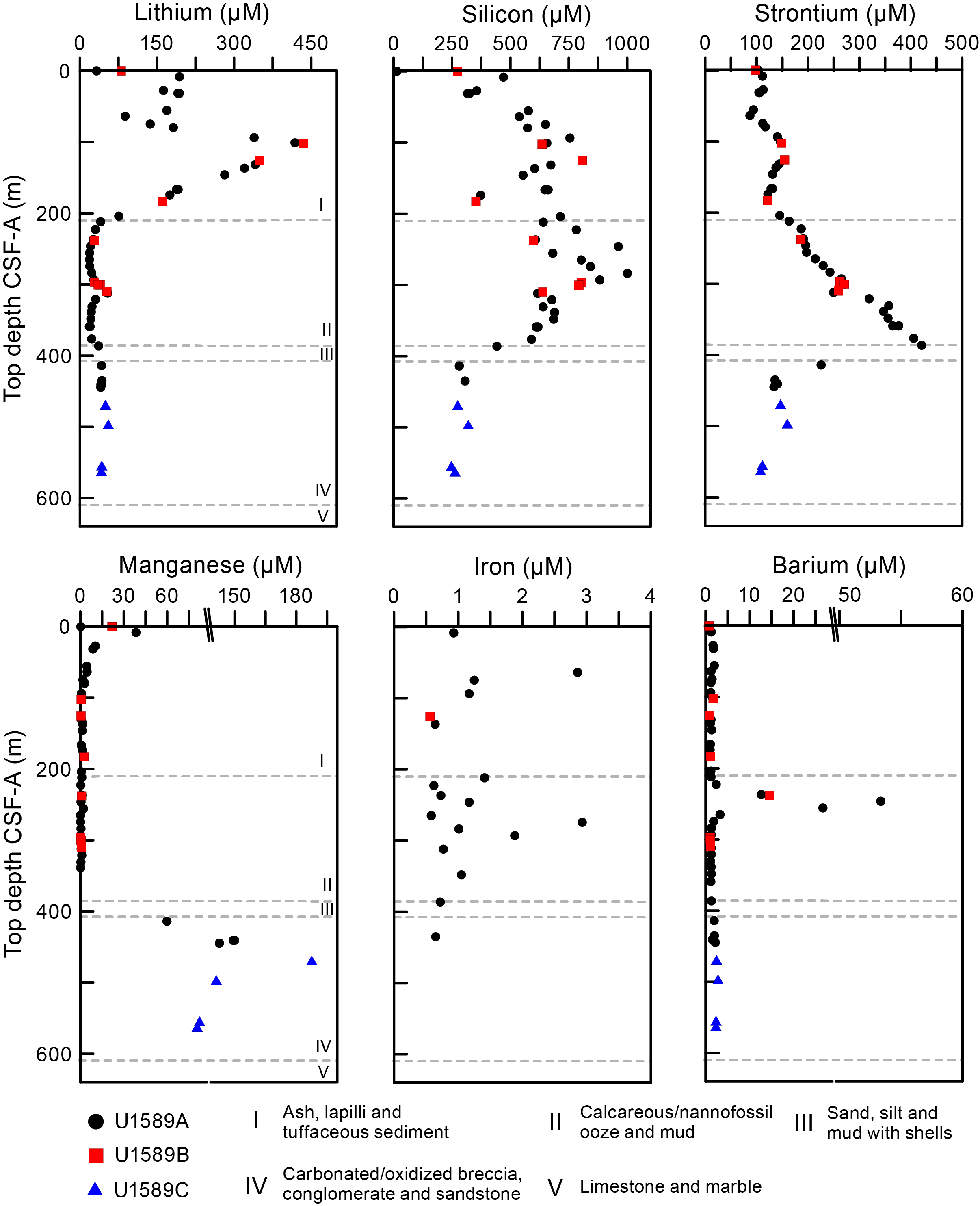
Figure F56. IW Li, Si, Sr, Mn, Fe, and Ba.
9.2.5. Manganese, iron, barium, and phosphorus
Concentrations of Mn, Fe, Ba, and P are low or below detection limit in most samples (Table T18; Figure F56). Manganese concentrations have peaks in the uppermost and lowermost samples, likely indicating zones of organic matter degradation and Mn oxide dissolution. Downhole trends for Fe show two maxima at 64 and 274 mbsf, but concentrations are scattered or below detection limit otherwise. Barium concentrations are <2.5 µM throughout the hole except for a peak at 246 mbsf that corresponds to the lowest SO42− concentrations observed. The correlation between Ba and SO42− may represent a zone of SO42− reduction. Except for three sections (398-U1589A-9H-4, 22F-2, and 44F-2), phosphorus values are below detection limit and thus are not plotted.
9.3. Sediment bulk geochemistry
A total of 71 sediment samples were analyzed for bulk geochemistry (Table T19). Of these, 66 were analyzed for total carbon, hydrogen, and nitrogen (CHN), and 69 were analyzed for inorganic carbon and carbonate content following the protocols explained in Geochemistry in the Expedition 398 methods chapter (Kutterolf et al., 2024). For the CHN analysis, duplicates were run on ~10% of the samples to determine analytical reproducibility. Calcium carbonate values are elevated between ~200 and ~390 mbsf, with CaCO3 content as high as ~70 wt%, corresponding to lithologies described as hemipelagic sediments and calcareous ooze (Figure F57).
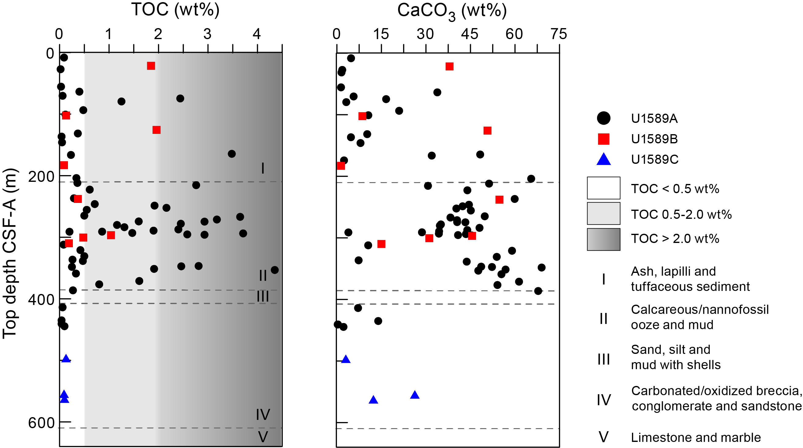
Figure F57. TOC and carbonate.
9.3.1. Sapropel identification
TOC was calculated using TC and inorganic carbon values. Following convention set forth by Kidd et al. (1978), units with TOC values >2.0 wt% were identified as sapropels and units with TOC values of 0.5–2.0 wt% were identified as sapropelitic. Using these values, 12 units were identified as sapropels and 19 units were identified as sapropelitic (Figure F57).
9.4. Headspace gas analysis
Headspace gas analyses were performed at a resolution of one sample per full-length core (9.5 m advance) or one sample every other core for half-length cores (4.7 m advance) throughout Holes U1589A and U1589C. The aim was to monitor the presence and abundance of C1–C3 hydrocarbons as part of the standard IODP safety protocol (Pimmel and Claypool, 2001). A total of 51 headspace gas samples were analyzed using gas chromatography (GC) (see Geochemistry in the Expedition 398 methods chapter [Kutterolf et al., 2024]). Methane is the dominant hydrocarbon present at low concentrations in the uppermost 230 m of Hole U1589A. Ethane, propane, butane, and other heavier hydrocarbons are either low or below the detection limit. A very slight increase in methane concentration occurs at 240–350 mbsf (Figure F58).
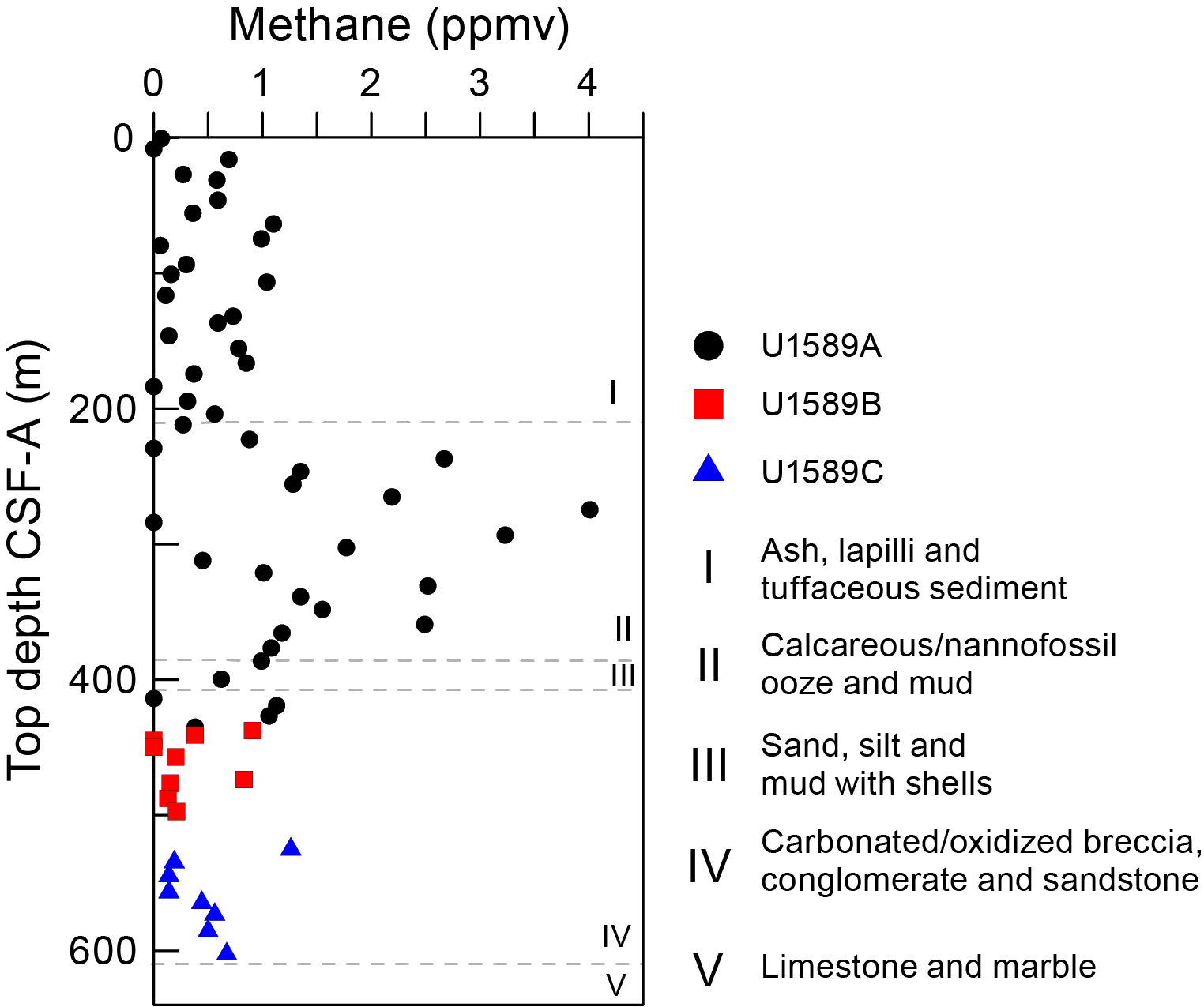
Figure F58. Headspace gas analyses of methane.
Headspace gas analyses were resumed for Hole U1589C when coring reached deeper than in Hole U1589A (446 mbsf). Below this depth, headspace gas analyses were performed at a resolution of one sample per core to the base of the hole. A total of 16 headspace gas samples were analyzed using GC. No elevated methane concentrations were observed (Figure F58).
10. Downhole logging
10.1. Operations summary
Logging operations were conducted in Hole U1589C. Prior to logging operations, formation temperature was measured using the APCT-3 and SET2 tools in Holes U1589A and U1589B (see Physical properties). The average formation temperature of ~15°C verified that the Site U1589 formation is within a suitable temperature range for wireline logging tools. After completion of coring operations in Hole U1589C at the final depth of 621.9 mbsf (1115.5 mbrf), the driller pumped a 50 bbl (1 bbl = one 42 gallon barrel) sepiolite mud sweep to clean the hole. The rotary shifting tool was deployed to release the bit. A 20 bbl heavy barite mud pill was emplaced to stop backflow. The top drive was racked back, and the string was tripped up to 50.4 mbsf and then spaced out with a 30 ft knobby to 65.0 mbsf, which is the topmost depth limit for logging operations. Note that all the depths in this section are indicated in meters wireline log matched depth below seafloor (WMSF) (see Operations).
The triple combo tool string was deployed in Hole U1589C. Three paths by the triple combo tool string with various logged intervals were obtained during logging operations at Site U1589 (Figures F59, F60). The first pass was a down-log of the triple combo tool string from the bottom of the pipe to a target depth 5 m above the maximum cored depth. As a result of either a narrowing hole diameter or drilling debris toward the bottom of the hole, the string only reached 544.9 mbsf; this was determined as the maximum loggable depth in Hole U1589C. The second pass was an up-log of the triple combo tool string from 544.9 mbsf planned to 150 mbsf. During this first pass, the caliper tool was opened to detect borehole diameter (Figure F60). The up-log was completed to 35 m above the original target depth, enabling us to confirm the borehole condition (the rugged interval started at ~481.4–461.4 mbsf becomes much smoother within the formation shallower than ~396.4 mbsf). Borehole wall condition was detected with caliper measurements and observed reasonably safe to run the tool string for the 185 m interval near the bottom of the hole (Figures F59, F60).
Figure F59. Logging operations.
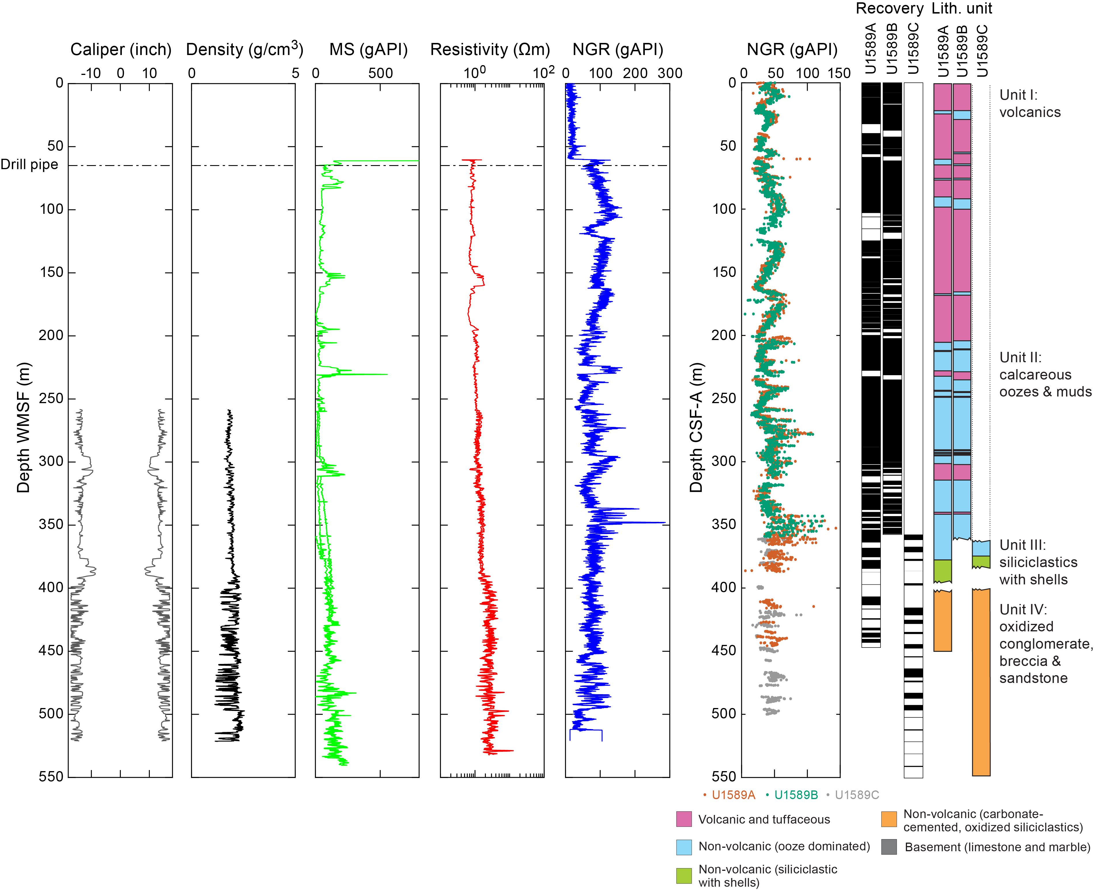
Figure F60. Logging data.
The triple combo tool string was sent down once more to 544.9 mbsf with the caliper closed, and then the second up-log was attempted. This up-log was initiated with a caliper opened aiming for the depth at the bottom of the pipe. When the triple combo tool string reached 227.7 mbsf, the head tension exceeded the wire tension, indicating that the tool was stuck. The Schlumberger engineer attempted to free the tool string by rocking winch/wire tensions, but the release of head tension did not occur. The tool string was officially determined to be retrieved. The logging operation in Hole U1589C was finalized at the rig floor by deploying the T-bar approach to retrieve the tool string. The eventual return of the triple combo tool string on deck took place at 1240 h on 30 December 2022.
10.2. Logging data summary
The triple combo tool string provided whole-hole in situ NGR, resistivity, density, and MS measurements at various sampling rates (see Downhole measurements in the Expedition 398 methods chapter [Kutterolf et al., 2024]). Depending on locations of each sensor package within the triple combo tool string, the first down-log data for each of the in situ physical properties became available for various logged intervals from seafloor to 1038 m WMSF. It should be noted that density can only be processed where caliper tool data were obtained (258.28–532.50 m WMSF).
Caliper data indicate that the variations in borehole diameter are significant, suggesting the borehole wall topography is irregular within Lithostratigraphic Unit IV, where core recovery rates decreased as a result of the hardness and heterogeneity of materials that compose the terrigenous formation. The maximum hole diameter reached > 17 inches at places in this logged interval. Shallower than 395 m WMSF, the borehole wall condition becomes much smoother, nominally 15 inches with occasional ledges narrowing the hole close to the bit size.
Resistivity logs show a dichotomy in ranges of logged values between Unit IV and the rest of the upper formation at Site U1589. In Unit IV, the deep resistivity penetration log has a nominal range of 0.5–6.4 Ωm, whereas the logged interval above Unit IV has values of 0.6–1.2 Ωm. A noticeable layer with a factor 3 higher resistivity than neighboring formations is located at 152.51–159.77 m WMSF. Nearby lithology in recovered cores around this depth includes a ~5 m thick lapilli layer (Cores 398-U1589A-21F and 22F; 398-U1589B-26F).
NGR logs (total counts) confirm the whole-hole trend of NGR measurements on whole-round core sections acquired on the shipboard instrument (see Physical properties). These NGR logs can be a reliable tool for integrating various core-based observations to interpretations on the log and seismic scales because of (1) higher sampling rates (see Downhole measurements in the Expedition 398 methods chapter [Kutterolf et al., 2024]); (2) the continuous, repeat nature of downhole NGR log data compared to the discrete NGR measurements on whole-round core sections; and (3) in situ formation measurements that assume materials are undisturbed (instead of relocated during coring).
The downhole density log suggests that Unit IV has the highest density values compared to the shallower formation, which is consistent with the trend observed by shipboard measurements (see Physical properties). Density logs from Unit IV have the widest range of variability (1.14–2.26 g/cm3), whereas Unit III and above has narrower range (1.56–2.13 g/cm3). Density logs have apparent correlation with the caliper log, suggesting that the condition of borehole wall influences the data acquisition quality, even after post-postprocessing to correct volume.
The MS log has two distinctive intervals above and below ~380 m WMSF. The formation above 380 m WMSF includes a few intervals with distinctively high MS (173 × 10−5 to 215 × 10−5 SI) compared to the neighboring intervals (nominally <50 × 10−5 SI). These intervals include 77–80, 223–230, and 295.5–311.5 m WMSF, all of which reside in Unit I and volcanic layers in Unit II (Figure F15). Throughout the logged interval of the formation below 380 m WMSF, where lithology mostly consists of terrigenous sediment, high MS (>100 × 10−5 SI) is observed.
In addition to physical properties logging data, the temperature sensor housed on the MS sensor package indicated that the borehole fluid is 17.36° and 18.50°C at 100.4 and 536.7 m WMSF, respectively, linearly increasing with depth. It should be noted that the borehole was replaced with heavy mud ~4 h prior to the first pass (the whole-hole down-log).
References
Aze, T., Ezard, T.H.G., Purvis, A., Coxall, H.K., Stewart, D.R.M., Wade, B.S., and Pearson, P.N., 2011. A phylogeny of Cenozoic macroperforate planktonic foraminifera from fossil data. Biological Reviews, 86(4):900–927. https://doi.org/10.1111/j.1469-185X.2011.00178.x
Backman, J., Raffi, I., Rio, D., Fornaciari, E., and Pälike, H., 2012. Biozonation and biochronology of Miocene through Pleistocene calcareous nannofossils from low and middle latitudes. Newsletters on Stratigraphy, 45(3):221–244. https://doi.org/10.1127/0078-0421/2012/0022
Blackwell, D.D., 1983. Heat flow in the northern basin and range province. Geothermal Resources Council Special Report, 13. https://publications.mygeoenergynow.org/grc/1005448.pdf
Cardozo, N., and Allmendinger, R.W., 2013. Spherical projections with OSXStereonet. Computers & Geosciences, 51:193–205. https://doi.org/10.1016/j.cageo.2012.07.021
Castradori, D., 1993. Calcareous nannofossil biostratigraphy and biochronology in eastern Mediterranean deep-sea cores. Rivista Italiana Di Paleontologia E Stratigrafia, 99(1):107–126.
Cerling, T.E., Brown, F.H., and Bowman, J.R., 1985. Low-temperature alteration of volcanic glass: Hydration, Na, K, 18O and Ar mobility. Chemical Geology: Isotope Geoscience section, 52(3):281–293. https://doi.org/10.1016/0168-9622(85)90040-5
Crundwell, M., Scott, G., Naish, T., and Carter, L., 2008. Glacial–interglacial ocean climate variability from planktonic foraminifera during the mid-Pleistocene transition in the temperate southwest Pacific, ODP Site 1123. Palaeogeography, Palaeoclimatology, Palaeoecology, 260(1–2):202–229. https://doi.org/10.1016/j.palaeo.2007.08.023
Crundwell, M.P., and Woodhouse, A., 2022. A detailed biostratigraphic framework for 0–1.2 Ma Quaternary sediments of north-eastern Zealandia. New Zealand Journal of Geology and Geophysics. https://doi.org/10.1080/00288306.2022.2054828
Di Stefano, A., and Sturiale, G., 2010. Refinements of calcareous nannofossil biostratigraphy at the Miocene/Pliocene boundary in the Mediterranean region. Geobios, 43(1):5–20. https://doi.org/10.1016/j.geobios.2009.06.007
Druitt, T., Kutterolf, S., and Höfig, T.W., 2022. Expedition 398 Scientific Prospectus: Hellenic Arc Volcanic Field. International Ocean Discovery Program. https://doi.org/10.14379/iodp.sp.398.2022
Druitt, T.H., Mercier, M., Florentin, L., Deloule, E., Cluzel, N., Flaherty, T., Médard, E., and Cadoux, A., 2016. Magma storage and extraction associated with Plinian and Interplinian activity at Santorini Caldera (Greece). Journal of Petrology, 57(3):461–494. https://doi.org/10.1093/petrology/egw015
Fisher, R.V., and Schmincke, H.-U., 1984. Pyroclastic Rocks: Berlin (Springer). https://doi.org/10.1007/978-3-642-74864-6
Fuller, S., Carey, S., and Nomikou, P., 2018. Distribution of fine-grained tephra from the 1650 CE submarine eruption of Kolumbo volcano, Greece. Journal of Volcanology and Geothermal Research, 352:10–25. https://doi.org/10.1016/j.jvolgeores.2018.01.004
Gradstein, F.M., Ogg, J.G., Schmitz, M.D., and Ogg, G.M. (Eds.), 2020. The Geologic Time Scale 2020: Amsterdam (Elsevier BV). https://doi.org/10.1016/C2020-1-02369-3
Hayward, B.W., Grenfell, H.R., Reid, C.M., and Hayward, K.A., 1999. Recent New Zealand shallow-water benthic foraminifera: taxonomy, ecologic distribution, biogeography, and use in paleoenvironmental assessment. In Institute of Geological & Nuclear Sciences Monograph, 21: Lower Hutt, NZ.
Hooft, E.E.E., Nomikou, P., Toomey, D.R., Lampridou, D., Getz, C., Christopoulou, M.-E., O’Hara, D., Arnoux, G.M., Bodmer, M., Gray, M., Heath, B.A., and VanderBeek, B.P., 2017. Backarc tectonism, volcanism, and mass wasting shape seafloor morphology in the Santorini-Christiana-Amorgos region of the Hellenic Volcanic Arc. Tectonophysics, 712–713:396–414. https://doi.org/10.1016/j.tecto.2017.06.005
Hübscher, C., Ruhnau, M., and Nomikou, P., 2015. Volcano-tectonic evolution of the polygenetic Kolumbo submarine volcano/Santorini (Aegean Sea). Journal of Volcanology and Geothermal Research, 291:101–111. https://doi.org/10.1016/j.jvolgeores.2014.12.020
Jelínek, V., and Kropáček, V., 1978. Statistical processing of anisotropy of magnetic susceptibility measured on groups of specimens. Studia Geophysica et Geodaetica, 22(1):50–62. https://doi.org/10.1007/BF01613632
Jutzeler, M., White, J.D.L., Talling, P.J., McCanta, M., Morgan, S., Le Friant, A., and Ishizuka, O., 2014. Coring disturbances in IODP piston cores with implications for offshore record of volcanic events and the Missoula megafloods. Geochemistry, Geophysics, Geosystems, 15(9):3572–3590. https://doi.org/10.1002/2014GC005447
Kidd, R.B., Cita, M.B., and Ryan, W.B.F., 1978. Stratigraphy of eastern Mediterranean sapropel sequences recovered during DSDP Leg 42A and their paleoenvironmental significance. In Hsü, K., Montadert, L., et al., Initial Reports of the Deep Sea Drilling Project. 42(1): Washington, DC (US Government Printing Office), 421–443. https://doi.org/10.2973/dsdp.proc.42-1.113-1.1978
Kutterolf, S., Druitt, T.H., Ronge, T.A., Beethe, S., Bernard, A., Berthod, C., Chen, H., Chiyonobu, S., Clark, A., DeBari, S., Fernandez Perez, T.I., Gertisser, R., Hübscher, C., Johnston, R.M., Jones, C., Joshi, K.B., Kletetschka, G., Koukousioura, O., Li, X., Manga, M., McCanta, M., McIntosh, I., Morris, A., Nomikou, P., Pank, K., Peccia, A., Polymenakou, P.N., Preine, J., Tominaga, M., Woodhouse, A., and Yamamoto, Y., 2024. Expedition 398 methods. In Druitt, T.H., Kutterolf, S., Ronge, T.A., and the Expedition 398 Scientists, Hellenic Arc Volcanic Field. Proceedings of the International Ocean Discovery Program, 398: College Station, TX (International Ocean Discovery Program). https://doi.org/10.14379/iodp.proc.398.102.2024
Kutterolf, S., Freundt, A., Hansteen, T.H., Dettbarn, R., Hampel, F., Sievers, C., Wittig, C., Allen, S.R., Druitt, T.H., McPhie, J., Nomikou, P., Pank, K., Schindlbeck-Belo, J.C., Wang, K.-L., Lee, H.-Y., and Friedrichs, B., 2021. The medial offshore record of explosive volcanism along the central to eastern Aegean Volcanic Arc: 1. tephrostratigraphic correlations. Geochemistry, Geophysics, Geosystems, 22(12):e2021GC010010. https://doi.org/10.1029/2021GC010010
Le Maitre, R.W., Steckeisen, A., Zanettin, B., Le Bas, M.J., Bonin, B., and Bateman, P. (Eds.), 2002. Igneous Rocks: A Classification and Glossary of Terms (Second edition): Cambridge, UK (Cambridge University Press). https://doi.org/10.1017/CBO9780511535581
Lirer, F., Foresi, L.M., Iaccarino, S.M., Salvatorini, G., Turco, E., Cosentino, C., Sierro, F.J., and Caruso, A., 2019. Mediterranean Neogene planktonic foraminifer biozonation and biochronology. Earth-Science Reviews, 196:102869. https://doi.org/10.1016/j.earscirev.2019.05.013
Lourens, L., Hilgen, F., Shackleton, N.J., Laskar, J., and Wilson, D., 2004. The Neogene period. In Smith, A.G., Gradstein, F.M. and Ogg, J.G., A Geologic Time Scale 2004. Cambridge, UK (Cambridge University Press), 409–440. https://doi.org/10.1017/CBO9780511536045.022
Lourens, L.J., Hilgen, F.J., and Raffi, I., 1998. Base of large Gephyrocapsa and astronomical calibration of early Pleistocene sapropels in Site 967 and Hole 969D: solving the chronology of the Vrica Section (Calabria, Italy). In Robertson, A.H.F., Emeis, K.-C., Richter, C., and Camerlenghi, A. (Eds.), Proceedings of the Ocean Drilling Program, Scientific Results. 160: College Station, TX (Ocean Drilling Program), 191. https://doi.org/10.2973/odp.proc.sr.160.017.1998
Maffione, M., and Herrero-Bervera, E., 2022. A relative paleointensity (RPI)-calibrated age model for the Corinth syn-rift sequence at IODP Hole M0079A (Gulf of Corinth, Greece). Frontiers in Earth Science, 10. https://doi.org/10.3389/feart.2022.813958
Martini, E., 1971. Standard Tertiary and Quaternary calcareous nannoplankton zonation. Proceedings of the Second Planktonic Conference, Roma, 1970:739–785.
Nomikou, P., Carey, S., Papanikolaou, D., Croff Bell, K., Sakellariou, D., Alexandri, M., and Bejelou, K., 2012. Submarine volcanoes of the Kolumbo volcanic zone NE of Santorini caldera, Greece. Global and Planetary Change, 90–91:135–151. https://doi.org/10.1016/j.gloplacha.2012.01.001
Nomikou, P., Hübscher, C., Papanikolaou, D., Farangitakis, G.P., Ruhnau, M., and Lampridou, D., 2018. Expanding extension, subsidence and lateral segmentation within the Santorini - Amorgos basins during Quaternary: implications for the 1956 Amorgos events, central - south Aegean Sea, Greece. Tectonophysics, 722:138–153. https://doi.org/10.1016/j.tecto.2017.10.016
Nomikou, P., Hübscher, C., Ruhnau, M., and Bejelou, K., 2016. Tectono-stratigraphic evolution through successive extensional events of the Anydros Basin, hosting Kolumbo volcanic field at the Aegean Sea, Greece. Tectonophysics, 671:202–217. https://doi.org/10.1016/j.tecto.2016.01.021
Nomikou, P., Papanikolaou, D., Alexandri, M., Sakellariou, D., and Rousakis, G., 2013. Submarine volcanoes along the Aegean volcanic arc. Tectonophysics, 597–598:123–146. https://doi.org/10.1016/j.tecto.2012.10.001
Nomikou, P., Parks, M.M., Papanikolaou, D., Pyle, D.M., Mather, T.A., Carey, S., Watts, A.B., Paulatto, M., Kalnins, M.L., Livanos, I., Bejelou, K., Simou, E., and Perros, I., 2014. The emergence and growth of a submarine volcano: the Kameni islands, Santorini (Greece). GeoResJ, 1–2:8–18. https://doi.org/10.1016/j.grj.2014.02.002
Ogawa, Y., Shikazono, N., Ishiyama, D., Sato, H., and Mizuta, T., 2005. An experimental study on felsic rock–artificial seawater interaction: implications for hydrothermal alteration and sulfate formation in the Kuroko mining area of Japan. Mineralium Deposita, 39(8):813–821. https://doi.org/10.1007/s00126-004-0454-8
Okada, H., and Bukry, D., 1980. Supplementary modification and introduction of code numbers to the low-latitude coccolith biostratigraphic zonation (Bukry, 1973; 1975). Marine Micropaleontology, 5(3):321–325. https://doi.org/10.1016/0377-8398(80)90016-X
Pimmel, A., and Claypool, G., 2001. Introduction to shipboard organic geochemistry on the JOIDES Resolution. Ocean Drilling Program Technical Note, 30. https://doi.org/10.2973/odp.tn.30.2001
Potter, D.K., and Stephenson, A., 1988. Single-domain particles in rocks and magnetic fabric analysis. Geophysical Research Letters, 15(10):1097–1100. https://doi.org/10.1029/GL015i010p01097
Preine, J., Hübscher, C., Karstens, J., and Nomikou, P., 2022a. Volcano-tectonic evolution of the Christiana-Santorini-Kolumbo rift zone. Tectonics, 41(11):e2022TC007524. https://doi.org/10.1029/2022TC007524
Preine, J., Karstens, J., Hübscher, C., Crutchley, G.J., Druitt, T.H., Schmid, F., and Nomikou, P., 2022b. The hidden giant: how a rift pulse triggered a cascade of sector collapses and voluminous secondary mass-transport events in the early evolution of Santorini. Basin Research, 34(4):1465–1485. https://doi.org/10.1111/bre.12667
Preine, J., Karstens, J., Hübscher, C., Nomikou, P., Schmid, F., Crutchley, G.J., Druitt, T.H., and Papanikolaou, D., 2022c. Spatio-temporal evolution of the Christiana-Santorini-Kolumbo volcanic field, Aegean Sea. Geology, 50(1):96–100. https://doi.org/10.1130/G49167.1
Rio, D., Raffi, I., and Villa, G., 1990. Pliocene-Pleistocene calcareous nannofossil distribution patterns in the western Mediterranean. In Kastens, K.A., Mascle, J., et al., Proceedings of the Ocean Drilling Program, Scientific Results. 107: College Station, TX (Ocean Drilling Program), 513–533. https://doi.org/10.2973/odp.proc.sr.107.164.1990
Roberts, A.P., Chang, L., Rowan, C.J., Horng, C.-S., and Florindo, F., 2011. Magnetic properties of sedimentary greigite (Fe3S4): an update. Reviews of Geophysics, 49(1):RG1002. https://doi.org/10.1029/2010RG000336
Roberts, A.P., Stoner, J.S., and Richter, C., 1999. Diagenetic magnetic enhancement of sapropels from the eastern Mediterranean Sea. Marine Geology, 153(1):103–116. https://doi.org/10.1016/S0025-3227(98)00087-5
Schacht, U., Wallmann, K., Kutterolf, S., and Schmidt, M., 2008. Volcanogenic sediment–seawater interactions and the geochemistry of pore waters. Chemical Geology, 249(3):321–338. https://doi.org/10.1016/j.chemgeo.2008.01.026
Snowball, I.F., 1997a. Gyroremanent magnetization and the magnetic properties of greigite-bearing clays in southern Sweden. Geophysical Journal International, 129(3):624–636. https://doi.org/10.1111/j.1365-246X.1997.tb04498.x
Snowball, I.F., 1997b. The detection of single-domain greigite (Fe3S4) using rotational remanent magnetization (RRM) and the effective gyro field (Bg): mineral magnetic and palaeomagnetic applications. Geophysical Journal International, 130(3):704–716. https://doi.org/10.1111/j.1365-246X.1997.tb01865.x
Stephenson, A., and Snowball, I.F., 2001. A large gyromagnetic effect in greigite. Geophysical Journal International, 145(2):570–575. https://doi.org/10.1046/j.0956-540x.2001.01434.x
Tarling, D.H., 1983. Paleomagnetism: Principles and Applications in Geology, Geophysics and Archaeology: Dordrecht, Netherlands (Springer). https://doi.org/10.1007/978-94-009-5955-2
Tauxe, L., and Kent, D.V., 2004. A simplified statistical model for the geomagnetic field and the detection of shallow bias in paleomagnetic inclinations: was the ancient magnetic field dipolar? In Channell, J.E.T., Kent, D.V., Lowrie, W., and Meert, J.G. (Eds.), Timescales Of The Paleomagnetic Field. Geophysical Monograph, 145: 101–115. https://doi.org/10.1029/145GM08
Woodhouse, A., Procter, F.A., Jackson, S.L., Jamieson, R.A., Newton, R.J., Sexton, P.F., and Aze, T., 2023. Paleoecology and evolutionary response of planktonic foraminifera to the mid-Pliocene Warm Period and Plio-Pleistocene bipolar ice sheet expansion. Biogeosciences, 20(1):121–139. https://doi.org/10.5194/bg-20-121-2023