Flecker, R., Ducassou, E., Williams, T., and the Expedition 401 Scientists
Proceedings of the International Ocean Discovery Program Volume 401
publications.iodp.org
https://doi.org/10.14379/iodp.proc.401.103.2025
Site U16091
![]() R. Flecker,
R. Flecker,
![]() E. Ducassou,
E. Ducassou,
![]() T. Williams,
T. Williams,
![]() U. Amarathunga,
U. Amarathunga,
![]() B. Balestra,
B. Balestra,
![]() M.A. Berke,
M.A. Berke,
![]() C.L. Blättler,
C.L. Blättler,
![]() S. Chin,
S. Chin,
![]() M. Das,
M. Das,
![]() K. Egawa,
K. Egawa,
![]() N. Fabregas,
N. Fabregas,
![]() S.J. Feakins,
S.J. Feakins,
![]() S.C. George,
S.C. George,
![]() F.J. Hernández-Molina,
F.J. Hernández-Molina,
![]() W. Krijgsman,
W. Krijgsman,
![]() Z. Li,
Z. Li,
![]() J. Liu,
J. Liu,
![]() D. Noto,
D. Noto,
![]() F. Raad,
F. Raad,
![]() F.J. Rodríguez-Tovar,
F.J. Rodríguez-Tovar,
![]() F.J. Sierro,
F.J. Sierro,
![]() P. Standring,
P. Standring,
![]() J. Stine,
J. Stine,
![]() E. Tanaka,
E. Tanaka,
![]() M. Teixeira,
M. Teixeira,
![]() X. Xu,
X. Xu,
![]() S. Yin, and
S. Yin, and
![]() M.Z. Yousfi2
M.Z. Yousfi2
1 Flecker, R., Ducassou, E., Williams, T., Amarathunga, U., Balestra, B., Berke, M.A., Blättler, C.L., Chin, S., Das, M., Egawa, K., Fabregas, N., Feakins, S.J., George, S.C., Hernández-Molina, F.J., Krijgsman, W., Li, Z., Liu, J., Noto, D., Raad, F., Rodríguez-Tovar, F.J., Sierro, F.J., Standring, P., Stine, J., Tanaka, E., Teixeira, M., Xu, X., Yin, S., and Yousfi, M.Z., 2025. Site U1609. In Flecker, R., Ducassou, E., Williams, T., and the Expedition 401 Scientists, Mediterranean–Atlantic Gateway Exchange. Proceedings of the International Ocean Discovery Program, 401: College Station, TX (International Ocean Discovery Program). https://doi.org/10.14379/iodp.proc.401.103.2025
2 Expedition 401 Scientists’ affiliations.
1. Background and objectives
Site U1609 is located at 1659.5 meters below sea level (mbsl) on the continental slope of the Portuguese margin (37°22.6159′N, 09°35.9119′W) close to Cape São Vicente (Figure F1). The primary scientific objective of Site U1609 was to recover a distal sedimentary record of the Late Miocene–Pliocene Mediterranean overflow plume (Figure F2). The aim was to capture the evolution of the plume’s equilibrium depth with time from the earliest evidence of overflow through the Rifian Corridor (~7.8 Ma; Capella et al., 2017) through the Mediterranean’s Messinian Salinity Crisis (MSC) (5.97–5.33 Ma; Roveri et al., 2014) to the Early Pliocene (~4 Ma). This interval of major gateway and Mediterranean environmental change is likely to have substantially influenced both the density and chemistry of the overflow on subprecessional to million-year timescales (Krijgsman et al., 2024).
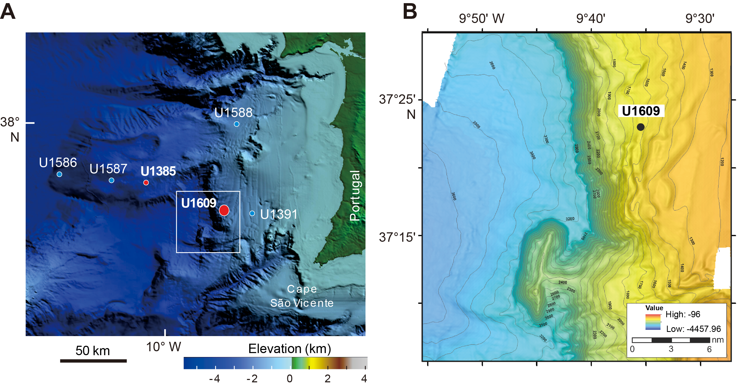
Figure F1. Bathymetry location map.
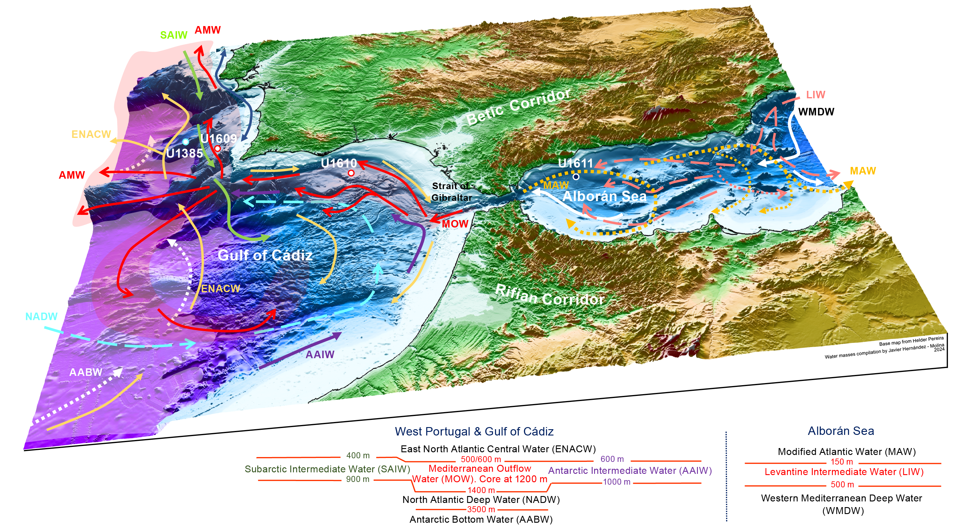
Figure F2. Present-day water mass circulation patterns.
Site U1609 is 17 km west and downslope from Integrated Ocean Drilling Program Expedition 339 Site U1391 (Figure F1), which targeted the Pliocene–Quaternary contourite depositional system (Expedition 339 Scientists, 2013). The succession recovered there comprised Pliocene–Quaternary muddy contourites with interbedded sands, hemipelagites, and several layers of mass movement deposits (Expedition 339 Scientists, 2013). On seismic profiles linking Site U1391 with Site U1609 (Figure F3), packages of contouritic drift migrate landward with time (Rodrigues et al., 2020). Site U1609 was located seaward of Site U1391 to target both the older Miocene–Pliocene succession and take advantage of the surface erosion visible in the seismic data. This erosion of the late Quaternary succession renders the older interval of interest (8–4 Ma) more accessible at shallower depths than elsewhere. The seismic data also suggest that the Late Miocene succession at Site U1609 is likely to provide a more complete record of the Mediterranean overflow plume than at Site U1610 (Figure F2), which is closer to the gateway. The more distal position of Site U1609 ensures that a less clastic, more hemipelagic succession is recovered, generating sediments suitable for high-resolution astrochronological tuning. This robust age framework is essential for investigating the subprecessional evolution, variability, and driving mechanisms of the Mediterranean overflow plume.
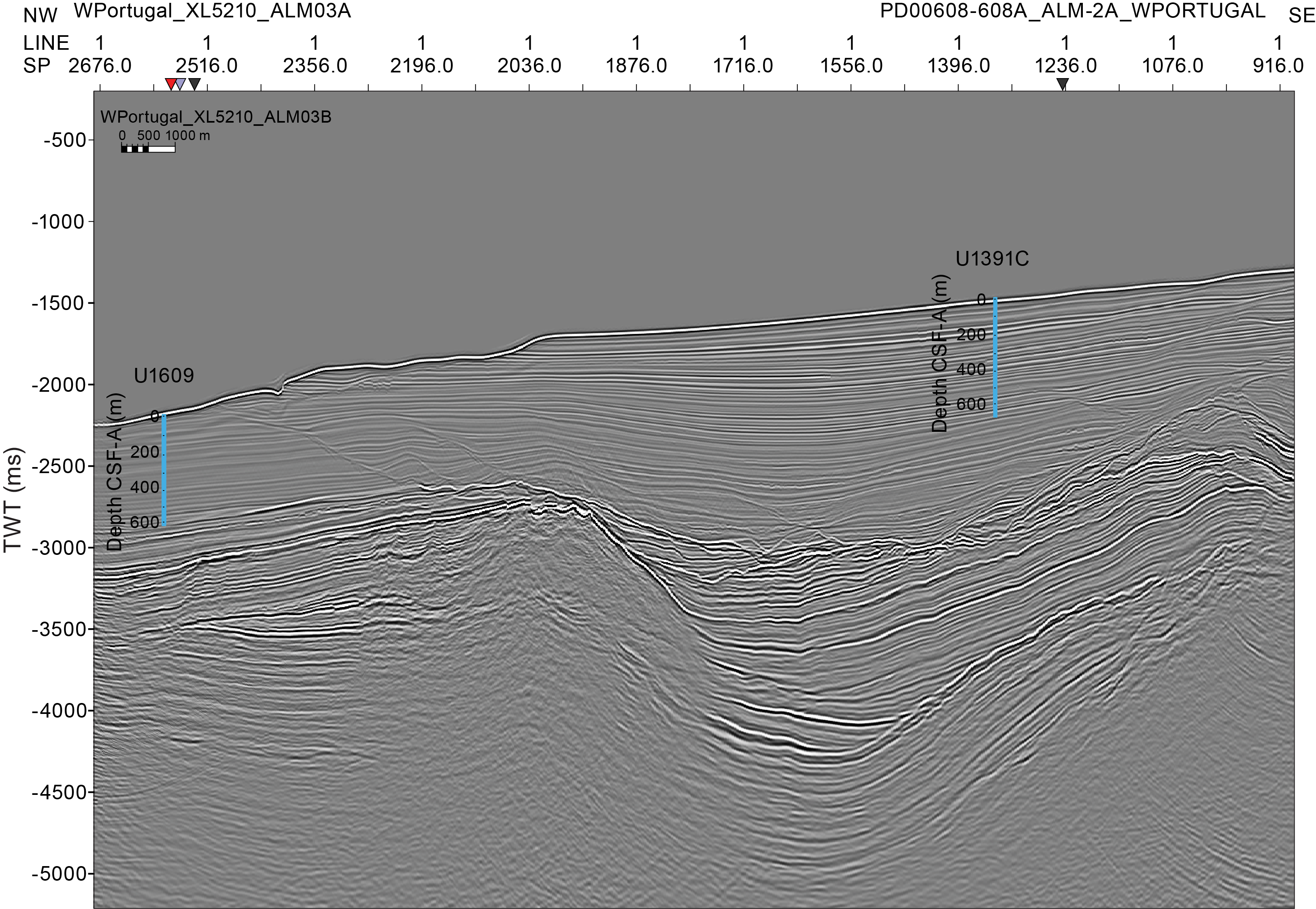
Figure F3. Seismic Profile IL1774.
1.1. Objectives
The major objective for Site U1609 was to recover a 8–4 Ma succession that records the distal evolution of the Mediterranean overflow plume during a phase of major Mediterranean–Atlantic gateway change and the formation of a salt giant in the Mediterranean. This has potential consequences for global climate change (Krijgsman et al., 2024). In combination with other Expedition 401 Atlantic sites, the record from Site U1609 also allows us to investigate more specific objectives including the following:
- To establish the age of the earliest contourites formed as a result of Mediterranean overflow,
- To evaluate the impact of extreme environmental fluctuations in the Mediterranean on its overflow plume and the structure of the Atlantic water masses, and
- To provide quantitative constraints on the mixing behavior of dense overflows by reconstructing the strength and attenuation rate of the Atlantic–Mediterranean exchange signal beyond the gateway.
2. Operations
The ship arrived at Site U1609 at 1655 h on 17 December 2023 after completing the 1220 nmi voyage from Amsterdam (Netherlands) in 4.5 days. All thrusters were down and secure at 1712 h, and the ship switched to full auto dynamic positioning (DP) mode at 1720 h, marking the start of operations at Site U1609. Operations started on the rig floor with assembly of the bottom-hole assembly (BHA). For Site U1609, we used a polycrystalline diamond compact (PDC) drill bit, and for the extended core barrel (XCB) cores we used a PDC cutting shoe. During recent International Ocean Discovery Program (IODP) expeditions, including Expedition 397 in the same area, this combination was found to yield very good recovery of XCB cores.
2.1. Hole U1609A
At 0430 h on 18 December 2023 after one missed mudline, we were successful in starting Hole U1609A (37°22.6259′N, 9°35.9120′W), with the seafloor calculated at 1659.5 mbsl based on the core recovery and mudline depth in Core 1H. Cores 1H–25H penetrated from the seafloor to 224.7 meters below seafloor (mbsf) and recovered 224.7 m (85%). Advanced piston corer temperature (APCT-3) tool temperature measurements were made during Cores 4H, 7H, 10H, and 13H, and all recorded smooth 10 min long temperature equilibration curves. At 0300 h on 19 December, we switched to the half-length advanced piston corer (HLAPC) system. Cores 26F–37F penetrated from 224.7 to 269.7 mbsf and recovered 45 m (102%). At 1430 h at 269.7 mbsf, we changed to XCB coring. Cores 38X–73X penetrated from 269.7 to 610.0 mbsf and recovered 340.3 m (99%) (Table T1). Over the course of the hole, the driller pumped eight 30 bbl sepiolite mud sweeps from 274.7 to 571.0 mbsf.
After confirming that early Tortonian sediments had been reached and thus we had recovered the Messinian to late Tortonian target stratigraphy, we stopped coring. The last core (401-U1609A-73X) reached 610.0 mbsf and came on deck at 2015 h on 22 December. We recovered 572.23 m of sediment over a 610.0 m cored interval (93.8% recovery) from Hole U1609A.
We prepared the hole for downhole logging by sweeping it with 30 bbl of sepiolite mud to flush out any loose sediment, displacing it with 230 bbl of barite-weighted mud to stabilize the borehole walls, and setting the end of pipe to 56.4 mbsf. The triple combo downhole logging tool string was assembled by 0130 h on 23 December, but before it could be run down the pipe, the wireline heave compensator control computer was found to be unresponsive. After troubleshooting diagnosed a probable hard drive failure, we decided to log without heave compensation. Ship heave was around 2.5 m throughout the day, higher than desirable but not atypical for logging from the ship. The triple combo logged borehole physical properties data to within 5 m of the bottom of the hole. The second tool string, the Versatile Seismic Imager (VSI), also reached close to the bottom of the hole for the check shot survey. Concurrently, we observed for protected marine species. Only 2 of the 13 check shot stations gave reliable first-arrival times because most of the borehole was too wide to achieve good coupling. Fortunately, those 2 stations were in the lower part of the hole where the data are most useful for tying borehole depth to the seismic profiles. Because of the wide borehole and the lack of heave compensation, we decided not to run the Formation MicroScanner tool and instead to run a sonic velocity and natural gamma ray tool string as the third and final logging run. This tool string also reached close to the base of the hole. The logging equipment was rigged down by 2230 h on 23 December. We raised the pipe, and the bit cleared the seafloor at 2235 h, ending Hole U1609A.
2.2. Hole U1609B
The ship was offset 20 m south of Hole U1609A along the slope, and at 0305 h on 24 December 2023 we started Hole U1609B (37°22.6159′N, 9°35.9119′W) by drilling down without recovery. The plan was to drill down without coring to spend more time coring the Early Pliocene to Late Miocene target interval; however, in these clay-rich sediments, drilling was no faster than taking cores. At 0930 h, we retrieved the center bit and started taking advanced piston corer (APC) cores at 72.6 mbsf. Cores 2H–4H penetrated from 72.6 to 101.4 mbsf and recovered 28.5 m (95%). Core 4H had partial recovery and required 20,000 lb of overpull to retrieve it, so we switched to coring with the HLAPC system at 101.1 mbsf. Cores 5F–32F penetrated from 101.4 to 234.1 mbsf and recovered 133.0 m (101%). We ran the Sediment Temperature 2 (SET2) tool after Core 32F at 234.1 mbsf to measure formation temperature deeper than had been possible with the APCT-3 tool in Hole U1609A to establish how deep the negative temperature anomaly observed in the APCT-3 data penetrated (see Physical properties).
At 1630 h on 25 December, we switched to the XCB coring system. At 1600 h on 26 December after taking Core 401-U1609B-48X at 389.3 mbsf, we ran the SET2 tool a second time. XCB coring proceeded until cores reached the age of 8.4 Ma, old enough to cover the main events in the history of the Mediterranean–Atlantic gateways. Cores 33X–61X penetrated from 234.1 to 508.7 mbsf and recovered 264.9 m (91%) (Table T1). We recovered 410.75 m of sediment over a 436.1 m cored interval (94.2% recovery) from Hole U1609B. At 1700 h on 27 December, we set back the top drive and started to pull up the drill pipe. The bit cleared the seafloor at 1905 h, and the BHA was on deck by 2345 h. The thrusters were raised, and we started the transit to Site U1610 at 2354 h, ending Site U1609.
Overall, we spent 10.2 days at Site U1609, about 2 days shorter than in the original operations plan because the maximum age target was shallower than had been anticipated. For this reason, we were able to recover two cored records of the target interval rather than the single core record that was originally planned.
3. Lithostratigraphy
Three main lithologies were described at Site U1609: calcareous mud, calcareous silty mud, and clayey calcareous ooze. Minor coarser grained deposits (e.g., calcareous silt, sandy silt, and calcareous sand) were also observed (Figure F4) (see hand drawn logs of lithologic successions in HANDDRAWN in Supplementary material). Based on subtle lithologic changes, Holes U1609A and U1609B are divided into four stratigraphic units (Figure F5). Contacts between these units and the lithologies within them are mainly gradational (Figure F5), characterized by subtle changes in color and grain size. Only the coarser silts and sandier beds are characterized by sharp to erosive basal contacts. In Hole U1609A, Unit I (0–344 m core depth below seafloor, Method A [CSF-A]) is characterized by alternating calcareous mud and calcareous silty mud. Unit II (344–457 m CSF-A) consists of alternating calcareous mud and clayey calcareous ooze. Unit III (457.7–531.5 m CSF-A) contains alternating calcareous mud of two different colors (lighter/darker) and clayey calcareous ooze. Darker calcareous muds are the dominant lithology in this unit, with thicknesses often >1 m. Unit IV (531.5–609.3 m CSF-A) also contains two distinct types of calcareous muds (brownish/darker) and clayey calcareous ooze, with the brown calcareous muds the dominant lithology. In this unit, bed thickness is usually <1 m and there are high-frequency changes in lithology. The coarser sandy and silty deposits were observed primarily in Units II and III (Figure F5).
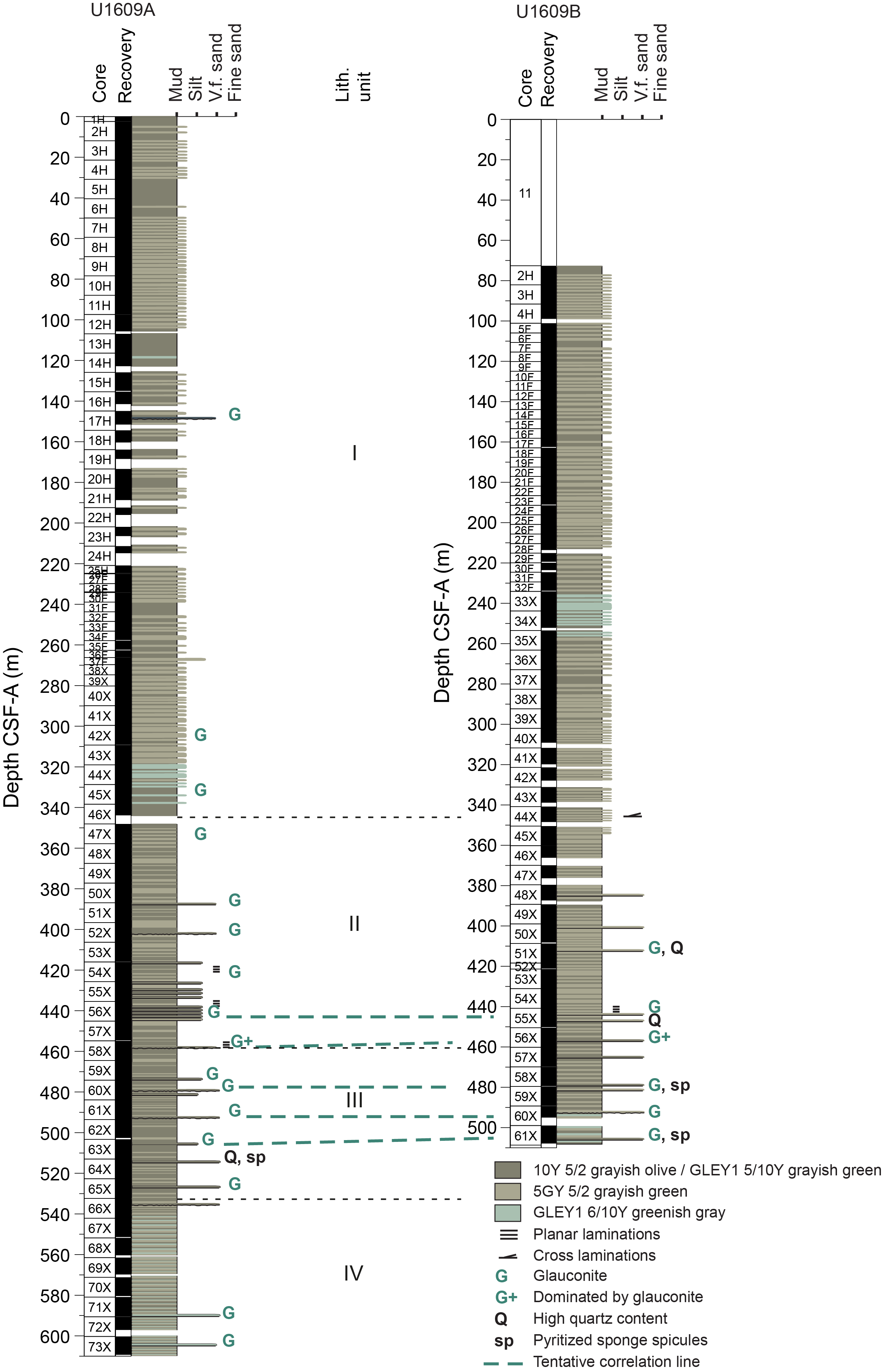
Figure F4. Lithologic synthesis.
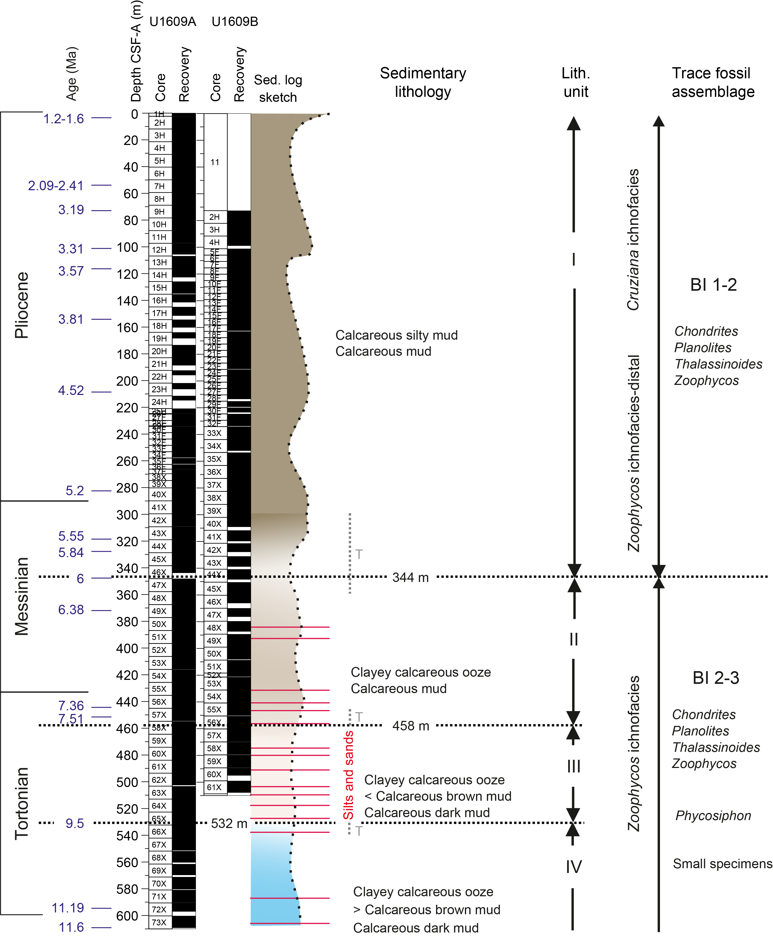
Figure F5. Lithologic summary.
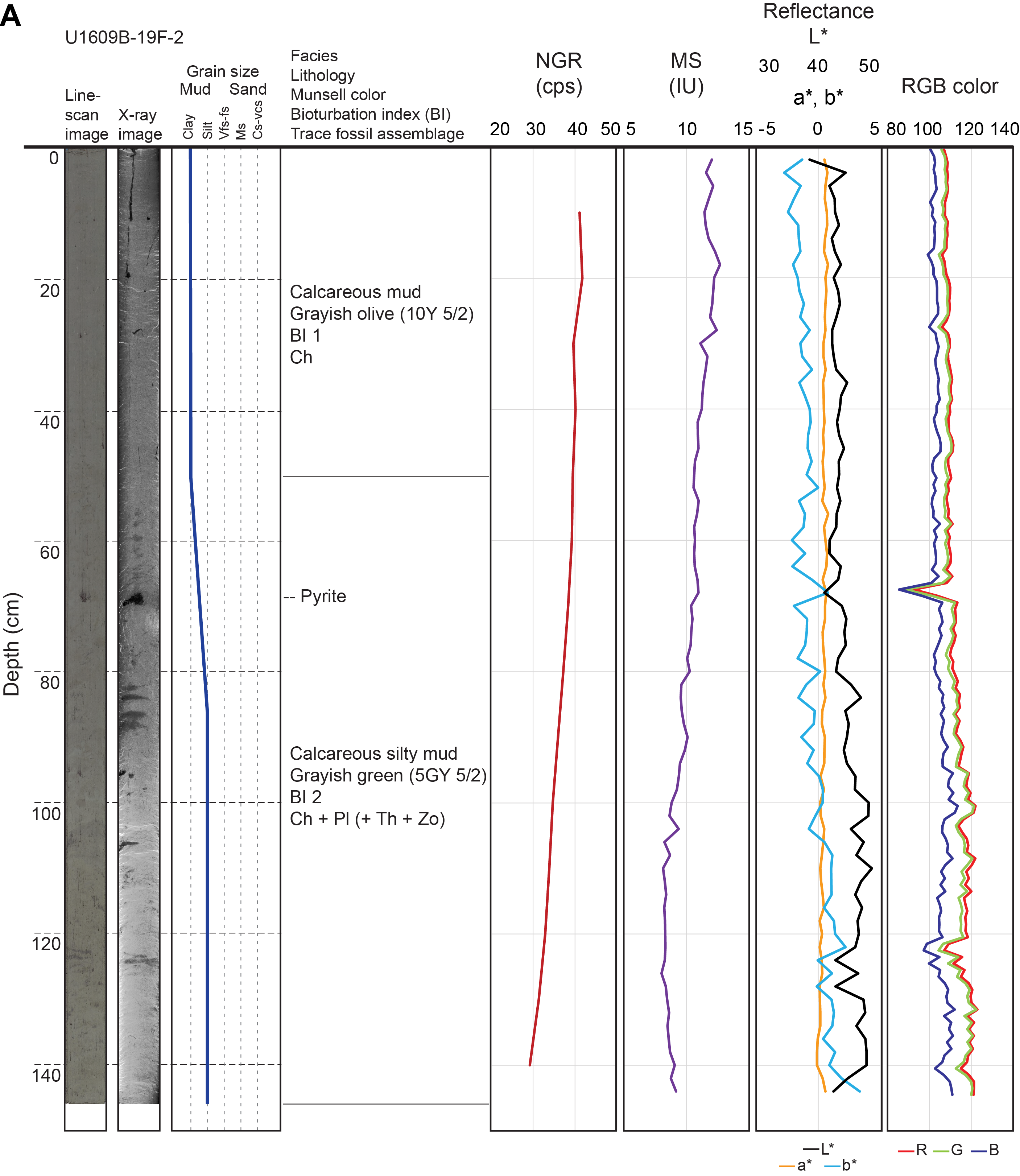
Individual bed thickness for each primary lithology was calculated for both holes (Figure F6). However, the top and bottom of each core were excluded because they represent only a portion of the bed and, therefore, a minimum value of bed thickness. For cores entirely composed of a single lithology, the thickness was still calculated but it represents the minimum bed thickness. It is important to note that the boundaries between lithologies are predominantly gradational, so the contacts are placed within the transitional interval between lithologies. True bed thickness can only be determined by integrating visual core description with physical properties data (e.g., magnetic susceptibility [MS] and natural gamma radiation [NGR]) (Figure F7A).
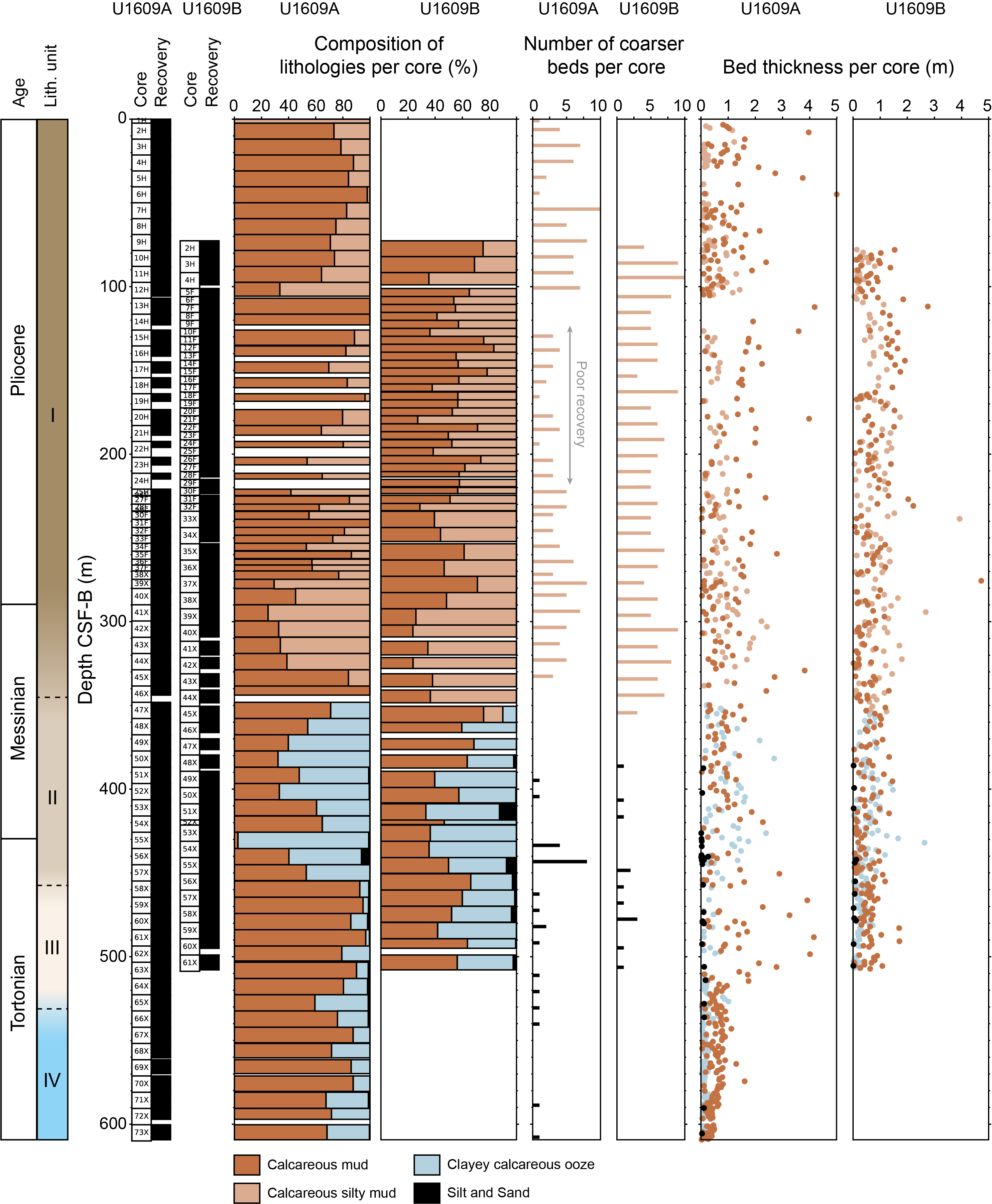
Figure F6. Core and bed thickness by lithology.
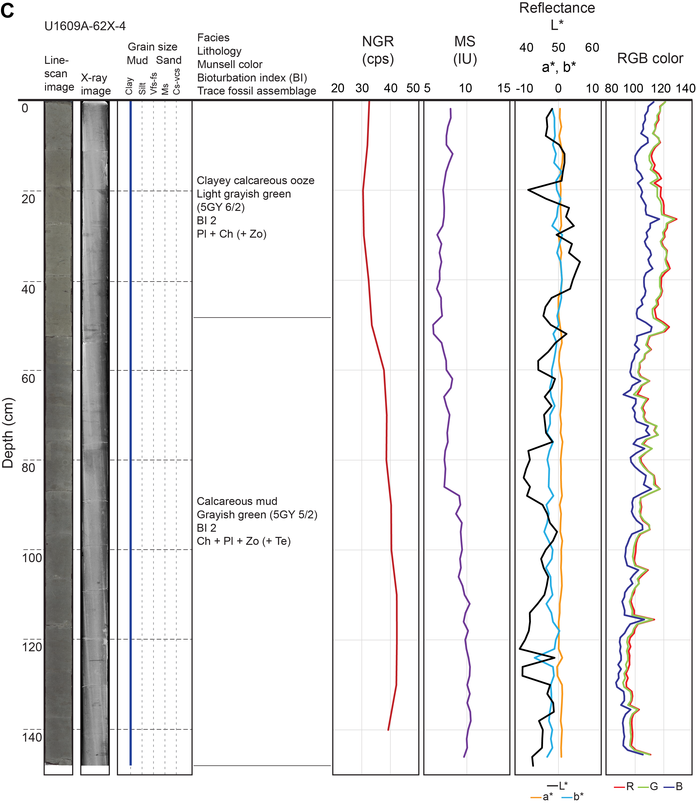
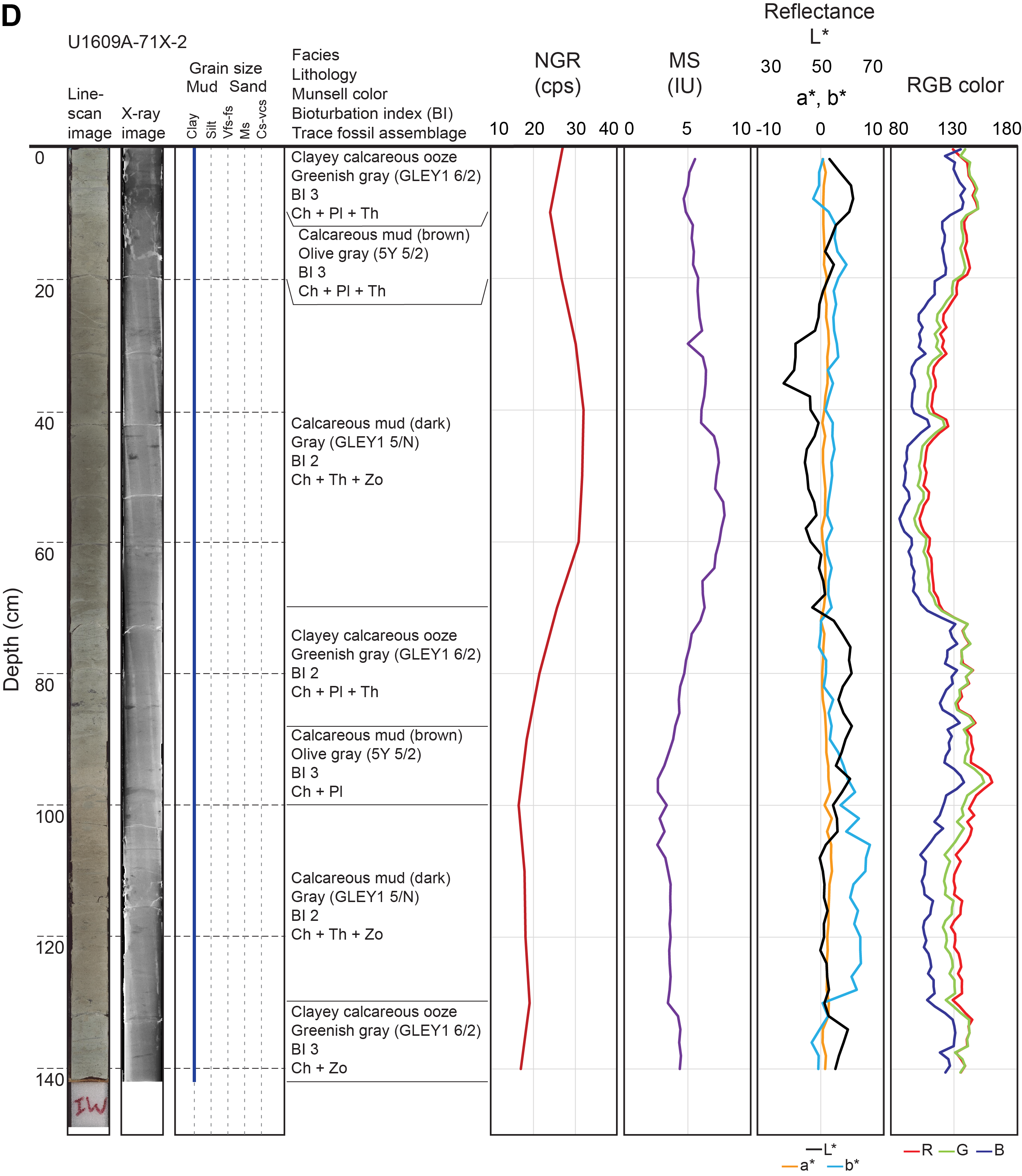
Figures F7. Facies description for each unit.
The trace fossil assemblage at Site U1609 is abundant and moderately diverse. Seven ichnotaxa have been recognized at the ichnogenus level, including abundant Chondrites, Planolites, and Zoophycos; frequent Phycosiphon and Thalassinoides; rare Palaeophycus; and occasional Asterosoma, Ophiomorpha, Scolicia, and Teichichnus together with undifferentiated horizontal and vertical structures. Crosscutting relationships are frequent among the ichnotaxa. Evidence of bioturbation is absent in only a few horizons in the cores.
Petrographic analysis of smear slides was taken regularly from Hole U1609A (n = 153). Smear slides prepared from Hole U1609B (n = 22) were analyzed to confirm the sediment classifications determined from Hole U1609A. Samples were selected from Hole U1609A squeeze cake residues (n = 22) or directly from cores (n = 11) for powder X-ray diffraction (XRD) analysis of bulk mineralogy and the mineral assemblage in the clay size (<2 µm) fraction to gain a general understanding of the bulk mineralogy of sediments and identify any large-scale trends with depth. Based on shipboard analyses for Hole U1609A, the total carbonate content in these cores ranges 19.5–74.9 wt% (see Geochemistry). The resulting scans of bulk mineralogy from all squeeze cake samples are shown in Figure F8. Although the mineralogy is overall uniform downhole, relative peak intensities, especially those of illite, quartz, calcite, and feldspar, change with depth. The primary minerals identified include quartz, calcite, plagioclase, K-feldspar, chlorite, mixed-layer illite/smectite (I/S), illite, and kaolinite, and minor dolomite and pyrite. Quartz and calcite are the dominant peaks. The two feldspars are present in all samples and make up a small component of the sediments.
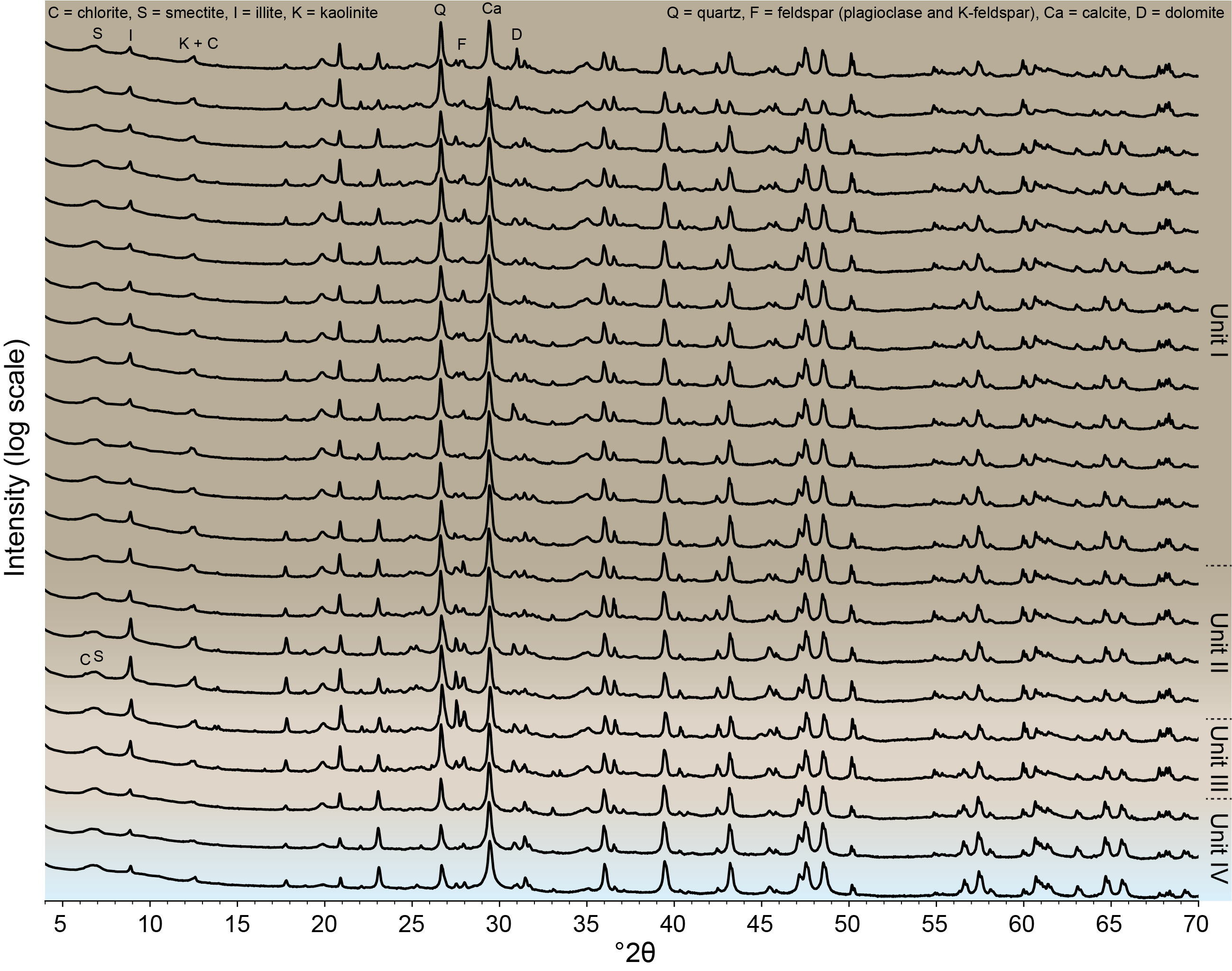
Figure F8. Powder XRD patterns, squeeze cake residues.
Clay minerals including chlorite, mixed-layer I/S, illite, and kaolinite are present in all samples. The reflection between 16° and 17.7°2θ indicates randomly ordered mixed-layer I/S (R0 I/S in Figure F9), although the presence of a fair amount of quartz and calcite in the <2 µm fraction makes it challenging to accurately determine the percentage of illite-type layers in the mixed-layer I/S. More detailed characterization of the clay mineral assemblage requires separation of the even finer fraction, although diffraction patterns of the <2 µm fraction reveal changes in the relative abundance between clay minerals and quartz/calcite and the relative abundance of different clay minerals with depth. Another general difference in the clay mineral assemblage is the presence of ordered mixed-layer I/S in the clay fraction of sediments from Unit II to Unit IV based on the strong reflection present at ~6.5°2θ (R1 I/S in Figure F9). The ordered I/S is absent in Unit I sediments based on the squeeze cake samples analyzed. Descriptions of XRD results in the following sections will focus on bulk mineralogy. The relative abundance of different minerals in all squeeze cake samples and samples collected from the three main lithologies is shown in Figure F10. The calcite percentage and changes in calcite content with depth determined from XRD data are consistent with the carbonate content determined by the coulometry method (see Geochemistry) on the same squeeze cake samples (Figure F11).
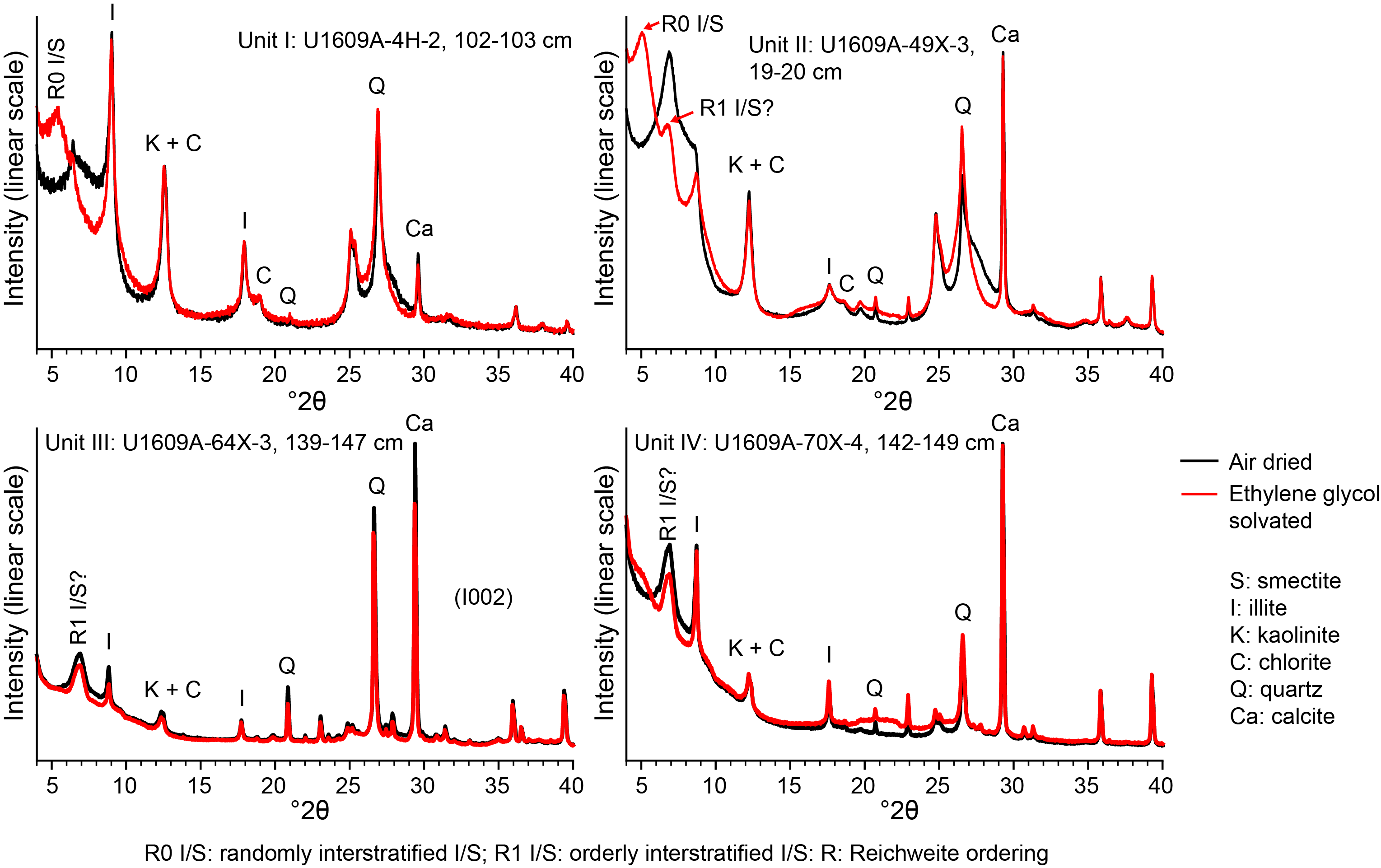
Figure F9. XRD patterns, <2 µm fractions.
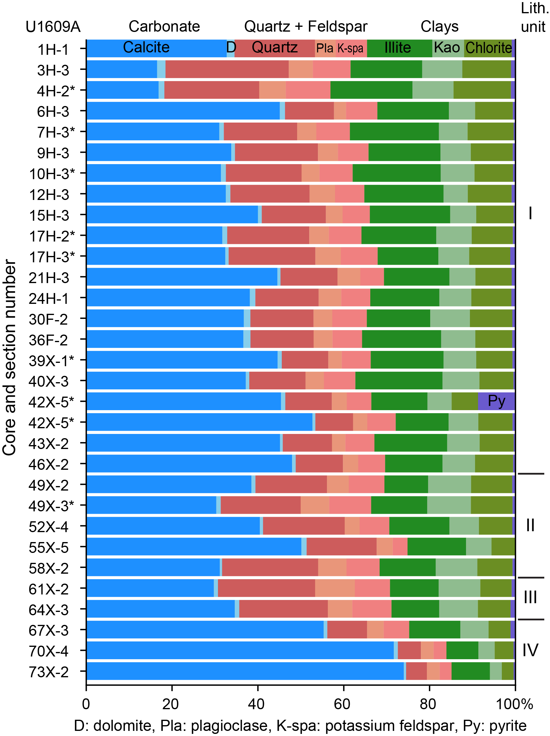
Figure F10. Mineral composition and percentage.
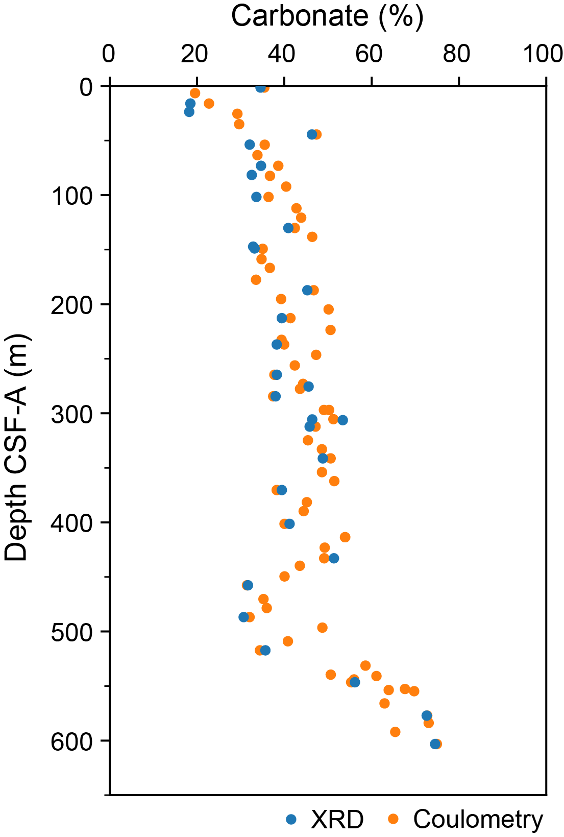
Figure F11. Variation in carbonate composition.
3.1. Unit I
- Intervals: 401-U1609A-1H-1 through 46X-CC; 401-U1609B-2H-1 through 44X-3
- Depths: Hole U1609A = 0–343.84 m CSF-A; Hole U1609B = 0–347.27 m CSF-A
- Age: Calabrian to late Messinian
3.1.1. Lithologies, bedding, and color
Unit I is composed of calcareous mud and calcareous silty mud deposits (Figure F6). These beds alternate with vertical thickness variations. The average bed thickness in Hole U1609A Unit I is ~100 cm for calcareous mud and ~60 cm for calcareous silty mud. Average bed thickness for Hole U1609B Unit I is ~75 cm for calcareous mud and ~70 cm for calcareous silty mud. Note that the uppermost part of Unit I was only recovered in Hole U1609A, which is where some of the thickest beds were observed. Contacts between lithologies are predominantly gradational, with transitions between calcareous muds and calcareous silty muds occurring over ~5 cm or more (Figure F7A). Occasionally, the transition from calcareous silty mud to calcareous mud occurs more rapidly and has a sharp contact (e.g., Section 401-U1609A-33F-1, 27.5–30 cm). Bed thickness analysis in the upper part of Unit I (0 to ~160 m CSF-A) shows that calcareous silty mud intervals are usually thinner than calcareous muds. This trend is broadly reversed in the lower part of the unit (Figure F6).
In Unit I, the calcareous muds have a mainly grayish olive color (10Y 5/2) and the calcareous silty muds are mainly grayish green (5GY 5/2). Minor color variations include weak red (2.5Y 5/2), reddish gray (2.5Y 5/1), light grayish green (5GY 6/2), and light brownish gray. Subtle and patchy color mottling is present throughout Unit I. Red-green-blue (RGB) data were occasionally used qualitatively to differentiate between certain similar colors or delineate subtle color variations of lithologies in Unit I. For example, although both calcareous mud (grayish olive) and calcareous silty mud (grayish green) in Unit I have a similar spread of RGB values, the red and green values are spread slightly farther from the blue values for calcareous silty mud (Figure F7A). Although this was not always the case, it did occasionally assist in identification of lithologies.
In interval 401-U1609A-17H-3, 112–115 cm (148.95–148.98 m CSF-A), there is a thin silty sand layer with a sharp erosive basal contact that is not continuous on the core width (Table T2). This greenish black interval, which contains about 2% glauconite, was not observed in Hole U1609B at an equivalent depth.
3.1.2. Structure and texture
Sedimentary structures in Unit I are subtle because of the very fine grained nature of the deposits and the abundance of bioturbation. Transitions between lithologies are often gradual, resulting in a common coarsening-upward trend from calcareous mud to calcareous silty mud, followed by a fining-upward trend from calcareous silty mud to calcareous mud. This facies association corresponds to a bigradational sequence with inverse to normal grading (e.g., Section 401-U1609A-44X-3) (Figure F12). There are a few examples where the central part of the sequence contains parallel to low-angle cross lamination, subtle centimeter-scale grain size and color variations (referred to as banding or centimeter-scale layering), and potential reactivation surfaces (Figure F12), which should be better identified with further postcruise analysis. This interval also contains less bioturbation than the surrounding lithologies. Within these sequences, it is still possible to identify subtle color banding at the centimeter scale, primarily associated with small-scale changes in composition within the calcareous silty mud deposits. Dominant textures are mud and silty muds with high proportions of clay. Based on smear slide analysis in Unit I (Figures F13, F14), the calcareous mud contains 1%–5% sand, 5%–30% silt, and 65%–95% clay. Calcareous silty mud contains 0%–5% sand, 5%–55% silt, and 45%–90% clay.
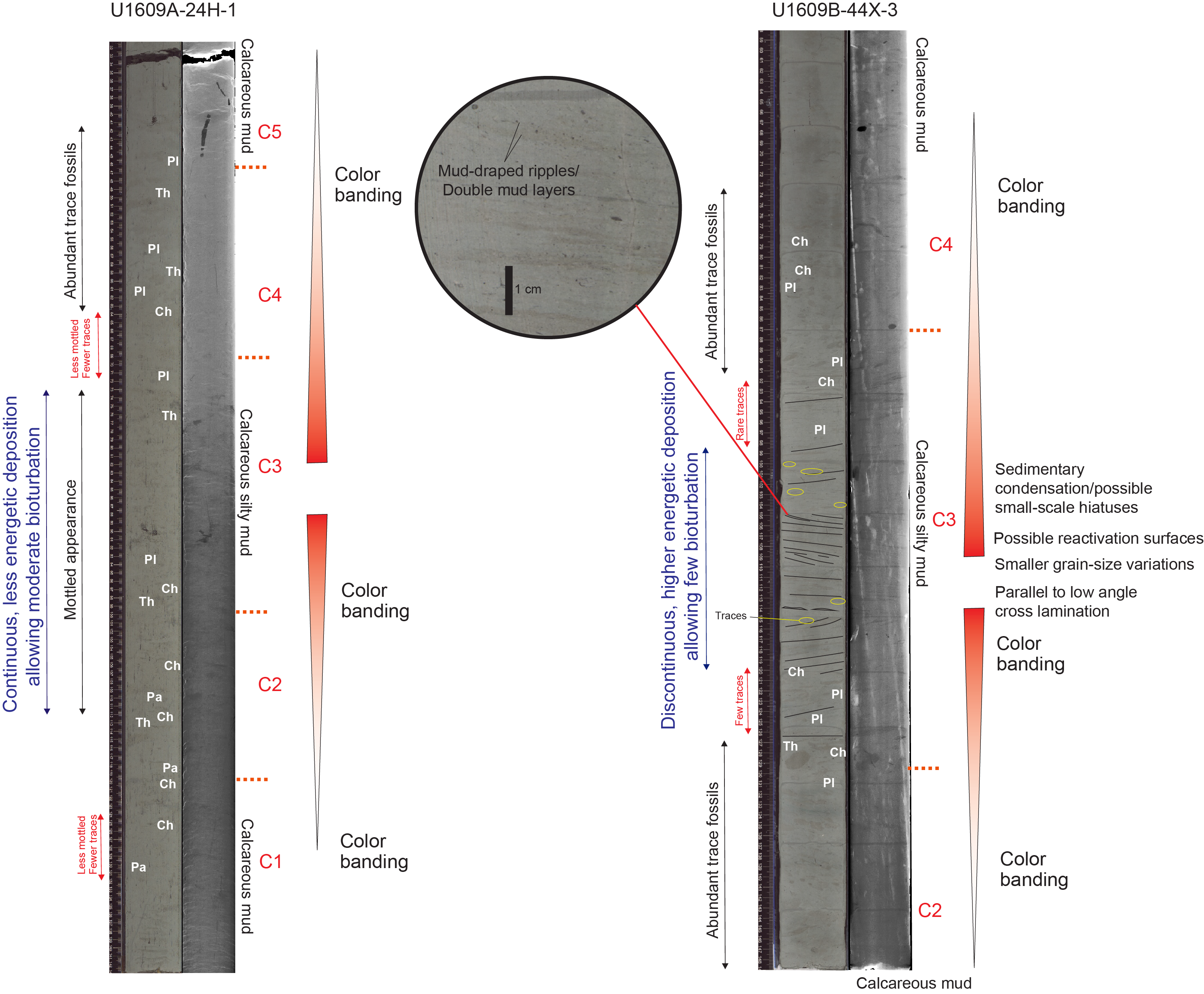
Figure F12. Fine-grained contourites, Unit I.
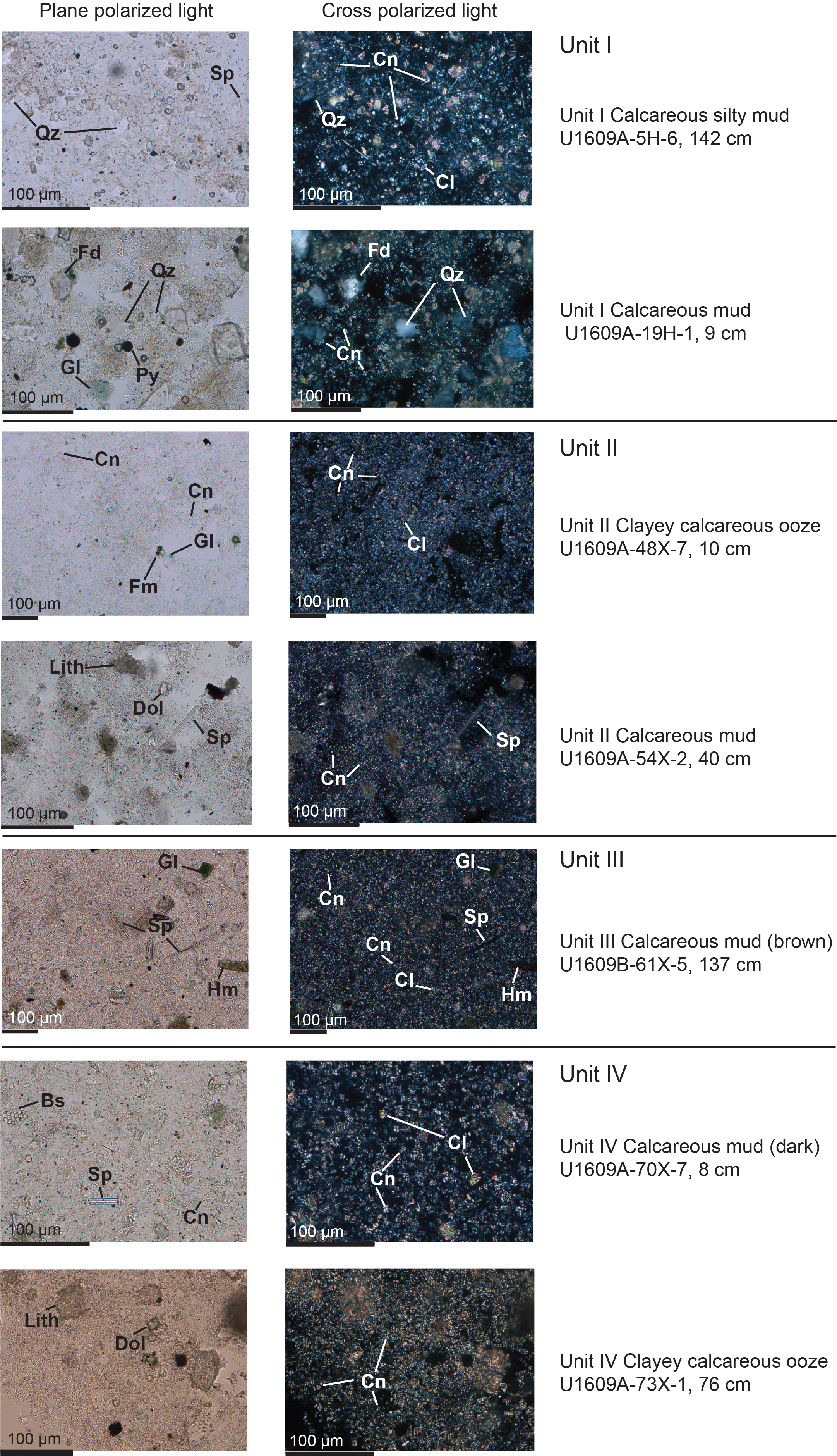
Figure F13. Major lithologies, Units I–IV.
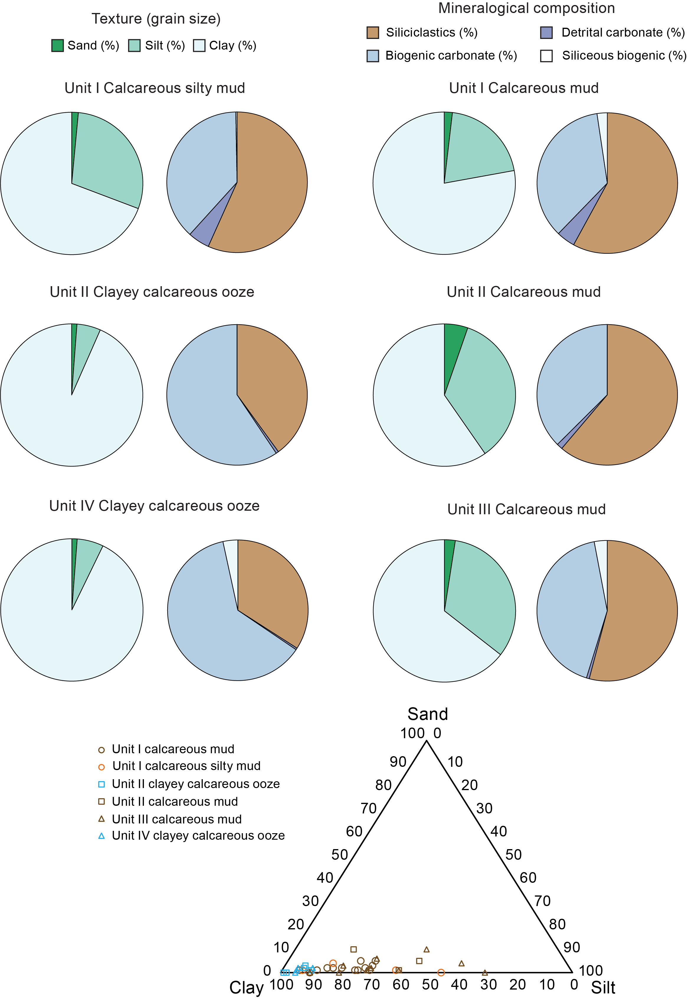
Figure F14. Texture and mineralogical composition in main lithologies.
3.1.3. Bioturbation and trace fossils
Unit I sediments are completely bioturbated, creating a mottled appearance. This mottled appearance refers to a patchy texture caused by bioturbation within originally soft to soupy or incoherent sediment. Thus, the trace fossils do not have distinct outlines and do not display a recurrent geometry that would allow their classification. Overprinting this mottled background, well-defined trace fossils are recognized. The relative abundance of discrete trace fossils is sparse to moderate according to the bioturbation index (BI) (mainly BI = 1–2), and typical trace fossil types include Chondrites, Planolites, Thalassinoides, and Zoophycos (Figure F15). Other ichnotaxa (i.e., Palaeophycus) as well as undifferentiated trace fossils are rare. In general, the calcareous silty muds have a higher BI (around 2) and trace fossil diversity than the calcareous muds (BI = 1). In the upper part of Unit I, calcareous silty muds commonly have a mottled appearance; this mottling is less common in the lower part of Unit I.
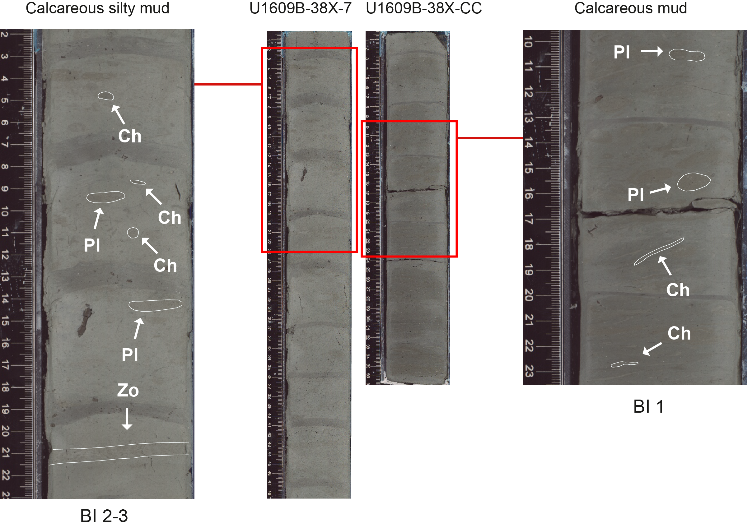
Figure F15. Trace fossil assemblages, Unit I.
Within the bigradational sequences, the ichnological record varies in respect to abundance and composition of the trace fossils (Figure F12). Some sequences show a moderately diverse trace fossil assemblage through the entire sequence (e.g., Section 401-U1609A-24F-1), including Chondrites, Planolites, and Thalassinoides. However, others show less bioturbation in the lower part of the sequence, a mottled appearance in the central part, and an upward increase in trace fossil abundance toward the top of the sequence. Other types of sequences are typified by a lower abundance of trace fossils and a clear vertical variation (e.g., Section 44X-3). The lower part of the sequence contains abundant trace fossils (i.e., Chondrites, Planolites, and Thalassinoides), and the central part displays a clear diminution in trace fossil abundance with a greater scarcity and even sometimes an absence of trace fossils. There is a progressive upward increase in trace fossil abundance in the upper part of the sequence.
3.1.4. Composition and bulk mineralogy
Lithologies in Unit I are mainly composed of clay minerals and bioclasts (dominantly calcareous nannofossils and some foraminifer fragments), quartz, feldspar, lithic grains, opaque minerals, pyrite, and planktonic and benthonic foraminifers, with some occurrence of siliceous biogenic components (e.g., sponge spicules), and shell fragments. Based on smear slide analysis, the calcareous mud in Unit I contains 50%–65% siliciclastic minerals, 0%–15% detrital carbonate, 25%–50% biogenic carbonate, and 0%–10% biogenic silica. Calcareous silty mud in Unit I contains 35%–75% siliciclastic minerals, 0%–15% detrital carbonate, 20%–65% biogenic carbonate, and 0%–1% biogenic silica. Within interval 401-U1609A-17H-3, 112–115 cm (148.95–148.98 m CSF-A), darker silty sand was observed; it is composed of abundant quartz, clay minerals, and calcareous nannofossils; common feldspar and lithic fragments; and about 2% glauconite.
Additional mineral composition results from XRD analysis on 13 squeeze cake residues and 8 samples collected from the working half of Unit I in Hole U1609A were obtained. Based on squeeze cake samples, Unit I (to ~283 m CSF-A; Section 401-U1609A-40X-3; Figure F10) contains 17%–45% calcite (average = 35%), 11%–29% quartz (average = 15%), and 8%–14% plagioclase and K-feldspar (average = 10%). Chlorite, illite, and kaolinite together make up on average 35% of the sediments of Unit I.
One pair of calcareous mud and calcareous silty mud samples in Unit I were taken from Core 401-U1609A-17H for XRD analysis. Despite the rather similar calcite and quartz contents, the calcareous mud (Section 17H-2; 147.26 m CSF-A) contains a higher amount of clay minerals compared to the calcareous silty mud (Section 17H-3; 148.92 m CSF-A), supporting their lithologic designations (Figure F16). The higher pyrite content in the calcareous silty mud is consistent with the more common presence of pyrite on the core surface and its slightly darker color compared to the calcareous mud.
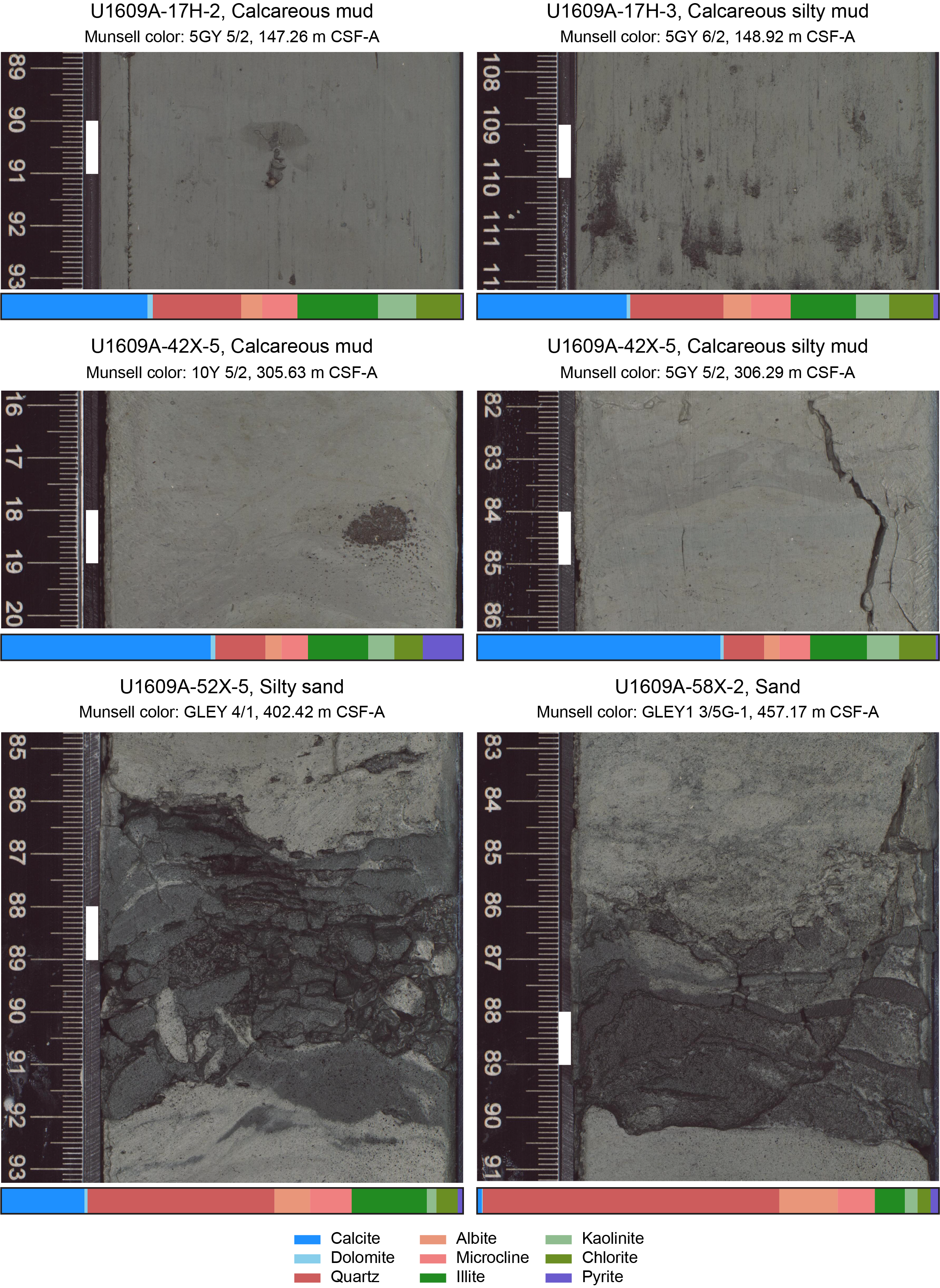
Figure F16. Lithologic names and mineral compositions.
3.2. Unit II
- Intervals: 401-U1609A-47X-1 through 58X-2; 401-U1609B-44X-4 through 56X-5
- Depths: Hole U1609A = 343.84–457.73 m CSF-A; Hole U1609B = 347.27–457.91 m CSF-A
- Age: late Messinian to late Tortonian
3.2.1. Lithologies, bedding, and color
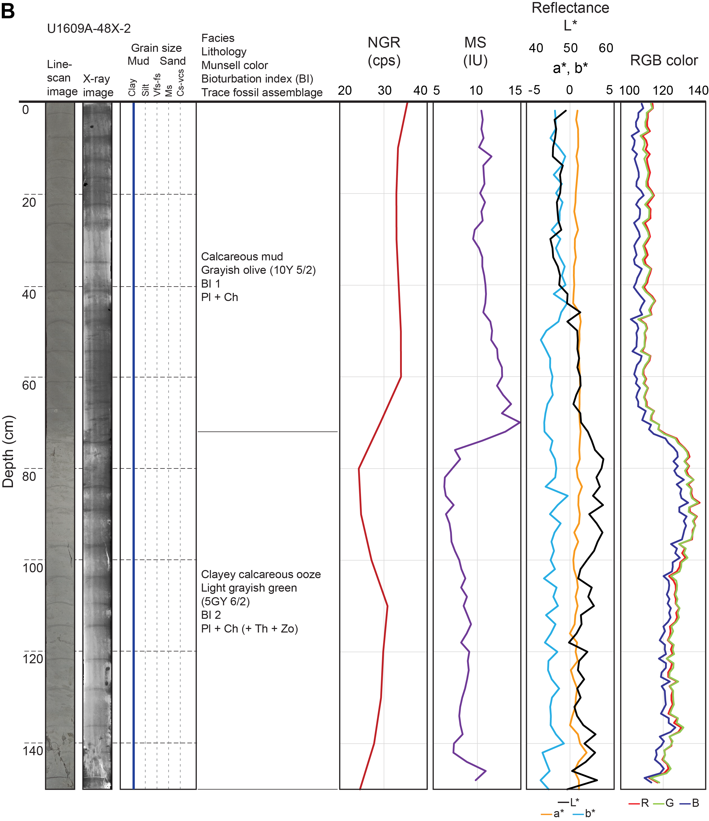
Unit II is composed of calcareous mud and clayey calcareous ooze (Figure F7B) with minor thin layers of fine sand and silty sand. These beds vary vertically in thickness and are associated with distinct but gradual color changes. Transitions between the lithologies are often gradual and can occur rapidly (over 2–5 cm) or more gradually (>10 cm); the contacts are often bioturbated. The clayey calcareous ooze is generally lighter in color and is the most dominant (>50%) lithology in this unit.
There are three dominant colors in Unit II, two of which are associated with primary lithologies. The calcareous muds are predominantly grayish olive (10Y 5/2) and occasionally dark greenish gray (GLEY1 4/1). Clayey calcareous ooze deposits are predominantly light grayish green (5GY 6/2) and occasionally greenish gray (GLEY1 6/1) and light greenish gray (GLEY1 7/1). Coarser deposits (e.g., sandy intervals) are dark greenish gray (GLEY1 4/1), light brownish gray (10YR 6/2), and very dark greenish gray (GLEY1 3/1). Clayey calcareous ooze typically has higher RGB values compared to calcareous mud (Figure F7B), demonstrating the gradational nature of many of the contacts between lithologies.
Individual bed thickness for each primary lithology was calculated (Figure F6). Average bed thickness for Hole U1609A Unit II is ~80 cm for calcareous mud and ~80 cm for clayey calcareous ooze. Rare coarser silty and sandy lithologies were observed and have an average thickness of ~5 cm. Average bed thicknesses for Hole U1609B Unit II are ~55 cm for calcareous mud, ~55 cm for clayey calcareous ooze, and ~5 cm for the coarser silty and sandy lithologies. Beds show no thickness variations relative to their depth within Unit II.
3.2.2. Structure and texture
Contacts between the calcareous mud and clayey calcareous ooze deposits are gradational (Figure F7B). The calcareous mud in Unit II is similar compositionally to that in Unit I, but the grain size in Unit II is noticeably coarser (Figure F14). The calcareous mud contains 1%–10% sand, 20%–45% silt, and 50%–70% clay. The clayey calcareous ooze is finer grained than the calcareous mud and contains 0%–3% sand, 1%–10% silt, and 90%–99% clay.
The rare sand and silty sand deposits in Unit II are characterized by sharp-based beds, with a massive lower part and/or normal grading (Table T2), that are occasionally parallel laminated. These deposits are interpreted to be turbidites.
3.2.3. Bioturbation and trace fossils
Lithologies from Unit II are commonly fully bioturbated. In some cases, bioturbation causes a mottled appearance by trace fossils that do not have distinct outlines and do not display a recurrent geometry. This mottled appearance is overprinted by well-defined trace fossils. Trace fossil assemblages are similar to those observed in Unit I, including Chondrites, Planolites, Thalassinoides, and Zoophycos, with rare occurrences of other ichnotaxa (i.e., Palaeophycus and Asterosoma), as well as undifferentiated trace fossils. However, with respect to Unit I, Unit II has a higher total abundance of trace fossils, an increased presence of Zoophycos, and local abundance of Phycosiphon. These changes were mainly observed in the clayey calcareous oozes, which have a higher abundance and diversity of traces than the calcareous muds, as well as frequent crosscutting relationships.
The turbidites in Unit II commonly have a lower, black, coarser grained division that is unbioturbated and an upper, lighter, finer grained part with abundant trace fossils including Chondrites, Planolites, and Zoophycos (e.g., Section 401-U1609A-56X-5; Figure F17). In this case, the clayey calcareous oozes below the turbidite contain fewer trace fossils (i.e., Planolites), with an infill that is similar to the host sediment, in this case clayey calcareous ooze.
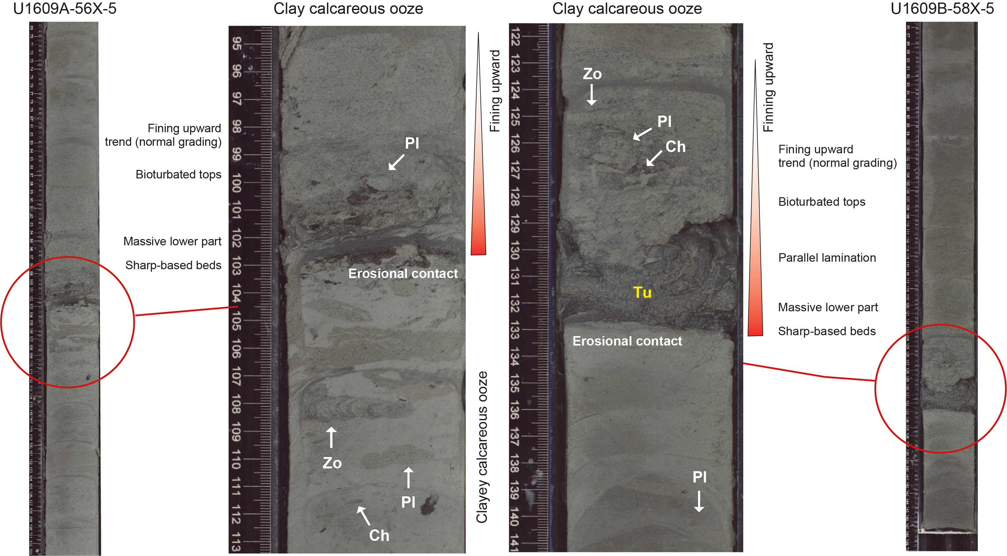
Figure F17. Turbidite beds in clayey calcareous oozes.
3.2.4. Composition and bulk mineralogy
Both Unit II lithologies are dominated by clay minerals and bioclasts (mainly calcareous nannofossils), with variable occurrence of siliceous components and shell fragments. They also contain quartz, feldspar, lithic grains, opaque minerals, pyrite, planktonic and benthonic foraminifers, sponge spicules, and minor biosiliceous fragments (Figures F13, F14). The calcareous mud in Unit II has a similar composition to that found in Unit I and contains 40%–75% siliciclastic minerals, 0%–5% detrital carbonate, 20%–60% biogenic carbonate, and <1% biogenic silica. Although the clayey calcareous ooze contains a larger percentage of biogenic carbonate, the prevalence of clay minerals in the sediments indicates it is not a true calcareous ooze. These sediments contain 20%–50% siliciclastic minerals, 0%–3% detrital carbonate, 50%–80% biogenic carbonate, and <1% biogenic silica.
XRD analyses were conducted on four squeeze cake residues and three samples collected from the working halves of Unit II in Hole U1609A. There appears to be a transition zone at the bottom of Unit I into the underlying Unit II (Figures F5, F10), reflected by the elevated calcite content (average = 45%) of the squeeze cake samples from Sections 401-U1609A-43X-2 and 46X-2. However, in terms of the limited number of XRD analyses undertaken, it is not possible to discriminate between Units I, II, and III. The mineral composition of one pair of calcareous mud and calcareous silty mud samples from Section 42X-5 (in the transition zone) was analyzed by XRD (Figure F10). The calcareous mud (305.63 m CSF-A) has a lower calcite content than the calcareous silty mud (306.29 m CSF-A; Figure F16). This highlights the downhole changes in sediment characteristics even for those with the same lithology name and the need to integrate bulk mineralogical data and direct observations of sediments to reliably infer their depositional histories.
Despite the relatively high calcite content, Unit II is interrupted by thin event beds characterized by significantly lower quantities of calcite and higher quantities of siliciclastic grains such as quartz and feldspars, as shown in the silty sand and sand samples from Sections 401-U1609A-52X-5 and 58X-2 (Figure F16). The illite component interpreted from the XRD patterns of these two samples likely includes a moderate amount of glauconite due to their overlapping peak positions. The presence of glauconite in these beds is confirmed by smear slide observations.
Results from smear slide analysis from the coarser intervals (Table T2) show that glauconite ranges <1%–30% and pyrite ranges <1%–20%. Some coarser intervals contain larger biogenic particles, such as benthonic foraminifers and sponge spicules. Alteration to siliciclastic components (e.g., inherited quartz overgrowths and clay-altered feldspars) have been identified in a few samples. These compositions allowed correlation between some of the sandy intervals between Holes U1609A and U1609B based on relative proportions of minerals in turbidites in the two holes. A total of 16 of these coarser beds were observed in Hole U1609A, but only 6 of these beds were identified in Hole U1609B, 4 of which may correlate with Hole U1609A based on smear slide analysis and correlation of NGR and MS (see Physical properties; Figures F41B, F4, F50; Table T2).
3.3. Unit III
- Intervals: 401-U1609A-58X-3 through 65X-6; 401-U1609B-56X-6 through 61X-CC
- Depth: Hole U1609A = 457.7–531.5 m CSF-A; Hole U1609B = 457.91–507.86 m CSF-A
- Age: late to middle Tortonian
3.3.1. Lithologies, bedding, and color
Unit III is composed of calcareous mud and clayey calcareous ooze. Contacts between lithologies are mostly diffuse, gradational, and typically associated with color changes (Figure F7C). Transitions from calcareous mud to clayey calcareous ooze mostly occur progressively over several centimeters (e.g., 50–55 cm). The transition from clayey calcareous ooze to calcareous mud can also occur more rapidly and be a sharp contact (e.g., Section 401-U1609A-65X-6, 36 cm).
Subtle and gradual changes in color are associated with the primary lithologies in Unit III. The clayey calcareous ooze in Unit III is generally lighter in color than the calcareous mud. The clayey calcareous ooze appears predominantly light grayish green (5GY 6/2) or occasionally grayish green (5GY 5/2) in Hole U1609A and pale green (GLEY1 6/1) in Hole U1609B. The calcareous mud occurs in two distinct colors, grayish green (5GY 5/2) or occasionally light grayish green (5GY 6/2) in Hole U1609A and grayish olive (10Y 5/2), grayish green (GLEY1 5/2), or olive-gray (5Y 5/2) in Hole U1609B. The generally darker grayish green calcareous mud dominates this unit.
Clayey calcareous ooze and calcareous mud beds alternate and vary in thickness. Average bed thickness for Unit III (Figure F6) in Hole U1609A is ~120 cm for calcareous mud, ~30 cm for clayey calcareous ooze, and ~10 cm for the silty and sandy intervals that have a maximum thickness of 17 cm. Average bed thickness for Unit III in Hole U1609B is ~60 cm for calcareous mud, ~25 cm for clayey calcareous ooze, and ~4 cm for sandy intervals.
There are also some sandy deposits in Unit III. These coarser intervals (e.g., silty and/or calcareous sands) appear grayish olive (10Y 5/2), pale yellow, (5Y 7/3), dark grayish green (GLEY1 4/1), or very dark greenish gray (GLEY1 3/1). Similar to Unit II, the clayey calcareous ooze typically has slightly higher RGB values compared to calcareous mud (Figure F7C).
3.3.2. Structure and texture
The calcareous mud in Unit III has a similar texture to the calcareous mud in Unit II, but this lithology is noticeably finer grained than in Unit I (Figure F14). The calcareous mud contains 0%–10% sand, 10%–70% silt, and 30%–90% clay. The clayey calcareous ooze in Unit III is finer grained by comparison and contains ~2% sand, 20% silt, and 80% clay. Because of the fine-grained nature of these sediments, sedimentary structures are difficult to see, particularly in the calcareous mud and clayey calcareous ooze.
The sandy layers are occasionally parallel or cross laminated, and the base of the beds can be either normally graded or massive. Most sandy layers have a sharp or erosional lower contact, and this is sometimes bioturbated or irregular. These facies are interpreted to be turbidites. Seven of these coarser beds were detected in Hole U1609A, but only five were detected in Hole U1609B, three of which may correlate with Hole U1609A (see Physical properties) (Figures F4, F41B; Table T2). The texture of the sandy deposits varies in maximum grain size from very fine to fine sand. The coarsest beds have a proportion of grain sizes of the different fractions up to 65% sand, 15% silt, and 20% clay, and the finer beds can be as fine as 3% sand, 45% silt, and 50% clay.
3.3.3. Bioturbation and trace fossils
Lithologies from Unit III are commonly fully bioturbated. In some cases, bioturbation causes a mottled appearance and trace fossils that do not have distinct outlines and do not display a recurrent geometry. This mottled appearance is overprinted by well-defined trace fossils. The trace fossil assemblage is similar to that observed in Unit II, mainly including Chondrites, Planolites, Thalassinoides, and Zoophycos, maintaining the changes previously observed, such as the abundance of Zoophycos and the local record of Phycosiphon. Occasionally, very small specimens of Chondrites and Zoophycos, around 1 mm in diameter, were observed, with a typical size range up to 2–3 mm in Chondrites and up to 4–5 mm in Zoophycos.
Several turbidites were observed in Unit III (Figure F17). One particular example (Section 401-U1609B-58X-5) has a lower black, coarser grained, and unbioturbated interval overlain by an upper lighter, finer grained interval with moderate amounts of trace fossils (e.g., Planolites). Moreover, the clayey calcareous ooze below the turbidite contains abundant trace fossils with variable infilling material. Occasionally the infilling material of these trace fossils is similar to the turbidite material (i.e., Zoophycos infilled by material from the turbidite).
3.3.4. Composition and bulk mineralogy
Lithologies in Unit III mainly comprise clay minerals and bioclasts (mainly calcareous nannofossils and some foraminifers fragments), with some siliceous components and shell fragments. They also contain quartz, feldspar, lithic grains, opaque minerals, pyrite, planktonic and benthonic foraminifers, sponge spicules, and minor biosiliceous fragments (Figures F13, F14). The calcareous mud contains 35%–80% siliciclastic minerals, 0%–5% detrital carbonate, 15%–60% biogenic carbonate, and 0%–10% biogenic silica. Although the clayey calcareous ooze in Unit III contains a larger percentage of biogenic carbonate, the prevalence of clay minerals in the sediments indicates it is not true calcareous ooze. These sediments contain 65%–70% siliciclastic minerals, 30%–35% biogenic carbonate, and no detrital carbonate or biogenic silica.
XRD analyses were conducted on two squeeze cake residues of Unit III in Hole U1609A. The calcite content is relatively low (~30%) in Unit III (Figures F10, F11), consistent with lower values in the deepest Unit II squeeze cake sample (Section 58X-2) compared to other samples in Unit II. Unit III samples are characterized by relatively high quartz (20%) and feldspar (15%) contents.
Some sandy intervals sampled for smear slide analysis provide semiquantitative compositional data (Table T2). For these samples, glauconite and pyrite range <1%–25% and in some cases is particularly noticeable (e.g., 401-U1609B-58X-4; ~25%). The glauconite grains in the turbidites are mostly well rounded (Figure F18). Some coarser intervals contain larger biogenic particles, such as sponge spicules, some of which have been pyritized (Figure F18). Some turbidite samples contain completely or partially pyritized sponge spicules, which tend to have robust and chunky shapes. In the same smear slide, fresh-looking, nonpyritized sponge spicules can also be observed (Figure F18). The concentration of foraminifers is higher in the sandy interval of Section 58X-5. Alteration to siliciclastic components (e.g., clay-altered feldspar and quartz overgrowths) was identified in a few samples. These compositions, as well as correlation with NGR and MS (Figure F4, F50), have allowed correlation between some of the sandy intervals between Holes U1609A and U1609B. This is partly because it appears that glauconite abundance produces a spike in the MS record (see Physical properties) (Figure F41). However, not all sandy intervals were possible to correlate between Hole U1609A and U1609B.
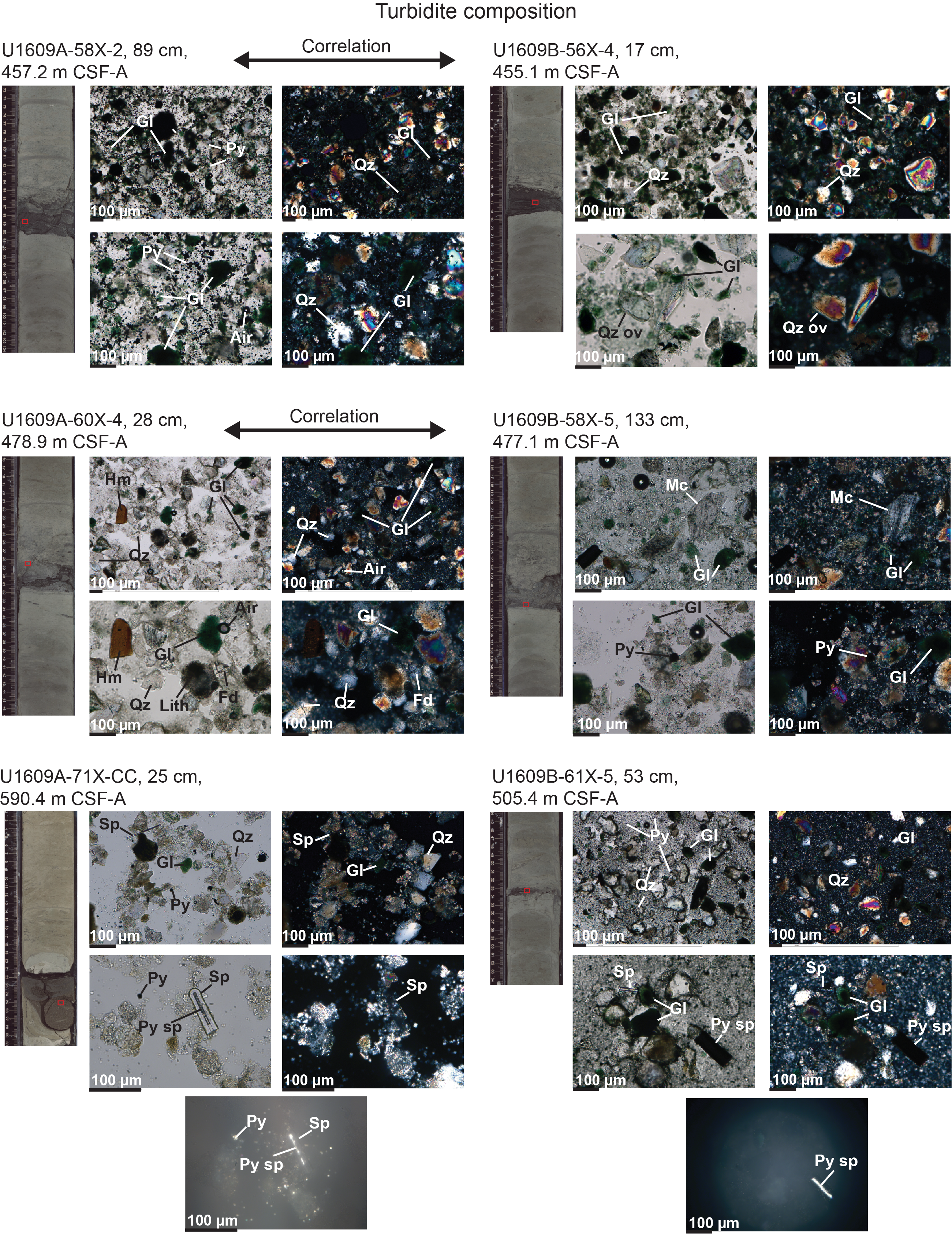
Figure F18. Turbidite composition, turbidite layers.
3.4. Unit IV
- Interval: 401-U1609A-65X-7 through 73X-CC; not present in Hole U1609B
- Depth: Hole U1609A = 531.5–609.3 m CSF-A
- Age: middle to early Tortonian
3.4.1. Lithologies, bedding, and color
Lithologies in Unit IV consist of two distinct calcareous muds distinguished primarily on color and a clayey calcareous ooze (Figure F7D). Contacts between the primary lithologies are gradational and indicated by subtle changes in color. However, color changes were much more distinct in Unit IV compared to the more subtle changes observed in Units I–III. Bed thickness in Unit IV is notably thinner than for all other units, with an average thickness of ~50 cm for the calcareous muds and ~15 cm for the clayey calcareous ooze deposits (Figure F6).
In Unit IV, the calcareous mud appears gray (GLEY1 5/N) and olive-gray (5Y 5/2), whereas the clayey calcareous ooze appears pale green (GLEY1 6/2). The silty sand layers are dark greenish gray (GLEY1 3/1). Similar to Units II and III, clayey calcareous ooze typically has higher RGB values compared to calcareous mud (Figure F7D). However, this was complicated by different colors in the calcareous mud lithology. Although the dark calcareous mud (gray) has similar RGB values to those of the clayey calcareous ooze and higher than those of the brown calcareous mud (olive-gray), it exhibits a greater spread between the red, blue, and green values, whereas the clayey calcareous ooze has red and green values that typically overlap.
3.4.2. Structure and texture
Because of the fine-grained nature of the two main lithologies, sedimentary structures are difficult to identify, but the silty sand layers show normal grading and typically sharp to erosional lower contacts. The calcareous mud in Unit IV has a similar texture to the calcareous mud in Unit I (Figure F14) and contains 0%–2% sand, 30%–40% silt, and 60%–70% clay. The clayey calcareous ooze in Unit IV has a similar grain size distribution as the clayey calcareous ooze in Unit II and III and contains 0%–2% sand, 5%–10% silt, and 90%–95% clay.
Three sandy intervals were identified in Unit IV of Hole U1609A that are fine to very fine sands; however, no primary sedimentary structures were observed in these deposits. These intervals are less frequent than in Units II and III. Of the three intervals that were identified, only two have a determinable lower contact that is sharp and erosional (one was obscured by drilling disturbance). The coarser silty and sandy intervals have an average thickness of ~9 cm with a maximum of 12 cm.
3.4.3. Bioturbation and trace fossils
Lithologies from Unit IV contain similar ichnological features to those observed in Units II and III. In some cases, bioturbation causes a mottled appearance and trace fossils do not have distinct outlines and do not display a recurrent geometry. This mottled appearance is overprinted by well-defined trace fossils, mainly consisting of Chondrites, Planolites, Thalassinoides, and Zoophycos relationships. As in Unit III, small and large Chondrites and Zoophycos were recognized.
3.4.4. Composition and bulk mineralogy
The calcareous mud in Unit IV contains 60% siliciclastic minerals, 30%–35% biogenic carbonate, and 1%–10% biogenic silica. The clayey calcareous ooze in Unit IV contains 25%–50% siliciclastic minerals, 0%–2% detrital carbonate, 50%–75% biogenic carbonate, and 1%–10% biogenic silica. XRD analyses were conducted on three squeeze cake residues from Unit IV in Hole U1609A. Unit IV is characterized by a distinctly higher content of calcite (more than 50% and up to 75%; Figure F11) and a lower content of quartz and feldspar. Of the four units, Unit IV contains the lowest content of chlorite, illite, and kaolinite (Figure F10).
Of the three sandy intervals identified in Unit IV, two intervals were analyzed as smear slides, providing semiquantitative data on their composition. Glauconite ranges from few (1%–5%) to common (10%), and pyrite ranges from few (1%–5%) to common (20%). One sample contains partially pyritized sponge spicules (Table T2). The sandy interval from Section 401-U1609A-71X-CC contains many foraminifers, in contrast to the other samples.
3.5. Discussion
The lithologic changes described in the two holes at Site U1609 are both subtle and gradational (Figure F6), particularly with respect to grain size and composition. Although unit boundaries were defined by partly integrating the chemical (percent carbonate) and physical properties (NGR and MS logs) data with the lithologic characteristics described in this chapter, these should not be regarded as sharp. It would be possible to define lithostratigraphic units at other depths. In particular, the boundary between Units I and II may be located in a transition zone ranging from ~300 m CSF-A to the defined unit boundary at 344.0 m CSF-A (Figure F4). This is particularly important regarding the calcite content determined from the XRD data and through the coulometry method (see Geochemistry). A high-resolution grain size and X-ray fluorescence (XRF) record will be required to resolve key questions about both the lithologic changes that occur and the sedimentary processes that drove them.
3.5.1. Dominant sedimentary facies and trace fossil assemblage
The calcareous mud, calcareous silty mud, and clayey calcareous ooze deposits identified in Units I–IV represent deepwater sedimentary facies vertically associated in a clear rhythmic pattern. The overall absence of primary traction structures, poor sorting, and common bioturbation is typical of pelagic sediment with low terrigenous input (Hüneke and Henrich, 2011; Stow and Smillie, 2020; de Castro et al., 2021).
The trace fossil assemblage in Unit I can be assigned to the distal expression of the Cruziana ichnofacies transitioning to the Zoophycos ichnofacies (MacEachern et al., 2007), supporting the interpretation of a hemipelagic environment. In Units II and III, the trace fossil assemblage is generally similar to that observed in Unit I. However, the observed changes, such as the increase in the total abundance of trace fossils and the greater abundance of Zoophycos, could be related to the archetypal Zoophycos ichnofacies (MacEachern et al., 2007), pointing to changes toward more distal and probably deeper environments. The record of Phycosiphon, a trace fossil related to local increase in benthonic food availability and low oxygen conditions (Rodríguez-Tovar et al., 2014), could be associated with increased inputs of benthonic food. The local presence of very small trace fossil specimens in Unit III can be interpreted in the context of a quiet benthonic environment allowing development of very delicate structures. The trace fossil assemblage in Unit IV reveals similar paleoenvironment conditions to those of Unit III.
Relatively abundant and moderately diverse trace fossil assemblages at the site, usually overprinting a mottled background, reveal generally favorable paleoenvironmental (i.e., ecological and depositional) conditions for the macrobenthonic trace fossil maker community in terms of organic matter supply, sedimentation rate, and oxygenation (Rodríguez-Tovar, 2022).
3.5.2. Bottom current deposits
Evidence of bottom current deposits is visible in Unit I. For example, there is a rhythmic pattern, with gradual transitions between calcareous mud and calcareous silty mud (average thicknesses between 0.6 and 1 m) and the occurrence of subtle centimeter-scale changes in color and grain sizes (lamination or centimeter-scale layering). In particular in cores around 270 m CSF-A, these lithologies are associated with visible centimeter-scale layering that could be symmetric and asymmetric bigradational sequences (e.g., Section 401-U1609A-24H-1; Figure F12), characteristic of very fine grained contourites (Gonthier et al., 1984; Stow and Faugères, 2008; Stow and Smillie, 2020). These deposits not only have subtle grain size variations but also color lamination that has been described in finer grained contourite deposits (Hüneke et al., 2021; Hernández-Molina et al., 2022).
Some of the bigradational sequences with coarser sediments at the very bottom of Unit I (e.g., Section 401-U1609B-44X-3; Figure F12) have parallel to cross lamination in the central division, as well as vertical smaller grain size variations, possible reactivation surfaces, fossil traces indicative of sedimentary condensation, and possible small hiatuses (based on the trace fossil assemblage). All these features have been identified in contourite sequences (Gonthier et al., 1984; Stow and Faugères 2008; Mulder et al., 2013; Rodríguez-Tovar et al., 2019; Stow and Smillie, 2020; Hüneke et al., 2021; Hernández-Molina et al., 2022; Rodríguez-Tovar, 2022; Rodrigues et al., 2022). Rare bigradational sequences show that the facies associations mimic the division of C1–C5 proposed by Stow and Faugères (2008). The facies associations described here are typically associated with a contourite drift (e.g., de Castro et al., 2020, 2021) and will be confirmed by further analysis such as grain size measurements.
Variability in the ichnological record of the contouritic deposits in Unit I (Figure F12) reflects subtle changes in depositional environment, indicating higher energy conditions with some assemblages associated with less favorable conditions for the macrobenthonic trace fossil maker community. Regardless of energy conditions, a similar pattern is observed in ichnological features from the bottom to the top of the contourite deposits, allowing differentiation of several divisions that support the identification of the standard bigradational sequences for the contourite deposits (Rodríguez-Tovar and Hernández-Molina, 2018; Rodríguez-Tovar et al., 2022).
3.5.3. Turbidites
The characteristics of the centimeter-scale sand and silty sand deposits identified in Units II–IV are clear evidence of a decelerating turbulent flow suspension fallout (e.g., Bouma et al., 1962). These facies are interpreted to be deposits from low-density turbidity currents (Lowe, 1982; Postma, 1986; Stanley, 1988; Stow and Wetzel, 1990; de Castro et al., 2020, 2021; de Weger et al., 2021; Hüneke et al., 2021). The massive and/or normal grading and the upper parallel lamination (when visible) are linked to deposition from a waning turbidity current. Bioturbation occurs primarily toward the top of the turbidite deposits (Rodríguez-Tovar, 2022). The partial turbiditic sequences described here are typical of fine-grained turbidites (Piper and Stow, 1991; Stow and Piper, 1984).
The varying composition of the turbidites in terms of quartz, glauconite, pyrite, pyritized sponge spicules, and foraminifer content (Table T2) differentiates turbidites from contourites and likely points to different sources for the gravity flows. Turbidites with a dominant siliciclastic component can be attributed to a provenance in a shallower environment and/or continental sources because of the angular to subangular shapes of the quartz, feldspar, and lithic grains (Figure F18). The sources of the turbidites containing predominantly intrabasin deepwater bioclastic components are likely from reworking of deposits in more proximal areas of the middle slope but not from shallow-marine environments. Some of the quartz, feldspar, and lithic grains are angular to subangular (Figure F18), suggesting an immature provenance direct from a riverine source rather than long-term reworking in a shallow-marine environment. The presence of quartz overgrowths in some layers, likely to have been inherited from a previous depositional–burial–erosional cycle, suggests that the original sandstones had been relatively deeply buried.
High concentrations of glauconite help with correlation (e.g., in the turbidite containing 30% glauconite in Holes U1609A [Section 401-U1609A-58X-2; 1% pyrite] and U1609B [Section 401-U1609B-56X-4]; Table T2). The glauconite likely originated in a shallower marine environment than the drilled location of Site U1609 and was transported downslope by turbidity currents. Although glauconite is particularly concentrated in only some turbidites, the general content in other depositional facies of the site is high (>5%). The glauconite from the turbidites may have been an important source for partial reworking into the hemipelagic calcareous muds and clayey oozes. It is possible that this increased contribution of glauconite via turbidity currents and other downslope processes from a glauconite factory area may explain the upward increase in gamma ray response in Unit III from Unit IV (see Physical properties). However, although optimal conditions for glauconite formation are on the outer shelf/upper slope (Hesse and Schacht, 2011), many deepwater occurrences down to 2000 m water depth have been reported (e.g., Odin and Stephan, 1982), so some of the glauconite in the fine-grained sediments likely formed in situ.
The wide variability of pyrite abundance, in particular the co-occurrence of pyritized and nonpyritized biogenic debris, together with the pervasive evidence for extensive reworking of these sediments by marine fauna and thus a mainly oxygenated bottom water environment, strongly argues against in situ pyritization. This indicates transport of pyrite from sediments upslope that have undergone active bacterial sulfate reduction. Variable composition of the turbidites suggests changing source areas for the turbidity currents.
The ichnological records associated with turbidites can be linked to distinct depositional processes. In some cases, downward bioturbation is visible, and trace fossils are filled with material matching the composition of the overlying turbidite (i.e., Zoophycos), which suggests temporarily interrupted or reduced sedimentation rates allowing the marine fauna to develop (Figure F12). In other cases, the absence of trace fossils underneath the turbidite or trace fossils with infill of a different lithology than the turbidite suggests continuous deposition, which prevented bioturbation by animals (Figure F17).
The wide variation in glauconite abundance (<1%–30%) partly controls the gamma ray response (Figures F18, F41) (see Physical properties), which was used for preliminary correlations between Holes U1609A and U1609B (Table T2). Only some turbidites were possible to correlate between Holes U1609A and U1609B, 20 m apart parallel to the continental margin, indicating that at least sometimes the gravity flow was laterally limited. However, the extensive reworking of some of the turbidites by bioturbation, as demonstrated by the ichnological records (Figure F17), has likely removed direct evidence for some turbidites at one or the other of the holes.
3.5.4. General sedimentary model
The identified sedimentary facies and facies associations (Figures F6, F7) can be attributed to deepwater, very fine grained deposits (Kennett, 1982, Pickering and Hiscott, 2015; Stow and Smillie, 2020; Rotzien et al., 2022a, 2022b). Site U1609 is located along the middle slope terrace offshore of west Portugal in a proximal part of the continental slope (Figure F1). This area is bounded to the south and north by the large São Vicente and Setúbal submarine canyons. Sediment supply was funneled across the middle slope through the submarine canyons, allowing pelagic and bottom current processes to dominate the area cored. Vertical and lateral variability of the bottom currents may explain the interrelation between the pelagic sediments and the contourites, especially during deposition of Unit I. Offshore west of Portugal a large, middle-slope plastered drift (the Sines Drift) was active during the Pliocene and the Quaternary (Hernández-Molina et al., 2016; Rodrigues et al., 2020). Site U1609 recovered part of this Pliocene and Quaternary drift (see Background and objectives) (Figure F3).
In this general sedimentary model, turbidite deposits were developed in the early Messinian and the Tortonian, a period of high tectonic instability across the region (Suárez Alba et al., 1989; Riaza and Martínez Del Olmo, 1996; Sierro et al., 1996; Maldonado et al., 1999; Ledesma, 2000; Martínez del Olmo and Martín, 2016). The increased turbidite deposition recorded in Units II and III may coincide with those tectonic events (see Background and objectives) (Figure F3). Relative sea level variations may be another controlling mechanism for triggering gravity flows during this time interval, especially during periods of relative sea level fall.
The strong cyclicity visible in both the sedimentary facies and the physical properties data may be explained by climatic variations and the bottom current variability at a scale of precessional cyclicity. Bottom currents during the deposition of Unit I were weak but vigorous enough at intermediate depths for developing a plastered drift along the middle continental slope (e.g., Hernández-Molina et al., 2008). The thinner, more finely interbedded primary lithologies identified in Units I and IV may be linked to periods of lower sedimentation rate during the Tortonian and the Pliocene. On the longer time scale, the general shallowing trend identified based on the trace fossil assemblages from the Tortonian to the Pliocene can be related to the long-term sea level regression (landward) and later progradation (basinward) of the margin (Riaza and Martínez Del Olmo, 1996; Sierro et al., 1996; Maldonado et al., 1999; Ledesma, 2000; Martínez del Olmo and Martín, 2016).
4. Biostratigraphy
The sedimentary record recovered at Site U1609 is mostly continuous, although minor discontinuities cannot be totally excluded based on the low resolution of the biostratigraphic sampling on board the ship. Preservation of microfossils is generally good with abundant calcareous nannofossils and planktonic foraminifers, whereas benthonic foraminifers are rare. Integrated foraminifer and nannofossil bioevents are illustrated in Figure F19 and the datums found in Holes U1609A and U1609B are listed in Tables T3, T4, T5, and T6.
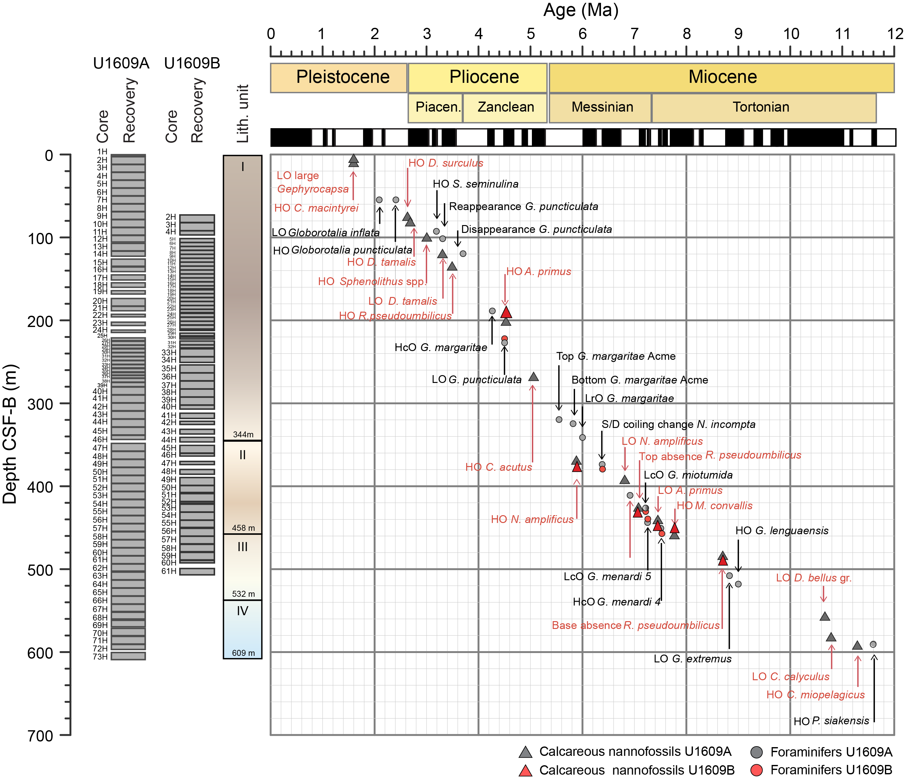
Figure F19. Preliminary age model.
Based on the calcareous nannoplankton assemblage, the top of the sequence recovered in Hole U1609A is estimated to be older than 1.24 Ma (Table T3), indicating that a significant proportion of the Pleistocene sequence is missing at this location. A continuous series of calcareous nannoplankton and planktonic foraminifer events were recorded at this site spanning from ~1.24 Ma to the earliest Tortonian (Figure F19). Some of the calcareous nannofossil bioevents, specifically the highest occurrence (HO) events, may have been affected by reworking and redeposition. However, the ages derived from both nannofossils and foraminifers suggest that this is not a major issue. Sedimentation rates for the lower part of the sequence combined with the oldest bioevent (11.19 Ma) (Table T4) suggest an age close to the Tortonian/Serravallian boundary for the base of Hole U1609A. This age is consistent with the calcareous nannoplankton assemblage found at the bottom of Hole U1609A (Table T3), which indicates that the lowermost cores must be younger than 13.16 Ma.
During the Pliocene, sedimentation rates range 37–90 m/My (Figure F19), in line with those estimated from the magnetostratigraphic record (see Paleomagnetism). Miocene sedimentation rates are lower (39–71 m/My).
4.1. Calcareous nannofossils
We examined all the core catcher (CC) samples from Hole U1609A and a few samples from Hole U1609B (Tables T5, T6) for additional age control in the sequence (Table T3). Samples were selected between core catcher samples from Hole U1609A to more precisely constrain the depth of specific bioevents using only marker species. Calcareous nannofossil assemblages are very abundant and diverse, and preservation is good. Small placolith species (<3 µm) dominate most of the assemblages. The abundances of fragmented siliceous fossils, siliciclastic grains, and pyrite framboids vary from rare to common, and rare to few specimens of reworked (mainly Cretaceous and Paleogene) species occur throughout all the sections.
A total of 19 nannofossil datums defined and/or calibrated by Raffi et al. (2020 and references therein) were identified in Hole U1609A, and 6 datums were identified in Hole U1609B (Table T3).
The top of Hole U1609A is estimated to be ~1.24 Ma based on the co-occurrence of the HO of Helicosphaera sellii and presence of large Gephyrocapsa in Sample 1H-CC. This indicates that the seafloor here is either eroded or nondepositional. The lowest occurrence (LO) of large Gephyrocapsa spp. (1.59 Ma) was recorded between Samples 1H-CC and 2H-1, 23 cm (2.47 m core depth below seafloor, Method B [CSF-B]).
Between Samples 401-U1609A-2H-3, 43 cm, and 2H-4, 38 cm (6.30 m CSF-B), Calcidiscus macintyrei (1.66 Ma) was identified (Table T5). The HO of Discoaster surculus (2.53 Ma), identified between Samples 6H-CC and 7H-1, 64 cm (50.20 m CSF-B), was used as the limit for the Pleistocene/Pliocene boundary. The HO of Discoaster tamalis (2.76 Ma) was identified between Samples 9H-CC and 10H-CC (83.13 m CSF-B). The HO of the group Sphenolithus spp. (3.61 Ma) occurs in Sample 16H-CC (138.22 m CSF-B). The LO of D. tamalis (3.8 Ma) was identified between Samples 17H-CC and 18H-CC (155.94 m CSF-B). Below this event, Discoasters occur sparsely throughout the sedimentary succession, so events using this genus will need to be refined with postcruise high-resolution counting.
The HO of Reticulofenestra pseudoumbilicus, considered a globally synchronous bioevent at 3.82 Ma, was identified between Samples 401-U1609A-18H-CC and 19H-CC (164.40 m CSF-B). The HO of Amaurolithus primus (4.5 Ma) was identified in Samples 23H-CC and 24H-CC (210.62 m CSF-B). However, we use this bioevent with caution because of the scarcity of specimens in the samples analyzed. The HOs of Ceratolithus acutus (5.04 Ma) and Orthorhabdus rugosus (5.23 Ma) were both identified between Samples 36F-4, 12–17 cm, and 37F-CC (267.92 m CSF-B). However, because of the scarcity of C. acutus, it was not possible to identify its LO, and this bioevent was also used with caution, making it difficult to locate the Pliocene/Miocene boundary. This will also be refined with postcruise high-resolution counting.
The HO (5.98 Ma) and LO (6.82 Ma) of Nicklithus amplificus were identified between Samples 401-U1609A-46X-CC and 47X-CC (350.80 m CSF-B) and between Samples 49X-CC and 50X-CC (382.05 m CSF-B), respectively. The LO of A. primus (7.45 Ma) was identified between Samples 55X-CC and 56X-CC (437.39 m CSF-B). The HO of Minylitha convallis (7.78 Ma) was identified between Samples 56X-CC and 57X-CC (437.39 m CSF-B). The base of the paracme of R. pseudoumbilicus (>7 µm), which has an assigned age of 8.8 Ma, was recorded between Samples 61X-CC and 62X-CC (498.06 m CSF-B). The LO of the Discoaster bellus group (10.64 Ma) was identified between Samples 66X-CC and 67X-CC (546.71 m CSF-B). Two other bioevents were identified at the bottom of Hole U1609A: the LO of Catinaster calyculus (10.8 Ma) between Samples 67X-CC and 68X-CC (555.83 m CSF-B) and the HO of Coccolithus miopelagicus (11.04 Ma) between Samples 71X-CC and 72X-CC (593.77 m CSF-B).
Only a few samples from Hole U1609B were analyzed (Table T6). The purpose of these analyses was to provide more closely spaced sample coverage to refine dating of the sequence at Site U1609. The HO of A. primus (4.5 Ma) was identified between Samples 401-U1609B-26F-2, 25 cm, and 26F-2, 100 cm (202.95 m CSF-B). The HO of N. amplificus (5.98 Ma) was identified between Samples 46X-CC and 47X-3, 65–67 cm (369.85 m CSF-B). This species was very rare throughout the interval analyzed, and the event should be used with caution. The top of the absence of R. pseudoumbilicus (7.1 Ma) was placed between Samples 54X-5, 125 cm, and 54X-CC (439.40 m CSF-B), and the base (8.80 Ma) occurred between Samples 60X-CC and 61X-CC (501.42 m CSF-B). The LO of A. primus (7.45 Ma) was identified between Samples 54X-CC and 55X-1, 125 cm (441.43 m CSF-B). The HO of M. convallis (7.78 Ma) was identified between Samples 55X-3, 125 cm, and 55X-CC (447.58 m CSF-B).
4.2. Planktonic foraminifers
Planktonic foraminifers are dominant with respect to benthonic foraminifers in all samples from Site U1609 (Table T7) and have very good preservation.
In the Pliocene and Pleistocene, planktonic foraminifer assemblages are dominated by Globigerina bulloides, Neogloboquadrina incompta, Globigerinoides ruber, and different species of Globorotalids, which are the species mainly used in biostratigraphy. Most of the planktonic foraminifer bioevents referred to in Biostratigraphy in the Expedition 401 methods chapter (Flecker et al., 2025a) were recognized at this site. All core catcher samples from Hole U1609A were analyzed, and in some specific intervals additional samples were taken to constrain the depths of the most important planktonic foraminifer events. In the Pleistocene, only the core catcher samples were analyzed; consequently, the bioevents were not precisely located in the sedimentary succession. This explains the occurrence of both the LO of Globorotalia inflata and the HO of Globorotalia puncticulata between Samples 401-U1609A-6H-CC and 7H-CC (49.901–59.4 m CSF-B) despite their different ages (2.09 and 2.41 Ma, respectively) (Table T4). The HO of Sphaeroidinellopsis seminulina (3.19 Ma) was recorded between Samples 10H-CC and 11H-CC (87.89–97.35 m CSF-B).
The reappearance of G. puncticulata at 3.31 Ma, after a time when this species was absent in the northeast Atlantic and Mediterranean, was recorded between Samples 401-U1609A-11H-CC and 12H-CC (97.35 and 105.67 m CSF-B). The disappearance of G. puncticulata (3.57 Ma) was recorded between Samples 13H-CC and 14H-CC (116.4 and 122.75 m CSF-B, respectively). The highest common occurrence (HcO) of Globorotalia margaritae was used instead of the HO of the species because this event can be better recognized in a low-resolution record. This event (3.98 Ma) was recorded between Samples 17H-CC and 18H-CC (151.53 and 160.35 m CSF-B).
The LO of G. puncticulata (4.52 Ma) was an important event during Expedition 401 because it was used as a reference to identify the top of the 4–8 Ma time window, which is the age target of the expedition and the Investigating Miocene Mediterranean–Atlantic Gateway Exchange (IMMAGE) Land-2-Sea project. Below this event, planktonic foraminifer assemblages were analyzed in both Holes U1609A and U1609B. The LO of G. puncticulata was identified between Samples 401-U1609A-23H-CC and 24H-1, 59–61 cm (206.43 and 212.01 m CSF-B) (Table T8), and between Samples 401-U1609B-27F-3, 24–26 cm, and 27F-4, 24–26 cm (210.07 and 209.87 m CSF-B) (Table T9).
Because there is no planktonic foraminifer event close to the Miocene/Pliocene boundary, we used the abundance of G. margaritae to identify the acme of this species in the late Messinian. This has been recorded in southwest Spain and northern Morocco between 5.55 and 5.84 Ma (Krijgsman et al., 2004; van den Berg et al., 2015). The top and bottom of the G. margaritae acme were identified in the sequence. However, the limits may be relatively gradual, and the exact location of these two events will be refined with postcruise high-resolution counting. The top of the G. margaritae acme was located between Samples 401-U1609A-43X-CC and 44X-1, 124–126 cm ([319 and 320.23 m CSF-B). The position of the lowest regular occurrence of G. margaritae is always ambiguous because this species or very similar morphotypes can be present from early Messinian times. However, in this study, we identified this event when typical specimens of G. margaritae occurred regularly in the sediments. This event (~6.08 Ma) was recorded between Samples 47X-1, 124–126 cm, and 47X-3, 124–126 cm (349.336 and 352.288 m CSF-B). This interval was not sampled in Hole U1609B.
In the late Messinian, the sinistral/dextral coiling change of N. incompta, usually known as Neogloboquadrina acostaensis in the Late Miocene (6.37 Ma), was recorded between Samples 401-U1609A-49X-4, 16–18 cm, and 49X-6, 67–69 cm (372.029 and 375.453 m CSF-B), and between Samples 401-U1609B-47X-3, 65–67 cm, and 47X-4, 82–84 cm (373.55 and 375.19 m CSF-B). The lowest common occurrence (LcO) of Globorotalia miotumida, which was used to identify the Tortonian/Messinian boundary in the Oued Akrech section in northern Morocco (Hilgen et al., 2000), was recorded in Sample 401-U1609A-55X-CC (435.351 m CSF-B) and between Samples 401-U1609B-54X-3, 124–126 cm, and 54X-5, 124–126 cm (435.19 and 438.064 m CSF-B).
Globorotalia menardii 5 was replaced by the group G. miotumida at the Tortonian/Messinian boundary, and both species coexist only during a short time period for about 20 ky (Sierro, 1985). The presence of abundant individuals of both species in Sample 401-U1609A-55X-CC (435.38 m CSF-B) therefore indicates unambiguously that the Tortonian/Messinian boundary is located at this level or immediately below.
Abundant and well-preserved specimens of G. menardii 5 were found below the Tortonian/Messinian boundary. During the interval when this species is abundant, a change in coiling from sinistral to dextral in Globorotalia scitula was observed. This event was described by Sierro et al. (1993) and astronomically dated at 7.28 Ma in the Mediterranean (Hüsing et al., 2009). The LcO of G. menardii 5 (7.36 Ma) was located between Samples 401-U1609A-56X-5, 124–126 cm, and 56X-CC (442.517 and 445.1 m CSF-B), and between Samples 401-U1609B-55X-1, 124–126 cm, and 55X-3, 124–126 cm (442.517 and 445.1 m CSF-B). The HcO of G. menardii 4 (7.51 Ma) was placed between Samples 401-U1609A-57X-1, 124–126 cm, and 57X-3, 124–126 cm (446.36 and 449.32 m CSF-B), and between Samples 401-U1609B-57X-1, 124–126 cm, and 57X-3, 124–126 cm (461.46 and 464.43 m CSF-B). Although both holes were drilled a very short distance apart, there is a discrepancy of 15 m in the depth position of this event between the two holes.
In the middle and early Tortonian, three events were identified only in Hole U1609A. The LO of Globigerinoides extremus was recorded between Samples 401-U1609A-62X-CC and 63X-CC (502.57 and 513.19 m CSF-B). There is a significant offset in the age of this event between the Mediterranean and tropical regions. In the Mediterranean, it has been dated at 8.37 Ma (Lirer et al., 2019), whereas in the tropical Atlantic it was dated at 8.83 Ma (geologic timescale 2020 [GTS2020]; Raffi et al., 2020). In this study, the older, tropical Atlantic age was used because this event has been more precisely tuned. The HO of Globorotalia lenguaensis was identified between Samples 63X-CC and 64X-CC (513.2 and 522.9 m CSF-B) at 9 Ma.
Paragloborotalia siakensis and Paragloborotalia mayeri were grouped together because both species show a similar morphology. The HO of this species was recorded between Samples 401-U1609A-71X-CC and 72X-CC (590.51 and 597.08 m CSF-B). Significant discrepancies exist for the ages of this event in the Mediterranean and the tropical regions, and a discussion of its chronology can be found in the GTS2020 (Raffi et al., 2020). In this report, we use the Mediterranean chronology for this event dated at 11.19 Ma.
4.3. Benthonic foraminifers
A total of 18 core catcher samples from Hole U1609A were processed and studied for the abundance of more than 72 species of benthonic foraminifers (Table T7). Additionally, the mudline sample of Hole U1609A was treated with Rose Bengal stain and analyzed under a microscope after 10 days. This treatment helps distinguish cytoplasm-containing tests from empty tests (Bernhard, 2000). The stain is adsorbed onto the proteins (cytoplasm) rendering living foraminifers a pink color, whereas dead foraminifers remain white. Close inspection of the mudline sample under the microscope after processing the stained sample showed that it did not contain any foraminifers, either stained or unstained. This confirms that the top of Hole U1609A is an erosion/nondepositional surface on which no recent/fresh sediment has accumulated.
Elongate uniserial foraminifers, like Stilostomella, went extinct during the mid-Pleistocene Transition (Hayward, 2002; Kawagata et al., 2005). The first core catcher (Sample 401-U1609A-1H-CC) contained Stilostomella lepidula, confirming an age older than 1.2 Ma.
Although foraminifer preservation was good in all 18 of the samples, benthonic abundance was low, making up <4% of the total foraminifer population (Table T7). The planktonic (P) to benthonic (B) foraminifer ratio (%P = P/[P + B]) has been used as an index of paleodepth (Grimsdale and Van Morkhoven, 1955; van der Zwaan et al., 1990) because the relative abundance of planktonic foraminifers steadily increases with depth. However, the sensitivity of this method also declines with depth, and deeper than 1200 m the assemblage is almost completely dominated by planktonic foraminifers. The %P calculated for Hole U1609A samples ranges 94%–99%, indicating that the site was at depths >1200 m throughout the interval recovered, consistent with the water depth today of 1659.5 m. The common benthonic foraminifer species identified in Hole U1609A belong to the genera Brizalina, Bulimina, Globobulimina, Globocassidulina, Melonis, Oridorsalis, Sigmoilopsis, Trifarina, and Uvigerina in varying proportions. These species characterize upper bathyal environments (Saidova, 2008, Pérez-Asensio et al., 2012).
None of the benthonic foraminifer species constitute more than 20% of the benthonic foraminifer fraction. The abundance of elevated epibenthonic assemblages in the Gulf of Cádiz region have been used as an indicator for Mediterranean Overflow Water (MOW); in recent benthonic foraminifer assemblages, the epibenthonic species are very abundant (60% or more) in areas with high near-bottom current velocities, whereas their abundances are only 3%–18% in areas of weak bottom current. Hole U1609A samples contain elevated epibenthonic species like Cibicidoides spp.; their highest total abundance of 34% occurs in Sample 65X-CC, and their abundance is less than 20% in Samples 38X-CC, 45X-CC, and 46X-CC. This suggests the site was not directly under any high-velocity current in the studied interval. Further interpretation of changes in energy of bottom water current would require studies at higher resolution.
5. Paleomagnetism
Paleomagnetic investigation of the 73 cores from Hole U1609A and 61 cores from Hole U1609B focused on demagnetization of the natural remanent magnetization (NRM) of archive-half split core sections and discrete samples from the working-half split core sections. The Icefield MI-5 core orientation tool (#2043) was used to orient the uppermost 24 cores in the APC section of Hole U1609A (Table T10). Demagnetization results are plotted in stratigraphic order against CSF-B depth. These reveal the magnetostratigraphic pattern in Holes U1609A (Figure F20) and U1609B (Figure F21), which were then correlated to the most recent geomagnetic polarity timescale (GPTS; Raffi et al., 2020) to obtain magnetostratigraphic age constraints for the polarity reversals in the holes and to calculate sediment accumulation rates for the three lithostratigraphic units.
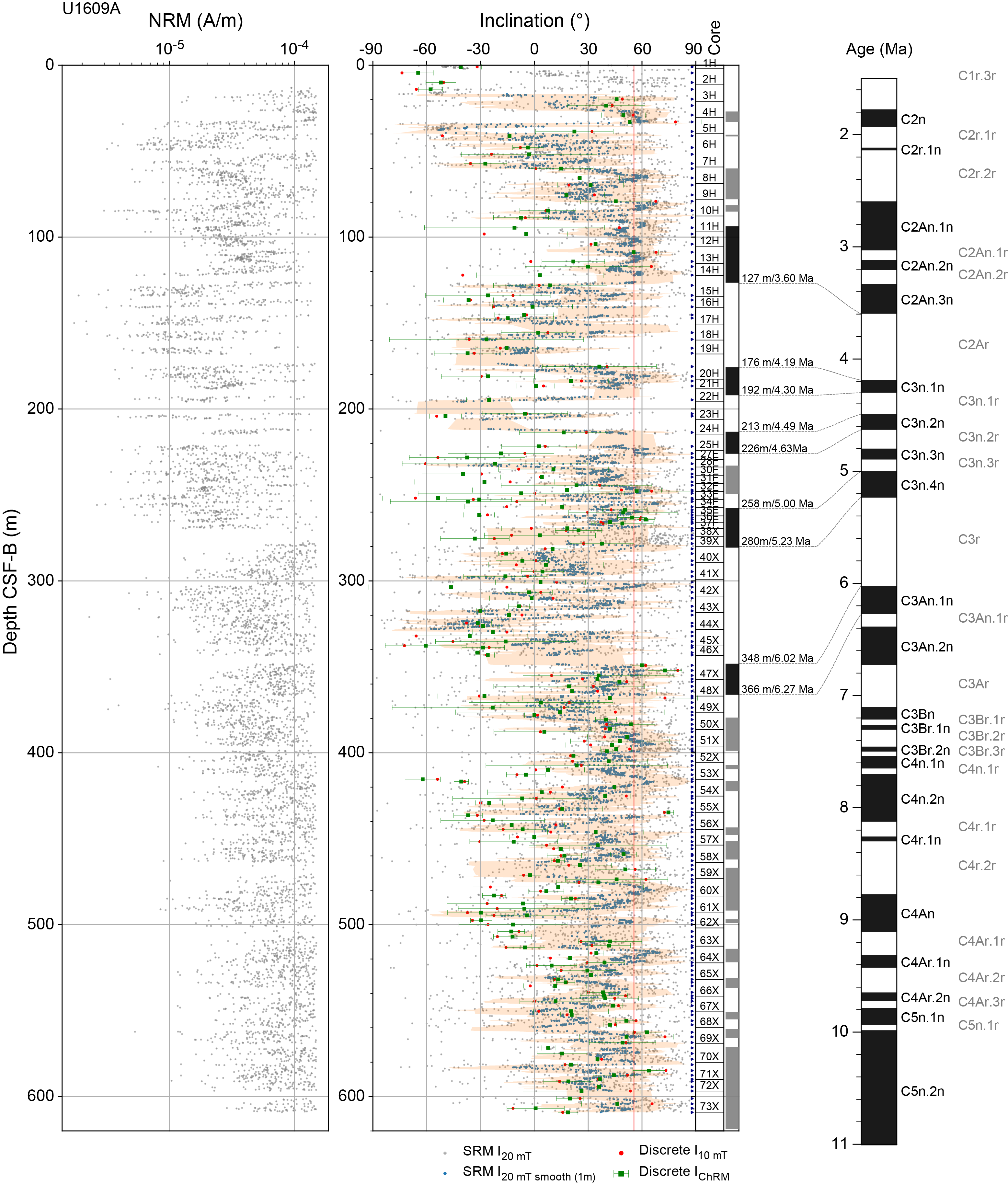
Figure F20. Paleomagnetic results, Hole U1609A.
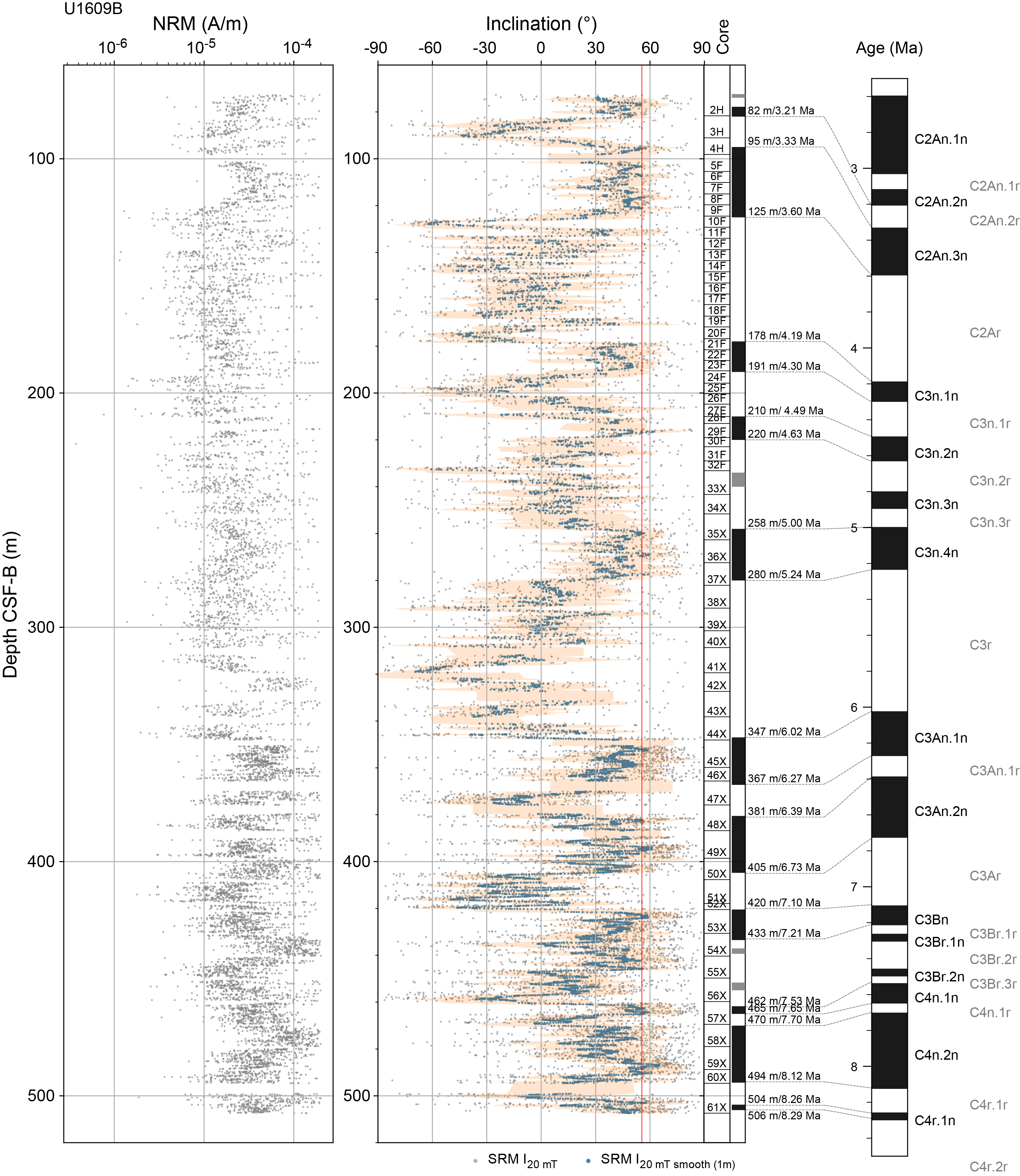
Figure F21. Paleomagnetic results, Hole U1609B.
Pass-through paleomagnetic measurements at Site U1609 were performed using the superconducting rock magnetometer (SRM) to investigate the NRM on a total of 842 archive halves (483 section halves from Hole U1609A and 359 section halves from Hole U1609B). No pass-through measurements were made on core catcher sections. Alternating field (AF) demagnetization was performed on the SRM by applying stepwise peak fields of 5, 10, 15, and 20 mT, with measurement of the remaining magnetization taken at 5 cm resolution after each step for Cores 401-U1609A-2H through 41X and at 2 cm resolution for Cores 42X–73X and 401-U1609B-1H through 61X. SRM measurements were sporadically disturbed by the occurrence of artificial flux-jumps; these results were removed from the database. SRM data were extracted from the Laboratory Information Management System (LIMS) database and processed to remove all measurements collected from anomalous peak intensity intervals and all measurements that were made within 5 cm of the section ends, which are biased by measurement edge effects. A smoothing window of 1 m was used for the inclination values to suppress the influence of data points that deviate significantly from the expected geocentric axial dipole (GAD) inclinations (+56°) at the site latitude (37.2°N). The processed NRM inclination, declination, and intensity data after 20 mT peak field AF demagnetization are listed in Tables T11 and T12.
In addition, a total of 318 discrete oriented cube samples were collected from the working-half sections by manually pushing standard 7 cm3 plastic cubes in the cores when the cores were soft enough and by using an extruder when the cores became more indurated. For each core, 3–7 discrete samples were taken, avoiding visually disturbed intervals. The depth levels from which the measured discrete samples were taken are indicated by small blue triangles beside the core number panel in Figure F20. The anisotropy of magnetic susceptibility (AMS) and bulk MS were measured on all samples using the MFK2 KappaBridge unit. After the AMS measurements, the NRM of 196 cube samples was measured on the AGICO JR-6A spinner magnetometer. Stepwise AF demagnetization was performed on Cores 401-U1609A-2H through 30F at successive peak fields of 0, 5, 10, 15, 20, 25, 30, and 35 mT to verify the reliability of the SRM measurements and to help determine the overprint component in the sections. For Cores 30F–73X, AF demagnetization in smaller steps of 2, 4, 6, 8, and 10 mT was applied to remove the overprint and determine the direction of the component remaining at 10 mT. The inclination data after 10 mT peak field AF demagnetization of the discrete samples are listed in Table T13.
5.1. Paleomagnetic signals
The intensity of NRM after 20 mT peak field AF demagnetization for Holes U1609A and U1609B is similar in magnitude, ranging about 1.5 × 10⁻⁵ to 4.0 × 10⁻¹ A/m (Figures F20, F21). The NRM intensity in the uppermost 15 m CSF-B of Hole U1609A shows relatively high intensities with an average of 5 × 10⁻² A/m. Below, intensities drop to average values ranging 1.5 × 10⁻⁵ to 5 × 10⁻³ A/m. The NRM intensities at the uppermost 10 cm of each core show peak values between 1 × 10⁻² and 1 × 10⁻¹ A/m, suggesting core drilling/handling overprints. AMS results show an overall vertical direction of the K min axis in agreement with a sedimentary fabric.
For both holes, the NRM removed below 10 mT is likely related to an overprint caused by core drilling (Acton et al., 2002). Inclination values after AF demagnetization at 20 mT were used to tentatively identify magnetic reversals. All sections showed many significantly deviated and scattered data points that may be due to the concentration of magnetic iron sulfides. These were subsequently removed during data processing. For Hole U1609A, normal polarity intervals can be recognized based on the smoothed inclination records, when successive SRM inclination values fall consistently at the expected GAD inclination (+56°) at the coring site (37.2°N) and the discrete sample inclination is positive, especially in the uppermost 400 mbsf (Figure F20). Reversed directions are less clearly defined, probably because of incomplete overprint removal. Reversed intervals are inferred when successive SRM inclination values fall below the GAD inclination and sample inclination is negative. Below 400 mbsf, the magnetic signal was still more uncertain and it was difficult to identify normal and reversed intervals. The magnetostratigraphy of Hole U1609B is only based on SRM inclinations (Figure F21).
NRM intensities of the discrete samples are similarly weak, even as low as to 10 × 10−5 A/m, which is close to the background noise of the JR-6A (2 × 10⁻⁵ A/m). Detailed analyses showed that an overprint component was generally removed between 0 and 10 mT, after which a second dual-polarity component remained that we interpret to be the characteristic remanent magnetization (ChRM) component (Figure F22). This component could not be properly demagnetized in the applied magnetic fields, and in some cases the samples seemed to acquire a gyroremanent magnetization (suggesting presence of the iron sulfide greigite) that obscures the primary signal (Roberts et al., 2011). The inclinations from the discrete samples generally confirm the polarities suggested by the inclination values measured on the archive-half core sections, and in some cases they even provided additional directional information that could not be deciphered from the SRM data.
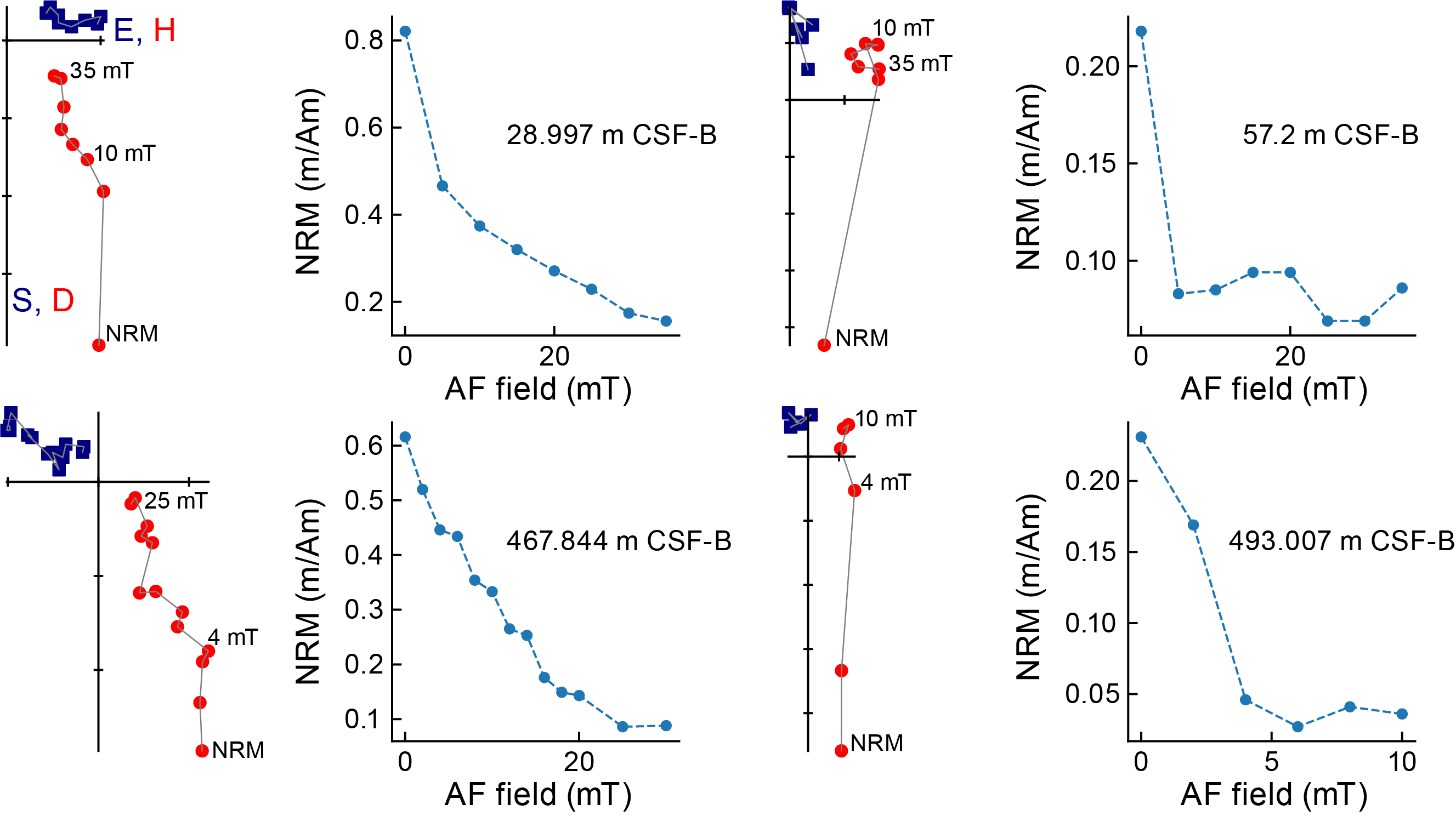
Figure F22. AF demagnetization results.
5.2. Magnetostratigraphy
The inclination data from both SRM and discrete samples were combined to generate an integrated polarity pattern for Hole U1609A (Figure F20; Table T14). The uppermost 60 m CSF-B shows dominantly reversed polarities with a short normal polarity interval between 20 and 40 mbsf. Biostratigraphic age constraints indicate an early Pleistocene age for this interval, and we therefore correlate this normal polarity interval to Chron C2n (Olduvai). A dominantly normal polarity interval is also observed between 90 and 125 mbsf that most likely corresponds to Chron C2An (Gauss), although the characteristic pattern was not clearly resolved. Next, a long interval of reversed polarity with up to four short normal polarity intervals correlates well to the Chron C3n pattern with the normal Cochiti, Nunivak, Sidufjall (not very clear), and Thvera Chrons resolved between 176 and 280 mbsf. The long reversed polarity interval between 280 and 348 mbsf then correlates to Chron C3r. This is the chron in which the Miocene/Pliocene boundary is defined (at 5.33 Ma) (Van Couvering et al., 2000) and the entire MSC (5.97–5.33 Ma) took place (Roveri et al., 2014). Downhole, the magnetic signal becomes less clear, and the GPTS indicates many short polarity intervals. The scatter in this interval made it very hard to determine and correlate polarity reversals robustly. Thus, below Chron C3An.1n at 366 mbsf we refrain from drawing correlation lines (Figure F20). The interval 490–515 mbsf is marked by mostly reversed polarity, and the most logical correlation would be to the long reversed Chron C4r, which would place the N/R reversal at 516 mbsf at the base of Chron C4r.2r. Downward extrapolation, assuming no major breaks in sedimentation, gives an age of ~10.5 Ma for the base of Hole U1609A (Figure F20).
The polarity pattern for Hole U1609B is entirely based on SRM data. Despite the two holes only being ~20 m apart, the demagnetization data appear to show better defined polarity reversals and clearer inferred reversed intervals, most of them containing negative inclinations. The normal polarities around 100 mbsf correlate again with Chron C2An (Gauss). Similar to Hole U1609A, a long interval of reversed polarity with up to 4 short normal polarity intervals correlates well to the Chron C3n pattern with the normal Cochiti, Nunivak, Sidufjall (again not very clear), and Thvera Chrons resolved between 178 and 280 mbsf. Downhole, the long reversed Chron C3r is clearly resolved as well as the two normal chrons, C3An.1n (347–368 mbsf) and C3An.2n (381–399 mbsf). The top of the next normal chron (CBn) is also clearly determined at 420 mbsf (Figure F23). This chron is located just above the Tortonian/Messinian boundary (~first regular occurrence of the G. miotumida group; Hilgen et al., 2000), which is in good agreement with the foraminifer data that indicates this bioevent is at 435 mbsf (Table T4). The complex latest Tortonian interval of Chron C3Br with multiple short polarity intervals is poorly resolved, and the position of the two normal polarity intervals Chrons C3Br.1n and C3Br.2n is only speculative (Figure F23) and here primarily based on the well-established biostratigraphic constraints of the G. menardii group (Table T4). The polarity pattern of 450–490 mbsf shows mainly normal polarities with two short negative inclination intervals at 455–462 and 465–470 mbsf that correlate well to Chrons C3Br.3r and C4n.1r, respectively. Downward correlation of the polarity pattern provides an estimated age of ~8.3 Ma for the base of Hole U1609B.
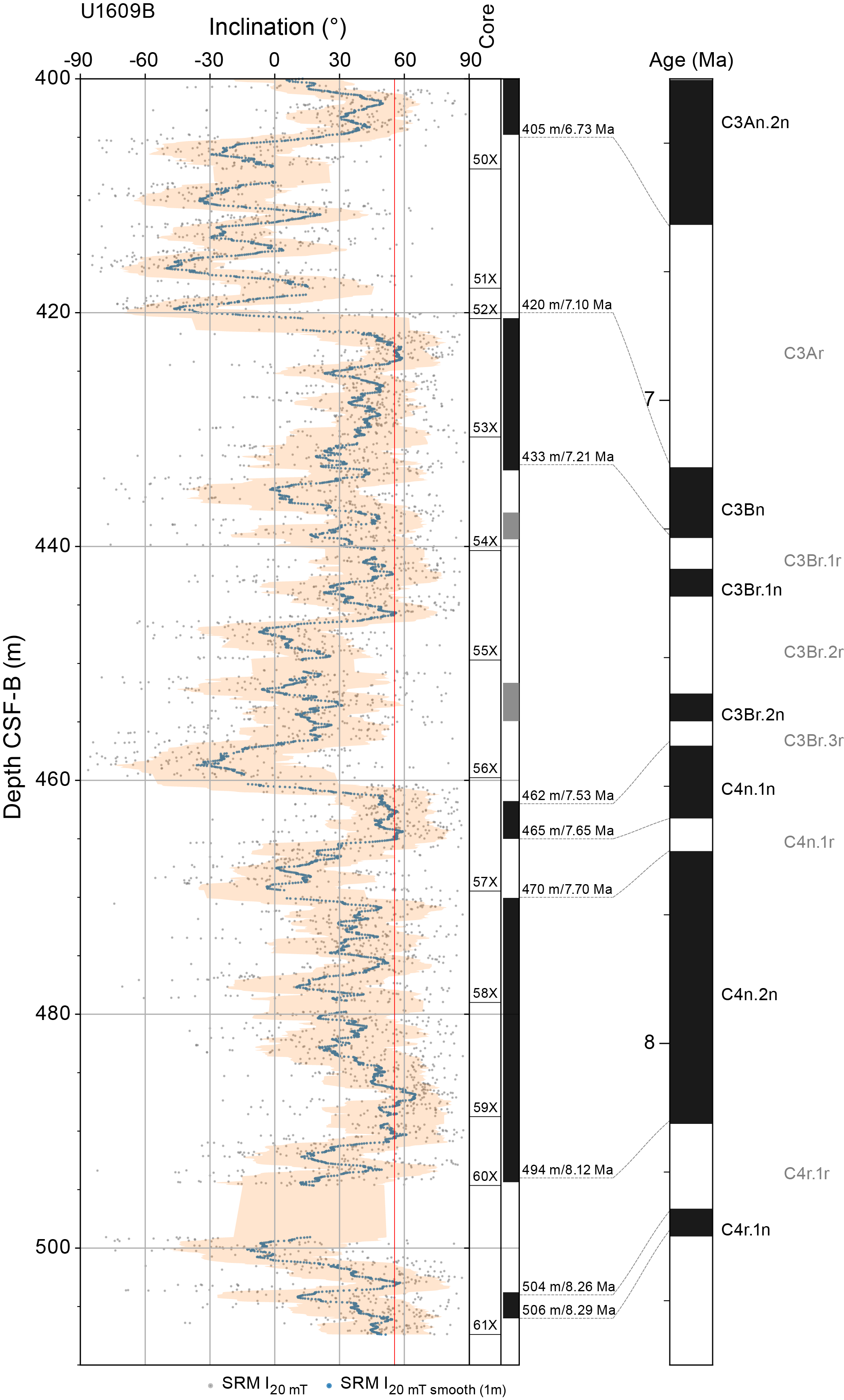
Figure F23. Paleomagnetic results, upper Tortonian–lowermost Messinian.
Finally, the magnetostratigraphic results of Holes U1609A and U1609B were compared by plotting them next to each other on the same depth scale (Figure F24). This showed overall good correlation, giving more confidence to the preliminary magnetostratigraphic interpretations of each hole. The ages of the well-identified magnetic reversals plotted against stratigraphic depth (CSF-B scale) provide sediment accumulation rates for both holes (Figure F25). These curves indicate average accumulation rates of ~10 cm/ky for Lithostratigraphic Unit I (Pliocene), decreasing downhole to 8 cm/ky for Unit II (Messinian) and <5 cm/ky for Unit III (Tortonian).
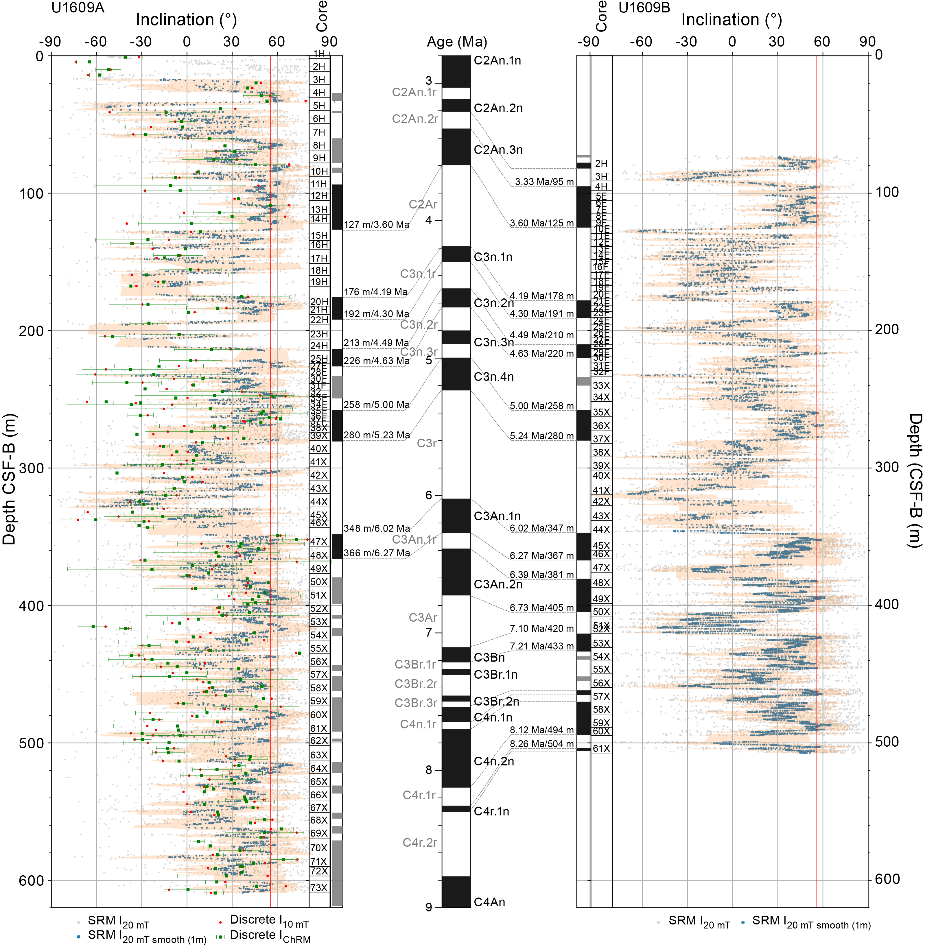
Figure F24. Correlation of magnetostratigraphy.
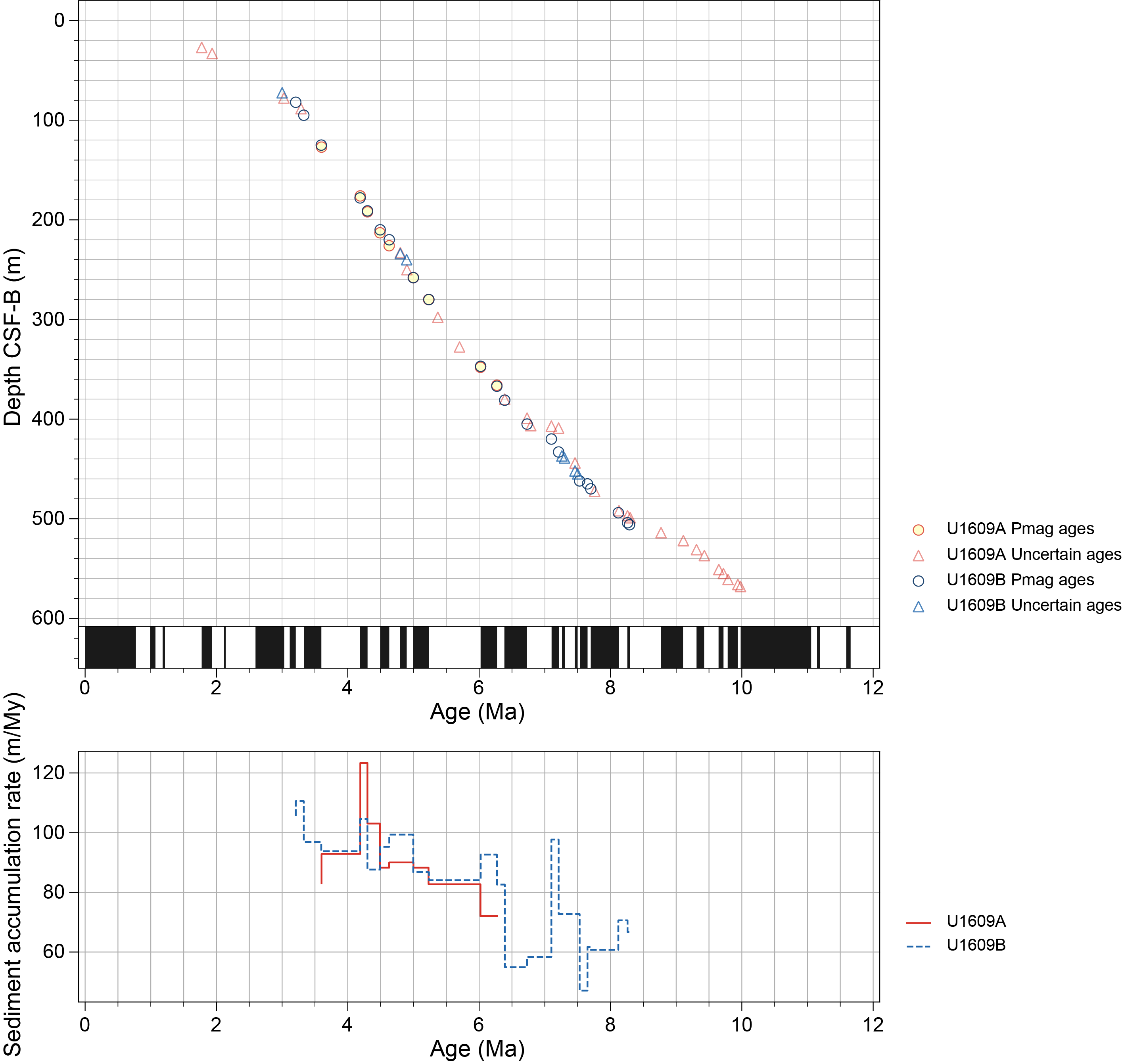
Figure F25. Sediment accumulation curves.
6. Geochemistry
6.1. Volatile hydrocarbons
Headspace gas analysis was performed as part of the standard protocol required for shipboard safety and pollution prevention monitoring. In total, 66 headspace samples from Hole U1609A (sampling resolution of one per core or one every other half-length core) were analyzed (Figure F26; Table T15). In Hole U1609A, methane (C1), ethane (C2), ethene (C2=), and propane (C3) were detected. Methane was first detected at 25.8 m CSF-A (Section 401-U1609A-4H-4), increasing to 36,640 parts per million by volume (ppmv) by 112.6 m CSF-A (Section 13H-5), and reaching a maximum of 42,690 ppmv at 246.7 m CSF-A (Section 32F-3). Methane levels decrease deeper than 279.2 m CSF-A (Section 39X-4) to less than 20,000 ppmv with one exception of 36,850 ppmv at 389.8 m CSF-A (Section 51X-3). At the base of Hole U1609A, the concentration of methane is 1008 ppmv. Ethane was first detected at 73.3 m CSF-A (Section 9H-4). In Hole U1609A, ethane reaches a maximum of 3.3 ppmv at 256.2 m CSF-A (Section 34F-3) with a concentration profile that is broadly similar to methane but four orders of magnitude smaller. The median C1:C2 ratio is 19,052. Ethene was detected in an isolated sample at 279.1 m CSF-A (Section 39X-4) and then again in three samples toward the base of the core (Sections 67X-4, 69X-4, and 72X-2). Propane was detected in five samples, all at <0.5 ppmv; the shallowest detection was 0.42 ppmv at 256.2 m CSF-A (Section 34F-3), and the deepest detection was 0.1 ppmv at 449.6 m CSF-A (Section 57X-4).
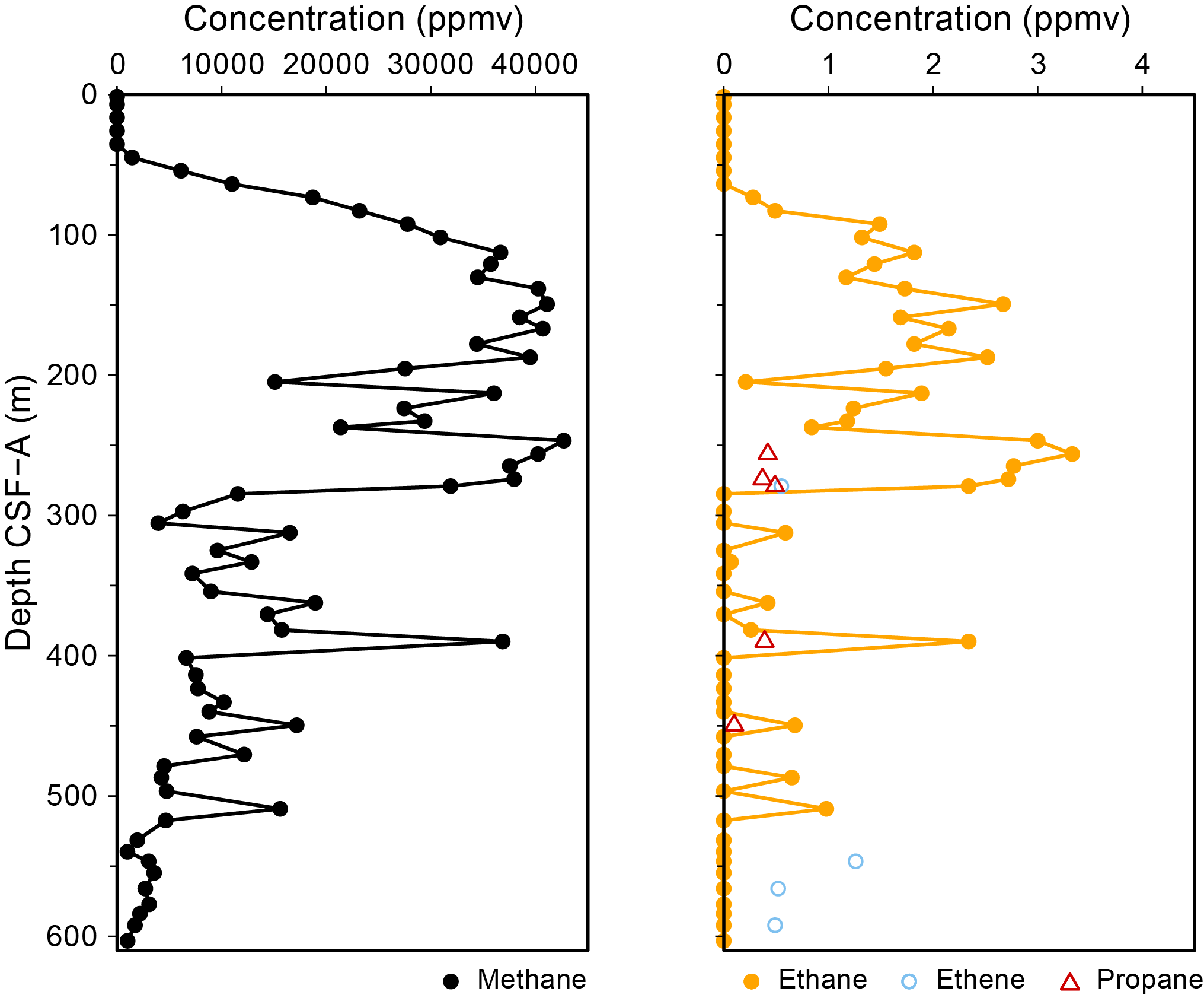
Figure F26. Headspace gas methane, ethane, ethene, and propane.
These concentrations of volatile hydrocarbons do not present a drilling concern. Although methane, ethane, and propane are commonly assumed to be indicative of deep subsurface thermogenic production in the oil window >250°C, these gases are also now known to be produced by biogenic processes (Oremland et al., 1988; Hinrichs et al., 2006). The distribution of methane and ethane peaking below the sulfate reduction zone is consistent with microbial methanogenic (as well as trace ethanogenic and propanogenic) production. At the base of the core, ethene detection and ethene/ethane ratios >1 suggest a different pathway of microbial production (Weniger et al., 2019) than that in the shallower depths of the core.
6.2. Interstitial water chemistry
Water was poured from the top of the liner of Core 401-U1609A-1H into a bucket while it was on the catwalk. This mudline sample approximates a bottom water sample. Interstitial water (IW) was extracted from a total of 66 whole-round samples from Hole U1609A at a sampling resolution of one sample per APC and XCB core or every other HLAPC core (Tables T16, T17). No IW samples were taken in Hole U1609B.
6.2.1. Alkalinity, pH, and salinity
Alkalinity increases from a minimum of 2.4 mM in the mudline sample (401-U1609A-1H-1, 0 cm) to a maximum of 20.0 mM at 166.8 m CSF-A (Section 19H-2) (Figure F27; Table T16). Below this peak, alkalinity declines to ~6.5 mM at 354.1 m CSF-A (Section 47X-4) before rising again slightly to no higher than 9.5 mM at 546.5 m CSF-A. Values for pH range from a minimum of 7.4 to a maximum of 7.8 (Figure F27), with peak values occurring in the shallow subsurface at 25.7 m CSF-A (Section 4H-3) and at 333.1 m CSF-A (Section 45X-3). Salinity ranges 32–35, with 32 being the dominant value for much of Hole U1609A (Table T16).
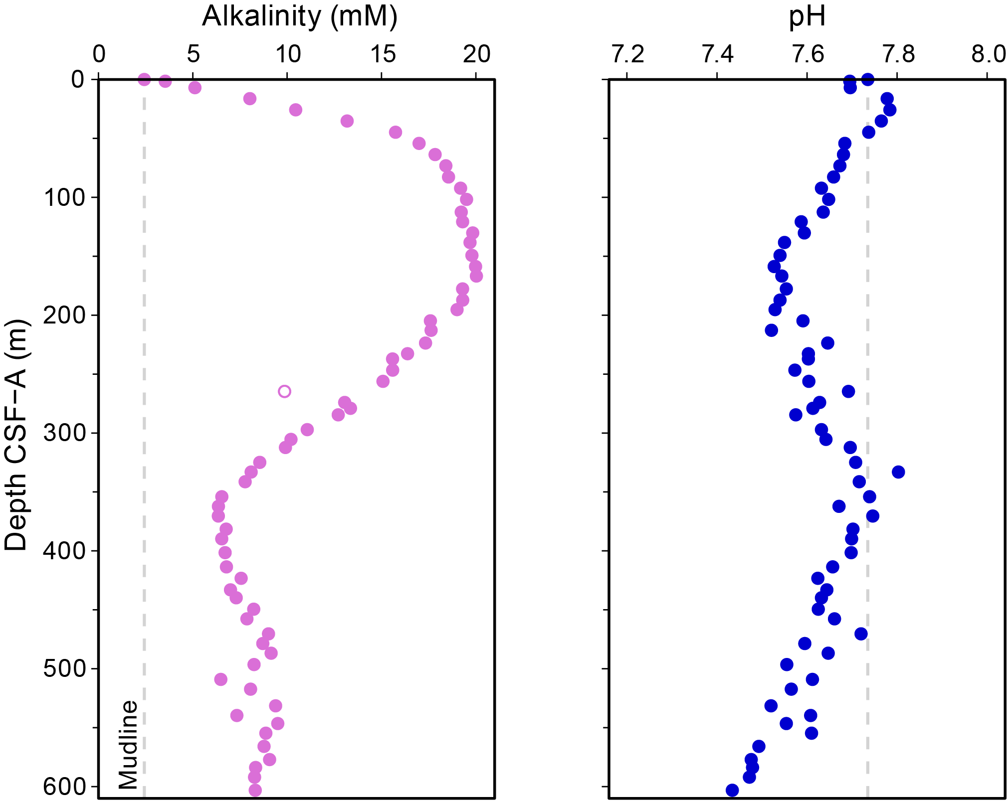
Figure F27. IW alkalinity and pH.
We interpret the initial rise in alkalinity to be predominantly caused by microbial sulfate reduction in Cores 401-U1609A-1H through 6H followed by net carbonate dissolution in Cores 7H–19H despite the excellent carbonate microfossil preservation (glassy foraminifers) based on visual inspection (see Biostratigraphy). These changes are accompanied by a decrease in pH as a result of respiration of organic matter. Below 200 m CSF-A, net carbonate precipitation and dissolution contribute to alkalinity decreasing and increasing, respectively, again accompanied by changes in pH.
6.2.2. Major ions
Major ion concentrations (Na+, Cl–, Ca2+, Mg2+, K+, SO4 2−, and Br−) of IW were analyzed by ion chromatography (Table T16). Sodium and chloride vary by approximately 3% and show close covariation (Figure F28). An increase in sodium and chloride of approximately 2% occurs immediately between the mudline sample and the first IW sample (401-U1609A-1H-1, 145–150 cm), followed by a decrease in both ions to approximately 150 m CSF-A before an increase toward the bottom of the hole. These variations are likely driven by uptake and release of water into interstitial layers of clay minerals, potentially both in situ and during the process of core recovery and depressurization. The observed change in chloride concentrations of approximately plus or minus 1.4% in this hole relative to the mudline value could be achieved by loss/gain of 0.77 mol of H2O per 1 mL of IW, which is within a reasonable amount for the proportions of clay observed at this site (see Lithostratigraphy). The Na/Cl ratio varies minimally around the mudline value, reflecting minor uptake of sodium ions into clays or zeolites.
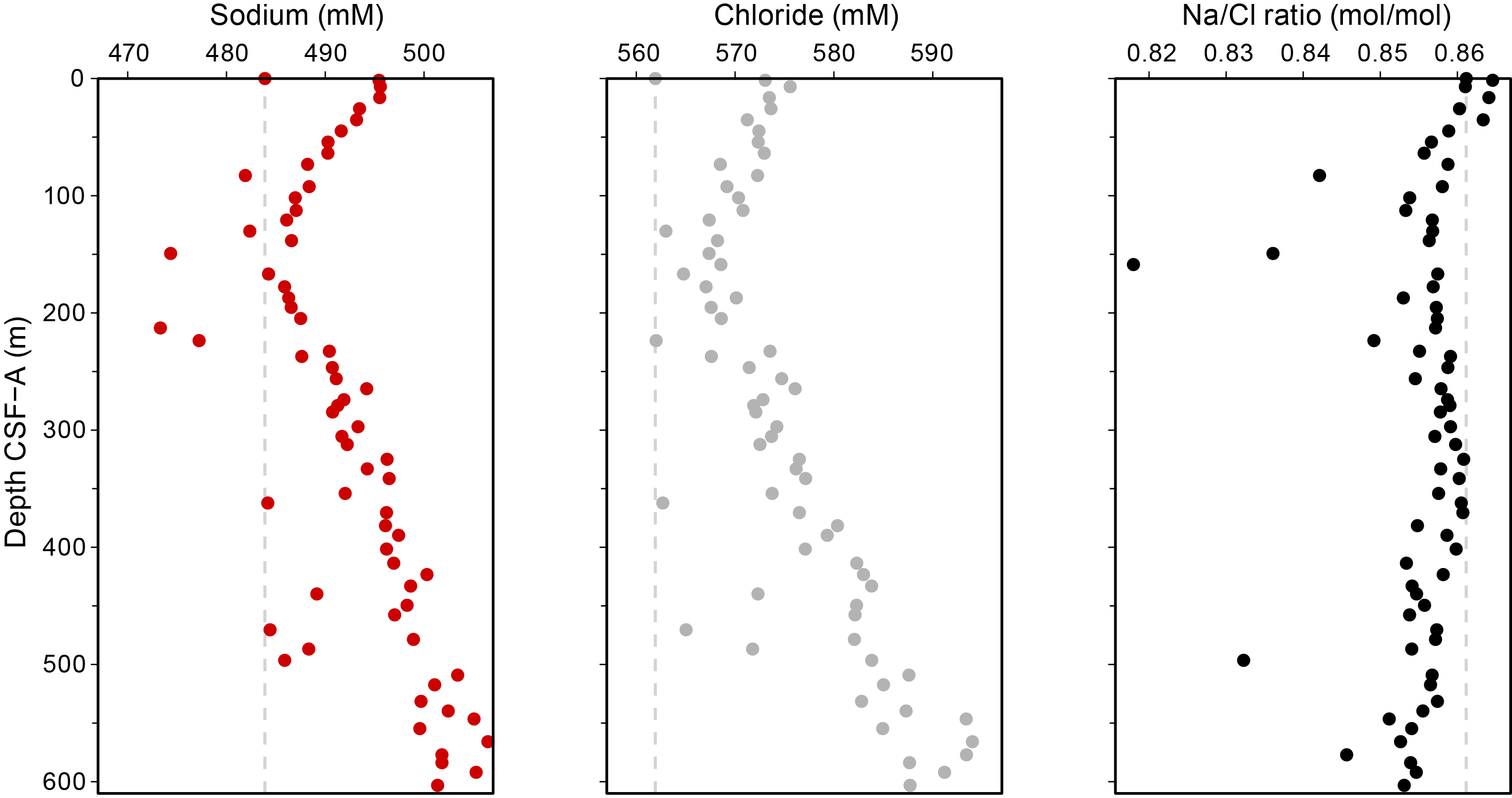
Figure F28. IW sodium, chloride, and Na/Cl.
Calcium decreases from 10.8 mM in the mudline sample to a minimum of 4.5 mM at 35.2 m CSF-A (Section 401-U1609A-5H-3) with a gradual rise to 8.8 mM at 195.3 m CSF-A (Section 22H-2) (Figure F29). This rise is followed by a second decline to 6.2 mM at 362.2 m CSF-A (Section 48X-3) and another coherent rise to the maximum value of 14.6 mM at 603.1 m CSF-A (Section 73X-2) at the base of the profile. The calcium decrease in the upper part of the hole indicates authigenic carbonate precipitation associated with the alkalinity rise caused by sulfate reduction. The lower variations in calcium are inversely correlated with pH, indicating that these pH variations and associated change in calcium carbonate saturation state are likely driving net carbonate mineral dissolution and precipitation. The total range of calcium concentrations observed, 10 mM, could be produced by the net dissolution of just 1 mg of CaCO3 per milliliter, so the trend in IW composition has likely not made an observable difference in the percent of sedimentary carbonate.
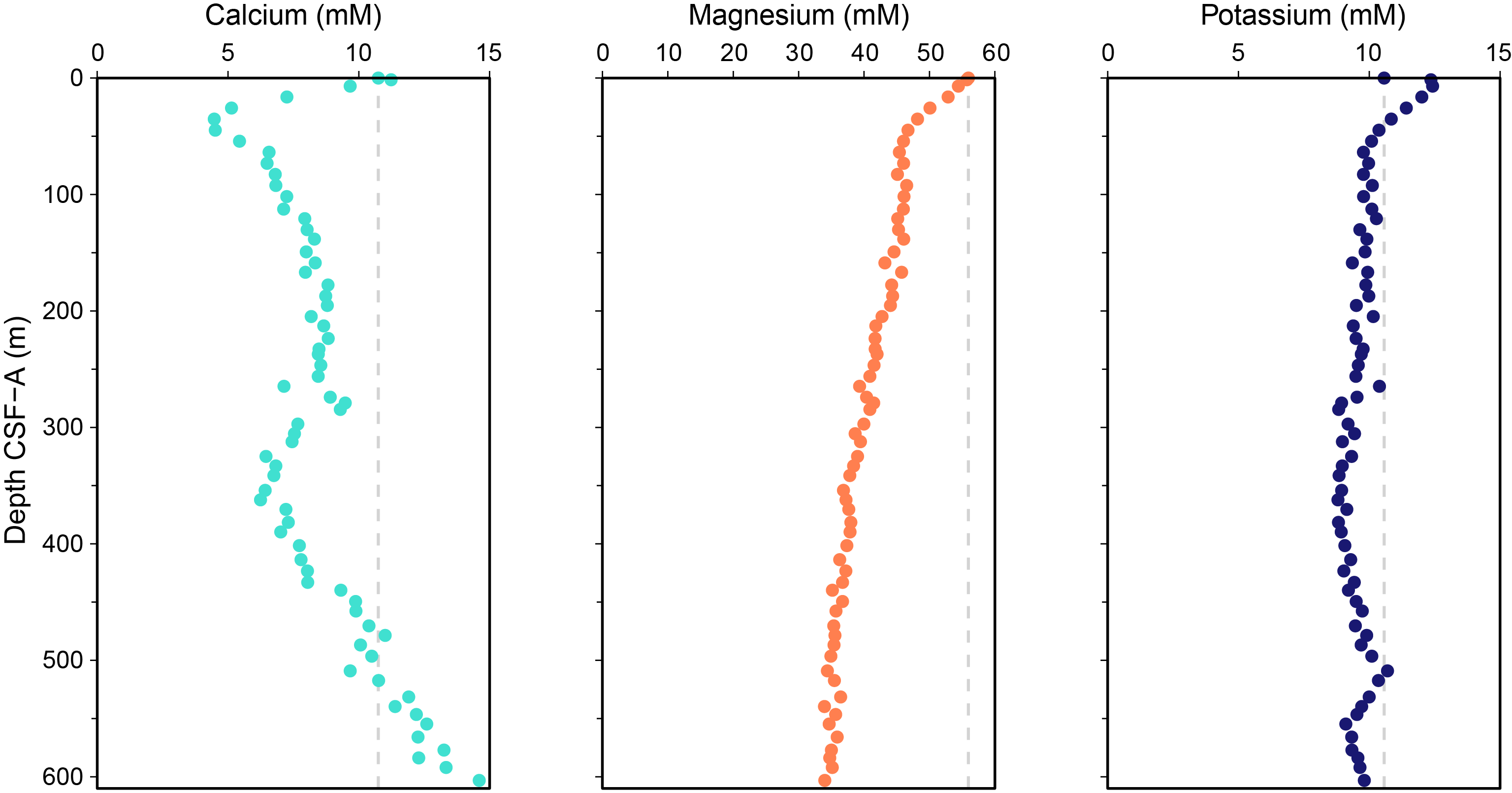
Figure F29. IW major cation concentrations.
Magnesium decreases from 56.0 mM in the mudline sample to 48.2 mM at 35.2 m CSF-A (Section 401-U1609A-5H-3) with a gradual decrease continuing linearly to 34.0 mM at the bottom of the hole (Figure F29). Some of the decrease in magnesium could be related to authigenic magnesium carbonate precipitation in the zone of sulfate reduction, based on the co-occurring decrease in calcium, but the greater magnitude of drawdown in magnesium compared to that for calcium and the similarity between the magnesium and potassium profiles suggest that most of the magnesium decline may be related to clay formation, probably both smectites (incorporating Mg) and illites (incorporating K). Potassium increases from 10.6 mM at the surface to 12.4 mM in the first IW sample at 1.45 m CSF-A (Sample 1H-1, 145–150 cm), followed by a decline to relatively stable values between 8.8 and 10.0 mM for the remainder of the hole. The similarity between the potassium profile and the Na/Cl ratio suggests that these trends are driven by the uptake and release of monovalent ions into clay minerals.
Sulfate concentrations decrease from 29.2 mM in the mudline sample to levels below detection at 54.2 m CSF-A in Section 401-U1609A-7H-3 (Figure F30), defining the base of the zone of sulfate reduction. Sulfate remains <2.5 mM throughout the rest of the hole. The sulfate–methane transition zone (SMTZ) occurs near 44.8 m CSF-A (Section 6H-3). Bromide concentrations increase from a minimum of 0.87 mM at the surface to 1.00 mM by 256.1 m CSF-A (Section 34F-2), likely being released from the degradation of organic matter through the sulfate reduction and methanogenic zones.
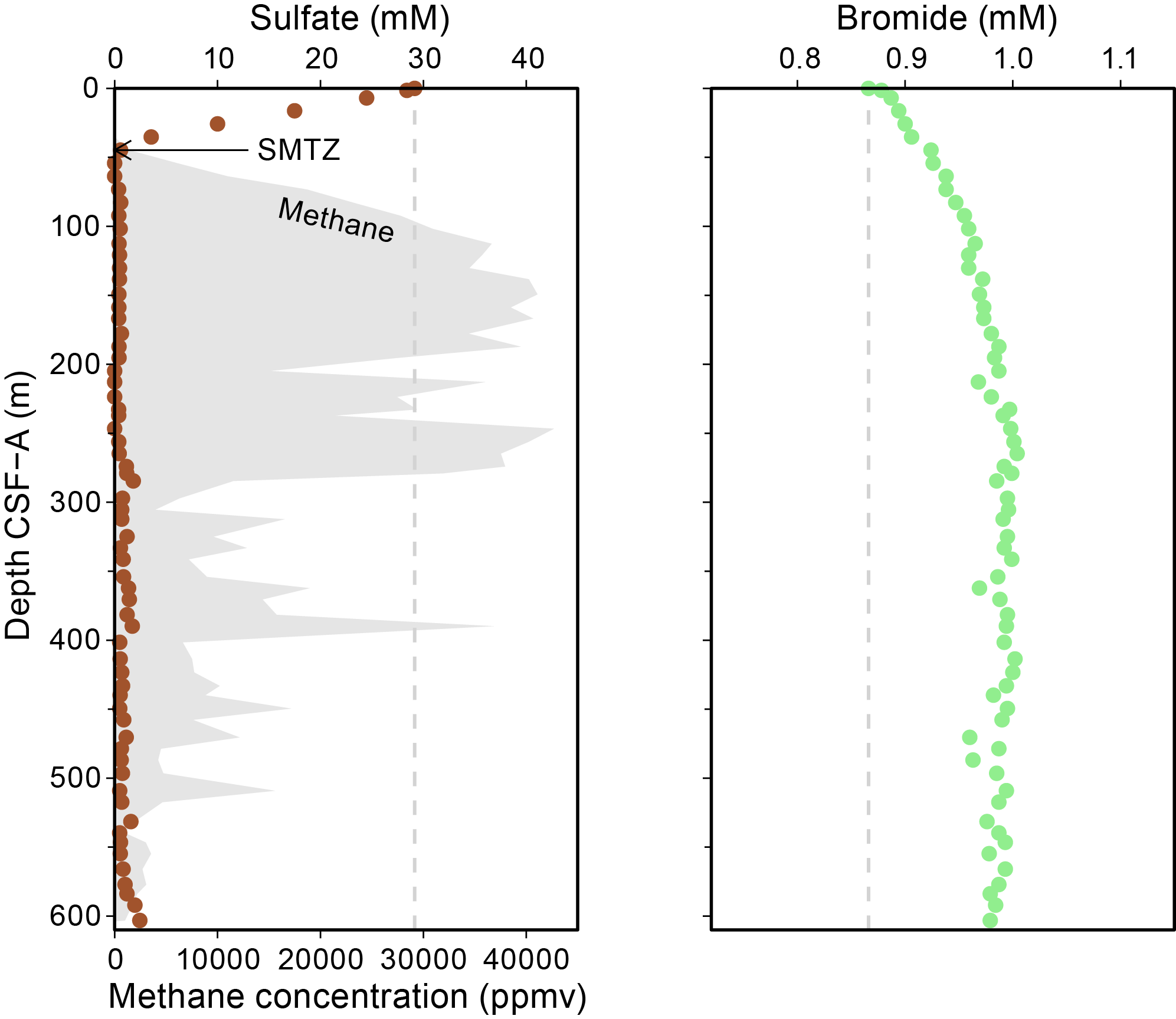
Figure F30. IW major anion concentrations.
6.2.3. Ammonium, phosphate, and total phosphorus
Ammonium and phosphate concentrations in IW were analyzed by spectrophotometry (Figure F31; Table T16). Ammonium concentrations increase rapidly downcore from 0 µM in the mudline sample to more than 3500 µM in the uppermost 200 m CSF-A before declining below 250 m consistently to 1779 µM at 603.1 m CSF-A (Section 401-U1609A-73X-2). Phosphate concentrations also increase initially from 3.42 µM at the surface (Section 1H-1) to a maximum of 32.4 µM at 35.2 m CSF-A (Section 5H-3) before declining to <10 µM below 92.3 m CSF-A (Section 11H-3) and <6 µM below 232.7 m CSF-A (Section 28F-2). Total P measured by inductively coupled plasma–atomic emission spectroscopy (ICP-AES) yields higher phosphorus concentrations across the uppermost 300 m CSF-A, with a maximum of 36.8 µM at 35.2 m CSF-A (Section 5H-3) and levels around 22 µM from 83 to 167 m CSF-A (Figure F31; Table T17). These higher levels of P may reflect a dissolved organic P phase in addition to phosphate.
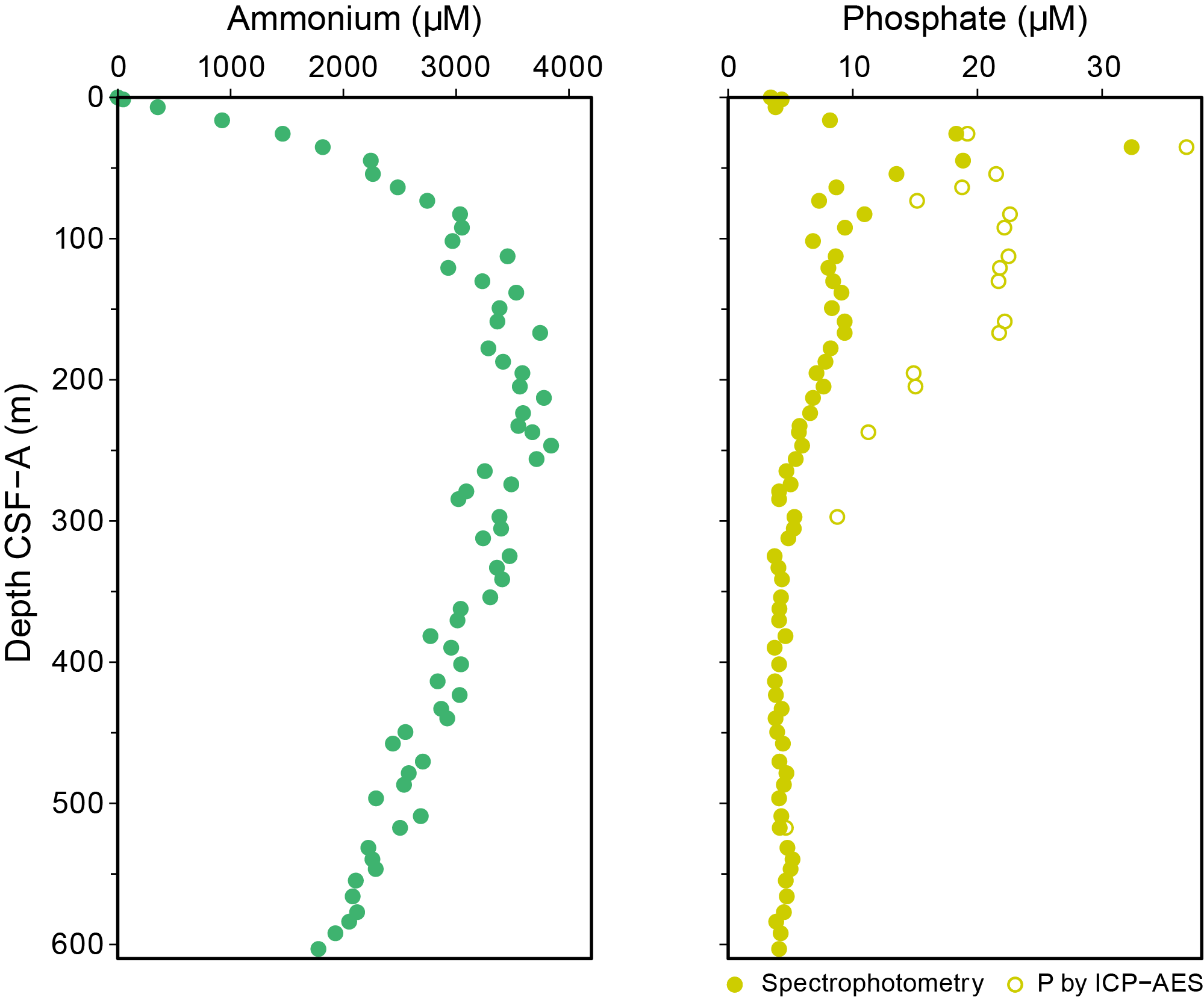
Figure F31. IW major nutrient concentrations.
Both ammonium and phosphate are released into IW during anaerobic respiration of organic matter. We interpret the different rates of decrease with depth to reflect downward diffusion for ammonium and a sink for phosphorus into iron minerals or authigenic carbonate-fluorapatite (Filippelli and Delaney, 1996; Paytan and McLaughlin, 2007).
6.2.4. Trace elements (Li, Si, Ba, B, Sr, Fe, and Mn)
Trace element concentrations in IW were analyzed by ICP-AES (Table T17). Lithium and silicon show similar downcore patterns (Figure F32) that are generally inverse to that for pH (Figure F27). The maximum values observed are 186 µM for Li and 862 µM for Si. The inverse correlation with pH likely reflects silica solubility and precipitation and dissolution of clay phases.
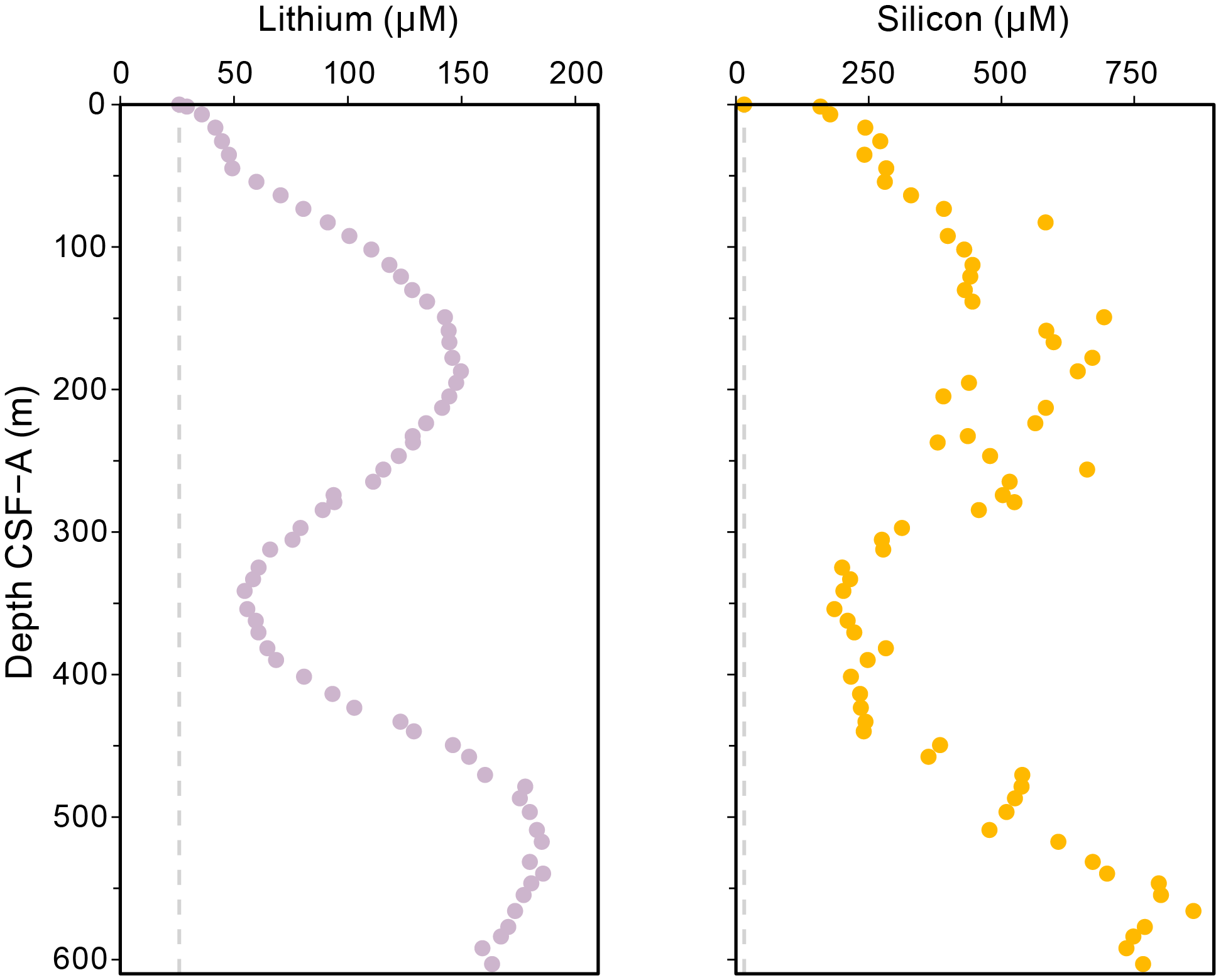
Figure F32. IW minor element concentrations.
Barium concentrations are very low where sulfate is present in the uppermost few cores and rise to as high as 100 µM below the SMTZ, with some additional fluctuations at depth (Figure F33). The barium profile is largely controlled by barite (BaSO4) solubility and possibly silica dissolution (Brumsack and Gieskes, 1983). The profile for boron is very similar to that for potassium, suggesting that it is also controlled by clay mineral reactions. Strontium concentrations increase gradually from ~92 µM (Core 401-U1609A-1H) to 283 µM at 381.5 m CSF-A (Section 50X-3) before a greater rate of increase to 924 µM at 603.1 m CSF-A (Section 73X-2). This more rapid increase in Sr below 381.5 m CSF-A (Figure F33) is likely due to increased carbonate dissolution, as signaled by a decrease in pH and increase in alkalinity (Figure F27) and Ca concentrations (Figure F29). The trend in the overlying sediment may reflect slow carbonate recrystallization and/or upward diffusion of the strontium being actively released at greater depths (Martin and Scher, 2004).
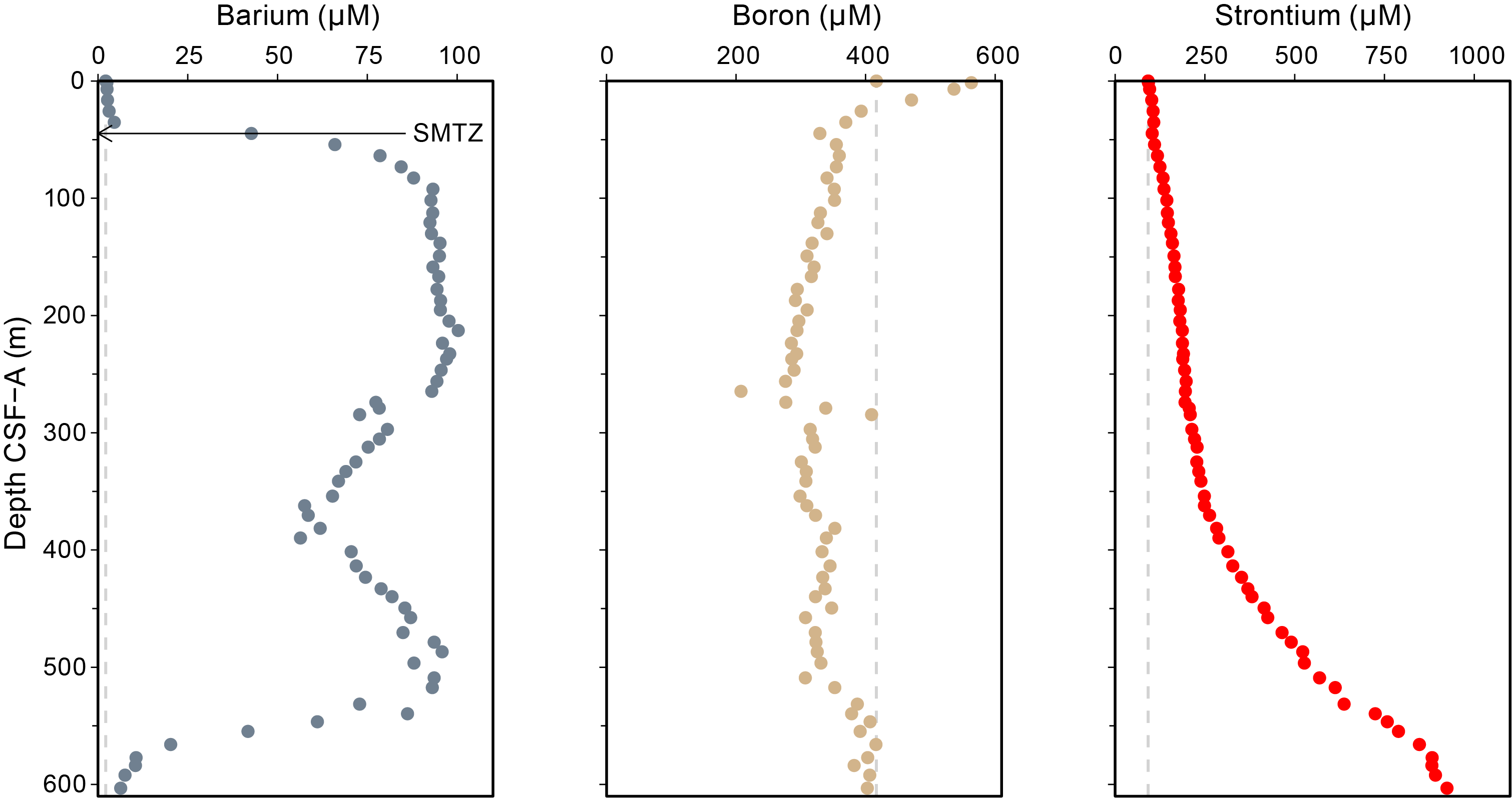
Figure F33. IW minor and trace element concentrations.
Iron concentrations increase from below the limit of detection in the uppermost few cores to a subsurface maximum of 23.8 µM at 138.3 m CSF-A (Section 401-U1609A-16H-2) before declining back to low levels below 285 m CSF-A (Figure F34). Manganese is below detection in the mudline sample and present in low concentrations (generally <2 µM) throughout the core, reaching its maximum of 3.4 µM in the uppermost IW sample at 1.5 m CSF-A (Section 1H-1). The iron and manganese concentrations generally reflect the redox environment of the IW in the sulfate reduction and methanogenic zones, with the possibility of some metabolic manganese reduction occurring within Section 1H-1.
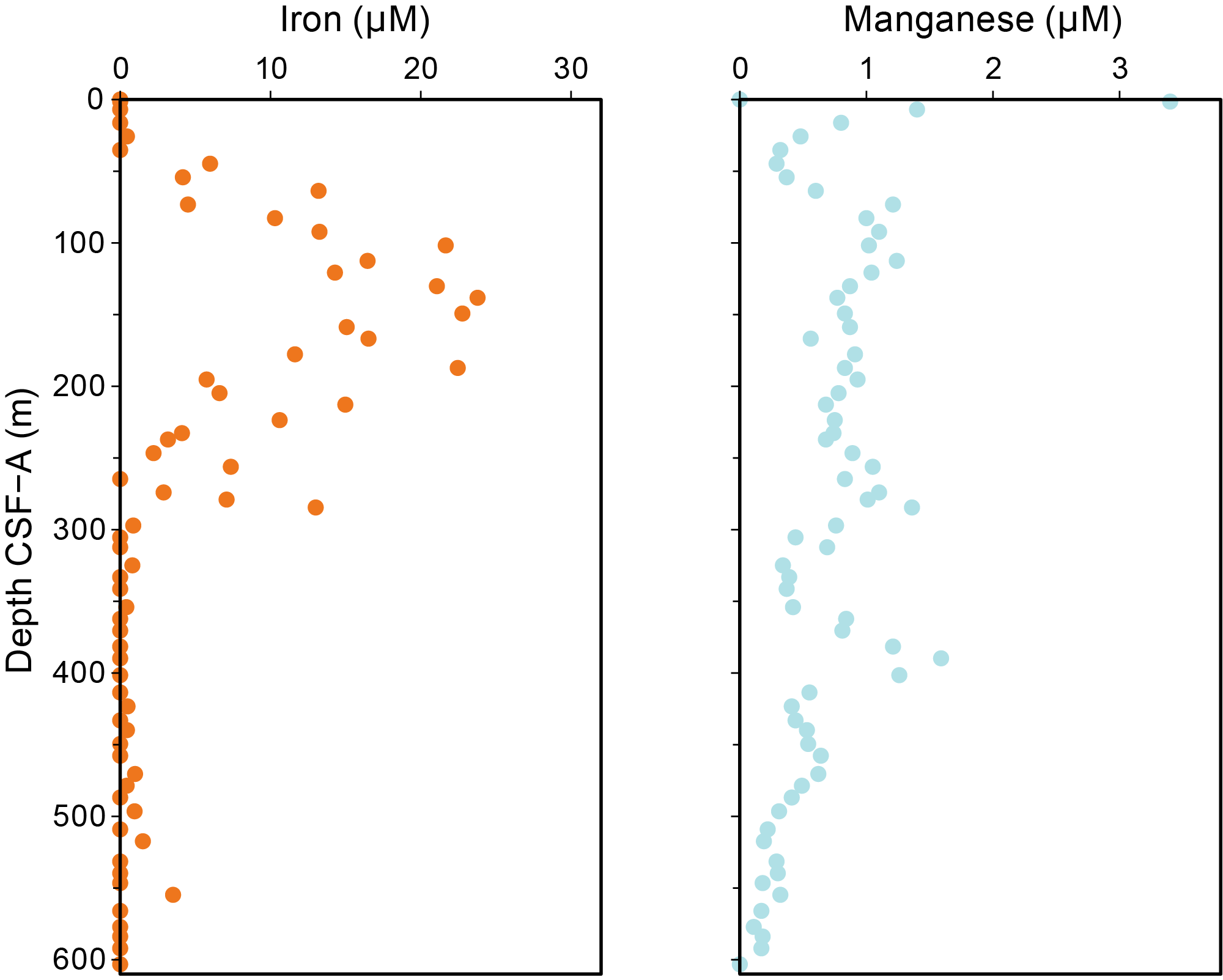
Figure F34. IW trace element concentrations.
6.3. Sedimentary geochemistry
Sediment samples were collected for analysis of solid-phase geochemistry at a resolution of one sample per core or one sample every other half-length core in Hole U1609A (Table T18). These samples came from a fraction of the IW squeeze cake residue. Some additional samples were taken from both Holes U1609A and U1609B to identify the geochemical variation across lithologic color cycles identified by the shipboard sedimentologists.
6.3.1. Calcium carbonate
CaCO3 varies from 19.5 to 74.9 wt% (Figure F35; Table T18) with a mean of 45.2 wt% and a standard deviation of 11.5 wt%. CaCO3Follows a gently increasing trend from 20 to 40 wt% in the uppermost 180 m CSF-A and then varies between 30 and 50 wt% before an interval (457.7–486.8 m CSF-A; Sections 401-U1609A-58X-2 through 61X-2) of low values between 31 and 36 wt%. Below this interval, CaCO3 increases to 74.9 wt% in the deepest sample at 603.1 m CSF-A (Section 73X-2). The CaCO3 content determined by coulometry agrees well with quantification of the mineral assemblage from the XRD spectra (Figure F36).
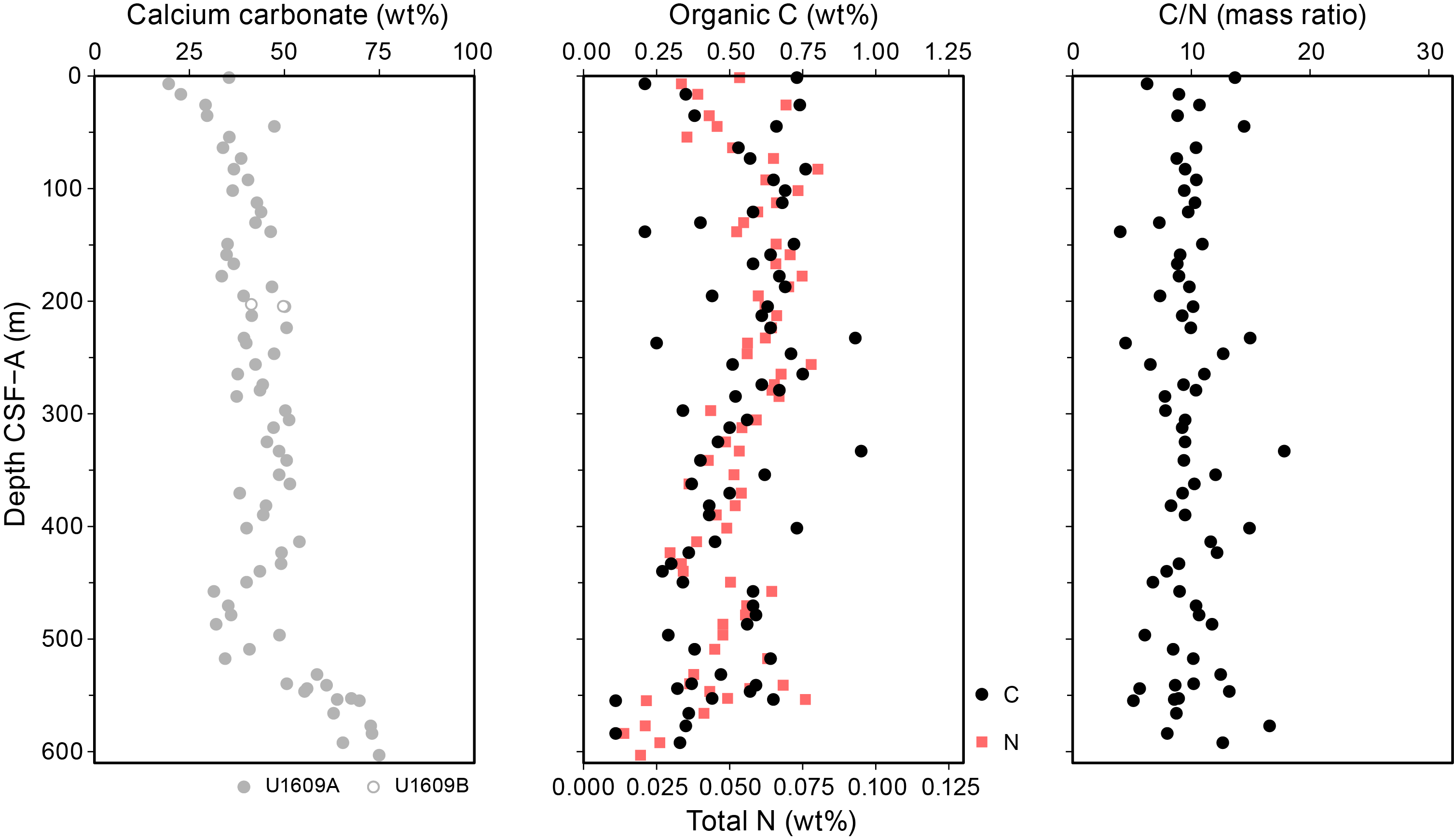
Figure F35. CaCO3, organic carbon, nitrogen, and C/N.
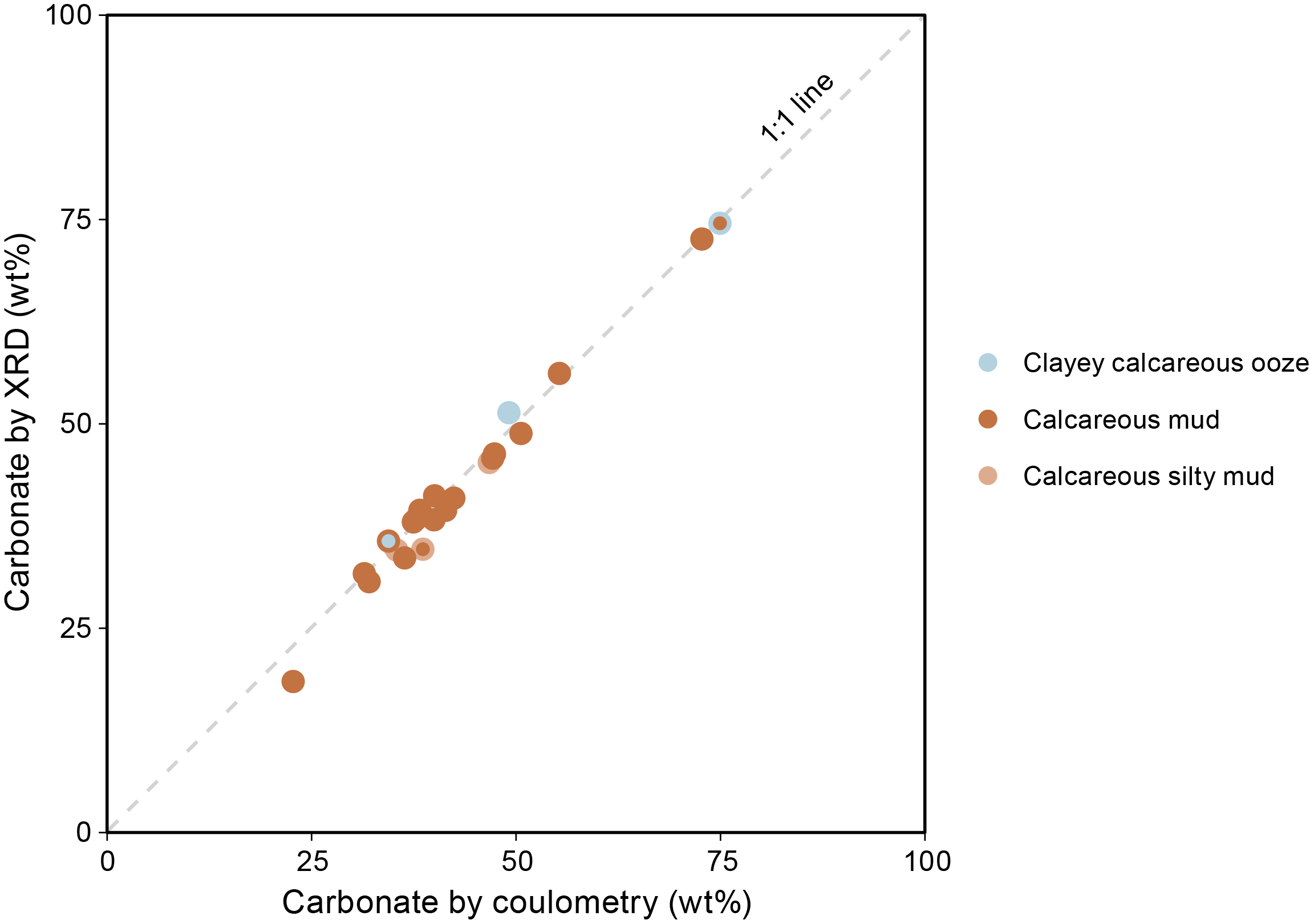
Figure F36. Carbonate weight percent, XRD and coulometry.
The highest carbonate concentrations at the bottom of Hole U1609A presumably reflect higher carbonate productivity and/or lower dilution or dissolution compared to the upper sediments. The decrease in CaCO3From 40 to 20 wt% in the uppermost 180 m CSF-A may indicate decreased production and/or increased dissolution. Smaller scale variability in the CaCO3 weight percent measurements likely represents random sampling of the higher frequency lithologic cycles, detected visually in color variations (see Lithostratigraphy) and in measurements of physical properties of the cores (see Physical properties). A strong negative correlation (R 2 = 0.81) between the CaCO3 weight percent and the NGR measurements taken closest to the IW samples shows that the proportion of the carbonate sedimentary fraction dominates the cycles in NGR and that the CaCO3 range and cyclicity is aliased by the discrete analyses from the squeeze cake samples, which represent 5–7 cm integration and ~10 m spacing (Figure F37). In XCB cores, whole-round IW sampling was selective for core sections with more intact lithology, avoiding sediments visibly disturbed by drilling rather than sampling specific lithologies to evaluate their carbonate content. Consequently, some bias may result in the reported CaCO3 weight percent because part of the natural range may be unsampled.
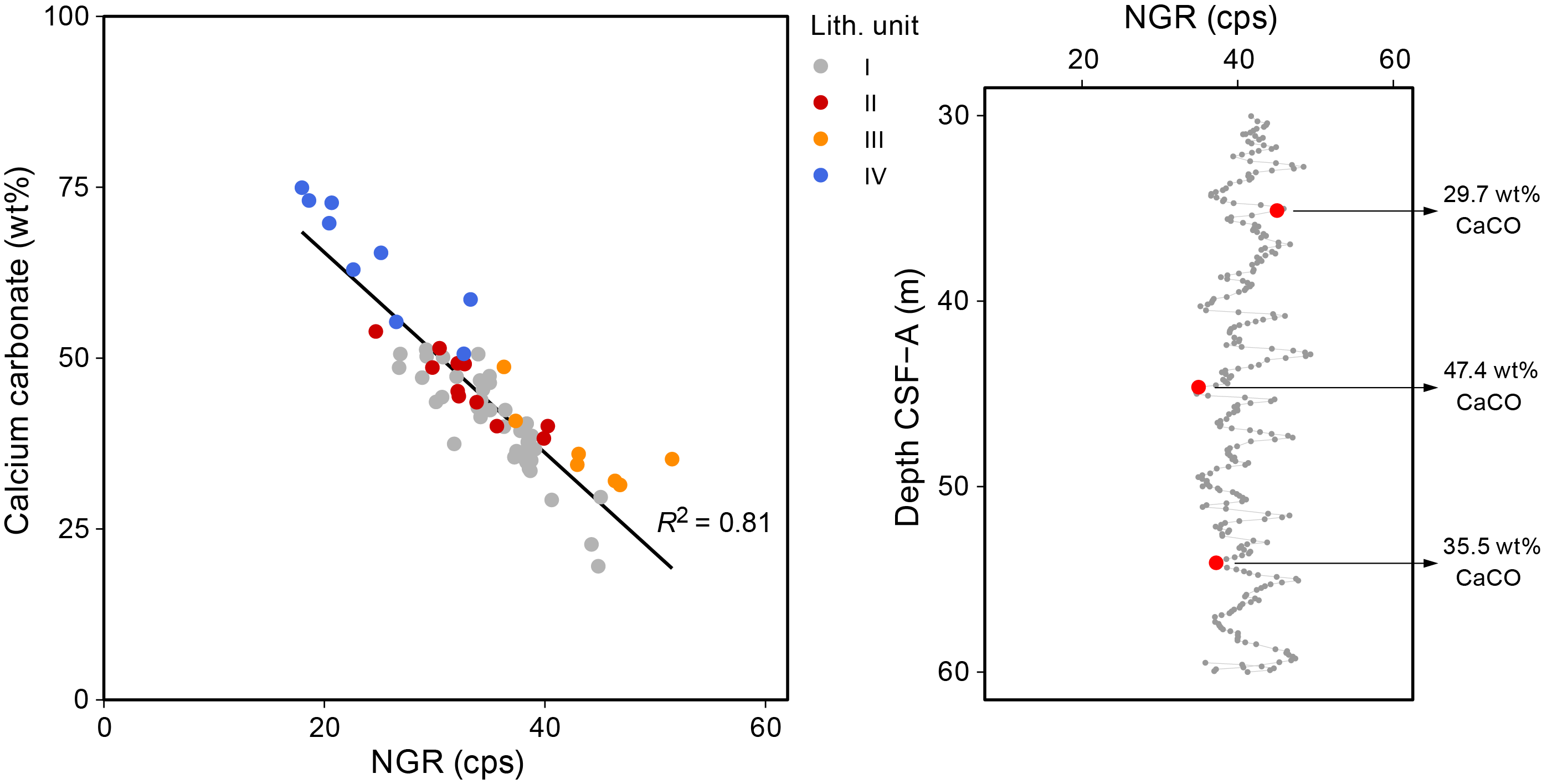
Figure F37. Carbonate weight percent and NGR.
6.3.2. Carbon and nitrogen
Total organic carbon (TOC) is calculated to be between 0 and 0.95 wt% (Figure F35; Table T18) based on the difference between total carbon (TC) and total inorganic carbon (TIC) (TOC = TC − TIC). For two samples, analysis of TC yielded a lower number than TIC, most likely caused by minor loss (incomplete transfer) of the sample in weighing or analysis, so these results were discarded. Weight percent nitrogen (Figure F35; Table T18) was measured downhole and ranges 0.014–0.109 wt%. The C/N mass ratio (using TOC and total nitrogen [TN]) is used to distinguish the origin of organic matter (marine versus terrestrial) in sediment (Emerson and Hedges, 1988; Meyers, 1997) and may also be influenced (decreased) by degradation of organic matter (Ruttenberg and Goñi, 1997). The data set has a mean C/N ratio of 9.7 and a standard deviation of 2.6, indicating that the organic carbon is dominantly of marine origin with a lesser contribution from terrestrial organic matter (Figure F35; Table T18). There is no downhole trend in the data, suggesting that marine production and terrestrial inputs, as well as organic degradation, are broadly consistent across the whole record. Variability in the C/N ratio may be related to provenance or productivity changes, but some component of the variability is likely scatter due to the analytical challenge of obtaining TOC from TC − TIC.
6.3.3. Carbonate fraction geochemistry
In addition to the standard shipboard measurements of calcium carbonate concentrations in sediments, we performed geochemical analyses on the acid-soluble (carbonate) fraction of the sediment (Table T19). Because variable amounts of carbonate are present in each sample, the carbonate geochemistry data are reported as elemental ratios relative to calcium (Figure F38). The carbonate Mg/Ca ratios show a few high values up to 54 mmol/mol (Sample 401-U1609A-2H-3, 147–152 cm) in the uppermost few cores before stabilizing between 2 and 5 mmol/mol below approximately 100 m CSF-A. The Mg/Ca ratios likely reflect small amounts (mostly <1%) of dolomite, which were also detected in smear slides and in bulk sedimentary XRD analysis (see Lithostratigraphy). The amount of dolomite permitted by the carbonate Mg/Ca ratios is generally smaller than the estimates of dolomite from the XRD analysis. This could be due to nonstoichiometric dolomite with Mg/Ca < 1. Carbonate Mn/Ca ratios are also high in the uppermost few cores before stabilizing between 0.2 and 0.5 mmol/mol, with the exception of the interval between 285 and 450 m CSF-A (Cores 40X and 57X), which shows higher and variable Mn/Ca ratios. This interval may reflect distinct early diagenetic redox conditions, during which manganese can be reduced and mobilized in anoxic IW and subsequently incorporated into authigenic or recrystallizing carbonate minerals (Froelich et al., 1979; Boyle, 1983; Thomson et al., 1986). Carbonate Sr/Ca ratios show lower values between 1 and 2 mmol/mol in Cores 1H–7H and then stable values around 2.1–2.2 mmol/mol downcore. The lower strontium concentrations together with higher magnesium and manganese suggest more intense carbonate diagenesis occurred in the shallowest sediments recovered from Hole U1609A.
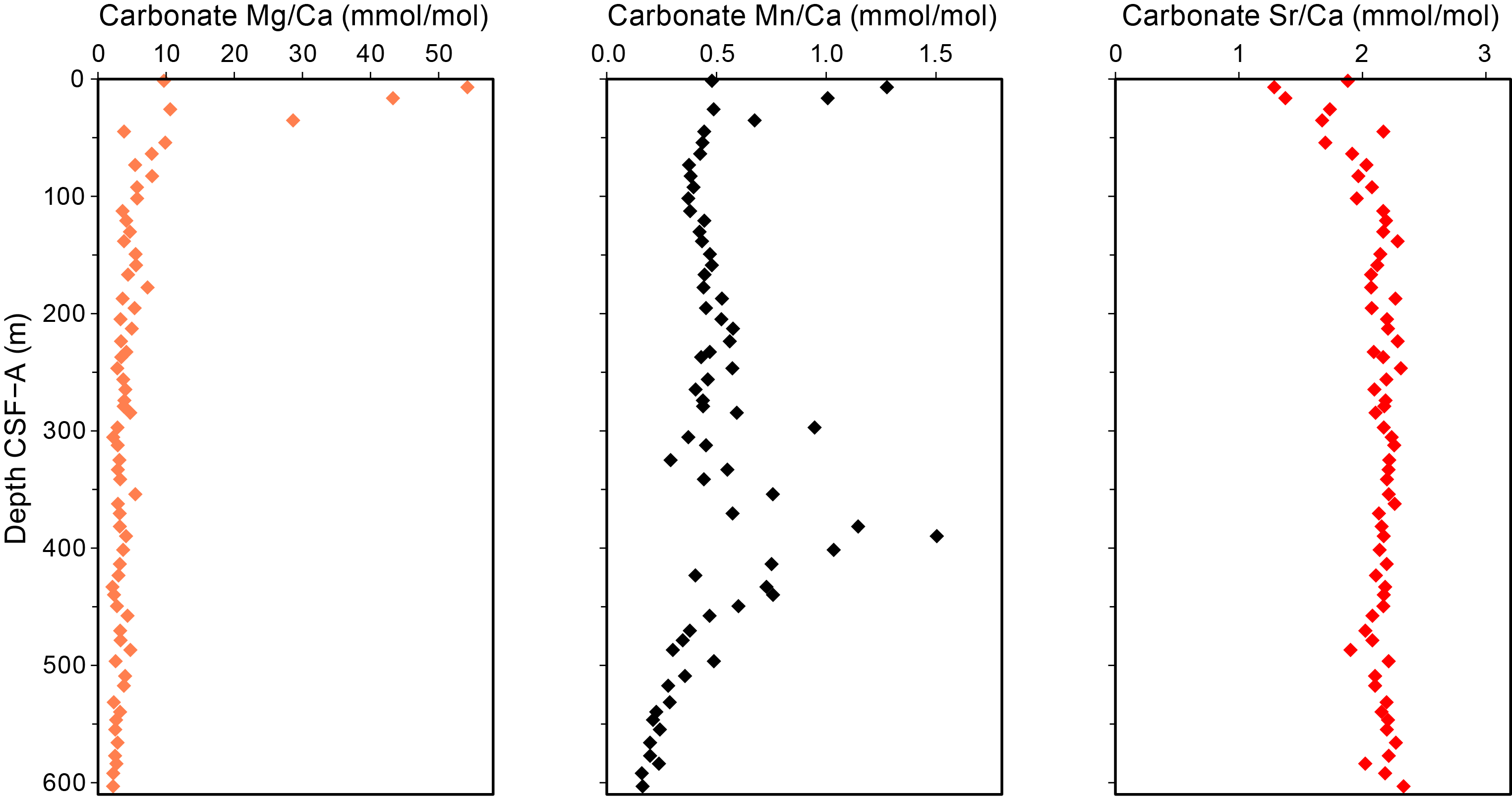
Figure F38. Carbonate Mg/Ca, Mn/Ca, and Sr/Ca.
7. Physical properties
Physical properties at Site U1609 were determined in Holes U1609A and U1609B at 2.5 cm spacing on the Whole-Round Multisensor Logger (WRMSL) and Section Half Multisensor Logger (SHMSL) and at 10 cm spacing on the Natural Gamma Radiation Logger (NGRL) (see Physical properties in the Expedition 401 methods chapter [Flecker et al., 2025a]). The Special Task Multisensor Logger (STMSL) was only used for Hole U1609B for the real-time stratigraphic correlation purposes at 5 cm spacing. Thermal conductivity was measured on Section 2 of each core in Hole U1609A and was not measured in Hole U1609B. P-wave velocity measurements on working-half sections were obtained from all the sections from Hole U1609A and on Cores 401-U1609B-33X through 61X. Moisture and density (MAD) measurements on discrete cylindrical samples were determined for every second section of Cores 401-U1609A-1H through 43X and for every first and last section of Cores 401-U1609A-44X through 73X.
Four physical properties units were defined at Site U1609 (Figure F39) with boundaries at 344, 458, and 531 m CSF-B. The physical properties units are the same as the lithostratigraphic units (see Lithostratigraphy). The similarity between physical properties of Holes U1609A and U1609B (Figures F39, F40, F41) can be attributed to the 20 m horizontal distance between holes where stratigraphy is expected to be the same. Any apparent differences are assumed to be drilling related (e.g., associated with core gaps, drilling disturbance, or borehole inclination).
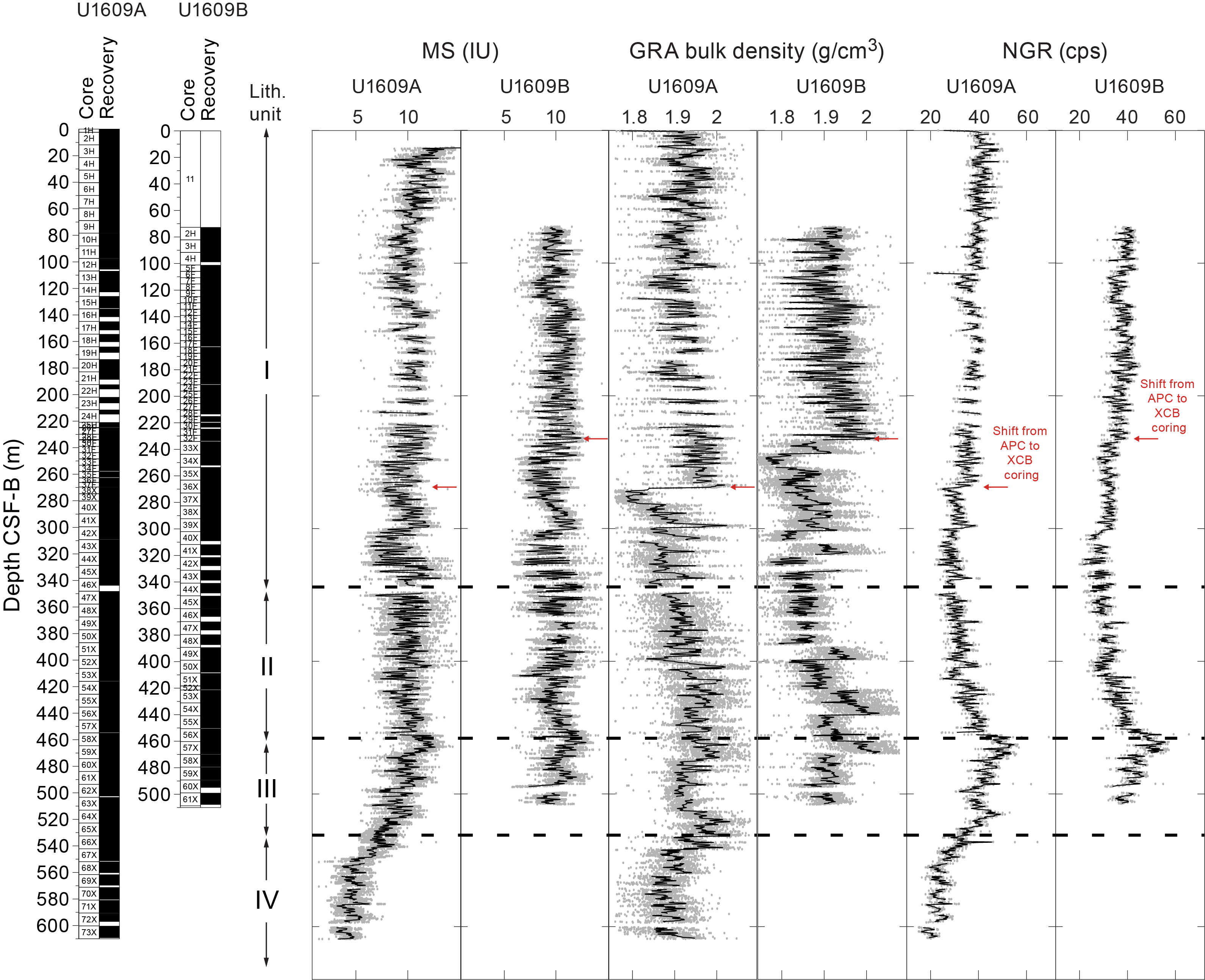
Figure F39. MS, GRA density, and NGR.
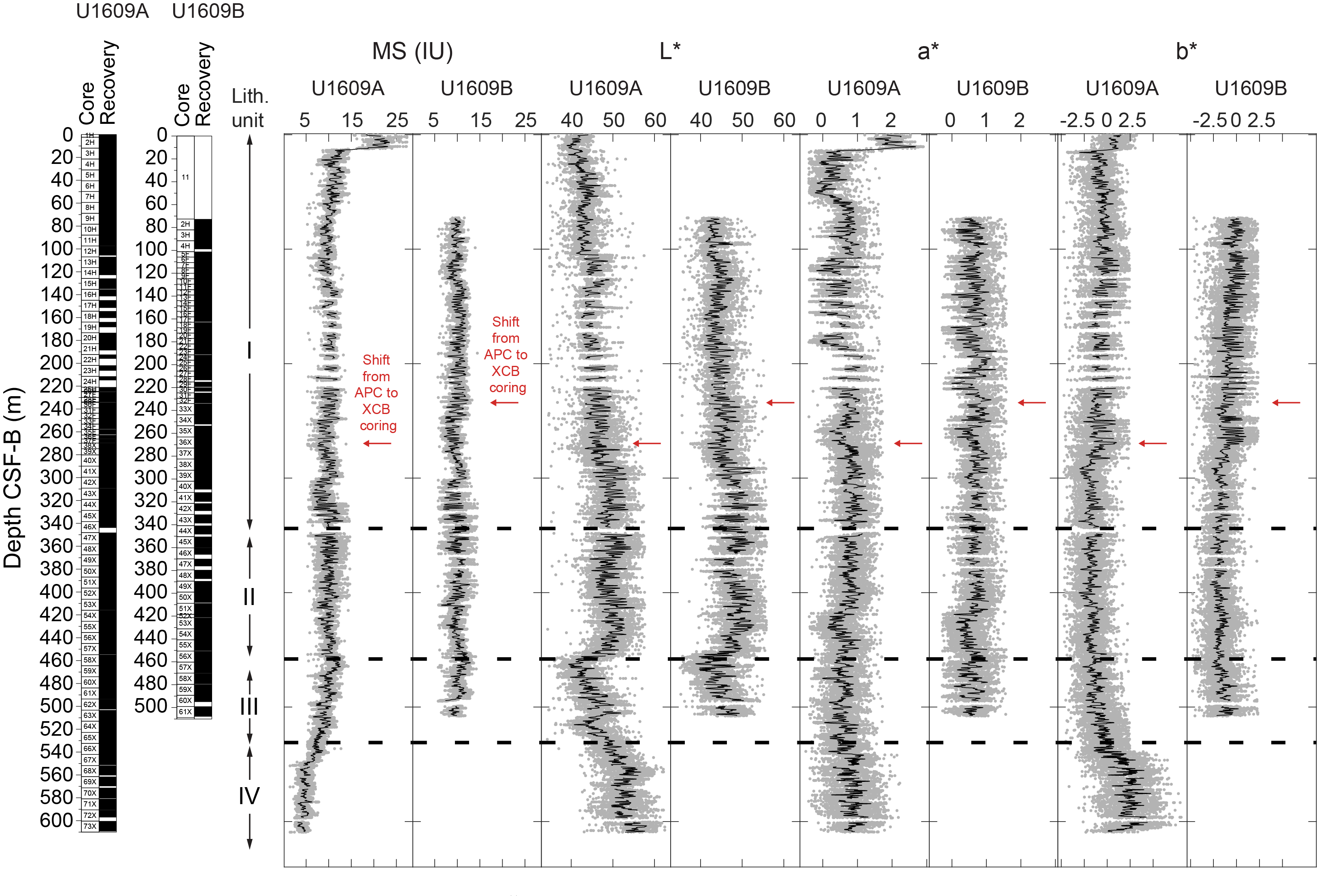
Figure F40. MS and L*, a*, and b* color variation.
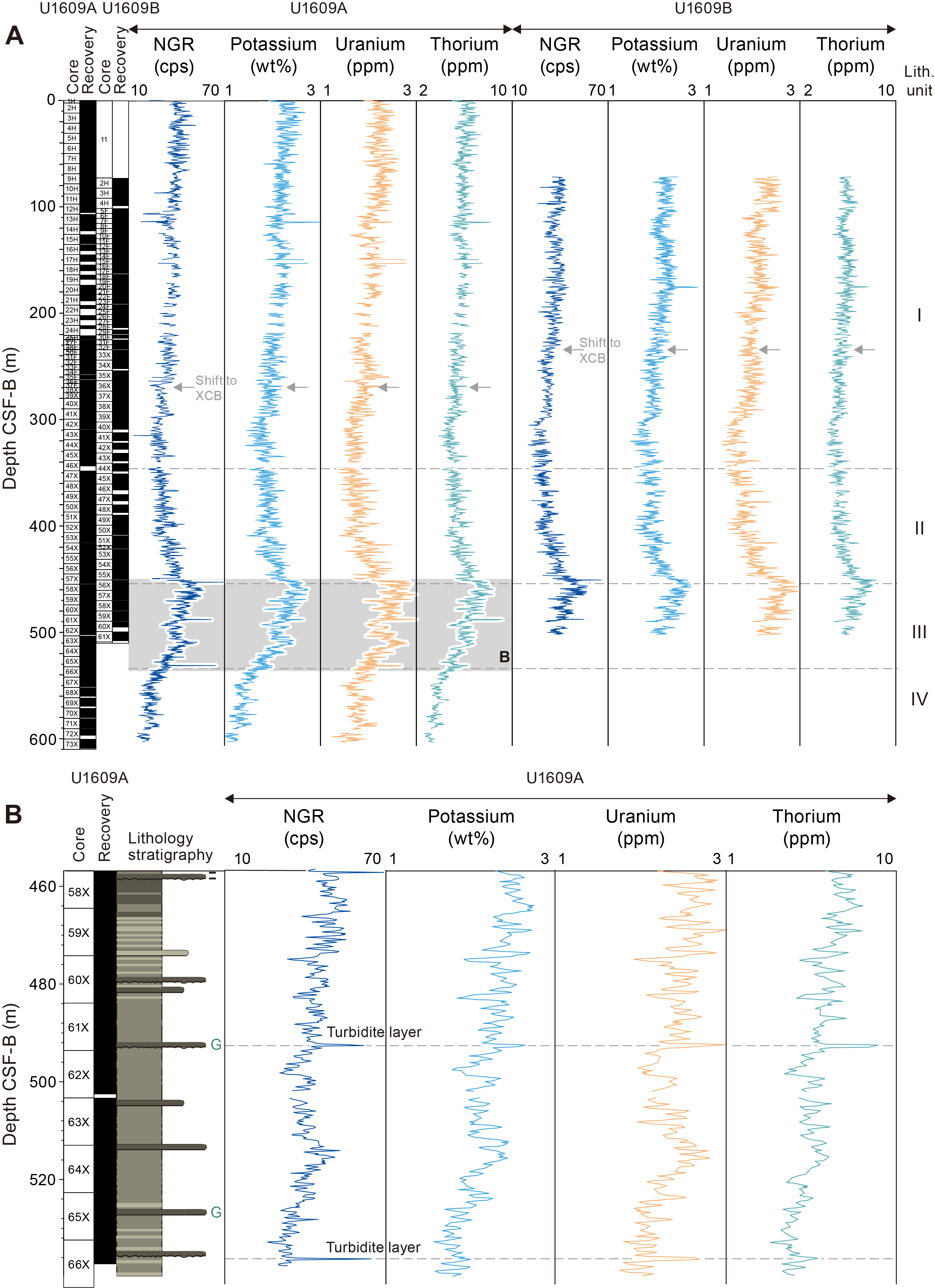
Figure F41. NGR measurements.
The lower boundary of Unit I at 344 m CSF-B (Figure F39) occurs at a transition from the older clayey calcareous oozes and muds (Unit II) to calcareous muds and calcareous silty muds (see Lithostratigraphy). Unit I cyclicity is evident in MS and best resolved in Hole U1609B because of gaps in recovery in Hole U1609A. Within Unit I, MS decreases a little downhole in Hole U1609A with a steep drop at ~20 m CSF-B, as does the total count of NGR. Drill bit changes at ~270 and ~230 m CSF-B in Holes U1609A and U1609B, respectively, are noted in case these are related to discontinuities in the physical properties.
NGR and MS show a similar trend throughout the entire core depth (Figure F39). The L* data show an inverse relative to MS and NGR (Figure F40). There is less coherence between Hole U1609A and U1609B gamma ray attenuation (GRA) density data sets, likely due to differences in the quality and the diameter of the cores (Figure F39). NGR, GRA, and MS decline relatively consistently with depth in Units III and IV, although a peak in NGR and MS is noted at ~500 m CSF-B and three peaks in GRA are noted at ~520–540 m CSF-B. Unit III contains coarser sandy layers (see Lithostratigraphy) that are detected as abrupt spiky peaks in NGR (e.g., at ~490 m CSF-B; Figure F41). Variations in NGR, MS, and GRA physical properties are associated with visible color changes and reflectance data (Figure F40), both likely related to changes in lithology.
7.1. Magnetic susceptibility
The uppermost 20 m CSF-B of Hole U1609A has MS values nearly double (~25 instrument units [IU]) the rest of the record (Figure F40), with an abrupt decrease at 20 m. Below this, MS is relatively consistent from 20 to 600 m CSF-B with cyclicity at ~0.5–3 m wavelength (Figure F39). These high-frequency cycles are superimposed on lower frequency oscillations. From 20 to 120 m CSF-B, there is a gradual decrease in MS values to a low at ~120 m CSF-B. This is followed by a rising trend with another low at 270 m CSF-B that is visible in both Holes U1609A and U1609B, suggesting that it is related to lithology. Although this transition also corresponds to the depth at which drilling shifted from APC to XCB coring in Hole U1609A (269.7 m CSF-B), the switch in drilling techniques occurred higher in Hole U1609B (234.1 m CSF-B) and thus appears unrelated.
From ~270 m CSF-B to the Unit I/II boundary (344 m CSF-B), the MS record exhibits 40 m scale undulations with a trough at 308 m CSF-B and two peaks at ~289 and ~330 m CSF-B. MS values shift back to a ~100 m undulation in Unit II, which consists of a trough at ~430 m CSF-B as well as two peaks roughly corresponding to the upper and lower boundaries of the unit (344 and 458 m CSF-B, respectively) (Figure F39). The peak at ~458 m CSF-B appears to be a common feature traceable across the MS, GRA density, and NGR data sets (Figure F39), associated with low carbonate concentrations (see Geochemistry). Units III and IV show high-frequency 0.5–1.5 m cycles superimposed on a decreasing trend, which is a feature common to both the GRA density and NGR data sets and is related to increasing carbonate concentrations.
7.2. Gamma ray attenuation bulk density
GRA density values vary from ~1.7 to 2.1 g/cm3For both holes, with high-frequency variations (0.5–3 m cycles) superimposed on low-frequency trends. The dominant feature in the downcore record is the large drop in GRA at the shift from APC to XCB coring that occurs at 269.7 m CSF-B in Hole U1609A and 234.1 m CSF-B in Hole U1609B (arrows in Figure F39). GRA calculations assume the liner is full, but if they are not this implies a lower-than-measured GRA density, and this will have a larger influence on the narrower diameter XCB cores; therefore, this step in GRA values is an artifact due to the change in coring method. Smaller amplitude, coring technology-related artifacts may be detected in the MS and NGR data (arrows in Figure F39).
GRA density has no discernible trend in Unit I other than the drilling related change. GRA density values in Unit II increase modestly with depth with a low at the Unit II/III boundary and generally decrease with depth in Unit III and IV with some peaks in GRA around the Unit III/IV boundary. In Unit III, there are two peaks at ~460 and ~520 m CSF-B in Hole U1609A; the peak at 460 m CSF-B is seen in the MS data, but there is no corresponding change in MS at 520 m CSF-B, suggesting that the lithologic nature of these high density features differ. Unit IV is characterized by low GRA density values, and these are caused by high-carbonate concentrations (see Geochemistry) and lithology (see Lithostratigraphy; Figure F4).
Some cores from Hole U1609B have abruptly higher/lower values compared to adjacent cores that are not seen at the equivalent depth in Hole U1609A (Figure F39); for example, GRA values step down by 0.1 g/cm3From Core 401-U1609B-54X to Core 55X and step up by ~0.05 g/cm3From Core 56X to Core 57X. Inspection of core images and X-ray scans shows that the cores with higher GRA values also have relatively thicker intervals of gravy (lightly fluidized sediment surrounding more coherent sediment biscuits) that fill the core liner, in contrast to the cores with lower GRA values, which tend to have open space between the core and core liner. For these reasons, MAD bulk density is preferred for characterizing large-scale trends because of compaction.
7.3. Natural gamma radiation
NGR fluctuates between 20 and 60 counts/s at Site U1609 (Figure F41). The four physical property and lithology units have significantly different characteristics of NGR values. In Unit I (0–344 m CSF-B), NGR values show a gradually decreasing trend with depth from approximately 40 counts/s at the top to 30 counts/s at 340 m CSF-B (Figure F41). In Unit II (344–458 m CSF-B), NGR counts increase with depth, increasing more rapidly at the boundary and peaking at close to 60 counts/s at the top of Unit III (458–531 m CSF-B) and thereafter decreasing throughout Units III and IV (531–610 m CSF-B) to ~20 count/s at the base of the hole. The high NGR at the top of Unit III is associated with low carbonate concentration and appears to match a peak in NGR from Expedition 397 Site U1586 (~100 km west of Site U1609) at 270 m CSF-B at ~8 Ma (Hodell et al., 2023). The declining NGR in Units III and IV is associated with the increasing carbonate concentration below 487 m CSF-B (see Calcium carbonate).
The three components of NGR (potassium, uranium, and thorium) were extracted from the NGR signals using the shipboard codes based on the method described by De Vleeschouwer et al. (2017). These components show similar patterns of long-term variations as total NGR, but the amplitudes are different (Figure F41). The K, U, and Th components all peak in Unit III associated with low carbonate before decreasing in step with the increasing carbonate content at the base of the hole.
NGR counts also show clear cycles repeating every 0.5–3 m, depending on the sedimentation rate (Figure F41). These cycles are also visible in the MS and color reflectance data (Figures F39, F40). Variations in carbonate concentration also likely explain the cyclic variations in NGR, but the geochemical measurements are available at lower resolutions than the physical properties data (see Calcium carbonate). In addition, several thin NGR peaks, mostly in Unit III, correlate to thin turbidite layers. Uranium and thorium peak in all turbidite layers (Figure F41B), but sometimes potassium shows no contribution to the NGR peak. The potassium response demonstrates differing source material for turbidites (see Lithostratigraphy). For example, potassium peaks with uranium and thorium peaks correspond to turbidites with high glauconite content, which most likely is the cause of the NGR peaks (G in Figure F41B).
7.4. Spectrophotometry
Lightness (L*), green–red (a*), and blue–yellow (b*) color variation data sets for both Holes U1609A and U1609B display similar signal trends to the other measured physical properties. Color changes are relatively subtle both visually in the core and in the spectrophotometry values but are reproduced in the two holes. Like MS, GRA density, and NGR, color shows a remarkable high-frequency cyclicity with a wavelength of ~0.5–3 m. This broadly agrees with the Munsell color variation noted in Lithostratigraphy, which averages a color change every ~0.76 m (equivalent to an average ~1.52 m cycle). These high-frequency variations are imposed on a few larger amplitude low-frequency oscillations (~16–40 m in wavelength). The L* record shows a similar but inverse pattern of highs and lows to that seen in the MS, GRA density, and NGR data sets (Figures F39, F40), whereas the a* and b* records show less long-term variability.
Color variations are relatively consistent between both holes, and shifting from APC to XCB coring does not appear to affect color (arrows in Figure F40). Sediments are relatively darker, redder, and yellower in the uppermost 20 m CSF-B of Hole U1609A; lighter, greener, and bluer from 20 to 535 m CSF-B; and after a dark shift at the Unit II/III boundary, become progressively lighter and yellower from 535 to 610 m CSF-B.
In Unit I, only L* values appear to have secular variation in this unit, generally increasing with depth. The larger amplitude troughs in MS at ~120 and ~270 m CSF-B (Figures F39, F40) correlate to peaks and troughs in the L* and a* data, respectively. This is less clear in the b* data at ~120 m CSF-B, but at ~270 m CSF-B there does appear to be a small peak as well as a shift to lower amplitude cycles (Figure F40). The Unit I/II boundary (~345 m CSF-B) does not appear to correlate to any distinct change in the L*, a*, and b* data, suggesting that the changes in NGR, MS, and GRA here are not associated with an obvious color change other than darkening (Figure F40).
In Unit II, both the L* and a* data show similar peak–trough patterns to that visible in the MS data, particularly in Hole U1609B. A more subtle response may be visible in the b* values as well. The Unit II/III boundary (~460 m CSF-B) is marked by a sharp decline in L* values that is also visible in the MS, GRA density, and NGR data sets (Figure F39) but is not evident in either the a* or b* data sets at this depth (Figure F40). This implies that although sediments become notably darker in the transition from Unit II to Unit III, there is no corresponding change in green, red, blue, or yellow colors.
The L* and b* values in Units III and IV become lighter and yellower with depth (Figure F40), mirroring the decrease in the MS, GRA density, and NGR data sets (Figure F39). These trends are associated with increasing carbonate concentrations (see Geochemistry). A more subtle trend toward redder a* values with depth is also visible.
7.5. Thermal conductivity
Thermal conductivity was measured in triplicate at one position per core using a half-space probe (H51033), mostly on Section 2 in Hole U1609A. The section used was modified if there were cracks in Section 2 that prevented obtaining good measurements. Thermal conductivity values vary between 1.24 and 1.99 W/(m·K), generally increasing with depth (Figure F42). The lowermost measurement at ~603 m CSF-B is an outlier (2.3 W/[m·K]). In the uppermost 200 m CSF-B (Cores 401-U1609A-1H through 22H), thermal conductivity is less variable (1.31–1.56 W/[m·K]), which is in the range obtained at nearby Expedition 339 Site U1391 (Expedition 339 Scientists, 2013). Between ~200 and ~300 m CSF-B (Cores 401-U1609A-23H through 41X) the range is larger (1.24–1.75 W/[m·K]), and below 300 m CSF-B it increases to 1.36–1.99 W/(m·K). Thermal conductivity measurements broadly show the same trends as GRA density (Figure F42). The substantial offsets seen in the GRA density record associated with the change from APC to XCB coring are not seen in the thermal conductivity records; the coherent core pieces in the XCB cores are sufficiently large and undisturbed to provide good thermal conductivity measurements.
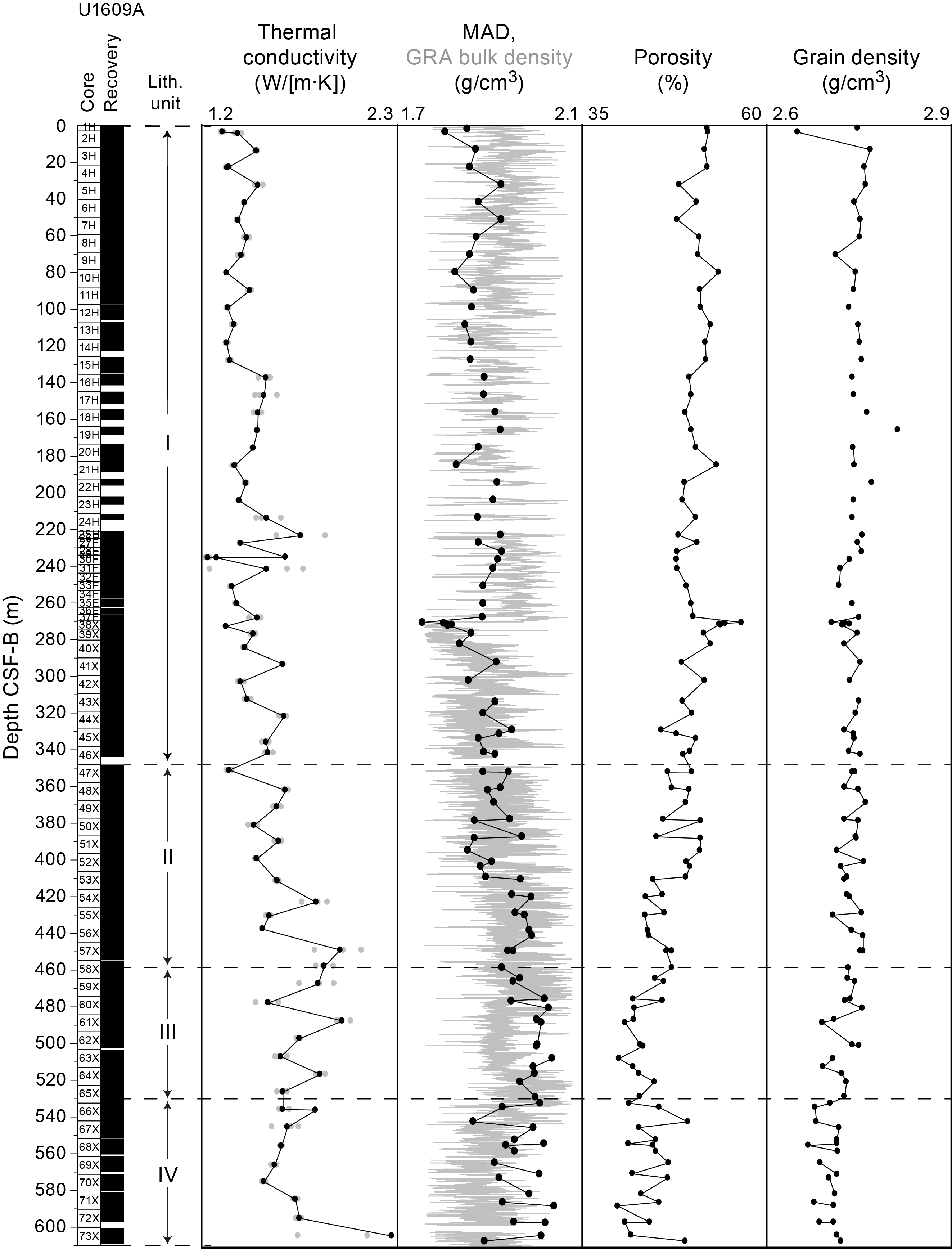
Figure F42. Thermal conductivity, bulk density, porosity, and grain density.
7.6. P-wave velocity
P-wave velocities were measured with the WRMSL (P-wave logger [PWL]) for Holes U1609A and U1609B (Figure F43). Highly scattered PWL values were obtained from the WRMSL for the sediments in Holes U1609A (90 to ~460 m CSF-B) and U1609B (235 to ~432 m CSF-B). The gap between the sediment and the core liner is likely the reason for the scattered P-wave values.
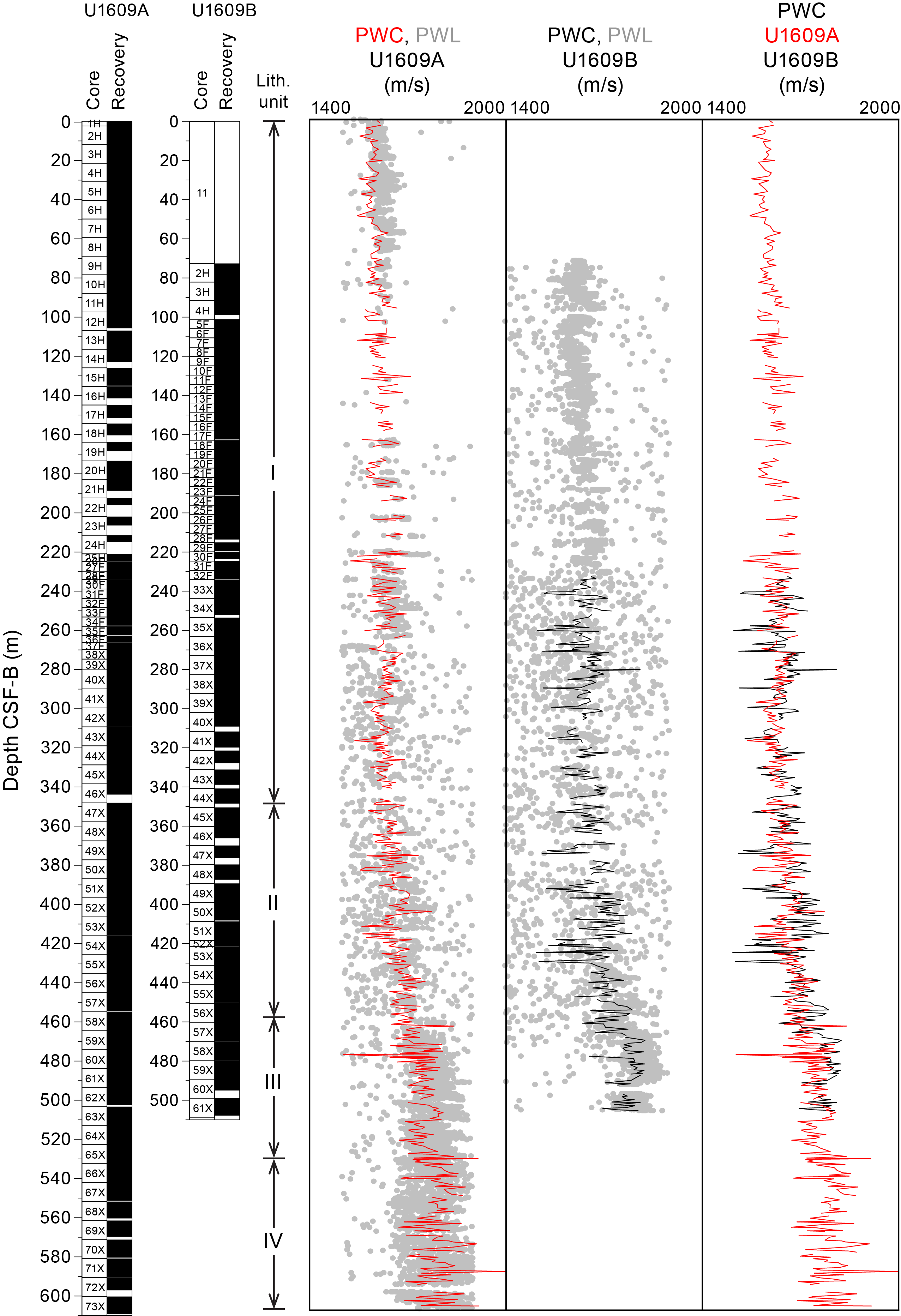
Figure F43. PWL and PWC.
Discrete P-wave velocities were measured on working halves using the caliper system (P-wave caliper [PWC]). One or two measurements were conducted near the top and the bottom of each section in Hole U1609A, depending on the integrity of the sediment and the corresponding lithologies. The PWC gave more coherent velocity values than the highly scattered PWL (Figure F43), although they exhibit slightly more scatter below Core 401-U1609A-65X (535 m CSF-B).
For Hole U1609A, P-wave velocity increases with depth (Figure F43). The highest values (1998 m/s) are at ~589.96 m CSF-B, and the lowest values (1503 m/s) are at ~478.97 m CSF-B.
For Hole U1609B (Figure F43), the same PWC measurement strategy was applied on each section below Core 401-U1609B-33X (240 m CSF-B). Measurements were not conducted on all the sections in Hole U1609B because the P-wave results of previous cores obtained by the WRMSL appeared to be more stable (Figure F43). Generally, P-wave velocity values measured using the caliper lie between 1478 (434.15 m CSF-B) and 1825 m/s (471.61 m CSF-B), and the trend changes at around 430 m CSF-B. Both PWL and PWC velocity values underestimate the in situ velocity measured during downhole logging (see Downhole measurements).
7.7. Moisture and density measurements
Water content, porosity, and wet and dry bulk densities are interdependent. Bulk density measurements were taken for Hole U1609A. Bulk density values were calculated from moisture and volume measurements made on cylindrical discrete samples taken from the working halves. At least one sample per core was taken; however, the number of samples taken in each core varied depending on the lithology, recovery, and quality of the sediments. At least two samples were taken from each XCB core to check, at a slightly higher resolution, the reliability of the GRA density measured on the WRMSL (Figure F42). A total of 102 samples were taken for MAD measurements. MAD density values are lower than GRA values in APC and HLAPC cores but higher than the GRA densities deeper than 480 m CSF-B. Because GRA bulk density can be affected by the gaps between sediment and core liner or interior cracks and differences in core diameter, the MAD bulk density measurements are more reliable. For example, MAD densities show a downhole compaction trend, whereas GRA densities do not (Figure F42).
7.7.1. Bulk density, grain density, and porosity
MAD bulk density typically varies between 1.75 and 2.0 g/cm3 in Hole U1609A (Figure F42). An anomalously low bulk density of 1.75 g/cm3 was recorded at 270 m CSF-B because of the difficulty in finding a good sample in the uppermost XCB cores. MAD bulk density at 270 m CSF-B is higher than the GRA bulk density measured by the WRMSL.
Grain density typically varies between 2.65 and 2.81 g/cm3 in Hole U1609A (Figure F42). The lowest grain density (2.65 g/cm3) was measured at 3.97 m CSF-B, and the highest grain density (2.81 g/cm3) occurred at 165.55 m CSF-B. Generally, grain density decreases with depth.
Discrete porosity values range from ~56.6% at the base of Unit I (344 m CSF-B) to ~39.8% near the bottom of the hole (586.4 m CSF-B) (Figure F42). Porosity decreases with increasing depth. By comparing with the other physical properties in Hole U1609A, bulk density, grain density, and porosity all seem to correlate well with P-wave velocity and thermal conductivity.
8. Downhole measurements
Following coring in Hole U1609A, the hole was prepared for downhole logging (see Operations). On 23 December 2023, three tool strings were deployed in Hole U1609A: (1) a 34.05 m long triple combo, consisting of the Magnetic Susceptibility Sonde (MSS), High-Resolution Laterolog Array (HRLA), Hostile Environment Litho-Density Sonde (HLDS), Hostile Environment Natural Gamma Ray Sonde (HNGS), and the logging equipment head-pressure temperature (LEH-PT), which measure MS, electrical resistivity, density, natural gamma ray, and temperature, respectively; (2) a 12.11 m VSI for the check shot survey consisting of VSI, Enhanced Digital Telemetry Cartridge (EDTC), and LEH-PT; and (3) a 28.3 m long sonic tool, consisting of the Dipole Sonic Imager (DSI), HNGS, EDTC, and LEH-PT. Immediately prior to downhole logging, an attempt was made to activate the heave compensator but without success because of a failure of the compensator control computer that could not be replaced at short notice. Consequently, despite a ship heave of ~2.5 m over the course of the day, logging was undertaken without heave compensation.
The bottom of the borehole was reached at ~602 m wireline log depth below seafloor (WSF). The triple combo repeat and main runs started from the bottom of the borehole at 602 m WSF and logged up to ~504 m WSF and to the seafloor, respectively. The logged borehole mainly comprised calcareous muddy sediment with 1–5 m scale repeating cycles in NGR, MS, and density, superimposed on a compaction trend. The bottom 80 m are more carbonate rich than the overlying sediments (see Lithostratigraphy). These broad features can be seen in the downhole logs (Figure F44).

Figure F44. Physical properties comparison.
Attempts to record seismic shots from the air gun during the VSI run were successful only in the bottom, unwashed-out part of the hole where check shots were recorded at three depth stations (Figure F44). The far-field waveforms at the third, uppermost, station were not good quality and could not be used. Several other shot stations at shallower depths were attempted (e.g., 500, 250, 200, 100, and 70 m WSF), but all the recorded waveforms were noisy because the borehole was mostly wider than 15 inches and the geophone could not be coupled well to the borehole wall. When the VSI was raised back to the ship, the caliper arm of the tool was found to be broken, which could explain why it was not possible to clamp the hydrophone to the hole wall and obtain a good signal. The two check shots that yielded a clear first arrival time gave an interval velocity of 2245 m/s for the depth interval between 557 and 602 m WSF.
The HLDS caliper revealed that except for the lowermost part of the hole, between 520 and 602 m WSF, the wall of the hole had very irregular width and was disturbed by washouts along most of its length (Figure F45). The caliper data also indicated the presence of several 1 m thick bridged sections with a diameter smaller than the bit size (9⅞ inches; e.g., ~199, 380, and 403 m WSF) (Figure F45). The borehole appeared to be slightly inclined because the measured deviation yielded values that increase from ~3° at the seafloor up to ~9° at ~600 m WSF (Figure F45).
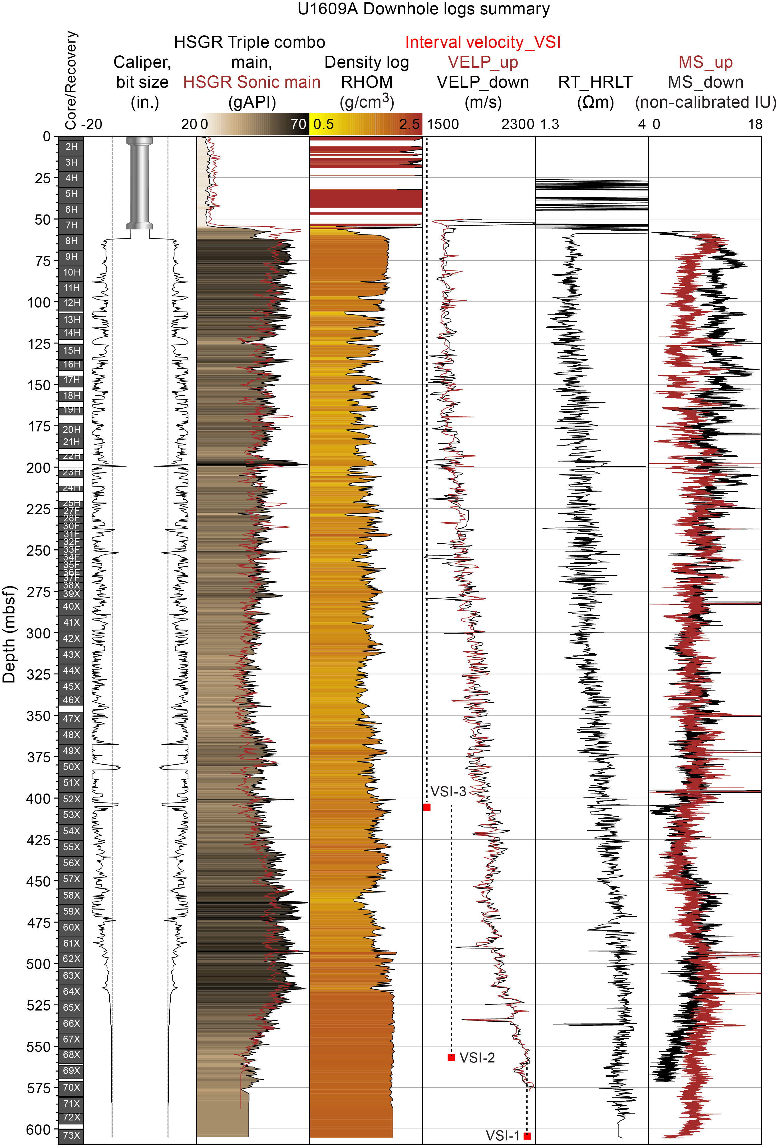
Figure F45. Downhole logging data summary.
Of the logging tools, only the HNGS gives formation data inside the drill pipe, and the gamma ray data collected is attenuated. The total spectra gamma ray (HSGR) logs show that the base of the pipe is at ~564.5 m WSF (Figure F45).
All of the downhole logs are probably affected to some extent by the borehole conditions. For example, resistivity log values range between ~1.5 and ~3.5 Ω/m and comprise higher amplitude oscillations in the washed-out part of the borehole than in the uppermost and lowermost parts of the hole where the condition of the borehole is better. The gamma ray (HSGR) and sonic P-wave velocity (VELP) logs are more robust to variations in hole width; these two logs show anomalous values only in proximity to the largest bridged sections within the borehole (Figure F45). HSGR logs from both the triple combo and the sonic strings are shown in Figure F45. HSGR is corrected for hole diameter in the triple combo tool string but not in the sonic tool string, accounting for some of the differences between the two logs. The similarity of the two logs indicates that the quality of the data is good.
The sonic velocity log repeated reasonably well between the upward and downward passes of the logging tool (Figure F45) even though different frequencies were used (high frequency downward and medium frequency upward). The data are therefore considered to be robust and to reflect real formation properties. The P-wave velocity values increase with depth, ranging ~1600 m/s at 60 m WSF to 2250 m/s at 570 m WSF.
The MS log is also less affected by the borehole conditions than the resistivity and density data and shows long-term trends. The MS data collected during the two passes of the triple combo show broadly the same trends at the >5 m scale, but the absolute amplitudes differ especially in the uppermost 200 m WSF (Figure F45) because of incomplete MSS temperature drift correction at those depths (see Downhole measurements in the Expedition 401 methods chapter [Flecker et al., 2025a]).
The gamma ray, sonic, and MS downhole logs all show short repeating changes in value that may reflect astronomical cyclicities (Figure F45). However, the tool motion was irregular both as a result of the uncompensated heave and because of the roughness of the borehole walls. This lends uncertainty to the depth that the tool makes its measurement (shorter than the ~3 m scale), so it is difficult in some intervals to correlate cycle-for-cycle to the core physical properties data. Over longer depth intervals, the log and core data show similar patterns.
8.1. Downhole versus core logs
8.1.1. Gamma ray logs: HSGR versus NGR
Despite different measurement units, the gamma ray data from both the downhole and core data set logs appear to follow similar trends (Figure F44). At higher resolution, the gamma ray data sets are in phase except for a few intervals where there appears to be a phase shift varying from ~0.5 to 3 m between the data sets (e.g., ~250 to ~254 m WSF). This could have a variety of causes, including string pulls or different depth scales between the coring and the logging operations. The regularity of the gamma ray data sets from the different runs, and their similarity to the core logs indicates that combining the gamma ray logs with other data should help determine the lithologies in intervals with low recovery.
8.1.2. Magnetic susceptibility logs: MSS versus WRMSL
Comparison of the MS downhole log curve with the data measured on the cores (WRMSL; Figure F44) shows features thicker than ~5 m along most of the length of the borehole in both data sets. There are two exceptions (~115–200 and ~425–485 m WSF) in which records appear to stay generally in phase but the amplitude of the downhole MS shifts to lower values compared to the core logs, which is probably caused by the incomplete temperature drift correction of the MSS measurement.
8.1.3. Density logs: HLDS versus WRMSL and MAD
The density log (RHOM) data range ~1.1 to ~2 g/cm3 and are strongly impacted by the washouts in the borehole walls because the HLDS tool requires that the detector should be very close to the borehole wall. Comparison of the densities obtained from the downhole log and the densities measured on the cores (GRA and MAD bulk densities) (Figure F44) indicates that they are only similar in the topmost (~1.8 g/cm3) and bottommost (1.9 g/cm3) parts of the hole where no washouts and/or bridgings are present. The very low densities (<1.6 g/cm3) obtained in the downhole log coincide with washouts and do not reflect real formation measurements. Assuming the top and bottom of the downhole and core density logs do reflect the rock properties, the data suggest that density does not increase substantially with depth.
8.1.4. Vertical seismic profile and sonic velocity versus PWL and PWC
Comparison between the sonic wireline log (VELP), PWL, and PWC shows similar P-wave velocity values ranging 1600–1700 m/s in the uppermost 200 m WSF of the hole. Below 200 m WSF, the sonic log continues to increase with depth, whereas PWC and PWL velocities remain unvaried to ~450 m WSF (Figure F44). This discrepancy is mainly because the measurements on the core are made after it has been recovered and expanded, resulting in an underestimate of the in situ velocities.
8.1.5. Core-downhole-seismic integration
Time-depth relationships are crucial for correlating seismic profiles to drill hole information. One important challenge for Expedition 401 is to establish the age and lithologic origin of the seismic reflections previously identified in seismic profiles covering the study area. At least three different data sets could be used to tie the recovered cores to the seismic units interpreted on the seismic profiles in Hole U1609A: (1) vertical seismic profile (VSP) check shot traveltimes, (2) traveltime derived from the sonic log, and (3) synthetic seismograms. Because the construction of synthetic seismograms needs sonic and density logs that are free from artifacts, we used the VSP check shots and sonic log for a preliminary core-downhole-seismic tie. Figure F46 shows the different time-depth relationships (TDRs) available from both core and downhole logs. Each of these result in a different tie. The TDR that we used to tie the Hole U1609A cores to Seismic Profile WPortugal_XL5210 is the downhole sonic log calibrated to the bottommost check shot of the VSI. The obtained TDR yields values (2856 ms at 605 m WSF) that are slightly slower than the original sonic log (Figure F46). Another important correction that was made for the tie is the inclination of the borehole measured during the downhole triple combo run (Figure F44), which reached nonnegligible values of ~9.5° in the bottommost part of Hole U1609A. The 270° azimuth along which the borehole is inclined is taken from the measured inclination and azimuth during the APC coring down to ~205 m WSF and assumes that the azimuth does not change much in the rest of the borehole.
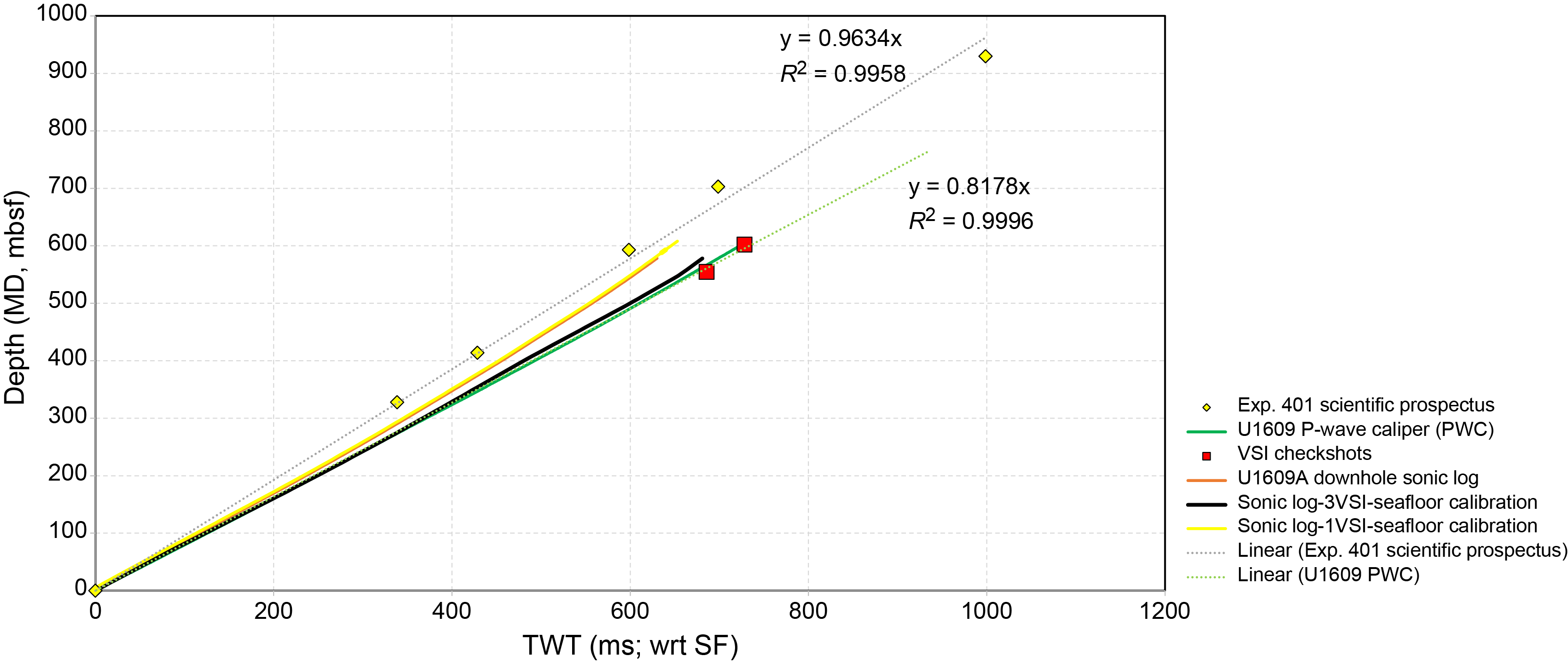
Figure F46. Time-depth relationship models.
The result of the tie with all these corrections is shown in Figure F47. The maximum penetration depth of the borehole reached a two-way traveltime depth of 2.85 s (Figure F47).
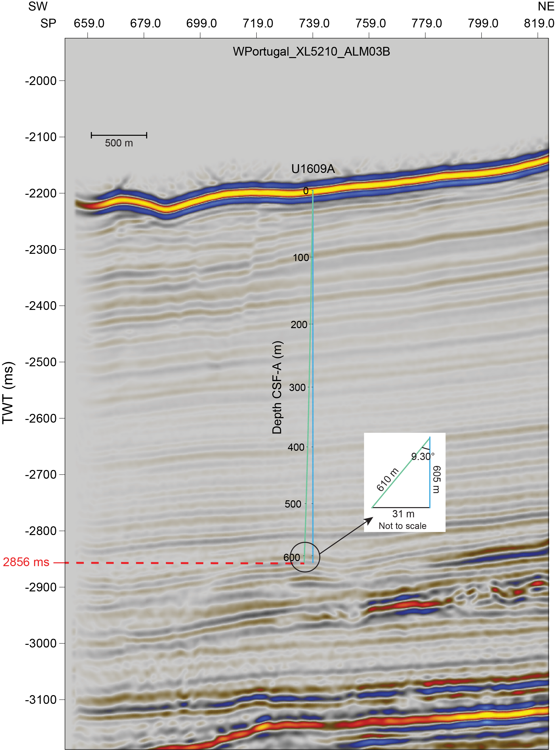
Figure F47. Seismic profile with estimated penetration and dip.
8.2. Downhole temperature measurements
During APC coring in Hole U1609A, the APCT-3 probe was used to measure in situ formation temperature at selected depths ~30 m apart while coring Cores 401-U1609A-4H, 7H, 10H, and 13H (Table T20). The SET2 probe was deployed following Cores 401-U1609B-32F and 48X. Figure F48 shows for each deployment the intervals in the temperature records that were used to estimate formation temperature by finding a best fit for a theoretical model to the temperature decay as a function of time (~10 min) as it recovers from the frictional heating generated when entering the formation.
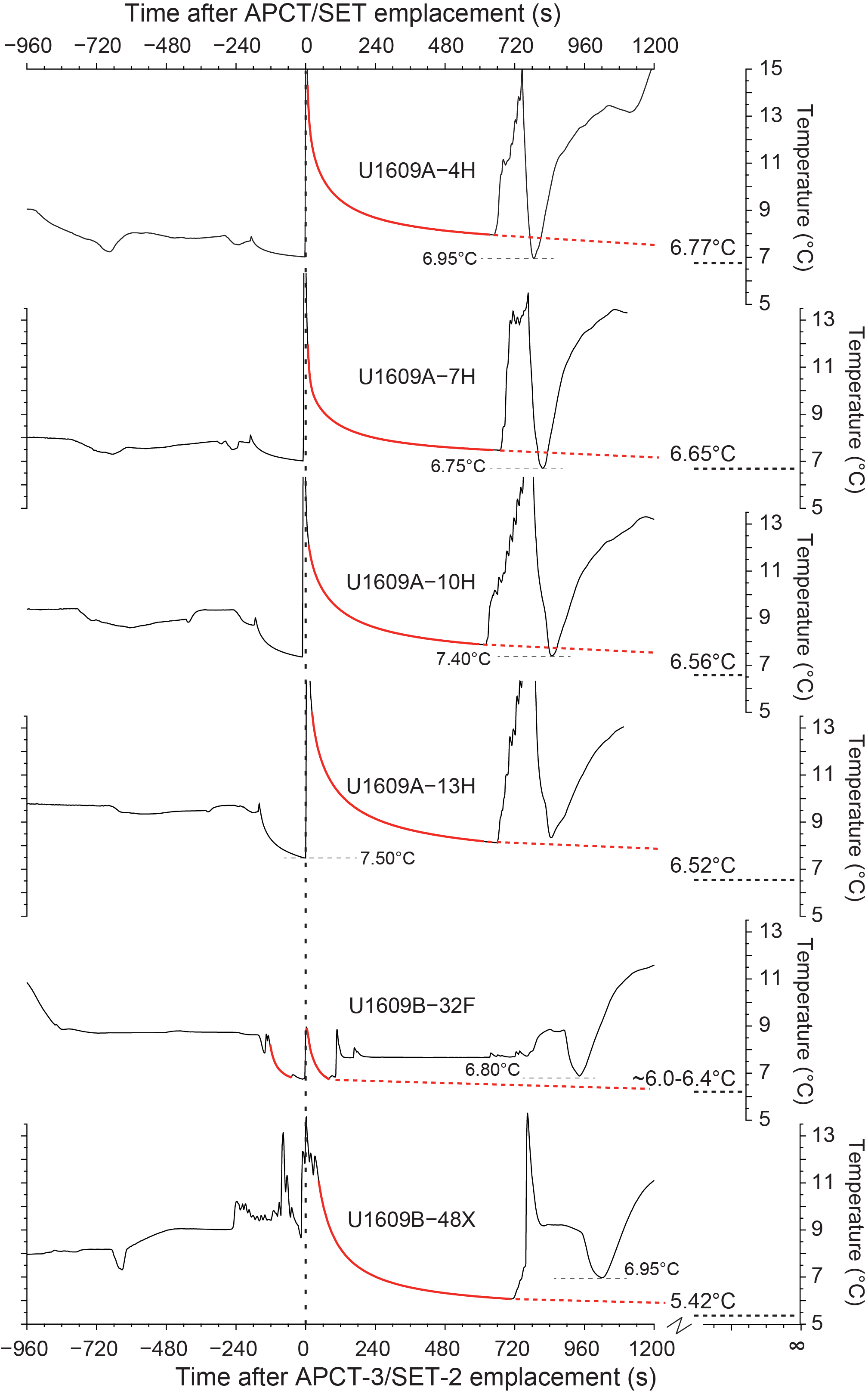
Figure F48. Downhole temperature.
The formation temperature results from Site U1609 are unusual because they decrease with depth, contrary to the expected geothermal temperature increase (Figure F49). All four APCT-3 measurements were made with the same instrument, so they are likely to be reliable measurements. The SET2 measurement after Core 401-U1609B-32F did not yield a long enough equilibration to be reliable, but the measurement after Core 48X yielded a clean equilibration curve without jumps; the calibration data will be checked after the expedition. The lowest temperature during probe retrieval, a gauge of bottom water temperature, is a loose indication of quality—each deployment should detect a similar bottom water temperature: these values range 6.75°–7.5°C, close to the seafloor value of 6.9°C derived from the upward extrapolation of the APCT-3 results.
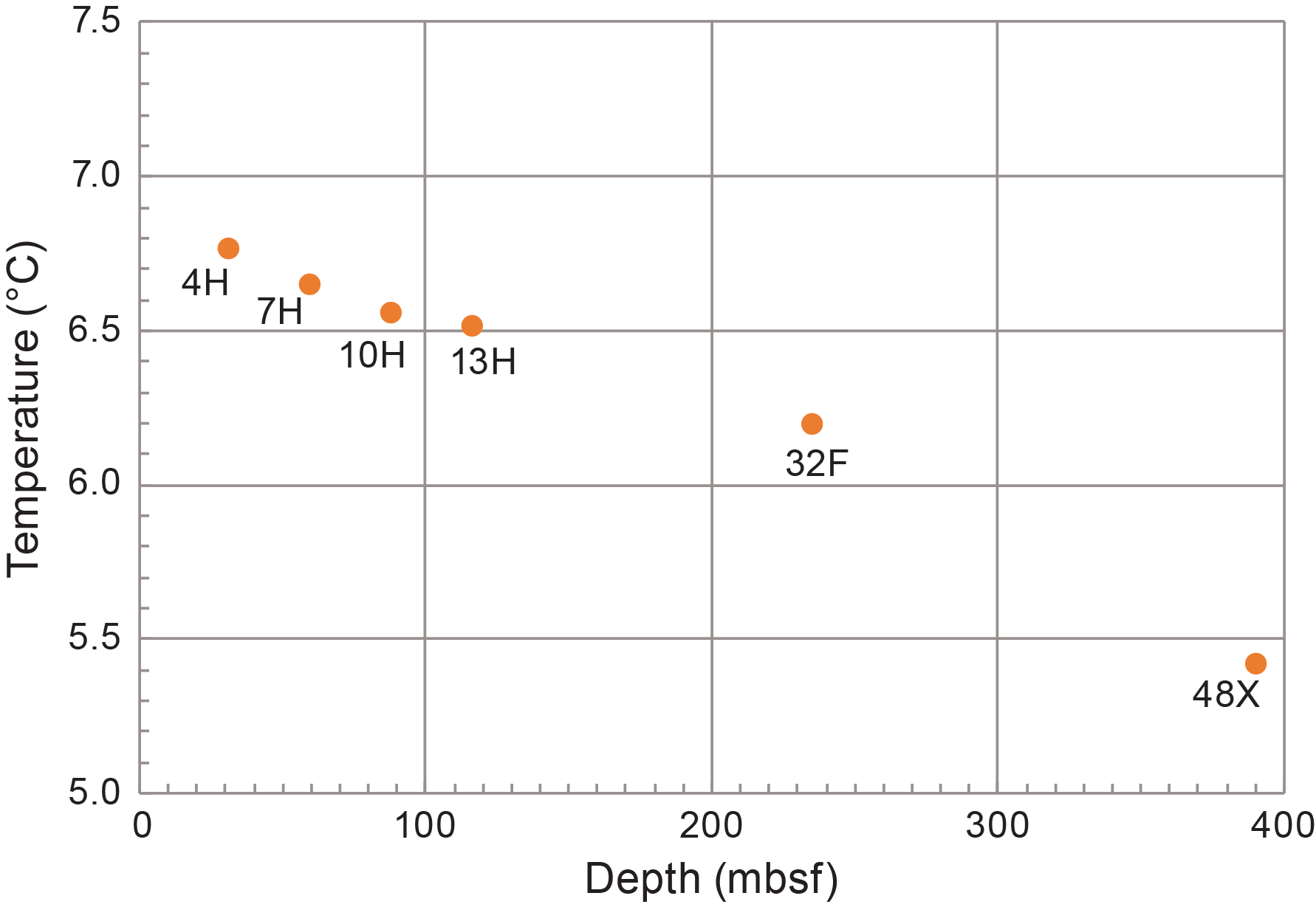
Figure F49. APCT-3 and SET2 formation temperature.
One possible explanation of the temperature profile is that a warmer water mass moved over the site, warming the seafloor and propagating that warmth conductively downward. Site U1609 sits under the lower part of relatively warm MOW, and colder Northeast Atlantic Deep Water lies only a few 100 m below in the present day (Ambar et al., 2002). The subsurface depth extent of the cooling trend implies that the seafloor warming started on the order of centuries to millennia ago. Other possible explanations include a subsurface tongue of cold pore water moving from the scarp ~5 km west of Site U1609 or a calibration problem with the SET2 tool.
9. Stratigraphic correlation and age model
Stratigraphic correlation between the two holes using physical properties and downhole logging data suggest that many of the gaps encountered in Hole U1609A were recovered in Hole U1609B (Figure F50). We used the Correlator software to identify stratigraphic features (in NGR or MS) in laterally adjacent cores in Holes U1609A and U1609B. An affine tie was applied to move the feature in one hole to occur at the same depth as in the other hole, and so on, down the succession (Table T21). As a second step, core intervals from each hole that seemed to have the clearest stratigraphy were spliced together to form a more complete stratigraphic succession than possible from each hole alone (Table T22; Figure F50). Several short gaps remain, but they are all <2 m. Only Hole U1609A covers the uppermost 70 m CSF-B and lowermost 100 m CSF-B of the hole, and larger gaps are found in those intervals. A 1 m gap was applied below each core in the uppermost 70 m CSF-B of Hole U1609A to account for core expansion, but no a priori expansion was applied to cores below that; instead, the manual affine ties between Holes U1609A and U1609B account for core expansion. The affine and splice tables and corresponding plots presented here are from May 2024 and had been updated iteratively after the expedition based on new XRF scanning data, mainly the XRF Ca/Ti elemental ratio, for Cores 401-U1609A-36F through 51X and 401-U1609B-36X through 51X, which cover the MSC interval. The affine ties and splice are likely to be further refined during the postcruise phase.
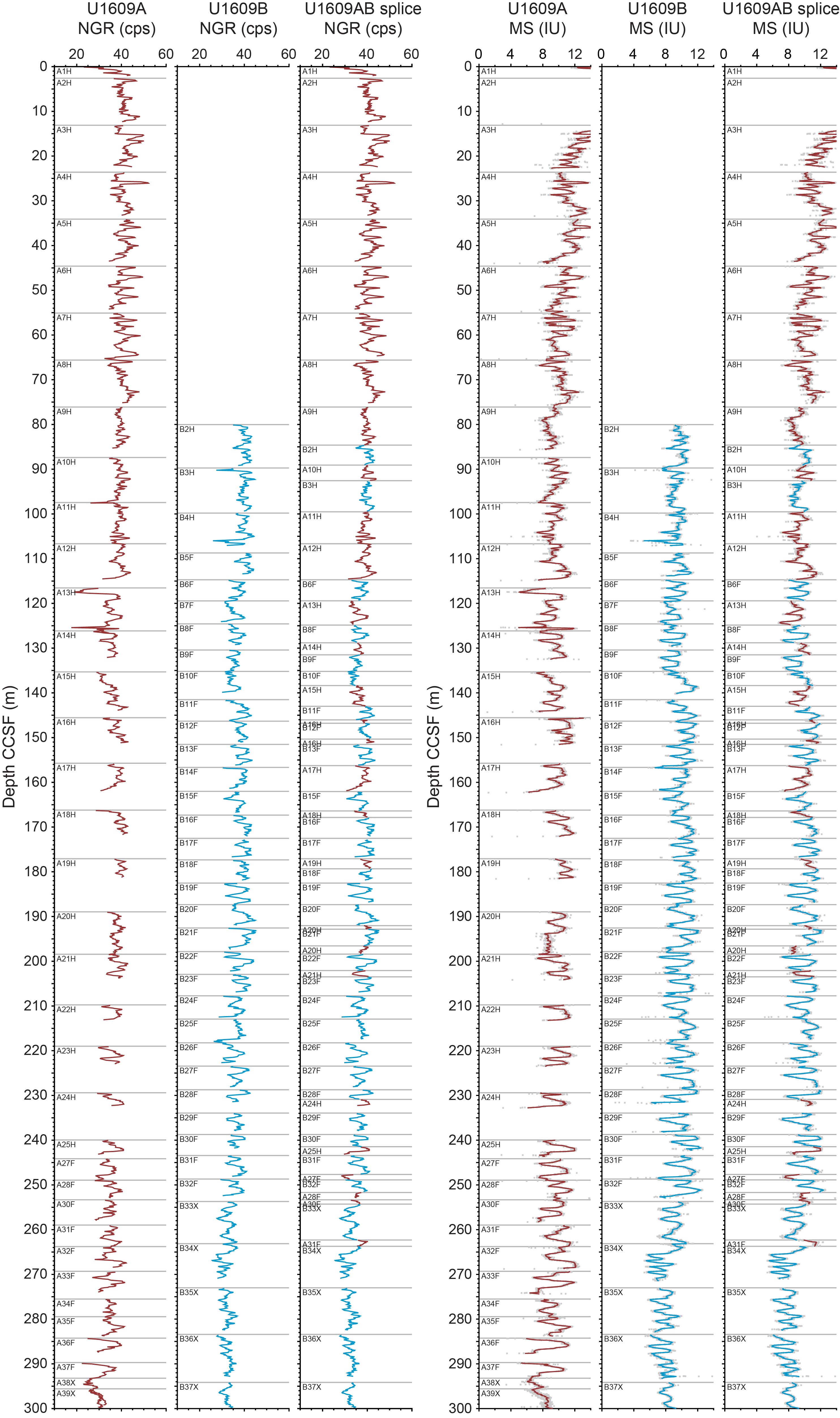
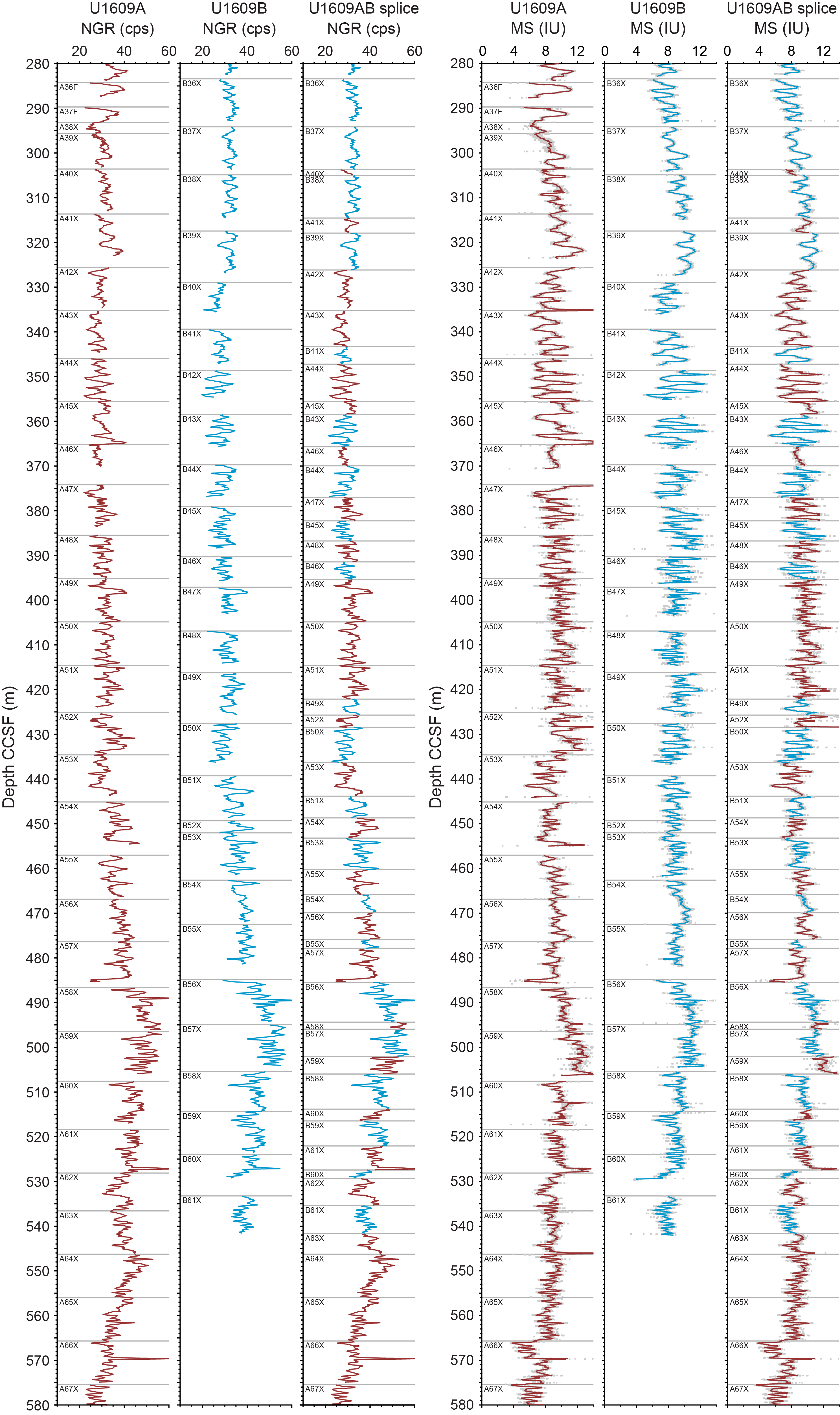
Figure F50. NGR and MS record.
The depths of biostratigraphic events in each hole are offset by between a few centimeters to several meters in others (see Biostratigraphy). There is good correspondence between foraminifer and nannofossil bioevents and the interpreted paleomagnetic chron boundaries for Holes U1609A and U1609B (Figure F51A), particularly between 100 and 500 m CSF-B. The overall trend suggests an increasing sedimentation rate with time, but it is not obvious if this is a gradational transition or occurs in a more step-like fashion. Calculating the sediment accumulation rate of each dataset (foraminifers, nannofossils, and magnetostratigraphy) separately helps to mask the potential for each age datum to act as an inflection point unrelated to real changes in accumulation rate (Figure F51A). These data for both Holes U1609A and U1609B indicate that there was a relatively constant sedimentation rate between 3.2 and 6 Ma and between 8 and 9 Ma (Figure F51B) but that it increased between 8 and 6 Ma and declined after 3.2 Ma.
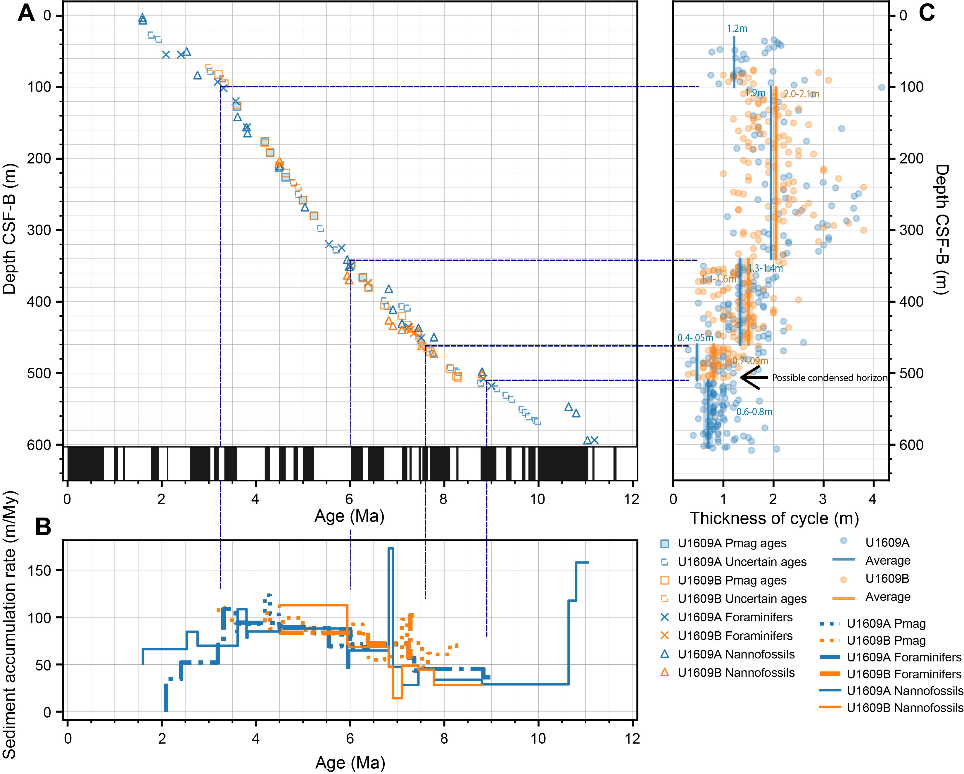
Figure F51. Age model tie points.
Because the physical properties records at Site U1609 show strong, regular cyclicity, one way to assess the time at which sedimentation rates changed is to measure cycle thickness to evaluate the depths at which cycle thicknesses change, assuming the likely case that the cycles were precessionally forced. Figure F51C illustrates the thickness of cycles observed in the MS data of Holes U1609A and U1609B (Table T23). Despite the scatter, these data show several abrupt changes at 100 (3.2 Ma), 340 (6 Ma), 460 (7.6 Ma), and 510 m CSF-B (8.9 Ma). The latter three changes broadly correspond to the unit boundaries identified in the lithofacies and physical properties (see Lithostratigraphy and Physical properties).
Using changes in cycle thickness to define abrupt sedimentation rate changes allows the calculation of average cycle thickness and linear sedimentation rates between these boundaries (not shown), assuming a 21.7 ky duration for these likely precessional cycles. Additionally, as a cross-check that the cycles are precessional, the bio- and magnetostratigraphically determined duration of each interval can then be used to predict the expected thickness of sedimentary cycles of a given precessional cyclicity. The calculated thickness of precessional cycles for each interval and each hole are plotted as vertical lines on Figure F51C. These have been calculated both from linear regression through all the magneto- and biostratigraphic data points in that interval and by calculating the sedimentation rate of the top and bottom age tie point for each interval (Tables T24, T25). In most cases, precessional thickness calculated from the sedimentation rates correspond well with the distribution of the cycle thickness measurements, suggesting that the dominant cyclicity visible in the sediments recovered at Site U1609 is precessional. However, the sedimentation rates calculated in Hole U1609A between 460 and 510 m CSF-B produce precessional cycle thickness that is visibly lower than the measured cycle thickness for this interval (0.4–0.5 m; Figure F51C). This is a consequence of the influence of the lowest age/depth events in this interval, which have the effect of reducing calculated sedimentation rate by both the regression and top-bottom tie point methods (Table T22). It is likely that the sedimentation rate over this interval as a whole is reflected more accurately by the cycle thickness than the calculated rates. However, there may be an abrupt reduction in cycle thickness at around 500 m CSF-B, perhaps corresponding to a condensed interval. There is insufficient thickness data in Hole U1609A to test this, but the data from right at the bottom of Hole U1609B does support an abrupt reduction in cycle thickness at the same depth (Figure F51C).
References
Acton, G.D., Okada, M., Clement, B.M., Lund, S.P., and Williams, T., 2002. Paleomagnetic overprints in ocean sediment cores and their relationship to shear deformation caused by piston coring. Journal of Geophysical Research: Solid Earth, 107:2067–2081. https://doi.org/10.1029/2001JB000518
Ambar, I., Serra, N., Brogueira, M.J., Cabeçadas, G., Abrantes, F., Freitas, P., Gonçalves, C., and Gonzalez, N., 2002. Physical, chemical and sedimentological aspects of the Mediterranean outflow off Iberia. Deep Sea Research, Part II: Topical Studies in Oceanography, 49(19):4163–4177. https://doi.org/10.1016/S0967-0645(02)00148-0
Bernhard, J.M., 2000. Distinguishing live from dead foraminifera: methods review and proper applications. Micropaleontology, 46:38–46. http://www.jstor.org/stable/1486179
Bouma, A.H., Keunen, P.H., and Shepard, F.P., 1962. Sedimentology of Some Flysch Deposits: a Graphic Approach to Facies Interpretation: Amsterdam (Elsevier).
Boyle, E.A., 1983. Manganese carbonate overgrowths on foraminifera tests. Geochimica et Cosmochimica Acta, 47(10):1815–1819. https://doi.org/10.1016/0016-7037(83)90029-7
Brumsack, H.J., and Gieskes, J.M., 1983. Interstitial water trace-metal chemistry of laminated sediments from the Gulf of California, Mexico. Marine Chemistry, 14(1):89–106. https://doi.org/10.1016/0304-4203(83)90072-5
Capella, W., Hernández-Molina, F.J., Flecker, R., Hilgen, F.J., Hssain, M., Kouwenhoven, T.J., van Oorschot, M., Sierro, F.J., Stow, D.A.V., Trabucho-Alexandre, J., Tulbure, M.A., de Weger, W., Yousfi, M.Z., and Krijgsman, W., 2017. Sandy contourite drift in the late Miocene Rifian Corridor (Morocco): Reconstruction of depositional environments in a foreland-basin seaway. Sedimentary Geology, 355:31-57. https://doi.org/10.1016/j.sedgeo.2017.04.004
de Castro, S., Hernández-Molina, F.J., de Weger, W., Jiménez-Espejo, F.J., Rodríguez-Tovar, F.J., Mena, A., Llave, E., and Sierro, F.J., 2021. Contourite characterization and its discrimination from other deep-water deposits in the Gulf of Cadiz contourite depositional system. Sedimentology, 68(3):987–1027. https://doi.org/10.1111/sed.12813
de Castro, S., Hernández-Molina, F.J., Rodríguez-Tovar, F.J., Llave, E., Ng, Z.L., Nishida, N., and Mena, A., 2020. Contourites and bottom current reworked sands: bed facies model and implications. Marine Geology, 428:106267. https://doi.org/10.1016/j.margeo.2020.106267
De Vleeschouwer, D., Dunlea, A.G., Auer, G., Anderson, C.H., Brumsack, H., de Loach, A., Gurnis, M.C., Huh, Y., Ishiwa, T., Jang, K., Kominz, M.A., März, C., Schnetger, B., Murray, R.W., Pälike, H., and Expedition 356 Shipboard Scientists, 2017. Quantifying K, U, and Th contents of marine sediments using shipboard natural gamma radiation spectra measured on DV JOIDES Resolution. Geochemistry, Geophysics, Geosystems, 18(3):1053–1064. https://doi.org/10.1002/2016GC006715
de Weger, W., Hernández-Molina, F.J., Miguez-Salas, O., de Castro, S., Bruno, M., Chiarella, D., Sierro, F.J., Blackbourn, G., and Manar, M.A., 2021. Contourite depositional system after the exit of a strait: case study from the late Miocene South Rifian Corridor, Morocco. Sedimentology, 68(7):2996–3032. https://doi.org/10.1111/sed.12882
Emerson, S., and Hedges, J.I., 1988. Processes controlling the organic carbon content of open ocean sediments. Paleoceanography, 3(5):621–634. https://doi.org/10.1029/PA003i005p00621
Expedition 339 Scientists, 2013. Site U1391. In Stow, D.A.V., Hernández-Molina, F.J., Alvarez Zarikian, C.A., and the Expedition 339 Scientists, Proceedings of the Integrated Ocean Drilling Program. 339: Tokyo (Integrated Ocean Drilling Program Management International, Inc.). https://doi.org/10.2204/iodp.proc.339.109.2013
Filippelli, G.M., and Delaney, M.L., 1996. Phosphorus geochemistry of equatorial Pacific sediments. Geochimica et Cosmochimica Acta, 60(9):1479–1495. https://doi.org/10.1016/0016-7037(96)00042-7
Flecker, R., Ducassou, E., Williams, T., Amarathunga, U., Balestra, B., Berke, M.A., Blättler, C.L., Chin, S., Das, M., Egawa, K., Fabregas, N., Feakins, S.J., George, S.C., Hernández-Molina, F.J., Krijgsman, W., Li, Z., Liu, J., Noto, D., Raad, F., Rodríguez-Tovar, F.J., Sierro, F.J., Standring, P., Stine, J., Tanaka, E., Teixeira, M., Xu, X., Yin, S., and Yousfi, M.Z., 2025a. Expedition 401 methods. In Flecker, R., Ducassou, E., Williams, T., and the Expedition 401 Scientists, Mediterranean–Atlantic Gateway Exchange. Proceedings of the International Ocean Discovery Program, 401: College Station, TX (International Ocean Discovery Program). https://doi.org/10.14379/iodp.proc.401.102.2025
Flecker, R., Ducassou, E., Williams, T., and the Expedition 401 Scientists, 2025b. Supplementary material, https://doi.org/10.14379/iodp.proc.401supp.2025. In Flecker, R., Ducassou, E., Williams, T., and the Expedition 401 Scientists, Mediterranean–Atlantic Gateway Exchange. Proceedings of the International Ocean Discovery Program, 401: College Station, TX (International Ocean Discovery Program).
Froelich, P.N., Klinkhammer, G.P., Bender, M.L., Luedtke, N.A., Heath, G.R., Cullen, D., Dauphin, P., Hammond, D., Hartman, B., and Maynard, V., 1979. Early oxidation of organic matter in pelagic sediments of the eastern equatorial Atlantic: suboxic diagenesis. Geochimica et Cosmochimica Acta, 43(7):1075–1090. https://doi.org/10.1016/0016-7037(79)90095-4
Gonthier, E.G., Faugères, J.-C., and Stow, D.A.V., 1984. Contourite facies of the Faro Drift, Gulf of Cadiz. Geological Society, London, Special Publications, 15(1):275–292. https://doi.org/10.1144/GSL.SP.1984.015.01.18
Grimsdale, T.F., and Van Morkhoven, F.P.C.M., 1955. The ratio between pelagic and benthic foraminifers as a means of estimating depth of deposition of sedimentary rocks. Proceedings of the 4th World Petroleum Congress:473–491.
Hayward, B.W., 2002. Late Pliocene to middle Pleistocene extinctions of deep-sea benthic Foraminifera (“Stilostomella extinction”) in the Southwest Pacific. Journal of Foraminiferal Research, 32(3):274–307. https://doi.org/10.2113/32.3.274
Hernández-Molina, F.J., de Castro, S., de Weger, W., Duarte, D., Fonnesu, M., Glazkova, T., Kirby, A., Llave, E., Ng, Z.L., Mantilla Muñoz, O., Rodrigues, S., Rodríguez-Tovar, F.J., Thieblemont, A., Viana, A.R., and Yin, S., 2022. Contourites and mixed depositional systems: A paradigm for deepwater sedimentary environments. In Rotzien, J.R., Yeilding, C.A., Sears, R.A., and Hernández-Molina, F.J., and Catuneanu, O. (Eds.), Deepwater Sedimentary Systems. Amsterdam (Elsevier), 301–360. https://doi.org/10.1016/B978-0-323-91918-0.00004-9
Hernández-Molina, F.J., Llave, E., and Stow, D.A.V., 2008. Continental slope contourites. In Rebesco, M., and Camerlenghi, A. (Eds.), Contourites. Developments in Sedimentology, 60: (Elsevier), 379–408. https://doi.org/10.1016/S0070-4571(08)10019-X
Hernández-Molina, F.J., Sierro, F.J., Llave, E., Roque, C., Stow, D.A.V., Williams, T., Lofi, J., Van der Schee, M., Arnáiz, A., Ledesma, S., Rosales, C., Rodríguez-Tovar, F.J., Pardo-Igúzquiza, E., and Brackenridge, R.E., 2016. Evolution of the Gulf of Cadiz margin and southwest Portugal contourite depositional system: tectonic, sedimentary and paleoceanographic implications from IODP Expedition 339. Marine Geology, 377:7–39. https://doi.org/10.1016/j.margeo.2015.09.013
Hesse, R., and Schacht, U., 2011. Early diagenesis of deep-sea sediments. In HüNeke, H., and Mulder, T. (Eds.), Deep-Sea Sediments. Developments in Sedimentology, 63: 557–713. https://doi.org/10.1016/B978-0-444-53000-4.00009-3
Hilgen, F.J., Iaccarino, S., Krijgsman, W., Villa, G., Langereis, C.G., and Zachariasse, W.J., 2000. The global boundary stratotype section and point (GSSP) of the Messinian Stage (uppermost Miocene). Episodes Journal of International Geoscience, 23(3):172–178.
Hinrichs, K.-U., Hayes, J.M., Bach, W., Spivack, A.J., Hmelo, L.R., Holm, N.G., Johnson, C.G., and Sylva, S.P., 2006. Biological formation of ethane and propane in the deep marine subsurface. Proceedings of the National Academy of Sciences of the United States of America, 103(40):14684–14689. https://doi.org/10.1073/pnas.0606535103
Hodell, D.A., Abrantes, F., Alvarez Zarikian, C.A., and the Expedition 397 Scientists, 2023. Expedition 397 Preliminary Report: Iberian Margin Paleoclimate. International Ocean Discovery Program. https://doi.org/10.14379/iodp.pr.397.2023
Hüneke, H., and Henrich, R., 2011. Pelagic sedimentation in modern and ancient oceans. In Hüneke, H., and Mulder, T. (Eds.), Deep-Sea Sediments. Developments in Sedimentology, 63: 215–351. https://doi.org/10.1016/B978-0-444-53000-4.00004-4
Hüneke, H., Hernández-Molina, F.J., Rodríguez-Tovar, F.J., Llave, E., Chiarella, D., Mena, A., and Stow, D.A.V., 2021. Diagnostic criteria using microfacies for calcareous contourites, turbidites and pelagites in the Eocene–Miocene slope succession, southern Cyprus. Sedimentology, 68(2):557–592. https://doi.org/10.1111/sed.12792
Hüsing, S.K., Kuiper, K.F., Link, W., Hilgen, F.J., and Krijgsman, W., 2009. The upper Tortonian–lower Messinian at Monte dei Corvi (Northern Apennines, Italy): completing a Mediterranean reference section for the Tortonian Stage. Earth and Planetary Science Letters, 282(1):140–157. https://doi.org/10.1016/j.epsl.2009.03.010
Kawagata, S., Hayward, B.W., Grenfell, H.R., and Sabaa, A., 2005. Mid-Pleistocene extinction of deep-sea foraminifera in the North Atlantic Gateway (ODP Sites 980 and 982). Palaeogeography, Palaeoclimatology, Palaeoecology, 221(3):267–291. https://doi.org/10.1016/j.palaeo.2005.03.001
Kennett, J.P., 1982. Marine Geology: Englewood Cliffs, NJ (Prentice-Hall).
Krijgsman, W., Gaboardi, S., Hilgen, F.J., Iaccarino, S., de Kaenel, E., and van der Laan, E., 2004. Revised astrochronology for the Ain el Beida section (Atlantic Morocco): No glacio-eustatic control for the onset of the Messinian Salinity Crisis. Stratigraphy, 1(1):87–101. http://dx.doi.org/10.29041/strat.01.1.05
Krijgsman, W., Rohling, E.J., Palcu, D.V., Raad, F., Amarathunga, U., Flecker, R., Florindo, F., Roberts, A.P., Sierro, F.J., and Aloisi, G., 2024. Causes and consequences of the Messinian salinity crisis. Nature Reviews Earth & Environment, 5(5):335–350. https://doi.org/10.1038/s43017-024-00533-1
Ledesma, S., 2000. Astrobiocronología y Estratigrafía de Alta Resolución del Neógeno de la Cuenca del Guadalquivir-Golfo de Cadiz [PhD dissertation]. University of Salamanca, Salamanca, Spain.
Lirer, F., Foresi, L.M., Iaccarino, S.M., Salvatorini, G., Turco, E., Cosentino, C., Sierro, F.J., and Caruso, A., 2019. Mediterranean Neogene planktonic foraminifer biozonation and biochronology. Earth-Science Reviews, 196:102869. https://doi.org/10.1016/j.earscirev.2019.05.013
Lowe, D.R., 1982. Sediment gravity flows; II, Depositional models with special reference to the deposits of high-density turbidity currents. Journal of Sedimentary Research, 52(1):279–297. https://doi.org/10.1306/212F7F31-2B24-11D7-8648000102C1865D
MacEachern, J.A., Bann, K.L., Pemberton, S.G., Gingras, M.K., MacEachern, J.A., Bann, K.L., Gingras, M.K., and Pemberton, S.G., 2007. The Ichnofacies Paradigm: high-resolution paleoenvironmental interpretation of the rock record. In MacEachern, J.A., Bann, K.L., Gingras, M.K., and Pemberton, S.G. (Eds.), Applied Ichnology. SEPM Short Course Notes, 52: 27–64. https://doi.org/10.2110/pec.07.52.0027
Maldonado, A., Somoza, L.s., and Pallarés, L., 1999. The Betic orogen and the Iberian–African boundary in the Gulf of Cadiz: geological evolution (central North Atlantic). Marine Geology, 155(1):9–43. https://doi.org/10.1016/S0025-3227(98)00139-X
Martin, E.E., and Scher, H.D., 2004. Preservation of seawater Sr and Nd isotopes in fossil fish teeth: bad news and good news. Earth and Planetary Science Letters, 220(1–2):25–39. https://doi.org/10.1016/S0012-821X(04)00030-5
Martínez del Olmo, W., and Martín, D., 2016. El Neógeno de la cuenca Guadalquivir-Cádiz (Sur de España). Revista de la Sociedad Geológica de España, 29(1):35–58.
Meyers, P.A., 1997. Organic geochemical proxies of paleoceanographic, paleolimnologic, and paleoclimatic processes. Organic Geochemistry, 27(5–6):213–250. https://doi.org/10.1016/S0146-6380(97)00049-1
Mulder, T., Hassan, R., Ducassou, E., Zaragosi, S., Gonthier, E., Hanquiez, V., Marchès, E., and Toucanne, S., 2013. Contourites in the Gulf of Cadiz: a cautionary note on potentially ambiguous indicators of bottom current velocity. Geo-Marine Letters, 33(5):357–367. https://doi.org/10.1007/s00367-013-0332-4
Odin, G.S., and Stephan, J.-F., 1982. The occurrence of deep water glaucony from the eastern Pacific; the result of in situ genesis or subsidence? In Watkins, J.S., Moore, J.C., et al., Initial Reports of the Deep Sea Drilling Project. 66: Washington, DC (US Government Printing Office), 419–428. https://doi.org/10.2973/dsdp.proc.66.110.1982
Oremland, R.S., Whiticar, M.J., Strohmaier, F.E., and Kiene, R.P., 1988. Bacterial ethane formation from reduced, ethylated sulfur compounds in anoxic sediments. Geochimica et Cosmochimica Acta, 52(7):1895–1904. https://doi.org/10.1016/0016-7037(88)90013-0
Paytan, A., and McLaughlin, K., 2007. The Oceanic Phosphorus Cycle. Chemical Reviews, 107(2):563–576. https://doi.org/10.1021/cr0503613
Pérez-Asensio, J.N., Aguirre, J., Schmiedl, G., and Civis, J., 2012. Messinian paleoenvironmental evolution in the lower Guadalquivir Basin (SW Spain) based on benthic foraminifera. Palaeogeography, Palaeoclimatology, Palaeoecology, 326–328:135–151. https://doi.org/10.1016/j.palaeo.2012.02.014
Pickering, K.T., and Hiscott, R.N., 2015. Deep Marine Systems: Processes, Deposits, Environments, Tectonics and Sedimentation: Hoboken, NJ (John Wiley & Sons).
Piper, D.J.W., and Stow, D.A.V., 1991. Fine-grained turbidites. In Einsele, G., Ricken, W., and Seilacher, A. (Eds.), Cycles and Events in Stratigraphy. Berlin (Springer-Verlag), 360–376.
Postma, G., 1986. Classification for sediment gravity-flow deposits based on flow conditions during sedimentation. Geology, 14(4):291–294. https://doi.org/10.1130/0091-7613(1986)14<291:CFSGDB>2.0.CO;2
Raffi, I., Wade, B.S., Pälike, H., Beu, A.G., Cooper, R., Crundwell, M.P., Krijgsman, W., Moore, T., Raine, I., Sardella, R., and Vernyhorova, Y.V., 2020. The Neogene Period. In Gradstein, F.M., Ogg, J.G., Schmitz, M.D., and Ogg, G. (Eds.), Geologic Time Scale 2020. (Elsevier), 1141–1215. https://doi.org/10.1016/B978-0-12-824360-2.00029-2
Riaza, C., and Martínez Del Olmo, W., 1996. Depositional model of the Guadalquivir – Gulf of Cadiz Tertiary basin. In Friend, P.F. and Dabrio, C.J., Tertiary Basins of Spain: The Stratigraphic Record of Crustal Kinematics. Cambridge (Cambridge University Press), 330–338. https://doi.org/10.1017/CBO9780511524851.047
Roberts, A.P., Chang, L., Rowan, C.J., Horng, C.-S., and Florindo, F., 2011. Magnetic properties of sedimentary greigite (Fe3S4): an update. Reviews of Geophysics, 49(1):RG1002. https://doi.org/10.1029/2010RG000336
Rodrigues, S., Hernández-Molina, F.J., Hillenbrand, C.-D., Lucchi, R.G., Rodríguez-Tovar, F.J., Rebesco, M., and Larter, R.D., 2022. Recognizing key sedimentary facies and their distribution in mixed turbidite–contourite depositional systems: the case of the Pacific margin of the Antarctic Peninsula. Sedimentology, 69(4):1953–1991. https://doi.org/10.1111/sed.12978
Rodrigues, S., Roque, C., Hernández-Molina, F.J., Llave, E., and Terrinha, P., 2020. The sines contourite depositional system along the SW Portuguese margin: onset, evolution and conceptual implications. Marine Geology, 430:106357. https://doi.org/10.1016/j.margeo.2020.106357
Rodríguez-Tovar, F.J., 2022. Ichnological analysis: a tool to characterize deep-marine processes and sediments. Earth-Science Reviews, 228:104014. https://doi.org/10.1016/j.earscirev.2022.104014
Rodríguez-Tovar, F.J., and Hernández-Molina, F.J., 2018. Ichnological analysis of contourites: past, present and future. Earth-Science Reviews, 182:28–41. https://doi.org/10.1016/j.earscirev.2018.05.008
Rodríguez-Tovar, F.J., Hernández-Molina, F.J., Hüneke, H., Llave, E., and Stow, D., 2019. Contourite facies model: improving contourite characterization based on the ichnological analysis. Sedimentary Geology, 384:60–69. https://doi.org/10.1016/j.sedgeo.2019.03.010
Rodríguez-Tovar, F.J., Nagy, J., and Reolid, M., 2014. Palaeoenvironment of Eocene prodelta in Spitsbergen recorded by the trace fossil Phycosiphon incertum. Polar Research, 33:23786. https://doi.org/10.3402/polar.v33.23786
Rodríguez-Tovar, F.J., Miguez-Salas, O., and Dorador, J., 2022. Deepwater ichnology: new observations on contourites. In Rotzien, J.R., Yeilding, C.A., Sears, R.A., and Hernández-Molina, F.J., and Catuneanu, O. (Eds.), Deepwater Sedimentary Systems. Amsterdam (Elsevier), 533–554. https://doi.org/10.1016/B978-0-323-91918-0.00022-0
Rotzien, J.R., Hernández-Molina, F.J., Fonnesu, M., and Thieblemont, A., 2022a. Deepwater sedimentary processes. In Rotzien, J.R., Yeilding, C.A., Sears, R.A., and Hernández-Molina, F.J., and Catuneanu, O., (Eds.), Deepwater Sedimentary Systems. Amsterdam (Elsevier), 179–202. https://doi.org/10.1016/B978-0-323-91918-0.00021-9
Rotzien, J.R., Hernández-Molina, F.J., Fonnesu, M., and Thieblemont, A., 2022b. Deepwater sedimentation units. In Rotzien, J.R., Yeilding, C.A., Sears, R.A., and Hernández-Molina, F.J., and Catuneanu, O. (Eds.), Deepwater Sedimentary Systems. Amsterdam (Elsevier), 203–249. https://doi.org/10.1016/B978-0-323-91918-0.00009-8
Roveri, M., Flecker, R., Krijgsman, W., Lofi, J., Lugli, S., Manzi, V., Sierro, F.J., Bertini, A., Camerlenghi, A., De Lange, G., Govers, R., Hilgen, F.J., Hübscher, C., Meijer, P.T., and Stoica, M., 2014. The Messinian salinity crisis: past and future of a great challenge for marine sciences. Marine Geology, 352:25–58. https://doi.org/10.1016/j.margeo.2014.02.002
Ruttenberg, K.C., and Goñi, M.A., 1997. Phosphorus distribution, C:N:P ratios, and δ13Coc in arctic, temperate, and tropical coastal sediments: tools for characterizing bulk sedimentary organic matter. Marine Geology, 139(1):123–145. https://doi.org/10.1016/S0025-3227(96)00107-7
Sierro, F.J., 1985. The replacement of the “Globorotalia menardii” group by theGloborotalia miotumida group: an aid to recognizing the Tortonian-Messinian boundary in the Mediterranean and adjacent Atlantic. Marine Micropaleontology, 9(6):525–535. https://doi.org/10.1016/0377-8398(85)90016-7
Sierro, F.J., Delgado, J.A.G., Dabrio, C.J., Flores, J.A., and Civis, J., 1996. Late Neogene depositional sequences in the foreland basin of Guadalquivir (SW Spain). In Friend, P.F. and Dabrio, C.J., Tertiary Basins of Spain: The Stratigraphic Record of Crustal Kinematics. Cambridge (Cambridge University Press), 339–345. https://doi.org/10.1017/CBO9780511524851.048
Sierro, F.J., Flores, J.A., Civis, J., Delgado, J.A.G., and Francés, G., 1993. Late Miocene globorotaliid event-stratigraphy and biogeography in the NE-Atlantic and Mediterranean. Marine Micropaleontology, 21(1):143–167. https://doi.org/10.1016/0377-8398(93)90013-N
Stanley, D.J., 1988. Turbidites Reworked by Bottom Currents: Upper Cretaceous Examples from St. Croix, U.S. Virgin Islands: Washington, DC (Smithsonian Institution Press). https://doi.org/10.5479/si.01960768.33
Stow, D., and Smillie, Z., 2020. Distinguishing between deep-water sediment facies: turbidites, contourites and hemipelagites. Geosciences, 10(2):68. https://doi.org/10.3390/geosciences10020068
Stow, D.A.V., and Faugères, J.C., 2008. Contourite facies and the facies model. In Rebesco, M., and Camerlenghi, A. (Eds.), Contourites. Developments in Sedimentology, 60: (Elsevier), 223–256. https://doi.org/10.1016/S0070-4571(08)10013-9
Stow, D.A.V., and Piper, D.J.W., 1984. Deep-water fine-grained sediments; history, methodology and terminology. Geological Society, London, Special Publications, 15(1):3–14. https://doi.org/10.1144/GSL.SP.1984.015.01.01
Stow, D.A.V., and Wetzel, A., 1990. Hemiturbidite: a new type of deep-water sediment. In Cochran, J.R.S., D.A.V., et al., Proceedings of the Ocean Drilling Program, Scientific Results. 116: College Station, TX (Ocean Drilling Program), 25–34. https://doi.org/10.2973/odp.proc.sr.116.152.1990
Suárez Alba, J., Martínez del Olmo, W., Serrano Oñate, A., and Leret Verdú, G., 1989. Estructura del sistema turbidítico de la Formación Arenas del Guadalquivir. In Libro homenaje a Rafael Soler y José. Madrid (Asociación de Geólogos y Geofísicos Españoles del Petróleo), 123–136.
Thomson, J., Higgs, N.C., Jarvis, I., Hydes, D.J., Colley, S., and Wilson, T.R.S., 1986. The behaviour of manganese in Atlantic carbonate sediments. Geochimica et Cosmochimica Acta, 50(8):1807–1818. https://doi.org/10.1016/0016-7037(86)90140-7
Van Couvering, J.A., Castradori, D., Cita, M.B., Hilgen, F.J., and Rio, D., 2000. The base of the Zanclean Stage and of the Pliocene Series. Episodes, 23(3):179–187. https://doi.org/10.18814/epiiugs/2000/v23i3/005
van den Berg, B.C.J., Sierro, F.J., Hilgen, F.J., Flecker, R., Larrasoaña, J.C., Krijgsman, W., Flores, J.A., Mata, M.P., Bellido Martín, E., Civis, J., and González Delgado, J.A., 2015. Astronomical tuning for the upper Messinian Spanish Atlantic margin: disentangling basin evolution, climate cyclicity and MOW. Global and Planetary Change, 135:89–103. https://doi.org/10.1016/j.gloplacha.2015.10.009
van der Zwaan, G.J., Jorissen, F.J., and de Stigter, H.C., 1990. The depth dependency of planktonic/benthic foraminiferal ratios: Constraints and applications. Marine Geology, 95(1):1–16. https://doi.org/10.1016/0025-3227(90)90016-D
Weniger, P., Blumenberg, M., Berglar, K., Ehrhardt, A., Klitzke, P., Krüger, M., and Lutz, R., 2019. Origin of near-surface hydrocarbon gases bound in northern Barents Sea sediments. Marine and Petroleum Geology, 102:455–476. https://doi.org/10.1016/j.marpetgeo.2018.12.036