Flecker, R., Ducassou, E., Williams, T., and the Expedition 401 Scientists
Proceedings of the International Ocean Discovery Program Volume 401
publications.iodp.org
https://doi.org/10.14379/iodp.proc.401.102.2025
Expedition 401 methods1
![]() R. Flecker,
R. Flecker,
![]() E. Ducassou,
E. Ducassou,
![]() T. Williams,
T. Williams,
![]() U. Amarathunga,
U. Amarathunga,
![]() B. Balestra,
M.A. Berke,
B. Balestra,
M.A. Berke,
![]() C.L. Blättler,
S. Chin,
M. Das,
C.L. Blättler,
S. Chin,
M. Das,
![]() K. Egawa,
K. Egawa,
![]() N. Fabregas,
N. Fabregas,
![]() S.J. Feakins,
S.J. Feakins,
![]() S.C. George,
S.C. George,
![]() F.J. Hernández-Molina,
F.J. Hernández-Molina,
![]() W. Krijgsman,
W. Krijgsman,
![]() Z. Li,
Z. Li,
![]() J. Liu,
D. Noto,
J. Liu,
D. Noto,
![]() F. Raad,
F. Raad,
![]() F.J. Rodríguez-Tovar,
F.J. Rodríguez-Tovar,
![]() F.J. Sierro,
F.J. Sierro,
![]() P. Standring,
P. Standring,
![]() J. Stine,
J. Stine,
![]() E. Tanaka,
E. Tanaka,
![]() M. Teixeira,
M. Teixeira,
![]() X. Xu,
X. Xu,
![]() S. Yin, and
S. Yin, and
![]() M.Z. Yousfi2
M.Z. Yousfi2
1 Flecker, R., Ducassou, E., Williams, T., Amarathunga, U., Balestra, B., Berke, M.A., Blättler, C.L., Chin, S., Das, M., Egawa, K., Fabregas, N., Feakins, S.J., George, S.C., Hernández-Molina, F.J., Krijgsman, W., Li, Z., Liu, J., Noto, D., Raad, F., Rodríguez-Tovar, F.J., Sierro, F.J., Standring, P., Stine, J., Tanaka, E., Teixeira, M., Xu, X., Yin, S., and Yousfi, M.Z., 2025. Expedition 401 methods. In Flecker, R., Ducassou, E., Williams, T., and the Expedition 401 Scientists, Mediterranean–Atlantic Gateway Exchange. Proceedings of the International Ocean Discovery Program, 401: College Station, TX (International Ocean Discovery Program). https://doi.org/10.14379/iodp.proc.401.102.2025
2 Expedition 401 Scientists' affiliations.
1. Introduction
This chapter outlines the procedures and methods employed for coring and drilling operations as well as in the various shipboard laboratories of the R/V JOIDES Resolution during International Ocean Discovery Program (IODP) Expedition 401. The laboratory information applies only to shipboard work described in the Expedition reports section of the Expedition 401 Proceedings of the International Ocean Discovery Program volume that used the shipboard sample registry, imaging and analytical instruments, core description tools, and the Laboratory Information Management System (LIMS) database. Methods used by investigators for shore-based analyses of Expedition 401 data will be documented in separate publications.
All shipboard scientists contributed in various ways to this volume with the following primary responsibilities (authors are listed in alphabetical order; see Expedition 401 scientists for contact information):
- Background and objectives: R. Flecker, E. Ducassou
- Operations: T. Williams
- Lithostratigraphy: K. Egawa, N. Fabregas, S. George, Z. Li, J. Hernandez-Molina, D. Noto, F.J. Rodriguez-Tovar, P. Standring
- Biostratigraphy and micropaleontology: U. Amarathunga, B. Balestra, S. Chin, M. Das, F. Sierro, Z. Yousfi
- Paleomagnetism: W. Krijgsman, J. Liu
- Geochemistry: M. Berke, C. Blattler, S. Feakins, E. Tanaka
- Physical properties and downhole logging: F. Raad, J. Stine, M. Teixeira, S. Yin, X. Xu
1.1. Operations
The International Ocean Discovery Program (IODP) Environmental Protection and Safety Panel (EPSP) approved three primary and six alternate drilling sites for Expedition 401 as described in the Expedition 401 Scientific Prospectus (Flecker et al., 2023). The shipboard GPS navigation system (WGS84 datum) was used to position the vessel at the Expedition 401 sites. The Knudsen Chirp 3260 dual channel echo sounder was used to monitor seafloor depth during the approach to each site and to confirm the seafloor depth on arrival. Once the vessel was positioned at a site, the thrusters were lowered to enable dynamic positioning control of the vessel, constrained by the navigational input from the GPS system (Figure F1). The final hole position was calculated as the mean position of at least 1000 GPS position fixes when the hole was first occupied. The ship's position is known to better than 1 m, but the exact position of the hole is less certain because of the deviation of the pipe below the ship, which can vary depending on water currents, tides, and water depth; consequently, the hole position is typically known within 10 m accuracy. At Site U1610 in the Gulf of Cádiz, the westward-flowing bottom current (Mediterranean Overflow Water) reaches over 1 m/s, and it may have influenced the hole position and perhaps also the deviation of the borehole from vertical (see Operations in the Site U1610 chapter [Flecker et al., 2025a]).
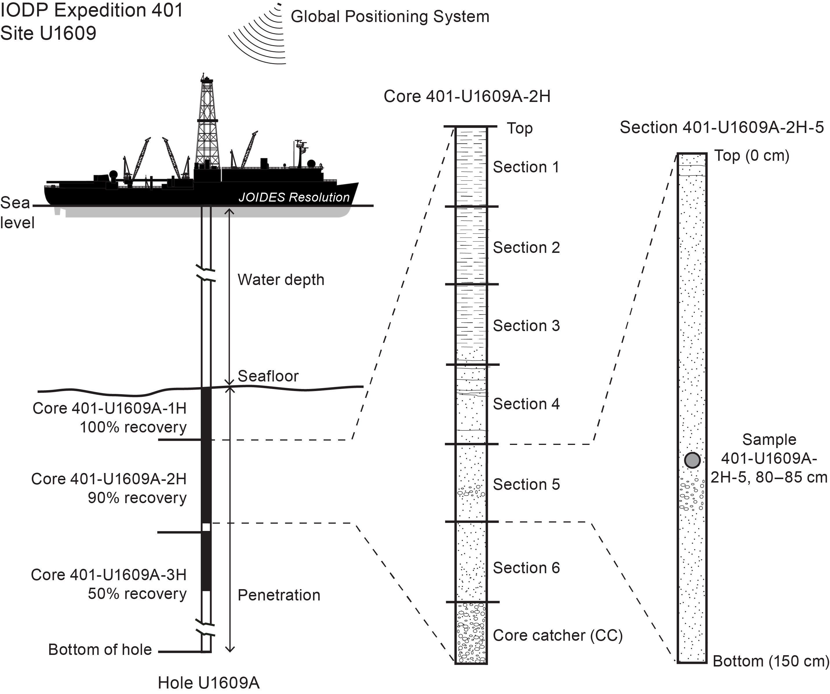
Figure F1. IODP naming convention.
Drilling sites were numbered according to the series that began with the first site drilled by the D/V Glomar Challenger in 1968. Starting with Integrated Ocean Drilling Program Expedition 301, the prefix "U" designates sites occupied by JOIDES Resolution. When drilling multiple holes at a site, hole locations were typically offset from each other by ~20 m (Hole U1611B was a special case, offset ~1300 m from Hole U1611A; see Operations in the Site U1611 chapter [Flecker et al., 2025b]). A letter suffix distinguishes each hole drilled at the same site. The first hole drilled is assigned the site number modified by the suffix "A," the second hole takes the site number and the suffix "B," and so forth. During Expedition 401, we occupied three new sites, U1609, U1610, U1611, and reoccupied Site U1385, which was previously cored during Integrated Ocean Drilling Program Expedition 339 and IODP Expedition 397; therefore, the first location drilled at Site U1385 during Expedition 401 was Hole U1385K. Expedition 401 drilled seven new holes.
1.2. JOIDES Resolution standard coring systems
The advanced piston corer (APC), half-length APC (HLAPC), extended core barrel (XCB), and rotary core barrel (RCB) systems were used during Expedition 401 (Figures F2, F3, F4). These tools and other drilling technology are documented in Graber et al. (2002). Expedition 401 emplaced casing in Holes U1610A and U1611A. We drilled down without coring in all three holes at Sites U1610 and U1611 to reach the depths of the Late Miocene to Early Pliocene target stratigraphy more rapidly. As a result, most of the cored sediments were too compacted for APC and HLAPC coring; these coring methods were used only at Site U1609, which began core recovery at the seafloor.
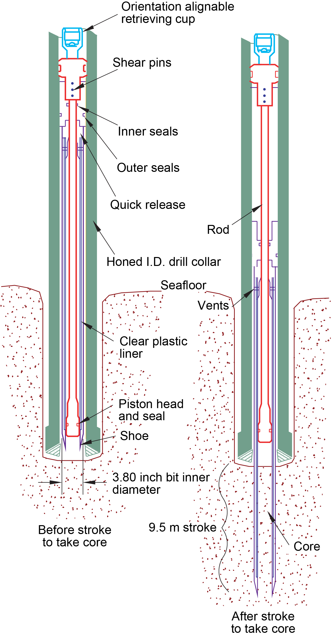
Figure F2. APC coring system.
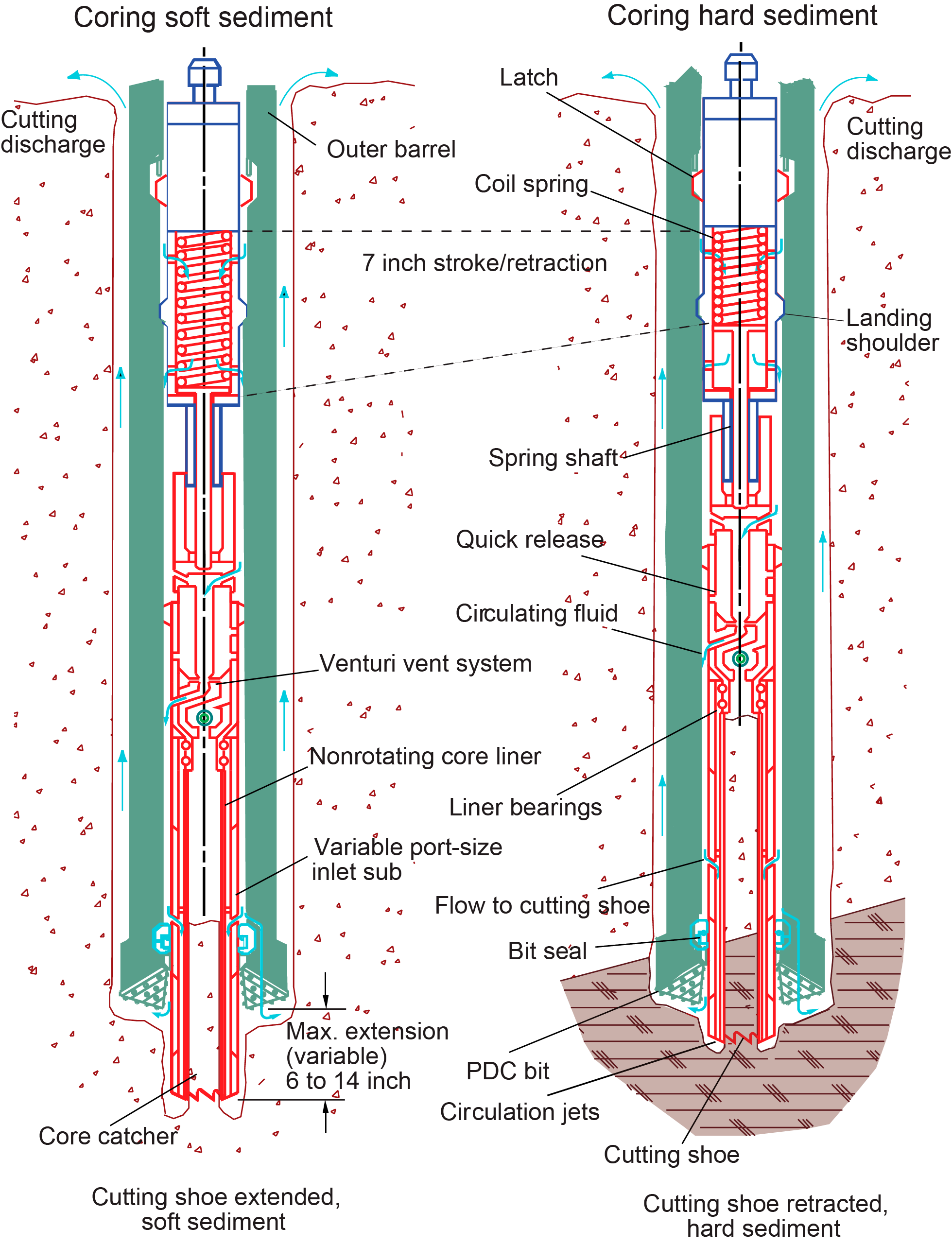
Figure F3. XCB coring system.
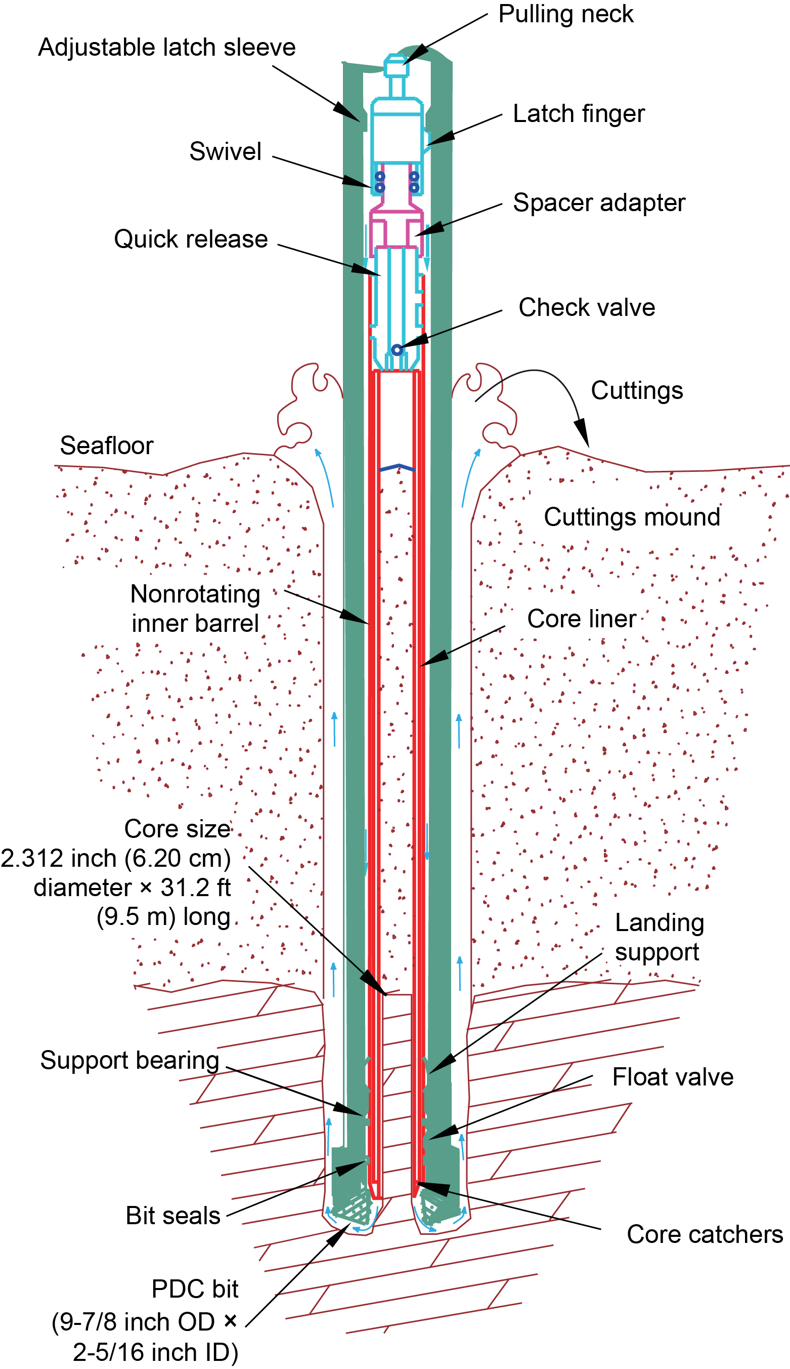
Figure F4. RCB coring system.
The bottom-hole assembly (BHA) used for APC and XCB coring during Expedition 401 was composed of an 11⁷⁄₁₆ inch (~29.05 cm) polycrystalline diamond compact (PDC) bit, a bit sub, a seal bore drill collar, a landing saver sub, a modified top sub, a modified head sub, 8¼ inch control length drill collars, a tapered drill collar, two stands of 5½ inch transition drill pipe, and a crossover sub to the drill pipe that extended to the ship. This type of PDC bit had previously been used during Expedition 397 to achieve high recovery rates and only lightly to moderately biscuited XCB cores; they found the core quality was superior to that obtained with the HLAPC.
The APC and HLAPC systems cut soft-sediment cores with minimal coring disturbance relative to other IODP coring systems. After the APC/HLAPC core barrel is lowered through the drill pipe and lands above the bit, the inside of the drill pipe is pressured up until one or two shear pins that hold the inner barrel attached to the outer barrel fail. The inner barrel then advances into the formation at high speed and cuts a core with a diameter of 66 mm (2.6 inches) (Figure F2). The driller can detect a successful cut, or full stroke, from the pressure gauge on the rig floor because the excess pressure accumulated prior to the stroke drops rapidly. The depth limit of the APC system, often referred to as APC refusal, is indicated in two ways: (1) the piston fails to achieve a complete stroke (as determined from the pump pressure and recovery reading) because the formation is too hard, or (2) excessive force (>60,000 lb) is required to pull the core barrel out of the formation. When a full stroke cannot be achieved, one or more additional attempts are typically made, and each time the bit is advanced by the length of the core recovered (note that for these cores, this results in a nominal recovery of ~100%). When a full or partial stroke is achieved but excessive force is insufficient to retrieve the core barrel, it can be drilled over, meaning that after the inner core barrel was successfully shot into the formation the drill bit is advanced to total depth to free the APC barrel.
The standard APC system uses a 9.6 m long core barrel, whereas the HLAPC system uses a 4.7 m long core barrel. The HLAPC typically is deployed after the standard APC has repeated partial strokes at a depth where the sediment has become too compacted to achieve a full stroke. During use of the HLAPC, the same criteria is applied in terms of refusal as for the APC system. Nonmagnetic core barrels were used for all APC and HLAPC coring. APC cores were oriented using the Icefield MI-5 core orientation tool when coring conditions allowed. The XCB system is typically used when the APC/HLAPC system has difficulty penetrating the formation and/or damages the core liner or core. The XCB system can also be used to either initiate holes where the seafloor is not suitable for APC coring or interchanged with the APC/HLAPC when dictated by changing formation conditions. The XCB system is used to advance the hole when APC or HLAPC refusal occurs before the target depth is reached or when drilling conditions require it.
The XCB system has a small cutting shoe that extends below the large rotary APC/XCB bit (Figure F3). The smaller bit can cut a semi-indurated core with less torque and fluid circulation than the main bit, optimizing recovery. The XCB cutting shoe (bit) extends ~30.5 cm ahead of the main bit in soft sediment but retracts into the main bit when hard formations are encountered. It cuts cores with a nominal diameter of 5.87 cm (2.31 inches), slightly less than the 6.6 cm diameter of APC cores. XCB cores are often broken (torqued) into biscuits, which are disc-shaped pieces a few to several centimeters long with remolded sediment (including some drilling slurry) interlayering the discs in a horizontal direction and packing the space between the discs and the core liner in a vertical direction. This type of drilling disturbance may give the impression that the XCB cores have the same thickness (66 mm) as the APC cores.
The RCB system is designed to recover semi- to fully lithified sediments and sedimentary rocks. The BHA, including the bit and outer core barrel, is rotated with the drill string while bearings allow the inner core barrel to remain stationary (Figure F4). A typical RCB BHA includes a 9⅞ inch drill bit, a bit sub, an outer core barrel, a modified top sub, a modified head sub, a variable number of 8¼ inch control length drill collars, a tapered drill collar, two stands of 5½ inch drill pipe, and a crossover sub to the drill pipe that extends to the surface. As far as we are aware, Expedition 401 was the first time a PDC bit was used with the RCB BHA. The excellent core recovery rates achieved (>70%) from more than 1 km drilling depths suggest that, for marine sediments at least, this drilling configuration is far more effective than traditional RCB coring.
1.3. Drilling disturbance
Cores may be significantly disturbed by the drilling process and contain extraneous material because of the coring and core handling process. Particularly in formations with loose granular layers (sand, ash, foraminifer ooze, chert fragments, shell hash, etc.), material from intervals higher in the hole may settle and accumulate in the bottom of the hole because of drilling circulation and be sampled with the next core. The uppermost 10–50 cm of each core must therefore be examined critically for potential fall-in.
1.4. Downhole measurements
1.4.1. Formation temperature
Formation temperature measurements were taken at specified intervals at Site U1609 with the advanced piston corer temperature (APCT-3) tool (see Downhole measurements) embedded in the APC coring shoe. The Sediment Temperature 2 (SET2) tool was deployed at Sites U1609, U1610, and U1611. These measurements were used to obtain temperature gradients and heat flow estimates. No temperature measurements were taken at Site U1385, as they were taken at this site during Expedition 339. Information on downhole tool deployments is provided in the Operations, Physical properties, and Downhole measurements sections of each site chapter.
1.4.2. Wireline logging
During wireline logging operations, downhole logs are recorded with Schlumberger and IODP logging tools combined into tool strings, which are lowered into the hole after the completion of coring operations. Tool strings deployed during Expedition 401 were the modified triple combination (triple combo), a quad combo, the formation MicroScanner (FMS)-sonic, sonic-resistivity, and Versatile Seismic Imager (VSI) tool strings. These tools measure gamma radiation, porosity, density, electrical resistivity, magnetic susceptibility (MS), and P- and S-wave velocity. Each tool string contains a telemetry cartridge for communicating through the wireline to the Schlumberger multitasking acquisition and imaging system (MAXIS) on the ship. Downhole measurements tracking hole inclination were also used during Expedition 401 (see Downhole measurements in the Site U1610 chapter and Downhole measurements in the Site U1611 chapter [Flecker et al., 2025a, 2025b]).
In preparation for logging, the boreholes were flushed of debris by circulating drilling fluid and were at least partially filled with seawater-based logging gel (sepiolite mud mixed with seawater) to help stabilize the borehole walls in sections where instability was expected from drilling and coring disturbance. The tool strings were then lowered downhole on a seven-conductor wireline cable before being pulled up at a constant speed of 550 m/h (apart from the VSI, which measures when static at certain depths in the borehole) to provide continuous log measurements of several properties simultaneously. Further details on the logging operations are described in the Downhole measurements sections of each site.
1.5. Core and section handling
1.5.1. Whole-round cores
When a core barrel reached the rig floor, the core catcher from the bottom of the core was removed and taken to the core receiving platform (catwalk), and a sample was extracted for paleontological analysis (Figure F5). Next, the sediment core was extracted from the core barrel in its plastic liner. The liner was carried from the rig floor to the core processing area on the catwalk outside the core laboratory, where it was split into ~1.5 m sections. The exact section length was noted and entered into the database as created length using the Sample Master application. This number was used to calculate core recovery.
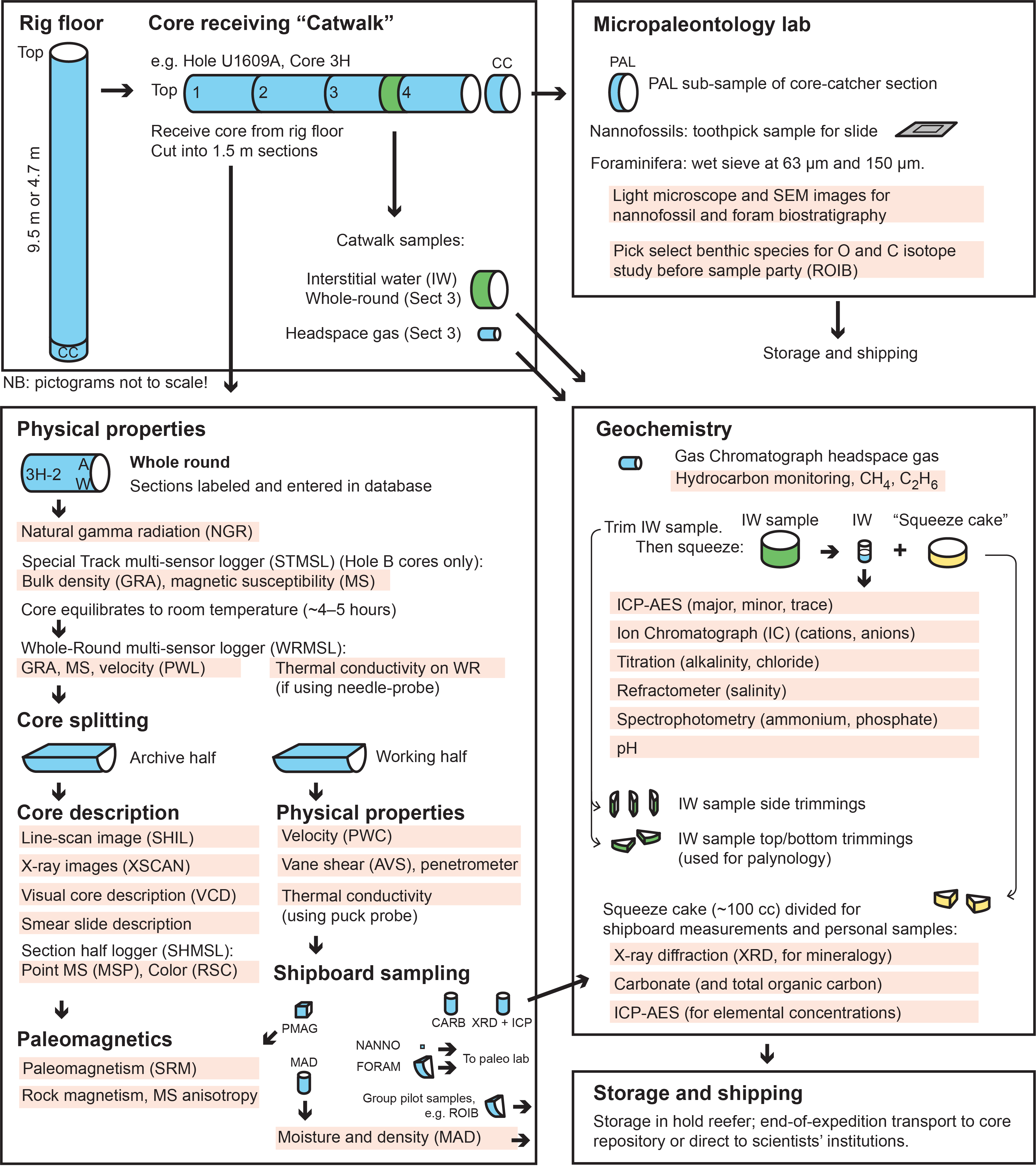
Figure F5. Laboratory core flow.
Once the core was cut into sections, whole-round samples were immediately taken for interstitial water (IW) chemical analyses from the bottom of selected core sections and headspace samples were taken from the top of a selected section (typically one per core) using a syringe for immediate gas analyses according to the IODP hydrocarbon safety monitoring protocol. Whole-round samples were also taken for microbiological analysis every ~20 m in Hole U1611B adjacent to the IW samples. The microbiology samples were immediately frozen (see Geochemistry). When catwalk sampling was complete, liner caps (blue = top; colorless = bottom; yellow = bottom if a whole-round sample was removed from the section) were glued with acetone onto liner sections and sections were placed in core racks for analysis.
The curated length of the sediment cores was set equal to the created length and was updated very rarely (e.g., in cases of data entry errors or when section length kept expanding by more than ~2 cm). Depth in hole calculations are based on the curated section length (see Depth calculations). The core sections then were placed in a core rack in the laboratory, core information was entered into the database, and the sections were labeled. All core sections were run through the Whole-Round Multisensor Logger (WRMSL) for MS and gamma ray attenuation (GRA) bulk density (see Physical properties). The core sections were also run through the Natural Gamma Radiation Logger (NGRL), and thermal conductivity measurements were taken once per core when the material was suitable.
1.5.2. Core section halves
After completion of whole-round section analyses, the sections were split lengthwise from bottom to top into working and archive halves. Cores were split with a wire or saw. Investigators should note that older material can be transported upward on the split face of a section during splitting. This is particularly true of pyritized burrows that can be dragged upward by the wire.
Discrete samples were then taken from the working half of each core for moisture and density (MAD), paleomagnetic (PMAG), X-ray diffraction (XRD), carbonate (CARB), and inductively coupled plasma–atomic emission spectroscopy (ICP-AES) analyses (sample flow is summarized graphically in Figure F5). Samples were not collected when the core lithology was a high-priority interval for the expedition or postcruise research, the core material was unsuitable, or the core was severely deformed. During the expedition, samples for personal postcruise research were taken where they concerned ephemeral properties (e.g., IW). We also took a limited number of personal or shared pilot samples for palynological study, microbiology, and oxygen isotope analyses, which will help to guide postcruise sampling.
At the end of the expedition the following "residue" samples were distributed among the shipboard party for postexpedition analysis: paleomagnetic samples (PMAG cubes); MAD samples; micropaleontology (PAL) slides, >150 and 63–150 µm and sieved fractions; and the residues from the alkalinity analyses of the IW samples, slices of the interstitial water (IW) squeeze cake.
The archive half of each core was scanned on the Section Half Imaging Logger (SHIL) to provide line-scan images and then measured for point MS (MSP) and reflectance spectroscopy and colorimetry on the Section Half Multisensor Logger (SHMSL). All archive-half core sections were also X-ray imaged. Labeled foam pieces were used to denote missing whole-round intervals in the SHIL images. The archive-half sections were then described visually and by means of smear slides for sedimentology. Finally, the magnetization of archive-half sections and working-half discrete pieces was measured with the cryogenic magnetometer and spinner magnetometer. When all steps were completed, the cores were wrapped, sealed in plastic D-tubes, boxed, and transferred to cold storage space aboard the ship. At the end of the expedition, all working halves were shipped to the IODP Bremen Core Repository at the Center for Marine Environmental Sciences (MARUM) (Germany). The archive halves of the cores were sent to the IODP Gulf Coast Core Repository at Texas A&M University for X-ray fluorescence (XRF) core scanning. Once XRF scanning is completed, all cores will be returned to the IODP Bremen Core Repository for permanent storage.
1.6. Sample naming
1.6.1. Editorial practice
Sample naming in this volume follows standard IODP procedure. A full sample identifier consists of the following information: expedition, site, hole, core number, core type, section number, section half, and offset in centimeters measured from the top of the core section (Figure F1). For example, a sample identification of "401-U1609A-1H-2W, 10–12 cm," represents a sample taken from the interval between 10 and 12 cm below the top of the working half of Section 2 of Core 1 ("H" designates that this core was taken using the APC system) of Hole U1609A during Expedition 401. The drilling system used to obtain a core is designated in the sample identifiers as follows: H = APC, F = HLAPC, X = XCB, R = RCB. Integers are used to denote the core type of drilled intervals (e.g., the drilled interval at the top of Holes U1609B, U1610A, U1385K, U1385L, U1611A, and U1611B where we washed down before starting to core, this interval is denoted by Core "11"). When working with data downloaded from the LIMS database or physical samples that were labeled on the ship, three additional sample naming concepts may be encountered: text ID, label ID, and printed labels.
1.6.2. Text ID
Samples taken on JOIDES Resolution are uniquely identified for use by software applications using the text ID, which combines two elements:
- Sample type designation (e.g., SHLF for section half) and
- A unique sequential number for any sample and sample type added to the sample type code (e.g., SHLF30495837).
1.6.3. Label ID
The label ID is used throughout the JOIDES Resolution workflows as a convenient, human-readable sample identity. However, a label ID is not necessarily unique. The label ID is made up of two parts: primary sample identifier and sample name.
1.6.3.1. Primary sample identifier
The primary sample identifier is very similar to the editorial sample name described above, with two notable exceptions:
- Section halves always carry the appropriate identifier (401-U1609B-50X-2A and 401-U1609B-50X-2W for archive and working half, respectively).
- Sample top and bottom offsets, relative to the parent section, are indicated as "35/37" rather than "35–37 cm."
1.7. Depth calculations
Sample and measurement depth calculations were based on the methods described in IODP Depth Scales Terminology v.2 (https://www.iodp.org/policies-and-guidelines/142-iodpdepth- scalesterminology-april-2011/file) (Table T1). The definition of multiple depth scale types and their distinction in nomenclature should keep the user aware that a nominal depth value at two different depth scale types (and even two different depth scales of the same type) generally does not refer to exactly the same stratigraphic interval in a hole. The SI unit for all depth scales is meters (m).
Depths of cored intervals were measured from the drill floor based on the length of drill pipe deployed beneath the rig floor and referred to as drilling depth below rig floor (DRF), which is traditionally referred to as meters below rig floor (mbrf). The depth of each cored interval, measured on the DRF scale, can be referenced to the seafloor by subtracting the seafloor depth measurement (on the DRF scale) from the cored interval (on the DRF scale). This seafloor referenced depth of the cored interval is reported on the DSF scale, which is traditionally referred to as meters below seafloor (mbsf). In the case of APC coring, the seafloor depth was the length of pipe deployed minus the length of the mudline core recovered.
Depths of samples and measurements in each core were computed based on a set of rules that result in the core depth below seafloor, Method A (CSF-A), depth scale. The two fundamental rules for this scale are that (1) the top depth of a recovered core corresponds to the top depth of its cored interval (top DSF depth = top CSF-A depth) regardless of type of material recovered or drilling disturbance observed and (2) the recovered material is a contiguous stratigraphic representation even when core segments are separated by voids when recovered, the core is shorter than the cored interval, or it is unknown how much material is missing between core pieces. When voids were present in the core on the catwalk, they were closed by pushing core segments together whenever possible. The length of missing core should be considered a depth uncertainty when analyzing data associated with core material.
When core sections were given their curated lengths, they were also given a top and a bottom depth based on the core top depth and the section length. Depths of samples and measurements on the CSF-A scale were calculated by adding the offset of the sample (or measurement from the top of its section) to the top depth of the section.
Per IODP policy established after the introduction of the IODP Depth Scales Terminology v.2, sample and measurement depths on the CSF-A depth scale are commonly referred to with the custom unit mbsf, just like depths on the DSF scale. The reader should be aware, however, that the use of mbsf for different depth scales can cause confusion in specific cases because different mbsf depths may be assigned to the same stratigraphic interval. For example, a soft-sediment core from less than a few hundred meters below seafloor often expands upon recovery (typically by a few percent to as much as 15%), and the length of the recovered core exceeds that of the cored interval. Therefore, a stratigraphic interval in a particular hole may not have the same depth on the DSF and CSF-A scales. When recovery in a core exceeds 100%, the CSF-A depth of a sample taken from the bottom of the core will be deeper than that of a sample from the top of the subsequent core (i.e., some data associated with the two cores overlap on the CSF-A scale). To overcome the overlap problem, core intervals can be placed on the core depth below seafloor, Method B (CSF-B), depth scale. The CSF-B approach scales the recovered core length back into the interval cored, from >100% to exactly 100% recovery. If cores had <100% recovery to begin with, they are not scaled. When downloading data using the JOIDES Resolution Science Operator (JRSO) LIMS Reports (https://web.iodp.tamu.edu/LORE), depths for samples and measurements are by default presented on both the CSF-A and CSF-B scales.
Wireline logging data are collected at the wireline log depth below rig floor (WRF) scale, from which a seafloor measurement is subtracted to create the wireline log depth below seafloor (WSF) scale. For Expedition 401, the WSF depth scale was only used for preliminary data usage on the ship. Immediately after data collection was completed, the wireline logging data were transferred to the Lamont-Doherty Earth Observatory Borehole Research Group (LDEO-BRG), where multiple passes and runs were depth matched using the natural gamma radiation (NGR) logs. The data were returned to the ship using the wireline log matched depth below seafloor (WMSF) scale, which is the final and official logging depth scale type for investigators. During Expedition 401, a mixture of CSF-A and CSF-B was used, depending on the data set (e.g., lithologic descriptions in the GEODESC software are only in CSF-A). Physical properties data are typically plotted in CSF-B, to avoid apparent depth reversals at core breaks where there is greater than 100% recovery. Biostratigraphic and magnetostratigraphic datum depths are given in both CSF-A and CSF-B in the tables.
Core composite depth below seafloor (CCSF) depth scales were constructed for Sites U1609 and U1385 to create as continuous a stratigraphic record as possible. This also helps to mitigate the CSF-A core overlap problem and the coring gap problem. Using shipboard core logger–based physical properties data, core depths in adjacent holes at a site are vertically shifted to correlate between cores recovered in adjacent holes. This process produces the CCSF depth scale. The correlation process is achieved using the Correlator program (version 4.0.1 was used during Expedition 401) and results in affine tables that indicate the vertical shift of cores on the CCSF scale relative to the CSF-A scale. Once the CCSF scale is constructed, a splice that best represents the stratigraphy of a site by using and splicing the best portions of individual sections and cores from each hole is defined. Because of core expansion, the CCSF depths of stratigraphic intervals are typically 10%–15% deeper than their CSF-A, at least down to approximately 300–400 m, where the expansion decreases as the sediment becomes more lithified. CCSF depth scale construction reveals that coring gaps on the order of 0.5–1.5 m typically occur between two subsequent cores, even where core recovery is apparently >100% recovery. For more details on construction of the CCSF depth scale, see Stratigraphic correlation and Age model sections in the site chapters for U1609 and U1385 where splices were constructed. Although two holes were drilled at Site U1611, no splice was constructed because of significant differences between the sequences recovered from Holes U1611A and U1611B.
2. Lithostratigraphy
Sedimentary successions recovered during Expedition 401 were described macroscopically from archive-half sections and microscopically from smear slides and thin sections. All observations were recorded using separate macroscopic and microscopic GEODESC templates. X-ray imaging (X-Ray Linescan Logger [XSCAN]) of archive-half core sections was carried out in addition to digital color imaging using the SHIL. Color spectrophotometry and MSP were determined using the SHMSL. Synthetic logs (hand-drawn sedimentary logs) were produced based on both visual core description (VCD) sheets and core photos. Samples were also selected from squeeze cakes and the working half of the section for XRD analyses of both bulk mineralogy and clay mineral assemblage. Methods associated with percent carbonate and percent organic matter (carbon-hydrogen-nitrogen-sulfur analyzer [CHNS]) measurements on shipboard sediment samples selected by the lithostratigraphy group are described in Geochemistry.
2.1. Section-half images
2.1.1. Preparation for core imaging and description
The standard method of splitting soft-sediment cores into working and archive halves by pulling a wire lengthwise through its center (see Introduction) tends to smear the cut surface and obscure fine details of lithology and sedimentary structure. When necessary during Expedition 401, the archive halves of soft-sediment cores were gently scraped across rather than along the core section using a glass scraper to prepare the surface for unobscured sedimentologic examination and digital imaging. Scraping parallel to bedding with a freshly cleaned tool prevented cross-stratigraphic contamination.
2.1.2. Digital color imaging using the Section Half Imaging Logger
The surface of the cleaned archive half was imaged using the SHIL. Imaging was conducted as soon as possible after splitting to avoid sediment color changes caused by oxidation and drying. In cases of watery or soupy sediment, the surface was allowed to dry sufficiently prior to scanning to avoid excessive light reflection and overexposure. The SHIL continuously captures high-resolution images for analysis and description. The SHIL uses three pairs of advanced illumination, high-current, focused LED line lights to illuminate the core. Each of the LED pairs has a color temperature of 6,500 K and emits 200,000 lux at 7.6 cm. Digital images were taken by a linescan camera (JAI manufactured) at an interval of 10 lines/mm to create a high-resolution image file. The camera height was set so that each pixel imaged a 0.1 mm2 section of the core surface, but the actual core width per pixel can vary because of slight differences in the section-half surface height. Low-resolution cropped raster files of the core section surface and high-resolution raster files with a grayscale and depth ruler were created from the image files.
For each section, scanned output from the SHIL included a region of interest file of the original data with links to the TIFF file and an enhanced, uncropped JPEG file. A manually cropped JPEG image was generated to assist in visual core description. Postprocessing of data included construction of a composite JPEG image of each core.
2.1.3. X-ray imaging
The XSCAN collects linescan X-radiographs from the whole-round cores or split-core halves. During Expedition 401, continuous linescan X-radiographs were obtained solely in plane view on the archive-half sections (Figure F6). The XSCAN comprises an X-ray scanner with a 210 W, 160 kV, and 1.3 mA constant potential X-ray source and linescan detector. The source is a Spellman XRBD 160PN210 Monoblock X-ray generator with a 0.5 mm focal spot. The beam angle is 90° × 12° located ~36 cm from the source. The detector is a Hamamatsu C12300-321, composed of a charge-coupled device (CCD) sensor with a ~22 cm field of view utilizing time-delayed integration and a resolution of 48 µm per pixel. Imaging acquisition and processing was completed within the IMS system (v 14). Processing of the images during Expedition 401 was limited to black and white correction and image cropping. XSCAN images can facilitate the identification of sedimentary structures, traces fossils, objects such as fractures, and materials with distinct densities (e.g., alteration zones and oxide and sulfide concentrations). Core sections were measured using energies between 90 and 100 kV and between 0.80 and 0.90 mA. Calibration of the XSCAN was done for the aforementioned energies before core measurements were obtained.
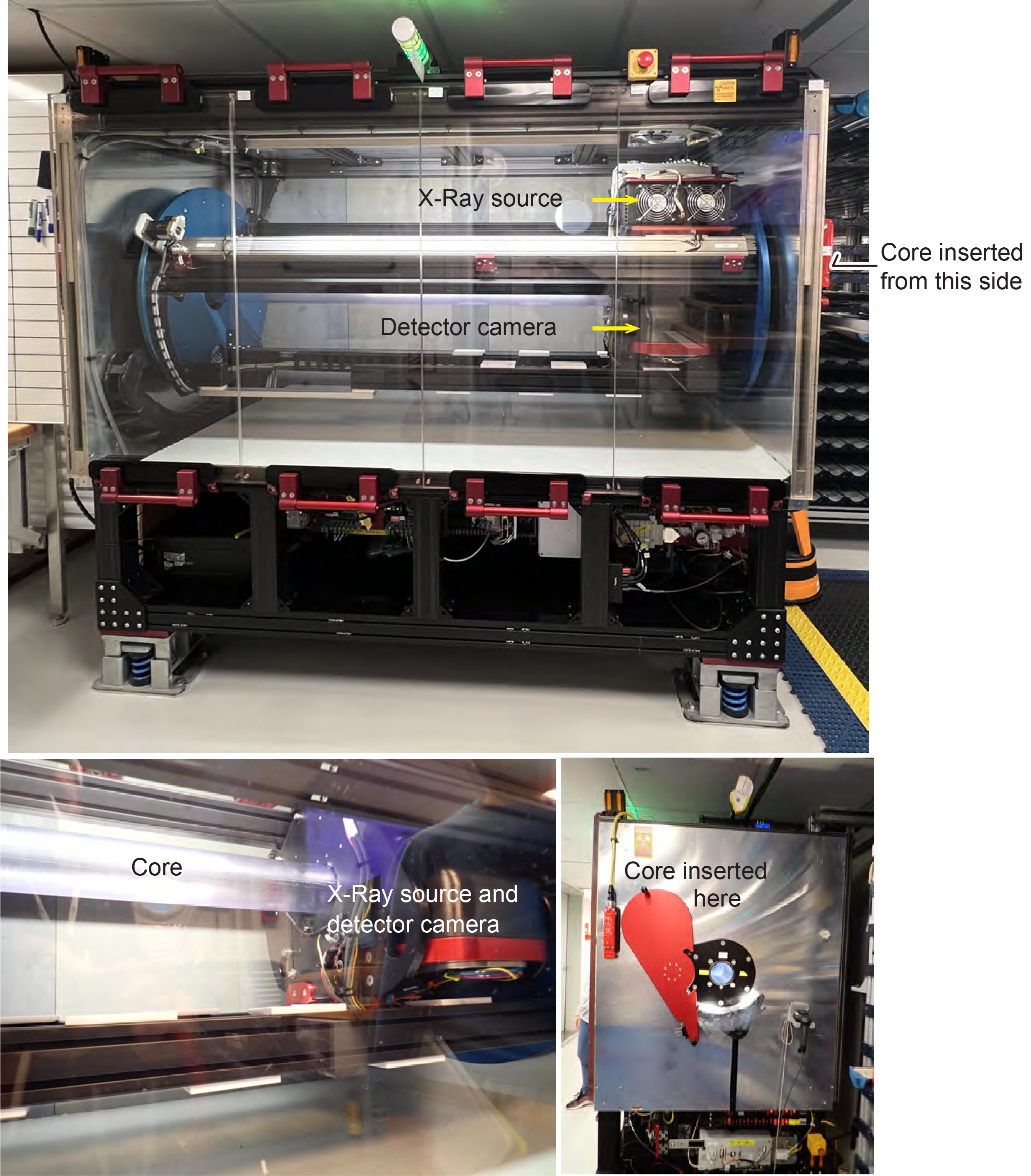
Figure F6. X-Ray Linescan Logger.
2.2. Section Half Multisensor Logger
Spectrophotometry and magnetic susceptibility of the archive-half sections were measured with the SHMSL. The SHMSL takes measurements in empty intervals and intervals where the core surface is well below the level of the core liner but cannot recognize relatively small cracks, disturbed areas of core, or plastic section dividers. Thus, SHMSL data may contain spurious measurements that should be manually edited out of the data set. Additional detailed information about measurement and interpretation of spectral data can be found in Balsam et al. (1997, 1998) and Balsam and Damuth (2000).
2.2.1. Spectrophotometry and colorimetry
The SHMSL employs multiple sensors to measure bulk physical properties in a motorized and computer-controlled instrument track. The sensors included in the SHMSL are a spectrophotometer, a point magnetic susceptibility sensor, and a laser surface analyzer. During this expedition, the point measurement interval for the spectrophotometer and the point magnetic susceptibility sensor measurements was 2 cm for all sections. To achieve a flush contact between point sensors and the split-core surface while also avoiding transferring sediment to the instrument surfaces, archive halves were covered with clear plastic wrap prior to measurement. The laser surface analyzer aids in the recognition of irregularities in the split-core surface (e.g., cracks and voids), and data from this tool were recorded to provide an independent check on SHMSL measurement fidelity.
Magnetic susceptibility was measured with a Bartington Instruments MS2 meter and an MS2K contact probe. Instrument details are given in Physical properties. Reflectance spectroscopy (spectrophotometry) was carried out using an Ocean Optics QE Pro detector, which measures the reflectance spectra of the split core from the ultraviolet to near-infrared range. Each measurement was recorded in 2 nm spectral bands from 390 to 732 nm. The data were converted to the L*a*b* color space system, which expresses color as a function of lightness (L*; grayscale where more white is positive and more black is negative) and color values a* and b*, where a* reflects the balance between red (positive a*) and green (negative a*) and b* reflects the balance between yellow (positive b*) and blue (negative b*).
2.3. Sediment classification
The sediments recovered during Expedition 401 are composed of biogenic and siliciclastic components. They were described using a classification scheme derived from those of Ocean Drilling Program (ODP) Leg 155 (Shipboard Scientific Party, 1995), Integrated Ocean Drilling Program Expeditions 303 and 339 (Expedition 303 Scientists, 2006; Expedition 339 Scientists, 2013), Shepard (1954), and Stow (2005). The biogenic component consists of the skeletal debris of marine calcareous and siliceous microfauna (e.g., foraminifers and radiolarians), microflora (e.g., calcareous nannofossils and diatoms), and macrofossil (e.g., plant and shell fragments). The siliciclastic component consists of mineral and rock fragments derived from igneous, sedimentary, and metamorphic rocks. The relative proportion between siliciclastic and biogenic components is used to define the major classes of sediments in this scheme (Figure F7).
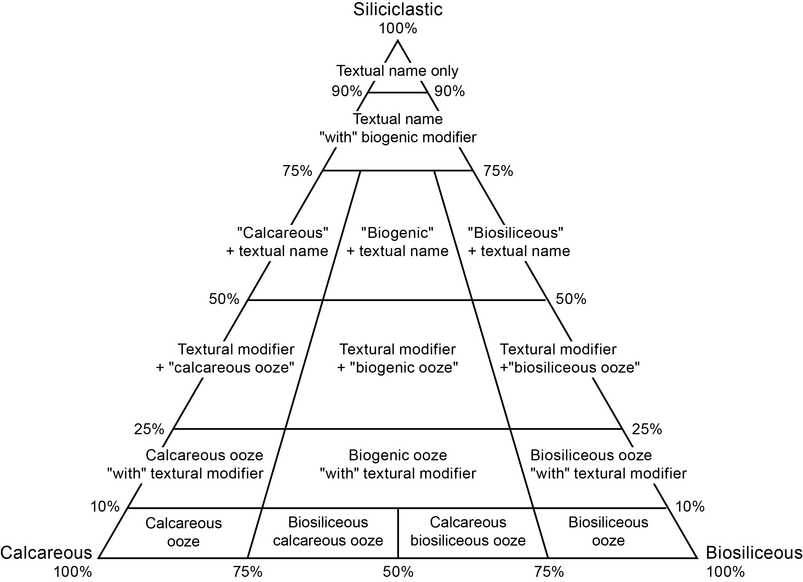
Figure F7. Sediment name ternary diagram.
Naming conventions for Expedition 401 follow the general guidelines of the ODP sediment classification scheme (Mazzullo et al., 1988). Sediments containing <50% siliciclastic grains were classified as either biosiliceous or calcareous depending on the dominance of biogenic silica or carbonate, whereas siliciclastic sediments are those that contain >50% siliciclastic grains and <50% biogenic grains (Figure F7). During Expedition 401, no ash layers or neritic and chemical sediments were encountered except as accessory components; therefore, these categories are not addressed below.
Sediment grain size divisions for both biogenic and siliciclastic components are based on Wentworth (1922), with eight major textural categories defined on the basis of the relative proportions of sand-, silt-, and clay-sized particles (Figure F8) however, distinguishing visually between some of these categories can be difficult (e.g., silty mud versus sandy mud) without accurate measurements of grain size abundances. The term "clay" is only used to describe particle size and applies to both clay minerals and all other grains <4 µm in size. Size-textural qualifiers were not used for biogenic sediment names (e.g., nannofossil clay implies that the dominant component is detrital clay rather than clay-sized nannofossils).
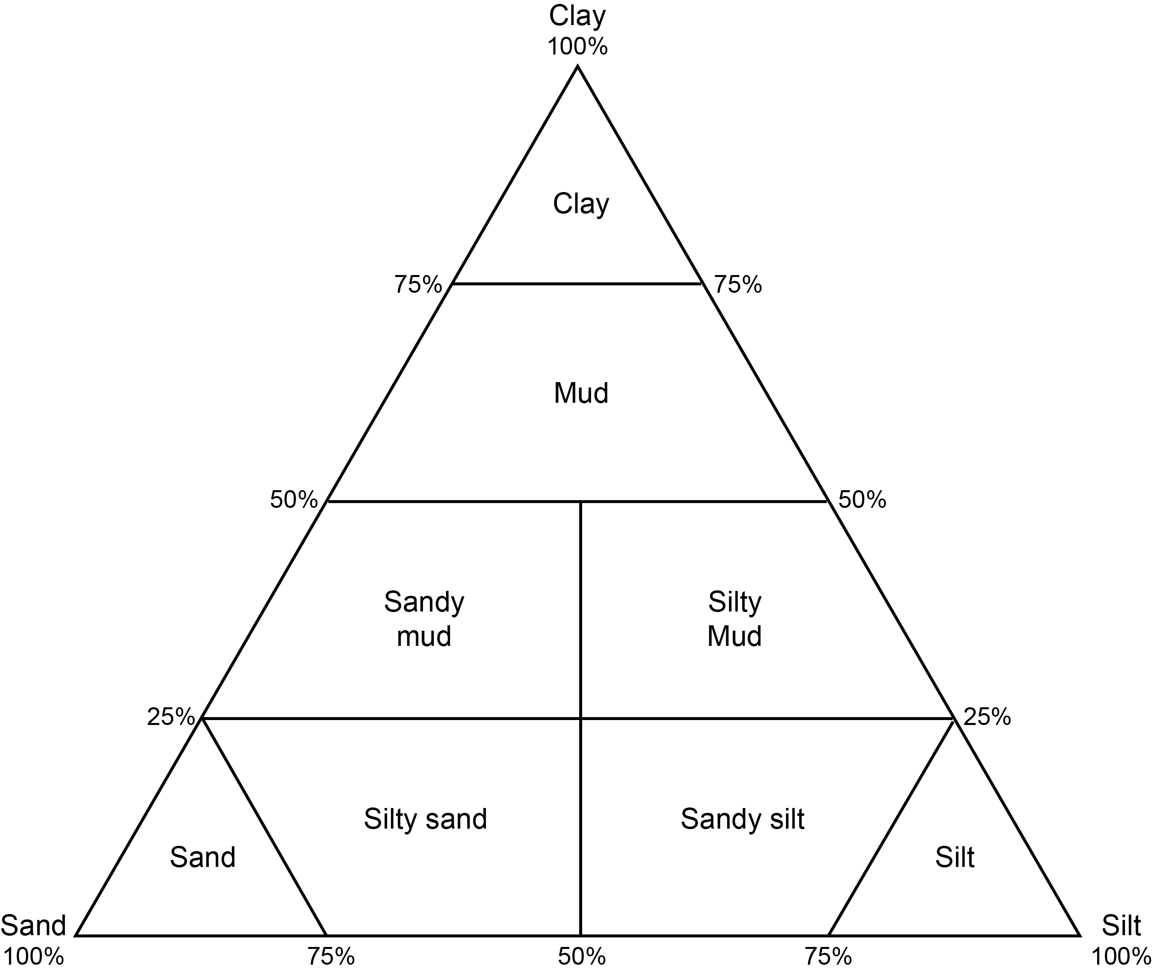
Figure F8. Textural name ternary diagram.
The lithologic names assigned to these sediments consist of a principal name and modifiers based on composition and degree of lithification and/or texture as determined from visual description of the cores and smear slides. The total calcium carbonate content of sediments determined on board (see Sedimentary inorganic carbon, organic carbon, and nitrogen content) also aided in classification.
For sediment that contains >90% of one component (either the siliciclastic or biogenic component), only the principal name is used. For sediment with >90% biogenic components, the name applied indicates the most limited group of grains that exceed the 90% threshold value (Figure F7). For example, sediment composed of >90% calcareous nannofossils is called "nannofossil ooze," sediment composed of 50% foraminifers and 45% calcareous nannofossils is called "calcareous ooze," and sediment composed of 40% foraminifers, 40% calcareous nannofossils, and 15% diatoms is called "biosiliceous calcareous ooze." For sediment with >90% siliciclastic grains, the principal name is based on the textural characteristics of all sediment particles (both siliciclastic and biogenic) (Figure F8).
For sediment that contains a significant mixture of siliciclastic and biogenic components (between 25% and 75% of both siliciclastic and biogenic components), the principal name is determined by the more abundant component. If the siliciclastic component is more abundant, the principal name is based on the textural characteristics of all sediment particles (both siliciclastic and biogenic) (Figures F7, F8). If the biogenic component is more abundant, the principal name is either (1) based on the predominant biogenic component if that component forms >75% of the biogenic particles or (2) the more encompassing term "biogenic ooze."
If one component forms 75%–90% of the sediment, then the principal name is followed by a minor modifier (e.g., "with diatoms"), with the minor modifier based on the most abundant component that forms 10%–25% of the sediment. If the minor component is biogenic, then the modifier describes the most limited group of grains that exceeds the 10% abundance threshold. If the minor component is siliciclastic, then the minor modifier is based on the texture of the siliciclastic fraction.
If one component forms 50%–75% of the sediment, then the principal name is preceded by a major modifier that is based on the component that forms 25%–50% of the sediment. If the less abundant component is biogenic, then the major modifier describes the most limited group of grains that exceeds the 25% abundance threshold (e.g., nannofossil versus calcareous versus biogenic). If the less abundant component is siliciclastic, then the major modifier is based on the texture of the siliciclastic fraction. If the sediment is calcareous based on total carbonate content but the dominant carbonate mineral is dolomite, "dolomitic" was used along with the texture description of the siliciclastic fraction.
If the primary lithology for an interval of core has a major modifier, then that major modifier is indicated in the Graphic lithology column of the VCD sheets using a modified version of the lithologic pattern for the primary lithology (Figure F9). The modified lithologic patterns are shown in Figure F10. The minor modifiers of sediment lithologies are not included in the Graphic lithology column.
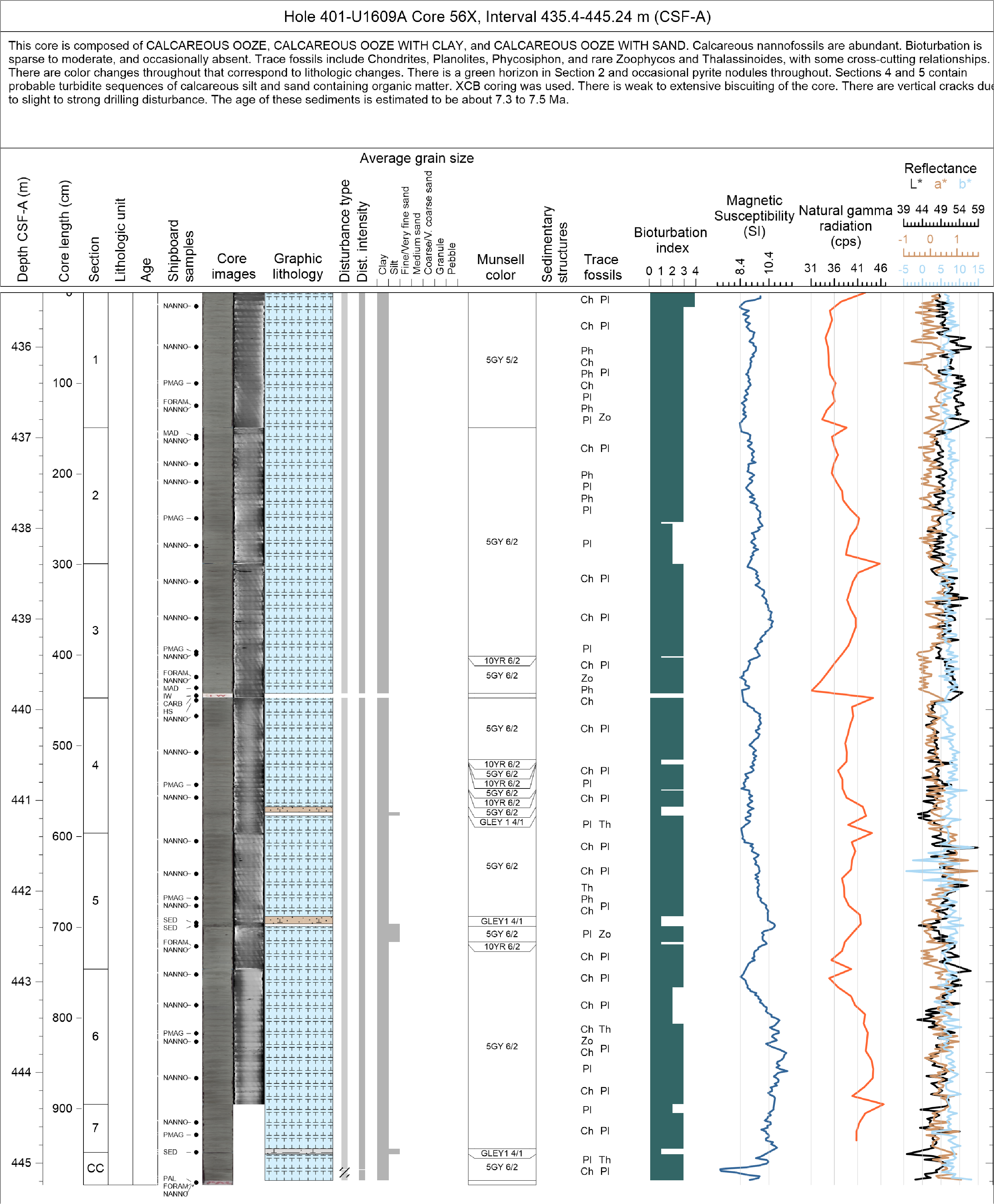
Figure F9. Example VCD.
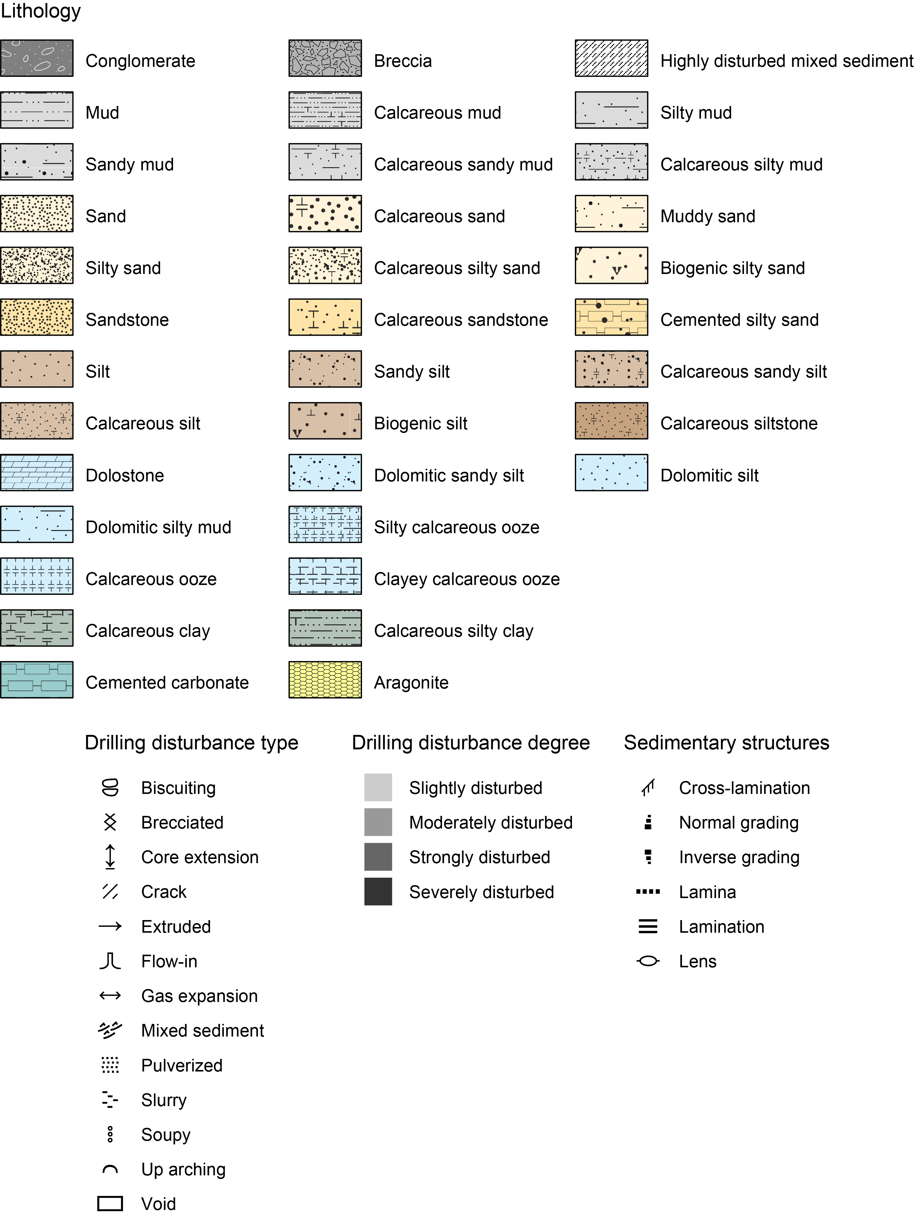
Figure F10. VCD graphic key.
The following terms describe lithification that varies depending on the dominant composition:
- Sediment composed predominantly of calcareous, pelagic organisms (e.g., calcareous nannofossils and foraminifers): the lithification terms "ooze" and "chalk" reflect whether the sediment can be deformed with a finger (ooze) or scratched easily by a fingernail (chalk).
- Sediments composed predominantly of siliciclastic material: if the sediment can be deformed easily with a finger, no lithification term is added and the sediment is named for the dominant grain size (i.e., sand, silt, or clay). For more consolidated material, the lithification suffix "‑stone" is appended to the dominant size classification (e.g., claystone).
- Sediments that are well consolidated/cemented by carbonate are described as cemented carbonate in general or dolostone if the dominant carbonate mineral has been determined as dolomite.
2.4. Sedimentologic core description
2.4.1. Handwritten core description forms
Macroscopic descriptions of each section (nominally 0–150 cm long) were recorded on handwritten core description forms (barrel sheets) that included color images collected using the SHIL (Figure F11). Standard sedimentologic observations of drilling disturbance type and intensity, lithology, maximum grain size, primary and secondary (i.e., syn- and postsedimentary deformation) sedimentary structures, bioturbation index (BI), trace fossils, color. (Munsell Color Company, Inc., 2010), and depths were recorded in individual columns on the barrel sheets (Figures F10, F11). Macroscopic biogenic remains (e.g., shell fragments and plant matter), character of the lower and upper contacts, diagenetic features, and compositional characteristics of coarse clasts (>2 cm) were recorded as comments. The identification of distinct sedimentary features or lithologic intervals was supported by inspection of physical properties data (whole-round core measurements of magnetic susceptibility and natural gamma radiation [NGR]; see Physical properties), as well as split-core point magnetic susceptibility and color reflectance. As an example, changes in NGR or magnetic susceptibility aided in identification of gradual transitions in the lithologies that were otherwise difficult to distinguish. Copies of these original descriptions were scanned and converted to PDF files and are included in HANDDRAWN in Supplementary material.
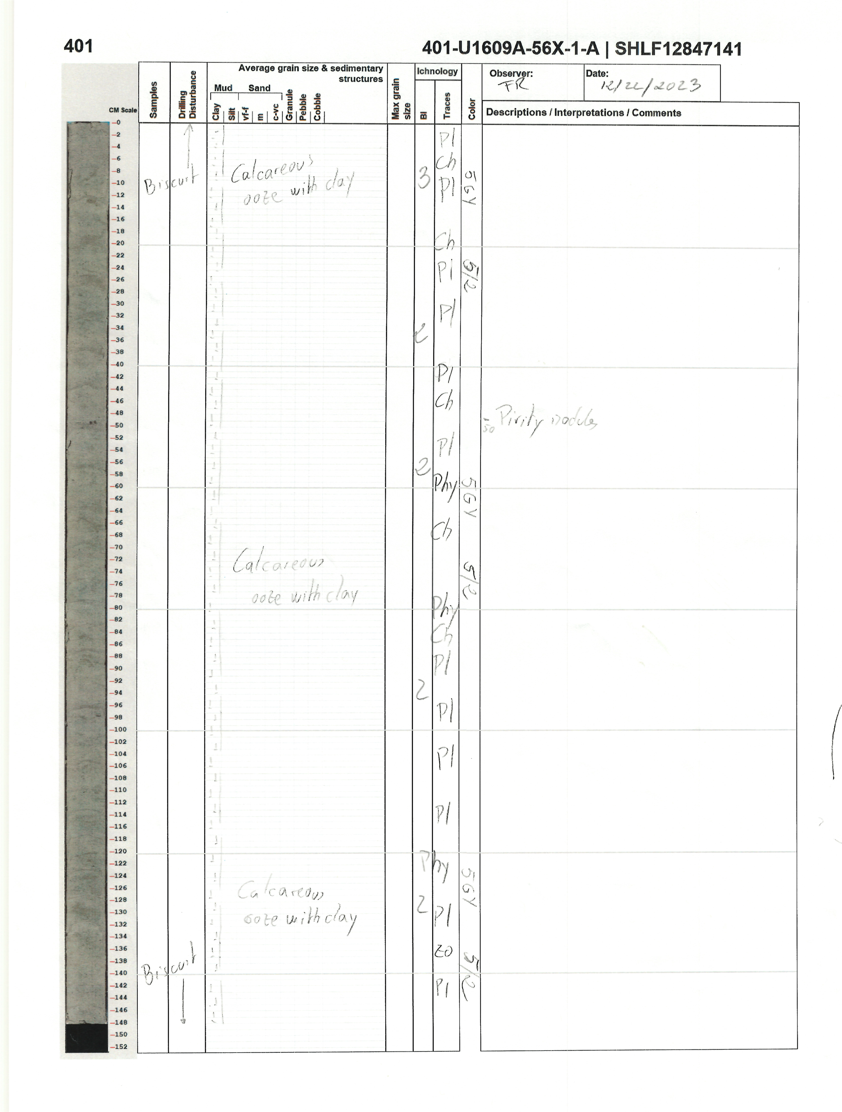
Figure F11. Sedimentary core description log.
2.4.2. GEODESC data capture software
Data from the handwritten core description sheets were compiled and entered into the IODP Laboratory Information Management System (LIMS) database using the GEODESC software. A macroscopic template was developed in the GEODESC Template Manager for Expedition 401 and includes the following categories:
- Lithology (major lithology, with prefix and suffix modifiers indicating variable biogenic content),
- Average and maximum grain size,
- Lower contact (shape, definition, and attitude),
- Sedimentary structures,
- Grading type,
- Diagenetic constituents/composition,
- Deformational features,
- Bioturbation index,
- Trace fossils,
- Macrofossils, and
- Munsell color.
Four additional GEODESC templates were constructed for (1) drilling disturbance (type and intensity), (2) core summary (written description of major lithologic findings by core), and two microscopic templates for observations of (3) smear slides and (4) thin sections. The two microscopic templates describe the relative abundance of major lithogenic and/or biogenic components and accessory constituents. The thin section summary and smear slide summary templates provide overviews and links to photomicrographs. All information entered into GEODESC was subsequently uploaded to the LIMS database (accessible via GEODESC Data Access) and used as input to a simplified one-page VCD graphic report for each core (Figure F9).
2.4.3. Sediment visual core description sheets
Strater software was used to generate a simplified, annotated VCD for each core (Figure F9). Site, hole, depth (core depth below seafloor, Method A [CSF-A] depth scale), and core summary are given at the top of the VCD sheet, with the corresponding depths of core sections along the left margin. Columns on the VCD sheets include Lithologic unit, Age, Shipboard samples, Core image(s), Graphic lithology, Drilling disturbance (type and intensity), Average grain size, Munsell color, Sedimentary structures, Trace fossils, and Bioturbation index. Profiles of magnetic susceptibility, natural gamma radiation (NGR), and color reflectance (L*, a*, and b*) are also included. These columns are discussed in more detail below.
2.4.4. Visual core description components
2.4.4.1. Graphic lithology
Lithologies of the core intervals recovered are represented on the VCD sheets by graphic patterns in the Graphic lithology column, using the symbols illustrated in Figure F10. The transition between lithologies, also referred as a contact, can be gradational, bioturbated, sharp, or erosive. A maximum of two different lithologies (for interbedded sediments) can be represented within the same core interval. The major modifier of a primary lithology is shown using a modified version of the primary lithology pattern. A secondary lithology present as interbeds within the primary lithology is shown by a pattern along the right side of the column, with a solid vertical line dividing the primary and secondary lithologies. Lithologic abundances are rounded to the nearest 10%; lithologies that constitute <10% of the core are generally not shown but are listed in the Description section. However, some distinctive secondary lithologies, such as aragonite layers, are included graphically in the Graphic lithology column as the primary lithology for a thin stratigraphic interval. Relative abundances of lithologies reported in this way are useful for general characterization of the sediment but do not constitute precise, quantitative observations.
2.4.4.2. Drilling disturbance
Drilling-related sediment disturbance is recorded in the Disturbance column of the VCD sheet using the symbols shown in Figure F10. The style of drilling disturbance is described for soft and firm sediments using the following terms (see Jutzeler et al., 2014):
- Brecciated: converted into, characterized by, or resembling a breccia, which is a rock structure marked by an accumulation of angular fragments or of an ore texture showing mineral fragments without notable rounding.
- Crack: parting of the core, often horizontal where sediments are broken but not displaced or rotated significantly.
- Pulverized: reduced to fine particles.
- Flow-in: flow structures and fabrics dominated by vertical banding in the lower portion of a piston core are interpreted to have flown or been sucked in by piston action.
- Mixed sediment: sediments are visibly mixed by the coring process.
- Soupy: intervals are water saturated and have lost all aspects of original bedding, having the appearance or consistency of soup.
- Slurry: a highly fluid mixture of water and finely divided material.
- Core extension: piston cores are frequently extended or expanded to some degree by a combination of elastic rebound, gas expansion, and friction along the core liner.
- Up-arching: soft-sediment layers in the plastic core liner bending down around the cut periphery because of friction when the core barrel is shot into the sediment.
- Fall-in: out-of-place material at the top of a core has fallen downhole onto the cored surface.
- Gas expansion: voids several centimeters long are observed, or core recovery is greater than ~110%, indicating it is unlikely to be caused by elastic rebound and mechanical stretching alone.
- Void: a completely empty space.
- Biscuiting: sediments of intermediate stiffness show vertical variations in the degree of disturbance. Softer intervals are washed and/or soupy, whereas firmer intervals are relatively undisturbed.
- Extruded: when material came out of the core liner and had to be reassembled.
- Missing material from edge, narrow core: material missing from along the edge of the core rather than a horizontal void.
2.4.4.3. Average grain size
The average grain size is represented by a bar based on qualitative/visual examination of grain size. The first line to the right represents a clay average grain size, the second line represents a silt average grain size, the third line represents very fine sand/fine average grain size, the fourth line represents medium sand average grain size, the fifth line represents coarse/very coarse sand average grain size, the sixth line represents the granule average grain size, and the seventh line represents the pebble average grain size. Most transitions in our cores were gradational and bioturbated even if the VCD scale makes them look sharp.
2.4.4.4. Ichnology
2.4.4.4.1. Bioturbation and bioturbation index
Five levels of BI are recognized based on the amount of reworking with respect to the original sedimentary fabric, with some modifications with respect to previous studies (Reineck, 1963; Taylor et al., 2003; Bann et al., 2004). BI is classified as complete (100%), abundant (61%–99%), moderate (11%–60%), sparse (≤10%), and absent (none) (Figure F12). These levels are illustrated with a numeric scale (4–0, respectively) in the Bioturbation index column of the VCD sheet.
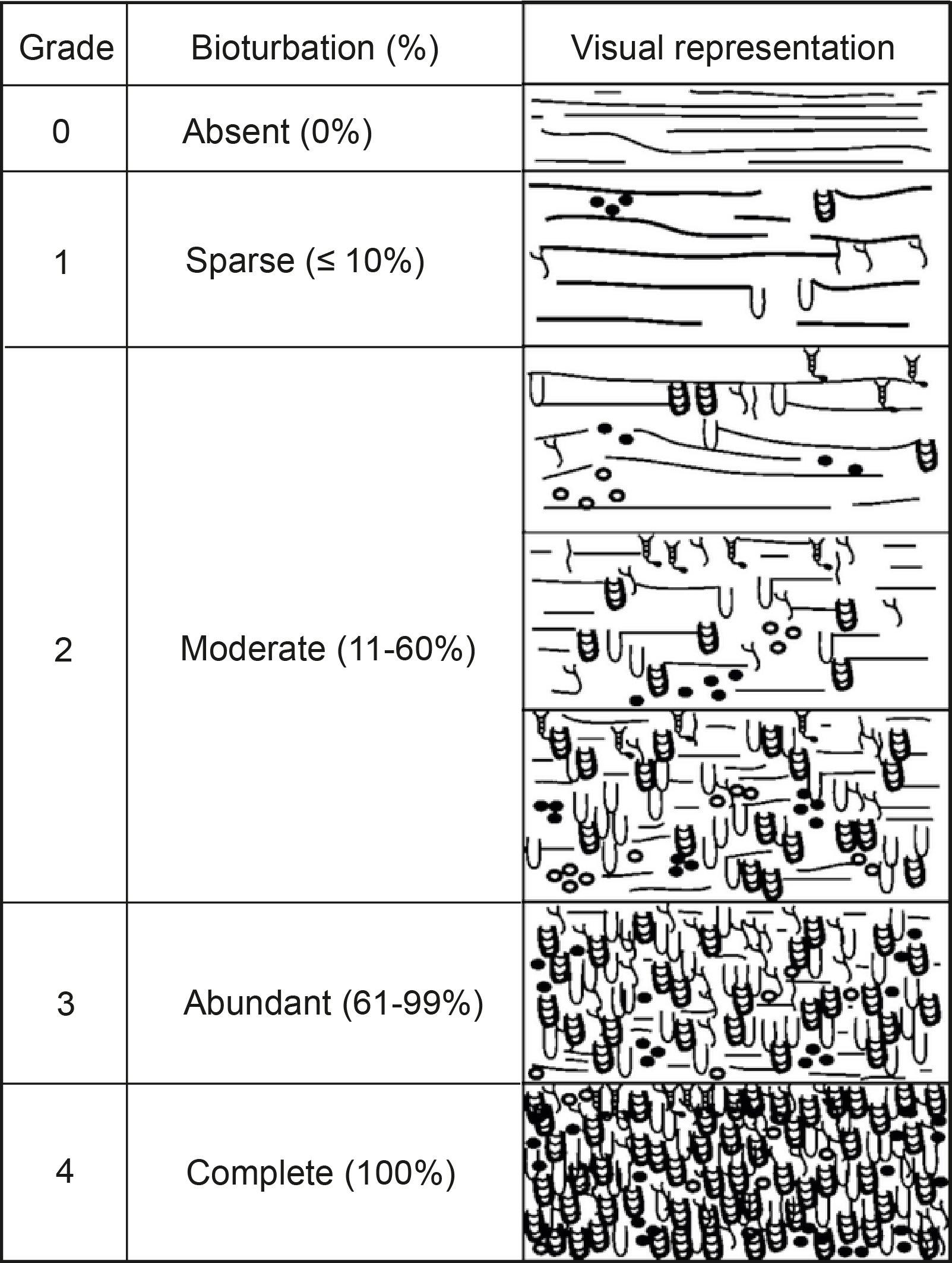
Figure F12. Bioturbation index.
2.4.4.4.2. Trace fossils
Discrete traces have been differentiated and taxonomically classified at the ichnogenus level, when possible, according to characteristic features in cores (see Knaust, 2017). Some of the most frequent ichnogenera are Chondrites, Planolites, and Zoophycos, among others (Figure F13). When ichnotaxonomic classification was not possible, they are referred to as undifferentiated trace fossils.
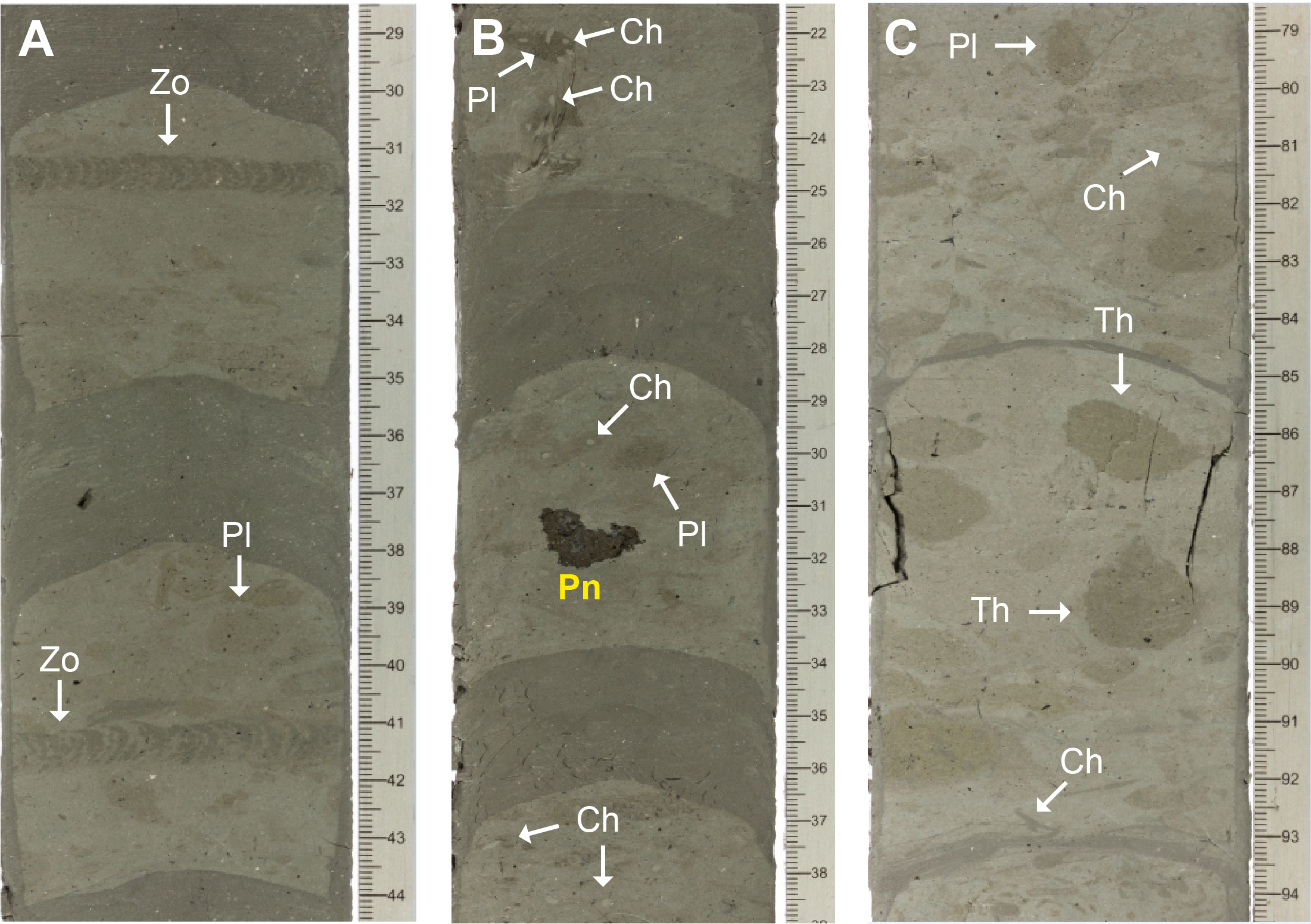
Figure F13. Trace fossils.
2.4.4.5. Stratification and sedimentary structures
The locations and types of stratification and sedimentary structures visible on the prepared surfaces of the split cores are shown in the Sedimentary structures column of the VCD sheet. Symbols in this column indicate the locations and scales of interstratification, as well as the locations of individual bedding features and any other sedimentary features, such as parallel and cross lamination, and fining-upward, coarsening-upward, or bigradationally bedded intervals (Figure F10).
For Expedition 401, we described strata <1 cm thick as lamination and >1 cm as beds (based on Boggs, 2001; Stow, 2005).
2.4.4.6. Color
Color was determined qualitatively using Munsell soil color charts (Munsell Color Company, Inc., 2010) and was described immediately after cores were split whenever possible or up to 2 h after splitting, to minimize color changes associated with drying and redox reactions. When portions of the split-core surface required cleaning with a stainless steel or glass scraper, this was done prior to determining the color. Munsell color names and the corresponding hue and chroma value are provided in the Color column on the VCD sheets.
2.4.4.7. Shipboard samples
Sample material taken for shipboard sedimentologic and chemical analyses consisted of interstitial water (IW) whole rounds, micropaleontology samples, smear slides, thin section billets, and discrete samples for XRD and carbonate analysis. Typically, 1–3 smear slides were made per core. One IW sample was taken at designated intervals (so that core is missing from those intervals), and a micropaleontology sample was obtained from the core catcher of most cores. XRD samples were taken from a split of the carbonate samples from the IW samples at designated intervals and selected from the working half to better characterize mineral composition of a given lithostratigraphic unit. Tables summarizing relative abundance of sedimentary components from the smear slides were also generated.
2.4.4.8. Remarks
The written description at the top of the VCD sheets for each core contains a brief overview of primary and secondary lithologies present, as well as notable features such as sedimentary structures, grading, and disturbances resulting from the coring process. Preliminary ages provided by micropaleontology are also noted in these summaries.
2.5. Synthetic logs
Hand-drawn sedimentary logs for the cores follow the template from Expedition 339 (Expedition 339 Scientists, 2013) and are a representation of the recovered sediment sequence based on the visual descriptions of the cores as recorded on the VCD sheets and in core photographs (see SYNTHLOGS in Supplementary material). These graphic representations were drawn at the vertical scale of 10 m per page, with the core and section indicated on the left. Hand drawn logs are shown with a reduced vertical scale (0.5 m per 5 mm square) in each site chapter. An example hand-drawn log is shown in Figure F14 with a legend example in Figure F15.
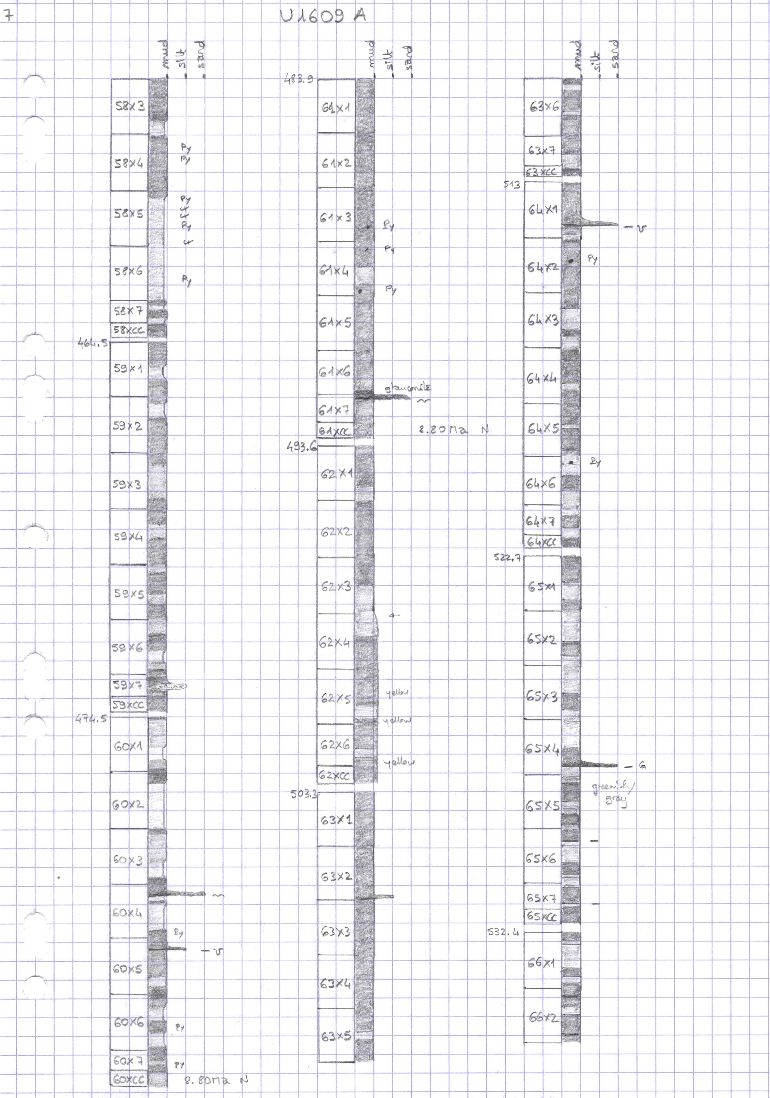
Figure F14. Synthetic log (hand drawn).
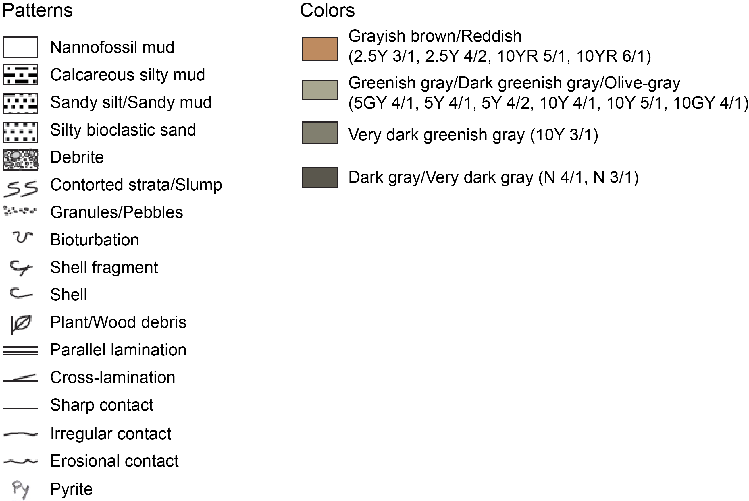
Figure F15. Hand-drawn log graphic key.
The lithologies are represented by patterns as follows:
- All lithologies, except for cemented carbonate and conglomerates, are represented by mean grain size and colors based on the Munsell color assigned (Munsell Color Company, Inc., 2010):
- Light green = GLEY1 7,
- Dark green = GLEY1 6,
- Lighter gray = GLEY1 or 5GY 5,
- Medium gray = GLEY1 4,
- Darker gray = GLEY1 3 or N,
- Dark orange = 10YR 3, or
- Light orange = 10YR 6.
- Conglomerates/debrites are represented by large open dots in matrix corresponding to Munsell color.
- Cemented carbonate is represented by a yellow limestone brick pattern.
- Granules, pebbles, and cobbles are represented by large open dots.
Contacts are represented as follows:
- Gradational contact: no horizontal line is drawn, and there is a gradational curve between the two lithologies.
- Bioturbated contact: no horizontal line is drawn. Occasionally, a burrow is drawn at the right of the average grain size curve to show if the contact is sharp and bioturbated.
- Sharp contact: a ruled straight line is drawn between the two lithologies.
- Erosional/scoured contact: a wavy line is drawn between the two lithologies.
Additional features are represented as follows (Figure F15):
- Identified slumps: contorted strata.
- Shelly sediments and shell hash: small drawings of a shell to the right of the average grain size curve.
- Woody fragments: a leaf.
- Coral fragments: a small coral cylinder.
- Parallel laminated sediments: 3 small dashes arranged vertically.
- Cross lamination: 2 small dashes forming a small angle.
The contact between cores is represented continuously if the previous core is full and the lithologies between the two cores are the same. If this is not the case, a small space is shown between the core catcher of the previous core and the first section of the following core.
Other specific annotations have been included at the right of the average grain size, such as a green "G" for glauconite presence or "sandstone" in the case of fully indurated/lithified sediment.
2.6. Smear slides
Smear slide samples were taken from the archive halves during core description. For each sample, a small amount of sediment was removed with a wooden toothpick, dispersed evenly in deionized water on a 25 mm × 75 mm glass slide, and dried on a hot plate at a low setting. A drop of mounting medium and a 22 mm × 30 mm cover glass were added, and the slide was placed in an ultraviolet light box for ~15 min. Once fixed, each slide was examined at 200×–500× magnification with a transmitted light petrographic microscope using an eyepiece micrometer to assess grain size distributions in clay (<4 µm), silt (4–63 µm), and sand (>63 µm) fractions. The eyepiece micrometer was calibrated once for each magnification and combination of ocular and objective, using an inscribed stage micrometer.
Relative proportions of each grain size and type were estimated by microscopic examination. It is significant to note that smear slide analyses tend to underestimate the abundance of sand-sized and larger grains (e.g., foraminifers, radiolarians, and siliciclastic sand) because these are difficult to incorporate into the smear. Clay-sized biosilica, which is transparent and isotropic, is also very difficult to quantify. Clay minerals, micrite, and nannofossils can also be difficult to distinguish at the very finest (<4 µm) size range.
After scanning for grain size distribution, several fields were examined for mineralogical and microfossil identification using the IODP digital references for smear slide analysis of marine mud (Marsaglia et al., 2013, 2015) and Rothwell (1989). Standard petrographic techniques were employed to identify the commonly occurring minerals and biogenic groups, as well as important accessory minerals and microfossils.
Smear slide analysis data tables are included in Core descriptions. These tables include information about the sample location, description of where the smear slide was taken, the estimated percentages of texture (i.e., sand, silt, and clay), and the estimated percentages of composition (i.e., ash, organic carbon, siliciclastics, detrital carbonate, biogenic carbonate, authigenic carbonate, and biogenic silica). Relative abundances of identified components such as mineral grains, microfossils, and biogenic fragments were assigned on a semiquantitative basis using the following abbreviations:
- A = abundant (>20% in field of view [FOV]).
- C = common (>5%–20% in FOV).
- F = few (1%–5% in FOV).
- R = rare (<1% in FOV).
- P = present (1 per 1–10 FOVs).
- B = barren (none in FOV).
Components of smear slides were entered into the Smear Slide template for GEODESC. Photomicrographs of some smear slides and their components were taken in plane and polarized light, and occasionally reflected light, and uploaded to the LIMS database.
2.7. Grain mounts
Grain mounts were prepared and analyzed using a scanning electron microscope (SEM)–energy dispersive spectrometry (EDS) when necessary to better evaluate the grain size and mineral composition of various lithologies. These samples were prepared to create an even, polished cross section of a sample for optical or electron beam analysis using the following procedure. The material was prepared by rinsing with deionized (DI) water and/or isopropanol to assure that they are dry and clean. Buehler mold release agent was sprayed into blue silicone Buehler molds into which the material was mounted to the bottom. A 3:1 (A:B) ratio of Epo-Tek Part A and Part B was mixed and added to the grain mount mold using a disposable pipettor (4–7 mm, depending on how much material must be removed from the bottom to expose a sufficient cross section). To remove dissolved gases, the grain mount mold was briefly (~10 min) held under a low vacuum, making sure to not reach the epoxy's boiling pressure, which will create excess bubbles. The epoxy was cured using a low-temperature hot plate. Once cured, the grain mount was removed from the mold. Material from the bottom of the surface of the grain mount was removed using the coarse grinding disk on the Buehler lap wheel until the amount of exposed material was satisfactory for analysis. The grain mount was then lapped using the 400 grit abrasive disk, cleaned with DI water/isopropanol, and lapped with the 600 grit abrasive disk. The grain mount was then cleaned, and the thin section preparation procedure was carried out.
2.8. Thin sections
Descriptions of consolidated sediments were complemented by shipboard thin section microfacies analysis. Standard thin section billets (30 mm × 20 mm) were cut or sawed from selected intervals in core sections that were undisturbed by drilling. Samples were initially sprayed with isopropyl alcohol and left to dry for 10 min before being placed in Epo-Tek 301 epoxy for 12 h under vacuum. For some samples, this epoxy was stained with Petroproxy 154 blue dye to show pore space in the thin section. Samples were then placed in molds before being sanded to obtain a flat, smooth surface that was adhered to a glass slide with epoxy. Next, they were cut and then ground to ~25 µm thickness. In some cases, the nature of the sediment led to plucking of the surface during grinding, so some thin sections were left thicker than 30 µm (~60–100 µm).
Some thin sections containing carbonate were stained using potassium ferricyanide and Alizarin Red S. The following colors were used to distinguish the carbonate forms (Dickson, 1965):
- Calcite: very pale pink to red.
- Ferroan calcite: purple to mauve.
- Dolomite: no color.
- Ferroan dolomite and ankerite: pale to deep turquoise, depending on ferrous content.
Thin sections were examined and imaged with a Zeiss AXIO microscope equipped with transmitted and reflected light and a standard eyepiece micrometer. Several fields of view were examined at magnification levels ranging from 5× to 50× to assess the types and approximate abundance of detrital, biogenic, and authigenic components as well as textural relationships. Narrative visual descriptions of thin section microfacies (including the components) were entered into a Thin Section Summary template for GEODESC. Photomicrographs of thin sections were acquired and uploaded to the LIMS database.
2.9. X-ray diffraction analysis
XRD analysis was performed on both bulk sediment and clay (<2 µm) fractions to identify primary minerals present in different lithologies and lithostratigraphic units (or subunits) and detect large-scale mineralogical changes with depth. In general, 1 sample per 3 cores was collected for XRD analysis either from ⅓ of the whole-round sediment squeeze cake residues or deeper cores (where no IW was obtained). Additional XRD samples were taken from the working-half sections on the sample table where specific lithologies were recognized based on visual core observations (e.g., color variability and visual changes in lithology and texture) and smear slide investigations. Most of samples taken for XRD analysis were also analyzed for sedimentary inorganic carbon (i.e., carbonate analysis), organic carbon, and elemental analysis (i.e., CHNS and resultant total organic carbon) in the geochemistry laboratory (see Geochemistry).
For bulk sediment analysis, samples were freeze-dried and stored in a desiccator to prevent re-absorption of moisture. Freeze-dried samples were finely ground using a mortar and pestle. Prepared samples were top-mounted onto a sample holder and analyzed using a D4 Endeavor X-ray diffractometer mounted with a Vantec-1 detector using CuKα radiation.
The standard locked coupled scans to assess bulk samples were as follows:
- Voltage = 40 kV.
- Current = 40 mA.
- Goniometer scan = 4°–70°2θ.
- Step size = 0.02°2θ.
- Scan speed = 2 s/step.
- Divergence slit = 0.3°.
Digital files with the diffraction patterns are available from the LIMS database. Diffractograms of bulk samples were evaluated with the aid of the EVA software package, which allowed for mineral identification and basic peak characterization (e.g., baseline removal and maximum peak intensity). Files were created that contained d-values, diffraction angles, and peak intensities with and without background removed. These files were scanned and searched using EVA to find d-spacing values characteristic of rock-forming minerals common in sediments or sedimentary rocks, using quartz or calcite as an internal standard, that were anticipated to be present in the sediments and that had peaks with little interference from other minerals present in the sample (Table T2) (Cook et al., 1975; Flood, 1978; Shipboard Scientific Party, 1995).
The Rietveld refinements were performed on bulk XRD patterns using DIFFRAC.TOPAS to semiquantitatively determine the relative abundance of identified minerals. The quality of these estimates relative to the absolute percentages within the mass of total solids depends on the abundance of amorphous solids (e.g., biogenic silica, volcanic glass, and organic matter), as well as the total of all other minerals that occur in trace quantities. Additionally, the Rietveld refinements can take into account the most significant peak of mixed-layer illite/smectite (I/S), but it is difficult to quantitatively determine the amount of mixed-layer I/S due to the disordering of mixed-layer structure. Thus, the mineral percentages determined from bulk powder XRD data should only be used to identify changes in relative abundance of primary minerals or mineral groups in the sediments with depth at each site and across different sites.
For clay mineral analysis, samples (~2 g) were crushed and dispersed in distilled water using an ultrasonic probe. For some samples, 25 mL of 1% sodium hexametaphosphate solution was added to prevent flocculation. For each suspension, the clay fraction (<2 µm) was separated by gravity settling in water in a 50 mL settling tube. After settling, clays that remained in suspension were concentrated by centrifugation (1 h at 3000 rpm). The <2 µm fraction was pipetted directly onto amorphous quartz sample discs ("zero background" plate). The clay fraction sample was scanned in the air-dried state first; after saturation with ethylene glycol for ~12 h, they were reanalyzed to determine the presence of expandable clays (e.g., clays interlayered with smectite). The shipboard results were mainly used to identify the clay mineral types present in the sediments based on the peak positions of the most common clay minerals. All digital diffraction patterns are available from the LIMS database.
The standard locked coupled scans to assess clay samples were as follows:
- Voltage = 40 kV.
- Current = 40 mA.
- Goniometer scan = 4°–36°2θ.
- Step size = 0.02°2θ.
- Scan speed = 2 s/step.
- Divergence slit = 0.3°.
3. Biostratigraphy
Bioevents were based on semiquantitative analyses of nannofossil and planktonic and benthonic foraminifer assemblages in core catcher samples. Planktonic foraminifer and calcareous nannofossil assemblages are useful indicators for sea-surface temperature, salinity and nutrient availability, and productivity (e.g., Schiebel et al., 2018; Rogalla and Andruleit, 2005; Balestra et al., 2017; Martínez-Sánchez et al., 2019; Ausín et al., 2020). The composition of planktonic and benthonic foraminifer assemblages is expected to be crucial in planning for future stable isotope studies to select the most appropriate species based on their occurrence at different sites.
Preliminary ages were assigned based on biostratigraphic events identified in core catcher samples. Intermediate samples were taken for examination when a more refined age determination was required. Calcareous nannofossil age events were estimated by correlating with the geomagnetic polarity timescale and Raffi et al. (2006) and the geologic timescale (GTS2020) by Raffi et al. (2020). Ages for planktonic foraminifer events were estimated according to GTS2020 (Raffi et al., 2020), GTS2004 by Lourens et al. (2004) and Lirer et al. (2019), and other regional biostratigraphic studies (Tables T3, T4).
The following terminology was applied for each group:
- LO = lowest occurrence (first occurrence).
- HO = highest occurrence (last occurrence).
- LcO = lowest common occurrence (first common occurrence).
- HcO = highest common occurrence (last common occurrence).
- LrO = lowest regular occurrence.
- HrO = highest regular occurrence.
- T = top.
- B = bottom.
- TP = top paracme.
- BP = base paracme.
3.1. Calcareous nannofossils
Preliminary bioevents were assigned based on the occurrence of calcareous nannofossils (presence, absence, or dominance) in core catcher samples and selected samples. Calibration of the identified events was derived mainly from Raffi et al. (2003, 2006, 2020). Martini (1971) and Okada and Bukry (1980) standard zonal schemes were adopted. Additionally, we also considered bioevents based on astronomical tuning between open ocean sites with Mediterranean reference sections in the northeast Atlantic and Mediterranean over the last decades to compile the biostratigraphic report (Krijgsman et al., 2004; Hilgen et al., 2000a; Morigi et al., 2007; Di Stefano and Sturiale, 2010). All bioevents considered are included in Table T3 together with the references to literature where these events were defined or astronomically dated. The magnetostratigraphy for the Cenozoic is based on Lourens et al. (2004) and Raffi et al. (2020).
For the taxonomy, we grouped the Gephyrocapsa species in several size categories. Specimens <3 µm, mainly Gephyrocapsa ericsonii and Gephyrocapsa aperta, were classified as "small Gephyrocapsa." Specimens of Gephyrocapsa muellerae and Gephyrocapsa margerelii, as well as other identified specimens in the 3–5.5 µm size range, were referred to as "medium Gephyrocapsa." The "large Gephyrocapsa" category includes forms >5.5 µm. Gephyrocapsa oceanica was divided into G. oceanica >5 µm and G. oceanica <5 µm.
Reticulofenestra specimens were also considered following a size concept. Reticulofenestra pseudoumbilicus was divided into R. pseudoumbilicus >7 µm and R. pseudoumbilicus <7 µm. Reticulofenestra haqii and Reticulofenestra minutula were considered "medium Reticulofenestra," ranging 3–5 µm. Forms <3 µm were "small Reticulofenestra," mainly corresponding to Reticulofenestra minuta. Reticulofenestra asanoi was divided into R. asanoi >6 µm and R. asanoi <6 µm. Also, Sphenolithus moriformis and Sphenolithus abies were grouped together as Sphenolithus spp. Following Young and Bown (2014), Triquetrorhabdulus rugosus was called Orthorhabdus rugosus. In general, taxonomic concepts for Neogene taxa were adopted from Perch-Nielsen (1985). Reworked calcareous nannofossils (i.e., taxa belonging to older [Mesozoic and Paleogene-Neogene] stratigraphic intervals) were estimated as well.
3.1.1. Methods
Samples were prepared following the standard smear slide technique with Norland optical adhesive. Calcareous nannofossils were examined with a Zeiss polarized microscope at 1000× magnification.
Preservation includes the effects of dissolution and overgrowth. Preservation of calcareous nannofossils was categorized as follows:
- G = good (little or no evidence of dissolution and/or overgrowth; specimens identifiable to the species level).
- M = moderate (minor to moderate dissolution and/or overgrowth; most specimens identifiable to the species level).
- P = poor (extreme dissolution and overgrowth).
Total abundance of calcareous nannofossils was categorized as follows:
- V = very abundant (>100 specimens per FOV).
- A = abundant (11–100 specimens per FOV).
- C = common (1–10 specimens per FOV).
- F = few (1 specimen per 2–10 FOVs).
- R = rare (1 specimen per ≥11 FOVs).
- B = barren.
Abundances of individual taxa or groups of calcareous nannofossils were categorized as follows:
- D = dominant (>20 specimens per FOV).
- A = abundant (11–20 specimens per FOV).
- C = common (1–10 specimens per FOV).
- F = few (1 specimen per 2–10 FOVs).
- R = rare (1 specimen per ≥11 FOVs).
3.2. Foraminifers
Sediments were analyzed from the mudline and the core catcher. From each core catcher, 20–30 cm3 of sediment was analyzed for planktonic and benthonic foraminifers. Unlithified sediment samples were soaked in tap water and washed over a 63 µm sieve. Before washing, samples with high clay content were agitated in tap water on a shaker table in erlenmeyer flasks to aid clay disaggregation. Washed samples were dried at 60°C. The dried residue (>63 µm size fraction) was split for planktonic (25%) and benthonic foraminifer (75%) assemblage studies. To avoid contamination between successive samples, sieves used for wet sieving were cleaned by wet spraying and compressed air, and they were further immersed in methylene blue to dye any contaminants and those used for dry sieving were cleaned with compressed air. The samples were analyzed under ZEISS Discovery V8 and ZEISS Stemi SV11 stereomicroscopes, respectively. Mudline samples were collected by emptying the sediment/water material from the top core liner of the hole into a bucket and then transferring it to a polyvinyl chloride bottle. A mixture of Rose Bengal and ethanol solution was added to determine which specimens had been alive immediately prior to sample collection. The samples were stained for 7–10 days, after which they were gently washed over a 63 µm sieve and dried in an oven at 50°C for analysis under the ZEISS Stemi SV11 stereomicroscope.
3.2.1. Planktonic foraminifers
Preliminary ages were assigned based on the occurrence of planktonic foraminifers, their relative abundance, and the coiling changes in core catcher samples. Planktonic foraminifer bioevents reported in the northeast Atlantic and Mediterranean over the last decades were considered to support this biostratigraphic report, especially those that have been accurately dated based on astronomical tuning with Mediterranean reference sections. All bioevents are included in Table T4 together with the references to literature where these events were defined or astronomically dated. Ages for most of these events were reported in the geologic timescale (GTS2004) by Lourens et al. (2004) and Lirer et al. (2019). Some of the events used in this study were not reported in the GTS2020 (Raffi et al., 2020), but the ages reported by Lourens et al. (2004) are still valid. A table and figure showing the depths and ages for each bioevent was prepared for each hole. The ages for some of the bioevents, such as the coiling change of Neogloboquadrina incompta together with the highest common occurrence of Globorotalia miotumida and the lowest common occurrence of Globorotalia margaritae were updated based on the more precise tuning of Bulian et al. (2023). In this report, we used the name N. incompta as equivalent to Neogloboquadrina acostaensis that is widely used in most biostratigraphic studies for the late Miocene.
We used bioevent names as reported by the previous authors. Globorotalia conomiozea and G. miotumida were grouped together under the name of the G. miotumida group after Sierro (1985). In the Miocene, the Globorotalia menardii group also includes Globorotalia plesiotumida and Globorotalia merotumida following Sierro et al. (1993). Globorotalia crassaformis comprises the two subspecies G. crassaformis hessi and G. crassaformis ronda. Globigerinoides extremus includes Globigerinoides obliquus because it is difficult to distinguish these two species in Pliocene sediments from the Atlantic and Mediterranean regions. Globigerinella calida and Globigerinella obesa were grouped as well. Neogloboquadrina pachyderma dextral in the Pleistocene and N. acostaensis in the Miocene and Pliocene were grouped together under the name of N. incompta. Otherwise, taxonomic concepts for Neogene taxa were adopted from Kennett and Srinivasan (1983).
3.2.2. Benthonic foraminifers
Benthonic foraminifers provide limited biostratigraphic age control, but they are useful for paleobathymetric and paleoenvironmental interpretation. Assuming carbonate dissolution to be negligible, the ratio of planktonic to benthonic foraminifers can be used to infer general sea level trends to depths of 1200 m (van Morkhoven et al., 1986; van der Zwaan et al., 1999) along with changes in abundance of certain marker species (Perez-Asensio et al., 2012).
Paleobathymetry was estimated using the following categories:
Taxonomic assignments for benthonic foraminifer species predominantly follow van Morkhoven et al. (1986), Jones (1994), Boltovskoy et al. (1980), Holbourn et al. (2013), and Hanagata (2003). The generic classification of Loeblich and Tappan (1984) was used. Identification of benthonic foraminifer taxa was generally made on the >150 µm size fraction when there were a lot of benthonic foraminifers in the coarse fraction; however, 63–125 µm size fractions were examined for benthonic foraminifers when foraminifer abundance was reduced and detrital particles dominated.
Abundances of benthonic foraminifers were categorized as follows:
- D = dominant (>50% abundance).
- A = abundant (20%–50% abundance).
- C = common (5%–20% abundance).
- R = rare (1%–5% abundance).
- P = present (<1% abundance).
The abundance of elevated epibenthonic foraminifers, shallow-water foraminifers, Uvigerinids, and Bolivinids were studied to understand the bottom water conditions. The percentage of elevated epibenthonic foraminifers (as listed in Schönfeld, 2002) has been used as a proxy for near-bottom current velocities by a few studies in the Gulf of Cádiz (Schönfeld and Zahn, 2000; Schönfeld, 2002). The morphogroup analysis can be used as a proxy for combined oxygenation and food availability in the deep ocean (Jorissen et al., 2007).
3.3. Other microfossils
The presence of other microfossils in the fraction larger than 125 µm was reported, including ostracods, sponge spicules, radiolarians, diatoms, fish fragments, echinoderm remains, and so on.
4. Paleomagnetism
During Expedition 401, paleomagnetic measurements focused on obtaining a magnetostratigraphy for all holes, sediment transport directions for coarser grained intervals, and paleoenvironmental reconstructions through time. First, the natural remanent magnetization (NRM) was measured on each archive section half of the cores, which were subsequently demagnetized by alternating field (AF) magnetization up to a peak field of 20 mT on a superconducting rock magnetometer (SRM). In addition, discrete samples taken from the working halves were AF demagnetized and measured on an AGICO JR-6A spinner magnetometer. All demagnetization results were combined to obtain a magnetic polarity stratigraphy that was correlated to the most recent geomagnetic polarity timescale (GPTS; Ogg, 2020; Raffi et al., 2020) (Figure F16) to help constrain the age model for each hole. Next, the anisotropy of magnetic susceptibility (AMS) was measured using a MFK2 KappaBridge; its shape may reflect the transport direction of the sediment. If time permitted, additional rock magnetic analyses were performed to determine the changes in magnetic carriers.
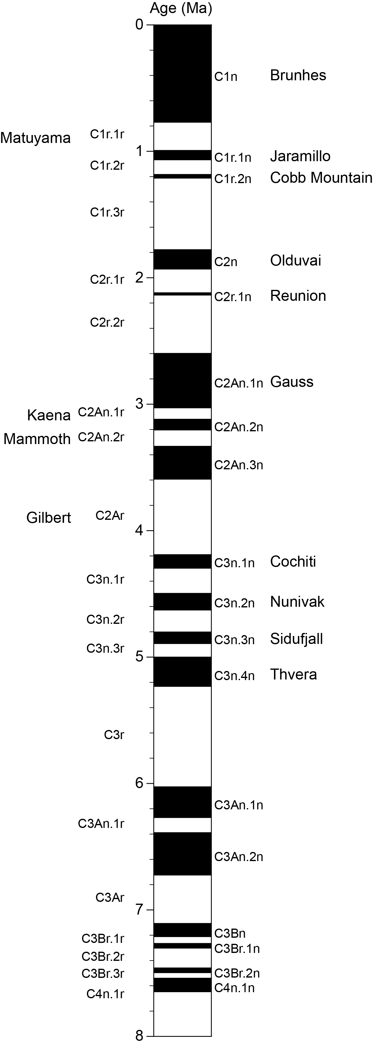
Figure F16. Geomagnetic polarity timescale.
4.1. Preoperations instrumentation tests
Prior to the start of coring operations, we used shipboard testing samples to cross-check sample coordinate schemes on the SRM (see Core collection and coordinates) and the AGICO JR-6A spinner magnetometer. This allowed us to ensure that both the SRM and JR-6A yielded similar directional and intensity data. To do this, a set of 4 standard samples were imparted an isothermal remanent magnetization along the Z-axis in a field of 100 mT and measured across a range of intensities and directions. A comparison of the directional and intensity measurements are listed in Table T5 and shown in Figure F17.
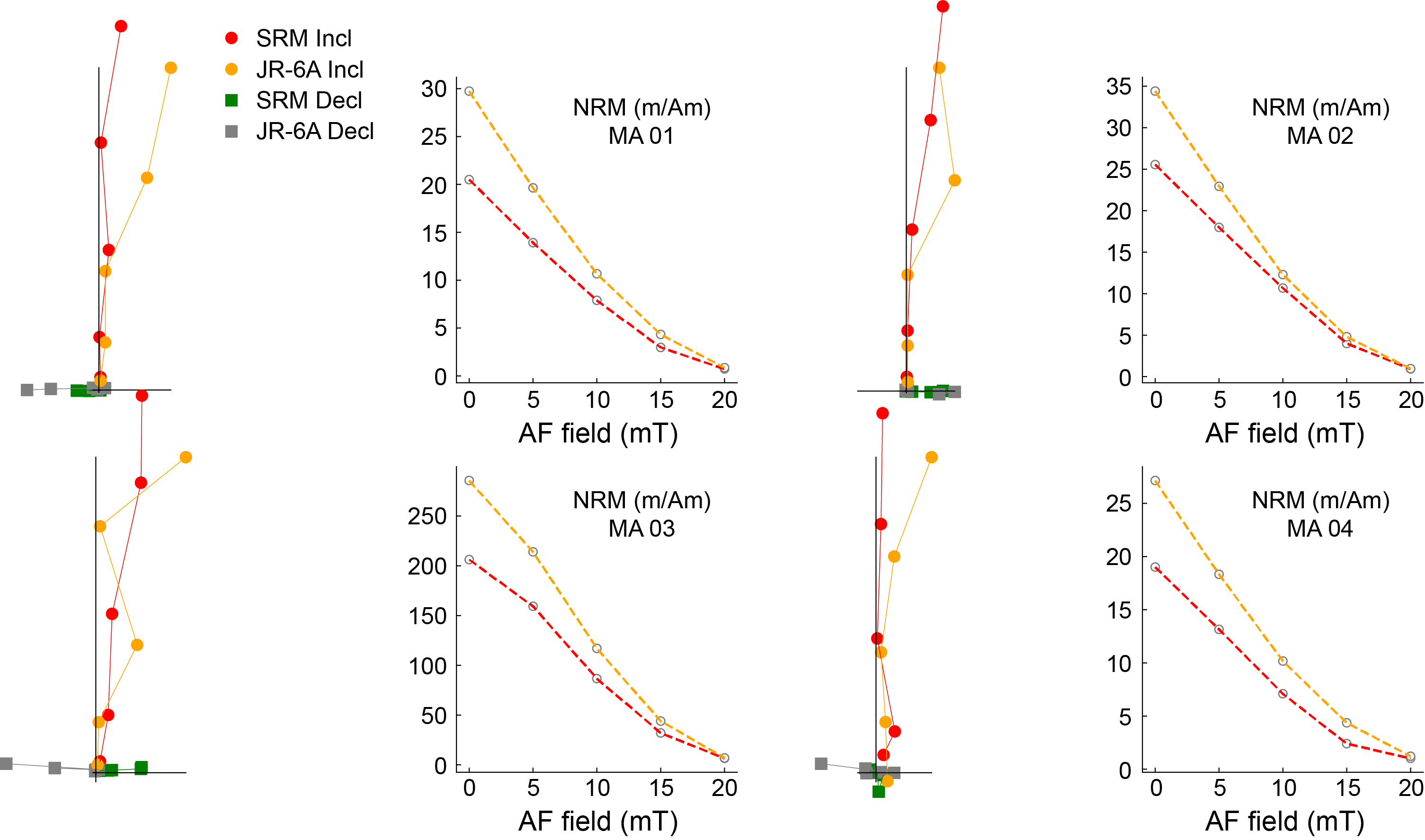
Figure F17. Orthogonal plots and NRM decay curves.
4.2. Core collection and coordinates
Cores were collected using nonmagnetic core barrels for the APC and HLAPC systems. These nonmagnetic core barrels are more brittle and cannot be used in conjunction with the XCB or RCB coring systems. The BHA included a monel (nonmagnetic) drill collar that was used for all APC and XCB cores. This collar can potentially reduce the magnetic field near where the core is cut and within the core barrel.
All magnetic data are reported relative to IODP orientation conventions: +x points away from the face of the working half (toward the "double line"), +y points toward the left side of the working half when looking downcore, and +z points downcore. The hatched arrows on the samples point "upcore" or in the −z direction. The relationship between the SRM coordinates (X, Y, and Z) and the sample coordinates (x, y, and z) is +X = +x, +Y = +y, and +Z = −z for archive halves and +X = −x, +Y = −y, and +Z = −z for working halves (Figure F18A, F18B). Note that the orientation of the SRM axes form a left-handed coordinate system (Figure F18C). This is converted to a right-handed system within the IMS software by multiplying the calibration constant for the y-axis by −1.
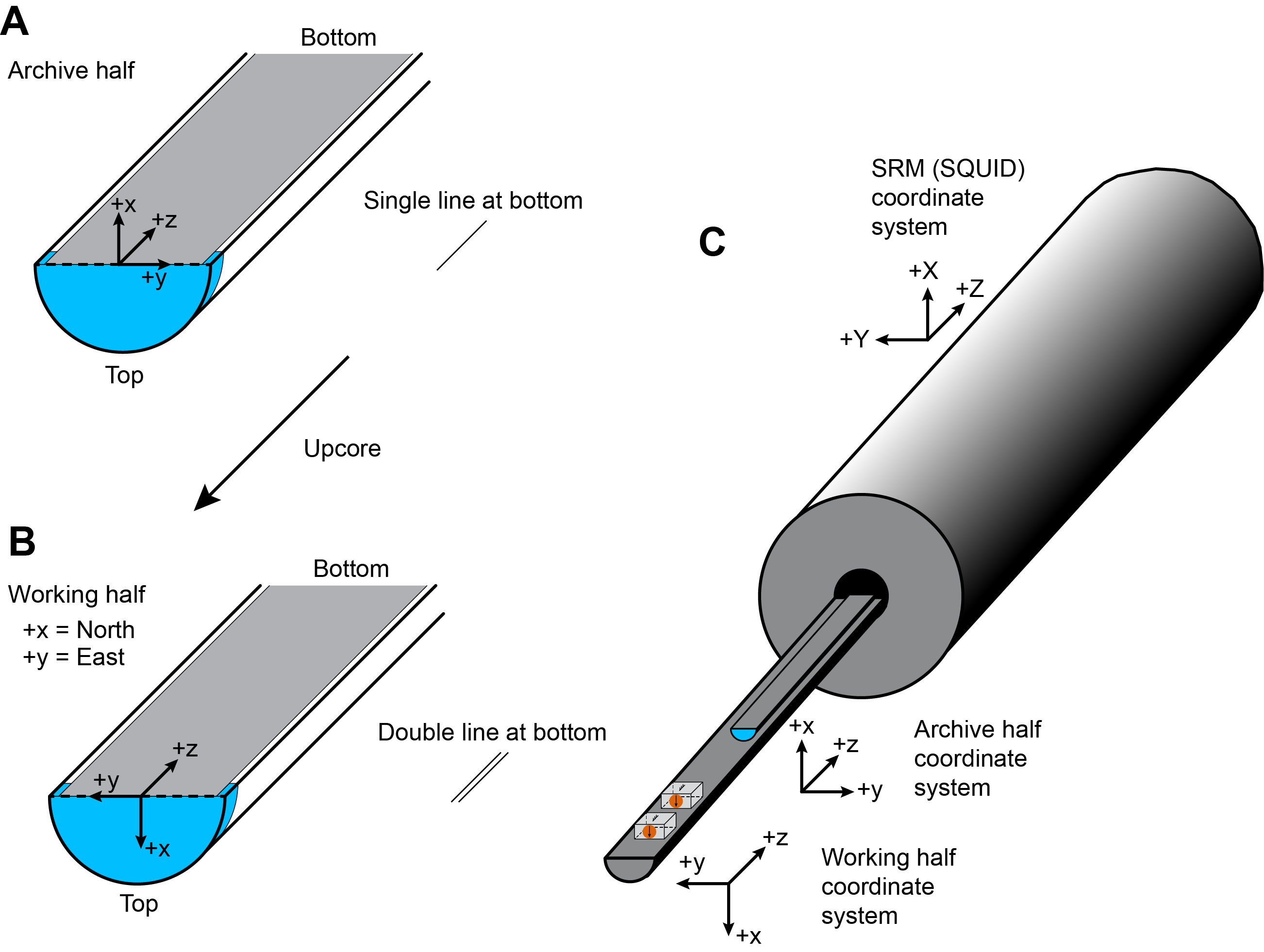
Figure F18. Coordinate systems for section halves and SRM.
Discrete sample labeling is shown in Figure F19A With the SRM, we measured the archive halves using the face = top/arrow = away orientation settings. The discrete samples (from the working halves) were measured on the JR-6A, using azimuth = 0, dip = 90, P1 = 12, P2 = 0, P3 = 12, and P4 = 0, with the −z (hatched) arrow pointing to the northwest and the x arrow pointing away from the user (into the holder) (Figure F19B).
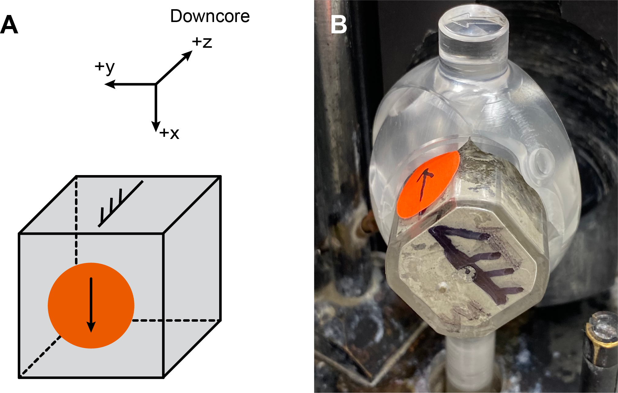
Figure F19. Coordinate system for J-cube samples and JR-6A.
4.3. Samples and measurements
4.3.1. Archive sections
Remanence measurements on archive halves were made using a 2G Enterprises Model-760R-4K SRM equipped with direct-current superconducting quantum interference devices (DC-SQUIDs) and a three-axis, inline, automated AF demagnetizer capable of peak fields of 80 mT. The spatial resolution for archive-half section measurements is a function of the integrated response function (following Acton et al., 2017) with effective lengths of 7.30 cm for the X-axis, 7.30 cm for the Y-axis, and 9.00 cm for the Z-axis. The practical noise level of the SRM is ~2 × 10⁻⁹ Am2 and is primarily controlled by the magnetization of the core liner and the background magnetization of the measurement tray.
We cleaned the sample tray with soapy water daily or more often if deemed necessary. The sample tray was then AF demagnetized with a peak field of 80 mT, and its remanence was measured using the "section background" routine to update the background correction values for the empty sample tray. The empty sample tray was subsequently measured with the updated background correction values subtracted for QA/QC purposes.
NRM measurements of the archive-half sections were made at 5 and 2 cm intervals, along with a 5 cm trailer and leader to monitor the background magnetic moment. We began with measuring the initial NRM and the remanent magnetization remaining after AF demagnetization steps of 5, 10, 15, and 20 mT peak fields.
4.3.2. Discrete samples
We collected four oriented discrete samples from the working half of each site, focusing on fine-grained sediments and avoiding disturbed intervals. Discrete samples were collected by pushing plastic Natsuhara-Giken ("Japanese") cubes (J-cubes; 2 cm external edge length and internal volume of ~7 cm3) into working-half sections with the hatched arrow marker on the cube pointing toward the stratigraphic up direction (Figure F19A) and the "flags" pointing to +y. When the sediment was more indurated, a hollow metal tube (shaped to match the plastic cubes) was pushed into the working half and a plunger was used to extrude the sample onto a clean surface. The plastic cube was then placed over the sampled sediment, again with the hatched arrow marker pointing toward stratigraphic up, allowing for an identical orientation frame of reference as the "pushed" samples. For very indurated sediments, we used the parallel saw to cut 8 cm3 specimens from the core, with arrows etched onto the cube in the same sense as for the J-cubes (upcore with flags to +y).
The JR-6A and D-TECH 2000 were used for many cube measurements including AF demagnetization. The sample measurement protocol in the JR-6A spinner magnetometer was as follows: the instrument was calibrated using the 7.99 A/m cube standard with an 8 cm3 volume. A holder correction was determined by measuring the empty specimen holder. Data acquisition settings were as follows:
- Holder: Automatic (sample is automatically rotated around 3 mutually perpendicular axes).
- Specimen type: Cube.
- Acquisition time: Normal.
- Speed of rotation: High (87.7 revolutions/s).
- Specimen volume: 7 cm3 for J-cubes.
- Orientation Parameters P1–P4: 12, 0, 12, and 0 (see Core collection and coordinates).
- Azimuth and Dip: 0 and 90 (see Core collection and coordinates).
The P1–P4 orientation parameters, azimuth, and dip allow the AGICO software to convert the declination and inclination measured in the specimen coordinate system to geographic declination and inclination, which are the data reported in this volume.
4.3.3. AMS analyses
The discrete samples were analyzed for bulk magnetic susceptibility as part of the measurement of AMS using a MFK2 KappaBridge. AMS characterizes the orientation of the para- (mainly phyllosilicates) and ferromagnetic minerals in sediments and can be interpreted in terms of depositional processes (e.g., Ellwood, 1980; Taira, 1989; Tauxe et al., 2015). Settling of particles produces an oblate magnetic fabric with the minimum susceptibility axis clustered around the pole of the depositional plane. In still waters, the maximum and intermediate susceptibility axes are uniformly dispersed, defining a planar, near-horizontal, gravity- or compaction-induced settling fabric. The magnetic fabric of sediments deposited by flowing water is typified by current-oriented magnetic foliation that can be either horizontal or tilted (imbricated) and/or clustering of the maximum susceptibility parallel to the flow direction. Disturbance by slumping or other deformation generally yields triaxial fabrics.
For AMS measurements, the MFK2 KappaBridge was calibrated prior to each session using the AGICO cylindrical standard, which has maximum susceptibility along the axis of the cylinder and minimum susceptibility in the transverse direction. Each analysis consists of measuring the specimen along the three axes while it rotates within the applied field, followed by a bulk susceptibility measurement.
4.4. Editing of archive measurements for coring disturbance
Sediment disturbance due to coring or geologic processes (slumping, faulting, etc.) often leads to distorted and unreliable paleomagnetic directional records and largely altered sediment fabric. The paleomagnetic data were therefore filtered to remove these intervals. The SRM data were systematically filtered as follows:
- Deletion of all measurements within 5 cm of the section ends to remove the edge effects inherent in all pass-through measurement systems such as the SRM, as well as potential accumulation of fall-in material from the top of the cores.
- Deletion of all data from intervals that were assigned "moderate" and greater drilling disturbance during visual core description (see Lithostratigraphy) to remove data in intervals affected by coring-induced disturbance.
In some cases, we inspected core composite photographs and X-radiographs for evidence of coring or sedimentary disturbance. X-radiographs for all APC and HLAPC sections were used to identify additional features that might adversely affect the NRM but that may not be readily apparent during visual description (e.g., large burrows beneath the core surface). X-radiographs and paleomagnetic data are collected from the archive section halves, so features observed in x-radiographs are directly relevant to paleomagnetic data.
4.5. Magnetostratigraphy
Magnetic polarity zones were assigned based on changes in inclination after 10–20 mT peak AF demagnetization. Once a polarity stratigraphy was established for a given hole, we correlated the pattern to the GPTS of the geologic timescale 2020 (GTS2020; Ogg et al., 2020; Raffi et al., 2020) summarized in Figure F16. Correlation to the GPTS was assisted by discussion with the shipboard biostratigraphy team when needed.
5. Geochemistry
The shipboard geochemistry program for Expedition 401 included measurements for headspace gas content; interstitial water (IW) composition; and sedimentary geochemistry including total inorganic carbon, total carbon, total nitrogen, and composition of the acid-soluble (carbonate) fraction. These analyses were carried out to satisfy routine shipboard safety and pollution prevention requirements, characterize the diagenetic regime by IW analysis, and provide bulk sediment and carbonate geochemistry data for shipboard interpretation, which will provide a basis for sampling for shore-based research. In addition, samples for geomicrobiological analysis of Hole U1611B were taken by the shipboard geochemistry team, although these samples were not analyzed further.
5.1. Headspace gas geochemistry
One sediment sample (5 cm3) from each core, collected immediately after retrieval on deck, was placed in a 20 cm3 glass vial and then sealed with a septum and a metal crimp cap. When consolidated or lithified samples were encountered, chips of material were placed in the vial and sealed. If an IW sample was obtained, the headspace sample was taken from the top of the section immediately next to the IW sample whenever possible. The vial was labeled with the core, section, and interval from which the sample was taken and then placed in an oven at 70°C for 30 min. A 5 cm3 volume of gas extracted through the septum was then injected with a gas-tight glass syringe into a gas chromatograph (GC).
The GC (Agilent 6890 equipped with a flame ionization detector [FID]) set at 250°C was used to accurately and rapidly measure the concentrations of methane (C1), ethane (C2), ethene (C2=), and propane (C3). A 2.4 m × 2.0 mm stainless steel column packed with 80/100 mesh HayeSep "R" is installed in the oven. The injector consists of a ¹⁄₁₆ inch Valco union with a 7 µm screen connected to a Valco-to-Luer lock syringe adapter. This injector connects to a 10 port Valco valve that is switched pneumatically by a digital valve interface. The injector temperature was set at 120°C. Samples were introduced into the GC through a 0.25 cm3 sample loop connected to the Valco valve. The valve can be switched automatically to backflush the column. The oven temperature was programmed to start at 80°C, hold for 8.25 min, and then increase to 150°C at a rate of 40°C/min, and hold for 5 min. Helium was used as the carrier gas. Initial helium flow in the column was 30 mL/min. Flow was then ramped to 60 mL/min after 8.25 min to accelerate elution of C3. The analysis run time was 15 min. The GC is also equipped with an electronic pressure control module to control the overall flow into the GC. When sample vials included large amounts of water in addition to sediment, retention times during chromatography were sometimes affected, and in such cases data quality control was assured by checking peak integration windows to correctly identify gas compounds.
5.2. Interstitial water chemistry
5.2.1. Sample collection
Routine IW samples were obtained by squeezing whole-round sections cut from cores immediately after core retrieval. Standard whole-round samples are 5 cm long, but as water content decreased downhole, the size of the whole-round samples increased to 7 cm and then to 10 cm to enable extraction of enough water (ideally 10–20 mL) for shipboard analyses. For XCB and RCB coring, 10 cm long whole-round cores were always taken to ensure enough coherent material (e.g., without fractures) for sampling of uncontaminated IW. Whole-round samples were cut and capped as quickly as possible after the core arrived on deck and were immediately moved to the chemistry laboratory for squeezing. Whole-round samples were typically collected at a frequency of 1 sample per core or 1 sample per every other half-core until IW extraction was no longer possible. The exterior of the whole-round sample was carefully cleaned by scraping with a spatula to remove potential contamination from drilling fluid. For XCB and RCB cores, the intruded drilling mud between biscuits was also removed to eliminate contamination from drilling fluid. The cleaned sediment was transferred into a 9 cm inner diameter titanium squeezer that was then placed in a Carver hydraulic press (Manheim and Sayles, 1974) and squeezed with slowly increasing pressures as high as 30,000 lb (~21 MPa) if needed. After discarding the initial drops to avoid contamination, the squeezed IW was collected into a high-density polyethylene syringe washed with 10% HCl attached to the squeezing assembly and subsequently filtered through a 0.45 µm polyethersulfone membrane filter into various sample containers.
Sample allocation was determined based on the pore fluid volume obtained and analytical priorities of the expedition; any residual water was archived for shore-based analysis. For shipboard analyses, IW samples were analyzed following the protocols in Gieskes et al. (1991), Murray et al. (2000), and the International Ocean Discovery Program (IODP) user manuals for shipboard instrumentation. Aliquots for shipboard analysis by inductively coupled plasma–atomic emission spectroscopy (ICP-AES) were acidified by adding ~10 µL of trace metal–grade concentrated HNO3 and placed in 4 mL cryovials. Aliquots for titration and ion chromatography (IC) analyses were put in 14 mL polypropylene vials. All samples were stored at 4°C after collection. For samples with low IW yield, priority was given to ICP-AES and IC analyses.
Salinity, alkalinity, and pH were analyzed immediately after IW was obtained. Other shipboard analyses were carried out in batches. Dissolved sodium, magnesium, calcium, potassium, chloride, bromide, and sulfate were analyzed by IC. Ammonium and phosphate were analyzed by spectrophotometry. Major and minor element concentrations were analyzed by ICP-AES.
After IW extraction was complete, a sample was taken from the sediment squeeze cakes for shipboard bulk chemical analyses, with the remainder divided up and retained for various shore-based analyses by the shipboard science party.
5.2.2. Salinity, alkalinity, and pH
Salinity, alkalinity, and pH were measured immediately after squeezing, following the procedures in Gieskes et al. (1991). Salinity was measured using a Fisher temperature-compensated handheld refractometer. pH was measured with a combination glass electrode, and alkalinity was determined by Gran titration with an autotitrator (Metrohm 794 basic Titrino) using 0.1 N HCl at 25°C. International Association for the Physical Sciences of the Oceans (IAPSO) standard seawater was used for calibration and was analyzed at the beginning and end of a set of samples for each site and after every 10 samples. Alkalinity titrations had a precision better than 2% based on repeated analysis of IAPSO standard seawater.
5.2.3. Sulfate, chloride, bromide, calcium, magnesium, potassium, and sodium
Sulfate, chloride, bromide, calcium, magnesium, potassium, and sodium concentrations were analyzed by IC (Metrohm 850 Professional IC) using aliquots of 100 µL that were diluted 1:100 with deionized water (18 MΩ/cm). At the beginning and end of each run, different dilutions of IAPSO standard seawater were analyzed for quality control and to determine accuracy and precision. Analytical precision was generally better than 3% for all major ions.
5.2.4. Ammonium and phosphate
Ammonium and phosphate concentrations were determined using an Agilent Technologies Cary Series 100 UV-Vis spectrophotometer with a sipper sample introduction system following the protocol in Gieskes et al. (1991). For ammonium concentration analysis, a 0.1–0.2 mL sample aliquot was diluted with reagent water to a volume of 2.2 mL, to which 1.0 mL phenol ethanol, 1.0 mL sodium nitroprusside, and 2 mL oxidizing solution (trisodium citrate and sodium hydroxide) were added (Gieskes et al., 1991). The solution was kept in the dark at room temperature for ~6.5 h to develop color. For phosphate concentration analysis, a 0.3–1.2 mL sample aliquot was diluted with reagent water to a volume of 2.6 mL, to which 2.0 mL mixed reagent of ammonium molybdate, sulfuric acid, ascorbic acid, and potassium antimonyl-tartrate was added. The solution was kept at room temperature for approximately 30 min to develop color. Ammonium and phosphate concentrations were determined at an absorbance of 640 and 885 nm, respectively. Precision and accuracy of the ammonium analyses were within 2.5% and 3%, respectively.
5.2.5. Major and minor elements
Dissolved major (Na+, K+, Ca2+, SO42−, and Mg2+) and minor (Li, Sr, B, Si, Mn, Fe, P, and Ba) elements were determined by an Agilent 5110 ICP–optical emission spectroscopy (OES) in AES mode with a SPS4 autosampler (Table T6). The shipboard ICP-AES analyses of IW samples followed an analytical protocol originally developed at the Institute for Chemistry and Biology of the Marine Environment (ICBM; Oldenburg University, Germany). Each acidified IW sample was diluted 1:10 by adding 500 µL IW and 100 µL spike solution containing 100 ppm each of internal standards beryllium (Be), indium (In), and scandium (Sc) and 200 ppm antimony (Sb) to 4.4 mL of 2% HNO3 in 18 MΩ deionized water. The multielement spike was used to evaluate both atomic and ionic interferences. Serial dilutions of IAPSO standard seawater (0%, 1%, 5%, 10%, 25%, 50%, 75%, and 100%) were prepared to calibrate IW concentrations lower than or equal to normal seawater. Additional calibration solutions for major and minor element concentrations exceeding seawater (Ca, B, Ba, Fe, Li, Mn, P, Si, and Sr) were prepared in a matrix of 3.5% NaCl. Calibration solutions were spiked in the same way as the IW samples. Calibration solutions were made up from certified stock solutions for minor elements (Li, Sr, B, Si, Mn, Fe, P, and Ba).
During each ICP-AES run, a complete set of all in-house and IAPSO dilutions were analyzed at the beginning and end of each batch. Furthermore, solutions of 100% concentration in-house and IAPSO standards were run every 8–10 samples to monitor instrumental drift. The elemental concentrations reported for each sample were average values from three replicate integrations from each sample measured consecutively via continuous flow, as set by instrumental parameters; the standard error in the average was also calculated by the instrument software.
Following each ICP run, the measured concentrations were recalculated after setting background correction parameters and adjusting peak centers by using software that accompanies the ICP. Replicate analyses of IAPSO standard seawater between every 10 IW samples were used to estimate the accuracy of the measurements for all elements; accuracies were typically better than 5%. Precision was determined by the instrument from threefold runs of each sample.
5.2.6. Comparison of multiple data sets
Where more than one analysis method was used to obtain the concentration of a dissolved species, we rely upon the more standard or robust method or test the suitability of the approach on a site-by-site basis. For example, Ca, Mg, K, Na, and S were measured by both IC and ICP-AES. For all of these major ions, the data from the IC are preferred and showed consistently less scatter than those from ICP-AES. Matrix effects were also identified for ICP-AES analyses, particularly for Mg and Ca, that may be related to sulfate concentrations in the samples; these effects result in a deviation from a 1:1 comparison between concentrations analyzed by IC and by ICP-AES. Spectrophotometry and ICP data for phosphate and total phosphorus, respectively, provide a useful comparison with the possibility of identifying different P phases. Specific wavelengths were chosen for analysis by ICP-AES based on which wavelength and mode (axial versus radial) produced the best calibration for the standards within that run (Table T6).
5.3. Microbiology
No microbiology was planned for Expedition 401; however, after the observation of high-salinity IW in Hole U1611A, we decided to take microbiological samples from the equivalent interval of Hole U1611B. Modified sampling protocols were used to minimize contamination and preserve samples for potential future study. No tracer was used, but whole-round samples (5 cm long) were collected on the catwalk adjacent to and directly above the IW samples. All cutting tools were sprayed with reagent alcohol immediately prior to use. Samples were sealed with autoclaved end caps, placed inside sterile Whirlpak bags, and immediately frozen at −86°C.
5.4. Sedimentary geochemistry
5.4.1. Sedimentary inorganic carbon, organic carbon, and nitrogen content
Sediment samples were collected from the IW squeeze cakes with additional samples taken from intervals of distinct lithology. Samples were freeze-dried for ~12 h, crushed using an agate pestle and mortar, and then analyzed for total inorganic carbon, total carbon, and total nitrogen.
Total carbon and total nitrogen of sediment samples were determined with a ThermoElectron Corporation FlashEA 1112 carbon-hydrogen-nitrogen-sulfur (CHNS) elemental analyzer equipped with a ThermoElectron packed column CHNS/NCS GC and a thermal conductivity detector (TCD). Approximately 15 mg of sediment was weighed into a tin cup and then combusted at 950°C in a stream of oxygen. The reaction gases were passed through a reduction chamber to reduce nitrogen oxides to nitrogen and were then separated by the GC column before detection by TCD. All measurements were calibrated to the National Institute of Standards and Technology (NIST) Standard Reference Material SRM2704 Buffalo River Sediment (containing 3.349 wt% carbon and 0.18 wt% nitrogen), which was run every 10 samples. Replicate precision was 0.08% (1 standard deviation [1σ]) on total carbon and 0.01% (1σ) on total nitrogen. The peak areas from the TCD were calculated to determine the total carbon and total nitrogen of the samples.
Total inorganic carbon (TIC) was determined using a Coulometrics 5015 CO2 coulometer. Approximately 15 mg of sediment was weighed into a glass vial and acidified with 2 N HCl. The liberated CO2 was titrated, and the corresponding change in light transmittance in the coulometric cell was monitored using a photodetection cell. The weight percent of calcium carbonate was calculated from the inorganic carbon content, assuming no contributions from other carbonate minerals such as dolomite, using the following equation:
For samples containing dolomite rather than calcite, the standard coulometry calculations assuming a composition of calcium carbonate will yield overestimates of the weight percent carbonate by approximately 8% because of the lower mass of magnesium relative to calcium. For other samples containing a mixture of dolomite and calcite (dolomite is generally <10% of the total carbonate fraction), the correction is minor. Siderite was occasionally detected as a minor (<5%) sedimentary component, but because of its slow dissolution kinetics, its contributions to total carbonate may not be well characterized by coulometry. Overall, the comparison between coulometry and XRD carbonate yielded consistent results and was used as a cross-check on data quality by each approach; when mismatches occurred, these samples were rerun on the coulometer.
Standard CaCO3 (>99.9% calcium carbonate; Fisher Scientific) was used to assess accuracy (replicate precision, 1σ = 1.13%). Total organic carbon content was calculated by subtraction of inorganic carbon from the total carbon.
5.4.2. Acid-soluble fraction (carbonate) geochemistry
Major, minor, and trace element analyses were performed by ICP-AES on the acid-soluble fraction of squeeze cake samples to determine the geochemistry of the carbonate component of the sediment. These analyses were performed only on samples from Holes U1609A, U1610A, and U1611A. Approximately 100 mg of sediment was weighed and treated with 5 mL of 1 N ammonium acetate solution (pH of ~7) to leach exchangeable ions. After 10 min of ultrasonication, samples were centrifuged and the supernatant was poured off. After three washes with deionized water, the carbonate component of the sample was dissolved with 10–14 mL of 0.1 N acetic acid buffered to pH of ~5 with ammonium acetate. Sediments were resuspended, shaken, and sonicated for several hours to ensure complete reaction of the carbonate sediment. Samples were again centrifuged, and the supernatant was analyzed by ICP-AES to determine concentrations of Al, Ca, Fe, K, Li, Mg, Mn, Na, S, and Sr. Samples were prepared at 100–200 ppm Ca and quantified with matrix-matched standards. Precision was determined by the instrument from three runs of each sample, which yielded 20% relative standard deviation (RSD) for Al and better than 15% RSD for all other elements. Fe concentrations were not analyzed at Site U1609. Concentrations are reported as ratios relative to Ca because of variable percent carbonate in each sample.
6. Physical properties
During Expedition 401, high-resolution physical property measurements were conducted to provide evidence for lithologic variation and stratigraphic correlation. Physical properties data contribute to the following:
- Obtaining physical property stratigraphic logs to complement the lithologic logs,
- Determining the presence of astronomical cycles for chronostratigraphic control,
- Correlating borehole data to seismic profiles,
- Site-to-site stratigraphic correlation for construction of composite stratigraphic sections, and
- Identifying major seismic reflectors and construction of synthetic seismic profiles.
A series of techniques and instruments were used to characterize the physical properties of sediment recovered by Expedition 401, as described in the following sections.
6.1. Sediment cores
Core sections are generally 1.5 m in length, so a typical coring length (stroke) of 9.5 m yields six sections plus a shorter seventh section. Each section was run through two core logging systems: (1) sections were run through the Special Task Multisensor Logger (STMSL) immediately after they were sectioned on the catwalk, and (2) after core sections had warmed to ambient laboratory temperature (20°–21°C) they were run through the WRMSL. The linear track of the STMSL houses a GRA bulk densitometer and a magnetic susceptibility sensor loop. The WRMSL employs, in order, a GRA bulk densitometer, a magnetic susceptibility sensor loop, and a compressional P-wave velocity sensor.
After WRMSL scanning, the whole-round sections were logged for NGR. Thermal conductivity was then measured on certain whole-round sections (Section 3 of each core) using a needle probe inserted into the section through a small hole drilled through the plastic core liner close to the middle of the section.
After the whole-round measurements, the sections were split into working and archive halves. Discrete samples were collected from the working halves of every second section to measure wet bulk density, dry bulk density, water content, porosity, and grain density using MAD procedures. Compressional P-wave velocity measurements on split cores were made for every section for one hole (usually Hole A), employing transducers oriented in x-axis direction. Archive halves were documented by the SHIL and analyzed on the SHMSL for color reflectance and point magnetic susceptibility. A full discussion of all methodologies and calculations used aboard JOIDES Resolution in the physical properties laboratory is available in Blum (1997).
6.2. Whole-Round Multisensor Logger
The WRMSL on JOIDES Resolution is capable of simultaneously and nondestructively measuring (1) GRA bulk density, (2) magnetic susceptibility, and (3) P-wave velocity. To optimize WRMSL performance, the same sampling spacing, typically 2.5 cm, was set for all sensors. To optimize the measurement process, sampling intervals and measurement integration times were the same for all sensors, except for specific cores of interest, which were run at higher 1 cm resolution. These sampling intervals are common denominators of the distances between the sensors installed on the WRMSL (30 cm), which allows sequential and simultaneous measurements. After the completion of each core, QA/QC was performed by passing a single core liner through the WRMSL. This core liner contained an aluminum rod submerged in deionized water that together acted as a standard for the three measurements. P-wave logger (PWL) values in the standard were measured at ~1490 m/s (depending on ambient temperature), and GRA densities were around 1 g/cm3, with correlation coefficients in excess of 0.99.
6.2.1. Gamma ray attenuation bulk density
GRA bulk density is a reflection of water-saturated porosity, grain density (dominant mineralogy), grain packing, and coring disturbance. To measure bulk density, the GRA densitometer uses a 10 mCi 137Cs capsule as a gamma ray source (with the principal energy peak at 0.662 MeV) placed within a lead shield with a 5 mm collimator, which is directed downward through the whole-round core. The gamma ray detector on the opposite side of the core from the source includes a 5 mm scintillator and an integral photomultiplier tube to record the gamma radiation that passes through the core. The attenuation of gamma rays occurs primarily by Compton scattering, in which gamma rays are scattered by electrons in the formation (e.g., Evans, 1965); the degree of scattering is related to the material bulk density. Therefore, for a known thickness of sample, the density (ρ) is proportional to the intensity of the attenuated gamma rays and can be expressed as
- I = measured intensity of gamma rays passing through the sample,
- I0 = gamma ray source intensity,
- μ = Compton attenuation coefficient, and
- d = sample diameter.
Because the attenuation coefficient is similar for most common minerals and aluminum, bulk density is obtained through direct calibration of the densitometer using aluminum rods of different diameters mounted in a core liner filled with distilled water. The GRA densitometer has a spatial resolution of <1 cm.
6.2.2. Magnetic susceptibility
Magnetic susceptibility (χ) is a dimensionless measure of the degree to which material can be magnetized by an external magnetic field, and is typically expressed as
Magnetic susceptibility is primarily determined by the concentration of minerals that retain a strong remanent magnetization in the absence of an applied field (i.e., ferro- and ferrimagnetic phases; e.g., magnetite and maghemite), but is additionally influenced by minerals with a weak remanent magnetization (i.e., antiferromagnetic phases; e.g., hematite and goethite), and "nonmagnetic" minerals including paramagnetic (e.g., silicates and clays) and diamagnetic (e.g., quartz and carbonate) phases (Liu et al., 2012). MS can also give insights into magnetic mineral origins and subsequent diagenetic processes. While magnetic susceptibility is complex to interpret, given all the possible variations, in marine settings the commonly varying proportions of calcareous deposits with low magnetic susceptibility with iron-bearing minerals in siliciclastic deposits with higher magnetic susceptibility, means magnetic susceptibility is often a useful parameter for high resolution detection of changes in sediment composition complementing lower frequency analysis of carbonate concentrations (see Geochemistry) and lithology (see Lithostratigraphy).
Magnetic susceptibility was measured using a Bartington Instruments MS3 susceptometer coupled to a Bartington MS2C loop sensor with an 8 cm internal diameter. An oscillator circuit in the sensor produces a low-intensity, nonsaturating alternating magnetic field. Sediment cores passing through this field cause a change in oscillator frequency (Blum, 1997). WRMSL operated at a frequency of 567 Hz. STMSL operated at 678 Hz, a >20% frequency differential to prevent interference with WRMSL. Frequency information returned in pulse form is converted to MS by multiplying by a correction factor (1.000 for WRMSL and 1.174 for STMSL) to compensate for instrument scaling and the geometric ratio between core and loop dimensions. Magnetic susceptibility is reported in dimensionless instrument units.
6.2.3. P-wave velocity
P-wave velocity varies with the material's lithology, porosity, and bulk density, as well as state of stress, temperature, and fabric or degree of fracturing. In sediment and rock, velocity is controlled by the degree of consolidation and lithification, fracturing, and occurrence and abundance of free gas and gas hydrate. Together with bulk density, velocity data are used to calculate acoustic impedance and reflection coefficients to construct synthetic seismic profiles and to estimate the depth of specific seismic horizons. P-wave velocity (VP) is defined by the time required for a compressional wave to travel a specific distance (e.g., Hamilton, 1970):
The P-wave velocity sensor measures the ultrasonic P-wave velocity of the whole-round sample residing in the core liner. The P-wave logger transmits a 500 kHz P-wave pulse across the core section at a specified repetition rate. Traveltime is determined by signal processing software that automatically detects the first arrival of the P-wave signal to a precision of 50 ns. The total observed travel time (tcore) is composed of the following:
- tdelay = time delay related to transducer faces and electronic circuitry.
- tpulse = delay related to the peak detection procedure.
- tliner = transit time through the core liner.
- tcore = traveltime through the sediment.
The system is calibrated using a core liner filled with distilled water, which provides control for tdelay, tpulse, and tliner. From these calibrations, VP can be calculated for the whole-round specimens in core liners as
- dcl = measured diameter of core and liner,
- dliner = linear wall thickness, and
- t0 = measured total traveltime.
6.3. Natural Gamma Radiation Logger measurements
The NGRL measures NGR on whole-round cores using a system designed by the Integrated Ocean Drilling Program US Implementing Organization (USIO) (Texas A&M University, USA) (Vasiliev et al., 2011; Dunlea et al., 2013). This instrument measures the cumulative radiation emitted during natural decay of three long-lived radioisotopes, potassium (40K), thorium (232Th), and uranium (238U), which have half-lives of 1.3 × 10⁹, 1.4 × 10¹⁰, and 4.4 × 10⁹ y, respectively. These isotopes and their daughter products emit gamma radiation at specific energy levels unique to each isotope. NGR is used to estimate the abundance of each isotope based on the strength of the signal at characteristic energies (Blum, 1997; Gilmore, 2008). High counts in marine sediments generally reflect fine-grained deposits, containing K-rich clays and adsorbed U and Th, whereas low counts are often associated with biogenic carbonates. NGR variations downcore are a primary means of core-to-core stratigraphic interpretations, core-to-wireline log data comparisons, and correlations between holes.
The NGRL system consists of eight sodium iodide (NaI) detectors arranged along the core measurement axis at 20 cm intervals surrounding the lower half of the section. The detector array is equipped with both passive (layers of lead) and active (plastic scintillators) shielding to reduce the background environmental and cosmic radiation. The overlying plastic scintillators detect incoming high-energy gamma and muon cosmic radiation above 3 MeV and subtract this signal from that counted by the NaI detectors.
For Expedition 401, NGR detection used the two-position configuration with measurements 10 cm apart and a counting period of 300 s, using 8 sensors, advancing downcore for a total of 16 measurements (10 cm apart) per 150 cm core section (total acquisition time 10 min per core section). NGR was measured in the core sections as they were obtained (i.e., before equilibration to ambient room temperature). Sections less than 50 cm length were not measured on the NGRL. Postprocessing removed data spikes such as those associated with core ends, cracks in the core liner, core caps, and metal drill fragments.
6.3.1. Thermal conductivity
The thermal conductivity depends on the sediment's chemical composition, porosity, density, structure, and fabric (e.g., Jumikis, 1966). This physical property measures the material's ability to transmit heat by molecular conduction. Heat flow characterizes the material but also indicates the type and age of ocean crust and the fluid circulation processes at both shallow and deep depths (Blum, 1997).
Thermal conductivity measurements were performed in one hole per site and in one section per core, typically Section 3, using the TK04 (Teka Bolin) system through the needle probe method for whole-round sediment cores (Von Herzen and Maxwell, 1959). The needle probe has a heater wire and a calibrated thermistor. For soft sediments, the probe was inserted into a 2 mm hole drilled through the liner along one of the splitting lines of the core. For lithified sediments, the analysis was done on section-half cores through a contact probe put on the cut surface of the core.
During the measurement of thermal conductivity, the core section was placed in an enclosed box outfitted with foam to avoid interference from airflow in the laboratory. Because the probe is much more conductive than the sediment, it is assumed to be a perfect conductor. Assuming this, the temperature of the superconductive probe has a linear relationship with the natural logarithm of the time after the initiation of the heat:
- T = temperature (K),
- q = heat input per unit length per unit time (J/m/s),
- k = thermal conductivity (W/[m·K]),
- t = time after the initiation of the heat (s), and
- C = instrumental constant.
Three automatic measuring cycles were performed at each probe location to calculate average conductivity. A self-test, which included a drift study, was conducted at the beginning of each measurement cycle. Once the probe temperature stabilized, the heater circuit was closed and the temperature rise in the probe was recorded. Thermal conductivity was calculated from the rate of temperature rise while the heater current was flowing. Temperatures measured during the first 150 s of the heating cycle were fitted to an approximate solution of a constantly heated line source (e.g., Kristiansen, 1982; Blum, 1997). Measurement errors were 5%–10%.
For cores retrieved using the XCB and RCB coring systems, thermal conductivity measurements usually retrieved no results because cracks in the sediment caused bad coupling of the probe to the sediment. In these cases, the measurement procedure failed and no results were reported to the database.
6.3.2. X-ray imaging (XSCAN)
The X-Ray Linescan Logger (XSCAN) produces images through linescan X-radiographs on both whole-round and section-half cores. XSCAN analysis enables the interpretation of geologic processes, depositional settings, environmental and tectonic conditions, and the identification of different structures in the sediment, such as laminations. XSCAN also helps in core-splitting and whole-round sampling decisions aiming at minimizing sediment structures damage or disturbance, which can aid in making decisions about coring and measurement strategies and assist with stratigraphic correlation.
During Expedition 401, continuous linescan X-radiographs were performed on the surface of split-core halves. The XSCAN imager comprises an X-ray scanner with a 210 W, 160 kV, 1.3 mA constant potential X-ray source and linescan detector. The source is a Spellman XRBD 160PN210 Monoblock X-ray generator with a 0.5 mm focal spot. The beam angle is 90° × 12°, which is ~36 cm from the source. The detector is a Hamamatsu C12300-321, composed of a charge-coupled device (CCD) sensor with a ~22 cm field of view utilizing time-delayed integration (TDI) and a resolution of 48 µm per pixel. Core sections were measured using energies between 90 and 100 kV and between 0.80 and 0.90 mA.
Image acquisition and processing were accomplished through the IMS software system. Image processing consisted of black and white correction and cropping. Calibration of the XSCAN was done before core measurements for the measuring energies previously used.
6.4. Section Half Measurement Gantry
P-wave velocity measurements on split cores were performed by using the x-axis caliper-type contact probe transducers on the Section Half Measurement Gantry (SHMG) with one analysis per section.
Measurements were usually taken at ~75 cm section depth; however, if this interval provided no good sediment/transducer coupling (e.g., caused by high amounts of sand or cracks), different positions were chosen to generate viable data. Cores drilled with the XCB or RCB systems generally did not provide usable data because of bad sediment/liner contact and disturbed sediments. In some cases in which sediment was sufficiently indurated, P-wave measurements were carried out on discrete pieces taken from the liner.
The system uses Panametrics-NDT Microscan delay line transducers that transmit at 0.5 MHz. The signal received through the sample was recorded by the computer attached to the system, and the peak (P-wave arrival) was chosen with autopicking software. In case of a weak signal, the first arrival was manually picked. The distance between transducers was measured with a built-in linear voltage displacement transformer (LDVT).
Calibration was performed with a series of acrylic cylinders of differing thicknesses and a known P-wave velocity of 2750 ± 20 m/s. The determined system time delay from calibration was subtracted from the picked arrival time to give a traveltime of the P-wave through the sample. The thickness of the sample (calculated by LDVT in meters) was divided by the traveltime (in seconds) to calculate P-wave velocity in meters per second.
6.4.1. Discrete P-wave velocity measurements
P-wave velocities on working halves were measured with the P-wave caliper (PWC). The PWC measures the P-wave velocity vertical to the sectional plane of the section (x-axis). The system uses Panametrics-NDT Microscan delay line transducers that transmit at 500 kHz. During measurement, the signal transmitted through the core was recorded by the attached computer system, which then used an automated algorithm in the processing software to choose the peak (P-wave) arrival. In cases of poor contact or a weak signal, the instrument operator manually picked the first arrival. The distance between transducers was measured with a built-in LDVT. Calibrations were performed with an acrylic standard with a known thickness and a published velocity of 2730 m/s. The system time delay determined from the calibration was subtracted from the chosen arrival time to calculate a P-wave traveltime through the sample. Sample thickness (calculated by LDVT in meters) was divided by the traveltime (in seconds) to calculate P-wave velocity (in meters/second).
6.4.2. Shear strength with AVS
Shear strength on selected working halves was measured on board with the automated vane shear (AVS). The AVS provides in situ determination of the undrained strength of intact, fully saturated clays (undrained strengths < 100 kN/m2). The test is not suitable for other types of sediments or if the clay contains sand or silt laminations. A four-bladed vane was inserted into the working-half section of the core and rotated at a constant rate to determine the torque required to cause a cylindrical surface (with a diameter equal to the overall width of the vane) to be sheared by the vane. The rotation axis of the vane was parallel to the bedding plane, and the rotation rate was between 6° and 12° per min. The torque required to shear the sediment along the vertical and horizontal edges of the vane is a relatively direct measure of the shear strength. Once the sediment became too firm for insertion of the vane, the measurements were discontinued. The shear stress was calculated by the GeoLab software that controls the AVS as follows:
6.5. Moisture and density measurements
Discrete samples from working halves were selected to carry out MAD measurements to determine wet and dry bulk density, grain density, water content, and porosity. For soft-sediment cores, ~10 cm3 samples were collected with a plastic syringe. Generally, 1 or 2 samples per core were collected with the aim of representing the complete core lithology. For harder sediments or rocks, samples were taken with a metallic syringe, a chisel, or adjacent to the samples that were cut and prepared for other laboratories such as paleomagnetism. On cores with large lithologic variability, three or more MAD samples were measured to obtain representative values.
Sediment samples were placed in numbered, preweighed ~16 mL Wheaton glass vials to obtain wet and dry sediment mass and dry volume measurements. Wet sample mass was first measured on each vial before placing it in a convection oven for approximately 24 h at 105° ± 5°C to dry. Wet and dry sample masses were determined to an accuracy of 0.005 g using two Mettler Toledo electronic balances, with one balance acting as a reference and the other as an unknown. A standard mass of similar value to the sample mass was placed on the reference balance to increase the accuracy of the unknown sample measurement. An averaging algorithm in the MADMax software corrects for the motion of the ship. The default measurement setting of the two balances was 300 measurements over an interval of ~1.5 min. In the case of heavy seas resulting in ship heave and roll affecting the balances, 600–800 measurements were taken.
Dry sample volume was determined using a six-celled, custom-configured Micrometrics AccuPyc 1330TC helium-displacement pycnometer. The precision of each cell is 1% of the full-scale volume. Volume measurements were preceded by three purges of the sample chamber with helium warmed to ~28°C. Three measurement cycles were run for each sample. A set of two calibration spheres was periodically placed in each chamber to check for instrument drift and systematic error. The volumes occupied by the numbered Wheaton vials were calculated before the expedition by multiplying the weight of each vial against the average density of the vial glass. The procedures for the determination of these physical properties comply with American Society for Testing and Materials (ASTM) designation (D) 2216 (ASTM International, 1990). The relationships and assumptions for the calculations of the physical property parameters are discussed in detail in Blum (1997) and Weber et al. (1997) and summarized below. The MADMax shipboard program was used for computing the displayed MAD properties.
6.5.1. Mass and volume calculation
Wet mass (Mwet), dry mass (Mdry), and dry volume (Vdry) were measured in the laboratory as detailed above. The mass ratio (rm) is a computational constant of 0.965 (i.e., 0.965 g of freshwater per 1 g of seawater). Salt precipitated in sediment pores during the drying process is included in the Mdry and Vdry values. The mass of the evaporated water (Mwater) and salt (Msalt) in the sample are given by
where s is the assumed saltwater salinity (0.035%) corresponding to a pore water density (ρpw) of 1.024 g/cm3 (from experimental and empirical relations between salinity and density at laboratory conditions; Blum, 1997) and a salt density (ρsalt) of 2.22 g/cm3. The corrected mass of pore water (Mpw), volume of pore water (Vpw), mass of solids excluding salt (Msolid), volume of salt (Vsalt), wet volume (Vwet), volume of solids excluding salt (Vsolid) and are defined as follows:
Wet (or total) volume (Vt), dry mass (Mdry), and dry volume (Vdry) were measured in the laboratory. Total mass, including the freshwater of the pore water, is calculated using a water density of 1 g/cm3 by
Assuming a pore water density of 1.024 g/cm3, the volume of the pore water is calculated as
Finally, the mass of the pore water is estimated as
6.5.2. Calculation of bulk properties
Water content (w) is expressed as the ratio of the mass of pore water to wet sediment (total) mass:
Wet bulk density (ρwet), dry bulk density (ρdry), sediment grain density (ρsolid), porosity (ϕ), and void ratio (VR) are calculated using the following expressions:
7. Downhole measurements
Continuous recording of a geophysical parameter along a borehole produces a geophysical downhole log. The downhole logs then become crucial for determining the physical, chemical, and structural properties of the geologic formations penetrated by a borehole. Because the data are measured continuously in situ and plotted as a function of depth, they then can be interpreted in terms of stratigraphy, lithology, mineralogy, and geochemical composition, among others. Where core recovery is incomplete or disturbed, which is often the case in deep offshore drilling, downhole logging data may become the only input that allows characterization of the borehole formation and fills the gaps between the cores. For full recovery intervals, downhole logging data are not only complementary to core data and may be interpreted jointly, but they also provide in situ undisturbed measurements of the geological formations. The downhole formation properties are intermediate-scale measurements between regional geophysical surveys (e.g., seismic reflection surveys) and laboratory measurements obtained from core samples (e.g., shear wave velocity). One of the common uses of the downhole logging data is to evaluate the P-wave velocities (see Acoustic velocity and Versatile Seismic Imager) of the encountered geologic formations, which allows integrating and tying the logs to the seismic reflection profiles, thus improving the geologic interpretation of the seismic data on a regional scale. In addition, logging the formation temperature (see Downhole formation temperature) alongside depth gives a temperature gradient that combined with thermal conductivity measurements (see Physical properties) allow estimation of the local geothermal heat flux.
7.1. Wireline logging operations and tool strings
In preparation for wireline logging, the boreholes were reamed to widen the borehole where it had started to close in, the debris was flushed by circulating high-viscosity drilling fluid mud (sepiolite) mixed with seawater and weighted with barite (approximate density = 10.5 lb/gal), and the holes were filled with a seawater-based logging gel to help stabilize the walls of the boreholes. The BHA was pulled up to 56.4 m WSF at Site U1609, 516.5 m WSF at Site U1610, and 676 m WSF at Site U1611 to cover the upper part of the open holes. Tool handling, deployment, and field data collection were undertaken by the Schlumberger wireline logging engineer on board.
During wireline logging operations, logs were recorded with a variety of Schlumberger logging tools that, combined into several tool strings (Figure F20; see Table T7 for acronyms and measurement units), were lowered into the hole after the completion of drilling and coring operations. The tool strings were lowered downhole on a seven-conductor wireline cable before being pulled up at a variable speed between ~425 and ~550 m/h to provide continuous measurements of several properties simultaneously. In general, three tool strings were used during Expedition 401. The first downhole logging run in Holes U1609A and U1611A was typically done with the modified triple combination (triple combo) tool string (Figure F20), which included the Magnetic Susceptibility Sonde (MSS), High-Resolution Laterolog Array (HRLA), Hostile Environment Litho-Density Sonde (HLDS), and Hostile Environment Natural Gamma Ray Sonde (HNGS). The first run also served to assess hole conditions such as the presence of washouts. These compromise the efficacy of wireline recordings, especially for tools that require centralization and contact with the borehole wall such as the FMS. For Hole U1610A the MSS was replaced by the Dipole Sonic Imager (DSI; Figure F20). The second run included the DSI and HNGS (Figure F20). The third and last recorded borehole log was the VSI tool, which was used to obtain a Vertical Seismic Profile (VSP) (Figure F20). The order and progress of these runs varied from site to site because of logistical considerations (Figure F20; see Downhole measurements in each site chapter for details). During the logging runs, incoming data were recorded and monitored in real time on the Schlumberger Minimum Configuration multitasking acquisition and imaging system (MAXIS) (MCM) logging computer for QC.
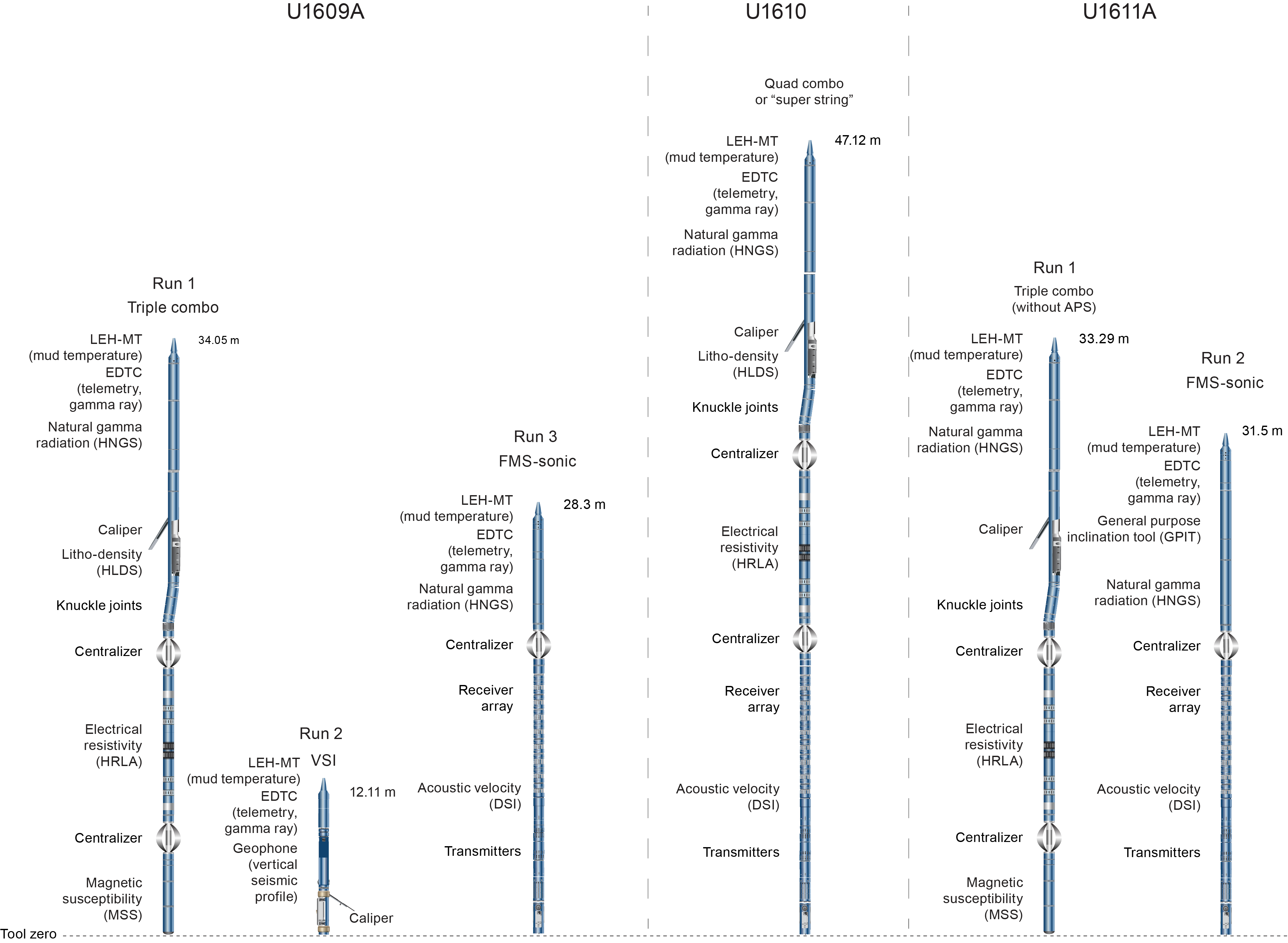
Figure F20. Downhole logging tool strings.
Regardless of the sea state, a wireline heave compensator (WHC) was normally deployed during the wireline logging operations to compensate for vertical motion, maintain a steady motion of the logging tools, and ensure high-quality data acquisition (Liu et al., 2013; Iturrino et al., 2013). However, the heave compensator was not employed at Site U1609 because of technical problems with the computer that runs the compensator's software. The WHC uses a vertical accelerometer (motion reference unit [MRU]) positioned under the rig floor near the ship's center of gravity to calculate the vertical motion of the ship with respect to the seafloor. The length of the wireline is adjusted by varying the distance between two sets of pulleys through which the cable passes to minimize downhole tool motion. Real-time measurements of uphole (surface) and downhole acceleration are made simultaneously by the MRU and Enhanced Digital Telemetry Cartridge (EDTC), respectively, and software analyzes and compares the real-time data to monitor the efficiency of the compensator.
7.2. Logging tool measurement principles
The logged properties of the geologic formations and petrophysical principles used in the measurement tools are described hereafter. More detailed information on individual tools and their petrophysical/geologic applications can be found in Serra (1984, 1986, 1989), Schlumberger (1989, 1994), Rider (1996), Goldberg (1997), Lovell et al. (1998), and Ellis and Singer (2007).
7.2.1. Magnetic Susceptibility Sonde
Magnetic susceptibility (MS) is the ease with which formations are magnetized when subjected to a magnetic field. The ease of magnetization is related to the size, distribution, and composition of magnetic minerals in the formation (e.g., magnetite). These measurements are extremely useful for stratigraphic analyses. MS can also be used to resolve astronomical cyclicity of sedimentary changes at the drilling sites and correlate between holes on a regional scale, thereby illuminating the depositional history of a wider area.
The Magnetic Susceptibility Sonde (MSS) is run as the lowest logging tool in the triple combo tool string (Figure F20) and therefore collects one of the largest open hole coverages of all the logging tools. The MSS uses a single-coil sensor to measure borehole MS in approximate SI units referred to here as noncalibrated instrument units (IU) at a vertical resolution of ~12 cm with shallow (~3 cm) depth of penetration. A lower resolution (~36 cm) but greater depth of penetration (36 cm) is also collected, which provides a quality check for the higher resolution reading. The sensor of the MSS is an electric inductor constructed such that when positioned against the borehole wall its inductance is affected by the volume susceptibility of the formation within the measured formation rock volume. The tool is calibrated to a 9⅞ inch borehole diameter, and larger or washed-out holes will result in lower susceptibility measurements, whereas higher temperatures lead to higher susceptibility measurements. Temperature measurements were not run alongside the MSS. For QC and environmental corrections, the MSS also measures internal tool temperature, z-axis acceleration, and low-resolution borehole conductivity.
7.2.2. Electrical resistivity
Resistivity is measured to aid in identifying poorly recovered sections of the hole because different materials have different electrical conductivities. It can also be used to evaluate porosity for a given salinity and resistivity of interstitial water using Archie's equation.
The HRLA tool records six resistivity measurements across different depths of investigation, including the borehole (mud) resistivity and five measurements of formation resistivity with increasing depth of penetration into the formation. The sonde sends a focused electric current into the formation and measures the intensity necessary to maintain a constant drop in voltage across a fixed interval, providing direct resistivity measurements. The array has one central (source) electrode and six electrodes above and below it that serve alternatively as focusing and returning current electrodes. By rapidly changing the roles of these electrodes, a simultaneous resistivity measurement at six penetration depths is achieved. The tool is designed to ensure that all signals are measured at exact times and tool positions. This reduces the sensitivity to "shoulder bed" effects when crossing sharp beds thinner than the electrode spacing. The design of the HRLA eliminates the need for a surface reference electrode, which improves formation resistivity evaluation compared to traditional dual induction and allows the full range of resistivity to be measured from low (e.g., in high-porosity sediments) to high (e.g., in basalt). The HRLA is run centralized in the borehole for optimal results. Knuckle joints are used to centralize the HRLA while allowing the density tool to maintain good contact with the borehole wall. Three depths of investigation, including shallow (RLA1), medium (RLA3), and true (RT_HRLT) resistivity measurements are presented in the Downhole measurements section in each site chapter, with RT_HRLT representing an estimate of the true formation from the area least influenced by drilling fluid invasion.
7.2.3. Density and photoelectric factor
Formation density is measured with the HLDS. The HLDS contains a cesium (137Cs) gamma ray source (662 keV) and far and near gamma ray detectors mounted on a shielded skid that is pressed against the borehole wall by a hydraulically activated decentralizing arm. The tool emits gamma radiation, which undergoes Compton scattering, and the gamma ray signal received by the detectors is proportional to the density of electrons in the formation, which is in turn related to bulk density and porosity (the latter requires that matrix or grain density is known). The density log is also particularly important for identifying clay-bearing rocks, which suffer from poor neutron porosity determinations because of clay-bound water. Throughout this report, wireline bulk density is presented as the HLDS corrected bulk density (RHOM) in grams per cubic centimeter.
The HLDS also computes the photoelectric effect (PEF), a measure of the photoelectric absorption of low-energy gamma radiation. Photoelectric absorption occurs when the energy of the gamma rays falls below 150 keV as a result of scattering by electrons in the formation. PEF is determined by comparing the counts from the far detector in the high-energy region, where only Compton scattering occurs, to those in the low-energy region, where count rates depend on both reactions. Because PEF depends on the atomic number of the elements in the formation (heavier elements have higher PEF), it also varies according to the chemical composition of the minerals present and can aid assessment of the matrix mineralogy formation (Serra, 1984; Schlumberger, 1989). The PEF delivers data in barns per electron units and requires good contact between the tool and the borehole wall; poor contact results in underestimation of density values. Both the density correction and caliper measurement of the hole are used to check hole conditions and assess likely contact quality. Barium in the logging mud can distort PEF signals even with corrections for mud effects and should therefore be treated with extra caution in poor hole conditions.
7.2.4. Natural gamma radiation
The Hostile environment Natural Gamma ray Sonde (HNGS) measures the natural gamma radiation of a formation. Two bismuth germanate scintillation detectors in the HNGS tool string measure potassium (weight percent), thorium (parts per million), and uranium (parts per million) concentrations from the characteristic gamma ray energies of isotopes in the 40K, 232Th, and 238U radioactive decay series that dominate the natural radiation spectrum. In addition to the HNGS, the EDTC also houses a total gamma ray sensor. The computation of the elemental abundances uses a least-squares method of extracting U, Th, and K elemental concentrations from the spectral measurements. The HNGS filters out gamma ray energies below 500 keV, eliminating sensitivity to bentonite or KCl in the drilling mud and thus improving measurement accuracy. The inclusion of a gamma ray tool in every tool string allows the use of gamma ray data for precise depth matching between logging runs, aids core-log integration, and enables precise identification of the seafloor. Standard (total) gamma ray is reported as total spectral gamma ray (HSGR) in American Petroleum Institute gamma radiation (gAPI) units throughout the Downhole measurements section in each site chapter. The HNGS response is influenced by borehole diameter and requires borehole diameter corrections (caliper derived) during acquisition.
7.2.5. Acoustic velocity
The sound velocity through formations is measured by the DSI, which generates acoustic pulses from various sonic transmitters and records the waveforms with an array of eight receivers. The waveforms are then used to calculate sonic VP and VS velocities in the formation. The omnidirectional monopole transmitter emits high-frequency (5–15 kHz) pulses to extract the VP of the formation, as well as VS when it is faster than the sound velocity in the borehole fluid. The DSI also has two cross-dipole transmitters that allow an additional measurement of shear wave velocity in slow (e.g., poorly consolidated) formations, where VS is slower than the velocity in the borehole fluid. The waveforms produced by the two orthogonal dipole transducers can be used to identify sonic anisotropy that can potentially be associated with variations in the local stress regime. The direct measurement is a combination of replicate measurements and therefore is relatively free from the effects of formation damage and an enlarged borehole (Schlumberger, 1989).
7.2.6. Versatile Seismic Imager
The VSI consists of three parts (a measurement sonde, power cartridge, and control cartridges). The configuration of the tool, including the number of sensor packages, sensor spacing, and type of connection, can all be varied to optimize acquisition for specific hole targets. The VSI was deployed only in Hole U1609A (Figure F20). During the VSP experiment performed during Expedition 401, the VSI was anchored against the borehole wall at regularly spaced intervals (20–50 m depending on borehole conditions) to record the full waveform of elastic waves generated by the seismic source positioned just below the sea surface. A total of 5–10 air gun shots were taken at each station. These check shot measurements relate depth in the hole to traveltime in seismic reflection profiles. The recorded waveforms were stacked, and one-way traveltime was determined from the median of the first breaks for each station.
The seismic air guns used were two 250 inch3 Sercel G guns in parallel clusters separated by 1 m and fired at 2000 psi. The source was positioned on the port side of JOIDES Resolution at ~3–5 meters below sea level (mbsl) with a horizontal borehole offset of ~47.5 m. Precautions were taken to protect marine mammals and diving birds following the restrictions in place for seismic surveys. If there were no such fauna in or approaching the safety radius (940 m for water depths over 1000 m and 1850 m for water depths between 100 and 1000 m), air gun operations commenced using a ramp-up or "soft start" procedure (gradually increasing the operational pressure and air gun firing interval) to guarantee enough time for undetected fauna to respond to the sounds and vacate the area. Once the guns were at full power, the check shot survey proceeded. Observations for relevant wildlife continued during the check shot survey, and the survey was suspended when marine mammals or diving birds entered the safety radius or if visibility conditions decreased. For sites where downhole sonic logs and VSI data were acquired, a direct measurement of the depth-traveltime relationship is given by the first arrival times in the zero-offset VSP (see above). These initial depth-traveltime results are useful for a preliminary borehole-seismic tie and also serve as the foundation for postcruise analysis.
7.2.7. Borehole inclination measurements
The inclination of the borehole at Sites U1609 and U1610 was recorded by the LEH-MT tool integrated within the top of the triple combo tool string (Figure F20). Because of the challenges of matching the borehole to the seismic data resulting from the significant borehole inclination encountered at Site U1610, at Site U1611 a General Purpose Inclination Tool (GPIT) was added to the Run 2 FMS-sonic tool string. This tool monitors both the inclination and the azimuth of the borehole (Figure F20).
7.3. Logging data flow, data quality, and log processing
Data for each wireline logging run were monitored in real time and recorded using the Schlumberger MAXIS 500 system. Logging measurement depth is determined from the length of the cable payout from the winch on the ship, and the depth scale is referred to as wireline log depth below rig floor (WRF) in meters below rig floor (mbrf). The seafloor is usually identified on the HSGR log by the abrupt upward reduction in gamma ray count at the water/sediment interface (mudline), and the seafloor depth is subtracted to give the wireline depth below seafloor (WSF). Discrepancies between DSF and WSF depth scales may occur because of incomplete heave compensation, incomplete correction for cable stretch, and cable slip. The correlation among different properties including MSS and HSGR was used to determine the correct seafloor depth.
The most determining factors influencing the log data quality are the condition of the borehole wall and the vertical movement of the ship. Where the borehole diameter varies over short intervals because of washouts of softer material or ledges of harder material, the logs from tools that require good contact with the borehole wall may be degraded. "Bridged" sections, where borehole diameter is significantly below the bit size, also cause irregular log results. The quality of the borehole is improved by minimizing the circulation of drilling fluid while drilling, flushing the borehole to remove debris, and logging as soon as possible after drilling and conditioning are completed.
Following acquisition, the collected data were sent to the Lamont-Doherty Earth Observatory (LDEO) for standardized processing. All raw logging data were first depth matched to the total gamma ray logging value from the main pass of the triple combo logging run. Prominent features were matched manually between gamma ray in all tool runs and the reference gamma ray log, and then all logging data in the same tool run were depth shifted by the same set of corrections. All depth-matched logs were then shifted to the seafloor (0 m) as defined by the clear increase in gamma ray for this transition, resulting in the common depth reference wireline log matched depth below seafloor (WMSF) in meters. The Schlumberger GeoQuest's GeoFrame software package was used for most of the wireline log data processing. Standard borehole size environmental corrections were applied to the HNGS (gamma ray), HRLA (resistivity), and HLDS (density/photoelectric) of the triple combo tool string automatically during acquisition and quality checked by the Schlumberger wireline technician on board. The DSI was operated in the monopole P-wave/S-wave, upper and lower dipole, and Stoneley modes during acquisition for all passes. Additional processing includes corrections to certain tools and logs, log documentation including assessment of log quality, and data format conversion to ASCII and GIF. Data were delivered back to the ship for visualization and interpretation as processed digital log information standard (DLIS) format image log files. Expedition 401 shipboard scientists uploaded, plotted, and interpreted the processed data using Schlumberger Techlog and Petrel software.
7.4. Downhole formation temperature
In situ temperature measurements were made with the advanced piston corer temperature (APCT-3) tool (Heesemann et al., 2006). The APCT-3 tool is composed of a battery pack, data logger, and platinum resistance-temperature device calibrated over a temperature range of 0°–30°C. This instrument perfectly fits into the coring shoe of the advanced piston corer (APC) system. Upon deployment, the APCT-3 tool is halted at the mudline for 5 min to thermally equilibrate with bottom water before entering the borehole. Frictional heating is created as the APCT-3 moves into the formation causing instantaneous temperature increases. This heat gradually dissipates into the surrounding sediment as the APCT-3 tool equilibrates to the temperature of the formation. Then the APCT-3 tool is held in place for ~10 min while it acquires the temperature of the cutting shoe every second.
The equilibrium temperature of the sediment is estimated by applying a mathematical heat-conduction model to the temperature decay record (Horai and Von Herzen, 1985). The synthetic thermal decay curve for the APCT-3 is a function of the geometry and thermal properties of the probe and the sediment (Bullard, 1954; Horai and Von Herzen, 1985). Equilibrium temperature is estimated according to a fitting procedure (Pribnow et al., 2000). However, if the APC does not achieve a full stroke or if the ship pulls the APC up from full penetration, the temperature equilibration curve is disturbed, and the temperature determination is thus not accurate. The nominal accuracy of APCT-3 temperature measurements is ±0.05°C.
APCT-3 downhole temperature data are finally combined with thermal conductivity measurements (see Physical properties) obtained from the central section of each individual core. Heat flow is estimated according to the Bullard method to be consistent with the synthesis of Ocean Drilling Program (ODP) heat flow data by Pribnow et al. (2000).
References
Acton, G., Morris, A., Musgrave, R., Zhao, X., and IODP SRM Personnel, 2017. Assessment of the New Superconducting Rock Magnetometer (SRM) on the JOIDES Resolution. http://iodp.tamu.edu/publications/JRSO/SRM_Workshop_2017.pdf
Anthonissen, E.D., 2009. A new Pliocene biostratigraphy for the northeastern North Atlantic. Newsletters on Stratigraphy, 43/2:91–126. https://doi.org/10.1127/0078-0421/2009/0043-0091
ASTM International, 1990. Standard method for laboratory determination of water (moisture) content of soil and rock (Standard D2216–90). In Annual Book of ASTM Standards for Soil and Rock Philadelphia (American Society for Testing Materials).
Ausín, B., Hodell, D.A., Cutmore, A., and Eglinton, T.I., 2020. The impact of abrupt deglacial climate variability on productivity and upwelling on the southwestern Iberian margin. Quaternary Science Reviews, 230:106139. https://doi.org/10.1016/j.quascirev.2019.106139
Backman, J., and Raffi, I., 1997. Calibration of Miocene nannofossil events to orbitally tuned cyclostratigraphies from Ceara Rise. In Shackleton, N.J., Curry, W.B., Richter, C., and Bralower, T.J. (Eds.), Proceedings of the Ocean Drilling Program, Scientific Results. 154: College Station, TX (Ocean Drilling Program), 83–99. https://doi.org/10.2973/odp.proc.sr.154.101.1997
Backman, J., Raffi, I., Rio, D., Fornaciari, E., and Pälike, H., 2012. Biozonation and biochronology of Miocene through Pleistocene calcareous nannofossils from low and middle latitudes. Newsletters on Stratigraphy, 45(3):221–244. https://doi.org/10.1127/0078-0421/2012/0022
Balestra, B., Flores, J.A., Hodell, D.A., Hernández Molina, F.J., and Stow, D.A.V., 2015. Pleistocene calcareous nannofossil biochronology at IODP Site U1385 (Expedition 339). Global and Planetary Change, 135:57–65. https://doi.org/10.1016/j.gloplacha.2015.10.004
Balestra, B., Grunert, P., Ausin, B., Hodell, D., Flores, J.A., Alvarez-Zarikian, C.A., Hernández-Molina, F.J., Stow, D., Piller, W.E., and Paytan, A., 2017. Coccolithophore and benthic foraminifera distribution patterns in the Gulf of Cadiz and Western Iberian Margin during Integrated Ocean Drilling Program (IODP) Expedition 339. Journal of Marine Systems, 170:50–67. https://doi.org/10.1016/j.jmarsys.2017.01.005
Balsam, W.L., and Damuth, J.E., 2000. Further investigations of shipboard vs. shore-based spectral data: implications for interpreting Leg 164 sediment composition. In Paull, C.K., Matsumoto, R., Wallace, P.J., Dillon, W.P. (Eds.), Proceedings of the Ocean Drilling Program, Scientific Results. 164: College Station, TX (Ocean Drilling Program), 314–324. https://doi.org/10.2973/odp.proc.sr.164.222.2000
Balsam, W.L., Damuth, J.E., and Schneider, R.R., 1997. Comparison of shipboard vs. shore-based spectral data from Amazon Fan cores: implications for interpreting sediment composition. In Flood, R.D., Piper, D.J.W., Klaus, A., and Peterson, L.C. (Eds.), Proceedings of the Ocean Drilling Program, Scientific Results. 155: College Station, TX (Ocean Drilling Program), 193–215. https://doi.org/10.2973/odp.proc.sr.155.210.1997
Balsam, W.L., Deaton, B.C., and Damuth, J.E., 1998. The effects of water content on diffuse reflectance spectrophotometry studies of deep-sea sediment cores. Marine Geology, 149(1):177–189. https://doi.org/10.1016/S0025-3227(98)00033-4
Bann, K.L., Fielding, C.R., MacEachern, J.A., and Tye, S.C., 2004. Differentiation of estuarine and offshore marine deposits using integrated ichnology and sedimentology: Permian Pebbley Beach Formation, Sydney Basin, Australia. Geological Society, London, Special Publications, 228(1):179–211. https://doi.org/10.1144/GSL.SP.2004.228.01.10
Berggren, W.A., Kent, D.V., Swisher, C.C., III, Aubry, M.-P., Berggren, W.A., Kent, D.V., Aubry, M.-P., and Hardenbol, J., 1995. A revised Cenozoic geochronology and chronostratigraphy. In Berggren, W.A., Kent, D.V., Aubry, M.-P., and Hardenbol, J. (Eds.), Geochronology, Time Scales and Global Stratigraphic Correlation. SEPM Special Publication, 54. https://doi.org/10.2110/pec.95.04.0129
Blum, P., 1997. Physical properties handbook: a guide to the shipboard measurement of physical properties of deep-sea cores. Ocean Drilling Program Technical Note, 26. https://doi.org/10.2973/odp.tn.26.1997
Boggs, S., 2001. Principles of Sedimentology and Stratigraphy (3rd edition): Eugene, OR (Pearson Prentice Hall).
Boltovskoy, E., Giussani, G., Watanabe, S., and Wright, R., 1980. Atlas of Benthic Shelf Foraminifera of the Southwest Atlantic: Dordrecht, Netherlands (Springer). https://doi.org/10.1007/978-94-009-9188-0
Bulian, F., Jiménez-Espejo, F.J., Andersen, N., Larrasoaña, J.C., and Sierro, F.J., 2023. Mediterranean water in the Atlantic Iberian margin reveals early isolation events during the Messinian Salinity Crisis. Global and Planetary Change, 231:104297. https://doi.org/10.1016/j.gloplacha.2023.104297
Bullard, E.C., 1954. The flow of heat through the floor of the Atlantic Ocean. Proceedings of the Royal Society of London, A: Mathematical and Physical Sciences, 222(1150):408–429. https://doi.org/10.1098/rspa.1954.0085
Chaisson, W.P., and Leckie, R.M., 1993. High-resolution Neogene planktonic foraminifer biostratigraphy of Site 806, Ontong Java Plateau (western equatorial Pacific). In Berger, W.H., Kroenke, L.W., Mayer, L.A., et al., Proceedings of the Ocean Drilling Program, Scientific Results. 130: College Station, TX (Ocean Drilling Program), 137–178. https://doi.org/10.2973/odp.proc.sr.130.010.1993
Chaisson, W.P., and Pearson, P.N., 1997. Planktonic foraminifer biostratigraphy at Site 925: middle Miocene-Pleistocene. In Shackleton, N.J., Curry, W.B., Richter, C., and Bralower, T.J. (Eds.), Proceedings of the Ocean Drilling Program, Scientific Results. 154: College Station, TX (Ocean Drilling Program), 3–31. https://doi.org/10.2973/odp.proc.sr.154.104.1997
Cook, H.E., Johnson, P.D., Matti, J.C., and Zemmels, I., 1975. Methods of sample preparation and X-ray diffraction data analysis, X-ray Mineralogy Laboratory, Deep Sea Drilling Project, University of California, Riverside. In Hayes, D.E., Franes, L.A., et al., Initial Reports of the Deep Sea Drilling Project. 28: Washington, DC (US Government Printing Office), 999–1007. https://doi.org/10.2973/dsdp.proc.28.app4.1975
Curry, W.B., Shackleton, N.J., Richter, C, et al., 1995. Proceedings of the Ocean Drilling Program, Initial Reports: College Station, TX (Ocean Drilling Program). https://doi.org/10.2973/odp.proc.ir.154.1995
Dickson, J.A.D., 1965. A modified staining technique for carbonates in thin section. Nature, 205(4971):587. https://doi.org/10.1038/205587a0
Di Stefano, A., and Sturiale, G., 2010. Refinements of calcareous nannofossil biostratigraphy at the Miocene/Pliocene Boundary in the Mediterranean region. Geobios, 43(1):5–20. https://doi.org/10.1016/j.geobios.2009.06.007
Dunlea, A.G., Murray, R.W., Harris, R.N., Vasiliev, M.A., Evans, H., Spivack, A.J., and D'Hondt, S., 2013. Assessment and use of NGR instrumentation on the JOIDES Resolution to quantify U, Th, and K concentrations in marine sediment. Scientific Drilling, 15:57–63. https://doi.org/10.2204/iodp.sd.15.05.2013
Ellis, D.V., and Singer, J.M., 2007. Well Logging for Earth Scientists (2nd edition): New York (Elsevier). https://doi.org/10.1007/978-1-4020-4602-5
Ellwood, B.B., 1980. Induced and remanent magnetic properties of marine sediments as indicators of depositional processes. Marine Geology, 38(1):233–244. https://doi.org/10.1016/0025-3227(80)90061-4
Evans, H.B., 1995. GRAPE* - A Device For Continuous Determination Of Material Density And Porosity. Presented at the SPWLA 6th Annual Logging Symposium (Volume II).
Expedition 303 Scientists, 2006. Site U1302–U1308 methods. In Channell, J.E.T., Kanamatsu, T., Sato, T., Stein, R., Alvarez Zarikian, C.A., Malone, M.J., and the Expedition 303/306 Scientists, Proceedings of the Integrated Ocean Drilling Program. 303/306: College Station, TX (Integrated Ocean Drilling Program Management International, Inc.). https://doi.org/10.2204/iodp.proc.303306.102.2006
Expedition 339 Scientists, 2013. Site U1385. In Stow, D.A.V., Hernández-Molina, F.J., Alvarez Zarikian, C.A., and the Expedition 339 Scientists, Proceedings of the Integrated Ocean Drilling Program. 339: Tokyo (Integrated Ocean Drilling Program Management International, Inc.). https://doi.org/10.2204/iodp.proc.339.103.2013
Flecker, R., Ducassou, E., Williams, T., Amarathunga, U., Balestra, B., Berke, M.A., Blättler, C.L., Chin, S., Das, M., Egawa, K., Fabregas, N., Feakins, S.J., George, S.C., Hernández-Molina, F.J., Krijgsman, W., Li, Z., Liu, J., Noto, D., Raad, F., Rodríguez-Tovar, F.J., Sierro, F.J., Standring, P., Stine, J., Tanaka, E., Teixeira, M., Xu, X., Yin, S., and Yousfi, M.Z., 2025a. Site U1610. In Flecker, R., Ducassou, E., Williams, T., and the Expedition 401 Scientists, Mediterranean–Atlantic Gateway Exchange. Proceedings of the International Ocean Discovery Program, 401: College Station, TX (International Ocean Discovery Program). https://doi.org/10.14379/iodp.proc.401.104.2025
Flecker, R., Ducassou, E., Williams, T., Amarathunga, U., Balestra, B., Berke, M.A., Blättler, C.L., Chin, S., Das, M., Egawa, K., Fabregas, N., Feakins, S.J., George, S.C., Hernández-Molina, F.J., Krijgsman, W., Li, Z., Liu, J., Noto, D., Raad, F., Rodríguez-Tovar, F.J., Sierro, F.J., Standring, P., Stine, J., Tanaka, E., Teixeira, M., Xu, X., Yin, S., and Yousfi, M.Z., 2025b. Site U1611. In Flecker, R., Ducassou, E., Williams, T., and the Expedition 401 Scientists, Mediterranean–Atlantic Gateway Exchange. Proceedings of the International Ocean Discovery Program, 401: College Station, TX (International Ocean Discovery Program). https://doi.org/10.14379/iodp.proc.401.106.2025
Flecker, R., Ducassou, E., Williams, T., and the Expedition 401 Scientists, 2025c. Supplementary material, https://doi.org/10.14379/iodp.proc.401supp.2025. In Flecker, R., Ducassou, E., Williams, T., and the Expedition 401 Scientists, Mediterranean–Atlantic Gateway Exchange. Proceedings of the International Ocean Discovery Program, 401: College Station, TX (International Ocean Discovery Program).
Flood, R.D., 1978. X-ray mineralogy of DSDP Legs 44 and 44A, western North Atlantic; lower continental rise hills, Blake Nose, and Blake-Bahama Basin. In Benson, W.E., Sheridan, R.E., et al., Initial Reports of the Deep Sea Drilling Project. 44: Washington, DC (US Government Printing Office), 515–521. https://doi.org/10.2973/dsdp.proc.44.112.1978
Gartner, S., 1977. Nannofossils and biostratigraphy: an overview. Earth-Science Reviews, 13(3):227–250. https://doi.org/10.1016/0012-8252(77)90001-0
Gieskes, J.M., Gamo, T., and Brumsack, H.J., 1991. Chemical methods for interstitial water analysis aboard JOIDES Resolution. Ocean Drilling Program Technical Note, 15. https://doi.org/10.2973/odp.tn.15.1991
Gilmore, G.R., 2008. Practical Gamma‐Ray Spectrometry: Hoboken, NJ (John Wiley & Sons). https://doi.org/10.1002/9780470861981.fmatter
Goldberg, D., 1997. The role of downhole measurements in marine geology and geophysics. Reviews of Geophysics, 35(3):315–342. https://doi.org/10.1029/97RG00221
Graber, K.K., Pollard, E., Jonasson, B., and Schulte, E. (Eds.), 2002. Overview of Ocean Drilling Program engineering tools and hardware. Ocean Drilling Program Technical Note, 31. https://doi.org/10.2973/odp.tn.31.2002
Hamilton, E.L., 1970. Sound velocity and related properties of marine sediments, North Pacific. Journal of Geophysical Research, 75(23):4423–4446. https://doi.org/10.1029/JB075i023p04423
Hanagata, S., 2003. Miocene-Pliocene foraminifera from the Niigata oil-fields region, northeastern Japan. Micropaleontology, 49(4):293–340. https://doi.org/10.1661/0026-2803(2003)049[0293:MFFTNO]2.0.CO;2
Heesemann, M., Villinger, H.W., Tréhu, A.T.F.M., and White, S., 2006. Data report: testing and deployment of the new APCT-3 tool to determine in situ temperatures while piston coring. In Riedel, M., Collett, T.S., Malone, M.J., and the Expedition 311 Scientists, Proceedings of the Integrated Ocean Drilling Program. 311: Washington, DC (Integrated Ocean Drilling Program Management International, Inc.). https://doi.org/10.2204/iodp.proc.311.108.2006
Hilgen, F., Aziz, H.A., Bice, D., Iaccarino, S., Krijgsman, W., Kuiper, K., Montanari, A., Raffi, I., Turco, E., and Zachariasse, W.-J., 2005. The global boundary stratotype section and point (GSSP) of the Tortonian Stage (Upper Miocene) at Monte Dei Corvi. International Union of Geological Sciences, 28(1):6–17. https://doi.org/10.18814/epiiugs/2005/v28i1/001
Hilgen, F.J., 1991a. Astronomical calibration of Gauss to Matuyama sapropels in the Mediterranean and implication for the Geomagnetic Polarity Time Scale. Earth and Planetary Science Letters, 104(2–4):226–244. https://doi.org/10.1016/0012-821X(91)90206-W
Hilgen, F.J., 1991b. Extension of the astronomically calibrated (polarity) time scale to the Miocene/Pliocene boundary. Earth and Planetary Science Letters, 107(2):349–368. https://doi.org/10.1016/0012-821X(91)90082-S
Hilgen, F.J., Bissoli, L., Iaccarino, S., Krijgsman, W., Meijer, R., Negri, A., and Villa, G., 2000a. Integrated stratigraphy and astrochronology of the Messinian GSSP at Oued Akrech (Atlantic Morocco). Earth and Planetary Science Letters, 182(3):237–251. https://doi.org/10.1016/S0012-821X(00)00247-8
Hilgen, F.J., Iaccarino, S., Krijgsman, W., Villa, G., Langereis, C.G., and Zachariasse, W.J. , 2000b. The global boundary stratotype section and point (GSSP) of the Messinian Stage (uppermost Miocene). Episodes Journal of International Geoscience, 23(3):172–178.
Hilgen, F.J., and Krijgsman, 1999. Cyclostratigraphy and astrochronology of the Tripoli diatomite formation (pre-evaporite Messinian, Sicily, Italy). Terra Nova, 11(1):16–22. https://doi.org/10.1046/j.1365-3121.1999.00221.x
Hilgen, F.J., Krijgsman, W., Langereis, C.G., Lourens, L.J., Santarelli, A., and Zachariasse, W.J., 1995. Extending the astronomical (polarity) time scale into the Miocene. Earth and Planetary Science Letters, 136(3):495–510. https://doi.org/10.1016/0012-821X(95)00207-S
Hilgen, F.J., Krijgsman, W., Raffi, I., Turco, E., and Zachariasse, W.J., 2000c. Integrated stratigraphy and astronomical calibration of the Serravallian/Tortonian boundary section at Monte Gibliscemi (Sicily, Italy). Marine Micropaleontology, 38(3–4):181–211. https://doi.org/10.1016/S0377-8398(00)00008-6
Hodell, D.A., Curtis, J.H., Sierro, F.J., and Raymo, M.E., 2001. Correlation of Late Miocene to Early Pliocene sequences between the Mediterranean and North Atlantic. Paleoceanography, 16(2):164–178. https://doi.org/10.1029/1999PA000487
Holbourn, A., Henderson, A.S., and MacLeod, N., 2013. Atlas of Benthic Foraminifera: United Kingdom (John Wiley & Sons, Ltd.). https://doi.org/10.1002/9781118452493
Horai, K., and Von Herzen, R.P., 1985. Measurement of heat flow on Leg 86 of the Deep Sea Drilling Project. In Heath, G.R., Burckle, L. H., et al., Initial Reports of the Deep Sea Drilling Project. 86: Washington, DC (US Government Printing Office), 759–777. https://doi.org/10.2973/dsdp.proc.86.135.1985
Hüsing, S.K., Kuiper, K.F., Link, W., Hilgen, F.J., and Krijgsman, W., 2009. The upper Tortonian–lower Messinian at Monte dei Corvi (Northern Apennines, Italy): completing a Mediterranean reference section for the Tortonian Stage. Earth and Planetary Science Letters, 282(1):140–157. https://doi.org/10.1016/j.epsl.2009.03.010
Iturrino, G., Liu, T., Goldberg, D., Anderson, L., Evans, H., Fehr, A., Guerin, G., Inwood, J., Lofi, J., Malinverno, A., Morgan, S., Mrozewski, S., Slagle, A., and Williams, T., 2013. Performance of the wireline heave compensation system onboard D/V JOIDES Resolution. Scientific Drilling, 15:46–50. https://doi.org/10.2204/iodp.sd.15.08.2013
Jones, R.W., 1994. The Challenger Foraminifera: Oxford, UK (Oxford University Press).
Jorissen, F.J., Fontanier, C., and Thomas, E., 2007. Paleoceanographical proxies based on deep-sea benthic foraminiferal assemblage characteristics. In Hillaire–Marcel, C., and De Vernal, A. (Eds.), Developments in Marine Geology (Volume 7): Earth and Life Processes Discovered from Subseafloor Environments: A Decade of Science Achieved by the Integrated Ocean Drilling Program (IODP). R. Stein (Series Ed.). Amsterdam (Elsevier), 263–325. https://doi.org/10.1016/S1572-5480(07)01012-3
Jumikis, A.R., 1966. Thermal Soil Mechanics: New Brunswick, NJ (Rutgers University Press).
Jutzeler, M., White, J.D.L., Talling, P.J., McCanta, M., Morgan, S., Le Friant, A., and Ishizuka, O., 2014. Coring disturbances in IODP piston cores with implications for offshore record of volcanic events and the Missoula megafloods. Geochemistry, Geophysics, Geosystems, 15(9):3572–3590. https://doi.org/10.1002/2014GC005447
Kennett, J.P., and Srinivasan, M.S., 1983. Neogene Planktonic Foraminifera: A Phylogenetic Atlas: London (Hutchinson Ross).
Knaust, D., 2017. Atlas of Trace Fossils in Well Core: Cham, Switzerland (Springer). https://doi.org/10.1007/978-3-319-49837-9
Krijgsman, W., Gaboardi, S., Hilgen, F.J., Iaccarino, S., de Kaenel, E., and van der Laan, E., 2004. Revised astrochronology for the Ain el Beida section (Atlantic Morocco): No glacio-eustatic control for the onset of the Messinian Salinity Crisis. Stratigraphy, 1(1):87–101. http://dx.doi.org/10.29041/strat.01.1.05
Krijgsman, W., Hilgen, F.J., Raffi, I., Sierro, F.J., and Wilson, D.S., 1999. Chronology, causes and progression of the Messinian salinity crisis. Nature, 400(6745):652–655. https://doi.org/10.1038/23231
Kristiansen, J.I., 1982. The transient cylindrical probe method for determination of thermal parameters of earth materials [PhD dissertation]. Åarhus University, Åarhus, Denmark. http://digitallib.oit.edu/digital/collection/geoheat/id/2103/
Lancis, C., and Flores, J.-A., 2006. A new biostratigraphically significant calcareous nannofossil species in the Early Pliocene of the Mediterranean. Micropaleontology, 52(5):477–481. https://doi.org/10.2113/gsmicropal.52.5.477
Langereis, C.G., and Hilgen, F.J., 1991. The Rossello composite: a Mediterranean and global reference section for the Early to early Late Pliocene. Earth and Planetary Science Letters, 104(2):211–225. https://doi.org/10.1016/0012-821X(91)90205-V
Lirer, F., Foresi, L.M., Iaccarino, S.M., Salvatorini, G., Turco, E., Cosentino, C., Sierro, F.J., and Caruso, A., 2019. Mediterranean Neogene planktonic foraminifer biozonation and biochronology. Earth-Science Reviews, 196:102869. https://doi.org/10.1016/j.earscirev.2019.05.013
Liu, Q., Roberts, A.P., Larrasoaña, J.C., Banerjee, S.K., Guyodo, Y., Tauxe, L., and Oldfield, F., 2012. Environmental magnetism: principles and applications. Reviews of Geophysics, 50(4):RG4002. https://doi.org/10.1029/2012RG000393
Liu, T., Iturrino, G., Goldberg, D., Meissner, E., Swain, K., Furman, C., Fitzgerald, P., Frisbee, N., Chlimoun, J., Van Hyfte, J., and Beyer, R., 2013. Performance evaluation of active wireline heave compensation systems in marine well logging environments. Geo-Marine Letters, 33(1):83–93. https://doi.org/10.1007/s00367-012-0309-8
Loeblich, A.R., and Tappan, H., 1984. Suprageneric classification of the Foraminiferida (Protozoa). Micropaleontology, 30(1):1–70. https://pubs.geoscienceworld.org/micropress/micropal/article/30/1/1/84777/Suprageneric-classification-of-the-Foraminiferida
Lourens, L., Hilgen, F., Shackleton, N.J., Laskar, J., and Wilson, D., 2004. The Neogene period. In Smith, A.G., Gradstein, F.M. and Ogg, J.G., A Geologic Time Scale 2004. Cambridge, UK (Cambridge University Press), 409–440. https://doi.org/10.1017/CBO9780511536045.022
Lourens, L.J., Antonarakou, A., Hilgen, F.J., Van Hoof, A.A.M., Vergnaud-Grazzini, C., and Zachariasse, W.J., 1996a. Evaluation of the Plio-Pleistocene astronomical timescale. Paleoceanography, 11(4):391–413. https://doi.org/10.1029/96PA01125
Lourens, L.J., Hilgen, F.J., and Raffi, I., 1998. Base of large Gephyrocapsa and astronomical calibration of early Pleistocene sapropels in Site 967 and Hole 969D: solving the chronology of the Vrica Section (Calabria, Italy). In Robertson, A.H.F., Emeis, K.-C., Richter, C., and Camerlenghi, A. (Eds.), Proceedings of the Ocean Drilling Program, Scientific Results. 160: College Station, TX (Ocean Drilling Program), 191. https://doi.org/10.2973/odp.proc.sr.160.017.1998
Lourens, L.J., Hilgen, F.J., Raffi, I., and Vergnaud-Grazzini, C., 1996b. Early Pleistocene chronology of the Vrica Section (Calabria, Italy). Paleoceanography, 11(6):797–812. https://doi.org/10.1029/96PA02691
Lovell, M.A., Harvey, P.K., Brewer, T.S., Williams, C., Jackson, P.D., and Williamson, G., 1998. Application of FMS images in the Ocean Drilling Program: an overview. In Cramp, A., MacLeod, C.J., Lee, S.V., and Jones, E.J.W. (Eds.), Geological Evolution of Ocean Basins: Results from the Ocean Drilling Program. Geological Society, London, Special Publication, 131: 287–303. https://doi.org/10.1144/GSL.SP.1998.131.01.18
Manheim, F.T., and Sayles, F.L., 1974. Composition and origin of interstitial waters of marine sediments, based on deep sea drill cores. In Goldberg, E.D., The Sea (Volume 5): Marine Chemistry: The Sedimentary Cycle. New York (Wiley), 527–568. http://pubs.er.usgs.gov/publication/70207491
Marsaglia, K., Milliken, K., and Doran, L., 2013. IODP digital reference for smear slide analysis of marine mud, Part 1: Methodology and atlas of siliciclastic and volcanogenic components. Integrated Ocean Drilling Program Technical Note, 1. https://doi.org/10.2204/iodp.tn.1.2013
Marsaglia, K., Milliken, K., Leckie, R., Tentori, D., and Doran, L., 2015. IODP smear slide digital reference for sediment analysis of marine mud, Part 2: Methodology and atlas of biogenic components. Integrated Ocean Drilling Program Technical Note, 2. https://doi.org/10.2204/iodp.tn.2.2015
Martínez-Sánchez, M., Flores, J.-A., Palumbo, E., Alonso-Garcia, M., Sierro, F.-J., and Amore, F.O., 2019. Reconstruction of surface water dynamics in the North Atlantic during the Mid-Pleistocene (~540–400 ka), as inferred from coccolithophores and planktonic foraminifera. Marine Micropaleontology, 152:101730. https://doi.org/10.1016/j.marmicro.2019.03.002
Martini, E., 1971. Standard Tertiary and Quaternary calcareous nannoplankton zonation. Proceedings of the Second Planktonic Conference, Roma, 1970:739–785.
Mazzullo, J., Meyer, A., and Kidd, R., 1988. Appendix I: New sediment classification scheme for the Ocean Drilling Program. In Mazzullo, J., and Graham, A.G. , Handbook for shipboard sedimentologists. Ocean Drilling Program Technical Note. 8: 44–67. https://doi.org/10.2973/odp.tn.8.1988
Morigi, C., Negri, A., Giunta, S., Kouwenhoven, T., Krijgsman, W., Blanc-Valleron, M.-M., Orszag-Sperber, F., and Rouchy, J.-M., 2007. Integrated quantitative biostratigraphy of the latest Tortonian–early Messinian Pissouri section (Cyprus): an evaluation of calcareous plankton bioevents. Geobios, 40(3):267–279. https://doi.org/10.1016/j.geobios.2007.02.002
Munsell Color Company, 2010. Munsell soil color charts: with genuine Munsell color chips: Grand Rapids, MI (Munsell Color). https://search.library.wisc.edu/catalog/9910109259802121
Murray, R.W., Miller, D.J., and Kryc, K.A., 2000. Analysis of major and trace elements in rocks, sediments, and interstitial waters by inductively coupled plasma–atomic emission spectrometry (ICP-AES). Ocean Drilling Program Technical Note, 29. https://doi.org/10.2973/odp.tn.29.2000
Ogg, J.G., 2020. Geomagnetic Polarity Time Scale. In Gradstein, F.M., Ogg, J.G., Schmitz, M., and Ogg, G. (Eds.), Geologic Time Scale 2020. Amsterdam (Elsevier), 159–192. https://doi.org/10.1016/B978-0-12-824360-2.00005-X
Okada, H., and Bukry, D., 1980. Supplementary modification and introduction of code numbers to the low-latitude coccolith biostratigraphic zonation (Bukry, 1973; 1975). Marine Micropaleontology, 5(3):321–325. https://doi.org/10.1016/0377-8398(80)90016-X
Perch-Nielsen, K., 1985. Cenozoic calcareous nannofossils. In Bolli, H.M., Saunders, J.B., and Perch-Nielsen, K. (Eds.), Plankton Stratigraphy (Volume 1). Cambridge, UK (Cambridge University Press), 427–554.
Pérez-Asensio, J.N., Aguirre, J., Schmiedl, G., and Civis, J., 2012. Messinian paleoenvironmental evolution in the lower Guadalquivir Basin (SW Spain) based on benthic foraminifera. Palaeogeography, Palaeoclimatology, Palaeoecology, 326–328:135–151. https://doi.org/10.1016/j.palaeo.2012.02.014
Pribnow, D.F.C., Kinoshita, M., and Stein, C.A., 2000. Thermal data collection and heat flow recalculations for ODP Legs 101–180: Hannover, Germany (Institute for Joint Geoscientific Research, GGA). http://www-odp.tamu.edu/publications/heatflow/
Raffi, I., 2002. Revision of the Early-Middle Pleistocene calcareous nannofossil biochronology (1.75–0.85 Ma). Marine Micropaleontology, 45(1):25–55. https://doi.org/10.1016/S0377-8398(01)00044-5
Raffi, I., Backman, J., Fornaciari, E., Pälike, H., Rio, D., Lourens, L., and Hilgen, F., 2006. A review of calcareous nannofossil astrobiochronology encompassing the past 25 million years. Quaternary Science Reviews, 25(23):3113–3137. https://doi.org/10.1016/j.quascirev.2006.07.007
Raffi, I., Backman, J., Rio, D., and Shackleton, N.J., 1993. Plio-Pleistocene nannofossil biostratigraphy and calibration to oxygen isotope stratigraphies from Deep Sea Drilling Project Site 607 and Ocean Drilling Program Site 677. Paleoceanography and Paleoclimatology, 8(3):387–408. https://doi.org/10.1029/93PA00755
Raffi, I., and Flores, J.-A., 1995. Pleistocene through Miocene calcareous nannofossils from eastern equatorial Pacific Ocean (Leg 138). In Pisias, N.G., Mayer, L.A., Janecek, T.R., Palmer-Julson, A., and van Andel, T.H. (Eds.), Proceedings of the Ocean Drilling Program, Scientific Results. 138: College Station, TX (Ocean Drilling Program), 233–286. https://doi.org/10.2973/odp.proc.sr.138.112.1995
Raffi, I., Mozzato, C., Fornaciari, E., Hilgen, F.J., and Rio, D., 2003. Late Miocene calcareous nannofossil biostratigraphy and astrobiochronology for the Mediterranean region. Micropaleontology, 49(1):1–26. https://doi.org/10.2113/49.1.1
Raffi, I., Rio, D., d'Atri, A., Fornaciari, E., and Rocchetti, S., 1995. Quantitative distribution patterns and biomagnetostratigraphy of middle and late Miocene calcareous nannofossils from equatorial Indian and Pacific oceans (Legs 115, 130, and 138). In Pisias, N.G., Mayer, L.A., Janecek, T.R., Palmer-Julson, A., and van Andel, T.H. (Eds.), Proceedings of the Ocean Drilling Program, Scientific Results. 138: College Station, TX (Ocean Drilling Program), 479–502. https://doi.org/10.2973/odp.proc.sr.138.125.1995
Raffi, I., Wade, B.S., Pälike, H., Beu, A.G., Cooper, R., Crundwell, M.P., Krijgsman, W., Moore, T., Raine, I., Sardella, R., and Vernyhorova, Y.V., 2020. The Neogene Period. In Gradstein, F.M., Ogg, J.G., Schmitz, M.D., and Ogg, G. (Eds.), Geologic Time Scale 2020. (Elsevier), 1141–1215. https://doi.org/10.1016/B978-0-12-824360-2.00029-2
Reineck, H.E., 1963. Sedimentgefüge im Bereich der südlichen Nordsee. Abhandlungen der Senckenbergischen Naturforschenden Gesellschaft, 505.
Rider, M.H., 1996. The Geological Interpretation of Well Logs (Second edition): Houston, TX (Gulf Publishing Company).
Rio, D., Raffi, I., and Villa, G., 1990. Pliocene-Pleistocene calcareous nannofossil distribution patterns in the western Mediterranean. In Kastens, K.A., Mascle, J., et al., Proceedings of the Ocean Drilling Program, Scientific Results. 107: College Station, TX (Ocean Drilling Program), 513–533. https://doi.org/10.2973/odp.proc.sr.107.164.1990
Rogalla, U., and Andruleit, H., 2005. Precessional forcing of coccolithophore assemblages in the northern Arabian Sea: implications for monsoonal dynamics during the last 200,000 years. Marine Geology, 217(1):31–48. https://doi.org/10.1016/j.margeo.2005.02.028
Rothwell, R.G., 1989. Minerals and Mineraloids in Marine Sediments: Dordrecht, Netherlands (Springer). https://doi.org/10.1007/978-94-009-1133-8
Schiebel, R., Smart, S.M., Jentzen, A., Jonkers, L., Morard, R., Meilland, J., Michel, E., Coxall, H.K., Hull, P.M., de Garidel-Thoron, T., Aze, T., Quillévéré, F., Ren, H., Sigman, D.M., Vonhof, H.B., Martínez-García, A., Kučera, M., Bijma, J., Spero, H.J., and Haug, G.H., 2018. Advances in planktonic foraminifer research: new perspectives for paleoceanography. Revue de Micropaléontologie, 61(3):113–138. https://doi.org/10.1016/j.revmic.2018.10.001
Schlumberger, 1989. Log Interpretation Principles/Applications, SMP-7017: Houston (Schlumberger Education Services).
Schlumberger, 1994. IPL Integrated Porosity Lithology, SMP-9270: Houston (Schlumberger Education Services).
Schönfeld, J., 2002. Recent benthic foraminiferal assemblages in deep high-energy environments from the Gulf of Cadiz (Spain). Marine Micropaleontology, 44(3):141–162. https://doi.org/10.1016/S0377-8398(01)00039-1
Schönfeld, J., and Zahn, R., 2000. Late Glacial to Holocene history of the Mediterranean Outflow. Evidence from benthic foraminiferal assemblages and stable isotopes at the Portuguese margin. Palaeogeography, Palaeoclimatology, Palaeoecology, 159(1–2):85–111. https://doi.org/10.1016/S0031-0182(00)00035-3
Serra, O., 1984. Fundamentals of Well-log Interpretation (Volume 1): The Acquisition of Logging Data: Amsterdam (Elsevier).
Serra, O., 1986. Fundamentals of Well-Log Interpretation (Volume 2): The Interpretation of Logging Data: Amsterdam (Elsevier).
Serra, O., 1989. Formation MicroScanner Image Interpretation, SMP-7028: Houston (Schlumberger Education Services).
Shackleton, N.J., and Crowhurst, S., 1997. Sediment fluxes based on an orbitally tuned time scale 5 Ma to 14 Ma, Site 926. In Shackleton, N.J., Curry, W.B., Richter, C., and Bralower, T.J. (Eds.), Proceedings of the Ocean Drilling Program, Scientific Results. 154: College Station, TX (Ocean Drilling Program), 69–82. https://doi.org/10.2973/odp.proc.sr.154.102.1997
Shackleton, N.J., Crowhurst, S., Hagelberg, T., Pisias, N.G., and Schneider, D.A., 1995. A new late Neogene time scale: application to Leg 138 sites. In Pisias, N.G., Mayer, L.A., Janecek, T.R., Palmer-Julson, A., and van Andel, T.H. (Eds.), Proceedings of the Ocean Drilling Program, Scientific Results. 138: College Station, TX (Ocean Drilling Program), 73–101. https://doi.org/10.2973/odp.proc.sr.138.106.1995
Shepard, F.P., 1954. Nomenclature based on sand-silt-clay ratios. Journal of Sedimentary Research, 24(3):151–158. https://doi.org/10.1306/D4269774-2B26-11D7-8648000102C1865D
Shipboard Scientific Party, 1995. Explanatory notes. In Flood, R.D., Piper, D.J.W., Klaus, A., et al., Proceedings of the Ocean Drilling Program, Initial Reports. 155: College Station, TX (Ocean Drilling Program), 47–81. https://doi.org/10.2973/odp.proc.ir.155.104.1995
Sierro, F.J., 1985. The replacement of the"Globorotalia menardii" group by theGloborotalia miotumida group: an aid to recognizing the Tortonian-Messinian boundary in the Mediterranean and adjacent Atlantic. Marine Micropaleontology, 9(6):525–535. https://doi.org/10.1016/0377-8398(85)90016-7
Sierro, F.J., Flores, J.A., Civis, J., Gonza´lez Delgado, J.A., and France´s, G., 1993. Late Miocene globorotaliid event-stratigraphy and biogeography in the NE-Atlantic and Mediterranean. Marine Micropaleontology, 21(1):143–167. https://doi.org/10.1016/0377-8398(93)90013-N
Sierro, F.J., Hernandez-Almeida, I., Alonso-Garcia, M., and Flores, J.A., 2009. Data report: Pliocene-Pleistocene planktonic foraminifer bioevents at IODP Site U1313. In Channell, J.E.T., Kanamatsu, T., Sato, T., Stein, R., Alvarez Zarikian, C.A., Malone, M.J., and the Expedition 303/306 Scientists, Proceedings of the Integrated Ocean Drilling Program. 303/306: College Station, TX (Integrated Ocean Drilling Program Management International, Inc.). https://doi.org/10.2204/iodp.proc.303306.205.2009
Sierro, F.J., Hilgen, F.J., Krijgsman, W., and Flores, J.A., 2001. The Abad composite (SE Spain): a Messinian reference section for the Mediterranean and the APTS. Palaeogeography, Palaeoclimatology, Palaeoecology, 168(1):141–169. https://doi.org/10.1016/S0031-0182(00)00253-4
Sprovieri, R., 1993. Pliocene-Early Pleistocene astronomically forced planktonic foraminifera abundance fluctuations and chronology of Mediterranean calcareous plankton bio-events. Rivista Italiana Di Paleontologia E Stratigrafia, 99(3):371–414. https://doi.org/10.13130/2039-4942/8903
Stow, D.A.V., 2005. Sedimentary Rocks in the Field. A Colour Guide: London (Manson Publishing).
Taira, A., 1989. Magnetic fabrics and depositional processes. In Taira, A., and Masuda, F. (Eds.) Sedimentary Facies in the Active Plate Margin. Tokyo (Terra Scientific Publication Company).
Tauxe, L., Sugisaki, S., Jiménez-Espejo, F., Escutia, C., Cook, C.P., van de Flierdt, T., and Iwai, M., 2015. Geology of the Wilkes Land sub-basin and stability of the East Antarctic ice sheet: insights from rock magnetism at IODP Site U1361. Earth and Planetary Science Letters, 412:61–69. https://doi.org/10.1016/j.epsl.2014.12.034
Taylor, A., Goldring, R., and Gowland, S., 2003. Analysis and application of ichnofabrics. Earth-Science Reviews, 60(3):227–259. https://doi.org/10.1016/S0012-8252(02)00105-8
Thierstein, H.R., Geitzenauer, K.R., Molfino, B., and Shackleton, N.J., 1977. Global synchroneity of late Quaternary coccolith datum levels validation by oxygen isotopes. Geology, 5(7):400–404. https://doi.org/10.1130/0091-7613(1977)5<400:GSOLQC>2.0.CO;2
van den Berg, B.C.J., Sierro, F.J., Hilgen, F.J., Flecker, R., Larrasoaña, J.C., Krijgsman, W., Flores, J.A., Mata, M.P., Bellido Martín, E., Civis, J., and González Delgado, J.A., 2015. Astronomical tuning for the upper Messinian Spanish Atlantic margin: disentangling basin evolution, climate cyclicity and MOW. Global and Planetary Change, 135:89–103. https://doi.org/10.1016/j.gloplacha.2015.10.009
Van der Zwaan, G.J., Duijnstee, I.A.P., den Dulk, M., Ernst, S.R., Jannink, N.T., and Kouwenhoven, T.J., 1999. Benthic foraminifers: proxies or problems?: A review of paleocological concepts. Earth-Science Reviews, 46(1):213–236. https://doi.org/10.1016/S0012-8252(99)00011-2
van Morkhoven, F.M., Berggren, W.A., and Edwards, A.S., 1986. Cenozoic cosmopolitan deep-water benthic foraminifera. Bulletin des centres de Recherches exploration-production elf-aquitaine, 11.
Vasiliev, M.A., Blum, P., Chubarian, G., Olsen, R., Bennight, C., Cobine, T., Fackler, D., Hastedt, M., Houpt, D., Mateo, Z., and Vasilieva, Y.B., 2011. A new natural gamma radiation measurement system for marine sediment and rock analysis. Journal of Applied Geophysics, 75(3):455–463. https://doi.org/10.1016/j.jappgeo.2011.08.008
Von Herzen, R., and Maxwell, A.E., 1959. The measurement of thermal conductivity of deep-sea sediments by a needle-probe method. Journal of Geophysical Research, 64(10):1557–1563. https://doi.org/10.1029/JZ064i010p01557
Weaver, P.P.E., and Clement, B.M., 1986. Synchroneity of Pliocene planktonic foraminiferal datums in the North Atlantic. Marine Micropaleontology, 10(4):295–307. https://doi.org/10.1016/0377-8398(86)90033-2
Weber, M.E., Niessen, F., Kuhn, G., and Wiedicke, M., 1997. Calibration and application of marine sedimentary physical properties using a multi-sensor core logger. Marine Geology, 136(3–4):151–172. https://doi.org/10.1016/S0025-3227(96)00071-0
Wei, W., 1993. Calibration of Upper Pliocene-Lower Pleistocene nannofossil events with oxygen isotope stratigraphy. Paleoceanography and Paleoclimatology, 8(1):85–99. https://doi.org/10.1029/92PA02504
Wei, W., 2003. Upper Miocene nannofossil biostratigraphy and taxonomy of Exxon core CH30-43-2 from the Gulf of Mexico. Journal of Nannoplankton Research, 25(1):17–23.
Wentworth, C.K., 1922. A scale of grade and class terms for clastic sediments. The Journal of Geology, 30(5):377–392. https://doi.org/10.1086/622910
Young, J.R., and Bown, P.R., 2014. Some emendments to calcareous nannoplankton taxonomy. Journal of Nannoplankton Research, 33(1):39–46.
Zachariasse, W.J., Zijderveld, J.D.A., Langereis, C.G., Hilgen, F.J., and Verhallen, P.J.J.M., 1989. Early Late Pliocene biochronology and surface water temperature variations in the Mediterranean. Marine Micropaleontology, 14(4):339–355. https://doi.org/10.1016/0377-8398(89)90018-2
Zeeden, C., Hilgen, F., Westerhold, T., Lourens, L., Röhl, U., and Bickert, T., 2013. Revised Miocene splice, astronomical tuning and calcareous plankton biochronology of ODP Site 926 between 5 and 14.4Ma. Palaeogeography, Palaeoclimatology, Palaeoecology, 369:430–451. https://doi.org/10.1016/j.palaeo.2012.11.009
Zijderveld, J.D.A., Hilgen, F.J., Langereis, C.G., Verhallen, P.J.J.M., and Zachariasse, W.J., 1991. Integrated magnetostratigraphy and biostratigraphy of the upper Pliocene-lower Pleistocene from the Monte Singa and Crotone areas in Calabria, Italy. Earth and Planetary Science Letters, 107(3–4):697–714.