Flecker, R., Ducassou, E., Williams, T., and the Expedition 401 Scientists
Proceedings of the International Ocean Discovery Program Volume 401
publications.iodp.org
https://doi.org/10.14379/iodp.proc.401.104.2025
Site U16101
![]() R. Flecker,
R. Flecker,
![]() E. Ducassou,
E. Ducassou,
![]() T. Williams,
T. Williams,
![]() U. Amarathunga,
U. Amarathunga,
![]() B. Balestra,
M.A. Berke,
B. Balestra,
M.A. Berke,
![]() C.L. Blättler,
S. Chin,
M. Das,
C.L. Blättler,
S. Chin,
M. Das,
![]() K. Egawa,
K. Egawa,
![]() N. Fabregas,
N. Fabregas,
![]() S.J. Feakins,
S.J. Feakins,
![]() S.C. George,
S.C. George,
![]() F.J. Hernández-Molina,
F.J. Hernández-Molina,
![]() W. Krijgsman,
W. Krijgsman,
![]() Z. Li,
Z. Li,
![]() J. Liu,
D. Noto,
J. Liu,
D. Noto,
![]() F. Raad,
F. Raad,
![]() F.J. Rodríguez-Tovar,
F.J. Rodríguez-Tovar,
![]() F.J. Sierro,
F.J. Sierro,
![]() P. Standring,
P. Standring,
![]() J. Stine,
J. Stine,
![]() E. Tanaka,
E. Tanaka,
![]() M. Teixeira,
M. Teixeira,
![]() X. Xu,
X. Xu,
![]() S. Yin, and
S. Yin, and
![]() M.Z. Yousfi2
M.Z. Yousfi2
1 Flecker, R., Ducassou, E., Williams, T., Amarathunga, U., Balestra, B., Berke, M.A., Blättler, C.L., Chin, S., Das, M., Egawa, K., Fabregas, N., Feakins, S.J., George, S.C., Hernández-Molina, F.J., Krijgsman, W., Li, Z., Liu, J., Noto, D., Raad, F., Rodríguez-Tovar, F.J., Sierro, F.J., Standring, P., Stine, J., Tanaka, E., Teixeira, M., Xu, X., Yin, S., and Yousfi, M.Z., 2025. Site U1610. In Flecker, R., Ducassou, E., Williams, T., and the Expedition 401 Scientists, Mediterranean–Atlantic Gateway Exchange. Proceedings of the International Ocean Discovery Program, 401: College Station, TX (International Ocean Discovery Program). https://doi.org/10.14379/iodp.proc.401.104.2025
2 Expedition 401 Scientists' affiliations.
1. Background and objectives
Site U1610 is the Expedition 401 Atlantic site closest to the Gibraltar Strait and by extension to the Mediterranean–Atlantic gateway during the Late Miocene (Figure F1). It is located at 556.3 meters below sea level (mbsl) in the Gulf of Cádiz (36°41.9812′N, 7°25.8844′W). The aim of drilling at Site U1610 was to provide a proximal record for the proximal–distal transect along the path of the Mediterranean overflow plume (Figure F2) during the Late Miocene and Early Pliocene.
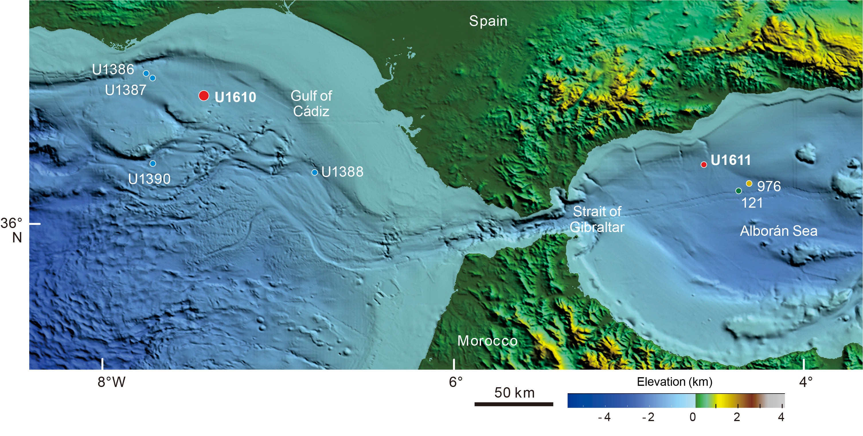
Figure F1. Map, Mediterranean–Atlantic gateway.
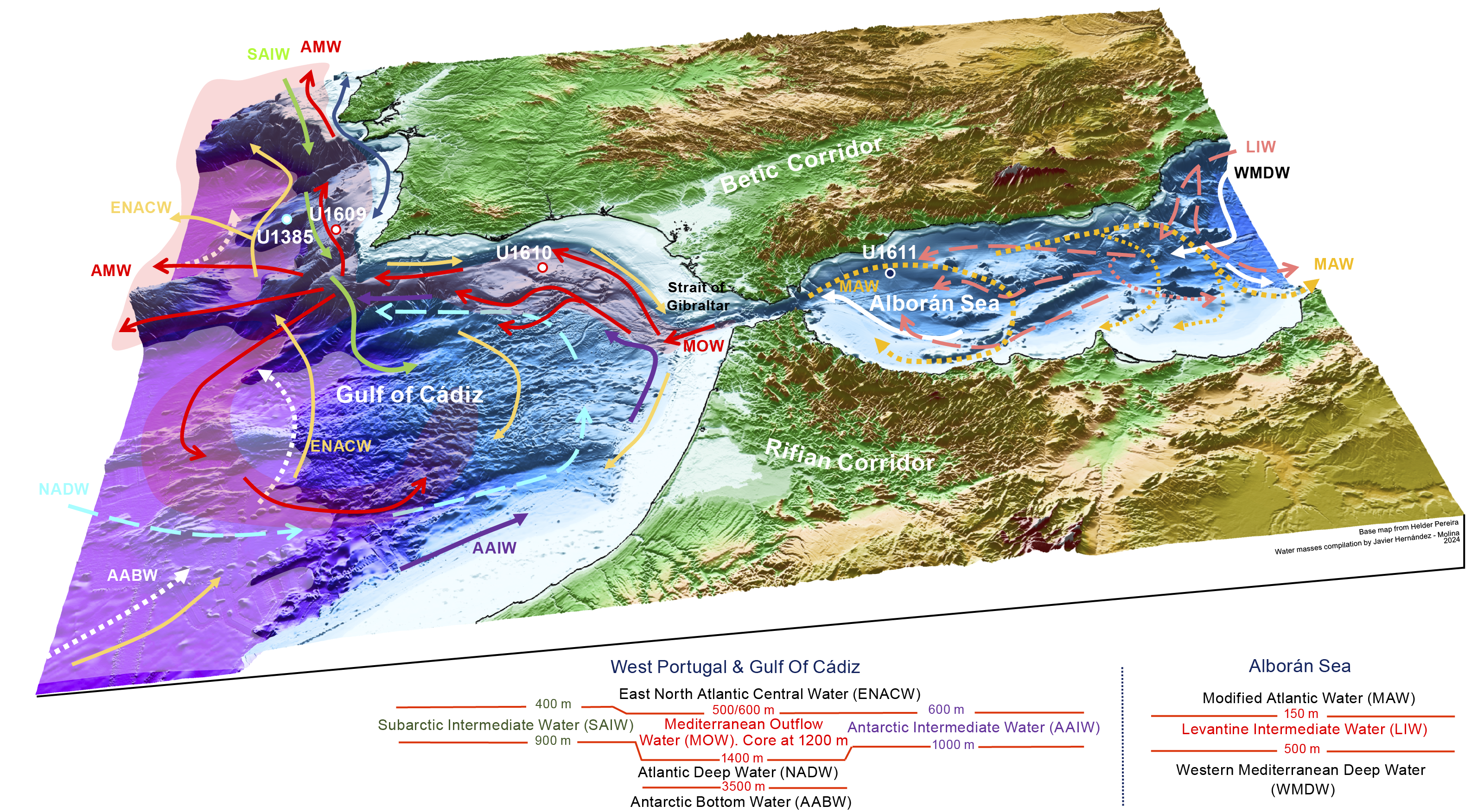
Figure F2. Present-day water mass circulation patterns.
Identifying an appropriate location for this site was challenging. There is considerable uncertainty about exactly when the different Mediterranean–Atlantic gateways opened and closed during the Late Miocene (Krijgsman et al., 2018), so a proximal Mediterranean overflow plume target needed to be positioned in a location that would capture a record of Mediterranean overflow wherever it was coming from, throughout the 8–4 Ma interval of interest (Figure F3). The Miocene target interval also needed to be sufficiently shallowly buried (<1700 m) and in deep enough water to be accessible to the R/V JOIDES Resolution drilling capability. However, the Pliocene–Pleistocene succession in the Gulf of Cádiz derives from both more recent Mediterranean overflow and substantial clastic deposition from mainland Spain and Portugal (Ledesma, 2000; Ng et al., 2021b). Much of this is the progradational extension of sediment funneled down the northeast–southwest oriented Guadalquivir Basin (Ng et al., 2022), which exploits the ancestral Betic Corridor (Figure F3), through which Mediterranean–Atlantic exchange occurred during the Tortonian (Krijgsman et al., 2018). The Pliocene–Pleistocene cover is therefore both thick and has progressively filled much of the offshore accommodation space, burying the Late Miocene relatively deeply while also making the Gulf of Cádiz relatively shallow water. Finally, for safety reasons, all potential International Ocean Discovery Program (IODP) sites need to be in locations where hydrocarbon accumulations are demonstrably absent, which was also challenging for this location. As a result of all these issues, there was very little choice about the location of Site U1610.
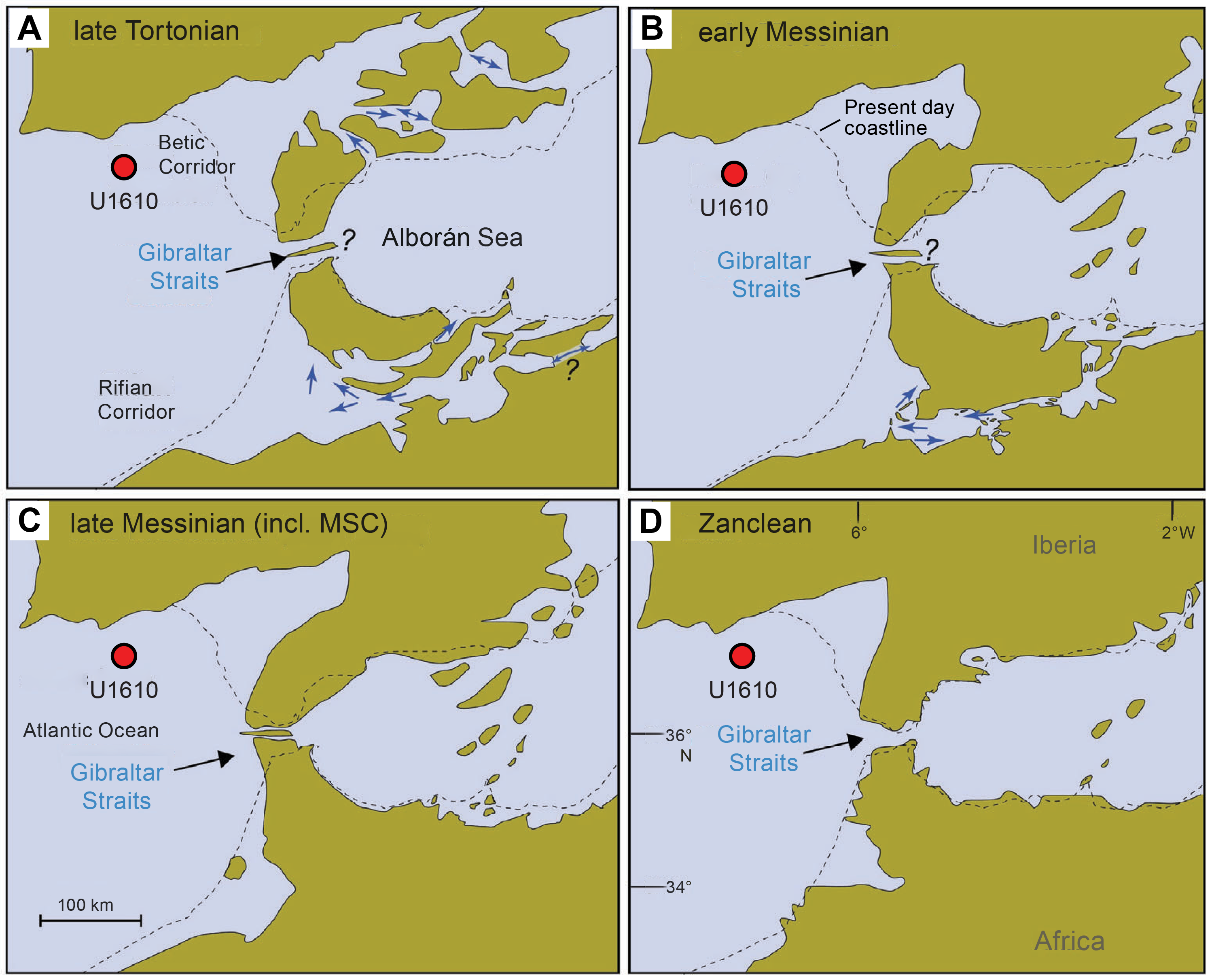
Figure F3. Paleogeographic evolution, Mediterranean–Atlantic gateways.
At Site U1610, the Messinian–Tortonian interval has a target depth of 1460 m. The velocity-depth conversion used for the Pliocene–Pleistocene succession at Site U1610 was derived from adjacent Integrated Ocean Drilling Program Expedition 339 Sites U1386 and U1387 (Expedition 339 Scientists, 2013a), which lie ~20 km northeast (Figure F4). This suggested that the Pliocene–Pleistocene succession at Site U1610 was ~750 m thick. The drilling strategy adopted was not to core the Pleistocene and the top of the Pliocene but to save time by washing down and casing the hole down to 550 m.
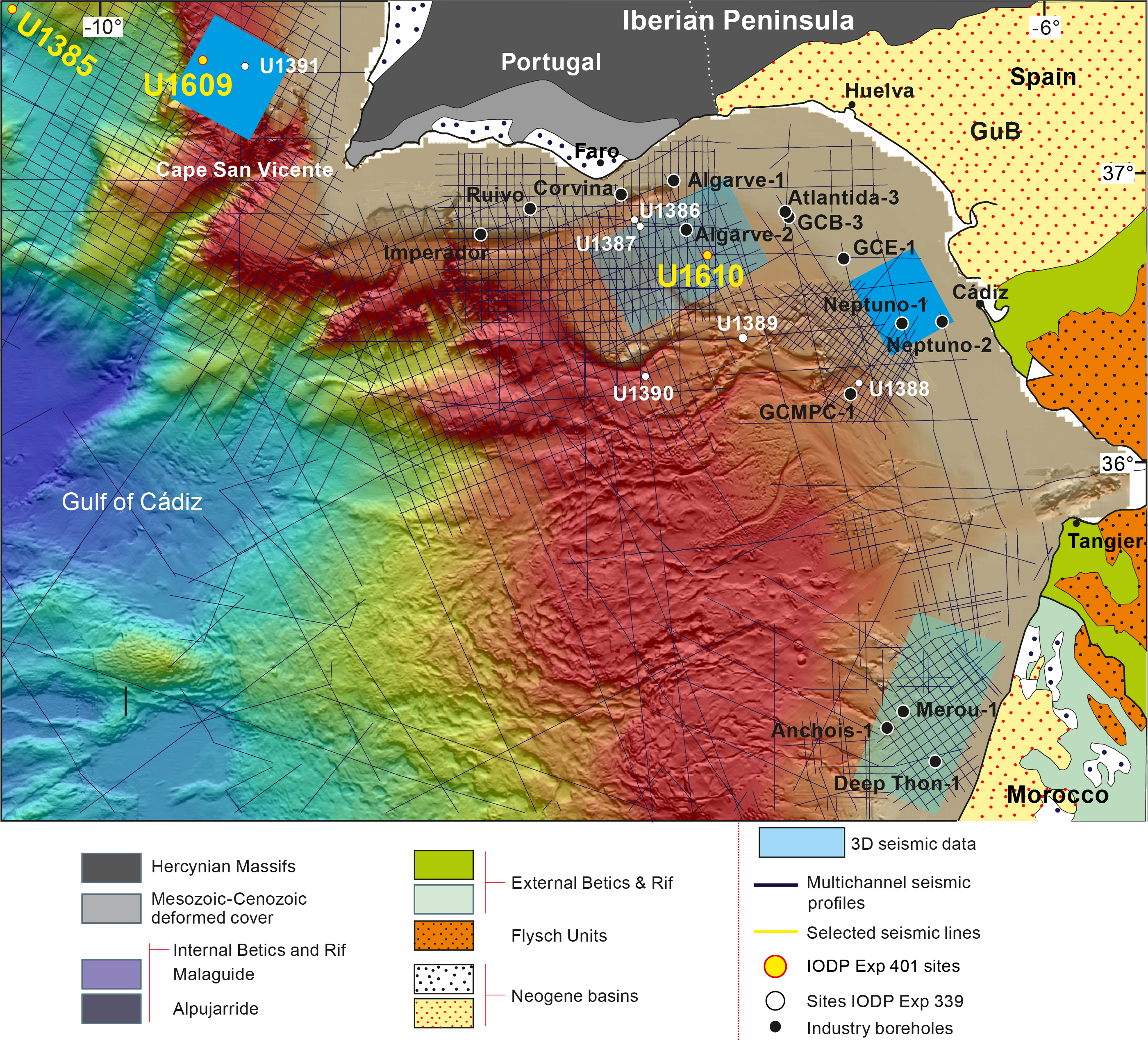
Figure F4. Location of Site U1610.
Ng et al. (2022) studied the seismic profiles of the Deep Algarve Basin, including the line on which Site U1610 is located (Figure F4). Based on regional correlations to Expedition 339 sites and industry wells (Figure F4), they divided the Late Miocene sequence into four distinct stages (Figure F5), charting the progradation of a submarine fan system sourced from the Guadalquivir Basin. At Site U1610, this results in an upward transition from distal submarine lobes (low-amplitude unit below 2 s two-way traveltime [TWT]; Figure F6) to more proximal, coarser grained (higher amplitude) submarine lobes. This is then overlain by the Pliocene–Quaternary contouritic drift sequence that dominates the Gulf of Cádiz (Hernández-Molina et al., 2003, 2014a; van der Schee et al., 2016).
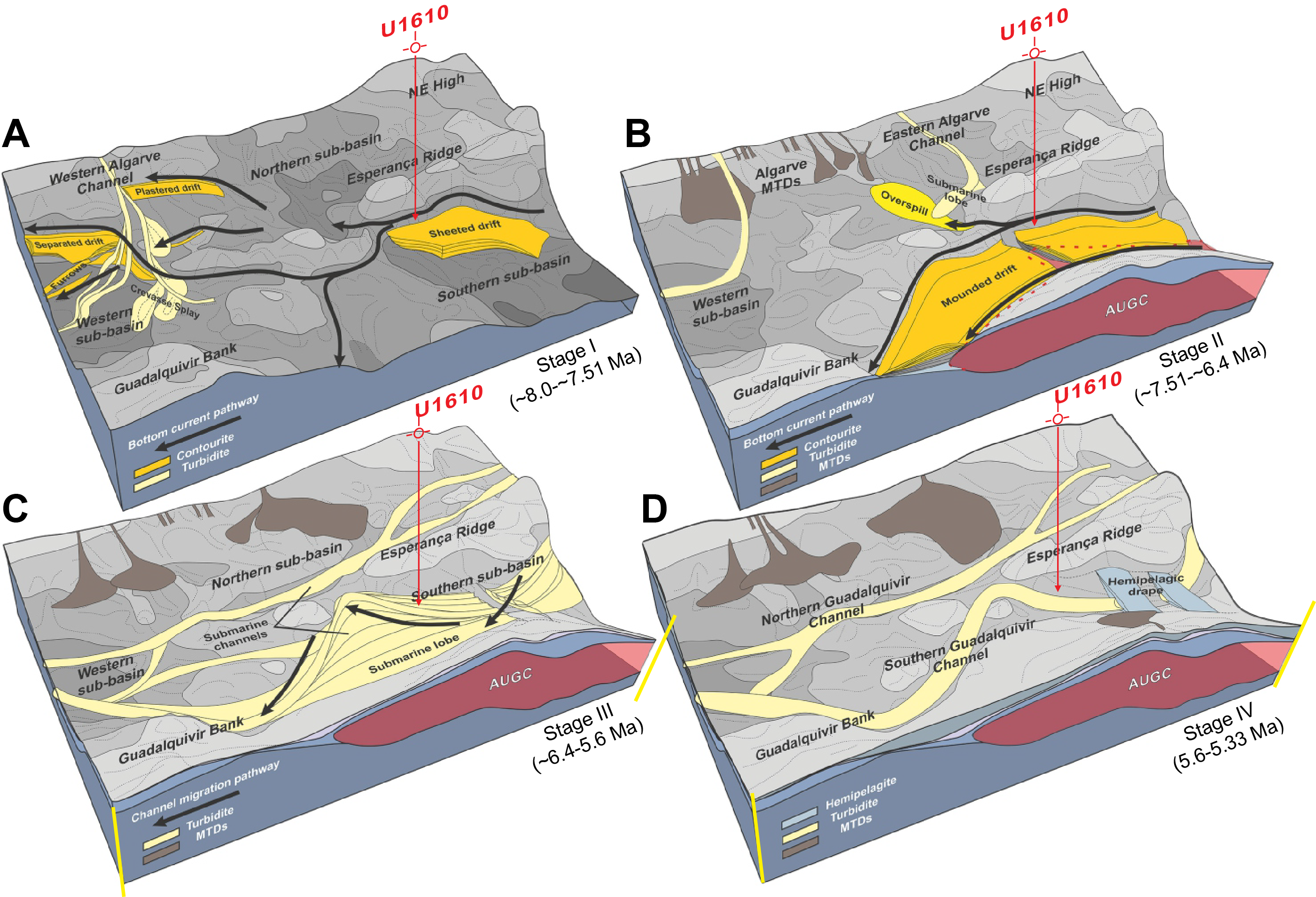
Figure F5. 4-stage evolutionary block model.
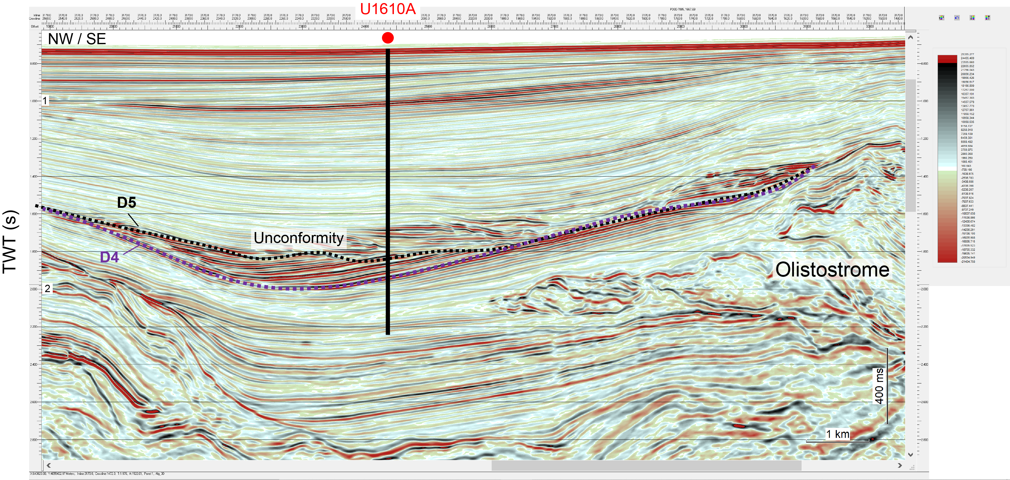
Figure F6. Seismic section.
The upper part of the Late Miocene target interval on the seismic line (Figure F6) was identified as a Messinian Transparent Unit (MTU; figure F12 in Flecker et al., 2023). During Expedition 339, the top of this unit was drilled at Site U1387 and hemipelagic sediments were recovered (Expedition 339 Scientists, 2013a) that have been interpreted to be of latest Miocene age (van der Schee et al., 2016). This is consistent with the interpretation of this interval regionally as a fine-grained succession (e.g., Ng et al., 2022). Beneath this is a channel fill succession described by Ng et al. (2022) as a series of migrating reflectors, below which is an unconformity and a succession of dipping bright reflectors underlain by a package of parallel-bedded, lower amplitude reflectors (Figure F6) thought to be of Tortonian age (Ng et al., 2022). Close to the bottom of the target at around 2.1 s TWT is a wedge-shaped unit that appears to be the extension of a chaotic unit. This is thought to be an olistostrome (Figure F6) (Torelli et al., 1997; Maldonado et al., 1999; Medialdea et al., 2004).
To minimize the time spent coring the Pliocene–Pleistocene interval that had already been recovered close by at Sites U1386 and U1387 (Expedition 339 Scientists 2013a), Expedition 401 planned to wash down to 550 m, which was assumed to be just above the 4.52 Ma bioevent (see Biostratigraphy). The hole would then be cased to increase stability and improve the chances of successful coring and logging. The aim was to reach sediment older than 8 Ma, which was assumed to be just below the chaotic olistostrome interval (Figure F6).
1.1. Objectives
The major objective for Site U1610 was to recover an 8–4 Ma succession that records the proximal evolution of the Mediterranean overflow plume during a phase of major Mediterranean–Atlantic gateway change and the formation of a salt giant in the Mediterranean. This in turn may have consequences for global climate change (Krijgsman et al., 2024). In combination with other Expedition 401 Atlantic sites, the record from Site U1610 also allows us to investigate more specific objectives, including the following:
- To establish the age of the earliest contourites formed as a result of Mediterranean overflow,
- To evaluate the impact of extreme environmental fluctuations in the Mediterranean on its overflow plume and the structure of the Atlantic water masses, and
- To provide quantitative constraints on the mixing behavior of dense overflows by reconstructing the strength and attenuation rate of the Atlantic–Mediterranean exchange signal beyond the gateway.
2. Operations
Site U1610 consists of one hole, U1610A, from which 751.2 m of sediment was collected over a 933.5 m cored interval (80.5% recovery). The uppermost 501.9 m of the hole was cased to prevent caving and make it easier to flush cuttings out of the borehole, with the aim of increasing the chances of coring and logging successfully to the target depth of 1460 meters below seafloor (mbsf). The Pleistocene and Late Pliocene stratigraphy, which was not recovered in the uppermost 501 m at Site U1610, is already known from nearby Expedition 339 Site U1387, located ~27 km west-northwest.
2.1. Hole U1610A
The ship completed the 122 nmi voyage to Site U1610 (36°41.9812′N, 7°25.8844′W) at an average speed of 11.5 kt, arriving at 1010 h on 28 December 2023. The hydraulic release tool (HRT) casing was prepared, consisting of the HRT assembly, HRT base, and 498 m of 10¾ inch casing (Figure F7). The rig team then made up the bottom-hole assembly (BHA), including the bit, underreamer bit, and mud motor. The BHA and drill pipe were lowered through the casing until the bit and underreamer extended below the casing by 3 m. The HRT running tool was attached to the casing, and the funnel was welded on; the entire casing system was then lowered through the moonpool, and the ship was positioned over the hole coordinates.
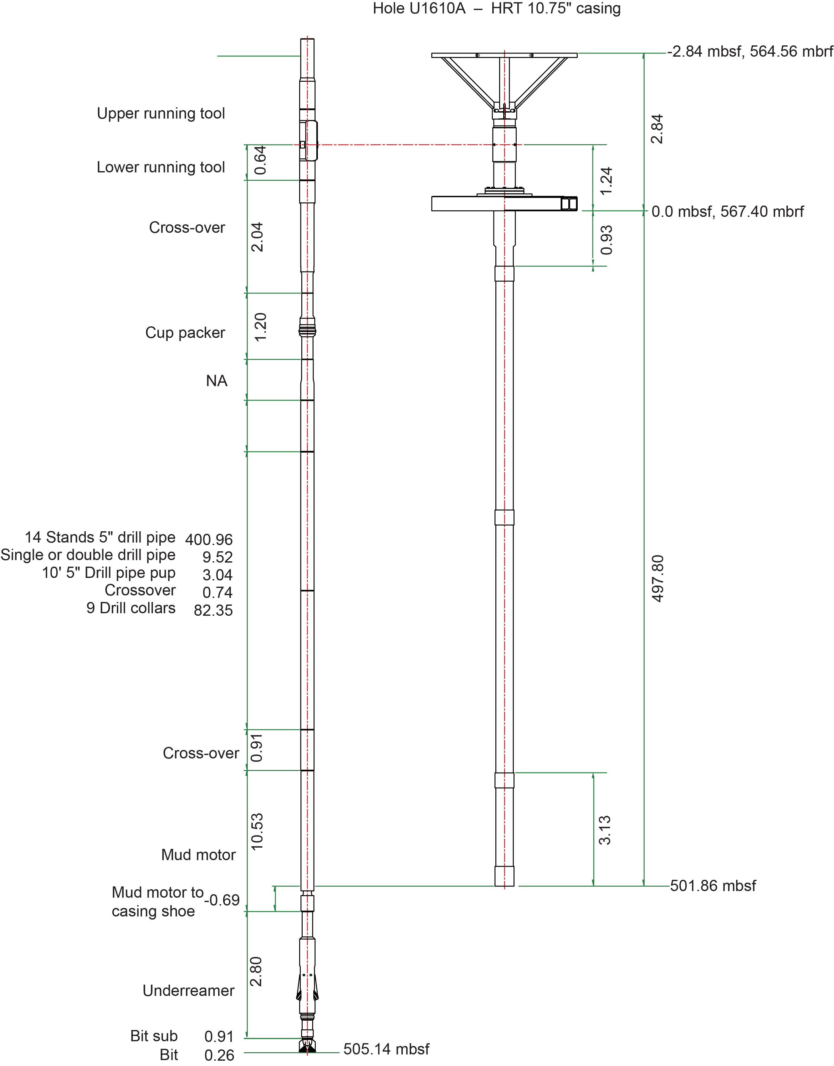
Figure F7. Reentry and casing system
Hole U1610A started at 1200 h on 29 December when the seafloor was tagged at 561.7 mbsl. The casing system was drilled in until it reached 480 mbsf at 1700 h on 30 December, when the subsea camera was deployed to observe the funnel's approach to the seafloor. The base landed on the seafloor with the casing shoe at 501.9 mbsf. After the casing was released, the bit was raised, clearing the seafloor at 2215 h and clearing the rotary table at 0302 h on 31 December, completing casing operations.
We elected to start coring in Hole U1610A with the extended core barrel (XCB) coring system because it had recovered good quality cores at equivalent depths in Hole U1609A. The nonmagnetic drill collar was left out of the assembly to improve the robustness of the BHA, and a lockable float valve was included for potential downhole logging.
Hole U1610A was reentered at 0940 h, and during this process the depth to seafloor was found to be 556.3 mbsl, identical to the precision depth recorder reading but shallower than the previous estimate of 561.7 mbsl. The bit was lowered to the base of the hole (505.2 mbsf), and the first science activity at the site was to run the Sediment Temperature 2 (SET2) tool. At 1430 h, we started coring Core 2X and continued into the new year.
At 0100 h on 3 January 2024 with Core 401-U1610A-26X at 738.0 mbsf, we started a more rigorous headspace gas sampling protocol for the depth interval 724–960 mbsf at this site, following the recommendation by the IODP Environmental Protection and Safety Panel and the Texas A&M University Safety Panel. The headspace gas results from each core were analyzed before advancing the bit to collect the next core. This protocol was in effect because a detailed preexpedition analysis of 3D seismic data showed that there is a nonzero but very low risk of finding gas at the Site U1610 location. Headspace gas results from all XCB cores were found to be in the normal (safe) range of methane/ethane ratios and absolute methane values. Void space gas sampling was also performed, opportunistically sampling visible air pockets through the core liner above, within, and below the special protocol zone. The results showed methane/ethane results are comparable to headspace and useful because they are analyzed immediately and available sooner, unlike sediments, which require the 30 min incubation step prior to headspace analysis (see Geochemistry). Cores 2X–36X penetrated from 505.2 to 827.8 mbsf and recovered 322.6 m (93%).
At 0700 h on 4 January, there was a failure in the top drive brake system, causing the brake to engage and overheat. We stopped coring and pulled up Core 401-U1610A-36X, which had advanced 3 m. The bit was raised to 793.5 mbsf, the top drive was racked to allow repair, and the bit was raised to 495.2 mbsf just inside the casing. The first interval of top drive inspections and repair ran from 0945 to 1330 h. The cause of the failure appeared to be the exhaust valve on the brake. A portion of the diaphragm in the exhaust valve had broken off, lodged in the valve, and kept air pressure to the energizing bladder behind the brake bands. This kept the brake engaged. There was significant damage to the brake and bladder assembly from the resultant overheating, and the entire brake assembly needed to be replaced with the spare unit from the warehouse.
Meanwhile, we decided to change from the XCB coring system to the rotary core barrel (RCB) coring system for the remainder of the hole. We raised the bit to the ship, clearing the seafloor at 1423 h and the rig floor at 1630 h. Repairs to the top drive continued and were complete by 0215 h on 5 January. The rig floor team then assembled the RCB BHA with a new 9⅞ inch polycrystalline diamond compact (PDC) bit, and Hole U1610A was reentered at 0548 h. Core 50R marked the end of the special headspace gas protocol, and results were within the normal range for the interval where the enhanced gas safety protocol was in effect. The procedure resulted in a delay of ~45 min per core across 25 cores.
Coring continued with very good recovery to Core 401-U1610A-95R, which recovered just 15 cm of hard dolostone rock pieces. Core 96R was empty, so we ran the bit deplugger to remove any potential obstructing rock lodged in the bit. Although the drilling rate indicated that we were drilling recoverable sediments and had passed below the hard lithified sediments that had been partly recovered in Core 95R, no sediments were recovered, so we stopped coring at 0515 h on 11 January with Core 100R. Cores 37R–100R penetrated from 827.8 to 1438.7 mbsf and recovered 610.9 m (74%). In total, Cores 2X–100R penetrated from 505.2 to 1438.7 mbsf and recovered 751.2 m (80.5%) (Table T1).
We prepared for downhole logging by releasing the bit at the bottom of the hole, filling the hole with 354.3 bbl of heavy (10.5 lb/gal) barite mud, and raising the pipe. When the end of the pipe reached 779.4 mbsf, the drill pipe became stuck. After an overpull of 60,000 lb would not free the pipe, the circulating head was attached so that fluid could be pumped and the top drive was picked up so that the pipe could be rotated. After several attempts, the pipe came free at 1215 h with 90,000 lb of overpull and a pump pressure of 600 psi. The end of pipe was set at 516.6 mbsf for logging, 14.7 m below the casing shoe.
At 1415 h, we started to assemble the quad combo tool string, including natural gamma radiation (NGR), density, resistivity, and sonic velocity tools. The tool string was lowered down the hole, passing out of the casing into the open hole at 1640 h. At ~726 mbsf, the tool string encountered an obstruction and, after eight attempts, could not pass any farther down the hole. This depth interval is the same one that closed in on the drill pipe earlier in the day. However, useful log data were acquired from the ~208 m open hole logged interval.
The inclinometer in the cablehead of the quad combo logging tool string showed that Hole U1610A was inclined between 13° and 15° from vertical in the logged interval. We had suspected the hole was not vertical based on the observation of inclined beds in the cores.
The downhole logging equipment was rigged down by 0045 h on 12 January, and the pipe was raised, clearing the seafloor at 0130 h and the rig floor at 0300 h. The rig floor was secured for transit, we raised the thrusters at 0336 h, and we started the sea passage to Site U1385 at 0348 h, ending Site U1610.
3. Lithostratigraphy
Seven primary lithologies were described in Hole U1610A: calcareous clay, calcareous mud, calcareous silty mud, calcareous (sandy) silt(stone), calcareous (silty) sand(stone), clayey calcareous ooze, and dolostone. Minor coarser grained lithologies were also observed (Figure F8; see HANDDRAWN in Supplementary material). Based on these lithologic descriptions, Site U1610 is divided into five stratigraphic units (Figures F9, F10). Contacts between lithologies are predominantly gradual, with subtle color and grain size changes; however, some contacts are sharp to erosive.
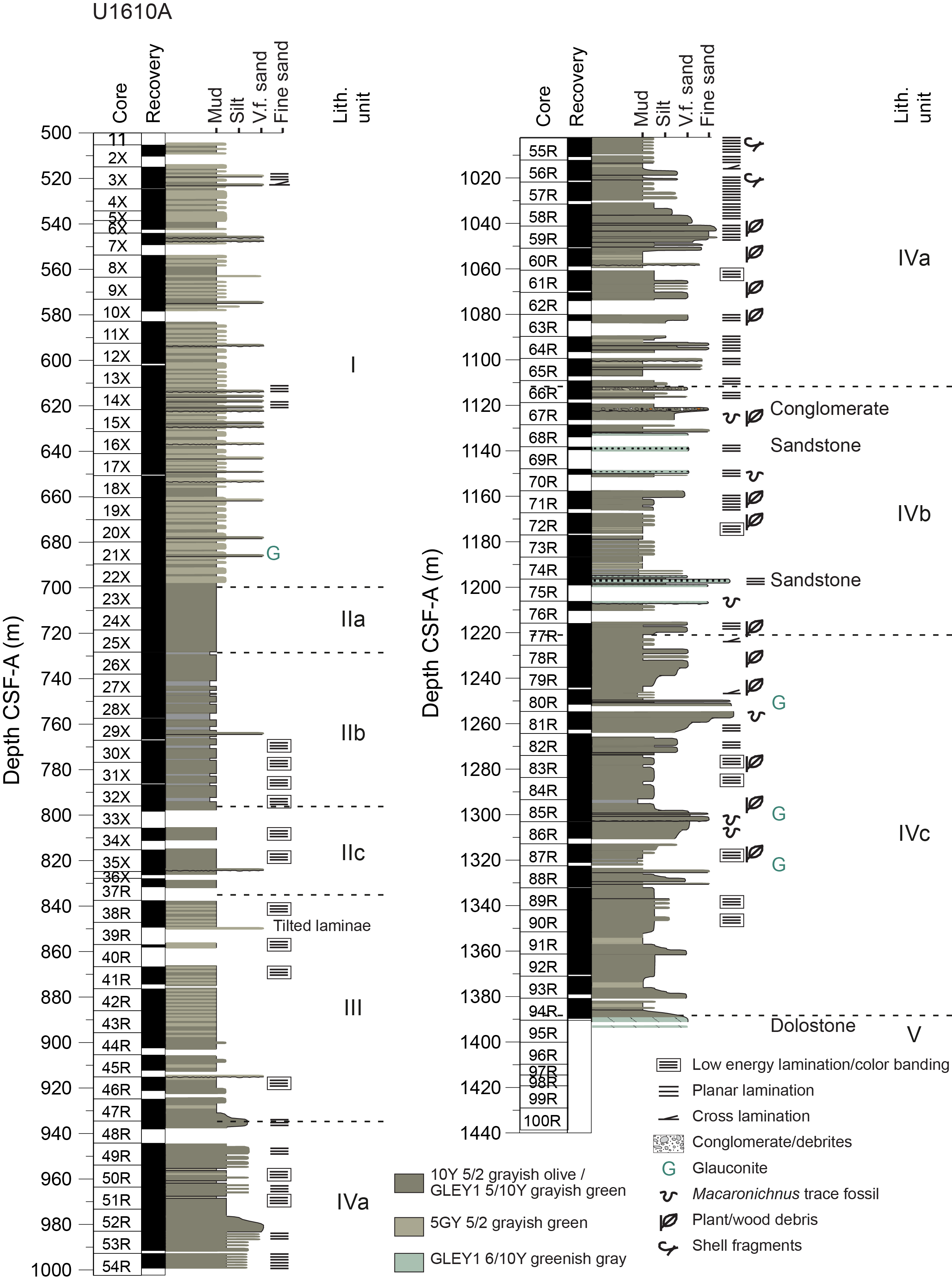
Figure F8. Lithologic synthesis.
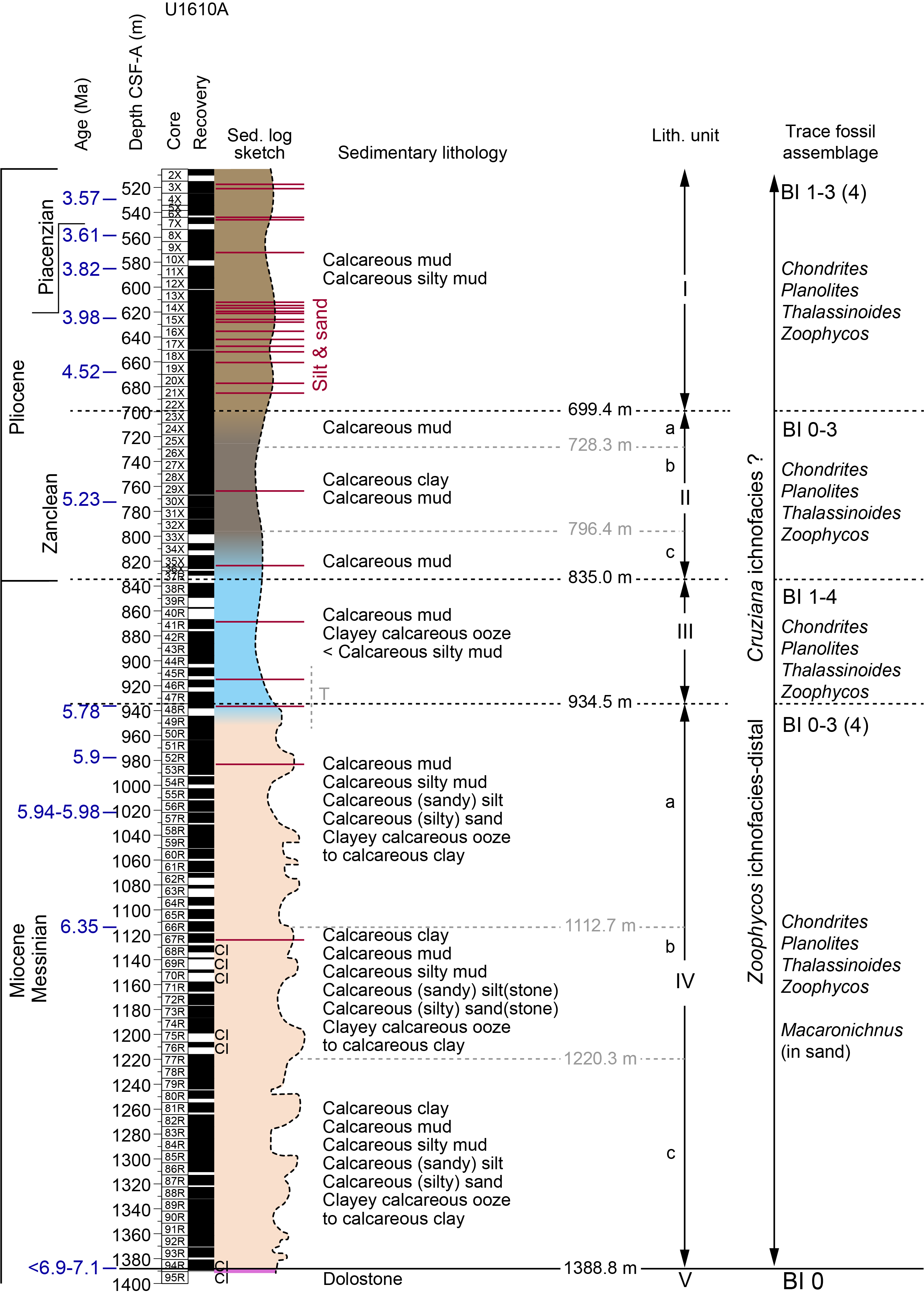
Figure F9. Lithologic summary.
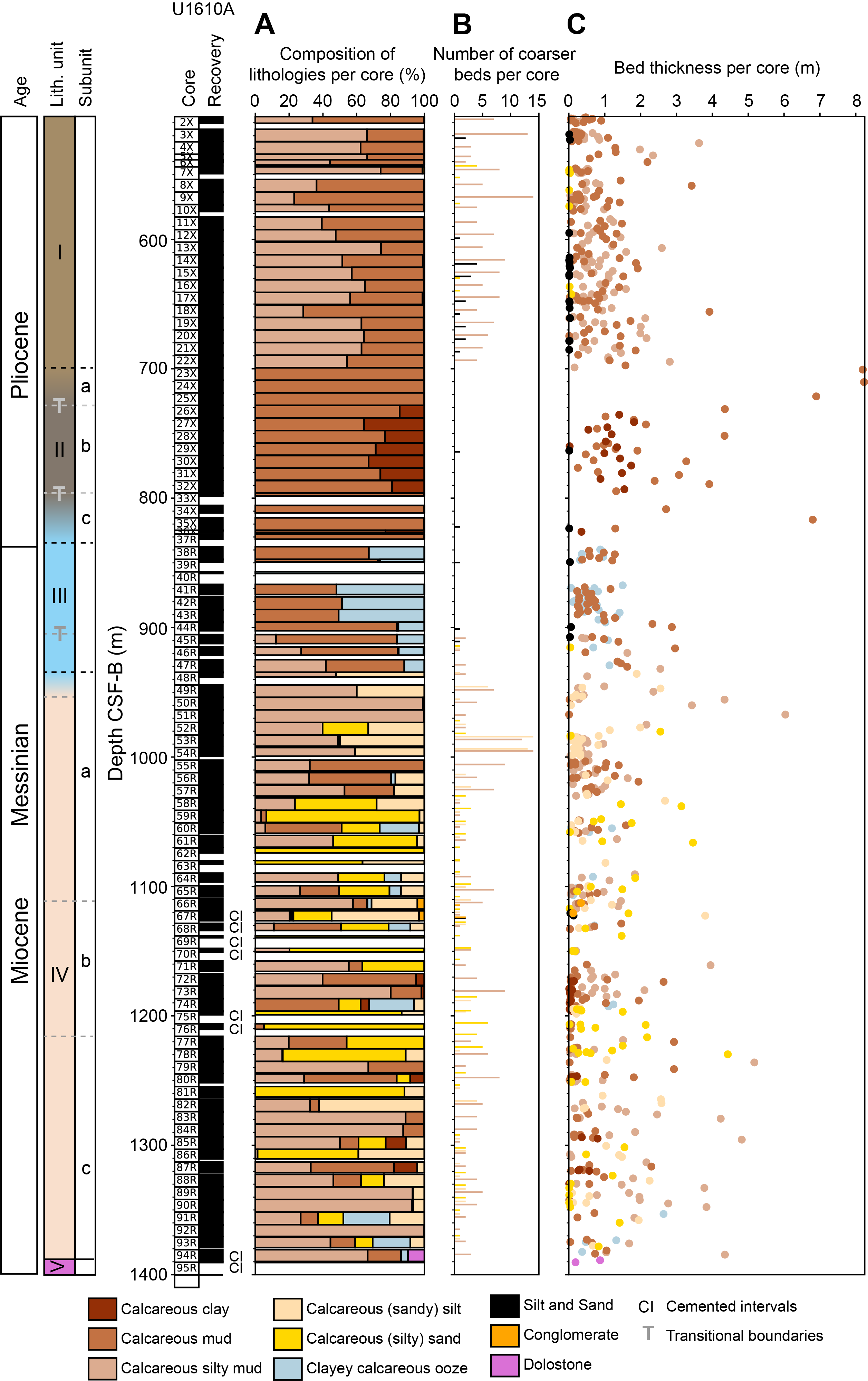
Figure F10. Core and bed thickness by lithology.
Unit I (505.2–699.4 m core depth below seafloor, Method A [CSF-A]) comprises alternating calcareous mud and calcareous silty mud, with minor coarser, sandy intervals. Unit II (699.4–835.0 m CSF-A) consists of three subunits: Subunit IIa (699.4–728.3 m CSF-A) is composed entirely of calcareous mud, Subunit IIb (728.3–796.4 m CSF-A) is composed of alternating calcareous mud and calcareous clay, and Subunit IIc (796.4–835.0 m CSF-A) is predominantly composed of calcareous mud. Unit III (835.0–934.5 m CSF-A) consists of interbedded calcareous mud and clayey calcareous ooze to calcareous silty mud, with minor coarser, sandy intervals. Unit IV (934.5–1388.8 m CSF-A) is divided into three subunits. Subunit IVa (934.5–1112.7 m CSF-A) consists of alternating calcareous silty mud, calcareous sandy silt, calcareous mud, and coarser grained sand and silty sand intervals, with minor clayey calcareous ooze to calcareous clay. Subunit IVb (1112.7–1220.3 m CSF-A) consists of calcareous mud, calcareous silty mud, calcareous sandy silt, and calcareous sand (very fine, fine, and medium), with some clayey calcareous ooze to calcareous clay and minor lithified siltstone, sandstone (fine to medium), and conglomerate. Subunit IVc (1220.3–1388.8 m CSF-A) consists of alternating calcareous mud, calcareous silty mud, calcareous sandy silty, and coarser grained sand and silty sand intervals, with minor clayey calcareous ooze to calcareous clay and calcareous clay. Unit V (1388.8–1390.6 m CSF-A) consists entirely of dolostone. Cores 401-U1610A-96R through 100R (1390.6–1438.7 m CSF-A) had 0% recovered sediments and were not included in the unit definition.
Individual bed thickness for each primary lithology was calculated (Figure F10). The top and bottom of each core were excluded because they represent only a portion of the bed and, therefore, the minimum value of bed thickness. For the nine cores entirely composed of a single lithology, the thickness was still calculated but represents the minimum bed thickness. The gradual transitions between lithologies preclude the calculation of a true bed thickness, which can only be determined by integrating visual core description with physical properties data (e.g., NGR, magnetic susceptibility [MS], reflectance, and red-green-blue [RGB] color) (Figure F11).
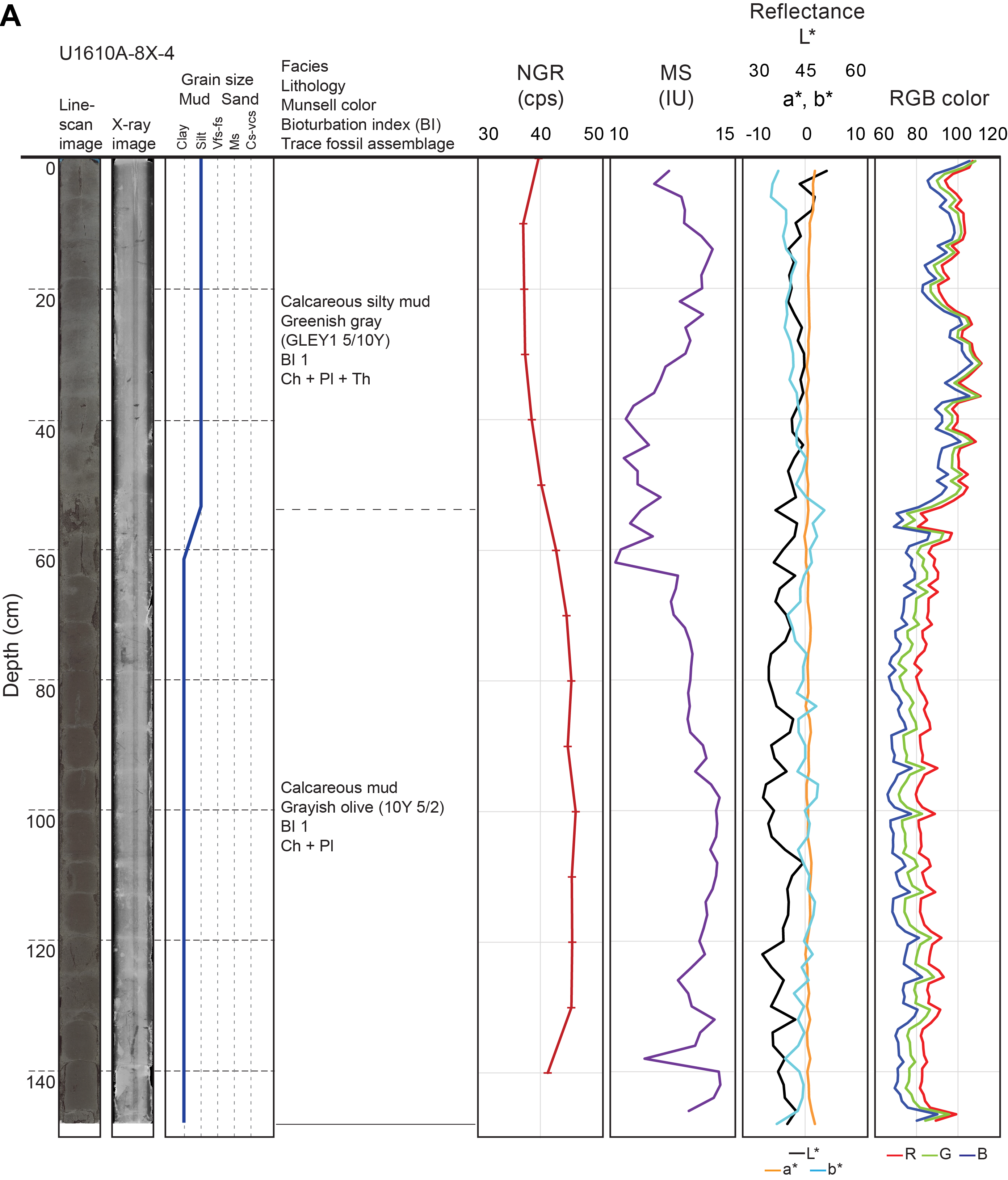
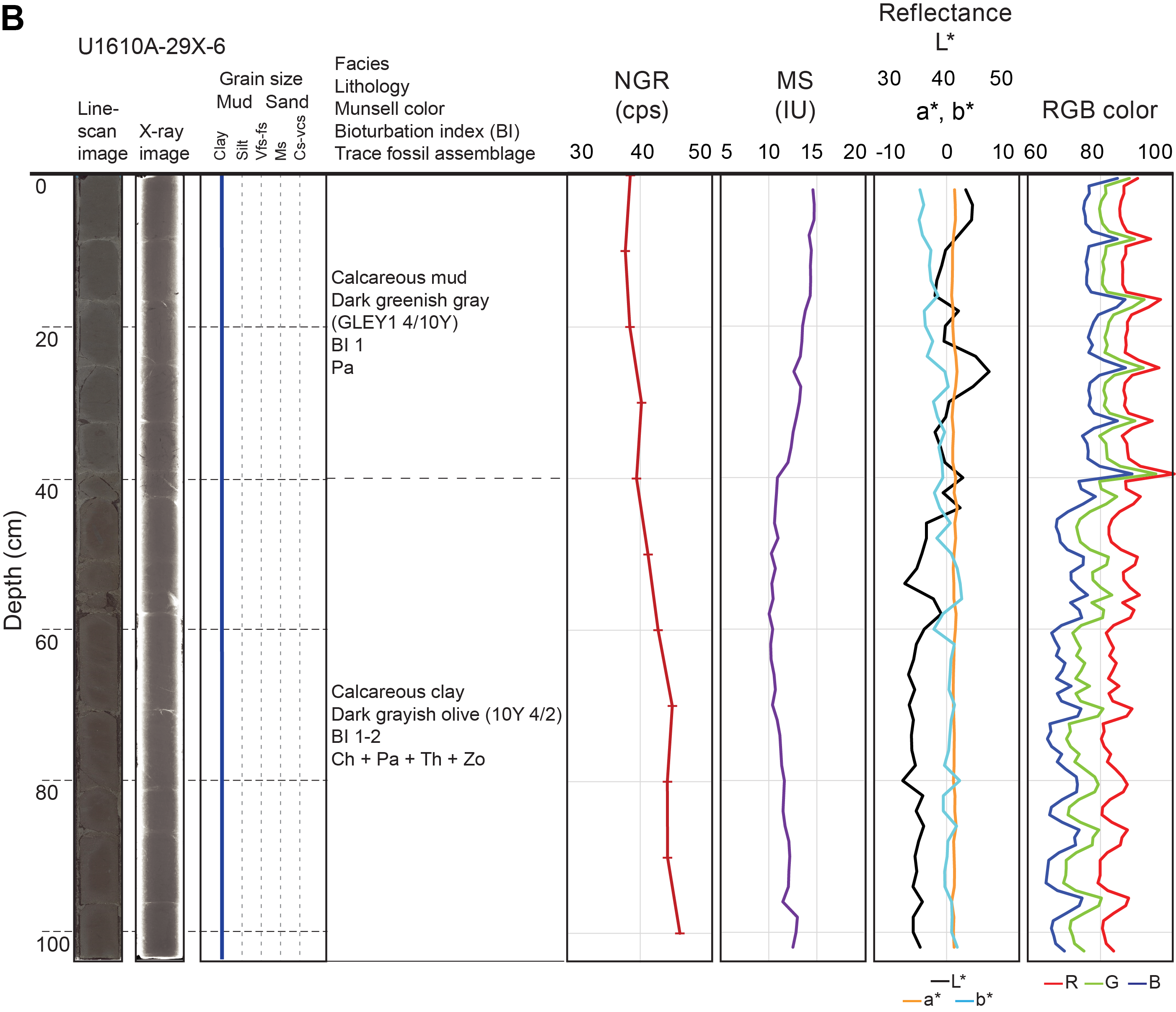
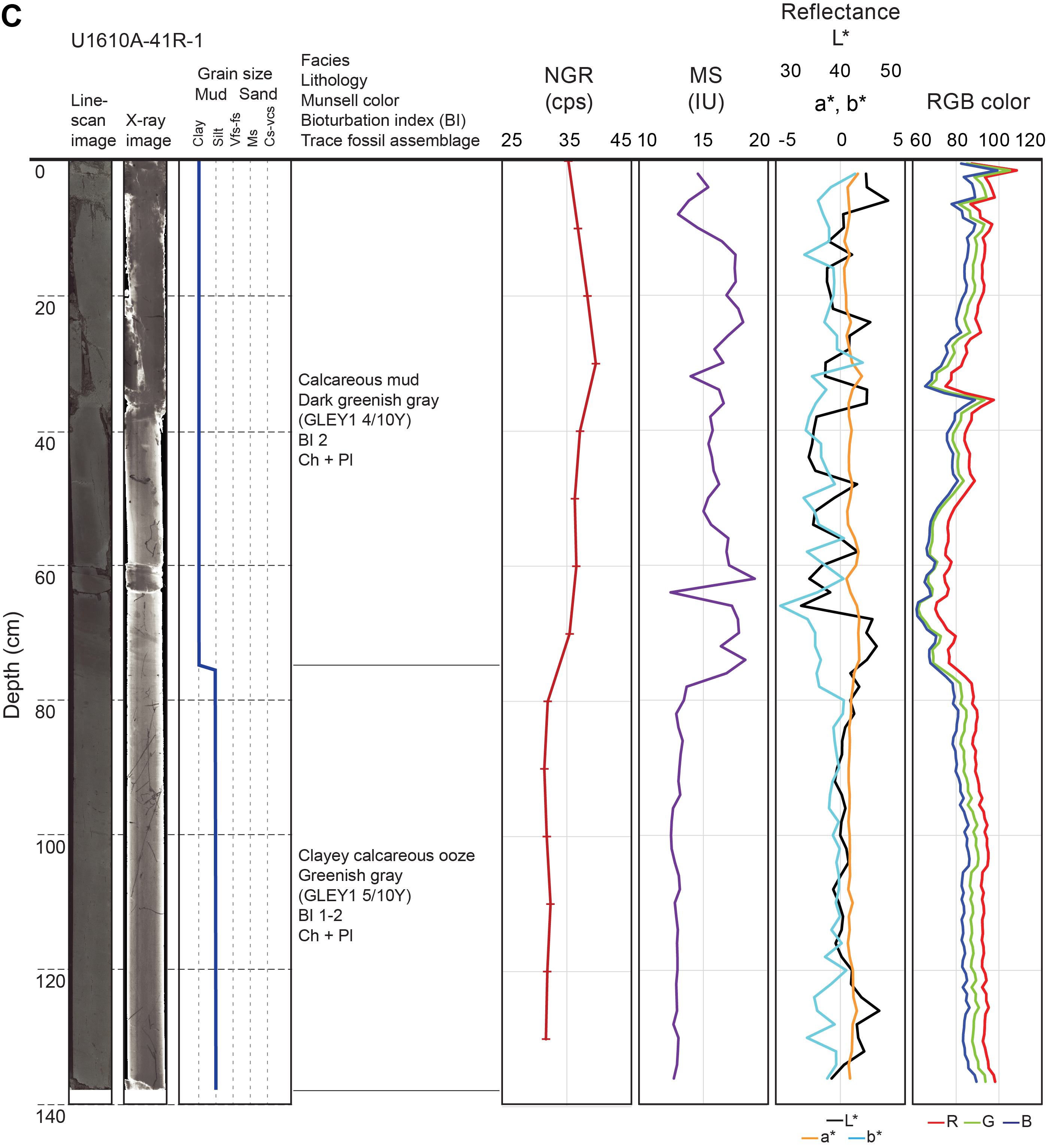
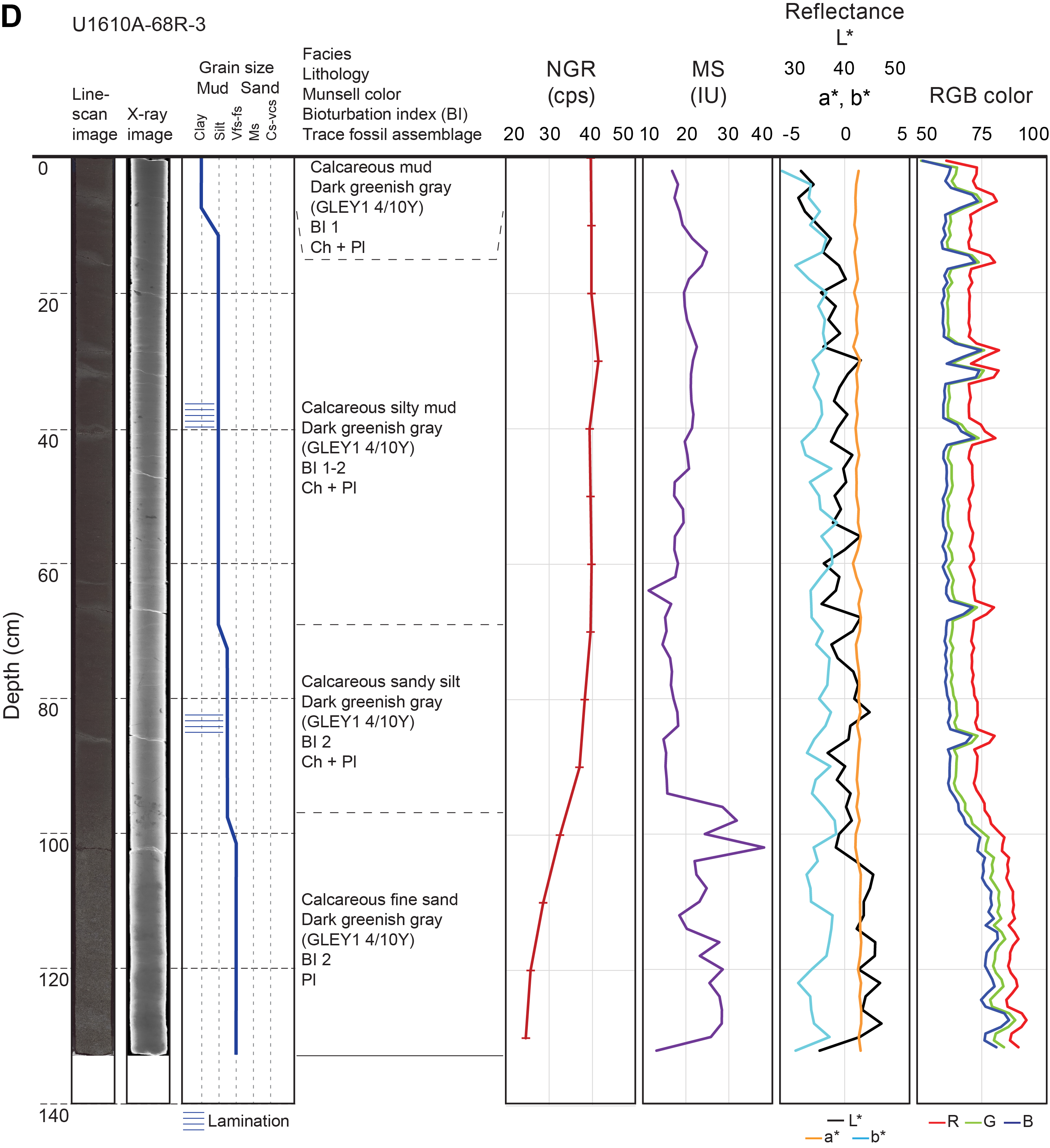
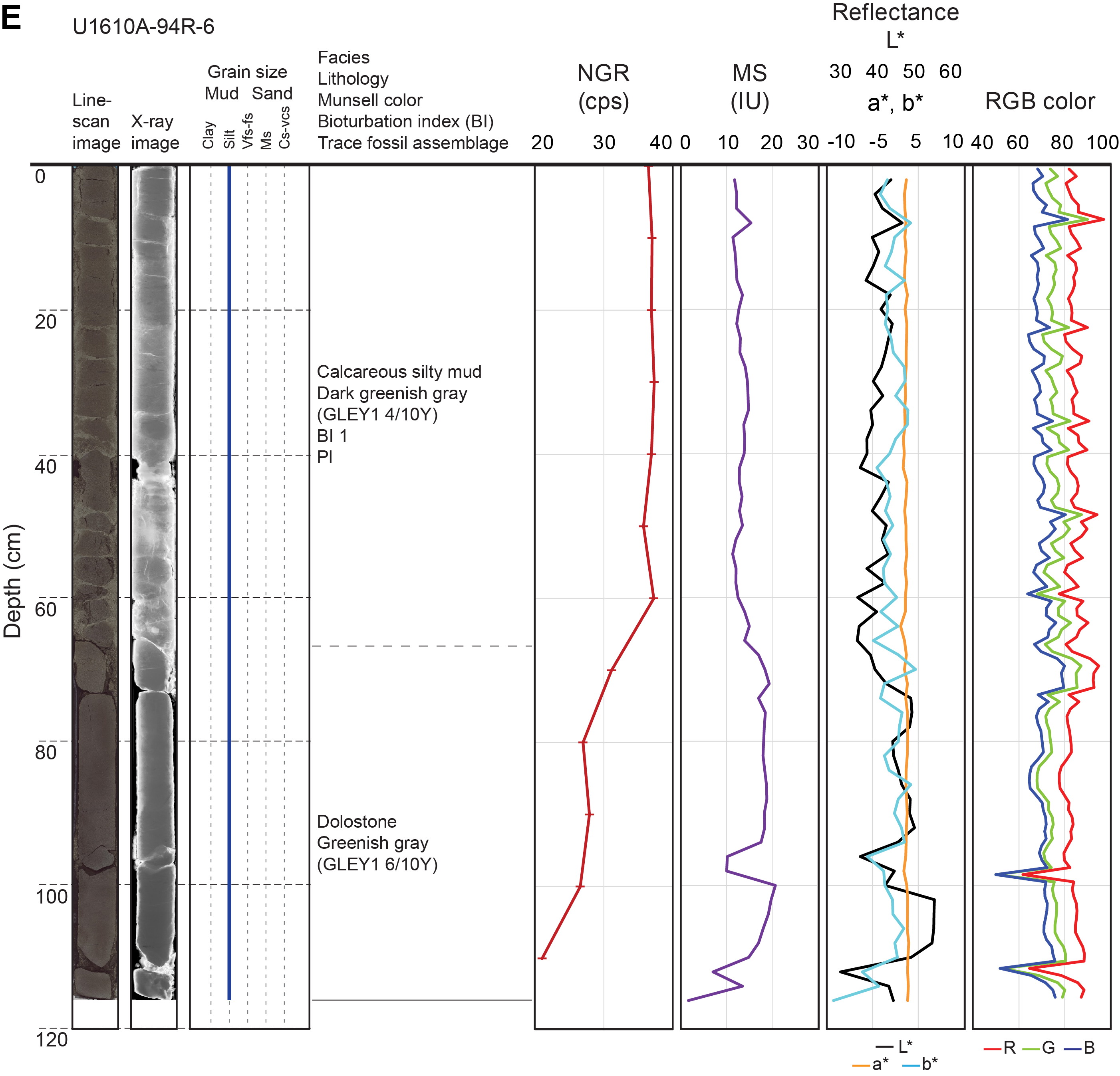
Figure F11. Facies description for each unit.
The trace fossil assemblage at Site U1610 varies in abundance and diversity throughout the cores, with some intervals having abundant trace fossils (bioturbation index [BI] = 4), whereas in other intervals bioturbation is absent (BI = 0). A total of 12 ichnotaxa were recognized at the ichnogenus level, including abundant Chondrites and Planolites, frequent Zoophycos and Thalassinoides, rare Palaeophycus, and occasional Arenicolites, Asterosoma, Ophiomorpha, Phycosiphon, and Teichichnus. Macaronichnus occurs locally at a high abundance, as does Trichichnus, which was observed in X-Ray Linescan Logger (XSCAN) images (Figure F12). Undifferentiated horizontal and vertical structures were also observed, and crosscutting relationships are frequent among the ichnotaxa.
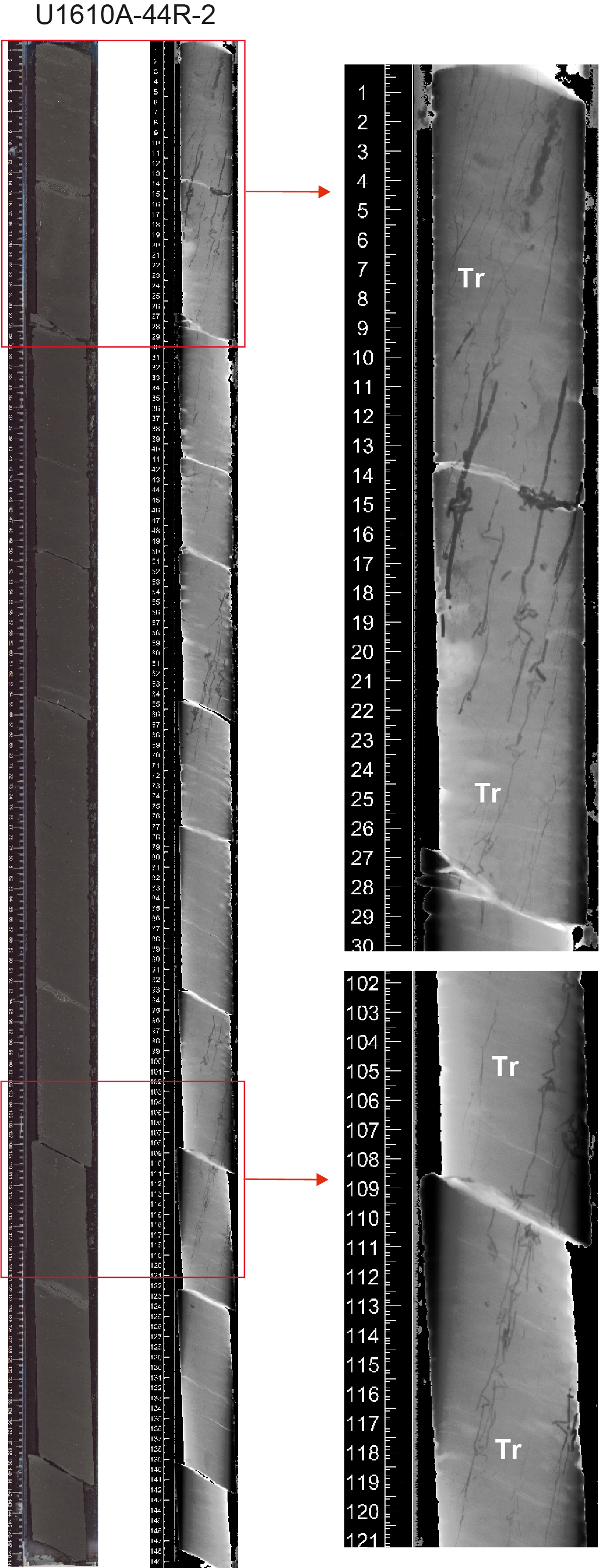
Figure F12. Burrows of Trichichnus.
Petrographic analysis of smear slides taken regularly from Hole U1610A (n = 200) aided the lithologic description. Smear slide data in Table T2 are organized by depth and lithology. Most of the smear slide grain size data from the primary lithologies in each unit plot along the bottom edge of the texture ternary diagram (Figure F13A) between clay and silt, with deviations toward sand for coarser grained lithologies. Compositionally, most of the primary lithologies cluster near the siliciclastic corner of the composition ternary diagram (Figure F14A), with clayey calcareous ooze and some calcareous mud spreading toward biogenic carbonate. All lithologies contain little to no biogenic silica (≤5%; Table T2). Detrital carbonate is a minor component of the finer lithologies but is more abundant in some of the coarser lithologies (Figure F14). Average texture and composition by lithology within each unit are plotted in Figures F13B and F14B.
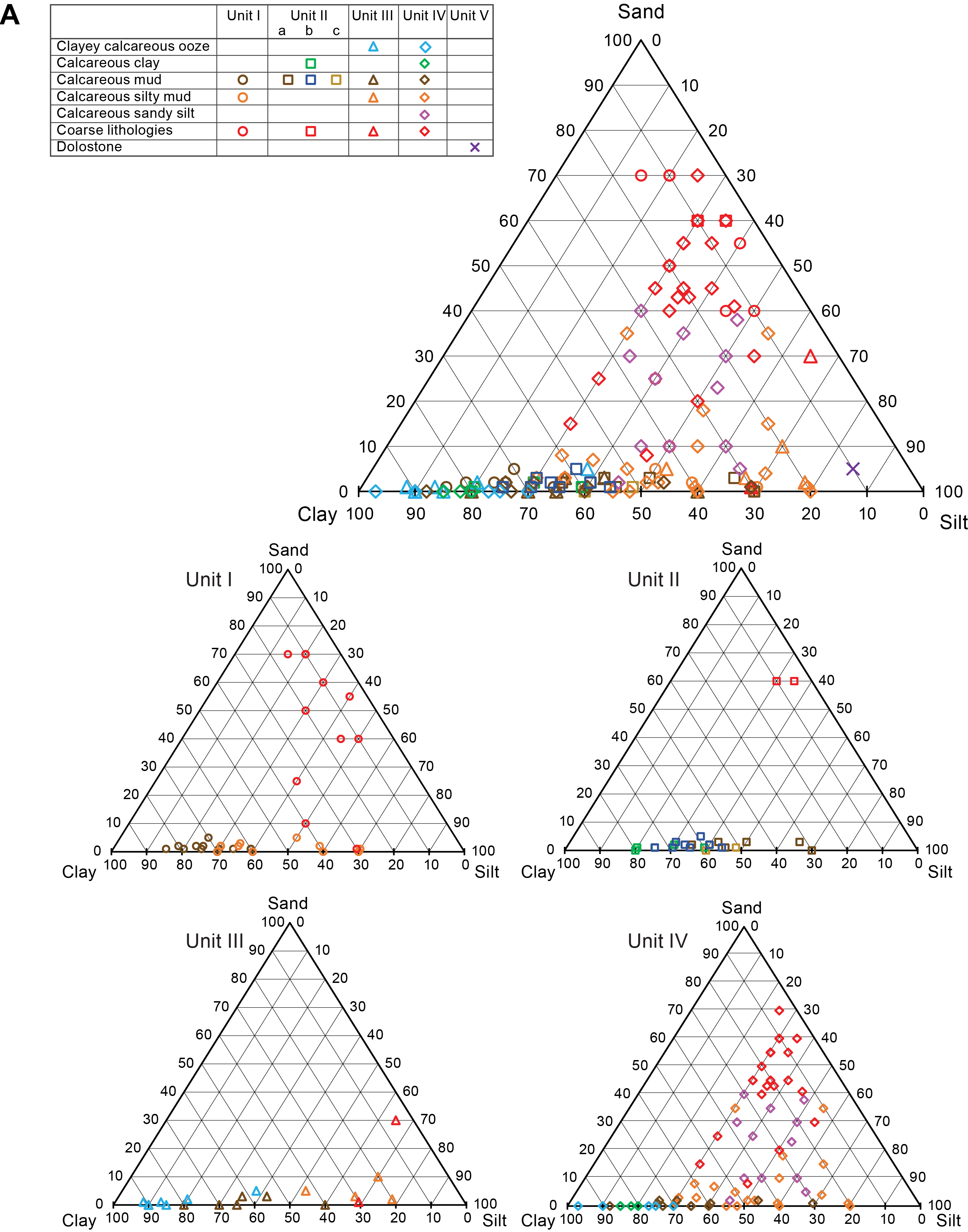
Figure F13. Texture of lithologies.
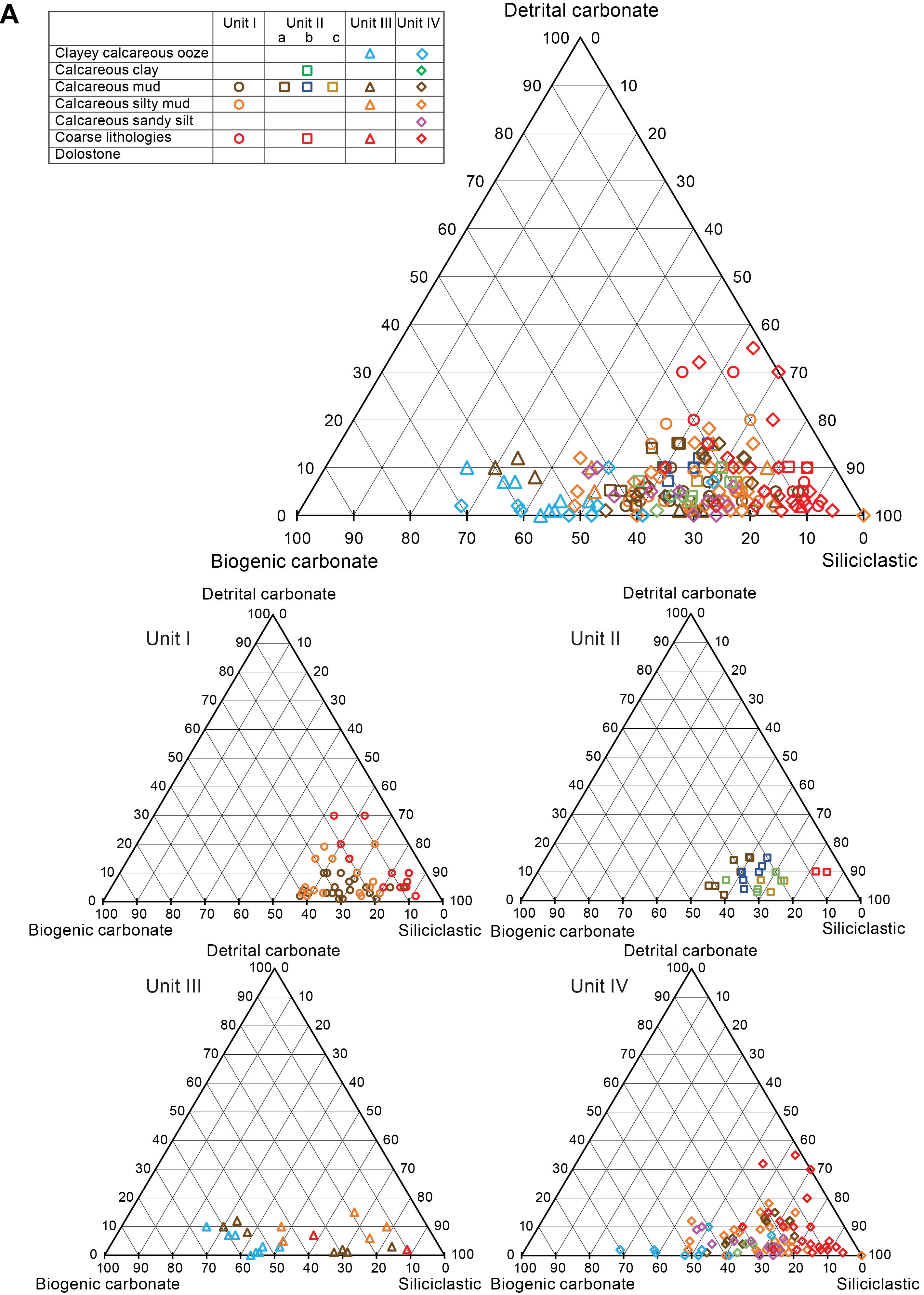
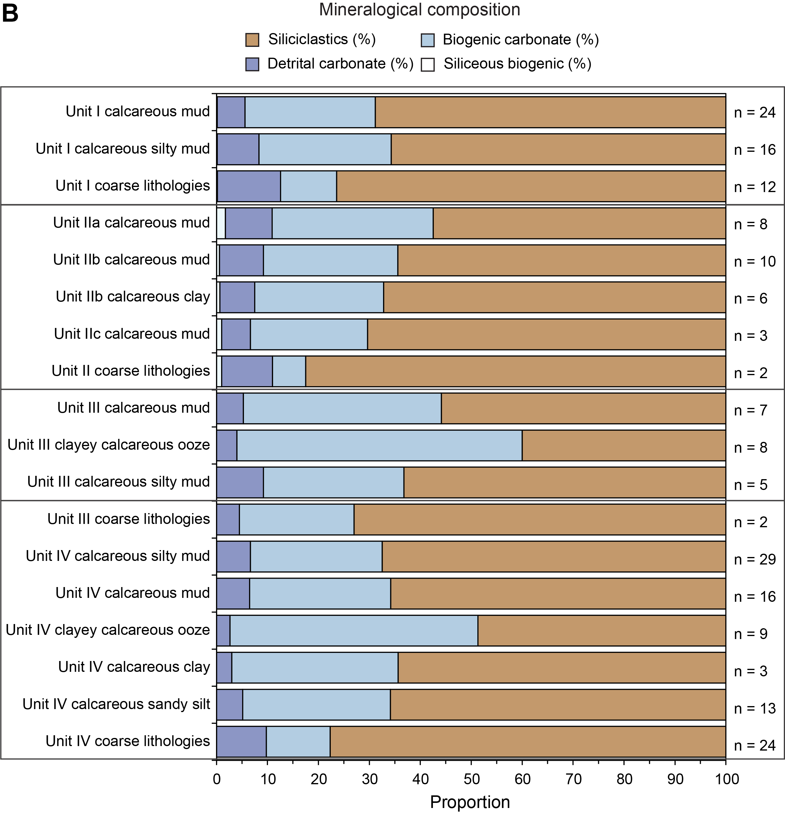
Figure F14. Composition of lithologies.
Based on shipboard analyses for Hole U1610A, the total carbonate content in these cores ranges 25.4%–79.8% (see Geochemistry; Figure F48). X-ray diffraction (XRD) analyses were conducted on 20 squeeze cake residues and 37 spot samples collected from the working halves of Hole U1610A to gain a general understanding of the bulk mineralogy of sediments and identify any large-scale trends with depth. Representative diffraction patterns of the bulk mineralogy of primary lithologies in the five units are shown in Figure F15. The primary minerals identified include quartz, calcite, feldspars (plagioclase and K-feldspar), and clay minerals, including chlorite, mixed-layer illite/smectite (I/S), illite (or mica), and kaolinite, and minor dolomite and pyrite. Distinct peaks suggesting the presence of siderite were detected in only a few samples. The bulk mineral assemblage is fairly uniform downhole from Unit I to Unit IV with a distinct change to a dolomite-dominated lithology in Unit V (Figure F15). Where total carbonate content was analyzed through both coulometry and XRD methods on samples from the same stratigraphic intervals, the results are largely consistent with each other (see Geochemistry; Figures F16, F49). The relative abundance with depth at Site U1610 of different minerals and mineral groups in all the XRD samples, including samples for which the lithologies are known and squeeze cake samples for which the lithologies cannot be confidently determined, is shown in Figure F17, together with organic carbon content (see Geochemistry; Figure F47). In general, calcite content dominates the total carbonate in Units I–IV. Calcite content is about 30% through Units I and II, distinctly increases at around 880 m CSF-A in Unit III, decreases to about 20% in Subunits IVa and IVb, and slightly increases to about 30% in Subunit IVc. The overall variations in the content of quartz, feldspars, and clay minerals have an inverse trend with respect to the variation in the calcite content for most lithologies in Units I–IV. However, the sand-dominated lithologies in Unit IV are characterized by relatively low calcite and clay contents and relatively high dolomite content. The dolomite content is overall constant in other primary lithologies in Units I–IV but is significantly higher in Unit V, which contains a negligible amount of calcite and a much lower quantity of siliciclastic minerals.
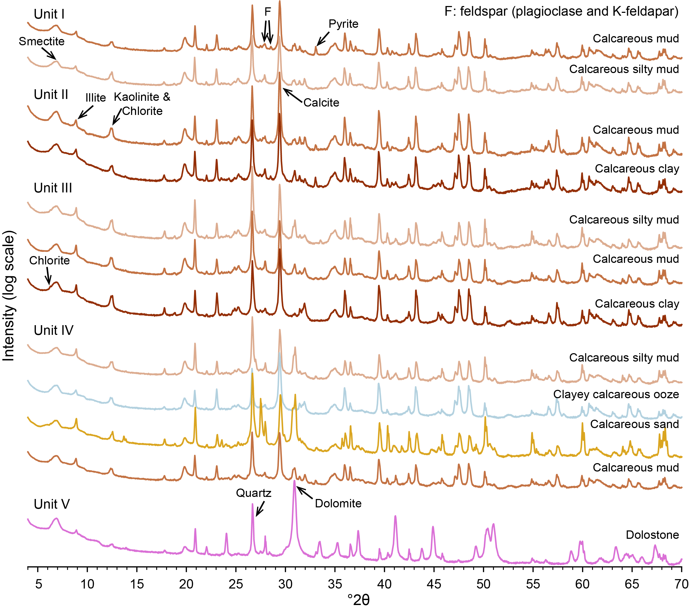
Figure F15. Powder XRD patterns.
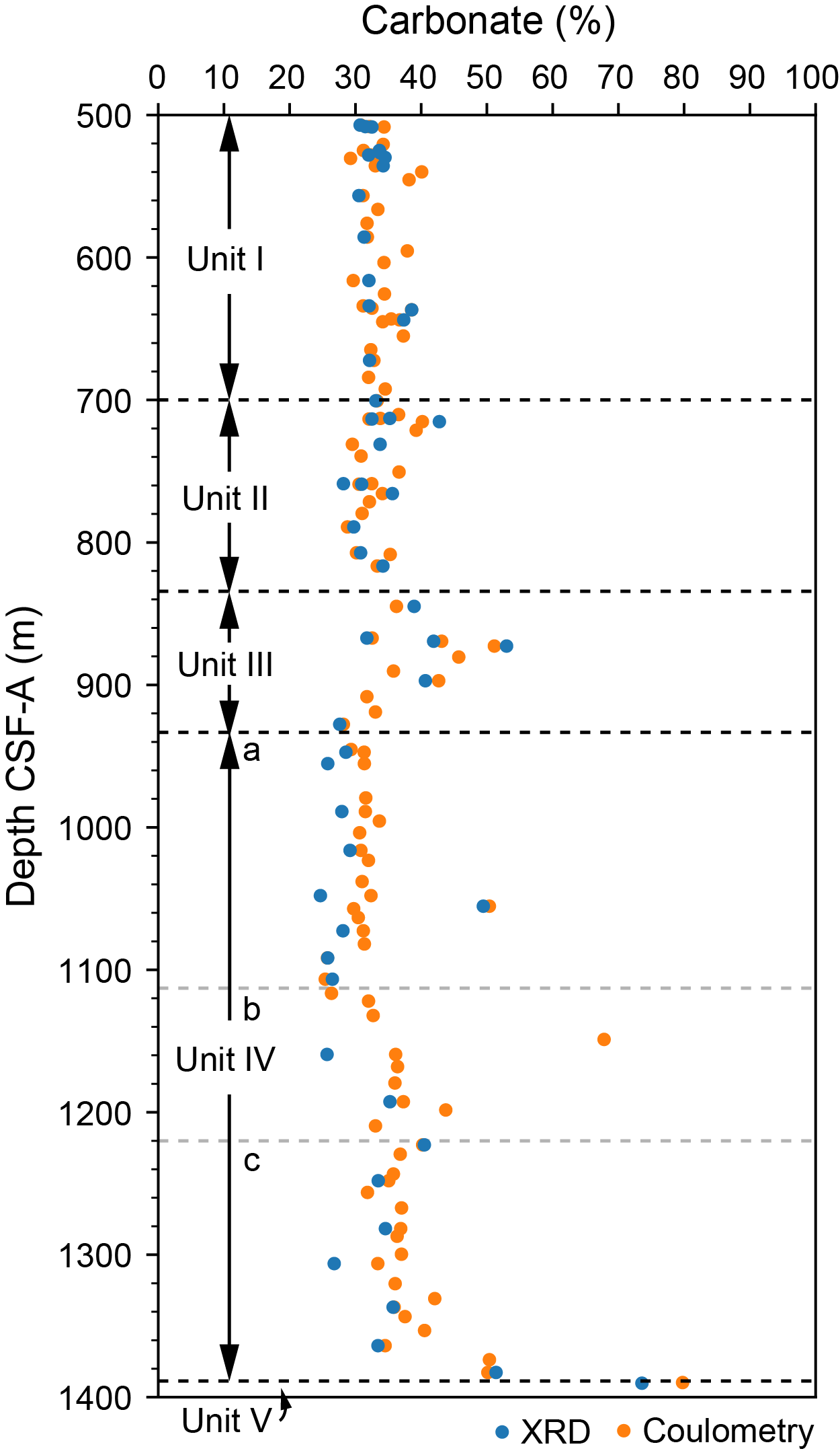
Figure F16. Variation in total carbonate content.
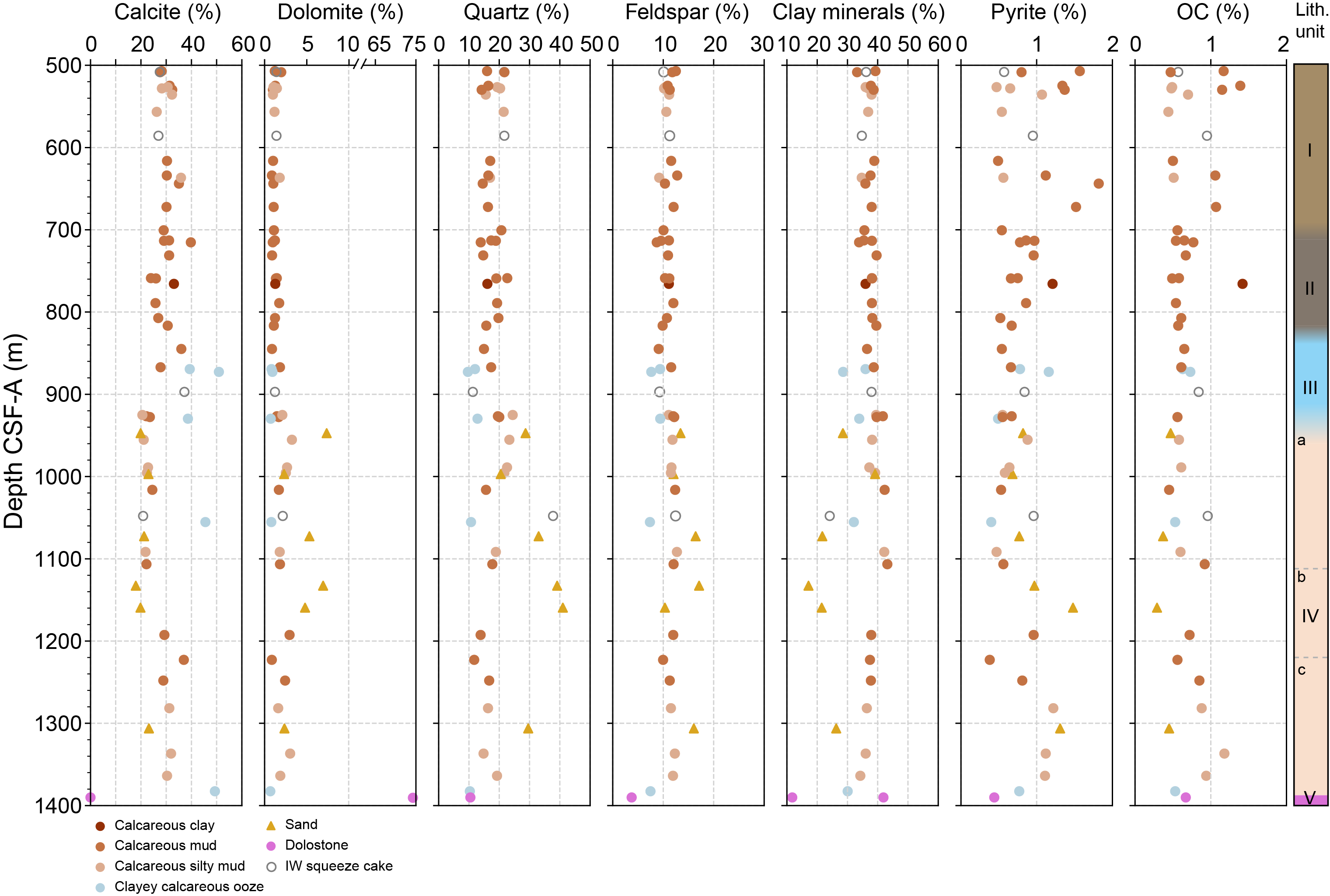
Figure F17. Variations in mineralogical composition.
3.1. Unit I description
3.1.1. Lithologies, bedding, and color
Unit I comprises the top of the cored interval in Hole U1610A (505.2–699.4 m CSF-A). It is composed of calcareous mud, calcareous silty mud, and minor sand and silt intervals (Figure F10). These lithologies alternate and vary in thickness, but beds are rarely thicker than 2 m. The average thickness ranges from ~75 cm for calcareous mud to ~70 cm for calcareous silty mud.
Contacts between lithologies are predominantly gradational, transitioning over a few centimeters in terms of color and grain size (Figure F11A), with occasional sharp and bioturbated contacts. Transitions upward from calcareous silty muds to calcareous muds are occasionally abrupt with a more distinct color change (e.g., Section 401-U1610A-3X-6, 43 cm) in comparison with the transitions upward from calcareous muds to calcareous silty muds (e.g., Section 3X-7, 54–56 cm). Coarser intervals such as silt, sand, or calcareous (silty) sand (Figure F18) commonly have a sharp or erosional basal contact and an average thickness of ~2 cm (e.g., Sections 14X-1, 79–81 cm, and 15X-1, 36–40 cm).
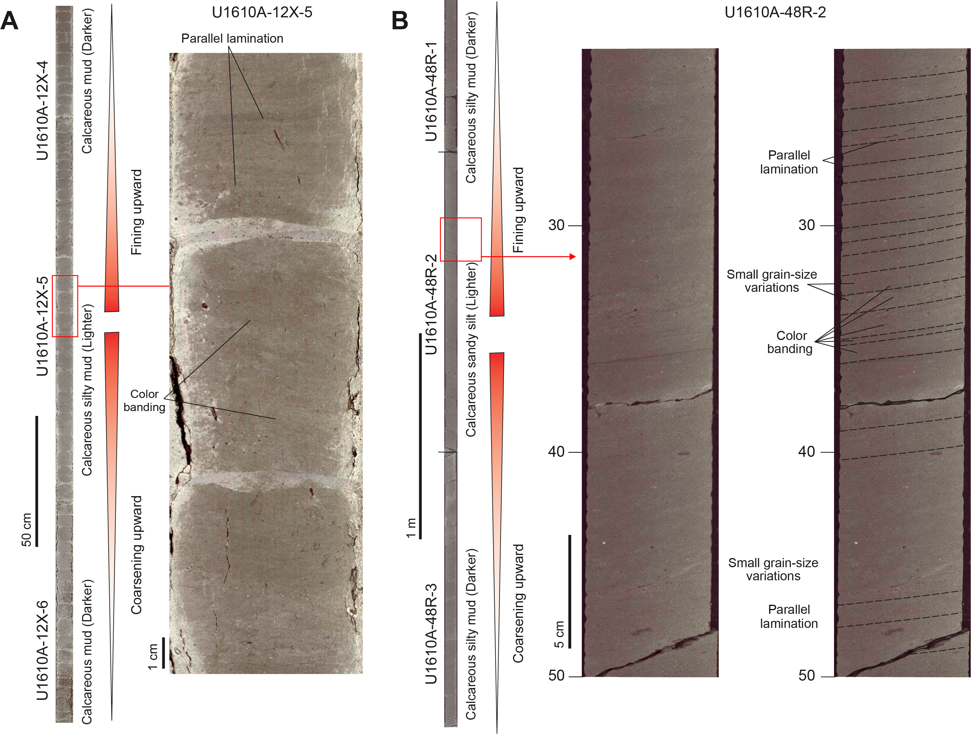
Figure F18. Bigradational sequences of contourites.
The calcareous muds are predominantly grayish olive (10Y 5/2) and more rarely a darker shade of grayish olive (10Y 4/2), and the calcareous silty mud is typically greenish gray (GLEY1 5/10Y). Coarser grained sand and silt intervals are dominantly greenish gray (GLEY1 5/10Y) to dark greenish gray (GLEY1 4/10Y). Because of the subtle and gradational changes observed between lithologies, physical properties data were sometimes used to revise lithologic boundaries. For example, Unit I calcareous mud has relatively higher b* reflectance values, relatively lower L* reflectance and RGB color values, and relatively higher NGR values compared to calcareous silty mud (Figure F11A).
3.1.2. Structure and texture
Sedimentary structures in fine-grained sediments are typically hard to see. However, Unit I calcareous muds, which are usually homogeneous, sometimes contain both subtle parallel lamination and very rare cross lamination (Figure F19A). Some intervals have an apparent dip in parallel lamination mostly due to inclination of the borehole (see Operations). Calcareous silty mud has a greater variety of sedimentary structures than calcareous mud, with parallel and cross lamination, color banding, and rare erosional surfaces (Figure F18B). The calcareous silty mud sometimes has rare and very subtle detrital organic matter laminae that are darker than the surrounding lithology (Figure F19D). Bigradational sequences are commonly associated with upward transitions from calcareous mud to calcareous silty mud and back to calcareous mud (Figure F18A). Silty sand, fine sand, and very fine sand usually have sharp and erosional basal contacts, normal grading, and occasional parallel lamination (Figure F18). The parallel lamination is frequently partly bioturbated. Most of these sandier deposits are interbedded with calcareous silty mud and are rarely associated with calcareous mud (e.g., Section 401-U1610A-14X-2, 79–81 cm, in Figure F19C and Section 16X-4, 93–109 cm, in Figure F20).
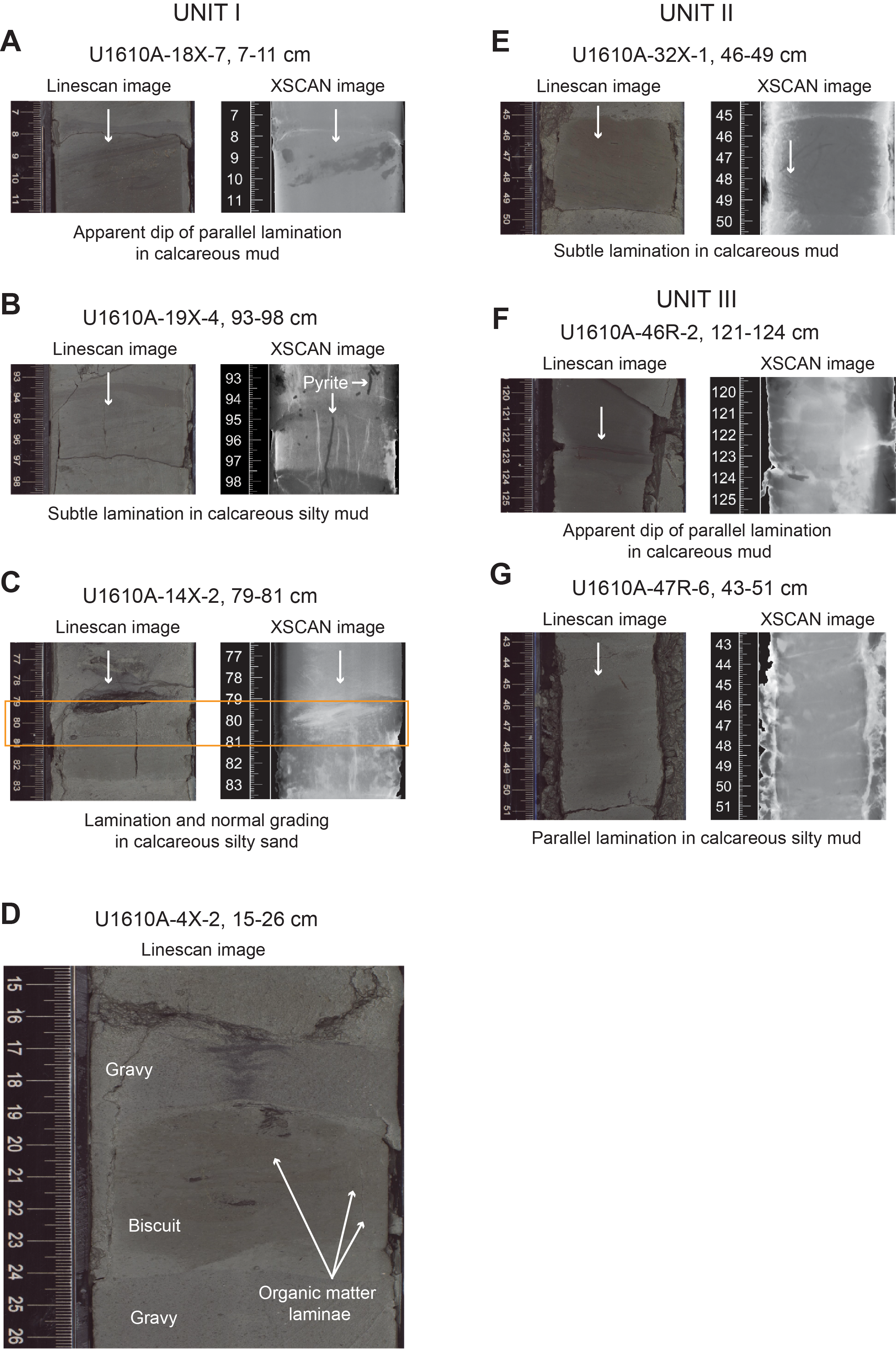
Figure F19. Lamination and normal grading, Units I–III.
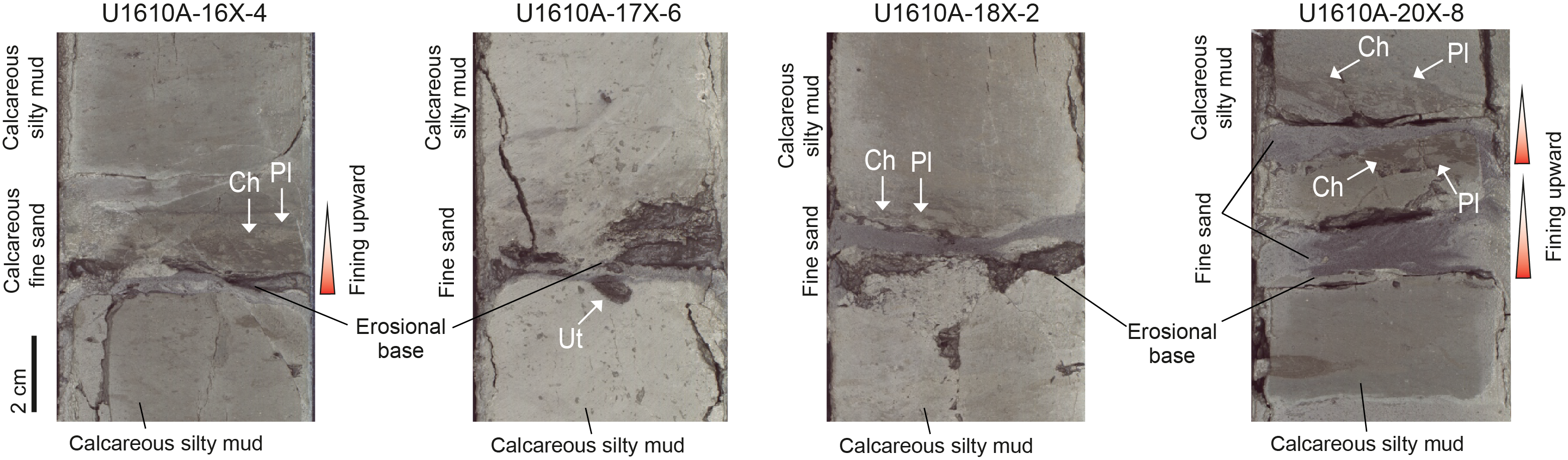
Figure F20. Turbidites and trace fossils, Unit I.
Based on smear slide analysis for Unit I (Table T2), calcareous mud contains 0%–5% sand, 15%–80% silt, and 20%–85% clay (Figure F13). Calcareous silty mud contains 0%–5% sand, 30%–70% silt, and 30%–70% clay. Coarser sandy and silty intervals contain 1%–70% sand, 15%–70% silt, and 5%–40% clay.
3.1.3. Bioturbation and trace fossils
The relative abundance of discrete trace fossil bioturbation index is sparse to moderate (mainly BI = 1–3) and occasionally abundant (BI = 4) or absent (BI = 0). The trace fossil assemblage consists of abundant Chondrites and Planolites and frequent Zoophycos and Thalassinoides. Other ichnotaxa (i.e., Arenicolites, Palaeophycus, and Teichichnus), as well as undifferentiated trace fossils, are rare. In general, calcareous silty muds have a higher bioturbation index (BI = 2–3) and trace fossil diversity than calcareous muds (BI = 1). Sharp-based sand intervals have, in most cases, an upper bioturbated part with Chondrites and Planolites and occasionally a lower bioturbated contact (Figure F20).
3.1.4. Composition and bulk mineralogy
Based on smear slide data (Table T2), the Unit I calcareous mud and calcareous silty mud are compositionally similar (Figure F14). The calcareous mud contains 55%–85% siliciclastic grains, 1%–15% detrital carbonate, 10%–40% biogenic carbonate, and 0%–2% biogenic silica (Figures F14B, F21A). The Unit I calcareous silty mud contains 55%–80% siliciclastic grains, 2%–20% detrital carbonate, 10%–40% biogenic carbonate, and 0%–2% biogenic silica. Coarser grained lithologies (e.g., calcareous silty sand) have wider ranges in composition, 55%–90% siliciclastic grains, 2%–30% detrital carbonate, 5%–20% biogenic carbonate, and 0%–2% biogenic silica (Figure F14B). Additional components include plant fragments and pyrite that are disseminated throughout. Shell fragments and visible foraminifers are only present in some samples, particularly from the lower part of the unit.
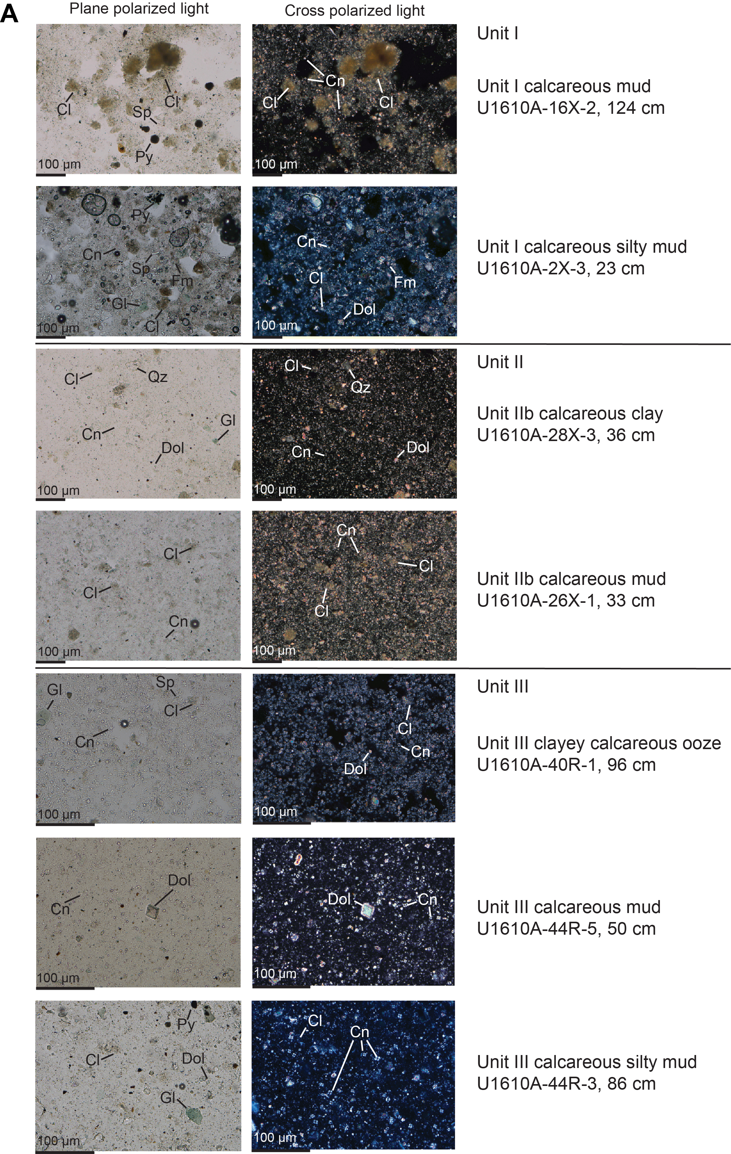
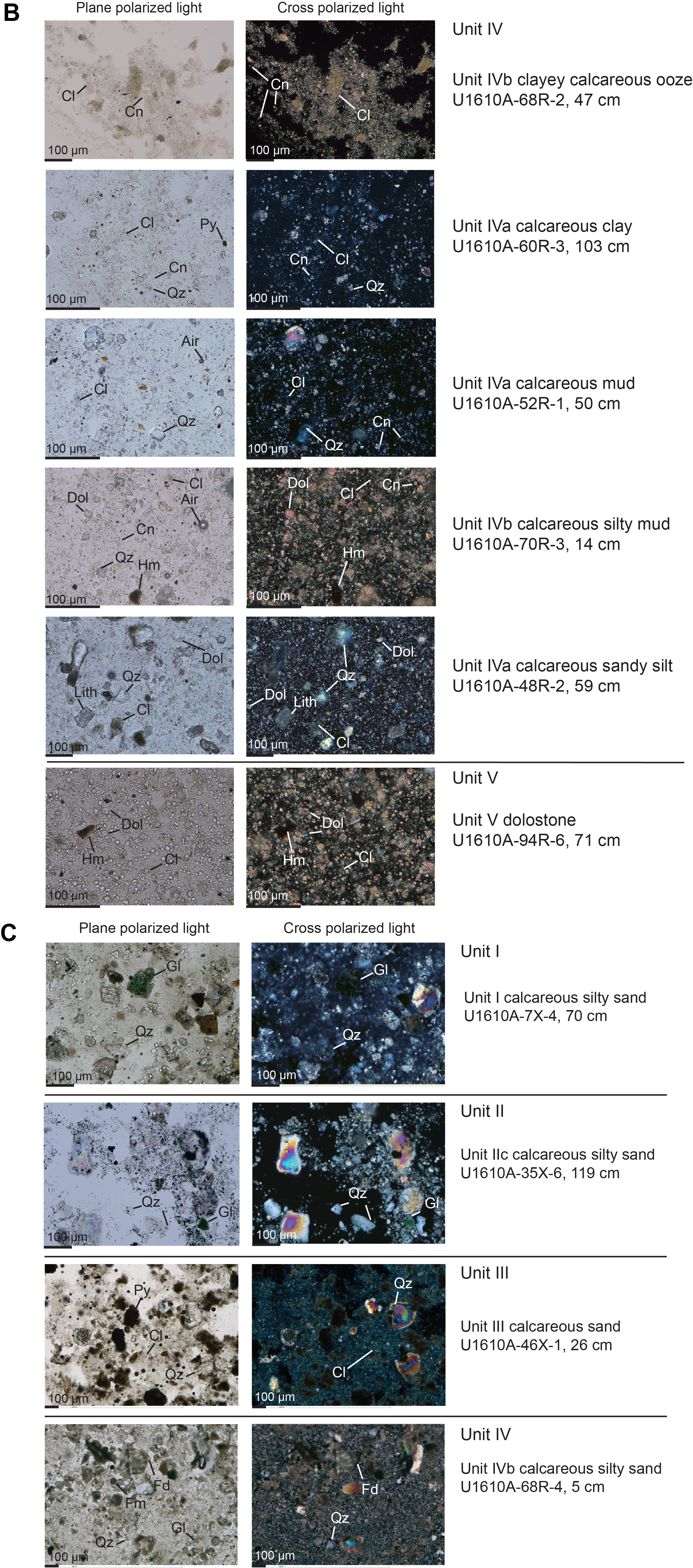
Figure F21. Major lithologies, Units I–V.
Based on XRD analyses of 15 samples from Unit I, the calcite content of Unit I ranges 26%–36% and averages 30% (Figure F17). The quartz content ranges 14%–22% and averages 18%. The average content of feldspars, including plagioclase and K-feldspar, is 12%. On average, clay minerals make up 37% of the sediments of Unit I. The calcareous mud and calcareous silty mud in Unit I are very similar in terms of mineralogical composition, despite their differences in color and bioturbation style. This similarity highlights the need for more detailed analysis of grain size, texture, and organic matter composition to fully resolve the depositional and environmental conditions under which they were formed. Nevertheless, the calcareous mud in Unit I seems to have a slightly higher pyrite content (average = 1.4%) and organic carbon content compared to the calcareous silty mud (Figure F17), consistent with the relatively darker color of the calcareous mud.
3.2. Unit II description
- Interval: 401-U1610A-23X through 37R
- Depth: 699.4–835 m CSF-A
- Age: mid-Zanclean to latest Messinian
- Subunit IIa interval: 401-U1610A-23X through 25X
- Subunit IIa depth: 699.4–728.3 m CSF-A
- Subunit IIb interval: 401-U1610A-26X through 32X
- Subunit IIb depth: 728.3–796.4 m CSF-A
- Subunit IIc interval: 401-U1610A-33X through 37R
- Subunit IIc depth: 796.4–835.0 m CSF-A
3.2.1. Lithologies, bedding, and color
Unit II is composed predominantly of calcareous mud, which represents more than 95% of Subunits IIa and IIc (Figure F10). Subunit IIb consists of ~60% calcareous mud and ~40% or less calcareous clay. Minor silty sand beds were observed in Subunits IIb and IIc. Beds of calcareous mud in Unit II have the highest bed thickness values, with some beds up to 8 m thick. The average calcareous mud bed thickness is ~2.7 m, and calcareous clays of Subunit IIb are on average ~1.1 m thick (maximum thickness is 1.8 m). The average bed thickness for the silty sand intervals is ~1 cm, and these beds are rare with only two occurrences in the entire Unit II.
Contacts between the calcareous mud and calcareous clay are mostly gradational, with subtle changes in color and grain size (Figure F11B), although they are occasionally separated by sharp boundaries characterized by a distinct color change. The contact between silty sand and other lithologies is usually sharp.
The calcareous mud in Unit II is dark greenish gray (GLEY1 4/10Y) to dark grayish olive (10Y 4/2), and the calcareous clay in Subunit IIb is dark grayish olive (10Y 4/2). The minor silty sand beds in Subunits IIb and IIc are dark gray (GLEY1 4/N). Although the calcareous mud and calcareous clay in Subunit IIb have distinct color differences, gradual changes in lithology were sometimes difficult to determine, and physical properties data were used as complementary information to confirm lithologic boundaries. For example, Unit II calcareous muds have lower NGR and b* reflectance values and slightly higher MS, L* reflectance, and RGB color values compared to calcareous clay (Figure F11B).
3.2.2. Structure and texture
Sedimentary structures are largely absent in Unit II, which is homogeneous, especially in Subunits IIa and IIc. In Subunit IIb (Cores 401-U1610A-31X and 32X), some subtle parallel lamination marked by changes in color and grain size are present (Figure F19E). Possible diagenetic color variations and organic matter laminae are also present in Subunit IIb. There are very occasional sandy silt beds in Unit II, with a maximum grain size of very fine sand.
Based on smear slide analysis (Table T2), calcareous clay, which is only present in Subunit IIb, contains 0%–2% sand, 20%–30% silt, and 60%–80% clay (Figure F13). Calcareous mud varies slightly in texture throughout Unit II, with sand, silt, and clay values in Subunit IIa more comparable to the calcareous silty mud of Unit I (Figure F13B). Subunit IIa calcareous mud contains 0%–3% sand, 30%–70% silt, and 30%–70% clay (Figure F13A). The calcareous muds in Subunits IIb and IIc are very similar; Subunit IIb contains 1%–5% sand, 25%–45% silt, and 55%–75% clay, and Subunit IIc contains 0%–2% sand, 40%–50% silt, and 50%–60% clay. The transitional nature between Units I and II is well expressed by the textural characteristics of Subunit IIa. The disappearance of calcareous silty mud and the siltier—but not silty enough to be named calcareous silty mud—calcareous mud in Subunit IIa represent the gradual coarsening-upward trend from Unit II to Unit I. The deeper calcareous muds in Subunits IIb and IIc appear more comparable to the calcareous mud in Unit I. The coarser grained sediments in Unit II are composed of 60% sand, 30%–35% silt, and 5%–10% clay (Figure F13).
3.2.3. Bioturbation and trace fossils
Bioturbation in Unit II is noticeably less intense compared to Unit I. Trace fossils are sparse to moderately abundant (BI = 1–2) and are absent (BI = 0) in some intervals. Both the bioturbation index and trace fossil diversity increase with depth; they are comparatively scarce, even absent, in Subunit IIa, which is dominated by calcareous mud, to moderately abundant in Subunits IIb and IIc. The trace fossil assemblage of Unit II comprises dominantly Chondrites and Planolites and frequent Zoophycos and Thalassinoides. Higher abundance and diversity with increasing depth is accompanied by the increasing occurrence of Palaeophycus and the presence of rare Arenicolites.
3.2.4. Composition and bulk mineralogy
Unit II calcareous muds are compositionally similar to Unit I, with a slight increase in the siliciclastic component of the sediments with depth (Figure F14). This unit has the highest biosiliceous content compared to other units. Subunit IIa calcareous mud consists of 50%–65% siliciclastics, 2%–15% detrital carbonate, 25%–40% biogenic carbonate, and 0%–5% biogenic silica. Subunit IIb calcareous mud contains 60%–70% siliciclastics, 5%–15% detrital carbonate, 20%–30% biogenic carbonate, and 0%–3% biogenic silica (Figure F21A). Subunit IIc calcareous mud contains 65%–75% siliciclastics, 3%–5% detrital carbonate, 20%–25% biogenic carbonate, and 0%–3% biogenic silica. Subunit IIb calcareous clay consists of 55%–75% siliciclastic grains, 3%–10% detrital carbonate, 20%–35% biogenic carbonate, and 0%–3% biogenic silica. Unit II coarser grained lithologies contain significantly less biogenic carbonate than all other lithologies and consist of 80%–85% siliciclastics, 10% detrital carbonate, 5%–8% biogenic carbonate, and 0%–2% biogenic silica (Figures F14, F21C). Additional components including pyrite and some plant fragments are disseminated throughout the entire unit.
Based on XRD analyses of 11 samples from Unit II, the calcite content of Unit II ranges 24%–40% and averages 30% (Figure F17). The quartz content ranges 14%–23% and averages 18%. The average content of feldspars including plagioclase and K-feldspar is 11%, and clay minerals make up an average of 37% of the sediments of Unit II. The bulk mineralogy of Unit II is very similar to that of Unit I (Figure F17), and there is less amplitude of variation in pyrite and organic carbon content in Unit II, which supports the observation that Unit II is more homogeneous. The one sample of the calcareous clay analyzed in Unit II has a higher pyrite and organic carbon content compared to the calcareous mud (Figure F17). More data points are needed to more thoroughly characterize the difference in sediment composition between calcareous mud and calcareous clay.
3.3. Unit III description
3.3.1. Lithologies, bedding, and color
Unit III primarily consists of calcareous mud, clayey calcareous ooze to calcareous clay, and a few coarser grained sandy intervals (Figure F10). The fining-upward transition from Unit IV to Unit III coincides with the appearance of clayey calcareous ooze. Calcareous silty mud is only present in the lower part of Unit III below Core 401-U1610A-45R (907.9 m CSF-A).
The term "clayey calcareous ooze" is used to refer to the lithology in Unit III with a distinctly lighter color, which has an elevated carbonate content (>40%). However, although smear slide observations suggest a mostly >50% carbonate content (Figures F13, F14B), both XRD and coulometry analyses indicate that only a few of these samples have more than 50% carbonate content (Figure F16), so strictly speaking this lighter lithology is mainly calcareous clay. Clayey calcareous ooze is used in Unit III to distinguish this lithology with its lighter greenish gray color (GLEY1 5/10Y) from the dark grayish olive (10Y 4/2) calcareous clay in Unit II.
Bed thickness in Unit III is commonly <2 m, with an average thickness of ~90 cm for the calcareous mud and ~70 cm for the clayey calcareous ooze. The bed thickness for the calcareous silty mud is at least ~35 cm and increases with depth. Coarser grained lithologies (e.g., sandy silt and silty sand) are on average ~4 cm thick, with a maximum thickness of 6 cm.
Contacts between lithologies are typically gradational with subtle changes in color and grain size (Figure F11C). Contacts are occasionally sharp or erosional between the calcareous mud and the clayey calcareous ooze (e.g., Core 401-U1610A-42R) and at the base of the sandy intervals.
The calcareous mud and calcareous silty mud, as well as the sandy intervals, are mainly dark greenish gray (GLEY1 4/10Y), and the clayey calcareous ooze appears greenish gray (GLEY1 5/10Y). Because of the gradual subtle changes between lithologies, visual core descriptions were integrated with physical properties data to help identify lithologic boundaries. For example, Unit III calcareous mud has slightly higher NGR and MS values and slightly lower reflectance (L* and b*) values compared to the clayey calcareous ooze (Figure F11C).
3.3.2. Structure and texture
The calcareous mud and clayey calcareous ooze are relatively homogeneous and lack sedimentary structures. Calcareous silty mud contains subtle parallel lamination (e.g., Section 401-U1610A-47R-6), which sometimes have an apparent dip (e.g., Section 46R-2) in the lower part of Unit III (Figure F19F, F19G). The sandier deposits have sharp erosional bases and sometimes normal grading and bioturbated upper contacts.
The maximum grain size observed was typically silt but occasionally very fine to medium sand. Based on smear slide analysis (Table T2), Unit III calcareous mud contains 0%–3% sand, 10%–60% silt, and 40%–90% clay, and the clayey calcareous ooze contains 0%–5% sand, 10%–40% silt, and 60%–90% clay (Figure F13). The calcareous silty muds in Unit III contain 1%–10% sand, 50%–80% silt, and 20%–40% clay, and the coarser-grained intervals contain 1%–30% sand, 65%–70% silt, and 5%–30% clay.
3.3.3. Bioturbation and trace fossils
The trace fossil assemblage in Unit III is commonly more abundant and diverse than Unit II and is typically associated with the lighter colored clayey calcareous ooze in Unit III. The trace fossil assemblage comprises dominant Chondrites and Planolites, frequent Zoophycos and Thalassinoides, scarce Palaeophycus, and rare Teichichnus (Figure F12). Bioturbation intensity varies from abundant (BI = 4) to sparse (BI = 1). In some cases, abundant bioturbation and crosscutting relationships make ichnotaxonomical characterization difficult. There is a lower abundance and ichnodiversity in the calcareous mud compared to the clayey calcareous ooze (Figure F22). XSCAN images reveal the presence of near-vertical, straight to slightly winding, thin burrows of Trichichnus associated with pyrite nodules (Figure F12).
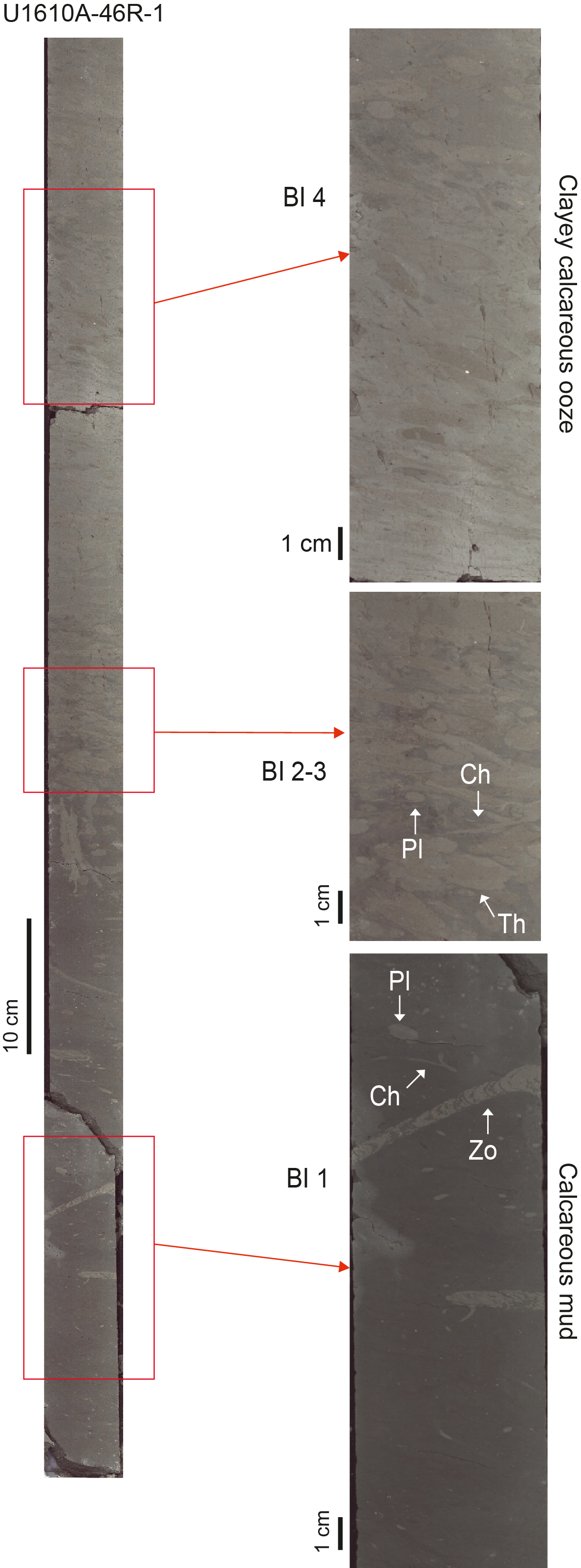
Figure F22. Bioturbation intensity and ichnodiversity, Unit III.
3.3.4. Composition and bulk mineralogy
The Unit III lithologies all contain <1% biogenic silica, and although the calcareous muds and calcareous silty muds are compositionally similar to each other, they are more varied than in Unit I (Figure F14). The calcareous mud contains 30%–80% siliciclastic grains, 1%–10% detrital carbonate, and 15%–60% biogenic carbonate, and the calcareous silty mud consists of 50%–80% siliciclastic grains, 5%–15% detrital carbonate, and 12%–45% biogenic carbonate (Figures F14, F21A). The clayey calcareous ooze consists of 25%–50% siliciclastic grains, 0%–10% detrital carbonate, and 50%–65% biogenic carbonate. Similar to Unit I, the coarser grained lithologies contain less biogenic carbonate compared to the other lithologies in this unit and consist of 60%–90% siliciclastic grains, 2%–10% detrital carbonate, and 10%–35% biogenic carbonate. Additional components of Unit III are pyrite, shell fragments, and foraminifers disseminated throughout (Figure F21C).
Based on XRD analyses of nine samples from Unit III, the calcite content ranges 21%–51% and averages 33% (Figure F17). The quartz content ranges 10%–24% and averages 16%. The average quantity of feldspars including plagioclase and K-feldspar is 10%. On average, clay minerals make up 37% of the sediments of Unit III. The clayey calcareous ooze is characterized by an elevated carbonate content (>40%) and smaller quantities of quartz, feldspars, and clay minerals (Figure F17). The higher carbonate content compared to other lithologies was also observed in smear slide analysis (Figures F13, F14B); however, both XRD and coulometry analyses indicate there are only a few samples in Unit III that have more than 50% carbonate content (Figure F16).
3.4. Unit IV description
- Interval: 401-U1610A-48R to 94R-6, 74 cm
- Depths: 934.5–1388.8 m CSF-A
- Age: late to early Messinian
- Subunit IVa interval: 401-U1610A-48R-1 to 66R-3, 67 cm
- Subunit IVa depth: 934.5–1112.7 m CSF-A
- Subunit IVb interval: 401-U1610A-66R-3, 67 cm, through 77R-3
- Subunit IVb depth: 1112.7–1220.3 m CSF-A
- Subunit IVc interval: 401-U1610A-77R-4, through 94R-6, 6–74 cm
- Subunit IVc depth: 1220.3–1388.8 m CSF-A
3.4.1. Lithologies, bedding, and color
Unit IV consists of calcareous silty mud, calcareous mud, calcareous sandy silt, and coarser grained sand and silty sand intervals, with minor clayey calcareous ooze, calcareous clay, and lithified sediments (siltstone, sandstone, and conglomerate) (Figure F10). Subunits are defined based on the presence of lithified and cemented sediments in Subunit IVb (Figures F23, F24, F25). Contacts between lithologies are typically gradual (Figure F11D), with some sharp or erosive contacts at the base of lithified sediments. Most lithologies are dark greenish gray (GLEY1 4/10Y), except for clayey calcareous ooze and calcareous clay, which are greenish gray (GLEY1 5/10Y), and the lithified sediments, which consist of a range of colors including dark gray (GLEY1 4/N), gray (GLEY1 5/N and GLEY1 6/N), light greenish gray (GLEY1 7/N), and white (WHITE N/8).
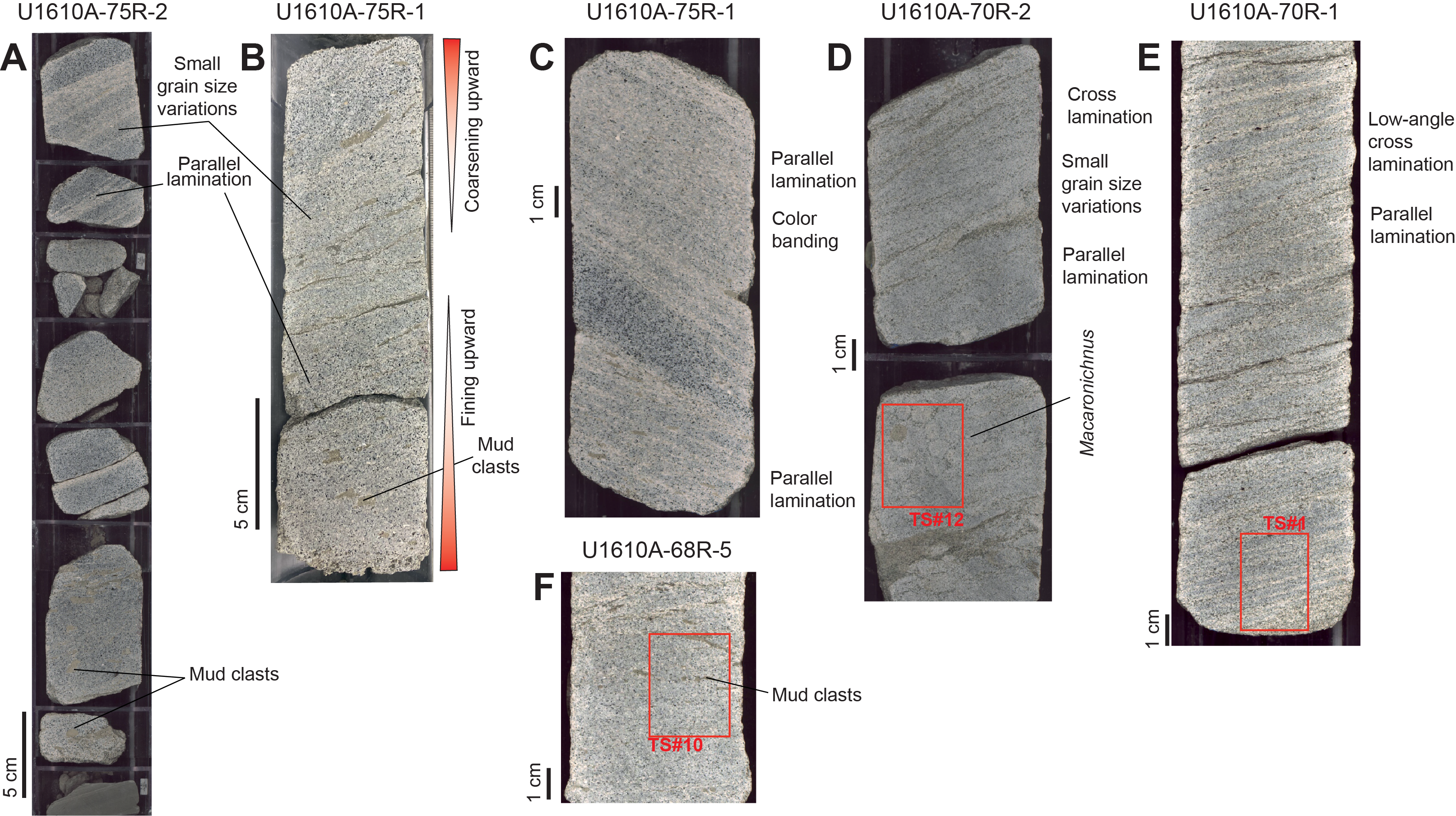
Figure F23. Lithified sandstones, Subunit IVb.
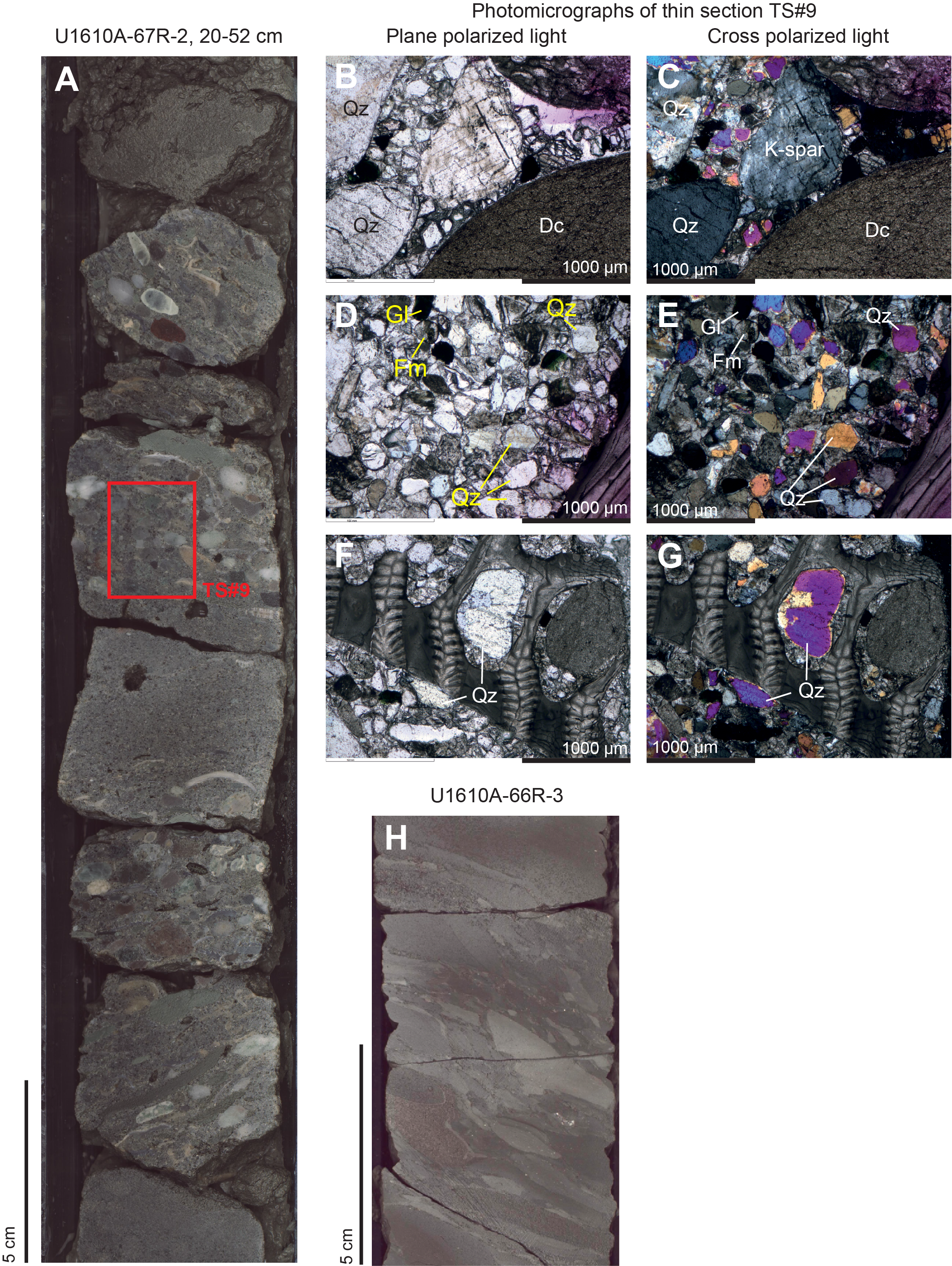
Figure F24. Subunit IVb conglomerates.
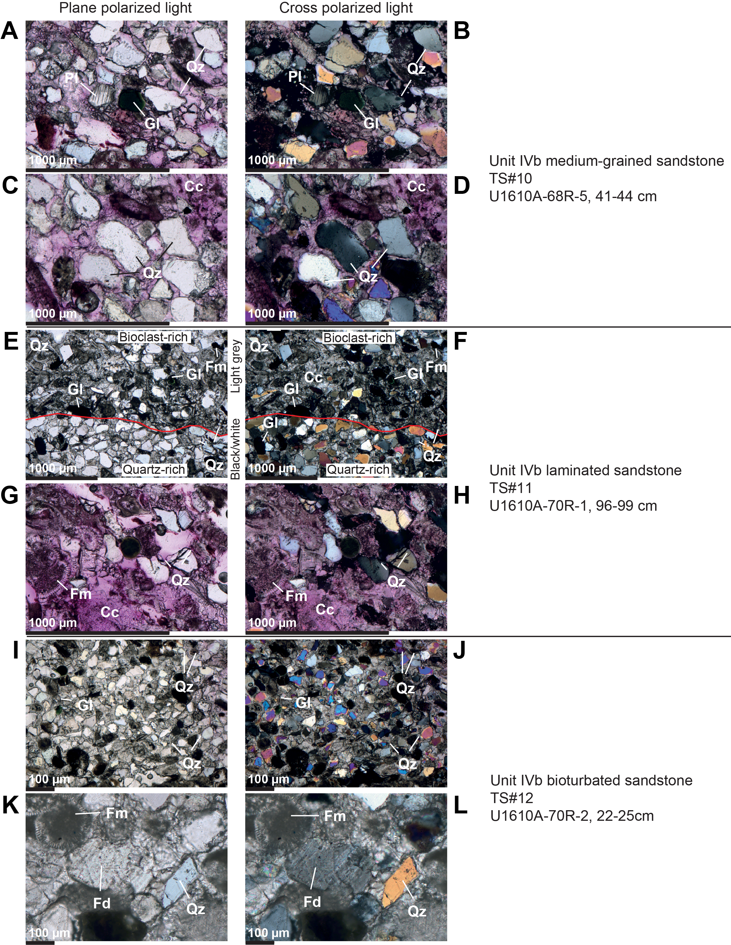
Figure F25. Subunit IVb sandstone.
Subunit IVa consists of calcareous silty mud, calcareous sandy silt, calcareous mud, and coarser grained sand and silty sand intervals, with minor clayey calcareous ooze. In the upper part of Subunit IVa, lithologies are predominantly calcareous silty mud and calcareous sandy silt, alternating with gradual transitions and variable bed thicknesses. These facies are sometimes associated with bigradational sequences, as in Core 401-U1610A-48R (Figure F18). Additionally, these alternations become more distinct, with sharp contacts in the middle of the subunit in Core 56R (1021.13 m CSF-A). Core 56R has a fining-upward sequence, transitioning from calcareous sandy silt to calcareous mud, with parallel lamination, cross lamination, and thin lenticular beds (Figures F26C). Subunit IVa is extensively laminated. Rare sharply bounded clayey calcareous ooze intervals are interbedded with calcareous mud and calcareous silty mud. The calcareous ooze can be recognized by distinct color changes to a lighter shade of greenish gray and more intense bioturbation.
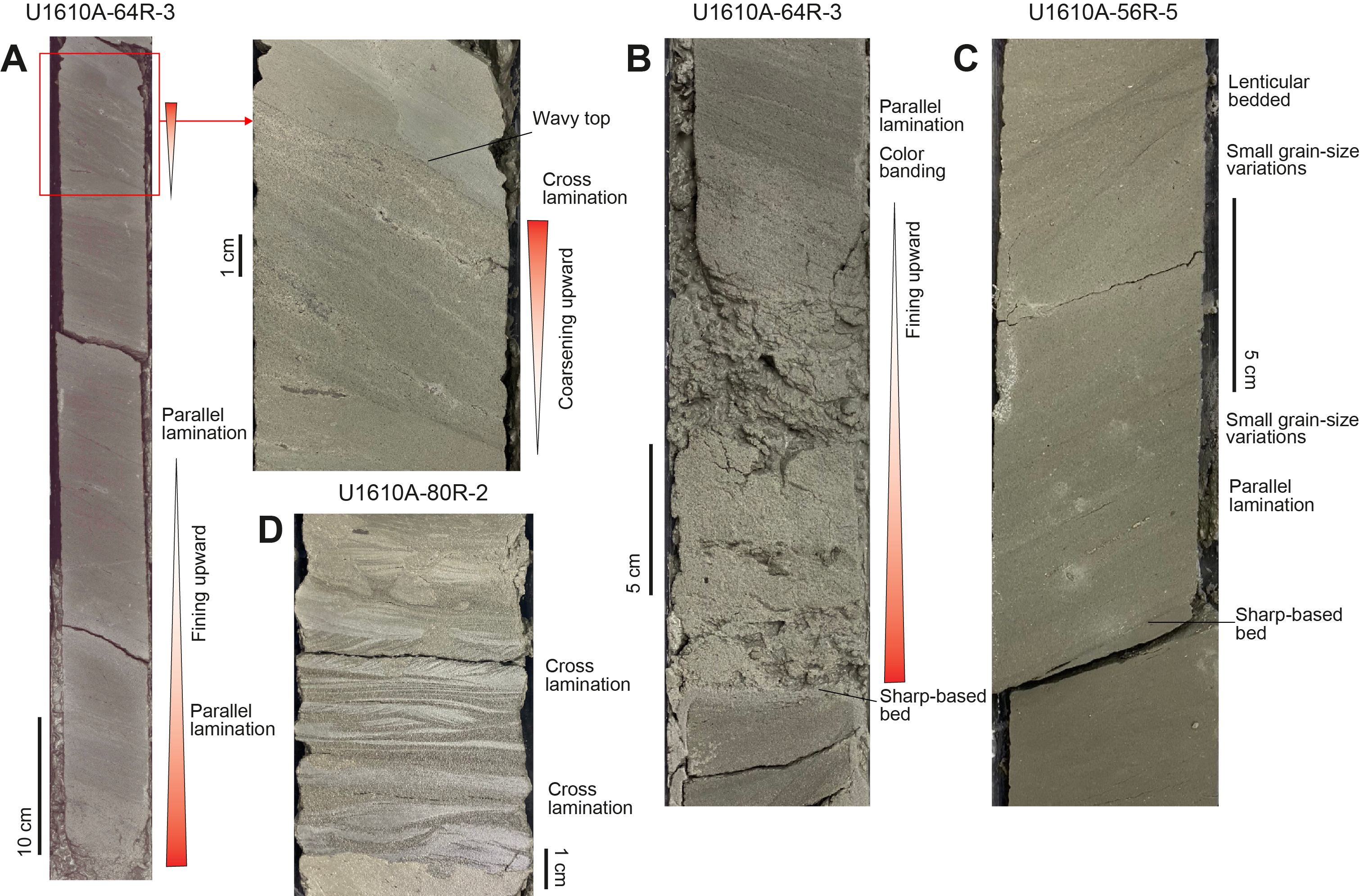
Figure F26. Unit IV turbidite deposits.
In Subunit IVb, there are substantial missing successions, and the dominant recovered lithologies include calcareous mud, calcareous silty mud, calcareous sandy silt, and calcareous sand (very fine, fine, and medium), with some clayey calcareous ooze and minor lithified siltstone, sandstone (fine and medium), and conglomerate. Contacts between lithologies are typically gradational (Figure F11D), with some sharp or erosive contacts at the base of lithified sediments.
Subunit IVc is characterized by gradual changes between calcareous mud, calcareous silty mud, and calcareous sandy silt similar to those in Subunit IVa, with some sharp contacts between coarser grained sand and silty sand (very fine, fine, and medium sand) and occasional interbedding between calcareous clay and clayey calcareous ooze. Based on thin section analysis, Section 401-U1610A-86R-1 contains calcareous fine sand that was partially cemented by calcite (Figure F27A, F27D–F27G). However, no other lithified interval was observed in this subunit.
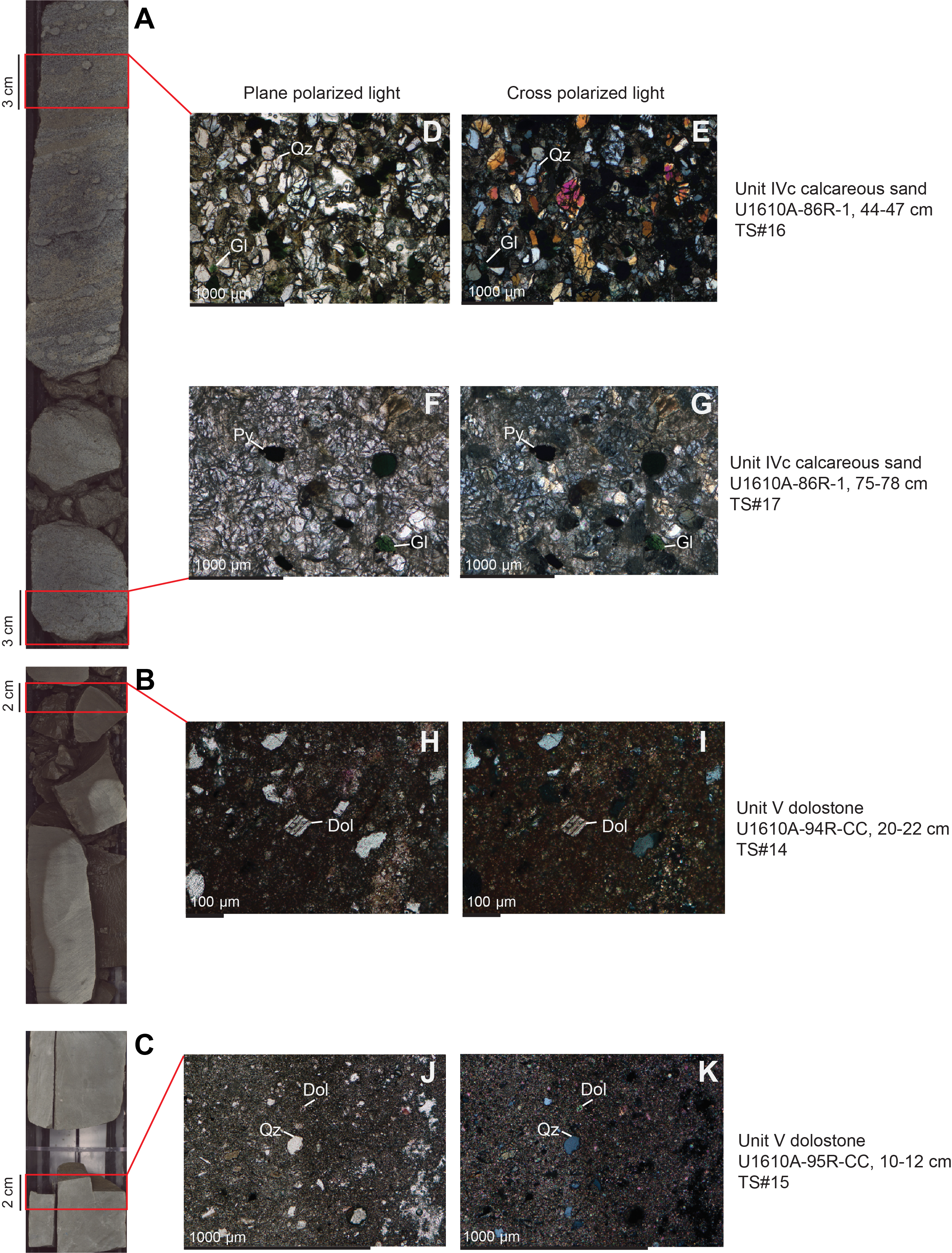
Figure F27. Subunit IVc calcareous sand and Unit V dolostone.
Physical properties data were also used to help confirm lithologic boundaries in Unit IV. For example, sandier deposits (e.g., calcareous fine sand) have lower NGR values and higher MS, L* reflectance, and RGB color values compared to the finer grained lithologies (e.g., calcareous silty mud) in Unit IV (Figure F11D).
3.4.2. Structure and texture
The calcareous silty mud in Unit IV contains a variety of sedimentary structures including parallel lamination, low-angle cross lamination, small variations in grain size and/or slight color variation (color banding), and erosional surfaces. Frequently, plant fragments were observed. The calcareous sandy silt is characterized by parallel lamination, normal grading with sharp basal contacts, and rare lenticular bedding (Figure F26C). The alternations between calcareous silty mud and calcareous sandy silt are interpreted to be bigradational sequences, some of which are several meters thick and include lamination as well as color and/or grain size banding (Cores 401-U1610A-48R and 49R; Figure F18B). Rare coarsening-upward sequences from calcareous silty mud to calcareous sandy silt were identified (e.g., Section 89R-6).
The silty sand intervals commonly have normal grading, parallel lamination, and bioturbation at the top and sometimes at the base. The very fine and fine sand beds have sharp basal contacts, normal grading, lamination, and banding. Occasionally, coarsening-upward successions with wavy upper contacts were observed in the sand intervals (Figure F26A). Wood fragments and plant debris are also present in the sandy deposits. The medium-grained sandstones have sharp basal contacts with mud clasts, parallel and cross lamination (Cores 401-U1610A-68R, 70R, and 75R), normal grading, and rare instances of inverse grading (Figure F23A, F23B). Glauconite-bearing bands (Figure F23A–F23C, F23E) are the most significant structures in the sandstones, exhibiting frequent variations in both grain size and color. Sometimes lamination is also characterized by variations in the proportion of quartz and bioclasts (e.g., Section 70R-1; Figure F25E–F25H). Siltstones are also commonly laminated.
Two sections in Subunit IVb (Sections 401-U1610A-66R-3 and 67R-2) contain conglomerates, some with soft clasts (e.g., calcareous silty mud, sandy silt, silty sand, and carbonate bioclasts) and hard clasts (e.g., metamorphic rock and dolostone with weathered holes) up to pebble size (several centimeters) in a matrix dominantly composed of calcareous muds (Figure F24). The conglomerate in Section 67R-2 contains a variety of clasts up to 3 cm wide and shell fragments and is overall poorly sorted. The space between the gravel-sized clasts is filled with mostly fine sand–sized particles and calcite cement, resulting in very little residual porosity. The gravel-sized clasts are subrounded to rounded, and the fine sand–sized particles are subangular to subrounded. No significant abundance of clay was observed in the space between framework minerals or clasts, which may need to be confirmed with thinner and better polished thin sections.
Based on smear slide data (Table T2), the Unit IV calcareous mud consists of 0%–2% sand, 10%–70% silt, and 30%–90% clay, and the calcareous silty mud consists of 0%–35% sand, 30%–80% silt, and 10%–70% clay (Figure F13). The finer grained Unit IV lithologies have comparable textures, with the clayey calcareous oozes containing 0% sand, 3%–30% silt, and 70%–95% clay and the calcareous clays containing 0% sand, 15%–20% silt, and 80%–85% clay. The Unit IV calcareous sandy silts consist of 2%–55% sand, 30%–65% silt, and 15%–55% clay, and the coarser-grained lithologies (e.g., sand, and silty sand) have a variable texture with 8%–70% sand, 25%–55% silt, and 5%–55% clay (Figure F13).
3.4.3. Bioturbation and trace fossils
Unit IV has lower trace fossil abundance and diversity than Unit III, which can be attributed to the greater influx of coarser sediments. The trace fossil assemblage is dominated by Chondrites and Planolites, with common Zoophycos and Thalassinoides and rare Palaeophycus. Bioturbation intensity is moderate (BI = 3) to sparse (BI = 1), and intervals with no trace fossils (BI = 0) are common. Macaronichnus is locally abundant (BI = 4) in the calcareous fine sands, occurring below the conglomerate in Section 401-U1610A-67R-2, 50–66 cm (Figure F28).
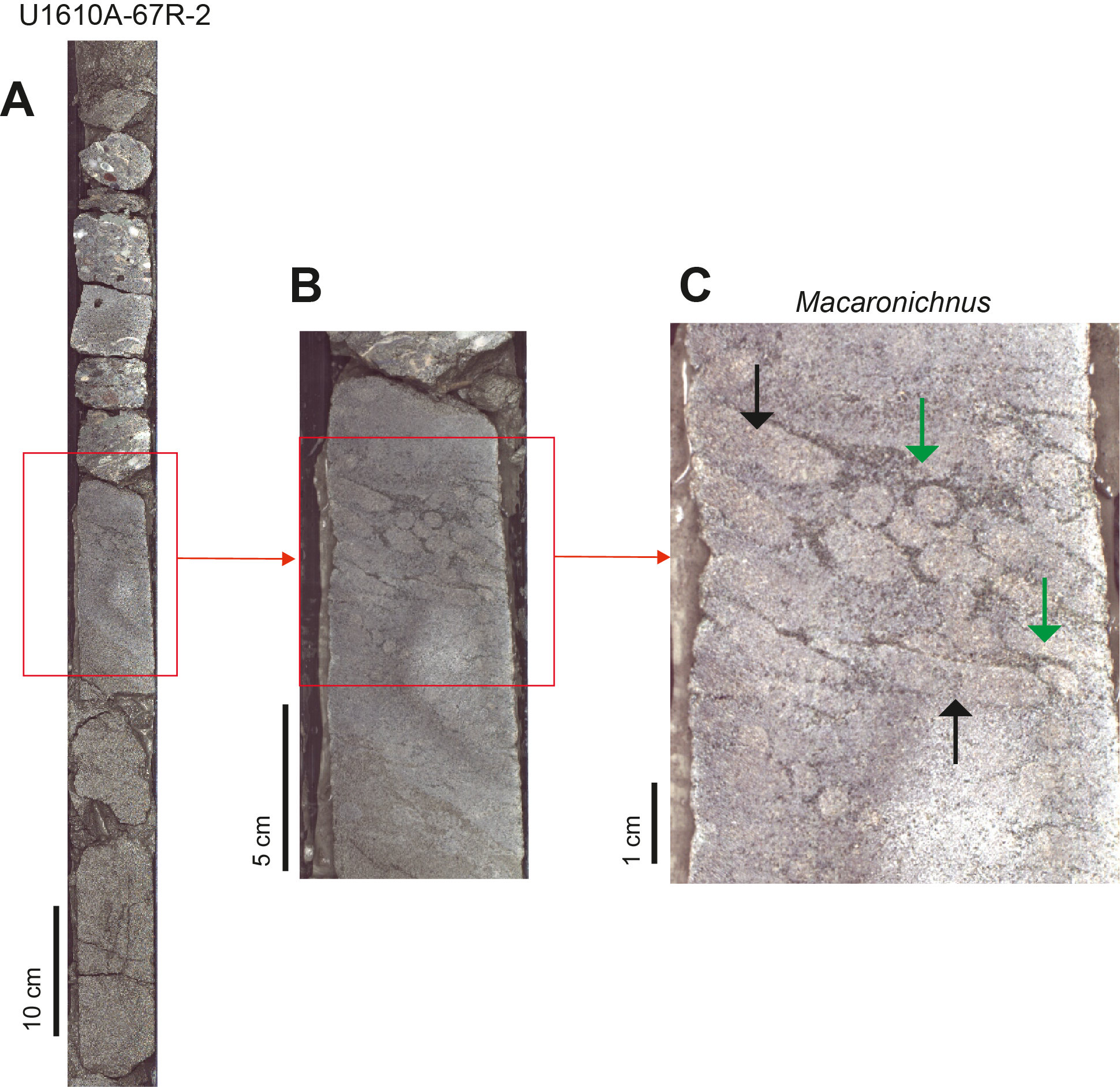
Figure F28. Macaronichnus trace fossil.
3.4.4. Composition and bulk mineralogy
As in Units I–III, Unit IV calcareous silty mud and calcareous mud are compositionally similar and only differ significantly in texture (Figures F13, F14). The calcareous silty mud contains 45%–100% siliciclastic grains, 0%–20% detrital carbonate, 0%–50% biogenic carbonate, and 0%–1% biogenic silica and in 5 of the 29 smear slides is not strictly calcareous (17%–24% carbonate; Table T2). The calcareous mud consists of 55%–75% siliciclastic grains, 0%–15% detrital carbonate, 15%–45% biogenic carbonate, and <1% biogenic silica.
Although the clayey calcareous ooze and the calcareous clay are texturally similar (Figure F13), they have different compositions (Figure F14). The Unit IV calcareous clay contains 60%–70% siliciclastic grains, 1%–5% detrital carbonate, 30%–35% biogenic carbonate, and <1% biogenic silica. The clayey calcareous ooze in Unit IV is compositionally similar to the Unit III clayey calcareous ooze, but on average it contains less biogenic carbonate. The Unit IV clayey calcareous ooze consists of 30%–70% siliciclastic grains, 0%–10% detrital carbonate, 25%–70% biogenic carbonate, and <1% biogenic silica; therefore, it is compositionally different from the calcareous clay.
The Unit IV calcareous sandy silt is compositionally similar to the Unit IV calcareous clay and only differs significantly in texture (Figures F13, F14). The Unit IV calcareous sandy silt consists of 50%–80% siliciclastic grains, 0%–15% detrital carbonate, 15%–45% biogenic carbonate, and <1% biogenic silica. The Unit IV coarser grained lithologies (silty sand and very fine to medium sand) contain more siliciclastic components and consist of 55%–95% siliciclastic grains, 1%–35% detrital carbonate, 0%–30% biogenic carbonate, and <1% biogenic silica. Additional components are pyrite, shell fragments, and disseminated foraminifers visible on the cut core surfaces.
Based on XRD analysis of 17 samples from Unit IV, the calcite content ranges 18%–49% and averages 27% (Figure F17). The quartz content ranges 10%–41% and averages 23%. The average feldspar content is 12%. Clay minerals on average make up 33% of the sediments of Unit IV. The bulk mineral composition of the calcareous mud, calcareous silty mud, and clayey calcareous ooze in Unit IV is very similar to these lithologies in the other units (Figure F17). Only unlithified sands in Unit IV were sampled for XRD analysis, with no data from the lithified sandstones. The more common sand-dominated lithologies in Unit IV are characterized by distinctly lower calcite (~20%) and clay mineral (<30%) contents; higher amounts of dolomite (~5%), quartz (~30%), and feldspar (10%–16%); and lower organic carbon contents compared to the finer grained lithologies in Unit IV and other units (Figure F17).
Four thin sections were made from the well-cemented sandstones in Subunit IVb (Figures F23D–F23F, F25). The sandstone in Section 401-U1610A-68R-5 (TS10) is medium grained, moderately to well sorted, and contains subangular to rounded grains of quartz, feldspar, lithic grains, glauconite (~6%), and bioclasts (~14%) (Table T3; Figure F25A–F25D). Carbonate staining shows that it is cemented by calcite, which constitutes about 10% of the sandstone.
The sandstone in Section 401-U1610A-70R-1 is characterized by alternations of 1–3 mm thick light and dark layers over the section from 74 to 116 cm (total thickness is ~40 cm), which is then overlain by more homogeneous sandstone without layering (at least 50 cm thick). A thin section (70R-1 [TS11]) made from the layered part of this sandstone (Figure F23E) shows that the sandstone is on average fine sand sized and well sorted (Figure F25E–F25H; Table T3). The light-colored layers are composed dominantly of quartz, whereas the dark layers contain more bioclasts. The glauconite content is low (~3%) and is similar in both layers. This sandstone is cemented by calcite, which constitutes about 30% of the sandstone.
The sandstone in Section 401-U1610A-70R-2 (TS12) is on average fine sand in grain size, bioturbated, and well sorted (Figures F23D, F25I–F25L). It contains about 30% quartz, 30% bioclasts, 8% feldspars, 10% lithic grains, and about 20% calcite cement (Table T3).
The average grain size of the sandstone in Section 401-U1610A-75R-1 (TS13) is medium sand (Table T3). The sandstone is characterized by alternations between 1–2 cm thick dark layers and paler layers (Figure F23B). Thin section microscopy shows that the dark layers are richer in glauconite (up to 15%), which is sometimes green in the thinner areas of the thin section but appear almost black in other parts of the thin section and in hand specimens. The darker layers contain 50% quartz and well-sorted, rounded to subrounded grains cemented by about 15% poikilotopic calcite. The lighter layers are richer in carbonate bioclasts, more poorly sorted, less rounded with more angular grains, and cemented by about 10% calcite.
Two thin sections were made from the partially cemented calcareous sand in Section 401-U1610A-86R-1 (TS16 and TS17). The thin section at 44–47 cm (TS16) crosses a Macaronichnus trace fossil burrow (Figure F27A, F27D, F27E). The sample is on average fine sand in grain size and contains moderately sorted and subangular to subrounded quartz, feldspar, and lithic grains and well-rounded glauconite (about 10%; Table T3). Darker particles including glauconite, a higher proportion of clay mineral, and very fine detrital carbonate grains are concentrated on the rim of the burrow. Grains inside the burrow are better sorted than outside the burrow. The sand is nearly completely cemented by calcite, which occupies about 20% of the thin section. The thin section at 75–78 cm (TS17) is well sorted and contains dominantly very fine sand–sized subangular grains, including about 35% quartz, except for the 5% glauconite that is well-rounded (Figure F27A, F27F, F27G; Table T3). This sand contains about 1% pyrite and about 20% calcite cement.
The sandstones and conglomerate in Unit IV contain sedimentary rock fragments such as chert fragments and detrital dolomite (Figure F29A–F29D, F29G, F29H), metamorphic quartz (Figure F29G, F29H), and metamorphic rock fragments (e.g., schist fragment in Figure F29E, F29F). The chert fragments and dolomite fragment were likely derived from recycled sedimentary rocks. The metamorphic quartz and metamorphic rock fragments were likely derived from rivers that drained the metamorphic hinterland.
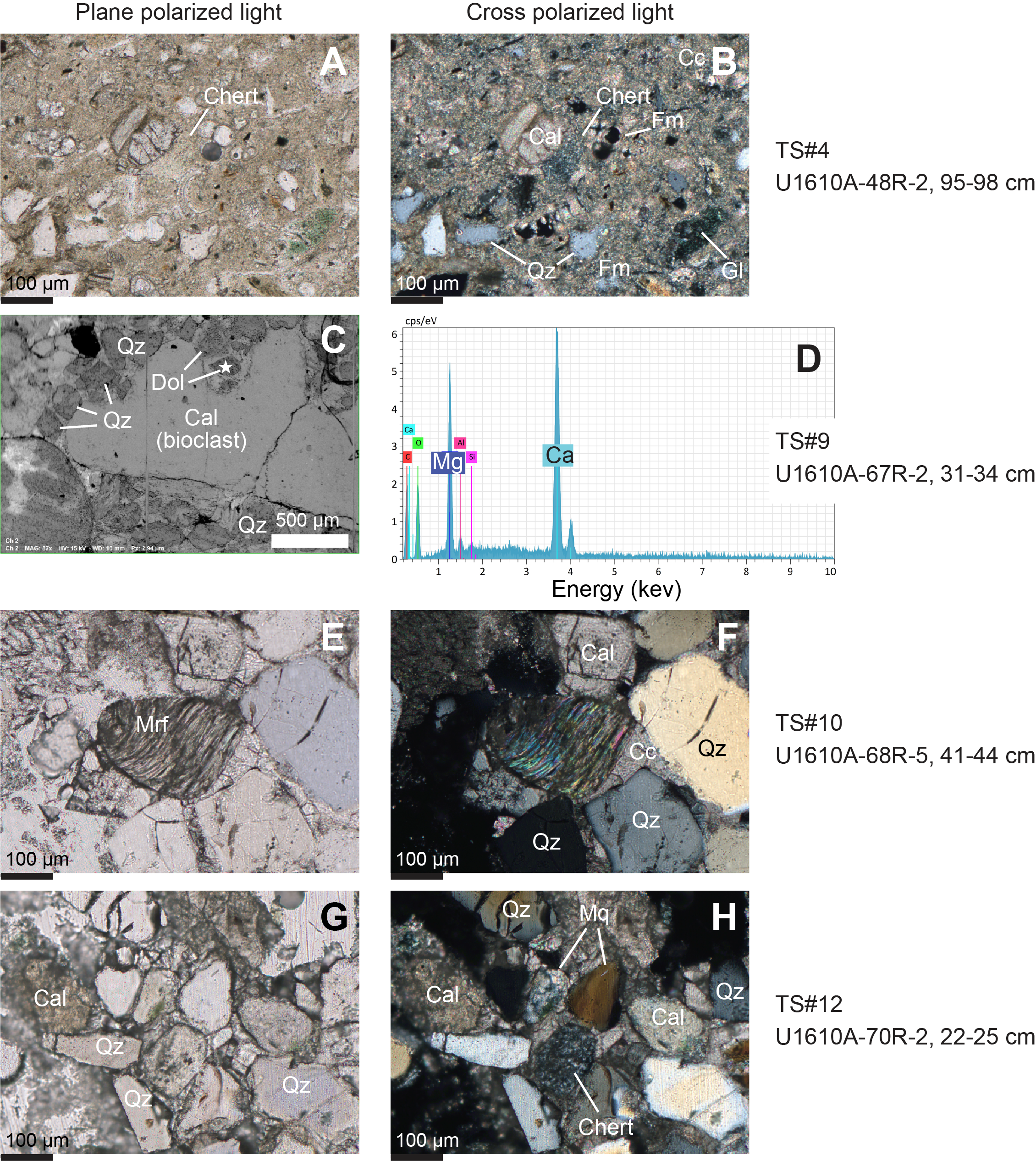
Figure F29. Calcareous sandy silt, conglomerate, sandstone, and sandstone.
3.5. Unit V description
3.5.1. Lithologies, bedding, and color
Unit V consists of dolostone and silty mud cemented predominantly by dolomite. Only 1.8 m was recovered, and subsequent cores were empty, making it impossible to estimate the exact thickness of the unit. The dolostone is greenish gray (GLEY1 6/10Y) (Figure F11E). There was a gradation over about 20 cm where the overlying calcareous silty mud in Unit IV became progressively dolomitized, as suggested by a smear slide (401-U1610A-94R-6, 71 cm) (Table T2).
3.5.2. Structure and texture
There were no primary structures observed in this unit. The maximum grain size is fine sand. The one smear slide from this unit consists of 5% sand, 85% silt, and 10% clay (Table T2).
3.5.3. Bioturbation and trace fossils
The dolostone does not appear to be bioturbated, and no trace fossils were identified.
3.5.4. Composition and bulk mineralogy
Thin sections of the dolostone reveal a fully dolomitized micritic cement that is strongly poikilotopic (Figure F27B, F27C, F27H–F27K). Detrital grains include quartz, feldspars including microcline, and lithic fragments (e.g., metamorphic rock fragments). The grains are angular to subrounded and poorly sorted, with grain size ranging 20–200 µm (average very fine sand). Additionally, there are a few large, degraded dolomite rhombs (200–300 µm) surrounded by the micritic cement (Figure F27).
One XRD sample was collected from the dolostone in Section 401-U1610A-94R-CC. The dolostone is dominantly dolomite (~74%), with small amounts of quartz and feldspar (14%), clay minerals (12%), and less than 1% calcite and pyrite (Figure F17).
3.6. Discussion
3.6.1. Boundaries between lithostratigraphic units and subunits
Unit boundaries are transitional in Hole U1610A (Figure F9), except for the Unit IV/V boundary, where the boundary is sharp because of the occurrence of the dolostone interval in Unit V. Units I–III are largely muddy (≥50%), with Subunits IIa and IIc comprising almost exclusively calcareous mud, except for some thin silty or sandy intervals. These two dominantly muddy subunits are located at unit transitions and reflect the disappearance of lithologies with different grain sizes. Subunit IIa is between Unit I, which contains calcareous silty mud, and Subunit IIb, which contains calcareous clay (Figure F10). Subunit IIc is between Subunit IIb and the underlying Unit III, which contains clayey calcareous ooze. The transition between these units/subunits occurs gradually. The apparent dips of some beds and lamination in Hole U1610A are mainly due to the nonvertical borehole.
3.6.2. Bed thickness variations
Bed thicknesses are variable at this site, with the calcareous mud lithology being the thickest, up to 8 m (Figure F10). Bed thickness was only calculated within a core, without making any assumptions about the nature of the gaps between cores or intervals with no recovery. The calculated maximum thickness of the coarsest lithologies is capped by the core length. It is possible that some lithologies are up to 30 m thick (e.g., in Subunit IIa). Beds are commonly thinner in Units I and III and increase in thickness substantially in Unit II. Calcareous (silty) sand beds are thicker in Subunits IVb and IVc. A general thinning and fining-upward trend was detected in the upper part of Subunit IVa, and there are thickening and coarsening-upward trends in Subunits IVb and IVc.
3.6.3. Links between sediment composition and physical properties
The calcareous silty mud, calcareous mud, and calcareous clay in Units I–III have rather similar bulk mineral compositions, except that the finer grained lithologies seem to have a slightly higher pyrite and organic carbon content, which are positively correlated (Figure F17). The higher pyrite and organic carbon content likely contribute to the darker color, higher RGB values, and higher NGR values in the finer grained lithologies (Figure F11A–F11C). The relationship between pyrite and organic carbon content and physical properties, as well the possible roles of other factors such as the impact of clay mineralogy on the physical properties of these lithologies that only differ subtly from each other based on visual inspections require more detailed petrographic, mineralogical, and geochemical analyses. The lighter color, lower NGR values, and higher RGB values of the clayey calcareous ooze can be linked to the distinctly higher carbonate content and lower clay content (Figures F11C, F17). Although MS varies between lithologies, there seem to be factors other than the grain size and pyrite content that influence the MS of particular lithologies in Units I–III; for example, clay content and the trace amounts of magnetic minerals such as magnetite, greigite, and hematite that cannot be detected by XRD (Figure F11A–F11C).
The mineral composition and organic carbon content of the calcareous mud and calcareous silty mud in Unit IV are similar to those in Units I and II. The sand-dominated lithologies in Unit IV have greater quantities of quartz, feldspar, and dolomite and smaller quantities of calcite, clay, and organic carbon, resulting in lower NGR values and a lighter color (Figure F11D). We speculate that the higher MS of the sand-dominated lithologies may be due to siliciclastic grains coated with iron oxides. Interestingly, the amount of dolomite increases appreciably in Unit IV, particularly with the sandier intervals (Figure F17) and just above the Unit V dolostone. The variations in dolomite content in these sand-dominated lithologies are inversely related to calcite content and are positively correlated to changes in quartz and feldspar content, which could be attributed to a detrital origin of the dolomite in these sand-dominated lithologies. The detrital origin of dolomite in Unit IV is supported by the presence of detrital dolomite in the conglomerate (Figure F29C, F29D). Alternatively, this relationship may reflect a focusing of diagenetic dolomitization during burial of the coarser lithologies. Unlike the finer grained lithologies, the Unit IV sandy lithologies exhibit an inverse relationship between pyrite and organic matter (Figure F17). This inverse relationship may suggest that the pyrite in these sands was derived from reworking of previously deposited sediments or that the pyrite was formed in situ through microbial degradation of organic matter. Further analyses are needed to resolve the origin of pyrite in these sand-dominated lithologies, which may shed light on their depositional and burial conditions and the relative sediment accumulation rates.
3.6.4. Dominant sedimentary facies
3.6.4.1. Hemipelagic deposits
The clayey calcareous ooze, calcareous clay, calcareous mud, and calcareous silty mud deposits identified in the four upper units represent a deepwater sedimentary facies association characterized by poor sorting, common bioturbation, and no evidence of traction-current-generated structures, which corresponds to sedimentation in a pelagic or hemipelagic setting (Hüneke and Henrich, 2011; Stow and Smillie, 2020, de Castro et al., 2021). These facies can be considered to be the background sedimentation in the Site U1610 area, with a general increase in the amount of clayey calcareous ooze and a corresponding decrease in the amount of calcareous silty mud upward (Figures F10) from Unit IV to Unit III, although these lithologies are interstratified with other identified lithologies.
3.6.4.2. Contourite deposits
Evidence of bottom current (contouritic) processes and the occurrence of contourites are visible in Unit I with the vertical association of calcareous mud and calcareous silty mud in symmetric and asymmetric bigradational sequences (Figure F18A) that are characteristic of very fine grained contourites (Gonthier et al., 1984; Stow and Faugères 2008; Stow and Smillie, 2020). There is no evidence of bottom currents in Units II and III, but the top of Unit IV starts with clear bigradational sequences (Figure F18B) between 935 (Core 401-U1610A-48R) and 950 m CSF-A (Core 49R), with the first bigradational sequence being relatively thick (~3.5 m). The calcareous silty sand and sandy silt deposits in Subunit IVa alternate, with gradual transitions and variable bed thicknesses, and are associated with bigradational sequences, lamination, and color (banding) in the central part of the subunit. In Subunits IVb and IVc, the occurrence of parallel and cross lamination, grain size and color variations (banding), and coarsening- and fining-upward trends, are also indicative of contourite deposits (Hüneke et al., 2021; Hernández-Molina et al., 2022; Rodríguez-Tovar, 2022; Rodrigues et al., 2022a, 2022b).
3.6.4.3. Turbidites and reworked turbidites
The sharp basal contacts and normal grading (Figures F20, F23, F26) that are found in Units I, III, and IV and rarely in Unit II are evidence of a decelerating turbulent flow suspension fallout and deposition from a waning turbidity current (e.g., Bouma, 1962). Bioturbation occurs primarily toward the top of these turbidite deposits (Rodríguez-Tovar, 2022), and the preservation of wood fragments supports their link with rapid deposition by turbidity currents. The silty sands, very fine and fine sands, and sandstones are therefore interpreted to be deposits from low-density turbidity currents (Lowe, 1982; Stow and Piper, 1984; Postma, 1986; Stanley, 1988; Stow and Wetzel, 1990; Piper and Stow, 1991; de Castro et al., 2020, 2021; Hüneke et al., 2021; de Weger et al., 2021).
In Unit IV, there is evidence of reworking in the top, middle, and lower portions of most of the turbidite deposits (Figure F26). Parallel and cross lamination, grain size and color variations (banding), coarsening-upward trends (inverse grading), lenticular bedding, and wavy upper contacts are commonly observed, consistent with turbidites partially or entirely reworked by bottom currents (Stanley, 1988; Shanmugam et al., 1993a, 1993b; Hüneke et al., 2021; Hernández-Molina et al., 2022; Rodríguez-Tovar, 2022; Rodrigues et al., 2022a, 2022b). Additional postcruise analyses will be required to characterize these deposits in more detail to differentiate between the sandy contourites and the reworked turbidites more clearly.
3.6.4.4. Debrites
The identified conglomerates (Figure F24) can be interpreted to be debris flow deposits (debrites) that commonly coexist with turbidites, contourites, and hemipelagic/pelagic deposits. Although debrites may occur over a wide range of depositional environments, their formation mainly relies on occasional synsedimentary instability. One possible source of the wide variety of clasts, including shallow-water debris, in the conglomerates is the olistostrome, which is located around 10 km east-southeast from Site U1610 and contains a great variety of shallow-water and deepwater Mesozoic and Cenozoic lithologies (e.g., Maldonado et al., 1999). Further postcruise research should determine the source of these conglomeratic deposits.
3.6.5. Trace fossils
The moderately abundant and diverse trace fossil assemblages observed in all units of Hole U1610A (abundant Chondrites and Planolites, frequent Zoophycos and Thalassinoides; rare Palaeophycus; occasional Arenicolites, Asterosoma, Ophiomorpha, Phycosiphon, and Teichichnus; and locally abundant Macaronichnus), could be assigned to the Zoophycos ichnofacies. However, the abundance of Zoophycos is variable and in some cases sparse, so this assemblage may be associated with a distal expression of the Cruziana ichnofacies transitioning to the Zoophycos ichnofacies (MacEachern et al., 2007). Variable bioturbation intensity (BI = 4–0) can be interpreted in relation to changes in paleoenvironmental conditions in a deep-sea environment. The assemblage suggests favorable paleoenvironmental (i.e., ecological and depositional) conditions for macrobenthonic trace makers in terms of organic matter supply, sedimentation rate, and oxygenation (Rodríguez-Tovar, 2022). However, where trace fossils are absent, this indicates unfavorable habitats. This is more common in the coarser grained intervals, where higher energy conditions may have prevented bioturbation.
The local abundance of Macaronichnus in the calcareous fine sands of Subunit IVb is an important finding. This trace fossil is frequently associated with proximal shallow-water environments such as foreshore, shoreface, and delta-front deposits. However, Macaronichnus has recently been observed in Late Miocene contourites from the South Rifian Corridor (Morocco), associated with bottom water current dynamics and organic matter availability (Miguez-Salas et al., 2020). Typical mineralogical segregation in this trace fossil between the cylinder tube core (lighter minerals; black arrows in Figure F28C) and the surrounding rim (darker and heavy minerals; green arrows) means that the bioturbation resulted in significant changes in the petrophysical properties of the sand (i.e., enhanced porosity; Dorador et al., 2021; Rodríguez-Tovar et al., 2021; Miguez-Salas et al., 2022). Mineralogical segregation in Macaronichnus favors postdepositional cementation during diagenesis (Dorador et al., 2021).
3.6.6. Cementation of the sandstones and conglomerate
The sandstones and conglomerate in Subunit IVb and the partially lithified sand in Subunit IVc contain variable amounts of calcite cement (Figures F24, F25, F27; Table T3). Sometimes the sandstones have a poikilotopic texture, with up to 30% calcite cement, whereas in other sandstones there is less calcite cement (10%). There is a slight positive correlation between the proportion of bioclasts and the proportion of cement, except for a moderately to poorly sorted sandstone, although this is based on a rather limited data set (Table T3). One possibility is that locally derived carbonate from more bioclast-rich sands was dissolved and then reprecipitated, enabling more rapid and earlier carbonate cementation in the pore space prior to much destruction of porosity due to burial. In contrast, in other intervals there was more compaction of the framework grains prior to calcite cementation. More detailed petrographic examination (e.g., point counting using thinner and better-polished thin sections) is required to corroborate this relationship.
Compared to the unconsolidated sands in Unit IV, the sandstones are generally coarser grained, better sorted, and more mature, without the high mud or clay content of the unconsolidated sands (Figures F25, F27). The partitioning of glauconite grains into layers in one sandstone (Section 401-U1610A-75R-1 [TS13]) and quartz and bioclast into layers in another sandstone (Section 70R-1 [TS11]) (Figure F25E–F25H), as well as the lack of mud in these lithified sandstones, are strong lines of evidence for transport by gravity currents into the deepwater environment, followed by winnowing, sorting, and reworking by bottom currents. This implies that the sandstones were deposited in a relatively high energy environment where the coarse lithologies were preferentially concentrated by bottom currents.
3.6.7. General sedimentary model
Site U1610A is located in the southern part of the Deep Algarve sedimentary basin in the Gulf of Cádiz (see Background and objectives; Figure F2). During deposition of Unit IV in the early to late Messinian (<6.9–7.1 Ma to around 5.78 Ma), the interplay of gravitational and bottom currents (contouritic) and pelagic/hemipelagic processes governed the evolution of a mixed (turbidite–contourite) depositional system where the turbiditic deposits were reworked by bottom currents. The bottom current processes are associated with an intermediate water mass flowing along the middle slope of the margin, and two possible candidates should be considered: the Antarctic Intermediate Water (AAIW) and/or the Mediterranean Overflow Water (MOW). There is strong evidence of reworking from the base to the top of Unit IV (e.g., Cores 401-U1610A-48R and 49R). This mixed depositional system underwent long-term evolution from Subunit IVc to IVa, with a wide spectrum of features and deposits formed under synchronous and asynchronous interactions of gravity and contouritic processes (Mulder et al., 2008; Sansom, 2018; Fonnesu et al., 2020; Fuhrmann et al., 2020; Rodrigues et al., 2022a, 2022b). Turbidite deposits have been described in both the Guadalquivir Basin and the Deep Algarve Basin during the Messinian and are associated with continental margin progradation, tectonic instability, and relative sea level variations (Suárez Alba et al., 1989; Riaza and Martínez Del Olmo, 1996; Sierro et al., 1996; Maldonado et al., 1999; Ledesma, 2000; Martínez del Olmo and Martín, 2016; Ng et al., 2022).
During deposition of Units III and II in the latest Messinian/Early Pliocene (5.78 to >4.52 Ma), an important change in the depositional style with respect to Unit IV took place, with the development of hemipelagic deposits and very occasional very fine grained turbidites not affected by bottom currents. This result agrees with the previous interpretation for the upper part of the Messinian in the Gulf of Cádiz that proposed hemipelagic sedimentation during the late Messinian (Expedition 339 Scientists, 2013a; Hernandez-Molina et al., 2016; van der Schee et al., 2016; Ng et al., 2021a, 2021b, 2022), but at Site U1610 it appears that this change happened earlier than previously documented based on seismic data on the same area (Ng et al., 2021a, 2021b, 2022).
Units III and II are both dominated by hemipelagic sediments with rare thin, fine-grained turbidites. There is a conspicuous absence of evidence for bottom water current reworking and contourite deposition. This is consistent with the hypothesis based on the interpretation of seismic data that the earliest Pliocene did not have any significant MOW influx and suggests an earlier precontourite phase at this site (Llave et al., 2011; Brackenridge et al., 2013; Hernandez-Molina et al., 2016). However, this hypothesis for the lack of bottom water current reworking and contourite deposition is contrary to other authors who considered the influence of MOW since the Miocene/Pliocene boundary (e.g., Nelson et al., 1993, 1999; Maldonado et al., 1999).
During deposition of Unit I later in the Pliocene (5.04–4.52 to 3.57 Ma), bottom water current (contouritic) and pelagic/hemipelagic sediments dominate the succession. Similar Pliocene sequences observed elsewhere in the Gulf of Cádiz are considered to result mainly from MOW bottom currents (e.g., Nelson et al., 1999; Llave et al., 2001, 2011; Marchès et al., 2010; Roque et al., 2012; Expedition 339 Scientists, 2013a; Hernandez-Molina et al., 2014a, 2014b; 2016; Rodrigues et al., 2020; among others).
4. Biostratigraphy
Hole U1610A was washed down with the intent to start retrieving samples from the lower Pliocene. Based on calcareous nannoplankton and foraminifers recovered from the topmost core catcher, an age between 3.61 and 3.57 Ma was estimated. Beneath this, a continuous series of calcareous nannoplankton and planktonic foraminifer events were recorded at Site U1610 (Figure F30). The presence of Globorotalia miotumida and Reticulofenestra rotaria at the bottom of the hole gives an age between 6.37 and ~7.2 Ma. During the Pliocene, sedimentation rates from the microfossil records show high values on the order of ~160 m/My (Figure F58; Tables T4, T5), which are corroborated by the estimated sedimentation rates derived from the paleomagnetic records (see Paleomagnetism). During the Miocene, the sedimentation rates are higher still, reaching values of at least 240 m/My (see Age model; Figure F58). The preservation of microfossils was generally good with abundant calcareous nannofossils and planktonic foraminifers, although the concentration of planktonic foraminifers was low in most of the Late Miocene samples. Benthonic foraminifers were rare. It is also worth mentioning that some of the calcareous nannofossil bioevents recorded at this site, specifically the highest occurrence (HO) events, may have been affected by reworking and redeposition in younger strata.
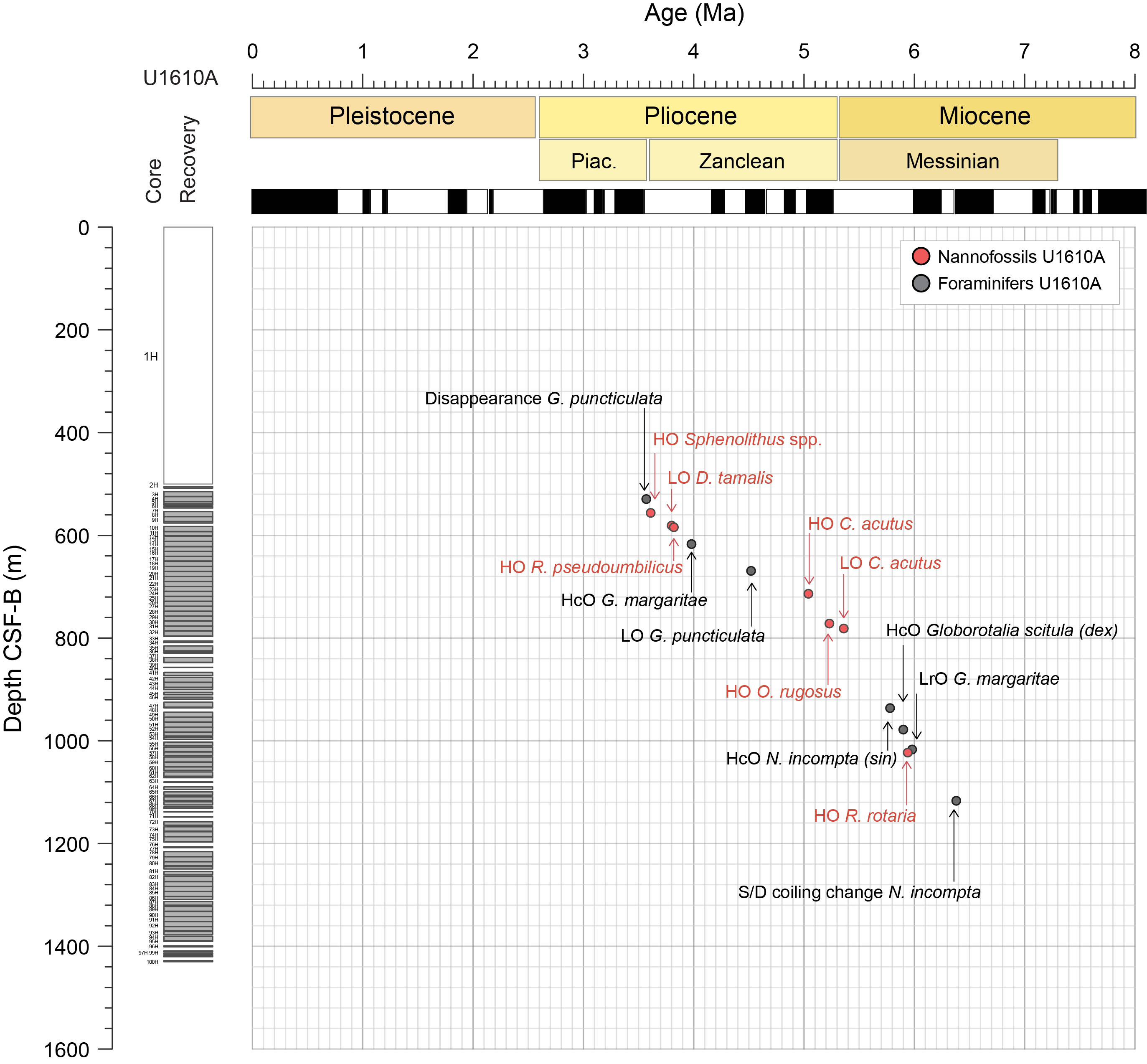
Figure F30. Biostratigraphic events and sedimentation rates.
4.1. Calcareous nannofossils
We examined 95 core catcher samples from Hole U1610A. Additionally, selected samples were analyzed to constrain bioevents using only the marker species. Calcareous nannofossil assemblages were abundant and diverse, and preservation is good. Small placolith species (<3 µm) dominate most of the assemblages. Input of fragmented siliceous fossils, siliciclastic grains, and pyrite framboids as sedimentary components varied from rare to common, whereas reworked (mainly Cretaceous and Paleogene) species varied from rare to few throughout all the sections (Table T6). Exceptionally, Samples 53R-CC and 54R-CC were characterized by the presence of common reworked (mainly Cretaceous and Paleogene) species. The lowermost two core catchers (Samples 99R-CC and 100R-CC) were characterized by the presence of dolomitization and were almost barren of coccoliths.
A total of seven nannofossil datums defined and/or calibrated by Raffi et al. (2020 and references therein) and Hilgen et al. (2000) were identified in Hole U1610A (Table T5). The uppermost event recognized was the HO of Sphenolithus spp. (3.61 Ma) identified between Samples 401-U1610A-7X-CC and 8X-CC (556.33 m core depth below seafloor, Method B [CSF-B]). It can be used to define the Piacenzian/Zanclean boundary. The lowest occurrence (LO) of Discoaster tamalis (3.8 Ma) was identified between Samples 10X-CC and 11X-1, 85 cm (586.23 m CSF-A; 581.05 m CSF-B). At this site, Discoasters occur randomly through the sedimentary succession; therefore, the events using this genus will be better refined by high-resolution counting. The HO of Reticulofenestra pseudoumbilicus (3.82 Ma), considered to be a globally synchronous bioevent, was identified between Samples 11X-1, 85 cm, and 11X-2, 78 cm (585.75 m CSF-A; 584.29 m CSF-B). The HO of Ceratolithus acutus (5.04 Ma) was identified between Samples 23X-CC and 24X-CC (723.73 m CSF-A; 713.73 m CSF-B). The HO of Orthorhabdus rugosus (5.23 Ma) was identified between Samples 29X-CC and 30X-CC (781.80 m CSF-A; 771.73 m CSF-B). However, we use this bioevent with caution due to the scarcity of specimens in the samples analyzed. The LO of C. acutus (5.36 Ma) was placed between Samples 30X-CC and 31X-CC (790.61 m CSF-A; 781.41 m CSF-B).
To help constrain the ages, we identified the HO of R. rotaria (5.94 Ma) (Theodoridis, 1984; Young, 1998; Wei, 2003; Raffi et al., 2003) between Samples 401-U1610A-56R-CC and 57R-2, 145–147 cm (1026.51 m CSF-A; 1022.96 m CSF-B). However, this event needs to be used with caution because it is considered diachronous (Morigi et al., 2007). R. rotaria was identified throughout Hole U1610A, including the very bottom (Sample 94R-6, 71 cm [1389.73 m CSF-A and CSF-B]), to the lowermost core catcher sample (95R-CC), which is almost barren in coccoliths and contains dolomite minerals with rhombohedral shape. Literature from the Mediterranean area indicates that the lowest common occurrence (LcO) of R. rotaria (astronomically dated in the age range of 7.276–7.279 Ma) represents a reproducible secondary event useful for biostratigraphy for the latest Tortonian interval (Morigi et al., 2007; Hilgen et al., 2000). Therefore, because R. rotaria was present, the age of the bottom of the hole has been considered younger than ~7.2 Ma (Morigi et al., 2007; Hilgen et al., 2000).
4.2. Planktonic foraminifers
The concentration of planktonic foraminifers in the sediments is generally low, probably due to the high siliciclastic content. In the Pliocene and the late Messinian, the preservation of planktonic foraminifers was good, although frequently they are filled with pyrite or glauconite. In the lower part of the hole, some of the foraminifers show a pale yellow color, probably due to major diagenetic alteration resulting in mineral precipitation filling the shell interior. A detailed study of the mineral crystals inside the shell can help to understand the origin of the alteration. Some very rare, reworked foraminifers such as Rotalipora gandolfii from the Cretaceous or Morozovella from the Eocene were observed in some samples.
The Early Pliocene planktonic foraminifer assemblages are dominated by Globigerina bulloides, Neogloboquadrina incompta, Globigerinoides ruber, Globigerinoides extremus, Globorotalia puncticulata, and Globorotalia margaritae, whereas in the Messinian G. miotumida is dominant. A sequence of late Messinian–Early Pliocene planktonic foraminifer bioevents was recognized at this site. All core catcher samples were analyzed, and in some specific intervals, additional samples were taken to constrain the depths of the most important planktonic foraminifer events (Table T7).
The disappearance of G. puncticulata (3.57 Ma), the first event registered in this hole, was observed between Samples 401-U1610A-3X-CC and 4X-CC (mean depth = 519.75 m CSF-A; 529.41 m CSF-B).
The highest common occurrence (HcO) of G. margaritae was used instead of the HO of the species because this event can be better recognized in a low-resolution record. This event (3.98 Ma) was recorded between Samples 401-U1610A-14X-CC and 15X-CC (mean depth = 616.75 m CSF-A; 617.055 m CSF-B).
Because a precise location of the LO of G. puncticulata is important to determine sediment age, three additional samples were taken from Core 401-U1610A-19X. The LO of this species was identified between Samples 19X-6, 39–41 cm, and 19X-CC (mean depth = 669.17 m CSF-A; 669.184 m CSF-B). The acme of G. margaritae was not identified at this site. The species is frequent in the sediments but never reaches the high percentages normally seen during this time period in other geographic locations. The absence of the acme of G. margaritae may be due to a gap in the sedimentary sequence or to the low sampling resolution that did not allow its recognition. The acme of this species in the late Messinian has been recorded in southwest Spain and northern Morocco between 5.55 and 5.84 Ma, respectively (Krijgsman et al., 2004, van den Berg et al., 2015). Locating the LO of G. margaritae can be difficult because this species may be sporadically present from the early Messinian, in this study we used its LcO (6.08 Ma). This species is regularly present in the planktonic foraminifer assemblage between Samples 55R-CC and 56R-CC (mean depth = 1016.95 m CSF-A; 1016.95 m CSF-B).
In the late Messinian, the sinistral/dextral coiling change of N. incompta (6.37 Ma) was recorded between Samples 401-U1610A-66R-5, 102–104 cm, and 66R-CC (mean depth = 1117.43 m CSF-A; 1116.755 m CSF-B). The HcO of G. miotumida was recorded between Samples 66R-2, 23–25 cm, and 66R-3, 130–132 cm (mean depth = 1112.09 m CSF-A; 1112.09 m CSF-B). This event is dated at 6.34 Ma in southwest Spain (Bulian et al., 2023) and northwest Morocco (Krijgsman et al., 2004).
Based on the planktonic foraminifer assemblage from the lowermost nondolomitized core catcher, the bottom of Hole U1610A must be early Messinian, older than 6.37 Ma and younger than 7.24 Ma, because we always found abundant G. miotumida.
4.3. Benthonic foraminifers
A total of 61 core catcher samples from Hole U1610A were processed and studied for the abundance of more than 105 species of benthonic foraminifers (Table T8). The level of preservation of the benthonic foraminifers was noted, along with their abundance with respect to planktonic foraminifers; the presence or absence of other calcareous microfossils and detrital grains was also noted. The combined information from all studied samples documents the entire succession recovered at Site U1610.
Preservation of the foraminifers is good in the shallower cores to Sample 401-U1610A-36X-CC. Preservation deteriorates to moderate to poor in the deeper core catcher samples, especially below Sample 70R-CC. The >150 µm fraction of washed samples was analyzed, and in most of the samples benthonic foraminifer abundance was a bit less than planktonic foraminifers, indicating intermediate depths. The planktonic (P) to benthonic (B) foraminifer ratio (%P = P/[P + B]) has been used as a marker of paleodepth (Grimsdale and Van Morkhoven, 1955; Van der Zwaan et al., 1990) because the number of planktonic foraminifers steadily increases with depth; however, there are limitations that need to be considered. The benthonic foraminifer abundance of some species varies directly with availability of food and oxygen, affecting the planktonic to benthonic ratio (Milker, 2010). Depth marker species, like Ammonia beccarii, inhabiting the inner–middle shelf, and Oridorsalis umbonatus, inhabiting the middle–lower slopes, have also been used to determine the paleodepth (Hohenegger, 2005); however, transportation of shallow-water taxa can result in underestimation of water depth. The poor preservation of the foraminifers in Hole U1610A along with presence of shallow-water benthonic foraminifers like the genera Ammonia and Elphidium and neritic fauna like coral fragments, echinoid plates, spines, bivalves, and bryozoans in the older sediments (in most cores from Cores 70R through 95R; Figure F31) indicates sediment reworking. Therefore, paleodepth could not be reliably determined.
Figure F31. Benthonic foraminifer assemblage abundance.
Foraminifer preservation is very poor in Samples 401-U1610A-39R-CC, 49R-CC, 52R-CC, and 53R-CC, and this interval also contains common occurrences of shallow-water benthonic assemblages including echinoid plates/spines, bivalves, and pyritized corals and high abundances of detrital material and mud nodules. Samples 58R-CC and 62R-CC contain considerable quantities of agglutinated detrital matter held together by calcareous cement. All of these could be indicative of downslope transport.
The abundance of elevated epibenthonic assemblages in the Gulf of Cádiz region have been used as an indicator for MOW (Schönfeld, 1997, 2002; Schönfeld and Zahn, 2000); their abundance is 7%–18% in low-energy environments and increases to 60%–90% in high-energy environments. Hole U1610A shows elevated epibenthonic species like those of Cibicidoides spp. and Textularia spp., and their total abundance remains between 20% and 40% in most samples. The epibenthonic abundance is highest (up to 60%) in Sample 73R-CC (Figure F31), which could be due to a high-energy bottom water current.
The most common benthonic foraminifer species in Hole U1610A belong to the genera Bulimina, Cibicidoides, Globocassidulina, Melonis, Oridorsalis, Sigmoilopsis, Trifarina, and Uvigerina in varying proportions. The species abundance of individual benthonic foraminifer species varies from abundant (>20%) to present (<1%). The Uvigerinids become dominant (~50% of total assemblage) (Figure F31) in Samples 27X-CC and 28X-CC in the organic-rich calcareous clay of Subunit IIb; Uvigerina peregrina is the dominant species in Sample 27X-CC, and in Sample 28X-CC a relatively robust costate species, Uvigerina elongostriata, dominates. A study by Zhu (2001) related different species of the genus Uvigerina to high organic carbon input, whereas the slender costate forms dominate at shallower depths compared to the thicker and heavily costate forms (Guimerans and Currado, 1999). The cyclic interbedding of calcareous clay, calcareous silty mud, and calcareous mud horizons in Cores 27X and 28X (see Lithostratigraphy) suggests that further study of these cores at a higher resolution may help us better understand the relationship of the Uvigerinid abundance with changing lithologies.
5. Paleomagnetism
Paleomagnetic investigation of the 93 cores from Hole U1610A focused on demagnetization of the natural remanent magnetization (NRM) of archive-half split core sections and discrete samples of the working-half split core sections. Combined demagnetization results of split core sections and discrete samples were used to establish a preliminary magnetostratigraphy for Hole U1610A that was tentatively correlated to the most recent geomagnetic polarity timescale (GPTS 2020; Raffi et al., 2020).
Pass-through paleomagnetic measurements at Site U1610 were performed on all archive-half split core sections using the superconducting rock magnetometer (SRM). No pass-through measurements were made on core catcher sections. Alternating field (AF) demagnetization was performed using the SRM by applying stepwise peak fields of 5, 10, 15, and 20 mT, with measurement of the remaining magnetization taken at 2 cm resolution after each step. Cores 401-U1610A-20X through 24X were measured at 5 cm resolution. SRM measurements were sporadically disturbed by the occurrence of artificial flux-jumps, and these results were removed from the database. SRM data were processed to remove all measurements that were made within 5 cm of the section ends, which are biased by measurement edge effects. A smoothing window of 1 m was used for the inclination values to suppress the influence of data points that deviate significantly from the expected geocentric axial dipole (GAD) inclination (+56°) at the site latitude (36.4°N). The processed NRM inclination, declination, and intensity data after 20 mT peak field AF demagnetization is listed in U1610SRMafter20mT.xlsx in PMAG in Supplementary material.
In addition, a total of 279 discrete oriented plastic cube samples (7 cm3) were collected from the working-half sections of Cores 401-U1610A-2X through 76R using an extruder. A total of 57 cubes (8 cm3) were cut from the more indurated Cores 77R–94R with a double-bladed saw. For each core, 3–7 discrete samples were taken, avoiding visually disturbed intervals. First, the anisotropy of magnetic susceptibility (AMS) and bulk MS were measured on all samples using the MFK2 KappaBridge instrument. After the AMS measurements, the NRM of 156 plastic cube samples was measured on the AGICO JR-6A spinner magnetometer. Stepwise AF demagnetization was performed at successive peak fields of 5, 10, 15, and 20 mT for Cores 2X–36X, and in some cases, additional steps of 25, 30, 35, and 40 mT were taken to better determine the characteristic magnetic component in the sections (Figure F32). For the rotary drilled Cores 37R–93R, AF demagnetization was performed at steps of 5, 10, 15, 20, 30, 40, 50, 60, 70, 80, and 100 mT, typically until samples showed signs of acquiring a gyroremanent magnetization (GRM). Pass-through paleomagnetic measurements were performed on the sawed 8 cm3 cubes of Cores 77R–94R using the SRM by applying stepwise peak fields of 5, 10, 15, 20, 30, 40, 50, 60, 70, and 80 mT. The inclination data after 20 mT peak field AF demagnetization of the discrete samples on the JR-6A and the SRM are listed in Tables T9 and T10, respectively.
Figure F32. AF demagnetization results.
5.1. Paleomagnetic signals
AMS results of Hole U1610A show Kmin directions that are tilted between 10° and 20° at a random azimuth (Figure F33). Assuming the rocks at Site U1610 have a sedimentary fabric, Kmin should be perpendicular to the bedding plane. This indicates either a significant dip of the strata or an inclined drilling orientation. Taking into account the seismic profiles of the area, which show a clear horizontal orientation of the strata in the upper part of the succession (Figure F6), we calculated the average inclination of Kmin for the uppermost 27 and lowermost 56 discrete samples, which is 75° and 73° from horizontal, respectively (Table T11). This suggests an inclined drilling direction of ~15° for Hole U1610A, in agreement with downhole inclinometer measurements (see Downhole measurements) and visual observations of tilted beds in the half cores. Accurate measurements of the magnetic declination and/or inclination could, in principle, be used to calculate the azimuthal direction of the core and the borehole.
Figure F33. AMS determinations.
The NRM intensity in Hole U1610A ranges about 5.0 × 10⁻⁴ to 1.0 × 100 A/m, with noticeably high values between 950 and 1150 m CSF-B (Figure F34). The NRM removed below 10–20 mT is likely related to an overprint caused by the core drilling (Acton et al., 2002). Some sections showed significantly deviated and scattered data points that may be due to the concentration of magnetic iron sulfides. In Hole U1610A, normal polarity intervals are typically easy to identify based on the SRM inclination records at 20 mT, only in the uppermost (500–537 m CSF-B) and lower (1018–1390 m CSF-B) parts of the succession (Figure F34).
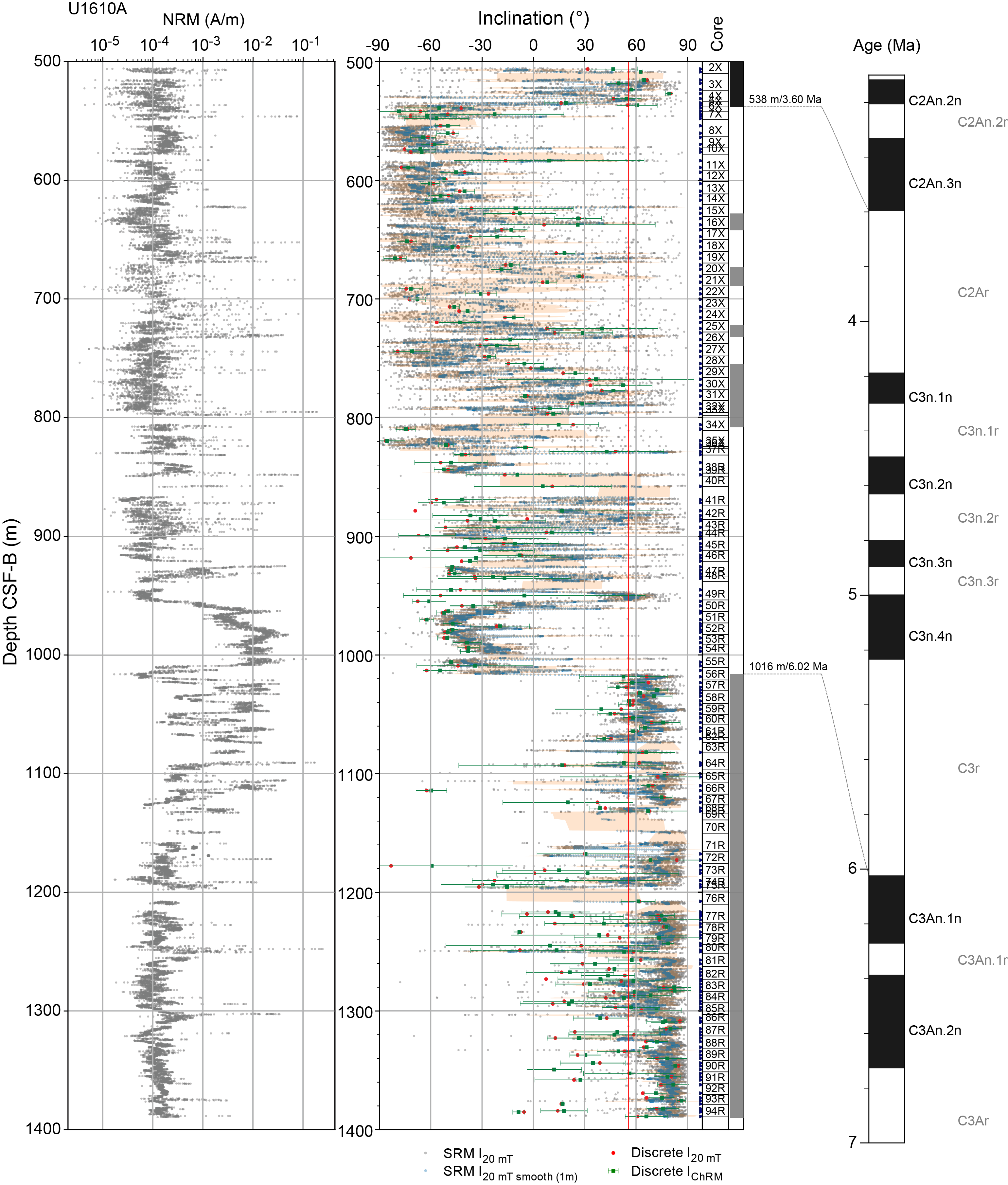
Figure F34. Paleomagnetic results.
NRM intensities of the discrete samples range 1.3 × 10⁻⁵ to 4 × 10⁻² A/m. Detailed analyses showed that, similar to the section-half demagnetizations, a normal polarity overprint component was generally removed between 0 and 20 mT, after which a second dual-polarity component remained, which we interpret to be the characteristic remanent magnetization (ChRM) component (Figure F32). The ChRM component of most samples was successively demagnetized at higher applied magnetic fields. Samples in the interval between 950 and 1150 m CSF-B commonly acquired a GRM at peak fields between 40 and 70 mT (Figure F32). This suggests the iron sulfide greigite is the dominant magnetic mineral between 950 and 1150 m CSF-B in Hole U1610A rocks (Roberts et al., 2011). Samples from other depth intervals in Hole U1610A show weak NRM and no GRM, together with ubiquitous pyrite particles, which are likely evidence of relict magnetic minerals (Liu et al., 2022). Demagnetization diagrams (Z-plots) from the discrete samples are mostly easy to interpret and the inclinations at 20 mT are generally robust, showing multiple magnetic polarity reversals (Figure F32). The inclinations of the discrete samples, however, do not always confirm the polarities suggested by the SRM inclination values measured on the archive-half core sections.
5.2. Magnetostratigraphy
Demagnetization results are plotted versus depth in Figure F34, and the inclination data from both SRM and discrete samples were combined to generate an integrated polarity pattern for Hole U1610A (Figure F34; Tables T9, T10; see U1610SRMafter20mT.xlsx in PMAG in Supplementary material).
The uppermost part of Hole U1610A (500–540 m CSF-B) clearly shows positive inclinations in both SRM and JR-6A records. In the following interval (540–830 m CSF-B), reversed directions are dominant and many SRM inclination values approach the expected antipodal GAD inclination at the coring site (−56°). Normal polarity intervals in this interval are unclear, and only few intervals show successive inclinations at the expected GAD inclination. The results of the discrete samples are also scattered. We define tentative normal and reversed polarity zones when at least two successive inclination values are above 20° (normal) and below −20° (reversed), respectively (Figures F32, F34). Single polarity samples values above/below 20°/−20° are shown by a gray bar in the polarity column. The position of the reversal boundaries can then be determined between the stratigraphic levels of two opposite polarity samples (neglecting again all inclination values between −20° and +20°). Applying these criteria reveals a polarity pattern with two relatively long reversed intervals at 540–630 and 810–1010 m CSF-B, although it should be noted that especially the lower interval contains substantial intervals of positive inclination values in the SRM record that are unconfirmed by discrete sample measurements. The most logical correlation of these two long reversed intervals to the GPTS is to Chrons C2Ar and C3r, respectively. In between, the GPTS contains the four normal polarity chrons of C3n: Cochiti (C3n.1n), Nunivak (C3n.2n), Sidufjall (C3n.3n), and Thvera (C3n.4n). The corresponding interval in Hole U1610A contains three normal polarity intervals and two single normal polarity half intervals. The best-fit correlation of the magnetostratigraphic pattern of Hole U1610A to the GPTS 2020 is that the thickest normal polarity interval at 755–808 m CSF-B correlates to Thvera (C3n.4n), the normal interval at 722–732 correlates to Sidufjall (C3n.3n), and the normal polarity interval at 628–642 m CSF-B correlates to Cochiti (C3n.1n). The single polarity interval at 688–673 m CSF-B then best correlates to Nunivak (C3n.2n) (Table T12). This further implies that the normal polarity interval at the top of Hole U1610A at 500–538 m CSF-B most likely correlates to the lowermost Gauss (C2An.3n) Chron. The long normal polarity interval (1018–1390 m CSF-B) remains equivocal. The magnetic signal there appears to be similar to other parts of the records showing stable polarity components that gradually decay with AF demagnetization. The most logical correlation is to Chron C3An; from a paleomagnetic point of view there is no evidence that we reached levels older than 6.7 Ma in Hole U1610A (Figure F34).
The tentative magnetostratigraphic correlation of the polarity pattern of Hole U1610A to the GPTS can be used to calculate sediment accumulation rates for the different lithostratigraphic units (Figure F35). This curve indicates average accumulation rates of ~17 cm/ky for Lithostratigraphic Unit I (Pliocene), increasing downward to ~26 cm/ky for Unit II (Messinian Salinity Crisis interval), and >53 cm/ky for Unit III (Messinian).
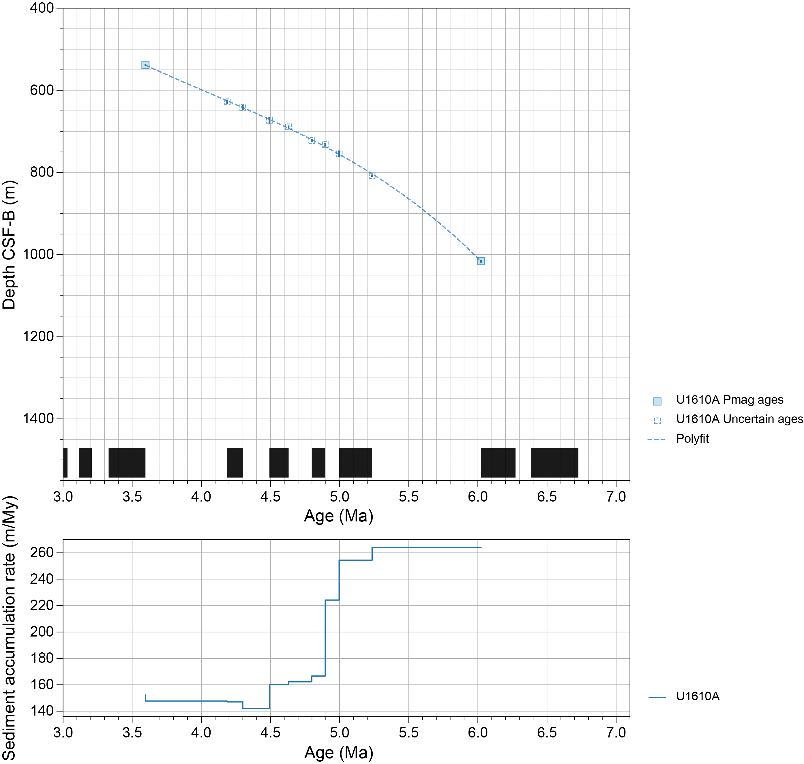
Figure F35. Sediment accumulation curve.
6. Geochemistry
6.1. Volatile hydrocarbons
Headspace gas analysis was performed as part of the standard protocol required for shipboard safety and pollution prevention monitoring, with additional special safety protocols in place because some of the reflectors between 740 and 960 mbsf are known to be hydrocarbon seals regionally. These protocols required drilling to wait for headspace results prior to advancing, necessitating a 50 min delay for each core, or ~1 day additional drilling time. Hydrocarbons were found to be well below threshold safety levels and lower than those in Hole U1609A. The measured values may be useful to reassess risk and to inform future drilling in this region.
In total, 91 headspace samples from Hole U1610A (sampling resolution of one per core if recovery permitted) were analyzed (Figure F36; Table T13). Routine headspace sampling began at 508.2 m CSF-A (Section 401-U1610A-2X-3) at the base of the casing and continued until 1383.7 m CSF-A (Section 94R-3) in the last recovered core. Void space gases were also sampled opportunistically on the catwalk by piercing the core liner and extracting gases when void spaces were visible, sometimes at high pressures (e.g., Section 18X-3), through a valve into a syringe; 17 of these samples were collected across 563.9–1257.7 m CSF-A (Sections 9X-1 through 81R-4) (i.e., beyond the monitoring range). Although the absolute concentrations of void space gases are not meaningful and therefore not shown, the constituent gases and their relative abundances can be compared to that of the headspace gases.
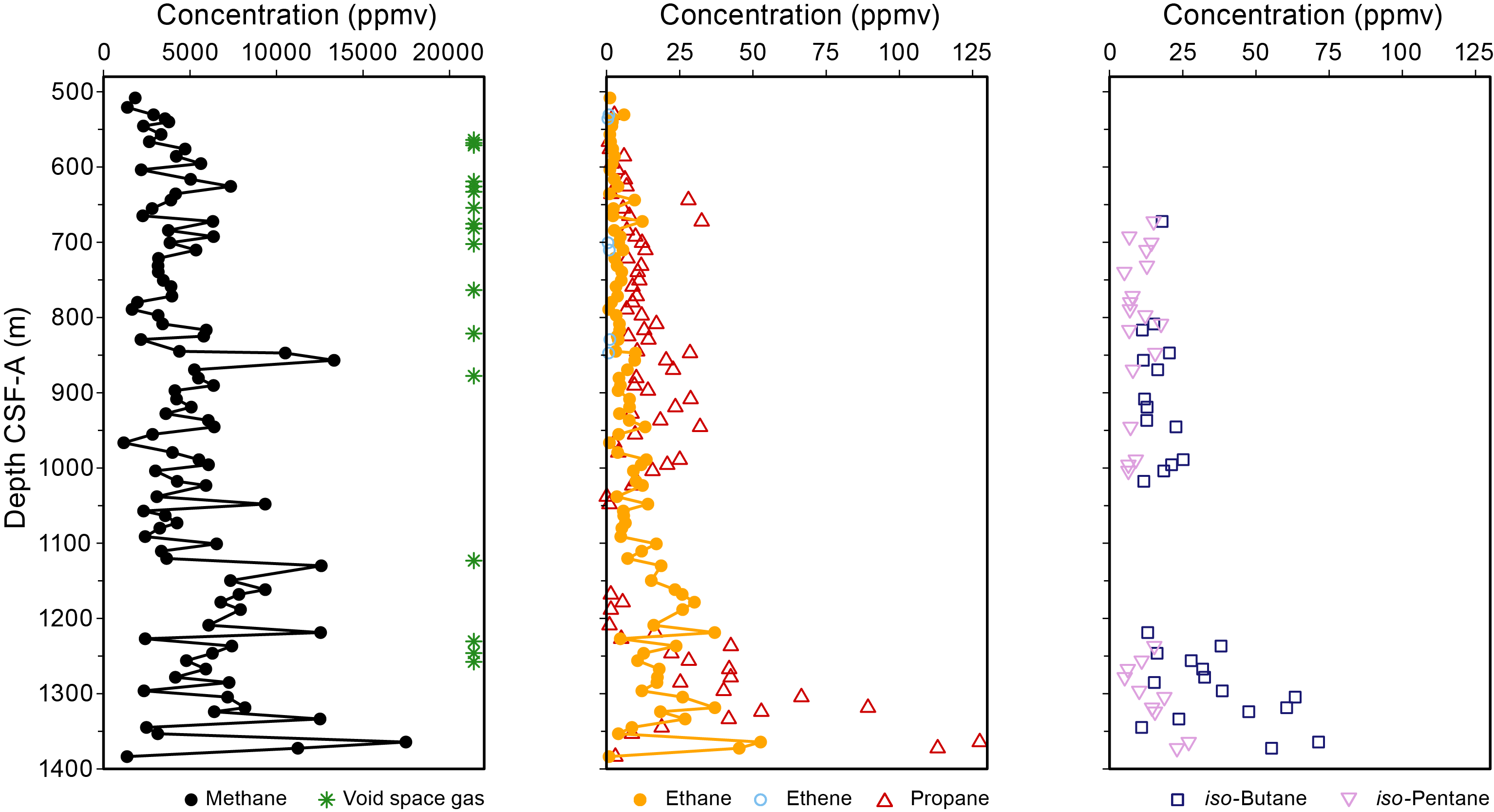
Figure F36. Methane, ethane, ethene, propane, iso-butane, and iso-pentane.
In Hole U1610A, methane (C1), ethane (C2), and propane (C3) were typically detected in headspace and void space gases with additional measurable components of ethene (C2=), iso-butane (C4), n-butane (C4), iso-pentane (C5), and n-pentane (C5) in some samples. Methane is dominant in all samples, ranging 1,172–17,473 parts per million by volume (ppmv) in headspace analyses, which is considerably lower than levels that are a concern for safety (monitored over 100,000 ppmv), as well as lower than concentrations measured in Hole U1609A. Methane concentrations and variability tend to increase with depth (Figure F36). The C1:C2 ratio ranges 194–4139 in headspace samples and 1080–3848 in the available void space samples (Figure F37). These concentrations of methane, ethane, and other volatile hydrocarbons do not present a drilling concern.
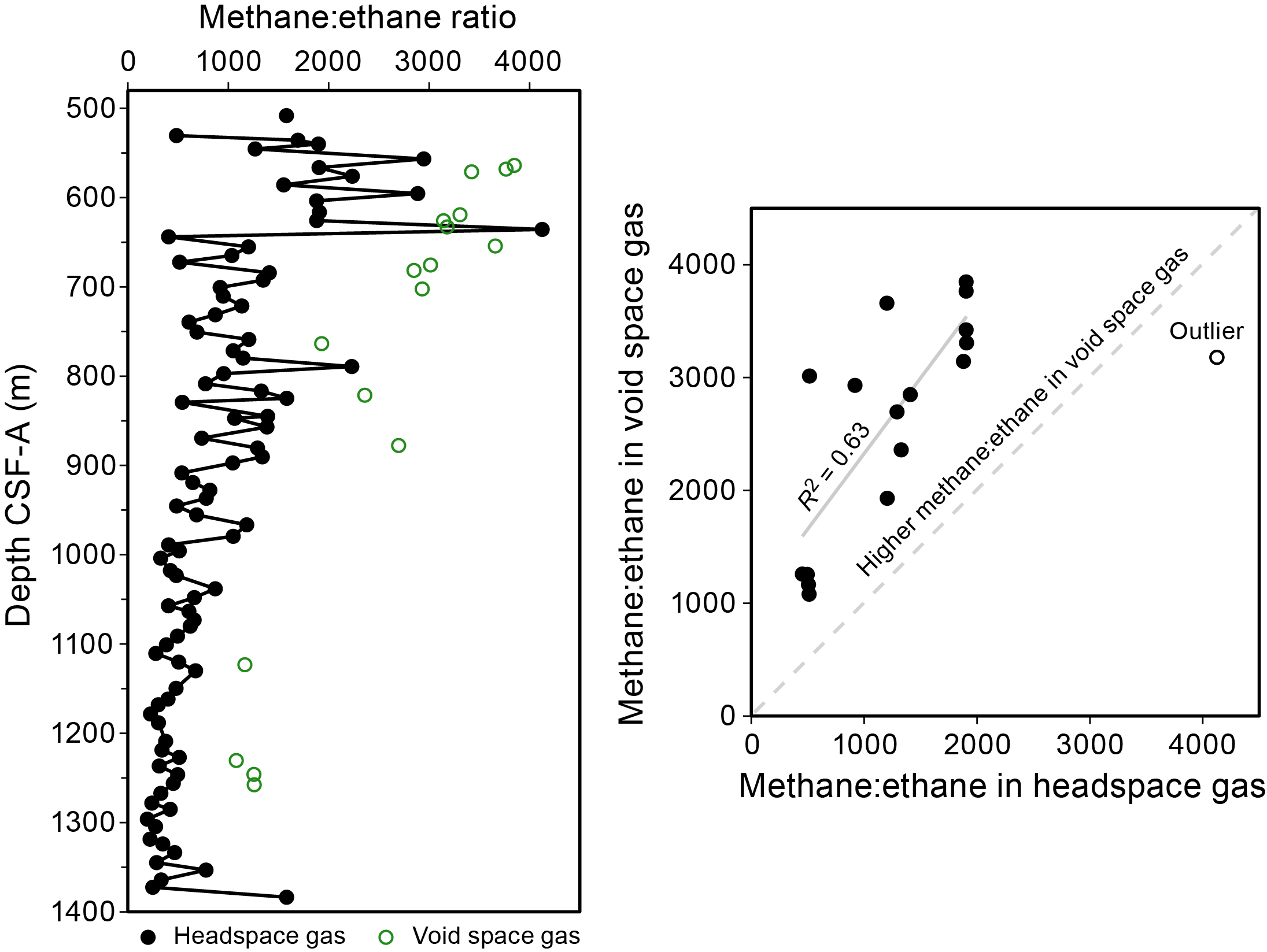
Figure F37. Methane:ethane ratios.
Downcore ethane is <53 ppmv and propane is <127 ppmv (Figure F36). Propane is dominant over ethane in two zones, 603.7–1017.7 m CSF-A (Sections 401-U1610A-13X-2 through 56R-5) and deeper than 1218.8 m CSF-A (Section 77R-3). Ethene was detected in a few isolated samples from 700.7 to 847.2 m CSF-A (Sections 23X-2, 24X-2, 37R-2, and 39R-1). iso-butane and iso-pentane were detected in two zones, 650–1050 m CSF-A and from 1150 m CSF-A to the base of the recovered core, with maximum concentrations of 247 and 42 ppmv, respectively. n-butane and n-pentane were not detected in headspace samples; however, n-butane was detected in four void space samples, and n-pentane was detected in one sample. The presence of iso-butane and iso-pentane was confirmed in the void space samples in which iso-butane and iso-pentane were present at greater abundances than the normal-chain counterpart (Sections 21X-2, 29X-5, 35X-5, and 81R-4) (Table T13). These gases appear to be of in situ biogenic origins.
The gas concentration profiles reveal two distinct zones where constituent gases >C2 appear, specifically propane, iso-butane, and iso-pentane (Figure F36), separated by a zone at 1050–1150 m CSF-A that contains only methane and ethane. Sediments in this zone are drier based on gamma ray attenuation (GRA) bulk density measurements (see Physical properties). It is possible that there are one or more zones of reduced porosity or permeability that explain the separation of the gases in the downcore profile, which could be established based on comparison to the Lithostratigraphy and Physical properties data. This zonation of the gas profile shows barriers to gas migration, also seen in the liquid data based on the inorganic geochemical composition of interstitial water (IW), which shows that fluid migration is somewhat restricted below 1050 m CSF-A. We also note low concentrations of methane and ethane hydrocarbons slightly shallower at 966.5 m CSF-A in Section 401-U1610A-51R-3. Although this could be an analytical artifact, we suspect it is a narrow zone that has already lost most of the evolved gases. We note that no IW was taken from Core 51R because of the brecciated nature of the sediments from drilling disturbance. These fractured and firmer sediments not only yielded low gas concentrations but also appear to present the shallowest barrier for diffusion based on the inorganic geochemical composition of IW above and below Section 51R-3 (see below).
6.2. Interstitial water chemistry
Two bottom water samples were taken, one during verification of the casing installation and one during reentry at the seafloor. IW was extracted from a total of 54 whole-round samples from Hole U1610A at a sampling resolution of one per XCB and RCB core when permitted by core recovery (Tables T14, T15). We note that no sample was taken from brecciated Core 401-U1610A-51R because of the inability to collect a sample without contamination (Figure F36). Water was extracted from all collected samples. When possible, the full suite of standard IW analyses was performed, although low volumes of extracted water for the deeper IW samples limited some of the analyses (especially alkalinity and pH determinations) and only salinity was measured on Section 72R-1. Where possible, IW chemistry from Site U1610 is presented in comparison to the shallower fluid profiles from Expedition 339 Sites U1386 or U1387 to provide context and comparison. The two Expedition 339 sites are approximately 30 km away and recovered IW samples from the uppermost 449 and 350 m, respectively, from younger sediments. Site U1610 only recovered cores below 500 m CSF-A, but many of the IW properties generally continue trends seen in the shallower samples from Sites U1386 or U1387 (Figure F38).
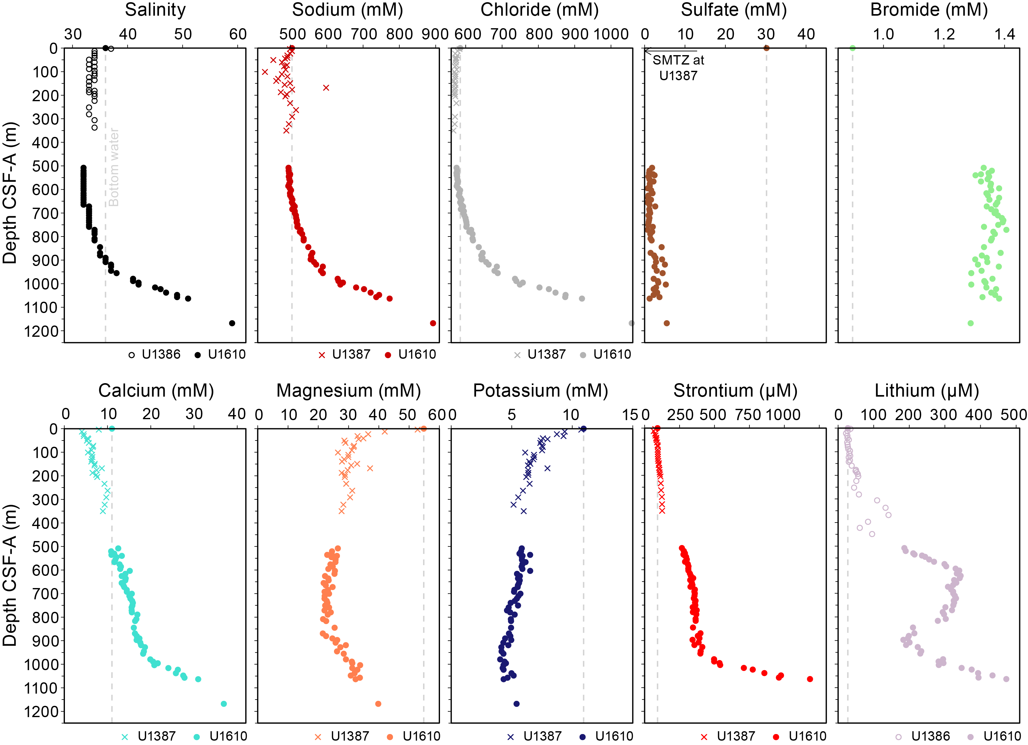
Figure F38. IW chemical profile comparison to nearby sites.
6.2.1. Alkalinity, pH, and salinity
Alkalinity, pH, and salinity of the bottom water are 2.5 mM, 7.8, and 36, respectively, and are shown for comparison to the IW (Figure F39; Table T14). The bottom water salinity at Site U1610 is one unit higher than the mudline sample at Site U1609 (salinity = 35). Even though Site U1610 lies outside the core channels of the modern MOW, this higher salinity likely reflects the stronger influence of the MOW closer to the Mediterranean–Atlantic gateway (Sánchez-Leal et al., 2017). In the IW, alkalinity ranges 1.5–4.7 mM between 508.1 and 844.9 m CSF-A (Sections 401-U1610A-2X-2 through 38R-5) and then declines to <1.5 below 869.4 m CSF-A (Section 41R-2). Values for pH are weakly negatively correlated with those for alkalinity, with a mean value of 7.7 and a range of 7.5–8.0. The samples between 508.1 and 816.6 m CSF-A (Sections 2X-2 through 35X-1) have lower pH than the modern bottom water, whereas those below 844.9 m CSF-A (Section 38R-5) have similar or higher pH compared to the bottom water, with some exceptions (i.e., 535.2 m CSF-A). Salinity ranges 32–34 between 508.1 and 816.6 m CSF-A (Sections 2X-2 through 35X-1), followed by a notable increase from 35 to 59 between 844.9 and 1168.0 m CSF-A (Sections 38R-5 through 72R-1). Within the generally smooth rise in salinity (considering measurements with only integer precision), there are more abrupt changes accompanied by an increased rate of salinity increase between Sections 50R-1 and 52R-5 (955.3 and 979.3 m CSF-A) and Sections 55R-1 and 56R-3 (1003.8 and 1016.2 m CSF-A) that may indicate separation by low-permeability zones.
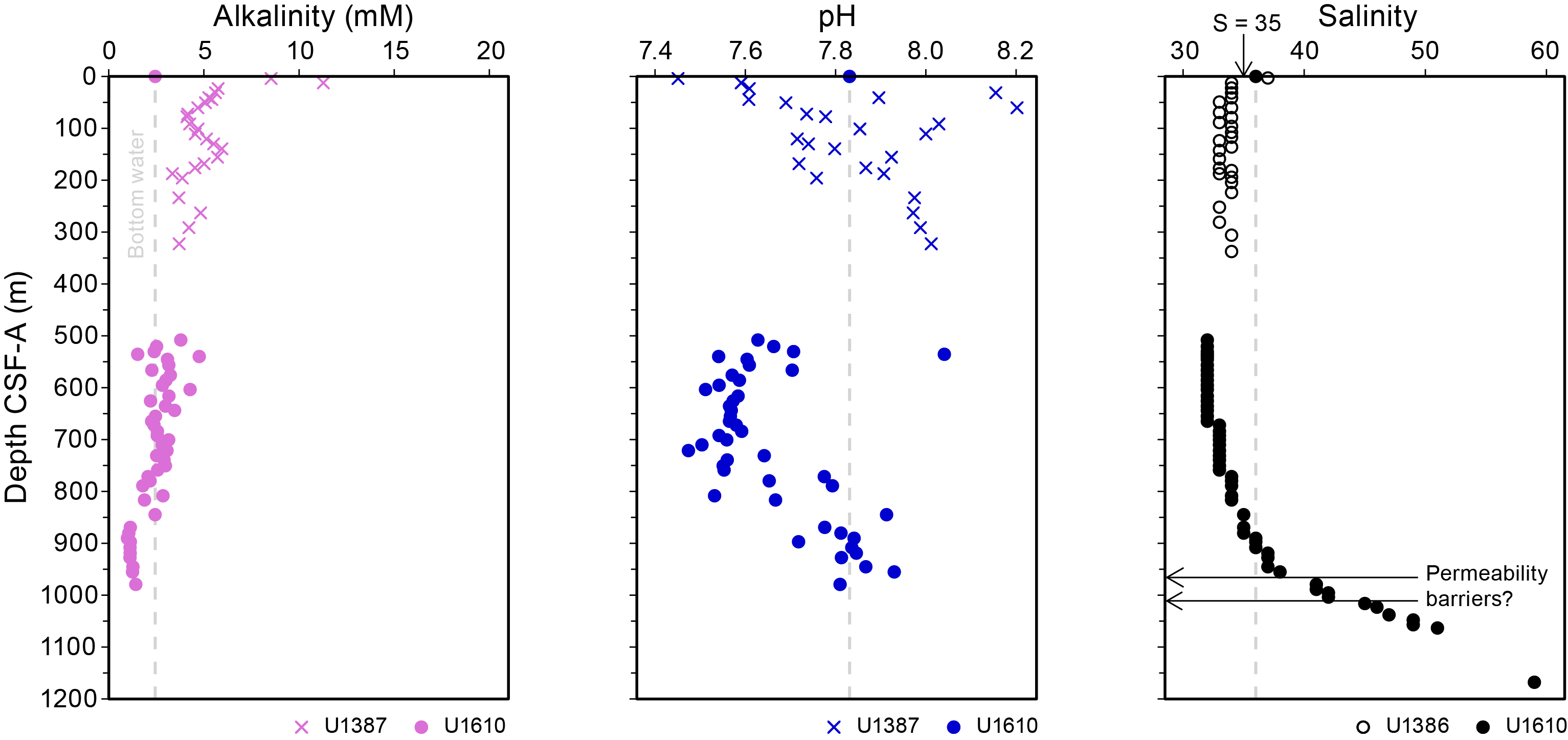
Figure F39. IW alkalinity, pH, and salinity.
High salinities were also reported within the shallower settings and younger sediments collected at Expedition 339 Sites U1388 (maximum = 47), U1389 (maximum = 56), and U1390 (maximum = 101) (Expedition 339 Scientists, 2013b, 2013c, 2013d). Other chemical properties of these high-salinity waters (e.g., Br and the Br/Cl ratio; see below) are consistent with the trend being largely driven by dissolution of halite rather than by a seawater-derived brine. A candidate source for the halite is the olistostrome unit (also known as the Allochthonous Unit of the Gulf of Cádiz), which contains Triassic-aged evaporites (Medialdea et al., 2004). Seismic stratigraphy places the olistostrome near the bottom of the drilled interval in Hole U1610A, so the source of the high-salinity waters at depth would be consistent with diffusion of waters laterally and upward that have been affected by mineral dissolution from that unit. A similar mechanism can be invoked for high-salinity IW at Expedition 339 Sites U1388–U1390, which have thinner sediment accumulations overlying the olistostrome.
6.2.2. Major ions
Major ion concentrations (Na+, Cl−, Ca2+, Mg2+, K+, SO42−, and Br−) of IW were analyzed by ion chromatography (IC) (Table T14). Sodium and chloride show close covariation, including during the rise in salinity toward the bottom of the hole (Figure F40). Sodium and chloride concentrations vary only 2% from the bottom water between 508.1 and 721.3 m CSF-A (Sections 401-U1610A-2X-2 and 25X-2), followed by increases of approximately 80% by 1168.0 m CSF-A (Section 72R-1). The Na/Cl ratios range 0.84–0.86, remaining close to that of the bottom water (Na/Cl = 0.86). Dissolution of halite would be expected to increase the Na/Cl ratio toward 1, so the slight decrease in Na/Cl for the high-salinity waters may reflect additional loss of Na to clays or zeolites, similar to the mechanisms proposed to interpret the Na profile and Na/Cl ratios at Site U1609. High-salinity waters at nearby Expedition 339 Sites U1388, U1389, and U1390 also show stable or decreasing Na/Cl ratios as low as 0.7, supporting the inference that an additional Na sink is present in addition to the halite dissolution source (Expedition 339 Scientists, 2013b, 2013c, 2013d).
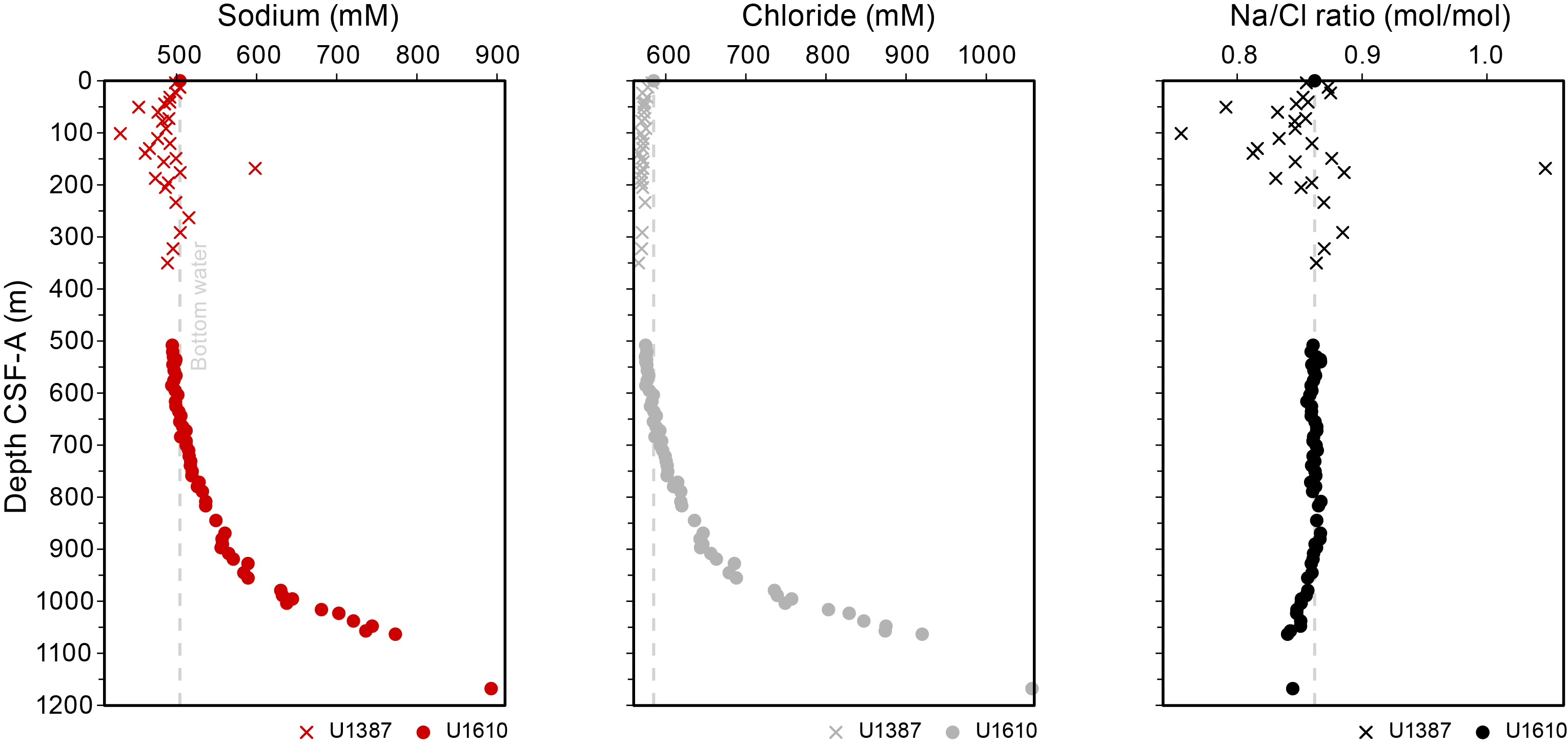
Figure F40. IW sodium, chloride, and Na/Cl.
Calcium shows a gradual increase from a minimum of 10.8 mM at 520.6 m CSF-A (Section 401-U1610A-3X-4) to 18.2 mM at 955.3 m CSF-A (Section 50R-1) before rising rapidly to a maximum of 36.9 mM at 1168.0 m CSF-A (Section 72R-1) (Figure F41). The transition between these two intervals with different rates of increasing Ca corresponds to a jump in salinity from 38 to 41 as well as a change in the concentrations of other species (e.g., Sr; see below), which may indicate a barrier to vertical diffusion of IW between Sections 50R-1 and 52R-5 (955.3–979.3 m CSF-A). Magnesium concentrations are relatively stable (21.5–26.5 mM) above 908.3 m CSF-A (Section 45R-2) and increase to 39.8 mM at the bottom of the core. Potassium gradually declines from approximately 6 mM at 508.1 m CSF-A (Section 2X-2) to a minimum of 4.0 mM at 979.3 m CSF-A (Section 52R-5), followed by an increase to 5.4 mM at 1168.0 m CSF-A (Section 72R-1). The calcium increase indicates carbonate dissolution at depth, with an additional source of calcium (possibly also from carbonate dissolution) associated with the high-salinity waters. Similarities in the magnesium and potassium trends could be related to clay formation/dissolution, and differences may reflect the additional influence of carbonate mineral reactions on magnesium concentrations.
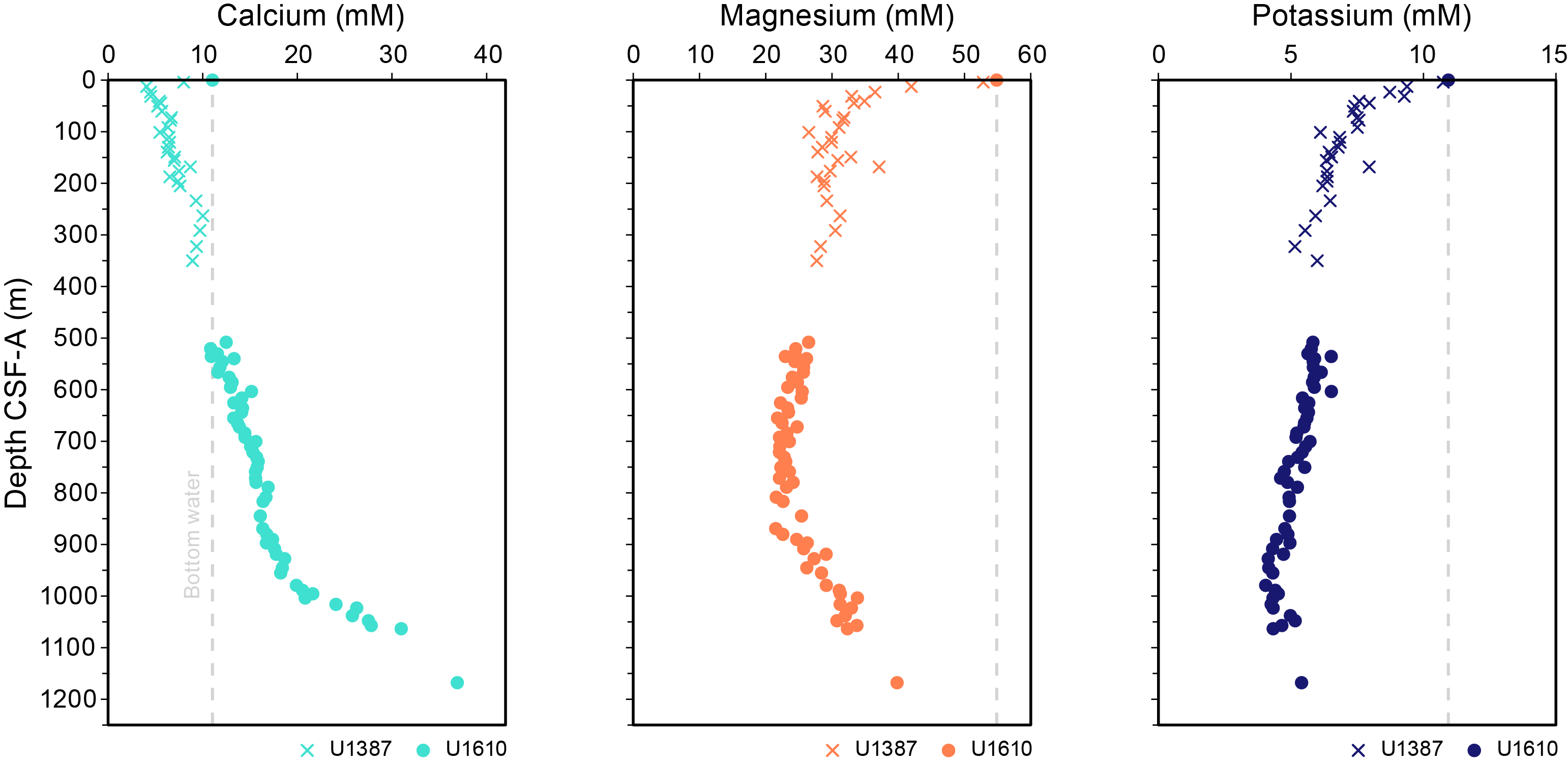
Figure F41. IW major cation concentrations.
Sulfate concentrations are less than 2.5 mM in the upper half of the core (above 816.6 m CSF-A; Section 401-U1610A-35X-1) and shift to 1.23–5.49 mM in the lower half of the core (below 844.9 m CSF-A; Section 38R-5) (Figure F42). The sulfate–methane transition zone (SMTZ) was identified at both Sites U1386 and U1387 by sulfate depletion at 12.5 m CSF-A, and the low levels of sulfate throughout the IW samples at Site U1610A indicate that the cores at this site were similarly well below the SMTZ. Bromide concentrations are relatively constant with an average of 1.35 mM. The consistent Br concentrations downcore indicate that the rise in salinity is not related to water loss and resulting seawater brine concentration, which would produce similar trends in both chloride and bromide as well as other conservative elements.
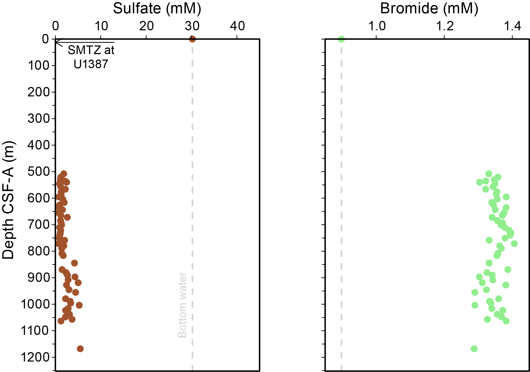
Figure F42. IW major anion concentrations.
6.2.3. Ammonium, phosphate, and total phosphorus
Ammonium and phosphate concentrations in IW were analyzed by spectrophotometry (Figure F43; Table T14). Ammonium concentrations range 4,892–6,770 µM between 508.1 and 1003.8 m CSF-A (Sections 401-U1610A-2X-2 and 55R-1) and then sharply increase to nearly 11,000 µM at 1168.0 m CSF-A (Section 72R-1). Phosphate concentrations are less than 7.1 µM above 945.3 m CSF-A (Section 49R-1) and less than 2.5 µM below 979.3 m CSF-A (Section 52R-3). Total P measured by inductively coupled plasma–atomic emission spectroscopy (ICP-AES) is below the detection limit throughout the core (Table T15). Ammonium and phosphate should be released during respiration of organic matter in both the zones of sulfate reduction and methanogenesis, but although ammonium accumulates in the IW throughout both zones, phosphate commonly appears to be drawn down in the methanogenic zone (e.g., Shipboard Scientific Party, 1996; Bernasconi, 1999). It is possible that authigenic apatite formation is promoted in this diagenetic environment (Murray et al., 1998), although the mechanism driving this process specifically within the methanogenic zone is not clear.
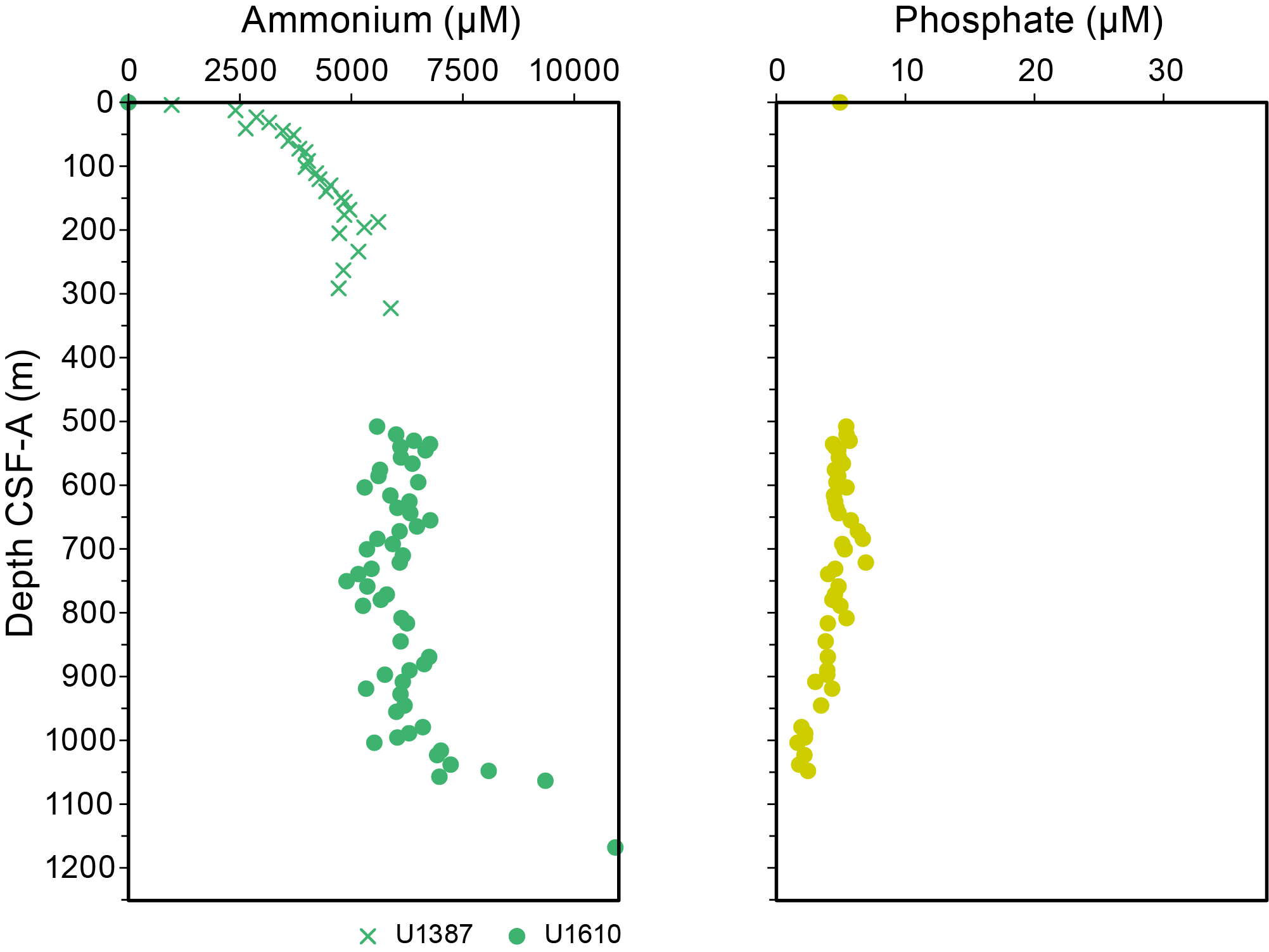
Figure F43. IW major nutrient concentrations.
6.2.4. Trace elements (Li, Si, Ba, B, Sr, Fe, and Mn)
Trace element concentrations in IW were analyzed by ICP-AES (Table T15). Silicon shows a similar depth profile to alkalinity, roughly inverse to pH, which could indicate authigenic clay precipitation in the deeper part of the core (Figure F44). In contrast to the behavior seen at Site U1609, lithium has a different depth profile than silicon at Site U1610: Li concentrations increase from 186 µM at 508.1 m CSF-A (Section 2X-2) to approximately 300 µM across 576.0–603.6 m CSF-A, before decreasing to a local minimum of 183 µM at 897.1 m CSF-A and then increasing to 472 µM at 1063.3 m CSF-A. High Li concentrations at Site U1610 may be attributed to clay diagenesis or local terrigenous sources with high Li content, with the possibility of additional clay diagenesis accompanying the high-salinity waters at the bottom of Hole U1610A (Shipboard Science Party, 1996; Scholz et al., 2010).
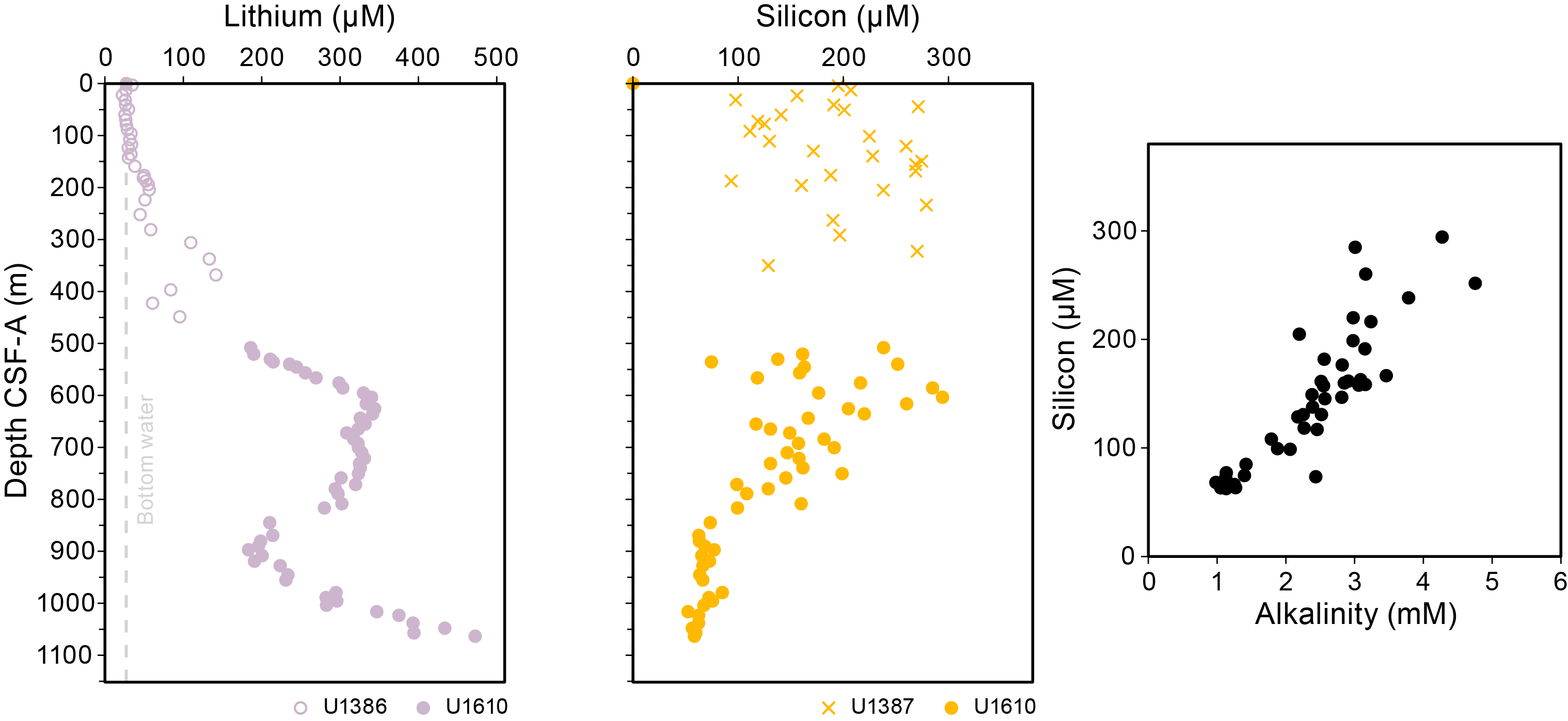
Figure F44. IW minor element concentrations.
Barium concentrations fluctuate between 31 and 124 µM, likely reflecting variable barite solubility (note the hyperbolic relationship between Ba and sulfate concentrations) (Figure F45). Boron concentrations range 92–566 µM. Apart from a few scattered high values, the general trend is from <200 µM at the top of the hole gradually increasing to 326 µM at 700.6 m CSF-A (Section 401-U1610A-23X-1), followed by a gradual decrease to ~200 µM. Strontium concentrations increase gradually from 267 (Core 2X) to 399 µM at 955.3 m CSF-A (Section 50R-1) and then much more rapidly to 1184 µM at 1063.2 m CSF-A (Section 61R-2). The similar depth profiles of strontium and calcium reflect carbonate diagenesis, including dissolution and/or recrystallization associated with the high-salinity waters. The transition between Sections 50R-1 and 52R-5 (955.3–979.3 m CSF-A), below which Ca and Sr concentrations rise steeply, likely includes an interval of low permeability that limits vertical diffusion of fluids, as noted when describing hydrocarbon profiles (above). Although Core 51R was not sampled for IW because of the firm and brecciated nature of the sediments, gas concentrations are low at 966.5 m CSF-A (Section 51R-3), consistent with an interval of low porosity/permeability. Visual inspection of foraminifers indicates a sepia color and other aspects of less good preservation or infilling at and below Core 54R, with the poorer preservation dominantly noted below Core 86R, especially in horizons that are associated with coarser turbiditic deposits. The alternating preservation between samples being apparently dependent on lithology and depositional environment means that in situ preservation does not explain the observed IW trends, but rather a smooth curve of Ca and Sr concentrations appears to show a diffusion profile from carbonate degradation at depth with some upward barriers to migration as previously described.
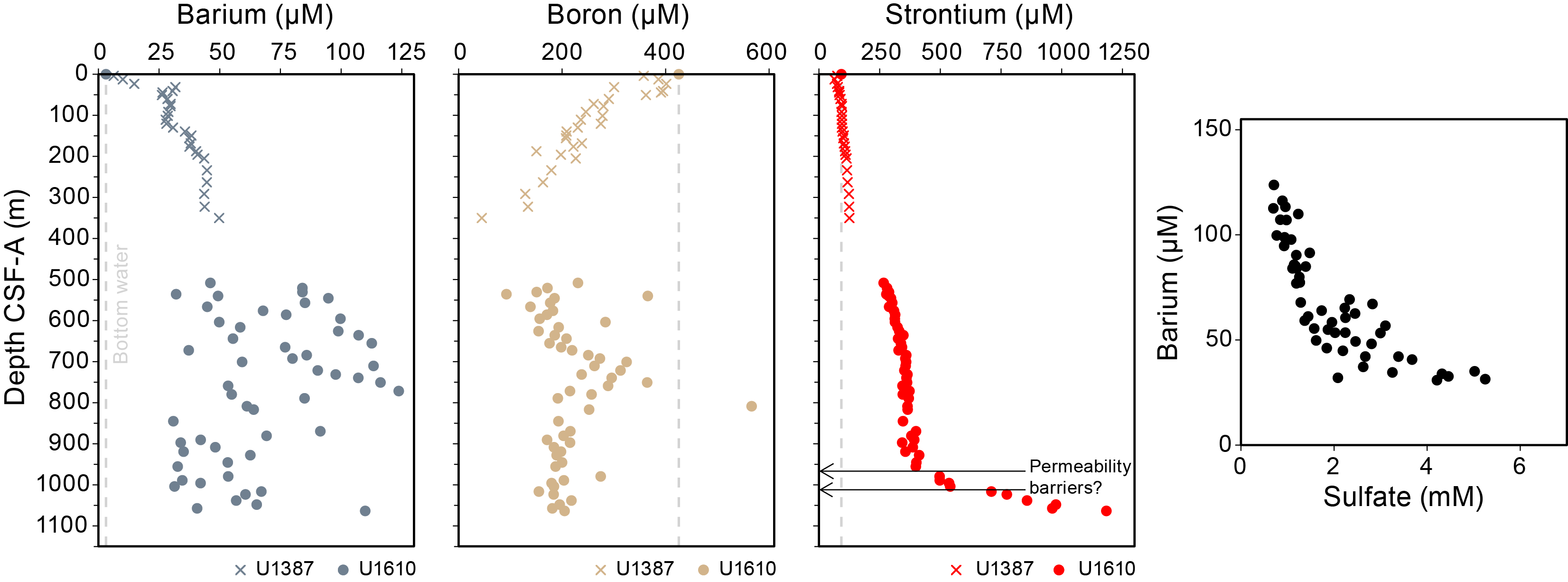
Figure F45. IW minor and trace element concentrations.
Iron concentrations are less than 1.1 µM throughout Site U1610. Manganese concentrations shift from <1 µM to a maximum of 2.6 µM at ~1000 m CSF-A, implying changes in redox conditions below this depth (Figure F46). However, the signal is not consistent or strong enough to confidently ascribe this to the same fluid migration patterns described for gases, salinity, and Sr.
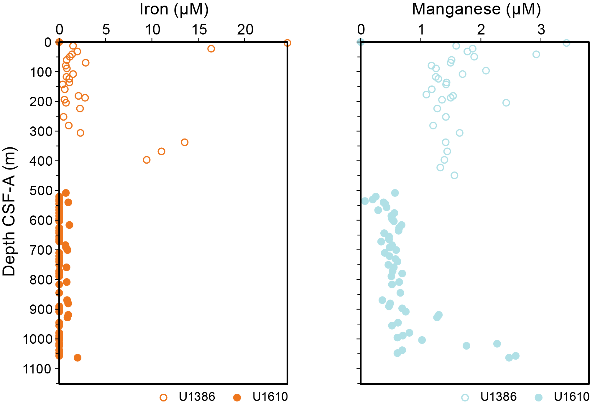
Figure F46. IW trace element concentrations.
6.3. Sedimentary geochemistry
Sediment samples were collected for analysis of solid-phase geochemistry at a resolution of one sample per core when recovery permitted in Hole U1610A (Table T16). For Cores 401-U1610A-2X through 61R as well as Core 72R, these samples came from a fraction of the IW squeeze cake residue. Additional samples were taken at a rate of one sample per core below Core 62R, with some additional samples to identify the geochemical variation across cycles in color and different lithologies identified by the shipboard sedimentologists.
6.3.1. Calcium carbonate
Overall, CaCO3 ranges 25.4–79.8 wt% (Figure F47; Table T16) with a mean of 35.3 wt% and a standard deviation of 7.3 wt%. Standard reproducibility was 1.12 wt% (n = 13). CaCO3 is generally relatively invariant at Site U1610, with most samples ranging within 28–40 wt% downcore. Some samples with high carbonate were detected in both routine sampling from IW squeeze cake residues as well as discrete samples selected based on visual core inspection. In the routine squeeze cake sampling, carbonate concentrations higher than 40 wt% are only recorded between 869.4 and 897.1 m CSF-A (Sections 401-U1610A-41R-2 through 44R-1), peaking at 51.1 wt% at 872.7 m CSF-A in Section 41R-5. A sample of clayey calcareous ooze specifically targeted for sampling at 1055.3 m CSF-A in Section 60R-4 yielded 50.4 wt% CaCO3 (Figure F48). Lower values of 25.7, 25.4, and 26.4 wt% are recorded at 1091.7, 1106.6, and 1116.5 m CSF-A (Sections 64-2, 65R-5, and 66R-5). We note an apparent increase in the average CaCO3 below Section 68R-3: average of 37.9 wt% between 1132.1 and 1363.8 m CSF (Sections 68R-3 through 92R-2). Discrete high values in this interval are 67.8 wt% at 1148.9 m CSF-A (Section 70R-1), 43.7 wt% at 1198.4 m CSF-A (Section 75R-2), 42.1 wt% at 1330.8 m CSF-A (Section 88R-6), and 40.5 wt% at 1353.2 m CSF-A (Section 91R-2). The base of the core includes 3 carbonate-rich samples, ~50 wt% CaCO3 recorded in Sections 93R-2 and 94R-2 and 79.8 wt% recorded at 1389.7 m CSF (Section 94R-CC) in a sample identified lithologically as a dolostone (see Lithostratigraphy). For samples containing dolomite rather than calcite, the standard coulometry calculations assuming a composition of calcium carbonate will overestimate the weight percent carbonate by approximately 8% because of the lower mass of magnesium relative to calcium. Applying a correction for dolomite, Sample 94R-CC instead would reflect 73.4 wt% dolomite, which agrees well with the amount of dolomite determined from the XRD spectra (Figure F49). For other samples containing a mixture of dolomite and calcite (dolomite is generally <10% of the total carbonate fraction), the correction is minor. There also appears to be a grain size bias during determination of carbonate for either (or both) coulometry or XRD analysis, although the mechanism is not known: sandy samples systematically show higher carbonate determination for coulometry than for XRD (Figure F49).
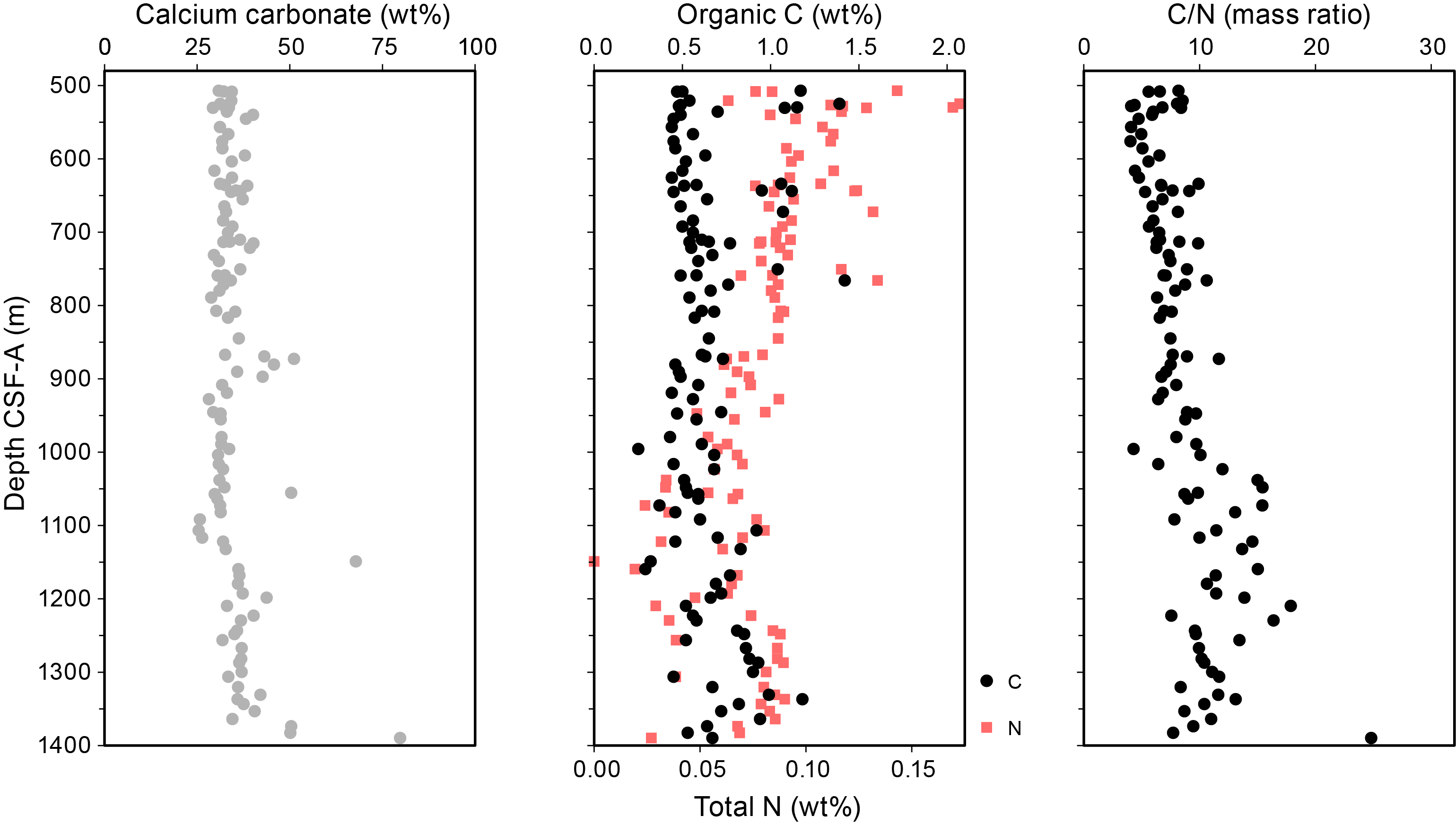
Figure F47. CaCO3, organic carbon, nitrogen, and C/N.
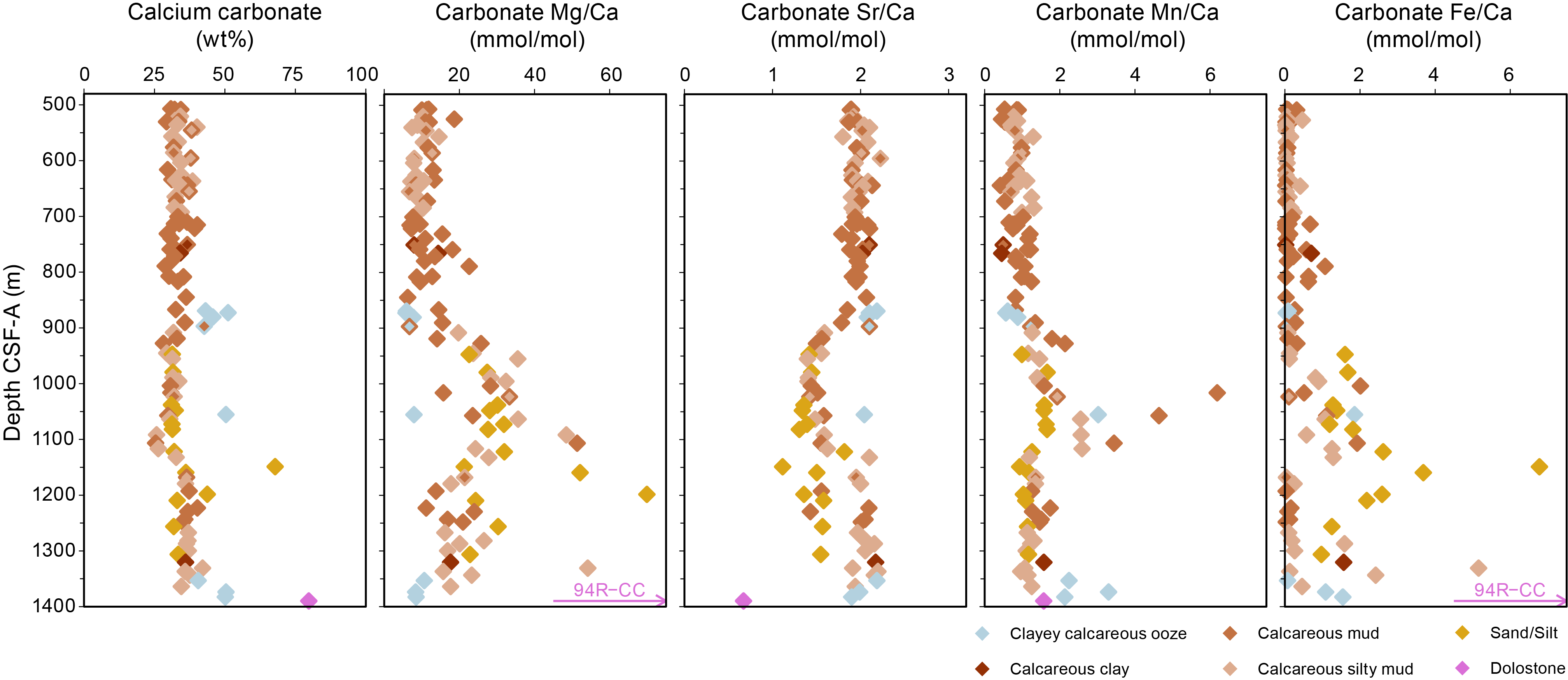
Figure F48. Carbonate geochemistry results.
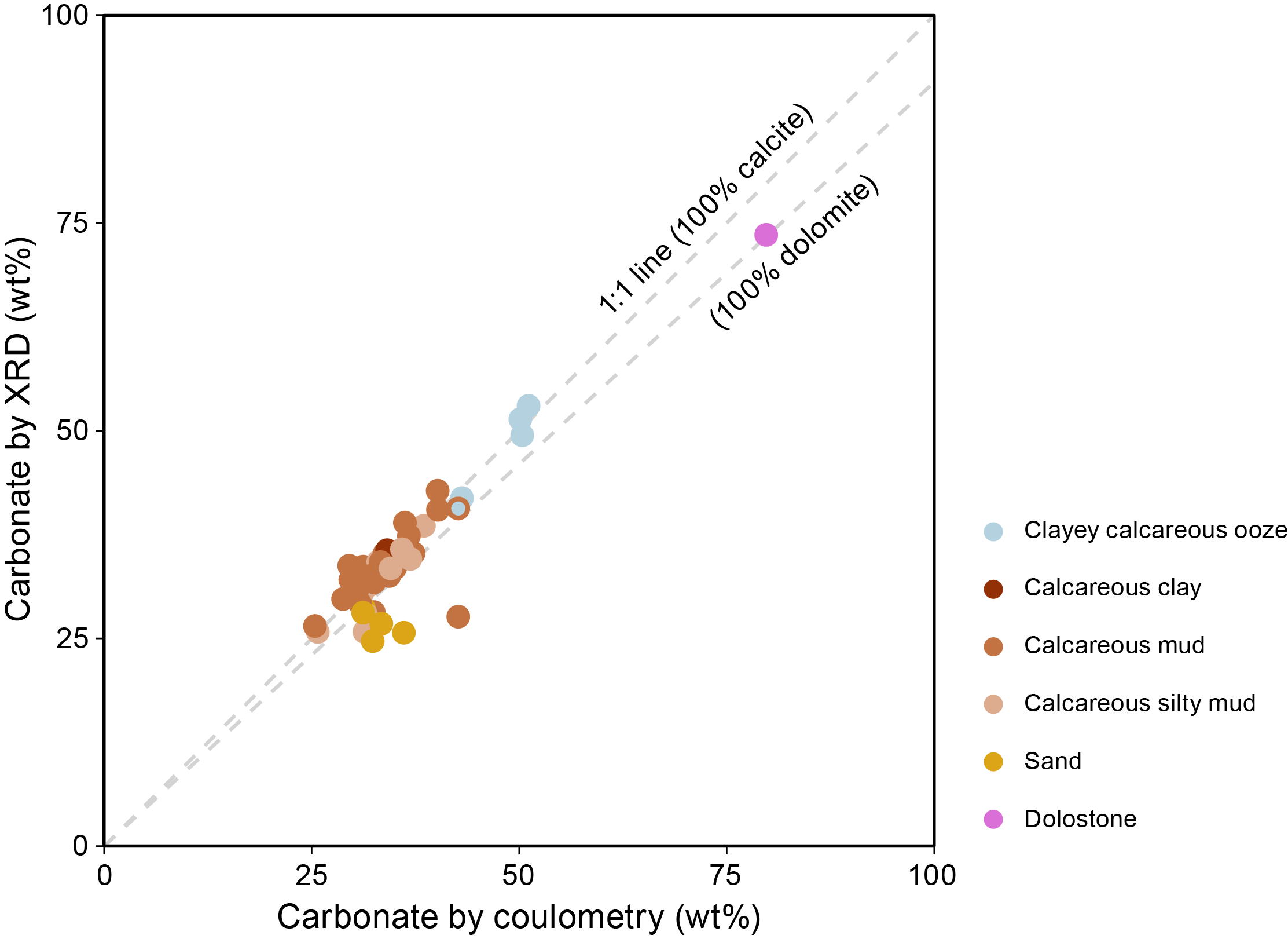
Figure F49. Carbonate weight percent, XRD and coulometry.
A weak correlation between CaCO3 and NGR measurements (Figure F50) suggests that most of the variability in NGR is unrelated to carbonate content and instead is perhaps controlled by quartz/silica abundance, with the exception of the very high carbonate samples such as those described at the base of the core. Some of the range in carbonates may be missed when based on IW sampling, but targeted sampling performed below the limits of IW sampling (below Core 401-U1610A-61R) may have been more effective at capturing the full range of variation. MS has a less clear relationship with CaCO3, although it appears that the carbonate fraction within the sediments may dilute the magnetic mineral fraction within the sediments (Figure F50).
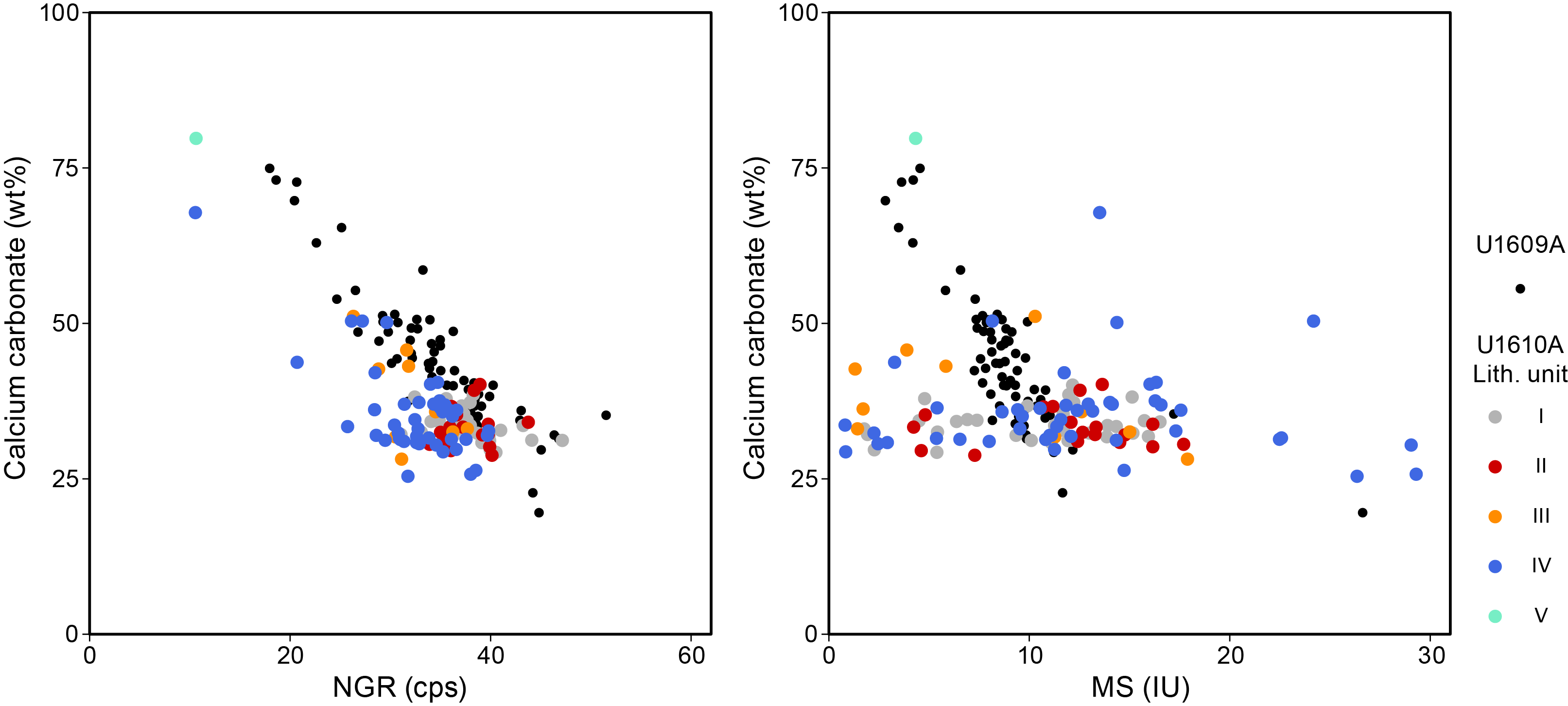
Figure F50. Carbonate weight percent, NGR, and MS.
6.3.2. Carbon and nitrogen
Organic carbon ranges 0.25–1.42 wt% (mean = 0.65 wt%; standard deviation = 0.22 wt%; n = 106) (Table T16). Higher carbon contents occur in discrete samples, with an increasing trend deeper than 1100 m CSF-A (Figure F47). Total nitrogen (TN) ranges 0.03–0.08 wt% (Figure F47; Table T16). Standard reproducibility was 0.02 wt% for N and 0.08 wt% for C (n = 12). C/N (using total organic carbon [TOC] and TN) ranges 4.0–24.8 (mean = 8.8 wt%; standard deviation = 3.4 wt%, n = 105); one sample has TN below detection level and thus C/N is not reported, but this result implies terrestrial sourcing (Emerson and Hedges, 1988; Meyers, 1997). Low C/N values (4–10) suggest marine-sourced organic carbon, with terrestrial sources typically having values of 20–30; however, C/N ratios increase with organic matter degradation. The range of values observed at Site U1610 suggests dominantly marine organic matter, as expected in a marine environment with variable terrestrial input (Figure F47). Prominent terrestrial additions resulting in C/N ratios between that of marine and terrestrial end-members are noted deeper than 1000 m CSF-A (e.g., in Sections 401-U1610A-58R-5, 59R-5, 62R-2, 63R-2, 67R-3, 70R-1, 78R-3, 80R-3, and 94R-CC). In some cases, including in Sample 94R-CC, macroscopic woody debris was noted in the coarse sediment fraction (see Biostratigraphy and Lithostratigraphy). Only in Sample 94R-CC can the C/N ratio be interpreted to be purely terrestrial organic matter with negligible marine organic input if fresh. However, this sample is also noted to have poor foraminifer preservation, and the organic matter is likely also highly degraded, which would result in the loss of proteins (containing N) and thus increase C/N, masking the marine component in the resulting C/N values.
6.3.3. Carbonate fraction geochemistry
In addition to the standard shipboard measurements of calcium carbonate concentrations in sediments, we performed geochemical analyses on the acid-soluble (carbonate) fraction of the sediment (Table T17). Because variable amounts of carbonate are present in each sample, the carbonate geochemistry data are reported as elemental ratios relative to calcium. The carbonate Mg/Ca ratios are generally between 6 and 15 mmol/mol for the uppermost 900 m of Hole U1610A with a few higher values up to 23 mmol/mol (Figure F51). These ratios correspond to a carbonate mineral fraction containing the equivalent of 1%–3% dolomite, which is less than the abundance of dolomite estimated from XRD analysis (Figure F49). Deeper in the core, carbonate Mg/Ca ranges approximately 8–35 mmol/mol with a few higher values up to 70 mmol/mol (Sample 401-U1610A-75R-2, 54–55 cm). Sample 94R-CC, 45–50 cm (1389.7 m CSF-A), was identified as a dolostone and has a Mg/Ca ratio of 0.74 mol/mol, indicating that it is not a pure stoichiometric dolomite. Carbonate Sr/Ca ratios show a broadly inverse trend to the Mg/Ca ratios, with a baseline value around 2.0 mmol/mol that decreases to 1.0–1.5 mmol/mol during intervals of higher Mg/Ca (Cores 45R–71R) (Figure F51). The Sr/Ca ratios show a dependence on lithology, with lower Sr/Ca ratios generally present in silty and sandy samples relative to mud- and clay-rich lithologies, especially below Core 70R. Some of the sandier samples with low Sr/Ca also have higher Mg/Ca ratios. These geochemical patterns likely reflect the impact of carbonate diagenesis, although detrital carbonate grains may also contribute to the observed signal. The dependence on lithology is also consistent with diagenesis because sandier intervals often have greater porosity and permeability, which can permit more intense carbonate diagenesis relative to finer grained lithologies. These diagenetic effects cannot be linked to the geochemical observations of the modern IW samples, which do not show corresponding intervals of consumption/release of Mg and Sr but instead must have occurred previously, possibly during shallow burial and the early diagenetic window.
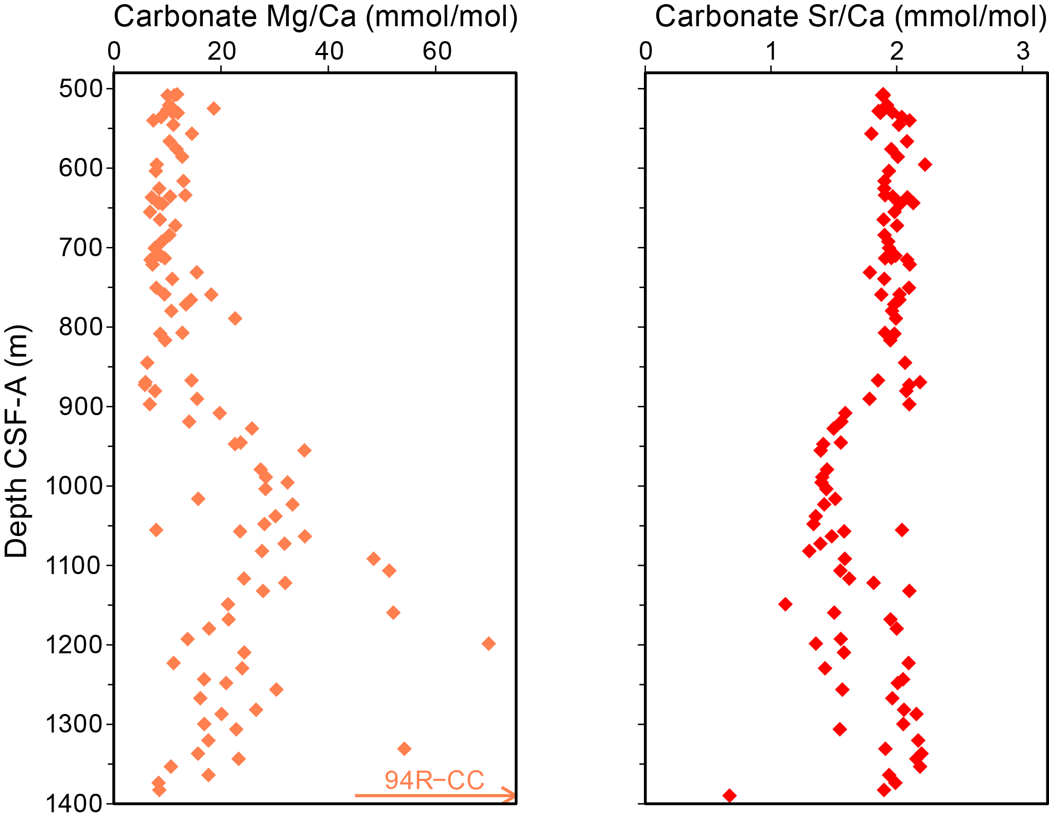
Figure F51. Carbonate Mg/Ca and Sr/Ca.
Carbonate Mn/Ca ratios range 0.5–1.4 mmol/mol in the uppermost 900 m of Hole U1610A before increasing to approximately 1.0–1.7 mmol/mol between approximately 900 and 1080 m CSF-A, where a few samples show significantly higher Mn/Ca ratios up to 6.2 mmol/mol (Cores 401-U1610A-45R and 63R) (Figure F52). Deeper in the core, ratios stabilize around 1.2 mmol/mol, again with a few higher values up to 3.3 mol/mol. There is a dependence on lithology, with finer grained material (oozes, clays, and muds) showing higher Mn/Ca ratios than coarser grained lithologies. The dolostone sample (94R-CC, 45–50 cm; 1389.7 m CSF-A) does not have anomalously high Mn/Ca ratios.
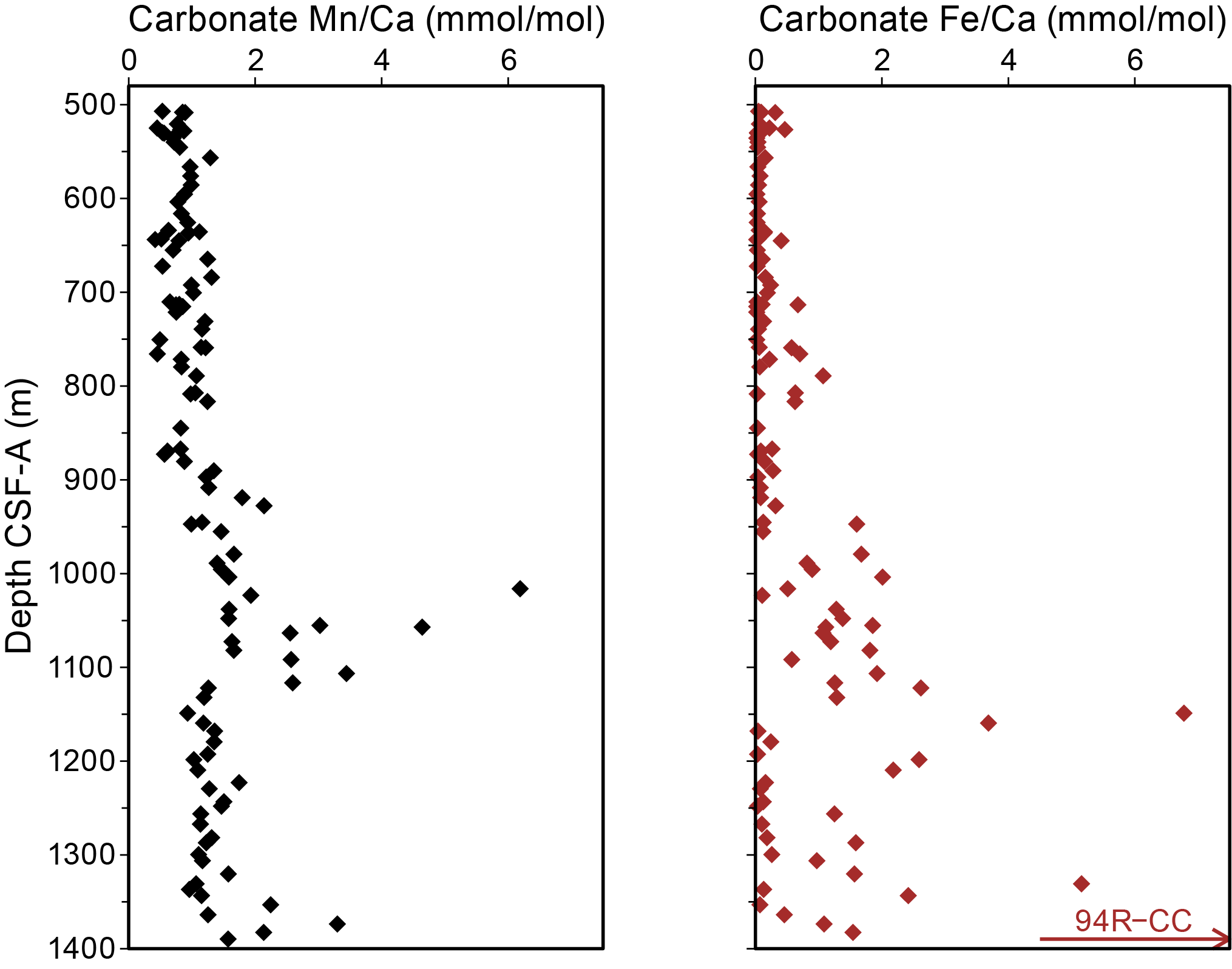
Figure F52. Carbonate Mn/Ca and Fe/Ca.
Carbonate Fe/Ca ratios are generally less than 0.6 mmol/mol in the uppermost 900 m with one at 1.0 mmol/mol. Below 900 m CSF-A, Fe/Ca generally range 1.0–2.5 mmol/mol with a couple of higher values reaching 6.8 mmol/mol (Figure F52). These ratios are equivalent to 0.01%–0.3% siderite in the carbonate fraction, which is much less than the ~5%–10% siderite (relative to the sum of all carbonate minerals) estimated from XRD analysis; it is possible that slow dissolution kinetics of siderite or oxidation reactions prevented accurate quantification of the iron carbonate fraction or that the XRD estimates systematically overestimate the abundance of the low-abundance carbonate minerals (both dolomite and siderite) relative to calcite. Fe/Ca ratios are generally higher in the coarser grained lithologies. The dolostone sample (401-U1610A-94R-CC, 45–50 cm; 1389.7 m CSF-A) has the highest Fe/Ca ratio of 41.8 mmol/mol. Apart from the dolostone sample, the Fe/Ca ratios are weakly positively correlated with Mg/Ca and Mn/Ca ratios and negatively correlated with Sr/Ca ratios, suggesting that all these geochemical patterns are related to carbonate diagenesis associated with anoxic subsurface environments.
In summary, we find that the fluid and sedimentary profiles at this site indicate distinct zones within the core defined by more/less terrestrial sourced solids, more/less pore water influence from the olistostrome, and variable degradation of solid constituents, depending on lithology and depositional setting. Some barriers to permeability in the middepths of the profile preserve a separate fluid environment above 955.3 m CSF-A (Section 401-U1610A-50R-1), with salinities notably higher than seawater below.
7. Physical properties
Physical properties at Site U1610 were determined at 2.5 cm spacing on the Whole-Round Multisensor Logger (WRMSL) and Section Half Multisensor Logger (SHMSL) and at 10 cm spacing on the Natural Gamma Radiation Logger (NGRL) (see Physical properties in the Expedition 401 methods chapter [Flecker et al., 2025a]). Thermal conductivity probes were applied on one section per core, with the chosen interval selected based on core cohesiveness and relative lithologic homogeneity. P-wave velocity was obtained on split core sections (working half) and/or cubic specimens (from Cores 401-U1610A-74R through 94R). To determine whether lithologic cycles correlated with changes in density, porosity and/or any other petrophysical property, 1 or 2 discrete samples were taken from each core for moisture and density (MAD) and/or P-wave caliper (PWC) measurements. MAD measurements were initially measured on cylindrical specimens for Cores 2X–73R but switched to cubic specimens from Cores 74R–94R. The same cubic specimens were used for P-wave velocity and MAD measurements to preserve as much of the working-half core as possible.
A few clear changes are visible in most or all of the physical properties data sets. A good example is the uphole increase in the range of variation in NGR, reflectance, and RGB color that occurs at 700 m CSF-B (Figure F53), coinciding with the Lithostratigraphic Unit I/II boundary (Figure F11; see Lithostratigraphy). However, some of the prominent changes in one physical properties data set are not seen in others. The shape of the obvious peak in MS between 950 and 1000 m CSF-B is not clearly mirrored in the other records. Overall, changes observed in the various physical properties data sets typically correlate well with the lithostratigraphic unit and subunit boundaries.
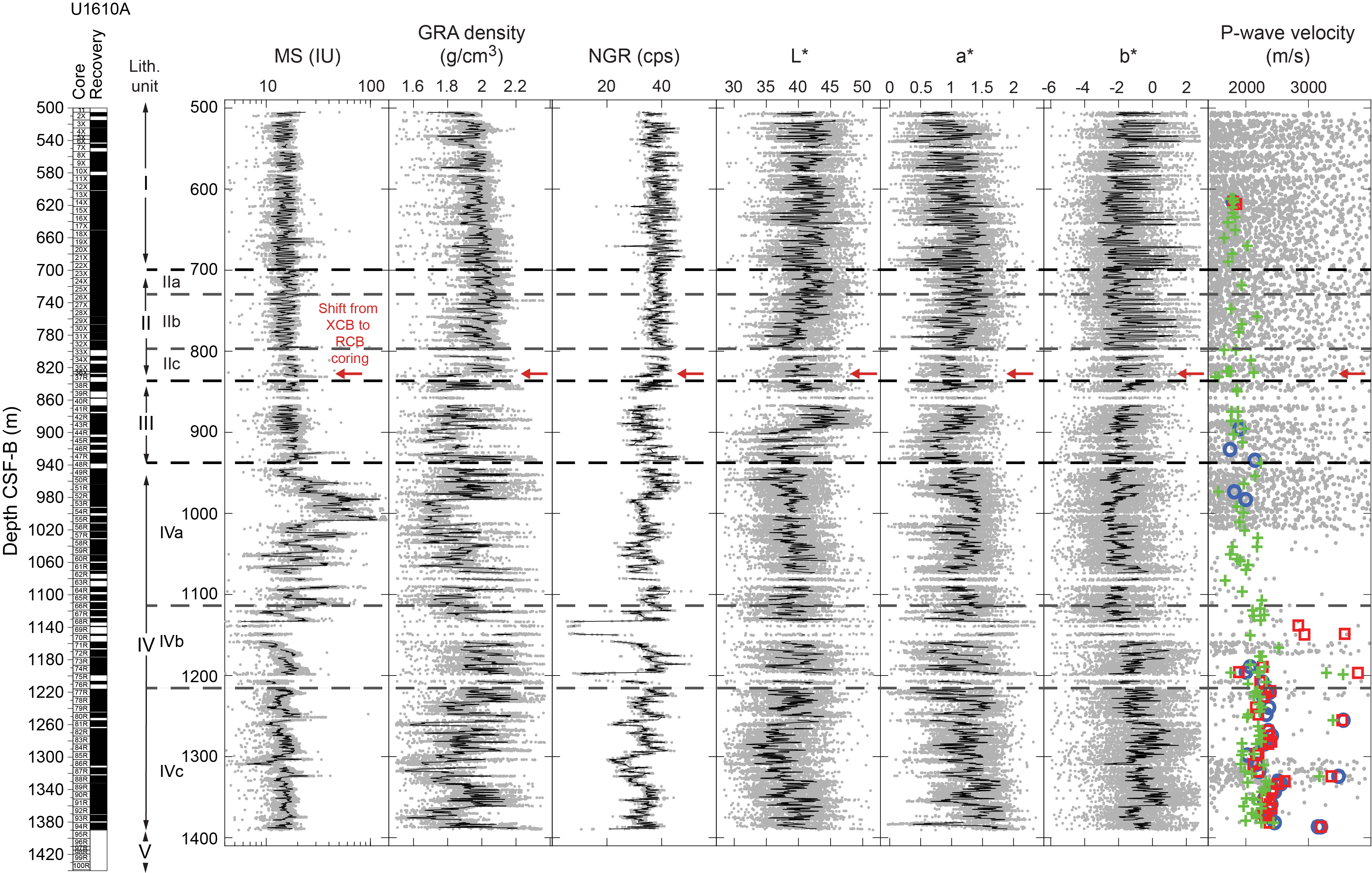
Figure F53. MS; GRA; NGR; L*, a*, and b*; and P-wave velocity.
7.1. Magnetic susceptibility
The broad pattern of the MS record in Hole U1610A can be split into three main intervals (Figure F53): (1) the uppermost 500–950 m, which displays 2–7 m thick small-amplitude cycles with minimal trend, (2) 950–1000 m CSF-B, where a central prominent peak in values with higher amplitude variability is evident, and (3) the interval between 1100 m CSF-B and the bottom of the hole, characterized by discrete low-amplitude packages that are 50–100 m thick.
In detail, there are more subtle changes, for example, a downhole increase in the thickness of the striking cyclicity at ~700 m CSF-B. Cycles in the uppermost 700 m are ~2–5 m thick, whereas those between 700 and 800 m CSF-B are ~5–7 m thick (Figures F53, F58; see Age model). This change corresponds to the Lithostratigraphic Unit I/II boundary, which marks the decrease in deposition of calcareous silty mud sediments (Figure F9). The relationship between MS and NGR changes at 800 m CSF-B. Between 685 and 800 m CSF-B, high MS corresponds to low NGR and vice versa (Figure F54A); however, below 800 m CSF-B, high MS corresponds to high NGR and vice versa (Figure F54B). The change in the phasing of MS–NGR cycles at 800 m CSF-B is also marked by a prominent change in the amplitude of reflectance and color variability (Figure F53) and corresponds to the shift to higher siliciclastic input that occurs at the transition from Subunit IIb to Subunit IIc (Figure F53).
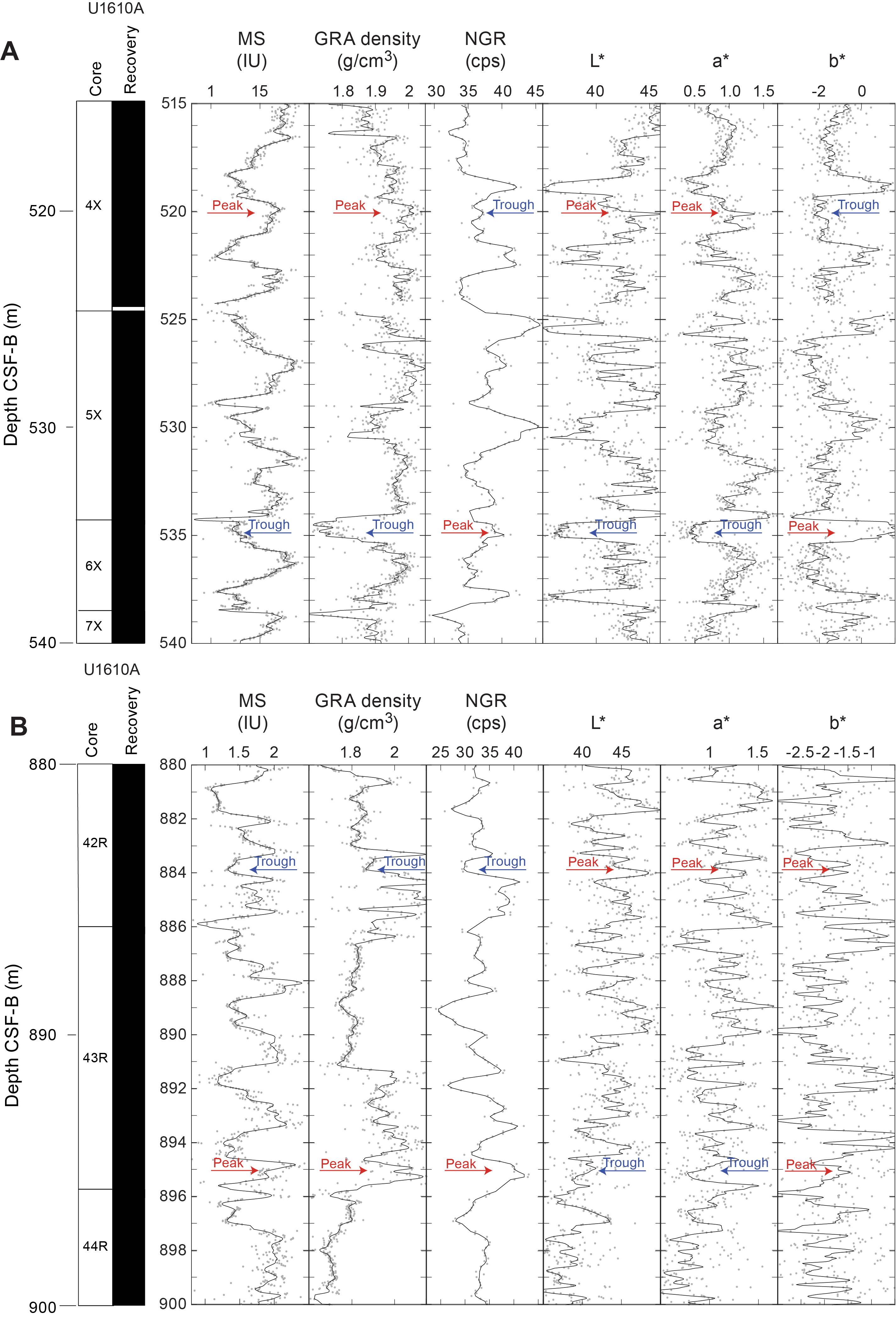
Figure F54. MS; GRA; NGR; and L*, a*, and b*.
7.2. Gamma ray attenuation bulk density
Average GRA density varies from ~1.9 to 2.4 g/cm3 in Hole U1610A (Figure F53). Gaps between sediments and surrounding core liners for the XCB and RCB cores impact the bulk density values measured on the WRMSL. The scale of the deviation of the GRA bulk density values from the real value (taken to be the MAD bulk density) depends on the scale of the gap, where wider gaps between the sediment and the liner result in lower GRA densities. This issue affects the Hole U1610A data most clearly from Core 401-U1610A-38R downward, where there is a large difference between GRA and MAD bulk density values (Figure F55). This is probably the reason why the GRA density values do not show the typical compaction-driven increasing trend with depth and indicates that GRA bulk density values are less reliable than the MAD bulk density.
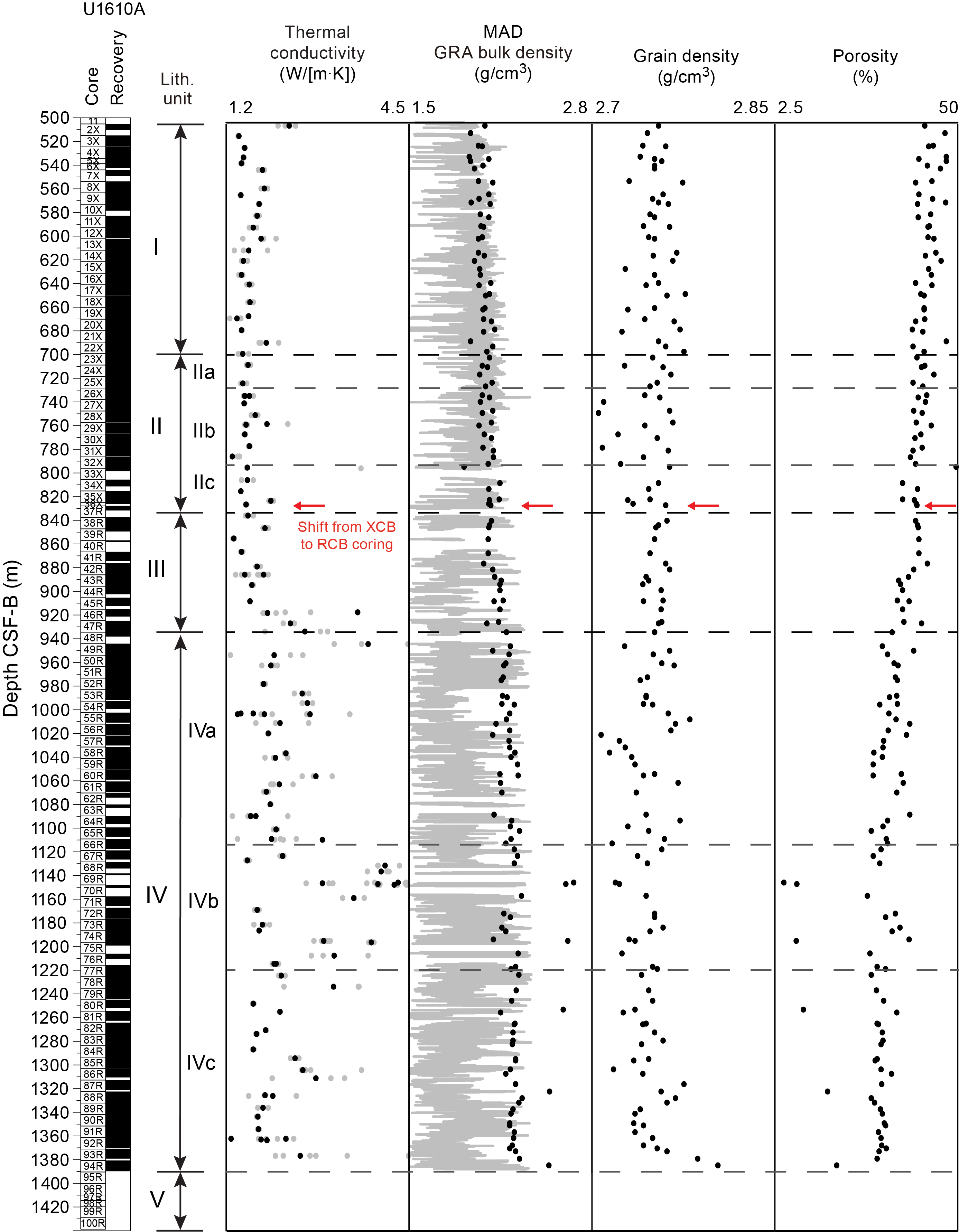
Figure F55. Thermal conductivity, bulk and grain density, and porosity.
7.3. Natural gamma radiation
Both the amplitude and frequency of the NGR variability change downhole in Hole U1610A. A well-defined change at ~700 m CSF-B shows higher amplitude regular cycles above and lower amplitude more variable fluctuations below (Figure F53). The prominent step at 980 m CSF-B is likely a function of a core liner gap that is clearly visible in the GRA density data. Below this, the amplitude and frequency of the cycles is larger from 1150 m CSF-B to the bottom of the hole.
Spectral potassium, uranium, and thorium contents were extracted from the original NGR spectra (De Vleeschouwer et al., 2017) (Figure F56). All three components show the same long-term variations as total NGR count; however, the amplitude of the thorium cycles at the top of the core (500–800 m CSF-B) is subdued relative to uranium and potassium.
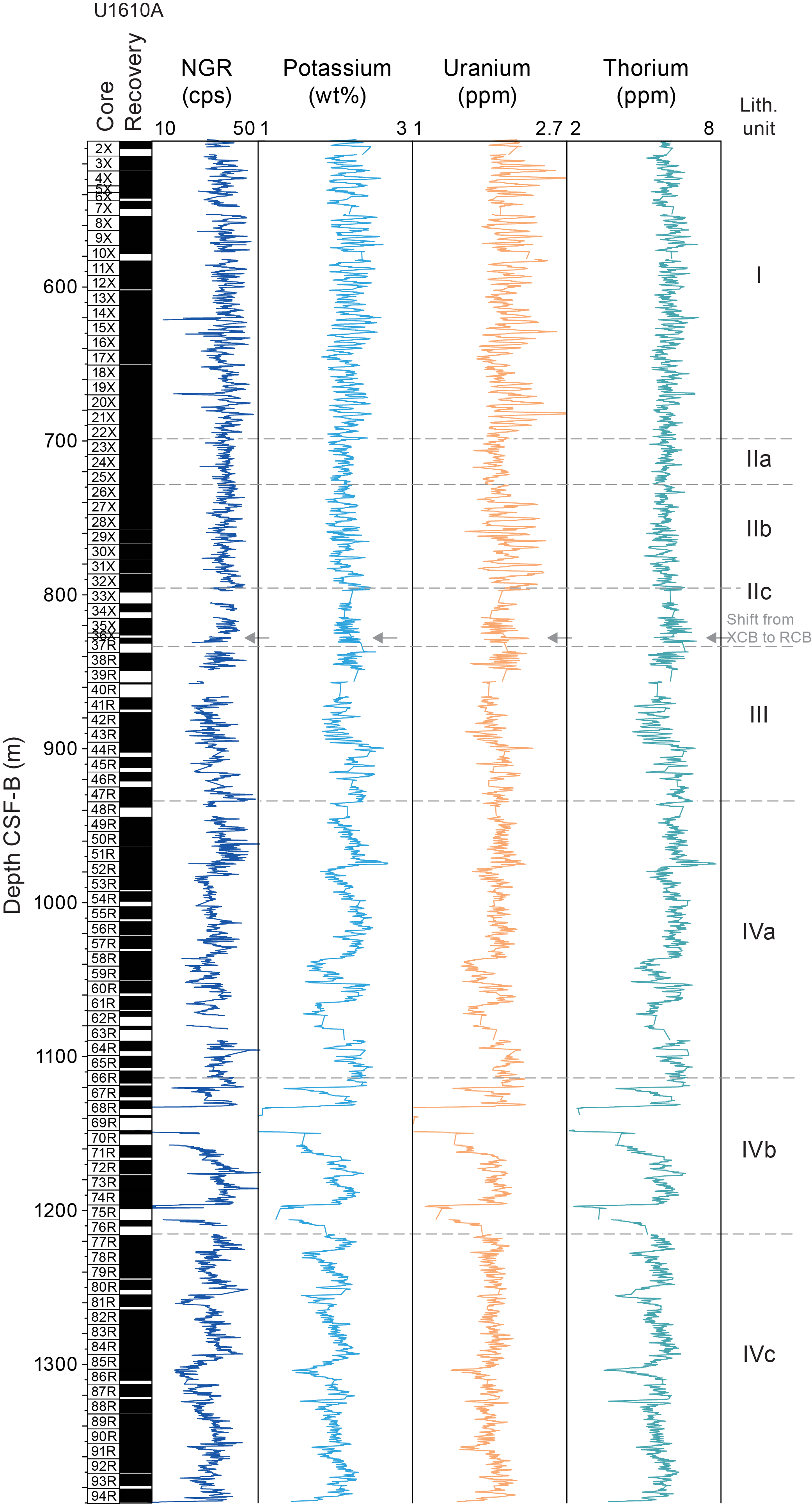
Figure F56. NGR measurements.
7.4. Spectrophotometry
The color of most of the sediments in Hole U1610A is gray (GLEY1 5/10Y and 10Y 5/2; see Lithostratigraphy); however, subtle variations are visible in the digital color data. The main features of the lightness (L*), green–red (a*), and blue–yellow (b*) color variation records are a change in frequency and amplitude at 700 m CSF-B that corresponds to the Unit I/II boundary; a change in amplitude at 800 m CSF-B that reflects the onset of siliciclastic input (Figure F9) in the Early Pliocene; a sharp decline in L* and to a lesser extent a* from 880 to 900 m CSF-B; and an interval with high-amplitude variability at 1150–1200 m CSF-B. These correspond to the hard, pale, coarse-grained sandstones in Subunit IVb (Figure F9).
Spectrophotometry results from Hole U1610A display similar patterns to the other measured physical properties (Figure F53). The range of lightness and color changes is in general quite small. Like MS, GRA density, and NGR, color is dominated by short cycles with wavelengths ranging ~3–5 m (Figure F54), except for the interval shallower than 700 m CSF-B which has thicker cycles. As expected, color data show little to no change at the shift from XCB to RCB coring. Except for Units III and IV, the L* and a* variations appear to generally be in phase with one another (lighter sediments are also slightly less green). Additionally, both values appear to be generally in phase with MS, implying that higher MS corresponds to lighter sediment and vice versa. By contrast, b* appears to have a generally inverse relationship with the other three values, implying that higher MS more commonly corresponds to slightly bluer sediment.
The color values of Unit I are characterized by high-frequency ~3–5 m cycles in all three data sets (Figure F54). The uppermost 115 m of Unit II (685–800 m CSF-B) is characterized by a shift to lower amplitude and lower frequency (~5–7 m) cycles in L* and a* values. By contrast, b* values shift to ~5–7 m cycles with no noticeable change in amplitude. Like the MS data set, all three color values return to a shorter (~3–5 m cycle) signal below 800 m CSF-B that remains the dominant frequency for the remainder of the core.
A noticeable peak in L* and a* values (toward lighter and redder colors) occurs in the lower portion of Unit II at ~900 m CSF-B. b* values show no corresponding peak or trough (Figure F53).
From 900 m CSF-B to the Unit III/IV boundary (1130 m CSF-B), L* shows a marked decrease in values with little amplitude variation. By contrast a* values steadily rise at the Unit III boundary, whereas b* values show little to no variation outside of the high-frequency cycles (Figure F53). This is notable because it implies that the increase in MS values within Unit III only corresponds to an increase in redness. Units IV and V show a change to high-amplitude/high-frequency cycles with a subtly negative and positive secular trend for the L* and a* values with depth. Notably, L* values have a sharp trough approximately at the Unit IV/V boundary (1295 m CSF-B). b* values display both higher median values (yellower color) and higher amplitudes in Units IV and V, perhaps reflecting the varying degrees of dolomitization in these lithostratigraphic units (see Lithostratigraphy).
7.5. Thermal conductivity
At Site U1610, thermal conductivity was measured in triplicate at one position per core, mostly in Section 2, using half-space probes (H51033 and H11080). A different section was measured when Section 2 was cracked or fragmented or when there were multiple lithologic variations along the sedimentary record.
The values for thermal conductivity at Site U1610 range 1.29–4.31 W/(m·K) (Figure F55), which is higher than the range of values obtained from nearby sites, including Site U1609 (this expedition) and Site U1391 (Expedition 339 Scientists, 2013e), as may be expected from the higher degree of compaction and lithification in the deeper levels of this site. The values obtained at Site U1610 are low and relatively constant between 500 (top of the core) and ~900 m CSF-B (Units I–III), with an average of 1.64 W/(m·K). At depths greater than 900 m CSF-B, the thermal conductivity data are more varied, with a higher average value (2.40 W/[m·K]) between ~900 and ~1300 m CSF-B (Figure F55). The highest values are found between 1130 and 1160 m CSF-A. Recovery from this interval is poor, but what was recovered were coarse, well-cemented sandstones and conglomerates (Figure F8). These higher thermal conductivity values also coincide with both higher discrete (MAD) density values and low porosity.
In Subunit IVc (1295 m CSF-B to the bottom of the hole), thermal conductivity slightly decreases relative to Subunit IVb (Figure F55), having an average value of ~2 W/(m·K). This unit shows some high values that correspond to harder sediment layers.
7.6. P-wave velocity
The P-wave logger (PWL) data are unreliable because of the large gap between the core and the liner that induces poor contacts with sensors and attenuated P-wave propagation.
PWC values in the depth interval from 500 and 610 m CSF-A did not yield reasonable P-wave values due to the softness of the non-consolidated sediments in that interval. In the interval between Cores 401-U1610A-13X and 73R (~610–1190 m CSF-A), PWC values were obtained from measurements conducted on cubic samples cut from the core catcher. Afterwards, the PWC data were obtained from discrete cubic samples (later used for MAD measurements) from Cores 74R–94R (1190–1400 m CSF-B). These smaller, portable, discrete cubic specimens allowed for the measurement of P-wave velocity in the x-, y-, and z-directions (red squares, blue circles, and green crosses, respectively, in Figure F53). P-wave velocity responds better to hard sediments than soft ones, so more reliable data were obtained from the well-cemented intervals (e.g., below 1120 m CSF-B [Figure F53] and Subunit IVb [Figure F9]). There is a general trend toward higher values with depth probably due to the increased compaction of the sediments.
7.7. Moisture and density measurements
Bulk density values were calculated from moisture and volume measurements made on cylindrical (Cores 401-U1610A-2X through 73R) and cubic (Cores 74R–94R) discrete samples taken from the working halves of Hole U1610A. Samples for Cores 74R–94R were used both to produce more accurate PWC results (see P-wave velocity) and afterward for MAD measurements to preserve as much of the working halves as possible for postcruise research sampling.
Because gaps between the sediments and liner and/or drilling-induced cracks partially or completely obscure the original petrophysical signals of the core, 1 or 2 MAD samples were taken per core to verify the accuracy of the GRA density measured by the WRMSL (see Bulk density, grain density, and porosity). A total of 157 samples were measured from Hole U1610A, but the sample resolution varied depending on lithology, recovery, and quality of the individual core sections.
MAD values increase downcore and are commonly higher than GRA values at the same level (Figure F55). The range of GRA values expands to include lower values below the switch to RCB coring (Figure F55), probably as a result of a smaller core diameter. MAD measurements on geometrically uniform and discrete samples therefore commonly provide more reliable density values than the GRA density data set. The MAD trend toward higher values downhole is likely to be the result of compaction.
7.7.1. Bulk density, grain density, and porosity
Bulk density from MAD measurements typically ranges 1.90–2.67 g/cm3 in Hole U1610A. Grain density typically ranges 2.71–2.80 g/cm3 (750.94–1386.6 m CSF-B) through Hole U1610A. Most of the recorded values are quite variable; however, the interval between 840 and 940 m CSF-B has rather consistent values, which correlates with the homogeneous and less siliciclastic Unit III (Figure F9). Porosity declines with depth because of compaction (Figure F55). Discrete porosity values range from ~49.8% in Core 401-U1610A-33X (797.07 m CSF-B) to ~2.7% in the sandstone layer at 1148.2 m CSF-B.
8. Downhole measurements
Following coring in Hole U1610A, the hole was prepared for downhole logging on 11 January 2024 (see Operations). The first downhole logging run consisted of a 47.12 m long quad combo tool string (see Figure F20 in the Expedition 401 methods chapter [Flecker et al., 2025a]) consisting of the Dipole Sonic Imager (DSI), High-Resolution Laterolog Array (HRLA), Hostile Environment Litho-Density Sonde (HLDS), Hostile Environment Natural Gamma Ray Sonde (HNGS), and logging equipment head-pressure temperature (LEH-PT). These tools measure shear (S-wave) and compressional wave (P-wave) velocities, electrical resistivity, density, NGR, temperature, and borehole inclination, respectively. The DSI was added to the normal triple combo tool string and the Magnetic Susceptibility Sonde was left out because borehole conditions were anticipated to be difficult and would be likely to degrade before a second tool string could be run.
Just below the casing, as the tool string was being lowered down the hole, the quad combo encountered obstructions and had to be worked down through bridges and ledges. The tool string reached 726 m wireline log depth below seafloor (WSF), but after eight unsuccessful attempts to penetrate deeper, we decided to log up through the open hole and casing to the seafloor. The logged open hole interval was Lower Pliocene calcareous silty mud with 2–6 m scale repeating cycles in core NGR, MS, and density (see Unit I description in Lithostratigraphy and Physical properties; Figures F9, F53).
8.1. Borehole conditions and downhole data set quality
The borehole walls of Hole U1610A were very rough, characterized by washouts, bridges, and ledges (Figure F57). Inclined beds observed in the cores (see Lithostratigraphy) suggested that the hole might be angled away from vertical, and the inclinometer in the logging cablehead confirmed this to be the case. At the end of the pipe, the borehole was inclined at ~10° from vertical and the inclination increased with depth to reach ~14° at 682 m WSF (Figure F57).
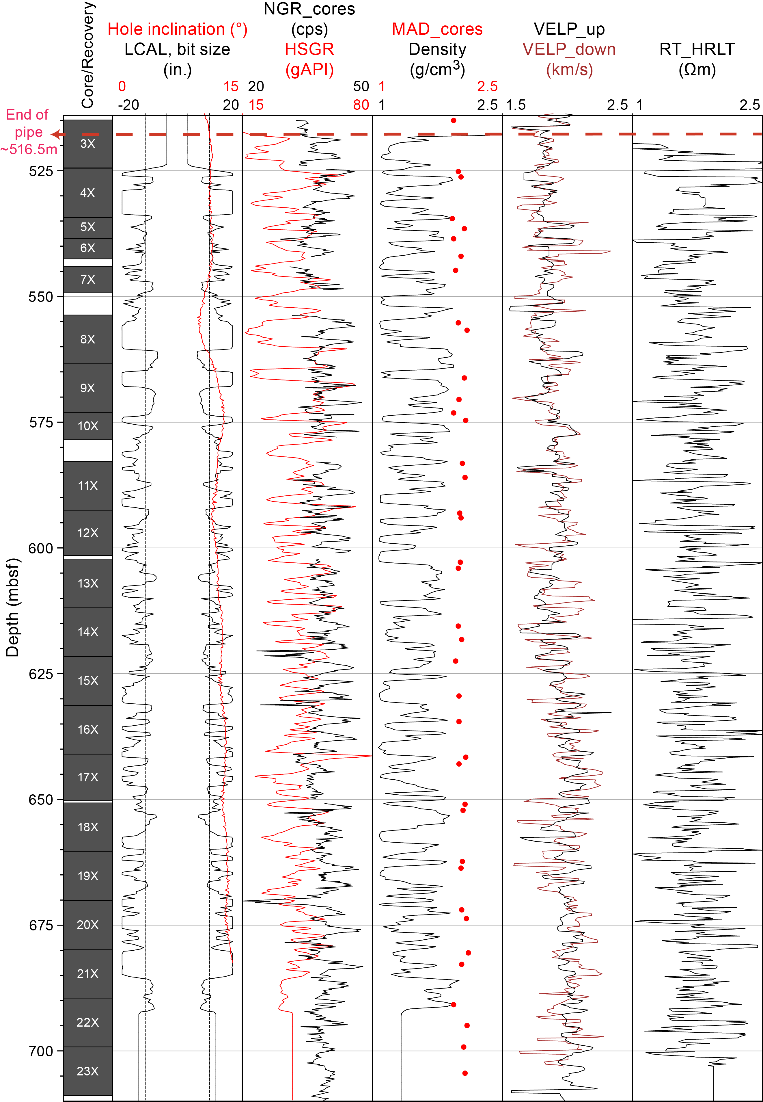
Figure F57. Downhole logging data summary.
The HNGS logs show that the base of the pipe is at 516.5 m WSF (Figure F57) and the seafloor is at ~566 m WSL. The HNGS gives formation gamma ray data inside the casing and the drill pipe, albeit attenuated. It may be possible to use this data to study Pliocene–Quaternary sedimentary cyclicity, when corrected for the additional attenuation at thicker pipe joints.
Comparison of the downhole gamma ray signal with equivalent NGR data measured on the cores confirms that the HNGS data is affected by the washouts, which result in anomalously low values (e.g., washout between ~529 and 533 m CSF-B and between ~555 and 560 m CSF-B; Figure F57). The density log values range between ~1 and ~2 g/cm3 and are also substantially impacted by the hole conditions as evidenced by the mimicking of this log to the caliper log (Figure F57). The envelope of the higher density values of the downhole density measurement lies on a similar trend as the MAD measurements on core samples but have smaller (~0.3–0.6 g/cm3) absolute values than the MAD values (Figure F57; see Physical properties). The resistivity log yields values ranging from ~0.8 and ~2.6 Ωm and also mimics the caliper log suggesting that the resistivity data is also highly impacted by washouts and bridgings (Figure F57).
The sonic P-wave velocity log repeated reasonably well between the upward and downward passes of the logging tool (Figure F57), so the data are considered to be robust and reflect real formation measurements. For the downward pass, the transmitter was set at standard (high) frequency, and for the upward pass it was changed to medium frequency to give a more robust signal in the poor borehole conditions. P-wave velocity had to be rederived from the DSI slowness time coherence on shore, and these reprocessed logs are plotted here (Figure F57). P-wave velocity slightly increases with depth, with average values ranging from ~1.8 km/s in the upper half (~520–620 m WSF) of the hole and increases to ~2 km/s in the lower half (~620–715 m WSF). Despite only covering a 204 m interval, these velocity logs are useful for constraining the relationship between depth and TWT in the upper part of Hole U1610A.
8.2. Downhole temperature
The SET2 tool was run before taking Core 401-U1610A-2X at 505.2 m WSF. It gave a clean 10 min temperature equilibration curve, and from this we derived a formation temperature of 24.8°C. Assuming a linear gradient to the seafloor temperature (12°C based on Conductivity-Temperature-Depth [CTD] measurements at this site), the geothermal gradient is 25.3°C/km.
8.3. Core-downhole-seismic integration
The presence of inclined beds in the cores (tilted laminae; Figure F8) indicated a potential deviation of the borehole from vertical. This suspicion was confirmed by measurements recorded by the inclinometer in the logging cablehead, revealing that, at the end of the pipe, the borehole exhibited an inclination of approximately 10° away from the vertical axis. Furthermore, the inclination gradually deviated further from vertical with depth, reaching approximately 14° at a depth of 682 m WSF (Figure F57).
This inclination may explain the difficulty encountered in lowering the tool string down the borehole past ledges. Paleomagnetic AMS analysis on core samples also suggests that the borehole was inclined, up to ~15° at ~1350 m CSF-B (see Paleomagnetism). The inclination of the borehole has implications for the TWT to depth conversion when tying the borehole to the seismic reflection profile, because the true vertical depth will be shallower than the measured depth along the borehole path (CSF scale). For example, at 1400 m CSF-B, a borehole with an average inclination of 12° would have a true vertical depth of 1369.4 m CSF-B, 30.6 m shallower than the measured depth. Such an inclination will make a difference to the estimated penetration on the scale of the seismic profile when tied to the borehole. Considering the lack of velocity data at such depths in this area of the basin, a proper core-seismic tie will require further analysis (e.g., synthetic seismic profile) that will be carried out as part of the postexpedition research.
9. Age model
Biostratigraphic and magnetostratigraphic analysis of Site U1610 generated nannofossil (n = 7), foraminifer (n = 8), and paleomagnetic (n = 10) age control datums between 3.57 and 6.38 Ma (Table T18). Gaps in age tie points between 781.4 and 936.3 m CSF-B and 5.36–5.78 Ma and below 1116.8 m CSF-B and 6.38 Ma to the base of the hole at ~1400 m CSF-B make these intervals more poorly constrained.
There is a good correspondence between foraminifer and nannofossil bioevents and the paleomagnetic chron boundaries for Site U1610 holes (Figure F58A), except for the interval between 713 and 808 m CSF-B, where stratigraphic and age order are not consistent (Table T18). The two C. acutus nannofossil bioevents are based on the identification of a species that occurs only rarely in these samples, and the bioevent should be used with caution (see Biostratigraphy). The HO of O. rugosus is also considered to be unreliable, which may explain why its stratigraphic position is at odds with the Thvera Chron boundary C3n.1n, which is identified at 808 m CSF-B (see Paleomagnetism). With or without these three less certain age constraints, the age-depth distribution of biostratigraphic and magnetostratigraphic events indicates that there is an increase in sedimentation rate from ~15 to ~30 cm/ky somewhere between 800 and 950 m CSF-B (Figure F58A). Because of the paucity of age constraints across this 150 m interval, it is not clear what the pattern of sedimentation rate changes is (CSF-B scale). Sedimentation rates below 1116.8 m CSF-B and 6.38 Ma are unconstrained, but an extrapolation of 30 cm/ky sedimentation rate would imply 7.4 Ma for the base of the hole.
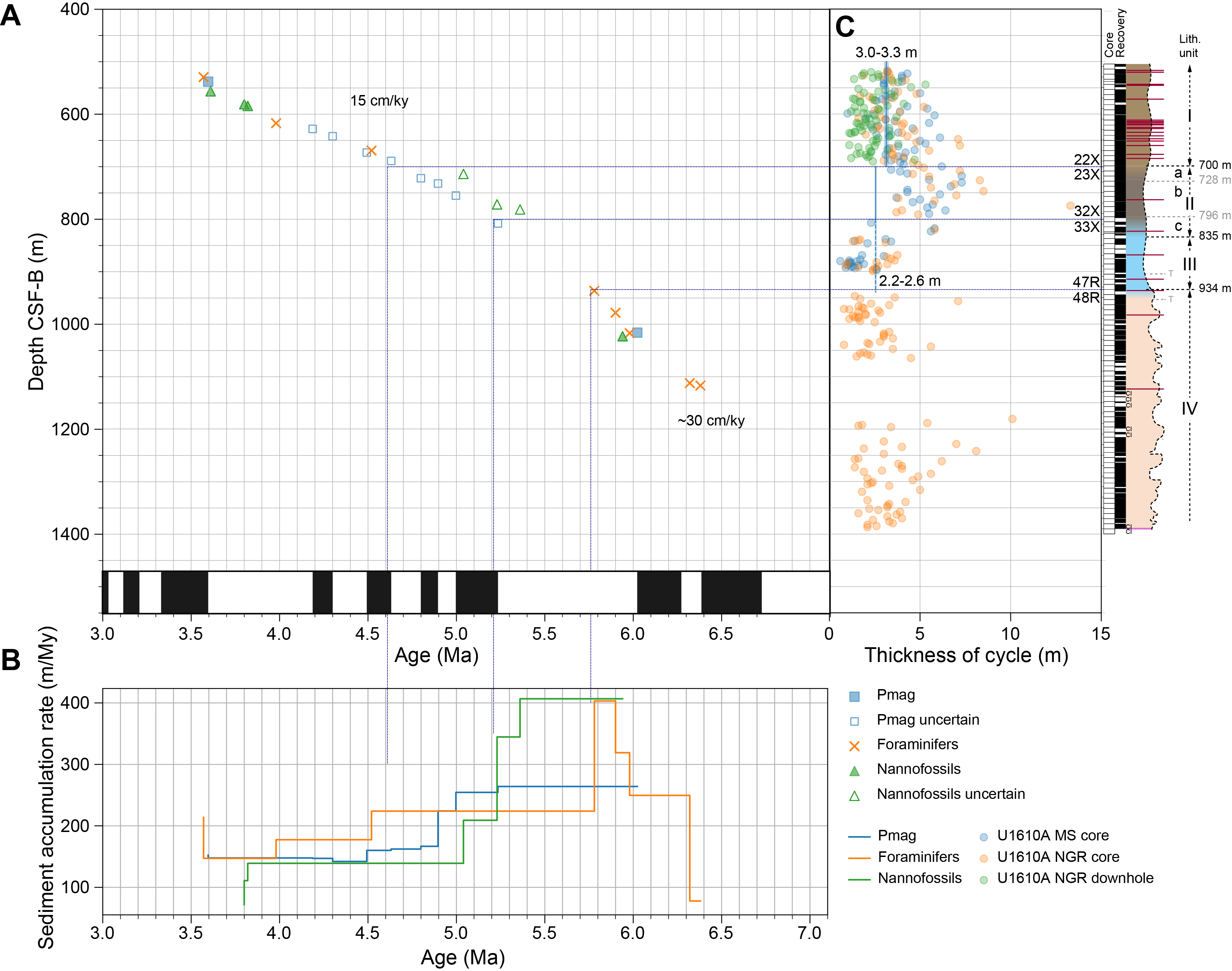
Figure F58. Age model tie points.
Regular cyclicity visible in the physical properties data can be used to provide an independent evaluation of the depth at which sedimentation rates changes occur. Regular cyclicity is visible in both the gamma ray (core and downhole data) and MS data in the upper part of Hole U1610A to around 940 m CSF-B (see Physical properties). Below this level, these data sets show more complex patterns that probably relate in part to the influx of sand with variable grain size and cementation (see Physical properties and Lithostratigraphy). Turbiditic deposition can complicate estimates of sedimentation rate, and more age control is desirable for the lower reaches of this site.
Figure F58C illustrates the thickness of cycles observed in the gamma ray (both downhole log and core) and MS core data in Hole U1610A (Table T19). Despite the scatter, these thickness data show two abrupt changes at 700 (4.6 Ma) and 800 m CSF-B (5.2 Ma). These boundaries correspond to the boundaries between Lithostratigraphic Units I and II and between Subunits IIb and IIc, respectively (Figure F9). On the basis of cycle thickness, the sedimentation rate appears to be similar in Unit I and Subunit IIc–Unit III and substantially higher in the interval between 700 and 800 m CSF-B that corresponds to Subunits IIa and IIb.
Using cycle thickness to define abrupt sedimentation rate changes allows calculation of linear sedimentation rates between these boundaries using the available age-depth tie point data. In each interval, these can then be used to predict the thickness of sedimentary cycles of a given duration such as Milankovitch periodicity. The calculated thickness of precessional cycles for each interval and each hole are shown as vertical lines on Figure F58C. These have been calculated both from linear regression through all the age tie points within that interval and by calculating the sedimentation rate of the top and bottom age tie point for each interval (Table T18; see U1610sedrates.xlsx in AGEMODEL in Supplementary material).
In the upper interval between 500 and 700 m CSF-B, precessional cycle thickness calculated from the sedimentation rates corresponds well with the distribution of the cycle thickness measurements (Figure F58), suggesting that the dominant cyclicity visible in the sediments here is precessional. However, the sedimentation rate calculated between 700 and 800 m CSF-B produces a precessional cycle thickness (2.2–3.6 m) that is thinner than the measured cycle thickness for this interval (4–7 m) (Figure F58C). This suggests that the cyclicity observed in the physical properties data is not precessional. Lithologically the Subunit IIc/IIb boundary marks the onset of increased siliciclastic input, but this cannot account for the discrepancy between cycle thickness and calculated sedimentation rates. An alternative possibility is that the cyclicity in this interval is more dominated by obliquity than precession.
There are no reliable age constraints for the 800–940 m CSF-B interval (Subunit IIc–Unit III), so no sedimentation rates can be calculated for comparison with the cycle thickness data (Figure F58C). However, the calculated precessional thickness from the overlying age constraints (700–800 m CSF-B) are consistent with the thickness data. This may indicate that sedimentation rate calculated in the upper part of the core (~15 cm/ky) is relatively constant through the 940–700 m CSF-B interval but that the sedimentary cyclicity is driven initially by precession and then possibly by obliquity, followed by a dominantly precessional interval that continues to the top of Hole U1610A (Figure F58C).
References
Acton, G.D., Okada, M., Clement, B.M., Lund, S.P., and Williams, T., 2002. Paleomagnetic overprints in ocean sediment cores and their relationship to shear deformation caused by piston coring. Journal of Geophysical Research: Solid Earth, 107:2067–2081. https://doi.org/10.1029/2001JB000518
Bernasconi, S.M., 1999. Interstitial water chemistry in the western Mediterranean: results from Leg 161. In Zahn, R., Comas, M.C., and Klaus, A. (Eds.), Proceedings of the Ocean Drilling Program, Scientific Results. 161: College Station, TX (Ocean Drilling Program). https://doi.org/10.2973/odp.proc.sr.161.228.1999
Booth-Rea, G., R. Ranero, C., and Grevemeyer, I., 2018. The Alboran volcanic-arc modulated the Messinian faunal exchange and salinity crisis. Scientific Reports, 8(1):13015. https://doi.org/10.1038/s41598-018-31307-7
Bouma, A.H., Keunen, P.H., and Shepard, F.P., 1962. Sedimentology of Some Flysch Deposits: a Graphic Approach to Facies Interpretation: Amsterdam (Elsevier).
Brackenridge, R.E., Hernández-Molina, F.J., Stow, D.A.V., and Llave, E., 2013. A Pliocene mixed contourite–turbidite system offshore the Algarve Margin, Gulf of Cadiz: seismic response, margin evolution and reservoir implications. Marine and Petroleum Geology, 46:36–50. https://doi.org/10.1016/j.marpetgeo.2013.05.015
Bulian, F., Jiménez-Espejo, F.J., Andersen, N., Larrasoaña, J.C., and Sierro, F.J., 2023. Mediterranean water in the Atlantic Iberian margin reveals early isolation events during the Messinian Salinity Crisis. Global and Planetary Change, 231:104297. https://doi.org/10.1016/j.gloplacha.2023.104297
Capella, W., Barhoun, N., Flecker, R., Hilgen, F.J., Kouwenhoven, T., Matenco, L.C., Sierro, F.J., Tulbure, M.A., Yousfi, M.Z., and Krijgsman, W., 2018. Palaeogeographic evolution of the late Miocene Rifian Corridor (Morocco): reconstructions from surface and subsurface data. Earth-Science Reviews, 180:37–59. https://doi.org/10.1016/j.earscirev.2018.02.017
de Castro, S., Hernández-Molina, F.J., de Weger, W., Jiménez-Espejo, F.J., Rodríguez-Tovar, F.J., Mena, A., Llave, E., and Sierro, F.J., 2021. Contourite characterization and its discrimination from other deep-water deposits in the Gulf of Cadiz contourite depositional system. Sedimentology, 68(3):987–1027. https://doi.org/10.1111/sed.12813
de Castro, S., Hernández-Molina, F.J., Rodríguez-Tovar, F.J., Llave, E., Ng, Z.L., Nishida, N., and Mena, A., 2020. Contourites and bottom current reworked sands: bed facies model and implications. Marine Geology, 428:106267. https://doi.org/10.1016/j.margeo.2020.106267
De Vleeschouwer, D., Dunlea, A.G., Auer, G., Anderson, C.H., Brumsack, H., de Loach, A., Gurnis, M.C., Huh, Y., Ishiwa, T., Jang, K., Kominz, M.A., März, C., Schnetger, B., Murray, R.W., Pälike, H., and Expedition 356 Shipboard Scientists, 2017. Quantifying K, U, and Th contents of marine sediments using shipboard natural gamma radiation spectra measured on DV JOIDES Resolution. Geochemistry, Geophysics, Geosystems, 18(3):1053–1064. https://doi.org/10.1002/2016GC006715
de Weger, W., Hernández-Molina, F.J., Miguez-Salas, O., de Castro, S., Bruno, M., Chiarella, D., Sierro, F.J., Blackbourn, G., and Manar, M.A., 2021. Contourite depositional system after the exit of a strait: case study from the late Miocene South Rifian Corridor, Morocco. Sedimentology, 68(7):2996–3032. https://doi.org/10.1111/sed.12882
Dorador, J., Rodríguez-Tovar, F.J., and Miguez-Salas, O., 2021. The complex case of Macaronichnus trace fossil affecting rock porosity. Scientific Reports, 11(1):1975. https://doi.org/10.1038/s41598-021-81687-6
Emerson, S., and Hedges, J.I., 1988. Processes controlling the organic carbon content of open ocean sediments. Paleoceanography, 3(5):621–634. https://doi.org/10.1029/PA003i005p00621
Expedition 339 Scientists, 2013a. Expedition 339 summary. In Stow, D.A.V., Hernández-Molina, F.J., Alvarez Zarikian, C.A., and the Expedition 339 Scientists, Proceedings of the Integrated Ocean Drilling Program. 339: Tokyo (Integrated Ocean Drilling Program Management International, Inc.). https://doi.org/10.2204/iodp.proc.339.101.2013
Expedition 339 Scientists, 2013b. Site U1388. In Stow, D.A.V., Hernández-Molina, F.J., Alvarez Zarikian, C.A., and the Expedition 339 Scientists, Proceedings of the Integrated Ocean Drilling Program. 339: Tokyo (Integrated Ocean Drilling Program Management International, Inc.). https://doi.org/10.2204/iodp.proc.339.106.2013
Expedition 339 Scientists, 2013c. Site U1389. In Stow, D.A.V., Hernández-Molina, F.J., Alvarez Zarikian, C.A., and the Expedition 339 Scientists, Proceedings of the Integrated Ocean Drilling Program. 339: Tokyo (Integrated Ocean Drilling Program Management International, Inc.). https://doi.org/10.2204/iodp.proc.339.107.2013
Expedition 339 Scientists, 2013d. Site U1390. In Stow, D.A.V., Hernández-Molina, F.J., Alvarez Zarikian, C.A., and the Expedition 339 Scientists, Proceedings of the Integrated Ocean Drilling Program. 339: Tokyo (Integrated Ocean Drilling Program Management International, Inc.). https://doi.org/10.2204/iodp.proc.339.108.2013
Expedition 339 Scientists, 2013e. Site U1391. In Stow, D.A.V., Hernández-Molina, F.J., Alvarez Zarikian, C.A., and the Expedition 339 Scientists, Proceedings of the Integrated Ocean Drilling Program. 339: Tokyo (Integrated Ocean Drilling Program Management International, Inc.). https://doi.org/10.2204/iodp.proc.339.109.2013
Flecker, R., Ducassou, E., and Williams, T., 2023. Expedition 401 Scientific Prospectus: Mediterranean Atlantic Gateway Exchange. International Ocean Discovery Program. https://doi.org/10.14379/iodp.sp.401.2023
Flecker, R., Ducassou, E., Williams, T., Amarathunga, U., Balestra, B., Berke, M.A., Blättler, C.L., Chin, S., Das, M., Egawa, K., Fabregas, N., Feakins, S.J., George, S.C., Hernández-Molina, F.J., Krijgsman, W., Li, Z., Liu, J., Noto, D., Raad, F., Rodríguez-Tovar, F.J., Sierro, F.J., Standring, P., Stine, J., Tanaka, E., Teixeira, M., Xu, X., Yin, S., and Yousfi, M.Z., 2025a. Expedition 401 methods. In Flecker, R., Ducassou, E., Williams, T., and the Expedition 401 Scientists, Mediterranean–Atlantic Gateway Exchange. Proceedings of the International Ocean Discovery Program, 401: College Station, TX (International Ocean Discovery Program). https://doi.org/10.14379/iodp.proc.401.102.2025
Flecker, R., Ducassou, E., Williams, T., and the Expedition 401 Scientists, 2025b. Supplementary material, https://doi.org/10.14379/iodp.proc.401supp.2025. In Flecker, R., Ducassou, E., Williams, T., and the Expedition 401 Scientists, Mediterranean–Atlantic Gateway Exchange. Proceedings of the International Ocean Discovery Program, 401: College Station, TX (International Ocean Discovery Program).
Fonnesu, M., Palermo, D., Galbiati, M., Marchesini, M., Bonamini, E., and Bendias, D., 2020. A new world-class deep-water play-type, deposited by the syndepositional interaction of turbidity flows and bottom currents: the giant Eocene Coral Field in northern Mozambique. Marine and Petroleum Geology, 111:179–201. https://doi.org/10.1016/j.marpetgeo.2019.07.047
Fuhrmann, A., Kane, I.A., Clare, M.A., Ferguson, R.A., Schomacker, E., Bonamini, E., and Contreras, F.A., 2020. Hybrid turbidite-drift channel complexes: an integrated multiscale model. Geology, 48(6):562–568. https://doi.org/10.1130/G47179.1
Gonthier, E.G., Faugères, J.-C., and Stow, D.A.V., 1984. Contourite facies of the Faro Drift, Gulf of Cadiz. Geological Society, London, Special Publications, 15(1):275–292. https://doi.org/10.1144/GSL.SP.1984.015.01.18
Grimsdale, T.F., and Van Morkhoven, F.P.C.M., 1955. The ratio between pelagic and benthic foraminifers as a means of estimating depth of deposition of sedimentary rocks. Proceedings of the 4th World Petroleum Congress:473–491.
Guimerans, P.V., and Currado, J.C., 1999. The recent Uvigerinids (benthic foraminifera) in the northeastern Gulf of Cadiz. Boletin Instituto Espanol de Oceanografia, 15(1–4):191–202. https://digital.csic.es/bitstream/10261/319575/3/294-295-1-PB.pdf
Hernández-Molina, F.J., de Castro, S., de Weger, W., Duarte, D., Fonnesu, M., Glazkova, T., Kirby, A., Llave, E., Ng, Z.L., Mantilla Muñoz, O., Rodrigues, S., Rodríguez-Tovar, F.J., Thieblemont, A., Viana, A.R., and Yin, S., 2022. Contourites and mixed depositional systems: A paradigm for deepwater sedimentary environments. In Rotzien, J.R., Yeilding, C.A., Sears, R.A., and Hernández-Molina, F.J., and Catuneanu, O. (Eds.), Deepwater Sedimentary Systems. Amsterdam (Elsevier), 301–360. https://doi.org/10.1016/B978-0-323-91918-0.00004-9
Hernández-Molina, F.J., Llave, E., Preu, B., Ercilla, G., Fontan, A., Bruno, M., Serra, N., Gomiz, J.J., Brackenridge, R.E., Sierro, F.J., Stow, D.A.V., García, M., Juan, C., Sandoval, N., and Arnaiz, A., 2014a. Contourite processes associated with the Mediterranean Outflow Water after its exit from the Strait of Gibraltar: global and conceptual implications. Geology, 42(3):227–230. https://doi.org/10.1130/G35083.1
Hernández-Molina, F.J., Sierro, F.J., Llave, E., Roque, C., Stow, D.A.V., Williams, T., Lofi, J., Van der Schee, M., Arnáiz, A., Ledesma, S., Rosales, C., Rodríguez-Tovar, F.J., Pardo-Igúzquiza, E., and Brackenridge, R.E., 2016. Evolution of the Gulf of Cadiz margin and southwest Portugal contourite depositional system: tectonic, sedimentary and paleoceanographic implications from IODP Expedition 339. Marine Geology, 377:7–39. https://doi.org/10.1016/j.margeo.2015.09.013
Hernández-Molina, F.J., Stow, D.A.V., Alvarez-Zarikian, C.A., Acton, G., Bahr, A., Balestra, B., Ducassou, E., Flood, R., Flores, J.-A., Furota, S., Grunert, P., Hodell, D., Jimenez-Espejo, F., Kim, J.K., Krissek, L., Kuroda, J., Li, B., Llave, E., Lofi, J., Lourens, L., Miller, M., Nanayama, F., Nishida, N., Richter, C., Roque, C., Pereira, H., Sanchez Goñi, M.F., Sierro, F.J., Singh, A.D., Sloss, C., Takashimizu, Y., Tzanova, A., Voelker, A., Williams, T., and Xuan, C., 2014b. Onset of Mediterranean outflow into the North Atlantic. Science, 344(6189):1244–1250. https://doi.org/10.1126/science.1251306
Hernández-Molina, J., Llave, E., Somoza, L., Fernández-Puga, M.C., Maestro, A., León, R., Medialdea, T., Barnolas, A., García, M., Díaz del Río, V., Fernández-Salas, L.M., Vázquez, J.T., Lobo, F., Alveirinho Dias, J.M., Rodero, J., and Gardner, J., 2003. Looking for clues to paleoceanographic imprints: a diagnosis of the Gulf of Cadiz contourite depositional systems. Geology, 31(1):19–22. https://doi.org/10.1130/0091-7613(2003)031%3C0019:LFCTPI%3E2.0.CO;2
Hilgen, F.J., Iaccarino, S., Krijgsman, W., Villa, G., Langereis, C.G., and Zachariasse, W.J., 2000. The global boundary stratotype section and point (GSSP) of the Messinian Stage (uppermost Miocene). Episodes Journal of International Geoscience, 23(3):172–178.
Hohenegger, J., 2005. Estimation of environmental paleogradient values based on presence/absence data: a case study using benthic foraminifera for paleodepth estimation. Palaeogeography, Palaeoclimatology, Palaeoecology, 217(1):115–130. https://doi.org/10.1016/j.palaeo.2004.11.020
Hüneke, H., and Henrich, R., 2011. Pelagic sedimentation in modern and ancient oceans. In Hüneke, H., and Mulder, T. (Eds.), Deep-Sea Sediments. Developments in Sedimentology, 63: 215–351. https://doi.org/10.1016/B978-0-444-53000-4.00004-4
Hüneke, H., Hernández-Molina, F.J., Rodríguez-Tovar, F.J., Llave, E., Chiarella, D., Mena, A., and Stow, D.A.V., 2021. Diagnostic criteria using microfacies for calcareous contourites, turbidites and pelagites in the Eocene–Miocene slope succession, southern Cyprus. Sedimentology, 68(2):557–592. https://doi.org/10.1111/sed.12792
Krijgsman, W., Gaboardi, S., Hilgen, F.J., Iaccarino, S., de Kaenel, E., and van der Laan, E., 2004. Revised astrochronology for the Ain el Beida section (Atlantic Morocco): No glacio-eustatic control for the onset of the Messinian Salinity Crisis. Stratigraphy, 1(1):87–101. http://dx.doi.org/10.29041/strat.01.1.05
Krijgsman, W., Capella, W., Simon, D., Hilgen, F.J., Kouwenhoven, T.J., Meijer, P.T., Sierro, F.J., Tulbure, M.A., van den Berg, B.C.J., van der Schee, M., and Flecker, R., 2018. The Gibraltar Corridor: Watergate of the Messinian Salinity Crisis. Marine Geology, 403:238–246. https://doi.org/10.1016/j.margeo.2018.06.008
Krijgsman, W., Rohling, E.J., Palcu, D.V., Raad, F., Amarathunga, U., Flecker, R., Florindo, F., Roberts, A.P., Sierro, F.J., and Aloisi, G., 2024. Causes and consequences of the Messinian salinity crisis. Nature Reviews Earth & Environment, 5(5):335–350. https://doi.org/10.1038/s43017-024-00533-1
Ledesma, S., 2000. Astrobiocronología y Estratigrafía de Alta Resolución del Neógeno de la Cuenca del Guadalquivir-Golfo de Cadiz [PhD dissertation]. University of Salamanca, Salamanca, Spain.
Liu, J., Nowaczyk, N.R., Jiang, X., Zhong, Y., Wirth, R., Liu, Q., and Arz, H.W., 2022. Holocene paleosecular variations recorded by relict magnetic minerals in the anoxic Black Sea sediments. Journal of Geophysical Research: Solid Earth, 127(5):e2022JB024179. https://doi.org/10.1029/2022JB024179
Llave, E., Hernández-Molina, F.J., Somoza, L., Díaz-del-Río, V., Stow, D.A.V., Maestro, A., and Alveirinho Dias, J.M., 2001. Seismic stacking pattern of the Faro-Albufeira contourite system (Gulf of Cadiz): a Quaternary record of paleoceanographic and tectonic influences. Marine Geophysical Researches, 22(5):487֪֪–508. https://doi.org/10.1023/A:1016355801344
Llave, E., Matias, H., Hernández-Molina, F.J., Ercilla, G., Stow, D.A.V., and Medialdea, T., 2011. Pliocene–Quaternary contourites along the northern Gulf of Cadiz margin: sedimentary stacking pattern and regional distribution. Geo-Marine Letters, 31(5):377–390. https://doi.org/10.1007/s00367-011-0241-3
Lowe, D.R., 1982. Sediment gravity flows; II, Depositional models with special reference to the deposits of high-density turbidity currents. Journal of Sedimentary Research, 52(1):279–297. https://doi.org/10.1306/212F7F31-2B24-11D7-8648000102C1865D
MacEachern, J.A., Bann, K.L., Pemberton, S.G., Gingras, M.K., MacEachern, J.A., Bann, K.L., Gingras, M.K., and Pemberton, S.G., 2007. The Ichnofacies Paradigm: high-resolution paleoenvironmental interpretation of the rock record. In MacEachern, J.A., Bann, K.L., Gingras, M.K., and Pemberton, S.G. (Eds.), Applied Ichnology. SEPM Short Course Notes, 52: 27–64. https://doi.org/10.2110/pec.07.52.0027
Maldonado, A., Somoza, L.s., and Pallarés, L., 1999. The Betic orogen and the Iberian–African boundary in the Gulf of Cadiz: geological evolution (central North Atlantic). Marine Geology, 155(1):9–43. https://doi.org/10.1016/S0025-3227(98)00139-X
Marchès, E., Mulder, T., Gonthier, E., Cremer, M., Hanquiez, V., Garlan, T., and Lecroart, P., 2010. Perched lobe formation in the Gulf of Cadiz: interactions between gravity processes and contour currents (Algarve Margin, Southern Portugal). Sedimentary Geology, 229(3):81–94. https://doi.org/10.1016/j.sedgeo.2009.03.008
Martín, J., Puga-Bernabéu, Á., Aguirre, J., and Braga, J., 2014. Miocene Atlantic-Mediterranean seaways in the Betic Cordillera (southern Spain). Revista de la Sociedad Geológica de España, 27:175–186.
Martínez del Olmo, W., and Martín, D., 2016. El Neógeno de la cuenca Guadalquivir-Cádiz (Sur de España). Revista de la Sociedad Geológica de España, 29(1):35–58.
Medialdea, T., Vegas, R., Somoza, L., Vázquez, J.T., Maldonado, A., Díaz-del-Río, V., Maestro, A., Córdoba, D., and Fernández-Puga, M.C., 2004. Structure and evolution of the "Olistostrome" complex of the Gibraltar Arc in the Gulf of Cádiz (eastern Central Atlantic): evidence from two long seismic cross-sections. Marine Geology, 209(1):173–198. https://doi.org/10.1016/j.margeo.2004.05.029
Meyers, P.A., 1997. Organic geochemical proxies of paleoceanographic, paleolimnologic, and paleoclimatic processes. Organic Geochemistry, 27(5–6):213–250. https://doi.org/10.1016/S0146-6380(97)00049-1
Miguez-Salas, O., Dorador, J., Rodríguez-Tovar, F.J., and Linares, F., 2022. X-ray microtomography analysis to approach bioturbation's influence on minor-scale porosity distribution: a novel approach in contourite deposits. Journal of Petroleum Science and Engineering, 208:109251. https://doi.org/10.1016/j.petrol.2021.109251
Miguez-Salas, O., Rodríguez-Tovar, F.J., and De Weger, W., 2020. Macaronichnus and contourite depositional settings: bottom currents and nutrients as coupling factors. Palaeogeography, Palaeoclimatology, Palaeoecology, 545:109639. https://doi.org/10.1016/j.palaeo.2020.109639
Milker, Y., 2010. Western Mediterranean shelf foraminifera: Recent distribution, Holocene sea-level reconstructions, and paleoceanographic implications [PhD dissertation]. Universität Hamburg, Germany. http://ediss.sub.uni-hamburg.de/volltexte/2010/4709/
Morigi, C., Negri, A., Giunta, S., Kouwenhoven, T., Krijgsman, W., Blanc-Valleron, M.-M., Orszag-Sperber, F., and Rouchy, J.-M., 2007. Integrated quantitative biostratigraphy of the latest Tortonian–early Messinian Pissouri section (Cyprus): an evaluation of calcareous plankton bioevents. Geobios, 40(3):267–279. https://doi.org/10.1016/j.geobios.2007.02.002
Mulder, T., Faugères, J.C., and Gonthier, E., 2008. Mixed turbidite–contourite systems. In Rebesco, M., and Camerlenghi, A. (Eds.), Contourites. Developments in Sedimentology, 60: (Elsevier), 435–456. https://doi.org/10.1016/S0070-4571(08)10021-8
Murray, R.W., Wigley, R., and the Shipboard Scientific Party, 1998. Interstitial water chemistry of deeply buried sediments from the southwest African margin: a preliminary synthesis of results from Leg 175. In Wefer, G., Berger, W.H., Richter, C., et al., Proceedings of the Ocean Drilling Program, Initial Reports. 175: College Station, TX (Ocean Drilling Program). https://doi.org/10.2973/odp.proc.ir.175.120.1998
Nelson, C.H., Baraza, J., and Maldonado, A., 1993. Mediterranean undercurrent sandy contourites, Gulf of Cadiz, Spain. Sedimentary Geology, 82(1):103–131. https://doi.org/10.1016/0037-0738(93)90116-M
Nelson, C.H., Baraza, J., Maldonado, A., Rodero, J., Escutia, C., and Barber Jr, J.H., 1999. Influence of the Atlantic inflow and Mediterranean outflow currents on late Quaternary sedimentary facies of the Gulf of Cadiz continental margin. Marine Geology, 155(1–2):99–129. https://doi.org/10.1016/S0025-3227(98)00143-1
Ng, Z.L., Hernández-Molina, F.J., Duarte, D., Roque, C., Sierro, F.J., Llave, E., and Manar, M.A., 2021a. Late Miocene contourite depositional system of the Gulf of Cádiz: the sedimentary signature of the paleo-Mediterranean Outflow Water. Marine Geology, 442:106605. https://doi.org/10.1016/j.margeo.2021.106605
Ng, Z.L., Hernández-Molina, F.J., Duarte, D., Sierro, F.J., Ledesma, S., Rogerson, M., Llave, E., Roque, C., and Manar, M.A., 2021b. Latest Miocene restriction of the Mediterranean Outflow Water: a perspective from the Gulf of Cádiz. Geo-Marine Letters, 41(2):23. https://doi.org/10.1007/s00367-021-00693-9
Ng, Z.L., Hernández-Molina, F.J., Ledesma, S., Sierro, F.J., Duarte, D., Llave, E., Roque, C., and Arnáiz, Á., 2022. Late Miocene evolution of the eastern Deep Algarve basin: interaction of bottom currents and gravitational processes in a foredeep setting. Marine and Petroleum Geology, 141:105695. https://doi.org/10.1016/j.marpetgeo.2022.105695
Piper, D.J.W., and Stow, D.A.V., 1991. Fine-grained turbidites. In Einsele, G., Ricken, W., and Seilacher, A. (Eds.), Cycles and Events in Stratigraphy. Berlin (Springer-Verlag), 360–376.
Postma, G., 1986. Classification for sediment gravity-flow deposits based on flow conditions during sedimentation. Geology, 14(4):291–294. https://doi.org/10.1130/0091-7613(1986)14<291:CFSGDB>2.0.CO;2
Raffi, I., Mozzato, C., Fornaciari, E., Hilgen, F.J., and Rio, D., 2003. Late Miocene calcareous nannofossil biostratigraphy and astrobiochronology for the Mediterranean region. Micropaleontology, 49(1):1–26. https://doi.org/10.1661/0026-2803(2003)049[0001:LMCNBA]2.0.CO;2
Raffi, I., Wade, B.S., Pälike, H., Beu, A.G., Cooper, R., Crundwell, M.P., Krijgsman, W., Moore, T., Raine, I., Sardella, R., and Vernyhorova, Y.V., 2020. The Neogene Period. In Gradstein, F.M., Ogg, J.G., Schmitz, M.D., and Ogg, G. (Eds.), Geologic Time Scale 2020. (Elsevier), 1141–1215. https://doi.org/10.1016/B978-0-12-824360-2.00029-2
Riaza, C., and Martínez Del Olmo, W., 1996. Depositional model of the Guadalquivir – Gulf of Cadiz Tertiary basin. In Friend, P.F. and Dabrio, C.J., Tertiary Basins of Spain: The Stratigraphic Record of Crustal Kinematics. Cambridge (Cambridge University Press), 330–338. https://doi.org/10.1017/CBO9780511524851.047
Roberts, A.P., Chang, L., Rowan, C.J., Horng, C.-S., and Florindo, F., 2011. Magnetic properties of sedimentary greigite (Fe3S4): an update. Reviews of Geophysics, 49(1):RG1002. https://doi.org/10.1029/2010RG000336
Rodrigues, S., Hernández-Molina, F.J., Fonnesu, M., Miramontes, E., Rebesco, M., and Campbell, D.C., 2022a. A new classification system for mixed (turbidite-contourite) depositional systems: examples, conceptual models and diagnostic criteria for modern and ancient records. Earth-Science Reviews, 230:104030. https://doi.org/10.1016/j.earscirev.2022.104030
Rodrigues, S., Hernández-Molina, F.J., Hillenbrand, C.-D., Lucchi, R.G., Rodríguez-Tovar, F.J., Rebesco, M., and Larter, R.D., 2022. Recognizing key sedimentary facies and their distribution in mixed turbidite–contourite depositional systems: the case of the Pacific margin of the Antarctic Peninsula. Sedimentology, 69(4):1953–1991. https://doi.org/10.1111/sed.12978
Rodrigues, S., Roque, C., Hernández-Molina, F.J., Llave, E., and Terrinha, P., 2020. The sines contourite depositional system along the SW Portuguese margin: onset, evolution and conceptual implications. Marine Geology, 430:106357. https://doi.org/10.1016/j.margeo.2020.106357
Rodríguez-Tovar, F.J., 2022. Ichnological analysis: a tool to characterize deep-marine processes and sediments. Earth-Science Reviews, 228:104014. https://doi.org/10.1016/j.earscirev.2022.104014
Rodríguez-Tovar, F.J., Miguez Salas, O., and Dorador, J., 2021. Mercury intrusion porosimetry to evaluate the incidence of bioturbation on porosity of contourites. Rivista Italiana Di Paleontologia E Stratigrafia, 127(1). https://doi.org/10.13130/2039-4942/15208
Roque, C., Duarte, H., Terrinha, P., Valadares, V., Noiva, J., Cachão, M., Ferreira, J., Legoinha, P., and Zitellini, N., 2012. Pliocene and Quaternary depositional model of the Algarve margin contourite drifts (Gulf of Cadiz, SW Iberia): seismic architecture, tectonic control and paleoceanographic insights. Marine Geology, 303–306:42–62. https://doi.org/10.1016/j.margeo.2011.11.001
Sánchez-Leal, R.F., Bellanco, M.J., Fernández-Salas, L.M., García-Lafuente, J., Gasser-Rubinat, M., González-Pola, C., Hernández-Molina, F.J., Pelegrí, J.L., Peliz, A., Relvas, P., Roque, D., Ruiz-Villarreal, M., Sammartino, S., and Sánchez-Garrido, J.C., 2017. The Mediterranean Overflow in the Gulf of Cadiz: a rugged journey. Science Advances, 3(11):eaao0609. https://doi.org/10.1126/sciadv.aao0609
Sansom, P., 2018. Hybrid turbidite–contourite systems of the Tanzanian margin. Petroleum Geoscience, 24(3):258–276. https://doi.org/10.1144/petgeo2018-044
Scholz, F., Hensen, C., De Lange, G.J., Haeckel, M., Liebetrau, V., Meixner, A., Reitz, A., and Romer, R.L., 2010. Lithium isotope geochemistry of marine pore waters – insights from cold seep fluids. Geochimica et Cosmochimica Acta, 74(12):3459–3475. https://doi.org/10.1016/j.gca.2010.03.026
Schönfeld, J., 1997. The impact of the Mediterranean Outflow Water (MOW) on benthic foraminiferal assemblages and surface sediments at the southern Portuguese continental margin. Marine Micropaleontology, 29(3):211–236. https://doi.org/10.1016/S0377-8398(96)00050-3
Schönfeld, J., 2002. Recent benthic foraminiferal assemblages in deep high-energy environments from the Gulf of Cadiz (Spain). Marine Micropaleontology, 44(3):141–162. https://doi.org/10.1016/S0377-8398(01)00039-1
Schönfeld, J., and Zahn, R., 2000. Late Glacial to Holocene history of the Mediterranean Outflow. Evidence from benthic foraminiferal assemblages and stable isotopes at the Portuguese margin. Palaeogeography, Palaeoclimatology, Palaeoecology, 159(1–2):85–111. https://doi.org/10.1016/S0031-0182(00)00035-3
Shanmugam, G., Spalding, T.D., and Rofheart, D.H., 1993a. Process sedimentology and reservoir quality of deep-marine bottom-current reworked sands (sandy contourites): an example from the Gulf of Mexico. AAPG Bulletin, 77(7):1241–1259. https://doi.org/10.1306/BDFF8E52-1718-11D7-8645000102C1865D
Shanmugam, G., Spalding, T.D., and Rofheart, D.H., 1993b. Traction structures in deep-marine, bottom-current-reworked sands in the Pliocene and Pleistocene, Gulf of Mexico. Geology, 21(10):929–932. https://doi.org/10.1130/0091-7613(1993)021<0929:TSIDMB>2.3.CO;2
Shipboard Scientific Party, 1996. Site 977. In Comas, M.C., Zahn, R., Klaus, A., et al., Proceedings of the Ocean Drilling Program, Initial Reports. 161: College Station, TX (Ocean Drilling Program), 299–353. https://doi.org/10.2973/odp.proc.ir.161.107.1996
Sierro, F.J., Delgado, J.A.G., Dabrio, C.J., Flores, J.A., and Civis, J., 1996. Late Neogene depositional sequences in the foreland basin of Guadalquivir (SW Spain). In Friend, P.F. and Dabrio, C.J., Tertiary Basins of Spain: The Stratigraphic Record of Crustal Kinematics. Cambridge (Cambridge University Press), 339–345. https://doi.org/10.1017/CBO9780511524851.048
Stanley, D.J., 1988. Turbidites Reworked by Bottom Currents: Upper Cretaceous Examples from St. Croix, U.S. Virgin Islands: Washington, DC (Smithsonian Institution Press). https://doi.org/10.5479/si.01960768.33
Stow, D., and Smillie, Z., 2020. Distinguishing between deep-water sediment facies: turbidites, contourites and hemipelagites. Geosciences, 10(2):68. https://doi.org/10.3390/geosciences10020068
Stow, D.A.V., and Faugères, J.C., 2008. Contourite facies and the facies model. In Rebesco, M., and Camerlenghi, A. (Eds.), Contourites. Developments in Sedimentology, 60: (Elsevier), 223–256. https://doi.org/10.1016/S0070-4571(08)10013-9
Stow, D.A.V., and Piper, D.J.W., 1984. Deep-water fine-grained sediments; history, methodology and terminology. Geological Society, London, Special Publications, 15(1):3–14. https://doi.org/10.1144/GSL.SP.1984.015.01.01
Stow, D.A.V., and Wetzel, A., 1990. Hemiturbidite: a new type of deep-water sediment. In Cochran, J.R.S., D.A.V., et al., Proceedings of the Ocean Drilling Program, Scientific Results. 116: College Station, TX (Ocean Drilling Program), 25–34. https://doi.org/10.2973/odp.proc.sr.116.152.1990
Suárez Alba, J., Martínez del Olmo, W., Serrano Oñate, A., and Leret Verdú, G., 1989. Estructura del sistema turbidítico de la Formación Arenas del Guadalquivir. In Libro homenaje a Rafael Soler y José. Madrid (Asociación de Geólogos y Geofísicos Españoles del Petróleo), 123–136.
Theodoridis, S., 1984. Calcareous nannofossil biozonation of the Miocene and revision of the helicoliths and discoasters [PhD dissertation]. Christian-Albrechts-Universitä, Kiel, Germany. https://dspace.library.uu.nl/handle/1874/205891
Torelli, L., Sartori, R., and Zitellini, N., 1997. The giant chaotic body in the Atlantic Ocean off Gibraltar: new results from a deep seismic reflection survey. Marine and Petroleum Geology, 14(2):125–138. https://doi.org/10.1016/S0264-8172(96)00060-8
van den Berg, B.C.J., Sierro, F.J., Hilgen, F.J., Flecker, R., Larrasoaña, J.C., Krijgsman, W., Flores, J.A., Mata, M.P., Bellido Martín, E., Civis, J., and González Delgado, J.A., 2015. Astronomical tuning for the upper Messinian Spanish Atlantic margin: disentangling basin evolution, climate cyclicity and MOW. Global and Planetary Change, 135:89–103. https://doi.org/10.1016/j.gloplacha.2015.10.009
van der Schee, M., Sierro, F.J., Jiménez-Espejo, F.J., Hernández-Molina, F.J., Flecker, R., Flores, J.A., Acton, G., Gutjahr, M., Grunert, P., Garcia-Gallardo, A., and Andersen, N., 2016. Evidence of early bottom water current flow after the Messinian Salinity Crisis in the Gulf of Cadiz. Marine Geology, 380:315–329. https://doi.org/10.1016/j.margeo.2016.04.005
van der Zwaan, G.J., Jorissen, F.J., and de Stigter, H.C., 1990. The depth dependency of planktonic/benthic foraminiferal ratios: Constraints and applications. Marine Geology, 95(1):1–16. https://doi.org/10.1016/0025-3227(90)90016-D
Wei, W., 2003. Upper Miocene nannofossil biostratigraphy and taxonomy of Exxon core CH30-43-2 from the Gulf of Mexico. Journal of Nannoplankton Research, 25(1):17–23.
Young, J.R., 1998. Neogene. In Bown, P.R., Calcareous Nannofossil Biostratigraphy. Dordrecht, Netherlands (Kluwer Academic Publishing), 225–265.
Zhu, X., 2001. Characteristics of Uvigerina in the northwestern Indian Ocean: paleo-environmental implications. Chinese Science Bulletin, 46(1):116–119. https://doi.org/10.1007/BF03187250