Zitellini, N., Malinverno, A., Estes, E.R., and the Expedition 402 Scientists
Proceedings of the International Ocean Discovery Program Volume 402
publications.iodp.org
https://doi.org/10.14379/iodp.proc.402.102.2025
Expedition 402 methods1
![]() A. Malinverno,
A. Malinverno,
![]() N. Zitellini,
N. Zitellini,
![]() E.R. Estes,
E.R. Estes,
![]() N. Abe,
N. Abe,
![]() N. Akizawa,
N. Akizawa,
![]() M. Bickert,
M. Bickert,
![]() E.H. Cunningham,
E.H. Cunningham,
![]() A. Di Stefano,
A. Di Stefano,
![]() I.Y. Filina,
I.Y. Filina,
![]() Q. Fu,
Q. Fu,
![]() S. Gontharet,
S. Gontharet,
![]() L.E. Kearns,
L.E. Kearns,
![]() R.K. Koorapati,
R.K. Koorapati,
![]() C. Lei,
C. Lei,
![]() M.F. Loreto,
M.F. Loreto,
![]() L. Magri,
L. Magri,
![]() W. Menapace,
W. Menapace,
![]() T. Morishita,
T. Morishita,
![]() A. Pandey,
A. Pandey,
![]() V.L. Pavlovics,
V.L. Pavlovics,
![]() P.A. Pezard,
P.A. Pezard,
![]() E.M. Poulaki,
E.M. Poulaki,
![]() M.A. Rodriguez-Pilco,
M.A. Rodriguez-Pilco,
![]() A. Sanfilippo,
A. Sanfilippo,
![]() B.D. Shuck,
B.D. Shuck,
![]() P. Vannucchi, and
P. Vannucchi, and
![]() X. Zhao2
X. Zhao2
1 Malinverno, A., Zitellini, N., Estes, E.R., Abe, N., Akizawa, N., Bickert, M., Cunningham, E.H., Di Stefano, A., Filina, I.Y., Fu, Q., Gontharet, S., Kearns, L.E., Koorapati, R.K., Lei, C., Loreto, M.F., Magri, L., Menapace, W., Morishita, T., Pandey, A., Pavlovics, V.L., Pezard, P.A., Poulaki, E.M., Rodriguez-Pilco, M.A., Sanfilippo, A., Shuck, B.D., Vannucchi, P., and Zhao, X., 2025. Expedition 402 methods. In Zitellini, N., Malinverno, A., Estes, E.R., and the Expedition 402 Scientists, Tyrrhenian Continent–Ocean Transition. Proceedings of the International Ocean Discovery Program, 402: College Station, TX (International Ocean Discovery Program). https://doi.org/10.14379/iodp.proc.402.102.2025
2 Expedition 402 Scientists' affiliations.
1. Introduction
This chapter documents the procedures and tools employed in the coring operations and in the various shipboard laboratories of the research vessel (R/V) JOIDES Resolution during the International Ocean Discovery Program (IODP) Expedition 402: Tyrrhenian Continent–Ocean Transition. This information applies only to the shipboard work described in the Expedition reports section of the Expedition 402 Proceedings of the International Ocean Discovery Program volume. Methods used by investigators for shore-based analyses of expedition samples and data will be described in individual postcruise research publications. This introductory section describes the procedures and equipment used for drilling, coring, core handling, sample registration, computation of depth for samples and measurements, the sequence of shipboard analyses, and the protocols implemented for the safe handling of cores containing asbestiform minerals. Subsequent sections describe laboratory procedures and instruments in more detail.
Unless otherwise noted, all depths in this volume refer to the core depth below seafloor, Method A (CSF-A), depth scale, which is equivalent to meters below seafloor (mbsf).
1.1. Site locations and holes
GPS coordinates (WGS84 datum) from precruise site surveys were used to position the vessel at each site. A Knudsen CHIRP 3260 subbottom profiler was used to monitor the seafloor depth during the approach to each site and to confirm the seafloor depth once on site. Once the vessel was positioned at a site, the thrusters were lowered and the position maintained via dynamic positioning. Dynamic positioning control of the vessel used navigational input from the GPS weighted by the estimated position accuracy; no beacons were deployed. The final hole position was the mean position calculated from the GPS data collected over a significant portion of the time during which the hole was occupied.
Drill sites are numbered according to a series that began with the first site drilled by Glomar Challenger in 1968. Starting with Integrated Ocean Drilling Program Expedition 301, the prefix “U” designates sites occupied by JOIDES Resolution. A letter suffix identifies each hole drilled at the same site. The first hole drilled receives the site number modified by the suffix “A,” the second hole takes the site number and the suffix “B,” and so forth. During Expedition 402, fourteen holes were drilled at six sites (U1612–U1617).
1.2. JOIDES Resolution standard coring systems
To successfully drill both soft and hardened sediments as well as the continental basement, basalts, and mantle rocks encountered during Expedition 402, all four standard coring tools available on JOIDES Resolution were deployed: the advanced piston corer (APC), half-length APC (HLAPC), extended core barrel (XCB), and rotary core barrel (RCB) systems. Operations took place in water depths of ~2650–3750 m.
The APC and HLAPC systems cut soft-sediment cores with minimal coring disturbance compared to other IODP coring systems. After the APC/HLAPC core barrel is lowered through the drill pipe and lands above the bit, the drill pipe is hydraulically pressurized until the two shear pins that attach the inner barrel to the outer barrel fail. The inner barrel then advances into the formation and cuts the core (Figure F1). The driller can detect a successful cut, or full stroke, by observing the pressure gauge on the rig floor as the excess pressure accumulated prior to the stroke drops rapidly.
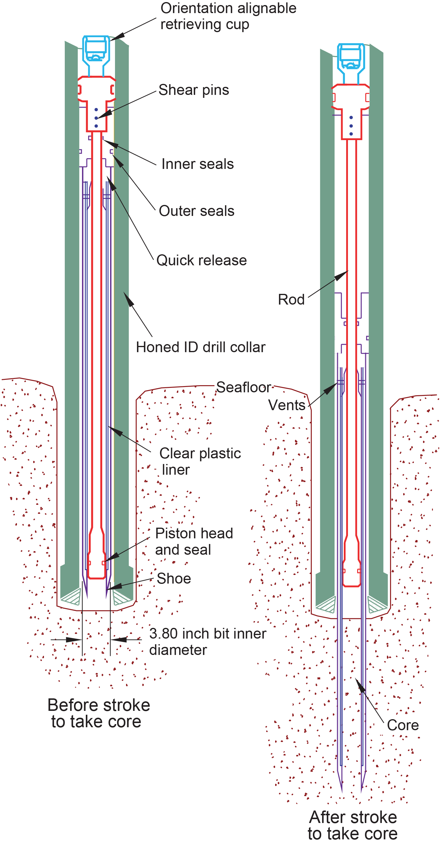
Figure F1. APC system.
APC refusal is conventionally defined in one of two ways: (1) the piston fails to achieve a complete stroke (as determined from the pump pressure and recovery reading) because the formation is too hard, or (2) excessive force (>60,000 lb) is required to pull the core barrel out of the formation. For APC cores that do not achieve a full stroke, the next core can be taken after advancing to a depth determined by the recovery of the previous core (advance by recovery) or to the depth of a full APC core (typically 9.5 m). If a full stroke is not achieved, one or more additional attempts are typically made, each time advancing the bit by the length of the recovered core (note that for these cores, this results in a nominal recovery of ~100%). If a full or partial stroke is achieved but excessive force is not able to retrieve the barrel, the core barrel can be drilled over, meaning that after the inner core barrel is successfully shot into the formation, the drill bit is advanced to total depth to free the APC barrel.
The standard APC system uses a 9.5 m long core barrel, and the HLAPC system uses a 4.7 m long core barrel. In most instances, the HLAPC system is used after the standard APC system has suffered repeated partial strokes and/or core liner damage. Use of the HLAPC system follows the same criteria in terms of refusal as the APC system. The use of the HLAPC system allowed significantly greater APC sampling depths than would have otherwise been possible and allowed for successful recovery of clay layers interspersed with sand and volcaniclastics.
The XCB system is a rotary system with a small cutting shoe that extends below the large rotary APC/XCB bit (Figure F2). The smaller bit can cut a semi-indurated core with less torque and fluid circulation than the main bit, potentially improving recovery. It is primarily used in sediments, but it can also core short intervals of hard rock, such as sills or the sediment/basement interface. The XCB system is used when the APC/HLAPC system has difficulty penetrating the formation and/or damages the core liner or core. The XCB system can also be used to either initiate holes where the seafloor is not suitable for APC coring or be interchanged with the APC/HLAPC system when required by changing formation conditions. The XCB system is used to advance the hole when HLAPC refusal occurs before the target depth is reached or when drilling conditions require it. The XCB cutting shoe typically extends ~30.5 cm ahead of the main bit in soft sediments, but a spring allows it to retract into the main bit when hard formations are encountered. Shorter XCB cutting shoes can also be used. Expedition 402 relied on polycrystalline diamond compact XCB cutting shoes, which improved recovery across the sediment/basement interface.
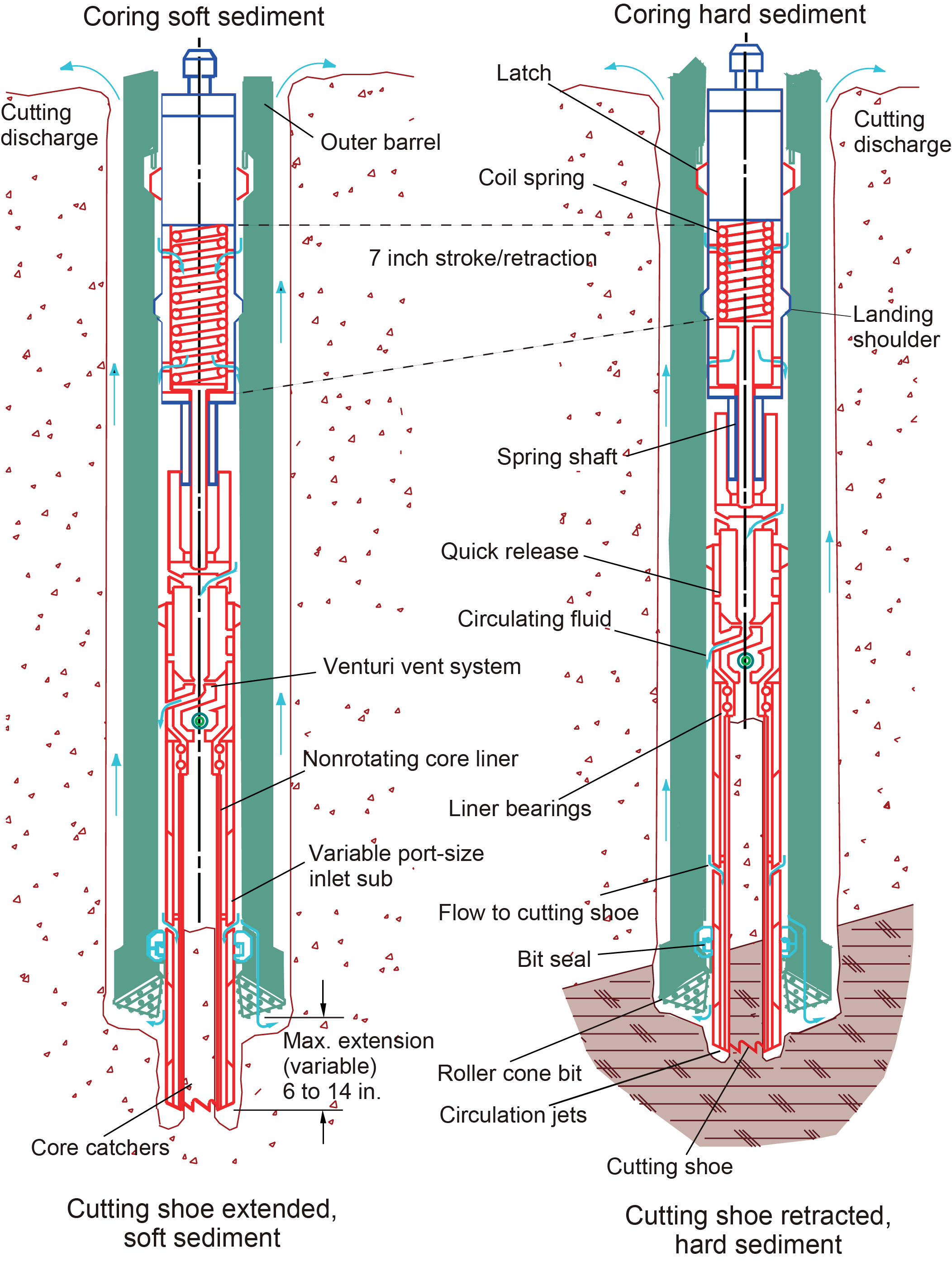
Figure F2. XCB system.
The bottom-hole assembly (BHA) used for APC and XCB coring is typically composed of an 11⁷⁄₁₆ inch (~29.05 cm) roller cone drill bit, a bit sub, a seal bore drill collar, a landing saver sub, a modified top sub, a modified head sub, 8¼ inch control length drill collars, a tapered drill collar, two stands of 5½ inch transition drill pipe, and a crossover sub to the drill pipe that extends to the surface (Figure F3).
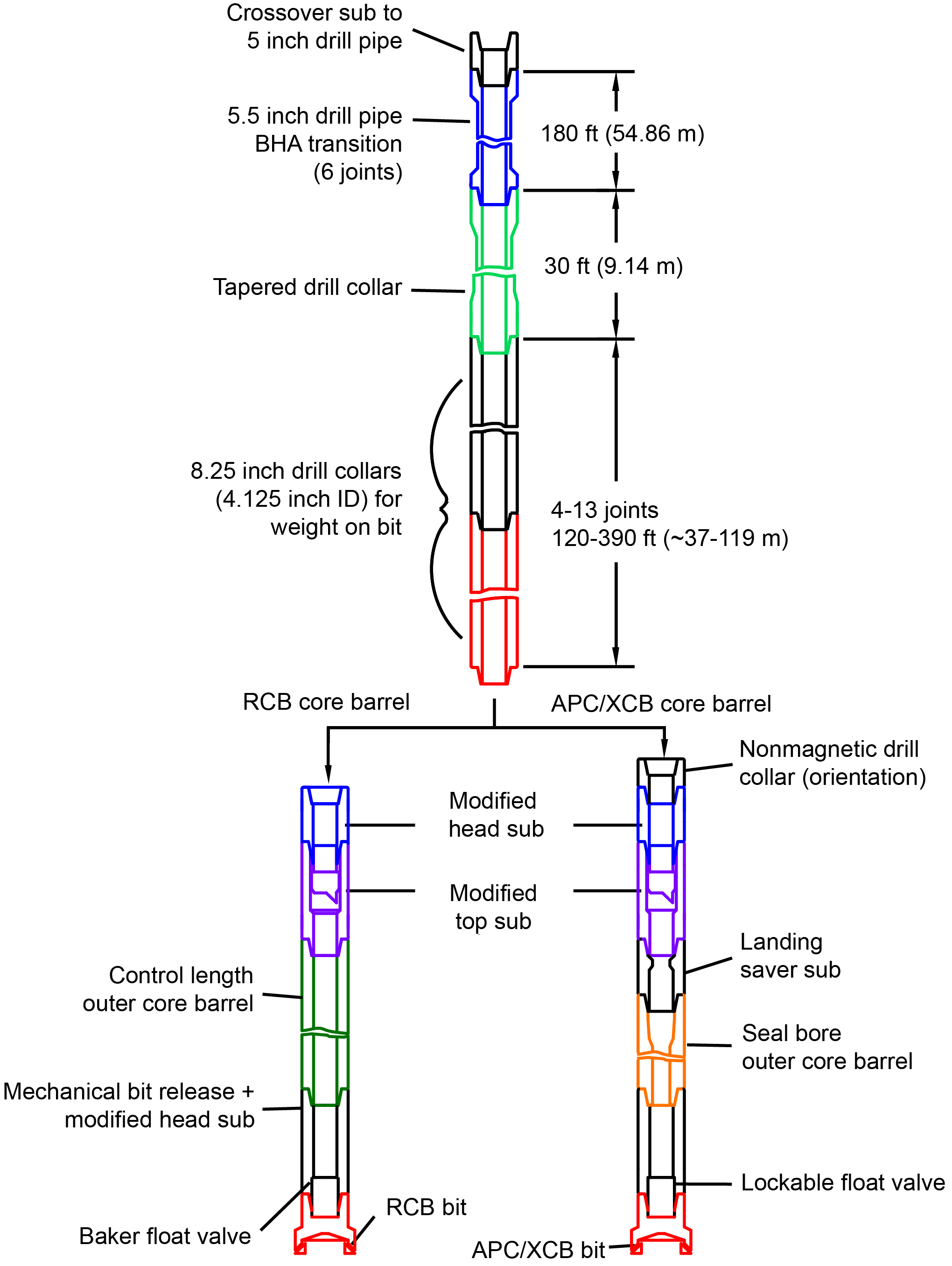
Figure F3. BHA for the RCB system and APC/XCB systems.
The RCB system is a rotary system designed to penetrate firm to hard sediments and basement rocks. The BHA, including the bit and outer core barrel, rotates with the drill string while the inner core barrel is held stationary by bearings (Figure F4).
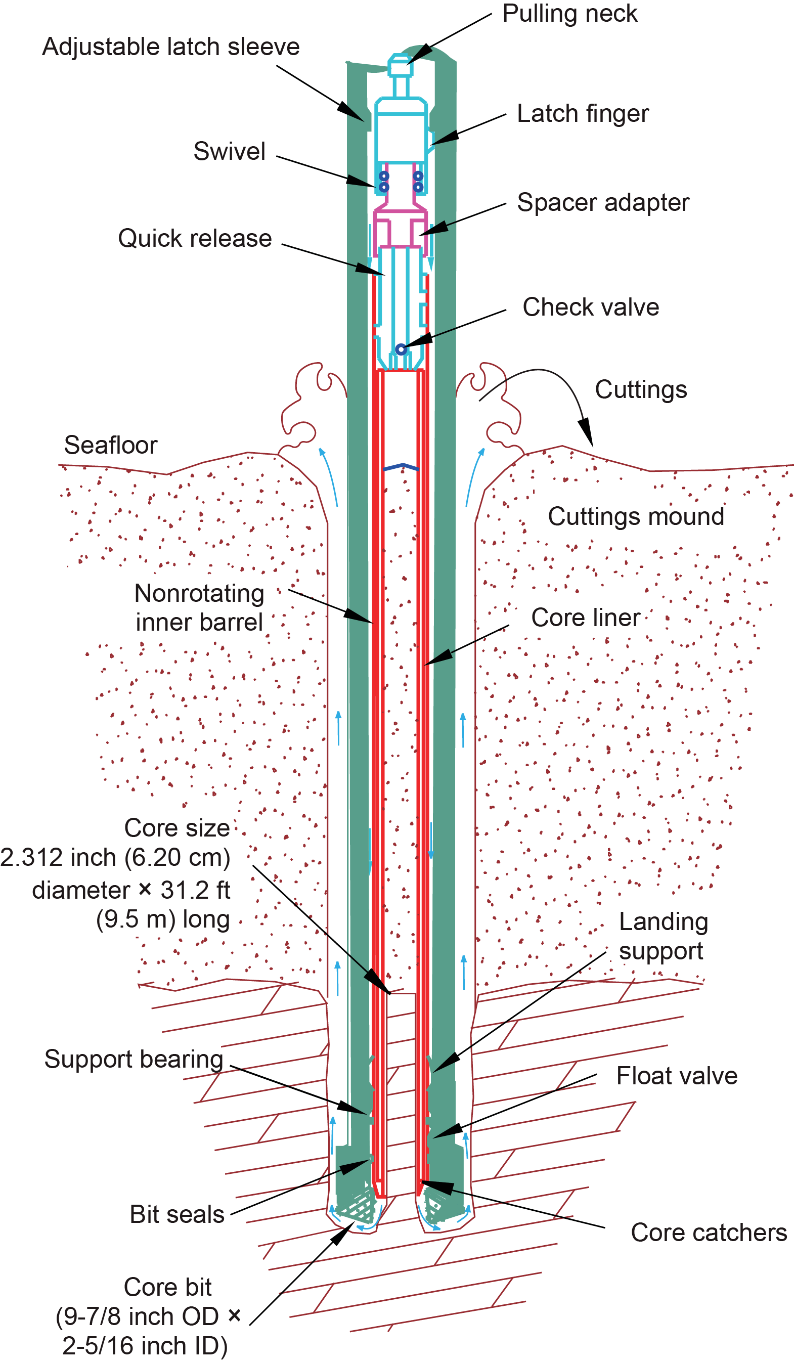
Figure F4. RCB system.
A typical RCB BHA includes a 9⅞ inch drill bit, a bit sub, an outer core barrel, a modified top sub, a modified head sub, a variable number of 8¼ inch control length drill collars, a tapered drill collar, two stands of 5½ inch drill pipe, and a crossover sub to the drill pipe that extends to the surface. Figure F3 shows a typical BHA for each coring system (APC/XCB and RCB, respectively).
Nonmagnetic core barrels were used for all APC, HLAPC, and RCB coring. APC cores were oriented using the Icefield MI-5 core orientation tool when coring conditions allowed. Formation temperature measurements were taken with the third-generation advanced piston corer temperature tool (APCT-3) during APC/XCB coring or the Sediment Temperature 2 (SET2) tool during RCB drilling; see Downhole measurements. Information on recovered cores, drilled intervals, downhole tool deployments, and related information are provided in the Operations, Paleomagnetism, and Downhole measurements sections of each site chapter.
1.3. IODP depth conventions
The primary depth scales used are defined by the length of the drill string deployed (e.g., drilling depth below rig floor [DRF] and drilling depth below seafloor [DSF]), the depth of the core recovered (e.g., core depth below seafloor [CSF] and core composite depth below seafloor [CCSF]), and the length of the logging wireline deployed (e.g., wireline log depth below rig floor [WRF] and wireline log depth below seafloor [WSF]) (see IODP Depth Scales Terminology for sediments at http://www.iodp.org/policies-and-guidelines/142-iodp-depth-scales-terminology-april-2011/file). In cases where multiple logging passes are made, wireline log depths are mapped to one reference pass, creating the wireline log matched depth below seafloor (WMSF) scale. All units are always expressed in meters. The relationship between scales is defined either by protocol, such as the rules for computation of CSF depth from DSF depth, or by user-defined correlations, such as core-to-log correlation. The distinction in nomenclature is intended to make the reader aware that a nominal depth value in different depth scales usually does not refer to the exact same stratigraphic interval.
Depths of cored intervals are measured from the drill floor based on the length of drill pipe deployed below the rig floor (DRF scale). The depth of the cored interval is referenced to the seafloor (DSF scale; Figure F5) by subtracting the seafloor depth of the hole (i.e., water depth) from the DRF depth of the interval. Standard depths of cores in meters below seafloor (CSF-A scale) are determined based on the assumption that (1) the top depth of a recovered core corresponds to the top depth of its cored interval (on the DSF scale) and (2) the recovered material is a continuous section even if sediment core segments are separated by voids when recovered. Standard depths of samples and associated measurements (CSF-A scale) are calculated by adding the offset of the sample or measurement from the top of its section and the lengths of all higher sections in the core to the top depth of the core.
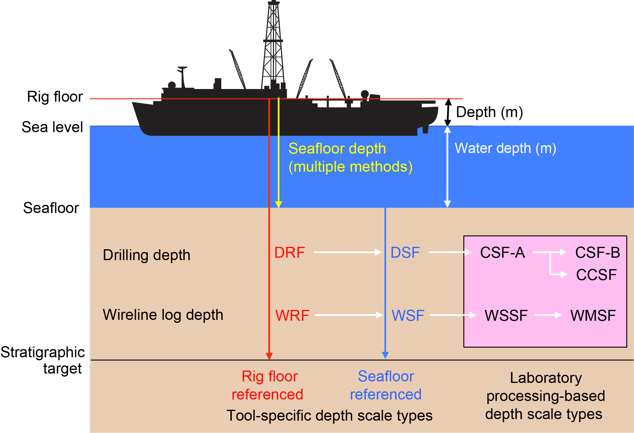
Figure F5. Depth scales.
1.3.1. Sediment core depth scales
If a core has <100% recovery, for curation purposes all cored material is assumed to originate from the top of the drilled interval as a continuous section. In addition, voids in the core are closed by pushing core segments together during core handling, if possible. Therefore, the true depth interval within the cored interval is unknown. This result should be considered a sampling uncertainty in age-depth analysis or in correlation of core data with downhole logging data.
When core recovery is >100% (the length of the recovered core exceeds that of the cored interval), the CSF depth of a sample or measurement taken from the bottom of a core will be deeper than that of a sample or measurement taken from the top of the subsequent core (i.e., the data associated with the two core intervals overlap on the CSF-A scale). This overlap can occur when a soft to semisoft sediment core recovered from a few hundred meters below the seafloor expands during recovery (typically by a few percent to as much as 15%). In this case the core depth below seafloor, Method B (CSF-B), depth scale can be employed, where the core is (digitally) linearly compressed to fit within the cored interval. Where core recovery is <100%, CSF-A and CSF-B depth scales are exactly equivalent. A stratigraphic interval may not have the same nominal depth on the DSF and CSF scales in the same hole.
During Expedition 402, all core depths below the seafloor were calculated according to the CSF-A scale unless otherwise noted. Depths on the CSF-A scale are reported as mbsf or m CSF-A. The very rare cases of recoveries greater than 100% meant that CSF-B was not widely used. No formal stratigraphic correlation between holes or sites was made.
1.3.2. Basement core depth scales
Basement depth is also reported in m CSF-A. The curatorial process for hard rock (see Core handling and analysis) results in depths (CSF-A/mbsf) that do not reflect true depths because of incomplete recovery, in addition to the assumption that all material comes from the top of the cored interval, and to subsequent spacing out of the recovered material to bin it, which adds void intervals.
1.4. Sample depth calculations and naming conventions
Numbering of sites, holes, cores, and samples follows standard IODP procedures. A complete curatorial identifier for a sample consists of the following information: expedition, site, hole, core number, core type, section number, section half, piece number (only for samples curated as hard rocks, including igneous and metamorphic rocks), and interval in centimeters measured from the top of the core section. For example, a sample identification of “402-U1614A-10H-2W, 46–48 cm,” indicates a 2 cm long sample taken from the interval between 46 and 48 cm below the top of Section 2 (working half) of Core 10 (“H” designates that this core was taken with the APC system) of Hole A at Site U1614. The coring system used to obtain a core is designated in the sample identifiers as follows: H = APC, F = HLAPC, R = RCB, and X = XCB. Integers placed after the core number are used to denote the core type of drilled intervals (e.g., a drilled interval prior to Core 2R would be designated as Core 11 [i.e., Core 1 and Type 1]).
1.5. Core handling and analysis
1.5.1. Sediment
When the core barrel reached the rig floor, the core catcher was removed from the bottom of the core and taken to the core receiving platform (catwalk), and a sample was extracted for paleontological (PAL) analysis. Next, the sediment core was extracted from the core barrel in its plastic liner. The liner was carried from the rig floor to the core processing area on the catwalk outside the core laboratory, where it was labeled and split into ~1.5 m sections. Blue (uphole direction) and clear (downhole direction) liner caps were adhered at the ends of the cut liner sections with acetone. In cores where oxygen measurements were taken, liner caps were not glued with acetone until after analyses were completed.
Once the core was cut into sections, whole-round samples were taken for interstitial water (IW) chemical analyses and microbiological research. When a whole-round sample was removed, a yellow end cap was placed at the bottom of the remaining core section to indicate it was taken. For the first hole at each site, syringe samples were taken for gas analyses according to the IODP hydrocarbon safety monitoring protocol.
The core sections were placed in a core rack in the laboratory, core information was entered into the database, and the section liners were laser engraved. Oxygen probe measurements were taken as soon as possible after core recovery, typically before core sections reached equilibrium with laboratory temperature (after ~4 h; see Microbiology). Core sections were then run through the Whole-Round Multisensor Logger (WRMSL) for P-wave velocity (VP), magnetic susceptibility (MS), and gamma ray attenuation (GRA) bulk density measurements (see Physical properties). The core sections were also run through the Natural Gamma Radiation Logger (NGRL), often prior to temperature equilibration because the temperature does not affect the natural gamma radiation (NGR) data. Thermal conductivity measurements were taken once per core when the recovered material was suitable.
Core sections were then split lengthwise from bottom to top into working and archive halves. Investigators should note that material can be transported upward on the split face of each section during splitting. The working halves of each core section were then laid out on the sampling tables, and samples were taken for moisture and density (MAD) and paleomagnetic (PMAG) analyses and for remaining shipboard geochemical analyses such as X-ray diffraction (XRD), carbonate (CARB), and inductively coupled plasma–atomic emission spectrometry (ICP-AES). Samples were not collected when the lithology was a high-priority interval for expedition or postexpedition research, the core material was unsuitable, or the core was severely deformed. Samples for personal postexpedition research were also flagged, entered into the SampleMaster application, and collected while the working half of each core was on the sampling table.
The archive half of each core was scanned on the Section Half Imaging Logger (SHIL) to provide linescan images and then measured for point MS (MSP) and reflectance spectroscopy and colorimetry (RSC) on the Section Half Multisensor Logger (SHMSL). Labeled pieces of foam were used to mark removed whole-round intervals in the SHIL images. The archive halves were then described visually and with smear slides for sedimentology and structural geology. Finally, the magnetization of the archive and working halves was measured with the cryogenic magnetometer and spinner magnetometer.
When all steps were completed, the cores were wrapped in plastic wrap, sealed in plastic tubes, and transferred to cold storage space aboard the ship. At the end of the expedition, the working halves of the cores were sent to the Bremen Core Repository (BCR). The archive halves of the cores were first sent to the Gulf Coast Repository (GCR), where a subset was scanned for X-ray fluorescence spectrometry (XRF) before being forwarded to the BCR for long-term storage. The sediment core flow is summarized in Figure F6.
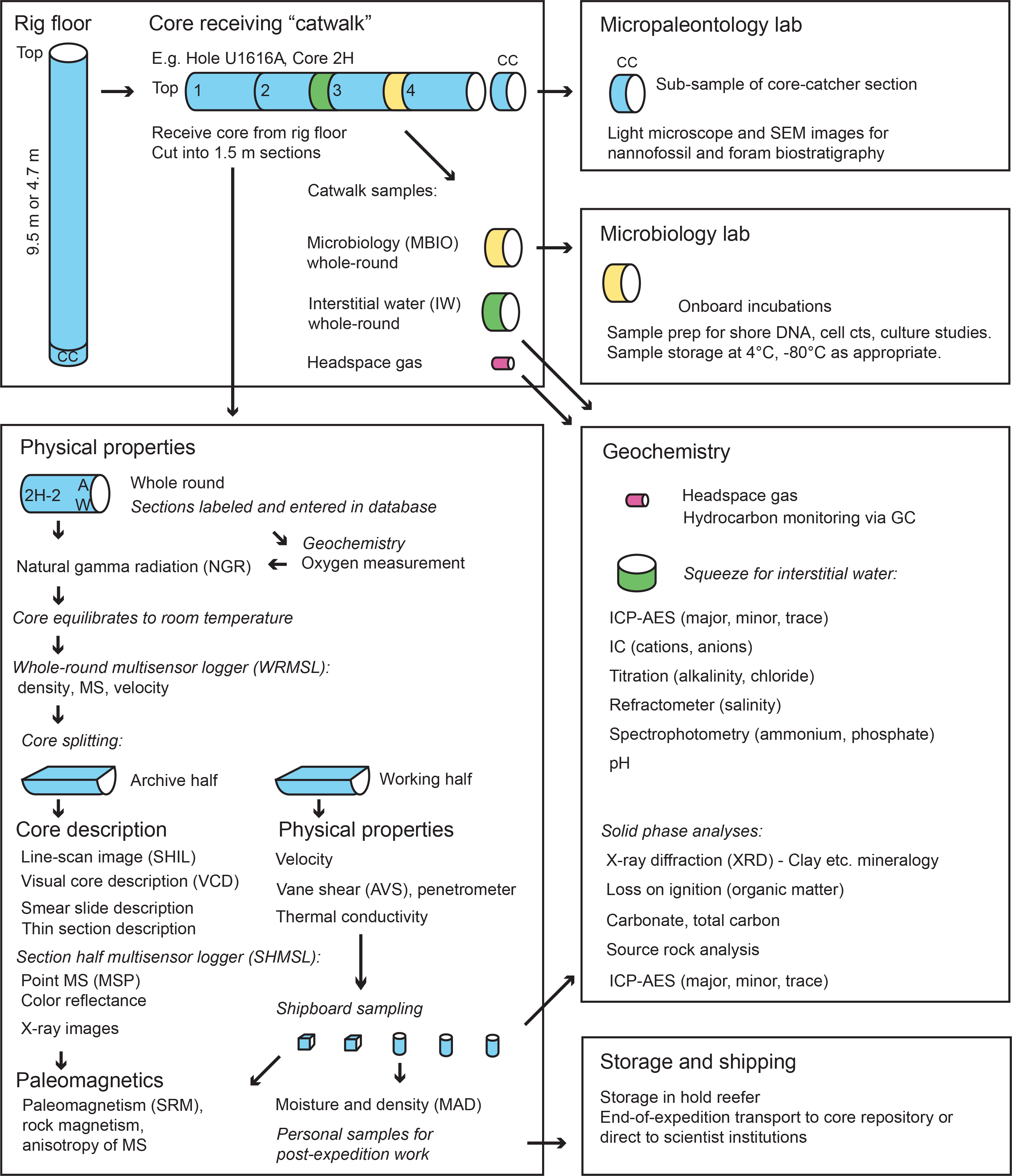
Figure F6. Sediment core workflow.
1.5.2. Basement material (igneous, metamorphic, and sedimentary rock)
Hardened sediments and rock cores were extracted from the core barrel in its plastic liner. The liner was carried from the rig floor to the core processing area on the catwalk outside the core laboratory, where it was split into ~1.5 m sections. These sections were immediately carried into the splitting room. Pieces were extracted from the core liner in the splitting room and immediately examined by a designated petrologist for the presence of asbestiform minerals. If present, core curation and handling could continue as normal, but the core splitting and sample cutting were performed according to the asbestos safety protocols described below.
The cores were then placed in split plastic liners in sequential order while maintaining the original orientation of pieces as much as possible. The pieces were then pushed to the top of the 1.5 m liner sections, and the total rock length was measured. The length was entered into the database as “recovered length” using the SampleMaster application. This number was used to calculate recovery. If a core catcher sample was present, it was taken separately to the core splitting room and added to the bottom section of the recovered core.
Oriented pieces of core that could not have rotated on a horizontal axis during drilling were marked on the bottom with a blue- or red-colored wax pencil to preserve orientation. Adjacent but broken pieces that could be fit together along fractures were curated as single pieces. The structural geologists confirmed piece matches, marked a split line on each piece, and marked the working half with the letter “W,” which defined how the pieces were to be cut into two equal halves. The aim was to preserve representative lithologic and mineralogical features in both archive and working halves while ensuring the availability of key lithologies and vein features in the working halves for sampling purposes. Where possible, cutting lines were drawn in the dip direction of structural features to maximize the expression of dipping structures on the cut face of the core. A plastic spacer was secured with acetone to the split core liner between individual pieces or reconstructed continuous groups of subpieces. These spacers can add artificial gaps or represent significant intervals of no recovery. The length of each section of core, including spacers, was entered into the database as “curated length,” which commonly differs by multiple centimeters from the length measured on the core receiving platform. Finally, the curated depth of each piece in the database was recalculated based on the curated length. The curatorial process can result in overestimation or underestimation of the depth from which a piece was cored.
When the core sections reached equilibrium with laboratory temperature (after ~4 h), the whole-round core sections were run through the WRMSL and NGRL (see Physical properties). Whole-round samples for geotechnical and structural geologic personal research were selected following analyses on the whole-round track systems and removed from the core.
Each piece of core was split with a diamond-impregnated saw into an archive half and a working half, with the same positions of the plastic spacers between the pieces in both halves. Pieces were numbered sequentially from the top of each section, beginning with 1. Separate subpieces within a single piece were assigned the same number but lettered consecutively (e.g., 1A, 1B, and so on). Labels were applied with epoxy only on the outer cylindrical surfaces of the core. If it was evident that an individual piece had not rotated around a horizontal axis during drilling, an arrow pointing to the top of the section was added to the label. The orientation of each piece was recorded in the database using the SampleMaster application.
The archive half of each core was scanned on the SHIL and measured for MSP and RSC on the SHMSL. Thermal conductivity measurements were made on selected archive-half pieces (see Physical properties). After the archive-half sections of each core were fully described by the petrologists and structural geologist on shift, samples were taken from the working-half sections for shipboard analyses (billets for thin sections; chips for ICP-AES; and cube samples [~8 cm3] for paleomagnetism analyses, MAD, and discrete VP measurements; see Igneous and metamorphic petrology, Igneous geochemistry, Paleomagnetism, and Physical properties). The magnetizations of archive-half sections and pieces, as well as discrete cube samples taken from the working-half sections, were measured with the cryogenic magnetometer and spinner magnetometer, respectively (see Paleomagnetism).
Sampling for personal research was conducted shipboard during sample parties after all cores from a site had been received, analyzed, and described. After all laboratory processing steps and cutting of personal samples were completed, the cores were shrink wrapped, sealed in plastic tubes, and transferred to cold storage on board the ship. At the end of the expedition, the cores were shipped to the BCR for long-term storage. The basement core flow differed from sediment core flow primarily in the absence of microbiological, IW, and headspace gas samples. The order of analyses and description is otherwise the same as shown in Figure F6.
1.6. Drilling and core disturbance
Cores may be significantly disturbed and contain extraneous material because of the coring and core handling process (Jutzeler et al., 2014). In formations with loose layers, material from intervals higher in the hole may be washed down by drilling circulation, accumulate at the bottom of the hole, and be sampled with the next core. Therefore, the uppermost 10–50 cm of each core must be examined critically during description for potential fall-in material. At sites in the Vavilov Basin, substantial fall-in of volcaniclastic gravel was common and occasionally comprised multiple sections of each core.
Common coring-induced deformations include the concave-downward appearance of originally horizontal bedding. Piston action can result in fluidization (flow-in) at the bottom of APC/HLAPC cores. The rotation and fluid circulation used during XCB and RCB coring can also cause the cored material to fragment into discrete pieces (biscuits) that may rotate relative to each other. A slurry of drilling fluid, seawater, and fluidized sediment can be injected between and around the biscuits, producing what is colloquially termed “biscuits and gravy.” Retrieval from depth to the surface can also result in elastic rebound. Gas that is in solution at depth can be released and drive core segments apart within the liner. If the gas content is high, pressure must be relieved for safety reasons by drilling holes into the plastic liner before the cores are cut into segments. These holes force some sediment as well as gas out of the liner. Such observed disturbances are described in each site chapter and graphically illustrated in the visual core descriptions (VCDs).
1.7. Asbestos safety protocols
Because serpentinized mantle peridotites may contain asbestiform minerals as alteration products (e.g., chrysotile, tremolite, and actinolite), a protocol was developed and implemented for safe handling of potentially asbestos-containing cores. This protocol was developed in collaboration with Texas A&M Environmental Health & Safety and incorporated the information generated during air testing of workspaces while handling dry cores for core curation and description, and sample cutting of Expedition 399 serpentinized peridotite cores at the GCR. Air testing during Expedition 399 core processing at the GCR verified that, for serpentinized peridotites, standard curation and description processes did not create substantial risk of exposure to airborne asbestos fibers (Penkrot et al., 2024). Due to the use of abrasive saws and a greater chance of airborne fiber generation, core splitting and sample cutting required more extensive precautions. Overall, we chose to maximize our precautionary approach to prevent airborne fiber exposure, which included the use of administrative and engineering controls, as well as enhanced personal protective equipment (PPE) during some stages of core processing.
1.7.1. Core receiving and initial lithologic inspection
Based on air testing results during Expedition 399 core processing at the GCR, core receiving could proceed normally. Technicians handling the core wore nitrile gloves, hard hats, and safety glasses as per standard catwalk protocols. Any slurry material in the core liner after core transfer was carefully drained into the ship's sediment drain lines. The core receiving platform was also washed down after each core.
The cores were then carried into the splitting room and gently shaken out into new split liners. Here, the designated petrologist for each shift performed an initial inspection of the cores, wearing nitrile gloves and, if desired, a mask or fitted respirator. Limited personnel were allowed in the splitting room during the inspection period. The petrologist would declare whether the core contained asbestiform minerals; if a single piece contained asbestos minerals, the entire core was treated as asbestos-containing. Very few cores from Expedition 402 contained asbestos minerals with fibrous habits. However, to take a maximally precautious approach, cores containing any asbestos minerals, regardless of habit, were split and sampled according to the asbestos safety protocols. The most commonly identified asbestiform mineral was tremolite.
1.7.2. Core description and core laboratory analyses
Cores were analyzed on the track systems and described as usual, with some enhanced cleaning procedures implemented. Adhesive floor mats were installed at core laboratory entrances/exits to limit transfer of dust on shoes outside of the laboratory. Horizontal work surfaces such as the core sampling and description tables were cleaned with wet wipes before laying out each new batch of cores. At the end of each shift, floors were wet mopped using a mop with disposable pads and/or HEPA vacuumed. Separate trash bins were maintained for normal waste and waste (gloves, wet wipes, and mop pads) that had been in contact with core material. Waste in this second category was double-bagged for separate disposal per local regulations for asbestos-containing waste. As always, scientists and technicians were required to wear nitrile gloves while handling cores. Masks or fitted respirators were available upon request.
After description and analyses were completed, the core sections were shrink-wrapped prior to boxing. Each D-tube was marked with an “asbestos hazard” label.
1.7.3. Core splitting, cutting, and sample preparation
All core splitting, sample cutting, and sample preparation procedures that generate fine particles were performed by JOIDES Resolution Science Operator (JRSO) technical staff using enhanced PPE. Core splitting and sample cutting were done in batches to the degree possible to simplify workflow and limit the time of potential exposure. Technical staff performed core splitting and sample cutting in the splitting room with the doors closed and the extraction fan on to create a negative air pressure zone relative to the surrounding laboratories. Personnel wore Tyvek suits and used either fitted respirators or the ship's supplied air breathing air system, in addition to wearing nitrile gloves and safety glasses. A decontamination area was set up at the stratigraphic correlation station where Tyvek suits and respirators could be cleanly donned/removed and stored or used suits disposed of. Custom-made plexiglass enclosures were placed around the rock saws and splitting saws used on cores and samples to minimize potential particle distribution in the splitting room. The entire splitting room was thoroughly cleaned at the end of each splitting session and the waste was disposed separately from normal waste.
Special procedures were also developed for thin section sample preparation and for milling of samples to produce powder splits for chemistry analyses. Technical staff wore nitrile gloves and fitted respirators. The thin section billets were impregnated with epoxy prior to initial cutting and grinding to aid in material immobilization, and the cutting saw was enclosed. Lapping and polishing were done wet. For powder sample preparation, the sample was sealed in the enclosed capsules while grinding equipment was in use. A benchtop enclosure was built for transfer of the powder from the powdering vessel to a sealed vial. The grinding vessels were then submerged in water and rinsed into the sediment drain system. Subsampling of powders was done inside the benchtop enclosure or in a fume hood.
2. Lithostratigraphy
The lithology of sediment recovered during Expedition 402 was primarily determined from visual (macroscopic) core description, smear slides, and thin sections. Digital core imaging, color reflectance spectrophotometry, MS analysis (see Physical properties), and in some cases XRD and carbonate content measurements (see Sediment and interstitial water geochemistry), provided complementary descriptive information. The methods employed during this expedition were a modified version of those used during IODP Expedition 379 (Gohl et al., 2021). We used the GEODESC application to record and upload visual descriptive data into the Laboratory Information Management System (LIMS) database (GEODESC user guide can be found at https://tamu-eas.atlassian.net/
The standard method of splitting cores into working and archive halves (using either a piano wire or a saw) can affect the appearance of the split core surface and obscure fine details of lithology and sedimentary structure. Prior to visual description and imaging of sediments, the archive halves of soft-sediment cores were gently scraped across the core section using a stainless steel or glass scraper to prepare the surface for sedimentologic examination and description, digital imaging, MSP, and color measurements. Scraping parallel to bedding with a freshly cleaned tool prevented cross-stratigraphic contamination. Cleaned archive halves were imaged using the SHIL as soon as possible after splitting. Thereafter, archive halves were visually described and then finally analyzed using the SHMSL.
2.1. Visual core description
VCDs of the archive-half split cores provide a visual overview of the descriptive lithostratigraphic, biostratigraphic, and physical properties data obtained during shipboard analyses (Figure F7). All associated data are uploaded to the LIMS database.
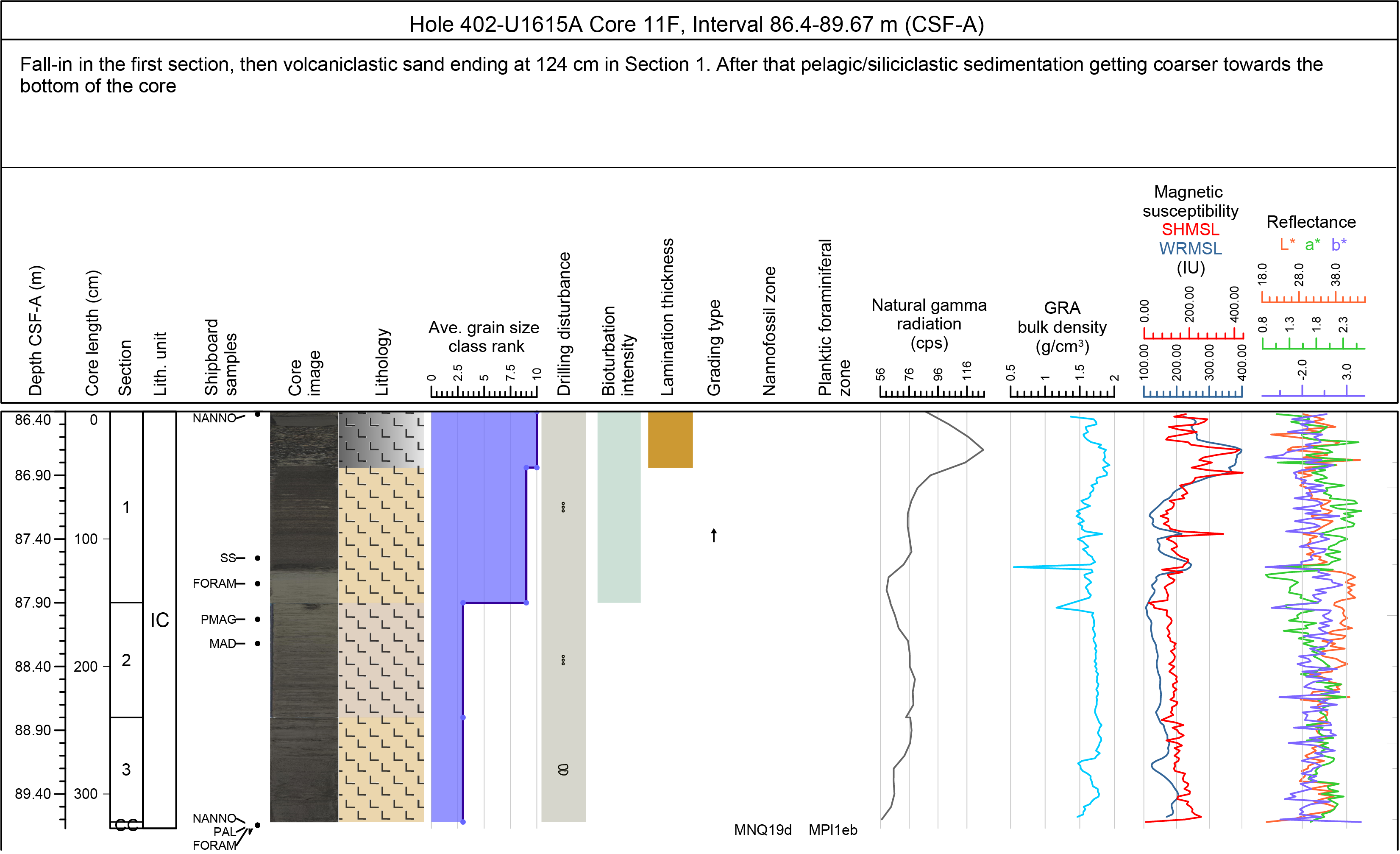
Figure F7. Example VCD.
Site, hole, and core depth (calculated primarily using the CSF-A depth scale except for Site U1617, where the CSF-B depth scale was used to account for >100% recovery) are shown at the top of each VCD. Core depths are reported in the mbsf depth scale, and the depth in each core section is indicated along the left margin. Visual core descriptions correspond to entries in GEODESC, including bioturbation intensity, macrofossil presence, sedimentary structures, diagenetic constituents, and drilling disturbance. Symbols used in the VCDs are shown in Figure F8. Additionally, sedimentary VCDs display GRA bulk density, MS, NGR, color reflectance, the locations of samples taken for shipboard measurements, and nannofossil and foraminifera biozones. The written description for each core contains a succinct overview of major and minor lithologies, the Munsell colors, and notable features such as sedimentary structures or major disturbances resulting from the coring process.
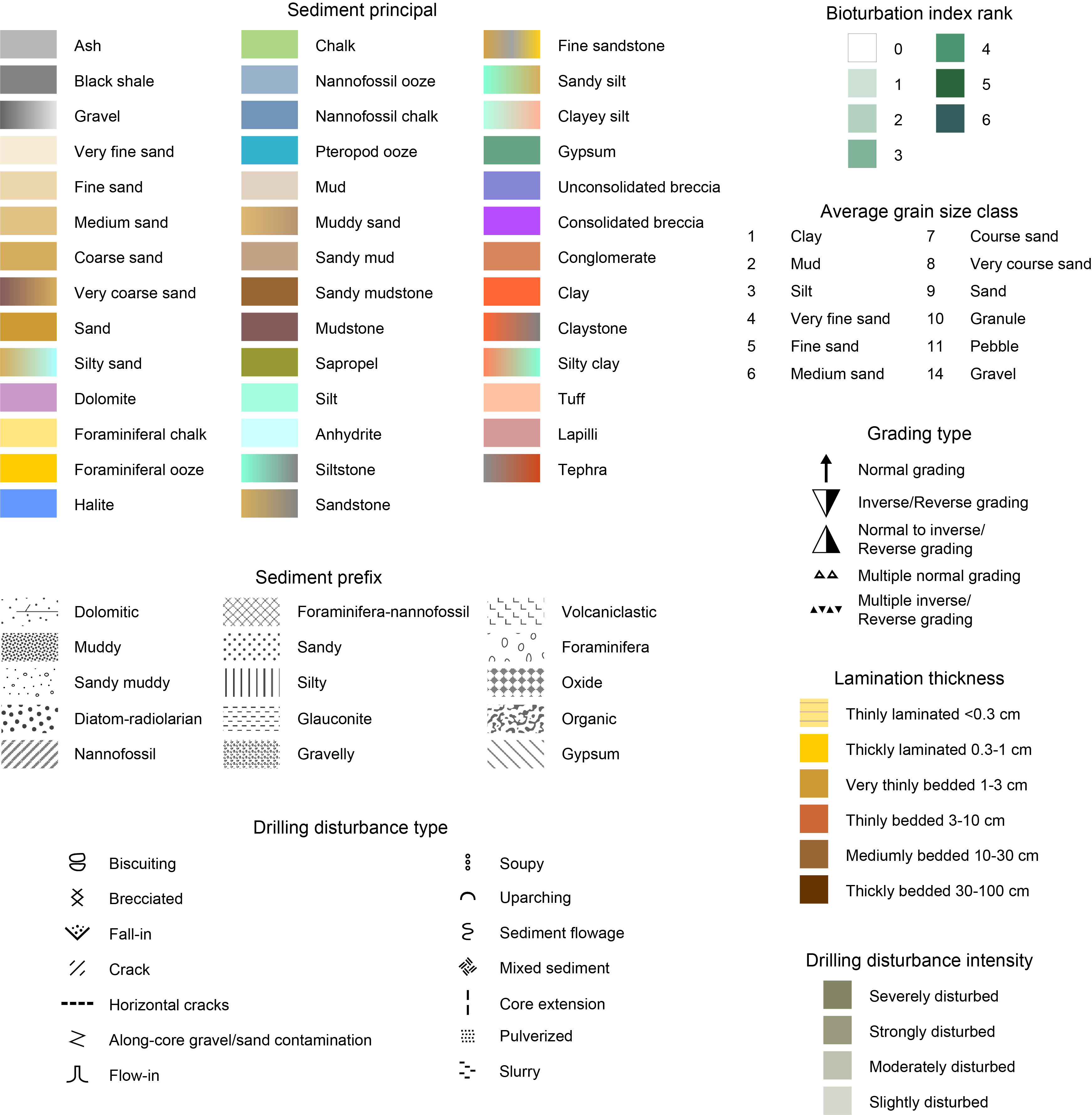
Figure F8. VCD legend.
2.1.1. Section summary
Lithologies of the core intervals recovered are represented on the VCDs by graphic patterns in the Lithology column. Modifiers of primary lithologies (sediment prefix) are shown as patterns on top of the primary lithology color (Figure F8). Minor sediment modifiers (suffix) are recorded in GEODESC. In the interest of VCD readability, secondary lithologies are not shown, but they are accessible using the LIMS database or GEODESC Data Access. Relative abundances of lithologies reported in this way are useful for general characterization of the sediment but do not constitute precise quantitative observations.
2.1.2. Sedimentary structures
Sedimentary structures and stratification types recognized on the split cores are reported on the VCD sheet and are recorded in GEODESC. Symbols used to represent category, location, and scale of these features include distinct stratifications, laminations and beddings, lens, color banding, and grading surfaces (Figure F8). The following terminology has been adopted to classify bed thickness (Stow, 2005) and is represented in the VCD:
- Thinly laminated = <0.3 cm.
- Thickly laminated = 0.3–1 cm.
- Very thinly bedded = 1–3 cm.
- Thinly bedded = 3–10 cm.
- Mediumly bedded = 10–30 cm.
- Thickly bedded = 30–100 cm.
Descriptive terms to indicate the characteristics of each bed boundary type (e.g., sharp, erosive, gradual, undulating/wavy, and bioturbated) are noted in GEODESC.
2.1.3. Bioturbation intensity
A semiquantitative assessment of bioturbation intensity was conducted using a similar scheme to Bottjer and Droser (1991) (Figure F9). The assessment was done based on the percentage of sediment reworked by biological activity on a scale from 0 (no observable bioturbation) to 6 (extensive bioturbation). These levels were recorded graphically in the Bioturbation column on the VCD:
- 0 = no bioturbation detected.
- 1 = sparse bioturbation.
- 2 = uncommon bioturbation.
- 3 = moderate bioturbation.
- 4 = common bioturbation.
- 5 = abundant bioturbation.
- 6 = complete bioturbation.
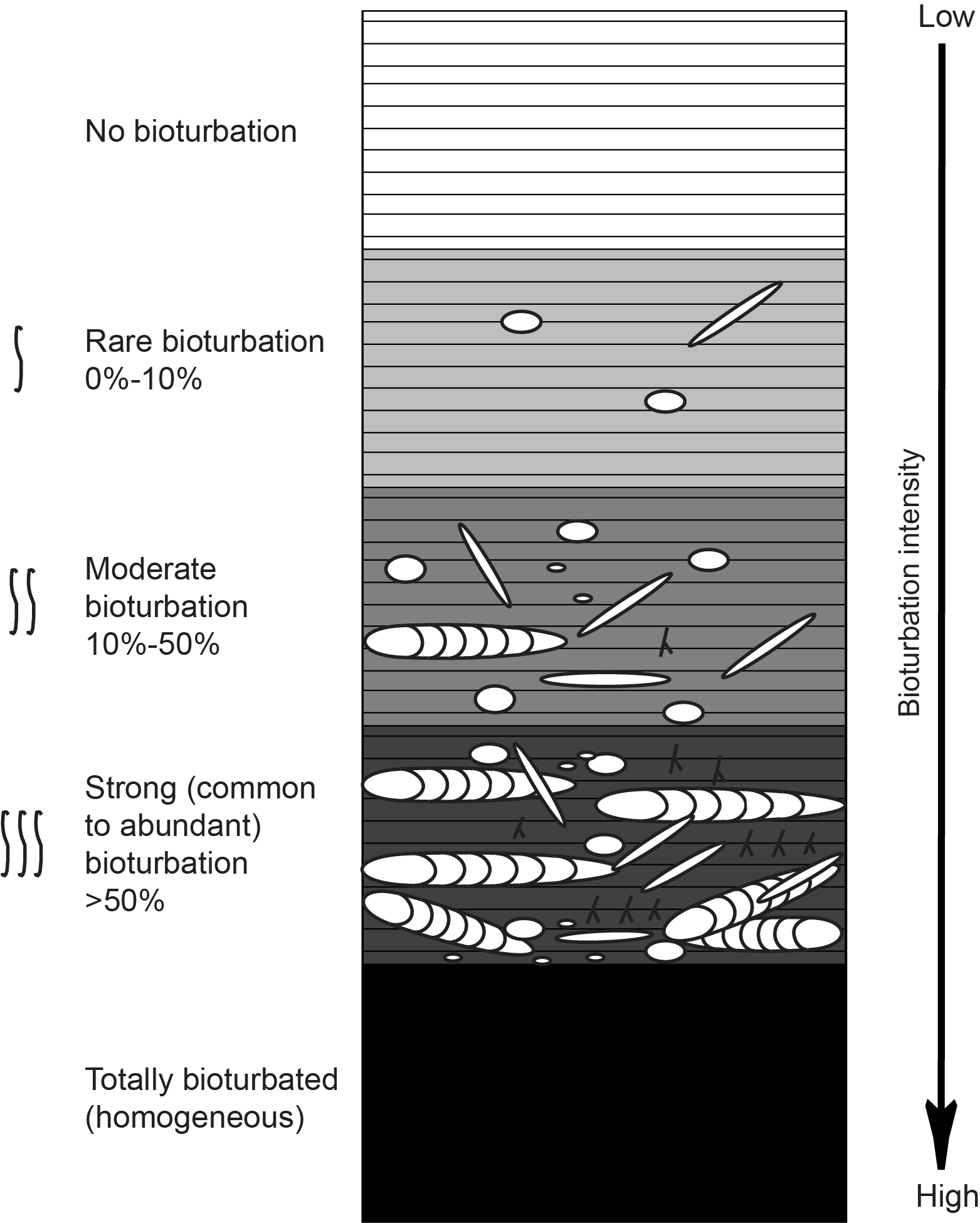
Figure F9. Ichnofabric index key.
2.1.4. Drilling disturbance
Drilling-related sediment disturbance is recorded in the Disturbance column of the VCDs using the symbols shown in Figure F8. The style of drilling disturbance is described for soft and firm sediments using the following terms:
- Fall-in: part of the formation at the top of a hole that has fallen to the bottom and has been subsequently cored.
- Uparching: bedding contacts are slightly to moderately deformed but subhorizontal and continuous.
- Flow-in: significant soft-sediment stretching and/or compressional shearing structures are present and attributed to the coring/drilling process.
- Soupy: intervals are water saturated and have lost all aspects of original bedding.
- Mixed sediment: intervals where sediment is mixed and has lost all aspects of original bedding.
- Biscuiting: sediments of intermediate stiffness show vertical variations in the degree of disturbance. Softer intervals (gravy) are washed and/or soupy, whereas firmer intervals (biscuits) are relatively undisturbed but may no longer be in their original orientation.
- Cracked or fractured: firm sediments are broken but not displaced or rotated significantly.
- Fragmented or brecciated: firm sediments are pervasively broken and may be displaced or rotated.
- Pulverized: firm sediments are pervasively broken, resulting in a soft texture.
- Along-core gravel and/or sand contamination: core is coated by coarser material on its external diameter.
- Core expansion: expansion of sediments in the core related to either the presence of gas or to decompression, which often leads to a >100% recovery.
The degree of drilling disturbance within sediments is described using the following categories:
2.1.5. Age
The age of the sediments was provided by the shipboard biostratigraphers (using calcareous nannofossils and planktic foraminifera; see Biostratigraphy) and is listed in the age column on the VCD.
2.2. Sediment classification
The lithologic classification scheme used for Expedition 402 is based on a combination of various types of classifications, as summed up in Marsaglia and Milliken (2023).
Three main sedimentary lithologic classes are defined based on the primary origin of the sediment constituents (but not the depositional process):
- Biogenic: >50% carbonate, chemical, and biogenic particles.
- Siliciclastic: >50% siliciclastic particles, <25% volcanic particles, and <50% biogenic particles; therefore, nonvolcanic siliciclastic particles dominate chemical and biogenic particles.
- Ash and volcaniclastic: the term “ash” is applied to fine-grained (smaller than gravel) volcanic sediments that contain >50% volcanic particles. The volcaniclastic prefix is applied to biogenic and siliciclastic sediments that contain >25% volcanic clasts and grains mixed with nonvolcanic particles (either nonvolcanic siliciclastic, biogenic, or both). Note that the term volcaniclastic is used sensu Fisher (1961) and therefore includes both volcanic and tuffaceous lithologies.
2.2.1. Principal names and modifiers
The lithologic nomenclature is based on the relative abundance of siliciclastic, volcaniclastic, and biogenic grains (Figure F10) (Marsaglia and Milliken, 2023).
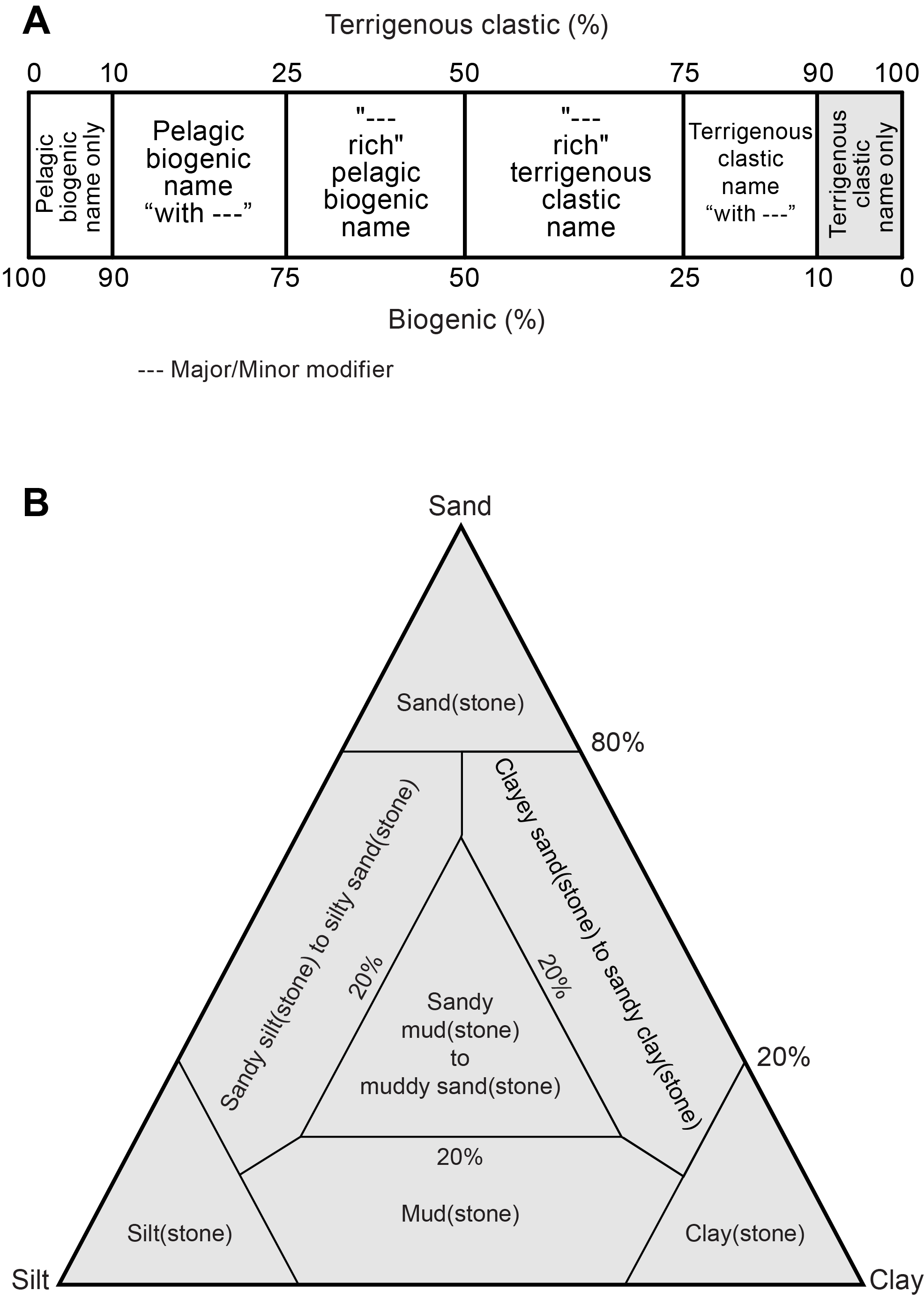
Figure F10. Sediment classification schemes and nomenclature.
The principal names classification is based on the estimate of clay, silt, sand, and gravel grain size, using the Wentworth (1922) scale. The sizes of each grain category plotted on the VCD sheet are as follows (Figure F8):
- Gravel: 2–4096 mm; 14.
- Boulder: 256–4096 mm; 13.
- Cobble: 64–256 mm; 12.
- Pebble: 4–64 mm; 11.
- Granule: 2–4 mm; 10.
- Sand: 0.63–2 mm; 9.
- Very coarse sand: 1–2 mm; 8.
- Coarse sand: 0.5–1 mm; 7.
- Medium sand: 250–500 µm; 6.
- Fine sand: 125–250 µm; 5.
- Very fine sand: 63–125 µm; 4.
- Silt: 3.9–63 µm; 3.
- Mud: <3.9–63 µm; 2.
- Clay: <3.9 µm; 1.
The principal sediment and/or rock name was determined based on the relative abundances of sand, silt, and clay (e.g., silt, sandy silt, silty sand, and so on) (Naish et al., 2006, after Shepard, 1954, and Mazzullo et al., 1988). Mud is defined as a mixture of silt and clay in which neither component exceeds 80%. If the mixture characterizing the sediment is at least 20% each of sand, silt, and clay, it is described as sandy mud to muddy sand (Figure F10).
Major and minor modifiers were applied to the principal names, building on the scheme adopted during Expedition 371 (Sutherland et al., 2019), and 379 (Gohl et al., 2021):
- Major biogenic and siliciclastic modifiers are expressed by 25%–50% of the grain abundance and are indicated by the suffix “-rich” (e.g., clay-rich or diatom-rich, preceding the principal sediment name).
- Minor modifiers are those components with abundances of 10%–25% and follow the principal name, using “with” (e.g., with clay or with diatoms).
The following nomenclatures indicate degree of lithification with different dominant compositions:
- Calcareous microfossils (e.g., calcareous nannofossils and foraminifera) dominance: the terms ooze and chalk indicate sediment that can be easily deformed or is slightly lithified, respectively. Where not possible to take smear slide samples with a toothpick, we use the lithification term limestone. Physical properties data helped in constraining lithification transitions and therefore major lithologic units within carbonate facies.
- Siliciclastic material dominance: where the sediment deforms easily, we add no lithification term and the sediment is named for the dominant grain size (i.e., sand, silt, clay, or tephra). If the sediment is more consolidated, the lithification suffix “-stone” is added to the principal lithology name (e.g., claystone).
2.3. Spectrophotometry
The Ocean Optics USB4000 spectrophotometer, mounted on the automated SHMSL, was used to measure the reflectance of visible light from the archive-half sediment cores. The split cores were placed on the SHMSL with a clear plastic wrap cover. A 2 cm spacing was used as the measurement interval to provide a high-resolution stratigraphic record showing color variations for visible wavelengths. Each measurement was recorded in 2 nm wide spectral bands from 390 to 730 nm. The reflectance parameters recorded during Expedition 402 are L*, a*, and b* (Balsam et al., 1997). This CIELAB color space expresses color as three values: L* for perceptual lightness and a* and b* for the four unique colors of human vision: red, green, blue, and yellow. Additional adopted measurement and interpretation techniques are thoroughly explained in Balsam et al. (1997, 1998) and Balsam and Damuth (2000). Instrument details are reported in Physical properties.
2.4. Smear slide observation
To aid lithologic classification, smear slide microscopic analysis was used to estimate sediment constituent size, composition, and abundance. Smear slide samples of the main lithologies were collected from the archive half of each section unless the lithology was better represented in the working half. Additional samples were collected from specific areas of interest. The position of all smear slide samples was marked in the Shipboard sample column of the VCD. A small amount of sediment was removed from the archive half using a flat wooden toothpick and placed on a 25 mm × 75 mm glass slide. The sample was homogenized with a drop of deionized water and spread evenly using a toothpick to create a thin, uniform layer of sediment. Samples were then placed on a hot plate at a low setting (100°–150°C) until dried. Some drops of adhesive (Norland Optical Adhesive Number 61) were added as a mounting medium to the sample and then a 22 mm × 40 mm glass coverslip was carefully placed on top of the dried sample to prevent air bubbles from being trapped in the adhesive. Air bubbles were removed by gentle tapping with a wooden toothpick. The smear slide was then placed in an ultraviolet light box for ~10 min to cure.
Smear slides were examined using a petrographic microscope (Zeiss AXIO Scope.A1) equipped with a standard eyepiece micrometer. To assess the identity and abundance of detrital, biogenic, and authigenic components, different levels of magnification were examined (5×, 10×, 20×, 40×, and 50×). The relative percent abundances of the sedimentary constituents were visually estimated based on the techniques of Rothwell (1989). The texture of siliciclastic lithologies (relative abundance of clay-, silt-, sand-, fine ash-, and coarse ash-sized grains) and the proportions of biogenic (carbonate and silicate), mineral (siliciclastic and carbonate), and organic components were recorded in GEODESC. Samples were named following the method described in Principal names and modifiers. General observations were also recorded as comments.
2.5. Thin section observation
Descriptions of consolidated sediments were supplemented by shipboard thin section analyses. Standard thin section billets (20 mm × 15 mm) were cut or sawed from selected intervals that were either undisturbed or slightly disturbed by drilling. Samples were initially sprayed with isopropyl alcohol and left to dry for 10 min before being placed in Epo Tek 301 epoxy for 12 h under vacuum. Samples were then placed in molds before being sanded to obtain a flat, smooth surface that was adhered to a glass slide with epoxy. Next, samples were cut and then ground down to ~150 µm thickness. Coverslips were placed on thin sections using Immersol immersion oil, and a photomicrograph of the thin section was produced for reference. Thin sections were then examined with a transmitted-light petrographic microscope equipped with a standard eyepiece micrometer. Description data were entered into the thin section tab of the GEODESC microscopic template.
2.6. X-ray diffraction analyses
Samples for XRD analyses were selected from the working half, generally at the same depth as smear slide samples, and were taken routinely on every IW squeeze cake. Approximately one 5 cm3 sample was taken of a representative lithology per core. Samples analyzed for bulk mineralogy were freeze-dried and homogenized by grinding in a metal ball mill. Prepared samples were top mounted onto a sample holder and analyzed with a Malvern Panalytical AERIS diffractometer mounted with a PIXcel1D-Medipix3 detector using nickel-filtered CuKα radiation. Settings for the standard bulk sample scan were as follows:
- Voltage = 40 kV.
- Current = 15.0 mA.
- Goniometer scan = 5°–89°2θ.
- Step size = 0.0110°2θ.
- Time per step = 38 s/step.
- Divergence slit = 0.23°.
Diffractograms of bulk samples were evaluated with the aid of Malvern Panalytical's XRD High Score software suite, which allowed for mineral identification and basic peak characterization (e.g., baseline removal and characteristic peak intensity). Files were created that contained d-spacing values, diffraction angles, and peak intensities with and without the background removed. These files were read by the High Score software to find d-spacing values characteristic of a limited range of key minerals typically used to distinguish broad sediment types. Where appropriate, peak areas were further quantitatively estimated using the High Score software to yield semiquantitative results of the relative abundances of the most common mineralogical components.
3. Biostratigraphy
The primary objective of the biostratigraphic work during Expedition 402 was to provide biozonal assignments, integrating biostratigraphic and magnetostratigraphic data for all drilled sites.
Preliminary age assignments were based on calcareous nannofossils and planktic foraminifera analyses from 5–10 cm whole-round samples. Most samples were taken from core catchers or from the base of cores where the core catcher was not recovered. Where appropriate, additional 10 cm3 wedge samples were taken from split cores to better define the position of bioevents and zonal boundaries.
Information on the presence of other biogenic remains (e.g., radiolarians, mollusk fragments, diatoms, and sponge spicules) was also recorded. Quantitative estimates of these additional components were not given, but their presence was reported in the comments associated with the samples in which they were found.
The geologic timescale of Gibbard and Head (2020), Gradstein et al. (2020), and Raffi et al. (2020), along with regional Mediterranean planktic foraminifera biostratigraphic schemes and datums (e.g., Rio et al., 1990; Lourens, 2004; Lirer et al., 2019) and the nannofossil zonation scheme of Di Stefano et al. (2023) were used to integrate the determined biostratigraphy with the geologic data acquired during Expedition 402. Observations of uncertainties within microfossil datums that appear diachronous with the adopted Mediterranean biostratigraphic schemes, possibly due to local oceanographic differences, were noted for future calibration. The detected bioevents were integrated with paleomagnetic data obtained during the expedition to obtain age constraints and to verify the reliability of the previous calibrations.
3.1. Planktic foraminifera
3.1.1. Planktic foraminifera taxonomy and biozonation scheme
The taxonomy for planktic foraminifera follows a modified version of the phylogenetic classification of Kenneth and Srinivasan (1983). Additional species concepts are based on Huber et al. (2016), Schiebel and Hemleben (2017), and Lam and Leckie (2020). Relative foraminiferal abundance, preservation states, and zonal data for each sample examined were recorded in the GEODESC software package and are available in the LIMS database.
Locally calibrated ages for all foraminiferal datums were based on Lirer et al. (2019) and supplemented with additional regional datums sourced from Lourens (2004) and Farouk et al. (2022) (Figure F11; Table T1). Ages of other planktic foraminiferal datums are from the geologic timescale of Gibbard and Head (2020), Gradstein et al. (2020), and Raffi et al. (2020).
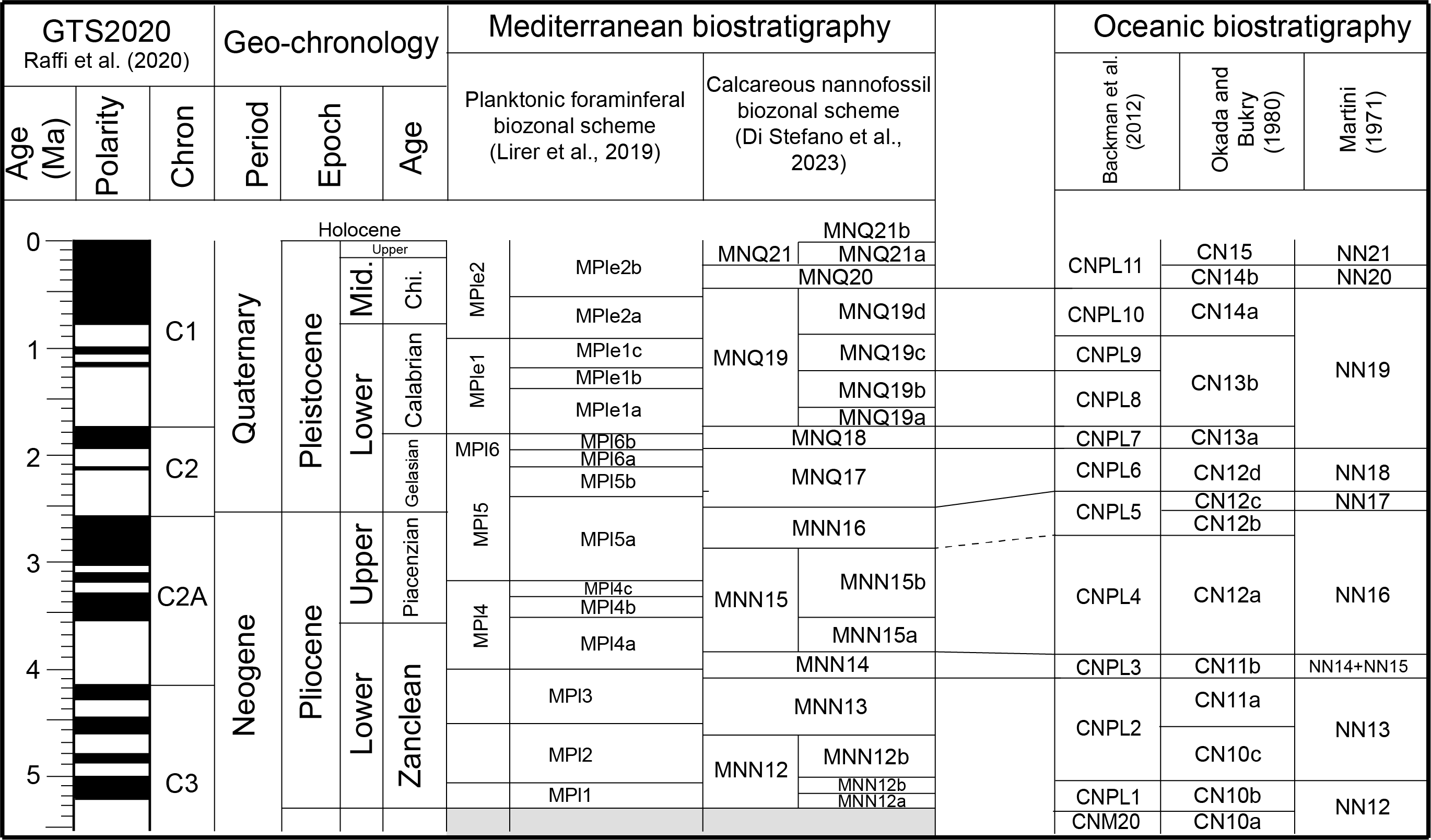
Figure F11. Mediterranean planktic foraminiferal and calcareous nannofossil zonal schemes.
Qualifiers for foraminiferal taxa identified in this study were as follows:
- cf. = confer (compare with).
- aff. = affinis (affinity with).
- sp. = unidentified species assigned to the genus.
- spp. = more than one unidentified species assigned to the genus.
- s.l. = sensu lato.
- ? = identification uncertain.
3.1.2. Sampling, sample preparation, and analysis
Samples (5–10 cm whole rounds) were prepared by manually breaking the core into small pieces followed by disaggregation and washing over a 63 µm mesh sieve to remove all mud and silt particles using the Easy washer apparatus developed by Fabricio Ferreira of the JRSO technical group. If needed, more lithified sediments were manually broken down into smaller chunks using a mortar and pestle, and if still necessary, these were soaked in a solution of hot water and/or hydrogen peroxide (H2O2; 30%) to chemically disaggregate the microfossils from the sediments. The washed microfossil residue retained on the sieve was then dried at low temperature (~50°C) in a thermostatically controlled drying cabinet. The residue was further sieved using a 125 µm mesh sieve to decrease the presence and/or misdetection of juvenile species. The remaining residue was divided using a microsplitter into equal aliquots for examination under the microscope. As a precaution against cross-contamination, sieves were cleaned with a water jet after use, placed in an ultrasonic bath for 15 min, dried with compressed air, and thoroughly inspected.
During examination of samples, the relative abundance of planktic foraminifera was determined quantitatively from random counts of 100 particles in the 125–500 µm grain-size fractions of washed residues. Age-diagnostic planktic foraminifera specimens were picked from the 125–500 µm grain-size fraction and mounted onto 60-division faunal slides coated with gum tragacanth. When time allowed, other species and biogenic remains of microfossils were also picked and mounted onto the same slides.
Preliminary images of the extracted residue were taken using a camera mounted on the Zeiss Discovery V8 stereo microscope. Scanning electron microscope (SEM) images of planktic foraminifera species were acquired by mounting the specimens on a stub and imaging with a Hitachi TM3000 tabletop microscope.
During examination of microfossil samples, the abundance of planktic foraminifera in the 125–500 µm grain-size fractions of washed samples was determined visually and categorized as follows:
- D = dominant (foraminifera compose >100 individuals on the picking tray).
- A = abundant (foraminifera compose 50–100 individuals on the picking tray).
- C = common (foraminifera compose 10–50 individuals on the picking tray).
- F = few (foraminifera compose 5–10 individuals on the picking tray).
- R = rare (foraminifera compose <5 individuals on the picking tray).
- X = present (present in sample, abundance undetermined).
- B = barren (not present).
In addition, the preservation states of foraminifera were categorized as follows:
- VG = very good (specimens mostly whole, very well preserved ornamentation and surface ultrastructure, and no visible modification of the test wall).
- G = good (specimens often whole, ornamentation and surface ultrastructure preserved but sometimes abraded or overgrown, and visible evidence of modification of the test wall).
- M = moderate (specimens often etched or broken, ornamentation and surface ultrastructure modified, and majority of specimens identifiable to species level).
- P = poor (most specimens crushed or broken, recrystallized, diagenetically overgrown, or infilled with crystalline calcite; most specimens difficult to identify to species level).
- VP = very poor (all specimens crushed or broken, recrystallized, diagenetically overgrown, or infilled with secondary minerals; most specimens difficult to identify to genus level).
- X = not present (sedimentary layers barren of planktic foraminifera specimens and/or dominating volcaniclastic sedimentary layers reducing the presence of planktic foraminifera to a bare minimum).
3.2. Calcareous nannofossils
3.2.1. Taxonomy and biozonation scheme
The taxonomy of most of the taxa considered here follows species concepts from Aubry (1984, 1988, 1989, 1990, 1999), Theodoridis (1984), Perch-Nielsen (1985), Bown (1998), Young et al. (2003), and/or Jordan et al. (2004). Useful information is also available from the Nannotax3 web site (Young et al., 2017). Remarks on the taxa considered here, listed in Table T2, are reported in Table T3.
The key biohorizons adopted in the present study are the lowest and highest occurrences of marker species and are referred to as base (B) and top (T), respectively, and the levels where marker species begin to be common or decline are referred to as base common (Bc) or top common (Tc), respectively. Other relevant biohorizons are the base of paracme (PB) and top of paracme (PT) (paracme = interval of temporary absence of a taxon); the base of acme (AB) and top of acme (AT) (acme = interval of sharp increase in abundance of a taxon); and the abundance crossover (X), which is the level where a taxon replaces another. The informal term influx (inf) indicates a brief appearance of significant taxa below or above their classical distribution range.
Because all sites are in the Mediterranean, we adopted the calcareous nannofossil biostratigraphic scheme of Di Stefano et al. (2023) established from the offshore and onshore sedimentary successions of the Mediterranean region. Comparisons were made with biozones established for oceanic successions (e.g., Martini, 1971; Okada and Bukry, 1980; Backman et al., 2012) and with the foraminiferal scheme of Lirer et al. (2019) (Table T1). Bioevents used for the biostratigraphic division of the successions drilled during Expedition 402 are listed in Table T4.
3.2.2. Sampling, sample preparation and analysis
Samples for nannofossils were prepared according to the smear slide protocol (Bown and Young, 1998, in Bown, 1998) and were analyzed using standard transmitted light microscope techniques on a Zeiss Axio microscope with cross-polarization and phase contrast at 1000× or 1250× magnification. All taxa were assigned qualitative abundance codes.
The total abundance in the sediments and the individual calcareous nannofossil taxa abundance were recorded as follows:
- D = dominant (>100 specimens per field of view [FOV]).
- A = abundant (>10–100 specimens per FOV).
- C = common (1–10 specimens per FOV).
- F = few (1 specimen per 1–10 FOVs).
- R = rare (<1 specimen per 10 FOVs).
- VR = very rare (<5 specimens seen while logging slide).
- X = present (present in sample, abundance undetermined).
- B = barren (not present).
For critical intervals or critical taxa, quantitative analysis was carried out (e.g., estimating the percentage of selected taxa within a prefixed number of specimens belonging to the same genus or within a prefixed number of specimens, larger than 4 µm, of the total assemblage).
The preservation of nannofossils was categorized as follows:
- VG = very good (specimens very well preserved).
- G = good (specimens generally well preserved, rarely overgrown).
- M = moderate (specimens moderately preserved, often recrystallized and diagenetically overgrown but generally identifiable to species level).
- P = poor (specimens badly preserved, recrystallized and diagenetically overgrown, hardly identifiable to species level).
- VP = very poor (specimens badly preserved, recrystallized and diagenetically overgrown, not identifiable to species level).
4. Paleomagnetism
Paleomagnetic analysis during Expedition 402 assessed both sedimentary and igneous basement cores recovered at all sites. Natural remanent magnetization (NRM) was measured on archive-half sections using a 2G Enterprises Model-760R-4K superconducting rock magnetometer (SRM) and on discrete cube samples from working-half sections using an AGICO JR-6A spinner magnetometer. Samples were demagnetized in an alternating field (AF) to reveal primary NRM and reconstruct the magnetostratigraphy at each site, when possible. NRM of igneous and metamorphic basement cores was measured, and magnetic measurements were performed on characteristic discrete samples from different rock units.
Rock magnetic measurements on discrete samples were performed to provide insights into the sedimentary fabric, magnetic mineralogy, and the nature of NRM carriers. These magnetic measurements include anisotropy of MS (AMS), anhysteretic remanent magnetization (ARM), and isothermal remanent magnetization (IRM).
4.1. Core collection, orientation, and sample coordinates
Nonmagnetic stainless steel core barrels were employed while coring with the APC and RCB systems to reduce the drill string overprint (Lund et al., 2003). All magnetic data are reported relative to IODP orientation conventions: +x points into the face of the working half (toward the double line), +y points toward the left side of the working half when looking downcore, and +z is downcore. The relationship between the SRM coordinates (X, Y, and Z) and the sample coordinates (x, y, and z) is +X = +x, +Y = +y, and +Z = −z for archive halves and +X = −x, +Y = −y, and +Z = −z for working halves (Figure F12). Data were stored using the standard IODP file format and automatically uploaded to the LIMS database using the IMS software for the SRM that was first used during Expedition 362 (McNeill et al., 2017). For discrete samples, positioning in the SRM and the JR-6A spinner magnetometer can depend upon the collection method (extruder or push-in). For this expedition, +x points toward the lid of the cube, which is the same as in the push-in method. For the JR-6A spinner magnetometer, azimuth = 0, dip = 90, P1 = 12, P2 = 0, P3 = 12, and P4 = 0. The −z arrow (i.e., the upcore direction) points northwest in the holder, and the +x arrow points away from the user (into the holder).
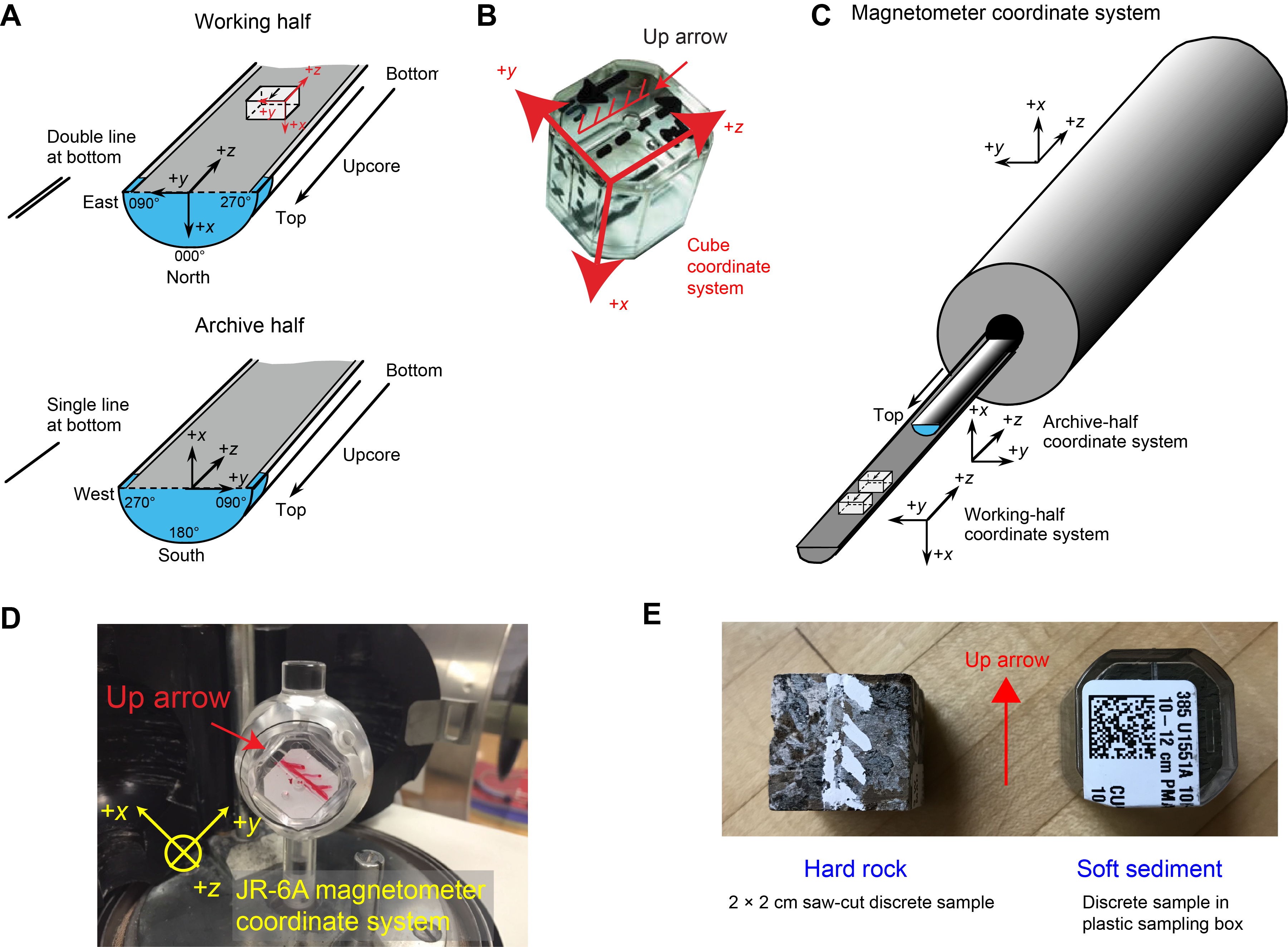
Figure F12. IODP paleomagnetic coordinate systems.
4.2. Archive-half measurements
NRM measurements of the archive-half sections were made at 2 cm intervals for sediments and included a 14 cm leader and trailer to monitor the background magnetic moment. Following the initial measurement of NRM, the remanent magnetization was sequentially demagnetized and measured in 4 steps, which were set to 5, 10, 15, and 20 mT peak fields for sediment cores drilled using the APC system; for a few cores drilled using the RCB system, an extra demagnetization at 25 mT peak AF was applied. Sample trays were cleaned with deionized water at the beginning of each shift and AF demagnetized with a peak field of 30 mT. The remanence was then measured to update the background correction values for the empty sample tray.
For basement rocks, demagnetization steps were set to 5, 10, 15, and 20 mT peak fields to reveal the polarity of their NRM and to preliminarily estimate the nature of the remanence carriers. The measurements were only carried out for intact segments of rocks, and intervals of fragmented pieces were skipped.
4.3. Paleomagnetic and rock magnetic measurements of discrete samples
Discrete sediment samples were collected using 7 cm3 plastic Natsuhara-Giken sampling cubes for detailed demagnetization to reveal the coercivity range of characteristic remanent magnetization (ChRM), providing constraints on the magnetostratigraphy of archive-half sections. One to two samples per core were extracted from the working-half sections; the positioning of samples depended on the lithology and paleomagnetic results of the archive-half sections.
Lithified sediments and hard rock material were removed with a tile saw equipped with two parallel blades to cut discrete sample cubes (8 cm3). Orientation arrows were drawn directly on the cube face and were used for AF demagnetization experiments. Recovery and nature of material in the working-half hard rock sections determined the sampling frequency. Usually, two samples per core were selected based on identified hard rock units described by shipboard petrologists. When hydrothermal alteration was identified, discrete samples were taken and measured to assess the altered magnetic properties.
Before demagnetization, discrete samples were measured on the MFK2-FA multifunction frequency Kappabridge (AGICO) for AMS using 975 Hz frequency (sensitivity = 2 × 10⁻⁸ SI). The susceptibility tensor and associated eigenvalues were calculated using Anisoft (AGICO) software (v.5.1.03) to estimate the following parameters:
- Magnetic lineation (L = Kmax/Kint) (Balsley and Buddington, 1960),
- Magnetic foliation (F = Kint/Kmin) (Stacey et al., 1960),
- Anisotropy degree (P) (Jelinek, 1981), and
- Shape parameter (T) (Jelinek, 1981).
These data can provide insight into deformation due to drilling or tectonics, as well as sediment compaction and possible paleocurrents.
Discrete samples were measured for NRM on the AGICO JR-6A spinner magnetometer before and after a manual three-axis AF demagnetization using a D-Tech AF demagnetizer (Model D-2000). Peak AFs were incremented at 5, 10, 15, 20, 30, 40, 60, 80, 100, and 120 mT. The maximum AF level was adjusted depending on demagnetization behavior of discrete samples.
Following NRM demagnetization, ARM was applied with a peak AF of 70 mT and a bias field of 50 µT using a D-Tech AF demagnetizer (Model D-2000). ARM was measured before and after demagnetization in 20 steps up to 80 mT peak AF. After demagnetization of ARM, characteristic samples were sequentially magnetized from 5 mT to 1 T using an ASC scientific Impulse Magnetizer (Model IM-10-30) and measured on the JR-6A spinner magnetometer to obtain IRM acquisition curves. ARM and IRM related parameters were used to evaluate the linkage between magnetic minerals and the lithology of sediment and rock samples.
4.4. Magnetostratigraphy
The six Expedition 402 drill sites are located at latitudes between 40.0°N and 40.2°N. Assuming a geocentric axial dipole model (e.g., Tauxe, 2010), the sites have a predicted field inclination of approximately ±59.2° for normal and reversed polarity, respectively, based on the dipole formula (i.e., tan [I] = 2 tan [lat], where I = inclination and lat = latitude). Magnetic polarity zones were assigned based on changes in inclination after 20 mT peak AF demagnetization of archive-half sections as well as on ChRM of discrete samples. When applicable, the polarity stratigraphy of each site was correlated to the geomagnetic polarity timescale (GPTS2020) (Gradstein et al., 2020) assisted by the biostratigraphy of each site.
5. Igneous and metamorphic petrology
The description of igneous and metamorphic rocks followed during Expedition 402 is consistent with that followed during Integrated Ocean Drilling Program Expeditions 304, 305, 309, 312, and 335 and IODP Expeditions 399 and 360. Description was carried out by a team that worked on different shifts but ensured consistency of observations throughout the core. Each team member was responsible for one or more aspects of the description (e.g., lithology, textures, mineral modes, veins, and/or alteration) following the steps described in Figure F13. The cores were described macroscopically in the archive half and in some cases microscopically from thin sections from the working half. All the rock characteristics were entered into the LIMS database through the GEODESC application in templates created by the team at the beginning of the expedition.
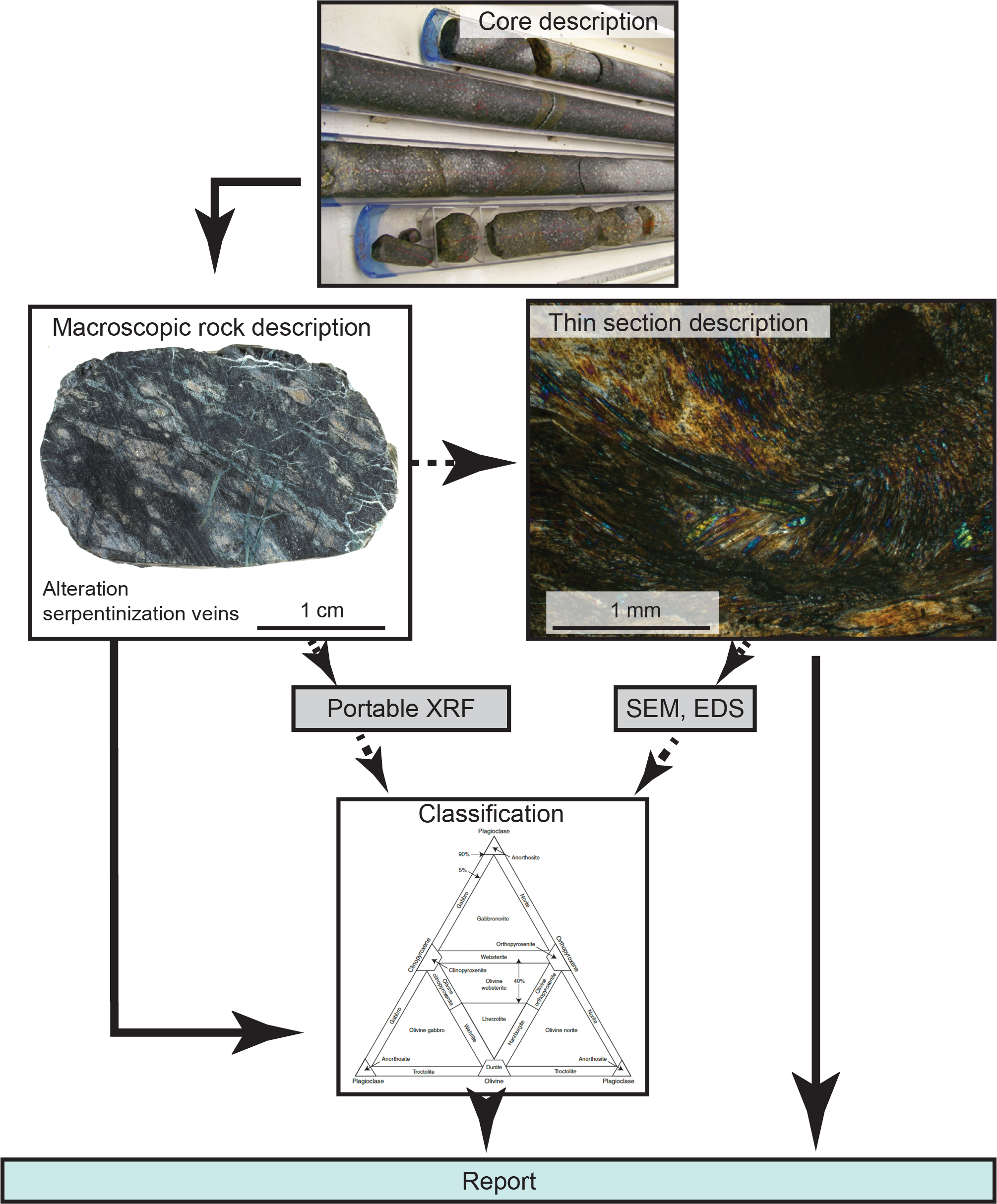
Figure F13. Rock description flowchart.
5.1. Plutonic rocks
The first step of the description was the igneous petrologic characterization of the rocks according to mineral modes, abundance, classification schemes, and original igneous textures (if preserved), as described below.
5.1.1. Description of lithology
5.1.1.1. Mafic plutonic rocks
Mafic rocks were classified based on primary mineral modal abundance, grain size, and texture (Figure F14) according to the International Union of Geological Sciences (IUGS) classification scheme (Streckeisen, 1974; Le Maitre, 1989; Le Maitre et al., 2002). This classification defines the following common plutonic rocks (Figure F15):
- Gabbro/diorite: plagioclase ± clinopyroxene ± amphibole ± mica (>95%), plagioclase (>10%) ± quartz (<5%).
- Olivine gabbro: olivine + plagioclase (<5%) + clinopyroxene (<5%).
- Troctolite: olivine (>10%) + plagioclase (>95%).
- Gabbronorite: plagioclase (>5%) + clinopyroxene (>5%) + orthopyroxene (>5%).
- Quartz diorite: quartz (5%–20%) + alkali feldspar (<10%) + plagioclase.
- Tonalite: quartz (20%–60%) + alkali feldspar (<10%).
- Trondhjemite: tonalite with total mafic mineral content <10%.
- Anorthosite: plagioclase >90%.
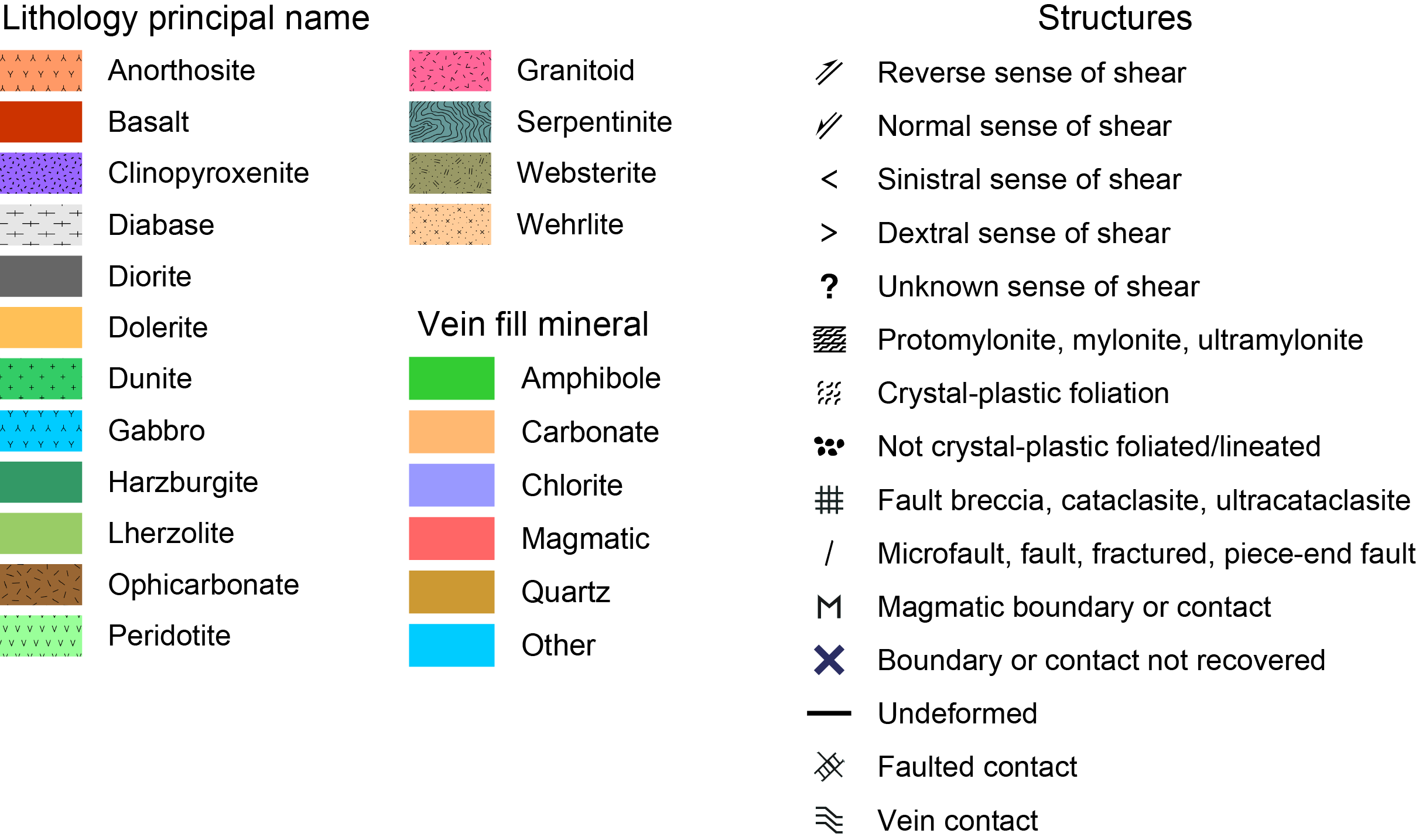
Figure F14. Lithologic classification scheme.
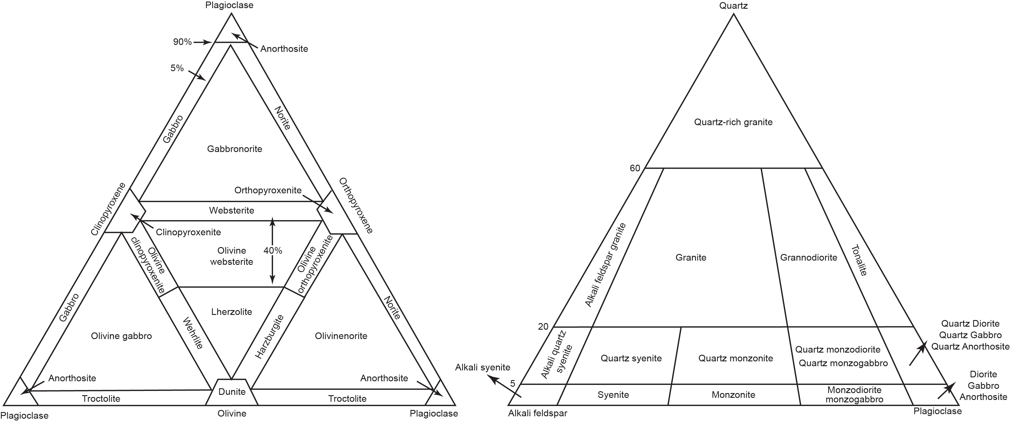
Figure F15. Plutonic rock classification.
In the IUGS classification, diorite is distinguished from gabbro by the anorthite content of plagioclase. Plagioclase in diorite is <50 mol% anorthite, whereas gabbros have plagioclase containing >50 mol% anorthite. Because this difference cannot be determined by macroscopic description, we used the following convention: if a gabbroic rock contained quartz (<5%) or primary amphibole and mica, indicating a relatively high degree of fractionation, the rock was classified as diorite. If no quartz or primary amphibole and mica was present, the rock was classified as gabbro.
5.1.1.2. Felsic plutonic rocks
For the description of felsic rocks, we followed the IUGS mineralogical classification scheme based on modal mineralogy as shown in Figure F15 (right).
5.1.1.3. Ultramafic rocks
For the description of the ultramafic rocks, the following IUGS recommended nomenclature was used (Figure F13):
- Dunite: olivine >90%.
- Orthopyroxenite: orthopyroxene (>90%).
- Clinopyroxenite: clinopyroxene (>90%).
- Lherzolite: olivine (>40%) + orthopyroxene (>10%) + clinopyroxene (>5%).
- Harzburgite: olivine + orthopyroxene ± clinopyroxene (<5%).
- Wehrlite: olivine + clinopyroxene ± orthopyroxene (<5%).
- Websterite: orthopyroxene + clinopyroxene ± olivine (<5%).
- Olivine websterite: olivine (<40%) + orthopyroxene + clinopyroxene.
- Olivine orthopyroxenite: olivine (<40%) + orthopyroxene (<5%).
- Olivine clinopyroxenite: olivine (<40%) + clinopyroxene ± orthopyroxene (<5%).
Minor modifications were made to the IUGS system to divide the rock types more accurately based on significant differences rather than cutoffs based on the abundance of a single mineral. To maintain consistency, we have attempted to follow as closely as possible the descriptions from Ocean Drilling Program (ODP) Leg 209 (Shipboard Scientific Party, 2004); IODP Expeditions 399 (McCaig et al., 2024) and 360 (MacLeod et al., 2017); and Integrated Ocean Drilling Program Expeditions 304/305 (Expedition 304/305 Scientists, 2006), 309/312 (Expedition 309/312 Scientists, 2006), and 335 (Expedition 335 Scientists, 2012).
5.1.2. Veins in the plutonic rocks
Vein and rock names include a modifier based on modal mineralogy (Figure F14). All veins were described in collaboration with the structural geology team and incorporated in both GEODESC spreadsheets.
For the descriptions, the following rock name modifiers were used:
- Disseminated oxide: if Fe-Ti oxide ranges 1%–2%.
- Oxide bearing: if Fe-Ti oxide is more than 2% but less than 5%.
- Oxide: if Fe-Ti oxide is more than 5% but less than 50%.
- Olivine bearing: if olivine ranges 1%–5%.
- Orthopyroxene bearing: if orthopyroxene ranges 1%–5%.
- Olivine rich: if olivine <70%.
- Plagioclase bearing: if plagioclase is more than 1%.
Following the Streckeisen (1974) classification scheme (Figure F15), any mineral >5% should be added as a suffix without any hyphen.
Additional rock name modifiers were defined as follows:
- Leucocratic: light-colored, high proportions of plagioclase.
- Micro: dominant grain size < 1 mm.
- Diabasic: fine- or medium-grained gabbroic rocks with dominant ophitic or subophitic textures.
5.1.3. Texture of plutonic rocks
In the plutonic rocks we encountered, the primary rock-forming minerals are spinel, olivine, plagioclase, clinopyroxene, orthopyroxene, amphibole, Fe-Ti oxide, sulfide, quartz plagioclase, and mica. The following information was recorded in the GEODESC igneous_petrology spreadsheet for each primary silicate:
- Visually estimated modal percent: in fresh rocks, this represents the modal mineralogy as observed. In partially altered rocks, this represents the estimated igneous mineral content before alteration. Modal estimates were visually estimated and normalized to 100%.
- Grain size:
- Detailed (absolute grain sizes of each mineral phase):
- Where oxides and sulfides form aggregates:
- Mineral habits:
The texture of igneous rocks was defined based on three categories: grain size, grain size distribution, and the relationships between different grains.
Grain size distributions were classified as follows:
- Equigranular: all minerals are of similar size.
- Inequigranular: grain size varies significantly.
- Seriate: continuous range of crystal sizes.
- Varitextured: domains with contrasting grain size.
- Poikilitic: relatively large oikocrysts enclosing smaller crystals, termed chadacrysts, of one or more other minerals.
To describe the textural relationship between different grains, the following terms were used (Figure F16):
- Granular: aggregation of grains of approximately equal size.
- Intergranular: coarser grains (typically plagioclase) form a connected framework with interstices filled with crystalline material.
- Intersertal: coarser grains form a connected framework with interstices filled with glass.
- Subophitic: partial inclusion of plagioclase in clinopyroxene.
- Ophitic: total inclusion of plagioclase chadacrysts in clinopyroxene oikocrysts.
- Poikilitic: large oikocrysts containing numerous chadacrysts of any type.
- Porphyritic: texture containing large grains within a finer-grained matrix.
- Comb structure: comb-like arrangement of crystals growing inward from a contact.
- Skeletal: either hopper crystals or hourglass shape.
- Dendritic: branching arrangement of elongate crystals.
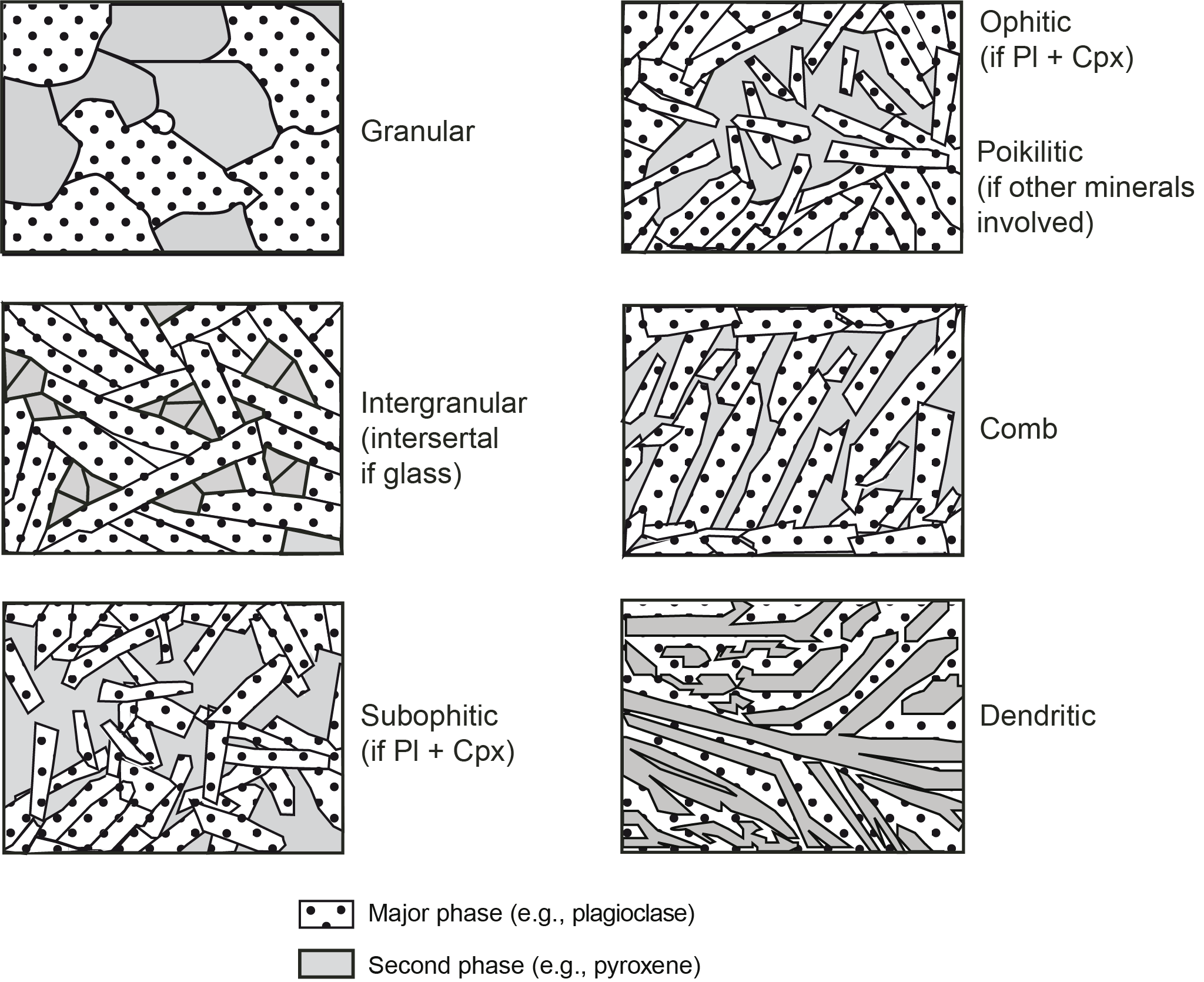
Figure F16. Igneous texture terminology.
5.2. Volcanic rocks
For volcanic and hypabyssal rocks, the following definitions were used:
- Basalt: all nonintrusive igneous rocks of basaltic composition with grain sizes that range between glassy and medium-grained.
- Diabase or dolerite: holocrystalline, very fine to medium-grained intrusive rocks of basaltic composition often with well-developed subophitic or ophitic textures.
Basalt was divided according to phenocryst content using the following convention:
- Aphyric: <1% phenocrysts.
- Sparsely phyric: 1%–5% phenocrysts.
- Moderately phyric: >5%–10% phenocrysts.
- Highly phyric: >10% phenocrysts.
If present and >5%, phenocryst phases were placed as modifiers in front of the rock name without any hyphen in between. If <1% phenocryst was present, the rock was given the modifier “aphyric.”
In volcanic and hypabyssal rocks, groundmass, phenocrysts (if any), and vesicles were described.
Groundmass grain size was described using the following convention:
- Glassy.
- Cryptocrystalline = <0.1 mm.
- Microcrystalline = 0.1–0.2 mm.
- Fine-grained = >0.2–1 mm.
- Medium grained = >1–5 mm.
- Coarse-grained = >5–30 mm.
Phenocryst phases were described using the following convention:
Vesicles were described using the following convention:
- Abundance (in percentage).
- Vesicularity.
- Size distribution: minimum, maximum, and modal size (in millimeters).
- Roundness (rounded, subrounded, or well-rounded).
- Sphericity (highly spherical, moderately spherical, slightly spherical, or elongate [direction was noted]).
- Filling (in percentage).
- Fill composition.
5.3. Alteration
Following the igneous petrographic descriptions, all cores that have experienced alteration (defined here as metamorphism ± deformation) were described using the alteration worksheets in GEODESC with the following procedure:
- Determine the number of different alteration intervals in each section and assign each interval [domain] to a row in the GEODESC worksheet.
- Estimate the proportion of mylonitic areas in each alteration interval and identify the minerals that form dynamically recrystallized neoblasts.
- Estimate the proportion by area of the three groups of static alteration, namely, background, halo, and patch.
- Estimate the static alteration intensity and assign a rank scale based on each primary mineral, namely, olivine, pyroxene, and plagioclase for gabbroic rocks:
- 0 = fresh (alteration <3%).
- 1 = slight (3%–9%).
- 2 = moderate (10%–29%).
- 3 = substantial (30%–59%).
- 4 = extensive (60%–89%).
- 5 = complete (≥90%).
- Identify any secondary minerals that replace each primary mineral.
- Describe all features of alteration in the interval in the General comments column.
- Create a section summary description.
Overall, we recognized three types of alteration: static alteration, ductile alteration associated with crystal-plastic deformation, and brittle alteration associated with cataclastic deformation.
Static alteration was categorized into three groups: pervasive background alteration, halo alteration in proximity to veins, and localized patch alteration. Where a primary phase was completely decomposed to form a polycrystalline pseudomorph, it was categorized as background alteration. The approximate proportions of each group of static alteration styles were estimated in each descriptive interval. The static alteration intensities of rocks and individual igneous minerals were recorded in the GEODESC worksheets using a rank scale for their volume proportions rather than assigning a percentage to these proportions. Uncertainties derive from grain size, inhomogeneous distribution, and complex textures of alteration minerals difficult to observe on the mesoscopic scale.
Representative rocks with evidence of crystal-plastic deformation were further investigated mesoscopically and microscopically. In granitic rocks, the deformation of quartz and feldspar was used to estimate the degree of mylonitization, temperature, and strain (Passchier and Trouw, 2005). In mafic and ultramafic rocks with mylonitic fabric, neoblasts of olivine, pyroxene, and plagioclase formed by dynamic recrystallization were not counted in alteration products because of the difficulty in distinguishing a monomineralic aggregate of recrystallized neoblasts from a porphyroclast and identifying individual neoblastic minerals within multiphase aggregates. Secondary clinopyroxene was not distinguished from primary clinopyroxene in macroscopic descriptions because its identification was possible only under the microscope. Plagioclase that exhibited a milky white appearance was counted as an alteration product.
5.4. Thin section descriptions
All the thin sections were photographed in both plane-polarized light (PPL) and cross-polarized light (XPL), and the photomicrographs were uploaded to the LIMS database. The thin section descriptions closely follow the macroscopic descriptions. In thin sections that contained areas with different primary lithology, mineralogy, and/or texture (not alteration related), each area was described separately. The data were recorded and entered into the thin section worksheets of GEODESC.
5.4.1. Plutonic and ultramafic rocks
The following definitions were used for plutonic rocks:
- Rock name based on thin section observations, using the same definitions as those for macroscopic descriptions.
- Relative mineral abundance (in percent).
- Igneous domain texture (granular, intergranular, intersertal, subophitic, ophitic, comb structure, skeletal, dendritic, porphyritic, or poikilitic).
- Texture comment, emphasizing textures in thin sections.
- Igneous domain grain size modal name (glassy, cryptocrystalline, microcrystalline, fine-grained, medium-grained, coarse-grained, or pegmatitic).
- Total rock alteration estimate.
5.4.2. Volcanic rocks
For the textures in volcanic rock, we followed the following definitions.
Holohyaline (100% glass) to holocrystalline (100% crystals) rock was described as follows:
- Phyric: indicates the presence of phenocrysts.
- Glomeroporphyritic: indicates the presence of clusters of phenocrysts.
For a continuous range in grain size, the texture is seriate. In cases where there is no significant grain size difference between groundmass crystals and slightly larger and more euhedral crystals that do not meet the definition of phenocrysts, the term “microphenocryst” is used.
In holohyaline to hypohyaline rock, glass was divided into four distinct types:
- Fresh glass (amber in PPL and isotropic under XPL), commonly found in the outermost parts of preserved chilled margins.
- Dark (because of abundant crystallites) interstitial volcanic glass of basaltic composition, termed “tachylitic.”
- Glass that contains abundant fibrous spherulites.
- Glass that has been altered to clay minerals.
5.4.3. Alteration
Samples that exhibit alteration were evaluated based on the following procedure:
- Enter comments for alteration associated with mylonitic and cataclastic features, if any.
- List secondary minerals and estimate the alteration intensity (percent) and proportion of alteration minerals (percent). Describe the textural relationships between the secondary and primary minerals.
- Estimate the total alteration intensity.
- Establish chronological relationships, where discernible, between different secondary minerals or paragenesis and record them in “Detailed comments.”
- Create a summary description worksheet for the alteration features in the thin sections worksheet. The summary appears in the thin section form report along with the summaries from the igneous petrology and structural geology teams (Figure F17).
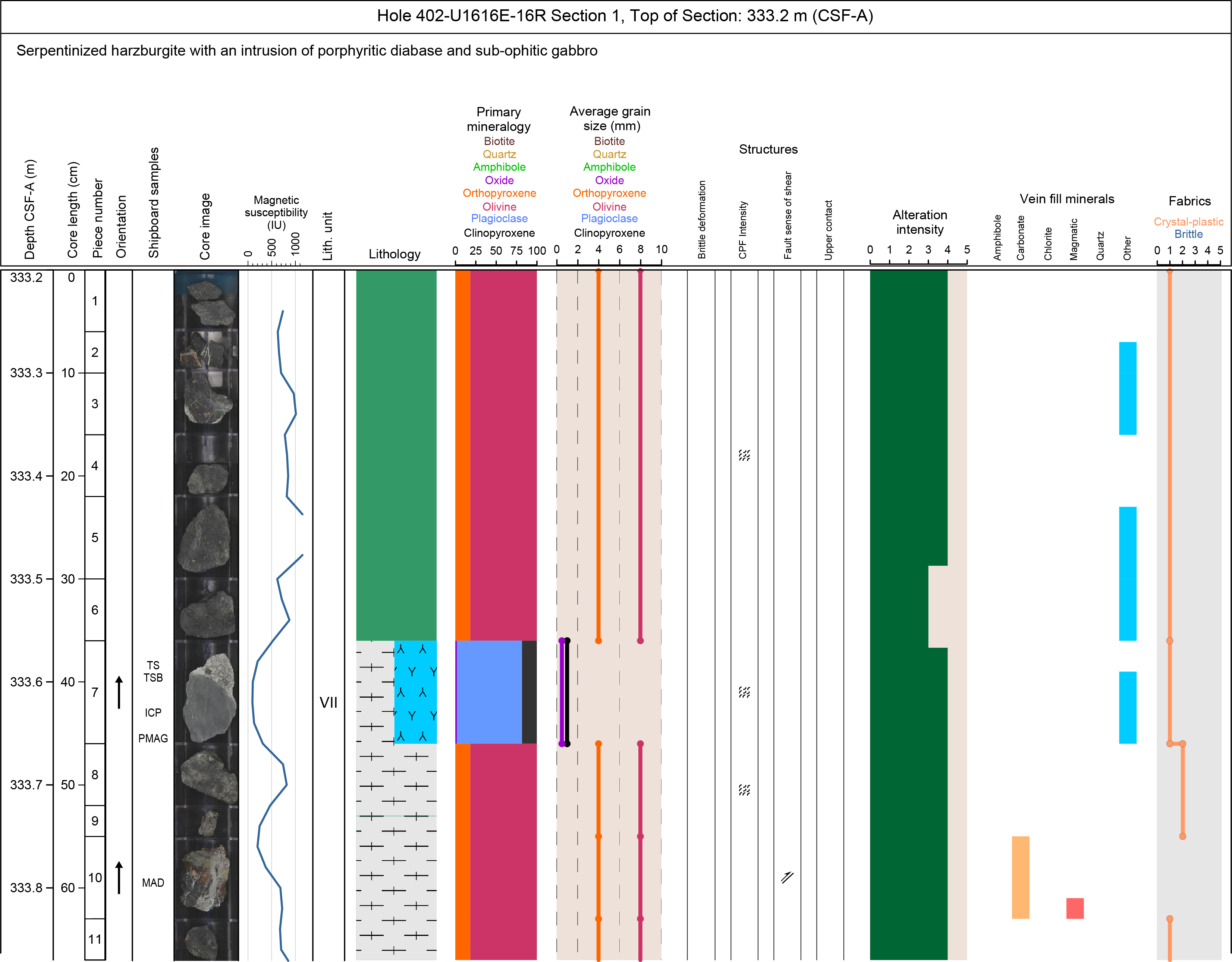
Figure F17. Example hard rock VCD.
6. Structural geology
During Expedition 402, we drilled through the continent–ocean transition of the Tyrrhenian Basin. In this environment, we conducted structural analyses on gabbroic and mantle rocks exhumed in the footwall of a detachment fault buried under variable thicknesses of sediment layers. Consequently, the methods described below have a common section describing the methods to acquire structural orientations, followed by two separate sections on sediment and hard rock domains.
These hard rocks are expected to retain a record of both magmatic accretion and superimposed, or coincident, deformation events during their cooling and exhumation. The continuum of these superimposed events is likely to span the transition from hypersolidus to subsolidus, from ductile to brittle deformation, as temperature decreases with time. Ultramafic rocks may host original mantle fabrics and/or lower temperature overprints due to tectonic and hydrothermal processes during denudation to the seafloor. Based on this premise, the methods described below are organized according to the down-temperature pattern of the deformation.
Conventions for structural studies established during previous hard rock drilling projects (e.g., Expeditions 360 and 399) were generally followed during Expedition 402. The GEODESC software application was used to enter and upload the information into the LIMS database (see Introduction).
6.1. Structural orientations
Our principal objective was to record the structures observed in the core and their orientations. These data will contribute to our aim of investigating the processes and in situ conditions that lead to lithospheric thinning and mantle exhumation. This goal was achieved by making detailed structural observations and measurements following the methods used during previous expeditions, with modifications to more fully describe the structures encountered during Expedition 402.
The methods for documenting structural features in the cores of Expedition 402 largely follow those of Integrated Ocean Drilling Program Expeditions 334 and 344 and IODP Expeditions 352, 360, 362, 375, and 399 (Expedition 334 Scientists, 2012; Harris et al., 2013; Reagan et al., 2015; MacLeod et al., 2017; McNeill et al., 2017; Wallace et al., 2019; McCaig et al., 2024). Structures observed in the split cores were classified and quantified in terms of depth, extent, orientation, and, where possible, sense and magnitude of displacement. Each structure was recorded manually on a description table sheet at the core table. For planar structures, the dip, strike, and dip direction were computed from apparent orientation measurements using trigonometric transformations applied in an Excel spreadsheet. The resulting orientations defined in a core reference frame were then logged using the GEODESC interface to the LIMS database (see Introduction), together with other descriptive information about each structure and the material in which the structure occurs.
Structural features categorized as magmatic, crystal plastic, and brittle deformation, schistose and serpentinite foliation, along with alteration, magmatic veins, and igneous contacts were recorded by interval in centimeters from the top of each section. Depth intervals of structures were recorded as the distance from the top of the section to the top and bottom of the feature, where the feature intersects the center of the section half surface (Figure F18). We measured structures on the working half relative to the standard IODP core reference frame (Figure F19). The plane normal to the axis of the borehole is referred to as the horizontal plane. On this plane, a 360° net is used with pseudosouth (180°; −x-direction) pointing into the archive half and pseudonorth (000°; x-direction) pointing from the split surface out of the archive half. Therefore, the cut surface of the section half is a vertical plane striking 090°–270°.
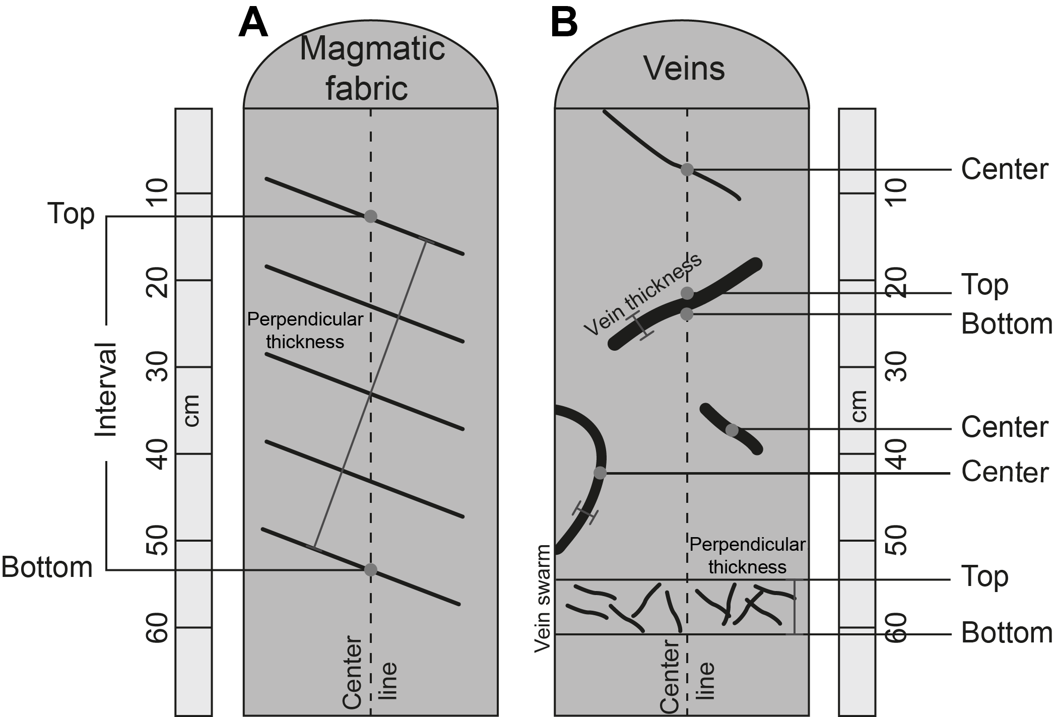
Figure F18. Schematic illustration of how structures were logged during Expedition 402.
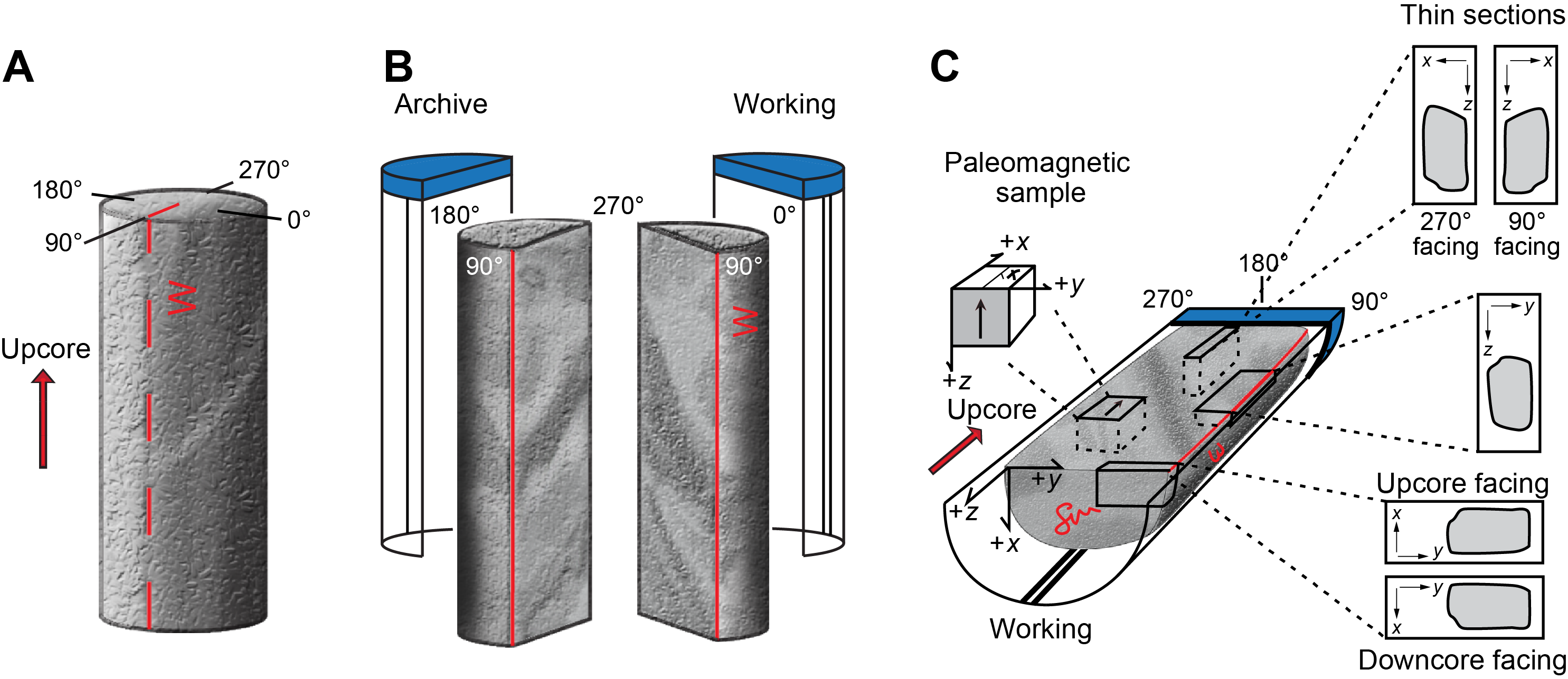
Figure F19. Core reference frame for structural and paleomagnetic orientation measurements.
6.1.1. Structural data acquisition and orientation measurements
The current basis for making quantitative structural measurements was defined during Expedition 334 (Expedition 334 Scientists, 2012) and further modified during Expeditions 344, 352, 360, 362, and 375 (Harris et al., 2013; Reagan et al., 2015; MacLeod et al., 2017; McNeill et al., 2017; Wallace et al., 2019). We used a plastic protractor to measure orientation (Figure F20).
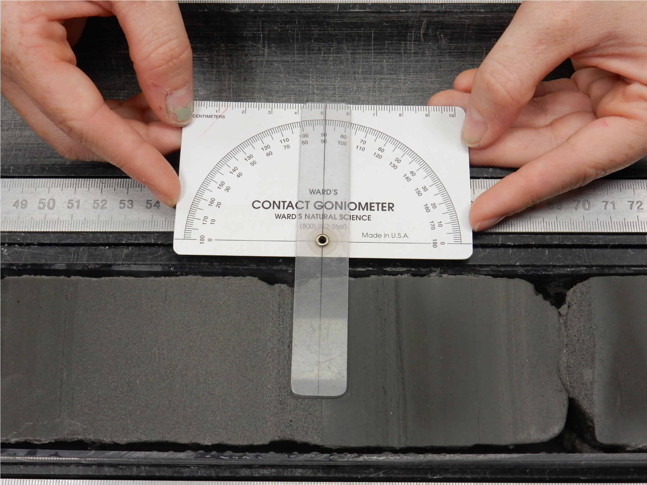
Figure F20. Protractor for measuring structures.
This measurement process was preferably performed on the working half because it allowed greater flexibility in removing and cutting pieces of the core for structural measurements, if necessary. Structures were also measured on the archive half when this was the only way to document certain features. Specifications on whether we used the working or archive halves were recorded in the description table sheet. Orientations of planar and linear features in cores were determined relative to the core axis, which represents the vertical axis in the core reference frame, and to the split line marked on the working half of the split core liner. The split line represents 000° (and 360°) in the plane perpendicular to the core axis (Figure F21).
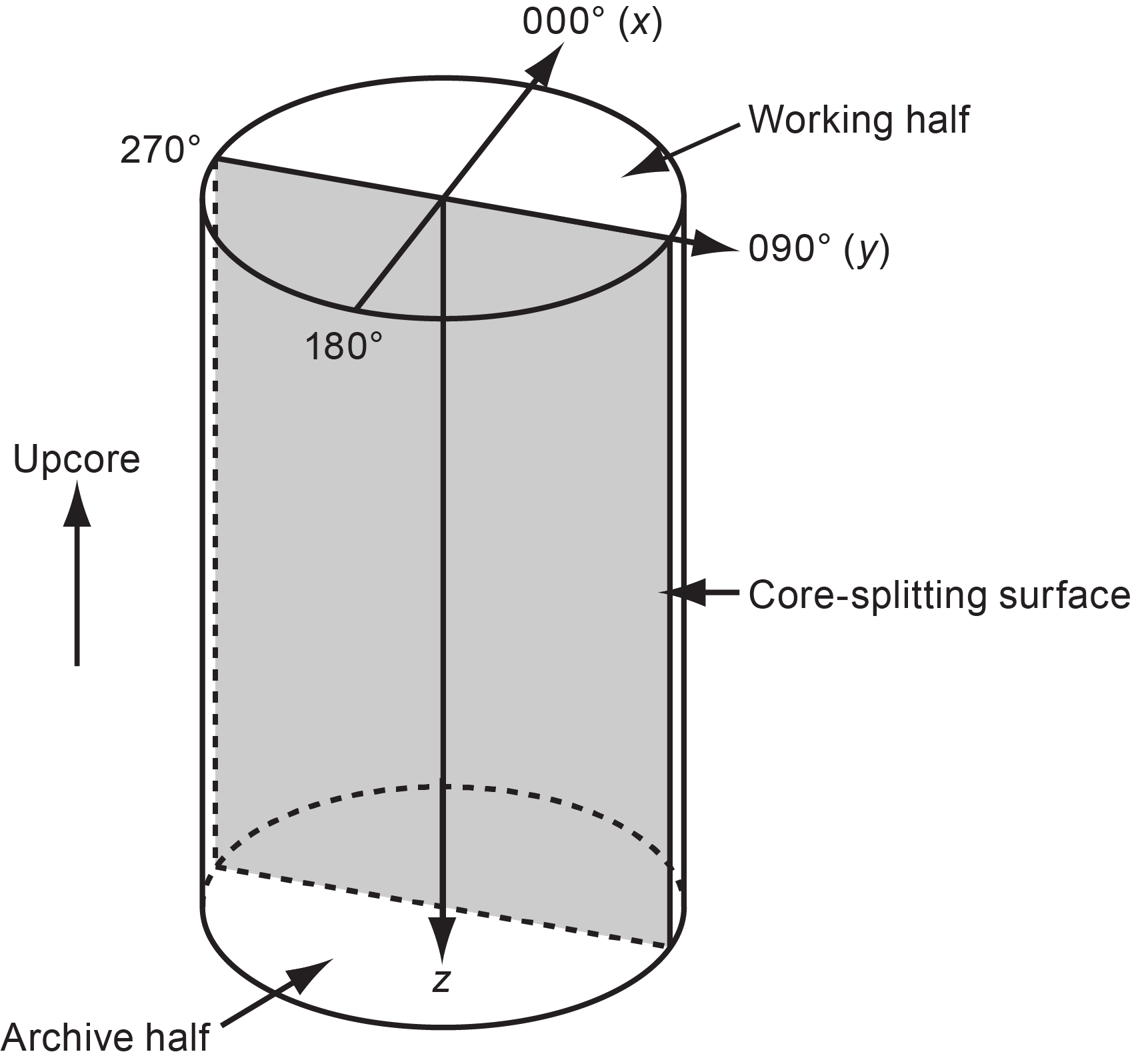
Figure F21. Core reference frame and x-, y-, and z-coordinates used in orientation calculations.
To determine the orientation of a planar structural feature, apparent dips were measured in two independent sections in the core reference frame. An apparent dip is represented by the intersection of the planar feature with the split face of the core and is quantified by measuring the plunge and trend of this line in the core reference frame (Figure F20). Such a measurement has a trend of either 090° or 270° and plunge ranges 0°–90° (α1 and β1, respectively) (Figure F22A). A second apparent dip is represented by the intersection of the planar feature with a cut or fractured surface at a high angle to the split face of the core. In most cases, this surface is either parallel or perpendicular to the core axis. If parallel, the apparent dip trace trends 000° or 180° and plunge ranges 0°–90° (α2 and β2, respectively) (Figure F22B); if perpendicular, the trend ranges 000°–360° and plunges 0° (α2 and β2, respectively) (Figure F22C).
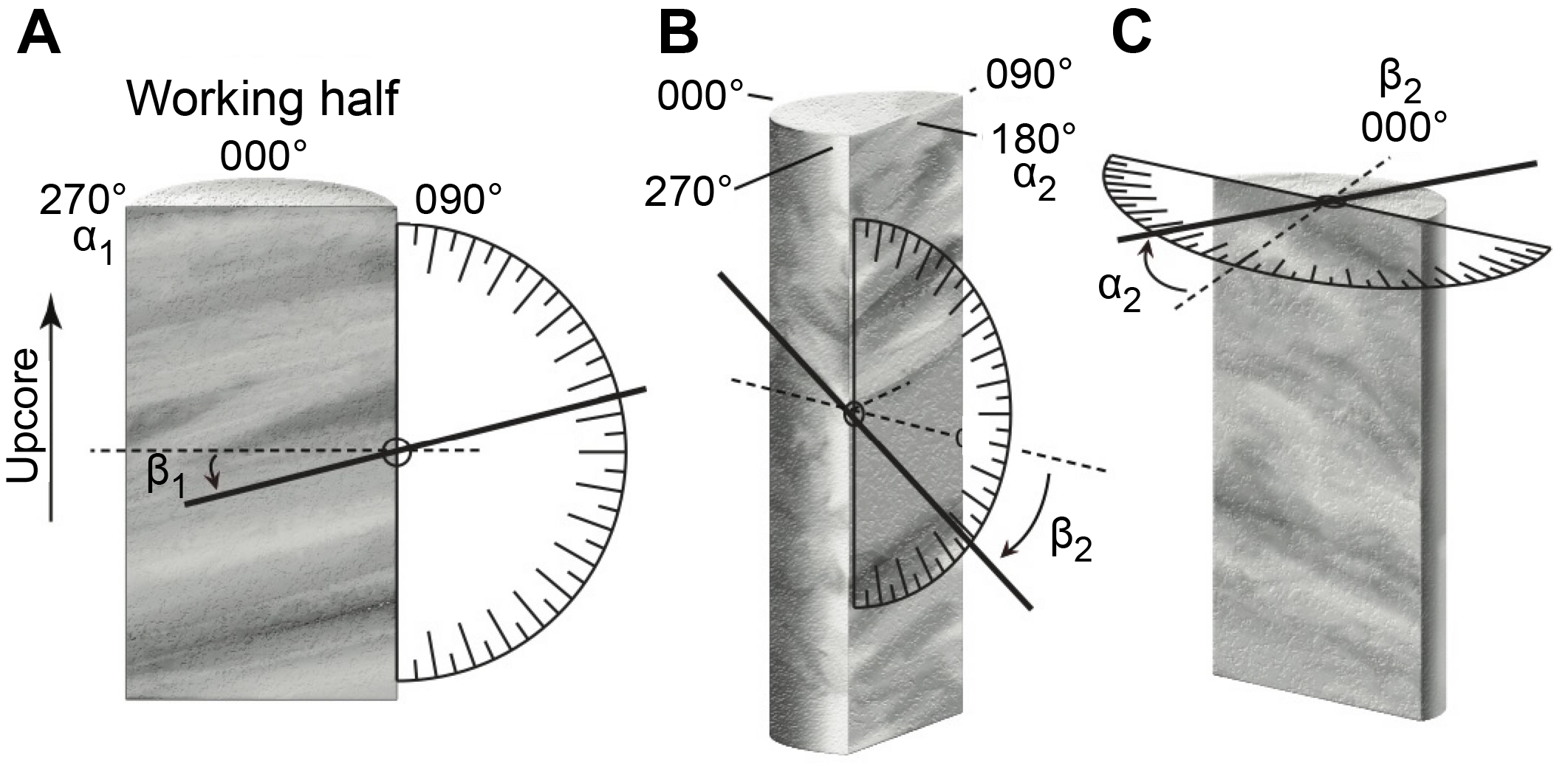
Figure F22. Calculation of plane orientation from two apparent dips.
Linear features observed in cores are typically defined by a trend and plunge in the core reference frame, like for the apparent dips described above. Lines may also be associated with planar structures (e.g., a striation on a fault plane), and their orientations can be determined by measuring the rake on the associated plane. For example, for a fault with striations, the apparent rake angle of the striation (ϕa) on the fault surface was measured from either the 090° or 270° direction of the split core surface trace (Figure F23). Fault orientation was calculated from the two apparent dips described above.
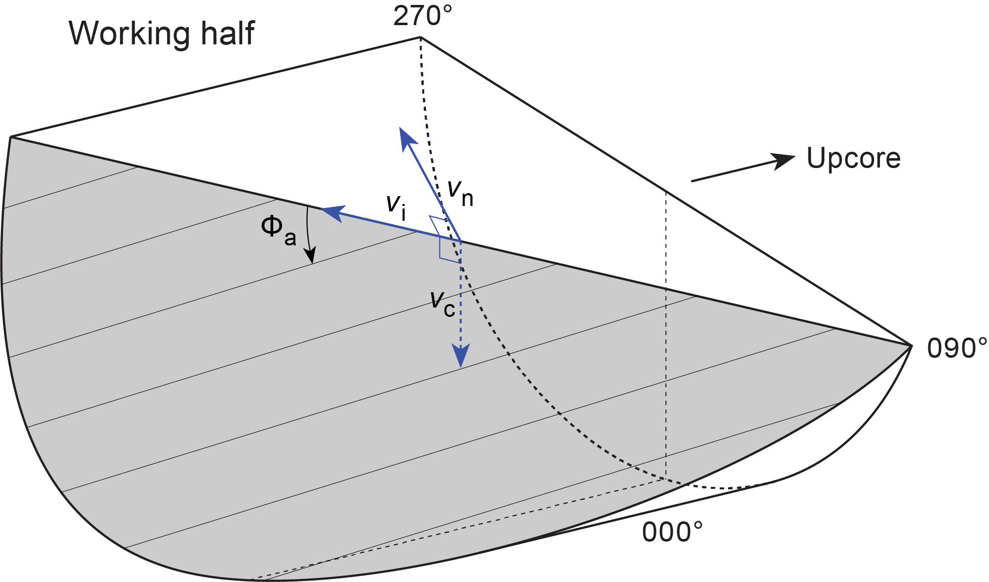
Figure F23. Apparent rake measurement for striations on a fault surface.
For planar structures, the two apparent dips were converted to a plane in the core reference frame represented by a dip angle, a strike, and a dip direction using an Excel spreadsheet (see STRUCTURE in Supplementary material).
A rake angle (ϕ) relative to the strike line in the core reference frame was also calculated trigonometrically in the Excel spreadsheet. Details of the calculation are described by the Expedition 334 Scientists (2012). We further confirmed conversions from apparent dips and rakes to orientations of planes and lines graphically using the Stereonet software (Version 11.5.4) developed by Allmendinger (2023) for representative measurements.
The reorientation of data from the core reference frame to a true geographic reference frame was initially planned for some intervals using paleomagnetic data (Figure F24). For these calculations, we followed methods used during past IODP expeditions and detailed by the Expedition 334 Scientists (2012).
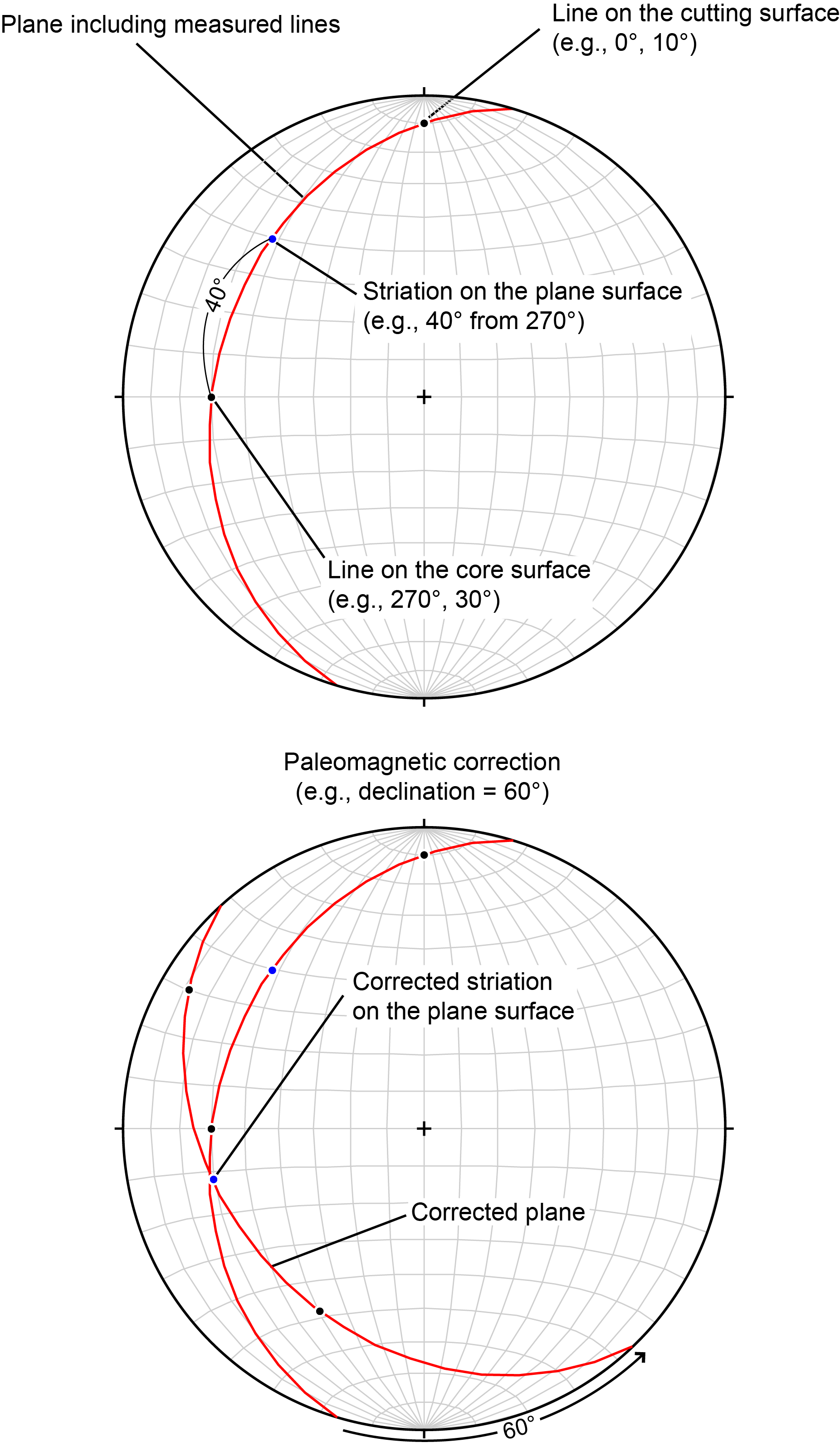
Figure F24. Procedure for converting 2D measured data to 3D data.
The azimuthal core orientation was determined based on the paleomagnetic declination obtained from the continuous magnetic remanence data if the core was complete and continuous. If the core was discontinuous, the orientation was determined through discrete paleomagnetic measurements from samples within the segment carrying the structure. Variability in both inclination and declination values introduces uncertainty in these orientation corrections. To be used for reorientations, declinations were required to be consistent (within a range of 30°) over 10 cm intervals in nonbiscuited intervals containing no polarity reversals. For discontinuous cores, we aimed for two discrete samples and the measurement was considered good if the declination was within a 30° range. This method could not be applied to intervals with severe core disturbances, including biscuiting on a centimeter scale or less, uparched bedding, or midcore flow. The presence of mass transport deposits or other zones of intense soft-sediment deformation also presented challenges for core reorientation. However, many of these zones of sediment deformation occurred in zones where relative rotations were minimal, in which case more reliable declination data from the bracketing zones could be used to reorient the structures.
Recognizing that it may be difficult to accurately measure orientations in cores, orientation measurements have been assigned a confidence level of 1 to 3. A Level 3 measurement is one for which it was easy to define and measure the structure, which is also unlikely to have been altered by drilling disturbance, and for which confidence is high. A Level 1 measurement is one where it was difficult to define and/or measure the feature accurately and it is uncertain whether it has been altered by drilling disturbance. This confidence level also includes, where applicable, whether the sense of slip is uniquely determined by the observations. For faults and shear zones, the highest confidence level is assigned only if offset marker horizons are visible in the core and/or if striations define the slip direction (e.g., dip-slip versus strike-slip).
6.1.2. Statistical analysis of true-dip vein and fracture data
Statistical analysis of the true dip of discrete planar features with small lengths compared to the length of the borehole, such as veins and fractures, requires an understanding of two geometric effects classified as follows and defined below:
- The length-scale or spherical effect, which leads to overrepresentation of steeply dipping planar structures.
- The borehole effect, which favors sampling of shallow-dipping planar structures over steeper dipping structures.
When the length scale of structures such as igneous contacts, layering, or crystal-plastic fabric (CPF) deformation considerably exceeds the diameter of the core, the length-scale or spherical effect does not apply. However, these features are still subject to the borehole effect, so steeply dipping features are undersampled relative to gently dipping features. The combined impact of these effects is that a random distribution of dips will produce a population of measurements with a Gaussian distribution centered on a 45° dip (Shipboard Scientific Party, 1992; MacLeod et al., 2017) (Figure F25). Histograms of dip angles were plotted during Expedition 402 to determine whether the measured distributions reflected random or systematic populations. Further discussion of the statistical impact of the length-scale effect and borehole effect are given in Shipboard Scientific Party (1992).
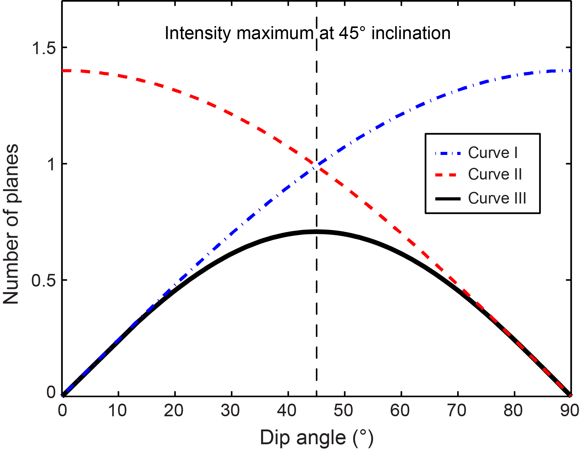
Figure F25. Predicted distribution of a random set of planar features.
6.2. Macroscopic core description and terminology
6.2.1. Workflow organization
During Expedition 402, the structural geologists worked in different shifts, sharing their expertise with the sedimentology, igneous, and metamorphic petrology teams. Each core section was described and logged with detailed structural information. All descriptions and structural measurements were made on working halves unless otherwise noted. Whole-round pieces in hard rocks were oriented by a designated member of the science party, usually from the structural geology team, for splitting prior to curation. Cores with hard rocks were marked and split to maximize the dip of planar structures so that the dominant structure dipped toward 090° in the core reference frame (Figure F20). When a lineation (e.g., stretching and/or intersection) was apparent, cores were marked and split parallel to the lineation. Where no obvious structures were present, cores were split to maximize contiguity and/or to ensure that representative material was present in both the working and archive halves of the core. This convention was adopted primarily to facilitate the measurement of structural features and provide some indication of the relative orientation of other structural features, such as amphibole veins and CPFs.
6.2.2. Sedimentary structures
For sediments, we created a specific structural geology template for GEODESC to help describe and classify the observed structures. We describe here the workflow and the terminology used to describe deformation structures, both for clarity and as a basis for distinguishing natural structures from drilling-induced features. We adopted a descriptive hierarchy for our structure classification where we first defined a structure type (e.g., bedding, fabric, fold, fracture, fault, deformation band, or vein) and then added a secondary descriptor to further classify the structure.
- Bedding: characterized by a lithologic contrast, a grain-size variation, including laminae, or any structure that was indicative of an original horizontal depositional surface on the seafloor.
- Fabric: zones where the arrangement of the constitutive elements of the sediment and/or rock, such as grains, minerals, porosity, and the like, align in subparallel patterns with a penetrative, spaced, or distributed geometry. Fabric type of planar, anastomosing, or stylolitic was recorded for the corresponding interval of the core.
- Folds: described in terms of their aperture and shape.
- Fractures and faults: described as open or closed and occurring as a single feature or in networks. Faults were distinguished from fractures by the presence of at least one indicator of movement, such as striation or displaced bedding. The fault's displacement sense was noted for faults and shear bands: normal, reverse, strike slip, or indeterminate. An indeterminate fault was defined as one where the surface had slickenlines suggesting displacement but not enough markers to define the sense of slip.
- Deformation bands: defined as continuous features that can be classified as shear bands (showing evidence of shear displacement), compaction bands, dilation bands, and indeterminate deformation bands where the type of strain accommodated was determined. Faults are distinguished from shear bands because they contain at least one discrete discontinuity along which shear displacement has occurred. The internal structure of both faults and deformation bands was noted with additional qualifiers (Riedel shears, S-C structures, or planar fabrics). Fault rocks were also noted (gouge, cataclasite, breccia, hydrothermal breccia, and pseudotachylite), as well as the nature of the fault rock itself (cohesive, semicohesive, or incohesive) and its grain size, if determined. Additional geometric descriptors used to define the morphology of the various features include planar, wavy, curved, or anastomosing planar features and en echelon and sigmoidal fractures.
- Veins: recorded as filled fractures and described based on their geometric arrangement (planar, curved, irregular, tip, jog, and fault vein). Additional qualifying observations included their mineralogy and internal structure. Additional information, such as the relationship of the vein and the host rock, was included in the comments section of the vein description.
Faults, deformation bands, and veins are tabular features and therefore have a thickness that was determined where possible. Other structures included diagenetic features such as clastic dikes or drilling disturbance. Recognizing that there is often uncertainty in distinguishing natural structures (sedimentary or tectonic) from those induced by drilling, we assigned each observation an interpretation probability level to minimize the potential for any conflict and to identify any observations in the database that remain ambiguous; the intent was to provide the means to include or exclude observations in postcruise analyses based on confidence thresholds. Our probability scale is defined from 1 to 3, where 1 is no confidence that the observed structure is natural (i.e., a fault is 100% certain to be drilling-induced) and 3 is perfect confidence in a tectonic or synsedimentary origin. In practice, probability values are in the range of 1.1–2.9 to maintain some possibility that each individual structure may have a component of natural or drill-induced deformation.
Orientations of veins, clastic dikes, distributed fabrics, and other structural features are part of the routine structural description.
6.2.3. Hard rock
We created a dedicated structural geology template for GEODESC, gathering worksheets from previous IODP Expeditions 360 and 399 to facilitate the description and classification of observed structures. We describe here the workflow and the terminology used to describe deformation structures, both for clarity and as a basis for distinguishing natural structures from drilling-induced features. We adopted a descriptive hierarchy for our structure classification where we first defined a structure type (e.g., mantle fabric, crystal-plastic or brittle deformation, fault, or vein) and then added a secondary descriptor and/or comment to further classify the structure.
The parameter “Certainty of the observed feature” was also included to qualify the level of confidence related to the identification of the logged structure. The term "uncertain" refers to weakly characterized features; the terms “likely” and “certain” are related to moderate and well-defined structures, respectively.
The most representative and/or prominent structural features in the cores from Expedition 402 were plotted on the VCD forms (e.g., Figure F7). Prominent structural features include the following:
- Magmatic fabric and structures;
- Deformation: CPF and/or brittle;
- Brittle deformation intensity (fault rock intensity and fracture density);
- Alteration and magmatic veins or dikes and igneous contacts; and
- Fault and shear veins.
For each of the above structures, we measured the dip and dip azimuth.
Brief explanations of the terms and abbreviations used in each structural category are given below, based on the definitions given in Ramsay and Huber (1987), Twiss and Moores (1992), Passchier and Trouw (2005), Davis et al. (2011), and Whitney and Evans (2010). They are also visually summarized in Figures F26, F27, and F28.
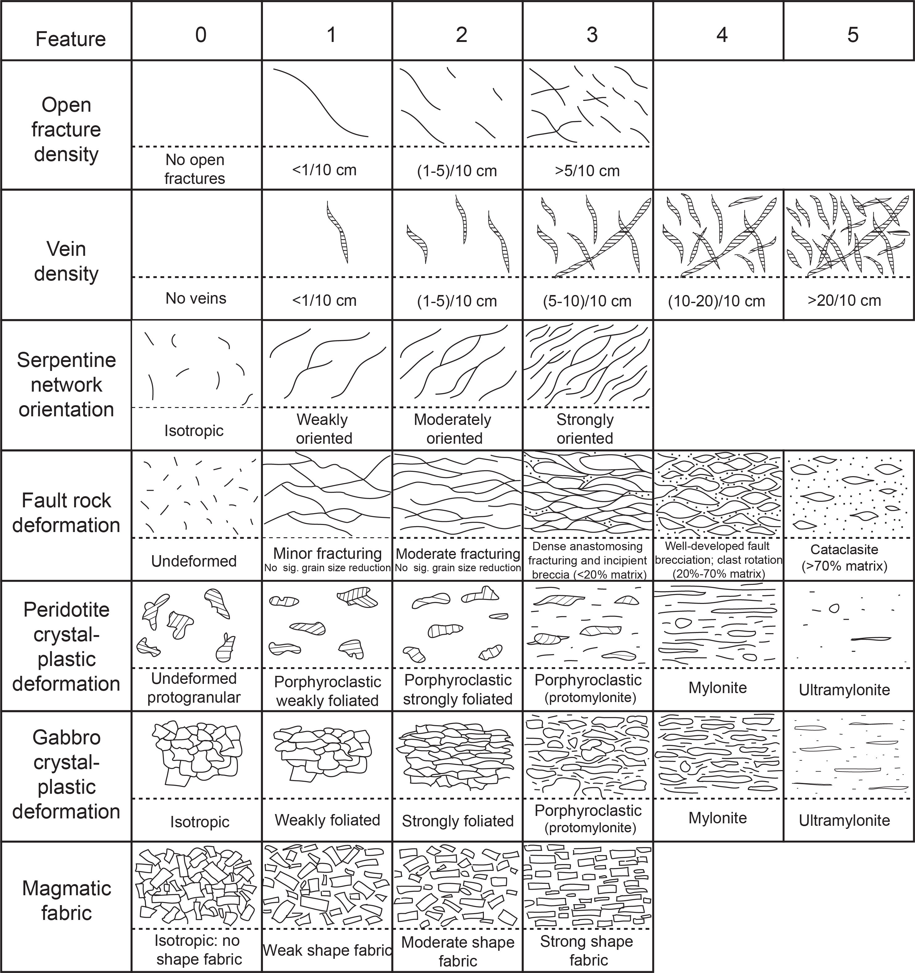
Figure F26. Intensity ranks.
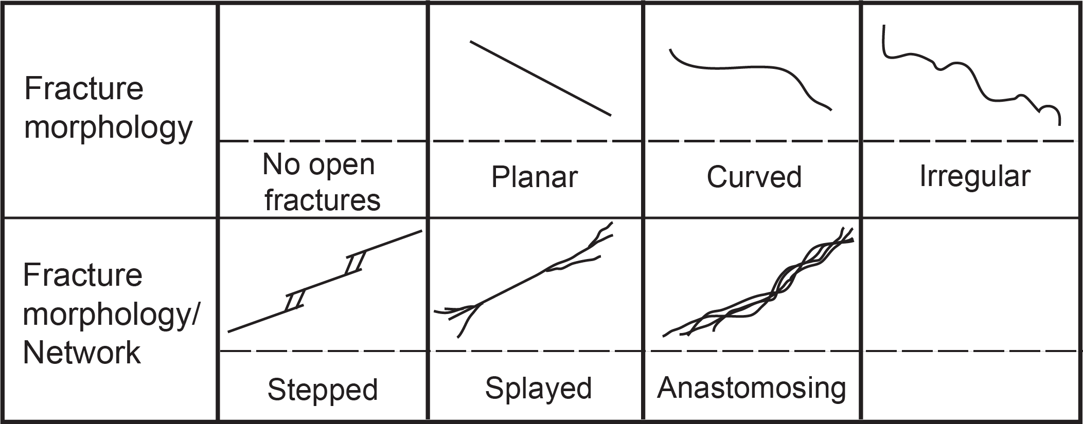
Figure F27. Fracture and fracture network morphology classifications.
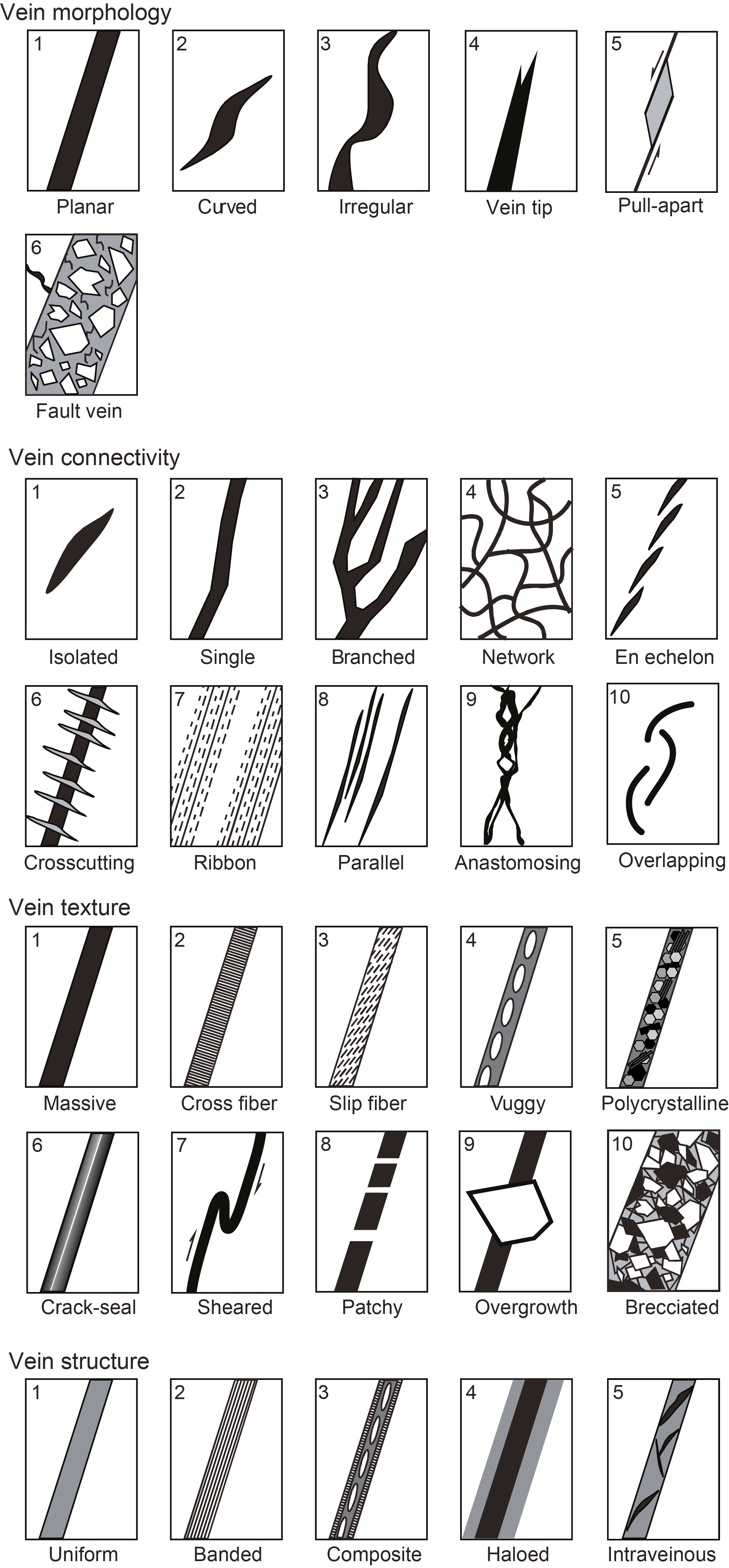
Figure F28. Veins and vein network classifications.
6.2.3.1. Magmatic structures
Intrusive and structural contacts were measured and described according to the igneous petrology (see Igneous and metamorphic petrology). Descriptions include the following:
- Contact relationship: sharp, gradational, or sutured (contacts where individual mineral grains are interlocked across the contact).
- Contact geometry: planar, curved, or irregular.
- Contact orientation: dip and dip azimuth in the core reference frame.
Magmatic fabrics were defined by the presence and intensity of any shape-preferred orientation of magmatic phases. A magmatic fabric intensity of 0 was assigned to intervals characterized by isotropic texture and/or where no igneous textures are preserved because of crystal-plastic overprinting (Figure F26). The structural team measured the orientations of those individually defined magmatic veins that were previously defined as an interval by the petrology team. Descriptions of magmatic fabric include the following:
- Magmatic fabric type: modal layering, grain-size layering, shape-preferred orientation, or isotropic; if none of these describe the observations well, the nature of layering is described in the comments.
- Magmatic fabric intensity accompanied by intensity rank (Figure F26):
- Magmatic fabric shape-preferred orientation geometry (if present): planar, linear, or planar-linear.
- Magmatic fabric boundary definition: sharp or diffuse.
- Magmatic phase(s) that define the preferred shape orientation: olivine (ol), plagioclase (pl), clinopyroxene (cpx), orthopyroxene (opx), or oxides (ox).
- Orientation of the magmatic fabric (dip and dip azimuth of magmatic fabrics, as well as trend and plunge of any lineation in the layering, measured in the core reference frame).
- Magmatic fabric comment.
- Magmatic fabric thickness (in centimeters).
6.2.3.2. Crystal-plastic fabrics
CPFs include planar or linear fabrics defined by crystals exhibiting plastic strain. CPFs associated with mantle deformation in peridotites were classified separately from mantle fabrics produced by discrete shear zones. Schistosity was reported from zones of alteration, where fabrics are controlled by secondary minerals such as talc, chlorite, and amphibole. Serpentine foliations were reported from serpentinized peridotite where mesh textures show a preferred orientation, which may pseudomorph a preexisting mantle fabric. Abyssal peridotites pose a special problem for grading crystal-plastic deformation because they have usually been emplaced from the Earth's deep interior by high-temperature crystal-plastic creep processes and therefore lack a primary igneous texture. They generally have either protogranular or porphyroclastic textures when unmodified by relatively shallow deformation processes associated with unroofing and exposure to the seafloor. We therefore use a separate textural criterion for mantle fabrics in abyssal peridotites, which we based on the methodology used during ODP Leg 209 (Shipboard Scientific Party, 2004) and Expeditions 357, 360, and 399 (Früh-Green et al., 2017; MacLeod et al., 2017; McCaig et al., 2024) (Figure F26).
Protogranular textures are generally the primitive fabric, characterized by smoothly curved grain boundaries with complex cusps and lobes. Because alteration has largely obscured olivine grain size and shape entirely in hand specimens of abyssal peridotites, the visual core description is almost entirely based on pyroxene and spinel textures. Rocks with a purely protogranular texture are graded 0 because this is the earliest formed texture and may or may not have a preferred crystallographic mineral fabric or a shape fabric. Porphyroclastic textures are generally superimposed on protogranular textures, and frequently elements of both are present. Rocks with porphyroclastic texture are graded 1 (weak foliation) if the pyroxene shape fabric is weak or absent. When pyroxenes exhibit a significant shape fabric, the sample is graded a 2 (strong foliation) under the crystal-plastic field with the caveat that at this grade only a few protogranular textural elements are present. These samples are still referred to as porphyroclastic. When the texture starts to become strong and foliation develops accompanied by significant grain-size reduction, the texture is called protomylonitic and is graded 3 under crystal-plastic deformation. At this grade there are generally no protogranular textural elements left. If the peridotite has significant grain-size reduction and consists of a fine-grained mass of olivine with embedded pyroxene porphyroclasts and a prominent foliation, the rock is graded 4 and listed as a mylonite. If there is no visible foliation due to extreme grain-size reduction, the rock is listed as an ultramylonite and graded 5. This deformation scale closely parallels that used for crystal-plastic deformation of gabbro and other crustal rocks during previous scientific drilling expeditions and corresponds to similar intensities of deformation at each grade.
Schistose fabrics formed by alteration minerals are classified separately. During Expedition 402, the rocks recovered show a series of variably deformed serpentinites formed during alteration (Bonatti et al. 1990; ODP Leg 107). These fabrics were mostly found in alteration veins. The compositional characteristics of these schists are reported by the metamorphic team, whereas the type, intensity (ranked from 0 to 3), and orientation of schistose fabrics within these rock types are reported here as part of the structural geology section.
Serpentine foliation produced by background alteration of mantle peridotites is reported as a distinct fabric. Strong planar fabrics can be formed during serpentinization by the development of closely spaced subparallel veins termed ribbon texture (O'Hanley, 1996). The texture is characterized by anastomosing, often cross-fiber, replacement serpentine veins. In general, the veins wrap around relict or pseudomorphed pyroxene grains with little evidence of shear offset. These produce a strongly foliated serpentinite that is a variant of the hourglass serpentine texture and largely represents in situ replacement of the primary olivine (O'Hanley, 1996). This texture may parallel preexisting crystal-plastic foliation, and its intensity may reflect the stress state or the presence of a preexisting fabric in the rock. The strength of serpentine foliation is rated on a scale from 0 (no foliation) to 5 (strongly foliated).
Descriptions for CPFs include the following:
- Deformation intensity and rank (Figure F26):
- 0 = undeformed (O).
- 1 = weakly foliated/lineated.
- 2 = strongly foliated/lineated.
- 3 = protomylonitic.
- 4 = mylonitic.
- 5 = ultramylonitic.
- CPF boundary sharpness: sharp or diffuse.
- CPF perpendicular thickness (in centimeters).
- Comments on CPF (additional description such as lithology, crosscutting vein, type of contact, etc.).
- Sense of shear: normal (n), reversed (r), dextral (d), sinistral (s), a combination of these (nd, ns, rd, or rs), or unknown.
- Orientation of the CPF (dip and dip azimuth, where measurable in the core reference frame; in practice, almost exclusively foliation planes).
- Certainty of the observed feature (CPF, peridotite fabric, or sense of shear):
- Schistose fabric intensity:
- Serpentine foliation intensity:
- 0 = no mesh.
- 1 = incipient mesh.
- 2 = regular mesh.
- 3 = weakly foliated mesh.
- 4 = moderately foliated mesh.
- 5 = strongly foliated mesh.
- 6 = undetermined.
- Schistose/Serpentine fabric type: planar (S), anastomosing, S-C fabric, or mesh texture.
- Schistose/Serpentine fabric comment.
- Lineation mineral.
- Lineation intensity: weak or strong.
- Orientation of the lineation: trend and plunge, where measured in the core reference frame.
- Orientation of fabric and the measured fabric type: dip and dip azimuth in the core reference frame; in practice, almost exclusively foliation planes.
The final characterization of the structure was performed after petrographic inspection, when possible.
6.2.3.3. Brittle deformation
Brittle fabrics described during Expedition 402 include breccias, faults (defined as fractures with shear displacement), and fractures (including open and drilling induced). Drilling-induced fractures are subhorizontal and have rounded edges and no mineralization. The orientation of drilling-induced fractures was not measured; however, their density (number of fractures per 10 cm) was measured. Descriptions include the following:
- Fault rock type and degree, based on the percentage of matrix present in each fault rock (Figure F26):
- 0 = undeformed.
- 1 = minor fracturing (no significant grain-size reduction).
- 2 = moderate fracturing (no significant grain-size reduction).
- 3 = dense anastomosing fracturing and no significant clast rotation, incipient breccia (grain-size reduction < 20%).
- 4 = well-developed fault, breccia, and clast rotation (20%–70% grain-size reduction).
- 5 = cataclasite (grain-size reduction > 70%).
- Brittle deformation comments.
- Fault rock cohesion:
- Apparent fault offset (in centimeters), where measurable.
- Sense of shear: normal (n), reversed (r), dextral (d), sinistral (s), a combination of these (nd, ns, rd, or rs), or unknown.
- Certainty of the observed fault rock:
- Average size of clast in fault rock (in millimeters).
- Fracture morphology: planar, curved, irregular, or no open fractures if none were recorded (Figure F27).
- Fracture network morphology: stepped, splayed, or anastomosing (Figure F27).
- Fracture perpendicular thickness (in centimeters).
- Orientation (dip and dip azimuth) of fracture and trend and plunge of associated lineation (e.g., slickensides/slickenlines/slickenfibers).
- Striae comments (e.g., slickensides/slickenlines/slickenfibers).
- Orientation (dip and dip azimuth) of fracture and trend and plunge of associated striae (e.g., slickensides/slickenlines/slickenfibers) including striae in veins.
- Vein density:
- 0 = no open veins.
- 1 = <1 vein per 10 cm.
- 2 = 1–5 veins per 10 cm.
- 3 = 6–10 veins per 10 cm.
- 4 = 11–15 veins per 10 cm.
- 5 = >15 veins per 10 cm.
- Fracture density:
6.2.3.4. Alteration and magmatic veins
The igneous, metamorphic, and structural teams described the veins together. Structural descriptions of veins are summarized in Figure F28 and include the following:
- Vein type: magmatic, metamorphic or both.
- Vein connectivity: isolated, branched, single, network, en échelon, crosscutting, ribbon, parallel, anastomosing, and overlapping.
- Vein deformation: pull-apart, brecciated, crack-seal, sheared, tension gash, and secondary cementation of breccia.
- Vein fill minerals, whether magmatic (plagioclase, pyroxenes, etc.) or alteration minerals (for example, amphibole, serpentine, talc, etc.).
- Sense of shear: normal (n), reversed (r), dextral (d), sinistral (s), a combination of these (nd, ns, rd, or rs), or unknown.
- Comments on vein structure, including relation to other veins or vein orientations, crosscutting relationships, sets of parallel veins, or conjugate vein sets and opening directions if macroscopically observable.
- Orientation of the vein given by dip and dip azimuth and in the core reference frame.
6.3. Microstructures
6.3.1. Workflow organization
To better characterize the different types of deformation, we studied the microstructural features of interesting and/or prominent mesoscopic structures. Thin sections were examined to achieve the following objectives:
- Characterize the microstructure of the rocks,
- Confirm macroscopic descriptions of structures,
- Document crystal-plastic and brittle overprinting of magmatic fabrics,
- Provide information on the kinematics of deformation,
- Identify crosscutting relationships between magmatic and crystal-plastic deformation and alteration processes, and
- Document downhole strain variations.
The shipboard thin sections were systematically oriented relative to the core reference frame, as marked on each thin section (Figure F20). Marking two directions is necessary to obtain a unique orientation of the thin sections cut parallel to the cut surface of the core. Macroscopic observations were refined by microscopic description. Digital photomicrographs were taken to document microstructures that best illustrated different deformation styles, crosscutting relationships, and intensity recorded in the LIMS database. Microstructural notes were entered into the ts_structures worksheet in the GEODESC thin section workbook.
6.3.2. Microstructure terminology
We followed the terminology used during Expedition 360, which largely follows that of Passchier and Trouw (2005). In the ts_structures worksheet of the thin section workbook, we described the following microscopic features for each thin section:
- Type of microstructure: magmatic, submagmatic/transitional, crystal-plastic, fault rock, or metamorphic.
- Recrystallized grain size: fine (<100 µm), medium (100–300 µm), or coarse (>300 µm).
- Recrystallized grain shape: anhedral, subhedral, euhedral, equigranular, or inequigranular.
- Crystal-plastic subgrain boundaries: straight, curved, serrate, or polygonal.
- Intracrystalline deformation features: fractures, undulose extinction, deformation twins, subgrains, kinked, or bent, specifying the deformed minerals.
- Intensity of static recrystallization: absent, weak, strong, partial, or complete.
- Intensity of magmatic fabric and rank:
- Intensity of dynamic recrystallization: absent, weak, strong, or complete.
- CPF intensity: listed for each individual phase using the same descriptors as above.
- Intensity of overall CPF with intensity rank:
- 0 = undeformed.
- 1 = weakly foliated/lineated.
- 2 = strongly foliated/lineated.
- 3 = porphyroclastic/protomylonitic.
- 4 = mylonitic.
- 5 = ultramylonitic.
- CPF sense of shear: normal (n), reversed (r), dextral (d), sinistral (s), a combination of these (nd, ns, rd, or rs), or unknown (u).
- Maximum lineation intensity (independent of phase): weak or strong.
- Lineation intensity: listed for each individual phase using same descriptors as above.
- Fault rock intensity and rank:
- 0 = undeformed.
- 1 = minor fracturing.
- 2 = moderate fracturing.
- 3 = dense anastomosing fracturing with incipient breccia.
- 4 = well-developed fault breccia.
- 5 = cataclasite.
- Fractures: absent, rare, or common.
- Fault rock clast percent of cataclasite/brittle fracture.
- Size (in millimeters) of clasts in cataclasite/brittle fracture.
- Sense of shear: normal (n), reversed (r), dextral (d), sinistral (s), a combination of these (nd, ns, rd, or rs), or unknown.
- Fracture abundance:
- 0 = no fracture.
- 1 = rare fractures.
- 2 = few fractures.
- 3 = common fractures.
- 4 = abundant fractures.
- Vein abundance:
- Serpentine foliation intensity:
- Maximum schistosity intensity (independent of phase):
- Schistose/serpentine fabric type, listed for each mineral: planar (s), anastomosing, S-C fabric, or mesh texture.
- Schistose sense of shear: normal (n), reversed (r), dextral (d), sinistral (s), a combination of these (nd, ns, rd, or rs), or unknown (u).
- General microstructure comments: any features not listed in the above categories, for example, crosscutting relationships, the shear sense indicator(s) used to determine the shear sense in deformed rocks.
7. Sediment and interstitial water geochemistry
During Expedition 402, shipboard geochemical analyses were performed on both IW and sediment samples. In addition, headspace analysis of hydrocarbon gases was conducted at each site according to the routine shipboard safety and pollution prevention protocol. Geochemical analyses included inorganic chemical analysis of the IW present in the pores and fractures of the cored sediments and rocks and organic and inorganic chemical analysis of the solid matrix. Table T5 lists precision and detection limits for all analyses made during this expedition. All data obtained during this expedition have been uploaded to the LIMS database.
7.1. Headspace gas analysis
As a part of standard shipboard monitoring procedures, hydrocarbon gas concentrations and compositions were routinely monitored from headspace samples to ensure safety, following the sampling and analysis protocols described in Kvenvolden and McDonald (1986), Pimmel and Claypool (2001), and the IODP pollution prevention and safety protocol (Fritz, 1980; JOIDES Pollution Prevention and Safety Panel, 1992; Shipboard Scientific Party, 1994). To avoid drilling into sediments containing hydrocarbon concentrations above safety levels, the molar ratios of different hydrocarbon gases were calculated, including methane (C1 or CH4), ethene + ethane (C2), propene + propane (C3), i-butane (i-C4), n-butane (n-C4), i-pentane (i-C5), n-pentane (n-C5), i-hexane (C6), and n-hexane (n-C6).
Sediment plugs of ~5 cm3 were collected from each core immediately after retrieval on deck using a brass boring tool for soft to moderately consolidated sediments. Where consolidated sediments or igneous rocks were encountered, small rock chips were used when available. A headspace sample was taken in each core at the top of Section 5, immediately below the IW sample, unless core disturbance or incomplete recovery necessitated selection of a different section. Each sample was then placed in a properly labeled 20 cm3 glass serum vial (labeled “HS” with the core and section number and the depth interval from which it was taken) and sealed with crimped metal cap with a polytetrafluoroethylene (PTFE)/white silicone septum. The vial was placed in an oven at 60°C for 30 min to allow dissolved hydrocarbon gases to equilibrate with the headspace. A 5 cm3 aliquot of the evolved headspace gas was extracted from each vial through the septum using a gas-tight syringe and manually injected onto an Agilent 7890 Series II gas chromatograph (GC) equipped with a split/splitless injector and a flame ionization detector (FID) set at 300°C with a split ratio of 30:1. The GC column used was an Agilent J&W PLOT Alumina/S column (25 m × 320 µm diameter × 8 µm film thickness). Helium was used as the carrier gas at a constant flow rate of 3 mL/min. The oven temperature program was set to hold at 35°C for 4 min and then increase to 200°C for 5 min at a rate of 25°C/min, followed by a final hold at 200°C for 5 min. The total run time per injection was 15.6 min.
Data were collected and evaluated using the Hewlett Packard 3365 ChemStation software (2001–2016). The FID response was calibrated using gas standards with variable amounts of low molecular weight hydrocarbons provided by Scott Specialty Gases (Air Liquide) and checked daily. The concentration of the analyzed hydrocarbon gases was reported in parts per million by volume, and the value of two different ratios were calculated: C1/C2 and C1/C+. The latter ratio was obtained as follows and was used during the previous Expedition 385 (Teske et al., 2021):
7.2. Interstitial water collection and analysis
7.2.1. Interstitial water sampling from sediment
Inorganic geochemical data from IW profiles provide information on abiotic and biotic reactions as well as water-rock interactions and fluid migration. During Expedition 402, whole-round samples for IW analysis were cut from cores on the catwalk, capped as quickly as possible, and immediately transported to the chemistry laboratory for squeezing. Standard whole-round samples were 5 cm long, but as porosity decreased downhole, the sample size could be increased to 15 cm to extract enough water for shipboard analyses. Typically, one IW sample was collected in each core from the bottom of Section 4. After removing the whole-round from the core liner, the surface of each whole-round sample was carefully scraped off with a spatula under ambient laboratory conditions to remove potential contamination from seawater, drilling fluids, drilling disturbances, and/or sediment smeared along the inside of the core liners. The cleaned sediments were transferred to a 9 cm diameter titanium squeezer that was then loaded into a Carver hydraulic laboratory press (Manheim and Sayles, 1974) and squeezed to extract IW at pressures up to ~25,000 lb (~24.3 MPa) to prevent water release from clay minerals during squeezing. The IW extracted from the squeezed sediment samples was filtered through a nanopure water (resistivity of 18.2 MΩ·cm) precleaned Whatman Number 1 filter placed in the squeezer cell above a titanium mesh screen. Approximately 30 mL of IW was collected in a 60 mL HCl- and water-washed (18.2 MΩ·cm) high-density polyethylene (HDPE) syringe attached to the squeezer assembly and then filtered through a 0.45 µm polyethersulfone membrane filter into separate sample containers. Aliquots for analysis using ICP-AES (the inductively coupled plasma–optical emission spectrometer [ICP-OES] on board is run only in ICP-AES mode) were acidified by adding ~10 µL of trace metal–grade concentrated HNO3 and placed in 2 mL cryovials. Aliquots for titration and ion chromatograph (IC) and spectrophotometric (ammonium and phosphate) analyses were put in 12 mL HDPE vials. IW samples were analyzed on board following the protocols outlined by Gieskes et al. (1991), Murray et al. (2000), and the IODP user manuals for shipboard instrumentation (https://tamu-eas.atlassian.net/
After each use, the squeezer was cleaned with tap water, rinsed with 18.2 MΩ·cm deionized water, and thoroughly dried with compressed air prior to further sample processing. The squeeze cake residues were then subsampled into plastic bags for shipboard analyses (total inorganic carbon [TIC] content, total carbonate content, and total organic matter content, as well as total carbon [TC], total organic carbon [TOC], total nitrogen [TN], and total sulfur [TS] contents; see below) and postcruise research. The remaining squeeze cakes were stored at 4°C.
7.2.2. Salinity, alkalinity, and pH
Salinity, alkalinity, and pH were measured immediately after IW sampling following the procedures in Gieskes et al. (1991). Salinity measurements were made using a Fisher Model S66366 optical refractometer. International Association for the Physical Sciences of the Oceans (IAPSO) standard seawater (salinity = 35) was used for salinity calibration.
The IW alkalinity was determined by Gran titration with a Metrohm 794 basic Titrino autotitrator, and IW pH was measured using a combination glass electrode. A 3 mL sample was titrated against 0.1 M HCl at 25°C to reach an endpoint of pH = 4.2. The IAPSO standard seawater (alkalinity = 2.325 mM; certified value) and laboratory-made standards (5–100 mM of Na2CO3 alkalinity, made by mixing different proportions of 0.7 M KCl + 0.1 M Na2CO3) were used for calibration. The IAPSO standard was analyzed at the beginning and end of a set of samples for each site and after every 10 samples. Repeated measurements of IAPSO seawater for alkalinity gave an analytical precision better than 2.0%.
7.2.3. Major cations and anions
The concentrations of major anions (SO42–, Br–, and Cl–) and cations (Na+, Ca2+, Mg2+, and K+) in IW samples were measured using a Metrohm 850 Professional IC using IW aliquots of 100 µL that were diluted at 1:100 with 18.2 MΩ·cm water. For anion analysis, a Metrosep C6 column (100 mm long; 4 mm inner diameter) was used with 3.2 mM Na2CO3 and 1.0 mM NaHCO3 solutions as eluents. For cation analysis, a Metrosep A supp 7 column (150 mm long; 4 mm inner diameter) was used with 1.7 mM of HNO3 and pyridine-2,6-dicarboxylic acid (PDCA) solutions as eluents. For quality control, IAPSO seawater standards were used at various dilutions to generate a 9-point calibration curve. Repeated measurements of anion and cation concentrations in IAPSO standard seawater yielded the following precision for each ion: Cl– < 0.8%, SO42– < 0.9%, Br– < 1.4%, Na+ < 0.8%, Mg2+ < 1.3%, K+ < 1.1%, and Ca2+ < 4.4%.
7.2.4. Spectrophotometric analysis of ammonium, phosphate, and total free sulfides
Concentrations of dissolved ammonium (NH4+), phosphate (PO43–), and total free sulfides (ΣH2S) were determined using an Agilent Technologies Cary Series 100 UV-Vis spectrophotometer with a sipper sample introduction system following the protocol in Gieskes et al. (1991) and Cline (1969) for ammonium and phosphate measurements and a modified method from Cline (1969) and Grasshoff et al. (1999) for sulfide measurements.
For analysis of NH4+ concentration, each IW sample of 0.1 mL was diluted with 1 mL of 18.2 MΩ·cm water prior to addition of 0.5 mL phenol-ethanol, 0.5 mL sodium nitroprusside, and 1 mL oxidizing solution (trisodium citrate and sodium hydroxide) in a 5 mL capped glass vial. The determination of ammonium is based on diazotization of phenol and subsequent oxidation of the diazo compound by Clorox to produce a blue color. The sample-reagent mixture was held at room temperature for ~6.5 h for full color development, and its absorbance was measured spectrophotometrically at 640 nm in the microplate reader. A regular 9-point calibration curve (0, 50, 100, 150, 200, 400, 600, 800, and 1000 µM) was used, and check standards (50 and 600 µM) were run every 10 samples. The precision and accuracy of the NH4+ analyses were better than 4% and 3%, respectively.
The determination of PO43– concentrations was based on the reaction of orthophosphate with Mo(VI) and Sb(III) in an acidic solution to form an antimony-phosphomolybdate complex, which is subsequently reduced by ascorbic acid to form a blue color. Each sample of 0.3 mL was diluted prior to color development with 1 mL deionized water (18.2 MΩ·cm) in a 4 mL glass vial. After adding 2 mL of mixed reagent (ammonium molybdate, sulfuric acid, ascorbic acid, and potassium antimony tartrate), the vial was capped and kept at room temperature for 30 min to develop color. Then, the concentrations of PO43– were determined at an absorbance of 885 nm. A regular 9-point calibration curve (0, 5, 10, 15, 20, 40, 60, 80, and 100 µM) was used, and check standards (10 and 60 µM) were run every 10 samples. The precision and accuracy of PO43– analyses were both better than 4%.
For the analysis of total sulfides (ΣH2S = S2− + HS− + H2S), zinc sulfide (ZnS) precipitate in IW samples was measured colorimetrically as methylene blue after reaction of zinc sulfide or zinc acetate under acidic conditions with N,N-dimethyl-p-phenylenediamine or DMPD ([CH3]2NC6H4NH2·2HCl, 19 mM; 20 µL per 1 mL of sample) and ferric chloride (FeCl3 100 mM; 20 µL per 1 mL of sample) using a modified method from Cline (1969) and Grasshoff et al. (1999). Sulfide concentrations were measured without dilution for concentrations ranging 1–60 µM and with dilution for concentrations ranging 60–600 µM using a dilution factor of 10. Dilutions were made with N2-purged deionized 18.2 MΩ·cm water. The intensity of the methylene blue is read colorimetrically at 670 nm after 5 min waiting for color development. For each dilution factor, a 7-point calibration curve (0, 2, 4, 10, 20, 40, and 80 µM) was drawn using a solution of 0.75 mM sodium sulfide (Na2S) in N2-purged deionized water (18.2 MΩ·cm), and check standards (20 µM) were run every 10 samples. Precision and accuracy of ΣH2S analyses were 2.4% and 6.2%, respectively.
7.2.5. Major and minor elements by inductively coupled plasma–optical emission spectrometry
Selected elements (Ca, Mg, Na, K, Li, Sr, B, Si, Mn, Fe, and Ba) were analyzed using an Agilent 5110 ICP-OES (in ICP-AES mode) with an SPS 4 autosampler. Samples were analyzed according to the methods of Murray et al. (2000). IW samples were diluted prior to analysis with a dilution factor of 10. The diluent is 2% HNO3 spiked with 100 ppm Be, In, and Sc with 200 ppm Sb. The IAPSO seawater and salt solutions containing each major and minor element at various concentrations were used as calibration standards.
Samples were run in batches. Each sample was analyzed five times, and the average of these five runs was taken as the reported measurement. Each batch (of ~50 samples) contained six artificial standards with known concentrations of all elements of interest. Two additional standards were measured periodically to monitor instrumental drift. All raw intensity data were downloaded and converted to concentration values based on standards using the ICP-OES software. Replicate analyses of standard solutions were used to estimate precision and accuracy. These values were typically less than 1% and 5%, respectively. Table T6 shows the list of wavelengths performed for major and minor element analysis measured on IW using ICP-AES.
7.3. Sediment collection and bulk geochemistry
7.3.1. Sediment collection
Geochemical analyses were conducted on approximately 5–10 cm3 of bulk sediment collected in sampling bags from both IW squeeze cake residues and from intervals of sedimentologic interest noted in the split cores. All these samples were freeze-dried for a minimum of 12 h, ground to a fine powder, and homogenized using an agate pestle and mortar, and then analyzed for (1) TIC and total carbonate contents; (2) TC, TN, and TS contents; (3) TOC and sedimentary organic matter contents; and (4) XRD analysis. The remaining sample was stored in a glass vial and archived. The XRD methodology is reported in Lithostratigraphy. Finally, all squeeze cake residues and additional sediment samples collected by sedimentologists were also used to measure the abundance of various elements using onboard portable X-ray fluorescence spectrometry (pXRF) (see Igneous geochemistry).
7.3.2. Total inorganic carbon content and total carbonate content
During Expedition 402, the nature of carbonate phases (aragonite, low- and high-magnesian calcite, iron- and/or calcium-rich dolomite, and stoichiometric dolomite) occurring in each sample was first determined using XRD analysis before the measurement of TIC and total carbonate contents.
TIC content was measured by quantifying the carbon dioxide (CO2) released from an acidification process on carbonate minerals using an UIC Coulometrics 5017 CO2 coulometer. Approximately 10–12 mg of freeze-dried and powdered sediment was accurately weighed into a clean glass vial using two electronic balances and a computerized averaging system that corrects for ship motion (Cahn C-31 automated electrobalance). The sediment was then reacted with 5.0 mL of 1 M HCl on a hot plate set at 50°C, resulting in a release of CO2. This reaction converts any present carbonate to CO2. The released CO2 was then transferred with an N2 carrier gas to a coulometer cell filled with a solution containing excess monoethanolamine and a colorimetric pH indicator. As the gas passed through the cell, CO2 was quantitatively absorbed and reacted with the monoethanolamine to form the carbamate salt of monoethanolamine. This solution was titrated with electrochemically generated OH– to a colorimetric endpoint, and the corresponding change in light transmittance in the coulometric cell was monitored with a photodetection cell. This change in light transmittance was proportional to the TIC content of the sample. If a sample contains only calcium carbonates (aragonite and low- and/or high-Mg calcite), all the evolved CO2 was attributed to the dissolution of calcium carbonate and the TIC content was measured 5 min after the start of the reaction. The weight percent of calcium carbonate was calculated from the TIC content using the following equation:
Weighed amounts of standard calcium carbonate (>99.9% CaCO3; Fisher Scientific) and of standard dolomite (MgCa[CO3]2; British Chemical Standards No. 368) were used to monitor analytical precision (1.46%) and accuracy (better than 1%).
If carbonate phases other than calcium carbonate were identified by XRD, the evolved CO2 was derived from the dissolution of all these minerals and the equation cited above could not be used. In this case, the qualitative and relative semiquantitative mineralogical composition of the carbonate fraction was determined using both XRD results and the total carbonate content. To estimate the total carbonate content, 0.50 to 3.00 ± 0.05 g of each bulk sediment sample powder was weighed into a 45 mL plastic centrifuge tube using a Mettler Toledo balance. Total carbonate content, expressed in percent, was estimated as the difference between freeze-dried weight of the sediment and weight of the remaining sediments dried at 60°C after hydrochloric acid treatment (2 M; 30 min).
7.3.3. Total carbon, total nitrogen, and total sulfur content
Approximately 15–17 mg of freeze-dried and powdered bulk sediment was accurately weighed into tin cups with the Cahn C-31 automatic electrobalance. The samples were mixed with an equivalent mass of V2O5 catalyst, and the tin cups were carefully folded to enclose the sample powders. The bulk sediment powder was combusted (950°C) in a stream of O2 on a Flash EA-1112 Series Thermo Electron Corporation carbon-hydrogen-nitrogen-sulfur (CHNS) analyzer. The reaction gases were passed through a reduction chamber to reduce nitrogen oxides to N2, and the mixture of CO2, N2 and SO2 gases was separated by packed column CHNS/CNS GC (Thermo Electron) and detected using a thermal conductivity detector (TCD). Peak areas from the TCD were calculated to determine the TC, TN, and TS of the samples. A reference standard of Buffalo River Sediment (NIST 8704; C = 3.35%, N = 0.18%, and S = 0.4%) was run every 10 samples and used to determine analytical precision (TC = 1.1%; TN = 10.0%; TS = 10.0%).
7.3.4. Total organic carbon and organic matter contents
For each bulk sediment sample, the TOC content was calculated by subtracting the weight percent of TIC from the TC content determined with the CHNS analyzer (see above).
The atomic TOC/TN ratio was calculated to identify the source (marine or terrestrial) of the organic matter (Meyers, 1994). The relationships between TS content and TOC content in sediments were also calculated and compared to the normal marine trend, which has a TOC/TS ratio of 2.8 in fine-grained, reducing, and organic-rich (TOC < 6 wt%) sediments deposited under an oxygenated water column (Goldhaber and Kaplan, 1974; Berner, 1982). A TOC/TS value less than 2.8 may indicate anoxic depositional conditions (Leventhal, 1983) or fluid circulation in the sediment (e.g., Passier et al., 1996).
To estimate the total organic matter content, each powdered bulk sediment sample of 1.00 to 5.00 ± 0.05 g was weighed into an alumina crucible using a Mettler Toledo balance. Total organic matter content of the sediment, expressed in percent, was estimated as the difference between the freeze-dried weight and the weight of the residue after heating at 550°C for 6 h in a muffle furnace (Parker, 1983; Santisteban et al., 2004).
7.3.5. Source rock analysis and organic matter characterization
For selected samples at Site U1617 (Holes U1617A and U1617B), the amount, type, and maturity of organic carbon present in these sediments were determined by pyrolysis assay using the source rock analyzer (SRA; Weatherford Laboratories). For this purpose, all measurements were performed using ~80 mg of freeze-dried and ground sediments, which were preceded by a blank analysis and calibration using rock standard STD 533 from Weatherford Laboratories. The SRA parameters include the following:
- S1 peak (mg HC/g rock): formed by free hydrocarbons (HC) already present in the samples released during a first heating step at 300°C for 3 min under helium condition.
- S2 peak (mg HC/g rock): formed by hydrocarbons resulting from the cracking of kerogen and high molecular weight free hydrocarbons generated by the pyrolysis of organic matter during the programmed temperature increase from 300° to 600°C at a heating speed of 25°C/min under helium condition.
- Tmax (°C): nominal temperature at which the maximum of hydrocarbon yield is reached during the pyrolysis step.
- S3 peak (mg CO2/g rock): formed by CO2 released during low-temperature pyrolysis between 340° and 390°C.
- S4 peak (mg C/g rock): formed by CO2 produced by oxidation of the organic matter remaining in the sample after pyrolysis (pyrolysis residue). Because the instrument automatically combines convertible carbon (pyrolyzed carbon) with the residual carbon (RC) and reports the TOC value to determine the S4 value, calibration was conducted based on the following equation:
TOCSRA, in unit weight of carbon per unit weight of whole rock, was calculated from S1, S2, and S4, assuming that S1 and S2 are an average carbon content of hydrocarbons of 83% by atomic weight, as follows:
The hydrogen index (HI; mg HC/g TOC) and the oxygen index (OI; mg CO2/g TOC), two pyrolysis parameters that are frequently used in conventional elemental analysis of kerogen and coal (Espitalié et al., 1985), were calculated as follows:
The HI and OI ratios were commonly plotted on a Van Krevelen diagram (Figure F29) to determine the type of kerogen and its thermal maturity. Three basic kerogens have been identified (Tissot et al., 1973):
- Type I, with high initial HI and low initial OI, is derived primarily from algal organic matter deposited mainly in lacustrine environments, producing primarily waxy oil.
- Type II, which is moderately hydrogen rich and oxygen poor, is derived from autochthonous organic matter deposited under anoxic conditions in marine environments and produces moderate oil upon thermal maturation.
- Type III, with low initial HI and high initial OI, is derived from terrestrial plant debris (especially wood) and/or aquatic organic matter deposited in an oxidizing environment that produces primarily gas upon thermal maturation.
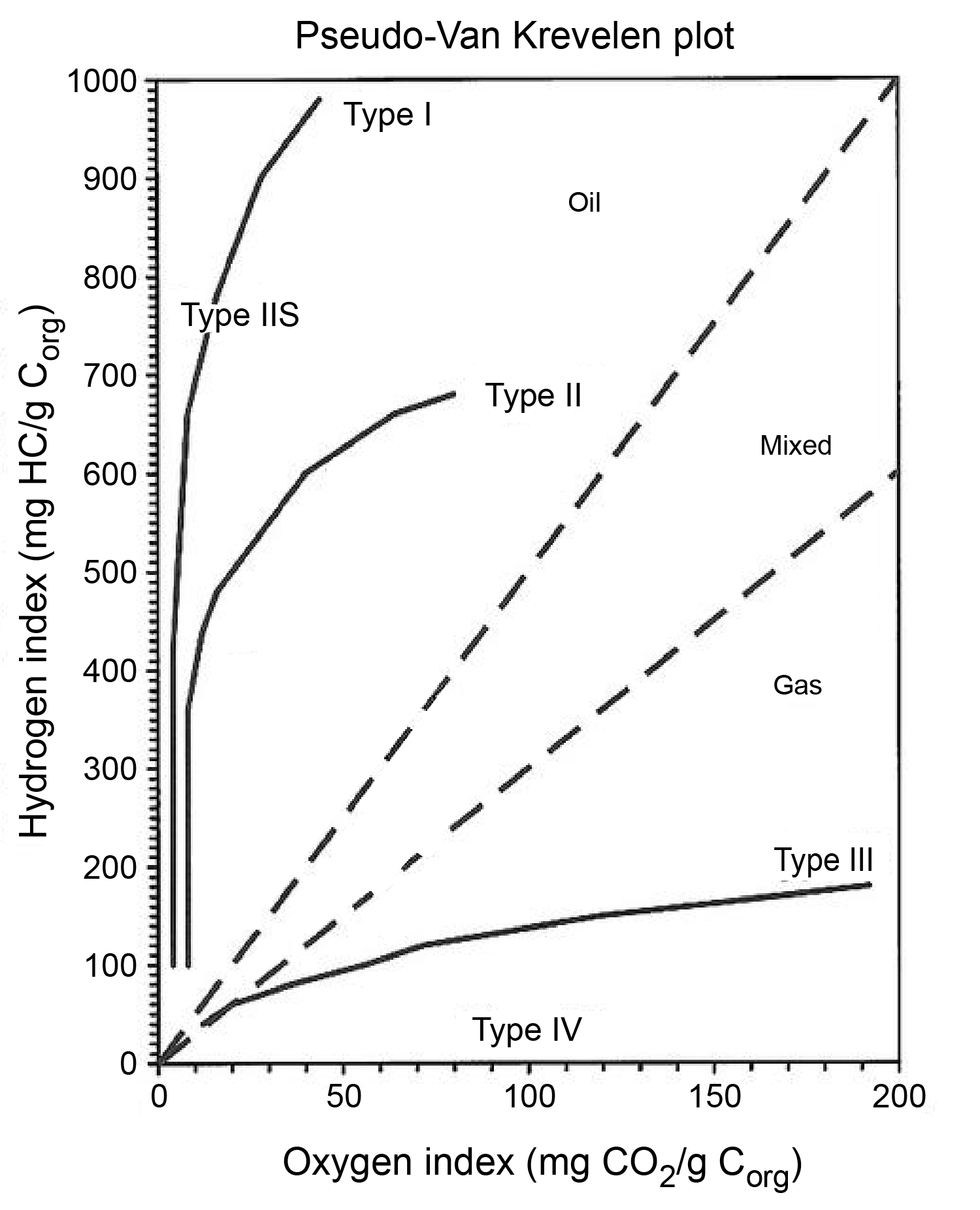
Figure F29. Hydrogen index and oxygen index.
Two other kerogen types were also common: Type IIS and Type IV. Type IIS kerogen, characterized by high initial HI and low initial OI, is derived from autochthonous organic matter deposited under highly reducing marine environments (Orr, 1986), resulting in a substitution of oxygen by sulfur in the kerogen structure. Type IV kerogen, with a very low initial HI and a variable initial OI, is a product of significant alteration and/or oxidation of organic matter in the depositional environment composed of mostly inert matter with no hydrocarbon-generating potential (Tissot and Welte, 1984). However, because the chemical composition of the organic matter is susceptible to evolution during burial, the type of kerogen (I, II, IIS, III, IV, or a mixture of these) determined from the chemical composition is not a proper indicator of the origin of the organic matter (Tissot and Welte, 1978).
8. Igneous geochemistry
Igneous samples recovered during Expedition 402 were characterized using a variety of analytical techniques, including ICP-AES, pXRF, loss on ignition (LOI), XRD, calcium carbonate, TC, organic carbon, and TS measurements. Sampling strategies and analytical procedures for igneous geochemistry largely follow the methods of Expeditions 345, 352, 366, 369, 376, and 390/393 (Gillis et al., 2014; Reagan et al., 2015; Fryer et al., 2018; Huber et al., 2019; de Ronde et al., 2019; Coggon et al., 2024).
8.1. Inductively coupled plasma–atomic emission spectrometry and loss on ignition
8.1.1. Sample collection and preparation
Whole-rock chemical analyses of major and minor/trace elements were performed on samples collected during Expedition 402 using an Agilent 5110 ICP-AES. Rock samples consisted of ~2–8 cm3 of material cut from the core with a diamond saw blade. Samples for petrographic analysis or thin sections were generally taken from an adjacent interval (see Igneous and metamorphic petrology). Saw marks and alteration rinds, byproducts of the drilling process, were removed from the outer surfaces of the rock samples by grinding on a diamond-impregnated grinding wheel. Each sample was then sonicated for 15 min in acetone. After decanting the acetone, the samples were sonicated twice more in nanopure deionized water (18 MΩ·cm) for 10 min. The cleaned samples were dried for 10–12 h at 110°C and afterward were crushed to <1 cm chips using two disks of Delrin plastic installed in a Jaw Crusher hydraulic press. A SPEX 8515 Shatterbox powdering system with a tungsten carbide mill was then used to grind the chips to a fine powder. Possible contamination from the tungsten carbide mills was investigated during Leg 206 (Shipboard Scientific Party, 2003), and contamination was found to be negligible for major elements and most of the minor/trace elements measured on board (Sc, V, Cr, Ni, Zn, Cu, Sr, Y, Zr, and Ba). However, Expedition 304/305 conducted systematic analysis of the shipboard powders, which indicated a possible Co contamination during powdering (Godard et al., 2009).
After grinding, a 5.0 ± 0.5 g aliquot of the sample powder was weighed on a Mettler Toledo balance and ignited at 950°C using a quartz crucible for 4 h to determine LOI with an estimated precision of 0.02 g (0.4%).
Shipboard protocols for digestion of rock samples for ICP-AES analysis are described in Murray et al. (2000). The following procedures are abbreviated from Murray et al. (2000) with minor modifications specific to Expedition 402. Ignited powders of 100.0 ± 0.2 mg were weighed and mixed with 400.0 ± 0.5 mg of lithium metaborate (LiBO2) flux. Samples and standards were weighed on a Cahn C-31 microbalance especially designed to measure on a moving platform, with weighing errors of ±0.05 mg under relatively smooth sea conditions. Standard rock powders and full procedural blanks were included with unknowns in each ICP-AES run. To prevent cooled glass beads from sticking to the crucible, a 10 µL aliquot of 0.172 mM aqueous LiBr solution was added to the mixture of flux and rock powder as a nonwetting agent. Samples were then fused individually in Pt-Au (95:5) crucibles for ~12 min at a maximum temperature of 1050°C in an internally rotating induction furnace (Bead Sampler NT-4100). After cooling, beads were transferred to 125 mL HDPE bottles and dissolved in 50 mL of 10% (by volume) dilution of concentrated trace-metal grade HNO3 (hereafter referred to as 10% HNO3), aided by shaking with a Burrell wrist-action bottle shaker for 1–2 h. After digestion of the glass beads, the solutions were passed through a 0.45 µm filter into a clean 60 mL wide-mouth HDPE bottle. The solutions analyzed for major and minor/trace elements were prepared from the filtered solutions and resulted in a final solution-to-sample dilution factor of 5000×.
Unknown samples were prepared by pipetting 0.5 mL into a polyethylene centrifuge tube, which was diluted with 4.4 mL of 10 wt% HNO3 and 0.1 mL of an internal standard solution containing Be, In, and Sb (final concentrations of 100 µg/L Be and In and 200 µg/L Sb).
The Expedition 393 science party showed that solutions prepared at the final dilution factor for ICP-AES analysis (5000:1) can be stored for several weeks without deterioration if refrigerated. A new preparation protocol was developed whereby standard solutions for calibration, drift, and quality check were prepared in larger volumes to be used for several ICP-AES runs (Coggon et al., 2024). This procedure was adapted for the ICP-AES analyses of the rocks recovered during Expedition 402. Calibration and drift standard solutions were prepared by pipetting 10 mL into a polyethylene bottle and then diluted with 88 mL of 10 wt% HNO3 and 2 mL of internal standard solution containing Be, In, and Sb (final concentrations of 100 µg/L Be and In and 200 µg/L Sb). Standard solutions for quality check were prepared for each sample run similar to the unknown samples.
8.1.2. Inductively coupled plasma–atomic emission spectrometry analyses
Major (Al, Ca, Fe, K, Mg, Mn, Na, Si, and Ti) and minor/trace (Ba, Co, Cr, Cu, Ni, P, Sc, Sr, V, Y, Zn, and Zr) element concentrations of standards and samples were determined using an Agilent 5110 ICP-AES. Table T7 lists the analyzed elements and wavelengths used for sample analysis during Expedition 402. Plasma was ignited for at least 30 min before each run of samples to allow for instrument stabilization and warm-up time. Each sample was analyzed three times from the same dilute solution within a given sample run. For elements measured at more than one wavelength, we used either the wavelength that gave the best calibration line in each run or, if the calibration lines for more than one wavelength were similar, we used the data from all wavelengths and reported the average concentration.
Typically, 12 unknown samples were analyzed during a single run. A 10% HNO3 rinse solution was run for 90 s between each sample analysis. Procedural blank solutions were run at the beginning and end of each run. Certified international rock reference materials run as calibration, drift, and quality check standard solutions were included with the unknown samples for each sample run. Basalt reference material BHVO-2 was used as a drift monitoring solution to check internal drift corrections; it was analyzed in approximately every fourth sample position and at the beginning and end of each run. Certified international rock reference materials for calibration standard solutions were chosen for their wide range of compositions to bracket the expected range of compositions of unknown samples. During Expedition 402, these consisted of a set of 12 certified rock standards analyzed at the beginning and, for a subset of standards, at the end of the sequence to check repeatability: peridotites JP-1 and DTS-1; basalts BHVO-2, BIR-1, BCR-2, JB-1b, and JB-2a; gabbros MRG-1 and JGb-1; andesite AGV-1; granite JG-2; and carbonate NBS-1C. Two certified international rock reference materials of basalt BHVO-2 and peridotite JP-1 were chosen for their compositional similarity to that of the analyzed material and were run as unknowns to check the precision and accuracy of major and minor/trace element analyses.
8.1.3. Inductively coupled plasma–atomic emission spectrometry data reduction
After drift correction using internal standards (Be, In, and Sb) and subtraction of the procedural blank, a calibration line for each element was calculated using the results for the certified rock standards from Agilent's ICP Expert software. Concentrations used for the calibrations were compiled values from Govindaraju (1994) and the GeoRem website (http://georem.mpch-mainz.gwdg.de; Jochum et al., 2005). Total Fe oxide concentrations were reported as Fe2O3t.
Estimates of accuracy and precision of major and minor/trace element analyses were based on the standard deviation between the three analyses of each sample and the replicate analyses of check standards, compared to published values. Run-to-run relative standard deviation (RSD) using ICP-AES was generally ±1%–5% for major elements and ±1%–15% for minor/trace elements (Table T8). The RSD of P2O5 in peridotite JP-1 is exceptionally high (up to 21%) because P2O5 content is extremely low (down to 0.03 wt%) (Table T8).
8.2. Portable X-ray fluorescence analysis
Previous expeditions have demonstrated the usefulness of pXRF to provide an initial assessment of the composition of igneous rock (e.g., Expeditions 352 [Ryan et al., 2017], 366 [Johnston et al., 2018], and 390/393 [Coggon et al., 2024]). Measurements using pXRF were conducted on sediment and igneous rock samples from all sites during Expedition 402. Most of these analyses were done either on the cut surfaces of archive halves or on sediment cakes left after IW squeezing to aid core description activities.
Expedition 402 used a Bruker Tracer 5 pXRF, which employs a rhodium X-ray source that allows for a broad range of excitation conditions. Each run used the Geoexploration mode, which analyzes for elements in three phases at energies between 15 and 50 kV and currents from 13 to 27 µA. Each phase was analyzed for 45 s with a total analytical period of 135 s. The pXRF instrument is internally calibrated, which ensures comparable raw data output in percent for all elements measured.
To improve inter-instrument data comparisons, calibration curves for the different elements measured with pXRF were determined using the reference standard materials of peridotites JP-1 and DTS-1; basalts BIR-1, JB-2, and JB-3; gabbro JGb-1; andesites AGV-1 and JA-1; nephelinites NKT-1 and BE-N; quartz; pyrite; chalcopyrite; and sodium chloride (Table T9). Powder mounts for each of the reference materials were analyzed to develop the calibration lines. Slope and intercept values from the calibration lines were used to correct concentration results for unknowns (Figure F30; Table T10). Reproducibility based on these analyses was evaluated using reference material of basalt BHVO-2 and was 2%–10% (expressed as a percent of 1 RSD) for most of the elements whose concentrations were reasonably above detection limits (Table T11). Vanadium displayed more variability (25%) but was nevertheless precise enough to assist with basic characterization of solid materials encountered in the cores and IW sediment cakes (Table T11). Because no check standards for S and Cl were available aboard ship, their precision could not be evaluated, but we present these values to assist in understanding their presence in materials.
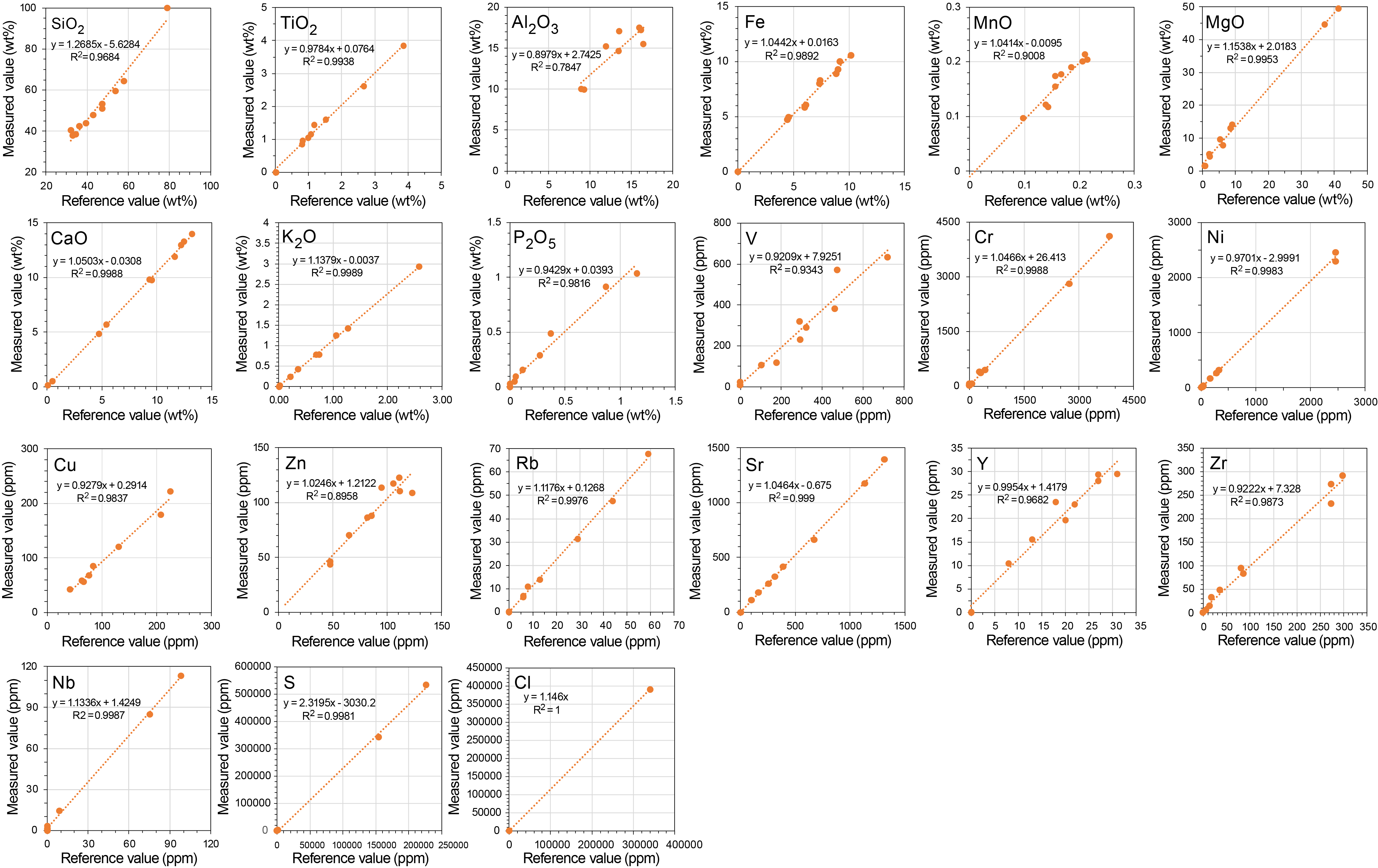
Figure F30. pXRF element calibration curves.
We found that corrected pXRF data for compositions high in SiO2 and MgO often yield analytical totals >100 wt% for samples recovered from Hole U1616E. When plotting analytical totals versus SiO2 content using raw pXRF data, these values are correlated even though their rock type is diverse (Figure F31), suggesting that the built-in Bruker calibration (Geoexploration) conducts artificial internal corrections that differ for compositions with <50 wt% SiO2 (Figure F31A) compared with compositions with >50 wt% SiO2 (Figure F31B). This probably leads to overestimation of the SiO2 content in the corrected pXRF data. A similar difference in correction was observed for MgO. It appears that the instrument's performance is not ideal on our set of various samples (i.e., Da Silva et al., 2023). However, we still report corrected data with analytical totals >100 wt% only for qualitative use because they were beneficial when identifying lithologies. We recommend referencing the raw data for intervals whose corrected data total more than 100 wt%.
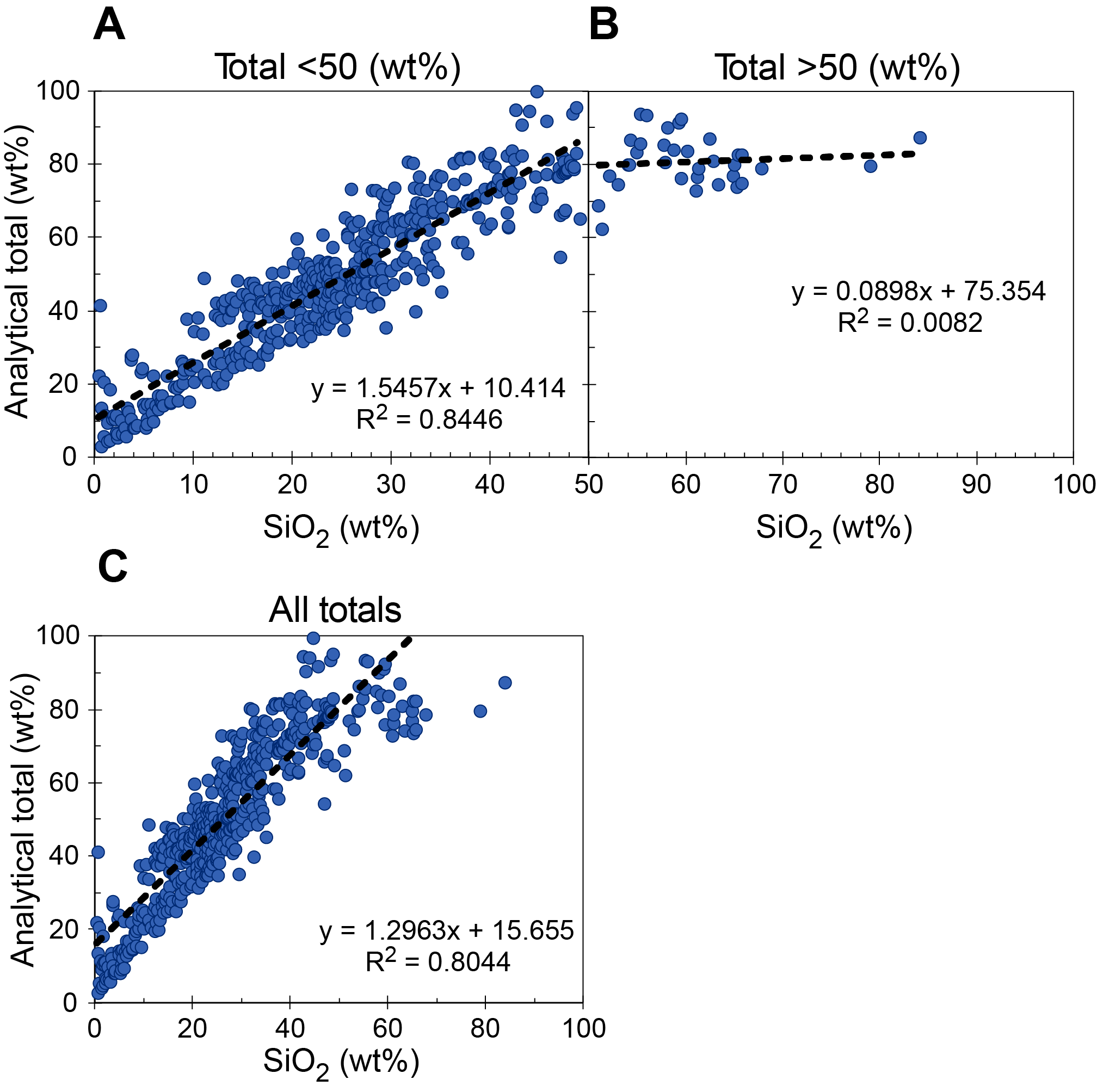
Figure F31. Raw pXRF data scatter plots.
8.3. X-ray diffraction
Bulk XRD analysis was occasionally performed on powders produced for analysis using ICP-AES. XRD analysis was usually conducted only for specific samples following ICP-AES analyses and was only done when needed to complement the ICP-AES data. Powders were mounted on a sample holder and analyzed using a Malvern Panalytical AERIS diffractometer mounted with a PIXcel1D-Medipix3 detector using nickel-filtered CuKα radiation. Analytical settings for the bulk sample scan were as follows:
- Voltage = 40 kV.
- Current = 15 mA.
- Goniometer scan = 5°–90°2θ.
- Step size = 0.0108664°2θ.
- Time per step = 40 s/step.
- Divergence slit = 0.25°.
Diffractograms of bulk samples were evaluated with the aid of Malvern Panalytical's XRD High Score software suite, which allowed for mineral identification and basic peak characterization (e.g., baseline removal and characteristic peak intensity). Files were created that contained d-spacing values, diffraction angles, and peak intensities with or without the background removed. These files were scanned to find d-spacing values characteristic of a limited range of key minerals typically used to distinguish carbonate minerals in mantle lithologies.
8.4. Calcium carbonate, total carbon, and total sulfur contents
Calcium carbonate, TC, organic carbon, and TS contents were occasionally analyzed on powders produced for analysis using ICP-AES. These analyses were usually conducted only for specific carbonated and noncarbonated mantle lithologies to address their carbonation processes on the ocean floor. Calcium carbonate analysis was followed using the method described in Sediment and interstitial water geochemistry. The analytical procedures of TC and TS followed those of the Sediment and interstitial water geochemistry, except for the sample amount, which was increased to 50 mg for mantle lithologies because of their low sulfur abundance compared to sediments.
9. Physical properties
Physical properties, namely density, compressional VP, MS, and thermal conductivity, were measured on whole-round cores and section halves. X-ray and digital images of the cores were also taken. In addition, density, porosity, and VP measurements were made on a series of discrete samples taken from the working halves of split cores. Table T12 summarizes the set of physical properties measured during Expedition 402.
9.1. Whole round measurements
9.1.1. X-Ray Linescan Logger
X-ray scans were carried out on whole-round sections and section halves to image the internal architecture of both sedimentary and basement rocks (Figure F32A). At the beginning of the expedition, X-Ray Linescan Logger (XSCAN) measurements of sedimentary and hard rock whole rounds were regularly carried out. After significant testing and tuning the XSCAN parameters, especially for hard rocks, we found that the whole-round images were too attenuated because of the greater thickness of material along the X-ray image path and did not yield useful results. In contrast, XSCANs of hard rock section halves yielded better images of internal structure and were also easier to compare with SHIL images, structural observations, and petrographic thin sections. Near the middle of the expedition, whole-round XSCAN imaging was abandoned in favor of scanning section halves immediately after splitting (see X-Ray Linescan Logger in Section-half measurements).
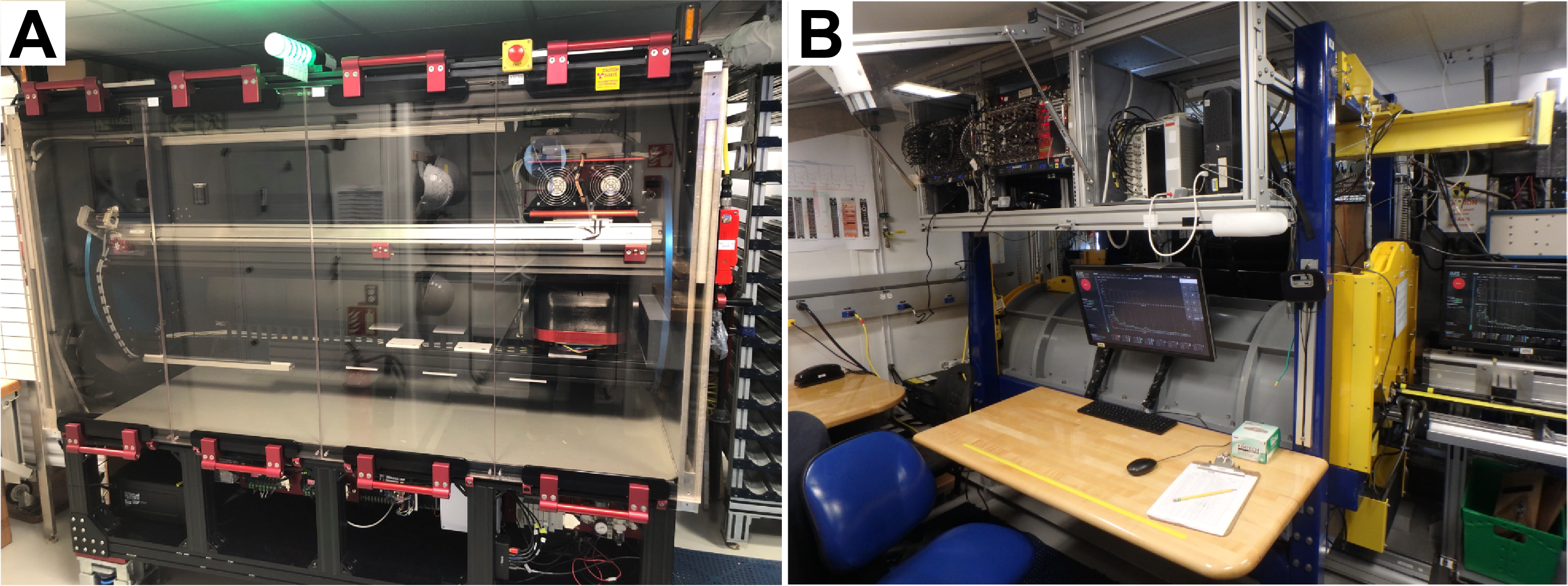
Figure F32. XSCAN and NGRL.
9.1.2. Natural Gamma Radiation Logger
NGR measurements were made on whole rounds (Figure F32B). Because these measurements do not require the core to adjust to room temperature, they were taken immediately after core sections were cut and labeled. The NGRL records gamma emissions using a system designed and built at Texas A&M University (USA) (Vasiliev et al., 2011; Dunlea et al., 2013). This instrument measures the total gamma radiation emitted during the natural decay of potassium (40K), thorium (232Th), and uranium (238U) using eight sodium iodide detectors spaced 20 cm apart. Each set of measurements is done for 300 s, followed by a 10 cm core shift and another 300 s of measurements. As a result, 16 points spaced 10 cm apart are collected for a 150 cm long section. Core catchers were typically too short in length and not scanned with the NGRL.
9.1.3. Whole-Round Multisensor Logger
The WRMSL (Figure F33) was used to simultaneously collect nondestructive measurements of GRA bulk density, MS, and VP. WRMSL measurements were collected after waiting at least 4 h after recovery to give time for equilibration to ambient room temperature (~20°C). To optimize WRMSL performance and make data comparable with all other petrophysical measurements, the same 2 cm sampling interval was set for all sensors. All sampling intervals used are common denominators of the spacings between the sensors installed on the WRMSL (30 cm), allowing for the collection of collocated measurements. After each core section was measured, we performed QA/QC by passing a calibration core liner through the WRMSL. The calibration core liner contained an aluminum rod immersed in deionized water, which together acted as a standard for the three measurements. VP logger values in the standard were measured at ~1490 m/s (depending on ambient temperature), and GRA bulk densities were approximately 1 g/cm3.
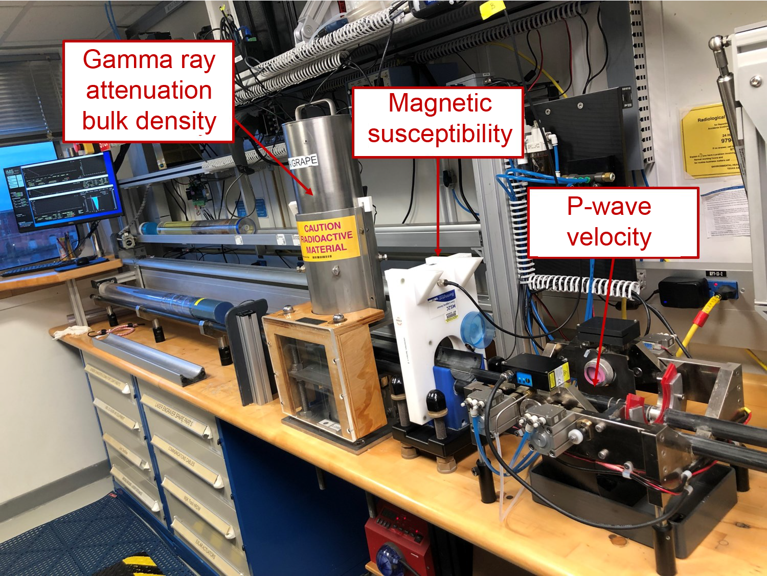
Figure F33. WRMSL.
When hard sedimentary or basement rocks were recovered, incomplete filling of the core liner resulted in erroneous bulk density and VP data. The extra space in the core liner causes bulk density measurements to be lower than MAD results and degrades the coupling of the WRMSL transducers for VP measurements. Anomalously low VP values (<1450 m/s) measured using the WRMSL were disregarded when plotting data and computing average values in lithostratigraphic units. For hard rocks, a 12% increase correction factor for WRMSL GRA bulk density data resulted in a good match to MAD results, so we used this correction when plotting the data and computing average values described in the text. In these cases, raw GRA bulk density values are plotted in gray and still shown in corresponding tables.
9.1.3.1. Gamma ray attenuation bulk density
GRA bulk density is defined on the basis of the fraction of gamma rays that are not scattered by a sample, which is related to the bulk density of the medium. The GRA densitometer on the WRMSL operates by passing gamma rays from a 137Cs source located at the top of a whole-round section and are detected by a 75 mm × 75 mm sodium iodide detector located directly below. When the 0.662 MeV gamma ray energy passes through the core, it is attenuated by Compton scattering in proportion to the bulk density in the core, which in turn depends on lithology and porosity. Because the attenuation coefficient is similar for most common minerals and aluminum, the bulk density is obtained through direct calibration of the GRA densitometer using aluminum rods of various diameters mounted in a core liner filled with distilled water. Recalibration was performed when needed. The GRA densitometer has a spatial resolution of <1 cm.
Variations in rock bulk density measured using this method reflect changes in mineralogy, chemical composition, and porosity. Similar to VP, erroneous bulk density values were recorded in areas of pervasive drilling disturbance, expansion cracks, and incompletely filled core liners. For typical marine sediment cores, values between 1 and 2 g/cm3 were usually recorded. Outliers and bad measurements, where GRA bulk density values were less than 1.0 g/cm3 or greater than 3.5 g/cm3, were filtered out for the purposes of plotting and computing reasonable average values. No other data manipulation was done shipboard, aside from applying a simple 12% correction factor for GRA bulk density measured on basement rocks. Inaccurate GRA bulk density measurements commonly result in lower than true values, and we therefore considered the upper envelope of GRA bulk density data as a reasonable first-order estimate of bulk density.
9.1.3.2. P-wave velocity
VP is a measure of the speed at which a compressional body wave (P-wave) propagates through a medium. The VP of rocks is directly related to the bulk density and elastic moduli (compressibility and shear modulus) of the sample and indirectly related to the porosity, mineralogy, fabric, chemical composition or lithology of the material. Shipboard VP measurements on recovered cores are particularly useful in correlating data across different scales, from regional seismic imaging to borehole logs to core-based data. VP was measured using the VP logger (PWL) on the WRMSL. The PWL uses a 500 kHz compressional wave pulse transmitted across the core liner between two transducer-coupled calipers. A trickle of water flows continuously across the caliper surfaces to acoustically couple the liner and the calipers. The waveform crossing the core is filtered with a bandpass ranging 0.4–1.0 MHz. Stacked waveforms are then used for the automatic picking of first arrivals using the WRMSL software. The PWL is corrected for the presence of the acrylic liner and is calibrated using known velocities of a freshwater-filled liner and aluminum standards.
VP measurements were reliable when recovery was high and core liners were full, ensuring good contact between the transducers, core liner, and rock sample. VP data were typically better for sediments, with a typical range of ~1.48–1.8 km/s. Erroneous outlier VP data from the WRMSL were disregarded (VP < 1450 m/s and VP > 4000 m/s), and broad velocity-lithology-depth trends were observed from the main clusters of values. Furthermore, because cores obtained using the XCB and RCB systems in hard rocks may have gaps, or the core liners may not be filled completely and may contain air-filled voids, VP was measured with the PWL only on sediment cores and typically turned off for hard rock scanning on the WRMSL.
9.1.3.3. Magnetic susceptibility
MS is a measure of the degree to which a material can be magnetized by an external magnetic field:
where M is the magnetization induced in the material by an external field of strength H.
MS is measured using a Bartington Instruments MS2 meter coupled to an MS2C sensor coil with a diameter of 8.8 cm operating at a frequency of 565 Hz (Bartington Instruments, 2011) incorporated into the WRMSL. The sensor output can be set to centimeter-gram-second (cgs) units or SI units; IODP standard practice is to use the SI setting. MS is measured in instrumental units (IU); to convert the results into dimensionless units, the data are multiplied by a correction factor, which is a function of the type of probe, the diameter of the core, and the size of the circuit. Because incomplete cores may contain small pieces of rock of varying dimensions, a single correction factor is not sufficient and so no correction is applied. These MS data are comparable with paleomagnetic data measured in the same physical units (SI). The MS2C coil is calibrated with a homogeneous mixture of magnetite and epoxy resin and has a resolution of ±4 cm for the continuous central section. Therefore, MS discontinuities in the core over an interval less than 8 cm thick will be smoothed out.
9.2. Section-half measurements
9.2.1. X-Ray Linescan Logger
XSCANs of section halves yielded better quality images of internal core structures than whole-round images that suffered from near-complete attenuation. This imaging did not require the core to be warmed to the ambient laboratory temperature. The instrument produced an image of the core with a 48 µm resolution, allowing for detection of internal features such as fractures, veins, or local inhomogeneities. The instrument also offers the option of using a custom processing utility to optimize the internal features. Three files were output by the scanner: a raw TIFF image (filename_R.tif) and two JPEG files (a cropped filename_C.jpg and a processed filename_P.jpg).
For sedimentary rocks, X-ray imaging was performed on section halves immediately after splitting to detect internal features such as fractures, bedding, ash layers, and other sedimentary structures. The imaging was usually done on the working half of the core. XSCAN parameters of 98 kV and 0.8 mA were found to be best for imaging sediment cores.
For basement rocks, quality XSCANs were best achieved on section halves. The XSCAN parameters were adjusted to 110 kV and 0.9 mA, which increased the instrument power to handle the denser basement rocks. These settings provided ideal images of recovered mantle rocks, including magmatic and alteration vein networks and high-temperature metamorphic fabrics (aligned spinel minerals). XSCANs of paleomagnetism-MAD (PMAG-MAD) cubes were also performed to view relationships between structural features and physical properties measurements, including directional VP variations.
9.2.2. Section-Half Multisensor Logger
9.2.2.1. Reflectance spectrometry
Color reflectance was measured on archive-half sections using an Ocean Optics USB4000 spectrophotometer mounted on the SHMSL (Figure F34). Readings were taken every 2 cm to be consistent with all other physical properties and paleomagnetic measurements. Empty intervals, voids, and gaps were skipped to avoid spurious data. The color reflectance spectrometer calibrates on two spectra: pure white (reference) and pure black (dark). Color calibration was conducted automatically every ~6 h (twice per shift).
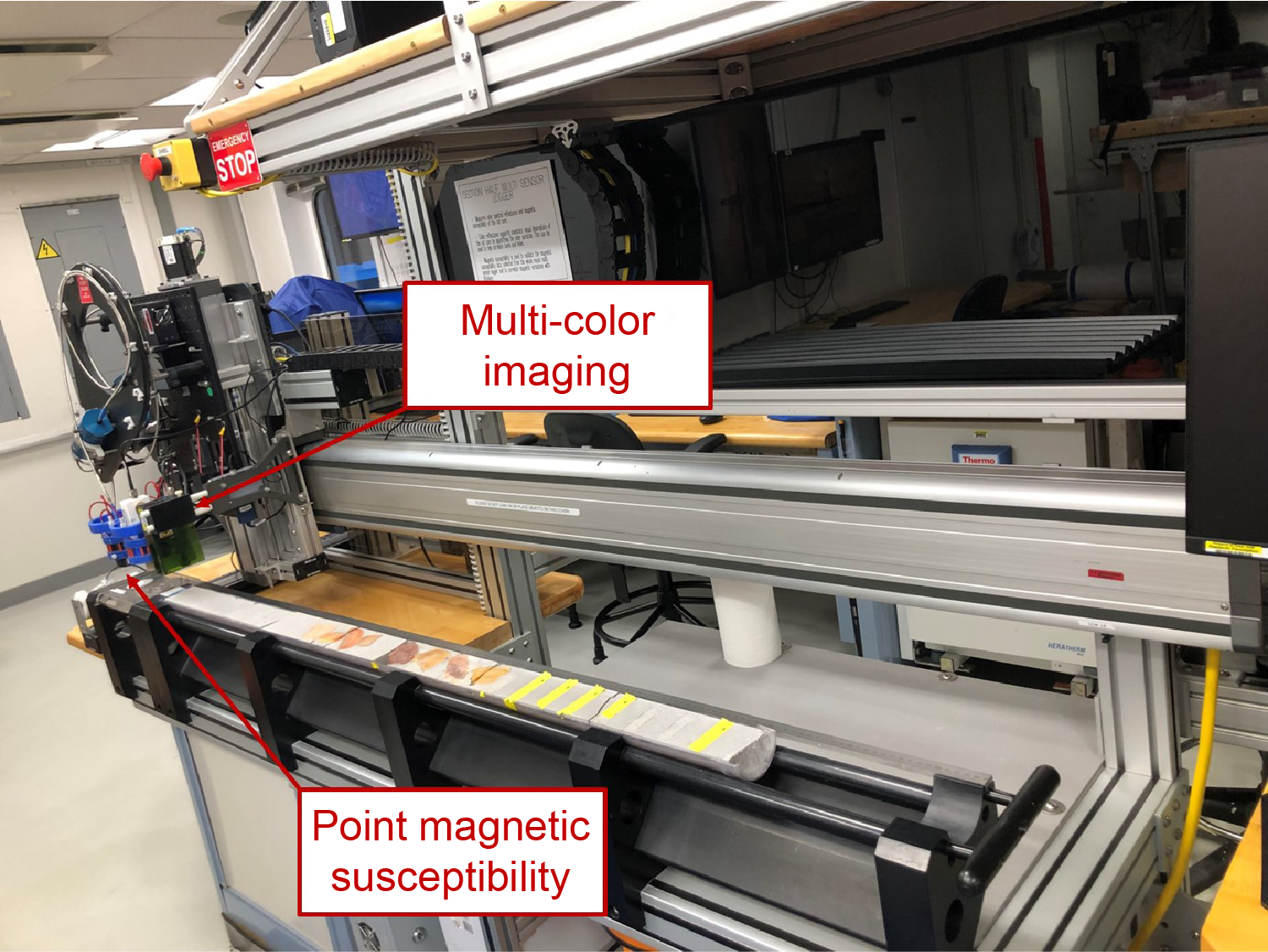
Figure F34. SHMSL.
9.2.2.2. Point magnetic susceptibility
A Bartington MS2 meter and an MS2K contact probe with a flat 15 mm diameter round sensor were used to measure MSP. MS data were obtained every 2 cm by taking the average of three measurements. The output displayed by the MSP sensor is converted to dimensionless SI units by multiplying by 10−5. The MSP meter was calibrated by the manufacturer before installation on the ship and is quality checked every ~6 h together with color reflectance sensor calibration.
9.2.3. Thermal conductivity
Thermal conductivity is a measure of how easily a material conducts heat and is a key physical property that relates heat flow to the geothermal gradient. The thermal conductivity of rocks is affected by their mineralogy, porosity, density, and fabric. Thermal conductivity measurements are key to understanding thermal insulation and heat dissipation processes from the deeper crust and mantle, through the sediments, and into the ocean.
The TK-04 (Teka Bolin) system (Blum, 1997) was used to measure thermal conductivity (Figure F35A). A needle probe was initially used to measure soft sedimentary rocks; however, poor measurements were frequently obtained because of the presence of sand, which prevented adequate coupling. This method was quickly abandoned in favor of the caliper (puck system), which provided better results for both sediments and hard rocks (Figure F35A, F35C). After turning on a heat source with a heating power of 2.5 W/m, the temperature is recorded for 60 s using the caliper. The measured temperature changes as a function of the logarithm of the elapsed time were fitted with a straight line, and the thermal conductivity was obtained from the following heat conduction equation (Kristiansen, 1982; Blum, 1997):
- T = temperature (K),
- q = heat input per unit length per unit time (J/m/s),
- k = thermal conductivity (W/[m·K]),
- t = time after the initiation of the heat (s), and
- C = instrumental constant.
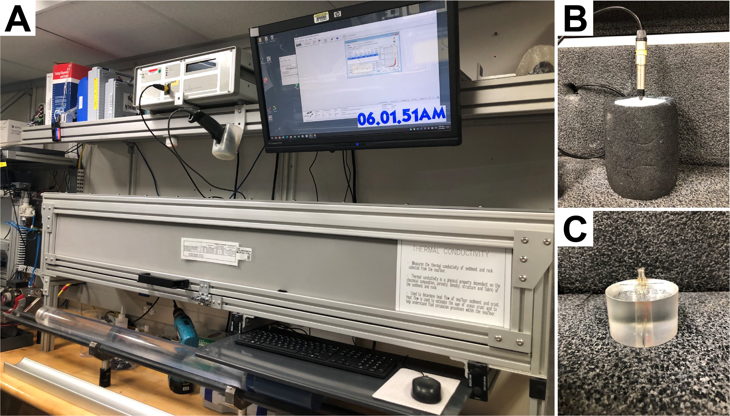
Figure F35. Thermal conductivity station, needle probe tool, and puck tool.
The instrument was set to take a total of three measurements with 10 min between each measurement to allow the sample to cool off. To ensure complete saturation of the pore space, hard rock samples were soaked in seawater using a vacuum pump for at least 4 h prior to thermal conductivity measurements.
9.3. Discrete measurements
9.3.1. Moisture and density
Discrete samples from the working halves were selected for MAD measurements to determine wet and dry bulk density, grain density, water content, and porosity. In soft sediment cores, ~10 cm3 samples were collected with a plastic syringe. In harder sediments or rocks, ~8 cm3 samples were taken with a metal syringe or a chisel or cut with a rock saw. Samples were often placed next to the samples being cut and prepared for other laboratories such as paleomagnetism. In general, 1–2 samples per core were collected with the aim of representing the complete core lithology. In cores with large lithologic variability, three or more MAD samples were sometimes measured to obtain representative values. Sediment samples were placed in numbered, preweighed ~16 mL Wheaton glass vials to obtain wet and dry sediment mass and dry volume measurements. Following the measurement of wet mass, samples were dried in a convection oven for 24 h at 105° ± 5°C. Dried samples were then cooled in a desiccator for at least 2 h before the dry mass and volume were measured. For hard rock, the procedure included resaturation with seawater for 4 h under a vacuum before the wet mass measurement was conducted.
Wet and dry sample masses were determined to an accuracy of 0.005 g using dual-Mettler Toledo (XS204) electronic balances (Figure F36A), with one balance acting as a reference and one as an unknown. A standard of similar known mass to the sample mass was placed on the reference balance to increase the accuracy of the unknown sample measurement. An averaging algorithm in the MADMax software was used to correct for the motion of the ship. The default measurement setting of the two balances was 300 measurements over an interval of ~1.5 min. In the case of heavy seas where the heave and roll of the ship affected the balances, 600–800 measurements were taken.
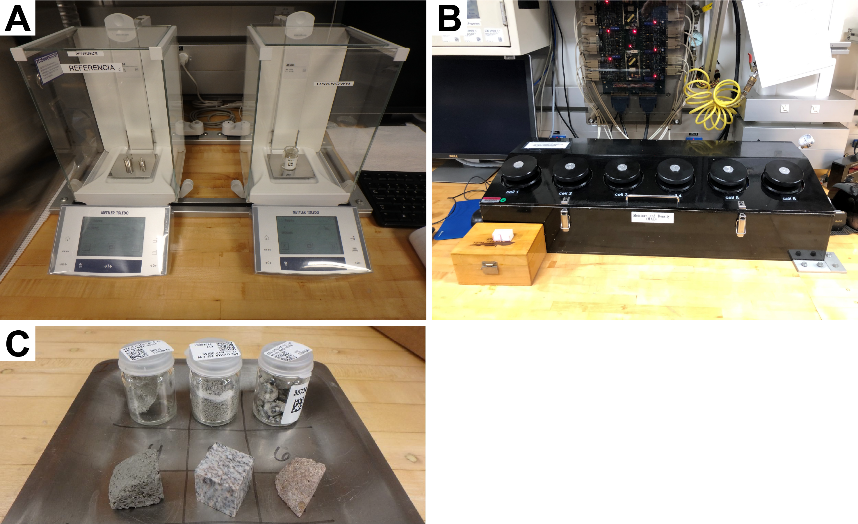
Figure F36. MAD workstation.
Dry sample volumes were determined using a six-cell, custom-configured Micromeritics AccuPyc 1330TC helium-displacement pycnometer (Figure F36B). The precision of each cell is 1% of the full-scale volume. Volume measurements were preceded by three purges of the sample chamber with helium warmed to ~28°C. For each measurement, five unknown cells and one cell that contained two stainless steel calibration spheres with a total volume of ~10 cm3 were run. The calibration spheres were rotated sequentially through the cells to detect any systematic error and/or instrument drift. The volumes occupied by the numbered Wheaton vials were calculated before the expedition by dividing the weight of each vial against the average density of the vial glass (Figure F36C). The procedures for the determination of these physical properties comply with the American Society for Testing and Materials (ASTM) designation (D) 2216 (ASTM International, 1990). The relationships and assumptions for the calculations of the physical properties parameters are discussed in detail in Blum (1997) and Weber et al. (1997). The MADMax shipboard program was used for computing the displayed MAD properties.
9.3.2. P-wave velocity bayonet and P-wave velocity caliper
The VP bayonet (PWB) and VP caliper (PWC) were used to measure VP on both working-half sections and discrete samples in three orthogonal orientations. Two separate PWB tools equipped with transducers measured VP along the long (Z-axis) and intermediate (Y-axis) directions of section halves (Figure F37). A single PWC transducer system measured VP along the short (X-axis) direction of the section halves.
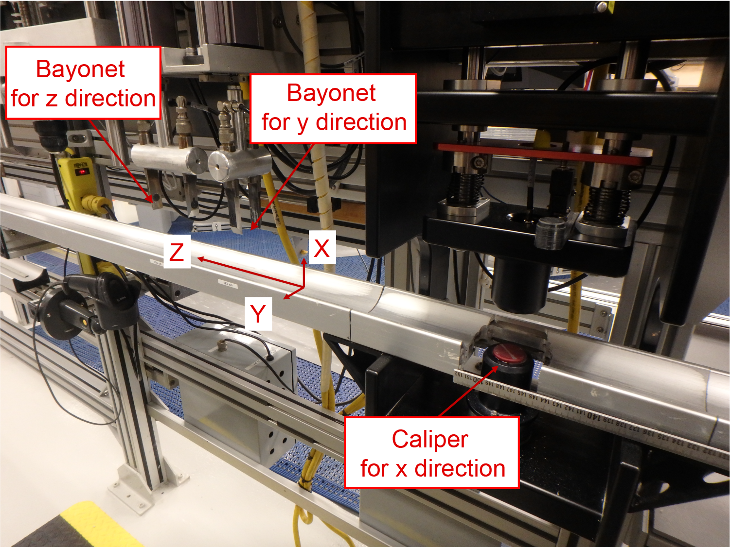
Figure F37. Gantry system.
Obtaining quality measurements using the PWB tools requires penetration of the transducers into the section halves, so the PWB system was only attempted on soft sedimentary sections. Even with soft sediments, core-transducer coupling was generally very poor and quality waveform measurements were infrequent. Because the PWB resulted in severe damage to core sections and did not yield quality results, this method was generally not performed for the duration of the expedition. For stiff sediments and hard rocks, we measured VP on section halves using only the PWC (i.e., only in the X-direction). Discrete cubes cut from the working-half sections were analyzed using the PWC to obtain VP measurements in all three orientations.
The Gantry system uses Panametrics-NDT Microscan delay line piezoelectric transducers, which transmit an ultrasonic pulse at a frequency of 500 kHz. Velocity Gantry IMS v. 14 IODP software automatically picked the P-wave first arrival and was manually adjusted when necessary, such as when coupling was poor or the signal-to-noise ratio was low. The length of the P-wave path between transducers was measured with a built-in linear voltage displacement transformer (LDVT), and the corresponding VP was automatically calculated from the first arrival pick times. Parameters of the Gantry processing software were frequently tuned to ensure that the automatic picking algorithm best captured the first arrival of the P-wave.
Calibration of the VP measurements was performed regularly to ensure proper instrument function and data quality. A suite of acrylic cylinders with varying thicknesses and a known VP of 2750 ± 20 m/s was used to calibrate the PWC, and distilled water was used to calibrate the PWB tools. The system time delay determined from calibration was subtracted from the picked arrival time to give the traveltime of the P-wave through the sample. The sample thicknesses measured with the LDVT (in meters) were divided by the traveltimes (in seconds) to calculate VP (meters per second) and compared to the known value. The system delay time was adjusted until the velocity measurements were accurate within ~1% for the PWC and ~0.5% for the PWB. Distilled water was applied to the transducer-core contact to enhance the transmitted signals.
At most sites, PWB measurements were not possible below Core 3 because the sediments become compacted. For hard rocks, discrete cubes with dimensions of 2 cm × 2 cm × 2 cm were cut from the working half for MAD, paleomagnetic, and Gantry analyses. Cube samples were oriented following the technique of Blum (1997). Gantry VP measurements were taken on seawater-saturated cubes to better reflect in situ conditions. Triaxial measurements (X-axis, Y-axis, and Z-axis) were obtained using the PWC system and by rotating the cube between runs. The corresponding VP anisotropy was calculated from the multidirectional analyses.
10. Downhole measurements
Downhole geophysical experiments included formation temperature measurements taken during coring operations at all sites and the deployment of downhole wireline tools in the borehole after drilling.
Downhole wireline sensors measure the petrophysical, chemical, structural, and dynamic properties of the formation surrounding a borehole. After coring is completed, the measurements are made by lowering sondes with an electrical wireline into the borehole. The data are measured in situ and continuously recorded as a function of depth at sampling intervals ranging 2.5 mm to 15 cm. These downhole profiles record formation properties at the centimeter scale for borehole wall images and the decimeter to meter scale for other measurements. These scales are intermediate between those obtained from laboratory measurements on core samples and those from geophysical surveys.
The downhole measurements can be used for a number of applications (e.g., providing a depth-velocity relationship to correlate borehole observations with seismic images). Downhole wireline profiles can be analyzed for stratigraphy; lithology; mineralogy; magnetic, electrical, and acoustic properties; fluid flow in and out of the borehole; and geochemical composition of the penetrated formation. Data on the shape, size, and possible deformation of the borehole induced by drilling or the in situ stress field are also recorded. In intervals where the core recovery is incomplete or disturbed, downhole data might provide the only way to characterize the penetrated formation and can be used to supplement core recovery. Where core recovery is good, core data and downhole geophysical profiles complement one another and may be analyzed jointly.
10.1. Downhole geophysical operations
During wireline downhole geophysical operations, measurement profiles and images were recorded from a variety of sensors assembled into tool strings. Two primary tool strings were used during Expedition 402 (Figure F38): a petrophysical combination to be deployed first, followed by an imaging combination. The first string of sensors (referred to as the triple combination [triple combo] tool string) measures the spectrum of natural gamma ray, bulk formation density, electrical resistivity, and MS. The second tool string provides high-resolution centimeter-scale resistivity images of the borehole wall with the Formation MicroScanner (FMS) and measures sonic velocities and shear wave anisotropy with the Dipole Sonic Imager (DSI). The Hostile Environment Natural Gamma Ray Sonde (HNGS), which measures spectral natural gamma ray emissions, is run at the top of each string for depth correlation between runs. Each tool string also includes the General Purpose Inclinometry Tool (GPIT) to measure orientation to magnetic north and the Enhanced Digital Telemetry Cartridge (EDTC) to communicate with the multitasking acquisition and imaging system (MAXIS). Individual tools are listed in Table T13. If the borehole is found to be too large for FMS deployment, the Ultrasonic Borehole Imager (UBI), which provides centimeter-scale acoustic images of the borehole surface, can be used in conjunction with the DSI instead of the FMS. Because we were unable to deploy the FMS or UBI imaging tools during Expedition 402, we do not further discuss these instruments.
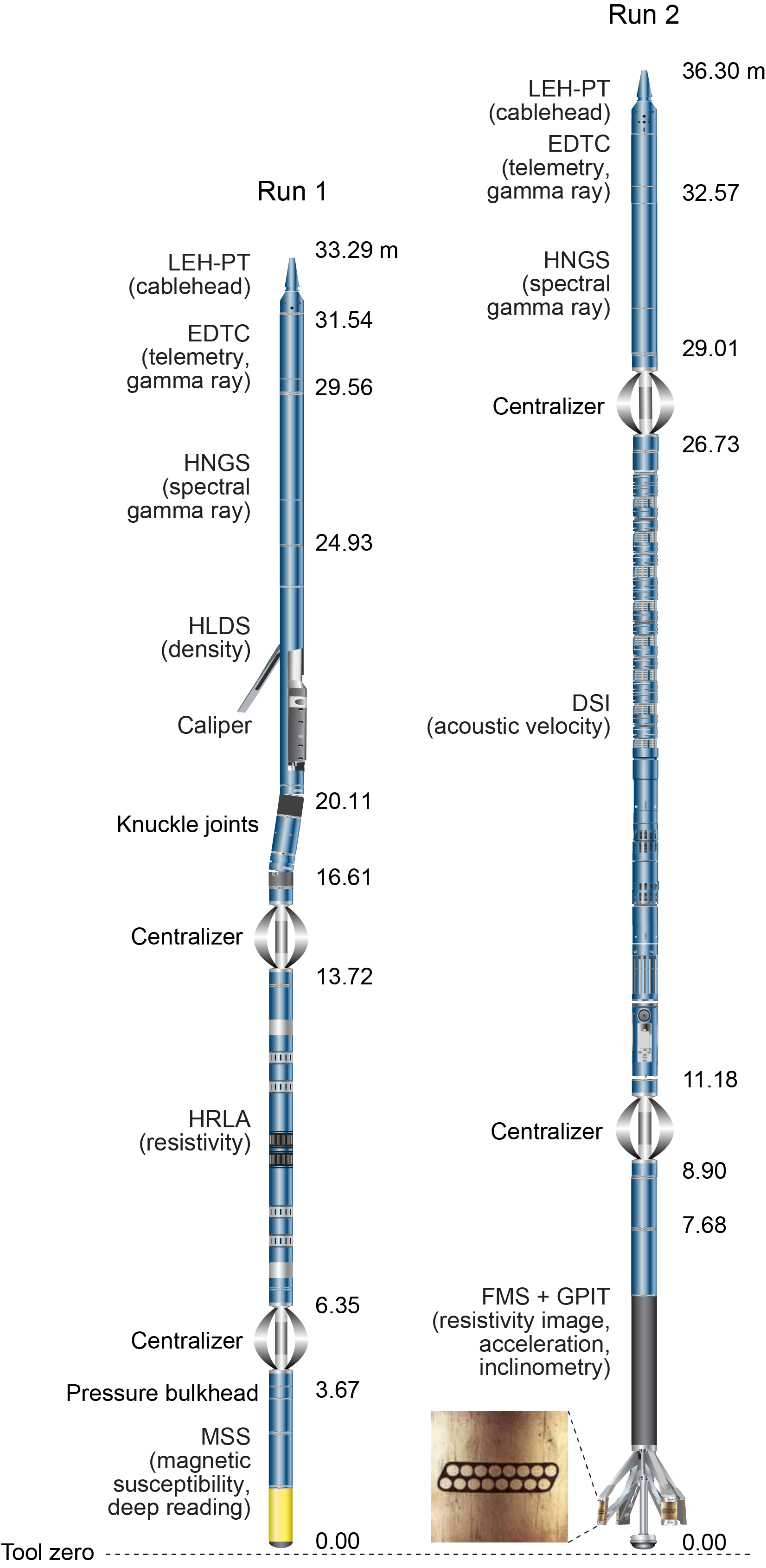
Figure F38. Wireline tool strings.
In preparation for downhole geophysical measurements, boreholes were flushed of debris by circulating viscous drilling fluid and then filled with seawater or a seawater-based gel (sepiolite mud mixed with seawater) to help stabilize the borehole. The RCB drill bit was dropped at the bottom of the hole (or on the seafloor) and the base of the drill string was set below the seafloor or at a greater depth if there were concerns about hole instability within the sediment column. The tool strings were then sequentially lowered downhole. The spectral gamma sensor is the only sensor that provides meaningful data inside the drill pipe, although they are mostly qualitative. These data are used primarily to identify the depth of the seafloor and the sediment/basement boundary but can also be used for stratigraphic characterization.
Each tool string deployment is called a logging run and begins with the vertical assembly of the tool string in the derrick and any necessary calibration. The tool string is then lowered to the bottom of the hole while recording a partial set of data and is pulled up at a constant speed (typically 250–500 m/h, depending on the sensors) to record the main data set. During each run, tool strings may be lowered down and pulled up the hole several times, either for repeatability or to try to improve the data quality. Each lowering or raising of a tool string while collecting data is called a pass. During each pass, the incoming data were recorded and monitored in real time on the ship. A logging run is complete once a tool string returns to the rig floor and is disassembled. A wireline heave compensator (WHC) is employed to minimize the effect of the ship's heave on the position of downhole sensors (see Wireline heave compensator).
10.2. Petrophysical properties and sensor measurement principles
The downhole measurements recorded during Expedition 402 are listed in Table T14. The petrophysical properties and measurement principles used by the associated sensors are briefly described here. More detailed descriptions of individual sensors with geologic applications can be found in Serra (1984, 1986), Schlumberger (1989), Goldberg (1997), and Ellis and Singer (2007). An online list of acronyms for the Schlumberger tools, sensors, and downhole measurements is also available at http://www.apps.slb.com/cmd/index.aspx.
10.3. Natural gamma ray
The HNGS was used on all tool strings to measure natural radioactivity in the formation. The HNGS uses two bismuth germanate scintillation detectors and a five-window spectroscopy inversion method to determine the concentrations of potassium (in weight percent), thorium (in parts per million), and uranium (in parts per million) from the characteristic gamma ray energies of isotopes in the 40K, 232Th, and 238U radioactive decay series, which dominate the natural radiation spectrum. The computation of the elemental abundances uses a least-squares Kalman filtering method to extract U, Th, and K elemental concentrations from the energy spectrum. The HNGS filters out gamma ray energies below 500 keV, eliminating sensitivity to bentonite or KCl in the drilling mud and improving measurement accuracy. The HNGS also provides a measure of the total spectral gamma ray (HSGR) emission expressed in American Petroleum Institute gamma radiation units (gAPI). The HNGS response is influenced by the borehole diameter, and HNGS data are corrected for borehole diameter variations during acquisition.
The EDTC is primarily used to communicate data to the surface (see Auxiliary logging equipment). It includes a sodium iodide scintillation detector that also measures the natural gamma ray emission. It is not a spectral tool, but it provides an overall total gamma ray profile for each pass, which is used for depth matching between individual downhole passes.
10.4. Bulk density
Formation bulk density was measured using the Hostile Environment Litho-Density Sonde (HLDS). The HLDS contains a radioactive cesium (137Cs) gamma ray source (622 keV) and far and near gamma ray detectors mounted on a shielded skid pressed against the borehole wall by a hydraulically activated arm. Gamma rays emitted by the cesium source undergo Compton scattering, where gamma rays are scattered by formation electrons. The intensity of scattered gamma rays that reach the detectors is proportional to the formation electron density, which is proportional to bulk density. Porosity can be derived from the bulk density for a given matrix grain density.
For low-energy gamma radiation, the HLDS also measures the photoelectric absorption of gamma rays, called the photoelectric effect (PEF). Photoelectric absorption occurs when the gamma ray energy falls below 150 keV because of repeated scattering by electrons in the formation. Because PEF depends on the atomic number of the elements in the formation (heavier elements have higher PEF), it varies according to the chemical composition of the minerals with little effect from porosity (Ellis and Singer, 2007).
Good contact between the tool and borehole wall is essential to record good quality HLDS data. Poor contact can result in underestimation of the bulk density. Both the density correction and hole size (caliper) measurements can be used to evaluate the contact quality.
10.5. Porosity
A porosity estimate can be derived from bulk density and the mineral densities determined from the physical properties measurements. Porosity can also be estimated from VP measurements when porosity is less than 30% (Wyllie et al., 1956) or from electrical resistivity (Archie, 1942). These porosity estimates may be used to evaluate the presence of overpressure in the sediments (Revil et al., 1998, 1999).
10.6. Formation electrical resistivity
The High-Resolution Laterolog Array (HRLA) provides six electrical resistivity measurements with different depths of investigation (including the borehole, or mud, resistivity and five measurements of formation resistivity with increasing penetration into the formation). The HRLA sends a focused current into the formation and measures the current intensity required to maintain a constant drop in voltage across a fixed interval, providing direct resistivity measurements. The array has one central source electrode and six electrodes above and below that serve alternately as focusing and returning current electrodes. By rapidly changing the role of these electrodes, a simultaneous resistivity measurement at six penetration depths is achieved. The tool is designed to ensure that all signals are measured at exactly the same time and tool position and to reduce the sensitivity to shoulder bed effects when crossing beds thinner than the electrode spacing. The HRLA needs to be run centralized in the borehole for optimal results, so knuckle joints are used to centralize the HRLA while allowing the density tool located right above it in the tool string to maintain good contact with the borehole wall (Figure F38).
Minerals from sedimentary and crustal rocks are generally considered to be electrical insulators, and ionic solutions constituting IW are electrical conductors. In rocks, the electrical conduction is a combination of several processes (Waxman and Smits, 1968; Pezard, 1990; Lévy et al., 2018). Electrolytic conduction in pore volumes comes from ion transport through the pore fluid and depends on porosity, connectivity between pores, in situ temperature, and the nature and ionic strength of the pore fluid (Archie, 1942). Surface conduction along pore surfaces is directly related to the mineralogy of the rock matrix (Pezard and Anderson, 1989; Pezard, 1990). Although the surface conduction tends to dominate the overall electrical signal in clays, it might be negligible in rocks such as carbonates and fresh gabbros.
10.7. Magnetic susceptibility
The Magnetic Susceptibility Sonde (MSS) is a nonstandard wireline instrument developed by the Lamont-Doherty Earth Observatory (LDEO). It measures the ease with which formations are magnetized when subjected to a magnetic field. The ease of magnetization, or susceptibility, is ultimately related to the concentration and composition (size, shape, and mineralogy) of magnetic minerals in the formation (typically magnetite). These measurements provide one of the best methods for investigating stratigraphic changes in mineralogy and lithology because the measurement is fast, repeatable, and nondestructive and because different lithologies often have strongly contrasting susceptibilities. The data can be compared to the susceptibility measurements made on the recovered core using the WRMSL and the MSP measurements made using the SHMSL (see Physical properties).
The MSS dual-coil sensor provides measurements with ~40 cm vertical resolution and ~20 cm depth of horizontal investigation. The MSS was run as the lowermost tool in the triple combo tool string using a specially developed data translation cartridge that enabled the MSS to be run in combination with the Schlumberger tools. MSS data are in uncalibrated units and are affected by temperature and borehole size. For quality control and environmental correction, the MSS also measures internal tool temperature, z-axis acceleration, and low-resolution borehole conductivity.
10.8. Acoustic velocities
The DSI measures the transit times between sonic transmitters and an array of eight receivers. The waveforms are then used to calculate the velocity of compressional and shear waves in the formation. The omnidirectional monopole transmitter emits high-frequency (5–15 kHz) pulses to extract the compressional VP of the formation, as well as the shear S-wave velocity when it is faster than the sound velocity in the borehole fluid. It combines replicate measurements, thus providing a direct VP measurement that is relatively free from the effects of formation damage or an enlarged borehole (Schlumberger, 1989). Along with the monopole transmitter, the DSI also has two crossed-dipole transmitters that allow for orthogonal shear wave velocity measurements and the determination of anisotropy. In rocks with porosity values less than 30%, the VP slowness can be related to porosity using an arithmetic mixing law (Wyllie et al., 1956).
10.9. Auxiliary logging equipment
The Schlumberger logging equipment head (LEH), commonly referred to as the cable head, measures the cable tension at the top of the tool string and diagnoses difficulties in running the tool string up or down the borehole or when exiting or entering the drilling string or casing.
The EDTC placed at the top of each tool string transmits downhole data from the tools to the surface and receives information from a surface computer. The EDTC also includes a sodium iodide scintillation detector to measure the total natural gamma ray emission of the formation. This gamma ray profile is used to match the depths between the different passes and runs. In addition, it includes an accelerometer whose data can be used in real time to evaluate the efficiency of the WHC.
Because the tool strings combine tools of different generations and with various designs, they include several adapters and joints between individual tools to allow communication, isolation, reduction of interferences (mechanical and acoustic), and termination of wiring, in addition to positioning the tool properly in the borehole. In particular, the knuckle joints are used to allow some of the tools such as the HRLA to remain centralized in the borehole while the overlying density tool (HLDS) is pressed against the borehole wall. All these additions contribute to the total length of the tool strings.
10.10. Log data quality
The condition of a borehole is the principal factor affecting the quality of the downhole geophysical data. Ideal conditions for logging include a consistent borehole diameter matching the bit size with no washouts or bridges. Oversized borehole diameters can have a significant impact on measurements, especially those that require tool eccentering (e.g., HLDS). The measurement principles of the eccentered tools require direct contact with the formation for the acquisition of high-quality data. Deep investigation measurements such as gamma radiation, resistivity, and sonic velocity, which do not require contact with the borehole wall, are generally less sensitive to borehole conditions, although data are optimized in boreholes where the tools can be centralized (up to ~20 inches diameter).
If the borehole diameter varies over short intervals because of washouts of softer material or ledges of harder material, the logs from tools that require good contact with the borehole wall (e.g., bulk density) may be degraded. Bridged sections, where the borehole diameter is significantly less than the bit size, will also cause irregular log results. The quality of the borehole can be improved by minimizing the circulation of drilling fluid while drilling, flushing the borehole to remove debris prior to logging, and logging as soon as possible after drilling and conditioning.
The quality of the wireline depth measurements depends on several additional factors. The depth of the logging measurements is determined from the length of the cable spooled out from the winch on the ship. Uncertainties in logging depth occur because of ship heave, cable stretch, cable slip, and tidal changes. To minimize the wireline tool motion caused by ship heave, a hydraulic WHC is used to adjust the wireline depth for rig motion during wireline logging operations.
The seafloor is identified on the gamma ray log by the abrupt change in gamma ray count at the water/sediment interface (mudline). This provides an important reference datum to match logging depths and provide depth consistency across all logging data. Discrepancies between the drilling core depth and wireline logging depth may occur because of core expansion, incomplete core recovery, incomplete heave compensation, and drill pipe stretch. The differences between the two data sets can be reconciled by a comparison of the common data sets acquired in situ and on the core (e.g., MS and NGR).
10.11. Wireline heave compensator
During wireline logging operations, the up-and-down motion of the ship (heave) causes a similar motion of the downhole logging tools. If the amplitude of this motion is large, depth discrepancies can be introduced into the logging data. The risk of damaging downhole instruments is also increased. The WHC system was designed to compensate for vertical motions of the ship and maintain a steady motion of the logging tools to ensure high-quality logging data (Iturrino et al., 2013; Liu et al., 2013). The WHC uses a vertical accelerometer (motion reference unit [MRU]) positioned under the rig floor near the ship's center of gravity to calculate the vertical motion of the ship with respect to the seafloor. It then adjusts the length of the deployed wireline by varying the distance between two sets of pulleys through which the cable passes to minimize the vertical motion of the downhole tool string.
10.12. Logging data flow and depth scales
Data for each wireline logging run were monitored in real time and recorded using the Schlumberger surface acquisition system. Shortly thereafter, data were transferred onshore to LDEO for standardized data processing, formatting for the online logging database, and archiving. Processed data were returned to the ship and made available to the shipboard scientists within a few days of logging.
The onshore processing included several stages. First, using the gamma ray logs recorded by each tool string, a visually interactive program was used to match the depths of recognizable features across all the passes to a reference curve, commonly the gamma ray log of the longest upward pass. After depth matching, all the logging depths were shifted from the rig floor depth reference (in which they were initially recorded) to a seafloor depth reference, based on the seafloor as identified by the step in gamma radiation at the sediment/water interface. The processed data were made available in ASCII and DLIS formats for most logs and in GIF format for the images.
10.13. In situ temperature measurements
In situ formation temperature measurements were made at selected depths in the sediments at all sites to assess the thermal structure of the sedimentary section along the transect and measure the local heat flow.
The APCT-3 tool fits directly into a modified coring shoe of the APC system and consists of a battery pack, data logger, and a platinum resistance-temperature device calibrated over a temperature range of 0°–30°C. Before entering the borehole, the tool is stopped at the seafloor for 5–10 min to thermally equilibrate and measure the temperature at the seafloor. Alternatively, the lowest temperature recorded during the down run may be preferable to the average temperature at the seafloor as an estimate of water bottom temperature because (1) it is a more repeatable measurement and (2) the water bottom is expected to have the lowest temperature in the profile. After the APC penetrates the sediment, it is held in place for ~10 min as the APCT-3 tool records the temperature of the cutting shoe every second. When the APCT-3 tool is fired into the formation, there is typically an instantaneous temperature rise due to frictional heating. The heat gradually dissipates into the surrounding sediment as the temperature at the APCT-3 tool equilibrates toward the temperature of the sediment. During RCB coring operations, we deployed the SET2 tool. This tool inserts a 1 m long probe into the bottom of the hole, recording the temperature for about 10 min. The SET2 tool provided temperature measurements at sites where no APC/XCB hole was cored and allowed measurement of deeper, more compacted sediment than what the APCT-3 can measure.
The equilibrium temperature of the sediment was estimated by applying a mathematical heat-conduction model to the temperature decay record (Horai and Von Herzen, 1985). The predicted thermal decay curve for the SET2 and APCT-3 tools is a function of the geometry and thermal properties of the probe and the sediment (Bullard, 1954; Horai and Von Herzen, 1985). The equilibrium temperature is estimated in the TP-Fit software by applying a fitting procedure (Heesemann et al., 2006). However, when the APCT-3 tool did not achieve a full stroke or when ship heave pulled up the APCT-3 or SET2 tool from contact with the formation, the temperature equilibration curve was disturbed and temperature determination was less accurate. The nominal accuracy of the APCT-3 temperature sensor is ±0.05°C, and the nominal accuracy of the SET2 temperature sensor is ±0.006°C.
At Sites U1612 and U1613, the seafloor temperatures measured with the SET2 sensor were found to be more than 1.5°C higher than those recorded during previous expeditions (Kastens, Mascle, Auroux, et al., 1987; Comas, Zahn, Klaus, et al., 1996). As a consequence, a shipboard correction factor was determined for each of the temperature sensors in the two SET2 tools and the APCT-3 tool and applied to all data generated during Expedition 402 (Table T15). Although all sensors gave measurements close to the reference provided by a Fisher Scientific quartz digi-thermo probe, the SET2 (Probe Number 449) was found to be the most accurate near 50°C (hot tap water), and the other two were more accurate near 23°C (cold tap water; Figure F39). Measurements in air were not used to compute the correction factor (Figure F39).
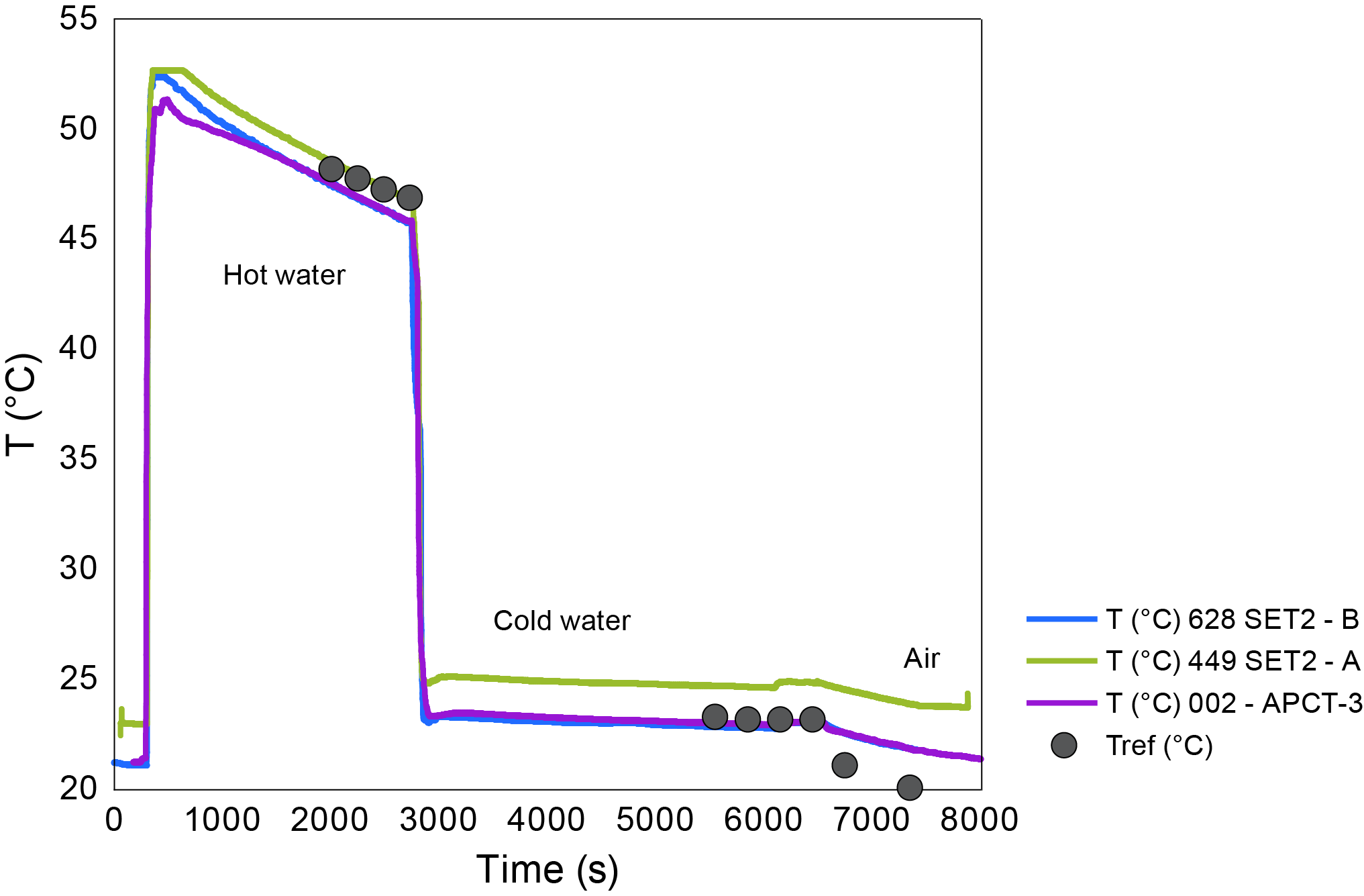
Figure F39. SET2 and APCT-3 sensor calibration.
10.14. Heat flow
A first-order estimate of the vertical conductive heat flow at each site can be obtained from a least-squares linear fit of the in situ temperatures measured as a function of depth. The slope of this linear fit is the temperature gradient, and the local vertical conductive heat flow is the product of this gradient with the mean thermal conductivity measured on the cores.
If thermal conductivity varies with depth, a more accurate measure of the heat flow is based on a Bullard plot (Bullard, 1939). If the vertical heat flow (q) is assumed constant with depth, as in a predominantly conductive regime, the temperature at depth Z can be calculated by a simple integration:
where To is the temperature at the seafloor and K(z) is the thermal conductivity at a depth z. The value in the integral is the thermal resistance of the interval between the seafloor and Z. If the heat flow is constant with depth, this defines a linear relationship between temperature and thermal resistance, and its slope is the conductive heat flow (Bullard, 1939). During Expedition 402, the thermal conductivity measured on sediment core samples did not display a significant trend with depth. Heat flow was estimated from the product of the geothermal gradient and the average thermal conductivity in the depth interval where sediment temperatures were measured.
11. Microbiology
Microbial communities associated with sediments are highly diverse and can extend meters below the seafloor. Analyses of microbial diversity in these environments have identified dominant taxa at different locations (Petro et al., 2017). They play a fundamental role in the availability of nutrients in the ecosystem. In addition, factors like oxygen availability influence the distribution and activity of microbes below the seafloor (D'Hondt et al., 2015). Within these microbial communities, viruses affect the activity and diversity of microorganisms and consequently the biogeochemical cycles. However, the relationship between microorganisms and biochemical cycles are not fully understood.
11.1. Contamination testing of drilling fluid
The study of microbial diversity and activity depends on the quality of the samples. It is important to acquire pristine, uncontaminated samples to obtain unbiased results.
Drilling contamination testing was performed during past IODP expeditions (e.g., 366, 376, 385, and 390/393) as a crucial part of ensuring the quality of microbiological samples. The primary source of contamination during drilling is the introduction of circulating seawater or drilling fluid into the borehole during the drilling process, which can contaminate the cores with microorganisms from the water column (de Ronde et al., 2019).
A tracer was added to the drilling fluid in the APC/XCB holes where sediments were the priority (Holes U1614A, U1615A, U1616A, U1616B, and U1617A). We used perfluorodecalin (PFD), for which detection in the interior of a core sample is a conservative measure of contamination because the PFD molecules have a smaller volume than microbial cells (Teske et al., 2021).
PFD was continuously injected into the drilling fluid using a high-pressure liquid chromatography pump, and the pump rate was set to vary with the drilling fluid pump rate (final concentration ~0.4 mL/L). Once the core was cut in sections, the sampling plan followed the Expedition 390/393 methods (Coggon et al., 2024), which consisted of taking two samples per core where microbiological samples were taken. The first sample was collected near the core liner (exterior), and the second sample was taken from the core center (interior). Samples were collected using sterile ~3 cm3 syringes (with cutoff ends) and placed into 20 mL headspace vials, which were sealed and labeled. In addition, drilling fluids were also taken for comparison with core samples. All samples were stored at ~4°C for further analysis by GC.
For analysis, the samples were volatilized at 70°C and injected into an Agilent Technologies 6890N GC after calibration standards were prepared and run using 10−4, 10−6, 10−8, and 10−10 dilutions of the tracer. If the exterior sample contained measurable PFD, it was assumed that the tracer was successfully delivered to the core. A positive interior measurement indicated contamination.
11.2. Oxygen measurements
Oxygen penetration into the sediments was measured using a PreSens PM-PSt7 oxygen profiling microsensor, which allowed measurement of up to 10 oxygen and temperature profiles simultaneously. The calibration setup and the data collected were processed using the PreSens Measurement Studio 2 software available for Windows OS. We used the same equipment and software used during Expedition 390/393 (Coggon et al., 2024). Oxygen was measured in Holes U1612A, U1613A, U1614, U1615A, U1616A, U1616B, and U1617A.
Calibration solutions were prepared daily. The 0 cal solution (0%; oxygen-free) contained 1 g of sodium sulfite (Na2SO3) dissolved in 100 mL ultrapure water, and the 100 cal solution (100% oxygen; full saturation) consisted of 100 mL of ultrapure water (Coggon et al., 2024).
Oxygen measurements were performed on the cores prior to splitting. In the upper 2–3 cores, measurements were taken in at least every core section. Once a depth was encountered where consistent zero-oxygen measurements were made, measurement frequency was reduced to one per core or less.
To make a measurement, probes were manually inserted by drilling two holes, one for the oxygen probe, and one for the temperature probe. We targeted undisturbed sections (preferably not the first or last sections of a core) when recovery allowed. Measurements were taken only on core sections that were at least 80 cm in length so that both the oxygen and temperature probes could be inserted and separated by a minimum distance of 20–30 cm.
11.3. Microbiological sampling and sample selection
For sediment sampling, 5 cm whole-round samples were collected on the catwalk within the upper 100 m. The less disturbed samples were selected for enrichment and viral activity experiments (see sections below). Samples were cut and sprayed with 70% ethanol, bagged immediately after collection, and placed in the anaerobic chamber until further processing.
11.4. Viral metagenomics and 16S rRNA gene sequencing
Viral metagenomic analysis will assess the viral community and its functional role in deep-sea sediments. Whole rounds (5 cm) were collected every 20 m and stored at −80°C for onshore viral metagenomic analysis.
Amplification of the 16S gene allows identification of the microbial diversity that resides in the sediments. A 10 cm3 plug sample was collected using autoclaved syringes (ends cut off) for 16S rRNA gene amplification and sequencing for every core. Syringes were used for sample collection until sediment was too indurated for insertion. After collection, the sediment plug was sprayed with 70% alcohol, double bagged, and stored at −80°C for onshore analysis.
11.5. Viral counts
A 1 cm3 plug sample was taken at the same frequency as the 16S rRNA samples, fixed with 4 mL of formaldehyde 4% solution in 100 mM phosphate-buffered saline (PBS), and stored at 4°C for onshore analysis using a Nycodenz density gradient to separate viruses from the sediments (Pan et al., 2019) followed by epifluorescence microscopy to enumerate the number of virus-like particles.
11.6. Viral production and prophage induction experiments
To measure viral activity, one or two sediment samples were selected for viral production using the dilution method (Dell'Anno et al., 2009) and prophage induction experiments. Samples of 10 cm3 were extracted from the middle of the whole round using sterile cutoff syringes. A slurry was prepared by diluting each sample in 10 mL of anaerobic seawater. The slurry was divided into four vials, which were then topped off with 20 mL of anaerobic seawater. For prophage induction, the vials were supplemented with mitomycin C (1 µg/mL final concentration). Subsamples were taken in triplicates at t = 0, 4, 8, 12, and 24 h in sterile cryotubes. Each subsample was fixed with 54 µL of formaldehyde and incubated 10 min at 4°C before being frozen at −80°C for further onshore processing. These experiments were performed under anaerobic conditions.
11.7. Enrichment experiments
Sulfate reduction is an important microbial process that occurs within the first few meters below the seafloor in organic-rich sediments, where microorganisms use sulfate present in seawater as an electron acceptor during the degradation of organic matter, leading to the production of hydrogen sulfide (Fakhraee and Katsev, 2017).
In the anaerobic chamber, different glass vials were used to start microbial enrichments using a minimal medium (MMJHS) and an enriched medium (MJYPGS) with the goal of isolating sulfate reducers (see recipes in Table T16); these enrichments were then supplemented with an anaerobic reductant (Na2S, Na2S2O3, or Na2SO3; final concentration 0.001 g/mL). One or two 20 cm3 samples were placed in a 500 mL bottle; 200 mL of anaerobically filtered and autoclaved seawater was added to make a slurry. The slurry was distributed among the vials, which were topped off with the media and reductants. The vials were sealed and stored in the dark at room temperature for shore-based analyses. The enrichment cultures will be analyzed for microbial growth before DNA extractions and sequencing to characterize the enriched microbial communities.
References
Allmendinger, R.W., 2023. Stereonet 11. https://www.rickallmendinger.net/stereonet
Archie, G.E., 1942. The electrical resistivity log as an aid in determining some reservoir characteristics. Transactions of the AIME, 146(01):54–62. https://doi.org/10.2118/942054-G
ASTM International, 1990. Standard method for laboratory determination of water (moisture) content of soil and rock (Standard D2216–90). In Annual Book of ASTM Standards for Soil and Rock Philadelphia (American Society for Testing Materials).
Aubry, M.-P., 1984. Handbook of Cenozoic Calcareous Nannoplankton, Book 1: Ortholithae (Discoasters): New York (Micropaleontology Press).
Aubry, M.-P., 1988. Handbook of Cenozoic Calcareous Nannoplankton, Book 2: Ortholithae (Holococcoliths, Ceratoliths, Ortholiths, and Others): New York (Micropaleontology Press).
Aubry, M.-P., 1989. Handbook of Cenozoic Calcareous Nannoplankton, Book 3: Ortholithae (Pentaliths, and Others), Heliolithae (Fasciculiths, Sphenoliths, and Others): New York (Micropaleontology Press).
Aubry, M.-P., 1990. Handbook of Cenozoic Calcareous Nannoplankton, Book 4: Heliolithae (Discoliths and Similar Structures): New York (Micropaleontology Press).
Aubry, M.-P., 1999. Handbook of Cenozoic Calcareous Nannoplankton, Book 5: Heliolithae (Rhabdoliths and Zygoliths): New York (Micropaleontology Press).
Backman, J., 1980. Miocene-Pliocene nannofossils and sedimentation rates in the Hatton-Rockall Basin, NE Atlantic Ocean. Stockholm Contributions in Geology, 36:1–91.
Backman, J., Raffi, I., Rio, D., Fornaciari, E., and Pälike, H., 2012. Biozonation and biochronology of Miocene through Pleistocene calcareous nannofossils from low and middle latitudes. Newsletters on Stratigraphy, 45(3):221–244. https://doi.org/10.1127/0078-0421/2012/0022
Backman, J., and Shackleton, N.J., 1983. Quantitative biochronology of Pliocene and early Pleistocene calcareous nannofossils from the Atlantic, Indian and Pacific oceans. Marine Micropaleontology, 8(2):141–170. https://doi.org/10.1016/0377-8398(83)90009-9
Balsam, W.L., and Damuth, J.E., 2000. Further investigations of shipboard vs. shore-based spectral data: implications for interpreting Leg 164 sediment composition. In Paull, C.K., Matsumoto, R., Wallace, P.J., Dillon, W.P. (Eds.), Proceedings of the Ocean Drilling Program, Scientific Results. 164: College Station, TX (Ocean Drilling Program), 314–324. https://doi.org/10.2973/odp.proc.sr.164.222.2000
Balsam, W.L., Damuth, J.E., and Schneider, R.R., 1997. Comparison of shipboard vs. shore-based spectral data from Amazon Fan cores: implications for interpreting sediment composition. In Flood, R.D., Piper, D.J.W., Klaus, A., and Peterson, L.C. (Eds.), Proceedings of the Ocean Drilling Program, Scientific Results. 155: College Station, TX (Ocean Drilling Program), 193–215. https://doi.org/10.2973/odp.proc.sr.155.210.1997
Balsam, W.L., Deaton, B.C., and Damuth, J.E., 1998. The effects of water content on diffuse reflectance spectrophotometry studies of deep-sea sediment cores. Marine Geology, 149(1):177–189. https://doi.org/10.1016/S0025-3227(98)00033-4
Balsley, J.R., and Buddington, A.F., 1960. Magnetic susceptibility anisotropy and fabric of some Adirondack granites and orthogneisses. American Journal of Science, 258-A:6–20.
Bartington Instruments, Ltd., 2011. Operation Manual for MS2 Magnetic Susceptibility System: Oxford, UK (Bartington Instruments, Ltd.). https://gmw.com/wp-content/uploads/2019/03/MS2-OM0408.pdf
Berner, R.A., 1982. Burial of organic carbon and pyrite sulfur in the modern ocean: its geochemical and environmental significance. American Journal of Science, 282(4):451–473. https://doi.org/10.2475/ajs.282.4.451
Blum, P., 1997. Physical properties handbook: a guide to the shipboard measurement of physical properties of deep-sea cores. Ocean Drilling Program Technical Note, 26. https://doi.org/10.2973/odp.tn.26.1997
Bonatti, E., Seyler, M., Channell, J.E.T., Giraudeau, J., and Mascle, G., 1990. Peridotites drilled from the Tyrrhenian Sea, ODP Leg 107. In Kastens, K.A., Mascle, J., et al., Proceedings of the Ocean Drilling Program, Scientific Results. 107: College Station, TX (Ocean Drilling Program), 37–47. https://doi.org/10.2973/odp.proc.sr.107.141.1990
Bottjer, D.J., and Droser, Mary L., 1991. Ichnofabric and basin analysis. Palaios, 6(3):199–205. https://doi.org/10.2307/3514901
Bown, P.R., 1998. Calcareous Nannofossil Biostratigraphy: Dordrect, Netherlands (Kluwer Academic Publishing).
Bown, P.R., and Young, J.R., 1998. Techniques. In Bown, P.R., Calcareous Nannofossil Biostratigraphy. Dordrect, Netherlands (Kluwer Academic Publishing), 16–28.
Bukry, D., and Bramlette, M.N., 1969. Some new and stratigraphically useful calcareous nannofossils of the Cenozoic. Tulane Studies in Geology and Paleontology, 7(3). https://journals.tulane.edu/tsgp/article/view/531
Bullard, E.C., 1939. Heat flow in South Africa. Proceedings of the Royal Society of London, A: Mathematical and Physical Sciences, 173(955):474–502. https://doi.org/10.1098/rspa.1939.0159
Bullard, E.C., 1954. The flow of heat through the floor of the Atlantic Ocean. Proceedings of the Royal Society of London, A: Mathematical and Physical Sciences, 222(1150):408–429. https://doi.org/10.1098/rspa.1954.0085
Caruso, A., 2004. Climatic changes during Late Pliocene and Early Pleistocene at Capo Rossello (Sicily, Italy): response from planktonic foraminifera. In Coccioni, R., Lirer, F., and Galeotti, S. (Eds.), Proceedings of the First Italian Meeting on Environmental Micropaleontology. Grzybowski Foundation Special Publication: 17–35.
Cline, J.D., 1969. Spectrophotometric determination of hydrogen sulfide in natural waters. Limnology and Oceanography, 14(3):454–458. https://doi.org/10.4319/lo.1969.14.3.0454
Coggon, R.M., Teagle, D.A.H., Sylvan, J.B., Reece, J., Estes, E.R., Williams, T.J., Christeson, G.L., Aizawa, M., Albers, E., Amadori, C., Belgrano, T.M., Borrelli, C., Bridges, J.D., Carter, E.J., D'Angelo, T., Dinarès-Turell, J., Doi, N., Estep, J.D., Evans, A., Gilhooly, W.P., III, Grant, L.C.J., Guérin, G.M., Harris, M., Hojnacki, V.M., Hong, G., Jin, X., Jonnalagadda, M., Kaplan, M.R., Kempton, P.D., Kuwano, D., Labonte, J.M., Lam, A.R., Latas, M., Lowery, C.M., Lu, W., McIntyre, A., Moal-Darrigade, P., Pekar, S.F., Robustelli Test, C., Routledge, C.M., Ryan, J.G., Santiago Ramos, D., Shchepetkina, A., Slagle, A.L., Takada, M., Tamborrino, L., Villa, A., Wang, Y., Wee, S.Y., Widlansky, S.J., Yang, K., Kurz, W., Prakasam, M., Tian, L., Yu, T., and Zhang, G., 2024. Expedition 390/393 methods. In Coggon, R.M., Teagle, D.A.H., Sylvan, J.B., Reece, J., Estes, E.R., Williams, T.J., Christeson, G.L., and the Expedition 390/393 Scientists, South Atlantic Transect. Proceedings of the International Ocean Discovery Program, 390/393: College Station, TX (International Ocean Discovery Program). https://doi.org/10.14379/iodp.proc.390393.102.2024
Comas, M.C., Zahn, R., Klaus, A., et al., 1996. Proceedings of the Ocean Drilling Program, Initial Reports, 161: College Station, TX (Ocean Drilling Program). https://doi.org/10.2973/odp.proc.ir.161.1996
Da Silva, A.C., Triantafyllou, A., and Delmelle, N., 2023. Portable x-ray fluorescence calibrations: workflow and guidelines for optimizing the analysis of geological samples. Chemical Geology, 623:121395. https://doi.org/10.1016/j.chemgeo.2023.121395
Davis, G.H., Reynolds, S.J., and Kluth, C.F., 2011. Structural Geology of Rocks and Regions, 3rd edition: New York (John Wiley & Sons).
de Kaenel, E.P., Siesser, W.G., and Murat, A., 1999. Pleistocene calcareous nannofossil biostratigraphy and the western Mediterranean sapropels, Sites 974 to 977 and 979. In Zahn, R., Comas, M.C., and Klaus, A. (Eds.), Proceedings of the Ocean Drilling Program, Scientific Results. 161: College Station, TX (Ocean Drilling Program). https://doi.org/10.2973/odp.proc.sr.161.250.1999
de Ronde, C.E.J., Humphris, S.E., Höfig, T.W., Brandl, P.A., Cai, L., Cai, Y., Caratori Tontini, F., Deans, J.R., Farough, A., Jamieson, J.W., Kolandaivelu, K.P., Kutovaya, A., Labonté, J.M., Martin, A.J., Massiot, C., McDermott, J.M., McIntosh, I.M., Nozaki, T., Pellizari, V.H., Reyes, A.G., Roberts, S., Rouxel, O., Schlicht, L.E.M., Seo, J.H., Straub, S.M., Strehlow, K., Takai, K., Tanner, D., Tepley III, F.J., and Zhang, C., 2019. Expedition 376 methods. In de Ronde, C.E.J., Humphris, S.E., Höfig, T.W., and the Expedition 376 Scientists, Brothers Arc Flux. Proceedings of the International Ocean Discovery Program, 376: College Station, TX (International Ocean Discovery Program). https://doi.org/10.14379/iodp.proc.376.102.2019
Deflandre, G., and Fert, C., 1954. Observations sur les coccolithophoridés actuels et fossiles en microscopie ordinaire et électronique. Annales de Paléontologie, 40:115–176.
Dell'Anno, A., Corinaldesi, C., Magagnini, M., and Danovaro, R., 2009. Determination of viral production in aquatic sediments using the dilution-based approach. Nature Protocols, 4(7):1013-1022. https://doi.org/10.1038/nprot.2009.82
D'Hondt, S., Inagaki, F., Alvarez Zarikian, C., Abrams, L.J., Dubois, N., Engelhardt, T., Evans, H., Ferdelman, T., Gribsholt, B., Harris, R.N., Hoppie, B.W., Hyun, J.-H., Kallmeyer, J., Kim, J., Lynch, J.E., McKinley, C.C., Mitsunobu, S., Morono, Y., Murray, R.W., Pockalny, R., Sauvage, J., Shimono, T., Shiraishi, F., Smith, D.C., Smith-Duque, C.E., Spivack, A.J., Steinsbu, B.O., Suzuki, Y., Szpak, M., Toffin, L., Uramoto, G., Yamaguchi, Y.T., Zhang, G.-l., Zhang, X.-H., and Ziebis, W., 2015. Presence of oxygen and aerobic communities from sea floor to basement in deep-sea sediments. Nature Geoscience, 8(4):299–304. https://doi.org/10.1038/NGEO2387
Di Stefano, A., Baldassini, N., Raffi, I., Fornaciari, E., Incarbona, A., Negri, A., Negri, A., Bonomo, S., Villa, G., Di Stefano, E., and Rio, D., 2023. Neogene-Quaternary Mediterranean calcareous nannofossil biozonation and biochronology: a review. Stratigraphy, 20(4):259–302. https://www.micropress.org/microaccess/check/2342
Di Stefano, A., and Sturiale, G., 2010. Refinements of calcareous nannofossil biostratigraphy at the Miocene/Pliocene Boundary in the Mediterranean region. Geobios, 43(1):5–20. https://doi.org/10.1016/j.geobios.2009.06.007
Di Stefano, A., Verducci, M., Lirer, F., Ferraro, L., Iaccarino, S.M., Hüsing, S.K., and Hilgen, F.J., 2010. Paleoenvironmental conditions preceding the Messinian Salinity Crisis in the Central Mediterranean: integrated data from the Upper Miocene Trave section (Italy). Palaeogeography, Palaeoclimatology, Palaeoecology, 297(1):37–53. https://doi.org/10.1016/j.palaeo.2010.07.012
Dunlea, A.G., Murray, R.W., Harris, R.N., Vasiliev, M.A., Evans, H., Spivack, A.J., and D'Hondt, S., 2013. Assessment and use of NGR instrumentation on the JOIDES Resolution to quantify U, Th, and K concentrations in marine sediment. Scientific Drilling, 15:57–63. https://doi.org/10.2204/iodp.sd.15.05.2013
Ellis, D.V., and Singer, J.M., 2007. Well Logging for Earth Scientists (2nd edition): New York (Elsevier). https://doi.org/10.1007/978-1-4020-4602-5
Espitalié, J., Deroo, G., and Marquis, F., 1985. Rock-eval pyrolysis and its applications (Pt. 1). Oil & Gas Science and Technology-Revue D Ifp Energies Nouvelles, 40(5):563–579.
Expedition 304/305 Scientists, 2006. Methods. In Blackman, D.K., Ildefonse, B., John, B.E., Ohara, Y., Miller, D.J., MacLeod, C.J., and the Expedition 304/305 Scientists, Proceedings of the Integrated Ocean Drilling Program. 304/305: College Station, TX (Integrated Ocean Drilling Program Management International, Inc.). https://doi.org/10.2204/iodp.proc.304305.102.2006
Expedition 309/312 Scientists, 2006. Methods. In Teagle, D.A.H., Alt, J.C., Umino, S., Miyashita, S., Banerjee, N.R., Wilson, D.S., and the Expedition 309/312 Scientists, Proceedings of the Integrated Ocean Drilling Program. 309/312: Washington, DC (Integrated Ocean Drilling Program Management International, Inc.). https://doi.org/10.2204/iodp.proc.309312.102.2006
Expedition 334 Scientists, 2012. Methods. In Vannucchi, P., Ujiie, K., Stroncik, N., and the Expedition 334 Scientists, Proceedings of the Integrated Ocean Drilling Program. 334: Tokyo (Integrated Ocean Drilling Program Management International, Inc.). https://doi.org/10.2204/iodp.proc.334.102.2012
Expedition 335 Scientists, 2012. Methods. In Teagle, D.A.H., Ildefonse, B., Blum, P., and the Expedition 335 Scientists, Proceedings of the Integrated Ocean Drilling Program. 335: Tokyo (Integrated Ocean Drilling Program Management International, Inc.). https://doi.org/10.2204/iodp.proc.335.102.2012
Fakhraee, M., Li, J., and Katsev, S., 2017. Significant role of organic sulfur in supporting sedimentary sulfate reduction in low-sulfate environments. Geochimica et Cosmochimica Acta, 213:502–516. https://doi.org/10.1016/j.gca.2017.07.021
Farouk, S., Ren, C., Abdeldaim, A., Salama, A., Wu, H., El-Kahtany, K., and Zaky, A.S., 2022. An astronomical time scale of early Pliocene from the Mediterranean Sea, Egypt. Global and Planetary Change, 215:103869. https://doi.org/10.1016/j.gloplacha.2022.103869
Fisher, R.V., 1961. Proposed classification of volcaniclastic sediments and rocks. Geological Society of America Bulletin, 72(9):1409–1414. https://doi.org/10.1130/0016-7606(1961)72[1409:PCOVSA]2.0.CO;2
Flores, J.A., Sierro, F.J., and Glacon, G., 1992. Calcareous plankton analysis in the pre-evaporitic sediments of the ODP Site 654 (Tyrrhenian Sea, western Mediterranean). Micropaleontology, 38(3):279–288.
Fornaciari, E., Raffi, I., Rio, D., Villa, G., Backman, J., and Olafsson, G., 1990. Quantitative distribution patterns of Oligocene and Miocene calcareous nannofossils from the western equatorial Indian Ocean. In Duncan, R.A., Backman, J., Peterson, L.C., et al., Proceedings of the Ocean Drilling Program, Scientific Results. 115: College Station, TX (Ocean Drilling Program), 237–254. https://doi.org/10.2973/odp.proc.sr.115.153.1990
Fritz, D., 1980. Safety and pollution prevention program, Deep Sea Drilling Project Leg 50, Sites 415 and 416. In Lancelot, Y., Winterer, E. L., Initial Reports of the Deep Sea Drilling Project. 50: Washington, DC (US Government Printing Office), 855–859. https://doi.org/10.2973/dsdp.proc.50.app5.1980
Früh-Green, G.L., Orcutt, B.N., Green, S.L., Cotterill, C., Morgan, S., Akizawa, N., Bayrakci, G., Behrmann, J.-H., Boschi, C., Brazelton, W.J., Cannat, M., Dunkel, K.G., Escartin, J., Harris, M., Herrero-Bervera, E., Hesse, K., John, B.E., Lang, S.Q., Lilley, M.D., Liu, H.-Q., Mayhew, L.E., McCaig, A.M., Menez, B., Morono, Y., Quéméneur, M., Rouméjon, S., Sandaruwan Ratnayake, A., Schrenk, M.O., Schwarzenbach, E.M., Twing, K.I., Weis, D., Whattam, S.A., Williams, M., and Zhao, R., 2017. Expedition 357 methods. In Früh-Green, G.L., Orcutt, B.N., Green, S.L., Cotterill, C., and the Expedition 357 Scientists, Atlantis Massif Serpentinization and Life. Proceedings of the International Ocean Discovery Program, 357: College Station, TX (International Ocean Discovery Program). https://doi.org/10.14379/iodp.proc.357.102.2017
Fryer, P., Wheat, C.G., Williams, T., Albers, E., Bekins, B., Debret, B.P.R., Jianghong, D., Yanhui, D., Eickenbusch, P., Frery, E.A., Ichiyama, Y., Johnson, K., Johnston, R.M., Kevorkian, R.T., Kurz, W., Magalhaes, V., Mantovanelli, S.S., Menapace, W., Menzies, C.D., Michibayashi, K., Moyer, C.L., Mullane, K.K., Park, J.-W., Price, R.E., Rayan, J.G., Shervais, J.W., Suzuki, S., Sissmann, O.J., Takai, K., Walter, B., and Zhang, R., 2018. Expedition 366 methods. In Fryer, P., Wheat, C.G., Williams, T., and the Expedition 366 Scientists, Mariana Convergent Margin and South Chamorro Seamount. Proceedings of the International Ocean Discovery Program, 366: College Station, TX (International Ocean Discovery Program). https://doi.org/10.14379/iodp.proc.366.102.2018
Gibbard, P.L., and Head, M.J., 2020. The Quaternary period. In Gradstein, F.M., Ogg, J.G., Schmitz, M.D., and Ogg, G.M. (Eds.), Geologic Time Scale 2020. Dordrecht, Netherlands (Elsevier), 1217–1255. https://doi.org/10.1016/B978-0-12-824360-2.00030-9
Gieskes, J.M., Gamo, T., and Brumsack, H.J., 1991. Chemical methods for interstitial water analysis aboard JOIDES Resolution. Ocean Drilling Program Technical Note, 15. https://doi.org/10.2973/odp.tn.15.1991
Gillis, K.M., Snow, J.E., Klaus, A., Guerin, G., Abe, N., Akizawa, N., Ceuleneer, G., Cheadle, M.J., Adrião, Á., Faak, K., Falloon, T.J., Friedman, S.A., Godard, M.M., Harigane, Y., Horst, A.J., Hoshide, T., Ildefonse, B., Jean, M.M., John, B.E., Koepke, J.H., Machi, S., Maeda, J., Marks, N.E., McCaig, A.M., Meyer, R., Morris, A., Nozaka, T., Python, M., Saha, A., and Wintsch, R.P., 2014. Methods. In Gillis, K.M., Snow, J.E., Klaus, A., and the Expedition 345 Scientists, Proceedings of the Integrated Ocean Drilling Program. 345: College Station, TX (Integrated Ocean Drilling Program). https://doi.org/10.2204/iodp.proc.345.102.2014
Godard, M., Awaji, S., Hansen, H., Hellebrand, E., Brunelli, D., Johnson, K., Yamasaki, T., Maeda, J., Abratis, M., Christie, D., Kato, Y., Mariet, C., and Rosner, M., 2009. Geochemistry of a long in-situ section of intrusive slow-spread oceanic lithosphere: results from IODP Site U1309 (Atlantis Massif, 30°N Mid-Atlantic-Ridge). Earth and Planetary Science Letters, 279(1–2):110–122. https://doi.org/10.1016/j.epsl.2008.12.034
Gohl, K., Wellner, J.S., Klaus, A., Bauersachs, T., Bohaty, S.M., Courtillat, M., Cowan, E.A., De Lira Mota, M.A., Esteves, M.S.R., Fegyveresi, J.M., Frederichs, T., Gao, L., Halberstadt, A.R., Hillenbrand, C.-D., Horikawa, K., Iwai, M., Kim, J.-H., King, T.M., Klages, J.P., Passchier, S., Penkrot, M.L., Prebble, J.G., Rahaman, W., Reinardy, B.T.I., Renaudie, J., Robinson, D.E., Scherer, R.P., Siddoway, C.S., Wu, L., and Yamane, M., 2021. Expedition 379 methods. In Gohl, K., Wellner, J.S., Klaus, A., and the Expedition 379 Scientists, Amundsen Sea West Antarctic Ice Sheet History. Proceedings of the International Ocean Discovery Program, 379: College Station, TX (International Ocean Discovery Program). https://doi.org/10.14379/iodp.proc.379.102.2021
Goldberg, D., 1997. The role of downhole measurements in marine geology and geophysics. Reviews of Geophysics, 35(3):315–342. https://doi.org/10.1029/97RG00221
Goldhaber, M.B., and Kaplan, I.R., 1974. The sulfur cycle. In Goldberg, E.D., The Sea (Volume 5): Marine Chemistry. New York (Wiley), 569–655.
Govindaraju, K., Rubeska, I., and Paukert, T., 1994. 1994 Report on Zinnwaldite ZW-C analysed by ninety-two GIT-IWG member-laboratories. Geostandards Newsletter, 18(1):1–42. https://doi.org/10.1111/j.1751-908X.1994.tb00502.x
Graber, K.K., Pollard, E., Jonasson, B., and Schulte, E. (Eds.), 2002. Overview of Ocean Drilling Program engineering tools and hardware. Ocean Drilling Program Technical Note, 31. https://doi.org/10.2973/odp.tn.31.2002
Gradstein, F.M., Ogg, J.G., Schmitz, M.D., and Ogg, G.M. (Eds.), 2020. Geologic Time Scale 2020: Amsterdam (Elsevier BV). https://doi.org/10.1016/C2020-1-02369-3
Grasshoff, K., Kremling, K., and Ehrhardt, M. (Eds.), 1999. Methods of Seawater Analysis (3rd edition): Hoboken, NJ (Wiley-VCH). https://doi.org/10.1002/9783527613984
Harris, R.N., Sakaguchi, A., Petronotis, K., Baxter, A.T., Berg, R., Burkett, A., Charpentier, D., Choi, J., Diz Ferreiro, P., Hamahashi, M., Hashimoto, Y., Heydolph, K., Jovane, L., Kastner, M., Kurz, W., Kutterolf, S.O., Li, Y., Malinverno, A., Martin, K.M., Millan, C., Nascimento, D.B., Saito, S., Sandoval Gutierrez, M.I., Screaton, E.J., Smith-Duque, C.E., Solomon, E.A., Straub, S.M., Tanikawa, W., Torres, M.E., Uchimura, H., Vannucchi, P., Yamamoto, Y., Yan, Q., and Zhao, X., 2013. Expediton 344 summary. In Harris, R.N., Sakaguchi, A., Petronotis, K., and the Expedition 344 Scientists, Proceedings of the Integrated Ocean Drilling Program. 344: College Station, TX (Integrated Ocean Drilling Program). https://doi.org/10.2204/iodp.proc.344.101.2013
Heesemann, M., Villinger, H.W., Tréhu, A.T.F.M., and White, S., 2006. Data report: testing and deployment of the new APCT-3 tool to determine in situ temperatures while piston coring. In Riedel, M., Collett, T.S., Malone, M.J., and the Expedition 311 Scientists, Proceedings of the Integrated Ocean Drilling Program. 311: Washington, DC (Integrated Ocean Drilling Program Management International, Inc.). https://doi.org/10.2204/iodp.proc.311.108.2006
Hilgen, F.J., Krijgsman, W., Langereis, C.G., Lourens, L.J., Santarelli, A., and Zachariasse, W.J., 1995. Extending the astronomical (polarity) time scale into the Miocene. Earth and Planetary Science Letters, 136(3):495–510. https://doi.org/10.1016/0012-821X(95)00207-S
Horai, K., and Von Herzen, R.P., 1985. Measurement of heat flow on Leg 86 of the Deep Sea Drilling Project. In Heath, G.R., Burckle, L. H., et al., Initial Reports of the Deep Sea Drilling Project. 86: Washington, DC (US Government Printing Office), 759–777. https://doi.org/10.2973/dsdp.proc.86.135.1985
Huber, B.T., Hobbs, R.W., Bogus, K.A., Batenburg, S.J., Brumsack, H.-J., do Monte Guerra, R., Edgar, K.M., Edvardsen, T., Garcia Tejada, M.L., Harry, D.L., Hasegawa, T., Haynes, S.J., Jiang, T., Jones, M.M., Kuroda, J., Lee, E.Y., Li, Y.-X., MacLeod, K.G., Maritati, A., Martinez, M., O'Connor, L.K., Petrizzo, M.R., Quan, T.M., Richter, C., Riquier, L., Tagliaro, G.T., Wainman, C.C., Watkins, D.K., White, L.T., Wolfgring, E., and Xu, Z., 2019. Expedition 369 methods. In Hobbs, R.W., Huber, B.T., Bogus, K.A., and the Expedition 369 Scientists, Australia Cretaceous climate and tectonics. Proceedings of the International Ocean Discovery Program, 369: College Station, TX (International Ocean Discovery Program). https://doi.org/10.14379/iodp.proc.369.102.2019
Huber, B.T., Petrizzo, M.R., Young, J.R., Falzoni, F., Gilardoni, S.E., Bown, P.R., and Wade, B.S., 2016. Pforams@microtax: a new online taxonomic database for planktonic foraminifera. Micropaleontology, 62(6):429–438. https://www.jstor.org/stable/26645533
Imai, N., Terashima, S., Itoh, S., and Ando, A., 1995. 1994 compilation of analytical data for minor and trace elements in seventeen GSJ geochemical reference samples, "igneous rock series". Geostandards Newsletter, 19(2):135–213. https://doi.org/10.1111/j.1751-908X.1995.tb00158.x
Incarbona, A., Sprovieri, M., Di Stefano, A., Di Stefano, E., Salvagio Manta, D., Pelosi, N., Ribera d'Alcalà, M., Sprovieri, R., and Ziveri, P., 2013. Productivity modes in the Mediterranean Sea during Dansgaard–Oeschger (20,000–70,000yr ago) oscillations. Palaeogeography, Palaeoclimatology, Palaeoecology, 392:128–137. https://doi.org/10.1016/j.palaeo.2013.09.023
Iturrino, G., Liu, T., Goldberg, D., Anderson, L., Evans, H., Fehr, A., Guerin, G., Inwood, J., Lofi, J., Malinverno, A., Morgan, S., Mrozewski, S., Slagle, A., and Williams, T., 2013. Performance of the wireline heave compensation system onboard D/V JOIDES Resolution. Scientific Drilling, 15:46–50. https://doi.org/10.2204/iodp.sd.15.08.2013
Jaeger, J.M., Gulick, S.P.S., LeVay, L.J., Asahi, H., Bahlburg, H., Belanger, C.L., Berbel, G.B.B., Childress, L.B., Cowan, E.A., Drab, L., Forwick, M., Fukumura, A., Ge, S., Gupta, S.M., Kioka, A., Konno, S., März, C.E., Matsuzaki, K.M., McClymont, E.L., Mix, A.C., Moy, C.M., Müller, J., Nakamura, A., Ojima, T., Ridgway, K.D., Rodrigues Ribeiro, F., Romero, O.E., Slagle, A.L., Stoner, J.S., St-Onge, G., Suto, I., Walczak, M.H., and Worthington, L.L., 2014. Methods. In Jaeger, J.M., Gulick, S.P.S., LeVay, L.J., and the Expedition 341 Scientists, Proceedings of the Integrated Ocean Drilling Program. 341: College Station, TX (Integrated Ocean Drilling Program). https://doi.org/10.2204/iodp.proc.341.102.2014
Jelinek, V., 1981. Characterization of the magnetic fabric of rocks. Tectonophysics, 79(3–4):T63–T67. https://doi.org/10.1016/0040-1951(81)90110-4
Jochum, K.P., Nohl, U., Herwig, K., Lammel, E., Stoll, B., and Hofmann, A.W., 2005. GeoReM: a new geochemical database for reference materials and isotopic standards. Geostandards and Geoanalytical Research, 29(3):333–338. https://doi.org/10.1111/j.1751-908X.2005.tb00904.x
Jochum, K.P., Weis, U., Schwager, B., Stoll, B., Wilson, S.A., Haug, G.H., Andreae, M.O., and Enzweiler, J., 2016. Reference values following ISO guidelines for frequently requested rock reference materials. Geostandards and Geoanalytical Research, 40(3):333–350. https://doi.org/10.1111/j.1751-908X.2015.00392.x
Johnston, R., Ryan, J.G. and the Expedition 366 Scientists, 2018. pXRF and ICP-AES characterization of shipboard rocks and sediments; protocols and strategies. In Fryer, P., Wheat, C.G., Williams, T., and the Expedition 366 Scientists, Proceedings of the International Ocean Discovery Program. 366: College Station, TX (International Ocean Discovery Program). https://doi.org/10.14379/iodp.proc.366.110.2018
JOIDES Pollution Prevention and Safety Panel, 1992. Ocean Drilling Program guidelines for pollution prevention and safety. JOIDES Journal, 18(7):24. http://www.odplegacy.org/PDF/Admin/JOIDES_Journal/JJ_1992_V18_No7.pdf
Jordan, R.W., Cros, L., and Young, J.R., 2004. A revised classification scheme for living haptophytes. Micropaleontology, 50(Suppl_1):55–79. https://doi.org/10.2113/50.Suppl_1.55
Jutzeler, M., White, J.D.L., Talling, P.J., McCanta, M., Morgan, S., Le Friant, A., and Ishizuka, O., 2014. Coring disturbances in IODP piston cores with implications for offshore record of volcanic events and the Missoula megafloods. Geochemistry, Geophysics, Geosystems, 15(9):3572–3590. https://doi.org/10.1002/2014GC005447
Kastens, K.A., Mascle, J., Auroux, C., et al., 1987. Proceedings of the Ocean Drilling Program, Initial Reports: College Station, TX (Ocean Drilling Program). https://doi.org/10.2973/odp.proc.ir.107.1987
Kennett, J.P., and Srinivasan, M.S., 1983. Neogene Planktonic Foraminifera: A Phylogenetic Atlas: London (Hutchinson Ross).
Kristiansen, J.I., 1982. The transient cylindrical probe method for determination of thermal parameters of earth materials [PhD dissertation]. Åarhus University, Åarhus, Denmark. http://digitallib.oit.edu/digital/collection/geoheat/id/2103/
Kvenvolden, K.A., and McDonald, T.J., 1986. Organic geochemistry on the JOIDES Resolution—an assay. Ocean Drilling Program Technical Note, 6. https://doi.org/10.2973/odp.tn.6.1986
Lam, A.R., and Leckie, R.M., 2020. Late Neogene and Quaternary diversity and taxonomy of subtropical to temperate planktic foraminifera across the Kuroshio Current Extension, northwest Pacific Ocean. Micropaleontology, 66(3):177–268. https://doi.org/10.47894/mpal.66.3.01
Le Maitre, R.W., 1989. A Classification of Igneous Rocks and Glossary of Terms: Boston (Blackwell).
Le Maitre, R.W., Steckeisen, A., Zanettin, B., Le Bas, M.J., Bonin, B., and Bateman, P. (Eds.), 2002. Igneous Rocks: A Classification and Glossary of Terms (Second edition): Cambridge, UK (Cambridge University Press). https://doi.org/10.1017/CBO9780511535581
Leventhal, J.S., 1983. An interpretation of carbon and sulfur relationships in Black Sea sediments as indicators of environments of deposition. Geochimica et Cosmochimica Acta, 47(1):133–137. https://doi.org/10.1016/0016-7037(83)90097-2
Lévy, L., Gibert, B., Sigmundsson, F., Flóvenz, Ó., Hersir, G., Briole, P., and Pezard, P., 2018. The role of smectites in the electrical conductivity of active hydrothermal systems: electrical properties of core samples from Krafla volcano, Iceland. Geophysical Journal International, 215(3):1558–1582. https://doi.org/10.1093/gji/ggy342
Lirer, F., Foresi, L.M., Iaccarino, S.M., Salvatorini, G., Turco, E., Cosentino, C., Sierro, F.J., and Caruso, A., 2019. Mediterranean Neogene planktonic foraminifer biozonation and biochronology. Earth-Science Reviews, 196:102869. https://doi.org/10.1016/j.earscirev.2019.05.013
Liu, T., Iturrino, G., Goldberg, D., Meissner, E., Swain, K., Furman, C., Fitzgerald, P., Frisbee, N., Chlimoun, J., Van Hyfte, J., and Beyer, R., 2013. Performance evaluation of active wireline heave compensation systems in marine well logging environments. Geo-Marine Letters, 33(1):83–93. https://doi.org/10.1007/s00367-012-0309-8
Lourens, L.J., 2004. Revised tuning of Ocean Drilling Program Site 964 and KC01B (Mediterranean) and implications for the δ18O, tephra, calcareous nannofossil, and geomagnetic reversal chronologies of the past 1.1 Myr. Paleoceanography, 19(3). https://doi.org/10.1029/2003PA000997
Lourens, L.J., Hilgen, F.J., and Raffi, I., 1998. Base of large Gephyrocapsa and astronomical calibration of early Pleistocene sapropels in Site 967 and Hole 969D: solving the chronology of the Vrica Section (Calabria, Italy). In Robertson, A.H.F., Emeis, K.-C., Richter, C., and Camerlenghi, A. (Eds.), Proceedings of the Ocean Drilling Program, Scientific Results. 160: College Station, TX (Ocean Drilling Program), 191. https://doi.org/10.2973/odp.proc.sr.160.017.1998
Lourens, L.J., Hilgen, F.J., Raffi, I., and Vergnaud-Grazzini, C., 1996. Early Pleistocene chronology of the Vrica Section (Calabria, Italy). Paleoceanography, 11(6):797–812. https://doi.org/10.1029/96PA02691
Lund, S.P., Stoner, J.S., Mix, A.C., Tiedemann, R., Blum, P., and the Leg 202 Shipboard Scientific Party, 2003. Appendix: observations on the effect of a nonmagnetic core barrel on shipboard paleomagnetic data; results from ODP Leg 202. In Mix, A.C., Tiedemann, R., Blum, P., et al., Proceedings of the Ocean Drilling Program, Initial Reports. 202: College Station, TX (Ocean Drilling Program). https://doi.org/10.2973/odp.proc.ir.202.114.2003
MacLeod, C.J., Dick, H.J.B., Blum, P., Abe, N., Blackman, D.K., Bowles, J.A., Cheadle, M.J., Cho, K., Ciazela, J., Deans, J.R., Edgcomb, V.P., Ferrando, C., France, L., Ghosh, B., Ildefonse, B.M., Kendrick, M.A., Koepke, J.H., Leong, J.A.M., Chuanzhou, L., Qiang, M., Morishita, T., Morris, A., Natland, J.H., Nozaka, T., Pluemper, O., Sanfilippo, A., Sylvan, J.B., Tivey, M.A., Tribuzio, R., and Viegas, L.G.F., 2017. Expedition 360 methods. In MacLeod, C.J., Dick, H.J.B., Blum, P., and the Expedition 360 Scientists, Southwest Indian Ridge Lower Crust and Moho. Proceedings of the International Ocean Discovery Program, 360: College Station, TX (International Ocean Discovery Program). https://doi.org/10.14379/iodp.proc.360.102.2017
Maiorano, P., Sion, L., Carlucci, R., Capezzuto, F., Giove, A., Costantino, G., Panza, M., D'Onghia, G., and Tursi, A., 2010. The demersal faunal assemblage of the north-western Ionian Sea (central Mediterranean): current knowledge and perspectives. Chemistry and Ecology, 26(S1):219–240. https://doi.org/10.1080/02757541003693987
Makishima, A., and Nakamura, E., 2006. Determination of major/minor and trace elements in silicate samples by ICP-QMS and ICP-SFMS applying isotope dilution-Internal Standardisation (ID-IS) and Multi-Stage Internal Standardisation. Geostandards and Geoanalytical Research, 30(3):245–271. https://doi.org/10.1111/j.1751-908X.2006.tb01066.x
Makishima, A., Nakamura, E., and Nakano, T., 1999. Determination of zirconium, niobium, hafnium and tantalum at ng g-1 levels in geological materials by direct nebulisation of sample HF solution into FI-ICP-MS. Geostandards Newsletter, 23(1):7–20. https://doi.org/10.1111/j.1751-908X.1999.tb00555.x
Manheim, F.T., and Sayles, F.L., 1974. Composition and origin of interstitial waters of marine sediments, based on deep sea drill cores. In Goldberg, E.D., The Sea (Volume 5): Marine Chemistry: The Sedimentary Cycle. New York (Wiley), 527–568. http://pubs.er.usgs.gov/publication/70207491
Manzi, V., Roveri, M., Gennari, R., Bertini, A., Biffi, U., Giunta, S., Iaccarino, S.M., Lanci, L., Lugli, S., Negri, A., Riva, A., Rossi, M.E., and Taviani, M., 2007. The deep-water counterpart of the Messinian Lower Evaporites in the Apennine foredeep: the Fanantello section (Northern Apennines, Italy). Palaeogeography, Palaeoclimatology, Palaeoecology, 251(3):470–499. https://doi.org/10.1016/j.palaeo.2007.04.012
Marsaglia, K.M., and Milliken, K.L., 2023. Technical Note 5: Handbook for Sedimentological Core Description: Shipboard and Shorebased. International Ocean Discovery Program. https://doi.org/10.14379/iodp.tn.5.2023
Martini, E., 1971. Standard Tertiary and Quaternary calcareous nannoplankton zonation. Proceedings of the Second Planktonic Conference, Roma, 1970:739–785.
Mazzullo, J., Meyer, A., and Kidd, R., 1988. Appendix I: New sediment classification scheme for the Ocean Drilling Program. In Mazzullo, J., and Graham, A.G. , Handbook for shipboard sedimentologists. Ocean Drilling Program Technical Note. 8: 44–67. https://doi.org/10.2973/odp.tn.8.1988
McCaig, A., Lang, S.Q., Blum, P., and the Expedition 399 Scientists, 2024. Expedition 399 Preliminary Report: Building Blocks of Life, Atlantis Massif. International Ocean Discovery Program. https://doi.org/10.14379/iodp.pr.399.2024
McNeill, L.C., Dugan, B., Petronotis, K.E., Backman, J., Bourlange, S., Chemale, F., Jr., Wenhuang, C., Colson, T.A., Frederik, M.C.G., Guèrin, G., Hamahashi, M., Henstock, T., House, B.M., Hüpers, A., Jeppson, T.N., Kachovich, S., Kenigsberg, A.R., Kuranaga, M., Kutterolf, S., Milliken, K.L., Mitchison, F.L., Mukoyoshi, H., Nair, N., Owari, S., Pickering, K.T., Pouderoux, H.F.A., Yehua, S., Song, I., Torres, M.E., Vannucchi, P., Vrolijk, P.J., Tao, Y., and Zhao, X., 2017. Expedition 362 methods. In McNeill, L.C., Dugan, B., Petronotis, K.E., and the Expedition 362 Scientists, Sumatra Subduction Zone. Proceedings of the International Ocean Discovery Program, 362: College Station, TX (International Ocean Discovery Program). https://doi.org/10.14379/iodp.proc.362.102.2017
Meyers, P.A., 1994. Preservation of elemental and isotopic source identification of sedimentary organic matter. Chemical Geology, 114(3–4):289–302. https://doi.org/10.1016/0009-2541(94)90059-0
Murray, R.W., Miller, D.J., and Kryc, K.A., 2000. Analysis of major and trace elements in rocks, sediments, and interstitial waters by inductively coupled plasma–atomic emission spectrometry (ICP-AES). Ocean Drilling Program Technical Note, 29. https://doi.org/10.2973/odp.tn.29.2000
Naish, T.R., Levy, R.H., and Powell, R.D., 2006. Scientific Logistics Implementation Plan for the ANDRILL McMurdo Ice Shelf Project. https://digitalcommons.unl.edu/andrillinfo/5/
Negri, A., Giunta, S., Hilgen, F., Krijgsman, W., and Vai, G.B., 1999. Calcareous nannofossil biostratigraphy of the M. del Casino section (northern Apennines, Italy) and paleoceanographic conditions at times of Late Miocene sapropel formation. Marine Micropaleontology, 36(1):13–30. https://doi.org/10.1016/S0377-8398(98)00024-3
Negri, A., and Villa, G., 2000. Calcareous nannofossil biostratigraphy, biochronology and paleoecology at the Tortonian/Messinian boundary of the Faneromeni section (Crete). Palaeogeography, Palaeoclimatology, Palaeoecology, 156(3):195–209. https://doi.org/10.1016/S0031-0182(99)00140-6
O'Hanley, D.S., 1996. Serpentinites: Records of Tectonic and Petrological History: Oxford, UK (Oxford University Press).
Okada, H., and Bukry, D., 1980. Supplementary modification and introduction of code numbers to the low-latitude coccolith biostratigraphic zonation (Bukry, 1973; 1975). Marine Micropaleontology, 5(3):321–325. https://doi.org/10.1016/0377-8398(80)90016-X
Orr, W.L., 1986. Kerogen/asphaltene/sulfur relationships in sulfur-rich Monterey oils. Organic Geochemistry, 10(1):499–516. https://doi.org/10.1016/0146-6380(86)90049-5
Pan, D., Morono, Y., Inagaki, F., and Takai, K., 2019. An improved method for extracting viruses from sediment: detection of far more viruses in the subseafloor than previously reported. Frontiers in Microbiology, 10:878. https://doi.org/10.3389/fmicb.2019.00878
Parker, J.G., 1983. A comparison of methods used for the measurement of organic matter in marine sediment. Chemistry and Ecology, 1(3):201–209. https://doi.org/10.1080/02757548308070802
Passchier, C.W., and Trouw, R.A., 2005. Microtectonics: Dordrecht, Netherlands (Springer Science & Business Media).
Passier, H.F., Middelburg, J.J., van Os, B.J.H., and de Lange, G.J., 1996. Diagenetic pyritisation under eastern Mediterranean sapropels caused by downward sulphide diffusion. Geochimica et Cosmochimica Acta, 60(5):751–763. https://doi.org/10.1016/0016-7037(95)00419-X
Penkrot, M., Malone, M.J., Blum, P., Avila-Santis, A., Broyles, C., Crowder, L., Novak, B., Kowalski, J., Peng, C., Lang, S.Q., and McCaig, A.M. Monitoring of Airborne Asbestos Fibers Generated While Processing Geologic Cores Containing Asbestiform Minerals. AGU Fall Meeting 2024; Washington DC.
Perch-Nielsen, K., 1985. Cenozoic calcareous nannofossils. In Bolli, H.M., Saunders, J.B., and Perch-Nielsen, K. (Eds.), Plankton Stratigraphy (Volume 1). Cambridge, UK (Cambridge University Press), 427–554.
Petro, C., Starnawski, P., Schramm, A., and Kjeldsen, K.U., 2017. Microbial community assembly in marine sediments. Aquatic Microbial Ecology, 79:177–195. https://doi.org/10.3354/ame01826
Pezard, P.A., 1990. Electrical properties of mid-ocean ridge basalt and implications for the structure of the upper oceanic crust in Hole 504B. Journal of Geophysical Research: Solid Earth, 95(B6):9237–9264. https://doi.org/10.1029/JB095iB06p09237
Pezard, P.A., and Anderson, R.N., 1989. Morphology and alteration of the upper oceanic crust from in-situ electrical experiments in DSDP/ODP Hole 504B. In Becker, K., Sakai, H., et al., Proceedings of the Ocean Drilling Program, Scientific Results. 111: College Station, TX (Ocean Drilling Program), 133–146. https://doi.org/10.2973/odp.proc.sr.111.139.1989
Pimmel, A., and Claypool, G., 2001. Introduction to shipboard organic geochemistry on the JOIDES Resolution. Ocean Drilling Program Technical Note, 30. https://doi.org/10.2973/odp.tn.30.2001
Pujos, A., 1987. Mise en place de la circulation au Pacifique central equatorial et des assemblages des nannofossiles calcaires au Neogene (Leg DSDP 85); II, Influence de l'emersion de l'isthme de Panama, entre 7 et 2 Ma. Bulletin de la Société Géologique de France, III(4):731–736. https://doi.org/10.2113/gssgfbull.III.4.731
Pujos, A., and Giraudeau, J., 1993. Répartition des Noelaerhabdaceae (nannofossiles calcaires) dans le Quaternaire moyen et supérieur des océans Atlantique et Pacifique. Oceanologica Acta, 16(4):349–362. https://archimer.ifremer.fr/doc/00099/21061/
Raffi, I., 2002. Revision of the Early-Middle Pleistocene calcareous nannofossil biochronology (1.75–0.85 Ma). Marine Micropaleontology, 45(1):25–55. https://doi.org/10.1016/S0377-8398(01)00044-5
Raffi, I., Backman, J., and Rio, D., 1998. Evolutionary trends of tropical calcareous nannofossils in the late Neogene. Marine Micropaleontology, 35(1–2):17–41. https://doi.org/10.1016/S0377-8398(98)00014-0
Raffi, I., Backman, J., Rio, D., and Shackleton, N.J., 1993. Plio-Pleistocene nannofossil biostratigraphy and calibration to oxygen isotope stratigraphies from Deep Sea Drilling Project Site 607 and Ocean Drilling Program Site 677. Paleoceanography and Paleoclimatology, 8(3):387–408. https://doi.org/10.1029/93PA00755
Raffi, I., and Flores, J.-A., 1995. Pleistocene through Miocene calcareous nannofossils from eastern equatorial Pacific Ocean (Leg 138). In Pisias, N.G., Mayer, L.A., Janecek, T.R., Palmer-Julson, A., and van Andel, T.H. (Eds.), Proceedings of the Ocean Drilling Program, Scientific Results. 138: College Station, TX (Ocean Drilling Program), 233–286. https://doi.org/10.2973/odp.proc.sr.138.112.1995
Raffi, I., Mozzato, C., Fornaciari, E., Hilgen, F.J., and Rio, D., 2003. Late Miocene calcareous nannofossil biostratigraphy and astrobiochronology for the Mediterranean region. Micropaleontology, 49(1):1–26. https://doi.org/10.2113/49.1.1
Raffi, I., and Rio, D., 1979. Calcareous nannofossil biostratigraphy of DSDP Site 132 Leg 13 (Tyrrhenian Sea-western Mediterranean). Rivista Italiana Di Paleontologia E Stratigrafia, 85(1):127–172.
Raffi, I., Wade, B.S., Pälike, H., Beu, A.G., Cooper, R., Crundwell, M.P., Krijgsman, W., Moore, T., Raine, I., Sardella, R., and Vernyhorova, Y.V., 2020. The Neogene Period. In Gradstein, F.M., Ogg, J.G., Schmitz, M.D., and Ogg, G. (Eds.), Geologic Time Scale 2020. (Elsevier), 1141–1215. https://doi.org/10.1016/B978-0-12-824360-2.00029-2
Ramsay, J.G., and Huber, M.I., 1987. The Techniques of Modern Structural Geology: Folds and Fractures: Cambridge, MA (Academic Press).
Reagan, M.K., Pearce, J.A., Petronotis, K., Almeev, R., Avery, A.A., Carvallo, C., Chapman, T., Christeson, G.L., Ferré, E.C., Godard, M., Heaton, D.E., Kirchenbaur, M., Kurz, W., Kutterolf, S., Li, H.Y., Li, Y., Michibayashi, K., Morgan, S., Nelson, W.R., Prytulak, J., Python, M., Robertson, A.H.F., Ryan, J.G., Sager, W.W., Sakuyama, T., Shervais, J.W., Shimizu, K., and Whattam, S.A., 2015. Expedition 352 methods. In Reagan, M.K., Pearce, J.A., Petronotis, K., and the Expedition 352 Scientists, Izu-Bonin-Mariana Fore Arc. Proceedings of the International Ocean Discovery Program, 352: College Station, TX (International Ocean Discovery Program). https://doi.org/10.14379/iodp.proc.352.102.2015
Revil, A., Cathles III, L.M., Shosa, J.D., Pezard, P.A., and de Larouzière, F.D., 1998. Capillary sealing in sedimentary basins: a clear field example. Geophysical Research Letters, 25(3):389–392. https://doi.org/10.1029/97GL03775
Revil, A., Pezard, P.A., and de Larouzière, F.-D., 1999. Fluid overpressures in western Mediterranean sediments, Sites 974–979. In Zahn, R., Comas, M.C., and Klaus, A. (Eds.), Proceedings of the Ocean Drilling Program, Scientific Results. 161: College Station, TX (Ocean Drilling Program). https://doi.org/10.2973/odp.proc.sr.161.274.1999
Rio, D., 1982. The fossil distribution of coccolithophore genus Gephyrocapsa Kamptner and related Plio-Pleistocene chronostratigraphic problems. In Prell, W.L., Gardner, J. V., et al., Initial Reports of the Deep Sea Drilling Project. 68: Washington, DC (US Government Printing Office), 325–343. https://doi.org/10.2973/dsdp.proc.68.109.1982
Rio, D., Fornaciari, E., and Raffi, I., 1990a. Late Oligocene through early Pleistocene calcareous nannofossils from western equatorial Indian Ocean (Leg 115). In Duncan, R.A., Backman, J., Peterson, L. C, et al., Proceedings of the Ocean Drilling Program, Scientific Results. 115: College Station, TX (Ocean Drilling Program), 175–235. https://doi.org/10.2973/odp.proc.sr.115.152.1990
Rio, D., Raffi, I., and Villa, G., 1990b. Pliocene-Pleistocene calcareous nannofossil distribution patterns in the western Mediterranean. In Kastens, K.A., Mascle, J., et al., Proceedings of the Ocean Drilling Program, Scientific Results. 107: College Station, TX (Ocean Drilling Program), 513–533. https://doi.org/10.2973/odp.proc.sr.107.164.1990
Rio, D., Sprovieri, R., Castradori, D., and Stefano, E.D., 1998. The Gelasian Stage (Upper Pliocene): a new unit of the global standard chronostratigraphic scale. Episodes, 21(2):82–87. https://doi.org/10.18814/epiiugs/1998/v21i2/002
Röhl, U., Thomas, D.J., Childress, L.B., Anagnostou, E., Ausín, B., Borba Dias, B., Boscolo-Galazzo, F., Brzelinski, S., Dunlea, A.G., George, S.C., Haynes, L.L., Hendy, I.L., Jones, H.L., Khanolkar, S.S., Kitch, G.D., Lee, H., Raffi, I., Reis, A.J., Sheward, R.M., Sibert, E., Tanaka, E., Wilkens, R., Yasukawa, K., Yuan, W., Zhang, Q., Zhang, Y., Drury, A.J., Crouch, E.M., and Hollis, C.J., 2022. Expedition 378 methods. In Röhl, U., Thomas, D.J., Childress, L.B., and the Expedition 378 Scientists, South Pacific Paleogene Climate. Proceedings of the International Ocean Discovery Program, 378: College Station, TX (International Ocean Discovery Program). https://doi.org/10.14379/iodp.proc.378.102.2022
Rothwell, R.G., 1989. Minerals and Mineraloids in Marine Sediments: An Optical Identification Guide: London (Elsevier). https://doi.org/10.1007/978-94-009-1133-8
Ryan, J.G., Shervais, J.W., Li, Y., Reagan, M.K., Li, H.Y., Heaton, D., Godard, M., Kirchenbaur, M., Whattam, S.A., Pearce, J.A., Chapman, T., Nelson, W., Prytulak, J., Shimizu, K., and Petronotis, K., 2017. Application of a handheld X-ray fluorescence spectrometer for real-time, high-density quantitative analysis of drilled igneous rocks and sediments during IODP Expedition 352. Chemical Geology, 451:55–66. https://doi.org/10.1016/j.chemgeo.2017.01.007
Santisteban, J.I., Mediavilla, R., López-Pamo, E., Dabrio, C.J., Zapata, M.B.R., García, M.J.G., Castaño, S., and Martínez-Alfaro, P.E., 2004. Loss on ignition: a qualitative or quantitative method for organic matter and carbonate mineral content in sediments? Journal of Paleolimnology, 32(3):287–299. https://doi.org/10.1023/B:JOPL.0000042999.30131.5b
Sato, T.K., Koji; Takamaya, Toshiaki, 1991. Calcareous nannofossil distribution on ODP Hole 117-720A. Pangaea. https://doi.org/10.1594/PANGAEA.728349
Schiebel, R., and Hemleben, C., 2017. Planktic Foraminifers in the Modern Ocean: Berlin (Springer). https://doi.org/10.1007/978-3-662-50297-6
Schlumberger, 1989. Log Interpretation Principles/Applications, SMP-7017: Houston (Schlumberger Education Services).
Serra, O., 1984. Fundamentals of Well-log Interpretation (Volume 1): The Acquisition of Logging Data: Amsterdam (Elsevier).
Serra, O., 1986. Fundamentals of Well-Log Interpretation (Volume 2): The Interpretation of Logging Data: Amsterdam (Elsevier).
Sgarella, F., and Moncharmont Zei, M., 1993. Benthic foraminifera in the Gulf of Naples (Italy): systematics and autoecology. Bollettino della Società Paleontologica Italiana, 32(2):145–264.
Sgarrella, F., Sprovieri, R., Di Stefano, E., and Caruso, A., 1997. Paleoceanographic conditions at the base of the Pliocene in the southern Mediterranean Basin. Rivista Italiana Di Paleontologia E Stratigrafia, 103(2).
Shepard, F.P., 1954. Nomenclature based on sand-silt-clay ratios. Journal of Sedimentary Research, 24(3):151–158. https://doi.org/10.1306/D4269774-2B26-11D7-8648000102C1865D
Shipboard Scientific Party, 1992. Site 504. In Dick, H.J.B., Erzinger, J., Stokking, L.B., et al., Proceedings of the Ocean Drilling Program, Initial Reports, 140. College Station, TX (Ocean Drilling Program), 37–200. https://doi.org/10.2973/odp.proc.ir.140.102.1992
Shipboard Scientific Party, 1994. Explanatory notes. In Westbrook, G.K., Carson, B., Musgrave, R.J., et al., Proceedings of the Ocean Drilling Program, Initial Reports. 146 (Part 1): College Station, TX (Ocean Drilling Program). https://doi.org/10.2973/odp.proc.ir.146-1.005.1994
Shipboard Scientific Party, 2003. Explanatory notes. In Wilson, D.S., Teagle, D.A.H., Acton, G.D., et al., Proceedings of the Ocean Drilling Program, Initial Reports. 206: College Station, TX (Ocean Drilling Program). https://doi.org/10.2973/odp.proc.ir.206.102.2003
Shipboard Scientific Party, 2004. Explanatory notes. In Kelemen, P.B., Kikawa, E., Miller, D.J., et al., Proceedings of the Ocean Drilling Program, Initial Reports. 209: College Station, TX (Ocean Drilling Program). https://doi.org/10.2973/odp.proc.ir.209.102.2004
Sprovieri, M., Coccioni, R., Lirer, F., Pelosi, N., and Lozar, F., 2006. Orbital tuning of a lower Cretaceous composite record (Maiolica Formation, central Italy). Paleoceanography, 21(4). https://doi.org/10.1029/2005PA001224
Sprovieri, R., 1993. Pliocene-Early Pleistocene astronomically forced planktonic foraminifera abundance fluctuations and chronology of Mediterranean calcareous plankton bio-events. Rivista Italiana Di Paleontologia E Stratigrafia, 99(3):371–414. https://doi.org/10.13130/2039-4942/8903
Sprovieri, R., Di Stefano, E., Howell, M.W., Sakamoto, T., Di Stefano, A., and Marino, M., 1998. Integrated calcareous plankton biostratigraphy and cyclostratigraphy at Site 964. In Robertson, A.H.F., Emeis, K.-C., Richter, C., and Camerlenghi, A. (Eds.), Proceedings of the Ocean Drilling Program, Scientific Results. 160: College Station, TX (Ocean Drilling Program), 155–165. https://doi.org/10.2973/odp.proc.sr.160.010.1998
Stacey, F.D., 1960. Magnetic anisotropy of igneous rocks. Journal of Geophysical Research (1896–1977), 65(8):2429–2442. https://doi.org/10.1029/JZ065i008p02429
Stow, D.A.V., 2005. Sedimentary Rocks in the Field. A Colour Guide: London (Manson Publishing).
Streckeisen, A., 1974. Classification and nomenclature of plutonic rocks recommendations of the IUGS subcommission on the systematics of Igneous Rocks. Geologische Rundschau, 63(2):773–786. https://doi.org/10.1007/BF01820841
Sutherland, R., Dickens, G.R., Blum, P., Agnini, C., Alegret, L., Asatryan, G., Bhattacharya, J., Bordenave, A., Chang, L., Collot, J., Cramwinckel, M.J., Dallanave, E., Drake, M.K., Etienne, S.J.G., Giorgioni, M., Gurnis, M., Harper, D.T., Huang, H.-H.M., Keller, A.L., Lam, A.R., Li, H., Matsui, H., Morgans, H.E.G., Newsam, C., Park, Y.-H., Pascher, K.M., Pekar, S.F., Penman, D.E., Saito, S., Stratford, W.R., Westerhold, T., and Zhou, X., 2019. Expedition 371 methods. In Sutherland, R., Dickens, G.R., Blum, P., and the Expedition 371 Scientists, Tasman Frontier Subduction Initiation and Paleogene Climate. Proceedings of the International Ocean Discovery Program, 371: (International Ocean Discovery Program). https://doi.org/10.14379/iodp.proc.371.102.2019
Tauxe, L., 2010. Essentials of Paleomagnetism: Oakland, CA (University of California Press).
Teske, A., Lizarralde, D., Höfig, T.W., Aiello, I.W., Ash, J.L., Bojanova, D.P., Buatier, M.D., Edgcomb, V.P., Galerne, C.Y., Gontharet, S., Heuer, V.B., Jiang, S., Kars, M.A.C., Khogenkumar Singh, S., Kim, J.-H., Koornneef, L.M.T., Marsaglia, K.M., Meyer, N.R., Morono, Y., Negrete-Aranda, R., Neumann, F., Pastor, L.C., Peña-Salinas, M.E., Pérez Cruz, L.L., Ran, L., Riboulleau, A., Sarao, J.A., Schubert, F., Stock, J.M., Toffin, L.M.A.A., Xie, W., Yamanaka, T., and Zhuang, G., 2021. Expedition 385 methods. In Teske, A., Lizarralde, D., Höfig, T.W., and the Expedition 385 Scientists, Guaymas Basin Tectonics and Biosphere. Proceedings of the International Ocean Discovery Program, 385: College Station, TX (International Ocean Discovery Program). https://doi.org/10.14379/iodp.proc.385.102.2021
Theodoridis, S., 1984. Calcareous nannofossil biozonation of the Miocene and revision of the helicoliths and discoasters [PhD dissertation]. Christian-Albrechts-Universitä, Kiel, Germany. https://dspace.library.uu.nl/handle/1874/205891
Tissot, B.P., Durand, B., and Espitalie, J., 1973. Influence of nature and diagenesis of organic matter in formation of petroleum. AAPG Bulletin, 57(4):809. https://doi.org/10.1306/83D90CEB-16C7-11D7-8645000102C1865D
Tissot, B.P., and Welte, D.H., 1978. Petroleum Formation and Occurrence: Berlin (Springer). https://doi.org/10.1007/978-3-642-96446-6
Tissot, B.P., and Welte, D.H., 1984. Petroleum Formation and Occurrence (2nd edition): Berlin Heidelberg GmbH (Springer-Verlag). https://www.osti.gov/biblio/6632464
Twiss, R.J., and Moores, E.M., 1992. Structural Geology: New York (W.H. Freeman).
Vasiliev, M.A., Blum, P., Chubarian, G., Olsen, R., Bennight, C., Cobine, T., Fackler, D., Hastedt, M., Houpt, D., Mateo, Z., and Vasilieva, Y.B., 2011. A new natural gamma radiation measurement system for marine sediment and rock analysis. Journal of Applied Geophysics, 75(3):455–463. https://doi.org/10.1016/j.jappgeo.2011.08.008
Wallace, L.M., Saffer, D.M., Barnes, P.M., Pecher, I.A., Petronotis, K.E., LeVay, L.J., Bell, R.E., Crundwell, M.P., Engelmann de Oliveira, C.H., Fagereng, A., Fulton, P.M., Greve, A., Harris, R.N., Hashimoto, Y., Hüpers, A., Ikari, M.J., Ito, Y., Kitajima, H., Kutterolf, S., Lee, H., Li, X., Luo, M., Malie, P.R., Meneghini, F., Morgan, J.K., Noda, A., Rabinowitz, H.S., Savage, H.M., Shepherd, C.L., Shreedharan, S., Solomon, E.A., Underwood, M.B., Wang, M., Woodhouse, A.D., Bourlange, S.M., Brunet, M.M.Y., Cardona, S., Clennell, M.B., Cook, A.E., Dugan, B., Elger, J., Gamboa, D., Georgiopoulou, A., Han, S., Heeschen, K.U., Hu, G., Kim, G.Y., Koge, H., Machado, K.S., McNamara, D.D., Moore, G.F., Mountjoy, J.J., Nole, M.A., Owari, S., Paganoni, M., Rose, P.S., Screaton, E.J., Shankar, U., Torres, M.E., Wang, X., and Wu, H.-Y., 2019. Expedition 372B/375 methods. In Wallace, L.M., Saffer, D.M., Barnes, P.M., Pecher, I.A., Petronotis, K.E., LeVay, L.J., and the Expedition 372/375 Scientists, Hikurangi Subduction Margin Coring, Logging, and Observatories. Proceedings of the International Ocean Discovery Program, 372B/375: College Station, TX (International Ocean Discovery Program). https://doi.org/10.14379/iodp.proc.372B375.102.2019
Waxman, M.H., and Smits, L.J.M., 1968. Electrical conductivities in oil-bearing shaly sands. Society of Petroleum Engineers Journal, 8(2):107–122. https://doi.org/10.2118/1863-A
Weber, M.E., Niessen, F., Kuhn, G., and Wiedicke, M., 1997. Calibration and application of marine sedimentary physical properties using a multi-sensor core logger. Marine Geology, 136(3–4):151–172. https://doi.org/10.1016/S0025-3227(96)00071-0
Wei, W., 1993. Calibration of Upper Pliocene-Lower Pleistocene nannofossil events with oxygen isotope stratigraphy. Paleoceanography and Paleoclimatology, 8(1):85–99. https://doi.org/10.1029/92PA02504
Wentworth, C.K., 1922. A scale of grade and class terms for clastic sediments. The Journal of Geology, 30(5):377–392. https://doi.org/10.1086/622910
Whitney, D.L., and Evans, B.W., 2010. Abbreviations for names of rock-forming minerals. American Mineralogist, 95(1):185–187. https://doi.org/10.2138/am.2010.3371
Wyllie, M.R.J., Gregory, A.R., and Gardner, L.W., 1956. Elastic wave velocities in heterogenous and porous media. Geophysics, 21(1):41–70. https://doi.org/10.1190/1.1438217
Young, J.R., Geisen, M., Gros, L., Kleyne, A., Sprengel, C., Probert, I., and Østergard, J., 2003. A guide to extant coccolithophore taxonomy. In Journal of Nannoplankton Research. Special Issue 1.
Young, J.R., Bown, P.R., and Lees, J.A., 2022. Nannotax3 website. International Nannoplankton Association. https://www.mikrotax.org/Nannotax3