Sager, W., Hoernle, K., Höfig, T.W., Blum, P., and the Expedition 391 Scientists
Proceedings of the International Ocean Discovery Program Volume 391
publications.iodp.org
https://doi.org/10.14379/iodp.proc.391.202.2026
Data report: calibrated XRF scanner analyses of massive basalt core, Walvis Ridge Hotspot track, IODP Expedition 391/397T: a template for XRF scanner analysis of basalt core1
John W. Shervais,2 Wendy R. Nelson,2 Katherine E. Potter,2 Stephan Homrighausen,2 Jesse L. Scholpp,2 Mike Widdowson,2 Drew White,3 David M. Buchs,2 Daniel E. Heaton,2 Aaron J. Avery,2 Rajneesh Bhutani,2 Robert A. Duncan,4 Cornelia Class,2 Mbili Tshiningayamwe,2 Yusuke Kubota,2 Xiao-Jun Wang,2 Tao Wu,5 William Sager,2 Kaj Hoernle,2 and Tobias W. Höfig2
1 Shervais, J.W., Nelson, W.R., Potter, K.E., Homrighausen, S., Scholpp, J.L., Widdowson, M., White, D., Buchs, D.M., Heaton, D.E., Avery, A.J., Bhutani, R., Duncan, R.A., Class, C., Tshiningayamwe, M., Kubota, Y., Wang, X.-J., Wu, T., Sager, W., Hoernle, K., and Höfig, T.W., 2026. Data report: calibrated XRF scanner analyses of massive basalt core, Walvis Ridge Hotspot track, IODP Expedition 391/397T: a template for XRF scanner analysis of basalt core. In Sager, W., Hoernle, K., Höfig, T.W., Blum, P., and the Expedition 391 Scientists, Walvis Ridge Hotspot. Proceedings of the International Ocean Discovery Program, 391: College Station, TX (International Ocean Discovery Program). https://doi.org/10.14379/iodp.proc.391.202.2026
2 Expedition 391 and 397T Scientists' affiliations. Correspondence author: [email protected]
3 Colorado State University, USA.
4 Oregon State University, USA.
Abstract
Massive submarine basalt flows discovered on the Tristan-Gough-Walvis hotspot track in the South Atlantic during International Ocean Discovery Program (IODP) Expeditions 391 and 397T were analyzed using Avaatech X-ray fluorescence (XRF) core scanners calibrated with three United States Geological Survey (USGS) rock standards: BHVO-1, BIR-1, and BCR-1. Count data on the core were converted to concentrations using the average counts/weight percent oxide or counts/parts per million (ppm) (µg/g) in the USGS rock standards and corrected using the ratio of Rh-tube line counts in the standards and unknowns. The calculated results were improved using a slope correction based on the calculated values versus the reference values of the standards. Results are generally consistent with whole-rock analyses of discrete samples for most elements, except for elements falling just below or above the Fe-absorption line (e.g., Cr and Ni); these data must be adjusted based on average shore-based whole-rock compositions. An alternate method based on the ratio of characteristic energy intensities/Rh-tube line intensities produces essentially identical results and requires fewer steps to calculate. Nonetheless, all the methods detailed in this contribution may be applied within a spreadsheet with no programming.
The procedures detailed here allow XRF scanner intensities to be converted into concentrations that are generally consistent with shipboard inductively coupled plasma–atomic emission spectroscopy (ICP-AES) and shore-based wavelength dispersive spectroscopy (WDS) XRF analyses of the same core after normalization to 100% and data-smoothing with a 5-point running average to account for modal variations in phenocrysts and grain-size effects. Some elements may require an empirical adjustment of a few percent to align with AES or WDS analyses. Other adjustments include a filter to eliminate analyses with abnormally high CaO that results from secondary calcite in veins or vesicles. Na is too light to be analyzed using energy dispersive spectrometers like the Avaatech instruments, so it must be estimated using shore-based analysis. Despite these shortcomings, calibrated XRF scanner analyses of continuous basalt core offer a powerful technique to monitor centimeter-scale compositional variations in massive basalt flows and detailed chemostratigraphy in normal submarine lavas (pillows and sheet flows). It is invaluable for nondestructive analysis of IODP igneous core material and may have applicability to other core types.
1. Introduction
International Oceanic Discovery Program (IODP) Expeditions 391 and 397T recovered continuous cores of massive basalt lava flows from the Tristan-Gough-Walvis (TGW) hotspot track, a chain of ridges and seamounts extending southwest off the coast of Namibia, known collectively as Walvis Ridge (Sager et al., 2023a, 2023d). For much of its existence, the TGW plume was contiguous with the newly formed south Mid-Atlantic Ridge spreading center. This enhanced (ridge + plume) volcanism built high-standing submarine plateaus: Valdivia Bank and Frio Ridge (O’Connor and Duncan, 1990; O’Connor and Jokat, 2015). As the TGW plume decoupled from the spreading center, it formed a series of guyots and linear ridges that track to the currently active Tristan de Cunha and Gough islands (e.g., O’Connor and Jokat, 2015).
The common occurrence of massive (≥3 m thick) basalt sheet flows necessitated drilling 5 m half-cores, resulting in multiple cores with 90%–100% recovery of continuous or near continuous rock core, including complete, intact lava flows (Sager et al., 2023a, 2023d). Shipboard analyses using the handheld portable X-ray fluorescence (pXRF) unit (e.g., Ryan et al., 2017; Jonnalagadda et al., 2024) documented chemical variations within several of the massive flows that are not consistent with a single homogeneous lava flow, despite the lack of physical flow contacts (Sager et al., 2023a, 2023d). This observation motivated us to undertake a more systematic and detailed evaluation of these cores using shore-based X-ray fluorescence (XRF) core scanners (Shervais et al., 2025).
Quantification of XRF core scans is a long-standing problem, especially for light elements, because of scattering caused by grain size effects, absorption of characteristic X-rays by other elements, secondary fluorescence due to characteristic X-rays of heavier elements, and variations in the average atomic number of the matrix (Potts, 1992; Potts and Webb, 1992; Sitko and Zawisza, 2012). These problems are overcome in normal whole-rock analyses by preparing glass discs with a light element flux (e.g., lithium tetraborate, lithium metaborate, or both) that eliminates grain size effects, lowers the overall mass absorption, and minimizes differences in average atomic number (Potts, 1992; Sitko and Zawisza, 2012). This allows application of various methods to correct for secondary fluorescence and absorption (Lucas-Tooth and Price, 1961; Lucas-Tooth and Pyne, 1963; Lachance and Traill, 1966; Lachance, 1979, 1984; De Jongh, 1973; Rousseau, 1984; Sitko and Zawisza, 2012). Unfortunately, these destructive approaches are not an option for high-spatial resolution XRF core scans. Several methods have been proposed for calibrating XRF core scans in sediment core, but these typically rely on element ratios rather than concentrations and do not yield quantitative results (Weltje and Tjallingii, 2008; Weltje et al., 2015; Hennekam et al., 2019, 2022).
Although it is possible to apply sophisticated matrix correction algorithms to XRF scan data, their efficacy is mitigated by several factors related to the natural mineralogical variability (modal abundance and grain size) in raw samples of rock. Natural core samples contain a range in grain sizes that scatter characteristic X-rays, and their mass absorption variations cannot be mitigated by dilution in a low-absorption matrix. Furthermore, the absorption of light element characteristic X-rays by the sample matrix (e.g., Na and Mg) can result in peak counts that barely rise above background; in many instrument setups, light elements like Na are not even counted. Most core scanners are not programmed to measure backgrounds for individual analytes.
We proposed (Shervais et al., 2025) a simple correction approach for cores with limited compositional range (e.g., basalts) that relies on matching reference standards to the core compositions and uses the fundamental relationship between element concentrations and X-ray intensities documented by Castaing (1951). For many elements, the matrix-corrected concentration data are sufficiently accurate, but other elements require a secondary correction to bring them into alignment with whole-rock analyses on corresponding core, typically using linear correlations of elemental ratios (e.g., Ryan et al., 2017; Coggon et al., 2024; Jonnalagadda et al., 2024).
This report presents detailed documentation of the approach used by Shervais et al. (2025) to enable others to replicate previously measured data sets and to foster broader development of a better quantitative XRF core logging approach. Furthermore, we present new slope correction methods that enhance the accuracy of analytical results, updated recommendations for scanner settings, a compilation of counting errors on core and on standards, and comparisons between our XRF core scans, ship-based inductively coupled plasma–atomic emission spectroscopy (ICP-AES) analyses, and shore-based WDS XRF analyses. Those interested in interpreted results should see Shervais et al. (2025). Our focus here is on methodology and recommendations for its application to scanning legacy IODP basalt core.
2. Methods
During normal shipboard operations, cores were visually logged, with special attention paid to flow boundaries in sheet flows and massive flows (Sager et al., 2023c). Flow units and subunits were defined by the shipboard science party using a combination of physical criteria (Sager et al., 2023b, 2023e, 2023f, 2023g, 2023h). Sheet flows are defined as <3 m thick, whereas massive sheet flows (“massive flows” hereafter) are defined as ≥3 m thick (Sager et al., 2023c). Sheet and massive flows were identified based on horizontal flow contacts, coarser grain size compared to pillow lava, and generally thicker vertical extent (most pillows are ≤1 m thick; Sager et al., 2023c). These contrast with pillow lava, per se, which was identified by the occurrence of curved quench margins, radiating tube vesicles, the common occurrence of glass, fine-grained or very fine-grained interiors, and the presence of interpillow sediment.
2.1. Instrumental methods
Eight massive basalt flows with high recovery rates were chosen for high-resolution XRF scanning using Avaatech XRF core scanners (Table T1). Cores from Sites U1575–U1578 (Expedition 391) were scanned at the Gulf Coast Repository of Texas A&M University (TAMU), College Station, Texas (United States), and cores from Site U1585 (Expedition 397T) were scanned at the Center for Marine Environmental Sciences (Zentrum für Marine Umweltwissenschaften; MARUM), Bremen (Germany). There are two core Avaatech XRF core scanners at TAMU that we refer to in this report as XRF1 and XRF2 (XRF2 is the newer model). The single Avaatech XRF core scanner at MARUM is referred to in this report as XRF3.
Three United States Geological Survey (USGS) powdered rock standards (BHVO-1, BIR-1, and BCR-1) were scanned episodically for quantification using the same parameters as the core scans. The USGS rock standards were prepared as pressed powder disks, 32 mm in diameter, after mixing with a few drops of 2% polyvinyl alcohol solution (which is transparent to X-rays) and pressed at ~5 tons pressure in a hydraulic press. These pressed powder pellets are much denser than the packed powder mounts typically used to calibrate pXRF measurements (e.g., Ryan et al., 2017; Jonnalagadda et al., 2024) and thus closely mimic the density of basalt core being scanned. They are also extremely robust, can be curated as archival reference materials, and reused for decades. Figure F1A shows the three standard disks mounted inside one of the Avaatech XRF core scanners.
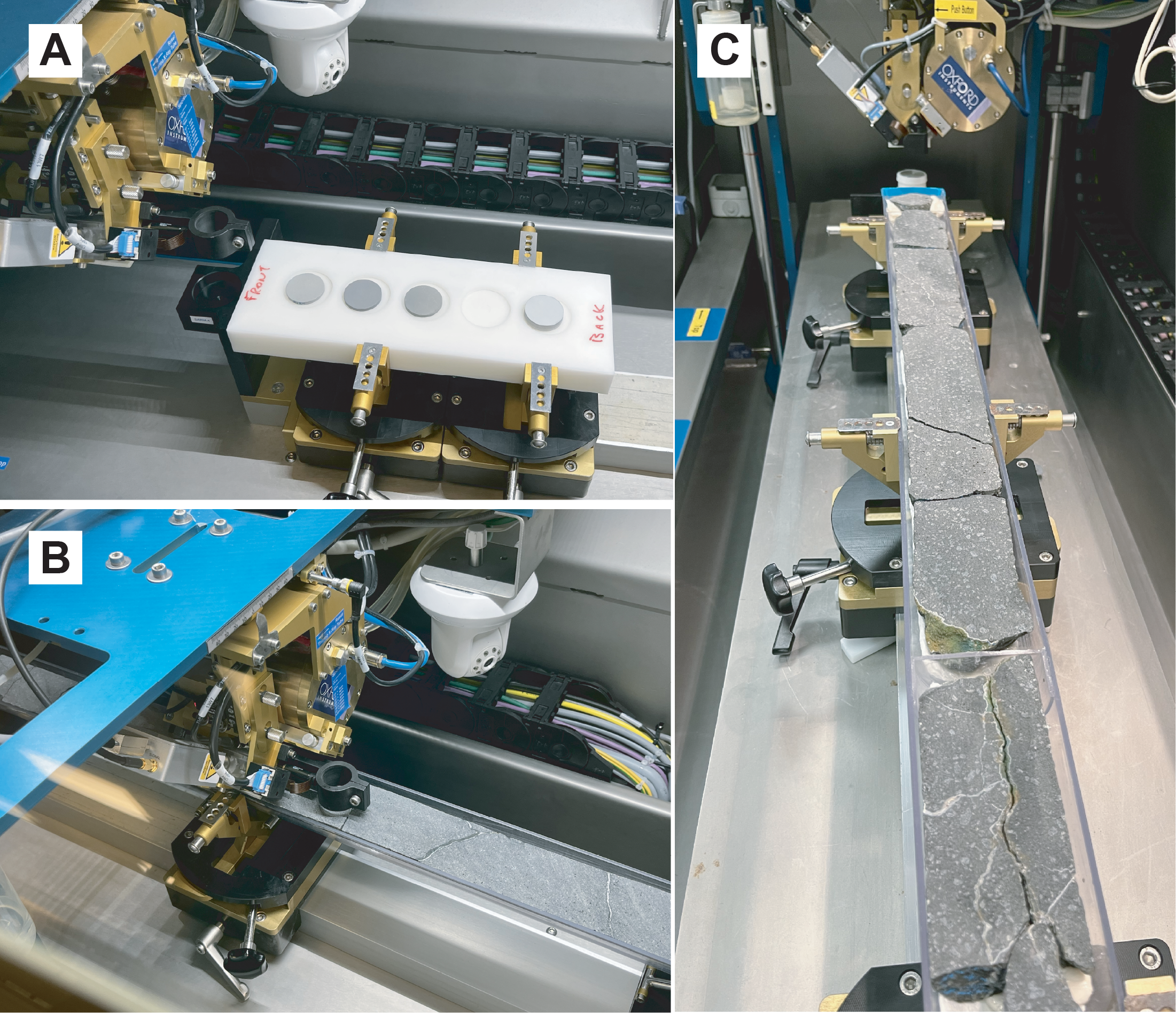
Figure F1. Avaatech core scanner.
Archival core section halves were scanned sequentially at 10, 30, and 50 kV accelerating potential. The nominal horizontal spacing interval was 3 cm at TAMU and 5 cm at MARUM, but this was interrupted in places by fractures, resulting in jumps of several centimeters (Figure F1B, F1C). The standard scanning setup was employed for each laboratory in terms of elements scanned at each accelerating potential, currents, count times, and filters. Count data were corrected for dead time internally by the scanner software. Elements counted at each energy level are shown in Table T2.
At 10 kV, the detector prism housing is flooded with helium, and there is no filter on the detector, thus minimizing absorption effects on the light element characteristic X-rays. Counting statistics on the scanned core at 10 kV show that standard deviations are typically ≤1% of total counts for major elements except Mg (~5%–6%), ≤6% for minor elements, and ~7%–11% for Cr (see CountingStats.docx in TABLES in Supplementary material). At 30 kV, standard deviations for major elements are again less than or equal to ~1% except for K, which are 7%–29%; this likely results from the thick Pd filter used on the detector at this excitation potential. Minor and trace element standard deviations are less than 2% for Mn, Ni, Sr, and Zr; 4%–6% for Co, Cu, Zn, Rb, and Y; and 17%–25% for Nb. Standard deviations in the counting statistics at 50 kV are similar to those at 30 kV, but total counts are generally lower at 50 kV (see CountingStats.docx in TABLES in Supplementary material).
In addition to analytes, Rh-tube lines were also counted (i.e., coherently scattered [Rayleigh] and incoherently scattered [Compton] tube lines). The tube lines are used to monitor and correct for mass absorption effects but do not account for secondary fluorescence of the light elements. At 10 kV, only the Rayleigh Lα line was counted. At 30 kV, both Rayleigh and Compton Kα were counted.
Argon is typically counted to monitor for atmospheric contamination. Detectable Ar values indicate poor contact between the detector and the core face or the presence of a significant fracture under the detector. Either situation will result in unreliable results, especially for the light elements. Prior to quantification, data with positive or low-negative counts on Ar should be deleted.
2.2. Mass absorption correction
The use of X-ray tube lines to correct for mass absorption has been discussed in several studies (e.g., DeLong and McCullough, 1973; Childs and Furkert, 1974; Nesbitt et al., 1976; Van Dyck and Van Grieken, 1980; Potts, 1992; Sitko and Zawisza, 2012), including the use of Rayleigh/Compton tube-line ratios (Hodoroaba and Rackwitz, 2014; Conti et al., 2014; Shen et al., 2019). We present corrections for Rh-Lα coherent (Rayleigh) scatter measured at 10 kV, Rh-Kα coherent (Rayleigh) scatter measured at 30 kV, Rh-Kα incoherent (Compton) scatter measured at 30 kV, and the ratio Rh-Kα Rayleigh/Compton scatter at 30 kV. The tube-line corrections represent the ratio of average counts on the three standards divided by the counts for each spot analysis on core (CRhs/CRhu); because the tube-line counts vary for each spot, the corresponding mass absorption correction varies as well. In Method 1, the tube-line corrections are applied after the first estimate (Cstd/Xstd) so that the most appropriate tube-line ratio can be chosen for each analyte. In Method 2, tube-line normalized data are used in both the calibration and the analysis.
All the Rh-tube line mass absorption corrections are typically ~3%–5%, reflecting the similarity of the core to the reference standards in terms of compositions and bulk density. For our final analytical data, we chose the Rayleigh Lα line to correct the lighter elements (below the Fe absorption edge) and the Kα Rayleigh/Compton ratio for heavier elements.
2.3. Quantification Method 1: counts/unit concentration
The quantification method of Shervais et al. (2025) was based on the relationship
- Xunk = concentration (mass fraction) in the unknown,
- Xstd = concentration (mass fraction) of measured standard,
- Cunk = counts on unknown,
- Cstd = counts on standard,
- CRhu = counts on Rh-tube line in the unknown,
- CRhs = counts on Rh-tube line in the standard, and
- Cstd/Xstd = counts on standard/mass fraction standard (i.e., counts/weight percent or counts/parts per million [ppm], depending on the element).
The critical values for quantification are the Cstd/Xstd ratios for each element of interest, often referred to as the sensitivity. Although it is possible to use a single standard that is well-matched to the unknowns, we used three standards that are all similar to the unknowns but provide a range in concentrations. The sensitivity values for Cstd/Xstd were calculated using the average of the counts under the peak for each element in each standard, divided by the accepted value for that element in each standard; the calculated values for Cstd/Xstd in the individual standards were then averaged, discarding outliers, to obtain the final values used for quantification.
Quantification for each element was obtained by dividing the total counts under the peak for each element by the value of Cstd/Xstd for that element (Shervais et al., 2025). This is equivalent to Castaing’s first approximation in electron microprobe analyses (Castaing, 1951). This first approximation must be refined by correcting for mass absorption effects using the ratio of tube-line counts for the standard and unknown (CRhs/CRhu), as discussed above. These results are shown in the calibration tables as calculated (see USGS_Standards_XRF1.xlsx, USGS_Standards_XRF2.xlsx, and USGS_Standards_XRF3.xlsx in TABLES in Supplementary material).
2.4. Quantification Method 2: slope correction of Method 1 results
Concentrations calculated using Methods 1 can be improved for many elements using a secondary slope correction to the calibration data. For each analyte, we regress the calculated concentrations against the reference values of the three USGS standards using the LINEST function in Microsoft Excel. This generates a slope and intercept that can be applied to the calculated concentrations to derive a slope-corrected concentration, designated “[Element name]-slope” in the calibration tables. This compensates for the fact that the sensitivity (counts/unit concentration) often varies as a function of concentration. The calculated slopes and intercepts for each scanner are presented in USGS_Standards_XRF1.xlsx, USGS_Standards_XRF2.xlsx, and USGS_Standards_XRF3.xlsx in TABLES in Supplementary material).
2.5. Quantification Method 3: ratio of analyte counts to Rh-tube lines
Quantification Method 3 is simply the well-known technique of ratioing all analyte count data to scattered tube-line intensities using the following relationship:
The Xstd/(Cstd/CRhs) ratio can be determined by regressing analyte count data/Rh-tube line counts versus concentration in the standard reference materials, which yields the equation for a line in the form mx + b, where mis the slope of the count ratio and bis the y-intercept. This regression may be carried out in Microsoft Excel using the LINEST function. Concentration in the unknown then becomes
Quantification for each analyte in the unknown is obtained by multiplying the ratio of counts under the peak for each element/Rh-tube line counts times the slope then adding the intercept. Selection of the appropriate scattered tube lines is informed by the Fe-absorption edge: for Fe and heavier elements, we find that ratio of coherent/incoherent scatter (Rayleigh/Compton) for Kα radiation works best because it better accounts for lack of background correction. For elements lighter than the Fe-absorption edge, we use the Raleigh-scattered Lα peak, which falls on the low-energy side of the Fe-absorption edge and thus is minimally affected by Fe-concentration. Results are shown in the calibration tables as traditional (Trad) (see USGS_Standards_XRF1.xlsx, USGS_Standards_XRF2.xlsx, and USGS_Standards_XRF3.xlsx in TABLES in Supplementary material).
Method 3 requires fewer steps than Method 2 and may be preferred for its simplicity. However, as we show below in the results, both methods are functionally identical and produce essentially the same results. This is shown by the intercepts, which are identical for both the slope correction (Method 2) and the traditional (Method 3), except where data for one standard are discarded as outliers in Method 1 (e.g., K in BIR-1). This relationship is derived in APPENDIX in Supplementary material.
2.6. Background corrections
The occurrence of continuum radiation (commonly known as background radiation) is a feature of all X-ray analytical methods, resulting from deceleration of electrons interacting with the X-ray target material (Potts, 1992; Potts and Webb, 1992). Most of the elements analyzed during the X-ray scans have relatively high peak/background ratios, making background corrections unnecessary. However, some trace elements with low peak/background ratios at low concentrations require correction for background counts to obtain valid calibration data. Although energy dispersive spectrometry (EDS) spectra can be convoluted to estimate the background at each energy level, it is easier to estimate the background for individual trace elements by regressing counts versus concentration: the counts (or count rate) at zero concentration are the effective background. When this background is subtracted from the counts on peak, the resulting background-corrected data can be used to calculate sensitivities for that element or ratioed to tube-line counts for Method 3. Theoretically, a background correction could applied to all peaks, but for most elements it has little to no impact on results.
2.7. Normalization and Na2O estimation
To account for variations in water content, porosity, and microporosity in the core, it is necessary to normalize the major element results to 100% to make these results compatible with discrete whole-rock analyses. However, the light element Na is typically not measured by EDS scanners because its characteristic X-rays are largely absorbed by the matrix. In addition, Na2O may be affected by seawater contamination. To compensate for the lack of analytical data for Na, we need to estimate Na2O in each XRF scan analysis prior to normalization. There are three reasonable options:
- Use the average Na2O/K2O ratio in each core, calculated from shipboard ICP-AES data or from shore-based WDS XRF analyses. This was the approach taken by Shervais et al. (2025) (Table T3). Correlation of our calculated Na2O values with shipboard ICP-AES data and shore-based WDS XRF analyses is generally good; however, spikes in K2O concentrations, which may result from localized alteration, likely overestimate actual Na2O concentrations.
- A second approach avoids these localized K2O spikes by simply using the average Na2O in each flow or at each site, as determined by shipboard ICP-AES or shore-based WDS XRF (Table T3). This avoids large irregular variations in Na2O that likely do not represent the core composition, but it does not allow for any natural variations that may be present.
- A third method avoids both of the issues discussed above by doing a linear regression of Na2O versus K2O and use this equation to calculate Na2O from K2O. This results in Na2O that varies with K2O but avoids large spikes in concentration caused by localized enrichments in K2O. This can be done using the LINEST function in Microsoft Excel, but it requires several whole-rock analyses to be statistically meaningful. If sufficient whole-rock data exist, this is the preferred method for estimating Na2O and the one we apply here in our updated tables (note that we have too few whole-rock analyses of Site U1578 Flow u9c to calculate a slope).
MgO calibration data on the XRF3 scanner are unusually low, apparently the result of a poor physical fit of the USGS pressed powder pellets in the sample holder and poor contact of the detector with the standards during calibration (S. Homrighausen, pers. comm., 2025). As a result, scanner-derived MgO concentrations in core from Site U1585 are more than double those measured by shipboard AES analyses and shore-based WDS XRF. This only affects the light element Mg, whose characteristic radiation is easily absorbed by air; other light elements (Al and Si) are not affected. We used the average ratio of XRF scanner MgO to shipboard ICP-AES and shore-based WDS XRF MgO (2.5) to correct the XRF scanner MgO values to match the observed WDS XRF results.
2.8. Running averages
Variations in phenocryst size, composition, and distribution can cause rapid short length scale variations in chemistry. To compensate for this, the data were smoothed using a 5-point running average. This average should be calculated after any anomalous values are deleted because the 5-point average will incorporate that anomalous value into averages both above and below it in the core. This creates a series of anomalous values from a single instance and can skew interpretations of the data.
2.9. Final empirical correction as needed
After all the steps discussed above are carried out, the final data are compared to representative whole-rock analyses of the same core by standard analytical methods (e.g., wavelength dispersive XRF or AES). This is most easily carried out by plotting both sets of analyses (scanner XRF and whole-rock analyses) versus depth. If the scanner-derived analyses exhibit a systematic deviation from the whole-rock data, it may be necessary to adjust the scanner data by an empirically derived constant factor to bring it into alignment with the whole-rock analyses.
3. Results
The final setups for each XRF scanner are shown in Tables T4, T5, and T6, which show the sensitivities for each scanner at 10, 30, and 50 kV, respectively, along with standard deviations. The preferred setups (i.e., best kilovolts for each analyte) are highlighted in yellow and discussed further below.
3.1. Counting statistics, backgrounds, and detection limits
Standard errors based on counting statistics for the reference standards are ≤1% for all major elements except MgO and P (~5%) and ≤5% for all trace elements except Rb (17%), Y (10%), and Nb (12%). These are basically the same as the standard errors for each analyte on the scanned core (see CountingStats.docx in TABLES in Supplementary material) and represent the minimum uncertainties for each element.
The sensitivity values Cstd/Xstd for each element among the three reference standards used vary from 2%–7% for most major elements except Mg (~10%). More abundant trace elements like Sr and Zr have ratios that vary by <5% at 30 kV, and less abundant elements have ratios that vary by 11%–22% at 30 kV and 5%–8% at 50 kV (see USGS_Standards_XRF1.xlsx, USGS_Standards_XRF2.xlsx, and USGS_Standards_XRF3.xlsx in TABLES in Supplementary material). Much of this variation is systematic as a function of concentration; this systematic variation in sensitivity is addressed by the slope correction (Method 2). There are small systematic differences in the average values of Cstd/Xstd between each of the instruments, so the calibrations are specific to the instrument used for each core and are not interchangeable.
Variations in the sensitivities between standards for several trace elements are improved by background corrections. The transition metals Cr and Ni have similar Cstd/Xstd ratios for standard reference materials BIR-1 and BHVO-1, but Cstd/Xstd ratios for BCR-1 (a basaltic andesite with ~54 wt% SiO2 and low Cr and Ni for a basalt [16 ppm Cr and 13 ppm Ni]) are 6× to 10× higher. This results in standard deviations of 120%–130% for Cr and Ni. Application of background corrections as discussed in Methods results in standard deviations for Cstd/Xstd ratios ~8%–35% (varies for each instrument and element). Similar improvements are observed for some trace elements in BIR-1 as well. However, the slope-corrected concentrations for elements with and without background corrections are essentially identical. When the traditional method (3) is applied, the slopes for uncorrected data and background-corrected data are identical, but the background-corrected intercepts are much closer to zero. As a result, the slope-corrected and traditional methods return essentially identical results for both uncorrected and background-corrected counts.
The calculation of background counts allows us to calculate theoretical lower limits of detection (LLD) for the trace elements. Using the 6σ formulation of Potts (1992), these are higher for the compatible elements Cr (3–7 ppm) and Ni (10–16 ppm) than for the incompatible elements (Rb, Sr, Y, Zr, and Nb), which are all generally less than or slightly higher than ~1 ppm (Table T7). The LLDs and precision of the analyses would be improved by longer count times; however, for most elements, the calculated LLDs are well below the concentrations in the unknowns.
3.2. Standards as unknowns
The efficacy of our calibration technique was evaluated first by applying it to the standard data used to calibrate it; that is, given that we use the average counts/unit concentration to calculate concentrations, how accurate are the measured values for each analyte amongst several independent measurements of the standards? If the measured values differ from the reference values, does the secondary slope correction bring the measured values into agreement with the reference values for each standard? And how do these slope corrected values compare to concentrations calculated from tube-line normalized count data (the traditional method)?
Tables T8, T9, and T10 present the reference values for each standard, mass absorption-corrected calculated values based on the average total counts for each analyte (Method 1), slope corrected values (Method 2), and values based on the traditional regressed slope and intercept (Method 3), as determined using XRF1, XRF2, and XRF3, respectively. A selection of these data are shown graphically in Figures F2, F3, and F4, which plot reference values at each kilovolt setting versus the tube-line corrected calculated values (Method 1) and the slope corrected values (Method 2). Traditional values based on analyte counts/tube-line counts (Method 3) are not shown because they are generally identical to the Method 2 results. The full set of calibration data are presented in FIGURES in Supplementary material.
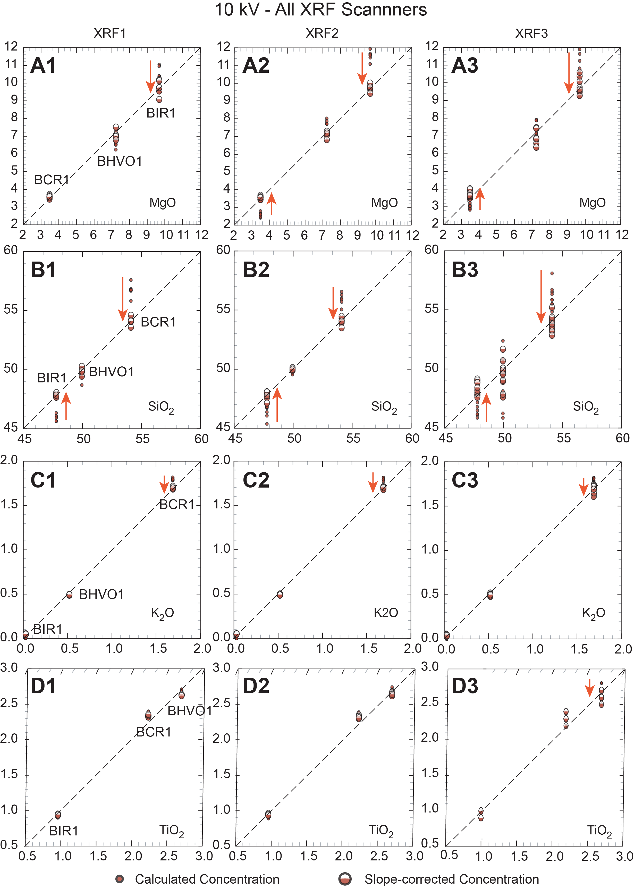
Figure F2. Standard calibrations vs. calculated values, 10 kV.
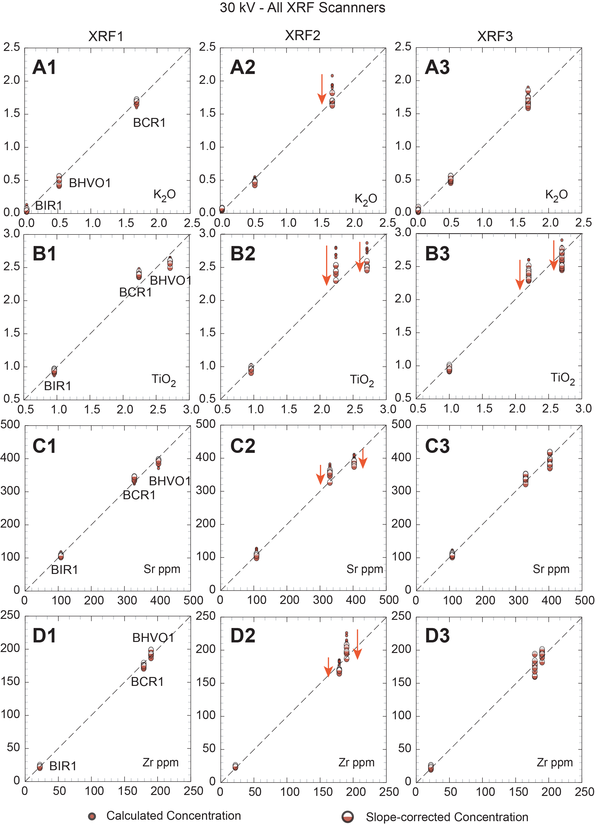
Figure F3. Standard calibrations vs. calculated values, 30 kV.
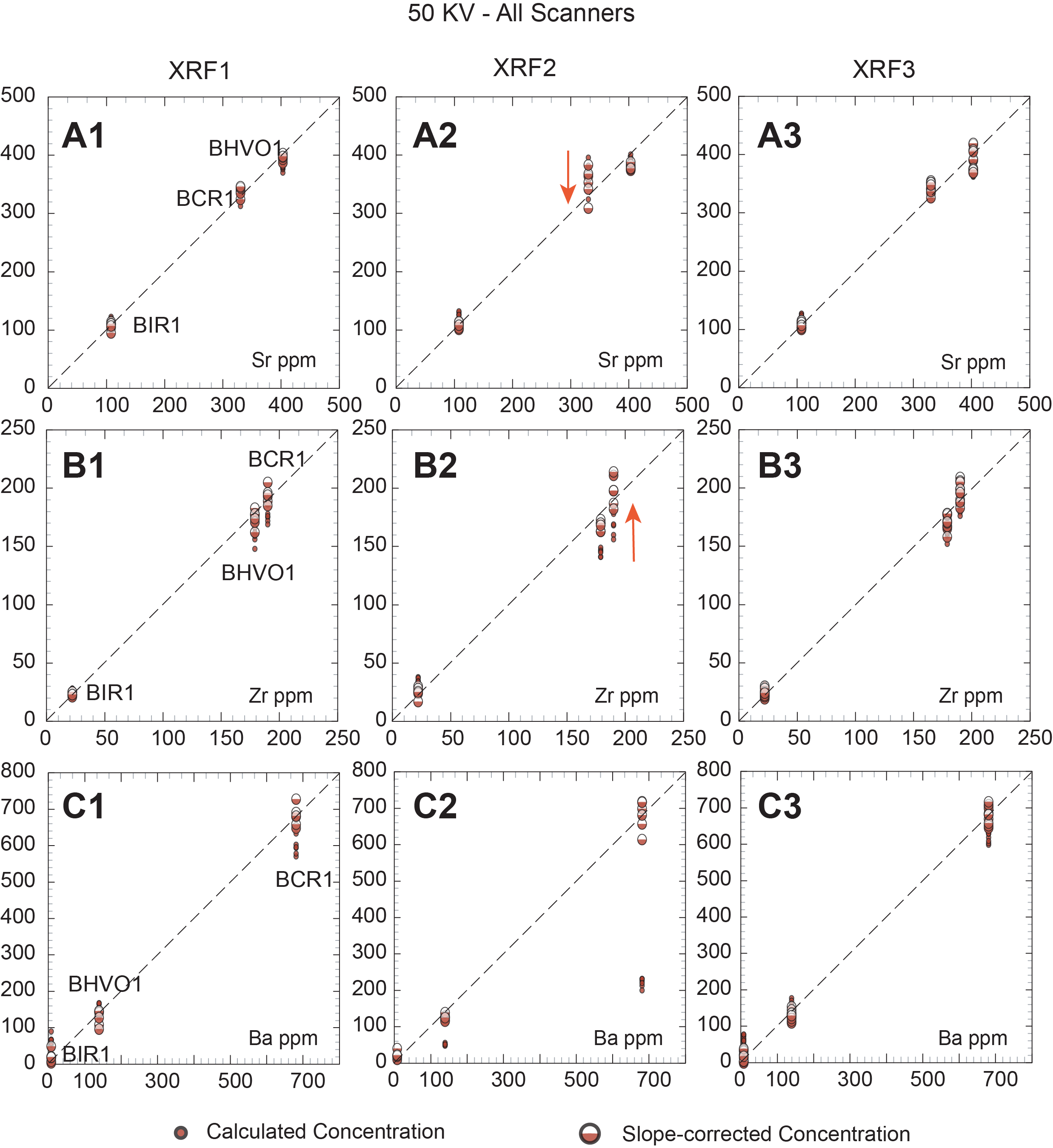
Figure F4. Standard calibrations vs. calculated values, 50 kV.
It can be seen from these plots and in Table T7 that for most elements the secondary slope correction provides only a minor improvement to the calculated concentrations. At 10 kV, K, P, Ca, Ti, and Fe are either unchanged or show modest improvement, typically for higher concentrations (e.g., Fe in BCR-1). In contrast, several elements show marked improvement: secondary corrections for Mg, Si, Al, and Mn all result in corrected values that closely match their reference values. At 30 kV, elements K, Ca, Ti, Sr, Y, and Zr show modest improvement with secondary correction, whereas Mn, Fe, Ni, Cr, and Rb show significant improvements. Slope-corrected values for Cr in BCR-1 match reference values well at 10 kV for XRF2 and XRF3 but are too high for XRF1 at 10 kV and for XRF3 at 30 kV. At 50 kV, Ca, Rb (except BIR-1), Sr, Y, Zr, Nb, and Ba all show minor or modest improvements with secondary corrections, and the slope-corrected values match the reference values well.
As discussed above, problems are evident for trace elements present in low concentrations in some standards, particularly K and Rb in BIR-1 and Cr and Ni in BCR-1. These elements have calculated and slope-corrected values that are too high relative to the reference values (see below). We suggest that this results from the lack of background correction in the scanner data. Background counts have little to no impact on elements with higher concentrations and count rates because this correction is contained within the y-intercept for slope-corrected and traditional methods (i.e., positive counts at zero concentration). However, when peak/background ratios are vanishingly small (as they are at very low concentrations), the background counts dominate and skew the quantitative results. Overcoming this issue would require selecting a few critical energies for background measurement at each excitation potential and calculating appropriate slope functions to project under low-concentration elements.
3.3. Calibrated results on core
Analytical results for scanned cores from each scanner are shown in IODP-XRF1.xlsx, IODP-XRF2.xlsx, and IODP-XRF3.xlsx in TABLES in Supplementary material. These tables present our full analytical correction scheme for all cores, compiled for each of the three separate Avaatech scanners used in this study. Each table in this group contains (for each element analyzed) the total counts under the peak and standard deviation on these counts, count per second on peak and corresponding standard deviation, and first approximation of concentration (equals total counts for the element divided by the counts/wt% or counts/ppm for that element from the USGS calibration standards). The first approximation is followed by the Rh-tube line corrections, including Rh-Lα Rayleigh (rh), Rh-Kα Rayleigh (rh-1), Rh-Kα Compton (rh-2), and Rh-Kα Rayleigh/Compton ratio (rh-3). All the Rh-tube line corrections represent the ratio of average counts in the USGS standards divided by the total counts under the peak for the appropriate tube line as measured at each analyzed location.
All the varied tube-line corrections are relatively small, generally about 3%–5%, and similar, although the simple Kα Rayleigh and Compton tube-line corrections are generally slightly larger than the Rayleigh/Compton ratio correction. For elements with characteristic X-rays that have lower excitation potentials than the Fe-absorption edge, the Rh-Lα Rayleigh line should be the most appropriate; this is the correction applied to all the elements in the 10 kV data set. Data scanned at 30 and 50 kV only use the Rh-Kα tube lines; for these elements, the Rh-Kα Rayleigh/Compton ratio correction is preferred. These mass absorption corrections are applied by multiplying the appropriate Rh-tube line correction (CRhs/CRhu) times the calculated concentration of each element for Method 1.
In IODP-XRF1.xlsx, IODP-XRF2.xlsx, and IODP-XRF3.xlsx (see TABLES in Supplementary material), the last two columns for each element are the slope-corrected values and the traditional regression values; these are each shown with the appropriate slope and intercept in Rows 2 and 3. These files also show the same data in values only format. Subsequent sheets in each spreadsheet present slope-corrected, normalized, and 5-point running averages for individual massive flows.
A final issue is the occurrence of calcium carbonate in many of the basalt core sections; these occur either as veinlets or vesicle fillings, which lead to elevated Ca contents that are not inherent to basalt being analyzed. Analyses with high apparent CaO should be screened out using a cutoff that minimizes or eliminates samples with potential calcite contamination. The appropriate cutoff depends on the normal CaO content of basalts, as determined by shore-based whole-rock analyses, but oceanic basalts rarely contain CaO >14 wt%. As noted above, application of the high Ca screen should be applied before calculating the running averages, to avoid ghost effects in the averaged analyses.
3.4. Validation of calibrated core scans
We validated our results by comparison to shipboard ICP-AES and shore-based WDS XRF analyses on discrete samples. A selection of these data for each massive lava flow are presented in Figures F5, F6, F7, F8, and F9, which plot USGS reference values on the x-axis, with calculated values and slope-corrected values on the y-axis.
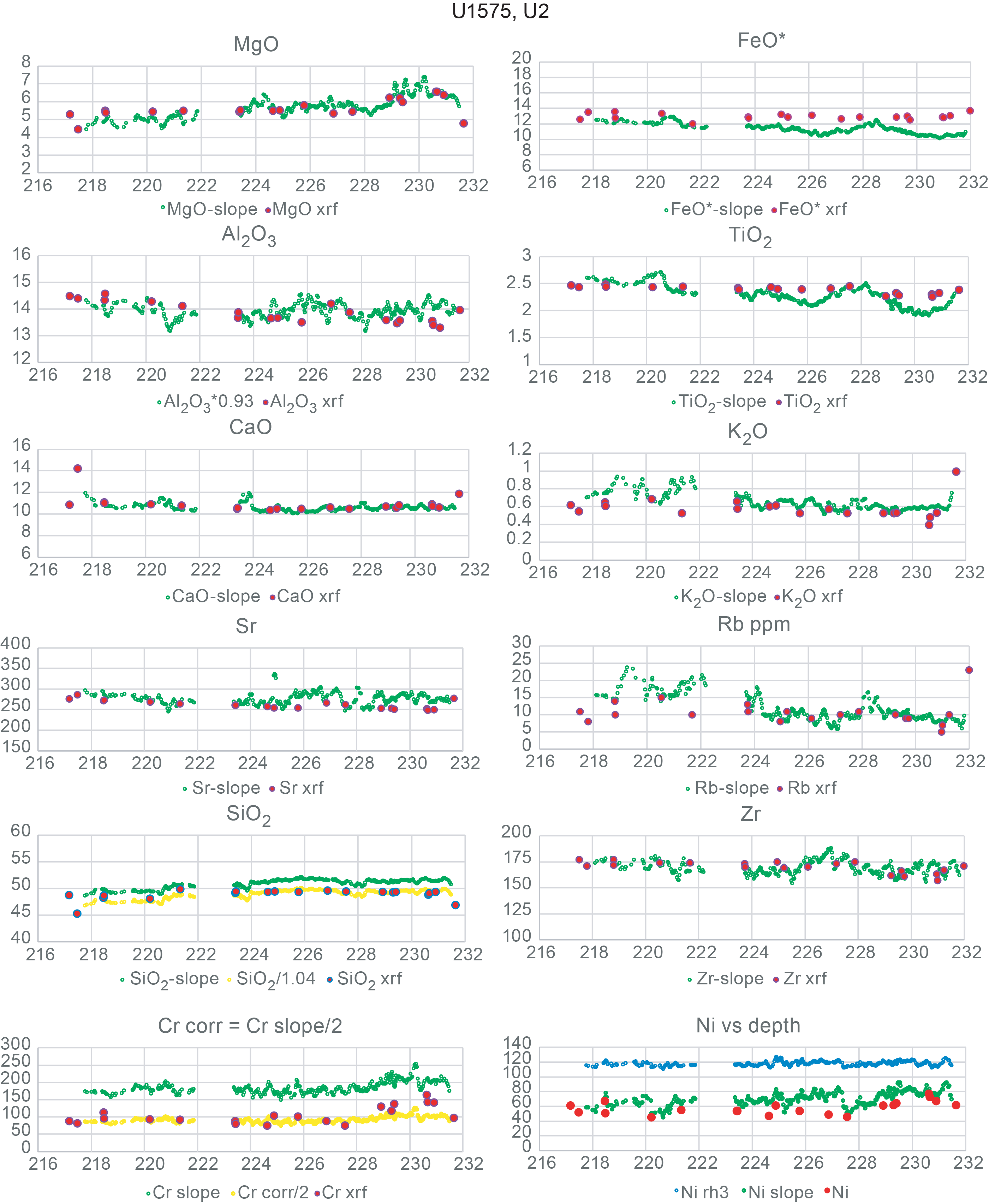
Figure F5. Concentration comparisons, Hole U1575A Flow Unit 2.
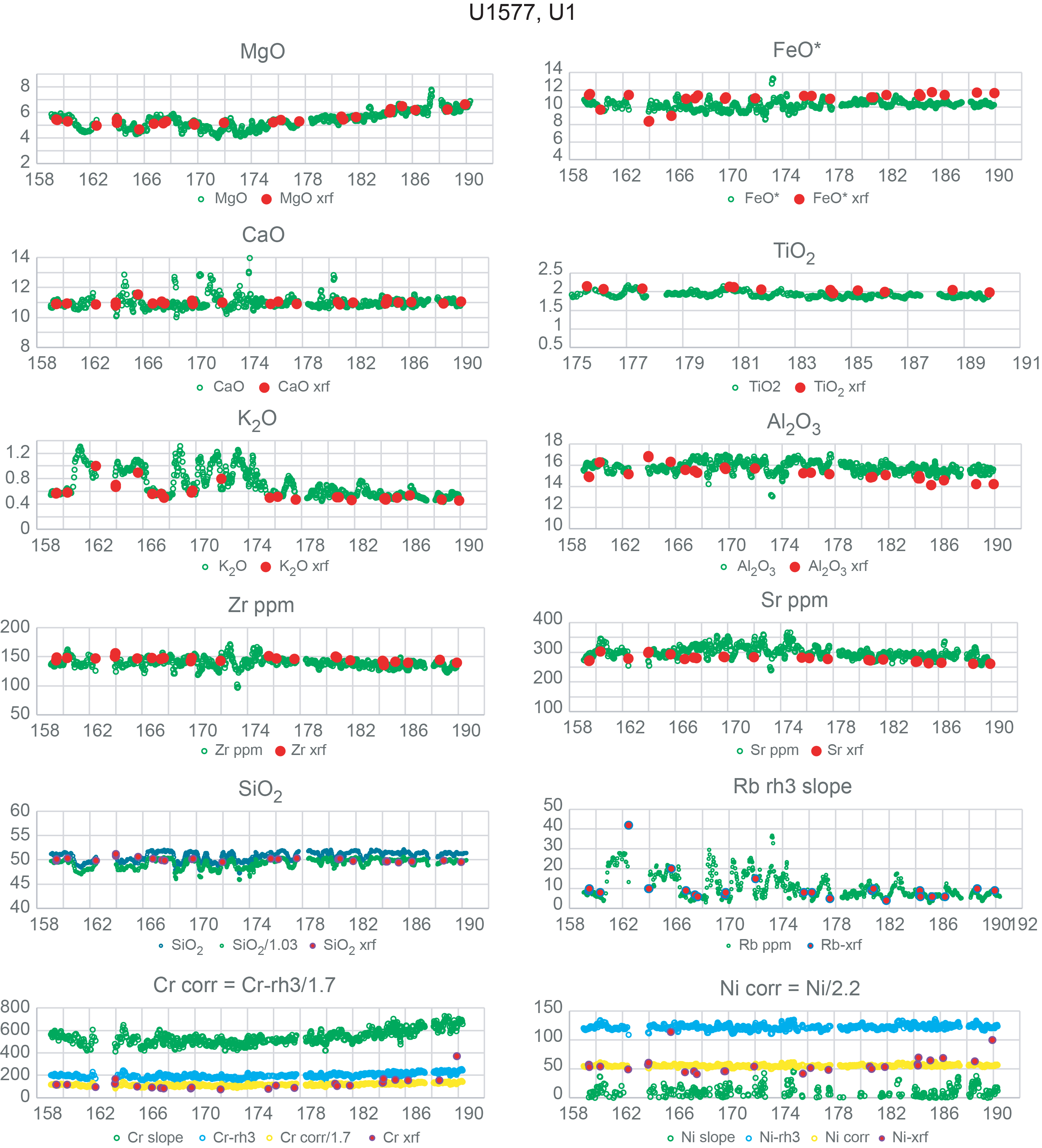
Figure F6. Concentration comparisons, Hole U1577A Flow Unit 1.
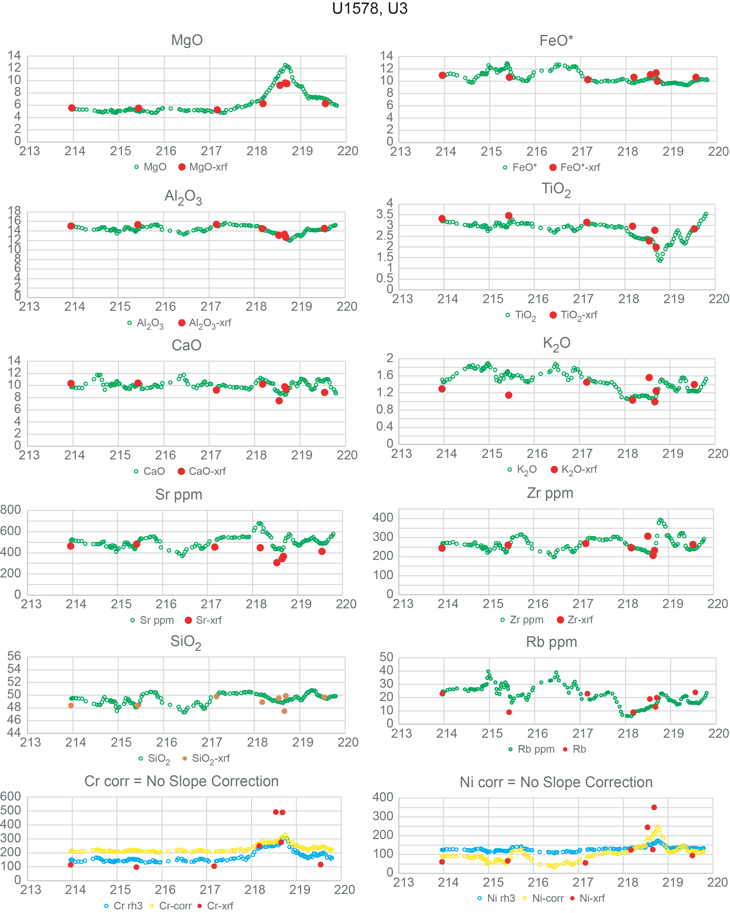
Figure F7. Concentration comparisons, Hole U1578A Flow Unit 3.
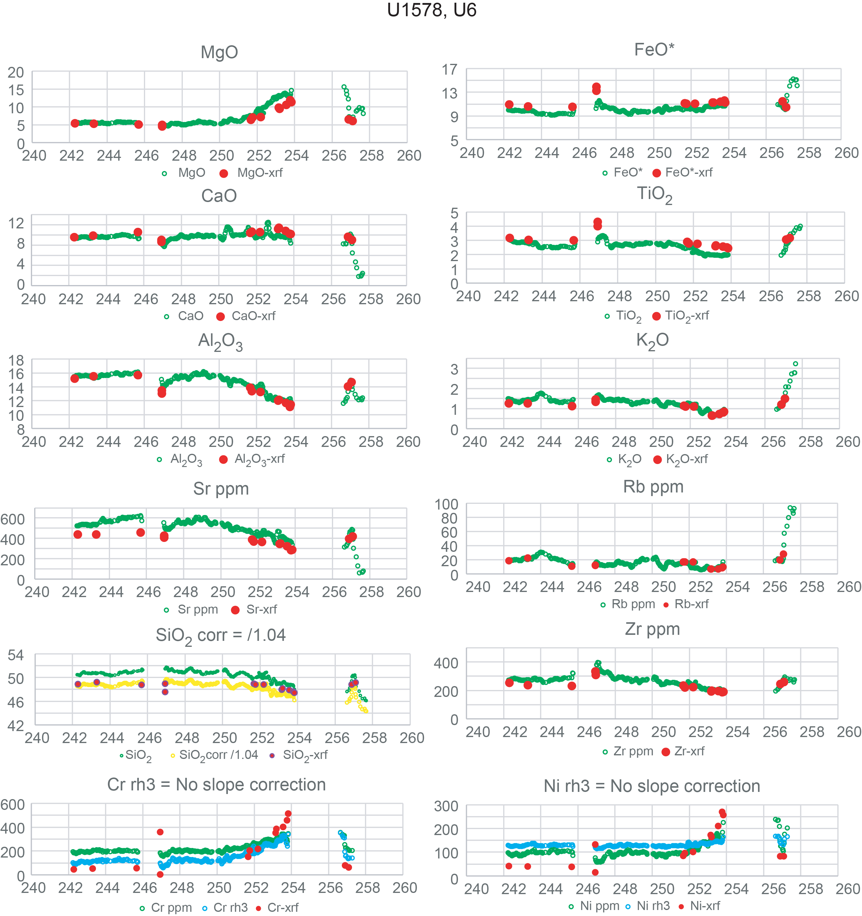
Figure F8. Concentration comparisons, Hole U1578A Flow Unit 6.
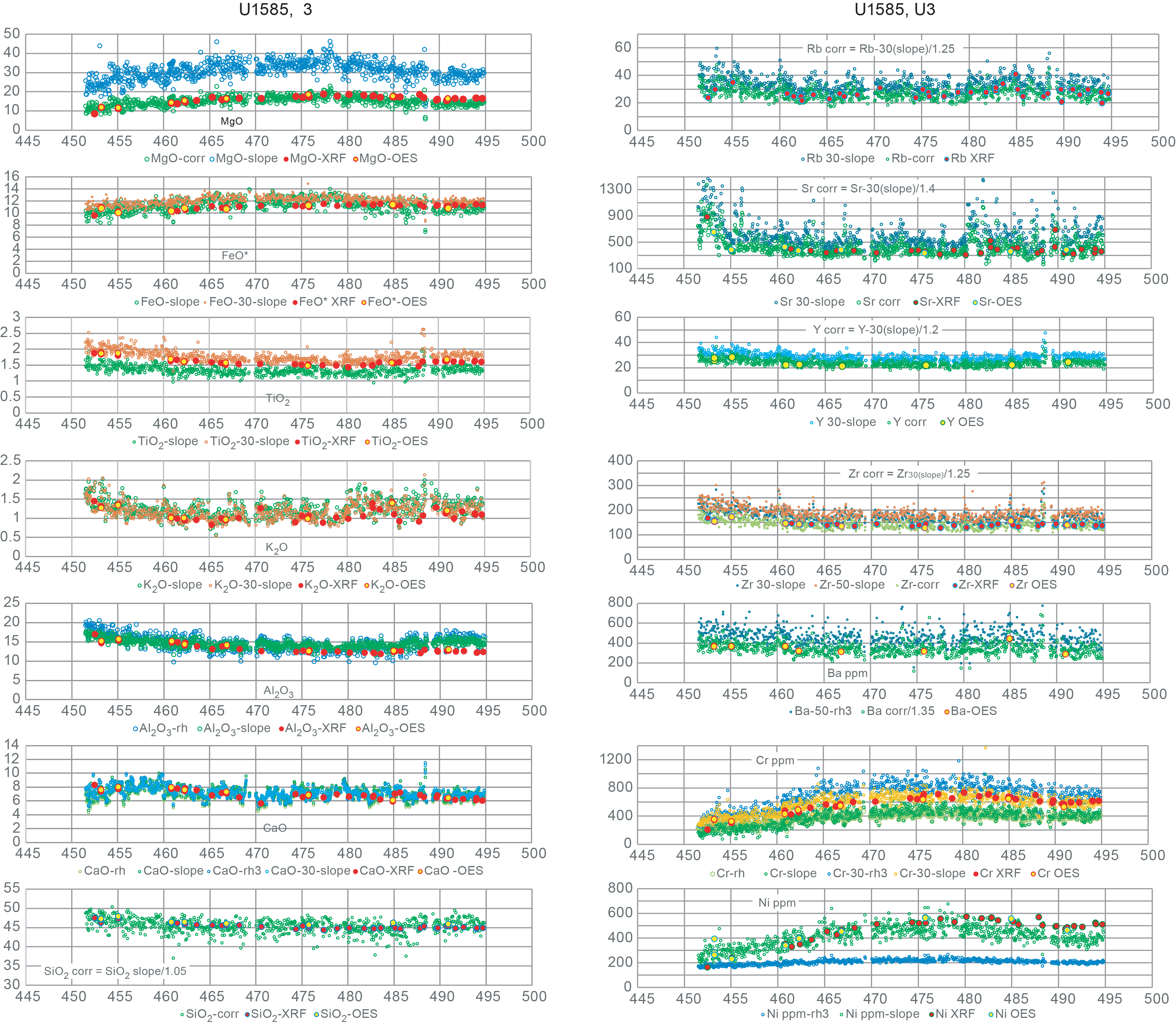
Figure F9. Concentration comparisons, Hole U1585A Flow Unit 3.
Concentration data obtained from the calibrated XRF scanner analyses are generally consistent with the shipboard ICP-AES and shore-based WDS XRF analyses for most elements. Even Na2O, which is estimated from calculated K2O concentrations, is remarkably close to concentrations observed in analyzed whole rocks. Silica can be off by 2%–3% but this can be remedied by application of an empirical correction factor. In addition, silica typically constitutes about half of each analysis and is more affected by normalization than the other elements.
4. Discussion
4.1. Calibrating XRF scanner analyses
4.1.1. Challenges and solutions
The calibration and quantification of XRF scanner data present a challenge not found in handheld pXRF analyses. This is because commercial pXRF instruments contain preprogrammed application protocols that include full matrix correction routines (typically based on alpha-coefficients or the fundamental parameters approach; Rousseau, 2013) and output measurements in unit concentrations (e.g., weight percent oxides for major elements or ppm [µg/g] for trace elements). Because these preprogrammed routines typically are standardless based on protocol being used (e.g., geologic materials), they commonly require the application of a secondary correction to align the results with reference values of rock standards (e.g., Ryan et al., 2017; Jonnalagadda et al., 2024; Heinonen and Luttinen, 2026). Such secondary corrections are relatively straightforward because interelement matrix effects are already accounted for in the original output.
By contrast, XRF scanners like the Avaatech instruments used here output data in raw counts that must be converted to quantitative values for each analyte (e.g., Shervais et al., 2025); alternatively, element ratios may be obtained (Morris et al., 2026). The quantification of XRF scanner data is subject to a number of issues inherent to energy dispersive XRF analysis of unprepared sample surfaces, and for those reasons can never be fully quantitative. These issues include surface roughness of the split cores, grain size variations that scatter characteristic X-rays, mass absorption variations that are not dampened by dilution in a light element flux (e.g., glass discs used in wavelength dispersive XRF analysis), variations in volatile contents (primarily water), variations in density caused by porosity and microporosity in the sample, and the preferential absorption of low energy characteristic X-rays from light elements; this last issue in particular affects Na (which is often not counted during analysis) and Mg (which has high standard deviations in its counting statistics).
Some of the issues mentioned above can be dealt with by normalizing results to 100% (e.g., volatile contents and porosity variations), but without an estimate for Na2O contents the results will overestimate the other elements, in particular silica. In the absence of analytical data on Na concentrations, Na2O must be estimated, adding another source of uncertainty.
Selecting the optimal conditions of analysis for each element can be guided by counting statistics. The lightest elements are counted only at 10 kV (Mg-K), but several elements are counted at more than one accelerating potential (e.g., fourth period transition metals [K-Fe]). The use of a thick Pd filter reduces total counts, but standard deviations are similar and in some cases lower at 30 kV. As a result, elements counted at both 10 and 30 kV can be used analyzed at either setting, depending on which data align best with shore-based analyses (Tables T4, T5, T6).
Most trace elements can be analyzed with similar precision at either 30 or 50 kV, although count rates are typically higher at 30 kV. Ba is the only element that can only be measured at 50 kV; if Ba is not critical for your purposes, time can be saved by not scanning at 50 kV and using 30 kV for most trace elements. Low abundance trace elements like Rb, Y, and Nb may be improved by increasing the count time from 6 to 10–12 s at 30 kV (i.e., by using the time normally used at 50 kV to extend counts at 30 kV).
A crucial point is that this approach relies on using standard reference materials that are matched as closely as possible to the core being analyzed. This minimizes differences in mass absorption and secondary fluorescence between the standard and the core and thus minimizes the magnitude of the applied corrections. It is also crucial that the standard reference materials are prepared as hydraulically pressed powder disks under ~4–5 tons pressure, with a 2% polyvinyl alcohol binder. Hydraulically pressed disks have tube-line intensities that are similar to crystalline basalts, indicating that they have similar density as well. The common practice of compacting powders by hand into rings backed by X-ray transparent film does not achieve densities comparable to natural basalt and should be avoided.
Using scattered tube lines (Reynolds or Compton) only accounts for absorption effects not secondary fluorescence. This seems mainly to affect Cr and Ni abundances, as these elements lie adjacent to the Fe-absorption edge and are known to strongly affected by Fe-abundance in the matrix (e.g., Sitko and Zawisza, 2012). Use of the scattered L-line for elements below the Fe-absorption edge ameliorates issues with using K-lines for these elements, which have energies above the Fe-absorption edge. However, it has been shown that a background setting around 0.8 kV is better for the lightest elements (Mg-P; Drake and McDonald, 2022; Drake et al., 2022).
An important point is that for many trace elements (e.g., the Rb-Nb series) the analytical precision of EDS analyses approaches or equals that obtained by WDS analysis (Webb et al., 1990; Ritchie et al., 2012). These elements are critical for evaluating the origin and evolution of basaltic magmas and are widely used in most petrogenetic models. The ability to obtain dense sampling of these elements in basaltic core will allow a more granular evaluation of magma formation and fractionation.
A major advantage of the approach taken here is that all the data reduction can be easily carried out in a spreadsheet using the raw scanner count data with no programming required other than simple arithmetic formulae. The results are not fully quantified absolutely because of the limitations inherent in the method. Importantly, the inability to measure Na concentrations and loss on ignition (LOI) in the scanned core and the effects of microporosity, phenocrysts, and surface roughness mean that fully quantified data are not possible even if a full matrix correction were applied. Nevertheless, the final data after all corrections are applied can be demonstrably close to the whole-rock analyses by WDS XRF or AES. Moreover, relative variations in composition throughout the core are relatively robust and document actual changes in composition at a scale that is not easily achievable with traditional whole-rock analyses.
4.1.2. Why bother with the light elements?
One of the more challenging aspects of calibrating XRF scanner data is achieving viable results on the light elements (e.g., Mg, Al, and Si), which is critical to producing analytical results that can be compared whole-rock analyses by WDS XRF or AES. The question arises: given that we can monitor many petrogenetic processes using heavier elements that have more robust fluorescence response, why expend extra effort calibrating the light elements?
The rationale for calibrating the light elements, in addition to heavier elements, is two-fold. First, producing complete major element analyses of our scanner data allows us to compare the scanner results more-or-less directly to discontinuous whole-rock analyses. Major element data that include MgO and SiO2 tell us whether we are dealing with basalt, more evolved lavas, or even refractory compositions.
Second, as petrologists, it allows us to envision a range of processes that concentration data or concentration ratios for a few heavy elements (e.g., TiO2 and K2O) cannot. In particular, the use of partial analyses restricts us to using incompatible element ratios rather than concentrations. These ratios are sensitive to changes in source composition or possibly extent of partial melting (for less incompatible versus more incompatible element ratios), but they cannot directly address fractionation, accumulation, or melt recharge. These processes require concentration data for both compatible and incompatible elements. This is demonstrated by data from Expedition 391, where increases in MgO document the occurrence of olivine-rich cumulate horizons in zoned flows (e.g., Shervais et al., 2025).
5. Recommendations
The application of XRF scanner technology to basalt core provides a rapid way to obtain chemostratigraphic data with high spatial resolution and for some elements accuracy that approaches more conventional AES or WDS analyses. The exact analytical procedures will likely vary depending on the scope and goals of the investigation; however, there are some broad recommendations that can be made based on our experience here:
- The core surface must be properly prepared according to standard core laboratory procedures, but no film covering is required for basalt core. Massive flows with continuous core can be scanned at regular step intervals (e.g., 3 or 5 cm), but fractured core and pillow lava must be programmed step-by-step.
- Unless Ba is essential, a third scanner run at 50 kV is unnecessary; it is generally better to omit the 50 kV run and increase the count times at 10 and 30 kV. This will improve counting statistics on both standards and unknowns. For example, counting 10 s at 10 kV and 12 s at 30 kV would not increase the total counts but would improve counting statistics by a factor of ~2. Trace elements at 30 kV are comparable or better than those at 50 kV. Our limited data suggest that Cr at 30 kV (XRF3) may be more robust than Cr at 10 kV (XRF1 and XRF2).
- Although all the major elements can be analyzed at 10 kV, some of the heavier major elements (K2O, CaO, TiO2, and FeO*) are included in the 30 kV run, and these would be suitable alternatives. Because all elements are counted simultaneously, results can be calculated at both settings and those with the best fits can be retained for each element.
- In this study, we used only three reference standards; in the future, we would recommend more standards, especially if Method 3 is used. Some standards are problematic for a few elements (e.g., BIR-1 for K2O and Rb; BCR-1 for Cr and Ni), and having more standards will compensate for these. Standards should be counted on a regular basis; if double counting standards is an option, that should be used.
- Standards should be prepared as hydraulically pressed powders with a polyvinyl alcohol binder, at about 4–5 tons pressure. These hydraulically pressed powders have tube-line scatter peaks with intensities similar to the basalt core, indicating similar mass densities. Loose powders packed in polymer holders with Chemplex Prolene film covering should be avoided as these will not match the density of the basalt core.
- Calibration Methods 2 and 3 provide essentially identical results, but Method 3 requires fewer steps.
- To compensate for modal variations in phenocrysts and other grain size variations, the final analyses should be smoothed with a 5-point running average. Individual point analyses can exhibit considerable scatter from point to point. The running average produces analyses that are more akin to bulk-rock analyses based on several grams of sample.
- As indicated in scanner laboratory procedures, samples with positive or low negative Ar counts reflect contamination with air and should be discarded. In addition, samples with abnormally high CaO relative to AES or WDS analyses of the same core indicate the presence of secondary calcite in veins or as vesicle fillings; these must be discarded before calculating a 5-point running average.
- To validate the XRF scanner analyses, shipboard ICP-AES or shore-based WDS XRF analyses should be obtained at regular intervals for comparison; when necessary, a final empirical adjustment may be required to bring the XRF scanner data into alignment with the discrete sample analyses.
6. Conclusion
Quantifying XRF scanner data is far more complex than processing handheld pXRF measurements because scanners output raw counts without built in matrix corrections. Unlike pXRF instruments, which apply standardless fundamental parameters or alpha coefficient routines and only require minor secondary adjustments, scanner data must be fully calibrated from first principles. This process is limited by factors inherent to energy dispersive XRF on unprepared core surfaces, including surface roughness, grain size effects, variable absorption, porosity, volatile contents, and the poor detection of light elements such as Na and Mg.
Some issues can be mitigated through normalization, but the absence of measurable Na2O introduces unavoidable uncertainty. Background-uncorrected data particularly affect low-abundance elements, but major elements and high-count trace elements remain more robust. Counting statistics show that 10 kV excitation is optimal for most major elements, whereas trace elements can be measured at 30 or 50 kV, with 30 kV generally offering higher count rates; Ba uniquely requires 50 kV.
Accurate calibration depends on using reference materials closely matched to the core to minimize absorption and fluorescence mismatches, although scattered tube-line corrections cannot fully account for secondary fluorescence, especially for Cr and Ni near the Fe absorption edge.
Despite these limitations, the method’s strength lies in its simplicity: quantitative corrections can be performed entirely in a spreadsheet, and although absolute concentrations cannot be fully achieved, corrected results closely approximate whole rock WDS XRF or AES analyses. Most importantly, the scanner reliably captures relative compositional variations along the core at a resolution unattainable with traditional whole rock sampling and is particularly valuable in rock core applications such as IODP archive half cores.
7. Acknowledgments
This research used samples and/or data provided by the International Ocean Discovery Program (IODP). The authors are grateful for support from IODP, the Gulf Coast Repository, the Bremen Core Repository, the JOIDES Resolution Facility, and the scientific staff and crew aboard the JOIDES Resolution during Expeditions 391 and 397T, as well as all Shipboard Scientists not included in this study. Funding support to United States participants (Shervais, Scholpp, Nelson, Potter, Duncan, Heaton, and Höfig) from the United States Science Support Program, and from the National Science Foundation (OCE 2317553 to Potter and Shervais, OCE-2317550 to Nelson, OCE-2054551 to Scholpp, OCE-2317552 to Duncan, and OCE-1326927 to Höfig) is gratefully acknowledged. Expedition participation for Widdowson and Buchs was supported by UK-IODP. Kubota was supported by the Japan Drilling Earth Science Consortium (J-DESC).
References
Castaing, R., 1951. Application des sondes électroniques à une méthode d’analyze ponctuelle chimique et cristallographique [PhD dissertation]. University of Paris, Paris, France.
Childs, C.W., and Furkert, R.J., 1974. The relative-intensity method of x-ray fluorescence analysis and its application to soils and rocks. Geoderma, 11(1):67–72. https://doi.org/10.1016/0016-7061(74)90008-1
Coggon, R.M., Teagle, D.A.H., Sylvan, J.B., Reece, J., Estes, E.R., Williams, T.J., Christeson, G.L., Aizawa, M., Albers, E., Amadori, C., Belgrano, T.M., Borrelli, C., Bridges, J.D., Carter, E.J., D’Angelo, T., Dinarès-Turell, J., Doi, N., Estep, J.D., Evans, A., Gilhooly, W.P., III, Grant, L.C.J., Guérin, G.M., Harris, M., Hojnacki, V.M., Hong, G., Jin, X., Jonnalagadda, M., Kaplan, M.R., Kempton, P.D., Kuwano, D., Labonte, J.M., Lam, A.R., Latas, M., Lowery, C.M., Lu, W., McIntyre, A., Moal-Darrigade, P., Pekar, S.F., Robustelli Test, C., Routledge, C.M., Ryan, J.G., Santiago Ramos, D., Shchepetkina, A., Slagle, A.L., Takada, M., Tamborrino, L., Villa, A., Wang, Y., Wee, S.Y., Widlansky, S.J., Yang, K., Kurz, W., Prakasam, M., Tian, L., Yu, T., and Zhang, G., 2024. Expedition 390/393 summary. In Coggon, R.M., Teagle, D.A.H., Sylvan, J.B., Reece, J., Estes, E.R., Williams, T.J., Christeson, G.L., and the Expedition 390/393 Scientists, South Atlantic Transect. Proceedings of the International Ocean Discovery Program, 390/393: College Station, TX (International Ocean Discovery Program). https://doi.org/10.14379/iodp.proc.390393.101.2024
Conti, C.C., Anjos, M.J., and Salgado, C.M., 2014. Determination of the mass attenuation coefficients for X-ray fluorescence measurements correction by the Rayleigh to Compton scattering ratio. Nuclear Instruments and Methods in Physics Research Section B: Beam Interactions with Materials and Atoms, 335:61–65. https://doi.org/10.1016/j.nimb.2014.06.004
De Jongh, W.K., 1973. X-ray fluorescence analysis applying theoretical matrix corrections. Stainless steel. X-Ray Spectrometry, 2(4):151–158. https://doi.org/10.1002/xrs.1300020404
DeLong, S.E., and McCullough, D., 1973. Compton-scattered tungsten X-rays as a measure of mass absorption coefficients in rocks. American Mineralogist, 58(11-12):1073–1075.
Drake, B.L., and MacDonald, B.L., 2022. Advances in Portable X-ray Fluorescence Spectrometry: Instrumentation, Application and Interpretation: (The Royal Society of Chemistry). https://doi.org/10.1039/9781839162695
Drake, B.L., Taylor, B., and Hamilton, M., 2022. Quantitative analysis. In Drake, B.L. and MacDonald, B.L., Advances in Portable X-ray Fluorescence Spectrometry: Instrumentation, Application and Interpretation. (The Royal Society of Chemistry), 81–107. https://doi.org/10.1039/9781839162695-00081
Heinonen, J.S., and Luttinen, A.V., 2026. Tracing the volcanic sources and differentiation of flood basalts using handheld XRF. Chemical Geology, 699:123147. https://doi.org/10.1016/j.chemgeo.2025.123147
Hennekam, R., Grant, K.M., Rohling, E.J., Tjallingii, R., Heslop, D., Roberts, A.P., Lourens, L.J., and Reichart, G.J., 2022. Accurately calibrated X-ray fluorescence core scanning (XRF-CS) record of Ti∕Al reveals Early Pleistocene aridity and humidity variability over North Africa and its close relationship to low-latitude insolation. Climate of the Past, 18(11):2509–2521. https://doi.org/10.5194/cp-18-2509-2022
Hennekam, R., Sweere, T., Tjallingii, R., de Lange, G.J., and Reichart, G.-J., 2019. Trace metal analysis of sediment cores using a novel X-ray fluorescence core scanning method. Quaternary International, 514:55–67. https://doi.org/10.1016/j.quaint.2018.10.018
Hodoroaba, V.-D., and Rackwitz, V., 2014. Gaining improved chemical composition by exploitation of Compton-to-Rayleigh intensity ratio in XRF analysis. Analytical Chemistry, 86(14):6858–6864. https://doi.org/10.1021/ac5000619
Jonnalagadda, M.K., Belgrano, T.M., Ryan, J.G., Kempton, P.D., Evans, A.D., Grant, L.J.C., Teagle, D.A.H., Coggon, R.M., Reece, J.S., Sylvan, J.B., Williams, T.J., Estes, E.R., and the Expedition 390/393 Scientists, 2024. Data report: high downhole resolution portable X-ray fluorescence geochemistry of South Atlantic Transect basement cores, IODP Expeditions 390C, 395E, 390, and 393. In Coggon, R.M., Teagle, D.A.H., Sylvan, J.B., Reece, J., Estes, E.R., Williams, T.J., Christeson, G.L., and the Expedition 390/393 Scientists, South Atlantic Transect. Proceedings of the International Ocean Discovery Program, 390/393: College Station, TX (International Ocean Discovery Program). https://doi.org/10.14379/iodp.proc.390393.210.2024
Lachance, G.R., 1979. The family of alpha coefficients in X-ray fluorescence analysis. X-Ray Spectrometry, 8(4):190–195. https://doi.org/10.1002/xrs.1300080411
Lachance, G.R., 1984. Introduction to Alpha Coefficients: Sainte-Foy, Quebec, Canada (Corporation Scientifique Claisse Inc).
Lachance, G.R., and Traill, R.J., 1966. Practical solution to the matrix problem in X-ray analysis. Canadian Spectroscopy, 11(2):43–48.
Lucas-Tooth, H.J., and Price, B.J., 1961. A mathematical method for the investigation of interelement effects in X-ray fluorescence analysis. Metallurgia, 64(2):149–152.
Lucas-Tooth, J., and Pyne, C., 1963. The accurate determination of major constituents by X-ray fluorescent analysis in the presence of large interelement effects. Advances in X-ray Analysis, 7:523–541. https://doi.org/10.1154/S0376030800002780
Morris, A.M., Lambart, S., Alvarez Zarikian, C.A., Millett, J.M., Jones, M.T., Planke, S., Betlem, P., Chatterjee, S., Christopoulou, M., Ferré, E.C., Filina, I.Y., Frieling, J., Scherer, R.P., Varela, N., Xu, W., and Yager, S.L., 2026. Recommendations for using core X-ray fluorescence data on basaltic rock as a tool to assess compositional variability. Scientific Drilling, 35(1):21–37. https://doi.org/10.5194/sd-35-21-2026
Nesbitt, R.W., Mastins, H., Stolz, G.W., and Bruce, D.R., 1976. Matrix corrections in trace-element analysis by X-ray fluorescence: An extension of the Compton scattering technique to long wavelengths. Chemical Geology, 18(3):203–213. https://doi.org/10.1016/0009-2541(76)90004-8
O’Connor, J.M., and Jokat, W., 2015. Tracking the Tristan-Gough mantle plume using discrete chains of intraplate volcanic centers buried in the Walvis Ridge. Geology, 43(8):715–718. https://doi.org/10.1130/G36767.1
O'Connor, J.M., and Duncan, R.A., 1990. Evolution of the Walvis Ridge-Rio Grande Rise hot spot system: implications for African and South American plate motions over plumes. Journal of Geophysical Research: Solid Earth, 95(B11):17475–17502. https://doi.org/10.1029/JB095iB11p17475
Potts, P.J., 1992. A Handbook of Silicate Rock Analysis: New York, NY (Springer). https://doi.org/10.1007/978-1-4615-3270-5
Potts, P.J., and Webb, P.C., 1992. X-ray fluorescence spectrometry. Journal of Geochemical Exploration, 44(1):251–296. https://doi.org/10.1016/0375-6742(92)90052-A
Ritchie, N.W.M., Newbury, D.E., and Davis, J.M., 2012. EDS measurements of X-ray intensity at WDS precision and accuracy Using a silicon drift detector. Microscopy and Microanalysis, 18(4):892–904. https://doi.org/10.1017/S1431927612001109
Rousseau, R., 2013. How to apply the fundamental parameters method to the quantitative X-ray fluorescence analysis of geological materials. Journal of Geosciences and Geomatics, 1(1):1–7. https://www.sciepub.com/jgg/abstract/267
Rousseau, R.M., 1984. Fundamental algorithm between concentration and intensity in XRF analysis 1—theory. X-Ray Spectrometry, 13(3):115–120. https://doi.org/10.1002/xrs.1300130306
Ryan, J.G., Shervais, J.W., Li, Y., Reagan, M.K., Li, H.Y., Heaton, D., Godard, M., Kirchenbaur, M., Whattam, S.A., Pearce, J.A., Chapman, T., Nelson, W., Prytulak, J., Shimizu, K., and Petronotis, K., 2017. Application of a handheld X-ray fluorescence spectrometer for real-time, high-density quantitative analysis of drilled igneous rocks and sediments during IODP Expedition 352. Chemical Geology, 451:55–66. https://doi.org/10.1016/j.chemgeo.2017.01.007
Sager, W., Blum, P., Bhutani, R., Carvallo, C.A., Heaton, D., Nelson, W.R., Tshiningayamwe, M., Widdowson, M., and the Expedition 391 Scientists, 2023a. Expedition 397T summary. In Sager, W., Hoernle, K., Höfig, T.W., Blum, P., and the Expedition 391 Scientists, Walvis Ridge Hotspot. Proceedings of the International Ocean Discovery Program, 391: College Station, TX (International Ocean Discovery Program). https://doi.org/10.14379/iodp.proc.391.109.2023
Sager, W., Blum, P., Bhutani, R., Carvallo, C.A., Heaton, D., Nelson, W.R., Tshiningayamwe, M., Widdowson, M., and the Expedition 391 Scientists, 2023b. Site U1585. In Sager, W., Hoernle, K., Höfig, T.W., Blum, P., and the Expedition 391 Scientists, Walvis Ridge Hotspot. Proceedings of the International Ocean Discovery Program, 391: College Station, TX (International Ocean Discovery Program). https://doi.org/10.14379/iodp.proc.391.108.2023
Sager, W., Hoernle, K., Höfig, T.W., Avery, A.J., Bhutani, R., Buchs, D.M., Carvallo, C.A., Class, C., Dai, Y., Dalla Valle, G., Del Gaudio, A.V., Fielding, S., Gaastra, K.M., Han, S., Homrighausen, S., Kubota, Y., Li, C.-F., Nelson, W.R., Petrou, E., Potter, K.E., Pujatti, S., Scholpp, J., Shervais, J.W., Thoram, S., Tikoo-Schantz, S.M., Tshiningayamwe, M., Wang, X.-J., and Widdowson, M., 2023c. Expedition 391 methods. In Sager, W., Hoernle, K., Höfig, T.W., Blum, P., and the Expedition 391 Scientists, Walvis Ridge Hotspot. Proceedings of the International Ocean Discovery Program, 391: College Station, TX (International Ocean Discovery Program). https://doi.org/10.14379/iodp.proc.391.102.2023
Sager, W., Hoernle, K., Höfig, T.W., Avery, A.J., Bhutani, R., Buchs, D.M., Carvallo, C.A., Class, C., Dai, Y., Dalla Valle, G., Del Gaudio, A.V., Fielding, S., Gaastra, K.M., Han, S., Homrighausen, S., Kubota, Y., Li, C.-F., Nelson, W.R., Petrou, E., Potter, K.E., Pujatti, S., Scholpp, J., Shervais, J.W., Thoram, S., Tikoo-Schantz, S.M., Tshiningayamwe, M., Wang, X.-J., and Widdowson, M., 2023d. Expedition 391 summary. In Sager, W., Hoernle, K., Höfig, T.W., Blum, P., and the Expedition 391 Scientists, Walvis Ridge Hotspot. Proceedings of the International Ocean Discovery Program, 391: College Station, TX (International Ocean Discovery Program). https://doi.org/10.14379/iodp.proc.391.101.2023
Sager, W., Hoernle, K., Höfig, T.W., Avery, A.J., Bhutani, R., Buchs, D.M., Carvallo, C.A., Class, C., Dai, Y., Dalla Valle, G., Del Gaudio, A.V., Fielding, S., Gaastra, K.M., Han, S., Homrighausen, S., Kubota, Y., Li, C.-F., Nelson, W.R., Petrou, E., Potter, K.E., Pujatti, S., Scholpp, J., Shervais, J.W., Thoram, S., Tikoo-Schantz, S.M., Tshiningayamwe, M., Wang, X.-J., and Widdowson, M., 2023e. Site U1575. In Sager, W., Hoernle, K., Höfig, T.W., Blum, P., and the Expedition 391 Scientists, Walvis Ridge Hotspot. Proceedings of the International Ocean Discovery Program, 391: College Station, TX (International Ocean Discovery Program). https://doi.org/10.14379/iodp.proc.391.103.2023
Sager, W., Hoernle, K., Höfig, T.W., Avery, A.J., Bhutani, R., Buchs, D.M., Carvallo, C.A., Class, C., Dai, Y., Dalla Valle, G., Del Gaudio, A.V., Fielding, S., Gaastra, K.M., Han, S., Homrighausen, S., Kubota, Y., Li, C.-F., Nelson, W.R., Petrou, E., Potter, K.E., Pujatti, S., Scholpp, J., Shervais, J.W., Thoram, S., Tikoo-Schantz, S.M., Tshiningayamwe, M., Wang, X.-J., and Widdowson, M., 2023f. Site U1576. In Sager, W., Hoernle, K., Höfig, T.W., Blum, P., and the Expedition 391 Scientists, Walvis Ridge Hotspot. Proceedings of the International Ocean Discovery Program, 391: College Station, TX (International Ocean Discovery Program). https://doi.org/10.14379/iodp.proc.391.104.2023
Sager, W., Hoernle, K., Höfig, T.W., Avery, A.J., Bhutani, R., Buchs, D.M., Carvallo, C.A., Class, C., Dai, Y., Dalla Valle, G., Del Gaudio, A.V., Fielding, S., Gaastra, K.M., Han, S., Homrighausen, S., Kubota, Y., Li, C.-F., Nelson, W.R., Petrou, E., Potter, K.E., Pujatti, S., Scholpp, J., Shervais, J.W., Thoram, S., Tikoo-Schantz, S.M., Tshiningayamwe, M., Wang, X.-J., and Widdowson, M., 2023g. Site U1577. In Sager, W., Hoernle, K., Höfig, T.W., Blum, P., and the Expedition 391 Scientists, Walvis Ridge Hotspot. Proceedings of the International Ocean Discovery Program, 391: College Station, TX (International Ocean Discovery Program). https://doi.org/10.14379/iodp.proc.391.105.2023
Sager, W., Hoernle, K., Höfig, T.W., Avery, A.J., Bhutani, R., Buchs, D.M., Carvallo, C.A., Class, C., Dai, Y., Dalla Valle, G., Del Gaudio, A.V., Fielding, S., Gaastra, K.M., Han, S., Homrighausen, S., Kubota, Y., Li, C.-F., Nelson, W.R., Petrou, E., Potter, K.E., Pujatti, S., Scholpp, J., Shervais, J.W., Thoram, S., Tikoo-Schantz, S.M., Tshiningayamwe, M., Wang, X.-J., and Widdowson, M., 2023h. Site U1578. In Sager, W., Hoernle, K., Höfig, T.W., Blum, P., and the Expedition 391 Scientists, Walvis Ridge Hotspot. Proceedings of the International Ocean Discovery Program, 391: College Station, TX (International Ocean Discovery Program). https://doi.org/10.14379/iodp.proc.391.106.2023
Shen, Y., Luo, L., Song, Y., Liu, J., Lao, C., Sun, M., and Yang, W., 2019. Matrix correction with Compton to Rayleigh ratio in a plant–soil–rock interface analysis using a laboratory micro-XRF. X-Ray Spectrometry, 48(5):536–542. https://doi.org/10.1002/xrs.3080
Shervais, J.W., Nelson, W.R., Potter, K.E., Homrighausen, S., Scholpp, J.L., Widdowson, M., White, D., Buchs, D.M., Heaton, D.E., Avery, A.J., Bhutani, R., Duncan, R.A., Class, C., Tshiningayamwe, M., Kubota, Y., Wang, X.-J., Wu, T., Sager, W., Hoernle, K., and Höfig, T.W., 2026. Supplementary material, https://doi.org/10.14379/iodp.proc.391.202supp.2026. In Shervais, J.W., Nelson, W.R., Potter, K.E., Homrighausen, S., Scholpp, J.L., Widdowson, M., White, D., Buchs, D.M., Heaton, D.E., Avery, A.J., Bhutani, R., Duncan, R.A., Class, C., Tshiningayamwe, M., Kubota, Y., Wang, X.-J., Wu, T., Sager, W., Hoernle, K., and Höfig, T.W., Data report: calibrated XRF scanner analyses of massive basalt core, Walvis Ridge Hotspot track, IODP Expedition 391/397T: a template for XRF scanner analysis of basalt core. In Sager, W., Hoernle, K., Höfig, T.W., Blum, P., and the Expedition 391 Scientists, Walvis Ridge Hotspot. Proceedings of the International Ocean Discovery Program, 391: College Station, TX (International Ocean Discovery Program).
Shervais, J.W., Scholpp, J.L., Widdowson, M., Nelson, W.R., Potter, K.E., Homrighausen, S., White, D., Buchs, D., Heaton, D.E., Avery, A., Bhutani, R., Duncan, R.A., Class, C., Tshiningayamwe, M., Kubota, Y., Wang, X.-J., Wu, T., Sager, W.W., Hoernle, K., and Höfig, T., 2025. Eruption, emplacement and internal architecture of massive and super-massive inflated submarine basalt lava flows, Walvis Ridge hotspot track, IODP Expeditions 391/397T. Geochemistry, Geophysics, Geosystems, 26(6):e2024GC012145. https://doi.org/10.1029/2024GC012145
Sitko, R., and Zawisza, B., 2012. Quantification in X-Ray Fluorescence Spectrometry. In Sharma, S.K.K., X-Ray Spectroscopy. London (IntechOpen), 137–162. https://doi.org/10.5772/29367
Van Dyck, P.M., and Van Grieken, R.E., 2002. Absorption correction via scattered radiation in energy-dispersive X-ray fluorescence analysis for samples of variable composition and thickness. Analytical Chemistry, 52(12):1859–1864. https://doi.org/10.1021/ac50062a020
Webb, P.C., Potts, P.J., and Watson, J.S., 1990. Trace element analysis of geochemical reference samples by energy dispersive X-ray fluorescence spectrometry. Geostandards Newsletter, 14(3):361–372. https://doi.org/10.1111/j.1751-908X.1990.tb00077.x
Weltje, G.J., Bloemsma, M.R., Tjallingii, R., Heslop, D., Röhl, U., and Croudace, I.W., 2015. Prediction of geochemical composition from XRF core scanner data: a new multivariate approach including automatic selection of calibration samples and Quantification of Uncertainties. In Croudace, I.W., and Rothwell, R.G. (Eds.), Micro-XRF Studies of Sediment Cores: Applications of a Non-destructive Tool for the Environmental Sciences. Developments in Paleoenvironmental Research: 507–534. https://doi.org/10.1007/978-94-017-9849-5_21
Weltje, G.J., and Tjallingii, R., 2008. Calibration of XRF core scanners for quantitative geochemical logging of sediment cores: theory and application. Earth and Planetary Science Letters, 274(3–4):423–438. https://doi.org/10.1016/j.epsl.2008.07.054